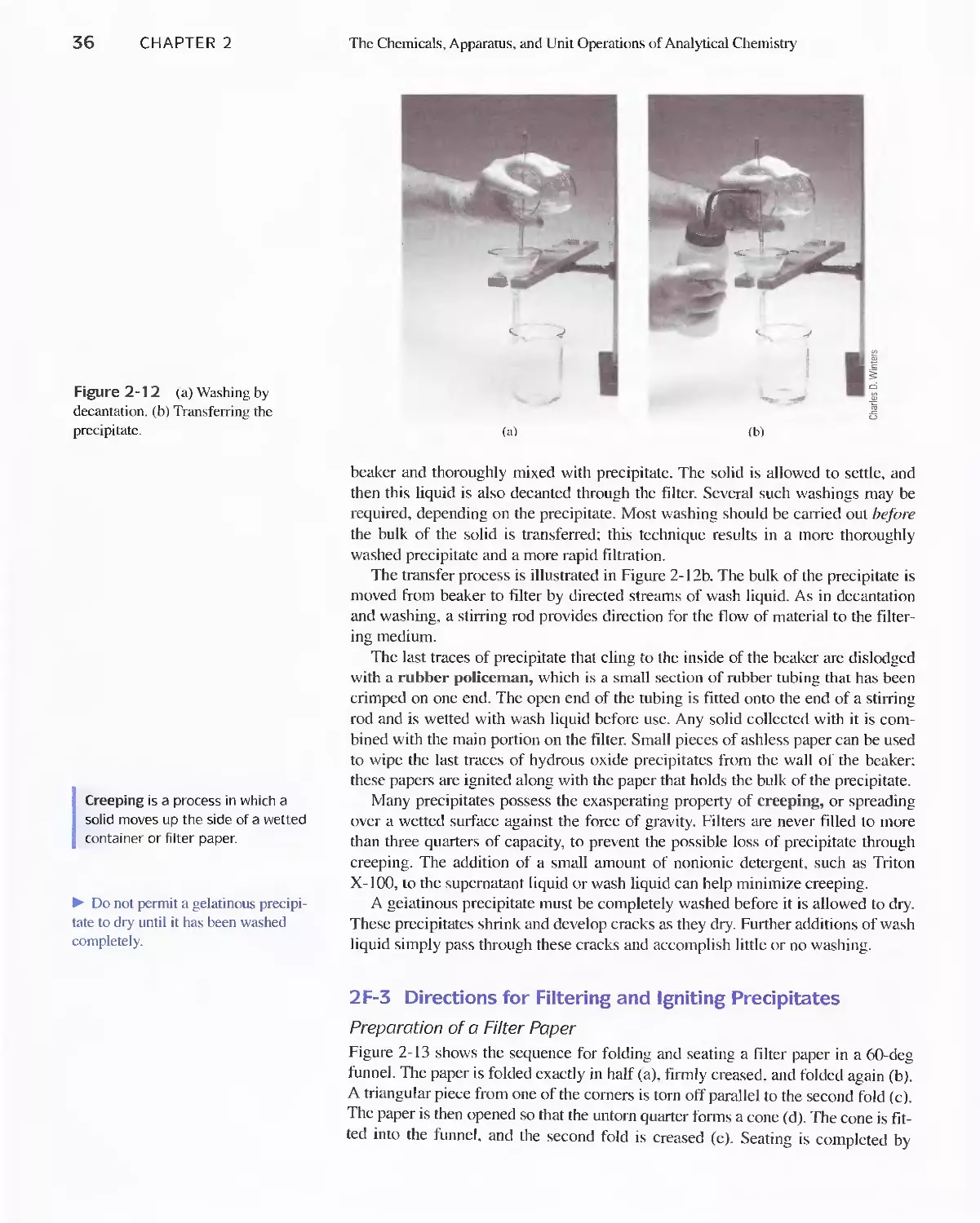
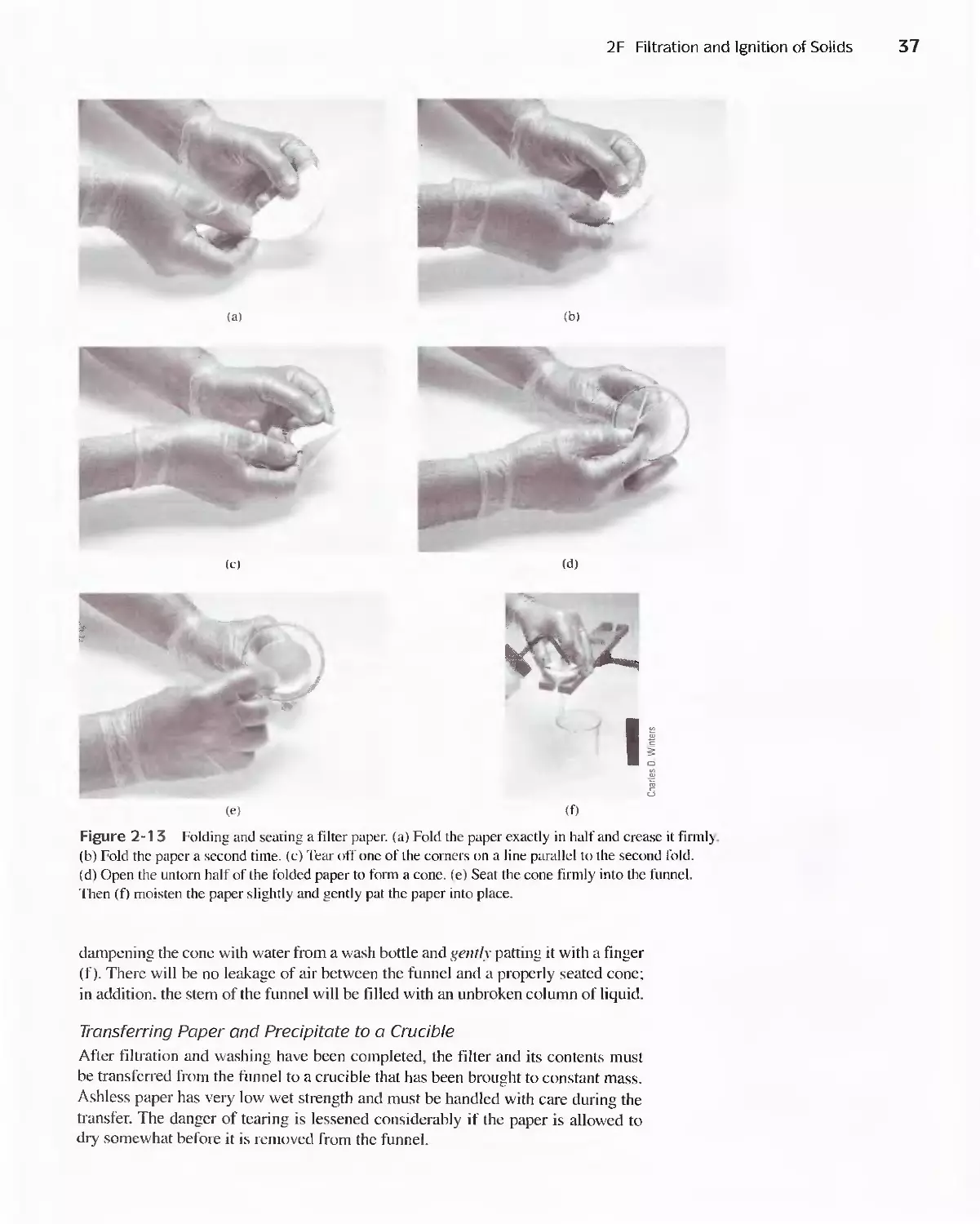
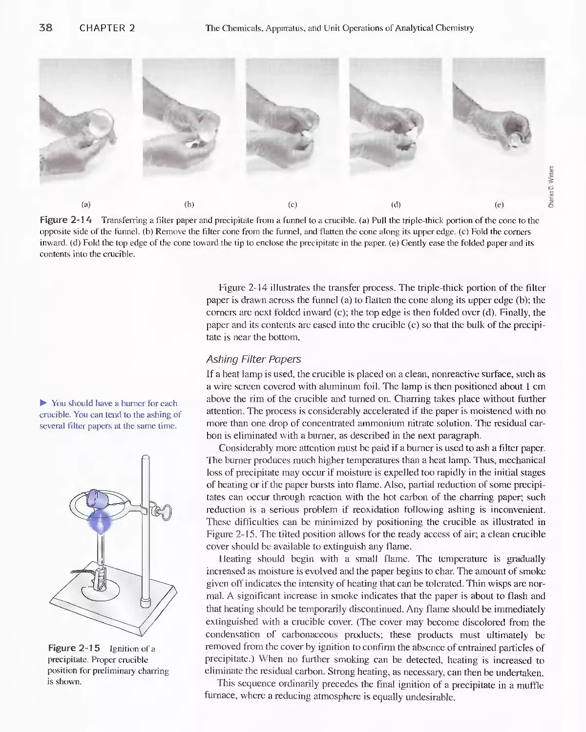
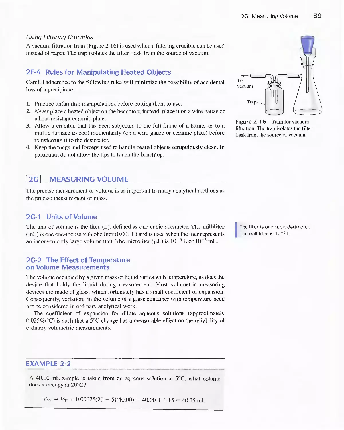
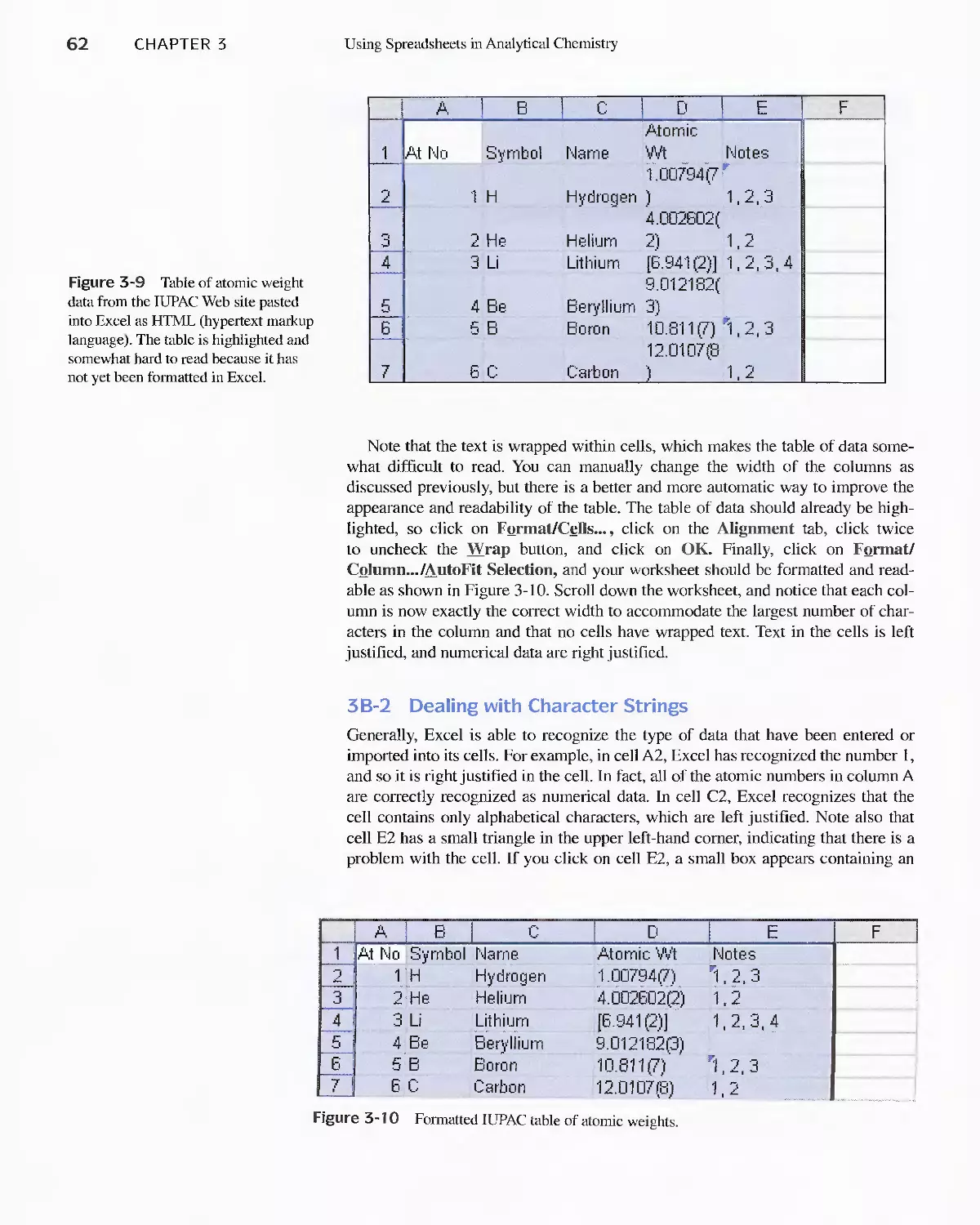
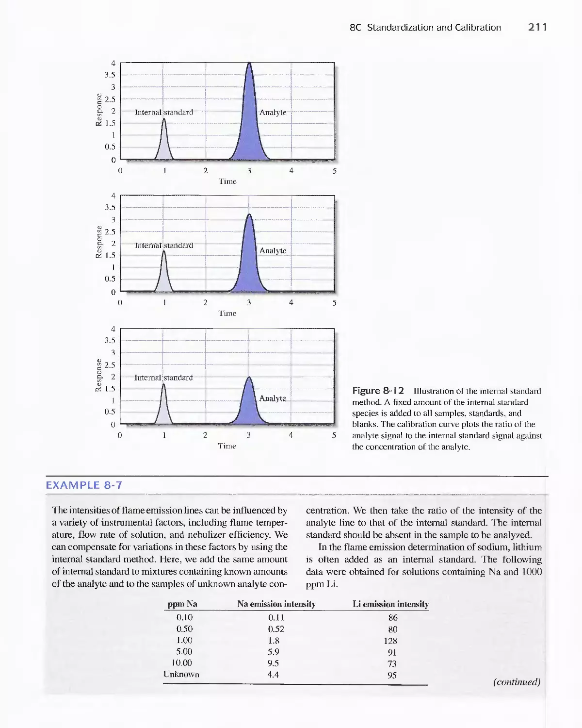
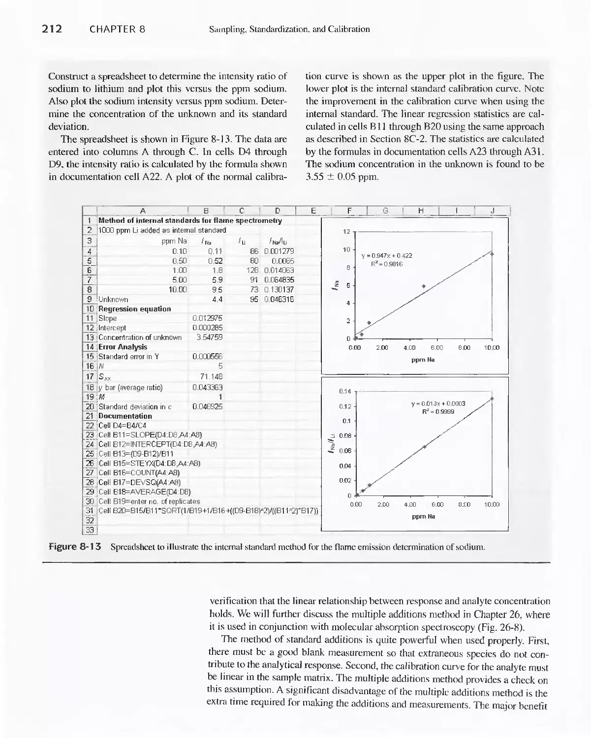
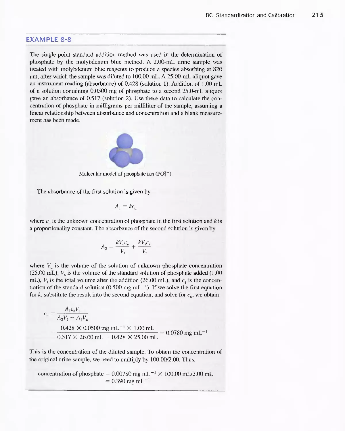
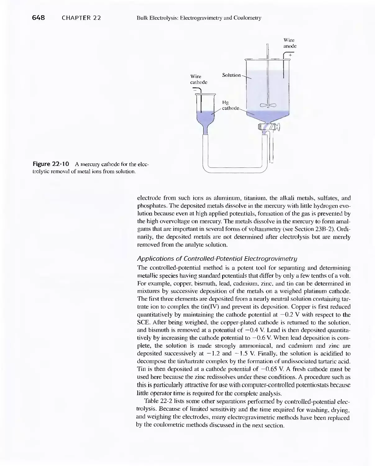
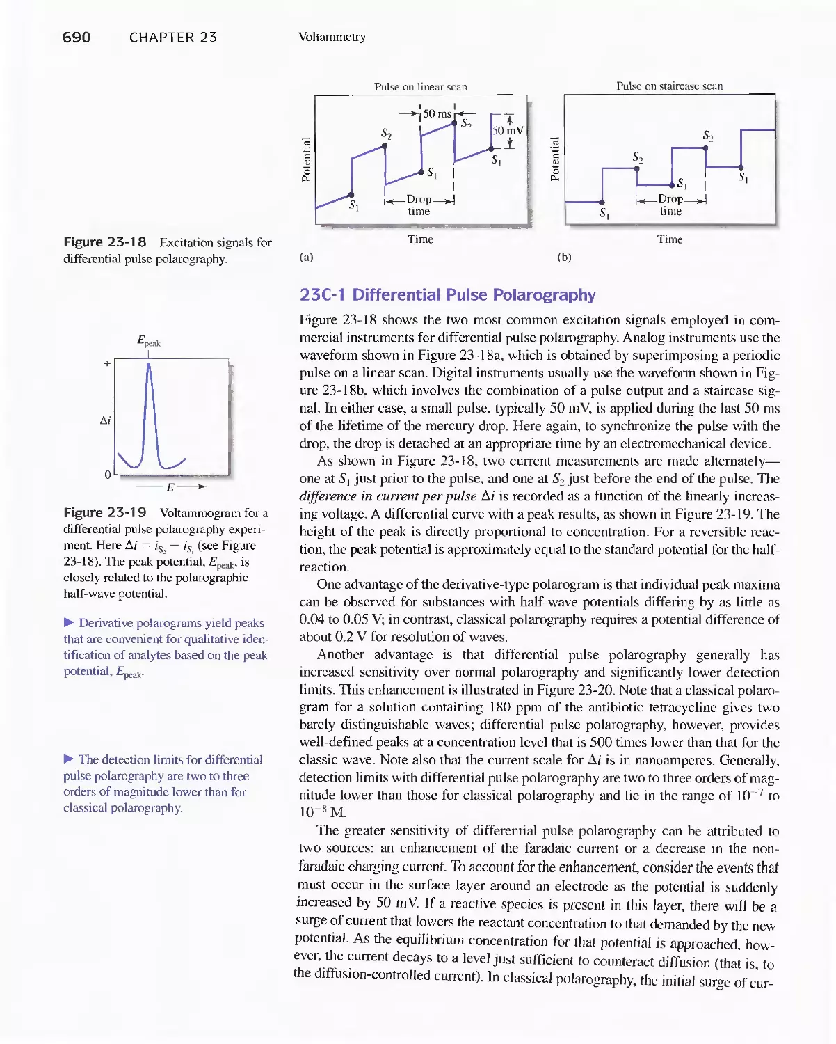
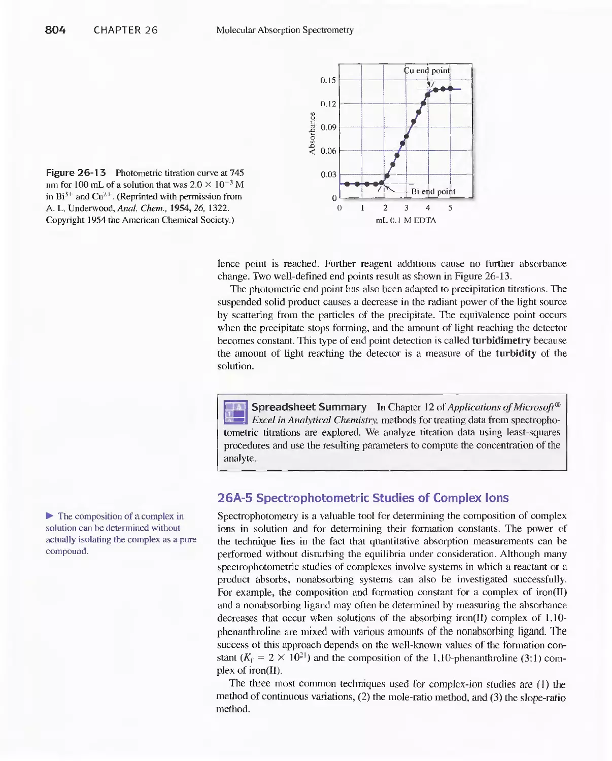
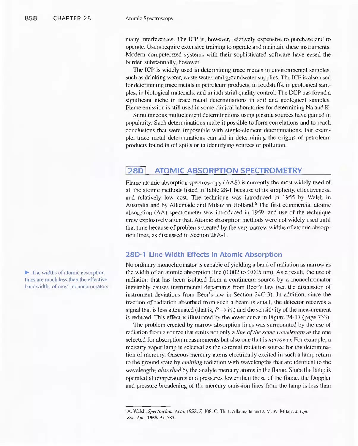
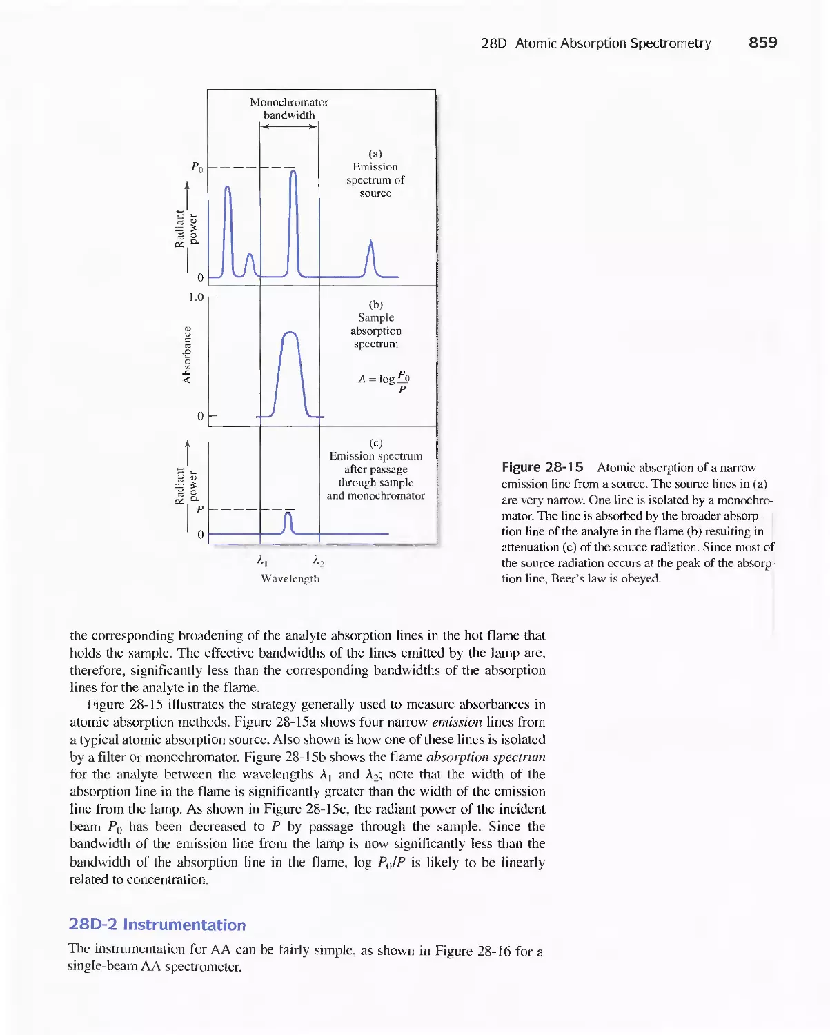
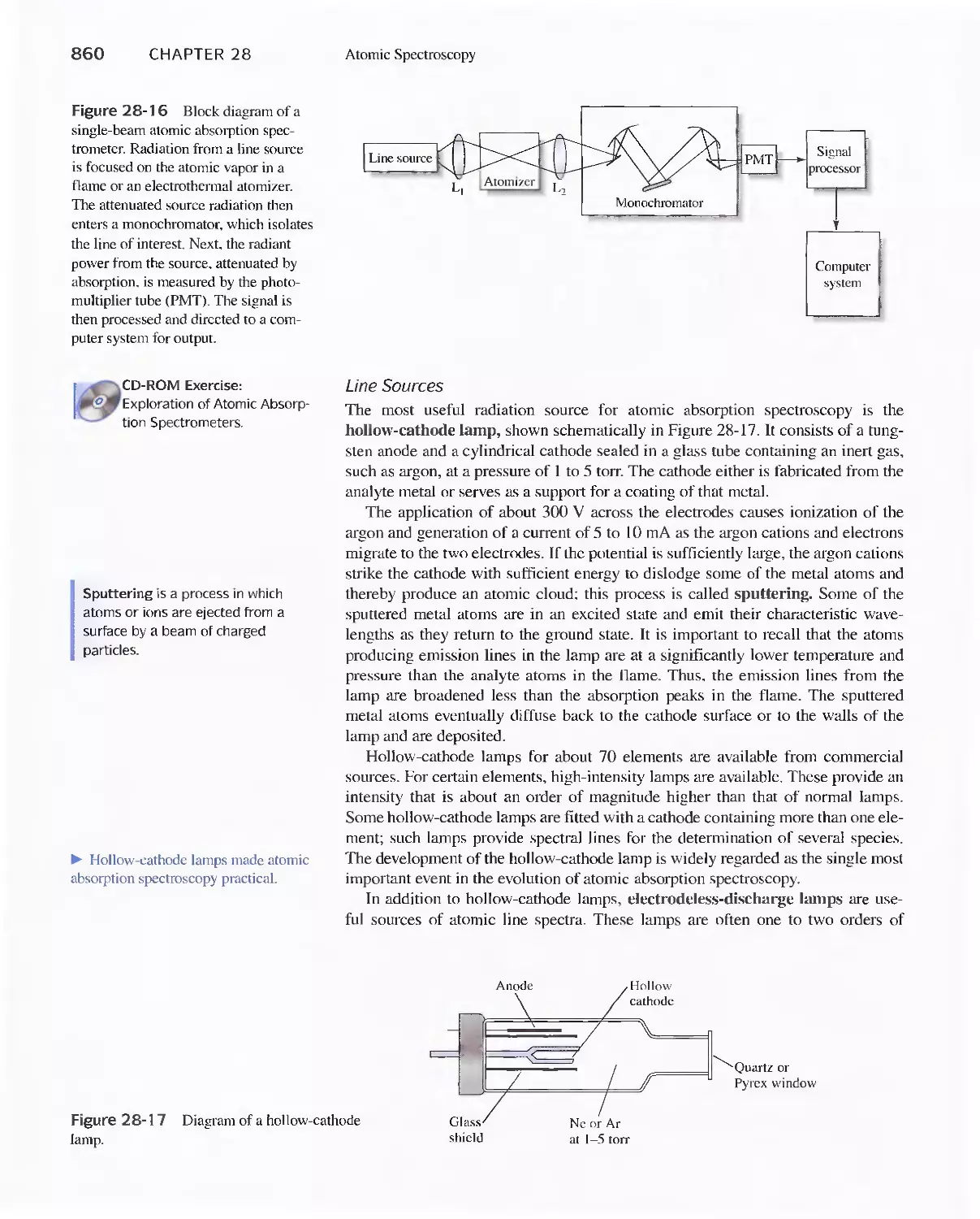
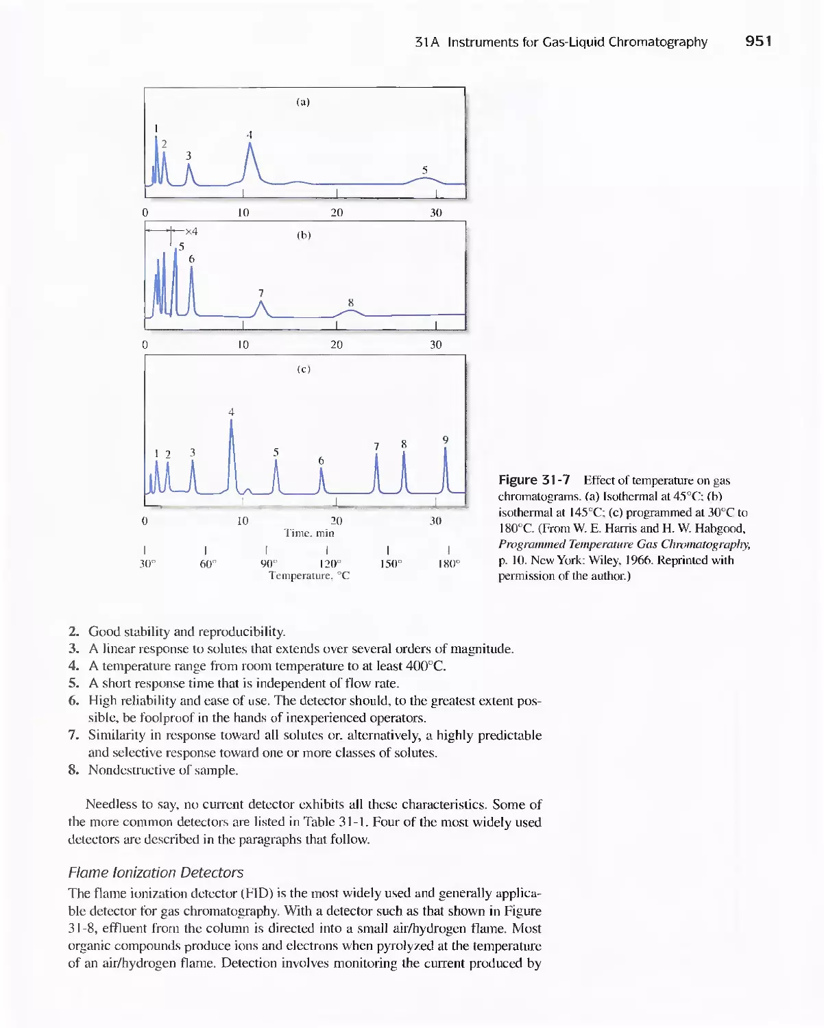
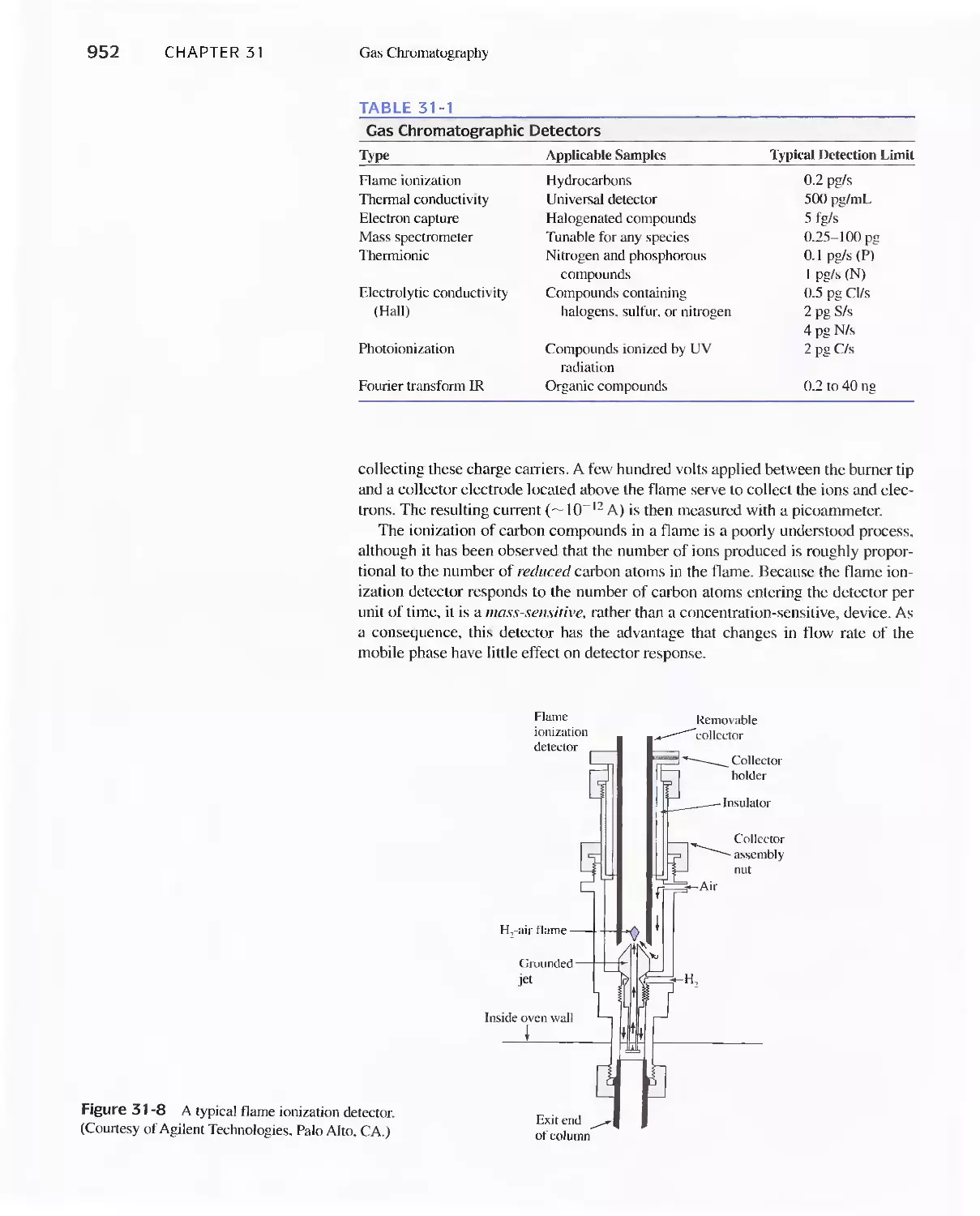
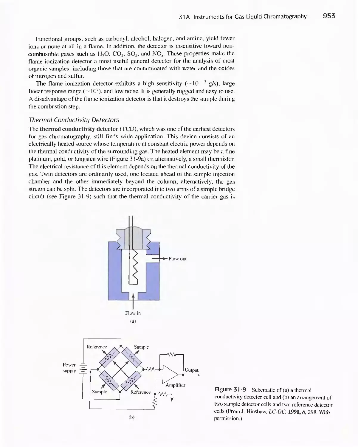
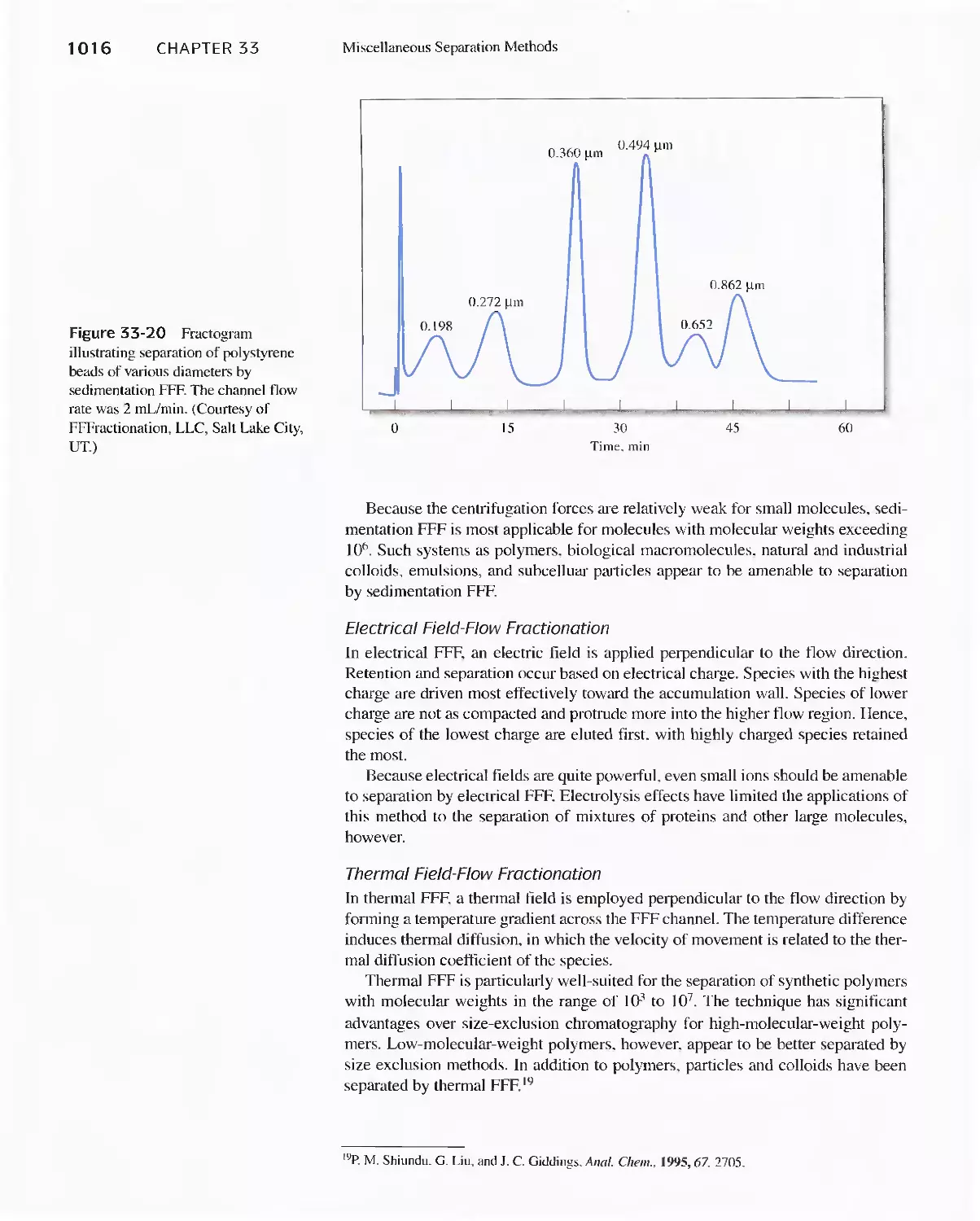
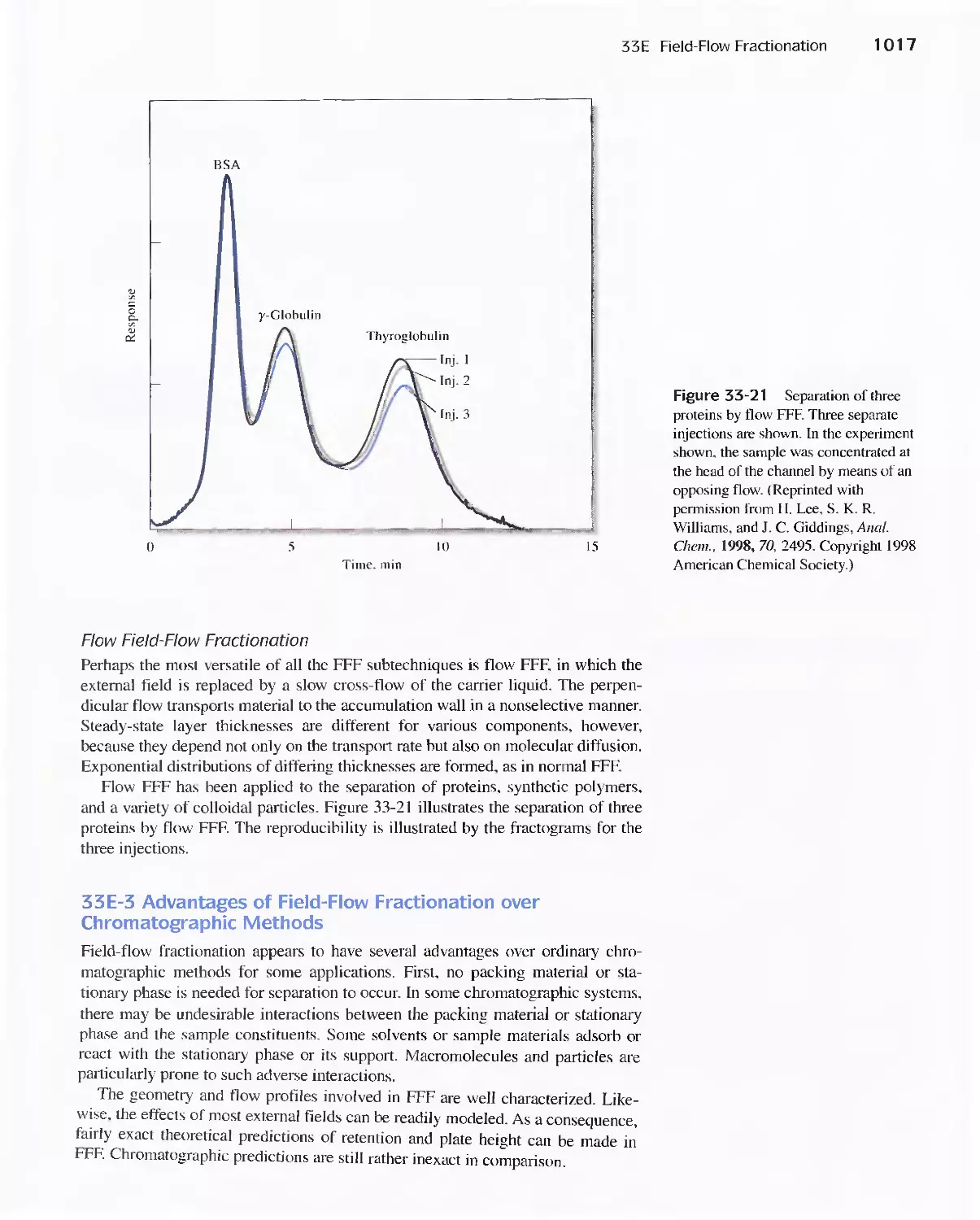
/


Author: Skoog D.A. West D.M Holler F.J. Crouch S.R.
Tags: chemistry analytical chemistry
ISBN: 978-0-03-035523-3
Year: 2004


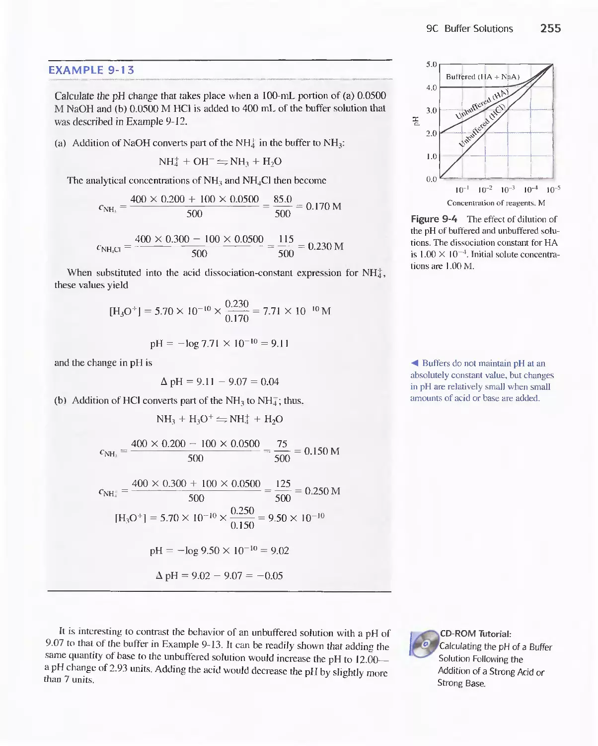
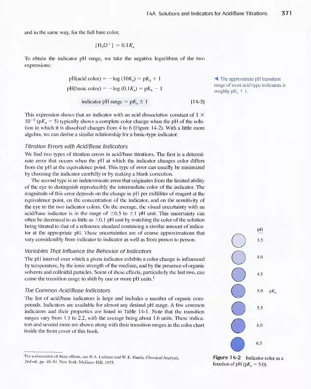
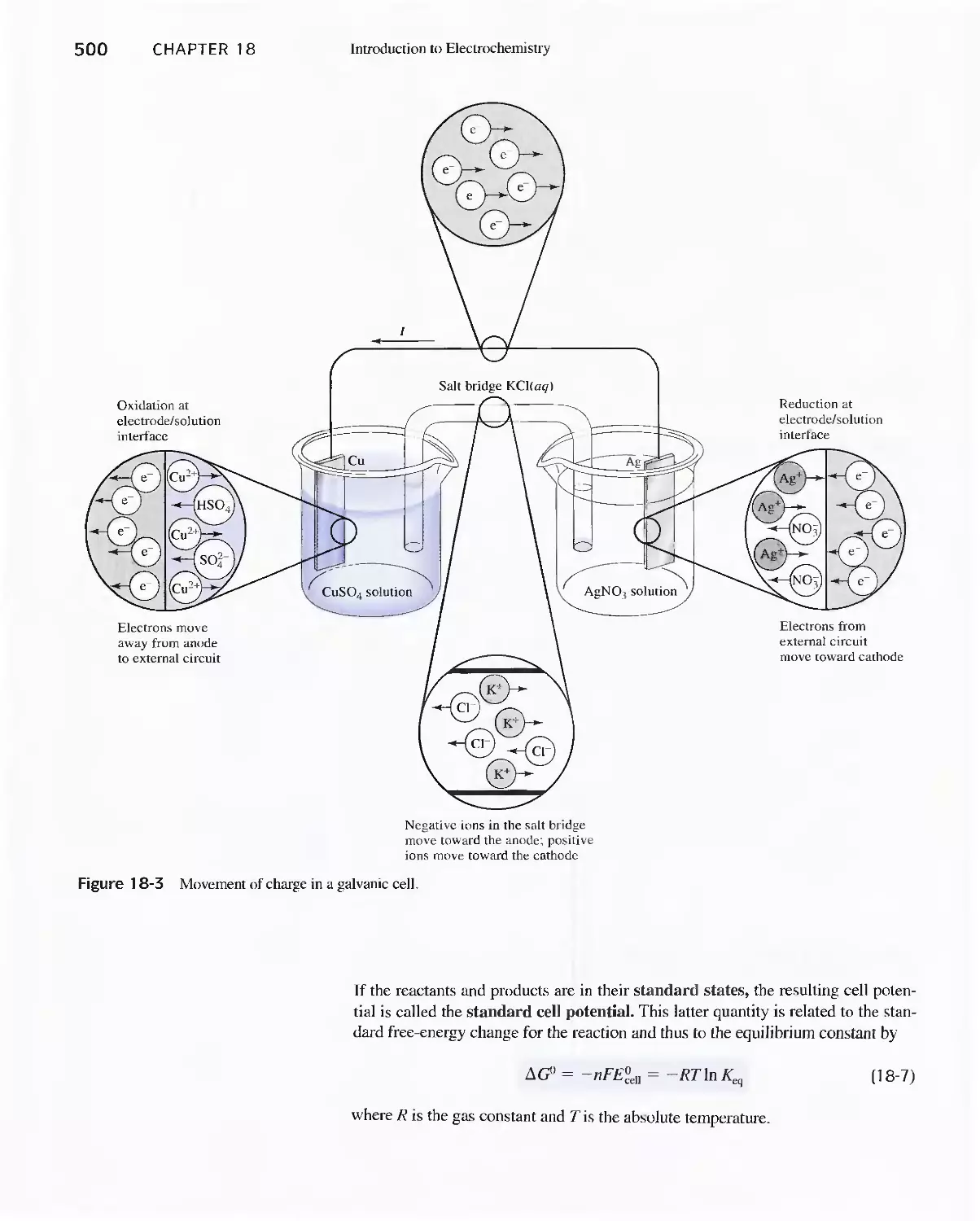
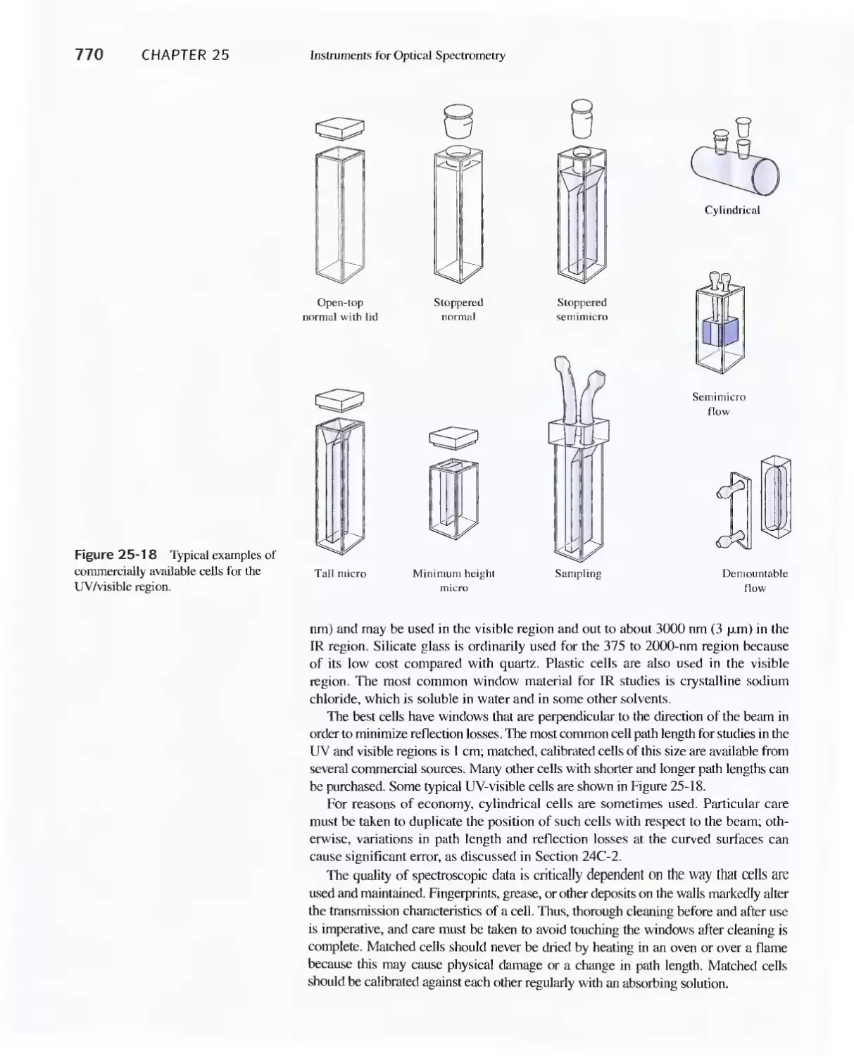
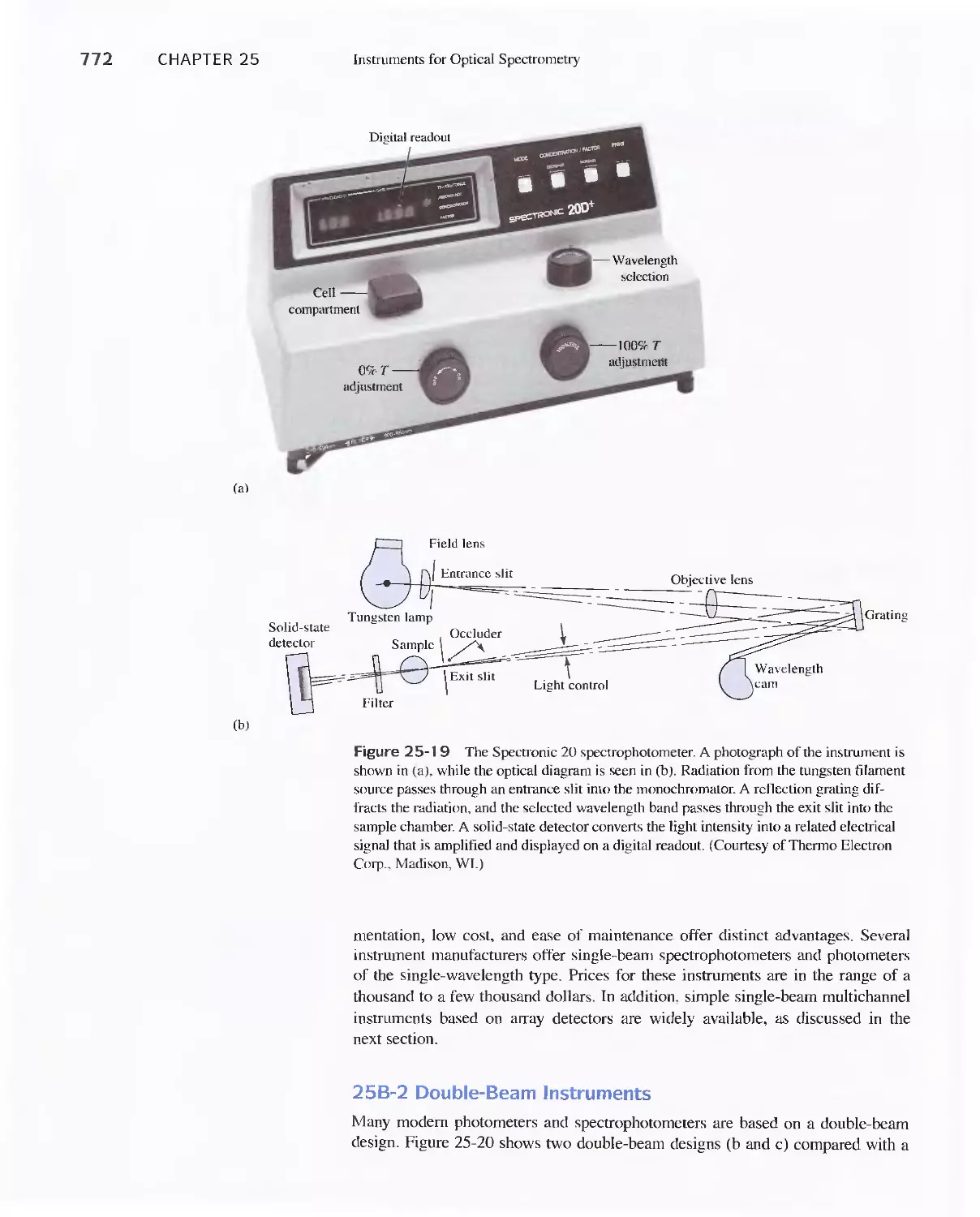
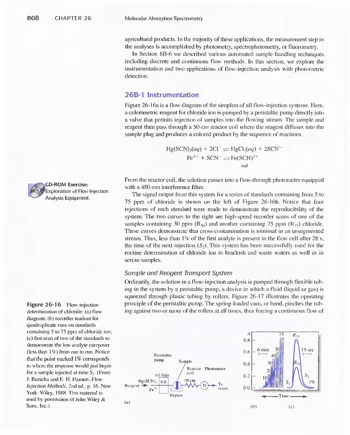
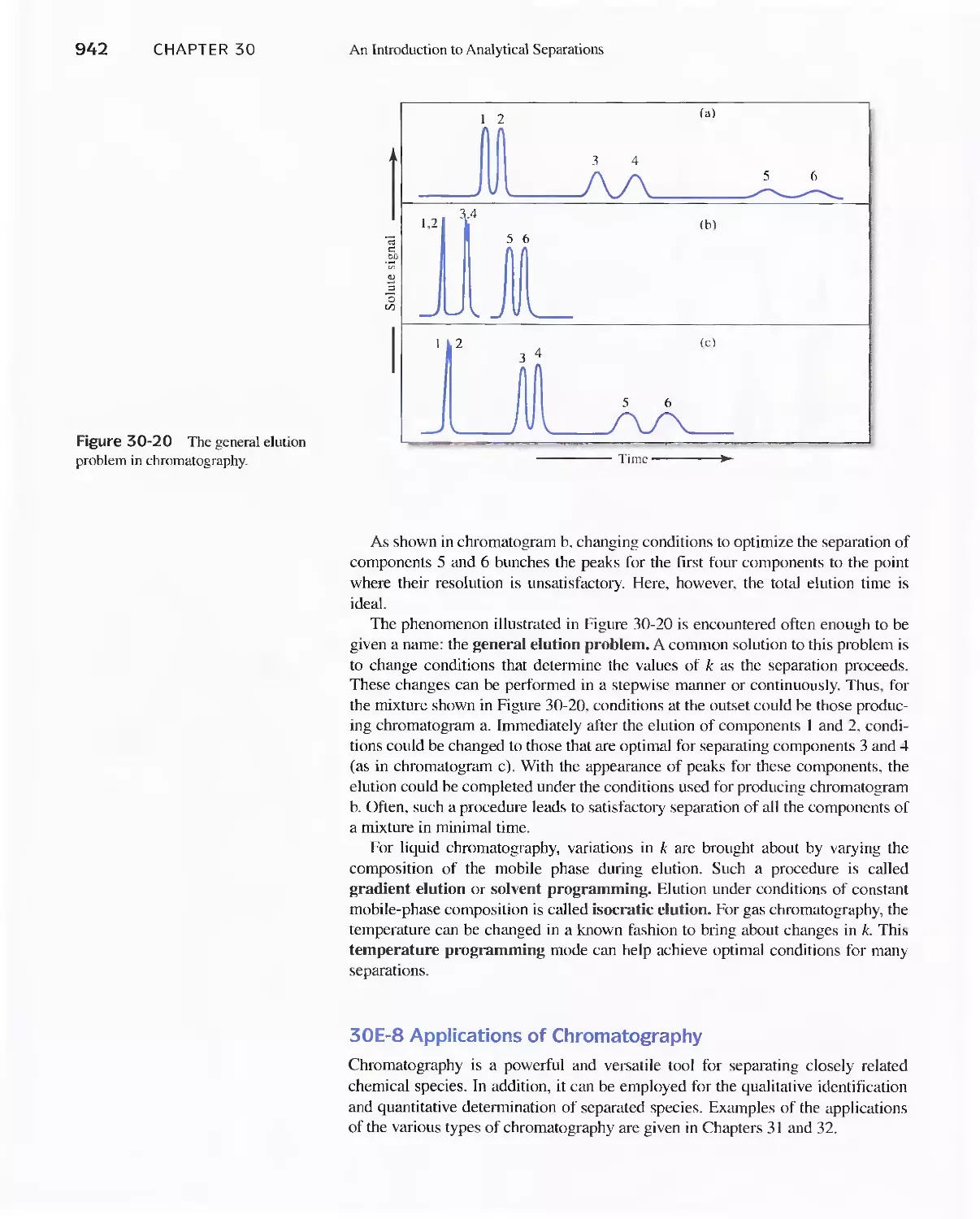
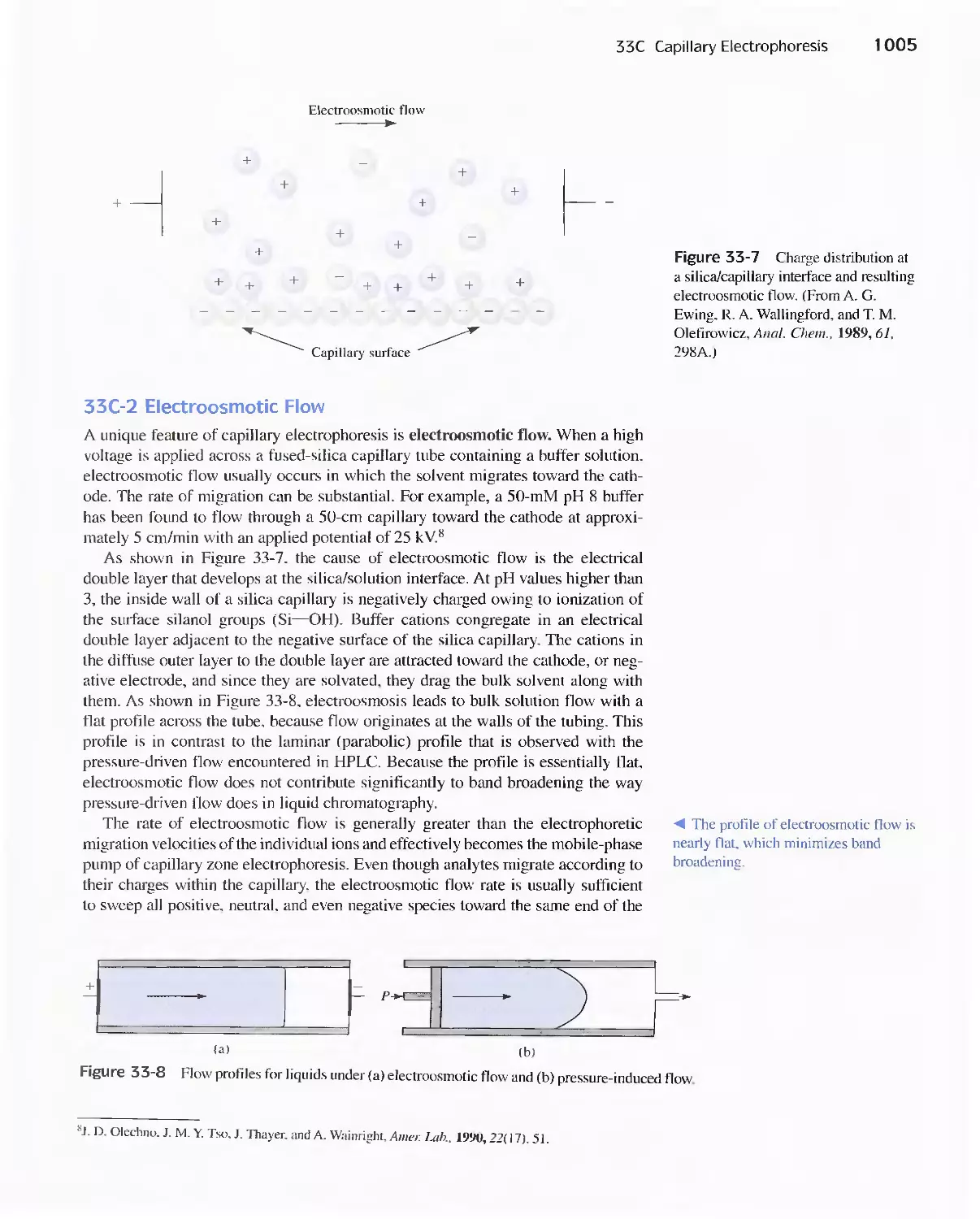
Text
Fundamentals if
Analytical Chemistry
EIGHTH FDITION
.
>'
.......
L .;
- ..
Ii.
k'
"
..
::....
-'"
11
.'
/
---.......:::r-I'
.'./
,... .
.,J
1 .;..
//
-
. .."
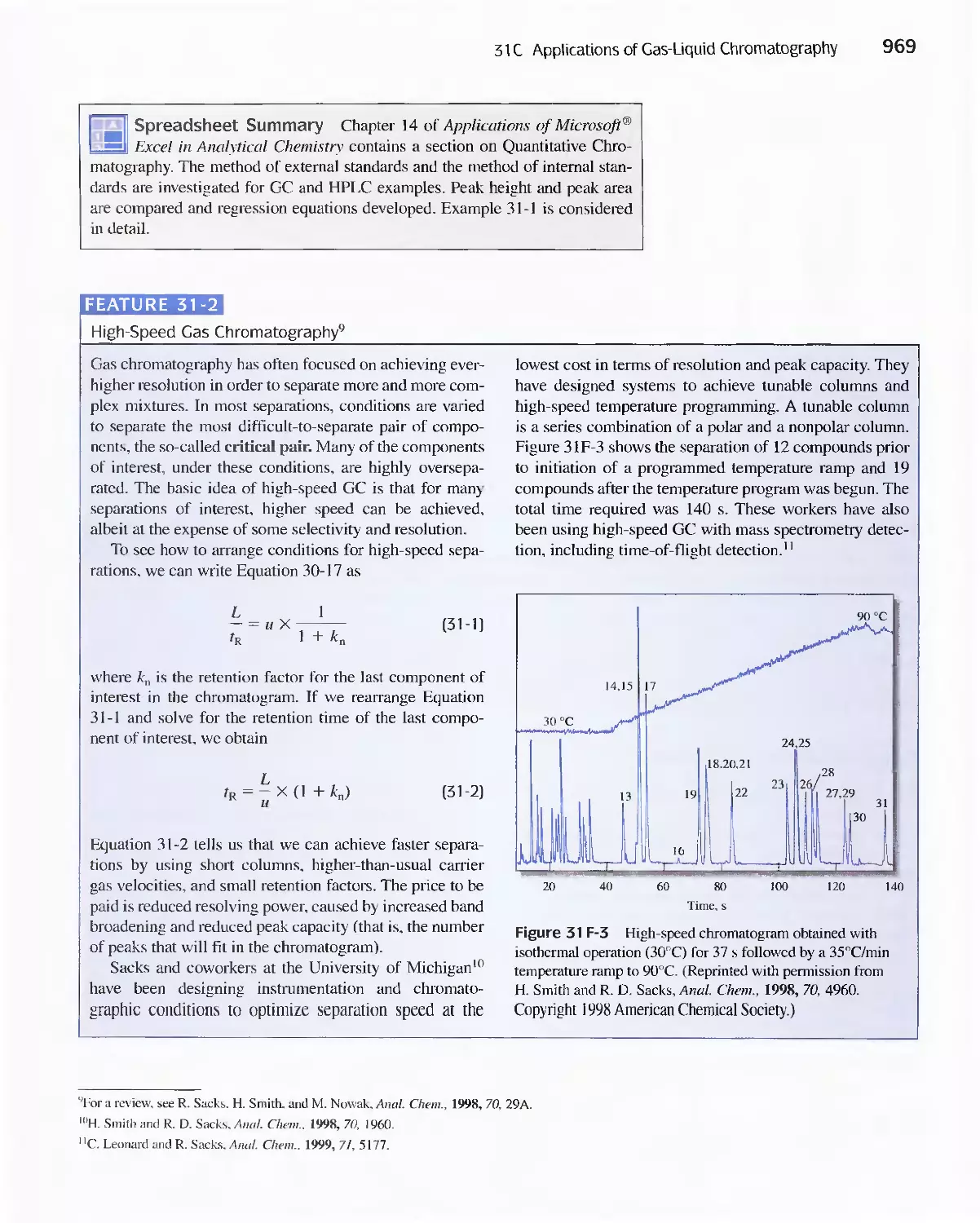
--
-:..',t
..JI
,/
..r. .
. '<:.
.
SKOOG ! WEST I HOLLER I CROUCH
Fundamentals of
Analytical
Chemistry
Douglas A. Skoog
Stanford University
Donald M. West
San Jose State University
F. James Holler
University of Kentucky
Stanley R. Crouch
Michigan State University
Australia Canada Mexico Singapore Spain
United Kingdom United States
Eighth Edition
THOMSON
*
BROOKS/COLE
THOMSON
*
BROOKS/COLE
Publisher, Chemistry: David Harris
Development Editor: Sandra Kiselica
Assistant Editor: Alyssa White
Editorial Assistants: Jessica Howard and Annie Mac
Technology Project Manager: Ericka Yeoman-Saler
Marketing Manager: Julie Conover
Marketing Assistant: Melanie Wagner
Advertising Project Manager: Stacey Purviance
Project Manager, Editorial Production: Lisa Weber
Print Buyer: Karen Hunt
Permissions Editor: Elizabeth Zuber
COPYRIGHT @ 2004 Brooks/Cole. a division of Thomson
Learning, Inc. Thomson Learning™ is a trademark used herein
under license.
ALL RIGHTS RESERVED. No part of this work covered by the
copyright hereon may be reproduced or used in any form or by
any means-graphic, electronic, or mechanical, including but not
limited to photocopying, recording, taping, Web distribution,
information networks, or information storage and retrieval sys-
tems-without the written permission of the publisher.
Primed in Canada
5 6 7 8 9 10 11 10 09 08 07
For more information about our products, contact us at:
Thomson Learning Academic Resource Center
1-800-423-0563
For permission to use material from this text,
contact us by:
Phone: 1-800-730-2214
Fax: 1-800-730-2215
Web: http://www.thomsonrights.com
Library of Congress Control Number: 2003105608
Student Edition: ISBN-13: 978-0-03-035523-3
ISBN-IO: 0-03-035523-0
International Student Edition: ISBN-13: 978-0-534-41797-0
ISBN-IO: 0-534-41797-3 (Not for sale in the United States)
Production Service: Nesbitt Graphics, Ine.
Text Designer: Kim Menning
Photo Researcher: Jane Sanders
Copy Editors: Bonnie Boehme. Linda Van Pelt
Illustrators: Rolin Graphics, Inc., and Nesbitt Graphics, Inc.
Cover Designer: Stephen Rapley
Cover Image: Charles D. Winters
Cover Printer: The Lehigh Press, Inc.
Compositor: Nesbitt Graphics, Inc.
Printer: R.R. DonnelIey/Willard
Brooks/Cole-Thomson Learning
10 Davis Drive
Belmont, CA 94002
USA
Asia
Thomson Learning
5 Shenton Way #01-01
UIC Building
Singapore 068808
Australia/New Zealand
Thomson Learning
102 Dodds Street
Southbank, Victoria 3006
Australia
Canada
Nelson
1120 Birchmount Road
Toronto, Ontario MIK 5G4
Canada
Europe/Middle East/Africa
Thomson Learning
High Holborn House
50/51 Bedford Row
London WCIR4LR
United Kingdom
On the Cover: Image of a plastic disc with micromachined channels and reservoirs used in
a total microanalysis system based on a microfluidics centrifuge platform. Capillary burst
valves provide control for the release of solutions from the reactant reservoirs (bottom and
right) into the channels and reaction chambers (center). and the analyte is monitored opti-
cally in the green chamber at the top. For fabrication details, see M. J. Madou, L 1. Lee, S.
Daunert, K. W. Koelling, S. Lai, and C-H Shih. "Design and Fabrication of CD-like
Microfluidic Platforms for Diagnostics: Microfluidic Functions," Biomed. Microdev., 2UU1,
3,245-254. For applications of the device, see I. H. A. Badr, R. D. Johnson, M. J. Madou,
and L G. Bachas. "Fluorescent Ion-Selective Optode Membranes Incorporated onto a
Centrifugal Microtluidics Platform," Anal. Chon., 2002,74, 5569-5575.
CONTENTS IN BRIEF
Chapter 1
The Nature of Analytical Chemistry 2
PART I Tools of Analytical Chemistry 1 7
Chapter 2 Chemicals, Apparatus, and Unit Operations of
Analytical Chemistry 20
Using Spreadsheets in Analytical Chemistry 54
Calculations Used in Analytical Chemistry 7I
Errors in Chemical Analyses 90
Random Errors in Chemical Analysis 105
Statistical Data Treatment and Evaluation 142
Sampling. Standardization, and Calibration 175
Chapter 3
Chapter 4
Chapter 5
Chapter 6
Chapter 7
Chapter 8
PART II Chemical Equilibria 225
Chapter 9 Aqueous Solutions and Chemical Equilibria 228
Chapter 10 Effect of Electrolytes on Chemical Equilibria 267
Chapter 11 Solving Equilibrium Calculations for Complex
Systems 2R I
PART III Classical Methods of Analysis 311
Chapter 12 Gravimetric Methods of Analysis 314
Chapter 13 Titrimetric Methods; Precipitation Titrimetry 337
Chapter 14 Principles of Neutralization Titrations 368
Chapter 15 Titration Curves for Complex Acid/Base Systems 395
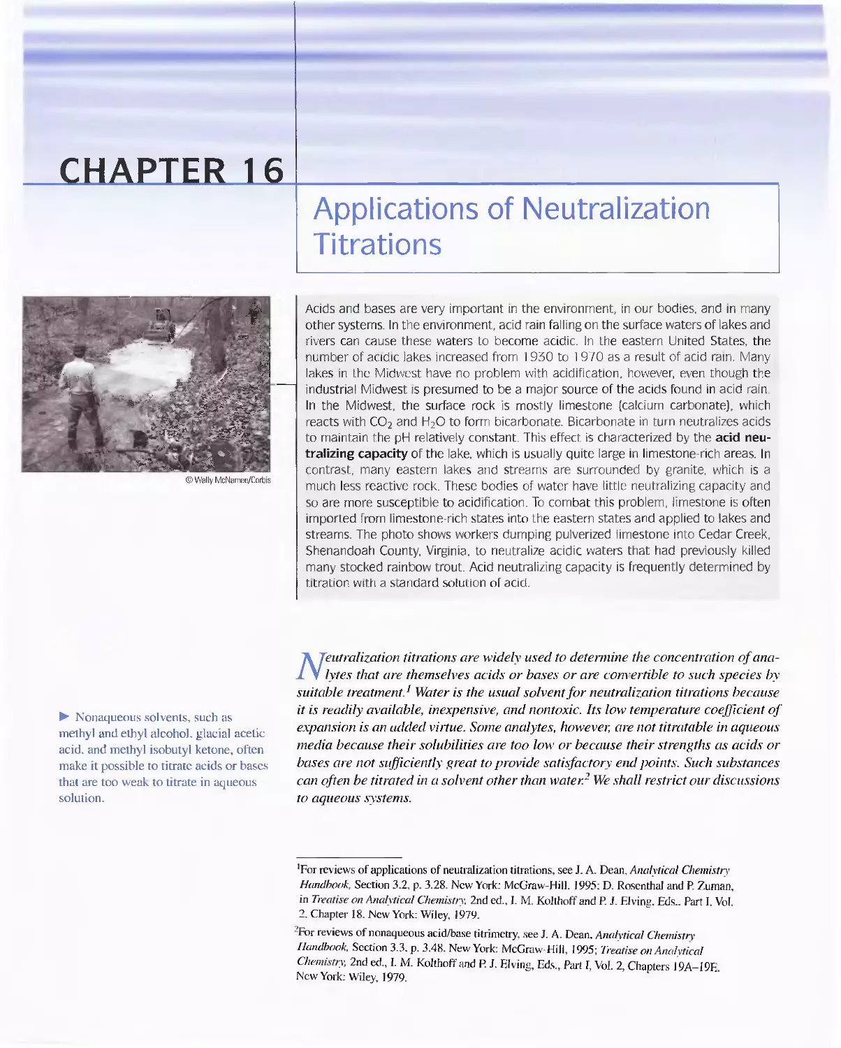
Chapter 16 Applications of Neutralization Titrations 428
Chapter 17 Complexation Reactions and Titrations 449
PART IV Electrochemical Methods 487
Chapter 18 Introduction to Electrochemistry 490
Chapter 19 Applications of Standard Electrode Potentials 523
Chapter 20 Applications of OxidationlReduction Titrations 560
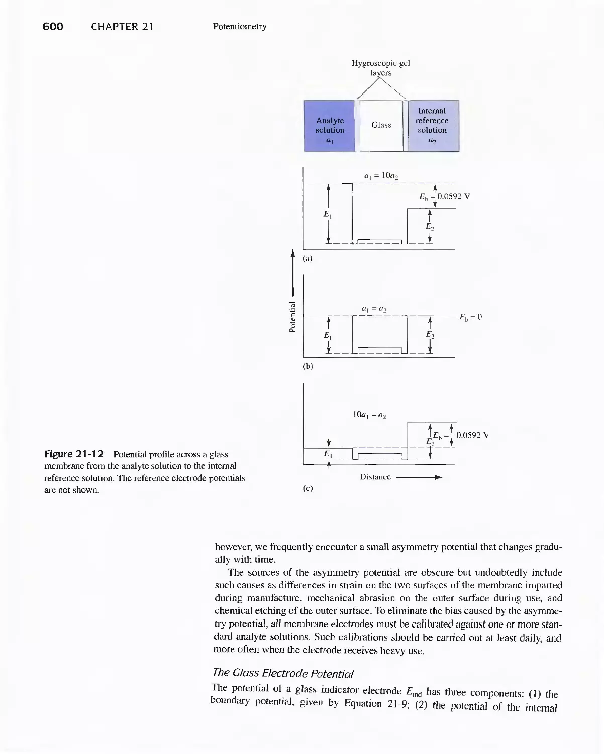
Chapter 21 Potentiometry 588
Chapter 22 Bulk Electrolysis: Electrugravimetry and Coulometry 633
Chapter 23 Voltammetry 665
PART V Spectrochemical Methods 707
Chapter 24 Introduction to Spectrochemical Methods 710
Chapter 25 Instruments for Optical Spectrometry 744
iii
Con
n
inBricl
Chapter 26
Chapter 27
Chapter 28
Molecular Absorption Spectrometry 784
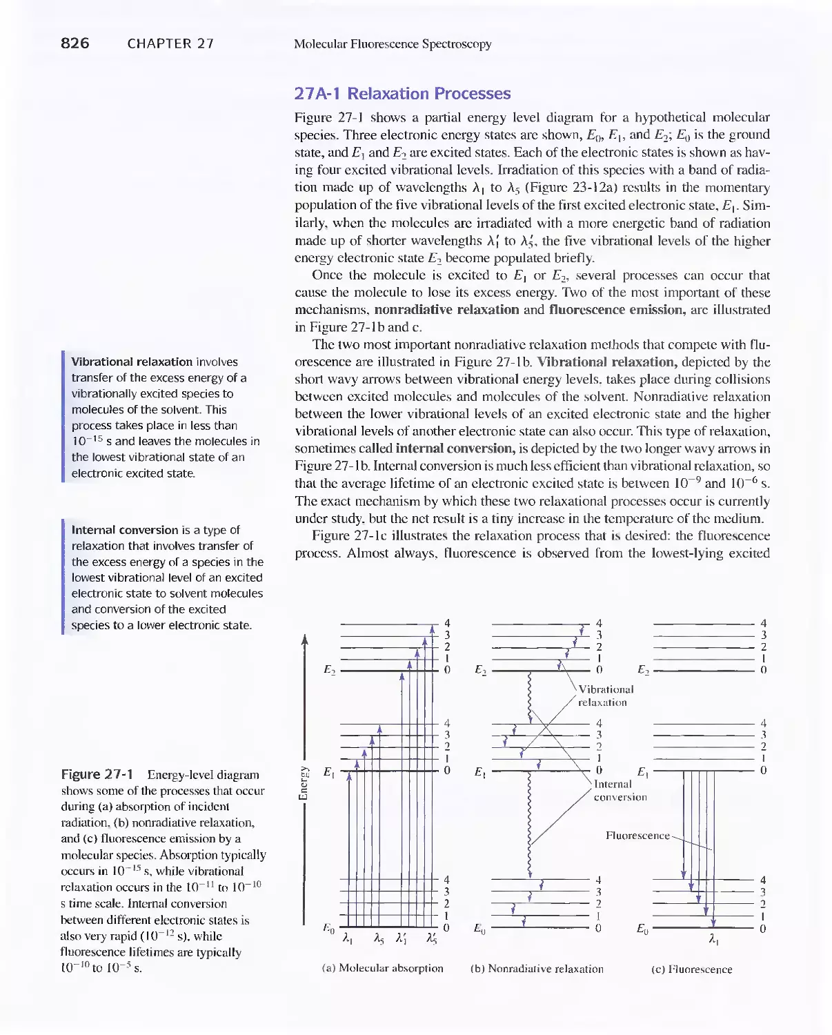
Molecular Fluorescence Spectroscopy 825
Atomic Spectroscopy 839
PART VI Kinetics and Separations 875
Chapter 29 Kinetic Methods of Analysis 878
Chapter 30 Introduction to Analytical Separations 906
Chapter 31 Gas Chromatography 947
Chapter 32 High-Performance Liquid Chromatography 973
Chapter 33 Miscellaneous Separation Methods 996
PART VII Practical Aspects of Chemical Analysis 1021
Chapter 34 Analysis of Real Samples 1024
Chapter 35 Preparing Samples for Analysis 1034
Chapter 36 Decomposing and Dissolving the Sample 1041
Chapter 37 Selected Methods of Analysis
This chapter is only available as Adobe Acrobat@ PDF file on the
Analytical Chemistry CD-ROM enclosed in this book or on our
Web site at http://chemistry.brookscole.com/skoogfac/.
Appendix 1
Appendix 2
Appendix 3
Appendix 4
Appendix 5
Appendix 6
Appendix 7
Appendix 8
Appendix 9
Glossary G-]
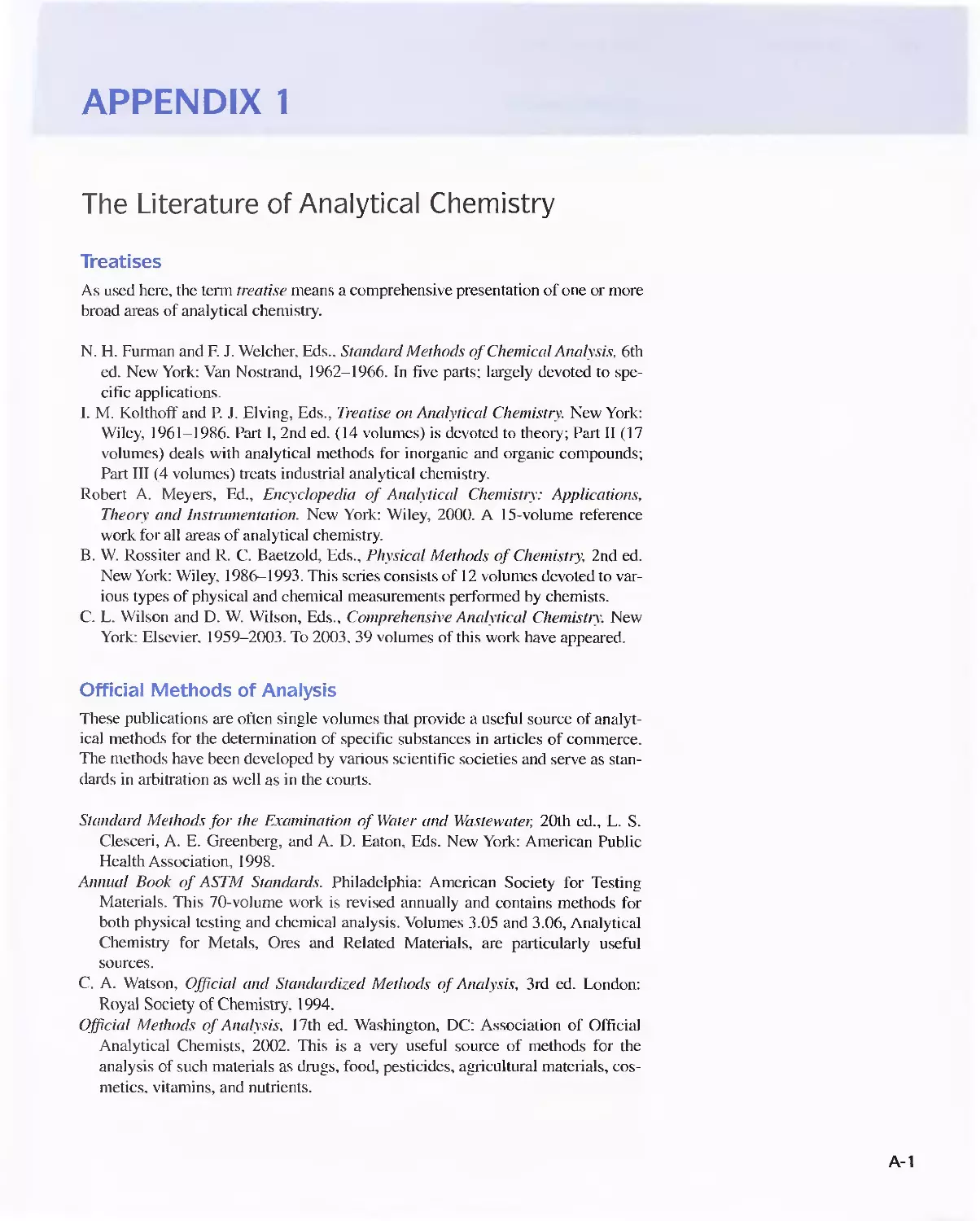
The Literature of Analytical Chemistry A-I
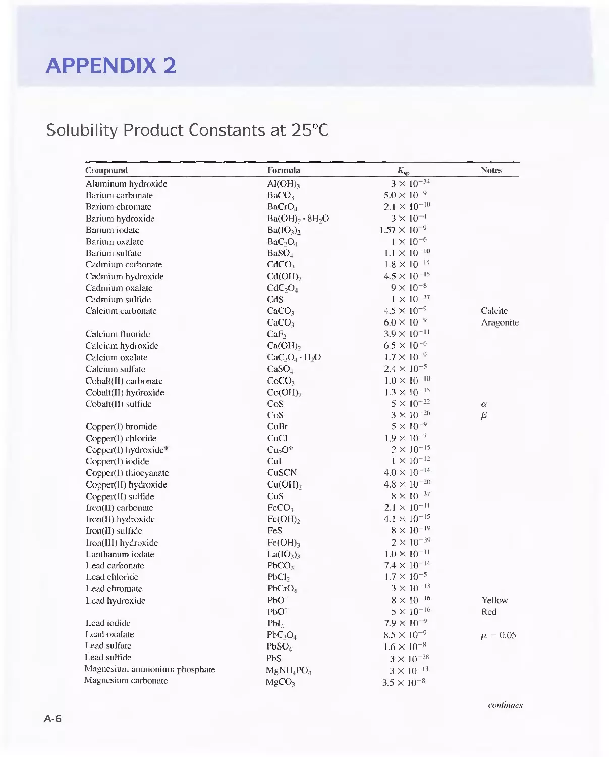
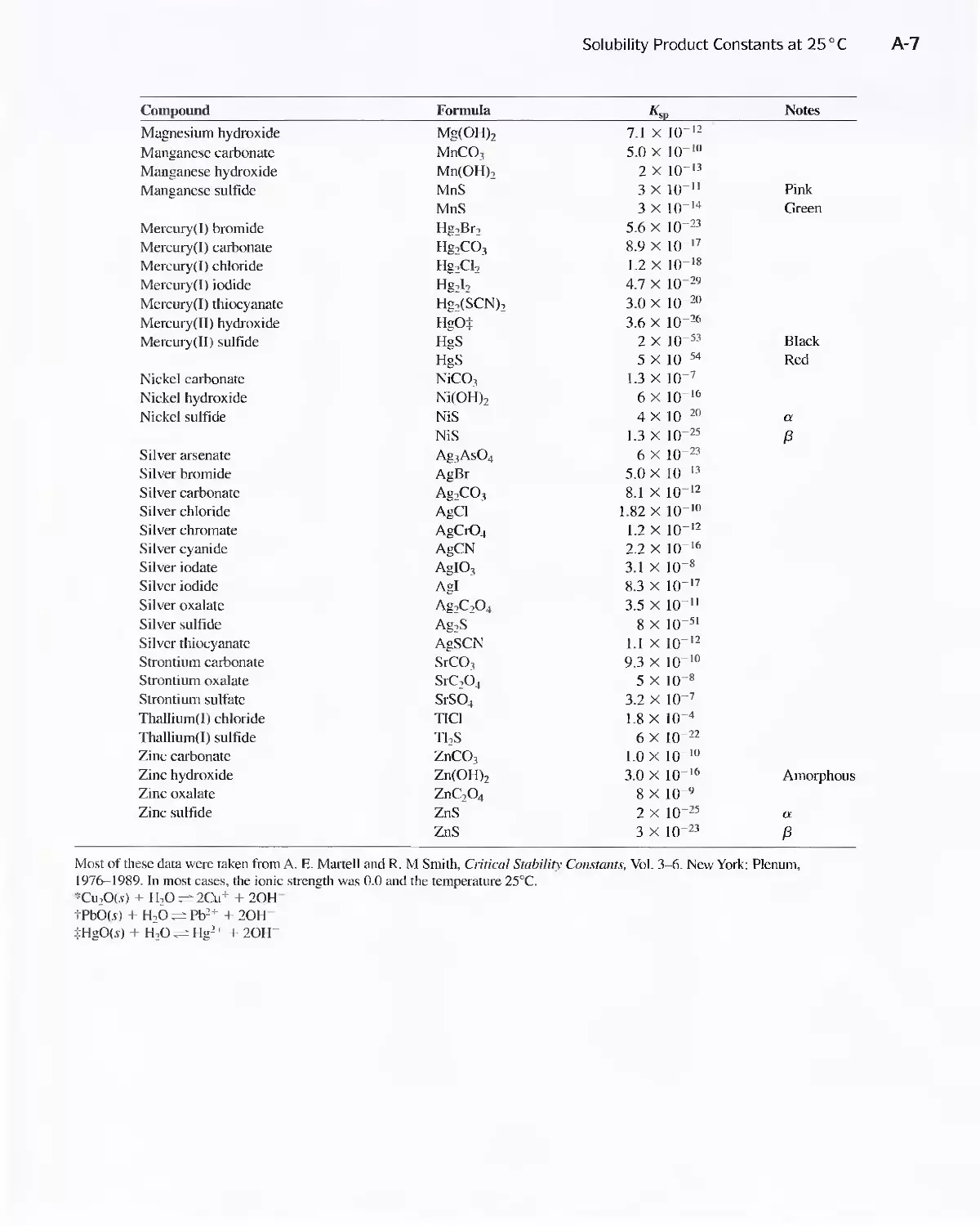
Solubility Product Constants at 25°C A-6
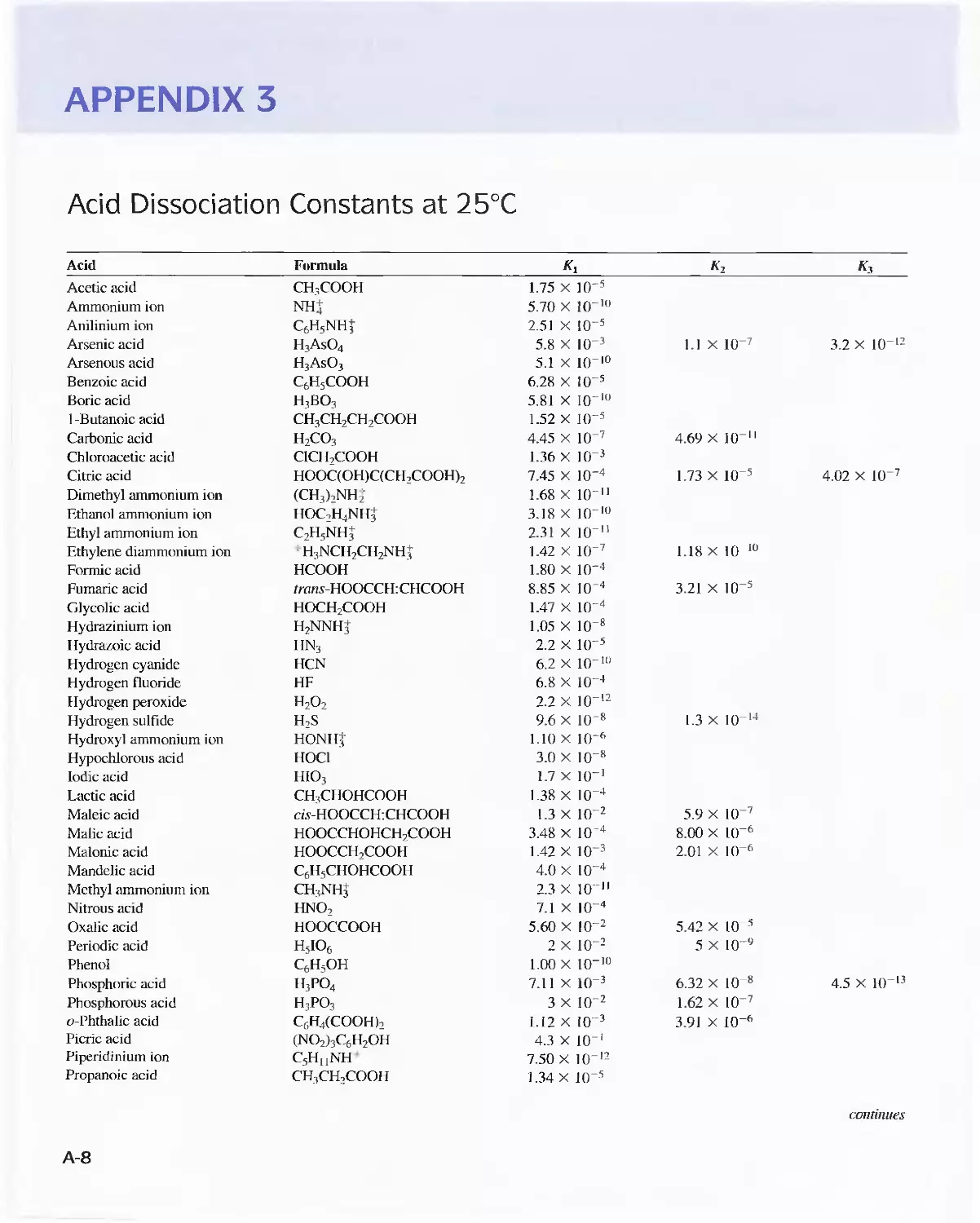
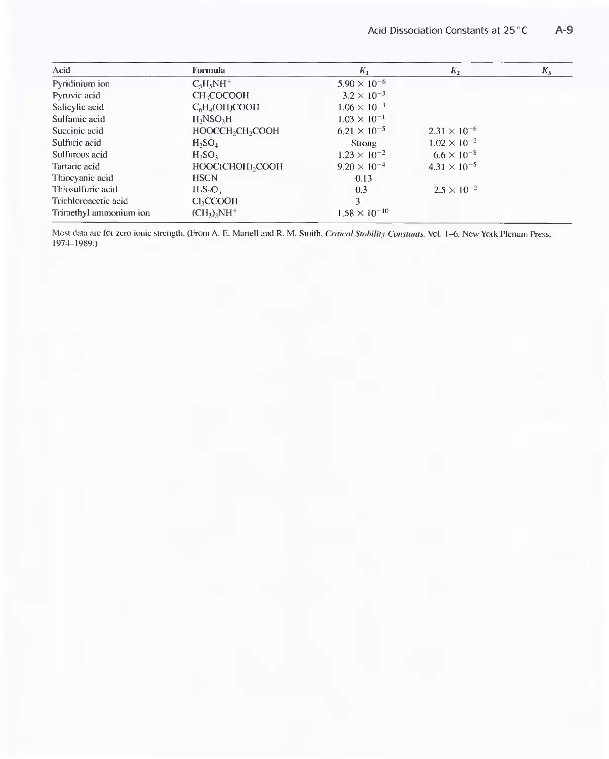
Acid Dissociation Constants at 25°C A-8
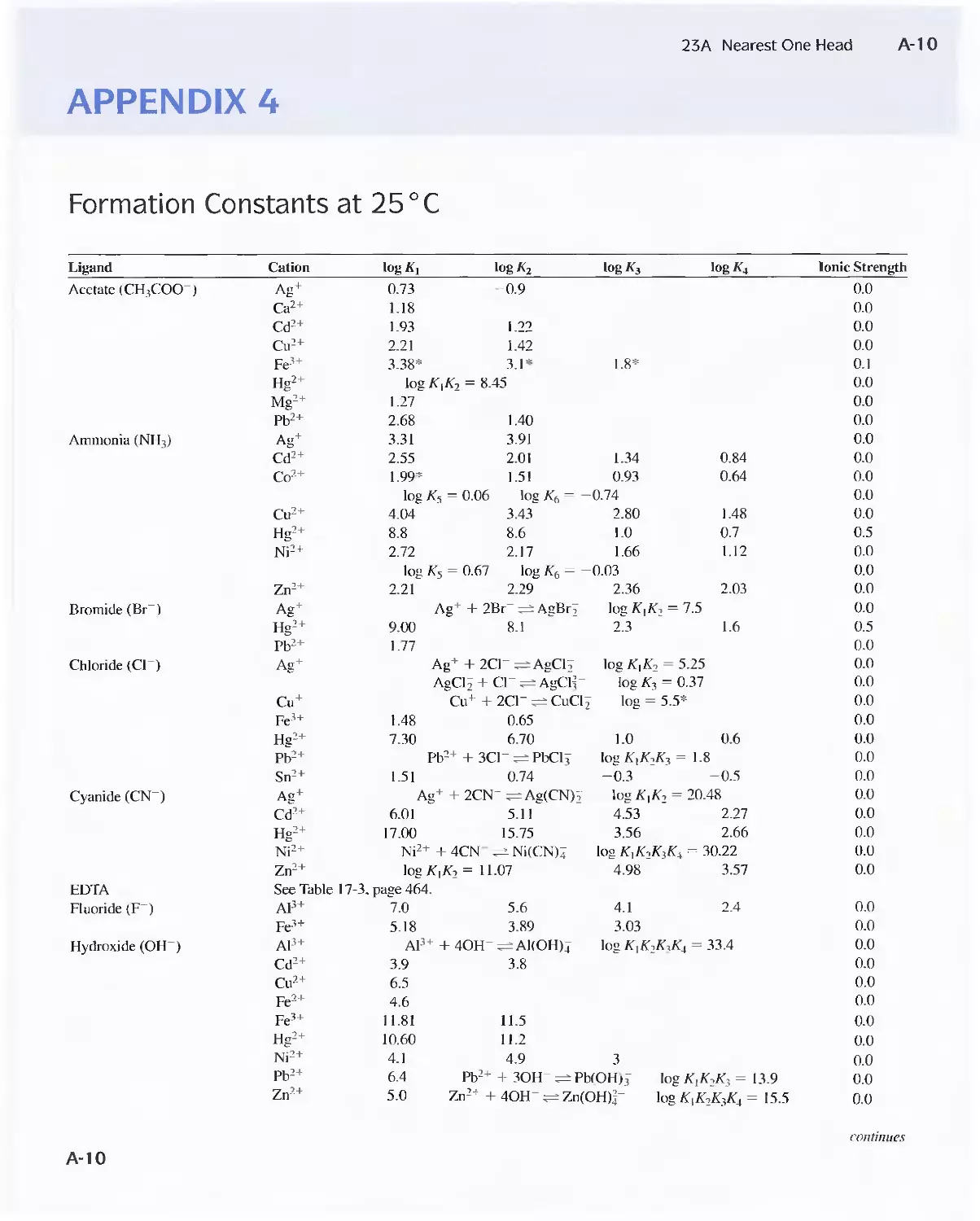
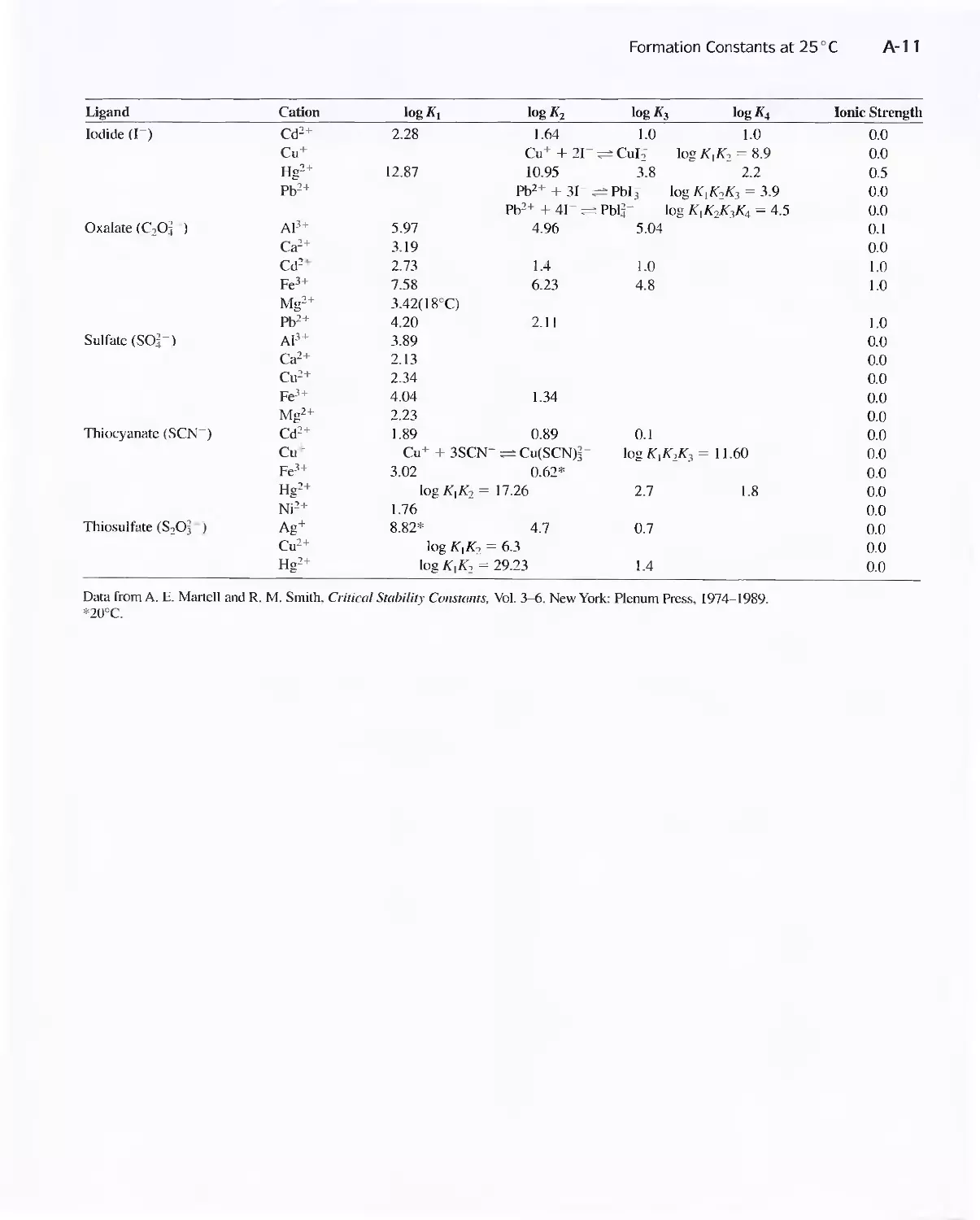
Formation Constants at 25°C A-lO
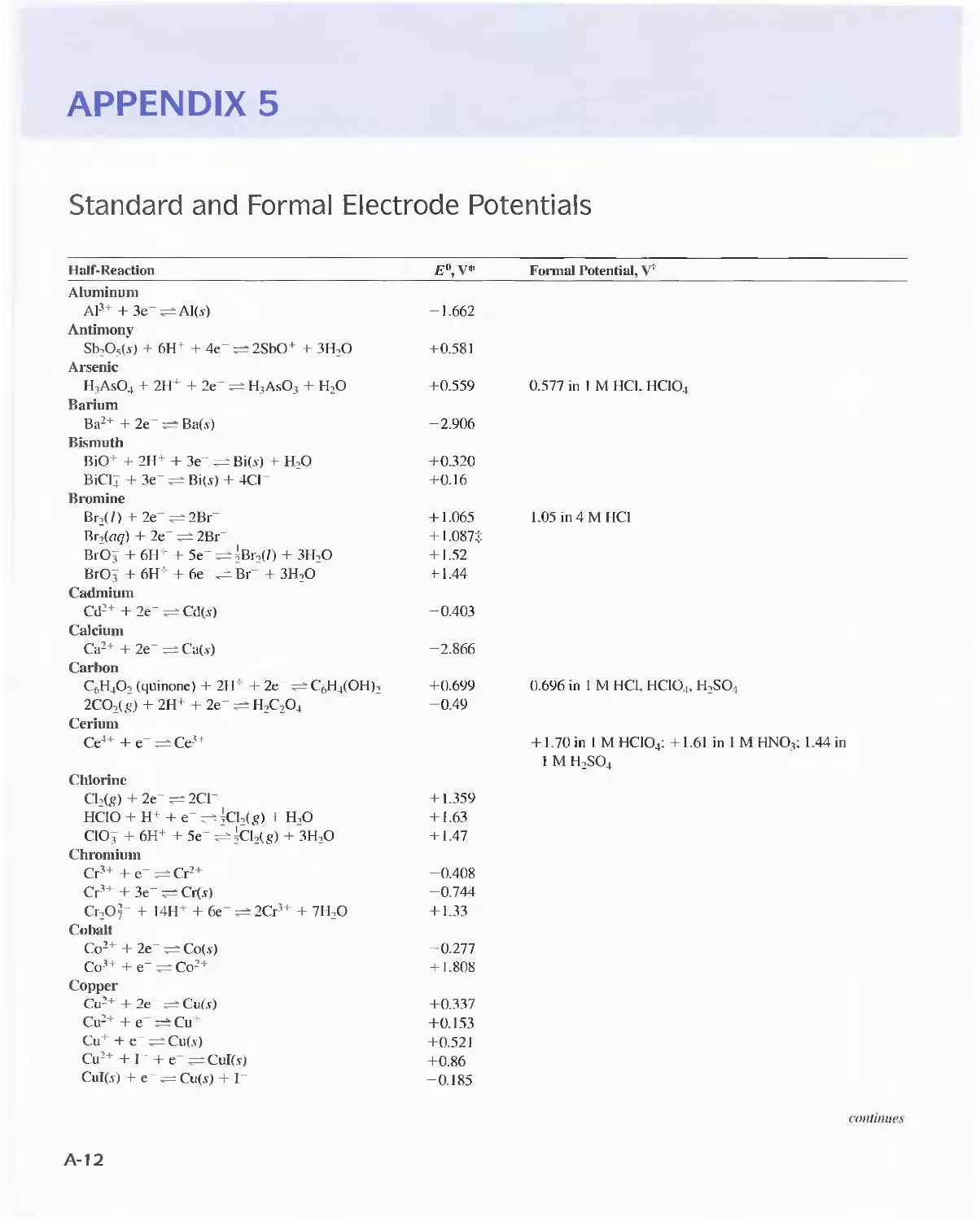
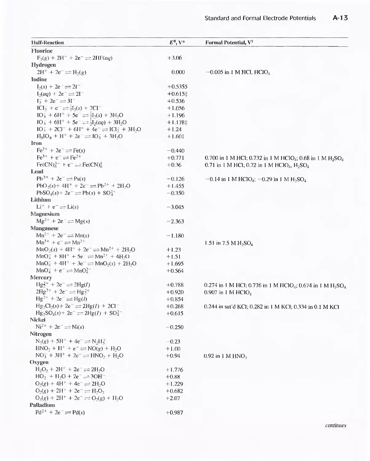
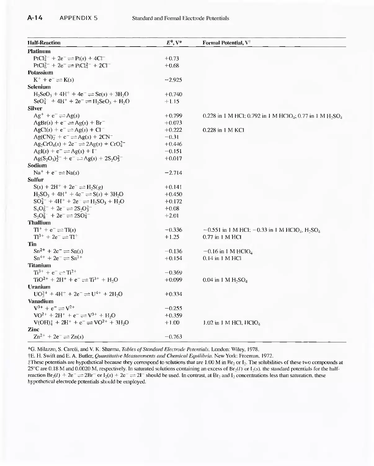
Standard and Fonnal Electrode Potentials A-12
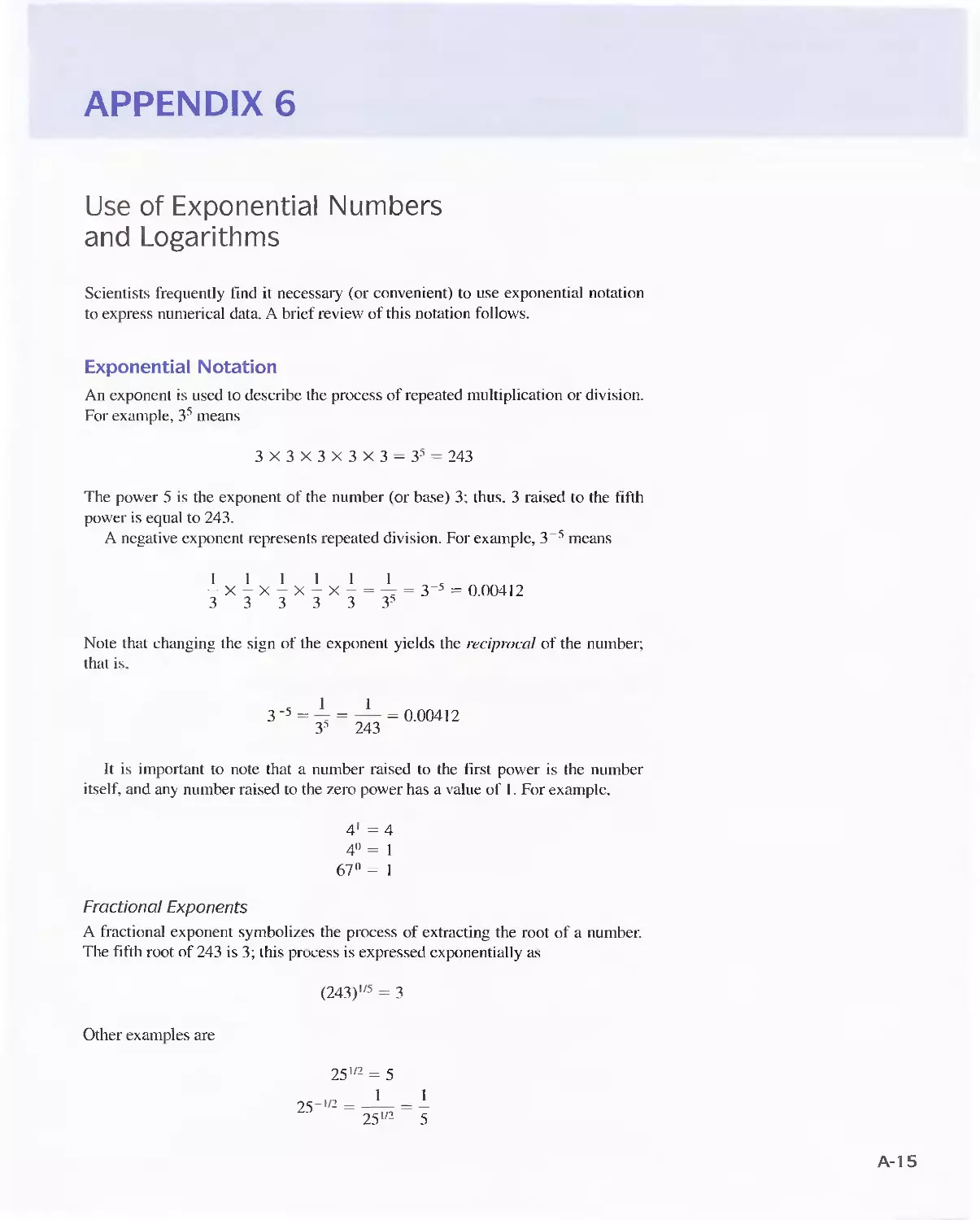
Use of Exponential Numbers and Logarithms A-15
Volumetric Calculations Using Nonnality and Equivalent
Weight A-19
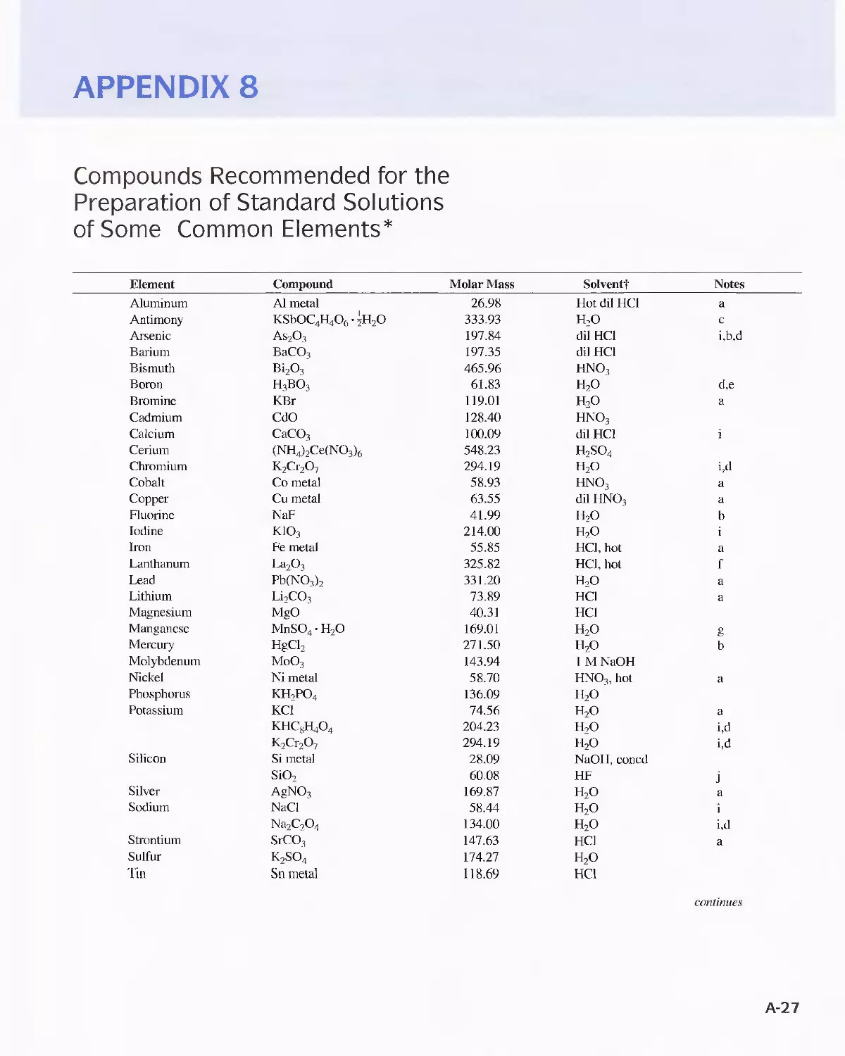
Compounds Recommended for the Preparation of Standard
Solutions of Some Common Elements A-27
Derivation of Error Propagation Equations A-29
Answers to Selected Questions and Problems A-34
Index I-I
CONTENTS
Chapter 1 The Nature of Analytical Chemistry 2
I A The Role of Analytical Chemistry 3
1 B Quantitative Analytical Methods 4
1 C A Typical Quantitative Analysis 5
1 D An Integral Role for Chemical Analysis:
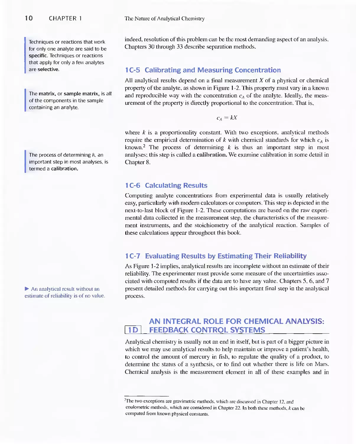
Feedback Control Systems 10
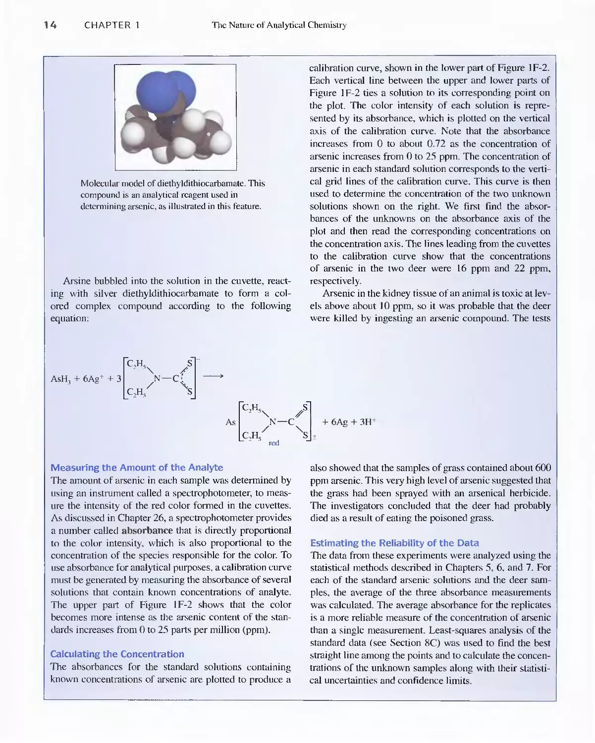
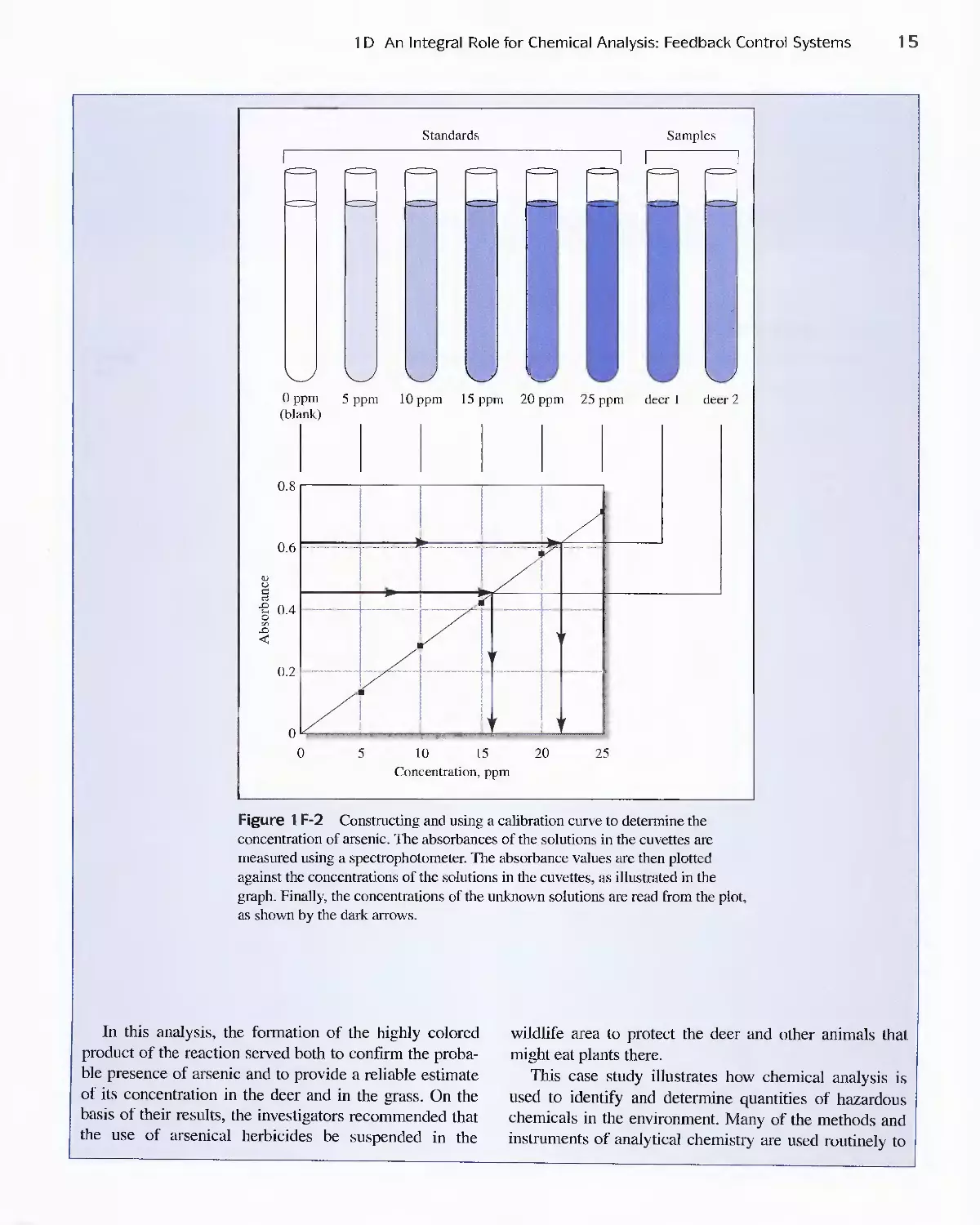
Feature 1-1 Deer Kill: A Case Study Illustrating the Use
of Analytical Chemistry to Solve a Problem
in Toxicology 12
PART I Tools of Analytical Chemistry 17
A Conversation with Richard N. Zare 18
Chapter 2 Chemicals, Apparatus, and Unit Operations
of Analytical Chemistry 20
2A Selecting and Handling Reagents and Other
Chemicals 21
2B Cleaning and Marking of Laboratory Ware 22
2C Evaporating Liquids 23
2D Measuring Mass 23
2E Equipment and Manipulations Associated with
Weighing 30
2F Filtration and Ignition of Solids 33
2G Measuring Volume 39
2H Calibrating Volumetric Glassware 48
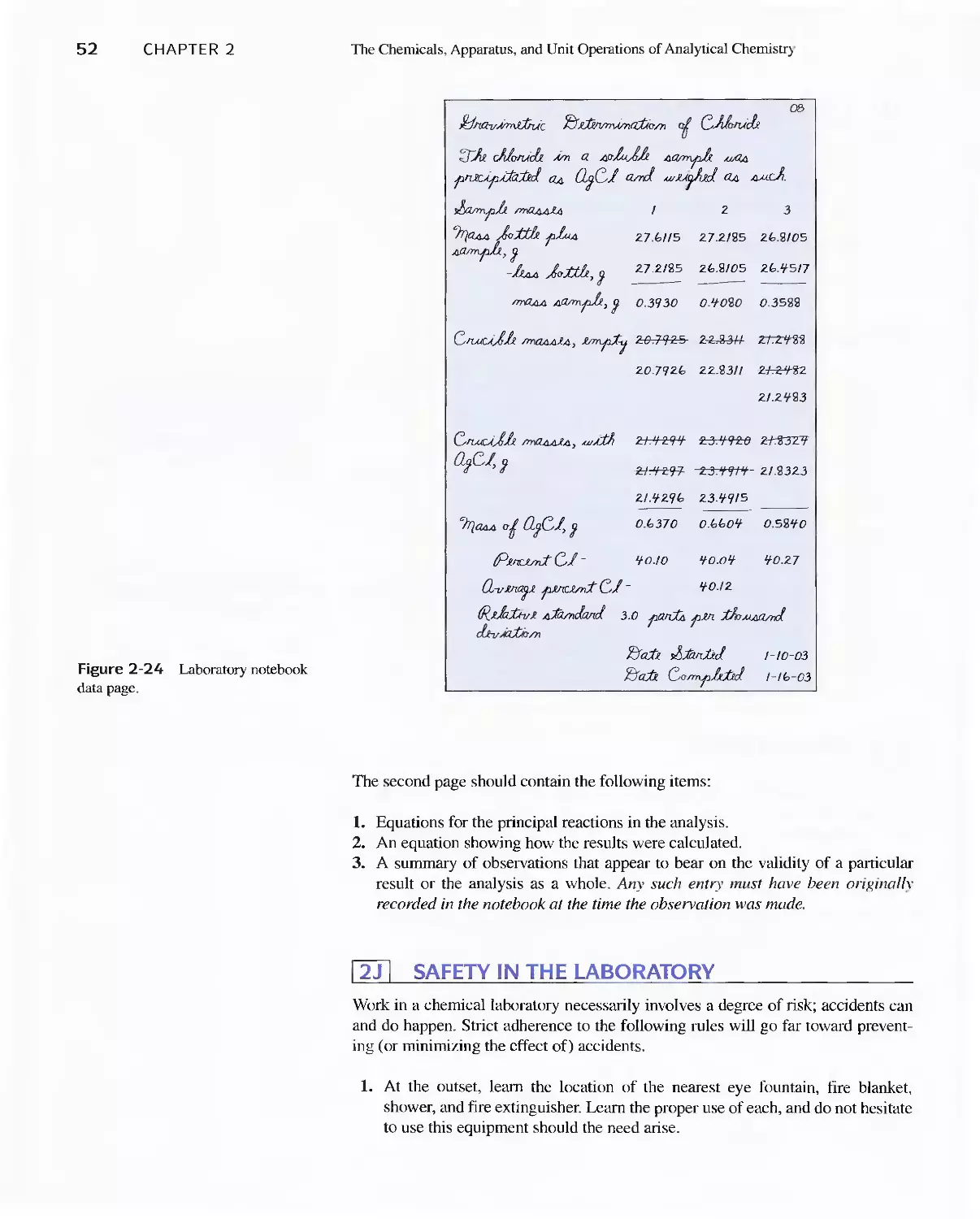
21 The Laboratory Notebook 51
2J Safety in the Laboratory 52
Chapter 3 Using Spreadsheets in Analytical
Chemistry 54
3A Keeping Records and Making Calculations:
Spreadsheet Exercise 1 55
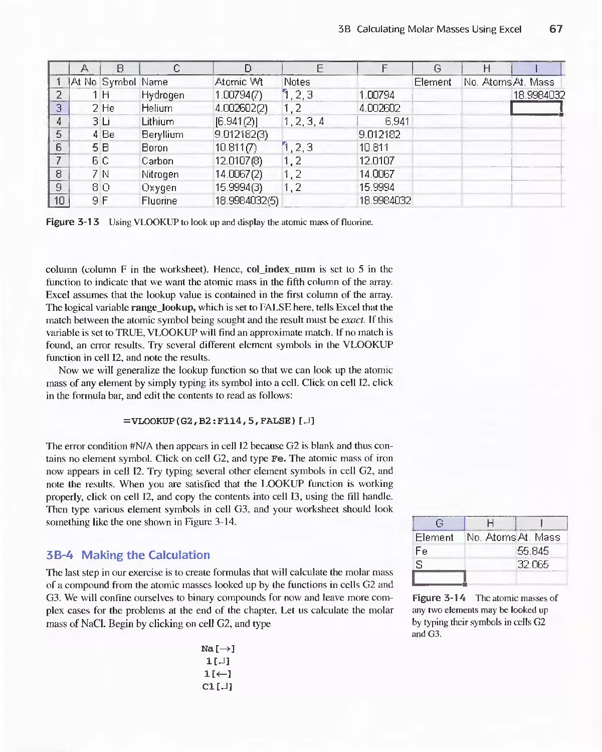
3B Calculating Molar Masses Using Excel: Spreadsheet
Exercise 2 60
Chapter 4 Calculations Used in Analytical
Chemistry 71
4A Some Important Units of Measurement 71
Feature 4-1 Atomic Mass Units and the Mole 73
4B Solutions and Their Concentrations 76
4C Chemical Stoichiometry 83
Chapter 5 Errors in Chemical Analyses 90
5A Some Important Terms 92
5B Systematic Errors 95
Chapter 6 Random Errors in Chemical Analysis 105
6A The Nature of Random Errors 105
Feature 6-1 Flipping Coins: A Student Activity to
Illustrate a Normal Distribution 109
6B Statistical Treatment of Random Error 110
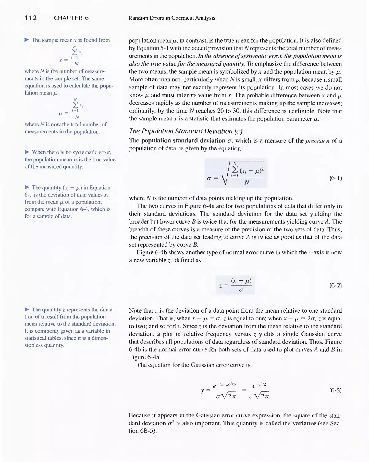
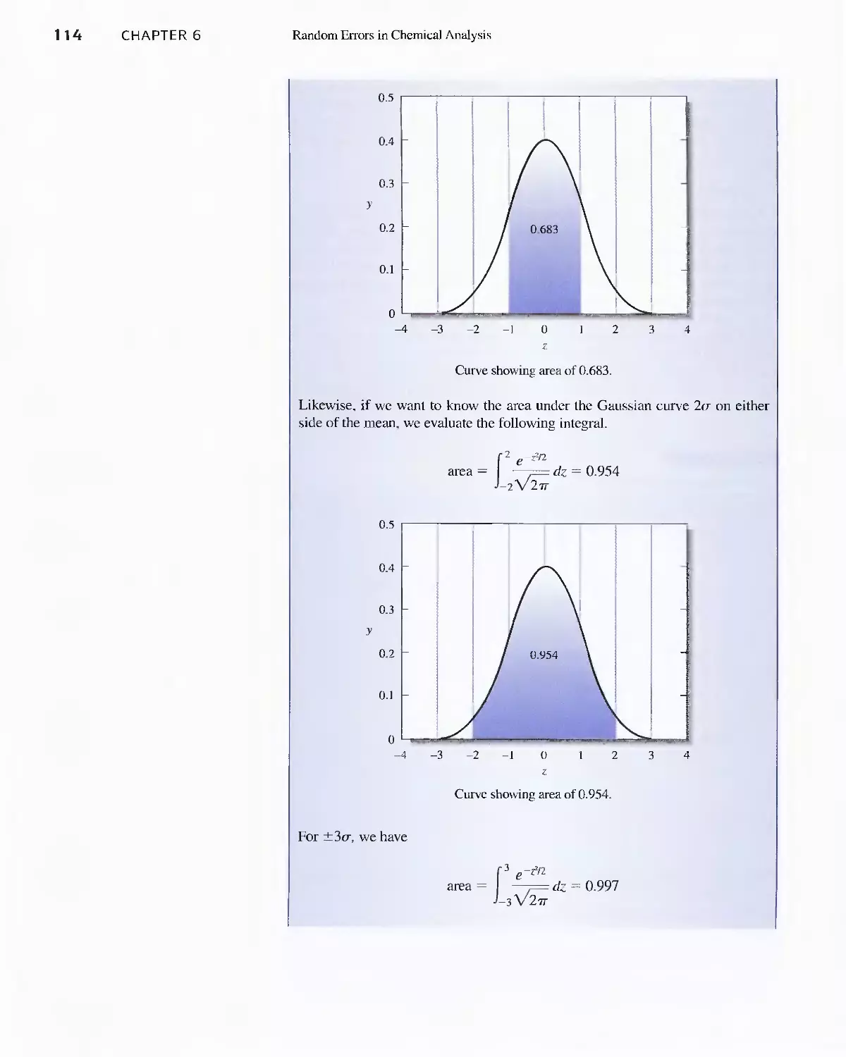
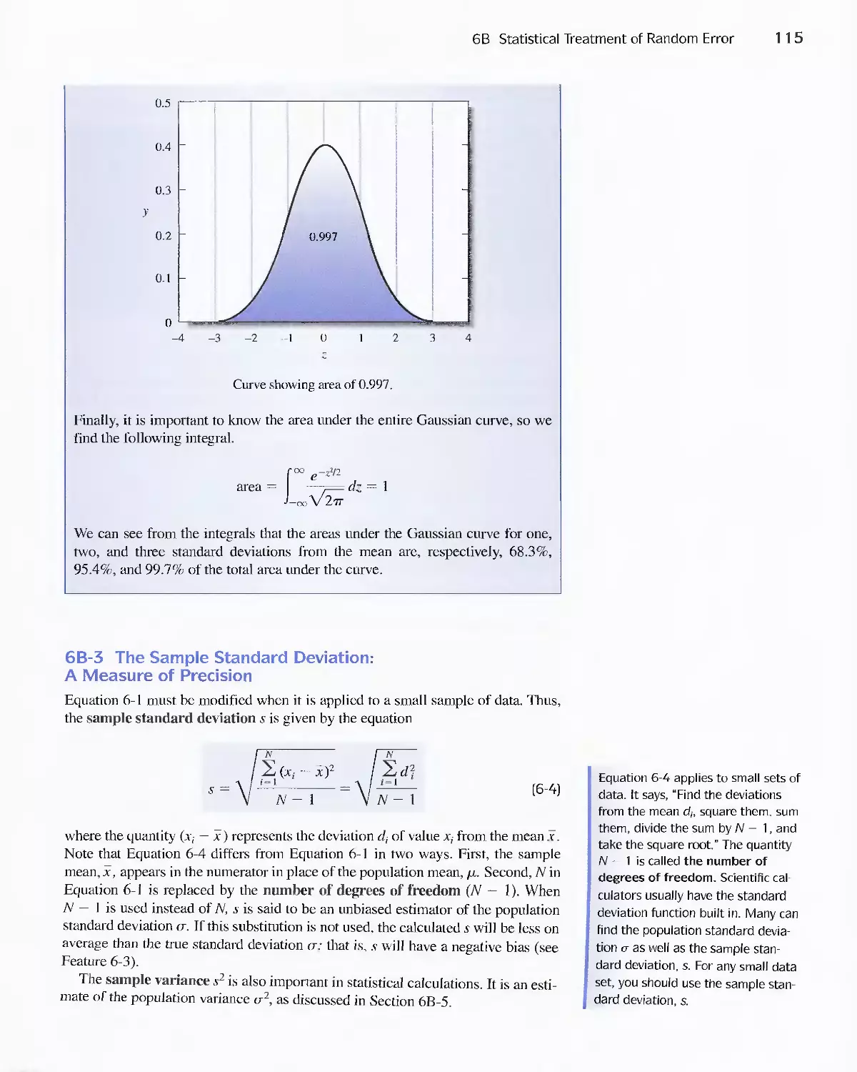
Feature 6-2 Calculating the Areas under the Gaussian
Curve II 3
Feature 6-3 The Significance of the Number of Degrees
of Freedom 11 6
Feature 6-4 Equation for Calculating the Pooled
Standard Deviation 124
6C Standard Deviation of Calculated Results 127
6D Reporting Computed Data 133
Chapter 7 Statistical Data Treatrnent and
Evaluation 142
7 A Confidence Intervals 143
Feature 7-1 Breath Alcohol Analyzers 148
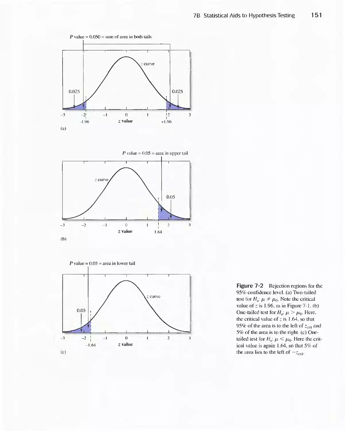
7B Statistical Aids to Hypothesis Testing 149
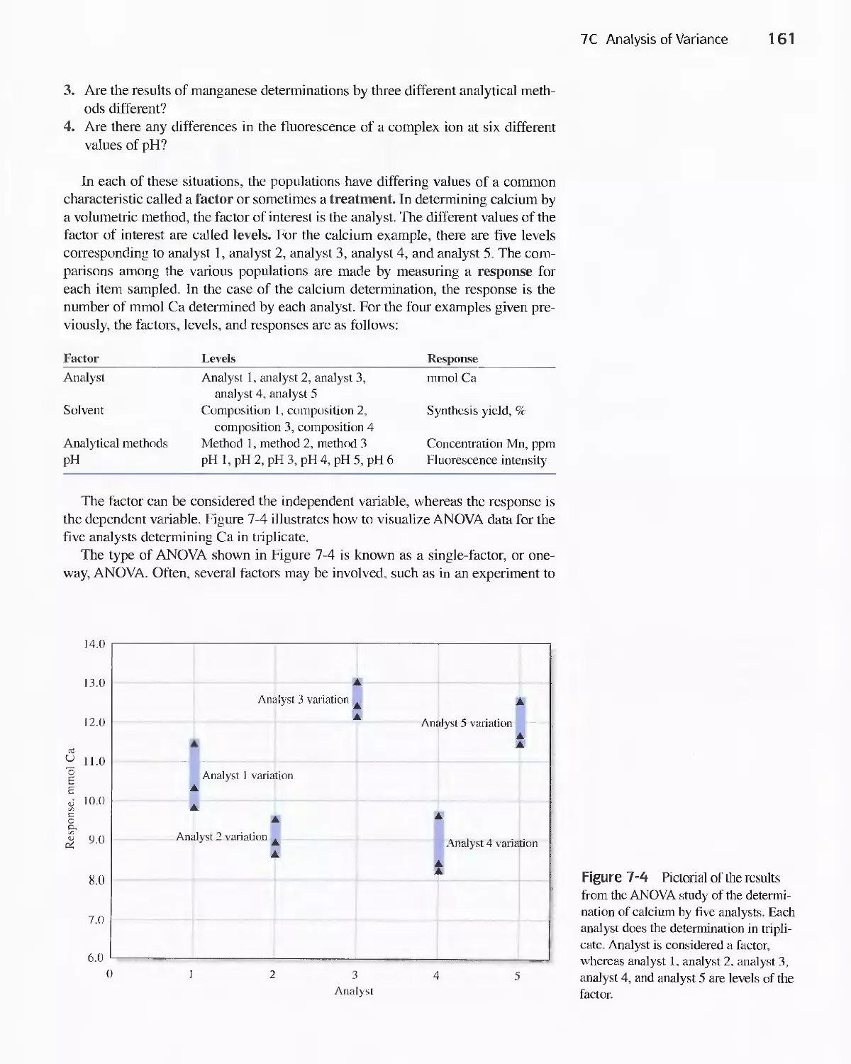
7C Analysis of Variance 160
7D Detection of Gross Errors 167
Chapter 8 Sampling, Standardization,
and Calibration 175
8A Analytical Samples and Methods 175
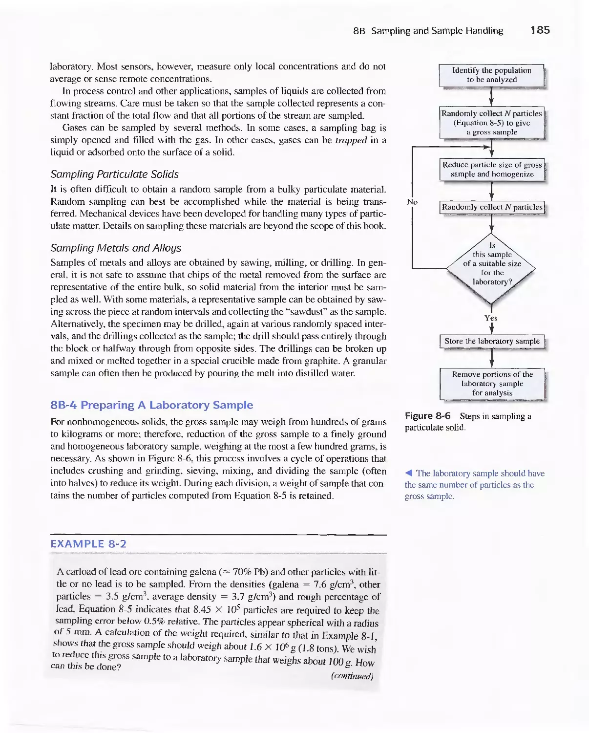
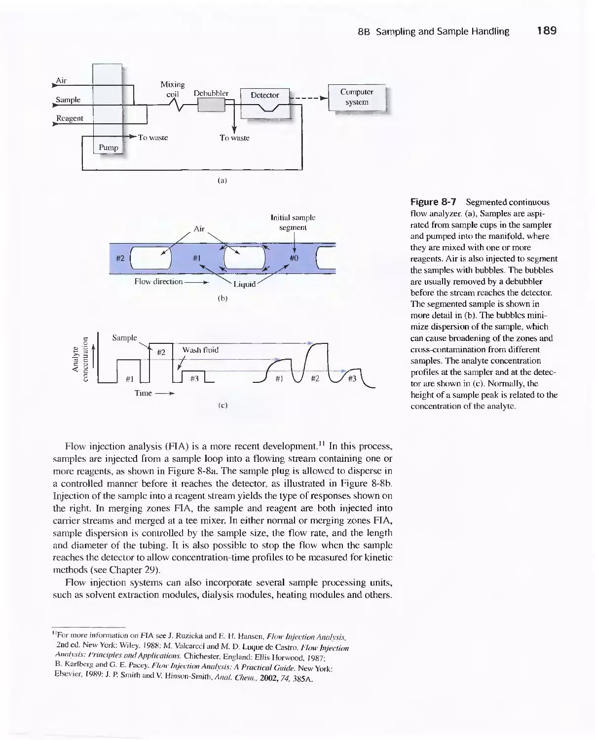
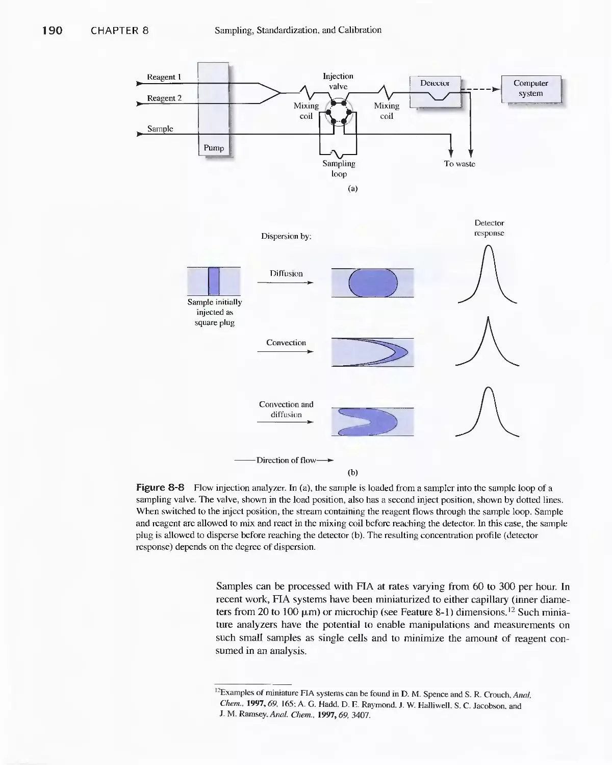
8B Sampling and Sample Handling 178
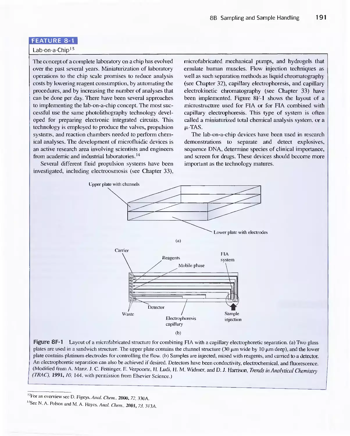
Feature 8-1 Lab-on-a-Chip 191
8C Standardization and Calibration 192
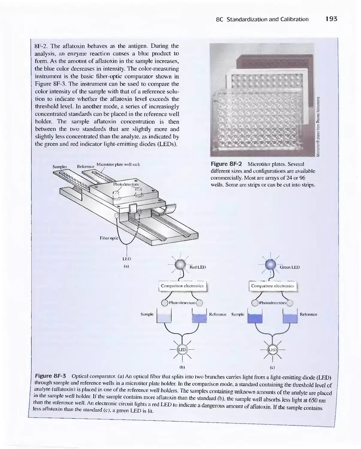
Feature 8-2 A Comparison Method for Aflatoxins 192
Feature 8-3 Multivariate Calibration 208
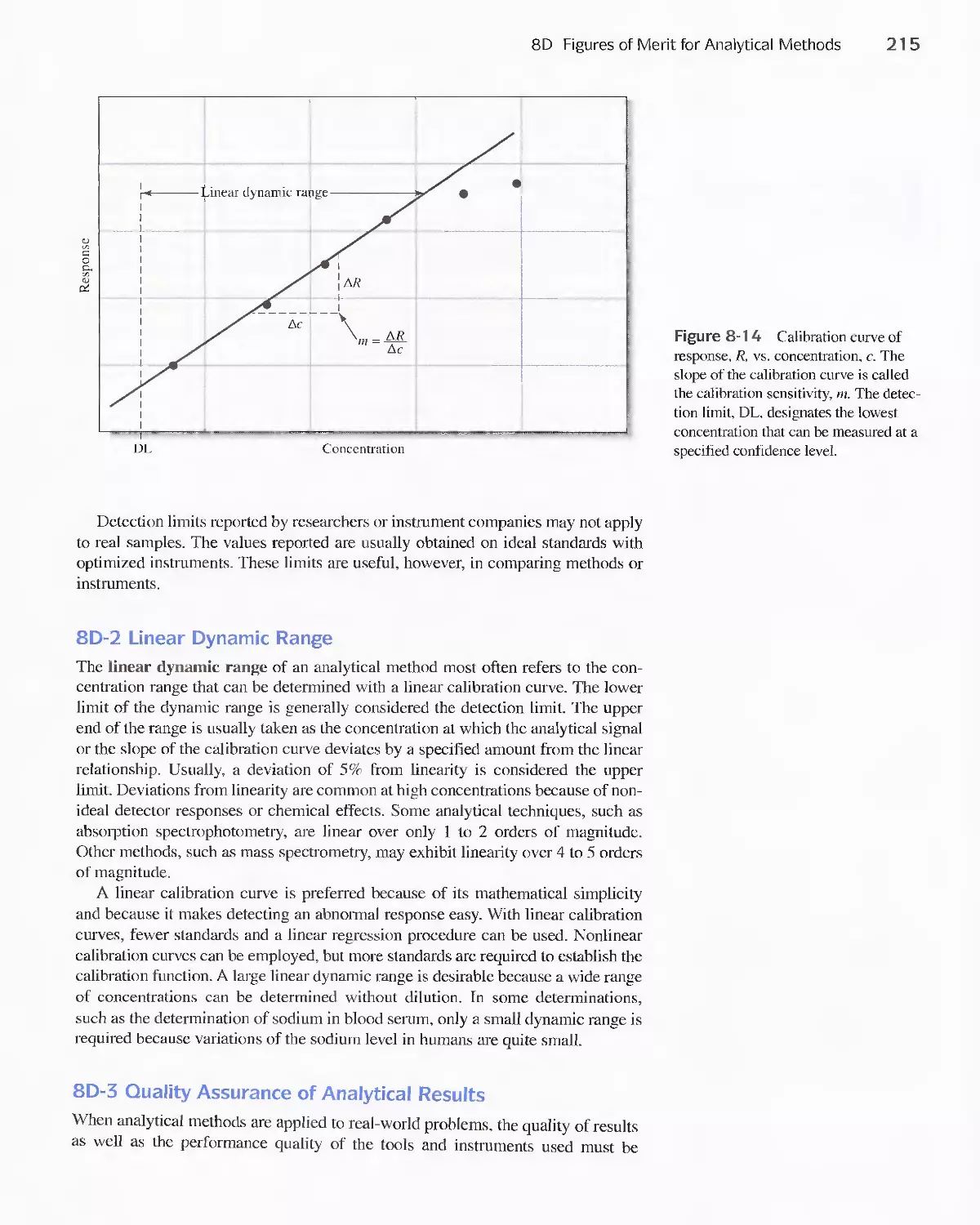
8D Figures of Merit for Analytical Methods 21 4
PART II Chemical Equilibria 225
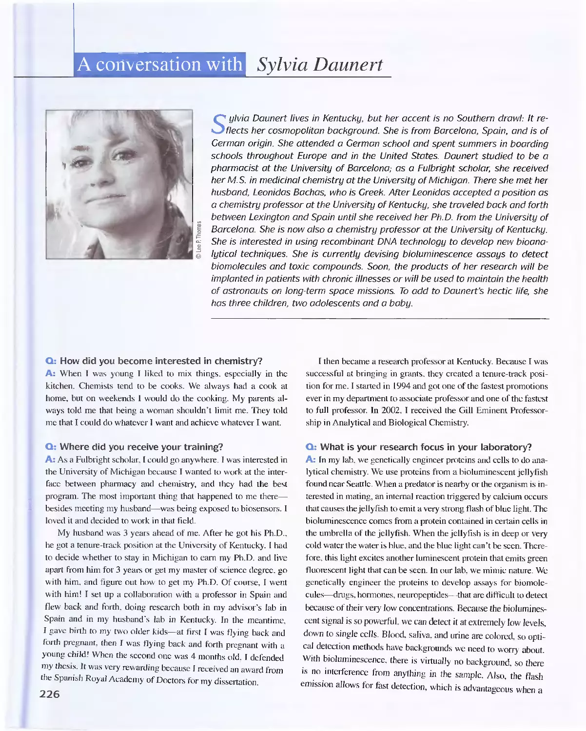
A Conversation with Sylvia Daunert 226
Chapter 9 Aqueous Solutions and Chemical
Equilibria 228
v
vi Contents
9A The Chemical Compositions of Aqueous
Solutions 228
9B Chemical Equilibrium 233
Feature 9-1 Stepwise and Overall Formation Constants
for Complex Ions 236
Feature 9-2 Why [H 2 0] Does Not Appear in Equilibrium-
Constant Expressions for Aqueous
Solutions 237
Feature 9-3 Relative Strengths of Conjugate Acid/Base
Pairs 244
Feature 9-4 The Method of Successive
Approximations 248
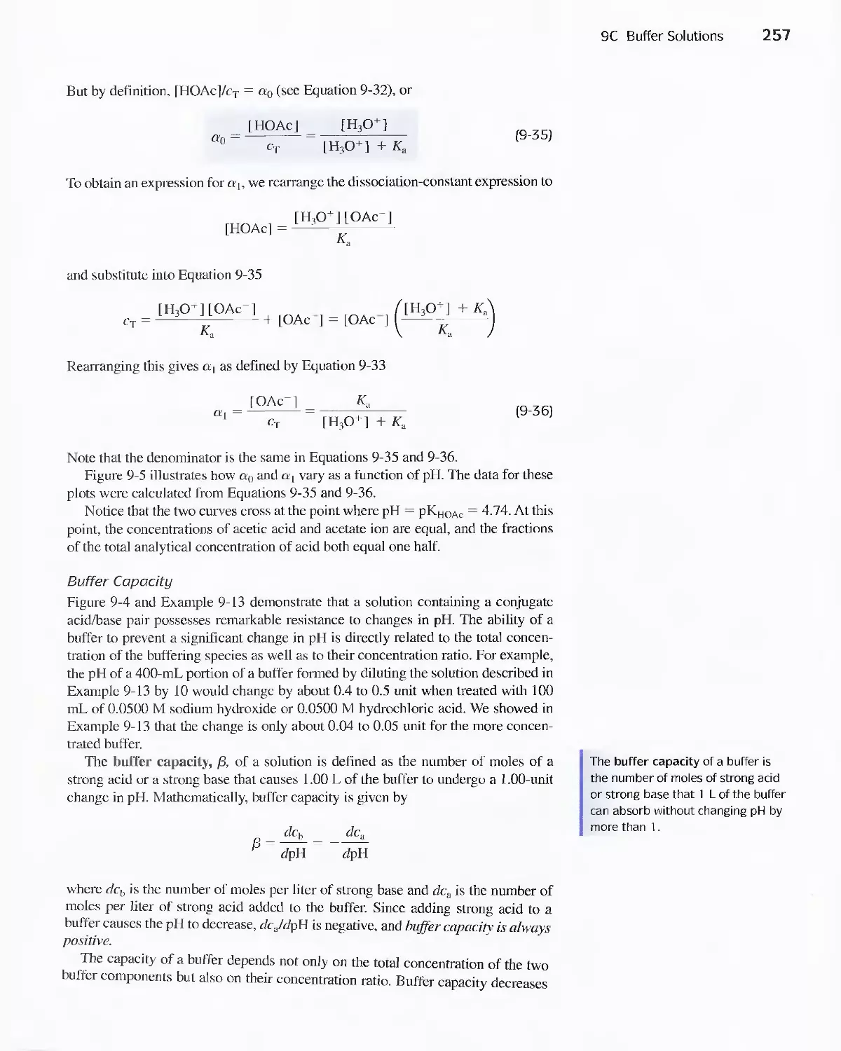
9C Buffer Solutions 251
Feature 9-5 The Henderson-Hasselbalch
Equation 252
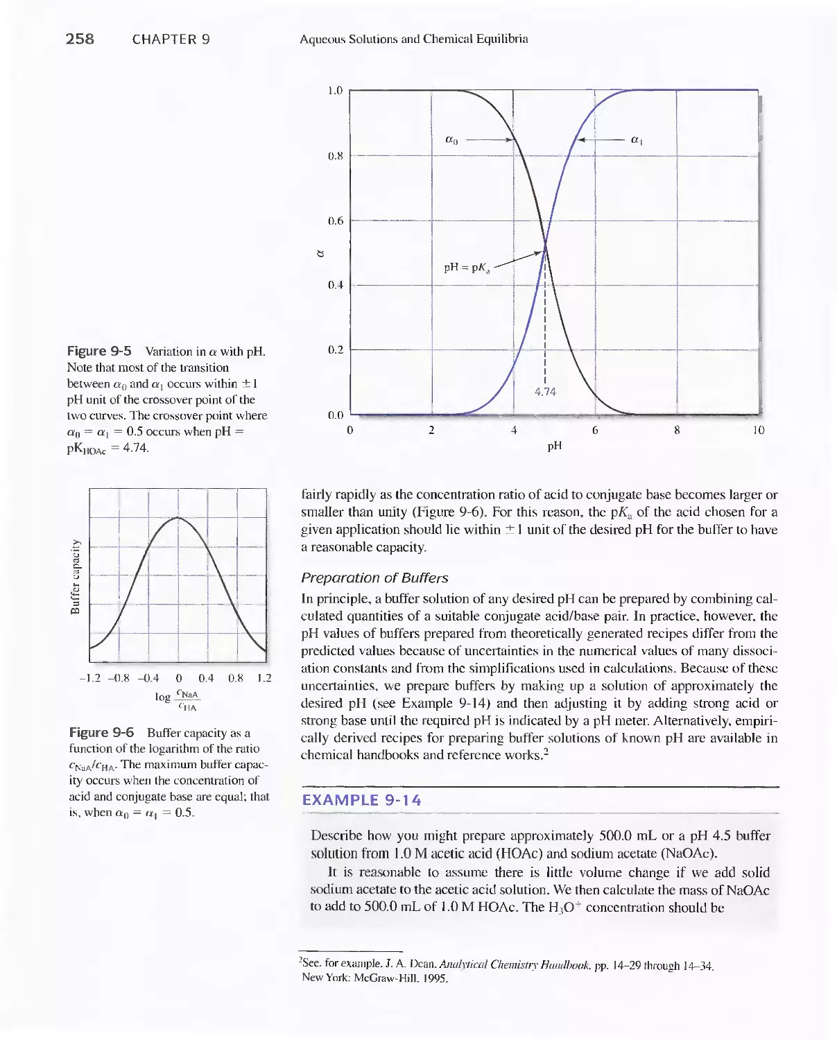
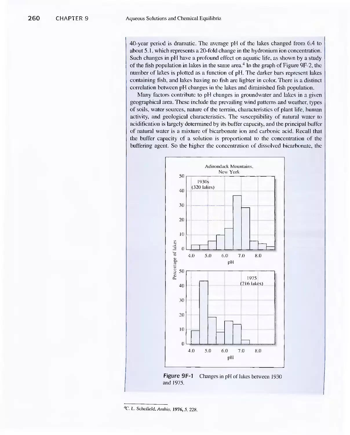
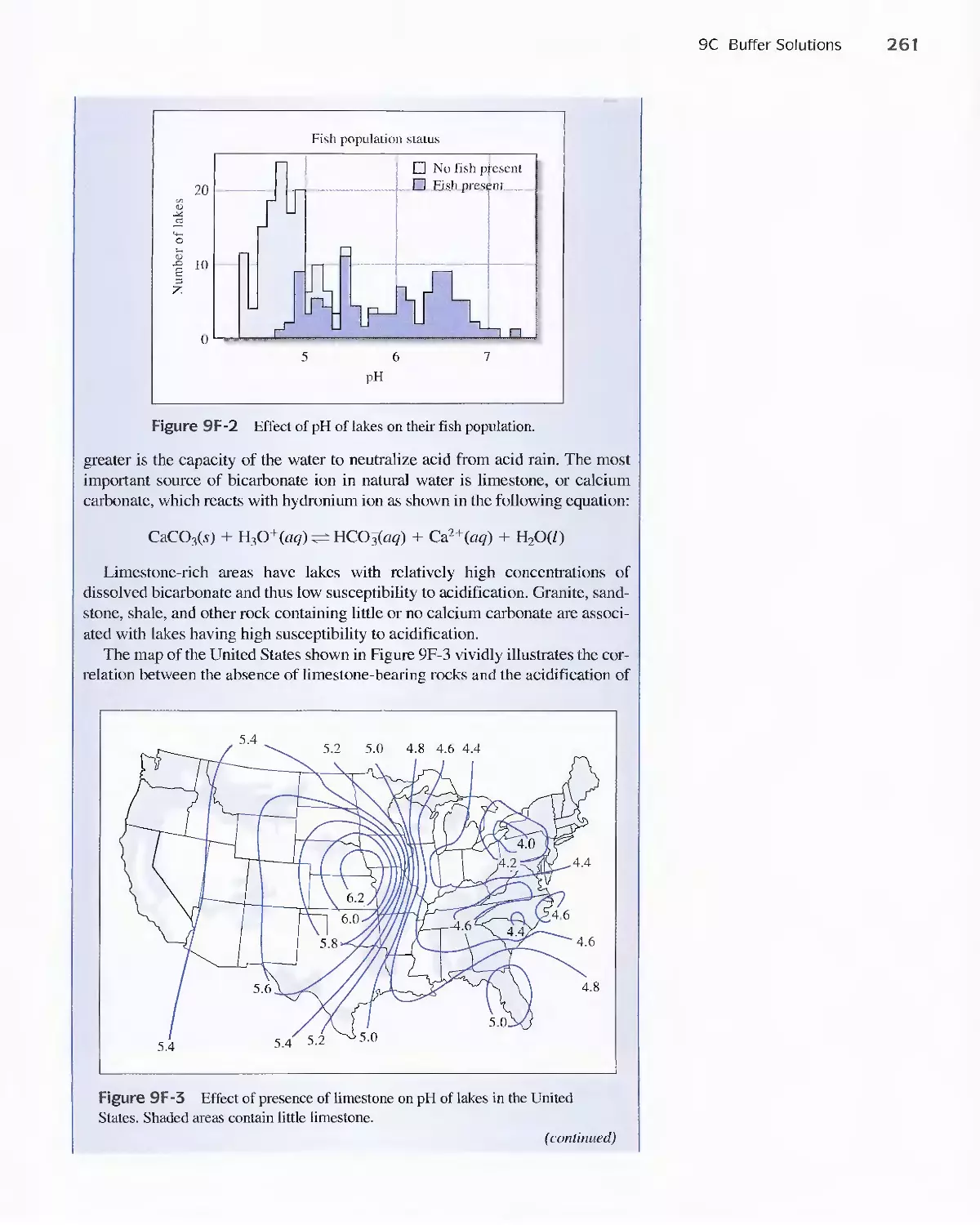
Feature 9-6 Acid Rain and the Buffer Capacity of
Lakes 259
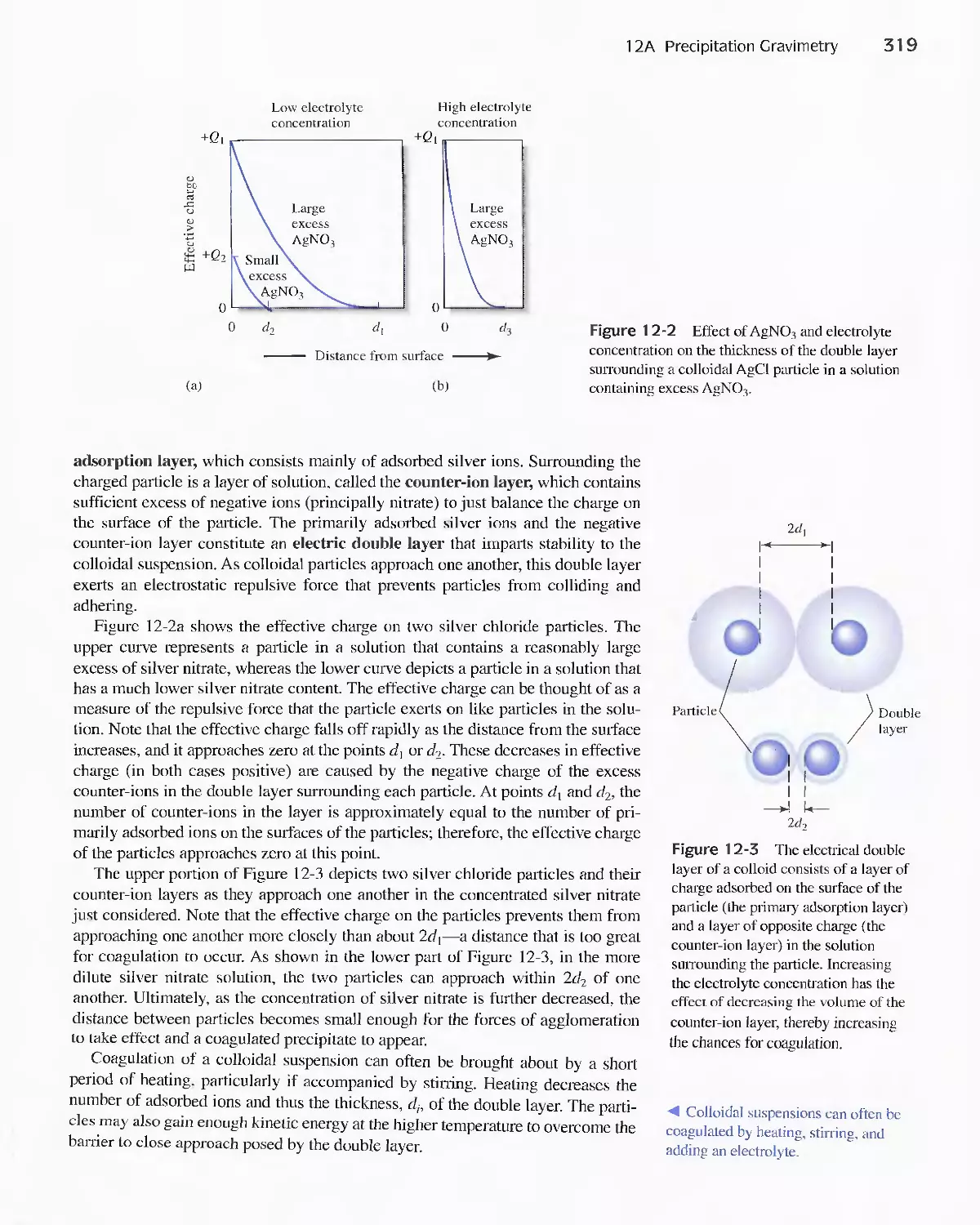
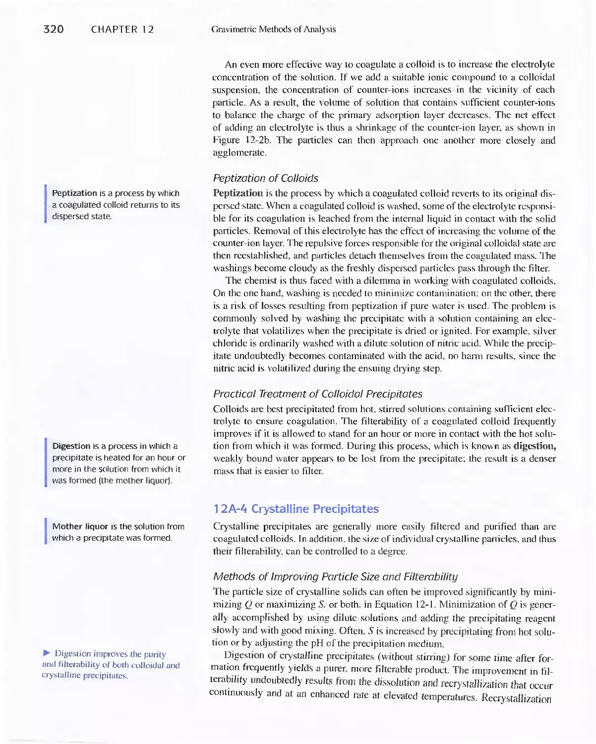
Chapter 10 Effect of Electrolytes on Chemical
Equilibria 267
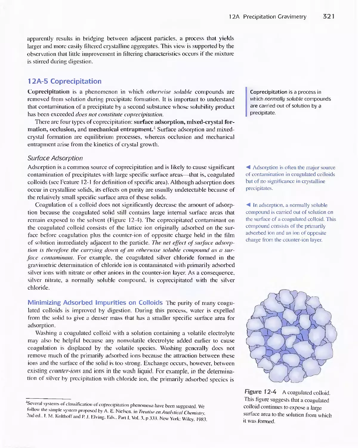
lOA The Effect of Electrolytes on Chemical
Equilibria 267
lOB Activity Coefficients 271
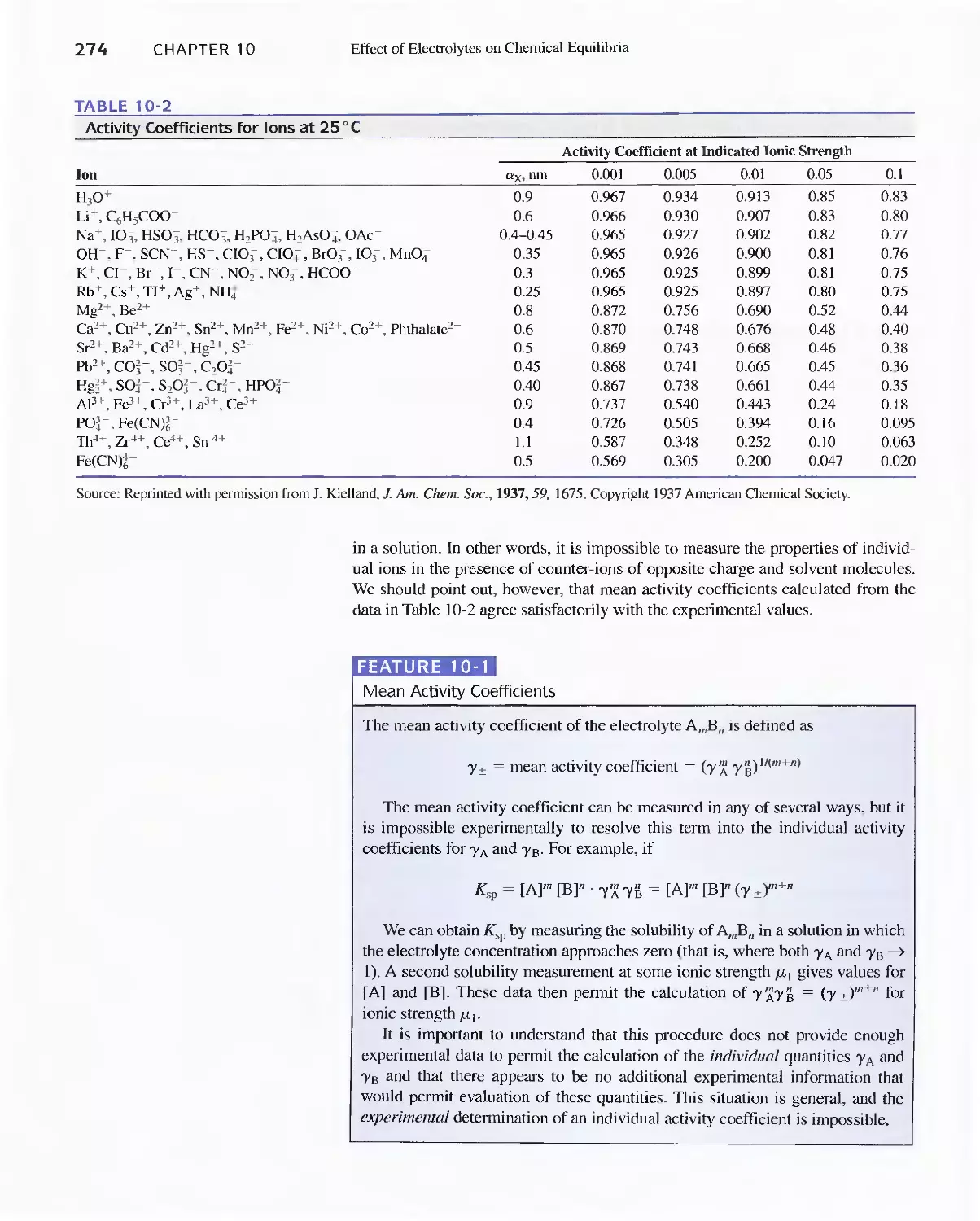
Feature 10-1 Mean Activity Coefficients 274
Chapter 11 Solving Equilibrium Calculation, for
Complex Systems 281
11 A Solving Multiple-Equilibrium Problems by a
Systematic Method 282
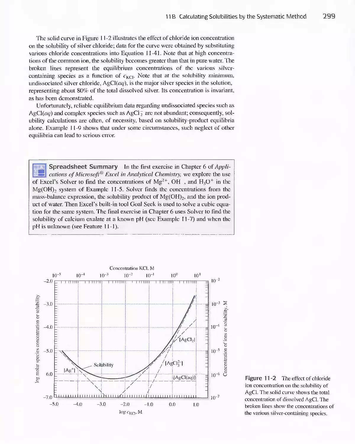
11 B Calculating Solubilities by the Systematic
Method 287
Feature 11-1 Algebraic Expressions Needed to
Calculate the Solubility of CaC 2 0 4 in
Water 294
11 C Separation of Ions by Control of the Concentration
of the Precipitating Agent 300
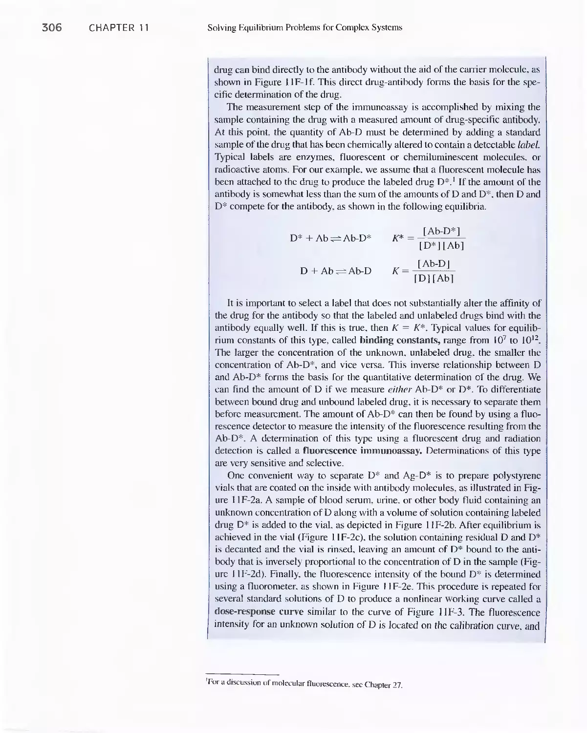
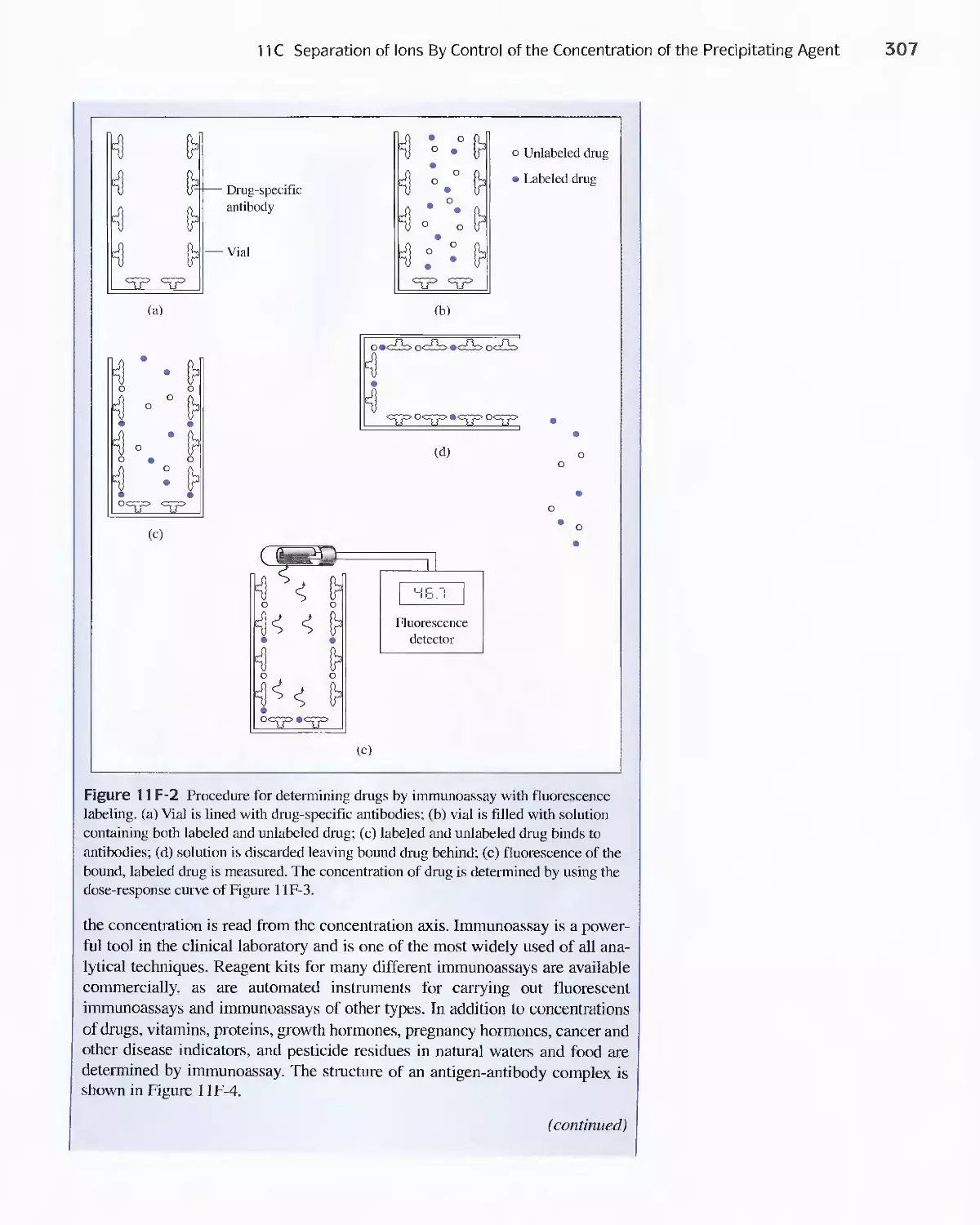
Feature 11-2 Immunoassay: Equilibria in the Specific
Determination of Drugs 304
PART III Classical Methods of Analysis 311
A Conversation with Larry R. Faulkner 312
Chapter 12 Gravimetric Methods of Analysis 314
12A Precipitation Gravimetry 315
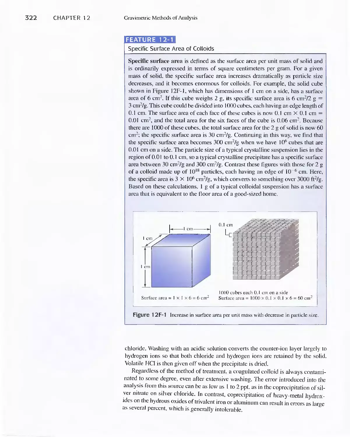
Feature 1 2-1 Specific Surface Area of Colloids 322
12B Calculation of Results from Gravimetric Data 326
12C Applications of Gravimetric Methods 329
Chapter 13 Titrimetric Methods; Precipitation
Titrimetry 337
13A Some Terms Used in Volumeric Titrimetry 338
13B Standard Solutions 340
1 3C Volumetric Calculations 341
Feature 1 3-1 Another Approach to
Example 13-6(a) 346
Feature 13-2 Rounding the Answer to
Example 1 3-7 347
13D Gravimetric Titrimetry 349
13E Titration Curves in Titrimetric Methods 350
13F Precipitation Titrimetry 353
Feature 13-3 Calculating the Concentration of Indicator
Solutions 361
Chapter 14 Principles of Neutralization Titrations 36
14A Solutions and Indicators for Acid/Base
Titrations 368
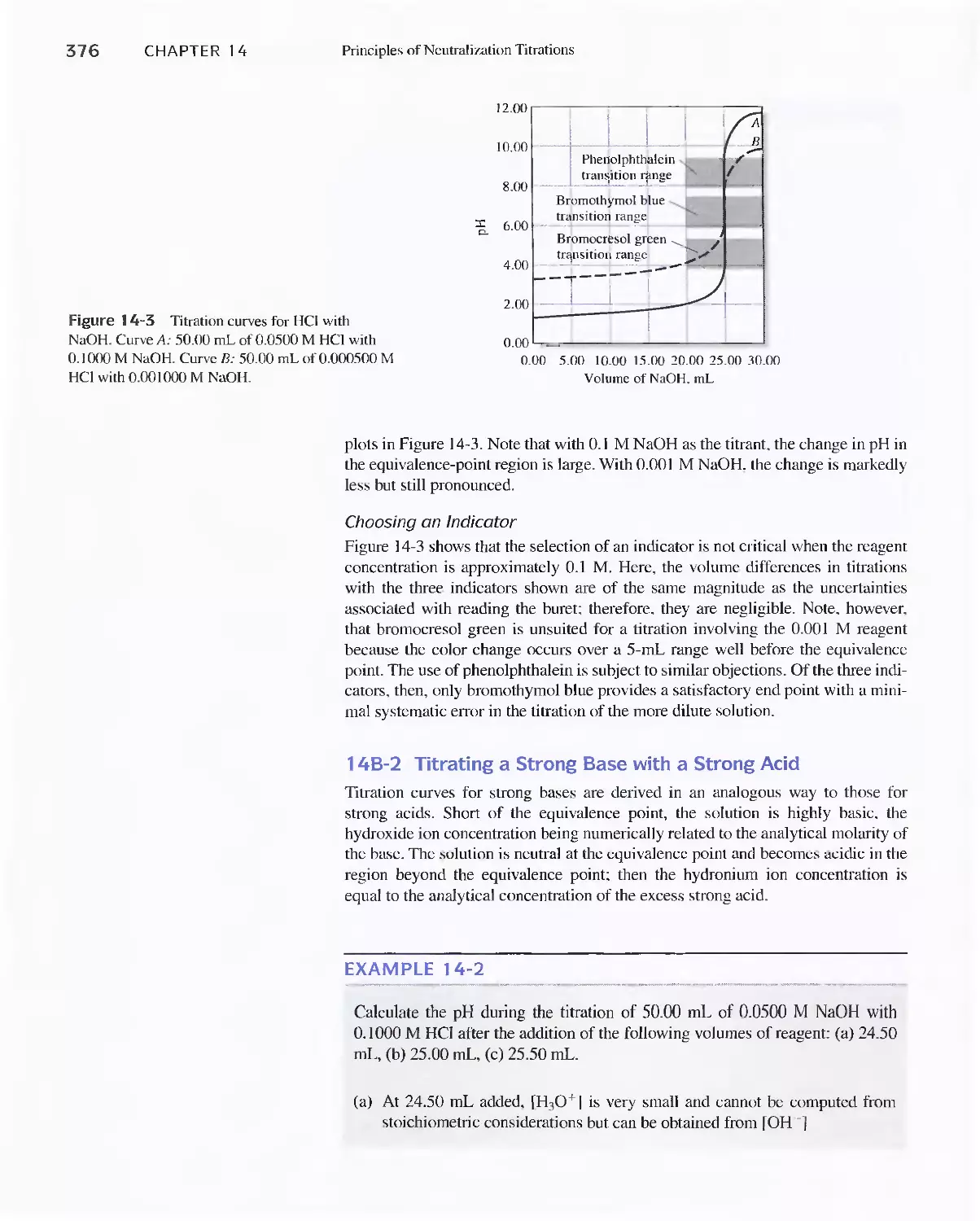
14B Titration of Strong Acids and Strong Bases 372
Feature 14-1 Using the Charge-Balance Equation to
Construct Titration Curves 375
Feature 14-2 How Many Significant Figures Should
We Retain in Titration Curve
Calculations? 378
14C Titration Curves for Weak Acids 378
Feature 14-3 Determining Dissociation Constants for
Weak Acids and Bases 381
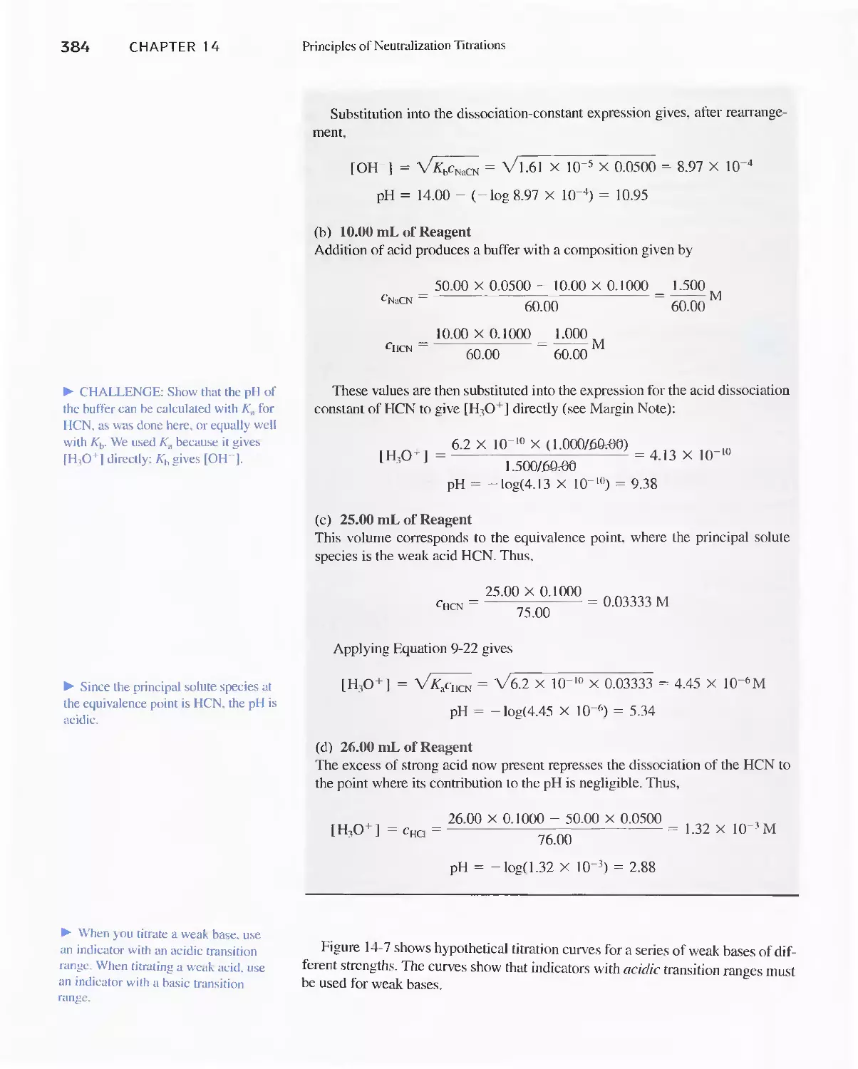
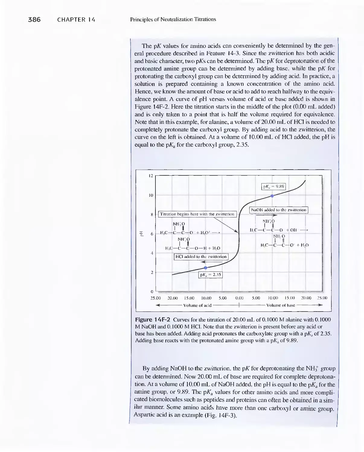
14D Titration Curves for Weak Bases 383
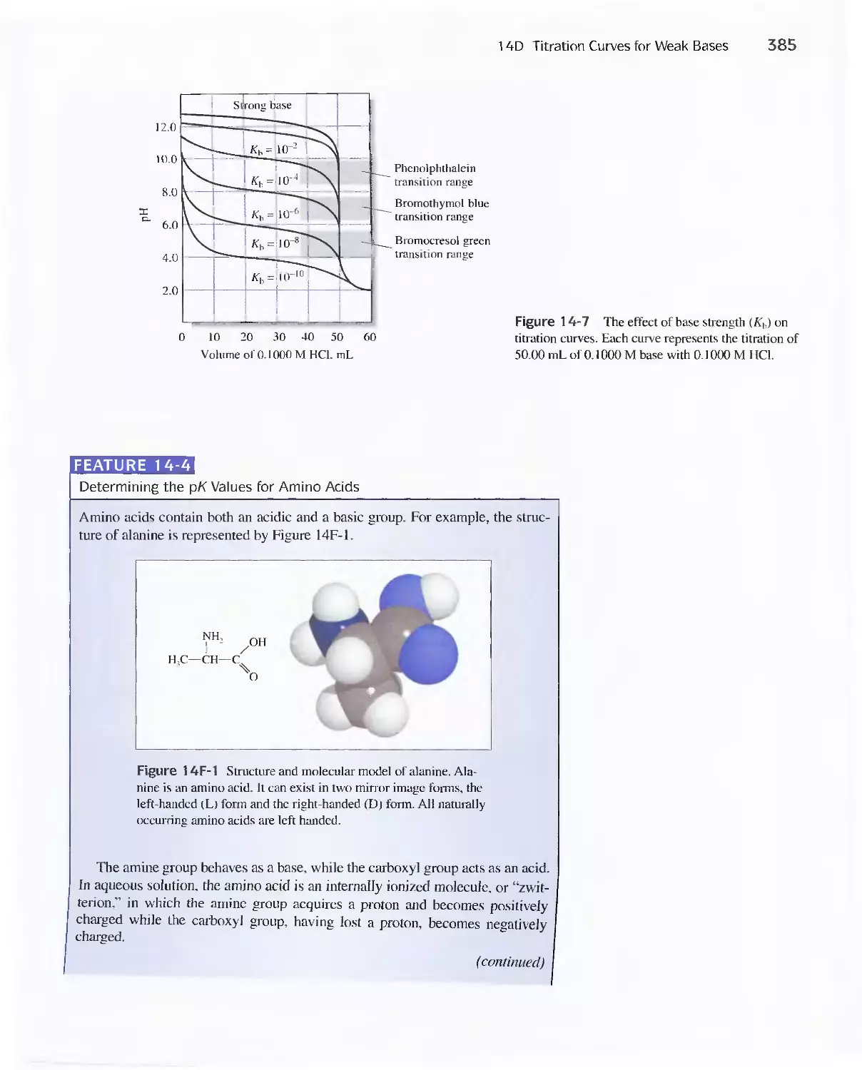
Feature 14-4 Determining the pK Values for Amino
Acids 385
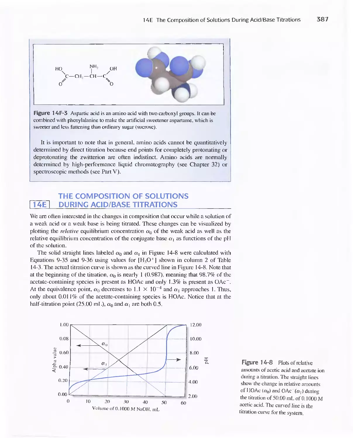
14E The Composition of Solutions During Acid/Base
Titrations 387
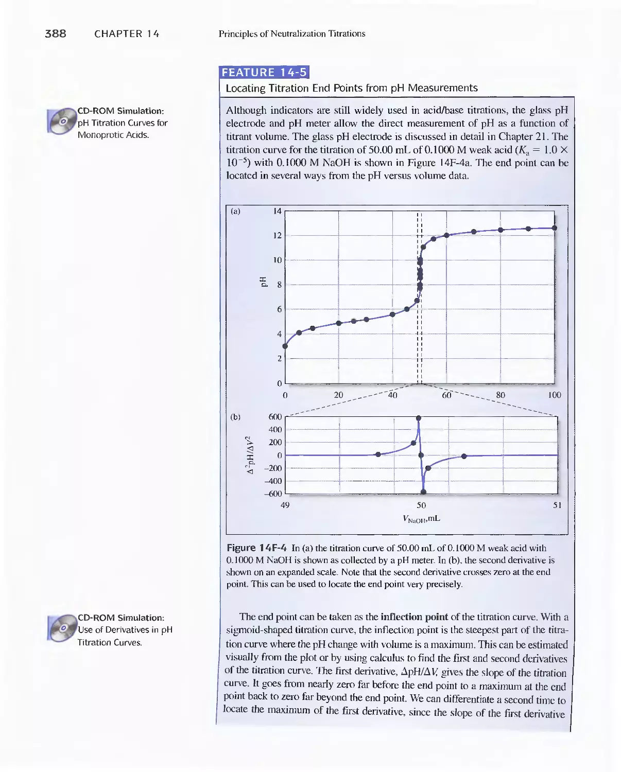
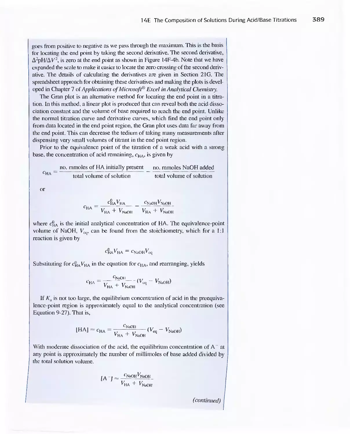
Feature 14-5 Locating Titration End Points from pH
Measurements 388
Chapter 15 Titration Curves for Complex Acid/Base
Systems 395
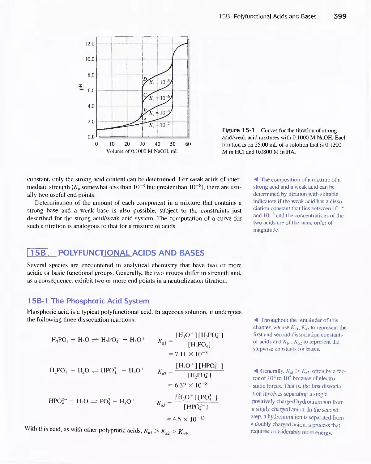
15A Mixtures of Strong and Weak Acids or Strong and
Weak Bases 398
15B Polyfunctional Acids and Bases 399
15C Buffer Solutions Involving Polyprotic Acids 401
1 5D Calculation of the pH of Solutions of NaHA 403
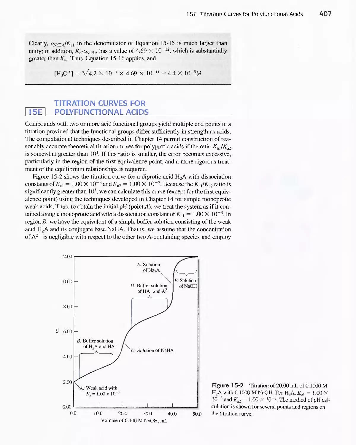
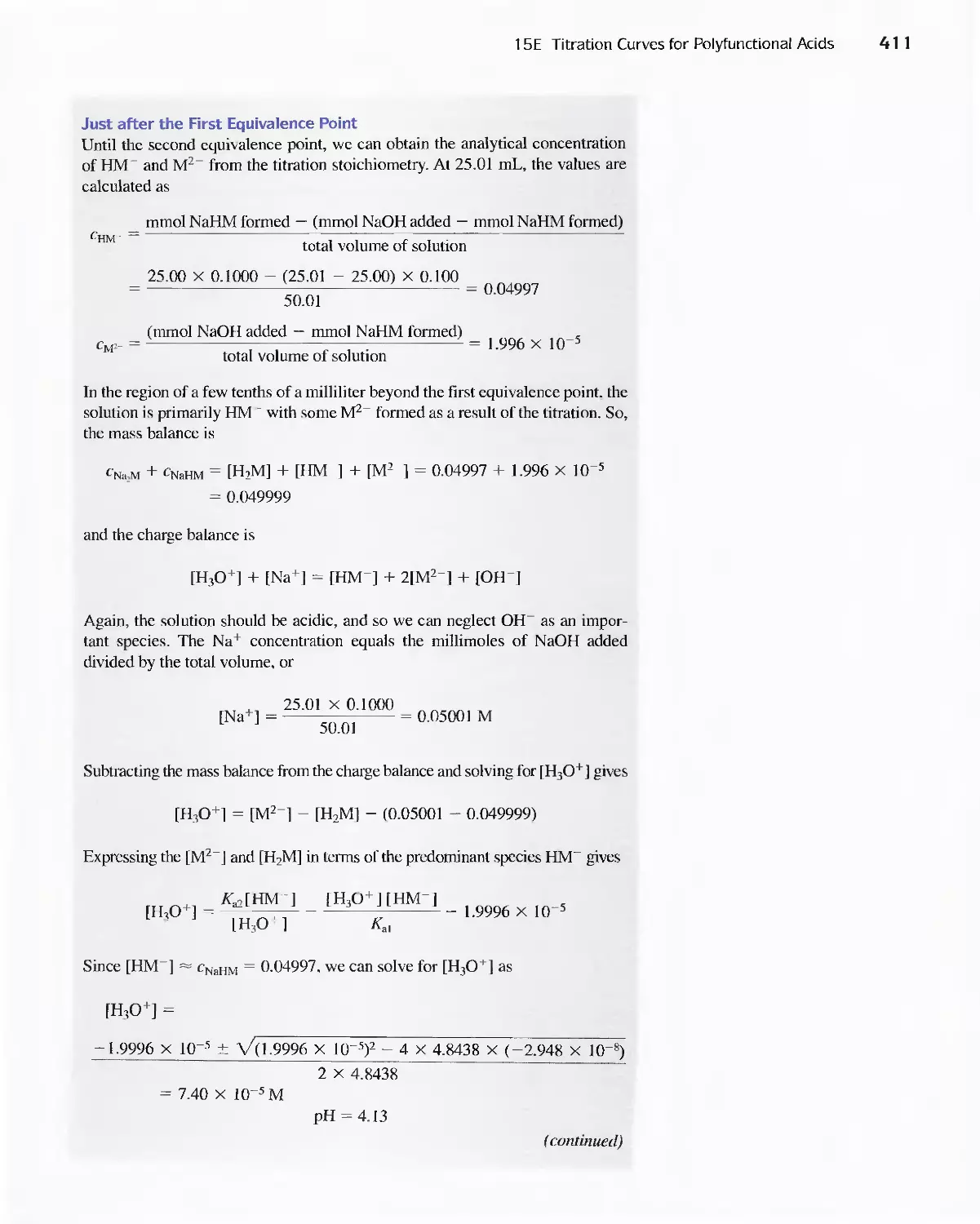
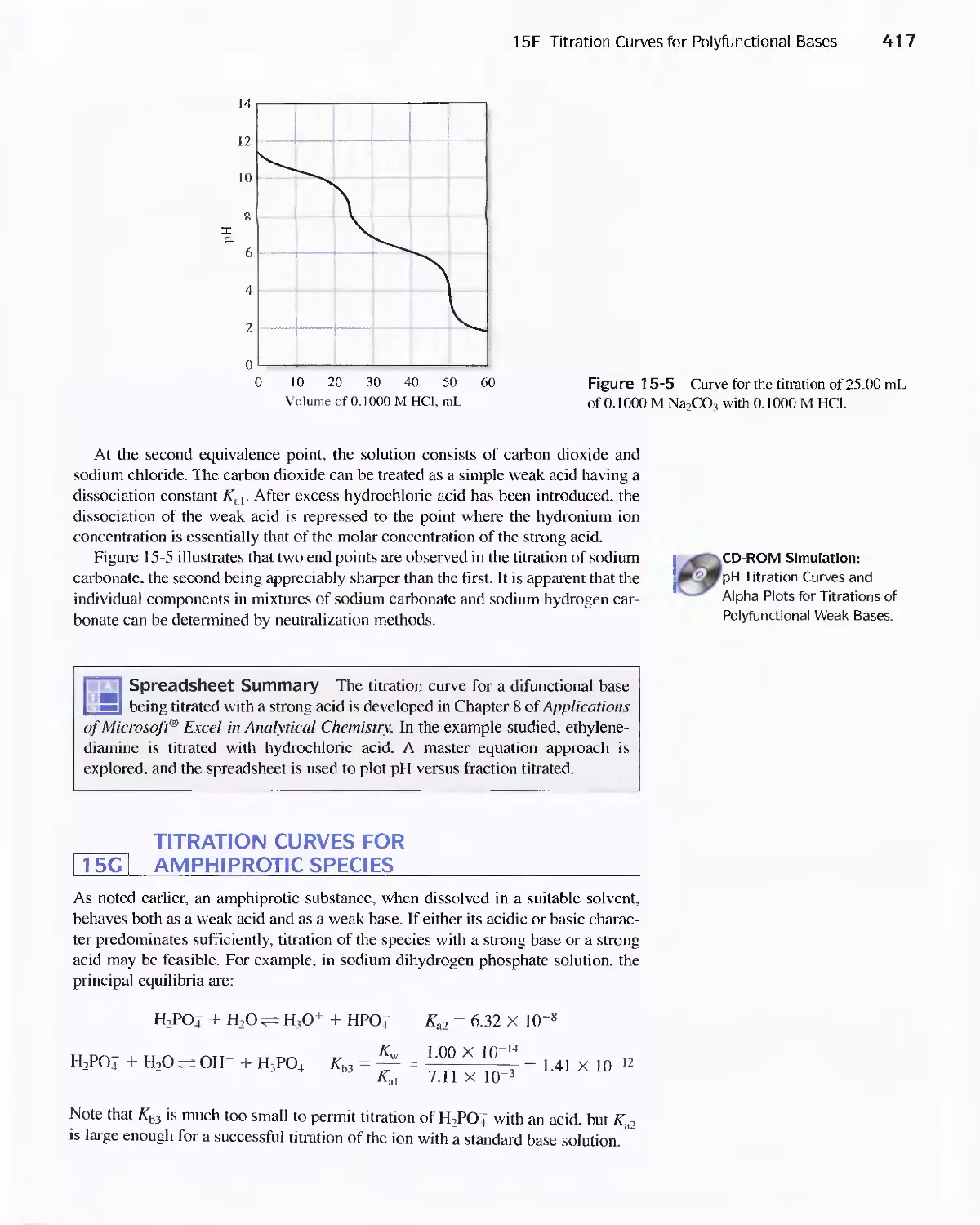
15E Titration Curves for Polyfunctional Acids 407
Feature 15-1 The Dissociation of Sulfuric Acid 415
15F Titration Curves for Polyfunctional Bases 416
15G Titration Curves for Amphiprotic Species 417
Feature 15-2 Acid/Base Behavior of Amino Acids 418
15H The Composition of Solutions of a Polyprotic Acid
as a Function of pH 41 9
Feature 15-3 A General Expression for Alpha
Values 420
Feature 15-4 Logarithmic Concentration Diagrams 422
Chapter 16 Applications of Neutralization
Titrations 428
16A Reagents for Neutralization Titrations 429
16B Typical Applications of Neutralization
Titrations 435
Feature 16-1 Determining Total Serum Protein 435
Feature 16-2 Other Methods for Determining Organic
Nitrogen 436
Feature 16-3 Equivalent Weights of Acids and
Bases 442
Chapter 17 Complexation Reactions and Titrations 449
I 7 A The Formation of Complexes 449
Feature 17-1 Calculation of Alpha Values for Metal
Complexes 452
17B Titrations with Inorganic Complexing Agents 455
Feature 17-2 Determination of Hydrogen Cyanide in
Acrylonitrile Plant Streams 456
17C Organic Complexing Agents 457
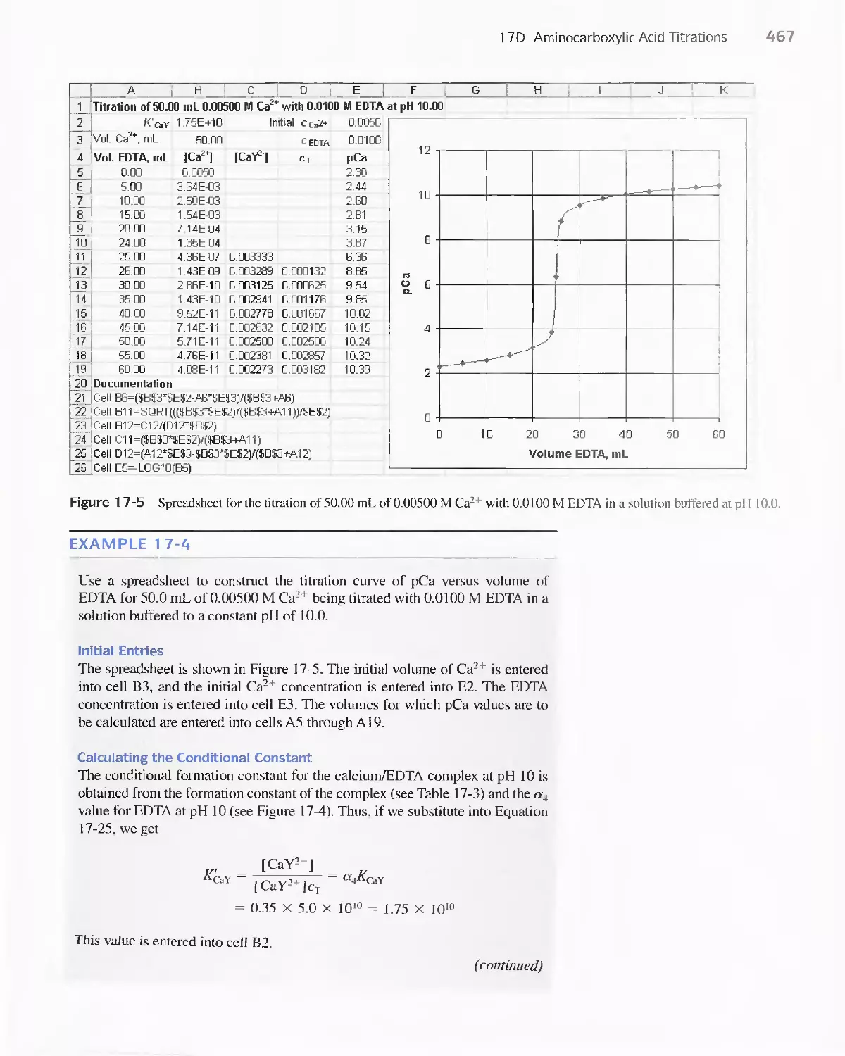
17D Aminocarboxylic Acid Titrations 458
Feature 17-3 Species Present in a Solution of EDTA 459
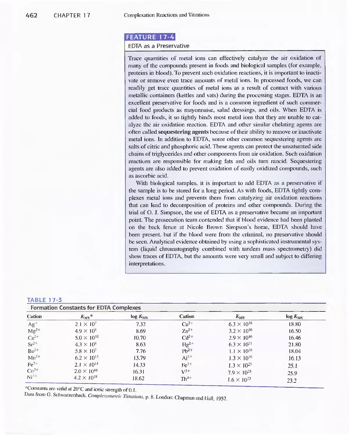
Feature 17-4 EDTA as a Preservative 462
Feature 17-5 EDTA Titration Curves When a Complex-
ing Agent Is Present 473
Feature 17-6 How Masking and Demasking Agents Can
Be Used to Enhance the Selectivity of
EDTA Titrations 480
Feature 17-7 Test Kits for Water Hardness 482
PART IV Electrochemical Methods 487
A Conversation with Allen J. Bard 488
Chapter 18 Introduction to Electrochemistry 490
18A Characterizing Oxidation/Reduction Reactions 490
Feature 18-1 Balancing Redox Equations 492
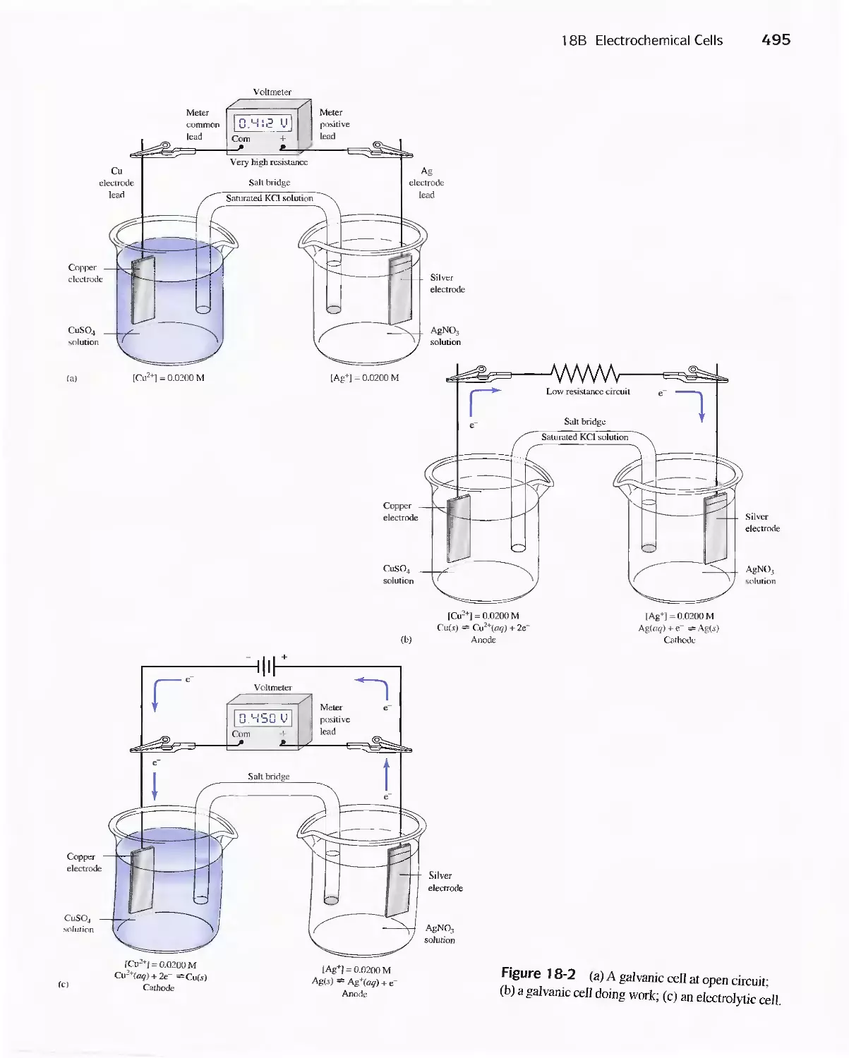
18B Electrochemical Cells 494
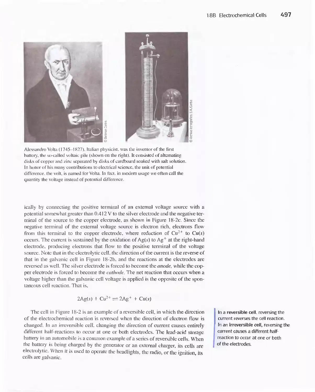
Feature 18-2 The Daniell Gravity Cell 498
18C Electrode Potentials 499
Feature 18-3 Why We Cannot Measure Absolute
Electrode Potentials 504
Feature 18-4 Sign Conventions in the Older
Literature 51 3
Feature 18-5 Why Are There Two Electrode Potentials
for Br2 in Table 18-1? 515
Chapter 19 Applications of Standard Electrode
Potentials 523
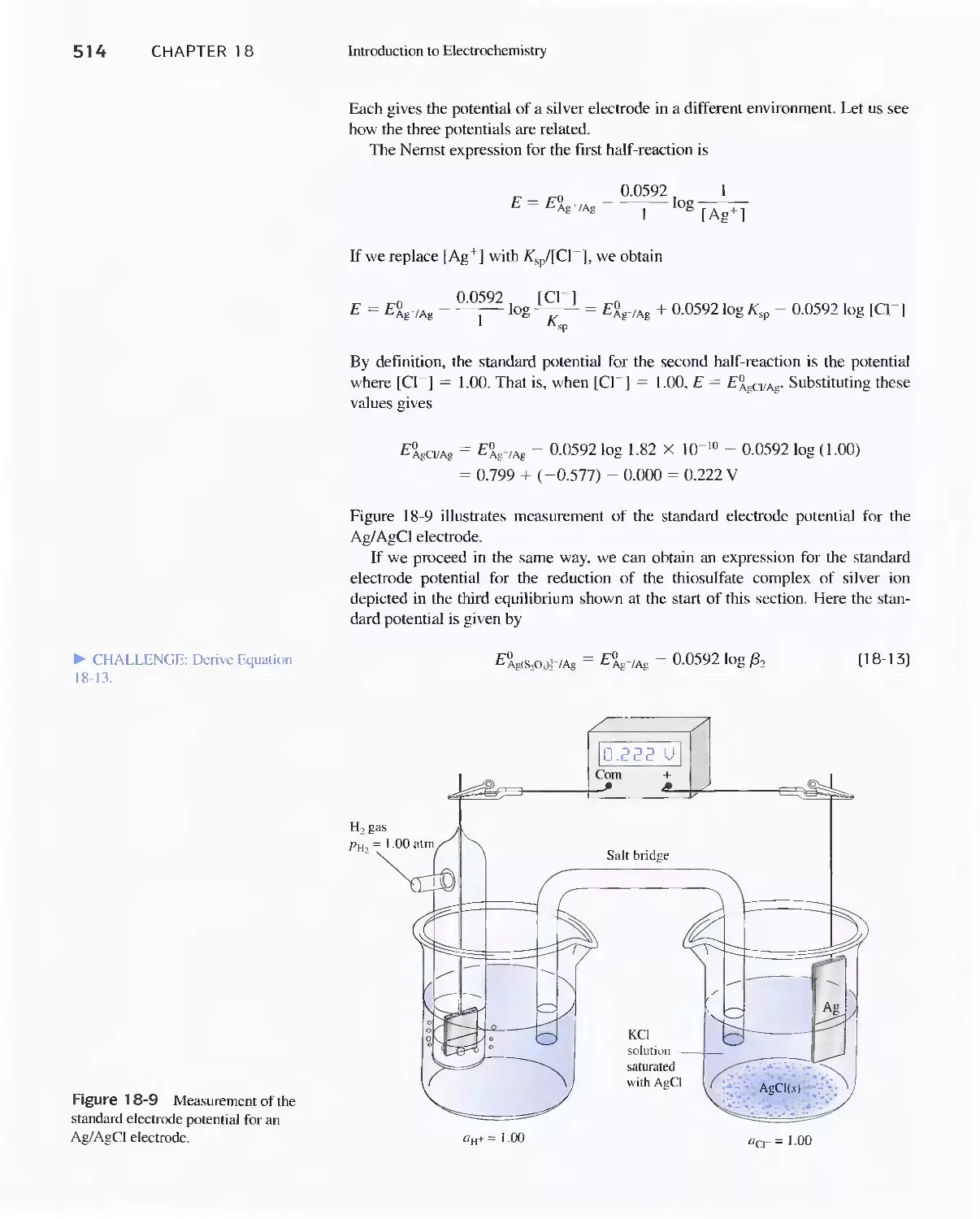
19A Calculating Potentials of Electrochemical Cells 523
19B Determining Standard Potentials
Experimentally 530
19C Calculating Redox Equilibrium Constants 532
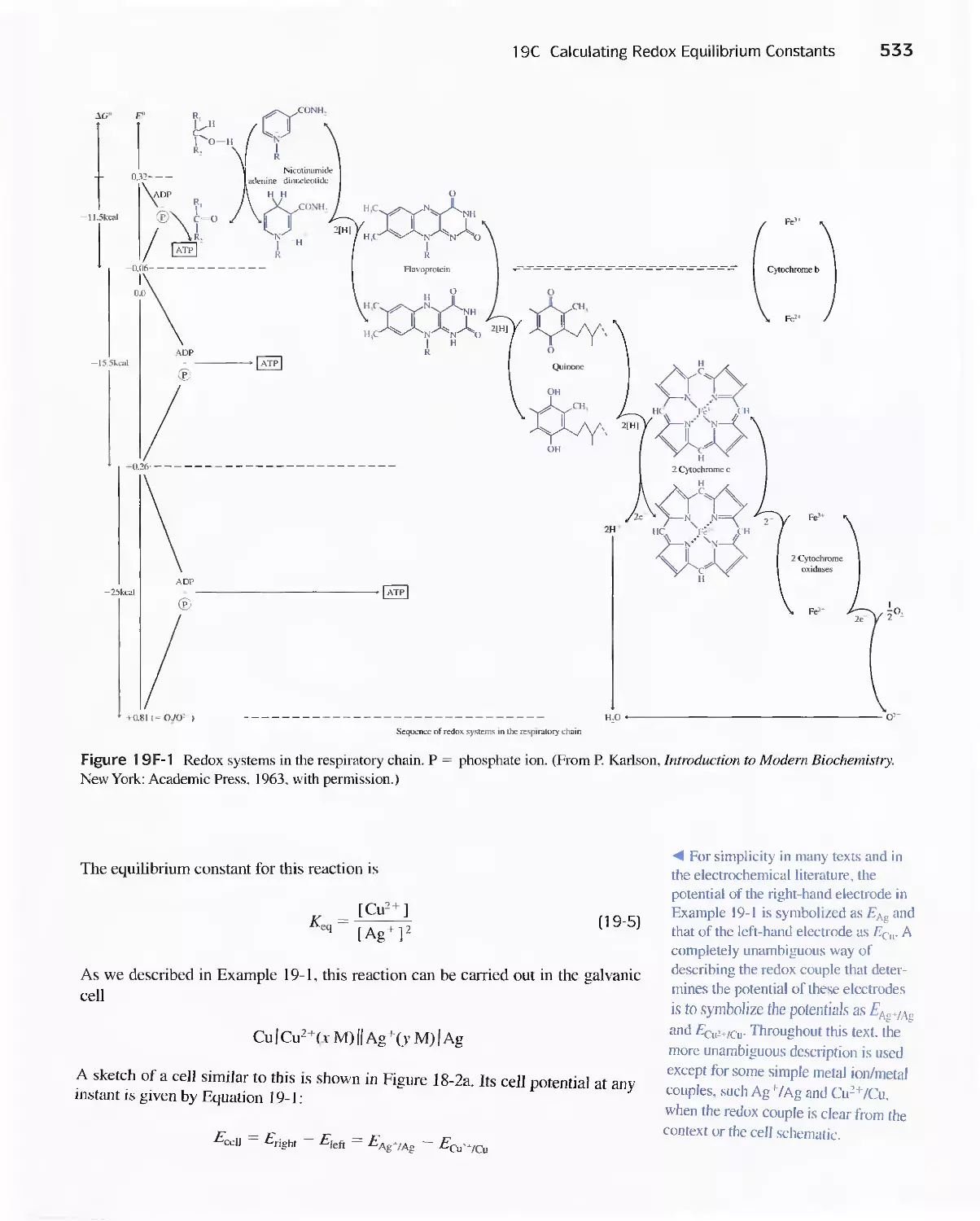
Feature 19-1 Biological Redox Systems 532
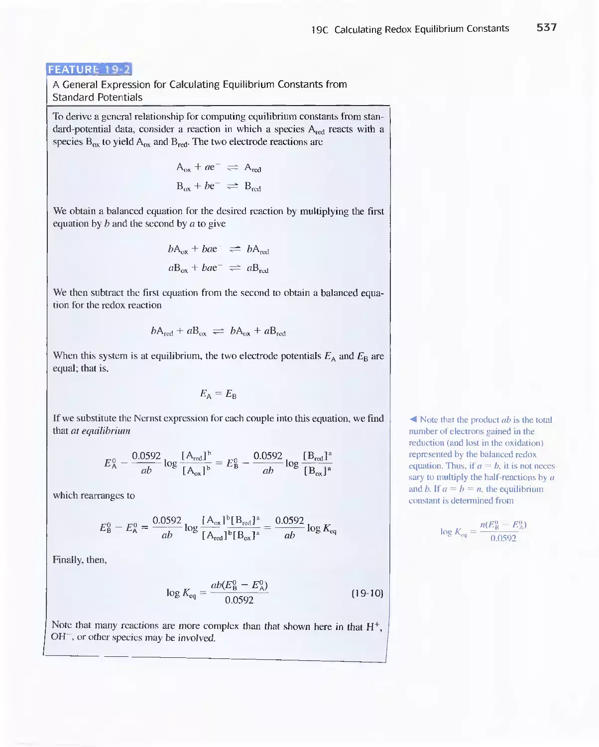
Feature 19-2 A General Expression for Calculating
Equilibrium Constants from Standard
Potentials 537
Contents vii
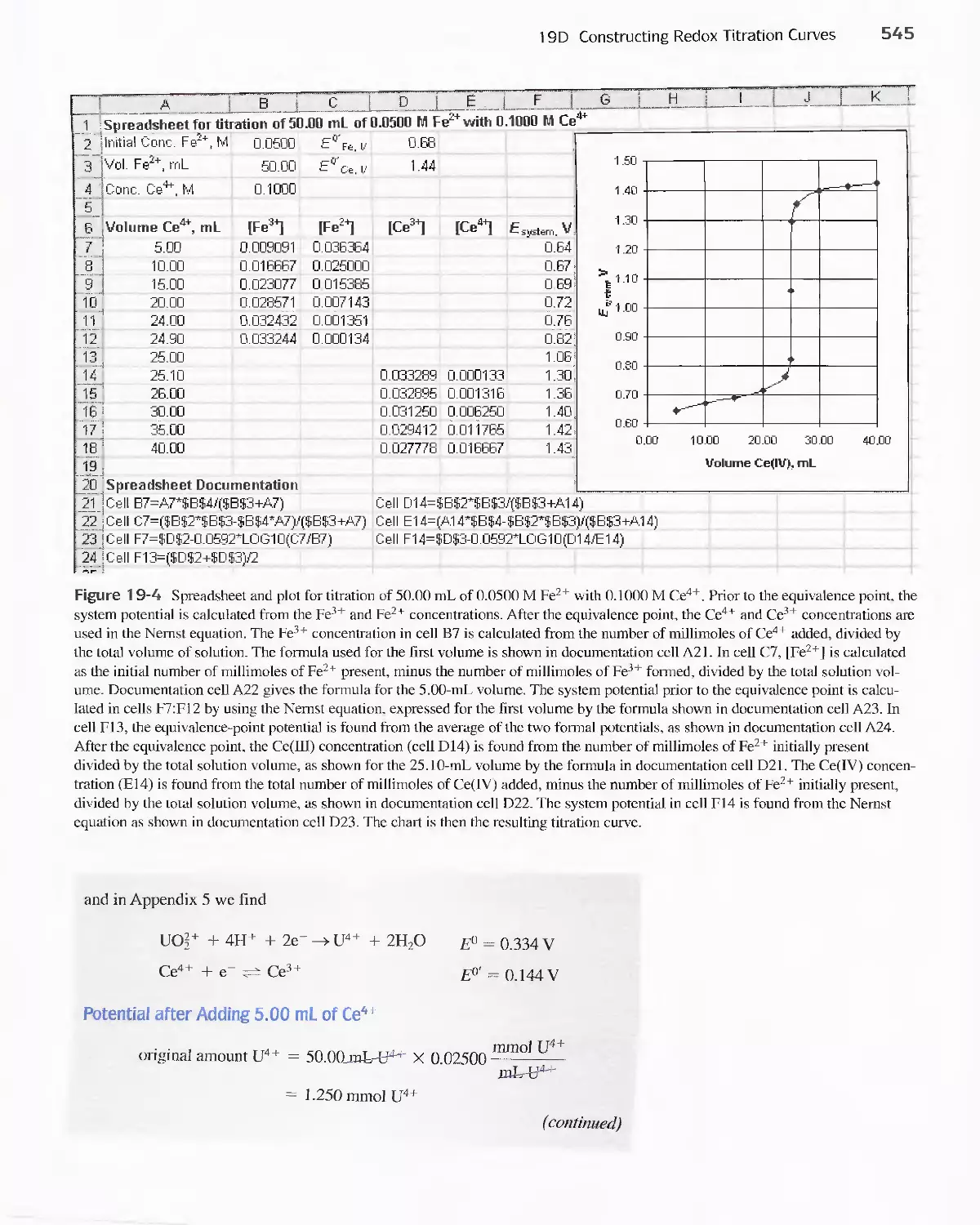
19D Constructing Redox Titration Curves 538
Feature 19-3 The Inverse Master Equation Approach
for Redox Titration Curves 547
Feature 1 9-4 Reaction Rates and Electrode
Potentials 552
19E Oxidation/Reduction Indicators 552
19F Potentiometric End Points 555
Chapter 20 Applications of OxidationlReduction
Titrations 560
20A Auxiliary Oxidizing and Reducing Reagents 560
20B Applying Standard Reducing Agents 562
20C Applying Standard Oxidizing Agents 566
Feature 20-1 Determination of Chromium Species in
Water Samples 568
Feature 20-2 Antioxidants 573
Chapter 2] Potentiometry 5SS
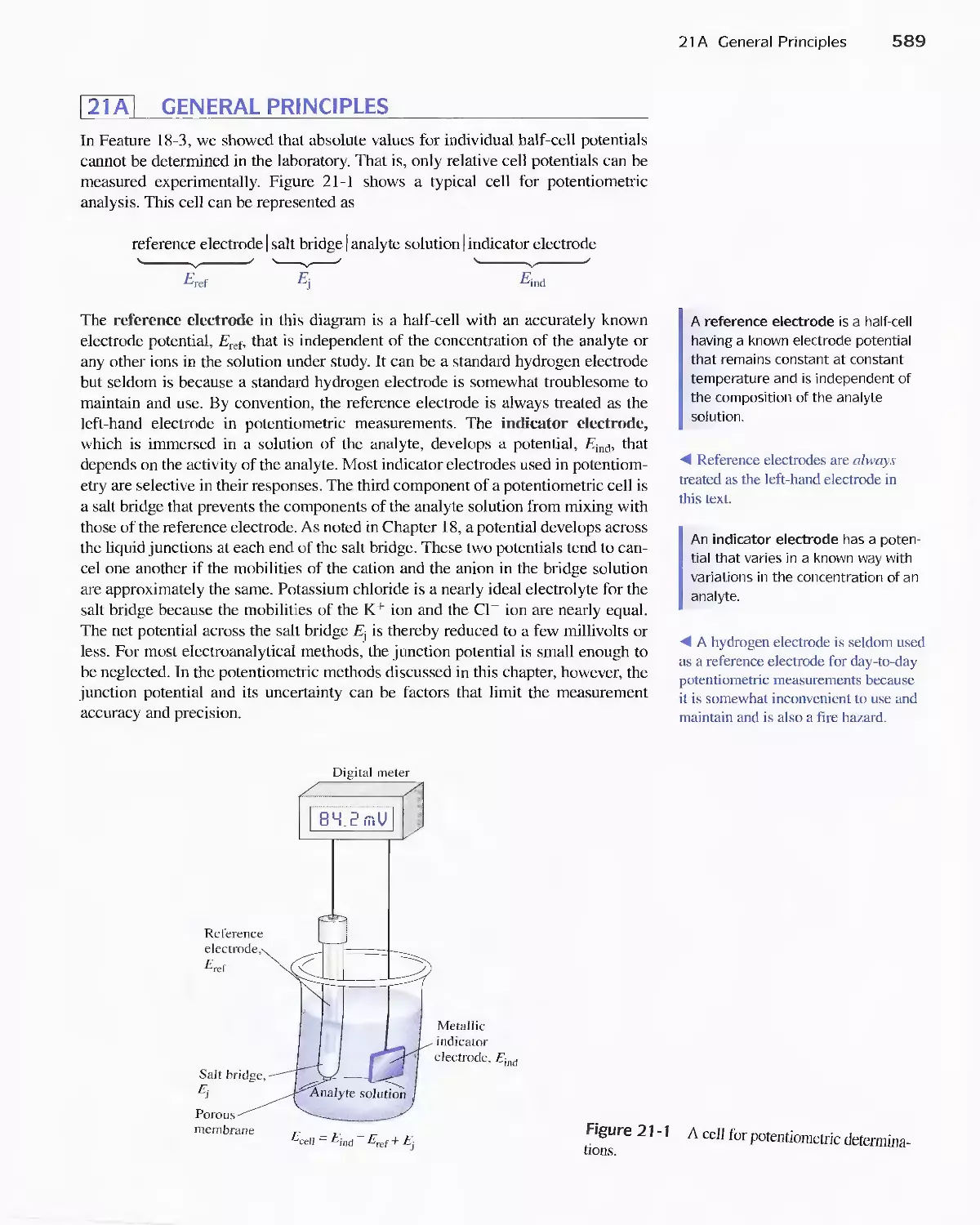
21A General Principles 589
21 B Reference Electrodes 590
21 C Liquid-Junction Potentials 592
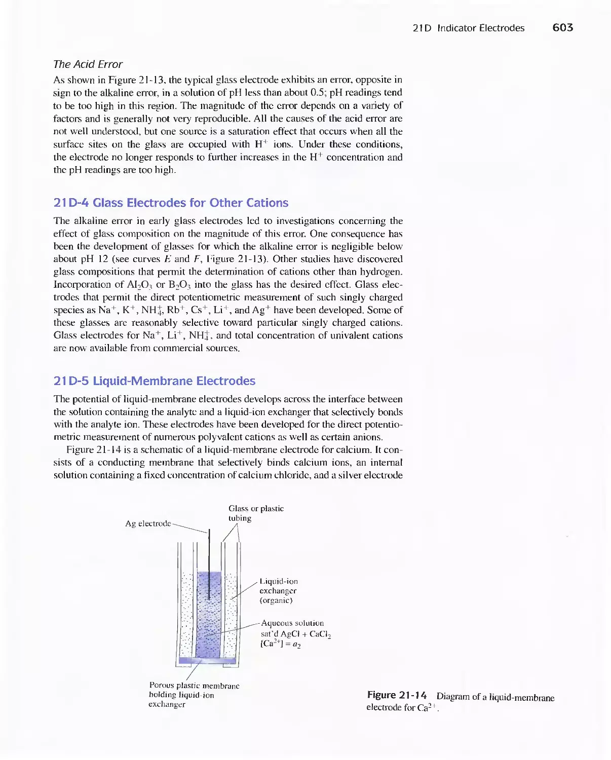
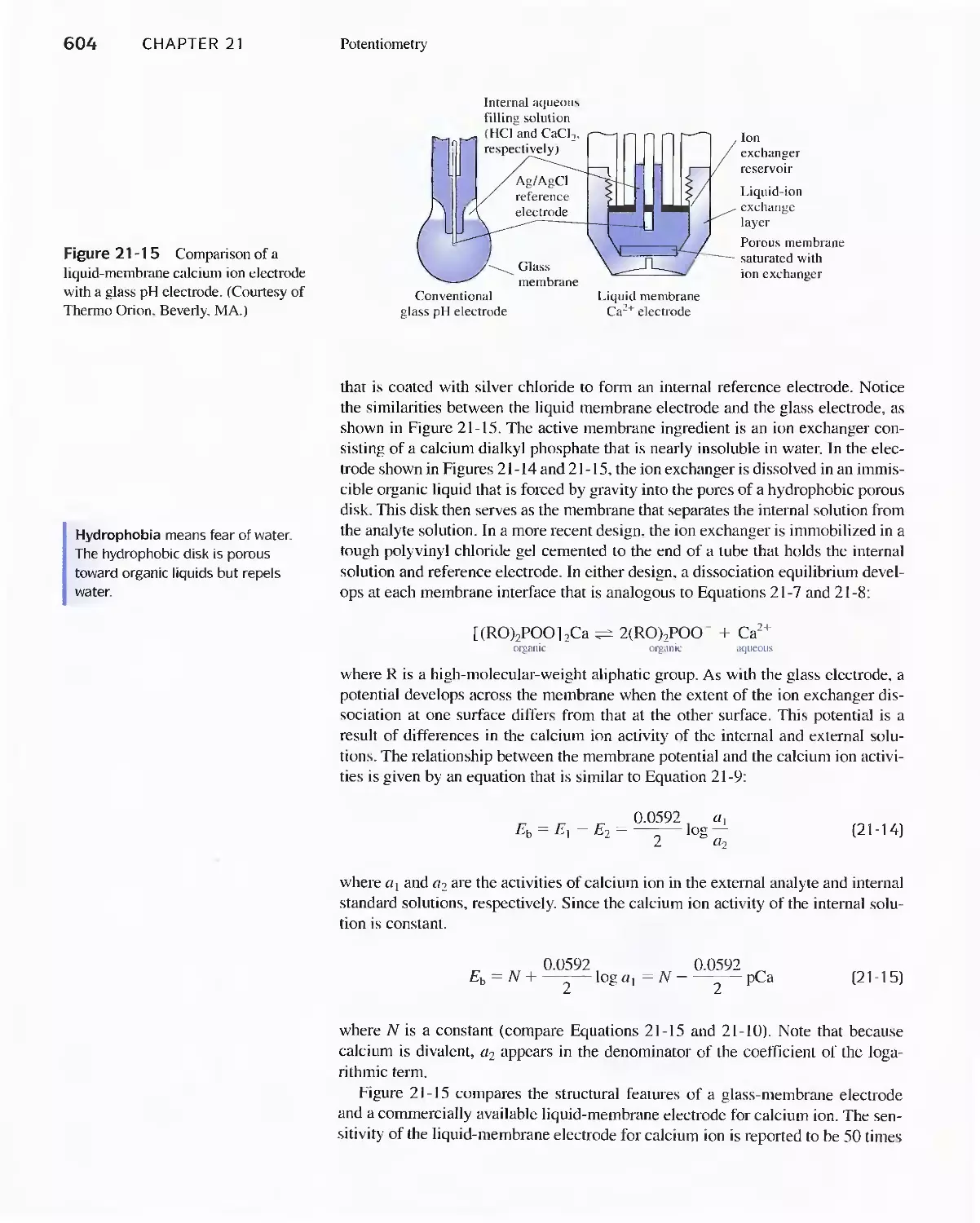
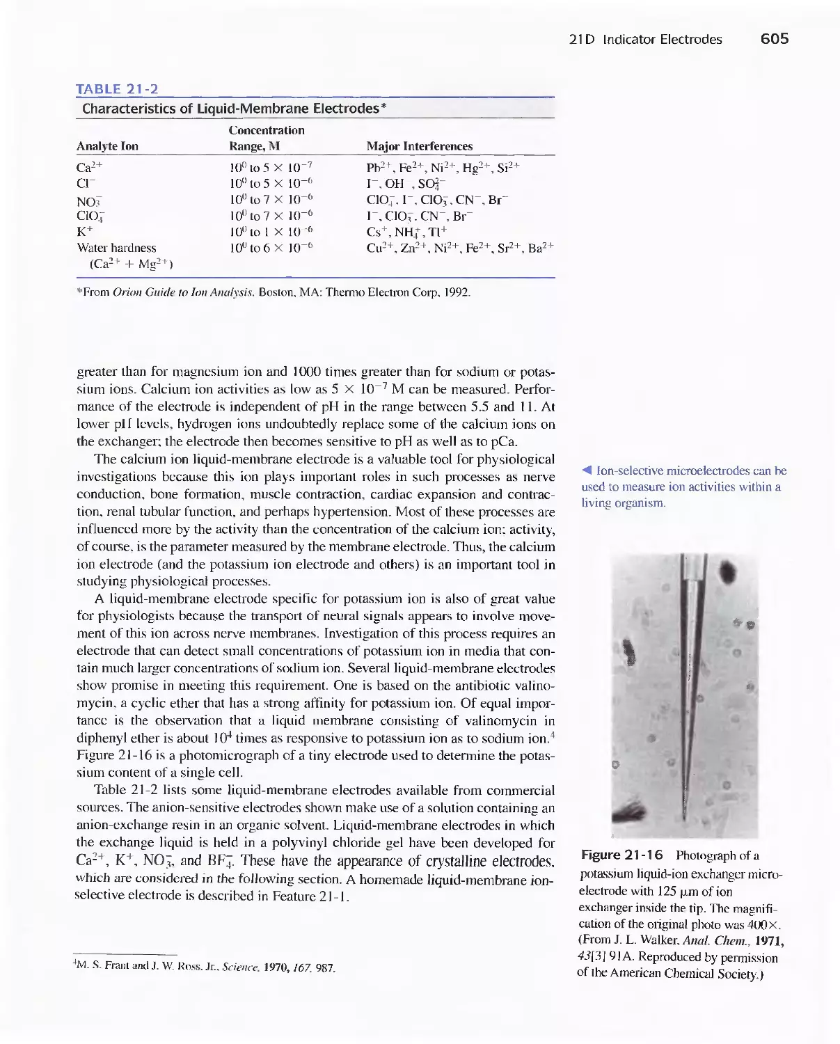
21 D Indicator Electrodes 593
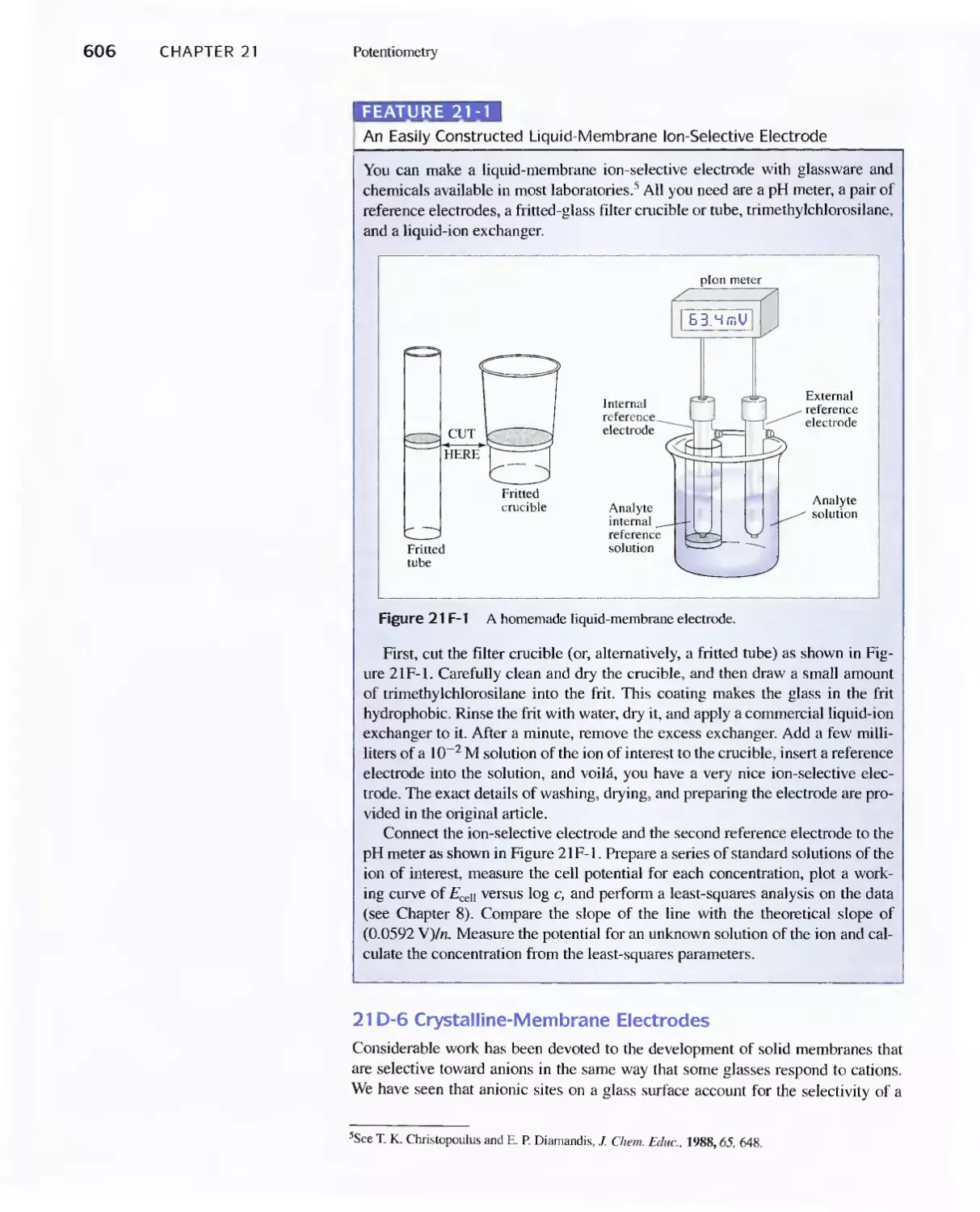
Feature 21-1 An Easily Constructed Liquid-Membrane
lon-Selective Electrode 606
Feature 21-2 The Structure and Performance of lon-
Selective Field Effect Transistors 608
Feature 21-3 Point-of-Care Testing: Blood Gases and
Blood Electrolytes with Portable
Instrumentation 612
21 E Instruments for Measuring Cell Potential 614
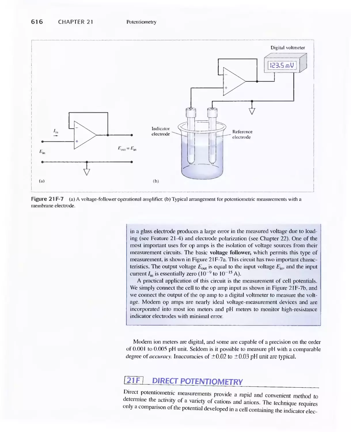
Feature 21-4 The Loading Error in Potential
Measurements 614
Feature 21-5 Operational Amplifier Voltage
Measurements 61 5
21 F Direct Potentiometry 61 6
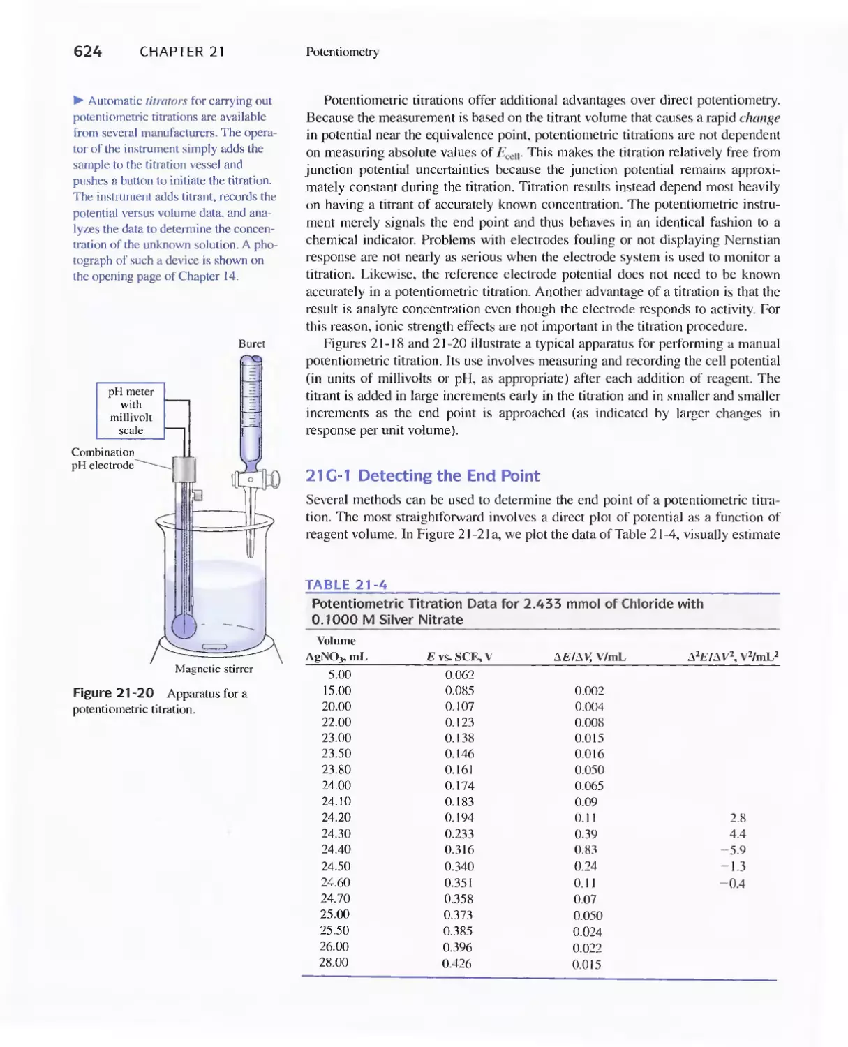
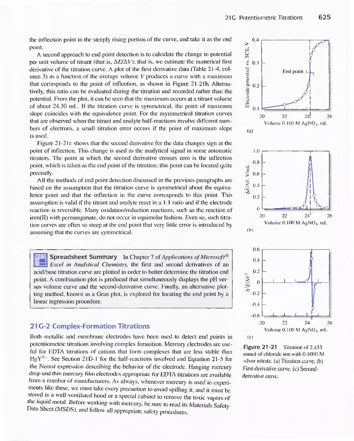
21 G Potentiometric Titrations 623
21 H Potentiometric Determination of Equilibrium
Constants 627
Chapter 22 Bulk Electrolysis: Electrogravimetry and
Coulometry 633
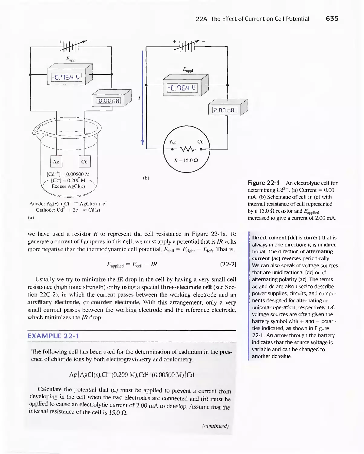
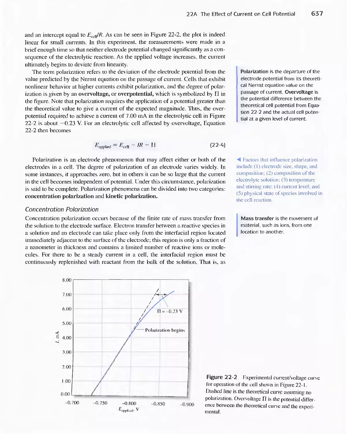
22A The Effect of Current on Cell Potential 634
Feature 22-1 Overvoltage and the Lead/Acid
Battery 641
22B The Selectivity of Electrolytic Methods 641
22C Electrogravimetric Methods 643
22D Coulometric Methods 649
Feature 22-2 Coulometric Titration of Chloride in
Biological Fluids 658
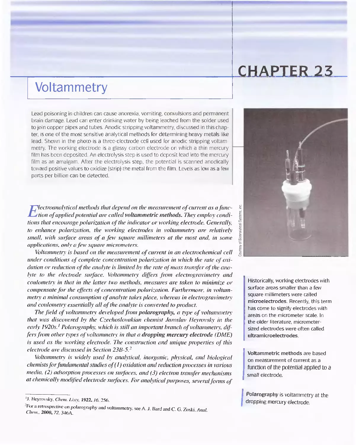
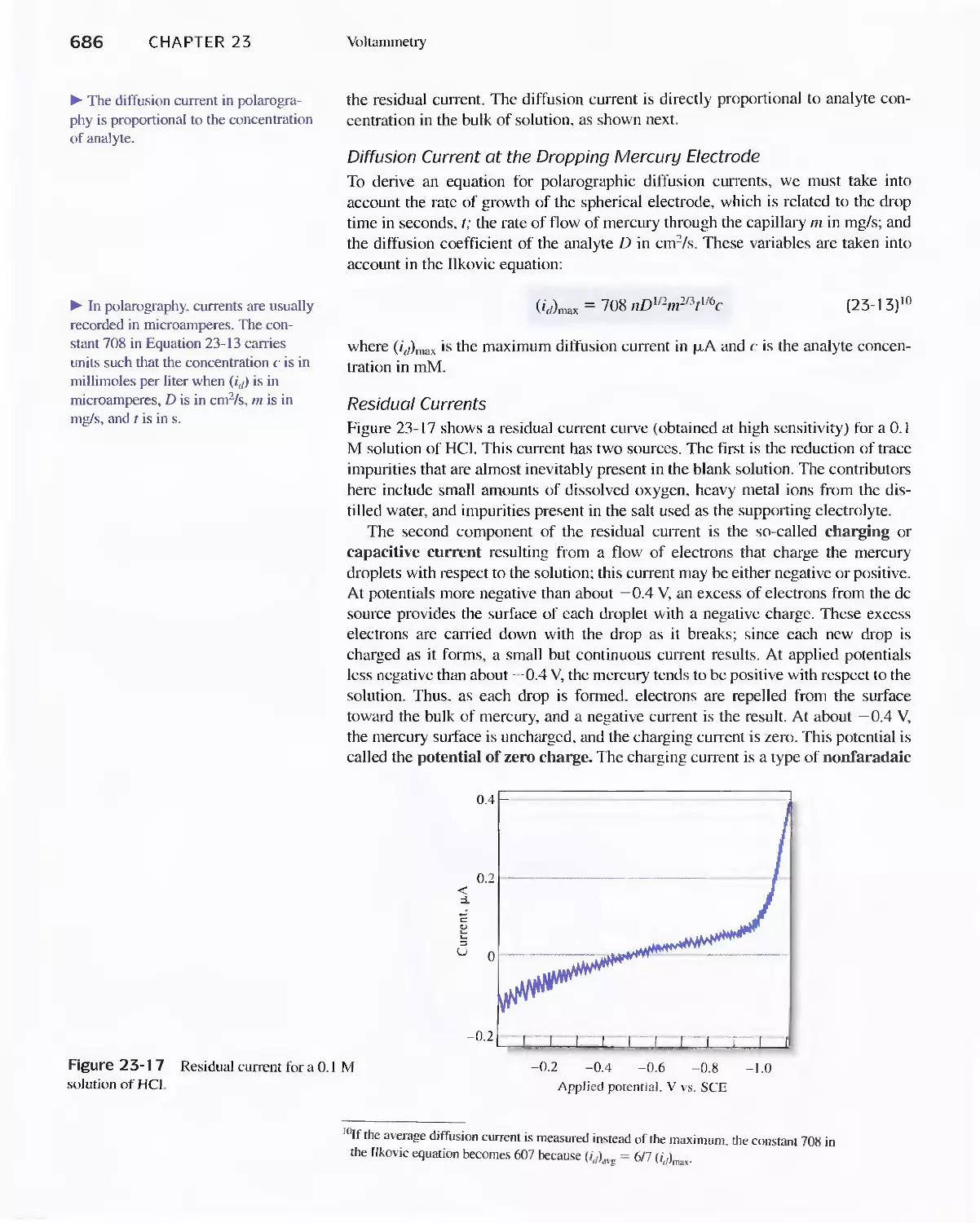
Chapter 23 Voltammetry 665
23A Excitation Signals 666
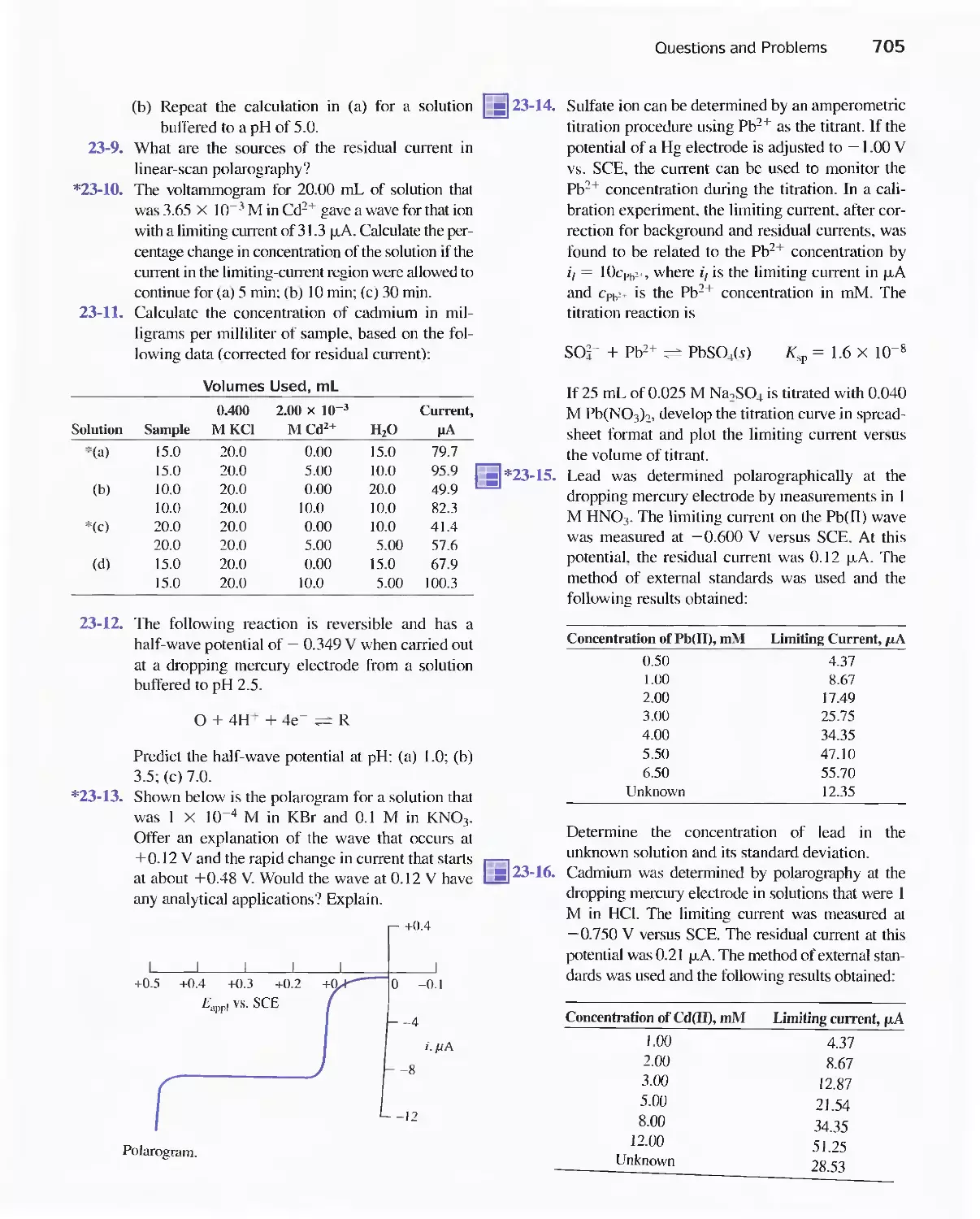
23B Linear Sweep Voltammetry 667
viii Contents
23C Pulse Polarographic and Voltammetric
Methods 689
Feature 23-1 Voltammetric Instruments Based on
Operational Amplifiers 668
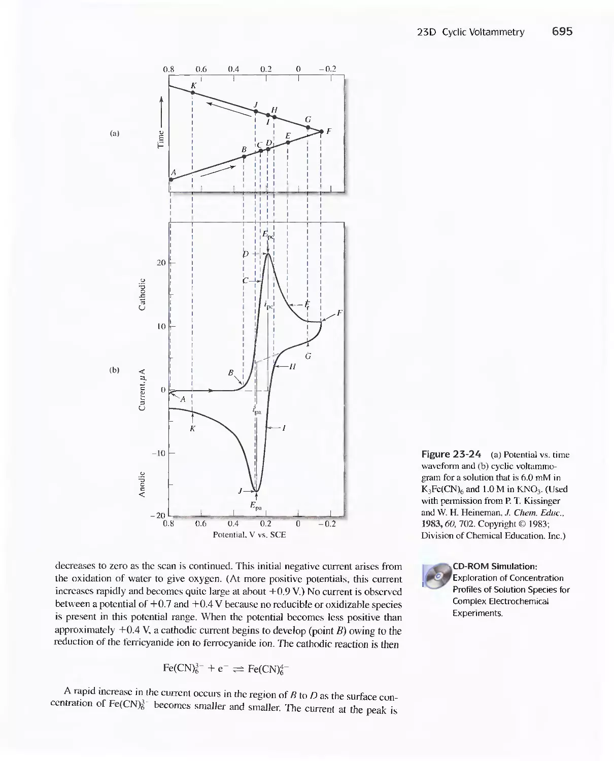
23D Cyclic Voltammetry 694
Feature 23-2 Modified Electrodes 697
23E Stripping Methods 699
23F Voltammetry with Microelectrodes 703
PART V Spectrochemical Methods 707
A Conversation with Gary M. Hieftje 708
Chapter 24 Introduction to Spectrochemical
Methods 710
24A Properties of Electromagnetic Radiation 711
24B Interaction of Radiation and Matter 714
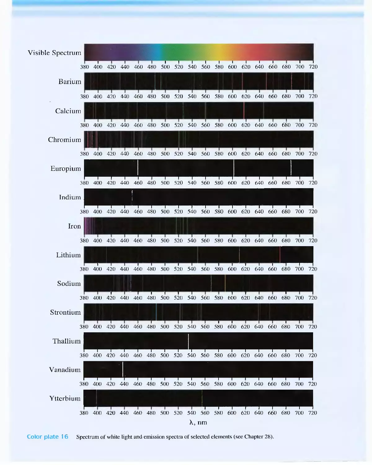
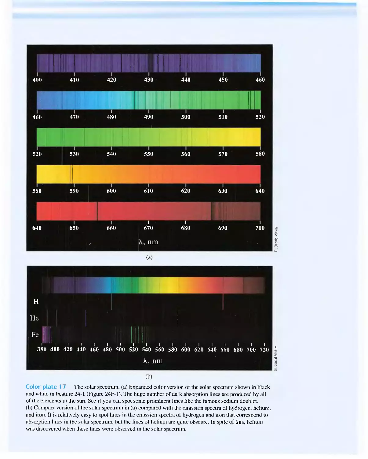
Feature 24-1 Spectroscopy and the Discovery of
Elements 71 7
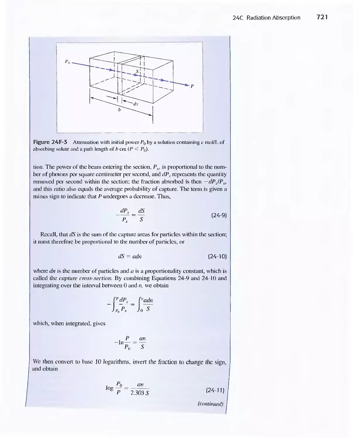
24C Radiation Absorption 718
Feature 24-2 Deriving Beer's Law 720
Feature 24-3 Why Is a Red Solution Red? 725
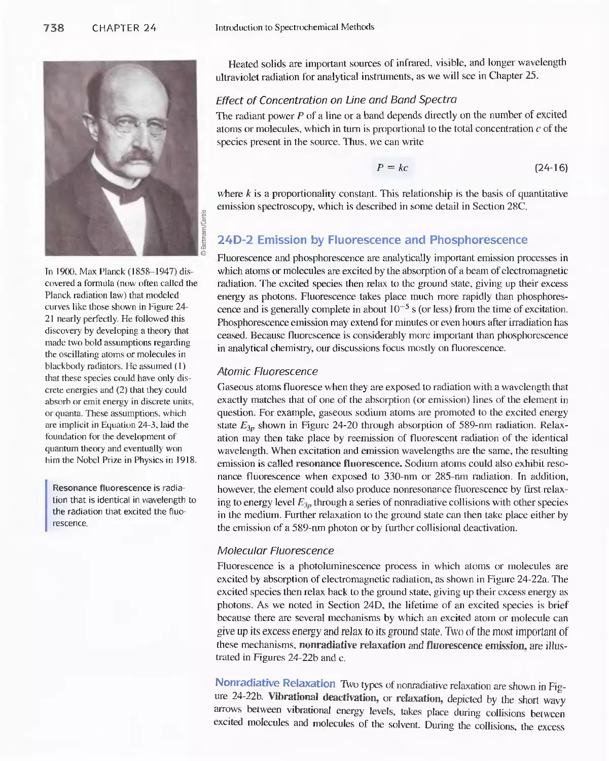
24D Emission of Electromagnetic Radiation 734
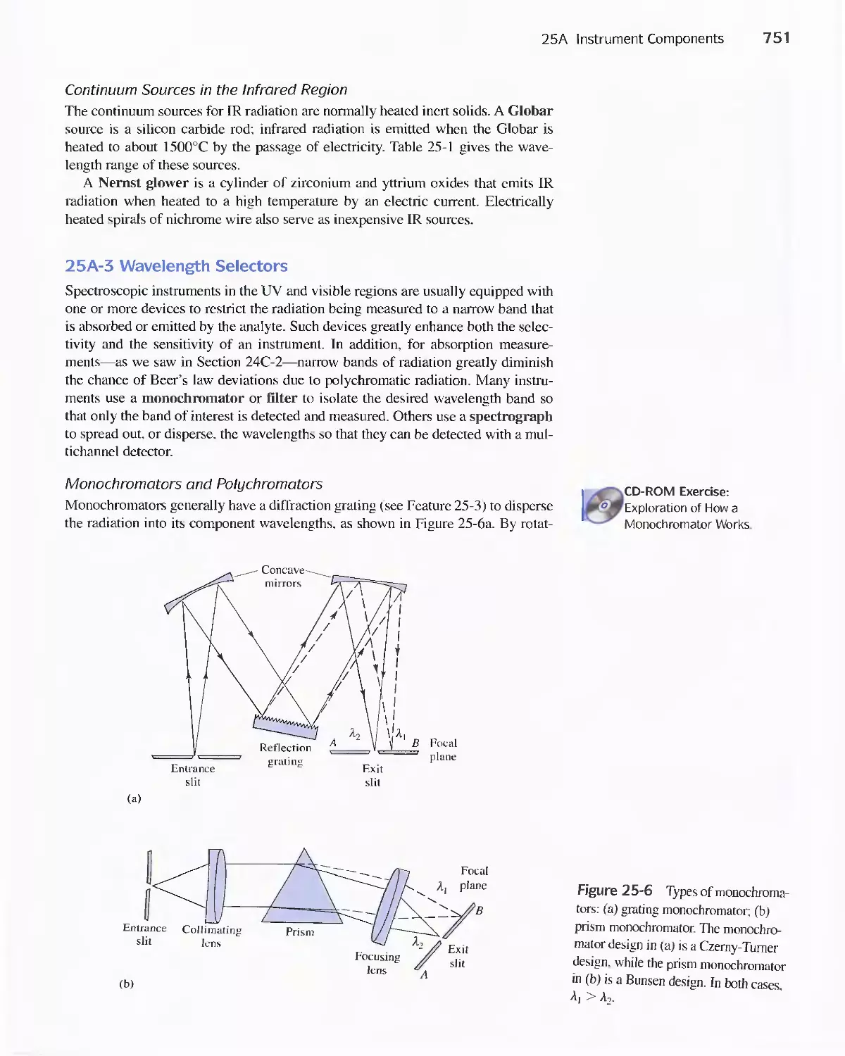
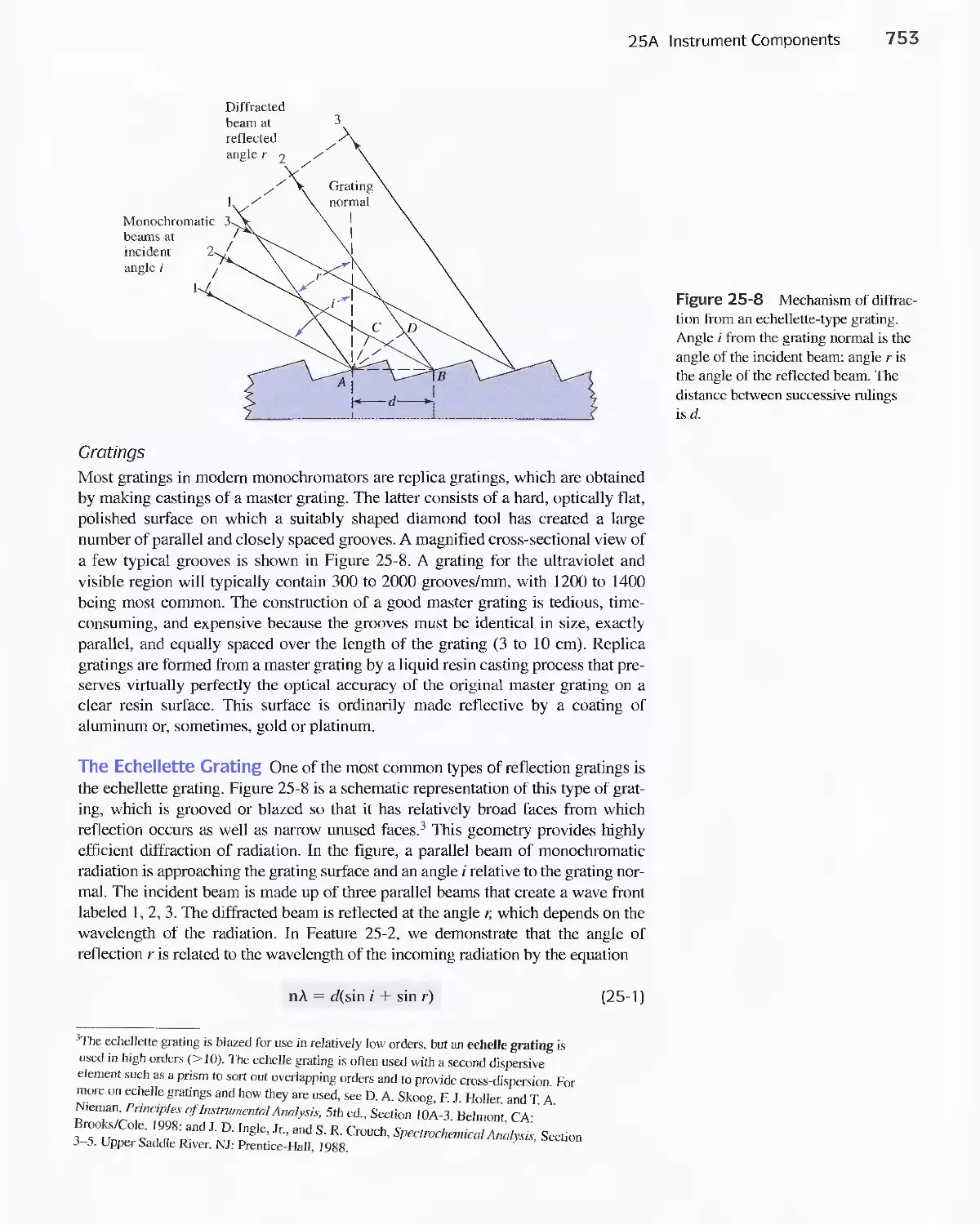
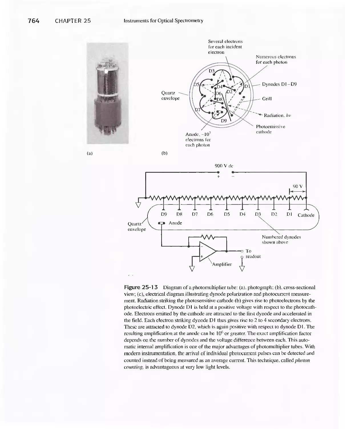
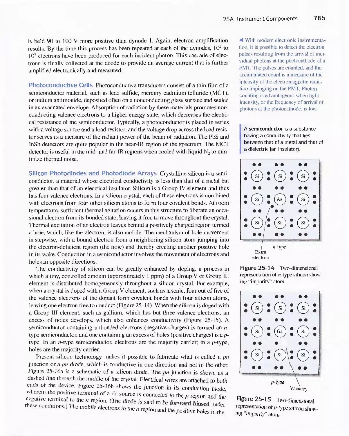
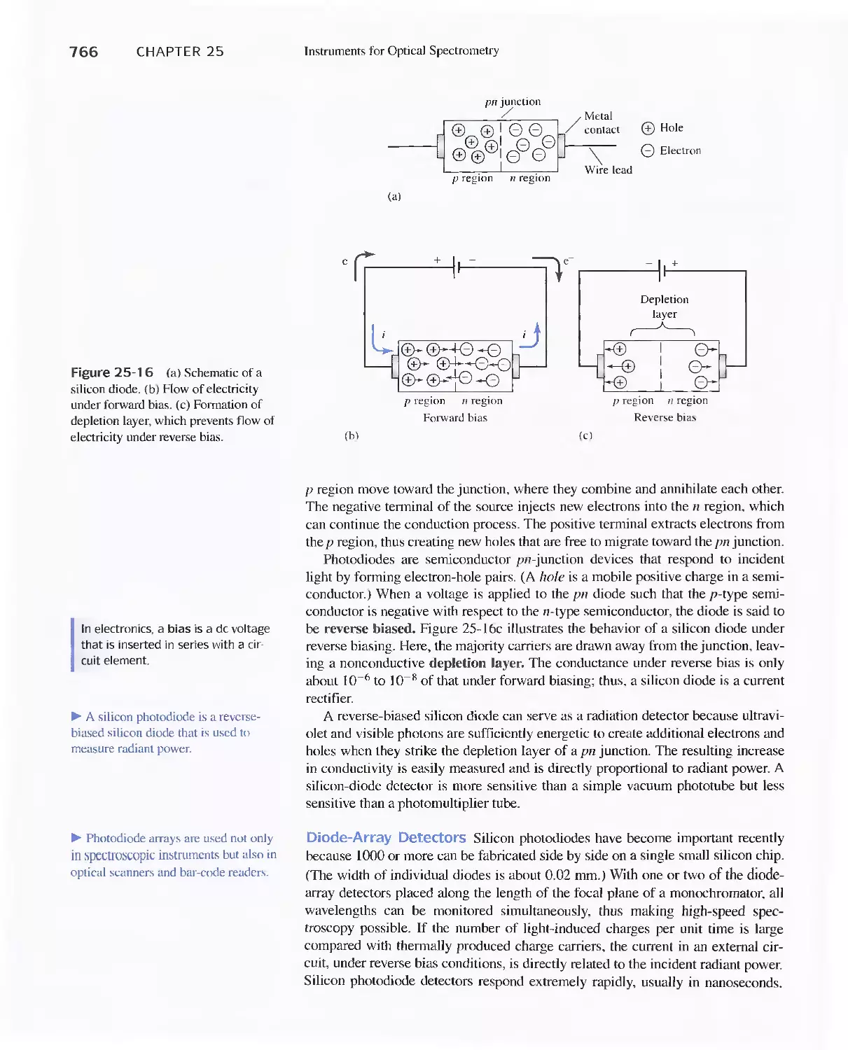
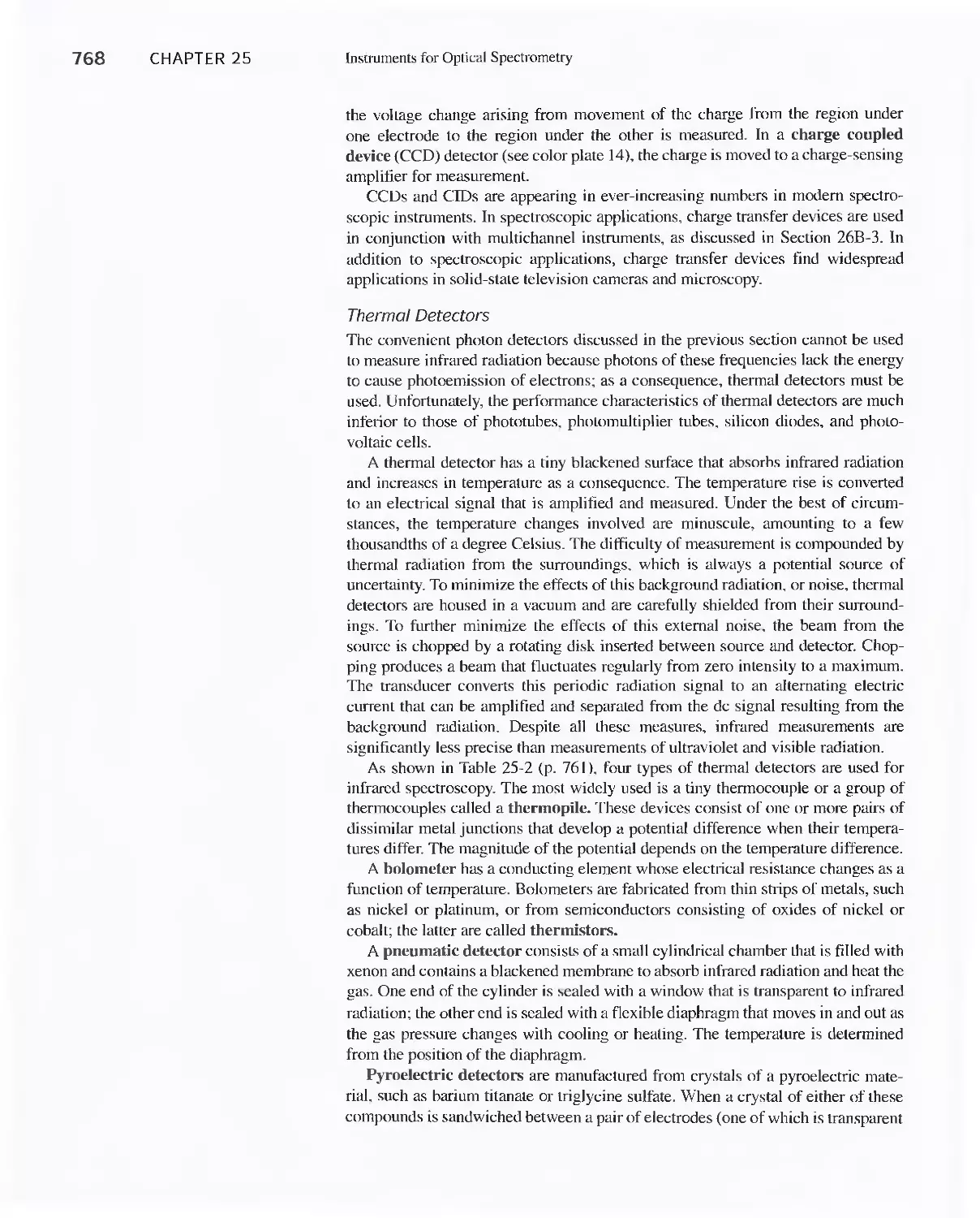
Chapter 25 Instruments for Optical Spectrometry 744
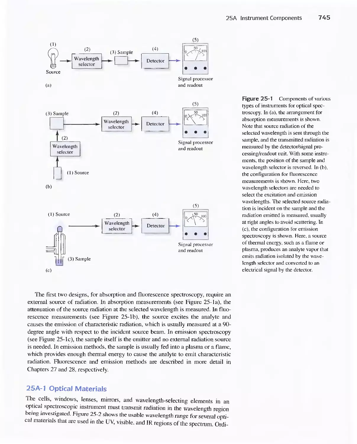
25A Instrument Components 744
Feature 25-1 Laser Sources: The Light Fantastic 748
Feature 25-2 Derivation of Equation 25-1 754
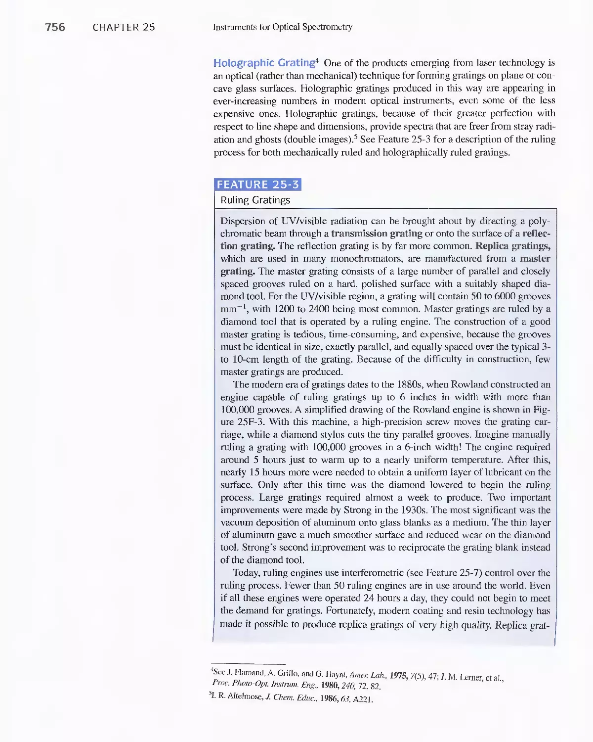
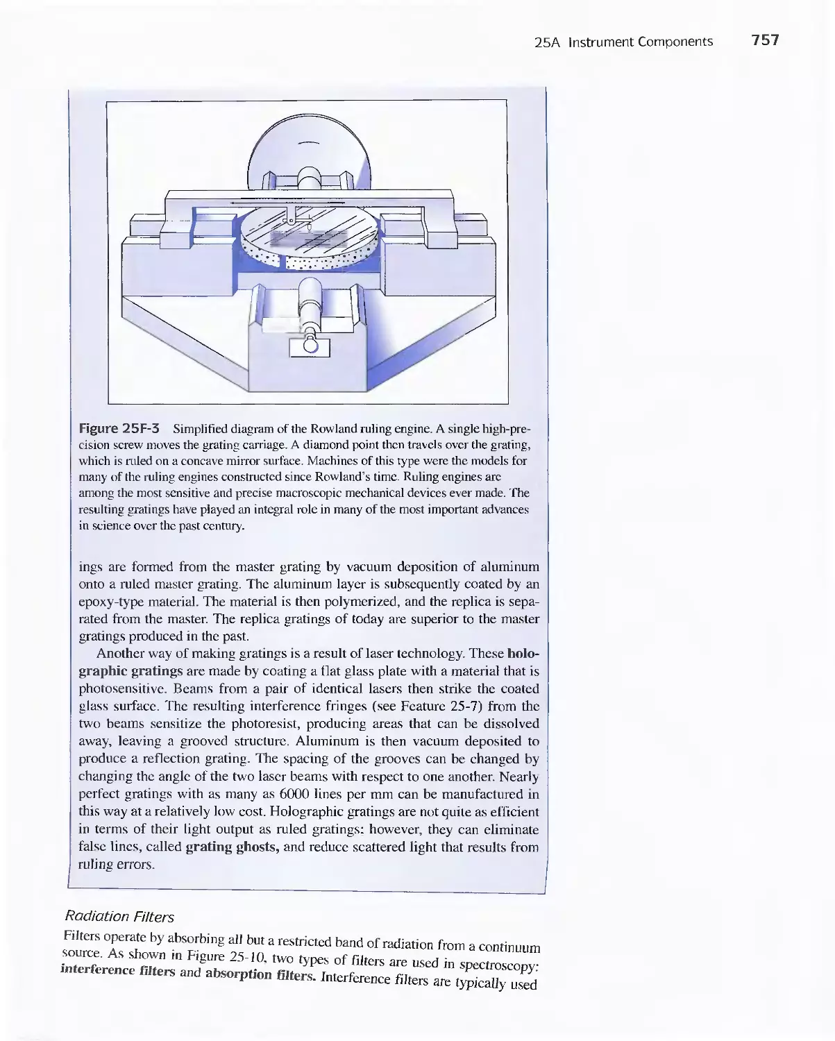
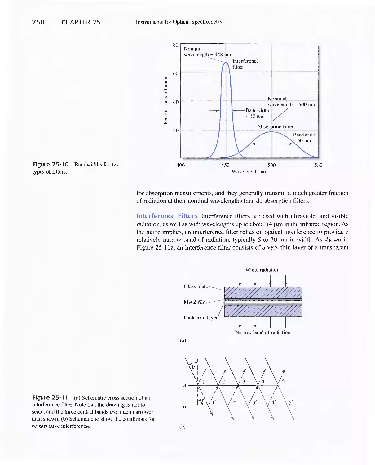
Feature 25-3 Ruling Gratings 756
Feature 25-4 Deriving Equation 25-2 759
Feature 25-5 Signals, Noise, and the Signal-to-Noise
Ratio 761
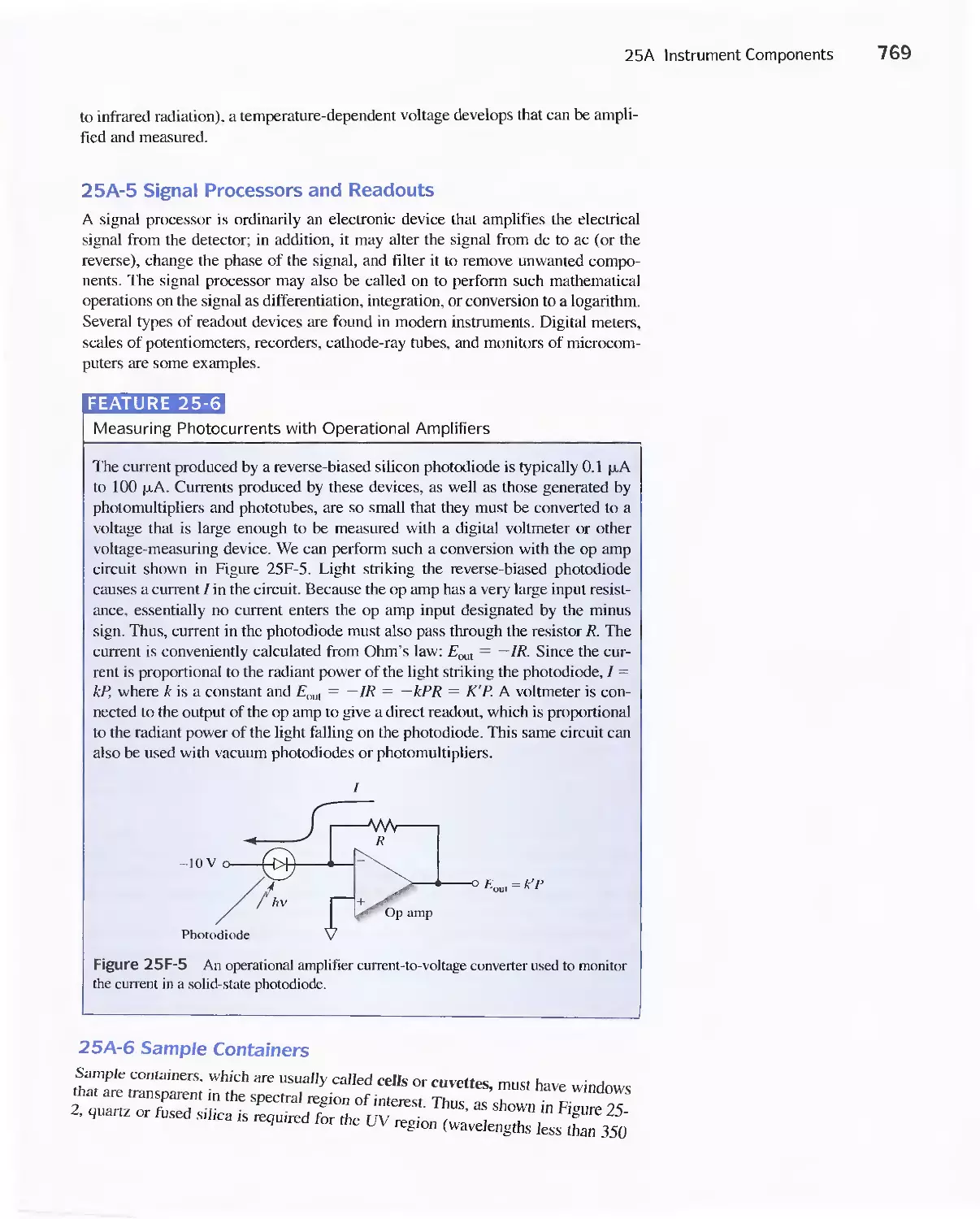
Feature 25-6 Measuring Photocurrents with
Operational Amplifiers 769
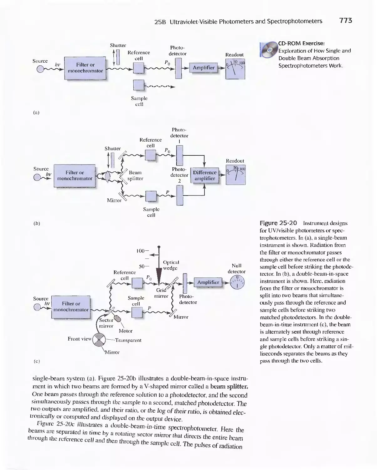
25B Ultraviolet-Visible Photometers and
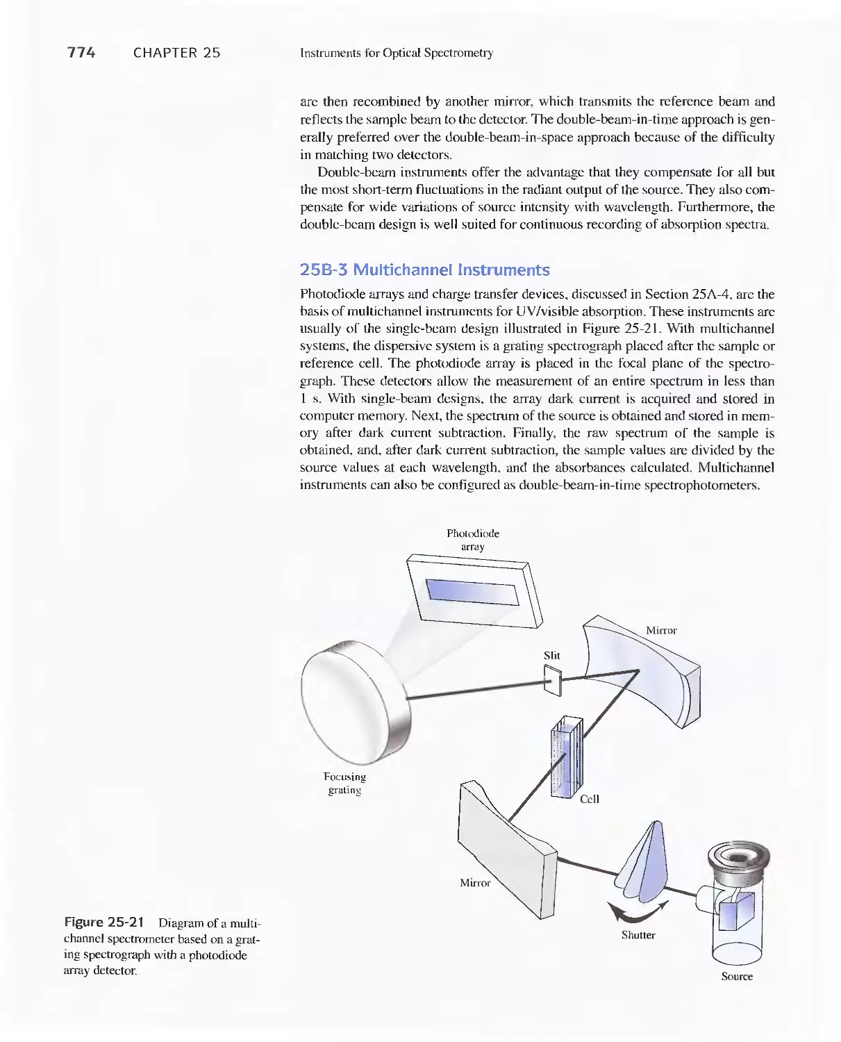
Spectrophotometers 771
25C Infrared Spectrophotometers
Feature 25-7 How Does a Fourier Transform Infrared
Spectrometer Work? 776
Chapter 26 Molecular Absorption Spectrometry 784
26A Ultraviolet and Visible Molecular Absorption
Spectroscopy 784
26B Automated Photometric and Spectrophotometric
Methods 807
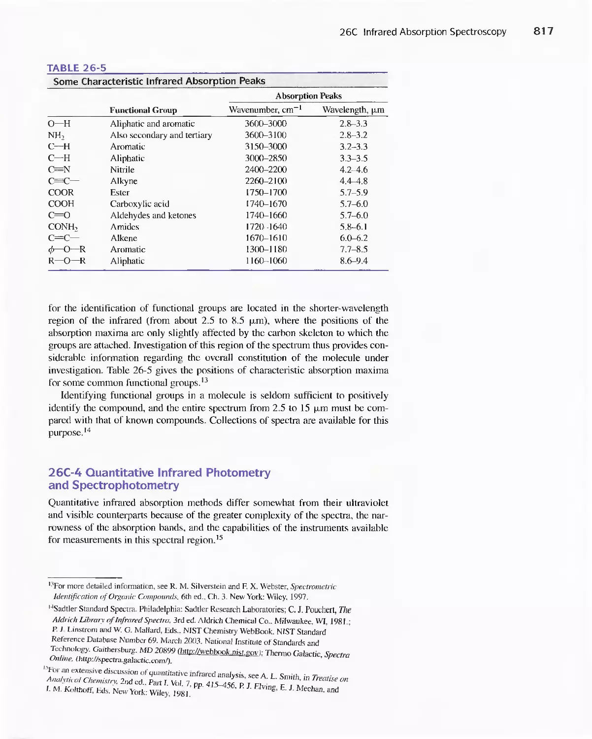
26C Infrared Absorption Spectroscopy 811
Feature 26-1 Using The Fourier Transform To Produce
I nfrared Spectra 81 8
Chapter 27 Molecular Fluorescence Spectroscopy 825
27 A Theory of Molecular Fluorescence 825
27B Effect of Concentration On Fluorescence
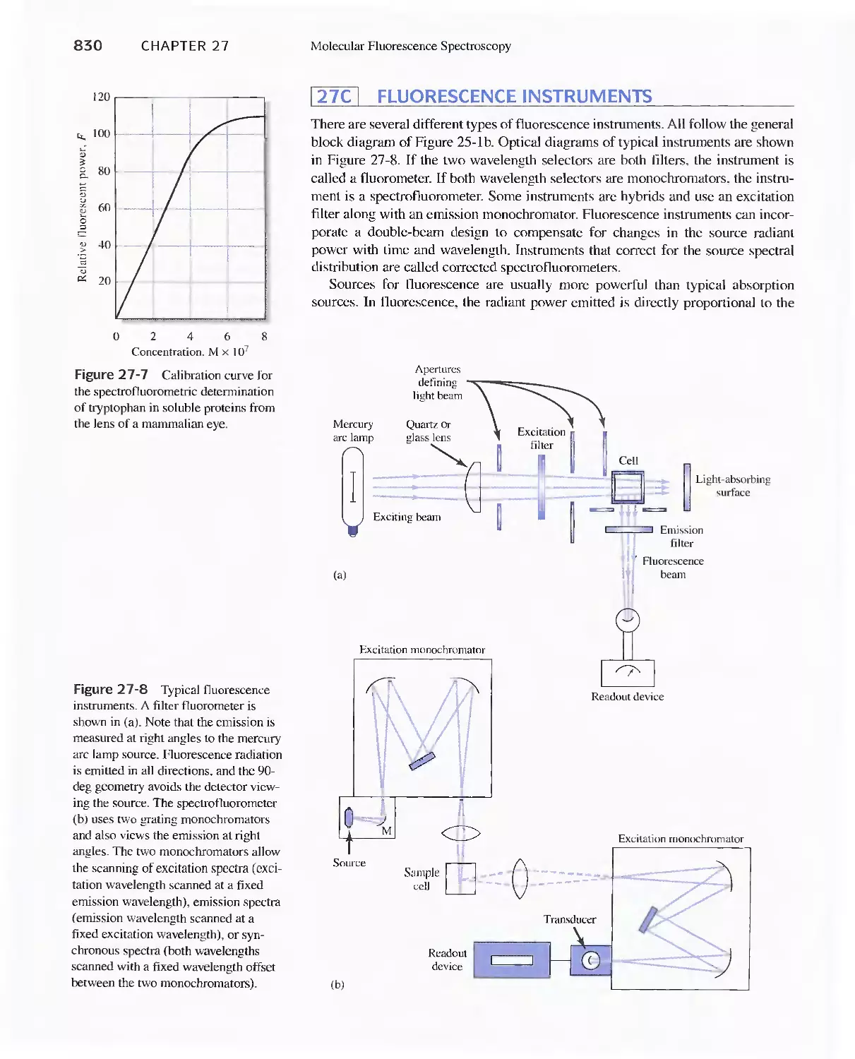
Intensity 829
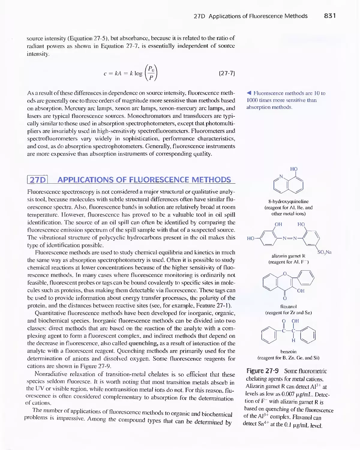
27C Fluorescence Instruments 830
27D Applications of Fluorescence Methods 831
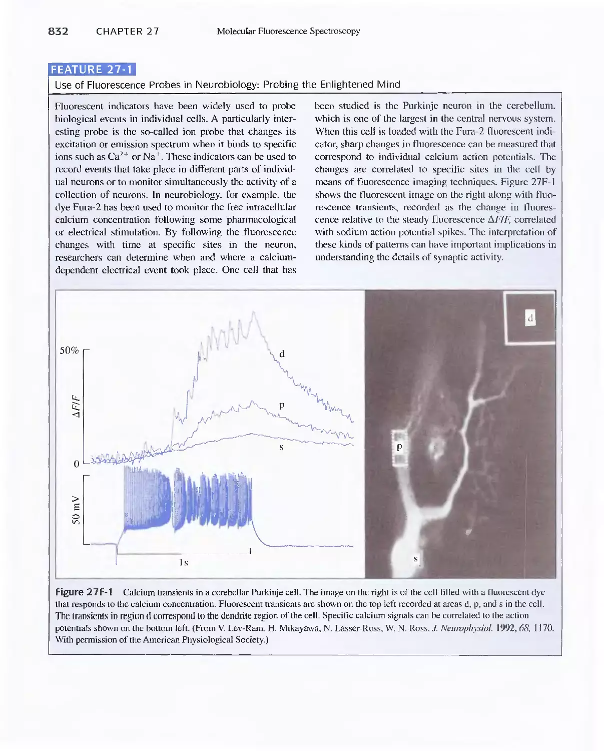
Feature 27-1 Use of Fluorescence Probes in Neurobiology:
Probing the Enlightened Mind 832
27E Molecular Phosphorescence Spectroscopy 834
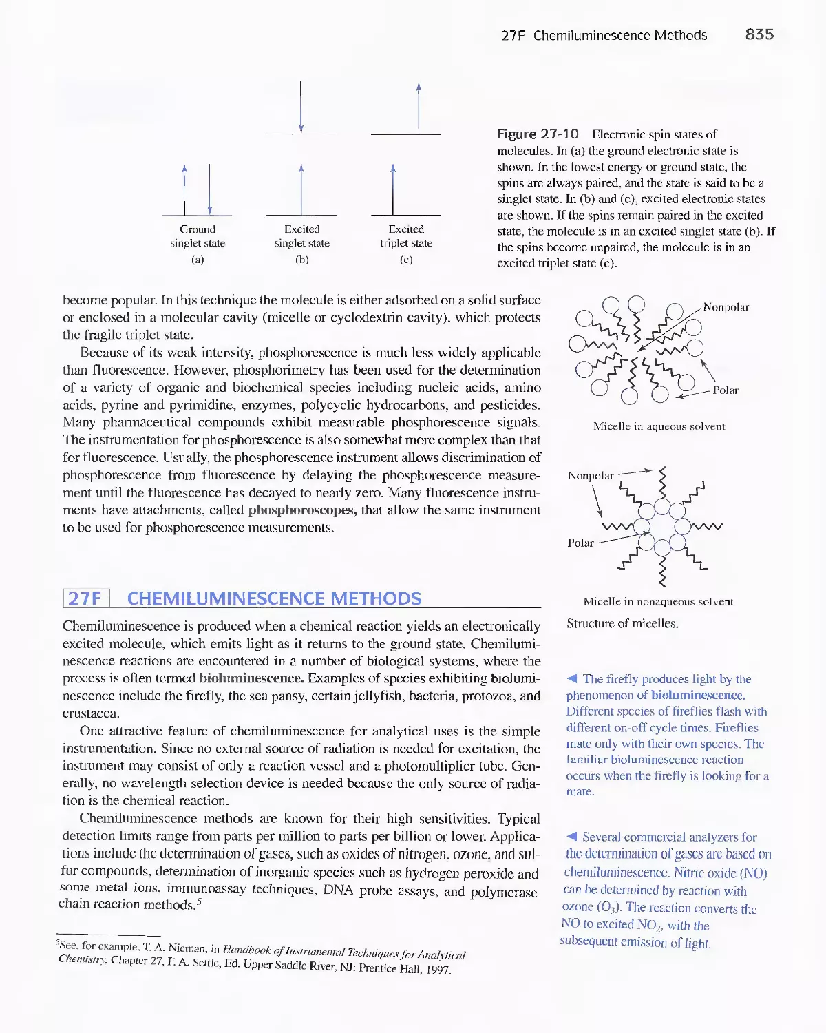
27F Chemiluminescence Methods 835
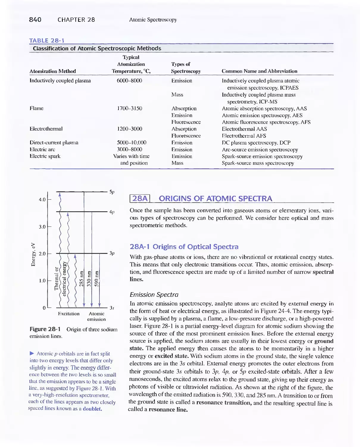
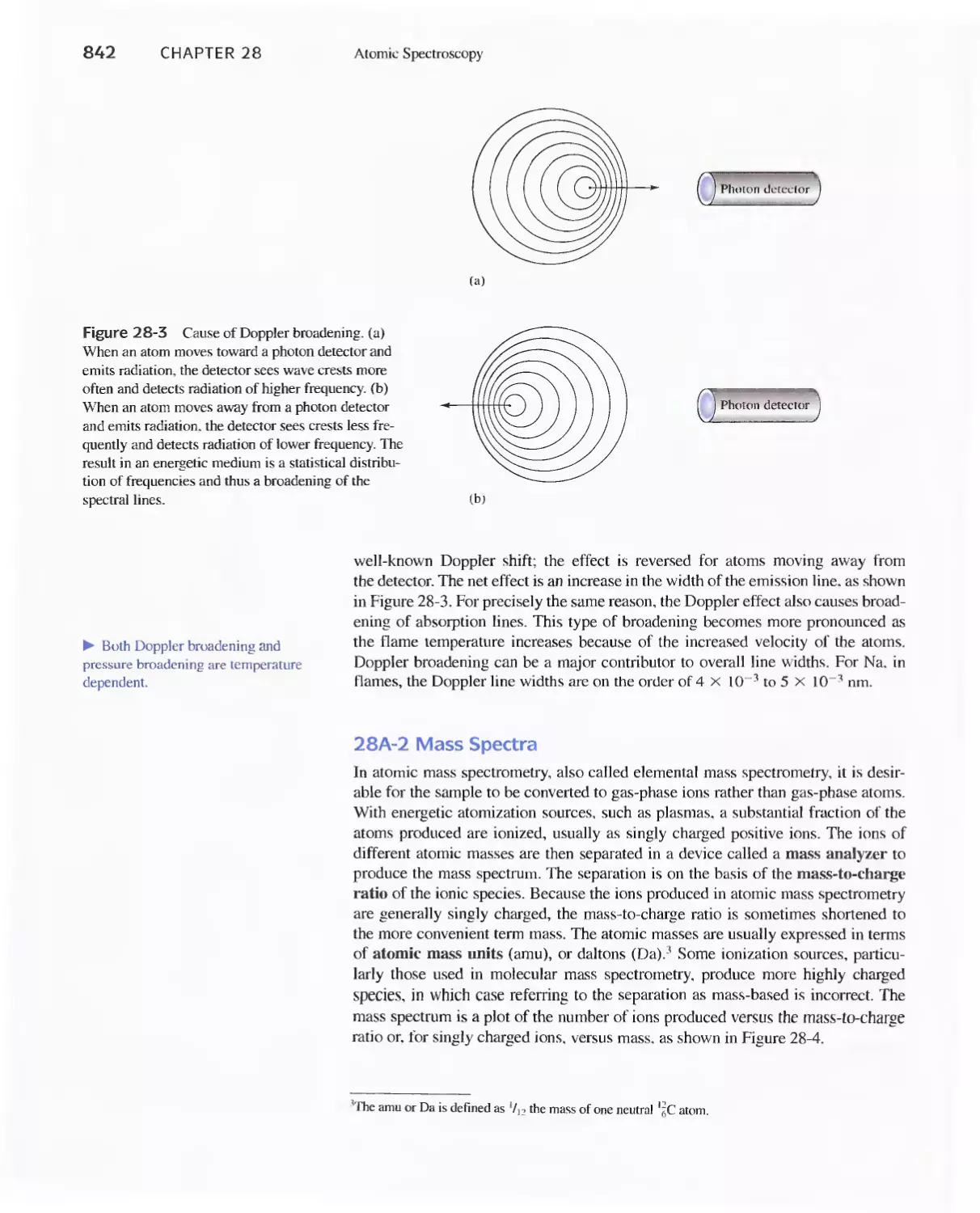
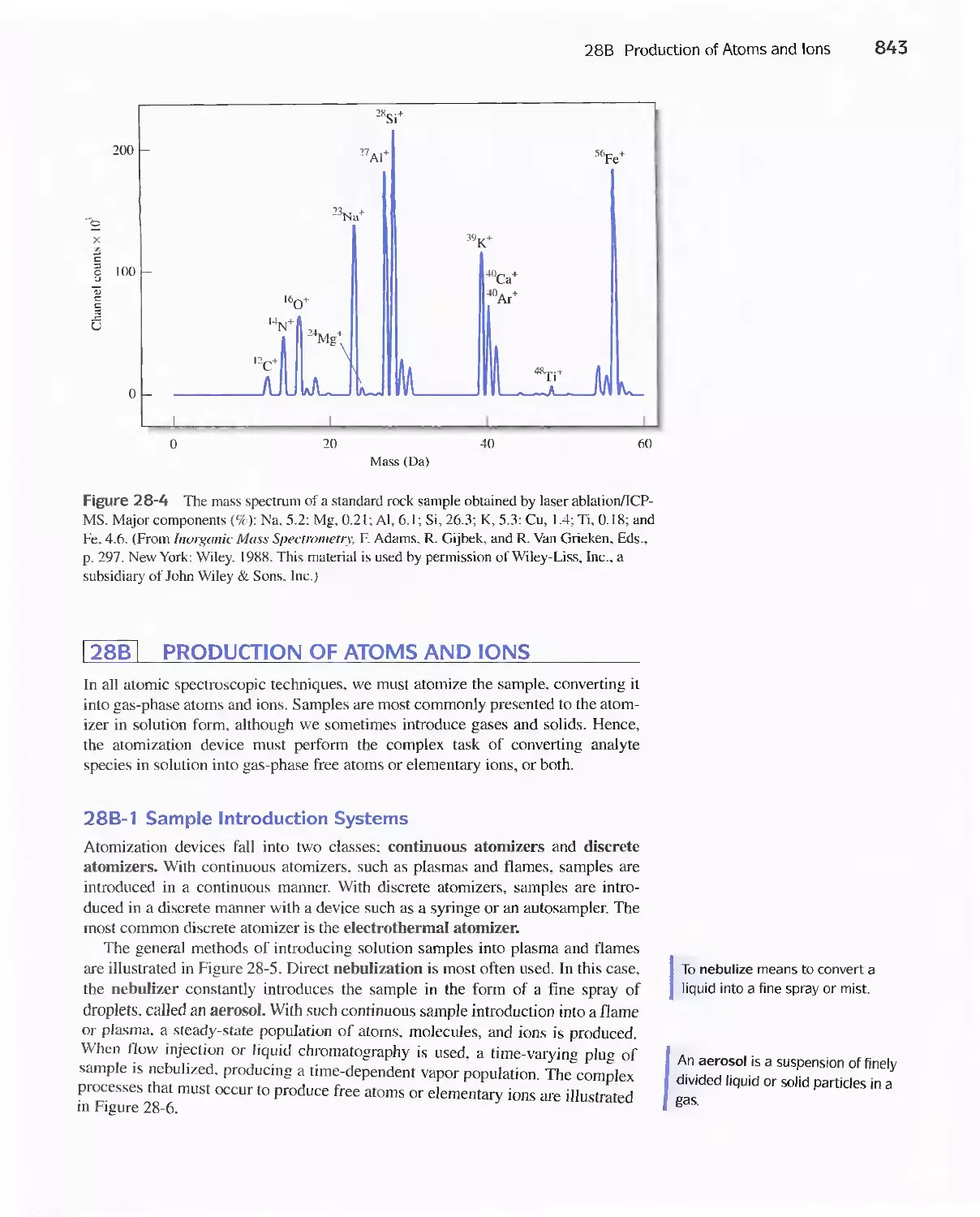
Chapter 28 Atomic Spectroscopy 839
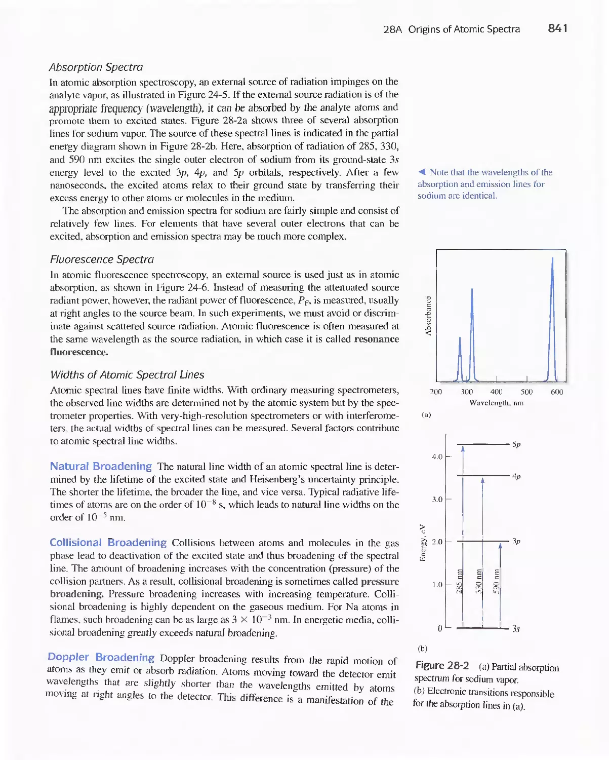
28A Origins of Atomic Spectra 840
28B Production of Atoms and Ions 843
28C Atomic Emission Spectrometry 854
28D Atomic Absorption Spectrometry 858
Feature 28-1 Determining Mercury by Cold-Vapor
Atomic Absorption Spectroscopy 865
28E Atomic Fluorescence Spectrometry 868
28F Atomic Mass Spectrometry 868
PART VI Kinetics and Separations 875
A Conversation with Isiah M. Warner 876
Chapter 29 Kinetic Methods of Analysis 878
29A Rates of Chemical Reactions 879
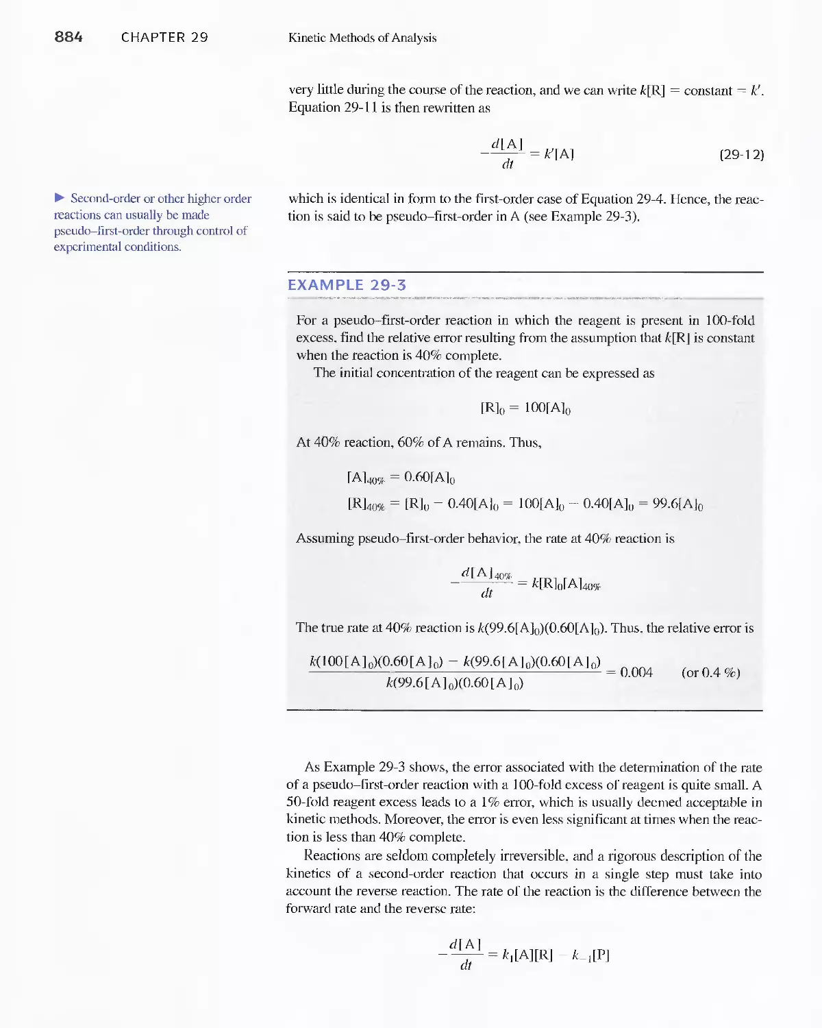
Feature 29-1 Enzymes 886
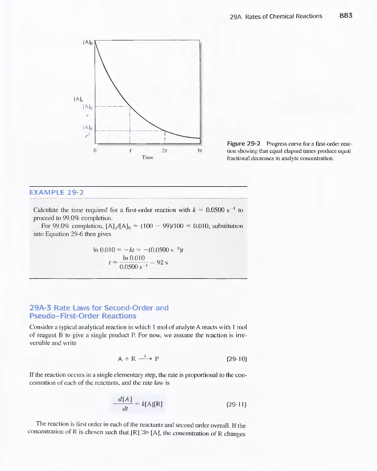
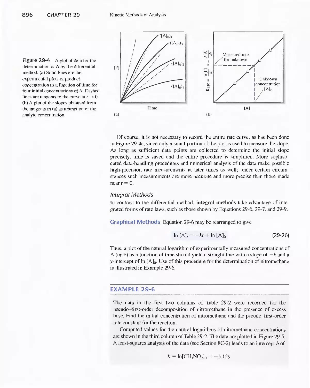
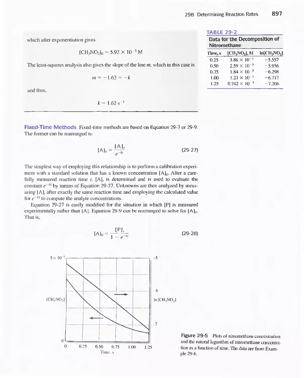
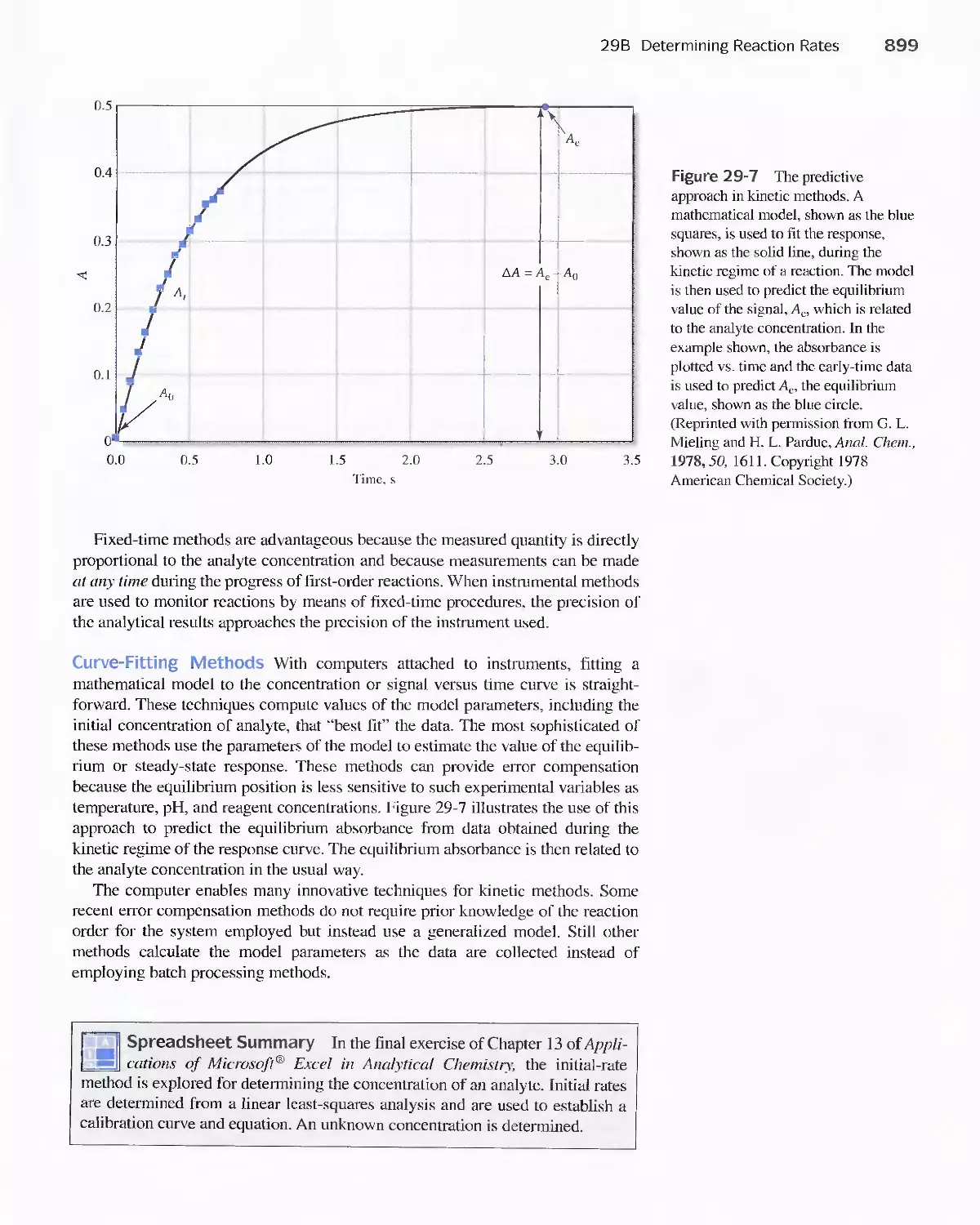
29B Determining Reaction Rates 892
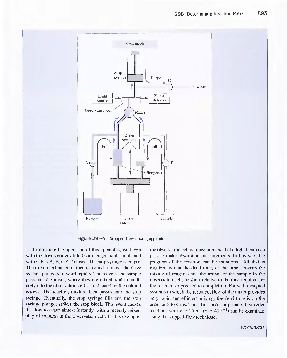
Feature 29-2 Fast Reactions and Stopped-Flow
Mixing 892
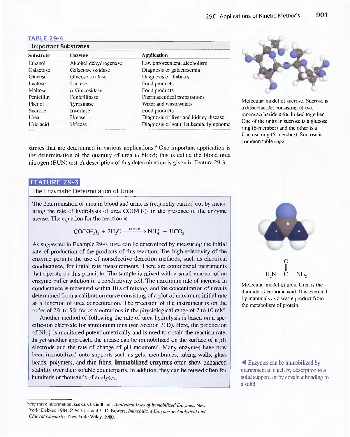
29C Applications of Kinetic Methods 900
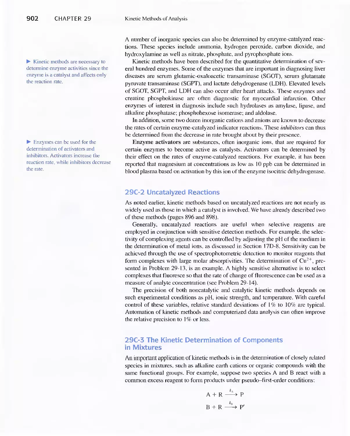
Feature 29-3 The Enzymatic Determination of Urea 901
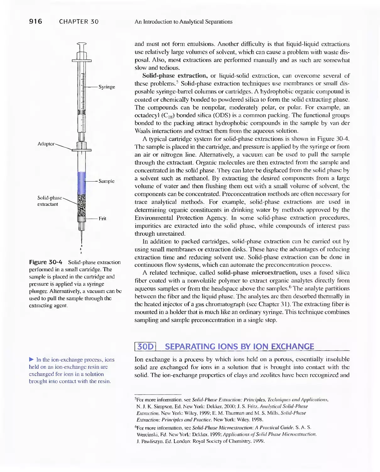
Chapter 30 Introduction to Analytical
Separations 906
30A Separation by Precipitation 907
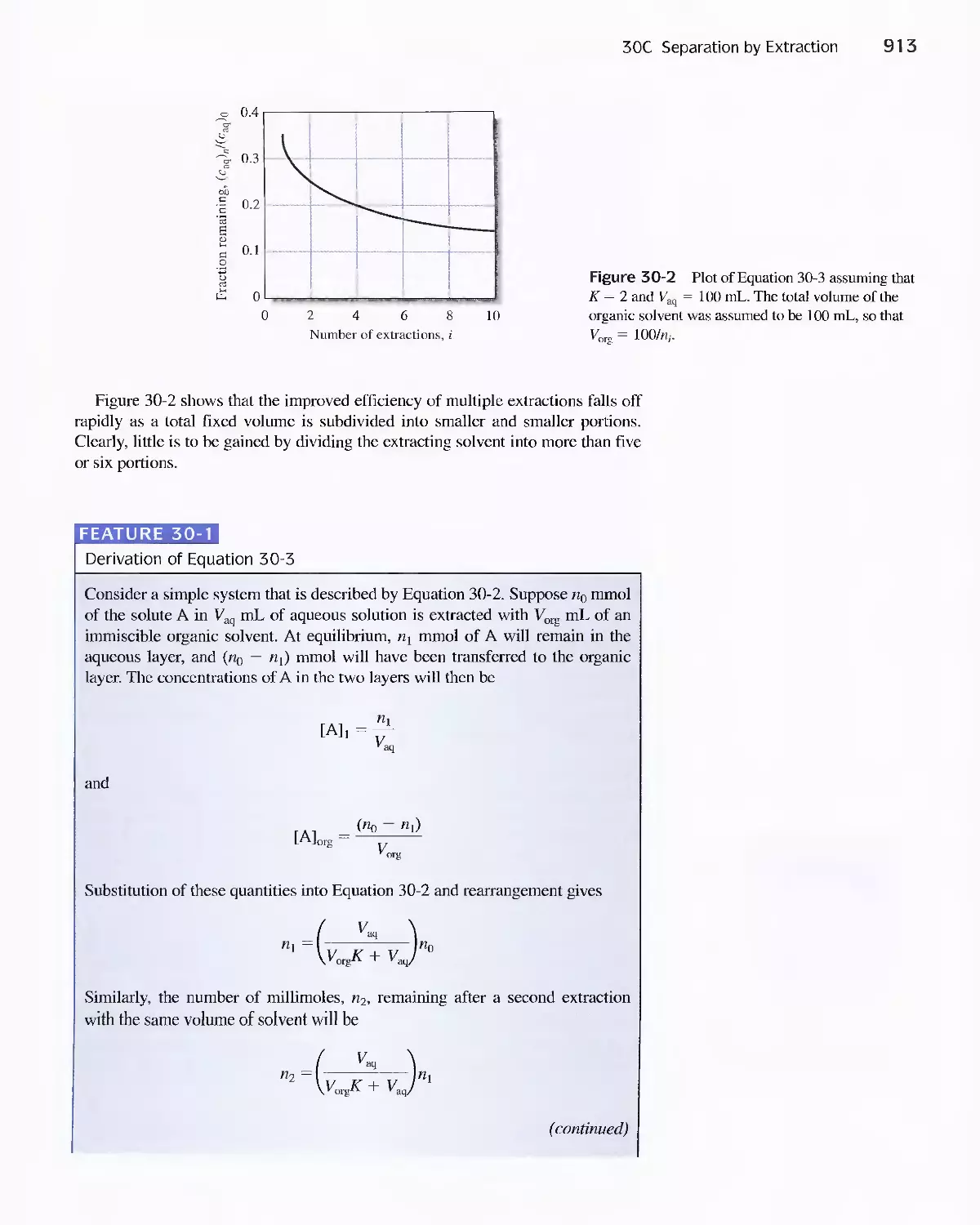
30B Separation of Species by Distillation 911
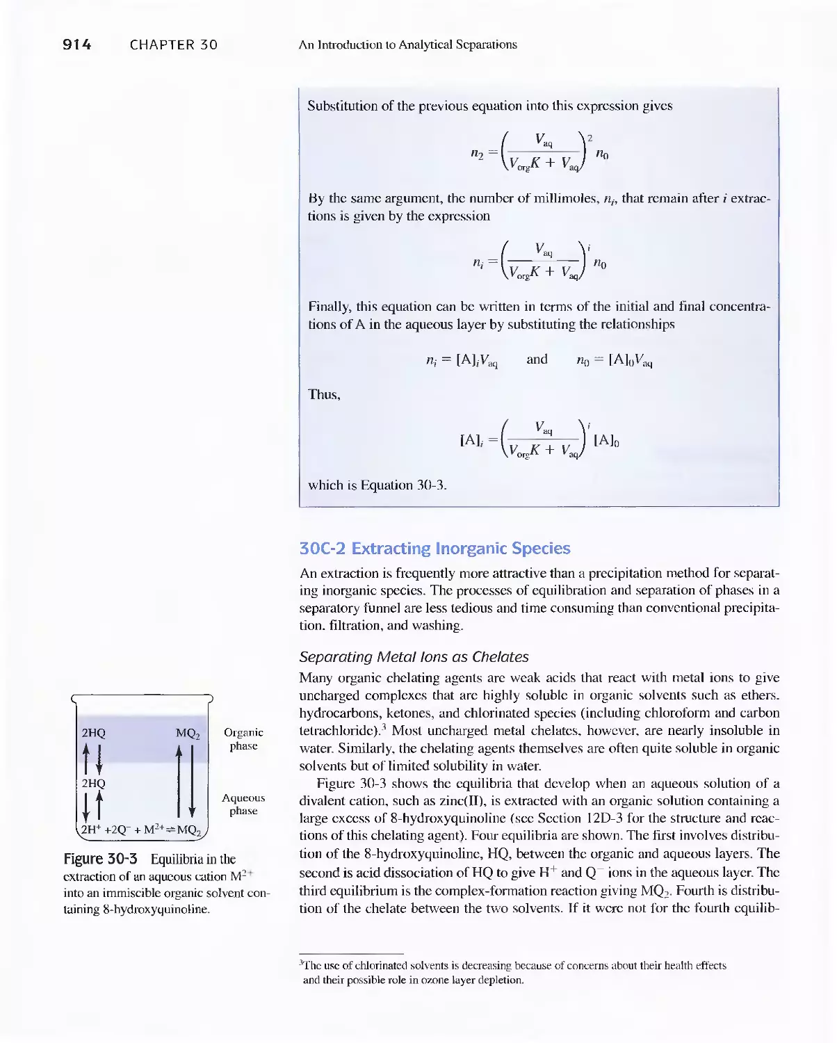
30C Separation by Extraction 911
Feature 30-1 Derivation of Equation 30-3 913
30D Separating Ions by Ion Exchange 916
Feature 30-2 Home Water Softeners 919
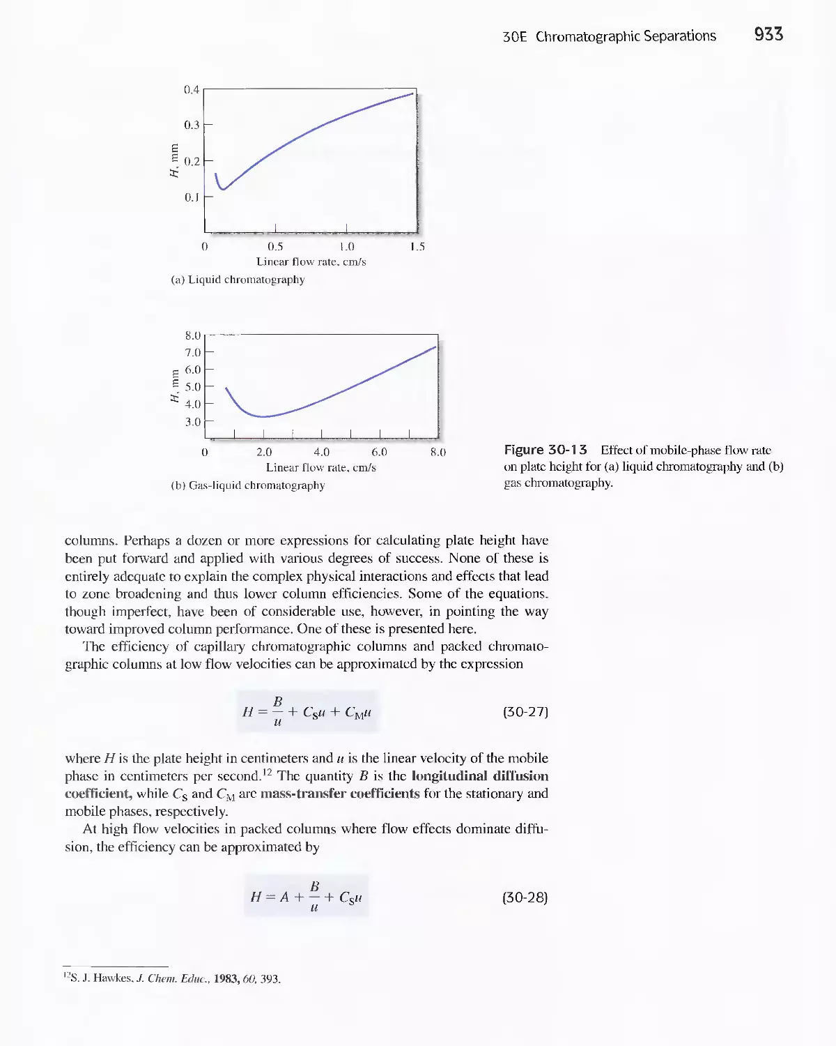
30E Chromatographic Separations 920
Feature 30-3 What is the Source of the Terms Plate and
Plate Height? 930
Chapter 31 Gas Chromatography 947
31 A Instruments for Gas-Liquid Chromatography 948
31 B Gas Chromatography Columns and Stationary
Phases 958
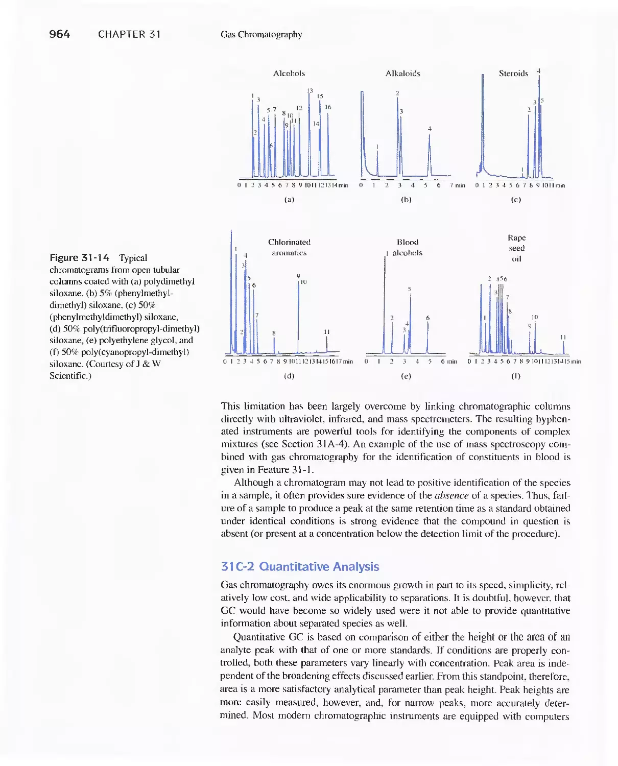
31 C Applications of Gas-Liquid Chromatography 963
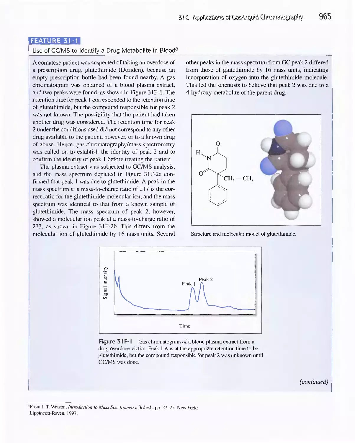
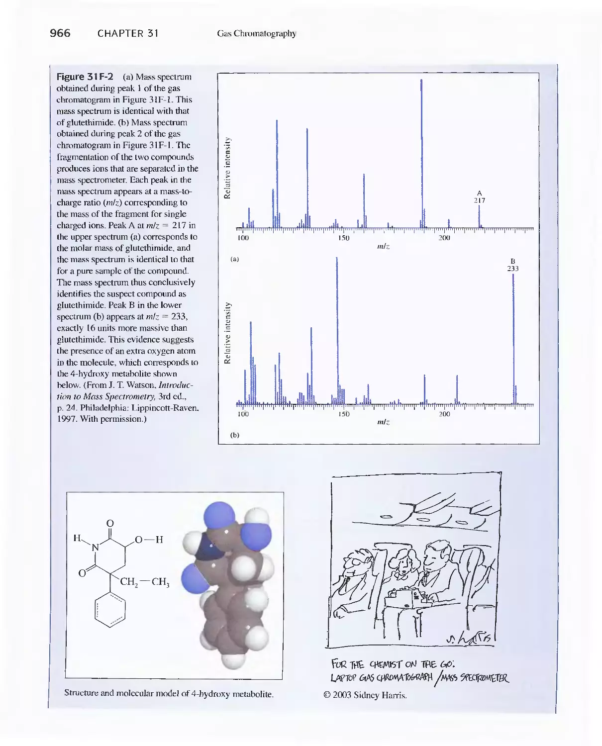
Feature 31-1 Use of GC/MS to identify a Drug
Metabolite in Blood 965
Feature 31-2 High-Speed Gas Chromatography 969
31 D Gas-Solid Chromatography 970
Chapter 32 High-Performance Liquid
Chromatography 973
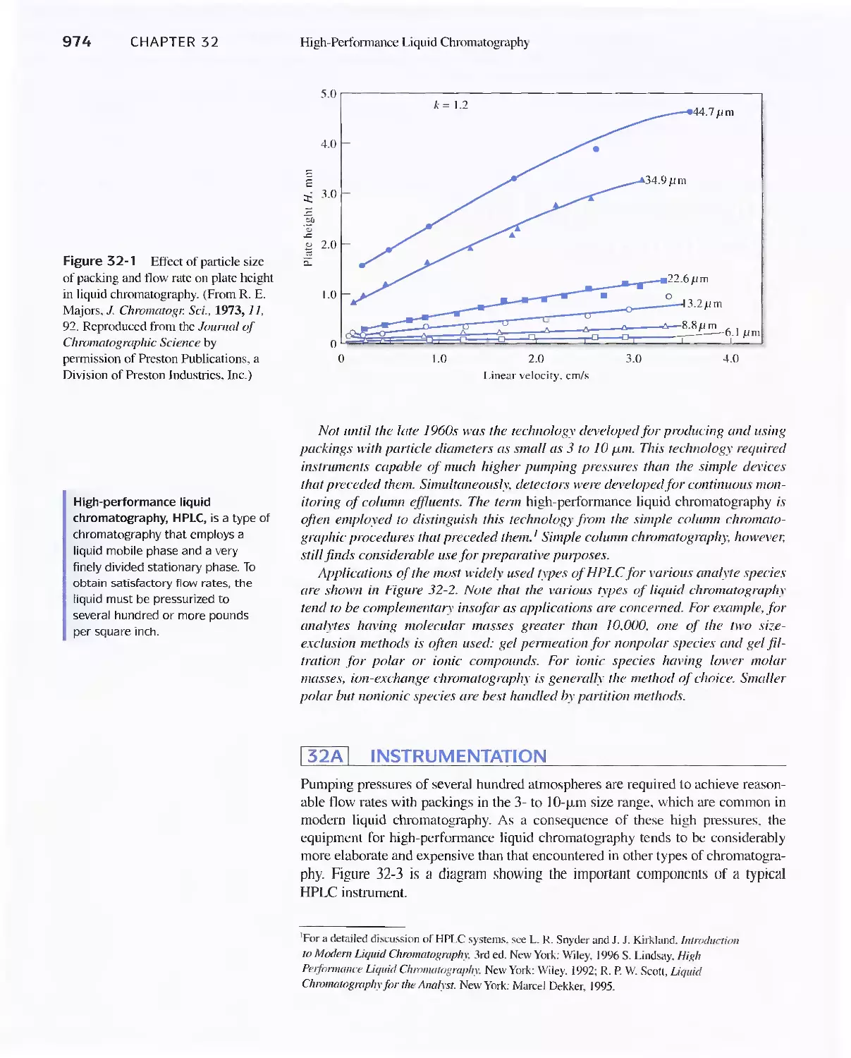
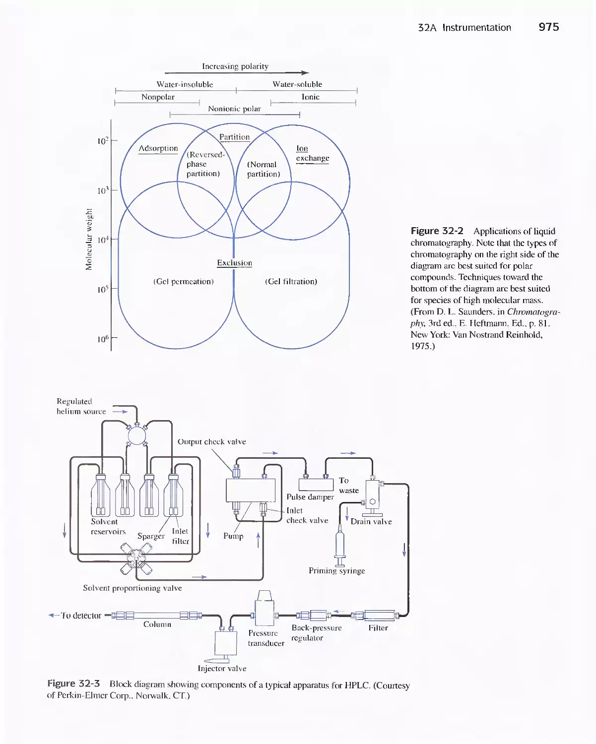
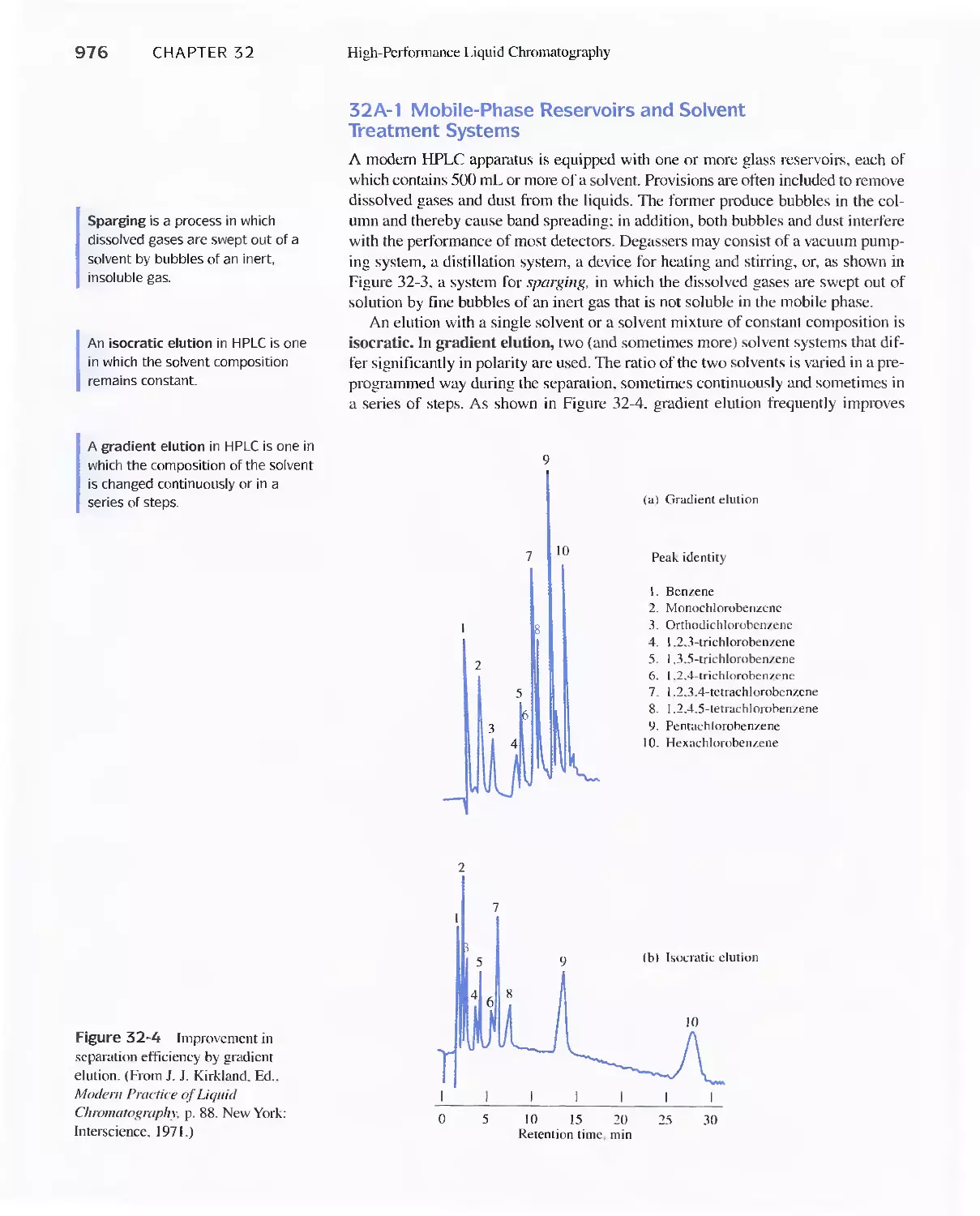
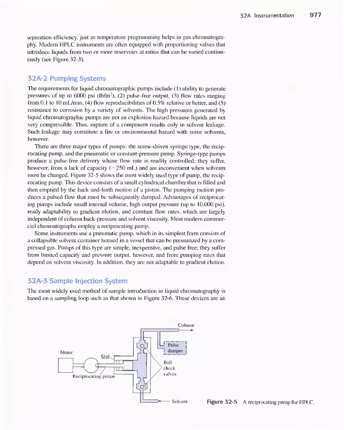
31 A Instrumentation 974
Feature 32-1 Liquid Chromatography (Lq/Mass
Spectrometry (MS) and LC/MS/NS 980
32B High-Performance Partition Chromatography 982
32C High-Performance Adsorption
Chromatography 986
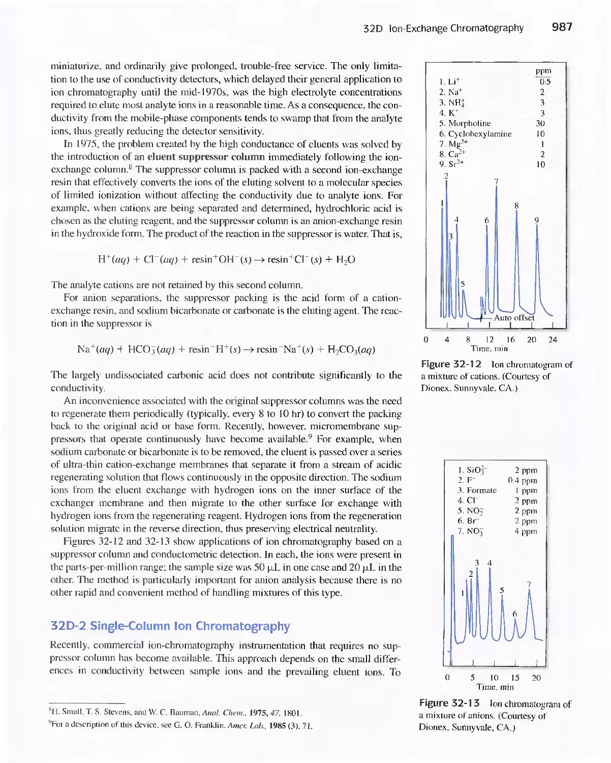
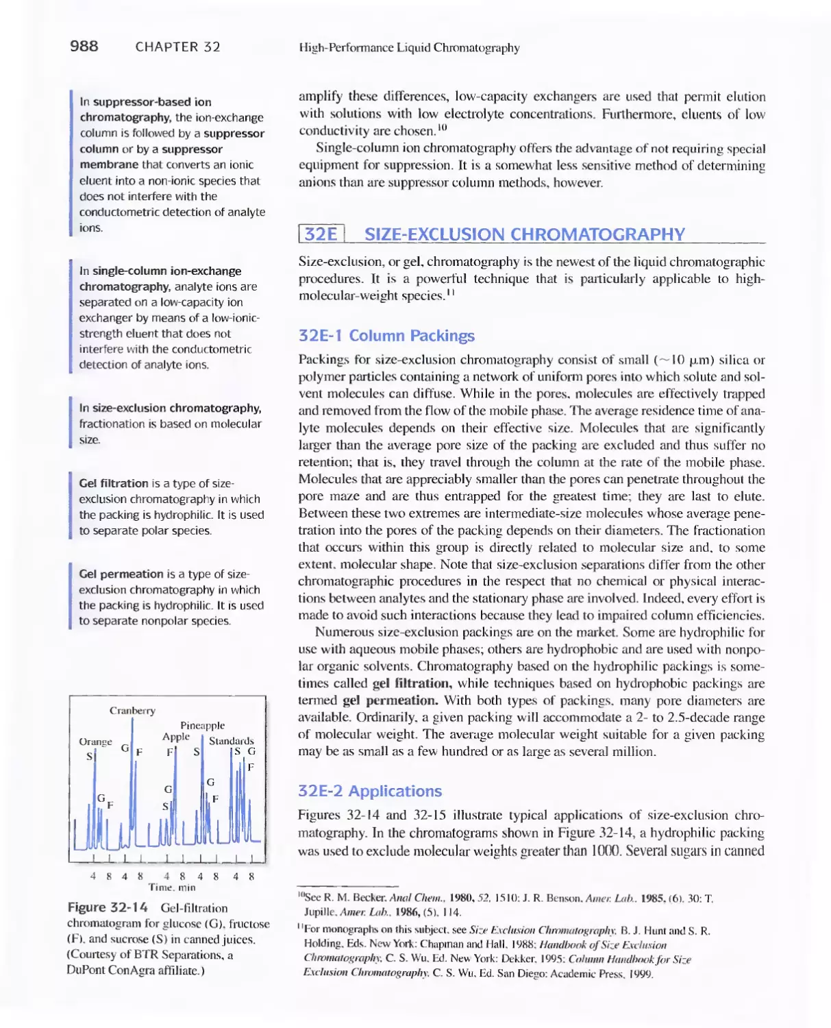
32D lon-Exchange Chromatography 986
32E Size-Exclusion Chromatography 988
Feature 32-2 Buckyballs: The Chromatographic
Separation of Fullerenes 989
32F Affinity Chromatography 991
32G Chiral Chromatography 991
32H Comparison of High-Performance Liquid
Chromatography and Gas Chromatography 992
Chapter 33 Miscellaneous Separation Methods 996
33A Supercritical-Fluid Chromatography 996
33B Planar Chromatography 1000
33C Capillary Electrophoresis 1003
Feature 33-1 Capillary Array Electrophoresis in DNA
Sequencing 1010
33D Capillary Electrochromatography 1011
33E Field-Flow Fractionation 1013
PART VII Practical Aspects of Chemical
Analysis 1021
A Conversation with Julie Leary 1022
Chapter 34 Analysis of Real Samples 1024
34A Real Samples 1024
34B Choice of Analytical Method 1026
34C Accuracy in the Analysis of Complex
Materials 1031
Chapter 35 Preparing Samples for Analysis 1034
35A Preparing Laboratory Samples 1034
35B Moisture in Samples 1036
35C Determining Water in Samples 1039
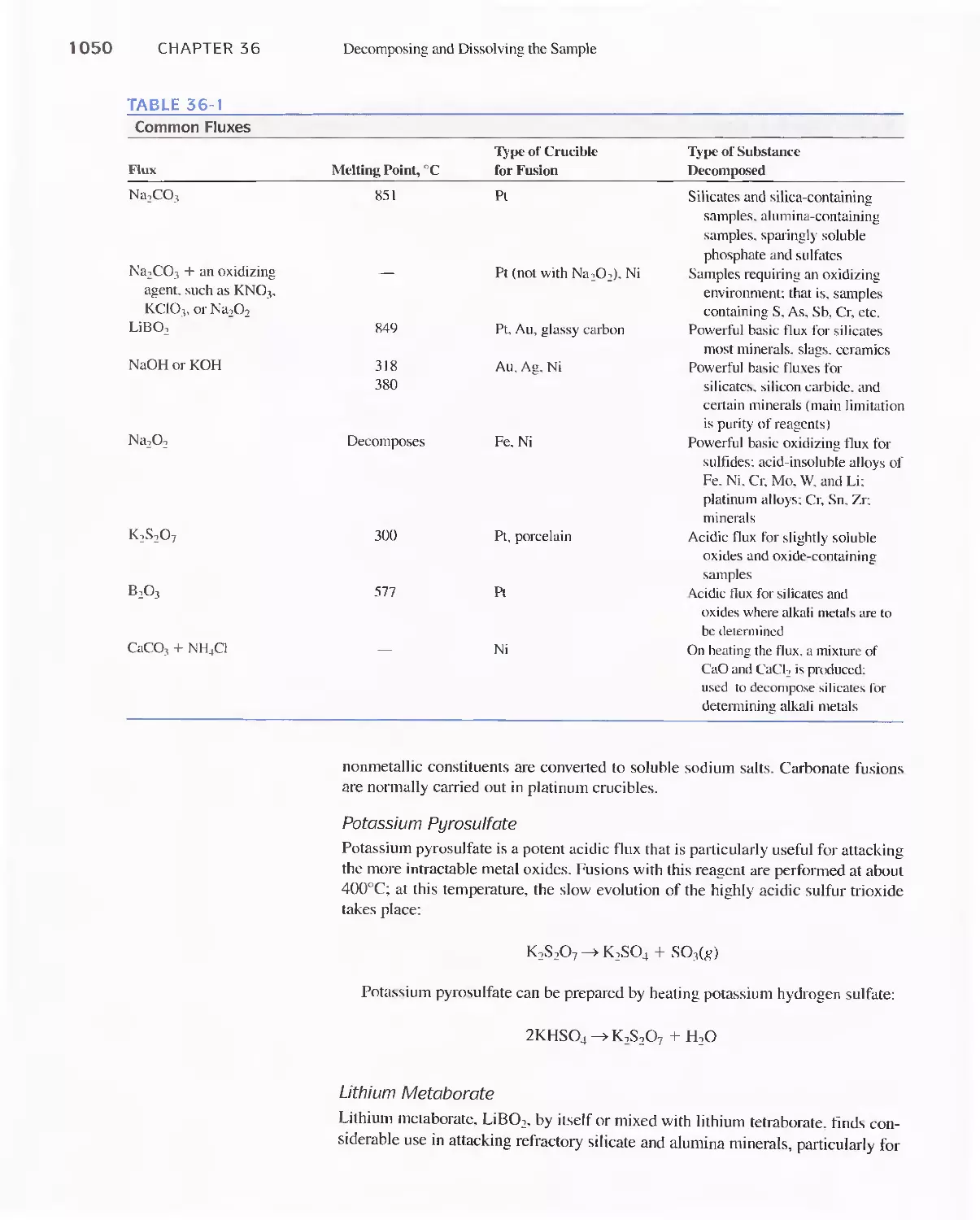
Chapter 36 Decomposing and Dissolving the
Sample 1041
36A Sources of Error in Decomposition and
Dissolution 1042
36B Decomposing Samples With Inorganic Acids in
Open Vessels 1042
36C Microwave Decompositions 1044
36D Combustion Methods for Decomposing Organic
Samples 1047
36E Decomposition of Inorganic Materials by
Fluxes 1049
Contents ix
Chapter 37 Selected Methods of Analysis
This chapter is only available as an Adobe Acrobat@
PDF file on the Analytical Chemistry CD-ROM
enclosed in this book or on our Web site at
http://chemistry.brookscole.com/skoogfac/.
37A An Introductory Experiment
37B Gravimetric Methods of Analysis
37C Neutralization Titrations
37D Precipitation Titrations
37E Complex-Formation Titrations with EDTA
37F Titrations with Potassium Permanganate
37G Titrations with Iodine
37H Titrations with Sodium Thiosulfate
371 Titrations with Potassium Bromate
37 J Potentiometric Methods
37K Electrogravimetric Methods
37 L Coulometric Titrations
37M Voltammetry
37N Methods Based on the Absorption of Radiation
370 Molecular Fluorescence
37P Atomic Spectroscopy
370 Application of Ion Exchange Resins
37R Gas-Liquid Chromatography
Glossary G-I
APPENDIX 1 The Literature of Analytical
Chemistry A-I
APPENDIX 2 Solubility Product Constants at
25°C A-6
APPENDIX 3 Acid Dissociation Constants at
25°C A-8
APPENDIX 4 Formation Constants at 25°C A-IO
APPENDIX 5 Standard and Formal Electrode
Potentials A-12
APPENDIX 6 Use of Exponential Numbers and
Logarithms A-15
APPENDIX 7 Volumetric Calculations Using Normality
and Equivalent Weight A-19
APPENDIX 8 Compounds Recommended for the
Preparation of Standard Solutions of
Some Common Elements A-27
APPENDIX 9 Derivation of Error Propagation
Equations A-29
Answers to Selected Questions and Problems A-34
Index 1-1
PREFACE
T he eighth edition of FUlldamelltals of Analytical Chemistry, like its predeces-
sors. is an introductory textbook designed primarily for a one- or two-semester
course for chemistry majors. Since the publication of the seventh edition, the scope
of analytical chemistry has continued to evolve, and in this edition we have
included many applications to biology. medicine, materials science, ecology, foren-
sic science. and other related fields. The widespread use of computers for instruc-
tional purposes has led us to incorporate many spreadsheet applications. examples,
and exercises. Our companion book. Applications of MicIVsojt@ Excel in Analytical
Chemist I}; provides students with a tutorial guide for applying spreadsheets to ana-
lytical chemistry and introduces many additional spreadsheet operations. We also
have added many current topics, such as atomic and molecular mass spectrometry,
field-flow fractionation, and chiral chromatography. We have revised many older
treatments to incorporate contemporary instrumentation and techniques. We recog-
nize that courses in analytical chemistry vary from institution to institution and
depend upon the available facilities. the time allocated to analytical chemistry in
the chemistry curriculum. and the de"ires of individual instructors. We have there-
fore designed the eighth edition of Fundamentals of Analytical Chemistl}' so that
instructors can tailor the text to meet their needs and students can encounter the
material on several levels, in descriptions, pictorials, illustrations, and interesting
features.
Objectives
Our major objective of this text is to provide a thorough background in those chem-
ical principles that are particularly important to analytical chemistry. Second. we
want students to develop an appreciation for the difficult task of judging the accu-
racy and precision of experimental data and to show how these judgments can be
sharpened by the application of statistical methods. Our third aim is to introduce a
wide range of techniques that are useful in modem analytical chemistry. Addition-
aUy, our hope is that with the help of this book, students wiU develop the skills nec-
essary to solve analytical problems in a quantitative manner, particularly with the
aid of the spreadsheet tools that are so commonly available. FinaUy, we aim to
teach those laboratory skills that will give students confidence in their ability to
obtain high-quality analytical data.
Coverage and Organization
The material in this text covers both fundamental and practical aspects of chemical
analysis. Users of earlier editions wi]) find that we have organized this edition in a
somewhat different manner than its predecessors. In particular, we have organized
xi
xii Preface
the chapters into PaJ1S that group together related topics. There are seven major
Parts to the text that follow the brief introduction in Chapter I.
· Part I covers the tools of analytical chemistry and comprises seven chapters.
Chapter 2 discusses the chemicals and equipment used in analyticallaborato-
ries and includes many photographs of analytical operations. A new Chapter 3,
"Using Spreadsheets in Analytical Chemistry," is a tutorial introduction to the
use of spreadsheets in analytical chemistry. Chapter 4 reviews the basic calcu-
lations of analytical chemistry, including expressions of chemical concentra-
tion and stoichiometric relationships. Chapters 5. 6. and 7 present topics in sta-
tistics and data analysis that are important in analytical chemistry and
incorporate extensive use of spreadsheet calculations. Analysis of Variance,
ANOVA. is a new topic included in Chapter 7. A new Chapter 8, "Sampling,
Standardization, and Calibration;' consolidates coverage of sampling, sample
handling, external and internal standards, and standard additions, and includes
new coverage of calibration and standardization.
· Part II covers the principles and application of chemical equilibrium systems
in quantitative analysis. Chapter 9 covers the fundarnentals of chemical equi-
libria. Chapter 10 discusses the effect of electrolytes on equilibrium systems.
The systematic approach for attacking equilibrium problems in complex sys-
tems is the subject of Chapter II.
. Part III brings together several chapters dealing with classical gravimetric and
volumetric analytical chemistry. Chapter 12 covers gravimetric analysis. In
Chapters 13 through 17, we consider the theory and practice of titrimetric
methods of analysis, including acid/base titrations, precipitation titrations, and
complexometric titrations. In these chapters, advantage is taken of the system-
atic approach to equilibria and the use of spreadsheets in calculations.
. Part IV is devoted to electrochemical methods. After an introduction to elec-
trochemistry in Chapter 18, Chapter 19 describes the many uses of electrode
potentials. Oxidation/reduction titrations are the subject of Chapter 20, while
Chapter 21 presents the use of potentiometric methods to obtain concentrations
of molecular and ionic species. Chapter 22 considers the bulk electrolytic
methods of electrogravimetry and coulometry, while Chapter 23 discusses
voltammetric methods including linear sweep and cyclic voltammetry, anodic
stripping voltammetry, and polarography.
. Part V covers spectroscopic methods of analysis. Basic matelial on the nature
of light and its interaction with matter is presented in Chapter 24. Spectro-
scopic instruments and their components are described in Chapter 25. The var-
ious applications of molecular absorption spectrometric methods are covered
in some detail in Chapter 26. while Chapter 27 is concerned with molecular
fluorescence spectroscopy. Chapter 28 discu
es various atomic spectrometric
methods, including atomic mass spectrometry, plasma emission spectrometry,
and atomic absorption spectroscopy.
· Part VI comprises five chapters dealing with kinetics and analytical separa-
tions. Kinetic methods of analysis are covered in Chapter 29. Chapter 30 intro-
duces analytical separations including the various chromatographic methods.
Chapter 31 discusses gas chromatography, while high-performance liquid
chromatography is presented in Chapter 32. The final chapter in this section,
Chapter 33, "Miscellaneous Separation Methods," is new to this edition and
includes coverage of supercritical fluid chromatography, capillary elec-
trophoresis, and field-flow fractionation.
Preface xiii
· The final Part VII consists of four chapters dealing with the practical aspects
of analytical chemistry. Real samples are considered and compared with ideal
samples in Chapter 34. Methods for preparing samples are discussed in Chap-
ter 35, while techniques for decomposing and dissolving samples are covered
in Chapter 36. Chapter 37 provides detailed procedures for 57 laboratory
experiments. covering many of the principles and applications discussed in
previous chapters. This chapter is only available as an Adobe Acrobat@ PDF
file on the Analytical Chemistry CD-ROM enclosed in this book or on our
Web site at http://chemistry.brookscole.comlskoogfac/.
Flexibility
Becau
e the text is divided into Parts, there i
a good deal of flexibility in the use of
material. Many of the Parts can stand alone or be taken in a different order. For
example, some instructors may want to cover spectroscopic methods prior to elec-
trochemical methods or separations prior to spectroscopic methods.
Highlights
This eJition incorporates many features and methods intended to enhance the
learning experience for the student and to provide a versatile teaching tool for the
instructor.
Important Equations. Equations that we feel are most important have been high-
lighted with a color screen for emphasis and ease of review.
Mathematical Level. Generally, the principles of chemical analysis developed
here are based on college algebra. Some of the concepts presented require basic
differential and integral calculus.
Worked Examples. A large number of worked examples serve as aids in under-
standing the concepts of analytical chemistry. As in the seventh edition. we follow
the practice of including units in chemical calculations and using the factor-label
method to check their COlTectness. The examples abu are models for the solution of
problems found at the end of most of the chapters. Many of these use spreadsheet
calculations, as described next.
New! Spreadsheet Calculations. Throughout the book we have introduced
spreadsheets for problem solving, graphical analysis, and many other applications.
Microsoft@ Excel has been adopted as the standard for these calculations, but the
instructions could be readily adapted to other programs. Several chapters have tuto-
rial discussions of how to enter values, formulas, and built-in functions. Many
other exarnples worked in detail are presented in our companion book. Applica-
tions of Microsoft@ Excel in Analytical Chemistry. We have attempted to document
each stand-alone spreadsheet with working formulas and entries.
New! Spreadsheet Summaries. References to our companion book Applications
of Microsoft@ Excel in Analytical Chemistry are given as Spreadsheet Summaries
in the text. These are intended to direct the user to examples, tutorials and elabora-
tions of the text topics.
Questions and Problems. An extensive set of questions and problems is included at
the end of most chapters. Answers to approximately half of the problems are given at
the end of the book. Many of the problems are best solved using spreadsheets. These
are identified by a spreadsheet icon placed in the margin next to the problem.
New! Challenge Problems. Most of the chapters have a challenge problem at
the end of the regular questions and problems. Such problems are intended to be
xiv Preface
open-ended, research-type problems that are more challenging than nonnal. These
problems may consist of multiple steps, dependent on one another, or may involve
library or Web searches to find information. We hope these challenge problems
stimulate discussion and extend the topics of the chapter into new areas. We
encourage instructors to use them in innovative ways, such as group projects.
inquiry-driven learning assignments, and case study discussions.
Features. A series of boxed and highlighted Features are found throughout
the text. These essays contain interesting applications of analytical chemistry to
the modern world, derivation of equations, explanations of more difficult theoreti-
cal points, or historical notes. Examples include Breath Alcohol Analyzers
(Chapter 7), Antioxidants (Chapter 20), Fourier Transfonn Spectroscopy (Chapter
25), LCIMS and LCIMSIMS (Chapter 32), and Capillary Electrophoresis in DNA
Sequencing (Chapter 33).
Illustrations and Photos. We feel strongly that photographs, drawings, pictorials.
and other visual aids greatly assist the learning process. Hence, we have included
new and updated visual materials to aid the student. Most of the drawings are done
in two colors to increase the information content and to highlight important aspects
of the figures. Photographs and color plates taken exclusively for this book by
renowned chemistry photographer Charles Winters are intended to illustrate con-
cepts, equipment, and procedures that are difficult to illustrate with drawings.
Expanded Figure Captions. Where appropriate. we have attempted to make the
figure captions quite descriptive so that reading the caption provides a second level
of explanation for many of the concepts. In some cases. the figures can stand by
themselves much in the manner of a Scientific American figure.
New! Interviews. Each Part begins with an interview of a noted analytical scien-
tist: Dick Zare (Stanford University), Sylvia Daunert (University of Kentucky),
Larry Faulkner (University of Texas), Allen Bard (University of Texas), Gary
Hieftje (Indiana University), Isiah Warner (Lousiana State University), and Julie
Leary (University of California, Berkeley). The interviews are informal question-
and-answer sessions designed to provide information about the scientists and their
backgrounds, their reasons for choosing analytical chemistry, their thoughts on the
importance of the field, their research areas, and other interesting topics. It is hoped
that these interviews will add interest to the subject matter by personalizing some
of the topics covered.
New! Web Works. At the end of most of the chapters we have included a brief
Web Works feature. In this feature, we ask the student to find information on the
Web, do online searches, visit the Web sites of equipment manufacturers, or solve
analytical problerns. These Web Works and the links given are intended to stimu-
late student interest in exploring the information available on the World Wide Web.
These links will be updated regularly on the Brooks/Cole Web site,
http://chemistry.brookscole.comlskoogfac/.
Glossary. The glossary at the end of the book defines the most important terms.
phrases, techniques. and operations used in the text. The glossary is intended to
provide students with quick access to meanings. without having to search through
the text.
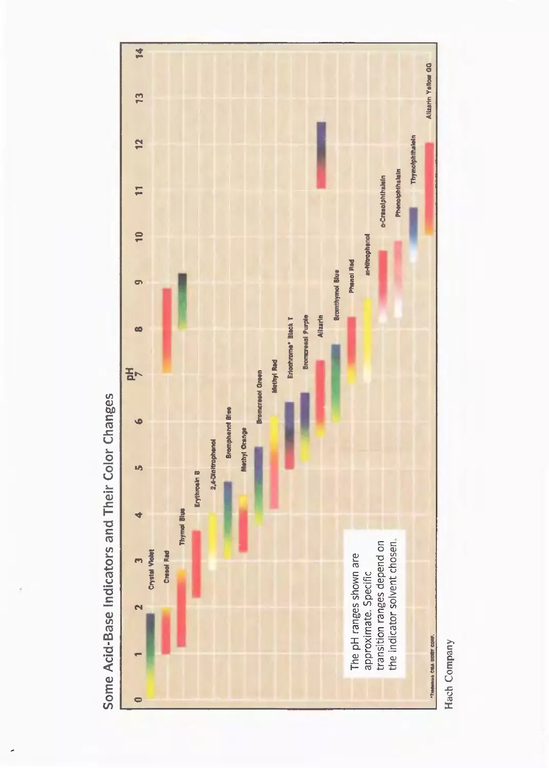
Appendixes and Endpapers. Included in the appendixes are an updated guide to
the literature of analytical chemistry, tables of chemical constants, electrode poten-
tials, and recomrnended compounds for the preparation of standard matelials;
sections on the use of logarithms and exponential notation, and on normality and
equivalents (tenns that are not used in the text itself); and a derivation of the
propagation of error equations. The inside front and back covers of this book pro-
vide a full-color chart of chemical indicators, a table of molar masses of com-
Preface xv
pounds of particular interest in analytical chemistry, a table of international atomic
masses, and a periodic table. In addition, the book has a tear-out reference card for
Microsoft@ Excel.
Changes in the Eighth Edition
Readers of the seventh edition will find that the eighth edition has numerous
changes in content as well as style and format.
Content. Several changes in content have been made to strengthen the book.
· New and exciting chapter opening introductions, accompanied by applied pho-
tos. present a relevant example of one of the chapter topics. Examples include
stalagmites and stalactites as an illustration of an equilibrium process (Chapter
9), the effects of acid rain (Chapter 16), and the oxidation/reduction properties
of chlorophyll (Chapter 19).
. Many chapters have been strengthened by adding spreadsheet examples, appli-
cations, and problems. The new Chapter 3 gives tutorials on the construction
and use of spreadsheets. Many other tutorials are included in our supplement,
Applications of MiclVsoft@ Excel in Analytical Chemistry.
. The chapters on statistics (Chapters 5-7) have been updated and brought into
conformity with the terminology of modern statistics. Analysis of Variance
(ANOVA) is included in Chapter 7. ANOVA is easy to perform with modem
spreadsheet programs and quite useful in analytical problem solving.
. A new Chapter 8 consolidates mateIial on sampling and integrates material on
calibration and standardization. Methods such as external standards, internal
standards, and standard additions are presented in this chapter, and their advan-
tages and disadvantages are discussed.
. The chapter on precipitation titrimetry has been eliminated, and some of the
material is included in Chapter 13 on titrimetric methods.
· Chapters 18. 19, 20, and 21 on electrochemical cells and cell potentials have
been extensively revised to clarify the discussion and introduce the free energy
of cell processes. Chapter 23 has been altered to decrease the emphasis on clas-
sical polarography. It now includes a discussion of cyclic voltammetry.
. Chapter 28 in this edition covers atomic mass spectrometry, including inductively
coupled plasma mass spectrometry. Flame photometry has been deemphasized.
. In Part VI. Chapter 30 is now a general introduction to separations. It includes
solvent extraction and precipitation methods, an introduction to chromatogra-
phy, and a new section on solid-phase extraction. Chapter 31 contains new
material on molecular mass spectrometry and gas chromatography/mass spec-
trometry. Chapter 32 includes new sections on affinity chromatography and
chiral chromatography. A section on LOMS has been added. A new Chapter
33, "Miscellaneous Separation Methods." has been included. It introduces cap-
illary electrophoresis and field-flow fractionation.
. Style and Format. To make the text more readable and student-friendly, we
have continued to change style and format.
. We have attempted to use shorter sentences, a more active voice, and a more
conversational writing style in each chapter.
. More descriptive figure captions are used whenever appropriate to allow a stu-
dent to understand the figure and its meaning without having to alternate
between text and caption.
. Molecular models are liberally used in most chapters to stimulate interest in the
beauty of molecular structures and to reinforce structural concepts and descrip-
tive chemistry presented in general chemistry and upper-level courses.
xvi Preface
· Photographs, taken specifically for this text, are used whenever appropriate to
illustrate important techniques. apparatus, and operations.
· Marginal notes are used throughout to emphasize recently discussed concepts
or to reinforce key infonnation.
· A running marginal glossary reinforces key terminology.
A Full Support Package for Students
. Solutions Manual. Written by Gary Kinsel, University of Texas, Arlington,
the solutions manual contains worked-out solutions for all the starred problems
in the text. For added value and convenience, the Student Solutions Manual can
be packaged with the text. Contact your Thomson . Brooks/Cole sales repre-
sentative for more information.
. Spreadsheet Applications. Applications (
f MiclVsoft@ Excel in Analytical
Chemistry, by Stanley R. Crouch and F. James Holler, treats in detail the
spreadsheet approaches summarized in the text. This supplement contains 16
chapters that lead the student from basic concepts and operations to using
spreadsheets for simulations, curve fitting, data smoothing. curve resolution.
and many other topics. Topics in this companion book are correlated with top-
ics in the text. See pages xvii and xviii for a correlation chart. Summaries in the
text point to specific chapters and sections in the companion book. For added
value and convenience, this ancillary can be packaged with the text. Contact
your Thomson. Brooks/Cole representative for details.
· Interactive Analytical Chemistry CD-ROM. Developed by William J. Vin-
ing, University of Massachusetts, Amherst, in conjunction with the text authors,
this CD-ROM is packaged free with every copy of the book. Prompted by icons
with captions in the text. students explore the corresponding Intelligent Tutors,
Guided Simulations, and Media-based Exercises. This CD-ROM includes tuto-
rials on statistics, equilibria, spectrophotometry, electroanalytical chemistry,
chromatography, atomic absorption spectroscopy, and gravimetric and combus-
tion analysis. Also included on the CD-ROM as an Adobe Acrobat@ PDF file is
Chapter 37, "Selected Methods of Analysis:' Students will be able to print only
those experiments that they will perform. and the printed sheets can be easily
used in the laboratory.
· Brooks/Cole Book Companion Web Site at http://chemistry.brookscole.coml
skoogfac/. The Web site includes a set of updated links to the Web sites men-
tioned in the Web Works, problems. and other places in this text. Instructors may
download spreadsheets developed in this book as well as those from Applications
of Microsoft@ Excel in Analytical Chemistl
': Instructors may download graphics
files containing all of the figures from the text to aid in preparing PowerPoint0
presentations. The Chapter 37 PDF file is also included on the Web site.
· InfoTrac@ College Edition. Every new copy of this book is packaged with
four months of free access to InfoTrac College Edition. This online resource
features a comprehensive database of reliable, full-length articles from thou-
sands of top academic journals and popular sources.
Additional Support for Professors
The following ancillaries are available to qualified adopters. Please consult your
Thomson. Brooks/Cole sales representative for details.
Preface xvii
· Instructor's Manual. Complete solutions to all of the problems in the text are
available on the Instructor's password-protected companion site for this text
located at http://chemistry.brookscole.com/skoogfac.
· Multimedia Manager for FUlldamentals of Analytical Chemistry, Eighth
Edition: A Microsoft@ PowerPoint@ Link Tool. The Multimedia Manager is
a digital library and presentation. dual-platform CD-ROM. Included is a library
of resources valuable to instructors, such as text art and tables. in a variety of e-
formats that are easily exported into other software packages. You can also cus-
tomize your own presentation by importing your personal lecture slides or
other material you choose.
. Overhead Transparencies. A set of 100 color overhead transparencies is
available to assist instructors in presenting student lectures.
. MyCourse 2.1. A new, free, online course builder that offers a simple solution
to creating a custom course Web site where professors can assign, track, and
report on student progress. Contact your Thomson . Brooks/Cole sales repre-
sentative for details or visit http://mycourse.thomsonlearning.com for a free
demo.
. Applicatiolls of Microsoft@ Excel in Analytical Chemistry, a clear and concise
companion to Fundamentals of Analytical Chemistl)', eighth edition, and Ana-
("tical Chemistl)
All Illtroduction, seventh edition, provides students and pro-
fessors with a valuable resource of the rnost useful spreadsheet methods.
. Correlation of Spreadsheet Supplement to Texts. The following chart lists
cross-references to Fundamentals of Analytical Chemistl}
Eighth Edition, and
Analytical Chemistry: An Introduction, Seventh Edition.
Applicatiol/s of Microsoft@ Excel
iI/ AI/alytical Chemistry
Chapter] Excel Basics
FUI/damel/tals of AI/alytical Chemistry,
Eighth edition
Chapter 3 Using Spreadsheets in
AI/alytical Chemistry, AI/II/troductiol/,
Se\'enth edition
Section 2J Using Spreadsheets in
Analytical Chemistry Analytical Chemistry
Chapter 2 Basic Statistical Chapters 5, 6 Basic Statistics Chapters 5, 6 Basic Statistics
Analysis with Excel
Chapter 3 Statistical Tests with Chapter 7 Statistical Data Treatment Chapter 7 Statistical Analysis
Excel
Chapter 4 Least Squares and Section 8C Standardization and Section 7D The Least Squares Method
Calibration Methods Calibration
Chapter 5 Equilibrium Activity Section 9B Chemical Equilibrium Section 4B Chemical Equilibrium
and Solving Equations
Chapter IO Electrolyte Effects Chapter 9 Electrolyte Effects
Chapter 6 The Systematic Chapter II Complex Equilibrium Chapter 10 Complex Equilibrium
Approach to Equilibria: Calculations Calculations
Solving: Many Equations
Chapter 7 Titrations and Chapter] 3 Titrimetric Methods and Chapter 11 Titrations
Graphical Representations Precipitation Titrations
Chapter 12 Precipitation Titrations
Chapter 14 Neutralization Titrations
Section 15B-2 Neutralization Titrations
Chapter-8 Polyfunctional Acids Chapter 15 Polyfunctional Acids Chapter 13 Polyfunctional Acids
and Bases and Bases and Bases
(continues)
xviii Preface
Applications of Microsoft@ Excel Fundamentals of Analytical Chemistry, Analytical Chemistry, An Introduction,
in Analytical Chemistry Eighth edition Seventh edition
Chapter 9 Complexometric Chapter 17 Complexation Reactions Chapter 15 Complexation Titrations
Titrations and Titrations
Chapter IO Potentiometry and Chapter 18 Introduction to Chapter 16 Elements of Electrochemistry
Redox Titrations Electrochemistry
Chapter 19 Standard Electrode Potentials
Chaptcr 17 Using Electrode Potentials
Chapter 20 Oxidation/ReductionTitrations
Chapter ] 8 OxidationlReduction Titfations
Chapter 2] Potentiometry
Chapter 19 Potentiometry
Chapter II Dynamic Chapter 22 Electrogravimetry and Chapter 20 Other Electro-analytical
Electrochemistry Coulometry Methods
Chapter 23 Voltammetry
Chapter 12 Spectroscopic Chapter 24 Introduction to Chapter 21 Spectroscopic Methods of
Methods Spectrochemical Methods Analysis
Chapter 25 Optical Instrumentation Chapter 22 Instruments for Measuring
Absorption
Chapter 26 Molecular Absorption
Spectroscopy
Chapter 23 Spectroscopic Methods
Chapter 27 Molecular Fluorescence
Spectroscopy
Chapter 13 Kinetic Methods Chapter 29 Kinetic Methods of Section 23A-2 Quantitative UV/Visible
Analysis Spectrophotometry
Chapter 14 Chromatography Chapter 30 Introduction to Analytical Chapter 24 Introduction to Analytical
Separations Separations
Section 3 I C- 2 Quantitative GC Section 25A-7 GC Applications
Chapter 15 Electrophoresis Section 30E-7 Column Resolution Section 24F-9 Column Resolution
and Other Separation Methods
Section 32H Comparison of HPLC Chapters 26 SFC, CE and other
and GC Separation Methods
Chapter 33 Miscellaneous Separation
Methods
Chapter 16 Data Processing Chapter 7 Statistical Data Treatment Chapter 7 Statistical Analysis
with Excel
Acknowledgments
We wish to acknowledge with thanks the comments and suggestions of many
reviewers who critiqued the seventh edition prior to our writing or who evaluated
the CUlTenr manuscript in various stages.
Joseph Aldstadt.
University of Wise OilS in. Milwaukee
Stephen Brown,
University of Delmvare
James Burlitch,
Cornell University
Michael DeGrandpre,
University of Montana
Simon Garrett,
Michigan State University
Carol Lasko,
Humboldt State University
Tingyu Li,
Vanderbilt University
Joseph Maloy,
Seton Hall University
Howard Lee McLean,
Rose-Hulman Institute of Technology
Frederick Northrup,
Northwestem University
Peter Palmer,
San Francisco State University
Reginald Penner,
University of Cal!fomia, Irvine
Jeanette Rice,
Georgia Southem University
Alexander Scheeline,
Universi
).' of Illinois, U rbana-
Champaign
Preface xix
James Schenk,
Washington State University
Maria Schroeder.
United States Naval Academv
Manuel Soriaga,
Texas A&M University
Keith Stevenson,
University ofTexlis
Larry Taylor,
Virginia Technical Institute
Robert Thompson,
Oberlin College
Richard Vachet,
University of Massachusetts
Joseph Wang,
New Mexico State University
We especially acknowledge the assistance of Professor David Zellmer, California
State University, Fresno, who reviewed several chapters and served as the accuracy
reviewer for the entire manuscript. In addition, we appreciate the comments and
suggestions of Professor Gary Kinsel of the University of Texas, Arlington, who
prepared the solutions manual, and Professor Scott Van Bramer, of Widener Uni-
versity, who checked all the solutions to the problems. We are grateful to Professor
Bill Vining of the University of Massachusetts. who prepared the accompanying
CD-ROM, and we are fortunate to have worked with Charles D. Winters, who con-
tributed many of the new photo
in the text and in the color plates.
Our writing team enjoys the services of a superb technical reference librarian,
Ms. Maggie Johnson. She assisted us in many ways in the production of this book,
including checking references, performing literature searches, and providing back-
ground information for many of the Features. We appreciate her competence,
enthusiasm, and good humor.
We are grateful to the many staff rnembers of Brooks/Cole/Thomson Learning
who provided excellent support dUling the production of this text. Senior Develop-
mental Editor Sandi Kiselica has done a superb job of organizing this project.
maintaining continuity. and making many important comments and suggestions.
Bonnie Boehme of Nesbitt Graphics is simply the best copy editor that we have
ever had. Her keen eye and consummate editorial skills have contributed greatly to
the quality of the text. Alyssa White has done an excellent job coordinating the
ancillmy materials, and Jane Sanders, our photo researcher, has shown style and
good humor in handling the various tasks associated with acquiring the many new
photos in the book.
Douglas A. Skoog
Donald M. West
F. James Holler
Stanley R. Crouch
Fundamentals of
Analytical
Chemistry
Eighth Edition
The Nature of Analytical
Chemistry
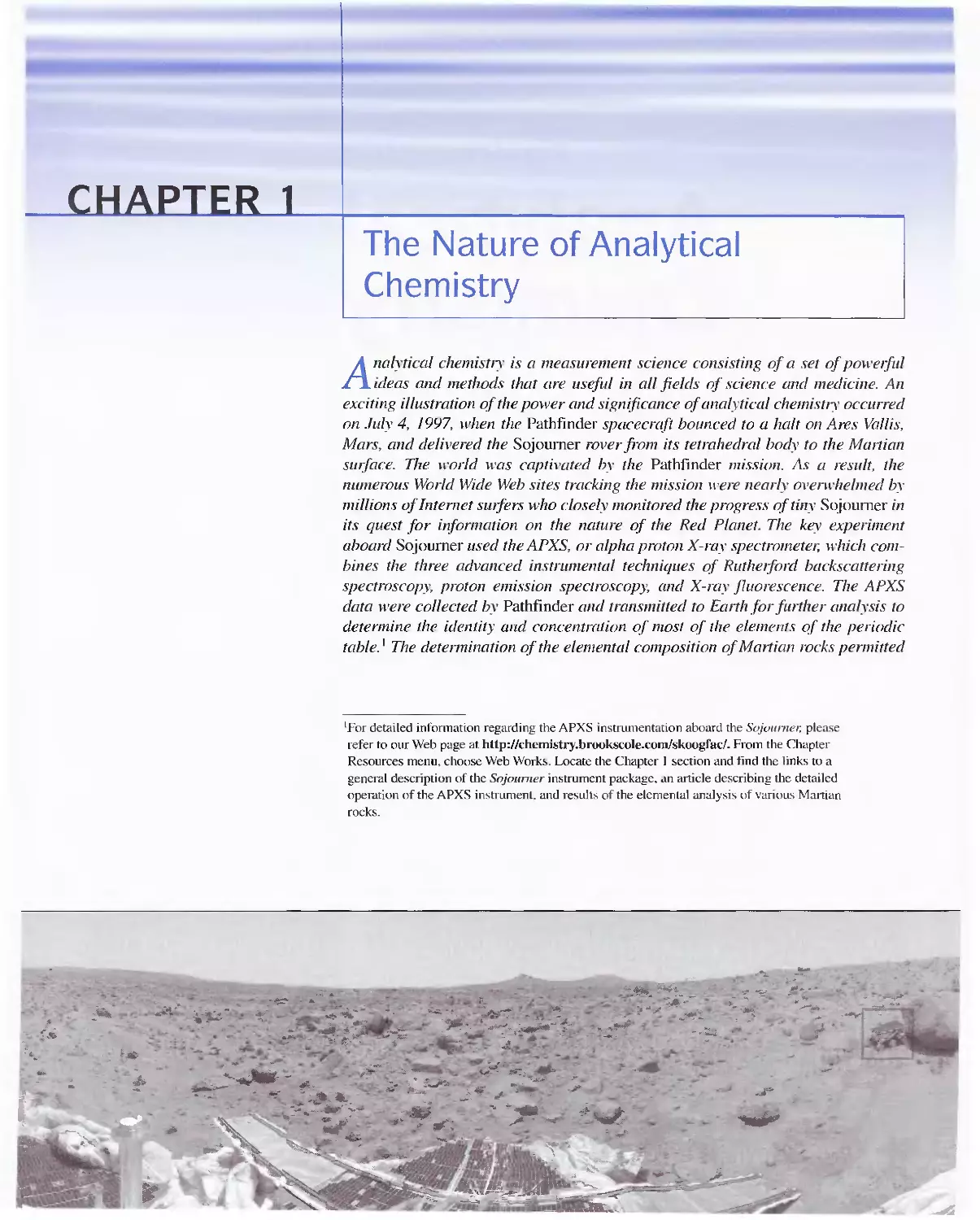
A nalytical chemistry is a measurement science consisting of a set of powelful
ideas and methods that are useful in all fields of science and medicine. An
exciting illustration qf the power and significance of analytical chemistry occurred
on July 4, 1997, when the Pathfinder spacec/"(
ft bounced to a halt on An?s Vallis,
Mars, and delivered the Sojourner rover from its tetrahedral body to the M1lI1ian
slllface. The world was captimted by the Pathfinder mission. As a result, the
numerous World Wide Web sites tracking the mission were nearly ovendlelmed by
millions (
f Inte17let swfers who closely monitored the progress of tiny Sojourner in
its quest for iJ1fonllation on the nature of the Red Planet. The key experiment
ahoard Sojourner llsed the APXS, or alpha proton X-ray spectrometel; which com-
bines the three advanced instrumental techniques qf Ruthelford backscattering
spectroscoP)
proton emission spectroscopy, and X-ray fluorescence. The APXS
data were collected by Pathfinder and transmitted to Earth for further analysis to
determine the identity and concentration qf most qf the elements of the periodic
table. I The deten17ination of the elemental composition of Martian rocks permitted
'For detailed information regarding the APXS instrumentation aboard the Sl
;()umel; please
refer to our Web page at http://chemistry.brookscole.comlskoogfacf. From the Chapter
Resources menu, choose Web Worh. Locate the Chapter I section and find the links to a
general description of the Sojollmer instrument package. an article describing the detailed
operation of the APXS instrument. and results of the elemental analysis of various Martian
rocks.
"
{,'Ii.
:
.
:_;;'f)f'
....
-
:f.1;;. "
""'__
,.../
-".
.. ..:
....
....
o;."'
!". ..
.
..-.....
--.....
:
:
..
..
...",:..
'.11-.-...-
.
r
--
- .<00-'--
.,.. -
"Zii
..
-
.
>
-
-..-
. .
-r
"
. '..-
c....
"
(
....
- ....
-
_
-h
- -= ";..
-
:..-
-- , ..-
"-
._ -c;.;;;
,
...... --=
...1\......
-
,;
/" / "
.: :Jij -,,".
"" ..,
'-
-:'';O:.J.:
tif. -"..-
-0...
"'- - ....,.
.;
..A"'"
.:.
-it>
.
"..
......,
"
;;,. t,
-
..
'\ '.
- "-
t"
"""l
;' ;
)#
-. "',
----
1 A The Role of Analytical Chemistry :3
geologisTS TO rapidly ident(fy them and compare them with terresTrial rocks. The
Pathfinder mission is a spectacular example illustrating the application of analyti-
cal chemistry to practical problems. The experiments aboard the spacecrqft and
the data jivm the mission also illustrate how analytical chemistry dra'ws on sci-
ence and technology in such widely dil'erse disciplines as nuclear physics and
chemistl:\" to identify and determine the relatil'e amounts of substances in samples
of matte/:
The Pathfinder example demonstrates that both qualitative information and
quantitative information are required in an analysis. Qualitative analysis estab-
lishes the chemical identiTY of the species in The sample. Quantitative analysis
determines the relative amounts of these species, or analytes, in numerical terms.
The data fivm the APXS spectrometer on Sojourner contain both t.'1Jes of il forma-
tion. Note that chemical separation of the I'Grious elements contained in the rocks
was unnecessary in the APXS experiment. More cOll111lOnly, a separation step is a
necessm)" part qf the analytical pmcess. As we shall see, qualitatil'e analysis is
ojien an integral part of the separation step, and dete1711ining the identity ( f the
anLllytes is an essential adjunct to quantitative analysis. In this text. we shall
explore quantitatil'e methods of analysis, separation methods, and the principles
behind their operation.
[]A] THE ROLE OF ANALYTICAL CHEMISTRY
Analytical chemistry is applied throughout industry, medicine. and all the sci-
ences. Consider a few examples. The concentrations of oxygen and of carbon
dioxide are detelmined in millions of blood samples every day and used to diag-
nose and treat illnesses. Quantities of hydrocarbons. nitrogen oxides. and carbon
monoxide present in automobile exhaust gases are measured to assess the effec-
tiveness of smog-control devices. Quantitative measurements of ionized calcium
in blood serum help diagnose parathyroid disease in humans. Quantitative deter-
mination of nitrogen in foods establishes their protein content and thus their
nutritional value. Analysis of steel during its production pennits adjustment in the
concentrations of such elements as carbon. nickel. and chromium to achieve a
desired strength, hardness, corrosion resistance, and ductility. The mercaptan
content of household gas supplies is monitored continually to ensure that the gas
.::-
, .
..,.
.'-
.......
. "-
-w- ,.
...
. "".L-'
.... 4
i'
.
-
-.... -"-".,;
f........ ......
-,,;:- ...-,
or'
"t
.- h..
...."'tIIt
......
.......
...
(.
" '.
,, ,.
'.
'-1 .
""!' I)
lIB J:lt t
1
U
-
,,-
...
'"
-
,
'-
"
->d
, -
Qualitative analysis reveals the
identity of the elements and
compounds in a sample.
Quantitative analysis indicates the
amount of each substance in a
sample.
Analytes are the components of a
sample that are to be determined.
Mars landscape. Courtesy of NASA
'V
-
'Ii
4
CHAPTER 1
The Nature of Analytical Chemistry
has a sufficiently noxious odor to warn of dangerous leaks. Farmers tailor fe11iliza-
tion and irrigation schedules to meet changing plant needs during the growing sea-
son, gauging these needs from quantitative analyses of the plants and the soil in
which they grow.
Quantitative analytical measurements also playa vital role in many research
areas in chemistry, biochemistry, biology, geology, physics, and the other sciences.
For example, quantitative measurements of potassium. calcium, and sodium ions in
the body fluids of animals permit physiologists to study the role of these ions in
nerve signal conduction as well as muscle contraction and relaxation. Chemists
unravel the mechanisms of chemical reactions through reaction rate studies. The
rate of consumption of reactants or forrnation of products in a chemical reaction
can be calculated from quantitative measurements made at equal time intervals.
Materials scientists rely heavily on quantitative analyses of crystalline germanium
and silicon in their studies of semiconductor devices. Impurities in these devices
are in the concentration range of I X 10- 6 to I X 10- 9 percent. Archaeologists
identify the source of volcanic glasses (obsidian) by measuring concentrations of
minor elements in samples taken from valious locations. This knowledge in turn
makes it possible to trace prehistoric trade routes for tools and weapons fashioned
from obsidian.
Many chemists, biochemists, and medicinal chemists devote much time in the
laboratory gathering quantitative information about systems that are important and
interesting to them. The central role of analytical chemistry in this enterprise and
many others is illustrated in Figure I-I. All branches of chemistry draw on the
ideas and techniques of analytical chemistry. Analytical chemistry has a similar
function with respect to the many other scientific fields listed in the diagram.
Chemistry is often called the central science; its top center position and the central
position of analytical chemistry in the figure emphasize this importance. The inter-
disciplinary nature of chemical analysis makes it a vital tool in medical. industrial.
government. and academic laboratories throughout the world.
o::ID QUANTITATIVE ANALYTICAL METHODS
We compute the results of a typical quantitative analysis from two measurements.
One is the rnass or the volurne of sample being analyzed. The second is the meas-
urement of some quantity that is proportional to the amount of analyte in the sam-
ple. such as mass. volume, intensity of light, or electrical charge. This second
measurement usually completes the analysis, and we classify analytical methods
according to the nature of this final measurement. Gravimetric methods deter-
mine the mass of the analyte or some compound chemically related to it. In a volu-
metric method, the volume of a solution containing sufficient reagent to react
completely with the analyte is measured. Electroanalytical methods involve the
measurement of such electrical prope11ies as potential, current. resistance, and
quantity of electrical charge. Spectroscopic methods are based on measurement
of the interaction between electromagnetic radiation and analyte atoms or mole-
cules or on the production of stich radiation by analytes. Finally, a group of mis-
cellaneous methods includes the measurement of such quantities as mass-to-
charge ratio of molecules by mass spectrometry, rate of radioactive decay, heat of
Geology
Geophysics
Geochemistry
Paleontology
Paleobiology
1 C A Typical Quantitative Analysis 5
\
Figure 1-1 The relationship between analytical chemistry, other branches of chemistry, and the other
sciences. The central location of analytical chemistry in the diagram signifies its importance and the
breadth of its interactions with many other disciplines.
reaction. rate of reaction, sample thermal conductivity, optical activity, and refrac-
tive index.
c:KJ A TYPICAL QUANTITATIVE ANALYSIS
A typical quantitative analysis involves the sequence of steps shown in the flow
diagram of Figure 1-2. In some instances, one or more of these steps can be omit-
ted. For example, if the sample is already a liquid, we can avoid the dissolution
step. The first 29 chapters of this book focus on the last three steps in Figure 1-2. In
6
CHAPTER 1
The Nature of Analytical Chemistry
Select
method
Acquire
sample
Process
sample
No
-
CatTY out
chemical dissolution
Yes
Change chemical
form
No
-
L
Yes
Eliminate
interferences
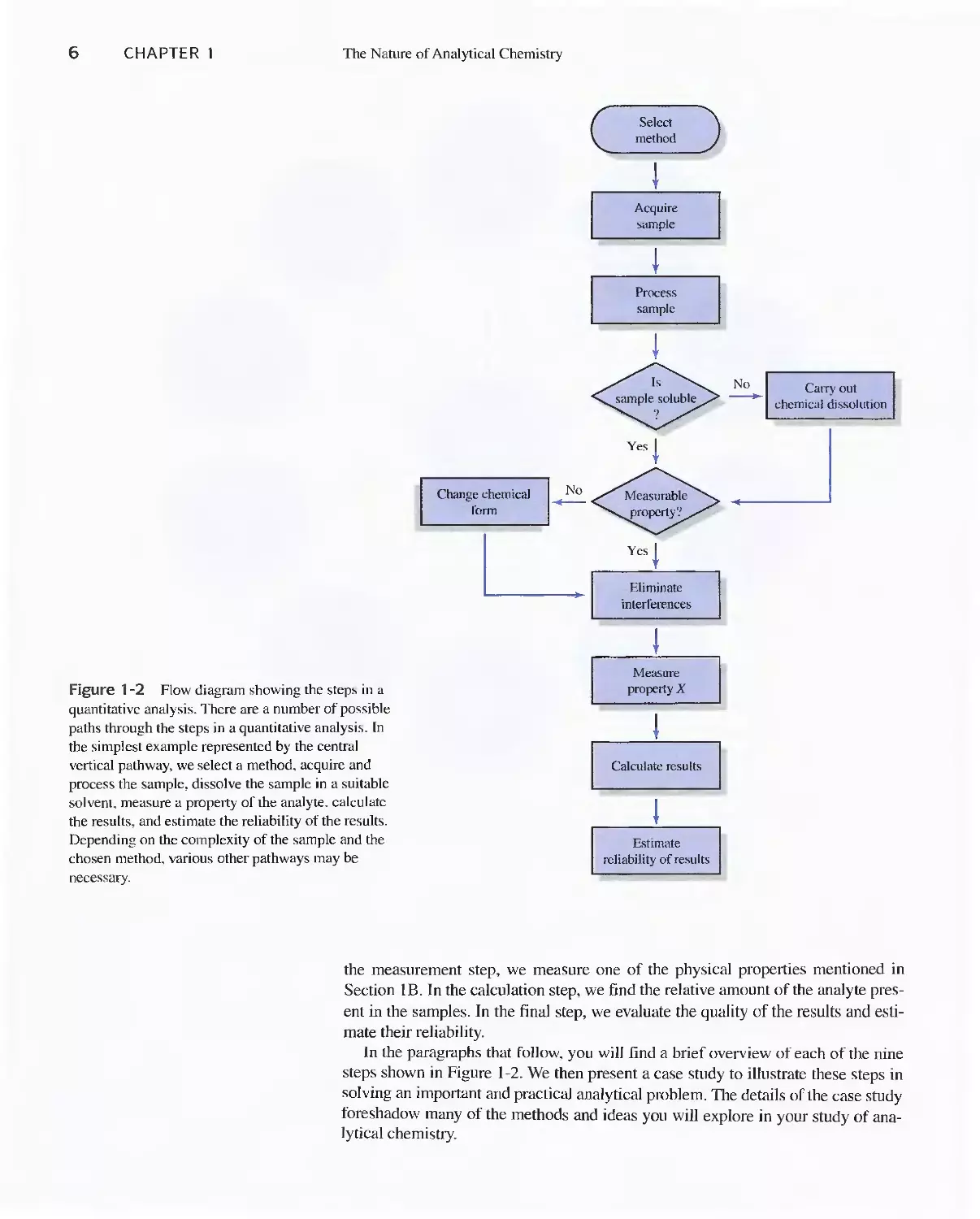
Figure 1-2 Flow diagram showing the steps in a
quantitative analysis. There are a number of possible
paths through the steps in a quantitative analysb. In
the simplest example represented by the central
vertical pathway, we select a method. acquire and
process the sample, dissolve the sample in a suitable
solvent. measure a property of the analyte. calculate
the results, and estimate the reliability of the results.
Depending on the complexity of the sample and the
chosen method, various other pathways may be
necessary.
Measure
property X
Calculate results
Estlmate
reliability of results
the measurement step, we measure one of the physical propelties mentioned in
Section I B. In the calculation step, we find the relative amount of the analyte pres-
ent in the samples. In the finaJ step, we evaJuate the quality of the resuJts and esti-
mate their reliability.
In the paragraphs that follow. you will find a brief overview of each of the nine
steps shown in Figure 1-2. We then present a case study to illustrate these steps in
solving an important and practical analytical probJem. The detaiJs of the case study
foreshadow many of the methods and ideas you wiJI explore in your study of ana-
lytical chemistry.
1 C A Typical Quantitative Analysis 7
I , I T I - J f[' . ,7 ,
'I I'
i! I ( $ '-. 1f'
' I f 't" r;- \wrJJr',
n ,- ili- f. lit-
,
J) I..ttlti's 'J7]i t \
LJ \ \--
Z- ?' . @
"IOPA'1 £vffi'iO!\t 1-\f\;S To KNoW '\N\-\kt's 1,0 It-\ f="OOP /oHM}"
IN I w,A-rGA r, 'Wt-!.k1's IN -r AIR?' 1i-\ir \5 tRULy I 'C,-oLJ)(;.rf
AGf:.. OF AtJAL1nc.AL. C.j-\£N\\51Ri. ..
g
"[
"
=
co
:I:
>
U3
>
'"
'"
1 C-1 Choosing a Method
The essential first step in any quantitative analysis is the selection of a method, as
depicted in Figure 1-2. The choice is sometimes difficult and requires experience as
well as intuition. One of the first questions to be considered in the selection process
is the level of accuracy required. Unf0l1unately, high reliability nearly always
requires a large investment of time. The selected method usually represents a corn-
promise between the accuracy required and the time and money available for the
analysis_
A second consideration related to economic factors is the number of samples
that will be analyzed. If there are many sarnples. we can afford to spend a signifi-
cant amount of time in preliminary operations such as assembling and calibrating
instruments and equipment and preparing standard solutions. If we have only a sin-
gle sample, or just a few samples. it may be more appropriate to select a procedure
that avoids or minimizes such preliminary steps.
Finally. the complexity of the sample and the number of components in the sam-
ple always influence the choice of method to some degree.
1 C-2 Acquiring the Sample
As illustrated in Figure 1-2. the next step in a quantitative analysis is to acquire the
sample. To produce meaningful information, an analysis must be performed on a
sample that has the same composition as the bulk of material from which it was
taken. When the bulk is large and heterogeneous, great effort is required to get a
representative sarnple. Consider, for exarnple, a railroad car containing 25 tons of
silver ore, The buyer and seller of the ore must agree on a price, which will be
ba ed primarily on the silver content of the shipment. The ore itself is inherently
heterogeneous, consisting of many lumps that vary in size as well as silver content.
A material is heterogeneous if its
constituent parts can be distin-
guished visually or with the aid of a
microscope. Coal. animal tissue, and
soil are heterogeneous materials.
8
CHAPTER 1
An assay is the process of determin-
ing how much of a given sample is
the material indicated by its name.
For example, a zinc alloy is assayed
for its zinc content, and its assay is a
particular numerical value.
We analy::.e samples and we deter-
mine substances. For example. a blood
sample is analyzed to determine the
concentrations of various substances
such as blood gases and glucose. We
therefore speak of the determination of
blood gases or glucose, IlOt the analysis
of blood gases or glucose.
The Nature of Analytical Chemistry
The assay of this shipment will be performed on a sample that weighs about one
gram. For the analysis to have significance, this small sample must have a compo-
sition that is representative of the 25 tons (or approximately 22,700,000 g) of ore in
the shipment. Isolation of one gram of material that accurately represents the
average composition of the nearly 23,000,000 g of bulk sample is a difficult under-
taking that requires a careful, systematic manipulation of the entire shipment. Sam-
pling is the process of collecting a small ma s of a material whose composition
accurately represents the bulk of the material being sampled. We explore the details
of sampling in Chapter 8.
The collection of specimens from biological sources represents a second type of
sampling problem. Sampling of human blood for the determination of blood gases
illustrates the difficulty of acquiring a representative sample from a complex
biological system. The concentration of oxygen and carbon dioxide in blood
depends on a variety of physiological and environmental variables. For exam-
ple. inappropriate application of a tourniquet or hand flexing by the patient may
cause blood oxygen concentration to fluctuate. Because physicians make life-
and-death decisions based on results of blood gas determinations, strict procedures
have been developed for sampling and transporting specimens to the clinicallabo-
ratory. These procedures ensure that the sample is representative of the patient
at the tirne it is collected and that its integrity is preserved until the sample can be
analyzed.
Many sampling problems are easier to solve than the two just described.
Whether sampling is simple or complex, however, the analyst must be sure that the
laboratory sample is representative of the whole before proceeding with an analy-
sis. Sampling is frequently the most difficult step and the source of greatest error.
The reliability of the final results of analysis will never be any greater than the reli-
ability of the sampling step.
1 (-3 Processing the Sample
The third step in an analysis is to process the sample. as shown in Figure 1-2.
Under certain circumstances, no sarnple processing is required prior to the meas-
urement step. For example, once a water sample is withdrawn from a stream, a
lake, or an ocean, its pH can be measured directly. Under most circumstances. we
must process the sample in any of a variety of different ways. The first step is often
the preparation of a laboratory sample.
Preparing Laboratory Samples
A solid laboratory sample is ground to decrease particle size, mixed to ensure
homogeneity, and stored for various lengths of time before analysis begins.
Absorption or desorption of water may occur during each step, depending on the
humidity of the environment. Because any loss or gain of water changes the chem-
ical composition of solids, it is a good idea to dry samples just before statting an
analysis. Alternatively. the moisture content of the sample can be determined at the
time of the analysis in a separate analytical procedure.
Liquid samples present a slightly different but related set of problems during the
preparation step. If such samples are allowed to stand in open containers, the sol-
vent may evaporate and change the concentration of the analyte. If the analyte is a
gas dissolved in a liquid, as in our blood gas example, the sample container must be
1 C A Typical Ouantitative Analysis 9
kept inside a second sealed container, perhaps during the entire analytical proce-
dure, to prevent contamination by atmospheric gases. Extraordinary measures,
including sample manipulation and measurement in an inert atmosphere, may be
required to preserve the integrity of the sample.
Defining Replicate Samples
Most chemical analyses are performed on replicate samples whose masses or vol-
urnes have been deterrnined by careful measurements with an analytical balance or
with a precise volumetric device. Replication improves the quality of the results
and provides a measure of reliability. Quantitative measurements on replicates are
usually averaged. and various statistical tests are performed on the results to estab-
lish reliability.
Preparing Solutions: Physical and Chemical Changes
Most analyses are perfOlmed on solutions of the sample made with a suitable sol-
vent. Ideally, the solvent should dissolve the entire sample, including the analyte.
rapidly and completely. The conditions of dissolution should be sufficiently mild
so that loss of the analyte cannot occur. In our flow diagram of Figure 1-2, we ask
whether the sample is soluble in the solvent of choice. Unfortunately, many materi-
als that rnust be analyzed are insoluble in common solvents. Examples include sil-
icate minerals. high-molecular-weight polymers, and specimens of animal tissue.
Under this circumstance, we must follow the flow diagram to the box on the right
and carry out some rather harsh chemistry. Conversion of the analyte in such mate-
rials into a soluble form is often the most difficult and time-consuming task in the
analytical process. The sample may require heating with aqueous solutions of
strong acids, strong bases, oxidizing agents. reducing agents, or some combination
of such reagents. It may he necessary to ignite the sample in air or oxygen or to per-
form a high-temperature fusion of the sarnple in the presence of various fluxes.
Once the analyte is made soluble, we then ask whether the sample has a property
that is proportional to analyte concentration and that we can measure. If it does not,
other chemical steps may be necessary to convert the analyte to a form suitable for
the measurement step, as we see in Figure 1-2. For example, in the determination
of manganese in steel, manganese must be oxidized to Mn04 before the
absorbance of the colored solution is measured (see Chapter 26). At this point in
the analysis, it rnay be possible to proceed directly to the measurement step, but
more often than not. we must eliminate interferences in the sample before making
measurements. as illustrateJ in the flow diagram.
1 (-4 Eliminating Interferences
Once we have the sample in solution and have converted the analyte to an appro-
priate form for measurement, the next step is to eliminate substances from the
sample that may interfere with measurement (see Figure 1-2). Few chemical or
physical properties of importance in chemical analysis are unique to a single chem-
ical species. Instead, the reactions used and the properties measured are character-
istic of a group of elements of compounds. Species other than the analyte that
affect the final measurement are called interferences, or interferents. A scheme
must be devised to isolate the analytes from interferences before the final measure-
ment is made. No hard and fa,>t rules can be given for eliminating interferences;
Replicate samples, or replicates,
are portions of a material of
approximately the same size that
are carried through an analytical
procedure at the same time and in
the same way.
An interference or interferent is a
species that causes an error in an
analysis by enhancing or attenuating
(making smaller) the quantity being
measured.
10
CHAPTER 1
Techniques or reactions that work
for only one analyte are said to be
specific. Techniques or reactions
that apply for only a few analytes
are selective.
The matrix, or sample matrix, is all
of the components in the sample
containing an analyte.
The process of determining k. an
important step in most analyses. is
termed a calibration.
An analytical result without an
estimate of reliability is of no value.
The Nature of Analytical Chemistry
indeed, resolution of this problem can be the most demanding aspect of an analysis.
Chapters 30 through 33 describe separation rnethods.
1 C-5 Calibrating and Measuring Concentration
All analytical results depend on a final measurement X of a physical or chemical
property of the analyte. as shown in Figure 1-2. This property rnust vary in a known
and reproducible way with the concentration C,1 of the analyte. Ideally. the meas-
urement of the property is directly proportional to the concentration. That is.
cA=kX
where k is a proportionality constant. With two exceptions. analytical methods
require the empirical determination of k with chemical standards for which CA is
known. 2 The process of determining k is thus an important step in most
analyses: this step is called a calibration. We exarnine calibration in sorne detail in
Chapter 8.
1 C-6 Calculating Results
Computing analyte concentrations frorn experirnental data is usually relatively
easy, particularly with modern calculators or computers. This step is depicted in the
next-to-Iast block of Figure 1-2. These cornputations are based on the raw ex peri-
rnental data collected in the measurement step, the characteristics of the rneasure-
ment instrurnents, and the stoichiometry of the analytical reaction. Samples of
these calculations appear throughout this book.
1 C-7 Evaluating Results by Estimating Their Reliability
As Figure 1-2 irnplies, analytical results are incornplete without an estimate of their
reliability. The experirnenter rnust provide sorne measure of the uncertainties asso-
ciated with cornputed results if the data are to have any value. Chapters 5, 6, and 7
present detailed methods for carrying out this important final step in the analytical
process.
AN INTEGRAL ROLE FOR CHEMICAL ANALYSIS:
CI:QJ FEEDBACK CONTROL SYSTEMS
Analytical chemistry is usually not an end in itself, but is part of a bigger picture in
which we may use analytical results to help maintain or irnprove a patient's health,
to control the amount of mercury in fish, to regulate the quality of a product, to
deterrnine the status of a synthesis, or to find out whether there is life on Mars.
Chemical analysis is the measurement element in all of these examples and in
The two exceptions are gravimetric methods. which are discu sed In Chapter 12. and
coulometric methods, which are considered in Chapter 22. In both these methods, k can be
computed from known physical constants.
1 D An Integral Role for Chemical Analysis: Feedback Control Systems 11
Start control
system
Determine
desired Slale
Change control
quantity
- I
.
Measure
actual state
Delay
-
Display
re ults
No
Ye
many other cases. Consider the role of quantitative analysis in deterrnining and
controlling glucose concentration in blood. The systern flow diagram of Figure 1-3
illustrates the process. Patients with insulin-dependent diabetes rnellitus develop
hyperglycernia. which manifests itself as a blood glucose concentration above the
normal value of 60 to 95 mg/dL We begin our example by determining that the
desired state is a blood glucose level below 95 rngldL. Many patients must monitor
their blood glucose levels by periodically subrnitting samples to a clinicallabora-
tory for analysis or by measuring the levels themselves using a handheld electronic
glucose monitor.
The first step in the monitoring process is to determine the actual state by col-
lecting a blood sample from the patient and rneasuring the blood glucose level. The
results are displayed, and then the actual state is cornpared with the desired (see
Figure 1-3). If the measured blood glucose level is above 95 mg/dL, the patient's
insulin level, which is a controllable quantity, is increased by injection or oral
administration. After a delay to allow the insulin tirne to take effect, the glucose
level is rneasured again to deterrnine if the desired state has been achieved. If the
level is below the threshold, the insulin level has been rnaintained, so no insulin is
required. After a suitable delay time. the blood glucose level is measured again, and
the cycle is repeated. In this way, the insulin level in the patienfs blood. and thus
the blood glucose level. is rnaintained at or below the critical threshold. which
keeps the metabolism of the patient under control.
The proce of continuous rneasurernent and control is often referred to as a
feedback system, and the cycle of measurernent, comparison, and control is called
a feedback loop. These ideas find wide application in biological and biornedical
systems. rnechanical systerns. and electronics. Frorn measuring and controlling the
concentration of manganese in steel to maintaining the proper level of chlorine in a
swimming pool, chemical analysis plays a central role in a broad range of systerns.
Figure 1-3 Feedback. system
tlow diagram. The desired state is
determined. the actual state of the
system is measured. and the two states
are compared. The difference between
the two states is used to change a
controllable quantity that results in a
change in the state of the system.
Quantitative measurements are again
performed on the system, and the
comparison is repeated. The new
difference between the desired state and
thc actual state is again used to change
thc state of lhc system if necessary.
The process provides continuous
monitoring and feedback to maintain
the controllable quantity, and thus the
actual state. at the proper level. The text
describes the monit01;ng and control of
blood glucose concentration as an
example of a feedback control system.
12
CHAPTER 1
The I\ature of Analytical Chemistry
FEATURE 1-1
Deer Kill: A Case Study Illustrating the Use of Analytical Chemistry to Solve
a Problem in Toxicology
The tools of rnodern analytical chemistry are widely
applied in environmental investigations. In this feature, we
describe a case study in which quantitative analysis was
used to determine the agent that caused deaths in a popu-
lation of white-tailed deer inhabiting a wildlife preserve
of a national recreational area in Kentucky. We begin with
a description of the problem and then show how the steps
illustrated in Figure 1-2 were used to solve the analytical
problem. This case study also shows how chemical analy-
sis is used in a broad context as an integral part of a feed-
back control system, as depicted in Figure 1-3.
The Problem
The incident began when a park ranger found a dead
white-tailed deer near a pond in the land between the
Lakes National Recreation Area in western Kentucky. The
park ranger enlisted the help of a chernist from the state
veterinary diagnostic laboratory to find the cause of death
so that further deer kills might be prevented.
The ranger and the chemist investigated the site where
the badly decomposed carcass of the deer had been found.
Because of the advanced state of decornposition, no fresh
organ tissue samples could be gathered. A few days after
the Oliginal inquiry, the ranger found two more dead deer
near the same location. The chernist was summoned to the
site of the kill. where he and the ranger loaded the deer onto
a truck for transport to the veterinary diagnostic laboratory.
The investigators then conducted a careful examination of
the surrounding area to find clues to the cause of death.
w
,
.
.
,-
"
.
f
White-tailed deer have proliferated in many parts of the country.
The search covered about 2 acres surrounding the pond.
The investigators noticed that grass surrounding nearby
power line poles was wilted and discolored. They specu-
lated that a herbicide might have been used on the grass.
A comrnon ingredient in herbicides is arsenic in anyone
of a variety of forms, including arsenic trioxide, sodium
arsenite. monosodium methanearsenate, and disodium
methanearsenate. The last compound is the disodium salt
of methanearsenic acid, CH 3 AsO(OHh, which is very
soluble in water and thus finds use as the active ingredient
in many herbicides. The herbicidal activity of disodiurn
rnethanearsenate is due to its reactivity with the sulfhydryl
(S-H) groups in the amino acid cysteine. When cysteine
in plant enzymes reacts with arsenical cornpounds, the
enzyme function is inhibited and the plant eventually dies.
Unfortunately, similar chemical effects occur in animals
as well. The investigators therefore cullected samples of
the discolored dead grass for testing along with samples
from the organs of the deer. They planned to analyze the
sarnples to confirrn the presence of arsenic and, if present,
to determine its concentration in the samples.
Selecting a Method
A scherne for the quantitative determination of arsenic in
biological samples is found in the published rnethods of
the Association of Official Analytical Chernists (AOAC).3
This method involves the distillation of arsenic as arsine,
which is then determined by colorirnetric measurements.
Processing the Sample: Obtaining
Representative Samples
Back at the laboratory, the deer were dissected and the
kidneys were removed for analysis. The kidneys were
chosen because the suspected pathogen (arsenic) is rap-
idly eliminated from an animal through its urinary tract.
Processing the Sample: Preparing
a laboratory Sample
Each kidney was cut into pieces and homogenized in a
:c high-speed blender. This step reduced the size of the
is
tissue pieces and homogenized the resulting laboratory
sample.
J
c
@
30fjicial Methods of Analysis, 15th ed., p. 626. Washington,
DC: Association of Official Analytical Chemists. 1990.
1 D An Integral Role for Chemical Analysis: Feedback Control Systems 13
Processing the Sample: Defining Replicate Samples
Three lO-g samples of the homogenized tissue from each
deer were placed in porcelain crucibles.
Doing Chemistry: Dissolving the Samples
To obtain an aqueous solution of the analyte for analysis.
it was necessary to dry ash the sample in air to convert its
organic matrix to carbon dioxide and water. This process
involved heating each crucible and sample cautiously over
an open flame until the sample stopped smoking. The cru-
cible was then placed in a furnace and heated at 555°C for
2 hours. Dry ashing served to free the analyte frorn
organic material and convert it to arsenic pentoxide. The
dry solid in each sample crucible was then dissolved in
dilute HCI, which converted the AS 2 0 5 to soluble H 3 As0 4 .
Eliminating Interferences
Arsenic can be separated from other substances that might
interfere in the analysis by converting it to arsine, AsH 3 , a
toxic, colorless gas that is evolved when a solution of
H 3 As0 3 is treated with zinc. The solutions resulting from
the deer and grass samples were combined with Sn 2 +, and
a small amount of iodide ion was added to catalyze the
reduction of H 3 As0 4 to H 3 As0 3 according to the follow-
ing reaction:
H3As04 + SnCI 2 + 2HCI H 3 As0 3 + SnCI 4 + H 2 0
Reaction mixture
containing arsenic
111roUghout this text, we will present models of molecules
that are important in analytical chemistry. Here we show
arsine. AsH 3 . Arsine is an extremely toxic. colorless gas
with a noxious garlic odor. Analytical methods involving
the generation of arsine must be canied out with caution
and proper ventilation.
The H 3 As0 3 was then converted to AsH3 by the addition
of zinc metal as follows:
H 3 As0 3 + 3Zn + 6HCI AsH3(g) + 3ZnCl 2 + 3H 2 0
The entire reaction was carried out in flasks equipped
with a stopper and delivery tube so that the arsine could be
collected in the absorber solution. as shown in Figure
IF-I. The an"angernent ensured that intelferences were
left in the reaction flask and that only arsine was collected
in the absorber in special transparent containers called
cuvettes.
Arsine gas
.
\'I
o
o 0
o 0
.0 0
b G
00<0"
0 09
, -----
Absorbent
solution
Cuvette
Figure 1 F-1 An easily constructed apparatus for generating
arsine, AsH].
14
CHAPTER I
The Nature of Analytical Chemistry
... ,
.
Molecular model of diethyldithiocarbamate. This
compound is an analytical reagent used in
determining arsenic, as illustrated in this feature.
Arsine bubbled into the solution in the cuvette, react-
ing with silver diethyldithiocarbamate to fonn a col-
ored cornplex compound according to the following
equation:
[ C'H' S J -
- -" ./
AsH.. + 6Ag+ + 3 N-C ,
C,H/ '\,S
,
calibration curve, shown in the lower part of Figure IF-2.
Each vertical line between the upper and lower parts of
Figure I F-2 ties a solution to its corresponding point on
the plot. The color intensity of each solution is repre-
sented by its absorbance, which is plotted on the vertical
axis of the calibration curve. Note that the absorbance
increases from 0 to about 0.72 as the concentration of
ar<;enic increases from 0 to 25 ppm. The concentration of
arsenic in each standard solution corresponds to the verti-
cal grid lines of the calibration curve. This curve is then
used to determine the concentration of the two unknown
solutions shown on the right. We first find the absor-
bances of the unknowns on the absorbance axis of the
plot and then read the corresponding concentrations on
the concentration axis. The lines leading frorn the cuvettes
to the calibration curve show that the concentrations
of arsenic in the two deer were 16 ppm and 22 ppm,
respectively.
Arsenic in the kidney tissue of an anirnal is toxic at lev-
els above about 10 ppm, so it was probable that the deer
were killed by ingesting an arsenic compound. The tests
[ C,H< "S J
- "'\.. #'
As N -C + 6Ag + 3H
/ '\..
C,H j S '
- red
Measuring the Amount of the Analyte
The arnount of arsenic in each sarnple was detennined by
using an instrument called a spectrophotometer, to meas-
ure the intensity of the red color formed in the cuvettes.
As discussed in Chapter 26, a spectrophotometer provides
a number called absorbance that is directly proportional
to the color intensity, which is also proportional to the
concentration of the species responsihle for the color. To
use absorbance for analytical purposes, a calibration curve
rnust be generated by rneasuring the absorbance of several
solutions that contain known concentrations of analyte.
The upper part of Figure IF-2 shows that the color
becornes more intense as the arsenic content of the stan-
dards increases from 0 to 25 parts per rnillion (ppm).
Calculating the Concentration
The absorbances for the standard solutions contammg
known concentrations of arsenic are plotted to produce a
also showed that the samples of grass contained about 600
ppm arsenic. This very high level of arsenic suggested that
the grass had been sprayed with an arsenical herbicide.
The investigators concluded that the deer had probably
died as a result of eating the poisoned grass.
Estimating the Reliability of the Data
The data from these experiments were analyzed using the
statistical methods described in Chapters 5, 6, and 7. For
each of the standard arsenic solutions and the deer sam-
ples, the average of the three absorbance measurements
was calculated. The average absorbance for the replicates
is a rnore reliable measure of the concentration of arsenic
than a single measurement. Least-squares analysis of the
standard data (see Section 8C) was used to find the best
straight line among the points and to calculate the concen-
trations of the unknown samples along with their statisti-
cal uncertainties and confidence limits.
1 D An Integral Role for Chemical Analysis: Feedback Control Systems 1 5
Standards
Samples
I I
LI D
--------
Oppm 5 ppm 10 ppm 15 ppm 20 ppm 25 ppm deer 1 deer 2
(blank)
I I
0.8 I
0.6 u -r r I
<!) I
u
c; =1.;r
"
.D 0.4
H
0
li
-<
0.2
I I
0
0 5 10 L5 20 25
Concentration, ppm
Figure 1 F-2 ConstnJcting and using a calibration curve to determine the
concentration of arsenic. The absorbances of the solutions in the cuvettes are
measured using a spectrophotometer. The absorbance values are then plotted
against the concentrations of the solutions in the cuvettes, as illustrated in the
graph. Finally, the concentrations of the unknown solutions are read from the plot,
as shown by the dark arrows.
In this analysis, the fomlation of the highly colored
product of the reaction served both to confirm the proba-
ble presence of arsenic and to provide a reliable estirnate
of its concentration in the deer and in the grass. On the
basis of their results, the investigators recommended that
the use of arsenical herbicides be suspended in the
wildlife area to protect the deer and other animals that
might eat plants there.
This case study illustrates how chemical analysis is
used to identify and determine quantities of hazardous
chemicals in the environment. Many of the methods and
instruments of analytical chemistry are used routinely to
16
CHAPTER 1
The Nature of Analytical Chemistry
provide vital information in environmental and toxicolog-
ical studies of this type. The system flow diagram of Fig-
ure 1-3 rnay be applied to this case study. The desired
state is a concentration of arsenic below the toxic level.
Chemical analysis is used to determine the actual state, or
the concentration of arsenic in the environment. and this
value is compared with the desired concentration. The dif-
ference is then used to determine appropriate actions
(such as decreased use of arsenical pesticides) to ensure
that deer are not poisoned by excessive arnounts of arsenic
in the environment. which in this exarnple is the con-
trolled system.
InfoTrac College Edition
http://infotrac.thomsonlearn i ng .com
For additional readings. go to InfoTrac College Edition, your online research library, at
-
. ! .
..
Tools of Analytical
Chemistry
Chapter 2
Chemicals, Apparatus, and Unit
Operations of Analytical Chemistry
Chapter 3
Using Spreadsheets in
Analytical Chemistry
Chapter 4
Calculations Used in
Analytical Chemistry
Chapter 5
Errors in Chemical Analyses
Chapter 6
Random Errors in
Chemical Analysis
Chapter 7
Statistical Data Treatment
and Evaluation
Chapter 8
Sampling, Standardization,
and Calibration
Richard N. Zare
R ichard Zare's career choice was made when a chemistry professor inadver-
tently introduced him to spectroscopy. 1 Once he realized the power of the
technique-and what he could do to improve on it-he'd found his life's work.
Zare introduced laser techniques to chemical analysis and has used them to
study important chemical problems. He has also overseen the development of
new separation techniques. Zare has had several academic appointments, in-
cluding the past 20 years at Stanford University. He has been the recipient of
many honorary degrees and prizes, most notably the 1983 National Medal of
Science, to honor his work in laser-induced fluorescence, and the 1999 Welsh
Award in Chemistry, a lifetime achievement award.
Ie .'
...
" ...
=
:E
'"
>-
'"
u
0: Were you encouraged by your family to become
a chemist?
A: My father studied to be a chemist but dropped out of graduate
school when he married my mother during the Depression. We
had many chemistry books around the house but I was told that
they lead only to unhappiness and I shouldn't read them. This only
encouraged me to look at them, and I used to read them with a
flashlight under the covers of my bed. My parents did not permit
me to have a chemistry set, so I formed a close relationship with
the local pharmacist, who supplied me with chemicals that today
would not be possible. With them I assembled various pyrotech-
nics. and once set the basement on tire.
0: How were you introduced to spectroscopy?
A: At Harvard [ took a course on quantitative analysis for which
we had to do the gravimetric analysis of calcium in limestone. But
the instructor told us that we were wasting our time; any sensible
person would use atomic spectroscopy. I asked what it was and he
told me to read a small book written by Gerhard Herzberg, who
would later win a Nobel Prize for spectroscopy. I did, and that
summer at home I made my own carbon arc for taking atomic
spectra of various compounds.
0: You have worked a lot with lasers, How has this
shaped your career?
A: When I was a graduate student, lasers were just being devel-
oped and physicists were calling them a solution in search of a
problem. I had a clear idea what they might be good for. First I
used them to take the first fluorescence spectra of molecule5.
Later I pioneered the use of laser-induced fluorescence and
resonance-enhanced multi photon ionization as detection schemes
that identify the internal state distribution of reaction products. I
was among the first to use lasers to prepare reagents in specific in-
ternal states so that their reactivity could be studied as a function
of the type and amount of intemal motion. I also developed the
use of polarized excitation and detection, which provides informa-
tion on the geometry of the transition state region.
A tull1ing point in my career was when I gave a talk at an
American Chemical Society meeting. I had developed a technique
for detecting reaction products from molecules formed in crossed
molecular beams. Dr. Larry Seit7, from the Department of Agri-
culture. wandered into this session by mistake. He asked whether I
could detect aflatoxin, a poisonous metabolite found in moldy
grains. I said that I could if I could put it in the gas phase and it flu-
oresced. I did not understand that aflatoxin decomposes upon heat-
ing. We corresponded. and I became intrigued with the question.
"How could you detect anatoxin when you can't vaporize it?"
This led me to think about making chromatographic separations
using laser-induced fluorescence as a detector. It was then only a
short step to becoming interested in all types of separation tech-
niques and all the types of detectors that could be coupled to them.
ll1Us. a hybrid physical chemist and analytical chemist was born.
I regard myself as a frustrated inventor. 1 keep arguing with
myself. "Isn't there a better way to do something'?" and I try
things out. I'm very much interested in advances of instrumenta-
tion, how they change the ability to analyze chemicals, and hov.
they need to work with increasingly smaller quantities of material.
0: You believe in the value of spectroscopy. What
is it about spectroscopy that makes it so valuable?
A: I see spectroscopy as the use of absorption. emission. or scat-
tering of electromagnetic radiation by matter to study qualitatively
I Spectroscopy is the science of the interaction of matter with electromagnetic radiation. as
descrihed in Chapters 24-28.
18
or quantitatively the nature of matter
and the processes it undergoes. The
matter can be atoms, molecules,
atomic or molecular ions, or solids.
The interaction of radiation with mat-
ter can cause redirection of the radia-
tion or transitions between energy
levels of the atoms and molecules, or
both. More subtle effects involve not
only the color or wavelength of the
radiation but its change in intensity
and in the polarization of the light. It
is by spectroscopy that we are able to
see so much of the world, including that which we cannot touch,
like analyzing starlight for what it tells us about stars.
I regard myself as a
frustrated inventor. I keep
arguing with myself,
"Isn't there a better way
to do something?" and I
try things out.
the receptor triggers a biochemical
cascade that amplifies the presence of
the analyte. Amplification can also be
achieved by opening an ion channel
in the cell membrane to let a large
number of ions flow across the mem-
brane, which can then be detected
with the patch-clamp technique. TIle
sensitivity is so high that the binding
of a single ligand to the receptor
gives a detectable signaL
I
Q: The use of cavity ring-down spectroscopy has
especially intrigued you. Can you describe this
technique?
A: For a long time people have been looking at absorption by
placing a sample between the light source and the detector and
noticing the attenuation of the intensity of the light beam as a
function of wavelength. Nearly everything has an absorption fea-
ture, but absorption is not very sensitive because tile light source
fluctuates in time. The way around this problem is to put your
sample between two mirrors and send a pulse of light into this op-
tical cavity. The light will bounce back and forth between the mir-
rors, each time traversing the sample. What a detector sees is a
train of light pulses that come out of the end mirror, with each
pulse having less intensity than the last. The optical cavity is actu-
ally an energy storage device. and the rate at which it loses energy.
called its rate of ring-down. depends on the quality of the mirrors
and the absorption of the sample but not on the intensity of the
light pulse. If you put into the cavity a big or a little pulse or even
a series of irreproducible pulses, they all ring down at the same
rate. Thus, by measuring the ling-down rate, we are able to make
absorption measurements more precisely. I use this technique to
study ions in plasmas as well as analytes in liquids.
Q: What kind of work have you focused on at the
molecular and cellular level?
A: I'm interested in analyzing the chemical constituents of cells:
how cells communicate with each otller, how they respond when
they're chemically stimulated, and how the individua] compart-
ments within cells work. Presently, I'm striving to miniaturize
separation devices for chemical analysis, using a capillary format
or the channels of a microchip. As we move to tllese tiny devices,
a premium is placed on the ability to detect what you have.
We're working on receptors and how they change conforma-
tion when a ligand. either an agonist or an antagonist, binds to
them. Recently we showed that the molecular recognition event of
Q: Tell us about your use of
lasers in spectrometry. What kinds of interesting
studies have you done?
A: We also developed laser-desorption laser-ionization mass
spectrometIy for tile analysis of adsorbates on surfaces, such as
interplanetary dust palticles and meteoritic samples. We use one
laser to rapidly heat the sample and evaporate molecules from the
surface. A second laser intercepts the rising plume of molecules
and ionizes those that absorb that color of light. We then weigh the
ion using a mass spectrometer. We have analyzed graphite parti-
cles extracted from meteorites and found polycyclic aromatic
molecules (PARs). The PARs have e t2 to C I3 isotope ratios that
match closely the graphite grains, which are believed to be the
remnants of the "star dust" from which our solar system con-
densed some 4.5 billion years ago. These are the first interstellar
molecules observed directly in the laboratory.
Recently we've been using laser ionization mass spectrometry to
look at contaminated dredge sediments to understand the nature of
environmental pollutants. like PARs and polychlorinated biphenyls
(PCBs t We've found that like binds with like: most of tile contami-
nation goes into coa] particles. This raises important questions of
the proper remediation for contaminated sites. Now they store the
sediment, but it might be better to add coal and keep it sequestered.
Until you know what's there, you can't make a rational policy.
I
I
I
I
I
Q: Even with all this research, you have found time
to teach many students. Can you briefly state your
philosophy and goals of teaching?
A: I've taught freshman chemistIy so many times that the course
is graded on an absolme basis. TIle advantage is that the students
are not competing, so they can work togetller and teach each other.
The lab integrates with the class. We synthesize a compound, pu-
rify it, and look at some of its physical properties, both structural
and dynamic. I want the students to become active problem
solvers and to understand that problems do not come with the
names of subdiscipline on them. In university teaching so much
knowledge is "dis-integrated" into courses taught in different
departments, whereas the solution of real problems requires "re-
integration" of that knowledge, often in a new way. .
19
--
I>"
,
{
--
I
Chemicals, Apparatus,
and Unit Operations of
Analytical Chemistry
At the heart of analytical chemistry is a core set of operations and equipment that is
necessary for laboratory work in the discipline and that serves as the foundation for
Its growth and development. In this photo. a student carries out an operation in the
process of determining nitrogen In a sample of organic matter by the KjeJdahJ
method. Although this method was developed over a century ago. it Is still used
widely in agriculture and soil science.
J
._
c
ro
D
[ n this chapter, we shall introduce the tools, techniques, and chemicals that are
used by analytical chemists. The development of these tools began over two cen-
turies ago and continues today. As the technology of analytical chemistry has
improved with the advent of electronic analytical balances, automated titrators,
and computer-controlled instruments, the speed, conrenience, accurac) and preci-
sion of analytical methods have generally improved as well. For example, the
detennination of the mass ofa sample that required 5 to 10 minutes 40 years ago is
now accomplished in a few seconds. Computations that took 10 to 20 minlltes using
tables of logarithms may now be carried out almost instantaneously with a com-
puter spreadsheet. Our e."\perience with such magnificent technological innova-
tions often elicits impatience with the sometimes tedious techniques of classical
analytical chemistry. It is this impatience that drives the quest to develop better
methodologies. Indeed, basic methods have often been lIlodified in the interest of
speed or convenience .vithout sacr!ficing accuracy or precisio/l.
We must emphasize. however, that many of the unit operations encountered in
the analytical laboratory are timeless. These tried and true operations have gradu-
ally evolved over the past two centuries. From time to time, the directions given in
this chapter may seem somewhat didactic. Although we attempt to explain why unit
operations are carried out in the way that we describe, you may be tempted to mod-
ify a procedure or skip a step here or there to save time and effort. We must caution
you against modifying techniques and procedures unless you have discussed your
proposed modification with your instructor and have considered its consequences
carefull): Such modifications may cause unanticipated results, including unaccept-
able levels of accuracy or precision; in a worst-case scenario, a serious accident
could result. Today, the time required to prepare a carefully standardized solution
of sodium hydroxide is about the same as it was 100 years ago.
2A Selecting and Handling Reagents and Other Chemicals 21
Mastery of the tools of analytical chemist!}, will serve you well in chemistry
courses and in related scientific fields. In adLlition, your efforts will be rewarded
with the considerable satisfaction of having completed an analysis with high stan-
dards ( f good analytical practice and with levels of accuracy and precision consis-
tent with the limitations of the technique.
SELECTING AND HANDLING REAGENTS
[lAJ AND OTHER CHEMICALS
The purity of reagents has an important bearing on the accuracy attained in any
analysis. It is therefore essential that the quality of a reagent be consistent with its
intended use.
2A-l Classifying Chemicals
Reagent Grade
Reagent-grade chemicals conform to the rnlmrnurn standards set forth by the
Reagent Chemical Committee of the American Chemical Society (ACS)! and are
used wherever possible in analytical work. Some suppliers label their products with
the maximum limits of impurity allowed by the ACS specifications; others print
actual concentrations for the various impurities.
Primary-Standard Grade
The qualities required of a primary standard, in addition to extraordinary purity,
are discussed in Section L3A-2. Primary-standard reagents have been carefully
analyzed by the supplier, and the assay is printed on the container label. The
National Institute of Standards and Technulogy is an excellent source for primary
standards. This agency also provides reference standards, which are complex
substances that have been exhaustively analyzed. 2
Special-Purpose Reagent Chemicals
Chemicals that have been prepared for a specific application are also available.
Included among these are solvents for spectrophotometty and high-performance liq-
uid chromatography. Infonnation pertinent to the intended use is supplied with these
reagents. Data provided with a spectrophotometric solvent. for example, might
include its absorbance at selected wavelengths and its ultraviolet cutoff wavelength.
2A-2 Rules for Handling Reagents and Solutions
A high-quality chemical analysis requires reagents and solutions of known purity.
A freshly opened bottle of a reagent-grade chemical can ordinarily be used with
'Committee on Analytical Reagents, Reagent Chemicals, 9th ed. Washington, DC: American
Chemica] Society, 2000.
2The Standard Reference Materials Program (SRMP) of the NTST provides thousands of
reference materials for sale. The NIST maintains a catalog and price list of these materials at
a Web site that is linked to the main NTST Web site at www.nist.gov. Standard reference
materials may be purchased onlme.
.... The National Institute of Standards
and Technology (NIST) is the current
name of what was formerly the
National Bureau of Standards.
22
CHAPTER 2
Unless you are directed otherwise,
do not dry the interior surfaces of glass-
ware or porcelain ware.
The Chemicals, Apparatus. and Unit Operations of Analytical Chemistry
confidence; whether this same confidence is justified when the bottle is half empty
depends entirely on the way it has been handled after being opened. The following
rules should be observed to prevent the accidental contamination of reagents and
solutions.
1. Select the best grade of chemical available for analytical work. Whenever pos-
sible, pick the smallest bottle that will supply the desired quantity.
2. Replace the top of every container immediately after removal of the reagent; do
not rely on someone else to do this.
3. Hold the stoppers of reagent bottles between your fingers; never set a stopper
on a desk top.
4. Unless specifically directed otherwise, never return any excess reagent to a bot-
tle. The money saved by returning excesses is seldom worth the risk of contam-
inating the entire bottle.
5. Unless directed otherwise, never insert spatulas, spoons, or knives into a bottle
that contains a solid chemical. [nstead, shake the capped bottle vigorously or
tap it gently against a wooden table to break up an encrustation; then pour out
the desired quantity. These measures are occasionally ineffective, and in such
cases a clean porcelain spoon should be used.
6. Keep the reagent shelf and the laboratory balance clean and neat. Clean up any
spills immediately, even though someone else is waiting to use the same chem-
ical or reagent.
7. Observe local regulations concerning the disposal of surplus reagents and solu-
tions.
CLEANING AND MARKING OF
[lID LABORATORY WARE
A chemical analysis is ordinarily performed in duplicate or triplicate. Thus, each
vessel that holds a sample must be marked so that its contents can be positively
identified. Flasks, beakers, and some crucibles have small etched areas on which
semipermanent markings can be made with a pencil.
Special marking inks are available for porcelain surfaces. The marking is baked
pennanently into the glaze by heating at a high temperature. A saturated solution of
iron(III) chloride, although not as satisfactory as the commercial preparation. can
also be used for marking.
Every beaker, flask, or crucible that will contain the sample must be thoroughly
cleaned before being used. The apparatus should be washed with a hot detergent
solution and then rinsed-initially with copious amounts of tap water and finally
with several small portions of deionized water. 3 Properly cleaned glassware will be
coated with a unifonn and unbroken film of water. II is seldom necessary to dry the
interior surface ( f glassware before l/se: drying is ordinarily a waste of time at best
and a potential source of contamination at worst.
An organic solvent, such as benzene or acetone, may be effective in removing
grease films. Chemical suppliers also market preparations for eliminating such films.
3References to deionized water in this chapter and Chapter 37 app1y equally to distilled
water.
[lg EVAPORATING LlOUIDS
It is frequently necessary to decrease the volume of a solution that contains a non-
volatile solute. Figure 2-1 illustrates how this is done. The ribbed cover glass
permits vapors to escape and protects the remaining solution from accidental con-
tamination. Using glass hooks to provide space between the rim of the beaker and
a conventional cover glass is less satisfactory than using the ribbed cover glass
shown.
Evaporation is frequently difficult to control because of the tendency of some
solutions to overheat locally. The bumping that results can be sufficiently vigorous
to cause partial loss of the solution. Careful and gentle heating will minimize the
danger of such loss. Where their use is permissible, glass beads will also minimize
bumping.
Some unwanted species can be eliminated during evaporation. For example,
chloride and nitrate can be removed from a solution by adding sulfuric acid and
evaporating until copious white fumes of sulfur trioxide are observed (this opera-
tion must be performed in a hood). Urea is effective in removing nitrate ion and
nitrogen oxides frorn acidic solutions. Ammonium chloride is best removed by
adding concentrated nitric acid and evaporating the solution to a small volume.
Ammonium ion is rapidly oxidized when it is heated; the solution is then evapo-
rated to dryness.
Organic constituents can frequently be eliminated from a solution by adding
sulfuric acid and heating to the appearance of sulfur trioxide fumes (in a hood); this
process is known as wet ashing. Nitric acid can be added toward the end of heating
to hasten oxidation of the last traces of organic matter.
[lQ] MEASURING MASS
In rnost analyses, an analytical balance must be used to obtain highly accurate
masses. Less accurate laboratory balances are also used for mass measurements
when the demands for reliability are not critical.
2 D-1 Types of Analytical Balances
By definition. an analytical balance is an instrument for determining mass with a
maxirnum capacity that ranges from I g to a few kilograms with a precision of at
least I part in 10 5 at maximum capacity. The precision and accuracy of many mod-
ern analytical balances exceed I part in 10 6 at full capacity.
The most commonly encountered analytical balances (macrobalances) have a
maximum capacity ranging between 160 and 200 g. With these balances, measure-
ments can be made with a standard deviation of ::!::O.l mg. Semimicroanalytical
balances have a maximum loading of 10 to 30 g with a precision of ::!::0.01 mg. A
typical microanalytical balance has a capacity of I to 3 g and a precision of
::!::0.001 mg.
The analytical balance has undergone a dramatic evolution over the past several
decades. The traditional analytical balance had two pans attached to either end of a
lightweight beam that pivoted about a knife edge located in the center of the beam.
The object to be weighed was placed on one pan; sufficient standard masses were
then added to the other pan to restore the beam to its original position. Weighing
with such an equal-arm balance was tedious and time consuming.
2D Measuring Mass 23
D
=
u
Figure 2-1 Arrangement for the
evaporation of a liquid.
I Bumping is sudden, often violent
boiling that tends to spatter solution
out of its container.
Wet ashing is the oxidation of the
organic constituents of a sample
with oxidizing reagents such as nitric
acid, sulfuric acid, hydrogen perox-
ide, aqueous bromine, or a combina-
tion of these reagents.
An analytical balance has a maxi-
mum capacity that ranges from I g
to several kilograms and a precision
at maximum capacity of at least I
part in lO s .
A macrobalance is the most com-
mon type of analytical balance;
it has a maximum load of 160 to
200 g and a precision of 0.1 mg.
I A semi microanalytical balance has
a maximum load of 10 to 30 g and a
precision of 0.01 mg.
I A microanalytical balance has a
maximum load of 1 to 3 g and a pre-
cision of 0.001 mg, or I fLg.
24
CHAPTER 2
I '"'". CD-ROM Exercise:
. () How Electronic Balances Work.
To levitate means to cause an object
to float in air.
A servo system is a device in which
a small electric signal causes a
mechanical system to return to a null
position.
Signal
Amplifier
and
control
Correction
current
The Chemicals, Apparatus, and Unit Operations of Analytical Chemistry
The first single-pan analytical balance appeared on the market in 1946. The
speed and convenience of weighing with this balance were vastly superior to what
could be realized with the traditional equal-arm balance. Consequently, this bal-
ance rapidly replaced the latter in most laboratOlies. The single-pan balance is cur-
rently being replaced by the electronic analytical balance, which has neither a
beam nor a knife edge. This type of balance is discussed in Section 2D-2. The
single-pan balance is still used in some laboratories, but the speed, ruggedness,
convenience, accuracy, and capability for computer control and data logging of
electronic balances ensure that the mechanical single-pan analytical balance will
soon disappear from the scene. The design and operation of a single-pan balance
are discussed briefly in Section 2D-3.
2D-2 The Electronic Analytical Balance 4
Figure 2-2 shows a diagram and a photo of an electronic analytical balance. The pan
rides above a hollow metal cylinderthat is surrounded by a coil that fits overthe inner
pole of a cylindrical pennanent magnet. An electric current in the coil produces a
magnetic field that supports or levitates the cylinder, the pan and indicator arm, and
whatever load is on the pan. The current is adjusted so that the level of the indicator
ann is in the null position when the pan is empty. Placing an object on the pan causes
the pan and indicator ann to move downward, which increases the amount of light
striking the photocell of the null detector. The increased current from the photocell is
amplified and fed into the coil, creating a larger magnetic field, which returns the pan
to its original null position. A device such as this, in which a small electric current
causes a mechanical system to maintain a null position, is called a servo system.
The current required to keep the pan and object in the null position is directly pro-
Null
deteclOr
Light
source
.......J
Indicator arm
-'-
..
Servo
drivc
ro
;j<
D
B
w
Figure 2-2 Electronic analytical balance. (a) Block diagram. (b) Photo of electronic balance. I (a) Reprintedfivm
R. M. SCh00I10Vel; AnaL Chern., 1982, 54, 973A. Published /1)82 American Chemical Society.]
4For a more dctailed discussion, see R. M. Schoonover, Alia/. Choll.. 1982,54. 973A; K. M.
Lang, Amer. Lab.. 1983, 15 (3), 72.
portional to the mass of the object and is readily measured, digitized, and dis-
played. The calibration of an electronic balance involves using a standard mass and
adjusting the current so that the mass of the standard is exhibited on the display.
Figure 2-3 shows the configurations for two electronic analytical balances. In
each, the pan is tethered to a system of constraints known collectively as a cell. The
ce11 incorporates several flexures that permit limited movement of the pan and pre-
vent torsional forces (resulting from off-center loading) from disturbing the align-
ment of the balance mechanism. At null, the beam is parallel to the gravitational
horizon and each t1exure pivot is in a relaxed position.
Figure 2-3a shows an electronic balance with the pan located below the ceIL
Higher precision is achieved with this arrangement than with the top-loading
design shown in Figure 2-3b. Even so, top-loading electronic balances have a pre-
cision that equals or exceeds that of the best mechanical balances and additionally
provides unencumbered access to the pan.
Electronic balances generally feature an automatic taring control that causes
the display to read zero with a container (such as a boat or weighing bottle) on the
pan. Most balances permit taring up to 100% of the capacity of the balance.
Some electronic balances have dual capacities and dual precisions. These fea-
tures permit the capacity to be decreased from that of a macrobalance to that of a
semimicrobalance (30 g) with a corresponding gain in precision to 0.01 mg. These
types of balances are effectively two balances in one.
A modern electronic analytical balance provides unprecedented speed and ease
of use. For example, one instrument is controlled by touching a single bar at vari-
ous positions along its length. One position on the bar turns the instrument on or
off, another automatically calibrates the balance against a standard mass or pair of
masses, and a third zeros the display, either with or without an object on the pan.
Reliable mass measurements are obtainable with little or no instruction or practice.
Electromagnetic
force cell Flexure
Null detector
Fulcrum
Load
coupler
Pan
Weighing pan
Digital readoUT
Cell
Coil Null detector
'""
(a)
(b)
Figure 2-3 Electronic analytical balances. (a) Classical configuration with pan beneath the
cell. (b) A top-loading design. Note that the mechanism is enclosed in a windowed case.
l(a) Reprintedfmm R. M. Schoonover, Anal. Chern., 1982,54, 973A. Puhlished 1982 American
Chemical Society. (b) ReprintedflVl11 K. M. Lang, Amer. Lab., 1983, 15(3), 72. Copyright 1983 by
Intel7wt;onal Scientific COnlllnl/l;cat;ons, Inc.]
2D Measuring Mass 25
A tare is the mass of an empty sam-
ple container. Taring is the process of
setting a balance to read zero in the
presence of the tare.
... Photographs of a modern electronic
balance are shown in color plates 19
and 20.
26
CHAPTER 2
The two knife edges in a mechanical
balance are prism-shaped agate
or sapphire devices that form low-
friction bearings with two planar
surfaces contained in stirrups also
of agate or sapphire.
To avoid damage to the knife edges
and bearing surfaces, the arrest system
for a mechanical balance should be
engaged at all times other than during
actual weighing.
Figure 2-4 Single-pan mechanical
analytical balance. (From R. M.
SChoollOJ'el; Anal. Chem.. 1982, 54.
973A. Published /982 Americall
Chemical SocieD:)
The Chemicals, Apparatus, and Unit Operations of Analytical Chemistry
2D-3 The Single-Pan Mechanical Analytical Balance
Components
Although they differ considerably in appearance and performance characteristics,
all mechanical balances, equal-arID as well as single-pan, have several common
components. Figure 2-4 is a diagram of a typical single-pan mechanical balance.
Fundamental to this instrument is a lightweight beam that is supported on a planar
surface by a prism-shaped knife edge (A!. Attached to the left end of the beam is a
pan for holding the object to be weighed and a full set of masses held in place by
hangers. These ma.-;ses can be lifted from the beam one at a time by a mechanical
arrangement that is controlled by a set of knobs on the exterior of the balance case.
The right end of the beam holds a counterweight of slIch size as to just balance the
pan and masses on the left end of the beam.
A second knife edge (B) is located near the left end of the beam and support as
a second planar surface, which is located in the inner side of a stirrup that couples
the pan to the beam. The two knife edges and their planar surfaces are fabricated
from extraordinarily hard materiab (agate or synthetic sapphire) and form two
bearings that permit motion of the beam and pan with a minimum of friction. The
performance of a mechanical balance is critically dependent on the perfection of
these two bearings.
Single-pan balances m'e also equipped with a beam arrest and a pan arrest.
The beam arrest is a mechanical device that raises the beam so that the central knife
edge no longer touches its bearing surface and simultaneously frees the stirrup
from contact with the outer knife edge. The purpose of both arrest mechanisms is to
prevent damage to the bearings while objects are being placed on or removed from
the pan. When engaged, the pan arrest supports most of the mass of the pan and its
contents and thus prevents oscillation. Both arrests are controlled by a lever
mounted on the outside of the balance case and should be engaged whenever the
balance is not in use.
Readout
---
----
Stirrup
Knife
edges
Built-in
weights
Counterweight
Pan
An air damper (also known as a dashpot) is mounted near the end of the beam
opposite the pan. This device consists of a piston that moves within a concentric
cylinder attached to the balance case. Air in the cylinder undergoes expansion and
contraction as the beam is set in motion: the beam rapidly comes to rest as a result
of this opposition to motion.
Protection from air currents is needed to permit discrimination between small
ditferences in mass «I mg). An analytical balance is thus always enclosed in a
case equipped with doors to permit the introduction or removal of objects.
Weighing with a Single-Pan Balance
The bearn of a properly adjusted balance assumes an essentially horizontal position
with no object on the pan and all of the masses in place. When the pan and beam
arrests are disengaged, the beam is free to rotate around the knife edge. Placing an
object on the pan causes the left end of the beam to move downward. Masses are
then removed systematically one by one from the beam until the imbalance is less
than 100 mg. The angle of det1ection of the beam with respect to its original hori-
LOntal position is directly proportional to the additional mass that must be removed
to restore the beam to its original horizontal position. The optical system shown in
the upper part of Figure 2-4 measures this angle of det1ection and converts this
angle to milligrams. A reticle, which is a small transparent screen mounted on the
beam, is scribed with a scale that reads 0 to 100 mg. A beam ofIight passes through
the scale to an enlarging lens, which in turn focuses a small part of the enlarged
scale onto a frosted glass plate located on the front of the balance. A vernier makes
it possible to read this scale to the nearest 0.1 mg.
Precautions in Using an Analytical Balance
An analytical balance is a delicate instrument that you must handle with care. Con-
sult with your instructor for detailed instructions On weighing with your particular
model of balance. Observe the following general rules for working with an analyt-
ical balance regardless of make or model:
1. Center the load on the pan a well as possible.
2. Protect the balance from corrosion. Objects to be placed on the pan should be
limited to nonreactive metals, nonreactive plastics, and vitreous materials.
3. Observe special precautions (see Section 2E-6) for the weighing of liquids.
4. Consult the instructor if the balance appears to need adjustment.
5. Keep the balance and its case scrupulously clean. A camel's-hair brush is useful
for removing spilled material or dust.
6. Always allow an object that has been heated to return to room tern perature
before weighing it.
7. Use tongs or finger pads to prevent the uptake of moisture by dried objects.
2D-4 Sources of Error in Weighing
Correction for Buoyancy'
A buoyancy error will affect data if the density of the object being weighed differs
significantly from that of the standard masses. This error has its origin in the
'For further information. see R. Battino and A. G. Williamson, J. Chem. Edllc.. 1984,64. 51.
2D Measuring Mass 27
I A buoyancy error is the weighing
error that develops when the object
being weighed has a significantly dif-
ferent density than the masses.
28
CHAPTER 2
Figure 2-5 Effect of buoyancy on
weighing data (density of weights =
8 g/cm 3 ). Plot of relative error il a
function of the density of the object
weighed.
The Chemicals. Apparatu . and Unit Operations of Analytical Chemistry
0.00
+0 I I I
- - -
L I
I
I
I
I
. .- - - - -
-U.lO
0
()
>
-
'"
c:r;
-0.20
-0.30
o
2
b
4
8
]() 12 14
Ib
18 20
Dem,ity of object. g/mL
difference in buoyant force exerted by the medium (air) on the object and on the
masses. Buoyancy corrections for electronic balances 6 may be accomplished with
the equation
( d d. )
WI=W2+W2 -
d Obj d"I'
(2-1)
where WI is the corrected mass ofthe object. W 2 is the mass of the standard masses.
d Obj is the density of the object, d wls is the density of the masses, and d air is the den-
sity of the air displaced by them: d air has a value of 0.0012 g/cm 3 .
The consequences of Equation 2-1 are shown in Figure 2-5, in which the relative
error due to buoyancy is plotted against the density of objects weighed in air
against stainless steel masses. Note that this error is less than 0.1 % for objects that
have a density of 2 g/cm 3 or greater. It is thus seldom necessary to apply a correc-
tion to the mass of most solids. The same cannot be said for low-density solids,
liquids, or gases, however, for these, the effects of buoyancy are significant and a
correction must be applied.
The density of masses used in single-pan balances (or to calibrate electronic
balances) ranges from 7.8 to 8.4 g/cm 3 . depending on the manufacturer. Use of
8 g/cm 3 is adequate for most purposes. If greater accuracy is required, the spec-
ifications for the balance to be used should be consulted for the necessary density
data.
6Air buoyancy corrections for single-pilll mechanical balances arc wmewhat different li'om
those for electronic balances. For a thorough discussion of the differences in the corrections,
see M. R. Winward el al.. Allal. Chem.. 1977,4<), 2126.
EXAMPLE 2-1
A bottle weighed 7.6500 g empty and 9.9700 g after introduction of an organic
liquid with a density of 0.92 g/cm 3 . The balance was equipped with stainless
steel masses (d = 8.0 g/cm 3 ). Correct the mass of the sample for the effects of
buoyancy.
The apparent mass of the liquid is 9.9700 - 7.6500 = 2.3200 g. The same
buoyant force acts on the container during both weighings; thus, we need to
consider only the force that acts on the 2.3200 g of liquid. By substituting
0.0012 g/cm 3 for d aip 0.92 g/cm 3 for d obj , and 8.0 g/cm 3 for d wts in Equation 2-1,
we find that the corrected mass is
( 0.001 2 0.0012 )
WI = 2.3200 + 2.3200 - - - = 2.3227 g
0.92 8.0
Temperature Effects
Attempts to weigh an object whose temperature is different from that of its sur-
roundings will result in a significant error. Failure to allow sufficient time for a
heated object to return to room temperature is the most common source of this
problem. Errors due to a difference in temperature have two sources. First, convec-
tion currents within the balance case exert a buoyant ettect on the pan and object.
Second, warm air trapped in a closed container weighs less than the same volume
at a lower temperature. Both effects cause the apparent mass of the object to be low.
This error can amount to as much as 10 or 15 mg for a typical porcelain filtering
crucible or a weighing bottle (Figure 2-6). Heated objects must always be cooled to
room temperature before being weighed.
0.0
-2.0
b!J
E
I
i
I
I
T
.J-+-+-
;:;
.oJ
"
5;
.D
<t:
-4.0 -
-6.0
-8.0
-]0.0
o
10 20
Time after removal from oven, nnn
2D Measuring Mass 29
<OIl Always allow heated objects to
return to room temperature before you
attempt to weigh them.
Figure 2-6 Effect of temperature
on weighing data. Absolute error as a
function of time after the object was
removed from a I I DOC drying oven.
A: porcelain filtering crucible. B:
weighing bottle containing about 7.5 g
of KCI.
30
CHAPTER 2
Use auxiliary laboratory balances
for weighings that do not require great
accuracy.
Drying or ignition to constant
mass is a process in which a solid
is cycled through heating, cooling,
and weighing steps until its mass
becomes constant to within 0.2 to
0.3 mg.
The Chemicals. Apparatus. and Unit Operations of Analytical Chemi try
Other Sources of Error
A porcelain or glass object will occasionally acquire a static charge sufficient to
cause a balance to perform enatically; this prohlem is paI1icularly serious when the
relative humidity is low. Spontaneous discharge frequently occurs after a Sh0l1
period. A low-level source of radioactivity (such as a photographer's brush) in the
balance case will provide sufficient ions to relieve the charge. Alternatively, the
object CaI1 be wiped with a faintly damp chamois.
The optical scale of a single-pan mechanical balaI1ce should be checked regu-
Imly for accuracy, particulmly under loading conditions that require the full scale
range. A staI1dmd 100-mg mass is used for this check.
2 D-5 Auxiliary Balances
BalaI1Ces that are less precise than analytical balances find extensive use in the ana-
lytical laboratory. These offer the advaI1tages of speed, ruggedness, large capacity,
and convenience; they should be used whenever high sensitivity is not required.
Top-loading auxilimy balances are particularly convenient. A sensitive top-
loading balance will accommodate 150 to 200 g with a precision of about I mg-
an order of magnitude less than a macroaI1alyticai balance. Some balances of this
type tolerate loads as great as 25.000 g with a precision of :to.05 g. Most are
equipped with a taring device that brings the balance reading to 7ero with an empt)
container on the pan. Some are fully automatic. require no manual dialing or mass
handling, and provide a digital readout of the mass. Modern top-loading balances
are electronic.
A triple-beam balance with a sensitivity less than that of a typical top-loading
auxiliary balance is also useful. This is a single-pan balaI1ce with three decades of
masses that slide along individual calibrated scales. The precision of a triple-beam
balance may be one or two orders of magnitude less thaI1 that of a top-loading
instrument but is adequate for many weighing operations. This type of balance
offers the advantages of simplicity, durability. and low cost.
EQUIPMENT AND MANIPULATIONS
[lI] ASSOCIATED WITH WEIGHING
The mass of many solid chaI1ge with hurnidity, owing to their tendency to absorb
weighable amounts of moisture. This effect is especially pronounced when a large
surface area is exposed, as with a reagent chemical or a sample that has been ground
to a fine powder. The first step in a typical aImlysis, then. involves drying the sample
so that the results will not be affected by the hurnidity of the surrounding atmosphere.
A sample, a precipitate, or a container is brought to constaI1t mass. by a cycle
that involves heating (ordinmily for one hour or more) at an appropriate tempera-
ture. cooling, aI1d weighing. This cycle is repeated as maI1Y times as needed to
obtain successive masses that agree within 0.2 to 0.3 mg of one another. The estab-
lishment of constant mass provides some assurance that the chemical or physical
processes that occur during the heating (or ignition) are complete.
2E-1 Weighing Bottles
Solids are conveniently dried and stored in weighing bottles, two Cornmon vari-
eties of which are shown in Figure 2-7. The ground-glass portion of the cap-style
2E Equipment and Manipulations Associated with Weighing
31
bottle shown on the left is on the outside and does not come into contact with the
contents; this design eliminates the possibility of some of the sample becoming
entrained on and subsequently lost from the ground-glass surface.
Plastic weighing bottles are available; ruggedness is the principal advantage of
these bottles over their glass counterparts.
2E-2 Desiccators and Desiccants
Oven drying is the most comrnon way of removing moisture from solids. This
approach is not appropriate for substances that decornpose or for those from which
water is not removed at the temperature of the oven.
To minirnize the uptake of moisture, dried materials are stored in desiccators
while they cooL Figure 2-8 shows the components of a typical desiccator. The hase
section contains a chemical drying agent, such as anhydrous calcium chloride, cal-
cium sulfate (Drierite), anhydrous magnesium perchlorate (Anhydrone or Dehy-
drite), or phosphorus pentoxide. The ground-glass surfaces are lightly coated with
grease.
When removing or replacing the lid of a desiccator, use a sliding motion to min-
irnize the likelihood of disturbing the sample. An airtight seal is achieved by slight
rotation and downward pressure on the positioned lid.
When placing a heated object in a desiccator. the increase in pressure as the
enclo-;ed air i warmed may be sufficient to break the seal between lid and base.
Conversely, if the seal is not broken, the cooling of heated objects can cause a par-
tial vacuum to develop. Both of these conditions can cause the contents of the des-
iccator to be physically lost or contaminated. Although it defeats the purpose of the
desiccator somewhat, allow some cooling to occur before the lid is seated. It is also
(a)
(b)
Top
.....-: .
/
Ground-glass
surfaces
'-
/.'.' E=\::) Desiccator
6 6 9 plate
Desiccant
-
'"
__ IiMiMiII!/Ii
""-
:-;-::;;
'Ii .
..
I!'
I
G6
Figure 2-7 Typical weighing
bottles.
A desiccator is a device for drying
substances or objects.
"'
'"
c
ci
G '"
'"
u
Figure 2-8 (a) Components of a typical desiccator. The bw,e \:ontains a chemical drying agent, which
is usually covered with a wire screen and a porcelain plate with holes to accommodate weighing bottles
or crucibles. (b) Photo of desiccator containing weighing bottles with dry solids.
32
CHAPTER 2
.
.c
- ------
-- --....
-
Figure 2-9 Arrangement for the
drying of samples.
.'
, \
Figure 2-10 Quantitative transfer of
solid sample. Note the use of tongs to
hold the weighing bottle and a paper
strip to hold the cap to avoid contact
between glass and skin.
The Chemicals, Apparatus. and Unit Operation of Analytical Chemistry
helpful to break the seal once or twice during cooling to relieve any excessive vac-
uum that develops. Finally, lock the lid in place with your thumbs while rnoving the
desiccator from one place to another.
Very hygroscopic materials should be stored in containers equipped with snug
covers, such as weighing bottles; the covers remain in place while in the desiccator.
Most other solids can be safely stored uncovered.
m
o
2E-3 Manipulating Weighing Bottles
Heating at lO5°C to llOoC for I hour is sufficient to remove the moisture from the
surface of most solids. Figure 2-9 shows the recommended way to dry a sample.
The weighing bottle is contained in a labeled beaker with a ribbed cover glass. This
arrangement protects the sample from accidental contamination and also allows for
free access of air. Crucibles containing a precipitate that can be freed of moisture
by simple drying can be treated sirnilarly. The beaker holding the weighing bottle
or crucible to be dried must be carefully marked for identification.
Avoid touching dried objects with your fingers because detectable amounts of
water or oil from the skin rnay be transferred to the objects. Instead. use tongs.
chamois finger cots, clean cotton gloves, or strips of paper to handle dried ohjects
for weighing. Figure 2-10 shows how a weighing bottle is manipulated with strips
of paper.
m
0=
ro
'-'
2E-4 Weighing by Difference
Weighing by difference is a simple method for deteol1ining a series of sample
masses. First the bottle and its contents are weighed. One sarnple is then transferred
from the bottle to a container; gentle tapping of the bottle with its top and slight
rotation of the bottle provide control over the amount of sample removed. Follow-
ing transfer, the bottle and its residual contents are weighed. The mass of the sam-
ple is the difference between the two weighings. It is essential that all the solid
rernoved from the weighing bottle be transferred without loss to the container.
m
2E-5 Weighing Hygroscopic Solids
o
m
0=
ro
'-'
Hygroscopic substances rapidly ahsorb moisture frorn the atmosphere and therefore
require special handling. You need a weighing bottle for each sample to be weighed.
Place the approximate amount of sample needed in the individual bottles and heat
for an appropriate tirne. When heating is cornplete, quickly cap the bottles and cool
in a desiccator. Weigh one of the bottles after opening it momentarily to relieve any
vacuum. Quickly empty the contents of the bottle into its receiving vesseL cap
immediately, and weigh the bottle again along with any solid that did not get trans-
ferred. Repeat for each sarnple and determine the sample masses by difference.
2E-6 Weighing Liquids
The mass of a liquid is always obtained by difference. Liquids that are noncorro-
sive and relatively nonvolatile can be transferred to previously weighed containers
with snugly fitting covers (such as weighing bottles); the mass of the container is
subtracted from the total mass.
A volatile or corrosive liquid should be sealed in a weighed glass ampoule. The
ampoule is heated. and the neck is then immersed in the sample; as cooling occurs,
2F Filtration and Ignition of Solids 33
the liquid is drawn into the bulb. The ampoule is then inverted and the neck sealed
off with a small flame. The ampoule and its contents, along with any glass removed
during sealing. are cooled to room temperature and weighed. The ampoule is then
transferred to an appropriate container and broken. A volurne correction for the
glass of the arnpoule may be needed if the receiving vessel is a volumetric flask.
[If] FILTRATION AND IGNITION OF SOLIDS
2F-1 Apparatus
Simple Crucibles
Simple crucibles serve only as containers. Porcelain, aluminum oxide, silica, and
platinum crucibles maintain constant mass-within the limits of experimental
error-and are used principally to convert a precipitate into a suitable weighing
form. The solid is first collected on a filter paper. The filter and contents are then
transferred to a weighed crucible, and the paper is ignited.
Simple crucibles of nickel. iron, silver, and gold are used as containers for the
high-temperature fusion of samples that are not soluble in aqueous reagents. Attack
by both the atmosphere and the contents may cause these crucibles to suffer ma
changes. Moreover, such attack will contaminate the sample with species derived
from the crucible. The crucible whose products will offer the least interference in
subsequent steps of the analysis should be used.
Filtering Crucibles
Filtering crucibles serve not only as containers but also as filters. A vacuum is used
to hasten the filtration: a tight seal between crucible and filtering flask is accom-
plished with any of several types of rubber adaptors (see Figure 2- I I: a complete
filtration train is shown in Figure 2-16). Collection of a precipitate with a filtering
crucible is frequently less time consuming than with paper.
Figure 2-11 Adaptors for filtering
crucibles.
34
CHAPTER 2
The Chemicals, Apparatus, and Unit Operations of Analytical Chemi try
Sintered-glass (also called fritted-glass) crucibles are manufactured in fine,
medium, and coarse porosities (markedf, 111, and c). The upper temperature limit
for a sintered-glass crucible is ordinarily about 200°C. Filtering crucibles rnade
entirely of quartz can tolerate substantially higher temperatures without damage.
The same is true for crucibles with unglazed porcelain or aluminum oxide frits. The
latter are not as costly as quartz.
A Gooch crucible has a perforated bottom that supports a fibrous mat. Asbestos
was at one time the filtering medium of choice for a Gooch crucible; current regu-
lations concerning this material have virtually eliminated its use. Small circles of
glass matting have now replaced asbestos; they are used in pairs to protect against
disintegration during the filtration. Glass mats can tolerate temperatures in excess
of 5UO°C and are substantially less hygroscopic than asbestos.
Filter Paper
Paper is an important filtering rnedium. Ashless paper is manufactured from cellu-
lose fibers that have been treated with hydrochloric and hydrofluoric acids to
remove metallic impurities and silica; ammonia is then used to neutralize the acids.
The residual arnrnonium salts in many filter papers may be sufficient to affect the
analysis for nitrogen by the Kjeldahl method (see Section 37C-II).
All papers tend to pick up moisture from the atmosphere, and ashless paper is no
exception. It is thus necessary to destroy the paper by ignition if the precipitate col-
lected on it is to be weighed. Typically, 9- or II-cm circles of ashless paper leave a
residue that weighs less than 0.1 mg, an amount that is ordinarily negligible. Ash-
less paper can be obtained in several porosities.
Gelatinous precipitates, such as hydrous iron(III) oxide, clog the pores of any
filtering medium. A coarse-porosity ashless paper is most effective for filtering
such solids, but even here clogging occurs. This problem can be minimized by mix-
ing a dispersion of ashless filter paper with the precipitate prior to filtration. Filter
paper pulp is available in tablet form from chemical suppliers; if necessary, the
pulp can be prepared by treating a piece of ashless paper with concentrated
hydrochloric acid and washing the disintegrated mass free of acid.
Table 2-1 surnrnarizes the characteristics of common filtering rnedia. None <;at-
isfies all requirements.
TABLE 2.1
Comparison of Filtering Media for Gravimetric Analyses
Gooch Crucible,
Glass Mat
Characteristic
Paper
Rapid
Convenient
Glass Porcelain Aluminum
Crucible Crucible Oxide Crucible
Rapid Rapid Rapid
Comeniem Conveniem Comeniem
200-500 1100 1450
Inert Inert Inert
Several available Several available Several available
Unsuitable: filter Unsuitable: filter Unsuitable: filter
tends to clog tends to clog tends to clog
High High High
Speed of filtration
Convenience and ease
of preparation
Maximum ignition
temperature, °C
Chemica] reactivity
Porosity
Convenience with
gelatinous precipitates
Cost
Slow
Troublesome.
inconvenient
None
Carbon has reducing
properties
Many available
Satisfactory
Lo\\
>500
Inert
Several available
Unsuitable: tilter
tends to clog
Low
2F Filtration and Ignition of Solids 35
Heating Equipment
Many precipitates can be weighed directly after being brought to constant mass in
a low-temperature drying oven. Such an oven is electricaUy heated and capable of
maintaining a constant temperature to within 1°C (or better). The maximum attain-
able temperature ranges from 140°C to 260°C. depending on make and model; for
rnany precipitates, 110°C is a satisfactory drying temperature. The efficiency of a
drying oven is greatly increased by the forced circulation of air. The passage of
predried air through an oven designed to operate under a pat1ial vacuum represents
an additional improvement.
Microwave laboratory ovens are currently quite popular. Where applicable,
these greatly shorten drying cycles. For example, slurry samples that require] 2 to
16 hours for drying in a conventional oven are reported to be dried within 5 to 6
minutes in a microwave oven. 7 The tirne needed to dry silver chloride, ca1cium
oxalate, and bariurn sulfate precipitates for gravimetric analysis is also shortened
significantly. 8
An ordinary heat lamp can be used to dry a precipitate that has been coUected on
ashless paper and to char the paper as welL The process is conveniently completed
by ignition at an elevated temperature in a mume furnace.
Burners are convenient sources of intense heat. The maximum attainable tem-
perature depends on the design of the burner and the cornbustion properties of the
fueL Of the three common laboratory burners, the Meker burner provides the high-
est temperatures. foUowed by the Tirrill and Bunsen types.
A heavy-duty electric furnace (muffle furnace) is capable of rnaintaining con-
trolled temperatures of II oooe or higher. Long-handled tongs and heat-resistant
gloves are needed for protection when transferring ohjects to or from such a furnace.
2F-2 Filtering and Igniting Precipitates
Preparation of Crucibles
A crucible used to convert a precipitate to a form suitable for weighing must main-
tain-within the limits of experimental error-a constant mass throughout drying
or ignition. The crucible is first cleaned thoroughly (filtering crucibles are con-
veniently cleaned by backwashing on a filtration train) and then subjected to the
same regimen of heating and cooling as that required for the precipitate. This
process is repeated until constant mass (page 30) has been achieved, that is, until
consecutive weighings differ by 0.3 mg or less.
Filtering and Washing Precipitates
The steps involved in filtering an analytical precipitate are decantation, washing,
and transfer. In decantation, as much supernatant liquid as possible is passed
through the filter while the precipitated solid is kept essentially undisturbed in the
beaker where it was formed. This procedure speeds the overall filtration rate by
delaying the time at which the pores of the filtering rnediurn becorne clogged with
precipitate. A stilTing rod is used to direct the flow of decantate (Figure 2-12).
When flow ceases, the drop of liquid at the end of the pouring spout is collected
with the stirring rod and returned to the beaker. Wash liquid is next added to the
7D. G. Kuehn. R. L Brandvig. D. C. Lundean. and R. H Jefferson. Amer. Lab., 1986,18(7),
31. See also Anal. Chem., 1986, 58. ] 424A: E. S. Beary, Anal. Chon., 1988, 60, 742.
gR. Q. Thompson and M. Ghadradhi, J. Chem. Educ., 1993, 70, 170.
.... Backwashing a filtering crucible
is done by turning the crucible up<;ide
down in the adaptor (Figure 2-11)
and sucking water through the inverted
crucible.
Decantation is the process of
pouring a liquid gently so as to
not disturb a solid in the bottom
of the container.
36
CHAPTER 2
Figure 2-12 (a) Washing by
decantation. (b) Transferring the
precipitate.
Creeping is a process in which a
solid moves up the side of a wetted
container or filter paper.
. Do not permit a gelatinous precipi-
tate to dry until it has been washed
completely.
The Chemicals, Apparatus, and Unit Operations of Analytical Chemistl)'
,.\
......
f
....
..I11III
..:::-
<-
...-
..
-..
'-
.J
-I
m
ci
,
.....
m
ro
U
(n)
(b)
beaker and thoroughly mixed with precipitate. The solid is allowed to settle, and
then this liquid is also decanted through the filter. Several such washings may be
required, depending on the precipitate. Most washing should be carried out before
the bulk of the solid is transferred; this technique results in a more thoroughly
washed precipitate and a more rapid filtration.
The transfer process is illustrated in Figure 2-12b. The bulk of the precipitate is
moved frorn beaker to filter by directed streams of wash liquid. As in decantation
and washing. a stirring rod provides direction for the flow of rnaterial to the filter-
ing medium.
The last traces of precipitate that cling to the inside of the beaker are dislodged
with a rubber policeman, which is a small section of rubber tubing that has been
crimped on one end. The open end of the tubing is fitted onto the end of a stirring
rod and is wetted with wash liquid before use. Any solid collected with it is com-
bined with the main portion on the filter. Small pieces of ashless paper can be used
to wipe the last traces of hydrous oxide precipitates from the wall of the beaker:
these papers are ignited along with the paper that holds the bulk of the precipitate.
Many precipitates possess the exasperating property of creeping, or spreading
over a wetted surface against the force of gravity. Filters are never filled to more
than three quarters of capacity, to prevent the possible loss of precipitate through
creeping. The addition of a small amount of nonionic detergent, such as Triton
X-IOO, to the supernatant liquid or wash liquid can help minimi?e creeping.
A gelatinous precipitate must be completely washed before it is allowed to dry.
These precipitates shrink and develop cracks as they dry. Further additions of wash
liquid simply pass through these cracks and accomplish little or no washing.
2F-3 Directions for Filtering and Igniting Precipitates
Preparation of a Filter Paper
Figure 2-13 shows the sequence for folding and seating a filter paper in a 60-deg
funnel. The paper is folded exactly in half (a). firmly creased. and folded again (b).
A triangular piece from one of the corners is tom otf parallel to the second fold (c).
The paper is then opened so that the untom quarter forms a cone (d). The cone is fit-
ted into the funnel, and the second fold is creased (e). Seating is completed by
2F Filtration and Ignition of Solids 37
..
\'
:)
'\.
.
.
-
(a)
(b)
...
..:
-::...
,...
'
(e) (d)
..
---n,
-\
tt(:, ' "--.
T, ,/
,.-
I
(e) (f)
Figure 2-1 3 Folding and searing a filter paper. (a) Fold the paper exactly in half and crease it firml)
(b) Fold the paper a second time. (c) Tear otT olle of the corners on a line parallel to the second fold.
(d) Open the untorn half of the folded paper to form a cone. (e) Seat the cone firmly into the funnel.
Then (n moisten the paper slightly and gently pat the paper into place.
dampening the cone with water tium a wash bottle and gemly patting it with a finger
(0. There will be no leakage of air between the funnel and a properly seated cone;
in addition. the stem of the funnel will be filled with an unbroken column of liquid.
Transferring Paper and Precipitate to a Crucible
After filtration and washing have been completed, the filter and its contents must
be transferred from the funnel to a crucible that has been brought to constant mass.
Ashless paper has very low wet strength and must be handlcd with care during the
transfer. The danger of tearing is lessened considerably if the paper is allowed to
dry somewhat before it is removed [rorn the funnel.
38
CHAPTER 2
Io.k.
The Chemicals, Apparatus, and Unit Operations of AnaJyticaJ Chemistry
""
'k
.'
',-
ru
3:
o
ru
=
(a) (b) (c) (d) (e)
Figure 2-14 Transferring a filter paper and precipitate from a funnel to a crucible. (a) Pull the tripJe-thick portion ofthe cone to the
opposite side of the funneL (b) Remove the filter cone from the funnel, and flatten the cone along its upper edge. (c) Fold the corners
inward. (d) Fold the top edge of the cone toward the tip to enclose the precipitate in the paper. (e) GentJy ease the folded paper and its
contents into the crucibJe.
You should have a burner for each
crucible. You can tend to the ashing of
several tilter papers at the same time.
Figure 2 -1 5 Ignition of a
precipitate. Proper crucible
position for preliminary charring
is shown.
Figure 2-14 illustrates the transfer process. The triple-thick portion of the filter
paper is drawn across the funnel (a) to flatten the cone along its upper edge (bt the
corners are next folded inward (c); the top edge is then folded over (d). Finally, the
paper and its contents are eased into the crucible (e) so that the bulk of the precipi-
tate is near the bottom.
Ashing Filter Papers
If a heat lamp is used, the crucible is placed on a clean, nonreactive surface, such as
a wire screen covered with aluminum foil. The lamp is then positioned about I cm
above the rim of the crucible and turned on. Charring takes place without further
attention. The process is considerably accelerated if the paper is moistened with no
rnore than one drop of concentrated ammonium nitrate solution. The residual car-
bon is eliminated with a burner, as described in the next paragraph.
Considerably more attention must be paid if a burner is used to ash a filter paper.
The burner produces much higher temperatures than a heat Jamp. Thus, mechanical
loss of precipitate may occur if moisture is expelled too rapidly in the initial stages
of heating or if the paper bursts into flame. Also, partial reduction of some precipi-
tates can occur through reaction with the hot carbon of the charring paper; such
reduction is a serious problem if reoxidation foJIowing ashing is inconvenient.
These difficulties can be minirnized by positioning the crucible as illustrated in
Figure 2-15. The tilted position allows for the ready access of air: a clean crucible
cover should be available to extinguish any flame.
Heating should begin with a small flame. The temperature is gradually
increased as moisture is evolved and the paper begins to char. The amount of srnoke
given off indicates the intensity of heating that can be tolerated. Thin wisps are nor-
maL A significant increase in srnoke indicates that the paper is about to flash and
that heating should be temporarily discontinued. Any flame should be immediately
extinguished with a crucible cover. (The cover rnay become discolored from the
condensation of carbonaceous products; these products must ultimately be
removed from the cover by ignition to confirm the absence of entrained particles of
precipitate.) When no further smoking can be detected, heating is increased to
eliminate the residual carbon. Strong heating, as necessary, can then be undertaken.
This sequence ordinarily precedes the final ignition of a precipitate in a muft1e
furnace, where a reducing atmosphere is equally undesirable.
Using Filtering Crucibles
A vacuum filtration train (Figure 2-16) is used when a filtering crucible can be used
instead of paper. The trap isolates the filter flask from the source of vacuum.
2F-4 Rules for Manipulating Heated Objects
Careful adherence to the following rules will minimize the po ibility of accidental
loss of a precipitate:
1. Practice unfamiliar manipulations before putting thern to use.
2. Nerer place a heated object on the benchtop: instead. place it on a wire gauze or
a heat-resistant ceramic plate.
3. Allow a crucible that has been subjected to the full flame of a burner or to a
muffle furnace to cool momentarily (on a wire gauze or ceramic plate) before
transferring it to the desiccator.
4. Keep the tongs and forceps used to handle heated objects scrupulously clean. In
particular, do not allow the tips to touch the benchtop.
MEASURING VOLUME
The precise measurement of volume is a important to many analytical methods as
the precise measurement of ma s.
2G-1 Units of Volume
The unit of volume is the liter (L), defined as one cubic decimeter. The milliliter
(mL) is one one-thousandth of a liter (0.00 I L) and is used when the liter represents
an inconveniently large volume unit. The rnicroliter (I-LL) is 10- 6 L or 10- 3 mL.
2G-2 The Effect of Temperature
on Volume Measurements
The volume occupied by a given mass of liquid varies with temperature, as does the
device that holds the liquid during measurement. Most volumetric rneasuring
devices are made of glass, which fortunately has a small coefficient of expansion.
Consequently, variations in the volume of a glass container with temperature need
not be considered in ordinary analytical work.
The coefficient of expansion for dilute aqueous solutions (approximately
0.0259CfDC) is uch that a 5°C change has a measurable effect on the reliability of
ordinary volumetric measurements.
EXAMPLE 2-2
A 40.00-mL sarnple is taken frorn an aqueous solution at 5°C; what volume
does it occupy at 20°C?
Vw o = V," + 0.00025(20 - 5)(40.00) = 40.00 + 0.15 = 40.15 mL
2G Measuring Volume 39
-
To
vacuum
Trap
Figure 2-16 Train for vacuum
filtration. 111e trap isolates the filter
flask from the source of vacuum.
I The lit s on.e cubic decimeter
The mIlliliter IS 10- 3 L.
40
CHAPTER 2
Glassware types include Class A and
Class B. Class A glassware is
manufactured to the highest tolerances
from Pyrex, borosilicate, or Kimax
glass (see tables on pages 41 and 42).
Class B (economy ware) tolerances are
about twice those of Class A.
Figure 2-17 Typical pipets:
(a) volumetric pipet, (b) Mohr pipet,
(c) serological pipet. (d) Eppendorf
micropipet, (e) Ostwald-Folin pipet,
(f) lambda pipet.
The Chemicals, Apparatus, and Unit Operations of Analytical Chemistry
Volumetric measurements must be referred to some standard temperature; this
reference point is ordinarily 20°C. The ambient temperature of most laboratories
is sufficiendy close to 20°C to eliminate the need for temperature corrections in
volume measurements for aqueous solutions. In contrast, the coefficient of expan-
sion for organic liquids may require corrections for temperature differences of 1°C
or less.
2G-3 Apparatus for Precisely Measuring Volume
Volume may be measured reliably with a pipet, a buret, or a volumetric flask.
Volumetric equipment is marked by the manufacturer to indicate not only the
manner of calibration (usually TD for "to deliver" or TC for "to contain") but also
the temperature at which the calibration strictly applies. Pipets and burets are ordi-
narily calibrated to deliver specified volumes, whereas volumetric flasks are cali-
brated on a to-contain basis.
Pipets
Pipets perrnit the transfer of accurately known volumes from one container to
another. Common types are shown in Figure 2-17; information conceming their use
is given in Table 2-2. A volumetric, or transfer, pipet (Figure 2-17a) delivers a sin-
Color
code
...
=
-
..,
Ground
rings
IIIIIII
3
4 4
6 6
(I')
g
9
(e)
Disposable
(c) tip Cd)
(b)
(a)
TABLE 2-2
Characteristics of Pipets
T 'pe of
Name Calibration*
Function
Delivery of fixed volume
Delivery of variable volume
Delivery of variable volume
Delivery of variable volume
Delivery of fixed volume
Containment of fixed volume
Delivery of fixed volume
Delivery of variable or fixed volume
Available
Capacity, mL
1-200
1-25
0.1-10
0.1-10
0.5-10
0,001-2
0.001-2
0.001-1
Volumetric
Mohr
Serological
Serological
Ostwald-Folin
Lambda
Lambda
Eppendorf
TD
TD
TD
TD
TD
TC
TD
TD
2G Measuring Volume 41
Type of Drainage
Free
To lower calibration line
Blowout last dropt
To lower calibration line
Blowout last drop!
Wash out with suitable solvent
Blowout last dropt
Tip emptied by air displacement
*TD. to deliver: TC to contain.
t A frosted ring llear the top of pipets indicates that the last drop is to be blown out.
gle, fixed volume between 0.5 and 200 mL. Many such pipets are color coded by
volume for convenience in identification and sorting. Measuring pipets (Figure
2-17b and c) are calibrated in convenient units to permit delivery of any volume up
to a maximum capacity ranging from 0.1 to 25 mL.
Volumetric and measuring pipets are filled to a calibration mark at the outset;
the manner in which the transfer is completed depends on the particular type.
Because an attraction exists between most liquids and glass, a small amount of liq-
uid tends to remain in the tip after the pipet is emptied. This residual liquid is never
blown out of a volumetric pipet or from some measuring pipets; it is blown out of
other types of pipets (Table 2-2).
Handheld Eppendorf micropipets (Figure 2-17d and Figure 2-18a) deliver
adjustable microliter volumes of liquid. With these pipets. a known and adjustable
volume of air is displaced from the plastic disposable tip by depressing the push-
button on the top of the pipet to a first stop. This button operates a spring-loaded
piston that forces air out of the pipet. The volume of displaced air can be varied by
a locking digital micrometer adjustment located on the front or top of the device.
The plastic tip is then inserted into the liquid, and the pressure on the button
released. causing liquid to be drawn into the tip. The tip is then placed against the
walls of the receiving vessel, and the pushbutton is again depressed to the first stop,
After I second, the pushbutton is depressed fmther to a second stop, which com-
pletely empties the tip, The range of volumes and precision of typical pipets of this
type are shown in the margin. The accuracy and precision of automatic pipets
depend somewhat on the skill and experience of the operators and thus should be
calibrated for critical work. 9
Numerous automatic pipets are available for situations that call for the repeated
delivery of a particular volume. In addition, motorized, computer-controlled micro-
liter pipets are now available (see Figure 2-18b). These devices are programmed to
function as pipets, dispensers of multiple volumes, burets. and means for diluting
samples. The volume desired is entered on a keypad and is displayed on an LCD
panel. A motor-driven piston dispenses the liquid. Maximum volumes range from
10 to 2500 I-LL.
9M. Connors and R. Curtis. AlIleJ: Lab. NeU',f Ed.. June 1999, pp 21-22.
Tolerances, Class A Transfer
Pipets
Capacity, mL Tolerances, mL
0.5 ::':::0.006
I ::':::0,006
2 ::':::0.006
5 ::':::0.01
10 ::':::0.02
20 ::':::0.03
25 ::':::0.03
50 ::':::0.05
100 ::':::0.08
Range and Precision of Typical
Eppendorf Micropipets
Volume Standard
Range, fLL Deviation, fLL
1-20 <0.04 @ 2 f-LL
<0.06 @ 20 f-LL
10-100 <0.10 @ 15 f-LL
<0.15 @ 100 fLL
20-200 <0.15 @ 25 JJ-L
<0.30 @ 200 JJ-L
100-1000 <0.6 @ 250 f-LL
<1.3 @ 1000 fLL
500-5000 <3 @ 1.0 mL
<8 @ 5.0 mL
42
CHAPTER 2
Figure 2-18 (a) Variable-volume
automatic pipet, 100-1000 fLL At 100
fLL, accuracy is 3.0% and precision is
0.6'k. At 1000 fLL, accuracy is 0.6%
and precision is 0.2%. Volume is
adjusted using the thumbwheel as
shown. Volume shown is 525 fLL (b) A
handheld, battery-operated, computer-
controlled, motoriLed pipet.
Tolerances, Class A Burets
Volume, mL
Tolerances, mL
5
10
25
50
100
2::0.01
::+::0.02
::+::0.03
::+::0.05
::+::0.20
Tolerances, Class A Volumetric
Flasks
Capacity, mL Tolerances, mL
5 ::!::0.02
10 ::!::0.02
25 ::!::0.03
50 ::!::0.05
100 2::0.08
250 2::0.12
500 2::0.20
1000 2::0.30
2000 ::!::0.50
The Chemicals, Apparatus. and Unit Operations of Analytical Chemistry
,c""" -..-
,oc .»:
- - .,...
ii "" :=--- Tip ejector
button
!!'i"
,
II
"
L.
"'--=r'"
Ii:
If'
Trigger ----1
I
Computer
control
module
<t
Liquid
end
'l
c
o
u
D
W
m
u
J
(a)
Disposable
tip
>
w
u
!
(b)
Burets
Burets, like measuring pipets, make it possible to deliver any volume up to the
maximum capacity of the device. The precision attainable with a buret is substan-
tially greater than the precision with a pipet.
A buret consists of a calibrated tube to hold titrant plus a valve anangement by
which the flow of titrant is controlled. This valve is the principal source of differ-
ence among burets. The simplest pinchcock valve consists of a close-fitting glass
bead inside a short length of rubber tubing that connects the buret and its tip (Fig-
ure 2-19a); only when the tubing is deformed does liquid flow past the bead.
A buret equipped with a glass stopcock for a valve relies on a lubricant between
the ground-glass surfaces of stopcock and barrel for a liquid-tight seaL Some solu-
tions, notably bases, cause glass stopcocks to freeze when they are in place for long
periods; therefore, thorough cleaning is needed after each use. Valves made of
Teflon are commonly encountered; these are unaffected by most common reagents
and require no lubricant (Figure 2-19b).
Volumetric Flasks
Volumetric flasks (Figure 2-20) are manufactured with capacities ranging from
5 mL to 5 L and are usually calibrated to contain a specified volume when filled to
a line etched on the neck. They are used for the preparation of standard solutions
and for the dilution of samples to a fixed volume prior to taking aliquots with a
pipet. Some are also calibrated on a to-deliver basis; these are readily distinguished
by two reference lines on the neck. If delivery of the stated volume is desired, the
flask is filled to the upper line.
@
C
l!
I I
I
I
(\ \
........ D
>=
(al (b) =
'-'
Figure 2-1 9 Burets: Figure 2-20 Typical volumetric
(a) glass-bead valve, tlasks.
(b) Teflon valve.
2G-4 Using Volumetric Equipment
Volume markings are bla7ed on clean volumetric equipment by the manufacturer.
An equal degree of cleanliness is needed in the laboratory if these markings are to
have their stated meanings. Only clean glass surfaces support a uniform film of liq-
uid. Dirt or oil causes breaks in this film: the presence of breaks is a certain indica-
tion of an unclean surface.
Cleaning
A brief soaking in a warm detergent solution is usually sufficient to remove the
grease and dirt responsible for water breaks. Prolonged soaking should be avoided
because a rough area or ring is likely to develop at a detergent/air interface. This
ring cannot be removed and causes a film break that destroys the usefulness of the
equipment.
After being cleaned. the apparatus must be thoroughly rinsed with tap water and
then with three or four portions of distilled water. It is seldom necessary to dry vol-
umetric ware.
Avoiding Parallax
The top surface of a liquid confined in a nalTOW tube exhibits a marked curvature.
or meniscus. It is common practice to use the bottom of the meniscus as the point
of reference in calibrating and using volumetric equipment. This minimum can be
established more exactly by holding an opaque card or piece of paper behind the
graduations (Figure 2-21).
In reading volumes. the eye must be at the level of the liquid surface to avoid an
error due to parallax, a condition that causes the volume to appear smaller than its
2G Measuring Volume 43
I A meniscus is the curved surface of
a liquid at its interface with the
atmosphere.
Parallax is the apparent displace-
ment of a liquid level or of a pointer
as an observer changes position.
Parallax occurs when an object is
viewed from a position that is not at
a right angle to the object.
44
CHAPTER 2
Figure 2-21 Reading a buret.
(a) The student reads the buret from a
position above a line perpendicular to
the buret and makes a reading (b) of
12.58 mL. (c) The student read the
buret from a position along a line
perpendicular to the buret and makes a
reading (d) of 12.62 mL (e) The
student reads the buret from a position
above a Jine perpendicular to the buret
and makes a reading (f) of 12.67 mL
To avoid the problem of parallax. buret
readings should be made consistently
along a line perpendicular to the buret,
as shown in (c) and (d).
The Chemicals, Apparatus, and Unit Operations of Analytical Chemistry
,...
f
- -; ::-.
,
;
i
I. J
(a)
(b)
.,---:;::::--
1 "',
r .
i _
--1'
I
f ,
_l
(c)
(d)
- ---..I.
-.--,
"
- _ I
-q- J
- . _. "'f .
-- _.-, {
c
D
0-
!
(c)
(f)
actual value if the meniscus is viewed from above and larger if the meniscus is
viewed from below (Figure 2-21 ).
2G-5 Directions for Using a Pipet
The following directions are appropriate specifically for volumetric pipets but can
be modified for using other types as welL
Liquid is drawn into a pipet through the application of a slight vacuum. The
mouth should never be used for suction because of the risk of accidentally ingest-
2G Measuring Volume 45
t
. .
£1
....
, '
"-:1iiiI ., - ....- -'=l
- - - !'
(a) (b) (e) (d)
-,; .. I P
'I
. . . 'I
'_\ I
..
" .. -,
, . )'
< , f I
\ . ;j
m ., ,r ...........
I "00
:j: "- '-- ."'l
..S%
_c-. !P _-ill ISO
m - .;;;.., >
=
ro
= 'On
U
(e) (f) (g) (h)
Figure 2-22 Dispensing an aliquot. (a) Draw a small amount of the liquid into the pipet and (b) wct the interior surface of the glass
by tilting and rotating the pipet. Repeat this procedure two more times. Then (c) while holding the tip of the pipet against the inside
surface of the volumetric flask, allow the liquid level to descend until the bottom of the meniscus is aligned with the line etched on the
stem of the pipet (d). Remove the pipet from the volumetric flask and tilt it (e) until liquid is drawn slightly up into the pipet and
(f) wipe the tip with a lintless tissue as shown. Then while holding the pipet vertically. (g) allow the liquid to flow into the receiving
flask until just a small amount of liquid remains in the inside of the tip and a drop remains on the outside. Finally. tilt the flask slightly
as shown in (h), and touch the tip of the pipet to the inside of the tlask. When this step is completed. a small amount of liquid will
remain in the pipet. Do not remol'e this remaining liquid. The pipet is calibrated to reproducibly deliver its rated volume when this liquid
remains in the tip.
ing the liquid being pipetted. Instead. a rubber suction bulb (Figure 2-22a) or a rub-
ber tube connected to a vacuum source should be used.
Cleaning
Use a rubber bulb to draw detergent solution to a level 2 to 3 cm above the calibra-
tion mark of the pipet. Drain this solution Lind then rinse the pipet with several por-
tions of tap water. Inspect for film breaks; repeat this p0l1ion of the cleaning cycle
if necessary. Finally. fill the pipet with distilled water to perhaps one third of its
c pa it and carefully rotate it so that the entire interior surface is wetted. Repeat
thIs nnsIng step at least twice.
46
CHAPTER 2
I An aliquot is a measured fraction of
the volume of a liquid sample.
The Chemicals, Apparatu , and Unit Operations of Analytical Chemistry
Measuring an Aliquot
Use a rubber bulb to draw a smalJ volume of the liquid to be sampled into the pipet
and thoroughly wet the entire interior surface. Repeat with at least two additional
portions. Then carefully fill the pipet to a level somewhat above the graduation
mark (Figure 2-22). Quickly replace the bulb with aforefinger to atTest the outflow
ofIiquid (Figure 2-22b). Make certain there are no bubbles in the bulk of the liquid
or foam at the surface. Tilt the pipet slightly from the vertical and wipe the exterior
free of adhering liquid (Figure 2-22c). Touch the tip of the pipet to the wall of a
glass vessel (not the container into which the aliquot is to be transferred), and
slowly allow the liquid level to drop by partially releasing the forefinger (Note 1).
Halt further flow as the bottom of the meniscus coincides exactly with the gradua-
tion mark. Then place the pipet tip well within the receiving vessel, and allow the
liquid to drain. When free flow ceases, rest the tip against the inner wall of the
receiver for a full 10 seconds (Figure 2-22d). Finally, withdraw the pipet with a
rotating motion to remove any liquid adhering to the tip. The small volume remain-
ing inside the tip of a volumetric pipet should not be blown or rinsed into the
receiving vessel (Note 2).
Notes
1. The liquid can best be held at a constant level if the forefinger is faintly moist.
Too much moisture makes control impossible.
2. Rinse the pipet thoroughly after use.
2G-6 Directions for Using a Buret
A buret must be scrupulously clean before it is used; in addition, its valve must be
liquid-tight.
Cleaning
Thoroughly clean the tube of the buret with detergent and a long brush. Rinse thor-
oughly with tap water and then with distilled water. Inspect for water breaks.
Repeat the treatment if necessary.
Lubricating a Class Stopcock
Carefully remove all old grease from a glass stopcock and its barrel with a paper
towel and dry both parts completely. Lightly grease the stopcock. taking care to
avoid the area adjacent to the hole. Insert the stopcock into the barrel and rotate it
vigorously with slight inward pressure. A proper amount of lubricant has been used
when (1) the area of contact between stopcock and barrel appears nearly transpar-
ent, (2) the seal is liquid-tight, and (3) no grease has worked its way into the tip.
Notes
1. Grease films that are unaffected by cleaning solution may yield to such organic
solvents as acetone or benzene. Thorough washing with detergent should fol-
low such treatment. The use of silicone lubricants is not recommended; con-
tamination by such preparations is difficult-if not impossible-to remove.
2. So long as the flow of liquid is not impeded, fouling of a buret tip with stopcock
grease is not a serious matter. Removal is best accomplished with organic sol-
vents. A stoppage during a titration can be freed by gentle wanning of the tip
with a lighted match.
3. Before a buret is returned to service after reassembly, it is advisable to test for
leakage. Simply fill the buret with water and establish that the volume reading
does not change with time.
Filling
Make certain the stopcock is closed. Add 5 to 10 mL of the titrant, and carefully
rotate the buret to wet the interior completely. Allow the liquid to drain through the
tip. Repeat this procedure at least two more times. Then fill the buret well above the
zero mark. Free the tip of air bubbles by rapidly rotating the stopcock and permit-
ting small quantities of the titrant to pass. Finally, lower the level of the liquid just
to or somewhat below the zero mark. Allow for drainage (= I min), and then record
the initial volume reading, estimating to the nearest 0.01 mL.
Titration
Figure 2-23 illustrates the preferred method for manipulating a stopcock; when you
position your hand as shown, your grip on the stopcock tends to keep the stopcock
firmly seated. Be sure the tip of the buret is well within the titration flask. Introduce
the titrant in increments of about I mL Swirl (or stir) constantly to ensure thorough
mixing. Decrease the size of the increments as the titration progresses; add titrant
dropwise in the immediate vicinity of the end point (Note 2). When it appears that
onl y a few more drops are needed to reach the end point, rinse the walls of the con-
tainer (Note 3). Allow the titrant to drain from the inner wall of the buret (at least
30 seconds) at the completion of the titration. Then record the final volume 1 again
'-'
to the nearest 0.0 I mL.
Notes
1. When unfamiliar with a particular titration. many workers prepare an extra sam-
ple. No care is taken with its titration. since its functions are to reveal the nature
of the end point and to provide a rough estimate of titrant requirements. This
deliberate sacrifice of one sample frequently results in an overall saving of time.
2. Increments smaller than one drop can be taken by allowing a small volume
of titrant to form on the tip of the buret and then touching the tip to the wall of
the flask. This partial drop is then combined with the bulk ofthe liquid as in Note 3.
3. Instead of being rinsed toward the end of a titration. the flask can be tilted and
rotated so that the bulk of the liquid pick" up any drops that adhere to the inner
surface.
2G-7 Directions for Using a Volumetric Flask
Before being put into use, volumetric flasks should be washed with detergent and
thoroughly rinsed. Only rarely do they need to be dried. If required. however, dry-
ing is best accomplished by clarnping the flask in an invel1ed position. Insel1ion of
a glass tube connected to a vacuum line hastens the process.
Direct Weighing into a Volumetric Flask
The direct preparation of a standard solution requires the introduction of a known
mass of solute to a volumetric flask. Use of a powder funnel minimizes the
possibility of losing solid dming the transfer. Rinse the funnel thoroughly; collect
the washings in the flask.
2G Measuring Volume 47
Buret readings should be estimated
to the nearest 0.01 mL
m
s:
c
-'-
. _"....-tIC-
.....
-,
Figure 2-23 Recommended method
for manipulating a buret stopcock.
48
CHAPTER 2
The solute should be completely
dissolved before you dilute to the mark.
The Chemicals, Apparatus, and Unit Operations of Analytical Chemistry
The foregoing procedure may be inappropriate if heating is needed to dissolve
the solute. Instead, weigh the solid into a beaker or flask. add solvent. heat to dis-
solve the solute, and allow the solution to cool to room temperature. Transfer this
solution quantitatively to the volumetric flask, as described in the next section.
Quantitative Transfer of Liquid to a Volumetric Flask
Insert a funnel into the neck of the volumetric flask; use a stirring rod to direct the
flow of liquid from the beaker into the funnel. With the stirring rod, tip off the last
drop of liquid on the spout of the beaker. Rinse both the stirring rod and the interior
of the beaker with distilled water and transfer the washings to the volumetric flask,
as before. Repeat the rinsing process at least two more times.
Diluting to the Mark
After the solute has been transferred, fill the flask about half full and swirl the con-
tents to hasten solution. Add more solvent and again mix well. Bring the liquid
level almost to the mark, and allow time for drainage (= I min); then use a medi-
cine dropper to make any necessary final additions of sui vent (see Note below).
Firmly stopper the flask, and invert it repeatedly to ensure thorough mixing. Trans-
fer the contents to a storage bottle that either is dry or has been thoroughly rinsed
with several small portions of the solution from the flask.
Note
If. as sometimes happens, the liquid level accidentally exceeds the calibration
mark. the solution can be saved by correcting for the excess volume. Use a self-
stick label to mark the location of the meniscus. After the flask has been emptied.
carefully refill to the manufacturer's etched mark with water. Use a buret to deter-
mine the additional volume needed to fill the flask so that the meniscus is at the
gummed-label mark. This volume must be added to the nominal volume of the
flask when calculating the concentration of the solution.
[2ill CALIBRATING VOLUMETRIC GLASSWARE
Volumetric glassware is calibrated by measuring the mass of a liquid (usually dis-
tilled or deionized water) of known density and temperature that is contained in (or
delivered by) the volumetric ware. In carrying out a calibration, a buoyancy correc-
tion must be rnade (Section 2D-4), since the density of water is quite different from
that of the masses.
The calculations associated with calibration, while not difficult, are somewhat
involved. The raw weighing data are first corrected for buoyancy with Equation
2-1. Next, the volume of the apparatus at the temperature of calibration (T) is
obtained by dividing the density of the liquid at that temperature into the corrected
mass. Finally. this volume is corrected to the standard temperature of 20°e. as in
Example 2-2.
Table 2-3 is provided to help with buoyancy calculations. Corrections for buoy-
ancy with respect to stainless steel or brass mass (the density difference between
the two is small enough to be neglected) and for the volume change of water and of
glass containers have been incorporated into these data. Multiplication by the
appropriate factor from Table 2-3 converts the mass of water at temperature Tto (1)
the corresponding volume at that temperature or (2) the volume at 20°e.
2H Calibrating Volumetric Glassware 49
TABLE 2-3
Volume Occupied by 1.000 g of Water Weighed in Air
Against Stainless Steel Weights *
10
II
12
I3
14
15
16
17
18
19
20
21
22
23
24
25
26
27
28
29
30
AtT
I. 001 3
1.0014
I. 0015
1.0016
I. 001 8
1.0019
].0021
1.0022
1.0024
1.0026
1.0028
1.0030
1.0033
1.0035
1.0037
1.0040
].0043
].0045
1.0048
1.005]
1.0054
Volume, mL
Corrected to
20°C
1.0016
1.0016
1.0017
1.0018
1.0019
1.0020
1.0022
1.0023
1.0025
1.0026
1.0028
1.0030
1.0032
1.0034
1.0036
1.0037
1.0041
1.0043
1.0046
1.0048
1.0052
Temperature, T, °C
* Corrections for buoyancy (stainless steel weights) and change in container
volume have been applied.
EXAMPLE 2-3
A 25-mL pipet delivers 24.976 g of water weighed against stainless steel mdSS at
25°e. Use the data in Table 2-3 to calculate the volume delivered by this pipet at
25°C and at 20°e.
At 25°C:
At 20 o e:
v = 24.976 g X 1.0040 mUg = 25.08 mL
V = 24.976 g X 1.0037 mUg = 27.07 mL
2H-1 General Directions for Calibration
All volumetric ware should be painstakingly freed of water breaks before being
calibrated. Burets and pipets need not be dry; volumetric flasks should be thor-
oughly drained and dried at room temperature. The water used for calibration
should be in thermal equilibrium with its surroundings. This condition is best
established by drawing the water well in advance, noting its temperature at fre-
quent intervals, and waiting until no further changes occur.
50
CHAPTER 2
The Chemicals. Apparatus. and Unit Operations of Analytical Chemistry
Although an analytical balance can be used for calibration, weighings to the
nearest milligram are pelfectly satisfactory for all but the very smallest volumes.
Thus a top-loading balance is more convenient to use than an analytical balance.
Weighing bottles or small. well-stoppered conical flasks can serve as receivers for
the calibration liquid.
Calibrating a Volumetric Pipet
Deterrnine the empty mass of the stoppered receiver to the nearest milligram.
Transfer a portion of temperature-equilibrated water to the receiver with the pipet,
weigh the receiver and its contents (again, to the nearest milligram), and calculate
the mass of water delivered from the difference in these masses. With the aid of
Table 2-3, calculate the volume delivered. Repeat the calibration several times; cal-
culate the mean volume delivered and its standard deviation.
Calibrating a Buret
Fill the buret with temperature-equilibrated water and make sure thaI no air bubbles
are trapped in the tip. Allow about I minute for drainage: then lower the liquid level
to bring the bottom of the meniscus to the O.OO-mL mark. Touch the tip to the wall
of a beaker to remove any adhering drop. Wait 10 minutes and recheck the volume;
if the stopcock is tight. there should be no perceptible change. During this interval,
weigh (to the nearest milligram) a l25-mL conical flask fitted with a rubber
stopper.
Once tightness of the stopcock has been established, slowly transfer (at about 10
mL/min) approximately 10 mL of water to the flask. Touch the tip to the wall of the
tlask. Wait I minute, record the volume that was apparently delivered, and refill the
buret. Weigh the tlask and its contents to the nearest milligram: the difference
between this mass and the initial value gives the mass of water delivered. Use Table
2-3 to conveI1 this ma-;s to the true volume. Subtract the apparent volume from the
true volume. This difference is the correction that should be applied to the apparent
volume to give the true volume. Repeat the calibration until agreement within
:to.02 mL is achieved.
Starting again from the zero mark, repeat the calibration, this time delivering
about 20 mL to the receiver. Test the buret at 10-mL intervals over its entire vol-
ume. Prepare a plot of the correction to be applied as a function of volume deliv-
ered. The correction associated with any interval can be determined from this plot.
Calibrating a Volumetric Flask
Weigh the clean. dry tlask to the nearest milligram. Then fill to the mark with
equilibrated water and reweigh. With the aid of Table 2-3. calculate the volume
contained.
Calibrating a Volumetric Flask Relative to a Pipet
The calibration of a volumetric flask relative to a pipet provides an excellent
method for partitioning a sample into aliquots. These directions pertain to a 50-mL
pipet and a 500-mL volumetric flask: other combinations are equally convenient.
Carefully transfer ten 50-mL aliquots from the pipel to a dry 500-mL volumet-
ric tlask. Mark the location of the meniscus with a gummed label. Cover with a
label varnish to ensure permanence. Dilution to the label permits the same pipet to
deliver precisely a one-tenth aliquot of the solution in the flask.. Note that recali-
bration is necessary if another pipet is used.
[2I] THE LABORATORY NOTEBOOK
A laboratory notebook is needed to record measurements and observations con-
cerning an analysis. The book should be permanently bound with consecutively
numbered pages (if necessary. the pages should be hand numbered before any
entries are made). Most notebooks have more than ample room: there is no need to
crowd entries.
The first few pages should be saved for a table of contents that is updated as
entries are made.
21-1 Maintaining a Laboratory Notebook
1. Record all data and observatiollS directly into the notebook in ink. Neatness is
desirable, but you should not achieve neatness by transclibing data from a sheet
of paper to the notebook or from one notebook to another. The risk of misplac-
ing-or incorrectly transcribing-crucial data and thereby ruining an experi-
ment is unacceptable.
2. Supply each entry or series of entries with a heading or label. A series of weigh-
ing data for a set of empty crucibles should carry the heading "empty crucible
mass" (or something similar), for example, and the mass of each crucible
<;hould be identified by the same number or letter used to label the crucible.
3. Date each page of the notebook as it is used.
4. Nerer attempt to erase or obliterate an incorrect entry. Instead. cross it out with
a single horizontal line and locate the correct entt-y as nearby as possible. Do
not write over incorrect numbers: with time, it may become impossible to dis-
tinguish the correct entry from the incorrect one.
5. Nerer remove a page from the notebook. Draw diagonal lines across any page
that is to be disregarded. Provide a brief rationale for disregarding the page.
21-2 Notebook Format
The instructor should be consulted concerning the format to be used in keeping the
laboratOl-Y notebook. 10 One convention involves using each page consecutively for
the recording of data and observations as they occur. The completed ,malysis is
then summarized on the next available page spread (that is, left and right facing
pages). As shown in Figure 2-24, the first of these two facing pages should contain
the following enhies:
1. The title of the experiment ('The Gravimetric Determination of Chloride").
2. A brief statement of the principles on which the analysis is based.
3. A complete summary of the weighing. volumetric, and/or instrument response
data needed to calculate the results.
4. A report of the best value for the set and a statement of its precision.
IIIS ee also Howard M. Kanare. Writing tile Laboratory Notebook. Washington. DC 20036:
The American Chemical Society. 1985.
21 The Laboratory Notebook 51
-<III Remember that you can discard an
experimental measurement only ifyoll
have certain knowledge that you made
an experimental errm: Thus, you must
carefully record experimental observa-
tions in your notebook as soon as they
occur.
-<III An entry in a laboratory notebook
should never be erased but should be
crossed out instead.
52
CHAPTER 2
Figure 2-24 Laboratory notebook
data page.
The Chemicals, Apparatus, and Unit Operations of Analytical Chemistr)
08
if/1avAimdlUc 'j} ai:ia/n at CMrud£
0'Ae cJJcwd£ #n a A.a.L.Jit A.
f/1iCAjMiai£J aA. ajCI and .w1'Ajlz1'J aA. AJAcli.
rlwmplt A. 2 3
'lrifl44 .Ja;tt;le flA-lA. 27.<:'//5 27.2/95 2<:'.9/05
A.annplt, j
-1.R..4.4 .Ja;tt;le, j
/7T"I1.4A. A.annplt, j 0.3930 0.'1090 0.3599
27.2/95
2<:'.9/05 2<:'.'15/7
C/1A.ICA-.JiJ. JrnlMA.J'A., .R/mfky- 2
20.792<:' 22.93//
2/.2 '193
CrwcA-.JiJ. .tmaA..A.J'.d, .w£i:JI 2-f:'t3Z1f
ajCl, j 2.3 . '1'1 i 'I 2/.9323
2/.'129<:' 23.'19/5
'lria.d.4 at ajCl, j 0.<:'370 0.<:'<:'0'1 0.59'10
tPm:uJ Cl- '10./0 '10.0'1 '10.27
a-v )'/1'1' fl'11CJ'n,:T Cl - '10./ 2
(J(ddtv1' JrundareJ 3.0 fa4 f1'I1;tk
dtv.i.diY/n
lJ a1:£ slJ.iarc;t)d
lJaJ£ Ca/Tr1(11d:ed
/-/0-03
1-1<:'-03
The second page should contain the following items:
1. Equations for the principal reactions in the analysis.
2. An equation showing how the results were calculated.
3. A summary of observations that appear to bear on the validity of a particular
result or the analysis as a whole. Any such entry must have been originally
recorded in the notebook at the time the observation was made.
[1I] SAFETY IN THE LABORATORY
Work in a chemical laboratory necessarily involves a degree of risk; accidents can
and do happen. Strict adherence to the following rules will go far toward prevent-
ing (or minimizing the effect of) accidents.
1. At the outset, learn the location of the nearest eye fountain, tire blanket,
shower, and fire extinguisher. Learn the proper use of each, and do not hesitate
to use this equipment should the need alise.
2J Safety in the Laboratory 53
2. Wear eye protectioll at all times. The potential for serious and perhaps perma-
nent eye injury makes it mandatory that adequate eye protection be worn at all
times by students, instructors. and visitors. Eye protection should be donned
before entering the laboratory and should be used continuously until it is time
to leave. Serious eye injll1ies have occurred to people performing such innocu-
ous tasks as computing or writing in a laboratory notebook; such incidents
usually result from someone else's loss of control over an experiment. Regular
prescription glasses are not adequate substitutes for eye protection approved
by the Office of Safety and Health Administration (OSHA). Contact lenses
should never be used in the laboratory because laboratory fumes may react
with them and have a harmful effect on the eyes.
3. Most of the chemicals in a laboratory are toxic; some are very toxic, and
some-such as concentrated solutions of acids and bases-are highly corro-
sive. Avoid contact between these liquids and the skin. In the event of such
contact. immediately flood the affected area with copious quantities of water.
If a corrosive solution is spilled on clothing, remove the garment immediately.
Time is of the essence; do not be concerned about modesty.
4. NEVER perfOlm an unauthorized expeliment. Unauthorized experiments are
grounds for disqualification at many institutions.
5. Never work alone in the laboratory; be certain that someone is always within
earshot.
6. Never bring food or beverages into the laboratory. Do not drink from labora-
tory glassware. Do not smoke in the laboratory.
7. Always use a bulb or other device to draw liquids into a pipet: NEVER use
your mouth to provide suction.
8. Wear adequate foot covering (no sandals). Confine long hair with a net. A lab-
oratory coat or apron will provide some protection and may be required.
9. Be extremely tentative in touching objects that have been heated; hot glass
looks just like cold glass.
10. Always fire-polish the ends of freshly cut glass tubing. NEVER attempt to
force glass tubing through the hole of a stopper. Instead, make sure that both
tubing and hole are wet with soapy water. Protect your hands with several lay-
ers of towel while inserting glass into a stopper.
11. Use fume hoods whenever toxic or noxious gases are likely to be evolved. Be
cautious in testing for odors: use your hand to waft vapors above containers
toward your nose.
12. Notify your instructor immediately in the event of an injury.
13. Dispose of solutions and chemicals as instructed. £t is illegal to flush solutions
containing heavy metal ions or organic liquids down the drain in many locali-
ties; altemative arrangements are required for the disposal of such liquids.
InfoTrac College Edition
For additional readings, go to InfoTrac College Edition, your online research library, at
http://infotrac.thomsonlearn i ng .com
,.
"
t'
..
.
-;.
Using Spreadsheets
in Analytical Chemistry
From the ways that we deal with our finances. using software applications such as
Quicken, to our modes of communication with our friends. relatives. and colleagues.
using Eudora and Microsoft Outlook. the personal computer has revolutionized
nearly every aspect of our lives Physical chemists use applications such as Hyper-
chem and Gaussian to carry out quantum calculations. Biological chemists and
organic chemists use molecular mechanics programs such as Spartan to build and
investigate the properties of molecules. Inorganic chemists exploit ChemDraw
to visualize molecules. Certain programs transcend specialization and are used in
a broad range of fields. In analytical chemistry and most other chemical and scien-
tific pursuits. spreadsheet programs provide a means for storing. analyzing. and
organizing numerical and textual data Microsoft Excel is an example of this type of
program.
I
iD
>
c
m
:I:
@
T he personal computer revolution of the past 20 years has produced 111any use-
ful tools for students, chemists, and other scientists. One of the best examples
of these applications is the spreadsheet, which is \'e/:wtile. powe/ful. and easy to
use. Spreadsheets are usedfor record keeping, mathematical calculations, statisti-
cal analysis, curve fitting, data plotting. financial analysis, database management,
and a variety o.fother tasks limited only by the inlOgination of the use/: State-( rtl1e-
art spreadsheet programs have many built-in functions to assist in accomplishing
the computational tasks ( f analytical chemistry. Throughout this text, we present
examples to illustrate some of these tasks and spreadsheets for pe/jl)J'Jning them.
Ytm will find many IllOre examples, more elab()rate explanations o.f spreadsheet
methodology, and expanded treatments of some of the them)' of analytical chem-
istrr in the companion text Applications of Microsoft@ Excel in Analytical Chem-
istry. I There is an increasing need to build and maintain analytical chemist/:'. data-
bases with iI,formatiOlI that has been collected in the laboratory, downloaded, or
imported from the Internet. or e-mailedto us by our colleagues. This need o.ften
requires reformatting the resulting data tables to suit our Pll/]JOSes. In this chapter
we sholl' I/O}\" this is done using a fe}\' basic string functions, then shol1' how the
resulting data tables can be used to make useful calculatiollS. In later chapters we
explore how to process and display large amounts of data using Etce/'s built-in
numerical, statistical, and graphing functions.
r For more information on the use of spreadsheets in chemistry. see F. J. Holler and S. R.
Crouch. Applicatiolls of MiclVsoft@ E\'ce! ill Allah-tical Chemistn: Belmont. CA:
Brooks/Cole. 2003. '.
3A Keeping Records and Making Calculations 55
KEEPING RECORDS AND MAKING
[M] CALCULATIONS
The most popular spreadsheet programs include Microsoft Excel, Lotus 1-2-3, and
Quauro Pro. Because of its wide availability and general utility, we have chosen to
illustrate our examples using Microsoft Excel on the Pc. Although the syntax and
commands for other spreadsheet applications are somewhat different from those
for Excel. the general concepts and principle of operation are similar. The exam-
ples we present may be accomplished using any of the popular spreadsheet appli-
cations; the precise instructions must be modified if an application other than Excel
is w.,ed." In our exarnples, we will aSsume that Excel is configured with default
options as delivered from the manufacturer unless we specifically note otherwise.
It is our belief that we learn best by doing, not by reading about doing. Although
software manufacturers have made great strides in writing manuals for their prod-
ucts, it is still generally true that when we know enough to read a software manual
efficiently, we no longer need the manual. With that in mind, we have designed a
series of spreadsheet exercises that evolve in the context of analytical chemistry. We
introduce commands and syntax only when they are needed for a pm1icular task, so
if you need more detailed information. please consult the Excel help screens or
your software documentation. Help is available at the click of a mouse button from
within Excel by clicking on He lp/Microsoft Excel He lp, or it may be called up by
typing the Fl key. In addition, the latest versions of Microsoft Office, which
include Excel, feature a pull-down menu in the upper right-hand corner of the
screen that permits you to type questions and obtain context-sensitive help.
3A-l Getting Started
In this book. we will assume that you are familiar with Windows. If you need
assistance with Windows, please consult the Windows guide Getting Stm1ed or use
the on-line help facility available in Windows. In most versions of Windows, for
example, you can get help by opening the Start menu and clicking on Help. To
illustrate spreadsheet use. we will use Excel to carry out the functions of the labo-
ratory notebook page that is depicted in Figure 2-25. To begin, we must start Excel
by double-clicking on its icon. shown in the margin, on the computer desktop.
Alternatively, in recent versions of Windows and Microsoft Office, click on
Start/Programs/Microsoft Excel on the toolbar. The window shown in Figure 3-1
then appears.
The window contains a worksheet consisting of a grid of cells arranged in rows
and columns. The rows are labeled I, 2. 3. and so on. and the columns are labeled
A. B. C, and so forth. in the margin of the worksheet. Each cell has a unique loca-
tion specified by its address. For example. the active cell, which is surrounded by a
dark outline in Figure 3-1, has the address A I. The address of the active cell is
always displayed in the box just above the first column of the displayed worksheet
in the formula bar. You may verify this display of the active cell by clicking on
various cells of the worksheet.
20. iamond and V. C. A. Hanratty. Spreadsheet Appliwtio/l.' in Chemistry Using Microsoft
Excel. New York: John Wiley & Sons. 1997: H. Freiser. Concepts & Calculations in Analytical
Chl'mistl:\.: A Spreadsheet Approach. Boca Raton. FL: CRC Press. 1992: R. de Levie.
Principles ()(Qualltitative Cllemical Allalv..i.l. New York: McGraw-HilI. 1997; R. de Levie, A
Spreadslleet Workbookfor QuallTitatirl' Chemical Ana(l'sis. New York: McGraw-Hili. 1992.
SPREADSHEET r;1
EXERCISE 1
Microsoft Excel
56
CHAPTER 3
Using Spreadsheets in Analytical Chemistry
Microsoft bccel - Book1
_'0 X
Eile dit ew rnsett
0 '!1
Arial . 10
fQ.lmat Iools Q.ata ndow !:[elp
T)'pe a question for help . _ 151 x
A1 ....
".
I(') . r-" ""
. H 1Kt1 1 i 100%
.EZl.
B I
t t
{f". A
-
fx
S-L c
----,
.J ::-
-
1
2
3
4
5
6
7
Active cell
o
------------ Mouse pointer
Formula bar
r.
o
...0- '
9
10
11
12
t 13
I ., - ." \ Sheet! !. Sheet2 l. Sheet3 /
Draw. A!,!toShapes. "'- '.. 0 0 41
o <'
....
:.ii
I
&i..t>A..=
"
....
r
:=;-..
Ready /.
//.,
Figure 3-1 The opening window in Microsoft Excel. Note the location of the menu bar. Ihe toolbars. the active cell. and the mouse
pointer.
Entering Text in the Spreadsheet
Cells may contain text, numbers. or formulas. We will hegin by typing some text
into the worksheet. Click on cell A I, and type Gravimetric Determination
of Chloride followed by the Enter key [...1]. Notice that the active cell is now
A2, so you may type Samples [...1]. As you type. the data that you enter appear in
the formula bar. If you make a mistake, just click the rnouse in the formula bm', and
make necessary corrections using the backspace key or the delete key. Continue to
type text into the cells of column A as shown below.
Mass of bottle plus sample, g[...1]
Mass of bottle less sample, g[...1]
Mass of sample, g[...1]
[...1]
Crucible masses, with AgCI, g[...1]
Crucible masses, empty, g[ ]
Mass of AgCI, g[...1]
[...1]
% Chloride[...1]
Mean % Chloride[...1]
Standard Deviation, % Chloride[.J]
RSD, parts per thousand[...1]
3A Keeping Records and Making Calculations 57
ABC D
Gravimetric Determination of Chloride
2 Samples
3 tv1ass of bottle plus sarnple, 1
4 tv1ass of bottle less sarnple, g
5 tv1ass of sample, g
G
7 Crucible masses, v 'ith A.gCI, g
8 Crucible masses, empty, 1
9 Mass of A.gCI, 9
10
11 etc, Chloride
12 tv1ean % Chloride
13 Standard deviation, % Chloride
14 RSD )at1s per thousand
15
.
Figure 3-2 The appearance of the
worksheet after entering the labels.
When you have finished entering the text. the worksheet should appear as shown in
Figure 3-2.
Changing the Width of a Column
Notice that the labels that you typed into column A are wider than the column. You
can change the width ofthe column by placing the mouse pointer on the boundary
between column A and column B in the column head. as in Figure 3-3a, and
dragging the boundary to the right so that all of the text shows in the column, as in
Figure 3-3b.
.f'... !I:!
'1 Gravimetric Oeterrnination of Chloride
2 Samples
3 Mass of bottle plus sarnple. 9
4 Mass of bottle less sarnple, 9
5 1V'lass of sample, 9
G
7 Crucible rnasses, 'I'lith ,A,gCI, 9
8 Crucible rnasses, empty, 9
9 Mass of AgCI, 9
10
11 % Chloride
12 Mean % Chloride
13 Standard deviation, %Chlotide
14 RSO ;,arts er thousand
'15
,A, + 6 C
1 Gravimetric Deterrnination of Chloride
2 Sarnples
3 1\,1ass of bottle plus sample, 9
4 1\,1ass of bottle less sample, 9
5 1\,1ass of sample, 9
G
7 Crucible masses, .vith ,A{ICI, 9
8 Crucible masses, empty, g
9 Mass of AgCI, 9
"to
11 % Chloride
12 Mean % Chloride
B Standard deviation, % Chloride
14 RSD paris per thousand
15
.
16
16
(a)
(b)
6
.
Figure 3-3 Changing the column width. (a) Place the mouse pointer on the boundary between column A and column B
and drag to the right to the position shown in (b).
58
CHAPTER 3
Figure 3-4 Sample data entry.
Excel formulas always begin with
an equals sign [=].
Using Spreadsheets in Analytical Chemistry
A 8
1 Gravimetric Determination of Chloride _ I
2 Samples 1 2
3 tv1ass of bottle plus sample, 9 _ _ 27.6115 27.2185
4 tv1ass of bottle less sample, g +- 27.2185 _ 26.8105
5 t'v'1ass of sam p le. 9 _ 0.3930 ,
3
26.8105
26.4517
I
.
6
7 C_rucible asses, with A.gCI, 1
8 Crucible masses, em p t y , 9
9 Mass of A.gCI, 9
Entering Numbers into the Spreadsheet
Now let us enter some numerical data into the spreadsheet. Click on cell B2 and type
1[...1]
27.6115[...1]
27.2185[...1]
In cell 85, we want to calculate the difference between the data in cells B3 and B4.
so we type
=b3-b4 [...1]
The expression you just typed is called a formula. In Excel, formulas begin with an
equals sign [=] followed by the desired numerical expression. Notice that the dif-
ference between the contents of cell B3 and cell B4 is displayed in cell B5. Now
continue entering data until your spreadsheet looks like the one in Figure 3-4.
Filling Cells Using the Fill Handle
The formulas for cells C5 and D5 are identical to the formula in cell B5 except that
the cell references for the data are different. In cell C5, we want to compute the dif-
ference between the contents of cells C3 and C4, and in cell D5, we want the dif-
ference between D3 and D4. We could type the formulas in cells C5 and D5 as we
did for cell 85, but Excel provides an easy way to duplicate formulas, and it auto-
matically changes the cell references to the appropriate values for us. To duplicate
a fOlIDula in cells adjacent to an existing formula, simply click on the cell contain-
ing the formula. which is cell B5 in our example. then click on the fill handle (see
Figure 3-1) and drag the corner of the rectangle to the right so that it encompa:-.ses
the cells where you want the formula to be duplicated. Try it now. Click on cell B5,
click on the fill handle, and drag to the right to fill cells C5 and D5. When you let
up on the mouse button, the spreadsheet should appear like Figure 3-5. Now click
on cell B5, and view the formula in the formula bar. Compare the formula with
those in cells C5 and D5.
We want to perform the same operations on the data in rows 7, 8, and 9 of Fig-
ure 3-6, so enter the remaining data into the spreadsheet now.
Now click on cell B9, and type the following formula:
=b7-b8 [...1]
3A Keeping Records and Making Calculations 59
o
t-\
1 Gravimetric Determination of Chloride
2 Samples
3 tv1ass of bottle plus sample, 9
4 Mass of bottle less sample, 9
5 Mass of sample, 9
I
1
27.6115
27.2185
0.393u
2
27.2185
268"105
U.4080
3
26.8105
26.4517
0.3588 1
.
Again click on cell B9, click on the fill handle, and drag through columns C and D
to copy the formula to cells C9 and D9. The mass of silver chloride should now be
calculated for all three crucibles.
3A-2 Making Complex Calculations with Excel
As we shall learn in Chapter 12, the equation for finding the % chloride in each of
the sarnples is
mass AgCl
X molar mass CI
molar mass A uCI
C}( chloride = b X 100%
mass sample
ma s AgCl
X 35.4527 grams/mol
143.321 grams/mol
X 100%
mass sample
Our task is now to translate this equation into an Excel formula and type it into cell
Bll as shown:
=B9*35.4527*100/143.321/B5[ ]
Once you have typed the formula, click on cell B II and drag on the fill handle to
copy the formula into cells CII and Dil. The % chlOlide for samples 2 and 3
should now appear in the spreadsheet. as in Figure 3-7.
We will complete and document the spreadsheet in Chapter 6 after we have
explored some of the imp0l1ant calculations of statistical analysis. For now, click
on File/Save As... in the menu bar, enter a file name such as grav_chloride,
and save the Excel spreadsheet on a floppy disk or other medium for retrieval and
A
1 Gravimetric Determination of Chloride
2 Samples
3 r'lhss of bottle plus sample, 9
4 tv1ass of bottle less sample, 9
5 Mass of sample, 9
6
2
272185
26.8105 26.45171
n 40 ° [1 0 -::' 5 00 j
_" U .J uu
- -
234915 21 .B323
22.8311 2'1.2483
26.810 1
27.E;115
27.2185
0.3930
7 Crucible masses, with ,A,gCI, 9
8 Crucible masses, empty, 9
9 Mass of.A. CI.
21 .4296
20.7926
Figure 3-5 Using the fill handle to
copy formulas into adjacent cells of a
spreadsheet. In this example. we
clicked on cell B5, clicked on the fill
handle, and dragged the rectangle to the
right to fill cells C5 and D5. The
formulas in cells B5, C5, and D5 are
identical. but the cell references in the
formulas refer to data in columns B. C.
and D, respectively.
.... The fill handle permits you to copy
the contents of a cell to other cells
either horizontally or vertically, but not
both. Just click on the fill handle and
drag from the cun-ent cell to the last
cell where you want the original cell
copied.
Figure 3-6 Entering the data into
the spreadsheet in preparation for
calculating the mass of dry silver
chloride in the crucibles.
60
CHAPTER 3
'!SJ' Microsoft blcel - Gray _Chloride.Hls
..J Eile !;dit iew lnse.rt
D L!5 I!j @ C9. vY
Using Spreadsheets in Analytical Chemistry
FQrmat IDOls Qata Window tle1p
Type a question for help
-IDI 19
. _ 151 x
Arial
10 .
Jf, . L . ! J.:') r:.t
B I!! o8.; gt = _
<J ; aD 100%
m $ % ,
.. (1) -
-A
ft..
fi = 6995 .4527*1 0[1/143.321/65
6
...,
611
....
!
Gravimetric Determination of Chloride
2 Samples
3 l1ass of bottle plus sample. 9
4 tv1ass of bottle less sample, 'J
::;, l1ass of sample, g
6
7 Crucible masses, with AgCI, g
t: Crucible masses, empty, 9
9 l1ass of AgCI, 9
10
11 % Chloride
12 l1ean % Chloride
13 Standard deviation, % Chloride
14 RSD, parts per thousand
15
16
I .-.1 \sheeul Sheet2 /. Sheet3/
Ready
E
H
F
G
1
27.6115
2
27.2185
26.8105
0.4080
3
26.8105
26.4517
0.3588
27.2"1::15
0.3930
21 .4296
20.7925
0.6370
23.4915
22.8311
0.6604
21.8323
21.24t:3
0.5840
40.0946
402624 1
.0
40.0393
I I
.11
Sum: 120. 3964
Figure 3-7 Completing the calculation of percent chloride. Type the formula in cell B II. click on the till handle. and drag to the
right through cell D II.
SPREADSHEET 1 0 _1
EXERCISE 2 -
editing later. Excel will autornatically append the file extension .xls to the file
narne so that it will appear as grav _chloride. xIs on the disk.
In constructing this spreadsheet. we have learned some of the basics of spread-
sheet operation, including typing text into a spreadsheet. changing column widths
with the mouse, duplicating cells with the fill handle, and entering forrnulas into a
spreadsheet
CALCULATING MOLAR MASSES USING EXCEL
In this exercise, we will learn how to impol1 data from an external data source. to
manipulate the data to obtain the desired numerical values for rnolar masses of the
elernents, to look up the appropriate values of the molar masses of the elernents,
and finally, to calculate rnolar masses of compounds. The Excel functions neces-
sary to accomplish these tasks will serve us well in carrying out a variety of other
data manipulations and computations.
38-1 Importing Data from Web Pages
The developrnent of the Internet and the resulting capability for widespread storage
and retrieval of textual and numerical data have rnade it quite easy to gain access to
38 Calculating Molar Masses Using Excel 61
Paste Special
? X
Source:
OK
r. !:aste:
r Paste link:
6s:
.1 TML
Unicode Text
Text
Cancel
...
..::J r Displa}l as icon
Result
Ci
Inserts the contents of the Clipboard as HTML
Format,
Figure 3-8 Option window for the Edit/Paste SpeciaL.. command in Excel.
the latest values for rnolar masses. universal constants of nature, and raw data from
the scientific literature. The rnost important potential advantage of direct import of
nurnerical data is the elirnination of hurnan transcription errors. In addition, if you
require rnore than a few values, importing thern rnay save considerable tirne. If only a
few values need to be irnported, the easiest way to get the data into a spreadsheet is to
use the basic editing features of all Windows programs. For exarnple, you may sirn-
ply highlight the desired nurnber or string of characters, click on EditlCopy (or the
keyboard shortcut [Ctrl-c]), and then place the cursor in the desired location in
your spreadsheet and click on Edit/faste [Ctrl-v] or Edit/Paste SpeciaL.. You
can test this function by using your Web browser to surf to www.googIe.com
searching for docurnents containing the keywords "iupac atomic weights." and
navigating to the Web site of the International Union of Pure and Applied Chern-
istry (IUPAC). This site has a Web page containing a table of the latest atornic
weights. 3 Use your rnouse to highlight the entire table, including the five headings
above the colurnns, and type [Ctrl-c]. This action copies the table of data to the
clipboard of your cornputer. Then switch to Excel, click in cell Al in an ernpty
worksheet, and click on Edit/Paste Special... , and a window sirnilar to the one in
Figure 3-8 will appear.
Click on HTML so that it is highlighted and then OK, and your spreadsheet
should appear as shown in Figure 3-9. HTML refers to hypertext rnarkup language,
which is the language used to encode rnany Web pages. When you copied the data
frorn the table. hidden HTML instructions were included that allow Excel
to arrange the data in your worksheet in rnuch the same way they originally
appeared on the Web page. If your version of Excel does not have the Edit/Paste
Special...IHTML option, then click on cell AI, just paste the table [Ctrl-v],
and you should get similar results.
Type [All-tab] to switch between
programs.
.... Importing data often minimizes
typing errors and may save a lot of
time.
3T. B. Coplen. Pure Appl. Chelll., 2001,73.667-683.
62 CHAPTER 3
Figure 3-9 Table of atomic weight
data from the IUPAC Web site pasted
into Excel as HTML (hypertext markup
language). The table is highlighted and
somewhat hard to read because it has
not yet been formatted in Excel.
Using Spreadsheets in Analytical Chemistry
jJ., D E F
Atornic
At 'J 0 Symbol 'Jame Wt 'Jotes
'1.oo794(7r
2 '1 H Hydrogen ) 1,2,3
4. 002602 (
3 2 He Helium 2) 1 -,
,L
4 3Li Lithiurn [G.94'1 (.2)] '1,2,3,4
9.012182(
5 4 Be Ber}/iliurn 3)
6 5 B Boron 10.8"11 (1) \ 2,3
12.0107(8
7 , 6 C Carbon 1,2
Note that the text is wrapped within cells, which rnakes the table of data sorne-
what difficult to read. You can rnanually change the width of the colurnns as
discussed previously, but there is a better and rnore autornatic way to irnprove the
appearance and readability of the table. The table of data should already be high-
lighted, so click on FQrmat/C lIs..., click on the Alignment tab, click twice
to uncheck the W rap button, and click on OK. Finally, click on FQrmat/
CQlumn...IAutoFit Selection, and your worksheet should be forrnatted and read-
able as shown in Figure 3-10. Scroll down the worksheet, and notice that each col-
umn is now exactly the correct width to accornrnodate the largest nurnber of char-
acters in the colurnn and that no cells have wrapped text. Text in the cells is left
justified, and nurnerical data are right justified.
38-2 Dealing with Character Strings
Generally, Excel is able to recognize the type of data that have been entered or
imported into its cells. For example, in cell A2, Excel has recognized the nurnber I,
and so it is right justified in the ceIL In fact, all of the atornic numbers in column A
are correctly recognized as nurnerical data. In cell C2, Excel recognizes that the
cell contains only alphabetical characters, which are left justified. Note also that
cell E2 has a small triangle in the upper left-hand corner, indicating that there is a
problern with the ceIL If you click on cell E2, a srnall box appears containing an
A C D E F
'Jame Atomic \lVt 'Jotes
2 Hydrogen '1.00794(7) '1,2,3
3 Helium 4.002E;02(2) 1,2
4 I Lithium [E;.941 (2) J 1,2,3,4
5 Berylliurn 9.012182(3)
E; Boron 10.811(7) '1 ? 3
, -,
7 Carbon 12.0107(8) 1,2
Figure 3-10 Formatted IUPAC table of atomic weights.
38 Calculating Molar Masses Using Excel 63
exclamation point, and if you posItIon your cursor over the box, another box
appears telling you thai there is some confusion as to the type of data in the cell.
Excel interprets the data ( I, 2, 3) as a date. We will not be using the data in column
E, so we will ignore errors of this type in the column. Numbers in colurnn E with-
out cornrnas are interpreted as numerical.
Let us now focus on the atornic weights (rnasses) in column D and note sorne
irnportant characteristics of the data. Frorn now on, and throughout this book. we will
refer to atomic masses rather than atomic weights. First. Excel has interpreted the
data in colurnn D as text rather than nurnerical data. This happens because there is
a digit in parentheses at the end of each line. This digit is the uncertainty in the last
place of the atornic rnass. For example, we rnight write the atornic rnass of hydrogen
as 1.00794 :::!:: 0.00007 rather than 1.00794(7). As we shallieam in Chapter 6, uncer-
tainties in atornic masses can be used to compute the uncertainty in any results that
are derived fi'orn atomic masses, such as molar masses of compounds. Although it is
a relatively sirnple matter to cut ([Ctrl-x] or Edit/Cut) and paste the uncertainty
into another cell, it could just be deleted from each cell if it is not to be used. To see
how Excel interprets the atomic rnasses without the parenthetical uncertainty, click
on D2, copy the data, click on cell 02, and paste the data into the cell. Then click in
the formula bar, use the backspace or delete key to remove the characters "(7)", and
depress the [Enter] key. Notice that now Excel interprets the atomic mass of
hydrogen as nurnerical data, and the nurnber 1.00794 is right justified in the cell. It
would be straightforward but rather tedious to perform these operations on all of the
113 atomic rnasses in the table: furthermore, there would be rnany opportunities to
delete the wrong characters and create errors in the table. Fortunately, Excel has
many built-in functions that allow us to treat situations such as that encountered here.
Find and Replace
One way to remove, or strip, the parenthetical uncertainties in the table of atornic
masses is to use Excel's Find/Replace function. We will illustrate this approach
with a few of the entries. Copy the atomic rnasses from hydrogen through copper,
including the uncertainties, to column F, cells F2:F30. Now highlight cells F2:F30.
00 to the Edit rnenu and choose R place. This should bring up the Find and
Replace window shown below. Make sure the R place tab is selected as shown.
Find and Replace
.1J
Fing RegJace
Find what: jc* )
Rwlace with: I
.:J
.:.I
.::J
..=J' 11\10 Format Set
..=J' 11\10 Format Set
r r'.1atch £ase
r r'.1atch entire cell cQntents
Format... I.:J
Format... I I
Witnin:
ISheet
I By Rows
I Formulas
2 e arch:
Replace 8.11 I
Replace
Find All II Eind l\Iext
I :
Op ions < < _
.
,=-ookin:
Close
64
CHAPTER 3
I A string is a group of alphabetical
and/or numerical characters.
The FIND function locates a charac-
ter or string of characters within
another string and reveals its location.
The formula =FIND ("&", "Law &
Order") produces the number 5
because "&" is in the fifth position in
the string "Law & Order".
Using Spreadsheets in Analytical Chemistry
Type (*) in the Find what: box and leave the R place with: box blank. Here
the asterisk is a wild card. Choosing (*) as your search text rneans that the paren-
theses and anything enclosed will be found and replaced with nothing in this case.
In the Search box, choose By Columns. Now click on Replace All. Note that the
29 entries have been stripped of the parenthetical characters. Now delete the 29
entries in column F, since we will not explore this approach further.
Although the Find/Replace function works well for these data, it is not as gen-
erally useful as the built-in functions for rnanipulating strings of alphabetical char-
acters and nurnbers. These functions are called string functions. We will use string
functions to strip the parenthetical uncertainties frorn the data in column D and pro-
duce a colurnn of nurnerical atornic masses.
The FIND Function
The Excel worksheet function FIND(find_text,within_text,starCnum) perrnits
us to find the position in a text string of any alphanumerical character that we spec-
ify. For example, in our table of atornic masses, it would be useful to know where
the parentheses are in each of the text strings of column D. Consider once again the
atomic mass of hydrogen represented in cell D2 as the text string "1.00794(7)". We
surround the string with quotation marks because Excel recognizes characters in
quotation marks to be strings. If we count the characters in the string frorn left to
right, we find that the left parenthesis is in the eighth position and the right paren-
thesis is in the tenth. Excel permits us to automatically find the position of the left
parenthesis by using the function FINDC"C',"1.00794(7)",l) where the string "C' is
find_text, the string ""1.00794(7)" is within_text, and the nurnber I is starCnum,
which is the character position in the string where we would like Excel to begin
counting. If starCnum is ornitted, it is assurned to be the first character of the
string. Test the function by clicking on cell 02 and typing
=FIND(I(I,11.00794(7)",l)[ ]
which produces the nurnber 8 in cell 02, indicating that the left parenthesis
occurs in the eighth character position of the atornic rnass. Now click on cell 03,
and type
=FIND(I)II,11.00794(7)",1)[ ]
and the nurnber 10 appears in cell 03, indicating the position of the right parenthe-
sis. We can use the FIND function to locate the position of any character in any
string. Now instead of typing the string, we may use its cell reference, which in the
case of the atornic rnass of hydrogen is D2. Click on cell 02 and type
=FIND(II(II,D2) [ ]
and once again the nurnber 8 appears in the cell. Note that starCnum has been
omitted because we wish to begin the search with the first character in the string.
Now use the fill handle to copy cell 02 to cells 03:0 10, and your worksheet should
appear as shown in Figure 3-11. After you have observed the results of finding the
parentheses in cells 03:010 and checked that the resulting nurnbers correspond to
38 Calculating Molar Masses Using Excel 65
A C 0 E
1 At rlJo Symbol Jame Atomic VI/t I Jotes
2 1 H Hydrogen 1 .00794 (7) '1,2,3 n
0
3 2 He Helium 4. oo2Ei02 (2) 1,2 9
4 3Li Lithium [6.941 (2)] 1,2,3,4 7
-.
5 4 Be Beryllium q 0121 n--:, OJ) 9
_. o.<. -'
Ei 5B E, oro n 10.811 (7) '1,2,3 7
----.j
7 6C Carbon 12.0107(8) 1 -, .-,
,L 0
8 7 r'J Jitrogen 14.0067(2) 1 -, 8
,L
9 80 Oxygen 15.9994(3) '1,2 8
10 9 F Fluorine 18.9984032(5) 11
.
Figure 3-11 Worksheet showing the results of using the FIND function to locate the position of the left
parenthesis in each of the atomic masses of cells D2 through D I O.
the positions of the left parentheses in cells D2:DIO, depress the Delete key to
clear column G.
The MID Function
Now that we have learned how to find characters within strings, we can use the
Excel function MID(text,starCnum,num_chars) to extract the nurnerical atomic
mass data frorn the strings of column D. The variable text is the string of interest,
starCnum is the character position where we would like the extraction to begin,
and num_chars is the number of characters that we want extracted frorn the string.
In our exarnple, the starting position is always I because the strings all begin with
the tirst digit of the atornic rnass. The nurnber of characters will be determined by
the FIND function, which will locate the right parenthesis for us as before. We can
try it by clicking on cell F2 and typing
=MID(D2,1,FIND(U(U,D2»[ ]
You will notice that the atomic rnass of hydrogen appears in cell F2, but we do
not quite have it right yet because the left parenthesis appears at the end of the
string. This difficulty is easily fixed by typing -I at the end of the FIND func-
tion, which subtracts one from the character position of the left parenthesis to
give the last character position of the atomic rnass. Click on cell F2, then click in
the formula bar at the end of the FIND function, and change the cell contents to
the following:
=MID(D2, 1,FIND(U (U ,D2) -1) [ ]
Now the atomic mass of hydrogen appears as 1.00794 in the ceIL All that remains
is to click on the fill handle of cell F2 and drag to the bottom of the table to extract
the atomic masses frorn the strings. Your worksheet should now appear as shown in
Figure 3-12. Scan column F, and you will see that sorne atomic rnasses are still not
displayed correctly. The atomic mass of lithium appears as [6.941. and others (ele-
ments 43, 61. 84-89, and 93-114) appear with the notation #VALUE!. which indi-
cates an error because there are no parentheses in these strings. For now, you can
.... The MID function produces a string
from a second string by specifying the
position of the first character of the
sought-for string and the desired num-
ber of characters. For example, =MID
(UOh, Brother, Where Art
Thou?" , 5, 7) gives the string
"Brother". Note thaI spaces count as
characters.
66 CHAPTER 3 Using Spreadsheets in Analytical Chemistry
A C 0 E
'1 I'Jame Atomic \flit I'Jotes
2 Hydrogen 1.00794(7) ,2!} 1.uu7 4
3 2,He Helium 4.002602(2) '1,2 4.002602
4 3Li Lithium [6.941 (2)] 1,2,3,4 [Ei.94'1
5 4 Be Beryllium 9.012182(3) 9.012182
6 5 B Boron 10.8"1'1 (7) ,2, 3 10.811
7 6 C Carbon 12.0107(8) 1 -, 12.0107
,L
f' 7 I\J ' Nitrogen 14.0067(2) 1 ':' '14.0067
-' ,L
9 80 Oxygen 15.9994(3) 1 -, 15.9994
,L
W 9 F Fluorine 18.9984032(5) 18.9984032
VLOOKUP("mass",
Al :B5,2,FALSE) scans the first column
of the array, extending from cell A I
to B5 (see below) for the string "mass",
<U1d returns the value in column 2
corresponding to the string. In this
example, we obtain 0.357. If an exact
match is not found, an error occurs.
fJ..
_1 Jvolurne
2 Itemperature
",
3 'rnass
4_J rnoles
5 19?s(;(Instant
8
2
300
0.357
0.5
0.0821
Figure 3-12 Extracting atomic masses from strings. Most of the atomic masses appear
correctly in column F except for lithium and several others that contain square brackets.
just copy the string values from column D, paste them into colurnn F, and individu-
ally edit the strings so that no parentheses, square brackets, or uncertainties appear
in column D. Problerns at the end of the chapter ask you to devise formulas to rnake
these conversions autornatically. Excel has functions that permit you to perform
checks on results of functions so that when errors occur, you can perform auto-
rnatic corrections. We will save the discussion of these functions for later.
38-3 Using VLOOKUP to Locate Data
in a Worksheet
The ultimate goal in this exercise is to calculate rnolar rnasses of cornpounds in a
relatively straightforward and automatic fashion. Since we have the syrnbols for all
of the elernents in colurnn B of our worksheet and the corresponding atornic
masses of the elements in colurnn D, it would be quite useful if there were a way to
look up a given atomic mass by just specifying its syrnboL Excel provides a con-
venient rneans to accomplish this task. The function VLOOKUP(lookup_value,
table_array,col_index_num,range_lookup) finds lookup_value in the first col-
umn of a section of a worksheet specified by table_array and returns the COITe-
sponding contents in the column indicated by col_index_num. Let us now use
this function to look up the atomic rnass of fluorine. Begin by clicking in cell G I
and typing
Element[----*]
No. Atoms [ ----* ]
At. Mass[.J]
=VLOOKUP(HF H ,B2:Fl14,5,FALSE) [.J]
Your worksheet should look like the one shown in Figure 3- L3, with the molar
rnass of fluorine displayed in cell 12. Excel has looked up the atomic rnass of fluo-
rine (specified by its symbol "F" as the lookup_value) in the rectangular region of
the worksheet specified by the variable table_array, which in this example is
82:FI14. This region, or array, contains the atornic syrnbols in the first colurnn of
the array (column B in the worksheet) and the extracted atomic masses in the fifth
38 Calculating Molar Masses Using Excel 67
A C D E H I
1 .A.t No Symbol Name .A.tomie Wt rlJotes No. AtomsAt. Iv1ass
2 '1 H Hydrogen '1.00794(7) '1,2,3 1.00794 18. 9984032
3 2 He Helium 4.002602(2) 1,2 4.002602 I I
I .
4 3 Li Lithium [Ei. 94'1 e2l] 11,2,3,4 6.941
_.5] 4 Be Berylliurn 9.012'182(3) 9.012182
6 5B Boron 10.811 (7) '1,2,3 10 811 ,
--<--
7 6C Carbon 12.0107(8) 1,2 12.0107 -+- t
8 7N Nitrogen 14.0067(2) 1 -, 14.0067
,L
9 80 Oxygen 15.9994(3) '1,2 15.9994 I
10 9F Fluorine 18.9984032(5) 18.9984032
Figure 3-1 3 Using VLOOKCP to look up and display the atomic mass of fluorine.
colurnn (column F in the worksheet). Hence, col_index_num is set to 5 in the
function to indicate that we want the atomic rnass in the fifth colurnn of the array.
Excel assumes that the lookup value is contained in the first column of the array.
The logical variable range_lookup, which is set to FALSE here, tells Excel that the
rnatch between the atomic syrnbol being sought and the result must be exact. [f this
variable is set to TRUE, VLOOKUP will find an approxirnate rnatch. If no rnatch is
found, an error results. Try several different element symbols in the VLOOKUP
function in cell 12, and note the results.
Now we will generalize the lookup function so that we can look up the atomic
rnass of any elernent by sirnply typing its symbol into a cell. Click on cell 12, click
in the formula bar, and edit the contents to read as follows:
=VLOOKUP(G2,B2:Fl14,5,FALSE) [ ]
The error condition #N/A then appears in cell 12 because 02 is blank and thus con-
tains no elernent syrnboL Click on cell 02, and type Fe. The atomic mass of iron
now appears in cell [2. Try typing several other elernent symbols in cell 02, and
note the results. When you are satisfied that the LOOKUP function is working
properly, click on cell 12, and copy the contents into cell 13, using the fill handle.
Then type various elernent syrnbols in cell 03. and your worksheet should look
sornething like the one shown in Figure 3-14.
3B-4 Making the Calculation
The last step in our exercise is to create formulas that will calculate the rnolar mass
of a compound from the atornic rnasses looked up by the functions in cells 02 and
03. We will confine ourselves to binary cornpounds for now and leave rnore com-
plex cases for the problems at the end of the chapter. Let us calculate the molar
mass of NaCI. Begin by clicking on cell G2, and type
Na [ ----* ]
1[ ]
1[ ]
Cl[ ]
: G
Element
Fe
S
I
I H I
.jo. AtomsAt. 1"i1ass
55.845
32.065
I
.
Figure 3-14 The atomic masses of
any two elements may be looked up
by typing their symbols in cells G2
and G3.
68
CHAPTER 3
Figure 3-1 5 Calculation of the
molar mass of NaC!. The worksheet is
general for binary compounds. Type the
symbol for the first element in cell G I
and the number of atoms of the element
in HI. Type the symbol and the number
of atoms of the second element in G2
and H2. The molar mass of the
compound is displayed in cell J4.
Our worksheet works for two ele-
ments only. What changes must you
make to extend it to more than two ele-
ments'! Is there a way to implement the
worksheet for any number of elements?
You may find that as you fill your
Excel toolbox. there may be better and
more sophisticated ways to compute a
molar mass.
Using Spreadsheets in Analytical Chemistry
I H I J
No. Atoms At. Iv1ass I... ass
-
1 22.989770 22.98977
1 35.453 35.453
58.44277
I I
.
I G
Element
rlJa
CI
Your worksheet should now display the atornic masses of N a and CI in cells 12 and
13, respectively, and the number I in cells H2 and H3 to indicate the nurnber of
atorns of each elernent in the forrnula of NaCl. Now click on cell 11 and enter the
following.
Mass[.J]
=H2*I2 [.J]
Copy the formula frorn 12 to 13 using the fill handle. and enter the following equa-
tion in cell 14.
=J2+J3 [.J]
This formula adds the contents of cells 12 and 13, which contain the total mass of
Na and CI, and displays the molar mass of NaCI in cell 14. Your worksheet should
now be sirnilar to the one in Figure 3-15. Test this worksheet with several binary
compounds in the table of molar masses on the inside back cover of this textbook.
Check the molar masses from the worksheet against those you find in the table.
Note that Excel has no automatic way to keep track of significant figures, and so
molar masses calculated using your worksheet must be rounded to reflect only
those digits that are significant. In Chapter 6, we shall explore rnethods for dealing
with significant figures in computed results. To finish this activity, give your work-
sheet a descriptive file name and save to a disk for future use.
In this chapter, we have begun to explore the use of spreadsheets in analytical
chernistry. We have examined rnany of the basic operations of spreadsheet use,
including data entry, data import, string handling, and basic calculations. In other
spreadsheets in this book and in Applications of Micms( ff@ Excel in Analytical
Chemistry, we will build on the techniques that we have acquired and learn rnuch
rnore about Excel that will be useful in our study of analytical chemistry and
related fields.
WEB WORKS
wwwwwwww
WWWWWWWW
'WWWWWWW
Direct your Web browser to a search engine, and perform a search to locate an
HTML table of water density as a function of ternperature in at least one-degree
intervals over the range of 15°C to 30°C. Use key words "water temperature den-
sity table g!rnL" Copy the table, and paste it into a worksheet as HTML so that the
data are displayed in an array of cells. Save the worksheet in a file for later retrieval
in Problem 3-10.
Questions and Problems 69
Questions and Problems
*3-1. Describe the use of the following Excel functions
after reading about them in the Excel help facility.
(a) SQRT
(b) SUM
(c) PI
(d) FACT
(e) EXP
(f) LOG
3-2. Use the Excel help facility to look up the use of the
COUNT function. Use the function to determine the
nurnber of data in each column of the spreadsheet of
Figure 3-7. The count function is quite useful for
determining the number of data entered into a given
area of a spreadsheet.
3-3. Prepare a spreadsheet similar to the one shown in
Figure 3-7 for the gravimetric determination of nick-
el using dimethylglyoxirne. See Section 37B-3 for
details. Use the worksheet frorn Problern 3-9 to cal-
culate the rnolar mass of Ni(DMGh if it is available.
*3-4. Write an Excel formula using the FIND and MID
functions to elirninate the square brackets and the
uncertainty from the atornic mass of lithiurn in the
IUPAC table and display the numeric characters of
the atomic weight.
3-5. Devise an Excel formula for elernents 43, 61, 84 to
89, and 93 to 114 that will automatically remove the
square brackets from the IUPAC table of atomic
masses and eliminate the #VALUE! error described
in Section 3B-2.
*3-6. Devise an Excel forrnula using the FIND and MID
functions that will automatically display the uncer-
taintie:" of the atornic rnas!> s in the IUPAC table.
3-7. Use the worksheet of Figure 3-15 to calculate the
molar rnasses of the following compounds.
(a) HCI
(b) NH 3
(c) ZnS
(d) AgCI
(e) PbCI 2
(f) Bi 2 0 3
(g) AI 2 0 3
3-8. Modify the Excel worksheet of Figure 3-15 to com-
pute the rnolar rnass of compounds containing (a)
three elements and (b) five elements.
3-9. Modify the worksheet of Figure 3-15 to calculate the
rnolar rnasses of the following compounds.
(a) Na2S04
(b) Ba(I0 3 h
(c) CaC 2 0 4
(d) KMnO..
(e) K..Fe(CN)6
(f) Na2SZ03' 5H z O
3-10. Challenge Problem. Equation 2-] perrnits the
calculation of air buoyancy corrections for rnass
data. Suppose that you are calibrating a 100-rnL
pipet by weighing aliquots of water on an analytical
balance, and you want to prepare a worksheet to cor-
rect your rnasses of water for buoyancy at various
laboratory temperatures. The final column of your
worksheet should contain the percent error in the
weighing as a function of temperature. As a starting
point, use the table of water densities that you
obtained from this chapter's Web Works.
Alternatively, you rnay look up the data in the CRC
Handbook of Chemistry and Physics or another ref-
erence source. and type thern into your worksheet.
Use the ideal gas law to calculate the density of air at
ternperatures frorn 15°C to 30°C at intervals of one
degree. Assume that air is 78% nitrogen and 22%
oxygen, the density of the standard rnasses used to
calibrate your balance is 8.0 g!crn 3 , and atmospheric
pressure is 1 atm.
(a) Do your results indicate that it is necessary to
make air buoyancy corrections when calibrating
a pipet? Justify your decision.
(b) Is tern perature an important variable in rnaking
buoyancy corrections during pipet calibration?
Explain your answer.
(c) What other role does your table of water density
versus temperature play in the calibration of a
pipet?
(d) If you made 10 replicate determinations of the
rnass of water delivered by a 100-mL pipet, and
the average apparent rnass of water delivered at
19°C was 99.736 g, what is the uncorrected vol-
ume of the pipet?
(e) What is the volume of the pipet COiTected for air
buoyancy in your weighings?
*Answers are provided at the end of the book for questions and pmb]em marked with an asterisk.
70
CHAPTER 3
Using Spreadsheets in Analytical Chemistry
(f) An additional factor that determines the volume
of liquid delivered by a pipet is the expan-
sion and contraction of the glass as the tempera-
ture changes. The volume of a glass vessel
at a given temperature T is given by V T = V 20
[l + a(T - 20°C)], where V 20 is the volume
of the vessel at 20°C and a is the coefficient of
cubic expansion of the glass. The coefficient of
cubic expansion varies with the type of glass, but
for typical borosilicate glass, a = 0.000010
mL/mL/°C. Add a column to your worksheet
that corrects for expansion of the glass with tem-
perature, and comment on this effect relative to
other effects you have investigated.
(g) What is the true volume of the loo-mL pipet?
InfoTrac College Edition
For additional readings, go to InfoTrac College Edition, your online research library, at
http://infotrac.thomsonlearning.com
Calculations Used in
Analytical Chemistry
Avogadro's number is one of the most important of all physical constants and is cen-
tral to the study of chemistry. A worldwide effort is under way to determine this
important number to I part in 100 million. Several spheres like the one shown in the
photo have been fabricated specifically for this task, and it is claimed they are the
most perfect spheres in the world. The diameter of the 10-cm sphere is uniform to
within 40 nm. By measuring the diameter, the mass, the molar mass of silicon, and
the spacing between silicon atoms, it is possible to calculate Avogadro's number
Once determined, this number may be used to provide a new standard mass-the
silicon kilogram. For more information, see Problem 4-39 and Web Works.
.
-'i
o
[ n this chapter, we describe several methods used to compute the results of a @
qUllntitative analysis. We begin by presenting the SI system of units llnd the dis-
tinction between mass and weight. We then discuss the mole, a measure of the
amount of a chemical substance. Next, we consider the various ways that concen-
trations of solutions are expressed. Finally, we treat chemical stoichiometry. You
have probably encountered mllch of the material in this chapter in YOllr general
chemistry courses.
SOME IMPORTANT UNITS OF MEASUREMENT
4A-1 SI Units
Scientists throughout the world have adopted a standardized system of units known
as the International System of Units (SI). This system is based on the seven fun-
damental base units shown in Table 4-1. Numerous other useful units, such as volts,
hertz, coulombs, and joules, are derived from these base units.
To express small or large measured quantities in terms of a few simple digits,
prefixes are used with these base units and other derived units. As shown in Table
4-2, these prefixes multiply the unit by various powers of 10. For example, the
wavelength of yellow radiation used for determining sodium by flame photometry
is about 5.9 X 10- 7 m, which can be expressed more compactly as 590 nm
(nanometers); the volume of a liquid injected onto a chromatographic column is
often roughly 50 X 10- 6 L, or 50 f-LL (microliters); or the amount of memory on
some computer hard disks is about 20 X 10 9 bytes, or 20 Gbytes (gigabytes).
In analytical chemistry, we often determine the amount of chemical species
from mass measurements. For such measurements, metric units of kilograms (kg),
grams (g), milligrams (mg). or micrograms (f-Lg) are used. Volumes of liquids are
measured in units of liters (L), milliliters (mL), and sometimes microliters (f-LL).
CHAeIER _4_
I""
I' ,
. .
,.
j
.,.
....
[' ""
,.,
..
.....
CD-ROM Tutorial:
o SI Units and Unit Conversions.
.... SI is the acronym for the French
"Systeme International d'Unites."
The angstrom unit A is a non-SI
unit of length that is widely used to
express the wavelength of very short
radiation such as X-rays (1 A = 0.1
nm = 10- 10 m). Thus, typical
X-radiation lies in the range of O. I
to 10 A.
72
CHAPTER 4
ID
U
'"
_U
a;
*-. ..
.,
"f ./. I.
. ,.t. ,'"
"
ID
"
I
'"
ID
<D
;'
....)
:
.......
For more than a century, the kilogram
has been defined as the mass of a single
platinum-iridium standard housed in a
laboratory in Sevres, France. Unfortu-
nately, the standard is quite imprecise
relative to other standards such as
the meter, which is defined to be
the distance that light travels in
1/299792458 of a second. A worldwide
consortium of metrologists is working
on determining Avogadro's number to I
part in 100 million, and this number
may then be used to define the standard
kilogram as 1000/12 of Avogadro's
number of carbon atoms. For more on
this project. see the chapter opening
photo and Problem 4-39.
Calculations Used in Analytical Chemistry
TABLE 4-1
51 Base Units
Physical Quantity
Mass
Length
Time
Temperature
Amount of substance
Electric current
Luminous intensity
Name of Unit
kilogram
meter
second
kelvin
mole
ampere
candela
Abbreviation
kg
m
K
mol
A
cd
The liter. the SI unit of volume, is defined as exactly 10- 3 m 3 . The milliliter is
defined as 10- 6 m3, or I cm 3 .
4A-2 The Distinction Between Mass and Weight
It is important to understand the difference between mass and weight. Mass is an
invariant measure of the amount of matter in an object. Weight is the force of
attraction between an object and its surroundings, principally the earth. Because
gravitational attraction varies with geographical location, the weight of an object
depends on where you weigh it. For example. a clllcible weighs less in Denver than
in Atlantic City (both cities are at approximately the same latitude) because the
attractive force between the clllcible and the earth is smaller at the higher altitude
of Denver. Similarly, the clllcible weighs more in Seattle than in Panama (both
cities are at sea level) because the earth is somewhat t1attened at the poles, and the
force of attraction increases measurably with latitude. The mass of the crucible,
however, remains constant regardless of where you measure it.
TABLE 4-2
Prefixes for Units
Mass m is an invariant measure of Prefix Abbreviation Multiplier
the amount of matter. Weight w is yotta- Y 10 24
the force of gravitational attraction zetta- Z 10 21
between that matter and Earth. E 10 18
exa-
peta- P 10 15
tera- T 10 12
giga- G 10 9
mega- M 10 6
kilo- k 10 3
hecto- h 10 2
deca- da 10 1
deci- d 10- 1
centi- c 10- 2
milli- m 10- 3
!Tll cro- f1 10- 6
nano- n 10- 9
pICO- P 10- 12
femto- f 10- 15
atto- a 10- 18
zepto- z 10- 21
yocto- Y 10- 24
4A Some Important Units of Measurement 73
Weight and mass are related by the familiar expression
w = mg
where w is the weight of an object, m is its mass, and g is the acceleration due to
gravity.
A chemical analysis is always based on mass so that the results will not depend
on locality. A balance is used to compare the mass of an object with the mass of one
or more standard masses. Because g affects both unknown and known equally, the
mass of the object is identical to the standard masses with which it is compared.
The distinction between mass and weight is often lost in common usage, and
the process of comparing masses is ordinarily called weighing. In addition, the
objects of known mass as well as the results of weighing are fiequently called
weights. Always bear in mind, however, that analytical data are based on mass rather
than weight. Therefore, throughout this text we will use mass rather than weight to
describe the amounts of substances or objects. On the other hand, for lack of a bet-
ter word, we will use "weigh" for the act of determining the mass of an object.
Also, we will often say "weights" to mean the standard masses used in weighing.
4A-3 The Mole
The mole (abbreviated mol) is the SI unit for the amount of a chemical species. It
is always associated with a chemical formula and represents Avogadro's number
(6.022 X 10²³) of particles represented by that formula. The molar mass (.'i1-l) of a
substance is the mass in grams of I mol of that substance. Molar masses are calcu-
lated by summing the atomic masses of all the atoms appearing in a chemical for-
mula. For example. the molar mass of formaldehyde, CHzO. is
n.f _ I meH:' 12.0g 2 meH1 1.0 g I rneJ:-t:) 16.0 g
:lVL, X-+ X-+ X-
CH,O - mol CHzO mel-e mol CHzO meH1 mol CHzO rneJ:-t:)
= 30.0 g/mol CHzO
and that of glucose, C 6 H lZ06, is
I
_or
*rt
\. _:-" 1« '" .
"" aIL. f._ '",iI!
:.) ,-
;< ,,-""'=':
'".
-;,
. -
-4
....-0:.
-\ - ""
;.'< .
. . :1
. . lIP'"
.g -- :-,,=
r. ;) >w
<t --, ,
- -.:' ."
--
-'==
I ;-= "" ' - . - ! ., J
1 < 5; 1:
,
_"!:I!.
..ff'
Photo of Edwin "Buzz" Aldrin taken by
Neil Armstrong in July 1969. Arm-
strong's reflection may be seen in
Aldrin's visor. The suits worn by Arm-
strong and Aldrin during the Apollo 11
mission to the Moon appear to be mas-
sive. But because the mass of the Moon
is only 1/81 that of Ea11h and the accel-
eration due to gravity is only 1/6 that
on Earth, the weight of the suits on the
Moon was only 1/6 of their weight on
Earth. The mass of the suits, however,
was identical in both locations.
6 mel-e 12.0 g 12 meH1 1.0 g 6 meKJ 16.0 g
:M CH 0 - X - + X - + X - = 180.0g/moIC6H]206
6 " 6 - mol C 6 H l2 0 6 mel-e mol C 6 H 12 0 6 meH1 mol C 6 H 12 0 6 meKJ
Thus, I mol of formaldehyde has a mass of 30.0 g and I mol of glucose has a mass
of 180.0 g.
FEATURE 4-1
Atomic Mass Units and the Mole
The masses for the elements listed in the table inside the back cover of this text
are relative masses in terms of atomic mass units (amu) or daltons. The atomic
mass unit is based on a relative scale in which the reference is the 12(: carbon
isotope, which is assigned a mass of exactly 12 amu. Thus, the amu is by defini-
tion I112 of the mass of one neutral 12 C atom. The molar mass :M of 12C is then
( continued)
i-r--==--=---
I / : j
. b.()1.1. X IOZ3=:
A mole of a chemical species is 6.022
X 10 23 atoms, molecules, ions, elec-
trons, ion pairs, or subatomic particles.
74
CHAPTER 4
CHALLENGE: Show that the fol-
lowing interesting and useful relation-
ship is correct: I mol of atomic mass
units = 6.022 X 10 23 amu = ] g.
The number of moles I1X of a species
X of molar mass g..,{x is given by
massx
1Jx =-
Mx
gX
amount X = I1X =
g X/mol X
mol X
=oXX-
o gX
The number of millimoles is given by
oX
amount X = 1Jx = b
g X/mmol X
= gX X mmolX
gX
In making calculations of this kind.
you should include all units as we do
throughout this chapter. This practice
often reveals errors in setting up
equations.
I mmol = 10- 3 mol
I -
CD-ROM Tutorial:
. Calculating Amounts in Moles.
Calculations Used in Analytical Chemistry
defined as the mass in grams of 6.022 X 10 23 atoms of the carbon-I 2 isotope, or
exactly 12 g. Likewise, the molar mass of any other element is the mass in
grams of 6.022 X 10 23 atoms of that element and is numerically equal to the
atomic mass of the element in amu units_ Thus, the atomic mass of naturally
occurring oxygen is 15.9994 amu; its molar mass is 15.9994 g.
q!, o;..'..u;
",r
. - . ci;1':-;';
_ ,.o;
f 'j
'i\*,," "'"'. o,_::
:.;..;" l!
, fii :
--
__ 1
!J .
, 'J
'J- "
M\
" ':.
"'"
-
ID
C
c::i
ID
L
ro
'-'
Approximately one mole of each of several different elements.
Clockwise from the upper left we see 64 g of copper beads. 27 g of
crumpled aluminum foil, 207 g of lead shot, 24 g of magnesium
chips. 52 g of chromium chunks, and 32 g of sulfur powder. The
beakers in the photo have a volume of 50 mL.
4A-4 The Millimole
Sometimes it is more convenient to make calculations with millimoles (mmol)
rather than moles; the millimole is 111000 of a mole. The mass in grams of a mil-
limole, the millimolar mass (m9'vf). is likewise 1/1000 of the molar mass.
4A-5 Calculating the Amount of a Substance in Moles
or Millimoles
The two examples that follow illustrate how the number of moles or millimoles of
a species can be determined from its mass in grams or from the mass of a chemi-
cally related species.
EXAM PlE 4-1
How many moles and milIimoles of benzoic acid (g..,{ = 122.1 g/mol) are con-
tained in 2.00 g of the pure acid?
4A Some Important Units of Measurement 75
If we use HBz to represent benzoic acid, we can write that I mol of HBz has
a mass of 122.1 g. Thus,
I mol HBz
amount of HBz = nHBz = 2.00 g-HBz X
122.1 g-HBz
= 0.0164 mol HBz
(4-1)
To obtain the number of millimoles, we divide by the millimolar mass (0 1221
g/mmol). That is,
I mmol HBz
amount HBz = 2.00 g.HBZ X = 16.4 mmol HBz
0.1221 g..HBZ
EXAMPLE 4-2
How many grams of Na+ (22.99 g/mol) are contained in 25.0 g of Na2S04
(142.0 g/mol)?
The chemical formula tells us that I mol of NazSO-t contains 2 mol of Na+.
That is,
+ 2molNa+
amount Na = llNa+ = no. X
To obtain the number of moles of Na Z S04 we proceed as in Example 4-1:
I mol Na Z S0 4
amount Na Z S04 = llNa,SO. = 25.0 X
142.0
Combining this equation with the first leads to
+ I 2molNa+
amount Na = nNa' = 25.0 X 0 "'.T X _ 1 "T---O-A-
142. 2UV'4 2'::>V4
To obtain the mass of sodium in 25.0 g of Na Z S0 4 , we multiply the number of
moles of Na + by the molar mass of Na +, or 22.99 g. That is,
22.99 g Na+
massNa+ = no. X
Substituting the previous equation gives the number of grams of Na +:
I 2 moI--Na+ 22.99 g Na+
massNa+=25.0 X - X X
142.0 n:JG1-Na+
= 8.10 g Na+
.
.
.. ..
.
.. ..
.
Molecular model of benzoic acid,
C 6 H s COOH. Benzoic acid occurs
widely in nature, particularly in ben'ies.
It finds broad use as a preservative in
foods, fats, and fruit juices; as a mor-
dant for dying fabric; and as a standard
in calorimetry and in acid/base analysis.
"7
CD-ROM Tutorial:
Calculating Mass from Amount
in Moles.
76
CHAPTER 4
Calculations Used in Analytical Chemistry
FEATURE 4-2
The Factor-Label Approach to Example 4-2
Some students and instructors find it easier to write out the solution to a problem
so that units in the denominator of each succeeding term eliminate the units in
the numerator of the preceding one until the units of the answer are obtained.
This method has been referred to as the factor-label method, dimensional
analysis, or the picket fence method. For instance, in Example 4-2, the units of
the answer are g Na + and the units given are g Na Z S04' Thus, we can write
mol Na Z S04
25.0 X
142.0
First eliminate mol NazSO
25.0 x
142.0
2 mol Na+
X
and then eliminate mol Na +. That is,
2 22.99gNa+
25.0 X I42.0 X X =8.lOgNa+
SOLUTIONS AND THEIR CONCENTRATIONS
48-1 Concentration of Solutions
Chemists express the concentration of species in solution in several ways. The most
imp0l1ant ways are described in this section.
Molar Concentration
The molar concentration C x of a solution of a chemical species X is the number of
moles of that species that is contained in I L of the solution (not 1 L of the solvent).
The unit of molar concentration is molarity, M, which has the dimensions of mol L -I.
Molarity also expresses the number of millimoles of a solute per milliliter of solution.
no. mol solute no. mmol solute
Cx = =
no. L solution no. mL solution
(4-2)
EXAMPLE 4-3
Calculate the molar concentration of ethanol in an aqueous solution that con-
tains 2.30 g of CZHjOH (46.07 g/mol) in 3.50 L of solution.
Because molarity is the number of moles of solute per liter of solution, both
of these quantities will be needed. The number of liters is given as 3.50, so all
we need to do is convert the number of grams of ethanol to the corresponding
number of moles.
I mol CzHsOH
amount C?HjOH = n c H OH = 2.30 u r X
- 2 , 'j'-"U 46.07
= 0.04992 mo] CZHjOH
48 Solutions and Their Concentrations 77
To obtain the molar concentration, CC,H,OH. we divide by the volume. Thus,
I mol C,H,OH
2.30g x - -
- - 46.07
3.50L
= 0.0143 mol C 2 H s OH/L = 0.0143 M
CC,H,OH =
Analytical Molarity The analytical molarity of a solution gives the total
number of moles of a solute in I L of the solution (or the total number of mil-
limoles in I mL). That is, the analytical molarity specifies a recipe by which the
solution can be prepared. For example. a sulfuric acid solution that has an analyti-
cal concentration of 1.0 M can be prepared by dissolving 1.0 mol. or 98 g, of
H 2 S0 4 in water and diluting to exactly 1.0 L.
Equilibrium Molarity The equilibrium molarity expresses the molar con-
centration of a particular species in a solution at equilibrium. To state the species
molarity, it is necessary to know how the solute behaves when it is dissolved in a
solvent. For example, the species molarity of H 2 S0 4 in a solution with an analyti-
cal concentration of 1.0 M is 0.0 M because the sulfuric acid is entirely dissociated
into a mixture of H+, HSO 4", and SO - ions; essentially no H 2 S0 4 molecules as
such are present in this solution. The equilibrium concentrations and thus the
species molarity of these three ions are 1.0 I, 0.99, and 0.0 I M. respectively.
Equilibrium molar concentrations are often symbolized by placing square
brackets around the chemical formula for the species, so for our solution of H 2 S0 4
with an analytical concentration of 1.0 M, we can write
[H 2 SO-\] = 0.00 M
[HS04"] = 0.99 M
[H+] = l.0l M
[SO -] = 0.0 I M
EXAM PLE 4-4
Calculate the analytical and equilibrium molar concentrations of the solute
species in an aqueous solution that contains 285 mg of trichloroacetic acid,
Cl 3 CCOOH (163.4 g/mot), in 10.0 mL (the acid is 73% ionized in water).
As in Example 4-3, we calculate the number of moles of Cl 3 CCOOH, which
we designate as HA, and divide by the volume of the solution, 10.0 mL, or
0.01000 L. Thus,
I g-H1\
amount HA = nHA = 285.mg--HA X X
1000.mg--HA
= 1.744 X 10- 3 mol HA
I mol HA
163.4 .g-HA:
The analytical molar concentration, CHA, is then
CHA =
1.744 X 10- 3 mol HA
X
10.0 rut
1000 rut mol HA
I L - 0.174 L =O.I74M
(continued)
Analytical molarity is the total num-
ber of moles of a solute. regardless
of its chemical state. in 1 L of solu-
tion. The analytical molarity
describes how a solution of a given
molarity can be prepared.
Equilibrium molarity is the molar
concentration of a particular species
in a solution.
.... Some chemists prefer to distinguish
between species and analytical concen-
trations in a different way. They use
molar concentration for species con-
centration and formal concentration
(F) for analytical concentration. Apply-
ing this convention to our example. we
can say that the formal concentration of
H 2 S0 4 is 1.0 F, whereas its molar con-
centration is 0.0 M.
.... In this example the analytical
molarity of H 2 S0 4 is given by ("H.SO, =
[SOl] + [HSO:;-] because these are the
only two sulfate-containing species in
the solution.
," .' CD-ROM Tutorial:
'.0.: Calculating Molarity of a
Compound in Solution.
CD-ROM Tutorial:
c, Calculating Molarity of Ions
Produced by Dissolution of an
Ionic Compound.
78
CHAPTER 4
Molecular model of trichloroacetic
acid, Cl 3 CCOOH. The rather strong
acidity of trichloroacetic acid is usually
ascribed to the inductive effect of the
three chlorine atoms attached to the end
of the molecule opposite the acidic
proton. Electron density is withdrawn
away from the carboxylate group so
that the trichloroacetate anion that is
formed when the acid dissociates is sta-
bilized. The acid is used in protein pre-
cipitation and in dermatological prepa-
rations for the removal of undesirable
skin growths.
The number of moles of the species
A in a solution of A is given by
mol
no. mol A = llA = CA X VA = - XL
L
where V A is the volume of the solution
in liters.
I -,,, . CD-ROM Tutorial:
_ '.' Preparing a Solution by Direct
Addition of a Solute.
Calculations Used in Analytical Chemistry
In this solution. 73% of the HA dissociates, giving H+ and A -:
HA H+ + A-
The species molarity of HA is then 27% of CHA' Thus,
[HA] = CHA X (100 - 73)/100 = 0.174 X 0.27 = 0.174 moIlL
= 0.047 M
The species molarity of A-is equal to 73% of the analytical concentration of
HA. That is,
73 mol A - mel--H1t
[A] = X 0.174 = 0.127 M
100 mel--H1t L
Because I rnole of H+ is formed for each mole of A -, we can also write
[H+] = [A -1 = 0.127 M
EXAMPLE 4-5
Desclibe the preparation of 2.00 L of 0.1 OS M BaCl z from BaClz' 2H 2 0
(244.3 g/mol).
To detel111ine the number of grams of solute to be dissolved and diluted to
2.00 L, we note that 1 mol of the dihydrate yields 1 mol of BaCl z . Therefore. to
produce this solution we will need
0.108 mol BaCI,. 2H z O
2.001; X - = 0.216 mol BaCl z ' 2H,O
-
The mass of BaClz . 2H z O is then
244.3 g BaCl, . 2H,O
0.216 m01 BaCL .2H,O X - - = 52.8 g BaCl z ' 2H J O
- mol BaCl z ' 2HiO -
Dissolve 52.8 g of BaCl z . 2H z O in water and dilute to 2.00 L.
EXAM PLE 4-6
Describe the preparation of 500 mL of 0.0740 M Cl- solution from solid
BaCl z ' 2H z O (244.3 g/mon.
0.0740.mel---el I rr:wl-BaCI 2 . 2H 2 D
mass BaCI . 2H O = X 0.500 X
- - 2 .nmI-e1
244.3 g BaCl z . 2H z O
X mol BaCl z . 2H 2 0 = 4.52 g BaClz . 2H z O
Dissolve 4.52 g of BaClz . 2H z O in water and dilute to 0.500 L or 500 mL.
48 Solutions and Their Concentrations 79
Percent Concentration
Chemists frequently express concentrations in tenDS of percent (parts per hundred).
Unfortunately, this practice can be a source of ambiguity because percent composi-
tion of a solution can be expressed in several ways. Three common methods are
weight solute
weight percent (w/w) = . . x 100%
weIght solutIOn
volume solute
volume percent (v/v) = . X 100%
volume solutIon
weioht solute 0
weight/volume percent (w/v) = b .' b X 100%
volume solutIOn. mL
Note that the denominator in each of these expressions refers to the sulutiun
rather than to the solvent. Note also that the first two expressions do not depend
on the units employed (provided, of course, that there is consistency between
numerator and denominator). In the third expression, units must be defined because
the numerator and denominator have different units that do not cancel. Of the
three expressions, only weight percent has the virtue of being temperature
independent.
Weight percent is frequently employed to express the concentration of commercial
aqueous reagents. For example. nitlic acid is sold as a 70% solution, which means
that the reagent contains 70 g of HN0 3 per 100 g of solution (see Example 4-10).
Volume percent is commonly used to specify the concentration of a solution pre-
pared by diluting a pure liquid compuund with another liquid. For example, a 5%
aqueous solution of methanol usually describes a solution prepared by diluting
5.0 mL of pure methanol with enough water to give 100 mL.
Weight/volume percent is often employed to indicate the composition of dilute
aqueous solutions of solid reagents. For example, 5% aqueous silver nitrate often
refers to a solution prepared by dissolving 5 g of silver nitrate in sufficient water to
give 100 mL of solution.
To avoid uncertainty. always specify explicitly the type of percent composition
being discussed. Ifthis information is missing. the user must decide intuitively which
of the several types is involved. The potential eHor resulting from a wrong choice
is considerable. For example, commercial 50% (w/w) sodium hydroxide contains
763 g of the reagent per liter, which cOHesponds to 76.3% (w/v) sodium hydroxide.
Parts per Million and Parts per Billion
For very dilute solutions, parts per million (ppm) is a convenient way to express
concentration:
mass of solute
C = X 10 6 ppm
ppm mass of solution
where c ppm is the concentration in parts per million. Obviously, the units of mass in
the numerator and denominator must agree. For even more dilute solutions,
10 9 ppb rather than 10 6 ppm is employed in the foregoing equation to give the
results in parts per billion (ppb). The tenD parts per thousand (ppt) is also encoun-
tered, especially in oceanography.
.... Weight percent would be more prop-
erly called mass percent and abbrevi-
ated m/m. The term "weight percent" is
so widely used in the chemical litera-
ture, however, that we will use it
throughout this text.
.... You should always specify the type
of percent when reporting concentra-
tions in this way.
.... A handy rule in calculating parts per
million is to remember that for dilute
aqueous solutions whose densities are
approximately 1.00 g/mL, I ppm =
1.00 mg/L. That is,
mass solute (mg)
c ppm = (4-3)
volume solution (L)
mass solute (g)
c p b = x 109 pp b
p mass solution (g)
= 1.00 fJ.g/L
80
CHAPTER 4
The most well known p-function
is pH. which is the negative logarithm
of [H+].
Calculations Used in Analytical Chemistry
EXAMPLE 4-7
What is the molarity of K+ in a solution that contains 63.3 ppm of K 3 Fe(CN)6
(329.3 gimol)?
Because the solution is so dilute, it is reasonable to assume that its density is
1.00 g/mL. Therefore. according to Equation 4-2.
63.3 ppm K 3 Fe(CN)6 = 63.3 mg K 3 Fe(CNJ6fL
no. mol K 3 Fe(CN)6 63.3
= X
L L
I mol K 1 Fe(CN)6
X -
329.3
mol
= 1.922 X 10- 4 - = 1.922 X 10- 4 M
L
I
10OO
+ 1.922 X 1O- 4 .rn.oJ-K.rFeteNJ6
[K ] = X
L
mol K +
= 5.77 X 10- 4
L
3 rnol K +
l
= 5.77 X 10- 4 M
Solution-Diluent Volume Ratios
The composition of a dilute solution is sometimes specified in terms of the volume
of a more concentrated "olution and the volume of solvent used in diluting it. The
volume of the former is separated from that of the latter by a colon. Thus, a 1:4 HCI
solution contains four volumes of water for each volume of concentrated
hydrochloric acid. This method of notation is frequently ambiguous in that the con-
centration of the original solution is not always obvious to the reader. Moreover,
under some circumstances 1:4 means dilute one volume with three volumes.
Because of such uncertainties, you should avoid using solution-diluent ratios.
p-Functions
Scientists frequently express the concentration of a species in terms of its
p-function, or p-value. The p-value is the negative logarithm (to the base 10) of
the molar concentration of that species. Thus, for the species X,
pX = -log [X]
As shown by the following examples, p-values offer the advantage of allowing
concentrations that vary over ten or more orders of magnitude to be expressed in
terms of small positive numbers.
EXAMPLE 4-8
Calculate the p-value for each ion in a solution that is 2.00 X 10- 3 M in NaCJ
and 5.4 X 10- 4 M in HCL
pH = -log [H+J = -Jog (5.4 X 10- 4 ) = 3.27
48 Solutions and Their Concentrations 81
To obtain pNa, we wflte
pNa = -log (2.00 X 10- 3 ) = -log 2.00 X 10- 3 = 2.699
The total Cl concentration is given by the sum of the concentrations of the
two solutes:
[Cl-1 = 2.00 X 10- 3 M + 5.-1- X 10- 4 M
= 2.00 X 10- 3 M + 0.54 X 10- 3 M = 2.54 X 10- 3 M
pCl = -log 2.54 X 10- 3 = 2.595
Note that in Example 4-S, and in the one that follows, the results are rounded
according to the rules listed on page 135.
EXAMPLE 4-9
Calculate the molar concentration of Ag+ in a solution that has a pAg of 6.372.
pAg = -log [Ag+] = 6.372
log [Ag+] = -6.372
[Ag+1 = 4.246 X 10- 7 = 4.25 X 10- 7
4B-2 Density and Specific Gravity of Solutions
Density and specific gravity are terms often encountered in the analytical literature.
The density of a substance is its mass per unit volume, whereas its specific gravity is
the ratio of its mass to the mass of an equal volume of water at 4°C. Density has units
of kilograms per liter or grams per milliliter in the metric system. Specific gravity is
dimensionless and so is not tied to any particular system of units. For this reason, spe-
cific gravity is widely used in describing items of commerce (see Figure 4-1). Since
the density of water is approximately 1.00 g/mL and since we employ the metric
system throughout this text, density and specific gravity are used interchangeably.
The specific gravities of some concentrated acids and bases are given in Table 4-3.
EXAMPLE 4-10
Calculate the molar concentration of HN0 3 (63.0 g/mol) in a solution that has a
specific gravity of 1.42 and is 70.5% HN0 3 (w/w).
Let us first calculate the grams of acid per liter of concentrated solution
g HNO)
L reagent
1.42 kg-reagem X 10 3 g.reagem X 70.5 g HNO) = 1001 g HNO)
L reagent kg-reage1rf 100 g.reagem L reagent
(continued)
.
Molecular model of HCI. Hydrogen
chloride is a gas consisting of heteronu-
clear diatomic molecules. The gas is
extremely soluble in water; when a
solution of the gas is prepared, only
then do the molecules dissociate to
form aqueous hydrochloric acid, which
consists of H 3 0+ and CI- ions.
Density expresses the mass of a
substance per unit volume. In SI
units, density is expressed in units of
kg/L or, alternatively, g/mL
Specific gravity is the ratio of the
mass of a substance to the mass of
an equal volume of water.
82
CHAPTER 4
Calculations Used in Analytical Chemistry
2.5 L 9535-03
Hydrochloric Acid,
36.5-38.0%
Acide Hydrochlorique
'BAKER ANAL YZED'@ A.C.S. Reagent
HCI FW 36.46
LOT ...
Meets A.C.S. Specifications
r n_t _ _C fi_ i o .t t n . _o_noi3 Test
Assay (as HCI) (by acid-base titm). . 36.5 - 38.0 %
Color (APHA) . ........ 10max.
Extractable Organic Substances . 5 ppm max.
Free Chlorine (as CI) . . . . _ 1 ppm max.
Residue after Ignition _ . . . . . . . . . 3 ppm max.
Specific Gravity at 60"/60"F. . . . 1.185 - 1.192
Bromide(Br) .............. 0005%max.
Trace Impunties (In ppm).
Phosphate (PO.) _ _ _ _. _ .
Sulfate (SO.) _
Sulfite (50 3 ) _ _ _ _
Amm i dnl,es (In ppb)
AlumInum (AI) _ _ _ _ _
Arsenic and Antimony (as As)
Boron(S) _
g CCdr) _
fJ(; fU)...... .
Heavy Metals (as Ph)
J ptf - _._
Magnesium (Mg)
Manganese (Mn)
, ce 7Jr :
Potassium (K)
Sodium (Na) __
Tin (Sn). _...
Titamum (Ti) _
Zinc (2n)
__ 1 max
05max
OBmax
3max
100max
__ _ Smax
50 max.
200 max
.. 100 max.
100 max.
100 max.
100max.
100max
50max.
300 max
300 max.
.. 5 max.
.. 100max.
300 max
300 max
300 max
300 max
100max.
Water. . . . . . . . . . . . . . . . . . . . . . . . . . .. CAS No: 7732-18,5
Hydrogen Chloride. . . . . . . . . . . . . . . . .. CAS No: 7647'()1'()
DOT Name: HYDROCHLORIC ACID
UN1789
CAS NO: 7647-01-0
J. T. Baker NEUTRASORB@ or TEAM@'Low Na+' acid
neutralizers are recommended for spills of this product
MADE IN USA
NFPA
011021691
G34
-t'lCD
JIBaker
"
SpeCldtry Products
Figure 4-1 Label from a bottle of reagent-grade hydrochloric acid. Note that the specific gravity of
the acid over the temperature range of 60° to 80°F is specified on the labeL (Label provided by
Mallinckrodt Baker, Inc., Phillipsburg, NJ 08865)
Then
CRNO} =
100! g HN0 3 1 mol HN0 3
X
L reagent 63.0 g HN0 3
15.9 mol HN0 3
L reagent
= 16M
TABLE 4-3
Specific Gravities of Commercial Concentrated Acids and Bases
Reagent Concentration, % (w/w) Specific Gravity
Acetic acid 99.7 1.05
Ammonia 29.0 0.90
Hydrochloric acid 37.2 1.19
Hydrofluoric acid 49.5 U5
Nitric acid 70.5 1.42
Perchloric acid 71.0 1.67
Phosphoric acid 86.0 I. 71
Sulfuric acid 96.5 1.84
EXAMPLE 4-11
Describe the preparation of 100 mL of 6.0 M HO from a concentrated solution
that has a specific gravity of US and is 37% (w/w) HCl (36.5 glmol).
Proceeding as in Example 4-10, we first calculate the molarity of the concen-
trated reagent. We then calculate the number of moles of acid that we need for
the diluted solution. Finally, we divide the second figure by the first to obtain the
volume of concentrated acid required. Thus, to obtain the molarity of the con-
centrated reagent. we write
CHCI =
US X 10 3 g-reagem
X
L reagent
37 g-Het
X
100 g-reagem
I mol HCI
= 120M
36.5 g-He1
The number of moles HCI required is given by
Il: 6.0 mol HO
no. mol HCl = 100 rnI::: X X = 0.600 mol HO
1000 rnI::: l:
Finally, to obtain the volume of concentrated reagent. we write
1 L reagent
vol concd reagent = 0.600.m.Gl-Hel X
12.0 .m.Gl-HeI
= 0.0500 L or 50.0 mL
Thus dilute 50 mL of the concentrated reagent to 600 mL.
The solution to Example 4-11 is based on the following useful relationship,
which we will be using countless times:
Veoned X Ceoned = V dil X Cdil
(4-4)
where the two terms on the left are the volume and molar concentration of a con-
centrated solution that is being used to ptepare a diluted solution having the volume
and concentration given by the corresponding terms on the right. This equation is
based on the fact that the number of moles of solute in the diluted solution must
equal the number of moles in the concentrated reagent. Note that the volumes can
be in milliliters or liters as long as the same units are used for both solutions.
CHEMICAL STOICHIOMETRY
Stoichiometry is defined as the quantitative relationship among reacting chemical
species. This section provides a brief review of stoichiometry and its applications
to chemical calculations.
4C-1 Empirical Formulas and Molecular Formulas
An empirical formula gives the simplest whole number ratio of atoms in a chemical
compound. In contrast, a molecular formula specifies the number of atoms in a
molecule. Two or more substances may have the same empirical fommla but different
4C Chemical Stoichiometry 83
Equation 4-4 can be used with Land
mol/L or mL and mmol/mL Thus,
molwncd moldil
Lconc-d X - = Ldil X-
Lconcd il
mmolc"On<-d mmoldil
mLconcd X - mLdil X-
mL wllcd mL"il
I j/ .
CD-ROM Tutorial:
Preparing a Solution by
Dilution of a Concentrated
Stock Solution of Known
Concentration.
The stoichiometry of a reaction is
the relationship among the number
of moles of reactants and products
as shown by a balanced equation.
84
CHAPTER 4
Figure 4-2 Flow diagram for mak-
ing stoichiometric calculations.
(1 ) When the mass of a reactant or
product is given. the mass is first con-
verted to the number of moles, using
the molar mass. (2) The stoichiometric
ratio given by the chemical equation
for the reaction is then used to find the
number of moles of another reactant
that combine with the original sub-
stance or the number of moles of prod-
uct that form. (3) Finally, the mass of
the other reactant or the product is
computed from its molar mass.
Often the physical state of sub-
stances appearing in equations is indi-
cated by the letters (g), (l), (s), and
(aq), which refer to gaseous, liquid,
solid, and aqueous solution states,
respectively.
.' -; CD-ROM Tutorial:
.. '- .'. Calculating Yields of Reactions
, Using Masses of Reacting
Species.
Calculations Used in Analytical Chemistry
C (1) 0 (2) 0 (3) c
L:J O O L:J
Divide by
molar mas,
Multiply by
stoichiometric
ratio
Multiply by
molar mass
molecular formulas. For example, CH 2 0 is both the empirical and the molecular for-
mula for formaldehyde; it is also the empirical formula for such diverse substances
as acetic acid, C 2 H 4 0 b glyceraldehyde, C 3 H 6 0 3 , and glucose, C 6 H l2 0 6 , as well as
more than 50 other substances containing 6 or fewer carbon atoms. The empirical
formula is obtained from the percent composition of a compound. The molecular
formula requires, in addition, a knowledge of the molar mass of the species.
A structural formula provides additional information. For example, the chemi-
cally different ethanol and dimethyl ether share the same molecular formula C 2 H 6 0.
Their structural formulas, C 2 H s OH and CH 3 0CH 3 , reveal structural differences
between these compounds that are not shown in their common molecular formula.
4C-2 Stoichiometric Calculations
A balanced chemical equation gives the combining ratios, or stoichiometry-in
units of moles-of reacting substances and their products. Thus, the equation
2NaI(aq) + Pb(N0 3 )z(aq) --+ PbI 2 (s) + 2NaNO/aq)
indicates that 2 mol of aqueous sodium iodide combine with I mol of aqueous lead
nitrate to produce I mol of solid lead iodide and 2 mol of aqueous sodium nitrate. I
Example 4-12 demonstrates how the weight in grams of reactants and products
in a chemical reaction are related. As shown in Figure 4-2, a calculation of this type
is a three-step process involving (I) transformation of the known mass of a sub-
stance in grams to a corresponding number of moles, (2) multiplication by a factor
that accounts for the stoichiometry, and (3) reconversion of the data in moles back
to the metric units called for in the answer.
EXAMPLE 4-12
(a) What mass of AgN0 3 (169.9 g/mol) is needed to convert 2.33 g of Na2COJ
(106.0 g/mol) to Ag 2 C0 3 ? (b) What mass of Ag 2 C0 3 (275.7 g/mol) will be
forrned?
(a) Na2C03(aq) + 2AgN0 3 caq) --+ Ag 2 C0 3 CS) + 2NaN0 3 caq)
Step 1.
1 mol Na2C03
no. mol Na2C03 = nNa,CO = 2.33 X
- 3 106.0
= 0.02198 mol Na2C03
IHere it is advantageous ro depict the reaction in terms of chemical compounds. If
we wish to focus on reacting species, the net ionic equation is preferable:
2I-(aq) + Pb 2 + (aq) PbI 2 (s)
Step 2. The balanced equation reveals that
2 mol AgN0 3
no. mol AgN0 3 = I1AgN0 3 = 0.02198 mol NazE53 X
I mol NazE53
= 0.04396 mol AgN0 3
Here the stoichiometric factor is (2 mol AgN0 3 )/( I mol Na2C01).
169.9 g AgN0 3
Step 3. mass AgN0 3 = 0.04396 X
= 7.47 g AgN0 3
(b) no. mol Ag 2 C0 3 = no. mol Na2C03 = 0.02]98 mol
275.7 g Ag 2 C0 3
mass Ag 2 C0 3 = 0.02198 X
= 6.06 g Ag 2 C0 3
EXAMPLE 4-13
What mass of Ag 2 C0 3 (275.7 g/mol) is formed when 25.0 mL of 0.200 M
AgN0 3 are mixed with 50.0 mL of 0.0800 M Na2C03?
Mixing these two solutions will result in one (and only one) of three possible
outcomes. specifically:
(a) An excess of AgN0 3 will remain after reaction is complete.
(b) An excess of Na;!C0 3 will remain after reaction is complete.
(c) An excess of neither reagent will exist (that is. the number of moles of
Na;!C0 3 is exactly equal to twice the number of moles of AgN0 3 ).
As a first step. we must establish which of these situations applies by calcu-
lating the amounts of reactants (in chemical units) available at the outset.
Initial amounts are
1
amount AgN0 3 = I1AgNO, = 25.0 rnL--AgN(JJ X
1000 rnL--AgN(JJ
0.200 mol AgN0 3
X = 5.00 X 10- 3 mol AgN0 3
I
no. mol Na C0 3 = I1 Na co = 50.0 rnL--NaoeO; 2 3 X
- , , 10OO
0.0800 mol Na,C0 3 3
X - = 4.00 X 10- mol Na2CO)
2 3
Because each COj- ion reacts with two Ag+ ions, 2 X 4.00 X 10- 3 = 8.00
X 10- 3 mol AgN0 3 is required to react with the Na;!C0 3 . Since we have insuf-
ficient AgN0 3 , situation (b) prevails and the amount of Ag 2 C0 3 produced will
be limited by the amount of AgN0 3 available. Thus,
3 275.7 CJ A CJ 2 C0 3
mass Ag 2 C0 3 = 5.00 X 1O-3 X - X b b
2..mel--AgNOJ
= 0.689 g Ag:?C0 3
4C Chemical Stoichiometry 85
CD-ROM Simulation:
o The Control of Mass of
Product in a Chemical
Reaction by the Amounts of
Reacting Species Present.
86
CHAPTER 4
Calculations Used in Analytical Chemistry
EXAM PLE 4-1 4
What will be the analytical molar Na2C03 concentration in the solution produced
when 25.0 mL of 0.200 M AgN0 3 are mixed with 50.0 mL of 0.0800 M Na;!C0 3 ?
We have seen in the previous example that fonnation of 5.00 X 10- 3 mol of
AgNO) will require 2.50 X 10- 3 mol of Na2C03. The number of moles of unre-
acted Na2C03 is then given by
nNa 2 CO, = 4.00 X 10- 3 mol Na2C03 -
3 I mol Na1C0 3
5.00 X 10- X -
2
= 1.50 X 10- 3 mol Na z C0 3
By definition the molarity is the number of moles of Na2COiL Thus,
CNa,CO, =
1.50 X 10- 3 mol Na2C03
X
(50.0 + 25.0) rnI:::
I 000 rnI:::
= 0.0200 M Na 2 C03
I L .
In this chapter, we have reviewed many of the basic chemical concepts and
skills necessary for effective study of analytical chemistry. In the remaining chap-
ters of this book, you will build on this firm foundation as you explore methods of
chemical analysis.
WEB WORKS
WWWWWWWWW
IWWWWWWWW
WWWWWWWWW
This chapter opened with a photo of a nearly perfect silicon sphere that is being
used to determine Avogadro's nurnber. Use your Web browser to connect to
http://chemistry.brookscole.comlskoogfac/. From the Chapter Resources Menu,
choose Web Works. Locate the Chapter 4 section and click on the link to the Aus-
tralian National Measurement Laboratory. Read the article on Avogadro's number
and the silicon kilogram. What factors limit accuracy in the determination of this
number? What are the present and ultimate uncertainties in the measurement of the
molar mass of silicon, the number of atoms per unit cell, the mass, the volume, and
the lattice parameter of silicon?
QUESTIONS AND PROBLEMS
4-1. Define
*(a) millimole.
(b) molar mass.
*(c) millimolar mass.
(d) parts per million.
4-2. What is the difference between species molarity
and analytical molarity?
*4-3. Give two examples of units derived from the fun-
damental base SJ units.
4-4. Simplify the following quantities using a unit with
an appropriate prefix:
*(a) 3.2 X 10 5 Hz.
(b) 4.56 X 10- 8 g.
*(c) 8.43 X 10 5 f.lmol.
(d) 6.5 X 10 6 s.
*(e) 8.96 X l()4 TIm.
(f) 72,000 g.
*4-5. How many Na+ ions are contained in 5.43 g of
Na3P04 ?
4-6. How many K+ ions are contained in 6.76 mol of
K 3 P0 4 ?
*4-7. Find the number of moles of the indicated species
III
(a) 4.96 g of B 2 0 3 .
(b) 333 mg of Na2B407 . lOH 2 0.
(c) 8.75 g of Mn304'
(d) 167.2 mg ofCaC 2 0 4 .
4-8. Find the number of millimoles of the indicated
species in
(a) 57 mg of P 2 0 S '
(b) 12.92 g of CO 2 ,
(c) 40.0 g of NaHC0 3 .
(d) 850 mg of MgNH 4 P0 4 .
*4-9. Find the number of milIimoles of solute in
(a) 2.00 L of3.25 X 10- 3 M KMn04'
(b) 750 mL of 0.0555 M KSCN.
(c) 250 mL of a solution that contains 5.41 ppm of
CUS04'
(d) 3.50 L of 0.333 M KCI.
4-10. Find the number of milIimoles of solute in
(a) 175 mL of 0.320 M HCI0 4 .
(b) 15.0 L of 8.05 X 10- 3 M K2Cr04'
(c) 5.00 L of an aqueous solution that contains
6.75 ppm of AgN0 3 .
(d) 851 mL of 0.0200 M KOB.
*4-11. What is the mass in milligrams of
(a) 0.777 molofHN0 3 ?
(b) 500 mmol of MgO?
(c) 22.5 mol ofNH 4 N0 3 ?
(d) 4.32 mol of (NH4hCe(N03)6 (548.23 g/mol)?
4-12. What is the mass in grams of
(a) 7.1 mol ofKBr?
(b) 20.1 mmol ofPbO?
(c) 3.76 mol of MgS0 4 ?
(d) 9.6 mmol of Fe(NH 4 )iS04h. 6H 2 0?
4-13. What is the mass in milligrams of solute in
*(a) 26.0 mL of 0.250 M sucrose (342 g/mol)?
*(b) 2.92 L of 4.76 X 10- 3 M H 2 0 2 ?
(c) 656 mL of a solution that contains 4.96 ppm of
Pb(N0 3 h?
(d) 6.75mLofO.0619MKN0 3 ?
4-14. What is the mass in grams of solute in
*(a) 450 mL of 0.164 M H 2 0 2 ?
*(b) 27.0 mL of 8.75 X 10- 4 M benzoic acid
(I22 g/mol)?
(c) 3.50 L of a solution that contains 21.7 ppm of
SnCI 2 ?
(d) 21.7 mL of 0.0125 M KBr03?
Questions and Problems 87
4-15. Calculate the p-value for each of the indicated ions
in the following:
*(a) Na+, CI-, and OH- in a solution that is
0.0335 M in NaCl and 0.0503 M in NaOB.
(b) 8a2+, Mn 2 + , and CI- in a solution that is 7.65
X 10- 3 M in BaCI 2 and 1.54 M in MnCI 2 .
*(c) H+, Cl-, and Zn2+ in a solution that is 0.600
M in HCl and 0.10 I M in ZnCI 2 .
(d) Cu2+, Zn 2 +, and NO 3" in a solution that is
4.78 X 10- 2 M in Cu(N0 3 h and 0.104 M in
Zn(N0 3 h.
*(e) K+, OH-, and Fe(CN) - in a solution that is
2.62 X 10- 7 M in K 4 Fe(CN)6 and 4.12
X 10- 7 M in KOH.
(f) H+, Ba2+, and CIO;;- in a solution that is 3.35
X 10- 4 M in Ba(CI0 4 h and 6.75 X 10- 4 M in
HCI0 4 .
4-16. Calculate the molar H 3 0+ ion concentration of a
solution that has a pH of
*(a) 4.76. *(c) 0.52. *(e) 7.32. *(g) -0.31.
(b) 4.58. (d) 13.62. (f) 5.76. (h) -0.52.
4-17. Calculate the p-functions for each ion in a solution
that is
*(a) 0.0200 M in NaBr.
(b) 0.0100 M in BaBr2'
*(c) 3.5 X 10- 3 M in Ba(OHh-
(d) 0.040 M in HCI and 0.020 M in NaCl.
*(e) 6.7 X 10- 3 M in CaCI 2 and 7.6 X 10- 3 M in
BaCI 2 .
(f) 4.8 X 10- 8 M in Zn(N0 3 h and 5.6 X 10- 7 M
Cd(N0 3 h.
4-18. Convert the following p-functions to molar con-
centrati ons:
*(a) pH = 9.67. *(e) pLi = -0.221.
(b) pOH = 0.135. (f) pN0 3 = 7.77.
*(c) pBr = 0.034. *(g) pMn = 0.0025,
(d) pCa = 12.35. (h) pCI = 1.020.
*4-19. Sea water contains an average of 1.08 X 10 3 ppm
ofNa+ and 270 ppm of SO -. Calculate
(a) the molar concentrations of Na+ and SO -
given that the average density of sea water is
1.02 g/mL.
(b) the pNa and pS04 for sea water.
4-20. Average human blood serum contains 18 mg of
K+ and 365 mg ofCl- per 100 mL. Calculate
(a) the molar concentration for each of these
species; use 1.00 g/mL for the density of serum.
(b) pK and pCI for human serum.
*4-21. A solution was prepared by dissolving 5.76 g of
KCI. MgCI 2 . 6H 2 0 (277.85 g/mol) in sufficient
water to give 2.000 L. Calculate
88
CHAPTER 4
Calculations Used in Analytical Chemistry
(a) the molar analytical concentration of KC1.
MgCl 2 in this solution.
(b) the molar concentration of Mg z +.
(c) the molar concentration ofCl-.
(d) the weight/volume percentage of KC1.
MgClz .6H 2 0.
(e) the number ofmillimoles ofCl- in 25.0 mL of
this solution.
(f) ppm K+.
(g) pMg for the solution.
(h) pCI for the solution.
4-22. A solution was prepared by dissolving 1210 mg of
K 3 Fe(CN)6 (329.2 g/mol) in sufficient water to
give 775 mL. Calculate
(a) the molar analytical concentration of
K 3 Fe(CNk
(b) the molar concentration of K+.
(c) the molar concentration ofFe(CN) -.
(d) the weight/volume percentage of K3Fe(CNk
(e) the number of millimoles of K+ in 50.0 mL of
this solution.
(f) ppm Fe(CN)g-.
(g) pK for the solution.
(h) pFe(CN)/i for the solution.
*4-23. A 6.42% (w/w) Fe(N0 3 h (241.86 g/mol) solution
has a density of 1.059 g/mL. Calculate
(a) the molar analytical concentration of
Fe(N0 3 h in this solution.
(b) the molar NO] concentration in the solution.
(c) the mass in grams of Fe(N0 3 h contained in
each liter of this solution.
4-24. A 12.5% (w/w) NiCl z (129.61 g/mol) solution has
a density of 1.149 g/mL. Calculate
(a) the molar concentration of NiCl z in this solu-
tion.
(b) the molar Cl- concentration of the solution.
(c) the mass in grams of NiCl z contained in each
liter of this solution.
*4-25. Describe the preparation of
(a) 500 mL of 4.75% (w/v) aqueous ethanol
(CzHsOH, 46.1 g/mol).
(b) 500 g of 4.75% (w/w) aqueous ethanol.
(c) 500 mL of 4.75% (v/v) aqueous ethanol.
4-26. Describe the preparation of
(a) 2.50 L of 21.0% (w/v) aqueous glycerol
(C 3 H s 0 3 , 92.1 g/moJ).
(b) 2.50 kg of 21.0% (w/w) aqueous glyceroL
(c) 2.50 L of 21.0% (v/v) aqueous glycerol.
*4-27. Describe the preparation of 750 mL of 6.00 M
H 3 P0 4 from the commercial reagent that is 86%
H 3 P0 4 (W/W) and has a specific gravity of 1.71.
4-28. Describe the preparation of 900 mL of 3.00 M
HN0 3 from the commercial reagent that is 70.5%
HN0 3 (w/w) and has a specific gravity of 1.42.
*4-29. Describe the preparation of
(a) 500 mL of 0.0750 M AgN0 3 from the solid
reagent.
(b) 1.00 L of 0.285 M HCI, starting with a 6.00 M
solution of the reagent.
(c) 400 mL of a solution that is 0.0810 M in K+,
starting with solid K 4 Fe(CNk
(d) 600 mL of 3.00% (w/v) aqueous BaCI 2 from a
0.400 M BaCl 2 solution.
(e) 2.00 L of 0.120 M HCI0 4 from the com-
mercial reagent [71.0% HCI0 4 (w/w), sp gr
1.67].
(f) 9.00 L of a solution that is 60.0 ppm in Na+,
starting with solid Na z S04'
4-30. Describe the preparation of
(a) 5.00 L of 0.0500 M KMn04 from the solid
reagent.
(b) 4.00 L of 0.250 M HCl0 4 , starting with an
8.00 M solution of the reagent.
(c) 400 mL of a solution that is 0.0250 M in 1 -,
starting with Mgl z .
(d) 200 mL of 1.00% (w/v) aqueous CUS04, from
a 0.365 M CUS04 solution.
(e) 1.50 L of 0.215 M NaOH from the concen-
trated commercial reagent [50% NaOH (w/w),
sp gr 1.525].
(f) 1.50 L of a solution that is 12.0 ppm in K+,
starting with solid Fe(CNk
*4-31. What mass of solid La(10 3 )3 (663.6 g/mol) is
formed when 50.0 mL of 0.250 M La H are mixed
with 75.0 mL of 0.302 M 103?
4-32. What mass of solid PbCl z (278.10 g/mol) is
formed when 200 mL of 0.125 M Pb2+ are mixed
with 400 mL of 0.175 M Cl-?
*4-33. Exactly 0.2220 g of pure Na Z C0 3 was dissolved in
100.0 mL of 0.0731 M HCl.
(a) What mass in grams of CO 2 were evolved?
(b) What was the molarity of the excess reactant
(HCI or Na Z C0 3 )?
4-34. Exactly 25.0 mL of a 0.3757 M solution of Na3P04
were mixed with 100.00 mL of 0.5151 M HgN0 3 .
(a) What mass of solid Hg 3 P0 4 was formed?
(b) What is the molarity of the unreacted species
(Na3P04 or HgN0 3 ) after the reaction was
complete?
*4-35. Exactly 75.00 mL of a 0.3132 M solution of
Na 2 S0 3 were treated with 150.0 mL of 0.4025 M
HCI0 4 and boiled to remove the SOz formed.
(a) What was the mass in grams of SO: that was
evolved?
(b) What was the concentration of the unreacted
reagent (Na2S03 or HCl0 4 ) after the reaction
was complete?
4-36. What mass of MgNH 4 P0 4 precipitated when
200.0 mL of a 1.000% (w/v) solution of MgCI:!
were treated with 40.0 mL of 0.1753 M Na3P04
and an excess of NHp What was the molarity of
the excess reagent (Na)P0 4 or MgCl 2 ) after the
precipitation was complete?
*4-37. What volume of 0.01000 MAgNO) would be
required to precipitate all of the [- in 200.0 mL of
a solution that contained 24.32 ppt KI?
4-38. Exactly 750.0 mL of a solution that contained
480.4 ppm of Ba(NO)h were mixed with 200.0
mL of a solution that was 0.03090 M in AI 2 (S04h-
(a) What mass of solid BaS04 was formed?
(b) What was the molarity of the unreacted
reagent [AI 2 (S04h or Ba(N0 3 )2]?
4-39. Challenge Problem. Accurding to Kenny et aL2,
Avogadro's number N A may be calculated from the
following equation using measurements on a sphere
fabricated from an ultrapure single crystal of silicon.
n9\I s l4/3)7T r 3
N A =
ma 3
where
N A = Avogadro's number
n = the number of atoms per unit cell in the
crystal lattice of silicon
!M Si = the molar mass of silicon
r = the radius of the silicon sphere
m = the mass of the sphere
2M. J. Kenny et aL, IEEE Trans. Instrllln. Mem., 2001,
50,587.
Ouestions and Problems 89
a = the crysta l lattice param eter =
d(220) V 2 2 + 2 2 + 0 2
(a) Derive the equation for Avogadro's number.
(b) From the data assembled by Kenny et aI., in
the table below, calculate the density of silicon
and its uncertainty. You may wish to delay the
uncertainty calculations until you have studied
Chapter 6.
Variable
Sphere radius, m
Sphere mass, kg
Molar mass, kg
Lattice spacing d(220), m
Atoms/unit cell
Value
0.046817226
1.001132893
0.028085521
192015.585 X 10- 15
7.99999992
Uncertainty
0.0000000015
0.000000075
0.000000004
0.010 X 10- 15
0.0000000 I
(c) Calculate Avogadro's number and its uncer-
tainty.
(d) Which of the variables in the table have the
most significant influence on the value that
you calculated and why?
(e) What experimental methods were used to
make the measurements shown in the table?
(f) Comment on experimental variables that
might contribute to the uncertainty in each
measurement.
(g) Suggest ways that the determination of Avo-
gadro's number might be improved.
(h) Look up the accepted value and its uncertainty
(1998 or later) for Avogadro's number at the
NIST Web site on fundamental physical con-
stants, and compare them with your computed
values. What is the error in your value for
Avogadro's number? Use Google to locate the
NIST Web site.
(i) What technological innovations of the past
several decades have led to the easy availabil-
ity of ultrapure silicon?
InfoTrac College Edition
For additional readings. go to InfoTrac College Edition, your online resemch library, at
http://infotrac.thomsonlearn i ng .com
--- "
--
,-...;..- . . '"
,p
..:,..
f
- -'
"-
'1
( I.'
! ,",:"' ."" -\;;. ",' ../
I ....: I' "\ ,.
i 1"7-" \- - - ;
T . . i:-,C,." '-;.".', ..'
I -' I. , - '.'J\. ! . .
,'.4. . ' .., :'"
at \k ,:.,.-. ''':..... .<l.......';
--:... . ._ .... __ . .0: ," .... . ---"' ' _ "
The term error has two slightly dif-
ferent meanings. First, error refers
to the difference between a meas-
ured value and the "true" or "known"
value. Second, error often denotes
the estimated uncertainty in a meas-
urement or experiment.
Errors in Chemical
Analyses
'- .
ID
=
1ii
"
'>
Errors can sometimes be calamitous, as this picture of the famous train accident at
Montparnasse station in Paris illustrates. A train from Granville, France, on October
22, 1895, crashed through the platform and the station wall because the brakes
failed. The engine fell 30 feet into the street below, killing a woman. Fortunately, no
one on the train was seriously hurt, although the passengers were badly shaken.
Errors in chemical analyses are seldom this dramatic, but they may have equally
serious effects, as described in this chapter. Among other applications, analytical
results are often used in the diagnosis of disease, in the assessment of hazardous
wastes and pollution, in the solving of major crimes, and in the quality control of
industrial products. Errors in these results can have serious personal and societal
effects. This chapter considers the various types of errors encountered in chemical
analyses and the methods we can use to detect them.
ID
:f M easurements invariably involve errors and uncerTainties. Onl)' a few oj these
are due to mistakes on the part of the experimentel: More C0I11111On/.,; errors
are caused b)' fault)' calibrations or standardizations or random variations and
uncertainties in results. Frequent calibrations, standardizations, and analyses of
known samples can sumetimes be used to lessen all but the random errors and
uncerTainties. In the limit, however, measurement errors are an inherent parT of the
quantized world in which we live. Because of this, it is impossible to pe/jorm a
chemical analysis that is totallyfree of errors or uncertainties. We con only hope to
minimize errors and estimate their size with acceptable accuracy. J In this and the
next two chapters, we explore the nature of experimental errors and their effects on
the results of chemical analyses.
The effect of errors in analytical data is illustrated in Figure 5-1, which shows
results for the quantitative detel7nination of iron. Six equal portions of an aqueous
solution with a "known "2 concentration of20.00 ppm ofiron(lll) were analyzed in
.@
IUnfortunately, many people do not understand these truths. For example, when asked by
a defense attorney in a celebrated homicide case what the rate of error in a blood test was.
the assistant district attorney replied that their testing laboratories had no percentage of
error because ..they have not committed any errors" (Sail Francisco Clzmnicle, June 29,
1994, p. 4).
1Although actual concentrations can never be "known" exactly, in many situations we are
quite certain of the value, as. for example, when it is derived from a high-quality reference
standard.
exactly the same way. Note that the results range from a low of 19.4 ppm to a high
of 20.3 ppm of iron. The average, or meall, value, X. of the data is 19.78 ppm,
which rounds to 19.8 ppm (see Section 6D- 1 for rounding numbers and the signifi-
cant figures convention).
Every measurement is inj7uenced by many uncertainties, which comhine to
produce a scatter of results like that in Figure 5- 1. Because measurement uncer-
tainties can never be completely eliminated, measurement data can give us only an
estimate of the "true" value. However, the probable magnitude of error in a meas-
urement can often be evaluated. It is then possible to define limits within which the
true value of a measured quantity lies with a given level of probability.
Although it is not always easy to estimate the reliability of experimental data.
it is important to do so whenever we collect laboratory results, because data
of unknown quality are wm1hless. On the other hand, results that do not seem
especially accurate may be of considerable value if the limits of uncertainty are
known.
Ul fortunately, there is no simple and widely applicable method for determining
the reliability of data with absolute certainty. Often, estimating the quality of
experimental results requires as much effort as collecting the data. Reliability can
be assessed in several ways. Experiments designed to reveal the presence of errors
can be pelformed. Standards of known composition can be analyzed and the results
compared with the known composition. A few minutes in the library to consult the
chemical literature can be profitable. Calibrating equipment usually enhances the
quality of data. Finally. statistical tests can be applied to the data. Because none of
these options is pelfect. we must ultimately make judgments as to the probable
accuracy of our results. These judgme1l1s tend to become harsher and less opti-
mistic with experience. The quality assurance of analytical methods and the ways
to validate and report results are further discussed in Section 8D-J.
One of the first questions to answer before beginning an analysis is, "What
maximum error can I tolerate in the result?" The answer to this question often
detennines the method chosen and the time required to complete the analysis. For
example. experiments to determine whether the mercury concentration in a river
water sample exceeds a certain value can often be done more rapidly than those to
detennine the specific concentration accurately. To increase the accuracy of a
dete1771ination by 10-fold may take hours, days, or even weeks of added labO/: No
one can afford to waste time generating data that are more reliable than is necessary
for the job at hand.
x= 19.78
XI = 20.00
. .. .
.
.
19.2
19.6 20.0
ppm iron( III)
20.4
SA Some Important Terms 91
The symbol ppm stands for parts
per million. that is. 20.00 parts of
iron(lll) per million parts of solution.
.... Measurement uncertainties cause
replicate results to vary.
Figure 5-1 Results from six repli-
cate determinations of iron in aqueous
samples of a standard solution contain-
ing 20.0 ppm iron(IIl).
92
CHAPTER 5
I Replicates are samples of about the
same size that are carried through
an analysis in exactly the same way.
The mean of two or more measure-
ments is their average value.
The symbol LXi means to add all of
the values Xi for the replicates.
The median is the middle value in a
set of data that has been arranged
in numerical order. The median is
used advantageously when a set of
data contains an outlier, a result
that differs significantly from others
in the set. An outlier can have a sig-
nificant effect on the mean of the set
but has no effect on the median.
I Precision is the closeness of results
to others obtained in exactly the
same way.
Errors in Chemical Analyses
SOME IMPORTANT TERMS
Because one analysis gives no information about the variability of results, chemists
usually carry two to five portions (replicates) of a sample through an entire analyt-
ical procedure. Individual results from a set of measurements are seldom the same
(see Figure 5-1), so we usually consider the "best" estimate to be the central value
for the set. We justify the extra effort required to analyze several samples in two
ways. First, the central value of a set should be more reliable than any of the indi-
vidual results. Usually, the mean or the median is used as the central value for a set
of replicate measurements. Second, an analysis of the variation in data allows us to
estimate the uncertainty associated with the central result.
5A-1 The Mean and Median
The most widely used measure of central value is the mean, x. The mean, also
called the arithmetic mean, or the average, is obtained by dividing the sum of
replicate measurements by the number of measurements in the set:
N
LX,
i=1
x=-
N
(5-1)
where Xi represents the individual values of X making up the set of N replicate
measurements.
The median is the middle result when replicate data are arranged according to
increasing or decreasing value. There are equal numbers of results that are larger and
smaller than the median. For an odd number of results, the median can be evaluated
directly. For an even number, the mean of the rniddle pair is used (see Example 5-1).
In ideal cases, the mean and rnedian are identical, but when the number of meas-
urements in the set is small. the values often differ. as shown in Example 5-1.
EXAM PLE 5-1
Calculate the mean and rnedian for the data shown in Figure 5-1.
19.4 + 19.5 + 19.6 + 19.8 + 20.1 + 20.3
6
= 19.78 = 19.8 ppm Fe
mean = X =
Because the set contains an even number of measurements, the median is the
average of the central pair:
19.6 + 19.8
median =
2
19.7 ppm Fe
5A-2 Precision
Precision describes the reproducibility of measurements-in other words. the
closeness of results that have been obtained in exactly the same way. Generally, the
precision of a measurement is readily determined by simply repeating the measure-
ment on replicate samples.
Three terms are widely used to describe the precision of a set of replicate data:
standard deviation, variance, and coefficient of variation. These three are func-
tions of how much an individual result Xi ditlers from the mean, which is called the
deviation from the mean d i .
d i = IXi - xl
(5-2)
The relationship between deviation from the mean and the three precision terms is
given in Section 6B.
SA-3 Accuracy
Accuracy indicates the closeness of the measurement to the true or accepted value
and is expressed by the enV1: Figure 5-2 illustrates the difference between accuracy
and precision. Note that accuracy measures agreement between a result and the
accepted value. Precision. on the other hand, describes the agreement among sev-
eral results obtained in the same way. We can determine precision just by measur-
ing replicate samples. Accuracy is often more difficult to determine because the
true value is usually unknown. An accepted value must be used instead. Accuracy
is expressed in terms of either absolute or relative error.
Absolute Error
The absolute error E in the measurement of a quantity x is given by the equation
E = Xi - Xt
(5-3)
where Xt is the true or accepted value of the quantity. If we return to the data dis-
played in Figure 5-1, the absolute error of the result immediately to the left of
the true value of 20.00 ppm is -0.2 ppm Fe; the result at 20.10 ppm is in error by
Low accuracy. lov. precision
Low accuracy. high precision
High accuracy. low precision
High accuracy, high precision
5A Some Important Terms 93
Note that deviations from the mean
are calculated without regard to sign
Accuracy is the closeness of a
measured value to the true or
accepted value.
The term "absolute" has a different
meaning here than it does in mathemat-
ics. An absolute value in mathematics
means the magnitude of a number
ignoring iTS sign As we use it, the
absolute error is the difference between
an experimenTal resulT and an accepTed
value including iTS sign.
The absolute error of a measure-
ment is the difference between the
measured value and the true value.
The sign of the absolute error tells
you whether the value in question is
high or low. If the measurement
result is low. the sign is negative: if
the measurement result is high, the
sign is positive.
Figure 5-2 Illustration of accuracy
and precision using the pattern of darts
on a dartboard. Note that we can have
very precise results (upper right) with a
mean that is not accurate. and an accu-
rate mean (lower left) with data points
that are imprecise.
94
CHAPTER 5
The relative error of a measure-
ment is the absolute eITor divided by
the true value. Relative error may be
expressed in percent, part per thou-
sand, or parts per million. depending on
the magnitude of the result.
NH NH,Cl
/ -
s
I
H-C-H
6
benzyl isolhiourea hydrochloride
o
II
o- C-OH
::0... I
N
nicminic acid
Small amounts of a vitamin, nicotinic
acid, which is often called niacin. occur
in all living cells, and it is essential
in the nutrition of mammals. It is used
in the prevention and treatment of
pellagra.
Figure 5-3 Absolute error in the
micro-Kjeldahl determination of nitro-
gen. Each dot represents the error asso-
ciated with a single determination.
Each vertical line labeled (Xi - X,) is
the absolute average deviation of the set
from the true value. (Data from C. O.
Willits and C. L. Ogg, J. Assoc. Offic.
Anal. Chem., 1949,32, 561. With per-
mission.)
Errors in Chemical Analyses
+0.1 ppm Fe. Note that we retain the sign in stating the absolute error. The nega-
tive sign in the first case shows that the experimental result is smaller than the
accepted value, while the positive sign in the second case shows that the experi-
mental result is larger than the accepted value.
Relative Error
Often, the relative error Er is a more useful quantity than the absolute error. The
percent relative error is given by the expression
Xi - X,
Er = - X 100%
Xi
(5-4)
Relative error is also expressed in parts per thousand (ppt). For example. the rela-
tive error for the mean of the data in Figure 5-1 is
19.8 - 20.0
Er = X 100% = -1 %, or -10 ppt
20.0
5A-4 Types of Errors in Experimental Data
The precision of a measurement is readily determined by comparing data from
carefully replicated experiments. Unfortunately, an estimate of the accuracy is not
as easy to obtain. To determine the accuracy, we have to know the true value, which
is usually what we are seeking in the analysis.
Results can be precise without being accurate and accurate without being pre-
cise. The danger of assuming that precise results are also accurate is illustrated in
Figure 5-3, which summarizes the results for determining nitrogen in two pure
compounds. The dots show the absolute errors of replicate results obtained by four
analysts. Note that analyst I obtained relatively high precision and high accuracy.
Analyst 2 had poor precision but good accuracy. The results of analyst 3 are sur-
(XI -Xt) ____'
Analvst 1
Benzyl isothiourea
hydrochloride
I
Analyst 2
Benzyl isothiourea
I :ydrochloride
(Xz - Xt)
. .
(X3- X t)____1
Analyst 3
Nicotinic acid
/(XrXt)
Analyst 4
Nicotinic acid
.
-2.0
-1.5
-1.0 -0.5
o
0.5
1.0
Absolute error (xi - X,), %N
prisingly common. The precision is excellent, but there is significant error in the
numerical average for the data. Both the precision and the accuracy are poor for the
results of analyst 4.
Figures 5-1 and 5-3 suggest that chemical analyses are affected by at least two
types of errors. One type, called random (or indeterminate) error, causes data to
be scattered more or less symrnetrically around a mean value. Refer again to Figure
5-3, and notice that the scatter in the data, and thus the random error, for analysts 1
and 3 is significantly less than that for analysts 2 and 4. In general, then, the ran-
dom error in a measurernent is reflected by its precision. Random errors are dis-
cussed in detail in Chapter 6.
A second type of error, called systematic (or determinate) error, causes the
mean of a data set to differ from the accepted value. For example, the mean of the
results in Figure 5-1 has a systematic error of about -0.2 ppm Fe. The results of
analysts I and 2 in Figure 5-3 have little systematic error, but the data of analysts 3
and 4 show systematic errors of about -0.7% and -1.2% nitrogen. In general, a
systematic error in a series of replicate measurements causes all the results to be
too high or too low. An exarnple of a systematic error is the unsuspected loss of a
volatile analyte while heating a sample.
A third type of error is gross error. Gross errors differ from indeterminate and
determinate errors. They usually occur only occasionally, are often large, and may
cause a result to be either high or low. They are often the product of human errors.
For example, if part of a precipitate is lost before weighing, analytical results will
be low. Touching a weighing bottle with your fingers after its empty mass is deter-
mined will cause a high mass reading for a solid weighed in the contaminated bot-
tle. Gross errors lead to outliers, results that appear (0 differ markedly from all
other data in a set of replicate measurements. There is no evidence of a gross error
in Figures 5-1 and 5-3. Had one of the results shown in Figure 5-1 occurred at, say,
21.2 ppm Fe, it might have been an outlier.
Various statistical tests can be performed to determine if a result is an outlier
(see Section 7D).
SYSTEMATIC ERRORS
Systematic errors have a definite value and an assignable cause, and are of the same
magnitude for replicate measurements made in the same way. Systematic errors
lead to bias in measurement results. Note that bias affects all of the data in a set in
the same way and that it bears a sign.
5B-1 Sources of Systematic Errors
There are three types of systematic errors: (I) Instrumental errors are caused by
nonideal instrument behavior, by faulty calibrations, or by use under inappropriate
conditions. (2) Method errors arise from nonideal chemical or physical behavior
of analytical systems. (3) Personal errors result from the carelessness. inattention,
or personal limitations of (he experimenter.
Instrument Errors
All measuring devices are potential sources of systematic errOrs. For example,
pipets, burets, and volumetric flasks may hold or deliver volumes slightly different
from those indicated by their graduations. These differences arise from using glass-
58 Systematic Errors 95
Random, or indeterminate, errors
affect measurement precision.
I Systematic, or determinate, errors
affect the accuracy of results.
An outlier is an occasional result
in replicate measurements that dif-
fers significantly from the rest of
the results.
Bias measures the systematic error
associated with an analysis. It has
a negative sign if it causes the
results to be low and a positive sign
otherwise.
96
CHAPTER 5
Of the three types of systematic
errors encountered in a chemical analy-
sis. method errors are usually the most
difficult to identify and correct.
Errors in Chemical Analyses
ware at a temperature that differs significantly from the calibration temperature,
from distortions in container walls due to heating while drying, from errors in the
original calibration, or from contaminants on the inner surfaces of the containers.
Calibration eliminates most systematic errors of this type.
Electronic instruments are subject to instrumental systematic errors. These can
have many sources. For example, errors may emerge as the voltage of a battery-
operated power supply decreases with use. Errors can also occur if instruments are
not calibrated frequently or calibrated incorrectly. The experimenter may also use
an instrument under conditions in which errors are large. For example, a pH meter
used in strongly acidic media is prone to an acid error, as discussed in Chapter 20.
Temperature changes cause variation in many electronic components, which can
lead to drifts and errors. Some instruments are susceptible to noise induced from
the alternating current (ac) power lines, and this noise may influence precision and
accuracy. In many cases, errors of these types are detectable and correctable.
Method Errors
The nonideal chemical or physical behavior of the reagents and reactions on which
an analysis is based often introduces systematic method errors. Such sources of
non ideality include the slowness of some reactions, the incompleteness of others,
the instability of some species, the nonspecificity of rnost reagents, and the possi-
ble occurrence of side reactions that interfere with the measurement process. For
example, a common method error in volumetric analysis results from the small
excess of reagent required to cause an indicator to undergo the color change that
signals completion of the reaction. The accuracy of such an analysis is thus limited
by the very phenomenon that makes the titration possible.
Another example of method error is illustrated by the data in Figure 5-3, in
which the results by analysts 3 and 4 show a negative bias that can be traced tu the
chemical nature of the sample, nicotinic acid. The analytical method used involves
the decomposition of the organic samples in hot concentrated sulfuric acid, which
converts the nitrogen in the samples to ammonium sulfate. Often a catalyst, such as
mercuric oxide or a selenium or copper salt, is added to speed the decomposition.
The amount of ammonia in the amrnonium sulfate is then detennined in the meas-
urement step. Experiments have shown that compounds containing a pyridine ring,
such as nicotinic acid (see structure, page 94), are incompletely decomposed by
the sulfuric acid. With such compounds, potassiurn sulfate is used to raise the boil-
ing temperature. Samples containing N-O or N-N linkages must be pretreated or
subjected to reducing conditions. 3 Without these precautions. low results are
obtained. It is highly likely the negative errors, (X3 - XI) and (X4 - XI)' in Figure 5-
3 are systematic errors that Can be blamed on incomplete decornposition of the
samples.
Errors inherent in a method are often difficult to detect and are thus the most
serious of the three types of systematic error.
Personal Errors
Many measurements require personal judgments. Examples include estimating the
position of a pointer between two scale divisions, the color of a solution at the end
point in a titration, or the level of a liquid with respect to a graduation in a pipet or
"1. A. Dean, Allal\"tical ChemisTry Handbook, Section 17, p. 17.4. New York: McGraw-
Hill, 1995.
buret (see Figure 6-5, page 134). Judgments of this type are often subject to sys-
tematic, unidirectional errors. For example, one person may read a pointer consis-
tently high, another may be slightly slow in activating a timer, and a third may be
less sensitive to color changes. An analyst who is insensitive to color changes tends
to use excess reagent in a volumetric analysis. Analytical procedures should always
be adjusted so that any known physical limitations of the analyst cause negligibly
small errors.
A universal source of personal error is prejudice, or bias. Most of us, no matter
how honest, have a natural tendency to estimate scale readings in a direction that
improves the precision in a set of results. Alternatively, we may have a precon-
ceived notion of the true value for the measurement. We then subconsciously cause
the results to fall close to this value. Number bias is another source of personal
error that varies considerably from person to person. The most frequent number
bias encountered in estimating the position of a needle on a scale involves a prefer-
ence for the digits 0 and 5. Also common is a prejudice favoring small digits over
large and even numbers over odd.
58-2 The Effect of Systematic Errors on
Analytical Results
Systematic errors may be either constant or proportional. The magnitude of a
constant error stays essentially the same as the size of the quantity measured is var-
ied. With constant errors, the absolute error is constant with sample size, but the
relative error varies when sample size is changed. Proportional errors increase or
decrease according to the size of the sample taken for analysis. With proportional
errors the absolute error varies with sample size, but the relative error stays con-
stant with changing sample size.
Constant Errors
The effect of a constant error becomes more serious as the size of the quantity
measured decreases. The effect of solubility losses on the results of a gravimetric
analysis, shown in Example 5-2, illustrates this behavior.
EXAMPLE 5-2
Suppose that 0.50 mg of precipitate is lost as a result of being washed with
200 mL of wash liquid. If the precipitate weighs 500 mg. the relative error due
to solubility loss is -(0.50/500) X 100% = -0.1%. Loss ofthe same quantity
from 50 mg of precipitate results in a relative error of -1.0%.
The excess of reagent required to bring about a color change during a titration is
another example of constant errOL This volume, usually small, remains the same
regardless of the total volume of reagent required for the titration. Again, the rela-
tive error from this source becomes more serious as the total volume decreases.
One way of reducing the effect of constant error is to increase the sample size until
the error is tolerable.
58 Systematic Errors 97
Color blindness is a good example
of a limitation that could cause a per-
sonal error in a volumetric analysis. A
famous color-blind analytical chemist
enlisted his wife to come to the labora-
tory to help him detect color changes at
end points of titrations.
Digital and computer displays on pH
meters, laboratory balances, and other
electronic instruments eliminate num-
ber bias because no judgment is
involved in taking a reading. However,
many of these produce results with
more figures than are significant. The
rounding of insignificant figures can
also produce bias (see Section 6D-1).
To preserve the integrity of the col-
lected data, persons who make meas-
urements must constantly guard again t
personal bias.
I Constant errors are independent of
the size of the sample being ana-
lyzed. Proportional errors decrease
or increase in proportion to the size
of the sample.
98
CHAPTER 5
After entering a reading into the
laboratory notebook, many scientists
habitually make a second reading and
then check this against what has been
entered, to ensure the correctness of
the entry.
Standard reference materials
(SRMs] are substances sold by the
National Institute of Standards and
Technology (NIST] and certified to
contain specified concentrations of
one or more analytes.
Enors in Chemical Analyses
Proportional Errors
A common cause of proportional errors is the presence of interfering contaminants
in the sample. For example, a widely used method for determining copper is based
on the reaction of copper(lI) ion with potassiurn iodide to give iodine (see Sections
20B-2, 37H-3. and 37H-4). The quantity of iodine is then measured and is propor-
tional to the amount of copper. Iron(III), if present. also liberates iodine from potas-
sium iodide. Unless steps are taken to prevent this interference, high results are
observed for the percentage of copper because the iodine produced will be a meas-
ure of the copper(ll) and iron(III) in the sample. The size of this error is fixed by
the fraction of iron contamination, which is independent of the size of sample
taken. If the sample size is doubled, for example, the amount of iodine liberated by
both the copper and the iron contaminant is also doubled. Thus, the magnitude of
the reported percentage of copper is independent of sample size.
58-3 Detection of Systematic Instrument and
Personal Errors
Some systematic instrurnent errors can be found and corrected by calibration. Peri-
odic calibration of equipment is always desirable because the response of rnost
instruments changes with time as a result of wear, corrosion, or mistreatment.
Many systematic instrument errors involve interferences in which a species present
in the sample affects the response of the analyte. Simple calibration does not com-
pensate for these effects. Instead, the methods described in Section 8C-3 can be
used when such interference effects exist.
Most personal errors can be minimized by care and self-discipline. It is a good
habit to check instrument readings, notebook entries, and calculations systemati-
cally. Errors due to limitations of the experimenter can usually be avoided by care-
fully choosing the analytical method.
58-4 Detection of Systematic Method Errors
Bias in an analytical method is particularly difficult to detect. We may take one or
more of the following steps to recognize and adjust for a systematic error in an ana-
lytical method.
Analysis of Standard Samples
The best way of estimating the bias of an analytical method is by the analysis
of standard reference materials, materials that contain one or more analytes at
known concentration levels. Standard reference materials are obtained in several
ways.
Standard materials can sometimes be prepared by synthesis. Here, carefull)
measured quantities of the pure components of a material are mixed in such a way
as to produce a homogeneous sample whose composition is known from the quan-
tities taken. The overall composition of a synthetic standard material must approx-
imate closely the composition of the samples to be analyzed. Great care must be
taken to ensure that the concentration of analyte is known exactly. Unf0I1unately, a
synthetic standard may not reveal unexpected interferences, so the accuracy of
determinations may not be known. Hence, this approach is not often practical.
Standard reference material can be purchased from a number of governmental
and industrial sources. For example, the National Institute of Standards and Tech-
nology (NIST) (formerly the National Bureau of Standards) offers more than 1300
standard reference materials, including rocks and minerals. gas mixtures, glasses,
hydrocarbon mixtures, polymers. urban dusts. rainwaters. and river sediments. 4
The concentration of one or more of the components in these materials has been
determined in one of three ways: (I) by analysis with a previously validated refer-
ence method; (2) by analysis with two or more independent, reliable measurement
rnethods; or (3) by analysis by a network of cooperating laboratories that are
technically competent with and thoroughly knowledgeable about the material
being tested. Several comrnercial supply houses also offer analyzed materials for
method testing. 5
Often, analysis of standard reference materials gives results that differ from the
accepted value. The question then becomes one of establishing whether such a dif-
ference is due to bias or to random error. In Section 7B-I, we demonstrate a statis-
tical test that can help you answer this question.
Independent Analysis
If standard samples are not available, a second independent and reliable analytical
method can be used in parallel with the method being evaluated. The independent
method should differ as much as possible from the one under study. This minimizes
the possibility that some common factor in the sample has the same effect on both
methods. Here again. a statistical test must be used to determine whether any dif-
ference is a result of random errors in the two rnethods or due to bias in the method
under study (see Section 7B-2).
Blank Determinations
A blank contains the reagents and solvents used in a determination, but no analyte.
Often, many of the sample constituents are added to simulate the analyte environ-
ment, often called the sample matrix. In a blank determination, all steps of the
analysis are performed on the blank material. The results are then applied to correct
the sample measurements. Blank determinations reveal errors due to interfering
contaminants from the reagents and vessels used in the analysis. Blanks are also
used to correct titration data for the volume of reagent needed to cause color
change in an indicator.
Variation in Sample Size
Example 5-2 on page 97 demonstrates that as the size of a measurement increases,
the effect of a constant error decreases. Thus, constant errors can often be detected
by varying the sample size.
"See U.S. Department of Commerce. NIST Standard Reference Materials Catalog, 1998-99
ed., NIST Special Publication 260-98-99. Washington, D.C.: U.S. Government Printing
Oftlce, ! 998. For a description of the reference material programs of NIST, see R. A.
Alvarez, S. D. Rasberry. and G. A. Uriano. Anal. Cl1em.. ]982,54. 1226A: see also
http://www.nist.gov.
'For example. in the clinical and biological sciences area, see Sigma Chemical Co.. 3050
Spruce St., St. Louis, MO 63103. or Bio-Rad Laboratories, 1000 Alfred Nobel Dr..
Hercules, CA 94547.
5B Systematic Errors 99
- -l
'"
en;
0;
II.
i
z
m
£
o
>
'"
o
I
g
:L"
-- -----
<'&-
-'-"-
'''7
"JflAT
n{lL;J:
-....
h
lM'
'" '-'''1
; r,,,,,,,,
;;.
. .
\.-.I
....
.........
em
f
Standard reference materials ti'om
NIST.
.... In using SRMs it is often difficult to
separate bias from ordinary random
errot:
A blank solution contains the sol-
vent and all of the reagents in an
analysis. Whenever feasible, blanks
may also contain added constituents
to simulate the sample matrix.
The term matrix refers to the collec-
tion of all the constituents in the
sample.
100
CHAPTER 5
SPREADSHEET I _ _ I
EXERCISE
Errors in Chemical Analyses
A MEAN CALCULATION
In this spreadsheet exercise, we learn to calculate the mean of a data set. First, we
define formulas to calculate the mean, and then we use the built-in functions of
Excel to accomplish the task.
Entering the Data
We start Excel with a clean spreadsheet. In cell B l. enter the heading Data [.J].
Now enter in column B under the heading, the data Xi given in Example 5-1 Click
on cell All, and type
Total[.J]
N[.J]
Mean [...1]
Your worksheet should now look like the following.
A
o
c
1
2
3
4
19.4
19.5
19.6
19.8
20.11
20.3
5
6
7
8
9
10
11 Total
12 N
13 Mean
14
15
Finding the Mean
Click on cell B II, and type
= SUM (B2 : B7) [...1]
This formula calculates the sum of the values in cells B2 through B7 and displays
the result in cell B II. Now, in cell B 12, type
=COUNT(B2:B7) [...1]
The COUNT function Counts the number of nonzero cells in the range B2:B7 and
displays the result in cell B 12. Since we have found the sum of the values and the
number N of data points, we can find the mean x by typing the following formula
in cell B 13.
=Bll/B12 [...1]
At this point in the exercise, your worksheet should appear as shown below.
A B
_ ata
19.4
19.5
19.6
19.8
20.1
20.3
1
2
3
4
5
6
7
8
1 9 0 - - - ----+- - +-
11 Total 118.7
12 iN 6
13 'Mean 19.78:333
'14 - I 1
15 I
I
---+-
r
I
I
I
--,-----,
1 _ 1
We will discuss in Section 6D-3 how to round data such as the mean to retain only
significant figures.
Using Excel's Built-in Functions
Excel has built-in functions to compute many of the quantities that are of interest to
us. Now we shall see how to use them to calculate the mean, or in Excel's syntax.
the average. Click on cell C 13 and type
=AVERAGE(B2:B7)[ ]
Notice that the mean determined using the built-in AVERAGE function is iden-
tical to the value in cell B 13 that you detennined by typing a fonnula. Before
proceeding or terminating your Excel session, save your file to a disk as
average.xIs.
Finding the Deviations from the Mean
With the definition given in Equation 5-2, we can now use Excel to determine the
deviation from the mean of each of the data in our worksheet. Click on cell C2
and type
=ABS(B2-$B$13) [ ]
This fonnula computes the absolute value ABS () of the difference between our
first value in B2 and the mean value in B 13. The formula is a bit different from
those we have used previously. We have typed a dollar sign, $, before the Band
before the 13 in the second cell reference. This type of cell reference is called an
absolute reference. It means that no matter where we might copy the contents of
the cell C2, the reference will always pertain to cell B 13. The other type of cell ref-
erence that we consider here is the relative reference, exemplified by B2. The rea-
son we use a relative reference for B2 and an absolute reference for B 13 is that we
want to copy the formula in C2 into cells C3-C7, and we want the mean $B$13 to
A Mean Calculation 1 01
102
CHAPTER 5
Errors in Chemical Analyses
be subtracted from each of the successive data in column B. We now copy the for-
mula by clicking on cell C2, clicking on the fill handle, and dragging the rectangle
through C7. When you release the mouse button. your worksheet should look like
the one below.
19.4 0.383333
"> 19.5 0.283333
1-'
4 19.6 0.183333
5 19.8 0.016667
6 20.1 0.316667
7 20.3 0.5161367
.
8
9
10.
@jTotal 118.7
. 12 N 6
ffit" 19.78333 19.78333
14
15
Now click on cell C3, and notice that it contains the formula =ABS (B3-$B$13).
Compare this formula with the one in cell C2 and in cells C4 through C7. The
absolute cell reference $B$13 appears in all cells. As you can see. we have accom-
plished our task of calculating the deviation from the mean for all of the data. Now
we will edit the formula in cell C 13 to find the mean deviation of the data.
Editing Formulas
To edit the forrnula to calculate the mean deviation of the data, click on C 13, and
then click on the fonnula in the formula bar. Use the an-ow keys, [+-] and [-*],
and either the [Backspace] or the [Delete] key to replace both Bs in the for-
mula with Cs so that it reads =A VERAGE (C2 : C7 ) . Finally, press [.J], and the
mean deviation will appear in cell Cl3. Type the label Deviation in cell CI so
that your worksheet appears as shown below.
A
C
Deviation
19.4 0.383333
19.5 0.283333
19.6 0.183333
19.8 0.0166E?
20.1 0.316667
20.3 0.516667
r -
,
j-
1
2
3
4
5
6
7
8
9
- -----I
10 _ _----+__ 1-__+___
11 To al_ 118.7 1 _-J-
12 N -L 6 1 I
13 rv1ear 19.78333 0.283333
14 I I
15 I ·
Questions and Problems 1 03
Save the file by clicking on the save icon in the toolbar, by clicking Eile/S.ave, or by
typing [Ctr1+S].
In this exercise, we have learned to calculate a mean, using both the built-in Excel
AVERAGE function and a fonnula of our own design. In Chapter 6, we will use
STDEV and other functions to complete our analysis of the data from the gravimetric
detetmination of chloride that we began in Chapter 2. You may now close Excel by
typing Eile/Exit or proceed to Chapter 6 to continue with the spreadsheet exercises.
savel
WEB WORKS
vwwwwwwww
vwwwwwwww
vwwwwwwww
Statistical methods are extremely important, not only in chemistry but in all
walks of life. Newspapers, magazines, television, and the World Wide Web
bombard us with confusing and often misleading statistics. Browse to http://
chemistry.brookscole.comlskoogfac/. From the Chapter Resources menu, choose
Web Works, and locate the Chapter 5 section. There you will find a link to a Web
site that contains an interesting presentation of statistics for writers. Use the links
there to look up the detinitions of mean and median. You will find some nice exam-
ples using salaries that clarify the distinction between the two measures of central
tendency, show the utility of comparing the two, and point out the importance of
using the appropriate measure for a particular data set. For the nine salaries given.
which is larger, the mean or the median? Why are these so different in this case?
QUESTIONS AND PROBLEMS
5-1.
Explain the difference between
*(a) constant and proportional en-or.
(b) random and systematic en-or.
*(c) mean and median.
(d) absolute and relative error. 5-10.
Suggest some sources of random error in measuring
the width of a 3-m table with a l-m metal rule.
Name three types of systematic errors.
Describe at least three systematic elTors that might
occur while weighing a solid on an analytical balance. 5-11.
Describe at least 3 ways in which a systematic en-or
might occur while using a pipet to transfer a known
volume of liquid.
How are systematic method en-ors detected?
What kinds of systematic en-ors are detected by
varying the sample size? [;] 5-12.
A method of analysis yields weights for gold that
are low by 0.4 mg. Calculate the percent relative
error caused by this uncertainty if the weight of
gold in the sample is
*(a) 700 mg.
(b) 450 mg.
*(c) 250 mg.
(d) 40 mg.
The method described in Problem 5-8 is to be used
for the analysis of ores that assay about 1.2% gold.
What minimum sample weight should be taken if
*5-2.
*5-3.
5-4.
*5-5.
5-6.
*5-7.
5-8.
5-9.
the relative elTor resulting from a 0.4-mg loss is not
to exceed
*(a) -0.2%? (b) -0.5%?
*(c) -0.8%? (d) -1.2%?
The culor change of a chemical indicator requires
an overtitration of 0.04 mL. Calculate the percent
relative error if the total volume of titrant is
*(a) 50.00 mL. (b) 10.0 mL.
*(c) 25.0 mL. (d) 40.0 mL.
A loss of 0.4 mg of Zn occurs in the course of an
analysis for that element. Calculate the percent rela-
tive elTor due to this loss if the weight of Zn in the
sample is
*(a) 40 mg. (b) 175 mg.
*(c) 400 mg. (d) 600 mg.
Find the mean and median of each of the following
sets of data. Determine the deviation from the mean
for each data point within the sets and find the mean
deviation for each set. Use a spreadsheet if you like.
*(a) 0.0110 0.0104 O.oJ05
(b) 24.53 24.68 24.77 24.81 24.73
*(c) 188 190 194 J87
(d) 4.52 X 10- 3 4.47 X 10- 3
4.63 X 10- 3 4.48 X 10- 3
4.53 X 10- 3 4.58 X 10- 3
*(e) 39.83 39.61 39.25 39.68
(f) 850 862 849 869 865
104
CHAPTER 5
Errors in Chemical Analyses
5-13. Challenge Problem. Richards and Willard 6 deter-
mined the atomic mass of lithium and collected the
following data.
ative error of the mean value determined by
Richards and Willard.
(d) Find in the chemical literature at least three
values for the atomic mass of lithium deter-
mined since 1910 and arrange thern chrono-
logically in a table or spreadsheet along with
the values since 1817 given in the table on
page 10 of the paper by Richards and Willard.
Construct a graph of atomic mass versus year
to illustrate how the atomic rnass of lithium
has changed over the past two centuries. Sug-
gest possible reason(s) why the value changes
abruptly in about 1830.
(e) The incredibly detailed experiments described
by Richards and Willard suggest that it is
unlikely that major changes in the atomic mass
of lithium will occur. Discuss this assertion in
light of your calculation in part c.
(n What factors have led to changes in atomic
ma!> ince 1910?
(g) How would you determine the accuracy of an
atomic mass?
Experiment Molar Mass, glmol
6.9391
2 6.9407
3 6.9409
4 6.9399
5 6.9407
6 6.9391
7 6.9406
(a) Find the mean atomic mass determined by
these workers.
(b) Find the median atomic mass.
(c) Assuming that the currently accepted value for
the atomic mass of lithium is the true value,
calculate the absolute error and the percent reI-
6T. W. Richards and H. H. Willard. J. Am. Chem. Soc.. 1910,32. 4.
InfoTrac College Edition
For additional readings, go to InfoTrac College Edition, your online research library, at
http://infotrac.thomsonlearning.com
Random Errors in
Chemical Analysis
The probability distributions discussed in this chapter are fundamental to the use of
statistics for judging the reliability of data and for testing various hypotheses. The
quincunx shown in the photo is a mechanical device that forms a normal probability
distribution. Every 10 minutes 30,000 balls drop from the center top of the
machine. which contains a regular pattern of pegs to randomly deflect the balls. Each
time a ball hits a peg, it has a 50:50 chance of falling to the right or to the left After
each ball passes through the array of pegs. it drops into one of the vertical "bins" of
the transparent case. The height of the column of balls in each bin is proportional to
the probability of a ball falling into a given bin. The smooth curve shown traces out
the probability distribution.
A ll measurements contain random errors. In this chaptei; we consider the
sources of random errors, the detennination of their magnitude, and their
effects 0/1 computed results of chemical analyses. We also introduce the significant
figure convention and illustrate its use in reporting analytical results.
[M]
THE NATURE OF RANDOM ERRORS
Random, or indeterminate, errors exist in every measurement. They can never be
totally eliminated and are often the major source of uncertainty in a determination. c
Random errors are caused by the many uncontrollable variables that are an
inevitable part of every analysis. Most contributors to random error cannot be pos-
itively identified. Even if we can identify sources of uncertainty, it is usually
impossible to measure them because most are so small that they cannot be detected
individually. The accumulated effect of the individual uncertainties, however,
causes replicate measurernents to fluctuate randomly around the mean of the set.
For example, the scatter of data in Figures 5-1 and 5-3 is a direct result of the accu-
mulation of small random uncertainties. We have replotted the Kjeldahl nitrogen
data from Figure 5-3 as a three-dirnensional plot in Figure 6-1 in order to better see
the precision and accuracy of each analyst. Notice that the random error in the
results of analysts 2 and 4 is much larger than that seen in the results of analysts I
and 3. The results of analyst 3 show good precision, but poor accuracy. The results
of analyst I show excellent precision and good accuracy.
. .
. t
.-
.
)..
'. AI.
. ,
\:
.111
. .....
m
t..--
.1
-,'
I ,
,'//
"
..
,. , . .,
.. I
.. ..;; :" I
.t. ' '" "'i/' "
j. ... ... ¥ -# #. 'iIi "_""..'
'" #-_'" i# .,. , #l-
t- . . tI ,r., .".
. .. _ '" .. 4L
d.,..t
\ ' i . 'i '
lilt' ,,;'
".' . fill.
.. -
106
CHAPTER 6
Figure 6-1 Three-dimensional plot
showing absolute error in Kjeldahl
nitrogen determination for four differ-
ent analysts. Note that the results of
analyst 1 are both precise and accurate.
The results of analyst 3 are precise. but
the absolute error is large. The results
of analysts 2 and 4 are both imprecise
and inaccurate.
Random Errors in Chemical Analysis
5
4
'"
'3
'"
..... 3
a
....
<U
LJ
E
"
Z 2
Ik . 5
I t 4
J!J
'3
'"
3 '-
::J
....
<U
LJ
E
"
2 Z
--.
---
-
:?<
. o.. _
-
1
/lnalYst
o
-D.5 0
-I "I
-2 -1.5 teeD'O{' 0
l\bsO\U
6A-1 Random Error Sources
We can get a qualitative idea of the way small undetectable uncertainties produce a
detectable random error in the following way. Imagine a situation in which just
four small random errors combine to give an overall error. We will assume that
each error has an equal probability of occurring and that each can cause the final
result to be high or low by a fixed amount :!: U.
Table 6-1 shows all the possible ways the four errors can combine to give the
indicated deviations from the mean value. Note that only one combination leads to
TABLE 6-1
Possible Combinations of Four Equal-Sized Uncertainties
Combinations of Magnitude of Number of
Uncertainties Random Error Combinations
Relative
Frequency
1/16 = 0.0625
+ VI + V z + V 3 + V 4
- VI + V z + V 3 + V 4
+ VI - V z + V 3 + V 4
+ VI + V z - V 3 + V 4
+ VI + V z + V 3 - V 4
- VI - V z + V 3 + V 4
+ VI + V z - V 3 - V 4
+ VI - V z + V 3 - V 4
- VI + V z - V 3 + V 4
- VI + V z + V 3 - V 4
+ VI - V z - V 3 + V 4
+ VI - V z - V 3 - V 4
- VI + V z - V 3 - V 4
- VI - V z + V 3 - V 4
- VI - V z - V 3 + V 4
- VI - V z - V 3 - V 4
+4V
+2V
4
4/16 = 0.250
o
6
6/16 = 0.375
-2V
4
4/16 = 0.250
-4V
1/16 = 0.0625
6A The Nature of Random Errors 107
a deviation of +4 U, four combinations give a deviation of + 2 U, and six give a
deviation of 0 U. The negative errors have the same relationship. This ratio of
I :4:6:4: I is a measure of the probability for a deviation of each magnitude. If we
make a sufficiently large number of measurements, we can expect a frequency dis-
tribution like that shown in Figure 6-2a. Note that the y-axis in the plot is the rela-
tive frequency of occurrence of the five possible combinations.
Figure 6-2b shows the theoretical distribution for 10 equal-sized uncertainties.
Again we see that the most frequent occurrence is zero deviation from the mean. At
the other extreme, a maximum deviation of 10 U occurs only about once in 500
measurements.
When the same procedure is applied to a very large number of individual errors,
a bell-shaped curve like that shown in Figure 6-2c results. Such a plot is called a
Gaussian curve, or normal error curve.
6A-2 Distribution of Experimental Results
From experience with many determinations, we find that the distribution of repli-
cate data from most quantitative analytical experiments approaches that of the
Gaussian curve shown in Figure 6-2c. As an example, consider the data in the
spreadsheet in Table 6-2 for the calibration of a lO-mL pipet.' In this experiment a
small flask and stopper were weighed. Ten milliliters of water were transferred to
the flask with the pipet, and the flask was stoppered. The flask, the stopper, and the
water were weighed again. The temperature of the water was also rneasured to
determine its density. The mass of the water was then calculated by taking the dif-
ference between the two rnasses. The mas of water divided by its density is the
volume delivered by the pipet. The experiment was repeated 50 times.
In Table 6-2, the mean is calculated with Excers function =AVERAGE () as
described in the Spreadsheet Exercise in Section 5B-4. Note that since the data are
in different columns we use =AVERAGE(B3:B19,E3:E19,H3:H18) in the
calculation. The median is calculated using Excel's function =MEDIAN ( ). The
standard deviation function in Excel is described in Section 6B-3. The maximum
value is found with =MAX () and the minimum value with =MIN ( ) . The spread is
the maximum value minus the minimum value. The data in Table 6-2 are typical of
those obtained by an experienced worker weighing to the nearest milligram (which
corresponds to 0.00] mL) on a top-loading balance and being careful to avoid sys-
tematic error. Even so, the results vary from a low of 9.969 mL to a high of 9.994
mL This 0.025-mL spread of data results directly from an accurnulation of all ran-
dom uncertainties in the experiment.
The information in Table 6-2 is easier to visualize when the data are rearranged
into frequency distribution groups, as in Table 6-3. Here, we tabulate the number of
data points falling into a series of adjacent O.003-mL ranges and calculate the per-
centage of measurements in each range. Note that 26% of the results occur in the
volume range from 9.981 to 9.983 mL. This is the group containing the mean and
median value of 9.982 mL. Note also that more than half the results are within
::'::0.004 mL of this mean.
'See Section 37 A-4 for an experiment on calibration of a pipet.
.... In our example, all the uncertainties
have the same magnitude. This restric-
tion is not necessary to derive the equa-
tion for a Gaussian curve.
;>,
u
'"
0.3
c::r
ClJ
tl:: 0.2
ClJ
>
'" 0.1
Q)
p::
(a)
0.4
o
-6U -4U -2U
o +2U +4U +6U
Deviation from mean
0.4
;>,
u
03
'" .
c::r
£ 0.2
ClJ
.
'" 0.1
Q)
p:: 0
-12U -8U -4U 0 +4U +8U+12U
Deviation from mean
(b)
OA
;>,
u
c: 0.3
ClJ
'"
c::r
0.2
.....
ClJ
. 0.1
;::;
Q)
p:: 0
...
u
. +
Deviation from mean
(c)
Figure 6-2 Frequency distribution
for measurements containing (a) 4 ran-
dom uncertainties; (b) 10 random
uncertainties; (c) a very large number
of random uncertainties.
The spread in a set of replicate
measurements is the difference
between the highest and lowest
result.
108
CHAPTER 6
A histogram is a bar graph such
as that shown by plot A in Figure 6-3.
Random Errors in Chemical Analysis
1
2 Trial Volume, ml Trial Volume, ml Trial Volume, ml
3 1 9.988 18 9.975 35 9.976
4 2 9.973 19 9.980 36 9.990
5 3 9.986 20 9.994 37 9.988
6 4 9.980 21 9.992 38 9.971
7 :. 9.975 22 9.984 39 9.986
8 6 9.982 23 9.981 40 9.978
9 7 9.986 24 9.987 41 9.986
10 8 9.982 25 9.978 42 9.982
11 9 9.981 26 9.983 43 9.977
12 10 9.990 27 9.982 44 9.977
13 11 9.980 28 9.991 45 9.986
14 12 9.989 29 9.981 4Ei 9.978
13 9.978 30 9.969 47 9.983
16 14 9.971 31 9.985 48 9.980
i 15 9982 32 9.977 49 9.984
18 1Ei 9.983 33 9.97Ei 50 9.979
19 17 9.988 34 9.983
20 *Data listed In the order obtall1ed
21 I Mean 9.982 Maximum 9.994
22iMedian 9.982 Minimum 9.969
23 Std. Dev. 0.0056 Spread 0.025
The frequency distribution data in Table 6-3 are plotted as a bar graph, or
histogram (labeled A in Figure 6-3). We can imagine that as the number of meas-
urements increases. the histogram approaches the shape c.f the continuous curve
shown as plot B in Figure 6-3. This plot shows a Gaussian curve, or normal error
curve, which applies to an infinitely large set of data. The Gaussian curve has the
same mean (9.982 mL), the same precision, and the same area under the curve as
the histogram.
Variations in replicate measurements, such as those in Table 6-2, result from
numerous small and individually undetectable random errors that are attributable to
uncontrollable variables in the experiment. Such small error;, ordinarily tend to can-
cel one another and thus have a minimal effect on the mean va lue. Occasionally, how-
ever, they occur in the same direction to produce a large posit ve or negative net error.
TABLE 6-3
Frequency Distribution of Data from Table 6-2
Volume Range, mL
9.969-9.971
9.972-9.974
9.975-9.977
9.978-9.980
9.981-9.983
9.984-9.986
9.987-9.989
9.990--9.992
9.993-9.995
Number in Range
3
I
7
9
13
7
5
4
1
Total = 50
% in Range
6
2
14
18
26
14
IO
8
2
Total = 100%
6A The Nature of Random Errors 1 09
28
L 24
<=
ClJ
EO 20
2 16
5
<.-
12
"'"
oj
8
l::
ClJ
0.., 4
1--1 !
-t--+
-+
,
1-
'---+--
o
I
--1
9.969 9.972 9.975 9.978 9.98] 9.984 9.987 9.990 9.993
9.971 9.974 9.977 9.980 9.983 9.986 9.989 9.992 9.995
Range of measured values, mL
Sources of random uncertainties in the calibration of a pipet include (I) visual
judgments, such as the level of the water with respect to the marking on the pipet
and the mercury level in the thermometer; (2) variations in the drainage time and
in the angle of the pipet as it drains: (3) temperature fluctuations, which affect the
volume of the pipet, the viscosity of the liquid. and the performance of the balance;
and (4) vibrations and drafts that cause small variations in the balance readings.
Undoubtedly, there are many other sources of random uncertainty in this calibra-
tion process that we have not listed. Even the simple process of calibrating a pipet
is affected by many small and uncontrollable variables. The cumulative influence
of these variables is responsible for the observed scatter of results around the mean.
"r:En
Flipping Coins: A Student Activity to Illustrate a Normal Distribution
If you flip a coin 10 times, how many heads will you get? Try it, and record your
results. Repeat the experiment. Are your results the same? Ask friends or rnem-
bel's of your class to perform the sarne experiment and tabulate the results. The
table below contains the results obtained by several classes of analytical chem-
istry students over the period from 19RO to 1998.
Number ()f Heads 0
Frequency 1
2 3
22 42
4
102
56789
104 92 48 22 7
Add your results to those in the table, and plot a histograrn sirnilar to the one
shown in Figure 6F-1. Find the mean and the standard deviation (see Section
6B-3) for your results and compare them with the values shown in the plot. The
smooth curve in the figure is a norrnal error curve for an infinite number of tri-
als with the same mean and standard deviation as the data set. Note that the
mean of 5.06 is very close to the value of 5 that you would predict based on the
laws of probability. As the number of trials increases, the histogram approaches
the shape of the smooth curve and the mean approaches 5.
(continued)
Figure 6-3 A histogram (A) show-
ing distribution of the 50 results in
Table 6-3 and a Gaussian curve (B)
for data having the same mean and
standard deviation as the data in the
histogram.
A Gaussian, or normal error, curve
is a curve that shows the symmetri-
cal distribution of data around the
mean of an infinite set of data such
as the one in Figure 6-2c.
10
1
110
CHAPTER 6
Statistical analysis reveals only
information that is already present in a
data set. That is, no new it!formatiol1 is
created by statistical treatments. Statis-
tical methods do allow us, however, to
categorize and characterize data in dif-
ferent ways and to make objective and
intelligent decisions about data quality
and interpretation.
A population is the collection of all
measurements of interest to the
experimenter, while a sample is a
subset of measurements selected
from the population.
Random Errors in Chemical Analysis
120
100 --L
I
80
>.
g
'!; 60
::r
:u
Ll:
40
20
0
U 2 4
-+
"U = 5.04
a = 1.62
6
Number of heau,
8
10
Figure 6F-1 Results of a coin-flipping experiment by 395 students over an
18-year period.
mID STATISTICAL TREATMENT OF RANDOM ERROR
We can use statistical methods IO evaluate the random errors discussed in the pre-
ceding section. Ordinarily, we base statistical analyses on the assumption that ran-
dom errors in analytical results follow a Gaussian, or normal, distribution, such as
that illustrated in curve B in Figure 6-3 or in Figure 6-2c. Analytical data can follow
distributions other than the Gaussian distribution. For example, experiments in
which there is either a successful outcome or a failure produce data that follow the
binomial distribution. Radioactive or photon-counting experiments produce results
that follow the Poisson distribution. However. we often use a Gaussian distribution
to approximate these distributions. The approximation becomes better in the limit
of a large number of experiments. Thus, we base this discussion entirely on nor-
mally distributed random errors.
68-1 Samples and Populations
Typically in a scientific study, we infer infonnation about a population or universe
from observations made on a subset or sample. The population is the collection of
all measmements of interest and must be carefully defined by the experimenter. In
some cases the population is finite and real, while in other cases the population is
hypothetical or conceptual in natme.
As an example of a real population, consider a production run of multivitamin
tablets producing hundreds of thousands of tablets. We usually would not have the
time or resources to test all the tablets for quality control purposes. Hence, we select
a sample of tablets for analysis according to statistical sampling principles (see Sec-
tion 8B). We then infer the characteristics of the population from those of the sample.
In many of the cases encountered in analytical chemistry. the population is con-
ceptual. Consider, for example, the determination of calcium in a community water
supply to measure water hardness. Here the population is the very large, nearly
68 Statistical Treatment of Random Error 1 1 1
infinite, number of measurements that could be made if we analyzed the entire
water supply. Likewise, in deterrnining glucose in the blood of a diabetic patient,
we could hypothetically make an extremely large number of measurements if we
used the entire blood supply. The suhset of the population :-,elected for analysis in
both these cases is the sample. Again, we infer characteristics of the population
from those of the selected sample.
Statistical laws have been derived for populations; often they must be modified
substantially when applied to a small sample because a few data points may not
represent the entire population. In the discussion that follows, we first describe the
Gaussian statistics of populations. Then we show how these relationships can be
modified and applied to small samples of data.
6B-2 Properties of Gaussian Curves
Figure 6-4a shows two Gaussian curves in which we plot the relative frequency y of
various deviations from the mean versus the deviation from the mean. As shown in
the margin, curves such as these can be described by an equation that contains just
two parameters, the population mean JL and the population standard deviation
(T. The tenTI parameter refers to quantities such as JL and (T that define a popula-
tion or distribution. This is in contrast to quantities such as the data values x that are
variables. The term statistic refers to an estimate of a parameter that is made from
a sample of data, as discussed below. The sample mean and the sample standard
deviation are examples of statistics that estimate parameters JL and u, respectively.
The Population Mean JL and the Sample Mean x
Statisticians find it useful to differentiate between the sample mean and the popula-
tion mean. The sample mean -" is the arithmetic average of a limited sample drawn
from a population of data. The sample mean is defined as the sum of the measure-
ment values divided by the number of measurements, as given by Equation 5-1, page
92. In that equation. N represents the number of measurements in the sample set. The
0.4 0.4
>. 0.3 >. 0.3
u u
" i)
<!)
:;j :;j
0' 0'
4- 0.2 0.2
<!) <!)
> >
!;'j oj
OJ OJ
p:: p::
0.1 0.1
0 0
- .. 0 . + -4 -2
Deviation from mean, x - fJ -
o
x -fJ
(a) (b) a
Figure 6-4 Normal error curves. The standard deviation for curve B is twice that for curve A: that
is, UB = 2uA- (a) The abscissa is the deviation from the mean in the units of measurement. (b) The
abscissa is the deviation from the mean in units of u. Thus, the two curves A and Bare identica] here.
.... Do not confuse the statistical sam-
ple with the analytical sample. Four
ana]ytica] samples analyzed in the labo-
ratory represent a single statistica] sam-
ple. This is an unfortunate duplication
ofthe term sample.
.... The equation for a Gaussian curve
has the form
e-('r-/l-f1.l2a 2
v=
uViii
I "'. CD-ROM Simulation:
'._: _ :" Exploration of the Relationship
Between Gaussian Distributions
and Observed Samples.
2
4
112
CHAPTER 6
The sample mean i' is found from
.v
LX;
- ;=1
x=-
N
where N is the number of measure-
ments in the sample set. The same
eljuation i used to calculate the popu-
lation mean f.L
N
LX,
;=1
f.L=-
N
where N is now the total number of
measurements in the population.
When there is no systematic error,
the population mean f.L is the true value
of the measured quantity.
The quantity Ct; - f.L) in Equation
6-1 is the deviation of data values Xi
from the mean f.L of a population:
compare with Equation 6-4, which is
for a sample of data.
The quantity Z represents the devia-
tion of a result from the population
mean relative to the standard deviation.
It is commonly given as a variable in
statistical tables. since it is a dimen-
sionless quantity.
Random Errors in Chemical Analysi
population mean JL. in contrast. is the true mean for the population. It is also defined
by Equation 5-1 with the added provision that N represents the total number of meas-
urements in the population. /11 the absellce of systematic enYJ/; the populatioll meall is
also the true value/or the measured (jul/Ilti!.\: To emphasize the difference between
the two means, the sample mean is symbolized by x and the population mean by JL.
More often than not. particularly when N is small, x differs from JL because a small
sample of data may not exactly represent its population. In most cases we do not
know JL and must infer its value from X. The probable difference between _¥ and /-i
decreases rapidly as the number of measurements making up the sample increa es;
ordinarily. by the time N reaches 20 to 30, this difference is negligible. Note that
the sample mean x is a statistic that estimates the population parameter JL.
The Population Standard Deviation (a)
The population standard deviation a. which is a measure of the precisioll of a
population of data, is given by the equation
a=
(6-1 )
N
2: (Xi - JL?
i=l
N
where N is the number of data points making up the population.
The two curves in Figure 6-4a are for two populations of data that differ only in
their standard deviations. The standard deviation for the data set yielding the
broader but lower curve B is twice that for the measurements yielding curve A. The
breadth of these curves is a measure of the precision of the two sets of data. Thus,
the precision of the data set leading to curve A is twice as good as that of the data
set represented by curve B.
Figure 6-4b shows another type of normal error curve in which the x-axis is now
a new variable.::, defined as
(X - JL)
(6-2)
z=
a
Note that z is the deviation of a data point from the mean relative to one standard
deviation. That is, when X - JL = a, z is equal to one; when X - JL = 2a, z is equal
to two; and so fOIth. Since.: is the deviation from the mean relative to the standard
deviation, a plot of relative frequency versus z yields a single Gaussian curve
that describes all populations of data regardless of standard deviation. Thus, Figure
6-4b is the normal error curve for both sets of data used to plot curves A and B in
Figure 6-4a.
The equation for the Gaussian error curve is
e-(X-/")'f2<T'
e -,'f2
(6-3)
v=
avS;
uvS;
Because it appears in the Gaussian error curve expression, the square of the stan-
dard deviation u 2 is also imponant. This quantity is called the variance (see Sec-
tion 6B-5).
68 Statistical Treatment of Random Error 11 3
A nonnal error curve has several general properties: (a) The mean occurs at the
central point of maximum frequency, (b) there is a symmetrical distribution of pos-
itive and negative deviations about the maximum, and (c) there is an exponential
decrease in frequency as the magnitude of the deviations increases. Thus, small
uncertainties are observed much more often than very large ones.
Areas under a Gaussian Curve
Feature 6-2 shows that, regardless of its width, 68.3% of the area beneath a Gauss-
ian curve for a population lies within one standard deviation (:::f::lu) of the mean JL.
Thus, roughly 68.3% of the values making up the population will lie within these
bounds. Furthennore, approximately 95.4% of all data values are within :::f::2u of
the mean and 99.7% are within :::f::3u. The vertical dashed lines in Figure 6-4 show
the areas bounded by :::f::lu. :::f::2u. and :::f::3u.
Because of area relationships such as these, the standard deviation of a popula-
tion of data is a useful predictive tool. For example, we can say that the chances
are 68.3 in 100 that the random uncertainty of any single measurement is no more
than :::f::lu. Similarly, the chances are 95.4 in 100 that the error is less than :::f::2u,
and so forth. The calculation of areas under the Gaussian curve is described in
Feature 6-2.
FEATURE =IfI
Calculating the Areas Under the Gaussian Curve
We often refer to the area under a curve. ln the context of statistics, it is impor-
tant to be able to detennine the area under the Gaussian curve between defined
limits. The area under the curve between a pair of limits gives the probability of
a measured value occurring between those limits. A practical question arises:
How do we determine the area under a curve? Equation 6-3 describes the Gauss-
ian curve in terms of the population mean JL and the standard deviation u, or
the variable z. Suppose we want to know the area under the curve between -Iu
and + I u of the mean. In other words, we want the area from JL - u to JL + u.
We can perfonn this operation using calculus because integration of an equa-
tion gives the area under the curve described by the equation. In this case, we
wish to find the definite integral from -u to +u.
I u e-(x-/")'/2u'
area = dx
-u uv];;;
It is easier to use the form of Equation 6-3 with the variable z, so our equation
becomes
I I e-::!-/2
area = -I V];;; dz
Since there is no closed form solution, the integral must be evaluated numeri-
cally. The result is
I I e-::!-/2
area = - dz = 0.683
-IV];;;
(continued)
114
CHAPTER 6
Random Errors in Chemical Analysis
0.5
0.4
0.3
y
0.2
0.1
o
-4
2
3
4
-3
-2
-]
o
Likewise. if we want to know the area under the Gaussian curve 2u on either
side of the mean. we evaluate the following integraL
0.5
0.4
0.3
y
0.2
0.1
For ::'::3u, we have
z
Curve showing area of 0.683.
f 2 e-z212
area = - dz = 0.954
-2 yf2;
o
-4
-3
-2
-1
o
2
z
Curve showing area of 0.954.
(3 -il2
area = L d::; = 0.997
- 3 yf2;
j
3
4
68 Statistical Treatment of Random Error 115
0.5
0.4 -
0.3 -
y
0.2
0.1
o
-4
2
-3
-2
3
-1
u
4
Curve showing area of 0.997.
Finally, it is important to know the area under the entire Gaussian curve, so we
find the following integraL
J 00 -z'/2
area = d:. = I
-00 Th
We can see from the integrals that the areas under the Gaussian curve for one,
two, and three standard deviations from the mean are, respectively, 68.3%,
95.4%, and 99.7% of the total area under the curve.
68-3 The Sample Standard Deviation:
A Measure of Precision
Equation 6-1 must be modified when it is applied to a small sample of data. Thus,
the sample standard deviation s is given by the equation
s=
(6-4)
N
2: (Xi - X)2
i l
N-}
where the quantity (Xi - x) represents the deviation d; of value Xi from the mean.r.
Note that Equation 6-4 differs from Equation 6-1 in two ways. First, the sample
mean, x, appears in the numerator in place of the population mean, JL. Second, N in
Equation 6-1 is replaced by the number of degrees of freedom (N - 1). When
N - I is used instead of N, s is said to be an unbiased estimator of the population
standard deviation u. If this substitution is not used. the calculated s will be less on
average than the true standard deviation u: that is, s will have a negative bias (see
Feature 6-3).
The sample variance 8 2 is also important in statistical calculations. It is an esti-
mate of the population variance u 2 , as discussed in Section 6B-5.
Equation 6-4 applies to small sets of
data. It says, "Find the deviations
from the mean d;, square them. sum
them, divide the sum by N - 1, and
take the square root." The quantity
N - I is called the number of
degrees of freedom. Scientific cal.
culators usually have the standard
deviation function built in. Many can
find the population standard devia-
tion u as well as the sample stan-
dard deviation, s. For any small data
set, you should use the sample stan-
dard deviation, s.
116
CHAPTER 6
Random Errors in Chemical Analysis
FEATURE 6-3
The Significance of the Number of Degrees of Freedom
The number of degrees of freedom indicates the number of independent results
that enter into the computation of the standard deviation. When /J.- is unknown,
two quantities must be extracted from a set of replicate data: x and s. One degree
of freedom is used to establish x because, with their signs retained, the sum of
the individual deviations must be zero. Thus. when N - I deviations have been
computed. the final one is known. Consequently. only N - I deviations provide
an independent measure of the precision of the set. Failure to use N - I in cal-
culating the standard deviation for small samples results in values of s that are,
on average, srnaller than the true standard deviation u.
An Alternative Expression For Sample Standard Deviation
To calculate s with a calculator that does not have a standard deviation key, the fol-
lowing rearrangement of Equation 6-4 is easier to use than directly applying Equa-
tion 6-4:
N
LXf -
i=l
C xy
s=
N
N - I
(6-5)
Example 6-1 illustrates the use of Equation 6-5 to calculate s.
EXAM PLE 6-1
The following results were obtained in the replicate determination of the lead
content of a blood sample: 0.752,0.756.0.752,0.751, and 0.760 ppm Pb. Cal-
culate the mean and the standard deviation of this set of data.
To apply Equation 6-5, we calculate l x;- and (l x;i/N
Sample x. x
I I
I 0.752 0.565504
2 0.756 0.571536
3 0.752 0.565504
4 0.751 0.56400 I
5 0.760 0.577600
:lx; = 3.771 :l t;- = 2.844145
_ LX; 3.771
X = Ii = ----s- = 0.7542 = 0.754 ppm Pb
(LxY (3.77V 14.220441
N 5 5 = 2.8440882
68 Statistical Treatment of Random Error 117
Substituting into Equation 6-5 leads to
) 2.844145 - 2.8440882 ) 0.0000568
s = = = 0.00377 = 0.004 ppm Pb
5 - I 4
Note in Example 6-1 that the difference between 2:xT and (2:xi)2/N is very
smaIL If we had rounded these numbers before subtracting them. a serious error
would have appeared in the computed value of s. To avoid this source of error,
never TVund a standard deviation calculation until the very end. Furthermore, and
for the same reason, never use Equation 6-5 to caJculate the standard deviation
of numbers containing five or more digits. Use Equation 6-4 instead. 2 Many calcula-
tors and computers with a standard deviation function use a version of Equation 6-5
internally in the calculation. You should always be alert forroundoff errors when cal-
culating the standard deviation of values that have five or more significant figures.
When you make statistical calculations, remember that because of the uncertainty
in X, a sample standard deviation may differ significantly from the population stan-
dard deviation. As N becomes larger, x and s become better estimators of JL and u.
Standard Error of the Mean
The probability figures for the Gaussian distribution calculated as areas in Feature
6-2 refer to the probable error for a sinf{le measurement. Thus, it is 95.4% probable
that a single result from a population will lie within ::'::2u of the mean JL. If a series
of replicate results. each containing N measurements, are taken randomly from a
population of results, the mean of each set will show less and less scatter as N
increases_ The standard deviation of each mean is known as the standard error of
the mean and is given the symbol Sm' The standard error is inversely proportional
to the square root of the number of data points N used to calculate the mean, as
given by Equation 6-6.
s
s", = Vi{
(6-6)
Equation 6-6 tells us that the mean of 4 measurements is more precise by vI4 = 2
than individual measurements in the data set. For this reason, averaging results is
often used to improve precision. However, the improvement to be gained by aver-
aging is somewhat limited because of the square root dependence seen in Equation
6-6. For example. to increase the precision by a factor of 10 requires 100 times as
many measurements. It is better. if possible. to decrease s than to keep averaging
more results, since Sm is directly proportional to s, but only inversely proportional
to the square root of N. The standard deviation can sometimes be decreased by
being more precise in individual operations, by changing the procedure, and by
using more precise measurement tools.
"In most cases, the first two or three digits in a set of data are identical to each other. As an
alternative, then, to using Equation 6-4. these identical digits can be dropped and the
remaining digits used with Equation 6-5. For example, the standard deviation for the data in
Example 6-1 could be based on OJ)52, 0.056, 0.052, and so fOlth (or even 52, 56, 52, etc.).
..... Any time you subtract two large,
approximately equal numbers, the dif-
ference will usually have a relatively
large uncertainty.
..... As N --+ 00, x --+ JL. and s --+ u
The standard error of the mean,
5/11, is the standard deviation of a set
of data divided by the square root of
the number of data points in the set.
118
CHAPTER 6
SPREADSHEET fiiiij
L EXERCISE
.
Q {='
. AutoSum r
Random Errors in Chemical Analysis
COMPUTING THE STANDARD DEVIATION
In this exercise, we will calculate the standard deviation, the variance, and the rela-
tive standard deviation of two sets of data. We begin with the spreadsheet and data
from the Spreadsheet Exercise in Chapter 5. The standard deviation s is given by
the equation
s=
N
2: (x - X)2
i=] 1
N- I
and the variance is s2.
Finding the Variance
If you are continuing the Spreadsheet Exercise from Chapter 5, begin with the data
on your computer screen. Otherwise, retrieve the file average. xIs from your
disk by clicking on Eile/Qpen. Make celJ Dl the active cell, and type
Deviation"2[.J]
CelJ D2 should now be the active cell, and your worksheet should appear as
follows:
A
1
2
3
4
5
I)
7
8
'3
10
11 Total
12 I'J
13 I-,...Iean
14
19,4
19,5'
19,6 [1183333
198 [1.[116667
2[1.1 031EU;7
20,3 0.516667
118.7
6
19,7E:333 [I. 283333
Now type
=C2"2 [.J]
and the square of the deviation in celJ C2 appears in 02. Copy this formula into the
other cells in column D by once again clicking on cell D2, clicking on the fill han-
dle, and dragging the fill handle through cell D7. You have now calculated the
squares of the deviations of each of the data from the mean value in cell B 13.
A Shortcut for Performing a Summation
To find the variance, we must find the sum of the squares of the deviations, so now
click on celJ D] ], and then click on the AutoSum icon shown in the margin.
Computing the Standard Deviation 11 9
SUM
A
... X" '" =SUM(D2:D10)
BCD
Data Deviation Deviation"2
19.4 0.383333nf.T46944j
19.5 0.283333! 0.080278!
19.6 0.183333! 0.033611j
19.8 0.016667! 0.OOO278j
20.1 0.31EE671 01002781
20.3 0516667! 0.266944:
I I
I I
I I
I I
118.7 su Mi
6
19.78333 0.283333
1
2
3
4
5
6
7
8
9
10
11 Total
12 N
13 Mean
14
The dashed box shown above now surrounds the column of data in cells 02-0 I 0,
which appear as arguments of the SUM function in cell 0 II and in the formula bar.
Note that Excel assumes that you want to add all of the numerical data above the
active cell and automatically completes the formula. When you type [...1], the sum
of the squares of the deviations appears in cell D 11. Since cells 08-0 I 0 are blank.
they contribute zero to the sum, and so there is no harm in leaving the references to
D8-0 lOin the formula. Be aware, however. that references to blank cells could
pose difficulty under certain circumstances. You can always resize the box to
include only the data of interest.
The final step in calculating the variance is to divide the sum of the squares of
the deviations by the number of degrees of freedom, which is N - I. We shall type
the formula for carrying out this last calculation in cell D 12. Before proceeding,
type the label Variance in F 12. Now click on D 12. and type
=Dll/ (B12-1) [...1]
The variance is calculated and appears in the cell. Notice that you must enclose the
ditference Bl2 - I in parentheses so that Excel computes the number of degrees of
freedom before the division is carried out. If we had not enclosed the number
of degrees of freedom, B 12 - I, in parentheses, Excel would have divided 0 II
by B 12 and then subtracted I, which is incorrect. To illustrate this point, suppose
DII = 12 and B 12 = 3. If we leave off the parentheses, DII/B 12 - I = 3. but if
we put them in, D II I(B 12 - I) = 6. The order of mathematical operations in Excel
is extremely important. Remember that just as in algebra. Excel performs exponen-
tiation before multiplication and division, and it performs multiplication and divi-
sion before addition and subtraction. As in the present example, we can change the
order of operations by properly placing parentheses. The order that Excel uses in
evaluating various mathematical and logical operations is shown in the margin.
Finding the Standard Deviation
Our next step is to calculate the standard deviation by extracting the square root of
the variance. Click on D 13, and type
=SQRT (D12) [...11
Order of Operations
Order Operator
I
2 %
3 1\
4 * and /
5 + and -
6 =,<,>,
<=,>=,
<>
Description
Negation
Percent
Exponentiation
Multiplication
and division
Addition and
subtraction
Comparison
120
CHAPTER 6
Random Errors in Chemical Analysis
Then click on F13. and type
Standard Deviation[ ]
Your worksheet should then appear similar to the foHowing.
1
2
3
4
5
6
7
8
9
10
11 Total
12 N
13 Mean
14
A
o
Deviation Deviation"2
19.4 0.383333 0.146944
19.5 0.283333 0.080278
19.6 0.183333 0.033611
19.8 0.016667 0.000278
20.1 0.316667 0.100278
20.3 0.516667 0.266944
118.7 0.628333
6 0.125667
19.78333 0.283333 0.354495
Variance
Standard Deviation
) 1 -
Notice that we have deliberately left cells EI2 and EI3 blank. We wiJI now use the
built-in variance and standard deviation functions of Excel to check our formulas.
The Built-in Statistical Functions of Excel
Click un cell E12, and then type
=VAR(
Now click in cell 82. and drag the mouse into cell B7 so that the worksheet appears
as follows:
1
2
3
4
5
6
7
8
9
10
11 Total
12 N
13 Mean
14
SUM
A
. )(.J I< =VAR(B2B7
BCD
Data Deviation Deviation"2
r---194j 0.383333 0.146944
1 19.51 0.283333 0.080278
1 19.61 0.183333 0.033611
19.81-0.016667 0.000278
1 20.11 0.316667 0.100278
LQ.2QJ 0.516667 0.266944
,- 6R x IC I
118.7 0.628333
6 0.125667 1 ( B2:B7 jV ariance
19.78333 0.283333 0.354495 Standard Deviation
Computing the Standard Deviation 1 21
Notice that the cell references B2:B7 appear in cell E 12 and in the formula bar.
Now, let up on the mouse button, and press [.J], and the variance appears in cell
E 12. If you have performed these operations conectly, the values displayed in cells
D 12 and E 12 are identical.
The active cell should now be E 13. If it is not, click on it. and type
= STDEV (
and click and drag to highlight cells B2:B7 as you did previously. Let up on the
mouse button, press [.J]. and the standard deviation appears in cell E13. The com-
puted values in cells DI3 and EI3 should he equal. It is important to note that the
Excel STDEV and VAR functions calculate the sample standard deviation and
the sample variance, not the cOlTesponding population statistics. These built-in
functions are quite convenient. since your sample will generally be sufficiently
small that you will want to calculate sample statistics rather than population statis-
tics. Excel also has STDEVP and VARP functions that calculate the standard devi-
ation and variance values for an entire population, respectively, but these should
not be used for samples of data.
Up to this point. we have paid little attention to the numher of decimal places
displayed in the cells. To control the number of decimal places in a cell or range of
cells, highlight the target cell(s), and click on the Increase Decimal button shown in
the margin. Highlight D13:E13 now, and try it. Then click on the Decrease Decimal
icon to reverse the process. Excel ha<; no idea how many significant figures to dis-
play in a cell; you must control this aspect yourself. Now decrease the number of
decimal places until only one significant figure is displayed. Note that Excel con-
veniently rounds the data for us.
The Coefficient of Variation, or Percent Relative
Standard Deviation
Our final goal for this exercise is to calculate the coefficient of variation (CV), also
known as the percent relative standard deviation (%RSD) (see Section 6B-5 for
an explanation of this tel m). As shown by Equation 6-9 on page 126. the CV is
given by
s
CV = - X 100%
x
Click in cell E14, and type
=E13*100/B13 [.J]
Then click in cell F13 and type the label CV, % [.J]. Your worksheet should now
look something like the one that follows. Note that we have multiplied the ratio of
E 13 to B 13 by 100 so that the relative standard deviation is expressed as a percent-
age. Move the decimal point to indicate only significam figures in the CY.
.00 t: _ , £ _ = . = .
If +.0
Increase Decimal I
122
CHAPTER 6
Random Errors in Chemical Analysis
A
C
Deviation Deviation A 2
19.4 0.383333 0.146944
19.5 0.283333 0.080278
19.6 0.183333 0.033611
19.8 0.016667 0.000278
20.1 0.316667 0.100278
20.3 0.516667 0.266944
. 1
2
13
14
15
16
7
8
19
10
111 Total
112 t
1 13 Mean
114
15
118.7
6
19.78333 0.283333
0.628333
0.125667
0.4
0.125667 Variance
0.4 Standard De'liation
1.791887 CV , %
I !
We have now constructed a general-purpose spreadsheet that you may use to
make basic statistical calculations. To complete this part of the exercise, select a
convenient location, construct a fommla to display the number of degrees of free-
dom, and then add a label in an adjacent cell to identify this important variable.
Save the file for future use in problems and laboratory calculations. Use the spread-
sheet now to check the calculations in Example 6-1. To clear the data from your
worksheet, just click and drag to highlight cells B2:B7, and strike [Delete].
Altematively, you may simply click on 82, and begin typing the data. Terminate
each piece of data with [.J]. Be sure to delete the data in cells B7:D7.
As a final exercise. retrieve the spreadsheet that we created in Chapter 3 for the
gravimetric determination of chloride. which we called grav_chloride.xls.
Entcr formulas into cells B 12-B 14 to compute the mean, standard deviation. and
the RSD in parts per thousand of the percent chloride in the ample . In this exam-
ple, multiply the relative standard deviation by 1000 in cell B14. Adjust the deci-
mal point in the results to display the proper number of significant figures. The
worksheet below shows the results. Save your worksheet so that you can use it as a
model for making laboratory calculations.
A
1 Gravimetric Determination of Chloride
2 Samples 1 2 3
3 Mass of bottle plus sample, 9 27.6'115 27.2185 26.8105
4 Mass of bottle less sample, 9 27.2185 26.8105 26.4517
5 Mass of sample, 9 0.3930 0.4080 0.3588
6
7 Crucible masses, with A.gCI. 9 21.4296 23.4915 21.8323
8 Crucible masses I empty I 9 20.7926 22.83'1'1 21.2483
9 Mass of AgCI. 9 0.6370 0.6604 0.5840
10
"11 %Chloride 40.0947 40.0393 40.2625
12 Mean % Chloride 40. '1322
'13 Standard Deviation, % Chloride 0.'12
14 RSD, parts per thousand 290
15 , I
.
Computing the Standard Deviation 123
6B-4 Reliability of 5 as a Measure of Precision
In Chapter 7 we describe several statistical tests that are used to test hypotheses, to
produce confidence intervals for results, and to reject outlying data points. Most of
these tests are based on sample standard deviations. The probability that these sta-
tistical tests provide correct results increases as the reliability of s becomes greater.
As N in Equation 6-4 increases. s becomes a better estimator of the population stan-
dard deviation, u. When N is greater than about 20, S is usually a good estimator of
u, and these quantities can be assumed to be identical for most purposes. For exam-
ple, if the 50 measurements in Table 6-2 (page 108) are divided into 10 subgroups
of 5 each, the value of s varies widely from one subgroup to another (0.0023 -
0.0079 mL), even though the average of the computed values of s is that of the
entire set (0.0056 mL). In contrast, the computed values of s for two subsets of 25
each are nearly identical (0.0054 and 0.0058 mL).
The rapid improvement in the reliability of s with increases in N makes it feasi-
ble to obtain a good approximation of u when the method of measurement is not
excessively time consurning and when an adequate supply of sample is available.
For example, if the pH of numerous solutions is to be measured in the course of an
investigation, it is useful to evaluate s in a series of preliminary experiments. This
measurement is simple, requiring only that a pair of rinsed and dried electrodes be
immersed in the test solution and the pH read from a scale or a display. To deter-
mine s, 20 to 30 portions of a buffer solution of fixed pH can be measured with all
steps of the procedure being followed exactly. Norrnally. it is safe to assume that
the random error in this test is the same as that in subsequent measurements.
The value of s calculated from Equation 6-4 is a good estimator of the population
value, u.
',: Spreadsheet Summary In Chapter 2 of Applications ofMicrosojt@
!! Excel in Analytical Chemistl}', we introduce the use of Excel's Analysis
ToolPak to compute the mean, standard deviation, and other quantities. In addi-
tion, the Descriptive Statistics package finds the standard error of the mean, the
median, the range, the maximum and minimum values, and parameters that
reflect the symmetry of the data set.
Pooling Data to Improve the Reliability of 5
If we have several subsets of data, we can get a better estimate of the population
standard deviation by pooling (combining) the data than by using only one data set.
Again, we must assume the same sources of random error in all the measurements.
This assumption is usually valid if the samples have similar compositions and have
been analyzed in exactly the sarne way. We must also assume that the samples are
randomly drawn from the same population and thus have a common value of u.
The pooled estimate of u. which we call spooled, is a weighted average of the
individual estimates. To calculate spooled, deviations from the mean for each subset
are squared; the squares of the deviations of all subsets are then summed and
divided by the appropriate number of degrees of freedom. The pooled S is obtained
by taking the square root of the resulting number. One degree of freedom is lost for
each subset. Thus, the number of degrees of freedom for the pooled .\' is equal to the
total number of measurements minus the number of subsets. Equation 6-7 in Fea-
.... CHALLENGE: Construct a spread-
sheet containing the data in Table 6-2,
and show that s better estimates u as N
becomes larger. Also show that s is
nearly equal to u for N > 20.
124
CHAPTER 6
Random Errors in Chemical Analysis
tUfe 6-4 gives the full equation for obtaining Spooled for t data sets. Example 6-2
illustrates the application of this type of computation.
FEATURE 6-4
Equation for Calculating the Pooled Standard Deviation
The equation for computing a pooled standard deviation from several sets of
data takes the form
N, N, N J
:L<x; - XI)2 + <Xj - xz)2 + :L(Xk - X3)2 +
;= I j= I k= I
N I + N 2 + N 3 + ... -Nt
(6-7)
Spooled =
where N I is the number of results in set I, N 2 is the number in set 2. and so forth.
The term Nt is the total number of data sets that are pooled.
EXAMPLE 6-2
Glucose levels are routinely monitored in patients suffering from diabetes. The
glucose concentrations in a patient with mildly elevated glucose levels were
determined in ditlerent months by a spectrophotometric analytical method. The
patient was placed on a low-sugar diet to reduce the glucose levels. The follow-
ing results were obtained during a study to determine the effectiveness of the
diet. Calculate a pooled estimate of the standard deviation for the method.
Mean Sum of S<luares
Glucose Glucose, of De" iation Standard
Time Concentration. mg/L mg/L from Mean De"iation
Month I 1108, 1122. 1075. 1099. 1115, 1100.3 1687.43 16.8
1083, 1100
Month 2 992.975,1022,1001,991 996.2 1182.80 17.2
Month 3 78R, R05, 779, R22, 800 798.8 IOR6.80 16.5
Month 4 799.745,750,774, 777. ROO. 758 771.9 2950.86 22.2
Total number of measurements = 24 Total sum of squares = 6907.89
For the first month, the sum of the squares in the next to last column was calcu-
lated as follows:
Sum of squares = (1108 - 1100.3)2 + (1122 - 1100.3)2
+ (1075 - 1100.3f + (1099 - 1100.3)2 + (1115 - ] 100.3)2
+ (1083 - 1100.3f + (IIOO - 1100.3)2 = 1687.43
The other sums of squares were obtained similarly. The pooled standard devia-
tion is then
Spooled =
6907.89
24 _ 4 = 18.58 = 19 mg/L
Computing the Standard Deviation 125
Note this pooled value is a better estimate of (T than any of the individual s
values in the last column.
\-,
.
" "
"
'"
i
. '"
! J]
o
'"
:r:
'"
>
'"
'"
A glucose analyzer.
Note also that one degree of freedom is lost for each of the four data sets.
Because 20 degrees of freedom remain, however, the calculated value of scan
be considered a good estimate of u.
DI Spreadsheet Summary In Chapter 2 of Applications of Microsoft@
Excel in Analytical Che111istl} we develop a worksheet to calculate the
pooled standard deviation of the data from Example 6-2. The Excel function
DEVSQ() is introduced to find the sum of the squares of the deviations. As
extensions of this exercise, you may use the worksheet to solve some of the
pooled standard deviation problems at the end of this chapter. You can also
expand the worksheet to accommodate more data points within data sets and
larger Ilumbers of sets.
6B-5 Variance and Other Measures of Precision
Chemists ordinarily use the sample standard deviation in reporting the precision of
their data. We often encounter three other terms in analytical work.
Variance (52)
The variance is just thc square of the standard deviatioll. The sample variance s2
is an estimate of the population variance u 2 and is given by
N N
L (Xi - i)2 L(dY
, ;=1 ; r
s = (6-8)
N- I N- I
I The sample variance 52 is equal to
the square of the sample standard
deviation.
126
CHAPTER 6
The International Union of Pure and
Applied Chemistry recommends that
the symbol Sf be used for relative sam-
ple standard deviation and u, for rela-
tive population standard deviation. In
equations where it is cumbersome to
use RSD, we will use s, and U f '
I The coefficient of variation, CV,
is the percent relative standard
deviation.
Random Errors in Chemical Analysis
Note that the standard deviation has the same units as the data, while the variance
has the units of the data squared. People who do scientific work tend to use stan-
dard deviation rather than variance as a measure of precision. It is easier to relate a
measurement and its precision if they both have the same units. The advantage of
using variance is that vmiances are additive in many situations. as we will see later
in this chapter.
Relative Standard Deviation (RSD) and Coefficient
of Variation (CV)
Scientists frequently quote standard deviations in relative rather than absolute
terms. We calculate the relative standard deviation by dividing the standard devia-
tion by the mean value of the data set. The relative standard deviation, RSD, is
sometimes given the symbol Sf'
s
RSD = Sf = =
x
The result is often expressed in parts per thousand (ppt) or in percent by multiply-
ing this ratio by 1000 ppt or by 100%. For example,
S
RSD in ppt = = X 1000 ppt
x
The relative standard deviation multiplied by 100% is called the coefficient of
variation (CV).
S
CV = = X 100%
x
(6-9)
Relative standard deviations often give a clearer picture of data quality than do
absolute standard deviations. As an example, suppose that a copper detennination
has a standard deviation of 2 mg. If the sample has a mean value of 50 mg of
copper, the CV for this sample is 4% (5 2 0 X 100% ) . For a sample containing only
10 mg, the CV is 20%.
Spread or Range (w)
The spread, or range, is another tenn that is sometimes used to describe the
precision of a set of replicate results. It is the difference between the largest
value in the set and the smallest. Thus, the spread of the data in Figure 5-1 is
(20.3 - ] 9.4) = 0.9 ppm Fe. The spread in the results for month] in Example 6-2
is 1122 - 1075 = 47 mg/L glucose.
6C Standard Deviation of Calculated Results 127
EXAMPLE 6-3
For the set of data in Example 6-1, calculate (a) the variance, (b) the relative
standard deviation in parts per thousand, (c) the coefficient of variation, and (d)
the spread.
In Example 6-1, we found
x = 0.754 ppm Pb
and
s = 0.0038 ppm Pb
(a) s2 = (0.0038)2 = 1.4 X 10- 5
0.0038
(b) RSD = 0.754 X 1000 ppt = 5.0 ppt
0.0038
(c) CV = - X 100% = 0.509t
0.754
(d) w = 0.760 - 0.751 = 0.009 ppm Pb
STANDARD DEVIATION OF
CALCULATED RESULTS
We must often estimate the standard deviation of a result that has been calculated
from two or more experimental data point . each of which has a known ample
standard deviation. As shown in Tahle 6-4, the way such estimates are made
depends on the types of calculations that are involved. The relationships shown in
this table are derived in Appendix 9.
6(-1 Standard Deviation of a Sum or Difference
Consider the summation
+ 0.50
+ 4.10
- 1.97
2.63
(:t 0.02)
(:t 0.03)
(:t 0.05)
where the numbers in parentheses are absolute standard deviations. If the three
individual standard deviations happen by chance to have the same sign, the
standard deviation of the sum could be as large as +0.02 + 0.03 + 0.05 = +0.10
or -0.02 - 0.03 - 0.05 = -0.10. On the other hand, it is possible that the three
standard deviations could combine to give an accumulated value of zero: -0.02 -
0.03 + 0.05 = 0 or +0.02 + 0.03 - 0.05 = O. More likely, however. the standard
deviation of the sum will lie between these two extremes. The variance of a sum or
difference is equal to the sum of the individual variances. 3 The most probable value
-'See P. R. B vington and D. K Robinson. DaTa Reductio/l and Envr Anll(1"Sisfor the
PhyslcaI5C1ence.\", 2nd cd.. pp. 41-50. New York: McGraw-HilL 1992.
.... The variance of a sum or difference
is equal to the Sll1l1 of the variances of
the nLimbers making up that sum or
difference.
128
CHAPTER 6
For a sum or a difference. the
absolute standard deviation of the
answer is the square root of the sum
of the squares of the absolute stan-
dard deviations of the numbers used
to calculate the sum or difference.
Random Errors in Chemical Analysis
TABLE 6-4
Error Propagation in Arithmetic Calculations
Type of Calculation Example* Standard Deviation of yt
Addition or subtraction Y=lI+b-e Sy = V s + si + s (I)
Multiplication or division Y = 1I X h/e Sy ( y + ( y + ( y (2)
y
Exponentiation y = (/.' = x( )
(3)
S
Logarithm y = loglOli S, = 0.-1-34 --"- (4)
a
s,"
Antilogarithm y = antilog lO 1I - = 2.303 Sa (5)
)'
*a, h, and e are experimental variables with standard dcviations of Sa. S/" and s,., respectively
tThese relationships are derived in Appendix 9. The values for sJy are absnlutc values if J is a
negative number.
for a standard deviation of a sum or difference can be found by taking the square
root of the sum of the squares of the individual ab..,olute standard deviations. So, for
the computation
y = o( :!::s,,) + h( :!::SI» - c( :!::s,.)
The variance of y, s , is given by
'} '} ") ?
s. =s;;+sr;+sc
Hence, the standard deviation of the result Sy is
_ y 2 + ' + 2
Sy - Sa Sb S,
(6-10)
where sa' SI>, and s, are the standard deviations of the three terms making up the
result. Substituting the standard deviations from the example gives
S,. = Y (O.02f + (0.03)2 + (0.05)1 = 0.06
and the sum should be reported as 2.6-1- (:!::0.06).
6C-2 Standard Deviation of a Product or Quotient
Consider the following computation where the numbers in parentheses are agam
absolute standard deviations:
4.1O(:!::0.02) X 0.0050(:!::0.OOOI)
1.97(:!::0.04) = 0.010406(:!::?)
6C Standard Deviation of Calculated Results 129
In this situation. the standard deviations of two of the numbers in the calculation
are larger than the result itself. Evidently, we need a different approach for multi-
plication and division. As shown in Table 6-4. the relative standard deviation of a
product or 4uotient is determined by the relative standard deviatio1JS of the num-
bers forming the computed result. For example, in the case of
aXb
)7=-
< c
(6-11)
we obtain the relative standard deviation sJy of the result by summing the squares
of the relative standard deviations of a, b, and c and extracting the square root of
the sum:
s}'
(6-12)
( y + ( y + ( y
y
Applying this equation to the numerical example gives
s,.
y
( 0.02 ) 2 + ( 0.0001 ) 2 + ( 0.04 ) 2
4.10 0.0050 1.97
= V (0.0049)2 + (0.0200)2 + (O.020W = 0.0289
To complete the calculation, we must find the absolute standard deviation of
the result,
s,. = y X (0.0289) = 0.0104 X (0.0289) = 0.000301
and we can write the answer and its uncertainty as 0.0104 (::to.0003). Note that if y
is a negative number, we should treat syly as an absolute value.
Example 6-4 demonstrates the calculation of the standard deviation of the result
for a more complex calculation.
EXAM PLE 6-4
Calculate the standard deviation of the result of
L I 4.3(::t 0.2) - 11.6(::t0.2)] X 0.050(::t0.OOl) 6
= l.725(::t?) X 10-
[820(::t1O) + 1030(::t5)] X 42.3(::t0.4) .
First. we mu<;t calculate the standard deviation of the sum and the difference.
For the difference in the numerator.
sa = V (0.2)2 + (0.2)2 = 0.283
and for the sum in the denominator.
Sb = V (10)2 + (5)2 = 11.2
( comil111ed)
For multiplication or division, the rel-
ative standard deviation of the
answer is the square root of the sum
of the squares of the relative stan-
dard deviations of the numbers that
are multiplied or divided.
.... To find the absolute standard devia-
tion in a product or a quotient. first find
the relative standard deviation in the
result and then multiply it by the result
130
CHAPTER 6
Random Enors in Chemical Analysis
We may then rewrite the equation as
2.7(::'::0.283) x 0.050(::'::O.cJOl) 6
= 1.725 x 10-
1850(::'::11.2) X 42.3(::'::0.4)
The equation now contains only products and quotients, and Equation 6-12
applies. Thus,
Sy M( 0.283 ) 2 ( 0.001 ) 2 ( 11.2 ) 2 ( 0.4 )
- = - + - + - + - = 0.017
y 2.7 0.050 1850 42.3
To obtain the absolute standard deviation, we write
Sy = y X 0.107 = 1.725 X 10- 6 X 0.107 = 0.185 X 10- 6
and round the answer to 1.7(::'::0.2) X 10- 6 .
6C-3 Standard Deviations in Exponential Calculations
Consider the relationship
y = a'
where the exponent x can be considered free of uncertainty. As shown in Table 6-4
and Appendix 9. the relative standard deviation in y resulting from the uncertainty
in a is
= x ( )
(6-13)
Thus, the relative standard deviation of the square of a number is twice the relative
standard deviation of the number, the relative standard deviation of the cube root of
a number is one-third that of the number, and so forth. Examples 6-5 and 6-6 illus-
trate these calculations.
EXAMPLE 6-5
The standard deviation in measuring the diameter d of a sphere is ::'::0.02 cm.
What is the standard deviation in the calculated volume V of the sphere if d =
2.15 cm?
Prom the equation for the volume of a sphere. we have
4 4 ( d ) 3 4 ( 2.15 ) 3
V = 3 17r3 = 3 17 "2 = 3 17 2 = 5.20 cm 3
6C Standard Deviation of Calculated Results 1 31
Here we may write
S v S f 0.02
- = 3 X -'- = 3 X - = 0.0279
V d 2.15
The absolute standard deviation in V is then
Sv = 5.20 X 0.0279 = 0.145
Thus,
V=5.2(::'::O.l)cm 3
EXAMPLE 6-6
The solubility product K,p for the silver saJt AgX is 4.0 (::'::0.4) X 1O 8. The
molar solubility of AgX in water is
solubility = (K sp )1I2 = (4.0 X 1O 8)1I2 = 2.0 X 1O 4 M
What is the uncertainty in the calculated solubility of AgX in water? Substi
tuting y = solubility, a = K,p' and.r = 1/ 2 into Equation 6- I 3 gives
Sa 0.4 X 10 8
a 4.0 X 10- 8
s,. I 0.4
....:... = - X - = 0.05
y 2 4.0
Sy = 2.0 X 1O 4 X 0.05 = 0.1 X 10- 4
solubility = 2.0 (::'::0.1) X 10- 4 M
It is important to note that the error propagation in taking a number to a power is
different from the error propagation in multiplication. For example, consider the
uncertainty in the square of 4.0 (::':: 0.2). Here, the relative error in the result (16.0)
is given by Equation 6-13:
S,. = 2 ( 0.2 ) = 0.1. or IOIJf
y 4
The resuJt is then y = 16 (::'::2).
Consider now the situation where y is the product of 11m independently meas-
ured numbers that by chance happen to have identical values of al = 4.0 (::'::0.2)
132
CHAPTER 6
The relative standard deviation of
y = a 3 is not the same as the relative
standard deviation of the product of
three independent measurements
y = abc, where a = b = Co
Random Errors in Chemical Analysis
and az = 4.0 (::'::0.2). Here. the relative etTor of the product a)a2 = 16.0 is given by
Equation 6-12:
Sv
or 7%
y
( 0.2 ) 2 ( 0.2 ) 2
- + - = 0. 0 7
44'
The result is now y = 16 (::':: 1). The reason for the diUerence between this and the
previous result is that with measurements that are independent of one another, the
sign associated with one error can be the same as or different frorn that of the other
etTor. If they happen to be the same. the error is identical to that encountered in the
first case, where the signs must be the same. On the other hand, if one sign is posi-
tive and the other negative, the relative etTors tend to cancel. Thus the probable
etTor for the case of independent measurements lies somewhere between the maxi-
rnum (10%) and zero.
6(-4 Standard Deviations of Logarithms
and Antilogarithms
The last two entries in Table 6-4 show that for y = log a
Sa
s,. = 0...1-34-
- a
(6-14)
and for y = antilog a
Sv
-=- = 2.303s a
y
(6-15)
Thus, the absolute standard deviation of the logarithm of a number is determined
by the relative standard deviation of the nurnber; conversely, the relative standard
deviation of the antilogarithm of a number is determined by the absolute standard
deviation of the number. Example 6-7 illustrates these calculations.
EXAMPLE 6-7
Calculate the absolute standard deviations of the results of the following
calculations. The absolute standard deviation for each quantity is given in
parentheses.
(a) y = log[2.cJO( ::'::0.02) X IO- ] = -3.6990 ::'::?
(b) Y = antilog[1.200(::'::0.003)] = 15.849 ::'::?
(c) y = antilogI45.4(::'::0.3J] = 2.5119 X 10 45 ::'::?
6D Reporting Computed Data 1 33
(a) Referring to Equation 6-14. we see that we must rnultiply the relative stan-
dard deviation by 0.434:
0.02 X 10- 4
sv = 0.434 X 4 = 0.004
. 2.00 X 10-
Thus,
y = logl2.00(::'::0.02) X 10- 4 ] = -3.699 (::'::0.004)
(b) Applying Equation 6-15, we have
s,
- = 2.303 X (0.003) = 0.0069
\'
Sy = 0.006Y)' = 0.0069 X 15.849 = 0.11
Thus.
y = antilog[1.200(::'::0.003)] = 15.8::':: 0.1
Sv
(c) -'- = 2.303 X (0.3) = 0.69
y
Sy = 0.69)' = 0.69 X 2.5119 X 10' 5 = 1.7 X 10 45
Thus,
y = antilog[45.4(::'::0.3)] = 2.5(::'::1.7) X 10 45 = 3 (::'::2) X 10 45
Exanlple 6-7c dernonstrates that a large absolute en'or is associated with the
antilogarithrn of a number with few digits beyond the decimal point. This large
uncertainty is due to the fact that the numbers to the left of the decimal (the char-
acteristic) serve only to locate the decimal point. The large error in the antiloga-
rithm results from the relatively large uncertainty in the mantissa of the nurnber
(that is. 0.4 ::':: 0.3).
ffiQJ REPORTING COMPUTED DATA
A numerical result is worthless to users of the data unless they know something
about its quality. Therefore, it is always essential to indicate your best estimate of
the reliability of your data. One of the best ways of indicating reliability is to give a
confidence interval at the 90/;-c or 95lk confidence level. as we describe in Section
7 A-2. Another method is to report the absolute standard deviation or the coefficient
of variation of the data. In this ca.se, it is a good idea to indicate the number of data
points that were used to obtain the standard deviation so that the user has some idea
f the I eli bility of s. A less satisfactory but more comrnon indicator of data quality
IS the slgmficant figure convention.
134
CHAPTER 6
I The significant figures in a number
are all of the certain digits plus the
first uncertain digit
Rules for determining the number of
significant figures:
1. Disregard all initial zeros.
2. Disregard aU final zeros unless they
follow a decimal point.
3. All remaining digits, including
zeros between nonzero digits, are
significant.
30
31
Figure 6-5 Buret section showing
the liquid level and meniscus.
Express data in scientific notation to
avoid confusion in determining whether
terminal zeros are significant.
Random Errors in Chemical Analysis
6D-1 Significant Figures
We often indicate the probable uncertainty associated with an experimental meas-
urement by rounding the result so that it contains only significant figures. By def-
inition, the significant figures in a number are all of the digits known with certainty
plus the first uncertain digit. For example, when you read the 50-mL buret section
shown in Figure 6-5, you can easily tell that the liquid level is greater than 30.2 mL
and less than 30.3 mL. You can also estimate the position of the liquid between the
graduations to about 0.02 mL. So, using the significant figure convention, you
should report the volume delivered as 30.24 mL, which has four significant figures.
Note that the first three digits are certain and the last digit (4) is uncertain.
A zero mayor may not be significant, depending on its location in a number.
A zero surrounded by other digits is always significant (such as in 30.24 mL)
because it is read directly and with certainty trom a scale or instrument readout.
On the other hand, zeros that only locate the decimal point for us are not. If we
write 30.24 mL as 0.03024 L, the number of significant figures is the same. The
only function of the zero before the 3 is to locate the decimal point, so it is not
significant. Terminal, or final, zeros mayor may not be significant. For example,
if the volume of a beaker is expressed as 2.0 L, the presence of the zero tells us
that the volume is known to a few tenths of a liter, so both the 2 and the zero are
significant figures. If this same volume is reported as 2000 mL, the situation
becomes confusing. The last two zeros are not significant because the uncertainty
is still a few tenths of a liter, or a few hundred milliliters. To follow the significant
figure convention in a case such as this. use scientific notation and report the vol-
ume as 2.0 X 10 3 rnL
6D-2 Significant Figures in Numerical Computations
Care is required to determine the appropriate number of significant figures in the
result of an arithmetic combination of two or rnore numbers. 4
Sums and Differences
For addition and subtraction, the number of significant figures can be found by
visual inspection. For example, in the expression
3.4 + 0.020 + 7.31 = 10.730 (round to 10.7)
the second and third decimal places in the answer cannot be significant because 3.4
is uncertain in the first decimal place. Hence. the result should be rounded to 10.7.
Note that the result contains three significant digits. even though two of the num-
bers involved have only two significant figures.
Products and Quotients
A rule of thumb that i sometimes suggested for multiplication and division is to
round off the answer so that it contains the sarne number of significant digits as
the original number with the smallest number of significant digits. Unfortunately,
4For an extensive discussion of propagation ot signihcant figures, see L. M. Schwartz,
J. Chem. Educ.. 1985, 62. 693.
this procedure often leads to incorrect rounding. For example. consider the two
calculations
24 X 4.52
100.0
24 X 4.02
= 0.965
100.0
1.08
and
By the rule of thumb, the first answer would be rounded to 1.1 and the second to
0.96. If, however. we assume a unit uncertainty in the last digit of each number in
the first quotient, the relative uncertainties associated with each of these numbers
are l/24, 1/452, and 1/1000. Because the first relative uncertainty is much larger
than the other two, the relative uncertainty in the result is also 1/24; the absolute
uncertainty is then
I
1.08 X - = 0.045 = 0.04
24
By the same argument the absolute uncertainty of the second answer is given by
I
0.965 X - = 0.040 = 0.04
24
Therefore. the first result should be rounded to three significant figures, or 1.08. but
the second should be rounded to only two, that is. 0.96.
Logarithms and Antilogarithms
Be especially careful in rounding the results of calculations involving logarithms.
The following rules apply to most situations. 5 These rules are illustrated in Exam-
ple 6-8.
I. In a logarithrn of a number. keep as many digits to the right of the decimal point
as there are significant figures in the original number.
2. In an antilogarithm of a number, keep as many digits as there are digits to the
right of the decimal point in the original number.
EXAM PLE 6-8
Round the following answers so that only significant digits are retained:
(a) log 4.000 X 10- 5 = -4.3979400 and (b) antilog 12.5 = 3.162277 X 10 12 .
(a) Following rule I, we retain 4 digits to the right of the decimal point:
log 4.000 X 10- 5 = -4.3979
(b) Following rule 2. we may retain only 1 digit:
antilog 12.5 = 3 X 10 12
'd. E. Jones. J. Chcm. Educ.. 1971,49. 753.
6D Reporting Computed Data 135
.... As a rule of thumb, for addition and
subtraction, the result should contain
the same number of decimal places as
the number with the smallest number of
decimal places.
.... When adding and subtracting num-
bers in scientific notation. express the
numbers to the same power of 10. For
example,
2.432 X ]0 6 = 2.432 X 10 6
+6.512 X 10 4 = +0.06512 X 10 6
- 1.227 X 10 5 = -0.1227 X 10 6
2.37442 X 10 6
(round to 2.374 X 10⁶)
.... The weak link for multiplication and
division is the number of significant
figures in the number with the smallest
number of significant figures. Use this
rule of thumb with caution.
.... The number of signifIcant fIgures in
the mantissa, or the digits to the right
of the decimal point of a logarithm, is
the same as the number of significant
figures in the original number. Thus.
log (9.57 X 10⁴) = 4.981. Since 9.57
has 3 significant figures, there are 3
digits to the right of the decimal point
in the result.
136
CHAPTER 6
In rounding a number ending in 5.
always round so that the result ends
with an even number. Thus. 0.635
rounds to 0.64 and 0.625 rounds
to 0.62.
Random Errors in Chemical Analysis
60-3 Rounding Data
Always round the computed results of a chemical analysis in an appropriate way.
For example, consider the following replicate results: 61.60, 61.46, 61.55, and
61.61. The mean of this data set is 61.555, and the standard deviation is 0.069.
When we round the mean. do we take 61.55 or 61.56? A good guide to follow when
rounding a 5 is always to round to the nearest even number. In this way, we elimi-
nate any tendency to round in a set direction. In other words, there is an equal like-
lihood that the nearest even number will be the higher or the lower in any given sit-
uation. Accordingly, we might choose to report the result as 61.56 ::'::: 0.07. If we
had teason to doubt the reliability of the estimated standard deviation, we might
report the result as 61.6 ::'::: 0.1.
We should note that it is seldom justifiable to keep more than one significant figure
in the standard deviation because the standard deviation contains error as well. For
certain specialized purposes. such as reporting uncertainties in physical constants in
research articles, it may be useful to keep two significant figures, and there is cer-
tainly nothing wrong with including a second digit in the standard deviation. How-
ever, it is important to recognize that the uncertainty usually lies in the first digit. 6
60-4 Expressing Results of Chemical Computations
Two cases are encountered when reporting the results of chemical calculations. If
the standard deviations of the values making up the final calculation are known, we
then apply the propagation of error rnethods discussed in Section 6C and round the
results to contain significant digits. Often, however, you are asked to perform cal-
culations with data whose precision is indicated only by the significant figure con-
vention. In this second case, common sense assumptions must be made as to the
uncertainty in each number. With these assumptions, the uncertainty of the final
result is then estimated using the methods presented in Section 6C. Finally, the
tesult is rounded so that it contains only significant digits.
It is especially important to postpone rounding until the calculation is com-
pleted. At least one extra digit beyond the significant digits should be carried
through all of the computations in order to avoid a rounding error. This extra digit
is sometimes called a "guard" digit. Modern calculators generally retain several
extra digits that are not significant. and the user must be careful to round final
results properly so that only significant figures are included. Example 6-9 illus-
trates this procedure.
EXAMPLE 6-9
A 3,4842-g sample of a solid mixture containing benzoic acid, C 6 H s COOH
(122.123 g/mol), was dissolved and titrated with base to a phenolphthalein end
point. The acid consumed 41.36 ruL of 0.2328 M NaOH. Calculate the percent
benzoic acid (HBz) in the sample.
6Por more details on this topic, direct your Web browser to
http://www.chem.uky.edulcourseslche226/downloadlCIJor_sigma.html.
6D Reporting Computed Data 137
As shown in Section 13C-3, the calculation takes the following form:
%HBz =
mmol NaOH I mmol HBz
41.36 mL X 0.2328 X X
mL NaOH mmol NaOH
3.842 g sample
122.123 g HBz
1000 mmol HBz
X 100%
= 33.749%
Since all operations are either multiplication or division. the relative uncer-
tainty of the answer is detemlined by the relative uncertainties of the experi-
mental data. Let us estimate what these uncertainties are.
I. The position of the liquid level in a buret can be estimated to :to.02 mL
(Figure 6-5). Initial and final readings must be made, however, so that the
standard deviation of the volume Sv will be
Sv = V (O.02)2 + (0.02)2 = 0.028 mL
(Equation 6- 1 0)
The relative uncertainty in volume svlV is then
Sl 0.028
- = - X 1000 ppt = 0.68 ppt
V 41.36
2. Generally. the absolute uncertainty of a rnass obtained with an analytical
balance will be on the order of :to.000l g. Thu the relative uncertainty of
the denominator sDID is
0.0001
- X 1000 ppt = 0.029 ppt
3.4842
3. Usually we can assume that the absolute uncertainty in the molarity of a
reagent solution is :to.0001, and so the relative uncertainty in the molarity
of NaOH, sMIM, is
sfv} 0.000 I
- = _ 8 X 1000 ppt = 0.43 ppt
M 0.232
4. The relative uncertainty in the molar rnass of HBz is several orders of
magnitude smaller than any of the three experirnental data and is of no
consequence. Note, however, that we should retain enough digits in the cal-
culation so that the molar mass is given to at least one more digit (the guard
digit) than any of the experimental data. Thus, in the calculation, we use
122.123 for the molar IlillSS (here we are carrying two extra digits).
5. No uncertainty is associated with 100lk and the 1000 mmol HBz, since
these are exact numbers.
(continued)
138
CHAPTER 6
Random Errors in Chemical Analysis
Substituting the three relative uncertainties into Equation 6-12. we obtain
S,.
( 0.028 ) ( 0,0001 ) 2 ( O.OOOl )
4i36 + 3.4842 + 0.2328
= V (O.68f + (0.029f + (0.43)2
= 8.02 X 10- 4
Sy = 8.02 X 10- 4 X Y = 8.02 X 10- 4 X 33.749 = 0.027
J
Thus the uncertainty in the calculated result is 0.03'* HBz, and we should
report the result as 33.75% HBz or. better. 33.75 (::!::: 0.03)% HBz.
There is no relationship between the
number of digits displayed on a com-
puter screen or a calculator and the true
number of significant figures.
We must emphasize that rounding decisions are an impol1ant part of every cal-
culation and that such decisions connot be based on the nurnber of digits displayed
on an instrurnent readout, on the computer screen, or on a calculator display.
WEB WORKS
wwwwwwwww
wwwwwwwww
wwwwwwwww
The National Institute of Standards and Technology (NIST) maintains Web
pages of statistical data for testing software. Direct your Web browser to
http://chemistry.brookscole.com/skoogfac/. From the Chapter Resources menu,
choose Web Works, and locate the Chapter 6 section. Here you will find a link to
the NIST site. Browse the site to see what kinds of data are available for testing. We
LIse two of the NIST data sets in Problems 6-21 and 6-22. Find the software diag-
nostics site for the "Healthcare Standards Roadmap Project." Describe why the
project is needed and the NIST approach.
QUESTIONS AND PROBLEMS
6-1. Define
*(a) spread or range.
(b) coefficient of variation.
*(c) significant figures.
(d) Gaussian distribution.
6-2. Differentiate between
*(a) sample standard deviation and sarnple varI-
ance.
(b) population mean and sample mean.
*(c) accuracy and precision.
(d) random and systematic error.
6-3. Distinguish between
*(a) the meaning of the word "sample" as it is used
in a chernical and in a statistical sense.
(b) the sample standard deviation and the popula-
tion standard deviation.
6-4. What is the standard elTor of a mean? Why is the
standard deviation of the mean lower than the stan-
dard deviation of the data points in a set?
*6-5. Frorn the Gaussian error curve. what is the proba-
bility that a result from a population lies between 0
and + lu of the mean? What is the probability of a
result occurring that is between + I and + 2(J of the
mean?
6-6. From the norrnal curve of error. find the proba-
bility that a result is outside the limits of ::!:::2u
from the mean. What is the probability that a
result has a more negative deviation from the mean
than -2u?
6-7. Consider the following sets of replicate measure-
ments:
"'A B *C D *E F
3.5 70.24 0.8]2 2.7 70.65 0.514
3.1 70.12 0.792 3.0 70.63 0.503
3.1 70.10 0.794 2.6 70.64 0.486
3.3 0.900 2.8 70.21 0.497
2.5 3.2 0.472
For each set, calculate the (a) mean; (b) median;
(c) spread, or range; (d) standard deviation; and
(e) coefficient of variation.
6-8. The accepted values for the sets of data in Problem
6-7 are as follows: ':'set A, 3.0; set B, 70.05; *set C,
0.830: set D, 3.4; *set E. 70.05: set F. 0.525. For the
mean of each set, calculate (a) the absolute enor
and (b) the relative enol' in parts per thousand.
6-9. Estirnate the absolute standard deviation and the
coefficient of variation for the results of the follow-
ing calculations. Round each result so that it con-
tains only significant digits. The numbers in paren-
theses are absolute standard deviations.
*(a) y = 5.75(::!::0.03) + 0.833(::!::0.001)
- 8.021(:::'::0.001) = -1.438
(b) y = 18.97(:::'::0.04) + 0.0025(:::'::0.0001)
+ 2.29(:::'::0.08) = 21.2625
*(c) y = 66.2(:::'::0.3) X 1.13(::!::0.02) X 10- 17
= 7.4806 X 10- 16
860(:::'::2)
(d) y = 251(:::'::1) X 1.673(:::'::0.006)
= 129,025.70
*(e) v = 157(:::'::6) - 5Y(::!::3) = 7.5559 X 10- 2
1220(:::':: I) + 77(:::'::8)
(f) y = 1.97(:::'::0.01) = 8.106996 X 10- 3
243(:::'::3)
6-10. Estimate the absolute standard deviation and the
coefficient of variation for the results of the follow-
ing calculations. Round each result to include only
significant figures. The numbers in parentheses are
absolute standard deviations.
*(a) y = 1.02(:::'::0.02) X 10- 8 - 3.54(:::'::0.2)
X 10- 9
(b) y = 90.31(:::'::0.08) - 89.32(:::'::0.06)
+ 0.200(:::'::0.004)
*(c) y = 0.0020(:::'::0.0005) X 20.20(:::'::0.02)
X 300(::!:: I)
163(::!::0.03) X 10- 14
(d) \'-
- - 1.03(::!::0.04) X 10- 16
. 100( :::':: I)
"'(e) y = 2(:::':: I)
(f) y =
2.45(:::'::0.02) X 10- 2 - 5.06(:::'::0.06) X 10- 3
23.2(:::'::0.7) + 9.11(:::'::0.08)
6-11. Calculate the absolute standard deviation and the
coefficient of variation for the results of the follow-
ing calculations. Round each result to include only
significant figures. The numbers in parentheses are
absolute standard deviations.
Questions and Problems 139
*(a) y = log[2.00(:::'::0.03) X 10--1]
(b) y = log[4.42(:::'::0.0l) X 10 37 1
*(c) y = antilog[1.200(:::'::0.003)]
(d) y = antilog[49.54(:::'::0.04)]
6-12. Calculate the absolute standard deviation and the
coefficient of variation for the results of the follow-
ing calculations. Round each result to include only
significant figures. The numbers in parenthe es are
absolute standard deviation .
*(a) y = [4.73(:::'::0.03) X 1O-4P
(b) y = [2.145(:::'::0.002)]"4
*6-13. The inside diameter of an open cylindrical tank was
measured. The results of four replicate measure-
ments were 5.4, 5.2, 5.5. and 5.2 m. Measurements
of the height of the tank yielded 9.8,9.9, and 9.6 ill.
Calculate the volume in liters of the tank and the
standard deviation of the result.
6-14. In a volumetric determination of an analyte A, the
data obtained and their standard deviations are as
follows:
Initial buret reading 0.23 mL 0.02 mL
Pinal buret reading 8.76 mL 0.03 rnL
Sarnple weight 50.0 mg 0.2 mg
From the data, find the coefficient of variation of
the final result for the % A that is obtained by using
the equation below (the equivalent weight can be
treated as having no uncertainty).
% A = titrant volume X equivalent weight
X 100/sample weight
*6-15. In Chapter 28, we discuss inductively coupled
plasma atomic emission spectrometry. In that
method. the number of atoms excited to a particular
energy level is a strong function of temperature. For
an element of excitation energy E in joules (1), the
measured TCP ernission signal S can be written
S = k' e- ElkT
where k' is a constant nearly temperature independ-
ent. T is the absolute temperature in Kelvin (K). and
k is Boltzmann's constant (1.3807 X 10- 23 J K- 1 ).
For an ICP of average temperature 6000 K and for
Cu with an excitation energy of 6.12 X 10- 19 J,
how precisely does the ICP temperature need to be
controlled for the coefficient of variation in the
emission signal to be 1 % or less.
6-16. In Chapter 24, we show that quantitative molecular
absorption spectrometry is based on Beer's law,
which can be written
-log T = sbcx
[;] 6-18.
140
CHAPTER 6
Random Errors in Chemical Analysis
*6-17.
[;]
where T is the transmittance of a solution of an ana-
Iyte X, b is the thickness of the absorbing solution,
C x is the molar concentration of X, and £ is an
experimentally determined constant. By measuring
a series of standard solutions of X. £b was found to
have a value of 2505(::':: 12) M -I, where the number
in parentheses is the absolute standard deviation.
An unknown solution of X was measured in a
cell identical to the one used to deterrnine £b. The
replicate results were T = 0.273, 0.276, 0.268, and
0.274. Calculate (a) the molar concentration of the
analyte cx; (b) the absolute standard deviation of the
cx' and (c) the coefficient of variation of c x '
Analysis of several plant-food preparations for
potassium ion yielded the following data:
Sample Percent K
I 5.15,5.03.5.04,5.18,5.20
2 7.18,7.17,6.97
3 4.00. 3.93.4.15. 3.86
4 4.68.4.85.4.79.4.62
5 6.04, 6.02, 5.82, 6.06, 5.88
The preparations were randornly drawn from the
same population.
(a) Find the mean and standard deviation s for
each sample.
(b) Obtain the pooled value spooled'
(c) Why is this a better estirnate of u than the
standard deviation hom anyone sample?
Six bottles of wine ofthe same variety were analyzed
for residual sugar content with the following results:
Bottle Percent ("'/V) Residual Sugar
I 0.99,0.84. 1.02
2 1.02. 1.13, 1.17. 1.02
3 1.25, 1.32, 1.13, 1.20, 1.12
4 0.72. 0.77. 0.61, 0.58
5 0.90,0.92.0.73
6 0.70,0.88,0.72,0.73
*6-19.
[;]
(a) Evaluate the standard deviation s for each set
of data.
(b) Pool the data to obtain an absolute standard
deviation for the method.
Nine sarnples of illicit heroin preparations were
analyzed in duplicate by a gas chrornatographic
method. The samples can be assumed to have been
drawn randomly from the same population. Pool
the following data to establish an estimate of u for
the procedure.
[;] 6-20.
6-21.
[;]6-22.
Sample Heroin, % Sample Heroin, %
I 2.24, 2.27 6 1.07. 1.02
2 8.4,8.7 7 14.4,14.8
3 7.6,7.5 8 21.9.21.1
4 11.9. 12.6 9 8.8. 8.4
5 4.3, 4.2
Calculate a pooled estimate of u from the following
spectrophotornetric analysis for NTA (nitrilotri-
acetic acid) in water from the Ohio River:
Sample NTA, ppb
I 12.17.15.8
2 32.31. 32
3 25.29.23,29.26
Direct your Web browser to http://chemistry
.brookscole.com/skoogfac/. Frorn the Chapter Re-
sources menu, choose Web Works and locate the
Chapter 6 section. Find the link to the NIST page
for the speed of light measurements. After reading
the page, click on the link labeled Data file (ASCII
Format). The page that YOll see contains 100 values
for the speed of light as measured by E. N. Dorsey.
Transactions of the American Philosophical Soci-
ety. 1944,34, pp. 1-110. Table 22. Once you have
the data on the screen, use your mOU'ie to highlight
only the 100 values of the speed of light, and click
on EdiU.copy to place the data on the clipboard.
Then start Excel with a clean spreadsheet, and click
on Edit aste to insert the data in column A. Now,
find the mean and standard deviation, and corn pare
your values with those presented when you click on
Certified Values on the NIST Web page. Be sure to
increase the displayed number of digits in yuur
spreadsheet so that you can compare all of the
results. Comment on any ditferences between your
results and the certified values. Suggest possible
sources for the differences.
Challenge Problem. Direct your Web browser
to http://chemistry.brookscole.com/skoogfac/. Lo-
cate Web Works, Chapter 6, from the Chapter
Resources rnenu. Find the link to the NIST page
containing the atomic mass of silver as presented by
L. J. Powell, T. J. Murphy, and J. W. Gramlich,
''The Absolute Isotopic Abundance & Atomic
Weight of a Reference Sample of Silver," NBS Jour-
nal of Research, 1982, 87, pp. 9-19. The page that
you see contains 48 values for the atomic mass of
silver: 24 determined by one instrument and 24
determined by another.
Ouestions and Problems 141
(a) We will first import the data. Once you
have the data on the screen. click on File/Save
As..., and Ag_Atomic_ Wtt.dat will appear in
the File narne blank. Click on Save. Then start
Excel, click on File/Open. and be sure that
AI! Files (*. *) is selected in the Files of type:
blank. Find Ag_Atomic_ Wtt.dat, highlight the
file name, and click on Open. After the Test
Import Wi7ard appears, click on Delimited
and then Next. In the next window, be sure
that only Space is checked. and scroll down to
the bottom of the file to be sure that Excel
draws vertical lines to separate the two
columns of atomic mas:-- data: then click on
Finish. The data should then appear in the
spreadsheet. The data in the first 60 rows will
look a bit disorganized, but beginning in row
61, the atomic mass data should appear in two
columns of the spreadsheet.
(b) Now find the mean and standard deviation of
the two sets of data. Also determine the coeffi-
cient of variation for each data set.
(c) Next find the pooled standard deviation of the
two sets of data and compare your value with
that for the certified residual standard devia-
tion presented when you click on Certitied
Values on the NIST Web page. Be sure to
increase the displayed number of digits in
your spreadsheet so that you can compare all
of the results.
(d) Compare your sum of squares of the devia-
tions frorn the two means with the NIST value
for the certified surn of squares (within instru-
ment). Comrnent on any ditferences that you
find between your results and the certitied
values. and suggest possible reasons for the
ditferences.
(e) Compare the mean values of the two sets of
data for the atomic mass of silver with the cur-
rently accepted value. Assuming the currently
accepted value is the true value, determine the
absolute error and the percent relative error.
InfoTrac College Edition
For additional readings, go to InfoTrac College Edition, your online research library, at
¥
http://infotrac.thomsonlearning.com
- -
MC-j YflU 1
,"-._- --- -- .
l'
II"
"
,
\.
"." <...... : _'_' 5.. .- ..' .;""" ,:. . ,
American Illustrators Gallery, NYC. @ 2003 N .lOnal Mu eum of
American Illustration. Newport. RI.
I
Statistical Data Treatment
and Evaluation
The consequences of making errors In statistical tests are often compared with the
consequences of errors made in judicial procedures. Shown to the left is Norman
Rockwell's Saturday Evening Post cover The Holdout, from February 14, 1959. One
of the 12 jurors does not agree with the others, who are trying to convince her. In the
jury room, we can make two types of errors. An innocent person can be convicted or
a guilty person can be set free. In our justice system, we consider it a more serious
error to convict an innocent person than to acquit a guilty one.
Similarly, in statistical tests to determine whether two quantities are the same,
two types of errors can be made. A type I error occurs when we reject the hypothe-
sis that two quantities are the same when they are statistically identical. A type II
error occurs when we accept that they are the same when they are not statistically
identical. The characteristics of these errors in statistical testing and the ways we can
minimize them are among the subjects of this chapter.
/"
S cientists use statistical cl1lculations to sharpen their judgments concenling the
quality of experimental mel1surements. In this chapter. we consider several of
the most common applications of statistical tests to the treatment of analytical
results. These applications in elude the following:
1. Defining a numerical interval around the mean of a set of replicate analytical
results within which the population mean can be expected to lie with a certain
probability. This interval is called the confidence interval (CI). The interval is
related to the standard deviation of the mean.
2. Deterrnining the number of replicate measurements required to ensure that an
experimental mean falls within a certain range with a given level of probability.
3. Estimating the probability that (a) an experimental rnean and a true value or (b)
two experimental means are different; that is, whether the difference is real or
simply the result of random error. This test is particularly irnportant for discov-
ering systematic errors in a method and determining whether two samples come
from the same source.
4. Determining at a given probability level whether the precision of two sets of
measurements differs.
5. Comparing the means of more than two samples to determine whether differ-
ences in the means are real or the result of random error. This process is known
as analysis of variance.
6. Deciding with a cert in probability whether an apparent outlier in a set of repli-
cate measurements IS the result of a gross error and can thus be rejected or
whether it is a legitimate part of the population that mu t be retained in calcu-
lating the mean of the set.
LlAJ CONFIDENCE INTERVALS
In rnost of the situations encountered in chemical analysis. the true value of the
mean JL cannot be determined because a huge number of measurements (approach-
ing infinity) would be required. With statistics. however, we can establish an inter-
val surrounding an experirnentally deterrnined mean x within which the population
rnean JL is expected to lie with a certain degree of probability. This interval is
known as the confidence interval and the boundaries are called confidence limits.
For example, we might say that it is 99lfr probable that the true population mean for
a set of potassium measurements lies in the interval 7.25% ::!:: 0.15% K. Thus. the
mean should lie in the interval from 7.10% to 7.40% K with 99% probability.
The size of the confidence interval. which is cornputed from the sample standard
deviation, depends on how well the sample standard deviation s estimates the pop-
ulation standard deviation (J". If s is a good approxirnation of (J", the confidence
interval can be significantly narrower than if the estimate of (J" is based on only a
few rneasurernent values.
7 A-1 Finding the Confidence Interval When (T Is Known
or s Is a Good Estimate of u
Figure 7-] shows a series of five normal error curves. In each. the relative fre-
quency is plotted as a function of the quantity z (see Equation 6-2, page 112),
which is the deviation frorn the mean divided by the population standard deviation.
The shaded areas in each plot lie between the values of -z and +;;: that are indi-
cated to the left and right of the curves. The numbers within the shaded areas are
the percentage of the total area under the curve that is included within these values
of;;:. For example. as shown in curve (a). 50% of the area under any Gaussian curve
is located between -0.67/T and +0.67/T. Proceeding to curves (b) and (c), we see
that 80% of the total area lies between -1.28(J" and + 1.28(J", and 90% lies between
-1.64(J" and -- 1.64(J". Relationships such as these allow us to define a range of val-
ues around a measurement result within which the true rnean is likely to lie with a
certain probability provided we have a reasonable estimate of (J". For example, if
we have a result" from a data set with a standard deviation of (J", we may assume
that 90 times out of 100. the true mean JL will fall in the interval x ::!:: 1.64(J" (see
Figure 7-1 c). The probability is called the confidence level (CL). In the example of
Figure 7-lc, he confidence level is 90%, and the confidence interval is from
-1.64(J" to + .64(J". The probability that a result is nlltside the confidence interval
is often called the significance level.
If we make a single measurement x from a distribution of known (J", we can say
that the true mean should lie in the interval x ::!:: ;;:(J" with a probability dependent on
;;:. This probability is 90% for;;: = 1.64, 959r for z = 1.96, and 99% for z = 2.58. as
shown in Figure 7-1 c, d, and e. We find a general expression for the confidence
i 1terval of the true mean based on measuring a single value x by rearranging Equa-
tIon 6-2. (Remember that z can take positive or negative values.) Thus,
CI for JL = x ::!:: ;;:(J"
(7-1)
7 A Confidence Intervals 143
The confidence interval for the
mean is the range of values within
which the population mean fJ.- is
expected to lie with a certain
probability.
The confidence level is the probabil-
ity that the true mean lies within a
certain interval. It is often expressed
as a percentage.
Confidence level
"
(a) "
"
>
"
03
c::
-4 -3 -2 -I 0 1 2 3 4
-- '-/1
(J
'".
>->
"
(b) 1
"
>
"'"
03
c::
-4 -3 -2 -) 0 1 2 3 4
-- ., -/1
(J
'".
>->
"
g
(e)
""
"
>
"
-4 -3 -2 -I 0 ) 2 3 4
x-/1
(J
'".
;;
(d) 1
"
>
-::;
c::
-4 -3 -2 -) 0 I 2 4
. - <-/1
(J
>->
"
(e) !
"
>
-::;
c::
-4 -3 -2 -) 0 ) 2 3 4
z= x-/1
(J
Figure 7-1 Areas under a Gaussian
curve for variou values of :.':: . (a) ::: =
:.'::0.67; (b) = 1.29: (c)::: = 1.64;
(d)::: = 1.96; (e) ::: = :.'::2.58.
144
CHAPTER 7
Statistical Dam Treatment and Evaluation
TABLE 7-1
Confidence levels for Various
Values of z
TABLE 7-2
Size of Confidence Interval as
a Function of the Number of
Measurements Averaged
Confidence Level, % z
50
fiR
80
90
95
95.4
99
99,7
99.9
Number of
Measurements
Averaged
Relative Size of
Confidence
Interval
1.00
0.71
0.58
0.50
0.45
0.41
0.32
0.67
1.00
1.28
1.64
1.96
2.00
2.58
3.00
3.29
2
3
4
5
6
10
Rarely do we estimate the true mean from a single rneasurement, however. Instead,
we use the experimental rnean x of N measurements as a better estimate of JL. In
this case, we replace x in Equation 7-1 with.i' and (J" with the standard error of the
mean, (J"/VN. That is.
_ i:,(J"
CI for JL = x :!:: VN
(7-2)
Values for::: at various confidence levels are found in Table 7-1, and the relative size
of the confidence interval as a function of N is shown in Table 7 -2. Sample calcula-
tions of confidence limits and confidence intervals are given in Exarnples 7-1
and 7-2.
EXAMPLE 7-1
Determine the 80% and 95% confidence interval" for (a) the first entry (I 108
mg/L glucose) in Example 6-2 (page 124) and (b) the mean value (1100.3
mg/L) for month I in the example. Assume that in each part, s = 19 is a good
estimate of (T.
(a) From Table 7-1, we see that::: = 1.28 and 1.96 for the 80% and 95% confi-
dence levels. Substituting into Equation 7-1,
80% CI = 1108 :!:: 1.28 X 19 = 1108 :!:: 24.3 mg/L
95% CI = 1108 :!:: 1.96 X 19 = 1108 :!:: 37.2 mg/L
From these calculations, we conclude that it is 80% probable that fL. the
population mean (and. in the absence of determinate arm: the true value),
lies in the interval 1083.7 to 1132.3 rng/L glucose. Furthermore, the proba-
bility is 95% that JL lies in the interval between 1070.8 and 1145.2 mg/L.
(b) For the seven measurements,
1.28 X 19
80% CL = 1100.3 ::!:: Vi = 1100.3 ::!:: 9.2 mg/L
1.96 X II}
95% CL = 1100.3 ::!:: Vi = 1100.3 ::!:: 14.1 mg/L
Thus, there is an 80% chance that JL is located in the interval between
1091.1 and 1109.5 mg/L glucose and a 95% chance that it lies between
1086.2 and 1114.4 mg/L glucose.
EXAMPLE 7-2
How many replicate measurements in rnonth I in Example 6-2 are needed to
decrease the 95% contidence interval to 1100.3 ::!:: 10.0 mg/L of glucose?
zu
Here, we want the term ::!:: \IN to equal ::!:: 10.0 mg/L of glucose.
zu
1.96 X 19
\IN
10.0
VN
. r.-. N = 1.96 X 19
VN - = 3.724
10.0
N = 0.724)2 = 13.9
We thus conclude that 14 mea urements are needed to provide a slightly better
than 95% chance that the population rnean will lie within ::!:: 14 mg/L of the
experimental mean.
Equation 7-2 tells us that the confidence interval for an analysis can be halved
by carrying out four measurements. Sixteen measurements will narrow the interval
by a factor of 4. and so on. We rapidly reach a point of diminishing returns in
acquiring additional data. Ordinarily we take advantage of the relatively large gain
attained by averaging two to four measurements but can seldom afford the time or
amount of sample required to obtain narrower confidence intervals through addi-
tional replicate measurernents.
It is essential to keep in mind at all times that confidence intervals based on
Equation 7-2 apply only in the absence of bias and only (f"we can assume that s is
a good approximation ofu. We indicate that s is a good estimate of u by using the
symbol s (J" (s approaches u).
7 A Confidence Intervals 1 45
146
CHAPTER 7
The t statistic is often called
Student's t. Student was the name
used by W. S. Gossett when he wrote
the classic paper on t that appeared in
Biometrika, 1908, 6, I. Gossett was
employed by the Guinness Brewery
to statistically analyze the results of
determinations of the alcohol content
in their products. As a result of this
work, he discovered the now-famous
statistical treatment of small sets of
data. To avoid the disclosure of any
trade secrets of his employer, Gossett
published the paper under the name
Student.
Remember that the number of
degrees of freedom for small data sets
is equal to N - 1, not N.
Statistical Data Treatment and Evaluation
n:J1I Spreadsheet Summary In Chapter 2 of Applications of Microsoft@
Excel in Analytical Chemistry, we explore the use of the Excel function
CONFIDENCEO to obtain confidence intervals when (J" is known. The 80%
and 90% confidence intervals are obtained for one result and for seven results.
7 A-2 Finding the Confidence Interval When {T
Is Unknown
Often. limitations in time or in the arnount of available sample prevent us from
making enough measurements to assume s is a good estimate of (J". In this case, a
single set of replicate rneasurernents must provide not only a mean but also an esti-
rnate of precision. As indicated earlier, s calculated from a small set of data may be
quite uncertain. Thus, confidence intervals are necessarily broader when we must
use a small sample value of s as our estimate of (J".
To account for the variability of s, we use the important statistical parameter t,
which is defined in exactly the same way as z (see Equation 6-2) except that s is
substituted for u. For a single measurement with result x, we can define t as
x-J.1
t=-
s
(7-3)
For the mean of N measurements.
x-J.1
t=-
s/VN
(7-4)
Like z. in Equation 7-1, t depends on the desired confidence leveL But t also
depends on the number of degrees of freedom in the calculation of s. Table 7 - 3 pro-
vides values for t for a few degrees of freedom. More extensive tables are found in
various mathematical and statistical handbooks. Note that [ approaches:: as the
number of degrees of freedorn becomes large.
The confidence interval for the mean x of N replicate measurements can be cal-
culated from t by an equation similar to Equation 7-2:
ts
CI for J.1 = x ::!:: \.IN
(7-5)
The use of the t statistic for confidence intervals is illustrated in Example 7-3.
1"""31 Spreadsheet Summary In the final exercise in Chapter 2 of Appli-
LIJi cations of Microsoft@ Excel in Analytical Chemistry; we use the Analysis
ToolPak's Descriptive Statistics package to obtain the confidence interval for
cases in which we must use the sample standard deviation as an estimate of u.
The 95% confidence interval is obtained for glucose data of Example 7-1 of this
chapter.
7 A Confidence Intervals 147
TABLE 7-3
Values of t for Various levels of Probability
Degrees of
Freedom 80% 90'k 95'k 99% 99.9%
3.08 6.31 12.7 63.7 637
2 1.89 2.92 4.30 9.92 31.6
3 1.64 2.35 3.18 5.84 12.9
4 1.53 2.13 2.78 4.60 8.61
5 1.48 2.02 2.57 4.03 6.87
6 1.44 1.94 2.45 3.71 5.96
7 1.42 1.90 2.36 3.50 5.41
8 1.40 1.86 2.31 3.36 5.04
9 1.38 1.83 2.26 3.25 4.78
10 1.37 1.81 2.23 3.17 4.59
15 1.34 1.75 2.13 2.95 4.07
20 1.32 1.73 2.09 2.84 3.85
40 1.30 1.68 2.02 2.70 3.55
60 1.30 1.67 2.00 2.62 3.46
Y- 1.28 1.64 1.96 2.58 3.29
EXAMPLE 7-3
A chemist obtained the following data for the alcohol content of a sample of
blood: % C 2 H s OH: 0.084, 0.089, and 0.079. Calculate the 95% confidence
interval for the mean assuming (a) the three results obtained are the only indica-
tion of the precision of the method and (b) from previous experience on hun-
dreds of samples, we know that the standard deviation of the method s
0.005% C 2 H s OH and is a good estimate of 0".
(a) LXi = 0.084 + 0.089 + 0.079 = 0.252
Lxi = 0.007056 + 0.007921 + 0.006241 = 0.021218
) 0.021218 - (a.252f/3
s = = 0.0050£Y(' C,R,OH
3 - I - -
Here, i = 0.252/4 = 0.084. Table 7-3 indicates that t = 4.30 for two
degrees of freedom and the 95% confidence level. Thus,
ts 4.30 X 0.0050
95% CI = i ::!:: \IN = 0.084 ::!:: V3
= 0.084 ::t 0.012% C 2 H s OH
(b) Because s = 0.0050% is a good estirnate of 0",
_;:'0" 1.96 X 0.0050
95% CI = x ::t:: ;-;:; = 0.094 ::!:: r::
vN v3
= 0.084 ::t:: 0.006% C 2 H s OH
. Note that a sure knowledge of 0" decreases the confidence interval by a sig-
mficant amount. See Feature 7-1 for a description of alcohol analyzers.
148
CHAPTER 7
Statistical Data Treatment and Evaluation
FEATURE 7-1
Breath Alcohol Analyzers
Alcohol determinations at the roadside or at home are typicaUy done with a breath
analyzer or "breathalyzer." Because of rapid gas exchange and the vapor pressure
of ethanol, the concentration exhaled is directly related to the blood alcohol con-
centration. The blood alcohol concentration is widely used as a criterion for deter-
mining whether a person is under the influence of alcohol. Many states have ruled
that a blood alcohol level of 0.1 % or greater indicates intoxication.
There are four widely used types of breath alcohol analyzers. In the indicator
type, a chernical reaction occurs between ethanol and a reagent to produce a
color change that is semiquantitatively related to the ethanol concentration. A
second type is based on fuel cell technology. Here the ethanol is electrochemi-
cally oxidized to water and CO 2 at a selective platinum anode. The oxidation
reaction and the reduction of atmospheric oxygen at the cathode produce a cur-
rent proportional to the ethanol concentration (see Chapter 23 for principles of
voltammetry). Fuel cell devices are small and well suited for handheld instru-
ments. They require no source of electrical power to operate. A third type of
analyzer is based on the absorption of infrared radiation (see Chapter 26). A
sample of the breath is held in a gas cell, through which infrared radiation is
passed. The absorbance at a few wavelengths is used to quantitate the amount of
alcohol present. The prirnary wavelength detects ethanol plus organic con-
taminants. One or two secondary wavelengths are used to detect interfering
substances, which are then used to cOffecl the absorption at the primary wave-
length. Such instruments require power and are used in mobile and stationary
applications. The newest technology uses a semiconductor sensor. Here the
alcohol is adsorbed at the surface of a semiconductor. UsuaUy a change in elec-
trical conductance is monitored and related to blood alcohol level.
These devices are low in cost and simple to use. At present, technicallimita-
tions make them unsuitable for accurate quantitative applications. Hence, they
are primarily intended for personal home or automobile use. Two of the analyzer
types are pictured here.
'-
i ...
--
-
,
".
. !
' -
'f!'" ti
. ]
. ,
t 11"'- J
1
E
-=;
:r
.,.&
,
j .
"-.-.,
- "
Alcohol breath analyzers.
78 Statistical Aids to Hypothesis Testing 149
[1][] STATISTICAL AIDS TO HYPOTHESIS TESTING
Hypothesis testing is the basis for many decisions made in scientific and engineer-
ing work. To explain an observation, a hypothetical model is advanced and is tested
experimentally to determine its validity. If the results from these experiments do
not support the model, we reject it and seek a new hypothesis. If agreement is
found, the hypothetical model serves as the basis for further experiments. When the
hypothesis is supported by sufficient experimental data, it becomes recognized as a
useful theory until such time as data are obtained that refute it.
Experimental results seldom agree exactly with those predicted from a theoreti-
cal model. As a consequence, scientists and engineers frequently must judge
whether a numerical difference is a result of the random errors inevitable in all
measurements or a result of systematic errors. Certain statistical tests are useful in
sharpening these judgments.
Tests of this kind make use of a null hypothesis, which assumes that the numer-
ica quantities being compared are, in fact, the sarne. We then use a probability
distribution to calculate the probability that the observed differences are a result of
random error. Usually, ifthe observed difference is greater than or equal to the dif-
ference that would occur 5 times in 100 by random chance (a significance level of
0.05), the null hypothesis is considered questionable. and the difference is judged
to be significant. Other significance levels, such as 0.0 I (I %) or 0.00 I (0.1 %), may
also be adopted, depending on the certainty desired in the judgment. When
expressed as a fraction, the significance level is often given the symbol 0'. The con-
fidence level (CL) is related to 0' on a percentage basis by CL = (l - 0') X 100%.
Specific examples of hypothesis tests that chernists often use include the com-
parison of (I) the mean of an experirnental data set with what is believed to be the
true value; (2) the mean to a predicted or cutoff (threshold) value: and (3) the
means or the standard deviations from two or more sets of data. The sections that
follow consider some of the methods for rnaking these comparisons.
7B-1 Comparing an Experimental Mean with a
Known Value
There are rnany cases in which a scientist or an engineer needs to compare
the mean of a data set with a known value. In some cases, the known value is
the true or accepted value based on prior knowledge or experience. In other situa-
tions, the known value might be a value predicted from theory or il mighl be a
threshold value that we use in making decisions about the presence or absence of
a constituent. In all these cases. we use a statistical hypothesis test to draw con-
clusions about the population mean /L and its nearne s to the known value. which
we call /Lo.
There are two contradictory outcornes that we consider in any hypothesis test.
The first, the null hypothesis H(I, states that /L = /La. The second, the alternative
hypothesis Ha, can be stated in several ways. We might reject the null hypothesis in
favor of Ha if /L is different from /La (/L -=1= /La)' Other alternative hypotheses are /L >
/La or /L < /Lo. For example, suppose we are interested in determining whether the
concentration of lead in an industrial wastewater discharge exceeds the maximum
pelmissible amount of 0.05 ppm. Our hypothesis test would be written as follows:
Ho: /L = 0.05 ppm
Ha: /L > 0.05 ppm
In statistics, a null hypothesis
postulates that two or more
observed quantities are the same.
150
CHAPTER 7
Statistical Data Treatment and Evaluation
Now suppose instead that experiments over a several year period have deter-
mined that the mean lead level is 0.02 ppm. Recently, changes in the industrial
process have been made, and we suspect that the mean lead level is now different.
Here we do not care whether it is higher or lower than 0.02 ppm. Our hypothesis
test would be written as follows:
Ho: J-t = 0.02 ppm
Ha: J-t =1= 0.02 ppm
To carry out the statistical test. a test procedure must be implemented. The cru-
cial elements of a test procedure are the formation of an appropriate test statistic
and the identification of a rejection region. The test statistic is formulated from the
data on which we will base the decision to accept or reject Ho. The rejection region
consists of all the values of the test statistic for which Ho will be rejected. The null
hypothesis is rejected if the test statistic lies within the rejection region. For tests
concerning one or two means, the test statistic can be the z statistic if we have a
large number of measurements or if we know u. Alternatively, we must use the T
statistic for small numbers with unknown u. When in doubt. the t statistic should
be used.
Large Sample z Test
If a large number of results are available so that s is a good estimate of u. the::: test
is appropriate. The procedure that is used is smnmarized as follows:
1. State the null hypothesis: Ho: J-t = J-to
x - J-to
2. Form the test statistic: ::. = . c
u/vN
3. State the alternative hypothesis, Ha, and determine the rejection region:
For Ha: J-t =1= J-to, reject H() if z ::::: :::crit or if:: ::S -::erit
For Ha: J-t > J-t(), reject Ho if.::. ::::: ::crit
For Ha: J-t < J-to, reject Ho if z ::S -Zerit
The rejection regions are illustrated in Figure 7-2 for the 95% confidence leveL
Note that for Ha: J-t =1= J-to, we can reject for either a positive value of z or for a neg-
ative value of z that exceeds the critical value. This is called a two-tailed test. For
the 95% confidence level, the probability that Z exceeds ::crit is 0.025 in each tailor
0.05 total. Hence, there is only a 5% probability that random elTor will lead to a
value of:: ::::: Zerit or Z ::S -Zcrit. The significance level overall is 0' = 0.05. Frorn
Table 7-1, the critical value is 1.96 for this case.
For Ha: J-t > J-to, the test is said to be a one-tailed test. Here, we can reject only
when Z ::::: Zerit. Now for the 95% confidence level, we want the probability that .::.
exceeds Zerit to be 5% or the total probability in both tails to be 10%. The overall
significance level would be 0' = 0.10, and the critical value from Table 7-1 is 1.64.
Similarly. if the alternative hypothesis is J-t < J-to, we can reject only when:: ::S
- Zerit. The critical value of.::. is again 1.64 for this one-tailed test.
Example 7-4 illustrates the use of the Z test to determine whether the mean of 35
values agrees with a theoretical value.
P value = 0.050 = sum of area in both tails
-3
I
-?I
-I
-1.96
-I
o
z value
1 ?
1-
+1.96
(a)
P value = 0.05 = area in upper tail
-3 -2 -) 0 I 2 3
1
Z value 1.6-t
(b)
P value = 0.05 = area in lower tail
-3
-2: -J
-1.64
2
o
z value
(e)
7B Statistical Aids to Hypothesis Testing 151
3
3
Figure 7 -2 Rejection regions for the
95% confiuence level. (a) Two-tailed
test for H,,: /-L oF /-La. Note the critical
value of::: is 1.96, as in Figure 7-1. (b)
One-tailed test for H,,: /-L > /-La. Here,
the critical value of::: is 1.64. so that
95% of the area is to the left of :::cril and
5% of the area is to the right. (c) One-
tailed test for H,,: /-L < /-Ln. Here the crit-
ica] value is again 1.64, so that 5% of
the area I ies to the left of - :::cril'
152
CHAPTER 7
Statistical Data Treatment and Evaluation
EXAMPLE 7-4
A class of 30 students determined the activation energy of a chemical reaction to
be 27.7 kcal/mol (mean value) with a standard deviation of 5.2 kcal/mol. Are the
data in agreement with the literature value of 30.8 kcal/mol at (I) the 95% con-
fidence level and (2) the 99% confidence level? Estimate the probability of
obtaining a mean equal to the literature value.
We have enough values here so that s should be a good estimate of u. Our
null hypothesis is that J-t = 30.8 kcal/mol, and the alternative hypothesis is that
/-L *' 30.8 kcal/moL This is a two-tailed test. From Table 7-1, Zerit = 1.96 for the
95% confidence level and Zerit = 2.58 for the 99% confidence leveL The test sta-
tistic is calculated as follows:
-
_ _ x - /-La _ 27.7 - 30.8
- - u/VN - 5.2/\130
-3.26
Since;:; :::; -1.96. we reject the null hypothesis at the 95% confidence level.
Note also that since z :::; -2.58, we reject Ho at the 99% confidence leveL To
estimate the probability of obtaining a mean value J-t = 30.8 kcal/mol, we must
find the probability of obtaining a.: value of 3.26. From Table 7-1, the probabil-
ity of obtaining a Z value this large because of random error is only about 0.2%.
All these lead us to conclude that the student mean is actually different from the
literature value and not just the result of random error.
Small Sample t Test
For a small number of results, we use a procedure similar to the.: test except that
the test statistic is the t statistic. Here again, we test the null hypothesis Ho: J-t = J-to
where J-to is a specific value of J-t such as an accepted value, a theoretical value. or a
threshold value. The procedure is as follows:
1. State the null hypothesis: Ho: J-t = J-to
.. x - J-to
2. Form the test statIstIc: ( = ,r:-;
s/vN
3. State the alternative hypothesis. Ha, and determine the rejection region:
For Ha: J-t *' J-to, reject Ho if ( ::::: (erit or if ( :::; -(erit (two-tailed test)
For Ha: J-t > J-to, reject Ho if ( ::::: lerit
For Ha: J-t < /-Lo. reject Ho if (:::; -(erit
As an illustration, consider the testing for systematic error in an analytical
method wherein a sample of accurately known composition is analyzed. Determi-
nation of the analyte gives an experimental mean that is an estimate of the popula-
tion mean. If the analytical method had no systematic error. or bia . random errors
would give the frequency distribution shown by curve A in Figure 7-3. Method B
has some systematic error. so thati R , which estimates J-tB. differs from the accepted
value J-to. The bias is given by
bias = J-tB - J-to
(7-6)
78 Statistical Aids to Hypothesis Testing 153
32
Figure 7-3 Illustration of systematic elTor
in an analytical method. Curve A is the fre-
quency distribution for the accepted value by a
method without bias. Curve B illustrates the
frequency distribution of results by a method
that could have a significant bias
>.
g
:::;-
<l)
<l)
>
u
c.:
Analytical result. T;
In testing for bias. we do not know initially whether the difference between the
experimental mean and the accepted value is due to random error or to an actual sys-
tematic error. The t test is used to determine the significance of the difference. Exam-
ple 7-5 illustrates the use of the ttest to determine whether there is bias in a method.
EXAMPLE 7-5
A new procedure for the rapid determination of the percentage of sulfur in
kerosenes was tested on a sample known from its method of preparation to con-
tain 0.1231k (JLo = 0.123%) S. The results were % S = 0.112.0.118,0.115, and
0.119. Do the data indicate that there is a bias in the method at the 95% confi-
dence level?
The null hypothesis is Ho: JL = 0.123% S, and the alternative hypothesis is
Ha: JL =1= 0.123% S.
LX; = 0.112 + O.IIX + 0.115 + O.IIY = 0.464
x = 0.464/4 = 0.] 16% S
LXJ = 0.012544 + 0.013924 + 0.013225 + 0.014161 = 0.53854
0.053854 - (0.464f/4 )0.000030
s = = = 0.0032% S
4-1 3
The test statistic can now be calculated a
.x - JLo 0.116 - 0.123
t---
- s/VN - 0.032/V4
-4.375
From Table 7-3, we find that the critical value of t for 3 degrees of freedom
and the 95% confidence level is 3.18. Since t:::; -3.18, we conclude that there
is a significant difference at the 95% confidence level and thus bias in the
method. Note that if we do this test at the 99% confidence level, tcrit = 5.84 (see
Table 7-3). Since -5.84 < -4.375, we would accept the null hypothesis at the
99% confidence level and conclude that there is no difference between the
experimental and the accepted values. Note in this case that the outcome
depends on the confidence level thaI is used. As we will see, choice of the con-
fidence level depends on our willingness to accept an error in the outcome. The
significance level (0.05 or 0.01) is the probability of making an error by reject-
ing the null hypothesis (see Section 7B-3).
.... The probability of a difference this
large occurring because of only random
errors can be obtained from the Excel
function TDIST(x,degjreedom.tails),
where x is the test value of t( 4.375),
deg_freedom is 3 for our case, and
tails = 2. The result is
TDIST(4.375.3,2) = 0.022. Hence, it is
only 2.2% probable to get a value this
large because of random error. The crit-
ical value of t for a given confidence
level can be obtained in Excel from
TINV(probability,de freedom). In our
case. TINV(O.05,3) = 3.1825.
If it were confirmed by further exper-
iments that the method always gives
low results, we would say that the
method had a negative bias.
154
CHAPTER 7
I. 0
CD-ROM Simulation:
Exploration of the
Relationships Between Sample
Means, Standard Deviations,
and Significant Difference
Confidence.
Statistical Data Treatment and Evaluation
78-2 Comparison of Two Experimental Means
Frequently, chemists must judge whether a difference in the means of two sets of
data is real or the result of random error. In some cases, the results of chemical
analyses are used to determine whether two materials are identical. In other cases,
the results are used to determine whether two analytical methods give the same
values or whether two analysts using the same methods obtain the same means. An
extension of these procedures can be used to analyze paired data. Data are often
collected in pairs to eliminate one source of variability by focusing on the differ-
ences within each pair.
The t Test for Differences in Means
In the case of large numbers of measurements in both sets. the test, discussed in
the previous section. can be modified to take into account a comparison of two
\;ets of data. More often, both sets contain only a few results, and we must use the
t test. To illustrate, let us assume that N) replicate analyses by analyst I yielded a
mean value of .f t and that N 2 analyses by analyst 2 obtained by the same method
gave -""2' The null hypothesis states that the two means are identical and that any
difference is the result of random errors. Thus, we can write Ho: ILl = ILl' Most
often when testing differences in means, the alternative hypothesis is H,,: ILl =1= ILl,
and the test is a two-tailed test. In some situations, however, we could test H,,: ILl >
ILl or H.,: ILl < ILl and use a one-tailed test. We will assume here that a two-tailed
test is used.
If the data were collected in the same manner and the analysts were both careful,
it would often be safe to assume that the standard deviations of both data sets are
similar. Thus. both St and Sl are estimates of the population standard deviation u.
To get a better estimate of u than given by SI or Sl alone, we use the pooled stan-
dard deviation (see Section 6B-4). From Equation 6-6, the standard deviation of the
\'
mean of analyst I is given by sml = . . . The variance of the mean of analyst I is.
vN 1
o
Sill 1
o
sT
Nt
Likewise, the vmiance of the mean of analyst 2 is
o
') s
s-o =-
m_ N l
In the t test, we are interested in the difference between the means, or.x l - .xl' The
variance of the difference sJ between the means is given by
SJ = S l + S l
The standard deviation of the difference between the means is found by taking the
square root after substituting the values of S I and S nl from above.
Sd
VN
78 Statistical Aids to Hypothesis Testing 155
Now if we make the further assumption that the pooled standard deviation spooled is
a better estimate of u than smI or sm2' we can write
S,/
1 1
Spooled Spooled N I + N 2
-+--S
N) N 2 - pooled N I N 2
ViI
The test statistic t is now found from
t=
(7-7)
Spooled
The test statistic is then compared with the critical value of t obtained from the
table for the particular confidence level desired. The number of degrees of freedom
for finding the critical value of t in Table 7-3 is N] + N 2 - 2. If the absolute value
of the test statistic is less than the critical value, the null hypothesis is accepted and
no significant difference between the means has been demonstrated. A test value of
t greater than the critical value indicates a significant difference between the
means. Example 7-6 illustrates the llse of the t test to determine if two barrels of
wine came from different sources.
EXAMPLE 7-6
Two barrels of wine were analyzed for their alcohol content to determine
whether they were from different sources. On the basis of six analyses, the aver-
age content of the first barrel was established to be 12.61 % ethanol. Four analy-
ses of the second barrel gave a mean of 12.53% alcohol. The 10 analyses yielded
a pooled standard deviation spooled of 0.070%. Do the data indicate a difference
between the wines?
The null hypothesis is Ho: 11-1 = 11-2, and the alternative hypothesis is Ha:
11-1 =1= 11-2. Here we employ Equation 7-7 to calculate the test statistic t.
- - 12.61 - 12.53
XI - X2
t= 1.771
N I + N z M1
Spooicd N 1 X N 2 0.07 6 X 4
The critical value of 1 at the 95% confidence level for 10 - 2 = 8 degrees of
freedom is 2.31. Since I. 771 < 2.31, we accept the null hypothesis at the 95%
confidence level and conclude that there is no difference in the alcohol content of
the wines. The probability of getting a t value of 1.771 can be calculated using
the Excel function TDlSTO and is TDIST(I.77 1,8.2) = 0.1 I. Thus, there is more
than a 10% chance that we could get a value this large due to random error.
In Example 7-5. no significant difference between the two wines was detected at
the 95lk probability level. This statement is equivalent to saying that 11-1 is equal to
11-2 with a certain degree of confidence. The tests do not prove that the wines corne
156
CHAPTER 7
Statistical Data Treatment and Evaluation
from the same source, however. Indeed, it is conceivable that one wine is red
and the other is white. To establish with a reasonable probability that the two wines
are from the same source would require extensive testing of other characteristics.
such as taste. color. odor. and refractive index. as weB as tartaric acid. sugar, and
trace element content. If no significant differences are revealed by all these tests
and by others, then it might be possible to judge the two wines as having a common
origin. In contrast, the finding of one significant difference in any test would
clearly show that the two wines are different. Thus. the establishment of a signifi-
cant difference by a single test is much more revealing than the establishment of an
absence of difference.
If there is good reason to believe that the standard deviations of the two data sets
differ, the two-sample t test must be employed. I However, the significance level
for this t test is only approximate. and the number of degrees of freedom is more
difficult to calculate.
r=1I Spreadsheet Summary In the first exercise in Chapter 3 of Appli-
catiollS ofMiclVsoft@ Excel in Analytical Chemistry, we use Excel to per-
form the t test for comparing two means assuming equal variances of the two
data sets. We first manually calculate the value of t and compare it with the crit-
ical value obtained from Excel's function TINVO. We obtain the probability
from Excel's TDIST() function. Then. we use Excel's built-in function TTESTO
for the same test. Finally, we employ Excel' Analysis ToolPak to automate the
t test with equal variances.
Paired Data
Scienti<;ts and engineers often make use of pairs of measurements on the same sam-
ple to minimize sources of variability that are not of interest. For example, two
methods for determining glucose in blood serum are to be compared. Method A
could be performed on samples from five randomly chosen patients and Method B
could be performed on samples from five different patients. There would be VaIl-
ability. however. because of the different glucose levels of each patient. A better
way to compare the methods would be to use both methods on the same samples
and to focus on the differences.
The paired t test uses the same type of procedure as the normal t test except that
we analyze pairs of data. The standard deviation is now the standard deviation of
the mean difference. Our null hypothesis is Ho: Il-d = .1 0 , where .10 is a specific
value of the difference to be tested, often zero. The test statistic value is
d - Llo
t=
Sd rVN
where d is the average difference equal to Ld;lN. The alternative hypothesis could
be Il-d =1= Llo, Il-d > Llo, or Il-d < Llo. An illustration is given in Example 7-7.
I For more infonnation. see J. L. Devore and N. R. Farnum. Applied Statistics for Engineers
and Scientists. pp 340-344. Pacific Grove. CA: Duxbury Press at Brooks/Cole Publishing
Co.. 1999.
78 Statistical Aids to Hypothesis Testing 157
EXAMPLE 7-7
A new automated procedure for determining glucose in serum (Method A) is to
be compared with the established method (Method B). Both methods are per-
formed on serum from the same six patients to eliminate patient-to-patient vari-
ability. Do the following results confirm a difference in the two methods at the
95% confidence level?
Patient 1 Patient 2 Patient 3 Patient 4 Patient 5 Patient 6
Method A glucose, mg/L 1044 720 845 800 957 650
Method B glucose, mg/L 1028 71 I 820 795 935 639
Difference, mg/L 16 9 25 5 22 11
Let us now test the appropriate hypotheses. If JLd is the true average differ-
ence between the methods, we want to test the null hypothesis Ho: JLd = 0 and
the alternative hypothesis, Ha: JLd =1= O. The test statistic is
d-O
t=
Sd/ VN
Fro the table, N = 6, Ld; = 16 + 9 + 25 + 5 + 22 + II = 88. Ldr = 1592,
and d = 14.67_ The standard deviation of the difference Sd is given by
Sd =
( 88 ) '
159 7 - -
- 6
= 7.76
6-1
and the t statistic is
14.67
t = = 4.628
7.76/\/6
From Table 7-3, the critical value of tis 2.57 for the 95% confidence level and 5
degrees of freedom. Since t > t erit , we reject the null hypothesis and conclude
that the two methods give different results.
Note that if we merely average the results of Method A (X A = 836.0 mg/L)
and the results of Method B (XB = 821.3 mg/L) , the large patient-to-patient
variation in glucose level gives us large values for sA (146.5) and SB (142.7). A
comparison of means gives us a t value of 0.176, and we would accept the null
hypothesis. Hence, the large patient-to-patient variability masks the method dif-
ferences that are of interest. Pairing allows us to focus on the differences.
r;;J Spreadsheet Summary In Chapter 3 of Applications of Microsoft@
Excel in Analytical Chemistl}; we use Excel"s Analysis ToolPak to per-
form the paired t text on the data of Example 7-7. We compare the results
obtained with those found without pailing.
H
HO
H
H
::?"O
OH
H
OH
OH
OH
Structural formula of glucose, CJ-l1206'
_. - I
--,:
?
Molecular model of glucose.
158
CHAPTER 7
A type I error occurs when Ho is
rejected although it is actually true.
In some sciences. a type I error is
called a false negative. A type II
error occurs when Ho is accepted
and it is actually false. This is some-
times termed a false positive.
The consequences of making
errors in hypothesis testing are often
compared with the errors made in
judicial procedures. Thus, convicting an
innocent person is usually considered a
more serious error than setting a guilty
person free. If we make it less likely
that an innocent person gets convicted,
we make it more likely that a guilty
person goes free.
Statistical Data Treatment and Evaluation
78-3 Errors in Hypothesis Testing
The choice of a rejection region for the null hypothesis is made so that we can read-
ily understand the errors involved. At the 95% confidence level, for example. there is
a 5% chance that we will reject the null hypothesis even though it is true. This could
happen if an unusual result occurred that put our test statistic z or f into the rejection
region. The error that results from rejecting Ho when it is true is called a type I
error. The significance level 0' gives the frequency of rejecting Ho when it is true.
The other type of error that is possible is that we accept Ho when it is false. This
is termed a type II error. The probability of a type II error is given the symbol {3
No test procedure can guarantee that we will not commit one error or the other. The
error probabilities are the result of using a sample of data to make inferences about
the population. At first thought, making 0' smaller (0.01 instead of 0.05) would
appear to make sense to minimize the type I error rate. Decreasing the type I error
rate, however, increases the type II error rate because they are inversely related.
It is important when thinking about errors in hypothesis testing to determine the
consequences of making a type I or a type II elTor. If a type I error is much more
likely to have serious consequences than a type II error. it is reasonable to choose a
small value of 0'. On the other hand. in some situations a type II enor would be
quite serious, and !-.o a larger value of 0' is employed to keep the type II enol' rate
under controL As a general rule of thumb, the largest 0' that is tolerable for the sit-
uation should be used. This ensures the smallest type II error while keeping the
type I enol' within acceptable limits.
78-4 Comparison of Precision
At times, there is a need to compare the vmiances (or standard deviations) of two
populations. For example, the normal t test requires that the standard deviations oj
the data sets being compared are equal. A simple statistical test, called the F test,
can be used to test this assumption under the provision that the populations folio\>'
the nomlal (Gaussian) distribution. The F test is also used in comparing more than
two means (see Section 7C) and in linem- regression analysis (see Section 8C-2).
The F test is based on the null hypothesis that the two population variances
under consideration are equal, Ho: UT = u . The test statistic F, which is defined as
the ratio of the two sample variances (F = ST/S ), is calculated and compared with
the critical value of F at the desired significance level. The null hypothesis is
rejected if the test statistic differs too much from I.
Critical values of F at the 0.05 significance level are shown in Table 7-4. Note
that two degrees of freedom are given, one associated with the numerator and the
other with the denominator. Most mathematical handbooks give more extensive
tables of F values at valious significance levels.
The F test can be used in either a one-tailed mode or a two-tailed mode. For a
one-tailed test, we test the alternative hypothesis that one variance is greater than
the other. Hence, the variance of the supposedly more precise procedure is placed
in the denominator and that of the less precise procedure is placed in the numerator.
The alternative hypothesis is Ha: uy > ul The critical values of F for the 95%
confidence level are given in Table 7-4. For a two-tailed test, we are testing whether
the variances are different, Ha: UT *' u . For this application, the larger variance
always appem-s in the numerator. This arbitrary placement of the larger variance
makes the outcome of the test less certain; thus, the uncertainty level of the F val-
ues in Table 7-4 is doubled from 5 to 101k. Example 7-8 illustrates the use of the
F test for comparing measurement precision.
78 Statistical Aids to Hypothesis Testing 159
TABLE 7-4
Critical Values of F at the 5% Probability level (95% confidence level)
Degrees of
Freedom
(Denominator)
2
3
4
5
6
10
12
20
:x:
2
19.00
9.55
6.94
5.79
5.14
4.10
3.89
3.49
3.00
Degrees of Freedom (Numerator)
3 4 5 6 10
19.16 19.25 19.30 19.33 19.40
9.28 9.12 9.01 8.94 8.79
6.59 6.39 6.26 6.16 5.96
5.41 5.19 5.05 4.95 4.74
4.76 4.53 4.39 4.28 4.06
3.71 3.48 3.33 3.22 2.98
3.49 3.26 3.\\ 3.00 2.75
3.\0 2.87 2.71 2.60 2.35
2.60 2.37 2.21 2.10 1.83
12
19.41
8.74
5.91
4.68
4.00
2.91
2.69
2.28
1.75
20
19.45
8.66
5.80
4.56
3.87
2.77
2.54
2.\2
1.57
'X
19.50
8.53
5.63
4.36
3.67
2.54
2.30
1.84
1.00
EXAMPLE 7-8
A standard method for the determination of the carbon monoxide (CO) level in
gaseous mixtures is known from many hundreds of measurements to have a
standard deviation of 0.21 ppm CO. A modification of the method yields a value
for s of 0.15 ppm CO for a pooled data set with 12 degrees offreedom. A second
modification, also based on 12 degrees of freedom, has a standard deviation
of 0.12 ppm CO. Is either modification significantly more precise than the
original?
Here we test the null hypothesis Ho: U td = ul, where (T td is the variance of
the standard method and UT is the variance of the modified method. The alterna-
tive hypothesis is one-tailed, Ha: UT < U td' Because an improvement is
claimed. the variances of the modifications are placed in the denominator. For
the first modification.
and for the second.
S td (0.21 f
FI = 2 = ------:;- = 1.96
s, (0.15)-
(0.2 V
F? = -= 3.06
- (O.l2f
For the standard procedure. Sstd is a guod estimate of u, and the number of
degrees of freedom from the numerator can be taken as infinite. From Table 7-4,
the critical value of F at the 95% confidence level is Fcrit = 2.30.
Since F, is less than 2.30, we cannot reject the null hypothesis for the first
modification. We conclude that there is no improvement in precision. For the
second modification, however, F 2 > 2.30. Here, we reject the null hypothesis
and conclude that the second rnodification does appear to give better precision
at the 95% confidence level. (colItinued)
160
CHAPTER 7
I Analysis of variance (ANOVA) is
used to test whether a difference
exists in the means of more than
two populations.
Statistical Data TreaUllent and Evaluation
It is interesting to note that if we ask whether the precision of the second
modification is significantly better than that of the first. the F test dictates that
we must accept the null hypothesis. That is,
Sf (0.15f
F = ,. = --------:;- = 1.56
S2 (0.12)-
In this case, F crit = 2.69. Since F < 2.69, we must accept Ho and conclude that
the two methods give equivalent precision.
r:l Spreadsheet Summary In Chapter 3 of Application.\' (?fMicrosoft@
Excel in Analytical Chemistry, we use two Excel functions to perform the
F test. First, we use the built-in function FTESTO, which returns the probability
that the variances in two data arrays are not significantly different. Then we use
the Analysis TooIPak for the same comparison of variances.
[K] ANALYSIS OF VARIANCE
In Section 7B, we introduced methods to compare two sample means or one sam-
ple mean to a known value. In this section, we extend these principles to allow
comparisons among rnore than two population means. The rnethods used for multi-
ple comparisons fall under the general category of analysis of variance, often
known by the acronym ANOVA. These methods use a single test to determine
whether there is or is not a ditTerence among the population means rather than pair-
wise comparisons, as are done with the t test. After ANOVA indicates a potential
difference, multiple comparison procedures can be used to identify which specific
population means ditTer from the others. Experimental design methods take
advantage of ANOYA in planning and perforrning experiments.
7C 1 ANOVA Concepts
In ANOYA procedures, we detect differences in several population means by com-
paring the variances. For comparing I population means, IL" 1L2' 1L3, ... ILl- the null
hypothesis Ho is of the form
H(): ILl = 1L2 = 1L3 = ... = ILl
and the alternative hypothesis Ha is
Ha: at least two of the IL/S are different.
The following are typical applications of ANOYA:
1. Is there a difference in the results of five analysts dcterrnining calcium by a vol-
umetric method?
2. Will four different solvent cornpositions have differing influences on the yield
of a chemical synthesis?
3. Are the results of rnanganese determinations by three different analytical rneth-
ods different?
4. Are there any differences in the fluorescence of a complex ion at six different
values of pH?
In each of these situations, the populations have differing values of a common
characteristic called a factor or sometimes a treatment. In determining calcium by
a volumetric method, the factor of interest is the analyst. The different values of the
factor of interest are called levels. For the calciurn example, there are five levels
corresponding to analyst I, analyst 2, analyst 3, analyst 4, and analyst 5. The com-
parisons among the various populations are made by rneasuring a response for
each item sampled. In the case of the caIciurn determination, the response is the
nurnber of mmol Ca determined by each analyst. For the four exarnples given pre-
viously, the factors, levels, and responses are as follows:
Factor
Analyst
Levels
Analyst 1, analyst 2, analyst 3,
analyst 4, analyst 5
Composition I, composition 2,
composition 3, composition 4
Method I, method 2, method 3
pH 1, pH 2, pH 3, pH 4, pH 5, pH 6
Response
mmol Ca
Solvent
Synthesis yield, %
Analytical methods
pH
Concemration Mn, ppm
Fluorescence intensity
The factor can be considered the independent variable, whereas the response is
the dependent variable. Figure 7-4 illustrates how to visualize ANOYA data for the
five analysts determining Ca in triplicate.
The type of ANOYA shown in Figure 7-4 is known as a single-factor, or one-
way, ANOYA. Often, several factors may be involved, such as in an experirnent to
14.0
13.0
12.0
.v
U 11.0
"0
E
E
10.0
t:
C
OJ 9.0
8.0
7.0
6.0
0
A
Analyst 3 variation A
A
A
Analyst 5 variation
A
A
Analyst I variation
A
A
A
Analyst 2 variation A
A
)\.nalyst 4 variation
A
A
2
3
Analyst
4
5
7C Analysis of Variance 161
Figure 7-4 Pictorial of the results
from the ANOVA study of the determi-
nation of calcium by five analysts. Each
analyst does the determination in tripli-
cate. Analyst is considered a factor,
whereas analyst 1, analyst 2, analyst 3,
analyst 4, and analyst 5 are levels of the
factor.
162
CHAPTER 7
14.0
13.0
12.0
oj
u 11.0
"0
S
S
g- 10.0
t:
o
9.0
8.0
7.0
6.0
o
Statistical Data Treatment and Evaluation
Within-groups variation
--... ----
_ __ _ _ __ _ _ 13 e:_g / rouPs variation
- x5-- 1:-::._ ---.
...
...
I
X3 -"'--------
...
Xl--- --------
...
I
.- t- .====-- .-------- -
--- ..
...
I
I
i
Xz ...
...
_n.
I
x 4 -t------------ ---.
2
3
4
5
Analyst
Figure 7-5 Pictorial representation of the ANOVA principle. The results of each analyst are considered a group.
The triangles (.A.) represent individual results, and the circles (e) represent the means. Here the variation between
the group means is compared with that within groups.
The basic principle of ANOVA is to
compare the variations between the dif-
ferent factor levels (groups) with those
within factor levels.
determine whether pH and temperature influence the rate of a chemical reaction.
Here, the type of ANOVA is known as a two-way ANOVA. Procedures for dealing
with multiple factors are given in statistics books. 2 Here, we consider only single-
factor ANOVA.
Consider the triplicate results for each analyst in Figure 7-4 to be random sam-
ples. In ANOVA, the factor levels are often called groups. The basic principle of
ANOVA is to compare the between-groups variation with the within-groups varia-
tion. In our specific case, the groups (factor levels) are the ditTerent analysts, and
this is a comparison of the variation between analysts to the within-analyst varia-
tion. Figure 7-5 illustrates this cornparison. When Ho is true, the variation between
the group means is close to the variation within groups. When Ho is false, the vari-
ation between group means is large compared with the variation within groups.
The basic statistical test used for ANOVA is the F test described in Section 78-4.
Here, a large value of F compared with the critical value from the tables may give
us reason to reject Ho in favor of the alternative hypothesi .
7(-2 Single-Factor ANOVA
Several quantities are important in testing the null hypothesis HO: J-tl = J-tz =
IL3 = ... ILl' The sample means of the I populations are X/oX2,X3, ... XI and the
2S ee , for example. J. L. Devore and N. R. Farnum. Applied Statistics for Engineers and
Scientists. pp 41 1-464. Pacific Grove, CA: Duxbury Press at Brooks/Cole Publishing Co..
1999; J. L. Devore, Probability and Statistics for Engineering and the Sciences, pp 433-480.
Pacific Grove, CA: Duxbury Press at Brooks/Cole Publishing Co., 2000.
sarnple variances are ST, s , s ... sr. These are estimates of the olTesponding pop-
ulation values. In addition, we can calculate the grand average X, which is the aver-
age of all the data. The grand rnean can be calculated as the weighted average of the
individual group means, as shown in Equation 7-8:
x=
( NI ) X + ( Nz ) x + ( N) ) i + + ( Nl ) :x
N 1 N 2 N 3 N I
(7-8)
where N I is the munber of measurements in group I, N 2 is the number in group 2,
and so on. The grand average can also be found by surnming all the data values and
dividing by the total number of rneasurernents N.
To calculate the variance ratio needed in the F test. it is necessary to obtain sev-
eral other quantities called sums of squares:
1. The sum of the squares due to the factor (SSF):
SSF = N I (':1 - . )} + N 2 (x} . )} + N) (x) - )2 +
+ NI(x l - f (7-9)
2. The surn of the squares due to error (SSE):
N]
SSE = L (xli - XI)2 + L (X2i - X2)2 + (X3j - X)2 +
)=1 ' )=1 . )=)
N 1
" - 2
+ L.J (Xii - XI)
) 1 '
(7-10)
These two sums of squares are used to obtain the between-groups variation and
the within-groups variation. The error sum of the squares is related to the indi-
vidual group variances by
SSE = (N) - I)ST + (N} - l)s + (N 3 - l)sj + ... + (N I - I)s; (7-11)
3. The total surn of the square<; (SST) is obtained as the sum of SSF and SSE
SST = SSF + SSE
(7-12)
The total sum of the squares can also be obtained from (N - I ).I'z, where s2 is
the sarnple variance of all the data points.
To apply ANOYA methods, we need to make a few assumptions concerning
the populations under study. First. the usual ANOYA methods are based on an
equal variance assumption. That is, the variances of the I populations are
assumed to be identical. This assumption is sometimes tested (Hartley test) by
comparing the maximum and rninirnum variances in the set with an F test (see
Section 7B-4). However, the Hartley test is quite susceptible to departures from
the normal distribution. As a rough rule of thumb. the largest s should not be
much more than twice the smallest s for equal variances to be assumed. 3 Trans-
forming the data hy working with a new variable such as or log X can also
31. L. Devore, Prohahilitv ({lid Slatistics fur Engineering ({nd the Sciences, p 406. PacitlC
Grove, CA: Duxbury Press at Brooks/Cole Publishing Cu., 2000.
7C Analysis of Variance 163
164
CHAPTER 7
Statistical Data Treatment and Evaluation
be used to give populations with rnore equal variances. Second. each of the 1
populations is assurned to follow a Gaussian distribution. For cases in which
this last assumption is not true, there are distribution-free ANOYA procedures
that can be applied.
4. The number of degrees of freedom for each of the surn of squares must be
obtained. The total surn of the squares SST has N - I degrees of freedom. Just
as SST is the sum of SSF and SSE. the total number of degrees of freedom
N - I can be decornposed into degrees of freedorn associated with SSF and
SSE. Since 1 groups are being compared, SSF has 1 - I degree of freedom.
This leaves N - 1 degrees of freedom for SSE. Or,
SST SSF + SSE
(N - I) = (I - I) + (N - 1)
5. By dividing the surns of squares by their corresponding degrees of freedom, we
can obtain quantities that are estimates of the between-groups and within-groups
variations. These quantities are called mean square values and are defined as
SSF
Mean square due to factor levels = MSF = -
1 - I
(7-13)
SSF
Mean square error = MSE = -
N- I
(7-14)
The quantity MSE is an estimate of the variance due to error (lTD, while MSF
is an estimate ofthe error variance plus the between-groups variance (lTf + lT ).
If the factor has little effect, the between-groups variance should be small corn-
pared with the error variance. Thus. the two mean squares should be nearly
identical under these circurnstances. If the factor effect is significant, MSF is
greater than MSE. The test statistic is the F value, calculated as
MSF
F=-
MSE
(7-15)
To cornplete the hypothesis test, we cornpare the value of F calculated above
with the critical value ti'om the table at a significance level of a. We reject Ho if
F exceeds the critical value. It is common practice to sumrnarize the results of
ANOYA in an ANOVA table, as follows:
Source of Sum of Degrees of Mean Square Mean Square
Variation Squares (SS) Freedom (df) (MS) Estimates F
SSF (T + (T MSF
Between groups SSF 1- I MSF=- -
(factor effect) [- I MSE
Within groups SSE SSE (T
N- I MSE=-
(error) N-[
Total SST N-I
Example 7-9 shows an application of ANOYA to the determination of calcium
by five analysts. The data are those used to construct Figures 7-4 and 7-5.
EXAMPLE 7-9
Five analysts obtained the results (rnrnol Ca) shown in the following table for
determining calcium by a volumetric method. Do the rneans differ significantly
at the 95% confidence level?
Trial no. Analyst 1 Analyst 2 Anal}'St 3 Analyst 4 Analyst 5
I 10.3 9.5 12.1 9.6 11.6
2 9.8 8.6 13.0 8.3 12.5
3 11.4 8.9 12.4 8.2 11.4
First, we can obtain the means and standard deviations for each analyst. The
mean for analyst one is Xl = (10.3 + 9.8 + 11.4)/3 = 10.5 mmol Ca. The
remaining rneans are obtained in the same manner: X2 = 9.0 mrnol Ca, X3 =
12.5 mmol Ca, X4 = 8.7 rnrnol Ca, Xs = 11.833 rnmol Ca. The standard devia-
tions are obtained as described in Section 68-3. These results are surnrnarized as
follows:
Mean
Standard Dev.
Analyst 1
10.5
0.818535
Analyst 2
9.0
0.458258
Analyst 4
8_7
0.781025
Analyst 5
11.833
0.585947
Analyst 3
12.5
0.458258
The grand mean can be obtained frorn
- 3 _ _ _ _ _
X = 15(x\ + X2 + X3 + X4 + xs) = 10.507 mmol Ca
The between-groups sum of the squares is found frorn Equation 7-9:
SSF = 3(10.5 - 10.507)2 + 3(Y.0 - 10.507)2 + 3(12.5 - 1O.507f
+ 3(8.7 - 10.507)2 + 3(11.833 - 10.507)"
= 33.80267
Note that SSF has a sociated with it (5 - I) = 4 degrees of freedom.
The error surn of squares is easiest to find frorn the standard deviation and
Equation 7 -11 :
SSE = 2(0.818535)" + 2(0.458258)2
+ 2(0.458258P + 2(0.781025)2 + 2(0.585947)2
= 4.086667
The error sum of the squares has (15 - 5) = 10 degrees of freedom.
We can now calculate the mean square values, MSF and MSE, frorn Equa-
tions 7-13 and 7-14.
33.80267
MSF = = 8.450667
4
4.086667
MSE = = 0.408667
10
( cOlZtinued)
7C Analysis of Variance 165
166
CHAPTER 7
Statistical Data Treatment and Evaluation
111e F value obtained from Equation 7-15 is
F = 8.450667 = 20.6b
0.408667
Frorn the F table on page 159, the critical value of F at the 95% confidence level
for 4 and 10 degrees of freedorn is 3.48. Since F exceeds 3.48, we reject Ho at
the 95% confidence level and conclude that there is a significant ditTerence
arnong the analysts. The ANOYA table is shown here.
Source of Sum of Degrees of Mean Square
Variation Squares (SS) Freedom (dO (!\IS) F
Between groups 33.80267 4 8.450667 20.68
Within groups 4.086667 10 0...1-08667
Total 37.88933 14
r=l Spreadsheet Summary In Chapter 3 of ApplicaTions of MiclVs( ft@
L!lJ Excel in Analytical Che11listl} the use of Excel to perform ANOYA pro-
cedures is described. There are several ways to do ANOY A with Excel. First, the
equations from this section are entered rnanually into a worksheet, and Excel is
invoked to do the calculations. Second, the Analysis ToolPak is used to calTY out
the entire ANOYA procedure automatically. The results of the five analysts from
Example 7-9 are analyzed by both these methods.
7(-3 Determining Which Results Differ
If significant ditTerences are indicated in ANOYA. we are often interested in the
cause. Is one rnean different from the others? Are all the rneans different? Are there
two distinct groups that the means fall into? There are several methods to deter-
mine which means are significantly ditTerent. One of the simplest is the least sig-
nificant difference (LSD) method. In this method. a ditTerence is calculated that is
judged to be the smallest ditTerence that is significant. The ditTerence between each
pair of means is then corn pared with the least significant ditTerence to determine
which means are ditTerent.
For an equal number of replicates N g in each group, the least significant differ-
ence is calculated as follows:
.)2 X MSE
LSD = t
N
(7-16)
where MSE is the mean square for elTor and the value of t should have N - I
degrees of freedom. Exarnple 7-10 illustrates the procedure.
7D Detection of Gross Errors 167
EXAMPLE 7-10
For the results of Example 7-9, determine which analysts differ from each other
at the 95% confidence leveL
First, let us arrange the means in increasing order: 8.7. 9.0, 10.5. 11.833,
12.5. Each analyst did three repetitions. and so we can use Equation 7-16. We
obtain a value of I of 2.23 for the 95% confidence level and 10 degrees of free-
dom. Application of Equation 7-16 gives us
2 X 0.408667
LSD = 2.23 3 = 1.16
We now calculate the ditTerences in rneans and compare thern with 1.16. For the
various pairs:
- -
Xlarges! - Xsmallest = 12.5 - 8.7 = 3.8
i"2ndlargesl - xsmaUe!o.1 == 11.833 - 8.7 = 3.133
X3rJlargest - X,malles! = 10.5 - 8.7 = 1.8
X.hhl.lTgcst - Xsmallesl = 9.0 - 8.7 = 0.3
(a significant ditTerence)
(significant)
(significant)
(no significant ditTerence)
We then continue to test each pair to determine which are ditTerent. From this
we conclude that analysts 3, 5, and 1 differ from analyst 4, analysts 3, 5, and I
ditfer frorn analyst 2. analysts 3 and 5 differ from analyst I, and analyst 3 differs
from analyst 5.
[lQJ
DETECTION OF GROSS ERRORS
There are times when a set of data contain an outlying result that appears to be
olltside the range of what random errors in the procedure would give. It is generally
considered inappropriate and in sorne cases unethical to discard data without a rea-
son. However, the outlier could be the result of an undetected gross error. Hence,
we must develop a criterion to decide whether to retain or reject the outlying data
point. The choice of criterion for the rejection of a suspected result has its perils. If
our standard is too strict, so that it is quite difficult to reject a questionable result,
we run the risk of retaining a spurious value that has an inordinate etTect on the
rnean. If we set a lenient lirnit and thereby make the rejection of a result easy, we
are likely to discard a value that rightfully belongs in the set, thus introducing a
bias to the data. Although there is no universal rule to settle the question of reten-
tion or rejection. the Q test is generally acknowledged to be an appropriate rnethod
for rnaking the decision.
7D-1 The Q Test
The Q test is a sirnple, widely used statistical test for deciding whether a sus-
pected result hould be retained or rejected. 5 In this test. the absolute value of the
J. Mandel. in Treaflse 011 Allalytimi Chell/i.,"tr.\". 2nd ed.. I. M. Kolthotl" and P. J. Elving. Eds.,
ParI I. Vol. L pp 282-289. NewYurk: Wiley. 1978-
5R. B. Dean and W. J. Dixon. Allal. Chell/.. 1951,23. 636.
168
CHAPTER 7
CD-ROM Tutorial:
(, Detection of Gross Errors
Using the Q Test.
Statistical Data Treatment and Evaluation
difference between the questionable result x q and its nearest neighbor X n is divided
by the spread w of the entire set to give the quantity Q:
IXq - xnl
Q=
(7-17)
w
This ratio is then corn pared with critical values Qerit found in Table 7-5. If Q is
greater than Qcrit, the questionable result can be rejected with the indicated degree
of confidence (Figure 7-6).
EXAMPLE 7-11
The analysis of a calcite sarnple yielded CaO percentages of 55.95, 56.00,
56.04, 56.08, and 56.23. The last value appears anomalous; should it be retained
or rejected at the 95% confidence level?
The difference between 56.23 and 56.08 is 0.15%. The spread (56.23
- 55.95) is 0.28%. Thus,
0.15
{l = - = 0.54
0.28
For five measurements, {lent at the 95% confidence level is 0.7l. Because
0.54 < 0.71, we must retain the outlier at the 95% confidence level.
TABLE 7-5
Critical Values for the Rejection Quotient, Q*
Qcrit (Reject if Q > Qcrit)
Number of
Observations 90% Confidence 95% Confidence 99% Confidence
3 0.941 0.970 0.994
4 0.765 0.829 0.926
5 0.642 0.710 0.821
6 0.560 0.625 0.740
7 0.507 0.568 0.680
8 0.468 0.526 0.634
9 0.437 0.493 0.598
10 0.412 0.466 0.568
*Reprinted with permission from D. B. Rorabacher. Anal. Chel11.. 1991,63. 139. Copyright 1991
American Chemical Society.
r- d -1
XI x2 x3 X4 Xs x6
I I I I I I
I x .1
W
d=x6- x S
W = x6 - xl
Q=dlw
If Q > Qcrit' reject x 6
Figure 7-6 The Q test for olltlIers
7D-2 Other Statistical Tests
Several other statistical tests have been developed to provide criteria for rejection
or retention of outliers. Such tests. like the Q test, assume that the distribution of
the population data is normal, or Gaussian. Unfortunately, this condition cannot be
proved or disproved for samples that have less than about 50 results. Consequently.
statistical rules, which are perfectly reliable for normal distributions of data, should
be used with extreme caution when applied to sarnples containing only a few data.
J. Mandel, in discussing treatment of small sets of data, writes, "'Those who believe
that they can discard observations with statistical sanction by using statistical rules
for the rejection of outliers are simply deluding themselves:'6 Thus, statistical tests
for rejection should be used only as aids to cornmon sense when small sarnples are
involved.
The blind application of statistical tests to retain or reject a suspect measure-
ment in a small set of data is not likely to be rnuch more fruitful than an arbitrary
decision. The application of good judgment based on broad experience with an
analytical method is usually a sounder approach. In the end, the only valid reason
for rejecting a result from a small set of data is the sure knowledge that a rnistake
was made in the rneasurernent process. Without this knowledge, a cautious
approach to rejection of an outlier is wise.
7D-3 Recommendations for Treating Outliers
Recornrnendations for the treatrnent of a small set of result, that contains a suspect
value follow:
1. Reexamine carefully all data relating to the outlying result to see if a gross error
could have affected its value. This recornmendation dernands a properly kept
laborcltOl}' notebook containing carefitl notations of all observations (see
Section 21).
2. If possible, estimate the precision that can be reasonably expected frorn the pro-
cedure to be sure that the outlying result actually is questionable.
3. Repeat the analysis if sufficient sample and time are available. Agreement
between the newly acquired data and those of the original set that appear to be
valid will lend weight to the notion that the outlying result should be rejected.
Furthermore, if retention is still indicated, the questionable result will have a
small effect on the rnean of the larger set of data.
4. If more data cannot be secured, apply the Q test to the existing set to see if the
doubtful result should be retained or rejected on statistical grounds.
5. If the Q test indicates retention. consider reporting the rnedian of the set rather
than the rnean. The rnedian has the great virtue of allowing inclusion of all data
in a set without undue influence from an outlying value. In addition, the rnedian
of a norrnally distributed set containing three measurements provides a better
estimate of the correct value than [he mean of the set after the ourlying value
has been discarded.
6J. Mandel. in Treatise on Analytical Chemistl:l; 2nd ed., L M. Kalthoff and P. J. Elving, Eds.,
Part I. Vol. 1. P 282. New York: Wiley, 1978.
70 Detection of Gross Errors 1 69
.... U e extreme caution", hen rejecting
data for any rea (m.
170
CHAPTER 7
Statistical Data Treatment and Evaluation
WEB WORKS
wwwwwwwww
vwwwwwwww
vwwwwwwww
Point your Web browser to http://chemistry.brookscole.com/skoogfac/. From the
Chapter Resources menu, choose Web Works, and locate the Chapter 7 section.
Click on the link to the statistics on-line textbook. Click on the ANOYAIMANOYA
button. Read about the partitioning of the surn of squares in ANOYA procedures.
Click on the F-distribution link in this section. Look at the tail areas for an F-dis-
tribution with both degrees of freedom equal to 10. Determine the value of F for a
significance level of 0.10 with both degrees of freedom equal to 10.
QUESTIONS AND PROBLEMS
*7 -1.
Describe in your own words why the confidence
interval for the mean of five measurements is
smaller than that for a single result.
Assuming a large number of measurements so that 5
is a good estimate of (J", determine what confidence
level was used for each of the following confidence
intervals.
7-2.
_ 3.005
(a) x ::!::: \IN
_ 1.645
(b) x::!::: \IN
_ 2.005
(d) x::!::: VN
_ 5
(c) x ::!::: \IN
*7-3.
Discuss how the size of the confidence interval for
the mean is influenced by the following (all the
other factors are constant):
(a) the sample size N
(b) the confidence level.
(c) the standard deviation 5.
Consider the following sets of replicate measure-
ments:
7-4.
*A B *C D *E F
3.5 70.24 0.812 2.7 70.65 0.514
3.1 70.22 0.792 3.0 70.63 0.503
3.1 70.10 0.794 2.6 70.64 0.486
3.3 0.900 2.8 70.21 0.497
2.5 3.2 0.472
7-5.
Calculate the mean and the standard deviation for
each of these six data sets. Calculate the 95% confi-
dence interval for each set of data. What does this
interval mean?
Calculate the 95% confidence interval for each set
of data in Problem 7-4 if 5 is a good estimate of (J"
and has a value of: *set A, 0.20: set B, 0.070; *set
C, 0.0090: set D, 0.30; *set E, 0.15; set F, 0.0]5.
The last result in each set of data in Problem 7-4
may be an outlier. Apply the Q test (95% confi-
7-6.
*7-11.
*7-7.
dence level) to determine whether or not there is a
statistical basis for rejection.
An atomic absorption method for the determination
of the amount of iron present in used jet engine oil
was found, frorn pooling 30 triplicate analyses, to
have a standard deviation s = 2.4 j.Lg Fe/mL. If s is
a good estimate of (J", calculate the 80% and 95%
confidence intervals for the result. 18.5 j.Lg Fe/mL,
if it was based on (a) a single analysis. (b) the mean
of two analyses. (c) the mean of four analyses.
An atomic absorption method for determination of
copper content in fuels yielded a pooled standard
deviation of spooled = 0.32 j.Lg Cu/mL (s (J"). The
analysis of oil from a reciprocating aircraft engine
showed a copper content of 8.53 j.Lg CulmL. Calcu-
late the 90% and 99% confidence intervals for the
result if it was based on (a) a single analysis, (b) the
mean of four analyses, (c) the mean of 16 analyses.
How many replicate measurements are needed to
decrease the 95% and 999'c confidence intervals for
the analysis described in Problem 7-7 to ::':: 1.5 j.Lg
Fe/mL?
How many replicate measurements are necessary to
decrease the 95% and 99% confidence intervals for
the analysis described in Problem 7-8 to ::!::: 0.2 j.Lg
CulmL?
A volumetric calcium analysis on triplicate sarnples
of the blood serum of a patient believed to be suf-
fering from a hyperparathyroid condition produced
the following data: rneq CalL = 3.15. 3.25. 3.26.
What is the 95% confidence limit for the mean of
the data, assuming
(a) no prior information about the precision of the
analysis?
(b) S ---'). (J" = 0.056 meq CalL?
A chemist obtained the following data for percent
lindane in the triplicate analysis of an insecticide
preparation: 7.47, 6.98, 7.27. Calculate the 90%
7-8.
*7-9.
7-10.
7-12.
confidence interval for the mean of the three data,
assuming that
(a) the nly information about the precision of the
method is the precision for the three data items.
(b) on the basis of long experience with the method.
it is believed that S ---+ (J" = 0.28% lindane.
7-13. A standard method for the deterrnination of glucose
in serum is reported to have a standard deviation of
o 40 mg/dL If s = 0.40 is a good estirnate of (J", how
any r plicate determinations should be made for
the mean for the analysis of a sample to be within
*(a) 0.3 mg/dL ofthe true mean 99% of the tirne?
(b) 0.3 mg/dL of the true mean 95% of the time?
(c) 0.2 mg/dL of the true mean 90% of the time?
7 -14. A titrimetric method for the determination of calcium
in limestone was tested by analysis of a NIST lime-
stone containing 30.15% CaO. The mean result of
four analyses was 30.26% CaO, with a standard devi-
ation of 0.085%. By pooling data from several analy-
ses, it was established that s ---+ (J" = 0.094% CaO.
(a) Do the data indicate the presence of a system-
atic error at the 95% confidence level?
(b) Would the data indicate the presence of a sys-
tematic elTor at the 959t confidence level if no
pooled value for s had been available?
*7-15. To test the quality of the work of a commercial lab-
oratory, duplicate analyses of a purified benzoic
acid (68.8% C. 4.953% H) sample were requested.
It is assumed that the relative standard deviation of
the method is sr ---+ (J" = 4 ppt for carbon and 6 ppt
for hydrogen. The means of the reported results are
68.5% C and 4.882% H. At the 95ik confidence
level, is there any indication of systematic error in
either analysis?
7-16. A prosecuting attorney in a criminal case presented
as principal evidence small fragments of glass found
imbedded in the coat of the accused. The attorney
claimed that the fragments were identical in compo-
sition to a rare Belgian stained glass window broken
during the crime. The average of triplicate analyses
for five elernents in the glass are shown here. On the
basis of these data, does the defendant have grounds
for claiming reasonable doubt as to guilt? Use the
99'7c confid nce level as a criterion for doubt.
Concentration, ppm Standard Deviation
Element From Clothes From Window .f (J"
As
Co
La
Sb
Th
129
0.53
3.92
2.75
0.61
119
0.60
3.52
2.71
0.73
9.5
0.025
0.20
0.25
0.043
Questions and Problems 1 7 1
*7-17. Sewage and industrial pollutants dumped into a
body of water can reduce the dissolved oxygen con-
centration and adversely affect aquatic species. In
one study, weekly readings are taken from the same
location in a river over a 2-month period.
"Veek Number
I
2
3
4
5
6
7
8
Dissolved 02' ppm
4.9
5.1
5.6
4.3
4.7
4.9
4.5
5.1
Some scientists think that 5.0 ppm is a dissolved O 2
level that is marginal for fish to live. Conduct a sta-
tistical test to determine whether the mean dis-
solved 0, concentration is less than 5.0 ppm at the
95% confidence leveL State clearly the null and
alternative hypotheses.
7-18. The week 3 measurement in the data set of Problem
7-17 is suspected of being an outlier. Use the Q test
to determine if the value can be rejected at the 95%
confidence leveL
*7-19. Before agreeing to the purchase of a large order of
solvent. a cornpany wants to see conclusive evi-
dence that the mean value of a pal1icular impurity is
less than 1.0 ppb. Which hypotheses should be
tested? What are the type I and type II errors in this
situation?
7-20. The level of a pollutant in a river near a chemical
plant is regularly monitored. Over a period of years,
the normal level of the pollutant has been estab-
lished by chemical analyses. Recently. the company
has made several changes to the plant that appear to
have increased the level of the pollutant. The Envi-
ronmental Protection Agency (EPA) wants conclu-
sive proof that the pollutant level has not increased.
State the relevant null and alternative hypotheses
and describe the type J and type II elTors that might
occur in this situation.
7-21. State quantitatively the null hypothesis Ho and the
alternative hypothesis Ha for the situations given
here and describe the type J and type II errors. If
these hypotheses were to be tested statistically,
comment on whether a one- or two-tailed test
would be involved for each case.
*(a) Since this sample gave a concentration lower
than the 7.03 ppm level cet1ified by the
National Institute of Standards and Technology
(NIST), a systematic errOr must have occUlTed.
172
CHAPTER 7
Statistical Data Treatment and Evaluation
(b) The mean values for Ca detenninations by
atomic absorption and by titrations differ sub-
stantially.
*(c) The atomic absorption results obtained for Cd
are less precise than the electrochemical
results.
(d) Results show that the batch-to-batch variation
in the impurity content of Brand X acetonitrile
is lower than Brand Y acetonitrile.
7-22. The homogeneity of the chloride level in a water
sample from a lake was tested by analyzing por-
tions drawn frorn the top and from near the bottorn
of the lake, with the following results in ppm Cl:
(c) Does the conclusion depend on whether the
90%. 95%. or 99% confidence levels are
used?
7-24. Lord Rayleigh prepared nitrogen samples by sev-
eral different rnethods. The density of each sample
was measured as the mass of gas required to fill a
particular flask at a certain temperature and pres-
sure. Masses of nitrogen samples prepared by
decomposition of various nitrogen compounds were
2.29280 g. 2.29940 g, 2.29849 g, and 2.30054 g.
Masses of "nitrogen" prepared by removing oxygen
from air in various ways were 2.3100 I g, 2.31163 g.
and 2.31028 g. Is the density of nitrogen prepared
from nitrogen compounds significantly different
from that prepared from air? What are the chances
of the conclusion being in error? (Study of this dif-
ference led to the discovery of the inert gases by Sir
William Ramsey, Lord Rayleigh.)
The phosphorus content was measured for three dif-
ferent soil locations. Five replicate determinations
were made on each soil sample. A partial ANaVA
table follows:
Top Bottom
26.30 26.22
26.43 26.32
26.28 26.20
26.19 26.11 *7-25.
26.49 26.42
(a) Apply the t test at the 959t confidence level to
determine if the means are different.
(b) Now use the paired t test and determine whether
there is a significant difference between the top
and bottom values at the 95% confidence leveL
(c) Why is a different conclusion drawn from using
the paired 1 test than from just pooling the data
and using the nornlal 1 test for differences in
means?
*7-23. Two different analytical methods were used to deter-
mine residual chlorine in sewage effluents. Both
methods were used on the same samples, but each
sample came from various locations. with differing
amounts of contact time with the effluent. The con-
centration of CI in mglL was determined by the two
methods, and the following results were obtained:
Sample Method A Method B
I 0.39 0.36
2 0.84 1.35
3 1.76 2.56
4 3.35 3.92
5 4.69 5.35
6 7.70 8.33
7 10.52 10.70
8 10.92 10.91
Variation Source SS df MS F
Between soils
Within soils 0.0081
Total 0.374
(a) Fill in the missing entries in the ANaVA table.
(b) State the null and alternative hypotheses.
(c) Do the three :>oils differ in phosphorus content
at the 95% confidence level?
7-26. The ascorbic acid concentration of five different
brands of orange juice was measured. Six replicate
samples of each brand were analyzed. The follow-
ing partial ANaVA table was obtained.
Variation Source
Between juices
Within juices
Total
SS
df
MS
F
8.45
0.913
(a) Fill in the missing entries in the table.
(b) State the null and alternative hypotheses.
(c) Is there a difference in the ascorbic acid con-
tent of the five juices at the 95% confidence
level?
Five different laboratories participated in an inter-
laboratory study involving determinations of the
Fe level in water samples. The following results
(a) What type of t test should be used to compare
the two methods, and why? *7-27.
(b) Do the two methods give different results? State
and test the appropriate hypotheses.
are replicate determinations of the ppm Fe for
laboratories A-E.
Result No. Lab A LabB LabC LabD LabE
I 10.3 9.5 10.1 8.6 10.6
2 11.4 9.9 10.0 9.3 10.5
3 9.8 9.6 10.4 9.2 11.1
7-28.
(a) State the appropriate hypotheses.
(b) Do the laboratories differ at the 95% confidence
level? At the 99% confidence level (Feril
5.99)? At the 99.9% confidence level (Feril =
11.28)?
(c) Which laboratories are different from each
other at the 95% confidence level?
Four analysts calTY out replicate sets of Hg determi-
nations on the same analytical sarnple. The results
in ppb Hg are shown in the following table.
Determination Analyst 1 Analyst 2 Analyst 3 Analyst 4
I 10.24 10.14 10.19 10.19
2 10.26 10.12 10.11 10.15
3 10.29 10.04 10.15 10.16
4 10.23 10.07 10.12 10.10
*7-29.
(a) State the appropriate hypotheses.
(b) Do the analysts differ at the 95% confidence
level? At the 99% confidence level (Feril =
5.95)? At the 99.9% confidence level (Feril =
1O.80)?
(c) Which analysts differ from each other at the
95% confidence level?
Four different fluorescence now cell designs were
compared to see if they were significantly different.
The following results represented relative fluores-
cence intensities for four replicate measurements.
Measurement No. Design 1 Design 2 Design 3 Design 4
1 72 93 96 100
2 93 88 95 84
3 76 97 79 91
4 90 74 82 94
(a) State the appropriate hypotheses.
(b) Do the flow cell designs differ at the 95% confi-
dence level?
(c) If differences were detected in part (b), which
designs would differ from each other at the 95%
confidence level?
7-30. Three different analytical methods are compared
for determining Ca. We are interested in know-
ing whether the rnethods differ. The results
*7-31.
*7-33.
7-34.
Questions and Problems 173
shown here represent ppm Ca determined by
colorimetry, EDT A titration. and atomic absorption
spectrometry.
EDTA Atomic
Repetition No. Colorimetry Titration Absorption
I 3.92 2.99 4.40
2 3.28 2.87 4.92
3 4.18 2.17 3.51
4 3.53 3.40 3.97
5 3.35 3.92 4.59
7-32.
(a) State the null and alternative hypotheses.
(b) Determine whether there are differences in the
three methods at the 95% and 99% confidence
levels.
(c) If a difference was found at the 95% confidence
level, determine which methods differ from
each other.
Apply the Q test to the following data sets to deter-
mine whether the outlying result should be retained
or rejected at the 95% confidence level.
(a) 41.27,41.61,41.84,41.70
(b) 7.295,7.284, 7.388, 7.292
Apply the Q test to the following data sets to deter-
mine whether the outlying result should be retained
or rejected at the 95% confidence leveL
(a) 85.10.84.62.84.70
(b) 85.10.84.62,84.65,84.70
The following results were obtained for the deter-
mination of the ppm P in blood serum: 4.40. 4.42,
4.60, 4.48, 4.50. Determine whether the 4.60 ppm
result is an outlier or should be retained at the 95%
confidence level.
Challenge Problem. The following are three sets
of data for the atomic mass of antimony from the
work of Willard and McAlpine 7 :
Set 1
121.771
121.787
121.803
121.781
Set 3
121.752
121.784
121.765
Set 2
121.784
121.758
121.765
121.794
(a) Deterrnine the mean and the standard deviation
of each data set.
(b) Determine the 95% confidence intervals for
each data set.
7H. H. Willard and R. K. McAlpine. 1. Am. Chem. Soc.. 1921,
43. 797.
174
CHAPTER 7
Statistical Data Treatment and Evaluation
(c) Determine whether the 121.803 value in the
first data set is an outlier for that set at the 95%
confidence level.
(d) Use the t test to determine whether the mean of
data set 3 is identical to that of data set I at the
95% confidence level.
(e) Compare the means of all 3 data sets by
ANOVA. State the null hypothesis. Determine
whether the means differ at the 95% confidence
level.
(f) Pool the data and determine the overall mean
and the pooled standard deviation.
(g) Compare the overall mean of the 11 data points
with the currently accepted value. Report the
absolute error and the percent relative error,
assuming the cun'ently accepted value is the
true value.
InfoTrac College Edition
http://infotrac.thomsonlearning.com
For additional readings, go to InfoTrac College Edition, your online research library, at
Sampling, Standardization,
and Calibration
Sampling is one of the most Important operations in a chemical analysis. Chemical
analyses use only a small fraction of the available sample. The fractions of the sandy
and loam soil samples shown in the photo that are collected for analyses must be
representative of the bulk materials. Knowing how much sample to collect and how
to further subdivide the collected sample to obtain a laboratory sample is vital in the
analytical process. Sampling, standardization. and calibration are the focal points of
this chapter. All three steps require a knowledge of statistics
A s discussed in Chapter I. an analytical procedure consists ( f several important
steps. The specific analytical procedure chosen depends on hoti' much sample
is available and, in a broad sense, how much analyte is present. We discuss here a
general classification (l the types of determinations based on these factors. After
selecting the particular method to be used, a represellfative sample IIlust be
acquired. The sampling process involves obtaining a small amount ( f material that
accurately represents tIle bulk of the material being analy::.ed. Acquiring a repre-
sentative sample is a statistical process. Most analytical methods are not absolute
and require that results be compared with results on standard materials of accu-
rately knOl\'1l composition. SOllie met/lOds inro/re direct comparison with stan-
dm-ds, while others inl'Olve an indirect calibration procedure. We discuss here in
some detail standardi::.ation and calibration, including the use of the least-squares
method to construct calibration models. This chapter con eludes with a discussion
( f the methods used to compare alla/yticalmethods by using various pelformance
criteria, called figures afmerit.
eM]
ANALYTICAL SAMPLES AND METHODS
Many factors are involved in the choice of a specific analytical method, as dis-
cussed in Section I C-I. Among the most important factors are the amount of sam-
ple and the concentration of the analyte.
8A-1 Types of Samples and Methods
Analytical methods can be classified in many different ways. Often we distinguish
a method of identifying chemical species, a qualitative analysis, from one that
deteIl11ines the amount of a constituent, a quantitative analysis. Quantitative
methods, as discussed in Section lB, are traditionally classified as gravirnetric,
.
_CHAPTER 8_
\
.,
'IT
.. ..
,,, . t<; . ..::
. ;.if'"..
-: t C ;",;
..
...
!f . . '.
-'L
" '. i)'t
@ Bob Rowan. Progressive Image/Carbis
176
CHAPTER 8
Sample Size
>0.1 g
om to 0.1 g
0.000] to 0.01 g
< 10- 4 g
Analyte Level
1 % (Q 100'K
0.01% (100 ppm) to 1%
1 ppb to 100 ppm
<I ppb
Figure 8-1 Classification of
analyses by sample size.
Type of Analysis
Macro
Semimicro
Micro
Ultramicro
Type of
Constituent
Major
Minor
Trace
Ultratrace
Sampling. Standardization, and Calibration
volumetric, or instrumental. Another way to distinguish methods is based on the
size of the sample and the level of the constituents.
Sample Size
The size of the sample is often used to classify the type of analysis performed. As
shown in Figure 8-1, the term macro analysis is used for samples of mass more
than 0.1 g. A semimicro analysis is peliormed on a sample in the range of 0.0 I to
O.lg, while the samples for a micro analysis are in the range 10--'1 to 10- 2 g. For
samples whose mass is lower than 10--'1 g, the term ultramicro analysis is some-
times used.
From the classification in Figure 8-1, we see that the analysis of a I-g sample
of soil for a suspected pollutant would be called a macro analysis. while that of a
5-mg sample of a powder suspected to be an illicit drug would be a micro analysis.
A typical analytical laboratory handles samples ranging from the macro size to the
micro and even ultramicro size. Techniques for handling very small samples are
quite different from those for treating macro samples.
Constituent Types
The constituents determined in an analytical procedure can cover a huge range in
concentration. In sorne cases, analytical methods are used to determine major
constituents. These constituents are present in the relative weight range of 1%
to 100%. Many of the gravimetric and sorne of the volumetric procedures dis-
cussed in Pal1 III are examples of major constituent determinations. As shown in
Figure 8-2, species present in the range of 0.01 % to 1lJf, are usually termed minor
constituents, whereas those present in arnounts between 100 pprn (0.0 I %) and
I ppb are termed trace constituents. Components present in amounts less than I
ppb are usuall y considered to be ultra trace constituents.
Determination of Hg in the ppb to pspm range in a I-ILL (= I mg) sarnple of
river water would be a micro analysis of a trace constituent. Determinations of
trace and ultratrace constituents are particularly demanding because of potential
interferences and contaminations. In extreme cases, determinations must be per-
Macro
""
c
'"
'-
o
"
p.
>,
E-
Semimicro
Micro
Ultramicro I
0.0001
0.001 0.01
Sample ,iLe. g
lJ I
8A Analytical Samples and Methods 1 77
Major
c:
OJ
2
J'
;::
:::;
'-
o
OJ
Q,
»
E-
I
I
Ultratrace '
I ppb
O.lo/c
lUuo/c
I ppm
Analyte level
formed in special rooms that are kept meticulously clean and free from dust and
other contaminants. A general problem in trace procedures is that the reliability of
results usually decreases dramatically with a decrease in analyte level. Figure 8-3
shows how the standard deviation between laboratories increases as the level of
analyte decreases.
8A-2 Real Samples
The analysis of real samples is complicated by the presence of the sample matrix.
This matrix can contain species that have chemical properties similar to the
analyte. Such species can react with the same reagents as the analyte or they can
50
40
3
>
"
"'" 30
-g
z
'" 20
.::
"ij
OJ
IO
o
o
I ppm
J P b
-8 -10
-1
-4
-6
log concentration
Figure 8-2 Classification of
constituent types by analyte level.
Figure 8-3 [nterlaboratory error as a
function of analyte concentration. ;-.Jote
that the relative standard deviation
dramatically increases as the analyte
concentration decreases. In the
ultratrace range. the relative standard
deviation approaches 100%. (From
W Horowitz, Anal. Chem., 1982,54,
67A-76A.)
178
CHAPTER 8
Samples <Ire <lnaIY7ed. but
c()n titllent<; or c()ncentrati()n are
determined.
Sampling i often the mo t difficult
,l pect of an analy i
The compo ition of the gross
sample and the laboratoQ sample
mll<;t clo<;ely re emble the average
compo iti()n of the totalma s of
material to be analY7ed.
Sampling, Standardization. and Calihration
cause an instrument response that cannot be easily distinguished from the analyte.
These effects interfere with the determination of the analyte. If these interferences
are caused by extraneous species in the matrix, they are often called matrix effects.
Such effects can be induced not only by the sample itself but also by the reagents
and solvents used to prepare the sarnples for the determination. The composition of
the matrix containing the analyte may vary with time. as is the case when materials
lose water by dehydration or undergo photochemical reactions during storage. We
further discuss matrix effects and other interferences in the context of standardiza-
tion and calibration methods in Section 8C.
As discussed in Section I C, samples are allalyzed. but species or concentrations
are determined. Hence, we can correctly discuss the determination of glucose in
blood serum or the analysis of blood serum for glucose.
lliID
CAMpi ING 1\ '\JD SAMPLE HANDP I'\JG
A chemical analysis is most often peIformed on only a small fraction of the mate-
rial whose composition is of interest. Clearly, the composition of this fraction must
reflect as closely as possible the average composition of the bulk of the material if
the results are to have value. The process by which a representative fraction is
acquired is termed sampling. Often, sampling is the most difficult <;tep in the entire
analytical process and the step that limits the accuracy of the procedure. This state-
ment is particularly true when the rnaterial to be analyzed is a large and inhomoge-
neous liquid, such as a lake, or an inhomogeneous solid. such as an ore, a soil, or a
piece of animal tissue.
Sampling for a chemical analysis necessarily involves statistics because conclu-
sions will be drawn about a much larger amount of material from the analysis of a
srnalllaboratory sample. This is the same process that we discussed in Chapters 6
and 7 of exarnining a finite number of iterns drawn from a population. From the
observation of the sample, we use statistical tools. such as the mean and standard
deviation, to draw conclusions about the population. The literature on sampling is
extensive l ; we provide only a brief introduction in this section.
88-1 Obtaining A Representative Sample
The sampling process must ensure that the items chosen are representative of
the bulk of material or population. Here. the items chosen for analysis are often
called sampling units or sampling increments. For example, our population
might be 100 coins, and we might wish to know the average concentration of lead
in the collection of coins. Our sample is to be composed of five coins. Each coin is
a sampling unit or an increment. In the statistical sense. the sample corresponds to
several small parts taken from different parts of the bulk material. To avoid con-
fusion, chernists usually call the collection of sampling units or increments the
gross sample.
I Sce. for example. J. L. Devore and N. R. Farnum. Applied StaTistics for EngineerJ and
SciemiJts, pp. 158-166. Pacific Grove. CA: Duxbury Pres at Brooks/Cole Pub]i hing Co..
19,}9: J. C. Miller and J. N. Miller. StatisticJ lIlld Chemometrics!or Allah-tical Chl'lllistn;
4th ed. Upper Saddle River. NJ: Prentice-HaJJ, 2000: B. W. Woodget and D. Cooper.
Sallll''''" alld Stalldards. London: Wiley, 1987: EE PitaI'd. Pierre Gy'.\' Samplillg Theory
and Sampling Practice. Boca Raton, FL: CRC Press. 1989.
88 Sampling and Sample Handling 179
Identify the
population
Collect a
gross sample
Figure 8-4 Steps in obtaining a laboratory
sample. The laboratory sample consists of a few
grams to at most a fe'W hundred gram . It may
constitute as little as 1 part in 10 7 or ] 0 8 of the bulk
material.
Reduce the gross
sample to a
laboratory sample
For analysis in the laboratory, the gross sample is usually reduced in size and
made hornogeneous to become the laboratory sample. In sorne cases, such as
sampling powders. liquids, and gases, we do not have obvious discrete items. Such
materials may not be homogeneous because they may consist of micro c()pic parti-
cles of different compositions or, in the case of fluids, zones where concentrations
differ. With these materials, we can assure a representative sample by taking our
sample increments from ditferent regions of the bulk material. Figure 8-4 illus-
trates the three steps that are commonly involved in obtaining the laboratory sam-
ple. Ordinarily, step I is straightforward. with the population being as diverse as a
calton of bottles containing vitamin tablets. a field of wheat the brain of a rat, or
the mud from a stretch of river bottom. Steps 2 and 3 are seldom simple and may
require a good deal of effort and ingenuity.
Statistically, the goal:-. of the sampling process are
1. To obtain a mean value that is an unbiased estimate of the population rnean.
This goal can be realized only if all members of the population have an equal
probability of being included in the sample.
2. To obtain a variance that is an unbiased estimate of the population variance so
that valid confidence limits can be found for the mean. and various hypothesis
tests can be applied. This goal can be reached only if every possible sample is
equally likely to be drawn.
Both goals require obtaining a random sample. Here, the term random sample
does not imply that the samples are chosen in a haphazard manner. Instead, a ran-
domization procedure is applied to obtain such a sample. For example, suppose our
sample is to consist of 10 phannaceutical tablets to be drawn ti'om LOOO tablets off
a production line. One way to ensure a random sample is to choose the tablets to be
tested from a table of random numbers. These can be conveniently generated from
a random number table or from a spreadsheet as shown in Figure 8-5. Here, we
would assign each of the tablets a number from I to 1000 and use the sorted
random numbers in column C of the spreadsheet to pick tablet 37.71. 171, and so
forth for analysis.
88-2 Sampling Uncertainties
In Chapter 5. we concluded that both systematic and random errors in analytical
data can be traced to instrument, method, and personal causes. Most systematic
Sampling is the process by which a
sample population is reduced in
size to an amount of homogeneous
material that can be conveniently
handled in the laboratory and whose
composition is representative of the
population.
180
CHAPTER 8
Figure 8-5 Generating 10 random
numbers from I to 1000 by use of a
spreadsheet. The random number
function in Excel [=RAND ( ) ] generates
random numbers between 0 and 1. The
multiplier shown in the documentation
ensures that the numbers generated in
column B will be between I and 1000.
To obtain integer numbers, we use the
Format/Cells . . . command on the
menu bar, choose Number and then 0
decimal places. So that the numbers do
not change with every recalculation, the
random numbers in column B are
copied and then pasted as values into
column C using the EditlPaste Special .
. . command on the menu bar. In
column C, the numbers were sorted in
ascending order using Excel's Data
Sort. . . command on the menu bar.
When Sm < sJ3, there is no point in
trying to improve the measurement
precision. Equation 8-1 shows that So
is determined predominantly by the
sampling uncertainty under these
conditions.
Sampling, Standardization, and Calibration
A 8 C D E
1 Spreadsheet to generate ra. l1 dom numbers between 1 and 1000
2 Random Numbers Sot1ed Numbers
3 309 37
4 184 71
5 71 171
6 171 184
7 382 309
8 933 382
9 935 881
10 37 933
11 881 935
12 961 961
13
14 Spreadsheet Documentation
15 Cell B3=RANDO*(1 000-1)+1
errors can be eliminated by exercising care, by calibration, and by the proper use of
standards, blanks, and reference materials. Random errors, which are reflected in
the precision of data, can generally be kept at an acceptable level by closely con-
trolling the variables that influence the measurements. Errors due to invalid sam-
pling are unique in the sense that they are not controllable by the use of blanks and
standards or by closer control of experimental variables. For this reason, sampling
errors are ordinarily treated separately from the other uncertainties associated with
an analysis.
For random and independent uncertainties, the overall standard deviation So for
an analytical measurement is related to the standard deviation of the sarnpling
process Ss and to the standard deviation of the method Sm by the relationship
S = s + s
(8-1 )
In many cases, the method variance will be known from replicate measurements
of a single laboratory sample. Under this circumstance, Ss can be computed
from measurements of So for a series of laboratory samples, each of which is
obtained from several gross samples. An analysis of variance (see Section 7C)
can reveal whether the between-samples variation (sampling plus measurement
variance) is significantly greater than the within-samples variation (measurement
variance).
You den has shown that once the measurement uncertainty has been reduced to
one third or less of the sampling uncertainty (that is, sm < s/3). further improve-
menl in the measurement uncertainty is fruitless. 2 As a consequence. if the
sampling uncertainty is large and cannot be improved. it is often a good idea to
switch to a less precise but faster method of analysis so that more samples can be
2w. J. Youden, J. Assoc. Off. Anal. Chem., 1981,50, 1007.
8B Sampling and Sample Handling 181
analyzed in a given time. Since the standard deviation of the mean is lower by a
factor of VN. taking more samples can improve precision.
88-3 The Gross Sample
Ideally. the gross sample is a miniature replica of the entire mass of material to be
analyzed. It should cOITespond to the bulk material in chemical composition and, if
composed of particles, in particle size distribution.
Size of the Gross Sample
From the standpoint of convenience and economy, it is desirable that the gross sam-
ple weigh no more than absolutely necessary. Basically, gross sample weight is
determined by (I) the uncertainty that can be tolerated between the composition of
the gross sample and that of the whole, (2) the degree of heterogeneity of the
whole, and (3) the level of particle size at which heterogeneity begins. 3
The last point waITants arnplification. A well-mixed, homogeneous solution of a
gas or liquid is heterogeneous only on the molecular scale. and the weight of the
molecules themselves governs the minimum weight of the gross sample. A par-
ticulate solid, such as an ore or a soil. represents the opposite situation. In such
materiab, the individual pieces of sulid differ from each other in composition.
Here. heterogeneity develops in patticles that may have dimensions on the order of
a centimeter or more and may weigh several grams. Interrnediate between these
extremes are colloidal materials and solidified metals. With the former, hetero-
geneity is first encountered in the range of 10- 5 cm or less. In an alloy. heterogene-
ity first occurs in the crystal grains.
To obtain a truly representative gross sample. a certain number N of particles
must be taken. The magnitude of this number depends on the uncertainty that can
be tolerated and the heterogeneity of the material. The number may range from a
few particles to as many as 10 11 particles. The need for large numbers of particles
is of no great concern for homogeneous gases and liquids because heterogeneity
among particles first occurs at the molecular leveL Thus, even a very smaJi
weight of sample will contain more than the requisite number of particles. The
individual particles of a particulate solid may weigh a gram or more, however,
which sometimes leads to a gross sample that weighs several tons. Sampling of
such material is a costly, time-consuming procedure at best. To minimize cost. it is
important to determine the smallest weight of material required to provide the
desired information.
The laws of probability govern the compositiun of a gross sample removed ran-
domly from a bulk of rnateriaL Because of this. it is possible to predict the likeli-
hood that a selected fraction is similar to the whole. We can take an idealized case
of a two-component mixture as a first exarnple. A phannaceutical mixture contains
just two types of particles, type A particles, containing the active ingredient, and
type B particles. containing only an inactive filler materiaL All particles are the
Same size. We wish to collect a gross sarnple that will allo\\ us to determine the
percentage of particles containing the active ingredient in the bulk material.
Let us assume that the probability of randomly drawing a type A particle is
p and that of randomly drawing a type B particle is (1 - p). If N particles of the
-'For a paper on sample weight as a function of particle size. see G H Frick P G M '. //
F. P Staffien .tnd C L H '. e... ISC ] er:
. . '<. . ousmyer. AI/al. Chon., 1987, 59. 1213. .
.... The gross sample is the collection of
individual sampling units. It must be
representative of the whole in compo i-
tion and in particle size distribution.
.... The nllmber of particles required in
a gross sample ranges from a few parti-
cles to 101 particles.
182
CHAPTER 8
We use the ymbol (T, to indicate
relative tandard deviation in accor-
dance with the International Union of
Pure and Applied Chemistry (lUPAC)
recommendations (see footnote 5). You
hould bear in mind that (J", i a ratio.
Sampling, Standardization. and Calibration
mixture are taken, the most probable value for the number of type A particles is pN.
whereas the most probable number of type B particles is (I - p)N. For such a
binary population. the Bernoulli equation 4 can be used to calculate the standard
deviation of the number of A particles drawn, U A'
UA = VN p(1 - p)
(8-2)
The relative standard deviation u r s of drawing type A particles is a A/Np.
UA f1=JJ
U,= Np =-V
(8-3)
From Equation 8-3. we can obtain the number of particles needed to achieve a
given relative standard deviation, as shown in Equation 8-4.
] - P
N=-
pu
(8-4)
Thus, for example, if 80% of the particles are type A (p = 0.8) and the desired rel-
ative standard deviation is 1% (u r = 0.01). the number of particles making up the
gross sample should be
I - 0.8
N = = 2500
0.8(0.01 )2
Here, a random sarnple containing 2500 particles should be collected. A relative
standard deviation of 0.1 % would require 250,000 particles. Such a large number
of particles would, of course, be deterrnined by weighing, not by counting.
Let us now make the problem more realistic and assume that both of the compo-
nents in the mixture contain the active ingredient (analyte), but in differing per-
centages. The type A particles contain a higher percentage of analyte. P A' and the
type B particles contain a lesser amount. P B . Furthermore. the average density d of
the particles differs from the densities d A and dB of these components. We are now
interested in deciding the number of particles and thus the weight that we need to
ensure a sample with the overall average percenrage of active ingredient P, with a
sampling relative standard deviation of u,.. Equation 8-4 can be extended to include
these stipulations:
( d A d B ) 2 ( P A - PB ) 2
N = p(l - p) 7 u,P
(8-5)
From this equation, we see that the demands of precision are costly, in terms of the
sample size required, because of the inverse-square relationship between the allow-
4A. A. Benedetti Pichler. in Phy.fical MetllOd.f in Chemical Analysis. W. G. Ber!. Ed.. Vol. 3.
pp. 183-194; New York: Academic Press, 1956, A. A. Bencditti-Pichler. Esselltials of
Quantitative Analysis Chapter 19, New York. Ronald Press. 1956.
5Compendium of Analytical Nomenclature: Detinitive Rules. 1997. International Union of
Pure and Applied Chemistry. prepared by J. Inczedy. T. Lengyel. and A. M. Ure. pp. 2-8.
Malden. MA: Blad.well Science. 1998.
8B Sampling and Sample Handling 183
able standard deviation and the number of particles taken. Also, we can see that a
greater number of particles must be taken as the average percentage P of the active
ingredient becomes smaller.
The degree of heterogeneity a measured by P A - Ps ha a large intluence on
the number of particles required since N increases with the square of the difference
in composition of the two cornponents of the mixture.
We can rearrange Equation 8-5 to calculate the relative standard deviation of
sampling, U r .
U = Ip A - psi X dAds )p(l - p)
r P d 2 N
(8-6)
If we make the assumption that the sample mass 111 is proportional to the number of
panicles and the other quantities in Equation 8-6 are constant. the product of III and
U r should be a constant. This constant Ks is called Ingamells sampling constant. 6
Thus,
Ks = 117 X (u r X 100%)2
(8-7)
where the factor of 100% converts U r to the relative standard deviation in percent.
Hence, when u,. = 0.01, U r X 100% = I % and K is just equal to 117. We can thus
interpret the sampling constant K, to be the minimurn sarnple mass needed to
reduce the sampling uncertainty to 1%.
The problern of deciding on the weight of the gro s sarnple for a solid substance
is ordinarily even more difficult than this example because most materials not only
contain more than two components but also consist of a range of particle sizes. In
most instances. the first of these problems can be met by dividing the sample into
an imaginary two-component system. Thus, with an actual complex mixture of
substances, one component selected might be all the various analyte-containing
par1icles and the other all the residual components containing little or no analyte.
After average densities and percentages of analyte are assigned to each part, the
system is treated as if it has only two components.
The problem of variable particle size can be handled by calculating the number
of particles that would be needed if the sample consisted of particles of a single
size. The gross sample weight is then determined by taking into account the pani-
cle size distribution. One approach is to calculate the needed weight by assurning
that all particles are the size of the largest. This procedure is not very efficient.
however, for it usually requires removal of a larger weight of rnaterial than neces-
sary. Benedetti-Pichler gives alternative methods for computing the weight of gross
sample to be chosen. 7
An interesting conclusion from Equation 8-5 is that the number of particles in
the gross sample is independent of particle size. The weight of the sarnple, of
course, increases directly with the volurne (or as the cube of the particle diameter),
so that reduction in the particle size of a given material has a large effect on the
weight required in the gross sample.
be. 0. Ingamel/s ,md P. Switzer. Titlallla. 1973,20.547-568-
7 A. A. Benedeui-PiclJleJ' il1 Physical Methods iI/ Chemical AI/alvsis W G B I Ed ,1. I 3
p. J 92. New York: A<:ademic Press. 1956. - . . . er. ., vO. ,
.... To simplity the problem of defining
the weight of a gross sample of a multi-
component mixture, assume that the
sample i a hypothetical t\\'o-compo-
ncnt mixture.
184
CHAPTER 8
Well-mixed solutions of liquids and
gases require only a very small sample
because they are homogeneous down to
the molecular level.
Sampling, Standardization. and CalibI1ltion
Clearly. a great deal of information must be known about a substance to make
use of Equation 8-5. Fortunately, reasonable estimates of the variou parameters in
the equation can often be made. These estimates can be based on a qualitative
analysis of the substance, visual inspection, and inforrnation from the literature on
substances of similar origin. Crude measurements of the density of the various
sample components may also be necessary.
EXAMPLE 8-1
A column-packing material for chromatography consists of a mixture of two
types of particles. Assurne that the average particle in the batch being sampled is
approximately spherical with a radius of about 0.5 mrn, Roughly 20% of the
particles appear to be pink and are known to have about 30% by weight of a
polymeric stationary phase attached (analyte). The pink particles have a density
of 0.48 g/cm 3 . The remaining particles have a density of about 0.24 g/cm 3 and
contain little or no polymeric stationary phase. What mass of the material
should the gross sample contain if the sampling uncertainty is to be kept below
0.5% relative?
We first compute values for the average density and percent polymer:
d = 0.20 X 0.48 + 0.80 X 0.24 = 0.288 g/cm 3
(0.20 X 0.48 X 0.30) g polymer/cm 3
p = X 100% = 0.10%
0.288 g sample/cm 3
Then, substituting into Equation -5 gives
r 0 .48 X 0.24 ] 2 ( 30 - 0 ) 2
N = 0.20(1 - 0.20) (0.288)2 0.005 X 10.0
l.11 X 10 5 particles required
4 .c;n? 0.288 g
weight of sample = l.ll X 10 5 paRicleS X "3 7T(0.05)3 paRicte X .c;n?
= 5.3 g
Sampling Homogeneous Solutions of Liquids and Gases
For solutions of liquids or gases, the gross sample can be relatively small. since
ordinarily nonhomogeneity first occurs at the molecular level. and even small vol-
umes of sample will contain many rnore particles than the number computed from
Equation 8-5. Whenever possible, the liquid or gas to be analyzed should be stirred
well before sarnpling to make sure that the gross sample is homogeneous. With
large volumes of solutions, mixing may be impossible; it is then best to sample sev-
eral portions of the container with a "sample thief," a bottle that can be opened and
filled at any desired location in the solution. This type of sampling is important, for
example, in determining the constituents of liquids exposed to the atmosphere.
Thus. the oxygen content of lake water may vary by a factor of 1000 or more over
a depth difference of a few meters.
With the advent of portable sensors, it has become common in recent years
to bring the laboratory to the sample instead of bringing the sample back to the
8B Sampling and Sample Handling 185
laboratory. Most sensors. however, measure only local concentrations and do not
average or sense remote concentrations.
In process control and other applications, samples of liquids are collected from
flowing streams. Care must be taken so that the sample collected represents a con-
stant fraction of the total flow and that all portions of the stream are sampled.
Gases can be sampled by 1'>everal methods. In some cases, a sampling bag is
simply opened and filled with the gas. In other cases. gases can be trapped in a
liquid or adsorbed onto the surface of a solid.
Sampling Particulate Solids
It is often difficult to obtain a random sample from a bulky particulate material.
Random sampling can best be accomplished while the material is being trans-
ferred. Mechanical devices have been developed for handling many types of partic-
ulate matter. Details on sarnpling these materials are beyond the scope of this book.
Sampling Metals and Alloys
Samples of metals and alloys are obtained by sawing, milling, or drilling. In gen-
eraL it is not safe to assume that chips of the metal removed from the surface are
representative of the entire bulk, so solid material from the interior must be sam-
pled as well. With some materials, a representative sample can be obtained by saw-
ing across the piece at random intervals and collecting the "sawdust" as the sample.
Alternatively. the specimen may be drilled. again at various randomly spaced inter-
vals, and the drillings collected as the sample; the drill should pass entirely through
the block or halfway through frorn opposite sides. The drillings can be broken up
and rnixed or melted together in a special crucible made from graphite. A granular
sample can often then be produced by pouring the melt into distilled water.
88-4 Preparing A Laboratory Sample
For nonhornogeneous solids, the gross sample may weigh frorn hundreds of grams
to kilograms or more; therefore, reduction of the gross sample to a finely ground
and homogeneous laboratory sarnple. weighing at the most a few hundred grams. is
necessary. As shown in Figure 8-6. this process involves a cycle of operations that
includes crushing and grinding. sieving, rnixing, and dividing the sample (often
into halves) to reduce its weight. During each division, a weight of sample that con-
tains the number of particles computed from Equation 8-5 is retained.
EXAMPLE 8-2
A carload of lead ore containing galena (= 70% Pb) and other particles with lit-
tIe or no lead is to be sampled. Frorn the densities (galena = 7.6 g/cm 3 , other
particles = 3.5 g/cm 3 . average density = 3.7 g!cm 3 ) and rough percentage of
lead. Equation 8-5 indicates that 8.45 X 10 5 particles are required to keep the
sampling error below 0.5% relative. TIle particles appear spllerical with a radius
of 5 mm. A calculation of the weight required, similar to that in Example 8-1,
shows that the gross sample should weiah about 1.6 X 10 6 a ( 1 8 tons) nr . h
. c "'. . . vve WIS
to red lce this gross sample to a laboratory sample that weio-hs about 1000- H
can this be done? '" O' ow
( cOlltinued)
Randomly collect N particles
(Equation 8-5) to give
a gross sample
No
Yes
Remove portions of the
laboratory sample
for analysis
Figure 8-6 Steps in sampling a
particulate solid.
.... The laboratory sample should have
the same number of particles as the
gross sample.
186
CHAPTER 8
Sampling, Standardization. and Calibration
The laboratory sample should contain the same number of particles as the
gross sample, or 8.45 X 10 5 . For each particle,
1000-
avg wt of particle = b
8.45 X 10 5 particles
1.18 X 10- 4 g/particle
The average weight of a particle is related to its radius by the equation
. 4 [ ] 3.7 g
avg wt of partIcle = - IT r(cm)3 x-
3 cm 3
If we equate these two relationships and solve for I; we get
( 3 cm 3 ) 1/3
r = I.J 8 X 10- 4 g X - X -
4IT 3.7 g
1.97 X 10- 2 cm, or 0.2 rnm
Thus, the sarnple should be repeatedly ground. mixed. and divided until the par-
ticles are about 0.2 mm in diameter.
Additional information on details of preparing the laboratory sample can be
found in Chapter 35 and in the literature. 8
8B-5 Number of Laboratory Samples
Once the laboratory samples have been prepared, the question that remains is how
many samples should be taken for the analysis. If we have reduced the measurement
uncertainty such that it is less than one third the sampling uncertainty, the latter will
limit the precision of the analysis. The number, of course, depends on what confi-
dence interval we want to report for the mean value and the desired relative stan-
dard deviation of the method. If the sarnpling standard deviation u, is known from
previous experience. we can use the values of.: from the tables (see Section 7 A-I).
::'U,:>
CI for fL = x + -
VN
More often. we use an e<;timate of (T> and so must u<,e the t tables l"ee Section 7 A-2).
_ ts,
CI for fL = x + IN
The last tenn in this equation represents the absolute uncertainty that we can wler-
ate at a particular confidence level. If we divide this term by the mean value,
St{{1!dord Method, of Chemical A1!alysis, F. J. Welcher. Ed. Vol. 2, Pan A. pp. 21-55.
Princeton, NJ: Van Nostrand. ] 963. An extensive bibliography of specific sampling
information ha, been compiled by C. A. Bicking. in Treatise 01! A1!alWical Chemistn; I. M.
KoIthotJ' and P. J, Elving, Eds.. 2nd ed.. Vol. I. p. 299. New York: Wiiey. 1978. .
8B Sampling and Sample Handling 187
X. we can calculate the relative uncertainty U r that is tolerable at a given confidence
level.
ts s
u=-
r xVN
(8-8)
If we solve Equation 8-8 for the number of samples N, we obtain
t2s
N==;-
X Ur
(8-9)
The use of t instead of z in Equation 8-9 does lead to one cornplication, since the
value of t itself depends on N. Usually. however. we can solve the equation by iter-
ation as shown in Example 8-3 and obtain the desired number of samples.
EXAMPLE 8-3
The determination of copper in a sea water sample gave a mean value of 77.81
J.Lg/L and a standard deviation Ss of 1.74 J.Lg/L. (Note: The insignificant figures
were retained here because these results are used later in a calculation.) How
many sarnples must be analyzed to obtain a relative standard deviation of 1.7%
in the results at the 95% confidence level?
We begin by assurning an infinite nurnber of samples, which gives a value of
t of 1.96 at the 95% confidence level. Since U r = 0.017, s, = 1.74, and x =
77 .81. Equation 8-9 gives
(1.96? X (1.74f
N = = 6.65
(0.017)2 X (77.81)"
If we round this result to seven samples, we find the value of t for 6 degrees of
freedom is 2.45. A second value for N can then be calculated using this t value,
which gives N = 10.38. If we use 9 degrees of freedom and t = 2.26. the next
value is N = 8.84. The iterations converge with an N value of approximately 9.
Note that it would be good strategy to reduce the sampling uncertainty so that
fewer samples would be needed.
8B-6 Automated Sample Handling
Once sampling has been accomplished and the number of samples and replicates
chosen. sample processing begins (recall Figure 1-2). Because of their reliability
and cost-effectiveness. many laboratories are using autornated sample handling
metho s. In some cases, automated sample handling is used for only a few specific
operatJOns. sllch . dissolving the sample and removing interferences: in other
cases all the remammg steps in the analytical procedure are automated. Two differ-
ent methods of automated sample handling are described here' the batch 0 d'
crete approach, and the continuous flow approach. . , r IS-
. Automated sample handling
can lead to higher throughput (more
analyses per unit time), higher
reliability. and lower costs than
manual sample handling.
188
CHAPTER 8
Two types of continuous tlow
analy,ers are the !>egmented tlow
analYLer and the flow injection
analYLer.
Dispersion is a band-spreading or
mixing phenomenon that results
from the coupling of fluid flow with
molecular diffusion. Diffusion is
mass transport due to a concentra-
tion gradient.
Sampling, Standardization, and Calibration
Discrete Methods
Systems that process samples in a discrete manner often mimic the operations that
would be performed manually. Laboratory robots are used to process sarnples when
it might be dangerous for hurnans to be involved or when a large number of routine
steps might be involved. Small laboratory robots have been available commercially
since the mid-I 980s. 9 The robotic system is controlled by a computer programmed
by the user. Laboratory robots can be used to dilute. filter, partition. grind, cen-
trifuge, homogenize, extract, and treat samples with reagents. They can also be
trained to heat and shake samples, dispense measured volumes of liquids, inject
sarnples into chromatographic columns, weigh samples, and transport them to the
appropriate instrument for measurement.
Sorne discrete sample processors automate only the measurement step of the
procedure or a few chernical steps and the measurement step. One type. based on
the use of centrifugal force. mixes samples and reagents and transfers them to a
photometric instrument for rneasurement. Another type, based on multilayer film
technology, carries out a series of chernical reactions or physical processes in a
sequential manner. 1O
Continuous Flow Methods
In continuous tlow method:-., the sample is in!>erted into a flowing stream. where a
number of operations can be performed before it is transported to a flow-through
detector. Hence, these systems behave as automated analyzers in that they can per-
form not only sample processing operations but also the final rneasurement step.
Such sample processing operations as reagent addition. dilution. incubation, mix-
ing, dialysis. extraction, and many others can be implemented between the point of
sarnple introduction and detection. There are two different types of continuous flow
systems: segmented now analyzers and flow injection analyzers.
The segmented flow analyzcr divides the sample into discrete segments sepa-
rated by gas bubbles, as shown in Figure 8-7a. As shown in Figure 8-7b. the gas
bubbles provide barriers to prevent the sample from spreading out along the tube
as a result of dispersion processes. The bubbles thus confine the sample and mini-
mize cross-contamination between different samples. They also enhance mixing
between the samples and the reagents. The concentration profiles of the analyte are
shown in Figure 8-7c. Samples are introduced at the sampler as plugs (left). Some
broadening due to dispersion occurs by the tirne the samples reach the detector.
Hence, the type of signals shown on the right are typically used to obtain quantita-
tive information about the analyte. Samples can be analyzed at a rate of 30 to 120
per hour.
9For a description of laboratory robots, see G.J. Kost. Ed.. Hcmdbooh of Clinical
Au/oll1a/ioll. RoboTics and Ol'timi:arion. Nev< York: Wiley. 1996: J. R. Strimaltis and G. L.
Hav<k. Adl'ances in [abomtm:,' Aatomation-Rubotics. Hopkinton. MA: Zymark Corp.
1998: V Berry. Anal. Chem.. 1990,62, 337 A: J. R. Strimaltis. J. Chell1. Educ., 1989.66.
A8: 1990.67. A20: W. J. Hurst and J. W. Mortimer. [aboratorr Robotics. New York: VCH
Publishers. 1987.
IOf'or a more extensive discussion of automated analyzers based on multilayer fIlms. ,,,e
D. A. Skoog. F. J. Holler. and T. A. Nieman. Principles oJ Instrume1lt(/1 Allal1'sis. 5th ed.,
pp. 845-849. Belmont, CA: Brooks/Cole. 19\18.
8B Sampling and Sample Handling 189
Air
Computer
ystern
Sample
Reagent
To waste
To waste
Pump
(a)
#2 (
\
Initial sample
1/::)" j T c
- ' .-/
Flow direction --- Liquid /'
(b)
" .g I
t:::: ()
<t
;:
c:;
Sample
#2 Wash tluid
t
Time_
(c)
Flow injection analysis (FlA) is a more recent development.)l In this process.
samples are injected frorn a sample loop into a flowing strearn containing one or
more reagents, as shown in Figure 8-8a. The sample plug is allowed to disperse in
a controlled manner before it reaches the detector, as illustrated in Figure 8-8b.
Injection of the sample into a reagent stream yields the type of responses shown on
the right. In merging zones FIA, the sample and reagent are both injected into
can'ier streams and merged at a tee mixer. In either normal or merging zones FlA,
sample dispersion is controlled by the sample size. the tlow rate, and the length
and diameter of the tubing. It is also possible to stop the tlow when the sample
reaches the detector to allow concentration-time profiles to be measured for kinetic
methods (see Chapter 29).
Flow injection systems can also incorporate several sample processing units,
such as solvent extraction modules, dialysis modules, heating modules and others.
I 'For more information on FrA see J. Ruzicka and E. H. Hansen. Flow Injection Analv.ris,
2nd eu. New York: Wiley. J 988; M. ValcarceJ and M. D. Luque de Castro. FIn'" Injectinn
Analu"i.r: PrinCljlles and Applications. Chichester. England: EJJis Horwood. /987:
B. Karlbc.;g ilnd G. E. Pacey. Fluw InjeCfion Analysis: .4 Practical Guide. New York:
Elsevier. 1989: 1. P. Smith and V. Hinson-Smith. Anal. Chelll., 2002,74, 385A.
Figure 8-7 Segmented continuous
flow analyzer. (a), Samples are aspi-
rated from sample cups in the sampler
and pumped into the manifold, where
they are mixed with one or more
reagents. Air is also injected to segment
the samples with bubbles. The bubbles
are usual!) removed by a debubbler
before the stream reaches the detector.
The segmented sample is shown in
more detail in (b). The bubbles mini-
mize dispersion of the sample, which
can cause broadening of the zones and
cross-contamination from different
samples. The anaIyte concentration
profiles at the sampler and at the detec-
tor are shown in (c). Normally, the
height of a sample peak is related to the
concentration of the analyte,
190
CHAPTER 8
Sampling, Standardization, and Calibration
Reagent 1
I'
Sam Ie
De,eClur
Computer
system
Reagent 2
Sampling
loop
To waste
(a)
Dispersion by:
Detector
response
Convection
.
=:?>
A
A
=0=
DiffusIOn
( )
.
Sample initially
injected as
square plug
Convection and
diffusion
::=?
A
.
- Direction of flow-
(b)
Figure 8-8 Flow injection analyzer. In (a), the sample is loaded from a sampler into the sample loop of a
sampling valve. The valve, shown in the load position, also has a second inject position, shown by dotted lines.
When switched to the inject position, the stream containing the reagent flows through the sample loop. Sample
and reagent are allowed to mix and react in the mixing coil before reaching the detector. In this case, the sample
plug is allowed to disperse before reaching the detector (b). The resulting concentration profile (detector
response) depends on the degree of dispersion.
Sarnples can be processed with PIA at rates varying from 60 to 300 per hour. In
recent work, FIA systems have been miniaturized to either capillary (inner diame-
ters from 20 to 100 /l-m) or microchip (see Feature 8-1) dimensions. 12 Such minia-
ture analyzers have the potential to enable manipulations and measurernents on
such srnall sarnples as single cells and to minimize the amount of reagent con-
sumed in an analysis.
I Examples of miniature FlA systems can be found in D. M. Spence and S. R. Crouch. Ana/.
Chell[.. 1997,69. 165: A. G. Hadd. D. E. Raymond. J. W. Halliwell. S. C. Jacobson. and
J. M. Ramsey. Anal. Chem.. 1997,69.3407.
FEATURE 8-1
Lab-on-a-Chip 13
The concept of a complete laboratory on a chip has evolved
over the past several year . Miniaturization of laboratory
operations to the chip scale promises to reduce analysis
costs by lowering reagent consumption, by autornating the
procedures, and by increasing the number of analyses that
can be done per day. There have been several approaches
to implementing the lab-on-a-chip concept. The most suc-
cessful use the same photolithography technology devel-
oped for preparing electronic integrated circuits. This
technology is ernployed to produce the valves, propulsion
systems, and reaction chambers needed to perfonn chem-
ical analyses. The development of microfluidic devices is
an active research area involving scientists and engineers
from academic and industrial laboratories. 14
Several different fluid propulsion systems have been
investigated, including electroosmosis (see Chapter 33),
Upper plate with channels
Carrier
Waste
88 Sampling and Sample Handling 1 91
microfabricated mechanical pumps, and hydrogels that
emulate human muscles. Flow injection techniques as
well as such separation rnethods as liquid chromatograph)
(see Chapter 32), capillary electrophoresis, and capillaf)
electrokinetic chrornatography (see Chapter 33) have
been implemented. Figure 8P-I shows the layout of a
microstructure used for PIA or for PIA combined with
capillary electrophoresis. This type of systern is often
called a miniaturized total chernical analysis system. or a
IL-TAS.
The lab-on-a-chip devices have been used in research
demonstrations to separate and detect explosives,
sequence DNA, deterrnine species of clinical irnportance,
and screen for drugs. These devices should become more
important as the technology rnatures.
Lower plate with electrodes
(a)
FIA
system
Mobile phm,e
E1ectrophore is
capill ary
Sample
injection
(b)
Figure 8F-l Layout of a microfabricated structure for combining FlA with a capillary electrophoretic separation. (a) Two glass
plates are used in a sandwich structure. The upper plate contains the channel structure (30 I-Lm wide by 10 I-Lm deep), and the lower
plate contains platinum electrodes for controlling the flow. (b) Samples are injected, mixed with reagents, and carried to a detector.
An electrophoretic separation can also be achieved if desired. Detectors have been conductivity, electrochemical. and fluorescence.
(Modified from A. Manz. J. C. Fettinger, E. Verpoone, H. Ludi, H. M. Widmer, and D. J. Harrison, Trends in Ana vtical Chemistry
(TRAC), 1991,10. 144. with pennission from Elsevier Science.)
1JFor an overview ,ee D. Figeys, Ana/. Chem.. 2000. 72. 330A
I See N. A Polson and M. A Hayes. Anal. Chem.. 2001, 73. 313A.
192
CHAPTER 8
Sampling, Standardization, and Calibration
STANDARDIZATION AND CALIBRATION
A very irnportant part of all analytical procedures is the calibration and standardi-
zation process. Calibration determines the relationship between the analytical
response and the analyte concentration. Usually this is accomplished by the use of
chemical standards. In the deer kill case study of Feature I-I, the arsenic concen-
tration was found by calibrating the absorbance scale of a spectrophotometer with
solutions of known arsenic concentration. Almost all analytical methods require
some type of calibration with chemical standards. Gravirnetric methods (see Chap-
ter 12) and some coulometric methods (see Chapter 22) are among the few
absolute rnethods that do not rely on calibration with chemical standards. Several
types of calibration procedures are described in this section.
8C-1 Comparison with Standards
Two types of comparison methods are described in this section: the direct compar-
ison technique and the titration procedure.
Direct Comparison
Some analytical procedures compare a property of the analyte (or the product of a
reaction with the analyte) with a standard such that the property being tested matches
or nearly matches that of the standard. For example. in early colorimeters, the color
produced as the result of a chemical reaction of the analyte was compared with the
color produced by reaction of standards. If the concentration of the standard was
varied by dilution, it was possible to obtain a fairly exact color match. The concen-
tration of the analyte was then equal to the concentration of the standard after dilu-
tion. Such a procedure is called a null comparison or isomation method. IS
In sorne modern instrurnents, a variation of this procedure is used to deterrnine
if an analyte concentration exceeds or is less than sorne threshold level. Feature
8-2 gives an example of how such a comparator can be used to determine whether
the level of aflatoxin in a sarnple exceeds the level that would indicate a toxic
situation. The exact concentration of aflatoxin is not needed: only an indication that
the threshold has been exceeded is necessary. Alternatively. a simple comparison
with several standards can be used to indicate the approximate concentration of
the analyte.
--... .... -.-.. I
A Comparison Method for Aflatoxins 16
Aflatoxins are potential carcinogens produced by certain
rnolds that may be found in corn. peanuts. and other food
iterns. They are colorless, odorless, and tasteless. The
toxic nature of aflatoxins was made evident by a large
"turkey kill" in England in 1960. One method of detecting
aflatoxins is a competitive binding immunoassay. Such
assays are further discussed in Feature II-I.
In the analysis, antibodies specific to the aflatoxin are
coated on the base of a plastic cornpartment or microtiter
well in an alTay on a plate such as that shown in Figure
15S ee . for example. H. V. Malmstadt and J. D. Winefordner. AI/al. Chilli. Acta. 1960,2V. 283;
L. Ramaley and C. G. Enke, Anal. Chelll.. 1965,37. 1073.
16p' R. Kraus. A. P. Wade. S. R. Crouch. J. E Holland. and B. M. Miller. AI/al. Chem.. 1988,
60. 1387.
8F-2. The aflatoxin behaves as the antigen. During the
analysis. an enzyme reaction causes a blue product to
form. As the amount of aflatoxin in the sample increases,
the blue color decreases in intensity. The color-measuring
instrurnent is the basic fiber-optic comparator shown in
Figure 8F-3. The instrurnent can be used to cornpare the
color intensity of the sample with that of a reference solu-
tion to indicate whether the aflatoxin level exceeds the
threshold level. In another rnode, a series of increasingly
concentrated standards can be placed in the reference well
holder. The sample aflatoxin concentration is then
between the two standards that are slightly more and
slightly less concentrated than the analyte, as indicated by
the green and red indicator light-emitting diodes (LEDs).
LED
(a)
:'9/
Red LED
Sample
(b)
BC Standardization and Calibration 1 93
!'" "f' Y"-
i L-
.... -
"., -
!=::,--
I
J
..
....
;if \ _ J.... --- _ "fI1 ..." - k _ ... " IOC:- ..-
, + :!? .'
'"
0.
1
::>
Figure 8F-2 Microtiter plates. Several
different sizes and configurations are available
commercially. Most are arrays of 24 or 96
wells. Some are strips or can be cut into strips
"\. I /
- g . -Green LED
/ I
L
Reference Sample
I Reference
'"" /
-@-
/1"
(c)
Figure BF-3 Optical comparator. (a) An optical fiber that splits into two branches carries light from a light-emitting diode (LED)
through sample and reference wens in a microtiter plate holder. In the comparison mode, a standard containing the thresllOld level of
:malyte (anatoxin) is placed in one of the reference wen holders. The samples containing unknown amounts of the analyte are placed
In the sample wen holder. If the sample contains more aflatoxin than the standard (b). the sample well absorbs less liaht at 650 nm
than the ret rence well. An electronic circuit lights a red LED to indicate a dangerous amount of aflatoxin. If the sarno Ie contains
less aflatoXin than tIle standard (c), a green LED is lit. p
194
CHAPTER 8
Sampling. Standardization, and Calibration
Titrations
Titrations are among the most accurate of all analytical procedures. In a titration,
the analyte reacts with a standardized reagent (the titrant) in a reaction of known
stoichiornetry. Usually the arnount of titrant is varied until chemical equivalence is
reached, as indicated by the color change of a chernical indicator or by the change
in an instrurnent response. The amount of the standardized reagent needed to
achieve chemical equivalence can then be related to the amount of analyte present.
The titration is thus a type of chernical cornparison.
For example, in the titration of the strong acid HCI with the strong base NaOH,
a standardized solution of NaOH is used to deterrnine the amount of HCI present.
The reaction is
HCl + NaOH ---+ NaCI + H 2 0
The standardized solution of NaOH is added from a buret until an indicator like
phenolphthalein changes color. At this point. called the end point, the nurnber of
rnoles of NaOH added is approxirnately equal to the number of rnoles of HCl ini-
tially present.
The titration procedure is very general and can be used for a variety of determi-
nations. Chapters 13 through 17 consider the titration rnethod in rnore detail. Acid-
base titrations, cornplexation titrations, and precipitation titrations are described.
8C-2 External Standard Calibration
An external standard is prepared separately frorn the sample. By contrast, an
internal standard is added to the sample itself. The arsenic standards used to cali-
brate the absorbance scale of the spectrophotorneter in Feature I-I were external
standards used in the deterrnination of arsenic. External standards are used to cali-
brate instruments and procedures when there are no interference effects frorn
matrix components in the analyte solution. A series of such external standards con-
taining the analyte in known concentrations is prepared. Ideally, three or more such
solutions are used in the calibration process. In sorne routine analyses, however,
two-point calibrations can be reliable.
Calibration is accornplished by obtaining the response signal (absorbance. peak
height, peak ar'ea) as a function of the known analyte concentration. A calibration
curve is prepared by plotting the data or by fitting them to a suitable rnathernatical
equation, such as the linear relationship used in the method of least squares. The
next step is the prediction step, in which the response signal obtained for the sam-
ple is used to predict the unknown analyte concentration, c u , frorn the calibration
curve or best-fit equation. The concentration of the analyte in the original bulk
sample is then calculated frorn C u by applying the appropriate dilution factors from
the sample preparation steps.
The Least-Squares Method
A typical calibration curve is shown in Figure 8-9 for the determination of iso-
octane in a hydrocarbon sample. Here a series of isooctane standar'ds were injected
into a gas chrornatograph, and the ar'ea of the isooctane peak was obtained as a
function of concentration. The ordinate is the dependent variable (peak area), while
the abscissa is the independent variable (mole percent of isooctane). As is typical
and usually desirable, the plot approxirnates a straight line. Note, however, that
BC Standardization and Calibration 1 95
<::
f
c:;
d
!1'
c:;
v
c..
o
0.0
0.5
l.0
1.5
2.0
x. Concentration of isooctane. mol %
because of the indeterminate errors in the measurernent process, not all the data fall
exactly on the line. Thus, the investigator rnust try to draw the "best" straight line
arnong the data points. Regression analysis provides the means for objectively
obtaining such a line and also for specifying the uncertainties associated with its
subsequent use. We consider here only the basic method of least squares for two-
dimensional data.
Assumptions of the least-Squares Method Two assumptions are rnade in
using the method of least squares. The first is that a linear relationship actually
exists between the measured response y and the standard <lnalyte concentration x.
The mathernatical relationship describing this assumption is called the regression
model, which may be represented as
y = l/IX + b
where b is the y intercept (the value of y when x is zero) and III is the slope of the
line (Figure 8-10). We also assume that any deviation of the individual points from
the straight line arises from error in the mea.Hlrelllell!. That is, we assume that there
is no enor in the x values of the points (concentrations). Both these assumptions are
Figure 8-9 Calibration curve for
the determination of isooctane in a
hydrocarbon mixture.
\"- intercept = b
'
o
o
I1x
L'ly
Slope = m = I X
x
Figure 8-10 The slope-intercept
form of a straight line.
196
CHAPTER 8
Linear least-squares analysis gives
you the equation for the best straight
line among a set of x. y data points
when the x data contain negligible
uncertainty.
The equations for Su and S,.,. are the
numerators in the equations for the
variance in x and the variance in y_
Likewise, S,.. is the numerator in the
covariance of x and y.
CD-ROM Tutorial:
!'. . Construction and Use of a
Calibration Curve
Sampling. Standardization, and Calibration
appropriate for many analytical rnethods, but bear in mind that whenever there is
significant uncertainty in the x data, basic linear least-squares analysis rnay not
give the best straight line. In such a case, a more complex correlation analysis
may be necessary. In addition, simple least-squares analysis rnay not be appropriate
when the uncertainties in the)' values vary significantly with x. In this case. it may
be necessary to apply different weighting factors to the points and perforrn a
weighted least-squares analysis.
Finding the least-Squares line As illustrated in Figure 8-9, the vertical
deviation of each point frorn the straight line is called a residual. The line gener-
ated by the least-squares rnethod is the one that rninimizes the surn of the squares
of the residuals for all the points. In addition to providing the best fit between the
experimental points and the straight line. the method gives the standard deviations
for In and b.
The least-squares rnethod finds the sum of the squares of the residuals SSresid
and rninimizes these according to the rninimization technique of calculus. 17 The
value of SSrc,id is found frorn
N
SSresid = L [Yi - (b + mx;) F
i=1
where N is the number of points used. The calculation of slope and intercept is
sirnplified when three quantities are defined. Sx.<, Syy, and St.\"' as follows:
_ (LX;)2
S.. = L(x. - x)2 = LX --
- I I N
7 (LYY
S,.y = L(V i - yf = LYi - -----;:;-
LX;LYi
S = L(X; - X)(Yi - y) = LXiY; -
(8-10)
(8- 11)
(8-12)
where Xi and)'i are individual pairs of data for x and) N is the number of pairs. and
LX. LV'
.ct and \- are the average values for x and Y ; that is, x = ---.!. and \- = .
- N . N
Note that Sn and Syy are the surn of the squares of the deviations frorn the mean
for individual values of X and y. The expressions shown on the far right in Equa-
tions 8-10 through 8-12 are rnore convenient when a calculator without a built-in
regression function is being used.
Six useful quantities can be derived from Suo S,..\", and SX-" as follows:
1. The slope of the line. m:
S",
m = ---C..
Su
(8-13)
17The procedure involves differemiating SS'resid with respect to first Tn and then b and setting
the derivatives equal to zero. This yields two equations, called normal equations. in the two
unknowns m and b. These are then solved to give the least-squares best estimates of these
parameters.
8C Standardization and Calibration 1 97
2. The intercept. b:
b=Y-111X
(8-14)
3. The standard deviation about regression. sr:
Sr =
N-2
S,:,. - 111 Su
(8-15)
4. The standard deviation of the slope, Sm:
r;l
Sm = v i:;
(8- I 6)
5. The standard deviation of the intercept. Sb:
Sb = sr
= sr N _
LX;-
NLxJ - (LxY
I
(Lxi/Lx;-
(8-17)
6. The standard deviation for results obtained from the calibration curve, Sc:
S..
s=-
e 111
I I (Ye - y)2
-+-+
M N 111 2 S,-,
(8-18)
Equation 8-18 gives us a way to calculate the standard deviation frorn the rnean Ye
of a set of M replicate analyses of unknowns when a calibration curve that contains
N points is used; recall that y is the rnean value of.r for the N calibration points.
This equation is only approxirnate and assumes that slope and intercept are inde-
pendent pararneters, which is not strictly true.
The standard deviation about regression sr (see Equation 8-15) is the standard
deviation for y when the deviations are measured not frorn the mean of y (as is the
usual case) b t frorn the straight line that results from the least-squares prediction.
The value of Sr is related to SSresid by
S =
r
N-2
N
[(Yi - (b + mXi)]2
i 1
In this equation. the nurnber of degrees of freedom is N - 2, since one degree of
freedom is lost in calculating 171 and one in determining b. The standard deviation
about regression is often called the standard error of the estimate. It roughly
cOiTesponds to the size of a typical deviation from the estimated regression line.
Examples 8-4 and 8-5 illustrate how these quantities are calculated and used. The
sprea.dsh et cal ulation of these quantities is illustrated in the Spreadsheet Exercise
later III thlS sectlOn.
The standard deviation about
regression, also called the standard
error of the estimate or just the
standard error, is a rough measure
of the magnitude of a typical devia-
tion from the regression line.
198
CHAPTER 8
Sampling, Standardization. and Calibration
EXAMPLE 8-4
Carry out a least-squares analysis of the experimental data provided in the first
two columns of Table 8-1 and plotted in Figure 8-9_
TABLE 8-1
Calibration Data for the Chromatographic Determination of Isooctane
in a Hydrocarbon Mixture
Mole Percent Peak Area
Isooctane, Xi Yi
1.09
1.78
2.60
3.03
4.01
12.51
rl
I
0.12390
0.64481
1.16640
I. 90440
3.06250
6.90201
yf
XiYi
0.352
0.803
1.08
1.38
1.75
5.365
1.1881
3.1684
6.7600
9.1809
16.0801
36.3775
0.38368
1.42934
2.80800
4.18140
7.01750
15.81992
Colurnns 3,4, and 5 of the table contain computed values for xl, YT, andxiY;,
respectively, with their surns appearing as the last entry in each column. Note
that the number of digits carried in the computed values should be the maximum
allowed by the calculator or computer; that is, rounding should not be per-
formed until the calculation is complete.
We now substitute into Equations 8-10, 8-1 Land 8-12 and obtain
? (LXY (5.365f
Su = LXi - = 6.90201 5
? (LYY (12.51)2
S,.y = LYi - = 36.3775 - 5 = 5.07748
1.14537
LXiLY; 5.365 X 12.51
Sxy = LXi)'; - ------;:;- = 15.81992 - 5 = 2.39669
Substitution of these quantities into Equations 8-] 3 and 8-14 yields
111 =
2.39669
= 2.0925 = 2.09
1.14537
12.51 5.365
b = - - 2.0925 X - = 0.2567 = 0.26
5 5
Thus. the equation for the least-squares line is
y = 2.09x + 0.26
Substitution into Equation 8-15 yields the standard deviation about regression.
N-2
5.07748 - (2.0925)2 X 1.14537
5 - 2 = 0 ]442 = 0.14
Sf =
S,). - m 2 S u
8C Standardization and Calibration 1 99
and substitution into Equation 8-16 gives the standard deviation of the slope,
s = =
m \j s::
(0.1442)2
= 0.13
1.14537
Finally_ we find the standard deviation of the intercept frorn Equation 8-17:
Sb = 0.1442
1 = 0.16
5 - (5.365W6.9021
EXAMPLE 8-5
The calibration curve found in Example 8-4 was used for the chromatographic
determination of isooctane in a hydrocarbon mixture. A peak area of 2.65 was
obtained. Calculate the mole percent of isooctane in the rnixture and the stan-
dard deviation if the area was (a) the result of a single measurement and (b) the
mean of four rneasurernents.
In either ca e. the unknown concentration is found from rearranging the
least-squares equation for the line, which gives
y-b
x=-=
111
y - 0.2567
2.0925
2.65 - 0.2567
2.0925
1.144 mol %
(a) Substituting into Equation 8-18, we obtain
0.1442
s=-
c 2.0925
I I (2.65 - 12.51/W
- + - + = 0.076 mol %
I 5 (2.0925)2 X 1.145
(b) For the rnean of four rneasurements
0.1442
s=-
c 2.0925
1 I (2.65 - 12.51/5)2
- + - + = 0.046 mol %
4 5 (2.092W X 1.145
Interpretation of Least-Squares Results The closer the data points are to
the line predicted by a least-squares analysis. the srnaller are the residuals. The sum
of the squares of the residuals, SSresid, rneasures the variation in the ohserved values
of the dependent variable (y values) that are not explained by the presumed linear
relationship between \" and y.
N
SSreSld = 2: r Vi - (b + 1Il'!:J f
i=J -
(8-19)
We can also define a total sum of the squares, SSIO" as
SS - S -"" - 1 , (L)'Y
10' - n - L.( \' , ' - 1' ) - = L\,7 - -
.- " . I N
(8-20)
200
CHAPTER 8
The coefficient of determination
(R2) is a measure of the fraction of
the total variation in y that can be
explained by the linear relationship
between x and y.
A significant regre sion is one in
which the variation in the y value due
to the presumed linear relationship is
large compared with that due to en-or
(residuals). When the regression is
significant. a large value of F occurs.
Sampling, Standardization. and Calibration
The total sum of the squares is a measure of the total variation in the observed val-
ues of y because the deviations are measured from the mean value of )
An important quantity called the coefficient of determination (R 2 ) measures
the fraction of the observed variation in Y that i explained by the linear relationship
and is given by
R = I
SSre,id
(8-21)
SStOI
The closer R 2 is to unity. the better the linear model explains the y variations,
as shown in Exarnple 8-6. The difference between SStol and SSre'id is the sum of
the squares due to regression. SSregr' In contrast to SSre,ilb SSregr is a measure of the
explained variation. We can write.
SSregr = SStot - SSresid
SSre"r
R 2 = ------=-
SStot
and
By dividing the sum of squares by the appropriate number of degrees of freedom.
we can obtain the mean square values for regression and for the residuals (error)
and then the F value. The F value gives us an indication of the ignificance of the
regression. The F value is used to test the null hypothesis that the total variance in
y is equal to the variance due to error. A value of F smaller than the value from the
tables at the chosen confidence level indicates that the null hypothesis should be
accepted and that the regression is not significant. A large value of F indicates that
the null hypothesis should be rejected and that the regression is significant.
EXAM PLE 8-6
Find the coefficient of determination for the chromatographic data of Example
8-4.
For each value of Xi' we can find a predicted value of Yi from the linear rela-
tionship. Let us call the predicted values of Yi, S'i' We can write .Vi = b + mXi and
make a table of the observed Yi values, the predicted values, .Vi. the residuals,
Yi - Yi' and the squares of the residuals. CVi - S,y. By summing the latter val-
ues. we obtain SSresid' as shown in Table 8-2.
From Example R-4, the value of S)}" = 5.07748. Hence.
R 2 = 1
SSresid
0.0624 8
= 0.9 77
5.07748
SSIOI
This shows that more than 98% of the variation in peak area can be eXplained by
the linear model.
We can also calculate SSregr as
SSregr = SStot - SSresid = 5.07748 - 0.06240 = 5.01508
TABLE 8-2
Finding the Sum of the Squares of the Residuals
BC Standardization and Calibration 201
Xi
0.352
0.803
1.08
1.38
1.75
5.365
Yi
1.09
1.78
2.60
3.03
4.01
12.51
Yi
0.99326
1.93698
2.51660
3.14435
3.91857
Yi - Yi
0.09674
-0.15698
0.08340
-0.11435
0.09143
(Y; - Yi)2
0.00936
0.02464
0.00696
0.01308
0.00836
0.06240
Now we can calculate the F value. Five J.y pairs were used for the analysis. The
total sum of the squares has 4 degrees of freedom associated with it, since one is
lost in calculating the mean of the \' values. The sum of the squares due to the
residuals has 3 degrees of freedom because two parameters In and b are esti-
mated. Hence, SSregr has only I degree of freedorn because it is the difference
between SStol and SSre'id' In our case, we can find F from
SSre n / I
F= c
SSresid/ 3
5.01508/1
= 241.1l
0.0624/3
This very large value of F ha a very small chance of occurring by random
chance, and hence we conclude that this is a significant regression.
Transformed Variables Sometimes an alternative to a simple linear model is
suggested by a theoretical relationship or by exarnining residuals from a linear
regression. In sorne cases, linear least-squares analysis can be used after the simple
transformations shown in Table 8-3.
Although transforming variables is quite common, there are ome warnings that
should be heeded. The linear least-squares method will give best estimates of
the transformed variables, but these may not be optimal when transformed back
to obtain estirnates of the original parameters. For the original parameters, nonlin-
ear regression methods rnay give better estirnates. The transformed variables
method does not give good estimates if the errors are not normally distributed. The
statistics produced by ANOYA after transformation always refer to the transformed
variables.
TABLE 8-3
Transformations to linearize Functions
Function
Exponential: y = be"'"
Power: y = In'"
Reciprocal y = b + 1Il( )
Transformation to Linearize
y' = In(yl
y' = log(y), x' = log (x)
, ]
,. =-
x
Resulting Equation
y' = In(b) + 1Il'f
y' = log(b) + IIn'
y=b+lIlx'
202
CHAPTER 8
SPREADSHEET
EXERCISE
Sampling, Standardization, and Calibration
USING EXCEL TO DO LEAST SQUARES
Linear least-squares analysis is quite easy with Excel. This type of analysis can
be accornplished in several ways: by using the equations presented in this chapter,
by employing the basic built-in functions of Excel. or by using the regression
data analysis tool. Because the built-in functions are the easiest of these options.
we explore them in detail here and see how they may be used to evaluate analyt-
ical data.
The Slope and Intercept
As usual. we begin with a blank worksheet. Enter the data from Table 8-1 into the
worksheet so that it appears as follows.
p..
1 Y
2 0.352 1.09
3 O.Em 1.78
4 1.m 2.6
5 1.38 3.03
6 1.75 4.01
7
8 slope
9 intercept
11]
11
Now, click on cell B8, and then click on the Insert (Paste) Function icon shown in
the margin so that the Insert Function window appears, and then click on Statisti-
cal. The window appears as follows.
Insert Function
RE3J
2.earch for a function:
Type a brief description of what you want to do and then
click Go
Or select a £ategor l: I Statistical
o
....
-..f
Select a function:
.A VEDEV .. .... . .. .. . ... . ..
AVERAGE
AVERAGEA
BETADIST
BET AINV
BINOMDIST
CHIDIST
AYEDEY(number 1.number2....)
Returns the average of the absolute deviations of data points from their
mean. Arguments can be numbers or names, arrays, or references that
contain numbers.
..:J
Hel D on this function
OK .: 1
Cancel
8C Standardization and Calibration 203
Note that numerous statistical functions appear in the window labeled Select a
function:. Use the mouse to scroll down the list of functions until you come to the
SLOPE function, and then click on it. The function appears in bold under the left-
hand window, and a description of the function appears below it. Read the descrip-
tion of the slope function, and then click OK. The following window appears just
below the formula bar.
SLOPE X.J fi. SlOPEO
Function Arguments
Uf,J
SlOPE
Known_yOs l
Known_><'s l
-=!-
Reb.lTIS the slope (If the linear regressim line through the gIven data points.
Known_Y"jIi is an arr3).o' OF cell l'doge of numenc dependent d,3ta points and can be
numbers or names, arratS or references that contain numbers.
FOI'ffiula result =
HelD on this fu1cbon
OK
Cancel
Look at the information [hat is provided in the window and in the formula bar.
The SLOPEO function appears in the forrnula bar with no arguments, so we must
select the data that Excel will use to determine the slope of the line. Now click
on the selection button at the right end of the Known_y's box. use the mouse to
select cells C2:C6, and type [.J]. Similarly, click on the selection button for the
KnownJ's box and select cells B2:B8 followed by [.J], which produces the to]-
lowing in the windov..
SLOPE X.J Ii< SlOPE((2:C6,B2:B6J
Function Arguments
Df,J
SLOPE
Known_y"s I C2::C6
Known_M"s 1 82:86
{1.09;1.7S;2.6;3.03
{0.352;0.803;1.08;1
= 2.092506513
Returns the slope of the linear u=gres on line through the gi',ren data points.
Known )("s is the set of independent data pOints; and can be numbers or namas J
- arraysJ or references that contain numbers,
Formula re51-': =
2.O'T..506513
HelD on thIS functIon
OK
Cancel
The window shows not only the cell references for the x and y data but also the first
few of the data points to the right and displays the result of the slope calculation.
Now click on OK, and the slope of the line appears in cell B8.
Click on cell B9 followed by the Insert Function icon, and repeat the process
that we just carried out, except that now you should select the INTERCEPT func-
tion. When the intercept function window appears. select the Known_y's and the
Known_x's as before. and click OK. When you have finished, the worksheet will
have the following appearance.
204
CHAPTER 8
Sampling. Standardization. and Ca1ibration
A E: C
1 }( )1
2 0.352 1.09
3 0.803 1.78
4 1.08 2.6
5 1.38 3.03
Ei 1.75 4.01
7
8 slope 2.092507
9 intercept I 0.256741 !
10
At this point, you may wish to compare these results with those obtained for the
slope and intercept in Example 8-4. We should note at this point that Excel pro-
vides many digits that are not significant. We shall see how many figures are
significant after we find the standard deviations of the slope and intercept.
Using L1NEST
Now we see how the LINEST function can accomplish many important functions
in a single procedure. Begin by using the mouse to select an array of cells two cells
wide and five cells high, such as E2:F6. Then click on the Insert Function icon, select
STATISTICAL and LINEST in the left and right windows, respectively, and click
on OK. Select the Known-.)"s and Known_x's as before, then click on the box
labeled Const and type true. Also type true in the box labeled Stats. When you
click on each of the latter two boxes, notice that a description of the meaning of
these logical variables appears below the box. To activate the LINEST function. you
must now type the rather unusual keystroke combination Ctrl + Shift + [.J] .
This keystroke combination must be used whenever you perform a function on an
array of cells. The worksheet should now appear as follows.
E2 ...
A
1
2
3
4
}( Y
I 0.352
0.803
1.08
1.09
'1.78
2.6
3.03
4.01
2.092507 0.256741
o 1:34749 0 '15E:318
0.987712 0.1442'111
241.146E 31
5.0150F:S 0.0623911
=
5 1.38
6 175
Slope j 2.092507
!jjintercept 0.256741
As you can see, cells E2 and F2 contain the slope and intercept of the least-squares
line. Cells E3 and F3 are the respective standard deviations of the slope and inter-
cept. Cell E4 contains the coefficient of detennination (R 2 ). The standard deviation
about regression (sr' standard error of the estimate) is located in cell F4. The
smaller the Sf value, the better the fit. The square of the standard error of the esti-
mate is the mean square for the residuals (error). The value in cell E5 is the F sta-
tistic. Cell F5 contains the number of degrees of freedom associated with the error.
8C Standardization and Calibration 205
Finally. cells E6 and F6 contain the sum of the squares of the regression and the
sum of the slluares of the residuals, respectively. Note that the F value can he cal-
culated from these latter quantities, as described on page 201.
It is worth noting that the number of significant figures that are kept in a least-
squares analysis depend on the use for which the data are intended. If the results
are to be used to carry out further spreadsheet computations, wait until final results
are computed before rounding to an appropriate number of significant figures.
Excel provides 15 digits of numerical precision, and so. in generaL spreadsheet
computations will not contribute to the uncertainty in the results. Final answers
based on the least-squares equation should be rounded to be consistent with the
uncertainties reflected in the standard deviations of the slope and intercept and
the standard error of the estimate. The standard deviations of the slope and inter-
cept in our example suggest that at most, we should express both the slope and the
intercept to only two decimal places. Thus, the least-squares results for the slope
and intercept may be expressed as 2.09 ::t: 0.13 and 0.26 ::t: 0.16, respectively, or as
2.1 ::t: 0.1 and 0.3 ::t: 0.2.
Plotting a Graph of the Data and the Least-Squares Fit
It is customary and useful to plot a graph of the data and the least-squares fitted line
similar to Figure 8-9. The built-in Chart Wizard of Excel makes creating such plots
relatively easy. There are several ways to display the data points and the predicted
line simultaneously. One way is to plot the predicted values .v and the experimental
y values simultaneously. The predicted values are given in Table 8-2. The easiest
way is to have Excel add the line, called a TrendLine, itself.
To plot the points, select the xy data (cells B2:D6) from the original worksheet.
Click on the Chart Wizard icon shown in the rnargin. Select XY(Scatter) from the
standard type1> list and click on Next>. When the Step 2 of 4 window appears, click
on Next> again. Click on the Oridlines tab, and check Major gridlines under Value
(X) axis. Then click on the Titles tab, and enter x in the Vi!lue (X) axis blank and y
in the Vglue (Y) axis blank. Finally, click on Finish to produce the following graph
of the data.
4.5
4
3.5
'J
.J
,
L......I
>.
2
1.5
0.5
.
.
.
I . Series" I
(I
o
(1.5
1.5
,
L
x
Now right-click on any data point and then click on Add Irendline.... Under
Type. select Linear. Under options, check Display quation on chart and Display
R-squared value on chart. Then click on OK. The weight of the line can be adjusted
'''I l(m
.. . . ... . 0. . , "
j".;' " "
L ',1 ;;;dl
206
CHAPTER 8
Sampling. Standardization. and Calibration
by right-clicking on the line and selecting FQrmat Trendline. _ . . Under Patterns,
select a line of the desired weight. You can also rnove the equation and R 2 text to a
more convenient place. as indicated in the chart that follows.
4.5
4
3.5
3
2.5
>.
2
1.5
0.5
0
/
>",/
.../
//
/---+
v""'"
y = 2.0925)( + 0.2567
p2 = 0.9:::77
. Series1
- Linear (Series1)
o
0.5
1.5
,
L
x
As an extension of this exercise, modify your spreadsheet to include a column of
residuals, as shown in Table 8-2. Create a plot of the residuals as a function of x.
Residual plots can assist you in detecting any systematic deviations of the experi-
mental points from the least-squares line. Be sure to save your spreadsheet in a file
for reference and for use in analyzing laboratory data.
Although we have focused on linear calibration relationships. there are cases in
analytical chernistry in which nonlinear calibration is used. Sometimes the rela-
tionship between the analytical response and concentration is inherently nonlinear.
In other cases, nonlinearities arise because solutions do not behave ideally. In either
case, nonlinear regression can be used to develop the calibration model. ] 8
r::J Spreadsheet Summary Chapter 4 of Applications of Microsoji@
Excel in Analytical Chemistry introduces another way to perform a least-
squares analysis. The Analysis ToolPak Regression tool has the advantage of
producing a complete ANOV A table for the results. A chart of the fit and the
residuals can be produced directly from the Regression window. An unknown
concentration is found with the calibration curve, and a statistical analysis is
used to find the standard deviation of the concentration.
Errors in External Standard Calibration
When external standards are used, it is assumed that when the same analyte con-
centration is present in the sample and in the standard, the sarne response will be
obtained. Thus, the calibration functional relationship between the response and
18S ee D. M. Bates and D. G. Watts, Nonlinear Regression Analysis and Its Applications. New
York: Wiley. 1988.
BC Standardization and Calibration 207
the analyte concentration must apply to the sample as well. Usually in a determina-
tion, the raw response from the instrument is not used. Instead, the raw analytical
response is corrected by measuring a blank. The ideal blank is identical to the
sample, but without the analyte. In practice, with cornplex samples, it is too time
consuming or impossible to prepare an idea] b]ank, and a compromise must be
made. Most often, a real blank is either a solvent blank, containing the same sol-
vent in which the sample is dissolved, or a reagent blank, containing the solvent
plus all the reagents used in sample preparation.
Even with blank corrections, several factors can cause the basic assumption of
the external standard rnethod to break down. Matrix effects due to extraneou
species in the sample that are not present in the standards or b]ank can cause the
same analyte concentrations in the sample and standards to give different
responses. Differences in experimental variables at the tirnes at which blank, sarn-
pIe, and standard are measured can also invalidate the established calibration func-
tion. Even when the basic assurnption is valid, errors can still occur owing to con-
tamination during the sarnpling or sample preparation steps.
Systematic errors can also occur during the calibration process. For exarnple, if
the standards are prepared incorrect]y. an error will result. The accuracy with which
the standards are prepared depends on the accuracy of the gravimetric and volu-
metric techniques and equipment used. The chemical form of the standards must be
identical to that of the analyte in the sarnple; the state of oxidation, isomerization,
or complexation of the analyte can alter the response. Once prepared, the concen-
tration of the standards can change owing to decomposition, volatilization, or
adsorption onto container walls. Contamination of the standards can also result in
higher analyte concentrations than expected. A systematic error can occur if sorne
bias exists in the calibration rnodeL For example. errors can arise if the calibration
function is obtained without using enough standards to obtain good statistical esti-
mates of the parameters.
Random errors can also influence the accuracy of results obtained frorn calibra-
tion curves. From Equation 8-18, it can be seen that the standard deviation in the
concentration of analyte Sc obtained from a calibration curve is lowest when the
response Yc is close to the mean value y. The point X, y represents the centroid of
the regression line. Points close to this value are determined with more certainty
than those far away from the centroid. Figure 8-11 shows a calibration curve with
confidence limits. Note that rneasurements made near the center of the curve will
give less uncertainty in analyte concentration than those made at the extremes.
8C-3 Minimizing Errors in Analytical Procedures
There are several steps that can be taken to ensure accuracy in analytical proce-
dures. '9 Most of these depend on minimizing or correcting errors that might OCClll
in the measurement step. We should note, however, that the overall accuracy and
precision of an analysis might be limited not by the measurement step but by fac-
tors such as sarnpling, sample preparation, and calibration, as discussed earlier in
this chapter.
19por a more extensive discussion of error minimization, see J. D. Ingle, Jr., and S. R.
Crouch, Spectrochemical Analysis, pp. I76-183. Upper Saddle River, NJ: Prentice-Hall,
I988.
.... To avoid systematic errors in
calibration. the standards must be
accurately prepared and their chemical
state must be identical to that of the
analyte in the sample. The standards
should be stable in concentration, at
least during the calibration process.
208
CHAPTER 8
Figure 8-11 Effect of calibration
curve uncertainty. The dashed lines
show confidence limits for
concentrations determined by the
regression line. Note that uncertainties
increase at the extremities of the plot.
Usually, we estimate the uncertainty
in analyte concentration only from
the standard deviation of the response.
Calibration curve uncertainty can
significantly increase the uncertainty
in the analyte concentration from Sc
to sc'as shown.
Sampling. Standardization. and Calibration
12.5
10
,
,
,
,
- " ,,"
I I - -I I ,,,/// ' .-"
_ :::::. -- -L __ __ -_ -_-_ __-_-_ ":::._ ":::::.-_ -_ __ :::. -_ :::. -: : - I - -;. -.;,- .-"
.'1i ',' I I!I I,'" I;
. ,,' .........r It
Centrold,;x, v " I .............: :
X ' "".... I !
,.' ........, I' I;
" ,,,' I I :;
,.' -' -. I
,,' ,,' I I I
" " I I I:
"'" " I I II
,;',' I I 11
,,.,..' I I ':
,',' I J I,
,iii'" ,,-' scr . :
'.... I I
" I I I
".." I I :
,"'" I I Sc I
" I I I I
7.5
'"
o
'"
5
2.5
o
I
3
5
Concentration
7
l)
FEATURE 8-3
Multivariate Calibration
The least-squares procedure just described is an exarnple of a univariate calibra-
tion procedure because only one response is used per sarnple. The process of
relating multiple instrument responses to an analyte or a rnixture of analytes is
known as multivariate calibration. Multivariate calibration rnethods 2o have
become quite popular in recent years as new instruments becorne available that
produce multidimensional responses (absorbance of several sarnples at multiple
wavelengths, mass spectrum of chromatographically separated components. and
so forth). Multivariate calibration methods are very powerful. They can be used
to determine multiple components in mixtures simultaneously and can provide
redundancy in measurements to improve precision. Recall that repeating a
measurement N times provides a VN improvement in the precision of the mean
value. These methods can also be used to detect the presence of interferences
that would not be identified in a univariate calibration.
Multivariate techniques are inverse calibration methods. In normal least-
squares rnethods, often called classical least-squares methods, the system
response is modeled as a function of analyte concentration. In inverse methods,
the concentrations are treated as functions of the responses. The latter has sume
advantages in that concentrations can be accurately predicted even in the pres-
ence of chemical and physical sources of interference. In classical methods, all
components in the system need to be considered in the mathematical model pro-
duced (regression equation).
20For a more extensive discussion, see K. R. Beebe, R. J. Pel!. and M. B. Seasholtz.
Cf1elllollletrics: A Practical Guide. Chapter 5. New York: Wiley, 1998; H. Martens and
T Naes. Multivariate Calibration. New York: Wiley, 1989.
8C Standardization and Calibration 209
The common multivariate calibration methods are multiple linear regres-
sion, partial least-squares regression, and principal components regression.
These differ in the exact way in which variations in the data (responses) are used
to predict the concentration. Software for accomplishing multivariate ca1ibra-
tion is available from several cornpanies. The use of multivariate statistical
methods for quantitative analysis is part of the subdiscipline of chemistry called
chemometrics.
The multicomponent determination of Ni(II) and Ga(III) in mixtures is
an example of the use of multivariate calibration. 21 Both metals react with
4-(2-pyi;dylazo)-resorcinol (PAR) to forrn colored products. The absorption
spectra of the products are slightly different. and they form at slightly different
rates. Advantage can be taken of these small differences to perforrn simultane-
OllS determinations of the metals in rnixtures. In one analysis, 16 standard mix-
tures containing the two metals were used to obtain the calibration modeL A
multi wavelength diode array spectrometer (see Chapter 25) collected data for 26
time intervals and 26 wavelengths. Concentrations of the metals in the f.LM
range were determined in unknown mixtures at pH 8.5 with relative errors of
less than 10% by partial least-squares regression and principal components
regression.
o- N
-N \ --n-- OH
)-J
HO
Chemical structure of 4-(2-pyridylazo)-resorcinoI.
Separations
Sample cleanup by separation methods is an important way to minimize errors due
to possible interferences in the sample matrix. Techniques such as filtration, pre-
cipitation, dialysis, solvent extraction, volatilintion, ion exchange, and chromatog-
raphy are all useful in ridding the sample of potential interfering constituents. Most
separation methods are, however, time consuming and may increase the chances
that some of the analyte will be lost or that the sample may be contaminated. In
many cases, though, separations are the only way to eliminate an interfering
species. Some modern instruments include an automated front-end sample delivery
system that includes a separation step (flow injection or chromatography).
Saturation, Matrix Modification, and Masking
The saturation method involves adding the interfering species to all the sarnples.
standards, and blanks so that the interference effect becomes independent of the
original concentration of the interfering species in the sample. This can, however,
degrade the sensitivity and detectability of the analyte.
"IT. F. Cuneo and S. R. CrollCJ Anal. Chim. Acta. 2000, -107. 135.
...-
i
-wi
Molecular model of PAR
210
CHAPTER 8
Errors in procedures can be
minimized by saturating with
interfering species, by adding matrix
modifiers or masking agents, by
diluting the sample, or by matching
the matrix of the sample.
An internal standard is a reference
species, chemically and physically
similar to the analyte, that is added
to samples, standards, and blanks.
The ratio of the response of the ana-
Iyte to that of the internal standard
is plotted versus the concentration
of analyte.
In the method of standard
additions, a known amount of a
standard solution of analyte is
added to one portion of the sample.
The responses before and after the
addition are measured and used to
obtain the analyte concentration.
Alternatively, multiple additions are
made to several portions of the
sample. The standard additions
method assumes a linear response.
This should always be confirmed or
the multiple additions method
used to check linearity.
Sampling, Standardization, and Calibration
A matrix modifier is a species, not itself an interfering species, added to
samples, standards, and blanks in sufficient amounts to make the analytical
response independent of the concentration of the interfering species. For example,
a buffer might be added to keep the pH within limits regardless of the sample pH.
Sometimes a masking agent is added, which reacts selectively with the interfering
species to form a complex that does not interfere.
In both these methods, care must be taken that the added reagents do not contain
significant quantities of the analyte or other interfering species.
Dilution and Matrix Matching
The dilution method can sometimes be used if the intertering species produces no
significant effect below a certain concentration leveL With this method, the inter-
ference effect is minimized simply by diluting the sample. Dilution may influence
our ability to detect the analyte or to measure its response with accuracy and preci-
sion, so care is necessary in using this method.
The matrix matching method attempts to duplicate the sample matrix by
adding the major matrix constituents to the standard and blank solutions. For exam-
ple, in the analysis of sea water samples for a trace metal, the standards can be pre-
pared in a synthetic sea water containing Na+, K+, CI-, Ca2+, Mg2+ and other
components. The concentrations of these species are well known in sea water and
fairly constant. In some cases, the analyte can be removed from the original sample
matrix and the remaining components used to prepare standards and blanks. Again,
we must be careful that added reagents do not contain the analyte or cause extra
interference effects.
Internal Standard Methods
[n the intemal standard method, a known amount of a reference species is added
to all the samples, standards. and blanks. The response signal is then not the analyte
signal it,>elf but the ratio of the analyte signal to the reference species signaL A cal-
ibration curve is prepared in which the y-axis is the ratio of responses and the x-axis
is the analyte concentration in the standards, as usuaL Figure 8- [2 illustrates the
use of the internal standard method for peak-shaped responses.
The internal standard method can compensate for certain types of errors if these
influence both the analyte and the reference species to the same prop0l1ional
extent. For example, if temperature influences both the analyte and the reference
species to the same extent, taking the ratio can compensate for variations in tem-
perature. For compensation to occur, a reference species is chosen that has chemi-
cal and physical properties similar to those of the analyte. The use of an internal
standard in flame spectrometry is illustrated in Example 8-7.
Standard Addition Methods
We use the method of standard additions when it is difficult or impossible to dupli-
cate the sample matrix. In generaL the sample is "spiked" with a known amount or
amounts of a standard solution of the analyte. In the single-point standard addition
method, two portions of the sample are taken. One portion is measured as usual. but
a known amount of standard analyte solution is added to the second portion. The
responses for the two portions are then used to calculate the unknown concentration.
assuming a linear relationship between response and analyte concentration (see
Example 8-8). In the multiple additions method, additions of known amounts of
standard analyte solution are made to several portions of the sample. and a multiple
additions calibration curve is obtained. The multiple additions method gives some
8C Standardization and Calibration 211
4
3.5 =-=1 - --
3
" I
2.5 -------r--
0 2
internah;randard Amrlyte i
"
..: 1.5 I
] ----i- I
I
0.5 -r
0
0 2 3 4 5
Time
4
3.5 r I
3 I
" -+- I
2.5 ---t-
0
2 TtiternaIstatidai'd -4--
Q.) An alYt+-
..: 1.5
I
0.5 I
0
0 2 3 4 5
Time
4
3.5
3
--1= t
1.....--
I
Q.)
2.5
2
Q.)
..: 1.5
1
0.5
o
o
Intemafstandarct
---r-
-.-----
Figure 8-1 2 Illustration of the internal standard
method. A fixed amount of the internal standard
species is added to all samples. standards. and
blanks. The calibration curve plots the ratio of the
ana1yte signaJ to the internal standard signal against
the concentration of the analyte.
2
3 4
5
Time
EXAMPLE 8-7
The intensities of flame emission lines can be influenced by
a variety of instrumental factors, including tlarne tern per-
ature, flow rate of solution, and nebulizer efficiency. We
can compensate for variations in these factors by using the
internal standard method. Here, we add the same arnount
of internal standard to mixtures containing known amounts
of the analyte and to the samples of unknown analyte con-
centration. We then take the ratio of the intensity of the
analyte line to that of the internal standard. The internal
standard should be absent in the sample to be analyzed.
In the flame emission determination of sodium, lithium
is often added as an internal standard. The following
data were obtained for solutions containing Na and 1000
ppm Li.
ppm Na
0.10
0.50
1.00
5.00
JO.OO
Unknown
Na emission intensity
0.11
0.52
1.8
5.9
9.5
4.4
Li emission intensity
86
80
128
91
73
95
(continued)
212
CHAPTER 8
Sampling, Standardization. and Calibration
Constmct a spreadsheet to determine the intensity ratio of
sodium to lithium and plot this versus the ppm sodium.
Also plot the sodium intensity versus ppm sodium. Deter-
mine the concentration of the unknown and its standard
deviation.
The spreadsheet is shown in Figure 8-13. The data are
entered into columns A through C. In cells 04 through
D9. the intensity ratio is calculated by the fonnula shown
in documentation cell A22. A plot of the normal calibra-
A 8 C D
- -- - - -
Method of intenMI standards for flame spectrometJy
2 1000 ppm Li added as internal standard
3 J ppm Na I Na
41 0.10 0.11
5 I 0.50 0.52
lU 100 1.8
7 ' 5.00 5.9
8 10.00 9 5
9 . Unknown 4.4
10 ,Regression equation
l11SIope
12 : Intercept
13 I Concentration of unknown
14 'Error Analysis
15 ! Standard error In Y
iji >x
J8.lY bar (average ratio)
19:M
20: Standard deviation in c
21 'Documentation
22 'Cell 04=B4/C4
23 Cell 811 =SLOPE(D4:08 ,A4:.AB)
24 Cell B12=INTERCEPT(04D8,M..AB)
25 Cell 813=(09-B12)/811
2!L Cell 815=STEYX(04:08,A4:.AB)
27:Cell 816=COUNT(A4:.AB)
2 .iCell 817=OE\lSQ(.A.4:.AB)
2 Cell B18=!WERAGE(04D8)
30 J Cell B19=enter no, of replicates
11 iCell B20=B15iBl1*SGiRT(liB19+1/81E,+(D9-B18Y2)1«Bl1"2)*B17))
32
3 J
lu
INa/lu
0.001279
o .Om5
0.014CJE;3
0.064835
0130137
0.046316
86
80
'128
91
73
95
0.012975
0.000285
3.54759
0.000556
5
71 148
0043363
1
0.04Em5
tion curve is shown as the upper plot in the figure. The
lower plot is the internal standard calibration curve. Note
the improvement in the calibration curve when using the
internal standard. The linear regression statistics are cal-
culated in cells B II through 820 using the same approach
as described in Section 8C-2. The statistics are calculated
by the formulas in documentation cells A23 through A31.
The "odium concentration in the unknown is found to be
3.55 ::!:: 0.05 ppIll.
E
F-L G
J
H --L-!
12
10
y = 0.847>0+ 0 422 ../"
"m/
/
2y
.--.
o
0.00
8
6
4
2.00
4.00
6.00
8.00
10.00
ppmN..
0,14
0.12
y = 0.0'13'< + 0 003 /'1
R Z = 0888/ I
/
+",/
.,
0.1
:::i 0.08
0.06
0.04
0.02
o
000
2.00 4.00
<;.00 3.00 10.00
ppmN..
Figure 8-1 3 Spreadsheet to illustrate the internal standard method for the flame emission deternlination of sodium.
verification that the linear relationship between response and analyte concentration
holds. We will further discuss the multiple additions method in Chapter 26, where
it is used in conjunction with molecular absorption spectroscopy (Fig. 26-8).
The method of standard additions is quite powerful when used properly. First,
there must be a good blank measurement so that extraneous species do not con-
tribute to the analytical response. Second, the calibration curve for the analyte must
be linear in the sample matrix. The multiple additions method provides a check on
this assumption. A significant disadvantage of the multiple additions method is the
extra time required for making the additions and measurements. The major benefit
8C Standardization and Calibration 21 3
EXAM PlE 8-8
The single-point standard addition method was used in the determination of
phosphate by the molybdenum blue method. A 2.00-mL urine sample was
treated with molybdenum blue reagents to produce a species absorbing at 820
nm, after which the sample was diluted to 100.00 mL. A 25.00-mL aliquot gave
an instrument reading (absorbance) of 0.428 (solution 1). Addition of LOO mL
of a solution containing 0.0500 mg of phosphate to a second 25.0-mL aliquot
gave an absorbance of 0.517 (solution 2). Use these data to calculate the con
centration of phosphate in milligrams per milliliter of the sample, assuming a
linear relationship between absorbance and concentration and a blank measure-
ment has been made.
D
Molecular model of phosphate ion (POi-).
The absorbance of the first solution is given by
AI = kc u
where C u is the unknown concentration of phosphate in the first solution and k is
a proportionality constant. The absorbance of the second solution is given by
kVUc " kVsc s
Az = - +-
VI VI
where V u is the volume of the solution of unknown phosphate concentration
(25.00 mL), V s is the volume of the standard solution of phosphate added (1.00
rnL), V t is the total volume after the addition (26.00 mL), and C s is the concen-
tration of the standard solution (0.500 mg mL -I). If we solve the first equation
for k, substitute the result into the second equation, and solve for c u , we obtain
AtcsVs
C u ==
AzV I - Al V u
0.428 X 0.0500 mg mL - I X 1.00 mL I
= 0.0780 mg mL -
0.517 X 26.00 mL - 0.428 X 25.00 mL
This is the concentration of the diluted sample. To obtain the concentration of
the original urine sample, we need to multiply by 100.0012.00. Thus,
concentration of phosphate = 0.00780 rng mL - I X 100.00 rnL/2.00 mL
= 0.390 mg mL-I
214
CHAPTER 8
Sampling, Standardintion. and Calibration
is the potential compensation for cornplex interference effects that may be
unknown to the user.
r=tI Spreadsheet Summary In Chapter 4 of Applications of Microsojt@
Excel in Analytical Chemistl}; a multiple standard additions procedure is
illustrated. The detemlination of strontium in sea water with inductively coupled
plasma atomic emission spectrometry is used as an example. The worksheet is
prepared, and the standard additions plot is made. The unknown Sr concentra-
tion and its standard deviation are obtained.
FIGURES OF MERIT FOR
rnQJ ANALYTICAL METHODS
Analytical procedures are characterized by a number of figures of merit such as
accuracy, precision, sensitivity, detection limit, and dynamic range. We discussed
in Chapter 5 the general concepts of accuracy and precision. Here. we describe
those additional figure of merit that are commonly used and discuss the validation
and reporting of analytical results.
8D-1 Sensitivity and Detection Limit
The word sensitivity is often used in describing an analytical method. Unfortu-
nately, it is occasionally used indiscriminately and incorrectly. The most often-used
definition of sensitivity is the calibration sensitivity, or the change in the response
signal per unit change in analyte concentration. The calibration sensitivity is thus
the slope of the calibration curve, as shown in Figure 8-14. If the calibration curve
is linear. the sensitivity is constant and independent of concentration. If nonlinear.
sensitivity changes with concentration and is not a single value.
The calibration sensitivity does not indicate what concentration differences can be
detected. Noise in the response signals must be taken into account to be quantitative
about what differences can be detected. For this reason, the term analytical sensi-
tivity is sometimes used. The analytical sensitivity is the ratio of the calibration
curve slope to the standard deviation of the analytical signal at a given analyte con-
centration. The analytical sensitivity is usually a strong function of concentration.
The detection limit (DL) is the smallest concentration that can be reported with
a certain level of confidence. Every analytical technique has a detection limit. For
methods that employ a calibration curve, the detection limit is defined as the ana-
Iyte concentration yielding a response of a confidence factor k higher than the stan-
dard deviation of the blank, Sb, as given in Equation 8-22.
kS b
DL=-
In
(8-22)
where 111 is the calibration sensitivity. Usually, the factor k i<; chosen to be 2 or 3. A
k value of 2 corresponds to a confidence level of 92.1 %. while a k value of 3 corre-
sponds to a 98.3% confidence level. 22
!!See J. D. Ingle. Jr.. and S. R. Crouch. Spectrochemical Allalysis, p 174. Upper Saddle RiveT.
NJ: Prentice-Hall. 1988.
8D Figures of Merit for Analytical Methods 21 5
<3
(l)
c:<:
I
I -
I
I
___ t
I
I
I
I
I
I
1
I
I
I
I
I
1-
I
inear dynamic ra\lge
.
i
I
I
I
:t-.R
-I.
I
- - - - - --\
m= !1R
!1c
DL
Concentration
Detection limits reported by researchers or instrument companies may not apply
to real sarnples. The values reported are usually obtained on ideal standards with
optimized instrurnents. These lirnits are useful, however, in comparing methods or
instruments.
8D-2 Linear Dynamic Range
The linear dynamic range of an analytical method most often refers to the con-
centration range that can be detennined with a linear calibration curve. The lower
limit of the dynarnic range is generally considered the detection limit. The upper
end of the range is usually taken as the concentration at which the analytical signal
or the slope of the calibration curve deviates by a specified amount from the linear
relationship. Usually, a deviation of 5% from linearity is considered the upper
limit. Deviations from linearity are common at high concentrations because of non-
ideal detector responses or chernical effects. Some analytical techniques, such as
absorption spectrophotometry, are linear over only I to 2 orders of rnagnitude.
Other methods, such as rnass spectrornetry, may exhibit linearity over 4 to 5 orders
of magnitude.
A linear calibration curve is preferred because of its mathernatical simplicity
and because it makes detecting an abnonnal response easy. With linear calibration
curves, fewer standards and a linear regression procedure can be used. Nonlinear
calibration curves can be employed, but more standards are required to establish the
calibration function. A large linear dynarnic range is desirable because a wide range
of concentrations can be determined without dilution. In sorne determinations,
such as the deterrnination of sodium in blood serum, only a small dynamic range is
required because variations of the sodiurn level in humans are quite srnall.
8D-3 Quality Assurance of Analytical Results
When analytical methods are applied to real-world problems, the quality of results
as well as the performance quality of the tools and instruments used must be
Figure 8-14 Calibration curve of
response, R. vs. concentration, c. The
slope of the calibration curve is caJled
the calibration sensitivity, 111. The detec-
tion limit, DL. designates the lowest
concentration that can be measured at a
specified confidence level.
216
CHAPTER 8
A control chart is a sequential plot
of some characteristic that is a
criterion of quality.
Figure 8-1 5 A control chart for a
modern analytical balance. The results
appear to fluctuate normally about the
mean except for those obtained on day
17. Investigation led to the conclusion
that the questionable value resulted
from a dirty balance pan. UCL = upper
control limit; LCL = lower control
limit.
Sampling, Standardization, and Calibration
evaluated constantly. The major activities involved are quality control, validation of
results, and reporting. 13 We brietly describe each of these.
Control Charts
A control chart is a sequential plot of some characteristic that is important in
quality assurance. The chart also shows the statistical limits of variation that are
permissible for the characteristic being measured.
As an example, consider monitoring the performance of a modern analytical
balance. Both the accuracy and the precision of the balance can be monitored by
periodically determining the mass of a standard. We can then determine whether
the measurernents on consecutive days are within certain limits of the standard
mass. These limits are called the upper control limit (UCL) and the lower control
limit (LCL). They are defined as
30-
UCL = + VN
30-
LCL= --
VN
where is the population mean for the mass measurement, 0- is the population
standard deviation for the measurement, and N is the number of replicates that are
obtained for each sample. The population mean and standard deviation for the
standard mass must have been estimated from preliminary studies. Note that the
VCL and the LCL are three standard deviations on either side of the population
mean and form a range within which a measured mass is expected to lie 99.7% of
the time.
Figure 8-15 is a typical instrument control chart for an analytical balance. Mass
data were collected on 20 consecutive days for a 20.000-g standard mass certi-
fied by the National Institute of Standards and Technology_ On each day, five repli-
cate determinations were made. From independent experiments, estimates of
the population mean and standard deviation were found to be = 20.000 g and
20.0002
OJ] 20.0001
U
f 20.0000
19.9999
19.9998
o
5
to 15
Sample (day)
20
25
2-'For more infonnation. see 1. K Taylor. Qualitr Assurance of Chemical Measurements.
Chelsea. MI: Lewis Publishers, 1987.
8D Figures of Merit for Analytical Methods 21 7
(j = 0.00012 g, respectively. For the mean of five measurernents. 3 X (0.00012/V5) =
0.00016. Hence, the UCL value equals 20.00016 g, and the LCL value equals
19.99984 g. With these values and the mean masses for each day, the control chart
shown in Figure 8-15 can be constructed. As long as the sample rnean mass remains
between the LCL and the VCL, the balance is said to be in statistical control. On
day 17, the balance went out of control, and an investigation was made to find the
cause. In this example, the balance was not properly cleaned on day 17, so that there
was dust on the balance pan. Systematic deviations from the mean are relatively
easy to spot on a control chart.
o 0
II II
UC-"""""o-o/CD
Structure of ben.layl peroxide.
In another example, a control chart was used to monitor the production of med-
ications containing benzoyl peroxide, which are used for treating acne. Benzoyl
peroxide is a bactericide that is effective when applied to the skin as a cream or gel
containing 10% of the active ingredient. These substances are regulated by the
Food and Drug Administration (FDA). Concentrations of benzoyl peroxide must.
therefore, he monitored and maintained in statistical control. Benzoyl peroxide is
an oxidizing agent that can be combined with an excess of iodide to produce
iodine, which is titrated with standard sodium thiosulfate to provide a measure of
the benzoyl peroxide in the sample.
The control chart of Figure 8-16 shows the results of 89 production runs of a
cream containing a nominal 10% benzoyl peroxide measured on consecutive days.
Each sample is represented by the mean percent benzoyl peroxide determined from
the results of five titrations of different analytical sarnples of the cream.
The chart shows that until day 83, the rnanufacturing process was in statistical
control, with normal random fluctuations in the amount of benzoyl peroxide. On
day 83, the system went out of control, with a drarnatic systernatic increase above
the UCL. This increase caused considerable concern at the manufacturing facility
until its source was discovered and corrected. These examples show how control
charts are effective for presenting quality control data in a variety of situations.
Validation
Validation deterrnines the suitability of an analysis for providing the desired infor-
mation. Validation can apply to samples, to methodologies, and to data. Validation
is often done by the analyst but can also be done by supervisory personnel.
Validation of samples is often used to accept samples as members of the popula-
tion being studied, to admit samples for measurement, to establish the authenticity
of samples, and to allow for resarnpling if necessary. In the validation process, sam-
ples can be [ejected because of questions about the sample identity. questions about
sample handling, or knowledge that the rnethod of sample collection was not
appropriate or in doubt. For example. contamination of blood samples during col-
lection as evidence in a forensic examination would be reason to reject the samples.
There are several different ways to validate analytical methods. Some of these
were discllssed in Section 5B-4. The most comrnon methods include analysi
- -
-.
-.;
....
, "
.
Molecular model of benzoyl peroxide.
218
CHAPTER 8
Figure 8-1 6 A control chart for
monitOling the concentration of ben-
zoyl peroxide in a commercial acne
preparation. The manufacturing process
became out of statistical control with
sample 83 and exhibited a systematic
change in the mean concentration. UCL
= upper control limit; LCL = lower
control limit.
Sampling, Standardization. and Calibration
10.2
<J
10.1
;j
"'-
::;:
;j
..c
<J
;J
;j
c..
9.8
0
20
80
100
40 60
Sample (analysis number)
of standard reference materials when available, analy is by a different analyti-
cal method, analysis of "spiked" samples, and analysis of synthetic samples
approximating the chemical composition of the test samples. Individual analysts
and laboratories often must periodically demonstrate the validity of the rnethods
and techniques used.
Data validation is the final step before releasing results. This process starts with
validating the samples and methods used. Then the data are reported with statisti-
cally valid limits of uncel1ainty after a thorough check has been rnade to eliminate
errors in sampling and sample handling, in performing the analysis. in identifying
samples, and in the calculations used.
Reporting Analytical Results
The specific reporting formats and procedures vary from laboratory to laboratory.
A few general guidelines can be mentioned here, however. Whenever appropriate,
reports should follow the procedure of good laboratory practice (GLP).24
Generally, analytical results should be reported as the mean value and the stan-
dard deviation. Sometimes, the standard deviation of the mean is given instead of
that of the data set. Either of these is acceptable as long as it is clear what is being
presented. A confidence interval for the mean should also be reported. Usually, the
95% confidence level is a reasonable compromise between being too inclusive and
being too restrictive. Again, the interval and its confidence level should be explic-
itly stated. The results of various statistical tests on the data should also be included
when appropriate, as should the rejection of any outlying results along with the
rejection criterion.
Significant figures are imp0l1ant when reporting results. Significant figures
should be based on statistical evaluation of the data. The significant figure conven-
tion stated in Section 6D-1 should be followed when possible, and rounding of the
data should be done with careful attention to the guidelines.
Graphical presentation should include error bars on the data points to indicate
their uncertainty when possible. Some graphical software allows the user to choose
1. K. Taylor. Qllali \' Assllrance of Chemical Measllremellls. pp. J 13-1 J.t Chelsea. Ml:
Lewis Publishers. 1987.
Ouestions and Problems 21 9
different error bar limits of ::t: Is, ::t: 2s, and so forth, while other packages autornat-
ically choose the size of the error bars. Whenever appropriate, the regression equa-
tion and its statistics should also be reported.
Validating and reporting analytical results are not the most glamorous parts of
an analysis, but they can be considered one of the most important parts. Va1idation
gives us confidence in the conclusions drawn. The report is often the "public" part
of the procedure and rnay be brought to light during hearings, trials, patent applica-
tions, and other events.
WEB WORKS
vwwwwww
wwwwwww
'VWWWWWW
Go to http://chemistry.brookscole.com/skoogfac/. From the Chapter Resources
menu, choose Web Works, and locate the Chapter 8 section. Set your browser to the
NIST link. Look up information on Standard Reference Materials (SRMs) in the
Food and Agriculture area. Find the SRM for rice flour and look up the Certificate of
Analysis. For how many elements are there certified values? Which elements?
QUESTIONS AND PROBLEMS
*8-1. Describe the steps in a sampling operation.
8-2. What is the object of the sampling step in an
analysis?
*8-3. What factors determine the weight of a gross
sample?
8-4. The following results were obtained for the
determination of calciurn in a NIST limestone sam-
ple: % CaO = 50.38, 50.20, 50.31, 50.22, and
50.41. Five gross samples were then obtained for
a carload of lirnestone. The average percent CaO
values for the gross samples were found to be
49.53,50.12,49.60,49.87, and 50.49. Calculate the
relative standard deviation associated with the sam-
pling step.
*8-5. A coating that weighs at least 3.00 rng is needed to
impart adequate shelf life to a pharmaceutical
tablet. A random sarnpling of 250 tablets revealed
that 14 failed to meet this requirement.
(a) Use this information to estirnate the relative
standard deviation for the measurement.
(b) What is the 90% confidence interval for the
number of unsatisfactory tablets?
(c) Assuming that the fraction of rejects remains
unchanged, how rnany tablets should be takcn
to ensure a relative standard deviation of 10%
in the rneasurement?
8-6. Changes in the method used to coat the tablets low-
ered the percentage of rejects frorn 5.6% (see Prob-
lem 8-5) to 2.0%. How many tablets should be
taken for inspection if the permissible relative stan-
dard deviation in the measurement is to be
*(a) 25%? (b) 1O%? *(c) 5%? (d) I %?
*8-7. The mishandling of a shipping container loaded
with 750 cases of wine caused some of the bonles
to break. An insurance adjuster proposed to settle
the clairn at 20.8% of the value of the shipment.
based on a random 250-bottle sample in which 52
were cracked or broken. Calculate
(a) the relative standard deviation of the adjuster's
evaluation.
(b) the absolute standard deviation for the 750
cases (12 bottles per case).
(c) the 90% confidence interval for the total num-
ber of bottles.
(d) the size of a random sampling needed for a rel-
ative standard deviation of 5'()%, assuming a
breakage rate of about 21 %.
8-8. Approximately 15% of the particles in a shipment
of silver-bearing ore are judged to be argentite,
AgzS (d = 7.3 g cm- 3 , 87% Ag); the remainder are
siliceous (d = 2.6 g cm- 3 ) and contain essential1y
no silver.
(a) Calculate the number of particles that should
be taken for the gross sample if the relative
standard deviation due to sampling is to be 1%
or less.
220
CHAPTER 8
Sampling. Standardization. and Calibration
(b) Estimate the mass of the gross sample, assum-
ing that the particles are spherical and have an
average diameter of 4.0 mm.
(c) The sample taken for analysis is to weigh 0.600
g and contain the same number of particles as
the gross sample. To what diameter must the
particles be ground to satisfy these criteria?
*8-9. In the detelmination of lead in a paint sample. it is
known that the sampling vmiance is 10 pprn and the 8-13.
measurement variance is 4 ppm. Two different sam-
pling schemes are under consideration:
Scheme a: Take five sample increments and blend
them. Perform a duplicate analysis of the blended
sample.
Scheme b: Take three sample increments and per-
form a duplicate analysis on each.
Which sampling scheme, if any, should have the
lower variance of the mean?
8-10. The following data represent the concentration of
glucose in the blood serurn of an adult patient. On 4
consecutive days. a blood sample was drawn ti'om
the patient and analyzed in triplicate. The variance
for a given sample is an estimate of the measure-
ment variance, whereas the day-to-day variance
rellects both the measurement variance and the
sampling variance.
Day Glucose Concentration, mg/IOO mL
62 60 63
2 58 57 57
3 51 47 4S
4 54 59 57
(a) Perform an analysis of variance and see
whether the mean concentrations vary signifi-
cantly from day to day.
(b) Estimate the sampling variance.
(c) What is the best way to lower the overall
variance?
*8-11. The seller of a mining claim took a randorn ore
sample that weighed approximately 5 Ib and had an 8-14.
average particle diameter of 5.0 mm. Inspection
revealed that about lo/c of the sample was argentite
(see Problem 8-8), and the remainder had a density
of about 2.6 g cm 3 and contained no silver. The
prospective buyer insisted on knowing the silver
content of the claim with a relative error no greater
than 5%. Did the seller provide a .;utl'iciently large
sample to permit such an evaluation?
8-12. A method for the detem1ination of the c0l1ico-
steroid methylpredni olone acetate in solutions
obtained from pharmaceutical preparations yielded
a mean value of 3.5 mg mL -I with a standard devi-
ation of 0.2 mg mL -I. For quality control purposes.
the relative uncertainty in the concentration should
be no more than 5%. How many samples of each
batch should be analyzed to ensure that the relative
standard deviation does not exceed 5% at the 95%
confidence level?
The sulfate ion concentration in natural water can
be determined by measuring the turbidity that
results when an exce of BaCI 2 is added to a mea -
ured quantity of the sample. A turbidimeter, the
instrument used for this analysis, was calibrated
with a series of standard Na2S04 solutions. The fol-
lowing data were obtained in the calibration:
mg S03-/L, C x
0.00
5.00
10.00
15.0
20.0
Turbidimctcr Reading, R
0.06
1.48
2.28
3.98
4.61
Assume that a linear relationship exists between the
instrument reading and the concentration.
(a) Plot the data and draw a straight line through
the points by eye.
*(b) Compute the least-squares slope and intercept
for the best straight line among the points.
(c) Compare the straight line from the relationship
deterrnined in (b) with that in (a).
*(d) Do ANOVA and find the R 2 value, the adjusted
R 2 value, and the significance of the regression.
Comment on the interpretation of these values.
(e) Obtain the concentration of sulfate in a sample
yielding a turbidirneter reading of 2.84. Find
the absolute standard deviation and the coeffi-
cient of variation.
*(0 Repeat the calculations in (e) assuming that the
2.84 was the mean of six turbidimeter readings.
The following data were obtained in calibrating a
calcium ion electrode for the determination of pCa.
A linear relationship between the potential and pCa
is known to exist.
pCa = -log [Ca2+]
5.00
4.00
3.00
2.00
1.00
E,mV
-53.8
-27.7
+2.7
+31.9
+65.1
(a) Plot the data and draw a line through the points
by eye.
(b) Find the least-squares expression for the best
straight line through the points. Plot this line.
(c) Do ANOVA and report the statistics given in the
ANOVA table. Comment on the meaning of the
ANOVA statistics.
(d) Calculate the pCa of a serum solution in which
the electrode potential was 10.7 m V. Find the
absolute and relative standard deviations for
pCa if the result was from a single voltage 8-17.
measurement.
(e) Find the absolute and relative standard devia-
tions for pCa if the millivolt reading in (d) was
the rnean of two replicate measurements.
Repeat the calculation based on the mean of
eight rneasurements.
The following are relative peak areas for chro-
matograms of standard solutions of methyl vinyl
ketone (MVK).
8-15.
Concentration MVK, mmol/L
0.500
1.50
2.50
3.50
4.50
5.50
Relative Peak Area
3.76
9.16
15.03
20.42
25.33
31.97
Questions and Problems 221
la) Assuming a linear relationship, find the least-
squares estimates of the slope and intercept.
(b) What are the standard deviations of the slope
and intercept? What is the standard error of the
estimate?
(c) Determine the 95% confidence intervals for the
slope and intercept.
(d) A serum sample gave an absorbance of 0.350.
Find the 95% confidence interval for glucose in
the sample.
The data in this table represent electrode potential E
vs. concentration c.
E,mV
106
115
121
139
153
158
174
182
187
211
220
226
Conccntration c in mol L -I
0.20000
0.07940
0.06310
0.03160
0.02000
0.01260
0.00794
0.00631
0.00398
0.00200
0.00126
0.00 I 00
""(a) Deterrnine the coefficients of the best-fit line
using the least-squares method.
(b) Construct an ANOVA table.
(c) Plot the least-squares line as well as the experi-
mental points.
*(d) A sample containing MVK yielded relative
peak area of 10.3. Calculate the concentration
of MVK in the solution.
(e) Assume that the result in (d) represents a single
measurement as well as the mean of four meas-
urements. Calculate the respective absolute and
relative standard deviations.
*(f) Repeat the calculations in (d) and (e) for a sam-
ple that gave a peak area of 22.8.
The data in this table were obtained during a colori-
metric determination of glucose in blood serum.
*(a) Transform the data to E vs. -log c values.
(b) Plot E vs. -log c and find the least-squares esti-
mate of the slope and intercept. Write the least-
squares equation.
*(c) Find the 95l}(- confidence limits for the slope
and intercept.
(d) Use the F test to comment on the significance
of regression.
*(e) Find the standard error of the estirnate, the cor-
relation coefficient, and the rnultiple correlation
coefficient.
8-18. A study was done to determine the activation
energy E A for a chemical reaction. The rate con-
stant k was determined as a function of tempera-
ture T. and the data in the following table were
obtained.
8-16.
Glucose Concentration, mM
0.0
2.0
4.0
6.0
KO
10.0
Absorbance, A
0.002
0.150
0.194
0.434
0.570
0.704
Temperature, T, K
599
619
647
666
683
700
k, s-t
0.00054
0.0025
0.0052
0.01
0.025
0.064
222
CHAPTER 8
Sampling, Standardization, and Calibration
*8-19.
The data should fit a linear model of the form log
k = log A - E A /(2.303RT), where A is a preexpo-
nential factor and R is the gas constant.
(a) Fit the data to a straight line of the form log k =
(/ - 1000blT.
(b) Find the slope, intercept, and standard error of
the estirnate.
(c) Noting that E A = -b X 2.303R X 1000, find
the activation energy and its standard deviation.
(Use R = 1.987 cal mol- 1 K-I.)
(d) A theoretical prediction gave E A = 41.00 kcal
mol-I K- 1 . Test the null hypothesis that E A is
this value at the 950/... confidence level.
Water can be determined in solid samples by
infrared spectroscopy. The water content of calcium
sulfate hydrates is to be measured using calcium
carbonate as an internal standard to corn pens ate
for some systematic errors in the procedure. A
series of standard solutions containing calcium sul-
fate dihydrate and a constant known amount of the
internal standard are prepared. The solution of
unknown water content is also prepared with the
same amount of internal standard. The absorbance
of the dihydrate is measured at one wavelength
(A"'l11plc) along with that of the internal standard at
another wavelength (A'td)' The following results
were obtained.
Asam p le ASld % Water
0.15 0.75 4.0
0.23 0.60 8.0
0.19 0.31 12.0
0.57 0.70 16.0
0,43 0.45 20.0
0.37 0.47 Unknown
[j 8-20.
(a) Plot the absorbance of the sample (A,ample) vs.
the % water and determine whether the plot is
linear from the regression statistics.
(b) Plot the ratio A"ullplJA std vs. % water and com-
ment on whether use of the internal standard
improves the linearity frorn that in pan (a). If it
improves the linearity, why?
(c) Calculate the percentage of water in the
unknown using the internal standard data.
Potassium can be determined by flame ernission
spectrometry (flame photometry) using a lithium
internal standard. The following data were obtained
for standard solutions of KCl and an unknown
containing a constant known amount of LiCI as
the internal standard. All the intensities were cor-
*8-21.
*8-23.
rected for background by subtracting the intensity
of a blank.
Concentration
of K, ppm
1.0
2.0
5.0
7.5
10.0
20.0
Unknown
Intensity of
K Emission
Intensit ' of
Li Emission
10.0
15.3
34.7
65.2
95.8
110.2
47.3
10.0
7.5
6.8
8.5
10.0
5.8
9.1
8-22.
(a) Plot the K ernission intensity vs. the concentra-
tion of K and determine the linearity from the
regression statistics.
(b) Plot the ratio of the K intensity to the Li inten-
sity vs. the concentration of K and compare the
resulting linearity to that in part (a). Why does
the internal standard improve linearity?
(c) Calculate the concentration of K in the
unknown.
Copper was deterrnined in a river water sarnple by
atomic absorption spectrometry and the method of
standard additions. For the addition, 100.0 j.LL of a
1000.0 j.Lg/mL Cu standard was added to 100.0 rnL
of solution. The following data were obtained:
Absorbance of reagent blank = 0.020
Absorbance of sample = 0.520
Absorbance of sample plus addition - blank =
1.020
(a) Calculate the copper concentration in the sam-
ple.
(b) Later studies showed that the reagent blank
used to obtain these data was inadequate and
that the actual blank absorbance was 0.100.
Find the copper concentration with the appro-
priate blank and deterrnine the error caused by
using an irnproper blank.
The method of standard additions was used to
determine nitrite in a soil sample. An aliquot of 1.00
mL of the sample was mixed with 24.00 rnL of a
colorirnetric reagent. and the nitrite was converted
to a colored product with a blank-corrected
absorbance of 0.300. To 50.00 mL of the original
sample, 1.00 mL of a standard solution of 1.00 X
10- 3 M nitrite was added. The sarne color-forming
procedure was followed, and the new absorbance
was 0.530. What was the concentration of nitrite in
the original undiluted sample?
The following atomic absorption results were
obtained for determinations of Zn in a multivitamin
tablet. All absorbance values were corrected for the
appropriate reagenl blank (cz n = 0.0 ng/rnL). The
mean value for the blank was 0.0000 with a stan-
dard deviation of 0.0047 absorbance units.
CZ n , ng/mL
5.0
5.0
5.0
10.0
10.0
10.0
Tablet ample
Tablet sample
Tablet sample
.4
0.0519
0.0463
0.0485
0.0980
0.1033
0.0925
0.0672
0.0614
0.0661
8-24.
(a) Find the mean ahsorbance values for the 5.0
and 10.0 nglmL standards and for the tablet
sample. Find the standard deviations of these
values.
(b) Find the least-squares best line through the
points at CZ n = 0.0, 5.0, and 10.0 ng/rnL. Find
the calibration sensitivity and the analytical
sensitivity.
(c) Find the detection limit for a k value of 3. To
what level of confidence does this correspond?
(d) Find the concentration of Zn in the tablet
sample and the standard deviation in the
concentration.
Atomic ernission measurements were made to
determine sodium in a blood serum sample. The
following emission intensities were obtained for
standards of 5.0 and 10.0 ng/mL and for the serum
sample. All ernission intensities were corrected for
any blank emission. The mean value for the blank
intensity (CNa = 0.0) was 0.000 with a standard
deviation of 0.0071 (arbitrary units).
CNa, ng/mL
5.0
5.0
5.0
10.0
10.0
10.0
Serum
Serum
Serum
Emission Intensity
0.51
0.49
0.48
1.02
1.00
0.99
0.71
0.77
0.78
(a) Find the rnean emission intensity values for the
5.0 and 10.0 nglmL standards and for the serum
sample. Find the standard deviations of these
values.
Questions and Problems 223
*8-25.
(b) Find the least-squares best line through the
points at CNa = 0.0, 5.0. and 10.0 ng/mL. Find
the calibration sensitivity and the analytical
sensitivity.
(c) Find the detection limit for k values of 2 and
3. To what level of confidence do these
correspond?
Cd) Find the concentration of Na in the serum
sample and the tandard deviation in the
concentrati on.
The following data represent measurernents made on
a process for 30 days. One measurement was made
each day. Assuming that 30 measurements are
enough that i ---+ J-L and s ---+ a, find the mean of
the values, the standard deviation, and the upper and
lower control limits. Plot the data points along with
the statistical quantities on a chart and determine
whether the process was always in statistical control.
Day Value Day Value Day Value
1 49.8 II 49.5 21 58.8
2 48.4 12 50.5 22 51.3
3 49.8 13 48.9 23 50.6
4 50.8 14 49.7 24 4K8
5 49.6 15 48.9 25 52.6
6 50.2 16 48.8 26 54.2
7 51.7 17 48.6 27 49.3
8 50.5 18 48.1 28 47.9
9 47.7 19 53.8 29 51.3
10 50.3 20 49.6 30 49.3
8-26.
The following table gives the sample means and
standard deviations for six rneasurements each day
of the purity of a polymer in a process. The purity is
monitored for 24 days. Determine the overall mean
and standard deviation of the measurements and
construct a control chart with upper and lower con-
trol lirnits. Do any of the means indicate a loss of
statistical control?
Day Mean SD Day Mean SD
I 96.50 0.80 13 96.64 1.59
2 97.38 0.88 14 96.87 1.52
3 96.85 1.43 15 95.52 1.27
4 96.64 1.59 16 96.08 1.16
5 96.87 1.52 I7 96.48 0.79
6 95.52 1.27 /8 96.63 1,48
7 96.08 1.16 I /9 95.47 1.30
8 96.48 0.79 20 96.43 0.75
9 96.63 1.,,),8 21 97.06 1.34
10 95.47 1.30 22 98.34 1.60
II 97.38 0.88 23 96.42 1.22
]2 96.85 1.43 24 95.99 1.18
224
CHAPTER 8
8-27.
Sampling. Standardization, and Calibration
Challenge Problem. Zwanziger and Sarbu 25 con-
ducted a study to validate analytical rnethods and
instruments. The following data are results obtained
in the determination of mercury in solid wastes by
atomic absorption spectroscopy using two different
sample preparation methods: a microwave digestion
method and a traditional digestion method.
x, MercurJ
Concentration,
ppm (traditional)
7.32
15.80
4.60
9.04
7.16
6.80
9.90
28.70
y, Mercury
Concentration,
ppm (microwave)
5.48
13.00
3.29
6.84
6.00
5.84
14.30
18.80
(a) Perform a least-squares analysis on the data in
the table, assuming that the traditional method
(x) is the independent variable. Determine the
slope, the intercept, the R 2 value, the standard
error, and any other relevant statistics.
(b) Plot the results obtained in part (a) and give the
equation of the regression line.
(c) Now assume that the microwave digestion
rnethod (v) is the independent variable, once
again perform a regression analysis, and deter-
rnine the relevant statistics.
(d) Plot the data in part (c), and determine the
regression equation.
(e) Compare the regression equation obtained in
(b) with the equation from (d). Why are the
equations different?
(f) Is there any conflict between the procedure that
you have just performed and the assumptions of
the least-squares method? What type of statisti-
cal analysis would be more appropriate than
linear least -squares in dealing with data sets of
this type?
(g) Look up the paper in reference 25, and compare
your results with those presented in the paper
for Example 4 in Table 2. You will note that
your results from (d) differ from the authors'
results. What is the rnost probable explanation
for this discrepancy?
(h) Download the test data found in Table I of
reference 25 from our Web site http://chemistry
.brookscole.comlskoogfac/, perform the same
type of analysis for Example I and Exarnple 3,
and compare your results with those in Table 2
of the paper. Note that in Example 3, you must
include all 37 data pairs.
(i) What other methods for dealing with method
corn paris on data are suggested in the paper?
(j) What is irnplied when we compare two meth-
ods by linear regression and the slope is not
equal to one? What is implied when the inter-
cept is not zero?
InfoTrac College Edition
For additional readings, go to InfoTrac College Edition, your online research library, at
http://infotrac.thomsonlearning.com
5 H.W. Zwanziger and C. Siirbu, Anal. Clzem., 1998,70, ]277.
..... .
.-.
--.
Chemical Equilibria
Chapter 9
Aqueous Solutions and Chemical
Equilibria
Chapter 10
Effect of Electrolytes on Chemical
Equilibria
Chapter 11
Solving Equilibrium Problems for
Complex Systems
- -
. !. I
A conversation with
Sylvia Daunert
S ylvia Daunert lives in Kentucky, but her accent is no Southern drawl: It re-
flects her cosmopolitan background. She is from Barcelona, Spain, and is of
German origin. She attended a German school and spent summers in boarding
schools throughout Europe and in the United States. Daunert studied to be a
pharmacist at the University of Barcelona; as a Fulbright scholar, she received
her M.S. in medicinal chemistry at the University of Michigan. There she met her
husband, Leonidas Bachas, who is Greek. After Leonidas accepted a position as
a chemistry professor at the University of Kentucky, she traveled back and forth
between Lexington and Spain until she received her Ph.D. from the University of
Barcelona. She is now also a chemistry professor at the University of Kentucky.
She is interested in using recombinant DNA technology to develop new bioana-
Iytical techniques. She is currently devising bioluminescence assays to detect
biomolecules and toxic compounds. Soon, the products of her research will be
implanted in patients with chronic illnesses or will be used to maintain the health
of astronauts on long-term space missions. To add to Daunert's hectic life, she
has three children, two adolescents and a baby.
.....
Ij ,'t'C
, ,
..
,
-
>-
'"
ID
ID
@
Ij.'.
Q: How did you become interested in chemistry?
A: When 1 was young I liked to mix things. especially in the
kitchen. Chemists tend to be cooks. We always had a cook at
home, but on weekends I would do the cooking. My parents al-
ways told me that being a woman shouldn't limit me. They told
me that I could do whatever I want and achieve whatever I want.
I
Q: Where did you receive your training?
A: As a Fulbright scholar. I could go anywhere. I was interested in
the University of Michigan because I wanted to work at the inter-
face between pharmacy and chemistry, and they had the best
program. The most important thing that happened to me there-
besides meeting my husband-was being exposed to biosensors. I
loved it and decided to work in that field.
My husband was 3 years ahead of me. After he got his Ph.D.,
he got a tenure-track position at the University of Kentucky. I had
to decide whether to stay in Michigan to earn my Ph.D. and live
apart from him for 3 years or get my master of science degree. go
with him. and figure out how to get my Ph.D. Of course, I went
with him! J set up a collaboration with a professor in Spain and
flew back and forth. doing research both in my advisor's lab in
Spain and in my husband's lab in Kentucky. In the meantime,
I gave birth to my two older kids-at first I was flying back and
forth pregnant. (hen I was flying back and forth pregnant with a
young child! When the second one was 4 months old. I defellded
my thcsis. 1t was very rewarding because I received an award from
the Spanish Royal Academy of Doctors for my dissertation.
226
I then became a research professor at Kentucky. Because I was
successful at bringing in grants, they created a tenure-track posi-
tion for me. I started in 1994 and got one of the fastest promotions
ever in my department to associate professor and one of the fastest
to full professor. In 2002. I received the Gill Eminent Professor-
ship in Analytical and Biological Chemistry.
Q: What is your research focus in your laboratory?
A: In my lab. we genetically engineer proteins and cells to do ana-
lytical chemistry. We use proteins from a bioluminescent jellyfish
found near Seattle. When a predator is nearby or the organism is in-
terested in mating, an internal reaction triggered by calcium occurs
that causes the jellyfish to emit a very strong flash of blue light. The
bioluminescence comes from a protein contained in certain cells in
the umbrella of the jellyfish. When the jellyfish is in deep or very
cold water the water is blue. and the blue light can't be seen. There-
fore, this light excites another luminescent protein that emits green
fluorescent light that can be seen. In our lab. we mimic nature. We
genetically engineer the proteins 10 develop assays for biomole-
cules--dmgs, hormones, neuropeptides-that are difficult to detect
because of their very low concentrations. Because the biolumines-
cent signal is so powerful. we can detect it at extremely low levels.
down to single cells. Blood. saliva. and urine are colored, so opti-
cal detection methods have backgrounds we need to worry about.
With bioluminescence. there is virtually no background, so there
is no interference from anything in the sample. Also, the flash
emission allows for fast detection, which is advantageous when a
quick answer is needed, like III an
emergency room situation.
Advances in analytical
chemistry will be from
bringing in techniques
from other fields: material
science, nanotechnology,
microfabrication,
microelectronics, and,
of course, proteomics and
genomlCS.
Q: Are there any other
potential applications of
bioluminescence?
A: We genetically engineer whole
cells-bacterial, yeast. or even mam-
malian-to detect molecules in the
environment. In bacteria, we engineer
a plasmid to harbor a protein capable
of detecting a toxic compound. along
with a fl uorescent reporter protein.
The detector protein recognizes the
toxic compound, then allows for the
reporter protein to be produced and
generate a signal, usually light. Light
intensity is directly prop0l1ionai to the
amount of the toxic compound. We can engineer the cells to glow
in an array of colors-different colors for different compounds.
We are also working with engineers to microfabricate channeb
in a disk, like a CD, that we use in a Sony Walkman-like device.
The channels are at micron or submicron level; we put biosensing
systems in them based on either the genetically engineered bacte-
ria or rationally designed binding proteins. When the disk spins,
reagents go through the channels. We have a detection chamber at
the end, and the luminescence signal tells us how much of the
compound we have. We're interested in developing these detectors
for NASA to monilor the heallh of astronauts and the environment
in the spaceship. They are being designed to go to the space sta-
tion or someday to Mars, where you need to continually monitor
biochemicals in the body fluids of astronauts. Eventually, this
could be used for detection of organisms on other planets.
wires. Diabetic patients who need to
test insulin levels many times a day
may experience hypoglycemia during
the night and enter a diabetic coma.
These individuals will really benefit
from this device. It will act as an
almm for the onset of hypoglycemia.
Other applications we are targeting
are in cardiology, pain management,
and hormone treatment.
Q: Do you have any advice
for students interested in
analytical chemistry?
A: Students entering the field of ana-
lytical chemistry need to be open
minded. If you are a well-trained ana-
I ytical chemist, you must not be
afraid of touching other fields to solve your problem. There are no
boundarie ! Advance in analytical chemistry will be the result of
bringing ill techniques from other fields: material science, nan-
otechnology, microfabrication, microelectronics and, of course,
proteomics and genomics. Students need to leat'n to talk to people
in other disciplines.
Q: What products is your company, ChipRx,
working on?
A: I'm one of the founders ofChipRx. We're developing responsive
therapeutic systems for individualized therapy for patients. These
integrate biosensors with drug delivery technologies to fabricate
smart implantable devices. The biosensors are based on different
kinds of genetically engineered proteins. When they bind to an an-
alyte, they open and close like a hinge and generate a very specific
signal. Since no two patients respond to drugs in the smne manner.
by ensing the level of a particular molecule. you can administer
the right amount of drug. One example is glucose binding protein.
We are set to incorporate a biosensor into a device, which we will
implant subcutaneously, that continuously senses glucose levels.
When they are too high, the biosensor emits a signal that orders the
release of the right amount of insulin. The drug is in microfabri-
cared chambers in the dcvice, which are bla ted open. The device
opcrates on a tiny battery and works by telemetry, so there are no
Q: Have you received any acknowledgment for your
work?
A: In 2001, I won the Findeis Award from the American Chemical
Society Division of Analytical Chemistry, which is for a young
analytical chemist who is within 10 years of receiving the Ph.D. It
was special because it was given by my colleagues in the analyti-
cal chemistry community. They had a scientific session in my
honor, and I chose the speakers I wanted. It was really wonderful!
It made me remember the first paper 1 sent to the journal of Ana-
lytical Chemistry. One of the reviewers sent me the comment that
my paper was not analytical chemistry. but the other said that it
was beautiful science. Luckily the editor liked it. He thought that
it was the future of analytical chemistry, and he accepted it. At the
time, there was hardly anything to do with DNA in the journal; my
research was foreign. Now you see so much DNA work when you
open an analytical chemistry book!
Q: Is it difficult to balance your career and your
family life?
A: My husband has always been very encouraging to me in my ca-
reel; and he helps a lot with the kids. To get everything done, there'8
a lot of coordination between us. But still, it's hard. I work at home
a lot in the evenings and over the weekend. On vacations, r always
take my computer and all my electronic gadgets, and I work in my
free time. There's never a time that I'm not working. I enjoy my re-
search tremendously, so working on it doesn't seem like work!.
227
Aqueous Solutions and
Chemical Equilibria
"
.1 I
1
Most analytical techniques require the state of chemical equilibrium. At equilibrium.
the rate of a forward process or reaction and that of the reverse process are equal.
The photo at left shows the beautiful natural formation called "Frozen Niagra" in
Mammoth Cave National Park in Kentucky. As water seeps over the limestone sur-
face of the cave. calcium carbonate dissolves in the water according to the chemical
equilibrium
CaC0 3 (sJ + CO 2 (9J + H 2 0(lJ:;:= Ca 2 +(oqJ + 2HC0"3(oqJ
. I..
, . \
The flowing water becomes saturated with calcium carbonate; as carbon dioxide is
swept away the reverse reaction becomes favored. and limestone is deposited in for-
mations whose shapes are governed by the path of the flowing water. Stalactites and
stalagmites are examples of similar formations found where water saturated with cal-
cium carbonate drips from the ceiling to the floor of caves over eons.
:_'
,.
.
T his chapter provides afundamental approach to chemical equilibrium, includ-
.::: ing calculations of chemical composition and of equilibriulll concentrations
1 fnr lIlonoprotic acidlbase systems. Buffer solUTio/lS. \'hich are extremely important
j inlllany areas ( fscience, are also discussed. and the properties of buffer solutions
are described.
.....
J
rnKJ
THE CHEMICAL COMPOSITION
OF AQUEOUS SOLUTIONS
Water is the most plentiful solvent available on Earth, is easily purified, and is not
toxic. It therefore finds widespread use as a medium for caITying out chemical
analyses.
9A-1 Classifying Solutions of Electrolytes
Most of the solutes we will discuss are electrolytes, which form ions when dis-
solved in water (or certain other solvents) and thus produce solutions that conduct
electricity. Strong elecTmlytes ionize essentially completely in a solvent, whereas
weak electrolytes ionize only partially. This rnean that a solution of a weak elec-
trolyte will not conduct electricity as well as a solution containing an equal con-
centration of a strong electrolyte. Table 9-1 shows various solutes that act as strono-
b
9A The Chemical Composition of Aqueous Solutions 229
TABLE 9-1
Classification of Electrolytes
Strong
I. Inorganic acids such as HN0 3 , HClO-!.
H2S0 , HCI. HI. HBr, HCI0 3 . HBr03
2. Alkali and alkaline-earth hydroxides
3. Most salts
Weak
]. Many inorganic acids. including
H 2 CO,. H3B03. H 3 PO-!. H 2 S, H 2 S0 3
2. Most organic acids
3. Ammonia and most organic bases
4. Halides. cyanides, and thiocyanates of
Hg, Zn, and Cd
*H 2 SO-! is completely dissociated into HSO:;- and H 3 0+ ions and for this reason is
classified as a strong electrolyte. It should be noted. however. that the HSO:j ion is a weak
electrolyte. being only partially dissociated into SOl- and H 3 0+.
and weak electrolytes 111 water. Arnong the strong electrolytes listed are acids,
bases, and salts.
9A-2 Acids and Bases
In 1923. two chemists. J. N. Br0nsted in Denmark and J. M. Lowry in England.
proposed independently a theory of acid/base behavior that is particularly useful in
analytical chemistry. According to th Br0nsted-Lowry theory, an acid is a proton
donor and a hase is a proton acceptor. For a molecule to behave as an acid, it must
encounter a proton acceptor (or base). Likewise, a molecule that can accept a pro-
ton behaves as a base if it encounters an acid.
Conjugate Acids and Bases
An important feature of the Br0nsted-Lowry concept is the idea that the product
formed when an acid gives up a proton is a potential proton acceptor and is called
the conjugate base of the parent acid. For example. when the species acid J gives
up a proton. the species base I is formed. as shown by the reaction
acid I ::;::::": base) + proton
Here, acid) and basel are a conjugate acid/base pair.
Similarly, every base produces a conjugate acid as a result of accepting a pro-
ton. That is,
base:! + proton::;::::,,: acid 2
When these two processes are combined. the result is an acid/base. or neutraliza-
tion, reaction:
acid) + base2::;::::": basel + acid 2
The extent to which this reaction proceeds depends on the relative tendencies of the
two bases to accept a proton (or the two acids to donate a proton).
Examples of conjugate acid/base relationships are shown in Equations 9-1
through 9-4.
A salt is produced in the reaction of
an acid with a base. Examples
include NaC!. Na2S04' and
NaOOCCH 3 (sodium acetate).
I An acid donates protons; a base
accepts protons.
An acid donates protons only in the
presence of a proton acceptor (a base).
Likewise, a base accepts protons only
in the presence of a proton donor (an
acid).
A conjugate base is formed when an
acid loses a proton. For example,
acetate ion is the conjugate base of
acetic acid; similarly, ammonium ion
is the conjugate acid of the base
ammonia.
A conjugate acid is formed when a
base accepts a proton.
A substance acts as an acid only in
the presence of a base, and vice versa.
230
CHAPTER 9
Aqueous Solutions and Chemical Equilibria
109°
H
H I H
'" ------- ° --- /
° j °
HI' O / \ H
-o. o1-fo--o ,
, \ ° /01
,.....-\ ° ,--........... °
H \ / T o\/ -H
/0"" /O"-H
H °
I
H
1
'"
/'
Oxygen atom
o
Hydrogen atom
(a)
(b)
Figure 9-1 Possible structures for the hydronium ion. (a) The species H 9 0.:r has been observed in the
solid state and may be an important contributor in aqueous solution. (b) The species (H ObH+ exhibits
a dodecahedral caged sU"Ucture in mixed water-trimethylamine cluster ion:-. The hydronium ion (not
shown) is encased in the hydrogen-bonded cage with 10 non-hydrogen-bonded protons protrudmg from
its surface. S. Wei, Z. Shi. and A. W. Castleman, Jr., J. Chem. Phys. ]991,94.3268. Structure
reproduced by courtesy of the American Institute of Physics.
Many solvents are proton donors or proton acceptors and can thus induce
basic or acidic behavior in solutes dissolved in thern. For example, in an aqueous
solution of arnmonia. water can donate a proton and thus acts as an acid with
respect to the solute:
NH 3 + H20 NH! + OH-
base. acid:! conjugate conjugate
acid J base,2
(9-1 )
In this reaction, arnrnonia (basel) reacts with water, which is labeled acid 2 , to give
the conjugate acid amrnoniurn ion (acid t ) and hydroxide ion. which is the conju-
gate base (basel) of the acid water. In contrast. water acts a:, a proton acceptor. or
base, in an aqueous solution of nitrous acid:
H,O + HNO, H 1 0+ + NOi
ba el acid.... - con jugale conjugate
3ciu. hase::!
(9-2)
The conjugate base of the acid HN0 2 is nitrite ion. The conjugate acid of water is
the hydrated proton written as H 3 0+. This species is called the hydronium ion and
consists of a proton covalently bonded to one water molecule. Higher hydrates
such as HsOi, H 9 0:t, and the cage STructure shown in Figure 9-1 may also exist in
aqueous .solutions of protons. For convenience. however. chemists generally use
the not tl n H 3 0+ or. more simply H+, in writing chemical equations in which the
proton IS Involved.
9A The Chemical Composition of Aqueous Solutions 231
An acid that has donated a proton becomes a conjugate base capable of accept-
ing a proton to re-fonn the original acid; the converse holds equally welL Thus,
nitrite ion, the species produced by the loss of a proton from nitrous acid, is a
potential acceptor of a proton from a suitable donor. It is this reaction that causes an
aqueous solution of sodium nitrite to be slightly basic:
NO; + H,O HNO, + OH
base l - acid:! conjugate conjugate
Icidl base:!
.5
Ci
Species that possess both acidic and ba'iic properties are amphiprotic. An example 1
is dihydrogen phosphate ion.. H2PO 't which behaves as a base in the presence of a £
proton donor such as H)O+. i
"S
:r:
@
9A-3 Amphiprotic Species
H 2 P0 4 -r H30' H 3 P0 4 + H 2 0
ba cl acid:! acid] base:!
Here, H 3 P0 4 is the conjugate acid of the original base. In the presence of a pro-
ton acceptor, such as hydroxide ion. however, H 2 PO:i" behaves as an acid and
donates a proton to form the conjugate base HPo1-.
H 2 P04" + OH HPO;f- + H 2 0
acid. base! base) acid 2
The simple amino acids are an important class of amphiprotic compounds that
contain both a weak acid and a weak base functional group. When dissolved in
water, an arnino acid such as glycine undergoes a kind of internal acid/base reac-
tion to produce a zwitterion-a species that bears both a positive and a negative
charge. Thus,
NH,CH,COOH NH lCH,COO
- glycine - zwittcrion
This reaction is analogous to the acid/base reaction between a carboxylic acid and
an arnine:
RrCOOH + R"NH , R'COO- + R"NHt
acid. base! - ba e, acid;!
Water is the classic example of an amphiprotic solvent-that is, a solvent that
can act either as an acid (Equation 9-1) or as a base (Equation 9-2), depending on
the solute. Other cornmon amphiprotic solvents are methanol. ethanol. and anhy-
drous acetic acid. In rnethanol, for example, the equilibria analogous to those
shown in Equations 9-1 and 9-2 are
NH] + CH)OH NH% + CH,O-
h..t CI acid:! conjLJgate conjl!gate
acid I basc:!
CH]OH + HN0 2 CH 3 0H:j + NO;
basc. m;id 2 conjugate - conjugatc
acid. base!
(9-3)
(9-4)
--
Svante Arrhenius (1859-1927).
Swedish chemist. formulated many of
the early ideas regarding ionic
dissociation in solution. His ideas were
not accepted at first; in fact. he was
given the lowest possible passing grade
for his Ph.D. examination. In 1903,
Arrhenius was awarded the Nobel Prize
in chemistry for these revolutionary
ideas. He was one of the first scientists
to suggest the relationship between the
amount of carbon dioxide in the
atmosphere and global temperature, a
phenomenon that has come to be known
as the greenhouse effect. You may like
to read Arrhenius's original paper "On
the intluence of carbonic acid in the air
upon the temperature of the ground,"
London Edinburgh Duhlin Phi/os. Mag.
J. Sci., 1896,41, 237-276.
I A zwitterion is an ion that bears
both a positive and a negative
charge.
..... Water can act as either an acid or a
base.
I Amphiprotic solvents behave as
acids in the presence of basic solutes
and bases in the presence of acidic
solutes.
232
CHAPTER 9
Autoprotolysis (also called autoion-
ization) involves the spontaneous
reaction of molecules of a substance
to give a pair of ions.
Tile hydronium ion is the hydrated
proton formed when water reacts
with an acid. It is usually formulated
as H 3 0+, altllough there are several
possible higher hydrates, as shown
in Figure 9-1 .
In this text, we use the symbol
H 3 0+ in those chapters that deal with
acid/base equilibria and acid/base
equilibrium calculations. In the remain-
ing chapters, we simplify to the more
convenient H+, with the understanding
that this symbol represents the hydrated
proton.
The common strong bases include
NaOH, KOH, BatOR)2, and the quater-
nary ammonium hydroxide R.jNOH.
where R is an alkyl group such as CH 3
or C 2 H j .
The common strong acids include
HCI, HCI0 4 , HN0 3 , the first proton in
H 2 S0 4 , HBr, HI, and the organic sul-
fonic acid RS0 3 H.
Figure 9-2 Dissociation reactions
and relative strengths of some common
acids and their conjugate bases. Note
that HCI and HClO.j are completely
dissociated in water.
Aqueous Solutions and Chemical Equilibria
9A-4 Autoprotolysis
Amphiprotic solvents undergo self-ionization, or autoprotolysis, to form a pair of
ionic species. Autoprotolysis is yet another example of acid/base behavior, as illus-
trated by the following equations.
base) + acid, :;;::'": acid l + base2
H,O + H,O :;;::'": H 3 0 + OH-
CH 3 0H + CH 3 0H ::::::=: CH 3 0H! + CH 3 0-
HCOOH + HCOOH:;;::'": HCOOH! + HCOO-
NH 3 + NH 3 :;;::'": NH;t + NHz
The extent to which water undergoes autoprotolysis at roorn temperature is slight.
Thus, the hydroniurn and hydroxide ion concentrations in pure water are only about
10- 7 M. Despite the small values ofthese concentrations, this dissociation reaction
is of utmost importance in understanding the behavior of aqueous solutions.
9A-5 Strengths of Acids and Bases
Figure 9-2 shows the dissociation reactions of a few common acids in water. The
first two are strong acids because reaction with the solvent is sufficiently complete
that no undissociated solute molecules are left in aqueous solution. The remainder
are weak acids. which react incompletely with water to give solutions containing
significant quantities of both the parent acid and its conjugate base. Note that acids
can be cationic, anionic, or electrically neutral. The sarne hold, for bases.
The acids in Figure 9-2 become progressively weaker from top to bottom. Per-
chloric acid and hydrochloric acid are completely dissociated, but only about I % of
acetic acid (HC 2 H 3 0 2 ) is dissociated. Amrnonium ion is an even weaker acid; only
about 0.01 % of this ion is dissociated into hydroniurn ions and arnmonia mole-
cules. Another generality illustrated in Figure 9-2 is that the weakest acid forms the
strongest conjugate base; that is. amrnonia has a rnuch stronger affinity for protons
than any base above it. Perchlorate and chloride ions have no affinity for protons.
The tendency of a solvent to accept or donate protons determines the strength of
a solute acid or base dissolved in it. For exarnple, perchloric and hydrochloric acids
are strong acids in water. If anhydrous acetic acid, a weaker proton acceptor than
water, is substituted as The solvenT, neither of these acids undergoes complete dis-
sociation; instead, equilibria such as the following are established:
CH 3 COOH + HC10 4 :;;::'":CH 3 COOH! + CIO:;:
basel acid:! acid, ba e:?
Perchloric acid is, however, considerably stronger than hydrochloric acid in this
solvent. its dissociation being about 5000 times greater. Acetic acid thus acts as a
HCIO.j + H 2 0 - H 3 0+ + ClOi
HCI + H 2 0 - H}O+ + CI-
H 1 PO.j + H 2 0 == HyO+ + H 2 PO:j
Al(H 2 0Ji+ + H 2 0 == H 1 0+ + A10H(H>0) +
HC 2 H 1 0 2 + H 2 0 == H 3 0+ + C 2 H 1 0 :i - -
H 2 PO:j + H 2 0 == H}O+ + HPol-
NH + H 2 0 == H 3 0+ + NH 3
I Strongest acid I
I Weakest base I
J
differentiating solvent toward the two acid<; by revealing the inherent differences
in their acidities. Water, on the other hand, is a leveling solvent for perchloric,
hydrochloric, and nitric acids because all three are completely ionized in this sol-
vent and show no differences in strength. Differentiating and leveling solvents also
exist for bases.
rnID
CHEMICAL EQUILIBRIUM
The reactions used in analytical chernistry never result in complete conversion of
reactants to products. Instead. they proceed to a state of chemical equilibrium in
which the ratio of concentrations of reactants and products is constant. Equilib-
rium-constant expressions are algebraic equations that describe the concentration
relationships existing among reactants and products at equilibriurn. Among other
things, equilibrium-constant expressions permit calculation of the error in an
analysis resulting from the quantity of unreacted analyte that remallls when equi-
librium has been reached.
The discussion that follows deals with the use of equilibriurn-constant expres-
sions to gain information about analytical systerns in which no more than one or
two equilibria are present. Chapter II extends these methods to systerns containing
several simultaneous equilibria. Such complex systems are often encountered in
analytical chemistry.
98-1 The Equilibrium State
Consider the chemical reaction
H 3 As0 4 + 31 + 2H+ ::;:=: H3As03 + 13 + H 2 0
(9-5)
The rate of this reaction and the extent to which it proceeds to the right can be read-
ily judged by observing the orange-red color of the triiodide ion 13". (The other par-
ticipants in the reaction are colorless.) If. for example, I mmol of arsenic acid,
H3As0-t, is added to 100 mL of a solution containing 3 mmol of potassiurn iodide.
the red color of the triiodide ion appears almost immediately. Within a few seconds,
the intensity of the color becomes constant, which shows that the triiodide concen-
tration has becorne constant (see color plates I band 2b).
A solution of identical color intensity (and hence identical triiodide concentra-
tion) can also be produced by adding I mrnol of arsenous acid, H3As03' to 100 mL
of a solution containing I rnmol of triiodide ion (see color plate la). Here, the color
intensity is initially greater than in the first solution but rapidly decreases as a result
of the reaction
H 3 As0 3 + 13 + H 2 0::;:=: H3AsO-t + 3r + 2H+
Ultimately, the color of the two solutions is identical. Many other combinations of
the four reactants can be used to yield solutions that are indistinguishable from the
two just described.
The results of the experiments shown in color plates 1 and 2 illustrate that the
c?nce tr ltion relationship at chernical equilibriurn (that is, the position of equilib-
/nl/II) IS Illdependent of the route by which the equilibrium state is achieved. This
relationship is altered by the application of stress to the S y st em h
S h . owever.
uc stresses include changes in temperature. in pressure (if one of the reactants or
98 Chemical Equilibrium 233
In a differentiating solvent, various
acids dissociate to different degrees
and have different strengths. In a
leveling solvent, several acids are
completely dissociated and show
the same strength.
Of all the acids listed in the
marginal note on page 232 and in Fig-
ure 9-2. only perchloric acid is a strong
acid in methanol and ethanoL These
two alcohols are therefore also differen-
tiating solvents.
o
CD-ROM Simulation:
Exploration of the Equilibrium
State.
The position of a chemical equilib-
rium is independent of the route by
which equilibrium is reached.
234
CHAPTER 9
The Le Chatelier principle states
that the position of an equilibrium
always shifts in such a direction as to
relieve a stress that is applied to the
system.
The mass-action effect is a shift in
the position of an equilibrium caused
by adding one of the reactants or
products to a system.
Chemical reactions do not cease at
equilibrium. Instead, the amounts of
reactants and products are constant
because the rates of the forward and
reverse processes are identical.
Thermodynamics is a branch of
chemical science that deals with the
flow of heat and energy in chemical
reactions. The position of a chemical
equilibrium is related to these
energy changes.
Equilibrium-constant expressions
provide no information about whether a
chemical reaction is fast enough to be
useful in an analytical procedure.
"
...{!!Ia
Cato Guldberg (1836-1902) and Peter
Waage (1833-1900) were Norwegian
chemists whose primary interests were
in the field of thermodynamics. In 1864,
these workers were the first to propose
the law of mass action, which is
expressed in Equation 9-7. If you would
like to learn more about Guldberg and
Waage and read a translation of their
original paper on the Jaw of mass
action, use your Web browser to
connect to http://chemistry.brookscoJe
.com/skoogfac/. Prom the Chapter
Resources menu, choose Web Works.
find Chapter 9, and click on the link to
the paper.
Aqueous Solutions and Chemical Equilibria
products is a gas), or in total concentration of a reactant or a product. These effects
caD be predicted qualitatively frorn the principle of Le Chatelier, which states that
the position of chemical equilibrium always shifts in a direction that tends to
relieve the effect of an applied stress. For exarnple, an increase in temperature
alters the concentration relationship in the direction that tends to absorb heat, and
an increase in pressure favors those participants that occupy a srnaller total volurne.
In an analysis, the effect of introducing an additional arnount of a patticipating
species to the reaction mixture is particularly important. Here, the resulting stress is
relieved by a shift in equilibrium in the direction that pattially uses up the added
substance. Thus, for the equilibriurn we have been considering (Equation 9-5), the
addition of arsenic acid (H 3 As0 4 ) or hydrogen ions causes an increase in color as
rnore triiodide ion and arsenous acid are formed; the addition of arsenous acid has
the reverse effect. An equilibriurn shift brought about by changing the amount of
one of the participating species is called a mass-action effect.
Theoretical and experirnental studies of reacting systerns on the molecular level
show that reactions among the participating species continue even after equilibrium
is achieved. The constant concentration ratio of reactants and products results from
the equality in the rates of the forward and reverse reactions. In other words, chem-
ical equilibriurn is a dynarnic state in which the rates of the forward and reverse
reactions are identical.
98-2 Equilibrium-Constant Expressions
j
.::i
The influence of concentration (or pressure if the species are gases) on the position
of a chemical equilibrium is conveniently described in quantitative teons by means
of an equilibrium-constant expression. Such expressions are derived frorn thermo-
dynatl1ics. They are irnportant because they permit the chernist to predict the direc-
tion and completeness of a chernical reaction. An equilibriurn-constant expression,
however, yields no information concerning the rate at which equilibriurn is
approached. In fact, we sometirnes encounter reactions that have highly favorable
equilibriurn constants but are of little analytical use because their rates are low.
This limitation can often be overcorne by the use of a catalyst. which speeds the
attainrnent of equilibriurn without changing its position.
Consider a generalized equation for a chemical equilibriurn
.
I
w
>
<=
I
8
=
ro
=
=
@
wW + xX;;:::=:yY + zZ
(9-6)
where the capital letters repre ent the forrnulas of participating chemical species
and the lowercase italic letters are the small whole nurnbers required to balance the
equation. Thus, the equation states that 11' rnoles of W react with x moles of X to
forrn y rnoles of Y and;:: rnoles of Z. The equilibrium-constant expression for this
reaction is
[Y]Y[ZF
K=
[W]W[X]X
(9-7)
where the square-bracketed terms have the following meanings:
1. molar concentration if the species is a dissolved solute.
2. partial pressure in atrnospheres if the species is a gas; in fact. we will often
rep.lace the square bracketed term (say [Zj in Equation 9-7) with the symb I
whIch stands for the pattial pressure of the gas Z in atmospheres. 0 Pz'
If one (or rnore) of the species in Equation 9-7 is a pure liquid, a pure solid, or
the solvent present in excess, no term for this species appears in the equilibrium-
constant expression. For exarnple, if Z in Equation 9-6 is the solvent H 2 0, the equi-
librium-constant expression simplifies to
[YF
K=
[Wl"TXY
We discuss the reason for this simplification in the sections that follow.
The constant K in Equation 9-7 is a temperature-dependent numerical quantity
called the equilibriulIl constant. By convention, the concentrations of the products.
as the equation is written, are always placed in the numerator and the concentra-
tions of the reactants in the denominator.
Equation 9-7 is only an approximate forrn of a thermodynamic equilibrium con-
stant expression. The exact form is given by Equation 9-8 (in the margin). Gener-
ally, we use the approximate form of this equation because it is less tedious and
time consurning. In Section lOB. we show when the use of Equation 9-7 is likely to
lead to serious enors in equilibrium calculations and how Equation 9-8 is rnodified
in these cases.
98-3 Types of Equilibrium Constants Encountered in
Analytical Chemistry
Table 9-2 surnmarizes the types of chernical equilibria and equilibrium constants
that are of importance in analytical chernistry. Simple applications of sorne of these
constants are illustrated in the three sections that follow.
TABLE 9-2
Equilibria and Equilibrium Constants Important in Analytical Chemistry
Name and Symhol
of Equilibrium Constant
Ion-product constant. Kw
Solubility product. Ksp
Type of Equilibrium
Di sociation of water
Heterogeneous equilibrium
between a slightly soluble
substance and its ions in
a saturated solution
Typical Example
2 H20 H]0+ + OH
BaSOi. ) = BaN + SO -
Dissociation of a weak
acid or base
Dissociation constant.
K. or K
CH]COOH + H20
H,O+ + CHJCOO-
CHJCOO- + H 2 0 =
OH + CH 3 COOH
Formation of a complex ion
Ni 2 + + 4CN- Ni(CN) -
Formation constant, {3"
Oxidation/reduction
equilibrium
K redo '\
MnO-i + 5Fe 2 + + 8H+
Mn H + 5Fe 3 + + 4H 2 0
Distribution equilibrium for a
so/ute between immiscible
solvents
Kd
l2(aq) J 2 (0I:1?)
98 Chemical Equilibrium 235
[ZF in Equation 9-7 is replaced with
Po in atmospheres if Z is a gas. No term
for Z is included in the equation if this
species is a pure solid, a pure liquid, or
the solvent of a dilute solution.
CD-ROM Simulation:
.!? Exploration of Equilibrium
Systems and the Equilibrium
Constant.
Remember: Equation 9-7 is only an
approximate form of an equilibrium-
constant expression, The exact expres-
sion takes the form
d' X a:
K = Y 7 (9-8)
a\'(, X a*.
where ay, az, aw, and ax are the
activities of species Y, Z, W, and X (see
Section lOB).
CD-ROM Tutorial:
. o. Writing Equilibrium-Constant
Expressions.
Equilibrium-Constant
Expression
Kw = [H]O+][OH-]
K,p = [Ba2+HSO -]
[HJO ] [CH,COO I
K=- --
a [CH,COOH]
[OH ] [CH,COOH]
Kb =
[CH,COO- ]
[Ni(CN) - ]
{34 = [Ni2+] [CN-]4
[Mn2+] [Fe);-] j
K =
redo. [MnOiJ [Fe2 p[H-I-]8
[I2]or
Kd = ---::.
[J 2 L q
236
CHAPTER 9
"0
CD-ROM Tutorial:
Calculations Involving [H 3 0+].
[OH ]. pH and pOH.
I . . --
.'
CD-ROM Simulation:
Exploration of the
Relationships Between [H 3 0+].
[OH J, pH and pOH.
A useful relationship is obtained by
taking the negative logarithm of Equa-
tion 9-11.
-log Kw = -log [HJO J - log [OH-J
By the definition of p-fuIJction. (sec
Section 4B-I)
pK" = pH + pOH
At 25°C. pK" = 14.00.
(9-12)
Aqueous Solutions and Chemical Equilibria
FEATURE 9-1
Stepwise and Overall Formation Constants for Complex Ions
The formation of Ni(CN) - (Table 9-2) is typical in that it occurs in steps a'i
shown. Note that stepwise formation constants are syrnbolized by K" K2> and so
forth.
Ni 2 + + CN- Ni(CN)+
[Ni(CNV)
[Ni 2 +) [CN-)
[Ni(CN}z)
[Ni(CN)+ ) [CN-)
[Ni(CN)] )
[Ni(CN)zJ [CN-l
[Ni(CN) -l
[Ni(CN)]) [CN-)
K)=
Ni(CN)+ + CN- Ni(CNh
K 2 =
Ni(CN)z + CN- Ni(CN)]
K3 =
Ni(CNh + CN- Ni(CN)
K4 =
Overall constants are designated by the symbol PI!" Thus,
Ni H + 2CN- Ni(CN)z
[Ni(CNh)
f32 = KIKl = [Ni2+) [CN-)2
[Ni(CN)])
f3 -KKK-
3 - I 2 3 - [Ni2+) [CN-P
[Ni(CN) -]
P4 = K]K1K3K4 = [Ni2+ 1 [CN-)4
Ni 2 + + 3CN Ni(CN)]
Ni 2 + + 4CN- Ni(CN)1-
98-4 Applying the lon-Product Constant for Water
Aqueous solutions contain small concentrations of hydroniurn and hydroxide ions
as a consequence of the dissociation reaction
2H 1 0 H 3 0+ + OH-
(9-9)
An equilibrium constant for this reaction can be formulated as shown in Equation
9-7:
[H 1 0+] [OH-]
K= -
[H,OF
(9-10)
The concentration of water in dilute aqueous solutions is enormous, however, when
compared with the concentration of hydrogen and hydroxide ions. As a conse-
quence, [H 2 0j2 in Equation 9-10 can be taken as constant, and we write
K[H 2 0]2 = Kw = [H 3 0+][OH-]
[9-)) )
where the new constant K is (Jive . . 1 .
wate!: . w b n a speCla name, the IOII-PlVduCl COllslam for
Why [H 2 0] Does Not Appear in Equilibrium-Constant Expressions for
Aqueous Solutions
In a dilute aqueous solution, the molar concentration of water is
1000..g-HzO ] mol H 2 0
[H,O] = X = 55.6 M
- L H 2 0 18.0-%H1'J
Suppose we have 0.1 mol of HCI in I L of water. The presence of this acid will
shift the equilibrium shown in Equation 9-9 to the left. Originally, however,
there were only 10- 7 rnol/L OH- to consurne the added protons. Thus, even if
all the OH- ions are converted to H:>.O, the Water concentration will increase to
only
rnol H,O .rnol-9fF] mol H 2 0
[H 7 01 = 55.6 - + I X 10- 7 - L H - X 1 f"\1p. = 55.6 M
- LHzO 20 u
The percent change in water concentration is
1O- 7 M
- X 100% = 2 X 10- 7 %
55.6M
which is certainly inconsequentiaL Thus, K[H 2 0]2 in Equation 9-10 is. for all
practical purposes. a constant. That is.
K(55.6)Z = K" = 1.00 X 10- 14 at 25°C
At 25°C, the ion-product constant for water is 1.008 X 10- 14 . For convenience,
we use the approxirnation that at room temperature Kw = l.00 X 10- 14 . Table 9-3
shows the dependence of this constant on temperature. The ion-product constant
for water permits the ready calculation of the hydronium and hydroxide ion con-
centrations of aqueous solutions.
EXAMPLE 9-1
Calculate the hydronium and hydroxide ion concentrations of pure water at
25°C and 100°C.
Because OH- and H 3 0' are formed only from the dissociation of water,
their concentrations must be equal:
[HjOT] = [OH-]
Substitution into Equation 9-1 I gives
[H 3 0+f? = [OH-j2 = Kw
[H 3 0+] = [OH-] = VK;,
(continued)
98 Chemical Equilibrium 237
TABLE 9-3
Variation of Kw with
Temperature
Temperature, °C
K"
o
25
50
100
0,114 X 10- 14
1.01 X 10- 14
5.47 X 10- 14
49 X 10- 14
238
CHAPTER 9
When we say that a sparingly solu-
ble salt is completely dissociated, we
do not imply that all of the salt dis-
solves. Instead, the very small amount
that does go into solution dissociates
completely.
Aqueous Solutions and Chemical Equilibria
At 25°C,
[H 3 0+] = [OH-] = V 1.00 X 10- 14 = 1.00 X 1O 7 M
At 100°C, from Table 9-3,
[H 3 0+] = [OH-] = V4 9 X 1O 14 = 7.0 X 10- 7 M
EXAMPLE 9-2
Calculate the hydroniurn and hydroxide ion concentrations and the pH and pOH
of 0.200 M aqueous NaOH at 25°C.
Sodiurn hydroxide is a strong electrolyte, and its contribution to the hydrox-
ide ion concentration in this solution is 0.200 mol/L. As in Exarnple 9-1,
hydroxide ions and hydronium ions are forrned in equal amoUnTS frorn dissocia-
tion of water. Therefore, we write
[OH-] = 0.200 + lH 3 0+1
where [H 3 0+] accounts for the hydroxide ions contributed by the solvent. The
concentration of OH- from the water is insignificant. however. when corn pared
with 0.200, so we can write
lOH-l = 0.200
pOH = -log 0.200 = 0.699
Equation 9-11 is then used to calculate the hydroniurn ion concentration:
[ H 0+ ] - Kw 1.00 X 10- 14 = 5.00 X 10- 14 M
3 - [OH-l 0.200
pH = -log 0.500 X 10- 14 = 13.301
Note that the approximation
[OH-] = 0.200 + 5.00 X 10- 14 = 0.200 M
causes no significant error.
98-5 Applying Solubility-Product Constants
Most, but not aIL sparingly soluble salts are essentia]]y cornpletely dissociated in
saturated aqueous solution. For exarnple, when an excess of barium iodate is equil-
ibrated with water, the dissociation process is adequately described by the equation
Ba(l03hCs);;::::=: Ba 2 +(aq) + 2I0 3 (aq)
Using Equation 9-7. we write
[Ba2+] [10- F
K= 3
[Ba(I03) is)]
The denominator represents the rnolar concentration of Ba(10 3 h in the solid, which
is a phase that is separate frorn but in contact with the saturated solution. The con-
centration of a compound in its solid state is. however, constant. In other words, the
number of moles of Ba(I03h divided by the voillme of the solid Ba(10 3 h is con-
stant no rnatter how much excess solid is present. Therefore. the previous equation
can be rewritten in the form
K [Ba([03Ms)l = Ksp = IBa2+][IO")f
(9-13)
where the new constant is called the solubility-product constant or the solubility
product. It is irnportant to appreciate that Equation 9-13 shows that the position of
this equilibrium is independent of the allloL/111 of Ba([03h as long as some solid is
present: that is. it does not matter whether the amount is a few rnilligrarns or several
grarns.
A table of solubility-product constants for numerous inorganic salts is found in
Appendix 2. The exarnples that follow demonstrate some typical uses of solubility-
product expressions. Further applications are considered in later chapters.
The Solubility of a Precipitate in Pure Water
The solubility-product expression penn its the ready calculation of the solubility of
a sparingly soluble substance that ionizes cornpletely in water.
EXAMPLE 9-3
How rnany grams of Ba(10 3 h (487 g/mol) can be dissolved in 500 mL of water
at 25°C?
The solubility-product constant for Ba(l03h is 1.57 X 10- 9 (see Appendix
2). The equilibrium between the solid and its ions in solution is described by the
equation
Ba(10 3 h(s) Ba 2 + + 210")
and so
K,p = [Ba 2 +][103"f = 1.57 X 10- 9
The equation describing the equilibrium reveals that I mol ofBa 2 + is formed for
each mole of Ba(I0 3 h that dissolves. Therefore,
molar solubility of Ba(I03>:> = [Ba 2 +]
( continued)
9B Chemical Equilibrium 239
1 2 -
CD-ROM Simulation:
Exploration of Solubility of
Sparingly Soluble Ionic
Compounds.
.... For Equation 9-13 to apply, it is nec-
essary only that .wl1le solid be present.
}flU should always keep in mind that ill
the absence of Ba( 103)( s J, Equatio1/
9-13 is 1/01 applicable.
o
CD-ROM Tutorial:
Writing Equilibrium-Constant
Expressions for Solubility
Equilibria.
240
CHAPTER 9
Note that the molar solubility is
equal to [B a 2-t-] or to 4 [10 3 ],
I --. CD-ROM Simulation:
. Exploration of the Relationship
between Ionic Compound
Solubility and the Presence of
Ions Common to the Solubility
Equilibrium.
The common-ion effect is responsi-
ble for the reduction in solubility of
an ionic precipitate when a soluble
compound combining one of the ions
of the precipitate is added to the
solution in equilibrium with the pre-
cipitate (see color plate 4).
.. CD-ROM Tutorial;
Calculation of the Solubility
of an Ionic Compound in the
Presence of an Ion Common
to the Solubility Equilibrium.
Aqueous Solutions and Chemical Equilibria
Since two moles of iodate are produced for each mole of barium ion, the iodate
concentration is twice the barium ion concentration:
[10 3 ] = 2[Ba2+]
Substituting this last equation into the equilibrium-constant expression gives
[Ba2+](2[Ba 2 +])2 = 4[Ba 2 +]3 = 1.57 X 1O 9
( 1.57 X 1O 9 ) 1/3
[Ba 2 +] = 4 = 7.32 X 1O 4 M
Since I mol Ba 2 + is produced for every mole of Ba(I03h,
solubility = 7.32 X 1O 4 M
To compute the number of millimoles of Ba(I03h dissolved in 500 mL of solu-
tion, we write
mmol Ba(103)2
no. mmol Ba(IO') 2 = 7.32 X 10- 4 X 500 mt:
- mt:
The mass of Ba(I0 3 h in 500 mL is given by
mass Ba(I0 3 h =
g Ba(lO,),
(7.32 X 10- 4 X 500) X 0.487 . --
= 0.178 g
The Effect of a Common Ion on the Solubility of a Precipitate
The common-ion effect is a mass-action effect predicted from the Le Chatelier
principle and is demonstrated by the following exarnples.
EXAMPLE 9-4
Calculate the molar solubility of Ba(I03)2 in a solution that is 0.0200 M in
Ba(N0 3 h.
The solubility is no longer equal to [Ba2+J because Ba(N0 3 h is also a source
of barium ions. We know, however, that the solubility is related to [10 3 ]:
rnolar solubility of Ba(I0 3 h = [L03"1
There are two sources of barium ions: Ba(N0 3 h and Ba(10 3 h. The contribu-
tion from the former is 0.0200 M. and that from the latter is equal to the molar
solubility, or 4 [10 3 ]. Thus.
[Ba2+] = 0.0200 + ! [10 3 J
Substitution of these quantities into the solubility-product expression yields
(0.0200 + ![I0:31) [10 3 ]2 = 1.57 X 10- 9
Since the exact solution for [10:11 requires solving a cubic equation. we seek
an approximation that sirnplifies the algebra. The small numerical value of Ksp
suggests that the solubility of Ba(10 3 h is not large, and this is confirmed by the
result obtained in Example 9-3. Moreover, barium ion from Ba(N0 3 h will fur-
ther repress the limited solubility of Ba(T03h. Thus, it is reasonable to seek a
provisional answer to the problem by assuming that 0.0200 is large with respect
to [10 3 ]. That is, ! [10:1] «0.0200. and
[Ba 2 +] = 0.0200 + 4 [10 3 ] = 0.0200 M
The original equation then simplifies to
0.0200 [10 3 ]2 = 1.57 X 10- 9
[10 3 ] = V I.57 X 10- 9 /0.0200 = V 7.85 X IO-R = 2.80 X 1O- 4 M
The assumption that (0.0200 + X 2.80 X 10- 4 ) = 0.0200 does not appear to
cause serious error because the second term, representing the amount of Ba 2 +
arising from the dissociation of Ba(l03h, is only about 0.7% of 0.0200. Ordi-
narily, we consider an assurnption of this type to be satisfactory if the discrep-
ancy is less than 10%.' Finally, then,
solubility of Ba(I03h = 4 [10 3 ] = 4 X 2.80 X 10- 4 = 1.40 X 10- 4 M
If we compare this result with the solubility of bmium iodate in pure water
(Example 9-3), we see that the presence of a small concentration of the common
ion has lowered the rnolar solubility of Ba(10 3 h by a factor of about 5.
ITen percent error is a M'l11ewhat arbitrary cutoff: but since we do not consider activity
coefficients in our calculations, which often create ennrs of at leaM 10%, our choice is
rea,onable. Many general chemistry and analytical chemistry texts suggest that 5<;[ en'or is
.appr p 'I te: but such decision should be based on the goal of the calculation. If you require
an exact ansv,er. the method 01 successIve approximations presented in Feature 9-4 b
used- "1' . d h I . may e
. , splea s eet so utlOn may be appropriate for complex examples.
9B Chemical Equilibrium 241
242
CHAPTER 9
The uncertainty in [103"1 is 0.1 part
in 6.0 or I part in 60. Thus. 0.0200 X
C 1/60) = 0.0003, and we round to
0.0200 M.
A 0.02 M excess of Ba + decreases
the solubility of Ba(l03h by a factor of
about 5; this same excess ofI03" lowers
the solubility by a factor of about 200.
Aqueous Solutions and Chemical Equilibria
EXAM PLE 9-5
Calculate the solubility of Ba(I03) in a solution prepared by mixing 200 mL of
0.0 100 M Ba(N0 3 h with 100 mL of 0.100 M NaI0 3 .
First establish whether either reactant is present in excess at equilibrium. The
arnounts taken are
no. mmol Ba2+ = 200 mt: X 0.0100 rnrnol/mt:= 2.00
no. mmol 10:\ = 100 mt: X 0.100 mmol/mt: = 10.0
If the fonnation of Ba(I0 3 h is complete,
no. mmol excess Nal03 = 10.0 - 2 X 2.00 = 6.00
Thus,
6.00 mmol
[ 10 - ] -
3 - 200 mL + 100 mL
6.00 mmol
= 0.0200 M
300 mL
As in Example 9-3,
rnolar solubility of BaC I0 3 h = [Ba +l
Here, however,
[10 3 ] = 0.0200 + 2[Ba2+]
where 2[Ba 2 +] represents the iodate contributed by the sparingly soluble
Ba(I03h. We can obtain a provisional answer after making the assumption that
[10 3 ] = 0.0200; thus
Ksp
solubilit y of Ba ( 10' )2 = [ Ba2 + 1 =
J [10 3 f
= 3.93 x 10- 6 mol/L
1.57 X 10- 9
(0.0200)2
Since the provisional answer is nearly four orders of magnitude less than
0.02 M, our approximation is justified, and the solution does not need further
refinement.
Note that the results from the last two examples demonstrate that an excess of
iodate ions is more effective in decreasing the solubility of Ba(10 3 h than is the
same excess of barium ions.
9B-6 Applying Acid-Base Dissociation Constants
When a weak acid or a weak base is dissolved in water. partial dissociation occurs.
Thus, for nitrous acid, we can write
HN0 2 + H 2 0 H 3 0+ + NOi
K = [H 3 0+][ NO il
a [HN0 2 ]
where K" is the acid dissociation constant for nitrous acid. In an analogous way,
the base dissociation constant for ammonia is
NH 1 + H 2 0::;::::>o NHt + OH-
[NH!][OH-]
K b =
[NH 3 ]
Note that [H 2 01 does not appear in the denominator of either equation because the
concentration of water is so large relative to the concentration of the weak acid or
base that the dissociation does not alter [H 2 0] appreciably (see Feature 9-2). Just a
in the derivation of the ion-product constant for water, [H 2 0] is incorporated into
the equilibrium constants K" and Kh' Dissociation constants for weak acids are
found in Appendix 3.
Dissociation Constants for Conjugate Acid/Base Pairs
Consider the base dissociation-constant expression for ammonia and the acid dis-
sociation-constant expression for its conjugate acid. arnmonium ion:
NH 3 + H 2 0::;::::>o NHt + OH-
[NH1 ][OH -]
K b =
[NH 3 J
NH! + H 2 0::;::::>oNH 3 + H 3 0'
[NH 3 J [H 3 0+]
K = - .
a [NH!]
Multiplication of one equilibrium-constant expression by the other gives
KdKh = O+] X H-] = [H 3 0+][OH-J
but
Kw = lH 3 0+][OH-]
and therefore
Kw = KaKb
(9-14)
This relationship is general for all conjugate acid/base pairs. Many compilations of
equilibrium-constant data list only acid dissociation constants. since it is so easy to
calculate basic dissociation constants by using Equation 9-14. For example. in
Appendix 3. we find no data on the basic dissociation of arnmonia (nor for any
other bases). Instead, we find the acid dissociation constant for the conjugate acid,
ammonium ion. That is,
NH!+ H20 H30' + NH 3
[ HO+ ][ NH ]
K = 3 3 = 5.70 X 10- 10
a [NHi]
and we can write
Kb =
NH 3 + H 2 0 NH! + OH-
[NH-f J [OH-] Kw 1.00 X 10- 14
[NH ] = K" = 5.70 X 10- 10 = 1.75 X 10- 5
9B Chemical Equilibrium 243
... To find a dissociation COnstant for a
base at 25°C, we look up the dissocia-
[ion constant for its conjugate acid and
then divide 1.00 X 10- 14 by the Kd'
244
CHAPTER 9
I CD-ROM Tutorial:
Estimating the pH of a
Solution of a Weak Acid.
Aqueous Solutions and Chemical Equilibria
FEATURE 9-3
Relative Strengths of Conjugate Acid/Base Pairs
Equation 9-14 confirms the observation in Figure 9-2 that as the acid of a conju-
gate acid/base pair becomes weaker, its conjugate base becomes stronger and vice
versa. Thus, the conjugate base of an acid with a dissociation constant of 10- 2
will have a basic dissociation constant of 10- 12 , whereas an acid with a dissoci-
ation constant of 10- 9 has a conjugate base with a dissociation constant of 10- 5 .
EXAMPLE 9-6
What is Kb for the equilibrium
CN- + H 2 0 HCN + OH-
Appendix 3 lists a Ka value of 6.2 X 10- 10 for HCN. Thus,
Kw [HCN][OH-]
K b =-=
Ka [CN-]
1.00 X 10-]4 _ -5
Kb = 6.2 X 10- 10 - 1.61 X 10
Hydronium Ion Concentration of Solutions of Weak Acids
When the weak acid HA is dissolved in water, two equilibria are established that
yield hydronium ions:
HA + H20 H30+ + A-
[HO+][A-]
K = 3
a [HA]
Kw = [H 3 0+][OH-]
2H 2 0 ::::::= H 3 0+ + OH-
Ordinarily, the hydronium ions produced from the first reaction suppress the disso-
ciation of water to such an extent that the contribution of hydronium ions from the
second equilibIium is negligible. Under these circumstances, one H 3 0+ ion is
formed for each A - ion, and we write
[A -] = [H 3 0+]
(9-15)
Furthermore, the sum of the molar concentrations of the weak acid and its conju-
gate base must equal the analytical concentration of the acid CHA because the solu-
tion contains no other source of A - ions. Thus,
CHA = [A -] + [HA]
[9- 1 6)
Substituting [H,O+] for [A -] (see Equation 9-15) into Equation 9-16 yields
CHA = [H 3 0+] + [HA]
which rearranges to
[HA] = CHA - [H)O+]
(9-17)
When [A -1 and [HAJ are replaced by their equivalent terms from Equations 9-15
and 9-17, the equilibrium-constant expression becomes
[H 3 0+r
Ka =
CHA - [H,O+1
(9-18)
which rearranges to
[H,O+I:! + Ka [H)O+] - KaCHA = 0
(9-19)
The positive solution to this quadratic equation is
-K. + V K + 4K a CHA
[H)O+] =
(9-20)
2
As an alternative to using Equation 9-20. Equation 9-19 may be solved by succes-
sive approximations, as shown in Feature 9-4.
Equation 9-17 can frequently be simplified by making the additional assump-
tion that dissociation does not appreciably decrease the molar concentration of HA.
Thus, provided [H)O ] « CHA' CHA - [H)O ] = cHA, and Equation 9-18
reduces to
[H 3 0+ F
Ka =
(9- 21)
CHA
and
[H)O+] = VKaCHA
(9-22)
The magnitude of the error introduced by the assumption that [H 3 0+] « cHA
increases as the molar concentration of acid becomes srnaller and its dissociation
constant becomes larger. This statement is supported by the data in Table 9-4. Note
that the error introduced by the assumption is about 0.5% when the ratio CHAIK a is
10 4 . The error increa es to about 1.6% when the ratio is 10 3 , to about 5% when it is
1O:!, and to about 17% when it is 10. Figure 9-3 illustrates the effect graphically.
Notice that the hydronium ion concentration computed with the approximation
becomes equal to or greater than the molar concentration of the acid when the ratio
is less than or equal to I, which is clearly a meaningless result.
In general, it is good practice to make the simplifying assumption and obtain a
trial value for [H 3 0+] that can be compared with CHA in Equation 9-17. If the trial
value alt rs [HAl by an amount smaller than the allowable error in the calculation
the solutIOn may be considered satisfactory. Otherwise, the quadratic equatio
must b solved to obtain a better value for [H 3 0+]. Alternativel y th t h d f
S llC ' '. ' , e IDe. 0 0
. cesslve approximatIOns (see Feature 9-4) may be used.
9B Chemical Equilibrium 245
246
CHAPTER 9
Figure 9-3 Relative error resulting
from the assumption that lH 3 0+] «
CHA in Equation 9-18.
Aqueous Solution and Chemical Equilibria
TABLE 9-4
Error Introduced by Assuming H 3 0+ Concentration Is
Small Relative to CHA in Equation 9-1 6
[H 3 0+] Using
Assumption
Ka
CHA
CHA
Ka
[H 3 0+] Using More
Exact Equation
Percent
Error
1.00 X 10- 2
1.00 X 10- 4
1.00 X 10- 6
1.00 X 10- 3
1.00 X 10- 2
1.00 X 10- 1
1.00 X 10- 4
1.00 X 10- 3
1.00 X 10- 2
1.00 X 10-'
1.00 X 10- 5
1.00 X 10- 4
1.00 X 10- 3
1.00 X 10- 2
1.00 X 10- 1
3.16 X 10- 3
1.00 X 10- 2
3.16X 10- 2
1.00 X 10- 4
3.16 X 10- 4
1.00 X 10- 3
3.16X 10- 3
3.16 X 10- 6
1.00 X 10- 5
3.16 X 10- 5
1.00 X 10- 4
3.l6x 10- 4
10- 1
10°
10'
IOU
10 1
10 2
10 3
10 1
10 2
10 3
10 4
]0 5
0.92 X 10- 3
0.62 X 10- 2
2.70 X 10- 2
0.62 X 10- 4
2.70 X 10- 4
0.95 X 10- 3
3.1] X 10- 3
2.70 X 10- 6
0.95 X 10- 5
3.11 X 10- 5
9.95 X 10- 5
3.16 X 10- 4
244
61
17
61
17
5.3
1.6
17
5.3
1.6
0.5
0.0
20.0
15.0
...;
0
t:
Q) 10.0
Q)
>
'"
0)
0::
5.0
0.0
0.0
1.0
2.0
log cHA
Ka
3.0
LO
EXAMPLE 9-7
Calculate the hydronium ion concentration in 0.120 M nitrous acid. The princi-
pal equilibrium is
for which (see Appendix 2)
HN0 2 + H 2 0 H 3 0+ + N0 2
Ka = 7.1 X 10-4 = [H 3 0+] [NOil
[HNO z ]
Substitution into Equations 9-15 and 9-17 gives
[NO z ] = [H 3 0+]
[HN0 2 ] = 0.120 - [H 3 0+]
When these relationships are introduced into the expression for Ka, we obtain
[ H 0+ ] "
K = 3 - = 7.1 X 10- 4
a 0.120 - [H 3 0+ 1
If we now assume that [H10+] « 0.] 20, we find
[H 0+ F
3 =7.1 X 10- 4
0.]20
[H 3 0+] = YO .120 X 7.] X 10- 4 = 9.2 X 1O- 3 M
We now examine the assumption that 0.120 - 0.0092 = 0.120 and see that
the elTor is about 8%. The relative elTor in [H 3 0+] is actually srnaller than this
figure, however, as we can see by calculating log (CHA/KaJ = 2.2, which, from
Figure 9-3, suggests an error of about 4%. If a more accurate figure is needed,
solution of the quadratic equation yields 8.9 X 10- 3 M for the hydronium ion
concentration.
EXAMPLE 9-8
Calculate the hydronium ion concentration in a solution that is 2.0 X 10- 4 M in
aniline hydrochloride, C 6 H s NH,CL
In aqueous solution, dissociation of the salt to CI- and C 6 H s NHj is com-
p]ete. The weak acid C 6 H s NH! dissociates as follows:
K = [H 3 0+] [C 6 H s NHz]
a [C 6 H s NHtl
C 6 H s NH! + H 2 0;;::::::: C 6 H s NHz + H,O+
If we look in Appendix 3, we find that the Ka for C 6 H s NHj is 2.51 X I O-s.
Proceeding as in Example 9-7, we have
[H 3 0+1 = [C(,HsNHzl
rC 6 H s NH!] = 2.0 X 10- 4 - [H 3 0+]
Assume that [H 3 0+] « 2.0 X 10- 4 , and substitute the simplified value
for [C6HjNHt] into the dissociation-constant expression to obtain (see Equation
9-21)
[H,O+ f
2.0 10-4 = 2.51 X IO- s
[H 3 0+1 = V5 .02 X 10- 9 = 7.09 X 1O- s M
(continued)
9B Chemical Equilibrium 247
248
CHAPTER 9
Aqueous Solutions and Chemical Equilibria
Comparison of 7.09 X 10- 5 with 2.0 X 10- 4 suggests that a significant error
has been introduced by the assurnption that [H 3 0+] « CC 6 H,NH,. (Figure 9-3
indicates that this error is about 20%.) Thus, unless only an approximate value
for [H 3 0+] is needed, it is necessary to use the more nearly exact expression
(Equation 9-19)
[ H 0'- ] '
3 - = 2.51 X 10- 5
2.0 X 10- 4 - [H 3 0+]
which rearranges to
[H 3 0+]2 + 2.51 X 10- 5 [H O+] - 5.02 X 10-9 = 0
-2.51 X 10- 5 + V (2.54 X 10- 5 )2 + 4 X 5.02 X 10- 9
[HoO+] =
-, 2
= 5.94 X 10- 5 M
The quadratic equation can also be solved by the iterative method shown in
Feature 9-4.
FEATURE 9-4
The Method of Successive Approximations
For convenience, write the quadratic equation in Example 9-8 in the form
X2 + 2.5] X 1O- 5 x - 5.02 X 10-9 = 0
where x = [H 3 0T].
As a fIrst step, rearrange the equation to the fonn
x = V 5.02 X 10- 9 - 2.51 X W- 5 x
We then assume that x on the right-hand side of the equation is zero and calcu-
late a first val ue, x I'
Xl = V 5.02 X 10- 9 - 2.51 X 10- 5 X 0 = 7.09 X 10- 5
We then substitute this value into the original equation and derive a second
value. X2' That is,
X2 = V 5.02 X 10- 9 - 2.51 X 10- 5 X 7.09 X 10- 5 = 5.69 X 10- 5
Repeating th is calculation gives
X3 = V 5.02 X 10- 9 - 2.51 X 10- 5 X 5.69 X 10- 5 = 5.99 X 10- 5
Continuing in the same way, we obtain
X4 = 5.93 X 10- 5
X 5 = 5.94 X 10- 5
X6 = 5.94 X 10- 5
Note that after three iterations, x3 is 5.Y9 X 10- 5 , which is within about 0.8% of
the final value of 5.94 X 10⁻⁵ M.
The rnethod of successive approximations is particularly useful when cubic
or higher-power equations need to be solved.
As shown in Chapter 5 of Applications of MiclVsoft@ Excel in Analytical
Chemistry iterative solutions can be readily performed using a spreadsheet.
Hydronium Ion Concentration of Solutions of Weak Bases
The techniques discussed in previous sections are readily adapted to the calculation
of the hydroxide or hydronium ion concentration in solutions of weak bases.
Aqueous ammonia is basic by virtue of the reaction
NH 3 + H 2 0:;;:::=: NH! + OH-
The predominant species in such solutions has been clearly demonstrated to be
NH3. NeveI1hele . solutions of amrnonia are still called arnmonium hydroxide
occasionally because at one time chemists thought that N OH rather than NH 3
was the undissociated form of the base. Application of the mass law to the equilib-
rium a.,> written yields
K _ [NH.t] [OH-]
b - lNH 3 ]
EXAMPLE 9-9
Calculate the hydroxide ion concentration of a 0.0750 M NH solution. The pre-
dominant equilibrium is
NH 3 + HzO:;;:::=:NH! + OH-
As shown on page 243.
[NH.t] [OH-]
Kb =
rNH 3 ]
1.00 X 10- 14 _ -5
O 1 0 - 1.75 X 10 -
5.70 X I -
The chemical equation shows that
[NH1] = [OH-]
Both NH! and NH corne from the 0.0750 M solution. Thus,
[NH!] + [NH 3 ] = CNH 3 = 0.0750 M
If we substitute rOH-j for [NH!] in the second of these equations am]
reanange, we find that
rNH 3 ] = 0.0750 - [OH-]
(continued)
9B Chemical Equilibrium 249
r
I
CD-ROM Tutorial:
Estimating the pH of a
Solution of a Weak Base.
250
CHAPTER 9
Aqueous Solutions and Chemical Equilibria
Suhstituting these quantities into the di (Jciation-constant expression yields
[ OH- ] 2
= 1.75 X 10- 5
7.50 X 10- 2 - [OH-]
which is analogous to Equation 9-17 for weak acids. Provided that [OH-] «
7.50 X 10- 2 , this equation simplifies to
[OH-f = 7.50 X 10- 2 X 1.75 X 10- 5
[OH-] = 1.15 X 10- 3 M
Comparing the calculated value for [OH-] with 7.50 X 10- 2 , we see that the
error in [OH-] is less than 2%. If needed, a better value for [OH -] can be
obtained by solving the quadratic equation.
EXAM PLE 9-10
Calculate the hydroxide ion concentration in a 0.01 00 M sodium hypochlorite
solution.
The equilibrium between OCI- and water is
OCl- + H 2 0:;;:=: HOCI + OH-
for which
[HOCI][ OH- ]
[(, -
b - [OCI-l
Appendix 3 reveals that the acid dissociation constant for HOCI is 3.0 X 10- 8 .
Therefore. we reatTange Equation 9-14 and write
Kw 1.00 X 10- 14
Kb = - = = 3.33 X 10- 7
Ka 3.0 X 10- 8
Proceeding as in Exarnple 9-9, we have
[OH-] = [HOCl]
[OCI-] + [HOCl] = 0.0100
[OCn = 0.0100 - rOH -] = 0.0100
Here we have assumed that [OH-] «0.0 I 00. Substitution into the equilibrium-
constant expression gives
[OH- F
0.0100 = 3.33 X 10- 7
[OH-] = 5.8 X 10- 5 M
Note that the error resulting from the approximation is small.
o Spreadsheet Summary In the first three exercises in Chapter 5 of
Applications of Microsoft@ Excel in Analytical Chemistl} we explore the
solution to the types of equations found in chemical equilibria. A general pur-
pose quadratic equation solver is developed and used for equilibrium problems.
Then, Excel is used to find iterative solutions by successive approximations.
Excel's Solver is next employed to solve quadratic, cubic, and quartic equations
of the type encountered in equilibrium calculations.
[K]
BUFFER SOLUTIONS
By definition, a buffer solution resists changes in pH with dilution or with addition
of acids or bases. Generally, buffer solutions are prepared from a conjugate
acid/base pair, such as acetic acid/sodium acetate or ammonium chloride/ammonia.
Chemists Use buffers to maintain the pH of solutions at a relatively constant and
predetermined level. You will find many references to buffers throughout this text.
9C-1 Calculation of the pH of Buffer Solutions
A solution containing a weak acid, HA, and its conjugate base, A -, may be acidic,
neutral, or basic, depending on the position of two competitive equilibria:
HA + H 2 0;;::::::: H 3 0+ + A -
K = [H 3 0+] [A-]
a [ HA ]
(9-23)
A- + H 2 0;;::::::: OW + HA
[OH-] [HA] Kw
Kb = r A -] Ka
(9-24)
If the first equilibrium lies farther to the right than the second, the solution is acidic.
If the second equilibrium is more favorable, the solution is basic. These two equi-
librium-constant expressions show that the relative concentrations of the hydro-
nium and hydroxide ions depend not only on the magnitudes of Ka and Kb but also
on the ratio between the concentrations of the acid and its conjugate base.
To find the pH of a solution containing both an acid. HA. and its conjugate base,
NaA, we need to express the equilibrium concentrations of HA and NaA in terms
of their analytical concentrations. CHA and CNaA' An examination ofthe two equilib-
ria reveals that the first reaction decreases the concentration of HA by an amount
equal to [H30+J, whereas the second increases the HA concentration by an amount
equal to [OH-]. Thus, the species concentration of HA is related to its analytical
concentration by the equation
[HAl = cHA - [H30+] + [OH-]
(9-25)
Similarly, the first equilibrium will increase the concentration of A-by an
arnount equal to [H 3 0+], and the second will decrease this concentration by the
arnount [OH-]. Thus, the equilibrium concentration is given by a second equation
similar to Equation 9-25.
fA -] = CNaA + [H 3 0+] - [OH -]
(9- 2 6)
9C Buffer Solutions 251
A buffer is a mixture of a weak acid
and its conjugate base or a weak
base and its conjugate acid that
resists changes in pH of a solution.
... Buffers are used in all types of
chemistry whenever it is desirable to
maintain the pH of a solution at a
constant and predetermined level.
... Buffered aspirin contains buffers to
help prevent stomach ilTitation from the
acidity of the carboxylic acid group in
aspirin.
_.c '
;. .
. "\
.
(I.
;.tJ!I
f
Molecular model and structure of
aspirin. The analgesic action is thought
to arise because aspirin interferes with
the synthesis of prostaglandins, which
are hormones involved in the
transmission of pain signals.
252
CHAPTER 9
CD-ROM Tutorial:
0, Recognizing and Identifying
Buffer Solutions.
o
CD-ROM Simulation:
Comparison of the Effect of
Adding Acids and Bases to
Buffered and Unbuffered
Solutions.
Aqueous Solutions and Chemical Equilibria
Because of the inverse relationship between [H 3 0+l and [OH-], it is always
possible to eliminate one or the other from Equations 9-25 and 9-26. Moreover, the
difference in concentration between these two species is usually so small relative to
the molar concentrations of acid and conjugate base that Equations 9-25 and 9-26
simplify to
[HAl = CHA
(9-27)
[A -] = CNaA
(9- 28)
Substitution of Equations 9-27 and 9-28 into the dissociation-constant expres-
sion and rearrangement yields
[H 0+] = K CHA
3 a CNaA
(9-29)
The assumption leading to Equations 9-27 and 9-28 sometimes breaks down with
acids or bases that have dissociation constants greater than about 10- 3 or when the
molar concentration of either the acid or its conjugate base (or both) is very mall.
In these circumstances, either [OH-l or [HJO+] must be retained in Equations 9-25
and 9-26. depending on whether the solution is acidic or basic. In any case, Equa-
tions 9-27 and 9-28 should always be used initially. The provisional values for
[H 3 0+l and [OH-] can then be used to test the assumptions.
Within the limits imposed by the assumptions made in its derivation, Equation
9-29 says that the hydronium ion concentration of a solution containing a weak
acid and its conjugate base is dependent only on the ratio of the molar concentra-
tions of these two solutes. Furthermore, this ratio is independent of dilution
because the concentration of each component changes proportionately when the
volume changes.
FEATURE 9-5
The Henderson-Hasselbalch Equation
The Henderson-Hasselbalch equation, which is used to calculate the pH of
buffer solutions, is frequently encountered in the biological literature and bio-
chemical texts. It is obtained by expressing each term in Equation 9-29 in the
form of its negative logarithm and inverting the concentration ratio to keep all
signs positive:
CNaA
-log [H 3 0+l = -log Ka + log-
- cHA
Therefore,
CNaA
pH = pKa + log-
CHA
(9-30)
If the assumptions leading to Equation 9-28 are not valid, the values for [HA]
and IA -] are given by Equations 9-24 and 9-25. respectively. If we take the
negative logarithms of these expressions, we derive extended Henderson-
Hasselbalch equations.
EXAMPLE 9-11
What is the pH of a solution that is 0.400 M in forrnic acid and 1.00 M in
sodium formate?
The pH of this solution will be affected by the Kw of forrnic acid and the Kh
of formate ion.
HCOOH + H:P H 3 0+ + HCOO-
Ka = 1.80 X 10- 4
HCOO- + H 2 0 HCOOH + OH -
Kb = Kw = 5.56 X 10- 11
K.
Since the Ka for formic acid is orders of rnagnitude larger than the Kb for for-
mate, the solution will be acidic and Ka will deterrnine the H 3 0+ concentration.
We can thus write
[H 3 0+] [HCOO-I 4
K = - = 1.80 X lO-
a lHCOOHJ
[HCOO-] = CHCOO = 1.00 M
rHCOOH] = CHCOOH = 0.400 M
Substitution into Equation 9-29 gives, with rearrangement.
0.400
[H 3 0+] = 1.80 X 10- 4 X - = 7.20 X 10- 5 M
1.00
Note that the assumption that [H 3 0+] «CHcoaH and that [H 3 0+] «CHcaa IS
valid. Thus,
pH = -log (7.20 X 10- 5 ) = 4.14
As shown in Example 9-12, Equations 9-25 and 9-26 also apply to buffer sys-
tems consisting of a weak base and its conjugate acid. Furthermore, in most cases
it is possible to simplify these equations so that Equation 9-29 can be used.
EXAMPLE 9-12
Calculate the pH of a solution that is 0.200 M in NH 3 and 0.300 M in NH 4 Cl. [n
Appendix 3. we find that the acid dissociation constant Ka for NHl is 5.70 X
10- 10 .
The equilibria we must consider are
NH;t + H 2 0 NH 3 + H 3 0+
Ka = 5.70 X 10- 10
NH 3 + H 2 0 NH;t + OH-
Kw 1.00 X 10- 14
Kb = Ka = 5.70 X 10- 10 = 1.75 X 10- 5
(continued)
9C Buffer Solutions 253
o
CD-ROM Tutorial:
Calculating the pH of a Buffer
Solution.
254
CHAPTER 9
Aqueous Solutions and Chemical Equilibri.l
Using the arguments that led to Equations 9-25 and 9-26, we obtain
[NH!] = CNH,C1 + [OH-] - [H 3 0TJ = CNH,CI + [OH-]
[NH 3 ] = CNl-l, + [H 3 0+] - [OH-l = cNH, - [OH-]
Because Kb is several orders of magnitude larger than K", we have assurned
that the solution is basic and that [OH-l is much larger than [H 3 0Tl Thus, we
have neglected the concentration of H 3 0+ in these approximations.
Also assume that [OH-] is much smaller than CNH 4 Cl and cNH 3 so that
[NH!] = CNH.CI = 0.300 M
[NH 3 J = CNH, = 0.200 M
Substituting into the acid dissociation constant for NH!, we obtain a relation-
ship similar to Equation 9-29. That is,
[H30 L ]
Ka X [NH!]
[NH 3 ]
5.70 X
5.70 X 10- 10 X CNH,CI
CNH,
10- 10 X 0.300 10
0.200 = 8.55 X 10- M
To check the validity of our approximations. we calculate [OH-l Thus.
1.00 X 10- 14
[OH-l = = 1.17 X 10- 5 M
8.55 X 10- 10
which is cer1ainly rnuch smaller than CNH.CI or CNH, Thus, we may write
pH = -log (8.55 X 10- 10 ) = 9.07
9(-2 Properties of Buffer Solutions
In this section, we illustrate the resistance of buffers to changes of pH brought
about by dilution or addition of strong acids or bases.
The Effect of Dilution
The pH of a buffer solution remains essentially independent of dilution until the
concentrations of the species it contains are decreased to the point where the
approximations used to develop Equations 9-27 and 9-28 become invalid. Figure
9-4 contrasts the behavior of buffered and unbuffered solutions with dilution. For
each, the initial solute concentration is 1.00 M. The resistance of the buffered solu-
tion to changes in pH during dilution is clear:
The Effect of Added Acids and Bases
Example 9-13 illustrates a second property of buffer solutions, their resistance to
pH change after addition of small arnounts of strong acids or bases.
EXAMPLE 9-13
Calculate the pH change that takes place when a 100-mL portion of (a) 0.0500
M NaOH and (b) 0.0500 M HCl is added to 400 mL of the buffer solution that
was described in Example 9-12.
(a) Addition of NaOH converts part of the NH! in the buffer to NH 3 :
NH! + OH-:"'::::; NH) + H 2 0
The analytical concentrations of NH 3 and NH 4 Cl then become
= 400 X 0.200 + 100 X 0.0500 = 85,0 = 0.170 M
CNH, 500 500
= 400 X 0.300 - 100 X 0.0500 = = 0 no M
cNH,Cl 500 500 .-
When substituted into the acid dissociation-constant expression for NH!,
these values yield
O 0.230 10
[H 3 0+J = 5.70 X 10- 1 X - = 7.71 X 10- M
0.170
pH = -log 7.71 X 10- 10 = 9.11
and the change in pH is
b. pH = 9.11 - 9.07 = 0.04
(b) Addition of HCI converts part of the NH) to NH:i"; thus.
NH 1 + H 3 0+ :"'::::; NH! + H 2 0
. = 400 X 0.200 - 100 X 0.0500 = 75 = 0.150 M
(NH, 500 500
400 X 0.300 + 100 X 0.0500 = 125 = 0 250 M
CNH, =
500 500
10 0.250 10
[ H 0+ 1 = 5 70 X 10- X - = 9.50 X 10-
). 0.150
pH = -log 9.50 X 10- 10 = 9.02
j, pH = 9.02 - 9.07 = -0.05
It is interesting to contrast the behavior of an unbuffered solution with a pH of
9.07 to that of the buffer in Example 9-13. It can be readily shown that adding the
sarne quantity of base to the unbuffered solution would increase the pH to 12.00-
a pH cha ge of 2.93 units. Adding the acid would decrease the pH by slightly more
than 7 UllItS.
9C Buffer Solutions 255
5.0
:I:
c.
10- 1 10- 2 10- 3 10--1 10- 5
Concentration of reagent,. M
Figure 9-4 The effect of dilution of
the pH of buffered and unbuffered solu-
tions. The dissociation constant for HA
is 1.00 X 10 4. Initial solute concentra-
tions are 1.00 M.
... Buffers do not maintain pH at an
absolutely constant value, but changes
in pH are relatively small when small
amounts of acid or base are added.
o
CD-ROM Tutorial:
Calculating the pH of a Buffer
Solution Following the
Addition of a Strong Acid or
Strong Base.
256
CHAPTER 9
Alpha values do not depend on CT.
Aqueous Solutions and Chemical Equilibria
The Composition of Buffer Solutions as a
Function of pH; Alpha Values
The composition of buffer solutions can be visualized by plotting the relative equi-
librium concentrations of the two components of a conjugate acid/base as a func-
tion of the pH of the solution. These relative concentrations are called alpha values.
For example, if we let CT be the sum of the analytical concentrations of acetic acid
and sodium acetate in a typical buffer solution, we may write
CT = CHOAc + CNaOAc
(9-31)
We then define 0'0' the fraction of the total concentration of acid that is undissoci-
ated, as
[HOAc]
(9-32)
0'0 =
CT
and 0'10 the fraction dissociated, as
[OAc-]
(9-33)
0'1=
CT
Alpha values are unitless ratios whose sum must equal unity. That is.
0'0 + 0'\ = I
Alpha values depend only on [H 3 0'] and Ka and are independent of CT' To
obtain expressions for an, we rean'ange the dissociation-constant expression to
_ K.[HOAc]
[OAc ] = [H 3 0+]
The total concentration of acetic acid, CT, is in the fOim of either HOAc or OAc-.
Thus,
CT = [HOAc] + [OAc-]
(9-34)
Substituting Equation 9-34 into Equation 9-35 gives
K [ HOAc ] ( [H 0'] + K )
. = [ HOA ] + a = [HOAc] 3 d
(T C [H 3 0+] [H 3 0+]
On rearrangement, we obtain
[HOAc]
[H 3 0+]
[H 3 0+] + Ka
CT
But by definition, [HOAc]/CT = ao (see Equation 9-32), or
[HOAc J
[H 3 0+]
[H 3 0+] + Ka
(9-35)
ao =
CT
To obtain an expression for a l, we rearrange the dissociation-constant expression to
[H,O+] [OAc-]
[HOAc] = .
Ka
and substitute into Equation 9-35
[H,OT] LOAc-] ( [H 3 0+] + Ka )
CT = - + [OAc J = [OAc ]
Ka Ka
Rearranging this gives al as defined by Equation 9-33
[OAc-]
Ka
[H 3 0+] + Ka
(9-36)
a[=
CT
Note that the denominator is the same in Equations 9-35 and 9-36.
Figure 9-5 illustrates how ao and al vary as a function of pH. The data for these
plots were calculated from Equations 9-35 and 9-36.
Notice that the two curves cross at the point where pH = pK HOAc = 4.74. At this
point, the concentrations of acetic acid and acetate ion are equal, and the fractions
of the total analytical concentration of acid both equal one half.
Buffer Capacity
Figure 9-4 and Example 9-13 demonstrate that a solution containing a conjugate
acid/base pair possesses remarkable resistance to changes in pH. The ability of a
buffer to prevent a significant change in pH is directly related to the total concen-
tration of the buffering species as well as to their concentration ratio. For example,
the pH of a 400-mL portion of a buffer formed by diluting the solution described in
Example 9-13 by 10 would change by about 0.4 to 0.5 unit when treated with 100
mL of 0.0500 M sodium hydroxide or 0.0500 M hydrochloric acid. We showed in
Example 9-13 that the change is only about 0.04 to 0.05 unit for the more concen-
trated buffer.
The buffer capacity, {3, of a solution is defined as the number of moles of a
strong acid or a strong base that causes 1.00 L of the buffer to undergo a I.OO-unit
change in pH. Mathematically, buffer capacity is given by
dCb dC a
{3=-=
dpH dpH
where dCb is the nurnber of moles per liter of strong base and dC a is the nurnber of
moles per liter of strong acid added to the buffet: Since adding strong acid to a
buff:e causes the pH to decrease, dcjdpH is negative, and buffer capacity is always
posztlve.
he capacity of a butfer depends not only on the total concentration of the two
buffer components but also on their concentration ratio. Buffer capacity decreases
9C Buffer Solutions 257
The buffer capacity of a buffer is
the number of moles of strong acid
or strong base that 1 L of the buffer
can absorb without changing pH by
more than 1.
258
CHAPTER 9
Figure 9-5 Variation in a with pH.
Note that most of the transition
between ao and a, occurs within::!:: I
pH unit of the crossover point of the
two curves. The cro sover point where
au = a, = 0.5 occurs when pH =
pK HoAc = 4.74.
D
'-'
'"'
S-
....
<2::
....
::>
r:c
-1.2 -0.8 --0.4 0 0.4 0.8 1.2
log CNaA
CHA
Figure 9-6 Buffer capacity as a
function of the logarithm of the ratio
CNaJCHA' The maximum buffer capac-
ity occurs when the concentration of
acid and conjugate base are equal: that
is. when ao = al = 0.5.
Aqueous Solutions and Chemical Equilibria
1.0
al
an
0.8
0.6
0.-1
0.2
0.0
o
2
-I
6
8
10
pH
fairly rapidly as the concentration ratio of acid to conjugate base becornes larger or
smaller than unity (Figure 9-6). For this reason, the pKa of the acid chosen for a
given application should lie within::':: I unit of the desired pH for the buffer to have
a reasonable capacity.
Preparation of Buffers
In principle, a buffer solution of any desired pH can be prepared by cornbining cal-
culated quantities of a suitable conjugate acid/base pair. In practice. however, the
pH values of buffers prepared fi'orn theoretically generated recipes differ from the
predicted values because of uncet1ainties in the numerical values of many dissoci-
ation constants and from the simplifications used in calculations. Because of these
uncertainties, we prepare buffers by making up a solution of approximately the
desired pH (see Example 9-14) and then adjusting it by adding strong acid or
strong base until the required pH is indicated by a pH meter. Alternatively, empiri-
cally derived recipes for preparing buffer solutions of known pH are available in
chemical handbooks and reference works.:!
EXAM PLE 9-14
Describe how you might prepare approximately 500.0 mL or a pH 4.5 buffer
solution from 1.0 M acetic acid (HOAc) and sodium acetate (NaOAc).
It is reasonable to assume there is little volume change if we add solid
sodium acetate to the acetic acid solution. We then calculate the mass of NaOAc
to add to 500.0 mL of 1.0 M HOAc. The H 3 0+ concentration should be
2S ee . for example. J. A. Dean. Alla/rrical Chemistrr Halldboo/... pp. 14-29 through 14-34.
New York: McGraw-HilL 1995.
(H 3 0+] = 10- 4 .5 = 3.16 X 10- 5 M
( H O ] ( OA - ]
K = 3 C = 1.75 X 10- 5
a [HOAc]
1.75 X 10- 5 1.75
[H 3 0+] 3.16
[OAc-]
[HOAc]
X 10- 5
_ = 0.5534
X 10-.'
The acetate concentration should be
[OAc-] = 0.5534 X 1.0 M= 0.5534 M
The mass of NaOAc needed is then
0.5534 82.034 g NaOAc
mass NaOAc = l'; X 0.500 l'; X = 22.7 g
NaOAc
After dissolving this quantity of NaOAc in the acetic acid solution, we would
check the pH with a pH meter and, if necessary, adjust the pH slightly by adding
a small amount of acid or base.
Buffers are of trernendous importance in biological and biochemical studies in
which a low but constant concentration of hydronium ions (10- 6 to 10- 10 M) must
be maintained throughout experirnents. Chemical and biological supply houses
offer a variety of such buffers.
FEATURE 9-6
Acid Rain and the Buffer Capacity of Lakes
Acid rain has been the subject of considerable controversy over the past two
decades. Acid rain forms when the gaseous oxides of nitrogen and sulfur dis-
solve in water droplets in the air. These gases form at high temperatures in
power plants, automobiles, and other combustion sources. The combustion
products pass into the atmosphere, where they react with water to form nitric
acid and sulfuric acid as shown by the equations
4N0 2 (g) + 2H 2 0(l) + 02(g) ---+ 4HN0 3 (aq)
SOlg) + H 2 0(/) ---+ H 2 S04Caq)
Eventually, the droplets coalesce with other droplets to form acid rain. The
profound effects of acid rain have been highly publicized. Stone buildings and
monuments literally dissolve as acid rain flows over their surfaces Forests are
slowly being killed off in some locations. To illustrate the effects on aquatic life.
consider the changes in pH that have occurred in the lakes of the Adirondack
Mountains area of New York, illustrated in the bar graphs of Figure 9F-l.
The graphs show the distribution of pH in these lakes, which were studied
first in the 1930s and then again in J 975. 3 The shift in pH of the lakes over a
( contillued)
JR, E Wright and E. T. Gjessing. AII/bio. 1976,5. 2 J 9.
9C Buffer Solutions 259
260
CHAPTER 9
Aqueous Solutions and Chemical Equilibria
40-year period is dramatic. The average pH of the lakes changed from 6.4 to
about 5.1. which represents a 20-fold change in the hydronium ion concentration.
Such changes in pH have a profound effect on aquatic life. as shown by a study
of the fish population in lakes in the same area. 4 1n the graph of Figure 9F-2, the
number of lakes is plotted as a function of pH. The darker bars represent lakes
containing fish, and lakes having no tish are lighter in color. There is a distinct
correlation between pH changes in the lakes and diminished fish population.
Many factors contribute to pH changes in groundwater and lakes in a given
geographical area. These include the prevailing wind pattems and weather, types
of soils, water sources, nature of the terrain, characteristics of plant life, human
activity, and geological characteristics. The susceptibility of natural water to
acidification is largely determined by its buffer capacity, and the principal buffer
of natural water is a mixture of bicarbonate ion and carbonic acid. Recall that
the buffer capacity of a solution is prop0l1ional to the concentration of the
buffering agent. So the higher the concentration of dissolved bicarbonate. the
Adirondack Mountains.
New York
50
40
1930s
(320 lakes)
30
20
10
0
(3
<l)
5 JJ
4.0
5.0
6.0 7.0
pH
8.0
50
OJ
0...
40 L
1975
(216 lakes)
30 t
20
10
o
-LO
5.0
6.0 7.0
pH
8.0
Figure 9F-1 Changes in pH oflakes between 1930
and 1975.
4c. L Schofield. AlI/bio. 1976,5. 228.
-
Fi h population status
<1)
-""
'"
0
i3
.D 10
E
Z
U
o No fish present
o £ish pre'inJ _
I
I
I
+
5
6
7
pH
Figure 9F - 2 Effect of pH of lakes on their fish population.
greater is the capacity of the water to neutralize acid from acid rain. The most
imp0l1ant source of bicarbonate ion in natura! water is limestone, or calcium
carbonate, which reacts with hydronium ion as shown in the following equation:
CaC0 3 (s) + H 3 0+(aq)::;;::= HC0:3(aq) + Ca2+(aq) + H 2 0(l)
Limestone-rich areas have lakes with relatively high concentrations of
dissolved bicarbonate and thus low susceptibility to acidification. Granite, sand-
stone, shale, and other rock containing little or no calcium carbonate are associ-
ated with lakes having high susceptibility to acidification.
The map of the United States shown in Figure 9F-3 vividly illustrates the cor-
relation between the absence of limestone-bearing rocks and the acidification of
5.4
Figure 9F-3 Effect of presence of limestone on pH of lakes in the United
States. Shaded areas contain little limestone.
(continued)
9C Buffer Solutions 261
262
CHAPTER 9
Aqueous Solutions and Chemical Equilibria
groundwater. s Areas containing little limestone are shaded; areas rich in lime-
stone are white. Contour lines of equal pH for groundwater during the period
1978-1979 are superimposed on the map. The Adirondack Mountains area,
located in n0l1heastern New York, contains little limestone and exhibits pH in
the range of 4.2 to 4.4. The low buffer capacity of the lakes in this region com-
bined with the low pH of precipitation appears to have caused the decline of fish
populations. Similar correlations arnong acid rain. buffer capacity of lakes. and
wildlife decline occur throughout the industrialized world.
Although natural sources such as volcanos produce sulfur trioxide, and light-
ning discharges in the atmosphere generate nitrogen dioxide, large quantities of
these compounds come from the burning of high-sulfur coal and from automo-
bile emissions. To minimize emissions of these pollutants, some states have
enacted legislation imposing strict standards on automobiles sold and operated
within their borders. Sorne states have required the installation of scrubbers to
rernove oxides of sulfur frorn the emissions of coal-fired power plants. To mini-
rnize the effects of acid rain on lakes, powdered limestone is durnped on their
surfaces to increase the buffer capacity of the water. Solutions to these problems
require the expenditure of much time, energy, and money. We must sometimes
make difficult economic decisions to preserve the quality of our environment
and to reverse trends that have operated for many decades.
The 1990 Clean Air Act Amendments provided a dramatic new way to regu-
late sulfur dioxide. Congress issued specific emission limits to power plant
operators, as shown in Figure 9F-4, but no specific methods were proposed for
]2.0
c:
3
'-
a
8.0
.- 6.0
"
'"d
.;<
0
'5 4.0
'-
"3
C/) 2.0
0
]985
I
I ---
....---- t
- -, - ------ t
------
r ---J I
I I
----
--1
-f-
_ Actua]
- - - EP A's forecast without
1990 legislation
- Emission limits
1990
19'.J5
2000
2005
201U
Year
Figure 9F-4 Sulfur dioxide emissions from selected plants in the United States have
dropped below the levels required by law. (Reprinted with permission from R. A. Kerr.
Science, 1998, 2R2, 1024. Copyright 1998 American Association of the Advancement of
Science. Source: A. E. Smith et aI., 1998. and D. Burtaw, ] 998.)
5J. Root, et at. cited in The Effects of Air Pollution lInd Acid Rain on Fi.fh. Wildlife, and Their
Habitats-Introduction. U.S. Fish and Wildlife Service, Biological Services Pr gram,
Eastern Energy and Land Use Team, M. A. Peterson, Ed., p. 63. U.S. Government
Publication FWS/OBS-80/40.3.
meeting the standards. In addition. Congress established an emissions trading
systern by which power plants could buy. sell, and trade rights to pollute.
Although detailed scientific and economic analysis of the effects of these con-
gressional measures is still under way, it is clear from the results so far that the
Clean Air Act Amendments have had a profound positive effect on the causes
and effects of acid rain. 6
Figure 9F-4 shows that sulfur dioxide emissions have decreased dramatically
since 1990 and are well below levels forecasted by the EPA and within the lim-
its set by Congress. The effects of these measures on acid rain are depicted in
the map in Figure 9F-5. which shows the percent change in acidity in various
regions of the eastern United States from 1983 to 1994. The significant
improvement in acid rain shown on the map has been attributed tentatively to
the flexibility of the regulatory statutes imposed in 1990. Another surprising
result of the statutes is that their implementation has apparently been much less
costly than originally projected. Initial estimates of the cost of meeting the emis-
sion standards were as high as $10 billion per year, but recent surveys indicate
that actual costs may be as low as $1 billion per year.?
'
y
25
-20
-15
-10
-5
o
5
10
15
20
25
\
'-
':1.-'
Figure 9F -5 Precipitation over much of the eastern United States ha.<; become less
acidic, as shown by the percent change from 1983 to 1994. (Reprinted with permission
from R. A. Kerr. SCIence. 1998, 282. J 024. Copyright 1998 American Association of the
Advancement of Science. Source: James A. Lynch/Penn State University.)
OR. A. Kerr. Science. 1998, 282, 1024.
7c. C. Park, Acid Rain New York: Methuen, 1987.
9C Buffer Solutions 263
264
CHAPTER 9
Aljlleolls Solutions and Chemical Equilibria
WEB WORKS
wwwwwwwww
WWWWWWWWW
fWWWWWWWWW
Use your Web browser to connect to http://chemistry.brookscole.com/skoogfac/.
From the Chapter Resources menu. choose Web Works. Locate the Chapter 9 sec-
tion. and click on the link to the Web site of the Swedish Environmental Protection
Agency. Click on the Pollutants link on the left side of the home page. and then fol-
low the links to the Acidification and Liming page. Read the article on this page,
and answer the following questions. According to the ar1icle, where does most of
Sweden's pollution come from? The article describes the critical acid load. What
does this term mean? Roughly how much has soil pH changed in Sweden over the
last few decades? Why has southern Sweden been affected more than northern
Sweden? Characterize the effect of liming on the acidification of lakes in Sweden.
For an unusual connection with acid rain, browse to the Scientific American
Web site and perform a search using the words "acid rain." o.ne of the hits should
be an article on the effects of acid rain following the impact of a comet with Earth.
How would the effects of such an impact compare with the effects from pollution
that we have observed over the past few decades?
QUESTIONS AND PROBLEMS
9-1. Briefly describe or define and give an exarnple of
*(a) a weak electrolyte.
(b) a Br nsted-Lowry acid.
""(c) the conjugate acid of a Br nsted-Lowry base.
(d) neutralilation. in terms ofthe Bn;;nsted-Lowry
concept.
*(e) an amphiprotic solvent.
(f) a zwitterion.
*( g) autoprotolysis.
(h) a strong acid.
*(i) the Le Chatelier principle.
(j) the cornmon-ion effect.
9-2. Briefly describe or define and give an example of
*(a) an arnphiprotic solute.
(b) a differentiating solvent.
*(c) a leveling solvent.
(d) a mass-action effect.
*9-3. Briefly explain why there is no terrn in an equilib-
rium constant expression for water or for a pure
solid, even though one (or both) appears in the bal-
anced net ionic equation for the equilibrium.
9-4. Identify the acid on the left and its conjugate base
on the right in the following equations:
*(a) Ho.CI + H o.::;::::: H3o.+ + o.CI-
(b) Ho.NH + H o.::;::::: Ho.NHj + o.H-
*(c) NH! + H o.::;::::: NH 3 + H3o.+
(d) 2HCo. 3 ::;::::: H 2 Co. 3 + Co. -
*(e) Po.{- + H 2 Po.:( ::;::::: 2HPo. -
9-5. Identify the base on the left and its cunjugate add
on the right in the equations for Problem 9-4
9-6. Write expressions for the autoprotolysis of
*(a) H o..
(b) CH Co.o.H.
*(c) CH NH .
(d) CH 3 o.H.
9-7. Write the equilibriurn-constant expressions and
obtain numerical value for each constant in
*(a) the basic dissociation of ethyl amine. C2H5NH .
(b) the acidic dissociation of hydrogen cyanide.
HCN.
*(c) the acidic dissociation of pyridine hydrochlo-
ride, CsHsNHCl.
(d) the basic dissociation of NaCN.
*(e) the dissociation of H3Aso..j to H3o.+ and
Aso.i-.
(f) the reaction of Co.j- with H 2 O. to give H 2 Co. 3
and o.H-.
9-8. Generate the solubility-product expression for
*(a) CuI. (d) Bih
*(b) PbCIF. (e) MgNH.jPO .
*(c) PbI .
9-9. Express the solubility-product constant for each
substance in Problem 9-8 in terms of its rnolar solu-
bility S.
9-10. Calculate the solubility-product constant for each of
the following substances. given that the rnolar con-
centrations of their saturated solutions are as indi-
cated:
(a) CuSeo. 3 (1.42 X 10- 4 M).
*(b) Pb(Io. 3 h (4.3 X 10- 5 M).
(c) SrF 2 (8.6 X 10- 4 M).
*(d) Th(OH)4 (3.3 X 10- 4 M).
9-11. Calculate the solubility of the solutes in Problem
9-10 for solutions in which the cation concentration
is 0.050 M.
9-12. Calculate the solubility of the solutes in Problem
9-10 for solutions in which the anion concentration
is 0.050 M.
*9-13. What crO - concentration is required to
(a) initiate precipitation of Ag 2 Cr0 4 from a solu-
tion that is 3.41 x 10- 2 M in Ag+?
(b) lower the concentration of Ag+ in a solution to
2.00 X 10- 6 M?
9-14. What hydroxide concentration is required to
(a) initiate precipitation of A13+ from a 2.50 X
10- 2 M solution of AliS04h?
(b) lower the AI3+ concentration in the foregoing
solution to 2.00 X 10- 7 M?
*9-15. The solubility-product constant for Ce(I0 3 h is 3.2
x 10- 10 . What is the Ce3+ concentration in a solu-
tion prepared by mixing 50.0 mL of 0.0250 M Ce3+
with 50.00 rnL of
(a) water?
(b) 0.040 M 10}?
(c) 0.250 M IO}?
(d) 0.150 M IO}?
9-16. The solubility-product constant for K 2 PdCI 6 is 6.0
X 10- 6 (K 2 PdCI 6 :;;::::: 2K+ + PdCI ). What is the
K+ concentration of a solution prepared by mixing
50.0 mL of 0.200 M KCl with 50.0 mL of
(a) 0.0500 M PdCI -?
(b) 0.100 M PdCI -?
(c) 0.200 M PdCI -?
*9-17. The solubility products for a series of iodides are
CuI Ksp = I X 10- 12
AgI Ksp = 8.3 X 10- 17
PbI 2 Ksp = 7.1 X 10- 9
BiI3 Ksp = 8.] X 10- 19
List these four compounds in order of decreasing
molar solubility in
(a) water.
(b) 0.10 M NaL
(c) a 0.010 M solution of the solute cation.
9-18. The solubility products for a series of hydroxides are
BiOOH
Be(OH)2
Tm(OH)3
Hf(OH)4
Ksp = 4.0 X 10- IO = [BiO+] [OH-]
Ksp = 7.0 X 1O- 2
l(,p = 3.0 X 10- 24
Ksp = 4.0 X 10- 26
Questions and Problems 265
Which hydroxide has
(a) the lowest molar solubility in H 2 0?
(b) the lowest molar solubility in a solution that is
0.10 M in NaOH?
9-19. Calculate the pH of water at O°C and 100°e.
9-20. At 25°C, what are the molar H 3 0+ and OH con-
centrations in
*(a) 0.0300 M HOCI?
(b) 0.0600 M butanoic acid?
*(c) 0.100 Methylamine?
(d) 0.200 M trimethylamine?
*(e) 0.200 M NaOCI?
(f) 0.0860 M CH 3 CH 2 COONa?
*(g) 0.250 M hydroxylamine hydrochloride?
(h) 0.0250 M ethanolamine hydrochloride?
9-21. At 25°C, what is the hydronium ion concentration
111
*(a) 0.100 M chloroacetic acid?
*(b) 0.100 M sodium chloroacetate?
(c) 0.0100 M methylamine?
(d) 0.0100 M methylamine hydrochloride?
*(e) 1.00 X 10- 3 M aniline hydrochloride?
(f) 0.200 M HI0 3 ?
9-22. What is a buffer solution, and what are its proper-
ties?
*9-23. Define buffer capacity.
9-24. Which has the greater buffer capacity: (a) a mixture
containing 0.100 mol of NH 3 and 0.200 mol of
NH 4 CI or (b) a rnixture containing 0.0500 mol of
NH 3 and 0.100 mol of NH 4 Cl?
*9-25. Consider solutions prepared by
(a) dissolving 8.00 mmol of NaOAc in 200 mL of
0.1 00 M HOAc.
(b) adding 100 rnL of 0.0500 M NaOH to 100 rnL
of 0.175 M HOAc.
(c) adding 40.0 mL of 0.1200 M HCl to 160.0 mL
of 0.0420 M NaOAc.
In what respects do these solutions resemble one
another? How do they differ?
9-26. Consult Appendix 3 and pick out a suitable acid!
base pair to prepare a buffer with a pH of
*(a) 3.5. (b) 7.6. *(c) 9.3. (d) 5.1.
*9-27. What weight of sodium formate must be added to
400.0 mL of 1.00 M formic acid to produce a buffer
solution that has a pH of 3.507
9-28. What weight of sodium glycolate should be added
to 300.0 mL of 1.00 M glycolic acid to produce a
buffer solution with a pH of 4.00?
*9-29. What volume of 0.200 M HCI must be added to
250.0 mL of 0.300 M sodium mandelate to produce
a buffer solution with a pH of 3.37?
266
CHAPTER 9
Aqueou Solutions and Chemical Equilibria
9-30. What volume of 2.00 M NaOH rnust be added to
300.0 mL of 1.00 M glycolic acid to produce a
buffer solution having a pH of 4.00?
9-31. Is the following statement true or false. or both?
Define your answer with equations. examples, or
graphs. ,oA butfer rnaintains the pH of a solution
constant."
9-32. Challenge Problem: It can be shown 8 that the
buffer capacity is
(a) Show that
{3 = 2.303 ([OH-l + [H,O-r J + CTO'OO' , )
( K cK. [ H,O+] )
{3 = 2.303 w + [H,O ] + T a -'
[H 3 0+] .' (K a + [H,O+])1
(b) Use the equation in (a) to explain the shape of
Figure 9-6.
(c) Differentiate the equation presented at the
beginning of the problern and show that the
butfer capacity is at a maximum when 0'0 =
0', = OS
(d) Describe the conditions under which these
relationships apply.
where CT is the rnolar analytical concentration of
the buffer.
InfoTrac College Edition
For additional readings, go to InfoTrac College Edition. your online research library, at
- --«:.
http://infotrac.thomsonlearning.com
Xl. N. Buller. JOllic Equilibrium: A Mathematical Approach. p. 151. Menlo Park. CA:
Addjson-We le). 19M.
-
-
Effect of Electrolytes on
Chemical Equilibria
This calotype of a leaf was taken by the inventor of the process, William Henry Fox
Talbot, in 1844. In its earliest form, the photosensitive paper was created by coating
the paper' with a sodium chloride solution, allowing the paper to dry, and then apply-
ing a second coat of silver nitrate, which produced a film of silver chloride. The leaf
was then placed on the paper and exposed to light. The silver chlonde in the paper
was produced by the chemical equilibrium Ag+ + CI-:o= AgCI(s), which is driven by
the activities of reactants and products.
1 1 this chapter, we explore the detailed effects of electrolytes on chemical equilib-
ria. The equilibrium constantsfor chemical reactions should be, strictly speaking,
written in terms of the activities of the participating species. The activity of a species
is related to its concentration by a factor called the activity coefficient. In some
cases, the activity of a reactant is essentially equal to its concentration, and we can
write the equilibrium constant in tenns of" the concentrations of the participating
species. In the case of ionic equilibria, however, activities and concentrations can
be substantially different. Such equilibria are also (({fected by the concentrations of
electmlytes in solution that may not participate directly in the reaction.
The concentration-based equilibrium constant embodied in Equation 9-7 on
page 234 pmvides only an appmximation to real laboratory measurements. In this
chapteT: we show how the appmximate form of the equilibrium constant often leads
to significant errm: We explore the difference hetween the activity of a solute and its
concentration, calculate activity coefficients, and Ilse them to mod(-f)' the approxi-
mate expression to compute species concentrations that more closely match real
laboratory sysTems ar chemical equilibrium.
THE EFFECT OF ELECTROLYTES ON
110A I CHEMICAL EOUILIBRIA
Experimentally. we find that the position of most solution equilibria depends on the
electrolyte concentration of the medium, even when the added electrolyte contains
no ion in common with those involved in the equilibrium. For example, consider
again the oxidation of iodide ion by arsenic acid that we described in Section 98-1:
H 3 As0 4 + 31- + 2H+ H 3 As0 3 + 13 + H O
!f Il electrolyte, suc as barium nitrate, potassium sulfate, or sodium perchlorate,
IS added to thIS solutIOn, the color of the triiodide ion becomes less intense. This
,-" .,",,0\..
. .
g:;
J
a
u
j"
,..
.
'II
';:i
.'
" .
...
;....
...
.. "":,.
-
'"
. .
'\.
:=
F
. ...-..
.,.
".
:,,"
..,.
. ....,.A _',
. "'''
,
,
. '1:
J':' ...
F
.
,-..
. -...
.
,!>-
,..;
268
CHAPTER 10
Concentration-based equilibrium
constants are often indicated by adding
a prime mark, for example. K'w, K p' K;.
As the electrolyte concentration
becomes very small, concentration-
based equilibrium constants approach
their thermodynamic values: Kw, K,p' Ka.
Effect of Electrolytes on Chemical Equilibria
decrease in color intensity indicates that the concentration of 13 has decreased and
that the equilibrium has beell shifted to the left by the added electrolyte.
Figure 10-1 further illustrates the effect of electrolytes. Curve A is a plot of the
product of the molar hydronium and hydroxide ion concentrations (X 1014) as a
function of the concentration of sodium chloride. This concentration-based ion
product is designated K v' At low sodium chloride concentrations, K'v, becornes
independent of the electrolyte concentration and is equal to 1.00 X 10- 14 , which
is the thermodynamic ion-product constant for water, Kw. A relationship that
approaches a constant value as some parameter (here, the electrolyte concentration)
approaches zero is called a limiting law; the constant numerical value observed at
this limit is referred to as a limiting value.
The vertical axis for curve B in Figure 10-1 is the product of the molar concen-
trations of barium and sulfate ions (X 1010) in saturated solutions of barium sulfate.
This concentration-based solubility product is designated as K p' At low electrolyte
concentrations. K p has a lirniting value of 1.1 X 10- 10 , which is the accepted ther-
modynamic value of Ksp for bariurn sulfate.
Curve C is a plot of K (X 10 5 ), the concentration quotient for the equilibrium
involving the dissociation of acetic acid, as a function of electrolyte concentration.
Here again, the ordinate function approaches a lirniting value Ka, which is the ther-
rnodynamic acid dissociation constant for acetic acid.
The dashed lines in Figure 10-1 represent ideal behavior of the solutes. Note
that depar1ures from ideality can be significant. For example, the product of the
molar concentrations of hydrogen and hydroxide ion increases from 1.0 X 10- 14 in
pure water to about 1.7 X 10- 14 in a solution that is 0.1 M in sodium chloride, a
70% increase. The effect is even more pronounced with barium sulfate; here, K p in
0.1 M sodium chloride is more than twice that of its limiting value.
Figure 10-1 Effect of electrolyte concentration
on concentration-based equilibrium constants.
3.6
3.2
" 2.8
<=
0
u
. 2.4
:e
.;:;
c-
d) 2.0
-
;:
d) 1.6
u
<=
0
U
1.2
0
K; x 10 5
K X 10 14
-'-__-.J
10-6
10- 5
10-4
10- 3
10- 2
10- 1
Concentration NaCI, M
lOA The Effect of Electrolytes on Chemical Equilibria 269
The electrolyte effect shown in Figure 10-1 is not peculiar to sodium chloride.
Indeed, we would see identical curves if potassium nitrate or sodium perchlorate
were substituted for sodium chloride. In each case, the origin of the effect is the
electrostatic attraction between the ions of the electrolyte and the ions of reacting
species of opposite charge. Since the electrostatic forces associated with all singly
charged ions are approxirnately the sarne, the three salts exhibit essentially identi-
cal effects on equilibria.
Next, we consider how we can take the electrolyte effect into account when we
wish to rnake more accurate equilibrium calculations.
10A-1 The Effect of Ionic Charges on Equilibria
Extensive studies have revealed that the magnitude of the electrolyte effect is
highly dependent on the charges of the participants in an equilibrium. When only
neutral species are involved, the position of equilibrium is essentially independent
of electrolyte concentration. With ionic participants, the magnitude of the elec-
trolyte effect increa es with charge. This generality is demonstrated by the three
solubility curves in Figure 10-2. Note. for example, that in a 0.02 M solution of
potassiurn nitrate. the solubility of barium sulfate, with its pair of doubly charged
ions, is larger than it is in pure water by a factor of 2. This same change in elec-
trolyte concentration increases the solubility of barium iodate by a factor of only
1.25 and that of silver chloride by 1.2. The enh,mced effect due to doubly charged
ions is also refJected in the greater slope of curve B in Figure 10-1.
10A-2 The Effect of Ionic Strength
Systernatic studies have shown that the effect of added electrolyte on equilibria i<;
independent of the chemical nature of the electrolyte but depends on a property of
the solution called the ionic strength. This qumltity is defined as
I
ionic strength = JL = "2 ([A I z1 + [B] Z + [C] zl: + ...)
( 10-1)
where [A]. [B]. [C]. ... represent the species rnolar concentrations of ions A, B,
C, ... and ZA, ZB, Zc, ... are their charges.
3.0
I
BaSO _ Nt x 10 5
:g
-0
<r.
1.0
o
o 0.01 0.02 0.03 0.04 0.05
Concentration KN0 3 , M
Figure 10-2 Effect of electrolyte concentration
on the solubility of some salts.
270
CHAPTER 10
.E.
CD-Rom Tutorial:
Calculating Ionic Strength.
r . CD-Rom Simulation:
Exploration of the Effects of
Electrolyte Strength on
Solution Ionic Strength.
Effect of Electrolytes on Chemical Equilibria
EXAMPLE 10-1
Calculate the ionic strength of (a) a 0.1 M solution of KN0 3 and (b) a 0.1 M
solution of Na2S0".
(a) For the KNO] solution, [K +] and [NO.3] are 0.1 M and
I
J.t = - (0.1 M X 1 2 + 0.1 M X 12) = 0.1 M
2
(b) For the NazSO" solution, [Na+] = 0.2 M and [SO -] = 0.1 M. Therefore,
I
J.t = - (0.2 M X 1 2 + 0.1 M X 22) = 0.3 M
')
EXAMPLE 10-2
What is the ionic strength of a solution that is 0.05 M in KN0 3 and 0.1 M in
NalS0 ?
I
J.t = - (0.05 M X 1 2 + 0.05 M X 1 1 + 0.2 M X 1 2 + 0.1 M X 22) = 0.35 M
2
These examples show that the ionic strength of a solution of a strong electrolyte
consisting solely of singly charged ions is identical to its total molar salt concen-
tration. The ionic strength is greater than the molar-concentration, however, if the
solution contains ions with multiple charges (Table 10-1).
For solutions with ionic strengths of 0.1 M or less, the electrolyte effect is inde-
pendent of the kind of ions and dependent ollly 011 the ionic strength. Thus, the sol-
ubility of barium sulfate is the same in aqueous sodium iodide, potassium nitrate,
or aluminum chloride provided the concentrations of these species are such that the
ionic strengths are identical. Note that this independence with respect to electrolyte
species disappears at high ionic strengths.
TABLE 10-1
Effect of Charge on Ionic Strength
Type Electrolyte Example
Ionic Strength*
1: I
1:2
1:3
2:2
NaCI
Ba(N0 3 b NA2S0
AHN0 3 h, Na3PO
MgSO
c
3c
6c
4c
*c = molmity of the salt.
10A-3 The Salt Effect
The electrolyte effect (also called the salt effect). which we have just described,
results from the electrostatic attractive and repulsive forces that exist between the
ions of an electrolyte and the ions involved in an equilibrium. These forces cause
each ion from the dissociated reactant to be surrounded by a sheath of solution that
contains a slight excess of electrolyte ions of opposite charge. For example, when a
barium sulfate precipitate is equilibrated with a sodium chloride solution, each dis-
solved barium ion is surrounded by an ionic atmosphere that (because of electro-
static attraction and repulsion) carries a small net negative charge on the average
owing to repulsion of sodium ions and attraction of chloride ions. Sirnilarly, each
sulfate ion i urrounded by an ionic atmosphere that tends to be slightly positive.
These charged layers make the barium ions seem somewhat less positive and the
sulfate ions somewhat less negative than in the absence of electrolyte. The conse-
quence of this shielding effect is a decrease in overall attraction between barium
and sulfate ions and an increase in solubility, which becomes greater as the number
of electrolyte ions in the solution becomes larger. That is, the effective concentra-
tion of barium ions and of sulfate ions becomes less as the ionic strength of the
medium becornes greater.
1108 I ACTIVITY COEFFICIENTS
Chemists use a term called activity. a, to account for the effects of electrolytes on
chemical equilibria. The activity, or effective concentration, of species X depends
on the ionic strength of the medium and is defined by
ax = [X] 'Yx
(10-2)
where ax is the activity of the species X, [X] is its molar concentration, and 'Yx is a
dimensionless quantity called the activity coefficient. The activity coefficient and
thus the activity of X vary with ionic strength such that substitution of ax for [X] in
any equilibrium-constant expression makes the equilibrium constant independent
of the ionic strength. To illustrate. if XII/Y II is a precipitate, the thermodynamic sol-
ubility product expression is defined by the equation
Ksp = ax . a y
(10-3)
Applying Equation 10-2 gives
K. p = [X]II/ [Y]" . 'Yx 'Yy = K p . 'Yx 'Yv
(10-4)
Here K p is the concentration solubility product constant and Ksp is the thermo-
dynamic equilibrium constant I The activity coefficients 'Yx and 'Yy vary with ionic
II the cI:aptcrs that fuJluw. We U'e the prime nota!lon only when it is necessary to
dIstingUIsh between thermodynamic and concentratiun equilibrium constants.
lOB Activity Coefficients 271
.... The activity of a species is a
measure of its effective concentration
as determined by colligative properties
(such as increasing the boiling point or
decreasing the freezing point of water),
by electrical conductivity, and by the
mass action effect.
272
CHAPTER 10
As JL -+ 0, ')Ix -+ I, llX -+ [X]. and
K p Ksp-
Figure 10-3 Effect of ionic strength
on activity coeftlcients.
Effect of Electrolytes on Chemical Equilibria
strength in such a way as to keep Ksp numerically constant and independent of ionic
strength (in contrast to the concentration constant. K p)'
108-1 Properties of Activity Coefficients
Activity coefficients have the following properties:
1. The activity coefficient of a species is a measure of the effectiveness with which
that species influences an equilibrium in which it is a participant. In very dilute
solutions, in which the ionic strength is rninimal, this effectiveness becomes
constant, and the activity coefficient is unity. Under such circumstances, the
activity and the molar concentration are identical (as are therrnodynamic and
concentration equilibrium constants). As the ionic strength increases, however.
an ion loses some of its effectiveness, and its activity coefficient decreases. We
may summarize this behavior in terms of Equations 10-2 and 10-3. At moderate
ionic strengths. ')Ix < I: as the solution approaches infinite dilution, however.
'Yx -+ I and thus ax -+ [X] and K p -+ K,p- At high ionic strengths (J1- > 0.1 M),
activity coefficients often increase and may even become greater than unity.
Because interpretation of the behavior of solutions in this region is difficult, we
confine our discussion to regions of low or rnoderate ionic strength (that is,
where J1- :S 0.1 M). The variation of typical activity coefficients as a function of
ionic strength is shown in Figure 10-3.
2. In solutions that are not too concentrated, the activity coefficient for a given
species is independent of the nature of the electrolyte and dependent only on the
ionic strength.
3. For a given ionic strength, the activity coefficient of an ion departs farther
ti-om unity as the charge carried by the species increases. This etfect is shown in
Figure 10-3.
4. The activity coefficient of an uncharged molecule is approximatel) unity,
regardless of ionic strength.
5. At any given ionic strength, the activity coefficients of ions of the same charge
are approximately equaL The small variations that do exist can be cOlTelated
with the effective diameter of the hydrated ions.
l.0
;-.t'
0.8
0:;
.u
0.6
OJ
0
U
c
.:;: 0.4
U
."
." 0.2
<J
K+
Ca2-+-
AI +-
Fe(CN)i-
0.1
0.2
Vii
0.3
004
6. The activity coefficient of a given ion describes its effective behavior in all
equilibria in which it participates. For example, at a given ionic strength, a sin-
gle activity coefficient for cyanide ion describes the influence of that species on
any of the following equilibria:
HCN + H 2 0 ;;=: H30 + CN-
Ag+ + CN- AgCN(s)
Ni2+ + 4CN- Ni(CN) -
108-2 The Debye-HOckel Equation
In 1923. P. Debye and E. Hucke! used the ionic atmosphere model. described in
Section lOA-3, to derive an equation that perrnits the calculation of activity coeffi-
cients of ions from their charge and their average size. 2 This equation. which has
become known as the Debye-Hiickel equation, takes the form
0.51Z -V;
-log ')Ix =
I + 3.3ax v;;.
(10-5)
where
')Ix = activity coetficient of the species X
Zx = charge on the species X
J1- = ionic strength of the solution
ax = effective diameter of the hydrated ion X in nanometers (10- 9 m)
The constants 0.51 and 3.3 are applicable to aqueous solutions at 25°C; other val-
ues must be used at other temperatures.
Unfortunately, considerable uncertainty exists regarding the magnitude of ax in
Equation 10-5. Its value appears to be approximately 0.3 nm for most singly
charged ions; for these species, then, the denominator of the Debye-Hucke! equa-
tion simplifies to approximately I + ViL. For ions with higher charge, ax may be
as large as l.0 nm. This increase in size with increase in charge makes good chem-
ical sense. The larger the charge on an ion. the larger the nurnber of polar water
molecules that will be held in the solvation shell about the ion. The second term of
the denominator is small with respect to the first when the ionic strength is le s than
0.01 M. At these ionic strengths, uncertainties in aA are ofJittle significance in cal-
culating activity coefficients.
Kielland 3 has estimated values of ax for numerous ions from a variety of exper-
irnental data. His best values for effective diameters are given in Table 10-2. Also
presented are activity coefficients calculated from Equation 10-5 using these values
for the size parameter.
Experimental determination of single-ion activity coefficients such as those
shown in Table 10-2 is unfortunately impossible because aJJ experimental rnethods
give only a rnean activity coefficient for the positively and negatively charged ions
2p' Debyc and E. Hucke!, Physik. Z. 1923,24, 185.
Jl. KielIand, 1. Amer. Chem. Soc., 1937,59, 1675.
I DB Activity Coefficients 273
E
u,
4:
-
-
o
]-
.
OJ'
I
o
8 .
f:-
'" .
I
Peter Debye ( 1884-1966) was born and
educated in Europe but became Profes-
sor of Chemistry at Cornell University
in 1940. He was noted for his work in
several different areas of chemistry,
including electrolyte solutions. X-ray
diffraction. and the properties of polar
molecules. He received the 1936 Nobel
Prize in Chemistry.
.... When f-L is less than 0.0 I M,
1 + = I, and Equation 10-5
becomes
-log ')Ix = 0.51 .
This equation is referred to as the
Debye-Huckel Limiting Law (DHLL).
Thus, in solutions of very low ionic
strength (f-L < 0.0 I M), the DHLL can
be used to calculate approximate
activity coefficients.
r , CD-Rom Tutorial:
r. ':....' Calculating Activity
Coefficients.
274
CHAPTER 10
Effect of Electrolytes on Chemical Equilibria
TABLE 10-2
Activity Coefficients for Ions at 25 0 C
Ion
H 3 0+
Li+, CoH5COO-
Na+, 10}, HSO}. HCO}. H 2 PO:j", H 2 AsO:j", OAC
OW. F-. SCN-, HS-, CIOi , CIO; , Br03- ,10), MnOi
K+, CI-, Br-, 1-. CN-, NO:). N0 3 -, HCOO-
Rb+, Cs+, TI+,Ag+, NH 4
Mg2+, Bel+
Ca 2 +, Cul+, Zn 2 +. Sn2+, Mn 2 +, Fe H , Ni 2 +, C0 2 +, Phthalate 2 -
Sr2+. Ba 2 +, Cd 2 +, Hg2+, S2-
Pb 2 +, COj-, SO - , C 2 0l-
Hg +, SOi-. S20 -. Cd-, HPO -
AI3+, Fe3+, 0.3+, La3+, Ce3+
P01-, Fe(CN) -
Th 4 +, Zr4+, Ce 4 +, Sn 4+
Fe(CN)t-
ax, nm
Activity Coefficient at Indicated Ionic Strength
0.9
0.6
0.4-0.45
0.35
0.3
0.25
0.8
0.6
0.5
0.45
0.40
0.9
0.4
1.1
0.5
0.001
0.967
0.966
0.965
0.965
0.965
0.965
0.872
0.870
0.869
0.868
0.867
0.737
0.726
0.587
0.569
0.005
0.934
0.930
0.927
0.926
0.925
0.925
0.756
0.748
0.743
0.741
0.738
0.540
0.505
0.348
0.305
0.01
0.913
0.907
0.902
0.900
0.899
0.897
0.690
0.676
0.668
0.665
0.661
0.443
0.394
0.252
0.200
0.05
0.85
0.83
0.82
0.81
0.81
0.80
0.52
0.48
0.46
0.45
0.44
0.24
0.16
0.10
0.047
0.1
0.83
0.80
0.77
0.76
0.75
0.75
0.44
0.40
0.38
0.16
0.35
0.18
0.095
0.063
0.020
Source: Reprinted with permission from J. Kielland, J. Am. Chem. Soc., 1937, 59. 1675. Copyright 1937 American Chemical Society.
in a solution. In other words, it is impossible to measure the properties of individ-
ual ions in the presence of counter-ions of opposite charge and solvent rnolecules.
We should point out, however, that mean activity coefficients calculated from the
data in Table 10-2 agree satisfactorily with the experimental values.
FEATURE 10-1
Mean Activity Coefficients
The mean activity coefficient of the electrolyte AmBn is defined as
'Y:,:: = mean activity coefficient = ('Y '.::. 'Y iD 1/(m+/1)
The mean activity coefficient can be measured in any of several ways. but it
is impossible experimentally to resolve this term into the individual activity
coefficients for 'Y A and 'YB' For example, if
Ksp = [A]111 [B]/1 . "V'.::. "VI'! = [AJI11 [B]/1 ('Y :,::)'"+n
We can obtain Ksp by measuring the solubility of AmBn in a solution in which
the electrolyte concentration approaches zero (that is, where both 'Y A and 'YB
I). A second solubility measurement at some ionic strength ILl gives values for
[A] and [B]. These data then permit the calculation of 'YP:'Y = ('Y :,::)"'+11 for
ionic strength ILj.
It is important to understand that this procedure does not provide enough
experimental data to permit the calculation of the individual quantities 'Y A and
'YB and that there appears to be no additional experimental infonnation that
would pennit evaluation of these quantities. This situation is general, and the
e.tperimental detennination of an individual activity coefficient is impossible.
EXAMPLE 10-3
(a) Use Equation 10-5 to calculate the activity coefficient for Hg2+ in a solution
that has an ionic strength of 0.085 M. Use 0.5 nm for the effective diameter of
the ion. (b) Compare the value obtained in (a) with the activity coefficient
obtained by linear interpolation of the data in Table 10-2 for coefficients of the
ion at ionic strengths of 0.1 M and 0.05 M.
(a)
(0.51 )(2)2 \10.085
= 0.4016
+ (3.3)(0.5) \10.085
-log 'YHg' =
'YHg'T = lO-oAol6 = 0.397 = 0.40
(b) From Table 10-1
f-L
0.1 M
0.05 M
'YHg' ,
0.38
0.46
Thus. when ilJ.1. = (0.10 M - 0.05 M) = 0.05 M, il'YHg' = 0.46 - 0.38 =
O.O . At an ionic strength of 0.085 M.
!1J.1. = (0.100 M - 0.085 M) = O.oI5 M
and
0.015
.1'YHg' = - X 0.08 = 0.024
0.05
Thus,
'YHg' = 0.38 + 0.024 = 0.404 = 0.40
Based on agreement between calculated and experimental values of mean ionic
activity coefficients, we can infer that the Debye-Htickel relationship and the data
in Table 10-2 give satisfactory activity coefficients for ionic strengths up to about
0.1 M. Beyond this value, the equation fails, and we must determine mean activity
coetTicients experimentally.
108-3 Equilibrium Calculations Using
Activity Coefficients
Equilibrium calculations with activities yield results that agree with experimental
data more closely than those obtained with rnolar concentrations. Unless otherwise
specified. equilibrium constants found in tables are generally based on activities
an are thus thermodynarnic. The examples that follow illustrate how activity coef-
fiCIents from Table 10-2 are applied to such data.
lOB Activity Coefficients 215
.... Values for activity coefficients at
ionic strengths not listed in Table 10-2
can be approximated by interpolation,
as shown in Example 1O-3(b).
276
CHAPTER 10
Effect of Electrolytes on Chemical Equilibria
EXAMPLE 10-4
Find the relative error introduced by neglecting activities in calculating the sol-
ubility of Ba(l03h in a 0.033 M solution of Mg(l03h The thermodynamic sol-
ubility product for Ba(I03h is 1.57 X 10- 9 (see Appendix 2).
At the outset, we write the solubility-product expression in terms of activities:
aBa" . afo, = Ksp = 1.57 X 10- 9
where aBaH and alO, are the activities of barium and iodate ions. Replacing
activities in this equation with activity coefficients and concentrations from
Equation 10-2 yields
[Ba2+] 'YBa" . [IO.-if 'Yfo-, = K,p
where 'YBa" and 'YIO, are the activity coefficients for the two ions. Rearranging
this expression gives
, K,p
K,p = , = [Ba 2 +] [I03"f
'YBa"'Yib,
( 10-6)
where K p is the concentration-based solubility product.
The ionic strength of the solution is obtained by suhstituting into Equation
10-1:
J.L = 4crMi +] X 2 2 + [In\] X 12)
= 4 (0.033 M X 4 + 0.066 M X I) = 0.099 M = 0.1 M
In calculating J.L, we have assumed that the Ba 2 + and 103" ions from the precipi-
tate do not significantly affect the ionic strength of the solution. This simplifica-
tion seems justified, considering the low solubility of barium iodate and the rel-
atively high concentration of Mg(I03h. In situations in which it is not possible
to make such an assurnption, the concentrations of the two ions can be approxi-
mated by solubility calculation in which activities and concentrations are
a sumed to be identical (a in Examples 9-3, 9-4, and 9-5). These concentrations
can then be introduced to give a better value for IL.
Turning now to Table 10-2, we find that at an ionic strength of 0.1 M.
'YBa'- = 0.38
'YIO, = 0.77
If the calculated ionic strength did not match that of one of the columns in the
table, 'YBa" and 'YIO, could be calculated from Equation 10-5.
Substituting into the thermodynarnic solubility-product expression gives
1.57 X 10- 9
K = = 6.97 X 10- 9
'p (0.38)(0.77f
lBa 2 +] [I03"F = 6.97 X 10- 9
Proceeding now as in earlier solubility calculations,
solubility = [Ba 2 +]
[103"] = 2 X 0.033 M + 2[Ba 2 +] = 0.066 M
[Ba2+l (0.066)2 = 6.97 X 10- 9
[Ba 2 +] = solubility = 1.60 X 10- 6 M
If we neglect activities. the solubility is,
[B£1 2 +1 (0.066f = 1.57 X 10- 9
[Ba 2 +1 = solubility = 3.60 X 10- 7 M
3.60 X 10- 7 - 1.60 X 10- 6
relative error = 6 X 100% = -77%
1.60 X 10-
EXAMPLE 10-5
Use activities to calculate the hydronium ion concentration in a 0.120 M solu-
tion of HN0 2 that is also 0.050 M in NaCl. What i the relative percent error
incurred by neglecting activity corrections'!
The ionic strength of this solution is
I
J1- = - (0.0500 M X 1 2 + 0.0500 M X 12) = 0.0500 M
2
In Table 10-2. at ionic strength 0.050 M, we find
'YH,O = 0.85
'YNO, = 0.81
Also, from rule 4 (page 272), we can write
'YHNO, = 1.0
These three values for 'Y permit the calculation of a concentration-based dissoci-
ation constant from the thermodynamic constant of 7.1 X 10- 4 (see Appendix 3):
K' = [H 3 0+] [NO;-] K". 'YHNO,
3 [HN0 2 ] 'YH,O 'YNO;
7.1 X 10- 4 X 1.0 _ -3
- 1.03 X 10
0.85 X 0,81
Proceeding as in Example 9-7. we write
IH O+] = YK a X c a = Y I.03 X 10-) X 0.120 = 1.11 X 10- 2 M
(continued)
lOB Activity Coefficients 277
278
CHAPTER 10
Effect of Electrolytes on Chemical Equilibria
Note that assurning unit activity coefficients gives [H 3 0+] = 9.2 X 10- 3 M.
9.2 X 10- 3 - l.ll X 10- 2
relative error = ? X 100% = - 17%
1.11 X 10--
In this example, we assumed that the contribution of the acid dissociation to the
ionic strength was negligible. In addition, we used the approxirnate solution for
calculating the hydronium ion concentration. See Problern 10-18 for a discus-
sion of these approximation .
10B-4 Omitting Activity Coefficients in
Equilibrium Calculations
Ordinarily, we neglect activity coefficients and simply use rnolar concentrations in
applications of the equiliblium law. This approximation simplities the calcula-
tions and greatly decreases the arnount of data needed. For most purposes. the error
introduced by the assumption of unity for the activity coefficient is not large
enough to lead to false conclusions. It should be apparent ti.om the preceding
examples, however, that disregarding activity coefficients may introduce a signifi-
cant numerical error in calculations of this kind. Note. for example, that neglect-
ing activities in Example 10-4 resulted in an elTor of about -77%. Be alert to situ-
ations in which the substitution of concentration for activity is likely to lead to
the largest error. Significant discrepancies occur when the ionic strength is large
(0.01 M or larger) or when the ions involved have multiple charges (Table 10-2).
With dilute solutions (ionic strength < 0.01 M) of nonelectrolytes or of singly
charged ions, the use of concentrations in a mass-law calculation often provides
reasonably accurate results. When. as is often the case. solutions have ionic
strengths of more than 0.01 M, activity correctiom, must be made. Computer
applications such as Excel greatly reduce the time and effort required to make these
calculations.
It is also important to note that the decrease in solubility resulting frorn the
presence of an ion common to the precipitate is in part counteracted by the larger
electrolyte concentration associated with the presence of the salt containing the
cornrnon ion.
r;II Spreadsheet Summary In Chapter 5 of Applications of Microsoft@
LJ;JJ Excel in Analytical Clze1llistl'} we explore the solubility of a salt in the
presence of an electrolyte that changes the ionic strength of the solution. The
solubility also changes the ionic strength. An iterative solution i:-. first found, in
which the solubility is determined by assuming that activity coefficients are
unity. The ionic strength is then calculated and used to find the activity coeffi-
cients, wbich in turn are used to obtain a new solubility. The iteration process is
continued until the results reach a steady value. Excel's Solver is then used to
find the solubility directly from an equation containing all the variables.
Questions and Problems 279
WEB WORKS
wwwwwwwww
wwwwwwwww
wwwwwwwww
It is often interesting and instructive to read the Oliginal papers describing important
discoveries in your field of interest. Two Web sites, Selected Classic Papers from the
HistOlY l!f Chemistf)' and Classic Papers from the History of Chemistry (and Some
Physics too), present many original papers or their translations for those who wish to
explore pioneering work in chemistry. To learn about early work on the subject of this
chapter, use your Web browser to connect to http://chemistry.brookscole.coml
skoogfac/. From the Chapter Resources Menu, choose Web Works. Locate the Chap-
ter 10 section. Click on the link to One ofthe Web sites just listed. Locate the link to the
famous 1923 paper by Debye and Hiickel on the theory of electrolytic solutions and
click on it. Read the paper and compare the notation in the paper to the notation in this
chapter. What symbol do the authors use for the activity coefficient? What irnportant
phenomena do the authors relate to their theory? Note that the rnathematical details are
missing from the translation of the paper.
QUESTIONS AND PROBLEMS
*10-1. Make a distinction between
(a) activity and activity coefficient.
(b) thermodynamic and concentration equilib-
rium constants.
10-2. List general properties of activity coefficients.
*10-3. Neglecting any effects caused by volume changes,
would you expect the ionic strength to (I) increase,
(2) decrease, or (3) remain essentially unchanged
by the addition of NaOH to a dilute solution of
(a) magnesium chloride [Mg(OHh (s) forms]?
(b) hydrochloric acid?
(c) acetic acid?
10-4. Neglecting any effects caused by volume changes,
would you expect the ionic strength to (I)
increase, (2) decrease. or (3) remain essentially
unchanged by the addition of iron (III) chloride to
(a) HCI?
(b) NaOH?
(c) AgNO)?
*10-5. Explain why the initial slope for Ca2+ in Figure
10-3 is steeper than that for K+?
10-6. What is the numerical value of the activity coeffi-
cient of aqueous ammonia (NH 3 ) at an ionic
strength of 0.1 ?
10-7. Calculate the ionic strength of a solution that is
*(a) 0.040 M in FeSO .
(b) 0.20 M in (NH )2Cr04'
*( c) 0.10 M in FeCI) and 0.20 M in FeCl z .
(d) 0.060 M in La(N0 3 h and 0.030 M In
Fe(N0 3 h.
10-8. Use Equation 10-5 to calculate the activity coeffi-
cient of
*(a) Fe H at J.L = 0.075.
(b) Pb2+ at J.L = 0.012.
*(c) Ce H at J.L = 0.080.
Cd) Sn H at J.L = 0.060.
10-9. Calculate activity coefficients for the species In
Problem 10-8 by linear interpolation of the data in
Table 10-2.
10-10. For a solution in which J.L is 5.0 X 10- 2 . calculate
K p for
-:'(a) AgSCN.
(b) PbI .
*(c) La(lOhh.
(d) MgNH P04'
*10-11. Use activities to calculate the molar solubility of
Zn(OHh in
(a) 0.0100 M KCl.
(b) 0.0167 M K 2 S0 4 .
(c) the solution that results when you mix 20.0
mL of 0.250 M KOH with 80.0 mL of 0.0250
M ZnCI 2 .
(d) the solution that results when you mix 20.0
mL of 0.100 M KOH with 80.0 mL of 0.0250
M ZnCI 2 .
*10-12. Calculate the solubilities of the following corn-
pounds in a 0.0333 M solution of Mg(Cl0 4 h using
(I) activities and (2) molar concentrations:
(a) AgSCN.
(b) PbI 2 .
(c) BaS04'
(d) Cd]Fe(CNk
CdzFe(CN)ds) 2Cd 2 + + Fe(CN)t,-
K"p = 3.2 X 10- 17
280
CHAPTER 10
Effect of Electrolytes on Chemical Equilibria
*10-13. Calculate the solubilities of the following com-
pounds in a 0.0167 M solution of Ba(N0 3 h using
(I) activities and (2) molar concentrations:
(a) AgI0 3 .
(b) Mg(OHh
(c) BaS0-l'
(d) La(I0 3 h.
*10-14. Calculate the % relative error in solubility by using
concentrations instead of activities for the following
compounds in 0.05000 M KN0 3 using the thermo-
dynamic solubility products listed in Appendix 2.
*(a) CuCl (acu' = 0.3 nrn).
(b) Fe(OHh
*(c) Fe(OHh.
(d) La(I0 3 )3'
*(e) Ag3AsO-l (aAs0 4 = 0.4 nm).
10-15. Calculate the % relative error in hydronium ion
concentration by using concentrations instead of
activities in calculating the pH of solution of the
following species using the thermodynamic con-
stants found in Appendix 3.
*(a) 0.100 M HOAc and 0.200 M NaOAc.
(b) 0.0500 M NH 3 and 0.200 M NH-lCL
(c) 0.0100 M ClCH 2 COOH and 0.0600 M
CICH 3 COONa.
[;110-16. (a) Repeat- the computations of Problem 10-15
using a spreadsheet. Vary the concentration of
Ba(N0 3 h from 0.0001 M to I M in a manner sim-
ilar to that used in the spreadsheet exercise.
(b) Plot pS versus pc, where pc is the negative
logalithm of the concentration of Ba(N0 3 h-
c=J 10-17. Design and construct a spreadsheet to calculate
activity coefficients in a format similar to Table
10-2. Enter values of ax in cells A3, A4. A5. and
so forth. and enter ionic charges in cells B3. B4,
B5, and so forth. Enter in cells C2:G2 the same set
of values for ionic strength listed in Table 10-2.
Enter the formula for the activity coefficients in
cells C3:G3. Be sure to use absolute cell refer-
ences for ionic strength in your formulas for the
activity coefficients. Finally, copy the formulas for
the activity coefficients into the rows below row C
by highlighting C3:G3 and dragging the fill handle
downward. Compare the activity coefficients that
you calculate to those in Table 10-2. Do you find
any discrepancies? If so, explain how they arise.
[;110-18. Challenge Problem. In example 10-5. we ne-
glected the contribution of nitrous acid to the ionic
strength. We also used the simplified solution for
the hydronium ion concentration,
lH 3 0+] = VK:;,
(a) Carry out an iterative solution to the problem in
which you actually calculate the ionic strength.
fipit without taking into account the dissocia-
tion of the acid. Then calculate corresponding
activity coefficients for the ions using the
Debye-Hi.ickel equation, cornpute a new Ka,
and find a new value for lH 3 0+ J. Repeat the
process. but use the concentrations of [H 3 0+]
and [NO:!,] along with the 0.05 M NaCI to cal-
culate a new ionic strength: once again. find
the activity coefficients. Ka, and a new value for
[R O+]. Iterate until you obtain two consecu-
tive values of lH 3 0+] that are equal to \Nithin
0.1 %. How many iterations did you need?
What is the relative error between your final
value and the value obtained in Example 10-5
with no activity correction? What is the relative
error between the first value that you calcu-
lated and the last one? You may want to use a
spreadsheet to assist you in these calculations.
(b) Now perform the same calculation, except this
time calculate the hydronium ion concentra-
tion using the quadratic equation or the
rnethod of successive approximations each
time you compute a new ionic strength. How
much irnprovement do you observe over the
results that you obtained in (a)?
(c) When are activity corrections like those that
YOll carried out in (a) necessary? What vari-
ables rnust be considered in deciding whether
to make such cOlTections?
(d) When are corrections such as those in (b) nec-
essary? What criteria do you use to decide
whether these corrections should be made?
(e) Suppose that you are attempting to determine
ion concentrations in a complex matrix such
as blood serum or urine. h it possible to make
activity corrections in such a system? Explain
your answer.
InfoTrac College Edition
For additional readings, go to InfoTrac College Edition, your online research library, at
http://infotrac.thomsonlearning.com
Solving Equilibrium Problems
for Complex Systems
Complex equilibria are extremely important in many areas of science. Such equilibria
play important roles in the environment. Rivers and lakes, as shown in the photo, are
subject to many sources of pollution that may make the water unsuitable for drink-
ing, swimming, or fishing. One of the most common problems with lakes is the nutri"
ent overload caused by the increased flow of plant nutrients, such as phosphates
and nitrates, from sewage treatment plants, fertilizers, detergents, animal wastes,
and soil erosion. These nutrients are involved in complex equilibria that cause rooted
plants like water hyacinths and algae to undergo population explosions. When the
plants die and fall to the bottom of the lake. the decomposing bacteria deplete the
lake's lower layers of dissolved oxygen, which may lead food fish to die of oxygen
starvation.
The calculations involved in complex equilibria are the major subject of this chap-
ter. The systematic approach to solving multiple-equilibrium problems is described.
The calculation of solubility when the equilibrium is influenced by pH and the forma-
tion of complexes is also discussed.
A queous solutions el1coul1tered in the laboratory often contain se\'eral species
that illleract with one another and water 10 yield TWO or more equilibria that
filllctioll simllltaneolls(,: For example, when water is saturated Ivith sparinglY solu-
ble bariulIl slI(fare, three equilibria develop:
BaSOis) :;::=: Ba 2 + + so;t
SO - + H 3 0+ HSO,j + H 2 0
2H:P:;::=: H 3 0+ + OH-
( 11-1)
(11-2)
(11-3)
{f hydronium ions are added to this system, the secol1d equilibriulll is shifted to
the right by the common-iol1 efject. The resulting decrease in .m(fare concentration
causes the first equilibrium to shift to the right as well, which increases the .mlubil-
iTy of the barium sulfate.
The solubiliTy of bariulll su(fate is also increased "l-I'hen acetate ions are added to
an aqueous suspension of bariulll sulfate because acetate ions tend to f01711 a solu-
ble cOlllplex Il'ith bariulll i01ls. as ShOll'11 by the reactiol1
Ba 2 + + OAc- :;::=: BaOAc+
( 11-4)
Again, the cOllllllon-ion effect causes both this equilibrium and the solubiliTy equi-
librium to shift to the right; all ill crease ill solubiliTy results.
.,,\ I
V- ''1,1')1
.,'
,
. ':11 "1 . -f
\ I
i...
.II
..
'
r-
'"
'"
=
'-'
.... The introduction of a new
equilibrium system into a solution does
not change the equilibrium constants
for any existing equilibria.
282
CHAPTER 11
The term "mass-balance equation,"
although widely used, is somewhat
misleading because such equations
are really based on balancing
concentrations rather than masses.
Since all species are in the same
volume of solvent, however, equating
ma ses to concentrations does not
create a problem.
CD-ROM Tutorial:
o Performing Mass Balance
Calculations.
Solving Equilibrium Problems for Complex Systems
ff we wish to calculate the solubility of barium sulfate in a system containing
hwlronium and acetate ions, we must take imo account not only the solubility
equilibrium but also the other three equilibria. We find, howel'el; that using four
equilibrium-constant expressions to calculate solubility is much more difficult and
complex Than The simple procedure illustrated in Examples 9-4, 9-5, alld 9-6. To
solve this Ope of problem, the systematic approach described in Section 11 A is
helpfuL We then use this applVllch to illustrate the effect of pH and complex f0177lll-
tion on The solubili v of typical analytical precipitates. In later chapters, we use this
same systematic method for solution of problems involving multiple equilibria of
several Types.
I 11A I
SOLVING MULTIPLE-EQUILIBRIUM PROBLEMS
BY A SYSTEMATIC METHOD
Solution of a rnultiple-equilibriurn problem requires us to develop as many inde-
pendent equations as there are participants in the system being studied. For exam-
ple, if we wish to cornpute the solubility of barium sulfate in a solution of acid, we
need to he able to calculate the concentration of all the species present in the solu-
tion. There are five species: [Ba 2 +], [SO -l, [HSOi], [H 3 0+], and [OH-]. To
calculate the solubility of barium sulfate in this solution rigorously, it is then nec-
essary to develop five independent algebraic equations that can be solved simul-
taneously to give the five concentrations.
Three types of algebraic equations are used in solving multiple-equilibriurn
problems: (l) equilibrium-constant expressions, (2) mass-balance equations, and
(3) a single charge-balance equation. We showed in Section 4B how equilibrium-
constant expressions are written: we now turn our attention to the developrnent of
the other two types of equations.
11 A-1 Mass-Balance Equations
Mass-balance equations relate the equilibrium concentrations of various species
in a solution to one another and to the analytical concentrations of the various
solutes. We can derive such equations from information about how the solution wa.s
prepared and from a knowledge of the kinds of equilibria that are present in the
solution.
EXAMPLE 11-1
Write mass-balance expressions for a 0.0 I 00 M solution of HCl that is in equi-
librium with an excess of solid BaS0-l'
As shown by Equations 11-1, 11-2, and 11-3, three equilibria are present in
this solution. That is,
BaS04(s) ;;::':: Ba2+ + SO -
SO - + H 3 0+ ;;::':: HSOi + H 2 0
2H 2 0 ;.::::::: H 3 0+ + OH-
11 A Solving Multiple-Equilibrium Problems By a Systematic Method 283
Because the only source for the two sulfate species is the dissolved BaS04,
the barium ion concentration must equal the total concentration of sulfate-
containing species, and a mass-balance equation can be wIitten that expresses
this equality. Thus.
[Ba 2 +] = [SOl-] + [HSO,!]
The hydronium ions in the solution can exist either as free H 3 0+ ions or com-
bined with SO - to form HSO.-;-, according to the second reaction above. These
hydronium ions have two sources: HCI and the dissociation of water. Thu .
[H 3 0-t-] + [HSO.-;-] = CHCl + [OH-] = 0.0100 + [OH-]
Since the only source of hydroxide is the dissociation of water. [OH-l is equal
to the hydronium ion concentration frorn the dissociation of water.
EXAMPLE 11-2
Write mass-balance expressions for the system fonned when a 0.010 M NH 3
solution is saturated with AgBL
Here, equations for the pertinent equilibria in the solution are
AgBr(s) Ag+ + Br-
Ag+ + NH 3 AgNHt
Ag(NH 3 )+ + NH 3 Ag(NH 3 )!
NH 3 + H 2 0 NH1 + OH-
2H 2 0 H 3 0+ + OH-
Because AgBr is the only source of Br-,Ag+,Ag(NH 3 )+, and Ag(NH 3 )! and
because silver and brornide ions are present in a I: I ratio in that compound. it
follows that one mass-balance equation is
[Ag+] + [Ag(NH 3 )+] + [Ag(NH3)!J = [Br-]
where the bracketed terms are molar species concentrations. Also, we know that
the only source of ammonia-containing species is the 0.0 10M NH3' Therefore,
CNH, = [NH 3 ] + [NH.n + [Ag(NH))+] + 2 [Ag(NH 3 )!1 = 0.010
From the last two equilibria, we see that one hydroxide ion is forrned for each
NH 4 - and each hydronium ion. Therefore,
[OH-] = [NH!] + [H 3 0+]
.... For a slightly soluble salt with a
I: I stoichiometry, the equilibrium
concentration of the cation is equal to
the equilibrium concentration of the
anion. This equality is the mass-balance
expression. For anions that can be
protonated, the equilibrium
concentration of the cation is equal to
the sum of the concentrations of the
various forms of the anion.
.... For slightly soluble salts with
stoichiometries other than I: I, the
mass-balance expression is obtained by
multiplying the concentration of one of
the ions by the stoichiometric ratio. For
example, in a solution saturated with
Pb1 2 , the iodide ion concentration is
twice that of the Pb 2 +. That is,
[I-] = 2[Pb 2 +]
284
CHAPTER 11
o
CD-ROM Tutorial:
Performing Charge Balance
Calculations.
Always remember that a charge-
balance equation is based on
the equality in molar charge
concentrations and that to obtain the
charge concentration of an ion, you
must multiply the molar concentration
ofthe ion by its charge.
In some systems, a useful charge-
balance equation cannot be written
because not enough information is
available or because the charge-balance
equation is identical to one of the mass-
balance equations.
Solving Equilibrium Problems for Complex Systems
11 A-2 Charge-Balance Equation
Electrolyte solutions are electrically neutral even though they rnay contain millions
of charged ions. Solutions are neutral because the molar concentration of positive
charge in an electrolyte solution always equals the molar concentration o.fnegatil'e
charge. That is, for any solution containing electrolytes, we may write
no. rnol/L positive charge = no. mol/L negative charge
This equation represents the charge-balance condition and is called the charge-
balance equation. To be useful for equilibrium calculations. the equality must be
expressed in tenns of the molar concentrations of the species that carry a charge in
the solution.
How much charge is contributed to a solution by I mol of Na+? How about
I mol of Mg2+ or I mol of POi-? The concentration of charge contributed to a
solution by an ion is equal to the molar concentration of that ion multiplied by its
charge. Thus. the rnolar concentration of positive charge in a solution due to the
presence of sodium ions is the molar sodium ion concentration. That is,
mol positive charge
L
I mol positive charge
X
L
] X [Na+l
The concentration of positive charge due to magnesium ion., is
mol positive charge 2 mol positive charge
= X
L L
= 2 X [Mg 2 -t- I
since each mole of magnesium ion contributes 2 11101 of positive charge to the solu-
tion. Similarly, we may write for phosphate ion
11101 negative charge = 3 mol negative charge X .met-Pef'
L .met-Pef' L
= 3 X [PO -]
Now, consider how we would write a charge-balance equation for a 0.100 M
solution of sodiul11 chloride. Positive charges in this solution are supplied by Na+
and H 3 0+ (from dissociation of water). Negative charges come from 0- and OH-
The molarity of positive and negative charges are
mol/L positive charge = [Na+] + [H 3 0+] = 0.100 + I X 10- 7
mol/L negative charge = [0-] + [OH-l = 0.100 + ] X 10- 7
We write the charge-balance equation by equating the concentrations of positive
and negative charges. That is.
[Na+] + [H 3 0+] = [0-] + [OH-] = 0.100 + I X 10- 7
11 A Solving Multiple-Equilibrium Problems By a Systematic Method 285
Now consider a solution that has an analytical concentration of magnesium
chloride of 0.100 M. Here, the rnolarities of positive and negative charge are given
by
mollL positive charge = 2[Mg 2 +1 + [H 3 0+] = 2 X 0.100 + I X 10- 7
mollL negative charge = [Cr] + [OH-] = 2 X 0.100 + I X 10- 7
In the first equation, the molar concentration of magnesium ion is multiplied by
two (2 X 0.100) because I mol of that ion contributes 2 mol of positive charge to
the solution. In the second equation. the molar chloride ion concentration is twice
that of the magnesiurn chlOlide concentration, or 2 X 0.100. To obtain the charge-
balance equation, we equate the concentration of positive charge with the concen-
tration of negative charge to obtain
2[Mg 2 +] + [H 3 0+] = [CI-] + [OH-] = 0.200 + I X 10- 7
For a neutral solution, [H 3 0+] and [OH-] are very small and equal, so that we can 5.
ordinarily simplify the charge-balance equation to
2[Mg 2 +] = [Cn = 0.200 M
EXAMPLE 11-3
Write a charge-balance equation for the system in Example 11-2.
[Ag+] + [Ag(NH 3 )+] + [Ag(NH 3 )1] + [H 3 0+] + [NH!] = [OH-] + [Br-]
EXAM PLE 11-4
Write a charge-balance equation for an aqueous solution that contains NaCl,
Ba(CI0 4 h, and AliS04h-
[Na+J + [H 3 0+] + 2[Ba+] + 3[AI3+] =
[CIO"4] + [NO"3] + 2[SO -] + [HSO:;] + [OH-]
11 A-3 Steps for Solving Problems Involving
Several Equilibria
Step 1. Write a set of balanced chernical equations for all pertinent equiliblia.
Step 2. State the quantity being sought in terms of equilibrium concentrations.
Step 3. Write equilibrium-constant expressions for all equilibria developed in
Step 1, and find numerical values for the constants in tables of
equilibrium constants.
Step 4. Write rnass-balance expressions for the system.
Step 5. If possible, write a charge-balance expression for the system.
Write baJanced
I. chemical
equations
2.
3.
4.
6.
t
7.
8.
9.
No
Figure 11-1 A systematic method
for solving multiple-equilibrium
problems.
286
CHAPTER 11
Do not wa te time starting the
algebra in an equilibrium calculation
until you are absolutely sure that you
have enough independent equations to
make the solution feasible.
Approximations can be made only
in charge-balance and mass-balance
equations-never in equilibrium-
constant expressions.
Never be afraid to make an
a sumption while attempting to solve
an equilibrium problem. If the
assumption is not valid. you will know
it as soon as you have an approximate
answer.
Solving Equilibrium Problems for Complex Systems
Step 6. Count the number of unknown concentrations in the equations developed
in Steps 3, 4, and 5, and compare this number with the number of
independent equations. Step 6 is critical because it shows whether an
exact solution to the problem i!> possible. If the number of unknowns is
identical to the number of equations. the problem has been reduced to
one of algebra alone. That is, answers can be obtained with sufficient
perseverance. On the other hand. if there are not enough equations even
after approximations are made, the problem should be abandoned.
If a sufficient number of equations have been developed, proceed to
either Step 7a or Step 7b.
Step 7a. Make suitable approximations to reduce the nurnber of unknown
equilibrium concentrations and thus the number of equations needed to
provide an answer, as defined in Step 2. Proceed to Steps 8 and 9.
Step 7b. Solve the sirnultaneous equations exactly for the concentrations
required by Step 2 by means of a computer program.
Step 8. Solve rnanually the sirnplified algebraic equations to give provisional
concentrations for the species in the solution.
Step 9. Check the validity of the approxirnations.
These steps are illustrated in Figure] I-I.
11 A-4 Using Approximations to Solve
Equilibrium Calculations
When Step 6 of the systematic approach is complete, we have a mathematical
problem of solving several nonlinear simultaneous equations. This job is often for-
midable, tedious, and time consuming unless a suitable computer program is avail-
able or approximations can be found that decrease the number of unknowns and
equations. In this section, we consider in general terrns how equations describing
equilibrium relationships can be simplified by suitable approximations.
Bear in rnind that Dilly the mass-balance and charge-balance equations can be
simplified because only in these equations do the concentration terms appear as
sums or differences rather than as products or quotients. It is always possible to
assume that one (or more) of the terms in a sum or difference is so much smaller
than the others that it can be ignored without significantly affecting the equality.
The assurnption that a concentration terrn in an equilibrium-constant expression is
zero makes the expression meaningless.
The assurnption that a given term in a mass- or charge-balance equation is sum-
ciently small that it can be neglected is generally based on a knowledge of the
chemistry of the system. For example, in a solution containing a reasonable con-
centration of an acid. the hydroxide concentration will often be negligible with
respect to the other species in the solution. and the term for the hydroxide concen-
tration can usually be neglected in a mass- or charge-balance expression without
introducing significant error to such a calculation.
Many students find Step 7a to be troublesome because they fear that making
invalid approximations will lead to serious enors in their cornputed results. Such
fears are groulldless. Experienced scientists are often as puzzled as beginners when
making an approxirnation that sirnplifies an equilibrium calculation. Nonetheless.
they make such approximations without fear because they know that the effects of
an invalid assurnption will becorne obvious by the time a computation is completed
(see Exarnple 11-6). It is a good idea to try questionable assumptions early during
11 B Calculating Solubilities by the Systematic Method 287
solution of a problern. If the a:-,sumption leads to an intolerable error (which is eas-
ily recognized), recalculate without the faulty approxirnation to anive at a tentative
answer. It is usually more efficient to try a questionable assurnption at the begin-
ning of a problem than to make a rnore laborious and tirne-consuming calculation
without the assumption.
11 A-5 Use of Computer Programs to Solve
Multiple-Equilibrium Problems
So far, we have learned that if we knuw the chernical elluilibria involved in a
system, we can write a corresponding system of equations that allows us to solve
for the concentrations of all species in the system. Although the systematic rnethod
gives us the means to solve equilibriurn problerns of great complexity, it is sorne-
times tedious and time consurning, particularly when a systern rnust be solved for
various sets of experirnental conditions. For example, if we wish to find the solu-
bility of silver chloride as a function of the concentration of added chloride, the
system of five equations and five unknowns must be solved repetitively for each
different concentration of chloride (see Exarnple 11-9).
A number of powerful general-purpuse software applicatiuns are available for
solving equations. These include Mathcad, Mathematica, MATLAB, TK Solver,
and Excel, arnong rnany others. Once a system of equations has been set up, they
may be solved repetitively for rnany different sets of conditions. FurthemlOre, the
accuracy of the solutions to the equations may be controlled by choosing appropri-
ate tolerances within the prograrns. The equation-solving features of these applica-
tions coupled with their graphical capabilities enable you to solve complex systems
of equations and present the results in graphical form. In this way, you can explore
many different types of systems quickly and efficiently and develop your chemical
intuition based on the results. A word of cautiun is in order. Nearly all equation-
solving software requires initial estirnates of the solutions to solve systems of equa-
tions. To provide these estimates, you must think about the chemistry a bit before
beginning to solve the equations, and you should check the solutions that you find
to be sure that they rnake good chemical sense.
Computers know no chernistry. They will dutifully find solutions to the equa-
tions that you write based on the initial estimates that you give. If you make errors
in the equations, software applications can sometirnes flag errors based on certain
mathematical constraints, but they will not find errors in the chemistry. If a pro-
grarn does not find a solution to a set of equations. it is often because of faulty ini-
tial estimates. Always be skeptical of cornputer results and respectful of software
limitations. Used wisely, computer applications can be a marvelous aid in your
study of chemical equilibria. For examples of the use of Excel in solving systerns
of equations such as those found in this chapter, see Chapter 6 of Applications of
Microsoft@ Excel in Analytical Chemistry.
CALCULATING SOLUBILITIES BY THE
111 B I SYSTEMATIC METHOD
The use of the systematic rnethod is illustrated in the sections that follow with
exarnples involving the solubility of precipitates under various conditions. In later
chapters, we apply this method to other types of equilibria.
.... Severa] software packages are
available for solving multiple nonlinear
simultaneous equations rigorously.
Three such programs are Mathcad,
Mathematica. and Excel.
288
CHAPTER 11
To aITive at Equation 11-7, we
rea oned that if [OH-]H,o and
[OH-]M ,oHI, are the concentrations of
OH- produced from H O and
Mg(OHh, respectively, then
[OH ]H,O = [H 3 0+]
[OH-]M 'oHI, = 2[Mg +]
[OH-]total = [OH-]H,o + [OH-]M roH\,
= [H 3 0+]+ 2[Mg +]
Solving Equilibrium Problems for Complex Systems
11 B-1 The Solubility of Metal Hydroxides
Examples 11-5 and 11-6 involve caJculating the solubilities of two metal hydrox-
ides. These examples illustrate how to make approximations and check their
validity.
EXAMPLE 11-5
Calculate the molar solubility of Mg(OHh in water.
Step 1. Write Equations for the Pertinent Equilibria Two equilibria that
need to be considered are
Mg(OHh{s) :;;:=: Mg2+ + 20H-
2H 2 0 :;;:=: H 3 0+ + OH-
Step 2. Define the Unknown Since] mol of Mg 2 + is formed for each mole
of Mg(OH)2 dissulved,
solubility Mg(OHh = [Mg 2 +]
Step 3. Write All Equilibrium-Constant Expressions
IMg2+] [OH-f = 7.1 X 10- 12
[H 3 0+] [OH-] = l.00 X 10- 14
(11-5)
(11-6)
Step 4. Write Mass-Balance Expressions As shown by the two equilibrium
equations, there are two sources of hydroxide ions: Mg(OHh and H 2 0. The
hydroxide ion concentration resulting from dissociation of Mg(OHh is twice
the magnesium ion concentration. and the hydroxide ion concentration from
the dissociation of water is equal to the hydroniurn ion concentration. Thus.
[OH-] = 2lMg 2 +] + lH 3 0+]
(11-7)
Step 5. Write the Charge-Balance Expression
[OH-] = 2[Mg2+] + [H 3 0+]
Note that this equation is identical to Equation 11-7. Often, a mass-balance and
a charge-balance equation are the sarne.
Step 6. Count the Number of Independent Equations and Unknowns We
have developed three independent algebraic equations (Equations 11-5, 11-6,
and 11-7) and have three unknowns (fM g 2t- /, [OH-], and [HlO+]). Therefore,
the problem can be solved rigorously.
Step 7a. Make Approximations We can make approximations only in
Equation 11-7. Since the solubility-product constant for Mg(OH)2 is relatively
11 B Calculating Solubilities by the Systematic Method 289
large, the solution will be somewhat basic. Therefore, it is reasonable to
assume that [H 3 0+] « [OH-]. Equation 11-7 then simplifies to
2[Mg2+1 = [OH-]
(11 -8)
Step 8. Solve the Equations Substitution of Equation 11-8 into Equation
II-5 gives
[Mg2+](2lMg2+])2 = 7.1 X 10- 12
7 I X 10- 12
[ Mu 2 + ] 3 = . = 1.78 X 10- 12
b 4
[Mg2+] = solubility = (1.78 X \0-12)113 = 1.21 X 10- 4 or 1.2 X 10- 4 M
Step 9. Check the Assumptions Substitution into Equation 11-8 yields
[OR] = 2 X lo21 X \0-4 = 2.42 X \0-4 M
and from Equation 11-6.
1.00 X \0-14
[ H 0+ ] = = 4.1 X \0-11 M
3 2.42 X 10- 4
Thus. our assumption that lH 3 0+] « [OH-] is certainly valid.
EXAM PlE 11-6
Calculate the solubility of Fe(OHh in water. Proceeding by the systematic
approach used in Example 11-5, we write.
Step 1. Write Equations for the Pertinent Equilibrium
Fe(OHh(s) Fe3+ + 30H-
2H 2 0 H)O+ + OH-
Step 2. Define the Unknown
solubility = [Fe3+]
Step 3. Write All the Equilibrium-Constant Expressions
[Fe3+][OH-P = 2 X 10- 39
[H 3 0+][OH-] = 1.00 X 10- 14
( cOlltinued)
290
CHAPTER 11
Solving Equilibrium Problems for Complex Systems
Step 4 and 5. Write Mass-Balance and Charge-Balance Equations As in
Example 11-5, the rnass-balance equation and the charge-balance equations are
identical. That is,
lOH-] = 3[Fe3+1 + [H 3 0+]
Step 6. Count the Number of Independent Equations and Unknowns We
see that we have enough equations to calculate the three unknowns.
Step 7. Make Approximations As in Exarnple 11-5, assume that [H 3 0+] is
very small, so that [H 3 0+] «3[Fe3+]. and
3fFe3+] = [OR
Step 8. Solve the Equations Substituting [OH-] = 3[Fe 3 +] into the
solubility-product expression gives
[Fe3+](3[Fe3+])3 = 2 X 10- 39
( 1 X 10- 39 ) 1I4
[Fe3+J = - 'l7 = 9 X 10- 11
solubility = [Fe 3 +] = 9 X 10- 11 M
Step 9. Check the Assumption From the assurnption rnade in Step 7, we can
calculate a provisional value of [OH ]. That is,
[OH-] = 3[Fe3+J = 3 X 9 X 10- 11 = 3 X 10- 10 M
Then use this value of lOH-] to cornpute a provisio/Jal value for lH 3 0+ J:
l.00 X 10- 14
[H 0+] = = 3 X 10- 5 M
3 3 X 10- 10
But 3 X 10- 5 is not rnuch srnaller than three times our provisional value of
fFe3+]. This discrepancy rneans that our assurnption was invalid and the provi-
sional values for [Fe3+], [OH-], and [H 3 0'" J are all significantly in elTor. There-
fore. go back to Step 7a and assume that
3[Fe3+] « [H 3 0+]
Now the rnass-balance expression becornes
[H 3 0+) = [OH -]
Substituting this equality into the expression for Kw gives
[H 3 0+] = [OH-] = l.00 X 10- 7 M
11 B Calculating Solubilities by the Systematic Method 291
Substituting this nurnber into the solubility-product expression developed in
Step 3 gives
2 X 10- 39
[Fe3+] = = 2 X 10- 18 M
(1.00 X 10- 7 )3
In this case, we assurned that 3[Fe3+] « [OH-] or 3 X 2 X 10- 18 « 10- 7 .
Clearly, the assumption is valid, and we rnay write
solubility = 2 X 10- 18 M
Note the very large enOl" introduced by the invalid assumption.
11 B-2 The Effect of pH on Solubility
The solubility of precipitates containing an anion with basic properties, a cation
with acidic properties, 01" both will depend on pH.
Solubility Calculations When the pH Is Constant
Analytical precipitations are usually performed in buffered solutions in which the
pH is fixed at some predetermined and known value. The calculation of solubility
under this circumstance is illustrated by the following exarnple.
EXAMPLE 11-7
Calculate the rnolar solubility of calcium oxalate in a solution that has been
buffered so that its pH is constant and equal to 4.00.
Step 1. Write Pertinent Equilibria
CaC20 (s) Ca 2 + + C 2 0:i-
(11-9)
Oxalate ions react with water to forrn HC 2 0 4 and H Z C Z 0 4 . Thus, there are three
other equilihria present in this solution:
H2CzO-l + H 2 0 H 3 0+ + HC 2 0 4
HC 2 0 i + H 2 0 H 3 0+ + CzO -
2H 2 0 H 3 0+ + OH-
(11-10)
(11-11 )
Step 2. Define the Unknown Calcium oxalate is a strong electrolyte. so that
its molar analytical concentration is equal to the equilibrium calcium ion
concentration. That is,
solubility = [Ca 2 +]
(11-12)
(continued)
..... All precipitates containing an anion
that is the conjugate base of a weak
acid are more soluble at low than at
high pH.
.
.
The molecular structure of oxalic acid.
Oxalic acid occurs naturally in many
plants as the potassium or sodium salt,
and molds produce oxalic acid as the
calcium salt. The sodium salt is used as
a primary standard in redox titrimetry
(see Chapter 20). The acid is widely
used in the dye industry as a cleaning
agent in a variety of applications,
including the cleaning and restoration
of wood surfaces; in the ceramics
industry; in metallurgy; in the paper
industry; and in photography. It is poi-
sonous if ingested and may cause
severe gastroenteritis or kidney dam-
age. It can be prepared by passing car-
bon monoxide into concentrated
sodium hydroxide.
292
CHAPTER 11
I A buffer keeps the pH of a solution
nearly constant (see Chapter 9).
Solving Equilibrium Problems for Complex Systems
Step 3. Write All the Equilibrium-Constant Expressions
[Ca H ] [C20 -1 = K,p = 1.7 X 10- 9
[H 3 0+] [HCP;] = KJ = 5.60 X 10- 2
[H Z C 2 0 4 ]
[H 0+] [C 0'-]
) 2:t = K, = 5.42 X 10⁻⁵
[HCzO.:J] -
[H 3 0+] [OH-] = Kw = 1.0 X 10- 14
(11-13)
(11-14)
(11-15)
Step 4. Mass-Balance Expressions Because CaC 2 0 4 is the only source of
Ca 2 + and the three oxalate species.
[CaH] = [C20 -] + [HCzO.j] + [H Z C Z 0 4 ] = solubility (11-16)
Moreover, the problern states that the pH is 4.00. Thus,
[H)O+] = 1.00 X 10- 4 and [OH-l = Kj[H)O+] = 1.00 X 10- 10
Step 5. Write Charge-Balance Expression A buffer is required to rnaintain
the pH at 4.00. The buffer most likely consists of sorne weak acid HA and its
conjugate base, A -. The nature of the three species and their concentrations
have not been specified, however, so we do not have enough inforrnation to
write a charge-balance equation.
Step 6. Count the Number of Independent Equations and Unknowns We
have four unknowns (fCa 2 +], [C 2 01-], [HCz0.:!], and [H Z C Z 0 4 ]) as well as four
independent algebraic relationships (Equations L 1-13. 11-14. 11-15. and
11-16). Therefore. an exact solution can be obtained, and the problem becomes
one of algebra.
Step 7a. Make Approximations An exact solution is so readily obtained in
this case that we will not bother with approxirnations.
Step 8. Solve the Equations A convenient way to solve the problem is to
substitute Equations 11-14 and 11-15 into 11-16 in such a way as to develop a
relationship between [Ca H ], [C20 -]. and [H 3 0+]. Thus. we rean'ange
Equation 11-15 to give
[ H O ] [ c OL l
[HC 2 0;;- ] = 3' 2 4
Kz
Substituting numerical values for [H 3 0+] and K 2 gives
1.00 X 10⁻⁴[C,02- J
[ HC,O- ] = - 4 I 85 [ c 0' ]
- 4 5.42 X 10-5 =. 2 4-
11 B Calculating Solubilities by the Systematic Method 293
Substituting this relationship into Equation 11-14 and rearranging gives
[H O+ ][ c,o - J X 1.85
[H,C,O.] = ' -
- - .. K]
Substituting numelical values for rH 30+] and K] yields
1.85 X 10--t[C,02-]
[ H _ ,C _ ,O. ] = - -t = 3.30 X 10- 3 [ C,02- ]
.. 5.60 X 10⁻² - -t
Substituting these expressions for [HC 2 0:j ] and [H2C20-t] into Equation 11-16
gives
[Ca 2 +] = rC20 - + 1.85 lC20 -] + 3.30 X 10⁻³IC 2 0i-]
= 2.85 rC20 -1
or lC20 -] = rCa2+]/2.85
Substituting into Equation 11-13 gives
[Ca2+] [Ca 2 +]
= 1.7 X 10- 9
2.85
[Ca 2 +1 = solubility = V 2.85 X I.7 X 10- 9 = 7.0 X 10- 5 M
Solubility Calculations When the pH Is Variable
Computing the solubility of a precipitate such as calcium oxalate in a solution in
which the pH is not fixed and known is considerably rnore complicated than in the
exarnple that we just explored. Thus, to determine the solubility of CaC20-t in pure
water, we must take into account the change in OH- and H 3 0+ that accompanies
the solution process. In this example, there are four equilibria to consider.
CaC20-t(s) Ca 2 + + C20 -
C20 - + H 2 0 HC 2 0:;- + OH-
HC 2 0:j + H 2 0 H2C20-t + OH-
2H 2 0 H30 + OH-
In contrast to Example 11-7. the hydroxide ion concentration now becomes an
unknown. and an additional algebraic equation must therefore be developed to cal-
culate the solubility of calcium oxalate.
It is not difficult to write the six algebraic equations needed to calculate the sol-
ubility of calcium oxalate (see Feature II-I). Solving the six equations rnanuaHy,
however. is somewhat tedious and time consuming.
294
CHAPTER 11
Solving Equilibrium Problems for Complex Systems
FEATURE 11-1
Algebraic Expressions Needed to Calculate the Solubility of
CaC 2 0 4 in Water
Here, as in Example 11-7, the solubility is equal to the cation concentration,
[Ca1+].
solubility = [Ca2+] = [C20 -] + [HC 2 04"] + [H 2 C 2 0 4 J
In this case, however, we rnust take into account one additional equilib-
rium-the dissociation of water. The equilibrium-constant expressions for the
four equilibria are then
Ksp = [Ca2+] [C20 -] = 1.7 X 10- 9
K 2 = [H 3 0+1 [C20 -] = 5.42 X 10- 5
[HC 2 °4"]
[H 3 0+] [HC 2 0,!] ')
KJ = = 5.60 X 10--
[H 2 C Z 0 4 ]
Kw = [H 3 0+] [OH-] = 1.00 X 10- 14
(11-17)
(11-18)
(11-19)
(11-20)
The mass-balance equation is
[Ca2+] = [C20 -] + [HC Z 0 4 ] + [H 2 C 2 0 4 ]
(11-21)
The charge-balance equation is
2[Ca 2 +] + [H 3 0+] = 2[CP -1 + [HC Z 0 4 ] + [OH
(11-22)
We now have six unknowns ([Ca z +]. [CzO -l, [HC Z 0 4 ], [HZC20.t], [H 3 0+],
and [OH-]) and six equations (11-17 through Il-22). Thus, in principle, the
problern can be solved exactly.
11 B-3 The Effect of Undissociated Solutes on
Precipitation Calculations
Thus far, we have considered only solutes that dissociate completely when dis-
solved in aqueous media. There are sorne inorganic substances, however, such as
calcium sulfate and the silver halides, that act as weak electrolytes and only par-
tially dissociate in water. For example, a saturated solution of silver chloride
contains significant amounts of undissociated silver chloride molecules as well as
silver and chloride ions. Here, two equilibria are required to describe the system:
AgCl(s) AgCI(aq)
AgCI(aq) Ag+ + Cl-
(11-23)
(11-24)
11 B Calculating Solubilities by the Systematic Method 295
The equilibriurn constant for the first reaction takes the forrn
[AgCI(aq)]
=K
[AgCl(s) J
where the numerator is the concentration of the undissociated species in the solution
and the denorninator is the concentration of silver chloride in the solid phase. The
latter tenD is a constant, however (page 239), and so the equation can be written
[AgCI(aq)] = K[AgCl(s)] = K, = 3.6 X 10- 7
(11-25)
where K, is the constant for the equilibriurn shown in Equation I I -23. It is evident
frorn this equation that at a given ternperature, the concentration of the undissoci-
ated silver chloride is constant and independent of the chloride and silver ion con-
centrations.
The equilibrium constant Kd for the dissociation reaction (Equation 1 I -24) is
[ Au+ ] [ CI- J
b = Kd = 5.0 X 10- 4
[AgCI(aq) ]
(11-26)
The product of these two constants is equal to the solubility product:
[Ag+] [Cn = KuK, = Ksp
As shown by Example 11-8, both Reaction 11-23 and Reaction 11-24 contribute to
the solubility of silver chloride in water.
EXAM PLE 11-8
Calculate the solubility of AgCI in distilled water.
Solubility = S = [AgCl(aq)] + [Ag+l
[Ag'] = [Cl-I
[Ag+] [C n = Ksp = 1. 82 X 10-\0
[Ag+] = V I.82 X 10- 10 = 1.35 X 10- 5
Substituting this value and K, frorn Equation 11-25 gives
S = 1.35 X 10- 5 + 3.6 X 10- 7 = 1.38 X 10- 5 M
11 B-4 The Solubility of Precipitates in The Presence of
Complexing Agents
The solubility of a precipitate rnay increase dramatically in the presence of
reagents that form cornplexes with the anion or the cation of the precipitate. For
296
CHAPTER 11
The solubility of a precipitate
always increases in the presence of a
complexing agent that reacts with the
cation of the precipitate.
Solving Equilibrium Problems for Complex Systems
example. fluoride ions prevent the quantitative preCIpItation of alurninurn hy-
droxide even though the solubility product of this precipitate is rernarkably small
(2 X 10- 32 ). The cause of the increase in solubility is shown by the equations
AI(OHh(s) AI3+ + 30H-
+
6F-
H
AIF3-
6
The fluoride cornplex is sufficiently stable to permit fluoride ions to cornpete suc-
cessfully with hydroxide ions for alurninum ions.
Many precipitates react with excesses of the precipitating reagent to forrn solu-
ble complexes. In a gravirnetric analysis. this tendency may have the undesirable
effect of reducing the recovery of analytes if too large an excess of reagent is used.
For exarnple, silver is often deterrnined by precipitation of silver ion by addition of
an excess of a potassiurn chlOlide solution. The effect of excess reagent is complex,
as revealed by the following set of equations that describe the system:
AgCl(s) AgCl(aq)
(11-27)
(11-28)
(11-29)
(11-30)
AgCI(aq) Ag+ + CI-
AgCl(s) + Cl- AgCl2
AgCI"2 + CI- AgCI -
Note that Equilibriurn 11-28 and thus Equilibrium 11-27 shift to the left with added
chloride ion, whereas Equilibria 11-29 and 11-30 shift to the right under the same
circumstance. The consequence of these opposing effects is that a plot of silver
chloride solubility as a function of concentration of added chloride exhibits a rnin-
irnurn. Example 11-9 illustrates how this behavior can be described in quantitative
tenns.
EXAM PLE 11-9
Derive an equation that describes the effect of the analytical concentration of
KCI on the solubility of AgCl in an aqueous solution. Calculate the concentra-
tion of KCI at which the solubility is a minimurn.
Step 1. Pertinent Equilibria Equations 11-27 through 11-30 describe the
pertinent equiliblia.
Step 2. Definition of Unknown The rnolar solubility S of AgCI is equal to
the surn of the concentrations of the silver-containing species:
solubility = S = [AgCI(aq)] + lAg' ] + [AgCl z J + [AgCl -]
(11-31)
11 B Calculating Solubilities by the Systematic Method 297
Step 3. Equilibrium-Constant Expressions Equilibrium constants available
in the literature include
[Ag+1 [Cl-] = Ksp = 1.82 X 10- 10
(11-32)
tAg] [Cn
= Kd = 3.9 X 10- 4
[AgCl(aq) ]
(11-33)
[AgCl]]
= K 2 = 2.0 X 10- 5
IAgCl(aq)] [Cl-]
[AgCl}-]
=K 3 =1
[AgCl]] [Cl-1
(11-34)
(11-35)
Step 4. Mass-Balance Equation
[Cn = CKCl + [Ag+] - [AgCl]] - 2[AgCI}-]
(11-36)
The second term on the right-hand side of this equation gives the chloride ion
concentration produced by the dissolution of the precipitate, and the next two
terrns correspond to the decrease in chloride ion concentration resulting from
the fonnation of the two chloro complexes frorn AgCl.
Step 5. Charge-Balance Equation As in sorne of the earlier exarnples. the
charge-balance equation is identical to the rnass-balance equation.
Step 6. Number of Equations and Unknowns We have five equations
(11-32 through 11-36) and five unknowns ([Ag+], [AgCl(aq)l, [AgCI 2 ],
IAgCl}-j, and [Cl-l).
Step 7a. Assumptions We assurne that over a considerable range of chloride
ion concentrations, the solubility of AgCl is so small that Equation 11-36 can
be greatly sirnplified by the assurnption that
[Ag+] - [AgCl]] - 2[AgCI -1 < < CKCl
It is not certain that this is a valid assurnption, but it is worth trying because it
sirnplifies the problern so much. With this assumption, then, Equation 11-36
reduces to
[Cl-] = cKCI
(11-37)
Step 8. Solution of Equations For convenience, we multiply Equations
11-34 and 11-35 to give
[AgCIj-]
[Cl-P - K2 K 3 = 2.0 X 10- 5 X I = 2.0 X 10- 5
(11-38)
298
CHAPTER 11
Solving Equilibrium Problems for Complex Systems
To calculate [AgCl(aq)]. we divide Equation 11-32 by Equation 11-33 and
rearrange:
Ksp 1.82 X 10- 10
[AgCl(aq)] = - K = = 4.7 X 10- 7
d 3.9 X 10- 4
(11-39)
Note that the concentration of this species is constant and independent of the
chloride concentration.
Substitution of Equations 11-39, 11-32. 11-33. and 11-38 into Equation
11-31 permits us to express the solubility in tellliS of the chloride ion concentra-
tion and the several constants.
K,p Ksp
S = - + --- + K 2 [ er-] + K , K 1 fCn 2
Kd [CI- ] - .
(11-40)
Substitution of Equation 11-37 yields the desired relationship between the solu-
bility and the analytical concentration of KCI:
K p K p 1
S = - + - + K:>,CKCI + K:>.K 3 C kcl
Kd CKCI
( 11 -41)
To find the minirnum in S. we set the derivative of S with respect to CKCI eljual to
zero:
tiS Ks-p
- = 0 = ----:;- + K:>. + 2 K:>.K1cKCI
dCKCI CkCl
2 K:>.K3CkCl + Ck Cl K 2 - Ksp = 0
Substituting numerical values gives
(4.0 X 10- 5 ) CkCl + (2.0 X 10- 5 ) Ckcl - 1.82 X 10- 10 = 0
Following the procedure shown in Feature 6-4, we can solve this equation by
successive approxirnations to obtain
CKC! = 0.0030 = fer
To check the assumption rnade earlier, we calculate the concentrations of the
various species. Substitutions into Equations 11-32, 11-34, and 11-36 yield
[Ag+J = (1.82 X 10- 10 )/0.0030 = 6.1 X 10- 8 M
[AgCI2" J = 2.0 X 10- 5 X 0.0030 = 6.0 X 10- 8 M
[AgClj-] = 2.0 X 10- 5 X (o.o03of = 1.8 X 1O-IOM
Thus. our assumption that CKCl is much larger than the concentrations of the ions
of the precipitate is reasonable. The minimurn solubility is obtained by substitu-
tion of these concentrations and [AgCI(aq)] into Equation 11-31:
S = 4.7 X 10- 7 + 6.1 X 10- 8 + 6.0 X 10- 8 + 1.8 X 10- 10
= 5.9 X 10- 7 M
11 B Calculating Solubilities by the Systematic Method 299
The solid curve in Figure 11-2 illustrates the effect of chloride ion concentration
on the solubility of silver chloride; data for the curve were obtained by substituting
various chloride concentrations into Equation 11-41. Note that at high concentra-
tions of the cornrnon ion, the solubility becomes greater than that in pure water. The
broken lines represent the equilibrium concentrations of the various silver-
containing species as a function of CKCI. Note that at the solubility minimum,
undissociated silver chloride, AgCI(aq), is the rnajor silver species in the solution,
representing about 80% of the total dissolved silver. Its concentration is invariant,
as has been demonstrated.
Unfortunately, reliable equilibriurn data regarding undi:-.sociated species such as
AgCl(aq) and cornplex species such as AgCll" are not abundant; consequently, sol-
ubility calculations are often, of necessity, based on solubility-product equilibria
alone. Exarnple 11-9 shows that under sorne circurnstances, such neglect of other
equilibria can lead to serious error.
r=II Spreadsheet Summary In the first exercise in Chapter 6 of Appli-
L:.IJI cations of Microsoft@ Excel in Analytical Chemistry, we explore the use
of Excel's Solver to find the concentrations of Mg2+, OH-, and H 3 0+ in the
Mg(OHh systern of Example 11-5. Solver finds the concentrations from the
mass-balance expression, the solubility product of Mg(OH)z, and the ion prod-
uct of water. Then Excel's built-in tool Goal Seek is used to solve a cubic equa-
tion for the sarne system. The final exercise in Chapter 6 uses Solver to find the
solubility of calcium oxalate at a known pH (see Example 11-7) and when the
pH is unknown (see Feature 11-1).
10- 5
-2.0
Concentration KCL M
10- 3 10- 2 10- 1
10°
lO-4
.2
-3.0
]
i3
I
o
Vi
V ,-
V
I V ,
. ,f r- 1
'1/ T
I/.. _
1(/ [AgC1 2 1
/' I I
v1-, I
I 1 I
, I 2-
'\ Solubility I '/i I [AgCI 3 I
rA \\" L- _L ../1-/'- _J .- !...
--- T '- _ ____L _ --3 9
'\. I / II ' J
'\. ./
, 'i / /.
.'}.. , ,
'j -4.0
03
:J
C
o
:J
i'j -5.0
.u
<!)
7
oj
-0
S -6.0
cD
.s
-7.0
-5.0
-4.0
-3.0
-2.0
-1.0
0.0
Jog CKCI, M
lOJ
\.0
\0-2
10- 3 ::8
10-4
i3
'f1
c
.9
'0
\0-5 .g
e
c
<!)
:J
c
10- 6 (3
\0-7
Figure 11-2 The effect of chloride
ion concentration on the solubility of
AgCl. The solid curve shows the total
concentration of dissolved AgCl. The
broken lines show the concentrations of
the various silver-containing species.
300
CHAPTER 11
Solving Equilibrium Problems for Complex Systems
SEPARATION OF IONS BY CONTROL
OF THE CONCENTRATION OF THE
111 C I PRECIPITATING AGENT
Several precipitating agents permit separation of ions based on solubility differ-
ences. Such separations require close control of the active reagent concentration at
a suitable and predetelmined leveL Most often, such control is achieved by control-
ling the pH of the solution with suitable buffers. This technique is applicable to
anionic reagents in which the anion is the conjugate base of a weak acid. Examples
include sulfide ion (the conjugate base of hydrogen sulfide), hydroxide ion (the
conjugate base of water), and the anions of several organic weak acids.
11 C-1 Calculation of the Feasibility of Separations
The following example illustrates how solubility-product calculations are used to
determine the feasibility of separations based on solubility differences.
EXAMPLE 11-10
Can Fe3+ and Mg2+ be separated quantitatively as hydroxides frorn a solution
that is 0.10 M in each cation? If the separation is possible, what range of OH-
concentrations is permissible? Solubility-product constants for the two precipi-
tates are
[Fe3+] [OH-]3 = 2 X 10- 39
[Mg H ] [OH-j2 = 7.1 X 10- 12
The Ksp for Fe(OHh is so rnuch smaller than that for Mg(OHh that it appears
likely that the former will precipitate at a lower OH- concentration. We can
answer the questions posed in this problem by (I) calculating the OH- concen-
tration required to achieve quantitative precipitation of Fe3+ and (2) computing
the OH- concentration at which Mg(OHh just begins to precipitate. If (1) is
smaller than (2), a separation is feasible in principle. and the range of permissi-
ble OH- concentrations is defined by the two values.
To detelmine (I), we must first specify what constitutes a quantitative
removal of Fe3+ from the solution. The decision here is arbitrary and depends
on the purpose of the separation. In this example and the next, we consider a
precipitation to be quantitative when all but I pmt in 1000 of the ion has been
removed from the solution-that is, when LFe3+] < < I X 10- 4 M.
We can readily calculate the OH- concentration in equilibrium with I X
10- 1 M Fe3+ by substituting directly into the solubility-product expression:
(1.0 X 1O-4)[OH-P = 2 X 10- 39
(OH-] = (2 X 10- 39 )/(1.0 X 10- 4 )]113 = 3 X 10- 12 M
Thus, if we maintain the OH- concentration at about 3 X 10- 12 M, the Fe3+
concentration will be lowered to 1 X 10- 4 M. Note that quantitative precipita-
tion of Fe(OH)3 is achieved in a distinctly acidic mediurn.
11 C Separation of Ions By Control of the Concentration of the Precipitating Agent 301
To determine what maximum OH- concentration can exist in the solution
without causing formation of Mg(OHh, we note that precipitation cannot occur
until the product [Mg:!+] [OH-]2 exceeds the solubility product, 7.1 X 10- 12 .
Substitution of 0.1 (the molar Mg2+ concentration of the solution) into the solu-
bility-product expression permit the calculation of the maximum OH- concen-
tration that can be tolerated:
0.10 [OH-f = 7.1 X 10- 12
[OH-] = 8.4 X 10- 6 M
When the OH- concentration exceeds this level, the solution will be supersatu-
rated with respect to Mg(OHh, and precipitation may begin.
From these calculations, we conclude that quantitative separation of Fe(OH)3
can be achieved if the OH- concentration is greater than 3 X 10- 12 M and that
Mg(OHh will not precipitate until an OH- concentration of 8.4 X 10- 6 M is
reached. Therefore, it is possible, in principle, to separate Fe3+ from Mg2+ by
maintaining the OH- concentration between these levels. In practice, the con-
centration of OH- is kept as low as practical-often about 10- 10 M.
11 (-2 Sulfide Separations
Sulfide ion forms precipitates with heav) metal cations that have solubility prod-
ucts that vary from 10- 10 to 10- 90 or smaller. In addition, the concentration of
S:!- can be varied over a range of about 0.1 M to 10- 22 M by controlling the pH of
a saturated solution of hydrogen sulfide. These two properties make possible a
number of useful cation separations. To illustrate the use of hydrogen sulfide to
separate cations based on pH control. consider the precipitation of the divalent
cation M 2 + from a solution that is kept saturated with hydrogen sulfide by bub-
bling the gas continuously through the solution. The important equilibria in this
solution are:
MS(s) M:!+ + S2-
[M2+1 [S2-] = K
p
H 2 S + H:!O:;::::=:H 3 0' + HS-
[H 3 0+] [HS-]
= KI = 9.6 X 10- 8
[H 2 S]
[H 3 0+] [S2-]
= K 2 = 1.3 X 10- 14
[HS-]
HS- + H 2 0:;::::=: H 3 0+ + S:!-
We may also write
solubility = [M:!+]
The concentration of hydrogen sulfide in a saturated solution of the gas is
approximately 0.1 M. Thus, we may write as a mass-balance expres ion
0.1 = [S2-] + [HS -] + [H:!S]
302
CHAPTER 11
Solving Equilibrium Problems for Complex Systems
Because we know the hydronium ion concentration, we have four unknowns,
the concentration of the metal ion and the three sulfide species.
We can simplify the calculation greatly by assuming that (fS2 -I + rHS-n «
[H 2 S1. so that
[H 2 S] = 0.10 M
The two dissociation-constant expressions for hydrogen sulfide may be multiplied
to give an expression for the overall dissociation of hydrogen sulfide to sulfide ion:
H 2 S + 2H 2 0 2H 3 0+ + S2-
[ H O+ J ' [ SL ]
3 - - = K K, = 1.2 X 10- 21
[H 2 S] 1-
The constant for this overall reaction is simply the product of K( and K 2 .
Substituting the numerical value for [H 2 S] into this equation gives
rH 3 0 FrS 2 ]
0.10
1.2 X 10- 21
On rearranging this equation. we obtain
1.2 X 10- 22
rS 2 -, = [H,O+ J 2
(11-42)
Thus, we see that the sulfide ion concentration of a saturated hydrogen sulfide solu-
tion varies inversely with the square of the hydrogen ion concentration. Figure
11-3, which was obtained with this equation. reveals that the sulfide ion con centra-
Figure 11-3 Sulfide ion concentration as a
function of pH in a saturated H 2 S solutioll.
10- 22
10- 18
IO- I -t -L
, +
rVJ
10-1{)
10- 6
10- 2 -
0 2 4 6 8 10 12
pH
11 C Separation of Ions By Control of the Concentration of the Precipitating Agent 303
tion of an aqueous solution can be varied by more than 20 orders of magnitude by
varying the pH from I to 11.
Substituting Equation 11-42 into the solubility-product expression gives
[M 2 +] X 1.2 X 10- 22
- K . c p
[H 3 0-'- f'
[H 3 0+ fK,p
[M2+] = solubility =
1.2 X 10- 22
Thus, the solubility of a divalent metal sulfide increases with the square of the
hydronium ion concentration.
EXAMPLE 11-11
Cadmium sulfide is less soluhle than thallium(l) sulfide. Find the conditions
under which Cd2+ and TI+ can, in theory, be separated quantitatively with H 2 S
frorn a solution that is 0.1 M in each cation.
The constants for the two solubility equilibria are:
CdS(s):;::::'": Cd2+ + S2-
TI 2 S(s):;::::'": 2TI+ + S2-
ICd2+1 rS 2 -] = I X 10- 27
[TI+1 2 [S2-1 = 6 X 10- 22
Since CdS precipitates at a lower [S2-] than does TI 2 S, we first compute the sul-
fide ion concentration necessary for quantitative removal of Cd2+ from solution.
As in Example 11-10, we arbitrarily specify that separation is quantitative when
alJ but I part in 1000 of the Cd2+ has been removed; that is. the concentration of
the cation has been lowered to 1.00 X 10- 4 M. Substituting this value into the
solubility-product expression gives
10- 4 lS2-] = I X 10- 27
rS 2 -] = I X 10- 23 M
Thus, if we maintain the sulfide concentration at this level or greater, we may
assume that quantitative rernoval of the cadmium will take place. Next, we com-
pute the rS 2 - J needed to initiate precipitation of Tl 2 S from a 0.1 M solution. Pre-
cipitation will begin when the solubility product is just exceeded. Since the
solution is 0.1 M in Tl +,
(0.1)2 [S2- J =16 X 10- 22
[S2-] = 6 X 10- 20 M
These two calculations show that quantitative precipitation of Cd 2 + takes place
if [S2-] is rnade greater than I X 10- 23 M. No precipitation of TI + occurs, how-
ever. until [S2-1 becornes greater than 6 X 10- 20 M.
(continued)
Hydrogen sulfide is a colorless,
flammable gas with important chemical
and toxicological properties. It is the
product of a number of natural
processes, including the decay of
sulfur-containing material. Its noxious
odor of rotten eggs permits its detection
at extremely low concentration (0.02
ppm). Because the olfactory sense is
dulled by its action. however. higher
concentrations may be tolerated, and
the lethal concentration of 100 ppm
may be exceeded. Aqueous solutions of
the gas were used traditionally as a
source of sulfide for the precipitation of
metals. but because of the toxicity of
H 2 S, this role has been taken over by
other sulfur-containing compounds
such as thioacetamide.
304
CHAPTER 11
Solving Equilibrium Problems for Complex Systems
Substituting these two values for [S2-1 into Equation 11-42 permits calcula-
tion of the [H 3 0"'"] range required for the separation.
1.2 X 10- 22
[H 0"']- = = 12
3 1 X 10- 23
[H 3 0+] = 3.5 M
and
1.2 X 10- 22
[H,O+]- = = 2.0 X 10- 3
,1 6 X 10- 20
[H 3 0+] = 0.045 M
By maintaining [H 3 0"'"] between approximately 0.045 and 3.5 M, we can in the-
ory separate Cd2+ quantitatively from TI +.
FEATURE 11-2
Immunoassay: Equilibria in the Specific Determination of Drugs
The determination of dmgs in the human body is a matter of great importance in
dmg therapy and in the detection and prevention of drug abuse. The diversity of
drugs and their typical low levels of concentration in body fluids make it diffi-
cult to identify them and measure their concentrations. Fortunately, it is possible
to harness one of nature's own mechanisms, the immune response, to determine
quantitatively a variety of therapeutic and illicit drugs.
When a foreign substance, or antigen (Ag), shown schematically in Figure
II F-I a, is introduced into the body of a marnmal, the imrnune system synthe-
sizes protein-based molecules (Figure IIF-Ib) called antibodies (Ab), which
specifically bind to the antigen molecules via electrostatic interactions, hydro-
gen bonding, and other noncovalent short-range forces. These massive mole-
cules (molar mass = 150.000) fOim a complex with antigens. as shown in the
following reaction and in Figure II F-I c.
Ag +Ab AgAb
K=
[AgAb]
[Ag] [Ab]
The immune system does not recognize relatively small molecules. so we
must use a trick to prepare antibodies with binding sites that are specific for a
particular dmg. As shown in Figure II F-I d, we attach the drug covalently to an
antigenic carrier molecule such as bovine serum albumin (BSA), a protein that
is obtained from the blood of cattle.
D + Ag D-Ag
When the resulting drug-antigen conjugate (D-Ag) is injected into the blood-
stream of a rabbit, the immune system of the rabbit synthesizes antibodies with
11 C Separation of Ions By Control of the Concentration of the Precipitating Agent 305
C3 8
tv
(a) Antigen molecules
(b) Antibody mo]ecule
8
+. 8
Drug
Drug-Antigen Conjugate
(0- Ag)
lC) Antigen-antibody complex
(d) Formation of the drug-antigen conjugate
Drug-specific binding site
8+
(e) Synthesis of drug-specific antibody
. +
Drug
K
----""-
--
(f) Fonnation of tbe drug-antibody complex
Figure 11 F-1 Antibody-antigen interaction.
binding sites that are specific for the drug, as illustrated in Figure I IF-Ie.
Approximately 3 weeks after injection of the antigen. blood is drawn from the
rabbit, the serum is separated from the blood, and the antibodies of interest are
separated from the serum and other antibodies, usually by chromatographic
methods (see Chapters 31 and 32). It is imp0l1ant to note that once the drug-
specific antibody has been synthesized by the immune system of the rabbit, the
(continued)
306
CHAPTER 11
Solving Equilibrium Problems for Complex Systems
drug can bind directly to the antibody without the aid of the carrier molecule. as
shown in Figure I IF-If. This direct drug-antibody forms the basis for the spe-
cific determination of the drug.
The measurement step of the irnmunoassay is accomplished by mixing the
sample containing the drug with a measured amount of drug-specific antibody.
At this point. the quantity of Ab-D must be determined by adding a standard
sample of the drug that has been chemically altered to contain a detectable lobel.
Typical labels are enzymes, fluorescent or chemiluminescent molecules. or
radioactive atoms. For our example. we assume that a fluorescent molecule has
been attached to the drug to produce the labeled drug D':'. I If the amount of the
antibody is somewhat less than the sum of the amounts of D and D*. then D and
D* compete for the antibody. as shown in the following equilibria.
D + Ab Ab-D
[Ab-D*]
K* =
[D*] [Ab]
LAb-D]
K=
rD] [Ab]
D* + Ab Ab-D*
It is important to select a label that does not substantially alter the affinity of
the drug for the antibody so that the labeled and unlabeled drugs bind with the
antibody equally well. If this is true. then K = K*. Typical values for equilib-
rium constants of this type, called binding constants, range from 10 7 to IO I :!.
The larger the concentration of the unknown, unlabeled drug. the smaller the
concentration of Ab-D*, and vice versa. This inverse relationship between D
and Ab-D* forrns the basis for the quantitative determination of the drug. We
can find the amount of D if we measure either Ab-D* or D*. To differentiate
between bound drug and unbound labeled drug, it is necessary to <;eparate them
before measurement. The amount of Ab-D* can then be found by using a fluo-
rescence detector to rneasure the intensity of the fluorescence resulting from the
Ab-D*. A determination of this type using a fluorescent drug and radiation
detection is called a fluorescence immunoassay. Determinations of this type
are very sensitive and selective.
One convenient way to separate D* and Ag-D* is to prepare polystyrene
vials that are coated on the inside with antibody molecules, as illustrated in Fig-
ure II F-2a. A sample of blood semm. urine. or other body fluid containing an
unknown concentration of D along with a volume of :-olution containing labeled
drug D* is added to the vial. as depicted in Figure IIF-2b. After equilibrium is
achieved in the vial (Figure IIF-2c). the solution containing residual D and D'
is decanted and the vial is rinsed. leaving an amount of D' bound to the anti-
body that is inversely proportional to the concentration of D in the sample (Fig-
ure IIF-2d). Finally. the fluorescence intensity of the bound D* is determined
using a fluorometer. as shown in Figure II F-2e. This procedure is repeated for
several standard solutions of D to produce a nonlinear working curve called a
dose-response curve similar to the curve of Figure I IF-3. The fluorescence
intensity for an unknown solution of D is located on the calibration curve, and
'For a discussion of molecular tluorescence. see Chapter 27.
11 C Separation of Ions By Control of the Concentration of the Precipitating Agent 307
Drug-specific
antibody
.0
o. 0
. 0. (l,
o olr'
.
.
o Unlabeled drug
. Labeled drug
-Vial
c:u=='
c:u==' c:u=='
(a)
(b)
o.d:S o
.
.
(d)
o
o
.
o
· 0
.
(c)
I '-'c -, I
II_I. I
Fluorescence
detector
(e)
Figure 11 F-2 Procedure for determining drugs by immunoassay with fluorescence
labeling. (a) Vial is lined with drug-specific antibodies; (b) vial is filled with solution
containing both labeled and unlabeled drug; (c) labeled and unlabeled drug binds to
antibodies; (d) solution is discarded leaving bound drug behind; (e) fluorescence of the
bound, labeled drug is measured. The concentration of drug is determined by using the
dose-response curve of Figure IIF-3.
the concentration is read from the concentration axis. Immunoassay is a power-
ful tool in the clinical laboratory and is one of the most widely used of all ana-
lytical techniques. Reagent kits for many different immunoassays are available
commercially. as are automated instruments for carrying out fluorescent
immunoassays and immunoassays of other types. In addition to concentrations
of drugs, vitamins, proteins, growth hormones, pregnancy hormones, cancer and
other disease indicators, and pesticide residues in natural waters and food are
determined by immunoassay_ The structure of an antigen-antibody complex is
shown in Figure IIF-4.
(continued)
308
CHAPTER 11
Solving Equilibrium Problems for Complex Systems
Working region of curve
I
.
1!
Intensity of
unknown
v
;!
;:;
'"
u::
log [Dl
Figure 11 F-3 Dose-response curve for determining drugs by fluorescence-based
immunoassay.
Antigen .
, ,/ . -,..
.' . -
...., "
", ft.. "
AntibOdY, \',.
/ 4 ,
I; r
t'
'... t.4.( ) ,1
.1111
,,#
',,,, ,\
,..,
.
'.J ....-
(a) (h)
Figure 11 F-4 The molecular structure of an antigen-antibody complex. Pictured are
two representations of the complex formed between a digestion fragment of intact
mouse antibody A6 and genetically engineered human interferon-gamma receptor alpha
chain. (a) A space-filling model of the molecular structure of the complex. (b) A ribbon
diagram showing the protein chains in the complex. (From the Protein Data Base, Rutgers
University, Structure IJRH, S. Sogabe, F. Stuart. C. Henke. A. Bridges. G. Williams.
A. Birch. F. K Winkler, and J. A. Robinson. 1997: http://www.rcsb.org)
Questions and Problems 309
WEB WORKS
vwwwwwww
wwwwwww
.. .vwwwwww
The Centers for Disease Control and Prevention (CDC) maintains a Web site to
provide information related to AIDS and HIV Use your Web browser to connect to
http://chemistry.brookscoIe.com/skoogfac/. From the Chapter Resource Menu,
choose Web Works. Locate the Chapter II section, and click on the link to the CDC
Web site. Use the search facility at the CDC site to locate pages containing infor-
mation On testing for HIV You will find that various types of immunoassay are use-
ful for HIV testing. What are these immunoassay types? Then use Google to search
the Web for these types of immunoassay. What physical or chemical properties are
used in the immunoassays? What are the chemical principles behind these methods?
QUESTIONS AND PROBLEMS
11-1. Dernonstrate how the sulfide ion concentration is
related to the hydronium ion concentration of a solu-
tion that is kept saturated with hydrogen sulfide.
11-2. Why are simplifying assumptions restricted to
relationships that are sums or differences?
*11-3. Why do rnolar concentrations of some species
appear as multiples in charge-balance equations?
11-4. Write the mass-balance expressions for a solution
that is
*(a) 0.20 M in H3As04'
(b) 0.10 M in Na2HAs04'
*(c) 0.0500 M in HCIO and 0.100 M in NaClO.
(d) 0.25 M in NaF and saturated with CaF 2 .
*(e) 0.100 M in NaOH and saturated with
Zn(OHh, which undergoes the reaction
Zn(OH)2 + 20H- ::;:::": Zn(OH)l
(f) saturated with BaC 2 0 4 .
*(g) saturated with CaF 2 .
11-5. Write the charge-balance equations for the solu-
tions in Problem 11-4.
11-6. Calculate the molar solubility of Ag 2 C 2 0 4 in a
solution that has a fixed H 3 0+ concentration of
*(a) 1.0 X 10- 6 M.
(b) 1.0 X 10- 7 M.
*(c) 1.0 X 10- 9 M.
(d) 1.0 X 10- 11 M.
11-7. Calculate the molar solubility of BaS04 in a solu-
tion in which [H,O"'l is
*(a) 2.5 M.
(b) I.5 M.
*(c) 0.060 M.
(d) 0.200 M.
*11-8. Calculate the molar solubility of CuS in a solution
in which the [H 3 0+] concentration is held con-
stant at (a) 2.0 X 10- 1 M and (b) 2.0 X 10- 4 M.
11-9. Calculate the concentration of CdS in a solution in
which the [H,O+] is held constant at (a) 2.0 X
10- 1 M and (b) 2.0 X 10- 4 M.
11-10. Calculate the molar solubility ofMnS (green) in a
solution with a constant [H 3 0+] of *(a) 2.00 X
10- 5 and (b) 2.00 X 10- 7 .
*11-11. Calculate the molar solubility of PbC0 3 in a solu-
tion buffered to a pH of 7.00.
11-12. Calculate the molar solubility of Ag 2 S0 3 (K,p =
1.5 X 10- 14 ) in a solution buffered to a pH of 8.00.
*11-13. Dilute NaOH is introduced into a solution that is
0.050 M in Cu 2 + and 0.040 M in Mn 2 +.
(a) Which hydroxide precipitates first?
(b) What OH- concentration is needed to initiate
precipitation of the first hydroxide?
(c) What is the concentration of the cation forrn-
ing the less soluble hydroxide when the more
soluble hydroxide begins to form?
11-14. A solution is 0.040 M in Na2S04 and 0.050 M in
NaI03' To this is added a solution containing
Ba2+. Assuming that no HSOi is present in the
original solution,
(a) which barium salt will precipitate first?
(b) what is the Ba2+ concentration as the first
precipitate forms?
(c) what is the concentration of the anion that
forms the less soluble barium salt when the
more soluble precipitate begins to form?
*11-15. Silver ion is being considered as a reagent for sep-
arating J- from SCN- in a solution that is 0.060 M
in KI and 0.070 M in NaSCN.
(a) What Ag+ concentration is needed to lower
the 1- concentration to 1.0 X 10- 6 M?
(b) What is the Ag+ concentration of the solu-
tion when AgSCN begins to precipitate?
310
CHAPTER 11
Solving Equilibrium Problems for Complex Systems
[;I 11-21.
The solubility-product constant for CaSO is
2.6 X 10- 5 . Calculate the solubility of CaSO in
(a) water and (b) 0.0100 M Na2S0 . In addition.
calculate the percent of undissociated CaSO in
each solution.
Calculate the molar solubility of TIS as a function
of pH over the range of pH 10 to pH I. Find values
at every 0.5 pH unit and use the charting function
of Excel to plot solubility versus pH.
Challenge Problem.
(a) The solubility of CdS is ordinarily very low,
but can be increased by lowering the solution
pH. Calculate the molar solubility of CdS as
a function of pH from pH II to pH I. Find
values at every 0.5 pH unit and plot solubility
versus pH.
(b) A solution contains I X 10- 4 M of both Fe H
and Cd 2 +. Sulfide ions are slowly added to
this solution to precipitate either FeS or CdS.
Determine which ion precipitates first and
the range of S2- concentration that will allow
a clean separation of the two ions.
(c) The analytical concentration of H 2 S in a
solution saturated with H 2 S(g) is 0.10 M.
What pH range is necessary for the clean
separation described in part (b)?
(d) If there is no pH control from a buffer. what
is the pH of a saturated H 2 S solution?
(e) Plot the au and a) values for H 2 S over the pH
range of I 0 to I.
(f) A solution contains H 2 S and NH3' Four Cd 2 +
complexes form with NH 3 in a stepwise fash-
ion: Cd(NH 3 )2+. Cd(NH3) +' Cd(NH 3 H+.
and Cd(NH 3 )i+. Find the molar solubility of
CdS in a solution of 0.1 M NH3'
(g) For the same solution components as in part
(f), buffers are prepared with a total concen-
tration of NH 3 + NH Cl = 0.10 M. The pH
values are 8.0. 8.5, 9.0, 9.5, 10.0, 10.5, and
11.0. Find the molar solubility of CdS in
these solutions.
(h) For the solutions in part (g). how could you
determine whether the solubility increase
with pH is due to complex formation or to an
activity effect?
(c) What is the ratio of SCN- to T- when
AgSCN begins to precipitate?
(d) What is the ratio of SCN- to [- when the
Ag+ concentration is 1.0 X 10- 3 M?
11-16. Using 1.0 X 10- 6 M as the criterion for quantita-
tive removal. determine whether it is feasible to
use
(a) sOi- to separate 8a H and Sr H in a solution
that is initially 0.050 M in Sr H and 0.30 M
in Ba H .
(b) sOl- to separate Ba 2 + and Ag+ in a solution
that is initially 0.020 M in each cation. For
Ag2S0 . Ksp = 1.6 X 10- 5 .
(c) OH- to separate Be3+ and Hf H in a solution
that is initially 0.020 M in Be H and 0.01 0 M
in Hf 4 +. For Be(OHh, Ksp = 7.0 X 10- 22
and for Hf(OH)4' Ksp = 4.0 X 10- 26 .
(d) 10 3 to separate In3+ and TI+ in a solution
that is initially 0.20 M in In3+ and 0.090 M in
TI +. For [n(l03h, Ksp = 3.3 X 10- 11 ; for
TlI0 3 . K,p = 3.1 X 10- 6 .
*11-17. What weight of AgBr dissolves in 200 mL of
0.100 M NaCN?
[;111-20.
Ag+ + 2CN - Ag(CN)2
{32 = 1.3 X 10 21
[;I 11-18. The equilibrium constant for formation of CuCl z
is given by
Cu+ + 2CI- CuCI2
{32 = [CuCI2] = 7.9 X 10
[Cu+] [Cl-r
What is the solubility of CuCI in solutions having
the following analytical NaCl concentrations:
(a) 2.0 M?
(b) 2.0 X 10- 1 M?
(c) 2.0 X 10- 2 M?
(d) 2.0 X 10- 3 M?
(e) 2.0 X IO- M?
*11-19. In contrast to many salts. calcium sulfate is only
partially dissociated in aqueous olution:
CaSOlaq) Ca]+ + SO -
Kd = 5.2 X 10- 3
InfoTrac College Edition
For additional readings. go to InfoTrac CoJIege Edition, your online research library, at
http://infotrac.thomsonlearn;ng.com
¥
Classical Methods
of Analysis
Chapter 1 2
Gravimetric Methods of Analysis
Chapter 1 3
Titrimetric Methods;
Precipitation Titrimetry
Chapter 1 4
Principles of Neutralization
Titrations
Chapter 1 5
Titration Curves for Complex
Acid/Base Systems
Chapter 1 6
Applications of
Neutralization Titrations
Chapter 17
Complexation Reactions
and Titrations
PART III
conversation with
Larry R. Faulkner
L arry R. Faulkner once was one of the foremost analytical chemists in the
world. The past tense is appropriate because his analytical chemistry career
has given way to a second career in university administration. Now Faulkner is
the president of the University of Texas at Austin, where he thinks more about
improving undergraduate education and helping the university become more of
an asset to the Texas economy than about the electrochemical problems that
first captured his professional interests.
Faulkner began his career at Southern Methodist University, where he re-
ceived a B.S. in Chemistry in 1966. He then moved to Austin for the first time to
work toward his doctorate in chemistry at the University of Texas. Faulkner's ad-
visor was Allen 1. Bard, the subject of an interview in Part IV of this text. After
receiving his Ph.D., Faulkner went on to professorships at Harvard University,
the University of Illinois, and the University of Texas. He transitioned into admin-
istration when he returned to the University of Illinois to head the chemistry de-
partment. He was then made dean of the College of Liberal Arts and Sciences
and later provost and vice chancellor for academic affairs. He returned to the
University of Texas as its president in 1998.
As an analytical chemist, Faulkner published more than 120 papers. He and
Bard are co-authors of the textbook Electrochemical Methods: Fundamentals
and Applications, now in its second edition. He is also a co-inventor of the cyber-
netic potentiostat, an instrument for electrochemical research and analysis.
Among Faulkner's research awards are the American Chemical Society Award in
Analytical Chemistry, the U.S. Department of Energy Award for Outstanding
Scientific Achievement in Materials Chemistry, and the Charles N. Reilly Award
from the Society for Electroanalytical Chemistry.
\
.-..'.1
;<,
. ,.'t,:::.i
; ....;, ;,
..&;... 'i,
,; @ {
;:}. lt
«
""
a
-
'c
=>
Q: What influence did your early education have in
your choice of career?
A: As I look back. I was interested in electJicity. light. and optics
even in junior high school. II's interesting that I've caiTied those
interests through to a career-long engagement with electrochem-
istry. luminescence, and light-producing reactions. I had two spec-
tacular teachers in introductory chemistry, one in high school and
one in college. Both had great rapport with their classes. a real af-
fection for the subject. and a way of conveying it that imparted
enthusiasm. As an undergraduate I did research on the magnetic
susceptibility of inorganic compounds with a physical chemist.
He had a spectacular commitment to science and high standards
that I really wanted to be connected to.
Q: What interests did you pursue in your
doctoral work?
A: When I came to Texas. AI Bard was a 32-year-old associate
professor. He was young and enthusiastic. a marvelous teacher.
Al's a bJilliant cIlcmist wirh a very high order of dedication to sci-
ence-that is, to science understood broadly. I was captivated by
312
his enthusiasm for his subject. You can't be around him without
gaining a tremendous re pect for him and without his affecting
your view of what you want to do.
I came to Texa about 2 years after the discovery of electrogener-
ated chemiluminescence in Ars lab. where it had been learned that
species undergoing electron transfer reactions could produce light. I
was one of Ars first grad students in that area. and I stayed with it
for two decades at Harvard and Illinois. The \\oork had a lot to say
about how electron transfer reactions occurred and how molecules
handle the need to dissipate a large amount of energy in very ener-
getic electron transfer reactions. It led us imo the theory of electron
transfer and all of the chemistry and physics associated with that.
Q: What made you choose a career in academia?
A; I became interested in the academic world as a sophomore in col-
lege, when I began to realize the scope of things that happen in a uni-
versity. the interaction of teaching and research. and the generation
of lJew knowledge. 1 was fortunate to be around a group of people
whose level of dedication and JascinatiolJ was rea!ly attractive to me.
I was pointed in the academic direction through grad school. al-
though not exclusively. Even in my
last year I thought about taking the
industrial path, but I was drawn
back to the university because of
the independence of intellectual
activity.
ous component. Understanding
the environment and learning how
to protect it is centrally dependent
on analytical chemistry. Better
quality III manufacturing IS
strongly dependent on analytical
chemistry. Analytical chemistry in
my era ha literally gone from a
period of not having confidence in
its future to the point where it is a
central player in public policy.
rve been fortunate to live
through some of the most stun-
ning advances in analytical chemistry. When I was an undergrad, a
large part of analytical practice involved classical methods, such
as titration. In my years as a practicing scientist, not only did the
electronics revolution occur in analytical chemistry, but abo
brought into the field were tremendous advances ba ed on slllface
science and related fields, magnetic resonance, powerful separa-
tion methods,. . a whole host of instrumental approaches that
didn't exist in the 1960s came on the scene. It's a tremendous
privilege to have been a part of it all.
Analytical chemistry in my
era has literally gone from
a period of not having
confidence in its future to the
point where it is a central
player in public policy.
0: What do you consider to
be your most satisfying
research accomplishment?
A: My research group did a lot to
advance the art of electrochemical
instrumentation. The early I 980s
brought a new concept of coordination of instrumental methods that
brought artificial intelligence into machine-operator interactions.
Befme that time, investigators in electrochemistry had eparate ap-
paratuses to catTY out each of several expel1mental methods, or they
had extremely complicated multipurpose instillments. We inte-
grated about 40 methods into a single instrument that used a com-
puter to simplify the queries made of the operator. to allow opti-
mization of experimental conditions based on artificial intelligence.
and to provide elaborate presentation of results by graphical means.
Those things represent the standard now, but when we rust brought
the prototype out at the Pittsburgh Conference, it was pretty stun-
ning. Having had the imagination in our group to create the concept
and to bring it into n:ality has been very satisfying. The sign of real
success is that nearly everything in the world of electrochemical in-
strumentation-and in the larger instrumental world, too-works
that way now. Of course. that's not all due to our contribution, but I
do believe that we contributed significantly.
My group was also one of first into nanotechnology-although
we didn't call it that in the 1970s when we started. I got into struc-
tures based on very thin films on electrodes, into electron transfer
in controlled structures on electrodes, and into what could be done
to create sophisticated local electrochemical environments.
0: What are your thoughts on analytical chemistry?
A: Analytical chemistry is a remarkable domain of chemistry. It is
an area that has to take the techniques and knowledge of all of the
rest of chemistry and bend that knowledge toward the goal of de-
veloping methods and techniques that can produce answer to
very pragmatic question in very practical circumstance . I've al-
ways had an interest in fundamental science. but I'm also inter-
ested in its relationship to the industrial world, to the clinical
world. and to the environment. That is, how do we take things out
of the lab and bring them into the larger world of human society?
Over the years, J have watchcd analytical chemistry as it has
become central to huge questions of public concern. The global
question of how to deliver health care in cost-etfective ways rests
in large measure on analytical chemistry. The question of how
we're going to control terr0l1sm has analytical chemistry as a seri-
0: How did you become interested in being a
university president?
A: I was not always interested in university leadership, certainly
not at the presidential level. In fact, I never dealt seriously with
that possibility until I became a provost. There are the same num-
ber of provosts as presidents, so at that point you inevitably have
to confront whether you'd want to become a president! I decided
that I wanted to do that only for an institution that I cared a lot
about. so I didn't enter into many candidacies. At Texas I had been
both a student and a professor. My family roots are all in this re-
gion, and I was interested in helping to build the future of Texas.
0: What are the goals of your presidency?
A: In serving as president, my greatest desire is to preserve and
extend this tremendous invention that has come out of American
society. To achieve that goal, L and others who lead similar insti-
tutions. must be effective at communicating the essential social
role of the American research university. It's very important for
people to realize that the integration of our nation's basic research
capacity with its powerful universities is an American novelty.
There are other countries that have followed in that line after the
U.S. invented the model, but most countries do not use it. Instead,
they separate research into institutes or corporations and leave
universities mainly with a teaching role. In this country, we have
gained great synergy and have produced both a stronger educa-
tional enterprise and stronger research enterprise by bringing
these things together. It's a powerful concept, with proven results,
that needs to be understood by policymakers and by citizens. .
313
I
"
\
I'
Gravimetric methods are
quantitative methods that are based
on determining the mass of a pure
compound to which the analyte is
chemically related.
Gravimetric methods of analysis
are based on mas measurements
made with an analytical balance. an
instl11ment that yields highly accurate
and precise data. In fact, if you perform
a gravimetric chloride determination in
the laboratory_ you may make some of
the most accurate and precise
measurements of your life.
Gravimetric Methods of Analysis
The formation and growth of precipitates and crystals are very important in analyti-
cal chemistry and in other areas of sCience. Shown In the photo is the growth of
sodium acetate crystals from a supersaturated solution. Because supersaturation
leads to small particles that are difficult to filter. it is desirable in gravimetric analysis
to minimize the supersaturation and thus increase the particle size of the solid that is
formed.
The properties of precipitates that are used in chemical analysis are described in
this chapter. The techniques for obtaining easily filterable precipitates that are free
from contaminants are major topics in this chapter. Such precipitates are not only
used in gravimetric analysis but also employed in the separation of interferences for
other analytical procedures.
w
c
:;:
cO
w
ro
=
u
S everal analytical methods are based on mass measurements. In preci P . itatioll
gravimetry, the analyte is separatedfi'ol1l (/ solution ( rthe sample as (/ precipi-
tate and is conl'erted to a compound of known composition that can be weighed. In
volatilizatioll gravimetry, the analyte is separated from other constituents of a
sample by conl'ersion to a gas of known chemical composition. The weight of this
gas then sen'es as a measure of the wl£llyte concentration. These two t-,pes of
gravimetry are considered in this clwpte/:' In electrogravimetry, the al1alyte is sep-
arated by deposition on an electrode by an electrical current. The mass (d' this
pIVduct then provides a measure of the analyte concentration. Electrogravimetry is
described in Section 22C.
Ii\'() other t.\]Jes of analytical methods are based on mass. In gravimetric
titrimetry, which is described in Section 13D, the mass of a reagent, of known COll-
centration, required to react completely with the analyte provides the information
needed to determine the analyte concentration. Atomic mass spectromel1y uses a
mass spectrometer to separate the gaseous ions formedflVm the elements making
up a sample ( lmatte/: The concentration of the resulting ions is then determined by
measuring the electrical current produced when they fall on the .I'll/face (d' an ion
detectOJ: This technique is described briefly in Chapter 28.
'For an extensive treatment of gravimctric methods. see C. L. Rulfs. in Treat;se 011 Analyt;cal
C1 elllistl:\; I. M. Kalthoff and P.l. Elving. Eds.. Part 1. Vol. II. Chapter 13. New York: .
Wiley. ] 975.
112A I PRECIPITATION GRAVIMETRY
In precipitation gravimetry, the analyte is cOllvel1ed to a sparingly soluble precipi-
tate. This precipitate is then filtered, washed free of impurities. converted to a prod-
uct of known composition by suitable heat treatment. and weighed. For example, a
precipitation method for determining calcium in natural waters is recommended b}
the Association of Official Analytical Chemists. Here, an excess of oxalic acid.
H2C20-l. is added to an aqueous solution of the sample. Ammonia is then added,
which neutralizes the acid and causes essentially all of the calcium in the sample to
precipitate as calcium oxalate. The reactions are
2NH 3 + H2C20-l---* 2NH! + C 2 03-
Ca 2 +(aq) + C 2 03-(aq) ---* CaC 2 0 is)
The precipitate is filtered using a weighed filtering crucible. then dried and ignited.
This process converts the precipitate entirely to calcium oxide. The reaction is
.'!.
CaC 2 0is) ----+ CaO(s) + CO(g) + Cn Cf{)
After cooling. the crucible and precipitate are weighed. and the mass of calcium
oxide is determined by subtracting the known mass of the crucible. The calcium
content of the sample is then computed as shown in Example 12-1, Section 12B.
1 2A-1 Properties of Precipitates and
Precipitating Reagents
Ideally, a gravimetric precipitating agelll should react spec(fically or at least selec-
til'e1y with the analyte. Specific reagents, which are rare, react only with a single
chemical species. Selective reagents, which are more common, react with a limited
number of species. In addition to specificity and selectivity, the ideal precipitating
reagent would react with the analyte to give a product that is
1. easily filtered and washed free of contaminants:
2. of sufficiently low solubility that no significant loss of the analyte occurs during
filtration and washing:
3. unreactive with constituents of the atmosphere;
4. of known chemical composition after it is dried or. if necessary, ignited.
Few. if any, reagents produce precipitates that possess all these desirable properties.
The variables that int1uence solubility (the second property in the foregoing list)
are discussed in Section lIB. In the sections that follow, we are concerned with
methods to obtain easily filtered and pure solids of known composition. 2
For a more detailed treaunem of precipitates. see H. A. Laitinen and W. E. Harris. Chemical
AllalYsis. .2nd ed.. Chapter 8 and 9. New York: McGraw-Hili. 1975: A. E. Nielsen. in
Trell/he 011 AlIlIly/iCl/1 Clll'lI/i,wT. .2nd cd.. I. M. Kolthoff and P. J. Elving, Ed .. Part 1. Vol. 3.
Chapter 27. New Vork: Wiley, ] 983.
12A Precipitation Gravimetry 31 5
.... An example of a selective reagent is
AgN0 3 . The only common ions that it
precipitates from acidic olution are
Ct- . Br-, I . and SCN . Dimethylgly-
oxime, which is discussed in Section
12C-3. is a specific reagent that precipi-
tates only Ni + from all..aline solutions.
316
CHAPTER 12
I A colloid consists of solid particles
with diameters that are less than
10- 4 em.
In diffuse light, colloidal suspensions
may be perfectly clear and appear to
contain no solid. The presence of the
second phase can be detected, how-
ever, by shining the beam of a flash-
light into the solution. Because parti-
cles of colloidal dimensions scatter
visible radiation. the path of the
beam through the solution can be
seen by the eye. This phenomenon is
called the Tyndall effect [see color
plate 6).
The particles of a colloidal
suspension are not easily filtered. To
trap these particle , the pore size of the
filtering medium must be so small that
filtrations lake inordinately long. With
suitable treatment, however, the
individual colloidal particles can be
made to stick together. thus giving a
filterable mass.
Equation 12-1 is known as the Von
Weimarn equation in recognition of the
scientist who proposed it in 1925.
A supersaturated solution is an
unstable solution that contains a
higher solute concentration than a
saturated solution. With time. super-
saturation is relieved by precipita-
tion of the excess solute [see color
plate 5).
To increase the particle siLe of a pre-
cipitate. mini miLe the relative supersat-
uration during precipitate fOimation.
Nucleation is a process in which a
minimum number of atoms. ions, or
molecules join together to give a sta-
ble solid.
Precipitates form by nucleation and
by particle growth. If nucleation
predominates. a large number of very
tine particles results: if particle growth
predominates. a smaller number of
larger particles is obtained.
Gravimetric Methods of Analysis
12A-2 Particle Size and Filterability of Precipitates
Precipitates consisting of large particles are generally desirable for gravimetric
work because these particles are easy to filter and wash free of impurities. In addi-
tion. precipitates of this type are usually purer than are precipitates made up of fine
particles.
Factors That Determine the Particle Size of Precipitates
The particle size of solids formed by precipitation varies enormously. At one
extreme are colloidal suspensions, whose tiny particles are invisible to the naked
eye (10- 7 to \0-4 cm in diarneter). Colloidal particles show no tendency to settle
from solution and are not easily filtered. At the other extreme are particles with
dimensions on the order of tenths of a millimeter or greater. The temporary disper-
sion of such particles in the liquid phase is called a crystalline suspension. The
particles of a crystalline suspension tend to settle spontaneously and are easily
filtered.
Scientists have studied precipitate formation for many years, but the mechanism
of the process is still not fully understood. It is certain, however. that the particle
size of a precipitate is int1uenced by such experimental variables as precipitate sol-
ubility, temperature, reactant concentrations, and rate at which reactants are mixed.
The net effect of these variables can be accounted for, at least qualitatively, by
assuming that the particle size is related to a single property of the system called
the relative supersaturation, where
Q-S
relative supersaturation = -
S
(12-1)
In this equation, Q is the concentration of the solute at any instant and S is its equi-
librium solubility.
Generally, precipitation reactions are slow. so that even when a precipitating
reagent is added drop by drop to a solution of an analyte. some supersaturation is
likely. Experimental evidence indicates that the particle size of a precipitate varies
inversely with the average relative upersaturation during the time when the
reagent is being introduced. Thus, when (Q - S)/S is large, the precipitate tends to
be colloidal; when (Q - S)/S is small. a crystalline solid is more likely.
Mechanism of Precipitate Formation
The effect of relative supersaturation on particle size can be explained if we assume
that precipitates form in two ways; by nucleation and by particle growth. The par-
ticle size of a freshly formed precipitate is determined by the mechanism that
predominates.
In nucleation, a few ions, atoms, or molecules (perhaps as few as four or five)
come together to form a stable solid. Often, these nuclei form on the sLlIface of sus-
pended solid contaminants, such as dust particles. Further precipitation then
involves a competition between additional nucleation and growth on existing
nuclei (particle growth). If nucleation predominates. a precipitate containing a
large number of small particles results: if growth predominates, a smaller number
of larger particles is produced.
The rate of nucleation is believed to increase enormously with increasing rela-
tive supersatu ation. I contrast. the rate of particle growth is only mod 'ately
enhanced by hIgh relatIve supersaturations. Thus, when a precipitate is fonned at
high relative supersaturation, nucleation is the major precipitation mechanism, and
a large number of small particles is fonned. At low relative supersaturations, on the
other hand, the rate of particle growth tends to predominate, and deposition of solid
on existing particles occurs to the exclusion of further nucleation; a crystalline sus-
pension results.
Experimental Control of Particle Size
Experimental variables that minimize supersaturation and thus produce crystalline
precipitates include elevated temperatures to increase the solubility of the precipi-
tate (5 in Equation 12-1), dilute solutions (to minimize Q), and slow addition of the
precipitating agent with good stining. The last two measures also minimize the
concentration of the solute (Q) at any given instant.
Larger pmticles can also be obtained by controlling pH, provided the solubility
of the precipitate depends on pH. For example, large, easily filtered crystals of cal-
cium oxalate are obtained by fOffi1ing the buJk of the precipitate in a mildly acidic
environment in which the salt is moderately soluble. The precipitation is then com-
pleted by slowly adding aqueous ammonia until the acidity is sufficiently low for
removal of substantially all of the calcium oxalate. The additional precipitate pro-
duced during this step deposits on the solid particles formed in the first step.
Unfortunately, many precipitates cannot be formed as crystals under practical
laboratory conditions. A colloidal solid is generally encountered when a precipitate
has such a low solubility that 5 in Equation 12-1 always remains negligible relative
to Q. The relative supersaturation thus remains enonnous throughout precipitate
fonnation, and a colloidal suspension results. For example. under conditions feasi-
ble for an analysis, the hydrous oxides of iron(III). aluminum, and chromium(III)
and the sulfides of most heavy-metal ions form only as colloids because of their
very low solubilities. 3
1 2A-3 Colloidal Precipitates
Individual colloidal particles are so small that they are not retained by ordinary fil-
ters. Moreover, Brownian motion prevents their settling out of solution under the
influence of gravity. FOItunately, however, we can coagulate, or agglomerate, the
inuividual particles of most colloids to give a filterable. amorphous mass that will
settle out of solution.
Coagulation of Colloids
Coagulation can be hastened by heating, by stirring, and by adding an electrolyte to
the medium. To understand the effectiveness of these measures, we need to look
into why colloidal suspensions are stable and do not coagulate spontaneously.
Colloidal suspensions are stable because all of the pmticles of the colloid are
either positively or negatively charged. This charge results from cations or anions
that are bound to the smface of the particles. We can easily demonstrate that col-
loidal particles are charged by observing their migration when placed in an electri-
cal field. The process by which ions are retained on the swjace of a solid is known
as adsorption.
'Silver chloride illustrates that the relative supersaturation concept is imperfect. This
compound ordinarily forms as a colloid. yet its molar so1ubility is not significamly di1Ierem
from that of other compounds. such as BaS04. which generally fonn as crystals.
12A Precipitation Gravimetry 317
.... Precipitates that have very low
solubilities, such as many sulfides and
hydrous oxides, generally form as
colloids.
Adsorption is a process in which a
substance (gas, liquid, or solid) is
held on the surface of a solid. In
contrast, absorption involves
retention of a substance within the
pores of a solid.
-----
-............ @-- ---
//......8
@
/// @ Ag+ W @
I I 9 . u . + Au+ CI 9 g + CI 0 CI 0 g +,
_ \('''/ <ox <OJ
_ Ag) l c:l Cl , Cl
J Colloidal r----- r----. r-----
- ---I . Au+ CI ( Au+' n ( Au+ CI ( Au+\ C.
I solid <0 <0) - Y
----\ ( Au+ I Au) Cl fAu+ Cl rA!!+
_\ d 6.) "/
_ @ A.g+ CI ; CI- 0.J CI- CI
",g0 @ @ @ €3
"' Counter-ion @ "
", layer of solution ......
",with excess anion s. V...... ......
..............._ _____ ___ _ Q _---- Homogeneolls solution
I(Y .charges balanced) -
318
CHAPTER 12
The charge on a colloidal particle
formed in a gravimetric analysis is
determined by the charge of the lattice
ion that is in excess when the
precipitation is complete.
Gravimetric Methods of Analysis
The adsorption of ions on an ionic solid originates from the normal bonding
forces that are responsible for crystal growth. For example, a silver ion at the i>urface
of a silver chloride particle has a paI1ially unsatisfied bonding capacity for anions
because of its surface location. Negative ions are attracted to this site by the same
forces that hold chloride ions in the silver chloride lattice. Chloride ions at the sur-
face of the solid exert an analogous attraction for cations dissolved in the solvent.
The kind of ions retained on the smface of a colloidal particle aIld their number
depend. in a complex way, on several variables. For a suspension produced in the
course of a gravimetric analysis, however, the species adsorbed, and hence the
charge on the pm1icles, can be easily predicted because lattice ions are generally
more strongly held than others. For example. when silver nitrate is first adued to a
solution containing chloriue ion. the colloidal particles of the precipitate are nega-
tively charged as a result of adsorption of some of the excess chloride ions. This
charge, however, becomes positive when enough silver nitrate has been added to
provide an excess of silver ions. The surface charge is at a minimum when the
supernatant liquid contains an excess of neither ion.
The extent of adsorption and thus the charge on a given particle increase rapidly
as the concentration of a common ion becomes greater. Eventually, however, the
surface of the particles becomes covered with the adsorbed ions. and the charge
becomes constant and independent of concentration.
Figure 12-1 shows a colloidal silver chloride particle in a solution that contains
an excess of silver nitrate. Attached directly to the solid surface is the primary
Positively charged primary adsorption
layer on colloidal particle
---
@.........."
G},
,
"
"-
"-
r"\ \
.NO.., \
'-/ \-
\
I-
I
L..
I
I
t:;;;/-
el-
I
I
/
/
@///
./
/
@
s
u@
fA,,+
\: <0/
CI @
. u@
°3 f:::\
Figure 12-1 A colloidal silver chloride particle suspended in a solution of silver nitrate.
Low electrolyte
concentration
High electrolyte
concentration
+Qt
+Qt
<l)
OJ)
a
..c:
u
"
.
u
+Q2
Large
excess
AgNO,
o
o
d 2
d,
d 3
1 2A precipitation Gravimetry 31 9
Distance from surface ----..
Figure 12-2 Effect of AgN0 3 and electrolyte
concentration on the thickness of the double layer
smrounding a colloidal AgCl particle in a solution
containing excess AgN0 3 .
(a)
(b)
adsorption layer, which consists mainly of adsorbed silver ions. Surrounding the
charged particle is a layer of solution. called the counter-ion layer, which contains
sufficient excess of negative ions (principally nitrate) to just balance the charge on
the surface of the particle. The primarily adsurbed silver ions and the negative
counter-ion layer constitute an electric double layer that impmts stability to the
colloidal suspension. As colloidal pmticles approach one another, this double layer
exerts an electrostatic repulsive force that prevents particles from colliding and
adhering.
Figure 12-2a shows the effective charge on two silver chloride particles. The
upper curve represents a pmticle in a solution that contains a reasonably large
excess of silver nitrate, whereas the lower curve depicts a particle in a solution that
has a much lower silver nitrate content. The effective charge can be thought of as a
rneasure of the repulsive force that the particle exerts on like particles in the solu-
tion. Note that the effective charge falls off rapidly as the distance from the surface
increases, and it approaches zero at the points d] or d".!.. These decreases in effective
charge (in both cases positive) are caused by the negative charge of the excess
counter-ions in the double layer surrounding each particle. At points d 1 and db the
number of counter-ions in the layer is approximately equal to the number of pri-
marily adsorbed ions on the surfaces of the pmticles; therefore, the effective charge
of the pmticles approaches zero at this point.
The upper portion of Figure 12-3 depicts two silver chloride particles and their
counter-ion layers as they approach one another in the concentrated silver nitrate
just considered. Note that the effective charge on the particles prevents them from
approaching one another more closely than about 2d]-a distance that is too great
for coagulation to occur. As shown in the lower part of Figure 12-3, in the more
dilute silver nitrate solution, the two pmticles can approach within 2d 2 of one
another. Ultimately, as the concentration of silver nitrate is further decreased, the
distance between particles becomes small enough for the forces of agglomeration
to take effect and a coagulated precipitate to appear.
Coagulation of a colloidal suspension can often be brought about by a short
period of heating. particularly if accompanied by stining. Heating decreases the
number of adsorbed ions and thus the thickness, d i , of the double layer. The parti-
cles may also gain enough kinetic energy at the higher temperature to overcome the
barrier to close approach posed by the double layer.
2d]
1 · " I
1 1
1 1
I 1
.4 I 1
1 1
rtkk(
- ) Double
layer
1
1
1
---..! k-
2d 2
Figure 12-3 The electlical double
layer of a colloid consists of a layer of
charge adsorbed on the smface of the
particle (the primary adsorption layer)
and a layer of opposite charge (the
counter-ion layer) in the solution
sUlTounding the particle. Increasing
the electrolyte concentration has the
effect of decreasing the volume of the
counter-ion layer, thereby increasing
the chances for coagulation.
.... Colloidal suspensions .:an often be
coagulated by heating, stirring, and
adding an electrolyte.
320
CHAPTER 12
Peptization is a process by which
a coagulated colloid returns to its
dispersed state.
Digestion is a process in which a
precipitate is heated for an hour or
more in the solution from which it
was formed (the mother liquor).
Mother liquor is the solution from
which a precipitate was formed.
Digestion improves the purity
and filterability of both colloidal and
crystalline precipitates.
Gravimetric Methods of Analysis
An even more effective way to coagulate a colloid is to increase the electrolyte
concentration of the solution. If we add a suitable ionic compound to a colloidal
suspension, the concentration of counter-ions increases in the vicinity of each
particle. As a result, the volume of solution that contains sufficient counter-ions
to balance the charge of the primary adsorption layer decreases. The net effect
of adding an electrolyte is thus a shrinkage of the counter-ion layer. as shown in
Figure I2-2b. The par1icles can then approach one another more closely and
agglomerate.
Peptization of Colloids
Peptization is the process by which a coagulated colloid reverts to its original dis-
persed state. When a coagulated colloid is washed, some of the electrolyte responsi-
ble for its coagulation is leached from the internal liquid in contact with the solid
particles. Removal of this electrolyte has the effect of increasing the volume of the
counter-ion layer. The repulsive force responsible for the original colloidal state are
then reestablished, and particles detach themselves from the coagulated mass. The
washings become cloudy as the freshly dispersed particles pass through the filter.
The chernist is thus faced with a dilernma in working with coagulated colloids.
On the one hand. washing is needed to rninimize contamination: on the other. there
is a risk of losses resulting frorn peptization if pure water is used. The problem is
cornrnonly solved by washing the precipitate with a solution containing an elec-
trolyte that volatilizes when the precipitate is dried or ignited. For exarnple. silver
chloride is ordinarily washed with a dilute solution of nitric acid. While the precip-
itate undoubtedly becomes contaminated with the acid, no harm re LlIts, since the
nitric acid is volatili7ed during the ensuing drying step.
Practical Treatment of Colloidal Precipitates
Colloids are best precipitated from hot, stilTed solutions containing sufficient elec-
trolyte to ensure coagulation. The filterability of a coagulated colloid frequently
irnproves if it is allowed to stand for an hour or more in contact with the hot solu-
tion frorn which it was formed. During this process. which is known as digestion,
weakly bound water appears to be lost from the precipitate: the result is a denser
rnass that is easier to filter.
1 2A-4 Crystalline Precipitates
Crystalline precipitates are generally more easily filtered and purified than are
coagulated colloids. In addition. the siLe of individual crystalline particles, and thus
their filterability. can be controlled to a degree.
Methods of Improving Particle Size and Filterability
The particle size of crystalline solids can often be irnproved significantly by mini-
rnizing Q or maximizing S. or both. in Equation 12-1. Minirnization of Q is gener-
ally accornplished by using dilute solutions and adding the precipitating reagent
slowly and with good rnixing. Often. 5 is increased by precipitating frorn hot solu-
tion or by adjusting the pH of the precipitation medium.
Digestion of crystalline precipitates (without stilTing) for some rime after for-
rnation ti-equently yields a purer. more fiJterable product. The improvement in fil-
terability undoubtedly results from the dissolution and recrystallization that occur
continuously and at an enhanced rate at elevated ternperatures. Recrystallization
apparently results in bridging between adjacent particles, a process that yields
larger and more easily filtered crystalline aggregates. This view is supported by the
observation that little improvement in filtering characteristic, occurs if the mixture
is stirred during digestion.
1 2A-5 Coprecipitation
Coprecipitation is a phenomenon in which otherwise soluble compounds are
removed from solution during precipitate formation. It is important to understand
that contarnination of a precipitate by a second substance whose solubility product
has been exceeded does 1I0t cOllstitllte coprecipitatioll.
There are four types of coprecipitation: surface adsorption, mixed-crystal for-
mation, occlusion, and mechanical entrapment. Surface adsorption and rnixed-
crystal formation are equilibrium processes, whereas occlusion and mechanical
entrapment arise from the kinetics of crystal growth.
Surface Adsorption
Adsorption is a cornrnon source of coprecipitation and is likely to cause significant
contamination of precipitates with large specific sUlface areas-that is, coagulated
colloids (see Feature 12-1 for definition of specific area). Although adsorption does
occur in crystalline solids. its effects on purity are usually undetectable because of
the relatively small specific sUlface area of these solids.
Coagulation of a colloid does not significantly decrease the arnount of adsorp-
tion because the coagulated solid still contains large internal surface areas that
rernain exposed to the solvent (Figure 12-4). The coprecipitated contaminant on
the coagulated colloid consists of the lattice ion originally adsorbed on the sur-
face before coagulation plus the counter-ion of opposite charge held in the filrn
of solution imrnediately adjacent to the particle. The lIet effect of sl/lfllce lIdSOlp-
tioll i.\ therefore the ca/'lyillg d01l'1I of (111 ntherll'ise soluble cOl1lpoulld as a sur-
face coI/Tamillal/T. For example. the coagulated silver chloride formed in the
gravimetric determination of chloride ion is contaminated with primarily adsorbed
silver ions with nitrate or other anions in the counter-ion layer. As a consequence,
silver nitrate. a normally soluble compound, is coprecipitated with the silver
chloride.
Minimizing Adsorbed Impurities on Colloids The purity of many coagu-
lated colloids is improved by digestion. During this process, water is expelled
from the solid to give a denser mas, that ha, a srnaller specific surface area for
adsorption.
Washing a coagulated colloid with a solution containing a volatile electrolyte
may also be helpful because any nonvolatile electrolyte added earlier to cause
coagulation is displaced by the volatile species. Washing generally does not
remove much of the prirnarily adsorbed ions because the attraction between these
ions and the surface of the solid is too strong. Exchange occurs, however, between
existing (,olll1ter-iof/S and ions in the wash liquid. For example, in the determina-
tion of silver by precipitation with chloride ion. the prirnarily adsorbed species is
Sc\"enll systems of classification of coprecipiWtion phcnomena hm'e been suegested. We
folio\\" [he simple system proposed by A. E. Nie"en. in liratisl' 011 Al1oh-tico','Chl'mixtn-
2nd cd.. I. M. KoJ[hoff and P. J. Elving. 5.ls.. Pan I. Vol. 3. p 333. New York: Wiley. /9Rj.
12A Precipitation Gravimetry 321
Coprecipitation is a process in
which normally soluble compounds
are carried out of solution by a
precipitate.
.... Adsorption is often the major source
of contamination in coagulated colloids
but of no significance in crystalline
precipitates.
.... In adsorption. a normally soluble
compound is carried out of solution on
the surface of a coagulated colloid. This
compound consists of the primarily
adsorbed ion and an ion of opposite
charge from the counter-ion layer.
Figure J 2-4 A coagulated colloid.
This figure suggests that a coagulated
colloid continues to expose a large
surface area to the solution from which
it was formed.
322
CHAPTER 12
Gravimetric Methods of Analysis
FEATURE 12-1
Specific Surface Area of Colloids
Specific surface area is defined as the sUlface area per unit rnass of solid and
is ordinarily expressed in terms of square centirneters per grarn. For a given
mass of solid. the specific surface area increases dramatically as particle size
decreases, and it becornes enorrnous for colloids. For example, the solid cube
shown in Figure 12F-l, which has dirnensions of l crn on a side. has a surface
area of 6 crn 2 . If this cube weighs 2 g, its specific surface area is 6 crn 2 /2 g =
3 cm 2 /g. This cube could be divided into 1000 cubes, each having an edge length of
0.1 crn. The surface area of each face of these cubes is now 0.1 crn X 0.1 crn =
0.0l cm 2 , and the total area for the six faces of the cube is 0.06 cm 2 . Because
there are 1000 of these cubes, the total surface area for the 2 g of solid is now 60
cm 2 ; the specific sUlface area is 30 crn 2 /g. Continuing in this way, we find that
the specific surface area becomes 300 crn 2 /g when we have 101i cubes that are
0.01 crn on a side. The pm1icle size of a typical crystalline suspension lies in the
region of 0.0 I to 0.1 cm, so a typical crystalline precipitare has a specific surface
area between 30 cm 2 /g and 300 crn 2 /g. Contrast these figures with those for 2 g
of a colloid made up of 10 18 particles, each having an edge of 10- 6 cm. Here,
the specific area is 3 X 10 6 crn 2 /g, which converts to something over 3000 ft 2 /g.
Based on these calculations. I g of a typical colloidal suspension has a surface
area that is equivalent to the floor area of a good-sized home.
1' -
r
I cm
1
I_lcm-I
Surface area = I x I x 6 = 6 cm 2
1000 cubes each 0.1 em on a side
Surface area = 1000 x 0.1 x 0.1 x 6 = 60 cm 2
Figure 12F-l Increase in surface area per unit mass with decrease in particle size.
chloride. Washing with an acidic solution converts the counter-ion layer largely to
hydrogen ions so that both chloride and hydrogen ions are retained by the solid.
Volatile HCI is then given off when the precipitate is dried.
Regardless of the rnethod of treatment. a coagulated colloid is always contarni-
nated to some degree, even after extensive washing. The error introduced into the
analysis from this source can be as low as I to 2 ppt. as in the coprecipitation of sil-
:er nitrate on silver chloride. In contrast, coprecipitation of heavy-metal hydrox-
ldes on the hydrous oxides of trivalent iron or aluminum can result in errors as larue
as several percent, which is generally intolerable. to
Reprecipitation A drastic but effective way to minimize the effects of adsorp-
tion is reprecipitation. In this process. the filtered solid is redissolved and repre-
cipitated. The first precipitate ordinarily canies down only a fraction of the
contaminant present in the original solvent. Thus. the solution containing the redis-
solved precipitate has a ignificantly lower contaminant concentration than the
original. and even less adsorption occurs during the second precipitation. Repre-
cipitation adds substantially to the tirne required for an analysis but is often neces-
sary for such precipitates as the hydrous oxides of iron(llI) and alurninurn, which
have extraordinary tendencies to adsorb the hydroxides of heavy-metal cations
such as zinc, cadrnium, and manganese.
Mixed-Crystal Formation
In mixed-crystal formation, one of the ions in the crystal lattice of a solid is
replaced by an ion of another element. For this exchange to occur, it is necessary
that the two ions have the same charge and that their sizes differ by no more than
about 5%. Furtherrnore, the two salts must belong to the same Clystal class. For
example, barium sulfate formed by adding barium chloride to a solution containing
sulfate, lead. and acetate ions is found to be severely contaminated by lead sulfate
even though acetate ions normally prevent precipitation of lead sulfate by corn-
plexing the lead. Here, lead ions replace some of the barium ions in the bariurn sul-
fate crystals. Other exarnples of coprecipitation by mixed-crystal forrnation include
MgKPO in MgNH PO . SrSO in BaSO . and MnS in CdS.
The extent of rnixed-crystal contamination is governed by the law of rnass
action and increases as the ratio of contaminant to analyte concentration increases.
Mixed-crystal formation is a par1icularly troublesome type of coprecipitation
because little can be done about it when ceI1ain combinations of ions are present in
a sample matrix. This problem is encountered with both colloidal suspensions and
crystalline precipitates. When rnixed-crystal formation occurs, the interfering ion
rnay have to be separated before the final precipitation step. Alternatively. a differ-
ent precipitating reagent that does not give mixed crystals with the ions in question
rnay be used.
Occlusion and Mechanical Entrapment
When a crystal is growing rapidly during precipitate formation. foreign ions in the
counter-ion layer may become trapped. or occluded, within the growing clystaL
Because supersaturation and thus growth rate decrease as precipitation progresses,
the amount of occluded matelial is greatest in that par1 of a crystal that forms first.
Mechanical entraprnent occurs when crystals lie close together during growth.
Several crystals grow together and in so doing trap a portion of the solution in a
tiny pocket.
Both occlusion and mechanical entrapment are at a rninimul11 when the rate of
precipitate forrnation is low-that is, under conditions of low supersaturation. In
addition. digestion is often remarkably helpful in reducing these types of coprecip-
itation. Undoubtedly, the rapid solution and reprecipitation that go on at the ele-
vated ternperature of digestion open up the pockets and allow the irnpurities to
escape into the solution.
Coprecipitation Errors
Coprecipitated irnpurities may cause either negative or positive errors in an analy-
sis. If the contaminant is not a compound of the ion being determined, a positive
error will always result. Thus. a positive error is observed whenever colloidal silver
12A Precipitation Gravimetry 323
Mixed-crystal formation is a type
of coprecipitation in which a
contaminant ion replaces an ion
in the lattice of a crystal.
Occlusion is a type of coprecipitation
in which a compound is trapped
within a pocket formed during rapid
crystal growth.
.... Mixed-crystal formation may occur
in both colloidal and crystalline precip-
itates. whereas occlusion and mechani-
cal entrapment are confined to crys-
talline precipitates,
.... Coprecipitation can cause either
negative or positive errors.
324
CHAPTER 12
Homogeneous precipitation is a
process in which a precipitate is
formed by slow generation of a pre-
cipitating reagent homogeneously
throughout a solution.
Solids formed by homogeneous
precipitation are generally purer and
more easily filtered than precipitates
generated by direct addition of a
reagent to the analyte solution.
-
.,...."".,..-
-
Figure 12-5 Aluminum hydroxide
formed by the direct addition of
ammonia (left) and the homogeneous
production of hydroxide (right).
Gravimetric Methods of Analysis
chloride adsorbs silver nitrate during a chloride analysis. In contrast, when the con-
taminant does contain the ion being deterrnined, either positive or negative etTors
rnay be observed. For example. in the deterrnination of barium by precipitation as
barium sulfate, occlusion of other barium salts occurs. If the occluded contaminant
is barium nitrate, a positive etTor is observed because this compound has a larger
molar mass than the bariurn sulfate that would have formed had no coprecipitation
occUlTed. If barium chloride is the contaminant, the error is negative because its
molar mass is less than that of the sulfate salt.
1 2A-6 Precipitation from Homogeneous Solution
Precipitation from homogeneous solution is a technique in which a precipitating
agent is generated in a solution of the analyte by a slow chemical reaction. 5 Local
reagent excesses do not occur because the precipitating agent appears gradually
and homogeneously throughout the solution and reacts irnmediately with the ana-
Iyte. As a result, the relative supersaturation is kept low during the entire precipita-
tion. In general. homogeneously formed precipitates. both colloidal and crystalline,
are better suited for analysis than a solid formed by direct addition of a precipitat-
ing reagent.
Urea is often used for the homogeneous generation of hydroxide ion. The reac-
tion can be expressed by the equation
(H 2 NhCO + 3H 2 0 --7 CO 2 + 2NH + 20H
This hydrolysis proceeds slowly at temperatures just below 100°C, and I to 2 hours
is needed to cornplete a typical precipitation. Urea is particularly valuable for the
precipitation of hydrous oxides or basic salts. For exarnple, hydrous oxide lIf
iron(lIl) and alurninurn. forrned by direct addition of base, are bulky and gelatinous
rnasses that are heavily contaminated and difficult to filter. In contrast, when these
same products are produced by homogeneous generation of hydroxide ion, thcy are
dense and easily filtered and have considerably higher purity. Figure 12-5 shows
hydrous oxide precipitates of aluminurn formed by direct addition of base and by
homogeneous precipitates with urea. Homogeneous precipitation of crystalline
precipitates also results in marked increases in crystal size as well as irnprovemems
in purity.
Representative methods based on precipitation by homogeneously generated
reagents are given in Table 12-1.
1 2A-7 Drying and Ignition of Precipitates
After filtration, a gravimetric precipitate is heated until its mass becomes constant.
Heating removes the solvent and any volatile species carried down with the precipi-
tate. Some precipitates are also ignited to decompose the solid and forrn a com-
pound of known composition. This new compound is often called the weighing
.f{Jl1/1.
5For a gcn ral reference on this technique. ee L. Gordon. M. L. Salutsky. and H. H. Willard.
Pn'ClpIllitlOll fmm Homogeneous SO/utiOll. New York: Wiley. 1959.
12A Precipitation Gravimetry 325
TABLE 12-1
Methods for Homogeneous Generation of Precipitating Agents
Precipitating
Agent
Reagent
Generation Reaction
ow
POi-
c 2 01-
SO -
CO}-
H 2 S
DMGt
HOQt
Urea
Trimethyl phosphate
Ethyl oxalate
Dimethyl ulfate
Trichloroacetic acid
Thioacetamide*
Biacetyl + hydroxylamine
S-Acetoxyquinoline!i
(NH2)2CO + 3H 2 0 CO 2 + 2NH! + 20H
(CH O)3PO + 3H 2 0 3CH 3 0H + H3PO
(C 2 H,hC 2 0 4 + 2H 2 0 2C 2 H,OH + H2C20
(CH,OhS02 + 4H 2 0 2CH 3 0H + SO - + 2H O+
Cl 3 CCOOH + 20H- CHCI 3 + CO}- + H 2 0
CH,CSNH 2 + H 2 0 CH,CONH 2 + H 2 S
CH 3 COCOCH 3 + 2H 2 NOH DMG + 2H 2 0
CH 3 COOQ + H20 CH,COOH + HOQ
Elements
Precipitated
AI. Ga, Th. Bi. Fe, Sn
Zr. Hf
Mg. Zn. Ca
Ba. Ca. Sr, Pb
La. Ba. Ra
Sb, Mo. Cu, Cd
Ni
AI, U. Mg. Zn
S
II
*(,H -C-NH2
OHOH
I I
N N
II II
tDMG = Dimethylglyoxime = CH 3 -C-C-CH ,
OO OH N",
:j:HOQ = 8-Hydroxyquinolinc = I
,.;:::-
Q) """
O I Nh
II
KH,-('-O
The ternperatllre required to produce a suitable weighing form varies from pre-
cipitate to precipitate. Figure 12-6 shows mass loss as a function of ternperature for
several common analytical precipitates. These data were obtained with an auto-
rnatic thermobalance,6 an instrurnent that records the mass of a substance continu-
ously as its temperature is increased at a constant rate (Figure 12-7). Heating three
of the precipitates-silver chloride, barium sulfate, and aluminum oxide-simply
causes rernoval of water and perhaps volatile electrolytes. Note the vastly different
temperatures required to produce an anhydrous precipitate of constant mass. Mois-
ture is cornpletely removed from silver chloride at temperatures higher than llOoC,
but dehydration of aluminum oxide is not complete until a temperature greater than
1000°C is achieved. Aluminum oxide formed homogeneously with urea can be
completely dehydrated at about 650°C.
The thermal curve for calcium oxalate is considerably more complex than
the others shown in Figure 12-6. Below about 135°C, unbound water is eliminated
to give the monohydrate CaC20 . H 2 0. This compound is then converted to the
°For descriptions of thcrmobalances. see w. W. Wendlandt. Thermal Methods {?t Allall"..-is.
3rd ed.. Nev. Yor : Wiley. 1985: A. J. Pas/to, in Halldhook oIlllstrulllel11al Tec/1I1iqlle.\fnr
Allaly//col Chellll.\'l1:\ F. Settle, Ed., Upper Saddle River, NJ: Prentice HaIL 1997, Ch. 50.
.......
AgCl
,
BaSO
-
,
r
'"
AI 2 0 3
t
o 200 400 600 800 1000 1200
Temperature, °C
Figure 12-6 Effect of temperature
011 precipitate mass.
326
CHAPTER 12
Gravimetric Methods of Analysis
Figure 12-7 Schematic of thermobalance: A.-
beam; B: sample cup and holder: C: counterweight:
D: lamp and photodiodes; E: coil; F: magnet: G:
control amplifier: H: tare calculator; I: amplifier: and
J: recorder. (Courtesy of Mettler Toledo, Inc..
Columbus,OH.)
The temperature required to dehy-
drate a precipitate completely may be
as low as 100°C or as high as IOOO°e.
Recording thermal decomposition
curves is called thermogravimetric
analysis, and the mass versus
temperature curves are termed
thermograms.
CD-ROM Tutorial:
o. Calculating Percentage of a
Compound in a Sample Using
Production of a Different
Compound.
,
.c
anhydrous oxalate CaC 2 0 4 at 225°C. The abrupt change in mass at about 450°C
signals the decomposition of calcium oxalate to calcium carbonate and carbon
monoxide. The final step in the curve depicts the conversion of the carbonate to cal-
cium oxide and carbon dioxide. As can be seen, the compound finally weighed in a
gravimetric calcium determination based on oxalate precipitation is highly depend-
ent on the ignition ternperature.
CALCULATION OF RESULTS FROM
11 2B I GRAVIMETRIC DATA
The results of a gravimetric analysis are generally computed from two experimen-
talmeasurernents: the mass of sample and the mass of a product of known compo-
sition. The example that follow illustrate how such cornputations are carried out.
EXAMPLE 12-1
The calciurn in a 200.0-mL sample of a natural water was deterrnined by precip-
itating the cation as CaC 2 0 4 . The precipitate was filtered. washed, and ignited in
a crucible with an empty mass of 26.6002 g. The rnass of the crucible plus CaO
(56.0n g/rnoI) was 26.7134 g. Calculate the concentration ofCa (40.078 g/mol)
in water in units of grarns per 100 rnL of the water.
The rnass of CaO is
26.7134 g - 26.6002 g = 0.1132 g
The nurnber of rnoles Ca in the sarnple is equal to the number of rnoles CaO or
I mol CaO I mol Ca
amount of Ca = 0.1132 g CaO X X
56.077 g CaO mol CaO
= 2.0186 X 10-. 1 mol Ca
conc
2.0186 X 10- 3 mol Ca X 40.078 g Ca/mol Ca
Ca = X 100 mL
200 mL sample
= 0.04045 g/l 00 mL
128 Calculation of Results from Gravimetric Data 327
EXAMPLE 12-2
An iron ore was analyzed by dissolving a 1.1324-g sample in concentrated HC!.
The resulting solution was diluted with water. and the iron(lII) was precipitated
as the hydrous oxide Fe 03 . xH O by the addition of NH3' After filtration and
washing. the residue was ignited at a high ternperature to give 0.5394 g of pure
Fe 03 (159.69 glmoi). Calculate (a) the %- Fe (55.847 g/rnol) and (b) the
% Fe304 (231.54 g/rnol) in the sample.
For both parts of this problem, we need to calculate the number of moles of
Fe:P3' Thus.
I mol Fe203
amount Fe 03 = 0.5394 X
159.69
= 3.3778 X 10- 3 mol Fe203
(a) The number of rnoles of Fe is twice the nurnber of rnoles of Fe203' and
2..mclf1e a Fe
mass Fe = 3.3778 X 1O-3 X X 55.847
- - rno met-f'e
= 0.37728 g Fe
0.37728 g Fe
X 100% = 33.32%
1.1324 g sarnple
%Fe =
(b) As shown by the following balanced equation. 3 mol of Fe203 are cherni-
cally equivalent to 2 rnol of Fe30 , That is,
1
3Fe203 2Fep-l + 202
231.54gFep-I
mass Fe30 = 3.3778 X 1O-3 X . X
- 3
= 0.52140 g Fe'0-l
0.5140 g Fe O
% Fe30-l = - X 100% = 46.04%
1.1324 g sample
EXAMPLE 12-3
A 0.2356-g sarnple containing only NaCI (58.44 glmol) and BaCl 2 (208.23
g/mol) yielded 0.4637 g of dried AgCl (143.32 g/rnol). Calculate the percent of
each halogen cornpound in the sarnple.
If we let x be the mass of NaCI in grams and y be the mass of BaCI z in grams.
we can write as a first equation
x + J' = 0.2356 g sample
(continued)
4._ - CD-ROM Tutorial:
. 0-;.. Calculating Gravimetric Factors.
.. )CD-ROM Tutorial:
I : c- Using Gravimetric Analysis for
Determining Percent in a
Mixture.
328
CHAPTER 12
Gravimetric Methods of Analysis
To obtain the mass of AgCI from the NaCl, we write an expression for the num-
ber of moles of AgCl formed from the N aCI. That is.
1...mel--NaE1
arnount AgCl from NaCl = x..g-Nae1 X X
58.44
= 0.01711 Ix mol AgCl
I mol AgCl
mol-Nae1
The mass of AgCI from this source is
a A<>CI
mass AgCl frorn NaCI = 0.OJ7111x X 143.32 b b
= 2.4524x g AgCl
Proceeding in the same way, we can write that the number of moles of AgCl
frorn the BaCI 2 is given by
I..mel---Baet; 2 mol AgCl
amount AgCl frorn BaCI, = \' X - X
-. - 208.23
= 9.605 X 10-\ mol AgCI
<> AgCl
amount AgCl from BaCl 2 = 9.605 X IO-\ X 143 3"7 b
.- rool--AgC1
= 1.3766y g AgCl
Because 0.4637 g of AgCl comes from the two compounds. we can write
2.4524x + 1.3766-," = 0.4637
The first equation can be rewritten as
y = 0.2356 - x
Substituting into the previous equation gives
2.4524x + 1.3766 (0.2356 - x) = 0.4637
which rearranges to
1.0758 x = 0.13942
x = rnass NaCI = 0.12960 g NaCl
0.12956 g NaCl
% NaCl = X 100% = 55 OJ %
0.2356 g sample
% BaCI 2 = 100.00% - 55.01 % = 44.99%
12C Applications of Gravimetric Methods 329
r=1I Spreadsheet Summary In some chemical problems, two or more
LJI1I sirnultaneous equations must be solved to obtain the desired result.
Example 12-3 is such a problem. In Chapter 6 of Applications of MicIV.H ft@
Excel in Analytical Chemistry. the rnethod of determinants and the rnatrix inver-
ion method are explored for solving such equations. The matrix method is
extended to solve a systern of 4 equations in 4 unknowns. The rnatrix method is
used to confirm the results of Example 12-3.
112C I APPLICATIONS OF GRAVIMETRIC METHODS
Gravimetric rnethods have been developed for rnost inorganic anions and cations,
as well as for such neutral species as water, sulfur dioxide, carbon dioxide, and
iudine. A variety of organic substances can also be easily determined gravimetri-
cally. Examples include lactose in milk products, salicylates in drug preparations,
phenolphthalein in laxatives. nicotine in pesticides. cholesterol in cereals, and benz-
aldehyde in almond extracts. Indeed, gravimetric methods are among the most
widely applicable of all analytical procedures.
12(-1 Inorganic Precipitating Agents
Table 12-2 lists cornmon inorganic precipitating agents. These reagents typically
form Iightly soluble salts or hydrous oxides with the analyte. As you can see frorn
the many entries for each reagent, few inorganic reagents are selective.
1 2(-2 Reducing Agents
Table 12-3 lists several reagents that convert an analyte to its elemental form for
weighing.
12(-3 Organic Precipitating Agents
Nurnerous organic reagent have been developed for the gravimetric determination
of inorganic species. Some of these reagents are significantly rnore selective in
their reactions than are most of the inorganic reagents listed in Table 12-2.
We encounter two types of organic reagents. One forms slightly soluble non-
ionic products called coordination compounds; the other forms products in which
the bonding between the inorganic species and the reagent is largely ionic.
Organic reagents that yield sparingly soluble coordination compounds typically
contain at least two functional groups. Each of these groups is capable of bonding
with a cation by donating a pair of electrons. The functional groups are located in
the molecule such that a five- or six-membered ring results from the reaction.
Reagents that form compounds of this type are called chelating agents, and their
products are called chelates (see Chapter 17).
Metal chelates are relatively nonpolar and. as a consequence, have solubilities
that are low in water but high in organic liquids. Usually. these compounds possess
low d nsi ies and are often intensely colored. Because they are not wetted by water,
coordmatlon compounds are easily freed of moisture at low temperatures. Two
widely used chelating reagents are described in the paragraphs that follow.
.... Gravimetric methods do not require
a calibration or standardization step
(as do all other analytical procedures
except coulometry) because the results
are calculated directly from the
experimental data and atomic masses.
Thus. when only one or two amples
are to be analY7ed. a gravimetric
procedure may be the method of choice
because it requires less time and
effort than a procedure that requires
preparation of standards and calibration.
CH=CH 2 CH,
H,C
CH.
CH=CH,
H,C
HOOCCH CH,
CH,CH,COOH
,..r.
t
(
r
...
..
.
....
Chelates are cyclical metal-organic
compounds in which the metal is a part
of one or more five- or six-membered
rings. The chelate pictured here is
heme. which is a part of hemoglobin
the oxygen-carrying molecule in
human blood. Notice the four six-mem-
bered rings that are formed with Fe 2 +.
330
CHAPTER 12
TABLE 12-3
Some Reducing Agents
Employed in Gravimetric
Methods
Reducing Agent
S02
SO + H 2 NOH
H,NOH
H C20
H 2
HCOOH
NaN0 2
SnCl 2
Electrolytic
reduction
Analyte
Se,Au
Te
Se
Au
Re.Ir
Pt
Au
Hg
Co. Ni. Cu, Zn
Ag, In. Sn.
Sb. Cd. Re.
Bi
..
..
..
..
,
,
..
I.
.. I
..
Magnesium complex with 8-hydroxYl]uinoline.
Gravimetric Methods of Analysis
TABLE 12-2
Some Inorganic Precipitating Agents
Precipitating
Agent
NH 3 (aq)
Element Precipitated*
H,S
Be (BeO), Al (AI 03)' Sc (SC203). Cr (Cr O,)t, Fe (Fe203).
Ga (Ga203)' Zr (Zr02)' In (ln203)' Sn (Sn02), U (U 3 0 g )
Cu (CuO)t, Zn (ZnO. or ZnSO ), Ge (Ge02)' As ( As 2 0 3 , or
As 2 0 s ), Mo (Mo0 3 ), Sn (Sn02)t. Sb ( Sb 2 0 3 ), or Sb 2 0 5 ),
Bi (Bi 2 S 3 )
Hg ( HgS ). Co (C030 )
Mg (Mg 2 P 2 0 7 ), Al (AIP0 4 ), Mn rMn2P207), Zn (Ln2P207),
Zr (Zr2P207), Cd (Cd 2 P 2 0 7 ), Bi (BiPO )
Li. Mn. Sr. Cd. Ph. Ba (all as sulfates)
K (K 2 PtCl(,. or Pt). Rb ( Rb 2 PtCl 6 ) . Cs ( Cs 2 PtCI 6 )
Ca (CaO). Sr (SrO). Th (ThO )
Cd (CdMoO )t, Pb ( PbMoO )
Ag (AgC1), Hg (Hg 2 Cl 2 ), Na (as NaCl from butyl alcohol).
Si (Si0 2 )
CI (AgC1), Br ( AgBr) . [( AgI )
Bi (Bi 03)
Cu [Cu (SCNh]
Ru, Os, Ir (precipitated as hydrous oxides; reduced with H to
metallic state)
Sn (Sn02)
Hg [Hgs(I06h]
F (PbCIF)
SO - (BaSO )
PO - (Mg2P 07)
(NH hS
(NH hHP04
H2S0
H 2 PtCI 6
H2C 0
(NH hMoO
HCI
AgN0 3
(NH hC03
NH SCN
NaHC0 3
HN0 3
HsI06
NaCl, Pb(N0 3 h
BaCI 2
MgCI 2 , NH 4 Cl
*Boldface type indicates that gravimetric analysis is the preferred method for the element or ion.
The weighed form is indicated in parentheses.
t A dagger indicates that the gravimetIic method is seldom w,ed. An underscore indicates the
most reliable gravimetric method.
From W. F. Hillebrand. G. E. F. Lundell. H. A. Bright. and J. L Hoffman. Applied Inorganic
Analysis. New York: Wiley. 1953.
8-Hydroxyquinoline (oxine)
Approximately two dozen cations form sparingly soluble chelates with 8-hydroxy-
quinoline. The structure of magnesium 8-hydroxyquinolate is typical of these
chelates.
8= 0
:?" - I 'I
2 + Mg2+---+ :-.. N---+M(H-N
YN \\ /; I to
OH 0
+ 2H+
12C Applications of Gravimetric Methods 331
The solubilities of metal 8-hydroxyquinolates vary widely from cation to cation
and are pH dependent because 8-hydroxyquinoline is always deprotonated during
chelation reaction. Therefore. we can achieve a considerable degree of selectivity
in the use of 8-hydroxyquinoline by controlling pH.
Dimethylglyoxime
Dimethylglyoxime is an organic preCipItating agent of unparalleled specificity
Only nickel(Tl) i<; precipitated from a weakly alkaline solution. The reaction is
2
H C CH
'" /
C-C
CH -C-C-CH II II
II II /O-N", /N-O",
+ Ni H ---+ H Ni H + 2H+
'" / '" /
O-N N-O
II II
C-C
/ '"
H. C CH)
/N
OH
N
'"
OH
This precipitate is so bulky that only small amounts of nickel can be handled
conveniently. It also h<l an exasperating tendency to creep up the sides of the con-
tainer as it is filtered and washed. The solid is conveniently dried at I 10°C and has
the composition indicated by its formula.
Sodium Tetraphenylborate
Sodium tetraphenylborate, (C6H5) B-Na+, is an important example of an organic
precipitating reagent that forms salt-like precipitates. In cold mineral acid solu-
tions, it is a near-specific precipitating agent for potassium and ammonium ions.
The precipitates have stoichiometric composition and contain one mole of potas-
sium or ammoniurn ion for each mole of tetraphenylborate ion: these ionic com-
pounds are easily filtered and can be brought to constant ma at lO5°C to 120°C
Only mercury(II), rubidium. and cesiurn interfere and must be removed by prior
treatment.
1 2(-4 Organic Functional Group Analysis
Several reagents react selectively with certain organic functional groups and thus
can be used for the determination of most compounds containing these group . A
list of gravimetric functional group reagents is given in Table 12-4. Many of the
reactions shown can abo be used for volumetric and spectrophotometric determi-
nations.
12(-5 Volatilization Gravimetry
The two most common gravimetric methods based on volatilization are thme for
determining water and carbon dioxide.
I CD-ROM Tutorial:
& Performing an Analysis Using
an Organic Precipitating
Agent.
.
.
t
.
.
Nickel dimethylglyoxime is spectacular
in appearance. As shown in color plate
7. it has a beautiful vivid red color.
Q
< >- 6 B --\ >
Na+ I
Sodium tetraphenylborate.
...,
. .
'<
Molecular model of sodium
tetrapheny Iborate.
332
CHAPTER 12
Gravimetric Methods of Analysis
TABLE 12-4
Gravimetric Methods for Organic Functional Groups
Functional Group
Carbony I
Basis for Method
Mass of precipitate with 2,4-
dinitropheny Ihydrazine
Mass of CO 2 formed at 230°C
in quinoline: CO distilled.
absorbed. and weighed
Mass of Agl formed after
distillation and decomposition
of CH 3 I or C H,I
Mass loss of Sn
Mass loss of Cu
Mas of Ba salt
Aromatic carhonyl
Methoxyl and
ethoxyl
A\"Omatic nitID
Azo
Phosphate
Sulfamic acid
Mass of BaSO after oxidation
with HN0 2
Mass of Fe203 after ignition of
Fe(IIl) sulfinate
Sulfinic acid
Reaction and Product Weighed*
RCHO + H 2 NNHC 6 H 3 (N0 2 h
R-CH = NNHC6H3(NO h(s) + H 2 0 (RCOR r reacts similarly)
23()OC
ArCHO c;;cct Ar + CO (g)
ROCH l + HI ROH + CH1l }
RCOOCH 3 + HI RCOOH + CH) CH1I + Ag+ + H 2 0
ROC H, + HI ROH + C 2 H,l Agl(s) + CH;OH
RNO + Sn(s) + 6H- RNH 2 + SnH + 2 H 2 0
RN = N R' + 2C u(s) + 4H+ RNH + R'NH + 2Cu 2 +
o 0
II II
ROP (OHh -L Ba 2 + ROP0 2 Ba (s) + 2H+
RNHS0 3 H + HN0 2 + Ba2+ ROH + BaS04 (s) + N 2 + 2H
3ROSOH + Fe3+ (ROSOhFe(s) + 3H+
(ROSOhFect CO 2 + H 2 0 + S02 + Fe201 (S)
*The substance weighed is underlined.
Water is quantitatively distilled from many materials by heating. In direct deter-
mination, water vapor is collected on any of several solid desiccants, and its rnass is
determined from the mass gain of the desiccant. The indirect method, in which the
arnount of water is deterrnined by the loss of mass of the sample during heating, is
les satisfactory because it must be assumed that water is the only component
volatilized. This assumption is frequently unjustified. however. because heating of
many substances results in their decomposition and a consequent change in mass.
irrespective of the presence of water. Nevertheless. the indirect method has found
wide use for the determination of water in items of conm1erce. For example. a
semiautomated instrument for the determination of moisture in cereal grains can be
purchased. It consists of a platform balance on which a lO-g sarnple is heated with
an infrared lamp. The percent moisture is read directly.
An example of a gravimetric procedure involving volatilization of carbon diox-
ide is the deterrnination of the sodium hydrogen carbonate content of antacid
tablets. Here, a weighed ;"arnple of the finely ground tablets is treated with dilute
sulfuric acid to convelt the sodium hydrogen carbonate to carbon dioxide:
Automatic instruments for the
routine determination of water in
various products of agriculture and
commerce are marketed by several
instrument manufacturers.
NaHC0 3 (lIq) + H 2 S0 4 (lIlj) CO 2 (g) + H 2 0(l) + NaHS0 4 (aq)
As shown in Figure 12-8, this reaction is carried out in a flask connected to a
weighed absorption tube containing the absorbent Ascarite Il,1 which consists of
sodiurn hydroxide absorbed on a nonfibrous silicate. This material retains carbon
dioxide by the reaction
2NaOH + CO 2 Na2C03 + H 2 0
7Thoma Scientific. Swedesboro, NJ.
Nitrngen
.
Web Works 333
Water vapor and CO 2
.
CO 2
CO 2 + 2NaOH -- Na2C03 + H 2 0
Reaction mixture containing
bicarbonate and sulfuric acid
Drying tube containing
CaSO IDrierite)
Figure 12-8 Apparatu for determining the odium hydrogen carbonate content of antacid tablets by a gravimetric
volatilization procedure.
The absorption tube must also contain a desiccant to prevent loss of the water pro-
duced by the reaction.
Sulfides and sulfites can also be determined by volatilization. Hydrogen sulfide
or sulfur dioxide evolved from the sample after treatment with acid is collected in a
suitable absorbent.
Finally, the classical method for the determination of carbon and hydrogen in
organic compounds is a gravimetric volatilization procedure in which the combus-
tion products (H O and CO ) are collected selectively on weighed absorbents. The
increase in mass serves as the analytical parameter.
WEB WORKS
VWWWWWWWW
IlWWWWWWWW
WWWWWWW
Use your Web browser to connect to http://chemistry.brookscole.com/skoogfac/.
From the Chapter Resources menu, choose Web Works. Locate the Chapter 12 Sec-
tion. and click on the link to the articles on classical analysis by C. M. Beck. In
these articles, which were originally published in the scientific literature,8 Beck
makes a strong case for the revival of classical analysis. What is Beck's definition
of classical analysis? Why does Beck maintain that classical analysis should be
cultivated in this age of automated, cornputerized instrumentation? What solution
does he propose for the problern of dwindling numbers of qualified classical ana-
lysts? List three reasons why, in Beck's view. a supply of classical analysts must be
maintained.
c. M. Beei-.. Alla/. Chew., 1991,63(20). 993A-I003A. and C. M. Beck, Metr%o/{[ 1997
34(1).19-30. ." ,
334
CHAPTER 12
Gravimetric Methods of Analysb
QUESTIONS AND PROBLEMS
12-1. Explain the difference between
*(a) a colloidal and a crystalline precipitate.
(b) a gravimetric precipitation method and a
gravimetric volatilization method.
*(c) precipitation and coprecipitation.
(d) peptization and coagulation of a colloid.
*(e) occlusion and mixed-crystal formation.
(f) nucleation and particle growth.
12-2. Define
*(a) digestion.
(b) adsorption.
*(c) reprecipitation.
(d) precipitation from homogeneous solution.
*(e) counter-ion layer.
(f) mother liquor.
*(g) supersaturation.
*12-3. What are the structural characteristics of a chelating
agent?
12-4. How can the relative supersaturation be vmied dur-
ing precipitate t"orrnation?
*12-5. An aqueous solution contains NaN0 3 and KBr. The
bromide ion is precipitated as AgBr by addition of
AgN0 3 . After an excess of the precipitating reagent
has been added,
(a) what is the charge on the slllface of the coagu-
lated colloidal particles?
(b) what is the source of the charge?
(c) what ions make up the counter-ion layer?
12-6. Suggest a method by which Ni H can be precipi-
tated homogeneously as NiS.
*12-7. What is peptintion and how is it avoided?
12-8. Suggest a precipitation method for separation of K -
frorn Na+ and Li+.
12-9. Write an equation showing how the mass of the
substance sought can be converted to the mass of
the weighed substance on the right.
Sought
*(a) SO
(b) Mg
-:«c) In
(d) K
'"(e) CLIO
Sought
(f) MnCl,
(g) Pb30
(h) U P OII
*(i) Na]B 07' IOH]O
(j) Nap
Weighed
Mn304
PbO
P 05
B]03
Weighed
BaSO
Mg P]07
In 03
K ]PtCI 6
ClI (SCNh
"
-;-NaZn(UO )3(C H,0 )9 . 6H 0
*12-10. reatment of a 0.2500-g sample of impure potas-
sium chloride with an excess of AgNO l resulted in
the formation of 0.2912 g of AgCl. Calculate the
percentage of KCI in the sample.
12-11. The aluminum in a 0.91O-g sarnple of impure
ammonium aluminum sulfate was precipitated
with aqueous arnmonia as the hydrous Al 2 0 3 .
xH O. The precipitate was filtered and ignited at
IOOO°C to give anhydrous A1 2 0 3 , which weighed
0.2001 g. Express the result of this analysis in
terrns of
(a) % NH AI(SO h-
(b) % AI]03'
(c) % AI.
*12-12. What mass of Cu(}03h can be formed frorn 0.500
g of CUS04 . 5H 2 0?
12-13. What mass of KI03 is needed to convert the cop-
per in 0.2000 g of CuSO . 5H 2 0 to Cu(I03h?
*12-14. What rnass of AgJ can be produced frorn a 0.512-g
sample that assays 20.1 % A1l3?
12-15. Precipitates used in the gravimetric determination
of uraniurn include Na2U207 (634.0 g/rnol),
CU0 2 hP 2 0 7 (714.0 g/mo\). and V]O) . 2U0 3
(753.9 glrno\). Which of these weighing forms
provides the greatest mass of precipitate from a
given quantity of uraniurn?
12-16. A 0.8102-g sarnple of irnpure A1 2 (C0 3 h decom-
posed with HCI; the liberated CO] was collected on
calcium oxide and found to weigh 0.0515 g. Cal-
culate the percentage of aluminum in the sample.
12-17. The hydrogen sulfide in a 75.0-g sample of crude
petroleurn was rernoved by distillation and uncol-
lected in a solution of CdCI]. The precipitated CdS
wa then filtered. washed, and ignited to CdS0.t.
Calculate the percentage of H 2 S in the sample if
0.117 g of CdS0 4 was recovered.
*12-18. A 0.2121-g sample of an organic compound was
burned in a stream of oxygen, and the CO 2 pro-
duced was collected in a solution of barium
hydroxide. Calculate the percentage of carbon in
the sarnple if 0.6006 g of BaC0 3 was formed.
12-19. A 5.000-g sample of a pesticide wa decomposed
with metallic sodium in alcohol, and the liberated
chloride ion was precipitated as AgCl. Express the
results of this analysis in terms of percent DDT
(C I4 H 9 C1 5 ) based on the recovery of 0.1606 g of
AgCI.
*12-20. The mercury in a O.8142-g sample was precipi-
tated with an excess of paraperiodic acid. H5 I0 6:
5Hg2+ + 2H5IO(i -7 Hg 5 (JO(i)2 + 10H+
The precipitate was filtered, washed free of pre-
cipitating agent. dried. and weighed, and 0.4114- g
was recovered. Calculate the percentage of Hg 2 CI 2
in the sample.
12-21. The iodide in a sample that also contained chloride
was converted to iodate by treatment with an
excess of bromine:
3H 2 0 + 3Br2 + 1 6Br + 10 3 + 6H
The unused bromine was removed by boiling; an
excess of bariurn ion was then added to precipitate
the iodate:
Ba 2 + + 210 3 Ba(l03h
In the analysis of a 1.97-g sample, 0.0612 g of bar-
ium iodate was recovered. Express the results of
this analysis as percent potassium iodide.
*12-22. Ammoniacal nitrogen can be determined by treat-
ment of the sample with chloroplatinic acid; the
product is slightly soluble ammonium chloro-
platinate:
H 2 PtCI 6 + 2NHt (NH hPtCI6 + 2H+
The precipitate decomposes on ignition. yielding
metallic platinum and gaseous products:
(NH hPtCI6 Pt(S) + 2CI 2 (g) + 2NH,(g) + 2HCIIg)
Calculate the percentage of amrnonia in a sample
if 0.2115 g gave rise to 0.4693 g of platinum.
12-23. A 0.6447-g portion of manganese dioxide was
added to an acidic solution in which 1.1402 g of a
chloride-containing sample was dissolved. Evolu-
tion of chlorine took place as a consequence of the
following reaction:
Mn02(S) + 2CI- + 4H . Mn 2 + + CI 2 (g) + 2H 2 0
After the reaction was cornplete. the excess Mn02
was collected by filtration. washed, and weighed.
and 0.352] g was recovered. Express the results
of this analysis in terrns of percent aluminum
chloride.
*12-24. A series of sulfate samples is to be analyzed by
precipitation as BaSO . If it is known that the su]-
fate content in these samples ranges between 20%
and 559C. what minimum sample mass hould be
taken to ensure that a precipitate mass no smaller
Ouestions and Problems 335
than 0.200 g is produced? What is the rnaximum
precipitate weight to be expected if this quantity of
sample is taken?
12-25. The addition of dimethylglyoxime, H2C H602N2'
to a solution containing nickel(lI) ion gives rise to
a precipitate:
*12-26.
[:=J 12-27.
*12-28.
[:=J
12-29.
Ni 2 + + 2H2C H602N2 2H+ + Ni(HC H602N2)2
Nickel dirnethylglyoxime is a bulky precipitate
that is inconvenient to manipulate in amounts
greater than 175 mg. The amount of nickel in a
type of perrnanent-rnagnet alloy ranges between
24% and 35%. Calculate the sample size that
should not be exceeded when analyzing these
alloys for nickeL
The efficiency of a particular catalyst is highly
dependent on its zirconiurn content. The starting
material for this preparation is received in batches
that assay between 68% and 84% ZrCI 4 . Routine
analysis based on precipitation of AgCI is feasible,
it having been established that there are no sources
of chloride ion other than the ZrCl in the sample.
(a) What sample rnass should be taken to ensure
an AgCl precipitate that weighs at least
0.400 g?
(b) If this sample mass is used, what is the rnaxi-
mum weight of AgCl that can be expected in
this analysis?
(c) To simplify calculations. what sample mass
should be taken to have the percentage of
ZrCI exceed the mass of AgCI produced by a
factor of 100?
A 0.8720-g sarnple of a rnixture consisting solely
of sodium bromide and potassium bromide yields
1.505 g of silver bromide. What are the percent-
ages of the two salts in the sarnple?
A 0.6407-g sample containing chloride and iodide
ions gave a silver halide precipitate weighing
0.4430 g. This precipitate was then strongly
heated in a stream of Cl 2 gas to convert the Agi to
AgCl: on completion of this treatment, the precip-
itate weighed 0.3181 g_ Calculate the percentage
of chloride and iodide in the sample.
The phosphorus in a O. I 969-g sample was precipi-
tated as the slightly soluble (NH 4 )JP0 4 . 12MoO J .
This precipitate was filtered, washed, and then
redissolved in acid. Treatment of the resulting
solution with an excess of Pb 2 + resulted in the fOl
mation of 0.2554 g of PbMo0 4 . Express the
results of this analysis in terms of percent P20S'
336
*12-30.
12-31.
*12-32.
12-33.
12-34.
CHAPTER 12
Gravimeuic Methods of Analysis
How many grams of CO 2 are evolved from a
1.500-g sarnple that is 38.0% MgC0 3 and 42.0%
K 2 C0 3 by mass?
A 6.881-g sample containing rnagnesiurn chloride
and sodium chloride was dissolved in sufficient
water to give 500 mL of solution. Analysis for
the chloride content of a 50.0-mL aliquot
resulted in the formation of 0.5923 g of AgCl. The
rnagnesiurn in a second 50.0-mL aliquot was pre-
cipitated as MgNH PO.j; on ignition, 0.1796 g of
Mg 2 P 2 0 7 was found. Calculate the percentage of
MgCl 2 . 6H 2 0 and of NaCI in the sample.
A 50.0-mL p0l1ion of a solution containing 0.200
g of BaCI 2 . 2H 2 0 is mixed with 50.0 mL of a
solution containing 0.300 g of NaI03' Assume that
the solubility of Ba(I0 3 h in water is negligibly
small and calculate
(a) the mass of the precipitated Ba(I03h.
(b) the mass of the unreacted compound that
remains in solution.
When a 100.0-mL portion of a solution containing
0.500 g of AgN0 3 is mixed with 100.0 mL of a
solution containing 0.300 g of K2Cr04, a bright
red precipitate of Ag2Cr04 forms.
(a) Assuming that the solubility of Ag 2 CrO.j is
negligible, calculate the mass of the precipi-
tate.
(b) Calculate the mass of the unreacted compo-
nent that remains in solution.
Challenge Problem. Stones form in the urinary
tract when certain chemicals become too concen-
trated in urine. By far the most cornmon kidney
stones are those formed from calcium and oxalate.
Magnesium is known to inhibit the formation of
kidney stones.
(a) The solubility of calciurn oxalate (CaC 2 0 4 ) in
urine is 9 X 10- 5 M. What is the solubility
product, K,p' of CaC 2 0 4 in urine?
(b) The solubility of magnesium oxalate
(MgC20 ) in urine is 0.0093 M. What is the
solubility product, K,p' ofMgC20 in urine.
(c) The concentration of calcium in urine is
approximately 5 mM. What is the maximum
concentration of oxalate that can be tolerated
and not precipitate CaC 2 0 4 ?
(d) The pH of Subject A's urine was 5.9. What
fraction of total oxalate, CT' is present as
oxalate ion. C 2 0:r-, at pH 5.9? The K" values
for oxalic acid in urine are the same as in water.
Hint: Find the ratio [C20 -]lCT at pH 5.9.
(e) If the total oxalate concentration in Subject A's
urine was 15.0 mM, should a calcium oxalate
precipitate form?
(f) In actuality, Subject A does not show the pres-
ence of calcium oxalate crystals in urine. Give
a plausible reason for this observation.
(g) Why would magnesium inhibit the forrnation
of CaC20 crystals?
(h) Why are patients with CaC 2 0.j kidney stones
often advised to drink large amounts of water?
(i) The calcium and magnesium in a urine sample
were precipitated as oxalates. A mixed precip-
itate of CaC 2 0 4 and MgC 2 0 4 resulted and was
analyzed by a therrnogravimetric procedure.
The precipitate rnixture was heated to forrn
CaC0 3 and MgO. This second mixture
weighed 0.0433 g. After ignition to form CaO
and MgO. the resulting solid weighed 0.0285
g. What was the mass of Ca in the original
sarnple?
InfoTrac College Edition
For additional readings, go to InfoTrac College Edition. your online research library, at
http://infotrac.thomsonlearning.com
Titrimetric Methods;
Precipitation Titrimetry
Titrations are widely used in analytical chemistry to determine acids. bases. oxi-
dants. reductants. metal ions. proteins. and many other species. Titrations are based
on a reaction between the analyte and a standard reagent known as the titrant. The
reaction is of known and reproducible stoichiometry. The volume, or the mass. of the
titrant needed to react essentially completely with the analyte is determined and
used to obtain the quantity of analyte. A volume-based titration is shown in this fig-
ure. in which the standard solution is added from a buret. and the reaction occurs
in the Erlenmeyer flask. In some titrations, known as coulometric titrations. the
quantity of charge needed to completely consume the analyte is obtained. In any
titration. the point of chemical equivalence. experimentally called the end point. is
signaled by an indicator color change or a change in an instrumental response.
This chapter introduces the titration principle and the calculations involved. Titra-
tion curves. which show the progress of the titration, are introduced. The titration
process is illustrated by reactions involving the formation of precipitates.
T itrimetric methods include a lwge and pOll'elful groUjJ of ljuantitatil'e proce-
dures that are based on mea.HIring the llmowlt of a reagent of known ("(mcen-
tration that is consumed by an al1al.vte. Volumetric titrimetry inl'oll'es measuring
the volume of a solution of knOll'll concentration that is needed to react essentially
completely with the lIIll/lyte. Gravimetric titrimetry dijj"el:f only in that the mass of
the reagent is measured instead of its mlume. In coltlometric titrimetry, the
"reagellt" is a constant direct electrical currellt of knotl'll magnitude that con-
swnes the analyte; here, the time required (and tlzus the total charge) to complete
tI,e electrochemical reaction is measured.
This chapter prOl'ides introductory material that applies to all types of titrimet-
ric methods of analysis. using precipitation titrimetry to illustrate tile various tlleo-
reticalaspects of the titration process. Cllaptel:f /4. /5. and /6 are del'oted to tI,e
I'arious types (?f neutrali::.ation titration.I'. in which the analyte and titrants undergo
acid/bllse reactions. Chapter 17 provides information about titratiO/ls in which the
analytical reactions inl'olve complex formation. These methods are of particular
importance for the determination of a \'(/riety of catiollS. Finall.); Clzapters /8 ({Izd
/9 are deJ'oted to volumetric methods, in which the analytical reactions inl'oh'e
electron tmnsIel: These methods are ( ften called redox titratiolls. Some additional
titration methods are e.\p/ored in later chaptel:\'. The.I'e methods include ampero-
metric titratioll, ill Section 23B-{ and spectrophotometric titratiOlls, in Section
26A -4.
I
I
ID
I
-
C
ID
=
=
u
Titrimetry includes a group of
analytical methods that are based
on determining the quantity of a
reagent of known concentration
that is required to react completely
with the analyte. The reagent may
be a standard solution of a chemical
or an electric current of known
magnitude.
Volumetric titrimetry is a type of
titrimetry in which tile volume of a
standard reagent is the measured
quantity.
I Coulometric titrimetry is a type of
titrimetry in which the quantity of
charge III coulombs required to
complete a reaction with the analyte
is the measured quantity.
338
CHAPTER 13
I A standard solution is a reagent of
exactly known concentration that is
used in a titrimetric analysis.
Titration is a process in which a
standard reagent is added to a solu-
tion of an analyte until the reaction
between the analyte and reagent is
judged to be complete.
Back-titration is a process in which
the excess of a standard solution
used to consume an analyte is deter-
mined by titration with a second
standard solution. Back-titrations
are often required when the rate of
reaction between the analyte and
reagent is slow or when the standard
solution lacks stability.
The equivalence point is the point
in a titration when the amount of
added standard reagent is exactly
equivalent to the amount of analyte.
The end point is the point in a
titration when a physical change
occurs that is associated with the
condition of chemical equivalence.
In volumetric methods, the titration
error Et is given by
Et = V ep - V eq
where V ep is the actual volume of
reagent required to reach the end
point and V eq is the theoretical vol.
ume to reach the equivalence point
Titrimetric Methods; Precipitation Titrimetry
SOME TERMS USED IN
11 3A I VOLUMETRIC TITRIMETRyl
A standard solution (or a standard titrant) is a reagent of known concentration
that is used to carry out a titrimetric analysis. A titration is perforrned by slowly
adding a standard solution from a buret or other liquid-dispensing device to a solu-
tion of the analyte until the reaction between the two is judged complete. The
volume or mass of reagent needed to complete the titration is determined from the
difference between the initial and final readings. A volumetric titration process is
depicted in Figure 13-1.
It is sometimes necessary to add an exces of the standard titrant and then deter-
rnine the excess amount by back-titration with a second standard titrant. For
example, the amount of phosphate in a sample can be determined by adding a
measured excess of standard silver nitrate to a solution of the sample, which leads
to the formation of insoluble silver phosphate:
3Ag+ + POl- ---j- Ag 3 POis)
The excess silver nitrate is then back-titrated with a standard solution of potassium
thiocyanate:
Ag+ + SCN- ---j- AgSCN(s)
Hele. the amount of silver nitrate is chemically equivalent to the amount of phos-
phate ion plus the amount of thiocyanate used for the back-titration.
1 3A-1 Equivalence Points and End Points
The equivalence point in a titration is a theoretical point reached when the amount
of added titrant is chemically equivalent to the amount of analyte in the sample. For
example. the equivalence point in the titration of sodium chloride with silver nitrate
occurs after exactly I rnol of silver ion has been added for each mole of chloride ion
in the sample. The equivalence point in the titration of sulfuric acid with sodium
hydroxide is reached after introduction of 2 mol of base for each mole of acid.
We cannot determine the equivalence point of a titration experimentally.
Instead, we can only estimate its position by observing some physical change asso-
ciated with the condition of equivalence. This change is called the end point for the
titration. Every effort is made to ensure that any volurne or rnass difference
between the equivalence point and the end point is small. Such differences do exist,
however, as a result of inadequacies in the physical changes and in our ability to
observe them. The difference in volume or mass between the equivalence point and
the end point is the titration error.
Indicators are often added to the analyte solution to produce an observable
physical change (the end point) at or near the equivalence point. Large changes in
the relative concentration of analyte or titrant occur in the equivalence-point
region. These concentration changes cause the indicator to change in appearance.
Typical indicator changes include the appearance or disappearance of a color, a
'For a detailed discussion of volumetric methods. see J. r. Watters. in Treatise 011 Allah-tical
C1 e/llistl"): 1. M. Kolthoff and P. 1. Elving. Eds.. Part L Vol. II. Chapter 114. New Yo k:
Wiley, 1975.
o
=
ro
U
IS
Typical setup for caJTying
out a titration. The appara-
tus consists of a buret, a
buret stand and clamp with
a white porcelain base to
provide an appropriate
background for viewing
indicator changes. and a
wide-mouth Erlenmeyer
flask containing a precisely
known volume of the solu-
tion to be titrated. The solu-
tion is normally delivered
into the flask u ing a pipet.
as shown in Figure 2-22.
---"
5;
...." '-
,- -
---.,.
w
=
'-'
@
During titration. The titrant
is added to the flask with
swirling until the color of
the indicator persists. In the
initial region of the titra-
tion. titrant may be added
rather rapidly. bur as the
end point is approached,
inCl'easi ngly smaller por-
tions are added; at the end
point. less than half a drop
of titrant shouJd cause the
indicator to change color:
201
211,
.- 22 1
w
c
o
w
=
'"
u
@
Detail of the buret gradua-
tions. Normally, the buret is
filled with titrant solution to
within I or 2 mL of the zero
position at the top. The ini-
tial volume of the buret is
read to the nearest ::!:O.OI
mL The reference point on
the meniscus and the proper
position of the eye for read-
ing are depicted in Figure
2-21.
13A Some Terms Used in Volumetric Titrimetry
339
'.\
:;:'.
I
)
w
c
::\
=--
w
=
'"
=
'-'
@
Before the titration begins.
The solution to be titrated,
an acid in this example, b
placed in the flask and the
indicator is added a shown
in the photo. The indicator
in this case is phenolph-
thalein, which turns pink
in basic solution.
t \ '-
)
w
c :I t:-
w
=
'"
=
u
@ -
Titration end point. The end point is achieved when the
barely perceptible pink color of phenolphthalein persists.
The flask on the left shows the titration less than half a drop
prior to the end point; the middle flask shows the end point.
The tinal reading of the buret is made at this poinl, and the
volume of base delivered in the titration i calculated from
the difference between the initial and final buret readings.
The t1ask on the right shows what happens when a slight
excess of base is added to the titration mixture. The s urion
turns a deep pink color, and the end point has been exceeded.
III oJor plate 9. the color change at the end point is much
eaSIer to see thall ill this black-and-white version.
Figure 1 3-1
The titration process.
340
CHAPTER 13
A primary standard is an ultrapure
compound that serves as the
reference material for a titrimetric
method of analysis.
A secondary standard is a
compound whose purity has been
established by chemical analysis and
that serves as the reference material
for a titrimetric method of analysis.
Titrimetric Methods: Precipitation Titrimetry
change in color. or the appearance or disappearance of turbidity. As an example, the
indicator used in the precipitation titration of silver ion with potassium thiocyanate
is a small amount of ferric chloride. which reacts with thiocyanate ions to give a red
color. The indicator reaction is
Fe3+ + SCN- --+ FeSCN 2 -
reu
We often use instruments to detect end points. These instruments respond to
properties of the solution that change in a characteristic way during the titration.
Among such instruments are colorimeters, turbidimeters, temperature monitors.
refractometers, voltmeters, current meters. and conductivity meters.
1 3A-2 Primary Standards
A primary standard is a highly purified compound that serves as a reference
material in volumetric and mass titrimetric methods. The accuracy of a method is
critically dependent on the properties of this compound. Important requirements
for a primary standard are the following:
1. High purity. Established methods for confirming purity should be available.
2. Atmospheric stability.
3. Absence of hydrate water so that the composition of the solid does not change
with variations in humidity.
4. Modest cost.
5. Reasonable solubility in the titration medium.
6. Reasonably large molar mass so that the relative error associated with weighing
the standard is minimized.
Very few compounds meet or even approach these criteria. and only a limited
number of primary-standard substances are available commercially. As a conse-
quence.less pure compounds must sometimes be used in place of a primary standard.
The purity of such a secondary standard must be established by careful analysis.
1 1 38 I STANDARD SOLUTIONS
Standard solutions playa central role in all titrimetric methods of analysis. There-
fore, we need to consider the desirable properties for such solutions, how they are
prepared. and how their concentrations are expressed. The ideal standard solution
for a titrimetric method will
1. be sufficiently stable so that it is necessary to determine its concemration only once;
2. react rapidly with the analyte so that the time required between additions of
reagent is minimized:
3. react more or less completely with the analyte so that satisfactory end points are
realized; and
4. undergo a selective reaction with the analyte that can be described by a bal-
anced equation.
Few reagents meet all these ideals perfectly.
The accuracy of a titrimetric method can be no better than the accuracy of the
concentration of the standard solution used in the titration. Two basic methods are
used to establish the concentration of such solutions. The first is the direct
method, in which a carefully weighed quantity of a primary standard is dissolved
in a suitable solvent and diluted to an exactly known volume in a volumetric flask.
The second is by standardization, in which the titrant to be standardized is used to
titrate (1) a weighed quantity of a primary standard, (2) a weighed quantity of a
secondary standard. or (3) a measured volume of another standard solution. A
titrant that is standardiled against a secondary standard or against another standard
solution is sometimes referred to as a secundary-standard solution. The concen-
tration of a secondary-standard solution is subject to a larger uncertainty than is
that of a plimary-standard solution. If there is a choice. then, solutions are best pre-
pared by the direct method. Many reagents lack the properties required for a pri-
mary standard. however, and therefore require standardization.
11 3C I VOLUMETRIC CALCULATIONS
As we indicated in Section 48-1. we express the concentration of solutions in sev-
eral ways. For standard solutions used in titrimetry. either molarity c or normality
CN is usually employed. The first term gives the number of moles of reagent con-
tained in one liter of solution, and the second gives the number of equivalents of
reagent in the same volume.
Throughout this text. we base volumetric calculations exclusively on molality
and molar masses. We have also included in Appendix 6 a discussion of how volu-
metric calculations are performed based on normality and equivalent weights
because you may encounter these terms and their uses in the industrial and health
science literature.
1 3C-1 Some Useful Algebraic Relationships
Most volumetric calculations are based on two pairs of simple equations that are
derived from definitions of the millimole, the mole. and the molar concentration.
For the chemical species A, we may write
mass A (g)
amount A (mmol) =
millimolar mass A (g/mmol)
(13-1)
mass A (g)
amount A (mol) =
molar mass A (g/mol)
(13-2)
The second pair is derived from the definition of molar concentration. That is,
amount A (mmol) = V(mL) X CA (mmol A/mL>
(13-3)
amount A (mol) = VeL) X cA (molA/L)
(13-4J
where V is the volume of the solution.
Us Equations 13-1 and 13-3 when volumes are measured in milliliters and
EquatIOns 13-2 and 13-4 when the units al'e liters.
1 3C Volumetric Calculations 341
In a standardization, the concentra-
tion of a volumetric solution is deter-
mined by titrating it against a
carefully measured quantity of a pri-
mary or secondary standard or an
exactly known volume of another
standard solution.
iliA
....nA=-
'111"
where I1A is the amount of A.III" is the
mass of A. and 9I-f A is the molar ma<;s
of A.
n A
....CA=-
V
or
IIA = V X CA
.... Any combination of grams, moles,
and liters can be replaced with any
analogous combination expressed in
milligrams, millimoles. and milliliters.
For example, a 0.1 M solution contains
0.1 mol of a species per liter or 0.1
mmol per milliliter. Similarly, the
number of moles of a compound is equal
to the mass in grams of that compound
divided by its molar mass in grams or
the mass in milligrams divid;d by its
millimolar m.lSS in milligrams.
342
CHAPTER 13
Titrimetric Methods: Precipitation Titrimetry
13C-2 Calculating the Molarity of Standard Solutions
The following three examples illustrate how the concentrations of volumetric
reagents are computed.
EXAM PLE 1 3-1
Describe the preparation of 2.000 L of 0.0500 M AgN0 3 (169.87 g/mol) from
the primary-standard-grade solid.
Since the volume is in liters, we base our calculation" on the mole rather than
the millimole. Thus, to obtain the amount of AgN0 3 needed. we write
amount AgN0 3 = Vsoin(L) X cAgNo,(moIlL)
0.0500 mol Na,CO}
= 2.000.lS X . = 0.1000 mol AgNO,
.IS
To obtain the mass of AgN0 3 , we rearrange Equation 13-2 to give
169.87 g AgNO}
mass AgN0 3 = 0.1000 X
= 16.98 g AgN0 3
Therefore, the solution is prepared by dissolving 16.98 g of AgN0 3 in water and
diluting to exactly 2.000 L.
EXAMPLE 13-2
A standard 0.0100 M solution ofNa+ is required to calibrate a flame photomet-
ric method to detennine the element. Describe how 500 mL of this solution can
be prepared from primary standard Na Z C0 3 (105.99 g/rnL).
We wish to compute the mass of reagent required to give a species molarity
of 0.0100. Here, we will use millimoles, since the volume is in milliliters.
Because Na Z C0 3 dissociates to give two Na + ions, we can write that the number
of millimoles of Na Z C0 3 needed is
0.0100 rnme-J-Na+ I mmol Na Z C0 3
amount Na1C0 3 = 500 mt: X X
- mt; 2 rnme-J-Na+
= 2.50 mmol
From the defmition of millimole, we write
g Na Z C0 3
mass NaZCO] = 2.50 X 0.10599 = 0.265 g
-.
he olution is therefore prepared by dissolving 0.265 g of Na2COl in water and
ddutmg to 500 mL. .
EXAMPLE 13-3
How would you prepare 50.0-mL portions of standard solutions that are 0.00500
M, 0.00200 M, and 0.00100 M in Na+ from the solution in Example l3-2?
The number of millimoles of Na+ taken from the concentrated solution must
equal the number in the diluted solutions. Thus,
amount Na+ from concd soln = amount Na+ in dil soln
Recall that the number of millimoles is equal to the number of millimoles per
rnilliliter times the number of milliliters. That is,
Vconcd X Cconed = V dil X Cdil
where Vconcd and V dil are the volumes in milliliters of the concentrated and
diluted solutions, respectively, and cconcd and Cdil are their molar Na+ concentra-
tions. For the 0.00500-M solution, this equation rearranges to
V dil X Cdil
Vconcd =
C coned
50.0 mL X 0.0050 0Jllillol Na -'- hilt::
-'- = 25.0 mL
O.OIOO J11mGINa lInt::
Thus, to produce 50.0 mL of 0.00500 M Na +, 25.0 mL of the concentrated solu-
tion should be diluted to exactly 50.0 mL
Repeat the calculation for the other two molarities to confirm that diluting
10.0 and 5.00 mL of the concentrated solution to 50.0 mL produces the desired
solutions.
13(-3 Treating Titration Data
In this section. we describe two types of volumetric calculations. The first involves
computing the molarity of solutions that have been standardi7ed against either a
prirnary-standard or another standard !>olution. The second involves calculating the
amount of analyte in a sample from titration data. Both types are based on three
algebraic relationships. Two of these are Equations 13-1 and 13-3, both of which
are based on millimoles and milliliters. The third relationship is the stoichiometric
ratio of the number of millimoles of the analyte to the number of millimoles of
titrant.
Calculating Molarities from Standardization Data
Examples 13-4 and 13-5 illustrate how standardization data are treated.
EXAMPLE 13-4
A 50.00-rnL portion of an HCI solution required 29.71 mL of 0.01963 M
Ba(OHh to reach an end point with bromocresol green indicator. Calculate the
molarity of the HC!.
( cOl/til/lIed)
13C Volumetric Calculations 343
.... A useful algebraic relationship is
Vconcd X cconed = V dil X Cdil'
344
CHAPTER 13
In determining the number of
significant figures to retain in
volumetric calculations. the
stoichiometric ratio is assumed to be
known exactly without uncertainty.
. .;....)CD-ROM Tutorials:
.,£ '- - Analyzing Acids and Bases
Using Titrations.
Titrimetric Methods: Precipitation Titrimetry
In the titration, I mmol of Ba(OHh reacts with 2 mmol of HCr:
Ba(OHh + 2HCI ---7 BaCI 2 + 2H 2 0
Thus. the stoichiometric ratio is
2 mmol HCl
toichiometric ratio =
I mmol Ba(OHh
The number of millimoles of the standard is obtained by substituting into Equa-
tion 13-3:
mmol Ba(OH),
amount Ba(OHh = 29.71 X 0.01963 -
- -
To obtain the number of millimoles of HCl. we multiply this result by the stoi-
chiometlic ratio determined initially:
2 mmol HCI
amount HCl = (29.71 X 0.01963) X
- ] mmol B.1(OHJ2
To obtain the number of milIimoles of HCl per mL. we divide by the volume of
the acid. Thus.
(29.7] X 0.01963 X 2) mmol HCI
50.0 mL HCI
mmo] HCI
= 0.023328 = 0.02333 M
mL HC]
CHCl =
EXAMPLE 13-5
Titration of 0.2]21 g of pure Na2C204 (134.00 g/mo]) required 43.31 mL of
KMn04' What is the molarity of the KMnO.j solution? The chemical reaction is
2MnO:;- + 5C z ol- + 16H+ 2Mn z '- + IOCOz + 8H z O
From this equation, we see that
2 mmol KMnO.j
stoichiometric ratio =
5 mmol Na2C204
The amount of primary-smndard Na Z C Z 0 4 is given by Equation 13- I:
amount Na Z C 2 0 4 = 0.212] X 1 mmol Na Z C 2 0 4
- - O.l3400
13C Volumetric Calculations 345
To obtain the number of millil1101es of KMn04, we multiply this result by the
stoichiometric ratio:
0.2121 211111101 KMn04
amount KMnO-t = - JIlIDol Na,C,CJ4 X
0.1340 - - 5
The molarity is then obtained by dividing by the volume of KMn04 consumed.
Thus,
( 0.2121 2 )
X - mmol KMn0 4
0.13400 5
= 0.01462 M
43.31 mL KMn0 4
CKMn04 =
Note that units are carried through all calculations as a check on the correctness
of the relationships used in Examples 13-4 and 13-5.
Calculating the Quantity of Analyte from Titration Data
As shown by the examples that follow. the same systernatic approach just described
is also used to compute analyte concentrations from titration data.
EXAMPLE 13-6
A O.8040-g sample of an iron ore is dissolved in acid. The iron is then reduced
to Fe 2 + and titrated with 47.22 mL of 0.02242 M KMn04 solution. Calculate the
results of this analysis in terms of (a) % Fe (55.847 g/rnol) and (b) % Fe304
(231.54 g/mol). The reaction of the analyte with the reagent is described by the
equation
Mn04" + 5Fe 2 + + 8H+ Mn 2 + + 5Fe3+ + 4H 2 0
(a)
5 l11mol Fe2+
stoichiometric ratio =
I ml1101 KMn0 4
0.02242 11111101 KMnO-t
amount KMn04 = 47.21 mL-KMrrO:; X
mL-KMrrO:;
5 mmol Fe2+
amount Fe 2 + = (47.22 X 0.02242) X
I
The mass of Fe 2 + is then given by
u Fe 2 +
mass Fe 2 + = (47.22 X 0.02242 X 5) X 0.055847
(continued)
346
CHAPTER 13
Titrimetric Methods: Precipitation Titrimetry
The percent Fe 2 + is
47.22 X 0.02242 X 5 X 0.55847) g Fe 2 +
o/c Fe 2 + = X 100% = 36.77%
0.8040 g sample
(b) To determine the conect stoichiometric ratio, we note that
5 Fe 2 + == I Mn0 4
Therefore,
5Fe304 == 15Fe 2 + == 3MnO:;-
and
.. . . 5 ITImol Fe304
stOIchIOmetnc ratIO =
3 mrnol KMn04
As in part (a),
47.22 X 0.02242 mmol KMn0 4
amount KMn04 =
5 1TI1ll01 Fe104
amount Fe 1 04 = (47.22 X 0.02242) X . -
. 3
mass Fe304 = (47.22 X 0.02242 X ) X 0.23154
( 47.22 X 0.02242 X ) X 0.23154 g Fel04
3 -
% Fe304 = X 100% = 50.81o/c
0.8040 g sample
Another Approach to Example 1 3-6(a)
Some people find it easier to write out the solution to a problem in such a way
that the units in the denominator of each succeeding term eliminate the units in
the numerator of the preceding one until the units of the answer are obtained.
For example, the solution to part (a) of Example 13-6 can be written
0.02242 m.mel--IfMrrtJ4
47.22 x X
0.05585 g Fe 1
X _ X 0 8040 I X 100% = 36.77%Fe
UHtlU] re . g samp e
5
I
13C Volumetric Calculations 347
EXAM PLE 1 3- 7
A LUO.O-mL sample of brackish water was made ammoniacal, and the sulfide it
contained was titrated with 16.47 mL of 0.02310 M AgN0 3 . The analytical
reaction is
2Ag+ + S2- Ag 2 S(s)
Calculate the concentration of H 2 S in the water in parts per million.
At the end point
I mmol H 2 S
stoichiometric ratio =
2 mmol AgNO)
mmol AgN0 3
amount AgNO) = 16.47 X 0.02310 -
I mmol H1S
amoUnt H 1 S = (16.47 X 0.0231O) X -
- 2
mas H,S = ( 16.47 X 0.02310 X J. ) ..rnmel--H;S X 0.034802 g H 2 S
- 2 - mmel-H2S
= 6.620 X 10- 3 g H 2 S
6.620 X 10- 3 g H1S
concd H,S = - X 10 6 ppm
- 100.0 rnL.-s-ample X 1.000 g sample/
= 6.62 ppm H 2 S
FEATURE 13-2
Rounding the Answer to Example 13-7
Note that the input data for Example 13-7 all contained four or more significant
figures, but the answer wa rounded to three. Why?
We can make the rounding decision by doing a couple of rough calculations
in our head . Assume that the input data are uncertain to I part in the last signif-
icant figure. The largest re/mire error will then be associated with the sample
size. Here, the relative uncertainty is 0.1 II 00.0. Thus, the uncertainty is about I
pm1 in 1000 (compared with about I part in 1647 for the volume of AgN0 3 and
I part in 2300 for the reagent molarity). We then assume that the calculated
result is uncertain to about the same amount as the least precise measurement. or
I part in 1000. The absolute unce11ainty of the final result is then 6.62 ppm X
1/1000 = 0.0066, or about 0.01 ppm. and we round to the second figure to the
right of the decimal point. Thus, we report 6.62 ppl11.
Practi e making this rough type of rounding decision whenever you make a
computatIOn.
348
CHAPTER 13
Titrimetric Methods; Precipitation Titrimetry
EXAM PLE 1 3-8
The phosphorus in a 4.258-g sample of a plant food was converted to PO 1- and
precipitated as Ag3P0-t through the addition of 50.00 mL of 0.0820 M AgN0 3 .
The excess AgN0 3 was back-titrated with 4.86 l11L of 0.0625 M KSCN. Express
the results of this analysis in terms of % P 2 0 j .
The chemical reactions are
P 2 0 S + 9H 2 0 2PO - + 6H 3 0+
+
2Pol- + 6Ag 2 Ag 3 POis)
excess
Ag+ + SCN- AgSCN(s)
Thus, the stoichiometric ratios are
I mmol P 2 0 S
6 mmol AgN0 3
and
I l11mol KSCN
1l11mol AgN0 3
mmol AgN0 3
total amount AgN0 3 = 50.00 rnJ::; X 0.0820 - = 4.100
- mt:
amount AgN0 3 consumed by KSCN = 4.06 mL X 0.0625
mL
I mmol AgN0 3
X -
= 0.2538 ml1101
I mmol pryO
al110untPoO = (4.100 - 0.254) X 6 - -
-- ,
= 0.6410 mmol P 2 0 j
0.1419 g PoOs
0.6410 mmot X -
mmot
% P 2 0 S = X 100% = 2.14%
4.258 g sarnple
EXAMPLE 13-9
The CO in a 20.3-L sample of ga:- was converted to CO 2 by passing the gas over
iodine pentoxide heated to 150°C:
120s(s) + 5CO(g) 5COig) + 12(g)
The iodine was distilled at this temperature and was collected in an absorber
containing 8.25 mL of 0.0 I 101 M Na2S203'
1 2 (g) + 2S z 0j-(aq) 2r(aq) + S40l-(aq)
The excess Na2S10] was back-titrated with 2.16 mL of 0.00947 M To solution.
Calculate the concentration in milligrams of CO (28.0 I g/mol) per liter f sample.
Based on the two reactions. the stoichiometric ratios are
5 mmol CO
I mmol I}
2 mmol Na}S}03
I mmol 1 2
and
We divide the first ratio by the second to get a third useful ratio:
5 mmol CO
2 mmol Na 2 S 2 0 3
This relationship reveals that 5 mmol of CO are responsible for the consumption
of 2 mmol of Na2SZ03' The total amount of Na Z S}03 is
mmol Na2S203
amount Na 2 S 2 0 3 = 8.25 mL-N- X 0.01101
mL-J'-taf5: z 0 3
= 0.09083 mmol NaZS203
The amount of Na Z SZ03 consumed in the back-titration is
JJ:1ill6H:; 2 mmol Na2S}03
amount Na,S,03 = 2.16 mb-t; X 0.00947 - X
- - - - mb-i2 Ill-lilin i2
= 0.04091 mmol Na}S203
The nurnber of millimoles of CO can then be obtained by using the third sto-
ichiometric ratio:
5 mmol CO
amount CO = (0.09083 - 0.04091) X
2 m.mGl-J'
= 0.1248 mmol CO
28.01 mg CO
mass CO = 0.1248 mmol-eO X 1 : = 3.4956 mg
.!!lill8H:XJ
mass CO
vol sample
3.4956 mg CO mg CO
= 0.172
20.3 L sample L sample
11 3D I GRAVIMETRIC TITRIMETRY
Weight or gravimetric titrimetry differs from its volumetric counterpat1 in that
the moss of titrant is measured rather than the volume. Thus, in a weight titration, a
balance and a weighable solution dispenser are substituted for a buret and its mark-
ings. Weight titrimetry actually predates volumetric titrimetry by more than 50
years. 2 With the advent of reliable burets. however. weight titrations were largely
supplanted by volumetric methods because the former required relatively elaborate
equipment and were tedious and time consuming. The availability of sensitive,
For a brief history of gravimetric and volumetric titrimerry, see B. Kratochvil and C. Maitra.
Awn: Lab.. 1982 (11.21.
13D Gravimetric Titrimetry 349
350
CHAPTER 13
Titrimetric Methods; Precipitation Titrimetry
low-cost, top-loading digital analytical balances and convenient plastic solution
dispensers has changed this situation completely, and weight titrations can now be
perforrned rnore easily and rapidly than volurnetric titrations.
13D-1 Calculations Associated with Weight Titrations
The most convenient unit of concentration for weight titrations is weight molarity,
Mw, which is the number of rnoles of a reagent in one kilogram of solution or the
number of millimoles in one gram of solution. Thus, aqueous 0.1 Mw NaCI con-
tains 0.1 rnol of the salt in I kg of solution or 0.1 mrnol in I g of the solution.
The weight rnolarity cw(A) of a solution of a solute A is cornputed by rneans of
either of two equations that are analogous to Equation 4-1 :
no. rnol A no. mmol A
weight rnolarity =
no. kg solution no. g solution
(13-5)
l1A
cw(A) = -
m,oln
Weight titration data can then be treated by using the methods illustrated in Sec-
tions 13C-2 and 13C-3 after substitution of weight rnolarity for rnolarity and grams
and kilograms for rnilliliters and liters.
13D-2 Advantages of Weight Titrations
In addition to greater speed and convenience, weight titrations offer certain other
advantages over their volurnetric counterparts:
1. Calibration of glassware and tedious cleaning to ensure proper drainage are
cornpletely elirninated.
2. Ternperature corrections are unnecessary because weight molarity does not
change with ternperature. in contrast to volurne rnolarity. This advantage is par-
ticularly important in nonaqueous titrations because of the high coefficients of
expansion of rnost organic liquids (about ten times that of water).
3. Weight rneasurements can be rnade with considerably greater precision and
accuracy than can volurne rneasurernents. For example, 50 g or 100 g of an
aqueous solution can be readily rneasured to ::t:: I rng, which corresponds to
::t::0.00l rnL. This greater sensitivity makes it possible to choose sarnple sizes
that lead to significantly srnaller consurnption of standard reagents.
4. Weight titrations are rnore easily autornated than are volurnetric titrations.
TITRATION CURVES IN
113E I TITRIMETRIC METHODS
As noted in Section ] 3A-I, an end point is an observable physical change that
occurs near the equivalence point of a titration. The two most widely used end
points involve (1) changes in color due to the reagent, the analyte, or an indicator
and (2) a change in potential of an electrode that responds to the concentration of
the reagent or the analyte.
13E Titration Curves in Titrimetric Methods 351
To understand the theoretical basis of end points and the sources of titration errors,
we calculate the data points necessary to construct titration curves for the systerns
under consideration. Titration curves plot reagent volurne on the horizontal axis
and sorne function of the analyte or reagent concentration on the vertical axis.
1 3E-1 Types of Titration Curves
Two general types oftitration curves (and thus two general types of end points) are
encountered in titrirnetric rnethods. In the first type, called a sigrnoidal curve,
irnportant observations are confined to a small region (typically ::!::O.I to ::!::0.5 mL)
surrounding the equivalence point. A sigmoidal curve, in which the p-function of
analyte (or sometimes the reagent) is plotted as a function of reagent volurne, is
shown in Figure 13- 2a. In the second type of curve, called a linear segment curve,
rneasurernents are made on both sides of, but well away frorn, the equivalence
point. Measurernents near equivalence are avoided. In this type of curve, the verti-
cal axis represents an instrurnent reading that is directly proportional to the con-
centration of the analyte or the reagent. A typical linear segrnent curve is found in
Figure 13-2b. The sigrnoidal type offers the advantages of speed and convenience.
The linear segrnent type is advantageous for reactions that are cornplete only in the
presence of a considerable excess of the reagent or analyte.
In this chapter and several that follow, we deal exclusively with sigrnoida1 titra-
tion curves. We explore linear-segrnent curves in Section 26A-5.
13E-2 Concentration Changes during Titrations
The equivalence point in a titration is characterized by major changes in the rela-
tive concentrations of reagent and analyte. Table 13-1 illustrates this phenornenon.
The data in the second colurnn of the table show the silver ion concentration as a
50.00-rnL aliquot of a 0.1000 M solution of silver nitrate acid is titrated with a
0.1000 M solution of potassiurn thiocyanate. The precipitation reaction is
described by the equation
Ag'- + SCN- ---+ AgSCN(s)
(13-6)
TABLE 1 3-1
Concentration Change during the Titration of 50.00 mL of 0.1000 M
AgN0 3 with 0.1000 M KSCN
Volume of [Ag+]
0.1000 M KSCN mmol/L
0.00 1.0 X 10-\
40.91 1.0 X 10- 2
49.01 1.0 X 10- 3
49.90 1.0 X 10- 4
49.99 1.0 X 10- 5
50.00 1.0 X 10- 6
50.01 1.0 X 10- 7
50.10 1.0 X 10- 8
51.01 1.0 X 10- 9
61.11 1.0 X 10- 10
Milliliters KSCN to Cause
a Tenfold Decrease in [Ag+]
pAg
1.0
2.0
3.0
4.0
5.0
6.0
7.0
8.0
9.0
10.0
pSCN
40.91
8.10
0.89
0.09
0.01
0.01
0.09
0.91
10.10
10.0
9.0
8.0
7.0
6.0
5.0
4.0
3.0
2.0
.... Titration curves are plots of a
concentration-related variable as a
function of reagent volume.
.... The vertical axis in a sigmoidal
titration curve is either the p-function
of the analyte or reagent or the
potential of an analyte- or reagent-
sensitive electrode.
.... The vertical axis of a linear-segment
titration curve is an instrument signal
that is proportional to the concentration
of the analyte or reagent.
'"
.g
u
'"
2
6..
I Equivalence
/point
Reagent volume
(a) Sigmoidal curve
oJ]
'"
::a
oj
1::
t:
<l)
E
'"
,
I
I
I
I
I
I
Equivalence
/I/point
Reagent volume
(b) Linear-segment curve
Figure 1 3-2 Two types of titration
curves.
.... At the beginning of the titration
described in Table 13-1, about 41 mL
of reagent bring about a 10- fold
decrease in the concentration of A; only
0.00 I mL is required to cause this same
change at the equivalence point.
352
CHAPTER 13
Figure 1 3-3 Titration curve for the
titration of 50.00 mL of 0.1 000 M
AgNO] with 0.1000 M KSCN.
Titrimetric Methods: Precipitation TitrimetI)'
12.0
10.0
pSCN
8.0
-l-T---
Potential
end-point
region
__--L---
Equivalence
point
z
u
UJ
"'-
is 6.0
Olj
<C
0.
4.0
+
2.0
pAg
0.0
0.0
20.00 30.00 40.00
Volume 0.100 M KSCN. mL
50.00
60.00
10.00
To emphasize the changes in relative concentration that occur in the equivalence
point region, the volume increments computed are those required to cause tenfold
decreases in the concentration of Ag+. Thus, we see in the third column that an
addition of -1-0.91 mL of KSCN is needed to decrease the concentration of the silver
ion by one order of magnitude, from 0.10 M to 0.010 M. An addition of only 8.1
rnL is required to lower the concentration by another factor of 10 to 0.001 0 M: 0.89
mL causes yet another lO-fold decrease. A corresponding increase in thiocyanate
ion concentration occurs at the same time. End-point detection, then, is based on
this large change in relatil'e concentration of the analyte (or the reagent) that occurs
at and near the equivalence point for every type of titration.
The large changes in relative concentration that occur in the region of chemical
equivalence are shown by plotting the negative logarithm of the analyte or the
reagent concentration (the p-function) against reagent volume, as in Figure 13-3.
The data for these plots are found in the fourth and fifth columns of Table ] 3-1.
Titration curves for reactions involving complex formation, precipitation, and oxi-
dation/reduction all exhibit the same sharp increase or decrease in p-function as is
shown in Figure 13-3 in the equivalence-point region. Titration curves define the
properties required of an indicator and allow us to estimate the error associated
with titration methods. For exarnple, as shown in Figure 13-3, the equivalence
point is found in the center of the steeply rising part of the curve at a pAg of about
6.0. Any end-point signal that occurs at a pAg between about 4.0 and 8.0 will yield
a titration error of about ::':::0.01 rnL or less, which corresponds to a relative error of
about ::':::0.02% for an analysis based on this reaction.
113F [ PRECIPITATION TITRIMETRY
Precipitation titrirnetry, which is based un reactiuns that yield ionic cornpollnds of
lirnited solubility, is one of the oldest analytical techniques, dating back to the rnid-
1800s. Because of the slow rate of forrnation of rnost precipitates, however, there
are only a few precipitating agents that can be used in titrimetry. By far the rnost
widely used and most irnportant precipitating reagent is silver nitrate, which is used
for the deterrnination of the halides, the halide-like anions (SCN-, CN-, CNO-),
rnercaptan:-., fatty acids, and several divalent and trivalent inorganic anions. Titri-
rnetric methods based on silver nitrate are sornetirnes called argentometric
methods. In this text, we limit our discussion of precipitation titrirnetry to argento-
rnetric methods.
1 3F-1 Precipitation Titration Curves
Involving Silver Ion
The rnust curnmon method of deterrnining the halide ion concentration of aqueous
solutions is titration with a standard solution of silver nitrate. The reaction product
is solid silver halide. A titration curve for this rnethod usually consists of a plot of
pAg versus the volume of silver nitrate added. To construct titration curves, three
type of calculations are required, each of which corresponds to a distinct stage in
the reaction: (I) preequivalence, (2) equivalence. and (3) postequivalence. Exarnple
13-10 demonstrates huw pAg is deterrnined for each of these stages.
EXAMPLE 13-10
Perforrn calculations needed to generate a titration curve for 50.00 mL of 0.0500
M NaCI with 0.1000 M AgN0 3 (for AgCI, Ksp = 1.82 X 10- 10 ).
Reaction:
Ag+(aq) + CI-(aq) :;;:::=: AgCI(s)
(I) Preequivalence-Point Data
Here the rnolar analytical concentration CNaCt is readily computed. For exam-
ple, when 10.00 rnL of AgN0 3 has been added,
original nurnber of mrnol NaCI - no. mmol AgN0 3 added
CNaCJ =
total volurne solution
(continued)
13F Precipitation Titrimetry 353
... ArgentometIic is derived from the
Latin noun argentum, which means
silver.
354
CHAPTER 13
Titl1metric Methods; Precipitation Titrimetry
But
rnrnol NaCI
original nurnber of rnrnol NaCI = 50.00 mJ::: X 0.0500 = 2.500
mJ:::
rnrnol AgN0 3
number ofmmol A g NO:,added = 10.00mJ::: X 0.1000 . = 1.000
- mJ:::
no. rnrnol NaCl rernaining = 1.500
1.500 mrnol NaCl mmol NaCl
C = - 0.02500 0 02500 M
NaCl (50.00 + LO.OO) mL rnL =.-
[CI-j = 0.02500 M
1.82 X 10- 10
[ Acr+ ] = K / [ Cl- ] = = 7.28 X 10- 9 M
b sp 0.02500
pAg = Iog (7.28 X 10- 9 ) = 8.]4
Additional points defining the curve in the preequivalence-point region are
obtained in the sarne way. Results of calculations of this kind are shown in the
second colurnn of Table 13-2.
(2) Equivalence Point pAg
Here,
[Ag+] = [Cl-] and
[Ag+] = 1.349 X 10- 5 M
[Ag+][Cn = 1.82 X 10- 10 = [Ag+]2
and pAg = -log (].349 X 10- 5 ) = 4.87
(3) Postequivalence-Point Data
At 26.00 mL AgN0 3 added, Ag+ is in excess, so
+ 26.00 X 0.1000 - 50.00 X 0.0500 . -3
[Ag ] = CAgNO, = 50.00 _ 26.00 = 1.316 X 10 - M
pAg = -log (1.316 X 10- 3 ) = 2.88
Additional postequivalence-point data are obtained in the same way and are
shown in Table 13-2.
TABLE 1 3-2
Changes in pAg in the Titration of (1- With Standard AgN0 3
pAg
50.00 mL of 0.00500 lVI Na Cl
with 0.01000 M AgN03
7.14
6.59
5.87
4.87
3.88
3.20
2.78
Volume of AgN0 3
10.00
20.00
24.00
25.00
26.00
30.00
40.00
50.00 mL of 0.0500 lVI NaCl
with 0.1000 M AgN0 3
8.14
7.59
6.87
4.87
2.88
2.20
1.78
The Effect of Concentration on Titration Curves
The effect of reagent and analyte concentrations on titration curves was shown by
the two sets of data in Table 13-2 and the two titration curves in Figure 13-4. With
0.1 M AgN0 3 (Curve A), the change in pAg in the equivalence-point region is
large. With the 0.01 M reagent, the change is markedly less but still pronounced.
Thus, an indicator for Ag+ that produces a signal in the 4.0 to 6.0 pAg range should
give a rninimurn error for the stronger solution. For the more dilute chloride solu-
tion, the change in pAg in the equivalence-point region would be too srnall to be
detected precisely with a visual indicator.
The Effect of Reaction Completeness on Titration Curves
Figure 13-5 illustrates the effect of solubility product on the sharpness of the end
point in titrations with 0.1 M silver nitrate. Clearly, the change in pAg at the equiv-
alence point becornes greater as the solubility products become smaller, that is, as
the reaction between the analyte and silver nitrate becomes more cornplete. By
careful choice of indicator-one that changes color in the region of pAg frorn 4 to
6-titration of chloride ion should be possible with a minimal titration error. Note
that ions forming precipitates with solubility products rnuch larger than about
IO-]() do not yield satisfactory end points.
10
8
6
01)
-<
p.
Potential
end-point
region
J_____
4
2
o
0.00
10.00 20.00 30.00
Volume AgN0 3 , mL
40.00
13F Precipitation Titrimetry 355
.... You can derive a useful relationship
by taking the negative logarithm of
both sides of a solubility-product
expression. Thus, for silver chlOIide,
-log K. p ' -log(lAg+][Cl])
= -log[Ag+] - 10g[CI
pK,p = pAg + pCI
= -log(1.82 X 10- 1 °)
= 9.74 = pAg + pCl
I. , -
. CD-ROM Simulation:
Precipitation Titrations.
Figure 1 3-4 Titration curve for A,
50.00 mL of 0.0500 M NaCl with
O. I 000 M AgN0 3 , and B, 50.00 mL of
0.00500 M NaCi with 0.0100 M
AgN0 3 .
356
CHAPTER 13
Titrimetric Methods: Precipitation Titrimetry
Figure 1 3-5 Effect of reaction completeness on
precipitation titration curves. For each curve. 50.00
mL of a 0.0500 M solution of the anion was titrated
with 0.1000 M AgN0 3 , Note that smaller values of
Ksp give much sharper breaks at the end point.
]6.0
1- K,p = 8.3 X 10- 17 I
14.0 --
12.0
10.0
o Cl-
00:( 8.0
0-
6.0 10 3
4.0 ---+
BrOJ K'p=5.7X 10- 5
2.0 ----t
0.0
0.00
] 0.00 20.00
Volume 0.1000 MAgNO,. mL
30.00
13F-2 Titration Curves for Mixtures of Anions
The methods developed in the previous section for deriving titration curves can be
extended to rnixtures that form precipitates of different solubilities. To illustrate,
consider the titration of 50.00 mL of a solution that is 0.0500 M in iodide ion and
0.0800 M in chloride ion with 0.1000 M silver nitrate. The curve for the initial
stages of this titration is identical to the curve shown for iodide in Figure 13-5
because silver chloride, with its much larger solubility product, does not begin to
precipitate until well into the titration.
It is of interest to deterrnine how rnuch iodide is precipitated before appreciable
arnounts of silver chloride form. With the appearance of the smallest amount of
solid silver chloride. the solubility-product expressions for both precipitates apply,
and division of one by the other provides the useful relationship
[I-] 8.3 X \0-17 _ -7
[CI-] 1.82 x \0-10 - 4.56 X 10
W] = (4.56 X \0-7) [CI-1
From this relationship, we see that the iodide concentration decreases to a tiny frac-
tion of the chloride ion concentration before silver chloride begins to precipitate.
So for all practical purposes. silver chloride forrns only after 25.00 mL of titrant
have been added in this titration. At this point. the chloride ion concentration is
approximately
50.00 x 0.0800
CCI = [CI -] = 5 25 = 0.0533 M
0.00 + .00
Substituting into the previous equation yields
[1-] = 4.56 X 10- 7 X 0.0533 = 2.43 X \0-8 M
The percentage of iodide unprecipitated at this point can be calculated as follows:
no. mmolI- = (75.00 mt)(2.43 X 10- 8 mrnoll- /mt) = 1.82 X 10- 6
original no. mrnol I = (50.00 mt) (0.0500 rnrnol/mt = 2.50
1.82 X 10- 6
1- unprecipitated = X 100% = 7.3 X 10- 5 %
2.50
Thus, to within about 7.3 X 10- 5 percent of the equivalence point for iodide. no sil-
ver chloride forrns; up to this point, the titration curve is indistinguishable frorn that
for the iodide alone (Figure 13-6). The data points for the first part of the titration
curve, shown by the solid line in Figure 13-6, were cornputed on this basis.
As chloride ion begins to precipitate, the rapid decrease in pAg is terminated
abruptly at a level that can be calculated frorn the solubility-product constant for
silver chloride and the computed chloride concentration:
1.82 X 10- 10
[Ag+] = = 3.41 X 10 9
0.0533
pAg = -log (3.41 X 10- 9 ) = 8.47
Further additions of silver nitrate decrease the chloride ion concentration, and the
curve then becornes that for the titration of chloride by itself. For example, after
30.00 mL of titrant have been added,
50.00 X 0.0800 + 50.00 X 0.0500 - 30.00 X 0.100
c - [ Ci- ] -
C1 - - 50.00 + 30.00
]6.0 -t-
14.0
]2.0
Br:+ CI-
-, I
B -_
10.0 ....-
I'
oD
.0:: 8.0
0..
6.0
4.0- 11
I I
2.0
0.0
0.0
10.0 20.0 30.0 40.0 50.0 60.0 70.0
V oJume 0.] 000 MAgNO]. mL
13F Precipitation Titrimetry 357
Figure 13-6 Titration curves for
50.00 mL of a solution 0.0800 M in
CJ- and 0.0500 M in r- or Be.
358
CHAPTER 13
Titrimetric Methods; Precipitation Titrimetry
Here, the first two terrns in the numerator give the number of millimoles of chloride
and iodide, respectively, and the third is the nurnber of millirnoles of titrant added.
Thus,
[Cl-] = 0.0438 M
1.82 X 10 10
[Ag+] = = 4.16 X 10- 9
0.0438
pAg = 8.38
The remainder of the data points for this curve can be cornputed in the same way as
for a curve of chloride by itself.
Curve A in Figure 13-6, which is the titration curve for the chloride/iodide
rnixture just considered, is a cornposite of the individual curves for the two
anionic species. Two equivalence points are evident. Curve B is the titration
curve for a mixture of bromide and chloride ions. Clearly, the change associated
with the first equivalence point becornes less distinct as the solubilities of the two
precipitates approach one another. In the brornide/chloride titration. the initial
pAg values are lower than they are in the iodide/chloride titration because the
solubility of silver bromide exceeds that of silver iodide. Beyond the first equiva-
lence point, however, where chloride ion is being titrated, the two titration curves
are identical.
As shown in Section 37J-2, curves sirnilar to those in Figure 13-6 can be
obtained experirnentally by potential rneasurernent of a silver electrode immersed
in the analyte solution. These curves can then be ernployed for the determination of
the concentration of each of the ions in mixtures of this kind.
1 3F-3 Indicators for Argentometric Titrations
Three types of end points are encountered in titrations with silver nitrate: (I) chern-
ical, (2) potentiometric, and (3) amperornetric. Three chernical indicators are
described in the sections that follow. Potentiometric end points are obtained by
rneasuring the potential between a silver electrode and a reference electrode whose
potential is constant and independent of the added reagent. Titration curves similar
to those shown in Figures 13-3, 13-4, and 13-5 are obtained. Potentiornetric end
points are discussed in Section 21C. To obtain an amperometric end point. the
current generated between a pair of silver microelectrodes in the solution of the
analyte is measured and plotted as a function of reagent volume. Amperometric
rnethods are considered in Section 23B-4.
The end point produced by a chemical indicator usually consists of a color
change or, occasionally, the appearance or disappearance of turbidity in the solu-
tion being titrated. The requirements for an indicator for a precipitation titration
are that (l) the color change should occur over a lirnited range in p-function of
the reagent or the analyte and (2) the color change should take place within the
steep portion of the titration curve for the analyte. For exarnple, in Figure 13-5,
we see that the titration of iodide with any indicator providing a signal in the
pAg range of about 4.0 to 12.0 should give a satisfactory end point. [n contrast. the
end-point signal for the reaction of chloride ions would be limited to a pAg of
about 4.0 to 6.0.
Chromate Ion; The Mohr Method
Sodium chromate can serve as an indicator for the argentometric determination of
chloride. bromide. and cyanide ions by reacting with silver ion to form a brick-red
silver chromate (Ag 2 CrO..) precipitate in the equivalence-point region. The silver
ion concentration at chemical equivalence in the titration of chloride with silver
ions is given by
LAg+] = -vK:;, = \.11 .82 X \0-10 = 1.35 X 10- 5 M
The chromate ion concentration required to initiate forrnation of silver chro-
rnate under this condition can be computed frorn the solubility constant for silver
chromate,
Ksp 1.2 X 10- 12
[CrO -1 = [Ag+P = (1.35 X \O-5? = 6.6 X \0-3 M
In principle, then, chrornate should be added in an amount to give this concentra-
tion for the red precipitate to appear just after the equivalence point. In fact, how-
ever, a chromate ion concentration of 6.6 X 10- 3 M irnparts such an intense yellow
color to the solution that formation of the red silver chrornate is not readily
detected. and lower concentrations of chromate ion are generally used for this rea-
son. As a consequence. excess silver nitrate is required before precipitation begins.
An additional excess of the reagent rnust also be added to produce enough silver
chrornate to be seen. These two factors create a positive systernatic error in the
Mohr rnethod that becomes significant at reagent concentrations lower than about
O. I M. A correction for this error can readily be rnade by blank titration of a chlo-
ride-free suspension of calcium carbonate. Alternatively, the silver nitrate solution
can be standardized against prirnary-standard-grade sodium chloride using the
same conditions as in the analysis. This technique cornpensates not only for the
overconsurnption of reagent but also for the acuity of the analyst in detecting the
appearance of the color.
The Mohr titration must be carried out at a pH of 7 to 10 because chromate ion
is the conjugate base of the weak chrornic acid. Consequently, in rnore acidic solu-
tions, the chromate ion concentration is too low to produce the precipitate near the
equivalence point. Normally, a suitable pH is achieved by saturating the analyte
solution with sodium hydrogen carbonate.
Adsorption Indicators: The Fajans Method
An adsorption indicator is an organic compound that tends to be adsorbed onto
the surface of the solid in a precipitation titration. Ideally, the adsorption (or des-
orption) occurs near the equivalence point and results not only in a color change
but also in a transfer of color from the solution to the solid (or the reverse).
Fluorescein is a typical adsorption indicator that is useful for the titration of
chloride ion with silver nitrate. In aqueous olution, fluorescein partially dissoci-
ates into hydroniurn ions and negatively charged fluoresceinate ions that are
yellow-green. The fluoresceinate ion forms an intensely red silver salt. Whenever
this dye is used as an indicator, however, its concentration is never large enough to
precipitate 1I. silverfluoresceinate.
13F Precipitation Titrimetry 359
... The Mohr method was first
desclibed in 1865 by K. F. Mohr. a
German phaJ1l1aceuticai chemist who
was a pioneer in the development of
titrimetry. Because Cr(Vl) has been
discovered to be a carcinogen. the
Mohr method is now seldom used.
... Mohr method for chloride.
Titration reaction
Ag J + CI- AgCl(s)
\\hne
Indicator reaction
2 Ag+ + CrOl- Ag 2 Cr0 4 (.f)
red
... Adsorption indicators were fir-;t
described by K. Fajans. a Polish
chemist. in 1926. His name is pro-
nounced Fay'yahns.
360
CHAPTER 13
Fluorescein structural formula and
molecular model. This strongly
tluorescent dye has many applications.
It is widely used to study retinal
circulation and various diseases
involving the retina. The technique is
known as fluorescein angiography.
Fluorescein can be bound to DNA and
other proteins and its fluorescence used
as a probe of these molecules and their
interactions. Fluorescein is also used
for water tracing to provide information
on the contamination of underground
wells. In addition, it has been used as a
laser dye.
The Volhard method was first
described by Jacob Volhard, a German
chemist, in 1874.
Volhard method for chloride.
Ag+ + CI- Ag(](s)
exces whi(c
SCN- + Ag+ AgSCN(s)
while
Fe3+ + SCN- Fe(SCN)2+
red
Titrimetric Methods: Precipitation Titrimetry
o
OH
...
., . -
. . .
.. . .
.,
fluorescein
..
..
In the early stages of the titration of chloride ion with silver nitrate. the colloidal
silver chloride particles are negatively charged because of adsorption of excess
chloride ions (see Section 5B-2). The dye anions are repelled from this surface by
electrostatic repulsion and impart a yellow-green color to the solution. Beyond the
equivalence point. however, the silver chloride particles strongly adsorb silver ions
and thereby acquire a positive charge. Fluoresceinate anions are now attracted into
the counter-ion layer that sUlTounds each colloidal silver chloride particle. The net
result is the appearance of the red color of silver fluorescein ate in the swface layer
f the solution surrOll11ding the solid. It is important to emphasize that the color
change is an adsOlption (not a precipitation) process, because the solubility prod-
uct of the silver fluoresceinate is never exceeded. The adsorption is reversible, the
dye being desorbed on back-titration with chloride ion.
Titrations involving adsorption indicators are rapid, accurate, and reliable, but
their application is limited to the relatively few precipitation reactions in which a
colloidal precipitate is formed rapidly.
Iron(III) Ion; The Volhard Method
In the Volhard method, silver ions are titrated with a standard solution of thio-
cyanate ion:
Ag+ + SCN- :;;::::"" AgSCN(s)
lron(lII) serves as the indicator. The solution turns red with the first slight excess of
thiocyanate ion:
Fe3+ + SCN- :;;::::"" FeSCN2+
red
[ Fe ( SCN ) 2+ ]
K = l.05 X 10 3 =
f [Fe H ] [SCN-]
The titration must be calTied out in acidic solution to prevent precipitation of
iron(III) as the hydrated oxide.
13F Precipitation Titrimetry 361
FEATURE 1 -
Calculating the Concentration of Indicator Solutions
Experiments show that the average observer can just detect the red color of
Fe(SCN)2+ when its concentration is 6.4 X 10- 6 M. In the titration of 50.0 mL
of 0.050 M Ag+ with 0.100 M KSCN. what concentration of Fe3+ should be
used to lower the titration error to near zero?
For a zero titration error. the FeSCN2+ color should appear when the concen-
tration of Ag+ remaining in the solution is identical to the sum of the two thio-
cyanate species. That is, at the equivalence point
[Ag+] = [SCN-] + [Fe(SCN)2+]
Substituting the detectable concentration of FeSCN2+ gives
[Ag+] = [SCN-] + 6.4 X 10- 6
or
Ksp
[Ag+] =
[SCN- ]
l.l X 10- 12
= [SCN-] + 6.4 X 10- 6
[ SCN-]
which reaITanges to
[SCN-r + 6.4 X 10- 6 [SCN-] - l.l X 10- 12 = 0
[SC'N-] = 1.7 X 1O- 7 M
The forrnation constant for FeSCN2+ is
[Fe(SCN)2+ ]
Kf = l.05 X 10 3 =
[Fe 3 +] [SCN-]
If we now substitute the [SCN-] necessary to give a detectable concentration of
FeSCN2+ at the equivalence point, we obtain
6.4 X 10- 6
L.05 X 10 3 =
[Fe H ]l.7 X 10- 7
[Fe3+] = 0.036 M
The indicator concentration is not critical in the Volhard titration. In fact. calcu-
lations similar to those shown in Feature 13-3 demonstrate that a titration error of
one part in a thousand or less is possible if the iron (III) concentration is held
between 0.002 M and 1.6 M. In practice, an indicator concentration greater than 0.2
M il11 ts sufficient color to the solution to make detection of the thiocyanate com-
plex difficult because of the yellow color of Fe3+. Therefore, lower concentrations
(usually about 0.01 M) of iron(IIl) ion are employed.
362
CHAPTER 13
The Volhard procedure requires that
the analyte solution be distinctly acidic.
Titrimetric Methods: Precipitation Titrimetry
The most important application of the Volhard method is the indirect determina-
tion of halide ions. A measured excess of standard silver nitrate solution is added to
the sample, and the excess silver is determined by bad,-titration with a standard
thiocyanate solution. The strong acidic environment required for the Volhard pro-
cedure represents a distinct advantage over other titrimetric methods of halide
analysis because such ions as carbonate, oxalate, and arsenate (which form slightly
soluble silver salts in neutral media but not in acidic media) do not interfere.
Silver chloride is more soluble than silver thiocyanate. As a consequence, in
chloride determinations by the Volhard method. the reaction
AgCI(s) + SCN- AgSCN(s) + C\-
occurs to a significant extent near the end of the back-titration of the excess silver
ion. This reaction causes the end point to fade and results in an overconsumption of
thiocyanate ion, which in tUI1l leads to low values for the chloride analysis. This
error can be circumvented by filtering the silver chloride before undertaking the
back-titration. Filtration is not required in the determination of other halides
because they all form silver salts that are less soluble than silver thiocyanate.
13F-4 Applications of Standard Silver Nitrate Solutions
Table I3-3Iists some typical applications of precipitation titrations in which silver
nitrate is the standard solution. In most ofthese methods. the analyte is precipitated
with a measured excess of silver nitrate. and the excess is determined by a Volhard
titration with standard potassium thiocyanate.
Both silver nitrate and potassium thiocyanate are obtainable in primary-standard
quality. The latter is. however. somewhat hygroscopic. and thiocyanate solutions
are ordinarily standardized against silver nitrate. Both silver nitrate and potassium
thiocyanate solutions are stable indefinitely.
TABLE 1 3-3
Typical Argentometric Precipitation Methods
Substance Being Determined
AsO -. Br-, 1-, CNO-, SCN
C05-, crOa-, CN-, CI-, C 2 0;;-, POi-,
S2-, NCN2-
BHi
Epoxide
K+
Br-, CI-
Br-, Cl-, r-, SeO -
V(OH);, fatty acids. mercaptans
Zn +
F-
End Point
Volhard
Volhard
Remarks
Removal of silver salt not required
Removal of silver salt required before back-titration of
excess Ag+
Titration of excess Ag + following
BHt + 8Ag+ + 80H . 8Ag(s) + H B03 + 5H 2 0
Titration of excess Cl- following hydrohalogenation
Precipitation of K+ with known exce,s of B(C 6 H s ).t".
addition of excess Ag+ giving AgB(C 6 H s Ms), and
back-titration of the excess
In neutral solution
Modified Volhard
Volhard
Modified Volhard
2Ag+ + CrO - Ag2CrO.Jfs)
red
Adsorption indicator
Electroanalytical
Modified Volhard
Direct titration with Ag+
Precipitation as ZnHg(SCN)4, filtration. dissolution in
acid addition of excess Ag+. back-titration of excess
Ao+
Co
Precipitation as PbCIE filtration, dissolution in acid,
addition of excess Ag+. back-titration of excess Ag+
Modified Volhard
Questions and Problems 363
r=11 Spreadsheet Summary In the first exercise in Chapter 7 of Appli-
cations of Microsoft@ Excel in Analytical ChemistlY, we plot a titration
curve for the titration of NaCl with AgN0 3 (Example 13-10). A stoichiometric
approach is used to calculate the Ag+ concentration and pAg versus the volume
of titrant added. A master equation approach is then explored for the same titra-
tion. Finally, the problem is inverted, and the volume needed to achieve a given
pAg value is calculated.
Use your Web browser to connect to http://chemistry.brookscole.com/skoogfac/.
From the Chapter Resources menu, choose Web Works. Locate the Chapter 13 sec-
tion, and click on the link to the Virtual Titrator. Click on the indicated frame to
invoke the Virtual Titrator Java applet and display two windows: the Menu Panel
and the Virtual Titrator main window. To begin, click on Acids on the main window
menu bar, and select the diprotic acid o-phthalic acid. Examine the titration curve
that results. Then click on Graphs/Alpha Plot vs. pH and observe the result. Click
on Graphs/Alpha Plot vs. mL base. Repeat the process for several monoprotic and
polyprotic acids. and note the results.
wwwwwwwww
wwwwwwwww
wwwwwwwww
WEB WORKS
QUESTIONS AND PROBLEMS
13-1. Write two equation,> that-along with the stoichio-
metric factor-foffi1 the basis for the calculation
of volumetric titrimetry.
13-2. Define
' (a) millimole.
(b) titration.
*(c) stoichiometric ratio.
(d) titration error.
13-3. Distinguish between
*(a) the equivalence point and the end point of a
titration.
(b) a primary standard and a secondary standard.
*13-4. In what respect is the Fajans method superior to
the Volhard method for the titration of chloride
ion?
13-5. Calculations of volumetric analysis ordinarily con-
sist of transfoffi1ing the quantity of titrant used (in
chemical units) to a chemically equivalent quan-
tity of analyte (also in chernical units) through use
of a stoichiometric factor. Use chemical formulas
(NO CALCULATIONS REQUIRED) to express
this ratio for calculation of the percentage of
*(a) hydra7ine in rocket fuel by titration with stan-
dard iodine. Reaction:
(b) hydrogen peroxide in a cosmetic preparation by
titration with standard permanganate. Reaction:
5H O + 2Mn04" + 6H+
2Mn + + 50 (g) + 8H O
*(c) boron in a al11ple of borax, Na B 07 .
10 H O, by titration with standard acid. Reac-
tion:
B40 + 2H+ + 5H 2 0 -+ 4H)BO)
(d) sulfur in an agricultural spray that was con-
velted to thiocyanate with an unmeasured
excess of cyanide. Reaction:
S(s) + CN- -+ SCN-
After removal of the excess cyanide, the thio-
cyanate was titrated with a standard potassium
iodate solution in strong HC!. Reaction:
H NNH + 2I N;{!,') + 41- + 4H+
2SCN- + 310; + 2H+ + 6C1- -+
2S01- + 2CN- + 31C12" + H O
364
CHAPTER 13
Titrimetric Methods; Precipitation Titrimetry
*13-6. Why does a Volhard deterrnination of iodide ion
require fewer steps than a Volhard detern1ination of
(a) carbonate ion?
(b) cyanide ion?
13-7. Why does the charge on the surface of precipitate
palticles change sign at the equivalence point in a
titration?
*13-8. Describe the preparation of
(a) 500 mL of 0.0750 M AgN0 3 from the solid
reagent.
(b) 2.00 L of 0.325 M HCI, stalting with a 6.00 M
solution of the reagent.
(c) 750 mL of a solution that is 0.0900 M in K+,
starting with solid K 4 Fe(CNk
(d) 600 mL of 2.00% (w/v) aqueous BaCI 2 from a
0.500 M BaCI 2 solution.
(e) 2.00 L of 0.120 M HCI0 4 from the commer-
cial reagent [60% HCl0 4 (w/w), sp gr 1.60].
(f) 9.00 L of a solution that is 60.0 ppm in Na+,
starting with solid Na2S04'
13-9. Describe the preparation of
(a) 1.00 L of 0.150 M KMn04 from the solid
reagent.
(b) 2.50 L of 0.500 M HCI0 4 , starting with a
9.00 M solution of the reagent.
(c) 400 mL of a solution that is 0.0500 M in 1-,
starting with MgI2'
(d) 200 mL of 1.00% (w/v) aqueous CUS04, from
a 0.218 M CUS04 solution.
(e) 1.50 L of 0.215 M NaOH from the concen-
trated commercial reagent [50% NaOH (w/w),
sp gr 1.5251-
(f) 1.50 L of a solution that is 12.0 ppm in K+,
starting with solid Fe(CNk
*13-10. A solution of HCl0 4 was standardized by dissolv-
ing 0.4125 g of primary-standard-grade HgO in a
solution of KBr:
HgO(s) + 4Br- + H 2 0 ---7 HgBd- + 20H-
The liberated OH- consumed 46.51 mL of the
acid. Calculate the molarity of the HCI0 4 .
13-11. A 0.4512-g sample of primary-standard-grade
Na2C03 required 36.44 mL of an H 2 S0 4 solution
to reach the end point in the reaction
CO - + 2H+ ---* H 2 0 + C0 2 tg)
What is the molarity of the H 2 S0 4 ?
*13-12. A 0.4000-g sample that assayed 96.4% Na2S04
required 41.25 mL of a barium chloride solution.
Reaction:
Ba2+ + SO - ---* BaS04(s)
Calculate the analytical molmity of BaCl 2 in the
solution.
*13-13. A 0.3125-g sample of primary standard Na2C03
was treated with 40.00 mL of dilute perchloric
acid. The solution was boiled to remove COb fol-
lowing which the excess HCI0 4 was back-titrated
with 10.12 mL of dilute NaOH. In a separate
experiment. it was established that 27.43 rnL of
the HCI0 4 neutralized the NaOH in a 25.oo-mL
pOltion. Calculate the molarities of the HCI0 4 and
NaOH.
13-14. Titration of 50.00 mL of 0.05251 M Na2C204
required 36.75 mL of a potassium perrnangal1ate
solution.
2M110i + 5H 2 C 2 0 4 + 6H+---*
2Mn2+ + IOC0 2 (g) + 8H 2 0
Calculate the molarity of the KMn04 solution.
*13-15. Titration of the [2 produced from 0.1045 g of pri-
mary standard KI0 3 required 30.72 mL of sodium
thiosulfate.
10} + 51- + 6H+ ---* 31 2 + 3H 2 0
1 2 + 2S 2 0j- ---+ 2]- + S407,-
Calculate the concentration of the Na2S20).
*13-16. The monochloroacetic acid (CICH 2 COOH) pre-
servative in 100.0 mL of a carbonated beverage
was extracted into diethyl ether and then returned
to aqueous solution as CICH)COO- by extraction
with I M NaOH. This aqueous extract was acidi-
fied and treated with 50.00 mL of 0.04521 M
AgNO). The reaction is
CICH 2 COOH + Ag+ + H 2 0---+
HOCH 2 COOH + H+ + AgCI(s)
After filtration of the AgCl, titration of the filtrate
and washings required 10.43 mL of an NI-4SCN
solution. Titration of a blank taken through the
entire process used 22.98 mL of the NH 4 SCN.
Calculate the weight (in milligrams) of
ClCH 2 COOH in the sample.
13-17. An analysis for borohydride ion is based on its
reaction with Ag+:
BH;j + 8Ag+ + 80H- -+
H 2 B0 3 + 8Ag(s) + 5H 2 0
The purity of a quantity of KBH4 to be used in an
organic synthesis was established by diluting
3.213 g of the material to exactly 500.0 mL, treat-
ing a 100.0-mL aliquot with 50.00 mL of 0.2221
M AgN0 3 , and titrating the excess silver ion with
3.36 mL of 0.0397 M KSCN. Calculate the per-
cent purity of the KBH4 (53.941 g/mol).
*13-18. The arsenic in a 1.01O-g sample of a pesticide was
converted to H 3 As0 4 by suitable treatment. The
acid was then neutralized, and exactly 40.00 mL
of 0.06222 M AgN0 3 was added to precipitate the
arsenic quantitatively as Ag 3 As0 4 . The excess
Ag+ in the filtrate and in the washings frorn the
precipitate was titrated with 10.76 rnL of 0.1000
M KSCN; the reaction was
Ag+ + SCN- -+ AgSCN(s)
Calculate the percent AS 2 0 3 in the sample.
*13-19. The Association of Official Analytical Chemists
recommends a Volhard titration for analysis of the
insecticide heptachlor, ClOHsCh. The percentage
of heptachlor is given by
% heptachlor =
(mL Ag X CAg - mLSCN X CSCN) X 37.33
mass sarnple
What does this calculation reveal concerning the
stoichiometry of this titration?
13-20. A carbonate fusion was needed to free the Bi from
a 0.6423-g sample containing the mineral eulytite
(2Bi 2 0 3 . 3Si0 2 ). The fused mass was dissolved in
dilute acid, following which the Bi3+ was titrated
with 27.36 mL of 0.03369 M NaHzP04' The reac-
tion is
Bi3+ + H 2 P0 4 -+ BiP0 4 (s) + 2H+
Calculate the percent purity of eulytite (1112
g/mol) in the sample.
*13-21. A solution of Ba(OH)z was standardized against
0.1175 g of Plirnary-standard-grade benzoic acid,
C 6 H s COOH (122.12 g/mol). An end point was
observed after addition of 40.42 mL of base.
Questions and Problems 365
(a) Calculate the molarity of the base.
(b) Calculate the standard deviation of the molar-
ity if the standard deviation for weighing was
::1::0.2 rng and that for the volume measurement
was ::1::0.03 mL.
(c) Assuming an error of -0.3 mg in the weigh-
ing, calculate the absolute and relative system-
atic error in the molarity.
[;] 13-22. A 0.1475 M solution of Ba(OH)z was used to
titrate the acetic acid (60.05 g/mol) in a dilute
aqueous solution. The following results were
obtained.
Sample Sample Volume, mL
Ba(OH}z Volume, mL
1 50.00
2 49.50
3 25.00
4 50.00
43.17
42.68
21.47
43.33
(a) Calculate the mean w/v percentage of acetic
acid in the sample.
(b) Calculate the standard deviation for the
results.
(c) Calculate the 90% confidence interval for the
mean.
(d) At the 90% confidence level, could any of the
results be discarded?
(e) Assume that the buret used to measure out the
acetic acid had a systematic error of -0.05
mL at all volumes delivered. Calculate the
systematic error in the mean result.
*13-23. A 20-tablet sample of soluble saccharin was
treated with 20.00 mL of 0.08181 M AgN0 3 . The
reaction is
o 0
II, II,
/" I NNa + /" I NAg(s) +
I + Ag ----> I + Na
S02 S02
After removal of the solid, titration of the filtrate
and washings required 2.81 mL of 0.04124 M
KSCN. Calculate the average number of mil-
ligrams of saccharin (205.17 g/mol) in each tablet.
13-24. (a) A 0.1752-g sample of primary standard
AgN0 3 was dissolved in 502.3 g of distilled
water. Calculate the weight molarity of Ag+ in
this solution.
366
CHAPTER 13
Titrimetric Methods; Precipitation Titrimetry
(b) The standard solution described in part (a) was
used to titrate a 25.171-g sample of a KSCN
solution. An end point was obtained after
adding 23.765 g of the AgN0 3 solution. Calcu-
late the weight molarity of the KSCN solution.
(c) The solutions described in parts (a) and (b)
were used to detennine the BaCl 2 . 2H 2 0 in a
0.7120-g sample. A 20.102-g sample of the
AgN0 3 was added to a solution of the sample,
and the excess AgN0 3 was back-titrated with
7.543 g of the KSCN solution. Calculate the
percent BaCl 2 . 2H 2 0 in the sample.
13-25. A solution was prepared by dissolving 10.12 g of
KCI . MgCI 2 . 6H 2 0 (277.85 g/mol) in sufficient
water to give 2.000 L. Calculate
(a) the molar analytical concentration of KCl
MgCl 2 in this solution.
(b) the rnolar concentration of Mg2+.
(c) the molar concentration of Cl-.
(d) the weight/volume percentage ofKCI . MgCI 2 .
6H z O.
(e) the number ofmillimoles ofCl- in 25.0 mL of
this solution.
(f) ppm K+.
*13-26. The formaldehyde in a 5.00-g sample of a seed
disinfectant was steam distilled, and the aqueous
distillate was collected in a 500-mL volurnetric
flask. Mter dilution to volume, a 25.0-mL aliquot
was treated with 30.0 mL of 0.121 M KCN solu-
tion to convert the forrnaldehyde to potassium
cyanohydrin.
The CHI 3 produced from a 13.96-g sample was
treated with 25.00 mL of 0.02979 M AgN0 3 , and
the excess Ag+ was then titrated with 2.85 mL of
0.05411 M KSCN. Calculate the percentage of
warfarin in the sample.
13-28. A 5.00-mL aqueous suspension of elemental sele-
nium was treated with 25.00 mL of ammoniacal
0.0360 M AgN0 3 . Reaction:
6Ag(NH 3 >1 + 3Se(s) + 3H 2 0---+
2Ag 2 Se(s) + Ag2Se03(S) + 6NHt
After this reaction was complete. nitric acid was
added to dissolve the Ag 2 S0 3 bul not the Ag 2 Se.
The Ag+ from the dissolved Ag2Se03 and the
excess reagent required 16.74 mL of 0.01370 M
KSCN in a Volhard titration. How many mil-
ligrams of Se were contained in each milliliter of
sample?
*13-29. A 1.998-g sample containing Cl- and CIO; was
dissolved in sufficient water to give 250.0 mL of
solution. A 50.00-mL aliquot required 13.97 mL
of 0.08551 M AgN0 3 to titrate the Cl-. A second
50.oo-mL aliquot was treated with ViS04h to
reduce the CI0 4 to CI-:
CI0 4 + 4V 2 (S04h + 4H 2 0---+
CJ- + 12so3- + 8V02+ + 8H+
Titration of the reduced sample required 40.12 mL
of the AgN0 3 solution. Calculate the percentages
ofCl- and CI0 4 in the sample.
For each of the following precipitation titrations,
calculate the cation and anion concentrations at
equivalence as well as at reagent volumes corre-
sponding to ::!::20.00 mL, ::!:: 10.00 mL, and::!:: l.00
mL of equivalence. Construct a titration curve
from the data, plotting the p-function of the cation
versus reagent volume.
(a) 25.00 mL of 0.05000 M AgN0 3 with 0.02500
M NH 4 SCN.
(b) 20.00 mL of 0.06000 M AgN0 3 with 0.03000
MKI.
(c) 30.00 mL of 0.07500 M AgN0 3 with 0.07500
M NaCL
(d) 35.00 mL of 0.4000 M Na Z S04 with 0.2000 M
Pb(N0 3 h.
(e) 40.00 mL of 0.02500 M BaCh with 0.05000
M Na2S04'
K+ + CH 2 0 + CN- ---+ KOCH 2 CN
The excess KCN was then removed by addition of li!13-30.
40.0 mL of 0.100 MAgNO}.
2CN- + 2Ag+ ---+Ag 2 (CNh{s)
*13-27.
The excess Ag+ in the filtrate and washings re-
quired a 16.I-mL titration with 0.134 M NH 4 SCN.
Calculate the percent CH 2 0 in the sample.
The action of an alkaline 1 2 solution on the roden-
ticide warfarin, CI9Hl604 (308.34 g/mol), results
in the formation of 1 mol of iodoform, CHI 3
(393.73 g/rnol), for each mole of the parent com-
pound reacted. Analysis for wa1farin can then be
based on the reaction between CHI} and Ag+.
CHI 3 + 3Ag+ + H 2 0 ---+
3AgI(s) + 3H+ + CO(g)
13-31.
(f) 50.00 mL of 0.2000 M Nal with 0.4000 M
TIN0 3 (K,p for TlI = 6.5 X 10- 8 )
Calculate the silver ion concentration after the
addition of 5.00*, 15.00, 25.00. 30.00. 35.00,
39.00, 40.00*, 41.00, 45.00*, and 50.00 mL of
0.05000 M AgN0 3 to 50.0 mL of 0.0400 M KEr.
Construct a titration curve from these data plotting
pAg as a function of titrant volume.
Challenge Problem. The Volhard titration for Ag+
is being evaluated for use in determining silver in a
thiosulfate photographic fixing bath. An independ-
ent analysis of the bath solution by atomic absorp-
13-32.
Questions and Problems 367
tion spectrometry gives the known silver concentra-
tion for comparison. In the Volhard titration. a typi-
cal observer can just detect 1 X 10- 5 M
Fe(SCN)2+. The fOffi1ation constant for Fe(SCN)2+
is 1.05 X 10 3 . If a volume of 50.00 mL of the bath
solution is withdrawn and titrated with 0.025 M
SCN-, what titration en-or would result if the
known silver concentration was:
*(a) 0.250%.
(b) 0.100%.
*(c) 0.050%.
InfoTrae College Edition
For additional readings, go to InfoTrac College Edition, your online research library, at
http://infotrac.thomsonlearn i ng .com
¥
.
.
(
\ I .
. -
,.1
,0,1
-....
1
ri:1
I
--} =
.
...
1
.1
Principles of Neutralization
Titrations
Neutralization titratlons are widely employed to determine the amounts of acids and
bases. In addition, they can be used to monitor the progress of reactions that pro-
duce or consume hydrogen ions. In clinical chemistry, for example. pancreatitis can
be diagnosed by measuring the activity of serum lipase. Lipases hydrolyze the long-
chain fatty acid triglyceride. The reaction liberates two moles of fatty acid and
one mole of {3-monoglyceride for each mole of triglyceride present according to the
following:
lipase
triglyceride ----+ monoglyceride + 2 fatty acid
:i;
B
::Ii
"0
>
u
The reaction is allowed to proceed for a certain amount of time. and then the lib-
erated fatty acid is titrated with NaOH using a phenolphthalein indicator or a pH
meter. The amount of fatty acid produced in a fixed time is related to the lipase activ-
ity [see Chapter 29). The entire procedure can be automated with an automatic titra-
tor such as that shown here.
A cid/base equilibria are ubiquitous in both chemistry and science in general.
For example, you will find that the material in this chapter and in Chapter 15
is directly relerant to the acid/base reactions that are so important in biochemistrv
and the other biological sciences.
Standard solutions of strong acids and strong bases are used extensil'ely for
determining Gnalytes that are themsell'es acids or bases ()r that can be conrerted to
such species by chemical treatment. This chapter intmduces neutrali-::ation titm-
tiOlIS, deals with the principles of titratimz, and discusses the cm71l1l()n indicat()rs
that are used. In addition, titration curves that are plots ( lpH I'ersus volume of
titrant are explored, and sel'eral examples of pH calculations are presented. Titra-
tion cunes for strong and weak acids and bases are described.
SOLUTIONS AND INDICATORS FOR
114A I ACID/BASE TITRATIONS
Like all titrations, neutralization titrations depend on a chemical reaction between
the analyte and a standard reagent. The point of chemical equivalence is indicated
by a chemical indicator or an instrumental method. The discussion here focuses on
the types of standard solutions and the chemical indicators that are llsed for neu-
tralization titrations.
14A Solutions and Indicators for Acid/Base Titrations 369
14A-1 Standard Solutions
The standard solutions used in neutralization titrations are strong acids or strong
ba es because these substances react more completely with an analyte than do their
weaker counterparts. and they therefore provide sharper end points. Standard solu-
tions of acids are prepared by diluting concentrated hydrochloric, perchloric. or
sulfuric acid. Nitric acid is seldom used because its oxidizing properties offer the
potential for undesirable side reactions. Hot concentrated percllioric and sulfuric
acids are potent oxidi::ing agents and are I'ery ha::ardol/s. Fortunately, cold dilute
solutions of these reagents are relatively benign and can be used in the analytical
laboratory without any special precautions other than eye protection.
Standard solutions of bases are ordinarily prepared from sulid sodium. potas-
sium. and occasionally barium hydroxides. Again. eye protection should always be
used when handling dilute solutions of these reagents.
14A-2 Acid/Base Indicators
Many substances, both naturally occurring and synthetic, display colors that
depend on the pH of the solutions in which they are dissolved. Some of these sub-
stances, which have been used for centuries to indicate the acidity or alkalinity of
water. are stilI employed as acid/base indicators.
An acid/base indicator is a weak organic acid or a weak organic base whose undis-
sociated form differs in color from its conjugate base or its conjugate acid form. For
example, the behavior of an acid-type indicator. HIn, is described by the equilibrium
HIn + H,O In- + H,O+
acid color - base color
Here. internal structural changes accompany dissociation and cause the color
change (Figure 14-1). The equilibrium for a base-type indicator, In. is
In + H,O InH+ + OH
base color - acid color
In the paragraphs that follow, we focus on the behavior of acid-type indicators. The
principles, however, can be easily extended to base-type indicators as well.
The equilibrium-constant expression for the dissociation of an acid-type indica-
tor takes the forrn
[H,O+] [In-]
K,,=
[Hln]
(14-1)
Rearranging leads to
[Hln]
[H 3 0 1 - K. [In-]
(14-2)
We then see that the hydronium ion concentration determines the ratio of the acid
to the conjugate base form of the indicator. which in turn controls the color of the
solution.
The human eye is not very sensitive to color differences in a solution containing
a mixture of HIn and In-. particularly when the ratio [HlnJ/[ln-J is greater than
about 10 or smaller than about 0.1. Consequently, the color change detected by an
average observer occurs within a limited range of concentration ratios from about
.... The standard reagents used in
acid/base tjtrations are always strong
acids or strong bases, most commonly
HCI, HCIO-\, H 2 S0 4 , NaOH, and KOH.
Weak acids and bases are never used as
standard reagents because they react
incompletely with analytes.
.... For a list of common acid/base indi-
cators and their colors, look mside the
front cover of this book. See also color
plate 8 for photographs showing the
colors and transition ranges of 12 com-
mon indicators.
CD-ROM Simulation:
o Acid-Base Indicators.
370
CHAPTER 14
Figure 1 4-1 Color change and
molecular model for phenolphthalein.
Principles of Neutralization Titration
OH OH
AA
>J
C-OH
6 0
: I C ' 0-
II
o 0-
Q9
C
6 0
-;:::r C 0
I
+
HO
3
... '
...
.
co]orless
'"
red
lO to about 0.1. At greater or smaller ratios, the color appears essentially constant
to the eye and is independent of the ratio. As a result, we can write that the average
indicator, HIn, exhibits its pure acid color when
and its base color when
[HIn] lO
-:>-
[In-] - I
[HIn] I
-::S-
[In-] 10
The color appears to be intermediate for ratios between these two values. These
ratios vary considerably frorn indicator to indicator, of course. Furtherrnore, people
differ significantly in their ability to distinguish between colors; indeed a color-
blind person rnay be unable to distinguish any color change at all.
If the two concentration ratios are substituted into Equation L4-2, the range of
hydroniurn ion concentrations needed to change the indicator color can be evalu-
ated. So, for the full acid color,
[H 3 0+] lOKa
14A Solutions and Indicators for AcidlBase Titrations 371
and in the sarne way, for the full base color,
[H 3 0+] =O.IK a
To ohtain the indicator pH range, we take the negative logarithrns of the two
expressions:
pH(acid color) = -log (10K a ) = pKa + I
pH(basic color) = -log (0.1 Ka) = pKa - 1
indicator pH range = pKa ::!: 1
(14-3)
This expression shows that an indicator with an acid dissociation constant of 1 X
10- 5 (pKa = 5) typically shows a complete color change when the pH of the solu-
tion in which it is dissolved changes frorn 4 to 6 (Figure 14-2). With a little rnore
algebra. we can derive a sirnilar relationship for a basic-type indicator.
Titration Errors with Acid/Base Indicators
We find two types of titration errors in acid/base titrations. The first is a deterrni-
nate error that occurs when the pH at which the indicator changes color differs
frorn the pH at the equivalence point. This type of error can usually be minimized
by choosing the indicator carefully or by rnaking a blank correction.
The second type is an indeterminate elTor that originates frorn the lirnited ability
of the eye to distinguish reproducibly the interrnediate color of the indicator. The
rnagnitude of this error depends on the change in pH per milliliter of reagent at the
equivalence point, on the concentration of the indicator, and on the sensitivity of
the eye to the two indicator colors. On the average, the visual uncertainty with an
acid/base indicator is in the range of ::!:0.5 to ::!: I pH unit. This uncertainty can
often be decreased to as little as ::!:O.I pH unit by rnatching the color of the solution
being titrated to that of a reference standard containing a similar amount of indica-
tor at the appropriate pH. These uncertainties are of course approximations that
vary considerably from indicator to indicator as well as frorn person to person.
Variables That Influence the Behavior of Indicators
The pH interval over which a given indicator exhibits a color change is influenced
by temperature, by the ionic strength of the medium, and by the presence of organic
solvents and colloidal particles. Sorne of these effects, particularly the last two, can
cause the transition range to shift by one or more pH units. I
The Common Acid/Base Indicators
1l1e list of acid/base indicators is large and includes a nurnber of organic corn-
pounds. Indicators are available for alrnost any desired pH range. A few common
indicators and their properties are listed in Table 14-1. Note that the transition
ranges vary from 1.1 to 2.2, with the average being about 1.6 units. These indica-
tors and several more are shown along with their transition ranges in the color chart
inside the front cover of this book.
1 For a Lii,cu"inu of these effects, sce H.A. Laitinen and W. E. Harris, Chemical Analrsis
2nd ed.. pp. 48-51. New York: McGraw-Hili, 1975. . ,
.... The approximate pH transition
range of most acid-type indicators is
roughly pKa :+:: I.
pH
0 3.5
0 4.0
0 4.5
0 5.0 pKa
0 5.5
(. 6.0
Ii.S
Figure 14-2 Indicator color as a
function of pH (pKa = 5.0).
372
CHAPTER 14
In solutions of a strong acid that are
more concentrated than about I X 10- 6
M, we can assume that the equilibrium
concentration ofH 3 0+ is equal to the
analytical concentration of the acid.
The same is true for [OH-] in solutions
of strong bases.
Before the equivalence point, we
calculate the pH from the molar
concentration of unreacted acid.
Pnnciples of Neutralization Titrations
TABLE 14-1
Some Important Acid/Base Indicators
Common Name Transition Range, pH pK.* Color Changer Indicator Type:!:
Thymol blue 1.2-2.8 1.65* R-Y I
8.0-9.6 8.96* Y-B
Methyl yellow 2.9-4.0 R-Y 2
Methyl orange 3.1-4.4 3.46* R-O 2
Bromocresol green 3.8-5.4 4.66* Y-B 1
Methyl red 4.2-6.3 5.00* R-Y 2
Bromocresol purple 5.2-6.8 6.12* Y-P I
Bromothymol blue 6.2-7.6 7.10* Y-B 1
Phenol red 6.8-8.4 7.81* Y-R 1
Cresol purple 7.6-9.2 y-p I
Phenolphthalein 8.3-10.0 C-R 1
Thymolphthalein 9.3-10.5 C-B I
Alizarin yellow GG 10-12 C-Y 2
* At ionic strength of 0.1.
tB = blue; C = colorless; 0 = orange; P = purple; R = red; Y = yellow.
+< 1) Acid type: HIn + H 2 0 :;:= H 3 0+ + In ; (2) Base type: In + H 2 0 :;:= InH' + OH
*For the reaction InH+ + H 2 0 :;:= H,O+ + In.
TITRATION OF STRONG ACIDS AND
114B I STRONG BASES
The hydroniurn ions in an aqueous solution of a strong acid have two sources: (I)
the reaction of the acid with water and (2) the dissociation of water itself. In all but
the rnost dilute solutions, however, the contribution frorn the strong acid far
exceeds that frorn the solvent. So, for a solution of HCl with a concentration greater
than about 10- 6 M, we can write
[H 3 0+] = CHCI + [OH-] = CHCl
where [OH-l represents the contribution of hydroniurn ions from the dissociation
of water. An analogous relationship applies for a solution of a strong base, such as
sodium hydroxide. That is,
[OH-l = CNaOH + [H 3 0+] = CNaOH
14B-1 Titrating a Strong Acid with a Strong Base
We are interested here, and in the next several chapters, in calculating h)pothetica/
titration curves of pH versus volume of titrant. We distinguish between the curves
constructed by computing the values of pH and the experimental titration curves
observed in the laboratory. Three types of calculations must be done to construct
the hypothetical curve for titrating a solution of a strong acid with a strong base.
Each of these corresponds to a distinct stage in the titration: (1) preequivalence. (2)
equivalence, and (3) postequivalence. In the preequivalence stage. we cornpute the
concentration of the acid frorn its staI1ing concentration and the amount of base
14B Titration of Strong Acids and Strong Bases 373
added. At the equivalence point. the hydroniurn and hydroxide ions are present in
equal concentrations, and the hydronium ion concentration is derived directly from
the ion-product constant for water. In the postequivalence stage, the analytical con-
centration of the excess base is computed. and the hydroxide ion concentration is
assumed to be equal to or a multiple of the analytical concentration. Our approach
is analogous to the method that we used in the silver chloride titration in Example
13-10.
A convenient way of convening hydroxide concentration to pH is to take the
negative logarithm of both sides of the ion-product constant expression for water.
Thus,
Kw = [H 3 0+l[OH-]
-log Kw = -log[H 3 0+][OH-] = - log [H 3 0+] - log [OH-]
pKw = pH + pOH
-log 10- 14 = pH + pOH = 14.00
EXAMPLE 14-1
Generate the hypothetical titration curve for the titration of 50.00 mL of 0.0500
M HCI with 0.1000 M NaOH.
Initial Point
Before any ba:-.e is added, the solution is 0.0500 M in H 3 0+, and
pH = -log[H 3 0+] = -log 0.0500 = 1.30
After Addition of 10.00 mL of Reagent
The hydroniurn ion concentration is decreased as a result of both reaction with
the base and dilution. So the analytical concentration of HCI is
CHCI =
no. mmol HCl rernaining after addition of NaOH
total volume soln
original no. mrnol HCI - no. mmol NaOH added
total volume soln
(50.00 mL X 0.0500 M) - (10.00 mL x 0.1000 M)
50.00 mL + 10.00 rnL
(2.500 mmol - 1.000 mmol)
= = 2.500 X 10⁻²M
60.00 rnL
[H 3 0 ] = 2.500 X 10- 2 M
and pH = - log [H 3 0 +] = - Jog (2.500 X ]0-2) = 1.60
( continued)
.... Beyond the equivalence point,
we fIrst calculate pOH and then pH.
Remember that pH = pKw - pOH =
14.00 - pOH.
374
CHAPTER 14
At the equivalence point, the
solution is neutral. and pH = 7.00.
Principles of Neutralization Titration!>
TABLE 14-2
Changes in pH during the Titration of a Strong Acid with a Strong Base
pH
50.00 mL of 0.000500 M HCI
with 0.00100 M NaOH
Volume of NaOH, mL
50.00 mL of 0.0500 M HCI
with 0.100 M NaOH
0.00
10.00
20.00
24.00
24.90
25.00
25.10
26.00
30.00
1.30
1.60
2.15
2.87
3.87
7.00
10.12
11.12
11.80
3.30
3.60
4.15
4.87
5.87
7.00
8.12
9.12
9.80
We calculate additional points defining the curve in the region before the equiva-
lence point in the same way. The results of these calculations are shown in the
second colurnn of Table 14-2.
After Addition of 25.00 mL of Reagent: The Equivalence Point
At the equivalence point, neither HCl nor NaOH is in excess, and so the con-
centrations of hydronium and hydroxide ions rnust be equaL Substituting this
equality into the ion-product constant for water yields
[H O ] = ....;JC, = V 1.00 X 10- 14 = 1.00 X 10- 7 M
pH = log(1.00 X 10- 7 ) = 7.00
After Addition of 25.10 mL of Reagent
The solution now contains an excess of NaOH, and we can write
no. 11111101 NaOH added - original no. rnmol HCI
total volume soln
25.10 X 0.100 - 50.00 X 0.0500
75.10
and the equilibrium concentration of hydroxide ion is
CNaOH =
1.33 X 10- 4 M
[OH-] = CN.,OH = 1.33 X 10- 4 M
pOH = -log (1.33 X 10- 4 ) = 3.88
ami
pH = 14.00 - 3.88 = 10.12
We cornpute additional data defining the curve beyond the equivalence point
in the same way. The results of these cornputations are shown in Table 14-2
14B Titration of Strong Acids and Strong Bases 375
FEATURE 14-11
Using the Charge-Balance Equation to Construct Titration Curves
In Example 14-1. we generated an acid/base titration curve from the reaction
stoichiometry. We can show that all points on the curve can also be calculated
from the charge-balance equation.
For the systern treated in Example 14-1, the charge-balance equation is given
by
[H 3 0+] + [Na+] = [OH-] + [CI-]
where the sodium and chloride ion concentrations are given by
[Na+]
Vr\aOHCNaOH
V NaOH + V HC1
[CI-]
VHC1CHO
V NaOH + V HC1
We can rewrite the first equation in the form
[H 3 0+] = [OH-j + [Cn - [Na+]
For volumes of NaOH short ofthe equivalence point, [OH-] « [CI-l, so
[H 3 0+] = [Cl-] - [Na ]
and
[H 3 0"" 1
VHC]CHCI
V HO + V NaOH
VNaOHCNaOH
V HCJ + V NaOH
VHC1CHCl - VNaOHCNaOH
V HC1 + V NaOH
At the equivalence point, [Na+] = rCI-] and
[H 3 0+] = [OH-]
[H 3 0+] = VK:.
Beyond the equivalence point, [H30 ] « [Na+l. and the original equation
realTanges to
[OH-] = [Na+] - [Cl-]
VNaOHCNaOH
V NaOH + V HC1
VHC1CHCI
V NaOH + V HC1
VNaOHC:\IaOH - VHC1CHCJ
V NaOH + V HC1
The Effect of Concentration
The ffects of reag nt and analyte concentrations on the neutralization titration
curves for strong aCIds are shown by the two sets of data in Table 14-2. and the
376
CHAPTER 14
Principles of Neutralization Titrations
12.00
10.00
8.00
=& 6.00 -
Bromothymol blue
transition range
- .-
4.00
Bromocresol green........ . . /
_ t sJtlon n,- e ..,..:;:/
--",..,.. '"
--1--1
2.00
Figure 14-3 Titration curves for HCI with
NaOH. Curve A: 50.00 mL of 0.0500 M HCI with
0.1000 M NaOH. Curve B: 50.00 mL of 0.000500 M
HCI with 0.001000 M NaOH.
0.00
0.00 5.00 10.00 15.00 20.00 25.00 30.00
Volume of NaOH. mL
plots in Figure 14-3. Note that with 0.1 M NaOH as the titrant, the change in pH in
the equivalence-point region is large. With 0.001 M NaOH. the change is markedly
less but still pronounced.
Choosing an Indicator
Figure 14-3 shows that the selection of an indicator is not critical when the reagent
concentration is approxirnately 0.1 M. Here, the volume differences in titrations
with the three indicators shown are of the sarne rnagnitude as the uncertainties
associated with reading the buret: therefore. they are negligible. Note. however,
that brornocresol green is unsuited for a titration involving the 0.001 M reagent
because the color change occurs over a 5-mL range well before the equivalence
point. The use of phenolphthalein is subject to similar objections. Of the three indi-
cators, then, only bromothyrnol blue provides a satisfactory end point with a mini-
rnal systematic error in the titration of the rnore dilute solution.
14B-2 Titrating a Strong Base with a Strong Acid
Titration curves for strong bases are derived in an analogous way to those for
strong acids. Short of the equivalence point, the solution is highly basic, the
hydroxide ion concentration being numerically related to the analytical rnolarity of
the base. The solution is neutral at the equivalence point and becomes acidic in the
region beyond the equivalence point then the hydronium ion concentration is
equal to the analytical concentration of the excess strong acid.
EXAMPLE 14-2
Calculate the pH during the titration of 50.00 mL of 0.0500 M NaOH with
0.1000 M HCI after the addition of the following volumes of reagent: (a) 24.50
mL, (b) 25.00 mL, (c) 25.50 mL.
(a) At 24.50 mL added. fH 3 0+1 is very srnall and cannot be computed from
<;toichiornetric considerations but can be obtained from [OH -]
14B Titration of Strong Acids and Strong Bases 311
[OH-]
original no. rnmol NaOH - no. rnrnol HCI added
= cNaOH =
total volume of solution
= 50.00 X 0.0500 - 24.50 X 0.100 = 6.71 X 10⁻⁴ M
50.00 + 24.50
[H 3 0+] = Kj(6.71 X 10- 4 ) = 1.00 x \0-14/(6.71 X 10- 4 )
= 1.49 X \0-11 M
pH = -log(1.49 X \0-11) = 10.83
(b) This is the equivalence point where [H 3 0+] = [OH-]
[H30"'] = -vi<: = V I.OO X 10- 14 = 1.00 X 10- 7 M
pH = -log(1.00 X 10- 7 ) = 7.00
(c) At 25.50 mL added,
[H 3 0+ ]
(25.50 X 0.100 - 50.00 X 0.0500
75.50
= CHCI =
= 6.62 X 10- 4 M
pH = -log(6.62 X 10- 4 ) = 3.18
Curves for the titration of 0.0500 M and 0.00500 M NaOH with 0.1000 M and
0.0100 M HCI are shown in Figure 14-4. Indicator selection is based on the
same considerations described for the titration of a strong acid with a strong
base.
14
12
10
8
:I:
6
4
:2
0
0
A
-------
----
B
----..
5
IO
J 5 20 25
Volume HCJ mL
30 35 40
Figure J 4-4 Titration curves for
NaOH with HCl. Curve A: 50.00 mL
ofO.V500 M NaOH with 0.1000 M
HCl. Curve B: 50.00 mL of 0.00500
M NaOH with 0.0100 M HCl.
378
CHAPTER 14
Titration curve, for ,trong and weak
acids are identical just slightly beyond
the equivalence point. The same is true
for strong and weak bases.
Principles of NeutraJization Titrations
FEAT URE 14-2\
How Many Significant Figures Should We Retain in
Titration Curve Calculations?
Concentrations calculated in the equivalence-point region of titration curves are
generally of low precision because they are based on small differences between
large numbers. For example, in the calculation of CNaOH after introduction of
25.10 mL of NaOH in Exarnple 14-1, the nurnerator (2.510-2.500 = 0.010) is
known to only two significant figures. To minirnize rounding error. however,
three digits were retained in CNaOH (1.33 X 10- 4 ), and rounding was postponed
until pOH and pH were computed.
In rounding the calculated values for p-functions. you should remember (see
Section 6D-2) that it is the mantissa of a logarithm (that is. the number to the
right of the decimal point) that should be rounded to include only significant
figures because the characteristic (the number to the left of the decimal point)
serves merely to locate the decimal point. Fortunately, the large changes in
p-functions characteristic of most equivalence points are not obscured by the
limited precision of the calculated data. Generally, in deriving data for titration
curves. we round p-functions to two places to the right of the decirnal point
whether or not such rounding is called for.
114C I TITRATION CURVES FOR WEAK ACIDS
Four distinctly different types of calculations are needed to derive a titration curve
for a weak acid (or a weak base):
1. At the beginning, the solution contains only a weak acid or a weak. base, and the
pH is calculated from the concentration of that solute and its dissociation
constant.
2. After various increments of titrant have been added (in quantities up to, but not
including. an equivalent amoum), the solution consists of a series of buffers.
The pH of each buffer can be calculated frorn the analytical concentrations of
the conjugate base or acid and the residual concentrations of the weak acid or
base.
3. At the equivalence point. the solution contains only the conjugate of the weak
acid or base being titrated (that is. a salt). and the pH is calculated from the con-
centration of this product.
4. Beyond the equivalence point, the excess of strong acid or base titrant represses
the acidic or basic character of the reaction product to such an extent that the
pH is governed largely by the concentration of the excess titrant.
EXAMPLE 14-3
Generate a curve for the titration of 50.00 mL of 0.1000 M acetic acid with
0.1000 M sodium hydroxide.
14C Titration Curves for Weak Acids 379
Initial pH
First, we must calculate the pH of a 0 1000 M solution of HOAc using Equation
9-22.
[H 3 0+] = VK aCHOAC = V I.75 X 10- 5 X 0.100 = 1.32 X 10- 3 M
pH = -log (1.32 X 10- 3 ) = 2.88
pH after Addition of 5.00 mL of Reagent
A buffer solution consisting of NaOAc and HOAc has now been produced The
analytical concentrations of the two constituents are
CHOAc =
50.00 mL X 0.100 M - 5.00 mL X 0.100 M 4.500
=-M
60.00 mL 60.00
5.00 mL X 0.100 M 0.500
=-M
60.00 rnL 60.00
CNaOAc =
Now for the 5.00-rnL volume, we substitute the concentrations of HOAc and
OAc- into the dissociation-constant expression for acetic acid and obtain
[H 3 0 +] (0.500/.60:-00)
Ka = = 1.75 X 10- 5
4.5OO/6(}.OO
[H 3 0+] = 1.58 X 10- 4 M
pH = 3.80
Note that the total volume of solution is present in both nurnerator and denomi-
nator and thus cancels in the expression for [H 3 0+]. Calculations similar to this
provide points on the curve throughout the buffer region. Data frorn these calcu-
lations are presented in column 2 of Table 14-3.
TABLE 14-3
Changes in pH during the Titration of a Weak Acid with a Strong Base
pH
50.00 mL of 0.1 000 M HOAc 50.00 mL of 0.00 1 000 M HOAc
with 0.1000 M NaOH with 0.001000 M NaOH
2.88 3.91
4.]6 4.30
4.76 4.80
5.36 5.38
6.45 6.46
7.46 7.47
8B 7B
10.00 8.09
] 1.00 9.00
11.96 9.96
12.22 10.25
Volume of NaOH, mL
0.00
10.00
25.00
40.00
49.00
49.90
50.00
50.10
51.00
60.00
70.00
(continued)
380
CHAPTER 14
Note that the pH at the equivalence
point of this titration is greater than 7.
The solution is alkaline.
Principles of Neuualization Titrations
pH after Addition of 25.00 mL of Reagent
A'S in the previous calculation, the analytical concentrations of the two con-
stituents are
CHOAc =
50.00 mL X 0.100 M - 25.00 mL X 0.100 M 2.500
=-M
60.00 mL 60.00
CNaOAc =
25.00 mL X 0.100 M 2.500
=-M
60.00 mL 60.00
Now for the 25.00-mL volume. we substitute the concentrations of HOAc
and OAC into the dissociation-constant expression for acetic acid and obtain
[H 3 0 - ] ( /bG-:OO)
K,,=
/6Q{jO
pH = pKa = 4.76
[H 3 0+ 1 = 1.75 X 10- 5
At this point in the titration. both the analytical concentrations of the acid and
conjugate base as well as the total volume of olution cancel in the expression
for [H 3 0+1.
Equivalence Point pH
At the equivalence point. all the acetic acid has been converted to sodium
acetate. The solution is therefore similar to one formed by dissolving that salt in
water. and the pH calculation is identical to that shown in Example 9-10 (page
250) for a weak base. In the present example, the NaOAc concentration is
0.0500 M. Thus,
OAc- + H 2 0 HOAc + OH
[OH-] = LHOAc]
[OAc-] = 0.0500 - [OH-] = 0.0500
Substituting in the base dissociation-constant expression for OAc- gives
LOH-j2 Kw
0.0500 Ka
1.00 X 10- 14
= 5.71 X 10- 10
1.75 X 10- 5
[OH-] = Y O.0500 X 5.71 X 10- 10 = 5.34 X 10- 0 M
pH = 14.00 - (-log 5.34 X 10- 6 ) = 8.73
pH after Addition of 50.01 mt of Base
After the addition of 50.01 mL of NaOH. both the excess base and the acetate
ion are sources of hydroxide ion. The contribution from the acetate ion is small.
however, because the excess of strong base represses the reaction of acetate with
water. This fact becomes evident when we consider that the hydtOxide ion con-
centration is only 5.35 X 10- 6 at the equivalence point; once a tiny excess of
14C Titration Curves for Weak Acids 381
strong base is added, the contribution from the reaction of the acetate is even
smaller. We then have
50.01 mL X 0.1000 M - 50.00 mL X 0.1000 M
[OH- J = cNaOH = 100.01 mL
= 1.00 X \0-5 M
pH = 14.00 - [-log (1.00 X 10- 5 )] = 9.00
Note that the titration curve for a weak acid with a strong base is identical to that for
a strong acid with a strong base in the region slightly beyond the equivalence point.
Table 14-3 and Figure 14-5 compare the pH values calculated in this example
with a more dilute titration. The effect of concentration is discussed in Section
14C-1.
Note from Example 14-3 that the analytical concentrations of acid and conjugate
ba:-.e are identical when an acid has been half neutralized (after the addition of exactly
25.00 mL of base in this case). Thus. these terms cancel in the equilibrium-constant
expression. and the hydronium ion concentration is numerically equal to the dissoci-
ation constant. Likewise, in the titration of a weak base, the hydroxide ion concen-
tration is numerically equal to the dissociation constant of the base at the midpoint
in the titration curve. In addition, the buffer capacities of each of the solutions are
at a maximum at this point. These points are often called the half-titration points.
FEATURE 14-3 1
Determining Dissociation Constants for Weak Acids and Bases
The dissociation constants of weak acids or weak bases are often determined by
monitoring the pH of the solution while the acid or base i!> being titrated. A pH
meter with a glass pH electrode (see Section 2ID-3) is used for the measure-
ments. For an acid, the measured pH when the acid is exactly half neutralized is
numerically equal to pKa' For a weak base, the pH at half titration must be con-
vel1ed to pOH. which is then equal to pKb'
12
-+-
Phen ) phlhalein/
lran JtIOn range I +. . .. .. .
:r: 6 Bromolhymol blue d
c:... transition J"unge
10
8
4 ........-- I/ --
_ BTOn cresoJ green ---t.-
2 tran lhon range J
.... At the half-titration point in the
titration of a weak acid. [H 3 0+] = K"
or pH = pK".
.... At the half-titration point in the
titration of a weak base, [OH-] = Kb or
pOH = pKb'
CD-ROM Tutor:
- .'
o. Determining pKa from a pH
Titration Curve.
o
o 10 :W 30 40 50 60
Volume of NaOI-'1, mL
Figure 14-5 Curve for the titration of acetic acid
with sodium hydroxide. Curve A: 0.1000 M acid
with 0.1000 M base. Curve B: 0.001000 M acid with
0.00 I 000 M base.
382
CHAPTER 14
CHALLENGE: Show that the pH
values given in the third column of
Table 14-3 are correct.
Figure 14-6 The effect of acid strenoth
(di sociation constant) on titration curve . Each
curve represents the titration of 50.00 mL of
0.1000 M acid with 0.1000 M base.
Principle of Neutralization Titrations
14C-1 The Effect of Concentration
The second and third columns of Table 14-3 contain pH data for the titration of
0.1000 M and 0.001 000 M acetic acid with sodium hydroxide solutions of the same
two concentrations. In calculating the values for the more dilute acid, none of the
approximations shown in Example 14-3 were valid, and solution of a quadratic
equation was necessary until after the equivalence point. In the postequivalence
point region, the excess OH- predominates, and the simple calculation suffices.
Figure 14-5 is a plot of the data in Table 14-3. Note that the initial pH values are
higher and the equivalence-point pH is lower for the more dilute solution (curve B).
At intermediate titrant volumes, however, the pH values differ only slightly
because of the buffering action of the acetic acid/sodium acetate system that is
present in this region. Figure 14-5 is graphical confirmation that the pH of buffers
is largely independent of dilution. Note that the change in OH- in the vicinity of
the equivalence point becomes smaller with lower analyte and reagent concentra-
tions. This effect is analogous to the effect with the titration of a strong acid with a
strong base (see Figure 14-3).
14C-2 The Effect of Reaction Completeness
Titration curves for 0.1000 M solutions of acids with different dissociation con-
stants are shown in Figure 14-6. Note that the pH change in the equivalence-point
region becomes smaller as the acid becomes weaker-that is, as the reaction
between the acid and the base becomes less complete.
14C-3 Choosing an Indicator: The Feasibility
of Titration
Figures 14-5 and 14-6 show that the choice of indicator is more lirnired for the titra-
tion of a weak acid than for the titration of a strong acid. For example, Figure 14-5
illustrates that bromocresol green is totally unsuited for titration of 0.1 000 M acetic
acid. Bromothymol blue does not work either because its full color change occurs
over a range of titrant volume from about 47 mL to 50 mL of 0.1000 M base. An
indicator exhibiting a color change in the basic region, such as phenolphthalein,
however, should provide a sharp end point with a minirnal titration etmr.
12.0
tf-
I 'Ka = ;o-
10.0
:r::
0.
______ Bromocresol green
transition range
Phenolphthalein
transition range
Bromothymol blue
transition range
2.0
Strong acid
o 10 20 30 40 50 60
Volume ofO.lOOO M NaOI-'1, mL
14D Titration Curves for Weak Bases 383
The end-point pH change associated with the titration of 0.001000 M acetic acid
(curve B, Figure 14-5) is so small that a significant titration error is likely to be
introduced regardless of indicator. Use of an indicator with a transition range
between that of phenolphthalein and that of bromothymol blue in conjunction with
a suitable color comparison standard, however, makes it possible to establish the
end point in this titration with a reproducibility of a few percent relative.
Figure 14-6 illustrates that similar problems occur as the strength of the acid
being titrated decreases. Precision on the order of ::t2 ppt can be achieved in the
titration of a 0.1000 M acid solution with a dissociation constant of 10- 8 provided
a suitable color comparison standard is available. With more concentrated solu-
tions, somewhat weaker acids can be titrated with reasonable precision.
r=lI Spreadsheet Summary In the Acid/Base Titrations section of Chap-
L...IJI ter 7 of Applications of Microsoft@ Excel in Analytical Chemistry; a master
equation approach is used to cany out the calculations and plot a titration curve
for the titration of a weak acid with a strong base. Excel's Goal Seek is used to
solve the charge-balance expression for the H 3 0+ concentration and the pH.
114D I TITRATION CURVES FOR WEAK BASES
The calculations needed to draw the titration curve for a weak base are analogous
to those for a weak acid.
EXAMPLE 14-4
A 50.00-mL aliquot of 0.0500 M NaCN is titrated with 0.1000 M HC!. The
reaction is
CN- + H 3 0+ HCN + H 2 0
Calculate the pH after the addition of (a) 0.00. (b) 10.00, (C) 25.00, and (d)
26.00 mL of acid.
(a) 0.00 mL of Reagent
The pH of a solution of NaCN can be derived by the method shown in Example
9-10, page 250:
CN- + H 2 0 HCN + OH-
[OH-] [HCN] Kw
Kb =
[CN-] Ka
l.00 X 10- 14 _ -5
6.2 X 10⁻¹⁰ - 1.61 X 10
[OH-] = [HCN]
[CN-] = cNaCN - [OH-] cNaCN = 0.050 M
(continued)
384
CHAPTER 14
. CHALLENGE: Show that the pH of
the buffer can be calculated with K.. for
HCN, a a done here, or equally well
with Kb' We Llsed K., because it give
[HjO+) directly: Kh gives [OH-].
. Since the principal solute species at
the equivalence point is HCN, the pH is
acidic.
. When }OLl titrate a weak base. use
an indicator with an acidic tnmsition
range. When titrating a we,ll, acid. Lise
an indicator with a basic transition
range.
Principles of Neutralization Titrations
Substitution into the dissociation-constant expression gives. after rearrange-
ment,
r OH-] = Y KbcNaCN = Y 1.61 X 10- 5 X 0.0500 = 8.97 X 10- 4
pH = 14.00 - (- log 8.97 X 10- 4 ) = 10.95
(b) 10.00 mL of Reagent
Addition of acid produces a buffer with a composition given by
50.00 X 0.0500 - 10.00 X 0.1000 1.500
CNaCN = 60.00 = 60.00 M
CHCN =
10.00 X 0.1000 1.000
=-M
60.00 60.00
These values are then substituted into the expression for the acid dissociation
constant of HCN to give [H 3 0+] directly (see Margin Note):
6.2 X 10- 10 X (1.000/6QOO) 10
[ H,Om ] = = 4.13 X 10-
-, 1.500/6QOO
pH = -log(4.13 X 10- 1 °) = 9.38
(c) 25.00 mL of Reagent
This volume corresponds to the equivalence point where the principal solute
species is the weak acid HCN. Thus,
25.00 X 0.1000
CHCN = = 0.03333 M
75.00
Applying Equation 9-22 gives
lH 3 0+] = YKaCHCN = Y 6.2 X 10- 10 X 0.03333 = 4.45 X 10⁻⁶M
pH = -log(4.45 X 10- 6 ) = 5.34
(d) 26.00 mL of Reagent
The excess of strong acid now present represses the dis ociation of the HCN to
the point where its contribution to the pH is negligible. Thus,
_ _ 26.00 X 0.1000 - 50.00 X 0.0500 _ -1
r H 3 0+] - CHCl - 76.00 - 1.32 X 10 . M
pH = -log(l.32 X 10- 3 ) = 2.88
Figure 1-1--7 shows hypothetical titration curves for a series of weak bases of dif-
ferent strengths. The curves show that indicators with acidic transition rano-es IllLlst
be used for weak bases. b
14D Titration Curves for Weak Bases 385
12.0
lO.O
8.0
::r:
Q.
4.0
2.0
Phenolphthalein
transition range
S mng base
Bromothymol blue
transition range
Bromocresol green
transition range
o 10 20 30 .1-0 50 60
Volume of O. 1000 M HC!. mL
Figure 14-7 The effect of base strength (K,,) on
titration curves. Each curve represents the titration of
50.00 mL of 0.1000 M base with 0.1000 M HC!.
FEATURE 14-4
Determining the pK Values for Amino Acids
Amino acid contain both an acidic and a basic group. For example, the struc-
ture of alanine is represented by Figure 14F-I.
NH, OH
- /
H,C-CH-C
,
o
"
Figure 14F-1 Structure and molecular model of alanine. Ala-
nine is an amino acid. It can exist in two mirror image fonns, the
left-handed (LJ form and the right-handed (D) form. All naturally
occurring amino acids are left handed.
The amine group behaves as a base, while the carboxyl group acts as an acid.
In aqueous solution, the amino acid is an internally ionized molecule, or "zwit-
terion," in which the amine group acquires a proton and becomes positively
charged while the carboxyl group, having lost a proton, becomes negatively
charged.
( conrinued)
386
CHAPTER 14
Principles of Neutralization Titrations
The pK values for amino acids can conveniently be determined by the gen-
eral procedure described in Feature 14-3. Since the zwitterion has both acidic
and basic character, two pKs can be determined. The pK for deprotonation of the
protonated amine group can be determined by adding base. while the pK for
protonating the carboxyl group can be determined by adding acid. In practice, a
solution is prepared containing a known concentration of the amino acid.
Hence, we know the amount of base or acid to add to reach halfway to the equiv-
alence point. A curve of pH versus volume of acid or base added is shown in
Figure 14F-2. Here the titration staIts in the middle of the plot (0.00 mL added)
and is only taken to a point that is half the volume required for equivalence.
Note that in this example, for alanine, a volume of 20.00 mL of HCI is needed to
completely protonate the carboxyl group. By adding acid to the zwitterion, the
curve on the left is obtained. At a volume of 10.00 mL of HCI added, the pH is
equal to the pKa for the carboxyl group, 2.35.
12
6
NH,O
I II
H,C-C-C-O
NWO
I 'II
H,c-C-q-O-H + H,O
NH O
I II
H,C-C-C-O +OH
NH,O
I -II
H,C-C-C-O- + H,O
10
4
2
o
25.00 20.00 15.00 10.00 5.00 0.00 5.00 10.00 15.00 20.00 25.00
...
Volume of acid
Volume of base
..
Figure 14F-2 Curves for the titration of 20.00 mL of 0.1 000 M alanine with 0.1000
M NaOH and 0.1000 M HCI. Note that the zwitterion is present before any acid or
base has been added. Adding acid protonates the carboxylate group with a pKa of 2.35.
Adding base reacts with the protonated amine group with a pK" of 9.89.
By adding NaOH to the zwitterion, the pK for deprotonating the NH; group
can be deterrnined. Now 20.00 mL of base are required for complete deprotona-
tion. At a volume of 10.00 mL of NaOH added. the pH is equal to the pKa for the
amine group. or 9.R9. The pKa values for other amino acids and more compli-
cated biomolecules such as peptides and proteins can often be obtained in a sim-
ilar manner. Some amino acids bave more than one carboxyl or amine group.
Aspartic acid is an example (Fig. ] 4F-3).
14E The Composition of Solutions During Acid/Base Titrations 387
HO" H2 /OH
C-CH -CH-C
.f"
o 0
\.
.
Figure 14F-3 Aspwtic acid is an amino acid with two carboxyl groups. It can be
combined with phenylalanine to make the artificial sweetener aspartame. which is
sweeter and less fattening than ordinary sugar (sucrose).
It is important to note that in general. amino acid cannot be quantitatively
determined by direct titration becau e end points for completely protonating or
deprotonating the zwitterion are often indistinct. Amino acids are normally
determined by high-pelformance liquid chromatography (see Chapter 32) or
spectroscopic methods (see Part V).
THE COMPOSITION OF SOLUTIONS
114E I DURING ACID/BASE TITRATIONS
We are often interested in the changes in composition that occur while a solution of
a weak acid or a weak base is being titrated. These changes can be visualized by
plotting the relatire equilibrium concentration au of the weak acid as well as the
relative equilibrium concentration of the conjugate base al as functions of the pH
of the solution.
The solid straight lines labeled au and al in Figure 14-8 were calculated with
Equations 9-35 and 9-36 using values for [HJO+] shown in column 2 of Table
14-3. The actual titration curve is shown as the curved line in Figure 14-8. Note that
at the beginning of the titration, an is nearly 1 (0.987). meaning that 98.7% of the
acetate-containing species is present as HOAc and only 1.3% is present as OAc -.
At the equivalence point. au decreases to l.l X 10- 4 and a) approaches I. Thus,
only about 0.011 % of the acetate-containing species is HOAc. Notice that at the
half-titration point (25.00 mL), au and al are both 0.5.
1.00
12.00
10.00
8.00
X
0-
6.00
4.00
2.00
60
0.20
0.08
0.60
;;
.<::
8 0.40
<x:
0.00
o
I () 20 30 40 50
Volume of 0.1000 M NaOI-!. mL
Figure 14-8 Plots of relative
amounts of acetic acid and acetate ion
during a titration. The straight lines
show the change in relative amounts
of HOAc (a() and OAC(a,) during
the titration of 50.00 mL of O. I 000 M
acetic acid. The curved line is the
titration curve for the system.
388
CHAPTER 14
"0
CD-ROM Simulation:
pH Titration Curves for
Monoprotic Acids.
o
CD-ROM Simulation:
Use of Derivatives ill pH
Titration Curves.
Principles of Neutralization Titrations
FEATU RE 14-5
Locating Titration End Points from pH Measurements
Although indicators are still widely used in acid/base titrations, the glass pH
electrode and pH meter allow the direct measurement of pH as a function of
titrant volume. The glass pH electrode is discllssed in detail in Chapter 21. The
titration curve for the titration of 50.00 mL of 0.1000 M weak acid (K a = 1.0 X
10- 5 ) with 0.1000 M NaOH is shown in Figure 14F-4a. The end point can be
located in several ways from the pH versus volume data.
(a) 14
]2
10
:;. 8
6
I
I
"
-If
"
I= ij
"
"
"
4
2
o
o
20 __----40
60-----_
80
]00
(b) 600 -
400 I - r ---
N 200
;,.
:r:: 0 - -I I
('.p- -200
<1
-400
--600
49 50 51
VNaOH,mL
Figure 14F-4 In (a) the titration curve of 50.00 mL of 0.1000 M weak acid with
0.1000 M NaOH is shown as collected by a pH meter. In (b). the second derivative is
shown on an expanded scale. Note that the second derivative crosses zero at the end
point. This can be used to locate the end point very precisely.
The end point can be taken as the inflection point of the titration curve. With a
sigmoid-shaped titration curve, the inflection point is the steepest part of the titra-
tion curve where the pH change with volume is a maximum. This can be estimated
visually from the plot or by using calculus to find the first and second derivatives
of the titration curve. The first derivative, .1pH/ V. give the slope of the titration
curve. It goes from nearly zero far before the end point to a maximum at the end
point back to zero far beyond the end point. We can differentiate a second time to
locate the maximum of the first derivative, since the slope of the first derivative
14E The Composition of Solutions During Acid/Base Titrations 389
goes from positive to negative as we pass through the rnaximum. This is the basis
for locating the end point by taking the second derivative. The second derivative,
2pH/ V 2 . is zero at the end point as shown in Figure 14F-4b. Note that we have
expanded the scale to make it easier to locate the zero crossing of the second deriv-
ative. The details of calculating the derivatives are given in Section 21G. The
spreadsheet approach for obtaining these derivatives and making the plots is devel-
oped in Chapter 7 of Applications of MiclVsoft@ Excel in Analytical Chemistl}:
The Gran plot is an alternative method for locating the end point in a titra-
tion. In this method, a linear plot is produced that can reveal both the acid disso-
ciation constant and the volume of base required to reach the end point. Unlike
the normal titration curve and derivative curves, which find the end point only
from data located in the end point region. the Gran plot uses data far away from
the end point. This can decrease the tediurn of taking many measurements after
dispensing very small volumes of titrant in the end point region.
Prior to the equivalence point of the titration of a weak acid with a strong
base, the concentration of acid remaining, CHA, is given by
no. mmoles of HA initially present
CHA =
total volume of solution
no. mrnoles NaOH added
total volume of solution
or
C A V HA
CHA =
V HA + V NaOH
CNaOHV:>IaOH
V HA + V NaOH
where C A is the initial analytical concentration of HA. The equivalence-point
volume of NaOH, V eq , can be found from the stoichiometry, which for a 1:1
reaction is given by
C AVHA = CNaOHV eq
Substituting for c V HA in the equation for cHA, and rearranging, yields
CNaOH
L'HA = tl + V (Veq - V NaOH )
v HA NaOH
If Ka is not too large, the equilibrium concentration of acid in the preequiva-
lence-point region is approximately equal to the analytical concentration (see
Equation 9-27). That is,
CNaOH
[HA] = CHA = (V eq - V NaOH )
V HA + V NaOH
With moderate dissociation of the acid. the equilibrium concentration of A - at
any point is approximately the number of millimoles of base added divided by
the total solution volume.
[A -1 = CNaOR V NaOH
V HA + V NaOH
(continued)
390
CHAPTER 14
Principles of Neutralization Titrations
The concentration of H 30+ can be found from the equilibrium COnstant as
K a[ HA ]
[ H 0+ ] =
3 [A-l
KiVeq - V NaOH )
V NaOH
Multiplying both sides by V NaOH gives,
[H30+]VNaOH = KaVeq - KaVNaOH
A plot of the left-hand side of this equation versus the volume of titrant
V NaOH should yield a straight line with a slope of - Ka and an intercept of Ka V eq .
In Figure 14F-5, a Gran plot of the titration of 50.00 mL of 0.1000 M weak acid
(K a = 1.0 X 10- 5 ) with 0.1000 M NaOH is shown along with the least-squares
equation. From the intercept value of 0.0005, we calculate an end point volume of
50.00 mL by dividing by the value for Ka' Usually, points in the mid stages of the
titration are plotted and used to obtain the slope and intercept values. The Gran
plot can exhibit curvature in the early stages if Ka is too large. and it can curve near
the equivalence point. The spreadsheet approach to constructing Gran plots is
given in Chapter 7 of Applications of Microsoft@ Ercel ill Analytical Chemistry.
0.00035
0.00030
0.00025
:r:
Z 0.00020
;:..
+
q. 0.000[5
:s.
OJ)()() I 0
0.00005
0.00000
:w.oo
)' =-1£-05.1'+0.0005
. R 2 = I
25.00
30.00
35.00
40.00
45.00
50.00
VNaOH.mL
Figure 14F-5 Gran plot for the titration of 50.00 mL of 0.1000 M weak acid
(K a = 1.0 X 10- 5 ) with 0.1000 M NaOH. The least-squares equation for the
line is given in the figure.
r::JI Spreadsheet Summary In the final three exercises in Chapter 7 of
L:IJ Applications qlMicnJsoft@ Excel ill Analytical Chemistry: we first use Excel
to plot a simple distribution of species diagram (a plot) for a weak acid. Then, the
first and second derivatives of the titration curve are plotted to better detennine the
titration end point. A combination plot is produced that simultaneously displays the
pH vel sus volume curve and the second-derivative curve. Finally, a Gran plot is
explored for locating the end point by a linear regression procedure.
Questions and Problems 391
WEB WORKS
wwwwwwwww
'wwwwwwwww
fNWWWWWWWW
Use the search engine Google to locate the Web document The Fall of the Proton:
Why Acids React with Bases by Stephen Lower. This document explains acid/base
behavior in terms of the concept of proton free energy. How is an acid/base titration
described in this view? In a titration of strong acid with strong base, what is the free
energy sink? In a complex mixture of weak acid/base systems, such as serum, what
happens to protons?
QUESTIONS AND PROBLEMS
In this chapter, round all calculated values for pH and pOH
to two figures to the light of the decirnal point unless other-
wise instructed.
*14-1. Consider curves for the titration of 0.10 M NaOH
and 0.0 \0 M NH 3 with 0.10 M HC!.
(a) Briefly account for the differences between
curves for the two titrations.
(b) In what respect will the two curves be indistin-
guishable?
14-2. What factors affect end-point sharpness in an
acidlbase titration?
*14-3. Why does the typical acid/base indicator exhibit
its color change over a range of about 2 pH units?
14-4. What variables can cause the pH range of an indi-
cator to shift?
*14-5. Why are the standard reagents used in neutraliza-
tion titrations generally strong acids and bases
rather than weak acids and bases?
14-6. Which solute would provide the sharper end point
in a titration with 0.10 M HCl:
*(a) 0.10 M NaOCl or 0.10 M hydroxylamine?
(b) 0.10 M NH 3 or 0.10 M sodium phenolate?
*(c) 0.10 M methylarnine or 0.10 M hydroxyl-
arnine?
(d) 0.10 M hydrazine or 0.10 M NaCN?
14-7. Which solute would provide the sharper end point
in a titration with 0.10 M NaOH:
*(a) 0.10 M nitrous acid or O. 10 M iodic acid?
(b) 0.10 M anilinium hydrochloride (C 6 H s NH,Cl)
or 0.10 M benzoic acid?
*(c) 0.10 M hypochlorous acid or 0.10 M pyruvic
acid?
(d) 0.10 M salicylic acid or 0.10 M acetic acid?
14-8. Before glass electrodes and pH meters became so
widely used. pH was often deterrnined by measur-
ing the concentration of the acid and base forms of
the indicator colorimetrically. If bromothymol
blue is introduced into a solution and the concen-
tration ratio of acid to base form is found to be
1.43, what is the pH of the solution?
*14-9. The procedure described in Problem 14-8 was
used to determine pH with methyl orange as the
indicator. The concentration ratio of the acid to
base fonn of the indicator was 1.64. Calculate the
pH of the solution.
14-10. Values for K" at O°e, 50°e, and \OO°C are 1.14 X
IO- IS , 5.47 X 10- 14 , and 4.9 X \0-13, respec-
tively. Calculate the pH for a neutral solution at
each of these temperatures.
14-11. Using the data in Problem 14-\0, calculate pKw at
*(a) O°e.
(b) 50°e.
(c) 100°e.
14-12. Using the data in Problem 14-\0, calculate the pH
of a 1.00 X 10- 2 M NaOH solution at
*(a) O°e.
(b) 50°e.
(c) 100°e.
*14-13. What is the pH of an aqueous solution that is 14.0%
HCl by weight and has a density of 1.054 g/mL?
14-14. Calculate the pH of a solution that contains 9.00%
(w/w) NaOH and has a density of 1.098 g/mL.
*14-15. What is the pH of a solution that is 2.00 X 10- 8 M
in NaOH? (Hint: In such a dilute solution, you
must take into account the contribution of H 2 0 to
the hydroxide ion concentration.)
14-16. What is the pH of a 2.00 X \0-8 M HCI solution?
14-17. What is the pH of the solution that results when
0.102 g of Mg(OHh is mixed with
(a) 75.0 mL of 0.0600 M HCI?
(b) 15.0 mL of 0.0600 M HCI?
(c) 30.0 mL of 0.0600 M HCI?
(d) 30.0 mL of 0.0600 M MgCl z ?
*14-18. Calculate the pH of the olution that results when
mixing 20.0 mL of 0.2000 M HCI with 25.0 mL of
(a) distilled water.
(b) 0.132 M AgN0 3 .
(c) 0.132M NaOH.
(d) 0.132 M NH3'
(e) 0.232 M NaOH.
392
CHAPTER 14
Principles of Neutralization Titrations
*14-19. Calculate the hydronium ion concentration and pH
of a solution that is 0.0500 M in HCI
(a) neglecting activity conections.
(b) using activity coefficients.
14-20. Calculate the hvdroxide ion concentration and the
pH of a 0.0167 M Ba(OHh solution
(a) neglecting activity con'ections.
(b) using activity coefficients.
*14-21. Calculate the pH of an HOCI solution that is
(a) 1.00 X 10-\ M.
(b) 1.00 X 10- 2 M.
(c) 1.00 X 10- 4 M.
14-22. Calculate the pH of an NaOCI solution that is
(a) 1.00 X 10- 1 M.
(b) 1.00 X 10- 2 M.
(c) 1.00 X 10- 4 M.
*14-23. Calculate the pH of an ammonia solution that is
(a) 1.00 x 10-\ M.
(b) 1.00 X 10- 2 M.
(c) 1.00 X 10- 4 M.
14-24. Calculate the pH of an NH 4 CI solution that is
(a) 1.00 X 10-\ M.
(b) 1.00 X 10- 2 M.
(c) 1.00 X 10- 4 M.
*14-25. Calculate the pH of a solution in which the con-
centration of the piperidine is
(a) 1.00 X 10-\ M.
(b) 1.00 X 10- 2 M.
(c) 1.00 X 10 4 M.
14-26. Calculate the pH of an iodic acid solution that is
(a) 1.00 X 10- 1 M.
(b) 1.00 X 10- 2 M.
(c) 1.00 X 10- 4 M.
*14-27. Calculate the pH of a solution prepared by
(a) dissolving 43.0 g of lactic acid in water and
diluting to 500 mL.
(b) diluting 25.0 mL of the solution in (a) to 250 mL.
(c) diluting 10.0 mL of the solution in (b) to 1.00 L.
14-28. Calculate the pH of a solution prepared by
(a) dissolving 1.05 g of picric acid. (N02)3C6H20H
(229.11 glmol), in LOO mL of water.
(b) diluting 10.0 mL of the solution in (a) to
100 mL.
(c) diluting 10.0 rnL of the solution in (b) to 1.00 L.
*14-29. Calculate the pH of the solution that results when
20.0 mL of 0.200 M formic acid is
(a) diluted to 45.0 mL with distilled water.
(b) mixed with 25.0 mL of 0.160 M NaOH
solution.
(c) rnixed with 25.0 mL of 0.200 M NaOH
solution.
(d) mixed with 25.0 mL of 0.200 sodium formate
solution.
14-30. Calculate the pH of the solution that results when
40.0 mL of 0.100 M NH 3 is
(a) diluted to 20.0 mL with distilled water.
(b) mixed with 20.0 mL of 0.200 M HCI solution.
(c) mixed with 20.0 rnL of 0.250 M HCl solution.
(d) mixed with 20.0 mL of 0.200 M NH 4 CI
solution.
(e) mixed with 20.0 mL of 0.1 00 M HCI solution.
14-31. A solution is 0.0500 M in NH 4 CI and 0.0300 M in
NH3' Calculate its OH-concentration and its pH
(a) neglecting activity conections.
(b) taking activities coefficients into account.
*14-32. What is the pH of a solution that is
(a) prepared by dissolving 9.20 g of lactic acid
(90.08 g/mol) and IU5 g of sodium lactate
( 112.06 g/mol) in water and diluting to 1.00 L?
(b) 0.0550 M in acetic acid and 0.0110 M in
sodiurn acetate?
(c) prepared by dissolving 3.00 g of salicylic acid.
C 6 HiOH)COOH (138.12 g/mol), in 50.0 mL
of 0.1130 M NaOH and diluting to 500.0 mL?
(d) 0.0100 M in picric acid and 0.100 M in
sodium picrate?
14-33. What is the pH of a solution that is
(a) prepared by dissolving 3.30 g of (NH4)2S04 in
water. adding 125.0 mL of 0.1011 M NaOH,
and diluting to 500.0 mL?
(b) 0.120 M in piperidine and 0.080 M in its chlo-
ride salt?
(c) 0.050 M in ethylamine and 0.167 M in its
chloride salt?
(d) prepared by dissolving 2.32 g of aniline (93.13
g/mo1) in 100 mL of 0.0200 M HCI and dilut-
ing to 250.0 mL?
14-34. Calculate the change in pH that occurs in each of
the solutions listed below as a result of a tenfold
dilution with water. Round calculated values for
pH to three figures to the right of the decimal point.
*(a) H 2 0.
(b) 0.0500 M HC\.
*(c) 0.0500 M NaOH.
(d) 0.0500 M CH 3 COOH.
*(e) 0.0500 M CH 3 COONa.
(f) 0.0500 M CH 3 COOH + 0.0500 M
CH 3 COONa.
*(g) 0.500 M CH 3 COOH + 0.500 M CH 3 COONa.
14-35. Calculate the change in pH that occurs hen 1.00
mmol of a strong acid is added to 100 mL of the
solutions listed in Problem 14-34.
14-36. Calculate the change in pH that occurs when
1.00 mmol of a strong base is added to 100 mL
of the solutions listed in Problem 14-34. Calculate
values to three decimal places.
14-37. Calculate the change in pH to three decimal places
that occurs when 0.50 mmol of a strong acid is
added to 100 mL of
(a) 0.0200 M lactic acid + 0.0800 M sodiurn
lactate.
':'(b) o.mmo M lactic acid + 0.0200 M sodium
lactate.
(c) 0.0500 M lactic acid + 0.0500 M sodium
lactate.
[;] *14-38. A 50.00-mL aliquot of 0.1000 M NaOH is titrated
with 0.1000 M HCr. Calculate the pH of the solu-
tion after the addition of 0.00, 10.00, 25.00, 40.00,
45.00, 49.00, 50.00, 51.00, 55.00, and 60.00 mL
of acid, and prepare a titration curve from the data.
*14-39. In a titration of 50.00 rnL of 0.05000 M forrnic
acid with 0.1000 M KOH. the titration enol' must
be srnaller than 0.05 rnL What indicator can be
chosen to realize this goal?
14-40. In a titration of 50.00 mL of 0.1000 Methylamine
with 0.1000 M HCl0-l_ the titration error must be
no more than 0.05 mL. What indicator can be cho-
sen to realize this goal?
[;] 14-41. Calculate the pH after addition of 0.00, 5.00,
15.00, 25.00. 40.00. 45.00. 49.00. 50.00. 51.00,
55.00, and 60.00 mL of 0.1000 M NJ.OH in the
titration of 50.00 mL of
*(a) 0.1000 M HN0 2 .
(b) 0.1000 M lactic acid.
*(c) 0.1000 M pyridinium chloride.
[;] 14-42. Calculate the pH after addition of 0.00, 5.00,
15.00, 25.00. 40.00, 45.00, 49.00, 50.00, 51.00,
55.00, and 60.00 mL of 0.1000 M HCI in the titra-
tion of 50.00 rnL of
*(a) 0.1000 M ammonia.
(b) 0.1000 M hydrazine.
(c) 0.1000 M sodium cyanide.
14-43. Calculate the pH after addition of 0.00,5.00, 15.00,
25.00, 40.00, 49.00. 50.00, 51.00, 55.00, and 60.00
mL of reagent in the titration of 50.0 mL of
*(a) 0.1000 M aniliniurn chlOJide with 0.1000 M
NaOH.
(b) 0.01000 M chloroacetic acid with 0.01000 M
NaOH.
*(c) 0.1000 M hypochlorous acid with 0.1000 M
NaOH.
(d) 0.1000 M hydroxylamine with 0.1000 M HCI.
Construct titration Curves from the data.
Questions and Problems 393
c=l14-44. Calculate ao and a) for
*(a) acetic acid species in a solution with a pH of
5.320.
(b) picric acid species in a solution with a pH of
1.250.
*(c) hypochlorous acid species in a solution with a
pH of 7.000.
(d) hydroxylamine acid species in a solution with
a pH of 5.120.
*(e) piperidine species in a solution with a pH of
10.080.
*14-45. Calculate the equilibJium concentration of undis-
sociated HCOOH in a formic acid solution with an
analytical formic acid concentration of 0.0850 and
a pH of 3.200,
14-46. Calculate the equilibrium concentration of methyl-
ammonia in a solution that has a molar analytical
CH 3 NH 2 concentration of 0.120 and a pH of 11.471.
14-47. Supply the rnissing data in the table below.
Acid
*Lactic
lodic
Butanoic
Hypochlorous
Nitrous
Hydrogen
cyanide
"Sulbmic
Molar
Anal) tical
Concentration. CT
(CT = CIM + CA-)
0.120
0.200
pH [HA] [A-j a" a,
0.640
0.765
5.00 0.644
7.00
0.105 0.413 0.587
0.145 0.221
1.20
0.280
0.250
14-48. Challenge Problem. This photo shows a buret
that has at least two defects on the scale that were
created during its fabrication.
....,....
.,
'
. -?
\
'w
a:
b
\
Mislabeled buret.
-;
'0
I
u
394
CHAPTER 14
Principles of Neutralization Titrations
Answer the following questions about the buret, its origin,
and its use.
(a) Under what conditions is the buret usable?
(b) Assuming that the user do not notice the
defects in the buret, what type of en-or would
occur if the liquid level was between the sec-
ond 43-mL mark and the 48-mL mark?
(c) Assume that the initial reading in a titration is
0.00 rnL (very unlikely), and calculate the rel-
ative error in the volurne if the final reading is
43.00 mL (upper mark). What is the relative
error if the same reading is made on the lower
rnark? Perform the same calculation for a final
reading rnade at the 48.00-mL mark. What do
these calculations demonstrate about the type
of error caused by the defect in the buret?
(d) Speculate on the age of the buret. How would
you guess that the markings were made on the
glass? Is it likely that the same type of defect
would appear in a buret manufactured today?
Explain your answer.
(e) Modern electronic chernical instruments such
as pH rneters, balances, titrators, and spec-
trophotometers are norrnaUy assumed to be
free of manufacturing defects analogous to the
one illustrated in the photo. Comment on the
wisdom of making such assumptions.
(f) Burets in automated titrators contain a motor
connected to a screw-driven plunger that
delivers titrant in much the same way that a
hypodennic syringe delivers liquids. The dis-
tance of travel of the plunger is proportional to
the volume of liquid delivered. What kinds of
manufacturer's defects would lead to inaccu-
racy or imprecision in the volume of liquid
dispensed by these devices?
(g) What steps can you take to avoid measure-
rnent errors while usmg modern chemical
instruments?
InfoTrac College Edition
For additional readings, go to InfoTrac College Edition, your online research library, at
http://infotrac.thomsonlearn i ng .com
Titration Curves for Complex
Acid/Base Systems
Polyfunctional acids and bases play important roles in many chemical and biological
systems. The human body contains a complicated system of buffers within cells and
within bodily fluids, such as human blood. The photo is a scanning electronmicro-
graph of red blood cells traveling through an artery. The pH of human blood is con-
trolled to be within the range of 7.35 to 7.45. primarily by the carbonic acid/bicar-
bonate buffer system.
CO 2 (g) + H)O(l) 0=: H 2 C0 3 (aq)
H 2 C0 3 + H 2 0 = H 3 0+ + HCO'!.
This chapter describes polyfunctional acid and base systems. including buffer
solutions Calculations of pH and titration curves are also described.
1 1 this chaptel; we describe methods for calculating titratiol1 cUI'I'es for complex
acidlbase sySTems. For The pwpose ( l this discllssion, complex s.vstems are
defined as soluTions made up of ( 1) TwO acids or TwO bases of differe11l sTrengths. (2)
al1 acid or a base that has two or //lore acidic or basicfill1ctional groups. or (3) an
amphiprotic substance, which is capable of aCTing as both an acid and a base.
Equmionsfor more than Ol1e equilibrium are required to describe the characteris-
tics of any of These SYSTems.
MIXTURES OF STRONG AND WEAK ACIDS OR
11 SA I STRONG AND WEAK BASES
It is possible to deterrnine each of the components in a mixture containing a strong
acid and a weak acid (or a strong base and a weak base) provided that the concen-
trations of the two are of the sarne order of magnitude and that the dissociation con-
stant for the weak acid or base is somewhat less than about 10 4. To dernonstrate
that this statement is true, let us show how a titration curve can be constructed for a
solution containing roughly equal concentrations of HCl and HA, where HA is a
weak acid with a dissociation constant of 10- 4 .
r
....... .
I
"
Mt
<.11
...
' . ,!"
...
(: " , ' J '
, ,
f 'f,
. ,
,.
..
#,
...
@ Professor P Motta & s. Correr/Science Photo LibrarylPhoto
Researchers, Inc.
396
CHAPTER 15
Titration Curves for Complex AcidlBase Sy tems
EXAM PLE 1 5-1
Calculate the pH of a mixture that i!-. 0.1200 M in hydrochloric acid and 0.0800
M in the weak acid HA (Ka = 1.00 X IO- ) during its titration with 0.1000 M
KOH. Compute results for additions of the following volumes of base: (a) 0.00
mL and (b) 5.00 mL.
(a) 0.00 mL KOH Added
The molar hydronium concentration in this mixture is equal to the concentration
of HCI plus the concentration of hydronium ions that results from dissociation
of HA and H 2 0. In the presence of the two acids. however, we can be certain
that the concentration of hydronium ions from the dissociation of water is
extrernely small. We therefore need to take into account only the other two
sources of protons. Thus, we may write
[H 3 0+] = CHCl + [A -] = 0.1200 + [A-]
Note that [A -] is equal to the concentration of hydroniurn ions from the dissoci-
ation of HA.
Now assume that the presence of the strong acid so represses the dissociation
of HA that [A -1 < < 0.1200 M; then
[H 3 0+] = 0.1200 M, and the pH is 0.92
To check this assumption, the provisional value for [H 3 0+] is substituted into
the dissociation-constant expression for HA. When this expression is
rearranged, we obtain
[A-]
[HA]
Ka
[H 3 0+ ]
1.00 X 10- 4
= 8.33 X 10- 4
0.1200
This expression can be rearranged to
[HA] = [A -]/(8.33 X IO- )
From the concentration of the weak acid, we can write the mass-balance
expressIOn
CHA = [HA] + [A -1 = 0.0800 M
Substituting the value of [HAl from the previous equation gives
[A -]/(8.33 X 10- 4 ) + [A -] = (1.20 X 10 3 )[A-] = 0.0800 M
[A -] = 6.7 X 10- 5 M
We see that [A -] is indeed much smaller than 0.1200 M, as assumed.
(b) After Adding 5.00 mL of Base
25.00 X 0.1200 - 5.00 X 0.1000
CHCf = - 0083 " M
25.00 + 5.00 -._,
1 5A Mixtures of Strong and Weak Acids or Strong and Weak Bases 397
and we may write
[H 3 0+] = 0.0833 + [A -] = 0.0833 M
pH = 1.08
To determine whether our assumption is still valid, we compute [A -] as we
did in part (a), knowing that the concentration of HA is now 0.0800 X
25.00/30.00 = 0.0667, and find
LA -] = 8.0 X 10- 5 M
which is still much smaller than 0.0833.
Exarnple 15-1 demonstrates that hydrochloric acid represses the dissociation of
the weak acid in the early stages of the titration to such an extent that we can
assume that LA -] < < CHCI and [H 3 0+1 = CHCf' In other words, the hydronium ion
concentration is simply the molar concentration of the strong acid.
The approxirnation employed in Example 15-1 can be shown to apply until most
of the hydrochloric acid has been neutralized by the titrant. Therefore, the curve in
this region i. idelltical to the titratioll curl'e for a 0.1200 M solutioll of a stlVllg
acid by itself.
As shown by Example 15-2, the presence of HA rnust be taken into account as
the first end point in the titration is approached.
EXAMPLE 15-2
Calculate the pH of the solution that results when 29.00 mL of 0.1000 M NaOH
is added to 25.00 mL of the solution described in Example 15-1.
Here.
_ 25.00 X 0.1200 - 29.00 X 0.1000 _ -3
CHCI - 54.00 - 1.85 X 10 . M
25.00 X 0.0800 _')
CHA = 00 = 3.70 X 10 - M
54.
A provisional result based (as in the previous example) on the assumption that
[H 3 0+] = 1.85 X 10- 3 yields a value of 1.90 X 10- 3 for [A -]. Clearly, [A -] is
no longer rnuch smaller than [H 3 0+], and we must write
[H 3 0+) = CHCI + [A -] = 1.85 X 10- 3 + [A-]
( 15-1)
In addition, from mass-balance considerations, we know that
[HA] + LA -] = CHA = 3.70 X 10- 2
(15- 2)
(continued)
398
CHAPTER 15
Titration Curves for Complex Acid/Base Systems
We rearrange the acid dissociation-constant expression for HA and obtain
[H,O+] [A ]
[ HA ] - -
1.00 X 10- 4
Substitution ofthis expression into Equation 15-2 yields
[ H 0+] [A-]
3 . + IA-] = 3.70 X 10- 2
1.00 X 10- 4
3.70 X 10- 6
IA -] = [H 1 0+] + 1.00 X 10- 4
Substitution for [A -] and CHCI in Equation 15-1 yields
3.70 X 10- 6
[ H 0+ ] = 1.85 X 10- 3 +
3 [H 1 0+] + 1.00 X 10- 4
[H 3 0+]2 + (1.00 X 10- 4 ) [H 3 0+] = (1.85 X 10- 3 ) [H 3 0+] +
1.85 X 10- 7 + 3.7 X 10- 6
Collecting terms gives
[H 3 0+]2 - (1.75 X 10- 3 ) [H 3 0+] - 3.885 X 10- 6 = 0
Solving the quadratic equation gives
[H 3 0+] = 3.03 X 10- 3 M
pH = 2.52
Note that the contributions to the hydroniurn ion concentration from HCI (1.85
X 10- 3 M) and HA (3.03 X 10- 3 M - 1.85 X 10- 3 M) are of comparable
rnagnitude.
When the amount of base added is equivalent to the amount of hydrochloric acid
originally present, the solution is identical in all respects to one prepared by dis-
solving appropriate quantities of the weak acid and sodium chloride in a suitable
volume of water. The sodiurn chloride, however, has no effect on the pH (neglect-
ing the influence of increased ionic strength); thus, the remainder of the titration
curve is identical to that for a dilute solution of HA.
The shape of the curve for a mixture of weak and strong acids, and hence the
information obtainable from it, depends in large measure On the strength of the
weak acid. Figure 15-1 depicts the pH changes that occur during the titration of
mixtures containing hydrochloric acid and several weak acids. Note that the rise in
pH at the first equivalence point is small or essentially nonexistent when the weak
acid has a relatively large dissociation constant (curves A and B). For titrations such
as these, only the total nurnber of millimoles of weak and strong acid can be deter-
mined accurately. Conversely, when the weak acid has a very small dissociation
15B Polyfunctional Acids and Bases 399
12.0
10.0
8.0
:c
c. 6.0
4.0
2.0
0.0
o
10 20 30 40 50 bO
Volume of 0.1000 M NaOH. mL
Figure 1 5-1 Curves for the titration of strong
acid/weak acid mixture with 0.1000 M NaOH. Each
titration is on 25.00 mL of a solution that is 0.1200
M in HCI and 0.0800 M in HA.
constant. only the strong acid content can be determined. For weak acids of inter-
mediate strength (K a somewhat less than 10- 4 but greater than 10- 8 ), there are usu-
ally two useful end points.
Determination of the amount of each component in a mixture that contains a
strong base and a weak base is also possible, subject to the constraints just
described for the strong acid/weak acid system. The computation of a curve for
such a titration is analogous to that for a rnixture of acids.
115BI
POLYFUNCTIONAL ACIDS AND BASES
Several species are encountered in analytical chemistry that have two or rnore
acidic or basic functional groups. Generally, the two groups ditfer in strength and,
as a consequence, exhibit two or rnore end points in a neutralization titration.
158-1 The Phosphoric Acid System
Phosphoric acid is a typical polyfunctional acid. In aqueous solution, it undergoes
the following three dissociation reactions:
H 3 P0 4 + H 2 0:;;::::,,: H 2 P0 4 + H 3 0+
[H 3 0'] fH 2 Po.n
[H 3 P0 4 ]
=7.11 X 10- 3
Ka] =
H 2 POi + H 2 0:;;::::,,: HPOl- + H 3 0+
[H 3 0+] [HPOl-]
[H 2 PO.n
= 6.32 X 10- 8
K a2 =
HPOl- + H 2 0:;;::::,,: pol + H]O+
[H}O J(POJ-]
[HPOl-j
= 4.5 X 10- 13
Ka3 =
With this acid, as with other P ol yp rotic acids K > K > K
, al a2 a3'
<III! The composition of a mixture of a
strong acid and a weak acid can be
determined by titration with suitable
indicators if the weak acid has a disso-
ciation con tant that lies between 10- 4
and 10- 8 and the concentrations of the
two acids are of the same order of
magnitude.
<III! Throughout the remainder of this
chapter, we use K al , K a2 to represent the
first and second dissociation constants
of acids and K hl , K h2 to represent the
stepwise constants for bases.
<III! Generally. Kal > K,,2' often by a fac-
tor of 10 4 to 10 5 because of electro-
static forces. That is. the first dissocia-
tion involves separating a single
positively charged hydronium ion from
a singly charged anion. In the second
step. a hydronium ion is separated fTom
a doubly charged anion. a process that
requires considerably more energy.
400
CHAPTER 15
A second reason that Kat> K a2 is a
statistical one. In the first step. a proton
can be removed from two locations; in
the second step, only one can be
removed. Thus, the first dissociation is
twice as probable as the second.
Titration Curves for Complex Acid/Base Systems
When we add two adjacent stepwise equilibria, we multiply the two equilibrium
constants to obtain the equilibrium constant for the resulting overall reaction. Thus,
for the first two dissociation equilibria for H 3 P0 4 , we write
[H 0+ ] 2 [ HP0 2 - ]
KK- 3 4
al a2 - [ H PO ]
. 3 4
= 7.11 X 10 3 X 6.32 X 10 8 = 4.49 X 10- 10
Similarly, for the reaction
H 3 P0 4 :;;:::= 3H 3 0+ + PO -
we may write
[H 3 0+] 3 [PO -]
Kal K a2 K a3 =
H 3 P0 4
= 7.11 X 10- 3 X 6.32 X 10- 8 X 4.5 X 10-\3 = 2.0 X LO-22
158-2 The Carbon Dioxide Carbonic Acid System
When carbon dioxide is dissolved in water, a dibasic acid system is formed by the
following reactions:
[H 2 C0 3 J
CO 2 (aq) + H 2 0 :;;:::= H 2 C0 3 Kh d = - 2.8 X 10- 3
y [COzCaq)]
H 2 C0 3 + H 2 0 :;;:::= H 3 0+ + HCO)
K] = [H 3 0+] [HCO:;-] = I.5 X 10-4
[H 2 C0 3 J
(15-3)
(15-4)
HCO} + H 2 0 :;;:::= H 3 0+ + CO -
K 2 = [H 3 0+] [CO -] = 4.69 X IO-ll
[HCO:;-]
(15-5)
The first reaction describes the hydration of aqueous CO 2 to form carbonic acid.
Note that the magnitude of K hyd indicates that the concentration of COz(aq) is
much larger than the concentration of H 2 C0 3 (that is, [H 2 C0 3 ] is only about 0.3%
that of [C0 2 (aq)]). Thus, a more useful way of discussing the acidity of solutions
of carbon dioxide is to combine Equation 15-3 and 15-4 to give
CO 2 (aq) + 2H 2 0 :;;:::= H 3 0+ + HCO:;-
[H 3 0+] [HCO-jJ
K - ' -
al - [COz(aq)]
= 2.8 X 10- 3 X 1.5 X 10- 4
= 4.2 X 10- 7
K a2 = 4.69 X 10- 11
(15-7)
(15-6)
HCO:;- + H 2 0 :;;:::= H 3 0+ + CO -
EXAMPLE 15-3
Calculate the pH of a solution that is 0.02500 M CO 2 , From mass-balance
considerations,
Ceo, = 0.02500 = [C0 2 (aq)] + [H 2 C0 3 ] + [HC0 3 ] + [CO -]
15C Buffer Solutions Involving Polyprotic Acids 401
The small magnitude of K hyd ' KJo and Kz (see Equations 15-3, 15-4, and 15-5)
suggests that
([H z C0 3 ] + [HCO;-] + [COj-])« [COz{aq)]
and we may write
[C0 2 (aq)] = ceo, = 0.02500 M
From charge-balance considerations.
[H 3 0+] = [HC0 3 ] + 2[COj-l + [OH-]
We will then assume
2([COj-] + [OH-])« [HC0 3 ]
Thus,
[H 3 0+] = [HC0 3 1
Substituting these approximations into Equation 15-6 leads to
[ HO+P
3 = K = 4.2 X 10- 7
0.02500 al
[H 3 0+1 = \1 0.02500 X 4.2 X 10- 7 = 1.02 X 10- 4 M
pH = -log (1.02 X 10- 4 ) = 3.99
Calculated tentative values for [H 2 C0 3 I, [COj-], and [OH-] indicate that the
assumptions were valid.
The pH of polyfunctional systems, such as phosphoric acid or sodium carbon-
ate, can be computed rigorously through use of the systematic approach to multi-
equilibrium problems described in Chapter 11. Solution of the several simultane-
ous equations that are involved is difficult and time consuming, however.
Fortunately, simplifying assumptions can be invoked when the successive equilib-
rium constants for the acid (or base) differ by a factor of about 10 3 (or more). With
one exception. these assumptions make it possible to compute pH data for titration
curves by the techniques we have discussed in earlier chapters.
BUFFER SOLUTIONS INVOLVING
11 5C I POLYPROTIC ACIDS
Two buffer systems can be prepared from a weak dibasic acid and its salts. The first
consists of free acid H 2 A and its conjugate base NaHA, and the second makes use
of the acid NaHA and its conjugate base Na 2 A. The pH of the latter system is
.... CHALLENGE: Write a sufficicnt
number of equations to make it possible
to calculate all of the species in a
solution containing known molar
analytical concentrations of Na2C03
and NaHC0 3 .
402
CHAPTER 15
Titration Curves for Complex Acid/Base Systems
higher than that of the former because the acid dissociation constant for HA - i
always less than that for H 2 A
Sufficient independent equations are readily written to permit a rigorous evalua-
tion of the hydronium ion concentration for either of these systems. Ordinarily,
however, it is permissible to introduce the simplifying assumption that only one of
the equilibria is important in determining the hydronium ion concentration of the
solution. Thus, for a buffer prepared from H 2 A and NaHA, the dissociation of HA-
to yield A 2 - is neglected, and the calculation is based only on the first dissociation.
With this simplification, the hydronium ion concentration is calculated by the
method described in Section 9C-I for a simple buffer solution. As shown in Exam-
ple 15-4. it is easy to check the validity of the assumption by calculating an approx-
imate concentration of AJ.- and comparing this value with the concentrations of
H 2 A and HA-.
EXAMPLE 15-4
Calculate the hydronium ion concentration for a buffer solution that is 2.00 1'.1 in
phosphOlic acid and 1.501'.1 in potassium dihydrogen phosphate.
The principal equilibrium in this solution is the dissociation of H 3 P0 4 .
H 3 P0 4 + H 2 0 H 3 0+ + H 2 PO,;
[H 3 0+] [H 2 PO;]
= Kal
[H 3 P0 4 ]
= 7.11 X 10- 3
We assume that the dissociation of H 2 PO; is negligible; that is, [HPO -l and
LPO -] « [H 2 PO;] and [H 3 P0 4 ]. Then,
[H 3 P0 4 ] = CH,PO. = 2.001'.1
[H 2 P0 4 ] = CKH,PO. = 1.501\1
7.11 x 10- 3 X 2.00
[H}O+] = 1.50 = 9.48 X 10- 3 1'.1
We now use the equilibrium-constant expres ion for K a2 to show that [HPO -]
can be neglected:
[H 3 0+] [HPO -]
[H 2 PO;]
9.48 X 1O- 3 [HP02-]
4 = K. = 6.34 X 10- 8
1.50 a2
[HPO -] = 1.00 X 10- 5 1'.1
and our assuw-ption is valid. Note that [POl-] is even smaller than [HP01-].
For a buffer prepared from NaHA and Na2A, the second di sociation will ordi-
narily predominate, and the equilihrium
HA- + H20 H2A + OH-
15D Calculation of the pH of Solutions of NaHA 403
is disregarded. The concentration of HzA is negligible compared with that of HA -
or A 2 -. The hydronium ion concentration can be calculated from the second disso-
ciation constant, again employing the techniques for a simple buffer solution. To
test the assumption, we compare an estimate of the H 2 A concentration with the
concentrations of HA - and A 2 -, as in Example 15-5.
EXAMPLE 15-5
Calculate the hydronium ion concentration of a buffer that is 0.0500 M in potas-
siurn hydrogen phthalate (KHP) and 0.150 M in potassium phthalate (K 2 P).
HP- + H 2 0 H 3 0+ + p z -
[ H 0+ ] [ P - ]
3 - = K = 3.91 X 10- 6
[HP-] a
Provided that the concentration of H 2 P in this solution is negligible,
[HP-] = CKHP = 0.0500 M
[p 2 -1 = CK,P = 0.150 M
+ 3.91 X 10- 6 X 0.0500 -6
[H 3 0 ] = 0.150 = 1.30 X 10 M
To check the first assumption, an approximate value for [H 2 P] is calculated by
substituting numerical values for [H 3 0+] and [HP-] into the expression for Kat=
(1.30 X 10- 6 ) (0.0500) -3
- Kal = 1.12 X 10
[HzP]
[H 2 P] = 6 X 10- 5 M
This result justifies the assurnption that [H 2 P] < < [HP-] and [p2-]-that is.
that the reaction of HP- as a base can be neglected.
In aU but a few situations, the assumption of a single principal equilibrium, as
invoked in Exarnples 15-4 and 15-5, provides a satisfactory estimate of the pH of
buffer mixtures derived from polybasic acids. Appreciable errors occur, however,
when the concentration of the acid or the salt is very low or when the two dissocia-
tion constants are numerically close to one another. A more laborious and rigorous
calculation is then required.
115DI
CALCULATION OF THE pH OF SOLUTIONS
OF NaHA
Thus far, we have not considered how to calculate the pH of solutions of salts that
have both acidic and basic properties-that is, salts that are amphiprotic. Such salts
are formed during neutralization titration of polyfunctional acids and bases. For
example, when I mol of NaOH is added to a solution containing 1 mol of the acid
404
CHAPTER 15
Titration Curves for Complex Acid/Base Systems
H 2 A, I mol of NaHA is formed. The pH of this olution is determined by two equi-
libria established between HA - and water:
HA + H20 A2- + H 3 0+
and
HA- + H20 H2A + OH-
One of these reactions produces hydronium ions and the other hydroxide ions A
solution of NaHA will be acidic or basic depending on the relative magnitude of
the equilibrium constants for these processes:
[H 3 0 ] [A Z -]
K =
a [HA-]
Kw [H 2 A] [OH-]
K hry = - =
- Kal r HA - ]
(15-8)
(1 5-9)
where Kat and K a2 are the acid dissociation constants for H 2 A and K h2 is the basic
dissociation constant for HA -. If KhZ is greater than Kab the solution is basic; oth-
erwise, it is acidic.
To derive an expression for the hydronium ion concentration of a solution of
HA-, we employ the systematic approach described in Section IIA. We first write
a mass-balance expression. That is.
CNaHA = [HA -1 + [HzA] + [A z -]
(15-10)
The charge-balance equation takes the form:
[Na T ] + [H 3 0+] = [HA -] + 2LA z -1 + [OH
Since the sodium ion concentration is equal to the molar analytical concentration of
the salt, the last equation can be rewritten as
CNaHA + [H 3 0+] = [HA-] + 2[A Z -] + [OH-]
(15-11)
We now have four algebraic equations (Equations 15-10 and 15-11 and the two
dissociation constant expressions for H 2 A) and need one additional expression
to solve for the five unknowns. The ion-product constant for water serves this
purpose:
K", = [H 3 0+] rOH-1
The rigorous computation of the hydroniurn ion concentration from these five
equations is difficult. A reasonable approximation. applicable to solutions of most
acid salts, can be obtained as follows, however.
We first subtract the mass-balance equation from the charge-balance equation.
CNaHA + [H 3 0+] = [HA -] + 2[A z -] + [OH-]
cNaHA = [HzA] + [HA -] + [Az-]
[H 3 0+] = LA 2 -] + [OH-] - [H 2 A]
charge balance
mass balance
(15-12)
150 Calculation of the pH of Solutions of NaHA 405
We then rearrange the acid-dissociation constant expressions for H 2 A to obtain
[H 3 0 ] [HA-]
[H,A] =
- Kal
and for HA - to give
, Ka)[HA-]
[ A .- ] -
- = [H 3 0+]
Substituting these expressions and the expression for K" into Equation 15-12
yields
K, [ HA- ]
[ H OT] = a_ +
3 [H 3 0 ' ] [H 3 0' ]
[H 3 0+ J [HK J
Kw
Kal
Multiplying through by [H 3 0+] gives
[H O+r [HA
[H 3 0+j2 = Ka2 [HA ] + Kw _ 3
Kal
We collect tenns to obtain
[ H 0+ ] 2 ( [HA ] + I ) = K [ HA ] + K
3 K a2 w
..I
Finally, this equation rearranges to
[H 3 0+] =
(1 5-13)
K a2 [HA-] + K"
I + [HA-]/K a1
Under most circumstances, we can make the approximation that
[HA -] = cNaHA
(15-14)
Introduction of this relationship into Equation 15-13 gives
[H 3 0+] =
(15-15)
K a2 CNaHA + Kw
I + CNaHA/ Kal
The approximation shown as Equation 15-14 requires that [HA - J be much larger
than any of the other equilibrium concentrations in Equations 15-10 and 15-11.
This assumption is not valid for very dilute solutions of NaHA or when K a2 or
KjK al is relatively large.
Frequently. the ratio cNaHA/K al is much larger than unity in the denominator of
Equation 15-15, and K a2 CNaHA is considerably greater than Kw in the numerator.
With these assumptions, the equation simplifies to
[H 3 0+] = V KalKa2
(15-16)
.... Always check the assumptions thai
are inherent in Equation 15-16.
406
CHAPTER 15
Titration Curves for Complex Acid/Base Systems
Note that Equation 15-16 does not contain CNaHA' which implies that the pH of
solutions of this type remains constant over a considerable range of solute
concentrations.
EXAMPLE 15-6
Calculate the hydronium ion concentration of a 1.00 X 10- 3 M Na2HP04 solution.
TI1e pertinent dissociation constants are Kaz and Ka3' which both contain
[HPO -]. Their values are KaZ = 6.32 X 10- 8 and Ka3 = 4.5 X 10- 13 . Consid-
ering again the assumptions that led to Equation 15-16. we find that (1.0 X
10- 3 )/(6.32 X 10- 8 ) is much larger than I, so that the denominator can be sim-
plified. The product K:QCNa,HPO, is by no means much larger than Kw, however.
We therefore use a partially simplified version of Equation 15-15:
[HjO+] =
4.5 X 10- 13 X 1.00 X 10- 3 + 1.00 X 10-]4
= 8.1 X 10- 10 M
(1.00 X 10- 3 )/(6.32 X 10- 8 )
Use of Equation 15-16 yields a value of 1.7 X 10- 10 M.
EXAMPLE 15-7
Find the hydronium ion concentration of a 0.01 00 M NaH 2 P0 4 solution.
The two dissociation constants of importance (those containing [HzPOi])
are Kat = 7.11 X 10- 3 and K:Q = 6.32 X 10- 8 . We see that the denominator of
Equation 15-15 cannot be simplified, but the numerator reduces to K a2 CNdH,PO,.
Thus, Equation 15-15 becomes
[H 3 0+] =
6.32 X 10- 8 X 1.00 X 10- 2
= 1.62 X 10- 5 M
1.00 + (1.00 X 10- 2 )/(7.11 X 10- 3 )
EXAM PLE 1 5-8
Calculate the hydronium ion concentration of a 0.100 M NaHCO j solution.
We assume, as we have earlier (page 400), that [H 2 C0 3 ] « [COiaq)] and that
the following equilibria describe the system adequately:
HCO] + H 2 0;;::=: H 3 0+ + CO -
[H 3 0+] [HCO]]
Kt=
a [C0 2 (aq)]
= 4.2 X 10- 7
K = [H30+][CO -]
a_ [HCO)]
= 4.69 X 10- 11
CO 2 (aq) + 2H 2 0;;::=: H 3 0+ + HCOj
15E Titration Curves for Polyfunctional Acids 407
Clearly, CNaHA/K al in the denominator of Equation 15-15 is much larger than
unity; in addition, K a2 CNaHA has a value of 4.69 X 10- 12 , which is substantially
greater than Kw. Thus, Equation 15-16 applies, and
rH 1 0+1 = V 4.2 X 10- 7 X 4.69 X 10- 11 = 4.4 X 10⁻⁹M
TITRATION CURVES FOR
11 5E I POLYFUNCTIONAL ACIDS
Compounds with two or more acid functional groups yield multiple end points in a
titration provided that the functional groups differ sufficiently in strength as acids.
The computational techniques described in Chapter 14 permit construction of rea-
sonably accurate theoretical titration curves for polyprotic acids if the ratio Ka/Ka2
is somewhat greater than 10 3 . If this ratio is smaller, the error becomes excessive,
particularly in the region of the first equivalence point, and a more rigorous treat-
ment of the equilibrium relationships is required.
Figure 15-2 shows the titration curve for a diprotic acid H 2 A with dissociation
constants of Kal = 1.00 X 10- 3 andK a2 = 1.00 X 10- 7 . Because the K a ]/K a2 ratio is
significantly greater than 10 3 , we can calculate this curve (except for the first equiv-
alence point) using the techniques developed in Chapter 14 for simple monoprotic
weak acids. Thus, to obtain the initial pH (point A), we treat the system as if it con-
tained asinglemonoprotic acid with a dissociation constant of Kal = 1.00 X 10- 3 . In
region B, we have the equivalent of a simple buffer solution consisting of the weak
acid H 2 A and its conjugate base NaHA. That is, we assume that the concentration
of A 2 - is negligible with respect to the other two A-containing species and employ
12.00
10.00
E: Solution
of N a2A '-----y.---J
F: Solution
D: Buffer solution of NaOH
ofHA- and A 2 -
4.00
B: Buffer solution
ofH 2 A and HA-
D
""C: Solution of NaHA
8.00
:g, 6.00
2.00 ""
A: Weak acid with
Ka = 1.00 X 10- 3
0.00
0.0
Figure 1 5-2 Titration of 20.00 rnL of 0.1000 M
H 2 A with 0.1000 M NaOH. For H 2 A. Kal = 1.00 X
10- 3 and Ka2 = 1.00 X 10- 7 . The method of pH cal-
culation is shown for several points and regions on
the titration curve.
10.0 20.0 30.0 40.0
Volume of 0.100 M NaOH, mL
50.0
408
CHAPTER 1 5
'.
Molecular models of maleic acid. or
(Z)-butenedioic acid (top), and fumaric
acid. or (E)-butenedioic acid (bottom).
These geometric isomers exhibit strik-
ing differences in both their physical
and their chemical properties. Because
the cis isomer (maleic acid) has both
carboxyl groups on the same side of the
molecule. the compound eliminates
water to form cyclic maleic anhydride.
which is a very reactive precursor
widely used in plastics, dyes, pharma-
ceuticals. and agrichemicals. Fumaric
acid. which is essential to animal and
vegetable respiration. is used industri-
ally as an antioxidant. to synthesize
resins. and to fix colors in dyeing. It is
interesting to compare the pK" values
for the two acids: for fumaric acid, pK"1
= 3.05 and pKa2 = 4.49: for maleic
acid, pK.11 = 1.89 and pK a2 = 6.23.
Challenge: Explain the differences in
the pK" values based on differences in
the molecular structures.
Titration Curves for Complex Acid/Base Systems
Equation 9-29 (page 252) to obtain [H 3 0+]. At the first equivalence point (point C),
we have a solution of an acid salt and use Equation 15-15 or one of its sirnplifications
to compute the hydronium ion concentration. In the region labeled D, we have a sec-
ond buffer consisting of a weak acid HA - and its conjugate base NalA, and we cal-
culate the pH employing the second dissociation constant, K a2 = 1.00 X 10- 7 . At
point E. the solution contains the conjugate base of a weak acid with a dissociation
constant of 1.00 X 10- 7 . That is, we assume that the hydroxide concentration of the
solution is determined solely by the reaction of A 2- with water to form HA - and
OH-. Finally, in the region labeled F. we compute the hydroxide concentration
from the molarity of the NaOH and compute the pH from this quantity.
EXAMPLE 15-9
Construct a curve for the titration of 25.00 mL of 0.1000 M maleic acid,
HOOC-C H C H-COOH, with 0.1000 M NaOH.
Symbolizing the acid as H 2 M, we can write the two dissociation equilibtia as
H 2 M + Hl0 H30+ + HM-
HM- + H 2 0 H 3 0+ + M 2 -
Kat = 1.3 X 10- 2
K a2 = 5.9 X 10- 7
Because the ratio K al /K a1 is large (2 X 10 4 ), we proceed as just described.
Initial pH
Only the first dissociation makes an appreciable contribution to [H 3 0+]; thus,
[H 3 0-'-] = [HM-]
Mass balance requires that
CH,M = [H 2 M] + [HM-l = 0.1000 M
or
[H 1 M] = 0.1000 - [HM -] = 0.1000 - [H 3 0+]
Substituting these relationships into the expression for Ka] gives
[ H 0+ ] 2
Kat = 1.3 X 10-2 = 3
0.1000 - [H 3 0+]
Rearranging yields
[H 3 0+f + 1.3 X 10- 2 [H 3 0+] - I.3 X 10- 3 = 0
Because Kat for maleic acid is large, we must solve the quadratic equation
exactly or by successive approximations. When we do so, we obtain
[H 3 0+] = 3.01 X 10- 2 M
pH = 2 - log 3.01 = 1.52
15E Titration Curves for Polyfunctional Acids 409
First Buffer Region
The addition of 5 .00 mL of base results in the formation of a buffer consisting of
the weak acid HzM and its conjugate base HM-. To the extent that dissociation
of HM- to give M 2 - is negligible, the solution can be treated as a simple buffer
system. Thus, applying Equations 9-27 and 9-28 (page 252) gives
_ 5.00 X 0.1000 -2
CNaHM = [HM ] = = 1.67 X 10 M
30.00
25.00 X 0.1000 - 5.00 X 0.1000 66 0-')
CH,M = [H 2 M] = 30.00 = . 7 X I - M
Substitution of these values into the equilibrium-constant expression for Kal
yields a tentative value of 5.2 X 10- 2 M for [H 3 0+]. It is clear, however, that the
approximation [H 3 0+] < < cH2M or CHM- is not valid; therefore, Equations 9-25
and 9-26 must be used, and
fHM-] = 1.67 X 10- 2 + [H 3 0+] - [OH ]
[H 2 M] = 6.67 X 10- 2 - [H 3 0+1 + [OH-]
Because the solution is quite acidic, the approximation that [OH-] is very small
is surely justified. Substitution of these expressions into the dissociation-
constant relationship gives
[H 3 0+ ](1.67 X 10- 2 + [H 3 0+ 1) 2
= 1.3 X 10- = K
6.67 X 10- 2 - [Hp+] al
[H 3 0+f + (2.97 X 10- 2 ) [H 3 0+] - 8.67 X 10- 4 = 0
[H 3 0+] = 1.81 X 10- 2 M
pH = - log (1.81 X 10- 2 ) = 1.74
Additional points in the first buffer region can be computed in a similar way.
Just Prior to First Equivalence Point
Just prior to the first equivalence point, the concentration of H 2 M is so small that
it becomes comparable to the concentration of M 2 -, and the second equilibrium
mllst also be considered. Within approximately 0.1 mL of the first equivalence
point, we have a solution of primarily HM- with a small amount of H 2 M
remaining and a small amount of M2- formed. For example, at 24.90 mL of
NaOH added,
_ 24.90 X 0.1000 -2
[HM ] = CNaHM = 49.90 = 4.99 X 10 M
25.00 X 0.1000 24.90 X 0.1000 _ -4
CH,M = 49.90 49.90 - 2.00 X IO M
Mass balance gives
CH,M + CNaHM = [H 2 M] + [HM-] + [M2-]
(continued)
410
CHAPTER 15
Titration Curves for Complex Acid/Base Systems
Charge balance gives
[H 3 0+] + [Na+] = [HM-] + 2[Mz-] + [OH-]
Since the solution consists primarily of the acid HM- at the first equivalence
point, we can neglect [OH-] in the previous equation and can replace lNa+]
with CNaHM' After rearranging, we obtain
CNaHM = [HM-] + 2[M 2 -] - [H 3 0+]
Substituting this into the mass-balance expression and solving for [H 3 0+] gives
[H 3 0+] = CH,M + [M 2 -] - [H 2 M]
If we expre,s [M 2 -] and [HzM] in terms of [HM-] and [H 3 0+], the result is
K. , 7 [ HM] [H 1 0+ ][HM-]
[ H 0+ ] - C + <-. --
3 - H,M [ HO+ ] K
3 al
Multiplying through by [H 3 0+] gives. after rearrangement.
+ 2 ( [HM-] ) +
[H 3 0 1 I + Ka' - CH,M [H 3 0 1 - K a2 [HM ) = 0
Substituting [HM-] = 4.99 X 10- 2 , CH!v1 = 2.00 X 10- 4 , and the values for Kal
and K a2 leads to
4.838 lH 3 0+ J2 - 2.00 X 10 4 fH 3 0+1 - 2.94 X 10- 8
The solution for this equation is
[H 3 0+1 = 1.014 X 10- 4 M
or
pH = 3.99
The same reasoning applies at 24.99 mL of titrant. where we find
[H 3 0+] = 8.01 X 10- 5 M
pH = 4.10
First Equivalence Point
At the first equivalence point,
_ 25.00 X 0.1000 -7
[HM 1 = cNaHM = - 5.00 X 10 -M
50.00
Our simplification of the numerator in Equation 15-15 is clearly justified. On
the other hand. the second term in the denominator is not < < 1. So.
[H 3 0+1 =
KaZCHM
+ CHM /K al
5.9 X 10- 7 X 5.00 X 10- 2
I + (5.00 X 10- 2 )/(1.3 X 10- 2 )
= 7.80 X 10- 5 M
pH = - log (7.80 X 10- 5 ) = 4.11
15E Titration Curves for Polyfunctional Acids 41 1
Just after the First Equivalence Point
Until the second equivalence point, we can obtain the analytical concentration
of HM- and M 2 - from the titration stoichiometry. At 25.01 mL, the values are
calculated as
mmol NaHM formed - (mmol NaOH added - mmol NaHM formed)
CHlvr- =
total volume of solution
25.00 x 0.1000 - (25.01 - 25.00) x 0.100
= = 0.04997
50.01
(mmol NaOH added - mmol NaHM formed) -5
CM'- = = 1.996 x 10
total volume of solution
In the region of a few tenths of a milliliter beyond the first equivalence point. the
solution is primarily HM - with some M2- fanned as a result of the titration. So,
the mass balance is
CNa 2 M + cNaHM = [HzM] + [HM-] + [M 2 -] = 0.04997 + 1.996 x 10- 5
= 0.049999
and the charge balance is
[H 3 0+] + [Na+] = [HM-] + 2[M 2 -] + [OH-]
Again, the solution should be acidic, and so we can neglect OH- as an irnpor-
tant species. The Na+ concentration equals the millimoles of NaOH added
divided by the total volume, or
25.01 x 0.1 000
[Na+] = = 0.05001 M
50.01
Subtracting the mass balance from the charge balance and solving for [H 3 0+] gives
[H 3 0+] = [M 2 -] - [HzM] - (0.05001 - 0.049999)
Expressing the [M 2 -] and [H 2 M] in terms of the predominant species HM- gives
K [ HM - ]
[ H 0+ ] = a2
[H30 ]
[ H 0+ ] [ HM- ]
3 _ 1.9996 X 10- 5
Ka,
Since [HM-] = CNaHM = 0.04997, we can solve for [H 3 0+] as
[H O+] =
-1.9996 x 10- 5 ::t: \/(1.9996 x 10- 5 )2 - 4 X 4.8438 x (-2.948 x 10- 8 )
2 x 4.8438
= 7.40 X 10- 5 M
pH = 4.13
( continued)
412
CHAPTER 15
Titration Curves for Complex Acid/Base Systems
Second Buffer Region
Further additions of base to the solution create a new buffer system consisting of
HM- and M Z -. When enough base has been added that the reaction of HM -
with water to give OH- can be neglected (a few tenths of a milliliter beyond the
fust equivalence point), the pH of the mixture is readily obtained from K a2 .
When we introduce 25.50 mL of NaOH. for example.
., (25.50 - 25.00)(0.1000) 0.050
[M--] = CNa,M = 50.50 = 50.50 M
and the molar concentration of NaHM is
(25.00 X 0.1000) - (25.50 - 25.00)(0.1000) 2.45
[HM-] = cNaHM = 50.50 = 50.50 M
Substituting these values into the expression for K a2 gives
[H 3 0+ ](0.050/.5.0:50) 7
= 5.9 x 10-
2.45/.5.0:50
[H 3 0+] = 2.89 X 10- 5 M
The assumption that [H 3 0+] is small relative to CHM- and CM'- is valid, and pH =
4.54.
Just Prior to Second Equivalence Point
At 49.90 mL and 49.99 mL, the ratio M 2 -/HM- becomes large, and the imple
buffer equation no longer applies. At 49.90 mL, CHM = 1.335 X 10- 4 and
CM' = 0.03324. The primary equilibrium is now
M2- + H 2 0:;;=: HM + OH-
We can write the equilibrium constant as
Kw [OH-][HM-]
Kbl = - =
KaZ [M z -]
[OH- ](1.335 X 10- 4 + [OH-])
(0.03324 - [OH-])
1.00 x 10-]4
= 1.69 X 10- 8
5.9 X 10- 7
It is easier to solve for [OH-l than for [H 3 0+]. This gives
[OH-]2 + (1.335 x 10- 4 + K bl ) [OH-] - 0.03324 Kbl = 0
[OH-] = 4.10 x 10- 6 M
pOH = 5.39
and
pH = 14 - 5.39 = 8.61
1 5E Titration Curves for Polyfunctional Acids 413
This same reasoning is used for 49.99 mL, which leads to [OH-] = 1.80 X 10- 5
M and pH = 9.26.
Second Equivalence Point
After the addition of 50.00 mL of 0.1000 M sodium hydroxide, the solution is
0.0333 M in Na2M. Reaction of the base M2- with water is the predominant
equilibrium in the system and the only one that we need to take into account.
Thus,
[OH-] [HM-]
[M 2 -]
M 2 - + H 2 0:;;:::::'": OH- + HM-
K 1.00 X 10- 14
w = 1.69 X 10- 8 = K
K a2 5.9 X 10- 7 bI
[OH-] = [HM-]
[M 2 -] = 0.0333 - [OH-] = 0.0333 M
[OH F l.00 x 10- 14
0.0333 5.9 x 10- 7
[OH-] = 2.38 X 10- 5 M
pOH = - log(2.38 X 10- 5 ) = 4.62
pH = 14.00 - 4.62 = 9.38
pH Just Beyond the Second Equivalence Point
In the region just beyond the second equivalence point (50.01 mL, for example),
we still need to take into account the reaction of M 2 - with water. The analytical
concentration of M 2 - is the number of millimoles of M 2 - produced divided by
the total solution volume.
25.00 X 0.1
CM>- = = 0.03333 M
75.01
The [OH-] now comes from the reaction ofM 2 - with water and from the excess
OH- added as titrant. The excess OH- is then the number of millimoJes of
NaOH added minus the number required to reach the second equivalence point
divided by the total solution volume. Or,
(50.01 - 50.00) X 0.1
excess OH- = = 1.3333 X 10- 5 M
75.01
It is now relatively easy to solve for [HM-] from Kbl'
[M2-] = Cw- - [HM-] = 0.0333 - [HM-]
[OH-] = 1.3333 X 10- 5 + [HM-]
[HM-] [OH-] [HM-](1.3333 X 10- 5 + [HM-])
[M 2 -J 0.03333 - [HM-]
K b1 =
(continued)
414 CHAPTER 15
]4
]2
\0 -
8
::r:
c.
6
4
2
o
o 10 20 30 40 50 60
Volume of 0.]000 M NaOH. mL
Figure 15-3 Titration curve for 25.00
mL of O. I 000 M maleic acid. H 2 M, with
O.lOOOMNaOH.
I CD-ROM Simulation:
PH Titration Curves for
Polyprotic Acids.
In titrating a polyprotic acid or base,
two usable end points are obtained if
the ratio of dissociation constants is
greater than 10 4 and if the weaker acid
or base has a dissociation constant
greater than 10- 8 .
Titration Curves for Complex Acid/Base Systems
The quadratic formula for [HM-] is
[HM-F + (1.33 x 10- 5 + K bI ) [HM-] - 0.03333 Kbl = 0
[HM-] = 1.807 x 10- 5 M
[OH-] = 1.333 x 10- 5 + 1.807 x 10- 5 = 3.14 X 10- 5 M
pOH = 4.50 and pH = 14 - pOH = 9.50
The same reasoning applies to 50.10 mL. where the calculations give
pH = 10.14
pH Beyond the Second Equivalence Point
Further additions of sodium hydroxide repress the basic dissociation of M 2 -.
The pH is calculated from the concentration of NaOH added in excess of that
required for the complete neutralization of H 2 M. Thus, when 51.00 rnL of
NaOH have been added, we have 1.00 mL excess of 0.1000 M NaOH and
l.00 x 0.1000
[OH-] = = 1.32 X 10- 3 M
76.00
pOH = - log (1.32 x 10- 3 )
pH = 14.00 - pOH = 11.12
Figure 15-3 is the titration curve for 0.1000 M rnaleic acid constructed as shown
in Example 15-9. Two end points are apparent, either of which could in principle be
used as a measure of the concentration of the acid. The second end point is clearly
more satisfactory, however, inasmuch as the pH change is more pronounced.
Figure 15-4 shows titration curves for three other polyprotic acids. These curves
illustrate that a well-defined end point corresponding to the first equivalence point
is observed only when the degree of dissociation of the two acids is sufficiently dif-
ferent. The ratio of Kal to K a2 for oxalic acid (curve B) is approximately 1000. The
curve for this titration shows an inflection corresponding to the first equivalence
point. The magnitude of the pH change is too small to permit precise location of
equivalence with an indicator; however, the second end point provides a means for
the accurate determination of oxalic acid.
]4
]2 BaIl!tC
10
8
::r:
0-
6
4
2
Figure 1 5-4 Curve for the titration of polyprotic
acids. A O. I 000 M NaOH solution is used to titrate
25.00 mLofO.IOOO M H J P0 4 (curve A), 0.1000 M
oxalic acid (curve B), and 0.1000 M H 2 S0 4 (curve C).
o
o 10 20 30 40 50 ()o
Volume of 0.1000 M NaOH. mL
15E Titration Curves for Polyfunctional Acids 41 5
Curve A in Figure 15-4 is the theoretical titration curve for triprotic phosphoric
acid. Here, the ratio K al /K a2 is approximately 10 5 , as is K a2 /K a3 . This ratio results in
two well-defined end points, either of which is satisfactory for analytical purposes.
An acid range indicator will provide a color change when I mol of base has been
introduced for each mole of acid; a base range indicator will require 2 mol of base
per mole of acid. The third hydrogen of phosphoric acid is so slightly dissociated
(K a3 = 4.5 x ] 0- 13 ) that no practical end point is associated with its neutralization.
The buffering effect of the third dissociation is noticeable, however, and causes the
pH for curve A to be lower than the pH for the other two curves in the region
beyond the second equivalence point.
Curve C is the titration curve for sulfuric acid, a substance that has one fully dis-
sociated proton and one that is dissociated to a relatively large extent (K a2 = 1.02
x 10- 2 ). Because of the similarity in strengths of the two acids, only a single end
point, corresponding to the titration of both protons, is observed.
In general, the titration of acids or bases that have two reactive groups yields
individual end points that are of practical value only when the ratio between the
two dissociation constants is at least 10 4 . If the ratio is much smaller than this, the
pH change at the first equivalence point will prove less satisfactory for an analysis.
FEATURE 15-11
The Dissociation of Sulfuric Acid
Sulfuric acid is unusual in that one of its protons behaves as a strong acid and
the other as a weak acid (K a2 = 1.02 X 10- 2 ). As an example, consider how the
hydronium ion concentration of sulfuric acid solutions is computed using a
0.0400 M solution.
We first assume that the dissociation ofHSO; is negligible because ofthe large
excess of H 3 0+ resulting from the complete dissociation of H 2 S0 4 , Therefore,
[H 3 0+] = [HS0 4 ] = 0.0400 M
An estimate of [SO -] based on this approximation and the expression for K a2
reveals that
DMOO[SO -]
DMOO
1.02 X 10- 2
Clearly. [SO -] is not srnall relative to [HSO;]. and a more rigorous solution is
required.
From stoichiometric considerations, it is necessary that
[H 3 0+] = 0.0400 + [SO -]
The first term on the right is the concentration of H 3 0+ from dissociation of the
H SO to HS0 4 . The second telID is the contribution of the dissociation of
HSO 4". Rearrangement yields
[SO -] = [H 3 0+] - 0.0400
( continued)
-,. _ CD-ROM Simulation:
. 0 Use of Derivatives in Complex
pH Titration Curves.
CHALLENGE: Construct a titration
curve for 50.0 mL of 0.0500 M H SO
with 0.1000 M NaOH.
416
CHAPTER 15
CHALLENGE: Shuw that either K
or K"I can be used to calculate the pH
of a buffer that is 0.100 M in Na COJ
and 0.100 M in NaHCO J .
Titration Curves for Complex Acid/Base Systems
Mass-balance considerations require that
CH,SO, = 0.0400 = [HSO;;-] + [SO -]
Combining the last two equations and rearranging yield
[HSO;;-] = 0.0800 - [H 3 0+]
Introduction of these equations for [SO -1 and L HSO;;-] into the expression for
K a2 yields
[H 3 0+]([H 3 0T] - 0.0400)
= 1.02 X 10--
0.0800 - [H]O+]
[H 3 0+]2 - (0.0298) [H 3 0+1 - 8.16 X 10- 4 = 0
[H 3 0+1 = 0.0471 M
o Spreadsheet Summary In Chapter 8 of Applications ofMicrosoft@
Excel in Analytical Chemistry. we extend the treatment of neutralization
titration curves to polyfunctional acids. Both a stoichiometric approach and a
rnaster equation approach are used for the titration of maleic acid with sodium
hydroxide.
TITRATION CURVES FOR
11 SF I POlYFUNCTIONAl BASES
The construction of a titration curve for a polyfunctional base involves no new
principles. To illustrate. consider the titration of a sodium carbonate solution with
standard hydrochloric acid. The important equilibrium constants are
COj- + H 2 0 OH - + HC0 3
Kw 1.00 X IO-I
Kbl = - = 10- 11 = 2.13 X 10--1
K a2 4.69 X
Kw 1.00 X IO-I
Kb = - = = 2.4 X 10-H
- K,,] 4.2 X 10- 7
HC0 3 + H 2 0 OH - + COiaq)
The reaction of carbonate ion with water governs the initial pH of the solution.
which can be computed by the rnethod shown for the second equivalence point in
Example 15-9. With the first additions of acid. a carbonate/hydrogen carbonate
buffer is established. In this region, the pH can be calculated from either the
hydroxide ion concentration calculated from Kbl or the hydronium ion concentra-
tion calculated from Ka2. Because we are usually interested in calculating lH 3 0T]
and pH. the expression for K"2 is easier to use.
Sodium hydrogen carbonate i the principal solute species at the first equiva-
lence point, and Equation 15-16 is used to cornpute the hydronium ion concentra-
tion (see Example 15-8). With the addition of rnore acid. a new buffer consisting of
sodium hydrogen carbonate and carbonic acid is formed. The pH of this buffer is
readily obtained from either K b2 or K"I'
15F Titration Curves for Polyfunctional Bases 417
14
12 -L
8
10
:r:
o
o 10 20 30 40 50 60
Volume of 0.] 000 M HC], mL
Figure 15-5 Curve for the titration of 25.00 mL
of 0.1 000 M Na2COl with 0.1000 M HCI.
At the second equivalence point, the solution consists of carbon dioxide and
sodium chloride. The carbon dioxide can be treated as a simple weak acid having a
dissociation constant Kat. After excess hydrochloric acid has been introduced, the
dissociation of the weak acid is repressed to the point where the hydronium ion
concentration is essentially that of the molar concentration of the strong acid.
Figure 15-5 illustrates that two end points are observed in the titration of sodium
carbonate. the second being appreciably sharper than the first. It is apparent that the
individual components in mixtures of sodium carbonate and sodium hydrogen car-
bonate can be determined by neutralization methods.
CD-ROM Simulation:
pH Titration Curves and
Alpha Plots for Titrations of
Polyfunctional Weak Bases.
o Spreadsheet Summary The titration curve for a difunctional base
being titrated with a strong acid is developed in Chapter 8 of Applications
of Microsoft@ Excel in Analytical Chel11ist1 \". In the example studied, ethylene-
diamine is titrated with hydrochloric acid. A master equation approach is
explored. and the spreadsheet is used to plot pH versus fraction titrated.
TITRATION CURVES FOR
11 5G I AMPHIPROTIC SPECIES
As noted earlier, an amphiprotic substance, when dissolved in a suitable solvent,
behaves both as a weak acid and as a weak base. If either its acidic or basic charac-
ter predominates sufficiently, titration of the species with a strong base or a strong
acid may be feasible. For example. in sodium dihydrogen phosphate solution, the
principal equilibria are:
H2P0:i + H 2 0;;:= H O+ + HPOI
K a2 = 6.32 X 10- 8
H 2 POI + H 2 0;::::::: OH- + HJPO.j
Kw 1.00 X 10- 14
K hJ = - = 10- 3 = 1.41 X 10- 12
, Kal 7.11 x
Note that Kb3 is much too small to permit titration of H,POI with an acid. but K .,
is large enough for a successful titration of the ion with standard base solution. a_
418
CHAPTER 15
Amino acids are amphiprotic.
A zwitterion is an ionic species that
has both a positive and a negative
charge.
The isoelectric point is the pH at
which no net migration of amino
acids occurs when they are placed in
an electric field.
Titration Curves for Complex Acid/Base Systems
A different situation prevails in solutions containing disodium hydrogen phos-
phate, for which the analogous equilibria are:
HPO - + H 2 0:;::::::: H O+ + PO -
Ka = 4.5 X 10- 13
HPO - + H 2 0:;::::::: OH- + H 2 P04"
Kw 1.00 X 10- 14 _ -7
K bZ = K il2 = 6.32 X IO- - 1.58 X 10
The magnitude of the constants indicates that HPO - can be titrated with standard
acid but not with standard base.
FEATURE 15-21
Acid/Base Behavior of Amino Acids
The simple amino acids are an important class of amphiprotic compounds that
contain both a weak acid and a weak base functional group. In an aqueous solu-
tion of a typical amino acid, such as glycine, three important equilibria operate:
NH 2 CH 2 COOH:;::::::: NHtCHzCOO (15-17)
NHjCH 2 COO- + HzO:;:::::::
NH 2 CH 2 COO- + H 3 0+ Ka = 2 X 10- 10 (15-18)
NHjCHzCOO- + H 2 0 :;:::::::
NHjCH 2 COOH + OH- Kb = 2 X 10- 12 (15-19)
The first equilibrium constitutes a kind of internal acid/base reaction and is analo-
gous to the reaction one would observe between a carboxylic acid and an amine:
R(NH 2 + R 2 COOH:;::::::: R(NHj + R 2 COO-
(15-20)
The typical aliphatic amine has a base dissociation constant of 10- 4 to 10- 5
(see Appendix 3), while many carboxylic acids have acid dissociation constants
of about the same magnitude. The consequence is that both Reaction 15-18 and
Reaction 15-19 proceed far to the right, with the product Or products being the
predominam species in the solution.
The amino acid species in Equation 15-L7, which bears both a positive and a
negative charge, is called a zwitterion. As shown by Equations 15-18 and
15-19, the zwitterion of glycine is stronger as an acid than as a base. Thus, an
aqueous solution of glycine is sornewhat acidic.
The zwitterion of an amino acid. containing as it does a positive and a nega-
tive charge, has no tendency to migrate in an electric field, whereas the singly
charged anionic and cationic species are attracted to electrodes of opposite
charge. No lief migration of the amino acid occurs in an electric field when the
pH of the soLvent is such that the concentrations of the anionic and cationic
forms are identical. The pH at which no net migration occurs is called the iso-
electric point and is an important physical constant for characterizing amino
acids. The isoelectric point is readily related to the ionization constants for the
species. Thus, for glycine,
[H 3 0+] [NHzCHzCOO-]
K =
a [NHtCH 3 COO-]
1 5G Titration Curves for Amphiprotic Species 41 9
[OH-] [NH{CH 2 COOH]
Kb =
[NH{CH 2 COO-]
At the isoelectric point,
[NH 2 CH 2 COO-] = [NHjCH 2 COOHl
Thus, if we divide Ka by Kb and substitute this relationship, we obtain for the
isoelectric point
Ka
Kb
[H 3 0+] [NHzCHzCOO-]
[OH-] [NH{CH 2 COOH]
[H 3 0+ ]
[OH- ]
Substitution of K w /[H 3 0+] for [OH-] and rearrangement yield
ft K
[H 3 0+] =
Kb
The isoelectric point for glycine occurs at a pH of 6.0, as shown by the following:
[H 3 0+] =
L X 10- 6 M
(2 X 10- 10 )(1 X 10- 14 )
2 X 10- 12
For simple amino acids, Ka and Kb are generally so small that their determi-
nation by direct neutralization is impossible. Addition of formaldehyde removes
the amine functional group, however, and leaves the carboxylic acid available
for titration with a standard base. For example, with glycine,
NH 3 CH z COO- + CHzO ---+ CHz = NCHzCOOH + H 2 0
The titration curve for the product is that of a typical carboxylic acid.
r=I1 Spreadsheet Summary The final exercise in Chapter 8 of Applica-
tions of Microsoft@ Excel in Analytical Chemistry considers the titration
of an amphiprotic species, phenylalanine. A spreadsheet is developed to plot the
titration curve of this amino acid, and the isoelectric pH is calculated.
11SH I
THE COMPOSITION OF SOLUTIONS OF A
POlYPROTfC ACID AS A FUNCTION OF pH
n Section 14E, e showed how alpha values are useful in visualizing the changes
III the concentratIOn of various species that occur in titration of a simple weak acid.
Alpl a values can also be calculated for polyfunctional acids and bases. For exam-
ple, If we let CT be the sum of the molar concentrations of the maleate-containing
The molecular structure of the glycine
zwitterion, NHjCHzCOO-. Glycine is
one ofthe so-called nonessential amino
acids; it is nonessential in the sense that
it is synthesized in the bodies of mam-
mals and so is not generally essential in
the diet. Because of its compact struc-
ture, glycine acts as a versatile building
block in protein synthesis and in the
biosynthesis of hemoglobin. A signifi-
cant fraction of the collagen--Dr the
fibrous protein constituent of bone, car-
tilage, tendon, and other connective tis-
sue in the human body-is made up of
glycine. Glycine is also an inhibitory
neurotransmitter and, as a result, has
been suggested as a possible therapeu-
tic agent for diseases of the central
nervous system such as multiple sclero-
sis and epilepsy. The calming effects of
glycine are currently being investigated
to assess its usefulness in the treatment
of schizophrenia.
""") CD-ROM Simulation:
- pH Titration Curves and
Alpha Plots for Titrations of
Polyfunctional Weak Bases.
420
CHAPTER 15
CHALLENGE: Derive Equations
15-22, 15-23, and 15-24.
Titration Curves for Complex Acid/Base Systems
species in the solution throughout the titration described in Example 15-9, the
alpha value for the fi-ee acid 0'0 is defined as
[H 2 M]
0'0 =
CT
where
CT = [H 2 M] + [HM -] + [M2-]
(15-21)
Alpha values for HM and M 2 - are given by similar equations:
[HM- ]
0'1 =
CT
[M 2 -]
0'2 = -
CT
As noted in Section 9C-2, the Slill1 of the alpha values for a system must equal unity:
0'0 + 0'1 + 0'2 = I
Alpha values for the maleic acid system are expressed in terms of [H30 ], Kalo
and K a2 . To obtain such expressions, we follow the method used to derive Equa-
tions 9-35 and 1)-36 in Section 9C-2, and the following equations result.
[H 3 0+ F (15-22)
0'0 = [H 3 0+]2 + Kal [H 3 O+] + K.I K a2
Kal [H 3 0+ ] (15-23)
0'1= [H 3 0+]2 + Kal [H 3 O+] + Kal K a2
Kal K a2 (15-24)
0'2 = [H 3 0+]2 + K al [H 3 0+] + KaI K a2
Note that the denominator is the same for each expression. Note also that the frac-
tional amount of each species is fixed at any pH and is independent of the total con-
centration, CT'
A General Expression for Alpha Values
For the weak acid H"A. the denominator in all alpha value expressions takes the
form:
[H 3 0+]" + K al [H 3 0+j\,,-1) + KaIKa2[H30+Y,,-2) + . . . + Kaj K a2' . . Kan
The numerator for 0'0 is the first term in the denominator; for O'/> it is the second
term, and so forth. Thus, if we let D be the denominator, 0'0 = [H 3 0+]"/D and
0'1 = K al [H 3 0-'-J(-OfD.
Alpha. vaJues for polyfunctional bases are generated in an anaJogous way, with
the equatIons being written in terms ufbase dissociation constants and [OH-].
15H The Composition of Solutions of a Polyprotic Acid as a Function of pH 421
1.0
0.8
-+-
,.
I /
1/ 1
-I +--
I M1-
I
I
I
z
0.6
>
..c:
0-
:;;: 0.4
2
4 6
pH
8
10
Figure 1 5-6 Composition of H1M solutions as a
function of pH.
The three curves plotted in Figure 15-6 show the alpha values for each maleate-
containing species as a function of pH. The solid curves in Figure 15-7 depict the
same alpha values but now plotted as a function of volume of sodium hydroxide as
the acid is titrated. The titration curve is also shown by the dashed line in Figure
15-7. Consideration of these curves gives a clear picture of all concentration
changes that occur during the titration. For example, Figure 15-7 reveals that
before the addition of any base, an for H1M is roughly 0.7, and a, for HM- is
approximately 0.3. For all practical purposes. a2 is zero. Thus, approximately 70%
of the maleic acid exists as H1M and 30% as HM-. With addition of base, the pH
rises. as does the fraction of HM . At the first equivalence point (pH = 4.11).
e sentially all of the maleate is present as HM- (a, I). Beyond the first equiva-
lence point. HM- deCl'ea es and M 2 - incredses. At the second equivalence point
(pH = 9.38) and beyond, essentially all of the maleate exists as M 2 -_
I CD-ROM Simulation:
Alpha Plots for Polyfunctional
Acid-Base Systems.
1.0
]2.0
,.
10.0
8.0
6.0 :r:
0-
4.0
2.0
0.8
z
5
0.2
0.0
0.0
10.0 20.0 30.0 40.0 50.0
V ullime of 0.1000 M NaOH, mL
0.0
60.0
Figure J 5-7 Titration of 25.00 mL of O. I 000 M
maleic acid with 0.1000 M NaOH. The solid curves
are plots of alpha values as a function of volume.
The broken curve is a plot of pH as a function of
volume.
422
CHAPTER 15
Titration Curves for Complex Acid/Base Systems
FEATURE 15-41
Logarithmic Concentration Diagrams
A logarithmic concentration diagram is a plot of log con-
centration versus a mas[er variable such as pH. Such dia-
grams are useful because they express the concentrations
of all species in a polyprotic acid solution as a function of
pH. This allows us to observe at a glance the species that
are important at a particular pH. The logarithmic scale is
used because the concentrations can vary over many
orders of magnitude.
The logarithmic concentration diagram applies only
for a specific acid and for a particular initial concentration
of acid. Such diagrams can be readily obtained from the
distribution diagrams previously discussed. The details of
constructing logarithmic concentration diagrarns are
given in Chapter 8 of Applications ofMicrosoft@ Excel in
Analytical Chemistry.
Logarithmic concentration diagrams can be obtained
[rom the concentration of acid and the dissociation con-
stants. We use as an example the maleic acid system dis-
cussed previously. The diagram shown in Figure 15F-I is
a logarithmic concentration diagram for a maleic acid
First system point
0
HM
-1
-2
-3
-4
'"
.
u
Q.) -5 ,..
,
tn M 2 -,
.!2 -6 ,
-7 ,-'
,
-8 '-
,
,
-9
-10
0 2 4
concentration of 0.10 M (CT = 0.10 M maleic acid). The
diagram expresses the concentrations of all forms of
maleic acid, H 2 M, HM-, and M 2 -, as a function of pH.
We usually include the H 3 0+ and OH- concentrations as
well. The diagram is based on the mass-balance condition
and the acid dissociation constants. The changes in slope
in the diagram for the maleic acid species occur near what
are termed system points. These are defined by the total
acid concentration, 0.10 M in our case, and the pKa val-
ues. For maleic acid, the first system point occurs at log CT
= -1 and pH = pK al = -log (1.30 X 10- 2 ) = 1.89,
while the second system point is at pH = pK a2 = -log
(5.90 X 10- 7 ) = 6.23 and log CT = -I. Note that when
pH = pK a1 , the concentrations of H 2 M and HM are
equal, as shown by the crossing of the lines indicating
these concentrations. Also. note that at this first system
point, [M2-] < < [HM-] and [M 2 -] < < [H 2 M]. Near this
first system point, we can thus neglect the unprotonated
maleate ion and express the mass balance as CT = [H 2 M]
+ [HM-].
Second system point
./
./
./ OH-
./
./
./
./
./
/'
./'
; I
, I
./ I
./
,
-,
H?M"
- \-
,
6
8
10
pH
Figure ] SF-] Logarithmic concentration diagram for 0.100 M maleic acid.
15H The Composition of Solutions of a Polyprotic Acid as a Function of pH 423
To the left of this first system point, [H 2 M] > > [HM-]
and so CT = [H 2 M]. This is indicated on the diagram by
the slope of 0 for the H 2 M line between pH values of 0 to
about I. In this same region, the HM concentration is
steadily increasing with increasing pH since protons are
removed from HzM as the pH increases. From the Kat
expression, we can write
[HM-] = [H 2 M]K al = cTK al
[H 3 0+] [H 3 0+ 1
Taking the logarithms of both sides of this equation gives
log [HM-] = log CT + log Kat - log [H 3 0+]
= log CT + log Ka] + pH
Hence, to the left of the first system point (region A), a
plot oflog [HM-] versus pH is a straight line of slope + I.
Using similar reasoning, we conclude that to the right
of the first system point. CT = [HM-], and
C [ H 0+ ]
[H 2 M] = T 3
Kal
Taking the logarithms of both sides of this equation
reveals that a plot of log [HzM] versus pH (region B)
should be linear with a slope of -I. This holds until we
get near the second system point, which occurs at pH =
pK a2 = -log (5.90 X 10- 7 ) = 6.23 and log CT = - L.
At the second system point, the HM- and M2- concen-
trations are equaL Note that to the left of the second sys-
tem point, fHM-] = CT and log [M 2 -] increases with
increasing pH with a slope of + I (region C). To the right
of the second system point, [Mz-] = CT and log [HM-]
decreases with increasing pH with a slope of -I (region
D). The H 3 0+ lines and the OH- lines are easy to draw,
SInce
log [H 3 0+] = -pH and log [OH-] = pH - 14
We can draw a logarithmic concentration diagram eas-
ily by noting the relationships just given. An easier method
is to modify the distribution diagram so that it produces the
logarithmic concentration diagram. This is the method
illustrated in Applicatio1l.f of Micro.wft@ Excel in Analvti-
cal Che17listr); Chapter 8. Note that the plot is specific 'for
a total analytical concentration of 0.10 M and for maleic
acid, since the acid dissociation constants are included.
Estimating Concentrations at a Given pH Value
The log concentration diagram can be very useful in mak-
ing more exact calculations and in determining which
species are important at a given pH. For example, if we
are interested in calculating concentrations at pH 5.7. we
can use the diagram in Figure 15F-I to tell us which
species to include in the calculation. At pH 5.7, the con-
centrations of the maleate-containing species are [H 2 M]
= 10- 5 M, [HM-] = 0.07 M, and [M2-1 = 0.02 M.
Hence, the only maleate species of importance at this pH
are HM- and M 2 -. Since [OH-] is four orders of rnagni-
tude lower than [H 3 0+], we could carry out a more accu-
rate calculation than the previous estimates by consider-
ing only three species. If we do so, we find the following
concentrations: [H 2 M] = 1.18 X 10- 5 M. I HM-l = 0.077
M, and [M2-] = 0.023 M.
Finding pH Values
If we do not know the pH, the logarithmic concentration
diagram can also be used to give an approximate pH
value. For example, find the pH of a 0.1 M maleic acid
solution. Since the log concentration diagram expresses
mass balance and the equilibrium constants, we need only
one additional equation such as charge balance to solve
the problem exactly. The charge-balance equation for this
system is
[H 3 0+] = [HM-] + 2[M2-1 + rOH-]
The pH is found by graphically superimposing this equa-
tion on the log concentration diagrarn, as described later.
Beginning with a pH of 0, move from left to right along
the H 3 0+ line until it intersects a line representing one of
the species on the right-hand side of the charge-balance
equation. We see that the H 3 0+ line first intersects the
HM- line at a pH of approximately 1.5. At this point,
[H 3 0+] = [HM-]. We also see that the concentrations of
the other negatively charged species M2- and OH- are
negligible compared with the HM concentration. Hence,
the pH of a 0.1 M solution of maleic acid is approximately
1.5. A more accurate calculation using the quadratic for-
mula gives pH = 1.52.
We can ask another question: What is the pH of a 0.100
M solution of NaHM? In this case, the charge-balance
equation is
[H]O+] + [Na+] = [HM-] + 2[M2-] + [OH-]
( conuillted)
424
CHAPTER 15
Titration Curves for Complex Acid/Base Systems
The Na+ concentration is the total concentration of
maleate-containing pecies:
[Na+] = CT = IH 2 M] + [HM-] + [M 2 -]
Substituting this latter equation into the charge-balance
equation gives
[H,O+] + [H 2 M] = [M2-] + [OH ]
Now we superimpose this equation on the log concentra-
tion diagram. If we again begin on the left at pH 0 and
move along either the H 3 0+ line or the H 2 M line, we see
that at pH values greater than about 2, the concentration of
H 2 M exceeds the H 3 0+ concentration by about an order
of magnitude. Hence, we move along the HzM line until it
intersects either the M2- line or the OH- line. We see that
it intersects the M 2 - line first at pH = 4.1. Thus, [H 2 M] =
[M2-]. and the concentrations of the [H 3 0+] and [OH-]
are relatively smaIl compared with H 2M and MZ-. We con-
clude that the pH of a 0.100 M NaHM solution is approx-
imately 4.1. A more exact calculation using the quadratic
formula reveals that the pH of this solution is 4.08.
Finally, find the pH of a 0.100 M solution of Na2M.
The charge-balance equation is the same as before:
[H 3 0+] + [Na+] = [HM-] + 2[M 2 -] + [OH-]
Now, however. the Na+ concentration is given by
[Na+] = 2CT = 2[H z M] + 2[HM-] + 2[M 2 -]
Substituting this into the charge-balance equation gives
[H30 ] + 2[H 2 M] + [HM-] = [OH-]
In this case, it is easier to find the OR concentration.
Again, we move down the OH- line, now from right to
left, until it intersects the HM- line at a pH of approxi-
mately 9.7. Since [H 3 0+ I and [H 2 M] are negligibly small
at this intersection. [HM-] = [OH-]. we conclude that
9.7 is the approximate pH of a 0.100 M sulutiun of Na2M.
A more exact calculation using the quadratic formula
gives the pH as 9.61.
n:J Spreadsheet Summary In the first exercise in Chapter 8 of Appli-
L.IJ cations ( f Microso.ft@ Excel in Analytical Chemist1) we investigate the
calculation of distribution diagrams for polyfunctional acids and bases. The
alpha values are plotted as a function of pH. The plots are used to find concen-
trations at a given pH and to infer which species can be neglected in more exten-
sive calculations. A logarithmic concentration diagram is constructed. These
plots are used to estimate concentrations at a given pH and to find the pH for
various starting conditions with a weak acid system.
WEB WORKS
wwwwwwww
wwwwwwww
./wwwwww
Use your Web browser to connect to http://chemistry.brookscoIe.com/skoogfac/.
From the Chapter Resources menu, choose Web Works. Locate the Chapter 15 sec-
tion, and click on the link to the Virtual Titrator. Click on the indicated frame to
invoke the Virtual Titrator Java applet and display two windows: the Menu Panel
and the Virtual Titrator main window. To begin, click on Acids on the main window
menu bar, and select the diprotic acid i-phthalic acid. Examine the titration curve
that results. Then click on Graphs/Alpha Plot vs. pH and observe the result. Click
on Grap s/A pha Plot vs. mL base. Repeat the process for several monoprotic and
po]yprotlc aCIds. and note the results.
Ouestions and Problems 425
QUESTIONS AND PROBLEMS
*15-1. Why is it impossible to titrate all three protons of
phosphoric acid in aqueous solution?
15-2. Indicate whether an aqueous solution of the fol-
lowing compounds is acidic, neutral. or basic.
Explain your answer.
*(a) NH-tOAc
(b) KN0 2
*(c) KN0 3
(d) KHC 2 0 4
' (e) K2C20-t
(0 K2HAsO-t
*(g) KH2 AsO -t
(h) K 3 As0 4
15-3. Suggest an indicator that could be used to provide
an end point for the titration of the first proton in
H 3 P0 4 .
*15-4. Suggest an indicator that would give an end point
for the titration of the first two protons in H)PO-t.
15-5. Suggest a method for the determination of the
amounts of H3P0-t and NaH 2 P0 4 in an aqueous
solution.
15-6. Suggest a suitable indicator for a titration based
on the following reactions: use 0.05 M if an equiv-
alence point concentration is needed.
*(a) H)AsO-t + NaOH NaH 2 As0 4 + H 2 0
(b) H 2 P + 2NaOH Na2P + 2H 2 0
(H 2 P = o-phthalic acid)
-!'(c) H 2 T + 2NaOH Na2T + 2H 2 0
(H 2 T = tartaric acid)
(d) NH 2 C 2 H,NH 2 + HCI NH 2 C 2 H 4 NH 3 Cl
*(e) NH2C2H-tNH2 + 2HCl ClNH3C2H-tNH3 CI
(f) H 2 SO) + NaOH NaHS0 3 + H 2 0
*(g) H 2 S0 3 + 2NaOH Na2S03 + 2H 2 0
15-7. Calculate the pH of a solution that is 0.0400 M in
*(a) H)AsO).
(b) C 6 HiCOOHh.
*(c) H 3 PO).
(d) H 2 S0 3 .
*(e) H 2 S.
(f) H2NC2H-tNH2'
15-8. Calculate the pH of a solution that is 0.0400 M in
*(a) NaH2As04'
(b) NaHC20-t.
*(c) NaH2PO .
(d) NaHS0 3 .
*(e) NaHS.
(f) H2NC2H-tNH!CI-.
15-9. Calculate the pH of a solution that is 0.0400 M in
*(a) Na As04.
(b) Na2C204'
*(c) Na2HP03'
(d) Na2S03'
*(e) Na2S,
(f) C 2 HiNH!CI-h.
*15-10. Calculate the pH of a solution that is made up to
contain the following analytical concentrations:
(a) 0.0500 M in H3P0-t and 0.0200 M in
NaH 2 P0 4 .
(b) 0.0300 M in NaH 2 As0 4 and 0.0500 M 111
Na2HAs0-t.
(c) 0.0600 M in Na2C03 and 0.0300 M In
NaHC0 3 .
(d) 0.0400 M in H)P0 4 and 0.0200 M in Na2HP04'
(e) 0.0500 M in NaHS0-t and 0.0400 M in Na2S0-t.
15-11. Calculate the pH of a solution made up to contain
the following analytical concentrations:
(a) 0.240 M in H 3 P0 4 and 0.480 M in NaH2P0-t.
(b) 0.0670 M in Na2S0) and 0.0315 M in
NaHSO).
(c) 0.640 M In HOC2H-tNH2 and 0.750 M 111
HOC 2 H 4 NH)CI.
(d) 0.0240 in H2C20-t (oxalic acid) and 0.0360 M
in Na2C204.
(e) 0.0100 M in Na2C20-t and 0.0400 M in
NaHC 2 °-t.
*15-12. Calculate the pH of a solution that is
(a) 0.0100 M in HCl and 0.0200 M in picric acid.
(b) 0.0100 M in HCl and 0.0200 M in benzoic
acid.
(c) 0.0100 M in NaOH and 0.100 M in Na2C03.
(d) 0.0100 M in NaOH and 0.100 M in NH).
15-13. Calculate the pH of a solution that is
(a) 0.0100 M in HCl0 4 and 0.0300 M in mono-
chloroacetic acid.
(b) 0.0100 M in HCI and 0.0150 M in H 2 S0 4 ,
(c) 0.0100 M in NaOH and 0.0300 M in Na2S,
(d) 0.0100 M in NaOH and 0.0300 M in sodium
acetate.
*15-14. Identify the principal conjugate acid/base pair and
calculate the ratio between them in a solution that
is buffered to pH 6.00 and contains
(a) H 2 SOJ.
(h) citric acid.
(c) malonic acid.
(d) tartaric acid.
15-15. Identify the principal conjugate acid/base pair and
calculate the ratio between them in a olution that
is buffered to pH 9.00 and contains
426
CHAPTER 15
Titration Curves for Complex Acid/Base Systems
(a) H 2 S.
(b) ethylenediamine dihydrochloride.
(c) H,AsO "
(d) H 2 C0 3 .
*15-16. How many grams of Na2HPO,t"2H20 must be
added to 400 mL of 0.200 M H3PO to give a
buffer of pH 7.30?
15-17. How many grams of dipotassium phthalate must
be added to 750 mL of 0.0500 M phthalic acid to
give a buffer of pH 5.75?
*15-18. What is the pH of the buffer formed by mixing
50.0 mL of 0.200 M NaH 2 PO,t with
(a) 50.0 mL of 0.120 M HCI?
(b) 50.0 mL of 0.120 M NaOH?
15-19. What is the pH of the buffer formed by adding 100
mL of 0.150 M potassium hydrogen phthalate to
(a) 100 mL of 0.0800 M NaOH?
(b) 100 mL of 0.0800 M HCl?
*15-20. How would you prepare 1.00 L of a buffer with a
pH of 9.60 from 0.300 M Na2C03 and 0.200 M
HCI?
15-21. How would you prepare 1.00 L of a buffer with a
pH of 7.00 ti'om 0.200 M H,P04 and 0.160 M
NaOH?
>::15-22. How would you prepare 1.00 L of a buffer with a
pH of 6.00 from 0.500 M Na3As04 and 0.400 M
HCI?
15-23. Identify by letter the curve you would expect in
the titration of a solution containing
:r:
Co
:r:
Co
A
V olume of titrant
15-24.
*15-25.
15-26.
[;]
*15-27.
[;]
Volume of titrant
:r:
0..
:r:
c.
(a) disodium maleate, NazM, with standard acid.
(b) pyruvic acid, HP, with standard base.
(c) sodium carbonate, Na Z C0 3 , with standard acid.
Describe the composition of a solution that would
be expected to yield a curve resembling (see Prob-
lem 15-23):
(a) curve B.
(b) curve A.
(c) curve E.
Briefly explain why curve B cannot describe the
titration of a mixture consisting of H 3 P0 4
and NaH 2 P0 4 .
Construct a curve for the titration of 50.00 mL
of a 0.1000 M solution of compound A with a
0.2000 M solution of compound B in the follow-
ing list. For each titration, calculate the pH after
the addition of 0.00, 12.50, 20.00, 24.00, 25.00,
26.00, 37.50, 45.00, 49.00, 50.00, 51.00. and
60.00 mL of compound B:
A B
(a) H S03 NaOH
(b) ethylenediamine HCl
(c) H 2 S0 4 NaOH
Generate a curve for the titration of 50.00 mL of a
solution in which the analytical concentration of
NaOH is 0.1000 M and that for hydrazine is
0.0800 M. Calculate the pH after addition of 0.00,
10.00. 20.00, 24.00. 25.00. 26.00. 35.00. 44.00,
45.00. 46.00. and 50.00 mL of 0.2000 M HCI0 4 .
:r:
Co
Volume of titrant
D
Volume of titrant
Volume of titrant
Titration curves for Problem 15-23.
:r:
c.
Volume of titrant
15-28. Generate a curve for the titration of 50.00 mL of
a solution in which the analytical cuncentration of
HCIO is 0.1000 M and that for fOlmic acid is
0.0800 M. Calculate the pH after addition of 0.00.
10.00, 20.00, 24.00. 25.00, 26.00, 35.00, 44.00,
45.00, 46.00, and 50.00 mL of 0.2000 M KOB.
15-29. Formulate equilibrium constants for the following
equilibria, giving numerical values for the
constants:
*(a) HzAs04" + H 2 As04" :;;:=: H 3 As0 4 + HAsO -
(b) HAsO - + HAsO - :;;:=:AsO - + HzAs04"
*15-30. Compute the numerical value for the equilibrium
constant for the reaction:
NH.t + OAC :;;:=: NH 3 + HOAc
[;115-31. For pH values of 2.00, 6.00, and 10.00, calculate
the alpha value for each species in an aqueous
solution of
*(a) phthalic acid.
(b) phosphoric acid.
*(c) citric acid.
(d) arsenic acid.
*(e) phosphorous acid.
(f) oxalic acid.
15-32. Derive equations that define aD, ai, aZ, and 0'3 for
the acid H 3 As0 4 .
Questions and Problems 427
15-33. Challenge Problem. Malonic acid
HOOC-CHz-COOH. (H 2 Ml)
is a diprotic acid that undergoes the following acid
dissociation reactions:
HzMI:;;:=: HMI- + H+
HMl- :;;:=:MI 2 - + H"
pK al = 2.86
pKaZ = 5.70
(a) Construct a logarithmic concentration dia-
gram for a total malonic acid concentration,
CT, of 0.050 M.
(b) From the logarithmic concentration diagram,
detemline the approximate concentrations of
all species at pH values of 2.00, 3.60, 4.80,
and 6.10.
(c) Determine the pH of a solution containing
0.050 M sodium malonate, Na2Ml.
(d) Find the pH of a solutiun containing 0.050 M
sodium hydrogen malonate, NaHMl.
(e) Discuss how you might modify the logarith-
mic concentration diagram so that it shows the
pH in terms of the hydrogen ion activity a w
instead of the hydrogen ion concentration
(pH = - log aw instead of pH = - log CH ).
Be specific in your discussion and show what
the difficulties might be.
InfoTrac College Edition
For additional readings, go to InfoTrac College Edition, your online research library, at
http://infotrac.thomsonlearning.com
'.\'
" l..M .4.....
.r. ....A
,l . -1;
--: ' '-'" I
\ .," t---
:P, -' -.,' i;?J
-',_ ' :):.. lf )i
"."
. ?'
.. '-";:-
.t:...
"-""'o \, - f
- "'.,. .... -. -" .'y'.': - "
; ; '. '., -- ';.: ".
@ Wally McNamee/Corbis
Nonaqueous solvents, such as
methyl and ethyl alcohol. glacial acetic
acid. and methyl isobutyl ketone, often
make it possible to titrate acids or bases
that are too weak. to titrate in aq ueous
solution.
Applications of Neutralization
Titrations
Acids and bases are very important in the environment. in our bodies. and in many
other systems. In the environment. acid rain falling on the surface waters of lakes and
rivers can cause these waters to become acidic. In the eastern United States. the
number of aCidic lakes increased from 1930 to 1970 as a result of acid ram. Many
lakes in the Midwest have no problem with acidification. however. even though the
industrial Midwest IS presumed to be a major source of the acids found in acid rain
In the Midwest. the surface rock is mostly limestone (calcium carbonate). which
reacts with CO 2 and H 2 0 to form bicarbonate. Bicarbonate in turn neutralizes acids
to maintain the pH relatively constant. This effect is characterized by the acid neu-
tralizing capacity of the lake. which is usually quite large in limestone-rich areas. In
contrast. many eastern lakes and streams are surrounded by granite, which is a
much less reactive rock. These bodies of water have little neutralizing capacity and
so are more susceptible to acidification. To combat this problem. limestone is often
imported from limestone-rich states into the eastern states and applied to lakes and
streams. The photo shows workers dumping pulverized limestone into Cedar Creek.
Shenandoah County. Virginia. to neutralize acidic waters that had previously killed
many stocked rainbow trout. Acid neutralizing capacity is frequently determined by
titration with a standard solution of acid.
7\ Teutralization titratiolls are widely used to dete17lline the concentration of ana-
l V lytes that are themselves acids or bases or are conrertible to such species by
suitable treatment.] Water is the usual solvent for neutralization titrations because
it is readily available, inexpensive, and nontoxic. Its low temperature coefficient of
expansion is an lidded vi/1ue. Some analytes. however, are not titratable in aqueous
media because their solubilities are too low or because their strengths as acids or
bases are not sufficiently great to prol'ide satisfactory end points. Such substances
can often be titrated in a solvent other than water. 2 We shall restrict our discussions
to aqueous systems.
IFor reviews of applications of neun'alization titrations, see 1. A. Dean, Analytical Chemistry
Handbook. Section 3.2. p. 3.28. New York: McGraw-HilI. /995: D. Rosenthal and P. Zuman,
in Treatise on Ana(\"tical Chemistr); 2nd ed., I. M. Kolthoff and P. J. Elving. Eds.. Part I. Vol.
2, Chapter 18. New York: Wiley, 1979.
2For reviews of nonaqueous acidlbase titrimetry, see J. A. Dean, Analvtical Chemistr\'
Handbook. Section 3.3. p. 3.48. New York: McGraw-Hill, 1995; Tre tise on Analwical
Che/l1istr. 2nd ed., L M. Kolthoff and P. 1. Elving, Eds., Part I, Vol. 2, Chapters 19A-19E.
New York: Wiley, 1979.
16A Reagents for Neutralization Titrations 429
116A I REAGENTS FOR NEUTRALIZATION TITRATIONS
In Chapter 14, we noted that strong acids and strong bases cause the most pro-
nounced change in pH at the equivalence point. For this reason, standard solutions
for neutralization titrations are always prepared from these reagents.
1 6A-1 Preparation of Standard Acid Solutions
Hydrochloric acid is widely used for titration of bases. Dilute solutions of the
reagent are stable indefinitely and do not cause troublesome precipitation reactions
with most cations. It i reported that 0.1 M olutions of HCI can be boiled for as
long as an hour without loss of acid, provided that the water lost by evaporation is
periodically replaced; 0.5 M solutions can be boiled for at least 10 minutes without
significant loss.
Solutions of perchloric and sulfuric acid are also stable and are useful for titra-
tions where chloride ion interferes by forming precipitates. Standard solutions of
nitric acid are seldom encountered because of their oxidizing properties.
Standard acid solutions are ordinarily prepared by diluting an approximate
volume of the concentrated reagent and subsequently standardizing the diluted
solution against a primary-standard base. Less frequently, the composition of the
concentrated acid is established through careful density measurement; a weighed
quantity is then diluted to a known volume. (Tables relating reagent density to com-
position are found in most chemistry and chemical engineering handbooks.) A
stock solution with an exactly known hydrochloric acid concentration can also be
prepared by dilution of a quantity of the concentrated reagent with an equal volume
of water followed by distillation. Under controlled conditions, the final quarter of
the distillate, which is known as constant-boiling HCI, has a fixed and known com-
position. its acid content being dependent only on atmospheric pressure. For a pres-
sure P hetween 670 and 780 torr. the mass in air of the distillate that contains
exactly one mole of H]O+ is 3
mass of constant-builing HCI in g
+ = 164.673 + 0.02039 P
mol H30
(16-1)
Standard solutions are prepared by diluting weighed quantities of this acid to accu-
rately known volumes.
16A-2 The Standardization of Acids
Sodium Carbonate
Acids are frequently standardized against weighed quantities of sodium carbonate.
Primary-standard grade sodium carbonate is available commercially or can be
prepared by heating purified sodium hydrogen carbonate to 270°C to 300°C for
I hour:
2NaHCOis) ---+ Na2C03(S) + H 2 0(g) + CO 2 (g)
-'Official Methods of Allal\'si of the AOAC, 15th ed.. p. 692. Washington. D.C.: Association
of Official Analytical Chemists, 1990.
-<II Solutions of HCL HCIO-\. and
H z S04 are stable indefinitely.
Restandardization is not required unless
evaporation occurs.
-<II Sodium carbonate occurs naturally
in large deposits as wl/shing soda.
NaZCO] . IOH 2 0, and as tronl/.
NazCO] . NaHCO] . 2H z o. These
minerals find wide use in the glass
industry as well as many others.
Primary-standard sodium carbonate is
manufactured by extensive puritication
of these minerals.
430
CHAPTER 16
12
10 -. After boilino-
8 Before \ C
:r: 6 -L bOilin g \ -
4
2
o
o 10 20 30 40 50 60
Volume of O. 1000 M HC!. mL
Figure 16-1 Titration of 25.00 mL
of 0.1000 M Na!Co., with 0.1000 M
HCI. After about 49 mL of HCI have
been added, the solution is boiled,
causing the increase in pH shown. The
change in pH when more HCI is added
is much larger.
A high mass per proton consumed is
desirable in a primary sIallllard because
a larger mass of reagent must be used,
thus decreasing the relative weighing
error.
BOl"l/r, Na!B.j07 . IOH 2 0, is a
mineral that is mined in the desert and
is widely llsed in cleaning preparations.
A highly purified form of borax is llsed
as a primary standard for bases.
Applications of Neutralization Titrations
As shown in Figure 15-5, two end points are observed in the titration of sodium
carbonate. The first, corresponding to the conversion of carbonate to hydrogen
carbonate. occurs at about pH 8.3: the second, involving the formation of carbon
dioxide, is observed at about pH 3.8. The second end point is always used for stan-
dardization because the change in pH is greater than that of the first. An even
sharper end point can be achieved by boiling the solution briefly to eliminate the
reaction product, carbonic acid and carbon dioxide. The sample is titrated to the
first appearance of the acid color of the indicator (such as bromocresol green or
methyl orange). At this point, the solution contains a large amount of dissolved car-
bon dioxide and small amounts of carbonic acid and unreacted hydrogen carbon-
ate. Boiling effectively destroys this buffer by eliminating the carbonic acid:
H 2 C0 3 (llQ) CO 2 (g) + H 2 0(l)
The solution then becomes alkaline again due to the residual hydrogen carbonate
ion. The titration is completed after the solution has cooled. Now, however, a sub-
stantially larger decrease in pH occurs during the final additions of acid, thus giv-
ing a more abrupt color change (Figure 16-1).
As an alternative, the acid can be introduced in an amount slightly in excess of
that needed to convert the sodium carbonate to carbonic acid. The solution is boiled
as before to remove carbon dioxide and cooled; the excess acid is then back-titrated
with a dilute solution of base. Any indicator suitable for a strong acid/strong
base titration is satisfactory. The volume ratio of acid to base must of course be
established by an independent titration.
Other Primary Standards for Acids
Tris-(hydroxymethyl)aminomethane. (HOCH 2 hCNH 2 , known also as TRIS or
THAM, is available in primary-standard purity from commercial sources. It pos-
sesses the advantage of a substantially greater mass per mole of protons consumed
(121.1) than sodium carbonate (53.0) (see Example 16-1). The reaction of TRIS
with acids is
(HOCH 2 hCNH z + H 3 0+ :;;:::>: (HOCH 2 hCNH! + H 2 0
Sodium tetraborate decahydrate and mercury(II) oxide have abo been recom-
mended as primary standards. The reaction of an acid with the tetraborate is
B 4 0j- t 2H 3 0+ + 3H 2 0 4H 3 B0 3
EXAMPLE 16-1
Use a spreadsheet to compare the masses of (a) TRIS (121 g/mol), (b) Na2C03
(106 g/mol), and (c) Na2B407' JOH 2 0 (381 g/mol) that should be taken to stan-
dardize an approximately 0.020 molar solution of HCI for the following vol-
umes of HCI: 20.00 mL. 30.00 mL, 40.00 mL, and 50.00 mL If the standard
deviation associated with weighing out the primary-standard bases is 0.1 m!!,
use the spreadsheet to calculate the percent relative standard deviation that this
uncel1ainty would introduce into each of the calculated molarities.
1 6A Reagents for Neutralization Titrations 431
The spreadsheet is shown in Figure 16-2. We enter the molarity of HCI in cell
B2 and the molecular weights of the three primary standards in cells B3, B4, and
B5. Appropriate labels are entered into columns A and C. The volumes of HCl
for which the calculations are desired are entered in cells A8 through A 11. We
will do a sample calculation for the 20.0-mL volume here and show the spread-
sheet entry. In each case, the number of millimoles of HCI is calculated from
.
.
+
mmo] HCI
mmol HCI = IJIlAfet X 0.020
rnIrlfet
I rnmel--l'RtS 121 g TRIS/.nwJ-=FRiS
mass TRIS = mmel--He1 X X
mm-eHfet 1000 J11m0-l--FRfS/
CHoOH
I -
HoN -C-CH,OH
- I -
CH,OH
(a) For TRIS,
Molecular model and srruclllre of TRIS
For the 20.00-mL volume of HCI, the appropriate entry in cell B8 is =$B$2*
A8*$B$3/l000, as shown in the documentation section of Figure 16-2. The
result returned is 0.048 g. The formula in cell B8 is then copied into cells B9
through B I) to complete the column. The relative uncertainty in the molarity
due to weighing would be equal to the relative uncertainty in the weighing
process. For 0.048 g of TRIS. the percent relative standard deviation (%RSD) is
(continued)
J. _ A_ _ BCD E F _ _ G
1 ,Spreadsheet to compare masses re(luired for various bases in the standardization of 0.020 M HCI
2 'M HCI 0.020
3 _ M\i\l TFHS12'1 9lrnol Note: All '....lei9hin9s have standard deviations of 0, 1 rn9 (0.000'1 fj
r-",'1VV r",jalCO:3 1 OE; 9lrnol
iM\.'V r",JalE:407.Hl0 3:31 9lrnol
il mL HCI 9 TRIS RSD TRIS 9 Na2C03 RSD Na2C03 9 Na28407-H20 RSD Na28407-H20
Ei 2L1.00 0.Ll4E: 0.21 . 0.021 0.47 .. O.LlEi 0.13
9 30.00 0.073 0.14'" 0.032 0.31'" 0.1"1 0.09
10 40.00 0.097 0."10 J'" 0.042 0.24'" 0.15 0.07
1"1 50.00 0.121 o.m" 0.053 o. '19" 0.19 0.05
12
13 ; Documentation
14 Cell BEi=$B$2*A8*'1*$B$3l1000
'15 j Cell C:E:= (0.000 'llBE:) *'1 00
'1 G I Cell DE:=$E:$2*,AB*'I/2*$B$4r1 000
1] -I Cell EEi=(O.OOOllDEi)*100
18 Cell FE:=$B$2'A8*1.Q*$B$5/"1000
19 Cell GEi=(O.OCiO"1lFEI)*100
F.j ure 1 -2 Spreadsheet to compare masses and relative errors associated with using
dIfferent primary-standard bases £0 standardize HCI solutions.
432
CHAPTER 16
Absorption of carbon dioxide by a
tandardized solution of sodium or
potas iu111 hydroxide leads to a negative
systematic error in analyses in which an
indicator with a basic range is used: no
systematic error is incurred when an
indicator with an acidic range is used.
Applications of Neutralization Titrations
(0.0001 g/0.048 g) X 100%, so the entry in cell C8 is as shown in Figure 16-2.
This formula in cell C8 is then copied into C9:CIl.
(b) For N a2C03,
L
mass Na 2 CO" = mmel-He1 X
- 2 mmel-He1
106 g Na2C03h:ncl-N
1000 /
X
This result is entered into cell D8 as shown in Figure 16-2 and copied into
09:011. The percent relative standard deviation in cell E8 is calculated as
(0.0001/08) X 100. The formula in E8 is copied into E9:Ell.
(c) Similarly, for Na2B407' 10 H 2 0,
1 381 g borax/rncl--bonrX
mass borax = mmel-He1 X X
2 mmel-He1 1000 /rncl--bonrX
Note in Figure L6-2 thatthe relative standard deviation forTRIS is 0.10% or less
if the volume of HCl taken is more than 40.00 mL. For Na2C03, more than
50.00 mL of HCl would be required for this level of uncertainty. For borax, any
volume of more than about 26.00 mL would suffice.
1 6A-3 Preparation of Standard Solutions of Base
Sodium hydroxide is the most common base for preparing standard solutions,
although potassium hydroxide and barium hydroxide are also encountered.
Because none of these is obtainable in primary-standard purity, standardization of
these solutions is required after preparation.
The Effect of Carbon Dioxide on Standard Base Solutions
In solution as well as in the solid state, the hydroxides of sodium. potassium. and
barium react rapidly with atmospheric carbon dioxide to produce the correspon-
ding carbonate:
COz(g) + 20H- ---+ COj- + H 2 0
Although production of each carbonate ion uses up two hydroxide ions, the uptake
of carbon dioxide by a solution of base does not necessarily alter its combining
capacity for hydroniurn ions. Thus, at the end point of a titration that requires an
acid-range indicator (such as bromocresol green), each carbonate ion produced
frorn sodium or potassium hydroxide will have reacted with two hydronium ions of
the acid (see Figure 16- L ):
C01- + 2H 3 0+ ---+ H 2 C0 3 + 2H 2 0
16A Reagents for Neutralization Titrations 433
Because the amount of hydronium ion consumed by this reaction is identical to the
amount of hydroxide lost during formation of the carbonate ion, no error is
incurred.
Unfortunately. most applications of standard base require an indicator with a
basic transition range (phenolphthalein, for example). Here, each carbonate ion has
reacted with only one hydronium ion when the color change of the indicator is
observed:
COj- + H 3 0+ -+ HC0 3 + H 2 0
The effective concentration of the base is thus diminished by absorption of carbon
dioxide, and a systematic error (called a carbonate error) results.
EXAM PLE 1 6-2
A carbonate-free NaOH solution was found to be 0.05118 M immediately after
preparation. Exactly 1.000 L of this solution was exposed to air for some time
and absorbed 0.1962 g CO 2 , Calculate the relative carbonate error that would
arise in the determination of acetic acid with the contaminated solution if
phenolphthalein were used as an indicator.
2NaOH + CO 2 -+ Na z C0 3 + H 2 0
I J:IlOl-€tJ2 I mol Na2C03
cNa,CO, = 0.1962..g-eez X 0 X X
- 44. l
= 4.458 X \0-3 M
I
1.000 L soln
The effective concentration CNaOH of NaOH for acetic acid is then
mol NaOH
CNaOH = 0.05118
L
I IOOl-HeT
4.458 X \0-3
L
I mol NaOH
X X
IOOl-HeT
= 0.04672 M
'.
0.04672 - 0.05118
rel error = X 100 % = -8.7%
0.05118
The solid reagents used to prepare standard olutions of base are always con-
taminated by significant amounts of carbonate ion. The presence of this contami-
nant does not cause a carbonate error provided that the same indicator is used for
both standardization and analysis. It does, however, lead to less sharp end points.
Consequently, steps are usuaIly taken to remove carbonate ion before a solution of
a base is standardized.
The best method for preparation of carbonate-free sodium hydroxide solutions
takes advantage of the very low solubility of sodium carbonate in concentrated
solutions of the base. An approxirnately 50% aqueous solution of sodium hydrox-
..... Carbonate ion in standard base
solutions is undesirable because it
decreases the sharpness of end points.
.. WARNING: Concentrated solutions
of NaOH (and KOH) are extremely
corrosive to the skin. In making up
standard solutions of NaOH, a face
shield, rubber gloves, and protective
clothing must be worn at aU times.
434
CHAPTER 16
Water that is in equilibrium with
atmospheric constituents contains only
about 1.5 X 10- 5 mol CO/L, an
amount that has a negligible effect on
the strength of most standard bases. As
an alternative to boiling to remove CO 2
from supersaturated solutions of CO 2 ,
the excess gas can be removed by
bubbling air through the water for
several hours. Thi process is called
.\parging and produces a solution that
contains the equilibrium concentration
of CO 2 ,
Sparging is the process of removing
a gas from a solution by bubbling an
inert gas through the solution.
Solutions of bases are preferably
stored in polyethylene bottles rather
than glass because of the reaction
between bases and glass. Such
solutions should never be stored in
glass-stoppered bottles: after standing
for a period, removal of the stopper
often becomes impossible.
Standard solutions of strong bases
cannot be prepared directly by ma s
and must always be standardized
against a primary tandard with acidic
properties.
KH(fOlh, in contrast to all other
primary standards for bases. has the
advantage of being a strong acid. thus
making the choice of indicator less
critical.
Applications of Neutralization Titrations
ide is prepared (or purchased from commercial sources). The solid sodium carbon-
ate is allowed to settle to produce a clear liquid that is decanted and diluted to
give the desired concentration. (Alternatively. the solid is removed by vacuum
filtration.)
Water that is used to prepare carbonate-free solutions of base must also be free
of carbon dioxide. Distilled water, which is sometimes supersaturated with carbon
dioxide, should be boiled brietly to eliminate the gas. The water is then allowed to
cool to room temperature before the introduction of base, because hot alkali solu-
tions rapidly absorb carbon dioxide. Deionized water ordinarily does not contain
significant amounts of carbon dioxide.
A tightly capped polyethylene bottle usually provides adequate short-term pro-
tection against the uptake of atmospheric carbon dioxide. Before capping, the bot-
tle is squeezed to minimize the interior air space. Care should also be taken to keep
the bottle closed except during the brief periods when the contents are being trans-
ferred to a buret. Sodium hydroxide solutions will ultimately cause a polyethylene
bottle to become brittle.
The concentration of a sodium hydroxide solution will decrease slowly (0.1 % to
0.3% per week) if the base is tored in glass bottles. The loss in strength is caused
by the reaction of the base with the glass to fonn sodium silicates. For this reason,
standard solutions of base should not be stored for extended periods (longer than I
or 2 weeks) in glass containers. In addition, bases should never be kept in glass-
stoppered containers because the reaction between the base and the stopper may
cause the latter to "freeze" after a brief period. Finally, to avoid the same type of
freezing, burets with glass stopcocks should be promptly drained and thoroughly
rinsed with water after use with standard base solutions. Burets equipped with
Tetlon stopcocks do not have this problem.
1 6A-4 The Standardization of Bases
Several excellent primary standards are available for the standardization of bases.
Most are weak organic acids that require the use of an indicator with a basic transi-
tion range.
Potassium Hydrogen Phthalate
Potassium hydrogen phthalate, KHC s H 4 0 4 , is an ideal primary standard. It is a
nonhygroscopic crystalline solid with a high molar mass (204.2 g/mol). For most
purposes, the commercial analytical-grade salt can be used without further purifi-
cation. For the most exacting work. potassium hydrogen phthalate of certified
purity is available from the National Institute of Standards and Technology.
Other Primary Standards for Bases
Benzoic acid is obtainable in primary-standard purity and can be used for the stan-
dardization of bases. Because its solubility in water is limited, this reagent is ordi-
narily dissolved in ethanol prior to dilution with water and titration. A blank should
always be carried through this standardization because commercial alcohol is
sometimes slightly acidic.
Potassium hydrogen iodate, KH(I0 3 h, is an excellent primary standard with
a high molecular mass per mole of protons. It is also a strong acid that Can be
titrated using virtually any indicator with a transition range between a pH of 4
and 10.
168 Typical Applications of Neutralization Titrations 435
TYPICAL APPLICATIONS OF
116B I NEUTRALIZATION TITRATIONS
Neutralization titrations are used to detennine the innumerable inorganic, organic,
and biological species that possess inherent acidic or basic properties. Equally
important, however, are the many applications that involve conversion of an analyte
to an acid or base by suitable chemical treatment followed by titration with a
standard strong base or acid.
Two major types of end points find widespread use in neutralization titrations.
The first is a visual end point based on indicators such as those described in Section
14A The second is a potentiometric end point, in which the potential of a
glasslcalomel electrode system is determined with a voltage-measuring device. The
measured potential is directly proportional to pH. Potentiometric end points are
described in Section 21G.
1 6B 1 Elemental Analysis
Several important elements that occur in organic and biological systems are conve-
niently detennined by methods that involve an acid/base titration as the final step.
Generally, the elements susceptible to this type of analysis are nonmetallic and
include carbon, nitrogen, chlOline, bromine, and fluorine, as well as a few other
less common species. Pretreatment converts the element to an inorganic acid or
base that is then titrated. A few examples follow.
Nitrogen
Nitrogen occurs in a wide variety of substances of interest in research, industry, and
agriculture. Examples include amino acids, proteins, synthetic drugs, fertilizers,
explosives, soils, potable water supplies, and dyes_ Thus, analytical methods for
the determination of nitrogen, particularly in organic substrates, are of singular
importance.
The most common method for deterrnining organic nitrogen is the Kjeldahl
method, which is based on a neutralization titration. The procedure is straightfor-
ward, requires no special equipment, and is readily adapted to the routine analysis
of large numbers of samples. It (or one of its modifications) is the standard means
of determining the protein content of grains, meats, and other biological materials.
Since most proteins contain approximately the same percentage of nitrogen, multi-
plication of this percentage by a suitable factor (6.25 for meats, 6.38 for dairy
products, and 5.70 for cereals) gives the percentage of protein in a sample,
FEATURE 16-1
Determining Total Serum Protein
The detennination of total serum protein is an important clinical measurement
used in diagnosing liver malfunctions. Although the KjeldahI method is capable
of high precision and accuracy, it is too slow and cumbersome to be used
routinely in determining total serurn protein. The Kjeldahl procedure, however,
has historically been the reference method against which other methods are
compared. Methods commonly used include the Biuret method and the Lowry
(continued)
..
.
.
..
.
. ..
.. '.'
a
II
(X C-O K+
: I C-OH
II
a
Molecular model and structure of
potassium hydrogen phthalate.
..... Neutralization titrations are still
among the most widely used analytical
methods.
..... Kjeldahl is pronounced Kyell'dahl.
Hundreds of thousands of Kjeldahl
nitrogen determinations are performed
each year. primarily to provide a
measure of the protein content of
meats, grains, and animal feeds.
-,
....
-
.....
....
The Kjeldahl method was developed by
a Danish chemist who first described it
in 1883. (1. KjeldaW, Z. Anal. Cho71.,
1883,22, 366.)
436
CHAPTER 16
-NO
-N+=N-
-N=N- I
0-
azo group azoxy group
nitro group
Applicatlons of Neutralization Titrations
method. In the Biuret method, a reagent containing cupric ions is used, and a
violet-colored complex is formed between the Cu2+ ions and peptide bonds. The
increase in the absorption of visible radiation is used to measure serum protein.
This method is readily automated. In the Lowry procedure, the serum sample is
pretreated with an alkaline copper solution followed by a phenolic reagent. A
color develops because of reduction of phosphotungstic acid and phophomolyb-
dic acid to a blue heteropoly acid. Both the Biuret and Lowry methods use spec-
trophotometry (see Chapter 26) for quantitative measurements.
FEATURE 16-2
Other Methods For Determining Organic Nitrogen
Several other methods are used to detennine the nitrogen content of organic
materials. In the Dumas method, the sample is mixed with powdered copper(II)
oxide and ignited in a combustion tube to give carbon dioxide, water, nitrogen,
and small amounts of nitrogen oxides. A stream of carbon dioxide carries these
products through a packing of hot copper, which reduces any oxides of nitrogen
to elemental nitrogen. The mixture then is passed into a gas buret filled with
concentrated potassium hydroxide. The only component not absorbed by the
base is nitrogen, and its volume is measured directly.
The newest method for determining organic nitrogen involves combusting
the sample at I[ OO°C for a few minutes to convert the nitrogen to nitric oxide,
NO. Ozone is then introduced into the gaseous mixture, which oxidizes the
nitric oxide to nitrogen dioxide. This reaction gives off visible radiation (chemi-
luminescence), the intensity of which is measured and is proportional to the
nitrogen content of the sample. Chemiluminescence is discussed further in
Chapter 27. An instrument for thi procedure is available from commercial
sources.
In the Kjeldahl method. the sample is decomposed in hot. concentrated sulfuric
acid to convert the bound nitrogen to ammonium ion. The resulting solution is then
cooled, diluted, and made basic. The liberated ammonia is distilled, collected in an
acidic solution, and determined by a neutralization titration.
The critical step in the Kjeldahl method is the decomposition with sulfuric acid.
which oxidizes the carbon and hydrogen in the sample to carbon dioxide and water.
The fate of the nitrogen, however, depends on its state of combination in the origi-
nal sample. Amine and amide nitrogens are quantitatively converted to ammonium
ion. In contrast, nitro, azo, and azoxy groups are likely to yield the element or its
various oxides, all of which are lost from the hot acidic medium. This loss can be
avoided by pretreating the sample with a reducing agent to form products that
behave as amide or amine nitrogen. In one such prereduction scheme, salicylic acid
and sodium thiosulfate are added to the concentrated sulfuric acid solution contain-
ing the sample. After a brief peIiod, the digestion is performed in the usual way.
Certain aromatic heterocyclic compounds, such as pyridine and its derivatives,
are particularly resistant to complete decomposition by sulfuric acid. Such com-
pounds yield low results as a consequence (Figure 5-3) unless special precautions
are taken.
168 Typical Applications of Neutralization Titrations 437
The decomposition step is frequently the most time-consuming aspect of a KjeJ-
dahl determination. Some samples may require heating periods in excess of I hour.
Numerous modifications of the original procedure have been proposed with the
aim of shortening the digestion time. In the most widely used modification, a neu-
tral salt. such as potassium sulfate, is added to increase the boiling point of the sul-
furic acid solution and thus the temperature at which the decomposition occurs. In
another modification, a solution of hydrogen peroxide is added to the mixture after
the digestion has decomposed most of the organic matrix.
Many substances catalyze the decomposition of organic compounds by sulfu-
ric acid. Mercury, copper, and selenium, either combined or in the elemental
state, are effective. Mercury(II), if present, must be precipitated with hydrogen
sulfide prior to distillation to prevent retention of ammonia as a mercury(II)
ammine complex.
EXAMPLE 16-3
A 0.7121 g sample of a wheat flour was analyzed by the Kjeldahl method. The
ammonia formed by addition of concentrated base after digestion with H 2 S0 4
was distilled into 25.00 mL of 0.04977 M HC!. The excess HCI was then back-
titrated with 3.97 mL of 0.04012 M NaOH. Calculate the percent protein in the
flour.
mmol HCl
amount HCI = 25.00 IIIL--Het X 0.04977 1.2443 mmol
mh-Het
mmol NaOH
amount NaOH = 3.97 X 0.04012 = 0.1593 mmol
amount N = 1.0850 mmol
0.014007 g N
1.0850 mmet-N X
J11HIf)"!-N
N = X 100 % = 2.1341
0.7121 g sample
5.709c protein
9c protein 2.134 I .%-N X .%-N = 12.16
Sulfur
Sulfur in organic and biological matelials is conveniently determined by burning
the sample in a stream of oxygen. The sulfur dioxide (as well as the sulfur trioxide)
formed during the oxidation is collected by distillation into a dilute solution of
hydrogen peroxide:
S02(g) + H20r H 2 S0 4
The sulfuric acid is then titrated with standard base.
Other Elements
Table 16-1 lists other elements that can be determined by neutralization methods.
.... Sulfur dioxide in the atmosphere is
often determined by drawing a ample
through a hydrogen peroxide solution
and then titrating the sulfuric acid that
is produced.
438
CHAPTER 16
Applications of Neutralization Titrations
TABLE 1 6-1
Elemental Analyses Based on Neutralization Titrations
N
S
C
CI(Br)
F
p
Converted to
NH 3
S02
CO 2
HCI
SiF 4
H 1 P0 4
Adsorption or Precipitation Products
NH 3 (g) + H 3 0+ -+ NH;t + H 2 0
S02(g) + H 2 0 2 -+ H 2 S0 4
CO 2 (g) + Ba(OH}z -+ Ba(COMs) + H 2 0
HCI(g) + H 2 0 -+ cr + H 3 0+
SiF 4 (g) + H 2 0 -+ H 2 SiF 6
12H 2 Mo0 4 + 3NH;t+ H 3 P0 4 -+
(NH 4 hP0 4 . 12Mo0 3 (s) + 12H 2 0 + 3H+
(NH 4 )3P0 4 . 12Mo0 3 (s) + 260H- -+
HP - + l2MoO - + L4H 2 0 + 3NH 3 (g)
Titration
Excess HCI with NaOH
NaOH
Excess Ba(OH}z with HCI
NaOH
NaOH
Element
Excess NaOH with HCI
168-2 The Determination of Inorganic Substances
Numerous inorganic species can be determined by titration with strong acids or
bases. A few examples follow.
Ammonium Salts
Ammonium salts are conveniently determined by conversion to ammonia with
strong base followed by distillation. The arnmonia is collected and titrated as in the
Kjeldahl method.
Nitrates and Nitrites
The method just described for ammonium salts can be extended to the determina-
tion of inorganic nitrate or nitrite. These ions are first reduced to ammonium ion by
Devarda's alloy (50% Cu, 45% AI, 5% Zn). Granules of the alloy are introduced
into a strongly alkaline solution of the sample in a Kjeldahl flask. The ammonia is
distilled after reaction is complete. Arnd's alloy (60% Cu, 40% Mg) has also been
used as the reducing agent.
Carbonate and Carbonate Mixtures
The qualitative and quantitative determination of the constituents in a solution con-
taining sodium carbonate, sodium hydrogen carbonate, and sodium hydroxide,
either alone or admixed, provides interesting examples of how neutralization titra-
tions can be employed to analyze mixtures. No more than two of these three
constituents can exist in appreciable amount in any solution because reaction elim-
TABLE 16-2
Volume Relationships in the Analysis of Mixtures Containing Hydroxide,
Carbonate, and Hydrogen Carbonate Ions
Relationship between V phth and V beg in the
Constituents in Sample Titration of an Equal Volume of Sample*
NaOH V phth = V beg
N C03 V - I v.
phth - 2 beg
NaHC0 3 V phth = 0; V bcg > 0
NaOH, Na2C03 V > I V.
phth 2 beg
Na2C03, NaHC0 3 V < 1 V.
phth 2 beg
Vphth = volume of acid needed for a pbenolphthalein end point; V bc " = volume of acid needed
for a bromocresol green end point. 0
168 Typical Applications of Neutralization Titrations 439
inates the third. Thus, mixing sodium hydroxide with sodium hydrogen carbonate
results in the fonnation of sodium carbonate until one or the other (or both) of the
original reactants is exhausted. If the sodium hydroxide is u ed up, the solution will
contain sodium carbonate and sodium hydrogen carbonate; if sodium hydrogen
carbonate is depleted, sodium carbonate and sodium hydroxide will remain; if
equirnolar amounts of sodium hydrogen carbonate and sodium hydroxide are
mixed, the principal solute species will be sodium carbonate.
The analysis of such mixtures requires two titrations; one with an alkaline-range
indicator, such as phenolphthalein, and the other with an acid-range indicator, such
as bromocresol green. The composition of the solution can then be deduced from
the relative volumes of acid needed to titrate equal volumes of the sample (Table
16-2 and Figure 16-3). Once the composition of the solution has been established,
the volume data can be used to determine the concentration of each component in
the sample.
V phth
v bcg
r--....
.
.
.
V phth
v bcg
NaOH
Na2C03
(a)
(b)
V phth = 0 V phth .
v bcg . v bcg
NaHC0 3 NaOH and Na2C03
(CI (d)
Phenolphthalein transition range
Bromocresol green transition range
Vpb'h
v bcg
NaHC0 3 and Na C03
(e)
Figure 16-3 Titration curves and
indicator transition ranges for the
analysis of mixtures containino
hydroxide, carbonate, and hyd gen
carbonate ions.
440
CHAPTER 16
Compatible mixtures containing two
ofthe following can also be analyzed in
a similar way: HCI, H 3 PO--!, NaHzPO--!,
Na z HP0 4 , Na3PO--!, and NaOH.
How could you analyze a mixture of
HCI and H 3 P0 4 ? A mixture of Na3P04
and NazHPO--!? See Figure 15-4, curve A.
Applications of Neutralization Titrations
EXAMPLE 16-4
A solution contains NaHC0 3 , Na Z C0 3 , and NaOH, either alone or in permissi-
ble combination. Titration of a 50.0-mL portion to a phenolphthalein end point
requires 22.1 mL of 0.100 M HCl. A second 50.0-mL aliquot requires 48.4 mL
of the HCl when titrated to a bromocresol green end point. Deduce the compo-
sition, and calculate the rnolar solute concentrations of the original solution.
If the solution contained only NaOH, the volume of acid required would be
the same regardless of indicator (see Figure l6-3a). Sirnilarly, we can rule out
the presence ofNa z C0 3 alone because titration ofthis compound to a brorno Te-
sol green end point would consurne just twice the volurne of acid required to
reach the phenolphthalein end point (see Figure 16-3b). [n fact, however, the
second titration requires 48.4 mL. Because less than half of this amount is
involved in the first titration, the solution rnust contain some NaHC0 3 in addi-
tion to Na Z C0 3 (see Figure 16-3e). We can now calculate the concentration of
the two constituents.
When the phenolphthalein end point is reached, the CO - originally present
is converted to HCOi. Thus,
no. mmol Na Z C0 3 = 22.1 mE; X 0.100 mmol/mf::; = 2.21
The titration from the phenolphthalein to the brornocresol green end point
(48.4 - 22.1 = 26.3 mL) involves both the hydrogen carbonate originally pres-
ent and that forrned by titration of the carbonate. Thus.
no. mrnol NaHC0 3 + no. rnrnol Na Z C0 3 = 26.3 X 0.100 = 2.63
Hence,
no. mmol NaHC0 3 = 2.63 - 2.21 = 0.42
The molar concentrations are readily calculated frorn these data:
2.21 rnmol
CNa co = = 0.0442 M
2 3 50.0 mL
0.42 rnmol
CNaHCO = = 0.084 M
3 50.0 rnL
The rnethod described in Example L6-4 is not entirely satisfactory, because the
pH change corresponding to the hydrogen carbonate equivalence point is not :,uffi-
cient to give a sharp color change with a chemical indicator (Figure 15-5). Relative
errors of ] % or more must be expected as a consequence.
The accuracy of analytical rnethods for solutions containing mixtures of carbon-
ate and hydrogen carbonate ions or carbonate and hydroxide ions can be greatly
improved by taking advantage of the limited solubility of barium carbonate in neu-
tral and basic solutions. For example, in the VVinkler method for the analysis of
carbonate/hydroxide mixtures, both cornponents are titrated with a standard acid to
168 Typical Applications of Neutralization Titrations 441
the end point with an acid-range indicator, such as brornocresol green. (The end
point is established after the solution is boiled to remove carbon dioxide.) An
unrneasured excess of neutral barium chloride is then added to a second aliquot of
the sample solution to precipitate the carbonate ion, after which the hydroxide ion
is titrated to a phenolphthalein end point. The presence of the sparingly soluble bar-
ium carbonate does not interfere as long as the concentration of barium ion is
greater than O. I M.
Carbonate and hydrogen carbonate ions can be accurately determined in mix-
tures by first titrating both ions with standard acid to an end point with an acid-
range indicator (with boiling to elirninate carbon dioxide). The hydrogen carbonate
in a second aliquot is converted to carbonate by the addition of a known excess of
standard base. After a large excess of barium chloride has been introduced, the
excess base is titrated with standard acid to a phenolphthalein end point.
The presence of solid bariurn carbonate does not hamper end point detection in
either of these methods.
168-3 The Determination of Organic Functional
Groups
Neutralization titrations provide convenient rnethods for the direct or indirect
determination of several organic functional groups. Brief descriptions of methods
for the more comrnon groups follow.
Carboxylic and Sulfonic Acid Groups
Carboxylic and sulfonic acid groups are the two most cornmon structures that
impart acidity to organic compounds. Most carboxylic acids have dissociation con-
stants that range between 10- 4 and 10- 6 , and thus these cornpounds are readily
titrated. An indicator that changes color in a basic range, such as phenolphthalein,
is required.
Many carboxylic acids are not sufficiently soluble in water to permit direct titra-
tion in this mediurn. Where this problem exists, the acid can be dissolved in ethanol
and titrated with aqueous base. Alternatively. the acid can be dissolved in an excess
of standard base followed by back-titration with standard acid.
Sulfonic acids are generally strong acids and readily dissolve in water. Their
titration with a base is therefore straightforward.
Neutralization titrations are often employed to determine the equivalent weight
of purified organic acids (Feature 16-3). Equivalent weights serve as an aid in the
qualitative identification of organic acids.
Amine Groups
Aliphatic amines generally have base dissociation constants on the order of 10- 5
and can thus be titrated directly with a solution of a strong acid. In contra,>t, aro-
matic amines such as aniline and its derivatives are usually too weak for titration in
aqueous rnedium (K b = 10- 10 ). The same is true for cyclic arnines with aromatic
character, such as pyridine and its derivatives. Many saturated 'Yclic amines, such
as piperidine, tend to resemble aliphatic amines in their acid/base behavior and thus
can be titrated in aqueous media.
. Man amines that are too weak to be titrated as bases in water are readily
tItr t d III nonaqueous solvents, such as anhydrous acetic acid, which enhance their
basIcity.
The equivalent weight of an acid or
base is the mass of the acid or base
in grams that reacts with or contains
one mole of protons. Thus. the
equivalent weight of KOH (56. II
g/mol) is its molar mass; for
Ba(OHb, it is the molar mass
divided by 2 ( x 171.3 g/mol).
442
CHAPTER 16
Saponification is the process by
which an ester is hydrolyzed in alka-
line solution to give an alcohol and a
conjugate base. For example,
o
II
CH 3 COCH 3 + OH- -4
o
II
CH 3 C-0- + CH 3 0H
Applications of Neutralization Titrations
FEATURE 16-3
Equivalent Weights of Acids and Bases
The equivalent weight of a participant in a neutralization reaction is the weight
that reacts with or supplies one rnole of protons in a particular reaction. For
example, the equivalent weight of H 2 S0 4 is one half of its formula weight. The
equivalent weight of Na2C03 is usually one half of its fonnula weight because
in rnost applications its reaction is
Na2C03 + 2H 3 0+ ---+ 3H 2 0 + CO 2 + 2Na+
When titrated with some indicators, however, it cons urnes but a single proton:
Na2C03 + H 3 0+ ---+ NaHC0 3 + Na+
Here, the equivalent weight and the forrnula weight of Na2C03 are identical.
These observations dernonstrate that the equivalent weight of a cornpound can-
not be defined without having a particular reaction in mind (see Appendix 7).
Ester Groups
Esters are commonly detenmned by saponification with a measured quantity of
standard base:
R 1 COOR 2 + OH- ---+ R,COO- + HOR 2
The excess base is then titrated with standard acid.
Esters vary widely in their rates of saponification. Sorne require several hours of
heating with a base to cornplete the process. A few react rapidly enough to permit
direct titration with the base. Typically, the ester is refluxed with standard 0.5 M
KOH for 1 to 2 hours. After cooling, the excess base is deterrnined with standard
acid.
Hydroxyl Groups
Hydroxyl groups in organic compounds can be determined by esterification with
various carboxylic acid anhydrides or chlorides; the two most common reagents
are acetic anhydride and phthalic anhydride. With acetic anhydride, the reaction is
(CH3COhO + ROH ---+ CH 3 COOR + CH 3 COOH
The acetylation is ordinarily carried out by mixing the sample with a carefully
measured volume of acetic anhydride in pyridine. After heating, water is added to
hydrolyze the unreacted anhydride:
(CH 3 COhO + H 2 0 ---+ 2CH 3 COOH
The acetic acid is then titrated with a standard solution of alcoholic sodium or
potassiurn hydroxide. A blank is carried through the analysis to establish the origi-
nal amount of anhydride.
1 6B Typical Applications of Neutralization Titrations 443
Amines, if present, are converted quantitatively to amides by acetic anhydride; a
cOlTection for this source of intelference is frequently possible by direct titration of
another portion of the ..ample with standard acid.
Carbonyl Croups
Many aldehydes and ketones can be determined with a solution of hydroxylamine
hydrochloride. The reaction, which produces an oxime, is
RI
"-
C= O + NH,OH. HCl----?-
/ -
R1
RI
"-
C N OH + HCI + H10
/ -
R 2
where R 2 may be an atom of hydrogen. The liberated hydrochloric acid i<; titrated
with base. Here again, the conditions necessary for quantitative reaction vary. Typ-
ically, 30 minutes suffices for aldehydes. Many ketones require refluxing with the
reagent for I hour or more.
1 6B-4 The Determination of Salts
The total salt content of a solution can be accurately and readily determined by an
acid/base titration. The salt is converted to an equivalent amount of an acid or
a base by passage through a column packed with an ion-exchange resin. (This
application is considered in more detail in Section 33D).
Standard acid or base solutions can also be prepared with ion-exchange resins.
Here, a solution containing a known mass of a pure compound, such as sodium
chloride, is washed through the resin colurnn and diluted to a known volume. The
salt liberates an equivalent amount of acid or base from the resin. permitting calcu-
lation of the molarity of the reagent in a straightforward way.
WEB WORKS
WWWWWWW
NWWWWWW
WWWWW
Use your Web browser to connect to http://chemistry.brookscole.com/skoogfac/.
From the Chapter Resources menu, choose Web Works. Locate the Chapter 16 sec-
tion, and click on the link to the executive summary of the Lake Champlain Basin
Agricultural Watersheds Project. The report summarizes a project to improve water
quality in Lake Champlain in Verrnont and New York. Based on your reading of the
report, what appears to be the prirnary general cause of the eutrophication of Lake
Champlain? What types of industry arc the sources of the pollution? What meas-
ures have been taken to reduce the pollution? Briefly describe the experimental
design to detennine whether these measures have been effective. Total Kjeldahl
nitrogen (TKN) determinations were one of the quantities measured in this study:
name three others. Explain how TKN provides a rneasure of pollution in the lake.
Based on the TKN measurements and other data in the report, have the pollution
abatement measures been effective? What are the final recommendations of the
report?
444
CHAPTER 16
Applications of Neutralization Titrations
QUESTIONS AND PROBLEMS
*16-1. The boiling points of HCl and CO 2 are nearly the
same (-85°C and -78°C). Explain why CO 2 can
be removed from an aqueous solution by boiling
briefly while essentially no HCI is lost even after
boiling for I hour or rnore.
16-2. Why is HNO) seldom used to prepare standard
acid solutions?
*16-3. Describe how Na:,CO) of prirnary-standard grade
can be prepared from plirnary-standard NaHCO).
16-4. Why is it common practice to boil the solution
near the equivalence point in the standardization
of NaZCO) with acid?
*16-5. Give two reasons why KH(IO)h would be pre-
fen'ed over benzoic acid as a primary standard for
a 0.010 M NaOH solution.
16-6. Briefly describe the circurnstance in which the
molarity of a sodium hydroxide solution will
apparently be unaffected by the absorption of car-
bon dioxide.
16-7. What types of organic nitrogen-containing com-
pounds tend to yield low results with the Kjeldahl
method unless special precautions are taken?
*16-8. How would you prepare 2.00 L of
(a) 0.15 M KOH frorn the solid?
(b) 0.015 M Ba(OHh . 8H z O from the solid?
(c) 0.200 M HCl from a reagent that has a density
of 1.0579 g/mL and is 11.50% HCI (w/w)?
16-9. How would you prepare 500.0 rnL of
(a) 0.250 M HzSO from a reagent that has a
density of l.I539 g/rnL and is 21.8% H 2 S0 4
(w/w)?
(b) 0.30 M NaOH from the solid?
(c) 0.08000 M NazCO) from the pure solid?
*16-10. Standardization of a sodiurn hydroxide solution
against potassiurn hydrogen phthalate (KHP)
yielded the accompanying results.
mass KHP. g 0.7987 0.8365 0.8104 0.8039
volume NaOH. mL 38.29 39.96 38.51 38.29
Calculate
(a) the average molarity of the base.
(b) the standard deviation and the coefficient of
variation for the data.
(c) the spread of the data.
16-11. The molarity of a perchloric acid solution was
established by titration against prirnary-standard
sodium carbonate (product: CO 2 ); the following
data were obtained.
mass Na2C03' g 0.2068 0.1997 0.2245 0.2137
volume HC10 4 . mL 36.31 35.11 39.00 37.54
(a) Calculate the average molarity of the acid.
(b) Calculate the standard deviation for the data
and the coefficient of variation for the data.
(c) Does statistical justification exist for disre-
garding the outlying result?
*16-12. If 1.000 L of 0.1500 M NaOH is unprotected from
the air after standardization and absorbs 11.2
mmol of CO z , what will be its new molarity when
it is standardized against a standard solution of
HCI using
(a) phenolphthalein?
(b) brornocresol green?
16-13. A NaOH solution was 0.1019 M imrnediately
after standardization. Exactly 500.0 mL of the
reagent was left exposed to air for several days
and absorbed 0.652 g of CO 2 , Calculate the rela-
tive carbonate error in the detennination of acetic
acid with this solution if the titrations were per-
formed with phenolphthalein.
*16-14. Calculate the molar concentration of a dilute HCI
solution if
(a) a 50.00-mL aliquot yielded 0.6010 g of AgCI.
(b) titration of 25.00 mL of 0.04010 M Ba(OHh
required 19.92 mL of the acid.
(c) titration of 0.2694 g of primary-standard
Na2CO) required 38.77 mL of the acid (prod-
ucts: CO 2 and HzO).
16-15. Calculate the molarity of a dilute Ba(OH)z solu-
tion if
(a) 50.00 mL yielded 0.1684 g of BaS04'
(b) titration of 0.4815 g of primary-standard
potassium hydrogen phthalate (KHP) required
29.41 mL of the base.
(c) addition of 50.00 rnL of the base to 0.3614 g
of benzoic acid required a 4.13-mL back-titra-
tion with 0.05317 M HCr.
16-16. Suggest a range of sample rnasses for the indi-
cated primary standard if it is desired to use
between 35 and 45 mL of titrant:
*(a) 0.150 M HClO-i titrated against Na Z C0 3
(CO z product).
(b) 0.075 M HCI titrated against NazCzO :
Na2C204 NazCO) + CO
Coj- + 2H+ H 2 0 + CO z
*(c) 0.20 M NaOH titrated against benzoic acid.
(d) 0.030 M Ba(OHh titrated against KH(I 0 3h-
*(e) 0.040 M HCI0 4 titrated against TRIS.
(f) 0.080 1\1 H 2 S0--l titrated against Na2B--I07 .
1OH 2 0. Reaction:
B40 - + 2H 0+ + 3H 2 0 --+ 4H3B03
*16-17. Calculate the relative standard deviation in the
computed molarity of 0.0200 1\1 HCI if this acid
was standardized against the masses derived in
Exarnple 16- t for: (a) TRIS, (b) Na:!C0 3 , and (c)
Na2B--I07 . IOH 2 0. Assurne that the absolute stan-
dard deviation in the mass measurement is 0.0001
g and that this measurernent limits the precision of
the computed rnolarity.
16-18. (a) Compare the masses of potassium hydrogen
phthalate (204.22 g/mol); potassium hydro-
gen iodate (389.91 g/rnol); and benzoic acid
(122.12 g/rnol) needed for a 30.00-rnL stan-
dardization of 0.0400 M NaOH.
(b) What would be the relative standard deviation
in the rnolarity of the base if the standard
deviation in the measurement of mass in (a) is
0.002 g and this uncertainty limits the preci-
sion of the calculation?
*16-19. A 50.oo-mL sample of a white dinner wine
required 21.48 mL of 0.03776 M NaOH to
achieve a phenolphthalein end point. Express the
acidity of the wine in terms of grams of tartaric
acid (H 2 C 4 H 4 0 6 , 150.09 g/mol) per 100 mL.
(Assurne that both acidic protons of the compound
are titrated.)
16-20. A 25.0-mL aliquot of vinegar was diluted to 250
rnL in a volumetric flask. Titration of 50.0-mL
aliquots of the diluted solution required an aver-
age of 34.88 rnL of 0.09600 M NaOH. Express the
acidity of the vinegar in terrns of the percentage
(w/v) of acetic acid.
*16-21. Titration of a 0.7439-g sample of impure Na2B--I07
required 31.64 mL of 0.1081 M HCl (see Problem
16- L6f for reaction). Express the results of this
analysis in terms of percent
(a) Na:!B--I07'
(b) Na2B--I07' IOH 2 0.
(c) B 2 0 3 .
(d) B.
16-22. A 0.6334-g sample of irnpure mercury(Il) oxide
was dissolved in an unmeasured excess of potas-
sium iodide. Reaction:
HgO(s) + 41- + H 2 0 --+ HgT3- + 20H
Calculate the percentage of HgO in the sample if
titration of the liberated hydroxide required 42.59
mL of 0.1178 M HC!.
Questions and Problems 445
*16-23. The fonnaldehyde content of a pesticide prepara-
tion was determined by weighing 0.3124 g of the
liquid sample into a flask containing 50.0 mL of
0.0996 M NaOH and 50 mL of 3% H 02' On heat-
ing, the following reaction took place:
OH- + HCHO + H 2 02 --+ HCOO- + 2H 2 0
After cooling, the exce s base was titrated with
23.3 mL of 0.05250 M H 2 S0 4 , Calculate the per-
centage of HCHO (30.026 g/rnol) in the sample.
16-24. The benzoic acid extracted from 106.3 g of catsup
required a l4.76-mL titration with 0.0514 M
NaOH. Express the results of this analysis in
terms of percent sodium benzoate (144.10 g/rnol).
*16-25. The active ingredient in Antabuse, a drug used for
the treatrnent of chronic alcoholism. is
tetraethylthiuram disulfide
S S
II II
(C 2 H s hNCSSCN(C 2 H s h
(296.54 g/mol). The sulfur in a 0.4329-g sample
of an Antabuse preparation was oxidized to S02,
which was absorbed in H:!02 to give H 2 S0--l' The
acid was titrated with 22.13 rnL of 0.03736 M
base. Calculate the percentage of active ingredient
in the preparation.
16-26. A 25.oo-rnL sample of a household cleaning solu-
tion was diluted to 250.0 mL in a volurnetric flask.
A 50.00-rnL aliquot of this solution required
40.38 mL of 0.2506 M HCI to reach a bromocre-
sol green end point. Calculate the weight/volume
percentage ofNH 3 in the sample. (Assume that all
the alkalinity results from the arnmonia.)
*16-27. A O.140l-g sample of a purified carbonate was
dissolved in 50.00 mL of O. I 140 M HCI and
boiled to eliminate CO 2 , Back-titration of the
excess HCl required 24.21 mL of 0.09802 M
NaOH. Identify the carbonate.
16-28. A dilute solution of an unknown weak acid
required a 28.62-mL titration with 0.1084 M
NaOH to reach a phenolphthalein end point. The
titrated solution was evaporated to dryne s. Calcu-
late the equivalent weight (see Margin Note. page
441) of the acid if the sodium salt was found to
weigh 0.2 I 109.
*16-29. A 3.00-L sarnple of urban air was bubbled through
a solution containing 50.0 mL of 0.0116 M
Ba(OHh, which caused the CO 2 in the sample
to precipitate as BaC0 3 . The excess base was
back-.titrated to a phenolphthalein end point with
446
CHAPTER 16
Applications of Neutralization Titrations
23.6 mL of 0.0 I 08 M HC!. What is the concentra-
tion of Co. 2 in the air in parts per million (that is.
mL Co. 2 /10 6 mL air); use 1.98 g/L for the densit)
of Co. 2 .
16-30. Air was bubbled at a rate of 30.0 Llmin through
a trap containing 75 mL of 1 % H 2 o. 2 (H 2 o.:! +
So. 2 --+ H 2 So. 4 ). After 10.0 rninutes the H:!So. 4
was titrated with 11.1 mL of 0.00204 M Nao.H.
Calculate the So. 2 concentration in ppm (that is,
mL So. 2 /10 6 mL air) if the density of So. 2 is
0.00285 g/mL.
*16-31. The digestion of a 0.1417-g sample of a phospho-
rus-containing corn pound in a rnixture of
HNo. 3 and H:!So. 4 resulted in the formation
of Co.:!. H:!o.. and H;Po. 4 . Addition of
ammonium molybdate yielded a solid having the
composition (NH 4 hPo. 4 . 12Moo. 3 (1876.3 g/mol).
This precipitate was filtered. washed. and dis-
solved in 50.00 mL of 0.2000 M Nao.H:
(NH 4 hPo.... 12Moo. 3 (s) + 26o.H --+
HPo.l- + 12Moo.i- + 14H 2 o. + 3NH 3 (g)
After the solution was boiled to rernove the NH 3 ,
the excess Nao.H was titrated with 14.17 mL of
0.1741 M HCI to a phenolphthalein end point.
Calculate the percentage of phosphorus in the
sample.
*16-32. A 0.8160-g sample containing dimethylphthalate.
C 6 H 4 (Co.o.CH 3 h (194.19 g/mol), and unreactive
species was refluxed with 50.00 mL of 0.1031 M
Nao.H to hydrolyze the ester groups (this process
is called saponification).
C 6 H 4 (Co.o.H 3 h + 2o.H - --+ C 6 H..(Co.0)2- + H 2 O.
*16-33.
After the reaction was cornplete, the excess Nao.H
was back-titrated with 32.25 mL of 0.1251 M
HC\. Calculate the percentage of dirnethylphtha-
late in the sarnple.
Neohetrarnine. C 16 H:!Jo.N 4 (285.37 g/mol), is a
cornmon antihistarnine. A 0.1532-g sample
containing this cornpound was analyzed by the
Kjeldahl rnethod. The ammonia produced was
collected in H 1 Bo. 3 : the resulting H:!Bo.i was
titrated with 36.65 mL of 0.01522 M HCr. Cal-
culate the percentage of neohetramine in the
sample.
The Merck Index indicates that 10 mg of gua-
nidine. CHjN 3, may be administered for each
kilogram of body weight in the treatment of
myasthenia gravis. The nitrogen in a 4-tablet sam-
ple that weighed a total of 7.50 g was converted to
16-34.
[;]
*16-35.
16-36.
*16-37.
[;]
16-38
*16-39.
*16-40.
ammonia by Kjeldahl digestion, followed by dis-
tillation into 100.0 mL of 0.1750 M HC\. The
analysis was completed b) titrating the excess
acid with 11.37 mL of 0.1080 M Nao.H. How
many of these tablets represent a proper dose for
patients who weigh (a) 100 lb, (b) 150 lb, and (c)
275Ib?
A 0.992-g sample of canned tuna was analyzed by
the Kjeldahl method: 22.66 mL of 0.1224 M HCl
were required to titrate the liberated ammonia.
Calculate the percentage of nitrogen in the
sample.
Calculate the mass in grams of protein in a 6.50-
oz can of tuna in Problem 16-35.
A 0.5843-g sarnple of a plant food preparation
was analyzed for its N content by the Kjeldahl
method, the liberated NH 3 being collected in
50.00 mL of 0.1062 M HC\. The excess acid
required an 11.89-mL back-titration with 0.0925
M Nao.H. Express the results of this analysis in
terms of percent
*(a) N. *(c) (NH 4 hSo....
(b) urea, H:!NCo.NH:!. (d) (NH 4 hPo. 4 .
A 0.9092-g sample of a wheat flour was analyzed
by the Kjeldahl procedure. The arnmonia formed
was distilled into 50.00 mL of 0.05063 M HCI; a
7.46-rnL back-titration with 0.04917 M Nao.H
was required. Calculate the percentage of protein
in the flour.
A 1.219-g sarnple containing (NH )2So..., NH..No.],
and nonreactive substances was diluted to 200 mL
in a volumetric flask. A 50.00-rnL aliquot was
made basic with strong alkali, and the liberated
NH 3 was distilled into 30.00 mL of 0.08421 M
HCr. The excess HCI required 10.17 mL of
0.08802 M Nao.H. A 25.00-mL aliquot of the
sample was made alkaline after the addition of
Devarda's alloy. and the NO.] was reduced to
NH3' The NH 3 from both NH.i and NO.)" was then
distilled into 30.00 mL of the standard acid and
back-titrated with 14.16 mL of the base. Calculate
the percentages of (NH 4 hSo. 4 and NH 4 No. 3 in the
sample.
A 1.217-g sample of commercial Ko.H contami-
nated by K 2 Co. 3 was dissolved in water, and the
resulting solution was diluted to 500.0 mL. A
50.oo-mL aliquot of this solution was treated with
40.00 mL of 0.05304 M HCI and boiled to remove
Co. 2 . The excess acid consumed 4.74 mL of
0.04983 M Nao.H (phenolphthalein indicator). An
excess of neutral BaCI 2 was added to another
16-41.
50.00-mL aliquot to precipitate the carbonate as
BaC0 3 . The solution was then titrated with 28.56
rnL of the acid to a phenolphthalein end point.
Calculate the percentage KOH. K 2 C0 3 , and H 2 0
in the sample, assuming that these are the only
compounds present.
A 0.5000-g sample containing NaHC0 3 , Na2C03,
and H 2 0 was dissolved and diluted to 250.0 mL.
A 25.00-mL aliquot was then boiled with 50.00
mL of 0.01255 M HCr. After cooling, the excess
acid in the solution required 2.34 rnL of 0.01 063
M NaOH when titrated to a phenolphthalein end
point. A second 25.00-mL aliquot was then treated
with an excess of BaCl z and 25.00 rnL of the base:
precipitation of all the carbonate resulted, and
7.63 rnL of the HCl was required to titrate the
excess base. Calculate the composition of the
mixture.
Calculate the volume of 0.06122 M HCl needed to
ti trate
(a) 10.00. 15.00.25.00, and ..1-0.00 mL of 0.05555
M Na3P04 to a thyrnolphthalein end point.
(b) 10.00,15.00,20.00. and 25.00 mLofO.05555
M Na3P04 to a brornocresol green end point.
(c) 20.00,25.00,30.00, and 40.00 mL of a solu-
tion that is 0.02102 M in Na3P04 and 0.01655
M in Na2HP04 to a bromocresol green end
point.
(d) 15.00,20.00,35.00, and 40.00 mL of a solu-
tion that is 0.02102 M in Na3PO and 0.01655
M in NaOH to a thyrnolphthalein end point.
Calculate the volume of 0.07731 M NaOH needed
to titrate
(a) 25.00 mL of a solution that is 0.03000 M in
HCI and 0.01 000 M in H 3 P0 4 to a bromocre-
sol green end point.
(b) the solution in (a) to a thymol phthalein end
point.
(c) 10.00, 20.00,30.00, and ..\-0.00 mL of 0.06407
M NaHzPO.j to a thyrnolphthalein end point.
(d) 20.00. 25.00, and 30.00 mL of a solution that
is 0.02000 M in H 3 PO.j and 0.03000 M in
NaHzPO.j to a thyrnolphthalein end point.
A series of solutions containing NaOH, Na Z C0 3 ,
and NaHCO), alone or in compatible combina-
tion, were titrated with 0.1202 M HCr. Tabulated
be/ow are the volumes of acid needed to titrate
25.00-mL portions of each solution to a (I) phe-
nolphthalein and (2) bromocre<;ol green end
point. Use this information to deduce the compo-
sition of the solutions. In addition, calculate the
[;] *16-42.
[;]16-43.
[;] *16-44.
16-45.
*16-46.
16-47.
*16-48.
16-49.
Questions and Problems 447
concentration of each solute in milligrams per
milliliter of solution.
(1) (2)
(a) 22.42 22.44
(b) 15.67 42.13
(c) 29.64 36.42
(d) 16.12 32.23
(e) 0.00 33.333
A series of solutions containing NaOH, Na3AsO.j,
and Na2HAsO.j, alone or in compatible combina-
tion, were titrated with 0.08601 M HCr. Tabulated
below are the volurnes of acid needed to titrate
25.00-mL portions of each solution to a (I) phe-
nolphthalein and (2) bromocresol green end point.
Use this information to deduce the cornposition of
the solutions. In addition, calculate the concentra-
tion of each solute in milligrams per rnilliliter of
solution.
(I) (2)
(a) 0.00 18.15
{b} 21.00 28.15
(c) 19.80 39.61
(d) 18.04 18.03
(e) 16.00 37.37
Define the equivalent weight of (a) an acid and (b)
a base.
Calculate the equivalent weight of oxalic acid
dihydrate (H Z C 2 0 4 . 2H 2 0, 126.1 g/mol) when it
is titrated to (a) a bromocresol green end point and
(b) a phenolphthalein end point.
A 10.00-rnL sample of vinegar (acetic acid.
CH 3 COOH) was pi petted into a flask. two drops
of phenolphthalein indicator were added, and the
acid was titrated with 0.1008 M NaOH.
(a) If 45.62 mL of the base was required for the
titration, what was the rnolar concentration of
acetic acid in the sample?
(b) If the density of the pipetted acetic acid solu-
tion was 1.004 g/mL, what was the percentage
of acetic acid in the sample?
Challenge Problem
(a) Why are indicators used only in the forrn of
dilute solutions?
(b) Suppose that 0.1 % methyl red (molar mass
269 g/moJ) is used as the indicator in a titra-
tion to determine the acid neutralizing capac-
ity of an Ohio lake. Five drops (0.25 mL) of
rnethyl red olution are added to a lOO-mL
sarnple of water, and 4.74 mL of 0.0/072 M
hydrochloric acid is required to change the
indicator to the midpoint in its transition
448
CHAPTER 16
Applications of Neutralization Titrations
range. Assuming that there is no indicator
error. what is the acid neutralizing capacity of
the lake expressed as milligrams of calciurn
bicarbonate per liter in the sample?
(c) If the indicator was initially in its acid forrn.
what is the indicator error expressed as a per-
centage of the acid neutralizing capacity?
(d) What is the COD"ect value for the acid neutral-
izing capacity determination?
(e) List four species other than carbonate or
bicarbonate that may contribute to acid neu-
tralizing capacity.
([) It is normally assumed that species other
than carbonate or bicarbonate do not con-
tribute appreciably to acid neutralizing capac-
ity. Suggest circumstances under which this
assumption rna) not be valid.
(g) Particulate matter may make a significant con-
tribution to acid neutralizing capacity. Explain
how you would deal with this problem.
(h) Explain how you would determine separately
the contribution to the acid neutralizing capa-
city from particulate matter and the contribu-
tion from soluble species.
InfoTrac College Edition
For additional readings, go to InfoTrac College Edition, your online research library, at
http://infotrac.thomsonlearning.com
Complexation Reactions
and Titrations
Complexation reactions are important in many areas of science and everyday life, such
as black-and-white photography. Shown to the right are photomicrographs of a
capillary chromatography column at x 1300 (top) and x4900 (bottom) magnification_
Black-and-white film consists of an emulsion of finely divided AgBr coated on a polymer
strip. Exposure to light from the scanning electron microscope causes reduction of
some of the Ag+ ions to Ag atoms and corresponding oxidation of Br- to Br atoms.
These atoms remain in the crystal lattice of AgBr as invisible defects, or the so-called
latent image. Developing reduces many more Ag+ ions to Ag atoms in the granules of
AgBr containing Ag atoms from the original latent image. This produces a visible nega-
tive image. in which dark regions of Ag atoms represent areas where light has exposed
the film. The fixing step removes the unexposed AgBr by forming the highly stable sil-
ver thiosulfate complex [Ag(S203bI3-. The black metallic silver of the negative remains.
.
.
"
..
i
l
-"
d
.
..
1
.
--'..a-
AgBr(s) + 2S20 -(aq) [Ag(S203bP-(aq) + Br-(aq)
..
After the negative has been fixed, a positive image is produced by projecting light
through the negative onto photographic papeL (@ American Chemical Society. Cour-
tesy of R. N_ Zare, Stanford University. Chemistry Dept.)
.
C omplexatinn reactinns are widely used in analytical chemistry. One of the first
uses nf these reactions II 'as for titrating catiollS, the major topic of this chap-
tel: In addition, many complexes are colored or absorb ultral'iolet radiation; the
formation ( f these complexes is nften the basis fnr spectrophotometric determina-
tions (see Chapter 26). Some complexes {Ire sparingly soluble {lnd Clln be used in
gravimetric analysis (see Chapter 12) or for precipitation titrations (see Chapter
13). Complexes are also widely used to extract cations fivm one solvent to {//1Other
{lnd tn dissolve insoluble precipitates, The most useful complex fonning 1.'Cagents
are OIganic compounds containing sel'eral electmn-dnnor gmups that fnrm multi-
ple cm'alent bnnds with metal inns. Inorganic cmnplexing agents W'C also used to
contml.\'olubility and to form cnl{}J'Cd species or precipitates.
...
117 A I THE FORMATION OF COMPLEXES
Most metal ions react with electron-pair donors to form coordination compounds
or complexes. The donor species. or ligand, must have at least one pair of unshared
electrons available for bond formation. Water, ammonia, and halide ions are
450
CHAPTER 17
A ligand is an ion or a molecule that
forms a covalent bond with a cation
or a neutral metal atom by donating
a pair of electrons, which are then
shared by the two.
Chelate is pronounced kee'late and
is derived from the Greek word for
claw. The copper/glycine complexation
reaction is shown below.
NH,
I -
+ 2H -C-C-OH--"
I II
H 0
GlycIne
O=C-O O-C=O
I C I + 2W
H 2 C-NH NH-CH
Cu 2
Cu/glycine complex
Dentate (Latin] means having tooth-
like projections.
The selectivity of a ligand for one
metal ion over another refers to the
stability of the complexes formed. The
higher the formation constant of the
metal-ligand complex, the better the
selectivity of the ligand for the metal
relative to similar complexes formed
with other metals.
.
.
.
.
Molecular model of 18-crown-6. This
crown ether can roml strong complexes
with alkali metal ions The formation
constants of the Na+, K+ and Rb. L
complexes are in the 10 5 to 10 6 range.
Complexation Reactions and Titrations
common inorganic ligands. In fact, most metal ions in aqueous solution actually
exist as aquo complexes. Copper(Il) in aqueous solution, fOf example, is feadily
complexed by water molecules to fonn species such as Cu(H 2 0)1+. We often sim-
plify such complexes in chemical equations by writing the rnetal ion as if it were
uncomplexed Cu 2 -. Remember, however, that such ions are actually aquo com-
plexes in aqueous solution.
The number of covalent bonds that a cation tends to form with electron donors
is its coordination number. Typical values for coordination numbers are 2, 4, and 6.
The species formed as a result of coordination can be electrically positive. neutral.
or negative. For example, copper(lI), which has a coordination number of 4, forrns
a cationic ammine cornplex. Cu(NH 3 H+; a neutral complex with glycine.
Cu(NH 2 CH 2 COOh; and an anionic complex with chloride ion, CuCI1-.
Titrimetric methods based on cornplex formation, sometirnes called complexo-
metric methods, have been used for more than a century. The truly remarkable
growth in their analytical application, based on a pat1icular class of coordination
compounds called chelates, began in the 19405. A chelate is produced when a
metal ion coordinates with two or more donor groups of a single ligand to forrn a
five- or six-member heterocyclic ring. The copper complex of glycine mentioned in
the previous paragraph is an example. Here, copper bonds to both the oxygen of the
carboxyl group and the nitrogen of the arnine group (see Margin Note).
A ligand that has a single donor group, such as ammonia, is called unidentate
(single-toothed), whereas one such as glycine, which has two groups available for
covalent bonding, is called bidentate. Tridentate, tetradentate, pentadentate, and
hexadentate chelating agents are also known.
rOl
CO 0)
a a
oJ
rOl
er a 0 )0
I I ..&
a a
aJ
/\
( aV) )
NON
<--0 O
18-crown-6
dibenzo- ] 8-crown-6
cryptand 2.2.2
Crown ethers and cryptands.
Another important type of complex is formed between metal ions and cyclic
organic compounds, known as macrocycles. These molecules contain nine or more
atoms in the cycle and include at least three heteroatoms, usually oxygen. nitrogen,
or sulfur. Crown ethers such as 18-crown-6 and dibenzo-18-crown-6 are examples
of organic macrocycles. Some rnacrocyclic compounds forrn three-dimensional
cavities that can just accommodate appropriately sized metal ions. Ligands known
as cryptands are examples. Selectivity occurs to a large extent because of the size
and shape of the cycle or cavity relative to that of the metal. although the nature ot
the heteroatoms and their electron densities, the compatibility of the donor atoms
with the metal, and several other factors also play important roles.
1 7 A-I Complexation Equilibria
Complexation reactions involve a metal ion M reacting with a ligand L to form a
complex ML. as shown in Equation 17-1,
M + L:;:=ML
(] 7-1)
1 7 A The Formation of Complexes 451
where the charges on the ions have been omitted so as to be general. Complexation
reactions occur in a stepwise fashion: the reaction in Equation 17-1 is often fol-
lowed by additional reactions:
ML + L ML2
ML 2 + L ML3
(17-2)
(17-3)
ML II - 1 + L MLII
(17-4)
Unidentate ligands invariably add in a series of steps. as shown here. With multi-
dentate ligands, the maximum coordination number of the cation may be satisfied
with only one ligand or a few added ligands. For example, Cu(II). with a maximum
coordination number of 4, can form complexes with ammonia that have the formu-
las Cu(NH 3 )2+, Cu(NH 3 H+, Cu(NH 3 H+, and Cu(NH3) +.With the bidentate ligand
glycine (gly), the only complexes that fOffi1 are Cu(gly)2+ and Cu(glyH+.
The equilibrium constants for complex formation reactions are generally written
as formation constants, as discussed in Chapter 9. Thus, each of the Reactions 17-1
through 17-4 is associated with a stepwise formation constant, K] through K4' For
example, KJ = [ML]/[M][L], K 2 = [ML 2 J/[ML][L], and so on. We can also write
the equilibria as the sum of individual steps. These have overall formation con-
stants designated by the symbol /311' Thus,
M + L ML [ML] =K, (17-5)
/31 = [M][L]
M + 2L:;;::::::M [ML?]
/32 = [M] [LF = KIK2 (17-6)
M + 3L:;;::::::ML 3 /3 - [ML 3 ] - KKK (17-7)
3 - [M][Lj3 - I 2 3
M + llL MLII /3" = [ML"J = K K ...K (17-8)
[M] [L]" I 2 'I
Except for the first step, the overall formation constants are products of the step-
wise formation constants for the individual steps leading to the product.
For a given species like ML, we can calculate an alpha value, which is the frac-
tion of the total metal concentration existing in that form. Thus, aM is the fraction
of the total metal present at equilibrium as the free metal. aML is the fraction pres-
ent as ML, and so on. As derived in Feature 17-1. the alpha values are given by
I
a -
M - 1 + /3dL] + /32[L]2 + /33[Lj3 + ... + /3,.[L]"
/3, [L]
a -
ML - 1 + /31 [L] + /32[L]2 + /33[Lj3 + ... + /3,,[L]"
/32[L]2
aML, = ] + /3tfL] + /32[L]2 + /33[Lj3 + ... + /3n[L]"
/3n[L]n
a -
MLn - 1 + /31[L] + /32[Lj2 + /33[Lj3 + ... + /31[L]"
(17-9)
(17-10)
(17-11)
(17-12)
452
CHAPTER 17
" : CD-ROM Simulation:
_', Titration Curves and Alpha
...
Plots for Metal Complex-
forming Titrations.
Complexation Reactions and TitIations
Note that these expressions are analogous to the a expressions we wrote for poly-
functional acids and bases except that the equations here are written in terms of for-
mation equilibria while those for acids or bases are written in terms of dissociation
equilibria. Also, the master variable is the ligand concentration [L] instead of the
hydronium ion concentration. The denominators are the same for each a value.
Plots of the a values versus p[L] are known as distribution diagrams.
I ;"" Spreadsheet Summary In the first exercise in Chapter 9 of Appli-
,;!! cations of Microsoft@ E\'cel in Analytical Chemistr); a values for the
Cu(II)/NH 3 complexes are calculated and used to plot distribution diagrams.
The a values for the Cd(Il)/CI- system are also calculated.
FEATURE 17-1
Calculation of Alpha Values for Metal Complexes
The alpha values for metal-ligand complexes can be derived in the same way
that we derived values for polyfunctional acids in Section 15H. The alphas are
defined as
[M]
aM=-
CM
[ML 2 ]
aML
c M
[ML]
a ML =-
CM
[MLn]
a --
ML" - CM
The total metal concentration Cl\1 can be written
CM = [M] + [ML] + [MLz] + ... + [ML,J
From the overall formation constants (see Equations 17-5 through] 7-8), the
concentrations of the complexes can be expressed in terms of the free metal con-
centration [M], to give
C M = [M] + /31[M] [L] + /3z[M] [L]Z + ... + /3n[M] [L]n
[M]{L + /31[L] + /32[L]2 +... + /3n[L]n}
Now aM can be found as
[M]
aM=-=
c M
[M]
[M] + /31 [M] [L] + /3z[M] [L]2 + ... + /3n[M] [L]n
I
1 + /3I[L] + /3z[L]Z + /33[Lj3 + ... + /3n[L]n
17 A The Formation of Complexes 453
Note that the last form is Equation 17-9. We can find aML from
[ML]
Cl'ML=-=
c M
f31 [M] [L]
[M] + f31 [M] [L] + f32[M] [L]2 + ... + f3n[M] [L]n
f31 [L]
I + f3 1 fL] + f32[L]2 + f33[L]3 + ... + f3nfL]n
This last form is identical to Equation 17-10. The other alpha values in Equa-
tions 17-11 and 17-12 can be found in a similar manner.
17 A-2 The Formation of Insoluble Species
In the cases discussed in the previous section, the complexes formed are suluble in
solution. The addition of ligands to a metal ion, however, may result in insoluble
species, such as the familiar nickel-dimethylglyoxime precipitate. In many cases,
the intermediate uncharged complexes in the stepwise formation scheme may be
sparingly soluble, whereas the addition of more ligand molecules may result in sol-
uble species. For example. adding CI- to Ag+ results in the insoluble AgCl
precipitate. Addition of a large excess of CI produces soluble species
AgCI2", AgCG-, and AgCll- .
In contrast to complexation equilibria. which are most often treated as formation
reactions, solubility equilibria are normally treated as dissociation reactions, as dis-
cussed in Chapter 9. In general, for a sparingly soluble salt MxAy in a saturated
solution, we can write
MfAyts) xM'+(aq) + yA"- taq)
Ksp = [M'+Y[A'-)Y
(17-13)
where K,p is the solubility product. Hence. for BiI3, the solubility product is written
Ksp = [Bi3+][I-]3.
1 7 A-3 Ligands That Can Protonate
Complexation equilibria can be complicated by side reactions involving the metal
or the ligand. Such side reactions make it possible to exert some additional control
over the complexes that form. Metals can form complexes with ligands other than
the one of interest. If these complexes are strong, we can effectively prevent com-
plexation with the ligand of interest. Ligands can also undergo side reactions. One
of the most common side reactions is of a ligand that can protonate; that is, the
ligand is a weak acid.
Complexation with Protonating Ligands
Consider the formation of soluble complexes between the metal M and the ligand
L. Assume that L is the conjugate base of a polyprotic acid and forms HL, H2L, . . .
H"L, where again the charges have been omitted for generality. Adding acid to a
solution containing M and L reduces the concentration of free L available to com-
plex with M and, thus, decreases the effectiveness of L as a complexing agent (Le
454
CHAPTER 17
Complexation Reactions and Titrations
Chatelier's principle). For example, ferric ions (Fe3+) form complexes with oxalate
(C 2 01-, abbreviated Ox 2 -) with fonnulas (FeOx)+. (FeOx2J , and (FeOx3y3-.
Oxalate can proton ate to form HOx- and H 2 0x. In basic solution, where most of
the oxalate is present as Ox 2 - before complexation with Fe3+, the ferric/oxalate
complexes are very stable. Adding acid, however, protonates the oxalate ion. which
in turn causes dissociation of the ferric complexes.
For a diprotic acid like oxalic acid, the fraction of the total oxalate-containing
species in any given form (Ox 2 -, HOx-, and H 2 0x) is given by an alpha value
(recall Section 15H). Since
CT = [H 2 0x] + [HOx-) + [Ox 2 -1
(17-14)
we can write the alpha values 0'2. O'b and 0'0 as
[HzOxJ [H F
0'0 = CT [H+F + Kal [H+l + Kal K a2
[HOx- J Kal[H-r1
a, = CT [H+P + Kal [H+] + Ka,Ka2
[Ox 2 - ] Kal K a2
0'2 = CT [H+F + Kal [H+] + Kal K a2
(17-15)
(17-16)
(17-17)
Since we are interested in the free oxalate concentration. we will be most con-
cerned with the highest a value. here 0'2' From Equation 17-17, we can write
[Ox 2 -] = CT0'2
(17-18)
Note that as the solution gets rnore acidic, the first two terms in the denominator of
Equation 17-17 dominate, and 0'2 and the free oxalate concentration decrease.
When the solution is very basic, 0'2 becomes nearly unity, and [Ox 2 -1 = CT, indi-
cating that neat'ly all the oxalate is in the Ox 2 - form in basic solution.
Conditional Formation Constants
To take into account the effect of pH on the free ligand concentration in a complex-
ation reaction, it is useful to introduce a conditional or effective formation
constant. Such constants are pH-dependent equilibrium constants that apply at a
single pH only. For the reaction of Fe 3 + with oxalate, for example, we can write the
formation constant KJ for the first complex as
[FeOx+]
K, =
[Fe3+1 [Ox 2 -]
[FeOx+ J
[Fe3+] 0'2 C T
(17-19)
At a pat1icular pH value, 0'2 is constant, and we can combine Kt and 0'2 to yield a
new conditional con [anL, K,:
, [FeOx J
KI = 0',K 1 =
- [ Fe H ] CT
(17-20)
The use of conditional constants greatly simplifies calculations because CT is often
known or readily computed, whereas the free ligand concentration is not as easily
17B Titrations with Inorganic Complexing Agents 455
determined. The overall formation constants ({3 values) for the higher complexes,
(FeOx )- and (FeOx3)3-. can also be written as conditional constants.
r=1I Spreadsheet Summary Ligands that protonate are treated in Chap-
tel' 9 of Applications ofMicrosofi@ Excel in Analytical Chemist/ v. Alpha
values and conditional formation constants are calculated.
TITRATIONS WITH INORGANIC
117B I COMPLEXING AGENTS
Complexation reactions have many uses in analytical chemistry, but their classical
application is in complexometric titrations. Here, a metal ion reacts with a
suitable ligand to form a complex, and the equivalence point is determined by an
indicator or an appropriate instrumental method. The formation of soluble inor-
ganic complexes is not widely used for titrations. as discussed later, but the forma-
tion of precipitates, particularly with silver nitrate as the titrant, is the basis for
many important determinations (see Section l3F).
The progress of a complexometric titration is generally illustrated by a titration
curve, which is usually a plot of pM = - log [MJ as a function of the volume of
titrant added. Most often, in complexometric titrations the ligand is the titrant and
the metal ion the analyte, although occasionally the reverse is true. Many precipita-
tion titrations. as discussed in Section 13F, use the metal ion as the titrant Most
simple inorganic ligands are unidentate. which can lead to low complex stability
and indistinct titration end points. As titrants, multidentate ligands, particularly
tho:-,e having four or six donor groups, have two advantages over their unidentate
counterparts. First, they generally react more completely with cations and thus pro-
vide sharper end points. Second. they ordinarily react with metal ions in a single-
step process. whereas complex formation with unidentate ligands usually involves
two or more intermediate species (recall Equations 17-1 through 17-4).
The advantage of a single-step reaction is illustrated by the titration curves
shown in Figure 17-1. Each of the titrations involves a reaction that has an overall
.... Tetradentate or hexadentate ligand:-.
are more satisfactOl y as titrams than
ligands with a lesser number of donor
groups because thcir reactions with
cations are more complete and because
they tend to form I: I complnes.
20
15
4:1
10
c.
5
Figure 11-1 Titration curves for complexomelric
titrations. Titration of 60.0 mL of a solution that is
0.020 M in metal M with (A) a O.O:W M solution of
the tetradentate ligand D to give MD as the product:
(B) a 0.040 M solution of the bidentate ligand B to
give MB 2 : and (C) a 0.080 M solution of the
unidentate ligand A to give MA . The overall
fOlmation constant for each product is 10 211 .
o
o 10 20 30 40 50 60 70 80 90
Volume of reagem added, mL
456
CHAPTER 17
Complexation Reactions and Titrations
TABLE 11-1
Typical Inorganic Complex-Forming Titrations
Titrant
Hg(N0 3 h
Analyte
8r-, CI-, SCN-, CN-, thiourea
Remarks
Products are neutral Hg(Il) complexes;
various indicators used
Product is Ag(CN)2"; indicator is 1-:
titrate to first turbidity of AgI
Product is Ni(CN)1-; indicator is 1-;
titrate to first turbidity of AgI
Products are Cu(CN) -, Hg(CNh, and
Ni(CN) - : various indicators used
AgN0 3
CW
NiSO
CN-
KCN
Cu2+ , Hg2+, Ni2+
equilibrium constant of 1020. Curve A is derived for a reaction in which a metal ion
M having a coordination number of 4 reacts with a tetradentate ligand D to form
the complex of MD. (We have again omitted the charges on the two reactants for
convenience.) Curve B is for the reaction of M with a hypothetical bidentate ligand
B to give MBz in two steps. The forrnation constant for the first step is 10 12 and for
the second 10 8 . Curve C involves a unidentate ligand A that forms MA.t in four
steps with successive formation constants of J08, J06, 10 4 , and IO z . These curves
demonstrate that a much sharper end point is obtained with a reaction that takes
place in a single step. For this reason. multi dentate ligands are ordinarily preferred
for complexometric titrations.
The most widely used complexometric titration employing a unidentate ligand
is the titration of cyanide with silver nitrate, a method introduced by Liebig in the
1850s. This rnethod involves the forrnation of the soluble Ag(CN)2", as discussed in
Feature 17-2. Other common inorganic complexing agents and their applications
are listed in Table I7-1.
r=1 Spreadsheet Summary The complexometric titration of Cd! II)
L...=J with 0- is considered in Chapter 9 of Applications of MiclVsojt@ Excel
in Analytical Chemistry. A master equation approach is used.
FEATURE 17-2
Determination of Hydrogen Cyanide in Acrylonitrile Plant Streams
Acrylonitrile, CH z = CH - C = N. is an extremely impOt1ant chemical in the
production of polyacrylonitrile. This thermoplastic is drawn out into fine
threads and woven into synthetic fabrics such as OrIon, Acrilan, and Creslan.
Hydrogen cyanide is an impurity in the plant streams that carry aqueous acrylo-
nitrile. The cyanide is commonly determined by titration with AgN0 3 . The titra-
tion reaction is
Ag+ + 2CN- -4 Ag(CN) 2"
To determine the end point of the titration, the aqueous sample is mixed with a
basic solution of potassium iodide before the titration. Before the equivalence
17C Organic Complexing Agents 457
point, cyanide is in excess and all the Ag+ is complexed. As soon as all
the cyanide has been reacted, the first excess of Ag+ causes a permanent turbid-
ity to appear in the olution because of the fonnation of the AgI precipitate,
according to
Ag+ + 1- -4 AgI(s)
1 1 7C I ORGANIC COMPLEXING AGENTS
Many different organic complexing agents have become important in analytical
chemistry because of their inherent sen itivity and potential selectivity in reacting
with metal ions. Such reagents are pal1icularly useful in precipitating metals, in
binding metals to prevent interferences, in extracting metals from one solvent
to another, and in forming complexes that absorb light for spectrophotometric
determinations. The most useful organic reagents form chelate complexes with
metal ions.
Many organic reagents are used to convert metal ions into forms that can be
readily extracted from water into an immiscible organic phase. Extractions are
widely employed to separate metals of interest from potential interfering ions and
to achieve a concentrating effect by extracting into a phase of smaller volume.
Extractions are applicable to much smaller amounts of rnetals than precipitations.
and they avoid problems associated with coprecipitation. Separations by extraction
are considered in Section 30e.
Several of the most widely used organic complexing agents for extractions are
listed in Table 17-2. Some of these same reagents normally form insoluble pecies
with metal ions in aqueous solution. In extraction applications. however. the solu-
bility of the metal chelate in the organic phase keeps the complex from precipitat-
ing in the aqueous phase. In many cases, the pH of the aqueous phase is used to
achieve some control over the extraction process, since most of the reactions are
pH dependent. as shown in Equation 17-21.
nHX(Ol I?) + M/+(aq) MXIl(Olg) + nH'(aq)
TABLE 11-2
Organic Reagents for Extracting Metals
(17-21)
Reagent
8-Hydroxyquinoline
Metal Ions Extracted
Zn 2 +. Cu 2 +., Ni 2 +. AI3+.
many others
Cd2+, Coh, Cu 2 +. Pb2+,
many others
Fe3+. Cu 2 +, Zn 2 +, U(VI),
many others
Transition metals
Diphenylthiocarbazone
(dithizone)
Acetylacetone
Ammunium pyrrolidine
dithiocarbamate
T enoy Itritluoroacetone
Ca:>+, Sr 2 +. La3+. Pr H ,
other rare earths
Alkali metals. some
alkaline earths
Diben7o-18-crown-6
Solvents
Water --7 Chloroform
(CHCI 3 )
Water --7 CHCI 3 , or
CCI
Water --7 CHCI 3 ,
CC] , or C 6 H 6
Water --7 Methyl
isobutyl ketone
Water --7 Benzene
Water --7 Benzene
458
CHAPTER 17
EDTA, a hexadentate ligand, is
among the most important and widely
used reagents in titrimetry.
Complexation Reactions and Titrations
Another impOt1ant application of organic complexing agents is the formation
of stable complexes that bind a metal and prevent it from interfering in a
determination. Such complexing agents are called masking agents and are
discussed in Section 170-8. Organic complexing agents are also widely used in
spectrophotometric determinations of metal ions (see Chapter 26). Here, the metal-
ligand complex either is colored or absorbs ultraviolet radiation. Organic complex-
ing agents are also commonly employed in electrochemical determinations and in
molecular fluorescence spectrometry.
117D I AMINOCARBOXYLIC ACID TITRATIONS
Tertiary amines that also contain carboxylic acid groups form remarkably stable
chelates with many metal ions. I Gerold Schwarzenbach first recognized their
potential as analytical reagents in 1945. Since this original work, investigators
throughout the world have described applications of these compounds to the volu-
metric determination of most of the metals in the periodic table.
17D-1 Ethylenediaminetetraacetic Acid (EDTA)
Ethylenediaminetetraacetic acid-also called (ethylenedinitrilo )tetraacetic acid-
which is comrnonly shortened to EOTA, is the most widely used complexornetric
titrant. EDTA has the structural formula
HOOC-H,C CH _ ,-COOH
-" /
N-CH,-CH,-N
/ - - "
HOOC-H,C CH,-COOH
- -
The EOTA molecule has six potential sites for bonding a metal ion: the four car-
boxyl groups and the two amino groups. each of the latter with an unshared pair of
electrons. Thus, EOTA is a hexadentate ligand.
Acidic Properties of EDTA
The dissociation constants for the acidic groups in EOTA are KJ = 1.02 X 10- 2 ,
K 2 = 2.14 X I 0 3, K3 = 6.92 X 10- 7 , and K4 = 5.50 X 10 J]. It is of interest that
the first two constants are of the same order of magnitude. which suggests that the
two protons involved dissociate from opposite ends of the rather long molecule. As
a consequence of their physical separation. the negative charge created by the first
dissociation does not greatly affect the removal of the second proton. The same
cannot be said for the dissociation of the other two protons. however, which
are much closer to the negatively charged carboxylate ions created by the initial
dissociations.
The various EDTA species are often abbreviated H-lY H 3 Y-, H y2-, Hy3-, and
y4-. Figure 17-2 illustrates how the relative amounts of these five species vary as a
IS ee for example. R. Pribil. Applied Comple\U11letl"): New York: Pergamon. 198 : A.
Ringbo and E. Wanninen, in 7i-eatise VII Allalrtical Chemist/:\: 2nd ed.. I. M. Kolthoff and
P. J. Elvmg. Eds.. Part L Vol. 1. Chapter II. New York: Wiley. 1979.
17D Aminocarboxylic Acid Titrations 459
1.0
0.8
0.6
<::i
0.4
0.2
o
2
4
14
6 8
pH
10
12
function of pH. Note that the species H 2 y 2 - predominates in moderately acidic
medium (pH 3 to 6).
Reagents for EDTA Titrations
The free acid H4 Y and the dihydrate of the sodium salt, Na2H2 y . 2H 2 0, are com-
mercially available in reagent quality. The former can serve as a primary standard
after it has been dried for several hours at L30°C to 145°C. It is then dissolved in
the minimum amount of base required for complete solution.
Under normal atmospheric conditions, the dihydrate, Na2H2 Y . 2H 2 0, contains
0.3% moisture in excess of the stoichiometric amount. For all but the most exacting
work, this excess is sufficiently reproducible to pem1it use of a corrected weight of
the salt in the direct preparation of a standard solution. If necessary, the pure dihy-
drate can be prepared by drying at 80°C for several days in an atmosphere of 50%
relative humidity.
A number of compounds that are chemically related to EDTA have also been
investigated but do not appear to offer significant advantages. We thus limit our
discussion here to the properties and applications of EDTA
FEATURE 17-3
Species Present in a Solution of EDTA
When dissolved in water, EDTA behaves like an amino acid, such as glycine
tsee Features 14-4 and 15-2). Here, however, a double zwitterion forms, which
has the structure shown in Figure 17F-la. Note that the net charge on this
species is zero and that it contains four dissociable protons, two associated with
two of the carboxyl groups and the other two associated with the two amine
groups. For simplicity, we generally forrnulate the double zwitterion as H4 Y.
where y4- is the fully deprotonated form of Figure 17F-Ie. The first and second
steps in the dissociation process involve successive loss of protons from the two
carboxylic acid groups; the third and fourth steps involve dissociation of the
protonated amine groups. The structural formulas of H 3 Y-, H 2 y2-, and Hy 3 -
are shown in Figure 17F-I b, c, and d.
(continued)
Figure 17-2 Composition of EDT A
solutions as a function of pH. Note that
the fully protonated form, H4 Y is only
a major component in very acidic
solutions (pH < 3). Throughout the
pH range of 3 to 10, the species Hz y 2
and Hy3- are predominant. The fully
unprotonated form y4-is a significant
component only in very basic solutions
(pH> 10).
.... Standard EDTA solutions are ordi-
narily prepared by dissolving weighed
quantities of NazHzy . 2H 2 0 and dilut-
ing to the mark in a volumetric flask.
.... Nitrilotriacetic acid (NTA) is the
second most common aminopolycar-
boxylic acid used for titrations. It is a
tetradentate chelating agent and has the
structure
H 2
COOH-CH o C-COOH
-'" /
N
'"
CHz-COOH
Structural formula of NTA.
460
CHAPTER 17
Complexation Reactions and Titrations
I
I
I
Ir..
f' ......
......
I
"
"
;.,-- r
-;
Molecular model of the H 4 Y zwitterion.
-OOCCH, CH,COOH
-"'- / -
+H-N--cH,--cH,-N-H"
/ - - "'-
HOOCCH 2 CH 2 COO-
(a) H 4 Y
OOCCH 2 CH,COOH
"- / -
+ H-N--cH,--CH,-N-H "
/ - - "-
-OOCCH 2 CH 2 COO
(b) H 3 Y-
OOCCH 2 CH,COO
"- / -
+ H-N--cH,-CH,-N-H "
/ - - "-
OOCCH CH 2 COO
(c) H 2 y2
OOCCH, CH,COO-
-"'- / -
: N--c H,-CH,-N-H +
/ - - "-
-OOCCH 2 CH 2 COO-
(d) Hy3-
-OOCCH, CH,COO
"'- / -
: N--cH,-CH,-N:
/ - - "-
-OOCCH 2 CH 2 COO
(e) y4-
Figure 17F-1 Structure of H4 Y and its diswciation products. Note that the fully
protonated species H4 Y exists as the double zwitterion with the amine nitrogens and
two of the carboxylic acid groups protonated. The first two protons dissociate from the
carboxyl groups, while the last two come from the amine gToups.
170 Aminocarboxylic Acid Titrations 461
o
II
C
O
II Ho CH 2
/C--2 2 1
o( II
M---N-----CH
0---- 1 '" / 2
/ VN CH 2
-9"C---c/1 \
o H 2 0 CH,
\/ -
c
II
o
Figure 17-3 Structure of a metal/EDTA
complex. Note that EDTA behaves here as a
hexadentate ligand in that six donor atoms are
involved in bonding the divalent metal cation.
170-2 Complexes of EOTA and Metal Ions
Solutions of EDT A are particularly valuable as titrants because the reagent C01l1-
bines with metal iOlls in a J: J ratio regardless of the chm:f?e 011 the cation. For
example, the silver and aluminum complexes are formed by the reactions:
..... In general we Gill write the reacrion
of the EDTA anion with a metal ion
M" as M"+ + y-l _ My(,,--I,+
Ag+ + yl Agy3
AI3+ + y4- AIY-
EDTA is a remarkable reagent not only because it forms chelates with all
cations except alkali metals but also because most of these chelates are sufficiently
stable for titrations. This great stability undoubtedly results from the several com-
plexing sites within the molecule that give rise to a cage-like structure, in which the
cation is effectively unounded by and isolated from solvent molecules. One of the
common structures for metal/EDTA complexes is shown in Figure 17-3. The abil-
ity of EDTA to complex metals is responsible for its widespread use as a preserva-
tive in foods and in biological samples, as discussed in Feature 17-4.
Table 17-3 lists formation constants K My for common EDTA complexes. Note
that the constant refers to the equilibrium involving the fully unprotonated species
y4- with the metal ion:
M"+ + y-I- MY(1I-4!+
[MY(1I-4)+]
K My =
[M"+] [y4-]
(17-22)
1 70-3 Equilibrium Calculations Involving EDTA
A titration curve for the reaction of a cation M"+ with EDTA consists of a plot of
pM v.ersu.s reagent vol me. Values for pM are readily computed in the early stage
of a tl ratlon by assu llng that the equilihrium concentration of Mil + is equal to its
analytical concentratIOn. which in turn is readily derived from stoichiometric data.
462
CHAPTER 17
Complexation Reactions and TItrations
FEATURE 17-4
EDTA as a Preservative
Trace quantities of metal ions can effectively catalyze the air oxidation of
many of the compounds present in foods and biological samples (for example,
proteins in blood). To prevent such oxidation reactions, it is important to inacti-
vate or remove even trace amounts of metal ions. In processed foods, we can
readily get trace quantities of metal ions as a result of contact with various
rnetallic containers (kettles and vats) during the processing stages. EDTA is an
excellent preservative for foods and is a common ingredient of such commer-
cial food products as mayonnaise, salad dressings, and oils. When EDTA is
added to foods, it so tightly binds most metal ions that they are unable to cat-
alyze the air oxidation reaction. EDT A and other similar chelating agents are
often called sequestering agents because of their ability to remove or inactivate
metal ions. In addition to EDTA, some other common sequestering agents are
salts of citric and phosphoric acid. These agents can protect the unsaturated side
chains of triglycerides and other components from air oxidation. Such oxidation
reactions are responsible for making fats and oils turn rancid. Sequestering
agents are also added to prevent oxidation of easily oxidized compounds, such
as ascorbic acid.
With biological samples, it is important to add EDTA as a preservative if
the sample is to be stored for a long period. As with foods, EDTA tightly com-
plexes meta] ions and prevents them from catalyzing air oxidation reactions
that can lead to decomposition of proteins and other compounds. During the
trial of O. J. Simpson, the use of EDTA as a preservative became an important
point. The prosecution team contended that if blood evidence had been planted
on the back fence at Nicole Brown Simpson's home, EDTA should have
been present. but if the blood were frorn the criminal, no preservative should
be seen. Analytical evidence obtained by using a sophisticated instrumental sys-
tem (liquid chromatography combined with tandem mass spectrometry) did
show traces of EDTA. but the amounts were very srnall and subject to differing
interpretations.
TABLE 17-3
Formation Constants for EDTA Complexes
Cation K'I\* log K My Cation K My log KM\
Acr+ 2.1 X 10 7 7.32 Cu 2 + 6.3 X 10 18 18.80
'"
Mcr2+ 4.9 X 10 8 8.69 Zn2+ 3.2 X 10 16 16.50
'"
Ca 1 + 5.0 X 10 10 10.70 Cd2+ 2.9 X 10'6 16.46
Sr 2 + 4.3 X 10 8 8.63 Hcr 2 + 6.3 X 10 21 21.80
'"
Ba 2 + 5.8 X 10 7 7.76 Pb2+ l.l X 10 18 18.04
Mn 1 + 6.2 X 10 13 13.79 A]3+ 1.3 X W l6 ]6.13
Fe 1 + 2.1 X 10 14 14.33 Fe3+ 1.3 X 10 15 25.1
Co2+ 2.0 X 10'6 16.31 V 3 + 7.9 X 10 15 25.9
Ni 2 + 4.2 X 10 18 18.62 Th H 1.6 X 10 23 23.2
"'Constants are valid at 20°C and ionic strength of O. I.
Data from G. Schwarzenbach. Cmllp/exomelric TitratiollS, p. 8. London: Chapman and HaJJ, 1957.
170 Aminocarboxylic Acid Titrations 463
Calculation of M"+ at and beyond the equivalence point requires the use of
Equation 17-22. The computation in this region is troublesome and time consum-
ing if the pH is unknown and variable because both [MYI11-4J+] and [M/+] are pH
dependent. Fortunately. EDTA titration are always performed in solutions that are
buffered to a known pH to avoid interference by other cations or to ensure satisfac-
tory indicator behavior. Calculating [M/+] in a buffered solution containing EDTA
is a relatively straightforward procedure provided that the pH is known. In this
computation, use is made of the alpha value for H Y. Recall from Section 15H that
a4 for H4 Y can be defined as
[ y - ]
a 4 =-
CT
(17-23)
where CT is the total molar concentration of IIl1complexed EDTA
CT = [y4-] + [Hy3-] + [H 2 y2-] + [H 3 Y-] + [H 4 Y]
Conditional Formation Constants
To obtain the conditional formation constant for the equilibrium shown in Equation
17-22, we substitute a4cT from Equation 17-23 for [y4-] in the fonnation constant
expression (see Equation 17-22):
M/+ + y 4 - Myln-4)+
[MYIIl-41+ J
K --
MY - [M "+ ]
a4 c T
(17-24)
Combining the two constants a4 and K My yields the conditional formation con-
stant Kfvty
[My(n-4)+ ]
Kivrv = a.jK MY =
[Mn+]CT
(17-25)
where Kfvty is a constant Dilly at the pH for which a4 is applicable.
Conditional constants are readily computed and provide a simple means by
which the equilibrium concentration of the metal ion and the complex can be cal-
culated at the equivalence point and where there is an excess of reactant. Note that
replacement of [y4-] with Cr in the equilibrium-constant expression greatly sim-
plifies calculations because CT is easily determined from the reaction stoichiometry,
whereas [y4-] is not.
Computing a4 Values for EDTA Solutions
An expression for calculating a4 at a given hydrogen ion concentration is derived
by the method given in Section 15-H (see Feature 15-3). Thus. a4 for EDTA is
a 4 =
KIKzK1K4
[H+J4 + K] [H+P + KJK2[H+f + K 1 K 2 K 3 [H J + KJK2 K 3 K 4
(17-26)
a.j =
K{K2 K 3 K 4
(17-27)
D
.... Conditional formation constants are
pH dependent.
.... The alpha values for the other
EDTA species are calculated in a
similar manner and are found to be
ao = [H+WD 0'2 = KJK2fH+j2/D
0'/ = KJlH+J3/D 0'3 = KJK2K3fH+J/D
Only 0'-1 is needed in deriving titration
curves.
464
CHAPTER 17
Complexation Reactions and Titrations
1
2 K Values pH D Values 114
3 K 1 1.D2E-02 "1.0 1.10E-04 7.52E-18 1.20
.-
4 K_ 2.14E-03 2.0 2.24E-08 3.71 E-14
- 100
5 Kg 6.92E-07 3.0 330E-11 2.51 E-11
6 K4 5.50E-11 4.0 2.30E-13 3.61 E-09 0.80
7 5.0 234E-15 3.54E-07
8 6.0 369E-17 2.25E-05 0:4 0.60
9 7.0 1.73E-18 4.8DE-04
10 8.0 1.54E-19 5.39E-03 040
11 9.0 1.6DE-20 5.21 E-02
12 10.0 234E-21 0.35 020
1 -1 11.0 9.t:2E-22 0.85
14 12.0 846E-22 0.98 000
15 130 8.32E-22 1.00
16 14.0 831 E-22 1.00
17
'.i"81
]
/ I
/ I
(
f
/ I
/
/
,
6
7
8
9 10 11 -12 13 -14
pH
19 Documentation
20 i Cell 03=(1 0"-C3)"4 +8 $3*(1 0"-C3)'3+8$3*8$4*(1 0"-C3)"2+8$3*8$4*8$5*(1 0"-C3)+8$3*8$4*8$5*8$6
_ 1 Cell E3=8$3*8$4*8$5*8$6/D3
Figure 17-4 Spreadsheet to calculate C¥.j for EDTA at selected pH values. Note that the acid dissociation
constants for EDTA are entered in column B (labels in column A). Next. the pH values for which the calcula-
tions are to be done are entered in column C. The formula for calculating the denominator D in Equations
17-26 and 17-27 is placed into cell D3 and copied into D4 through D 16. The final column E contains the
equation for calculating the c¥4 values as given in Equation 17-27. The graph shows a plot of C¥.j versus pH.
where Kb Kz, K 3 , and K.j are the four dissociation constants for H4 Y and D is the
denorninator of Equation 17-26.
Figure 17-4 is an Excel spreadsheet that calculates lX.j at selected pH values
according to Equations 17-26 and 17-27. Note from the results that only about 4 X
10- 12 percent of EDT A exists as y4- at pH 2.00. Example 17-1 illustrates how y.j-
is calculated for a solution of known pH.
EXAMPLE 17-1
Calculate the rnolar y.j- concentration in a 0.0200 M EDTA solution buffered to
a pH of 10.00.
At pH 10.00, lX4 is 0.35 (see Figure 17-4). Thus,
[y 4 -] = lX4CT = 0.35 X 0.0200 = 7.00 X 10- 3 M
Calculation of the Cation Concentration in EDTA Solutions
In an EDT A titration, we are interested in finding the cation concentration as a
fu cti n f the amount f titrant (EDTA) added. Prior to the equivalence point. the
catIon IS III exc ss, and Its concentration can be found frorn the reaction stoichiom-
etry. At the eqUIvalence point and in the postequivalence-point region, however, the
17D Aminocarboxylic Acid Titrations 465
conditional formation constant of the complex must be used to calculate the cation
concentration. Example 17-2 demonstrates how the cation concentration can be
calculated in a solution of an EDTA complex. Example 17-3 illustrates this calcu-
lation when excess EDT A is present.
EXAMPLE 17-2
Calculate the equilibrium concentration of Ni 2 + in a solution with an analytical
Niy2- concentration of 0.0150 M at pH (a) 3.0 and (b) 8.0.
From Table 17-3,
Ni2+ + y4- ::::::=: Niy2-
[Niy2-]
K Niy = = 4.2 X 10 18
[Ni2+] [y4-]
The equilibrium concentration of Niy2- is equal to the analytical concentration
of the complex minus the concentration lost by dissociation. The latter is identi-
cal to the equilibrium Ni2+ cuncentration. Thus,
[Niy2-] = 0.0150 - [Ni 2 +1
Ifwe assume that [Ni 2 +] < < 0.0150, an assumption that is almost certainly valid
in light of the large formation constant of the complex, this equation simplifies to
[Niy2-1 = 0.0150
Since the complex is the only source of both Ni 2 + and the EDTA <;pecies,
[Ni 2 +] = [y4-] + [Hy3-1 + [H 2 y2-] + [H 3 Y-] + [H 4 Yl = CT
Substitution of this equality into Equation 17-25 give
[Niy2- ]
K' -
NiY - [Ni 2 +]cT
[Niy2-]
= a 4 K N ' Y
[Ni 2 + F 1
(a) The spreadsheet in Figure 17-4 indicates that a4 is 2.5 X 10- 11 at pH 3.0. [f
we substitute this value and the concentration of Niy2- into the equation
for K My . we get
0.0150
,+ , = 2.5 X 10- 11 X 4.2 X 10 18 = l.05 X 10 8
[Ni ] -
[Ni 2 +] = Y I.43 X 10- 10 = 1.2 X 1O- 5 M
(b) At pH 8.0, the conditional constant is much larger. Thus,
Kf..1jy = 5.4 X 10- 3 X 4.2 X 10/ 8 = 2.27 X 10/ 6
and afler we substitute this into the equation for Kf..1iY, we get
[Ni2+] = YO .0150(2.27 X 10/ 6 ) = 8.1 X 10-/ 0 M
Molecular model of Niy2-. This
complex is typical of Ihe strong
complexes that EDTA forms with
metal ions. The formation constant
of the Ni 2 + complex is 4.2 X 10 18 .
Note that for both pH 3.0 and pH
8.0, our assumption that [Ni 2 +J < <
0.0150 M is valid.
466
CHAPTER 17
The value for K ,y was found in
Example 17-2 to be 1.05 X lOx at pH
3.00.
Complexation Reactions and Titrations
EXAMPLE 17-3
Calculate the concentration of Ni 2 + in a solution that was prepared by mixing
50.0 mL of 0.0300 M Ni2+ with 50.00 mL of 0.0500 M EDTA. The mixture was
buffered to a pH of 3.0.
Here, the solution has an excess of EDTA. and the analytical concentration of
the complex is determined by the amount of Ni 2 + originally present. Thus,
0.0300 M
CNiY'+ = 50.00 mL X 10 0 mL = 0.0150 M
(50.0 X 0.0500) mmol - (50.0 X 0.0300) mmol
CEDTA = = 0.0100 M
100 mL
Again let us assurne that [Ni 2 +] « [Niy2-], so that
[Niy2-] = 0.0150 - [Ni2+] = 0.0150M
At this point, the total concentration of uncornplexed EDTA is given by its
molarity:
CT = 0.0100 M
If we substitute this value in Equation 17-25, we get
0.0150
Kf.,iY = [Ni 2 +]O.0100 = Q'4 K NiY
[ Ni 2+ ]
0.0150
0.0100 X 1.05 X 10 8
1.4 X 10- 8 M
Note again that our assumption that [Ni 2m ] < < fNiy2- J is valid.
r=II Spreadsheet Summary The alpha values for EDTA are obtained
LIIJ and used to plot a distribution diagram in Chapter 9 of Applications of
Microsoft@ Excel in Analytical Chemistry. The titration of the tetraprotic acid
EDT A with base is also considered.
17D-4 EDTA Titration Curves
The principles illustrated in Examples 17-2 and 17-3 can be used in the derivation
of the titration curve for a metal ion with EDTA in a solution of fixed pH. Example
17-4 demonstrates how the titration curve is constructed with a spreadsheet.
170 Aminocarboxylic Acid Titrations 467
A i BCD _ _ E _F I
Titration of50.00 ml 0.00500 M Ca 2 + with 0.0100 M EDTA at pH 10.00
2 K'c,y 1.75E+1O Initial Cc.2+
Vol. Ca 2 +, ml 50.00 CEOTA
4 Vol. EDTA, ml (Ca 2 1 (Cay2.) CT
5 0.00 0.0050
6 5.00 3.64E-03
7 10.00 2.S0E-03
8 15.00 1.54E-03
9 20.00 714E-04
10 24.00 1.35E-04
1 12 1 .1 25.00 4.36E-07 0.003333
26.00 1.43E-09 0.003289 0.000132
13 30.00 2.86E-10 0.003125 0.000625
. ' 1 14 5/ 35.00 1.43E-10 0.002941 0.001176
40.00 9.S2E-11 0.002778 0.001667
J6 ; 45.00 7.14E-11 0.002632 0.002105
17 I 50.00 5.71 E-11 0.002500 0.002500
18 l 55.00 4.76E-11 0.002381 0.002857
19 ' 60.00 4.C18E-11 0.002273 0.003182
20 Documentation
?1jCell B6=($B$3*$E$2-.A£*$E$3)/($B$3+A6)
22 I Cell B11 =SQRT((($B$3*$E$2)/($B$3+A 11 ))/$B$2)
23 I Cell B12=C12/(D12*$B$2)
241 Cell C11 =($B$3*$E$2)/($B$3+A 11)
25 ! Cell D12=(A.12*$E$3-$B$3*$E$2)/($B$3+.A.12)
26 Cell E5=-lOG1O(B5)
0.0050
0.0-100
pCa
2.30
2.44
2.60
2.81
3.15
3.87
6.36
8.85
9.54
9.85
10.02
10.15
10.24
10.32
10.39
G
H
J
I<
12
-----.
10
8
(-
'"
o 6
n.
4
2
o
o
10
20
30
40
50 60
Volume EDTA, ml
Figure 1 7 -5 Spreadsheet for the titration of 50.00 mL of 0.00500 M Ca 2 + with 0.0 I 00 M EDTA in a olution buffered at pH 10.0.
EXAMPLE 17-4
Use a spreadsheet to construct the titration curve of pCa versus volume of
EDTA for 50.0 mL of 0.00500 M Ca + being titrated with 0.0100 M EDTA in a
solution buffered to a constant pH of 10.0.
Initial Entries
The spreadsheet is shown in Figure 17-5. The initial volume of Ca + is entered
into cell B3, and the initial Ca 2 + concentration is entered into E2. The EDTA
concentration is entered into cell E3. The volumes for which pCa values are to
be calculated are entered into cells A5 through A19.
Calculating the Conditional Constant
The conditional formation constant for the calcium/EDTA complex at pH 10 is
obtained from the formation constant of the cornplex (see Table 17-3) and the a
value for EDTA at pH 10 (see Figure 17-4). Thus. if we substitute into Equation
17-25. we get
[Cay2-J
K "y = = a.j,K cty
[CaY + lCT
= 0.35 X 5.0 X lOw = L 75 X lOw
This value j, entered into cell B2.
(continued)
468
CHAPTER 17
Complexation Reactions and Titrations
Preequivalence-Point Values for pCa
The initial [Ca2+] at 0.00 mL titrant is just the value in cell E2. Hence, =E2 is
entered into cell B5. The initial pCa is calculated from the initial [Ca 2 +] by tak-
ing the negative logarithm, as shown in the documentation for cell E5 (cell
A26). This formula is copied into cells E6 through E19. For the other entries
prior to the equivalence point, the equilibrium concentration of Ca 2 + is equal to
the untitrated excess of the cation plus any dissociation of the complex. the lat-
ter being equal numerically to CT' Usually. CT is small relative to the analytical
concentration of the uncomplexed calcium ion. Thus. for example, after 5.00
mL of EDTA has been added,
[Ca 2 + ]
50.0 mL X 0.00500 M - 5.00 mL X 0.0100 M
(50 + 5.00) mL
50.0 mL X 0.00500 M - 5.00 mL X 0.0100 M
55.00 mL
+ CT
We thus enter into cell B6 the formula shown in the documentation section of
the spreadsheet (cell A2l). The reader should verify that the spreadsheet for-
mula is equivalent to the expression for [Ca 2 +] just given. The volume of titrant
(A6) is the only value that changes in this preequivalence-point region. Hence,
other preequivalence-point values of pCa are calculated by copying the formula
in cell B6 into cells B7 through B 10.
Equivalence-Point pCa
At the equivalence point (25.0U mL of EDTA), we follow the method shown in
Example 17-2 and first compute the analytical concentration of Cay2-:
CCaY'
(50.0 X 0.00500) mmol
(50.0 + 25.0) mL
The only source of Ca 2 ions is the dissociation of the cornplex. It also follows
that the Ca2+ concentration must be equal to the sum of the concentrations of
the uncomplexed EDTA, cT' Thus,
[Ca2+] = CT
and
[CaY2-] = CCaY' - [Ca2+] = CCaY'-
The formula for [CaY2-] is thus entered into cell CII, as shown in the docu-
rnentation in cell A24. The reader should again be able to verify this formula. To
obtain [Ca 2 +], we substitute into the expression for KCaY,
[CaY2-]
KCaY =
[Ca 2 +lc T
CCaY'-
[Ca2+ F
[Ca2+] = )CC:Y'-
KCaY
We thus enter into cell B II the formula corresponding to this expression. as
shown in cell A22.
170 Aminocarboxylic Acid Titrations 469
Postequivalence-Point pCa
Beyond the equivalence point, analytical concentrations of Ca y2- and EDTA
are obtained directly from the stoichiometric data. Since there is now excess
EDTA, a calculation sirnilar to that in Example 17-3 is performed. Thus, after
the addition of 26.0 rnL of EDT A. we can write
(50.0 X 0.00500) mmol
(50.0 + 26.0) mL
(26.0 X 0.0100) mL - (50.0 X 0.00500) mL
76.0 mL
CCaY'
CEDTA =
As an approximation,
2-t (50.0 X 0.00500) mmol
[Cay2-1 = CCaY'- - [Ca ] = CCaY' = (50.0 + 26.0) rnL
Since this expression is the same as that previously entered into cell CII, we
copy that equation into cell C12. We also note that [Cay2-] will be given by this
same expression (with the volume varied) throughout the remainder of the titra-
tion. Hence, the fomlUla in cell CI2 is copied into cells C13 through C19. Also,
we approxirnate
ry (26.0 X 0.0100) mL - (50.0 X 0.00500) mL
CT = CEDTA + [Ca -j-] = CEDTA = 6
7 .0 mL
We enter this formula into cell DI2 as shown in the documentation (cell A25)
and copy it into cells D 13 through D 16.
To calculate [Ca 2 +], we then substitute into the conditional formation-
constant expression and obtain
KCaY =
[CaY2-]
[Ca 2 +] X CT
Cc..y'-
CEDTA X KCaY
CCaY'-
[Ca 2 +] X CEDTA
[Ca 2 + ]
Hence. the [Ca 2 +] in cell BI2 is computed from the values in cells cn and
D 12. as shown in cell A23. We copy this formula into cells B 13 through B 19
and plot the titration curve shown in Figure 17-5.
Curve A in Figure 17-6 is a plot of data for the titration in Example 17-4. Curve
B is the titration curve for a solution of magnesium ion under identical conditions.
The formation constant for the EDT A complex of magnesium is smaUer than that
of t le calcium complex, which results in a smaller change in the p-function in the
eqUIvaJence-point region.
igure 17-7 provides titration curves for calcium ion in solutions buffered to
vaflOUS pH leveJs. Recall that 0'4, and hence KCay, becomes smaUer as the pH
470
CHAPTER 17
Complexation Reactions and Titrations
A
10.0
8.0
B
6.0
Caln- + Hy3- "'" HIn2- + Cay2-
red i blue
1
4.0
MgIn- + Hy3- "'" Hln2- + Mgy2-
red blue
Figure 11-6 EDTA titration curves
for 50.0 mL of 0.00500 M Ca 2 + (K CaY
= 1.75 X IOlD) and Mg2+ (KM"y =
I. 72 X IO s ) at pH 10.0. Note thaI
because of the larger formation
con tant, the reaction of calcium ion
with EDTA is more complete. and a
larger change occurs in the
equivalence-point region. The shaded
areas show the transition range for the
indicator Eriochrome Black T.
2.0
0.0
10.0
20.0
30,0
40.0
Volume 0.0]00 M EDT A for Ca 2 +. mL
0.0 10.0 20.0 30.0
Volume 0.0100 M EDTA for Mg 2 +. mL
-w.O
CD-ROM Simulation:
o EDTA Titration Curves.
decreases. The less favorable equilibrium constant leads to a smaller change in pCa
in the equivalence-point region. It can be seen from Figure 17-7 that an adequate
end point in the titration of calcium requires a pH of about 8 or greater. As shown
in Figure 17-8, however. cations with larger formation constants provide good end
12
]0
8
pH = 10
-. 6
U pH = 8
0,
4
Figure 1 7-7 Influence of pH on the titration of
0.0100 M Ca 2 + with 0.0100 M EDTA. Note that the
end point becomes less sharp as the pH decreases
because the complex formation reaction is less
complete under these circumstances.
2
o
o
10 20 30 40 50
Volume of 0.0100 M EDTA. mL
60
20.0
16.0
12.0
D.
8.0
4.0
10.0 20.0 30.0 40.0 50.0 60.0
Volume of 0.0100 M EDTA, mL
K Fey - = 1.3 X l025
K Hgy 2- = 6.3 X 10 21
KZny2- = 3.2 X 10 16
K Fcy 2- = 2.1 x 10 14
KCay2- = 5.0 X 10 12
17D Aminocarboxylic Acid Titrations 471
Figure 1 7 -8 Titration curves for 50.0 mL of
0.0 IOU M solutions of various cations at pH 6.0.
points even in acidic media. Figure 17-9 shows the minimum permissible pH for a
satisfactory end point in the titration of various metal ions in the absence of com-
peting complexing agents. Note that a moderately acidic environment is satisfac-
tory for many divalent heavy-metal cations and that a strongly acidic medium can
be tolerated in the titration of such ions as iron(I1I) and indium(I1I}.
28
26
24
22
>- 20
:<
:>.::
bJ)
..s 18
16
14
12
10
8
--1
!
LU3 /vo 2 +
Ni2+-----j" ./"' Cu 2 +
/Sm 3 +
Y 3+ } ./ Z "+
/1 11-
Pb 2 + T/ _____A]3+.
Cd2+/ / La 3 .;.
Co 2 +
-L
I-
I
o
2
4
6
pH
8
10
12
14
Figure 17-9 Minimum pH needed for
satisfactory titration of various cations with EDTA.
(From CN. Reilley and R. W Schmid, Anal. Chem.,
1958,30, 947. CopYlighl 1958 American Chemical
Society. Reprinted with permission of the American
Chemical Society.)
472
CHAPTER 17
Complexation Reactions and Titrations
r:J Spreadsheet Summary The titration curve for the titration of Ca 2 +
LIJ with EDTA is derived by both a stoichiometric approach and a master
equation approach in Chapter 9 of Applications of Microsoft@ Excel in Analyti-
cal Chemistry. The effect of pH on the shape and end point of the titration curve
is examined.
17D-5 The Effect of Other Complexing Agents on EDTA
Titration Curves
Often, auxiliary complexing agents
must be used in EDTA titration to
prevent precipitation of the analyte as a
hydrous oxide. Such reagents cause the
end points to be less sharp.
Many cations form hydrous oxide precipitates when the pH is raised to the level
required for their successful titration with EDTA. When this problem is encoun-
tered, an auxiliary complexing agent is needed to keep the cation in solution. For
example, zinc(II) is ordinarily titrated in a medium that has fairly high concentra-
tions of ammonia and ammonium chloride. These species buffer the solution to a
pH that ensures complete reaction between cation and titrant; in addition. ammonia
forms am mine complexes with zinc(Il) and prevents formation of the sparingly sol-
uble zinc hydroxide, particularly in the early stages of the titration. A somewhat
more realistic description of the reaction is then
Zn(NH 3 H+ + Hy3- Zny2- + 3NH 3 + NHt
The solution also contains such other zinc/ammonia species as Zn(NH 3 H+,
Zn(NH)) +, and Zn(NH))2+. Calculation of pZn in a solution that contains ammo-
nia must take these species into account. as shown in Feature 17-5. Qualitatively.
complexation of a cation by an auxiliary complexing reagent causes preequiva-
lence pM values to be larger than in a comparable solution with no such reagent.
Figure 17-10 shows two theoretical curves for the titration of 7inc(1I) with
EDTA at pH 9.00. The equilibrium concentration of ammonia was 0.100 M for
one titration and 0.0100 M for the other. Note that the presence of ammonia
16.0
14.0
12.0
c
N 10.0
0-
8.0
=!=f
t-
Znln- + Hy3- -=' HIn2- + Zny2-
red bl ue
Figure 1 7 -10 Intluence of ammonia
concentration on the end point for the titration of
50.0 mL of 0.00500 M Zn2+. Solutions are buffered
to pH 9.00. The shaded region shows the transition
range for Eriochrome Black T. Note that ammonia
decreases the change in pZIl in the equivalence-point
region.
6.0
4.0
0.0 10.0 20.0 30.0 40.0
Volume 0.0100 M EDTA. mL
17D Aminocarboxylic Acid Titrations 473
decreases the change in pZn near the equivalence point. For this reason. the con-
centration of auxiliary complexing reagents should always be the minimum
required to prevent precipitation of the analyte. Note that the auxiliary complexing
agent does not affect pZn beyond the equivalence point. Also keep in mind that ao.!,
and thus pH. plays an imp011ant role in defining this part of the titration curve (see
Figure L7-7).
FEATURE 17-5
EDTA Titration Curves When a Complexing Agent Is Present
A quantitative description of the effects of an auxiliary complexing reagent can
be derived by a procedure similar to that used to determine the influence of pH
on EDTA titration curves. Here. a quantity aM is defined that is analogous to a4'
[M"+]
aM=-
CM
(17-28)
where CM is the sum of the concentrations of pecies containing the metal ion
exclusil'e of that combined with EDTA. For solutions containing zinc(Il) and
ammonia. then
CM = [Zn +l + [Zn(NH 3 )2+ I + [Zn(NH 3 W]
+ [Zn(NH 3 )}+1 + [Zn(NH3) +1
(17-29)
The val ue of aM can be expressed readily in terms of the ammonia concentration
and the formation constants for the various ammine complexes. as described for
a general metal-ligand reaction in Feature 17-1. The result is an equation analo-
gous to Equation 17-9:
I
aM = I + f3,[NH 3 ] + f32[NH 3 F + f33[NH 3 J3 + f3--![NH 3 ]4
(17-30)
Finally, a conditional constant for the eljuilihrium between EDTA and zinc(II)
in an ammonia/ammonium chLoride buffer is obtained by substituting Equation
17-28 into Equation 17-25 and rearranging
[ZnY2-]
K nY = a4aMKZnY =
CMCT
(17-31)
where K nY is a new conditional constant that applies at a single pH as well as a
single concentration of ammonia.
To show how Equations 17-28 to 17-31 can be used to obtain a titration
curve, calculate the pZn of solutions prepared by adding 20.0, 25.0, and 30.0
mL of O.VIOV M EDTA to 50.0 mL of 0.00500 M Zn 2 +. Assume that both the
(continued)
474
CHAPTER 17
Complexation Reactions and Titrations
Zn2+ and EDTA solutions are U.I 00 M in NH 3 and 0.175 M in NH 4 CI to provide
a constant pH of 9.0.
In Appendix 4, we find that the logarithms of the stepwise formation constant
for the four zinc complexes with ammonia are 2.21, 2.29,2.36, and 2.03. Thus,
/31 = antilog 2.2] = 1.62 X 10 2
/32 = antilog (2.21 + 2.29) = 3.16 X 10 4
/33 = antilog (2.21 + 2.29 + 2.36) = 7.24 X 10 6
/34 = antilog (2.21 + 2.29 + 2.36 + 2.03) = 7.76 X 10 8
Calculation of a Conditional Constant
A value for aM can be obtained from Equation 17-30 by assuming that the molar
and analytical concentrations of ammonia are essentially the same; thus, for
rNH 1 1 = 0.100,
1
aM = I + 16 + 316 + 7.24 X 10 3 + 7.76 X 10 4
1.17 X 10- 5
A value for KZnY is found in Table 17-3, and U4 for pH 9.0 is given in Figure
17-4. Substituting into Equation 17-3], we find
K nY = 5.21 X 10- 2 X 1.17 X 10- 5 X 3.2 X 10 16 = 1.9 X 10¹⁰
Calculation of pZn after Addition of 20.0 ml of EDTA
At this point. only part of the zinc has been complexed by EDTA. The remain-
der is present as Zn2+ and the four ammine complexes. By definition. the sum of
the concentrations of these five species is CM' Therefore,
CM = 50.00 X 0.00500 - 20.0 X 0.0100 = 7.14 X 10⁻⁴ M
70.0
Substitution of this value into Equation 17-28 gives
[Zn2+j = cMaM = (7.14 X 10- 4 )(1.17 X 10- 5 ) = 8.35 X 10- 9 M
pZn = 8.U8
Calculation of pZn after Addition of 25.0 ml of EDTA
At the equivalence point, the analytical concentration of Zn y2 is
CZnY'
50.0 X 0.00500 0
- = 3.33 X 10-.' M
20.0 + 25.0
The sum of the concentrations of the various zinc species not combined with
EDTA equals the sum of the concentr.1tions of the uncomplexed EDTA species:
Cw' = CT
17D Aminocarboxylic Acid Titrations 475
and
[Zny2-) = 3.33 X 10- 3 - CM = 3.33 X 10- 3 M
Substituting into Equation 17-31, we have
" 3.33 X 10- 3
K ZnY = 2
CM
1.9 X 10¹⁰
CM = 4.19 X 1O- 7 M
With Equation 17-28, we obtain
[Zn2+) = CMC¥M = (4.18 X 1O- 7 )(1.l7 X 10- 5 ) = 4.90 X 10- 12 M
pZn = I I.3 I
Calculation of pZn after Addition of 30.0 mL of EDTA
The solution now contains an excess of EDTA; thus,
_ _ 30.0 X 0.0100 - 50.0 X 0.00500 _ 6 'J -4
CEDTA - CT - - . 5 X 10 M
80.0
and since essentially all of the original Zn2+ is now complexed,
,,')_ 50.00 X 0.00500 -3
CZny,-=[ZnI-)= =3.12XIO M
80.0
Rearranging Equation 17-31 gives
CM
[Zny2-)
cTK nY
3.12 X 10- 3 = 2.63 X 10- 10 M
(6.25 X 10- 4 )(1.9 X 10¹⁰)
and, from Equation 17-28.
[Zn 2 +) = CMC¥M = (2.63 X 1O- IO )(1.l7 X 10- 5 ) = 3.07 X 10- 15 M
pZn = 14.51
17D-6 Indicators for EDTA Titrations
Nearly 200 organic compounds have been investigated as indicators for metal ions
in EDTA titrations. The most common indicators are given by Dean. 2 In general,
these indicators are organic dyes that form colored chelates with metal ions in a pM
range that is characteristic of the particular cation and dye. The complexes are
often intensely colored and are discernible to the eye at concentrations in the range
of 10- 6 to 10- 7 M.
2J. A. Dean. Ana l'tiCllI Chelllistr\" Handbook. p. 3.95. New York: McGmw-Hill, 1995.
476
CHAPTER 17
Complexation Reactions and Titrations
02 N
OH
. .
. .
N
II
N
,.
Figure 17-11 Structure and molecular model of
Eriochrome Black T. The compound contains a
sulfonic acid group that completely dissociates in
water and two phenolic groups that only partially
dissociate.
.
OH
.
.
Eriochrome Black T is a typical metal ion indicator that is lI ed in the titration of
several common cations. The structural formula of Eriochrome Black T is shown in
Figure 17-11. Its behavior as a weak acid is described by the equations
H,O + H,In - HIn 2 - + HJO+
- reu bluc .
K j = 5 X 10- 7
,-
H,O + illn- In 3 - + Hl0
- blue or mg -
K 2 = 2.8 X 10- 12
Note that the acids and their conjugate bases have ditferent colors. Thus, Erio-
chrome Black T behaves as an acid/base indicator as well as a metal ion indicator.
The metal complexes of Eriochrome Black T are generally red, as is H 2 In-.
Thus, for metal ion detection, it is necessary to adjust the pH to 7 or above so that
the blue form of the species, HIn 2 -, predominates in the absence of a metal ion.
Until the equivalence point in a titration, the indicator complexes the excess metal
ion so that the solution is red. With the first slight excess of EDTA. the solution
turns blue as a consequence of the reaction
Mln- + Hy3- Hln 2 - + My2-
red blue
Eriochrome Black T forms red complexes with more than two dozen metal ions,
but the formation constants of only a few are appropriate for end point detection.
As shown in Example 17-5, the applicability of a given indicator for an EDTA titra-
tion can be determined from the change in pM in the equivalence-point region, pro-
vided that the formation constant for the metal indicator complex is known. 3
-'co N. Reilley and R. W. Schmid. Allal. Chcm.. 1959,3/.887.
17D Aminocarboxylic Acid Titrations 477
EXAMPLE 17-5
Determine the transition range for Eriochrome Black T in titrations of Mg1+
and Ca 2 + at pH 10.0. given that (a) the second acid dissociation constant for the
indicator is
Hln 2 - + H 2 0;;;:::= In 3 - + H 3 0+
[H 3 0'] [ln 3 -]
K _ , = = 2.8 X 10- 12
[ Hln 2 -]
(b) the formation constant for Mgln - is
Mg2+ + In 3 -;;;:::= Mgln-
[Mgln ]
K f =
[Mg 2 +] [ln 3 -]
1.0 X 10-
and (c) the analogous constant for Ca 2 + is 2.5 X 10 5 .
We assume, as we did earlier (see Section 14A-l). that a detectable color
change requires a IO-fold excess of one or the other of the colored species: that
is, a detectable color change is observed when the ratio [Mg[n-]/[Hln 2 -]
changes from 10 to 0.10. Multiplication of K 2 for the indicator by K f for Mgln-
gives an expression that contains this ratio:
[Mgln -] [H 3 0+]
= 2.8 X 10- 12 X 1.0 X 10 7 = 2.8 X 10- 5
[Hln 2 -] [Mg2+]
which rearranges to
[Mgln- J [H 3 0 0]
[ Mo-+ ] = X
to [Hln2-] 2.8 X 10- 5
Substitution of 1.0 X 10- 10 for [H 30+] and 10 and 0.10 for the ratio yields the
range of [Mg2+ J over which the color change occurs:
[Mg2+] = 3.6 X 10- 5 M
pMg = 5.4::!:: 1.0
to
3.6 X 10- 7 M
Proceeding in the same way, we find the range for pCa to be 3.8 ::!:: 1.0.
Transition ranges for magnesium and calcium are indicated on the titration
curves in Figure 17-6. As can be seen, the indicator is ideal for the titration of mag-
nesium but quite unsatisfactory for calcium. Note that the formation constant for
CaIn is only about ll. o that for Mgln -. As a consequence. signiticant conversion
of Caln- to Hln 2 - occurs well before equivalence. A similar calculation shows
that Eriochrome Black T is also well suited for the titration of Linc with EDT A (see
Figure 17-10).
A .Iimitation o ' Eriochrome Iack T is that its solutions decompose slowly with
standmg. It IS claimed that :-.ulutlOns of Calmagite (Figure 17-12), an indicator that
478
CHAPTER 17
Complexation Reactions and Titrations
M
noAyV
N
II
1IO
U CH3
.
. . . .
.
-
.
.
.
.
Figure 17-12 Structural formula and molecular
model of Calmagite. Note the similarity to
Eriochrome Black T (see Figure 17-11).
Direct titration procedures with a
metal ion indicator that respond to the
analyte are the easiest and most
convenient to use. Methods that use an
added metal ion are also widely
employed.
.
for all practical purposes is identical in behavior to Eriochrome Black T, do not suf-
fer this disadvantage. Many other metal indicators have been developed for EDTA
titrations. 4 In contrast to Eriochrome Black T, some ofthese indicators can be used
in strongly acidic media.
17D-7 Titration Methods Employing EDTA
Several different types of titration methods can be used with EDTA, as described
next.
Direct Titration
Many of the metal:-, in the periodic table can be determined by titration with stan-
dard EDTA solutions. Some methods are based on indicators that respond to the
analyte itself. while others are based on an added metal ion.
Methods Based on Indicators for the Analyte Deans lists nearly 40 metal
ions that can be determined by direct titration with EDTA using metal ion indica-
tors. Indicators that respond to the metal directly cannot be used in all cases,
either because no indicator with an appropriate transition range is available or
because the reaction between the metal ion and EDTA is so slow as to make
titration impractical.
Methods Based on Indicators for an Added Metal Ion When a good,
direct indicator for the analyte is unavailable, a small amount of a metal ion for
which a good indicator is available can be added. The metal ion must form a com-
plex that is less stable than the analyte complex. For example, indicators for
calciurn ion are generally less satisfactory than those we have desClibed for magne-
sium ion. Consequently, a small amount of magnesium chloride is often added to
an EDTA solution that is to be used for the determination of calcium. In this case,
Eriochrome Black T can be used in the titration. In the initial stages, magnesium
4S ee . for example, J. A. Dean. Analytical Chel11istrv Handbook. pp. 3.94-3.96. New York:
McGraw-HilL] 995.
Reference 4 pp. 3.104--3.109.
17D Aminocarboxylic Acid Titrations 479
ions are displaced from the EDTA complex by calcium ions and are free to combine
with the Eriochrome Black T. thus imparting a red color to the solution. When all of
the calcium ions have been complexed, however, the liberated magnesium ions again
combine with the EDTA until the end point is observed. This procedure requires
standardization of the EDTA solution against primary-standard calcium carbonate.
Potentiometric Methods Potential measurements can be used for end point
detection in the EDTA titration of those metal ions for which specific ion
electrodes are available. Electrodes of this type are described in Section 21 D-1. In
addition. a mercury electrode can be made sensitive to EDTA ions and used in titra-
tion with this reagent.
Spectrophotometric Methods Measurement of UV/visible absorption can
also be used to determine the end points oftitrations (see Section 26A-4). In these
cases, an instrument responds to the color change in the titration rather than relying
on a visual determination of the end point.
Back-titration Methods
Back-titration is useful for the determination of cations that form stable EDTA
complexes and for which a satisfactory indicator is not available. The method is
also useful for cations such as Cr(III) and Co(lll) that react only slowly with
EDTA. A measured excess of standard EDTA solution is added to the analyte solu-
tion. After the reaction is judged complete, the excess EDTA is back-titrated with a
standard magnesium or zinc ion solution to an Eriochrome Black T or Calmagite
end point. 6 For this procedure to be successful, it is necessary that the magnesium
or zinc ions form an EDTA complex that is less stable than the corresponding ana-
Iyte complex.
Back-titration is also useful for analyzing samples that contain anions that
would otherwise form sparingly soluble precipitates with the analyte under the ana-
lytical conditions. Here, the excess EDTA prevents precipitate formation.
Displacement Methods
In displacement titrations, an unmeasured excess of a solution containing the mag-
nesium or zinc complex of EDT A is introduced into the analyte solution. If the ana-
Iyte forms a more stable complex than that of magnesium or zinc, the following
displacement reaction occurs:
Mgy2- + M 2 + My2- + Mg2+
where M2+ represents the analyte cation. The liberated MgH or, in some cases
Zn 2 +, is then titrated with a standard EDTA solution.
17D-8 The Scope of EDTA Titrations
Complexometric titrations with EDTA have been applied to the determination of
viI1ually every metal cation. with the exception of the alkali metal ions. Because
EDTA complexes most carions. the reagent might appear at first glance to be totally
Or; d' .
or a IS<:l1SSlOn of the back-titration procedure see C M. '., d M F .
Edllc.. 1986, 63. 12 1. . . . .lC<:d an . IOrana, 1. Cl1em.
... Back-titration procedures are used
when no suitable indicator is available.
when the reaction between analyte and
EDTA is slow. or whell the analyte
forms precipitates at the pH required
for its titration.
... Displacement titrations are used
when no indicator for an cU1alyte is
available.
480
CHAPTER 17
A masking agent is a complexing
agent that reacts selectively with a
component in a solution to prevent
that component from interfering in a
determination.
Complexation Reactions and Titrations
lacking in selectivity. In fact, however, considerable control over interferences can
be realized by pH regulation. For example, trivalent cations can usually be titrated
without interference from divalent specie by maintaining the solution at a pH of
about I (see Figure 17-8). At this pH, the less stable divalent chelates do not form
to any significant extent, but the trivalent ions are quantitatively complexed.
Similarly, ions such as cadmium and zinc, which form more stable EDTA
chelates than does magnesium, can be determined in the presence of the latter ion
by buffering the mixture to a pH of 7 before titration. Eriochrome Black T serves as
an indicator for the cadmium or zinc end points without interference from magne-
sium because the indicator chelate with magnesium is not formed at this pH.
Finally, interference from a particular cation can sometimes be eliminated by
adding a suitable masking agent, an auxiliary ligand that preferentially forms
highly stable complexes with the potential inteIiering ion. 7 Thus. cyanide ion is
often employed as a masking agent to permit the titration of magnesium and cal-
cium ions in the presence of ions such as cadmium, cobalt, copper, nickel, zinc, and
palJadium. All of the latter form sufficiently stable cyanide complexes to prevent
reaction with EDTA. Feature 17-6 illustrates how masking and demasking reagents
are used to improve the selectivity of EDTA reactions.
How Masking and Demasking Agents Can Be Used to Enhance the
Selectivity of EDTA Titrations
Lead, magnesium, and zinc can be determined in a single sample by two titra-
tions with standard EDTA and one titration with standard Mg2+. The sample is
first treated with an excess of NaCN, which masks Zn2+ and prevents it from
reacting with EDTA:
Zn2+ + 4CN- :;:=: Zn(CN) -
The Pb 2 + and Mg2+ are then titrated with standard EDTA. After the eljuivalence
point has been reached, a solution of the complexing agent BAL (2-3-
dimercapto-I-propanol. CH 2 SHCHSHCH 2 0H), which we will write as R(SHh,
is added to the solution. This bidentate ligand reacts selectively to form a com-
plex with Pb 2 + that is much more stable than Pb y2-:
Pb y2- + 2R(SH)2 Pb(RSh + 2H + y4-
The liberated y4- is then titrated with a standard solution of Mg 2 . Finally, the
zinc is demasked by adding formaldehyde:
Zn(CN) - + 4HCHO + 4H 2 0 Zn2+ + 4HOCH 2 CN + 40H
The liberated 2n1+ is then titrated with the standard EDTA solution.
7For further in onnation. see D. D. Penin. Nfosking lInd Delllos/..ing of Chemical Reactions.
New Y rk: Wdey-Interscience. 1970: 1. A. Dean. Anll \'fical Chemistry Handbook,
pp. 3.9_-3.1 I I. New York McGraw-Hili, 1995.
170 Aminocarboxylic Acid Titrations 481
Suppose the initial titration of Mg2+ and Pb2+ required 42.22 mL of 0.02064
M EDTA. Titratiun of the y4- liberated by the BAL consumed 19.35 mL of
0.007657 M Mg2+. After addition of formaldehyde, the liberated Zn2+ wa
titrated with 28.63 mL of the EDTA. Calculate the percent of the three elements
if a 0.4085-g sample was used.
The initial titration reveals the number of millimoles ofPb2+ and Mg2+ pres-
ent. That is.
mmol (Pb 2 + Mg2+) = 42.22 X 0.02064 = 0.87142
The second titration gives the number of millimoles of Pb2+. Thus,
mmol Pb2+ = 19.35 X 0.007657 = 0.14816
mmol Mg2+ = 0.87142 - 0.14816 = 0.72326
Finally, from the third titration, we obtain
mmol Zn2+ = 28.63 X 0.02064 = 0.59092
To obtain the percentages. we write
0.014816 mme1-Pt5 X 0.2075 g Pb/mme1-Pt5
X 100% = 7.515% Pb
0.4085 g sample
0.72326 mmel--Mg X 0.024305 g Mg/mmel-Mg
X 100% = 4.303% Mg
0.4085 g sample
0.59095 X 0.06539 g Zn/
X 100% = 9.459% Ln
0.4085 g sample
170-9 The Determination of Water Hardness
Historically, water "hardness" was defined in terms ofthe capacity of cations in the
water to replace the sodium or potassium ions in soaps and to form sparingly solu-
ble products that cause "scum" in the sink or bathtub. Most multiply charged
cations share this undesirable property. In natural waters, however, the concentra-
tions of calcium and magnesium ions generally far exceed those of any other metal
ion. Consequently, hardness is now expressed in terms of the concentration of cal-
cium carbonate that is equivalent to the total concentration of all the multivalent
cations in the sample.
The dererminarion of hardness is a useful analyricaI test that provides a measure
of the quality of water for household and industrial uses. The test is imp0l1ant to
industry because hard water, on being heated, precipitates calcium carbonate,
which clogs boilers and pipes.
. ,Water har ness is ordinarily dete 'mined by an EDTA 6tration after the sample
has been buffered to pH 10. MagnesIUm, which forms the least stable EDTA com-
plex of all of the common multivalent cations in typical water samples, is nor
Hard water contains calcium, magne-
sium, and heavy-metal ions that
form precipitates with soap (but not
detergents).
482
CHAPTER 17
Complexation Reactions and Titrations
titrated until enough reagent has been added to complex all of the other cations in
the sample. Therefore. a magnesium ion indicator, such as Calmagite or Erio-
chrome Black T, can serve as indicator in water hardness titrations. Often, a small
concentration of the magnesium-EDTA chelate is incorporated into the buffer or
the titrant to ensure sufficient magnesium ions for satisfactory indicator action.
FEATURE 17-7 1
Test Kits for Water Hardness
Test kits for determining the hardness of household water are available at stores
selling water softeners and plumbing supplies. They usually consist of a vessel
calibrated to contain a known volume of water, a packet containing an appropri-
ate amount of a solid butfer mixture, an indicator sulution, and a bottle of stan-
dard EDTA, which is equipped with a medicine dropper. A typical kit is shown
in Figure 17F-2. The drops of standard reagent needed to cause a color change
are counted. The concentration of the EDTA solution is ordinarily such that one
drop corresponds to one grain (about 0.065 g) of calcium carbonate per gallon
of water. Home water softeners that use ion exchange processes to remove hard-
ness are discussed in Feature 30-2.
.. s . ...
:-
S
J
...
':I:
'" I u
;...:
.;:;.. :II: .
:r:
Figure 17F-2 Typical kit for te ting for water
hardness in household water.
WEB WORKS
wwwwwwww
VWWWWWWW
VWWWWWW
Go to http://chemistry.brookscole.com/skoogfad. From the Chapter Resources
menu, choose Web Works, and locate the Chapter 17 section, where you will find
links to several good educational sites that give additional help on complexation equi-
libria and complexometric titrations. Several Web sites describe experiments that can
be done in the laboratory based on complexation methods. Find [he abstract of the
paper fiom the Jou17lal of Chemical Education that deals with the determination of
zinc b EDTA .titration. Find the indicator and the buffer pH used in the titration.
There IS also a lmk to additional nforma i n on chemistry applied to aquatic systems.
C:0mpare om of the complexatIon eqUIlIbria described in these documents to those
dIscussed m thIs chapter.
Questions and Problems 483
QUESTIONS AND PROBLEMS
17-1. Define
*(a) chelate.
(b) tetradentate chelating agent.
*(c) ligand.
(d) coordination number.
-:«e) conditional formation constant.
(f) NTA.
' (g) water hardness.
(h) EDTA displacement titration.
17-2. Describe three general methods for performing
EDTA titrations. What are the advantages of each?
*17-3. Why are multidentate ligands preferable to
unidentate ligands for complexometric titrations?
17-4. Write chemical equations and equilibrium-con-
stant expressions for the stepwise formation of
*(a) Ni(CN)}-.
(b) Cd(SCN)1".
*17-5. Write chemical formulas for the following com-
plex ions:
(a) hexamminezinc(m.
(b) dichloroargentate.
(c) disulfatocuprate(Il).
(d) trioxalotofelTate(llI).
(e) hexacyanoferrate(lI).
17-6. Explain how stepwise and overall formation con-
stants are related.
17-7. Write equations in terms of the acid dissociation
constants and IH+] for the highest alpha value for
each of the following weak acid ligands:
(a) acetate (Ctl)'
(b) tartrate (Ct2)'
(c) phosphate (CtJ).
17-8. Write conditional formation constants for I: I
complexes of Fe(Ill) with each of the ligands in
Problem 17-7. Express these constants in terms of
the Ct value and the formation constant and in
terms of concentrations, as in Equation 17-20.
*17-9. Write a conditional overall formation constant for
Fe(Ox) - in terms of Ct2 for oxalic acid and the f3
value for the complex. Also express the condi-
tional constant in terms of concentrations as in
Equation 17-20.
17-10. Propose a complexometric method for the deter-
mination of the individual components in a solu-
tion containing In 3 +, Zn 2 +, and Mg2+.
*17-11. Given an overall complex formation reaction of
M + nL;;:::':ML" with an overall formation constant
of !3". sho\\- that the following relationship holds:
log !3" = pM + npL - pML"
17-12. Why is a small amount of Mg y2- often added to a
water specimen that is to be titrated for hardness?
*17-13. An EDT A solution was prepared by dissolving
3.156 g of purified and dried Na2H2Y2 . H 2 0 in
sufficient water to give 1.000 L. Calculate the
molar concentration, given that the solute con-
tained 0.3% excess moisture (see page 459).
17-14. A solution was prepared by dissolving about 3.0 g
of NaH2 Y '2H 2 0 in approximately I L of water
and standardizing against 50.00-mL aliquots
of 0.004517 M Mg 2 +. An average titration of
32.22 rnL was required. Calculate the molar con-
centration of the EDTA.
17-15. Calculate the volume of 0.0500 M EDT A needed
to titrate
*(a) 27.16 mL of 0.0741 M Mg(NO]h.
(b) the Ca in 0.1973 g of CaC0 3 .
*(c) the Ca in a O.5I O-g mineral specimen
that is 81.4% brushite, CaHPO...2H 2 0
(172.09 g/mol).
(d) the Mg in a 0.2222-g sample of the mineral
hydromagnesite, 3MgCO]Mg(OHh.3H 2 0
(365.3 g/mol).
*(e) the Ca and Mg in a 0.1414-g sample
that is 92.5% dolomite, CaC0 3 . MgCO]
(184A g/mol).
17-16. A solution contains 1.694 mg of CoSO..
(155.0 g/mol) per milliliter. Calculate
(a) the volume of 0.08640 M EDTA needed to
titrate a 25.00-mL aliquot of this solution.
(b) the volume of 0.009450 M Zn2+ needed
to titrate the excess reagent after addition
of 50.00 rnL of 0.008640 M EDTA to a
25.00-mL aliquot ofthis solution.
(c) the volume of 0.008640 M EDTA needed to
titrate the Zn 2 + displaced by C0 2 + following
addition of an unmeasured excess of Zn y 2 -to
a 25.00-mL aliquot of the CoSO.. solution.
The reaction is
C02+ + Zny2- --+ Coy2 + Zn2+
*17-17. The Zn in a O.7162-g sample offoot powder was
titrated with 21.27 mL of 0.01 645 M EDTA. Cal-
culate the percent Zn in this sample.
17-18. The Cr plating on a surface that measured 3.00 X
4.00 cm was dissolved in HC!. The pH was suit-
ably adjusted, following which 15.00 mL of
0.01768 M EDT A were introduced. The excess
reagent required a 4.30-mL back-titration with
484
CHAPTER 17
Complexation Reactions and Titrations
0.008 I 20 M Cu2+. Calculate the average weight
of Cr on each square cen6meter of surface.
*17-19. The TI in a 9.76-g sample of rodenticide was oxi-
dized [0 [he [rivalent state and treated with an
unmeasured excess of Mg/EDTA solution. The
reaction is
TI3+ + Mgy2- ---> TIY- + Mg2+
Titration of the liberated Mg 2 + required 13.34 mL
of 0.03560 M EDTA. Calculate [he percentage of
TI 2 S0 4 (504.8 g/mol) in the sample.
17-20. An EDTA solution was prepared by dissolving
approximately 4 g of the disodium salt in approxi-
mately I L of water. An average of 42.35 mL of
this solution was required to titrate 50.00-mL
aliquots of a standard that contained 0.7682 g of
MgC0 3 per liter. Titration of a 25.oo-mL sample
of mineral water at pH 10 required 18.81 mL of
the EDT A solution. A 50.00-mL aliquot of the
mineral water was rendered strongly alkaline to
precipitate the magnesium at Mg(OH}z. Titration
with a calcium-specific indicator required 31.54
mL of the EDTA solution. Calculate
(a) the molarity of the EDTA solution.
(b) the concentration of CaC0 3 in the mineral
water (ppm).
(c) the concentration of MgC0 3 in the mineral
water (ppm).
*17-21. A 50.00-mL aliquot of a solution containing
iron(ll) and iron(ITI) required 13.73 mL of
0.0 I 200 M EDTA when titrated at pH 2.0 and
29.62 mL when titrated at pH 6.0. Express the
concentration of the solution in terms of the parts
per million of each solute.
17-22. A 24-hour urine specimen was diluted to 2.000 L.
After the solution was buffered to pH 10. a
1O.00-mL aliquot was titrated with 27.32 mL of
0.003960 M EDTA. The calcium in a second 10.00-
mL aliquot was isolated as CaC 2 0is), redissolved
in acid. and titrated with 12.21 mL of the EDT A
solution. Assuming that 15 to 300 mg of magne-
sium and 50 to 400 mg of calcium per day are nor-
mal, did this specimen fall within these ranges?
*17-23. A 1.509-g sample of a Pb/Cd alloy was dissolved in
acid and diluted to exactly 250.0 mL in a volumet-
ric flask. A 50.00-mL aliquot of the diluted solution
wa.\ hrought to a pH of 10.0 with an NH'4/NH 3
buffer; the subsequent titration involved both
cations and required 28.89 mL of 0.06950 M
EDTA. A second 50.00-mL aliquot was brought to
a pH of 10.0 with an HCN/NaCN buffer, which
also served to mask the Cd2+; 11.56 mL of the
EDT A solution were needed to titrate the Pb 2 +.
Calculate the percent Pb and Cd in the sample.
17-24. A 0.6004-g sample of Ni/Cu condem.er tubing
wa" dissolved in acid and diluted to 100.0 mL in a
volumetric flask. Titration of both cations in a
25.00-mL aliquot of this solution required 45.81
mL of 0.05285 M EDTA. Mercaptoacetic acid and
NH 3 were then introduced; production of the Cu
complex with the former resulted in the release of
an equivalent arnount of EDTA, which required a
22.85-mL titration with 0.07238 M Mg2+. Calcu-
late the percent Cu and Ni in the alloy.
*17-25. Calamine, which is used for relief of skin irritations,
is a mixture of zinc and iron oxides. A 1.022-g sam-
ple of dried calamine was dissolved in acid and
diluted to 250.0 mL. Potassium t1uOlide was added
to a 10.OO-mL aliquot of the diluted solution to mask
the iron; after suitable adjustment of the pH, Zn2+
consumed 38.71 mL of 0.01294 M EDTA. A second
50.oo-mL aliquot was suitably buffered and titrated
with 2.40 mL of 0.002727 M Zny 2 -solution:
Fe3+ + Zn y2- Fe Y- + Zn 2
Calculate the percentages of ZnO and Fe203 in the
sample.
17-26. A 3.650-g sample containing bromate and bro-
mide was dissolved in sufficient water to give
250.0 mL. After acidification, silver nitrate was
introduced to a 25.00-mL aliquot to precipitate
AgBr, which was filtered, washed, and then redis-
solved in an ammoniacal solution of potassium
tetracyanonickelate( II):
Ni(CN)l- + 2AgBr(s) ---> 2Ag(CN)2" + Ni 2+ + 2Br-
The liberated nickel ion required 26.73 mL of
0.02089 M EDTA. The brornate in a LO.OO-mL
aliquot was reduced to bromide with arsenic(Il1)
Plior to the addition of silver nitrate. The same
procedure was followed, and the released nickel
ion was titrated with 21.94 mL of the EDTA solu-
tion. Calculate the percentages of NaBr and
NaBr03 in the sample.
*17-27. The potassium ion in a 250.0-mL sample ot
mineral water was precipitated with sodium
tetraphenylborate:
K+ + B(C{iHs);i---* KB(C{iHs)(s)
The precipitate was filtered. washed, and redis-
solved in an organic solvent. An excess of the
mercury(II)/EDTA chelate was added:
4Hgy2- + B(C6H )i + 4H 2 0--->
H}BO} + 4C6HsHg+ + 4Hy3- + OH
The liberated EDT A was titrated with 29.64mL of
0.05581 M Mg 2 +. Calculate the potassium ion
concentration in parts per million.
17-28. Chrome I is an alloy composed of nickel, iron,
and chromium. A 0.6472-g sample was dissolved
and diluted to 250.0 mL When a 50,OO-mL aliquot
of 0.05182 M EDTA was mixed with an equal vol-
ume of the diluted sample, all three ions were
chelated, and a 5.II-mL back-titration with
0.06241 M copper(II) was required. The chromium
in a second 50.0-mL aliquot was masked through
the addition of hexamethylenetetramine; titration
of the Fe and Ni required 36.28 mL of 0.05182 M
EDT A. Iron and chromium were rnasked with
pyrophosphate in a third 50.0-mL aliquot, and the
nickel was titrated with 25.91 mL of the EDTA
solution. Calculate the percentages of nickel.
chromium, and iron in the alloy.
*17-29. A 0.3284-g sample of brass (containing lead, zinc,
copper. and tin) was dissolved in nitric acid. The
sparingly soluble Sn02 .4H 2 0 was removed by fil-
tration. and the cornbined filtrate and washings
were then diluted to 500.0 mL. A 10.00-mL
aliquot was suitably butfered; titration of the lead,
zinc, and copper in this aliquot required 37.56 mL
of 0.002500 M EDTA. The copper in a 25.00-mL
aliquot was masked with thiosulfate; the lead and
zinc were then titrated with 27.67 mL of the
EDTA solution. Cyanide ion was used to mask the
copper and zinc in a 100-mL aliquot: 10.80 mL of
the EDTA solution was needed to titrate the lead
ion. Determine the composition of the brass sam-
ple; evaluate the percentage of tin by difference.
17-30. Calculate conditional constants for the formation
of the EDT A complex of Fe 2 + at a pH of (a) 6.0,
(b) 8.0. (c) 10.0.
*17-31. Calculate conditional constants for the formation
of the EDT A complex of Ba 2 + at a pH of (a) 7.0,
(b) 9.0, (c) 11.0.
17-32. Construct a titration curve for 50.00 mL of
0.01000 M Sr2+ with 0.02000 M EDTA in a solu-
17-33.
17-34.
17-35.
Questions and Problems 485
tion buffered to pH 11.0. Calculate pSr values
after the addition of 0.00. 10.00. 24.00, 24.90,
25.00. 25.10, 26.00, and 30.00 mL of titrant.
Construct a titration curve for 50.00 mL of 0.0 150
M Fe 2 + with 0.0300 M EDTA in a solution
buffered to pH 7.0. Calculate pFe values after the
addition of 0.00, 10.00, 24.00, 24.90, 25.00.
25.10, 26.00, and 30.00 mL of titrant.
Titration of Ca 2 + and Mg 2 + in a 50.00-mL sample
of hard water required 23.65 mL of 0.01205 M
EDTA. A second 50.oo-mL aliquot was made
strongly basic with NaOH to precipitate Mg2+ as
Mg(OHMs). The supernatant liquid was titrated
with 14.53 mL of the EDTA solution. Calculate
(a) the total hardness of the water sample,
expressed as ppm CaCO}.
*(b) the concentration in ppm of CaC0 3 in the
sample.
(c) the concentration in ppm of MgCO} in the
sample.
Challenge Problem. Zinc sulfide, ZnS, is spar-
ingly soluble under most situations. With ammo-
nia, Zn 2 ' forms four complexes, Zn(NH )2+,
Zn(NH H+. Zn(NH3) +' and Zn(NH 3 W. Ammo-
nia is, of course, a base, and S2-is the anion of the
weak diprotic acid, H 2 S. Find the molar solubility
of zinc sulfide in:
(a) pH 7.0 water.
(b) a solution containing 0.100 M NH3'
(c) a pH 9.00 ammonia/ammonium ion buffer with
a total NH 3 /NH1 concentration of 0.100 M.
(d) the same solution as in part (c) except that it
also contains 0.100 M EDTA.
(e) Use a search engine and locate a Materials
Safety Data sheet (MSDS) for ZnS. Deter-
mine what health hazards ZnS poses.
(f) Determine if there is a phosphorescent pig-
ment containing ZnS. What activates the pig-
ment to "glow in the dark""?
(g) Determine what use ZnS has in making opti-
cal components. Why is ZnS useful for these
components?
InfoTrac College Edition
For additional readings. go to InfoTrac College Edition, your online research library, at
http://infotrac.thomson/earning.com
-, .
C9
Electrochemical Methods
Chapter 1 8
Introduction to Electrochemistry
Chapter 1 9
Applications of Standard Electrode
Potentials
Chapter 20
Applications of
Oxidation/Reduction Titrations
Chapter 21
potentiometry
Chapter 22
Bulk Electrolysis: Electrogravimetry
and Coulometry
Chapter 23
Voltammetry
PART IV
A conversation with
Allen J. Bard
A lien 1. Bard is a New Yorker turned Texan by way of Boston. He received his
B.S. from City College of New York, completed his doctorate at Harvard, and
has been on the faculty at the University of Texas, Austin since 1958. At Texas.
he holds the Norman Hackerman/WeJch Regents Chair and is founder and direc-
tor of the Laboratory of Electrochemistry. The lab develops electro analytical
methods and instruments and applies them to the study of problems in elec-
troorganic chemistry, photoelectrochemistry, and electro analytical chemistry.
Bard and his laboratory hold more than 20 patents. Along with his former grad-
uate student Larry R. Faulkner, he co-authored the important textbook Electro-
chemical Methods. In 2002, Bard added the Priestly Medal, the top award from
the American Chemical Society, to his many other national and international
prizes in chemistry. He recently stepped down as editor-in-chief of the Journal of
the American Chemical Society, a position he held for 20 years.
...
,.
Q: How did you become interested in chemistry?
A: J went to the Bronx High School of Science. I liked chemistry
and WdS good at it. I also liked studying organisms, and I might
have gone into biology but didn't see a future in it. I thought of
biology as classifying and collecting, which shows how hort-
sighted I was! Of course, this was before molecular biology came
on the scene.
Q: Where did you do your graduate work?
A: I chose Harvard because it was a good school and I wanted to
leave New York. I started in inorganic chemistry. I was doing re-
search with Geoff Wilkinson, an assistant professor. who was
working on ferrocenes and related compounds. He didn't get
tenure my first semester at Harvard. so I had to find something
else to do. Later, he went on to get the Nobel Prize for his work on
sandwich (organometallic) compounds. I liked instru1l1emation
and I liked electronics. so my next choice was analytical chem-
istry. James J. Lingane was very prominent in the field, so 1
decided to work with hun.
Q: In your experience, have you seen any changes
in how science is done?
A: When I was in graduate school. science was not heavily sup-
ported by special funding. My Ph.D. advisor at Harvard never had
a federal research grant. There was little federal funding of sci-
ence before World War II. and dllling the war there was only
focused federal funding. The big change came in 1957, when
SputniJ.. went up and we found ourselves in a science and technol-
ogy race with Russia. All of a sudden. scientists were highly
funded! Big and bigger science really started at about that time. At
488
the start of my career, J bought some of my chemicals out of my
own pocket money. but soon I learned the game and got funding
early on-from the National Science Foundation and the Welch
Foundation, which stat1ed funding chemistry in Texas in the
1950s. Getting large grams has become more and more important
as the years have gone by. This has greatly increased the scope of
the science one can do, but a scientist must spend more time writ-
ing and reading proposals and repons than ever before. That's a
big drag on time and can affect one's creativity.
Q: Have you also seen any changes in the
relationship of academia with industry?
A: The nature of the interaction of academia with industry and
small companies has changed a lot over the year!.. When I got out
of graduate school, consulting for industry was not very common.
If you consulted for industry and said you were doing it to expand
your knowledge. the money would usually go into the department
pot. not the consultant's pocket. The idea that faculty would be-
come entrepreneurs and start their own companies was almost un-
heard of. The university also wasn't as hungry for patents as they
are today. For example. initially the Welch Foundation said that a
discovery should be dedicated to mankind and not patented. They
soon realized. however. that if you don't patent omething.
nobody's going to do anything with it! It's good to have industrial
interactions to broaden your knowledge. to expand your view of
science and what's important, and to get to know more people. It
can also have bad effects. however-for example. by encouraging
more applied research. If you get seriously into entreprenelllial
endeavors. it takes away from the time you have to spend on other
university functions, such as interacting with students.
The goal [of scanning probe
techniques] is to do analyses
not of a bulk sample, but of
little spots or areas on cells or
suifaces, a semiconductor
chip, or anything else.
ECL-based tags to form labeled
molecules for use in an im-
munoassay or as a DNA probe.
We're now trying to get new tags
and new analytical applications.
Our dream is [0 look at a single
molecule on a surface by this
technique, but we're not nearly
there yet.
Q: What advances have you
made in the field of
scanning electrochemical
microscopy?
A: For the past 10 years, we've
been developing the technique
of scanning electrochemical mi-
croscopy (SECM). which uses
very small electrodes. For some
applications, the smaller the bet-
ter. The biggest ones are 10 mi-
crometers, and they go down into
the 50-nanometer range. We can
bring these electrodes into close proximity with a surface contain-
ing a system of interest, such as a cell or a piece of matelial that's
undergoing a chemical change, and with very high resolution ex-
amine the chemistry on the surface. We can apply the technique to
biological systems to learn how things are transported through
membranes-i.e., to observe the flux of material through mem-
branes-and to see enzymes and how they're distributed on the
outside of a cell. We're now trying to combine that technique with
optical microscopy in a form called near-tield scanning optical
microscopy (NSOM), which is not limited by the wavelength of
light. In this technique. you pull down a tip of glass or quartz tiber
to a small point, much smaller than the wavelength of light, then
shine a laser down the tip. The resolution is determined by the size
of the tip. We're trying to combine this with scanning electro-
chemical micruscupy by putting an electrode around the tip. We
can then make simultaneous optical and electrical measurements
of the system.
One of the driving forces in all scanning probe techniques is to
examine things at very high spatial and temporal resolutions. The
goal is to do analyses not of a bulk sample. but of little spots or
areas on cells or surfaces. a semiconductor chip. or anything else.
Q: How do you prefer to
work?
A: There are all kinds of scientists who get their kicks in ditTerent
ways. There are the scientists who are like me. who like to be
by themselves in a field for a while, to try new things and probe
the frontier. I tend to get out of a field once it gets hot. Now there's
a huge tendency to be in fashionable areas. Congress and the fund-
ing agencies jump on bandwagons-right now it's nanoscience-
and they drop a whole lot of money into those fields. so younger
scientists tend to gravitate to these. I'd rather be at my own
frontier.
Q: What work are you doing in regard to
electrogenerated chemiluminescence?
A: Another area we really like that we've been III since the
1960s-and it has really blossomed-is electrogenerated chemi-
luminescence (ECL). ECL is the generation of light through
electrochemical reactions. We take an electrode and choose two
reactants that undergo an electron transfer reaction at the elec-
trode. The selected reaction is so energetic that it doesn't fmm
ground stale products but rather an excited state that gives out
light. Irs a little like fluore cence. but instead of inserting a pho-
ton to make an emitting excited state. you do it by an electron
transfer reaction. You can measure light with very high sensitivity.
Since light is coming out of the system but no light is going into it,
there are no problems with scattered light or impurities. It's
selective for the molecules that are capable of ECL and it's very
sensitive. It's been picked up by companies that have developed
Q: How do you feel about receiving awards and
honors for your work?
A: Most of the awards I've won recognize a body of work. I'm
proud to be the recipient of the 2002 Priestly medal. I think that in
your lifetime, you're either underappreciated or overappreciated.
When I was younger I was completely underappreciated: now I'm
sure I'm completely overappreciated!
Q: What do you enjoy most about working with
graduate students?
A: I like watching students develop. The greatest pleasure III
working with graduate students is that you can see them develop
from students who don't know very much about what they're
doing-who don't have any idea what science is about-and in
three or four years they become mature, valuable scientists who
you hate to see leave the lab. In teaching courses you see it too. al-
though you don't see quite that level of development. It's fascinat-
ing to watch students when they suddenly understand an idea
or concept.
Q: Do you have any advice for young people
considering a career in academic science?
A: The great thing about a career in science is that you're proba-
bly not going to make a lot of money but usually you interact with
a lot of very good people. You're doing interesting things. and if
you're in academia. your life is your own. You're the master of
your fate! To me these things are worth a heck of a lot. That to me
is the nice part about science. .
489
Iii
_.
,
@ Jeffrey L Rotman/Corbis
I Oxidation/reduction reactions are
sometimes called redox reactions.
I A reducing agent is an electron
donor. An oxidizing agent is an
electron acceptor.
Introduction to Electrochemistry
From the earliest days of experimental science, workers such as Galvani. Volta. and
Cavendish realized that electricity interacts in interesting and important ways with
animal tissues. Electrical charge causes muscles to contract for example. Perhaps
more surprising is that a few animals such as the torpedo (shown in the photo) pro-
duce charge by physiological means. More than 50 billion nerve terminals in the tor-
pedo's flat "wings" on its left and right sides rapidly emit acetylctlOline on the bottom
side of membranes housed in the wings. The acetylcholine causes sodium ions to
surge through the membranes. which produces a rapid separation of charge and a
corresponding potential difference, or voltage, across the membrane. 1 The potential
difference then produces an electric current of several amperes in the surrounding
sea water that may be used to stun or kill prey, detect and ward off enemies, or nav-
igate. Natural devices for separating charge and creating electrical potential differ-
ence are relatively rare, but humans have learned to separate charge mechanically.
metallurgically, and chemically to create cells, batteries, and other useful charge
storage devices.
TI Te now turn our attention to several analytical methods that are based on m:i-
Y Y dation/reduction reactions. These methods, .vhich are described in Chapters
18 thmugh 23, include oxidation/reduction titrimetry, potentiometl)', coul017letr)
electmgravimetr-, and l>oltal17l17etry. Fundamentals of electrochemistry that are
necessary for understanding the principles of these pmcedures are presented in
this chaptC1:
CHARACTERIZING OXIDATION/REDUCTION
1 18A I REACTIONS
In an oxidation/reduction reaction, electrons are transferred from one reactant to
another. An example is the oxidation of iron(ll) ions by cerium(lV) ions. The reac-
tion is described by the equation
Ce4+ + Fe 2 + ::;:::: Ce3+ + Fe3+
(18-1)
In this reaction. an electron is transferred from Fe2+ to Ce 4 + to form Ce 3 + and Fe 3 +
ions. A substance that has a strong affinity for electrons, such as Ce4+, is called an
oxidizing agent, or an oxidant. A reducing agent, or reductant, is a species, such
Iy' DUl1ant and M. Israel, Sci. Am. 1985, 252, 58.
18A Characterizing Oxidation/Reduction Reactions 491
as Fe 2 +, that easily donates electrons to another species. To describe the chemical
behavior represented by Equation 18-1. we say that Fe 2 + is oxidized by Ce H :
similarly, Ce H is reduced by Fe 2 +.
We can split any oxidation/reduction equation into two half-reactions that show
which species gains electrons and which loses them. For example, Equation 18-1 is
the sum of the two halt'-reactions
Ce H + e- Ce3+
Fe 2 + Fe3+ + e-
(reduction of Ce4+)
(oxidation of Fe2+)
.... h is important to llnder tand thai
while we can easily writc an equation
for a half-reaction in which electrons
are consumed or generated, we cannot
observe an isolated half-reaction
experimentally because there must
always be a second half-reaction that
serves as a source of electrons or a
recipient of electrons-that is, an
individual half-reaction is a theoretical
concept.
The rules for balancing half-reactions (see Feature 18-1) are the same as those
for other reaction types: that is. the number of atoms of each element as well as the
net charge on each side of the equation must be the same. Thus, for the oxidation of
Fe 2 + by MnO:i". the half-reactions are
MnO:j + 5e - + 8H+ Mn2+ + 4H 2 0
5Fe2+ 5Fe3+ + 5e-
In the first half-reaction, the net charge on the left side is (-I - 5 + 8) = + 2,
which is the same as the charge on the right. Note also that we have multiplied the
second half-reaction by 5 so that the number of electrons lost by Fe2+ equals the
number gained by MnO:;-. We can then write a balanced net-ionic equation for the
overall reaction by adding the two half-reactions
Mn0 4 + 5Fe 2 + + 8H- Mn 2 + + 5Fe3+ + 4H 2 0
1 8A-1 Comparing Redox Reactions to Acid/Base
Reactions
.... Recall that in the Bn nsted/Lowry
concept. an acid/base reaction_ is
described by the equation
Oxidation/reduction reactions can be viewed in a way that is analogous to the
Brpnsted-Lowry concept of acid/base reactions (see Section 9A-2). Both involve
acid, + base2:;::::"" base, + acid 2
B.C.
by johnny hart
WHAT
OXIDATION,
ANYWAY?'
&Ee:., I DON;-- KNOW ...MY
SCIE:tKE: ,S A Uirt.EO RtJSTY.
'V-
....
""
....
-
,
C11W3 CREATORS SYNDICATE. INC.
Copyright'993 by permission of Johnny Hart and Crea tor '" S d . 1
s yn ICate. nc.
492
CHAPTER 18
Introduction to Electrochemistry
FEATURE 18-1
Balancing Redox Equations
Knowing how to balance oxidation/reduction reactions is essential to understand-
ing all the concepts covered in this chapter. Although you probably remember
this technique from your general chemistry course, we present a quick review
here to remind you of how the process works. For practice, complete and bal-
ance the following equation after adding H+, OH-, or H 2 0 as needed.
MnO:! + NOi Mn 2 + + NO;
First. we write and balance the two half-reactions involved. For MnO:!, we
write
MnO; Mn 2 +
To account for the 4 oxygen atoms on the left-hand side of the equation we add
4H 2 0 on the right-hand side of the equation, which means that we must provide
8H+ on the left:
MnO:! + 8H+ Mn 2 + + 4H 2 0
To balance the charge, we need to add 5 electrons to the left side of the equaticn.
Thus,
MnO:! + 8H+ + 5e- Mn 2 + + 4H 2 0
For the other half-reaction,
N0 2 N03"
we add one H 2 0 to the left side of the equation to supply the needed oxygen and
2H+ on the right to balance hydrogen:
NO z + H 2 0 N03" + 2H+
Then we add two electrons to the right-hand side to balance the charge:
NO z + H 2 0 N03" + 2H+ + 2e-
Before combining the two equations, we must multiply the first by 2 and the
second by 5 so that the number of electrons lost will be equal to the number of
electrons gained. We then add the two half-reactions to obtain
2MnO:! + l6H+ + lOe- + 5NO z + 5H 2 0
2Mn 2 + + 8H 2 0 + 5N0 3 + lOH+ + lOe-
which then rearranges to the balanced equation
2MnO; + 6H+ + 5NO z 2Mn 2 + + 5N03" + 3H 2 0
18A Characterizing Oxidation/Reduction Reactions 493
the transfer of one or more charged particles from a donor to an acceptor-the par-
ticles being electrons in oxidationlreduction and protons in neutralization. When
an acid donates a proton. it becomes a conjugate base that is capable of accepting a
proton. By analogy, when a reducing agent donates an electron. it becomes an oxi-
dizing agent that can then accept an electron. This product could be called a conju-
gate oxidant, but that terminology is seldom, if ever, used. With this idea in mind,
we can write a generalized equation for a redox reaction as
Ared + Box Aox + Bred
(18-2)
Here, Box, the oxidized form of species B, accepts electrons from Ared to forrn the
new reductant, Bred' At the same time, reductant Ared' having given up electrons,
becomes an oxidizing agent, Aox. If we know from chemical evidence that the equi-
librium in Equation 18-2 lies to the right. we can state that Box is a better electron
acceptor (stronger oxidant) than Aox. Furthermore. Aced is a more effective electron
donor (better reductant) than Bred'
EXAMPLE 18-1
The following reactions are spontaneous and thus proceed to the right, as
written
2H L + Cd(s) Hz + Cd 1L
2Ag+ + H 2 (g) 2Ag(s) + 2H+
Cd 2 + + Zn(s) Cd(s) + Zn2+
What can we deduce regarding the strengths of H+, Ag+, Cd2+, and Zn2+ as
electron acceptors (or oxidizing agents)?
The second reaction establishes that Ag+ is a more effective electron accep-
tor than H+; the first reaction demonstrates that H+ is more effective than Cd2+.
Finally, the third equation shows that Cd2+ is more effective than Zn 1 +. Thus,
the order of oxidizing strength is Ag + > H+ > Cd 2 + > Zn 2 +.
18A-2 Oxidation/Reduction Reactions in
Electrochemical Cells
Many oxidation/reduction reactions can be carried oUI in either of two ways that
are physically quite different. In one, the reaction is performed by bringing the oxi-
dant and the reductant into direct contact in a suitable container. In the second. the
reaction is carried out in an electrochemical cell in which the reactants do not come
in direct contact with one another. A marvelous example of direct contact is the
farnous "silver tree" experiment, in which a piece of copper is immersed in a silver
nitrate solution (Figure 18-1). Silver ions migrate to the metal and are reduced:
Ag+ + e- Ag(s)
At the same time, an equivalent quantity of copper is oxidized:
Cu(s) Cu 2 + + 2e-
.
.. .'
't
>:
, ,
.:
r- .-
">;
i
I
'"
ci
U
Figure 18-1 Photograph of a "silver
tree:'
-till For an interesting illu!>tration of thi!>
reaction. immerse a piece of copper in a
solution of silver nitrate. The result is
the deposition of silver on the copper in
the form of a "silver tree.'" See Figure
I g-I and color plate 9.
D
CD-ROM Simulations
Electrochemical Cell Potentials
as a Function of Redox Active
Species.
494
CHAPTER 18
Salt bridges are widely used in
electrochemistry to prevent mixing of
the contents of the two electrolyte
solutions making up electrochemical
cells. Ordinarily, the two ends of the
bridge are fitted with sintered glass
disks or other porous materials to
prevent liquid from siphoning from one
part of the cell to the other.
When the CuS04 and AgN0 3
solutions are 0.0200 M, the cell
develops a potential of 0.412 V. as
shown in Figure l8-2a.
The equilibrium-constant expression
for the reaction shown in Equation 18-3
is
[CU2 J
K = - = 4.1 X 10"
eq [Ag+]
(18-4)
This expression applies whether the
reaction occurs directly between reac-
tants or within an electrochemical ceIL
At equilibrium. the two half-
reactions in a cell continue, but their
rates are equal.
The electrodes in some cells share
a common electrolyte; these are
known as cells without liquid
junction. For an example of such
a cell, see Figure 19-2 and Example
19-7.
Introduction to Electrochemistry
By rnultiplying the silver half-reaction by two and adding the reactions, we obtain
a net ionic equation for the overall process.
2Ag+ + Cu(s) ::;::= 2Ag(s) + Cu2+
(18-3)
A unique aspect of oxidation/reduction reactions is that the transfer of
electrons-and thus an identical net reaction-can often be brought about in an
electrochemical cell, in which the oxidizing agent and the reducing agent are
physically separated from one another. Figure 18-2a shows such an arrangement.
Note that a salt bridge isolates the reactants but maintains electrical contact
between the two halves of the cell. When a voltrneter of high internal resistance is
connected as shown or the electrodes are not connected externally, the cell is said to
be at open circuit and delivers the full cell potential. When the circuit is open, no
net reaction occurs in the cell, although we will show that the cell has the potential
for doing work. The voltrneter measures the potential difference, or voltage,
between the two electrodes at any instant. This voltage is a rneasure of the tendency
of the celJ reaction to proceed toward equilibriurn.
In Figure 18-2b, the cell is connected so that electrons can pass through a low-
resistance external circuit. The potential energy of the celJ is now converted to elec-
trical energy to light a lamp, run a motor, or do some other type of electrical work.
In the cell in Figure 18-2b, metallic copper is oxidized at the left-hand electrode,
silver ions are reduced at the right-hand electrode, and electrons flow through the
external circuit to the silver electrode. As the reaction goes on, the cell potential,
initially 0.412 V when the circuit is open, decreases continuously and approaches
zero as the overalJ reaction approaches equilibrium. When the cell is at equilib-
rium. both celJ half-reactions occur at the same rate, and the cell voltage is zero. A
cell with zero voltage does not perform work. as anyone who has found a "dead"
battery in a flashlight or in a laptop computer can attest.
When zero voltage is reached in the cell in Figure 18-2b, the concentrations of
Cu(lI) and Ag(l) ions will have values that satisfy the equilibrium-constant expres-
sion shown in Equation 18-4. At this point, no further net flow of electrons will
occur. It is important to recognize that the overall reaction and its position of equi-
librium are totally independent of the way the reaction is carried out, whether it is
by direct reaction in a solution or by indirect reaction in an electrochernical cell.
11881
ELECTROCHEMICAL CELLS
We can study oxidation/reduction equilibria conveniently by rneasuring the poten-
tials of electrochemical cells in which the two half-reactions making up the equi-
librium are participants. For this reason. we must consider sorne characteristics of
electrochemical cells.
An electrochemical cell consists of two conductors called electrodes, each of
which is immersed in an electrolyte solution. In most of the cells that will be of
interest to us, the solutions surrounding the two electrodes are different and rnust
be separated to avoid direct reaction between the reactants. The most common way
of avoiding mixing is to insert a salt bridge, such as that shown in Figure 18-2,
between the solutions. Conduction of electricity from one electrolyte solution to
the other then occurs by migration of potassiurn ions in the bridge in one direction
and chloride ions in the other. However, direct contact between copper metal and
silver ions is prevented.
Copper
electrode
CuSO.
..olution
(a)
Copper
electrode
CuSO,
olution
(el
Meter
common
lead
I n 1_11::1
u. 111_
Com
Cu
electrode
lead
Very high resistance
Salt bridge
Saturated KCl solution
[Cu 2 +] = 0.0100 M
r e -
I n '_, s -n . 11 I
u. I u..
Com
e-
[Cu'+] = 0.0200 M
Cu'+(aq) + 2e- ""Cu(s)
Cathode
Voltmeter
Voltmeter
Salt bridge
lAg+] = 0.0200 M
Copper
electrode
CuSO.
solution
II
+
I
Meter e-
positive
lead
fAg+' = 0.0200 M
Ag(s) "" Ag+(aq) + e-
Anode
188 Electrochemical Cells
Ag
electrode
lead
Silver
electrode
AgN03
solution
o
r
Low reo;oislance circuit
e-
e-
Salt bridge
Saturated KCl solution
(b)
[Cu 2 +] = 0.0200 M
Curs) "" Cu 2 +(aq) + 2e-
Anode
[Ag+] = 0.0200 M
Ag(aq) + e- "" Ag(s)
Cathode
Silver
electrode
AgNO]
solution
495
Silver
electrode
AgN0 3
olU[ion
Figure J 8-2 (a) A galvanic cell at open circuit;
(b) a galvanic cell doing work; (c) an electrolytic cell.
496
CHAPTER 18
I A cathode is an electrode where
reduction occurs An anode is an
electrode where oxidation occurs.
The reaction 2H + 2e -= H 2 CI?)
occurs at a cathode when an aqueolls
solution contains no easily reduced
peCles.
The Fe 2 +!Fe H half-reaction may
seem somewhat unllsual because a
cation rather than an anion migrates to
the anode and gives up an electron.
Oxidation of a cation at an anode or
reduction of an anion at a cathode is a
relatively common process.
The reaction 2H 2 0: 02(g) + 4H+
+ 4e- occurs at an anode when an
aqueous solution contains no other
easily oxidized species.
For both galvanic and electrolytic
cells. remember that ( I) reduction
always takes place at the cathode and
(2) oxidation always takes place at the
<mode The cathode in a galvanic cell
becomes the anode. however, whell the
cell is operated electrolytically.
Introduction to Electrochemistry
18B-1 Cathodes and Anodes
The cathode in an electrochemical cell is the electrode at which reduction occurs.
The anode is the electrode at which oxidation takes place.
Examples of typical cathodic reactions include
Ag+ + e- ;::::::::Ag(s)
Fe 3 + + e-;:::::::: Fe2+
NO] + lOH+ + 8e- ;:::::::: NH! + 3H 2 0
We can force a desired reaction to occur by applying a suitable potential to an elec-
trode rnade of an unreactive rnaterial such as platinum. Note that the reduction of
NO} in the third reaction reveals that anions can migrate to a cathode and be
reduced.
Typical anodic reactions include
Cu(s);:::::::: Cu2+ + 2e-
2 Cl- ;:::::::: CI 2 (g) + 2e-
Fe 2 + ;:::::::: Fe 3 + + e-
The first reaction requires a copper anode, but the other two can be carried out at
the surface of an inert platinum electrode.
18B-2 Types of Electrochemical Cells
Electrochernical cells are either galvanic or electrolytic. They can aJso be classified
as reversible or irreversible.
Galvanic, or voltaic, cells store electrical energy. Batteries are usually made
from several such cells connected in series to produce higher voltages than a single
cell can produce. The reactions at the two electrodes in such cells tend to proceed
spontaneously and produce a flow of electrons from the anode to the cathode via an
external conductor. The cell shown in Figure 18-2a is a galvanic cell that develops
a potential of about 0.412 V when no current is being drawn frorn it. The silver
electrode is positive with respect to the copper electrode in this ceIL The copper
electrode, which is negative with respect to the silver electrode. is a potential
source of electrons to the external circuit when the cell is discharged. The cell in
Figure 18-2b is the same galvanic cell, but now under discharge so that electrons
rnove through the external circuit from the copper electrode to the silver electrode.
While being discharged, the silver electrode is the cathode, since the reduction of
Ag+ occurs here. The copper electrode is the anode, since the oxidation of Cu(s)
occurs at this electrode. Galvanic cells operate spontaneously, and the net reaction
during discharge is called the spontaneous cell reaction. For the cell in Figure
18-2b, the spontaneous cell reaction is that given by Equation 18-3-that is.
2Ag+ + Cu(s) ;:::::::: 2Ag(s) + Cu 2 +.
An electrolytic cell, in contrast to a voltaic cell, requires an external source of
electrical energy for operation. The cell just considered can be operated electrolyt-
1
',:rl
\:
..
.". .
11
.3.
=l
I r'
r' rl
I -:i
I "
..
«
'"
a
-=
ro
=
.
H
,
-.-
!
T
,
,j
,;
. l
-it
a
.;=
U
<c
@
ft"
-'
f .
--
. UJ
r:.... .::;
r @
Alessandro Volta (17 5-1817). Italian physicist. was the inventor of the first
battelY. the so-called voltaic pile (shown on the right). It consisted of a]ternating
disks of copper and zinc separated by disks of cardboard soaked with sa]t solution.
In honor of his many contributions to electrical science, the unit of potential
difference. the volt, is named for Volta. In fact. in modern usage we often call the
quantity the voltage instead of potential difference.
ically by connecting the positive terminal of an external voltage source with a
potential sornewhat greater than 0.412 V to the silver electrode and the negative ter-
minal of the source to the copper electrode, as shown in Figure 18-2c. Since the
negative terrninal of the external voltage source is electron rich, electrons flow
from this tern1inal to the copper electrode. where reduction of Cu 2 + to Cu(s)
occurs. The current is sustained by the oxidation of Ag(s) to Ag+ at the right-hand
electrode. producing electrons that now to the po<;itive terminal of the voltage
source. Note that in the electrolytic cell, the direction of the current is the reverse of
that in the galvanic cell in Figure 18-2b. and the reactions at the electrodes are
reversed as well. The silver electrode is forced to become the anode. while the cop-
per electrode is forced to become the cathode. The net reaction that occurs when a
voltage higher than the galvanic cell voltage is applied is the opposite of the spon-
taneous cell reaction. That is.
2Ag(s) + Cu2+ 2Ag+ + Cu(s)
The cell in Figure 18-2 is an example of a reversible cell. in which the direction
of the electrochemical reaction is reversed when the direction of electron flow is
changed. In an irreversible cell, changing the direction of current causes entirely
different half-reactions to occur at one or both electrodes. The lead-acid storage
battery in an automobile is a common example of a series of reversible cells. When
the battery is being charged by the generator or an external charger. its cells are
electro]ytic. When it is lIsed to operate the headlights, the radio, or the ignition, its
cells are galvanic.
188 Electrochemical Cells 497
In a reversible cell. reversing the
current reverses the cell reaction.
In an irreversible cell, reversing the
current causes a different half-
reaction to occur at one or both
of the electrodes.
498
CHAPTER 18
A modern Daniell cell is shown in
color plate 10.
Introduction to Electrochemistry
FEATURE 18-2
The Daniell Gravity Cell
The Daniell gravity cell was one of the earliest galvanic cells to find widespread
practical application. It was used in the mid-1800s to power telegraphic commu-
nication systems. As shown in Figure 18F-I, the cathode was a piece of copper
immersed in a sawrated solution of copper sulfate. A much less dense solution
of dilute zinc sulfate was layered on top of the copper sulfate, and a massive zinc
electrode was located in this solution. The electrode reactions were
Zn(s) Zn2+ + 2e-
Cu2+ + 2e- Cuts)
This cell develops an initial voltage of 1.18 V, which gradually decreases as the
cell discharges.
+
1
- Zn electrode
----
Dilute ZnS0 4
Cu 2 +
Cu electrode
,. -: CuS04(saCd)
.'
Figure 18F -1 A Daniell gravity cell.
1 88-3 Representing Cells Schematically
Chemists frequently use a shorthand notation to describe electrochemical cells.
The cell in Figure I8-2a, for example, is described by
Cu I Cu 2 + (0.0200 M) /I Ag + (0.0200 M) lAg
(18-5)
By convention, a single vertical line indicates a phase boundary, or interface. at
which a potential develops. For exarnple, the first vertical line in this schematic
indicates that a potential develops at the phase boundary between the copper elec-
trode and the copper sulfate solution. The double vertical line represents two phase
boundaries, one at each end of the salt bridge. A liquid-junction potential devel-
ops at each of these interfaces. The junction potential results from differences in the
rates at which the ions in the cell compartments and the salt bridge migrate across
the interfaces. A liquid-junction potential can amount to as rnuch as several hun-
dredths of a volt but can be negligibly srnall if the electrolyte in the salt bridge has
an anion and a cation that migrate at nearly the same rate. A saturated solution of
potassium chloride, KCL is the electrolyte that is most widely used: it can reduce
the junction potential to a few millivolts or less. For our purposes, we will neglect
the contribution of liquid-junction potentials to the total potential of the cell. There
are also several examples of cells that are without liquid junction and therefore do
not require a salt bridge.
An alternative way of writing the cell shown in Figure 18-2a is
Cu I CuSOiO.0200 M) II AgN0 3 (O.0200 M) I Ag
Here, the compounds used to prepare the cell are indicated rather than the active
participants in the cell half-reactions.
1 8B-4 Currents in Electrochemical Cells
Figure 18-3 shows the movement of various charge carriers in a galvanic cell dur-
ing discharge. The electrodes are connected with a wire so that the spontaneous cell
reaction occurs. Charge is transported through such an electrochemical cell by
three mechanisrns:
1. Electrons carry the charge within the electrodes as well as the external conduc-
tor. Notice that by convention, current, which is norrnally indicated by the syrn-
bol !, is opposite in direction to electron flow.
2. Anions and cations are the charge carriers within the cell. At the left-hand elec-
trode, copper is oxidized to copper ions. giving up electrons to the electrode. As
shown in Figure 18-3. the copper ions formed rnove away from the copper elec-
trode into the bulk of solution, while anions. such as sulfate and hydrogen sul-
fate ions, migrate toward the copper anode. Within the salt bridge. chloride ions
migrate toward and into the copper compartment, and potassium ions rnove in
the opposite direction. In the right-hand compartment, silver ions move toward
the silver electrode. where they are reduced to silver rnetaL and the nitrate ions
move away from the electrode into the bulk of solution.
3. The ionic conduction of the solution is coupled to the electronic conduction in
the electrodes by the reduction reaction at the cathode and the oxidation reac-
tion at the anode.
118C I
ELECTRODE POTENTIALS
The potential difference that develops between the electrodes of the cell in Figure
18-4a is a measure of the tendency for the reaction
2Ag(s) + Cu2+ 2Ag+ + Cu(s)
to proceed from a nonequilibrium state to the condition of equilibrium. The cell
potential EcclI is related to the free energy of the reaction ole by
!::.e = -nFE cell
( 18-6)
18C Electrode Potentials 499
.... In a cell. electricity is caJTieu by the
movement of ions. Both anions and
cations contribute.
The phase boundary between an
electrode and its solution is called
an interface.
500
CHAPTER 18
Introduction to Electrochemistry
I
.
Oxidation at
electrode/solution
interface
Electrons muve
away from anude
to external circuit
Electrons from
external circuit
muve IOward cathode
Negative ions in the salt bridge
move toward the anode; positi ve
ions move toward the cathode
Figure 18-3 Movement of charge in a galvanic cell.
If the reactants and products are in their standard states, the resulting cell poten-
tial is called the standard cell potential. This latter quantity is related to the stan-
dard free-energy change for the reaction and thus to the equilibrium constant by
f:.(;D = -nFE eIl = -RTln Keq
(1 8- 7)
where R is the gas constant and T is the ab olute temperature.
18C Electrode Potentials
501
Cu electrode
(left)
Voltmeter
Ag electrode
(right)
(/
Cu electrode
anode
Ag electrode
anode
[Cu'+] ; 0.0200 Iv! lAg+] ; 0.0200 M
E"" ; 0.2867 V E"gh' ; 0.6984 V
(a) E col '; E righ ! - E,cf'; 0.6984 - 0.2867; 0.412 V
Curs) -> Cu' + 2e-
(/
lCu +] increases with time
[AltJ Uccrea es with time
En ht - E 1en decrease<;; with time
(h)
At equilibrium
1 0.000 1..1 I
Com
o
Voltmeter
Cu electrode
(left)
Ag electrode
(right)
(/
(
[Cu'+]; 0.03nn Iv! lAg+] 2.7 x 10- 9 M
E,<,,; 0.2919 V E ngh ,; 0.2919 V
(e) Ec<lI; Engh,-E1<ft; 0.2919 - 0.2919 = 0.000 V
Figure 18-4 Change in ceIl potential after passage of current until equilibrium is reached. In (a), the high-resistance voltmeter
prevents any significant electron flow, and the fuIl open circuit cell potential is measured. For the concentrations shown this is
+ 0.412 V In (b), the voltmeter is replaced with a low-resistance current meter, and the cell discharges with time until eventually
equilibrium is reached. In (c). after equilibrium is reached. the ceIl potentia] is again measured with a voltmeter and is found to be
0.000 V The concentrations in the ceIl are now those at equilibrium as shown.
502
CHAPTER 18
The standard state of a substance
is a reference state that allows us to
obtain relative values of such
thermodynamic quantities as free
energy, activity, enthalpy, and
entropy. All substances are assigned
unit activity in their standard state.
For gases, the standard state has
the properties of an ideal gas, but at
one atmosphere pressure. It is thus
said to be a hypothetical state. For
pure liquids and solvents. the
standard states are real states and
are the pure substances at a
specified temperature and pressure.
For solutes in dilute solution. the
standard state is a hypothetical state
that has the properties of an
infinitely dilute solute, but at unit
concentration (molarity, molality, or
mole fraction]. The standard state of
a solid is a real state and is the pure
solid in its most stable crystalline
form.
The ledds of voltmeter dre color
coded. The positive lead i red and the
COllllllon. or ground. lead i black.
Introduction to Electrochemistry
1 8C-1 Sign Convention for Cell Potentials
When we consider a normal chemical reaction, we speak of the reaction occUlTing
from reactants on the left side of the aITOW to products on the right side. By the Inter-
national Union of Pure and Applied Chemistry (IUPAC) sign convention. when we
consider an electrochemical cell and its resulting potential. we consider the cell
reaction to occur in a certain direction as well. The convention for cells is called the
plus right rule; it implies that we always measure the cell potential by connecting
the positive lead of the voltmeter to the right -hand electrode in the schematic or cell
drawing (Ag electrode in Figure 18-4) and the commOn, or ground, lead of the volt-
meter to the left-hand electrode (Cu electrode in Figure 18-4). If we always follow
this convention, the value of Ecell is a measure of the tendency of the cell reaction to
occur spontaneously in the direction written from left to right.
Cu I Cu2+(O.0200 M) II Ag+(O.0200 M) I Ag
That is, the direction of the overall process has Cu metal being oxidized to Cu 2 + in
the left-hand compartment and Ag+ being reduced to Ag metal in the right-hand
compartment. In other words, the reaction being considered is Cu(s) + 2Ag+ :;;=:
Cu 2 + + 2Ag(s).
Implications of the IUPAC Convention
There are several implications of the sign convention that may not be obvious.
First, if the measured value of Ecell is positive, the right-hand electrode is po"itive
with respect to the left-hand electrode, and the free energy change for the reaction
in the direction being considered is negative according to Equation 18-6. Hence,
the reaction in the direction being considered would occur spontaneoLlsly if the cell
were short-circuited or connected to some device to perform work (e.g., light a
lamp, power a radio, start a car). On the other hand, if Ecell is negative, the right-
hand electrode is negative with respect to the left-hand electrode, the free energy
change is positive, and the reaction in the direction considered (oxidation on the
left, reduction on the right) is not the spontaneous cell reaction. For our cell in Fig-
ure 18-4, EceIl = +0.412 V, and the oxidation of Cu and reduction of Ag+ occur
spontaneously when the cell is connected to a device and allowed to do so.
The IUPAC convention is consistent with the signs that the electrodes actually
develop in a galvanic celL That is. in the Cut Ag cell shown in Figure 18-4, the Cu
electrode becomes electron rich (negative) owing to the tendency of Cu to be oxi-
dized to Cu2+, while theAg electrode becomes electron deficient (positive) because
of the tendency for Ag+ to be reduced to Ag. As the galvanic cell discharges sponta-
neously, the silver electrode is the cathode, while the copper electrode is the anode.
Note that for the same cell written in the opposite direction
Ag I AgN0 3 (0.0200 M) II CUS04 (0.0200 M) I Cu
the measured cell potential would be Ecell = - 0.412 V, and the reaction considered
is 2Ag(s) +Cu2+ :;;=: 2Ag+ + Cu(s). This reaction is not the spontaneous cell reac-
tion since EceIl is negative and I1G is thus positive. It does not matter to the cell
which electrode is written in the schematic on the right and which is written on the
left. The spontaneous cell reaction is always Cu(s) + 2Ag+:;;=: Cu2+ + 2Ag(s). By
convention, we just measure the cell in a standard manner and consider the cell reac-
tion in a standard direction. Finally, we must emphasize that no matter how we may
write the cell schematic or arrange the cell in the laboratory, if we connect a wire or
18C Electrode Potentials 503
a low-resistance circuit to the cell. the spontaneolls cell reaction \rill OCCIlI: The
only way to achieve the reverse reaction is to connect an external voltage source
and force the electrolytic reaction 2Ag(s) + Cu 2 + :;;::::>: 2Ag+ + Cu(s) to occur.
Half-Cell Potentials
The potential of a cell such as that shown in Figure 18-4a is the difference between
two half-cell or single-electrode potentials. one associated with the half-reaction at
the right-hand electrode (E rigln ). the other associated with the half-reaction at the
left-hand electrode (E 1eft ). According to the IUPAC sign convention, as long as the
liquid-junction potential is negligible or there is no liquid junction, we may write
the cell potential Ecell as
Ecell = Erighl - E 1eft
( 1 8-8)
Although we cannot determine absolute potentials of electrodes such as these
(see Feature 18-3), we can easily determine relative electrode potentials. For exam-
ple, if we replace the copper electrode in the cell in Figure 18-2 with a cadmium
electrode immersed in a cadmium sulfate solution, the voltmeter reads about 0.7 V
more positive than the original celL Since the right-hand compartment remains
unaltered. we conclude that the half-cell potential for cadmium is about 0.7 V less
than that for copper (that is. cadmium is a stronger reductant than is copper). Sub-
stituting other electrodes while keeping one of the electrodes unchanged allows us
to construct a table of relative electrode potentials, as discussed in Section 18-C3.
Discharging a Galvanic Cell
The galvanic cell in Figure 18-4a is in a nonequilibrium state because the very high
resistance of the voltmeter prevents the cell from discharging significantly. So
when we measure the cell potential, no reaction occurs. and what we measure is the
tendency of the reaction to occur should we allow it to proceed. For the CuI Ag cell
with the concentrations shown. the cell potential measured under open circuit con-
ditions is + 0.412 V. as previously noted. If we now allow the cell to discharge by
replacing the voltmeter with a low-resistance current meter. as shown in Figure 18-
4b. the spontaneous cell reaction occurs. The current. initially high, decreases
exponentially with time (Figure 18-5). As shown in Figure 18-4c. when equilib-
rium is reached, there is no net current in the celL and the cell potential is 0.000 V.
The copper ion concentration at equilibrium is then 0.0300 M, while the silver ion
concentration falls to 2.7 X \0-9 M.
0.5
'-'
Chcmical
e<juilibrium
I
I = 0.000 A
E = ().OOO V
Figure J 8-5 Cell potential in the galvanic cell of
Figure 18-4b as a function of time. The cell current,
which is directly related to the cell potential, also
decreases with the same time behavior.
h
c.
'-'
l.i
o
o
Time .
504
CHAPTER 18
I The standard hydrogen electrode is
sometimes called the normal
hydrogen electrode (NHE).
SHE is the abbreviation for standard
hydrogen electrode.
Platinum black is a layer of finely
divided platinum that is formed on the
surface of a smooth platinum electrode
by electrolytic deposition of the metal
from a solution of chloroplatinic acid,
H 2 PtCI 6 . The platinum black provides a
large specific surface area of platinum
at which the H+/H2 reaction can occur.
Platinum black catalyzes the reaction
shown in Equation 18-9. Remember
that catalysts do not change the position
of equilibrium but simply shorten the
time it takes to reach equilibrium.
The reaction shown as Equation
18-9 involves two equilibria:
2H+ + 2e-:;:::=:H 2 (aq)
H 2 (aq):;:::=: H 2 (g)
The continuous stream of gas at
constant pressure provides the solution
with a constant molecular hydrogen
concentration.
Introduction to Electrochemistry
FEATURE 18-3
Why We Cannot Measure Absolute Electrode Potentials
Although it is not difficult to measure relative half-cell potentials, it is impossi-
ble to determine absolute half-cell potentials because all voltage-measuring
devices measure only differences in potentiaL To measure the potential of an
electrode, one contact of a voltmeter is connected to the electrode in question.
The other contact from the meter must then be brought into electrical contact
with the solution in the electrode compartment via another conductor. This sec-
ond contact, however, inevitably involves a solid/solution interface that acts as a
second half-cell when the potential is measured. Thus, an absolute half-cell
potential is not obtained. What we do obtain is the difference between the half-
cell potential of interest and a half-cell made up of the second contact and the
solution.
Our inability to measure absolute half-cell potentials presents no real obsta-
cle because relative half-cell potentials are just as useful provided that they are
all measured against the same reference half-celL Relative potentials can be
combined to give cell potentials. We can also use them to calculate equilibrium
constants and generate titration curves.
18(-2 The Standard Hydrogen Reference Electrode
For relative electrode potential data to be widely applicable and useful, we must
have a generally agreed-upon reference half-cell against which all others are com-
pared. Such an electrode must be easy to construct, reversible. and highly repro-
ducible in its behavior. The standard hydrogen electrode (SHE) meets these
specifications and has been used throughout the world for many years as a univer-
sal reference electrode. It is a typical gas electrode.
Figure 18-6 shows how a hydrogen electrode is constructed. The metal conduc-
tor is a piece of platinum that has been coated, or platinized, with finely divided
platinum (platinum black) to increase its specific surface area. This electrode is
immersed in an aqueous acid solution of known, constant hydrogen ion activity.
The solution is kept saturated with hydrogen by bubbling the gas at constant pres-
sure over the surface of the electrode. The platinum does not take part in the elec-
trochemical reaction and serves only as the site where electrons are transferred.
The half-reaction responsible for the potential that develops at this electrode is
2H+(aq) + 2e- Big)
(18-9)
The hydrogen electrode shown in Figure 18-6 can be represented schematically as
Pt, Hip = l.00 atm) I ([H ] = x M) II
Here, the hydrogen is specified as having a partial pressure of one atmosphere and
the concentration of hydrogen ions in the solution is x M. The hydrogen electrode
is reversible.
The potential of a hydrogen electrode depends on temperature and the activities
of hydrogen ion and molecular hydrogen in the solution. The latter, in turn, is pro-
portional to the pressure of the gas that is used to keep the solution saturated in
Platinized
platinum foil
Sintered
glass disk
[H+] = xM
18C Electrode Potentials 505
Figure 18-6 The hydrogen gas electrode.
hydrogen. For the SHE. the activity of hydrogen ions is specified as unity and
the partial pressure of the gas is specified as one atmosphere. By convention, the
potential of the standard hydrogen electrode is assigned a value of 0.000 Vat all
temperatures. As a consequence of this definition, any potential developed in a gal-
vanic cell consisting of a standard hydrogen electrode and some other electrode is
attributed entirely to the other electrode.
Several other reference electrodes that are rnore convenient for routine measure-
ments have been developed. Some of these are described in Section 21B.
18(-3 Electrode Potential and
Standard Electrode Potential
An electrode potential is defined as the potential of a cell in which the electrode in
question is the right-hand electrode and the standard hydrogen electrode is the left-
hand electrode. So if we want to obtain the potential of a silver electrode in contact
with a solution of Ag+, we would construct a cell as shown in Figure 18-7. In this
cell, the half-cell on the right consists of a strip of pure silver in contact with a solu-
tion containing silver ions; the electrode on the left is the standard hydrogen elec-
trode. The cell potential is defined as in Equation 18-8. Because the left-hand elec-
trode is the standard hydrogen electrode with a potential that has been assigned a
value of 0.000 V, we can write
Eeell = Eright - E lcft = E Ag - E SHE = E Ag - 0.000 = E Ag
where E Ag is the potential of the silver electrode. Despite its name, an electrode
potential is in fact the potential of an electrochemical cell involving a carefully
defined reference electrode. Often. the potential of an electrode, such as the silver
electr de in Figure 18-7, is referred to as E Ag versus SHE to emphasize that it is the
potentIal of a complete cell measured against the standard hydrogen electrode as a
reference.
.... At PH = 1.00 and (/H = 1.00. the
potential of the hydrogen electrode IS
assigned a value of exactly 0.000 V at
all temperature .
.... An electrode potential is the
potential of a cell that ha a standard
hydrogen electrode as the left electrode
(reference ).
506
CHAPTER 18
Figure 18-7 Measurement of the
electrode potential for an Ag electrode.
If the silver ion activity in the right-
hand compartment is 1.00. the cell
potential is the standard electrode
potential of the Ag+ / Ag half-reaction.
I A half-cell is sometimes called a
couple.
Introduction [Q Electrochemistry
I O.199V I
Com +
a
a
Salt bridge
Au
to
\
llH+ = 1.00
llAg+ = 1.00
The standard electrode potential, EO, of a half-reaction is defined as its elec-
trode potential when the activities of the reactants and products are all unity. For
the cell in Figure 18-7. the EJ value for the half-reaction
Ag+ + e- :;;=:'":Ag(s)
can be obtained by measuring Ecell with the activity of Ag + equal to 1.00. In this
case, the cell shown in Figure 18-7 can be represented schematically as
Pt, H 2 (p = 1.00 atm) I W'(aw
1.00) II Ag+(a Ag = 1.00) I Ag
or alternatively as
SHE II Ag+(aAg- = 1.00) I Ag
This galvanic cell develops a potential of + 0.799 V with the silver electrode on the
right: that is, the spontaneous cell reaction is oxidation in the left-hand compart-
ment and reduction in the right-hand compartment:
2Ag+ + H 2 (g):;;=:'": 2Ag(s) + 2H \-
Because the silver electrode is on the right, the measured potential is, by definition,
the standard electrode potential for the silver half-reaction, or the silver couple. Note
that the silver electrode is positive with respect to the standard hydrogen electrode.
Therefore, the standard electrode potential is given a positive sign, and we write
Ag+ + e- :;;=:'": Agts)
E2 g -/Ag = +0.799 V
Figure 18-8 illustrates a cell used to measure the standard electrode potential for
the half-reaction
Cd 2 + + 2e- Cd(s)
In contrast to the silver electrode. the cadmium electrode is negative with respect
to the standard hydrogen electrode. Consequently, the standard electrode potential
of the Cd/Cd2+ couple is by convention given a negative sign. and
E8d'+/Cd = -0.403 V. Because the cell potential is negative, the spontaneous cell
reaction is not the reaction as written (that is, oxidation on the left and reduction on
the right). Rather. the spontaneous reaction is in the opposite direction.
Cd(s) + 2H Cd2+ + H 2 (g)
A zinc electrode immersed in a solution having a zinc ion activity of unity
develops a potential of - 0.763 V when it is the right-hand electrode paired with a
.,tandard hydrogen electrode on the left. Thus. we can write E n'+/zn = -0.763 V.
The standard electrode potentials for the four half-cells just described can be
arranged in the following order:
Half-Reaction
Ag+ + e-:;;:::"" Ag(s)
2H + 2e- :;;:::"" H 2 (g)
Cd 2 + + 2e- :;;:::"" Cd(s)
Zn2+ + 2e- ;;;:=: Zn(s)
Standard Electrode Potential, V
+ 0.799
0.000
-0.403
- 0.763
I-O.lW3 IJ I
Com +
o
o
Salt bridge
a H + = 1.00
aCd 2 + = 1.00
18C Electrode Potentials 507
Figure 18-8 Measurement of
the standard electrode potential for
Cd 2 + + 2e-:;;:::"" Cd(s).
508
CHAPTER 18
An electrode potential i . by
detinition. a reduction pmential. An
O'(idation potential i the potential for
the half-reaction written in the oppo ite
way. The sign of an oxidation potential
i,. therefore. opposite that of a
reduction potential, but the magnitude
i the same.
The IUPAC ign convention is ba ed
on the actual ign of the half-cell ot
interest when it i part of a cell
containing the standard hydrogen
electrode as the other half-cel1.
Introduction to Electrochemistry
The magnitudes of these electrode potentials indicate the relative strength of the
four ionic species as electron acceptors (oxidizing agents): that is. in decreasing
strength, Ag+ > H+ > Cd2+ > Zn 2 +.
18C-4 Additional Implications of the IUPAC
Sign Convention
The sign convention described in the previous section was adopted at the IUPAC
meeting in Stockholm in 1953 and is now accepted internationally. Prior to this
agreement, chemists did not always use the same convention, and this was the
cause of controversy and confusion in the development and routine use of electro-
chemistry.
Any sign convention must be based on expressing half-cell processes in a single
way-that is, either as oxidations or as reductions. According to the IUPAC con-
vention, the term "electrode potential" (or, more exactly, "relative electrode poten-
tial") is reserved exclusively to describe half-reactions written as reductions. There
is no objection to the use of the term "oxidation potential" to indicate a process
written in the opposite sense, but it is not proper to refer to such a potential as an
electrode potential.
The sign of an electrode potential is determined by the sign of the half-cell in
question when it is coupled to a standard hydrogen electrode. When the half-cell of
interest exhibits a positive potential versus the SHE (see Figure 18-7). it will
behave spontaneously as the cathode when the cell is di charging. When the half-
cell of interest is negative versus the SHE (see Figure 18-8), it will behave sponta-
neously as the anode when the cell is discharging.
1 8C-5 Effect of Concentration on Electrode Potentials:
The Nernst Equation
An electrode potential is a measure of the extent to which the concentrations of the
species in a half-cell differ from their equilibrium values. Thus, for example. there
is a greater tendency for the process
Ag+ + e- Ag(s)
to occur in a concentrated solution of silver(l) than in a dilute solution of that ion.
It follows that the magnitude of the electrode potential for this process must also
become larger (more positive) as the silver ion concentration of a solution is
increased. We now examine the quantitative relationship between concentration
and electrode potential.
Consider the reversible half-reaction
aA + bB + ... + ne cC + dD + ...
(18-10)
where the capital letters represent formulas for the participating species (atoms,
molecules, or ions), e- represents the electrons, and the lower-case italic letters
indicate the number of moles of each species appearing in the half-reaction as it has
been written, The electrode potential for this process is given by the equation
RT [C]c[D]d...
E = EO - - In
nF [A]a[B]/J...
(18-11 )
where
EO = the standard electrode potell1ia[, which is characteristic for each half-reaction
R = the ideal gas constant. 8.314 J K- 1 mol-I
T = temperature. K
II = number of moles of electrons that appears in the half-reaction for the electrode
process as written
F = the faraday = 96.485 C (coulombs) per mole of electrons
In = natural logarithm = 2.303 log
If we substitute numerical values for the constants, convert to base lU logarithms,
and specify 25°C for the temperature, we get
0.0592 [C]c[D]"'"
E = EO - -log
11 [A]a[B]h...
(18-12)
Strictly speaking, the letters in brackets represent activities, but we will usually fol-
low the practice of substituting molar concentrations for activities in most calcula-
tions. Thus. if some participating species A is a solute. r A] is the concentration of A
in moles per liter. If A is a gas, [AI in Equation 18-12 is replaced by PA. the partial
pressure of A in atmospheres. If A is a pure liquid. a pure solid. or the solvent, its
activity is unity. and no term for A is included in the equation. The rationale for
these assumptions is the same as that described in Section 9B-2, which deals with
equilibrium-constant expressions.
Equation 18-12 is known as the Nernst equation in honor of the German chemist
Walther Nernst. who wa<; responsible for its development.
I'll
, Itllllll\,
,
I'''' 1111 , 1m1 .
. :H_ ...
'.' 84,:1 "
--- ",.
,
#
)
""
oS
......
,
J
u
«
:>
=
,
1"'"
.
J
,
f
, .
.,.
-
-- =-
.10'11......_
'r". ..
1 BC Electrode Potentials 509
... The meanings of the bracketed terms
in Equations 18-11 and 18-12 are.
for a solute A, [A] = molar
concentration
I'm a gas B. [Bj = Po = partial pressure
in atmospheres.
If one or more of the pecies appcaring
in Equation 18-11 is a pure liquid, a
pure solid. or the solvent present in
excess, then no bracketed term for
this species appears in the quotient
because the activities of these are
unity.
Walther Nernst (1864-1941) received
[he 1920 Nobel Prize in chemistry for
his numerous contributions to the field
of chemical them1Odynamics. Nernst
(far left) is seen here with Albert Ein-
stein, Max Planck, RobeI1 A. Millikan.
and Max von Laue in 1928.
510
CHAPTER 18
The Nernst expression in part (5)
of Example 18-2 requires an excess of
solid AgCl so that the solution is
saturated with the compound at all
times.
Introduction to Electrochemistry
EXAMPLE 18-2
Typical half-cell reactions and their corresponding Nernst expressions follow.
O 0.0592 1
E=E --log
2 [Zn 2 +]
No term for elemental zinc is included in the logarithmic term because it is
a pure second phase (solid). Thus, the electrode potential varies linearly
with the logarithm of the reciprocal of the zinc ion concentration.
(1) Zn2+ + 2e- :;;:::: Zn{s)
o 0.0592 [Fe 2 +]
E=E --log-
1 [Fe3+]
The potential for this couple can be measured with an inerT metallic elec-
trode immersed in a solution containing both iron species. The potential
depends on the logarithrn of the ratio between the rnolar concentrations of
these ions.
(2) Fe3+ + e- :;;:::: Fe2+{s)
(3) 2H+ + 2e- :;;:::: Hig)
O 0.0592 PH,
E=E --Io g -
2 [H+F
In this example, PH2 is the partial pressure of hydrogen (in atmospheres) at
the surface of the electrode. Usually. its value will be the sarne as atmos-
pheric pressure.
(4) MnO';- + 5e- + 8H+ Mn 2 + + 4H 2 0
O 0.0592 [Mn 2 + J
E = E - -100-
5 b [MnO-i] rH+]B
In this situation, the potential depends not only on the concentrations of the
manganese species but also on the pH of the solution.
(5) AgCI(s) + e-:;;:::: Ag(s) + CI
0.0592
E = EO - -log [CI-]
1
This half-reaction describes the behavior of a silver electrode immersed in a
chloride solution that is saturated with AgCl. To ensure this condition, an
excess of the solid AgCI must always be present. Note that this electrode
reaction is the sum of the following two reactions:
AgCHs):;;:::: Ag+ + CI-
Ag+ + e- :;;:::: Ag(s)
Note also that the electrode potential is independent of the arnount of AgCl
present as long as there is at least some present to keep the solution satu-
rated.
18C-6 The Standard Electrode Potential, EO
When we look carefully at Equations 18-11 and 18-12, we see that the constant EO
is the electrode potential whenever the concentration quotient (actually, the activity
quotient) has a value of I. This constant is by definition the standard electrode
potential for the half-reaction. Note that the quotient is always equal to I when the
activities of the reactants and products of a half-reaction are unity.
The standard electrode potential is an important physical constant that provides
quantitative information regarding the driving force for a half-cell reaction. 2 The
important characteristics of these constants are the following:
1. The standard electrode potential is a relative quantity in the sense that it is the
potentia] of an electrochemical cell in which the reference electrode (left-hand
electrode) is the standard hydrogen electrode, whose potential has been
assigned a value of 0.000 V.
2. The standard electrode potential for a half-reaction refers exclusively to a
reduction reaction; that is, it is a relative reduction potential.
3. The standard electrode potential rneasures the relative force tending to drive the
half-reaction from a state in which the reactants and products are at unit activity
to a state in which the reactants and products are at their equilibrium activities
relative to the standard hydrogen electrode.
4. The standard electrode potential is independent of the number of moles of reac-
tant and product shown in the balanced half-reaction. Thus, the standard elec-
trode potential for the half-reaction
Fe 3 + + e- :;::::=: Fe2+
EO = + 0.771 V
does not change if we choose to write the reaction as
5Fe3+ + 5e-:;::::=: 5Fe2+
f!J = + 0.771 V
Note, however, that the Nernst equation rnust be consistent with the half-
reaction as written. For the first case, it will be
0.0592 [Fe h J
E = 0.771 - -loa
I b [Fe3+]
and for the second
_ _ 0.0592 u [Fe + p _ _ 0.0592 u ( [Fe + ] ) 5
E - 0.771 5 lOb [Fe3+ p - 0.771 5 lOb [Fe F J
X 0.0592 [Fe +]
= 0.771 lo g
[Fe3+ I
5. A positive electrode potential indicates that the half-reaction in question i
spontaneoLls with respect to the standard hydrogen electrode half-reaction. That
For further reading on standard electrode potentials. see R. G. Bates, in Treatise 011
Allalytical Chel11 ,\.tl:\: 2nd ed.. I. M. Kolthoff and P. J. EJving, Eds., Part 1, VoL j. Cha tel"
13, New York: Wiley, 1978. p
18C Electrode Potentials 511
The standard electrode potential
for a half-reaction. EO, is defined as
the electrode potential when all
reactants and products of a half-
reaction are at unit activity.
.... Note that the two log terms have
identical value . That is.
0.0592 l Fe +]
-Ia o -
I b [Fe. 1L J
0.0592 [Fe + Ji<
=-10 0 -
$ b fFe.1 L /,1
512
CHAPTER 18
CD-ROM Tutorial:
Calculating Standard Cell
Potentials Using Tables of
Standard Reduction Half-Cell
Potentials.
Based on the EO values in Table 18-1
for FeJ+ and 1 3 , which species would
you expect to predominate in a solution
produced by mixing iron(IlI) and
iodide ions? See color plate II.
Introduction to Electrochemistry
is, the oxidant in the half-reaction is a stronger oxidant than is hydrogen ion. A
negative sign indicates just the opposite.
6. The standard electrode potential for a half-reaction is temperature dependent.
Standard electrode potential data are available for an enormous number of half-
reactions. Many have been deterrnined directly from electrochernical measure-
ments. Others have been computed from equilibriurn studies of oxidation/reduction
systems and from thermochemical data associated with such reactions. Table 18-1
contains standard electrode potential data for several half-reactions that we will
be considering in the pages that follow. A more extensive listing is found in
Appendix 5. 3
Table 18-1 and Appendix 5 illustrate the two common ways for tabulating stan-
dard potential data. In Table 18-1, potentials are listed in decreasing numerical
order. As a consequence, the species in the upper left part are the most effective
electron acceptors, as evidenced by their large positive values. They are therefore
the strongest oxidizing agents. As we proceed down the left side of such a table,
each succeeding species is less effective as an electron acceptor than the one above
it. The half-cell reactions at the bottom of the table have little or no tendency to
take place as they are written. On the other hand, they do tend to occur in the oppo-
site sense. The most effective reducing agents, then, are those species that appear in
the lower right portion of the table.
TABLE 18-1
Standard Electrode Potentials *
Reaction
Cl 2 lg) + 2e- 20-
Oz(g) + 4H+ + 4e- 2H z O
Br2(aq) + 2e- 2Br-
Brz(l) + 2e- 2Bc
Ag+ + e- Ag(s)
Fe 3 + + e- F e 2-t-
13 + 2e- 3I
Cu2+ + 2e- CU(S)
UO + + 4H+ + 2e- = U 4 + +2H z O
HgzClz(s) + 2e- 2Hg(l) +2Cl-
AgCI(s) + e- Ag(s) + CI-
Ag(Sz03)1- + e- Ag(s) + 2Sz0 -
2H+ + 2e- Hz(g)
Agl(s) + e- Ag(s) + 1-
PbS0 4 + 2e- Pb(s) + SO}-
Cd2+ + 2e- Cd(s)
Zn2+ + 2e- Zn(s)
EO at 25°C, V
+ 1.359
+1.129
+1.087
+1.065
+ 0.799
+ 0.771
+ 0.536
+ 0.337
+ 0.334
+ 0.268
+ 0.222
+ 0.017
0.000
- U.151
- 0.350
-0.403
- 0.763
*See Appendix 5 for a more extensive list.
3Comprehensive sources for srandard electrode potentials include Standard Potential.\" in
Aqueous Solution, A. I. Bard. R. Parsons. and J. Jordan. Eds. New Yorle Marcel Dekkec
1985: G. Milano and S. Caroli. Tables of Standard Electrode Potentials. New York: Wiley-
Interscience. 1977: M. S. Ante/man with F. I. Harris. II:. The Encyclopedia of Chemical
ElecTrode PoTelllia/s. New York: Plenum Press. 1982. Some compilations are arranued
alphabeticaIJy by element; others are tabulated according to the numerical value O/EO.
FEATURE 18-4
Sign Conventions in the Older Literature
Reference works, panicularly those published before 1953, often contain tabu-
lations of electrode potentials that are not in accord with the IUPAC recommen-
dations. For example, in a classic source of standard-potential data complied by
Latimer,4 one finds
Zn(s) Zn 2 + + 2e-
Cu(s) Cu2+ + 2e-
E = + 0.76 V
E = + 0.34 V
To convert these oxidation potentials to electrode potentials as defined by the
IUPAC convention, one rnust rnentally (1) express the half-reactions as reduc-
tions and (2) change the signs of the potentials.
The sign convention used in a tabulation of electrode potentials may not be
explicitly stated. This information can be readily deduced, however, by noting
the direction and sign of the potential for a half-reaction with which one is
familiar. If the sign agrees with the IUPAC convention, the table can be used as
is; if not, the signs of all of the data must be reversed. For example, the reaction
02(g) + 4H+ + 4e- 2H 2 0
E = + l.229V
occurs spontaneously with respect to the standard hydrogen electrode and thus
carries a positive sign. If the potential for this half-reaction is negative in a tabu-
lation, it and all the other potentials should be multiplied by -I.
Compilations of electrode-potential data, such as that shown in Table 18-1, pro-
vide chemists with qualitative insights into the extent and direction of electron-
transfer reactions. For example, the standard potential for silver(l) (+ 0.799 V) is
more positive than that for copper(II) (+ 0.337 V). We therefore conclude that a
piece of copper immersed in a silver(1) solution will cause the reduction of that ion
and the oxidation of the copper. On the other hand. we would expect no reaction if
we place a piece of silver in a copper(II) solution.
In contrast to the data in Table 18-1, standard potentials in Appendix 5 are
arranged alphabetically by element to make it easier to locate data for a given elec-
trode reaction.
Systems Involving Precipitates or Complex Ions
In Table 18-1, we find several entries involving Ag(l), including
Ag+ + e- Ag(s)
E g-/Ag = + 0.799 V
AgCI(s) + e- Ag(s) + Cl-
Ag(S2 0 3H- + e- Ag(s) + 2S 2 0J-
E gCIJAg = + 0.222 V
Egg(S,o,g-/Ag = + 0.017 V
w. M. Latimer. The Oxidation States of the ElemeJlts and Their Potentials in Aq
SOlutions. 2nd ed. Englewood Cliffs, NJ: Premice-Hall, 1952. ueous
18C Electrode Potentials 51 3
514
CHAPTER 18
CHALLENGE: Derive Equation
18-13.
Figure 1 8-9 Measurement of the
standard electrode potential for an
Ag/AgCI electrode.
Introduction to Electrochemistry
Each gives the potential of a silver electrode in a different environment. Let us see
how the three potentials are related.
The Nernst expression for the first half-reaction is
o 0.0592 I
E = EAa'/Aa - -Iog- +
eel rAg ]
If we replace IAg+] with K,p1[CI-], we obtain
o 0.0592 [Cl ] 0 _
E = EAa-/A2 - -log - = EAa-/Ag + 0.0592 log Ksp - 0.0592 log [Cl ]
c I Ksp C
By definition, the standard potential for the second half-reaction is the potential
where [Cl-] = 1.00. That is, when [Cl-] = 1.00. E = E gCIIAg' Substituting these
values gives
E gCIIAg = E g-/Ag - 0.0592 log 1.82 X 10- 10 - 0.0592 log (1.00)
= 0.799 + (-0.577) - 0.000 = 0.222 V
Figure 18-9 illustrates measurement of the standard electrode potential for the
Ag/ AgCl electrode.
If we proceed in the same way, we can obtain an expression for the standard
electrode potential for the reduction of the thiosulfate complex of silver ion
depicted in the third equilibrium shown at the start of this section. Here the stan-
dard potential is given by
E g{S,O,)j-/Ag = E g-/Ag - 0.0592 log {32
1 0.222 v i
Com +
o
Salt bridge
KCl
solution
saturated
with AgCl
GH+ = 1.00
(18-13)
o
----
Au
to
Go- = ] .00
where {32 is the formation constant for the complex. That is,
[Ag( S20 ) -]
{32 = rAg-] r S 2 0 j-f
EXAMPLE 18-3
Calculate the electrode potential of a silver electrode immersed in a 0.0500 M
solution of NaCI using (a) E g'/Ag = 0.799 V and (b) E gCl/Ag = 0.222 V.
(a) Ag+ + e- Ag(s) E1 g lAg = + 0.799 V
The Ag+ concentration of this solution is given by
K,p
l Ag" ] --
l Cl-]
1.82 X 10- 10
= 3.M X LO- 9 M
0.0500
Substituting into the Nernst expression gives
I
E = 0.799 - 0.0592 log 9 = 0.299 V
3.64 X 10-
(b) Here we may write
E = 0.222 - 0.0592 log rCI ] = 0.222 - 0.0592 log 0.0500
= 0.299 V
FEATURE 18-5
Why Are There Two Electrode Potentials for Br2 In Table 18-1?
In Table 18- L we find the following data for Br2:
Br2(aq) + 2e- 2Br-
Br2(/) + 2e- 2Br-
EO = + 1.087 V
EO = + 1.065 V
The second standard potential applies only to a solution that is saturated with
Br2 and not to undersaturated solutions. You should u e 1.065 V to calculate the
electrode potential of a 0.0100 M solution of KBr that is saturated with Br2 and
in contact with an excess of the liquid. In such a case.
0.0592 0 0.0592
E = 1.065 - log [Br-] = 1.065 - log (0.0100?
0.0592
1.065 - X (-4.00) = 1.183 V
( comillued)
1 BC Electrode Potentials 51 5
516
CHAPTER 18
Introduction to Electrochemistry
In this calculation, no term for Brz appears in the logarithmic term because it is
a pure liquid present in excess (unit activity).
The standard electrode potential shown in the first entry for Brz(aq) is hypo-
thetical because the solubility of Br2 at 25°C is only about 0.18 M. Thus, the
recorded value of 1.087 V is based on a system that-in terms of our definition
of E°-cannot be realized experimentally. Nevertheless, the hypothetical poten-
tial does permit us to calculate electrode potentials for solutions that are under-
saturated in Brz. For example, if we wish to calculate the electrode potential for
a solution that was 0.0100 M in KBr and 0.00100 M in Br2. we would write
E=
0.0592 [Br-p
1.087 - Iog
2 [Brz(aq)]
0.0592
1.087 - log 0.100 = Ul7 V
2
0.0592 (0.0100)2
1.087 - 100-
2 '" 0.001 00
18C-7 Limitations to the Use of Standard
Electrode Potentials
We will use standard electrode potentials throughout the rest of this text to calculate
cell potentials and equilibrium constants for redox reactions as well as to calculate
data for redox titration curves. You should be aware that such calculations some-
times lead to results that are significantly different frorn those you would obtain in
the laboratory. There are two main sources of these differences: (I) the necessity of
using concentrations in place of activities in the Nernst equation and (2) failure to
take into account other equilibria such as dissociation. association, complex forma-
tion, and solvolysis. Measurement of electrode potentials can allow us to investi-
gate these equilibria and detennine their equilibrium constants. however.
Use of Concentrations Instead of Activities
Most analytical oxidation/reduction reactions are calTied out in solutions that have
such high ionic strengths that activity coefficients cannot be obtained via the
Debye-Hiickel equation (see Equation 10-1, Section IOB-2). Significant elTors may
result, however, if concentrations are used in the Nernst equation rather than activ-
ities. For exarnple, the standard potential for the half-reaction
Fe3+ + e-::;::= Fe2+
E U = + 0.771 V
is + 0.771 V. When the potential of a platinum electrode immersed in a solution
that is 10 4 M in iron (III) ion. iron(I1) ion. and perchloric acid is measured against
a standard hydrogen electrode, a reading of close to + 0.77 V is obtained. as pre-
dicted by theory. If, however perchloric acid is added to this mixture until the acid
concentration is 0.1 M, the potential is found to decrease to about + 0.75 V. This
difference is attributable to the fact that the activity coefficient of iron(III) is con-
siderably sma]]er than that of iron(II) (0.4 versus 0.18) at the high ionic strength of
the 0.1 M perchloric acid medium (see Table 10-1, page 270). As a consequence,
the ratio of act vities of t two species ([Fe 2 +]/[Fe3+]) in the Nernst equation is
greater than ullIty. a condItIOn that leads to a decrease in the electrode potentia!. In
1M HCl0 4 , the electrode potentia! is stilJ smaller (= 0.73 V).
Effect of Other Equilibria
The application of standard electrode potential data to many systems of interest in
analytical chemistry is further complicated by association, dissociation, complex
formation, and solvolysis equilibria involving the species that appear in the Nernst
equation. These phenomena can be taken into account only if their existence is
known and appropriate equilibrium constants are available. More often than not.
neither of these requirements is met and significant discrepancies arise as a conse-
quence. For exarnple. the presence of I M hydrochloric acid in the iron(II)/iron(I1I)
mixture we have just discussed leads to a measured potential of + 0.70 V; in I M
sulfuric acid, a potential of + 0.68 V is observed; and in 2 M phosphoric acid, the
potential is + 0.46 V In each of these cases, the iron(Il)/iron(III) activity ratio is
larger because the complexes of iron(lII) with chloride, sulfate, and phosphate ions
are more stable than those of iron(II): thus, the ratio of the species concentrations.
[Fe +]I[Fe3+]. in the Nernst equation is greater than unity and the measured poten-
tial is less than the standard potential. If formation constants for these complexes
were available, it would be possible to rnake appropriate cOlTections. Unfortu-
nately, such data are often not available. or, if they are, they are not very reliable.
Formal Potentials
Formal potentials are empirically derived potentials that compensate for the types
of activity and competing equilibria effects that we have just described. The formal
potential EO'of a system is the potential of the half-cell with respect to the standard
hydrogen electrode measured under conditions such that the ratio of analytical con-
centrations of reactants and products as they appear in the Neffist equation is
eXc.ctiy unity and the concentrations of other species in the system are all carefully
specified. For example, the formal potential for the half-reaction
Ag+ + e- Ag(s)
EO' = 0.792 V in I M HCIO
could be obtained by measuring the potential of the cell shown in Figure 18-10.
Here, the right-hand electrode is a silver electrode immersed in a olution that is
l.00 M in AgN0 3 and l.00 M in HClO-l' the reference electrode on the left is a
standard hydrogen electrode. This cell develops a potential of + 0.792 V, which is
the formal potential of the Ag+ / Ag couple in 1.00 M HCI0-l. Note that the standard
potential for this couple is + 0.799 V.
Forrnal potentials for many half-reactions are listed in Appendix 5. Note that
large differences exist between the formal and standard potentials for some half-
reactions. For example, the formal potential for
Fe(CN) - + e- Fe(CN)c;-
EO = + 0.36 V
is 0.72 V in I M perchloric or sulfUlic acids, which is 0.36 V greater than the stan-
. dard electrode potential for the half-reaction. The reason for this difference is that
in the presence of high concentrations of hydrogen ion, hexacyanofelTate{Il) ions
(Fe(CN)i-) and hexacyanoferrate(III) ions (Fe(CN)g-) combine with one or more
protons to form hydrogen hexacyanoferrate(II) and hydrogen hexacyanoferrate(JII)
acid species. Because H-IFe(CN)6 is a weaker acid than H,Fe(CN ) the ratio of the
. - 6,
species concentrations, [Fe(CN)t-]l[Fe(CN)g-J, in the Nernst equation is less than
L and so the observed potentials are greater.
u.bstitL tion of formal potentials for standard electrode potentials in the Nernst
equatIon YIelds better agreement between calculated and experimental results-
1 BC Electrode Potentials 51 7
A formal potential is the electrode
potential when the ratio of analytical
concentrations of reactants and
products of a half-reaction is exactly
1.00 and the molar concentrations
of any other solutes are specified.
518
CHAPTER 18
Introduction to Electrochemistry
1 0.192 v i
Com +
o
o
H 2 gas
PH, = ] .00 atm
Salt bridge
---
\
Figure 18-10 Measurement of the
formal potential of the Ag + lAg couple
in I M HCI0 4 .
GH+ = 1.00
CAgN0 3 = 1.00 M
cHCIO.j = ] .00 M
provided, of course, that the electrolyte concentration of the solution approxirnates
that for which the fonna! potential is applicable. Not surprisingly. attempts to apply
formal potentials to systems that differ substantially in type and in concentration
of electrolyte can result in errors that are larger than those associated with the
use of standard electrode potentials. In this text, we use whichever is the more
appropriate.
r::11 Spreadsheet Summary In the first exercise in Chapter 10 of Appli-
L.:lJ cations qf Microsoft@ Excel in Analytical Chemistl v, a spreadsheet is
developed to calculate the electrode potentials as a function of the ratio of
reductant-to-oxidant concentration ([R]/[O]) for the case of two soluble species.
Plots of E versus [RlI[Ol and E versus 10g([RlI[O]) are made. and the slopes and
intercepts are detennined. The spreadsheet is modified for metal/metal ion sys-
tems.
WEB WORKS
wwwwwwww
vwwwwwww
vwwwwww
Fuel cells have been used to provide electrical power for spacecraft since the
I 960s. In recent years, fuel cell technology has begun to mature, and batteries
made up of fuel cells will soon be or are now available for small-scale power gen-
eration and electric automobiles. Use your Web browser to connect to http://
chemistry.brookscole.com/skoogfac/. From the Chapter Re1>ources menu, choose
Web Works. Locate the Chapter 18 section and click on the link to the Scientific
",!lIleric{[/ Web site article on fuel cells. Describe a proton-exchange membrane
frorn the mformation and links given.
Questions and Problems 51 9
QUESTIONS AND PROBLEMS
Note: Numerical data are molar analytical concentrations
where the full formula of a species is provided. Molar equi-
libriurn concentrations are supplied for species displayed
as ions.
18-1. Briefly describe or define
*(a) oxidation.
(b) oxidizing agent.
*(c) salt bridge.
(d) liquid junction.
*(e) Nernst equation.
18-2. Briefly describe or define
*(a) electrode potential.
(b) formaJ potential.
*(c) standard electrode potential.
(d) liquid-junction potential.
(e) oxidation potential.
18-3. Make a clear distinction between
Y-(a) reduction and reducing agent.
(b) a galvanic cell and an electrolytic cell.
' (c) the anode and the cathode of an electrochemi-
cal cell.
(d) a reversible electrochemical cell and an irre-
versible electrochemical cell.
':'(e) standard electrode potential and formal poten-
tiaL
*18-4. The following entries are found in a table of stan-
dard electrode potentials:
I (s) + 2e- 21
Izl(/q) + 2e- 21 -
EO = 0.5355 V
EO = 0.615 V
What is the significance of the difference between
these two standard potentials?
*18-5. Why is it necessary to bubble hydrogen through the
electrolyte in a hydrogen electrode?
18-6. The standard electrode potential for the reduction of
Ni + to Ni is - O.25V Would the potential of a
nickel electrode imrnersed in a 1.00 M NaOH solu-
tion saturated with Ni(OHh be more negative than
E i>lNi or less? Explain.
*18-7. Write balanced net ionic equations for the follow-
ing reactions. Supply H+ and/or H O as needed to
obtain balance.
*(a) Fe3+ + Sn - Fe2+ + Sn H
(b) Cr(s) + Ag+ Cr 3 + + Ag(s)
*(c) NO. 1 + Cu(s) N02Cr;) + CUlT
(d) MnOl- + H 2 S0 3 Mn + + So:;-
*(e) Ti.H + Fe(CN) - Ti02+ + Fe(CN)i-
(f) H O + Ce H O (g) + Ce 3 +
*(g) Ag(s) + 1 + Sn 4 + AgI(s) + Sn 2 +
(h) UO + + Zn(s) U 4 + + Zn +
*(i) HNO + MnO:j NO.3 + Mn +
(j) HN 2 NNH 2 + 10] + C\- N 2 (g) + ICI2"
*18-8. Identify the oxidizing agent and the reducing agent
on the left side of each equation in Problem 18-7:
write a balanced equation for each half-reaction.
18-9. Write balanced net ionic equations for the follow-
ing reactions. Supply H+ and/or H 2 0 as needed to
obtain balance.
*(a) MnO:j + V02+ Mn 2 + + V(OH)!
(b) I + H S(g) 1- + S(s)
*(c) Cr20 - + u 4 + Cr3+ + UO +
(d) C\- + Mn02(S) CI 2 (g) + Mn2+
tee) TO.3 + 1 - 1 2 (aq)
(f) TO.3 + I + CI- TCI l
*(g) HPOj- + MnO.-;- + OH- PO - + MnO -
(h) SCN- + BrO}" Be + SOl- + HCN
*(i) V2+ + V(OH)! VO i
(j) MnO:j + Mn2+ + OH- MnO (s)
18-10. Identify the oxidizing agent and the reducing agent
on the left side of each equation in Problem 18-9:
write a balanced equation for each half-reaction.
*18-11. Consider the following oxidationlreduction
reactions:
AgBr(s) + V2+ Ag(s) + V3+ + Br-
TI3+ + 2Fe(CN)i- TI+ + 2Fe(CN)t,-
2V3+ + Zn(s) 2V2+ + Zn 2
Fe(CN) - + Ag(s) + Br- Fe(CN)i- + AgBr(s)
SzOg- + TI+ 2S01- + TJ3+
(a) Write each net process in terrns of two bal-
anced half-reactions.
(b) Express each half-reaction as a reduction.
(c) Arrange the half-reactions in (b) in order of
decreasing effectiveness as electron acceptors.
18-12. Consider the following oxidation/reduction
reactions:
2H+ + Sn(s) HzCg) + Sn2+
Ag+ + Fe 2 + Ag(s) + Fe H
Sn 4 + + Hz(g) ---+ Sn2+ + 2H'
2Fe H + Sn 2 + 2Fe 2 + + Sn4+
Sn 2 + + Cots) Sn(s) + C02+
520
CHAPTER 18
Introduction to Electrochemistry
(a) Write each net process in terms of two bal-
anced half-reactions.
(b) Express each half-reaction as a reduction.
(c) Arrange the half-reactions in (b) in order of
decreasing effectiveness as electron acceptors.
*18-13. Calculate the potential of a copper electrode
immersed in
(a) 0.0440 M Cu(N0 3 h.
(b) 0.0750 M in NaCI and saturated with CuCl.
(c) 0.0400 M in NaOH and saturated with
Cu(OHh.
(d) 0.0250 M in Cu(NH 3 H+ and 0.128 M in NH 3 .
{34 for Cu(NH 3 )1+ is 5.62 X 10¹¹.
(e) a solution in which the molar analytical con-
centration ofCu(N0 3 h is 4.00 X 10- 3 M, that
for H 2 y2-is 2.90 X 10- 2 M (Y = EDTA). and
the pH is fixed at 4.00.
18-14. Calculate the potential of a zinc electrode
immersed in
(a) 0.0600 M Zn(N0 3 h.
(b) 0.01000 M in NaOH and saturated with
Zn(OHh.
(c) 0.0100 M in Zn(NH3) + and 0.250 M in NH 3 .
(34 for Zn(NH3) + is 7.76 X 10 8 .
(d) a solution in which the molar analytical con-
centration ofZn(N0 3 his 5.00 X 10- 3 , that for
H 2 y 2 - is 0.0445 M, and the pH is fixed at 9.00.
18-15. Use activities to calculate the electrode potential
of a hydrogen electrode in which the electrolyte is
0.0100 M HCI and the activity of Hz is l.00 atm.
*18-16. Calculate the potential of a platinum electrode
immersed in a solution that is
(a) 0.0263 M in KzPtCI4 and 0.1492 M in KCl.
(b) 0.0750 M in Sn(S04)Z and 2.5 X 10- 3 M in
SnS04'
(c) buffered to a pH of 6.00 and saturated with
H:,(g) at 1.00 atm.
(d) 0.0353 M in VOS0 4 . 0.0586 M in V 2 (S04h
and 0.100 M in HCI0 4 .
(e) prepared by mixing 25.00 mL of 0.0918 M
SnClz with an equal volume of 0.1568 M
FeCI 3 .
(f) prepared by mixing 25.00 mL of 0.0832 M
with 50.00 mL of 0.01087 M V z (S04h and
has a pH of ] .00.
18-17. Calculate the potential of a platinurn electrode
immersed in a solution that is
(a) 0.0813 M in K 4 Fe(CN)6 and 0.00566 M in
K 3 Fe(CN)6.
(b) 0.0400 M in FeS04 and 0.00845 M in
FeZ(S04h
(c) buffered to a pH of 5.55 and saturated with Hz
at l.00 atm.
(d) 0.1996 M in V(OH)!. 0.0789 M in VOz+. and
0.0800 M in HCI0 4 .
(e) prepared by mixing 50.00 mL of 0.0607 M
Ce(S04h with an equal volume of 0.100 M
FeCI 2 . Assume solutions were l.00 M in
H 2 S0 4 and use formal potentials.
(f) prepared by mixing 25.00 mL of 0.0832 M
V 2(S04h with 50.00 mL of 0.00628 M
V(OH)! and has a pH of 1.00.
*18-18. If the following half-cells are the right-hand elec-
trode in a galvanic cell with a standard hydrogen
electrode on the left, calculate the cell potential. If
the cell were shorted, indicate whether the elec-
trodes shown would act as an anode or a cathode.
(a) Ni I Ni 2 +(0.0943 M)
(b) Ag I AgI(sat'd), KI(0.0922 M)
(c) Pt, Oz{780 torr), HCI(1.50 X 10- 4 M)
(d) Pt I Sn2+(O.0944 M), Sn 4 +(O.350 M)
(e) Ag I Ag(SZ03) - (0.00753 M), Na Z SZ03
(0.1439 M)
18-19. The following half-cells are on the left and cou-
pled with the standard hydrogen electrode on the
right to form a galvanic cell. Calculate the cell
potential. Indicate which electrode would be
the cathode if each cell were short circuited.
(a) Cu I Cu 2 +(0.0897 M)
(b) Cu I CuI(sat'd), KI(0.1214 M)
(c) Pt, Hz{0.984 atm) IHCI(l.OO X 10- 4 M)
(d) Pt I Fe3+(O.0906 M), Fe2+(0.1628 M)
(e) Ag I Ag(CN)i (0.0827 M). KCN(0.0699 M)
*18-20. The solubility-product constant for Ag z S03 is
l.5 X 10- 14 . Calculate EO for the process
Ag z S0 3 (s) + 2e- 2Ag + SOJ-
18-21. The solubility-product constant for Ni 2 P z 0 7 IS
l.7 X 10- 13 . Calculate EO for the process
Ni z P z 07(S) + 4e- 2Ni(s) + PzOj-
*18-22. The solubility-product constant for TlzS is 6 X
10- 22 . Calculate EO for the reaction
Tl 2 S(s) + 2e- 2TI(. ) + 5 z -
18-23. The solubility product for Pb 3 (As0 4 )z is 4.1 X
10- 36 . Calculate EO for the reaction
wPb3(A 04hCs) + 6e- 3Pb(s) + 2AsOl-
*18-24. Compute EO for the process
Zny 2 - + 2e- Zn(s) + y4-
where y4- is the completely deprotonated anion
of EDTA. The formation constant for Zn y2- is
3.2 X 10 16 .
*18-25. Given the formation constants
Fe3+ + y4 FeY-
Fe 2 + + y-H Fe y2-
Kf = 1.3 X 1(f15
K f = 2.1 X 10 14
calculate EO for the process
FeY- + e- Fey2-
18-26. Calculate EO for the proces
[;J 18-27.
[;J 18-28.
[;J 18-29.
Cu(NH 3 H+ + e- Cu(NH 3 )t + 2 NH 3
given that
Cu+ + 2NH 3 Cu(NH 3 )t
Cu2+ + 4NH 3 Cu(NH3) +
{32 = 7.2 X IO ID
(34 = 5.62 X 10¹¹
For a Pt I Fe3+. Fe 2 + half-cell, find the potential for
the following ratios of [Fe3+]/[Fe2+]: 0.001,
0.0025.0.005.0.0075,0.010,0.025,0.050,0.075,
0.100,0.250.0.500,0.750, 1.00, 1.250, 1.50, 1.75,
2.50. 5.00. 10.00,25.00, 75.00, 100.00.
For a Pt I Ce4+. Ce3+ half-cell. find the potential
for the same ratios of [Ce4+]/[Ce3+] as given in
Problem 18-27 for [Fe 3 +]/[Fe2+].
Plot the half-cell potential versus concentration
ratio for the half-cells of Problems 18-27 and 18-
28. How would the plot look if potential were
plotted against log(concentration ratio)?
9
9 8 7 6
4
5
5p' E. Klopsteg, II/d. Ellg. Chem. 1922, 14, 399.
Ouestions and Problems 521
18-30. Challenge Problem. At one time, the standard
hydrogen electrode was used for measuring pH.
(a) Sketch a diagram of an electrochemical cell
that could be used to measure pH and label all
parts of the diagram. Use the SHE for both
half-cells.
(b) Derive an equation that gives the potential of
the cell in tenns of the hydronium ion concen-
tration [H 3 0+] in both half-cells.
(c) One half-cell should contain a solution of
known hydronium ion concentration and the
other should contain the unknown solution.
Solve the equation in (b) for the pH of the
solution in the unknown half-cell.
(d) Modify your resulting equation to account for
activity coefficients, and express the result in
terms of paH = - log aH, the negative loga-
rithm of the hydronium ion activity.
(e) Describe the circumstances under which you
would expect the cell to provide accurate
measurements of paH'
(f) Could your cell be used to make practical
absolute measurements of paH or would you
have to calibrate your cell with solutions of
known paH? Explain your answer in detail.
(g) How (or where) could you obtain solutions of
known paH?
(h) Discuss the practical problems that you might
encounter in using your cell for making pH
measurements.
(i) Klopsteg 5 discusses how to make hydrogen
electrode measurements. In Figure 2 of his
paper, he suggests using a slide rule, a seg-
ment of which is shown here, to convert
hydronium ion concentrations to pH and vice
versa.
10
1.5
3
2
522
CHAPTER 18
Introduction to Electrochemistry
Explain the principles of operation of this slide
rule and describe how it works. What reading
would you obtain from the slide rule for a hydro-
nium ion concentration of 3.56 X 10- 10 M? How
many significant figures are there in the resulting
pH? What is the hydronium ion concentration of a
solution of pH = 9.85?
InfoTrac College Edition
For additional readings, go to InfoTrac College Edition, your online research library, at
C(5
http://infotrac.thomsonlearning.com
Applications of Standard
Electrode Potentials
This composite satellite image displays areas on the surface of the Earth where
chlorophyll-bearing plants are located. Chlorophyll. which is one of nature's most
important biomolecules, is a member of a class of compounds called porphyrins.
This class also includes hemoglobin and cytochrome c, which is discussed in Feature
19-1. Many analytical techniques have been used to measure the chemical and
physical properties of chlorophyll to explore its role in photosynthesis. The redox
titration of chlorophyll with other standard redox couples reveals the oxidationl
reduction properties of the molecule that help explain the photophysics of the com-
plex process that green plants use to oxidize water to molecular oxygen.
1 1 this c!wptel; we show how standard electmde potelltials can be used for (1)
calculating thermodynamic cell potentials. (2) calculating equilibrium constants
for redox reactions, and (3) constructing redox titration curves.
CALCULATING POTENTIALS OF
119A I ELECTROCHEMICAL CELLS
We can use standard electrode potentials and the Nernst equation to calculate the
potential obtainable from a galvanic cell or the potential required to operate an
electrolytic cell. The calculated potentials (sometimes called thermodynamic
potentials) are theoretical in the sense that they refer to cells in which there is no
current. As we show in Chapter 22, additional factors must be taken into account if
a CUlTent is involved.
The thermodynamic potential of an electrochemical cell is the difference
between the electrode potential of the right-hand electrode and the electrode poten-
tial of the left-hand electrode. That is.
Ecell = Eright - E ,en
(19-1 J
where E right and E'eft are the electrode potentials of the right-hand and left-hand
electrodes, respectively.
"oJ
..
.::t.
....
"
'"
L
-!:.. :-.
Aoger Aessmeyer/Corbis
. It is important to note that Erich! and
E 1eft in Equation 19-1 are both el ctrode
potentials, as defined at the beginning
of Section 18C-3.
524
CHAPTER 19
......:... .......
r
..
,
,t
Gustav Robert Kirchhoff (1824-1877)
was a German phy icist who made
many important contributions to
physics and chemistry. In addition to
his work in spectroscopy, he is known
for Kirchhoff's laws of Cl1tTent and
voltage in electrical circuits. These
laws can be summarized by the fol-
lowing equations: 'if = 0 and 'iE = O.
These equations state that the sum of
the currents into any circuit point
(node) is zero and the sum of the
potential differences around any cir-
cuit loop is zero.
Applications of Standard Electrode Potentials
EXAMPLE 19-1
Calculate the thermodynamic potential of the following cell and the free energy
change associated with the cell reaction.
Cu I Cu 2 +(0.0200 M) II Ag+(O.0200 M) I Ag
Note that this cell is the galvanic cell shown in Figure 18-2a.
The two half-reactions and standard potentials are
i
.;,
5>
=
ID
on
a
Ag+ + e- Ag(s)
Cu2+ + 2e- Cu(s)
EO = 0.799 V
EO = 0.337 V
(19-2)
(19-3)
The electrode potentials are
I
EAg'/Ag = 0.799 - 0.0592 log 0.0200 = 0.6984 V
0.0592 I
ECu'+/Cu = 0.337 - log 0.0200 = 0.2g67 V
We see from the cell diagram that the silver electrode is the right-hand electrode
and the copper electrode is the left-hand electrode. Therefore. application of
Equation 19-1 gives
Ecell = Eright - E 1eft = EAg+/Ag - ECu'-/Cu = 0.6984 - 0.2867 = +0.412 V
The free energy change /::"G for the reaction Cuts) + 2Ag+ Cu 2 + + Ag(s) is
found from
.lG = -IlFE ccll = -2 X 96485 C X 0.412 V = -79,503 J (18.99 kcal)
EXAMPLE 19-2
Calculate the potential for the cell
Ag I Ag + (0.0200 M) II Cu 2 +(0.0200 M) I Cu
The electrode potentials for the two half-reactions are identical to the elec-
trode potentials calculated in Example 19-1. That is.
E Ag lAg = 0.6984 V
and
ECu] /Cu = 0.2867 V
In contrast to the previous example, however. the silver electrode is 011 the left
nd the co per electrode is on the right. Substituting these electrode potentials
Into EquatIOn 19-1 gives
Ecell = Eright - E 1eft = ECu'-/Cu - E Ag lAg = 0.2867 - 0.6984 = -0.412 V
19A Calculating Potentials of Electrochemical Cells 525
Examples 19-1 and 19-2 illustrate an important fact. The magnitude of the
potential difference between the two electrodes is 0.412 V independent of which
electrode is considered the left or reference electrode. If the Ag electrode is the left
electrode, as in Example 19-2, the cell potential has a negative sign, but if the Cu
electrode is the reference. as in Example 19-2, the cell potential has a positive sign.
No matter how the cell is arranged, however, the spontaneous cell reaction is
oxidation of Cu and reduction of Ag+. and the free energy change is 79.503 J.
Examples 19-3 and 19-4 illustrate othertypes of electrode reactions.
EXAMPLE 19-3
CD-ROM Tutorial:
" Calculating Cell Potentials
under Nonstandard Conditions
Using the Nernst Equation.
Calculate the potential of the following cell and indicate the reaction that would
occur spontaneously if the cell were short circuited (Figure 19-1).
Ptlu 4 +(0.200 M), UO + (0.0150 M), H+(O.0300 M)II
Fe +(O.OIOO M), Fe3+(O.0250 M)lpt
The two half-reactions are
Fe3+ + e- ::;::::: Fe2+
UO + + 4H+ + 2e- ::;::::: U4+ + 2H O
EO = +0.771 V
EO = +0.334 V
1 0.61'-1 V I
Com +
Salt bridge
u
+\
Platinum
eleclrode
[vO:i+J = 0.0150 M
[V +J = 0.200 M
[WJ = 0.0300 M
Figure 19-1 Cell for Example 19-3.
[Fe 3 +] = 0.0250 M
[Fe 2 +] = 0.0 I 00 M
(continued)
526
CHAPTER 19
Applications of Standard Electrode Potentials
The electrode potential for the right-hand electrode is
[Fe2+ ]
Eright = 0.771 - 0.0592 log 3+
[Fe ]
0.0100
= 0.771 - 0.0592 log 0.0250 = 0.771 - (-0.0236)
= 0.7946 V
The electrode potential for the left-hand electrode is
0.0592 [U 4 +]
E 1eft = 0.334 - log ruo +] [H+1 4
0.0592 0.200
= 0.334 - 10 0
2 b (0.0150)(0.0300)4
= 0.334 - 0.2136 = 0.1204 V
and
Eeen = Eright - E left = 0.7946 - 0.2136 = 0.674 V
The positive sign means that the spontaneous reaction is the oxidation of U4+ on
the left and the reduction of Fe3+ on the right, or
u 4 + + 2Fe3+ + 2H 2 0::;;:::,,:: uo + + 2Fe 2 + + 4H+
EXAMPLE 19-4
Calculate the cell potential for
Ag I AgCl(sat'd), HCI(0.0200 M) I H 2 (0.800 atm). Pt
Note that this cell does not require two compartments (nor a salt bridge)
because molecular H 2 has little tendency to react directly with the low concen-
tration of Ag+ in the electrolyte solution. This is an example of a cell without
liquid junction (Figure 19-2).
The two half-reactions and their corresponding standard electrode potentials
are (see Table 18-1)
2H+ + 2e- ::;;:::":: RzCg)
AgCl(s) + e- ::;;:::":: Ag(s) + Cl-
E +/H2 = 0.000 V
E gCjJAg = 0.222 V
19A Calculating Potentials of Electrochemical Cells 527
I -O.'i20V \
Com +
Silver
electrode
,
' H2gas
PH2 = 0.800 atm
Solid AgCl
[H+] = 0.0200 1\1
[Cn = 0.0200 1\1
Figure 19-2 Cell without liquid junction for Example 19-4.
The two electrode potentials are
Eright
0.0592 PH, 0.0592 0.800
= 0000 - -loG = --JOG
. 2 c [H+]2 2 D (0.0200)3
= -0.0977 V
EleCt = 0.222 - 0.0592 log [Cl ] = 0.222 - 0.0592 log 0.0200
= 0.3226 V
The cell potential is thus
Ecell = E right - E left = -0.0977 - 0.3226 = -0.420 V
The negative sign indicates that the cell reaction as considered
2H+ + 2Ag(s) H 2 (g) + 2AgCl(s)
is nonspOlIt,meuus. To get this reaction to occur, we would have to apply an
external voltage and construct an electrolytic cell.
528
CHAPTER 19
Applications of Standard Electrode Potentials
EXAMPLE 19-5
Calculate the potential for the following cell using (a) concentrations and (b)
activities:
Zn I ZnS0 4 (x M), PbSOisat'd) I Pb
where x = 5.00 X 10- 4 ,2.00 X 10- 3 , 1.00 X 10- 2 , and 5.00 X 10- 2 .
(a) Tn a neutral solution. little HSOi is formed. and we can assume that
[SOl-] = cZnso. = X = 5.00 X 10- 4 M
The half-reactions and standard electrode potentials are (see Table 18-1)
PbS0 4 (s) + 2e- Pb(s) + SO -
Zn2+ + 2e- Zn(s)
E bSOiPb = -0.350 V
E n!+/Zn = -0.763 V
The lead electrode potential is
o 0.0592 ,_
EpbSO.lPb = E PbSOiPb - ------z- log [SO:i ]
0.0592
= -0.350 - -log (5.00 X 10- 4 ) = -0.252 V
2
The zinc electrode potential is
_ 0 0.0592
EZn' /Zn - EZn' rzn - ------z-Iog [Zn 2 +]
0.0592
= -0.763 - -log = -0.860 V
2 5.00 X 10- 4
The cell potential is thus
Ecell = E right - E 1eft = EpbSOiPb - EZn"/Zn = -0.252 - (-0.860) = 0.608 V
Cell potentials at the other concentrations can be derived in the same way.
Their values are given in Table 19-1.
(b) To calculate activity coefficients for Zn2+ and soi-, we rnust first find the
ionic strength of the solution using Equation 10-1:
1
Jh = 2" [5.00 X 10- 4 X (2f + 5.00 X 10- 4 X (2)21 = 2.00 X 10- 3
I Table 10-1, we find that O'soJ = 0.4 nm and O'Zn'+ = 0.4 nm. If we sub-
stItute these values into Equation 10-5, we find that
19A Calculating Potentials of Electrochemical Cells 529
0.5\ X (2)2 "\12 .00 X 10- 3 2
-logYsoi = = 8.61 X 10-
\ + 3.3 X 0.4 "\12 .00 X 10- 3
Ysol-= 0.820
Repeating the calculations for Zn 2 +, we find that
Y:zn" = 0.825
The Nemst equation for the lead electrode is now
_ a 0.0592 .
EpbSO/Pb - EpbSOjPb - Iog (Ysol-)(csoi'-)
0.0592
-0.350 - -log (0.820 X 5.00 X 10- 4 ) = -0.250 V
2 '
and for the zinc electrode, we have
o 0.0592 I
EZn'./Zn = EZn'+/Zn - -log
2 (Yz,,2+ )(cz n '.)
0.0592 I
= -0.763 - -Iou = -0.863 V
2 b 0.825 X 5.00 X 10- 4
Finally, we tlnd the cell potential from
Eeen = Eright - E left = EphSOHb - EZn'./Zn = -0.250 - (-0.863) = 0.613 V
Values for other concentrations and experimentally determined potentials
for the cell are found in Table 19-\.
Table 19-1 shows that cell potentials calculated without activity coefficient cor-
rections exhibit significant error. It is also clear from the data in the fifth column
of the table that potentials computed with activities agree reasonably well with
experiment.
TABLE 19-1
Effect of Ionic Strength on the Potential of a Galvanic Cell *
Concentration Ionic E, V, based on E, V, based on £, V, Experimental
ZnS04, M Strength, p.. Concentrations Activities Values t
5.00 X IO- 2.00 X 10- 3 0.608 0.613 0.611
2.00 X 10- 3 8.00 X 10- 3 0.573 0.582 0.583
1.00 X 10- 2 4.00 X 10- 2 0.531 0.550 0.553
2.00 X 10- 2 8.00 X 10- 2 0.513 0.537 0.542
5.00 X 10- 2 2.00 X 10- 1 0.490 0.521 0.529
*Cell described in Example 19-5.
-Experimental data from L A. Cowperthwaite and V K L aM J A CZ
4333. " er,. mer. zen!. Soc.. 1931,53,
530
CHAPTER 19
Applications of Standard Electrode Potentials
EXAMPLE 19-6
Calculate the potential required to initiate deposition of copper from a solution
that is 0.010 M in CUS04 and contains sufficient H 2 S0 4 to give a pH of 4.00.
The deposition of copper necessarily occurs at the cathode. Since there is no
more easily oxidizable species than water in the system, O 2 will evolve at the
anode. The two half-reactions and their corresponding standard electrode poten-
tials are (see Table 18-1)
Oig) + 4H+ + 4e- ;;:= 2H 2 0
Cu 2 + + e- ;;:= Cu(s)
Eg,IH,O = + 1.229 V
E gCUAg = +0.337 V
The electrode potential for the Cu electrode is
0.0592 I
Ecu"/cu = +0.337 - -log - = +0.278 V
2 0.010
If O 2 is evolved at 1.00 atm, the electrode potential for the oxygen electrode is
0.0592 I
E O / HO = + 1.229 - -log + 4
, , 4 Po, X fH ]
0.0592 I
+ 1.229 - -log 4 = +0.992 V
4 (l atm)(l.OO X 10-)
and the cell potential is thus
Ecell = E right - EleCt = Ecu!+/cu - EO,fH,O = +0.278 - 0.992 = -0.714 V
The negative sign shows that the cell reaction
2Cu H + 2H 2 0;;:= 02(g) + 4H+ + 2Cu(s)
is nonspontaneous and that to cause copper to be deposited, we must apply a
cathode potential more negative than -0.714 V.
[;)I Spreadsheet Summary In the first exercise in Chapter 10 of Appli-
cations of Microsoft@ Excel in Analytical C/zemist1:v, a spreadsheet is
developed for use in calculating electrode potentials for simple half-reactions.
Plots are made of the potential versus the ratio of the reduced species to the oxi-
dized species and of the potential versus the logarithm of this ratio.
1 19B I
DETERMINING STANDARD POTENTIALS
EXPERIMENTAllY
Alth ugh .it is eas t look up standard electrode potentials for hundreds of haIf-
reactIOns In compI1 tIOn.s of electrochemical data, it is impor£ant to realize that
none of these potentJals, mc1uding the potential of the standard hydrogen electrode,
19B Determining Standard Potentials Experimentally 531
can be measured directly in the laboratory. The standard hydrogen electrode is a
hypothetical electrode, as is any electrode system in which the reactants and prod-
ucts are at unit activity or pressure. Such electrode systems cannot be prepared in
the laboratory hecause there is no way to prepare solutions containing ions whose
activities are exactly I. In other words. no theory is available that permits the cal-
culation of the concentration of solute that must be dissolved to produce a solution
of exactly unit activity. At high ionic strengths, the Debye-Hlickel relationship (see
Section 10B-2) and other extended forms of the equation do a relatively poor job of
calculating activity coefficients, and there is no independent experimental method
for determining activity coefficients in such solutions. Thus, for example. it is
impossible to calculate the concentration of HCI or other acids that will produce a
solution in which aH+ = I, and it is impossible to determine the activity experi-
mentally. In spite of this difficulty, data collected in solutions of low ionic strength
can be extrapolated to give valid estimates of theoretically defined standard elec-
trode potentials. The following example shows how such hypothetical electrode
potentials may be determined experimentally.
EXAM PLE 1 9- 7
D. A. MacInnes I found that a cell similar to that shown in Figure 19-2 had a
potential of 0.52053 V. The cell is described by the following notation.
Pt,H (I.OO atm)IHCI(3.215 X 10- 3 M), AgCI(sat'd) lAg
Calculate the standard electrode potential for the half-reaction
AgCl(s) + e- Ag(s) + CI-
Here, the electrode potential for the right-hand electrode is
E nghl = E go - 0.0592 log ('Yo )(CHO)
where 'Yo is the activity coefficient of CI-. The second half-cell reaction is
1
H+ + e- 2 H 2 (g)
and
o OS92 pU _
E . = EO - 100-
!elt H IH, I ( )( )
'Yw C HCI
The cell potential is then the difference between these two potentials
Ecell = E righ1 - E left
[ In ]
= [E gCl - 0.0592 }og(yCl- )(CHC/)J - E T/H2 - 0.0592 log PH,
('YH )(CHCI)
- E o 0 059 ") I ( 000 ('YH )(CHCI)
- AvCJ -. - Og 'YCJ-)(CHCI) - O. - 0.0592100-
c J 'J1I2
H,
(continued)
J D. A. Maclnnes. TlIe Principles of Elec(lVclIemisfrl; p. 187. New York: Reinhold, 1939.
532
CHAPTER 19
""
..',.
.-"
. ,
Molecular model of cytochrome c.
Applications of Standard Electrode Potentials
Notice that we have inverted the terrns in the second logarithmic relationship.
We now combine the two logarithmic terms to find that
_ ') _ 0 _I U ('Yw)('Yo )(cid
Ecell - 0.5 053 - E AoCI 0.059_10 0 111
o PH
The activity coefficients for H+ and Cl- can be calculated from Equation 10-5
using 3.215 X 10- 3 M for the ionic strength JL These values are 0.945 and
0.939, respectively. If we substitute these values and the experimental data into
the previous equation and rearrange it, we obtain
o _ (0.9-l5)(0.939)(3.215 X 10- 3 )2
E AgCI - 0.52053 + 0.0592 log l.001/2
= 0.2223 = 0.222 V
The mean for this and similar measurements at other concentrations is 0.222 V.
CALCULATING REDOX EQUILIBRIUM
CONSTANTS
Again consider the equilibrium that is established when a piece of copper is
immersed into a solution containing a dilute solution of silver nitrate:
Cu(s) + 2Ag+ ;;;::=: Cu2+ + 2Ag(s)
(19-4)
Biological Redox Systems
There are many redox systems of importance in biology and biochemistry. The
cytochromes are excellent examples of such systems. Cytochromes are iron-
heme proteins in which a porphyrin ring is coordinated through nitrogen atoms
to an iron atom. They undergo one-electron redox reactions, and their physio-
logical function is to facilitate electron transport. In the respiratory chain, the
cytochromes are intimately involved in the formation of water from H 2 .
Reduced pyridine nucleotides deliver hydrogen to flavoproteins. The reduced
flavoproteins are reoxidized by the Fe3+ of cytochrome b or co The result is the
formation of H- and the transport of electrons. The chain is completed when
cytochrome oxidase transfers electrons to oxygen. The resulting oxide ion (0 2 -)
is unstable and immediately picks up two H+ ions to produce H 2 0. The scheme
is illustrated in Figure 19F-1.
Most biological redox systems are pH dependent. It has become standard
practice to compile electrode potentials of these systems at pH 7.0 to make com-
parisons of oxidizing or reducing powers. The compiled values are typically for-
mal potentials at pH 7.0 and are sometimes symbolized as E9'.
Other redox systems of importance in biochemistry include the NADH/NAD
system, the flavins, the pyruvate/lactate system, the oxalacetate/malate system,
and the quinone/hydroquinone system.
.lG"
F" R a eONH ,
,,___ f::-" ') _ ;,=:
. OP , ?v I H H I CO\lH.
':0\ o l,J
/ ' 1 -H
1\--------
t
-ll.5li:cal
1
DP
-155lcaI
(€)
ADP
- 25kcal
19C Calculating Redox Equilibrium Constants
533
[HI
H N NH
H,e N Nrlo
I
R
)yCH'
\
OH
( c . )
Fe 2 "
Flavoprotein
----------------------
----------------------
H.r XX :C °
. I I NH
HC N NrlO
, I H
R
(
o
/
-0.26" - - - - - - - - - - - - - -- - - - - - - - --
\
2[H]
Quinone
2H
o
/
+O.811 O.JO' }
H,o
SeqUt.."I1ce of redox system In the respiratory chain
<J:
HC r 1 lH
\:()
H
2 Cytochrome c
FeJ
<J: ...,,
'" N N-
" .'
H
Fe J +
2 Cytochrome
oxidases
20
Figure 19F-l Redox systems in the respiratory chain. P = phosphate ion. (From P. Karlson, Introduction to Modern Biochemistry.
New York: Academic Press. 1963. with permission.)
The equilibrium constant for this reaction is
[ Cu + ]
Keq = [Ag + 12
(19-5)
As we described in Example 19-1, this reaction can be carried out in the galvanic
cell
Cu/Cu 2 +(r M)/IAg+(V M)/Ag
'!"- sketc.h of a cell similar to this is shown in Figure I8-2a. Its cell potentia] at any
Instant IS given by Equation 19-1:
Ecell = E rieht - E 'eft = EAa' /A a - E c h, C
.... C> co u- l' U
.... For simplicity in many texts and in
the electrochemical literature. the
potential of the right-hand electrode in
Example 19-1 is symboliled as E Ag and
that of the left-hand electrode as Ecu- A
completely unambiguous way of
describing the redox couple that deter-
mines the potential of these electrodes
is to symbolize the potentials as EA!!+/Ao
and Ecu2+/cu' Throughout this text the
more unambiguous description is used
except fOf some simple metal ion/metal
couples. such Ag /Ag and Cu 2 +/Cu.
when the fedox couple is clear from the
context or the ceIl schematic.
534
CHAPTER 19
Remember that when redm' .\Tstems
lire at equilibriulIl. the electrode poten-
tilils (!f all redor couples that are pres-
ent are idellfical. Thi generality
applies whether the reactions tak.e place
directly in \olution or indirectly in a
g,lhanic ccll.
Applications of Standard Electrode Potentials
As the reaction proceeds. the concentration of Cu(Il) ions increases and the con-
centration of Ag(I) ions decreases. These changes make the potential of the copper
electrode more positive and that of the silver electrode less positive. As shown in
Figure 18-6, the net effect of these changes is a continuous decrease in the potential
of the cell as it discharges. Ultimately, the concentrations of Cu(II) and AgtI) attain
their equilibrium values, as determined by Equation 19-5, and the CUlTent ceases.
Under these conditions, the potential of the cell becomes zero. Thus. at chemical
equilibrium, we may write
Ecell = 0 = Eright - E 1eft = E Ag - Ecu
or
E right = E 1eft = E Ag = Ecu
(19-6)
We can generalize Equation 19-6 by stating that at equilibrium, the electrode
potentials for all halj reactions in an oxidation/reduction system are equal. This
generalization applies regardless of the number of half-reactions present in the sys-
tem because interactions among all must take place until the electrode potentials
are identicaL For example. if we have four oxidation/reduction systerns in a solu-
tion, interaction among all four takes place until the potentials of all four redox
couples are equal.
Returning to the reaction shown in Equation 19-4, substitute Nernst expressions
for the two electrode potentials in Equation 19-6 to give
EO _ 0.0592 Iou = EO _ 0.0592 Iou I
Ag 2 b [Ag+P Cll 2 b [Cu2+]
(19-7)
Note that the Nernst equation is applied to the silver half-reaction as it appears in
the balanced equation (see Equation 19-4):
2Ag+ + 2e- 2Ag(s)
f!J = 0.799 V
RealTangement of Equation 19-7 gives
O _ 0 _ 0.0592 0.0592 I
E E lo - -Iou
Ag Cll - 2 b [Ag+]2 2 b [Cu2+]
If we invert the ratio in the second logarithmic term, we must change the sign of the
term. This gives
O 0 0.0592 I 0.0592 [Cu2+ ]
-E =-100' +-100'
E Ag Cll 2 b [Ag+j2 2 b I
Finally, combining the logarithmic terms and rearranging gives
2(f!lg - E2:u) [Cu 2 + ]
0.0592 = log [Ag+ 1 2 = log Keq
(19-8)
The concentration terms in Equation 19-8 are equilibrium concelltrations; the ratio
[Cu.:!+]/[Ag+]Z in the logarithmic term is therefore the equilibrium constantfor the
19C Calculating Redox Equilibrium Constants 535
reaction. Note that the term in parenthesis in Equation \9-8 is the standard cell
potential E ell' which in general is given by
E ell = Eg ght - EPeft
We can also obtain Equation 19-8 from the free energy change for the reaction, as
was given in Equation 18-7. Rearrangement of this equation gives
In Keq =
t:.CO
RT
nFE ell
(19-9)
RT
At 25°C after conversion to base 10 logarithms. we can write
nE eIl n(Eg ght - EPeft)
log Keq = 0.0592 0.0592
For the reaction given in Equation 19-4, substituting E g+/Ag for Eg ght and
E u'-/Cu for EPeft gives Equation 19-8.
EXAM PLE 1 9-8
Calculate the equilibrium constant for the reaction shown in Equation 19-4 at
25°C.
Substituting numerical values into Equation 19-8 yields
[Cu2+] 2(0.799 - 0.337)
log Keq = log +" = 0 = 15.61
[Ag ]- O. 592
Keq = antilog 15.61 = 4.1 x 10 15
EXAMPLE 19-9
Calculate the equilibrium constant for the reaction
2Fe 3 + + 31 - :;;::::::: 2Fe 2 + + 1 3 -
In Appendix 5, we find
2Fe 3 + + 2e- ;;= 2Fe 2 +
Ii + 2e - :;;::::::: 31-
EO = 0.771 V
EO = 0.536 V
We have multiplied the first half-reaction by 2 so that the numbe l ' of mol. f
F H d F"+ . . es 0
e- an e- WIll be the same as in the balanced overall equation. We write the
( contillued)
CD-ROM Tutorial:
o Calculating Redox Equilibrium
Constants Using Cell Potential
Data.
.... In making calculations of the son
shown in Example 19-8, follow the
rounding rule for antiJogs given on
page 135.
536
CHAPTER 19
Application of Standard Electrode Potentials
Nemst equation for Fe 3 + based on the half-reaction for a two-electron tram.fer.
That is,
_ () 0.0592 [Fe 2 + F
EFe.l+/Fe2+ - EFe.l+/Fe'+ - - log + 0
2 [Fe- 1-
and
0.0592 [1-1'
EI.JI = EY,II - log [1 3 1
At equilibrium, the electrode potentials are equal. and
EFc'+/rc'- = EI,/I
0.0592 [Fe 2 + ] 2 () 0.0592 [I - l'
EO --Iou =E- --100'-
Fe"IFe' 2 b[FeHF I,ll 2 b [1 3 ]
This equation rearranges to
2(E e' IFe' , - E?,/l) [Fe 2 +F [I l'
= Iou -100'-
0.0592 Co [Fe3+F Co [1 3 ]
[Fe2 j2 [1 3 ]
= Iou + 100'-
b [Fe3+f b [1- P
[Fe2 F[I3]
= Iou
b [Fe3+f[l-p
Notice that we have changed the sign of the second logarithmic term by invert-
ing the fraction. Further arrangement gives
[Fe 2 +]2[11"1 2(E e' IFe' - EY,II )
Iou ' =
b [FeHF[I-p 0.0592
Recall, however, that here the concentration terms are equilibrium concentra-
tions. and
2(E¥ e I+IFe'- - E?,/1 ) 2(0.771 - 0.536)
log Keq = = = 7.94
0.0592 0.0592
Keq = antilog 7.94 = 8.7 X 10 7
We round the answer to two figures because log Keq contains only two signifi-
cant figures (the two to the right of the decimal point).
19C Calculating Redox Equilibrium Constants 537
A General Expression for Calculating Equilibrium Constants from
Standard Potentials
To derive a general relationship for computing equilibrium constants from stan-
dard-potential data, consider a reaction in which a species Ared reacts with a
species Box to yield Aox and Bred' The two electrode reactions are
Aox + ae-
Ared
Box + be-
Bred
We obtain a balanced equation for the desired reaction by multiplying the first
equation by b and the second by a to give
bAox + bae-
aBox + bae-
bAred
aBred
We then subtract the first equation from the second to obtain a balanced equa-
tion for the redox reaction
bAred + aBox :;;:::::: bAox + aBred
When this system is at equilibrium, the two electrode potentials E A and E B are
equal; that is.
E A = E B
If we substitute the Nernst expression for each couple into this equation, we find
that at equilibrium
O 0.0592 [AredJ b 0 0.0592 [Bred]"
E --Ioo-=E --100-
A ab 0 [A"x]b B ab 0 [Box]a
which rearranges to
o _ 0 _ 0.0592 0 [Aox]b[Bred]" _ 0.0592 0
E B E A - 10 0 b - 10_Keq
ab [A red ] [Box]" ab
Finally, then,
ab(Eg - E )
10 0 K =
o eq 0.0592
(19-10)
Note that many reactions are more complex than that shown here in that H+,
OH- , or other species may be involved.
.... Note that the product lib i the total
number of electrons gained in the
reduction (and lost in thc oxidation)
repre cnted by the balanced redox
equation. Thus, if (/ = b. it is not neces-
sary to multiply the half-reactions by (/
and b. If a = b = 11. the equilibrium
constant is determined from
I1(E() - E()}
10 0 K = B A
b "'I 0.0592
538
CHAPTER 19
Applications of Standard Electrode Potentials
EXAMPLE 19-10
Calculate the equilibrium constant for the reaction
2MnO; + 3Mn2+ + 2H 2 0 5MnOis) + 4H+
In Appendix 5, we find
2MnO;;- + 8H + 6e- Mn02(S) + 4H 2 0
3MnO z (s) + 12H + 6e- 3Mn H + 6H 2 0
EO = + 1.695 V
EO = + 1.23 V
Again we have multiplied both equations by integers so that the numbers of
electrons are equaL When this system is at equilibrium.
EMno,iMnO, = EMnO,IMn'"
0.0592 I 0.0592 [Mn 2 + P
L.695 - log [MnO;;-F[H+]8 = 1.23 - log [H+]l2
If we invert the logarithmic term on the right and rearrange, we obtain
6(1.695 - 1.23) I [H+] 12
= Iou + Iou
u.0592 b [MnOiF[H+]8 b [Mn2+13
Adding the two logarithmic terms gives
6(1.695 - 1.23) [H+]l2
= Iou
0.0592 b [MnO;;-F[Mn2+p[H+p
[H+ ]4
= Iou = Iou K
b [MnOi]2[Mn2+ P b eq
Keq = antilog 47.1 = I X 10 47
47.]
Note that the final result has only one significant figure.
r:J Spreadsheet Summary In the second exercise in Chapter 10 of
Applications of Microsoft@ Excel in Analytical Chemistry, cell potentials
and equilibrium constants are calculated. A spreadsheet is developed for simple
reactions to calculate complete cell potentials and equilibrium constants. The
spreadsheet calculates E Jeft , E right , Ece\b E2elJ, log Keq, and Keq.
CONSTRUCTING REDOX TITRATION CURVES
Because most redox indicators respond to changes in electrode potential. the verti-
al axis in oxidation/reduction titration curves is generally an electrode potential
mstead of the logarithmic p-functions that were used for complex formation and
19D Constructing Redox Titration Curves 539
neutralization titration curves. We saw in Chapter 18 that there is a logarithmic
relationship between electrode potential and concentration of the analyte or titrant;
as a result, the redox titration curves are similar in appearance to those for other
types of titrations in which a p-function is plotted as the ordinate.
1 9D-1 Electrode Potentials during Redox Titrations
Consider the redox titration of iron(ll) with a standard solution of cerium(IV). This
reaction is widely used for the determination of iron in various kinds of samples.
The titration reaction is
Fe2+ + Ce 4 + ::;::= Fe3+ + Ce 3 +
This reaction is rapid and reversible, so that the system is at equilibrium at all times
throughout the titration. Consequently, the electrode potentials for the two half-
reactions are always identical (see Equation 19-6); that is,
ECe H /Ce 3 > = EFe.H/Fe'- = Esystern
where we have termed Esystern as the potential of the system. If a redox indicator
has been added to this solution, the ratio of the concentrations of its oxidized and
reduced forms must adjust so that the electrode potential for the indicator, E In , is
also equal to the system potential; thus. using Equation 19-6, we may write
E In = ECeHICe" = E Fe 3-lFe'+ = Esystern
We can calculate the electrode potential of a system from standard potential
data. Thus, for the reaction under consideration, the titration rnixture is treated as if
it were part of the hypothetical cell
SHE II Ce 4 +, Ce3+. Fe3+, Fe2+ I Pt
where SHE symbolizes the standard hydrogen electrode. The potential of the plat-
inum electrode with respect to the standard hydrogen electrode is determined by
the tendencies of iron(III) and cerium(IV) to accept electrons-that is, by the ten-
dencies of the following half-reactions to occur:
Fe 3 + + e-
Ce H + e-
Fe2+
Ce3+
At equilibrium, the concentration ratios of the oxidized and reduced fonns of the
two species are such that their attraction for electrons (and thus their electrode
potentials) are identical. Note that these concentration ratios vary continuously
throughout the titration, as must ESY'lern. End points are determined from the char-
acteri<;tic variation in E,ysrern that occurs during the titration.
Because ECcH/Ce'. = EFe"fFe' = Esyslern, data for a titration curve can be obtained
by applying the Nemst equation for either the ceriumnV) half-reaction or the
iro (I1I) half-reaction. It turns out. however. that one or the other will be more con-
velllel t. depending on the stage of the titration. Prior to the equivalence point, the
analytIcal concent ations of Fe(II), Fe(lIl), and Ce(ID) are immediately available
from the volumetnc data and reaction toichiometry, while the very smaII amount
.... Remember that when redox systems
are at equilibrium, the electrode poten-
tials of all /ll/lf-reactions are identical.
This generality applies whether the
reactions take place directly in solution
or indirectly in a galvanic cell.
.... Most end points in oxidation/reduc-
tion tjtrations are based on the rapid
changes in E,y"em that occur at or near
chemical equivalence.
.... Before the equivalence point, EW'lem
calculations are ea<;iest to make usi g
[he Nernst equation for the <.illalyte.
After the equivalence point, the Nem t
equation for the titrant is used.
540
CHAPTER 19
The concentration quotient in Equa-
tion 19-11 i not the usual ratio of prod-
uct concentration and reactant concen-
tration that appear in eql1ilihril1m-
<:onstant exprcssioll .
Applications of Standard Electrode Potentials
of Ce(IV) can be obtained only by calculations based on the equilibrium constant.
Beyond the equivalence point, a different situation prevails; here we can evaluate
concentrations of Ce(Ill). Ce(lV), and Fe(Il!) directly from the volumetric data,
while the Fe(Il) concentration is small and more difficult to calculate. In this
region. then. the Nernst equation for the cerium couple becomes the more conven-
ient to use. At the equivalence point, yet another situation exists; we can evaluate
the concentrations for Fe (III) and Ce(llI) from the stoichiometl)', but the concen-
trations of both Fe(II) and Ce(IV) will necessarily be quite small. A method for cal-
culating the equivalence-point potential is given in the next section.
Equivalence-Point Potentials
At the equivalence point, the concentrations of cerium(IV) and iron (II) are minute
and cannot be obtained from the stoichiometry of the reaction. Fortunately, equiva-
lence-point potentials are easily obtained by taking advantage of the fact that the
two reactant species and the two product species have known concentration ratios
at chemical equivalence.
At the equivalence point in the titration of iron(II) with cerium(IV), the potential
of the system is given by both
_ ° 0.0592 [Ce3+ J
Eeq - ECe 4 -ICe 3 + - ----.-log [Ce4+]
and
0.0592 [Fe 2 + J
E E --100--
eq = e'+/Fe! I b [Fe3+]
Adding these two expressions gives
0.0592 [Ce3+] [Fe 2 +]
2£ E F ' , + EO c 4- IC H - - 100-
eq = °e -"e" eel b [Ce 4 + ][Fe 3 + 1
(19-11)
The definition of equivalence point requires that
[Fe3+] = [Ce 3 +1
[Fe2+] = [Ce 4 +]
Substitution of these equalities into Equation 19-11 results in the concentration
quotient becoming unity and the logarithmic term becoming zero:
_ ° ° _ 0.0592 l-C r J _ () ()
2Eeq - E Fe , IFe'+ + Ece 4 ICe- H I log - EFeH/Fc'+ + E Ce 4 /Ce'-
E e'-lFe" + E8e 4 "ICe'-
Eeq =
2
(19-12)
Example 19-11 iIlusrrares how the equivalence-point potential is derived for a
more complex reaction.
19D Constructing Redox Titration Curves 541
EXAMPLE 19-11
Obtain an expression for the equivalence-point potential in the titration of
0.0500 M U4+ with 0.1000 M Ce4+. Assume both solutions are 1.0 M in H 2 S0 4 ,
u 4 + + 2Ce H + 2H:p UO + + 2Ce 3 + + 4H+
In Appendix 5. we find
UO + + 4H - + 2e- -?- U 4 + + 2H z O
Ce-t+ + e- Ce3+
£I' = 0.334 V
£0' = 1.44 V
Here we use the formal potential for Ce4+ in 1.0 M H 2 S0 4 ,
Proceeding as in the cerium(IV)/iron(II) equivalence-point calculation, we write
0.0592 [U 4 +]
E = EO vo '+ IU "" - - loa
eq , 2 to [UO +] [H-'-]4
_ 0' _ 0.0592 [Ce3+ ]
Eeq - ECe" ICe'. log 4+
I [Ce ]
To combine the logarithmic tenTIs, we must multiply the first equation by 2 to give
[U4+]
2Ee q = 2E v o 0'-1U4+ - 0.0592 lo g , -I
' [UO +]rH+]
Adding this to the previous equation leads to
_ ° 0' _ [U 4 +] [Ce3+ ]
3Ee q - 2E uo '+/v4+ + ECe"+ICe-'+ 0.0592 log 7+ -I 4
' [UO ]fCe + J[H+ 1
But at equivalence
[U4+] = [Ce4+]l2
and
[UO +] = [Ce 3 + J/2
Substituting these equations gives. on rearranging,
2EBo -/VH + Ege4-/ceh
Eeq = -
3
0.0592 2
- log2 [H+j4
0.0592 1
--log-
3 [H+]4
2EBo -1U4- + E8>/ceJ+
3
We see that in this titmtion, the equivalence-point potential is pH dependent.
.... Recall that we use the prime nota-
tion to indicate formal potentials. Thus.
the fonl1al potential for Ce-l+ /Ce3+ in
1.0 M H 2 S0 4 is symbolized by EO'.
542
CHAPTER 19
Remember, the equation for this
reaction is
Fe H + Ce H = Fe3+ + Ce3+
Strictly speaking, the concentrations
of Fe 2 + and Fe 3 + should be corrected
for the concentration of umeacted
Ce H . This correction would increase
[Fe2+l and decrease [Fe H ). The
amount of unreacted Ce H is usually so
small that we can neglect the correction
in both cases.
Applications of Standard Electrode Potentials
19D-2 The Titration Curve
Consider the titration of 50.00 mL of 0.0500 M Fe 2 + with 0.1000 M Ce H in a
medium that is 1.0 M in H2S0 at all times. Formal potential data for both half-cell
processes are available in Appendix 4 and are used for these calculations. That is,
Ce-l+ + e- Ce 3 +
Eo r = 1...1-4 V (I M H2S0 )
EO' = 0.68 V (I M H2S0 )
Fe 3 + + e- Fe 2 +
Initial Potential
The solution contains no cerium species before we add titrant. It is more than
likely that there is a small but unknown amount of Fe3+ present owing to air oxida-
tion of Fe2+. In any case, we do not have enough information to calculate an initial
potentiaL
Potential after the Addition of 5.00 mL of Cerium(JV)
When oxidant is added, Ce3+ and Fe3+ are formed, and the solution contains
appreciable and easily calculated concentrations of three of the participants; that of
the fourth, Ce H , is vanishingly smaIL Therefore, it is more convenient to use the
concentrations of the two iron species to calculate the electrode potential of the
system.
The equilibrium concentration of Fe(III) is equal to its analytical concentration
less the equilibrium concentratIOn of the unreacted Ce(lV):
3+ 5.00 X 0.1000 ,+ 0.500 ,+
[ Fe- ] - - [ Ce ] - - - [ Ce ]
50.00 + 5.00 55.00
Similarly, the Fe 2 + concentration is given by its molarity plu" the equilibrium con-
centration ofumeacted [Ce-l+]:
'+ 50.00 X 0.0500 - 5.00 X 0.1000 H 2.00 H
[Fe- 1 = + [Ce I = - + [Ce 1
55.00 55.00
Generally, redox reactions used in titrimetry are sufficiently complete that the equi-
librium concentration of one of the species (in this case rCe '" J) is minuscule with
respect to the other species present in the solution. Thus, the foregoing two equa-
tions can be simplified to
0.500
[Fe3+1 = -
55.00
and
, 2.00
[Fe-+J =-
55.00
Substitution for [Fe 2 +] and LFe 3 +] in the Nernst equation gives
0.0592 2.00/»:00
Esystem = +0.68 - -log - 0.64 V
1 0.20/»:00
Note that the volurnes in the numerator and denominator cancel, which indicates
that the potential is independent of dilution. This independence persists until the
solution becomes so dilute that the two assumptions made in the calculation
become invalid.
19D Constructing Redox Titration Curves 543
TABLE 19-2
Electrode Potential Versus SHE in Titrations with 0.100 M Ce 4 +
Potential, V vs. SHE*
Reagent 50.00 mL of 50.00 mL of
Volume, mL 0.0500 1\1 Fe + 0.02500 :\1l!H
5.00 0.64 0.316
15.00 0.69 0.339
20.00 0.72 0.352
24.00 0.76 0.375
24.90 0.82 0.-1-05
25.00 1.06 <- Equivalence 0.703
point
25.10 1.30 1.30
26.00 1.36 1.36
30.00 1.40 1.40
*H 2 SO.j concentration is such that [H+] = ].0 throughout in both titrations.
It is worth emphasizing again that the use of the Nernst equatIon for the
Ce(lV)/Ce(III) system would yield the ame value for Esystem, but to do so would
require computing [Ce-\+] by mean of the equilibrium constant for the reaction.
Additional potentials needed to define the titration curve short of the equiva-
lence point can be obtained similarly. Such data are given in Table 19-2. You may
want to confirm one or two of these values.
Equivalence-Point Potential
Substitution of the two formal potentials into Equation 19-12 yields
Eg e 4+/Ce'- + E '-/Fe'+
Eeq =
2
1.44 + 0.68
= l.06 V
2
Potential after the Addition of 25.10 mL of Cerium (I V)
The molar concentrations of Ce(Ill), Ce( IV), and Fe(Ill) are easily computed at this
point but that for Fe(Il) is not. Therefore, Esystem computations based on the cerium
half-reaction are more convenient. The concentrations of the two cerium ion
species are
' + 25.00 X 0.1000 , + 2.500
[Ce" ] = - [Fe- ] =-
75.10 75.10
[Ce H ] = 25.10 X 0.1000 - 50.00 X 0.0500 + [Fe2+] = 0.010
75.10 75.10
Here, the iron(II) concentration is negligible with respect to the analytical concen-
tl-ations of the two cerium species. Substitution imo the Nernst equation for the
cerium couple gives
E - + 1 44 0.0592 [Ce3+ 1 0.0592 2 1 00 1/7<: .J-Ft
- . - - log = + 1 44 - _ 100- '" .hr. 1 V
I [Ce-\+ 1 . 1 b O.OlO/15:t()
= + 1.30 V
In contrast to other titration curves
we have enoountered, oxidation/reduc-
tion curves are independent of reactant
concentration except for very dilure
solutions.
544
CHAPTER 19
Figure 1 9-3 Titration curves for
0.1000 M Ce 4 + titration. Curve A:
Titration of 50.00 mL of 0.05000 M
Fe 2 +. Curve B: Titration of 50.00 mL
of 0.02500 M U4+
<" CD-ROM Simulation'
I. .., , < Titration Curves for R dOX
Titrations of Different
Analytes.
Why is it impossible to calculate the
potential of the system before titrant is
added?
Redox titration curves are symmetric
when the reactants combine in a 1: 1
ratio. Otherwise, they are asymmetric.
Applications of Standard Electrode Potentials
1.5
1.3
:> 1.1
Eq ivale nce
point, Fe 2 +
-;:;
;:
<l)
o
0.9
<l)
"d
g
u
<l)
I
-+-
Fe 2 + -Ii Ce 4 + "'" Fe 3 + + Ce 3 +
, I
0.7 on
Equivalence
point, u 4 +
A'
0.5
--J-
I
u 4 + + 2Ce 4 + + 2H 2 0 "'" UO + + 2Ce 3 t + 4H+
I I I I
B,
0.3
o
20.0
25.0
30.0
5.0
10.0
15.0
Volume ofO.lOUO M Ce 4 +, mL
The additional postequivalence potentials in Table 19-2 were derived in a similar
fashion.
The titration curve of iron(II) with cerium(lV) appears as A in Figure 19-3. This
plot resembles closely the curves encountered in neutralization, precipitation, and
complex-formation titrations, with the equivalence point being signaled by a rapid
change in the ordinate function. A titration involving 0.00500 M iron (II) and
0.01000 M cerium(IV) yields a curve that for all practical purposes is identical to
the one we have derived, since the electrode potential of the system is independent
of dilution. A spreadsheet to calculate E,y'tem as a function of the volume of Ce(IV)
added is shown in Figure 19-4.
The data in the third column of Table 19-2 are plotted as curve B in Figure 19-3
to compare the two titrations. The two curves are identical for volumes greater than
25.10 mL because the concentrations of the two cerium species are identical in this
region. It is also interesting that the curve for iron(II) is symmetric around the
equivalence point, but the curve for uranium(IV) is not. In generaL redox titration
curves are symmetric when the analyte and titranl react in a I: I molar ratio.
EXAMPLE 19-12
Calculate data and construct a titration curve for the reaction of 50.00 mL of
0.02500 M U 4 + with 0.1000 M Ce4+. The solution is 1.0 M in H 2 S0 4 through-
out the titration. (For the sake of simplicity, assume that [H+] for this solution is
also about 1.0 M.)
The analytical reaction is
U 4 + + 2Ce 4 + + 2H 2 0 U01+ + 2Ce 3 + + 4H+
190 Constructing Redox Titration Curves 545
cl ! K ,
--'---
I A i B_ I D_.l_g-,,--L__ -1_
---- 2+ . 4+
1 'Spreadsheetfor titration of 50.00 ml of 0.0500 M Fe with 0.1000 M Ce
-2' \Initial Conc Fe 1 +, h.1 005[1[1 E Q ' Fe, V 0.68
- --; "'1+ Q
3 JVol. Fe- ,rnL 50.[1[1 E Ce, V
._ 1conc. Ce4+, h.1 0.1[1[10
6--1 Volume Ce 4 +, ml [Fe 3 i
7 ' 5.00 0,[1[19091
j 10.[1[1 0.016667
':J .1 15 .[1[1 0,023077
10 20.[1[1 0,028571
11 '1 24.[1[1 0,032432
12 24.90 0.033244
.1 25.[1[1
14 25.10
15"' 26.00
'16: 30.[1[1
17j 35.00
H
.L-._
G
1.50
1.44
...---
r/
/J
...--- ,.-- -..-
1.40
'1.30
[Fe 2 i
0.036364
0,025[1[10
o 015385
0,[1[17143
0.[1[11351
0,[1[10134
[Ce 3 i
[Ce 4 i
ES: i:S:l:em. V,
0.64
0,67
069:
0.72
0,76
0.82'
1.06'
1.30,
1.36
1.40,
1.42
1.43
'1.20
:> 1.10
-t
1oIJ"'1.00
0.90
0,30
0.033289
0.032895
0,[1[10133
0.[1[11316
0.[1[16250
o 011765
0.016667
0.70
0.031250
o .Ci294 '12
0.027778
0.60
0.00
10.00
20.00
30m 40.00
18 '
40.00
Volume Ce(IV), mL
__l J
20 : Spreadsheet Documentation
---1
- .:Li Cell Ei7=.A.7*$Ei$4/($B$3+A7)
?2 jCe II C7=($Ei $2"'$ B$3-$B $4 ''.A.7)1($B $3 +.A,7)
23 j Cell F7=$D$2-0.0592"LOG10(C7/B7)
2 !Cell F13=($D$2+$D$3)12
-.r:
Cell D14=$B$2"'$B$3/($Ei$3+A 14)
Cell E14=(AI4"$B$4-$B$2"$B$3)/($B$3+.A,14)
Cell F14=$D$3-0.0592"'LOG10(D14/E14)
Figure 19-4 Spreadsheet and plot for titration of 50.00 mL of 0.0500 M Fe 2 + with 0.1000 M Ce 4 +. Prior to the equivalence point. the
system potential is calculated from the Fe 3 + and Fe 2 + concentrations. After the equivalence point. the Ce 4 + and Ce3+ concentrations are
used in the Nernst equation. The Fe 3 + concentration in cell B7 is calculated from the number of millimoles of Ce 4 + added, divided by
the total volume of solution. The formula used for the first volume is shown in documentation cell A21. In cell C7, [Fe 2 +] is calculated
as the initial number of millimoles of Fe 2 + present, minus the number of millimoles of Fe3+ fornled, divided by the total solution vol-
ume. Documentation cell A22 gives the formula for the 5.00-mL volume. The system potential prior to the equivalence point is calcu-
lated in cells F7:F12 by using the Nernst equation. expressed for the first volume by the formula shown in documentation cell A23. In
cell F13, the equivalence-point potential is found from the average of the two formal potentials, as shown in documentation cell A24.
After the equivalence point, the Ce(lII) concentration (cell D14) is found from the number of millimoles of Fe 2 + initially present
divided by the total solution volume, as shown for the 25.10-mL volume by the formula in documentation cell D21. The Ce(IV) concen-
tration (EI4) is found from the total number of millimoles of Ce(IV) added, minus the number of miUimoles of Fe 2 + initially present,
divided by the total solution volume, as shown in documentation cell D22. The system potential in cell FI4 is found from the Nemst
equation as shown in documentation cell D23. The chart is then the resulting titration curve.
and in Appendix 5 we find
UO + + 4H+ + 2e- U 4 + + 2H 2 0
Ce 4 + + e- :;::===: Ce 3 +
EO = 0.334 V
EO' = 0.144 V
Potential after Adding 5.00 rot of Ce 4 +
. . mmol U4+
ongmal amount U 4 + = 50.00 X 0.02500
= 1.250 mmol U4+
(continued)
546
CHAPTER 19
Applications of Standard Electrode Potentials
mmol Ce4+
amountCeHadded = 5.00 X 0.1000
= 0.5000 mmol Ce4+
amount U 4 + remaining = 1.250 mmol U4+ - 0.2500
I mmol U 4 +
X
I
1.000 mmol U4+
total volume of solution = (50.00 + 5.00) mL = 55.00 mL
1.000 mmol U4+
concentration U 4 +remainin cr =
to 55.00 mL
__.., r<--A--+- I mmol UO +
0.5000 '. X _nln
2mll\-\j e'
concentratIon UO + formed =
55.00 mL
0.2500 mmol UO:\+
55.00 mL
Applying the Nernst equation for UO +, we obtain
0.0592 [U4+ ]
E = 0.334 - -lo g
2 [UO +] [H+]4
0.0592 [U4+]
= 0.334 - log [UO + 1(1.00)4
Substituting concentrations of the two uranium species gives
0.0592 1.000 mmol U4-/55-,OO-mt
E = 0334 - -log
. 2 0.2500 mmol UO ... /55,OO-mt
= 0.316 V
Other preequivalence-point data, calculated in the same way, are given in the
third column in Table 19-2.
Equivalence-Point Potential
Following the procedure shown in Example 19-11. we obtain
(2E <h+IUH + Ege'-'Cel ) 0.0592 I
Eeq = - 3 - Iog [H+]4
Substituting gives
2 X 0.334 + 1.44 0.0592 1
Eeq = 3 - log (1.00)4
2 X 0.334 + 1.44
3 = 0.703 V
19D Constructing Redox Titration Curves 547
Potential after Adding 25.10 ml of Ce 4 +
IOtal volume of solution = 75.10 mL
mmol U4+
original amount U 4 + = 50.00 X 0.02500
= 1.250 mmol U4+
mmol Ce4+
amoumCeHadded = 25.1O X 0.1000
= 2.510 mmol Ce4+
2 mrnol Ce H
1.250 X mmeH:f4+
75.10 mL
concentration of Ce 3 + formed =
concentration of Ce + remaining
2.510 mmol Ce H
I mmol Ce +
- 2 5 0 0 . X
.
75.10 mL
Substituting into the expression for the formal potential gives
2.500 /
E = 1.44 - 0.0592 log = 1.30V
O.OIO/
Table 19-2 contains other postequivalence-point data obtained in this same
way.
FEATURE 19-31
The Inverse Master Equation Approach for Redox Titration Curves
a Values for Redox Species
The a values that we used for acid/base and complexation equilibria are also
useful in redox equilibria. To calculate redox a values, we must solve the Nemst
equation for the ratio of the concentration of the reduced species to the oxidized
species. We LIse an approach similar to that of de Levie. 2 Since
a 2.303RT [RJ
E=E - 100--
nF b [OJ
(continued)
R. de Levie. 1. Eleamallal. Cl1ell1.. 1992,323,347-355.
CD-ROM Simulation:
-9. Alpha Plots of Different Redox
Systems Containing One or
More Redox Active Couples.
548
CHAPTER 19
Applications of Standard Electrode Potentials
we can write
[ R ] I1F(E-E')
- = 10- 2.303RT = 10-,(E-EO)
[0]
where at 25°C,
F I
f --
- -
2.303RT 0.0592
Now we can find the fractions a ofthe totallR] + [01 as follows:
[R] [R]/[O]
a - -
R - [R] + [0] - [R]/[O] +
10-n!(E-E"}
lO-n!(E-E") +
As an exercise, you can show that
1
a -
R - 10-,(E"-E) +
and that
I
a = I-a =
a R 10-'(£-£") +
Furthermore, you can reaITange the equations as follows:
lO-njE
aR =
10 -njE + 1O-,!fE"
1O-'ifE"
aa = 10-1ifE + 10-,ifE o
We express a values in this way so that they are in a sirnilar form to those for
a weak rnonoprotic acid (presented in Chapter 14).
[H 3 0+]
aD =
[H 3 0+] + Ka
Ka
a -
I - [H 3 0+] + Ka
or. alternatively,
lO-pH
aD =
10-pH + 10 pK,
lO-pK,
al=
10- pH + lO-pK
Notice the Vel)' similar forms of a values for redox species and for the weak
monoprotic acid. The term 1 O-,!/E in the redox expression is analogous to 10-pH
in the acid/base case, and the term 10-n!E" is analogous to I O-pK,. These analo-
gies will become more apparent when we plot ao and aR versus E in the same
way that we plotted aD and a, versus pH. It is important to recognize that we
obtain these relatively straightforward expressions for the redox alphas only for
redox half-reactions that have I: I stoichiometry. For other stoichiometries,
which we will not consider here. the expressions become considerably more
complex. For simple cases, these equations provide us with a nice way to visu-
alize redox chemistry and to calculate the data for redox titration curves. If we
have formal potential data in a constant ionic strength medium, we can use the
EO' values in place of the EO values in the a expressions.
19D Constructing Redox Titration Curves 549
Now let us examine graphically the dependence of the redox a-values on the
potential E. We shall determine this dependence for both the Fe 3 + !Fe 2 + and the
Ce H /Ce 3 + couples in 1 M H 2 S0 4 , where the fonnal potentials are known. For
these two couples, the a expressions are given by
10-jE
aFe2 = lO-jE + lO-jE
lO-jE ,
lO-jE + lO-jE ,
lO-jE ,
aCe 4 + = lO-jE + lO-jE .
aFe' =
10-jE
aCeJ+ = IO-jE + I O-jE ,
Note that the only difference in the expressions for the two sets of a values is the
two different formal potentials, E e = 0.68 V and E2 = 1.44 V in I M H 2 S0 4 ,
The effect of this difference will be apparent in the a-plots. Since n = L for both
couples, it does not appear in these equations for a.
The plot of a values is shown in Figure 19F-2. We have calculated the a val-
ues every 0.05 V from 0.50 V to 1.75 V. The shapes of the a-plots are identical
to those for acid/base systems (treated in Chapters 14 and 15t as you might
expect from the form of the analogous expressions.
It is worth mentioning that we normally think of calculating the potential of
an electrode for a redox system in terms of concentration rather than the other
way around. Just as pH is the independent variable in our a calculations with
acid/base systems, potential is the independent variable in redox calculations. It
is much easier to calculate a for a series of potential values than to solve the
expressions for potential given various values of a.
Inverse Master Equation Approach
At all points during the titration. the concentrations of Fe3+ and Ce3+ are equal
from the stoichiometry. Or
1.0
(J.8
1lJ 0.6
'"
C;;
>
b 0.4
0.2
0.0
0.50
[Fe3+] = [Ce3+]
Fe 2 +
0.75
1.00
U5
1.50
175
EV
Figure 19F-2 Alpha plot for the Fe 2 +/Ce 4 + system.
(continued)
550
CHAPTER 19
Applications of Standard Electrode Potentials
From the a values and the concentrations and volumes of the reagents. we can write
VFeCPe VCcC Ce
aFc3+ = aCe3+
V Fc + V Ce V Fe + V Ce
where V Fe and cFe are the initial volume and concentration. respectively, of Fe2+
pre ent, and VCc and CC c are the volume and concentration, respectively, of the
titrant. By multiplying both sides of the equation by V Pe + V Ce and dividing both
sides by VFeCFeaCe3+, we find that
VCeC Cc aFeH
,1..-_-_
'f'- -
VFeCFe aCe3+
where cP is the extent of the titration (fraction titrated). We then substitute the
expressions previously derived for the a values and obtain
I + 1O-/(E ,-E)
lA.Fe3+
cP = aCe H = I + 1O-/(£-E');,)
where E is now the system potentiaL We then substitute values of E in 0.5- V
increments from 0.5 to 1.40 V into this equation to calculate <b and plot the
resulting data, as shown in Figure 19F- 3. An additional point at 1.4-2 V was
added. since 1.45 V gave a cP value of more than 2. Compare this graph with Fig-
ure 19-4, which was generated using the traditional stoichiometric approach.
At this point, we should mention that some redox titration expressions are
more complex than those presented here for a basic I: I situation. If you are
interested in exploring the master equation approach for pH-dependent redox
titrations or other situations, consult the paper by de Levie. 2 You can find the
details of the calculations for the two plots in this feature in Chapter 10 of Appli-
cations ofMicrosoft@ Excel in Analytical Chemisl1}'.
1.50
1.30
> LlO
>.
r.! 0.90
0.70
0.50
o
0.50
100
1.50
rb
Figure 19F-3 Titration curve calculated using the inverse master equation approach.
The extent of titration cP is calculated for various values of the system potentIal Esy,tcm'
but the graph is plotted as E'y"em vs. cP. .
19D Constructing Redox Titration Curves 551
19D-3 Effect of Variables on Redox Titration Curves
In earlier chapters. we considered the effects of reactant concentration and com-
pleteness of the reaction on titration curves. Here. we describe the effects of these
variables on oxidation/reduction titration curves.
Reactant Concentration
A", we have just seen, Esystem for an oxidationlreduction titration is usually inde-
pendent of dilution. Consequently. titration curves for oxidation/reduction reac-
tions are usually independent of analyte and reagent concentrations. This charac-
teristic is in distinct contrast to that observed in the other types of titration curves
we have encountered.
Completeness of the Reaction
The change in potential in the equivalence-point region of an oxidation/reduction
titration becomes larger as the reaction becomes more complete. This effect is
demonstrated by the two curves in Figure 19-3. The equilibrium constant for the
reaction of cerium(IV) with iron(Il) is 7 X 10]2 while that for U(IV) is 2 X 10 37 .
The effect of reaction completeness is further demonstrated in Figure 19-5, which
shows curves for the titration of a hypothetical reductant having a standard elec-
trode potential of 0.20 V with several hypothetical oxidants with standard poten-
tials ranging from 0.40 to 1.20 V; the corresponding equilibrium constants lie
between about 2 X 10 3 and 8 X 10 16 . Clearly. the greatest change in potential of
the system is associated with the reaction that is most complete. In this respect.
then. oxidation/reduction titration curves are similar to those involving other types
of reactions.
A
Ef - !-;O" K<
1.0 -
0.8
A 1.00 V
B 0.80 V
C 0.60 V
D 0.40 V
E O.:WV
8 X 10 16
3 X 10 13
I X lOll!
6 X 10 6
2 X lO3
c
>
0.6
Lt[
J)
0.4
0.2
0 0
10.0
20.0
30.0
Volume of 0.1000 M titrant. mL
Figure 19-5 Effect of titrant €lec-
[rode porential on reaction cornple[e-
ness. The sIandard electrode potential
for the analyte (£2) is 0.200 V: starting
with curve A. standard electrode poten-
tials for the titrant (£¥) are L20, LOO,
0.80. 0.60. and 0.40, respectively.
Both analyte and titrant undergo a one-
electron change.
552
CHAPTER 19
Color changes for general redox
indicators depend only on the potential
of the system.
Applications of Standard Electrode Potentials
FEATURE 19-4
Reaction Rates And Electrode Potentials
Standard potentials reveal whether a reaction proceeds far enough toward
completion to be useful in a particular analytical problem. but they provide no
information about the rate at which the equilibrium state is approached. Conse-
quently, a reaction that appears extremely favorable thermodynamically may be
totally unacceptable from the kinetic standpoint. The oxidation of arsenic(III)
with cerium(IV) in dilute sulfuric acid is a typical example. The reaction is
H3As03 + 2Ce 4 + + H 2 0 H3As04 + 2Ce H + 2H+
The formal potentials EO' for these two sy tem are
Ce4+ + e- Ce H
EO' = + 1.3 V
EO' = +I.OOV
H3As04 + 2H+ + 2e- H 3 As0 3 + H 2 0
and an equilibrium constant of about 10 28 can be calculated from these data.
Even though this equilibrium lies far to the right. titration of arsenic (III) with
cerium(IV) is impossible without a catalyst because several hours are required
to achieve equilibrium. Fortunately, several substances catalyze the reaction and
thus make the titration feasible.
m Spreadsheet Summary In Chapter 10 of Applications of
Microsofi@ Excel in Analytical Chemistry, Excel is used to obtain ex val-
ues for redox species. These show how the species concentrations change
throughout a redox titration. Redox titration curves are developed by both a sto-
ichiometric and a master equation approach. The stoichiometric approach is also
used for a system that is pH dependent.
c:!]I] OXIDATION/REDUCTION INDICATORS
Two types of chemical indicators are used to obtain end points for oxidation/reduc-
tion titrations: general redox indicators and specific indicators.
19E-1 General Redox Indicators
General oxidationlreduction indicators are substances that change color on being
oxidi7ed or reduced. In contrast to specific indicators. the color changes of true
redox indicators are largely independent of the chemical nature of the analyte and
titrant and depend instead on the changes in the electrode potential of the system
that occur as the titration progresses.
19E Oxidation/Reduction Indicators 553
The half-reaction responsible for color change in a typical general oxidation!
reduction indicator can be written as
Inox + ne - :;:::::':: lnred
If the indicator reaction is reversible, we can write
O 0.0592 [lnred]
E-E --Io g -
- In,,JInred n [ I 1
nox
(19-13)
TypicaU y, a change from the color of the oxidized fonll of the indicator to the color
of the reduced forrn requires a change of about 100 in the ratio of reactant concen-
trations; that is, a color change is seen when
[lnred] I
-<:-
[lnoJ - 10
changes to
[lnred]
- 2: 10
[In ox ]
The potential change required to produce the full color change of a typical general
indicator can be found by substituting these two values into Equation 19-13, which
gives
_ 0 + 0.0592
E - E In -
n
This equation shows that a typical general indicator exhibits a detectable color
change when a titrant causes the system potential to shift from E?n + 0.0592/11 to
Ern - 0.0592/n, or about (0.118/n) V. For many indicators, n = 2. and a change of
0.059 V is thus sufficient.
Table 19-3 lists transition potentials for several redox indicators. Note that indi-
cators functioning in any desired potential range up to about + 1.25 V are available.
Structures for and reactions of a few of the indicators listed in the table are consid-
ered in the paragraphs that follow.
Iron(11} Complexes of Orthophenanthro/ines
A class of organic compounds known as 1,1 O-phenanthrolines, or orthophenan-
throlines, form stable complexes with iron(II) and certain other ions. The parent
compound has a pair of nitrogen atoms located in such positions that each can fonn
a covalent bond with the iron (II) ion.
.. Protons are involved in the reduction
of many indicators. Thus, the range of
potentials over which a color change
occurs (the transition potential) is often
pH dependent.
554 CHAPTER 19 Applications of Standard Electrode Potentials
The compound I.IO-phenanthroline is an TABLE 1 9-3 *
excellent complexing agent for Fe( II). Selected Oxidation/Reduction Indicators *
Color Transition
Indicator Oxidi7ed Reduced Potential, V Conditions
5-Nitro-I.10- Pale blue Red-viole! +1.25 I M H 2 SO 4
phenanthroline
iron(JJ) complex
2,3' -Diphenylamine Blue-violet Colorless + 1.12 7-10 M H 2 SO 4
dicarboxylic acid
I, 10-Phenanthroline Pale blue Red + 1.11 I M H 2 SO 4
jron(II) complex
5-Methyl 1,10- Pale blue Red +1.02 I M H 2 SO 4
.. phenanthroline
. . iron(JJ) complex
Erioglaucin A Blue-red Yellow-green +0.98 0.5 M H 2 SO 4
..
.. .. Diphenylamine Red-violet Colorless +0.85 Dilute acid
. sulfonic acid
.. . Diphenylamine Violet Colorless +0.76 Dilute acid
.. p-Ethoxychrysoidine Yellow Red +0.76 Dilute acid
... Methylene blue Blue Colorless +0.53 I Macid
..
j Indigo tetrasulfonate Blue Colorless +0.36 I Macid
Phenosafranine Red Colorless +0.28 I Macid
Fe2+
3
ferroin (phen)3Fe2+
NO,
5-ni!ro-1.
J O-phenanlhroline
5-melhyl- J .
IO-phenanthrofine
"Data in part from 1. M. Kalthoff and V. A. Stenger. Volumetric Analysis. 2nd ed.. VoL I. p. 140.
New York: Interscience, 1942.
Three orthophenanthroline molecules combine with each iron ion to yield a
complex with the structure shown in the margin.
This complex, which is ometimes called "'fermin," is conveniently formulated
as (phenhFe2+.
The complexed iron in the ferroin undergoes a reversible oxidation/reduction
reaction that can be written
(phenhFe3+ + e-
pale blue
(phe n h F e 2 +
red
In practice, the color of the oxidized form is so slight as to go undetected, and the
color change associated with this reduction is thus from nearly colorless to red.
Because of the difference in color intensity, the end point is usually taken when
only ahout 10% of the indicator is in the iron(II) form. The transition potential is
thus approximately + 1.1 I V in I M sulfuric acid.
Of all the oxidation/reduction indicators. ferroin approaches most closely the
ideal substance. It reacts rapidly and reversibly, its color change is pronounced, and
its solutions are stable and easily prepared. In contrast to many indicators, the oxi-
dized form of feIToin is remarkably ineIt toward strong oxidizing agents. At tem-
peratures above 60°C. feIToin decomposes.
A number of substituted phenanthrolines have been investigated for their indica-
tor properties, and some have proved to be as useful as the parent compound.
Among these. the 5-nitro and 5-methyl derivatives are noteworthy, with transition
potentials of + 1.25 V and + 1.02 Vo respectively.
Starch/Iodine Solutions
ta ' h. ich !o s a blue omplex. with triiodide ion. is a widely used specific
ndlcatOl.m oXidatIOn/reductIOn r actlOns involving iodine as an oxidant or iodide
IOn as a leductanl. A starch solutIon containing a little triiodide or iodide ion can
Web Works 555
also function as a true redox indicator. In the presence of excess oxidizing agent,
the concentration ratio of iodine to iodide is high. giving a blue color to the solu-
tion. With excess reducing agent, on the other hand, iodide ion predominates, and
the blue color is absent. Thus, the indicator system changes from colorless to blue
in the titration of many reducing agents with various oxidizing agents. This color
change is independent of the chemical composition of the reactants, depending
only on the potential of the system at the equivalence point.
The Choice of Redox Indicator
Figure 19-5 demonstrates that all the indicators in Table 19-3 except for the first
and the last could be used with titrant A. In contrast, with titrant D, only indigo
tetrasulfonate could be used. The change in potential with titrant E is too small to
be satisfactorily detected by an indicator.
19E-2 Specific Indicators
Perhaps the best-known specific indicator is starch. which forms a dark blue com-
plex with triiodide ion. This complex signals the end point in titrations in which
iodine is either produced or consumed.
Another specific indicator is potassium thiocyanate, which may be used, for
example, in the titration of iron (III) with solutions of titaniurn(IlI) sulfate. The end
point involves the disappearance of the red color of the iron(III)/thiocyanate com-
plex as a result of the marked decrease in the iron(IIl) concentration at the equiva-
lence point.
[ill]
POTENTIOMETRIC END POINTS
We can observe end points for rnany oxidation/reduction titrations by making the
solution of the analyte part of the cell
reference electrode II analyte solution I Pt
By measuring the potential of this cell during a titration, data for curves analogous
to those shown in Figures 19-3 and L9-5 can be generated. End points are easily
estimated from such curves. We consider potentiometric end points in detail in
Chapter 21.
WEB WORKS
iWWWWWWW
..'1 VWWWWWW
JrWWWWWWw
The Electroanalytical Chernistry Commission, which is a subdivision of the Ana-
lytical Chemistry Division of the International Union of Pure and Applied Chem-
istry (IUPAC), provides authoritative guidance on nomenclature, terminologies,
symbols, units, and procedures used in electroanalytical chemistry. Use your Web
browser to connect to http://chemistry.brookscoIe.comlskoogfac/. From the
Chapter Resources menu, choose Web Works. Locate the Chapter 19 section, and
click on the link to the Commission for Electroanalytical Chemistry Web site. Then
click on the link to projects, choo e one of the published reports, and view the
Adobe Acrobat PDF tile containing the report. Write a Sh0l1 summary of the report
and describe its purpose.
556
CHAPTER 19
Applications of Standard Electrode Potentials
QUESTIONS AND PROBLEMS
*19-1. Briefly define the electrode potential of a system
that contains two or more redox couples.
19-2. For an oxidation/reduction reaction, briefly distin-
guish between
(a) equilibrium and equivalence.
(b) a true oxidation/reduction indicator and a spe-
cific indicator.
19-3. What is unique about the condition of equilibrium
in an oxidation/reduction reaction?
*19-4. How is an oxidation/reduction titration curve gener-
ated through the use of standard electrode potentials
for the analyte species and the volumetric titrant?
19-5. How does calculation of the electrode potential of
the system at the equivalence point differ from that
for any other point of an oxidation/reduction titra-
tion?
*19-6. Under what circumstance is the curve for an oxi-
dation/reduction titration asymmetric about the
equivalence point?
19-7. Calculate the potentials of the following cells.
Indicate whether the reaction will proceed sponta-
neously in the direction considered (oxidation on
the left, reduction on the right) or an external volt-
age source is needed to force this reaction to occur.
(a) Pblpb + (0.1393 M)IICd 2 +(O.051l)ICd
(b) ZnIZn2+(o'0364 M)IITI3+(9.06 X 10- 3 M).
TI + (0.0620 M) I Pt
(c) Pt, H 2 (765 torr) I HCI(l.OO X 1O- 4 M)11
Ni 2 +(0.0214 M)INi
(d) Pb I PbI 2 (sat'd), 1-(0.0120 M) II Hg 2 -'-(4.59 X
10- 3 M) I Hg
(e) Pt, H 2 (1.00 atm) INH 3 (O.-J.38 M), NH!(0.379
M)IISHE
(f) Pt1TiO h (O.0790 M), Ti3+(0.00918 M),
H+(l.47 X 1O- 2 M)llvo2+(O.1340M),
V3+(0.0784 M), H+(O.0538 M) I Pt
*19-8. Calculate the potentials of the following cells. If
the ceIl is short circuited, indicate the direction of
the spontaneous cell reaction.
(a) ZnlZn2+ (0.0955 M)IICo2+(6.78 X 10- 3 M)I
CO
(b) PtIFe3+(O.1310 M), Fe 2 +(O.0681 M)IIHg2+
(0.0671 M)/Hg
(c) Ag1Ag+(o'J544 M)IH+(O.0794 M)IO (1.l2
atm). Pt
(d) Cu I Cu 2 +(0.060 I M) 1/ (0.1350 M), AgI(sat'd) I
Ag
(e) SHE II HCOOH(O. 1302 M), HCOO-(O.0764
M)/H 2 (1.00 atm), Pt
(f) PtIUO "'(7.93 X 10- 3 M), U4+(6.37 X
10- 2 M). H+(l.16 X 10- 3 M)II
Fe3+(0.003876 M), Fe2+(0.1134 M)lpt
19-9. Calculate the potential of the following two half-
cells that are connected by a salt bridge:
*(a) a galvanic cell consisting of a lead electrode
on the left immersed in 0.0848 M Pb 2 + and a
zinc electrode on the right in contact with
0.1364M Zn2+.
(b) a galvanic cell with two platinum electrodes,
the one on the left imrnersed in a solution
that is 0.0301 M in Fe3+ and 0.0760 M in
Fe 2 +, the one on the right in a solution that is
0.00309 M in Fe(CN) - and 0.1564 M in
Fe(CN) - .
*(c) a galvanic cell consisting of a standard
hydrogen electrode on the left and a platinum
electrode imrnersed in a solution that is 1.46
X 10- 3 M in Ti0 2 +, 0.02723 M in Ti3+, and
buffered to a pH of 3.00.
19-10. Use the shorthand notation (page 498) to
describe the cells in Problem 19-9. Each cell is
supplied with a salt bridge to provide electrical
contact between the solutions in the two cell
compartments.
19-11. Generate equilibrium-constant expressions for the
following reactions. Calculate numerical values
for Keq.
*(a) Fe- H + V2+ ;;.=: Fe2+ + VH
(b) Fe(CN) - + 0.2+ ;;.=: Fe(CN)t- + Cr3+
*(c) 2V(OH)! + U4+ ;;.=: 2V02+ + UO + +
4H 2 0
(d) TIH + 2Fe2+ ;;.=: TI+ + 2Fe3+
*(e) 2Ce4+ + H3As03 + H O ;;.=: 2Ce H +
H 3 As0 4 + 2H+ (I M HCI0 4 )
(f) 2V(OH)! + H 2 S0 3 ;;.=: SO - + 2VO + +
5H O
*(g) V02+ + V2+ + 2H+ ;;.=: 2V H + H 2 0
(h) Ti02+ + Ti2+ + 2H+ ;;.=: 2Ti H + H O
19-12. Calculate the electrode potential of the system at
the equivalence point for each of the reactions in
Problem 19-11. Use 0.100 M where a value for
[H+l is needed and is not otherwise specified.
19-13. If you start with 0.1000 M solutions and the first-
named species is the titrant, what wilJ be the con-
centration of each reactant and product al the
equivalence point of the titrations in Problem 19-
II? ss me that there is no change in [H+] during
the titratIOn.
Ouestions and Problems 557
Pt,H 2 (l atm) I HCl(17l).AgC\(sat"d) lAg
(b) Show that the expression can be written as
_ 0 RT
E - E - FIn YH;O YCi mH,o 111C1-
where YH,O- and YCI are the activity coefficients of
hydronium ion and chloride ion, respectively, and
I11H,O and 111C1- are their respective molal (mole
solute/kg solvent) concentrations.
(c) Under what circumstances is this expression
valid?
(d) Show that the expression in (b) may be written
E + 2k log 111 = pI - 2k logy, where k =
In I aRT! F. What are m and y?
(e) A considerably simplified version of the
Debye-Htickel expression that is valid for very
dilute solutions is log l' = -0.5V; + em,
where e is a constant. Show that the expres-
sion for the ceIl potential in (d) rnay be written
as E + 2k log m - kV; = EO - 2kc171.
(f) The previous expression is a "limiting law"
that becomes linear as the concentration of the
electrolyte approaches zero. The equation
assumes the form v = ax + h. where y = E +
2k log m - k V;.'x = m. the slope a = - 2kc,
and the y-intercept b = £0. Hamed and Ehlers
very accurately measured the potential of the
cell without liquid junction presented at the
beginning of the problem as a function of
19-16.
Select an indicator from Table 19-3 that might be
suitable for each of the titrations in Problem 19-
II. Write NONE if no indicator listed in Table 19-
3 is suitable.
Use a spreadsheet and construct curves for the fol-
lowing titrations. Calculate potentials after the
addition of 10.00. 25.00, 49.00. 49.90, 50.00,
50.10. 51.00. and 60.00 mL of the reagent. Where
necessary. assume that [H+) = 1.00 throughout.
*(a) 50.00 mL of 0.1000 M y2+ with 0.05000 M
Sn. H .
(b) 50.00 mL of 0.1000 M Fe(CN) - with
0.1000 M Cr 2 +.
':'(c) 50.00 mL of 0.\000 M Fe(CN) - with
0.05000 M TI3+.
(d) 50.00 rnL of 0.1000 M Pe H with 0.05000 M
Sn 2 +.
*(e) 50.00 mL of 0.05000 M U oH with 0.02000 M
MnO:J.
Challenge Problem. As paIt of a study measuring
the dissociation constant of acetic acid, Harned
and Ehlers 3 needed to measure £0 for the foIlow-
ing cell.
*19-14.
19-15.
(a) Write an expression for the potential of the
cell.
Potential Measurements of Cell Pt.H 2 (1 atm) I HCI(m),AgCI(sat'd) I Ag without liquid Junction as a Function of
Concentration (molality) and Temperature (0C)
E T , volts
In, molal Eo E, EIO E I5 E 10 E 15 E 30 E35
0.005 0.48916 0.49138 0.49338 0.49521 0.44690 0.49844 0.49983 0.50109
0.006 0.48089 0.48295 0.48480 0.48647 0...1-8800 0.48940 0.49065 0.49176
0.007 0.4739 0.47584 0.47756 0.47910 0.48050 0.481 n 0.48289 0.48389
0.008 0.46785 0.46968 0.47128 0.47270 0.47399 0.47518 0.47617 0.47704
0.009 0.46254 0.46426 0.46576 0.46708 0.46828 0.46937 0.47026 0.47103
0.01 0.4578 0.45943 0.46084 0.46207 0.46319 0.46419 0.46499 0.46565
0.02 0.42669 0.42776 0.42802 0.42925 0.42978 0.43022 0.43049 0.43058
0.03 0.40859 0.40931 0.40993 0.41021 0.41041 0.41056 0.41050 0.41028
0.04 0.39577 0.39624 0.39668 0.39673 0.39673 0.39666 0.39638 0.39595
0.05 0.38586 0.38616 0.38641 0.38631 0.38614 0.38589 0.38543 0.38484
0.06 0.37777 0.37793 0.37802 0.37780 0.37749 0.37709 0.37648 0.37578
0.07 0.37093 0.370911 0.37092 0.37061 0.37017 0.36965 0.36890 0.36808
0.08 0.36497 0.36495 0.36479 0.36438 0.36382 0.36320 0.36285 0.36143
0.09 0.35976 0.35963 0.35937 0.35888 0.35823 0.35751 0.35658 0.35556
0.1 0.35507 0.35487 0.33451 0.35394 0.35321 0.35240 0.35140 0.35031
EY 0.23627 0.23386 0.23126 0.22847 0.22550 0.22239 0.219] 8 0.21591
-' H. S. HarnecJ. R. W. Ehlers. J. Am. Chem. Soc.. 1932, 54(.tJ. 1350-1357.
558
CHAPTER 19
Applications of Standard Electrode Potentials
concentration of HCl (molal) and temperature
and obtained the data in the table on page 557.
For example, they measured the potential of
the cell at 25°C with an HCI concentration of
0.0 I m and obtained a value of 0.46419 volts.
Construct a plot of E + 2k log /11 - kV;;; ver-
sus Ill, and note that the plot is quite linear at
low concentration. Extrapolate the line to the
y-intercept, and estimate a value for EO. Com-
pare your value with the value of Harned and
Ehlers, and explain any difference. Also com-
pare the value to the one shown in Table 18-1.
The sirnplest way to cany out this exercise is
to place the data in a spreadsheet, and use the
Excel function INTERCEPT (known_y's,
known_x's) to determine the extrapolated
value for EO. Use only the data from 0.005 to
0.01 m to find the intercept.
(g) If you have used a spreadsheet to carry out the
data analysis in (t), enter the data for all tem-
peratures into the spreadsheet and determine
values for pI at all temperatures from 5°C to
35°C. Alternatively, you may download an
Excel spreadsheet containing the entire data
table. Use your Web browser to connect to
http://chemistry.brookscole.com/skoogfac/.
From the Chapter Resources menu, choose
Web Work:,. Locate the Chapter 19 section,
find the links for Chapter 19, and click on the
spreadsheet link for this problem.
(h) There are two typographical errors in the pre-
vious table that appeared in the original pub-
lished paper. Find the eITors, and COITect them.
How can you justify these cOITections? What
statistical criteria can you apply to justify your
action? In your judgment, is it likely that these
errors have been detected previously? Explain
your answer.
(i) Why do you think that these workers used
molality in their studies rather than molarity or
weight molarity? Explain whether it matters
which of these concentration units is used.
19-17. Challenge Problem. As we saw in Problem 19-16,
as a prelirninary experiment in their effOit to meas-
ure the dissociation constant of acetic acid. Harned
and Ehlers 3 measured EO for the cell without liquid
junction shown. To complete the study and deter-
mine the dissociation constant, these workers also
measured the potential of the foUowing cell.
Pt,HA I atm) I HOAc(lIlj), NaOAc( 17l 2),
NaCI( 17l 3)' AgCI(sat'd) lAg
(a) Show that the potential of this cell is given by
_ ° RT
E - E -F In (1'I'hO-) (1'0 ) 111H,0- 1110
where 1'H,o and 1'CI are the activity coeffi-
cients of hydronium ion and chloride ion.
respectively, and I11 I . hO - and 171C1- are their
respective molal (mole solute/kg solvent)
concentrations.
(b) The dissociation constant for acetic acid is
given by
1'H.O) (1'OAc ) IIIH.O 1II0 Ac
K= ' .
1'HOAc III HOAc
where 1'OA" and 1'HOAc are the activity coeffi-
cients of acetate ion and acetic acid, respec-
tively. and 1110 Ac and IIIHOAc are their respec-
tive equilibrium molal (mole solute/kg
solvent) concentrations. Show that the poten-
tial of the cell in part (a) is given by
rlJ RT III HOAc lll CI-
E=c..' +-In
F /11 OAC
RT (1'IW )(1'Cl-)(1'HoAc) RT
--In - -InK
F (1'H,O')(1'OAc) F
(c) As the ionic strength of the solution
approaches zero, what happens to the right-
hand side of this equation?
(d) As a result of the answer to part (c), we can
write the right-hand side of the equation as
-(RT/F)ln K'. Show that
, [ (E - E°)F ( IIlH . OACfl1C1' ) ]
K = exp - In
RT /nOAc
(e) The ionic strength of the solution in the cell
without liquid junction calculated by Harned
and Ehlers is
fL = /112 + 1113 + /11H
Show that this expression is correct.
(f) These workers prepared solutions of various
molal analytical concentrations of acetic
acid, sodium acetate, and sodium chloride
and measured the potential of the ceJ] pre-
sented at the beginning of this problem. Their
results are shown in the following table.
Ouestions and Problems 559
Potential Measurements of Cell Pt,H 2 (1 atm) I HOAc(cHoAc),NaOAc(cNaoAc),NaCl(cNacJJ,AgCI (sat'd) I Ag without
liquid Junction as a Function of Ionic Strength (molality) and Temperature (0 C)
CHOAc' m C :ilOAc' m CNaCb m Eo E- EIO E 15 E 2 1! E 25 E 30 E35
,
0.004779 0.004599 0.004896 0.61995 0.62392 0.62789 0.63] 83 0.63580 0.63959 0.64335 0.64722
0.012035 0.011582 0.012326 0.59826 0.60183 0.60538 0.60890 0.61241 0.61583 0.61922 0.62264
0.021006 0.020216 0.021516 0.58528 0.58855 0.59186 0.59508 0.59840 0.60154 0.60470 0.60792
0.04922 0.04737 0.05042 0.56546 0.56833 0.57128 0.57413 0.57699 0.57977 0.58257 0.58521)
0.08101 0.07796 0.08297 0.55388 0.55667 0.55928 0.56189 0.56456 0.56712 0.56964 0.57213
0.09056 0.08716 0.09276 0.55128 0.55397 0.55661 0.55912 0.56171 0.56423 0.56672 0.56917
Notice that the notation for molal concentra-
tion to this point in our discussion of the
Harned and Ehlers paper has been in terms of
the variables IIl x , where x is the species of
interest. Do these symbols represent molal
analytical concentrations, species, concentra-
tions, or both? Explain. Note that the sym-
bols for concentration in the table adhere to
the convention that we have used throughout
this book, not the notation of Harned and
Ehlers.
(g) Calculate the ionic strength of each of the
solutions using the expression for the K" of
acetic acid to calculate [H 3 0'1. [OAC J. and
[HOAc 1 with the usual suitable approxima-
tions and a provisional value of K" = 1.8 X
10- 5 . Use the potentials in the table for 25°C
to calculate values for K r with the expression
in part (d). Construct a plot of K' versus fL,
and extrapolate the graph to infinite dilution
(fL = 0) to find a value for K" at 25°C. Com-
pare the extrapolated value to the provisional
value used to calculate fL. What effect does
the provisional value of K" have on the
extrapolated value of K,,? You can perforrn
these calculations most easily using a spread-
sheet.
(h) If you have made these cornputations using a
spreadsheet. determine the dis1->ociation con-
stant for acetic acid at all other temperatures
for which data are available. How does K"
vary with temperature? At what temperature
does the maximum in Ka occur?
InfoTrac College Edition
For additional readings, go to InfoTrac College Edition. your online research library, at
http://infotrac.thomsonlearning.com .
Applications of
Oxidation/Reduction Titrations
"'"
"
Linus Pauling (1901-1994) was one of the most influential and famous chemists of
the 20th century. His work in chemical bonding, X-ray crystallography, and related
areas had a tremendous impact on chemistry, physics, and biology, spanned eight
decades, and led to nearly every award available to chemists. He is the only person
to receive two unshared Nobel prizes: for chemistry (1954) and. for his efforts to ban
huclear weapons, the peace prize (1962). In his last years, Pauling devoted his
immense intellect and energy to the study of various diseases and their cures. He
became convinced that vitamin C, or ascorbic acid, was a panacea. His many books
and articles on the subject fueled the popularity of alternative therapies ahd espe-
cially the wide use of vitamin C for preventative maintenance of health. This photo of
Pauling tossing an orange into the air is symbolic of this work and the importance of
being able to determine concentrations of ascorbic acid at all levels in fruits, vegeta-
bles, and commercial vitamin preparations. Redox titrations with iodine are widely
used to determine ascorbic acid.
""
. . ¥
-,
I
1 n this chapter, we describe the preparation of standard solutions of oxidants and
reductants and their applications in analytical chemistry. In addition, auxiliary
reagents that convert an analyte to a single oxidation state are discussed./
,
Ii
J
._. '-- ...
[lMJ
AUXILIARY OXIDIZING AND
REDUCING REAGENTS
The analyte in an oxidation/reduction titration must be in a single oxidation state at
the outset. Often, however, the steps that precede the titration, such as dissolving
the sample and separating interferences, convert the analyte to a mixture of oxida-
tion states. For example, when a sarnple containing iron is dissolved. the resulting
solution usually contains a mixture of iron(II) and iron(III) ion . If we choose to
use a standard oxidant to determine iron, we must first treat the sampk solution
with an auxiliary reducing agent to convert all of the iron to iron(Il). If we plan to
titrate with a standard reductant however. pretreatment with an auxiliary oxidizing
reagent is needed. 2
IPor :lIIther reading on redox titrimetlY, see.1. A. Dean, Al1a/rtim/ Chemistrv Hal1dbook
2 SectlOn3.pp. 3.65-3.75. Nev. York: McGraw-Hili. 1995. .,
Par a bnet summary of auxiliary reagents, see .1. A. Goldman and V " . . .
011 Al1a(\'flcal Chemistn; I. M. Kalthoff and P. J' . A. Stencel. mli-eatlse
7204--7206. New York:'Wiley, 1975. . . Elvmg. Eds., Part I, Vol. 11, pp.
20A Auxiliary Oxidizing and Reducing Reagents 561
To be useful as a preoxidant or a prereductant, a reagent must react quantita-
tively with the analyte. In addition, any reagent excess must be easily removable
because the excess reagent usually interferes with the titration by reacting with the
standard solution.
20A-1
Auxiliary Reducing Reagents
A number of metals are good reducing agents and have been used for the prereduc-
tion of analytes. Included among these are zinc. aluminum, cadmium, lead, nickel,
copper, and silver (in the presence of chloride ion). Sticks or coils of the metal can
be immersed directly in the analyte solution. After reduction is judged complete.
the solid is removed manually and rinsed with water. The analyte solution must be
filtered to remove granular or powdered forms of the metaL An alternative to filtra-
tion is the use of a reductor, such as that shown in Figure 20-1. 3 Here, the finely
divided metal is held in a vertical glass tube through which the solution is drawn
under a rnild vacuum. The metal in a reductor is ordinarily sufficient for hundreds
of reductions.
A typical Jones reductor has a diameter of about 2 cm and holds a 40- to 50-cm
column of amalgamated zinc. Arnalgarnation is accomplished by allowing zinc
granules to stand briefly in a solution of mercury(II) chloride. where the following
reaction occurs:
2Zn(s) + Hg2+ Zn + + Zn(Hg)(s)
Zinc amalgam is nearly as effective for reductions as the pure metal and has the
important virtue of inhibiting the reduction of hydrogen ions by zinc. This side
reaction needlessly uses up the reducing agent and also contaminates the sample
solution with a large amount of zinc(II) ions. Solutions that are quite acidic can be
passed through a Jones reductor without ignificant hydrogen formation.
Table 20-1 lists the principal applications of the Jones reductor. Also listed in
this table are reductions that can be accornplished with a Walden reductor, in
TABLE 20-1
Uses of the Walden Reductor and the Jones Reductor*
Walden
Ag(s) + CI- -+ AgCI(s) + e-
Fe 3 + + e- -+ Fez
Cu 2 + + e- -+ Cu
H 2 Mo0 4 + 2H+ + e- -+ MoO! + 2H 2 0
UO + + 4H- + 2e- -+ U H + 2H 2 0
.Jones
Zn(Hg)(s) -+ Zn2+ + Hg + 2e-
Fe 3 + + e- :;:::= Fe2+
Cu 2 + + 2e- Cu(s)
H 2 Mo0 4 + 6H + 3e-:;:::= Mo3+ + 3H 2 0
UO + + 4Rr + 2e- U 4 + + 2H 2 0
UO + + 4H+ + 3e-:;:::= U3+ + 2H 2 0'"
V(OH)! + 4H+ + 3e- :;:::= V2+ + 4H 2 0
Ti0 2 + + 2H+ + e- Ti2+ + H 2 0
Cr3+ + e- = Cr 2 +
V(OH)! + 2W + e- -+ V02+ + 3H 2 0
Ti0 2 + not reduced
Cr3+ not reduced
"From I. M. Kolthoff and R. Belcher. Volu/llellic Ana nis, Vol 3. p_ 12. New York: Interscience,
1957. Thi material is used by permission of John Wiley & Sons. Inc.
tA mi tur of oxidation states is obtained. The Jones reductor may still be used for the
dete mlllatlon of uranium. however. because an} U2+ formed can be converted t V T b
hakllJg the solution with air for a few minutes. 0 y
"For a discussion of d .
Kolthoff and P. J E;e c ;. see F. Hecht. 111 Treatise on Ana(\.tical Chemistn; I. M.
'. VIIJ<-. S.. Part I. Vol. II. pp. 6703-6707. New York: Wil y, 1975.
Granular
amalgam
Perflmlled or
[ritted disc
1(
Tn vacuum
Figure 20-1 A Jones reductor
562
CHAPTER 20
Applications of Oxidation/Reduction Titrations
which granular metallic silver held in a narrow glass column is the reductant. Silver
is not a good reducing agent unless chloride or sorne other ion that forms a silver
salt of low solubility is present. For this reason, prereductions with a Walden reduc-
tor are generally carried out from hydrochloric acid solutions of the analyte. The
coating of silver chloride produced on the metal is removed periodically by dipping
a zinc rod into the solution that covers the packing.
Table 20-1 suggests that the Walden reductor is somewhat more selective in its
action than is the Jones reductor.
20A-2 Auxiliary Oxidizing Reagents
Sodium Bismuthate
Sodium bismuthate is a powerful oxidizing agent capable, for example, of convert-
ing manganese(JI) quantitatively to permanganate ion. This bismuth salt is a par-
ingly soluble solid with a fOffimla that is usually wlitten as NaBi0 3 . although its
exact composition is somewhat uncertain. Oxidations are perforrned by suspending
the bisrnuthate in the analyte solution and boiling for a brief period. The unused
reagent is then rernoved by filtration. The half-reaction for the reduction of sodiurn
bismuthate can be written as
NaBi0 3 (s) + 4H+ + 2e- ;;::::: BiO+ + Na+ + 2H 2 0
Ammonium Peroxydisulfate
Arnrnoniurn peroxydisulfate, (NH..hS208' is also a powerful oxidizing agent. In
acidic solution, it converts chromium(lII) to dichromate, cerium(III) to cerium(lV),
and manganese(II) to permanganate. The half-reaction is
S20 - + 2e-;;::::: 2S0
The oxidations are catalyzed by traces of silver ion. The excess reagent is easily
decomposed by a brief period of boiling:
2S20 - + 2H 2 0 4S0 - + 02(g) + 4H -
Sodium Peroxide and Hydrogen Peroxide
Peroxide is a convenient oxidizing agent either as the solid sodium salt or as a
dilute solution of the acid. The half-reaction for hydrogen peroxide in acidic
solution is
H 2 0 2 + 2H+ + 2e- ;;::::: 2H 2 0
EO = 1.78 V
After oxidation is complete, the solution is freed of excess reagent by boiling:
2H 2 0 2 2H 2 0 + °2(g)
/208 I APPLYING STANDARD REDUCING AGENTS
St.an ard solutions of most reductants tend to react with atmospheric oxygen. For
this leason, reductants are seldom used for the direc t tl ' t1 ' at1 ' on ot ' . d " I
. d . < OX1 1zm o ana ytes'
111 Irect methods are used instead The two most d . C ,
11 . It: . '. common re lIctants Iron(II) and
110SU ate lOllS, are disclIssed in the paragraphs that follow. '
20B Applying Standard Reducing Agents 563
208-1 Iron(lI) Solutions
Solutions of iron(II) are easily prepared from iron (II) amrnomum sulfate,
Fe(NH 4 hCS04h. 6H 2 0 (Mohr's salt), or from the closely related iron(II) ethylene-
diarnine sulfate. FeC2HiNH3hCS04h . 4H 2 0 (Oesper's salt). Air oxidation of
iron(II) takes place rapidly in neutral solutions but is inhibited in the presence of
acids, with the most stable preparations being about 0.5 M in H 2 S0 4 , Such solu-
tions are stable for no rnore than one day, if that long. Numerous oxidizing agents
are conveniently determined by treatment of the analyte solution with a measured
excess of standard iron(1I) followed by immediate titration of the excess with a
standard solution of potassium dichromate or cerium(IV) (see Sections 20C-I and
20C-2). Just before or just after the analyte is titrated. the volumetric ratio between
the standard oxidant and the iron(II) solution is established by titrating two or three
aliquots of the latter with the former.
This procedure has been applied to the determination of organic peroxides;
hydroxylamine; chromium(VI); cerium(IV); molybdenum(VI); nitrate, chlorate,
and perchlorate ions; and nurnerous other oxidants (see, for example, Problems
20-37 and 20-39).
208-2 Sodium Thiosulfate
Thiosulfate ion (S20 -) is a moderately strong reducing agent that has been widely
used to determine oxidizing agents by an indirect procedure that involves iodine as
an intermediate. With iodine, thiosulfate ion is oxidized quantitatively to tetrathion-
ate ion (S40g-) according to the half-reaction
2S20 - S40g- + 2e-
The quantitative reaction with iodine is unique. Other oxidants can oxidize the
tetrathionate ion to sulfate ion.
The scheme used to determine oxidizing agents involves adding an unmeasured
excess of potassium iodide to a slightly acidic solution of the analyte. Reduction of
the analyte produces a stoichiometrically equivalent amount of iodine. The liber-
ated iodine is then titrated with a standard solution of sodiurn thiosulfate, Na2S203,
one of the few reducing agents that is stable toward air oxidation. An example of
this procedure is the deterrnination of sodium hypochlorite in bleaches. The
reactions are
OCl- t- 2r + 2H+ CI- + 1 2 + H 2 0
1 2 + S20j- 21- + S40 -
(unmeasured excess KI)
(20-1)
The quantitative conversion of thiosulfate ion to tetrathionate ion shown in
Equation 20-1 requires a pH smaller than 7. If strongly acidic solutions must be
titrated, air oxidation of the excess iodide must be prevented by blanketing the
solution with an inert gas, such as carbon dioxide or nitrogen.
Detecting End Points in /odine/Thiosu/fate Titrations
A solution that is about 5 X 10- 6 M in [2 has a discernible color, which con'e-
sponds to less than on dr p of a 0.05 M iodine solution in 100 mL Thus, provided
that the ana yte solutIOn IS colorless, the disappearance of the iodine color can
serve as the mdicator in titrations with sodiurn thiosulfate. <
Molecular model of thiosulfate ion.
Sodium thiosulfate, formerly called
sodium hyposulfite, or hypo. is used to
"fix" photographic images, to extract
silver from ore, as an antidote in
cyanide poisoning, as a mordant in the
dye industry, as a bleaching agent in a
variety of applications. as the solute in
the supersaturated solution of hot
packs, and, of course, as an analytical
reducing agent. The action of thiosul-
fate as a photographic fixer is based on
its capacity to form complexes with sil-
ver and thus dissolve unexposed silver
bromide from the surface of photo-
graphic film and paper. Thiosulfate is
often used as a dechlorinating agent to
make aquarium water safe for fish and
other aquatic life.
.... In its reaction with iodine, each
thiosulfate ion loses one electron.
.... Sodium thiosulfate is one of the few
reducing agents not oxidized by air.
564
CHAPTER 20
Starch undergoe decomposition in
solutions with high 1 2 concentrations.
In titrations of excess 1 2 with Na2S203,
addition of the indicator must be
deferred until most of the 1 2 has been
reduced.
When sodium thiosulfate is added to
a strongly acidic medium, a cloudiness
develops almost immediately as a con-
sequence of the precipitation of ele-
mental sulfur. Even in neutral solution,
this reaction proceeds at such a rate that
standard sodium thiosulfate must be
restandardized periodically.
Applications of Oxidation/Reduction Titrations
More cornmonly, titrations involving iodine are perforrned with a suspension of
starch as an indicator. The deep blue color that develops in the presence of iodine is
believed to arise from the absorption of iodine into the helical chain of f3-amylo<;e
(see Figure 20-2). a macrornolecular cornponent of most starches. The closely
related a-amylose forms a red adduct with iodine. This reaction is not easily
reversible and is thus undesirable. In commercially available 'U!uble starch, the
alpha fraction has been removed to leave principally f3-amylose; indicator solutions
are easily prepared frorn this product.
Aqueous starch suspensions decompose within a few days, prirnarily because of
bacterial action. The decomposition products tend to interfere with the indicator
properties of the preparation and may also be oxidized by iodine. The rate of
decomposition can be inhibited by preparing and storing the indicator under sterile
conditions and by adding mercury(II) iodide or chloroforrn as a bacteriostat. Per-
haps the simplest alternative is to prepare a fresh suspension of the indicator, which
requires only a few minutes, on the day it is to be used.
Starch decornposes irreversibly in solutions containing large concentrations of
iodine. Therefore, in titrating solutions of iodine with thiosulfate ion, as in the indi-
rect determination of oxidants. addition of the indicator is delayed until the color of
the solution changes from red-brown to yellow; at this point, the titration is nearly
complete. The indicator can be introduced at the outset when thiosulfate solutions
are being titrated directly with iodine.
Stability of Sodium Thiosulfate Solutions
Although sodium thiosulfate solutions are resistant to air oxidation, they do tend to
decompose to give sulfur and hydrogen sulfite ion:
S20 - + H+ :;;::::: HS03" + S(s)
Variables that influence the rate of this reaction include pH. the presence of microor-
ganisms. the concentration of the solution. the presence of copper(ll) ions. and expo-
sure to sunlight. These variables rnay cause the concentration of a thiosulfate solution
to change by several percentage points over a period of a few weeks. Proper attention
to detail will yield solutions that need only occasional restandardization. The rate of
the decomposition reaction increases markedly as the solution becomes acidic.
The most irnportant single cause of the instability of neutral or slightly basic
thiosulfate solutions is bacteria that metabolize thiosulfate ion to sulfite and sulfate
ions as well as to elemental sulfur. To minimize this problem, standard solutions of
the reagent are prepared under reasonably sterile conditions. Bacterial activity
appears to be at a minirnum at a pH between 9 and 10. which accounts. at least in
part, for the reagent's greater stability in slightly basic solutions. The presence of a
bactericide, such as chloroform, sodium benzoate, or mercury(I1) iodide, also
slows decornposition.
Standardizing Thiosulfate Solutions
Potassium iodate is an exceJlent primary standard for thiosulfate solutions. In this
application, weighed amounts of primary-standard grade reagent are dissolved in
water containing an excess of potassium iodide. When this mixture is acidified with
a strong acid, the reaction
IOj + 51- + 6H+ :;;::::: 3I: + 2H 2 0
2GB Applying Standard Reducing Agents 565
occurs instantaneously. The liberated iodine is then titrated with the thiosulfate
solution. The stoichiometry of the reaction is
I rnol 10 3 = 3 rnol 1 2 = 6 mol S20 -
EXAMPLE 20-1
A solution of sodium thiosulfate was standardized by dissolving 0.1210 g KIO-, (a)
(214.00 g/mol) in water. adding a large excess of KI, and acidifying with HCl.
The liberated iodine required 41.64 rnL of the thiosulfate solution to decolorize
the blue starch/iodine complex. Calculate the molarity of the Na2S203'
I 6 mrnol Na2S20-,
amount Na2S203 = O.J21O..g..-K-IeJ X n IL.I-A- X _ 1 rL..:<A-
0.21400-%-=- '--'3 lV3
= 3.3925 rnrnol Na2S203
3.3925 mmol Na,S,01
- - - = 0.08147M
41.64 mL Na2S203
c -
Na,S,O-, -
Other prirnary tandards for sodium thiosulfate are potassium dichromate.
potassium brornate. pota ium hydrogen iodate. potassium hexacyanoferrate(lIl),
and metallic copper. All these compounds liberate stoichiornetric amounts of
iodine when treated with excess potassium iodide.
Applications of Sodium Thiosulfate Solutions
Numerous substances can be detem1ined by the indirect method involving titration
with sodium thiosulfate; typical applications are summarized in Table 20-2.
TABLE 20-2
Some Applications of Sodium Thiosulfate as a Reductant
Anal te
Half- Reaction
Special Conditions
10:)
10:) + 8H + 7e-;;=,: 1 2 + 4H 2 0
10 4 + 2H + 2e ;;=': [0 3 + H 2 0
[0 3 + 6H + 5e- ;;=,: 12 + 3H 2 0
X0 3 + 6H + 6e ;;=': x- + 3H 2 0
X 2 + 21-;;=,: 1 2 + 2X-
HN0 2 + H' + e-;;=,:NO(g) + H 2 0
Cu 2 + + 1 + e- ;;=': Cul(.n
O 2 + IMn(OH)2(S) + 2H 2 0 ;;=': Mn(OHh(.f)
Mn(OHh(s) + 3H+ + e ;;=': Mn2+ + 3H 2 0
O (g) + 2H. + 2e-;;=':02(g) + H 2 0
ROOH + 2H + 2e-;;=,: ROH + H 2 0
Basic solution
Acidic solution
Acidic solution
"Jeutral solution
Strong acid
Strong acid
10 3
Br03' CI0 3
Br2' Cl 2
NO:;-
Cu 2 +
O 2
0 3
Organic peroxide
1
6 f-----.-.JCH 2 0H
HO-{--:+-"',/
HO
CH20H
HO 0
o
Ct20H
11 HO
OH
0-
11 > 1000
Qz.
j1j
(b)
Figure 20-2 Thousands of glucose
molecules polymerize to form huge
molecules of f3-amylose, as shown
schematically in (a). Molecules of
f3-amylose tend to assume a helical
structure. The iodine species [;- as
shown in (b) is incorporated into the
amylose helix. For further details. ee
R. C. Teitelbaum, S. L. Ruby. and T. 1.
Marks. J. AllleJ: Chem. Soc., 1980, 102,
3322.
566
CHAPTER 20
Molecular model of permanganate ion.
MnOi. In addition to its use as an ana-
lytical reagent. usually in the form of
its potassium salt. perIllanganate is very
useful as an oxidizing agent in syn-
thetic organic chemistry. It is used as a
bleaching agent with fats. oils. cotton.
silk. and other fibers. It has also been
used as an antiseptic and anti-infective,
as a component in outdoor survival kits.
for destroying organic Illatter in tish
ponds. in manufacturing printed wiring
hoards, for neutralizing the etfects of
the pesticide rotenone. and for scmb-
bing flue gases in the determination of
mercury. Solid potassium perman-
ganate reacts violently with organic
matter. and this effect is often used as a
demonstration in general chemistIy
COurses. To further explore these and
other uses of permanganate, go to
http://www.google.com/. Use "pellTJan-
ganate uses" as your search term.
Applications of Oxidation/Reduction Titrations
APPLYING STANDARD OXIDIZING AGENTS
Table 20-3 surnmarizes the properties of five of the most widely used volurnetric
oxidizing reagents. Note that the standard potentials for these reagents vary from
0.5 to 1.5 V. The choice among thern depends on the strength of the analyte as a
reducing agent, the rate of reaction between oxidant and analyte, the stability of the
standard oxidant solutions, the cost, and the availability of a satisfactory indicator.
20C-1 The Strong Oxidants-Potassium Permanganate
and Cerium(lV)
Solutions of permanganate ion and ceriurn(IV) ion are strong oxidizing reagents
whose applications closely parallel one another: Half-reactions for the two are
MnO.l + 8H+ + 5e- Mn2+ + 4H 2 0
Ce4+ + e- Ce H
EO = 1.51 V
EO' = 1.44 VO M H2S0 )
The formal potential shown for the reduction of cerium (IV) is for solutions that are
I M in sulfuric acid. In I M perchloric acid and I M nitric acid. the potentials
are 1.70 V and 1.61 V. respectively. Solutions of ceriurn(lV) in the latter two acids
are not very stable and thus find limited application.
The half-reaction shown for permanganate ion occurs only in solutions that are
0.1 M or greater in strong acid. In less acidic rnedia, the product may be Mn(lII),
Mn(lV), or Mn(VI), depending on conditions.
Comparing the Two Reagents
For all practical purposes, the oxidizing strengths of permanganate and
cerium(lV) solutions are comparable. Solutions of cerium(lV) in sulfuric acid.
TABLE 20-3
Some Common Oxidants Used as Standard Solutions
Reagent and Reduction Standard Standardized
Formula Product Potential, V with Indicator* Stability t
Potassium Mn 2 + 1.51' Na2C,0 . Fe. MnO:! (b)
permanganate. As 2 O,
KMnO
Potassium Br- 1.-14' KBr03 (I) (a)
bromate.
KBrO,
Cerium(lV), Ce3+ 1.44' Na2C20 . Fe, (2) (a)
Ce 4 + AS 2 0 3
Potassium Cr 3 + 1.33' K2Cr207, Fe. (3) (a)
dichromate,
K 2 Cr 2 0 -
Iodine, 1 2 I 0.536 t BaS20, . H 2 O, starch (c)
Na2S20,
. ( I ? a Na thofiavone: (2) I, I O-phenanthroline iron(Il) complex (ferroin): (3) diphenylamine
sultOI1lC aCid.
1'(a) Indefinit ly stable: (b) moderately stable. rcquires periodic standardi7ation: (c) somewhat
unstable. requIres frequent standardization.
tEo' in I M H2S0 .
20C Applying Standard Oxidizing Agents 567
however. are stable indefinitely, whereas permanganate solutions decompose
slowly and thus require occasional restandardization. Furtherrnore, cerium(IV)
solutions in sulfuric acid do not oxidize chloride ion and can be used to titrate
hydrochloric acid solutions of analytes; in contrast. permanganate ion cannot be
used with hydrochloric acid solution unless special precautions are taken to pre-
vent the slow oxidation of chloride ion that leads to overconsurnption of the stan-
dard reagent. A further advantage of cerium(IV) is that a primary-standard grade
salt of the reagent is available. thus making possible the direct preparation of stan-
dard solutions.
Despite these advantages of ceriurn solutions over permanganate solutions.
the latter are more widely used. One reason is the color of permanganate solu-
tions. which is intense enough to serve as an indicator in titrations. A second
reason for the popularity of permanganate solutions is their modest cost. The
cost of I L of 0.02 M KMnO-l solution is about $0.08, whereas I L of a cornpa-
rable strength Ce(IV) solution costs about $2.20 ($4.40 if reagent of primary-
standard grade is used). Another disadvantage of cerium(IV) solutions is their
tendency to forrn precipitates of basic salt in solutions that are less than 0.1 M
in strong acid.
Detecting the End Points
A useful property of a potassiurn permangan<1te solution is its intense purple color,
which is sufficient to serve as an indicator for most titrations. If you add as little as
0.0 I to 0.02 mL of a 0.02 M solution of permanganate to 100 mL of water, you can
perceive the purple color of the resulting solution. If the solution is very dilute,
diphenylamine sulfonic acid or the I, IO-phenanthroline cornplex of iron(II) (see
Table 19-2) provides a sharper end point.
The permanganate end point is not permanent because excess permanganate
ions react slowly with the relatively large concentration of manganese(II) ion
present at the end point. according to the reaction
2MnO'; + 3Mn 2 + + 2H 2 0 5Mn02(S) + 4H
The equilibrium consrant for this reaction is about 10 47 . which indicates that the
equilibrium concentration of permanganate ion is incredibly small even in highly
acidic rnedia. Fortunately, the rate at which this equilibrium is approached is so
slow that the end point fades only gradually over a period of perhaps 30 seconds.
SolutIOns of ceriurn(lV) are yellow-orange, but the color is not intense enough
to act as an indicator in titrations. Several oxidation/reduction indicators are avail-
able for titrations with standard solutions of cerium(IV). The most widely used of
these is the iron(II) complex of L lO-phenanthroline or one of its substituted
derivatives (see Table 19-2).
The Preparation and Stability of Standard Solutions
Aqueous solutions of permanganate are not entirely stable because of water
oxidation:
4MnO; + 2H]O 4Mn02(S) + 30 2 (g) + 40H-
Ithough the equilibrium constant for this reaction indicates that the products are
favored. pennanganate solutions, when properly prepared, are reasonably s able
568
CHAPTER 20
Permanganate solutions are moder-
ately stable provided that they are free
of manganese dioxide and are stored in
a dark container.
Applications of OxidationlReduction Titrations
because the decomposition reaction is slow. It is catalyzed by light. heat. acid5..
bases, manganese(II), and rnanganese dioxide.
Moderately stable solutions of perrnanganate ion can be prepared if the effects
of these catalysts. pm1icularly manganese dioxide, are rninimized. Manganese
dioxide is a contarninant in even the best grade of solid potassium perrnanganate.
Furthermore, this compound forrns in freshly prepared solutions of the reagent as a
consequence of the reaction of permanganate ion with organic rnatter and dust
present in the water used to prepare the solution. Rernoval of rnanganese dioxide
by filtration before standardization rnarkedly improves the stability of standard per-
manganate solutions. Before filtration, the reagent solution is allowed to stand for
about 24 hours or is heated for a blief period to hasten oxidation of the organic
species generally present in small amounts in distilled and deionized water. Paper
cannot be used for filtering because permanganate ion reacts with it to fonn
additional manganese dioxide.
Standardized perrnanganate solutions should be stored in the dark. Filtration
and restandardization are required if any solid is detected in the solution or on the
walls of the storage bottle. In any event, restandardization every I or 2 weeks is a
good precautionary measure.
Solutions containing excess standard perrnanganate should never be heated
because they decompose by oxidizing water. This decornposition cannot be corn-
pensated for with a blank. It is possible to titrate hot, acidic solutions of reductants
with permanganate without error, however. provided that the reagent is added
slowly enough so that large excesses do not accumulate.
FEATURE 20-1
Determination of Chromium Species in Water Samples
Chromium is an irnponant metal to rnonitor in environrnemal samples. Not
only is the total arnount of chrornium of interest, but also the oxidation state in
which the chrorniurn is found is quite important. In water, chromium can exist
as Cr(III) or as Cr(VI) species. Chrorniurn(III) is an essential nutrient and is
nontoxic. Chromium(VI), however. is a known carcinogen. Hence. the detenni-
nation of the amount of chromium in each of these oxidation states is often of
more interest than the total amount of chromium. There are several good meth-
ods available for determining Cr(VI) selectively. One of the most popular
involves the oxidation of the reagent I ,5-diphenylcarbohydrazide (diphenylcar-
bazide) by Cr(VI) in acid solution. The reaction produces a red-purple chelate
of Cr(III) and diphenylcarbazide that can be rnonitored colorimetrically (see
Section 26A-3). The direct reaction of Cr(III) itself and the reagent is so slow
that essentially only the Cr(VI) is measured. To detennine CrOll), the sample is
oxidized with excess perrnanganate in alkaline solution to convert all the
Cr(lll) to Cr(VI). The excess oxidant is destroyed with sodium azide. A new
colorimetric measurement is made that now determines total chromium [the
original Cr(VI) plus that formed by oxidation of Cr(IlI)]. The amount of Cr(Ill)
present is then obtained by subtracting the amount of Cr(VI) obtained in the
original measurement from the amount of total chromium obtained after per-
manganate oxidation. Note that here permanganate is being used as an auxil-
iary oxidizing agent.
20C Applying Standard Oxidizing Agents 569
"
. '5' -
'->-,-i Jj
- ,...- .
-: \ --.
""'\1
'- i'
""".
..,
.I
'\
-.
.
,,--
,
( { .
"'"
'. - '.'
,'-""'- ',
. > .
l,
.
."..
. # -'<
--
EXAMPLE 20-2
Describe how you would prepare 2.0 L of an approximately 0.010 M solution of
KMn04 (158.03 g/mol).
g KMn04
rnass KMnO..needed = 2.0 LX 0.010 X 158.03
L
= 3_16 g KMnO..
Dissolve about 3.2 g of KMnO in a little water. After solution is complete,
add water to bring the volume to about 2.0 L. Heat the solution to boiling for a
brief period, and let stand until it is cool. Filter through a glass-filtering crucible
and store in a clean dark bottle.
The most widely used compounds for the preparation of solutions of cerium(IV)
are listed in Table 20-4. Primary-standard grade cerium arnmoniurn nitrate is avail-
able commercially and can be used to prepare standard solutions of the cation
directly by weight. More comrnonly. less expensive reagent-grade cerium(lV)
TABLE 20-4
Analytically Useful Cerium(IV) Compounds
Name
Formula
1\Iolar Mass
Cerium (IV) ammonium nitrate
Cerium(lV) ammonium <;ulfilte
Cerium(lV) hydroxide
Ce(IV) hydrogen sulfate
Ce(N03)-l.2NH-lNOl
Ce(S0-lh . 2( NH -lhS0-l .2H 2 0
Ce(OH)-l
Ce(HS0-l)-l
548.2
632.6
208.1
528.4
.Jw. J. BIoI el at. J. OeCilp. E1l1'imll. Med.. 2000, -123(7). 194--199' J P F k
OeCllp_l:.ill'iroll. Mell. 2001, -13(7).635-640. . . . ryze et aL J
Chromium has long been prized for its
beauty as a polished coating on metals
(see photo) and for its anticorrosive
properties in stainless steel and other
alloys. In trace amounts, chromimum
(III) is an essential nutrient. Chromium
(VI) in the form of sodium dichromate
is widely used in aqueous solution as a
corrosion inhibitor in large-scale
industrial processes. See margin note
on page 574 for more details on
chromium.
:6
i
,3
D
D
@
570
CHAPTER 20
Autocatalysis is a type of catalysis
in which the product of a reaction
catalyses the reaction. This phenom-
enon causes the rate of the reaction
to increase as the reaction proceeds.
Solutions of KMnO.j and Ce H can
also be standardiLed with electrolytic
iron wire or with potassium iodide.
Applications of Oxidatiun/Reduction Titrations
ammonium nitrate or ceric hydroxide is used to prepare solutions that are subse-
quently standardized. In either case. the reagent is dissolved in a solution that is at
least 0.1 M in sulfuric acid to prevent the precipitation of basic salts.
Sulfuric acid solutions of cerium(IV) are remarkably stable and can be stored
for months or heated at 100°C for prolonged periods without a change in
concentration.
Standardizing permanganate and Ce(IV) Solutions
Sodium oxalate is a widely used primary standard. In acidic solutions. the oxalate
ion is converted to the undissuciated acid. Thus. its reaction with permanganate can
be described by
2MnOj" + 5H 2 C 2 0 4 + 6H+ 2Mn2+ + IOC0 2 (g) + 8H 2 0
The reaction between permanganate ion and oxalic acid is complex and proceeds
slowly even at elevated temperature unless manganese(I1) is present as a catalyst.
Thus, when the first few milliliters of standard permanganate are added to a hot
solution of oxalic acid, several seconds are required before the color of the per-
manganate ion disappears. As the concentration of manganese(ll) builds up, how-
ever. the reaction proceeds more and more rapidly as a result of autocatalysis.
It has been found that when solutions of sodium oxalate are titrated at 60°C to
90°C, the consumption of permanganate is from 0.1 % to 0.4<K less than theoretical,
probably because of the air oxidation of a fraction of the oxalic acid. This small
error can be avoided by adding 90% to 959c of the required permanganate to a cool
solution of the oxalate. After the added permanganate is completely consumed (as
indicated by the disappearance of color). the solution is heated to about 60°C and
titrated to a pink color that persists for about 30 seconds. The disadvantage of this
procedure is that it requires prior knowledge of the approximate concentration of
the permanganate solution so that a proper initial volume can be added: For most
purposes. direct titration of the hot oxalic acid solution is adequate (usually results
are 0.2% to 0.3% high). If greater accuracy is required, a direct titration of the hot
solution of one portion of the primary standard can be followed by titration of two
or three portions in which the solution is not heated until the end.
Sodium oxalate is also widely used to standardize Ce(IV) solutions. The
reaction between Ce 4 + and H 2 C 2 0.j is
2Ce4+ + H 2 C 2 0 4 2Ce3+ + 2COlg) + 2H+
Cerium(IV) standardizations against sodium oxalate are usually perforrned at 50°C
in a hydrochloric acid solution containing iodine monochloride as a catalyst.
EXAMPLE 20-3
You wish to standardize the solution in Example 20-2 against primary standard
Na C20.j (134.00 glmol). If you want to use between 30 and 45 mL of the
reagent for the standardization. what range of masses of the primary standard
should you weigh out?
20C Applying Standard Oxidizing Agents 571
For a 30-mL titration:
mmol KMn04
amount KMn0 4 = 30 X 0.010
= 0.30 mmol KMn04
5
massNa2C204=0.30 X 2
g Na,C,04
X 0.134 1 :T
2'--2V4
= 0.101 g Na2C204
Proceeding in the same way, we find for a 45-mL titration:
5
mass Na 2 C,0 4 = 45 X 0.010 X - X 0.134 = 0.151 g Na,C,0 4
- 2 -
Thus, you should weigh 0.10- to 0.15-g sarnples of the primary standard.
EXAMPLE 20-4
A 0.1278-g sample of primary-standard Na2C204 required exactly 33.31 mL of
the permanganate sulution in Example 20-2 to reach the end point. What wa:-. the
molarity of the KMn04 reagent?
I mmol Na2C204
amount Na,CO, = 0.1278 a l\T 4 X
- - 2'-'2'-'4 0.13400
= 0.95373 mmol Na 2 C 2 0 4
2 mmol KMn0 4 I
CKMnO. = 0.95373 X X
5 Illll1GI :N<1 2 C 2 L>:1 33.31 mL KMn0 4
= 0.01 L45 M
Using Potassium Permanganate and Cerium(lV) Solutions
Table 20-5 lists some of the many applications of permanganate and cerium(IV)
solutions to the volumetric determination of inorganic species. Both reaaents have
also .been applied to the determination of organic compounds with xidizable
functIOnal groups.
572
CHAPTER 20
Applications of OxidationlReduction Titrations
TABLE 20-5
Some Applications of Potassium Permanganate and Cerium(IV) Solutions
Substance Sought
Sn
H 2 0 2
Fe
Fe(CN) -
V
Mo
W
U
Ti
H2C20
Mg, Ca, Zn, Co, Pb, Ag
HN0 2
K
Na
Half-Reaction
Sn 2 +:;:::::"" Sn H + 2e-
H 2 0 2 :;:::::"" 02(g) + 2H L + 2e-
Fe 2 +:;:::::"" Fe3+ + e
Fe(CN) - :;:::::"" Fe(CN) - + e-
V02+ + 3H 2 0:;:::::"" V(OH)}+ + e-
Mo3+ + 4H 2 0 :;:::::"" Mo01- + 8H+ + 3e-
W3+ + 4H 2 0:;:::::"" WO - + 8H+ + 3e-
U 4 + + 2H 2 0:;:::::"" UO + + 4H+ + 2e-
Ti 3 + + H 2 0;;=,: Ti0 2 + + 2H+ + e-
H2C20 ;;=,: 2C0 2 + 2H+ + 2e-
H2C20 ;;=,:2C02 + 2H+ + 2e-
HNO z + H 2 0:;:::::"" NO) + 3H+ + 2e-
K 2 NaCo(N0 2 )6 + 6H 2 0:;:::::"" Co2+ + 6NO) +
12H+ + 2K+ + Na+ + Ile-
U H + 2H20:;:::::""UO + + 4H+ + 2e-
Conditions
Prereduction with Zn
Prereduction with SnCI 2 Or with Jones or Walden reductor
Prereduction with Bi amalgam or SO:!
Prereduction with Jones reductor
Pre reduction with Zn or Cd
Prereduction with Jones reductor
Prereduction with Jones reductor
Sparingly soluble metal oxalates filtered. washed, and
dissolved in acid: liberated oxalic acid titrated
15-min reaction time: exces KMnO back titrated
Precipitated as K 2 NaCo(N0 2 )6: filtered and dissolved in
KMnO ; excess KMnO back titrated
Precipitated as NaZn(U0 2 h(OAc)9: filtered washed.
dissolved: U determined as above
EXAMPLE 20-5
Aqueous solutions containing approximately 3% (w/w) H:!02 are sold in drug
stores as disinfectants. Propose a method for determining the peroxide content
of such preparation using the standard solution described in Examples 20-3 and
20-4. Assume that you wish to use between 30 and 45 mL of the reagent for a
titration. The reaction is
5H:!02 + 2MnO:i" + 6H+ 50:! + 2 Mn:!+ + 8H 2 0
The amount of KMn04 in 35 to 45 mL of the reagent is between
mmol KMn0 4
amount KMnO = 35 X 0.01145
and
= 0.401 mmol KMnO
amount KMn04 = 45 X 0.01 145 = 0.515 mmol KMn04
The amount of H 2 0 2 consumed by 0.401 I11mol of KMnO.J. is
5 mmol H,O,
amount H 2 0, = 0.401 X = 1.00 mmol H O,
- .. 2
and
5
amount H 2 0:! = 0.515 X 2" = 1.29 mmoI H:P?
20C Applying Standard Oxidizing Agents 573
We. therefore, need to take samples that contain from 1.00 to 1.29 mmol H O .
g H 2 0 2
masS sample = I.OO X 0.03401 1.IJ.-A-
..LJ.J..H-tt:tr I:! \J 2
= 1.1 g: sample
100 g sample
X -
3 g H 2 0 2
to
100
mass sample = 1.29 X 0.03401 X 3 = 1.5 g sample
Thus. our samples should weigh between 1.1 and 1.5 g. These should be diluted
to perhaps 75 to 100 mL with water and made slightly acidic with dilute H 2 S0 4
before titration.
FEATURE 20-21
Antioxidants 5
Oxidation can have deleterious effects on the cells and tissues of the human
body. There is a considerable body of evidence that reactive oxygen and nitro-
gen species, such as superoxide ion 02", hydroxyl radical OH', peroxyl radicals
RO l ', alkoxyl radicals RO', nitric oxide NO', and nitrogen dioxide NOlo,
damage cells and other body components. A group of compounds known as
antioxidants can help counteract the intluence of reactive oxygen and nitrogen
species. Antioxidants are reducing agents that are so easily oxidized that they
can protect other compounds in the body from oxidation. Typical antioxidants
include vitamins A. C. and E; minerals such as selenium; and herbs such as
ginkgo, rosemary, and milk thistle.
Several mechanisms of antioxidant action have been proposed. The presence
of antioxidants may result in the decreased formation of the reactive oxygen and
nitrogen species in the first place. Antioxidants may also scavenge the reactive
species or their precursors. Vitamin E is an example of this latter behavior in its
inhibition of lipid oxidation by reaction with radical intermediates generated
from polyunsaturated fatty acid . Some antioxidants can bind the metal ion
needed to catalyze the formation of the reactive oxidants. Other antioxidants can
repair oxidative damage to biomolecules or can intluence enzymes that catalyze
repair mechanisms.
Vitamin E. or a-tocopherol. is thought to deter atherosclerosis, accelerate
wound healing, and protect lung tissue from inhaled pollutants. It may also
reduce the risk of heart disease and prevent premature skin aging. Researcher!>
suspect that vitamin E has several other beneficial effects, ranging from alleviat-
ing rheumatoid arthritis to preventing cataracts. Most of us get enough vitamin
E through our diet and do not require supplements. Dark-green leafy vegetables,
nuts, vegetable oils, seafood, eggs, and avocados are food sources rich in
vitamin E.
(continued)
"See B. Halliwell. NUli: ReI:. 1997,55. S+!.
r
if"""
-.
.
Molecular model of vitamin E.
574
CHAPTER 20
<'
Molecular model of dichromate ion.
For many years, dichromate in the form
of its ammonium, potassium, or sodium
salts was used in nearly all areas of
chemistry as a powerful oxidi.ling
agent. In addition to its use as a pri-
mary standard in analytical chemistry,
it has been used as an oxidizing agent
in synthetic organic chemistry; as a
pigment in the paint, dye, and photo-
graphic industries; as a bleaching
agent; and as a corrosion inhibitor.
Chromic acid solution made from
sodium dichromate and sulfuric acid
was once the reagent of choice for thor-
ough cleaning of glassware. Dichro-
mate has been used as the analytical
reagent in the alcohol Breathalyzer@,
but in recent years these devices have
largely been replaced by analyzers
based on the absorption of infrared
radiation. Early color photography used
the colors produced by chromium com-
pound in the so-called gum bichro-
mate process, but this has been
replaced by silver bromide-based
processes. The use of cbromium com-
pounds in general and dicbromate in
particular has decreased over the past
decade because of tbe discovery that
chromium compounds are carcino-
genic. In spite of this, many millions of
pounds of chromium compounds are
manufactured and consumed by indus-
try each year. Before using dichromate
in laboratory work, read the MSDS for
potassium dichromate
(bttp://msds.pdc.comell.edu/) or
explore its chemical. toxicological. and
carcinogenic properties. Observe all
precautions in handling this useful bUI
potentially hazardous chemical either
in the solid form or in solution.
Standard solutions of K2Cr207 have
the great advantage that they are indefi-
nitely stable and do not oxidize HC/.
:urthermore. primary-standard grade is
Inexpensive and readily available com-
mercially.
Applications of Oxidation/Reduction Titrations
Selenium has antioxidant effects that complement those of vitamin E. Sele-
nium is a required constituent of several enzymes that remove reactive oxidants.
The metal may support the immune function and neutralize some heavy metal
poisons. It may also aid in deterring heaI1 disease and some cancers. Good
sources of selenium in the diet are whole grains. asparagus, garlic, eggs, mush-
rooms. lean meats, and seafood. Usually, diet alone provides sufficient selenium
for good health. Supplements should be taken only if prescribed by a doctor
because high doses can be toxic.
20C-2 Potassium Dichromate
In its analytical applications, dichromate ion is reduced to green chromium(lII)
ion:
Cr O - + 14 H + 6e- 2 Cr3+ + 7H 2 0
EO = 1.33 V
Dichromate titrations are generally carried out in solutions that are about I M in
hydrochloric or sulfuric acid. In these media, the formal potential for the half-
reaction is 1.0 to 1.1 V.
Potassium dichrornate solutions are indefinitely stable, can be boiled without
decomposition, and do not react with hydrochloric acid. Moreover, primary-
standard reagent is available commercially and at a modest cost. The disadvantages
of potassium dichromate compared with cerium (IV) and permanganate ion are its
lower electrode potential and the slownes of its reaction with certain reducing
agents.
Preparing Dichromate Solutions
For most purposes, reagent-grade potassium dichromate is sufficiently pure to per-
mit the direct preparation of standard solutions; the solid is simply dried at 150°C
to 200°C before being weighed.
The orange color of a dichromate solution is not intense enough for use in end
point detection. Diphenylamine sulfonic acid (see Table 19-2) is an excellent indi-
cator for titrations with this reagent. however. The oxidized form of the indicator is
violet. and its reduced form i essentially colorless; thus. the color change observed
in a direct titration is from the green of chromimlltIlI) to violet.
Applying Potassium Dichromate Solutions
The principal use of dichromate is the volumetric titration of iron(lI) based on the
reaction
Cr20 - + 6 Fe 2 + + 14 H 2Cr 3 + + 6 Fe 3 + + 7 H 2 0
Often, this titration is perfonned in the presence of moderate concentrations of
hydrochloric acid.
The reaction of dichromate with iron (II) has been widely used for the indirect
determination of a variety of oxidizing agents. In these applications. a measured
excess of an iron(II) solution is added to an acidic solution of the analyte. The
20C Applying Standard Oxidizing Agents 575
exces iron(ll) is then back-titrated with standard potassium dichromate (see Sec-
tion 20B-I). Standardization of the iron(II) solution by titration with the dichro-
mate is performed concurrently with the determination because solutions of
iron(ll) tend to be air oxidized. This method has been applied to the determination
of nitrate, chlorate. permanganate. and dichromate ions as well as organic
peroxides and several other oxidi7ing agents.
EXAMPLE 20-6
A 5.00-mL sample of brandy was diluted to 1.000 L in a volumetric flask. The
ethanol (C 2 H 5 0H) in a 15.00-mL aliquot of the diluted solution was distilled
into 50.00 mL of 0.01000 M K2Cr207 and oxidized to acetic acid with heating.
The reaction is
3 C 2 H j OH + 2 Cr207- + 16H+ 4Cr H + 3CH 3 COOH + IlH 2 0
After cooling, 20.00 rnL of 0.1253 M Fe2+ was pipetted into the flask. The
excess Fe 2 + was then titrated with 7.46 mL of the standard K2Cr207 to a
diphenylamine sulfonic acid end point. Calculate the percent (w/v) C 2 H j OH
(46.07 g/mol) in the brandy.
total amount K2Cr207
mmol K2Cr207
= (50.00 + 7.46) X 0.02000
--
= 1.1491 mmol K Z Cr Z 07
amount KZCr207 consurned by Fe2+
_ _T cJ-;- mmol Fe 2 + I mmol K 2 Cr 2 0 7
- 20.00 - X 0.1253 0 X 2
6mmolFe+
= 0.41767 mmol K2Cr207
amount K2Cr207 consumed by C 2 H 5 0H = (1.1492 - 0.41767) mmol K2Cr207
= 0.73153 mmol K2Cr207
mass C Z H 5 0H
3 gC 2 H j OH
= 0.73153 X - = 0.04607
- - 2
= 0.050552 g C 2 H j OH
0.050552 g CH;OH
percent C,H,OH = - . X 100%
- . 5.00 mL sample X 25.00 mU 1000 mLr:
= 40.4% C 2 H 5 0H
576
CHAPTER 20
Solutions prepared by dissolving
iodine in a concentrated solution of
potassium iodide are properly called
lriiodide solllliollS. In pi actice. how-
ever, they are often termed iodine solI/-
lions because this terminology accounts
for the stoichiometric behavior of these
solutions (12 + 2e- 21-).
Applications of OxidationlReduction Titrations
20C-3 Iodine
Iodine is a weak oxidizing agent used primarily for the determination of strong
reductants. The most accurate description of the half-reaction for iodine in these
applications is
13" + 2e- 31-
EO = 0.536 V
where 13 is the triiodide ion.
Standard iodine solutions have relatively limited application cornpared with the
other oxidants we have described because of their significantly smal1er electrode
potential. Occasionally, however, this low potential is advantageous because it
imparts a degree of selectivity that rnakes possible the determination of strong
reducing agents in the presence of weak ones. An important advantage of iodine is
the availability of a sensitive and reversible indicator for the titrations. Iodine
solutions lack stability, however, and must be restandardized regularly.
Properties of Iodine Solutions
Iodine is not very soluble in water (0.001 M). To obtain solutions having analyti-
cally useful concentrations of the element. iodine is ordinarily dissolved in
moderately concentrated solutions of potassium iodide. In this medium, iodine is
reasonably soluble as a consequence of the reaction
1 2 (s) + 1- 13"
K= 7.1 X 10 2
Iodine dissolves only very slowly in solutions of potassiurn iodide, particularly
if the iodide concentration is low. To ensure complete solution, the iodine is always
dissolved in a small volume of concentrated potassium iodide. care being taken to
avoid dilution of the concentrated solution until the last trace of solid iodine has
disappeared. Otherwise, the l110lmity of the diluted solution gradually increases
with time. This problern can be avoided by filtering the solution through a sintered
glass crucible before standardization.
Iodine solutions lack stability for several reasons, one being the volatility of the
solute. Losses of iodine from an open vessel occur in a relatively short time even in
the presence of an excess of iodide ion. In addition, iodine slowly attacks most
organic materials. Consequently, cork or rubber stoppers are never used to close
containers of the reagent, and precautions must be taken to protect standard solu-
tions from contact with organic dusts and furnes.
Air oxidation of iodide ion also causes changes in the molarity of an iodine
solution:
41- + Oig) + 4H+ 21 2 + 2H z O
In contrast to the other effects, this reaction causes the molarity of the iodine to
increase. Air oxidation is promoted by acids, heat, and light.
Standardizing and Applying Iodine Solutions
Iodine solutions can be standardized against anhydrous sodium thim.ulfate or bar-
ium thiosulfate monohydrate, both of which are available commercially. The reac-
tion between iodine and sodium thiosulfate is discussed in detail in Section 20B-2.
Often, solutions of iodine are standardized against solutions of sodium thiosulfate
that have in turn been standardized against potassium iodate or potassium dichro-
m t (.see Section 20B-2). Table 20-6 summarizes methods that use iodine as an
oXldl7mg agent.
20C Applying Standard Oxidizing Agents 577
TABLE 20-6
Some Applications of Iodine Solutions
Substance Determined Half-Reaction
As
Sb
Sn
H,S
SO,
S2 0 J-
N 2 H 4
Ascorbic acid
H,AsO, + H 2 0:;;=" H,AsO + 2H+ + 2e-
H J Sb0 3 + H 2 0:;;=" H J Sb0 4 + 2H+ + 2e-
Sn2+:;;=" Sn 4 + + 2e-
H 2 S:;;::::: S(s) + 2H+ + 2e-
SOJ- + H 2 0:;;=" SO - + 2H+ + 2e-
2S 2 0J-:;;=" S40 - + 2e-
N 2 H 4 :;;="Nig) + 4H+ + 2e-
C 6 H s 0 6 :;;=" C 6 H 6 0 6 + 2H - + 2e-
20C-4 Potassium Bromate as a Source of Bromine
Primary-standard potassium bromate is available from commercial sources and can
be used directly to prepare standard solution that are stable indefinitely. Direct
titrations with potassium bromate are relatively few. Instead, the reagent is a con-
venient and widely used stable source of bromine. 6 In this application, an unmea-
sured excess of potassiurn bromide is added to an acidic solution of the analyte. On
introduction of a measured volume of standard potassium bromate, a stoichiomet-
ric quantity of bromine is produced.
BrO) + 5Br- + 6H 3Br2 + 3H 2 0
standard excess
solution
... I mol KBr0 3 = 3 mol Br2'
This indirect generation circumvents the problems associated with the use of stan-
dard brornine solutions, which lack stability.
The primary use of standard potassium bromate is the determination of organic
compounds that react with bromine. Few of these reactions are rapid enough to
make direct titration feasible. Instead, a measured exce:, of standard bromate is
added to the solution that contains the ample plus an excess of potassium bromide.
After acidification, the mixture is allowed to stand in a glass-stoppered vessel until
the bromine/analyte reaction is judged complete. To determine the excess bromine.
an excess of potassium iodide is introduced so that the fol1owing reaction occurs:
21- + Br2 1 2 + 2Br-
The liberated iodine is then titrated with standard sodium thiosulfate (see Equa-
tion 20-1).
Substitution Reactions
Bromine is incorporated into an organic molecule either by substitution or by addi-
tion. Halogen substitution involves the replacement of hydrogen in an aromatic
ring with a halogen. Substitution methods have been successfu]]y applied to the
determination of aromatic compounds that contain strong ortho-para-directing
groups, particularly amines and phenols.
°For a di,cussion of bromate solutions and their a pp lications see M R F A h h
Ti t .' .' 0 . . '" s wort
I llllletlll" rgal/lC AI/aln-is Part I pp I I 8 - I ' 0 N ,v k I . '
. .... ,'. e\\- lOr': ntersclence. 1964.
578
CHAPTER 20
.
. .
Molecular model of sulfanilamide. In
the 1930s. sulfanilamide was found to
be an effective antibacterial agent. In an
effort to provide a ulution of the drug
that could be conveniently administered
to patients, drug companies distributed
sulfanilamide elixir containing a high
concentration of ethylene glycol, which
is toxic to the kidneys. Consequently,
more than 100 people died from the
effects of the solvent. This event led to
the rapid passage of the 1938 Federal
Food, Drug, and Cosmetic Act. which
required toxicity testing prior to mar-
keting and listing of active ingredients
on product labels. For more informa-
tion on the history of drug laws, see
http://www.fda.gov/fdac/special/
newdruglbenlaw.html.
Applications of OxidationlReduction Titrations
EXAMPLE 20-7
A 0.2981-g sarnple of an antibiotic powder was dissolved in HCI and the solu-
tion diluted to 100.0 mL A 20.00-mL aliquot was transferred to a t1ask. fol-
lowed by 25.00 mL of 0.01767 M KBr03' An excess of KBr was added to fonn
Br , and the flask was stoppered. After 10 min, during which time the Br2
brominated the sulfanilamide, an excess of KI was added. The liberated iodine
titrated with 12.92 mL of 0.1215 M sodium thiosulfate. The reactions are
Br03" + 5Br- + 6H+ 3Br + 3H 2 0
NH 2
NH2
Br
B1
+ 2H+ + 2Br-
+ 2Br2 ----7
S02 NH 2
S02 NH z
sulfanilamide
Br2 + 21- 2Br- + I
(excess KI)
1 2 + 2S20 - 2S O - + 21 -
Calculate the percent sulfanilamide (NH2C6H4S02NH , 172.21 g/mol) in the
powder.
3 mmol Br7
total amount Br2 = 25.00.mL---KB-reJ X 0.01767 . X -
-
= 1.32525 mmol Br2
We next calculate how much Brz was in excess over that required to brominate
the analyte:
amount excess Br2 = amount 1 2
1 nm101 1 2
= 12.92 X 0.1215 - X
- 2 mm81 Na z S z CJ.3
= 0.78489 mmol Brz
The amount of Brz consumed by the sample is given by
amount Brz = 1.32525 - 0.78489 = 0.54036 mmoJ Br 2
20C Applying Standard Oxidizing Agents 579
I g analyte
rnass analyte = 0.54036.rnrneH3T2 X X 0.17221
2mmeJ:-Br2
= 0.046528 g analyte
0.046528 g analyte
percent analyte = X 100%
0.2891 it sample X :W.OO mI::/ 100 mt:
= 80.47% sulfanilamide
An important example of the use of a bromine substitution reaction is the deter-
mination of 8-hydroxyquinoline:
OH OH
06 WB' t .........
I + Br l I + 2HBr .
# # .. .. .
.
., .
Br .. .. ..
In contrast to most bromine substitutions. this reaction takes place rapidly
enough in hydrochloric acid solution to make direct titration feasible. The titration
of 8-hydroxyquinoline with bromine is patticularly ignificant because the former
is an excellent precipitating reagent for cations (see Section 12C-3). For example,
aluminum can be determined according to the sequence
Molecular model of 8-hydroxy-
quinoline.
AI3+ + 3HOC.)H 6 N pH -1--9 ) AI(OC 9 H 6 N h(s) + 3H
AI(OC 9 H 6 N)3l S ) h0l4 M HCl ) 3HOC 9 H 6 N + AI3+
3HOC 9 H 6 N + 6Br 3HOC9H4NBr2 + 6HBr
The stoichiometric relationships in this case are
I mol AP+ = 3 mol HOC 9 H 6 N = 6 mol Br = 2 mol KBr03
Addition Reactions
Addition reactions involve the opening of an olefinic double bond. For example, I
mol of ethylene reacts with I mol of bromine in the reaction
H H
I I
H-C=C- H + Br2
H H
I I
H-C-C-H
I I
B1' B1'
580
CHAPTER 20
Applications of OxidationlReduction Titrations
The literature contains numerous references to the use of bromine for the esti-
mation of olefinic unsaturation in fats, oils, and petroleum products. A method for
the determination of ascorbic acid in vitamin C tablets is given in Section 371-3.
20C-5 Determining Water with the Karl Fischer Reagent
In industry and commerce, one of the most widely used analytical methods is the
Karl Fischer titration procedure for the determination of water in various types of
solids and organic liquids. This important titrimetric method is based on an oxida-
tion/reduction that is relatively specific for water. 7
Describing the Reaction Stoichiometry
The Karl Fischer reaction is based on the oxidation of sulfur dioxide by iodine. In
a solvent that is neither acidic nor basic-an aprotic solvent-the reaction can be
summarized by
1 2 + S02 + 2H 2 0 2HI + H2S0-t
In this reaction, two moles of water are consumed for each mole of iodine. The sto-
ichiometry, however, can vary from 2: I to 1:1 depending on the presence of acids
and bases in the solution.
Classical Chemistry To stabilize the stoichiometry and shift the e4uilibrium
further to the right, Fischer added pyridine (CsHsN) and used anhydrous methanol
as the solvent. A large excess of pyridine was used to complex the 1 2 and S02' The
classical reaction has been shown to occur in two steps. In the first step, 1 2 and S02
react in the presence of pyridine and water to form pyridiniurn sulfite and
pyridinium iodide.
CsHsN . 1 2 + CjHsN . S02 + CSH5N + H 2 0
2C s H s N . HI + CsHsN . SO]
CsHsN+ . SO) + CH]OH CsHsN(H)S04CHj
(20-2)
(20-3)
where Ilo SOlo and SO] are shown as complexed by the pyridine. This second step
is irnportant because the pyridinium sulfite can also consume water.
C s H s N+'SO:3 + H 2 0 CsHsNH+SO-tH-
(20-4)
This last reaction is undesirable because it is not as specific for water. It can be pre-
vented completely by having a large excess of methanol present. Note that the sto-
ichiometry is one mole of 1 2 per mole of H 2 0 present.
For volumetric analysis, the classical Karl Fischer reagent consists of 1 2 . S02'
pyridine, and anhydrous methanol or another suitable solvent. The reagent decom-
poses on standing and must be standardized often. Stabilized Karl Fischer reagents
are available commercially from several suppliers. For ketones and aldehydes, spe-
7Por a review of the composition and uses of the Karl Fischer reagent. see S. K. MacLeod.
AI/a/. Chem., 1 91, 63, 557A; 1. D. Mirchell Jr. and D. M. Smith, Aquametrv 2nd ed V. 1
3. New York: WIley. 1977. -' ., o.
20C Applying Standard Oxidizing Agents 581
cially formulated reagents are available from commercial sources. For coulometric
methods (see Chapter 22), the Karl Fischer reagent contains Kl instead of 1 2 since.
as we will see, the 1 2 is generated electrochernically.
Pyridine-Free Chemistry In recent years. pyridine, and its objectionable odor,
have been replaced in the Karl Fischer reagent by other amines. particularly imida-
zole, shown in the margin. These pyridine-free reagents are available commercially
for both volumetric and coulometric Karl Fischer procedures. More detailed stud-
ies of the reaction have been reported. 8 The reaction is now thought to occur as
follows:
(I) Solvolysis
(2) Buffering
(3) Redox
2ROH + S02 RS03" + ROHi
B + RS03" + ROH! BH+SOJR- + ROH
B.1 2 + BH+SOJR- + B + H20 BH+S04R + 2BH 1
Note that the stoichiometry is again one mole of 1 2 consumed for each mole of H 2 0
present in the sample.
Interfering Reactions Several reactions that cause interferences in the Karl
Fischer titration can occur. These undesired reactions can cause results to be too
high, too low, or just imprecise. Oxidation of iodide in the coulometric reagent by
reducing agents such as Cu(II). Fe(III), nitrite, Br2, C1 2 , or qui nones produces 1 2 ,
which can react with H 2 0 and cause low results because not as much generated 1 2
is needed. The carbonyl groups on aldehydes and ketones can react with S02 and
H 2 0 to form bisulfite complexes. Since this reaction consumes water, the titration
results are again too low. Substitution of a weaker base like pyridine for imidazole
can lessen the problem.
The iodine generated coulometrically or present in the reagent can be reduced by
oxidizable species such as ascorbic acid. ammonia, thiols, Tl+, Sn2+, In+, hydroxyl
amines, and thiosulfite. This results in consumption of 1 2 and water determinations
that are too high. Phenolic derivatives and bicarbonates also cause reduction of 1 2 ,
Some interfering compounds react to produce water. which causes the water
results to be too high. Carboxylic acids can react with alcohols to produce an ester
and water. To minirnize this problem, the alcohol can be eliminated in the reagent.
or an alcohol that reacts at a slower rate than rnethanol can be used. The pH of the
reagent can be increased because the formation of esters is usually acid catalyzed.
Ketones and aldehydes can react with alcoholic solvents to form ketals and acetals
with the production of water according to:
R 2 C =O + 2CH 3 0H ---+ R 2 C(OCH J h + H 2 0
Aromatic ketones are less reactive than aliphatic ketones; aldehydes are much more
reactive than ketones. Some commercial reagent preparations have been formu-
lated to minimize this problem by using alcohols that react slowly and by employ-
ing higher pH.
Silanols and cyclic siloxanes also can react with alcohols to produce ethers and
water. Some metal oxides, hydroxides. and carbonates can react with HI to produce
'E. Scholz. Karl Fischer Till1llioll. Berlin: Springer- Verlag. 1984.
0 CJ
N N
H
pyridine imidazole
582
CHAPTER 20
Applications of Oxidation/Reduction Titrations
water. All of these increase the amount of I:! consumed and produce results that are
too high.
Detecting the End Point
An end point in a Karl Fischer titration can be observed visually based on the
brown color of the excess reagent. More commonly. however. end points are
obtained from electroanalytical measurements. Several instrument manufacturers
offer automatic or semiautomatic instruments for performing Karl Fischer titra-
tions. All of these are based on electrometric end point detection. The details of
operation of Karl Fischer titrators are discussed in Chapter 22.
Reagent Properties
Karl Fischer reagent decomposes on standing. Because decomposition is particu-
larly rapid immediately after preparation, it is common practice to prepare the
reagent a day or two before it is to be used. Ordinarily, its strength must be estab-
lished at least daily against a standard solution of water in methanol. A proprietary
comrnercial Karl Fischer reagent reported to require only occasional restandardiza-
tion is now available.
It is obvious that great care must be exercised to keep atmospheric moisture
from contaminating the Karl Fischer reagent and the sample. All glassware must be
carefully dried before use, and the standard solution must be stored out of contact
with air. It is also necessary to minimize contact between the atmosphere and the
solution during the titration.
Applications
Karl Fischer reagent has been applied to the determination of water in numerous
types of samples. There are several variations of the basic technique, depending on
the solubility of the material, the state in which the water is retained, and the phys-
ical state of the sample. If the sample can be dissolved completely in methanol, a
direct and rapid titration is usually feasible. This method has been applied to the
detennination of water in many organic acids, alcohols, esters, ethers. anhydrides,
and halides. The hydrated salts of most organic acids, as well as the hydrates of a
nurnber of inorganic salts that are soluble in methanol. can also be determined by
direct titration.
Direct titration of samples that are only partially dissolved in the reagent usually
leads to incomplete recovery of the water. Satisfactory results with this type of
sample are often obtained. however. by the addition of excess reagent and back-
titration with a standard solution of water in methan 1 after a suitable reaction time.
An effective alternative is to extract the water from the sample by retluxing with
anhydrous methanol or other organic solvents. The resulting solution is then
titrated directly with the Karl Fischer solution.
WEB WORKS
WWWWWWWW
rwwwwwwww
.'WWWWWWW
Go to http://chemistry.brookscoJe.comlskoogfac/. From the Chapter Resources
menu. choose Web Works. Locate the Chapter 20 section, and click on the link to
t e Cornell University SDS We site. Locate and read the MSDS for potassium
dlchrol ate and ex lore lts chemIcal. toxicological, and carcinogenic properties.
':hat ill e the usual sIgns and symptoms of overexpo:-,ure? What first aid P rocedures
are suggested?
Questions and Problems 583
QUESTIONS AND PROBLEMS
*20-1. Write balanced net ionic equations to describe
(a) the oxidation of Mn2+ to Mn04" by ammo-
nium peroxydisulfate.
(b) the oxidation of Ce3+ to Ce H by sodium bis-
muthate.
(c) the oxidation of U 4 + to UO + by H O .
(d) the reaction ofV(OH).t in a Walden reductor.
(e) the titration ofH 2 0 2 with KMnO...
(f) the reaction between KI and CIO] in acidic
solution.
20-2. Write balanced net ionic equations to describe
(a) the reduction of Fe3+ to Fe2+ by S02'
(b) the reaction of H 2 MoO.. in a Jones reductor.
(c) the oxidation of HN0 2 by a solution of
MnO...
(d) the reaction of aniline (C6H..NH ) with a mix-
ture of KBr03 and KBr in acidic solution.
(e) the air oxidation of HAs03- to HAsol-.
(f) the reaction of KI with HN0 2 in acidic
solution.
*20-3. Why is a Walden reductor always used with solu-
tions that contain appreciable concentrations of
HCI?
20-4. Why is zinc amalgam preferable to pure zinc in a
Jones reductor?
*20-5. Write a balanced net ionic equation for the reduc-
tion of uo + in a Walden reductor.
20-6. Write a balanced net ionic equation for the reduc-
tion of Ti02+ in a Jones reductor.
*20-7. Why are standard solutions of reductants less
often used for titrations than standard solutions of
oxidants?
*20-8. Why are standard KMnO.. solutions seldom used
for the titration of solutions containing HCI?
20-9. Why are Ce" e solutions never used for the titration
of reductants in basic solutions?
*20-10. Write a balanced net ionic equation showing why
KMnO.. end points fade.
20-11. Why are KMnO.. solutions filtered before they are
standardized?
20-12. Why are solutions of KMnO.. and Na2S203 gener-
ally stored in dark reagent bottles?
*20-13. When a solution of KMn04 was left standing in a
buret for 3 hours. a brownish ring formed at the
surface of the liquid. Write a balanced net ionic
equation to account for this observation.
20-14. What is the primary use of standard K,Cr,07
? - -
*20-15. W!JY are iodine solutions prepared by dissolving
1 2 III concentrated K1?
20-16. A tandard solution of 1 2 increased in molarity
with standing. Write a balanced net ionic equation
that accounts for the increase.
*20-17. When a solution of Na2S203 is introduced into a
solution of HCI, a cloudiness develops almost
immediately. Write a balanced net ionic equation
explaining this phenomenon.
20-18. Suggest a way in which a solution of KIO] could
be used as a source of known quantities ofI 2 .
*20-19. Write balanced equations showing how KBr03
could be used as a primary standard for solutions
of Na2S203'
20-20. Write balanced equations showing how K2Cr207
could be used as a primary standard for solutions
of Na S20].
*20-21. Write a balanced net ionic equation describing the
titration ofhydrazine (N 2 H 4 ) with standard iodine.
20-22. In the titration of 1 2 solutions with Na2S 03' starch
indicator is never added until just before chemical
equivalence. Why?
20-23. A solution prepared by dissolving a 0.2256-g
sample of electrolytic iron wire in acid was passed
through a Jones reductor. The iron(II) in the
resulting solution required a 35.37-mL titration.
Calculate the molar oxidant concentration if the
titrant used was
*(a) Ce H (product: Ce3+).
(b) Cr20 - (product: Cr3+).
*(c) MnO; (product: Mn 2 +).
(d) V(OH)! (product: VO +).
*(e) 10i (product: ICIn.
*20-24. How would you prepare 500.0 mL of 0.02500 M
K 2 Cr 207?
20-25. How would you prepare 2.000 L of 0.02500 M
KBrO]?
*20-26. How would you prepare 2.0 L of approximatel}
0.0500 M KMnO..?
20-27. How would you prepare 2.0 L of approximately
0.05 M Ii?
*20-28. Titration of 0.1756 g of primary-standard
Na2C104 required 32.04 mL of a potassium per-
manganate solution. Calculate the molar concen-
tration of KMn04 in this solution.
20-29. A O.1809-g sample of pure iron wire was dis-
solved in acid, reduced to the +2 state, and
titrated with 31.33 mL of cerium(IV). Calculate
the molar concentration of the Ce H solution.
*20-30. The iodine produced when an excess of KI was
added to a solution containin a 0 125 9 (J f
KC 0' c. c 0
2 r2 7 reqUIred a 41.26-mL titration with
584
CHAPTER 20
Applications of OxidationlReduction Titrations
Na S 03' Calculate the molar concentration of the
thiosulfate solution.
20-31. A 0.10I7-g sample of KBr03 was dissolved in
dilute HCI and treated with an unmeasured excess
ofKI. The liberated iodine required 39.75 mL of a
sodium thiosulfate solution. Calculate the molar
concentration of the Na2S:P3'
*20-32. The Sb(lII) in a 0.978-g ore sample required a
44.87-mL titration with 0.02870 M I:>. [reaction
product: Sb(V)]. Express the results of this analy-
sis in terms of (a) percentage of Sb and (b) per-
centage of stibnite (Sb S3)'
20-33. Calculate the percentage of MnO:>. in a mineral
specimen if the 1 2 liberated by a 0.1344-g sample
in the net reaction
MnO:>.(s) + 4H+ + 21- Mn2+ + 1 2 + 2H O
required 32.30 mL of 0.07220 M Na S203'
*20-34. Under suitable conditions, thiourea is oxidized to
sulfate by solutions of bromate
3CS(NH:>.h + 4BrO; + 3H:>.O
3CO(NH 2 h + 3S0 - + 4Br- + 6H
A 0.0715-g sample of a material was found to
consume 14.1 mL of 0.00833 M KBr0 3 . What
was the percent purity of the thiourea sample?
*20-35. A O. 7120-g specimen of iron ore was brought into
solution and passed through a Jones reductor.
Titration of the Fe(I1) produced required 39.21
mL of 0.02086 M KMnO-t. Express the results
of tins analysis in terms of (a) percent Fe and (b)
percent Fe:>.03'
20-36. The Sn in a 0.4352-g nnneral specimen was
reduced to the +2 state with Pb and titrated with
29.77 mL of 0.01735 M K:>.Cr:>.07' Calculate the
results of this analysis in terms of (a) percent Sn
and (b) percent SnO:>..
*20-37. Treatment of hydroxylamine (H:>.NOH) with an
excess of Fe(lI) results in the formation of N 2 0
and an equivalent amount of Fe(II):
2H:>.NOH + 4Fe H N:>.O(g) + 4Fe 2 + + 4H+ + H:>.O
Ca1culate the molar concentration of an HoNOH
solution if the Fe(JJ) produced by treatment of a
50.00-mL aliquot required 19.83 rnL of 0.0325 M
K:>.Cr:>.07'
20-38. The organic matter in a 0.9280-g sample of burn
ointment was eliminated by ashing, foHowing
which the solid residue of ZnO was dissolved in
acid. Treatment with (NH-thC:>.O-t resulted in the
formation of the sparingly soluble ZnC20-t. The
solid was filtered, washed, and then redissolved in
dilute acid. The liberated H:>.C:>.O-t required 37.81
mL of 0.01508 M KMnO-t. Calculate the percent-
age of ZnO in the medication.
*20-39. The KCI0 3 in a 0.1279-g sample of an explosive
was determined by reaction with 50.00 mL of
0.08930 M Fe2+:
CIO; + 6Fe:>'+ + 6H+ CI- + 3H:>.O + 6Fe H
When the reaction was complete. the excess Fe:>'+
was back-titrated with 14.93 mL of 0.083610 M
Ce4+. Calculate the percentage of KCl0 3 in the
sample.
20-40. The tetraethyl lead [Pb(C:>.H 5 hl in a 25.00-mL
sample of aviation gasoline was shaken with
15.00 mL of 0.02095 M lo. The reaction is
Pb(C:>.H 5 )-t + 1 2 Pb(C 2 H 5 )3 1 + C 2 H sI
Afterthe reaction was complete, the unused I:>. was
titrated with 6.09 mL of 0.03465 M Na:>.S:>.03' Cal-
culate the weight (in rniJligrams) of Pb(C:>.H 5 )4
(323.4 g/moJ) in each liter of the gasoline.
*20-41. A 7.4I-g sample of an ant-control preparation was
decomposed by wet-ashing with H 2 S0 4 and HN0 3 .
The As in the residue was reduced to the trivalent
state with hydrazine. After removal of the excess
reducing agent, the As(lII) required a 24.56-mL
titration with 0.01985 M 1 2 in a faintly alkaline
rnedium. Express the results of this analysis in
terms of percentage of AS:>.03 in the original sample.
20-42. A sample of alkali metal chlorides was analyzed
for sodium by dissolving a 0.800-g sample in
water and diluting to exactly 500 mL. A 25.0-mL
aliquot of this was treated in such a way as to pre-
cipitate the sodium as NaZn(U0 2 h(OAc)9. 6H 2 o.
The precipitate was filtered, dissolved in acid, and
passed through a lead reductor, which conve11ed
the uranium to U 4 +. Oxidation of this to UO +
required 19.9 mL of 0.100 M K:>.Cr:>.07' Calculate
the percent NaCI in the sample.
*20-43. The ethyl mercaptan concentration in a mixture
was determined by shaking a 1.534-g sample with
50.0 mL of 0.01293 M I:>. in a tightly stoppered
flask:
2C 2 H 5 SH + 1 2 C:>.H 5 SSC:>.H s + 21- + 2H+
The excess I] was back-titrated with 15.72 rnL of
0.01425 M Na]S]03. Calculate the percentage of
C]HSSH (62.13 g/mol).
20-44. A 4.971-g sample containing the mineral tellurite
was dissolved and then treated with 50.00 mL of
0.03114 M K 2 Cr]07:
3TeO] + Cr]O - + 8H+
3H]TeO + 20.3+ + H]O
When the reaction is complete, the excess Cr20 -
required a 10.05-mL back-titration with 0.1135 M
Fe]+. Calculate the percentage of TeO] in the
sample.
*20-45. A sensitive method for [- in the presence of CI-
and Br- entails oxidation of the 1- to 10.1 with
Br]. The excess Br] is then removed by boiling or
by reduction with formate ion. The 10 3 - produced
is determined by addition of excess 1- and titra-
tion of the resulting I]. A 1.309-g sample of mixed
halides was dissolved and analyzed by the forego-
ing procedure: 19.96 mL of 0.05982 M thiosulfate
was required. Calculate the percentage of KI in
the sample.
*20-46. A 1.065-g sample of stainless steel was dissolved
in HCI (this treatment converts the Cr present to
Cr3+) and diluted to 500.0 mL in a volumetric
flask. One 50.00-mL aliquot was passed through a
Walden reductor and then titrated with 13.72 mL
of 0.01920 M KMnO . A 100.0-mL aliquot was
passed through a Jones reductor into 50 mL of
0.10 M Fe3+. Titration of the resulting solution
required 36.43 mL of the KMnO solution. Calcu-
late the percentages of Fe and Cr in the alloy.
20-47. A 2.559-g sample containing both Fe and V was
dissolved under conditions that converted the ele-
ments to Fe (Ill) and V(V). The solution was
diluted to 500.0 mL, and a 50.00-mL aliquot was
passed through a Walden reductor and titrated
with 17.74 mL of 0.1000 M Ce H . A second
50.00-mL aliquot was passed through a Jones
reductor and required 44.67 mL of the same Ce4+
solution to reach an end point. Calculate the per-
centage of Fe]03 and V]0 5 in the sample.
*20-48. A 25.0-mL aliquot of a solution containing TI(I)
ion was treated with K]CrO . The TI]Cr04 was fil-
tered, washed ti'ee of excess precipitating agent,
and dissolved in dilute H]SO . The Cr]O? - pro-
duced was titrated with 39.52 mL of 0.1044 M
Fe]+ solution. What was the mass of TI in the
sample? The reactions are
Questions and Problems 585
2TI+ + CrOl- TI]Cr0 4 (s)
2TI]Cr0 4 (s) + 2H+ 4Tl+ + Cr]O - + H]O
Cr]O - + 6Fe 2 + + 14H 6Fe3+ + 20.3+ + 7H]0
*20-49. A gas mixture was passed at the rate of 2.50 Llmin
through a solution of sodium hydroxide for a total
of 64.00 min. The SO, in the mixture was retained
as sulfite ion
S02(g) + 20H- SO - + H 2 0
After acidification with HC1, the sulfite was
titrated with 4.98 mL of 0.003125 M KI0 3 :
10; + 2H 2 S0 3 + 2Cl- lCl 2 + SO - + 2H+
Use 1.20 g/L for the density of the mixture and
calculate the concentration of SO] in ppm.
20-50. A 24.7-L sample of air drawn from the vicinity of
a coking oven was passed over iodine pentoxide at
150 a C, where CO was converted to CO] and a
chemically equivalent quantity of 1 2 was pro-
duced:
1 2 0 5 (s) + 5CO(g) 5C0 2 (g) + 1](g)
The I] distilled at this temperature and was col-
lected in a solution of KI. The Ii produced was
titrated with 7.76 mL of 0.00221 M Na]S]n .
Does the air in this space comply with federal reg-
ulations that mandate a maximum CO level no
greater than 50 ppm?
*20-51. A 30.00-L air sample was passed through an
absorption tower containing a solution of Cd2+,
where H 2 S was retained as CdS. The mixture was
acidified and treated with 10.00 mL of 0.0 I 070 M
I]. After the reaction
S]- + I] S(s) + 21 -
was complete, the excess iodine was titrated with
12.85 mL of 0.01344 M thiosulfate. Calculate the
concentration of H]S in ppm: use 1.20 g/L for the
density of the gas stream.
20-52. A square of photographic film 2.0 cm on an edge
was suspended in a 5% solution of Na2S20J to
dissolve the silver halides. After removal and
washing of the film, the solution was treated with
an excess of Br] to oxidize the iodide present to
I0 3 - and destroy the excess thiosulfate ion. The
586
CHAPTER 20
Applications of OxidationlReduction Titrations
*20-53.
solution was boiled to remove the bromine, and an
excess of iodide was added. The liberated iodine
was titrated with 13.7 mL of 0.0352 M thiosulfate
solution.
(a) Write balanced equations for the reaction,
involved in the method.
(b) Calculate the mass in milligrams of AgI per
square centimeter of film.
The Winkler method for dissolved oxygen in
water is ba ed on the rapid oxidation of solid
Mn(OHh to Mn(OHh in alkaline medium. When
acidified, the Mn(III) readily releases iodine from
iodide. A 150-mL water sample, in a stoppered
vessel, was treated with 1.00 mL of a concentrated
solution of Na1 and NaOH and 1.00 mL of a man-
ganese(lI) solution. Oxidation of the Mn(OHh
was complete in about I min. The precipitates
were then dissolved by addition of 2.00 mL of
concentrated H 2 S0 4 , whereupon an amount of
iodine equivalent to the Mn(OHh (and hence to
the dissolved 02) was liberated. A 25.0-mL
aliquot (of the 254 mL) was titrated with 13.67
mL of 0.00942 M thiosulfate. Calculate the mass
in milligrams O 2 per milliliter sample. (Assume
that the concentrated reagents are O 2 free, and
take their dilutions of the sample into account.)
Use a spreadsheet to do the calculations and plot
the titration curves for the following titrations.
Calculate potentials after the addition of titrant
corresponding to 10%, 20%, 30%, 40%,
50%, 60%, 70%, 80%, 90%, 95%, 99%, 99.9%,
100%, 101%, 105%, 110%, and 120% of the
equivalence-point volume.
(a) 25.00 mL of 0.025 M SnCl 2 with 0.050 M
FeCI 3 .
(b) 25.00 mL of 0.08467 M Na2S203 with
0.10235 M 1 2 ,
(c) 0.1250 g of primary-standard grade Na2C204
with 0.01035 M KMn04.
(d) 20.00 mL of 0.1034 M Fe 2 + with 0.01500 M
K 2 Cr 207'
(e) 35.00 mL of 0.0578 M 10 3 with 0.05362 M
Na,S,03'
ChaIle g Problem. Verdini and Lagier 9 devel-
oped an iodimetric titration procedure for deter-
rnining ascorbic acid in vegetables and fruits.
They compared the results of their titration exper-
irnents with similar results from an HPLC method
20-54.
20-55.
OR. A. Verdini, and C. M. Lagier. J. Agric. Awe! Chern.. 2000,48, 2812.
(see Chapter 32). The results of their comparison
are shown in the following table.
Sample
I
2
3
4
Method Comparison *
HPLC, rug/IOO g Voltaruruetry, rug/IOO g
138.6 140.0
126.6 120.6
138.3 140.9
126.2 123.7
* Ascorbic acid content determined in kiwi fruit samples by means of
HPLC wjth UV detection and voltammetric titration.
(a) Find the mean and standard deviation of each
set of data.
(b) Determine whether there is a difference in the
variances of the two data sets at the 95% leveL
(c) Determine whether the difference in the
means is significant at the 95% level.
The e workers also carried out a recovery study in
which they detemlined ascorbic acid in samples,
then spiked the samples with additional ascorbic
acid and redetemlined the mass of the analyte.
Their results are shown in the following table.
Recovery Study
Sample 1 2 3 4
Kiwi fruit
Amounts
Initial. mg 9.32 7.29 7.66 7.00
Added, mg 6.88 7.78 8.56 6.68
Found. rug 15.66 14.77 15.84 13.79
Spinach
InitiaL mg 6.45 7.72 5.58 5.21
Added, mg 4.07 4.32 4.28 4.40
Found, mg 10.20 11.96 9.54 9.36
(d) Calculate the percent recovery for total ascor-
bic acid in each sample.
(e) Find the mean and standard deviation of the
percent recovery, first for the kiwi fruit and
then for the spinach.
(f) Determine whether the variances of the per-
cent recovery between the kiwi fruit and the
spinach are different at the 95% confIdence
level.
(g) Determine whether the difference in the per-
cent recovery of ascorbic acid is significant at
the 95% confidence level.
(h) Discuss how you would apply the iodimetric
method for the determination of ascorbic acid
to various samples of fruits and vegetables. In
particular. comment on how you would apply
the results of your analysis of the data to the
analysis of new samples.
(i) References to several papers are listed on
determining ascorbic acid using different ana-
lytical techniques. If the papers are available
in your library. examine them and briet1y
describe the methods used in each.
(j) Comment on how each of the methods in (i)
might be used and under what circumstances
the might be chosen rather than iodimetry.
For each method, including iodimetry, com-
pare such factors as speed. convenience, cost
of analysis, and quality of the resulting data.
InfoTrac College Edition 587
References
A. Campiglio, Analyst, 1993, 1 I , 545.
L. Cassella, M. Gulloti, A. Marchesini, and M. Petrarulo, J.
Food Sci., 1989,54, 374.
Z. GaD. A. Ivaska, T. Zha. G. Wang, P. Li. and Z. Zhao.
Talanta, 1993,40, 399.
O. W. Lau, K. K. Shiu, and S. T. Chang, J. Sci. Food Agric.,
1985, 36, 733.
A. Marchesini, F. Montuori. D. Muffato, and D. Maestri, J.
Food Sci.. 1974,39, 568.
T. Moeslinger, M. Brunner, L Volf, and P. G. Spieckermann,
Gen. Clin. Chem.. 1995,41, 1177.
L. A. Pachla and P. T. Kissinger, Anal. Chem., 1976, 48,
364.
InfoTrac College Edition
For additional reading , go to InfoTrac College Edition, your online research library, at
¥
http://infotrac.thomsonlearning.com
_C H_AE.TEJL21
\
l..r r.
..
''f."'
W'!it.;-
......,,- ,
.....
, ,0
@ 11m HH (www.llm.um-hamburg del
Potentiometry
The research vessel Meteor, shown in the photo, is owned by the Federal Republic of
Germany through the Ministry of Research and Technology and IS operated by the
German Research Foundation. It is often used by a multinational group of chemical
oceanographers to collect data in an effort to better understand the changing chem-
ical composition of the earth's atmosphere and oceans. For example, during Decem-
ber 1992 and January 1993, Meteor sailed from Rio de Janeiro to Capetown, South
Africa, while monitoring carbon dioxide and other important ocean concentrations,
Including total alkalinity of sea water. These scientists made shipboard measure-
ments of total alkalinity by potentiometric titration, which is discussed in this
chapter.
P otentiometric methods of analysis are based 011 measuring the potelltial of
electlVchemical cells without drawing appreciable currelll. For nearly a cen-
tury, potentiometric techniques have been used to 10cMe end poillts in titratiom', In
more recent methods, ion concentrations are measured directlyfivm the potential
of ion-selective membrane electrodes. These electrodes are relatively free Jimn
intelferences and pIVvide a rapid. convenient. and nondestructive means of quanti-
tatively determining llllmelVUS importallt anions and cations. I
Analysts make more potentiometric measurements than perhaps any other type
of chemical instrumental measurement. The numher of potentiometric measure-
ments made on a daily basis is staggering. Manufacturers measure the pH of many
consumer pmducts; clinicallahoratories determine blood goses as important indi-
cators of disease states; industrial and municipal effluents are monitored continu-
ously to determine pH and concentrations of pollutants; and oceanographers
determine carbon dioxide and other related variables in sea watn: Potentiometric
measurements are also used in fundamental studies to determine thermodynamic
equilibrium constants such os Ka' K b , and K,p' These examples are but a few of the
many tIIOU.\ll11ds of applications olpotentiometric measurements,
The equipment for potelltiometric methods is simple LInd ineJ.pensh'e LInd
includes a reference electmde, an indicaTOr electlVde, and a potelltial-measuring
device. The principles of operation and design of each of these components are
described in the initial sections of this clwptel: Following these discussions, we
investigate analytical applications of potelltiometric measurements.
'R, S. Hutchins and L G. Bachas. in Hand/mol o!lnstrulllellla/ Tedmiqlle.f!orAllahtica/
Chemistn'. F. A. Settle. Ed.. Chapter 38. pp. 727-748. Upper Saddle River. NJ: Prel tice-
Hall. /997.
0K1
GENERAL PRINCIPLES
In Feature 18-3, we showed that absolute values for individual half-cell potentials
cannot be determined in the laboratory. That is, only relative cell potentials can be
measured experimentally. Figure 21-1 shows a typical cell for potentiometric
analysis. This cell can be represented as
reference electrode I salt bridge I analyte solution I indicator electrode
'------v-"
E ref Ej E ind
The reference electrode in this diagram is a half-cell with an accurately known
electrode potential, Eref, that is independent of the concentration of the analyte or
any other ions in the solution under study. It can be a standard hydrogen electrode
but seldom is because a standard hydrogen electrode is somewhat troublesome to
maintain and use. By convention, the reference electrode is always treated as the
left-hand electrode in potentiometric measurements. The indicator electrode,
which is immersed in a solution of the analyte, develops a potential, E ind , that
depends on the activity of the analyte. Most indicator electrodes used in potentiom-
etry are selective in their responses. The third component of a potentiometric cell is
a salt bridge that prevents the components of the analyte solution from mixing with
those of the reference electrode. As noted in Chapter 18, a potential develops across
the liquid junctions at each end of the salt bridge. These two potentials tend to can-
cel one another if the mobilities of the cation and the anion in the bridge solution
are approximately the same. Potassium chloride is a nearly ideal electrolyte for the
salt bridge because the mobilities of the K+ ion and the CI- ion are nearly equal.
The net potential across the salt bridge Ej is thereby reduced to a few millivolts or
less. For most electroanalytical methods, the junction potential is small enough to
be neglected. In the potentiometric methods discussed in this chapter, however, the
junction potential and its uncertainty can be factors that limit the measurement
accuracy and precision.
Digital meter
I St-L2mV I
Reference
electrode,,,,,,
Erer
MetaJJjc
i ndicaror
electrode. E ind
Salt bridge,
Ej
Porous
membrane
21 A General Principles 589
A reference electrode is a half-cell
having a known electrode potential
that remains constant at constant
temperature and is independent of
the composition of the analyte
solution.
.... Reference electrodes are always
treated as the left-hand electrode in
this text.
An indicator electrode has a poten-
tial that varies in a known way with
variations in the concentration of an
analyte.
.... A hydrogen electrode is seldom used
as a reference electrode for day-to-day
potentiometric measurements because
it is somewhat inconvenient to use and
maintain and is also a fire hazard.
Ecell = E ind - E ref +
Figure 21-1 A cell for potentiometric determina-
tions.
590
CHAPTER 21
Potentiometry
The potential of the cell we have just considered is given by the equation
Ecell = E ind - E ref + E.i
(21-1 )
The first term in this equation, E ind . contains the information that we are looking
for-the concentration of the analyte. To make a potentiometric determination of an
analyte, then. we must measure a cell potentiaL correct this potential for the refer-
ence and junction potentials, and compute the analyte concentration from the indi-
cator electrode potentiaL Strictly, the potential of a galvanic cell is related to the
activity of the analyte. Only through proper calibration of the electrode system with
solutions of known concentration can we determine the concentration of the analyte.
In the sections that follow, we discuss the nature and origin of the three poten-
tials shown on the right side of Equation 21-1.
REFERENCE ELECTRODES
The ideal reference electrode has a potential that is accurately known. constant. and
completely insensitive to the cornposition of the analyte solution. In addition. this
electrode should be rugged and easy to as emble and should maintain a constant
potential while passing minimal currents.
21 B-1 Calomel Reference Electrodes
A calomel electrode can be represented schematically as
Hg I Hg 2 CI 2 (sat'd), KCI(x M) II
The "saturated" in a saturated
calomel electrode refers to the KCI
concentration and not the calomel con-
centration. All calomel electrodes are
saturated with Hg 2 CI 2 (calomel).
where x represents the molar concentration of potassium chloride in the solution.
Concentrations ofpotassiurn chloride that are commonly used in calomel reference
electrodes are 0.1 M, I M, and saturated (about 4.6 M). The saturated calomel elec-
trode (SCE) is the rnost widely used because it is easily prepared. Its main disad-
vantage is that it is somewhat more dependent on temperature than the 0.1 M and
I M electrodes. This disadvantage is important only in those rare circumstances
when substantial tern perature changes occur during a rneasurernent. The potential
of the saturated calomel electrode is 0.2444 V at 25°C.
" ,'>. "' , "-.
M "',
-' , .
, ,\ 'tx
". .. '.
C Hg" ' .
The crystal structure of calomel, HgzClz. which has
limited solubility in water (K,p = 1.8 X 10- 18 at
25°C). Notice tIle Hg-Hg bond in the structure.
Tllere is considerable evidence that a similar type
of bonding occurs in aqueous solution. and so
mercury(I) is repre ented as Hg?+.
21 B Reference Electrodes 591
TABLE 21-1
Formal Electrode Potentials for Reference Electrodes as a Function of Composition and Temperature
Potential vs. SHE, V
Temperature, DC O.IM Calomel* 3.5 M Calomel-i' Sat'd Calomel* 3.5 M Ag/AgClt Sat'dAg/AgClt
12 0.3362 0.2528
15 0.3362 0.254 0.2511 0.212 0.209
20 0.3359 0.252 0.2479 0.208 0.204
25 0.3356 0.250 0.2444 0.205 0.199
30 0.3351 0.248 0.2411 0.201 0.194
35 0.3344 0.246 0.2376 0.197 0.189
*From R. G. Bates, in Treatise on Analytical Chemistry, 2nd ed., L M. Kolthoff and P. J. Elving, Eds., Part 1, Vol. I, p. 793. New York:
Wiley, 1978.
tFrom D. T. Sawyer, A. Sobkowiak, and 1. L. Roberts, Jr., Experimental Electrochel17istryfor Chemists. 2nd ed., p. 192. New York: Wiley, 1995.
The electrode reaction in calornel half-cells is
Hg 2 CI 2 (s) + 2e- 2Hg(l) + 2Cl-(aq)
Table 21-1 lists the compositions and formal electrode potentials for the three
rnost common calornel electrodes. Note that the electrodes differ only in their
potassium chloride concentrations; all are saturated with calomel (Hg 2 CI 2 ). Figure
21-2 illustrates a typical commercial saturated calomel electrode. It consists of a 5-
to 15-cm-Iong tube that is 0.5 to 1.0 cm in diameter. A mercury/mercury(l) chloride
paste in saturated potassium chloride is contained in an inner tube and connected to
the saturated potassium chloride solution in the outer tube through a small opening.
An inert rnetal electrode is immersed in the paste. Contact with the analyte solution
is rnade through a fritted disk, a porous fiber, or a piece of porous Vycor ("thirsty
glass") sealed in the end of the outer tubing.
Figure 21-3 shows a saturated calomel electrode that one can easily construct
from materials available in most laboratories. A salt bridge (see Section 18B-2)
provides electrical contact with the analyte solution.
Wire lead
Salt bridge
Hg
Fritted disk or
cotton plug
Solid KCI
Solution saturated
with KCI and Hg 2 CI 2
Solid Hg 2 CI 2
J
"f?
';'." .
PI wire
Hg
Figure 21-3
laboratory.
Half-reaction
Hg 2 CJ 2 (S) + 2e- = 2Hg + 2CI-
A saturated calomel electrode made from materials readily available in any
Electrical
lead
\
II
Inner tube containing
paste of Hg, Hg 2 C1 2 ,
and saturated KCl
.: :.
Saturated KCI
" .-
". ..
Sma]]
hole
----------- Fritted disk
Figure 21-2 Diagram of a typical
commercial saturated calomel electrode.
..... A salt bridge is easily constructed by
filling a U-tube with a conducting gel
prepared by heating about 5 g of agar in
100 mL of an aqueous solution contain-
ing about 35 g of potassium chloride.
When the liquid cools, it sets into a gel
that is a good conductor but prevents the
two solutions at the ends of the tube from
mixing. If either of the ions in potassium
chloride interfere with the measurement
process, ammonium nitrate may be used
as the electrolyte in salt bridges.
..... Agar, which is available as translu-
cent flakes, is a heteropolysaccharide
that is extracted from certain East Indian
seaweed. Solutions of agar in hot water
set to a gel when they are cooled.
Figure 21-4 Diagram of a silver/silver chloride
electrode showing the parts of the electrode that
produce the reference electrode potential E ref and
the junction pOlential Ej'
592
CHAPTER 21
At 25°C, the potential of the satu-
rJ.ted calomel electrode versus the stan-
dard hydrogen electrode is 0.244 V; for
the saturated silver/silver chloride elec-
trode, it is 0.199 V.
Porous
diaphragm
I I
I M I 10.01 M
HCII I HCl
I I
. I I
H+ I I
I I
I I
CI :
I I
+
_Ej_
Figure 21-5 Schematic representa-
tion of a liquid junction showing the
source of the junction potential. Ej' The
length of the arrows corresponds to the
relative mobilities of the ions.
Potentiot11etry
Saturated KCI +
I to 2 drops I M AgN0 3
E ref
Halt'-reaction
AgC\(s) + e- =Ag(s) + CI-
E i {
Solid KCI
______ Agar plug saturated
I with KCI
Porous plug
21 B-2 Silver/Silver Chloride Reference Electrodes
A system analogous to the use of a saturated calomel electrode ernploys a silver
electrode imrnersed in a solution that is saturated in both potassium chloride and
silver chloride:
Ag I AgCI(sat'd), KCI(sat'd) II
The half-reaction is
AgCI(s) + e- Ag(s) + CI-
The potential of this electrode is 0.199 V at 25°C.
Silver/silver chloride electrodes of various sizes and shapes are on the market. A
simple and easily constructed electrode of this type is shown in Figure 21-4. The
potential characteristics of silver/silver chloride reference electrodes are listed in
Table 21-1.
LIQUID-JUNCTION POTENTIALS
A liquid-junction potential develops across the boundary between two electrolyte
solutions that have different compositions. Figure 21-5 shows a very simple liquid
junction consisting of a I M hydrochloric acid solution that is in contact with a solu-
tion that is 0.01 M in that acid. An inel1 porous barrier, such as a fritted glass plate,
prevents the two solutions from mixing. Both hydrogen ions and chloride ions tend
to diffuse across this boundary from the rnore concentrated to the more dilute solu-
tion. The driving force for each ion is proportional to the activity difference between
the two solutions. In the present exarnple, hydrogen ions are substantially more
mobile than chloride ions. Thus, hydrogen ions diffuse more rapidly than chloride
ions, and, as shown in the figure, a separation of charge results. The more dilute
side of the boundary becomes positively charged because of the more rapid diffu-
sion of hydrogen ions. The concentrated side therefore ac q uires a neuative charu e
b b
from the excess of slower moving chloride ions. The charge developed tends to
counteract the differences in diffusion rates of the two ions so that a steady-state
condition is attained rapidly. The potential difference resulting from this charge
separation is the junction potential and may be several hundredths of a volt.
The magnitude of the liquid-junction potential can be minimized by placing a
salt bridge between the two solution:--. The salt bridge is most effective if the mobil-
itie of the negative and positive ions in the bridge are nearl) equal and if their con-
centrations are large. A saturated solution of potassium chloride is good from
both standpoints. The net junction potential with such a bridge is typically a few
millivolts.
[lIQ]
INDICATOR ELECTRODES
An ideal indicator electrode responds rapidly and reproducibly to changes in the
concentration of an analyte ion or group of analyte ions). Although no indicator
electrode is absolutely specific in its response, a few are now available that are
remarkably selective. Indicator electrodes are of three types: metallic, membrane,
and ion-sensitive field effect transistors.
21 D-1 Metallic Indicator Electrodes
It is convenient to classify metallic indicator electrodes as electrodes of the first
kind, electrodes of the second kind, or inert redox electrodes.
Electrodes of the First Kind
An electrode of the first kind i a pure metal electrode that is in direct equilibrium
with its cation in the solution. A ingle reaction is involved. For example, the equi-
librium between a metal X and its cation X/+ is
X/+(lIlf) + ne- :;;::= Xes)
for which
. = a _ 0.0592 CT = a 0.0592 CT
Emd E x''+rx lOb E X"-/X + 10", lIX '
n lIX" n
(21-2)
where E ind is the electrode potential of the rnetal electrode and ax I is the activity of
the ion (or, in dilute solution, approximately its molar concentration, [X/+]).
We often express the electrode potential of the indicator electrode in terms of
the p-fllnction of the cation (pX = -log llX'+)' Thus, substituting this definition of
pX into Equation 21-2 gives
_ a 0.0592 _ a _ 0.0592
E ind - Ex" rx + n log ax.. - EX"+fX n pX
(21-3)
This function is plotted in Figure 21-6.
Electrode systems of the first kind are not widely used for potentiometric deter-
minat!ons for several reasons. For one, metallic indicator electrodes are nor very
electJve a d respond not only [0 their own cations but also to other more easily
I.educe catlO 1s, or e ample, a copper electrode cannot be used for the determina-
tIOn of coppel (II) IOI1S 1/1 the presence of silver(I) ions because the electrode poten-
210 Indicator Electrodes 593
.... The net junction potential across a
typical 'ialt bridge is a few millivolts.
.... The results of porentiometric derer-
minations arc the activities of analytes.
in contrast to most analytical methods.
which give the concentrations of ana-
Iytes. Recall that the activity of a
species (Ix is related to the molar con-
centration of X by Equation 10-2
lIx = 1'x[Xl
where 1'x is the activity coefficient of
X, a parameter that varies with the
ionic strength of the solution. Because
potentiometric data are dependent on
activities. we will not in most cases
make the usual approximation that
(Ix = rX] in this chapter.
/' Intercept = E .+
-g
liJ-
pX
Figure 2 J -6 A plot of Equation
21-3 for an electrode of the first kind.
594
CHAPTER 21
-g
kf
"'-Intercept = E gCUAg
pCI
Figure 21-7 A plot of Equation
21-4 for an electrode of the second kind
forCI-.
Potentiometry
tial is also a function of the Ag+ concentration. In addition, rnany metal electrodes,
such as zinc and cadmiurn, can be used only in neutral or basic solutions because
they dissolve in the presence of acids. Third, other rnetals are so easily oxidized
that they can be used only when analyte solutions are deaerated to remove oxygen.
Finally, certain harder metals. such as iron, chromiurn, cobalt. and nickel. do not
provide reproducible potential!>. Moreover, for these electrodes, plots of pX versus
activity yield slopes that differ significantly and inegularly from the theoretical
(- 0.0592/n). For these reasons, the only electrode systems of the first kind that
have been used in potentiometry are Ag/Ag+ and Hg/Hg2+ in neutral solutions and
Cu/Cu 2 +, Zn/Zn2+, Cd/Cd 2 +, Bi/Bi3+, TIITI+, and Pb/Pb:!+ in de aerated solutions.
Electrodes of the Second Kind
Metals not only serve as indicator electrodes for their own cations but also respond
to the activities of anions that forrn sparingly soluble precipitates or stable com-
plexes with such cations. The potential of a silver electrode, for example, con'elates
reproducibly with the activity of chloride ion in a solution saturated with silver
chloride. Here, the electrode reaction can be written as
AgCl(s) + e- Ag(s) + CJ-(aq)
E2 g CI/Ag = 0.222 V
The Nemst expression for this process at 25°C is
E ind = E2 g CIIAg - 0.0592 log aCi = E2 g CI/Ag + 0.0592 pCl
(21-4)
Equation 21-4 shows that the potential of a silver electrode is proportional to pCI,
the negative logarithm of the chloride ion activity. Thus, in a solution saturated
with silver chloride, a silver electrode can serve as an indicator electrode of the sec-
ond kind for chloride ion. Note that the sign of the logarithmic term for an elec-
trode of this type is opposite that for an electrode of the first kind (see Equation 21-
3). A plot of the potential of the silver electrode versus pCI is shown in Figure 21-7.
Mercury serves as an indicator electrode of the second kind for the EDTA anion
y4-. For example, when a small amount of Hgy2- is added to a solution contain-
ing y4-, the half-reaction at a mercury electrode is
Hgy2- + 2e- Hg(l) + y4-
EO = 0.21 V
for which
0.0592 ay.
E inct =O.2I--log-
2 aHgy2-
The formation constant for Hgy2- is very large (6.3 X 10 2 ]), and so the concentra-
tion of the complex remains essentially constant over a large range ofy4- concen-
trations. The Nemst equation for the proce s can therefore be written as
0.059."2 0.0592
E=K--loga y . =K+-pY
2 2
(2 J -5)
where
K = 0.21 - 0.0592 100-
2 b QHgY'-
21 D Indicator Electrodes 595
The mercury electrode is thus a valuable electrode of the second kind for EDTA
titrations. as discussed in Section 21 G-2.
Inert Metallic Electrodes for Redox Systems
As noted in Chapter I R, several inert conductors respond to redox systems. Such
materials as platinum, gold. palladium, and carbon can be lIsed to monitor redox
systems. For example, the potential of a platinum electrode imrnersed in a solution
containing cerium(III) and ceriurn(IV) is
GCe"-
E ind = E e' ICe' - 0.0592 log -
aCe'
A platinum electrode is a convenient indicator electrode for titrations involving
standard cerium(IV) solutions.
21 D-2 Membrane Electrodes 2
For many years, the rnost convenient method to determine pH has involved meas-
urement of the potential that appears across a thin glass membrane that separates
two solutions with ditferent hydrogen ion concentrations. A diagram of the first
practical glass electrode is shown in Figure 21-!S. The phenomenon on which the
measurement is based was first reported in 1906 and by now has been extensively
studied by many investigators. As a result, the sensitivity and selectivity of glass
membranes toward hydrogen ions are reasonably well understood. Furthermore,
this understanding has led to the development of other types of membranes that
respond selectively to many other ions.
Membrane electrodes are sometimes called p-ion electrodes because the data
obtained from thern are usually presented as p-functions, such as pH, pC a, or
pN0 3 . In this section, we consider several types of p-ion membranes.
[t is important to note at the outset of this discussion that membrane electrodes
are fundamentally different frorn metal electrodes both in design and in principle.
We shall use the glass electrode for pH measurements to illustrate these differences.
Reference
electrode
Figure 21-8 The first practical glass electrode.
(From Haber and Klemensiewicz, Z. Phys. Chem.,
1909,65, 385.)
Glass
electrode
:'Some suggested sources for additional informatIOn on this topic are A. Evans. Potelltiomerrr
alld IOIl-Seleclil'e Electmdes. New YorL Wiley. 1911.7: J. Koryta. 101/.\'. Electrodes. alld .
Membralles. 2nd ed. New Yor": Wiley. 1991; R.S. Hutchins and L G. Bachas. in Halldbook
(ifIl/strtl/ 'ellfal Tedl1liqllesJ"rAlIa l"1ica/ Chemi.frr); E A. Settle. Ed. V er Saddl R'.
NJ: Prentice-Hail. 1997. pp e I\er,
596
CHAPTER 21
The membrane of a typical glass
electrode (with a thickness of 0.03 to
0.1 mm) has an electrical resistance of
50 to 500 MD..
Figure 21-9 Typical electrode sy'-
tem for measuring pH. (a) Glass elec-
trode (indicator) and saturated calomel
electrode (reference) immersed in a
solution of unknown pH. (b) Combina-
tion probe consisting of both an indica-
tor glass electrode and a silver/silver
chloride reference. A second silver/
silver chloride electrode serves as the
internal reference for the gla,s elec-
trode. The two electrodes are arranged
concentrically with the internal refer-
ence in the celller and the external ref-
erence outside. The reference makes
contact with the analyte solution
through the glass frit or other suitable
pOl'Ou medium. Combination probes
are the most common configuration of
glass electrode and reference for meas-
uring pH.
Potentiometry
21 D-3 The Glass Electrode for Measuring pH
Figure 21-9a shows a typical cell for measuring pH. The ce]] consists of a glass
indicator electrode and a saturated calomel reference electrode immersed in the
solution of unknown pH. The indicator electrode consists of a thin. pH-sensitive
gla:-.s membrane sealed onto one end of a heavy-walled gla!>s or plastic tube. A
small volume of dilute hydrochloric acid saturated with silver chloride is contained
in the tube. (The inner solution in some electrodes is a buffer containing chloride
ion.) A silver wire in this solution forms a silver/silver chloride reference electrode,
which is connected to one of the terminals of a potential-measuring device. The
calomel electrode is connected to the other terminal.
Figure 21-9a and the representation of this cell in Figure 21-10 show that a glass
electrode system contains two reference electrodes: the external calomel electrode
and the internal silver/silver chloride electrode. While the internal reference elec-
trode is a part of the gla'is electrode, it is not the pH-sensing element. Instead, it is
the thil1 glass membrane bulb at the tip of the electrode that responds to pH. At
first, it may seem unusual that an insulator like glass (see margin note) can be used
to detect ions, but keep in mind that whenever there is a charge imbalance across
any rnaterial. there is an electrical potential difference across the material. In the
case of the glass electrode, the concentration of protons inside the membrane is
constant. and the concentration outside is determined by the concentration, or
activity. of the protons in the analyte solution. This concentration difference pro-
duces the potential difference that we measure with a pH meter. Notice that the
internal and external reference electrodes are just the means of making electrical
contact with the two sides of the glass membrane. and their potentials are essen-
tially constant except for the junction potential. which depends to a small extent on
the composition of the analyte solution. The potentials of the two reference elec-
trodes depend on the electrochemical characteristics of their respective redox cou-
ples. but the potential across the glass membrane depends on the physicochemical
To
pH meter
Solution of
unknown pH
To
pH meter
Saturatcd calomel"
electrode. E SCE "
A
l p-Filling port
KCI
,olution I Agl AgCl reference
electrodes
Fill i ng port --------
Hea y-walled
glass
Ag WIre
O. I M H . -Glass frit
"'!lIrated": jth '
AgCI
Thin pH gldss
membrane
(a)
(b)
Reference
electrode I
Glass electrode
r
Exrernal
analyte solution
Inrernal
reference solution
SCE
I Glass I ' I
1\ [H,O+] = (I, membrane [H,O ] = (I,. [CI-] = 1.0 M. AgCl (sat d) Ag
E , E, '- ./
E SCE Ej
Eb = EI - E,
Reference electrode 2
EA.. A,CI
characteristics of the glass and its response to ionic concentrations on both sides of
the membrane. To understand how the glass electrode works, we must explore the
mechanism of the creation of the charge differential across the membrane that pro-
duces the membrane potentiaL In the next few sections, we investigate this rnecha-
nism and the important characteristics of these membranes.
In Figure 21-9b. we see the most cornmon configuration for measuring pH with
a glass electrode. In this arrangement, the glass electrode and its Ag/AgCl internal
reference electrode are positioned in the center of a cylindrical probe. Surrounding
the glass electrode is the external reference electrode, which is most often of the
Agl AgCI type. The presence of the external reference electrode is not as obvious as
in the dual-probe aITangement of Figure 21-9a, but the single-probe variety is con-
siderably rnore convenient and can be made much smaller than the dual system.
The pH-sensitive glass membrane is attached to the tip of the probe. These probes
are manufactured in many different physical shapes and sizes (5 cm to 5 ,um) to suit
a broad range of laboratory and industrial applications.
The Composition and Structure of Class Membranes
There has been a good deal of research devoted to the effects of glass composition
on the sensitivity of mernbranes to protons and other cations, and a number of for-
mulations are now used for the manufacture of electrodes. Corning 015 glass,
which has been widely used for membranes, consists of approximately 22% Na20,
6% CaO, and 72% Si0 2 . This membrane shows excellent specificity toward hydro-
gen ions up to a pH of about 9. At higher pH values, however, the glass becomes
sornewhat responsive to sodium, as well as to other singly charged cations. Other
glass formulations are now in use in which sodium and calciurn ions are replaced to
various degrees by barium and lithium ions. These membranes have superior selec-
tivity and lifetimes.
As shown in Figure 21-11 a silicate glass used for membranes consists of an
infinite three-dimensional network of groups in which each silicon is bonded to
four oxygens and each oxygen is shared by two silicons. Within the empty spaces
(interstices) inside this structure are sufficient cations to balance the negative
charge of the silicate group . Singly charged cations, such as sodium and lithium,
are mobile in the lattice and are responsible for electrical conduction within the
membrane.
The two surfaces of a glass membrane must be hydrated before it will function
as a pH electro e. Nonhygroscopic glasses show no pH function. Even hygroscopic
glasse lose th lr pH sensitivity after dehydration by storage over a desic al1t. The
;; :: :I;; ;I I wever, and the response of a glass electrode can be restored
21 D Indicator Electrodes 597
"
Figure 21-10 Diagram of
glass/calomel cell for the measurement
of pH. E scE is the potential of the refer-
ence electrode, Ej is the junction poten-
tial. a 1 is the activity of hydronium ions
in the analyte solution, EJ and £2 are
the potentials on either side of the glass
membrane, Eh is the boundary poten-
tial, and a is the activity of hydronium
ion in the internal reference solution.
I Glasses that absorb water are said
to be hygroscopic.
598
CHAPTER 21
potentiometry
).
..
.
.
. Silicon
o Oxygen
o 0 Cations
(a)
(b)
Figure 21-11 (a) Cross-sectional view of a silicate glass structure. In addition to the
three Si I 0 bonds shown, each silicon is bonded to an additional oxygen atom, either above
or below the plane of the paper. (Adapted with permission from G. A. Perley, Anal. ChOIl.,
1949,21, 395. Copyright 1949 American Chemical Society.) (b) Model showing three-
dimensional structure of amorphous silica with Na+ ion (large dark blue) and several H+
ions small dark blue incorporated. Note that the Na+ ion is surrounded by a cage of oxygen
atoms and that each proton in the amorphous lattice is attached to an oxygen. The cavities
in the structure, the small size. and the high mobility of the proton ensure that protons can
migrate deep into the surface of the silica. Other cations and water molecules may be incor-
porated into the interstices of the stmcture as well.
The hydration of a pH-sensitive glass membrane involves an ion-exchange reac-
tion between singly charged cations in the interstices of the glass lattice and pro-
tons from the solution. The process involves + I cations exclusively because +2
and + 3 cations are too strongly held within the silicate structure to exchange with
ions in the solution. The ion-exchange reaction can then be written as
R + Na+GI- :;::::::':: Na+ + H+G\-
soll1 gla !\ soln glass
(21-6)
Oxygen atoms attached to only one silicon atom are the negatively charged GI-
sites shown in this equation. The equilibriurn constant for this process is so large
that the surfaces of a hydrated glass membrane ordinarily consist entirely of silicic
acid (H+GI-). An exception to this situation exists in highly alkaline media, where
the hydrogen ion concentration is extremely srnall and the sodiurn ion concentra-
tion is large: here. a significant fraction of the sites are occupied by sodiurn ions.
Membrane Potentials
The lower part of Figure 21-10 shows four potentials that develop in a ceJI when
pH is being determined with a glass electrode. Two of these, EAg,AgCI and ESCb are
reference electrode potentials that are constant. A third potential is the junction
potential across the salt bridge that separates the calomel electrode from the ana-
Iyte solution. The fourth iUJd rnost irnportant potential shown in Figure 21- [0 is the
boundary potential, E b , which varies with the pH of the analyte solution. The two
reference electrodes simply provide electrical contacts with the solutions so that
changes in the boundary potential can be measured.
The Boundary Potential
Figure 21-10 shows that the boundary potential is determined by potentials, E[ and
£2' which appear at the two sUlfaces of the glass membrane. The source of these
two potentials is the charge that accumulates as a consequence of the reactions
H+Gns) H+(aq) + GI-(s)
gldSS. ..olnl glas"'l
(21-7)
H-'-Gns) H (alf) + GI (s)
£'dS!<.,! ..oln! gla!lo'1
(21-8)
where subscript I refers to the interface between the exterior of the glass and the
analyte solution and subscript 2 refers to the interface between the internal solution
and the interior of the glass. These two reactiom cause the two glass surface to be
negatively charged with respect to the solutions with which they are in contact.
These negative charges at the surfaces produce the two potentials EJ and E 2 shown
in Figure 21-10. The hydrogen ion concentrations in the solutions on the two sides
of the membrane control the positions of the equilibria of Equations 21-7 and 21-8
that in turn determine Eland E 2 . When the positions of the two equi libria differ, the
surface where the greater dissociation has occurred is negative with respect to
the other surface. The resulting difference in potential between the two sUlfaces of
the glass is the boundary potential. which is related to the activities of hydrogen ion
in each of the solutions by the Nernst-like equation
a(
E h = E[ - E 1 = 0.0592 log -
- £12
(21-9)
where a [ is the activity of the analyte solution and a2 is that of the internal solution.
For a glass pH electrode. the hydrogen ion activity of the internal solution is held
constant. so that Equation 2 I -9 simplifies to
Eh = L' + 0.0592 log £II = L r - 0_0592 pH
(21- 10)
where
L' = -0.0592 log a2
The boundary potential is then a measure of the hydrogen ion activity of the exter-
nal solution.
The significance of the potentials and the potential differences shown in Equa-
tion 2l-1O is illustrated by the potential profiles shown in Figure 21-12. The pro-
files are plotted across the membrane from the analyte solution on the left through
the membrane to the internal solution on the right. The important thing to note
about these profiles is that regardless of the absolute potential inside the hygro-
scopic layers or the glass, the boundary potential is determined by the difference in
potential on either side of the glass membrane, which is in turn determined by the
proton activity on each side of the membrane.
The Asymmetry Potential
When identical solutions and reference electrodes are placed on the two sides of
a glass membrane, the boundary potential should in principle be zero. In fact,
21 D Indicator Electrodes 599
600
CHAPTER 21
Potemiometry
Analyte
solution
al
Hygroscopic gel
A
I 01."
Internal
reference
solution
£12
al = IOa2
I
El
1__
.
Eb = 0.0592 V
t
t
E 2
_____L __i
t ,,'
'"
c
c:.
(II =a2
t t
El E 2
1__ -! _____L __1
Eb = 0
(b)
10ai = a2
Figure 21-1 2 Potential profile across a glass
membrane from the analyte solution to the internal
reference solution. The reference electrode potentials
are not shown.
t
S__
t Eb = to.0592 V
E 2 t
==1---
Distance
)
(c)
however, we frequently encounter a small asymmetry potential that changes gradu-
ally with time.
The sources of the asymmetry potential are obscure but undoubtedly include
such causes as differences in strain on the two sUltaces of the membrane imparted
during manufacture, mechanical abrasion on the outer surface during use, and
chemical etching of the outer surface. To eliminate the bias caused by the asymme-
try potential, all membrane electrodes must be calibrated against one or more stan-
dard analyte solutions. Such calibrations should be carried out at least daily, and
more often when the electrode receives heavy LIse.
The Class Electrode Potential
TIle potential of. a gl ss indicator electrode E ind has three components: (l) the
boundary potential, gIven by Equation 21-9; (2) the potential of the internal
21 D Indicator Electrodes 601
Ag/AgCI reference electrode; and (3) the small asymmetry potential, Easy' which
changes slowly with time. In equation form. we may write
Eilld = Eb + EAgIAgCl + Easy
Substitution of Equation 21-10 for Eb gives
Eilld = L' + 0.0592 log aJ + EAgIAgCI + Easy
or
Eb = L + 0.0592 log al = L - 0.0592 pH
(21-11 )
where L is a combination of the three constant terms. Compare Equations 21-11
and 21-3. Although these two equations are similar in form and both potentials are
produced by separation of charge, remember that the mechanisms of charge sepa-
ration that result in these expressions are considerably different.
The Alkaline Error
In basic solutions, glass electrodes respond to the concentration of both hydrogen
ion and alkali metal ions. The magnitude of the resulting alkaline error for four dif-
ferent glass membranes i hown in Figure 21-13 (curves C to F). These curve
refer to solutions in which the sodium ion concentration was held constant at I M
while the pH was varied. Note that the error is negative (that is, the measured pH
values are lower than the true values), which suggests that the electrode is respond-
ing to sodium ions as well as to protons. This observation is confirmed by data
obtained for solutions containing different sodium ion concentrations. Thus. at pH
12, the electrode with a Corning 015 membrane (curve C in Figure 21-13) regis-
tered a pH of 11.3 when immersed in a solution having a sodium ion concentration
of I M but 11.7 in a solution that was 0.1 M in this ion. All singly charged cations
induce an alkaline error whose magnitude depends on both the cation in question
and the composition of the glass membrane.
-1.0
A:,Corr1ingOI5. H 2 Sb l
B: Corni'ng 0 \5. HCl
C: Corning 0\5. \ M Na+
D: Bec"man-GP. I M Na'
E:, L & r;< Blac,," Dot" I M!'ja+ -t
F: Bee"njan Type E. 'I M-N<l+ --
I
-0.5
:r:
c.
<I
8
w
0.5
-::!
o
::!
4 6
pH
8
10 12
14
Figure 21 -1 3 Acid and alkaline errors for
selected gla s electrodes at 25°C. (From R. G. Bates,
DeTerminaTion of pH. 2nd ed., p. 365. New York:
Wiley, 1973.)
602
CHAPTER 21
In EquatIon 21-12, hI represents the
activity of some singly charged cation
such as Na+ or K+
The selectivity coefficient is a
measure of the response of an ion-
selective electrode to other ions.
Potentiometry
The alkaline error can be satisfactorily explained by assuming an exchange
equilibrium between the hydrogen ions on the glass surface and the cations in solu-
tion. This process is simply the reverse of that shown in Equation 21-6:
H+GI- + B+ ;;:=: B+GI- + H+
glrlSS .;.oln gla,'" ,",010
where B' represents some singly charged cation, such as sodium ion.
The equilibrium constant for this reaction is
alb;
Kcx = ----;- 1
a, J 1
(21-12)
where al and b l represent the activities of Hand B+ in solution and aj and bj are
the activities of these ions on the glass surface. Equation 21-12 can be rearranged
to give the ratio of the activitie B+ to H+ on the glass surface:
b; b,
----; = Kex
a, a,
For the gla ses used for pH electrodes, Kex is so small that the activity ratio b;/a; is
ordinarily minuscule. The situation differs in strongly alkaline media, however. For
example, bi/a; for an electrode immersed in a pH I I solution that is I M in sodium
ions (see Figure 21-13) is roll X Kcx' Here. the activity of the sodium ions relative
to that of the hydrogen ions becomes so large that the electrode responds to both
species.
Describing Selectivity
The effect of an alkali metal ion on the potential across a membrane can be
accounted for by inserting an additional term in Equation 21-10 to give
Eb = L' + 0.0592 log (al + kH.Bb,) (21-13)
where k H . B is the selectivity coefficient for the electrode. Equation 21-13 applies
not only to glass indicator electrodes for hydrogen ion but also to all other types of
membrane electrodes. Selectivity coefficients range from zero (no interference) to
values greater than unity. Thus, if an electrode for ion A responds 20 times more
strongly to ion B than to ion A, k H . B has a value of 20. If the response of the elec-
trode to ion C is 0.001 of its response to A (a much more desirable situation), k H . B
is 0.00 I. 3
The product kH.Bb, for a gla s pH electrode is ordinarily small relative to a, pro-
vided that the pH is less than 9; under the e conditions, Equation 21-13 simplities
to Equation 21-10. At high pH values and at high concentrations of a singl)
charged ion, however, the second term in Equation 21-13 assumes a more impor-
tant role in determining E b , and an alkaline error is encountered. For electrodes
specifically designed for work in highly alkaline media (curve E in Figure 21-13),
the magnitude of kH.Bb l is appreciably smaller than for ordinary glass electrodes.
3For tables of selectivity coefficients for a variety of membranes and ionic species. see
y. Ume7awa. CRC Halldbnnk of/oil Selecti!'e Electrodes: Selecti!'ity Coe.f/iciel!tx. Boca
Raton. FL: CRC Press. 1990.
21 D Indicator Electrodes 603
The Acid Error
As shown in Figure 21-13, the typical glass electrode exhibits an error, opposite in
sign to the alkaline error, in a solution of pH less than about 0.5; pH readings tend
to be too high in this region. The magnitude of the error depends on a variety of
factors and is generally not very reproducible. All the causes of the acid error are
not well understood, but one source is a saturation effect that occurs when all the
surface sites on the glas':i are occupied with H+ ions. Under these conditions,
the electrode no longer responds to further increases in the H+ concentration and
the pH readings are too high.
21 D-4 Glass Electrodes for Other Cations
The alkaline error in early glass electrodes led to investigations concerning the
effect of glass composition on the magnitude of this error. One consequence has
been the development of glasses for which the alkaline error is negligible below
about pH 12 (see curves E and F, Figure 21-13). Other studies have discovered
glass compositions that permit the determination of cations other than hydrogen.
Incorporation of AI 2 0, or B 2 0, into the glass has the desired effect. Glass elec-
trodes that permit the direct potentiometric measurement of such singly charged
species as Na+, K+, NH!, Rb+, Cs+, Li+, and Ag+ have been developed. Some of
these glasses are reasonably selective toward particular singly charged cations.
Glass electrodes for Na+, Li+, NH!, and total concentration of univalent cations
are now available from commercial sources.
21 D-5 Liquid-Membrane Electrodes
The potential of liquid-membrane electrodes develops across the interface between
the solution containing the analyte and a liquid-ion exchanger that selectively bonds
with the analyte ion. These electrodes have been developed for the direct potentio-
metric measurement of numerous polyvalent cations as well as certain anions.
Figure 21-1...J. is a schematic of a liquid-membrane electrode for calcium. It con-
sists of a conducting membrane that selectively binds calciurn ions, an internal
solution containing a fixed concentration of calcium chloride, and a silver electrode
Ag electrode___________
Gla or plastic
tubing
/\
.. ., Liquid-ion
.. .
.. exchanger
.' (organic)
.0 AljUeOUS sulution
sarti AgCI + CaCl,
[Ca 2 +] = {/2 -
Porous plastic membrane
holding liquid-ion
exchanger
Figure 21-14 Diagram of a liquid-membrane
electrode for Ca 2 I .
604
CHAPTER 21
Figure 21-1 5 Comparison of a
liquid-membrane calcium ion electrode
with a glass pH electrode. (Courtesy of
Thermo Orion. Beverly. MA.)
Hydrophobia means fear of water.
The hydrophobic disk is porous
toward organic liquids but repels
water.
Potentiometry
Ion
exchanger
reservoir
--........ Glass
membrane
Liquid-ion
exchange
layer
Porous membrane
-- saturated with
ion exchanger
Conventional
glass pH electrode
Liquid membrane
Ca 2 + electrode
that is coated with silver chloride to form an internal reference electrode. Notice
the similarities between the liquid membrane electrode and the glass electrode, as
shown in Figure 21-15. The active membrane ingredient is an ion exchanger con-
sisting of a calcium dialkyl phosphate that is nearly insoluble in water. In the elec-
trode shown in Figures 21-14 and 21-15, the ion exchanger is dissolved in an immis-
cible organic liquid that is forced by gravity into the pores of a hydrophobic porous
disk. This disk then serves as the membrane that separates the internal solution from
the analyte solution. In a more recent design. the ion exchanger is immobilized in a
tough polyvinyl chloride gel cemented to the end of a tube that holds the internal
solution and reference electrode. In either design. a dissociation equilibrium devel-
ops at each membrane interface that is analogous to Equations 21-7 and 21-8:
[(RO)zPOObCa:;;::= 2(RO)2POO- + Ca2+
orgamc
org.lIlic
J.queous
where R is a high-molecular-weight aliphatic group. As with the glass electrode, a
potential develops across the membrane when the extent of the ion exchanger dis-
sociation at one surface differs from that at the other surface. This potential is a
result of differences in the calcium ion activity of the internal and external solu-
tions. The relationship between the membrane potential and the calcium ion activi-
ties is given by an equation that is similar to Equation 21-9:
0.0592 a)
Eb=E] -E 2 =-log-
2 a2
(21-14)
where al and a2 are the activities of calcium ion in the external analyte and internal
standard solutions, respectively. Since the calciurn ion activity of the internal solu-
tion is constant.
0.0592 0.0592
Eb = N+ -log a) = N- -pCa
2 2
(21-15)
where N is a constant (compare Equations 21-15 and 21-10). Note that because
calcium is divalent, a2 appears in the denominator of the coetficient of the loga-
rithmic term.
Figure 21-15 compares the structural features of a glass-membrane electrode
and a commercially available liquid-membrane electrode for calcium ion. The sen-
sitivity of the liquid-membrane electrode for calcium ion is reported to be 50 time<;
TABLE 21-2
Characteristics of liquid-Membrane Electrodes *
Concentration
Range, 1\1
10° to 5 X 10- 7
10° to 5 X 10- 6
WI' to 7 X 10- 6
\00 to 7 X 10- 6
10° to I X 10- 6
\OU to 6 X \0-6
Anal}te Ion
Major Interferences
Ca 2 +
CI-
NO..
CIO.j
K+
Water hardness
(Ca 2 + + Mg2+)
Pb 2 +, Fe 2 +, Ni 2 +, Hg2+, Si 2 +
1-. OH-, SO -
CIO.i. 1-. Cl0 3 , CN-. Br-
1-, Cl0 1 . CN-, Br-
Cs+,NH 4 +,TI+
Cu 2 +, Zn 2 +, Ni 2 +, Fe 2 +. Sr 2 +, Ba 2 +
-"From Orioll Guide to lOll Allalysis. Boston. MA: Thermo Electtun Corp. 1992.
greater than for magnesium ion and 1000 times greater than for sodium or potas-
sium ions. Calcium ion activities a low as 5 X 10- 7 M can be measured. Perfor-
mance of the electrode is independent of pH in the range between 5.5 and II. At
lower pH levels, hydrogen ions undoubtedly replace some of the calcium ions on
the exchanger: the electrode then becomes sensitive to pH as well as to pCa.
The calcium ion liquid-membrane electrode is a valuable tool for physiological
investigations because this ion plays important roles in such processes as nerve
conduction. bone formation, muscle contraction. cardiac expansion and contrac-
tion. renal tubular function. and perhaps hypertension. Most of these processes are
influenced more by the activity than the concentration of the calcium ion: activity,
of course. is the parameter measured by the membrane electrode. Thus, the calcium
ion electrode (and the potassium ion electrode and others) is an important tool in
studying physiological processes.
A liquid-membrane electrode specific for potassium ion is also of great value
for physiologists because the transport of neural signals appears to involve move-
ment of this ion across nerve membranes. Investigation of this process requires an
electrode that can detect small concentrations of potassium ion in media that con-
tain much larger concentrations of sodium ion. Severalliquid-rnembrane electrodes
show promise in meeting this requirement. One is based on the antibiotic valino-
mycin. a cyclic ether dlat has a strong affinity for potassium ion. Of equal impor-
tance is the observation that a liquid membrane consisting of valinomycin in
diphenyl ether is about I O times as responsive to potassium ion as to sodium ion. 4
Figure 21-16 is a photomicrograph of a tiny electrode used to determine the potas-
sium content of a single cell.
Table 21-2 lists some liquid-membrane electrodes available from commercial
sources. The anion-sensitive electrodes shown make use of a solution containing an
anion-exchange resin in an organic solvent. Liqllid-rnembrane electrodes in which
the exchange liquid is held in a polyvinyl chloride gel have been developed for
Ca 2 +, K+, NO'3. and BF . These have the appearance of crystalline electrodes.
which are considered in the foJIowing section. A homemade liquid-membrane ion-
selective electrode is described in Feature 21-1.
4M. S. Frant and J. W. Ro,s. Jr.. Science. 1970, /67. 987.
21 D Indicator Electrodes 605
... Ion-selective microelectrodes can be
used to measure ion activities within a
living organism.
I
..
\
.
....
o
I
Figure 21-1 6 Photograph of a
pota<;sium liquid-ion exchanger micro-
electrode with 125 f1m of ion
exchanger inside the tip. The magnifi-
cation of the Oliginal photo was 400X.
(From J. L Walker. Anal. Chel71., 1971,
43[3] 9 I A. Reproduced by permission
of the American Chemical Society.)
606
CHAPTER 21
Potentiometry
FEATURE 21-1
- -
An Easily Constructed Liquid-Membrane lon-Selective Electrode
You can make a liquid-membrane ion-selective electrode with glassware and
chemicals available in most laboratories. s All you need are a pH meter, a pair of
reference electrodes, a fritted-glass filter crucible or tube, trimethylchlorosilane,
and a liquid-ion exchanger.
Fritted
tube
Analyte
internal
reference
solution
External
I reference
:----- electrode
CUT
HERE
Internal
reference---.
electrode
Fritted
crucible
Analyte
solution
Figure 21 F-1 A homemade liquid-membrane electrode.
First, cut the filter crucible (or, alternatively, a fritted tube) as shown in Fig-
ure 21F-1. Carefully clean and dry the crucible, and then draw a small amount
of trimethylchlorosilane into the frit. This coating makes the glass in the frit
hydrophobic. Rinse the frit with water, dry it, and apply a commercial liquid-ion
exchanger to it. After a minute, remove the excess exchanger. Add a few milli-
liters of a 10- 2 M solution of the ion of interest to the crucible, insert a reference
electrode into the solution, and voila, you have a very nice ion-selective elec-
trode. The exact details of washing, drying, and preparing the electrode are pro-
vided in the original article.
Connect the ion-selective electrode and the second reference electrode to the
pH meter as shown in Figure 21 F-I. Prepare a series of standard solutions of the
ion of interest, measure the cell potential for each concentration, plot a work-
ing curve of Ecell versus log c, and perform a least-squares analysis on the data
(see Chapter 8). Compare the slope of the line with the theoretical slope of
(0.0592 V)/n. Measure the potential for an unknown solution of the ion and cal-
culate the concentration from the least-squares parameters.
21 D-6 Crystalline-Membrane Electrodes
Considerable work has been devoted to the development of solid membranes that
are selective toward anions in the same way that some glasses respond to cations.
We have seen that anionic sites on a glass surface account for the selectivity of a
5S ee T. K. Christopoulus and E. P. Diamandis, 1. Chem. Educ.. 1988,65.648.
TABLE 21-3
Characteristics of Solid-State Crystalline Electrodes *
Analyte Ion
Br-
Cd 2 +
CI-
Cu +
CW
F-
I
Pb 2 +
Ag+/S -
Cuncentration
Range, M
10° to 5 X \0-6
\0-1 to I X \0-7
\OU to 5 X \0-5
10- 1 to I X 10- 8
IO- to I X 10- 6
Safd to I X \0-1>
IOU to 5 X 10- 8
10-[ to I X 10- 6
Ag+: IOU to I X 10- 7
S2-: IOU to 1 X 10- 7
\00 to 5 X 10- 6
I-,Bl-,CN-,S -
Major Interferences
CN-. r-. S2-
Fe2+. Pb 2 +. Hg2+, Ag+. Cu 2 +
CN-.I-, Br-, S2-. OH-, NH 3
Hg 2 +. Ag+. Cd 2 +
S2-.I-
OH-
CN-
Hg2+, Ag+. Cu2+
Hg2+
SCW
*From ()riOIl Guide TO Inn Analysis. Boston. MA: 1l1ermo Electron Corp., 1992.
membrane toward certain cations. By analogy, a membrane with cationic sites
might be expected to respond selectively toward anions.
Membranes prepared from cast pellets of silver halides have been used "uccess-
fully in electrodes for the selective determination of chloride. bromide. and iodide
ions. In addition. an electrode based on a polycrystalline Ag 2 S membrane is offered
by one rnanufacturer for the determination of sulfide ion. In both types of mem-
branes, silver ions are sufficiently mobile to conduct electricity through the solid
medium. Mixtures of PbS. CdS. and CuS with Ag 2 S provide membranes that are
selective for Pb 2 +, Cd 2 +, and Cu 2 +, respectively. Silver ion must be present in
these membranes to conduct electricity because divalent ions are immobile in crys-
tals. The potential that develops across crystalline solid-state electrodes is
described by a relationship similar to Equation 21-10.
A crystalline electrode for fluoride ion is available from commercial sources.
The membrane consists of a slice of a single crystal of lanthanum fluoride that has
been doped with europium(Il) tluoride to irnprove its conductivity. The membrane,
supP0l1ed between a reference solution and the solution to be measured, shows a
theoretical response to changes in fluoride ion activity from 10° to 10- 6 M. The
electrode is selective for fluoride ion over other common anions by severa] orders
of magnitude; only hydroxide ion appears to offer serious interference.
Some solid-state electrodes available from commercial sources are listed in
Table 21-3.
21 D-1 lon-Sensitive Field Effect Transistors (ISFETS)
The field effect transistor, or the metal oxide field effect transistor (MOSFET),
is a tiny solid-state semiconductor device that is widely used in computers and
other electronic circuits as a switch to conlrol CUD'ent in circuit . One of the prob-
lems in using this type of device in electronic circuits has been ils pronounced sen-
sitivity to ionic surhlce impurities: a great deal of money and effort has been
expended by the electronics industl'} 10 rninimize or eliminate Ihis sensitivity to
produce stable transIstors.
Scientists have exploited the sensitivities of MOSFE T t . f ' . '. .
. . . , . '. s 0 SUI ace I011lC Impun-
tIes fO! the selectIve potentlOmelnc determination of various ions Th' I f .
have led to the d If. . '. . ese s U(Ies
eve opment 0 d number of dIfferent ion-selective field effect
21 D Indicator Electrodes 607
G08
CHAPTER 21
ISFETs stands for ion-sensitive field
effect transistors.
Potentiometry
transistors, termed ISFETs. The theory of their selective ion sensitivity is well
understood and is described in Feature 21-2. 6
ISFETs offer a numoer of ignificant advantages over membrane electrodes,
including ruggedness, small size, inertness toward harsh environments, rapid
response, and low electrical impedance. In contrast to membrane electrodes.
FEATURE 21-2
The Structure and Performance of lon-Selective Field Effect Transistors
The metal oxide field effect transistor (MOSFET) is a solid-state semiconductor
device that is widely used to switch signals in computers and many other types
of electronic circuits. Figure 21F-2 shows a cross-sectional diagram (a) and a
circuit symbol (b) of an n-channel enhancement-mode MOSFET. Modern semi-
conductor fabrication techniques are used to construct the MOSFET on the sur-
face of a piece of JJ-type semiconductor called the substrate. For a discussion of
the characteristics of p-type and /Hype semiconductors, refer to the paragraphs
on silicon photodiodes in Section 25A-4. As shown in Figure 2IF-2a, two
islands of !Hype semiconductors are formed on the surface of the JJ-type sub-
strate, and the surface is then covered by insulating SiOz. The last step in the
fabrication process is the deposition of metallic conductors that are used to con-
nect the MOSFET to external circuits. There are a total of four such connections
to the drain, the gate, the source, and the substrate, as shown in the figure.
TIle area on the surface of the p-type material between the drain and the
source is called the channel (see the dark shaded area in Figure 21 F-2a). Note
that the channel is separated from the gate connection by an insulating layer of
SiOz. When an electrical potential is applied between the gate and the source,
I
-,
IHype
semiconductor
Drain
Gate
p
Substrate
Source
Source
II-type
semiconductor
(a)
(hI
Figure 21 F-2 A metal oxide field effect transistor (MOSFET). (a) Cross-sectional
diagram: (b) circuit symboL
6For a detailed explanation of the theory of ISFETs, see J. Janata. Prillciples of Chemical
Sell'ors. pp. 125-141. NewYDI1: Plenum. 1989.
the electrical conductivity of the channel is enhanced by a factor that is related
to the size of the applied potential.
The ion-selective field effect transistor. or ISFET. is very similar in construc-
tion and function to an n-channel enhancement mode MOSFET. The ISFET dif-
fers only in that variation in the concentration of the ions of interest provides the
variable gate voltage to control the conductivity of the channel. As shown in
Figure 2lF-3, instead of the usual metallic contact, the face of the ISFET is cov-
ered with an insulating layer of silicon nitride. The analytical solution, contain-
ing hydronium ions in this example, is in contact with this insulating layer and
with a reference electrode. The surface of the gate insulator functions very much
like the surface of a glass electrode. Protons from the hydronium ions in the test
solution are absorbed by available microscopic sites on the silicon nitride, Any
change in the hydronium ion concentration (or activity) of the solution results in
a change in the concentration of adsorbed protons. The change in concentration
of adsorbed protons then gives rise to a changing electrochemical potential
between the gate and the source, which in turn changes the conductivity of the
channel of the ISFET. The conductivity of the channel can be monitored elec-
tronically to provide a signal that is proportional to the logarithm of the activity
of hydronium ion in the solution. Note that the entire ISFET except the gate
insulator is coated with a polymeric encapsulant to insulate all electrical con-
nections from the analyte solution.
The ion-sensitive surface of the ISFET is naturally sensitive to pH changes,
but the device may be modified so that it becomes sensitive to other species by
coating the silicon nitride gate insulator with a polymer containing molecules
that tend to form complexes with species other than hydronium ion. Further-
more, several ISFETs may be fabricated on the same substrate so that multiple
measurements may be made at the same time. All the ISFETs may detect the
same species to enhance accuracy and reliability, or each ISFET rnay be coated
with a different polymer so that measurements of several different species may
be made. Their small size (about I to 2 mm 2 ), rapid response time relative to
glass electrodes, and ruggedness suggest that ISFETs may be the ion detectors
of the future for many applications.
Drain
Reference
electrode
Substrate
p
Source
Encapsulant
Figure 2 J F-3
An ion-selective field effect transistor ( I SFE . T) " . .
>01 measunng pH.
21 D Indicator Electrodes 609
610
CHAPTER 21
A gas-sensing probe is a galvanic
cell whose potential is related to the
concentration of a gas in a solution.
Often, these devices are called gas-
sensing electrodes in instrument
brochures. which is a misnomer.
Potentiometry
ISFET do not require hydration before use and can be stored indefinitely in the dry
state. Despite these many advantages, no ISFET-specific ion electrode appeared on
the markel until the early 1990s, more than 20 years after its invention. The reason
for this delay is that manufacturers were unable to develop the technology to
encapsulate the devices to give a product that did not exhibit drift and instability.
Several cornpanies now produce ISFETs for the determination of pH, but they are
certainly not as routinely used as the glass pH electrode at this time.
21 D-8 Gas-Sensing Probes
Figure 2 I -17 illustrates the essential features of a potentiometric gas-sensing
probe, which consists of a tube containing a reference electrode, a selective ion
electrode, and an electrolyte solution. A thin, replaceable, gas-perrneable mem-
brane attached to one end of the tube serves as a barrier between the internal and
analyte solutions. As can be seen horn Figure 21-17, this device is a complete elec-
trochemical cell and is more properly referred to as a probe rather than an elec-
trode, a term that is frequently encountered in advertisernents by instrument manu-
facturers. Gas-sensing probes have found widespread use in the deterrnination of
dissolved gases in water and other solvents.
Membrane Composition
A microporous membrane is fabricated frorn a hydrophobic polymer. As the
name implies, the membrane is highly porous (the average pore size is less than I
jLm) and allows the free passage of gases; at the same time, the water-repellent
polymer prevents water and solute ion,., from entering the pores. The thickness of
the membrane is about 0.1 nun.
The Mechanism of Response
Using carbon dioxide as an example, we can represent the transfer of gas to the
internal solution in Figure 21-17 by the following set of equations:
CO 2 (aq) :;:::': COig)
analvte olulion membrane pores
CO 2 (g) :;:::': CO 2 (aq)
membrane p{)re internal ..olulion
CO 2 (llq) + 2H 2 0 :;:::': HC0 3 + HJO+
inlernal !Ioolulion inlernal ..olulion
Reference electrode
Indicator
electrode
Imernal solution
UJ1
Figure 21-1 7 Diagram of a gas-sensing probe.
Gas-permeable
membrane
The last equilibrium causes the pH of the internal sUltace filrn to change. This change
is then detected by the intemal glass/calomel electrode system. A description of the
overall process is obtained by adding the equations for the three equilibria to give
CO 2 ([[lf) + 2H 2 0 HC0 3 + H 3 0+
311alyte solution imernal soluti0!1
The thermodynamic equilibriurn constant K for this overall reaction is
([[H,O )int(aHCO,h,l
K=
( [[co)..!
For a neutral species such as CO 2 _ [[co, = [C0 2 (llq) J. so
([[H,O )int(aHCO,hll
K=
[C0 2 (llQ) Lxt
where rC0 2 (lllj HeX! is the molar concentration of the gas in the analyte solution. For
the measured cell potential to vary linearly with the logarithm of the carbon diox-
ide concentration of the external solution, the hydrogen carbonate activity of the
internal solution must be sufficiently large that it is not altered significantly by the
carbon dioxide entering from the external solution. Assuming then that (aHCO)int is
constant, we can rearrange the previous equations to
(aH-,O )in!
[C0 2 (lllj)Je"
K
= Kg
( [[HCO',)int
If we allow ll) to be the hydrogen ion activity of the internal solution, we rearrange
this equation to give
(aH,O )int = III = K g [C0 2 (lllf)JexI
(21-16)
By substituting Equation 21-16 into Equation 21-11, we find
E ind = L + 0.0592 log £71 = L + 0.0592 log Kg [C0 1 (aq) lexi
= L + 0.0592 log Kg + 0.0592 log! CO 2 (llq)] ext
Combining the two constant terrns to give a new constant L' lead" to
E incJ = L' + 0.0592 log rC0 2 (llq)l ex l
(21 - 17)
Finally, since
Ecell = E ind - Erer
then
Ecell = L' + 0.0592 log [C0 1 (clq))ext - Erer
(21- 18)
or
Ecell = L" + 0.0592 log rC02(aq)lcxt
where
L" = L + 0.0592 log Ko - E f
re
210 Indicator Electrodes 611
612
CHAPTER 21
Although sold as gas-sensing elec-
trodes, these devices are complete elec-
trochemical cells and should be called
gas-sensing probes.
Hematocrit (Hct) is the ratio of the
volume of red blood cells to the total
volume of a blood sample expressed as
a percentage.
Potentiometry
Thus, the potential between the glass electrode and the reference electrode in the
internal solution is determined by the CO 2 concentration in the external solution.
Note that no electrode comes in direct contact with the analyte solution. Therefore,
these devices are gas-sensing cells, or probes, rather than gas-sensing electrodes.
Nevertheless, they continue to be called electrodes in some literature and many
advertising brochures.
The only species that interfere are other dissolved gases that permeate the mem-
brane and then affect the pH of the internal solution. The specificity of gas probes
depends only on the permeability of the gas rnembrane. Gas-sensing probes for
COb NO b H 2 S, S02, HF, HCN, and NH 3 are now available from commercial
sources.
FEATURE 21- J
Point-of-Care Testing: Blood Gases and Blood Electrolytes with Portable
Instrumentation
Modern medicine relies heavily on analytical measurements for diagnosis and
treatment in emergency rooms, operating rooms, and intensive care units.
Prompt reporting of blood gas values, blood electrolyte concentrations, and
other variables is especially important to physicians in these areas. In Clitical
life-and-death situations, there is seldom sufficient tirne to transport blood sam-
ples to the clinical laboratory, perform required analyses, and transrnit the
results back to the bedside. In this feature, we describe an automated blood gas
and electrolyte monitor designed specifically to analyze blood samples at the
bedside.? The i-STAT Portable Clinical Analyzer, shown in Figure 2IF-4, is a
handheld device that can rneasure a variety of important clinical analytes such
as potassium, sodium, pH. pC0l> p02, and hernatocrit (see margin note). In
addition, the computer-based analyzer calculates bicarbonate. total carbon diox-
ide, base excess, O 2 saturation, and hemoglobin in whole blood. In a study of
the performance of the i-STAT system in a neonatal and pediatric intensive care
unit, the results shown in the following table were obtained. 8 The results were
judged to be sufficiently reliable and cost effective to substitute for similar
measurements made in a traditional remote clinical laboratory.
Analyte Range Precision, %RSD Resolution
p 0 2 5-800 mm Hg 3.5 1 mm Hg
pC0 2 5- 130 mm Hg 1.5 0.1 rom Hg
Na+ 100-180 mmo]/L 0.4 I mmol/L
K+ 2.0-9.0 mmol/L 1.2 0.1 mmol/L
Ca2+ 0.25-2.50 illmol/L I.l 0.01 mmol/L
pH 6.5-8.0 0.07 0.001
1i-STAT Corporation, East Windsor. NI.
sI. N. Murthy, 1. M. Hicks, and S. J. Soldin, c/ill. Biuche11l., 1997,30, 385.
\:
.
.
.
;;;.
ifji-
c
a
ro
a
a
u
...
...
10.
-
a
ro
a
u
Figure 21 F-4 Photograph of i-STAT I portable clinical analyzer. (i-STAT Corpora-
tion, East Windsor. NJ.)
Most of the analytes (pC0 2 . Na+. K+, Ca H , and pH) are determined by
potentiometric measurements using membrane-based ion-selective electrode
technology. The hematocrit is measured by electrolytic conductivity detection,
and p02 is determined with a Clark voltarnmetric sensor (see Section 23B-4).
Other results are calculated frorn these data.
The central component of the monitor is the single-use disposable electro-
chemical i-STAT sensor array depicted in Figure 21 F-5. The individual micro-
fabricated sensor electrodes are located on chips along a narrow flow channel,
as shown in the figure. Each new sensor alTay is automatically calibrated prior
to the measurement step. A blood sarnple withdrawn from the patient is
deposited into the sarnple entry well, and the cartridge is inserted into the
i-STAT analyzer. The calibrant pouch. which contains a standard buffered
solution of the analytes, is punctured by the i-STAT analyzer and is com-
pressed to force the calibrant through the flow channel across the smface of the
sensor alTay. When the calibration step is complete, the analyzer compresses
the air bladder, which forces the blood sample through the flow channel to expel
the calibrant solution to waste and to bring the blood into contact with the
sensor array. Electrochemical measurements are then made, results are calcu-
lated, and the data are presented on the liquid crystal display of the analyzer.
The results are stored in the mernory of the analyzer and may be transmitted to
the hospital laboratory data management system for permanent storage and
retrieval.
This feature shows how modem ion-selective electrode technology coupled
with computer control of the measurement process and data reporting can be
used to provide rapid, essential measurements of analyte concentrations in
whole blood at the patient's bedside.
210 Indicator Electrodes 613
Cartridge
label
Sample entry
well ga ket
Fluid
channel
Caltridge
cover
Sample entry
well
Tape gasket
Biosensor
chips
Calibrant
pouch
Puncturing
barb
Cartridge
base
Air bladder
Figure 21 F-5 Exploded view of
i-STAT sensor anay cartridge. (i-STAT
Corporation, East Windsot NJ.)
614
CHAPTER 21
Potentiometry
[TIID
INSTRUMENTS FOR MEASURING
CELL POTENTIAL
Most cells containing a membrane electrode have very high electrical resistance (as
much as 10 8 ohms or more). To measure potentials of such high-resistance circuits
accurately, it is necessary that the voltmeter have an electrical resistance that is sev-
eral orders of magnitude greater than the resistance of the cell being measured. If
the meter resistance is too low, current is drawn from the cell. which has the etfect
of lowering its output potential, thus creating a negative loading erro/: When the
meter and the cell have the same resistance, a relative error of - 50% results. When
this ratio is 10, the error is about -9%. When it is 1000, the error is less than 0.1 %
relative.
FEATURE 21-4
The Loading Error in Potential Measurements
When we measure voltages in electrical circuits, the meter becomes a pm1 of the
circuit, perturbs the measurement process, and produces a loading error in the
measurement. This situation is not unique to potential measurements. In fact, it
is a basic example of a general limitation to any physical measurement. That is.
the proce:>s of rneasurement inevitably disturbs the systern of interest so that the
quantity actually measured differs from its value prior to the measurement. This
type of error can never be completely eliminated. but it can often be reduced to
an insignificant level.
The size of the loading elTor in potential measurements depends on the ratio
of the internal resistance of the meter to the resistance of the circuit being stud-
ied. The percent relative loading error Er associated with the measured potential
V M in Figure 21 F-6 is given by
E=
r
v - V
M x X 100%
V x
Voltage
source
n r------r
I I
I I
I RM V M I
I I
I I
I
L______I
DVM
Figure 21 F-6 Measurement of output V\ from a poremial source with a digital
voltmeter.
21 E Instruments for Measuring Cell Potential 615
where V x is the true voltage of the power source. The voltage drop across the
resistance of the meter is given by
R
V; - V M
Iv! - x RM + Rs
Substituting this equation into the previous one and rearranging gives
-R
E = S X 100%
r RIv! + R,
Note in this equation that the relative loading en-or becomes smaller as the
meter resistance RIv! becomes larger relative to the source resistance Rs. Table
21 F-I illustrates this effect. Digital voltmeters offer the great advantage of hav-
ing huge internal resistances (lOll to lOll ohms), thus avoiding loading errors
except in circuits having load resistances greater than about 10 9 ohms.
TABLE 21 F-1
Effect of Meter Resistance on the Accuracy of Potential Measurements
\1eter Resistance Resistance of Source Relative
R"'l!l R.,!l RMIRs Error, %
10 20 0.50 -67
50 20 2.5 -29
500 20 25 -3.8
1.0 X 10 3 20 50 -2.0
1.0 X 10⁻¹ 20 500 -0.2
Numerous high-resistance. direct-reading digital voltmeters with internal resist-
ances of > lOll ohms are now on the market. These meters are commonly called
pH meters but could more properly be referred to as pIon meters or ion meters,
since they are frequently used for the measurernent of concentrations of other ions
as welL A photograph of a typical pH meter is shown in Figure 21-18.
One of the most important developments in chemical instrurnentation over the
past three decades has been the advent of compact, inexpensive, versatile inte-
grated-circuit amplifiers (op amps).9 These devices allow us to make potential
measurements on high-resistance cells, such as those that contain a glass elec-
trode. without dmwing appreciable cunent. Even a srnall ClllTent (l0- 7 to 10- 10 A)
(continued)
"For" demiled description of op amp circuits. see H. V. Malmstadt. C. G. Enke. and S. R.
Crouch. Micmcompl/ters and Electronic Ins'rtlmellfllfiOl,: Makin!! the Riolll COIllle c ' , ' ( } .
Ch 5 W . ' I . D . . ., r, 1/.\,
. -. .IS 1ll1glOn. C: Amencan Chemica! Society. 1994.
,, .
:-. "':,," . _i';."..' .
"t)
b
""',
,.11
m
--- ..
.- /
........- ,
'"
m
=
m
=
u
... ---./
Figure 21-18 Photograph of a typi-
cal benchtop pH meter arranged for a
potentiometric titration. (Courtesy of
Mettler Toledo, Inc., CoJumbus, OR)
616
CHAPTER 21
Potentiometry
Digital voltmeter
I in Indicator Reference
electrode electrode
E in £OUl = £in
. .
/"" ----.....
(a) (b)
Figure 21 F-7 (a) A voltage-follower operational amplifier. (b) TypicaJ arrangement for potentiometric measurements with a
membrane electrode.
in a glass electrode produces a large en-or in the measured voltage due to load-
ing (see Feature 21-4) and electrode polarization (see Chapter 22). One of the
rnost important uses for op arnps is the isolation of voltage sources from their
measurement circuits. The basic voltage follower, which perrnits this type of
measurement. is shown in Figure 21 F-7a. This circuit has two imp0l1ant charac-
teristics. The output voltage EOUI is equal to the input voltage E in , and the input
cun-entl in is essentially zero (10- 9 to 10- 15 A).
A practical application of this circuit is the measurement of cell potentials.
We simply connect the cell to the op arnp input as shown in Figure 2IF-7b, and
we connect the output of the op amp to a digital voltrneter to rneasure the volt-
age. Modern op amps are nearly ideal voltage-measurement devices and are
incorporated into most ion meters and pH rneters to monitor high--resistance
indicator electrodes with minimal error.
Modern ion meters are digital, and some are capable of a precision on the order
of 0.00] to 0.005 pH unit. Seldom is it possible to measure pH with a comparable
degree of acclIrac.\: Inaccuracies of 2:0.02 to 2:0.03 pH unit are Iypical.
/ 21F /
DIRECT POTENTIOMETRY
Direct .potentjom t jc measurernents provide a rapid and convenient method to
determIne the actIvIty of a variet y ' of cations and anl ' ons Th t h . .
. . ,'. . < " e ec mque reqUIres
only a cornpalJson of the potential developed in a cell containing the indicator eJec-
trode in the analyte solution with its potential when immersed in one or rnore stan-
dard solutions of known analyte concentration. If the response of the electrode is
specific for the analyte, as it often is, no preliminary separation steps are required.
Direct potentiometric measurements are also readily adapted to applications
requiring continuous and automatic recording of analytical data.
21 F-1 Equations Governing Direct Potentiometry
The sign convention for potentiometry is consistent with the convention de<;cribed
in Chapter 18 for standard electrode potentiaL 10 In this convention, the indicator
electrode is always treated as the right-hand electrode and the reference electrode
as the left-hand electrode. For direct potentiometIic measurements, the potential of
a cell can then be expressed in terrns of the potentials developed by the indicator
electrode, the reference electrode, and a junction potential. as desClibed in
Section 21 A:
Ecell = E ind - E ref + Ii
(21-19)
In Section 21 D. we described the response of various types of indicator electrodes
to analyte activities. For the cation X"+ at 25°C, the electrode response takes the
general Nemstiall form
0.0592 0.0592
E d = L - - pX = L + -100- a x
In II n t"
(21-20)
where L is a constant and ax is the activity of the cation. For metallic indicator elec-
trodes, L is ordinarily the standard electrode potential: for membrane electrodes, L
is the summation of several constants, including the time-dependent asymrnetry
potential of uncertain rnagnitude.
Substitution of Equation 21-20 into Equation 21-19 yields, with rearrangement,
ECcll - (E j - E ref + L)
pX = -Io!!ax = .
0.0592/11
(21-21)
The constant terms in parentheses can be combined to give a new constant K.
(E cell - K)
pX = -100- ax = - =
t" 0.0592/n
n(Ecell - K)
0.0592
(21-22)
For an anion A"-. the sign of Equation 21-22 is reversed:
(E cell - K)
pA =
0.0592/n
n(Ecell - K)
0.0592
(21-23)
All direct potentiometric methods are based on Equation 21-22 or 21-23. The
difference in sign in the two equations has a subtle but important consequence in
/()Accordi g to Bates. the convention being described here has been endorsed b
st.'mdardlzl g rulipS in the .united States and Great Britain as weB as IUPAC see R. G.
B.nes. 1/1 liell1lSe 011 Allalvflcal Cltemisfn; 2nd ed I M Kolthof " d P J EI .
P . . . '0 .. . J an " VlIlu Eds
.lIt I. Vol. I. pp. 831--832. New York: Wiley. 1978. too .,
21 F Direct Potentiometry 617
618
CHAPTER 21
The electrode-calibration method is
also refen'ed to as the method of exter-
nal standards. which is desClibed in
some detail in Section 8C-2.
Potentiometry
the way that ion-selective electrode are connected to pH meters and pIon meters.
When the two equations are solved for Ecclh we find that for cations
0.0592
Ecell = K--pX
11
(21-24)
and for anions
0.0592
Ecell = K+-pA
11
(21-25)
Equation 21-24 shows that for a cation-selective electrode. an increase in pX
results in a decrease in Ecell' Thus. when a high-resistance voltmeter is connected to
the cell in the usual way. with the indicator electrode attached to the positive termi-
nal, the meter reading decreases as pX increases. Another way of saying this is that
as the concentration (and activity) of the cation X increases. pX = -log LX]
decreases, and Ecell increases. Notice that the sense of these changes is exactly the
opposite of our sense of how pH rneter readings change with increasing hydronium
ion concentration. To eliminate this reversal from our sense of the pH scale, instru-
ment manufacturers generally reverse the leads so that cation-sensitive electrodes
such as glass electrodes are connected to the negative terminal ofthe voltage-meas-
uring device. Meter readings then increase with increases in pX. and. as a result.
they decrease with increasing concentration of the cation. Anion-selective elec-
trodes, however, are connected to the positive terminal of the meter, so that
increases in pA also yield larger readings. This sign-reversal conundrum is often
confusing, so it is always a good idea to look carefully at the consequences of
Equations 21-24 and 21-25 to rationalize the output of the instrument with changes
in concentration of the analyte anion or cation and cOHesponding changes in pX
or pA.
21 F-2 The Electrode-Calibration Method
As we have seen from our discussions in Section 180, the constant K in Equations
21-22 and 21-23 is made up of several constants, of which at least one. the junction
potential. cannot be measured directly or calculated frorn theory without assump-
tions. Thus. before these equations can be used for the determination of pX or pA.
K must be evaluated experirnentally with a standard solution of the analyte.
In the electrode-calibration method, K in Equations 21-22 and 21-23 is deter-
mined by measuring Ecell for one or more standard solutions of known pX or pA.
The assumption is then rnade that K is unchanged when the standard is replaced by
the analyte solution. The calibration is ordinarily performed at the time that pX or
pA for the unknown is determined. With membrane electrodes. recalibration may
be required if measurements extend over several hours because of slow changes in
the asymmetry potential.
The electrode-calibration method offers the advantages of simplicity, speed, and
applicability to the continuous monitoring of pX or pA. It suffers, however, from a
somewhat limited accuracy because of uncertainties injunction potentials.
Inherent Error in the Electrode-Calibration Procedure
A serious disadvantage of the electrode-calibration method is the inherent error
that results from the assumption that K in Equations 21-22 and 21-23 remains con-
stant after calibration. This assumption can seldorn, if ever, be exactly true because
21 F Direct Potentiometry 61 9
the electrolyte composition of the unknown almost inevitably differs from that of
the solution used for calibration. The junction potential term contained in K varies
..lightly as a consequence, even when a salt bridge is used. This error is frequently
on the order of I mY or more. Unfortunately, because of the nature of the poten-
tial/activity relationship. such an uncertainty has an amplified effect on the inherent
accuracy of the analysis.
The magnitude of the elTor in analyte concentration can be estimated by differ-
entiating Equation 21-22 while assuming Ecell to be constant.
da) da,
-loulOe- = -0.434- =
b al a,
dK
0.0592/n
da, ndK
- = - = 3g.9ndK
al 0.0257
When we replace da) and dK with finite increments and multiply both sides of the
equation by 100%. we obtain
al
percent relative en-or = - X 100% = 38.9n K X 100%
a1
= 3.89 X 1 03n K% = 4000nLlK%
The quantity a/a, is the relative error in al associated with an absolute uncer-
tainty j.K in K. If. for example, !1K is ::1:0.00 I Y, a relative error in activity of about
.i:4n% can be expected. It is important to appreciate that this error is characteris-
tic of all measurements involving cells that contain a salt bridge and that this error
cannot be eliminated by even the most carefit/measurements of cell potentials or
the most sensitive and precise measuring del'ices.
Activity versus Concentration
Electrode response is related to analyte activity rather than analyte concentration.
We are usually interested in concentration. however, and the determination of this
quantity from a potentiometric measurement requires activity coefficient data.
Activity coefficients are seldom available because the ionic strength of the solution
either is unknown or else is so large that the Debye-HUckel equation is not
applicable.
The difference between activity and concentration is illustrated by Figure 21-19,
in which the response of a calciurn ion electrode i plotted against a logmithrnic
o
Figure 21-19 Response of a liquid-membrane
electrode to variations in the concentration and activ-
ity of calcium ion. (Courtesy of Thermo Electron
Corp., Beverly, MA.)
> +40
'"
+20
:Ii
C
0.
<..>
"2
v
US -20
10- 4 IO-. 10- 2 10-1
Activity or concentration of Ca 2 +, mol/L
620
CHAPTER 21
Many chemical reactions of physio-
logical importance depend on (he activ-
ity of metal ions rather than their con-
centration.
A total ionic strength adjustment
buffer (TISAB) is used to control the
ionic strength and the pH of samples
and standards in ion-selective elec-
trode measurements.
Potentiometry
function of caIciurn chloride concentration. The nonlinearity is due to the increase
in ionic strength with increasing electrolyte concentration and the consequent
decrease in the activity of calciurn ion. The upper curve is obtained when these
concentrations are converted to activities. This straight line has the theoretical
slope of 0.0296 (0.0592/2).
Activity coefficients for singly charged species are less affected by changes in
ionic strength than are the coefficients for ions with multiple charges. Thus, the
effect shown in Figure 21-19 is less pronounced for electrodes that respond to H+ ,
Na+, and other univalent ions.
[n potentiometric pH measurements. the pH of the standard buffer used for cali-
bration is generally based on the activity of hydrogen ions. Thus, the results are
also on an activity scale. If the unknown sample has a high ionic strength, the
hydrogen ion concentration will differ appreciably from the activity measured.
An obvious way to convert potentiometric measurements frorn activity to con-
centration is to make use of an empirical calibration curve. such as the lower plot in
Figure 21-19. For this approach to be successful, it is necessary to make the ionic
corn position of the standards essentially the sarne as that of the analyte solution.
Matching the ionic strength of standards to that of samples is often difficult, partic-
ularly for samples that are chemically complex.
When electrolyte concentration:-. are not too great. it is often useful to swarnp
both samples and standards with a measured excess of an inert electrolyte. The
added effect of the electrolyte from the sarnple matrix becomes negligible under
these circumstances, and the empirical calibration curve yields results in terms of
concentration. This approach has been used. for example, in the potentiornerric
determination of fluoride ion in drinking water. Both samples and standards are
diluted with a solution that contains sodium chloride, an acetate buffer, and a citrate
buffer; the diluent is sufficiently concentrated so that the samples and standards
have essentially identical ionic strengths. This method provides a rapid means of
measuring fluoride concentrations in the part-per-million range with an accuracy of
about 5% relative.
21 F-3 The Standard-Addition Method
The standard-addition method (see Section 8C-3) involves determining the poten-
tial of the electrode systern before and after a measured volume of a standard has
been added to a known volume of the analyte solution. Multiple additions can also
be made. Often, an excess of an electrolyte is incorporated into the analyte solution
at the outset to prevent any major shift in ionic strength that might accompany the
addition of standard. It is also necessary to assume that the junction potential
remains constant during the measurernents.
EXAMPLE 21-1
A cell consisting of a saturated calornel electrode and a lead ion electrode devel-
oped a potential of - 0.4706 V when immersed in 50.00 rnL of a sample. A
5.00-rnL addition of standard 0.02000 M lead solution caused the potential to
shift to - 0.4490 V. Calculate the molar concentration of lead in the sarnple.
We shall assume that the activity of Pb2+ is approximately equal to fPbHl
and apply Equation 21-22. Thus.
" E ell - K
P Pb = -Iou [ Pb-+ l = -
b 0.0592/2
where E ell is the initial rneasured potential (- 0.4706 V).
After the standard solution is added, the potential becomes E ell (- 0.4490
V). and
50.00 X [Pb 1 +] + 5.00 X 0.0200 E ell - K
-Iou = -
b 50,00 + 5.00 0.0592/2
E" -K
-log(0.9091 fPb 2 +] + 1.818 X 10-3 = _ cell
0.0592/2
Subtracting this equation from the first leads to
[Pb 2 +]
-Iou
b 0.09091 [Pb 2 +1 + 1.818 X 10- 3
2(E ell - E ell)
0.0592
2[ -0.4490 - (-0.4706)]
0.0592
= 0.7297
[Pb 2 +] .
"+ 1 = antllog(-0.7297) = 0.1863
0.09091 [Pb ] + 1.818 X 10-,
[Pb 2 +] = 4.08 X 1O- 4 M
21 F-4 Potentiometric pH Measurement with the
Glass Electrode 11
The glass electrode is unquestionably the most important indicator electrode for
hydrogen ion. It is convenient to use and subject to few of the interferences that
affect other pH-sensing electrodes.
The glass/calomel electrode systern is a remarkably versatile tool for the meas-
urement of pH under many conditions. It can be used without interference in solu-
tions containing strong oxidants. strong reductants, proteins. and gases; the pH of
viscous or even semisolid tluid1> can be determined. Electrodes for special applica-
tions are available. Included among these are <;rnall electrodes for pH measure-
ments in one drop (or less) of solution, in a tooth cavity, or in sweat on the skin;
microelectrodes that permit the measurernent of pH inside a living cell; rugged
electrodes for insertion in a flowing liquid stream to provide continuous monitor-
ing of pH: and smalJ electrodes that can be swallowed to measure the acidity of the
stomach contents. (The calomel electrode is kept in the mouth.)
"For" detailed discussion of potentiometric P H measurements see R G B . t
. . . " a es.
Deter/lll/latlOllofpH. 2nd ed. New York: Wiley. 1973.
21 F Direct Potentiometry 621
622
CHAPTER 21
Particular care must be taken in
measuring the pH of approximately
neutrJ.! unbuffered solutions, such as
samples from lakes and streams.
Perhaps the most common analytical
instrumental technique is the measure-
ment of pH.
By definition, pH is what you meas-
ure with a glass electrode and a pH
meter. It is approximately equal to the
theoretical definition of pH = -IOgliH .
Potentiometry
Errors Affecting pH Measurements
The ubiquity of the pH meter and the general applicability of the glas electrode
tend to lull the chemist into the attitude that any measurement obtained with such
equiprnent is surely COlTect. The reader must be aleI1 to the fact that there are dis-
tinct lirnitations to the electrode, some of which were discussed in earlier sections:
1. The alkaline errol; The ordinary gla s electrode hecomes somewhat sensitive to
alkali rnetal ions and gives low readings at pH values greater than 9.
2. The acid errO/; Values registered by the glass electrode tend to be somewhat
high when the pH is less than about 0.5.
3. Dehydration. Dehydration may cause erratic electrode performance.
4. Errors in low ionic strength solutions. It has been found that significant elTors
(as much as I or 2 pH units) may occur when the pH of samples of low ionic
strength, such as lake or stream water. is measured with a glass/calornel elec-
trode system. 12 The prirne source of such elTors has been shown to be nome-
producible junction potentials, which apparently result frorn partial clogging of
the friued plug or porous fiber that is used to restrict the flow of liquid from the
salt bridge into the analyte solution. To overcome this problern, free diffusion
junctions of various types have been designed, and one is produced commer-
cially.
5. Variation in junction potential. A fundarnental source of uncertainty for which
a cOlTection cannot be applied is the junction-potential variation resulting from
differences in the cornposition of the standard and the unknown solution.
6. Error in the pH of the standard buffel; Any inaccuracies in the preparation of
the buffer used for calibration or any changes in its composition during storage
cause an error in subsequent pH measurements. The action of bacteria on
organic buffer components is a common cause of deterioration.
The Operational Definition of pH
The usefulness of pH as a measure of the acidity and alkalinity of aqueous media.
the wide availability of cornmercial glass electrodes, and the relatively recent pro-
liferation of inexpensive solid-state pH rneters have made the potentiometric meas-
urernent of pH perhaps the most common analytical technique in all of science. It i
thus extrernely impoI1ant that pH be defined in a manner that is easily duplicated at
various tirnes and in various laboratories throughout the world. To meet this
requirement, it is necessary to define pH in operational terms-that is, by the way
the measurernent is made. Only then will the pH measured by one worker be the
same as that rneasured by another.
The operational definition of pH endorsed by the National Institute of Standards
and Technology (NIST). similar organizations in other countries. and the IUPAC is
based on the direct calibration of the meter with carefully prescribed standard
buffers followed by potentiometric determination of the pH of unknown solutions.
Consider, for exarnple, one of the glass/reference electrode pairs of Figure 21 -9.
When these electrodes are imrnersed in a standard buffer. Equation 21-22 applies,
and we can write
E -K
H - s
p s - 0.0592
I!See W. Davison and C. Woof, Anal. Chem., 1985,57. 2567; T. R. Harbinson and
W. Davison. Anal. Cl1em., 1987,59. 2450; A. KopeJove. S. Franklin. and G. M. MilJel
Ame/: Lab.. 1989,21(6).40.
where Es is the cell potential when the electrodes are irnrnersed in the buffer. Sirn-
ilarly, if the cell potential is Eu when the electrodes are irnrnersed in a olution of
unknown pH, we have
ED - K
pHl' = 0.0592
By subtracting the first equation from the second and solving for pHu, we find
( E - E )
H - H _ u s
p u - P s 0.0592
(21-26)
Equation 21-26 has been adopted throughout the world as the operational defini-
tion ( lpH.
Workers at NIST and elsewhere have used cells without liquid junctions to study
primary-standard buffers extensively. Sorne of the properties of these buffers are
discussed in detail elsewhere. 13 Note that the NIST buffers are described by their
molal concentrations (mol solute/kg solvent) for accuracy and precision of prepa-
ration. For general use, the butfers can be prepared from relatively inexpensive lab-
oratory reagents; for careful work, however, certified buffers can be purchased
frorn the NIST.
It should be emphasiLed that the strength of the operational definition of pH is
that it provides a coherent scale for the determination of acidity or alkalinity. Meas-
ured pH values cannot be expected to yield a detailed picture of solution cornposi-
tion that is entirely consistent with solution theory, however. This uncertainty sterns
from our fundarnental inability to rnea ure single-ion activities. That is, the opera-
tional definition of pH does not yield the exact pH as defined by the equation
pH = -log l'H [H+]
POTENTIOMETRIC TITRATIONS
A potentiometric titration involves measurernent of the potential of a suitable
indicator electrode a a function of titrant volume. The inforrnation provided by a
potentiometric titration is not the same as that obtained from a direct potentiomet-
ric measurement. For example, the direct measurement of 0.100 M solutions of
hydrochloric and acetic acids would yield two substantially different hydrogen ion
concentrations because the latter is only partially dissociated. In contrast, the
potentiornetric titration of equal vol urnes of the two acids would require the sarne
arnount of standard base because both solutes have the same number of titratable
protons.
Potentiometric titrations provide data that are rnore reliable than data from titra-
tions that use chemical indicators, and they are particularly useful with colored or
turbid solutions and for detecting the presence of unsuspected species. Potentio-
metric titrations have been autornated in a variety of different ways, and commer-
ial t.itrators are available from a number of manufacturers. Manual potentiometric
tltratlOns, however, sutTer from the disadvantage of being more time consuming
than those involving indicators.
'-'R. G. Bate,. DeTerminaTion of pH. 2nd ed.. Ch. 4. New York: Wiley. 1973.
21 G Potentiometric Titrations 623
.... An operational definition of a quan-
tity defines the quantity in terms of how
it is measured.
624
CHAPTER 21
Automatic titratnn for carrying out
potentiometric titrations are available
from several manufacturers. The opera-
tor of the instrument simply adds the
sample to the titration vessel and
pushes a button to initiate the titration.
The instrument adds titrant, records the
potential versus volume data. and ana-
lyzes the data to determine the concen-
tration of the unknown solution. A pho-
tograph of such a device is shown on
the opening page of Chapter 14.
Buret
pH meter
with
millivolt
scale
1=
Combination
pH electrode _________
---
=
Magnetic stirrer
Figure 21-20 Apparatus for a
potentiometric titration.
Potentiometr)
Potentiometric titrations otfer additional advantages over direct potentiometry.
Because the measurernent is based on the titrant volurne that causes a rapid chatlge
in potential near the equivalence point. potentiometlic titrations are not dependent
on measuring absolute values of Eccll' This makes the titration relatively free frorn
junction potential uncertainties because the junction potential remains approxi-
mately constant during the titration. Titration results instead depend rnost heavily
on having a titrant of accurately known concentration. The potentiometric instru-
ment merely signals the end point and thus behaves in an identical fashion to a
chemical indicator. Problems with electrodes fouling or not displaying Nernstian
response are not nearly as serious when the electrode system is used to monitor a
titration. Likewise, the reference electrode potential does not need to be known
accurately in a potentiometric titration. Another advantage of a titration is that the
result is analyte concentration even though the electrode responds to activity. For
this reason, ionic strength effects are not important in the titration procedure.
Figures 21-18 and 21-20 illustrate a typical apparatus for performing a manual
potentiometric titration. Its use involves measuring and recording the cell potential
(in units of millivolts or pH, as appropriate) after each addition of reagent. The
titrant is added in large increments early in the titration and in smaller and smaller
increments as the end point is approached (as indicated by larger changes in
response per unit volurne).
21 G-1 Detecting the End Point
Several methods can be used to determine the end point of a potentiometric titra-
tion. The rnost straightforward involves a direct plot of potential as a function of
reagent volume. In Figure 21-21 a, we plot the data of Table 21-4, visua1Jy estimate
TABLE 21 -4
Potentiometric Titration Data for 2.433 mmol of Chloride with
0.1000 M Silver Nitrate
Volume
AgN0 3 . mL
5.00
15.00
20.00
22.00
23.00
23.50
23.80
24.00
24.10
24.20
24.30
24.40
24.50
24.60
24.70
25.00
25.50
26.00
2KOO
j.E/!J.V, V/mL
!J. 2 E/!J.V 2 , V2/ m U
E vs. SCE, V
0.062
0.01\5
0.107
0.123
0.138
0.146
0.161
0.174
0.183
0.194
0.233
0.316
0.340
0.351
0.358
0.373
0.385
0396
0.-1-26
0.002
0.004
0.008
0.015
0.016
0.050
0.065
0.09
0.11
0.39
0.83
0.24
0.11
0.07
0.050
0.024
0.022
0.015
2.1\
4.4
-5.9
-1.3
-0.4
21 G Potentiometric Titrations 625
the inflection point in the steeply rising portion of the curve, and take it as the end
point.
A second approach to end point detection is to calculate the change in potential
per unit volume of titrant (that is, !::.E/!::,.Y): that is. we estimate the numerical first
derivative of the titration curve. A plot of the first-derivative data (Table 21-4. col-
umn 3) as a function of the average volurne V produces a curve with a rnaxirnurn
that conesponds to the point of inflection, as shown in Figure 21-2Ib. Alterna-
tively, this ratio can be evaluated during the titration and recorded rather than the
potential. From the plot, it can be seen that the maximum occurs at a titrant volurne
of about 24.30 mL. If the titration curve is symrnetricaL the point of maxirnum
slope coincides with the equivalence point. For the asymmetrical titration curves
that are observed when the titrant and analyte half-reactions involve different nurn-
bel's of electrons. a small titration enol' occurs if the point of maximurn slope
is used.
Figure 21-21c shows that the second derivative for the data changes sign at the
point of inflection. This change is used as the analytical signal in some automatic
titrators. The point at which the second delivative crosses zero is the inflection
point, which is taken as the end point of the titration: this point can be located quite
precisely.
All the methods of end point detection discussed in the previous paragraphs are
based on the assumption that the titration curve is syrnmetrical about the equiva-
lence point and that the inflection in the curve corresponds to this point. This
assumption is valid if the titrant and analyte react in a I: I ratio and if the electrode
reaction is reversible. Many oxidation/reduction reactions, such as the reaction of
iron(II) with permanganate, do not occur in equimolar fashion. Even so, such titra-
tion curves are often so steep at the end point that very little error is introduced by
assuming that the curves are syrnrnetrical.
rT- Spreadsheet Summary In Chapter 7 of Applications of Microsoft@
L.!I Excel ill Analytical Chemist/yo the first and second derivatives of an
acid/base titration curve are plotted in order to better deterrnine the titration end
point. A combination plot is produced that sirnultaneously displays the pH ver-
sm. volurne curve and the second-derivative curve. Finally, an alternative plot-
ting method, known as a Gran plot, is explored for locating the end point by a
linear regression procedure.
21 G-2 Complex-Formation Titrations
Both rnetallic and membrane electrodes have been used to detect end points in
potentiornetric titrations involving cornplex formation. Mercury electrodes are use-
ful for EDTA titration of cations that fonn complexes that are less stable than
Hgy2-. See Section 210-1 for the half-reactions involved and Equation 21-5 for
the Nernst expression describing the behavior of the electrode. Hanging mercury
drop and thin mercury film electrodes appropriate for EDTA titrations are available
from a .nurnber of rnanufacturers. As always, whenever mercury is used in experi-
rnents lke these, we must take every precaution to avoid spilling it, and it must be
stor d l a well-ventilated hood or a special cabinet to remove the toxic vapors of
th,e ,hqUld metal. Before working with mercury, be sure to read its Materials Safety
Data Sheet (MSDS), and follow all appropriate safety procedures.
0.4
>
w
u
UJ
::r. 0.3
>
N
:::..
0
0.<1 -0.2
v
C
0. 0.2
OJ
"0
e
::;
v
u:.J
0.1
20 22 24! 26
Volume 0.100 M AgN0 3 , mL
(a)
l.V
0.8
...J
0.6
::::
<J 0.4
L;:j
<J
0.2
o
20 22 24 1 26
Volume 0.100 M AgNO j . mL
(b)
0.6
0.4
0.2
-0.4
-0.6
20 22 24 26
Volume 0.100 M AgN0 3 , mL
(c)
Figure 21-21 Titration of 2.433
mmol of chloride ion with 0.1000 M
silvcr nitratc. (a) Titration curve, (b)
First-derivative curve. (c) Second-
derivative curve.
626
CHAPTER 21
Potentiometry
21 G-3 Neutralization Titrations
Experimental neutralization Lurves dusely approximate the theoretical curves
described in Chapters 14 and 15. Usually, the experimental curves are sornewhat
displaced from the theoretical curve<; along the pH axis because concentrations
rather than activities are used in their derivation. This displacement has little effect
on determining end points, and so potentiometric neutralization titrations are
quite useful for analyzing mixtures of acids or polyprotic acids. The same is true of
bases.
Determining Dissociation Constants
An approxirnate numerical value for the dissociation constant of a weak acid or
base can be estimated from potentiometric titration curves. This quantity can be
computed from the pH at any point along the curve. but a very convenient point is
the half-titration point. At this point on the curve
[HA] [A-]
Therefore.
[ Ho+ ] r
K = -' -I-'""' J = [ H 0+ ]
a JliA1 1
pK" = pH
It is important to note that the use of concentrations instead of activities may cause
the value of Ka to differ frorn its published value by a factor of 2 or more. A more
conect form of the dissociation constant for HA is
aH O-aA
K = .'
a aHA
aH,O"1'A--J-A=]
1'HAJliA1
QH,O+1'A
1'HA
(21-27)
Since the glass electrode provides a good approximation of aH,O ' the measured
value of Ka differs from the therrnodynamic value by the ratio of the two activity
coefficients. The activity coefficient in the denominator of Equation 21-27 does not
change significantly as ionic strength increases because HA is a neutral species.
The activity coefficient for A -. on the other hand. decreases as the electrolyte con-
centration increases. This means that the observed hydrogen ion activity must be
numerically larger than the thermodynamic dissociation constant.
EXAMPLE 21-2
To determine Kl and K 2 for H 3 P0 4 from titration data, careful pH rneasurements
are made after 0.5 and 1.5 mol of base are added for each rnole of acid. It is then
assumed that the hydrogen ion activities cornputed frorn these data are identical
to the desired dissociation constants. Calculate the relative error incun'ed by
the assumption if the ionic strength is 0.1 at the time of each measurement.
21 H Potentiometric Determination of Equilibrium Constants 627
(From Appendix 3. K. and K 2 for H3P0-l are 7.11 X 10- 3 and 6.34 X 10- 8 ,
respectively.)
lfwe rearrange Equation 21-27, we find that
( 'YHA )
KaCexptl) = (/H,O> = K 'YA
The activity coefficient for H3P0-l is approxirnately equal to I. since the free
acid has no charge. In Table 10-1, we find that the activity coefficient for H2POi
is 0.78 and that for HPO - is 0.36. When we substitute these values into the
equations for K, and K2' we find that
K)(exptl) = 7.11 X \0_ 3 ( 1.00 ) = 9.1 X 10- 3
0.78
9.1 X 10- 3 - 7.11 X 10- 3
en-or = , X 100% = 28%
7.11 X \0-.,
K (ex p tl) = 6.34 X 10_ 8 ( 0.78 ) = 1.37 X 10- 7
- 0.36
1.37 X 10- 7 - 6.34 X \0-8
en-or = X 100% = 116%
6.34 X 10- 8
It is possible to identify an unknown pure acid by perfolllling a single titration to
determine its e4uivalent mass (molar mass if the acid is monoprotic) and its disso-
ciation constant.
21 G-4 Oxidation/Reduction Titrations
An inert indicator electrode constructed of platinum is ordinarily used to detect end
points in oxidation/reduction titrations. Occasionally. other inert metals such as sil-
ver, palladium, gold. and mercury are used instead. Titration curves similar to those
constructed in Section 19D are usually obtained, although they may be displaced
along the potential (vertical) axis as a consequence of the high ionic strengths. End
points are determined by the methods described earlier in this chapter.
[lIB]
POTENTIOMETRIC DETERMINATION OF
EQUILIBRIUM CONSTANTS
Numerical values for solubility-product constants. dissociation constants, and for-
mation constants are conveniently evaluated through the measurement of cell
potentials. One important virtue of this technique is that the measurernent can be
) 1ade without appreciably affecting any equilibria that may be present in the solu-
Ion. For xa ple, the potential of a silver electrode in a solution containing silver
Ion. cyalllde lon and t le complex formed between them depends on the activities
of the three species. It IS possible to measure this potential with negligible current.
628
CHAPTER 21
Potentiometry
Since the activities of the participants are not altered during the rneasurernent, the
position of the equilibriurn
Ag+ + 2CN- Ag(CNY2"
is likewise undisturbed.
EXAMPLE 21-3
Calculate the forrnation constant Kt for Ag(CN)l:
Ag+ + 2CN- Ag(CNY2"
if the celt
SCE II Ag(CNY2(7.50 X 10- 3 Mt CN-co.0250 M) I Ag
develops a potential of -0.625 V.
Proceeding as in the earlier examples, we have
Ag+ + e- Ag(s)
EO = +0.799 V
-0.625 = Eright - E 1eft = E Ag < - 0.244
E Ag < = -0.625 + 0.244 = -0.381 V
We then apply the Nernst equation for the silver electrode to find that
0.0592 I
-0.381 = 0.799 - - 10 0 -
I b [Ag+]
10g 1 Ao 1 = -0.381 - 0.799 = -19.93
b 0.0592
[Ag+] = 1.2 X 10- 20
[Ag(CN)2J 7.50 X 10- 3
K-
f - [Ag+] [CN-]2 (1.2 X 10- 2 °)(2.5 X 1O-2?
= l.0 X 10 21 = ] X 10 21
In theory, any electrode system in which hydrogen ions are participants can be used
to evaluate dissociation constants for acids and bases.
EXAMPLE 21-4
Calculate the dissociation constant K HP for the weak acid HP if the cell
SCEIIHP(O.OlO M), NaP(0.040 M)/Pt, H 2 (1.00 atl1l)
develops a potential of -0.591 V.
Ouestions and Problems 629
The diagram for this cell indicates that the saturated calornel electrode is the
left-hand electrode. Thus.
E ce )] = Eright - E Ieft = E right - 0.244 = -0.591 V
Eright = -0.591 + 0.244 = -0.347 V
We then apply the Nemst equation for the hydrogen electrode to find that
log[H 3 0+]
0.0592 1.00
-0.347 = 0.000 - -log -
2 [H,O+P
2 X 0.0592 "
= 0.000 - log[H 1 0 .]
2 -
-0.347 - 0.000
= -5.86
0.0592
= 1.38 X 10- 6
[H 1 0+]
By substituting this value of the hydronium ion concentration as well as the con-
centrations of the weak acid and its conjugate base into the dissociation-
constant expression. we obtain
[H 1 0+] [P-] (1.38 X 10- 6 )(0.040) 6
K HP = - = = 5.5 X 10-
HP 0.010
WEB WORKS
'iWWWWWWWW
'1WWWWWWWW
WWWWWWWWW
Use a Web search engine such as Google to find sites dealing with potentiometric
titrators. This search should turn up such companies as Spectralab, Analyticon. Fox
Scientific, Brinkmann, Metrohm, Mettler-Toledo, and Thermo Electron. Set your
browser to one or two of these and explore the types of titrators that are cornrner-
cially available. At the sites of two different manufacturers. find application notes
or bulletins for determining two analytes by potentiometric titration. For each, list
the analyte, the instruments and the reagents that are necessary fur the determina-
tion, and the expected accuracy and precision of the results. Describe the detailed
chemistry behind each determination and the experimental procedure.
QUESTIONS AND PROBLEMS
21-1. Briet1y describe or define
*(a) indicator electrode.
(b) reference electrode.
*(c) electrode of the first kind.
(d) electrode of the second kind.
21-2. Briefly describe or define
*(a) liquid-junction potential.
(b) boundary potential.
(c) asymmetry potential.
*21-3. Describe how a mercury electrode could function
as
(a) an electrode of the first kind for Hg(II).
(b) an electrode of the second kind for EDTA.
What is meant by Nernstian behavior in an indica-
tor electrode?
Describe the source of pH dependence in a glass
membrane electrode.
21-4.
*21 -5.
630
CHAPTER 21
Potemiomeu)
21-6. Why is it necessary for the gla!.s in the mem-
brane of a pH-sensitive electrode to be apprecia-
bly hygroscopic?
*21-7. List several sources of uncertainty in pH measure-
ments with a glass/calomel electrode system.
21-8. What experimental factor places a limit on the
number of significant figures in the response of a
membrane electrode?
*21-9. Describe the alkaline error in the measurement of
pH. Under what circumstances is this error appre-
ciable? How are pH data affected by alkaline
error?
21-10. How does a gas-sensing probe differ from other
membrane electrodes?
21-11. What is the source of
*(a) the asymmetry potential m a membrane
electrode?
(b) the boundary potential in a membrane elec-
trode?
*(C) a junction potential in a glass/calomel elec-
trode system?
(d) the potential of a crystalline membrane elec-
trode used to determine the concentration of
F-?
*21-12. How does inf0l11lation supplied by a direct poten-
tiometric measurement of pH differ from
that obtained from a potentiometric acid/base
titration?
21-13. Give several advantages of a potentiometric titra-
tion over a direct potentiometric mea urement.
21-14. What is the "operational definition of pH?" Why
is it used?
*21-15. (a) Calculate EO for the process
AgI03Cs) + e- ::::::=: Ag(s) + 10 3
(b) Use the shorthand notation to describe a cel1
consisting of a saturated calomel reference
electrode and a silver indicator electrode that
could be used to measure pIO).
(c) Develop an equation that relates the potential
of the cell in (b) to pIO).
(d) Calculate plO) if the cel1 in (b) has a potential
of 0.294 V.
21-16. (a) Calculate EO for the process
PbI 2 (s) + e-::::::=: Pb(s) + 21-
(c) Generate an equation that relates the potential
of this cell to pL
(d) Calculate pI if this cell has a potential of
-0.348 V.
21-17. Use the shorthand notation to desclibe a cell con-
sisting of a saturated calomel reference electrode
and a silver indicator electrode for the rneasure-
ment of
(a) pSCN.
*(b) pI.
(c) pSO).
*(d) pPO-f.
21-18. Generate an equation that relates pAnion to
Ecell for each of the cells in Problem 21-17. (For
Ag 2 SO). Ksp = 1.5 X IO- I -f; for Ag)PO-f, K,p =
1.3 X 10- 20 .)
21-19. Calculate
*(a) pSCN if the cell in Problem 21- 17(a) has a
potential of 0.194 V.
(b) pI if the cell in Problem 21-17(b) has a
potential of - 211 m V.
Y-(c) pSO) if the cell in Problem 21-17(c) has a
potential of 267m V.
(d) pP0 4 if the cell ill Problem 21-17(d) has a
potential of 0.244 V.
*21-20. The cell
SCEIIAg 2 Cr0 4 (sat'd), CrO -(x M)IAg
is used for the determination of pCrO-f. Calculate
pCrO-f when the cell potential is 0.336 V.
*21-21. The cell
SCE II H+ (a = x) I glass electrode
*21-22.
has a potential of 0.2094 V when the solution in
the right-hand compartment is a buffer of pH
4.006. The followil.g potentials are obtained when
the buffer is replaced with unknowns: (a) -0.2910
V and (b) +0.2011 v. Calculate the pH and the
hydrogen ion activity of each unknown. (c)
Assuming an uncertainty of 0.002 V in the junc-
tion potentiaL what is the range of hydrogen ion
activities within which the true value might be
expected to lie?
A 0.5788-g sample of a purified organic acid was
dissulved in water and titrated potentiometrical1y.
A plot of the data revealed a single end point after
23.29 mL of 0.0994 M NaOH had been intro-
duced. Calculate the molecular mass of the acid.
Calculate the potential of a silver indicator elec-
trode versus the standard calomel electrode after
(b) Use the shorthand notation to describe a cell
consisting of a saturated calomel reference
electrode, and a lead indicator electrode that [;]21-23.
could be used for the measurement of pI.
the addition of 5.00, 15.00. 25.00, 30.00, 35.00,
39.00, 39.50, 36.60, 39.70, 39.80, 39.90, 39.95,
39.99, 40.00, 40.01, 40.05, 40.10, 40.20, 40.30,
40.40, 40.50, 41.00, 45.00. 50.00. 55.00. and
70.00 mL of 0.1000 M AgN0 3 to 50.00 mL of
0.0800 M KSeCN. Construct a titration curve and
a first- and second-derivative plot from these data
(K,p for AgSeCN = 4.20 X 10- 16 .)
21-24. A 40.00-mL aliquot of 0.05000 M HN0 2 is
diluted to 75.00 mL and titrated with 0.0800 M
Ce H . The pH of the solution is maintained at 1.00
throughout the titration; the formal potential of the
ceriurn system is 1.44 V.
*(a) Cakulate the potential of the indicator elec-
trode with respect to a saturated calomel ref-
erence electrode after the addition of 5.00,
10.00, 15.00, 25.00, 40.00, 49.00, 49.50,
49.60. 49.70. 49.80, 49.90, 49.95, 49.99,
50.00, 50.0 I, 50.05, 50.10, 50.20, 50.30,
50.40,50.50,51.00.60.00, 75.00, and 90.00
mL of ceriumllV).
(b) Draw a titration curve for the!.e data.
(c) Generate a first- and second-derivative curve
for these data. Does the volume at which the
second-derivative curve crosses zero cone-
spond to the theoretical equivalence point?
Why or why not?
[j 21-25. The titration of Fe(II) with permanganate yields a
particularly asymmetrical titration curve because
of the different number of electrons involved in the
two half-reactions. Consider the titration of 25.00
mL of 0.1 M Fe(1J) with 0.1 M MnO:t. The H+
concentration is maintained at 1.0 M throughout
the titration. Use a spreadsheet to generate a theo-
retical titration curve and a tirst- and second-deriv-
ative plot. Do the inflection points obtained from
the rnaximurn of the first-derivative plot or the zero
crossing of the second-derivative plot cones pond
to the equivalence point? Explain why or why not.
*21-26. The Na+ concentration of a solution was deter-
mined by measurement with a sodium ion-selec-
tive electrode. The electrode system developed a
potential of -0.2331 V when immersed in 10.0
mL of the solution of unknown concentration.
After addition of 1.00 mL of 2.00 X 10- 2 M
NaCL the potential changed to - 0.1846 V. Calcu-
late the Na + concentration of the original solution.
21-27. The F- concentration of a solution was deter-
mined by measurement with a liquid-membrane
electr de. The electrode system developed a
potentIal of 0.4965 V when immersed in 25.00 mL
of the sample and 0.4117 V after the addition of
Ouestions and Problems 631
[j21-28.
2.00 mL of 5.45 X 10- 2 M NaF. Calculate pF for
the sample.
A lithium ion-selective electrode gave the poten-
tials given in the table for the following standard
solutions of LiCl and three samples of unknown
concentration.
Solution tal j)
O.IOOM
0.050 M
0.010 M
0.001 M
Unknown I
Unknown 2
Potential ys. SCE, m V
+1.0
-30.0
-60.0
- 138.0
-48.5
-75.3
(a) Draw a calibration curve of electrode poten-
tial versus log aLi' and determine if the elec-
trode follows the Nernst equation.
(b) Use a linear least-squares procedure to deter-
mine the concentrations of the two unknowns.
[j21-29. A fluoride electrode was used to deterrnine the
amount of fluoride in drinking water samples. The
results given in the table were obtained for four
standards and two unknowns. Constant ionic
strength and pH conditions were used.
Solution Containing F-
5.00 X 10-.1 M
1.00 X IO--l M
5.00 X 10- 5 M
1.00 X 10- 5 M
Unknown I
Unknown 2
Potential vs. SCE, m V
0.02
41.4
61.5
100.2
38.9
55.3
(a) Plot a calibration curve of potential versus
10g[F-l. Determine whether the electrode sys-
tem shows Nernstian response.
(b) Determine the concentration of F- in the two
unknown samples by a linear least-squares
procedure.
21-30. Challenge Problem. In recent work Ceresa,
Pretsch, and Bakker l4 investigated three ion-selec-
tive electrodes (JSEs) for determining calcium
concentrations. All three electrodes used the same
rnembrane, but differed in the composition of the
inner solution. Electrode 1 was a conventional ISE
with an inner solution of 1.00 X 10- 3 M CaC1
and 0.10 M NaCl. Electrode 2 (low activity of
Ca"+) had an inner solurion containing the same
an 7ticaI concen ration of CaCl b but with 5.0 X
10 M EDTA adjusted to a pH of 9.0 with 6.0 X
J.lA. Ceresa, E. Prelsch, and E. Bakker. AI/al. Chol/., 2000, 72. 2054
632
CHAPTER 21
Potentiometry
10- 2 M NaOH. Electrode 3 (high Ca2+ activity)
had an inner sulution of 1.00 M Ca(N0 3 h.
(a) Determine the Ca 2 + concentration in the inner
solution of Electrode 2.
(b) Determine the ionic strength of the solution in
Electrode 2.
(c) Use the Debye-Hiickel equation and deter-
mine the activity of Ca 2 + in Electrode 2. Use
0.6 nm for the ax value for Ca 2 +.
(d) Electrode I was used in a cell with a calomel
reference electrode to measure standard cal-
cium solutions with activities ranging from
0.00 I M to 1.00 X 10- 9 M. The following
data were obtained.
Activity of Ca2+ , M
1.0 X 10- 3
1.0 X 10- 4
1.0 X 10- 5
1.0 X 10- 6
1.0 X \0-7
1.0 x IO-
1.0 X 10- 9
Again plot cell potential versus pCa and deter-
mine the range of linearity for Electrode 2.
Determine the slope and intercept for the lin-
ear p0l1ion. Does this electrode obey Equation
21-24 for the higher Ca 2 + activities?
(f) Electrode 2 is said to be super-Nernstian for
concentrations from 10- 7 M to 10- 6 M. Why
is this term used? If you have access to a
library that subscribes to Analytical Chelllist1:\'
or has Web access to the journal. read the arti-
cle. This electrode is said to have Ca 2 + uptake.
What does this mean and how might it explain
the response?
(g) Electrode 3 gave the following results.
Cell Potential, m"
93
73
37
2
-23
-51
-55
Activity of Ca2+ , M
1.0 X 10- 3
1.0 X 10- 4
1.0 x 1O-
1.0 X 10- 6
1.0 X 10- 7
1.0 X 10- 8
1.0 X 10- 9
Cell Potential, m V
175
150
123
88
75
72
71
Cell Potential, V
228
190
165
139
105
63
36
23
18
17
Plot the cell potential versus pCa and deter-
mine the range of linearity. Again determine
the slope and intercept. Does this electrode
obey Equation 21-24?
(h) Electrode 3 is :-.aid to have Ca 2 + release.
Explain this term from the article and describe
how it might explain the response.
(i) Does the article give any alternative explana-
tions for the experimental results? If so,
describe these alternatives.
Plot the cell potential versus the pCa and
determine the pCa value where the plot devi-
ates significantly from linearity. For the linear
portion, detern1ine the slope and intercept of
the plot. Does the plot obey the expected
Equation 21-24?
(e) For Electrode 2, the following results were
obtained.
Activity of Ca 2 +
1.0 X 10- 3
1.0 X 10- 4
1.0 X 10- 5
1.0 X 10- 6
5.6 X 10- 7
3.2 X 10- 7
1.8 X 10- 7
1.0 X 10- 7
1.0 X 10- 8
1.0 X 10- 9
InfoTrac College Edition
For additional readings, go to InfoTrac College Edition, your online research library, at
http://infotrac.thomsonlearn i ng .co m
¥..
Bulk Electrolysis:
Electrogravimetry and
Coulometry
Electrolysis is widely used commercially to provide attractive metal coverings to
objects such as truck bumpers. which are chromium plated; silverware. which is often
silver plated: and jewelry. which may be electroplated with various precious metals.
Another example of an electroplated object is the Oscar. shown in the photo. which
is given to recipients of Academy Awards. Each Oscar stands 1 3.5 inches tall. not
including the base. and weighs 8.5 pounds. The statuette is hand cast in brittanium.
an alloy of tin. copper. and antimony. in a steel mold. The cast is then electroplated
with copper. Nickel electroplating is applied to seal the pores of the metal. The stat-
uette is then washed in a silver-plate. which adheres well to gold. Finally. after polish,
ing. the statuette is electroplated with 24-karat gold and finished in a baked lacquer.
The amount of gold deposited on Oscar could be determined by weighing the stat-
uette before and after the final electrolysis step. This technique. called electro-
gravimetry, is one of the subjects of this chapter. Alternatively. the current during the
electroplating process could be integrated to find the total amount of charge
required to electroplate Oscar. The number of moles of electrons needed could then
be used to calculate the mass of gold deposited. This method. known as coulometry,
is also a subject of this chapter.
I I this chapter we describe two bulk electroanalyticalmethods: electlVgravime-
try and coulometl'): I In contrast to the potentiometric methods described in
Chapters J 8 to 2 J. the methods described here are electmlytic. with a net current
and a net cell reaction. ElectlVgravimetl')' and coulometry are related methods in
which electrolysis is carried Ollt for a sufficient length of time to ensure complete
oxidation or reduction of the analyte to a product of known compositiol/. In elec-
trogravillletl); the goal is to determine the al/wunt of onalyte present by converting
it electlVlytically to a plVduct that is weighed as a deposit on one of the electrodes.
In cOlllometric procedures. we determine the amount of lI/wlyte by measuril/g the
qllantity of electrical charge needed to completely convert it to a product.
Electrogravimetl)' and coulometry are moderately sensitive and among the most
{J{,{,II1Tlte and prN'i.fe tecl1l1ique.f OI'ailabie to the chemist. Lite the grm'imetric
tecl1llique.f di.fclI.Hed in Chapter /2. e!ectrogn/J'imetry requires I/O preliminary cal-
ibration against chemica! standards because the functional relationship benlieen
' or further inl{mnation conccrning the mcthods in this dmpler. see A. J. Bard and L R.
Faulkner. EleellY ehell/ical Mellnul.,'. 2nd ed.. Ch. II New York: Wiley. 200 I: J. A. Dean.
Allah-fleal Chell/lstry Hand/moA. Section 14 pp 1491- 1 . 1 13 N v k . M .
1995. . . . - 7. .'. ew Jor. cGraw-HIII.
.... -
;
-
\'P..,'
;- -
\ . '; . "'J
#.
Sue Ogrocki/Reuters/Corbis
';'
;4":'
; j.. ,. ...,
,'
"I:
\ t
"
M-'-
,
'"
"N!'
...
.,:
.".. .
. -
<III! Electrogravimetry and coulometry
can often exhibit accuracies of a few
pans per thousand.
634
CHAPTER 22
:i
r
. .
'.
Andre Marie Ampere (1775-1836),
French mathematician and physicist.
was the tirst to apply mathematics to
the study of electrical current. Consis-
tent with Benjamin Franklin's detini-
tions of positive and negative charge,
Ampere detined a positive ClIo-ent to be
the direction of tlow of positive charge.
Although we now know that negative
electrons call)' current in metals.
Ampere's detinition has survived to the
present. The unit of cUIl'ent. the
ampere, is named in his honor.
Current is the rate of charge flow in
a circuit or solution. One ampere of
CLlrrent is a charge flow rate of one
coulomb per second (I A = I CIs).
Voltage, the electrical potential dif-
ference, is the potential energy that
results from the separation of
charges. One volt of electrical poten-
tial results when one joule of poten-
tial energy is required to separate
one coulomb of charge (I V = I J/C)
Ohm's law: E = lR or 1= E/R. The
units of resistance are ohms (.0.). One
ohm equals one volt per ampere. Thus,
the product lR has the units of amperes
X volts/ampere = volts.
-
Bulk Electrolysis: Electrogravimetry and Coulometry
the quantity measured and the analvte concentration can be derived fi'om theory
alld atmnic mas!> data.
Since we have not previously considered, what happens when cUITent is present
in an electrochemical cell, we begin with a discussion of this. Then bulk electroly-
sis methods are discussed in some detail. The voltammetric methods described in
Chapter 23 also require a net current in the cell but use such small electrode areas
that no appreciable changes in bulk concentrations occur.
)
o
o
-I
:.::;
o
o
=
o
c
m
.g When there is a net cUlTent in an electrochemical cell. the measured potential
J across the two electrodes is no longer simply the difference between the two elec-
trode potentials as calculated from the Nernst equation. Two additional phenom-
ena. IR drop and polarization. must be considered when current is present.
-, Because of these phenomena, potentials larger than the thern10dynanlic potential
are needed to operate an electrolytic cell. When present in a galvanic cell. lR drop
and polarization result in the development of potentiab smaller than predicted.
Let us now examine these two phenomena in detail. As an example, consider the
following electrolytic cell for the determination of cadmium(Il) in hydrochloric
acid solutions by electrogravimetry or coulometry:
122AI
THE EFFECT OF CURRENT ON CELL POTENTIAL
AgIAgCl(s),Cr (0.200 M),Cd 2 +(O.00500 M)ICd
Similar cells can be used to determine Cu(Il) and Zn(lI) in acid solution. In this
cell, the right-hand electrode is a metal electrode that has been coated with a layer
of cadmium. Because this is the electrode at which the reduction of Cd H ions
occurs, this working electrode operates as a cathode. On the left is a silver/silver
chloride electrode whose electrode potential remains more-or-Iess constant during
the analysis. The left-hand electrode is thus the reference electrode. Note that this
is an example of a cell without liquid junction. As shown in Example 22-1, this
cell, as written, has a thermodynamic potential of -0.734 V. Here the negative sign
for the cell potential indicates that the spontaneous reaction is lIot the reduction of
Cd H on the right and the oxidation of Ag on the left. To reduce Cd 2 + to Cd, we
must construct an electrolytic cell and apply a potential somewhat more negative
than O.734 V. Such a cell is shown in Figure 22-la. With this cell, we force the Cd
electrode to become the cathode so that the net reaction shown in Equation 22-1
occurs in the left-to-right direction.
Cd2+ + 2Ag(s) + 2CI- ;;:::::: Cd(s) + 2AgCI(s)
(22-1)
Note that this cell is reversible, so that in the absence of the external voltage source
shown in the figure, the spontaneous cell reaction is in the right-to-Ieft direction
toward oxidation of Cd(s) to Cd 2 +. If the spontaneous reaction is allowed to occur
by short-circuiting the galvanic cell, the Cd electrode become" the anode.
22A-1 Ohmic Potential; IR Drop
Electrochemical cells, like metallic conductors, resist the flow of charge. Ohm's
law describes the effect of thi" resistance on the magnitude of the current in the
cell. The product of the re istance R of a cell in ohms Cn) and the current I in
amperes (A) is called the ohmic potential or the lR drop of the cell. In Figure 22-1 b,
22A The Effect of Current on Cell Potential 635
J
[Cd +] = 0.00500 M
(' [Cn:0:260M '\
Excess AgCl(s)
(b)
Anode: Ag(s) +,Cl- ""AgCl(s) + e-
Cathode: Cd-+ + 2e- "" Cd(s)
(a)
we have used a resistor R to represent the cell resistance in Figure 22-1 a. To
generate a current of I amperes in this ceIL we must apply a potential that is IR volts
more negative than the thermodynamic cell potentiaL Eccll = E righ . - E lef .- That is.
Eapplied = Ecell - I R
(22-2)
Usually we try to minimize the lR drop in the cell by having a very small cell
resistance (high ionic strength) or by using a special three-electrode cell (see Sec-
tion 22C-2). in which the current passes between the working electrode and an
auxiliary electrode, or counter electrode. With this arrangement only a very
small current passes between the working electrode and the reference electrode.
which minimizes the lR drop.
EXAMPLE 22-1
The following cell has been used for the determination of cadmium in the pres-
ence of chloride ions by both electrogravimetry and coulometry.
Ag/AgCl(s).CI (0.200 M),Cd2 (0.00500 M)/Cd
Calculate the potential that (a) must be applied to prevent a current from
dev loping in the cell when the two electrodes are connected and (b) must be
pphed to ause an electrolytic current of 2.00 mA to develop. Assume that the
Internal resIstance of the ceU is 15.0 D.
( cominued)
Figure 22-1 An electrolytic cell for
determining Cd 2 +. (a) Current = 0.00
mA. (b) Schematic of cell in (a) with
internal resistance of cell represented
by a 15.0 n resistor and Eapplied
increased to give a cun'em of 2.00 mA.
Direct current (dc) is current that is
always in one direction; it is unidirec-
tional. The direction of alternating
current (ac) reverses periodically.
We can also speak of voltage sources
that are unidirectional (dc] or of
alternating polarity (ac). The terms
ac and dc are also used to describe
power supplies, circuits, and compo-
nents designed for alternating or
unipolar operation, respectively. DC
voltage sources are often given the
battery symbol with + and - polari-
ties indicated, as shown in Figure
22-1. An arrow through the battery
indicates that the source voltage is
variable and can be changed to
another dc value.
636
CHAPTER 22
Bulk Electrolysis: Electrogravimetry and Coulol11etry
(a) In Appendix 5, we find the following standard reduction potentials:
Cd2+ + 2e- :;;::=: Cd(s)
AgCI(s) + e- :;;::=: Ag(s) + C1-
EO = -0.403 V
EO = 0.222 V
The potential of the cadmium electrode is
0.0592 I
E riuhl = -0.403 - -log = -0.471 V
u 2 0.00500
and that of the silver electrode is
E left = 0.222 - 0.0592 log (0.200) = 0.263 V
Since the current is to be 0.00 mA, we find from Equation 22-2,
Eapplied = Ecell = E righl - Eldi
= -0.471 - 0.263 = -0.734 V
Hence, to prevent the passage of current in this cell. we would need
to apply a voltage of -0.734 V, as shown in Figure 22-la. Note that to
obtain a current of 0.00 mA. the applied voltage must exactly match the gal-
vanic cell potential. This is the basis for a very precise null comparison
measurement of the galvanic cell potential. We use a variable. standard volt-
age source as the applied voltage and adjust its output until a CUlTent of 0.00
mA is obtained, as indicated by a very sensitive current meter called a
galvanometer. At this null point, the standard voltage is read on a voltmeter
to obtain the value of EcclI' Since there is no current at the null point,
this type of voltage measurement prevents the loading error discussed in
Section 2 IE.
(b) To calculate the applied potential needed to develop a current of 2.00 mA,
or 2.00 X 10- 3 A, we substitute into Equation 22-2 to give
Eapplied = Ecell - IR
= -0.734 - 2.00 X 10- 3 A X 15 n
= -0.734 - 0.030 = -0.764 V
Thus, to obtain a 2.00-mA current as in Figure 22-1 b, an applied poten-
tial of -0.764 V is required.
22A.2 Polarization Effects
If we solve Equation 22-2 for current I. we obtain
Ecell - E.,pplied
1=
R
Eapplied Eccll
--+-
R R
(22-3)
Note that a plot of current in an electrolytic cell versus applied potential should be
a straight line with a slope equal to the negative reciprocal of the resistance, - l/R,
22A The Effect of Current on Cell Potential 637
Figure 22-2 Experimental current/voltage curve
for operation of the cell shown in Figure 22-1.
Dashed line is the theoretical curve assuming no
polarization. Overvoltage IT is the potential differ-
ence between the theoretical curve and the experi-
mentaL
and an intercept equal to Ecdi/R. As can be seen in Figure 22-2. the plot is indeed
linear for small currents. In this experiment. the measuremenb were made in a
brief enough time so that neither electrode potential changed significantly as a con-
sequence of the electrolytic reaction. As the applied voltage increases, the current
ultimately begins to deviate from linearity.
The term polarization refers to the deviation of the electrode potential from the
value predicted by the Nemst equation on the passage of current. Cells that exhibit
nonlinear behavior at higher currents exhibit polarization. and the degree of polar-
ization is given by an overvoItage, or overpotential, which is symbolized by n in
the figure. Note that polarization requires the application of a potential greater than
the theoretical value to give a current of the expected magnitude. Thus. the over-
potential required to achieve a current of 7.00 mA in the electrolytic cell in Figure
22-2 is about -0.23 V. For an electrolytic cell affected by overvoltage, Equation
22-2 then becomes
Eapplied = Ecell - IR - n
(22-4)
Polarization is an electrode phenomenon that may affect either or both of the
electrodes in a cell. The degree of polarization of an electrode varies widely. In
some instances, it approaches zero, but in others it can be so large that the current
in the cell becomes independent of potential. Under this circumstance, polarization
is said to be complete. PolariLation phenomena can be divided into two categories:
concentration polarization and kinetic polarization.
Concentration Polarization
Concentration polarization occurs becau:o.e of the finite rate of mass transfer from
the solution to the electrode urface. Electron transfer between a reactive species in
a solution and an electrode can take place only from the interfacial region located
immediately adjacent to the surface of the electrode; this region is only a fraction of
a nanometer in thickness and contains a limited number of reactive ions or mole-
cules. For there to be a steady current in a cell, the interfacial region must be
continuously replenished with reactant from the bulk of the solution. That is, as
8.00
7.00
6.00
5.00
<1:
E 4.00
-:
3.00
2.00
LOO
0.00
-0.700
-0.750
-0.800
E"pplied' V
-0.850
-0.900
Polarization is the departure of the
electrode potential from its theoreti-
cal Nernst equation value on the
passage of current. Overvoltage is
the potential difference between the
theoretical cell potential from Equa-
tion 22-2 and the actual cell poten-
tial at a given level of current.
... Factors that intluence polaril'ation
include (I ) electrode size, shape, and
composition; (2) composition of the
electrolyte solution; (3) temperature
and stirring rate; (4) current level; and
(5) physical tate ohpecies involved in
the cell reaction.
I Mass transfer is the movement of
material. such as ions. from one
location to another.
638
CHAPTER 22
Reactants are transported to and
products away from an electrode by (I)
diffusion. (2) migration. and (3) con-
vection.
Diffusion is the movement of a
species under the influence of a con-
centration gradient. It is the process
that causes ions or molecules to
move from a more concentrated part
of a solution to a more dilute region.
CD-ROM Simulation:
Diffusion of Redox Active
Species as a Function of
Distance from an Electrode
Surface.
Figure 22-3 Pictorial diagram
(al and concentration vs. distance plot
(b) showing concentration changes at
the surface of a cadmium electrode. As
Cd 2 + ions are reduced to Cd atoms at
the electrode surface. the concentration
of Cd2+ at the surface becomes smaller
than the bulk concentration. Ions then
diffuse from the bulk of the solution to
the surface as a result of the concentra-
tion gradient. The higher the current.
the larger the concentration gradient
until the surface concentration falls 10
I'ero. its lowest possible value. At this
point. the maximum possible cUlTent,
called the limiting current. is obtained.
Bulk Electrolysis: Electrogravimetry and Coulometry
reactant ions or molecules are consumed by the electrochemical reaction, more
must be transported into the surface layer at a rate that is sufficient to maintain the
current. For example. to have a current of 2.0 mA in the cell described in Figure 22-
I b. it is necessary to transport cadmium ions to the cathode surface at a rate of
about 1 X 10- 8 mol/s or 6 X 10 15 cadmium ions per second. Similarly, silver ions
must be removed from the anode surface at a rate of 2 X 10- 8 mol/s. 2
Concentration polarization occurs when reactant species do not arrive at the sur-
face of the electrode or when product species do not leave the surface of the elec-
trodc fast enough to rnaintain the desired current. When this happens, the current is
limited to values less than that predicted by Equation 22-2.
Reactants are transported to the surface of an electrode by three mechanisms:
0) dijjilsion, (2) migration. and (3) convection. Products are removed from elec-
trode surfaces in the same ways.
Diffusion When there is a concentration difference between two regions of a
solution, ions or molecules move from the more concentrated region to the more
dilute. This process is called diffusion and ultimately leads to a disappearance of
the concentration gradient. The rate of diffusion is directly proportional to the
concentration difference. For example, when cadmium ions are deposited at a
cadmium electrode, as illustrated in Figure 22-3a, the concentration of Cd 2 + at the
electrode surface [Cd 2 +]o becomes lower than the bulk concentration. The differ-
ence between the concentration at the surface and the concentration in the bulk
solution [Cd 2 +] creates a concentration gradient that causes cadmium ions to
diffuse from the bulk of the solution to the surface layer near the electrode (see
Figure 22-3b).
Diffusion
Electrode layer
Bulk solution
(£)
(£)
(£)
8 8
8 Q
8
8 8
8
8
88
8 8
8
8
8
-e
Diffusion
layer
I
>1 Bulk concentration. cCd(l\)
«
8
'CdCII)
'I
;:;
;o!
is
'-'
2 CCdCIIP,
.;:
8
--G
----G
88
8
8(8
8
1O _]07
II )I
A
Distance from electrode
Electrons
o Freshly deposited Cd atoms
8 Cd ions
(a)
(h)
For more detaib. see D. A. Skoog. F. J. Holler. and T. A. Nieman. Principle" 'if bmrumellTal
An(( rsis. 5th ed.. pp. 622-623. Belmont. CA, Brooks/Cole/Thomson. /998.
22A The Effect of Current on Cell Potential 639
E
Limiting current
-:
On,et of polmizdtion
c
u
Figure 22-4 Current-potential curve for
electrolysis showing the linear or ohmic region.
the onset of polarization, and the limiting current
plateau. In the limiting current region, the electrode
is said to be completely polari7ed. since its potential
can be changed widely without affecting the current.
Applied voltage, Eapplicd, V
The rate of diffusion is given by
rate of diffusion to cathode surface = kr([Cd +J - [Cd2+Jo)
(22-5)
where [Cd +] is the reactant concentration in the bulk of the solution, rCd +]o is its
equilibrium concentration at the electrode surface, and k' is a proportionality or
rate constant. The value of [Cd2+Jo at any instant is fixed by the potential of the
electrode and can be calculated from the Nernst equation. In the present example,
we find the surface cadmium ion concentration from the relationship
o 0.0592 I
Ecathoue = E Cd' ICd - log [Cd2+] 0
where Ecalhode is the potential applied to the cathode. As the applied potential
becomes more and more negative. [Cd +]o becomes smaller and smaller. The result
is that the rate of diffusion and the current become correspondingly larger until the
surface concentration falls to zero and the maximum or limiting current is
reached, as illustrated in Figure 22-4.
Migration The electrostatic process by which ions move under the influence of
an electric field is called migration. This process, shown schematically in Figure
22-5. is the primary cause of mass transfer in the bulk of the solution in a ceIL The
rate at which ions migrate to or away from an electrode surface generally increases
as the electrode potential increases. This charge movement constitutes a current,
which also increases with potential. Migration causes anions to he attracted to the
positive electrode and cations to the negative electrode. Migration of ana]yte
species is undesirable in most types of electrochemistry. We want to reduce anions
as we1J as cations at an electrode of negative polarity and oxidize cations as well as
ani ns at ? positive electrode. Migration of ana1yte species can be minimized by
havmg hIgh concentration of .an inert electrolyte. called a supporting electrolyte,
!'resent In the cell. The urrent In the cell is then primarily due to charges carried b
IO S frohm th supportmg electrolyte. The supporting electrolyte also serves t
re uce t e resIstance of the cell, which decreases the IR drop.
Migration involves the movement of
ions through a solution as a result of
electrostatic attraction between the
ions and the electrodes
//
- III
+
G---:::-W
----iiJ e-=;-
-
Figure 22-5
The motion of ions through a solution
because of the e1ectr,)static attraction
between the ions and the electrodes is
called migration.
640
CHAPTER 22
Convection is the transport of ions
or molecules through a solution as a
result of stirring, vibration, or tem-
perature gradients.
The experimental variables that
intluence the degree of concentration
polarization are (I) reactant concentra-
tion. (2) total electrolyte concentration,
(3) mechanical agitation, and (4) elec-
trode siLeo
The current in a kinetically polari7ed
cell is governed by the rate of electron
transfer rather than the rate of mass
tJansfer
I Current density is the current per
unit surface area of the electrode
(A/cm 2 ).
Kinetic polarization is most com-
monly encountered when the reac-
tant or product in an electrochemical
cell is gas.
Bulk Electrolysis: Electrogravimetry and Coulometry
Convection Reactants can also be transferred to or from an electrode by mechanical
means. Forced convection, such as stirring or agitation, tends to decrease the thick-
ness of the diffusion layer at the surt"ace of an electrode and thus decrease concentra-
tion polarization. Natural convection resulting from temperature or density differ-
ences also contributes to the transport of molecules and ions to and from an electrode.
The Importance of Concentration Polarization As noted earlier, concen-
tration polarization occurs when the effects of diffusion, migration, and convection
are insufficient to transport a reactant to or from an electrode surt"ace at a rate that
produces a current of the magnitude given by Equation 22-2. Concentration polar-
ization requires applied potentials that are larger than calculated from Equation
22-2 to maintain a given current in an electrolytic cell (see Figure 22-2). Similarly,
the phenomenon causes a galvanic cell potential to be smaller than the value pre-
dicted on the basis of the theoretical potential and the IR drop.
Concentration polarization is important in several electroanalytical methods. In
some applications, its effects are undesirable, and steps are taken to eliminate it. In
others. it is essential to the analytical method, and conditions are adjusted to ensure
that it occurs.
Kinetic Polarization
In kinetic polarization, the magnitude of the current is limited by the rate of one or
both of the electrode reactions-that is. the rate of electron transfer between the
reactants and the electrodes. To offset kinetic polarization. an additional potential,
or overvoltage, is required to overcome the activation energy of the half-reaction.
Kinetic polarization is most pronounced for electrode processes that yield
gaseous products because the kinetics of the gas evolution process are involved and
often slow. Kinetic polarization can be negligible for reactions that involve the dep-
osition or solution of such metals as Cu, Ag, Zn, Cd. and Hg. Kinetic polarization
can be significant, however, for reactions involving transition metals, such as Fe,
Cr, Ni. and Co. Kinetic effects usually decrease with increasing temperature and
decreasing current density. These effects also depend on the composition of the
electrode and are most pronounced with sufter metals. such a lead, zinc, and par-
ticularly mercury. The magnitude of overvoltage effects cannot be predicted from
present theory and can only be estimated from empirical information in the litera-
ture. 3 Just as with IR drop, overvoltage effects require the application of voltages
larger than calculated to operate an electrolytic cell at a desired CllITent. Kinetic
polarization also causes the potential of a galvanic cell to be smaller than calculated
from the Nernst equation and the IR drop (see Equation 22-2).
The overvoltages associated with the formation of hydrogen and oxygen are
often I V or more and are quite important because these molecules are frequently
produced by electrochemical reactions. The high overvoltage of hydrogen on such
metab as copper. zinc. lead, and mercury is particularly interesting. These metals
and several others can, therefore, be deposited without interference from hydrogen
evolution. In theory. it is not possible to deposit zinc from a neutral aqueous solu-
tion because hydrogen forms at a potential that is considerably less than that
required for zinc deposition. [n fact, zinc can be deposited on a copper electrode
with no significant hydrogen formation because the rate at which the gas fonns on
-'Overvoltage data for various gaseous species on different electrode surfaces have been
compiled in I.A Dean, Analytical Chemistry Handbook. Section 14. pp. 14.Y6-14.Y7. New
York: McGraw-HilI. ]995.
22B The Selectivity of Electrolytic Methods 641
FEATURM2-1
Overvoltage and the Lead/Acid Battery
If it were not for the high overvoltage of hydrogen on lead and lead oxide elec-
trodes, the lead/acid storage batteries found in automobiles and trucks (Figure
22F-l) would not operate because of hydrogen formation at the cathode during
both charging and use. Certain trace metals in the system lower this overvoltage
and eventually lead to gassing. or hydrogen formation, which limits the lifetime
of the battery. The basic difference between a battery with a 48-month walTanty
and one with a 72-month warranty is the concentration of these trace metals in
the system. The overall cell reaction when the cell is discharging is
Pb(s) + Pb0 2 (s) + 2HSO;j + 2H+ 2PbS0-l(s) + 2H 2 0
The lead/acid storage battery behaves as a galvanic cell during discharge and as
an electrolytic cell when it is being charged. Such batteries acting as galvanic
cells were once used as voltage sources for electrolysis_ They have been sup-
planted for this purpose by modern line-operated power supplies.
Anode
Sulfuric
acid
electrolyte
/1
Lead gri II s
filled with
spongy lead
Lead grills filled
with Pb0 2
L
Figure 22F-1 The lead-acid storage battery.
both zinc and copper is negligible, as shown by the high hydrogen overvoltage
associated with these metals.
/ 228 I THE SELECTIVITY OF ELECTROLYTIC METHODS
In principl , Iectrolytic methods offer a rea onably selective means of separating
and determmmg a number of ions. The feasibility of and theoretical conditions for
ccomplishing give. separation. can be derived ti'om the standard electrode poten-
tials of the speCies of mterest, as Illustrated in Example 22-2.
642
CHAPTER 22
Bulk Electrolysis: Electrogravimetry and Coulometry
EXAMPLE 22-2
Is a quantitative separation of Cu2+ and Pb 2 + by electrolytic deposition
feasible in principle? If so. what range of cathode potentials versus the
saturated calomel electrode (SCE) can be used? Assume that the sample
solution is initially 0.1000 M in each ion and that quantitative removal of an
ion is realized when only I part in 10,000 remains undeposited.
In Appendix 5, we find
Cu2+ + 2e- Cu(s)
Pb2+ + 2e- Pb(s)
EO = 0.337 V
EO = -0.126 V
Note that based on the standard potentials, copper will begin to deposit at more
positive applied voltages than lead. First calculate the potential required to
reduce the Cu2+ concentration to \0-4 of its original concentration (that is, to
1.00 X 10- 5 M). Substituting into the Nernst equation, we obtain
0.0592 1
E = 0.337 - -lo b o 5 = 0.189V
2 1.00 X 10-
Similarly, we can derive the potential at which lead begins to deposit:
0.0592 1
E = -0.126 - -10 0 - = -0.156V
2 bO.IOOO
Therefore, if the cathode potential is maintained between 0.189 V and - 0.156
V versus the standard hydrogen electrode (SHE), we should get a quantitative
separation. Now we can conveIT these to potentia1s versus the saturated calomel
electrode by subtracting E SCE :
Ecell = Ecathode - E SCE = 0.189 - 0.244 = -0.055 V
for depositing Cu
and
Ecel1 = Ecathode - E SCE = -0.156 - 0.244 = -0.400 V
for depositing Pb
These results indicate that the cathode potential should be kept between - 0.055
V and - 0.400 V versus the SCE to deposit Cu without depositing any appre-
ciable amounts of Ph
Calculations such as those in Example 22-2 permit us to find the differences in
standard electrode potentials theoretically needed to determine one ion without
interference from another. These differences range from about 0.04 V for triply
charged ions to approximately 0.24 V for singly charged species.
These theoretical separation limits can be approached only by maintaining the
potential of the working electrode (usually the cathode, at which a metal deposits)
t the level re uired. he potential of this electrode can be controlled only by vary-
I g t e potentIal applIed to the cell. however. Equation 22-4 indicates that varia-
tIons III Eapphed affect not only the cathode potential but also the anode potential, the
22C Electrogravimetric Methods 643
IR drop. and the overpotentiaL As a consequence. the only practical way of achiev-
ing separation of species whose electrode potentials differ by a few tenths of a volt
is to measure the cathode potential continuously against a reference electrode
whose potential is known. The applied cell potential can then be adjusted to main-
tain the cathode potential at the desired level. An analysi perforrned in this way is
called a controlled-potential electrolysis. Controlled-potential methods are dis-
cussed in Sections 22C-2 and 22D-4.
122C I ElECTROGRAVIMETRIC METHODS
Electrolytic deposition has been used for more than a century for the gravimetIic
determination of metals. In most applications. the metal is deposited on a weighed
platinum cathode, and the increase in mass is determined. Some methods use
anodic deposition such as the determination of lead as lead dioxide on platinum
and of chloride as silver chloride on silver.
There are two general types of electrogravimetric methods. In one, no control of
the potential of the working electrode is exercised, and the applied cell potential is
held at a more or less constant level that provides a large enough current to com-
plete the electrolysis in a reasonable length of time. The second type of electro-
gravimetric method is the controlled-potential or potentiostatic method.
22C-1 Electrogravimetry without Potential Control
Electrolytic procedures in which no effort is made to control the potential of the
working electrode use simple and inexpensive equipment and require little operator
attention. In these procedures, the potential applied across the cell is maintained at
a rnore or less constant level throughout the electrolysis.
Instrumentation
As shown in Figure 22-6. the apparatus for an analytical electrodeposition without
cathode potential control consists of a suitable cell and a 6- to 12- V direct-current
Current
meter
6 to 1:1 V dc R
-IIII
Voltmeter
v
Motor
+
Tall-form
beaker
Ptanode
Ptgau/e
cathode
A working electrode is the electrode
at which the analytical reaction
occurs.
A potentiostatic method is an elec-
trolytic procedure in which the
potential of the working electrode is
maintained at a constant level versus
a reference electrode, such as the
SCE.
CD-ROM Simulation:
,.,. Controlled Current Electrolysis
Simulation Exploring the Elec-
trogravimetric Method.
Figure 2-6 Apparatus for electrodeposition of
m t 1s wIthout cathode-potential control. Note that
thl IS a two-electrode cell.
644
CHAPTER 22
Bulk Electrolysis: Electrogravimell) and Cou]ometry
power supply. The voltage applied to the cell is controlled by the variable resistor,
R. A current meter and a voltmeter indicate the approximate current and applied
voltage. To perform analytical electrolyses with this apparatus. the applied voltage
is adjusted with potentiometer R to give a current of several tenths of an ampere.
The voltage is then maintained at about the initial level until the deposition is
judged to be complete.
Electrolysis Cells
Figure 22-6 hows a typical cell for the deposition of a metal on a solid electrode.
Ordinarily, the working electrode is a large-surface-area platinum gauze cylinder 2
or 3 cm in diameter and perhaps 6 cm in length. Copper gauze cathodes and various
alloys have also been used. Otten, as shown, the anode takes the form of a solid
platinum stin'ing paddle that is located inside and connected to the cathode through
the external circuit.
Physical Properties of Electrolytic Precipitates
Ideally. an electrolytically deposited metal should be strongly adherent dense, and
smooth so that it can be washed, dried, and weighed without mechanical loss or
reaction with the atmosphere. Good metallic deposits are fine grained and have a
metallic luster. Spongy, powdery, or flaky precipitates are usually less pure and less
adherent than fine-grained deposits.
The principal factors that influence the physical characteristics of deposits are
current density. temperature, and the presence of complexing agents. Ordinarily,
the best deposits are formed at low current densities, typically less than 0.1 AlclT?'.
Gentle stirring usually improves the quality of a deposit. The effects of tern perature
are unpredictable and rnust be determined empirically.
Often, when metals are deposited from solutions of metal complexes, they form
smoother and more adherent films than when deposited from the simple ions.
Cyanide and ammonia complexes often provide the best deposits. The reasons for
this effect are not obvious.
Applications of Electrogravimetric Methods
Tn practice, electrolysis at a constant cell potential is limited to the separation of
easily reduced cations t\'01l1 those that are more difficult to reduce than hydrogen
ion or nitrate ion. The reason for this limitation is illustrated in Figure 22-7. which
shows the changes of current IR drop, and cathode potential during electrolysis in
the cell in Figure 22-6. The analyte here is copper(IT) ions in a solution containing
an excess of sulfuric or nitric acid. Initially. R is adjusted so that the potential
applied to the cell is about - 2.5 V, which, as shown in Figure 22-7a, leads to a cur-
rent of about 1.5 A. The electrolytic deposition of copper is then completed at this
applied potential.
As shown in Figure 22-7b, the IR drop decreases continually as the reaction pro-
ceeds. The reason for this decrease is primarily concentration polarization at the
cathode, which limits the rate at which copper ions are brought to the electrode sur-
face and thus the current. From Equation 22-4, it is apparent that the decrease in IR
must be offset by an increase in the cathode potential since the applied cell poten-
tial is constant
Ultimately, the decrease in current and the increase in cathode potential are
slowed at point B by the reduction of hydrogen ions. Because the solution contains
a large excess of acid, the current is now no longer limited by concentration polar-
ization, and codeposition of copper and hydrogen goes on simultaneously until the
22C Electrogravimetric Methods 645
1.5
-< 1.0
0.5
"
U
10 20 30
Time.min
(a)
-0.8
-0.6
>
-0.4
v
0 -0.2
c.
-:::;
v
"'- 0.0
"'-
-<
+0.2
+0.4
0 10 20 30
Time. min
(b)
Ecathodc
lR drop
Figure 22-7 (a) Current; (b) IR drop and cathode
potential change during electrolytic deposition of
copper at a constant applied cell potentiaL The cur-
rem (a) and lR drop (b) decrease steadily with time.
The cathode potential shifts negatively to offset the
decrease in IR drop (b). At point B, the cathode
becomes depolarized by the reduction of hydrogen
ions. Metals that deposit at points A or D interfere
with copper because of codeposition. A metal that
deposits at point C does not interfere.
remainder of the copper ions are deposited. Under these conditions, the cathode is
said to be depolarized by hydrogen ions.
Consider now the fate of some metal ion, such as lead(Il). that begins to deposit
at point A on the cathode potential curve. Lead(II) would codeposit well before
copper deposition was complete and would therefore interfere with the detennina-
tion of copper. In contrast, a metal ion, such as cobalt(U), that reacts at a cathode
potential corresponding to point C on the curve would not interfere because depo-
larization by hydrogen gas formation prevents the cathode frorn reaching this
potential.
Codeposition of hydrogen during electrolysis often leads to formation of
deposits that do not adhere well. These are usually unsatisfactory for analytical
purposes. This problem can be resolved by introducing another species that is
reduced at a less negative potential than hydrogen ion and does not adversely affect
the physical properties of the deposit One such cathode depolarizer is nitrate ion.
Hydrazine and hydroxylamine are also commonly used.
Electrolytic rnethods performed without electrode-potential control. while
limited by their lack of selectivity, do have several applications of practical
importance. Table 22-1 lists the common elements that are often determined by this
procedure.
A depolarizer is a chemical that is
easily reduced (or oxidized). It helps
maintain the potential of the work-
ing electrode at a relatively small
and constant value and prevents
interfering reactions that would
occur under more reducing or
oxidizing conditions.
22 C- 2 Controlled-Potential Electrogravimetry
In the discussion hat follows, we a sume that the workinG electrode is a cathod
where the analyte IS deposited as a metal. The principles ca be extended, however
646
CHAPTER 22
Figure 22-8 Apparatus for con-
trolled-potential electrolysis. The digi-
tal voltmeter monitors the potential
between the working and the reference
electrode. The voltage applied between
the working and the counter electrode
i varied by adjusting contact C on the
potentiometer to maintain the working
electrode (cathode in this example) at a
constant potential versus a reference
electrode. The current in the reference
electrode is essentially zero at all times.
Modem potenlios£ats are fully auto-
matic and often computer controlled.
The electrode symbols shown (--D
Working, -+ Reference, ---1 Counter)
are the currently accepted notation.
Bulk Electrolysis: Electrogravime[ry and Coulometry
TABLE 22-1
Some Applications of Electrogravimetry without Potential Control
Analyte Weighed as Cathode Anode Conditions
Au+ Au Pt Pt Alkaline CN- solution
t t
Br- AgBr (on anode) Pt Au
'"
Cd 2 + Cd Cu on Pt Pt Alkaline CN- solution
Cu 2 + Cu Pt Pt H 2 SOiHNO) solution
Mn 2 + Mn02 (on anode) Pt Pt dish HCOOH/HCOONa solution
Ni 2 + Ni Cu on Pt Pt Ammoniacal solution
Pb 2 + Pb0 2 (on anode) Pt Pt HNO) solution
Zn2+ Zn Cu on Pt Pt Acidic citrate solution
to an anodic working electrode where nonmetallic deposits are formed. The deter-
mination of Br- by forming AgBr and of Mn2+ by forming Mn02 are examples of
anodic depositions.
Instrumentation
To separate species with electrode potentials that differ by only a few tenths of a
volt, we rnust use a more sophisticated approach than the one just described.
Unless something is done, concentration polarization at the cathode causes the
potential of that electrode to become so negative that codeposition of the other
species present begins before the ana]yte is completely deposited (see Figure 22-7).
A large negative drift in the cathode potential can be avoided by employing the
three-electrode system shown in Figure 22-8 instead of the two-electrode system of
Figure 22-6.
The controlled-potential apparatus shown in Figure 22-8 is made up of two
independent electrical circuits that share a cornmon electrode. the working elec-
c
.4
---
Electrolysis
circuit
Working
electrode
Counter
electrode
Reference
circuit
Reference
electrode
Digital voltmeter
22C Electrogravimetric Methods 647
Figure 22-9 Changes in cell potential (A) and
current (B) during a controlled-potential deposition
of copper. The cathode is maintained at - 0.36 V (vs.
SCE) throughout the experiment. (Data from J. J.
Lingane, Anal. Chim. Acta, 1948,2, 590.)
2.4
<!C 2.0
;::
::; 1.6
u
"d
> 1.2
.
;:: 0.8
(1)
0
0-
0:; 0.4
u
0
0
----J
---1--
A
B
:>
10
15
20
Time. min
trode where the analyte is deposited. The electrolysis circuit consists of a dc
source, a potentiometer (ACB) that permits the voltage applied between the work-
ing electrode and a counter electrode to be continuously varied, and a current
meter. The control circuit is made up of a reference electrode (often an SCE), a
high-resistance digital voltmeter. and the working electrode. The electrical resist-
ance of the control circuit is so large that the electrolysis circuit supplies essentially
all of the current for the electrolysis. The control circuit continuously monitors the
voltage between the working electrode and the reference electrode and maintains it
at a controlled value.
The ClIn'ent and the cell potential changes that occur in a typical constant-poten-
tial electrolysis are illustrated in Figure 22-9. Note that the applied cell potential
has to be decreased continuously throughout the electrolysis. Manual adjustment of
the potential is tedious (particularly at the outset) and, above all, time consurning.
Modern controlled-potential electrolyses are performed with instruments called
potentiostats, which automatically rnaintain the working electrode potential at a
controlled value versus the reference electrode.
Electrolysis Cells
Electrolysis cells are similar to those shown in Figure 22-6. Tall-form beakers are
often used, and solutions are usually mechanically stin'ed to minimize concentra-
tion polarization; frequently, the anode is rotated to act as a mechanical stirrer.
The working electrode is usually a metallic gauze cylinder, as shown in Figure
22-6. Electrodes are often constructed of platinum, although copper, brass. and
other metals find occasional use. Some metals, such as bismuth. zinc, and gallium,
cannot be desposited directly onto platinurn without causing permanent damage to
the electrode. Because of this incompatibility, a protective coating of copper is
deposited on the platinum electrode before electrolyzing these metals.
The Mercury Cathode
A mer ury c thode, such as that shown in Figure 22-10, is particularly useful for
removmg easI1 reduced elernents as a preliminary step in an analysis. For exam-
ple, copper, nIckel, cobalt, silver, and cadmium are readily separated at this
.... The electrolysis current passes
between the working electrode and a
counter electrode. The counter elec-
trode has no effect on the reaction at
the working electrode.
A potentiostat maintains the work-
ing electrode potential at a constant
value relative to a reference elec-
trode.
.... Would Pb 2 + be expected to interfere
with the electrolysis shown in Figure
22-9? Why or why not?
648
CHAPTER 22
Bulk Electrolysis: Electrogravimetry and Coulometry
Wire
anode
+
Wire
cathode
Solution
-=J
Hg
cathode
Figure 22-10 A mercury cathode for the elec-
trolytic removal of metal ions from solution.
electrode from such ions as aluminum, titanium. the alkali metals, sulfates, and
phosphates. The deposited metals dissolve in the mercury with little hydrogen evo-
lution because even at high applied potentials, forrnation of the gas is prevented by
the high overvoltage on mercury. The metals dissolve in the mercury to form amal-
gams that are important in several forms of voltarnmetry lsee Section 23B-2). Ordi-
natily, the deposited metals are not determined after electrolysis but are merely
removed from the analyte solution.
Applications of Controlled-Potential Electrogravimetry
The controlled-potential method is a potent tool for sepat"ating and detennining
metallic species having standard potentials that differ by only a few tenths of a volt.
For example, copper, bismuth. lead, cadrnium, zinc. and tin can be determined in
mixtures by successive deposition of the metals on a weighed platinum cathode.
The first three elements are deposited from a nearly neutral solution containing tm-
trate ion to cornplex the tin(lV) and prevent its deposition. Copper is first reduced
quantitatively by maintaining the cathode potential at -0.2 V with respect to the
SCE. After being weighed, the copper-plated cathode is returned to the solution.
and bismuth is removed at a potential of -0.4 V. Lead is then deposited quantita-
tively by increasing the cathode potential to -0.6 V. When lead deposition is com-
plete, the solution is made strongly ammoniacal, and cadmium and zinc are
deposited successively at -1.2 and - 1.5 V. Finally. the solution is acidified to
decompose the tin/tartrate complex by the formation of undissociated tartaric acid.
Tin is then deposited at a cathode potential of -0.65 V. A fresh cathode must be
used here because the zinc redissolves under these conditions. A procedure such as
this is particularly attractive for use with computer-controlled potentiostats because
little operator time is required for the complete analysis.
Table 22-2 lists some other sepmations performed by controlled-potential elec-
trolysis. Because of limited sensitivity and the time required for washing. drying,
and weighing the electrodes, many electrogravimetric methods have been replaced
by the coulometric methods discussed in the next section.
TABLE 22-2
Some Applications of Controlled-Potential Electrolysis *
Potential vs. Other Elements That
Metal SCE Electrol .te Can Be Pl'esent
Ao
b
Cu
Bi
Sb
Sn
Pb
Cd
Ni
+ 0.10
- 0.30
- 0.40
- 0.35
- 0.60
- 0.60
- 0.80
- 1.10
Cu and heavy metals
Bi. Sb, Pb, Sn, Ni, Cd, Zn
Pb. Zn. Sb. Cd, Sn
Pb.Sn
Cd. Zn. Mn. Fe
Cd. Sn. Ni. Zn, Mn. AI. Fe
Zn
Zn. AI. Fe
Acetic acid/acetate buffer
TaI1rate + hydrazine + CI
Tartrate + hydrazine + CI-
HCI + hydrazine at 70°['
HCI + hydroxylamine
Tartrate + hydrazine
HCI + hydroxylamine
Ammoniacal tartrate +
sodium sulfite
"'From J. J. Lingane. EleClmanalytical Chemistry. 2nd ed.. p. 413. New York: Inter cience, 1958.
This material is used by permission of John Wiley & Sons. Inc.
122D I COULOMETRIC METHODS
Coulometric methods are performed by measuring the quantity of electIical charge
required to convert a sample of an analyte quantitatively to a different oxidation
state. Coulometric and gravimetric methods share the common advantage that the
proportionality constant between the quantity measured and the analyte ma s is
derived from accurately known physical constants, which can eliminate the need
for calibration with chemical standards. In contrast to gravimetric methods, coulo-
meu'ic procedures are usually rapid and do not require the product of the electro-
chemical reaction to be a weighable solid. Coulometric methods are as accurate as
conventional gravimetric and volumetric procedures and in addition are readily
automated:!
220-1 Determining the Electrical Charge
Electrical charge is the basis of the other electrical quantities---current, voltage,
and power. The charge on an electron (and proton) is defined as 1.6022 X 10- 19
coulombs (C). A rate of charge flow equal to one coulomb per second is the defini-
tion of one ampere (A) of current. Thus. a coulomb can be considered as that
charge calTied by a constant ClilTent of one ampere for one second. The charge Q
that results from a constant current of I amperes operated for t seconds is
Q = It
(22-6)
For a variable cun-ent i. the charge is given by the integral
Q = {i dt
(22-7)
-IFor additional information aoollt coulometric methods. ee J. A. Dean. Analytical ChemisfI)'
Handbook, Section 14. pp. 14.118-14.133. Ne\\ York: McGraw-HilI. 1995; D. J. Curran. in
LaboratOlY Technique., in Electmanalytical Chemistn; 2nd cd., P. T. Kissingcr and W. R.
Heinemann. Eds.. pp. 739-768. New York: Marcel D kker. 1996; J. A. Pla;beck.
ElectlVclIlalytical ChemisfI:\; Chapter 12. I\ew York: Wiley. 1982.
22D Coulometric Methods 649
The coulomb (C) is the amount of
charge required to produce
0.00111800 g of silver metal from
silver ions. One coulomb = I
ampere x 1 s = 1 A s.
.... In describing electric current. it is
common to use the upper case letter I
for a static or direct current (de). A
variable or alternating current lac) is
commonly indicated by the lower ca e
letter i. Likewise. de and ac voltages
are given the letters E and e. respec-
tively.
650
CHAPTER 22
The full constants for fundamental
quantities are available from the
National Institute of Standards and
Technology on their Web site, at
http://physics.nist.gov/cuu/Constants/
index.html. The 1998 value for the fara-
day is 96485.3415 C mol-I with a stan-
dard uncertainty of 0.0039 C mol-I.
The value for the electron charge is
1.602176462 X I O 19 C with a stan-
dard uncertainty of 0.000, 000, 063 X
10- 19 C. A detailed description of the
data and the analysis that led to the val-
ues can be found in P. J. Mohr and
B. N. Taylor, Rei'. Mod. Pin's., 2000,
72, 351.
l ..;;r.' \CD-ROM Tutorial:
.. . ., Calculating the Concentration
of an Analyte Using a
Measurement of Charge
Passed.
- ...
;..
, '
.
.......
Michael Faraday (1791-1867) was one
of the foremost chemists and physicists
of his time. Among his most important
discoveries was Faraday's law of elec-
trolysis. Faraday. a simple man who
lacked mathematical sophistication.
was a superb experimentalist and an
inspiring teacher and lecturer. The
quantity of charge equal to a mole of
electrons is named in his honor.
Constant-current coulometry is
also called coulometric titrimetry.
Bulk Electrolysis: Electrogravimetry and Coulometry
The faraday (F) is the quantity of charge that corresponds to one mole or 6.022 X
10 23 electrons. Since each electron has a charge of Ui022 X 10- 19 C, the faraday
also equals 96,485 C.
Faraday's law relates the number of moles of the analyte 11A to the charge
Q
nA=-
nF
(22-8)
where 11 is the number of moles of electrons in the analyte half-reaction. As shown
in Example 22-3, we can use these definitions to calculate the mass of a chemical
species that is formed at an electrode by a current of known magnitude.
EXAMPLE 22-3
A constant current of 0.800 A is used to deposit copper at the cathode and
oxygen at the anode of an electrolytic celL Calculate the number of grams of
each product formed in 15.2 min. assuming no other redox reaction.
The two half-reactions are
Cu 2 + + 2e- Cu(s)
2H 2 0 4 e- + 02(g) + 4H+
Thus, I mol of copper is equivalent to 2 mol of electrons and I mol of oxygen
corresponds to 4 mol of electrons.
Substituting into Equation 22-6 yields
Q = 0.800 A X 15.2 min X 60 s/min = 729.6 A's = 729.6 C
We can find the number of moles of Cu and O 2 from Equation 22-8:
ncu =
729.6 e = 3.781 X 10- 3 mol Cu
2 mel--C/mol Cu X 96,485 e/me-I-e
729.6 e
4mel--C/mol O 2 X 96,485 e/mel--C
no, =
1.890 X \0-3 mol O 2
The masses of Cu and O 2 are given by
63.55 g Cu
mass Cu = 3.781 X \O- 3 .mo1 X = 0.240 g Cu
mot
32.00 g 0,
mass O 2 = US90 X \O- 3 mot X - = 0.0605 g O 2
22D-2 Characterizing Coulometric Methods
Two methods have been developed that are based on measuring the quantity of
charge: controlled-potential (potentiostatic) coulometry and controlled-cur-
rent coulometry, often called coulometric titrimetry. Potentiostatic methods are
performed in much the same way as controlled-potential gravimetric methods, with
the potential of the working electrode being maintained at a constant value relative
to a reference electrode throughout the electrolysis. In controlled-potential coulom-
etry, however, the electrolysis current is recorded as a function of time to give a
curve similar to curve B in Figure 22-9. The analysis is then completed by integrat-
ing the current-time curve (see Equation 22-7) to obtain the charge and. from Fara-
day's law, the amount of analyte (see Equation 22-8).
Coulometric titrations are similar to other titrimetric methods in that analyses
are based on measuring the combining capacity of the analyte with a standard
reagent. In the coulometric procedure, the reagent consists of electrons, and the
standard solution is a constant CUITent of known magnitude. Electrons are added to
the analyte (via the direct current) or to some species that immediately reacts with
the analyte until an end point is reached. At that point, the electrolysis is discontin-
ued. The amount of analyte is determined from the magnitude of the current and
the time required to complete the titration. The magnitude of the current in amperes
is analogous to the molarity of a standard solution, and the time measurement is
analogous to the volume measurement in conventional titrimetry.
22D-3 Current-Efficiency Requirements
A fundamental requirement for all coulometric methods is 100% current effi-
ciency; that is. each faraday of electricity must bring about chemical change in the
analyte equivalent to one mole of electrons. Note that 100% current efficiency can
be achieved without direct participation of the analyte in electron transfer at an
electrode. For example, chloride ion may be detelmined quite easily using poten-
tiostatic coulometry or using coulometric titrations with silver ion at a silver anode.
Silver ion then reacts with chloride to form a precipitate or deposit of silver chlo-
ride. The quantity of electricity required to complete the silver chloride formation
serves as the analytical variable. In this instance, 100% current efficiency is real-
ized because the number of moles of electrons is essentially equal to the number of
moles of chloride ion in the sample despite the fact that these ions do not react
directly at the electrode surface.
22D-4 Controlled-Potential Coulometry
In controlled-potential coulometry, the potential of the working electrode is main-
tained at a constant level such that only the analyte is responsible for conducting
charge across the electrode/solution interface. The charge required to convel1 the
analyte to its reaction product is then determined by recording and integrating the
current-versus-time curve during the electrolysis.
Instrumentation
The instrumentation for potentiostatic coulometry consists of an electrolysis cell, a
potentiostat, and a device for determining the charge consumed by the analyte.
Cells Figure 22-1 ] illustrates two types of cells that are used for potentiostatic
coulometry. The firs! consists of a platinum-gauze working electrode, a platinum-
wire counter electrode, and a saturated calomel reference electrode. The counter
el ctrode is separated from the analyte solution by a salt bridge, which usually con-
tam the same electrolyte as the solution being analyzed. This bridge is needed to
prevent the reaction products formed at the counter electrode from diffusing into
the analyte sol tion and interfenng. For example, hydrogen gas is a common rod-
uct at a cathodIc counter electrode. Unless this species is physically isolated from
22D Coulometric Methods 651
.... Electrons are the reagent in a coulo-
metric titration.
"fr" .
0'
'-C.
CD-ROM Tutorial:
Calculating the Time Needed
to Deposit a Given Mass of
Metal at an Electrode Surface
Under a Constant Current.
One equivalent of chemical change
is the change brought about by I
mol of electrons. Thus, for the two
half-reactions in Example 22-3, one
equivalent of chemical change
involves production of mol of Cu or
mol of O 2 .
652
CHAPTER 22
SCE reference electrode -
Salt bridge tubes
45-mesh platinum -
gauze working
electrode
Bulk Electrolysis: Electrogravimetry and Couloll1etry
_ Platinum working
electrode lead
Stin'er,--------w
.:\ II ( SCE reference
II electrode
I nert gas -----..- 1
_ Stirrer
Teflon cell
cap
/Tetlon cell
cap
Reference electrode
salt bridge tube
Counter electrode
Porous Vycor 1
tube T
0.8 Cnl
f
Solution
/ Teflon-Plu g
stopcock
t t Tetlon-plug t
stopcock
Inert gas Waste Mercury Waste
(a) (b)
Figure 22-11 Electrolysis cells for potentiostatic coulometry. Working electrode: (a) platinum gauze, (b) mercury pool. (Reprinted
with pelmission from J. E. Harrar and C. L Pomernacki, Allal. Chelll., 1973,45, 57. Copyright 1973 American Chemical Society.)
r
::;
u
Q = r i dt
o
o
Time_
Figure 22-12 For a current that
varies with time. the quantity of charge
Q in a time t is the shaded area under
the curve, obtained by integration of the
current-time curve.
the analyte solution by the bridge, it will react directly with many of the analytes
that are determined by oxidation at the working anode.
The second cell. shown in Figure 22-llb, is a mercury-pool type, A mercury
cathode is particularly useful for separating easily reduced elements as a prelimi-
nary step in an analysis. In addition. however, it has found considerable use in the
coulometric determination of several metallic cations that form metals that are sol-
uble in mercury. In these applications, little or no hydrogen evolution occurs even
at high applied potentials because of the large overvoltage of hydrogen on mercmy
A coulometric cell such as that shown in Figure 22-11 b is also useful for the coulo-
metric determination of certain types of organic compounds.
Potentiostats and Coulometers For controlled-potential coulometry, we use
a potentiostat similar in design to that shown in Figure 22-8. GeneralIy, however,
the potentiostat is automated and equipped with a computer or an electronic CUlTent
integrator that gives the charge in coulombs necessary to complete the reaction, as
hown in Figure 22-12.
EXAMPLE 22-4
The Fe(IlI) in a O.8202-g sample was determined by coulometric reduction to
Fe(II) at a platinum cathode. Calculate the percentage of Fe2(S04h (M" =
399.88 g/mol) in the sample if 103.2775 C were required for the reduction.
Since 1 mol of Fe2(S04h consumes 2 mol of electrons, we may write from
Equation 22-8
103.2775.e
nFe,(SO'ih =
2 /mol FelS04h X 96,485 .e/
= 5.3520 X 10- 4 mol Fe2(S04h
4 399.88 g FeiS04)3
mass Fe} (S04h = 5.3520 X 1 0- X
-,
= 0.21401 g Fe2(S04h
0.21401 g Fe 2 (S04h
%Fez{S04h = X 100% = 26.09%
. 0.8202 g sample
Applications of Controlled-Potential Coulometry
Controlled-potential coulometric methods have been used to determine more than
55 elements in inorganic compounds. 5 Mercury is a popular cathode; methods have
been described for the deposition of more than two dozen metals at this electrode.
The method has found use in the nuclear-energy field for the relatively interfer-
ence-ti'ee determination of uranium and plutonium.
Controlled-potential coulometry also offers possibilities for the electrolytic
determination (and synthesis) of organic compounds. For example, trichloroacetic
acid and picric acid are quantitatively reduced at a mercury cathode whose poten-
tial is suitably controlled:
CI 3 CCOO- + H+ + 2e- -4 CI 2 HCCOO- + CI-
OH
OH
02 N
+ 6H 2 0
H N
N0 2
NH}
+ 18H + 18e-
NO}
NH}
Coulometric measurements permit the determination of these compounds with a
relative elTor of a few tenths of a percent.
r-:J] Spreadsheet Summary In the first experiment in Chapter II of
Applications ofMicrosoft@ Excel in Analytical Chemistry. numerical inte-
gration methods are investigated. The!>e methods are used to determine the
chargc rcquired to electrolyze a reagent in a controlled-potential coulometric
determination. A trapezoidal method and a Simpson's mle method are studied.
From the charge. Faraday's law is used to deterrnine the amount of analyte.
'For a ,,"nmary of applications. see J. A. Dean. Analytical Chemi.ftry Handbuot... Section 14,
pp. 14.119-14.123. New York: McGraw-Hili. 1995: A. J. Bard and L. R. Faulkner.
E1ecT/7Jcbemical Metbod.,'. 2nd ed.. pp. 4D-431. New York: Wiley. 200 I.
220 Coulometric Methods 653
.. ..
.
.
.. ..
.
.
Molecular model of picric acid. Picric
acid (2,4,6-trinitrophenol) is a close
relative of trinitrotoluene (TNT). It is
an explosive compound and has mili-
tary applications. Picric acid has also
been used as a yellow dye and staining
agent and as an antiseptic.
654
CHAPTER 22
I Constant-current generators are
sometimes called galvanostats.
Auxiliary reagents are essential in
coulometric titrations.
Bulk Electrolysis: Electrogravimetry and Coulometry
22D-5 Coulometric Titrations 6
Coulometric titrations are carried out with a constant-current source, sometimes
called a galvanostat, which senses decreases in current in a cell and responds by
increasing the potential applied to the cell until the current is restored to its original
level. Because of the effects of concentration polarization, 100g( current efficiency
with respect to the analyte can be maintained only by having present in large excess
an auxiliary reagent that is oxidized or reduced at the electrode to give a product
that reacts with the analyte. As an example, consider the coulometric titration of
iron(H) at a platinum anode. At the beginning of the titration, the primary anodic
reaction directly consumes Fe2+ and is
Fe + --) Fe3+ + e-
As the concentration of iron(II) decreases, however, the requirement for a constant
current results in an increase in the applied cell potentiaL Because of concentration
polarization, this increase in potential causes the anode potential to increase to the
point where the decomposition of water becomes a competing process:
2H 2 0 --) 02(g) + 4H + 4e-
The quantity of electricity required to complete the oxidation of iron(I1) then
exceeds that demanded by theory, and the current efficiency is less than 100%. The
lowered current efficiency is prevented, however, by introducing at the outset an
unmeasured excess of cerium(llI), which is oxidized at a lower potential than is
water:
Ce3+ --) Ce 4 + + e-
With stirring, the cerium(IV) produced is rapidly transported from the surface of
the electrode to the bulk of the solution, where it oxidizes an equivalent amount of
iron(II):
Ce 4 + + Fe2+ --) Ce3+ + Fe H
The net effect is an electrochemical oxidation of iron( II) with 100% current effi-
ciency, even though only a fraction of that species is directly oxidized at the elec-
trode surface.
Detecting the End Point
Coulometric titrations, like their volumetric counterparts, require a means for
determining when the reaction between analyte and reagent is complete. Generally.
the end points described in the chapters on volumetric methods are applicable to
coulometric titrations as well. Thus. for the titration of iron(I1) just described, an
oxidationlreduction indicator, such as I,IO-phenanthroline, can be used; as an
alternative, the end point can be determined potentiometrically. Potentiometric or
6For further de.tails on th s Technique. see D. J. Curran. in Lahomtory Techniques in
ElectrOGl1olyllcol Chcl1llstr); 2nd ed.. P. T. Kissinger and W. R. Heineman. Eds.. pp.
750-768. New York: Marcel Dekker, 1996.
amperometric (see Section 238-4) end points are used in Karl Fischer titrators.
Some coulometric titrations utilize a photometric end point (see Section 26A-4).
Instrumentation
As shown in Figure 22-13. the equipment required for a coulometric titration
includes a source of constant cunent from one to several hundred milliamperes. a
titration ceIL a switch. a timer, and a device for monitoring current. Moving the
switch to position I simultaneously starts the timer and initiates a current in the
titration cell. When the switch is moved to position 2, the electrolysis and the tim-
ing are discontinued. With the switch in this position. however, current continues to
be drawn from the source and passes through a dummy resistor Ro that has about
the same electrical resistance as the cell. This arrangement ensures continuous
operation of the source. which aids in maintaining a constant current.
Current Sources The constant-culTent source for a coulometric titration is an
electronic device capable of maintaining a current of 200 mA or more that is con-
stant to a few hundredths of a percent. Such constant-cunent sources are available
from several instrument manufacturers. The electrolysis time can be measured very
accurately with a digital timer or a computer-based timing system.
Cells for Coulometric Titrations Figure 22-14 shows a typical coulometric
titration cell consisting of a working electrode at which the reagent is produced and
a counter (auxiliary) electrode to complete the circuit. The working electrode used
to generate reactants in situ is often referred to as the generator electrode. It is usu-
ally a platinum rectangle, a coil of wire, or a gauze cylinder with a relatively large
surface area to minimize polarization effects. Ordinarily, the counter electrode is
isolated from the reaction medium by a sintered disk or some other porous medium
to prevent interference by the reaction products from this electrode. For example,
hydrogen is sometimes evolved at this electrode. Since hydrogen i an oxidizing
agent, a positive systematic error can occur unless the gas is produced in a separate
compartment.
: 2
Switch
Con tant current source
R D
Titration
cell
22D Coulometric Methods 655
Figure 22- J 3 Conceptual diagram
of a coulometric titration apparatus.
Commercial coulomelric tilrarors are
totally electronic and usually computer
controlled.
656
CHAPTER 22
Figure 22-14 A typical coulomet-
ric titration cell.
Coulometric methods are as accurate
and precise as comparable volumetric
methods.
Bulk Electrolysis: Eleclrogravimetry and Coulometry
To conqant-current source
Electrolyte
solution
Generator
electrode
Counter
electrode
Stirring
bar
Sintcred
glass disk
Magnetic stirrer
An alternative to isolation of the counter electrode is generation of the reagent
externally with a device similar to that shown in Figure 22- 15. The external gener-
ation cell is arranged so that electrolyte flow continues briefly after the CUlTent i<;
switched off, which flushes the residual reagent into the titration vessel. Note that
the generation device shown in Figure 22-15 provides either hydrogen or hydrox-
ide ions, depending on which arm is used. External generation cells have also been
used for the generation of other reagents such as iodine.
Comparing Coulometric and Conventional Titrations
The various components of the titrator in Figure 22- I 3 have their counterparts in
the reagents and apparatus required for a volumetric titration. The constant-current
source of known magnitude serves the same function as the standard solution in a
volumetric method. The digital timer and switch correspond to the buret and stop-
cock, respectively. Electricity is passed through the cell for relatively long periods
of time at the outset of a coulometric titration, but the time intervals are made
smaller and smaller as chemical equivalence is approached. Note that these steps
are analogous to the operation of a buret in a conventional titration.
Coulometric titration offers several significant advantages over a conventional
volumetric procedure. Principal among these is the elimination of the problems asso-
Electrolyte solution
from reservoir
+
Cathode reaction
2e + 2H z O- Hz + 20H
Anode reaction
H 2 0 - Oz + 2H++ 2e-
/ - Anode
+
Cathode
Glass wool
Figure 22- J 5 A ceJ/ for the external Coulollletric
generation of acid and base.
Source
of OH-
Source
ofH+
ciated with the preparation, standardization. and storage of standard solutions. This
advantage is particularly significant with reagents such as chlorine, bromine, and tita-
nium(IIl) ion. which are sufficiently unstable in aqueous solution to seriously limit
their value as volumetJic reagents. Their use in a coulometric determination is, how-
ever, straightforward because they are consumed as soon as they are generated.
Coulometric methods also excel when small amounts of analyte have to be
titrated because tiny quantities of reagent are generated with ease and accuracy
through the proper choice of current. With conventional titrations, it is inconvenient
and often inaccurate to use very dilute solutions and small volumes.
A further advantage of the coulometric procedure is that a single constant-cur-
rent source provides reagents for precipitation. complex formation, neutralization,
or oxidation/reduction titrations. Finally. coulometric titrations are more readily
automated, since it is easier to control electrical current than liquid flow.
The clln'ent-time measurements required for a coulometric titration are inher-
ently as accurate as or more accurate than the comparable volume/molarity meas-
urements of a conventional volumetric method. particularly when small quantities
of reagent are involved. When the accuracy of a titration is limited by the sensitiv-
ity of the end point, the two titration methods have comparable accuracies.
Applications of Coulometric Titrations
Coulometric titrations have been developed for all types of volumetric reactions.7
Selected applications are described in this section.
Neutralization Titrations Hydroxide ion can be generated at the surface of a
platinum cathode immer!>ed in a solution containing the analyte acid:
2H 2 0 + 2e- 20H + H 2 (g)
The platinum anode must be isolated by a diaphragm to eliminate potential inter-
ference from the hydrogen ions produced by anodic oxidation of water. As a con-
venient alternative, a silver wire can be substituted for the platinum anode, pro-
vided that chloride or bromide ions are added to the analyte solution. The anode
reaction then becomes
Ag(s) + Br- AgBr(s) + e-
Silver bromide does not interfere with the neutralization reaction.
Coulometric titrations of acid are much Ie susceptible to the carbonate error
encountered in volumetric methods (see Section 16A-3). The error can be avoided
if carbon dioxide is removed from the solvent by boiling it or by bubbling an inert
gas, such as nitrogen, through the solution for a brief period.
Hydrogen ions generated at the surface of a platinum anode can be used for the
coulometric titration of strong as well as weak bases:
2H 2 0 O 2 + 4H+ + 4e-
Here, the cathode must he isolated from the analyte solution to prevent interference
ti-om hydroxide ion.
7For a summary of application,. 'ee J. A. Dean. Ana rticol Chemistry Hondbook. Section 14.
1'1'.14.127-14.133. New York: McGraw-Hili. 1995.
22D Coulometric Methods 657
658
CHAPTER 22
Bulk Electrolysis: Electrogravimetry and Coulometry
TABLE 22-3
Summary of Coulometric Titrations Involving Neutralization, Precipitation, and
Complex-Formation Reactions
Species Detennined
Acids
Bases
Ci-, Br-, I.
Mercapt3ns rRSH)
Cl-, Br-. I .
Zn2+
Ca 2 +, Cu 2 +, Zn 2 +, Pb 2 +
Generator Electrode Reaction
Secondary Analytical Reaction
OH + H+ H 2 0
H+ +OH H 2 0
Ag + X- AgX(s)
Ag+ + RSH :;;= AgSR(s) + H+
Hg + + 2X- Hg 2 X 2 (s)
3Zn2+ + 2K" + 2Fe(CN>i- K2Zn3[Fe(C\T)6h(s)
Hy3- + Ca Z + Ca y2- + H+, etc.
2H 2 0 + 2e- 20H + Hz
H 2 0 2H+ + 02 + 2e-
Ag Ag+ + e-
Ag Ag-l- + e-
2Hg :::::=: Hg + + 2e-
Fe(CN) - + c :::::=: Fe(CN) -
See Equation 22-9
CHALLENGE: Derive the equation
hown in Feature 22-2 for the number
of moles of chloride ion in the
unknown. Begin with Faraday\ I<l\\.
Precipitation and Complex-Formation Reactions Coulometric titrations
with EDTA are carried out by reduction of the ammine mercury(II) EDTA chelate
at a mercury cathode:
HgNH 3 y2- +NH!+ 2e- Hg(l) + 2NH 3 + Hy 3 -
(22-9)
Because the mercury chelate is more stable than the cOITesponding complexes of
such cations as calcium, zinc, lead. or copper. complexation of these ions occurs
only after the ligand has been freed by the electrode process.
A» »hown in Table 22-3, several precipitating reagent> can be generated coulo-
metrically. The most widely used of these is silver ion, which is generated at a sil-
ver anode, as discussed in Feature 22-2.
Oxidation/Reduction Titrations Coulometric titrations have been developed
for many, but not all, redox titrations. Table 22--1- reveals that a vaJiety of redox
FEATURE 22-2
Coulometric Titration of Chloride in Biological Fluids
The accepted reference method for determining chloride in blood serum.
plasma. urine, sweat, and other body fluids is the coulometric titration proce-
dure.!! In this technique, silver ions are generated coulometrically. The silver
ions then react with chloride ions to form insoluble silver chloride. The end
point is usually detected by amperometry (see Section 23B-4) when a sudden
increase in CUlTent occurs on the generation of a slight excess of Ag+. In princi-
ple, the absolute amount of Ag+ needed to react quantitatively with CI- can be
obtained from application of Faraday's law. In practice, calibration is used.
First, the time t s required to titrate a chloride standard solution with a known
number of moles of chloride (net-). using a constant CUITent I is measured. The
same constant CUITent is next used in the titration of the unknown solution. and
the time t u is measured. The number of moles of chloride in the unknown (nCl-)u
is then obtained as follows:
t u
(IlCl-)u = - x (/led.
t .
.
L
. A. Kaplan an A. J. Pesce. Clinical ChemiJtrr: TheOl:\: Ana r.fis. and Correlation
p. 1060. SI. Loms: C. V. Mo by. 1984. .
c
. 0
"
,
Y9.
"<
.. \
l'
J
o O.Qj
L...:..... _
a
'-'
a
ro
; .I
Pc.cw . I.ABCC't«D II)
a
>-
ro
22D Coulometric Methods 659
Figure 22F-2 A commercial digital chloridometer. This coulometric titrator is
designed to determine chloride ion in sllch clinical samples as serum, urine, and sweat.
It is used in the diagnosis of cystic fibrosis. The chloridometer is also used in food and
environmental laboratories. (Courtesy of Labconco Corp.. Kansas City, MO.)
If the volumes of the standard solution and the unknown solution are the same.
concentrations can be substituted for number of moles in this equation. A com-
mercial coulometric titrator called a chloridometer is shown in Figure 22F-2.
Other popular methods to determine chloride are ion-selective electrodes
(see Section 2ID), photometric titrations (see Section 26A-4), and isotope dilu-
tion mass spectrometry.
reagents can be generated coulometrically. For example, the coulometric generation
of bromine forms the basis for a large number of coulometric methods. Of interest
as well are reagents such as silver(Il), manganese(III), and the chloride complex of
copper(l) that are too unstable to be used in conventional volumetric analysis.
TABLE 22-4
Summary of Coulometric Titrations Involving Oxidation/Reduction Reactions
Generator Electrode Reaction
Substance Determined
Reagent
Br2
2Br- Br2 + 2e-
CI,
1 2
Ce H
Mn H
Ag +
Fe 2 +
Ti 3 +
CLlCl -
U-I+
2CI- Ch + 2e-
21- [2 + 2e-
Ce 3 - Ce-l+ + e-
Mn + Mn3+ + e-
Ag+ ;::::::'"" Ag2+ + e
Fe 3 + + e- ;::::::'"" Fe 2 +
TiO H + 2H+ + e- = Ti3+ + H,O
Cu 2 + + 3Cr + e- = CuCl - -
Uo;T + ..J.lr + 2e- ;::::::'"" U H + 2H 2 0
As(III), Sb(III), U(IV), TI(I), 1-, SCN-, NH), N2 ,
NH 2 0H, phenol. aniline, mustard gas. mercaptans,
8-hydroxyquinoline, olefins
As(ITO. 1-. styrene. fatty acids
As(III). Sb(III), S20j-, H 2 S, ascorbic acid
Fe(m. WIll). U(IV), As(II1), 1-, Fe(CN)2-
H 2 C 2 0.j. FeW), As (III)
Ce(HI), V(lV), H 2 C 2 0 4 , As(II1)
Cr(VI), Mn(VIl), v(V), Ce(lV)
Fe(IIn, V(V), Ce(IV). U(VI)
V(V), Cr(VI), 10 3
Cr(VI), Ce(IV)
660
CHAPTER 22
Bulk Electrolysis: Electrogravimetry and Coulometry
Automatic Coulometric Titrations
A nurnber of instmment manufacturers offer automatic coulometric titrators, most
of which employ a potentiornetric end point. Some of these instruments are multi-
purpose and can be used for the detelmination of a variety of species. Others are
designed for a single type of analysis. Exarnples of the latter are chloride titrators,
in which silver ion is generated coulometrically; sulfur dioxide monitors. where
anodically generated bromine oxidizes the analyte to sulfate ions; carbon dioxide
rnonitors, in which the gas, absorbed in rnonoethanolarnine. is titrated with coulo-
metrically generated base; and water titrators. in which Karl Fischer reagent (see
Section 20C-5) is generated electrolytically.
[;) Spreadsheet Summary In the second experiment in Chapter II of
Applications of Microsoft@ Excel in Analwical Che11lisTl}: a spreadsheet
is developed to plot a coulometric titration curve. The end point is located by
first- and second-derivative rnethods.
WEB WORKS
wwwwwwwww
WWWWWWWWW
NWWWWWWWW
Go to http://chemistry.brookscoIe.com/skoogfac/. Frorn the Chapter Resources
menu, choose Web Works. Locate the Chapter 22 section, and click on the link to
Bioanalytical Systems. Investigate the electrochemical instmments produced by
this instmrnent company. In particular, describe the features and specifications of
the cell for bulk electrolysis. Use the Google search engine to find companies that
make coulometers. Cornpare the features of two instrurnems from two different
instmrnent companies.
QUESTIONS AND PROBLEMS
Note: Numerical data are rnolar analytical concentrations if
the full formula of a species is provided. Molar equilibriurn
concentrations are supplied for species displayed as ions.
22-1. Briefly distinguish between
*(a) concentration polarization and kinetic polar-
ization.
(b) a galvanostat and a potentiostat.
*(c) a coulomb and a faraday.
(d) a working electrode and a counter electrode.
(e) the electrolysis circuit and the control circuit
for controlled-potential methods.
22-2. Briefly define
*(a) current density.
(b) ohmic potentiaL
*(c) coulometric titration.
(d) controlled-potential electrolysis.
*(e) current efficiency.
(f) an electrochemical equivalent.
*22-3. Describe three rnechanisms responsible for the
transport of dissolved species to and frorn an elec-
trode surface.
22-4. How does the existence of a current affect the
potential of an electrochemical cell?
*22-5. How do concentration polarization and kinetic
polarization resemble one another'! How do they
differ?
22-6. What experimental variables affect concentration
polarization in an electrochemical cell?
22-7. What is a supporting electrolyte and what is its
role in electrochernistry?
*22-8. Describe conditions that favor kinetic polarization
in an electrochemical cell.
22-9. How do electrogravimetric and coulornetric meth-
ods differ from potentiometric methods? Consider
currents, voltages. and instmrnentation in your
answer.
*22-10. Identify three factors that influence the physical
characteristics of an electrolytic deposit.
22-11. What is the purpose of a depolari7er?
*22-12. What is the function of (a) a galvanostat and (b) a
potentiostar?
*22-13. Differentiate between controlled-potential coulo-
metry and constant-current coulometry.
*22-14. Why is it ordinarily necessary to isolate the work-
ing electrode from the counter electrode in a con-
trolled-potential coulometric analysis?
22-15. Why is an auxiliary reagent always required in a
coulornetric titration?
22-16. Determine the number of ions involved at the sur-
face of an electrode during each second that an
electrochemical cell is operated at 0.020 A at
WOC} current efficiency. and the iom involved are
(a) univalent.
*(b) divalent.
(c) trivalent.
22-17. Calculate the theoretical potential at 25°C needed
to initiate the deposition of
*(a) copper frorn a solution that is 0.150 M in
Cu 2 + and butIered to a pH of 3.00. Oxygen is
evolved at the anode at 1.00 atm.
(b) tin from a solution that is 0.120 M in Sn2+
and buffered to a pH of 4.00. Oxygen is
evol ved at the anode at 770 torr.
*(c) silver brornide on a silver anode from a solu-
tion that is 0.0864 M in Br- and buffered to a
pH of 3.40. Hydrogen is evolved at the cath-
ode at 765 torr.
(d) TI 2 0 3 frorn a solution that is 4.00 X 10- 3 M
in TI + and buffered to a pH of 8.00. The solu-
tion is also made 0.010 M in Cu2+, which
acts as a cathode depolarizer for the process
Tl 2 0 3 + 3H 2 0 + 4e- :;;:::" 2T1+ + 60H-
EO = 0.020 V
*22-18. Calculate the initial potential needed for a current
of 0.078 A in the cell
Co I C02+(6.40 X 10- 3 M)
IIZn2+(3.75 X 10- 3 M)IZn
if this cell has a resistance of 5.00 n.
22-19. The cell
Sn I Sn 2 +(8.22 X 10 -4 M)
IICd2+(7.50 X 10- 2 M)ICd
has a resistance of 3.95 n. Calculate the initial
potential that will be needed for a current of 0.072
A in this ceIL
*22-20. Copper is to be deposited from a solution that is
0.200 M in Cu(lI) and is buffered to a pH of 4.00.
Oxygen is evolved from the anode at a partial pres-
sure of 740 torr. The cell has a resistance of 3.60
D: the temperature is 25°C. Calculate
(a) the theoretical potential needed to initiate dep-
osition of copper frorn this solution.
(b) the IR drop associated with a current of 0.1 0 A
in this cell.
(C) the initial potential, given that the overvoltage
of oxygen is 0.50 V under these conditions.
Ouestions and Problems 661
(d) the potential of the cell when [Cu2+1 is 8.00 X
10- 11 M, assuming that IR drop and O 2 over-
voltage remain unchanged.
22-21. Nickel is to be deposited on a platinurn cathode (area
= 120 cm 2 ) from a solution that is 0.200 M in Ni 2 +
and buffered to a pH of 2.00. Oxygen is evolved at a
partial pressure of 1.00 atm at a platinum anode with
an area of 80 cm 2 . The celI has a resistance of 3.15
D; the temperature is 25°C. Calculate
(a) the therrnodynamic potential needed to initiate
the deposition of nickel.
(b) the IR dlOp for a current of LlO A.
(c) the current density at the anode and the cath-
ode.
(d) he initial applied potential, given that the over-
voltage of oxygen on platinum is approxi-
mately 0.52 V under these conditions.
(e) the applied potential when the nickel concen-
tration has decreased to 2.00 X 10- 4 M.
(Assume that all variables other than [Ni2+]
rernain constant.)
*22-22. Silver is to be deposited from a solution that is
0.150 M in Ag(CN)2, 0.320 M in KCN and
buffered to a pH of 10.00. Oxygen is evolved at the
anode at a partial pressure of 1.00 atrn. The cell
has a resistance of 2.90 f1; the temperature is
25°C. Calculate
(a) the theoretical potential needed to initiate dep-
osition of silver frorn this solution.
(b) the IR drop associated with a CUlTent of 0.12
A.
(C) the initial applied potential, given that the O 2
overvoltage is 0.80 V.
(d) the applied potential when [Ag(CN)il is 1.00
X 10- 5 M. assurning no changes in IR drop
and O 2 overvoltage.
22-23. A solution is 0.150 M in C02+ and 0.0750 M in
Cd2+.
(a) Calculate the C02+ concentration in the solu-
tion as the first cadrnium starts to deposit.
(b) Calculate the cathode potential needed to lower
the Co2+ concentration to 1.00 X 10- 5 M.
(c) Based on (a) and (b) above. can C02+ be quan-
titatively separated frorn Cd2+?
*22-24. A solution is 0.0500 M in BiO+ and 0.0400 M in
C027 and has a pH of 2.50.
(a) What is the concentration of the rnore readily
reduced cation at the onset of deposition of the
less reducible one?
(b) What is the potential of the cathode when the
concentration of the more easily reduced
species is 1.00 X 10- 6 M?
662
CHAPTER 22
Bulk Electrolysis: Electrogravimetry and CoulolTIetry
22-25.
(c) Can we achieve a quantitative separation
based on your results in (a) and (b) above?
Electrob'l"avimetric analysis involving control of
the cathode potential is proposed as a rneans to
separate Bi 3 + and Sn2+ in a solution that is 0.200
M in each ion and buffered to pH 1.50.
(a) Calculate the theoretical cathode potential at
the start of deposition of the rnore readily
reduced ion.
(b) Calculate the residual concentration of the
more readily reduced species at the outset of
the deposition of the less readily reduced
species.
(c) Propose a range (vs. SCE), if such exists,
within which the cathode potential should be
rnaintained; consider a residual concentration
less than 10- 6 M as constituting quantitative
removal.
Halide ions can be deposited on a silver anode via
the reaction
*22-26.
22-27.
Ag(s) + X- AgX(s) + e-
(a) If 1.00 X [0-5 M is used as the criterion for
quantitative rernovaI. is it theoretically feasi-
ble to separate Be from 1- through control of
the anode potential in a solution that is ini-
tially 0.250 M in each ion?
(b) Is separation of 0- and 1- theoretically feasi-
ble in a solution that is initially 0.250 M in
each ion?
(c) If separation is feasible in either (a) or (b),
what range of anode potential (vs. SCE)
should he used?
A solution is 0.100 M in each of two reducible
cations, A and B. Rernoval of the more reducible
species (A) is deemed cOlllplete when [AI has
been decreased to 1.00 X 10- 5 M. What minimulll
difference in standard electrode potentials will
permit the isolation of A without interference from
B when
Ais
(a) univalent
(b) divalent
(c) trivalent
(d) univalent
(e) divalent
(n trivalent
(g) univalent
(b) divalent
(i) trivalent
B is
univalent
univalent
univalent
divalent
divalent
divalent
rrivalent
to valent
trivalent
*22-28. Calculate the time needed for a constant cun-ent of
0.852 A to deposit 0.250 g of Co(II) as
(a) elemental cobalt on the surface of a cathode.
(b) C030-l on an anode.
Assurne 100% current efficiency for both gases.
22-29. Calculate the tirne needed for a con!>tant current of
1.20 A to deposit 0.500 g of
(a) T1(IlI) as the element on a cathode.
(b) TI(I) as TI 2 0 3 on an anode.
(c) TI(I) as the element on a cathode.
*22-30. A 0.2416-g sample of a purified organic acid was
neutralized by the hydroxide ion produced in 5
rnin and 24 s by a constant current of 367 rnA.
Calculate the gram equivalent weight of the acid.
22-31. The CN- concentration of 10.0 mL of a plating
solution was determined by titration with electro-
generated hydrogen ion to a methyl orange end
point. A color change occurred after 3 min and 22
s with a CUITent of 43.4 rnA. Calculate the number
of grarns of NaCN per liter of solution. Also calcu-
late the number of ppm of NaCN in the solution.
*22-32. An excess of HgNH 3 y2- was introduced to 25.00
mL of well water. Express the hardness of the
water in tenns of ppl1l CaC0 3 if the EDTA needed
for the titration was generated at a rnercury
cathode (see Equation 22-9) in l.05 rnin by a con-
stant CUITent of 52.7 I1lA. Assurne 100% current
efficiency.
22-33. Electrolytically generated 1 2 was used to deter-
mine the arnount of H 2 S in 100.0 mL of brackish
water. Following addition of excess KI. titration
required a constant current of 36.32 I1lA for 10.12
min. The reaction was
H 2 S + 1 2 S(s) + 2H + 21-
Express the results of the analysis in terms of ppm
H 2 S.
*22-34. The nitrobenzene in 194 mg of an organic mixture
was reduced to phenylhydroxylamine at a constant
potential of - 0.96 V (vs. SCE) applied to a mer-
cury cathode:
C6H N02 + 4H+ + 4e- C(,H 5 NHOH + H 2 0
The sample wa<; dissolved in 100 mL of methanol;
after electrolysis for 30 min, the reaction was
judged cornplete. An electronic coulometer in
series with the cell indicated that the reduction
required 31.23 C. Calculate the percentacre of
C(,H 5 N0 2 in the sample. 1:>
*22-35. The phenol content of water downstream from a
coking furnace was deterrnined by coulometric
analysis. A 100-mL sample was rendered slightly
acidic, and an excess of KBr was introduced. To
produce Br2 for the reaction
C 6 H 5 0H + 3Br2 Br)C 6 H 2 0H(s) + 2HBr
[;J 22-38.
a steady CUD'ent of 0.0313 A for 7 min and 33 s was
required. Express the results of this analysis in terms
of pru1s of C 6 H 5 0H per rnillion paI1s of water.
(Assume that the density of water is 1.00 g/mL.)
At a potential of -1.0 V (vs. SCE). CCl 4 in
methanol is reduced to CHCI) at a rnercury cathode:
[;J 22-36.
2CCl 4 + 2H+ + 2e-+ 2Hg(l) 2CHCl 3 + Hg 2 Cl 2 (s)
At -I. O V. the CHCl) further reacts to give CH 4 :
2CHCI) + 6H + 6e + 6Hg(/) 2CH 4 + 3Hg 2 CI 2 (s)
Several different 0.750-g samples containing CCI 4 ,
CHCI), and inert organic species were dissolved in
methanol and electrolyzed at -1.0 V until the cur-
rent approached zero. A coulorneter indicated the
charge required to complete the reaction, as given
in the rniddle column of the following table. The
potential of the cathode was then adjusted to - 1.8
V. The additional charge given in the last column
of the table was required at this potential.
Sample No.
Charge Required
at - 1.0 V, C
11.63
21.52
6.22
12.92
Charge Required
at -1.8 V, C
68.60
85.33
45.98
55.31
I
2
3
4
[;J 22-37.
Calculate the percentage of CCI 4 and CHCI) in
each mixture.
A single mixture containing only CHCI 3 and
CH 2 CI 2 was divided into five parts to obtain sarn-
pIes for replicate determinations. Each sample was
dissolved in methanol and electrolyzed in a cell
containing a mercury cathode: the potential of the
cathode was held constant at - 1.80 V (vs. SCE).
Both compounds were reduced to CH 4 (see Prob-
lem 22-36 for the reac[ion). Calculate the mean
value of the percemages of CHCIl and CHoClo in
the mixture. Find [he standard deviations a d -the
relative standard deviations.
*22-39.
Ouestions and Problems 663
Sample
I
2
3
4
5
Mass of Sample, g
0.1309
0.1522
0.1001
0.0755
0.0922
Charge Required, C
306.72
356.64
234.54
176.91
216.05
Construct a coulornetric titration curve of 100.0 mL
of a I M H 2 S0 4 solution containing Fe(II) titrated
with Ce(IV) generated from 0.075 M Ce(I11). The
titration is rnonitored by potentiometry. The initial
amount of Fe(II) present is 0.05182 mmor. A con-
stant current of 20.0 mA is used. Find the time corre-
sponding to the equivalence point. Then, for about
10 values of time before the equivalence point, use
the stoichiometry of the reaction to calculate the
arnount of Fe3+ produced and the amount of Fe 2 +
remaining. Use the Nemst equation to find the sys-
tem potential. Find the equivalence point potential in
the usual rnanner for a redox titration. For about 10
times after the equivalence point. calculate the
amount of Ce 4 + produced from the electrolysis and
the amount of Ce3+ remaining. Plot the curve of sys-
tern potential versus electrolysis tirne.
Traces of aniline. C 6 H 5 NH 2 . in drinking water can
be deterrnined by reaction with an excess of elec-
trolytically generated Br2:
NH2 NH2
3B" + 6 = B'-<:r' +
Br
3H+ + 3Br-
The polarity of the working electrode is then
reversed, and the excess Br2 is determined by a
coulometric titration involving the generation of
CuO):
Br2 + 2Cu+ 2Br- + 2Cu 2 +
Suitable quantities of KBr and CUS04 were added
to a 25.0-mL sample containing aniline. Calculate
the mass of C 6 H s NH2 (in micrograms> in the sam-
ple from the data:
Working Electrode
Functioning as
Anode
Cathode
Generation Time ,ith Constant
Current of 1.51 mA, min
3.76
0.270
664
CHAPTER 22
Bulk Electrolysis: Electrogravimetry and Coulometry
Q+sn'++
o
OH
2H+=9+
OH
Sn 4 +
(b) A particular wastewater standard gave a read-
ing of 1689.6 ng CI-. What total charge in
coulombs was required to generate the Ag+
needed to precipitate the sulfide in [his stan-
dard?
(c) The following results were obtained on 20.00-
mL samples containing known amounts of
sulfide (D. T. Pierce, M. S. Applebee.
C. Lacher, and J. Bessie, Envimn. Sci. Tech-
no/.. 1998,32, 1734). Each standard was ana-
lyzed in triplicate and the rnass of chloride
recorded. Convert each of the chloride results
to ng S:!-.
*22-40. Quinone can be reduced to hydroquinone with an
excess of electrolytically generated Sn(II):
The polarit) of the working electrode is then
reversed, and the excess Sn(lI) is oxidized with
Br:! generated in a coulornetric titration:
Sn1+ + Br2 Sn H + 2 Br-
Appropriate quantities of Sn04 and KBr were
added to a 50.0-rnL sample. Calculate the weight
of C 6 H 4 0:! in the sample from the data:
Working Electrode
Functioning as
Cathode
Anode
Generation Time with Constant
Current of 1.062 mA, min
8.34
0.691
Known mass Mass Cl-
S2-,ng determined, ng
fi365 10447.0 10918.1 10654.9
4773 8416.9 8366.0 8416.9
3580 6528.3 6320...1- 6638.9
1989 3779.4 3763.9 3936.4
796 1682.9 1713.9 1669.7
699 1127.9 1180.9 1174.3
466 705.5 736.4 707.7
373 506.4 521.9 508.6
233 278.fi 278.6 247.7
0 -22.1 -19.9 -17.7
22-41. Challenge Problem. Sulfide ion (S2-) is formed
in wastewater by the action of anaerobic bacteria
on organic matter. Sulfide can be readily proto-
nated to form volatile, toxic H S. In addition to
the toxicity and noxious oJor, <;ulfide and H 2 S
cause corrosion problems because they can be
easily converted to sulfuric acid when conditions
change to aerobic. One cornmon method to deter-
mine sulfide is by coulornetric titration with gen-
erated silver ion. At the generator electrode, the
reaction is Ag Ag+ + e-. The titration reaction
is S2- + 2Ag+ Ag 2 S(s).
(a) A digital chloridorneter was used to deterrnine
the mass of sulfide in a wastewater sample.
The chloridorneter reads out directly in ng
0-. In chloride determinations, the same
generator reaction is used, but the titration
reaction is CI- + Ag+ AgCI(s). Derive an
equation that relates the desired quantity, ng
S2-, to the chloridometer readout in ng 0-.
(d) Determine the average mass of S - in ng, the
standard deviation, and the % RSD of each
standard.
(e) Prepare a plot of the average mass of S2-
determined (ng) versus the actual mass (ng).
Deterrnine the slope, the intercept, the stan-
dard error, and the R 2 value. Comment on the
fit of the data to a linear rnodel.
(f) Determine the detection lirnit (DL) in ng and
in pprn using a J... factor of 2 (see Equation
8-22).
(g) An unknown wastewater sarnple gave an aver-
age reading of 893.2 ng CI:!-. What is the
rnass of sulfide in ng. If 20.00 mL of the
wastewater sarnple was introduced into the
titration vessel, what is the concentration of
S2- in pprn?
InfoTrac College Edition
For additional readings. go to fnfoTrac College Edition, your online research library, at
http://infotrac.thomson/earning.com
.
Voltammetry
Lead poisoning in children can cause anorexia. vomiting. convulsions and permanent
brain damage. Lead can enter drinking water by being leached from the solder used
to jOin copper pipes and tubes. Anodic stripping voltammetry. discussed In this chap-
ter. is one of the most sensitive analytical methods for determining heavy metals like
lead. Shown In the photo is a three-electrode cell used for anodic stripping voltam-
metry. The working electrode is a glassy carbon electrode on which a thin mercury
film has been deposited, An electrolysIs step is used to deposit lead into the mercury
film as an amalgam. After the electrolysis step, the potential is scanned anodically
toward positive values to oxidize [strip) the metal from the film. Levels as low as a few
parts per billion can be detected.
E 1ectroanalyticalmethods that depend on the measurement of current as afunc-
tion ( fapplied potential are called voltammetric methods. They employ condi-
tions that encourage polari ation of the indicator or working electrode. Generally,
to enhance polarization, the working electrodes in voltammetry are relatively
small, with swface areas (1' a few square millimeters at the most and, in some
applicatio11s, o11ly a few square micrometers.
Voltammetry is based 011 the measurement of current in an electrochemical cell
under conditions of complete c011centration polari ation in which the rate of oxi-
dation or reduction ( f the analyte is limited by the rate (1'mass transfer ( f the ana-
lyte to the electrode smface. Voltammetry d ffers jinm electrogravimetry and
cmdometlY in that in the latter two methods, measures are taken to minimi::;e or
compensate for the effects ( f concel11ration polari::;ation. Fm1hermore. in I'oltam-
metJ:v a minimal consumption qfanalwe takes place, whereas in electrogravimetry
and coulometJ:v essentially all ( f the analyte is converted to product.
The field of volta111111etry developed from polarography, a type of I'o!tammetry
that was discovered by the C::;ecllOslo\'{/kia11 chemist Ja , mslm Heyrol'sky in the
early 1920.1'.' Polamgraph.\ which is still an important branch ( fvolta111metry. dif-
fen from other types of volt am me try in that a dropping mercury electrode (DME)
is used as the working electrode. The construction and unique properties of this
electmde are discussed in Section 238-5. 2
Voltammetry is widely used by analytical, inOlganic, physical, and biological
cllemists.forJimdamental studies qf (1) oxidation (lnd reduction pmcesses in various
media, (2) ad OJ7Jtion processes on smjclCes, and (3) electron transfer mechanisms
at chemical(\' modified electmde swf(lces. For analytiut/ plll]Juses, several f017lls of
'J. Heyrovsky. Chem. Lisn; 1922. /6. 256.
For a retrospective on polarography and voltammetry. see A. J. Bard and C. G. Zoski. Al/lIl
Chem.. 2000, 72. 3-l6A. .
HAP-IER 2 3 _
l :
U :
\ .
I
I
1'j
1
os
o
m
a
U
Historically, working electrodes with
surface areas smaller than a few
square millimeters were called
microelectrodes. Recently, this term
has come to signify electrodes with
areas on the micrometer scale. In
the older literature, micrometer-
sized electrodes were often called
ultramicroelectrodes.
J Voltammetric methods are based
on measurement of current as a
function of the potential applied to a
small electrode.
I Polarography is voltammetry at the
dropping mercury electrode.
666
I
CHAPTER 23
(
"
Ii!!
l!I
.....
---
----
t
-
J,
,.
--..::=::
Jaroslav Heyrovsky was born in Prague
in I S90. He was awarded the 1959
Nobel PI;ze in chemistry for his discov-
ery and development of polarography.
Hi invention of the polarographic
method dates from 1922. and he con-
centrated the remainder of his career on
the development of this new branch of
electrochemistry. He died in 1967.
(al Linear
&can
(e) Square
wave
Name
Waveform
Voltammetry
1'0!tammetry are in current use. 3 Stripping 1'0!tammetry is now a significant trace
analytical method. p{//1icular/y for the detel7nination of metals in the environment.
Differential pulse polarogmpll\' and rapid-scan vultaml1letry are important for the
determination of species of pharmaceutical interest. Vo!tal1ll1letric and other elec-
trochemical detectors are frequently employed in high-pel:forl1lance liquid ell/V-
matography (HPLC) and capillary electrophoresis (see Sections 32A and 33C).
Amperometric techniques are widely used in sensor technology and in monitoring
titrations and reactio/lJ qf biological interest. Modern voltammetric methods COII-
tinue to be potent tools used by several d(fferel1t kinds qf chell/ist. interested in
stu( Ying and using oxidation. reduction. and adsol]Jtioll processes.
TIme ____
E
Time ----
J
;5
=>
;r
@
123AI
EXCITATION SIGNALS
In voltarnmetry. the voltage of the working electrode is varied systematically while
the current response is rneasured. Several different voltage-time functions. called
excitation signals, can be applied to the electrode. The simplest of these is a linear
scan, in which the potential of the working electrode is changed linearly with time.
Typically, the potential of the working electrode is varied over a 1- or 2- V range.
Other wavefonns that can be applied are pulsed wavefonns and triangular wave-
forms. The waveforms of four of the rnost cornmon excitation signals used in
voltammetry are shown in Figure 23-1. The classical voltammetric excitation sig-
nal is the linear scan shown in Figure 23-1 a, in which the dc voltage applied to the
Type
voltammetry
Name
Waveform
Type
voltammetry
Differential
pulse
polarography
Polarography
(11) Differential E
pulse
Hydrodynamic
voltammetr)
Time ____
Square wave
voltammetry
Cyclic
voltammetry
1\
1 \
1 \
1 \
\
(d) Triangular
Time ____
Figure 23-1 Voltage versus time excitation signals llsed in voltammetry.
1For further int(Jrmation on voltallJmctric methods se e J A De ' ln A I t . I CZ .
. . . " '. IW Y Ica lel/lIstrr
Handbook. SectIon /4. pp. 14.57-14.93. Ne.... York: McGraw-Hill. IY95: Anall"fica/ .
Volrammetl"); M. R. Smyth and F. G. Vos. Eds. New York: El evier. 1992; A. J. Bard and
L. R. Faulkner. Electrochemical Methods. 2nd ed New Yor k ' W ' l 'J OOI ' T . b
r, f.' . '. ley. - . LlI umturr
ec IIl1lJlles III Electmanahtical Chemi st I ' ! ' " lId ed P T K '. . .
. . . - .... Issmuer 'Illd W R H .
Eu . New York: Marcel Dekker, 1996. c' '. ememann,
238 Linear-Sweep Voltammetry 667
cell increases linearly as a function of time. The current that develops in the cell is
then measured as a function of the applied voltage.
Two pulse-type excitation signals are shown in Figure 23-lb and lc. Cunents
are measured at various times during the lifetimes of these pulses, as discussed in
Section 23C. With the triangular waveform shown in Figure 23-ld, the potential is
varied linearly between a rnaximum and a rninirnurn value. This process may be
repeated numerous times while the current is recorded as a function of potential.
The types of voltamrnetry that use the various excitation signals are also listed
in Figure 23-1. The first three of these techniques in parts a-c of Figure 23-1 are
discussed in detail in the sections that follow. Cyclic voltarnmetry has found
considerable application as a diagnostic tool that provides information about the
mechanisms of oxidationlreduction reactions under various conditions. Cyclic
voltarnmetry is discussed in Section 23D.
12381
LINEAR-SWEEP VOLTAMMETRY
In the first and simplest voltamrnetric rnethod. the potential of the working elec-
trode is increased or decreased at a typical rate of 2 to 5 mV/s. The current, which
is usually in the rnicroarnpere range, is then recorded to give a voItammogram,
which is a plot of current as a function of applied potential.
238-1 Voltammetric Instruments
Figure 23-2 shows the components of a simple apparatus for carrying out linear-
sweep voltamrnetric rneasurernents. The cell is rnade up of three electrodes
irnrnersed in a solution containing the analyte and also an excess of a nonreactive
electrolyte called a supporting electrolyte. (Note the similarity of this cell to the
one for controlled-potential electrolysis shown in Figure 22-7.) One of the three
electrodes is the working electrode, whose potential versus a reference electrode
is varied linearly with tirne. The dirnensions of the working electrode are kept small
to enhance its tendency to become polarized. The reference electrode has a poten-
tial that remains constant throughout the experirnent. The third electrode is a
- 11 1 +
B
R
A
c
CUlTent meter I 3.15 I'lA I
Counter
electrode
Digital voltmeter
A supporting electrolyte is a salt
added in excess to the analyte solu-
tion. Most commonly, it is an alkali
metal salt that does not react at the
working electrode at the potentials
being used. The salt reduces the
effects of migration and lowers the
resistance of the solution.
The working electrode is the elec-
trode at which the analyte is oxi-
dized or reduced. The potential
between the working electrode and
the reference electrode is con-
trolled. Electrolysis current passes
between the working electrode and a
counter electrode.
Figure 23-2 A manual potentiostat
for voltammetry.
668
CHAPTER 23
Vo!tammetry
counter electrode, which is often a coil of platinum wire or a pool of rnercury. The
current in the cell passes between the working electrode and the counter electrode. oJ
The signal source is a variable dc voltage source consisting of a battery in series
with a variable resistor R. The desired potential is selected by moving the contact C
to the proper position on the resistor. The digital voltrneter has such a high electri-
cal resistance (> 1011 0) that there is essentiaJly no current in the circuit containing
the rneter and the reference electrode. Thus, virtuaJly all the current frorn the
source passes between the counter electrode and the working electrode. A vo1tam-
mogram is recorded by rnoving the contact C in Figure 23-2 and recording the
resulting current as a function of the potential between the working electrode and
the reference electrode.
In principle, the rnanual potentiostat of Figure 23-2 could be used to generate a
linear-sweep voltamrnograrn. In such an experiment, contact C is moved at a con-
stant rate from A to B to produce the excitation signal shown in Figure 23-1 a. The
CUHent and voltage are then recorded at consecutive equal time intervals during the
voltage (or time) scan. In modern voltarnrnetric instruments. however, the excita-
tion signals shown in Figure 23-1 are generated electronically. These instrurnents
vary the potential in a systernatic way with respect to the reference electrode and
record the resulting current. The independent variable in this experiment is the
potential of the working electrode versus the reference electrode and not the poten-
tial between the working electrode and the counter electrode. A potentiostat that is
designed for linear-sweep voltarnmetry is described in Feature 23-1.
FEATURE 23-1
Voltammetric Instruments Based on Operational Amplifiers
In Feature 21-5, we described the use of operational arnplifiers to measure the
potential of electrochemical cells. "Op amps" also can be used to rneasure cur-
rents and carry out a variety of other control and rneasurernent tasks. Consider
the measurement of current, as illustrated in Figure 23F-l.
In this circuit, a voltage source E is attached to one electrode of an electro-
chemical cell, which produces a current J in the ceIL Because of the very high
input resistance of the op arnp, essentially all the current passes through the
resistor R to the output of the op amp. The voltage at the output of the op amp is
given by Eout = -JR, where the rninus sign arises because the amplifier output
voltage Eollt must be opposite in sign to the voltage drop across resistance R for
Early voltammetry was performed with a two-electrode system rather than the three-
electrode system shown in Figure 23-2. With a two-electrode system. the second electrode is
either a large metal electrode. such as a pool of mercury. or a reference electrode large
enough to prevent its polarization during an experiment. Tins second electrode combines the
functions of the reference electrode amI the counter elecn'ode jn Figure 23-2. Here. it is
assumed that the potential of this second electrode remains constant throughollt a scan. so
that the ]]] croelectrode potential is simply the difference between the applied potential and
the potentia' of the second electrode. With solutions of high electrical resistam:e. 11[}WeVer
Ihis ass mplion is nOI valid because the IR drop becomes signilicanr and increases ilS the .
current lIlcreases. .Distorted vo/tammograms are the consequence. Almost all voltammetl)' is
now performed wIlh three-electrode systems.
238 Linear-Sweep Voltammetry 669
R
-
I
Eo", = -IR
E
Figure 23F-l An op amp circuit for measuring voltammetric current.
the potentia] difference between the op arnp inputs to be close to zero volts. By
solving this equation for I. we have
-Eout
1=-
R
In other words, the current in the electrochernical cell is proportional to the volt-
age output of the op amp. The value of the CUITent can then be calculated frorn
the measured values of Eout and the resistance R. The circuit is called a current-
to-voltage converter.
Op arnps can be used to construct an autornatic three-electrode potentiostat,
as illustrated in Figure 23F-2. Notice that the current-rneasuring circuit of
Figure 23F-I is connected to the working electrode of the cell Cop arnp C). The
reference electrode is attached to a voltage follower (op amp B). As discussed in
Feature 21-4. the voltage follower monitors the potential of the reference
electrode without drawing any current from the cell. The output of op amp B,
Signal source
Linear
sweep
generator
Eou.
Current-to-voltage
converter
Data
acquisition
system
Figure 23F-2 An op amp potentiostat. Tbe three-electrode cell bas a workinu elec-
trode (WE), reference electrode (RE), and a counter electrode (CE). b
(continued)
670
CHAPTER 23
Large negative potentials can be
used with mercury electrodes.
I Metals that are soluble in mercury
form liquid alloys known as
amalgams.
Voltal11l11etry
which is the reference electrode potential, is fed back to the input of op amp A
to complete the circuit. The functions of op arnp A are (I) to provide the cunent
in the electrochemical cell between the counter electrode and the working
electrode and (2) to maintain the potential difference between the reference
electrode and the working electrode at a value provided by the linear-scan
voltage generator.
[n operation, the linear-scan voltage generator sweeps the potential between
the reference and working electrodes, and the current in the cel\ is monitored by
op amp C. The output voltage of op amp B, which is prop0l1ional to the current
I in the cel\, is recorded or acquired by a computer for data analysis and
presentation. 5
23B-2 Voltammetric Electrodes
The electrodes used in voltammetry take a variety of shapes and forms. Often, as
Figure 23- 3a shows. they are smal\ flat disks of a conductor that are press fitted into
a rod of an ineI1 material, such as Teflon or Kel-F A wire contact is irnbedded in
the material. The conductor may be an inert metal, such as platinum or gold;
pyrolytic graphite or glassy (vitreous) carbon: a s miconductor, such as tin or
indium oxide; or a metal coated with a film of mercury. As shown in Figure 23-4.
the range of potentials that can be used with these electrodes in aqueous solutions
varies and depends not only on electrode material but also on the composition of
the solution in which it is immersed. Generally, the positive potential limitations
are caused by the large currents that are due to oxidation of the water to give molec-
ular oxygen. The negative limits arise from the reduction of water, giving hydro-
gen. Note that relatively large negative potentiah ..::an be tolerated with mercury
electrodes owing to the high overvoltage of hydrogen on this metaL
Mercury electrodes have been widely used in voltammetry for several reasons.
One is the relatively large negative potential range just described. In addition. rnany
metal ions are reversibly reduced to amalgams at the surface of a mercury elec-
trode, which simplifies the chemistry. With mercury drop electrodes, a fresh metal-
lic surface is readily forrned by simply producing a new drop. Mercury electrodes
take several forms. The simplest of these is a mercury tilm electrode formed by
electrodeposition of the metal onto a disk electrode, such as that shown in Figure
23-3a. Figure 23-3b illustrates a hanging mercury drop electrode (HMDE). This
electrode. which is available frorn commercial sources, consists of a very fine cap-
illary tube connected to a mercury-containing reservoir. The metal is forced out of
the capil\ary by a piston anangement driven by a microrneter screw. The microme-
ter permits formation of drops with surface areas that are reproducible to 5% or
better.
Figure 23-3c shows a typical dropping mercury electrode (DME), which was
used in nearly all early polarographic experiments. It consists of roughly 10 cm of
a fine capillary tubing (inside diarneter = 0.05 mm) through which mercury is
forced by a mercury head of perhaps 50 cm. The diarneter of the capi/Jary is such
that a new drop forms and breaks every 2 to 6 s. The diameter of the drop is 0.5 to
I mm and is highly reproducible. In some applications, the drop time is controlled
SFor a complete discussion of op amp three-electrode po lentiostats see P T K ', . .
L I . '. ISSInger, In
a ?omtory :echniques in Electroanalytical Chemistr. : P. T Kissinger and \\-: R. Heineman
Eels., pp. 16.)-194. New York: Marcel Dekker, 1996. .
Wire
lead
..........- Teflon
Conducling
disk
(a)
He>
Capillary
(c)
{
JIg {
c{
Wire
lead
Tygon
/ tubing
Hu
to
(b)
Mercury
/
Solenoid
Guide bushing
Polyurethanc lip
Capillary seal
Ferrule support
(d)
Plunger
Compression spring
Valve seal
Ferrule (bonded
to capillary)
Capillary nut
Capillary
I M H2S0 (PO
I pH 7 Buffer (PI)
I I M NaOH (Pt)
J M H SO (Hgl
J IM KCI (Hg)
I
I
I I M HCIO IC)
I 0.11\1 KCI (C)
I
+1
,
o
E, V vs. SCE
I
+3
+2
J IM NaOH (Hg)
I O. I 1\1 Et NOH (Hg)
I
-I
I
-2
I
-3
238 Linear-Sweep Voltammetry
671
Figure 23-3 Some common ty es
of voltammetric electrodes: (a) a dIsk
electrode: (b) a mercury hanging drop
electrode: (c) a dropping mercllry elec-
trode: (d) a static mercury dropping
electrode.
Figure 23-4 Potential ranges for
three types of electrodes in varioliS Sllp-
porting electrolytes. (Adapted from A.
1. Bard and L R. Faulkner. Electm-
chemical Methods. 2nd ed. New York:
Wiley, 2001. back cover. This material
is used by permission of John Wiley &
Sons, Inc.)
Figure 23-5 Linear-sweep voltammogram for the
reduction of a hypothetical speciel> A to give a prod-
uct P. The limiting current it i proportional to the
analyte concent"ation and is used for quantitative
analysis. The hal1 wave potential EI/2 is related to
the standard porential for the haJt reaction and is
often used for qualitative identification of species.
The half-wave potential is the applied potential at
which the ClllTent i is i/2.
672
CHAPTER 23
The American sign convention for
voltammetry con<;iders cathodic cur-
rent, to be positive and anodic currents
to be negative. Vo1tammogram<; are
plotted with positive cun'ent in the top
hemi<,phere and negative currents in the
bottom. For mostly historical reasons,
the potential axis is arranged such that
potentials become less positive (more
negative) going from left to righl.
A voltammetric wave is an I-shaped
wave obtained in current-voltage
plots in voltammetry.
Vo1tammetry
by a mechanical knocker that dislodges the drop at a fixed time after it begins to
form.
Figure 23-3d shows a commercially available mercury electrode that can be
operated as a dropping mercury electrode or a hanging drop electrode. The mercury
is contained in a plastic-lined reservoir about 10 inches above the upper end of the
capillary. A compression spring forces the polyurethane-tipped plunger against the
head of the capillary, thus preventing a flow of mercury. This plunger is lifted on
activation of the solenoid by a signal from the control system. The capillary is
much larger in diameter (0.15 mm) than the typical one. As a result, the formation
of the drop is extremely rapid. After 50. 100, or 200 ms. the valve is closed. leaving
a full-sized drop in place until it is dislodged by a mechanical knocker that is buill
into the electrode SUPP0l1 block. This system has the advantage that the full-sized
drop forms quickly and current measurements can be delayed until the surface area
is stable and constant. This procedure largely eliminates the large cUlTent fluctua-
tions that are encountered with the classical dropping electrode.
23B-3 Voltammograms
Figure 23-5 shows a typical linear-sweep voltammogram for an electrolysis involv-
ing the reduction of an analyte species A to give a product P at a mercury film elec-
trode. Here. the electrode is assumed to be connected to the negative terminal of the
linear-sweep generator so that the applied potentials are given a negative sign, as
shown. By convention, cathodic (reduction) cUlTents are treated as being positive,
whereas anodic currents are given a negative sign. In this hypothetical experiment,
the solution is assumed to be about 10- 4 M in A. 0.0 M in P, and 0.1 M in KCl,
which serves as the supporting electrolyte. The half-reaction at the working elec-
trode is the reversible reaction
A + ne- P
For convenience. we have ignored the charges on A and P.
Linear-sweep voltammograms under slow sweep conditions (a few millivolts
per second) generally have the shape of a sigmoidal (I-shaped) curve called a
voltallimetric wave. The constant cUlTent beyond the steep rise (point Z on Figure
+100.0
Lilniting ClllTent
A + 111"'-;:= P
+80.0 (;T
+60.0
-<
:::t.
t +40.0 y t f - i l
:J
U !i')' J
+10.0 X
0.0
-1-------
-10.0
0.0 -0.2 -IJ,4 -0.6 -0.8 -1.0
E. ppl ' v
23B Linear-Sweep Voltammetry 673
23-5) is called the limiting current if, because it is limited by the rate at which the
reactant can be brought to the electrode sUlface by mass transport processes. Lim-
iting cUlTents are generally directly proportional to reactant concentration. Thus,
we may write
if = kCA
where CA is the analyte concentration and k is a constant. Quantitative linear-sweep
voltarnmetry is based on this relationship.
The potential at which the current is equal to one half of the limiting cUlTent is
called the half-wave potential and is given the symbol £1/2' The half-wave poten-
tial is closely related to the standard potential for the half-reaction but is usually not
identical to that constant. Half-wave potentials are sometimes useful for identifica-
tion of the components of a solution.
To obtain reproducible limiting currents rapidly. either (I) the solution or the
electrode must be in continuous and reproducible motion or (2) a dropping mercury
electrode must be used. Linear-sweep voltammetry in which the solution is stirred
or the electrode is rotated is called hydrodynamic voltammetry. Voltammetry
with the dropping mercury electrode is called polarography.
In the type of linear-sweep voltammetry discussed thus far, the potential is
changed slowly enough and mass transfer is rapid enough that a steady state is
reached at the electrode surface. Hence, the mass transport rate of analyte A to the
electrode just balances its reduction rate at the electrode. Likewise, the mass trans-
port of P away from the electrode is just equal to its production rate at the electrode
surface. There is another type of linear-sweep voltammetry in which fast scan rates
(I VIs or greater) are used with unstilTed solutions. In this type of voltammetry, a
peak-shaped current-time signal is obtained because of depletion of the analyte in
the solution near the electrode. Cyclic voltammetry (see Section 23D) is an exam-
ple of a process in which forward and reverse linear scans are applied. With cyclic
voltammetry, products formed on the forward scan can be detected on the reverse
scan if they have not moved away from the electrode or been altered by a chemical
reaction.
23B-4 Hydrodynamic Voltammetry
Hydrodynamic voltammetry is performed in several ways. One method involves
stining the solution vigorously while it is in contact with a fixed electrode. Alter-
natively, the electrode is rotated at a constant high speed in the solution, thus
providing the stilTing action. Still another way of canying out hydrodynamic
voltammetry is to allow the analyte solution to flow through a tube in which the
working electrode is mounted. This last technique is becoming widely used in the
detection of oxidizable or reducible analytes as they exit from a liquid chromato-
graphic column (see Section 32A-5).
As described in Section 22A-2, during electrolysis. reactant is canied to the sur-
face of an electrode by three mechanisms: (1) migration under the influence of an
electric field, (2) convection resulting from stirring or vibration, and (3) diffusion
due to any concentration difference between the electrode surface and the bulk of
the solution. In voltammetry, every effort is made to minimize the effect of rniora-
tion by' introducing an excess of an inactive suppm1ing electrolyte. When the c n-
centratI n of supporting electrolyte exceeds that of the analyte by 50- to 100-fold
the fractIOn of the total current calTied by the analyte approaches zero. As a result:
The limiting current in voltammetry
is the current plateau that is
observed at the top of the voltammet-
ric wave. It occurs because the surface
concentration of the analyte falls to
zero. At this point, the mass transfer
rate is its maximum value. The limit-
ing current plateau is an example of
complete concentration polarization.
I The half-wave potential occurs
when the current is equal to one half
of the limiting value.
Hydrodynamic voltammetry is a
type of voltammetry in which the
analyte solution is kept in continu-
ous motion.
.... Mass transport processes include
diffusion, migration, and convection.
614
CHAPTER 23
Electrolysis at a small voltammetric
electrode does not significantly change
the bulk concentration of the analyte
solution during the course of a voltam-
metric experiment.
Figure 23-6 Visualization of flow
patterns in a flowing stream. Laminar
flow, shown on the left, becomes turbu-
lent flow as the average velocity
increase . In turbulent flow, the mole-
cules move in an inegular. zigLag fash-
ion. and there are swirls and eddies in
the movement In laminar flow, the
streamlines are steady as layers of liq-
uid slide by each other in a regular
manner. (From An Album of Fluid
Motion, assembled by Milton Van
Dyke, No. 152. photograph by Thomas
Corke and Hassan Nagib. Parabolic
Press, Stanford, California, 1982.)
Voltammetry
the rate of migration of the analyte toward the electrode of opposite charge
becomes essentially independent of applied potential.
Concentration Profiles at Voltammetric Electrode Surfaces during
Electrolysis
Throughout this discussion. we consider the electrode reaction A + ne- P to
take place at a mercury-coated electrode in a solution of A that also contains an
excess of a supporting electrolyte. We have again left the charges off of A and P for
clarity. We further assume that the initial concentration of A is CA while that of P is
zero and that P is not soluble in the mercury. Finally. we assume that the reduction
reaction is rapid and reversible so that the concentration of A and P in the layer of
solution immediately adjacent to the electrode are given at any instant by the
Nernst equation:
_ 0 0.0592 c
E appl - E A - - log ----0 - E rei
n CA
(23-1)
where Eapp] is the potential difference between the working electrode and the refer-
ence electrode, E, is the standard electrode potential for the half-reaction, and c
and c2 are the molar concentrations of P and A ill a thin layer of soilltion vel:\, near
the electrode slllface. We also assume that because the electrode is very small. the
electrolysis, over Sh0l1 periods of tirne, does not appreciably change the bulk con-
centration of the solution. As a result, the concentration of A in the bulk of the solu-
tion CA is essentially constant. Also, the concentration of P in the bulk of the solu-
tion Cp remains, for all practical purpose, zero (cp = 0).
Voltammetric currents depend on the concentration gradient that is established
very near the electrode during electrolysis. To visualize these gradients, consider
concentration/distance profiles when the reduction described in the previous sec-
tion is performed at a planar electrode inu11ersed in a solution that is stirred vigor-
ously. To understand these profiles. we first consider the different types of liquid
flow patterns that can exist in a stirred solution. We can identify two types of flow
depending on the average flow velocity, as shown in Figure 23-6. Laminar
flow occurs at low flow velocities and has smooth and regular motion. Turbulent
flow, on the other hand, happens at high velocities and has irregular, fluctuating
motion. In a stilTed electrochemical cell. we have a region of turbulent flow in the
bulk of solution far from the electrode and a region of laminar flow as the electrode
is approached. These regions are illustrated in Figure 23-7. In the laminar flow
-'-- --' . . \.'. - 4O.
- ,-; ,''t.' \'. .. .' ..:1..."..
----- . .. " , A" F >" '..,.
l--_,' , . "'_ _. ,-.',..,... <t..... ..:. :'\, '." ,.,;
-....'-".1 '9'. ,. ," I : .... 1,
= - -: . ..:-"-;..,,.;. ,:, ".':.>
-- - _: , . .., ../ 't. J\ Ii"'. r:-. . . Jti! .
IL- ..J. ' 3f:....."''':,l. .. . '# .. .'. '" .
-Ai> .... :,. ''-- ', '''' Jl# t'...- l;;. .",;;.- j1
=-= --...IfII -- . j:..J t ' 1" . .
- -. .,- - TO: ,'..,. , Q....:
____ - }\. ."!". .:.:. .' ...c:;.'4> ,,;y';
. . "f""; 4Ii ,.. ... '.,..... ..... -t.
-- ! ... '. .....r,. I ,;;. ......:." ..A. .J i "
-- -::r- . fII. .v..." . . ,
J -. . ";lr- l.., .) . #..."U . '.
.. ' iJ "' J'¥' ..N. '. . . . .
.- 'j " .;oP'" r(.' " . o:-.!
==:::::i " .., . . A_.... '!it"
- * '-: . ;'I/ " "'t:". II ' : .. .. . :''':''.:
....... Yo ' ,liI
"L. Gt.... \ ,.
23B Linear-Sweep Voltammetry 675
Electrode
l5
J
Nernst diffusion laye ____________________
of 'tagnant solution ... 1
..
I(
I(
0(
I(
0(
I(
I(
I(
Laminar flow region
Turbulent flow region
(bulk ,olution)
&
region. the layers of liquid slide by one another in a direction parallel to the elec-
trode surface. Very near the electrode, at a distance 8 cm from the surface, frictional
forces give rise to a region where the flow velocity is essentially zero. The thin
layer of solution in this region is a stagnanl layer, called the Nemst diffusion
layer. It is only within the stagnant Nernst diffusion layer that the concentrations of
reactant and product vary as a function of distance from the electrode surface and
that concentration gradients exist. That is, throughout the laminar flow and turbu-
lent flow regions, convection maintains the concentration of A at its original value
and the concentration of P at a very small leveL
Figure 23-8a shows the concentration profiles for A at the three potentials
labeled X. Y. and Z in Figure 23-5. The solution is divided into two regions. One
region is the bulk of the solution. where mass transport takes place by mechanical
convection brought about by stirring. The concentration of A throughout this region
is CA' The second region is the Nernst diffusion layer. which is immediately adja-
cent to the electrode surface and has a thickness of 8 cm. Typically. 8 ranges from
0.01 to 0.001 cm depending on the efficiency ofthe stirring and the viscosity ofthe
liquid. Within the diffusion layer. mass transport takes place by diffusion alone. as
would be the case with the unstirred solution. With stilTing, however, diffusion is
limited to a nalTOW layer of liquid and cannot extend out indefinitely into the solu-
tion. As a consequence, steady, diffusion-controlled cUlTents are realized shortly
after the potential is applied.
Figure 23-8b gives concentration profiles for P at the three potentials X. Y. and Z
In the Nernst diffusion region. the concentration of P decreases linearly with dis-
tance from the electrode surface and approaches zero at 8.
Note in the figures that at potential X. the equilibrium concentration of A at the
electrode surface has been reduced to about 80% of its original value, while the
equilibrium concentration P has increased by an equivalent amount (that is, cB =
CA c2). At potential Y, which is the half-wave potential. the equilibrium concen-
tratI.on of he two species a the surface are approximately the same and are equal
to (,./ . Fmally, at potentIal Z and beyond. the surface concentration of A
approach s zero. where s that of P approaches the original concentration of A. c .
At potentIals more negatIve than Z essentially all A ions approaching the electrod
Figure 23-7 Flow patterns and
regions of interest near the working
electrode in hydrodynamic voltam-
metry.
676
CHAPTER 23
Figure 23-8 Concentration profiles
at an electrode/solution intert'ace during
the electrolysis A + ne- -4 P from a
stirred solution of A. See Figure 23-5
for potentials corresponding to curves
X, Y, and Z.
Voltammetry
::E
E
<i
c
c
<=
<l)
u
c:
C
U
C = cA/2
(a)
cg= CA
::E
E
0.:
c
.g
. cg= cA/2
;:;
;d
(3
u
(b)
Quiescent
solution
Stirred solution
o
CA
Convection
)0
)I .
o
/ _10- 2 to \0-3 crn
D
Distance x from electrode, cm
D-
Convection
o
\
\
\
\
z\
\
, \
, \
y' \
........ ',\
X.... ,\
........ ------------
Cp
o 8
Distance x from electrode. cm
surface are immediately reduced to P. The P ions formed in thi<; way rapidly diffuse
into the bulk of the solution so that the concentration of P in the surface layer
remains constant at cA-
Voltammetric Currents
The current at any point in the voltammetry experiment described in Figure 23-5 is
determined by a combination of (I) the rate of mass transport of A to the edge of
the Nernst diffusion layer by convection and (2) the rate of transpot1 of A from the
outer edge of the diffusion layer to the electrode surface. Because the producI of
the electrolysis P diffuses away from the sudace and is uJrimateJy swept away by
convection, a continuous current is required to maintain the surface concentrations
demanded by the Nernst equation. Convection, however, maintains a constant sup-
ply of A at the outer edge of the diffusion layer. Thus, a steady-state current results
that is determined by the applied potential.
Th cur"-:ent in this voltammetry experiment is a quantitative measure of how
fast A IS bemg brought to the surface of the electrode; this rate is given by ac AI ax,
23B Linear-Sweep Voltammetry 677
where x is the distance in centimeters from the electrode sUlface. For a planar elec-
trode, it can be shown that the current is given by the expression
( ac A )
; = IlFAD A -
ax
(23-2)
where i is the cUlTent in amperes. 11 is the number of moles of electrons per mole of
analyte reduced, F is the faraday, A is the electrode surface area in cm", D A is the
diffusion coefficient for A in cm"/s, and cA is the concentration of A in mol/cm 3 .
Note that iJcA/iJx is the slope of the initial pan of the concentration profiles shown
in Figure 23-8a; these slopes can be approximated by k.. - c. )/D. Therefore.
Equation 23-2 reduces to
11 FAD A
; = k.. - c ) = "A(CA - c )
(23-3)
where the constant k A is equal to nFAD A/D.
Equation 23-3 shows that as c becomes smaller as a result of a larger applied
potential, the current increases until the surface concentration approaches zero, at
which point the current becomes constant and independent of the applied potentiaL
Thus, when c ---+ O. the cUlTent becomes the limiting cUlTent ;1 (see Figure 23-5)
and
. nFAD A
l, = -c A = kAcA
D
(23-4)
This derivation is based on an oversimplified picture of the diffusion layer, in that
the interface between the moving and stationary layers is viewed as a sharply
defined edge where transport by convection ceases and transport by diffusion
begins. This sirnplified model does provide, however. a reasonable approximation
of the relationship between current and the variables that affect it. 6
Current/Voltage Relationships for Reversible Reactions
To develop an equation for the sigmoidal curve shown in Figure 23-5, we can sub-
stitute ;1 from Equation 23-4 for kAcA in Equation 23-3 and rearrange, which gives
i, - i
co--
A - k
A
(23-S)
The surface concentration of P can also be expressed in terms of the current by
employing a relationship similar to Equation 23-3. That is,
. I1FADp
, = - (cp - c )
(23-6)
where the minus sign results from the negative slope of the concentration profile
for P. Note that Dp is now the ditfusion coefficient of P. We said earlier. however,
6f' .
2 o " d ll1ore ngorous treatment, see A. J. Bard and L. R. FaLllkner. Electrochemical Method,
J] e .. pp. 137-153. New York: Wiley. 2001. "
CHALLENGE: Show that the units
of Equation 23-4 are amperes if the
units of the quantities in the equation
are as follow :
Quantity
Units
mol electrons/mol analyte
coulomb/mol electrons
cm
cm s I
mol analyte/cm J
em
1/
F
A
D A
cA
S
Although our model is oversimpli-
fied. it provides a rea onably accurate
picture of the processes occurring at the
electrode/solution interface.
618
CHAPTER 23
The half-wave potential is an identi-
tier tor the reuox couple and is closely
related to the tanuard reduction
potential.
An electrochemical process such as
A + ne- = P is said to be reversible
if the Nernst equation is obeyed
under the conditions of the experi-
ment. In a totally irreversible sys-
tem, either the forward or the
reverse reaction is so slow as to be
completely negligible. In a partially
reversible system, the reaction in
one direction is much slower than
the other, but not totally insignifi-
cant. A process that appears
reversible on a slow time scale may
show signs of irreversibility when the
time scale of the experiment is
increased.
Voltammetry
that throughout the electrolysis the concentration of P approaches zero in the bulk
of the solution and, therefore. when Cp = 0,
nFADp 0 _ J)
1= --Cp - kpcp
8
(23-7)
where k p = -llFAD p /8. Rean'anging this last equation gives
I
c o --
p-
k p
(23-8)
If we now substitute Equations 23-5 and 23-8 into Equation 23-1 and rearrange, we
obtain
o 0.0592 k.... 0.0592 ;
E =E - -Iou---Io g --E
appl .... II b k p 1/ ;, _ ; ref
(23-9)
The half-wave potential, E1/2, is defined as the applied potential when the current
; is one half of the lirniting current. We can see from Equation 23-9 that when
; = ;/2. the third term on the right side of this equation becomes equal to zero. At
this point. E appl = EI/2 and
_ 0 0.0592 k....
EI/2 - E A - - log ---;- - E ref
II I\p
(23- 1 0)
If we now substitute thi expression into Equation 23-9, we obtain an equation for
the entire voltammogram shown in Figure 23-5;
0.0592 ;
E app1 = E1/2 - -Iog----:--:
II II - I
(23-11)
Often, the ratio k.../k p in Equation 23-10 is nearly unity, so that we may write for
species A
EII2 = E2 - E ref
(23-1 2)
Current/Voltage Relationships for Irreversible Reactions
Many voltammetric electrode processes, particularly those associated with organic
systems, are pmtially or totally irreversible, which leads to drawn-out and less well
defined waves. The quantitative description of such waves requires an additional
term (involving the activation energy of the reaction) in Equation 23-11 to account
for the kinetics of the electrode process. Although half-wave potentials for irre-
versible reactions ordinarily show some dependence on concentration, diffusion
currents are usually still linearly related [0 concemrarion: many irreversible
processes can, therefore, be adapted to quantitative analysis.
Voltammograms for Mixtures
Ordinarily, the electroactive species in a mixture behave independently of one
another at a. voltammetric electrode; a voltammogram for a mixture is thus 'limply
the summatIOn of the waves for the individual components. Figure 23-9 shows the
voltammograms for a pair of two-component rnixtures. The half-wave potentials of
23B Linear-Sweep Voltammetry 679
Figure 23-10 Voltammetric behavior of iron(lI)
and iron(III) in a citrate medium. Curve A: anodic
wave for a solution in which cFe' = I X 10- 4 M.
Curve B: anodiclcathodic wave for a solution in
which CFe'+ = CFe U = 0.5 X 10- 4 M. Curve C:
cathodic wave for a solution in which cFe". = I X
10- 4 M.
the two reactants differ by about 0.1 V in curve A and by about 0.2 V in curve B.
Note that a single voltammogram may permit the quantitative determination of two
or more species provided that there is sufficient difference between succeeding
half-wave potentials to permit evaluation of individual diffusion CUlTents. Gener-
ally, a few tenths of a volt difference is required to resolve different species.
Anodic and Mixed Anodic/Cathodic Voltammograms
Anodic waves as well as cathodic waves are encountered in voltammetry. An exam-
ple of an anodic wave is illustrated in curve A of Figure 23-] 0, where the electrode
reaction involves the oxidation of iron(II) to iron (III) in the presence of citrate ion.
Note that by convention, anodic cunent is given a negative value. A limiting cur-
rent is obtained at about +0.1 V, which is due to the half-reaction
Fe:!+ Fe 3 + + e-
As the potential is made more negative, a decrease in the anodic current occurs; at
about -0.02 V, the current becomes zero because the oxidation of iron (II) ion has
ended.
Curve C represents the voltammogram for a solution of iron(llI) in the same
medium. Here. a cathodic wave results from reduction of the iron(III) to the diva-
lent state. The half-wave potential is identical to that for the anodic wave, indicat-
ing that the oxidation and reduction of the two iron species are peIfectly reversible
at the working electrode.
Curve B is the voltammogram of an equimolar mixture of iron(I1) and iron(III).
The portion of the curve below the zero-current line conesponds to the oxidation of
the iron(Il); this reaction ceases at an applied potential equal to the half-wave
potentiaL The upper portion of the curve is due to the reduction of iron(IIl).
Oxygen Waves
Dissolved oxygen is readily reduced at variou electrodes; an aqueous solution sat-
urated with air exhihits two distinct oxygen waves as shown in Figure 23-11. The
fIrst results from the reduction of oxygen to peroxide
02(g) + 2H+ + 2e- H 2 0:!
t
+:
"
1:: 0
u
1 Fe:!+- Fe 3 + + e-
B
J
+0.4 +0.2 II.U -0.2 -0.4 -0.6 -0.8
E appl , V VS. SCE
g
u
E appl ' V
Figure 23-9 Voltammograms for
two-component mixtures. Half-wave
potentials dift'er by 0.1 V in curve A and
0.2 V in curve B.
680
CHAPTER 23
VoItammetry
12
8
o + 4H+ + 4e- 2H 0
«
::!.
!l'
L:
U
4
O 2 + 2H+ + 2e- H20
[
Figure 23-11 VoItammogram for the reduction
of oxygen in an air-saturated O. I M KCl solurion.
The lower curve is for a 0.1 M KCI solution in which
the oxygen is removed by bubbling nitrogen through
the solution.
o
o -0.4 -0.8 -1.2 -1.6 -2.0
Eapp)' V VS. SCE
The second cOlTesponds to the further reduction of the hydrogen peroxide
H 2 0 2 + 2H L + 2e- 2H 2 0
Sparging is a process in which dis-
solved gases are swept out of a sol-
vent by bubbling an inert gas, such
as nitrogen, argon, or helium,
through the solution.
As would be expected, the two waves are of equal height. Figure 23-11 shows the
sum of the two processes near the second wave.
Voltarnmetric rneasurements offer d convenient and widely used rnethod to
determine dissolved oxygen in solutions. For determining other species, however,
oxygen often interferes with the rneasurements. Thus. oxygen removal is ordinarily
the first step in most voltarnmetric procedures. Usually, the solution is deaerated
for several minutes by bubbling a high-purity inert gas through it (sparging).
During the analysis, a stream of the sarne gas. usually nitrogen, is passed over the
surface to prevent oxygen from re-entering the solution.
Applications of Hydrodynamic Voltammetry
CUlTently, the most irnportant uses of hydrodynamic voltammetry include (I)
detection and determination of chemical species as they exit from chromatographic
columns or a continuous-flow apparatus; (2) routine determination of oxygen and
certain species of biochemical interest. such as glucose, lactate, and sucrose; (3)
detection of end points in coulometric and volumetric titrations; and (4) fundamen-
tal studies of electrochemical processes.
Voltammetric Detectors Hydrodynamic voltammetry is becoming widel)
used for detection and determination of oxidizable or reducible compounds or ions
in flowing streams. Compounds that have been separated by liquid chromatogra-
phy (see Chapter 32) or processed by flow-injection analyzers are typical exam-
ples. 7 In these applications, a thin-layer cell such as that shown in Figure 23-[2 is
used. In such cells, the working electrode is typically imbedded in the wall of an
insulating block that is separated from a counter electrode by a thin space!: as
shown. The volume of such a cell is typically 0.1 to I JlL. A potential cOITespon-
ding to the limiting current region for analytes is applied between the metal or
glassy carbon working electrode and a silver/silver chloride reference electrode
7 O ' a recen.t description of commercially available electrocbemical detectors for liquid
cblOmatogwpby, see B. E. Ellc!.son. Alla/. Che1l1., 2000, 72. 353A.
23B Linear-Sweep Voltammetry 681
From
column
Working
micruelectrode
_____ Spacer
Counter
electrode
Figure 23-12 A voltammetric system for detect-
ing electroactive species as they elute from a col-
umn. The cell volume is I V-L.
that is located downstream from the detector. In this type of application, analyte
detection limits as low as 10- 9 to IO- IU M have been obtained.
Amperometric Sensors A number of voltammetric systems are produced
commercially for the determination of specific species of interest in industry and
research. These are usually based on measuring the limiting cUlTent at a constant
applied potential and relating the measured cUlTent to concentration. This tech-
nique is often called amperometry. Amperometric devices are sometimes called
electrodes but are, in fact, complete voltammetric cells and are better refelTed to as
sensors. Two of these devices are described here.
The determination of dissolved oxygen in a variety of aqueous environrnents,
such as sea water, blood. sewage. effluents from chernical plants. and soils, is of
tremendous importance. One of the most common and convenient devices for
making such measurements is the Clark oxygen sensor, which was patented by
L C. Clark, Jr., in 1956. 8 A schematic of the Clark oxygen sensor is shown in Figure
23- 13. The cell consists of a cathodic platinum-disk working electrode imbedded in
a centrally located cylindrical insulator. Surrounding the lower end of this insulator
is a ring-shaped silver anode. The tubular insulator and electrodes are mounted
inside a second cylinder that contains a buffered solution of potassium chloride. A
thin replaceable oxygen-permeable membrane of Teflon or polyethylene is held in
place at the bottom end of the tube by an a-ring. The thickness of the electrolyte
solution between the cathode and the membrane is approximately 10 /-Lm.
When the oxygen sensor is immersed in a flowing or stirred solution of the
analyte. oxygen diffuses through the membrane into the thin layer of electrolyte
immediately adjacent to the disk cathode, where it diffuses to the electrode and is
immediately reduced to water. Two diffusion processes are involved-one through
the membrane and the other through the solution between the membrane and the
"F r a detailed discussion of the Clark oxygen sensor. see M. L. Hitchman. Measllremem of
Dlssoll'ed Oxygen. Chapters 3-5. New York: Wiley. 1978.
<III The Clark oxygen sensor is widely
used in clinical laboratories for the
determination of dissolved O 2 in blood
and other body tluids.
682
CHAPTER 23
Voltammetry
1.5 V
+
Insulating
rod
Buffered KCI
solution
Ring-shaped
Ag anode
Pt disk
cathode
Figure 23-1 3 The Clark voltammetric oxygen
sensor. Cathodic reaction: O 2 + 4H + 4e- ;;::::::
2H 2 0. Anodic reaction: Ag(s) + CI- AgCl(s)
+ e-.
Enzyme-based sensors can be based
on detecting hydrogen peroxide. oxy-
gen, or H+, depending on the analyte
and enzyme. Voltammetric sensors are
used for H 2 0 2 and O 2 , while a potentio-
metric pH electrode is used for H+.
'"
Molecular model of hydrogen peroxide.
Hydrogen peroxide is a strong oxidiz-
ing agent that plays an important role in
biological and environmental
processes. Hydrogen peroxide is pro-
duced in enzyme reactions involving
the oxidation of sugar molecules. Per-
oxide radicals can damage cells and
body tissues (see Feature 20-2). Perox-
ide radicals occur in smog and can
attack unburned fuel molecules in the
environment.
Layer of KCI
solution -10 11m
thick
Replaceable membrane
-10 11m thick, permeable
to 02
electrode surface. For a steady-state condition to be reached in a reasonable time
(10 to 20 s), the thickness of the membrane and the electrolyte film must be 20 fLm
or less. Under these conditions, it is the rate of equilibration of oxygen transfer
across the membrane that detennines the steady-state current that is reached. This
rate is directly proportional to the dissolved oxygen concentration in solution.
A number of enzyme-based amperometric sensors are available commercially.
An example is a glucose sensor that is widely used in clinical laboratories. This
device is similar in construction to the oxygen electrodc of Figure 23-13. The
membrane in this case is more complex and consists of three layers. The outer layer
is a polycarbonate filrn that is permeable to glucose but impermeable to proteins
and other constituents of blood. The middle layer is an immobilized enzyme-
here, glucose oxidase. The inner layer is a cellulose acetate membrane, which is
permeable to small molecules such as hydrogen peroxide. When this device is
immersed in a glucose-containing solution, glucose diffuses through the outer
membrane into the immobilized enzyme, where the following catalytic reaction
occurs
glucose oxidase I . . d + H 0
glucose + O 2 ' g ucomc aCl 2 2
The hydrogen peroxide then diffuses through the inner layer of membrane and to
the electrode surface, where it is oxidized to give oxygen. That is,
H 2 0 2 + 20H- O 2 + H 2 0 + 2e-
The resulting current is directly proportional to the glucose concentration of the
analyte solution.
Several other sensors are available that are based on the amperometric measure-
ment of hydrogen peroxide produced by enzymatic reactions. The analytes meas-
ured include sucrose, lactose, ethanol, and L-Iactate. A different enzyme is, of
course, required for each species. In some cases, enzyme electrodes can be based
on measuring oxygen or on measuring pH.
23B Linear-Sweep Voltammetry 683
Amperometric Titrations Hydrodynamic voltammetry can be employed to
estimate the equivalence point of titrations, provided that at least one of the partic-
ipants or products of the reaction involved is oxidized or reduced at an electrode.
The current at some fixed potential in the limiting current region is measured as a
function of the reagent volume (or of time ifthe reagent is generated by a constant-
current coulometric process). Plots of the data on either side of the equivalence
point are straight lines with differing slopes. We usually determine the end point by
extrapolation to the intersection of these straight-line portions.
Amperornetric titration curves typically take one of the forms shown in Figure
23-14. The curve in part a represents a titration in which the analyte reacts at the
electrode while the titrant does not. Figure 23-14b is typical of a titration in which
the reagent reacts at the electrode and the analyte does not. Figure 23-14c corre-
sponds to a titration in which both the analyte and the titrant react at the working
electrode.
Two types of amperometric electrode systems are encountered, One employs a
single polarizable working electrode coupled to a reference; the other uses a pair of
identical solid-state electrodes immersed in a stirred solution. For the first, the elec-
trode is often a rotating platinum disk connected to a stirring motor, as shown in
Figure 23- 15. A platinum wire electrode. constructed by sealing a platinum wire
into the side of a glass tube, is also Llsed. The dropping mercury electrode is also
occasionally employed for amperometric titrations.
Arnperometlic titrations with one indicator electrode have, with one notable
exception, been confined to tho'ie cases in 'W hich a precipitate or a stable complex
is the product. Precipitating reagents include silver nitrate for halide ions, lead(II)
nitrate for sulfate ion, and several organic reagents, such as 8-hydroxyquinoline,
dimethylglyoxime, and cupferron, for various metallic ions that are reducible at
voltammetric electrodes. Several metal ions have also been determined by titration
with standard solutions of EDTA. The exception just noted involves titrations
of organic compounds. such as certain phenols, aromatic amines, and olefins;
hydrazine; and arsenic(IIl) and antimony(III) with bromine. The bromine is often
generated coulometrically. Brornine has also been fonned by adding a standard
solution of potassium bromate to an acidic solution of the analyte that also contains
an excess of potassium bromide by the reaction
BrO} + 5Br- + 6H+ 3Br2 + 3H 2 0
This type of titration has been carried out with a rotating platinum electrode or twin
platinum electrodes. No current is observed prior to the equivalence point. After
chemical equivalence, a rapid increase in current takes place due to electrochemi-
cal reduction of the excess bromine.
The use of a pair of identical metallic electrodes to establish the equivalence
point in amperometric titrations offers the advantages of simplicity of equipment
and elimination of the need to prepare and maintain a reference electrode. This type
of system has been incorporated into equipment designed for the routine automatic
detennination of a single species. usually with a coulometric generated reagent. An
example of this type of systern is an instrument for the automatic determination of
chloride in samples of serurn. sweat, tissue extracts. pesticides, and food products.
Here, the reagent is silver ion coulometrically generated from a silver anode. The
indicator sy tem consists of a pair of twin silver electrodes that are maintained at a
potential of perhaps 0.1 V. Before the equivalence point in the titration of chloride
ion, there is essentially no current because no easily reduced species is present in
the solution. Consequently, electron transfer at the cathode is precluded and that
"i
c
d
Volume of
reagent. mL
(a)
U
_"J._
Volume of
reagenL mL
(b)
«
:::l.
v
"
,
,
c
t
d
Volume of
reagent, mL
(e)
Figure 23-14 Typical amperomet-
ric titration curves: (a) analyte is
reduced. reagent is not: (b) reagent is
reduced, analyte is nol; (c) both reagent
and analyte are reduced.
684
CHAPTER 23
or syringe
u
Ptdisk
Figure 23-1 5 Typical cell arrange-
ment for amperometric tjtrations with a
rotating platinum dj k electrode.
Polarographic current are con-
trolled by diffusion alone, not by
convection.
Vo1tammetry
electrode is completely polarized. Note that the anode is not polarized because the
reaction
Ag :;:::::::: Ag + + e-
occurs in the presence of a suitable cathodic reactant or depolarizer.
After the equivalence point has been passed, the cathode becomes depolarized
owing to the presence of a significant amount of silver ions, which can react to give
silver. That is,
Ag+ + e- :;::::::::Ag
A current develops as a result of this half-reaction and the corresponding oxida-
tion of silver at the anode. The magnitude of the current is, as in other amperomet-
ric methods, directly proportional to the concentration of the excess reagent. Thus,
the titration curve is similar to that shown in Figure 23-14b. In the automatic
titrator just rnentioned, the amperometric current signal causes the coulometric
generator cunent to cease: the chloride concentration is then computed from the
magnitude of the cunent and the generation time. The instrument is said to have a
range of I to 999.9 mM, a precision of 0,1 % relative, and an accuracy of 0.5%
relative. Typical titration time is 20 s.
The most common end-point detection method for the Karl Fischer titration for
determining water (see Section 20C-5) is the amperometric method with dual
polarized electrodes. Several manufacturers offer fully automated instruments for
use in performing these titrations. A closely related end-point detection method for
Karl Fischer titrations measures the potential difference between two identical
electrodes through which a small constant CUHent is passed.
o Spreadsheet Summary Amperornetric titrations are the subject of
the final exercise in Chapter II of Applications ( r Microsoft@ Excel in
Analytical Chemist1)'. An amperometric titration to determine gold in an ore
sample is used as an example. Titration curves consisting of two linear segments
are extrapolated to find the end point.
238-5 Polarography
Linear-scan polarography was the first type of voItalllmetry to be discovered and
used. It differs from hydrodynamic voItalllllletry in two regards. First. there is
essentially no convection or migration, and, second, a dropping mercury electrode
(DME), such as that shown in Figure 23-3c, is used as the working electrode.
Because there is no convection, diffusion alone controls polarographic limiting cur-
rents. Compared with hydrodynamic voltammetry, however, polarographic lirniting
currents are an order of magnitude or more smaller, since convection is absent in
polarography.9
9References dealing with poJarography include A. 1. Bard and L. R. Faulkner,
Electrochemical Methods. 2nd ed.. Ch. 7. New York: Wiley. 2001: R. C. Kapoor and B. S.
Aggarwal. Principles of Polamgraph.1: New York: Wiley. 1 <)9 J: T. Riley and A. Watson.
PO/lIIVgraphy and Other Voltalllllletric MetllOdv. New York: Wiley, 1987: A. M. Bond,
M(}den .P(}lamgra/ hic Methods in Ana l'tica/ Chemistr\'. New York: Dekkel 1980: 1. M.
Kolthoff and J. J. Lmgane. Po/arograph.': 2nd ed. New York: Wiley. 1<)52.
238 Linear-Sweep Voltammetry 685
Polarographic Currents
The CUITent in a cell containing a dropping mercury electrode undergoes periodic
fluctuations corresponding in frequency to the drop rate. As a drop dislodges from
the capillary. the current falls toward zero, as shown in Figure 23-16. As the surface
area of a new drop increases, so does the current. The diffusion cunent is usually
taken at the maximum of the cunent fluctuations. In the older literature, the
G1'erage current was measured because instruments responded slowly and damped
the oscillations. A." shown in curve A of Figure 23-16. some modern polarographs
have electronic filtering that allows either the maximum or the average CUITent to
be determined, provided that the drop rate t is reproducible. Note the effect of
irregular drops in the upper part of curve A. probably caused by vibration of the
apparatus.
Polarograms
Figure 23-16 shows two polarograms-one for a solution that is 1.0 M in
hydrochloric acid and 5.0 X 10- 4 M in cadmiurn ion (curve A), and the second for
the 1.0 M acid alone (curve B). The polarographic wave in curve A arises from
Cd + + 2e- + Hg Cd(Hg)
where Cd(Hg) represents elemental cadmiurn dissolved in rnercury to fonn an
arnalgam. The sharp increase in current at about -] V in both polarograms is
caused by the reduction of hydrogen ions to give hydrogen. Examination of the
polarogram for the supporting electrolyte alone reveals that a small current, called
the residual current, is present in the cell even in the absence of cadmium ions.
As in hydrodynamic voltammetry, limiting CUlTents are observed when the rnag-
nitude of the current is limited by the rate at which analyte can be brought up to the
electrode surface. In polarography, however. the only mechanism of mass transport
is diffusion. For this reason, polarographic limiting CUlTents are usually termed dif-
fusion currents and given the symbol it!. As shown in Figure 23-16, the diffusion
current is the ditlerence between the maximum (or average) Jirniting CUlTent and
20
Limiting current A
15
i max
,I,
iiWg
<t:
:::l. 10
:J
U
5
Diffusion
t current. id
J
i,J2
J B t,'I
o
o
-0.3 -0.6 -0.9
Applied potential. V vs. SCE
-1.2
The residual current in polarogra-
phy is the small current observed in
the absence of an electroactive
species.
Diffusion current is the limiting cur-
rent observed in polarography when
the current is limited only by the
rate of diffusion to the dropping
mercury electrode surface.
Figu re 23-1 6 Polarograms for A. a
I M solution of HCI that is 5 X \0-4 M
in Cd2+ and B. aIM solution of HCl.
(From D. T. Sawyer, A. Sobkowiak,
and J. L. Robens, Jr., Experimental
ElectlVchcmi.wyfor Chemists, 2nd ed.,
p. 59. New York: Wiley. 1995. This
material is used by permission of John
Wiley & Sons, Inc.)
686
CHAPTER 23
The diffusion current in polarogra-
phy is proportional to the concentration
of analyte.
In polarography. currents are usually
recorded in microamperes. The con-
stant 708 in Equation 23-13 carries
units such that the concentration c is in
millimoles per liter when (itl) is in
microamperes, D is in cm 2 /s, III is in
mg/s, and t is in s.
Figure 23-17
solution of HCI
Residual current for a 0.1 M
Voltammetry
the residual current. The diffusion cUlTent is directly proportional to analyte con-
centration in the bulk of solution, as shown next.
Diffusion Current at the Dropping Mercury Electrode
To derive an equation for polarographic diffusion cunents, we must take into
account the rate of growth of the spherical electrode, which is related to the drop
time in seconds, t; the rate of flow of rnercury through the capillary 111 in mg/s; and
the diffusion coefficient of the analyte D in cm 2 /s. These variables are taken into
account in the llkovic equation:
(id)max = 708 nDtl2111213tll6c
(23-1 3]10
where (id)max is the maximum diffusion cUlTent in /--LA and c is the analyte concen-
tration in mM.
Residual Currents
Figure 23-17 shows a residual current curve (obtained at high sensitivity) for a 0.1
M solution of HC!. This current has two sources. The first is the reduction of trace
impurities that are almost inevitably present in the blank solution. The contributors
here include small amounts of dissolved oxygen. heavy metal ions frorn the di,,-
tilled water, and impurities present in the salt used as the supporting electrolyte.
The second component of the residual cUlTent is the so-called charging or
capacitive current resulting from a flow of electrons that charge the mercury
droplets with respect to the solution; this current may be either negative or positive.
At potentials more negative than about -0.4 V, an excess of electrons frorn the dc
source provides the surface of each droplet with a negative charge. These excess
electrons are carried down with the drop as it breaks; since each new drop is
charged as it forms, a small but continuous current results. At applied potentials
less negative than about. .0.4 V, the mercury tends to be positive with respect to the
solution. Thus. as each drop is formed. electrons are repelled from the surface
toward the bulk of mercury, and a negative current is the result. At about -0.4 V,
the mercury sUlface is uncharged, and the charging current is Lero. This potential is
called the potential of zero charge. The charging current is a type of nonfaradaic
0.4
0.2
<:
::I.
'2
u
-0.2 -
-0.2
-0.4
-0.6
-0.8
-1.0
Applied porential. V vs. SCE
JOlfthe average diffusion cunent is measured in,tead of the maximum. the constant 701\ in
the IIkovic equation becomes 607 because (i,/).,g = 6/7 (itl)ma,.
238 Linear-Sweep Voltammetry 687
current in the sense that charge is carried across an electrode/solution interface
without an accompanying oxidation/reduction process.
Ultimately, the accuracy and sensitivity of the polarographic rnethod depend on
the magnitude of the nonfaradaic residual current and the accuracy with which a
conection for its effect can be determined.
Comparison of Currents from the Dropping Mercury and
Stationary Planar Electrodes
Constant currents are not obtained in reasonable periods of time with a planar elec-
trode in an unstirred solution because concentration gradients out from the elec-
trode surface are constantly changing with time. In contrast. the DME exhibits
constant reproducible currents nearly instantaneously after an applied voltage
adjustment. This behavior represents an advantage of the DME that accounted for
its widespread use in the early years of voltammetry.
The rapid achievement of constant cunents arises from the highly reproducible
nature of the drop formation process and, equally important. the fact that the solu-
tion in the electrode area becomes homogenized each time a drop breaks from the
capiJlary. Thus, a concentration gradient is developed only during the brief lifetime
of the drop. As we have noted, current changes due to an increase in surface area
occur during each lifetime. Changes in the concentration gradient dc/dx also occur
during this peliod, but these changes are highly reproducible, leading to currents
that are also very reproducible.
Effect of Complexation on Polarographic Waves
We have already seen (see Section 18C-6) that the poremial for the oxidation or
reduction of a metallic ion is greatly affected by the presence of species that form
complexes with that ion. It is not surprising to find that similar etfects are observed
with polarographic half-wave potentials. The data in Table 23-1 show clearly that
the half-wave potential for the reduction of a metal complex is generally more neg-
ative than that for reduction of the corresponding simple rnetal ion. In fact, this
negative shift in potential permits us to determine the cornposition of the complex
ion and its formation constant pmvided that the electmde reaction is re\'ersible.
Thus, for the reactions
M"+ + ne- + Hg:;;:::=: M(Hg)
and
M"+ + xA - :;;:::=: MAllI-x)+
TABLE 23-1
Effect of Complexing Agents on Polarographic Half-Wave
Potentials (£112' V)
Noncomplexing
Ion Media 1 M KCN IMKCI
oj2+ - 0.59 - 1.18 -0.64
Zn + -1.00 NR* - 1.00
Pb2+ - 0.40 -0.72 - 0.44
Ni + -1.0/ - /36 -1.20
Co + - 1.-/.5 -1.:!0
Cu 2 + +0.02 NR* + 0.04 and - O.22t
1 M NH 3 , 1 M NH 4 Cl
-0.81
- 1.35
-0.67
-1.10
- l.29
-0.24 and -O.5lt
:No red lelion oec rs before involvement of the supporting electrolyte.
. ReduelJon occurs III two steps having different electrode potentials.
A faradaic current in an electro-
chemical cell is the current that
results from an oxidation/reduction
process. A nonfaradaic current is a
charging current that results
because the mercury drop is expand-
ing and must be charged to the elec-
trode potential. The charging of the
double layer is similar to charging a
capacitor.
688
CHAPTER 23
The DME has a high overvoltage for
the reduction of H+ and a renewable
metal surface with each droplet. Repro-
ducible currcnts are obtained vcry rap-
idly with the DME.
Voltammelry
Lingane 11 derived the following relationship between the molar concentration,> of
the ligand CL and the shift in half-wave potential brought about by its presence:
0.0592 0.0592x
(EI/ )(" - EI/2 = --log K f - log c 1
- n 11
(23-14)
where (EI/2)(" and EI/2 are the half-wave potentials for the complexed and uncom-
plexed cations, respectively. K f is the formation constant of the complex, and x is
the number of moles of ligand combining with each mole of metal ion.
Equation 23-14 makes it possible to evaluate the formula for the complex. Thus.
a plot of the half-wave potential against log CL for several ligand concentrations
gives a straight line with a slope ofO.0592x/11. If 11 is known, the combining ratio of
ligand to metal ion x is readily calculated. Equation 23-14 can then be employed to
calculate K f .
Effect of pH on Polarograms
Most organic electrode processes and a few inorganic ones involve hydrogen ions.
We can represent the typical reaction as
R + nH+ + ne- RHII
where Rand RHII are the oxidized and reduced forms. respectively, of the reactant
species. Half-wave potentials for compounds of this type are therefore markedly
pH dependent. Furthermore. changing the pH may result in a different reaction
product.
An electrode process that consumes or produces hydrogen ions will alter the pH
of the solution at the electrode surface, often drastically, unless the solution is well
buffered. These changes affect the reduction potential of the reaction and cause
drawn-out, poorly defined waves. Moreover, where the electrode process is altered
by pH. nonlinearity in the diffusion current/concentration relationship will also be
encountered. Thus, good buffering is generally vital for the generation of repro-
ducible half-wave potentials and diffusion CUlTents for organic polarography.
Advantages and Disadvantages of the Dropping Mercury
Electrode
In the past, the dropping mercury electrode was the most widely used electrode for
voltammetry because of several unique features. The first is the unusually high
overvoltage associated with the reduction of hydrogen ions. As a consequence,
metal ions such as zinc and cadmium can be deposited from acidic solution even
though their thermodynamic potentials suggest that deposition of these metals
without hydrogen formation is impossible. A second advantage is that a new metal
surface is generated continuously. which makes the behavior of the electrode inde-
pendent of its past history. In contrast. solid metal electrodes are notorious for their
ilTegular behavior, which is related to adsorbed or deposited impurities. A third
unusual feature of the DME, which has already been described, is that reproducible
currents are immediately realized at any given potential whether this potentia] is
approached from lower or higher values.
One serious limitation of the DME is the ease with which mercury is oxidized;
this property severely limits the range of anodic potentials that can be used. At
potentials greater than about +0.4 V, formation of mercury(I) occurs, giving a
IIJ.1. Lingane. Chem. Rei'., 1941,29, I.
23C Pulse Polarographic and Voltammetric Methods 689
wave that masks the curves of other oxidizable species. In the presence of ions that
form precipitates or complexes with mercury(I), this behavior occurs at even lower
potentials. For example, in Figure 23-17, the beginning of an anodic wave can be
seen at 0 Vowing to the reaction:
2Hg + 2CI- Hg 2 Cl:MJ + 2e-
This anodic wave has been used, however, for the determination of chloride ion.
Another important disadvantage of the DME is the nonfaradaic residual or
charging current, which lirnits the sensitivity of the classical method to concentra-
tions of about 10- 5 M. At low concentrations. the residual current can be greater
than the diffusion current, which prohibits accurate diffusion current measurement.
As will be shown in the next sections, rnethods are now available for enhancing
detection limits by one to two orders of magnitude.
The dropping mercury electrode is also cumbersome to use and tends to mal-
function as a result of clogging. An additional problem with classical polarography
is the existence of peak.s on the current-voltage curves, termed polarographic
maxima. Although not entirely understood, polarographic maxima are thought to
arise from l:onvection around the expanding mercury drop. GeneralJy, the addition
of small amounts of surfactants, such as gelatin or Triton X -100, will eliminate
maxima. Care must be taken to avoid adding large amounts of these maxima sup-
pressors because they can change the solution viscosity and reduce the magnitude
of the diffusion current. These limitations, along with the toxicity of mercury, have
been responsible for the increasing popularity of solid electrodes versus the DME
in voltammetry.
r=J1 Spreadsheet Summary Polarography is considered in the voltam-
metry exercise in Chapter II of Applicatinns of Microsoft@ Excel in Ana-
lytical Clzemistt} A polarographic calibration curve is constructed first; then an
accurate detemlination of half-wave potential is made. Finally, the formation
constant and formula of a complex are determined from polarographic data.
PULSE POLAROGRAPHIC AND
123C I VOLTAMMETRIC METHODS
By the I 960s. linear-scan polarography ceased to be an important analytical tool in
rnost laboratories. The reason for the decline in use of this once-popular techmque
was not only the appearance of several more convenient spectroscopic methods but
also the inherent disadvantages of the method, including slowness, inconvenient
apparatus. and. particularly. poor detection limits. These limitations were largely
overcome by pulse methods and the development of electrodes such as those shown
in Figure 23- 3d. Here we discuss the two most important pulse techniques, differ-
ential pulse polarography and square-wave polarography. Both methods have
also been applied with electrodes other than the dropping mercury electrode, in
which case the procedures are called differential and square..wave voltammetry. 12
I"}F .
- or reviews on pulse and square-wave voJtammetr). see G. N. Eccles. Cril. Rel Anal.
Chem.. 1991,22.345: 1. Osteryoung. Ace. Chell/. Res.. 1993,26. 77. See also A 1. Bard and
L R. Faulkner. Electrochemical Method.>. .:!nd ed.. pp. 175-30 I. 1'\ew York: Wiley, 200 I.
.... The detection limit for classical
polarography is about 10- 5 M. Routine
determinations usually involve concen-
trations in the mM range.
690
CHAPTER 23
Figure 23-1 8 Excitation signals for
differential pulse polarography.
E peak
+
l':J.i
-E-
Figure 23-19 Voltammogram for a
differential pulse polarography experi-
ment. Here l:1i = is, - is, (see Figure
23-18). The peak potential, E peako is
closely related to the polarographic
half-wave potential.
Derivative polarograms yield peaks
that are convenient for qualitative iden-
tification of analytes based on the peak
potential, E peak '
The detection limits for differential
pulse polarography are two to three
orders of magnitude lower than for
classical polarography.
Voltammetry
Pulse on linear scan
Pube on stairca", scan
:g
c:
I!.)
(5
5,
-;.;
c:
I!.)
o
I
I
1___ Drop---+-1
time
Time
Time
(a)
(b)
23C-1 Differential Pulse Polarography
Figure 23-18 shows the two most common excitation signals employed in com-
mercial instrurnents for differential pulse polarography. Analog instruments use the
waveform shown in Figure 23-1 !5a, which is obtained by superimposing a periodic
pulse on a linear scan. Digital instruments usually use the waveform shown in Fig-
ure 23-18b. which involves the combination of a pulse output and a staircase sig-
nal. In either case, a small pulse. typically 50 m V, is applied during the last 50 ms
of the lifetime of the mercury drop. Here again, to synchronize the pulse with the
drop, the drop is detached at an appropriate time by an electromechanical device.
As shown in Figure 23-18. two cunent measurements are made alternately-
one at S] just prior to the pulse, and one at S"2 just before the end of the pulse. The
difference in current per pulse D.i is recorded as a function of the linearly increas-
ing voltage. A differential curve with a peak results, as shown in Figure 23-19. The
height of the peak is directly proportional to concentration. For a reversible reac-
tion, the peak potential is approximately equal to the standard potential for the half-
reaction.
One advantage of the derivative-type polarogram is that individual peak maxima
can be observed for substances with half-wave potentials differing by as little as
0.04 to 0.05 V; in contrast, classical polarography requires a potential difference of
about 0.2 V for resolution of waves.
Another advantage is that differential pulse polarography generally ha<;
increased sensitivity over normal polarography and significantly lower detection
limits. This enhancement is illustrated in Figure 23-20. Note that a classIcal polaro-
gram for a solution containing I !SO ppm of the antibiotic tetracycline gives two
barely distinguishable waves; differential pulse polarography, however, provides
well-defined peaks at a concentration level that is 500 times lower than that for the
classic wave. Note also that the current scale for .1i is in nanoamperes. Generally,
detection limits with differential pulse polarography are two to three orders of mag-
nitude lower than those for classical polarography and lie in the range of 10 -7 to
10- 8 M.
The greater sensitivity of differential pulse polarography can he attributed to
two sources: an enhancement of the faradaic cunent or a decrease in the non-
faradaic charging current. To account for the enhancement, consider the events that
must occur in the surface layer around an electrode as the potential is suddenly
increased by 50 m V. If a reactive species is present in this layel there will be a
surge of cunent that lowers the reactant concentration to that demanded by the new
potential. As the equilibrium concentration for that potential is approached, how-
ever, .t e unent decays to a level just sufficient to counteract diffusion (that is, to
the dlftusIOn-controlled current). In classical polarography, the initial surge of cur-
23C Pulse Polarographic and Voltammetric Methods 691
Normal polarogram
Differential pulse polarogram
I r 1
IIlA
1 C
;-
i:I3 20 nA U
I
-.8 -.9 -1.0 -1.1 -1.2 -1.3 -1.4 -1.5
Applied potential. V vs. SCE
-.8 -.9 -1.0 -1.1 -1.2 -1.3 -1.4
Applied potential. V v . SCE
(a)
(b)
rent is not observed because the time scale of the measurement is long relative to
the lifetime of the momentary current. In pulse polarography, however. the current
measureil1ent is made before the cunent spike has completely decayed. Thus, the
cunent measured contains both a diffusion-controlled component and a component
that has to do with reducing the surface layer to the concentration demanded by the
Nernst expression: the total current is typically several times larger than the diffu-
sion current. When the drop is detached, the solution again becomes homogeneous
with respect to the analyte. Thus, at any given voltage, an identical current spike
accompanies each voltage pulse.
When the potential pulse is first applied to the electrode, a surge in the non-
faradaic current also occurs as the charge on the drop increases. This current, how-
ever, decays exponentially with time and approaches zero near the end of the life of
a drop when its surface area is changing only slightly. Thus. by measuring currents
at this time only, the nonfaradaic residual current is greatly reduced, and the signal-
to-noise ratio is larger. Enhanced sensitivity results.
Reliable instruments for ditferential pulse polarography are available commer-
cially at reasonable cost. The method has thus become the most widely used
polarographic procedure.
23C-2 Square-Wave Polarography and Voltammetry13
Square-wave polarography is a type of pulse polarography that offers the advantage
of great speed and high sensitivity. An entire voltammogram is obtained in less
than 10 ms. With a DM£. the scan is perforrned during the last few milliseconds of
the life of a single drop when the charging CLIn'ent is essentially constant. Square-
'-'For additional information on 'quare-wave voltammetry. ,ee J. O'ter y oLinu Ae" CZ
R 1993 26 b' (,S. Ie/II.
es.. ,. 77: J. O\teryoung and J. J. O'Dea. £Iee/IVallal. Chem.. 1986, 14. 209:
J. Ostcryoung and R. A. Osteryoung. Anal. Chem.. 1985,57. IOIA. .
Figure 23-20 (a) Differential pulse
polarogram; 0.36 ppm tetracycline'HCl
in 0.1 M acetate buffer, pH 4, PAR
Model 174 polarographic analYLer.
DME. 50-mV pulse amplitude. I-s
drop. (b) DC polarogram: 180 pplll
tetracycline'HCI in 0.1 M acetate
buffer. pH 4. similar conditions.
(Reprinted with permission from J. B.
Flato. Allal. Clzel1l.. 1972,44, 75A.
Published 1972, American Chemical
Society.)
692
CHAPTER 23
3
&.
Time
(a)
+
&.
hruulJ
I I
'-I
Time
(b)
!
T-
!'>.Es + Esw
'5 1_
Cl..
2
I I
J..--T---! !'>.i = i l - i 2
Time
(d
Figure 23-21 Generation of a
square-wave voltammetry excitation
signal. The staircase signal in (a) is
added to the pulse train in (b) to give
the square-wave excitation signal in (c).
The current response l:1i is equal to the
current at potential I minus that at
potential 2.
Multiple scans from multiple drops
can be summed to improve the signal-
to-noise ratio of a square-wave
voltammogram.
Detection limits for both differential
pulse polarography and square-wave
voltammetryare 10- 7 to 10- 8 M.
Voltammetry
wave voltammetry has also been used with hanging drop electrode<; and in detec-
tors for liquid chromatography.
Figure 23-2lc shows the excitation signal in square-wave voltammetry, which is
obtained by superimposing the pulse train shown in part b on the staircase signal in
part a. The length of each step of the staircase and the period of the pulses (T) are
identical, usually about 5 ms. The potential step of the staircase /)'E s is typically 10
m V. The magnitude of the pulse 2Esw is often 50 mY. Operating under these condi-
tions, which correspond to a pulse frequency of 200 Hz, a I-V scan requires 0.5 s.
For a reversible reduction reaction, the size of a pulse is great enough that oxidation
of the product formed on the forward pulse occurs during the reverse pulse. Thus,
as shown in Figure 23-22, the forward pulse produces a cathodic current ii'
whereas the reverse pulse gives an anodic current i . Usually, the difference in these
currents J.i is plotted to give voltammograms. This difference is directly propor-
tional to concentration. The potential at the peak corresponds to the polarographic
half-wave potential. Because of the speed of the measurement, it is possible and
practical to increase the precision of analyses by signal averaging results from sev-
eral voltammetric scans. Detection limits for square-wave voltammetry are
reported to be 10- 7 to 10- 8 M.
Commercial instruments for square-wave voltammetry have recently become
available from several manufacturers, and. as a consequence, it seems likely that
this technique will gain considerable use for analysis of inorganic and organic
species. Square-wave voltarnmetry has also been used in detectors for liquid chro-
matography.14
23C-3 Applications of Pulse Polarography
In the past, linear-scan polarography was used for the quantitative determination of
a wide variety of inorganic and organic species, including molecules of biological
and biochemical interest. Currently, pulse methods have supplanted the classical
method almost completely because of their greater sensitivity. convenience. and
selectivity. Generally, quantitative applications are based on calibration curves in
which peak heights or areas are plotted as a function of analyte concentration. In
some instances the standard addition method (see Section 8C-3) is employed
in lieu of calibration curves. In either case, it is essential for the composition of
standards to resemble as closely as possible the composition of the sample in
regard to both electrolyte concentrations and pH. When this is done, relative stan-
dard deviations and accuracies in the 1 % to 3% range can often be realized.
Inorganic Applications
The polarographic method is widely applicable to the analysis of inorganic sub-
stances. Most metallic cations. for example, are reduced at the DME. Even the
alkali and alkaline-earth metals are reducible, provided that the supporting elec-
trolyte does not react at the high potentials required: here, the tetraalkyl ammonium
halides are useful electrolytes because of their high reduction potentials.
The successful polarographic determination of cations frequently depends on
the supporting electrolyte that is used. To aid in this selection, tabular compilations
14S e. or example, W. LaCourse. Pulsed E1ectmcl1e1l1ical Detection i/1 Higl1-PnjlJ/1/1l/11Ce
LI.qu d C111:omatograpl1.1: New York: Wiley. /997: S. M. Lunte. C. E. Lunte. and P. T.
Klssmger. m Laboratnrr Techniques i/1 E/ectmo/1a/wica/ Che1l1i.fflT 7nd ed P T K '.' .
and W R H . '. . .... ISSm!!el
. . ememann. Eds.. Ch. 27. New York: Marcel Dekker. 1996.
23C Pulse Polarographic and Voltammetric Methods 693
Figure 23-22 Current response for a reversible
reaction to excitation signal in Figure 23-2Ic. This the-
oretical response plots a dimensionless function of cur-
rent versus a function of potentia], I1(E - E1/2) in m V.
Here i I = forward current: i = reverse current: i 1- i
= CUITent difference. (From 1. J. O'Dea, 1. Oster-
young. and R. A. Osteryoung, Anal. Chem., 1981,53,
695. Copyright] 9R]. American Chemical Society.)
15
10
::;
'-'
'-'
5
f
<!)
.
,,-
t:::
E 0
Ci
-5
200
100
o -100 -200 -300 -400 -500
n(E - Eld. mY
of haJf-wave potential data are available. IS The judicious choice of anion often
enhances the selectivity of the method. For example, with potassium chloride as a
supporting electrolyte, the waves for iron (III) and copper(I1) interfere with one
another; in a fluoride medium. however, the half-wave potential of the former is
shifted by about -0.5 V. while that for the latter is altered by only a few hundredths
of a volt. The presence of fluoride thus results in the appearance of well-separated
waves for the two ions.
Pulse polarography is also applicable to the analysis of such inorganic anions as
bromate, iodate, dichromate, vanadate, selenite, and nitrite. In genera], po]aro-
grams for these substances are affected by the pH of the solution because the
hydrogen ion is a participant in their reduction. As a consequence, strong buffering
to some fixed pH is necessary to obtain reproducible data.
Organic Polarographic Analysis
Almost from its inception, polarography has been used for the study and analysis of
organic compounds. Several common functional groups are reduced at the drop-
ping electrode, thus making possible the determination of a wide variety of organic
compounds. 16
In general, the reactions of organic compounds at a voltammetric electrode are
slower and more complex than those for inorganic species. Consequently, theoreti-
cal interpretation of the data is often more difficult or impossible. Generally, a
much stricter adherence to detail is required for quantitative work. Despite these
handicaps, organic polarography has proved fruitful for the determination of struc-
ture. the quantitative analysis of mixtures, and occasionally the qualitative identifi-
cation of compounds.
15For example. see J. A Dean. Analytical Chemistr\" Handbook pp. 14.66--14.70. New York:
McGraw-Hili. 1995. D. T. Sawyer. A Sobkowiak. and J. L. Roberts. Jr.. Erperimema/
EleCimchemi.ll1yjor Chemists. 2nd cd.. pp. 100--130. New York: Wiley. 1995.
16For a de aiJe discussion of rganic polarographic analysis. see P. Zuman. Organic
Polarogmpluc AlIlI(I"SIS. Oxford: Per"amon Press 1 964 ' W F Smyth D I l ,r
. . . . " . <0 . . '" . rO lImgrap Ir OJ
Molell/le.\ oj BIOlogical Significllnce. New York: Academic Press, 1979.
.... The following organic functional
groups produce polarographic waves:
I. Carbonyl groups
2. Certain carboxylic acids
3. Most peroxides and epoxides
4. Nitro, nitroso, amine oxide, and azo
groups
5. Most organic halogen groups
6. Carbon/carbon double bonds
7. Hydroquinones and mercaptans.
694
CHAPTER 23
-', CD-ROM Simulation:
. .!? > Cyclic Voltammetry Simulation
Exploring the Relationship
between Electrochemical
Potentials and Mechanisms.
Figure 23-23 Cyclic voltammetfic
excitation signal
Voltammetry
123D I CYCLIC VOLTAMMETRy17
Cyclic voItammetry (CV) is an important and widely used electroanalytical tech-
nique. Although CV is infrequently used for quantitative analysis, it finds wide
applicability in the study of oxidation/reduction reactions, the detection of reaction
intermediates, and the observation of folIow-up reactions of products formed at
electrodes. In CV. the applied potential is swept in first one direction and then the
other while the current is measured. A CV experiment may use one full cycle, a
partial cycle, or several cycles.
During the CV experiment. the current response of a small stationary electrode
in an unstirred solution is excited by a triangular potential waveform, such a" that
shown in Figure 23-23. The triangular waveform produces the forward and then the
reverse scan. In the example of Figure 23-23, the potential is first varied linearly
from +0.8 V to -0.15 V versus a saturated calomel electrode. at which point the
scan direction is reversed and the potential is returned to its original value of +0.8
V. The scan rate in either direction is 50 mV/s in this example. The cycle is often
repeated several times. The potentials at which reversal takes place (in this case.
-0.15 V and +0.8 V) are called switching potentials. For a given experiment,
switching potentials are chu en so that we can observe a diffusion-cuntrolled oxi-
dation or reduction of one or more species. The direction of the initial scan may be
either negative, as shown, or positive, depending on the composition of the sample.
A scan in the direction of more negative potentials is termed a forward scan, while
one in the opposite direction is called a reverse scan. Generally, cycle times range
from I I11S or less to 100 s or more. In this example. the cycle time is 40 s.
Figure 23-24 shows the current response when a solution that is 6 mM in
K 3 Fe(CN)6 and 1 M in KN0 3 is subjected to the cyclic excitation signal shown in
Figure 23-23. The working electrode was (J carefully polished stationary platinum
electrode. and the reference electrode was a saturated calomel electrode. At the ini-
tial potential of +0.8 V, a tiny anodic current is observed. which irnmediately
-0.2
0.0
i:lJ +0.2
u
VJ
ui
;>
> +0.4
;:;
C +0.6
0-
+0.8
0 20 -to
Time. s
17For further discussion. ,ee A. J. Bard and L R. Faulkner. E1ectmchemical Methods. 2nd
ed.. pp. 23Y-246. New York: Wiley. 2001: p.T. Kissinger and W. R. Heineman. 1. Chem.
Edllc.. 1983,60. 702.
0.8
0.2
-0.2
0.6
0.4
o
1
(a) E
f=
A
I
I
I
I
I
I
I
I
I
20 ,-
I
. I
I
"'" I
::>
..<::
C I
I
,
\0 I-
I
,
I
,
(b) <C
::t
'"
U
J
: I,
: ! f _____
'0
B 1'''-r! I
--d1 '" ,
.......--______ I 'III I
_____ 1'1" I
I I,,' I
, ",,' ,
:: :
" , I
" ,
,T' ,
I : pJ
1 ",'
I 'I.'
P -t ,
I I: I
, I
I "
C
F
.
;;>
C
<C
F
I
-20
0.8
0.6 0.4 0.2 0
Potential. V vs. SCE
-0.2
decreases to zero as the scan is continued. This initiaJ negative current arises from
the oxidation of water to give oxygen. (At more positive potentials, this current
increases rapidly and becomes quite large at about +0.9 V) No current is observed
between a potential of +0.7 and +0.4 V because no reducible or oxidizable species
is present in this potential range. When the potential becomes less positive than
approximately +0.4 V, a cathodic current begins to develop (point B) owing to the
reduction of the ferricyanide ion to ferrocyanide ion. The cathodic reaction is then
Fe(CN) - + e- Fe(CN) -
A r< pid increase in the current occurs in the region of B to D as the surface con-
centratIOn of Fe(CN)i- becomes smaller and smaller. The current at the peak is
230 Cyclic Voltammetry 695
Figure 23-24 (a) Potential vs. time
waveform and (b) cyclic voltammo-
gram for a solution that is 6.0 mM in
K 3 Fe(CN)6 and 1.0 M in KN0 3 . (Used
with permission from P. T. Kissinger
and W. H. Heineman, 1. C/zem. Educ.,
1983, 60, 702. Copyright @ 1983;
Division of Chemical Education. Inc.)
o
,CD-ROM Simulation:
Exploration of Concentration
Profiles of Solution Species for
Complex Electrochemical
Experiments.
696
CHAPTER 23
Voltammetry
made up of two components. One is the initial current surge required to adjust the
surface concentration of the reactant to its equilibrium value given by the Nernst
equation. The second is the normal diffusion-controlled current. The first current
then decays rapidly (points D to F) as the diffusion layer is extended farther and
farther away from the electrode surface (see also Figure 23-7a). At point F (-0.15
V), the scan direction is switched. The current. however. continues to be cathodic
even though the scan is toward more positive potentials because the potentials are
still negative enough to cause reduction of Fe(CN)t. As the potential sweeps in the
positive direction, eventually reduction of Fe(CN) - no longer occurs, and the cur-
rent goes to zero and then becomes anodic. The anodic current results from the
reoxidation of Fe(CN) - that has accumulated near the surface during the forward
scan. This anodic current peaks and then decreases as the accumulated Fe(CN) - is
used up by the anodic reaction.
Important parameters in a cyclic voltammogram are the cathodic peak potential
Epc, the anodic peak potential E pa , the cathodic peak current ipc' and the anodic peak
current ipa. The definitions and rneasurements of these parameters are illustrated in
Figure 23-24. For a reversible electrode reaction, anodic and cathodic peak cunents
are approximately equal in absolute value but opposite in sign. For a reversible elec-
trode reaction at 25°C, the difference in peak potentials, Ep' is expected to be
l1Ep = I E pa - E pe I = O.05W/1
(23-15)
where /1 is the number of electrons involved in the half-reaction. Irreversibility
because of slow electron transfer kinetics results in :J..E" exceeding the expected
value. While an electron transfer reaction may appear reversible at a slow sweep
rate, increasing the sweep rate may lead to increasing values of !1Ep, a sure sign of
irreversibility. Hence, to detect slow electron transfer kinetics and to obtain rate
constants, l1E" is measured for ditTerent sweep rates.
Quantitative information is ubtained from the Randles-Sevcik equation, which
at 25°(" is
ip = 2.686 X 10 5 /13/2 AcD I2 V" 2
(23-16)
where ip is the peak current in A. A is the electrode area in cm 2 , D is the diffusion
coefficient in cm 2 /s, c is the concentration in mol/cm 3 , and \' is the scan rate in Vis.
Cyclic voltammetry offers a way of determining diffusion coefficients if the con-
centration, electrode area, and scan rate are known.
The major use of cyclic voltammetry is to provide qualitative information about
electrochemical processes under various conditions. As an example. consider the
cyclic voltammogram for the agricultural insecticide parathion that is shown in
Figure 23-25. Here. the switching potentials were about -1.2 V and +0.3 V The
initial forward scan was, however, started at 0.0 V and not +0.3 V. Three peaks are
observed. The first cathodic peak (A) results from a four-electron reduction of the
parathion to give a hydroxylamine derivative
c/JN0 2 + 4e- + 4H+ ---+ c/JNHOH + H 2 0
The anodic peak at B arises from the oxidation of the hydroxylamine to a nitroso
derivative during the reverse scan. The electrode reaction is
c/JNHOH ---+ c/JNO + 2H+ + 2e-
2
:::L
-
"
t:
"
u 0
-I
23D Cyclic Voltammetry 697
S
(C'H'OI' -O --< )- NO'
3
A
Figure 23-25 Cyclic voltammogram of the
insecticide pamthion in 0.5 M pH 5 sodium acetate
butler in 50% ethanol. Hanging mercury drop elec-
trode. Scan rate: 200 m V Is. (From W. R. Heineman
and P. T. Kissinger, AlIlel: Lab., 1982 (11 J. 34. Copy-
right 1982 by International Scientific Communica-
tions. Inc. Reprinted with permission.)
B
0.4
o -0.4 -0.6
Potential. V vs. Ag/AgCI
- 0.8
The cathodic peak at C results from the reduction of the nitroso compound to the
hydroxylamine as shown by the equation
<DNO + 2H+ + 2e- <DNHOH
Cyclic voltammograms for authentic samples of the two interrnediates confirm the
identities of the compounds responsible for peaks B and C.
Cyclic voltammetry is widely employed in organic and inorganic chemistry. It is
often the first technique selected for investigation of a system with electroactive
species. Often. cyclic voltammograms will reveal the presence of intermediates in
oxidationlreduction reactions (see Figlu'e 23-25, for example). Platinum electrodes
are often uStd in cyclic voltammetry. For negative potentials, mercury film electrodes
can be used. Other popular working electrodes include glassy carbon, gold, graphite,
and carbon paste. ChemicaJly modified electrodes are discussed in Feature 23-2.
PEATURE 23-21
Modified Electrodes 1s
An active area of research in electrochemistry is the development of electrodes
that are produced by chemical modification of various conductive substrates.
Such electrodes can, in principle, be tailored to accomplish various functions.
Modifications include the presence of irreversibly adsorbing substances with
(continued)
1XF . fi .
or l1l re 111 ormatIOn. see R. W. Murray. "Moleculm' Design of Electrode Surfaces:' in
TecllllllJlles ill Chemistrl; Vol XXII. W. Weissberger. Founding Ed. New York: Wiley. J 991:
A. J. Bard. /megrated Chemical Systems. New York: Wiley. 1994.
698
CHAPTER 23
Voltammetry
Metal
M OH
0, or
M electro hemical M 0
oxidation
M OH
Carbon
"--
<c
<c
<c
<c
<c
/c
0, or
-
electrochemical
oxidation
"--
C-OH
<
C=O
< O
< C-C"
OH
C
< O
C-C
< O
C-C
/
Figure 23F-3 Functional groups formed on a metal or carbon surface by oxidation.
Often, linking agents such as orgaonsilanes are bonded to the functionalized surface.
Reactive components. such as ferrocenes, viologens, and metal bipyridine complexes,
are then attached to form the modified surfaces shown in Figure 23F-4. (From A. J.
Bard, Integrated Chemical System.f. New York: Wiley. 1994. This material is used by
permission of John Wiley & Sons. Inc.)
desired functionalities. covalent bonding of components to the surface. and
coating of the electrode with polymer films or films of other substances. The
covalent attachment process is shown in Figures 23F-3 and 23F-4. Linking
agents such as organosilanes and amines are attached to the surface prior to
attaching the group of interest. Polymer films can be prepared from dissolved
polymers by dip coating, spin coating, electrodeposition, or covalent attach-
ment. They can also be produced from the monomer by thermal, plasma, photo-
chemical, or electrochemical polymerization methods. Immobilized enzyme
biosensors, such as the amperometric sensors described in Section 23B-4, are a
type of modified electrode. These can be prepared by covalent attachment,
adsorption, or gel entrapment.
Modifed electrodes have many potential applications. A primary interest has
been in the area of electrocatalysis. Here, electrodes capable of reducing oxygen
to water have been sought for use in fuel cells and batteries. Another potential
application is in the production of eJectrochromic cIevices that chanue color on
oxidation and reduction. Such devices could be used in displays or 11lart Will-
o
pt/PtO OSi(CH2)3NHfCH2hNHC - H2 - C 6 H.j - FeCP2
14 fl A/cm 2 I
(al
E vs. SCE. V
o
LII -0
graphite IC -NHCH 2 fiNRU(NH3) +
(b)
I
-0.3
I
-0.1 +0.1 +0.3
E vs. SCE, V
Figure 23 F-4 Electrodes modified by covalent attachment of various components.
To the right, the cyclic voltammograms are shown. In (a), a Pt electrode is shown with a
feITocene attached. (Reprinted with permission from J. R. Lenhard and R. W. Murray,
J. Am. Chem. Soc" 1978, lUU, 7870. Copyright 1978 American Chemical Society.) In
(b), a graphite electrode is shown with attached py-Ru(NH3) +' (Reprinted with permis-
sion from C. A. Koval and E C. Anson. Allal. Chem., 1978, 50, 223. Copyright 1978
American Chemical Society.)
dows and mirrors. Electrochemical devices that could serve as molecular elec-
tronic devices, such as diodes and transistors, are also under intense study.
Finally, the most important analytical use for such electrodes is as analytical
sensors that are prepared to be selective for a particular species or functional
group.
123EI
STRIPPING METHODS
Stripping methods encompass a variety of electrochemical procedures that include
a bulk electrolysis preconcentration step followed by a voltammetric step.19 In all
these procedures, the analyte is first deposited into a small volume of mercury, usu-
ally from a stilTed solution. A hanging mercury drop Or a thin mercury film is most
often used. After an accurately measured deposition time, the electrolysis is dis-
'"For filrther Ji,cussion of stripping methods. ee A. J. Bard and L R. Faulkner.
ElectlVchemical Methods. 2nd ed.. pp. 458--464. New York: Wiley. 2001: J. Wang.
Stdppillg A"(/ \'sis. Deerfield Bem:h. FL: VCH Publishers. J 985: A. M. Bond. Modem
Polllmgrllphic Methods ill Alla rfical Chemi.",y. Ch. 9. New York: Marcel Dekker. 1980.
23E Stripping Methods 699
700
CHAPTER 23
In anodic stripping methods. the
analyte is deposited by reduction
and then analyzed by oxidation from
the small-volume mercury film or
drop.
In cathodic stripping methods, the
analyte is electrolyzed into a small
volume of mercury by oxidation and
then stripped by reduction.
A major advantage of stripping
analysis is the capability for electro-
chemical preconcentration of the ana-
Iyte prior to the measurement step.
Figure 23-26 (a) Excitation sionaJ
for srripping determination of Cd 2 ':: and
Cu2+. (b) Anodic stripping voltammo-
gram.
Voltammetry
continued. the stirring is stopped. and the deposited analyte is determined by one of
the voltamrnetric procedures described in the previous section. During this second
step in the analysis, the analyte is redissolved or stripped ti'om the electrode; hence
the name. In anodic stripping methods, the working electrode hehaves as a cath-
ode during the deposition step and as an anode during the stripping step, with the
analyte being oxidized back to its original form. In a cathodic stripping method,
the electrode behaves as an anode during the deposition step and as a cathode
during stripping. Because the rnaterial is deposited into a much smaller volume
than the bulk solution volume, the analyte can be concentrated by factors of 100 to
more than 1000 in the deposition step.
Figure 23-26a illustrates the voltage excitation prograrn that is followed in an
anodic stripping method for determining cadmium and copper in an aqueous solu-
tion of these ions. A linear-scan voltammetric method is used to cornplete the
analysis. Initially, a constant cathodic potential of about -1 V is applied to the
electrode, which causes both cadmium and copper ions to be reduced and
deposited as metal amalgams. The electrode is rnaintained at this potential for sev-
eral rninutes. until a significant amount of the two metab has accumulated at the
electrode. The stirring is then stopped for perhaps 30 s while the electrode is rnain-
tained at - I V. Next, the potential of the electrode is decreased linearly to less
negative values while the current in the cell is recorded as a function of tirne, or
potential. Figure 23-26b shows the resulting voltarnmograrn. At a potential some-
what more negative than -0.6 V, cadrnium starts to be oxidized, causing a sharp
increase in the current. As the deposited cadmiurn is consumed, the current peaks
and then decreases to its original level. A second peak representing oxidation of the
Deposition
M 2 + + 2e--M
c
Stripping
. .
-1.0
(a) Excirarion igna]
I
I
I
I
1
----1-----
I
1
1
1
I I
I I
I
- ------- -------
> -0.8
c:
E -0.6
o
P..
-0.4
-0.2
0.0
<I:
"'-
...;
c:
t
'"
u
-1.0 -0.8 -0.6 -0.4 -0.2 00
Potcntial. V
(b) Voltammogram
copper is observed when the potential has decreased to approxirnately -0.1 V. The
heights of the two peaks are proportional to the rnass of the deposited metals.
Stripping methods are of prime importance in trace analysis because the elec-
trodeposition step concentrates the analyte and allows minute arnounts to be deter-
mined with reasonable accuracy. Thus. analytes in the 10- 6 to 10- 9 M range can be
determined with stripping methods that use simple and rapid procedures.
23E-l Electrodeposition Step
Ordinarily, only a fraction of the analyte is deposited during the electrodeposition
step; hence, quantitative results depend not only on control of electrode potential
but also on such factors as electrode size, deposition time, and stifling rate for both
the sarnple and standard solutions employed for calibration.
Electrodes for stripping rnethods have been formed from a variety of materials,
including rnercury, gold, silver, platinum, and carbon in various forms. The rnost
popular electrode is the hanging mercury drop electrode (HMDE), which con-
sists of a single drop of mercury in contact with a platinum wire. Hanging drop
electrodes are available from several commercial sources. These electrodes often
consist of a rnicrosyringe with a micrometer for exact control of drop size. The
drop is then forrned at the tip of a capillary by displacement of the mercury in the
syringe-controlled delivery system lsee Figure 23-lb). The system shown in Figure
23-1d is also capable of producing a hanging drop electrode.
To carry out the determination of a metal ion by means of anodic stripping, a
fresh hanging drop is formed. gentle stirring is begun, and a potential is applied
that is a few tenths of a volt more negative than the half-wave potential for the ion
of interest. Deposition is allowed to occur for a carefully measured periud, which
can vary from a rninute or less for 10- 7 M solutions to 30 min or longer for 10- 9 M
solutions. These times seldom result in complete removal of the analyte. The elec-
trolysis period is deterrnined by the sensitivity of the method ultimately ernployed
for completion of the analysis.
Another electrode that is widely used is a mercury film electrode, where the film
is deposited onto a glassy carbon or wax-impregnated disk. Such films are often
less than 10 nm in thickness. Mercury film electrodes have smaller volumes than a
conventional HMDE and thus permit higher sensitivity detenninations. Solid elec-
trodes have been used, but much less frequently than rnercury electrodes.
23E-2 Voltammetric Completion Step
The analyte collected in the HMDE or rnercury filrn can be determined by any of
several voltarnrnetric procedures. For example, in a linear anodic scan procedure,
such as described at the beginning of this section. stilTing is discontinued for per-
haps 30 s after termination of the deposition. The voltage is then decreased at a lin-
ear fixed rate from its original cathodic value. and the resulting anodic current is
recorded as a function of the applied voltage. This linear scan produces a curve of
the type shown in Figure 23-26b. Analyses of this type are generally based on cali-
bration with standard solutions of the cations of interest. With reasonable care, rel-
ative standard deviations of about 2o/c can be obtained.
Most of the other voltarnmetric procedures described in the previous section have
also been applied to the stripping step. The most widely used of these appears to be
an anodic differential pulse technique. Often, narrower peaks are produced by this
procedure, which is desirable when mixtures are to be analyzed. Use of the mercury
23E Stripping Methods 701
702
CHAPTER 23
Figure 23-27 Differential pulse
anodic stripping voltammogram of 25
ppm zinc, cadmium, lead, and copper.
(From W. M. Peterson and R. V. Wong.
Amer: Lab., 1981,13(11). 116. Copy-
right 1981 by International Scientific
Communications, Inc. Reprinted with
permission.)
T
5 nA
B
g
"
U
A
-0.4
-0.6
Potential. V
Figure 23-28 Differential pulse
vo]tammogram for 5 X 10- 10 M
riboflavin. Adsorptive preconcentratioll
for 5 min (A) and 30 mln (B) at -0.2 V.
(From J. Wang, Amer: Lab.. 1985 (5),
43. Copyright 1985 by International
Scientific Communications. Inc.
Reprinted with permission.)
Voltammetry
4.0
Cu
4
3.0
<i
c;;
5b 2.0
U3
Zn
I
1.0
0.0
-1.1
-U.Y -Q7 -U.5 -Q3 -QJ
Eapp)' V
U.I
film electrode also produces narrower peaks. Because the average diffusion-path
length from the film to the solution interface is much shorter than that in a drop of
mercury, the analyte can rapidly escape, which leads to narrower and larger voltam-
rnetric peaks. The HMDE appears to give more reproducible results. however, espe-
cially at higher analyte concentrations. Figure 23-27 is a differential-pulse anodic
stripping polarogram for a mixture of cations present at concentrations of 25 ppb
showing good resolution and adequate sensitivity for many purposes.
Many other variations of the stripping technique have been developed. For
example, a number of cations have been determined by electrodeposition on a plat-
inum cathode. The quantity of electricity required to remove the deposit is then
measured coulometrically. Here again, the rnethod is particularly advantageous for
trace analyses. Cathodic stripping methods for the halides have also been devel-
oped in which the halide ions are first deposited as mercury(l) salts on a mercury
anode. Stripping is then performed by a cathodic current.
23E-3 Adsorption Stripping Methods
Adsorption stripping rnethods are quite similar to the anodic and cathodic stripping
methods we have just considered. Here, a small electrode, rnost commonly a hang-
ing mercury drop electrode, is immersed in a stirred solution of the analyte for sev-
eral minutes. Deposition of the analyte then occurs by physical adsorption on the
electrode surface rather than by electrolytic deposition. After sufficient analyte has
accumulated, the stirring is discontinued, and the deposited material is determined
by linear-scan or pulsed voltamrnetric rneasurements. Quantitative infomlation is
based on calibration with standard solutions that are treated in the same way as
samples.
Many organic molecules of clinical and pharmaceutical interest have a strong
tendency to be adsorbed frorn aqueous solutions onto a rnercury surface, particu-
larly if the surface is maintained at about -0.4 V (vs. SCE) when the charge on the
mercury is zero (see page 686). With good stirring, adsorption is rapid, and only I
to 5 rnin are required to accumulate sufficient analyte for analysis from 10- 7 M
solutions- 10 to 20 min for 10- 9 M solutions. Figure 23-28 illustrates the sensitiv-
ity of iffe ential- ulse adsorptive stripping voltammetry when it is applied to the
determmatlOn of nbotlavin in a 5 X 10-/0 M solution. Many other examples of this
type can be found in the recent literature.
23F Voltammetry With Microelectrodes 703
Adsurptive st£ipping vo\taInmetry has also been applied to the determination of
a variety of inorganic cations at very low concentrations. In these applications, the
cations are generally cornplexed with surface active complexing agents, such as
dimethylglyoxirne. catechol. and bipyridine. Detection lirnits in the 10- 10 to 10- J I
M range have been reported.
123F I VOLTAMMETRY WITH MICROELECTRODES
Over the last two decades, a number of voltarnrnetric studies have been carried out
with microelectrodes that have dirnensions that are smaller by an order of rnagni-
tude or more than the electrodes we have described so far. The electrochemical
behavior of these tiny electrodes is significantly different from classical electrodes
and appears to offer advantages in certain analytical applications. 2o Such electrodes
have been sometirnes called microscopic electrodes, or ultramicroelectmdes, to
distinguish them from classical voltarnmetric electrodes. The dirnensions of such
electrodes are generally smaller than about 20 J..Lm and may be as small as a few
tenths of a micrometer. These miniature microelectrodes take several forms. The
most common is a planar electrode. formed by sealing a carbon fiber with a radius
of 5 J..Lm or a gold or platinum wire having dirnensions from 0.3 to 20 J..Lm into a
fine capillary tube; the fiber or wires are than cut flush with the ends of the tubes.
Cylindrical electrodes are also used, in which a srnall portion of the wire extends
from the end of the tube. There are several other forms of these electrodes.
Generally, the instrumentation used with microe\ectrodes is simpler than that
shown in Figure 23-2 because there is no need to ern ploy a three-electrode system.
The reason that the reference electrode can be eliminated is that the currents are so
small (in the picoampere to nanoampere range) that the IR drop does not distort the
voltarnmetric waves the way microampere currents do.
One of the reasons for the early interest in microscopic microelectrodes was
the desire to study chemical processes in single cells (Figure 23-29) or processes
inside organs of living species, sllch as in mammalian brains. One approach to this
,",
?
..
,
...
>II
.
20See A C. Michael and R. M. Wightman. in Labomlory Techniques in Eleclroanahlical
C/lemim:\: 2nd ed., P. T. Kissinger and W R. Heinemann. Eds.. Ch. 12. Ne" York: Marcel
Dekker. ] 996: . G. Zoski. in Modem 7('C-I111iques in Electroana \'sis. P. Vany,ek. Ed., Ch,
6. New York: Wdey. 1996: R. M. Wightman. Scieuce. 1988,240,415: S. Pons and
M. FleIschmann. Anal. Chem.. I987,5!i, 1391 A.
Figure 23-29 Optical image using
brightfield microscopy showing a car-
bon fiber microelectrode adjacent to a
bovine chromaffin cell from the adrenal
medulla. The extracellular solution was
IO mM TRIS buffer containing 150
mM NaC!. 2 mM CaCI 2 , 1.2 mM
MgCI 2 , and 5 mM glucose. The black
scale bar is 50 fUll. (From L Buhler
and R. M. Wightman. unpublished
work. With permission.)
704
CHAPTER 23
Voltammetry
problem is to use electrodes that are small enough not to CaUse significant alter-
ation in the function of the organ. It was also realized that rnicroelectrodes have
certain advantages that justify their application to other kinds of analytical prob-
lems. Among these advantages are the very small IR drops, which make them
applicable to solvents having low dielectric constants. such as toluene. Second.
capacitive charging currents, which often limit detection with ordinary voltammet-
ric electrodes. are reduced to insignificant proportions as the electrode size is
diminished. Third, the rate of rnass transport to and from an electrode increases as
the size of an electrode decreases; as a result, steady-state currents are established
in unstirred solutions in less than a microsecond rather than in a millisecond or
more, as is the case with classical electrodes. Such high-speed measurements per-
mit the study of intermediates in rapid electrochemical reactions. Undoubtedly, the
future will see many more applications of microelectrodes.
WEB WORKS
fWWWWWWWW
JWWWWWWWW
NWWWWWWWW
Use the Google search engine to find companies that make anodic stripping
voltammetry (ASV) instrurnents. You should discover in your search links to com-
panies such as ESA. Inc., Cypress Systems, Inc.. and Bioanalytical Systems. For
two instrurnent rnanufacturers, compare the working electrodes used for anodic
stripping voltamrnetry. Consider the types of electrodes (thin-film, hanging mer-
cury drop, etc.), whether they are rotating electrodes, and whether they pose any
health risks. Also, compare the specifications of two instruments from two different
manufacturers. Consider in your comparison the deposition potential ranges. the
available deposition tirnes, the scanning potential ranges, the scanning sweep rates,
and the prices.
QUESTIONS AND PROBLEMS
23-1. Distinguish between
*(a) voltammetry and polarograph).
(b) linear-scan polarography and pulse polarog-
raphy.
*(c) differential pulse polarography and square-
wave polarography.
(d) a hanging drop mercury electrode and a drop-
ping mercury electrode.
*(e) a limiting current and a residual current.
(f) a limiting current and a diffusion current.
*(g) laminar flow and turbulent flow.
(h) the standard electrode potential and the half-
wave potential for a reversible reaction at a
voltarnrnetric electrode.
23-2. Why is a high supporting electrolyte concentration
used in most electroanalytical procedures?
*23-3. Why is the reference electrode placed near the
working electrode in a three-electrode cell?
23-4. Define
(a) voltammograms.
(b) hydrodynamic voltamrnetry.
(c) NelTlst diffusion layer.
(d) a mercury film electrode.
(e) half-wave potential.
*23-5. Why is it necessary to buffer solutions in organic
voltammetry?
23-6. List the advantages and disadvantages of the drop-
ping mercury electrode compared with platinurn or
carbon electrodes.
*23-7. Suggest how Equation 23-11 could be ernployed to
detem1ine the nurnber of electrons involved in a
rever<;ible reaction at a voltammetric electrode.
23-8. Quinone (Q) undergoes a reversible reduction to
hydroquinone (H QJ at a dropping mercury elec-
trode. The reaction is
Q + 2H+ + 2e- :;::::: H Q
*(a) Assume that the diffusion coefficient for
quinone and hydroquinone are approximately
the same, and calculate the approximate half-
wave potential (vs. SCE) for the reduction of
hydroquinone at a planar electrode from a
stirred solution buffered to a pH of 7.0.
(b) Repeat the calculation in (a) for a solution 23-14.
buffered to a pH of 5.0.
23-9. What are the sources of the residual current in
linear-scan polarography?
*23-10. The voltammogram for 20.00 mL of solution that
was 3.65 X 10- 3 M in Cd 2 + gave a wave for that ion
with a limiting current of 31.3 /LA. Calculate the per-
centage change in concentration of the solution if the
cunent in the limiting-current region were allowed to
continue for (a) 5 min: (b) IO min; (C) 30 min.
23-11. Calculate the concentration of cadmium in mil-
ligrams per milliliter of sarnple, based on the fol-
lowing data (corrected for residual current):
Solution
"(a)
Volumes Used, mL
0.400 2.00 x 10- 3
1Vl KCl 1Vl Cd2+
20.0 0.00
20.0 5.00
20.0 0.00
20.0 10.0
20.0 0.00
20.0 5.00
20.0 0.00
20.0 10.0
[;J *23-15.
Current,
A
79.7
95.9
49.9
82.3
41.4
57.6
67.9
tOO.3
Sample
15.0
15.0
10.0
10.0
20.0
20.0
15.0
15.0
*(c)
H 2 0
15.0
10.0
20.0
10.0
10.0
5.00
15.0
5.00
(b)
(d)
23-12.
The following reaction is reversible and has a
h tIf-wave potential of - 0.349 V when carried out
at a dropping mercury electrode from a solution
butfered to pH 2.5.
° + 4H - + 4e- R
*23-13.
Predict the half-wave potential at pH: (a) 1.0; (b)
3.5; (c) 7.0.
Shown below is the polarogram for a solution that
was I X 10- 4 M in KBr and 0.1 M in KN0 3 .
Otfer an explanation of the wave that occurs at
+0.12 V and the rapid change in current that starts
at about +0.48 V. Would the wave at 0.12 V have
any analytical applications? Explain.
23-16.
+0.4
-12
Polarogram.
Ouestions and Problems 705
Sulfate ion can be deterrnined by an arnperometric
titration procedure using Pb 2 + as the titrant. If the
potential of a Hg electrode is adjusted to - 1.00 V
vs. SCE, the current can be used to monitor the
Pb2+ concentration during the titration. In a cali-
bration experiment. the limiting current. after cor-
rection for background and residual currents, was
found to be related to the Pb2+ concentration by
if = IOcPb'.' where if is the lirniting current in /LA
and Cpb" is the Pb 2 + concentration in mM. The
titration reaction is
so:t + Pb 2 + PbSo.M)
Ksp = 1.6 X 10- 8
If 25 mL of 0.025 M Na2S0 is titrated with 0.040
M Pb(N0 3 h. develop the titration curve in spread-
sheet format and plot the limiting current ver us
the volume of titrant.
Lead was deteDllined polarographically at the
dropping rnercury electrode by measurements in I
M HN0 3 . The limiting current on the Pb(Il) wave
was rneasured at -0.600 V versus SCE. At this
potentiaL the residual current was 0.12 /LA. The
method of external standards was used and the
following results obtained:
Concentration of Pb(II), m:\'I
0.50
1.00
2.00
3.00
4.00
5.50
6.50
Unknown
Limiting Current, pA
4.37
8.67
17.49
25.75
34.35
47.10
55.70
12.35
Determine the concentration of lead in the
unknown solution and its standard deviation.
Cadmium was deteDllined by polarography at the
dropping mercury electrode in solutions that were I
M in HCL The limiting current was measured at
-0.750 V versus SCE. The residual current at this
potential was 0.21 /LA The method of external stan-
dards was used and the following results obtained:
Concentration of Cd (II), mM
1.00
2.00
3.00
5.00
8.00
12.00
Unknown
Limiting current, fJ-A
4.37
K67
/2.87
21.54
34.35
51.25
28.53
706
23-17.
*23-18.
23-19.
23-20.
CHAPTER 23
Voltammetry
(b)
In one experirnent. the metal deposited was
Ag(s) frorn a solution that was 8.00 111M in
AgNO). The solution was electrolyzed for 30
min at a potential of -0.700 V versus a gold
top layer as a pseudoreference. A tubular
nanoband electrode was used. The silver was
then anodically stripped off the electrode
using a linear sweep rate of 0.10 V Is. The
following table represents idealized anodic
stripping results. By integration, determine
the total charge required to strip the silver
frorn the tubular electrode. You can do a
manual Sirnpson's rule integration or refer to
Applications of MiclVsoft@ Excel in Analyti-
cal Chemistry, Chapter II. to do the integra-
tion with Excel. From the charge, determine
the volume of the solution frorn which the
silver was deposited.
Determine the concentration of cadmium in the
unknown solution and its standard deviation.
Mea urements were made on a polarographic
wave to determine if the couple 0 + ne- :;;= R is
reversible and, if so, the number of electrons nand
the half-wave potential, EII ' The following data
were obtained at 25°C:
EaPI)licd vs. SCE, V i, mA
-0.395 0.49
-0..1.06 0.96
-0.415 1.48
-0.422 1.95
-0.431 2.42
-0.445 2.95
Determine if the couple behaves reversibly. Find n
and EII '
Why are stripping methods more sensitive than
other voltarnrnetric procedures?
What is the purpose of the electrodeposition step
in stripping analysis?
Challenge Problem. A new method for determin-
ing ultrasmall (nL) volumes by anodic stripping
voltarnmetry has been proposed (W. R. Vandaveer
and L Fritsch, Anal. Chem., 2002, 74, 3575). In
this method. a metal is exhaustively deposited
from the small volume to be measured onto an
electrode, from which it is later stripped. The
solution volume V s is related to the total charge Q
required to strip the metal by
v =JL
S nFC
where n is the number of moles of electrons per
mole of analyte, F is the Faraday, and C is the
molar concentration of the rnetal ion before elec-
trolysis.
(a) Beginning with Faraday's law (see Equation
22-8). derive the above equation for V s .
Potential, V Current, nA Potential, V Current, nA
-0.50 0.000 -0.123 -1.10
-0.45 -0.001 -0.115 -1.00
-0.40 -0.02 0.10 -0.80
-0.30 -0.10 -0.09 -0.65
-0.25 -0.20 -0.08 -0.52
-0.22 -0.30 -0.065 -0.37
0.20 -0..1.4 -0.05 -0.22
-0.18 -0.67 -0.025 -0.12
-0.175 -0.80 0.00 -0.05
-0.168 - 1.00 0.05 -0.03
-0.16 -1.18 0.10 -0.D2
-0.15 -1.34 0.15 -0.005
-0.135 - 1.28
(c) Can you suggest experirnents to show
whether all the Ag+ was reduced to AglS) in
the deposition step?
ld) Would it rnatter if the droplet were not a
hemispherical shape? Why or why not?
(e) Describe an alternative method against which
you might test the proposed method.
InfoTrac College Edition
For additional readings, go to InfoTrac College Edition, your online research library, at
http://infotrac.thomson/earning.com
.
. -' .
Spectrochemical Analysis
Chapter 24
Introduction to Spectrochemical
Methods
Chapter 25
Instruments for Optical
Spectrometry
Chapter 26
Molecular Absorption
Spectrometry
Chapter 27
Molecular Fluorescence
Spectroscopy
Chapter 28
Atomic Spectroscopy
A conversation with
Gary M. Hieftje
--
......... ,-"'"
-:,
,
,
..
. '"\-
G ary Hieftje has many stories to tell: about playing with dangerous com-
pounds as a young boy, setting up gas lines in the family's basement, and
driving people out of buildings when chemical reactions were left unattended.
He says that his gift of gab stems from his college days when he sold shoes to
support his family. He also says that he has never had a life plan-but the
places he has ended up are so well suited to him, it seems that he is living a life-
long dream. The common theme is that he has worked very hard, but on prob-
lems he finds fascinating.
Hieftje has been a professor in the chemistry department at Indiana Univer-
sity since 1969, where he is now Distinguished Professor and Mann Chair. As a
researcher, his goal is to make techniques and instruments better. He investi-
gates basic mechanisms in atomic emission, absorption, fluorescence, and mass
spectrometric analysis and is continuing to develop atomic methods of analysis.
He is interested in devising a method of on-line computer control of chemical in-
strumentation and experiments; using time-resolved luminescence processes for
analysis; applying information theory to analytical chemistry, analytical mass
spectrometry, and near-infrared reflectance analysis; and using stochastic
processes to extract basic and kinetic chemical information. His many awards
include being named a Fellow by the American Association for the Advancement
of Science and receiving the American Chemical Society (ACS] Award in Analyti-
cal Chemistry and the ACS Analytical Division Excellence in Teaching Award.
ID
II
.,;
o
>
ID
1:j
U
:?:
c
ro
o
.c
o
o
=
0.
0: What initially attracted you to the field of
chemistry?
A: My life was deeply affected by Marvin Overway, a high school
chemistry teacher who lived across the street. It wa.", he who kin-
dled my interest in science. Most chemists liked bright lights, col-
ors. tlashes, and explosions as kids. I played with a Gilbert
chemistry set and soon learned how to make gunpowder. My
mother was deeply offended by the terrible stink the sulfur diox-
ide created so T substituted cinnamon for the sulfur. which gave
off a pleasant fragrance but didn't burn as well. Then the chem-
istry teacher taught me the nature of oxidizing agems. So ] made
my own gunpowder, using potassium perchlorate-which is ex-
tremely dangerous-instead of potassium nitrate, cinnamon in-
stead of sulfur, and powdered charcoal. This was the way to go. I
could shoot a marble down the block!
When] was about 13 T wanted to do glass blowing with my
chemistry set. but the alcohol flame was too cool for Pyrex. So I
decided ] needed a Bunsen burner, and the teacher across the
street gave me one. My uncle W l<; a plumber. so r got pipe from
him. My dad went crazy 6 months later when he found out that I
ad put in a gas line! My uncle checked it, and it was all put in
:l g ht. My parents always encouraged my interests in science, eveD
10 domg stupld things like making gunpowder.
708
0: What were your undergraduate years like?
A: In college, I already had a family. To support them, ] worked
the midnight shift as a lab technician in a local chemical manufac-
turing plant. and I also sold shoes. I lived near Hope College in
Holland. Michigan. Hope is a small liberal arts college that had
three strengths: Chemistry was one, and that's how I chose my
major. I started doing research with the chairperson of the chem-
istry department. who was a synthetic organic chemist. One time.
I was doing the Grignard reaction by combining thiophene with
different unsaturated aldehydes. ( let the reaction go while I was at
calculus class, but someone turned on- the water. The result emp-
tied out the entire chemistry building!
0: How about your experience in graduate school?
A: After college, I intended to get a job in organic chemistry. but the
department chairperson convinced me to apply to gwduate sehoul. ]
chose the University of Illinois, but the cost of living was five times
as high l<; near HoHand. So for a year I worked as a physical
chemist at the State Geological Survey, and at night I sold shoes.
During that year: r met Howard Malmstadt. He had an enormous in-
fluenc.e On me and still does. He convinced me that I was really an
analytIcal cllemist. It wasn't the physical phenomena that intri!wed
me as much as 110W to go about measuring things cOlTectly. L
the gas temperature and the electron
temperature are different. That tell
U that the ICP is controlled by kinet-
ics, not thermodynamics. That obser-
vation leads us in all kinds of other
directions!
I keep following
interesting tributaries,
which sometimes become
more important than the
original river. The
interesting thing is the
more of these tributaries
you follow, the more you
see how they tie together.
I started graduate school in 1965 and
supported my family with a National
Science Foundation fellowship. I
worked in Malmstadt's group, which
was an incredibly productive and
stimulating environment. Everyone
worked hard because we didn't want
to look bad in Malmstadt's or in each
other's eyes.
0: How did you finally choose
a career in academia?
A: Malmstadt encouraged me to look
for an academic job. In the end. 1 took
the academic position. but I assumed
frum the outset that I wouldn't re-
ceive tenure. I figured that after 5
years of my having fun, they would kick me out, and I'd go into
industry and earn twice as much money! Surprisingly, I received
tenure and have been at Indiana University ever since.
0: What other topics are
you studying?
A: We also have a new light source
with interesting characteristics. It's
only about 20 microns in si7e Uld pro-
duces light pulses as short as 10 pi-
coseconds, with a repetition rate of
hundreds of millions per second. The
beam i incredibly stable. It doesn't
need power because it uses a radionu-
elide, a self-contained energy source. and some form of light-con-
version medium to change beta or alpha pulses into showers of
photons. We use this to study ultrafast events, such as the rapid ki-
netic features of various chemical and physical processes.
We developed an ICP time-of-flight mass spectrometer, which
is now a commercial instrument. We also have a new device. a
double-focusing mass spectrometer with a detector array, to look
at many different elements at the same time. The thIrd new type of
mass spectrometer geometry is a time-of-flight instrument that
uses two ion sources at the same time. One third of proteins con-
tain metal atoms, and we hope to separate the proteins by capillary
electrophoresis, then use this spectrometer to characterize the pro-
teins and measure their meta] atoms at the same time.
0: Are you more interested in fundamentals or in
applications?
A: I've alway been more interested in fundamental things than in
applications. 10 me, it's more exciting to discover why things hap-
pen. how to rr,ake techniques and instruments better. and how to
make improved measurements. If I see a new area that is interest-
ing. we play around in it for a few weeks. If it succeeds. we write
a proposal to work on It and go at it. I keep following interesting
tributaries. which sometimes become more important th Ul the
original river. The interesting thing is the more of these tributaries
you follow. the more you see how they tie together.
Q: What work have you done in understanding
plasmas?
A: We use fundamental principles in plasma physics to under-
stand the mec lanisms of interference in atomic spectrometry. One
project is to study plasmas. such as inductively coupled plasmas
(ICPs). in mo'e detail than has ever been possible before. In plas-
mas, electron, zoom around at enOI1TIOUS velocities. We blast a
laser into a plasma to measure the Doppler shift in light scattered
from electrons. This tells us how many electrons are there-the
more there aJ e, the greater the scatter-and the electron energy
distribution (that is, their velocities). We can get this information
on a spatial1y and time-resolved basis because of the pulsed laser;
it has a few- nanosecond pulse so that we can measure on a
nanosecond time scale. Using Rayleigh scattering. we also can
measure conc ntrations of argon in the pIa ma. from which we
can get the gas-kinetic temperature. We know from the ideal 0as
law that if the temperature is higher. there are fewer species in e
volume. and tl;e scattering is weakel: The interesting thing is that
0: What are your thoughts on teaching?
A: There are two important aspects of teaching for both under-
graduate Uld graduate students: One is in the classroom, and the
other is in the research lab. In the lab, you learn the nature of sci-
ence and the nature of analytical chemistry. There's the incredible
excitement of coming up with something that no one has ever
known before! There aren't too many things that are more satisfy-
ing. The only thing that comes close is seeing the lights come on in
tudents' eyes when they learn something they didn't know before.
To do original research. a person must focus. but there's a big
danger in becoming too focused. To become a good problem
solver, every scientist has to have a broad range of experiences.
Most discoveries are made by people who link things together. In
my research group, students have a wide range of activities, and
they work ide by side. Each scientist makes progress in a narrov.
area to get a degree but at the same time leams things from the
people around him. Students can do so much now because of the
sophistication of the instrumentation; as a result, they're better
trained. .
709
M Sigwarth. J Elrod. K S Balasubmmaniam. S Fletcher / NSO /
AURA / NSF
Other analytically useful types of
electromagnetic radiation include }I-ray.
X-ray, microwave, and RF radiation.
Optical spectroscopic methods involve
UV, visible, or IR radiation.
..
Introduction to
Spectrochemical Methods
(-
This composite image of a sunspot group was collected with the Dunn solar tele-
scope at the Sacramento Peak Observatory in New Mexico on March 29. 2001. The
lower portion, consisting of four frames, was collected at a wavelength of 393.4 nm,
and the upper portion was collected at 430.4 nm. The lower image represents cal-
cium ion concentration, with the intensity of the blue color proportional to the
amount of the ion in the sunspot. The upper image shows the presence of the CH
molecule. Using data like these. it is possible to determine the location and abun-
dance of virtually any chemical species in the observable universe. Note that the
Earth could fit into the large black core sunspot in the upper left of each of the com-
posite images.
M easurements based on light and otherforms of electromagnetic radiation are
widely used throughout analytical chemistry. The interactions of radiation
llnd matter are the subject of the science called spectroscopy. Spectroscopic ana-
lytical meth()ds are based on measuring the amount of radiation produced or
absorbed by molecular or atomic .species of imereST./ We can classify spectroscopic
Inethods according to the region of the elecTromagnetic spect11lm involved in
the measurement. The regions of the spectrum that have been used include l'-ray,
X-ray, ultraviolet (UV), visible, infrared (IRy, microwave, and radio frequency
(RF). Indeed, current usage extends the meaning of spectroscopy jil/1her to include
techniques that do not even involve electromagnetic radiation, such as acoustic,
mass. and electron spectroscopy.
Spectroscopy has played a vital role in the development of modem atomic the-
my. In addition, spectrochemical methods have provided perhaps the most widely
used tools for the elucidation of molecular strucTure as I'Fell as the quantitative and
qualitative determination of both inorganic and organic compounds.
In this chap tel; we discuss the basic principles that are necessary to understand
measurements made with electromagnetic radiation, particularly those dealing
with the absmption of UV, visible, and IR radiation. The nature of electromagnetic
radiation and its interactions with matter are stressed. The next four chapters are
devoted to .spectroscopic instruments (Chapter 25), molecular absVlption pec-
troscopy (Chapter 26), molecular fluorescence spectroscopy (Chapter 27), and
atomic spectroscopY' (Chapter 28).
'Por further study, see F. Settle. Ed.. Handhook of InstrumenTa/ Techniques for Analytical
::heJlusrrv. SectlOn III and IV Upper Saddle River, NJ: Prentice-HaJJ. IY97; 1. D. Ingle, Jr.,
and S. R. IO ch, Spectrochenllcal nalysis. Upper Saddle River, NJ: Prentice-HaJJ, 1988;
E. J. Meehan, Ill , Tleallse OJI Analvttca! Chemistl\' 2nd ed P J EI ' E J h
M K J] ff E . . , ., " VIng, . . Mee an and I
. 0 t 10 , ds., Part I, Vol. 7, Chapters 1-3. New York- Wile I. '.
Spectrum in Chemi,"tn' New " ork ' A . d . P . y, 981,1. E. Crooks. The
. . . ". ca emlc ress, 1978.
24A Properties of Electromagnetic Radiation 711
PROPERTIES OF ELECTROMAGNETIC
124A I RADIATION
Electromagnetic radiation is a form of energy that is transmitted through space at
enormous velocities. We call electromagnetic radiation in the UV/visible and some-
times in the IR region light, although strictly speaking the terrn refers only to visible
radiation. Electromagnetic radiation can be described a a wave with propertie of
wavelength, frequency, velocity, and amplitude. In contrast to sound waves, light
requires no supporting medium for its transmission; thus, it easily passes through a
vacuum. Light also travels nearly a million times faster than sound.
The wave model fails to account for phenomena associated with the absorption
and emission of radiant energy. For these processes, electromagnetic radiation can
be treated as discrete packets of energy or particles called photons or quanta.
These dual views of radiation as particles and waves are not mutually exclusive but
are complementary. In fact the energy of a photon is directly propOltional to its
frequency, as we shall see, Similarly, this duality applies to streams of electrons,
protons, and other elementary particles. which can produce intelference and dif-
fraction effects that are typically associated with wave behavior.
24A-l Wave Properties
In dealing with phenomena sllch as reflection, reti'action, interference, and diffrac-
tion, electromagnetic radiation is conveniently modeled as waves consisting of per-
pendicularly oscillating electric and magnetic fields, as shown in Figure 24-1 a. The
electric field for a single-frequency wave oscillates sinusoidally in space and time,
as shown in Figure 24-1 b. Here, the electric field is represented as a vector whose
length is proportional to the field strength. The x-axis in this plot is either time as
the radiation passes a tixed point in space or distance at a fixed time. Note that the
direction in which the field oscillates is perpendicular to the direction in which the
radiation propagates.
ElectI;c ficld
I
1 ·
I
y
+
I
tfI"'!f
- ..'.
. ,.........
'- \
"
- '"'
"
J
Courtesy of the Archives, California Institute of Technology
Richard P. Feynman (1918-1988) wa
one of the most well-known and
renowned scientists of the 20th century.
For hi role in the development of quan-
tum electrodynamics, he was awarded
the Nobel PriJ'e in Physics in 1965. In
addition to his many and varied scien-
tific contributions. he wa a skilled
teacher. and hi lectures and books had
a major influence on physics education
and science education in general.
... Now we knOll' how the electrons and
photons behm'e. BI/t what can I call it?
(I" I say they hehal'e like particles I gil'e
the wrong impression: also (f1say they
belwl'e W.e 1I'{n'es. They hehm'e in their
0\1'11 inimitable Im-, which techllica([y
could be called a quantum mechallical
lra.\: They behlll'e ill a way that is li"-e
notMng th£ll you Illll'C cl'er scen
bef(Jre.-R. P. Feynman 2
,
Wavelength. it-I
I
Magnetic field
"'"
0:;
<.;:::
.i:! 0
'"
'-'
ou
W
Direction
of
propagation
(a)
(b)
Figure 24-1 Wave nature of a beam of single-frequency electromagnetic radiation. In
(a). a plane-polarized wave is shown propagating along the x-axis. The electric tield oscil-
lates in a plane perpendicular to the magnetic field, If the radiation were un polarized, a
component of the electric tield would be seen in all planes. In (b). only the electric field
oscillations are shown. The amplitude of the wave is the length of the electric field vector
at the wave maximum, while the wavelength is the distance between successive maxima.
"R. P. Feynlllan. The Characterr f Physical L{/II; p. 122. New York: Random HOllse, 1994,
Time or distance
..
712
CHAPTER 24
The amplitude of an electromag-
netic wave is a vector quantity that
provides a measure of the electric or
magnetic field strength at a maxi-
mum point in the wave.
The period of an electromagnetic
wave is the time in seconds that it
takes for successive maxima or
minima to pass a point in space.
I The frequency of an electromagnetic
wave is the number of oscillations
that occur in 1 second.
The unit of frequency is the hertz
(Hz). which corresponds to one cycle
per second. That is, 1 Hz = IS-I.
The frequency of a beam of electro-
magnetic radiation does not change
as it passes through different media.
Radiation velocity and wavelength
both decrease as the radiation passes
from a vacuum or from air to a denser
medium. Frequency remains constant.
Note that in Equation 24-1, l' (dis-
tance/time) = JJ (waves/time) x A
( distance/wave).
To three significant figures, Equation
24-2 is equally applicable in air or a
vacuum.
The refractive index 1) of a medium
measures the extent of interaction
between electromagnetic radiation
and the medium through which it
passes. It is defined by 1) c/v. For
example, the refractive index of
water at room temperature is 1.33,
which means that radiation passes
through water at a rate of cl1.33 or
2.26 x 1010 cm S-l. In other words.
light travels 1.33 times slower in
water than it does in a vacuum. The
velocity and wavelength of radiation
become proportionally smaller as
the radiation passes from a vacuum
or from air to a denser medium,
while the frequency remains
constant.
Introduction to Spectrochemical Methods
TABLE 24-1
Wavelength Units for Various Spectral Regions
Region
X-ray
Ultraviolet/visible
Infrared
Unit
Angstrom unit, A
Nanometer. run
Micrometer, fun
Definition
IO- IU m
10- 9 111
10- 6 m
Wave Characteristics
In Figure 24-lb, the amplitude of the sine wave is shown, and the wavelength is
defined. The time in seconds required for the passage of successive maxima or
minima through a fixed point in space is called the period, p. of the radiation. The
frequency, v, is the number of oscillations of the electric field vector per unit time
and is equal to lip.
The frequency of a light wave, or any wave of electromagnetic radiation, is
deterrnined by the source that emits it and remains constant regardless of the
medium traversed. In contrast, the velocity, v, of the wave front through a medium
depends on both the medium and the frequency. The wavelength, A, is the linear
distance between successive maxima or minima of a wave, as shown in Figure 24-
I b. Multiplication of the frequency (in waves per unit time) by the wavelength (in
distance per wave) gives the velocity ofthe wave, in distance per unit time (cm S-I
or m S-I), as shown in Equation 24-1. Note that both the velocity and the wave-
length depend on the medium.
v = vA
(24-1)
Table 24-1 gives the wavelength units for several spectral regions.
The Speed of Light
In a vacuum. light travels at its maximum velocity. This velocity. which is given the
special symbol c, is 2.99792 X 10 8 m S-I. The velocity of light in air is only about
0.03% less than its velocity in a vacuum. Thus, for a vacuum or for air, Equation
24-1 conveniently gives the velocity of light.
c = vA = 3.00 X 10 8 m S-I = 3.00 X IO((J cm S-I
(24-2)
In a medium containing matter, light travels with a velocity less than c because
of interaction between the electromagnetic field and electrons in the atoms or mol-
ecules of the medium. Since the frequency of the radiation is constant, the wave-
length must decrease as the light passes from a vacuum to a medium containing
matter (see Equation 24-2). This effect is illustrated in Figure 24-2 for a beam of
visible radiation. Note that the effect can be quite large.
The wavenumber v is another way to describe electromagnetic radiation. It
is defined as the number of waves per centimeter and is equal to 1/ A. By definition.
v has the units of cm -I.
EXAMPLE 24-'
Calculate the wavenumber of a beam of infrared radiation with a wavelenuth of
5.00 /-LID.
I
1/ = 5.00 /-Lm X 10-4 cm//-L m = 2000 cm- I
24A Properties of Electromagnetic Radiation 713
v=6.0x IO I -IH7
A = 500 nrn
v = 6.0 X 10 14 Hz
A = 500 nrn
a
"
D..
«
Air
Glass
Air
Di stance
Figure 24-2 Change in wavelength as radiation passes from air into a dense glass and
back to air. Note that the wavelength shortens by nearly 200 nm. or more than 301ft-. as it
passes into glass: a reverse change occurs as the radiation again enters air.
Radiant Power and Intensity
The radiant power P in watts (W) is the energy of a beam that reaches a given area
per unit time. The intensity is the radiant power-per-unit solid angle. 3 Both quan-
tities are proportional to the square of the arnplitude of the electllc field (see Figure
24-1 b). Although it is not strictly correct, "radiant power" and "intensity" are fre-
quently used interchangeably.
24A-2 The Particle Nature of light: Photons
In many radiation/matter interactions. it is most useful to consider light as consist-
ing of photons or quanta. We can relate the energy of a photon to its wavelength,
frequency, and wavenumber by
hc _
E = hll = - = hCll
A
(24-3)
where h is Planck's constant (6.63 X 10- 34 J s). Note that the wavenumber and fre-
quency, in cOntrast to the wavelength. are directly proportional to the photon
energy. Wavelength is inversely proportional to energy. The radiant power of a
beam of radiation is directly proportional to the number of photons per second.
EXAMPLE 24-2
Calculate the energy in joules of One photon of the radiation described in
Example 24-1. Applying Equation 24-3, we write
I.XIf
E = hell = 6.63 X 10- 3 -1 J.,5 X 3.00 X 1010- X 2000cnf- 1
g
= 3.98 X 10- 20 J
-'Solid angle is the three-dimensional S p read at the \ en f .
. ex 0 a cone measured as the area
Intercepted by the cone on a unit sphere whose center is at the venex The U J '-
III slereradians (sr). . . ant e Is measured
The wavenumber 11 in cm- I (Kayser)
is most often used to describe radia-
tion in the infrared region. The most
useful part of the infrared spectrum
for the detection and determination
of organic species is 2.5 to 15 IJ.m,
which corresponds to a wavenumber
range of 4000 to 667 cm- I . The
wavenumber of a beam of electro-
magnetic radiation is directly pro-
portional to its energy and thus its
frequency.
A photon is a particle of electromag-
netic radiation having zero mass and
energy of hv.
Equation 24-3 gives the energy of
radiation in SI units of joules. where
one joule (J) is the work done by a
force of one newton (N) acting over a
distance of one meter.
-<III! Both frequency and wavenumber are
pmportional to the energy of a photon.
-<III! We sometimes speak of "a mole of
photons," meaning 6.022 X 10 23 pad.-
ets of radiation of a given wavelength.
The energy of a mole of photons with a
wavelength of 5.00 I1-m is then 6.022 X
1O 3 photons/mol photons X 3.98 X
1O- () J/photon = 24.0 kl/mol photons.
714
CHAPTER 24
TABLE 24-2
- -
Regions of the UV, Visible, and
IR Spectrum
Region
Wavelength Range
180-380 nm
380-780 nm
0.78-2.5 fUTI
2.5-50 fUTI
UV
Visible
Near-IR
Mid-IR
.. You can recall the order of the colors
in the spectlUm by the mnemonic ROY
G BIV. which is short for Red, Omnge,
Yellow. Green. Blue. Indigo. and
Violet.
I The visible region of the spectrum
extends from about 400 nm to
700 nm.
Type of
tju.!nmm change:
Change of spin
r
Introduction to Spectrochemical Methods
1248 I INTERACTION OF RADIATION AND MATTER
The most interesting types of interactions in spectroscopy involve transitions
between different energy levels of chemical species. Other types of interactions,
such as reflection. refraction. elastic scattering, interference, and diffraction, are
often related to the bulk properties of matelials rather than to energy levels of spe-
cific molecules or atoms. Although these bulk interactions are also of interest in
spectroscopy, we limit our discussion here to those interactions that involve
energy-level transitions. The specific types of interactions that we observe depend
strongly on the energy of the radiation used and the mode of detection.
24B-1 The Electromagnetic Spectrum
The electromagnetic spectrum covers an enormous range of energies (frequencies)
and thus wavelengths (Table 24-2). Useful frequencies vary from> I 0 19 Hz (')I-ray)
to 10 3 Hz (radio waves). An X-ray photon (ll = 3 X 10 18 Hz, A = 10- 10 m), for
example, is approximately 10.000 times as energetic as a photon emitted by an
ordinary light bulb (v = 3 X IOI Hz, A = 10- 6 111) and 10 15 times as energetic as a
radio-frequency photon (ll = 3 X 10 3 Hz, A = 10 5 m).
The major divisions of the spectrum are shown in color in the inside front cover of
this book. Note that the visible portion, to which our eyes respond. is only a minute
portion of the entire spectrum. Such different types of radiation as gamma (')I) rays or
radio waves differ from visible light only in the energy (frequency) of their photons.
Figure 24-3 shows the regions of the electromagnetic spectrum that are used for
pectroscopic analyses. Also shown are the types of atomic and molecular transi-
Change of Change of
orientation configuration Change of electron distribution
" ,----"---....,----"---.... r
Change of
nuclear
configuration
" ,----"---....
r - -
0-----0 --
t --- 0 = 0--0
t or
0------<: C) - - !\
Wavenumber. cm '
]02 I 100 10. 10" 10'
Wavelength
10m 100 cm Icm IOOl'-m 1000 nm IOnm 100 pm
Frequency, Hz
3 X 10 6 3XIO" 3 X 10'" 3 X 10'2 3 X 10'. 3 X 10'6 3 X IO 'R
Energy. J/mol
10- 3 10' 10 10' 10' 10 ' J(J9
I I I I
Type of NMR
'pectroscopy:
ESR
Microwave
Infrared
Visible and
ultraviolet
X-ray
y-ray
Figure 24-: The regions of the eIectron agnetic spe trul11. Interaction of an analyte with electromagnetic radiation Can result in the
types of chances shown. Note that changes III electron dlstribution occur in the UV/visible reo-j Th b' . I
quency. and energy are characteristics that describe electromao-netic ndiatio '" on. e wavenurn el, W,lve ength. fre-
tro.\'COP}: 3,'d ed., p. 7. New York; McGraw-Hi/I. /983.) c ' n. (From eN. Banwell, FlItldall/etltal.f of Molecular Spec-
248 Interaction of Radiation and Matter 715
tions that result from interactions of the radiation with a sample. Note that the low-
energy radiation used in nuclear magnetic resonance (NMR) and electron spin
resonance (ESR) spectroscopy causes subtle changes, such as changes in spin: the
high-energy radiation used in y-ra) spectroscopy can produce much more dramatic
effects, such as nuclear configuration changes.
Note that spectrochemical methods that use not only visible but also ultraviolet
and infrared radiation are often called optical methods in spite of the fact that the
human eye is sensitive to neither of the latter two types of radiation. This somewhat
ambiguous terminology arises as a result of both the many common features of
instruments for the three spectral regions and the similarities in the way in which
we view the interactions of the three types of radiation with matter.
24B-2 Spectroscopic Measurements
Spectroscopists use the interactions of radiation with matter to obtain information
about a sample. Several of the chernical elements were discovered by spectroscopy
(see Feature 24-1). The sample is usually stimulated in some way by applying
energy in the form of heat. electrical energy, light, particles, or a chemical reaction.
Ptior to applying the stimulus, the analyte is predominantly in its lowest energy
state. or ground state. The stimulus then causes some of the analyte species to
undergo a transition to a higher energy or excited state. We acquire infonnation
about the analyte by measuring the electromagnetic radiation emitted as it returns
to the ground state or by measuring the amount of electromagnetic radiation
absorbed as a result of excitation.
Figure 24--1- illustrates the processes involved in emission and chemilumines-
Cence spectroscopy. Here, the analyte is stimulated by heat or electrical energy or
by a chernical reaction. Emission spectroscopy usually involves methods in which
the stimulus is heat or electrical energy, while chemiluminescence spectroscoPJ
refers to excitation of the analyte by a chemical reaction. In hoth cases, rneasure-
ment of the radiant power emitted as the analyte returns to the ground state can give
information about its identity and concentration. The results of such a measure-
ment are often expressed graphically by a spectrum, which is a plot of the emitted
radiation as a function of frequency or wavelength.
Emitted
radiati on
P E
,
'2
E 21 = 11/)21 = hdA21
E 2 = h/)2 = hclA 2
--- EI = IWI = hC!)'1
, Samp-'ie
o
"-
,.,....,
(b)
/
PI:.
I
A
Thermal. electrical.
or chemical energy
A,
AI
A 2 /
(a)
(c)
Optical methods are spectroscopic
methods based on ultraviolet visi-
ble. and infrared radiation.
A familiar example of chemilumines-
cence is the light emitted by a firefly.
In the firefly reaction, an enzyme,
luciferase, catalyzes the oxidative
phosphorylation reaction of luciferin
with adenosine triphosphate to pro-
duce oxyluciferin, carbon dioxide,
adenosine monophosphate, and
light. Chemiluminescence involving a
biological or enzyme reaction is
often termed bioluminescence. The
popular light stick is another familiar
example of chemiluminescence.
Figure 24-4 Emission or chemilu-
minescence processes. In (a), the sam-
ple is excited by the application of ther-
maL electrical. or chemical energy.
These processes do not involve radiant
energy and are hence called nonradia-
tive processes. In the energy-level dia-
gram (b). the dashed lines with upward-
poinling mTOWS symboliLe these
nonradiative excitation processes, while
the solid lines with downward pointing
alTOWS indicate that the analyte loses its
energy by emission of a photon. In (c),
the resulting spectrum is shown as a
measurement of the radiant power emit-
ted P p as a function of wavelength, A.
716
CHAPTER 24
Introduction to Spectrochemical Methods
2
- £2 = hV2 = he/ A 2 A
"'.,nipli "
Incident -t; Transmitted EI = hVj = he/A I
radiation radiation
Po ",1'.
P 0 A
0 A 2 AI
(a) (b) (c)
Figure 24-6 Photoluminescence
methods (fluorescence and phosphores-
cence). Fluorescence and phosphores-
cence result from absorption of electro-
magnetic radiation and then dissipation
of the energy by emission of radiation
(a). In (b), the absorption can cause
excitation of the analyte to state I or
state 2. Once excited, the excess energy
can be lost by emission of a photon
(I umi nescence, shown as solid line) or
by nonradiative processes (dashed
lines). The emission occurs over aU
angles, and the wavelengths emitted (c)
correspond to energy differences
between levels. The major distinction
between fluorescence and phosphores-
cence is the time scale of emission,
with fluorescence being prompt and
phosphorescence being delayed.
Figure 24-5 Absorption methods. Radiation of incident radiant power Po can be
absorbed by the analyte, resulting in a transmitted beam of lower radiant power P For
absorption to occur, the energy of the incident beam must correspond to one of the energy
differences shown in (b). The resulting absorption spectrum is shown in (c).
When the sample is stimulated by application of an extemal electromagnetic
radiation source, several processes are possible. For exarnple, the radiation can be
scattered or reflected. What is important to us is that some of the incident radiation
can be absorbed and thus promote some of the analyte species to an excited state,
as shown in Figure 24-5. In absorption spectroscopy, we measure the amount of
light absorbed as a function of wavelength. This can give both qualitative and quan-
titative information about the sample. In photoluminescence spectroscopy
(Figure 24-6), the emission of photons is measured after absorption. The most
important fonns of photoluminescence for analytical purposes are fluorescence
and phosphorescence spectroscopy.
We focus here on absorption spectroscopy in the UV/visible region of the spec-
trum because it is so widely used in chemistry, biology, forensic science, engineer-
ing, agriculture, cJinical chemistry, and many other fields. Note that the processes
shown in Figures 24-4 through 24-6 can occur in any region of the electromagnetic
spectrum; the different energy levels can be nuclear levels, electronic levels, vibra-
tional levels, or spin levels.
Luminescence
P L
c\ .1
7
: IElE E 21 =hV21 =he/ A 21
I E 2 = hV2 = he/ A 2
EI = IlVl = he/A]
o
.-.
I.,".
(b)
...
Transmitted
radiation
P PI
Incident
radiation
Po
..
(a)
A
A 21
(c)
FEATURE 24-.1'
Spectroscopy and the Discovery of Elements
The modern era of spectroscopy began with the observa-
tion of the spectrum of the sun by Sir Isaac Newton in
1672. In Newton's experiment. rays from the sun passed
through a smalI opening into a dark room, where they
struck a prism and dispersed into the colors of the spec-
trum. The first description of spectral features beyond the
simple observation of colors was attributed to Wollaston
in 1802, who noticed dark lines on a photographic image
of the solar spectrurn. These lines, along with more than
500 others-which are shown in the solar spectrum of
Figure 24F-I-were later described in detail by Fraun-
hofer. Based on his observations, the first of which was
made in 1817, Fraul1hofer assigned the prominent lines
letters, starting with '"A" at the red end of the spectrum.
It remained, however, for Gustav Kirchhoff and Robert
Wilhelm Bunsen in 1859 and 1860 to explain the origin of
the Fraunhofer lines. Bunsen had invented his famous
burner (Figure 24F-2) a few years earlier, which made
possible spectral observations of emission and absorption
phenomena in a nearly transparent flame. Kirchhoff con-
<.11
I
I
380
I I I r I
400 420 440 460 480
I
500
520
248 Interaction of Radiation and Matter 717
cluded that the Fraunhofer '"D" lines were due to sodium
in the sun's atmosphere and the "A" and "'B" lines were
due to potassium. We still call the emiSSIOn lines of
sodium the sodium ""D" lines. These lines are responsible
for the familiar yellow color seen in flames containing
sodium or in sodium vapor lamps. The absence of lithium
in the sun's spectrum led Kirchhoff to conclude that there
was little lithium present in the sun. During these studies,
Kirchhoff also developed his famous laws relating the
absorption and emission of light from bodies and at inter-
faces. Together with Bunsen, Kirchhoff observed that dif-
ferent elernents could impart different colors to flames
and produce spectra exhibiting differently colored bands
or lines. Kirchhoff and Bunsen are thus credited with dis-
covering the use of spectroscopy for chemical analysis.
The method was soon put to many practical uses. includ-
ing the discovery of new elements. In 1860, the elements
cesium and rubidium were discovered, followed in 1861
by thallium and in 1864 by indium. The age of spectro-
scopic analysis had clearly begun.
I
540 560
knm
I
620
I
680
I
700 720
580
600
640
660
Figure 24F-l The solar spectrum. The dark vertical lines are the Fraunhofer lines. See color plate 18 for a full-color version of
the spectrum. Images crealed by Dr. Donald Mickey. University of Hawaii Institute for Astronomy, from National Solar Observatory
spectral data. NSOS/Kitt Peak FTS data used here were produced by NSFINOAO.
, I ';f
I' A
. 0 ",
. < . r II
I P I "- - ' ,\
! "
-
-:;-
...
(
co .
o. ' _=
F re 24F 2 Bunsen burner of the type used in early specrroscopic studies with a prism spectroscope of the type used by
Knchhoff. (Flom H. Kayser, Handbuch derSpecfro'\"copie. Stuttgart. Germany: S. Hirzel Verlag GmbH & Co., 1900.) -
718
CHAPTER 24
In spectroscopy, to attenuate means
to decrease the energy per unit area
of a beam of radiation. In terms of
the photon model, to attenuate
means to decrease the number of
photons per second in the beam.
The term monochromatic radiation
refers to radiation of a single color;
that is, a single wavelength or
frequency. In practice, it is virtually
impossible to produce a single color
of light We discuss the practical
problems associated with producing
monochromatic radiation in
Chapter 25.
Percent transmittance = % T =
P
- X 100%.
Po
o
CD-ROM Tutorial:
Converting between
Absorbance and Transmittance
Measurements.
Figure 24-7 Attenuation of a beam
of radiation by an absorbing solution.
The larger arrow on the incident beam
signifies a higher radiant power than is
transmitted by the solution. The path
length of the absorbing solution is b.
and the concentration is c.
Introduction to Spectrochemical Methods
124c I RADIATION ABSORPTION
Every molecular species is capable of absorbing its own characteristic frequencies
of electromagnetic radiation, as desClibed in Figure 24-5. This process transfers
energy to the molecule and results in a decrease in the intensity of the incident elec-
tromagnetic radiation. Absorption of the radiation thus attenuates the beam in
accordance with the absorption law desClibed later.
24C-1 The Absorption Process
The absorption law, also known as the Beer-Lambert law or just Beer's law, tells
us quantitatively how the amount of attenuation depends on the concentration of
the absorbing molecules and the path length over which absorption occurs. As light
traverses a medium containing an absorbing analyte. decreases in intensity occur a
the analyte becomes excited. For an analyte solution of a given concentration, the
longer the length of the medium through which the light passes (path length of
light), the more absorbers are in the path, and the greater the attenuation. Also, for
a given path length of the light, the higher the concentration of absorbers, the
stronger the attenuation.
Figure 24-7 depicts the attenuation of a parallel beam of monochromatic radi-
ation as it passes through an absorbing solution of thickness b centimeters and con-
centration c moles per liter. Because of interactions between the photons and
absorbing particles (recall Figure 24-5), the radiant power of the beam decreases
from Po to P. The transmittance T of the solution is the fraction of incident radia-
tion transmitted by the solution, as shown in Equation 24-4. Transmittance is often
expressed as a percentage called the percent transmittance.
T = P/P o
(24-4)
Absorbance
The absorbance A of a solution is related to the transmittance in a logarithmic man-
ner. as shown in Equation 24-5. Notice that as the absorbance of a solution increases,
the transmittance decreases. The relationship between transmittance and absorbance is
illustrated by the conversion spreadsheet shown in Figure 24-8. The scales on earlier
instmments were linear in transmittance; modem instmrnents have linear absorbance
scales or a cornputer that calculates absorbance from measured quantities.
Po
A = -log T = log -
p
(24-5)
Absorbing
solution of
concentration c
Po
T=£
Po
-4 A = Iou Po
lop
P
r
...b....
24C Radiation Absorption 719
,A, I 8 I C I D I E
1 Calculation of absorbance from transmittance
2 T %T A A
.. -
3 u.uu1 LL1 3.uuD 3.0UU
4 0.010 1.0 2.000 2.000
5 0050 5.0 1301 '1.30-1
6 0.075 7.5 1.125 1.125
7 0100 10.0 1.000 1.000
.'
8 0200 20.0 0.699 0.699
9 0300 30.0 0.523 0523 Figure 24.8 Conversion spread-
-
10 0.400 40.0 0.39c: 0.39c: sheet relating transmittance T, percent
11 0500 50.0 0.301 0.301 transmittance IJt T, and absorbance A.
12 0.600 60.0 0222 0.222 The transmittance data to be converted
13 0.700 70.0 0.155 0.155 are entered into cells A3 to A 16. The
percent transmittance is calculated in
14 0.c:00 m.o 0.097 0.097 cell B3 by the formula shown in the
15 0.900 90.0 0.04Ei 0046 documentation section, cellAl9. This
1Ei 1.000 100.0 0.000 0.000 formula is copied into cells B4 through
- B 16. The absorbance is calculated from
17
11:: 'Spreadsheet Documentation -log T in cells C3 through C 16 and
--I from 2 - log %T in cells D3 through
19 'Cell B:3=100"",A3
201Ceil C3=-LOG'10'A3) D 16. The formulas for the fir t cell in
the C and D columns are shown in cells
ifi Cell D3=2-LOG10(83) A10 and A21.
Measuring Transmittance and Absorbance
Ordinarily, transmittance and absorbance. as defined by Equations 24-4 and 24-5
and depicted in Figure 24-7, cannot be measured as shown because the solution to
be studied must be held in some sorl of container (cell or cuvette). Retlection and
scattering losses can occur at the cell walls. as shown in Figure 24-9. These losses
can be substantial. For example. about 8.5% of a beam of yellow light is lost by
reflection when it passes through a glass cell. Light can also be scattered in all
directions from the surface of large molecules or particles (such as dust) in the sol-
vent. and this scattering can cause further attenuation of the beam as it passes
through the solution.
Retlection losses
at interfaces
..
\ I
Scattering
losses in
solution
lncidem
beam. Pi
Emergent
beam, P,
Figure 24-9 Reflection and scatter-
ing losses with a solution contained in a
typical glass cell. Losses by retlection
can occur at all the boundaries that sep-
arate the different materials. In this
example, the light passes through the
foJIowing boundaries, called interfaces:
air-glass. glass-solution, solution-glass,
and glass-air.
I \
..
, Reflection losses
at interfaces
720
CHAPTER 24
The molar ab orptivity of a species
at an absorption maximum is character-
istic of that species. Peal molar ab orp-
tivities for many organic compounds
range from 10 or less to 10.000 or
more. Some tran<;ition metal complexes
have molar absorptivities of 10,000 to
50.000. High molar ab\orprivities arc
de lrable for quantitative analy i
bec.lu<;e they le.ld to high aI1.Ilytic.Ii
\ensitivity.
o
CD-ROM Simulation:
Exploration of Relationship
between Concentration and
Absorbance.
Introduction to Spectrochemical Methods
To compensate for these effects. the power of the beam transmitted through a
cell containing the analyte solution is compared with one that traverses either an
identical cell containing only the ulvent or a reagent blank. An experimental
absorbance that closely approximates the true absorbance for the solution is thus
obtained: that is,
P P
A = 100- = 100- sohent
b P b P solution
(24-6)
The terms Po and P will henceforth refer to the power of a beam that has passed
through cells containing the blank (solvent) and the analyte, respectively.
Beer's Law
According to Beer's law, absorbance is directly proportional to the concentration of
the absorbing species c and to the path length b of the absorbing medium, as
expressed by Equation 24-7.
A = log (PoIP) = abc
(24-7)
Here, a is a proportionality constant called the absorptivity. Because absorbance is
a unitless quantity. the absorptivity must have units that cancel the units of band c.
If. for exarnple, c has the units of g L -I and b has the units of cm. absorptivity has
the units of L g-I cm- I .
When we express the concentration in Equation 24-7 in rnoles per liter and b in
centimeters. the proportionality constant is called the molar absorptivity and is
given the special syrnbol. e. Thus,
A=ebc
(24-8)
where e has the units of L mol 1 cm- '.
. .
Deriving Beer's Law 4
To derive Beer's law, we consider the block of absorbing rnatter (solid, liquid, or
gas) shown in Figure 24F-3. A beam of parallel rnonochromatic radiation with
power Po strikes the block perpendicular to a surface; after passing through a
length b of the material, which contains n absorbing particles (atoms, ions, or
molecules), its power is decreased to P as a result of absorption. Consider now a
cross-section of the block having an area S and an infinitesimal thickness dx.
Within this section there are dn absorbing particles: associated with each particle,
we can imagine a smface at which photon capture will occur. That is, if a photon
reaches one of these areas by chance. absorption will follow immediately. The
total projected area of these capture smfaces within the section is designated a
ciS; tbe ratio of the capture area to the total area, then, is dS/S. On a statistical
average, this ratio represents the probability of capturing photons within the sec-
For derivations of Beer's law. see F. C. Strong. Allal. Ctzell/. 1952,24. 338: D. 1. Swineh
J. Ctzell/. Ed, 1972, P 331' and J DIu/ J art.
. . -, .. " n<- e. r.. and S. R. Crouch. Speamchell/ical
Allalms. pp.34--35. Upper Saddle River. NJ: Prentice-Hall. 1988.
Po
P
Figure 24F-3 Attenuation with initial power Po by a solution containing c mol/L of
absorbing solute and a path length of b em (P < Po).
tion. The power of the beam entering the section, P p is proportional to the num-
beT of photons per squaTe centirneter per second, and dP.. represents the quantity
removed per second within the section; the fraction absorbed is then -dP/P...
and this ratio also equals the aveTage probability of capture. The term is given a
minus sign to indicate that P undeTgoes a decrease. Thus,
dPx dS
Px S
(24-9)
Recall, that dS is the sum of the capture areas for particles within the section;
it must therefore be proportional to the nurnber of particles, OT
dS = adn
(24-10)
wheTe dll is the numbeT of particles and a is a proportionality constant, which is
called the capture cross-section. By combining Equations 24-9 and 24-10 and
integrating over the interval between 0 and n. we obtain
I p dP.. - f n a d ll
- - -
Po P, 0 S
which, when integrated, gives
P an
-In- = -
Po S
We then convert to base 10 logarithms, inverr the fraction to change the sign,
and obtain
Po an
loa - =
Co P 2.303 S
(24- 11 )
(colllinued)
24C Radiation Absorption 721
722
CHAPTER 24
Introduction to Spectrochemical Method
where 11 is the total number of particles within the block shown in Figure 24F- 3.
The cross-sectional area S can be expressed in terms of the volurne of the block
V in crn 3 and its length b in cm. Thus,
V
S = - crn-
b
By substituting this quantity into Equation 24-11, we find
Po lInb
10 0 - =
b P 2.303 V
(24-12)
Notice that n/V has the units of concentration (that is. number of particles per
cubic centirneter); we can easily convert lIIV to mole per liter. Thus, the number
of moles is given by
11 particles
number mol =
6.022 X 10⁻³ particles/mol
and c in mol/L is given by
11 1000 /L
c = 6.022 X 10²³ mol X v.c;m3
1000 n
mol/L
6.022 X 10 23 V
By combining this relationship with Equation 24-12, we have
Po 6.022 X 10 23 abc
10 0 - =
b P 2.303 X 1000
Finally. the constants in this equation can be collected into a single term s to give
Po
100-- = sbe = A
Co P
(24-13)
which is Beer's law.
Terms Used in Absorption Spectrometry
In addition to the terms we have introduced to describe absorption of radiant
energy, you may encounter other terms in the literature or with older instruments.
The terms, symbols, and definitions given in Table 24-3 are recornrnended by the
American Society for Testing Materials as weJl as by the Amelican Chemical
Society. The third column contains the older names and symbols. Because a stan-
dard nomenclature is highly desirable to avoid ambiguities, we urge you to learn
and use the recommended terms and symbob and to avoid the older terms.
TABLE 24-3
Important Terms and Symbols Used in Absorption Measurements
Term and S}mbol'" Definition Alternative Name and Symbol
Incident radiant power.
PI)
Transmitted radiant
power, P
Absorbance. A
Radiant power in watts incident
on sample
Radiant power transmitted by
sample
log{PI)/P)
Optical density. D:
extinction. E
Tran mission, T
I. d
Incident intensity. II)
Transmitted intensity. I
Tran mittance. T
Path length of
ample. b
Absorptivity, t a
Molar absorptivity,:!: E
P/P o
Length over which attenuation
occurs
AI( be)
AI( be)
Extinction coefficient. k
Molar extinction coefficient
*Terminology recommended by the American Chemical Society (Allal. Chem.. 1990, 62. 91).
Ie Illay be expressed in g L -) or in other specified concentration units; h Illay be expressed in
em or other units of length.
:!:e is expressed in mol L -I; b is expres ed in em.
Using Beer's Law
Beer's law, as expressed in Equations 24-6 and 24-8, can be used in several ways.
We can calculate rnolar absorptivities of species if the concentration is known. as
shown in Example 24-3. We can use the rneasured value of absorbance to obtain
concentration if absorptivity and path length are known. Absorptivities, however,
are functions of such variables as solvent. solution composition, and temperature.
Because of variations in absorptivity with conditions, it is never wise to depend on
literature values for quantitative work. Hence, a standard solution of the analyte in
the same solvent and at a similar ternperature is used to obtain the absorptivity at
the time of the analysis. Most often, we use a series of standard solutions of the
analyte to construct a calibration curve, or working curve, of A versus e (see Chap-
ter 26, Figure 23-6) or to obtain a linear regression equation (see Chapter 8). It rnay
also be necessary to duplicate closely the overall cornposition of the analyte solu-
tion to compensate for matrix effects. Alternatively, the method of standard addi-
tions (see Sections 8C-3 and 26A-4) is used for the same purpose.
EXAMPLE 24-3
A 7.25 X 10- 5 M solution of potassium permanganate has a transmittance of
44.1 % when rneasured in a 2.1 O-cm cell at a wavelength of 525 nm. Calculate
(a) the absorbance of this solution; (b) the molar absorptivity of KMn04'
(a) A = -log T = -log 0.441 = -(-0.3554) = 0.355
(b) Frorn Equation 24-8,
s = A/be = 0.3554/(2.10 cm X 7.25 X 1O- 5 mol L -I)
= 2.33 X 10 3 L mol- 1 cm-/
24C Radiation Absorption 723
'0
CD-ROM Tutorial:
Calculating Molar Absorptivity
Values Using UV-VIS Spectral
Data.
724
CHAPTER 24
Absorbances are additive if the
absorbing species do not interact.
A bit of Latin. One plot of
absorbance versus wavelength is called
a spectrum; two or more plots are
called spectra.
Figure 24-10 Typical absorption
spectra of potassium permangunate at
five different concentrations. The num-
bers adjacent to the curves indicate the
concentration of manganese in ppm.
The absorbing species is permanganate
ion, MnO:j; the cell path length b is
1.00 em. A plot of absorbance at the
peak wavelength at 525 nm versus con-
centration of pennanganate is linear.
and thus the absorber obeys Beer's law.
Introduction to Spectrochemical Methods
r=J Spreadsheet Summary In the first exercise in Chapter 12 of Appli-
LIJi cations of Microsoji@ Excel in Analytical Chemistry, a spreadsheet is
developed to calculate the molar absorptivity of permanganate ion. A plot of
absorbance versus permanganate concentration is constructed, and least-squares
analysis of the linear plot is carried out. The data are analyzed statistically to
determine the uncertainty of the molar absorptivity. In addition, other spread-
sheets are presented for calibration in quantitative spectrophotometric experi-
ments and for calculation of concentrations of unknown solutions.
Applying Beer's Law to Mixtures
Beer's law also applies to solutions containing more than one kind of absorbing
substance. Provided that there is no interaction among the various species. the total
absorbance for a rnulticornponent system at a single wavelength is the sum of the
individual absorbances. In other words,
A[m"l = AI + A + ... + A" = slbcl + B bc2 + ... + sllbc" (24-14)
where the subscripts refer to absorbing cornponents I, 2. . . . , 11.
24C-2 Absorption Spectra
An absorption spectrum is a plot of ahsorbance versus wavelength, as illustrated
in Figure 24-10. Absorbance could also be plotted against wavenumber or fre-
quency. Most modern scanning spectrophotometers produce such an absorption
spectrum directly. Older instruments sornetimes displayed transmittance and pro-
duced plots of T or % T versus wavelength. Occasionally, plots with log A as the
ordinate are used. The logarithmic axis leads to a loss of spectral detail but is con-
venient for comparing solutions of widely different concentrations. A plot of molar
absorptivity B as a function of wavelength is independent of concentration. This
1.0
0.8
Q) 0.6
'-'
::
-P
.D
<t: 0.4
0.2
0.0
400
450
500
550
it.nm
600
650
700
FEATURE 24-3
Why Is a Red Solution Red?
A solution such as Fe(SCN)2+ is red not because the cornplex adds red radiation
to the solvent, but because it absorbs green from the incoming white radiation
and transrnits the I"ed component unaltered (Figure 24F-4). Thus, in a
colorimetric determination of iron based on its thiocyanate complex, the maxi-
mum change in absorbance with concentration occurs with green radiation; the
absorbance change with red radiation is negligible. In general. the radiation
used for a colorimetric analysis should be the complementary color of the ana-
Iyte solution. The following table shows this relationship for variow. parts of the
visible spectrum.
The Visible Spectrum
Wavelength Region Color of Light
Absorbed, nm Absorbed
400-435 Violet
435-480 Blue
480-490 Blue-green
490-500 Green-blue
500-560 Green
560-580 Yellow-green
580-595 Yellow
595-650 Orange
650-750 Red
Complementary Color
Transmitted
Yellow-green
Yellow
Orange
Red
Purple
Violet
Blue
Blue-green
Green-blue
)
i Fe(SCN)'+ \-;
Solution
-------=
Lens Absorbs at Human eye
White light 460-500 nm detector
Figure 24F-4 Color of a solution. White light from a lamp or the sun strikes the
solution of Fe(SCN)2+. The fairly broad absorption pectrum shows a maximum
absorbance in the 460- to 500-nm range. The complementary red color is transmitted.
type of spectral plot is characteristic for a given molecule and is sornetimes used to
aid in identifying or confirming the identity of a particular species. The color of a
solution is related to its absorption spectrum (see Feature 24-3).
Atomic Absorption
Wh n a beam .o ' polychrornatic ultraviolet or visible radiation passes throuo-h a
medlUn? contammg gaseous atoms, only a few frequencies are attenuated by
abso tlOn f ' When recorded on a very higll resolution spectrometer, the S p ectrum
consIsts 0 a number of ver y n a ow b t . I .
n' a sorp IOn meso
24C Radiation Absorption 725
726
CHAPTER 24
51'
4.0
41'
'"
-0 3.0 -
>
t:
e
u
(l) 31'
Ci) 2.0
>.
?O
i:)
t:
""
1.0
E -
t:
V)
oc
N 35
0
Figure 24-11 Partial energy-level
diagram for sodium, showing the tran-
sitions resulting from absorption at 590.
330, and 285 nm.
The electron volt leV) is a unit of
energy. When an electron with
charge q = I .60 x 10- 19 coulombs
is moved through a potential differ-
ence of 1 volt = 1 joule/coulomb,
the energy expended [or released) is
then equal to E = qV = [1.60 X
10- 19 coulombs)(l joule/coulomb) =
1.60 x 10- 19 joule = leV.
1 eV = 1.60 x 10- 19 J
= 3.83 x 10- 20 calories
= 1.58 x 10- 21 L atm
An electronic transition involves
transfer of an electron from one
orbital to another. Both atoms
[atomic orbitals) and molecules
[molecular orbitals) can undergo this
type of transition.
Vibrational and rotational tran itiom.
occur with polyatomic species because
only thi type of specie<, ha vibrational
and rotational <'!ate with different
energies.
The ground tate of an atom or a
molecular pecies is the minimum
energy lale of the pecie . At room
temperature. mo t specie.. .Ire in their
ground Sidle.
Introduction to Spectrochemical Methods
Figure 24-11 is a partial energy-level diagram for sodium that shows the major
atomic absorption transitions. The transitions. shown as blue arrows between
levels, involve excitation of the single outer electron of sodium from its room-
temperature or ground-state 3s orbital to the 3[1, -J.p, and 5[1 orbitals. These excita-
tions are brought on by absorption of photons of radiation whose energies exactly
match the ditferences in energies between the excited states and the 3s ground
state. Transitions between two different orbitals are termed electronic transitions.
Atomic absorption spectra are not ordinarily recorded because of instrumental dif-
ficulties. Instead. atomic absorption is measured at a single wavelength using a
very nan'ow, nearly rnonochromatic source (see Section 28D).
EXAMPLE 24-4
The energy difference between the 3[1 and the 3s orbitals in Figure 24-11 b is
2.107 e V. Calculate the wavelength of radiation that would be absorbed in excit-
ing the 3s electron to the 3[1 state (l eV = 1.60 X 10- 19 J). Rearranging Equa-
tion 24-3 gives
he
A=-
E
6.63 X 10- 34 J Ii X 3.00 X 10¹⁰ em/s X 10 7 nm/em
2.107 eV X 1.60 X 10- 19 J/eV
= 590 nm
Molecular Absorption
Molecules undergo three different types of quantized transitions when excited by
ultraviolet, visible, and infrared radiation. For ultraviolet and visible radiation,
excitation involves promotion of an electron residing in a low-energy molecular or
atomic orbital to a higher energy orbitaL We have noted that the energy hI! of the
photon rnust be exactly the same as the energy difference between the two orbital
energies.
In addition to electronic transitions, molecules exhibit two other types of radia-
tion-induced transitions: vibrational transitions and rotational transitions.
Vibrational transitions occur because a molecule ha a multitude of quantized
energy levels (or vibrational states) associated with the bonds that hold the rnole-
cule together.
Figure 24-12 is a partial energy-level diagram that depicts some of the processes
that occur when a polyatomic species absorbs infrared, visible, and ultraviolet radi-
ation. The energies EI and E2' two of the several electronically excited states of a
rnolecule, are shown relative to the energy of the ground state Eo. In addition. the
relative energies of a few of the many vibrational states associated with each elec-
tronic state are indicated by the lighter horizontaJ Jines.
You can get an idea of the nature of vibrational states by picturing a bond in a
rnolecule as a vibrating spring with atoms attached to both ends. In FiQure 24-l3a.
two types of stretching vibrations are shown. With each vibration, atoms first
approach and .then move away from one another. The potential energy of such a
system at any IIlstant de p ends 0 th t t t h . .
. . n e ex en 0 W lch the spnng is stretched or com-
pressed. For an ordmary sprin o th f h .
" e energy 0 t e system vanes cominuously and
Figure 24-13 Types of molecular vibrations. The
plus sign ind cates motion from the page toward the
r ad r; th minus sign indicates motion in the oppo-
sIte dIrectIOn.
reaches a maxirnum when the spring is fuHy stretched or fully cornpressed. In con-
trast, the energy of a spring system of atornic dirnensions can assume only certain
discrete energies cal1ed vibrational energy levels.
Figure 24-13b shows four other types of molecular vibrations. The energies
associated with these vibrational states usually differ from one another and from
the energies associated with stretching vibrations. Some of the vibrational energy
levels associated with each of the electronic states of a molecule are depicted by the
lines labeled I, 2. 3. and 4 in Figure 24-12. (The lowest vibrational leve]s are
labeled 0.) Note that the differences in energ) among the vibrational states are sig-
nificantly smaller than arnong energy levels of the electronic states (typically, an
order of rnagnitude srnaller). Although they are not shown, a molecule has a host of
quantized rotational states that are associated with the rotational motion of a mole-
cule around its center of gravity. These rotational energy states are superirnposed
on each of the vibrational states shown in the energy diagram. The energy differ-
ences arnong these states are smaller than those among vibrational states by an
order of magnitude. The total energy E associated with a rnolecule is then given by
E = Eelectronic + Evibrational + Erotational
(24-]5)
where Eelectronic is the energy associated with the electrons in the various outer
orbitals of the molecule, E'ibrational is the energy of the molecule as a whole due to
interatornic vibrations. and Erotallonal accounts for the energy associated with rota-
tion of the molecule about its center of gravity.
Infrared Absorption Infrared radiation generally is not sufficiently energetic
to cause electronic transitions, but it can induce transitions in the vibrational and
rotational states associated with the ground electronic state of the molecule. Four of
y
y
Symmetric
Asymmetric
(a) Stretchmg vibrations
\
x
In-plane rocking
In-plane scissoring
+
+
+
y
y
Out-of-plane wagging
Out-of-plane twisting
(bl Bendmg vibrations
24C Radiation Absorption 727
IR
VIS
UV
E,
4
3
2
I
o
E,
OJ
t:
UJ
4
3
2
I
()
t
tl
Eo - t 11
Al A4 A;
4
3
2
I
o
A; A';
An
5
Figure 24-1 2 Energy-level diagram
showing some of the energy changes
that occur during absorption of infrared
lIR), visible (VIS), and ultraviolet
(UV) radiation by a molecular species.
Note that with Some molecules, a tran-
sition from Eo to EI may require UV
radiation instead of visible radiation.
With other molecules. the transition
from Eo to E 1 may occur with visible
radiation instead of UV radiation.
.... Infrared radiation is not sufficiently
energetic to cause electronic transi-
tions.
728
CHAPTER 24
Figure 24-14 Typical ultraviolet
absorption spectra. The compound is
1.2.4.5-tetrazine, In (a). the spectrum is
shown in the gas phase. where many
lines due to electronic. vibrational. and
rotational transitions are seen. In a non-
polar solvent (b). the electronic transi-
tions can be observed, but the vibra-
tional and rotational structure has been
lost. In a polar solvent (c). the strong
intermolecular forces have caused the
electronic peaks to blend together to
give only a single smooth absorption
peak. (From S. F. Mason. J. Chem.
Soc, 1959, 1265.)
Introduction to Spectrochemical Methods
these transitions are depicted in the lower left part of Figure 24-12 (AI to A 4 ). For
absorption to occur, the source has to emit radiation of frequencies corresponding
exactly to the energies indicated by the lengths of the four arrows.
Absorption of Ultraviolet and Visible Radiation The center arrows in
Figure 24-12 suggest that the molecules under consideration absorb visible radia-
tion of five wavelengths, thereby promoting electrons to the five vibrational levels
of the excited electronic level E t. Ultraviolet photons that are more energetic are
required to produce the absorption indicated by the five arrows to the right.
As suggested by Figure 24-12, molecular absorption in the ultraviolet and visi-
ble regions consists of absorption bands rnade up of closely spaced lines. A real
rnolecule has rnany more energy leveb than are shown here; thus, the typical
absorption band consists of a very large nurnber of lines. In a solution, the absorb-
ing species are sutTounded by solvent. and the band nature of molecular absorption
often becomes blurred because collisions tend to spread the energies of the quan-
turn states, giving smooth and continuous absorption peaks.
Figure 21-14 shows visible spectra for L2,4,5-tetrazine that were obtained
under three different conditions: gas phase, liquid phase, and aqueous solution.
Notice that in the gas phase, the individual tetrazine molecules are sufficiently sep-
arated from one another to vibrate and rotate freely, so rnany individual absorption
peaks resulting from transitions among the various vibrational and rotational states
appear in the spectrum. [n the liquid state and in solution. however, tetrazine rnole-
cules are unable to rotate freely, so we see no fine structure in the spectrum. Fur-
thermore, because frequent collisions and interactions between tetrazine and water
molecules cause the vibrational levels to be modified energetically in an irregular
way. the spectrurn appears as a single broad peak. The trends shown in the spectra
'"
<.J
t:
'"
.D
«
(b) Hexane
solution
(c) Aqlleoll\
solution
450
500
550
600
Wavelengtll. 11m
of tetrazine in this figure are typical of spectra of other rnolecules recorded under
similar conditions.
24C-3 Limits to Beer's Law
There are few exceptions to the linear relationship between absorbance and path
length at a fixed concentration. We frequently observe deviations from the direct
proportionality between absorbance and concentration, however, when the path
length b is a constant. Some of these deviations. called real deviations, are
fundamental and represent real limitations to the law. Others are a result of the
method that we use to rnake absorbance measurernents (instrumental deviations)
or a result of chemical changes that occur when the concentration changes (chem-
ical deviations).
Real Limitations to Beer's Law
Beer's law describes the absorption behavior only of dilute solutions and in this
sense is a limiting law. At concentrations exceeding about 0.01 M. the average dis-
tances between ions or molecules of the absorbing species are dirninished to the
point where each particle affects the charge distribution, and thus the extent of
absorption. of its neighbors. Because the extent of interaction depends on concen-
tration. the occurrence of this phenomenon causes deviations frorn the linear rela-
tionship between absorbance and concentration. A similar effect sornetirnes occurs
in dilute solutions of absorbers that contain high concentrations of other species,
particularly electrolytes. When ions are very close to one another. the molm
absorptivity of the analyte can be altered because of electrostatic interactions, and
this can lead to departures from Beer's law.
Chemical Deviations
As shown in Example 24-5. deviations from Beer's law appear when the absorbing
species undergoes association. dissociation. or reaction with the solvent to give
products that abl'orb differently from the analyte. The extent of such departures can
be predicted from the molar absorptivities of the absorbing species and the equilib-
rium constants for the equilibria involved. Unfortunately, since we are usually
unaware that such processes are atfecting the analyte, there is often no opportunity
to cOIl'ect the measurement. Typical equilibria that give rise to this effect include
monomer-dimer equilibria, metal cornplexation equilibria when more than one
complex is present, acid-base equilibria, and solvent-analyte association equilibria.
EXAMPLE 24-5
Solutions containing various concentrations of the acidic indicator HIn (K a =
1.42 X 10- 5 ) were prepared in 0.1 M HCI and 0.1 M NaOH. In both media,
plots of absorbance at either 430 nm or 570 nrn versus the total indicator con-
centration are nonlinear: however. Beer's law is obeyed at both 430 nm and 570
nm for the individual species Hln and In-. Hence, if we know the equilibrium
concentrations of HIn and In-, we could compensate for the fact that dissocia-
tion of Hln occurs. Usually, though the individual concentrations are unknown
mId only tIle total concentration, ClO1al = [HIn] + [In-], is known.
(continued)
24C Radiation Absorption 729
... Limiting laws in science are those
that hold under limiting conditions such
as dilute solutions. In addition to Beer's
law. other limiting laws in chemistry
include the Debye-Hiickellaw (see
Chapter 10) and the law of independent
migration. which describes the conduc-
tance of electricity by ions.
730
CHAPTER 24
[ntroduction to Spectrochemical Methods
Calculate the absorbance for a solution with C tara ] = 2.00 X 10- 5 M. The
magnitude of the acid dissociation constant suggests that for all practical pur-
poses, the indicator is entirely in the undissociated form (Hln) in the HCI solu-
tion and is completely dissociated as In- in NaOH. The molar absorptivities at
the two wavelengths are found to be
HIn (HCI solution)
In- (NaOH solution)
10 430
6.30 X 10 2
2.06 X 10 4
10 570
7.12 X 10 3
9.60 X 1()2
We would now like to find the absorbances (l.OO-cm cell) of unbuffered
solutions of the indicator ranging in concentration frorn 2.00 X 10- 5 M to
16.00 X 10- 5 M. First, find the concentration ofHln and In- in the unbuffered
2 X 1O 5 M solution. From the equation for the dissociation reaction, we know
that [H+] = [In-]. Furthennore, the mass-balance expression for the indicator
tells us that [In-] + [Hln] = 2.00 X 10- 5 M. Substitution of these relationships
into the Ka expression yields
[In ]I
2.00 X ]0-5 - [In-]
1.42 X 10- 5
which can be solved to give [In-] = I.l2 X LO- 5 M and [HInJ = 0.88 X 10- 5
M. The absorbances at the two wavelengths are found by substituting the
values for B, b, and C into Equation 24- 13. The result is that A 430 = 0.236 and
A 570 = 0.073. We could similarly calculate A for several other values of C tota ]'
Additional data. obtained in the same way, are shown in Table 24-4. Figure 24-
15 shows plots at the two wavelengths that were constructed from data obtained
in a similar manner.
CHALLENGE: Perform calculations to confinn that A 430 = 0.596 and that
A 570 = 0.401 for a solution in which the analytical concentration of Hln is
8.00 X 10- 5 M.
The plots of Figure 24-15 illustrate the kinds of departures frorn Beer's law that
occur when the absorhing systern undergoes dissociation or association. Notice
that the direction of curvature is opposite at the two wavelengths.
TABLE 24-4
Absorbance Data for Various Concentrations of the Indicators in
Example 2l.-5
CHI", M [HIn] [In] A 430 A S70
2.00 X 10- 5 0. 8 X 10- 5 1.12 X 10- 5 0.236 0.073
4.00 X 10- 5 2.22 X 10- 5 1.78 X 10- 5 0.381 0.175
8.00 X 10- 5 5.27 X 10- 5 2.73 X 10- 5 0.596 0.401
12.0 X 10- 5 8.52 X 10- 5 3.48 X 10- 5 0.771 0.640
16.0 X 10- 5 11.9 X 10- 5 4.11 X 10- 5 0.922 0.887
1.000
0.800
Q) 0.600
u
t:
'"
.s:;
<:
0.400
0.200
0.000
0.00
4.00
8.00
12.00
16.00
Indicator concentration. M x )0<
Instrumental Deviations: Polychromatic Radiation
Beer's law strictly applies only when measurements are made with monochromatic
radiation. In practice. polychromatic sources that have a continuous distribution of
wavelengths are used in conjunction with a grating or with a filter to isolate a
nearly symmetric band of wavelengths around the wavelength to be ernployed (see
Section 25A-3).
The following derivation shows the effect of polychromatic radiation on Beer's
law. Consider a beam of radiation consisting of just two wavelengths, A' and A".
Assuming that Beer's law applies strictly for each wavelength, we may write for A'
p'
A r = loo = 8'bc
c p'
or
p
p'
lo"'he
where p is the incident power and pr is the resultant power at A'. The syrnbols b
and c are the path length and concentration, respectively, of the absorber, and 8' is
the molar absorptivity at A r. Then
p' = p IO-E'he
SirniIady, fOl' A"
p" = P({IO-E"hc
When an absorbance measurement is made with radiation cornposed of both _
lengths, the power of the beam emerging from the solution is the sum of the ; :_
24C Radiation Absorption 731
Figure 24-1 5 Chemical deviations
from Beer's law for unbuffered solu-
tions of the indicator BIn. The
absorbance values were calculated at
various indicator concentrations, as
shown in Example 24-5. Note that there
are positive deviations at 430 nl11 and
negative deviations at 570 nm. At 430
nm. the absorbance is primarily due to
the ionized In- form of the indicator
and is in fact proportional to the frac-
tion ionized. The fraction ionized varies
nonlinearly with total concentration. At
lower total concentrations ([HIn] +
[In -]), the fraction ionized is larger
than at high total concentrations, and a
positive error occurs. At 570 nm. the
absorbance is due principally to the
undissociated acid HIn. The fraction in
this form begins as a low amount and
increases nonlinearly with the total
concentration, giving rise to the nega-
tive deviation shown.
.... Deviations from Beer"s law often
occur when polychromatic radiation is
used to measure absorbance.
.... Generally, the better the instrument,
the less likely are deviations from
Beer's law due to polychromatic
radiation.
732
CHAPTER 24
Polychromatic light, literally multi-
colored light, is light of many wave-
lengths. such as that from a tung-
sten light bulb. Monochromatic light
can be produced by filtering, diffract-
ing, or refracting polychromatic light
(see Chapter 25, Section 25A-3).
Figure 24-16 Deviations from
Beer's law with polychromatic radia-
tion. The absorber has the indicated
molar absoIptivities at the two wave-
lengths A' and A".
Introduction to Spectrochemical Methods
ers emerging at the two wavelengths P' + P". Likewise, the total incident power is
the sum Pb + P . Therefore, the measured absorbance Am is
( p r + P" )
Am = log P + P
We then substitute for pr and P" and find that
( P' + P" )
Am = log P[)I O-R''' + P I o-e"bc
or
Am = 10g(P + P ) - 10g(P;)IO-R'bc + P IO-"""C)
We see that when lOr = 8", this equation simplifies to
Am = log (Po + po) - log [(Pb + Po)( lO-e'/'c)]
= 10g(P + P ) - 10g(P() + P ) - log( IO-R'bC)
= 8'be = 8"be
and Beer's law is followed. As shown in Figure 24-16, however, the relationship
between Alii and concentration is no longer linear when the molar absorptivities dif-
fer. In addition, as the difference between lOr and 8" increases, the deviation from
linearity increases. This derivation can be expanded to include additional wave-
lengths; the effect remains the sarne.
If the band of wavelengths selected for spectrophotometric measurements corre-
sponds to a region of the absorption spectrum in which the rnolar absorptivity of
the analyte is essentially constant, departures frorn Beer's law will be rninimaL
Many molecular bands in the UV/visible region fit this description. For these,
Beer's law is obeyed, as demonstrated by BandA in Figure 24-17. Some absorption
bands in the UV/visible region and rnany in (he infrared region are very naITOW,
however, and departures from Beer's law are common, as illustrated for Band B in
1.00
0.20
0.80
OJ O.W
"
::
..p
2
£0 0.40
<:
0.00
0.0
2.0
4.0 6.0
8.0
10.0
Concentration, M x J O
Figure 24-18 Deviation from Beer's law caused
by various levels of stray light. Note that absorbance
begins to level off with concentration at high stray
light levels. Stray light always limits the maximum
absorbance that can be obtained because when the
absorbance is high, the radiant power transmitted
through the sample can become compal'able to or
lower than the stray light level.
Figure 24-17. Hence, to avoid deviations, it is advisable to select a wavelength
band near the wavelength of maximum absorption, where the analyte absorptivity
changes little with wavelength. Atomic absorption lines are so narrow that they
require special sources to obtain adherence to Beer's law, as discussed in Chapter
25, Section 25A-2.
Instrumental Deviations: Stray Light
Stray radiation, comrnonly called stray light, is defined as radiation from the
instrument that is outside the nominal wavelength band chosen for the determina-
tion. This stray radiation often is the result of scattering and reflection ofT the sur-
faces of gratings, lenses or minors, filters, and windows. When rneasurernents are
made in the presence of stray light, the observed absorbance is given by
Po + P,
A' = 100- .
<:0 P + Ps
where Psis the radiant power of the stray light. Figure 24-18 shows a plot of the
apparent absorbance A' versus concentration for various levels of P, relative to Po.
Stray light always causes the apparent absorbance to be lower than the true
ahsorbance. The deviations due to stray light are most significant at high
absorbance values. Because stray radiation levels can be as high as 0.5% in modern
instrurnents, absorbance levels greater than 2.0 are rarely measured unless special
precautions are taken or special instruments with extrernely low stray light levels
are used. Some inexpensive filter instruments can exhibit deviations from Beer's
law at absorbances as low as 1.0 because of high stray light levels or the presence
of polychromatic light.
Mismatched Cells
Another alrnost trivial but important deviation from adherence to Beer's law is
caused by mismatched cells. If the cells holding the analyte and blank solutions are
not of equal path length and are not equivalent in optical characteristics, an inter-
P, x 100%
Po
2.0
0.0%
0.2%
Io/c
'"
U
t:
'"
.D 1.0
.D
<:
I
-+-
5%
o
2.5 5.0 7.5
Concentration, M x 10 3
10.0
24C Radiation Absorption 733
'"
U
t:
oj
.D
.D
<:
Band A
--------
Wavelength
'"
:.>
t:
oj
.p
.D
<:
--
,."
." Band B
"
"
"
"
"
Concentration
Figure 24-17 The effect of poly-
chromatic radiation on Beer's law. In
the absorption spectrum at the top. the
absorptivity of the analyte i seen to be
nearly constant over Band A from the
source. Note in the Beer's law plot at
the bottom that using Band A gives a
linear relationship. In the spectrum,
Band B coincides with a region of the
spectrum over which the absorptivity of
the analyte changes. Note the dramatic
deviation from Beer's law that results
in the lower plot.
734
CHAPTER 24
Chemical species can be caused to
emit light by (I) bombardment with
electrons; (2) heating in a pla ma, a
flame, or an electric arc; or (3) irradia-
tion with a beam of light.
The line widths of atoms in a
medium such as a flame or plasma are
about 0.1 to 0.01 A. The wavelengths
of atomic lines are unique for each ele-
ment and are often used for qualitative
analysis.
Introduction to Spectrochemical Methods
cept will occur in the calibration curve. and A = she + k will be the actual equation
instead of Equation 24-8. This error can be avoided by using either carefully
matched cells or a linear regression procedure to calculate both the slope and the
intercept of the calibration curve. In rnost cases. this is the best strategy because an
intercept can also occur if the blank solution does not totally cornpensate for inter-
ferences. Another way to avoid the rnismatched-cell problem with single-bearn
instmments is to use only one cell and keep it in the same position for both blank
and analyte measuremenb. After obtaining the blank reading, the cell is emptied by
aspiration. washed. and filled with analyte solution.
r=1I Spreadsheet Summary In Chapter 12 of Applicatimls of
LIJj Microsoft@ Excel in Analytical Chemistry, spreadsheets are presented for
rnodeling the effects of chemical equilibria and stray light on absorption meas-
urernents. Chemical and physical variables may be changed to observe their
effects on instrument readouts.
12401
EMISSION OF ELECTROMAGNETIC RADIATION
Atoms, ions, and molecules can be excited to one or rnore higher energy levels by
any of several processes, including bombardment with electrons or other elemen-
tary particles: exposure to a high-temperature plasma, flame, or electric arc; or
exposure to a source of electromagnetic radiation. The lifetime of an excited
species is generally transitory (10- 9 to 10- 6 s), and relaxation to a lower energy
level or the ground state takes place with a release of the excess energy in the form
of electromagnetic radiation. heat, or perhaps both.
24D-1 Emission Spectra
Radiation frorn a source is conveniently characterized by means of an emission
spectmm, which usually takes the form of a plot of the relative power of the emit-
ted radiation as a function of wavelength or frequency. Figure 24-19 illustrates a
typical emission spectrum, which was obtained by aspirating a brine solution into
an oxyhydrogen flame. Three types of spectra are superimposed in the figure: a
line spectrum, a band spectrum, and a continuum spectrum. The line spectrum
is made up of a series of sharp, well-defined peaks caused by excitation of individ-
ual atoms. The band spectrum is cornposed of several groups of lines so closely
spaced that they are not completely resolved. The source of the bands is small mol-
ecules or radicals in the source flarne. Finally, the continuum spectrum, shown as a
blue dashed line. is responsible for the increase in the background that appears
above about 350 nm. The line and band spectra are superimposed on this contin-
uum. The source of the continuum is described on page 737.
Line Spectra
Line spectra occur when the radiating species are individual atomic particles that
are well separated, as in a gas. The individual particles in a gaseous medium behave
independently of one another, and the spectrum in most media consists of a series
of sharp lines with widths of 10- 1 to 1O- A (/O- to /0-3 nm). In Figure 24-19,
lines for sodium, potassium, strontium, caIciurn, and magnesium are identified.
240 Emission of Electromagnetic Radiation 735
-----+- Lines
, I r-
N
. N
g
U
00
:x;
I-D
or,
Q...
Bands
\
MgOH bands
r-
-<i
o
7
7
o
7
:.:
I
V) 00 ..0
::r:: 83
o '"" V)
C Z =5
'"
oc
or.
-0 co
o Z
N
V)
o
O
co
Z
N
o
<,",
V)
M -
,["'"--. If')
0\ v
v -..:i 00
:2;0;;; V)
z
..:
0)
c.
0)
:>
;;
<3
cr:
7
"j
-D
r'".
V1
'" '" 7
F...q- V".
77<1-
V?C'1
O'\O'\v \Dv)
('fj -.;j" If') \D r-
:-:
\\\r;
'"
""
-D
7
r-
o
r-
:r:
o
bIJ
---
---
,."
,;,.*'
,."
,."
,."
,."
--
--
,.-
--
--
- Continuum
325
350
375
400
A,nm
450
500
550
600
Figure 24-19 Emission spectrum of a brine sample obtained with an oxyhydrogen flame. The spectrum
consists of the superimposed line. band. and continuum spectra of the constituents of the sample. The character-
istic wavelengths of the species contributing to the spectrum are listed beside each feature. (R. Hermann and
C. T. J. Alkemade, Chemical Analysis by Flame Photometry, 2nd ed.. p. 484. New York: Interscience, 1979.)
The energy-level diagram in Figure 24-20 shows the source of three of the lines
that appear in the emission spectrum of Figure 24-19. The horizontal line, labeled
3s in Figure 24-20. corresponds to the lowest or ground-state, energy of the atom
Eo. The horizontal lines labeled 3p, 4p, and 4d are three higher energy electronic
levels of sodium. Note that each of the J1 and d states is split into two closely spaced
energy levels as a result of electron spin. The single outer-shell electron in the
ground state 35 OI'bital of a sodium atom can be excited into either of these levels
by absorption of thermal, electrical. or radiant enero y . Enero y levels E and E r
" b b 3p 3p
then lepresent the energl s of the atom when this electron has been promoted to the
two 3p state!> by absorp£Ion. The promotion to these states is depicted by the blue
lme between the 35 and the two 3p levels in Fioure ')4- 20 A fi .
b . ew nanoseconds after
736
CHAPTER 24
Figure 24-20 Energy-level diagram
for sodium in which the horizontal lines
represent the atomic orbitals, which are
identified with their respective labels.
The vertical scale is orbital energy in
electron volts (eV), and the energies of
excited states relative to the ground-
state 3s orbital can be read from the
vertical axis. The blue lines show the
allowed transitions resulting frolll emis-
sion of various wavelengths (in nm).
indicated adjacent to the lines. The hor-
izontal dashed line represents the ion-
ization energy of sodium. (Adapted
from J. D. Ingle, Jr., and S. R. Crouch,
Spectrochemical Analysis, p. 206.
Upper Saddle River, NJ: Prentice-Hall,
1988.)
Introduction to Spectrochemical Methods
6
5
E ion = 5.14 eV
=5d
4
5s
3d
>
<!)
;>:,
<!)
"
"'-I 3
4-,
2
o
3s
excitation, the electron returns frorn the 3p state to the ground state. emitting a pho-
ton whose wavelength is given by Equation 24-5.
he
Al = = 589.6 nm
(£31' - Eo)
In a sirnilar way, relaxation from the 3p' state to the ground state yields a photon
with A 2 = 589.0 nm. This emission process is once again shown by the blue line
between the 3s and 3p levels in Figure 24-20. The result is that the emission
process frorn the two closely spaced 3p levels produces two corresponding closely
spaced lines in the emission spectrum, called a doublet. These lines, indicated by
the transitions labeled D, and D 2 in Figure 24-20, are the famous Fraunhofer "D"
lines discussed in Feature 24-1. They are so intense that they are completely off
scale in the upper right comer of the emission spectrurn in Figure 24-19.
The transition from the more energetic 4p state to the ground state (see Figure
24-20) produces a second doublet at a shorter wavelength. The line appearing at
about 330 nm in Figure 24-19 results from these transitions. The 4d-to- 3p transi-
tion provides a third doublet at abuut 568 nrn. Notice that all three of these doublets
appear in the emission spectrurn of Figure 24-19 as single lines. This is a result of
the lirnited resolution of the spectrometer used to produce the spectrum, as dis-
240 Emission of Electromagnetic Radiation 737
cu ed in Section'i 25A- 3 and 28A-1. It is important to note that the emitted wave-
lengths shown in Figure 24-20 are identical to the wavelengths of the absorption
peaks for sodium (see Figure 24-1 I) because the transitions involved are between
the same pairs of states.
At first glance, it may appear that radiation could be absorbed and emitted by
atoms between any pair ofthe states shown in Figure 24-20, but in fact only certain
transitions are allowed. while others are forbidden. The transitions that are allowed
and forbidden to produce lines in the atomic spectra of the elernents are determined
by the laws of quantum mechanics in what are called selection rules. These rules
are beyond the scope of our discussion. 5
Band Spectra
Band spectra are often produced in spectral sources because of the presence of
gaseous radicals or small molecules. For example, in Figure 24-19, band for OH,
MgOH, and MgO are labeled and consist of a series of closely spaced lines that are
not fully resolved by the instrument used to obtain the spectrum. Bands arise from
the numerous quantized vibrational levels that are superimposed on the ground-
state electronic energy level of a molecule. For further discussion of band spectra,
see Section 28B-3.
Continuum Spectra
As shown in Figure 24-21. truly continuous radiation is produced when solids such
as carbon and tungsten are heated to incandescence. Themlal radiation of this kind,
which is called blackbody radiation, is more characteristic of the ternperature of
the emitting surface than of its material. Blackbody radiation is produced by the
innurnerable atomic and molecular oscillations excited in the condensed solid by
the thermal energy. Note that the energy peaks in Figure 24-2l shift to shorter
wavelengths with increasing ternperature. As the figure shows. very high tempera-
tures are required to cause a thermally excited source to emit a substantial fraction
of its energy as ultraviolet radiation.
Part of the continuurn background radiation in the tlame spectrum shown in Fig-
ure 24-19 is probably thermal emission from incandescent particles in the tlame.
Note that this background decreases rapidly as the wavelength approaches the
ultraviolet region of the spectrum.
10
>. 10J
<;;0
is
t:
<!)
<!) 1O
>
.
v
0:::
10
.... An emission band spectrum is made
up of many closely spaced lines that are
difficult to resolve.
.... Continuum emission spectra have no
line character and are generally pro-
duced by heating solids to a high
temperature.
500
2500 3000
Figure 24-2 J Blackbody radiation curves for
various light sources. Note the shift in the peaks as
the temperature of the sources changes.
1000 1500 2000
Wa elength. nm
5J. D. ngle. Jr.. and S. R. Crouch. Spectmchemico! Al1a!v5is. p. 205. U P p er Saddl R NJ '
PrentIce-Hail. /988. . elver, .
738
CHAPTER 24
'" '
"'"
, .'
Tn 1900, Max Planck (1858-1947) dis-
covered a formula (now often called the
Planck radiation law) that modeled
curves like those shown in Figure 24-
21 nearly perfectly. He followed this
discovery by developing a theory that
made two bold assumptions regarding
the oscillating atoms or molecules in
blackbody radiators. He assumed (1)
that these species could have only dis-
crete energies and (2) that they could
absorb or emit energy in discrete units,
or quanta. These assumptions. which
are implicit in Equation 24-3, laid the
foundation for the development of
quantum theory and eventually won
him the Nobel Prize in Physics in 1918.
Resonance fluorescence is radia-
tion that is identical in wavelength to
the radiation that excited the fluo-
rescence.
Introduction to Spectrochemical Methods
Heated solids are important sources of infrared, visible, and longer wavelength
ultraviolet radiation for analytical instruments, as we will see in Chapter 25.
Effect of Concentration on Line and Band Spectra
The radiant power P of a line or a band depends directly on the number of excited
atoms or molecules, which in turn is proportional to the total concentration c of the
species present in the source. Thus. we can write
P = kc
(24-16)
where k is a proportionality constant. This relationship is the basis of quantitative
emission spectroscopy, which is de cribed in ome detail in Section 28C.
l
&!
@
24D-2 Emission by Fluorescence and Phosphorescence
Fluorescence and phosphorescence are analytically important emission processes in
which atoms or molecules are excited by the absorption of a beam of electromagnetic
radiation. The excited species then relax to the ground state, giving up their excess
energy as photons. Fluorescence takes place much more rapidly than phosphores-
cence and is generally complete in about 10- 5 s (or less) from the time of excitation.
Phosphorescence emission may extend for minutes or even hours after irradiation has
ceased. Because fluorescence is considerably rnore impOt1ant than phosphorescence
in analytical chernistry, ow' discussions focus mostly on fluorescence.
Atomic Fluorescence
Gaseous atorns fluoresce when they are exposed to radiation with a wavelength that
exactly matches that of one of the absorption (or emission) lines of the element in
question. For exarnple, gaseous sodium atoms are promoted to the excited energy
state E 3p shown in Figure 24-20 through absorption of 589-nrn radiation. Relax-
ation may then take place by reemission of fluorescent radiation of the identical
wavelength. When excitation and emission wavelengths are the same, the resulting
emission is called resonance fluorescence. Sodium atoms could also exhibit reso-
nance fluorescence when exposed to 330-nm or 285-nm radiation. [n addition,
however, the element could also produce nonresonance fluorescence by first relax-
ing to energy level E 3p through a series of nonradiative collisions with other species
in the medium. Further relaxation to the ground state can then take place either by
the ernission of a 589-nm photon or by further collisional deactivation.
Molecular Fluorescence
Fluorescence is a photoluminescence process in which atoms or molecules are
excited by absorption of electromagnetic radiation, as shown in Figure 24-22a. The
excited species then relax back to the ground state. giving up their excess energy as
photons. As we noted in Section 24D. the lifetime of an excited species is brief
because there are several mechanisms by which an excited atom or molecule can
give up its excess energy and relax to its ground state. Two of the most imp011ant of
these mechanisrns. nonradiative reJaxation and fluorescence emission. are iIlus-
trated in Figures 24-22b and c.
Nonradiative Relaxation Two types of nonradiative relaxation are shown in Pio-
c
ure 24-22b. Vibrational deactivation, or relaxation, depicted by the short wavy
alT ws between vibrational energy levels, takes place during collisions between
excIted molecuJes and molecules of the solvent. During the collisions. the excess
240 Emission of Electromagnetic Radiation 739
4
3
. 2
I
E 0
4
3
2
I
:>, EI 0 EI
<.>
t:
!..LI
EI
Fluorescence ____
I
I
I
4
3
2
I
o
f 4
f 3
f 2
f I
Eo 0
Eo
A)
Eo
Aj Al Aj
Al
(a) Molecular absorption
(b) Nonradiative relaxation
(c) Fluore cence
vibrational energy is transferred to solvent rnolecules in a series of steps, as indicated
in the figure. The gain in vibrational energy of the solvent is reflected in a tiny increase
in the temperature of the medium. Vibrational relaxation is such an efficient process
that the average lifetime of an excited vibrational state is only about 10- 15 S. NOllI£!-
diative relaxation between the lowest vibrational level of an excited electronic state
and the upper vibrational level of another electronic state can also occur. This type of
relaxation, which is called internal conversion, is depicted by the two longer. wavy
arrows in Figure 24-22b and is much less efficient than vibrational relaxation, so that
the average lifetime of an electronic excited state is between 10- 9 and 10- 6 s. The
mechanisrns by which this type of relaxation occurs are not fully understood. but the
net effect is again a rise in the ternperature of the medium.
Fluorescence The relative number of molecules that fluoresce is small because
fluorescence requires structural features that slow the rate of the nonradiative relax-
ation processes illustrated in Figure 24-22b and enhance the rate of fluorescence
relaxation shown in Figure 24-22c. Most molecules lack these features and
undergo nonradiative relaxation at a rate that is significantly greater than the radia-
tive relaxation rate; therefore, fluorescence does not occur. As shown in Figure 24-
22c. bands of radiation are produced when rnolecules relax from the lowest lying
vibrational state of an excited state El to the many vibrational levels of the ground
state Eo. Like molecular absorption bands, molecular fluorescence bands are made
up of a large number of closely spaced lines that are usually difficult to resolve.
Notice that the transition from EI to the lowest lying vibrational state of the ground
state (A I) has the highest energy of all the transitions in the band. As a result, all the
other lines that terrninate in higher vibrational levels of the ground state are lower
n energy and produce fluorescence emission at longer wavelengths than AI' That
IS, molecular fluorescence bands consist largely of lines that are longer in wave-
le ?"t than the band of absorbed radiation responsible for their excitation. This
S?I1t III wavelength is sornetim s c.alled the Stokes shift. A more detailed discus-
SIOn of rnolecular fluorescence IS gIven in Chapter 27.
4
3
2
]
o
4
3
2
I
o
4
3
2
I
o
Figure 24-22 Energy-level diagram
showing some of the energy change
that occur during absorption. nonradia-
tive relaxation. and tluorescence by a
molecular species.
The Stokes shift refers to fluores-
cence radiation that occurs at wave-
lengths that are longer than the
wavelength of radiation used to
excite the fluorescence.
740
CHAPTER 24
Introduction to Spectrochemical Methods
WEB WORKS
'lWWWWWWWW
VWWWWWWWW
VWWWWWWWW
To learn more about Beer's law, use Google to find the IUPAC Glossary of Terms
Used in Photochemistry. Find how the molar absorptivity of a compound (8) is
related to the absorption cross section ((J). Multiply the absorption cross section by
Avogadro's number and note the result. How would the result change if ah'iorbance
were expressed as A = -In (P/P o ) rather than the usual definition in terms of base-
10 logarithms? What are the units of (J? Which of the quantities 8 or (J is a macro-
scopic quantity? Which is a microscopic quantity? Notice that the IUPAC term for
molar absorptivity is molar absorption coefficient. Which of these terms is most
descriptive? Explain and justify your answer.
QUESTIONS AND PROBLEMS
*24-1. Why is a solution of Cu(NH 3 H+ blue?
24-2. What is the relationship between
*(a) absorbance and transmittance?
(b) absorptivity a and molar absorptivity 8?
*24-3. Identify factors that cause the Beer's law relation-
ship to depart from linearity.
24-4. Describe the difference between "real" deviations
from Beer's law and those due to instrumental or
chemical factors.
24-5. How does an electronic transition resemble a
vibrational transition? How do they differ?
24-6. Calculate the frequency in hertz of
*(a) an X-ray beam with a wavelength of 2.97 A.
(b) an emission line for copper at 324.7 nm.
*(c) the line at 632.8 nm produced by a He-Ne
laser.
(d) the output of a CO 2 laser at 10.6 /-Lm.
*(e) an infrared absorption peak at 3.75 /-Lm.
(f) a microwave beam at 1.86 cm.
24-7. Calculate the wavelength in centimeters of
*(a) an airport tower transmitting at I 18.6 MHz.
(b) a VOR (radio navigation aid) transmitting at
114.1O kHz.
*(c) an NMR signal at 135 MHz.
(d) an infrared absorption peak with a wave
number of 1375 cm- I .
24-8. A typical simple infrared spectrophotometer cov-
ers a wavelength range from 3 to 15 /-Lm. Express
its range (a) in wavenumbers and (b) in hertz.
*24-9. A sophisticated ultravioletlvisible/near-IR instru-
ment has a wavelength range of 185 to 3000 nm.
What are its wavenumber and frequency ranges?
*24-10. Calculate the frequency in hertz and the energy in
joule of an X-ray photon with a wavelength of
2.35 A
24-11. Calculate the wavelength and the energy in joules
associated with a signal at 220 MHz.
24-12.
Calculate the wavelength of
*(a) the sodium line at 589 nm in an aqueous
solution with a refractive index of 1.27.
(b) the output of a He-Ne laser at 632.8 nm when
it is passing through a piece of quartz that
has a refractive index of 1.55.
What are the units for absorptivity when the path
length is given in centimeters and the concentra-
tion is expressed in
*(a) parts per million?
(b) micrograms per liter?
*(c) weight-volume percent?
(d) grams per liter?
Express the following absorbances III terms of
percent transrnittance:
*(a) 0.0350
(b) 0.936
*(c) 0.310
(d) 0.232
*(e) 0.494
(f) 0.104
Convert the accompanying transmittance data to
absorbances:
*(a) 22.7%
(b) 0.567
*(c) 31.5%
(d) 7.93%
*(e) 0.103
(f) 58.2%
Calculate the percent transmittance of solutions
that have twice the absorbance of the solutions in
Prohlem 24-14.
Calculate the absorbances of solutions with half
the transmittance of those ill Problem 24- I 5.
Evaluate the missing quantities ill the accompany-
ing table. Where needed, use 200 for the molar
mass of the analyte.
24-13.
24-14.
24-15.
24-16.
24-17.
24-18.
Questions and Problems 741
A
*(a) 0.172
(b)
*(c) 0.520
(d)
*(e)
(n
*(g) 0.798
(h)
*(i)
(j) 0.179
E a b c
%T L mol- 1 cm- 1 em-I ppm- 1 em M ppm
4.23 X 10 3 1.00
44.9 0.0258 1.35 X 10- 4
7.95 X 10' 1.00
39.6 0.0912 1.76
3.73 X 10 3 0.100 1.71 X 10- 3
83.6 1.00 8.07 X 10- 6
1.50 33.6
ILl 1.35 X 10 4 7.07 X 10- 5
5.23 9.78 X 10 3 5.24
1.00 7.19 X 10- 5
A solution contammg 8.75 ppm KMnO-,! has a
transmittance of 0.743 in a l.OO-cm cell at 520
nm, Calculate the molar absorptivity of KMn04'
Beryllium(I1) forms a complex with acetylacetone
(166.2 g/mol). Calculate the molar absorptivity of
the complex, given that a 1.34-ppm solution has a
transmittance of 55.7% when measured m a l.00-
cm cell at 295 nm, the wavelength of maximum
absorption.
At 580 nm, the wavelength of its maximum
absorption, the complex FeSCN 2 + has a molar
absorptivity of 7.00 X 10 3 L cm -I mol-I.
Calculate
(a) the absorbance of a 3.75 X 10- 5 M solution
of the complex at 580 nm in a 1.00-cm celL
(b) the absorbance of a solution in which the con-
centration ofthe complex is twice that in (a).
(c) the transmittance of the solutions described in
(a) and (b).
(d) the absorbance of a solution that has half the
transmittance of that described in (a).
A 5.00-mL aliquot of a solution that contains 5.94
ppm iron(III) is treated with an appropriate excess
of KSCN and is diluted to 50.0 mL. What is the
absorbance ofthe resulting solution at 580 nm in a
2.50-cm cell? See Problem 24-21 for absorptivity
data.
A solution containing the complex formed
between Bi(III) and thiourea has a molar absorp-
tivity of 9.32 X 10 3 L cm -I mol- 1 at 470 nm.
(a) What is the absorbance of a 6.24 X 10- 5 M
solution of the complex at 470 nm in a 1.00-
cm ceIJ?
(b) What is the percent transmittance of the solu-
tion described in (a)7
(c) What is the molar concentration of the com-
plex in a solution that has the absorbance
described in (11) when measured at 470 nm in a
5.00-cm ceH?
*24-19.
24-20.
*24-21.
*24-22.
24-23.
*24-24.
*24-25.
[;124-26.
*24-27.
[j
The complex formed between cum and 1,10-
phenanthroline has a molar absorptivity of 7000 L
cm- I mol-I at 435 nm, the wavelength of maxi-
mum absorption. Calculate
(a) the absorbance of a 6.77 X IO- M solution
of the complex when measured in a 1.00-cm
cell at 435 nm.
(b) the percent transmittance of the solution
in (a).
(c) the concentration of a solution that in a 5.00-
cm cell has the same absorbance as the solu-
tion in (a).
(d) the path length through a 3.40 X 10- 5 M
solution of the complex that is needed for an
absorbance that is the same as the solution
in (a).
A solution with a "true" absorbance [A =
-log(P/P o )] of 2.10 was placed in a spectropho-
tometer with a stray light percentage (PJPo) of
0.75. What absorbance A' would be measured?
What percentage error would result?
A compound X is to be determined by UV /visible
spectrophotometry. A calibration curve is con-
structed from standard solutions of X with the
following results: 0.50 ppm. A = 0.24: 1.5 ppm,
A = 0.36: 2.5 ppm, A = 0.44; 3.5 ppm, A = 0.59;
4.5 ppm, A = 0.70. Find the slope and intercept of
the calibration curve, the standard elTor in ) the
concentration of the solution of unknown X con-
centration, and the standard deviation in the con-
centration of X. Construct a plot of the calibration
curve and determine the unknown concentration
by hand from the plot.
One common way to determine phosphorus in
urine is to treat the sample, after removing the
protein, with molybdenum(VI) and then reduce
the resulting 12-molybdophosphate complex with
ascorbic acid to give an intense blue-colored
species called molybdenum blue. The absorbance
742
[j24-28.
CHAPTER 24
lntroduction to Spectrochemical Methods
of molybdenum blue can be measured at 650 nm.
A patient produced 1122 mL of urine in 24 hours.
A 1.00-mL aliquot of the sample was treated with
Mo(Vl) and ascorbic acid and was diluted to a
volume of 50.00 mL. A calibration curve was pre-
pared by treating 1.00-mL aliquots of phosphate
standard solutions in the ame manner as the urine
sample. The absorbances of the standards and the
urine sample were obtained at 650 nm, and the
following results were obtained:
Solution
1.00 ppm P
2.00 ppm P
3.00 ppm P
4.00 ppm P
U rine ample
Absorbance at 650 nm
0.230
0.--1-36
0.638
0.848
0.518
(a) Find the slope, intercept, and standard error in
\' of the calibration curve. Construct a plot of
the calibration curve. Determine the number
of ppm of P in the urine sample and its stan-
dard deviation from the least-squares equation
of the line. Compare the unknown concentra-
tion with that obtained manually from a cali-
bration curve.
(b) What mass in grams of phosphorus was elimi-
nated per day by the patient?
(c) What is the phosphate concentration in urine
inmM?
Nitrite is commonly determined by a colorimetric
procedure using a reaction called the Griess reac-
tion. In this reaction. the sample containing nitrite
is reacted with sulfanilimide and N-(l-Napthyl)
ethylenediamine to fonn a colored species that
absorb at 550 nm. By using an automated flow
analysis instrument, the following results were
obtained for standard solutions of nitrite and for a
sample containing an unknown amount:
Solution
2.00f-LM
6.00f-LM
10.00 p.M
14.00f-LM
18.00f-L M
Unknown
Absorbance at 550 nm
0.065
0.205
0.338
0.474
0.598
0.402
(a) Find the slope. intercept. and standard devia-
tion of the calibration curve.
(b) Construct a plot of the calibration curve.
(c) Detennine the concentration of nitrite in the
sample and its standard deviation.
24-29. The equilibrium constant for the reaction
2CrO - + 2H+ Cr O - + H O
is 4.2 X 10 14 . The molar absorptivities for the two
principal species in a solution of K2CrZ07 are
A,nm El(CrOi-) Ez{Cr20 -)
345 1.84 X 10 3 10.7 X 10 2
370 4.81 X 10 3 7.28 X 10 2
400 1.88 X 10 3 1.89 X 10 2
Four solutions were prepared by dissolving
4.00 X 10- 4 , 3.00 X 10- 4 . 2.00 X 10- 4 , and l.00
X 10- 4 moles of K2Cr 07 in water and diluting to
1.00 L with a pH 5.60 buffer. Calculate theoretical
absorbance values (l.OO-cm cells) for each solu-
tion and plot the data for (a) 345 nm; (b) 370 nm;
(c )400 nm.
24-30. Challenge Problem. NIST maintains a database
of the spectra of the elements at http://physlab2
.nist.govl The following energy levels for neutral
lithium were obtained from this database:
Electronic Configuration Level, e V
h 2sl 0.00000
b. 2 2pl 1.847819
1.847861
b' 3sl 3.373130
Is 3pl 3.834260
3.834260
I 3dl 3.878609
3.878614
1. 24. I 4.340944
Is 4pl 4.521650
4.52 I 650
Is 4d1 4.540722
4.540725
(a) Construct a partial energy-level diagram simi-
lar to the one in Figure 24-20. Label each
energy level with its corresponding orbital.
InfoTrac College Edition 743
Look up the first ionization energy for lithium
on the NIST site, and indicate it with a hori-
zontalline on your diagram.
(b) Brow<;e to the NIST Web site. and click on the
Physical Reference Data link. Locate and
click on the link for the Atomic Spectral Data-
base, and click on the Line" icon. Use the
form to retrieve the spectral lines for Li I
between 300 nm and 700 nm, including
energy level information. Note that the
retrieved table contains wavelength, relative
intensity. and changes in electron configura-
tion for the transitions that give rise to each
line. Add connecting lines to the partial
energy-level diagram from (a) to illustrate the
transitions, and label each line with the wave-
length of the emission. Which of the transi-
tions in your diagram are doublets?
(c) Use the intensity vs. wavelength data that
you retrieved in (b) to sketch an emission
spectrum for lithium. If you placed a sample
of LiC0 3 in a flame, what color would the
flame be?
(d) Describe how the flame spectrum of an ionic
lithium compound such as LiCO) displays the
spectrum of neutrallithiulll atoms.
(e) There appear to be no emission lines for lithium
between 544 nm and 610 nm. Why is this?
(f) Describe how the infOlmation obtained in this
problem could be used to detect the presence
of lithium in urine. How would you determine
the amount of lithium quantitatively?
InfoTrac College Edition
For additional readings, go to InfoTrac College Edition, your online research library, at
http://infotrac.thomsonlearn i ng .com
...
.. ..
..
-t.
,,'
... :.....
..
,.
...# . ". "
..'¥.. .. :t-t
;.. .;.,. c.. _
. . III
.j .i.
.....
"
:."
..
. .. " .:
.. '.
'.. :. '1
,.'... Jt
",'.
't '.
....
.
.._-
@ Anglo-Australian ObservalOry!Dav,d Malin Images
We often call the UV/visible and IR
regions of the spectrum the optical
region. Even though the optic nerve
is responsive only to visible radia-
tion, the other regions are included
because the lenses, mirrors, prisms,
and gratings used are similar and
function in a comparable manner.
Spectroscopy in the UV/visible and
IR regions is, therefore, often called
optical spectroscopy,
Instruments for Optical
Spectrometry
,
The bright star in the middle of the photograph is Supernova 1 987a, which was the
first supernova visible to the naked eye to appear in more than 400 years. The black
dots over the star's image were produced by superimposing a negative of a photo
taken 2 years before the supernova appeared on February 23, 1987. Coincident
with the supernova was an unusual burst of neutrinos, which was detected by the
newly refurbished Irvine-Michigan-Brookhaven underground detector. This detec-
tor consists of a 6800 cubic meter volume of water surrounded by 2048 high-
sensitivity, large-area photomultiplier tubes and housed in a salt mine under Lake
Erie. When at least 20 of the photomultipliers detect a pulse of blue Cherenkov radi-
ation from the impact of neutrinos with water molecules in the detector within a time
window of 55 ns, a neutrino is judged to have occurred. This detector and others like
it were built in an effort to detect the spontaneous decay of protons in the water mol-
ecules. These experiments are very long term, and data from the detector are
recorded continuously. As a result, the detector was poised to monitor the neutrino
burst from Supernova 1987a. The photomultiplier is one of the radiation detectors
described in this chapter.
.,
.. ,
,
.
The basic componelZts of analytical instrumelZts for absorption spectroscop-, as
1. well as for emission and fluorescence spectroscop-,; are remarkably alike in
function and ill general perform,ance requirements whether the instruments are
designed for ultraviolet (UV), visible, or i4rared (lR) radiation. Because of the
similarities, such instruments are frequelZtly referred to as optical instruments
even though the eye is sensitive only to the visible region. In this chapter, we first
examine the charactel1stics of the componelZts commo/! to all optical instruments.
We then consider the characteristics of typical instrltmelZts designed for UV,' visi-
ble, and IR absOlption spectroscop-,
125AI
INSTRUMENT COMPONENTS
Most spectroscopic instruments for use in the UV /visihle and IR regions are made
up of five components: (1) a stable source of radiant energy: (2) a wavelength
selector that isolates a limited region of the spectrum for measurement: (3) one or
more sample containers: (4) a radiation detector, which converts radiant energy to a
measurable electrical signal: and (5) a signal processing and readout unit, usually
consi ting of electronic hardware and, in modern instruments, a computer. Figure
25-1 Illustrates .the three configurations of these components for caJTying out opti-
cal spectrosco l measur ments. As can be seen in the figure, components (3), (4),
and (5) have sIIIular configurations for each type of measurement.
(5)
(4)
ITJ
r . . .
(3 1
Detector
(a)
Signal processor
and readout
(5)
(4)
f-- 1
. . .
..
Detector
Signal processor
and readout
(b)
(5)
(I) Source
ffi
f-- . . .
(4)
Detector
..
(3) Semple
Signal processor
and readout
(c)
The first two designs, for absorption and fluorescence spectroscopy, require an
external source of radiation. In absorption measurements (see Figure 25-la), the
attenuation of the source radiation at the selected wavelength is measured. In fluo-
rescence measurements (see Figure 25-lb), the source excites the analyte and
causes the emission of characteristic radiation, which is usually measured at a 90-
degree angle with respect to the incident source beam. In emission spectroscopy
(see Figure 25-lc), the sample itself is the emitter and no external radiation source
is needed. In emission methods. the sample is usually fed into a plasma or a flame,
which provides enough thermal energy to cause the analyte to emit characteristic
radiation. Fluorescence and emission methods are described in more detail in
Chapters 27 and 28, respectively.
25A-1 Optical Materials
Th cells, windows, lenses, mirrors, and wavelength-selecting elements in an
op lca spec roscopi instrument must transmit radiation in the wavelength region
bemg mv stlgated. FIgure 5-2 shows the usable waveJength range for several opti-
cal matenals that are used III the Uv, visibJe, and IR regions of the spectrum. Ordi-
25A Instrument Components 745
Figure 25-1 Components of various
types of instruments for optical spec-
troscopy. In (a). the arrangement for
absorption measurements is shown.
Note that source radiation of the
selected wavelength is sent through the
sample. and the transmitted radiation is
measured by the detector/signal pro-
cessing/readout unit. With some instru-
ment , the position of the sample and
wavelength selector is reversed. In (b).
the configuration for fluorescence
measurements is shown. Here, two
wavelength selectors are needed to
select the excitation and emission
wavelengths. The selected source radia-
tion is incident on the sample and the
radiation emitted is measured. usually
at right angles to avoid scattering. In
(c), the configuration for emission
spectroscopy is shown. Here, a source
of thermal energy, such as a flame or
plasma, produces an analyte vapor that
emits radiation isolated by the wave-
length selector and converted to an
electrical signal by the detector.
746
CHAPTER 25
Figure 25-2 Transmittance ranges
for various optical materials. Simple
glasses are fine in the visible region.
while fused silica or quartz is necessar)
in the UV region «380 nm). Halide
salts (KBr, NaCl, AgCl) are often used
in the IR region but have the Ji uJvan-
tages of being expensive and somewhat
water soluble.
A continuum source provides a
broad distribution of wavelengths
within a particular spectral range.
This distribution is known as a
spectral continuum.
Instruments for Optical Spectrometry
UV Vi
..)( )(
IR
).
I
LiF
Fu ed silica or quartz
Corex glass
Silicate gla,s
NaCl
AgCl
KBr
KRS-5: TlBr-TII
100
700 1000 2000 4000 7000 10.000 20,000 40.000
Wavelength. nm
200
400
nary silicate glass is cornpletely adequate for use in the visible region and has the
considerable advantage of low cost. In the UV region at wavelengths shorter than
about 380 nm. glass begins to absorb. and fused silica or quartz must be substi-
tuted. Also, in the lR region, glass, quartz, and fused silica all absorb at wave-
lengths longer than about 2.5 J...lm. Hence, optical elements for IR spectrometry are
typically made from halide salts or. in some cases. polymeric materials.
25A-2 Spectroscopic Sources
To be suitable for spectroscopic studies, a source must generate a beam of radiation
that is sufficiently powerful to allow easy detection and measurement. In addition.
its output power should be stable for reasonable periods of time. Typically, for
good stability. a well-regulated power supply must provide electrical power for the
source. Spectroscopic sources are of two types: continuum sources, which emit
radiation that changes in intensity only slowly as a function of wavelength, and line
sources, which emit a limited number of spectral lines, each of which spans a very
limited wavelength range. The distinction between these sources is illustrated in
Figure 25-3. Sources can also be classified as continuous sources, which emit radi-
ation continuously with time, or pulsed sources, which emit radiation in bursts.
.2
.r.
C
]
Figure 25-3 Spectral source types. The spectrum
of a continuum source (a) is much broader than that
of a line source (b).
(b)
Wavelength
TABLE 25-1
Continuum Sources for Optical Spectroscopy
Source
Xenon arc lamp
H 2 and D 2 lamps
Tungsten/halogen
lamp
Tungsten lamp
Wavelength Region, nID
250-600
160-380
240-2500
Type of SpectroscoPJ
Molecular fluorescence
LV molecular absorption
UV /visible/near-IR molecular
absorption
Visible/near-IR molecular
absorption
IR molecular absorption
IR molecular absorption
IR molecular absorption
350-2200
Nernst glower
Nichrome wire
Globar
400-20.000
750-20,000
1200-40,000
Continuum Sources in the Ultraviolet/Visible Region
The most widely used continuum sources in the UV/visible range are listed in
Table 25-1. An ordinary tungsten filament lamp provides a distribution of wave-
length" from 320 to 2500 nm (Figure 25-4). Generally. these lamps are operated at
a temperature of around 2900 K. which produces useful radiation from about 350
to 2200 nm.
Tungsten/halogen lamps, also called quanz/halogen lamps, contain a small
amount of iodine within the quartz envelope that houses the filament. Quartz
allows the filament to be operated at a temperature of about 3500 K, which leads to
higher intensities and extends the range of the lamp well into the UV region. The
lifetime of a tungsten/halogen lamp is more than double that of an ordinary tung-
sten lamp because the life of the latter is limited by sublimation of tungsten from
the tilament. In the presence of iodine, the sublimed tungsten reacts to give gaseous
WI 2 molecules, which then diffuse back to the hot filament, where they decompose
and redeposit as W atoms. These lamps are finding ever-increasing use in modern
spectroscopic instruments because of their extended wavelength range, greater
intensity, and longer life.
Deuterium (and also hydrogen) lamps are most often used to provide continuum
radiation in the UV region. A deuterium lamp consists of a cylindrical tube con-
taining deuterium at low pressure, with a quartz window from which the radiation
exits (Figure 25-5). The mechanism by which a continuum is produced by this
source involves the formation of an excited molecule D; (or H;) by absorption of
electrical energy. This species then dissociates to give two hydrogen or deuterium
atoms plus an ultraviolet photon. The reactions for hydrogen are
H 2 + Ee H; H r + H" + I1v
where Ee is the electrical energy absorbed by the molecule. The energy for the
overall process is
Ee = EHf = E H . + Ew + /1v
here E Hf is the fixed quantized energy of H 2 . and H' and H" are the kinetic ener-
gies of the two hydrogen atoms. The sum of the latter two energies can vary from
z ro to E Hf ,. .Thus, the energy and the frequency of the photon can also vary with'n
tl r;nge of energies. That is, when the two kinetic energies are by chance smal
IV IS arge, and when the two energies are Iaro-e h . ' ,
lamps produce a true continuum spect fi b' V JS small. As a result, hydrogelJ
, rum rom about 160 nm to the beginning of
25A Instrument Components 747
(a)
t
.
¥
500 1000 1500 :WOO
Wavelength, nm
(b)
Figure 25-4 (a) A tungsten lamp of
the type used in spectroscopy and its
spectmm (b). Intensity of the tungsten
source is usually quite low at wave-
lengths shorter than about 350 nm.
Note that the intensity reaches a maxi-
mum in the near-IR region of the spec-
trum ( - 1200 nm in this case).
748
CHAPTER 25
(a)
10- 1
I
E
c:
.
r.
,
10- 2
u
:::
<.<i'
10- 3
200
300
Wavelength. nm
400
(b)
Figure 25-5 (a) A deuterium lamp
of the type used in spectrophotometers
and (b) its spectrum. Note that the max-
imum intensity occurs at 225 nm.
Typically, instruments switch from deu-
terium to tungsten at 350 nl11.
Instruments for Optical Spectrometry
the visible region. Most modern lamps used to generate ultraviolet radiation con-
tain deuterium and are low voltage; in them, an arc is formed between a heated.
oxide-coated filament and a metal electrode (see Figure 25-5a). The heated fila-
ment provides electrons to maintain a direct current at a potential of about 40 V; a
regulated power supply is required for constant intensities. Both deuterium and
hydrogen lamps provide a useful continuum spectrum in the region from 160 to
375 nm, as shown in Figure 25-5b. The deuterium lamp is more widely used than
the hydrogen lamp, however. because the deuterium lamp is more intense. At
longer wavelengths (>360 nm), the lamps generate emission lines, which are
superimposed on the continuum. For many applications, these lines are a nuisance,
but they are useful for wavelength calibration of absorption instruments.
Other Ultraviolet/Visible Sources
In addition to the continuum sources just discussed, line sources are also important
for use in the UV/visible region. Low-pressure mercury arc lamps are very com-
mon sources that are used in liquid chromatography detectors. The dominant line
emitted by these sources is the 253.7-nm Hg line. Hollow-cathode larnps are also
common line sources that are specifically used for atomic absorption spectroscopy,
as discussed in Chapter 28. Lasers (see Feature 25- L) have also been used in molec-
ular and atomic spectroscopy, both for single-wavelength and for scanning applica-
tions. Tunable dye lasers can be scanned over wavelength ranges of several hun-
dred nanometers when more than one dye is used.
FEATURE 25-1
Laser Sources: The Light Fantastic
Lasers have become useful as sources in certain types of analytical spec-
troscopy. To understand how a laser works, consider an assembly of atoms or
molecules interacting with an electromagnetic wave. For simplicity, we consider
the atoms or molecules to have two energy levels: an upper level 2 with energy
E 2 and a lower level I with energy EI' If the electromagnetic wave is of a fre-
quency corresponding to the energy difference between the two levels, excited
species in level 2 can be stimulated to emit radiation of the same frequency and
phase as the original electromagnetic wave. Each stimulated emission gener-
ates a photon, while each absorption removes a photon. The number of photons
per second, called the radiant flux <1>, changes with distance as the radiation
interacts with the assernbly of atoms or molecules. The change in flux, dcfJ, is
proportional to the flux itself, to the difference in the populations of the levels,
112 - Ill> and to the path length of the interaction, dz, according to
dcfJ = kcfJ(1l2 - Ill) d;.
where k is a proportionality constant related to the absorptivity of the absorbing
species. If the upper-level population can be made to exceed that of the lower
level, there will be a net gain in flux, and the system will behave as an amplifier.
If 112 > 111. the atomic or molecular system is said to be an active medium and
to have undergone population inversion. The resulting amplifier is called a
laser, which stands for light amplification by stimulated emission of radiation.
he o ti al amplifier Can be converted into an oscil1ator by placing the active
medIUm mSlde a resonant cavity made from two mirrors, as shown in Figure
25A Instrument Components 749
Partially transparent
output mirror
' '
/' beam
Mirror
Active medium
Figure 25F-l Laser cavity. The electromagnetic wave travels back and forth
between the mirrors. and the wave is amplified with each pass. The output mirror is par-
tially transparent to allow only a fraction of the beam to pass out of the cavity.
25F-I. When the gain of the active medium equals the losses in the system, laser
oscillation begins.
Population inversion is often achieved by a multi-level atomic or molecular
system in which the excitation process. called pumping, is accomplished by
electrical means. by optical methods, or by chemical reactions. In some cases,
the population inversion can be sustained to produce a continuous wave (CW)
output beam that is continuous with respect to time. In other cases, the lasing
action is self terminating, so that the laser is operated in a pulsed mode to pro-
duce a repetitive pulse train or a single-shot action. I
There are many types of lasers. The first operating lasers were solid-state
lasers, in which the active medium was a ruby crystal. In addition to the ruby
laser, there are many other solid-state varieties. A widely used material contains
a small concentration of Nd3+ embedded in a yttrium-aluminum-garnet (YAG)
host. The active material is shaped into a rod and pumped optically by a flash-
lamp, as illustrated in Figure 25F-2a. The transitions involved are shown in Fig-
ure 25F-2b. The Nd:YAG laser generates nanosecond pulses with a very high
output power at a wavelength of 1.06 /-Lm. The Nd:YAG laser is very popular as
a pumping source for tunable dye lasers.
The very common helium-neon (He-Ne) laser is a gas laser that operates in a
CW mode. It is widely used as an optical alignment aid and as a source for some
types of spectroscopy. The nitrogen laser lases on a transition of the nitrogen
molecule at 337.1 nm. It is a self-terminating pulsed laser that requires a very
short electrical pulse to pump the appropriate transitions. The N laser is also
very popular for pumping tunable dye lasers, as discussed later. Excimer
(excited dimer or trimer) lasers are among the newest gas lasers. Rare-gas halide
excimer lasers were first demonstrated in 1975, In one popular type, a gas mix-
ture of Ar, F , and He produces ArF excimers when subjected to an electrical
discharge. The excimer laser is an important UV source for photochemical stud-
ies. for fluorescence applications, and for pumping tunable dye lasers.
Dye lasers are liquid lasers containing a fluorescent dye such as one of the
rhodamines, a coumarin. or a fluorescein. These have been made to lase at
wavelengths from the IR region to the UV region. Lasing typically occurs
between the first excited singlet state and the ground state. The lasers can be
pumped by flash lamps or by another laser, such as those discussed previously.
(continued)
IFor additional information. ,ee J. D. Ingle. Jr.. and S. R. Crouch. Spectrochemical Allalv..;...
Upper Saddle River. NJ: Prentice-Hall. 1988. -
750
CHAPTER 25
In tnllnents for Optical Spectrometry
MilTor
Polarizer
Fla,hlamp
I Filter
I ----==::::: \\
:
Fla,hlamp rod
Output
minor
Q-switch
I
I
(B
La,er
output
(a)
,
, ',Nonradiative
......... "'\."tran itions
, '
, '
, '
800nm
Laser
output
" / 1.06 11m
730 nm
Pump
'transitions
I
(b)
Figure 25F-2 Schematic of a Nd:YAG laser (a) and energy levels (b). The pump
transitions are in the red region of the spectrum. and the laser output is in the near-
infrared. The laser is flashlamp pumped. The region between the two minors is the laser
cavity.
Lasing can be sustained over a continuous range of wavelengths on the order of
40 to 50 nm. The broad band over which lasing occurs makes the dye laser suit-
able for tuning by inserting a grating, a filter, a prism, or an interferometric ele-
ment into the laser cavity. Dye lasers are very useful for molecular fluorescence
spectroscopy and many other applications.
Semiconductor lasers, also known as diode lasers, obtain population inver-
sion between the conduction band and the valence band of a jJl1-junction diode.
Various compositions of the semiconductor material can be used to give ditfer-
enl output wavelengths. Diode lasers can be tuned over small wavelength inter-
vals. Such lasers produce outputs in the IR region of the spectrum. They have
become extremely useful in CD players, CD-ROM drives, laser printers, and
spectroscopic applications, such as Raman spectroscopy.
Laser radiation is highly directional. spectrally pure, coherent. and of high
intensity. These properties have made possible many unique research applica-
tions that cannot easily be achieved with conventional sources. Despite the
many advances in laser science and technology, only recently have lasers
become routinely useful in analytical instruments. Even today, the high-pow-
ered Nd:YAG and excimer lasers are difficult to align and use. We should see
many new developments in laser technology in the near future.
Continuum Sources in the Infrared Region
The continuum sources for rR radiation are normally heated inert solids. A Globar
source is a silicon carbide rod; infrared radiation is emitted when the Globar is
heated to about 1500°C by the passage of electricity. Table 25- I gives the wave-
length range of these sources.
A Nemst glower is a cylinder of zirconium and yttrium oxides that emits IR
radiation when heated to a high temperature by an electl1c Current. Electrically
heated "pirals of nichrome wire also serve as inexpensive IR sources.
25A-3 Wavelength Selectors
Spectroscopic instruments in the UV and visible regions are usually equipped with
one or more devices to restrict the radiation being measured to a nalTow band that
is absorbed or emitted by the analyte. Such devices greatly enhance both the selec-
tivity and the sensitivity of an instrument. In addition, for absorption measure-
ments-as we saw in Section 24C-2-narrow bands of radiation greatly diminish
the chance of Beer's Jaw deviations due to polychromatic radiation. Many instru-
ments use a monochromator or filter to isolate the desired wavelength band so
that only the band of interest is detected and measured. Others use a spectrograph
to spread out. or disperse. the wavelength o that they can be detected with a mul-
tichannel detector.
Monochromators and Polychromators
Monochromators generally have a diffraction grating (see Feature 25-3) to disperse
the radiation into its component wavelengths, as shown in Figure 25-6a. By rotat-
Focal
plane
==
Entrance
slit
grati ng
Exit
slit
(a)
L -11I j\ - fk - " :f
/ :; _ _ B
Entr nce Collimating Prism /'
slIt lens A y E .
- xJt
Focusing slit
lens A
(b)
25A Instrument Components 751
I 0
CD-ROM Exercise:
Exploration of How a
Monochromator Works
Figure 25-6 Types of monochroma-
tors: (a) grating monochromator: (b)
prism monochromator. The monochro-
mator design in (a) is a Czerny- Turner
design. while the prism monochromator
in (b) is a Bunsen design. In both cases,
AI >A .
752
CHAPTER 25
A spectrograph is a device that uses
a grating to disperse a spectrum. It
contains an entrance slit to define
the area of the source to be viewed.
A large opening at its exit allows a
wide range of wavelengths to strike a
multi-wavelength detector. A mono-
chromator is a device that contains
an entrance slit and an exit slit. The
latter is used to isolate a small band
of wavelengths. One band at a time
is isolated. and different bands can
be transmitted sequentially by rotat.
ing the grating. A polychromator
contains multiple exit slits so that
several wavelength bands can be iso-
lated simultaneously.
....
v
<:>
0.
c:
'"
c;!
II
Effective
bandwidth
1/2 II
AI - 8A AI AI + 8A
Monochromator
wavelength setting
Figure 25-7 Output of an exit slit
as the monochromator is scanned from
Al - GA IOA I + GA.
The effective bandwidth of a wave-
length selector is the width of the
band of radiation in wavelength
units at half-peak height.
Instruments for Optical Spectrometry
ing the grating, different wavelengths can be made to pass through an exit slit.
Older instruments used prisms for this purpose (see Figure 25-6b). The output
wavelength of a monochromator is thus continuously variable over a considerable
spectral range. The wavelength range passed by a monochromator, called the spec-
tra] band-pass or effective bandwidth, can be less than I nm for moderately
expensive instruments to greater than 20 nm for inexpensive systems. Because of
the ease with which the wavelength can be changed with a monochromator-based
instrument, these systems are widely Llsed for spectral scanning applications as
well as applications requiring a fixed wavelength. With an instrument containing a
spectrograph, the sample and wavelength selector are reversed from the configura-
tion shown in Figure 25-1, Like the monochromator, the spectrograph contains a
diffraction grating to disperse the spectrum. The spectrograph has no exit slit, how-
ever, and this allows the dispersed spectrum to strike a multi-wavelength detector.
Still other instruments used for emission spectroscopy contain a device called a
polychromator, which contains multiple exit slits and multiple detectors. This
allows many discrete wavelengths to be measured simultaneously.
Figure 25-6a shows the design of a typical grating monochromator. Radiation
from a source enters the monochromator via a narrow rectangular opening, or slit.
The radiation is then collimated by a concave mirror, which produces a parallel
beam that strikes the surface of a reflection grating. Angular dispersion results from
diffraction, which occurs at the reflective surface. For illustrative purposes, the
radiation entering the monochromator is shown as consisting of just two wave-
lengths, A) and A2' where A) is longer than A 2 . The pathway of the longer radiation
after it is reflected from the grating is shown by the dashed lines; the solid lines
show the path of the shorter wavelength. Note that the shorter wavelength radiation
A 2 is reflected off the grating at a sharper angle than is A). That is. angular disper-
sion of the radiation takes place at the grating surface. The two wavelengths are
focused by another concave mirror onto the focal plane of the monochromator,
where they appear as two images of the entrance slit, one for A, and the other as A 2 .
By rotating the grating, either one of these images can be focused on the exit slit. If
a detector is located at the exit slit of the monochromator shown in Figure 25-6a,
and the grating is rotated so that one of the lines shown (say, A,) is scanned across
the slit from Al - 8A to Al + 8A (where 8A is a small wavelength difference), the
output of the detector takes the shape shown in Figure 25-7. 2 The effective band-
width of the monochromator, which is defined in the figure, depends on the size
and quality of the dispersing element, the slit widths, and the focal length of the
monochromator. A high-quality rnonochromator will exhibit an effective band-
width of a few tenths of a nanometer or less in the ultraviolet/visible region. The
effective bandwidth of a monochromator that is satisfactory for most quantitative
applications is about I to 20 nm.
Many monochromators are equipped with adjustable slits to permit some con-
trol over the bandwidth. A narrow slit decreases the effective bandwidth but also
diminishes the power of the emergent beam. Thus, the minimum practical band-
width may be limited by the sensitivity of the detector. For qualitative analysis, nar-
roW slits and minimum effective bandwidths are required if a spectrum is made up
of nalTow peaks. For quantitative work. however, wider slits permit operation of the
detector system at lower amplification, which in turn provides greater reproducibil-
ity of response.
The slit function is approximately triangular. Various instrument-related factors combine to
produce the shape shown in Figure 25-7.
Diffracted
beam at 3
reflected
angle r 2
Monochromatic
beams at
incident
angle i
Gratings
Most gratings in modem monochromators are replica gratings, which are obtained
by making castings of a master grating. The latter consists of a hard, optically flat,
polished surface on which a suitably shaped diamond tool has created a large
number of parallel and closely spaced grooves. A magnified cross-sectional view of
a few typical grooves is shown in Figure 25-8. A grating for the ultraviolet and
visible region will typically contain 300 to 2000 grooves/mrn. with 1200 to 1400
being most common. The construction of a good master grating is tedious, time-
consuming, and expensive because the grooves must be identical in size, exactly
parallel, and equally spaced over the length of the grating (3 to 10 cm). Replica
gratings are formed from a master grating by a liquid resin casting process that pre-
serves virtually perfectly the optical accuracy of the original master grating on a
clear resin surface. This surface is ordinarily made reflective by a coating of
aluminum or, sometirnes, gold or platinum.
The Echellette Grating One of the most cornmon types of reflection gratings is
the echellette grating. Figure 25-8 is a schematic representation of this type of grat-
ing, which is grooved or blazed so that it has relatively broad faces from which
reflection occurs as well as narrow unused faces. 3 This geometry provides highly
efficient diffraction of radiation. In the figure, a parallel beam of monochromatic
radiation is approaching the grating surface and an angle i relative to the grating nor-
rnaI. The incident beam is made up of three parallel beams that create a wave front
labeled I, 2, 3. The diffracted beam is reflected at the angle r, which depends on the
wavelength of the radiation. In Feature 25-2. we demonstrate that the angle of
reflection r is related to the wavelength of the incoming radiation by the equation
nA = d(sin i + sin r)
(25-1)
3The echellette grating is blazed for use in relatively low orders, but an echelle grating is
used in high orders (> 10). The echelle grating is often used with a second dispersive
eJement such as a pr sm to sort out overlapping orders and to provide cros -dispenion. For
mOl e UII echelle gratmgs and how they are used, See D. A Skoog, F. 1. HaUer, and T. A
NIeman. PrinCIples of Instrumental Analysij; 5th ed., Section IOA-3. Belmont. CA'
Brooks/Cole 1998' and J D lo g l 1 . d S R C . . .
3- 5 U '. '. " e,. r., an . . rouch, Spectrochemical Ana vsis, Section
. pper Saddle R,ver, N1: PrentIce-Hail. 1988.
25A Instrument Components 753
Figure 25-8 Mechanism of diffrac-
tion from an echellette-type grating.
Angle i from the grating normal is the
angle of the incident beam: angle r is
the angle of the reflected beam. The
distance between successive rulings
is d.
754
CHAPTER 25
Instruments for Optical Spectrometry
Equation 25-1 suggests that there are several values of A for a given diffraction
angle r. Thus, if a first-order line (n = I) of 900 nm is found at r, second-order (450
nm) and third-order (300 nm) lines also appear at this angle. Ordinarily, the first-
order line is the most intense, and it is possible to design gratings that concentrate
as much as 90% of the incident intensity in this order. The higher order lines can
generally be removed by filters. For example, glass, which absorbs radiation below
350 nm, eliminates the high-order spectra associated with first-order radiation in
most of the visible region.
FEATU R 5-2
Derivation of Equation 25-1
In Figure 25-8, parallel beams of monochromatic radiation labeled I and 2 are
shown striking two of the broad faces at an incident angle i to the grating nor-
mal. Maximum constructive interference occurs at the reflected angl e r. Bea m 2
travels a greater distance than beam I; this difference is equal to CB + BD. For
constructive interference to occur. this difference must equal nA:
nA = CB + BD
where n, a small whole number, is called the diffraction order. Note, however,
that angle CAB is equal to angle i and that angle DAB is identical to angle r.
Therefore, from trigonometry,
CB = d sin i
where d is the spacing between the reflecting surfaces. We also see that
BD = d sin r
Substituting the last two expressions into the first gives Equation 25-1. That is,
nA = d(sin i + sin r)
Note that when diffraction occurs to the left of the grating normal, values of n
are positive, and when diffraction occurs to the light of the grating normal, n is
negative. Thus, n = :!:: 1, :!::2, :!::3. and so forth.
One of the advantages of a monochromator with an echeHette grating is that in
contrast to a prism monochromator, the dispersion of radiation along the focal
plane is, for all practical purposes, linear. Figure 25-9 demonstrates this property.
The linear dispersion of a grating greatly simplifies the design of monochromators.
Concave Cratings Gratings can be formed on a concave surface in much the
same way as on a plane surface. A concave grating permits a monochromator
design without auxiliary collimating and focusing mirrors or lenses because the
concave surface both disperses the radiation and focuses it on the exit slit. Such an
arrangement is advantageous in tenTIS of cost: in addition, the reduction in number
of optical surf ces increases the energy throughput of a rnonochromator containing
a concave gratmg.
EXAMPLE 25-1
An echellette grating containing 1450 blazes per millimeter was irradiated with
a polyclu'omatic beam at an incident angle 48 degrees to the grating normal.
Calculate the wavelengths of radiation that would appear at an angle of reflec-
tion of +20. + 10. and 0 degrees (angle I; Figure 25-8). To obtain d in Equation
25-1, we write
I mm (] nm nm
d= X 10'-= 689.7
1450 blazes mm blaze
When r in Figure 25-8 equals +20 deg, A can be obtained by ubstituting into
Equation 25-1. Thus,
6 9.7 748.4
A = nm(sin48 + sin 20) = nm
n n
and the wavelengths for the first-, second-, and third-order reflections are 748.
374, and 249 nm, respectively. Further calculations of a similar kind yield the
following data:
Wavelength (nm) for
1; deg n = I n = 2 n = 3
20 748 374 249
10 632 316 211
o 513 256 ]71
200 300 400 500 600 700 8UO
A. nm I I I I I I I
Grating
(a)
200
A.nm I
250
I
300 350 400 500 600 800
I I I I I I I
Quartz pri m
(b)
A
I
o
I I
5.U 10.0 15.0 20.0
Distance y along focal plane, cm
B .
I
25.0
(c)
25A Instrument Components 755
figure 25-9 Dispersion of radiation
along the focal plane AS of a typical
prism (a) and echellette grating (b). The
positions of A and B in the scale in (c)
are shown in Figure 25-6.
756
CHAPTER 25
Instruments for Optical Spectrometry
Holographic Grating4 One of the products emerging from laser technology is
an optical (rather than mechanical) technique for forming gratings on plane or con-
cave glass surfaces. Holographic gratings produced in this way are appearing in
ever-increasing numbers in modern optical instruments, even some of the less
expensive ones. Holographic gratings, because of their greater perfection with
respect to line shape and dimensions, provide spectra that are freer from stray radi-
ation and ghosts (double images). 5 See Feature 25-3 for a description of the ruling
process for both mechanically ruled and holographically ruled gratings.
FEATURE 25-3
Ruling Gratings
Dispersion of UV/visible radiation can be brought about by directing a poly-
chromatic beam through a transmission grating or onto the surface of a reflec-
tion grating. The reflection grating is by far more common. Replica gratings,
which are used in many monochromators, are manufactured from a master
grating. The master grating consists of a large number of parallel and closely
spaced grooves ruled on a hard, polished surface with a suitably shaped dia-
mond tool. For the UV/visible region, a grating will contain 50 to 6000 grooves
mm-I, with 1200 to 2400 being most common. Master gratings are ruled by a
diamond tool that is operated by a ruling engine. The construction of a good
master grating is tedious, time-consuming, and expensive, because the grooves
must be identical in size, exactly parallel, and equally spaced over the typical 3-
to lO-cm length of the grating. Because of the difficulty in construction, few
master gratings are produced.
The modern era of gratings dates to the l880s, when Rowland constructed an
engine capable of ruling gratings up to 6 inches in width with more than
100,000 grooves. A simplified drawing of the Rowland engine is shown in Fig-
ure 25F-3, With this machine, a high-precision screw moves the grating car-
riage, while a diamond stylus cuts the tiny parallel grooves. Imagine manually
ruling a grating with 100,000 grooves in a 6-inch width! The engine required
around 5 hours just to warm up to a nearly uniform temperature. After this,
nearly 15 hours more were needed to obtain a uniform layer of lubricant on the
surface. Only after this time was the diamond lowered to begin the ruling
process. Large gratings required almost a week to produce. Two important
improvements were made by Strong in the 1930s. The most significant was the
vacuum deposition of aluminum onto glass blanks as a mediurn. The thin layer
of aluminum gave a much smoother surface and reduced wear on the diamond
tool. Strong's second improvement was to reciprocate the grating blank instead
of the diamond tool.
Today, ruling engines use interferometric (see Feature 25-7) control over the
ruling process. Fewer than 50 ruling engines are in use around the world. Even
if all these engines were operated 24 hours a day, they could not begin to meet
the demand for gratings. Fortunately, modem coating and resin technology has
made it possible to produce replica gratings of very high quality. Replica grat-
4S ee 1. Flamand, A Gri110, and G. Hayat. Amer. Lab., 1975,7(5),47; 1. M. Lerner, et at,
Proc. Phmo-Opt. Im>'lrulII. Dzg., 1980,240, 72, 82.
51. R. Alte1mose, J. Chem. Educ., 1986,63, A221.
25A Instrument Components 757
Figure 25F-3 Simplified diagram of the Rowland ruling engine. A single high-pre-
cision screw moves the grating caITiage. A diamond point then travels over the grating,
which is mled on a concave mirror surface. Machines of this type were the models for
many of the ruling engines constructed since Rowland's time. Ruling engines are
among the most sensitive and precise macroscopic mechanical devices ever made. The
resulting gratings have played an integral role in many of the most important advances
in science over the past century.
ings are formed from the master grating by vacuum deposition of aluminum
onto a ruled master grating. The aluminum layer is subsequently coated by an
epoxy-type material. The material is then polymerized, and the replica is sepa-
rated from the master. The replica gratings of today are superior to the master
gratings produced in the past.
Another way of making gratings is a result of laser technology. These holo-
graphic gratings are made by coating a flat glass plate with a material that is
photosensitive. Beams from a pair of identical lasers then strike the coated
glass surface. The resulting interference fringes (see Feature 25-7) from the
two beams sensitize the photoresist, producing areas that can be dissolved
away, leaving a grooved structure. Aluminum is then vacuum deposited to
produce a reflection grating. The spacing of the grooves can be changed by
changing the angle of the two laser beams with respect to one another. Nearly
perfect gratings with as many as 6000 lines per mm can be manufactured in
this way at a relatively low cost. Holographic gratings are not quite as efficient
in terms of their light output as ruled gratings: however, they can eliminate
false lines, called grating ghosts, and reduce scattered light that results from
ruling errors.
Radiation Fi/ters
Filters operate by absorbing all but a restricted band of radia tl ' on from a t .
A h . . con muum
ource. S sown m FIgure 25-10. two types of filters are used in s ectro' .
mterference filters and absorption filters lnt ,,," . fi1 P . scopy.
. ellel ence 1 ters are typIcally used
758
CHAPTER 25
Instruments for Optical Spectrometry
80
Nominal
wavelength = 448 nm
---------- Interference
filter
60
.,
;!
g
.;:
:;
;; 40
1=
'"
>-'
.,
p..
20
----
Nominal
wavelength = 500 nm
Bandwidth /
- lU nm I
Absorl?tion filter
Bandwidth
- 50 nm
..
Figure 25-10 Bandwidths for two
types of filters.
400
450 500
Wavelength. nm
550
for absorption measurernents, and they generally transmit a much greater fraction
of radiation at their nominal wavelengths than do absorption filters.
Interference Filters Interference filters are used with ultraviolet and visible
radiation, as well as with wavelengths up to about 14 J-.Lm in the infrared region. As
the llarne implies, an interference filter relies on optical interference to provide a
relatively narrow band of radiation. typically 5 to 20 nm in width. As shown in
Figure 25-1 la, an interference filter consists of a very thin layer of a transparent
White radiation
Metal film ---- ,
Dielectric layel
Narrow band of radiation
(a)
Figure 25-11 (a) Schematic cross section of aD
interference filter. Note that the drawing is not to
scale, and the three central bands are much narrower
than shown. (b) Schematic to show the conditions for
constructive interference. (b)
dielectric material (frequently calcium fluoride or magnesium fluoride) coated on
both sides with a film of metal that is thin enough to transmit approximately half
the radiation striking it and to reflect the other half. This array is sandwiched
between two glass plates that protect it from the atmosphere. When radiation
strikes the central array at a 90-degree angle, approximately half is transmitted by
the first metallic layer and the other half reflected. The transmitted radiation under-
goes a similar partition when it reaches the second layer of metal. [f the reflected
portion from the second layer is of the proper wavelength, it is partially reflected
from the inner portion of the first layer in phase with the incoming light of the same
wavelength. The result is constructive interference of the radiation of this wave-
length and destructive rernoval of most other wavelengths. As shown in Feature 25-
4, the nominal wavelength for an interference filter Amax is given by the equation
2tT}
Amax = -
n
(25- 2)
where t is the thickness of the central fluoride layer, T] is its refractive index, and n
is an integer called the interference order. The glass layers of the filter are often
selected to absorb all but one of the wavelengths transmitted by the central layer,
thus restricting the transmission of the filter to a single order. A dielectric is a non-
conducting substance or insulator. Such materials are usually optically transparent.
Deriving Equation 25-2
The relationship between the thickness of the dielectric layer t and the transmit-
ted wavelength A can be found with the aid of Figure 25-11 b. For clarity, the
incident beam is shown as arriving at an angle e from the perpendicular. At point
L, the radiation is partially reflected and partially transrnitted to point I r, where
partial reflection and transmission again take place. The same process occurs at
2. 2', and so forth. For reinforcement to occur at point 2, the distance traveled by
the beam reflected at I' must be some multiple of its wavelength in the medium
A', Since the path length between surfaces can be expressed as tlcus e, the con-
dition for reinforcement is that nA' = 2t/cos e where n is a small whole number.
In ordinary use, e approaches zero and cos e approaches unity, so that the
equation derived from Figure 25-11 simplifies to
nA' = 2t
where A' is the wavelength of radiation in the dielectric and t is the thickness of
the dielectric. The corresponding wavelength in air is given by
A = NT}
where. "TJ.is the refractive index of the dielectric medium. Thus. the wavelengths
of radIatIOn transmitted by the filter are
2tT}
A=-
n
25A Instrument Components 159
I A dielectric is a nonconducting sub-
stance or insulator. Such materials
are usually optically transparent.
760
CHAPTER 25
A transducer is a type of detector
that converts various types of chemi-
cal and physical quantities into elec-
trical signals such as electrical
charge. current, or voltage.
. Common noise sources include
vibration, pickup from 60-Hz line ,
temperature variations, frequency or
voltage fluctuations in the power
supply. and the random arrival of
photons at the detector.
Instruments for Optical Spectrometry
Figure 25-10 illustrates the performance characteristics of a typical interference
filter. Most filters of this type have bandwidths of less than l.5% of the nominal
wavelength. although this figure is lowered to 0.15% in some narrow-band filters;
the latter have a maximum transmittance of about 10%.
Absorption Filters Absorption filters, which are generally less expensive and
more rugged than interference filters, are limited in use to the visible region. This
type of filter usually consists of a colored glass plate that removes part of the
incident radiation by absorption. Absorption filters have effective bandwidths
that range from perhaps 30 to 250 nm. Filters that provide the narrowest band-
widths also absorb a significant fraction of the desired radiation and may have a
transmittance of I % or less at their band peaks. Figure 25-10 contrasts the per-
formance characteristics of a typical absorption filter with its interference counter-
pm1. Glass filters with transmittance maxima throughout the entire visible region
are available from commercial sources. While their perfonnance characteristics are
distinctly inferior to those of inteti'erence filters, their cost is appreciably less. and
they are perfectly adequate for many routine applications.
Filters have the advantages of simplicity, ruggedness. and low cost. Since one
filter can only isolate a single band of wavelengths; a new filter must be used for a
different selection. Therefore, filter instruments are used only when measurements
are made at a fixed wavelength or when the wavelength is changed infrequently.
In the IR region of the spectrum, most modern instruments do not disperse the
spectrum at all, although this was common with older instruments. Instead, an
interferometer is used, and the constructive and destructive interference of elec-
tromagnetic waves is used to obtain spectral information through a technique
called Fourier transformation. These IR instruments are further discussed in Fea-
ture 25-7 and in Section 26C-2.
25A-4 Detecting and Measuring Radiant Energy
To obtain spectroscopic information, the radiant power transmitted, tluoresced, or
emitted must be detected in some manner and converted into a measurable quan-
tity. A detector is a device that indicates the existence of some physical phenome-
non. Familiar examples of detectors include photographic tilm (for indicating the
presence of electromagnetic or radioactive radiation), the pointer of a balance (for
indicating mass differences), and the mercury level in a thermometer (for indicat-
ing temperature). The human eye is also a detector; it convet1s visible radiation into
an electrical signal that is passed to the brain via a chain of neurons in the optic
nerve and produces vision.
Invariably in modern instruments, the infonnation of interest is encoded and
processed as an electrical signal. The term transducer is used to indicate the type
of detector that convet1s quantities. such as light intensity. pH, mass, and tempera-
ture, into electrical signals that can be subsequently amplified, manipulated, and
tinally converted into numbers proportional 10 the magnitude of the original quan-
tity. All the detectors discussed here are radiation transducers.
Properties of Radiation Transducers
The ideal transducer for electromagnetic radiation responds rapidly to low levels of
radiant energy over a broad wavelength range. In addition, it produces an electrical
signal that is easily amplified and has a low electrical noise level. Finally, it is
TABLE 25-2
Common Detectors for Absorption Spectroscopy
Type Wavelength Range, nm
Photon Detectors
Phototubes
Photomultiplier tubes
Silicon photodiodes
Photoconductive cells
Thermal Detectors
Thermocouples
Bolometers
Pneumatic cells
Pyroelectric cells
150-- 1000
150--1000
350--1100
1000-50,000
600--20.000
600-20.000
600-40.000
1000-20.000
essential that the electrical signal produced by the transducer be directly propor-
tional to the radiant power P of the beam, as shown in Equation 25-3:
G = KP + K'
(25-3)
where G is the electrical response of the detector in units of current, voltage, or
charge. The proportionality constant K measures the sensitivity of the detector in
terms of electrical response per unit of radiant power input.
Many detectors exhibit a small constant response K', known as a dark current,
even when no radiation strikes their surfaces. Instruments with detectors that have
a significant dark-current response are ordinarily capable of cornpensation so that
the dark cunent is automatically subtracted. Thus. under ordinary circumstances,
we can simplify Equation 25-3 to
G=KP
(25-4)
Types of Transducers
As shown in Table 25-2, there are two general types of transducers: one type
responds to photons. the other to heat. All photon detectors are based on the inter-
action of radiation with a reactive surface either to produce electrons (photoemis-
sion) or to promote electrons to energy states in which they can conduct electricity
(photoconduction). Only UV, visible, and near-IR radiation possess enough
energy to cause photoemission to occur; thus, photoemissive detectors are limited
to wavelengths shorter than about 2 J.Lm (2000 nm). Photoconductors can be used
in the near-, mid-, and far-IR regions of the spectrum.
FEATURE 25-5
Signals, Noise, and the Signal-To-Noise Ratio
The output of an analytical instrument fluctuates in a random way. These fluctu-
ations limit the precision of the instrument and are the net result of a large
number of uncontrolled random variables in the instrument and in the chemical
system under study. An example of such a variable is the random arrival of pho-
tons t the photocathode of a photomultiplier tube. The term noise is used to
descrIbe these fluctuations, and each uncontrolled v ar l ' able I ' S .
a nOIse source.
(continued)
25A Instrument Components 761
Dark current is a current produced
by a photoelectric detector when no
light is falling on the detector.
... Generally. the output from analytical
instruments fluctuates in a random way
as a consequence of the operation of a
large number of uncontrolled variables.
These fluctuations, which limit the sen-
sitivity of an instrument, are called
noise. The terminology is derived from
radio engineering. where the pre. ence
of unwanted signal fluctuations is audi-
ble as static, or noise.
162
CHAPTER 25
ln truments for Optical SpectrometIy
I J I .I l
1\,1 :1
SIN
II
I/'
<J.)
u
'"
'"
.D :2
9
.D
5
10
20
50
100
450 500 550 600
Wavelength. nm
Figure 25F-4 Absorption spectra of hemoglobin wit\1 identical signal levels but dif-
ferent amounts of noise. Note that the curves have been offset on the absorbance axis
for clarity.
The term comes from audio and electronic engineering, where undesirable sig-
nal fluctuations appear to the ear as static, or noise. The average value of the
output of an electronic device is called the signal. and the standard deviation of
the signal is a measure of the noise.
An important figure of merit for analytical instruments, stereos, compact-disk
players, and many other types of electronic devices is the signal-to-noise ratio
(SIN). The signal-to-noise ratio is usually defined as the ratio of the average
value of the output signal to its standard deviation. The signal-to-noise behavior
of an absorption spectrophotometer is illustrated in the spectra of hemoglobin
shown in Figure 25F-4. The spectrum at the bottom of the figure has SIN = LOO.
and you can easily pick out the peaks at 540 nm and 580 nm. As the SIN degrades
to about two in the second spectrum from the top of the figure. the peaks are
barely visible. Somewhere between SIN = 2 and SIN = ]. the peaks disappear
altogether into the noise and are impossible to identify. As modem instruments
have become more computerized and controlled by sophisticated electronic cir-
cuits, various methods have been developed to increase the signal-to-noise ratio
of instrument outputs. These methods include analog filtering. lock-in amplifica-
tion, boxcar averaging, smoothing, and Fourier transformation. 6
fio. A. Skoog. F. 1. Ho1ler. and T. A Nicman. Principles (!rbml1llllel11al Analysis. 5th ed..
Chapter 5. Belmont. CA: Broo"s/Cole. 1995.
Generally. we detect IR radiation by measuring the temperature rise of a black-
ened material located in the path of the beam or by measuring the increase in elec-
trical conductivity of a photoconducting material when it absorbs IR radiation.
Because the temperature changes resulting from the absorption of the IR energy are
minute, close control of the ambient temperature is required if large errors are to be
avoided. It is usually the detector system that limits the sensitivity and precision of
an IR instrument.
Photon Detectors
Widely used types of photon detectors include phototubes, photomultiplier tubes,
silicon photodiodes, and photodiode arrays.
Phototubes and Photomultiplier Tubes The response of a phototube or a
photomultiplier tube is based on the photoelectric effect. As shown in Figure 25-12.
a phototube consists of a semicylindrical photocathode and a wire anode sealed
inside an evacuated transparent glass or quartz envelope. The concave surface of
the cathode supports a layer of photoemissive material. such as an alkali metal or a
metal oxide. that emits electrons when irradiated with light of the appropriate
energy. When a voltage is applied across the electrodes, the emitted photoelec-
trons are attracted to the positively charged wire anode. In the complete circuit
shown in Figure 25-12, a photocurrent then results that is easily amplified and
measured. The number of photoelectrons ejected from the photocathode per unit
time is directly proportional to the radiant power of the beam striking the surface.
With an applied voltage of about 90 V or more, all these photoelectrons are col-
lected at the anode to give a photocurrent that is also proportional to the radiant
power of the beam.
The photomultiplier tube (PMT) is similar in construction to the phototube but
is significantly more sensitive. Its photocathode is similar to that of the phototube,
with electrons being emitted on exposure to radiation. In place of a single wire
anode. however, the PMT has a series of electrodes called dynodes, as shown in
Figure 25-13. The electrons emitted frorn the cathode are accelerated toward the
first dynode. which is maintained 90 to 100 V positive with respect to the cathode.
Each accelerated photoelectron that strikes the dynode surface produces several
electrons, called secondary electrons. that are then accelerated to dynode 2, which
Cathode
Wire
anode
Photon
beam
Electrons
Evacuated glass or-
quartz envelope
dc amplifier
and
readout
90Vdc
- I1I 1 +
25A Instrument Components 763
Photoelectrons are electrons that
are ejected from a photosensitive
surface by electromagnetic radiation.
A photocurrent is the current in an
external circuit that is limited by the
rate of ejection of photoelectrons.
.... One of the major advantages of pho-
tomultipliers is their automatic internal
amplification. About 10 6 to 10 7 elec-
trons are produced at the anode for
each photon that strikes the photocath-
ode of a photomultiplier tube.
.... Photomultiplier tubes are among the
most widely used types of transducers
for detecting ultraviolet/visible
radiation.
Figure 25-12 A phototube and
accompanying circuit. The photocur-
rent induced by the radiation causes a
v /tage across the measuring resistor:
this voltage is then amplified and meas-
ured.
764
CHAPTER 25
...
'; :Ii' i
,J
- Ii"-
. "\",1 ....i.--
. -
(a)
Instruments for Optical Spectrometry
Several electron,
for each incident
electron
- - -
Quartz _______
envelope
Dynodes 01- 09
Grill
Anode. _10 7
electrons for
each photon
Photoemissive
cathode
(b)
900 V dc
+
90 V
1-----
Numhered dynodes
shown above
To
readout
Figure 25-13 Diagram of a photomultiplier tube: (a). photograph; (b). cmss-sectional
view; (c), electrical diagram illustrating dynode polari7ation and photoculTent measure-
ment. Radiation striking the photosensitive cathode (b) gives rise to photoelectrons by the
photoelectric effect. Dynode D I is held at a positive voltage with respect to the photocath-
ode. Electrons emitted by the cathode are attracted to the first dynode and accelerated in
the field. Each elecu'on striking dynode D I thus gives rise to 2 to 4 secondary electrons.
These are attracted to dynode D2, which is again positive with respect to dynode D 1. The
resulting amplification at the anode can be 10° or greater. The exact amplification factor
depends on the number of dynodes and the voltage difference between each. Tbis auto-
matic internal amplification is one of the major advantages of pbotomultiplier tubes. With
modem instmmentation. the arrival of individual photoClllTent pulses can be detected and
counted instead of being measured as an average CUlTent. This technique. called photoll
coul/ting, is advantageous at very low light levels.
is held I}U to 100 V rnore positive than dynode l. Again, electron amplification
results. By the time this process has been repeated at each of the dynodes, 10 5 to
10 7 electrons have been produced for each incident photon. This cascade of elec-
trons is finally collected at the anode to provide an average current that is further
amplified electronically and measured.
Photoconductive Cells Photoconductive transducers consist of a thin film of a
semiconductor material, such as lead sulfide, mercury cadmium telluride (MCT),
or indium antimonide, deposited often on a nonconducting glass surface and sealed
in an evacuated envelope. Absorption of radiation by these materials promotes non-
conducting valence electrons to a higher energy state, which decreases the electri-
cal resistance of the semiconductor. Typically, a photoconductor is placed in series
with a voltage source and a load resistor. and the voltage drop across the load resis-
tor serves as a measure of the radiant power of the beam of radiation. The PbS and
InSb detectors are quite popular in the near-IR region of the spectrum. The MCT
detector is useful in the mid- and far-IR regions when cooled with liquid N 2 to min-
imize thennal noise.
Silicon Photodiodes and Photodiode Arrays Crystalline silicon is a semi-
conductor, a material whose electrical conductivity is less than that of a metal but
greater than that of an electrical insulator. Silicon is a Group IV element and thus
has four valence electrons. In a silicon crystal. each of these electrons is cornbined
with electrons from four other silicon atoms to form four covalent bonds. At room
temperature, sufficient thennal agitation occurs in this structure to liberate an occa-
sional electron from its bonded state, leaving it free to move throughout the crystal.
Thennal excitation of an electron leaves behind a positively charged region tenned
a hole, which, like the electron, is ah,o mobile. The mechanisrn of hole movement
is stepwise, with a bound electron from a neighboring silicon atom jumping into
the electron-deficient region (the hole) and thereby creating another positive hole
in its wake. Conduction in a semiconductor involves the movement of electrons and
holes in opposite directions.
The conductivity of silicon can be greatly enhanced by doping, a process in
which a tiny, controlled amount (approxirnately I ppm) of a Group V or Group III
element is distributed homogeneously throughout a silicon crystaL For example,
when a crystal is doped with a Group V element. such as arsenic. four out of five of
the valence electrons of the dopant form covalent bonds with four silicon atoms,
leaving one electron free to conduct (Figure 25-14). When the silicon is doped with
a Group III element. such as gallium. which has but three valence electrons, an
excess of holes develops. which also enhances conductivity (Figure 25-15). A
semiconductor containing unbonded electrons (negative charges) is termed an n-
type serniconductor, and one containing an excess of holes (positive charges) is a p-
type. In an n-type semiconductor, electrons are the rnajority carrier: in a p-type.
holes are the majority carrier.
Present silicon technology makes it possible to fabricate what is called a pn
junction or a pn diode. which is conductive in one direction and not in the other.
Figure 25-16a is a schematic of a silicon diode. The pn junction is shown as a
dashed line through the middle of the crystal. Electrical wires are attached to both
ends. f the de i e. Figu -e 25-/6b shows the junction in its conduction mode,
whelem the pOSitIve tenmnal of a dc Source is conne cted to the .' d h
. . . P I eglOn an t e
negatIve t r 11Inal to the 1l region. (The diode is said to be forward biased
these condItIons.) The mobile electrons in the II reaion and the . t ' h 1 nder
b pOSl lve 0 es m the
25A Instrument Components 765
.... Wit\1 modern electronic instrumenta-
tion, it is possible to detect the electron
pulses resulting from the arrival of indi-
vidual photons at the photocathode of a
PMT. The pulses are counted. and the
accumulated count is a measure of the
intensity of the electromagnetic radia-
tion impinging on the PMT. Photon
counting is advantageous when light
intensity, or the frequency of anival of
photons at t\1e photocathode, is low.
A semiconductor is a substance
having a conductivity that lies
between that of a metal and t\1at of
a dielectric (an insulator).
..
..
..
:0:0:0:
..
..
..
: (0 :.8 : (0 :
.. ..
.
.
.
.
.
.
.. ..
II-type
Extra
electron
Figure 25-14 Two-dimensional
representation of IHype silicon show-
ing "impurity" atom.
..
..
..
. 0 . 0 . 0 .
. . . .
.. .. ..
. (0 . 8 . (0 .
. . . .
..
.
..
:0:0 0:
.. ..
p-type
Vacancy
Figure 25- J 5 Two-dimensional
representation ofp-type silicon show-
ing "impurity" atom.
766
CHAPTER 25
Figure 25-16 (a) Schematic of a
silicon diode. (b) Flow of electricity
under forward bias. (c) Formation of
depletion layer, which prevents flow of
electricity under reverse bias.
I in electronics, a bias is a dc voltage
that is inserted in series with a cir-
cuit element.
A silicon photodiode is a reverse-
biased silicon diode that is used to
measure radiant power.
Photodiode alTays are used not only
in spectroscopic instruments but also in
optical scanners and bar-code readers.
Instruments for Optical Spectrometry
pI! junction
/
e e'88
eel 8 8
ee 18 8
/ Metal
contact
e Hole
8 Electron
\
Wire lead
p region II region
(a)
e-
+
=jV-
+
l
Depletion
layer
I Er
Ie--
IEr
p region 11 region
Forward bias
p region n region
Reverse bias
(h\
(c)
p region move toward the junction, where they combine and annihilate each other.
The negative terminal of the source injects new electrons into the n region. which
can continue the conduction process. The positive tern1inal extracts electrons from
the p region, thus creating new holes that are free to migrate toward the pl1 junction.
Photodiodes are semiconductor pn-junction devices that respond to incident
light by forming electron-hole pairs. (A hole is a mobile positive charge in a semi-
conductor.) When a voltage is applied to the pn diode such that the p-type semi-
conductor is negative with respect to the IHype serniconductor, the diode is said to
be reverse biased. Figure 25-16c illustrates the behavior of a silicon diode under
reverse biasing. Here, the majority calTiers are drawn away from the junction, leav-
ing a nonconductive depletion layer. The conductance under reverse bias is only
about 10- 6 to 10- 8 of that under forward biasing; thus. a silicon diode is a cUlTent
rectifier.
A reverse-biased silicon diode can serve as a radiation detector because ultravi-
olet and visible photons are sufficiently energetic to create additional electrons and
holes when they strike the depletion layer of a pl1 junction. The resulting increase
in conductivity is easily measured and is directly proportional to radiant power. A
silicon-diode detector is more sensitive than a simple vacuum phototube but less
sensitive than a photomultiplieT tube.
Diode-Array Detectors Silicon photodiodes have become important recently
because 1000 or more can be fabricated side by side on a single small silicon chip.
(The width of individual diodes is about 0.02 mm.) With one OT two of the diode-
an'ay detectors placed along the length of the focal plane of a monochromator. all
wavelengths can be monitored simultaneously, thus making high-speed spec-
troscopy possible. If the numbeT of light-induced charges per unit time is large
compared with thermally produced charge carriers, the cun'ent in an external cir-
cuit, under reverse bias conditions, is directly Telated to the incident radiant power.
Silicon photodiode detectors respond extrernely rapidly, usually in nanoseconds.
They are more sensitive than a vacuum phototube but considerably less sensitive
than a photomultiplier tube. Diode arrays can also be obtained commercially with
front-end devices called image intensifiers to provide gain and allow the detection
of low light levels.
Charge Transfer Devices Photodiode arrays cannot match the performance of
photomultiplier tubes in terms of sensitivity, dynamic range, and signal-to-noise
ratio. Thus, their use has been limited to situations in which the multichannel
advantage outweighs their other shortcomings. In contrast. performance character-
istics of charge transfer device (CTD) detectors appear to approach those of
photornultiplier tubes in addition to having the multichannel advantage. As a
consequence, this type of detector is now appearing in ever-increasing numbers in
modern spectroscopic instruments.? A fUl1her advantage of charge transfer detec-
tors is that they are two dimensional in the sense that individual detector elements
are arranged in rows and columns. For example. one detector that we describe in
the next section consists of 244 row of detector elements. Each row is made up of
388 detector elements. giving a two-dimensional array of 19,672 individual detec-
tors, or pixels. contained on a silicon chip having dimensions of 6.5 mm by 8.7
rnm. With this device, it becomes possible to record an entire two-dimensional
spectrum.
Charge transfer detectors operate much like a photographic film in the sense that
they integrate signal information as radiation strikes them. Figure 25-17 is a cross-
sectional depiction of one of the pixels making up a charge transfer alTay. In this
case, the pixel consists of two conductive electrodes overlying an insulating layer
of silica. (A pixel in some charge transfer devices is made up of more than two
electrodes.) This silica layer separates the electrodes from a region of n-doped sili-
con. This assembly constitutes a metal oxide semiconductor capacitor, which
stores the charges formed when radiation strikes the doped silicon. When, as
shown, a negative charge is applied to the electrodes, a charge inversion region is
created under the electrodes, which is energetically favorable for the storage of
positive holes. The mobile holes created by the absorption of photons by the jlicon
then rnigrate and collect in this region. (Typically, this region, which is called a
potential well, is capable of holding as many as 10 5 to 10 6 charges before over-
flowing into an adjacent pixel.) In the figure, one electrode is shown as being more
negative than the other, making the accumulation of charge under this electrode
more favorable. The amount of charge generated during exposure to radiation is
measured in either of two ways. In a charge injection device (CID) detector,
-5 V -10 V
hv
El""""'11
+ +
25A Instrument Components 767
.... Silica is silicon dioxide. SiO!, which
is an electrical insulator.
/I-doped
si licon
Substrate
Figure 25- J 7 Cross section of one of the pixels
of a charge transfer device. The positive hole pro-
duced by the photon hv is collected under the neaa-
tive electrode. b
7For details on charge transter device,. see J V S dl C.'
59: J. V Sweedle R B BI ' lllO/l) P M E . . wee er. Ill. Rea Allal. Chel11., 1993,24,
. '. '" pperson G R S'
Chem.. 1988. 60, 282A. 327 A. - . . Ims. and M. B. Denton. Allal.
768
CHAPTER 25
Instruments for Optical Spectrometry
the voltage change arising from movement of the charge from the region under
one electrode to the region under the other is measured. In a charge coupled
device (CCD) detector (see color plate 14), the charge is moved to a charge-sensing
amplifier for measurement.
CCDs and CIDs are appearing in ever-increasing numbers in modern spectro-
scopic instruments. In spectroscopic applications, charge transfer devices are used
in conjunction with rnultichannel instrurnents, as discussed in Section 26B-3. In
addition to spectroscopic applications, charge transfer devices find widespread
applications in solid-state television cameras and microscopy.
Thermal Detectors
The convenient photon detectors discussed in the previous section cannot be used
to measure infrared radiation because photons of these frequencies lack the energy
to cause photoemission of electrons; as a consequence, thermal detectors must be
used. Unfortunately, the performance characteristics of thennal detectors are much
inferior to those of phototubes, photomultiplier tubes, silicon diodes, and photo-
voltaic cells.
A thermal detector has a tiny blackened surface that absorhs infrared radiation
and increases in temperature as a consequence. The temperature rise is converted
to an electrical signal that is amplified and measured. Under the best of circum-
stances, the temperature changes involved are minuscule, amounting to a few
thousandths of a degree Celsius. The difficulty of measurement is compounded by
thermal radiation from the surroundings, which is always a potential source of
uncel1ainty. To minimize the effects of this background radiation, or noise, thermal
detectors are housed in a vacuum and are carefully shielded from their sUiTound-
ings. To further minimize the effects of this external noise, the beam from the
source is chopped by a rotating disk inserted between source and detector. Chop-
ping produces a beam that fluctuates regularly from zero intensity to a maximum.
The transducer convel1S this periodic radiation signal to an alternating electric
current that can be amplified and separated from the dc signal resulting from the
background radiation. Despite all these measures, infrared measurements are
significantly less precise than measurements of ultraviolet and visible radiation.
As shown in Table 25-2 (p. 761>. four types of thermal detectors are used for
infrared spectroscopy. The most widely used is a tiny thennocouple or a group of
thermocouples called a thermopile. These devices consist of one or more pairs of
dissimilar metal junctions that develop a potential difference when their tempera-
tures differ. The magnitude of the potential depends on the temperature difference.
A bolometer has a conducting elemenI whose electrical resistance changes as a
function of temperature. Bolometers are fabricated from thin strips of metals, such
as nickel or platinum, or from semiconductors consisting of oxides of nickel or
cobalt; the latter are called thermistors.
A pneumatic detector consists of a small cylindrical chamber that is filled with
xenon and contains a blackened membrane to absorb infrared radiation and heat the
gas. One end of the cylinder is ealed with a window that is transparent to infrared
radiation; the other end is sealed with a flexible diaphragm that moves in and out as
the gas pressure changes with cooling or heating. The temperature is determined
from the position of the diaphragm.
Pyroelectric detectors are manufactured from crystals of a pyroelectric mate-
riaL such as barium titanate or triglycine sulfate. When a crystal of either of these
compounds is sandwiched between a pair of electrodes (one of which is transparent
25A Instrument Components 769
to infrared radiation). a temperature-dependent voltage develops that can be ampli-
fied and measured.
25A-5 Signal Processors and Readouts
A signal processor is ordinarily an electronic device that amplifies the electrical
signal from the detector; in addition, it may alter the signal from dc to ac (or the
reverse), change the phase of the signal, and filter it to remove unwanted compo-
nents. The signal processor may also be called on to perfonn such mathematical
operations on the signal as differentiation, integration, or conversion to a logarithm.
Several types of readout devices are found in modern instruments. Digital meters,
scales of potentiometers, recorders. cathode-ray tubes. and monitors of microcom-
puters are some examples.
FEATURE 25-6
Measuring Photocurrents with Operational Amplifiers
The current produced by a reverse-biased silicon photodiode is typically 0.1 !-lA
to 100 !-lA. Currents produced by these devices, as well as those generated by
photomultipliers and phototubes, are so small that they must be converted to a
voltage that is large enough to be measured with a digital voltmeter or other
voltage-rneasuring device. We can perform such a conversion with the op amp
circuit shown in Figure 25F-5. Light striking the reverse-biased photodiode
causes a current I in the circuit. Because the op amp has a very large input resist-
ance, essentially no current enters the op amp input designated by the minus
sign. Thus, current in the photodiode must also pass through the resistor R. The
current is conveniently calculated from Ohm's law: Eout = -JR. Since the cur-
rent is proportional to the radiant power of the light striking the photodiode, J =
kp, where k is a constant and Eout = -JR = -kPR = KrP' A voltmeter is con-
nected to the output of the op amp [0 give a direct readout, which is proportional
to the radiant power of the light falling on the photodiode. This same circuit can
also be used with vacuum photodiodes or photomultipliers.
I
-JOV
EoUl = k'P
Phorodiode
Figure 2SF-S An operational amplifier current-to-voltage converter used to monitor
the current in a solid-state photodiode.
25A-6 Sample Containers
Sample containers, which are usually called cells or cuvettes must h . d
that are transparent in the spectral region of interest T ' .ave .WIn OWS
2, quartz or fused silica is required f r the UV . . hus, as shown In FIgure 25-
reblOn (wavelengths less than 350
770
CHAPTER 25
Figure 25-18 Typical examples of
commercially available cells for the
UV/visible region.
Instruments for Optical Spectrometry
B
B
Cylindrical
Open-top
normal with lid
Stoppered
normal
Stoppered
semimicfO
Semi micro
flow
/'
m
Tall micro
Minimum height
micro
Demountable
flow
Sampling
nm) and may be used in the visible region and out to about 3000 nm (3 fl-m) in the
IR region. Silicate glass is ordinarily used for the 375 to 2000-nm region because
of its low cost compared with quartz. Plastic cells are also used in the visible
region. The most common window rnaterial for IR studies is crystalline soJiurn
chloride, which is soluble in water and in sorne other solvents.
The best cells have windows that are perpendicular to the direction of the beam in
order to minimize reflection losses. The most comrnon cell path length for studies in the
UV and visible regions is I cm; matched, calibrated cells of this size are available from
<;everal commercial sources. Many other cells with shorter and longer path lengths can
be purchased. Some typical UV-visible cells are shown in Figure 25-18.
For reasons of economy, cylindrical cells are sometimes used. Particular care
must be taken to duplicate the position of such cells with respect to the bearn; oth-
erwise, variations in path length and reflection losses at the curved surfaces can
cause significant error, as discussed in Section 24C-2.
The quality of spectroscopic data is critically dependent on the way that cells are
used and maintained. Fingerprints. grease, or other deposits on the walls rnarkedly alter
the transmission characteristics of a cell. Thus, thorough cleaning before and after use
is imperative, and care must be taken to avoid touching the windows after cleaning is
complete. Matched cells should never be dried by heating in an oven or over a flame
because this may cause physical damage or a change in path length. Matched cells
should be calibrated against each other regularly with an absorbing solution.
258 Ultraviolet-Visible Photometers and Spectrophotometers 771
ULTRAVIOLET-VISIBLE PHOTOMETERS
125B I AND SPECTROPHOTOMETERS
The optical components described in Figure 25-1 have been combined in various
ways to produce two types of instruments for absorption measurements. Several
cornrnon terrns are used to describe complete instruments. Thus. a spectrometer is
a spectroscopic instrument that uses a monochromator or a polychrornator in con-
junction with a transducer to convert the radiant intensities into electrical signals.
Spectrophotometers are spectrometers that allow measurement of the ratio of the
radiant powers of two beams, a requirement to rneasure absorbance. (Recall frorn
Equation 24-6 on page 720, that A = log Po/P = log Psolvem/Psolution)' Photometers
use a filter for wavelength selection in conjunction with a suitable radiation trans-
ducer. Spectrophotometers offer the considerable advantage that the wavelength
can be varied continuously, thus making it possible to record absorption spectra.
Photorneters have the advantages of simplicity, ruggedness, and low cost. Several
dozen models of spectrophotorneters are available commercially. Most spectropho-
tometers cover the UV /visible and occasionally the near-infrared region, while
photometers are most often used for the visible region. Photometers find consider-
able use as detectors for chromatography, electrophoresis, imrnunoassays, or
continuous-now analysis. Both photometers and spectrophotometers can be
obtained in single- and double-beam varieties.
25B-1 Single-Beam Instruments
Figure 25-19 shows the design of a simple and inexpensive spectrophotorneter, the
Spectronic 20, which is designed for use in the visible region of the spectrum. This
instrument first appeared on the market in the mid-1950s, and the modified version
shown in the figure is still being manufactured and widely sold. More of these
instruments are currently in use throughout the world than any other single spec-
trophotometer rnodeL
The Spectronic 20 reads out in transmittance or in absorbance on a light-
emitting diode display (LED). The instrument is equipped with an occluder,
which is a vane that automatically falls between the beam and the detector when-
ever the cylindrical cell is rernoved from its holder. The light-control device is a V-
shaped aperture that is moved in and out of the beam to control the amount of light
reaching the exit slit.
To obtain a percent transrnittance reading, the digital readout is first zeroed with
the sarnple compartment empty so that the occluder blocks the bearn and no radia-
tion reaches the detector. This process is called the 0% T calibration, or adjust-
ment. A cell containing the blank (often the solvent) is then inserted into the cell
holder. and the pointer is brought to the 100% T rnark by adjusting the position of
the light-control aperture and thus the amount of light reaching the detector. This
adjustrnent is called the 100% T calibration or adjustment. Finally, the sample is
placed in the cell compartment. and the percent transrnittance or the absorbance is
read directly from the LED readout.
The spectral range of the Spectronic 20 is 340 to 950 nm. Other specifications
include a spectral band-pass of 20 nm, a wavelength accuracy of :!:2.5 nm, and a
photometric accuracy of :!:2% T. The instrument may be interfaced to a computer
for data storage and analysis if this option is available.
Si,n Ie-beam instruments of the £ype described are well suited for quantitative
absOlptlOn measurements at a sin ale w avelena th H . 1 " .
b b' ere, sImp ICIty of mstru-
o
CD-ROM Exercise:
Exploration of How a Spectro-
scopic-20 Spectrophotometer
Works.
.... The 0% Tand 100% Tadjustments
should be made immediately before
each transmittance or absorbance meas-
urement. To obtain reproducible trans-
mittance mea urements, it is essential
that the radiant power of the source
remain constant while the 100% T
adjustment is made and the % Tis read
from thc meter.
772
CHAPTER 25
Instl uments for Optical Spectrometry
Digital readout
JfNP> ...
; . i 1l
2OD"'"
- . , /
-"
I
-
. ::;::..
-
- Wavelength
election
CeIl-
compartment .
O%T-
adjustment
,.., -1000/< T
adjustment
,-
a 'i
. , ,....
(;QC.o<,(1<lM
...F1 £:;;,..
(a)
Field lens
I Emrance lit
Solid-state
detector
Objective lens
I - - - -
Tung ten lamp - -- - =--- =-
\ Ocduder --==== - _
Sample __ _ --
O- \ E ' ) ." Wavelength
Xlt s II . \
LIght control cam
- Grating
\L
Filter
(b)
Figure 25-1 9 The Spectronic 20 spectrophotometer. A photograph of the instrument is
shown in (a), while the optical diagram is seen in (b). Radiation from the tungsten tIlament
source passes through an entrance slit into the monochromator. A reflection grating dif-
fracts the radiation, and the elected wavelength band passes through the exit slit into the
sample chamber. A solid-state detector converts the light intensity into a related electrical
signal that is amplitied and displayed on a digital readout. (Courtesy of Therl110 Electron
Corp.. Madison, WI.)
rnentation, low cost, and ease of maintenance offer distinct advantages. Several
instrument manufacturers offer single-beam spectrophotometers and photorneters
of the single-wavelength type. Prices for these instruments are in the range of a
thousand to a few thousand dollars. In addition. simple single-beam multichannel
instruments based on array detectors are widely available, as discussed in the
next section.
25B-2 Double-Beam Instruments
Many modern photometers and spectrophotometers are based on a double-beam
design. Figure 25-20 shows two double-beam designs (b and c) compared with a
25B Ultraviolet-Visible Photometers and Spectrophotometers 773
Source
Shutter
! n Reference
U cell
Amplifier
Photo-
detector
Readout
IT1
hv
Filter or
monochromator
-"'---",
Sample
cell
(a)
Source
Filter or
monochromator
Sample
cell
(b)
100-
Source
hv Filter or
monochromator
Front view
-Transparent
\Mirror
(c)
single-beam system (a). Figure 25-20b illustrates a double-beam-in-space instru-
ment in which two beams are fomled by a V-shaped minor called a beam splitter.
One beam passes through the reference solution to a photodetector, and the second
simultaneously passes through the sample to a second, matched photodetector. The
two .outputs are amplified, and their ratio, or the log of their ratio, is obtained elec-
tron caIly or computed and displayed on the output device.
Figure 25-20c ilIustrates a double-beam-in-time S p ectro p hot o t H h
beams are se t!' '. me er. ere t e
thr . h h' ,p ra e( III tune by a rotatmg sector mirror that directs the enti b
oug tel eterence cell and then throuGh the sam p le cell Th I e. e.am
b . e pu ses of radiatIOn
CD-ROM Exercise:
(., Exploration of How Single and
Double Beam Absorption
Spectrophotometers Work
Figure 25-20 Instrument designs
for UV/visible photometers or spec-
trophotometers. In (a), a single-beam
instrument is shown. Radiation from
the filter or monochromator passes
through either the reference cell or thc
sample cell before striking the photode-
tector. In (b), a double-beam-in-space
instrument is shown. Here. radiation
from the filter or monochromator is
split into two beams that simultane-
ously pass through the reference and
sample cells before striking two
matched photodetectors. In the double-
beam-in-time instrument (c), the beam
is alternately sent through reference
and sample cells before striking a sin-
gle photodetector. Only a matter of mil-
liseconds separates the beams as they
pass through the two cells.
774
CHAPTER 25
Figure 25-21 Diagram of a multi-
channel spectrometer based on a grat-
ing spectrograph with a photodiode
anay detector.
Instruments for Optical Spectrometry
are then recombined by another mirror, which transmits the reference beam and
reflects the sample beam to the detector. The double-beam-in-time approach is gen-
erally preferred over the double-beam-in-space approach because of the difficulty
in matching two detectors.
Double-beam instruments offer the advantage that they cornpensate for all but
the most short-term fluctuations in the radiant output of the source. They also com-
pensate for wide variations of source intensity with wavelength. Furthermore, the
double-beam design is well suited for continuous recording of absorption spectra.
258-3 Multichannel Instruments
Photodiode anays and charge transfer devices. discussed in Section 25A-4. are the
basis of multichannel instruments for UV/visible absorption. These instruments are
usually of the single-bearn design illustrated in Figure 25-21. With multichannel
systems. the dispersive system is a grating spectrograph placed after the sample or
reference cell. The photodiode array is placed in the focal plane of the spectro-
graph. These detectors allow the measurement of an entire spectrum in less than
I s. With single-beam designs, the array dark current is acquired and stored in
cornputer mernory. Next, the spectrum of the source is obtained and stored in mem-
ory after dark current subtraction. FinaJIy, the raw spectrum of the sarnple is
obtained, and, after dark cUlTent subtraction, the sample values are divided by the
source values at each wavelength. and the absorbances calculated. Multichannel
instrurnents can also be configured as double-beam-in-tirne spectrophotometers.
Photodiode
array
L
J
Focu,ing
grating
Source
25C Infrared Spectrophotometers 115
The spectrophotorneter shown in Figure 25-21 can be controlled by most per-
sonal computers. The instrument t without the computer) can be purchased for
about $10,000. Several instrument companies are combining alTay detector sys-
tems with fiber-optic probes that transport the light to and from the sample. These
instruments allow measurements in convenient locations that are remote to the
spectrometer. We are beginning to see more CCD and CID detectors used in multi-
channel systems, particularly when advantage can be taken of the two-dimensional
nature of these detectors for irnaging purposes (see color plate 14).
125CI
INFRARED SPECTROPHOTOMETERS
Two types of spectrometers are used in IR spectroscopy: the dispersive type and the
Fourier transform variety.
25(-1 Dispersive Infrared Instruments
The older IR instruments were invariably dispersive double-bearn designs. These
were often of the double-beam-in-time variety shown in Figure 25-2Oc except that
the location of the cell compartment with respect to the monochrornator was
reversed. [n most UV/visible instruments, the cell is located between the mono-
chromator and the detector in order to avoid photodecomposition of the sample,
which may occur if sarnples are exposed to the full power of the source. Note that
photodiode aITay instruments avoid this problem because of the short exposure
time of the sample to the beam. Infrared radiation, in contrast, is not sufficiently
energetic to bring about photodecornposition. Also, most samples are good emitters
of IR radiation. Because of this. the cell compartment is usually located between
the source and the monochromator in an IR instrument.
As discussed earlier in this section, the cornponents of IR instruments differ sig-
nificantly from those ofUV/visible instruments. Thus, IR sources are heated solids,
and IR detectors respond to heat rather than to photons. Furthennore, the optical
components of [R instruments are constructed from polished salts. such as sodium
chloride or potassium bromide.
25(-2 Fourier Transform Instruments
When Fourier transform infrared (FTIR) spectrometers first appeared on the mar-
ket in the early 1970s. they were bulky and expensive (more than $100,000) and
required frequent mechanical adjustments. For these reasons. their use was limited
to special applications in which their unique characteristics (great speed, high res-
olution, high sensitivity, and excellent wavelength precision and accuracy) were
essential. Currently, however, FfIR spectrometers have been reduced to benchtop
size and have become very reliable and easy to maintain. Furthermore, the simple
models are now priced similarly to simple dispersive spectrometers. Hence, FTIR
spectrometers al'e largely displacing dispersive instrurnents in rnost laboratories.
Fourier transform IR instrurnents contain no dispersing element, and all wave-
lengths are detected and measured simultaneously. Instead of a monochromator an
intetfero eter is. used to produce interference patterns that contain the infra ed
spect 'al mforrnatl0n. The same types of sources used in dispersive instruments are
used n FTIR spectrometers. Transducers are typically triglycine sulfate-a [0-
elec£flc transducer--or rnercury cadrnium teJJuride-a photoconductive t ns-
,/-
--:
"?
(. '
.,
'1,
M-.-'.
I.
I
:.::;
o
o
-\
'- -
."
."""..
........
Albert Abraham Michelson
(1852-1931) was one of the most gifted
and inventive experimentalists of all
time. He was a graduate of the United
States Naval Academy and eventually
became Professor of Physics at The
University of Chicago. Michelson spent
most of his professional life studying
the properties of light and performed
several experiments that laid the foun-
dation for our modern view of the uni-
verse. He invented the interferometer
described in Feature 25-7 to determine
the effect of the Earth's motion on the
velocity of light. For his many inven-
tions and their application to the study
of light. Michelson was awarded the
1907 Nobel Prize in Physics. At the
time of his death. Michelson and his
collaborators were attempting to meas-
ure the speed of light in a mile-long
vacuum tube located in what is now
Irvine. California.
Fourier transform spectrometers
detect all the wavelengths all the time.
They have greater light-gathering
power than dispersive instruments and
consequently better precision. Although
computation of the Fourier transform is
somewhat complex, it is easily accom-
plished with modem, inexpensive,
high-speed personal computers.
776
CHAPTER 25
Instruments for Optical Spectrometry
ducer. To obtain radiant power as a function of wavelength, the interferometer
modulates the source signal in such a way that it can be decoded by the rnathernat-
ical technique of Fourier transformation. This operation requires a high-speed
computer to do the necessary calculations. The theory of Fourier transform meas-
urements is discussed in Feature 25-7. 8
Most benchtop FTIR spectrometers are of the single-beam type. To obtain the
spectmm of a sarnple. the background spectrum is first obtained by Fourier trans-
formation of the interferogram from the background (solvent, ambient water. and
carbon dioxide). Next, the sample spectrurn is obtained. Finally, the ratio of the
single-beam sample spectrum to that of the background spectrum is calculated, and
absorbance or transmittance versus wavelength or wavenurnber is plotted. Often,
benchtop instruments purge the spectrometer with an inert gas or dry, COrfree air
to reduce the background absorption from water vapor and CO: .
The major advantages of FTIR instruments over dispersive spectrometers
include better speed and sensitivity, better light-gathering power, more accurate
wavelength calibration, simpler rnechanical design, and the virtual elimination of
the problems of stray light and IR emission. Becau e of these advantages. nearly all
the new IR instmments are FfIR systems.
FEATURE 25-7
How Does a Fourier Transform Infrared Spectrometer Work?
Fourier transform infrared spectrometers utilize an ingen-
ious device caUed a Michelson interferometer, which
was developed many years ago by A. A. Michelson for
rnaking precise meaSurements of the wavelengths of elec-
tromagnetic radiation and for making incredibly accurate
distance measurements. The plinciples of interferometry
are utilized in many areas of science including chemistry,
physics, astronomy. and metrology and are applicable in
many regions of the electromagnetic spectrum.
A diagrarn of a Michelson interferometer is shown in
Figure 25F-6. It consists of a collimated light source
(shown on the left of the diagram), a stationary mirror at
the top, a movable mirror at the right, a beam splitter, and a
detector. The light source may be a continuum source, as in
FTIR spectroscopy, or it may be a monochromatic source,
such as a laser or a sodium arc lamp for other uses-for
example, measuring distances. The mirrors are precision-
polished ultra-flat glass with a reflective coating vapor
deposited on their surfaces. The movable rnirror is usually
rnounted on a very precise linear bearing that allows it to
move along the direction of the light beam while remain-
ing perpendicular to it, as shown in the diagram.
The key to the operation of the interferometer is the
beam splitter, which is usually a partially silvered rnirror
similar to the "one-way" mirrors often seen in retail stores
and police interrogation roorns. The bearn splitter allows a
fraction of the light falling on it to pass through the mirror,
and another fraction is reflected. This device works in both
directions, so that light falling on either side of the beam
splitter is partially reflected and paI1iaUy transmitted.
For simplicity, we will use as our light source the blue
line of an argon-ion laser. Beam A from the source
impinges on the beam splitter. which is tilted at 45° to the
incorning bearn. Our bearn splitter i coated on the right
side, so bearn A enters the glass and is partially reflected off
the back side of the coating. It emerges from the beam
splitter as beam A' and moves up toward the stationary
mirror, where it is reflected back down toward the beam
splitter. PaI1 of the beam is then transmitted down through
the bearn splitter toward the detector. Although the beam
loses some intensity with each interaction with the station-
ary mirror and the beam splitter. the net effect is that a frac-
tion (bearn A') of incident beam A end:- up at the detector.
In its first interaction with the bearn splitter. the frac-
tion of beam A that is transmitted emerges to the right
toward the movable mirror as bearn B. It then is reflected
back to the left to the beam splitter, where it is reflected
down toward the detector. With careful alignrnent, both
RS ee also 1. D. Ingle. Jr.. and S. R. Crouch. f->jJectmchemical Allalysis. Upper Saddle River,
NJ: Prenlice-Hall. 199K D. A. Skoog. F. J. Holler. and T. A. Nieman. Prillciples of
/Ilstmlllental Allalysis. 5th ed. BeJmont, CA: Brooks/Cole. J 998.
)
Source \
A
Beam splitter A'
1 -: --- - ---:
, ,
--- - ---
Sample
25C Infrared Spectrophotometers 777
Stationary
mirror
A' A'
B
B
B
Movable
mirror
.
Detector
Figure 25F-6 Diagram of a Michelson interferometer. A beam from the light source at
left is split into two beams by the beam splitter. The two beams travel two separate paths
and converge on the detector. The two beams A' and B converge in the same region of space
and form an intetference pattern. As the movable mirror on the right is moved. the interfer-
ence pattern shifts across the detector and modulates the optical signal. The resulting refer-
ence interferogram is recorded and used as a measure of the power of the incident beam at
all wavelengths. An absorbing sample is then inserted into the beam, and a sample interfer-
ogram is recorded. The two interferograms are used to compute the absorption spectrum of
the sample.
beam A r and beam B are collinear and impinge on the
detector at the same spot.
The overall purpose of the interferometer optics is to
split the incident bearn into two bearns that move through
space along separate paths and then recombine at the
detector. It is in this region that the two beams, or wave-
fronts, interact to form an interference pattern. The ori-
gin of the interference pattern is illustrated in Figure 25F-
7. which is a two-dimensional representation of the
interaction of the two spherical wave fronts. Beam A' and
beam B converge and interact as two point sources of
light. represented in the upper portion of the figure. When
the two bearns interfere. they form a pattern similar to the
one shown. In regions where the waves interfere construc-
tively, bright bands appear, and where destructive interfer-
ence occurs. dark bands form. The alternating light and
dark bands are calIed interference fringes. These fringes
appear at the detector as the output irnage shown at the
bottom of the figure. In the earliest versions of the
Michelson interferometer, the detector was the human eye
aided by a telescope. The fringes could be counted or
measured through the telescope.
When the movable mirror is moved to the left at constant
velocity, the interference pattern gradually sweeps past
the detector as the path that beam B follows is gradually
shortened. The form of the interference pattern remains
the same, but the positions of constructive and destructive
interference are shifted as the path difference changes. For
example, if the wavelength of our laser source is A, as we
move the mirror a distance of Al4. the path difference
between the two beams changes by Al2, and where we had
constructive interference, we now have destructive inter-
ference. If we move the mirror another A/4, the path dif-
ference changes again by A/2. and we again return to con-
structive interference. As the mirror moves, the two
wave fronts are shifted in space relative to one another, and
alt rnate light and dark fringes sweep across the detector,
as Illustrated in Figure 25F-8a. At the detector, we find the
(continued)
778
CHAPTER 25
Instruments for Optical Spectrometry
Beam ;1,'
BemnB
Interference between Beam A' and Bc.nn H
Image at outpUl:
Figure 25F-7 A two-dimensional representation of the interference of two monochro-
matic wavefronts of the same frequency. Beam A' and beam B at the top form the interfer-
ence pattern in the middle, and the two wavefionts constructively and destructively inter-
fere. The image shown at the bottom wuuld appear at the output of the Michelson
interferometer perpendicular to the plane of the two-dimensional interference pattern.
sinusoidal intensity profile shown in Figure 25F-8b. This
profile is called an interferogram. The net effect of the
constant uniform motion of the mirror is that the light
intensity at the output of the interferometer is modulated,
or systematically varied, in a precisely controlled way, as
shown in the figure. In practice, it turns out not to be very
easy to move the interferometer mirror at a constant, pre-
cisely controlled velocity. There is a better and much
more precise way to monitor the mirror motion using a
second parallel interferometer. 9 Here, we assume that we
can rneasure or monitor the progress of the rnirror and
cornpensate for any nonuniforrn motion computationally.
We have established that a Michelson imetferometer
with a monochromatic light source produces a sinu-
soidally varying signal at the detector when the mirror is
moved at constant velocity. Now, we must investigate
what happens to the signal once it is recorded. Although
the characteristics of Michelson interferometers have
been well known for more than a century, and the mathe-
rnatical apparatus for dealing with the data has been in
place for nearly two centuries, the device could not be
used routinely for spectroscopy until two developments
occurred: (l) High-speed, inexpensive computers had to
become available, and (2) appropriate computational
methods had to be invented to handle the huge number of
rather simple calculations that must be applied to the data
acquired in interferometric experiments. Brietly. the prin-
ciples of Fourier synthesis and analysis tell us that an)
waveforrn can be represented as a series of sinusoidal
waveforrns, and, correspondingly, any combination of
sinusoidal waveforms can be broken down into a series of
sinusoids of known frequency. We can apply this idea to
the sinusoidal signal detected at the output of the Michel-
son interferometer shown in Figure 25F-8b.
If we subject the signal in the figure to Fourier analysis
via a cornputer algorithm called the fast Fourier transform
D. A. Skoog. F. 1. HolJer. and T. A. Nieman, Principles of JnslrtlmellTal Analysis, 5th ed.,
Chapter 5, p. 393. Belmont, CA: Brooks/Cole, 199K
(a)
One wavelength source
25C Infrared Spectrophotometers 779
(d)
Two wavelength source
" Q)
c:! V
.g .
0- 0-
>= E
-< <t:
(b) (e)
Time Time
Fourier transform Fourier transform
v v
t
Q)
3 3
0 0 4v
P-. P-.
(c)
Frequency
(f)
Frequency
Figure 25F-8 Formation of interferograms at the output of the Michelson interferometer.
(a) Interferem.:e pattern at the output of the interferometer resulting from a monochromatic source.
(b) Sinusoidally varying signal produced at the detector by the pattern in (a). (c) Frequency spec-
trum of the monochromatic light source resulting from the Fourier transformation of the signal in
(b). (d) Interference pattern at the output of the interferometer resulting from a two-color source.
(e) Complex signal produced by the interference pattern of (d) as it falls on the detector. (f) Fre-
quency spectrum of the two-color source.
(FFT), we obtain the frequency spectrum illustrated in
Figure 25F-8c. Notice that the original wavefonn in Fig-
ure 25F-8b is a time-dependent signal: the resultant output
from the FFT is a frequency-dependent signal. In other
words, the FFT takes amplitude signals in the time
domain and converts them to power in the frequency
domain. Since the output of the interferometer is a sine
wave of a single frequency, the frequency spectrum shows
a single spike of frequency v, the frequency of the original
sine wave. This frequency is proportional to the optical
frequency emitted by the laser source but of much lower
value, so that it can be measured and manipulated with
modem electronics. We now modify the interferorneter so
thaI we can obtain a second sine wave at the output. One
way to do this is simply to add a second wavelength to our
light source. Experimentally. a second laser or another
monochromatic light source at the input of the interferom-
eter give us a beam that contains just two wavelengths.
For example, assume that the second wavelength is one
quarter of the first one; that is, the second frequency is 4v.
Further assume that its intensity is one-half the intensity
of the original source. As a result, the signal appearing at
the output of the interferometer would exhibit a pattern
somewhat more complex than in the single-wavelength
example, as shown in Figure 25F-8d. The detector signa]
plot appears as the sum of two sine waves (Figure 25F-
8e). We then apply the FFT to the complex sinu. ida] sio--
nal ro produce the frequency spectrum of Figure 25F-8f.
(continued)
780
CHAPTER 25
lnstmments for Optical Spectromeu)
(a)
Figure 25F-9 (a) Spectrum of a
continuum light source. (b) Interfero-
gram of the light source in (a) produced
at the output of the Michelson interfer-
0meter.
(h)
This spectrum reveals just two frequencies at v and 4v,
and the relative magnitudes of the two frequency spikes
are proportional to the amplitudes of the two sine waves
composing the original signal. The two frequencies corre-
spond to the two wavelengths in our interferometer light
source, and the FFT has revealed the intensities of the
source at those two wavelengths.
To illustrate how the Michelson interferometer is used
in practical experiments, we place a continuum infrared
light source (Figure 25F-9a) containing a huge number of
wavelengths at the input ofthe interferometer. As the mir-
ror moves along its path. all wavelengths are modulated
simultaneously, which produces the very interesting inter-
ferogram shown in Figure 25F-9b. This interferogram
contains a11 the information that we require in a spec-
troscopy experirnent regarding the intensity of the light
source at all of its component wavelengths.
.
c:;
Wavelength
'-'
]
Q.
E
«
Time
As suggested in the previous section, there are a num-
ber of advantages to acquiring intensity information in
this way rather than using a scanning spectrometer. 10 First,
there is the advantage of speed. The milTor can be moved
in a matter of seconds, and a computer attached to the
detector can collect all necessary data during the course of
the minor scan. In just a few more seconds, the computer
can perfonn the FFf and produce the frequency spectrum
containing all the intensity inforrnation. Next is Fel1gett's
advantage, which suggests that Michelson interferometers
are capable of producing higher signal-to-noise ratios in a
shorter time than can equivalent dispersive spectrorneters.
Finally, we have the throughput, or Jacquinot's advantage.
which permits 10 to 200 tirnes more radiation to pas
through a sample than do standard dispersive spectrome-
ters. These advantages are often offset by the lower sensi-
tivity of detectors that are used in FTIR spectrometers.
1UJ..D. Ingle. Jr.. and S. R. Crouch. Spectrochemical AlIa \"SiJ. pp. 425-426. Upper Saddle
River. NJ: Prentice-Hail. /988.
Under these circumstances, the speed of the measurement
process and the simplicity and reliability of FTIR spec-
trometers become primary considerations. We discuss
some of these issues further in Chapter 26.
Up to this point in our discussion of the FTIR spec-
trometer, we have just shown how the Michelson interfer-
ometer can provide intensity information for a light
source as a function of wavelength. The spectrum of a
sample can be obtained by fIrst obtaining a reference
interferogram of the source with no sample in the light
path. as shown in Figure 25F-6. Then the sample is placed
in the path indicated by the arrow and dashed box in the
figure. and, once again. we scan the milTor and acquire a
second interferograrn. In FTIR spectrometry, the sample
absorbs infrared radiation, which attenuates the beams in
Questions and Problems 781
the interferometer. The difference between the second
(sample) interferogram and the reference interferogram is
then computed. Since the difference intetferogram
depends only on the absorption of radiation by the sam-
ple, the FFT is performed on the resulting data, which
produces the IR spectrum of the sample. We will discuss a
specific example of this process in Chapter 26. Finally, we
should note that the FFT can be accomplished using the
most basic modem personal computer equipped with the
proper software. Many software packages such as Math-
cad, Mathematica, Matlab, and even the Data Analysis
Toolpak of Excel have Fourier analysis functions built in.
These tools are widely used in science and engineering for
a broad range of signal processing tasks.
WEB WORKS
vwwwwwww
VWWWWWWW
WWWWWWW
Use your favorite search engine to find companies that manufacture monochroma-
tors. Navigate to several Web sites of these companies and find a UV/visible rnono-
chromator of the Czerny- Turner design that has better than O.I-nm resolution. List
several other important specifications of monochromators. and describe what they
rnean and how they affect the quality of analytical spectroscopic measurements.
From the specifications and, if available, the prices, determine the factors that have
the most significant effect on the cost of the monochromators.
QUESTIONS AND PROBLEMS
25-1. Describe the differences between the following
and list any particular advantages possessed by
one over the other:
':'(a) filters and monochromators as wavelength
selectors
(b) solid-state photodiodes and photo tubes as
detectors of electromagnetic radiation
*(c) phototubes and photomultiplier tubes
(d) conventional and diode-array spectropho-
tometers
25-2. Define the term effective bandwidth of a filter.
*25-3. Why are photornultiplier tubes unsuited for the
detection of infrared radiation?
25-4. Why do quantitative and qualitative analyses often
require different rnonochrornator slit widths?
*25-5. Why is iodine sometimes introduced into a tung-
sten lamp?
25-6. Describe the differences between the foJlowino
and list any particular advantages possessed b;
one over the other:
(a) spectrophotometers and photometers
(b) spectrographs and polychromators
(c) monochromators and polychromators
(d) single-beam and double-bearn instrurnents
for absorbance measurements
(e) conventional and diode-array spectropho-
tometers
25-7. The Wien displacernent law states that the wave-
length maximum in micrometers for blackbody
radiation is
A.maJ = 2.90 X 10 3
where T is the tern perature in kelvins. Calculate
the wavelength maximum for a blackbody that has
been heated to *(a) 4000 K. (b) 3000 K, *(c) 2000
K, and (d) 1000 K.
25-8. Stefan's law states that the total energy emitted by
a blackbody per unit time and per unit area is
Et = aT
where a is 5.69 X 10- 8 W/m 2 K-l. Calculate the
total energy output in W/m 2 for the blackbodies
782
CHAPTER 25
Instruments for Optical Spectrometry
described in Problem 25-7.
*25-9. The relationships described in Problems 23-7 and
23-8 may be of help in solving the following.
(a) Calculate the wavelength of maximum emis-
sion of a tungsten-filarnent bulb operated at
2870 K and at 3000 K.
(b) Calculate the total energy output of the bulb in
W/cm 2 .
25-10. What minimum requirement is needed to obtain
reproducible results with a single-beam spec-
trophotometer?
*25-11. What is the purpose of (a) the 0% T adjustment
and (b) the 100% T adjustment of a spectropho-
tometer?
25-12. What experimental variables must be controlled to
assure reproducible absorbance data?
*25-13. What are the major advantages of Fourier trans-
form IR instrurnents over dispersive IR instru-
ments?
25-14. A photorneter with a linear response to radiation
gave a reading of 595 m V with a blank in the light
path and 139 mV when the blank was replaced by
an absorbing solution. Calculate
*(a) the percent transrnittance and absorbance of
the absorbing solution.
(b) the expected transmittance if the concentra-
tion of absorber is one-half that of the origi-
nal solution.
*(c) the transmittance to be expected if the light
path through the original solution is doubled.
25-15. A portable photometer with a linear response to
radiation registered 83.2 J.1A with a blank solution
in the light path. Replacement of the blank with an
absorbing solution yielded a response of 45.1 J.1A.
Calculate
(a) the percent transmittance of the sarnple solu-
tion.
*(b) the absorbance of the sample sulution.
(c) the transmittance to be expected for a solu-
tion in which the concentration of the
absorber is one-third that of the original sam-
ple solution.
*(d) the transmittance to be expected for a solu-
tion that has twice the concentration of the
sample ,olution.
25-16. Why does a deuterium lamp produce a continuum
rather than a line spectrum in the ultraviolet
range?
*25-17. What are the differences between a photon detec-
tor and a heat detector?
25-18. Describe how an absorption photometer and a flu-
orescence photometer differ.
*25-19. Describe the basic design ditlerence between a
spectrometer for absorption measurements and
one for emission studies.
25-20. What data are needed to describe the performance
characteristics of an interference filter?
25-21. Define
*(a) dark current.
(b) transducer.
*(c) scattered radiation (in a monochromator).
(d) II-type semiconductor.
*(e) rnajority carrier.
(f) depletion layer.
*25-22. An interference filter is to be constructed for iso-
lation of the CS 2 absorption band at 4.54 rn.
(a) If the determination is to be based on first-
order interference, how thick should the
dielectric layer be (refractive index 1.34)?
(b) What other wavelengths will be transmitted?
25-23. The following data were taken from a diode array
spectrophotometer in an experiment to measure
the spectrum of the Co(Il)-EDTA complex. The
column labeled Psolution is the relative signal
obtained with sample solution in the cell after sub-
traction of the dark signal. The column labeled
P,olvcnt is the reference signal obtained with only
solvent in the cell after subtraction of the dark sig-
naL Find the transmittance at each wavelength and
the absorbance at each wavelength. Plot the spec-
trum of the compound.
Wavelength, nm
350
375
400
425
450
475
500
525
550
575
600
625
650
675
700
725
750
775
800
p oh{'nt
P solution
0.002689
0.006326
0.016975
0.035517
0.062425
0.095374
0.140567
0.188984
0.163103
0.318361
0.394600
0.4770]8
0.564295
0.655066
0.7391 RO
0.8/3694
0.885979
0.945083
1.000000
0.002560
0.005995
0.015143
0.031648
0.024978
0.019073
0.023275
0,(>37448
0.088537
0.200872
0.278072
0.363525
0.468281
0.611062
0.704126
0.777466
0.863224
0.921446
0.977237
25-24. Challenge Problem: Horlick ha described the
mathematical principles of the Fourier transform,
interpreted them graphically, and described how
they may be used in analytical spectroscopy. II
Read the article, and answer the following ques-
tions.
(a) Define time domain andfrelJllency domain.
(b) Write the equations for the Fourier integral
and its transformation. and define each of the
telms in the equations.
(C) The paper shows the time-domain signals for
a 32-cycle cosine wave. a 21-cycle cosine
wave, and a lO-cycle cosine wave as well as
the Fourier transforms of these signals. How
does the shape of the frequency-domain signal
change as the number of cycles in the original
waveform changes?
(d) The author describes the phenomenon of
damping. What effect does damping have on
the original cosine waves? What effect does it
t\.
..
(a)
(bi
InfoTrac College Edition 783
have on the resulting Fourier transformations?
(e) What is a resolution function?
(f) What is the process of convolution?
(g) Discuss how the choice of the resolution func-
tion can affect the appearance of a spectrum.
(h) Convolution may be used to decrease the
amount of noise in a noisy spectrum. Consider
the following plots of time-domain and fre-
quency-domain signals. Label the axes of the
five plots. For example, plot B should be
labeled as amplitude vs. time. Characterize
each plot as either a time-domain or a fre-
quency-domain signal.
(i) Descrihe the rnathematical relationships
among the plots. For example, how could you
anive at plot A frorn plots D and E?
(j) Discuss the practical importance of being able
to reduce noise in spectroscopic signals.
r---
(ci
(d)
(e)
InfoTrac College Edition
For additional readings. go to InfoTrac College Edition, your online re earch library, at
http://;nfotrac.thomson/earn;ng.com
"G. Horlick. Allal. Chem., 1971, -/3(8),61 A-66A.
::1
IIII '
I
.... r
1111:
! '
,.'
f -J
Molecular Absorption
Spectrometry
Glassmaking is among the oldest technologies. dating from the Neolithic period
nearly 10.000 years ago. Ordinary glass is transparent because valence electrons in
the silicate structure do not receive sufficient energy from visible light to be excited
from their ground states in the valence band of the silicate structure to the conduc-
tion band. Beginning with the Egyptians in the second millennium B.C.E., glassmak-
ers learned to add a variety of compounds to glasses to produce colored glass. These
additives often contain transition metals to provide accessible energy levels so that
absorption of light occurs, and the resulting glass is colored. Colored glass is used
widely in art and architecture as, for example, in the stained glass window shown
here. Optical spectroscopy is used to characterize colored glasses by recording their
absorption spectra. This information may be used in diverse fields such as art history
to characterize. identify. and trace the origin and development of works of art.
archaeology to explore the origins of humankind, and forensics to correlate evidence
in crime investigations.
"':'J
M olecular spectroscopy based on ultrcll'iolet, visible. and infi'ared radiation is
widely used for the identification and determination of many inorganic,
organic, and biochemical .\pecies. I Molecular ultravioletl1'isible absOlption spec-
troscopy is used primarily for quantitative analysis and is probably more exten-
sively applied in chemical and clinical laboratories throughout the world than any
other single method. b!frared absOl]Jtion spectroscopy i.\' (/ pOll"el.1itl tool for deter-
mining the structure of both inOlganic and O/ganic compounds. /n addition, it nmr
plays an important role in quantitative analysis, particularly in the area ( r envi-
ronmental pollution.
0;
:J:
<i.
'"
@
126AI
ULTRAVIOLET AND VISIBLE MOLECULAR
ABSORPTION SPECTROSCOPY
In this section, we first consider types of molecular species that absorb ultraviolet
and visible radiation. We then describe qualitative and quantitative applications of
'For more detailed treatment of absorption spectroscopy. see E. 1. Meehan. in urati.re on
Analytical Chemi.\.tl); 2nd ed.. Pan I. Vol. 7. Ch. 2. P. J. Elving. E. 1. Meehan. and L \'vI.
KO/lhotT. Eds. New YOlk Wiley. 1981: reclmiques ill Visible and Ultrm'iolet SpectlVmetn;
Vol. J. C. Burgess and A. Knowles. Eds.. New York: Chapman and Hall. /981; 1. D. l]]gJ .
Jr.. and S. R. Crouch. Spectmchemical AllalYsis. Ch. 12-14. Upper Sauule River. NJ: -
Prentice-Hall. 1988.
26A Ultraviolet and Visible Molecular Absorption Spectroscopy 185
spectroscopy in the UV-visible region of the spectrum. The section concludes with
a discussion of spectrophotometric titrations and studie" of the composition of
complex ions.
26A-l Absorbing Species
As noted in Section 24C-2, absorption of ultraviolet and visible radiation by mole-
cules generally occurs in one or more electronic absorption bands, each of which is
made up of many closely packed but discrete lines. Each line arises from the tran-
sition of an electron from the ground state to one of the many vibrational and rota-
tional energy states associated with each excited electronic energy state. Because
there are so many of these vibrational and rotational states and because their ener-
gies differ only slightly, the number of lines contained in the typical band is quite
large and their displacement from one very smalL
As we noted previously in Figure 24-14a (p. 728), the visible absorption spec-
trum for I ,2,3,4-tetrazine vapor shows the fine structure that is due to the numerous
rotational and vibrational levels associated with the excited electronic states of this
aromatic molecule. In the gaseous state, the individual tetrazine molecules are suf-
ficiently separated from one another to vibrate and rotate freely. and the many indi-
vidual absorption lines appear as a result of the large number of vibrational and
rotational energy states. In the condensed state or in solution, however, the tetrazine
molecules have little freedom to rotate. so lines due to differences in rotational
energy levels disappear. Furthermore. when solvent molecules sUITound the
tetrazine molecules, energies of the various vibrational levels are modified in a
nonuniform way, and the energy of a given state in a sample of solute rnolecules
appears as a single. broad peak. This effect is more pronounced in polar solvents,
such as water, than in nonpolar hydrocarbon media. This solvent effect is illustrated
in Figures 24- I 4b and 24-14c.
Absorption by Organic Compounds
Absorption of radiation by organic molecules in the wavelength region between
180 and 780 nm results from interactions berween photons and electrons that either
participate directly in bond fOlmation (and are thus associated with more than one
atom) or are localized about such atoms as oxygen, sulfur, nitrogen, and the
halogens.
The wavelength at which an organic molecule absorbs depends on how tightly
its electrons are bound. The shared electrons in carbon/carbon or carbon/hydrogen
single bonds are so firmly held that their excitation requires energies corresponding
to wavelengths in the vacuum ultraviolet region below 180 nm. Single-bond spec-
tra have not been widely exploited for analytical purposes because of the experi-
mental difficulties of working in this region. These difficulties occur hecause both
quartz and atmospheric components absorb in this region, which requires that evac-
uated spectrophotometers with lithium fluoride optics be used.
Electrons involved in double and triple bonds of organic molecules are not as
strongly held and are therefore rnore easily excited by radiation: thus, species with
unsaturated bonds genera\Jy exhibit useful absorption peaks. Unsaturated organic
functional groups that absorb in the ultraviolet or visible regions are known as
chromophores. T ble 26-1 lists common chromophores and the approximate
wavelengths at which th y absorb. The data for position and peak intensity can
serve only a a rough gll1de fOJ' identification purposes, since both are int1uenced
by solvent effects as well as other structural details of the molecule. In addition,
A band consists of a large number
of closely spaced vibrational and
rotational lines. The energies associated
with the Jines differ little from one
another.
I Chromophores are unsaturated
organic functional groups that
ab orb in the ultraviolet or visible
region.
786 CHAPTER 26 Molecular Absorption Spectrometry
100,000 TABLE 26-1
80,000 fJ--c.J.rorene Absorption Characteristics of Some Common Organic Chromophores
60,000
40.000 Chromophore Example Soh'ent A ma ,\:, 11m Ema
20,000 Alkene C6HIJC H=C H n-Heptane 177 13,000
0
350 400 450 500 550 600 650 Conjugated alkene CH2=CHC H=C H n-Heptane 217 21.000
1,250 Alkyne C5HIIC -CHJ n-Heptane 178 10.000
1,000 196 2,000
750 225 160
tV 500
i- 0
250 II
: 0
p. 250 270 290 310 330 350 Carbonyl CH 3 CCH 3 n-Hexane 186 1.000
280 16
..c
" 500 0 0
400 O:C-OH
" II
0 300 '" I O-C-CH.
200 " . CH 3 CH n-Hexane 180 Large
0
100 Acetylo;ulicyllc aCIt1 293 12
0 fuspirin
0
250 270 290 310 330 350 II
15 Carboxyl CH 3 COH Ethanol 204 4\
12 0
9 II
6 Amido CH3CNH Water 214 60
3
0 Azo CHJ N N CH 3 Ethanol 339 5
210230250270290310330350 Nitro CH3NO Isooctane 280 22
Wavelength. nm Nitroso C.)HgNO Ethyl ether 300 100
Figure 26-1 Absorption spectra for 665 20
typical organic compounds. Nitrate C H50N02 Dioxane 270 12
Aromatic Benzene II-Hexane 204 7,900
256 200
TABLE 26-2
Absorption by Organic
Compounds Containing
Unsaturated Heteroatoms
Compound
CHJOH
(CH 3 hO
CHJCl
CH 3 1
(CH 3 hS
CH 3 )NH 2
(CH 3 hN
Ama" nm
E ma '\.
167
184
173
258
229
215
227
1480
2520
200
365
140
600
900
conjugation between two or rnore chromophores tends to cause shifts in peak max-
irna to longer wavelengths. Finally, vibrational effects broaden absorption peaks in
the ultraviolet and visible regions, which often makes precise deteffilination of an
absorption maximum difficult. Typical spectra for organic compounds are shown in
Figure 26-1.
Saturated organic compounds containing such heteroatoms as oxygen, nitrogen.
sulfur, or halogens have nonbonding electrons that can be excited by radiation in the
170- to 250-nm range. Table 26-2 lists a few examples of such compounds. Some
of these compounds, such as alcohols and ethers, are common solvents, so their
absorption in this region prevents measuring absorption of analytes dissolved in
these compounds at wavelengths shorter than 180 to 200 nm. Occasionally. absorp-
tion in this region is lIsed for determining halogen- and sulfur-bearing compounds.
Absorption by Inorganic Species
In general, the ions and complexes of elements in the first two transition series
absorb broad bands of visible radiation in at least one of their oxidation states and
are, as a result, colored (see, for example, Figure 26-2). Here, absorption involves
transitions between filled and unfilled d-orbitals with energies that depend on the
ligands bonded to the metal ions. The energy differences between these d-orbitals
(and thus the position of the corresponding absorption peak) depend on the position
of the element in the periodic table, its oxidation state, and the nature of the ligand
bonded to it.
26A Ultraviolet and Visible Molecular Absorption Spectroscopy 787
Absorption spectra of ions of the lanthanide and actinide transitions series differ
substantially from those shown in Figure 26-3. The electrons responsible for
absorption by these elements (4/ and 5f, respectively) are shielded frorn extemal
influences by electrons that occupy orbitals with larger principal quantum num-
bers. As a result, the bands tend to be narrow and relatively unaffected by the
species bonded by the outer electrons (see Figure 26-3).
Charge- Transfer Absorption
For quantitative purposes, charge-transfer absorption is particularly important
because molar absorptivities are unusually large (E > 10,000), which leads to high
sensitivity. Many inorganic and organic complexes exhibit this type of absorption
and are therefore called charge-transfer complexes.
A charge-transfer complex consists of an electron-donor group bonded to an
electron acceptor. When this product absorbs radiation, an electron from the donor
is transferred to an orbital that is largely associated with the acceptor. The excited
state is thus the product of a kind of intemal oxidation/reduction process. This
behavior dit1ers from that of an organic chromophore, in which the excited electron
is in a molecular orbital that is shared by two or more atoms.
Familiar examples of charge-transfer cornplexes include the phenolic complex
of iron (III), the I.IO-phenanthroline complex of iron(II), the iodide complex of
molecular iodine, and the felTO/ferricyanide complex responsible for the color of
Prussian blue. The red color of the iron(llI)/thiocyanate complex is a further exam-
ple of charge-transfer absorption. Absorption of a photon results in the transfer of
an electron from the thiocyanate ion to an orbital that is largely associated with the
iron(II1) ion. The product is an excited species involving predominantly iron(lI)
and the thiocyanate radical SCN. As with other types of electronic excitation, the
electron in this complex ordinarily retums to its original state after a brief period.
Occasionally. however. an excited complex may dissociate and produce photo-
chemical oxidation/reduction products. Three spectra of charge-transfer complexes
are shown in Figure 26-4.
In most charge-transfer complexes involving a metal ion, the metal serves as the
electron acceptor. Exceptions are the 1, IO-phenanthroline complexes of iron (II)
(Section 37N-2) and copper(I), in which the ligand is the acceptor and the metal ion
the donor. A few other examples of this type of complex are known.
26A-2 Qualitative Applications of Ultraviolet/
Visible Spectroscopy
Spectrophotometric measurements with ultraviolet radiation are useful for detect-
ing chrornophoric groups, such as those shown in Table 26-1. 2 Because large parts
of even the most complex organic molecules are transparent to radiation longer
than 180 nm, the appearance of one or rnore peaks in the region from 200 to 400
nrn is clear indication of the presence of unsaturated groups or of atoms such as
sulfur or halogens. Often, you can get an idea as to the identity of the absorbing
groups by comparing the spectrum of an analyte with those of simple molecules
"For a detailed discussion of ulrraviolet absOlption pectroscopy in the identification of
orgalllc funcrlOnal group , see R. M. Silverstein and F X Wiebster S t .
ld ;r.. . .' .., 'Pee rometne
ent!Jll atwll of Organ/(' Compounds, 6th ed.. Ch. 7. New York: Wiley, 1997.
!
O I
400 500 600 700
10'000
8.000
6.000
OJ 4,000
S 2.000
'S: 0 . I
400 500 600 700
'!
6t L
400 500 1100 700
5
4 Co2+
jl,jl \. ,
400 500 600 700
Wavelength, nm
I
Cr20 -
i5-
5
15
'"
XI
a
o
Figure 26-2 Absorption spectra of
aqueous solutions of transition metal ions.
A charge-transfer complex is a
strongly absorbing species that is
made up of an electron-donating
species bonded to an electron-
accepting species.
t J jHO" I
400 500
600 700
Er 3 +
,R
600 700
Pr 3 +
i: U
._. 0
.; 400 500
,
8
.c)
c:
f\t
600
700
400 500
j k
S' : " I
700
400 500 600
Wavelength, nm
Figure 26-3 AbsOlption spectra of
aqueous solutions of rare earth ions.
788
CHAPTER 26
'"
;: D:" ,I
400 -150 500 550 600 650 700
. 12.000
.:: 10.000
P. 8.000
2 6.000
-g 4.000
'" 2.000
o
;:;;: 400 450 500 550 600 650 700
O ' I
20.000
".000 '>=0-[,
10,000
5.000
o . - I
400 450 500 550 600 650 700
Wavelength. nm
Figure 26-4 Ab orption spectra of
aqueous charge-transfer complexes.
Use small slit width for qualitative
studies to preserve maximum detail in
spectra.
Molecular Absorption Spectrometry
containing various chromophoric groups. 3 Usually, however, ultraviolet spectra do
not have sufficient fine structure to permit an analyte to be identified unambigu-
ously. Thus. ultraviolet qualitative data must be supplemented with other physical
or chemical evidence such as infrared, nuclear rnagnetic resonance. and mass spec-
tra as well as solubility and melting- and boiling-point information.
Solvents
Ultraviolet spectra for qualitative analysis are usually measured using dilute solu-
tions of the analyte. For volatile compounds, however, gas-phase spectra are often
more useful than liquid-phase or solution spectra (for example. compare Figure
24-14a and 24-14b). Gas-phase spectra can often be obtained by allowing a drop or
two of the pure liquid to evaporate and equilibrate with the atmosphere in a stop-
pered cuvette.
A solvent for ultraviolet/visible spectroscopy must be transparent in the region
of the spectrum where the solute absorbs and should dissolve a sufficient quantity
of the sample to give a well-defined analyte spectrum. In addition, we must con-
sider possible interactions of the solvent with the absorbing species. For exarnple,
polar solvents, such as water. alcohols. esters, and ketones. tend to obliterate vibra-
tion spectra and should thus be avoided to preserve spectral detail. Nonpolar sol-
vents. such as cyclohexane, often provide spectra that more closely approach that
of a gas (compare, for example, the three spectra in Figure 24-14). In addition. the
polarity of the solvent often influences the position of absorption maxima. For
qualitative analysis, it is therefore important to compare analyte spectra with spec-
tra of known compounds measured in the same solvent.
Table 26-3 lists common solvents for studies in the ultraviolet and visible
regions and their approxirnate lower wavelength limits. These limits strongly
depend on the purity of the !-.olvent. For example, ethanol and the hydrocarbon sol-
vents are frequently contaminated with benzene, which absorbs below 280 nm. 4
The Effect of Slit Width
The effect of variation in slit width, and hence effective bandwidth, is illustrated by
the spectra in Figure 26-5. Clearly, peak heights and separation are distorted at
wider bandwidths. Because of this. spectra for qualitative applications should be
measured with rninimum slit widths.
The Effect of Scattered Radiation at the Wavelength Extremes of
a Spectrophotometer
Earlier we dernonstrated that scattered radiation may lead to instrumental devia-
tions from Beer's law (p. 733). Another undesirable effect of this type of radiation
is that it occasionally causes false peaks to appear when a spectrophotometer is
JH. H. Perkampus, UV- VIS Atlas of Organic Compound,l, 2nd ed. Weinhcim: Wiley- VCH.
] 992. In addition. in the past. several organi.wtions have published catalogs of spectra that
may still be useful, including American Petroleum Institute. Ultraviolet Spectral Data. A.P.1.
Research Pmject 44. Pittsburgh: Carnegie Institute of Technology: Sadtler Handboo of
Ultra\'iolet Spectra. Philadelphia: Sadtler Research Laboratories: American Society for
Testing Materials. Committee E-13. Philadelphia.
-IMost major suppliers of reagent chemicals in the United States offer spectrochemical grades
of solvents. Spectral-grade solvents have been treated to remove absorbing impurities. and
they meet or exceed the requirements set forth in Reagent Chemicals. American Chcmical
Society SpecificatiollS, 9th ed. Washington. D.C.: American Chemical Society. 2000.
26A Ultraviolet and Visible Molecular Absorption Spectroscopy 789
TABLE 26-3 0.6
Solvents for the Ultraviolet and Visible Regions ..I
0.5 I
Lower Wavelength Lower Wavelength
Solvent Limit, nm Solvent Limit, nm 0.4
c
'"
Water 180 Carbon tetracholoride 260 -e 0.3
0
Ethanol 220 Diethyl ether 210 15 O?
Hexane 200 Acetone 330 <C .-
Cyclohexane 200 Dioxane 320 0.1
Cel1osolve 320 0.0
being operated at its wavelength extremes. Figure 26-6 shows an example of such
behavior. Curve B is the true spectrum for a solution of cerium(lV) produced with
a research-quality spectrophotometer responsive down to 200 nm or less. Curve A
was obtained for the same solution with an inexpensive instrument operated with a
tungsten source designed for work in the visible region only. The false peak at
about 360 nm is directly attributable to scattered radiation, which was not absorbed
because it was made up of wavelengths longer than 400 nm. Under most circum-
stances, such stray radiation has a negligible effect because its power is only a tiny
fraction of the total power of the beam exiting from the monochromator. At wave-
length settings below 380 nm. however. radiation from the monochromator is
greatly attenuated as a result of absorption by glass optical components and
cuvettes. In addition, both the output of the source and the photocell sensitivity fall
off dramatically below 380 nm. These factors combine to cause a substantial frac-
tion of the measured absorbance to be due to the scattered radiation of wavelengths
to which cerium(IV) is transparent. A false peak results.
This same effect is sometimes observed with ultraviolet/visible instruments
when attempts are made to measure absorbances at wavelengths lower than about
190 nrn.
26A-3 Quantitative Applications
Absorption spectroscopy based on ultraviolet and visible radiation is one of the
rnost useful tools available to the chemist for quantitative analysis. The important
characteristics of spectrophotometric and photometric methods are
1. Wide applicability. Enorrnous numbers of inorganic. organic, and biochemical
species absorb ultraviolet or visible radiation and are thus amenable to direct
quantitative determination. Many nonabsorbing species can also be determined
after chemical conversion to absorbing derivatives. It has been estimated that
rnore than 90% of the analyses perfonned in clinical laboratories are based on
ultraviolet and visible absorption spectroscopy.
2. High semitil'if): Typical detection limits for absorption spectroscopy range
from 1O- to 10- 5 M. With certain procedural modifications, this range can
often he extended to 10- 6 or even 10- 7 M.
3. Moderate to high se!ectil'if): Often a wavelength can be found at which the
analyte alone absorbs, thl!s making preliminary separations unnecessary. Fur-
t or , where overJappmg absorption bands do occur, conections based on
a ItlOnal measurements at other waveleno-ths sometim r'
for a separation step. b es e ImlI1ate the need
480
520
560
bOO
Wavelength. nm
Figure 26-5 Spectra for reduced
cytochrome c obtained with four
spectral bandwidths: (1) 20 nm. (2)
10 nm, (3) 5 nm, and (4) 1 nm. At
bandwidths < I nm, peak noise
became pronounced. (Courtesy ot
Varian. [nc.. Palo Alto, CA.)
1.00
I
'B
,
0.75 -
,
OJ
U
C
'" 0.50
-e
.L:;
<C
0.25
0.00
340
380
420
460
Wavelength. nm
Figure 26-6 Spectra of cerium(IV)
obtained with a spectrophotometer
having glass optics (A) and quartz
optics (B). The false peak in A OCcurs
when stray radiation is transmitred at
long wavelengths.
790
CHAPTER 26
Molecular Absorption Spectrometry
4. Good accuracy. The relative errors in concentration encountered with a typical
spectrophotometric or photornetric procedure using ultraviolet and visible radi-
ation lie in the range from lo/c to 5%. With special precautions, such errors can
often be decreased to a few tenths of a percent.
5. Ease and cOl1venience. Spectrophotornetric and photometric rneasurernents are
ea'iily and rapidly performed with modern instruments. In addition, the meth-
ods readily lend themselves to automation.
Scope
The applications of absorption analysis are not only numerous but also touch on
every area in which quantitative information is sought. The reader can obtain a
notion of the scope of spectrophotornetry by consulting review articles published in
Analytical Chemi stry 5 a well as monographs on the subject. 6
Application to Absorbing Species Table 26-1 (p. 786) lists many common
organic chromophores. Spectrophotornetric deterrnination of organic compounds
containing one or rnore of these groups is thus potentially feasible; many such
applications can be found in the literature.
A number of inorganic species also absorb. We have noted that many ions of the
transition metals are colored in solution and can thus be determined by spectropho-
tornetric rneasurernent. In addition. a nurnber of other species show characteristic
absorption peaks, including nitrite, nitrate, and chromate ions. the oxides of nitro-
gen. the elernental halogens, and ozone.
Applications to Nonabsorbing Species Many nonabsorbing analytes can
be deterrnined photometrically by causing them to react with chromophoric
reagents to give products that absorb strongly in the ultraviolet and visible regions.
The successful application of these color-forming reagents usually requires that
their reaction with the analyte be forced to near completion.
Typical inorganic reagents include the following: thiocyanate ion for iron,
cobalt, and molybdenum; the anion of hydrogen peroxide for titaniurn, vanadium,
and chromium; and iodide ion for bisrnuth, palladiurn, and tellurium. Of even
greater irnportance are organic chelating reagents that form stable colored com-
plexes with cations. Common examples include diethyldithiocarbarnate for the
deterrnination of copper, diphenylthiocarbazone for lead. I, lO-phenanthroline for
iron, and dirnethylglyoxime for nickel; Figure 26-7 shows the color-forrning reac-
tion for the first two of these reagents. The structure of the I, IO-phenanthroline
cornplex of iron(II) is shown on page 554, and the reaction of nickel with
dimethylglyoxime to form a red precipitate is described on page 331. In the appli-
cation of the last reaction to the photometric determination of nickel. an aqueous
solution of the cation is extracted with a solution of the chelating agent in an
imrniscible organic liquid. The absorbance of the resulting bright red organic layer
serves as a measure of the concentration of the rnetal.
'L. G. Hargis. 1. A. Howell. and R. E. Sutton. Anal. Chem. (Review). 1996,68. 169R: 1. A.
Howell and R. E. Sutton. Anal. Cl1em. (Review). 1998, 70. 107R.
6H. Onishi. Photometric DeterminaliOll (!f7i-aces (If Metals. 4th ed. ParI llA. ParI llB. New
York: Wiley. 1986. 1989: Colorimelric Determinalion of NOllmelals. 2nd ed.. D. F. BoIIL.
Ed. New York: Interscience. 1978: E. B. Sandell and H. Onishi. Photometric Determillalioll
o.fTmce. of Metals. 4th ed. New Yorl-.: Wiley. 1978. F. D. Snell. Pholometric alld
Flllommelric Methods o.tAllalysis. New York: Wiley. 1978.
26A Ultraviolet and Visible Molecular Absorption Spectroscopy 791
2
C,H, AS
-" -f"
N-C
/ "
C,H. SNa
S S C,H,
-1'''/'' /-
N-C M C-N + 2Na+
" / "-I' "
S S C,H,
C,H,
- "
+ M 2+ ;;::::=
/
C,H,
(a)
2
C.H,
/
N
-I'
C , H, N
, -" /
N-N=C
/ "
H SH
+ Pb 2 + ;;::::=
C,H-
/ .. ,
N-N S
CoH, " / - \ / '" /CoH,
N-N=C, / C=N-N
/ S \ / " H
H N=N
/
C"H,
(b)
Figure 26-7 Typical chelating reagents for absorption. (a) Diethyldithiocarbamate.
(b) Diphenylthiocarbazone.
Other reagents are available that react with organic functional groups to produce
colors that are useful for quantitative analysis. For example, the red color of the I: I
corn pIe xes that form between low-molecular-weight aliphatic alcohols and
ceriurn(lV) can be used for the quantitative estirnation of such alcohols.
Procedural Details
A first step in any photornetric or spectrophotornetric analysis is the development
of conditions that yield a reproducible relationship (preferably linear) between
absorbance and analyte concentration.
Wavelength Selection For maxirnum sensitivity, spectrophotometric absorbance
measurernents are ordinarily rnade at a wavelength corresponding to an absorption
maxirnum because the change in absorbance per unit of concentration is greatest at
this point. In addition, the absorption curve is often flat at a maximum, which leads
to good adherence to Beer's law (see Figure 24-17) and less uncertainty from fail-
ure to reproduce precisely the wavelength setting of the instrurnent.
Variables That Influence Absorbance Comrnon variables thaI influence the
absorption spectrurn of a substance include the nature of the solvent, the pH of the
solution, the ternperature, high electrolyte concentrations, and the presence of
intelfering substances. The effects of these variables must be known and conditions
for the analysis chosen such that the absorbance will not be materially affected by
small. uncontrolled variations in their magnitudes.
Determination of the Relationship between Absorbance and Con-
centration The calibration standards for a photometric or a spectrophotornetric
analysis should approximate as closely as possible the overall composition of the
actual samples, and should encompass a rea<;onable range of analyte concentra-
tions. fl is seldom safe to assume that Beer's law holds and to use only a single
standard to deterrnine the molar absorptivity. It is almost never a good idea to base
the l'esuILs of an analysis solely on a literature value for the molar absorptivity.
The Standard Addition Method Ideally, calibration standards should
approximate the composition of the samples to be analyzed with respect to not only
+ 2H'
,
--..
.;.
....
Molecular model of
diphenylthiocarhazone.
.... Ahsorption spectra are affected by
such variables as temperature.
electrolyte concentration, and the
presence of interferences.
792
CHAPTER 26
Molecular Absorption Spectrometry
the analyte concentration but also the concentrations of the other species in the
sample matrix in order to rninimize the effects of various components of the sam-
ple on the rneasured absorbance. For example, the absorbance of many colored
cornplexes of metal ions is decreased to a varying degree in the presence of sulfate
and phosphate ions as a consequence of the tendency of these anions to fonn color-
less complexes with metal ions. The color formation reaction is often less complete
as a consequence, and lo\\tered absorbances are the result. The rnatrix effect of sul-
fate and phosphate can often be counteracted by introducing into the standards
arnounts of the two species that approximate the arnounts found in the samples.
UnfoI1unately, when complex rnaterials such as soils, minerals, and plant ash are
being analyzed. preparation of standards that match the samples is often impossible
or extrernely difficult. When this is the case, the standard addition method is often
helpful in counteracting matrix effects.
The standard addition method can take several forms as discussed in Section
8C-3; the single-point method was described in Example 8-8. 7 The rnultiple addi-
tions method is often chosen for photometric or spectrophotornetric analyses, and
this method will be described here. This technique involves adding several incre-
rnents of a standard solution to sample aliquots of the same size. Each solution is
then diluted to a fixed volume before rneasuring its absorbance. When the amount
of sample is limited. standard additions can be carried out by succes ive addition of
incrernents of the standard to a single rneasured aliquot of the unknown. The meas-
urements are rnade on the original solution and after each addition of standard ana-
Iyte. This procedure is often more convenient for voltammetry.
Assume that several identical aliquots V.. of the unknown solutioll with a COIl-
centration c, are transferred to volumetric flasks having a volume V" To each of
these flasks is added a variable volume V s mL of a standard solution of the analyte
having a known concentration c s ' The color developrnent reagents are then added.
and each solution is diluted to volume. [f the chemical systern follow Beer's law,
the absorbance of the solution is descrihed by
A = ebVsc s + ebV..c..
-' V, V,
(26- 1)
= kVsc s + kV..c..
where k is a constant equal to eb/V , . A plot of A, as a function of V, should yield a
straight line of the form
As = mV s + b
where the slope 111 and the intercept b are given by
III = kc s
and
b = kV,c..
7S ee M. Bader, J. Chem. Educ.. 1980,57, 703.
26A Ultraviolet and Visible Molecular Absorption Spectroscopy 793
Least-squares analysis (Section 8C-2) of the data can be used to detennine 111 and
b; C, can then be calculated frorn the ratio of these two quantities and the known
values of V,. and V,. Thus,
111 kc s
b kV,c,
which rearranges to
bc s
c =-
x mV x
(26-2)
An approxirnate value for the standard deviation in c, can then be obtained by
assuming that the uncel1ainties in c., V" and V, are negligible with respect to those in
111 and b. Then, the relative variance of the result (sJc.Y is assumed to be the sum
of the relative variances of 111 and b. That is,
( SC ) 2 = ( s", ) 2 + ( Sb ) 2
c, 111 b
where SIll and s" are the standard deviations of the slope and intercept, respectively.
By taking the square root of this equation, we find the standard deviation of the
rneasured concentration Sc-
Sc = c, C;;y + ( y
(26-3)
EXAM PLE 26-1
Ten-rnillimeter aliquots of a natural water sarnple were pipened into 50.00-rnL
volumetric fla ks. Exactly 0.00, 5.00, 10.00, 15.00, and 20.00 mL of a standard
solution containing I I.l ppm ofFe3+ were added to each. followed by an excess
of thiocyanate ion to give the red complex Fe(SCN)2+. After dilution to volurne,
absorbances for the five solutions, measured with a photometer equipped with a
green filter. were found to be 0.240,0.437,0.621. 0.809, and 1.009, respectively
(0.982-cm cells). (a) What was the concentration of Fe3+ in the water sample?
(b) Calculate the standard deviation of the slope, the intercept. and the concen-
tration of Fe.
(a) In this problem, C , = Il.l pprn, V, = 10.00 mL, and V, = 50.00 mL. A plot
of the data, shown in Figure 26-8, dernonstrates that Beer's law is obeyed.
To obtain the equation for the line in Figure 26-8, the procedure i1lu trated
in Example 8-4 (p. 198) is followed. The result is I1l = 0.03820 and b =
0.2412, and thus
As = O.03820V, + 0.2412
(continued)
794
CHAPTER 26
Molecular Absorption Spectrometry
1.2
1.0
0.8
""
oj
0.6
.r;
«
OA
0.2
(V,)o
0.0 \
10.0 0.0
10.0 20.0
Volume standard solution. V s
Figure 26-8 Data for standard addition
method for the determination of Fe 3 + as the
Fe(SCNf+ complex.
Substituting into Equation 26-2 gives
C,.=
(0.2412)(11.1 ppm Fe3+)
= 7.01 ppm Fe. H
(0.03820 ) (10.00 .mt)
(b) Equations 8-16 and 8-17 give the standard deviation of the slope and the
intercept. That is, Sill = 3.07 X 10- 4 and Sh = 3.76 X 10- 3 .
Substituting into Equation 26-3 gives
Sc = 7.01 pprn Fe 3 +
= 0.12 ppm Fe 3 +
( 3.07 X 10 4 ) 2 + ( 3.76 X 10⁻³ ) 2
0.03820 0.24] 2
In the interest of saving time or sample. it is possible to perforrn a standard addi-
tion analysis using only two increments of sample. Here. a single addition of V,
mL of standard would be added to one of the two samples and we can write
sb\(c,
A - -
1=-
V,
E;b\(c, E;bV,c,
A, = ----'--'- + -----'---'-
- V, V,
26A Ultraviolet and Visible Molecular Absorption Spectroscopy 795
where A \ and A 2 are absorbances of the diluted sample and the diluted sample
plus standard, respectively. If we solve the first equation for sb. substitute the
result into the second equation. and solve for C" we find that
A\c,V"
C =
x A 2 V t - AtVx
(26-4)
Single-point standard addition methods are inherently more risky than
multiple-point rnethods. There is no check on linearity with single-point meth-
ods. and results depend strongly on the reliability of one rneasurement.
I; -II Spreadsheet Summary In Chapter 12 of Applications of Microsoft@
:<c_ Excel i/1 Analytical ChelllistlY, we investigate the multiple standard addi-
tions method for deterrnining solution concentration. A least-squares analysis of
the data leads to the determination of the concentration of the analyte as well as
the uncertainty of the measured concentration.
EXAMPLE 26-2
The single-point standard addition rnethod was used in the determination of
phosphate by the rnolybdenum blue method. A 2.00-mL urine sample was
treated with rnolybdenum blue reagents to produce a species absorbing at 820
nm, after which the sample was diluted to 100 mL. A 25.00-mL aliquot of this
solution gave an absorbance of 0.428 (solution 1). Addition of 1.00 rnL of a
solution containing 0.0500 mg of phosphate to a second 25.0-mL aliquot gave
an absorbance of 0.517 (solution 2). Use these data to calculate the concentra-
tion of phosphate in rnilligrams per milliliter of the specimen.
Here we substitute into Equation 26-4 and obtain
Atc,V,
C, =
A 2 V t - AtVx
(0.428)(0.0500 mg PO - / m:I::)(l.00 m:I::)
(0.517)(25.00 mL) - (0.428)(25.00 mL)
= 0.00780 mg PO - mL
This is the concentration of the diluted sarnple. To obtain the concentration of
the original urine sample. we need to multiply by 100.00/2.00. Thus,
concentration of phosphate = 0.00780 mg X 100.00.mt;
mL 2.00.mt;
= 0.390 mg/mL
796
CHAPTER 26
/--.....,
/ ,
t / '...... M+N
"" --,
.... "'
,
"
5
..c
<C
}"
A2
Wavelength_
Figure 26-9 Absorption spectrum
of a two-component mixture (M + N),
with spectra of the individual
components.
Molecular Absorption SpectrometI")
Analysis of Mixtures The total absorbance of a solution at any given wave-
length is equal to the sum of the absorbances of the individual components in the
solution (Equation 24-14). This relationship makes it possible in principle to deter-
mine the concentrations of the individual components of a mixture even if their
spectra overlap cornpletely. For exarnple, Figure 26-9 shows the spectrum of a
solution containing a rnixture of species M and species N as well as absorption
spectra for the individual components. We see that there is no wavelength at which
the absorbance is due to just one of these components. To analyze the rnixture,
molar absorptivities for M and N are first deterrnined at wavelengths Al and A 2 with
sufficient concentrations of the two standard solutions to be sure that Beer's law is
obeyed over an absorbance range that encompasses the absorbance of the sarnple.
Note that the wavelengths selected are ones at which the molar absorptivities of the
two components differ significantly. Thus, at Ajo the rnolar absorptivity of compo-
nent M is much larger than that for component N. The reverse is true for A 2 . To
complete the analysis, the absorbance of the rnixture is determined at the same two
wavelengths. From the known molar absorptivities and path length. the following
equations hold:
AI = tM)bcM + tN)bcN
A:! = tM!bcM + tN!bcN
(26-5)
(26-6)
where the subscript I indicates measurernent at AI and the subscript 2 indicates
measurernent at A:!. With the known values of t and b. Equations 26-5 and 26-6 rep-
re ent two equations in two unknowns (CM and c\'.J. which can be readily solved as
demonstrated in Exarnple 26-3.
EXAMPLE 26-3
Palladium(TJ) and gold(lII) can be detennined simultaneously by reaction with
rnethiorneprazine (CI9H2 N:!S:!). The absorption maximum for the Pd complex
occurs at 480 nm, while that for the Au cornplex is at 635 nm. Molar absorptiv-
ity data at these wavelengths are as follows:
Pd complex
Au complex
Molar Absorptivity, E
480 nm 635 nm
3.55 X 10 3 5.64 X Ie}!
2.96 X 10 3 1.45 X 1O
A 25.0-rnL sample was treated with an excess of methiomeprazine and subse-
quently diluted [0 50.0 mL. Calculate the molar concentrations of Pd(II), Cpd.
and Au(III), C Au, in the sample if the diluted solution had an absorbance of 0.533
at 480 run and 0.590 at 635 nrn when measured in a I.OO-cm cell.
At 480 nm from Equation 26-5
A 480 = tPd( 801 bCPd + tAu( 8U) bCAu
0.533 = (3.55 X 10 3 M -[ ) (1.00 em) Cpd
+ (2.96 X 10 3 M - I )( 1.00 em)cAu
26A Ultraviolet and Visible Molecular Absorption Spectroscopy 797
or
Cpd =
0.533 - 2.96 X 10 3 M- 1 CAu
3.55 X 10 3 M- I
At 635 nrn from Equation 26-6
A635 = Bpd(635) hCPd + B Auf6 35\ bCAu
0.590 = (5.64 X IO M -I cnr-+)( 1.00 crrr) c pd
+ (1.45 X IO M-l (1.00crrOcAu
Substitution for CPd in this expression gives
(5.64 X IO M- 1 )(0.533 - 2.96 X 10 3 M- 1 CAu)
0.590 = 3.55 X 10 3 M-l
+ (1.45 X 10 4 M-J)c Au
= 0.0847 - (4.70 X 10²M- 1 )cAu + (1.45 X IO M -1)CAu
(0.590 - 0.0847) 5
C A = = 3.60 X 10-, M
u (1.45 X 10 4 M- I - 4.70 X IO M-I)
and
Cpd =
0.533 - (2.96 X 10 3 M=-t)(3.60 X 10- 5 M)
3.55 X 10 3 M-I
1.20 X 10- 4 M
Since the analysis involved a twofold dilution. the concentrations of Pd(lI) and
Au(III) in the original sample were 7.20 X 10- 5 and 2.40 X 1 0- 4 M_ respectively_
Mixtures containing more than two absorbing species can be analyzed, in prin-
ciple at least, if one additional absorbance rneaSllfement is rnade for each added
component. The uncertainties in the resulting data become greater, however, as the
nurnber of measurements increases. Some computerized spectrophotometers are
capable of minimizing these uncertainties by overdetermining the system; that is,
these instruments use rnany more data points than unknowns and effectively rnatch
the entire spectrum of the unknown a closely as possible by calculating synthetic
spectra for various concentrations of the components. The calculated spectra are
then added, and the sum is compared with the spectrum of the analyte solution until
a close rnatch is found. The spectra for standard solutions of each component of the
mixture are acquired and stored in computer rnemory prior to making rneasure-
ments on the analyte mixture.
Spreadsheet Summary In Chapter 12 of Application.f of M;crosoft@
!AI Er:ce/ in Alla )"tica/ Chemistl): we use spreadsheet methods to determine
oncen rations of mix ure.s of nalytes_ Solutions to sets of simultaneous equa-
tlon ale e aluated usmg IteratIve techniques. the method of determinants, and
matriX mampulations.
798
CHAPTER 26
In the context of this discussion,
noise refers to random variations in
the instrument output due not only
to electrical fluctuations but also to
such other variables as the way the
operator reads the meter, the
position of the cell in the light beam,
the temperature of the solution, and
the output of the source.
Uncertainties in spectrophotometric
concentration measurements depend on
the magnitude of the transmittance
(absorbance) in a complex way. The
uncertainties can b e indepe ndent of T,
proportional to V T2 + T, or
proportional to T.
Molecular Absorption Spectrometry
The Effect of Instrumental Uncertainties 8
The accuracy and precision of spectrophotometric analyses are often limited by the
indeterminate error, or noise, associated with the instrument. As pointed out in
Chapter 25, a spectrophotometric absorbance measurement entails three steps: a
0% T adjustment, a 100% T adjustment, and a measurement of % T. The random
errors associated with each of these steps combine to give a net random error for
the final value obtained for T. The relationship between the noise encountered in
the measurement of T and the resulting concentration uncertainty can be derived
by writing Beer's law in the form
I -0.434
c = - - 10 0 T = In T
sb b sb
Taking the partial derivative of this equation while holding sb constant leads to the
expressIOn
-:\ -0.434 -:\
uC = uT
sbT
where ac can be interpreted as the uncertainty in c that results from the noise (or
uncertainty) in T. Dividing this equation by the previous one gives
ac = 0.434 ( aT )
clog T T
(26-7)
where aT is the relative random error in T attributable to the noise in the three rneas-
urement steps, and is the resulting relative random concentration error.
The best and most useful measure of the random error aT is the standard devia-
tion UT. which is easily measured for a given instrurnent by making 20 or more
replicate transmittance rneasurements of an absorbing solution. Substituting UT and
U(" for the corresponding differential quantities in Equation 26-5 leads to
U(" _ 0.434 ( UT )
- -
clog T T
(26-8)
where uT/T and U ("Ic are relative standard deviations.
Equation 26-6 shows that the uncertainty in a photometric concentration meas-
urement varies in a complex way with the rnagnitude of the transmittance. The sit-
uation is even more cornplicated than :"uggested by the equation, however, becau:"e
the uncertainty UT is, under many circumstances, also dependent on T. In a detailed
theoretical and experimental study, Rothman, Crouch, and [ngle 9 described several
sources of instrumental random errors and showed the net effect of these errors on
the precision of concentration measurernents. The errors fall into three categories:
tho se for w hich the rnagnitude of UT is (]) independent of T. (2) proportional to
V T2 + T. and (3) proportional to T. Table 26-4 summarizes information about
8For further reading, see 1. D. Ingle, Jr., and S. R. Crouch. Spectrochemical Analysis, Ch. 5.
Upper Saddle River. NJ: Prentice Hall. 1988.
9L. D. Rothman, S. R. Crouch, and J. D. Ingle, Jr., Anal. Chen1., 1975,47, 1226.
26A Ultraviolet and Visible Molecular Absorption Spectroscopy 799
TABLE 26-4
Categories of Instrumental Indeterminate Errors in
Transmittance Measurements
Category
Sources
Effect of T on Relative Standard
Deviation of Concentration
UT = k l
Readout resolution; thermal
detector noise: dark
current and amplifier noise
UT = k VT + T Photon detector shot noise
U c 0.434 k l
-=-X-
clog T T
(26-9)
UT = k3T Cell positioning uncertainty:
t1uctuation in SOurce
intensity
U c 0.434 R
- = - X k? I + - (26-10)
c log T - T
U c 0.434
- = - X k, (26-11)
clog T -
Note: UT is the standard deviation of the trdnsmittance measurements; uJc is the relative
standard deviation of the concentration measurements; T is transmittance; and k" kb and k3 are
constants for a given instrument.
these sources of uncertainty. When the three relationships for UT in the first column
are substituted into Equation 26-8, we obtain three equations for the relative stan-
dard deviation in the concentration uJc. These derived equations are shown in the
third column of Table 26-4.
Concentration Errors When O"T = k 1 For many photometers and spectropho-
torneters, the standard deviation in the measurement of T is constant and independ-
ent of the magnitude of T. We often see this type of random error in direct-reading
instrurnents with analog meter readouts, which have sornewhat limited resolution.
The size of a typical scale is such that a reading cannot be reproduced to better than
a few tenths of a percent of the fulJ-scale reading, and the magnitude of this uncer-
tainty is the sarne frorn one end of the scale to the other. For typical inexpensive
instrurnents, we find standard deviations in transrnittance of about 0.003 (UT
::'::0.003).
EXAM PlE 26-4
A spectrophotometric analysis was perfonned with a manual instrument that
exhibited an absolute standard deviation in transmittance of ::'::0.003 throughout
its transmittance range. Calculate the relative standard deviation in concentration
that results frorn this uncertainty when the analyte solution has an absorbance of
(a) l.000 and (b) 2.000.
(a) To convert absorbance to transmittance. we write
log T= -A = -1.000
T = antilog ( - 1.000) = 0.100
(continued)
800
CHAPTER 26
Figure 26-10 En-or curves for
various categories of instrumental
uncertainties.
Molecular Absorption Spectrometry
For this instrument, UT = k l = ::!::0.003 (see first entry in Table 26-4). Sub-
stituting this value and T = 0.100 into Equation 26-8 yields
U c 0.434 ( ::!::0.003 ) 3 m
- = = ::!::0.013 = ::!::l. IO
clog 0.100 0.100
(b) AtA = 2.000, T = antilog (-2.000) = 0.01 0
U c 0.434 ( ::!::0.003 )
- = = ::!::0.065 = ::!::6.5%
clog 0.010 0.010
The data plotted as curve A in Figure 26-10 were obtained from calculations
similar to those in Example 26-4. Note that the relative standard deviation in
the concentration passes through a minimurn at an absorbance of about 0.5
and rises rapidly when the absorbance is less than about 0.] or greater than
approxirnatel y IS
Figure 26-lla is a plot of the relative standard deviation for experirnentally
determined concentrations as a function of absorbance. It was obtained with a spec-
trophotometer similar to the one shown in Figure 25-19. The striking similarity
between this curve and curve A in Figure 26-10 indicates that the instrurnent stud-
ied is affected by an absolute indetelminate error in transrnittance of about ::!::0.003
and that this error is independent of transmittance. The source of this uncertainty is
probably the limited resolution of the transmittance scale.
Infrared spectrophotometers also exhibit an indeterminate error that is inde-
pendent of transrnittance. The source of the error in these instruments lies in the
6.0
5.0
0
0
x
b 1 " 4.0
I I
-+--+- -- -1--
I I I I
I I A:
I , I
I I
I I
1.0
('
..;
2
3.0
"
.
'"i3
2.0
1--
I
I
,
,(JT = k7 YT2 + T
! "-L _
I I
B
aT =: k 1 T
0.0
0.0
1.0 2.0
3.0
Absorbance
26A Ultraviolet and Visible Molecular Absorption Spectroscopy 801
4
Gary 118!
x
,<cl '" 2
C;
[fJ
oe:
'*'
Co
:::>
o
2 0
Absorhance
Absorbance
(a)
(bl
therm31 detector. Fluctuations in the output of this type of transducer are independ-
ent of the output; indeed, fluctuations are observed even in the absence of radiation.
An experiment31 plot of data frorn an infrared spectrophotometer is sirnilar in
appearance to Figure 26-11 a. The curve is displaced upward, however, because of
the greater standard deviation associated with inti"ared rneasurernents.
Concentration Errors When UT = k 2 V T 2 + T This type of random uncer-
tainty is characteristic ofthe highest quality spectrophotorneters. It has its origin in
the so-called shot noise that causes the output of photornultipliers and phototubes
to fluctuate randornly about a mean value. Equation 26-10 in Table 26-4 describes
the effect of shot noise on the relative standard deviation of concentration rneasure-
ments. A plot of this relationship appears as curve B in Figure 26-10. We calculated
these data assurning that k 2 = :::1::0.003, a value that is typical for high-quality spec-
trophotometers.
Figure 26-11b shows an analogous plot of experiment31 data obtained with a
high-quality research-type ultraviolet/visible spectrophotometer. Note that. in con-
trast to the less expensive instrurnent, absorbances of 2.0 or greater can be rneas-
ured here without serious deterioration in the concentration uncertainty.
Concentration Errors When UT = k3 T Substituting UT = k3T into Equation
26-8 reveals that the relative standard deviation in concentration from this type
of uncertainty is inversely proportional to the logarithrn of the transrnittance
(Equation 26-11 in Table 26-4). Curve C in Figure 26-10, which is a plot of Equa-
tion 26-11, shows that this type of uncertainty is important at low absorbances
(high transrnittances) but approaches zero at high absorbances.
At low absorbances, the precision obtained with high-quality double-beam
instruments is often described by Equation 26-11. The source of this behavior is
failure to position cells reproducibly with respect to the beam during replicate
measurements. This position dependence is probably the result of small imperfec-
tions in the cell windows, which cause reflective losses and transparency to differ
from one area of the window to another.
It is possible to evaluate Equation 26-11 by comparing the precision of
absorbance measurernents rnade in the usu31 way with rneasurements in which
th cells a e left undis urbed at 311 times, with replicate solutions being introduced
with a synnge. Expenments of this kind with a high-quality spectrophotometer
2
Figure 26-11 Experimental curves
relating relative concentration
uncertainties to absorbance for two
spectrophotometers. Data obtained with
(a) a Spectronic 20, a low-cost
instrument (Figure 25-19), and (b) a
Cary 118, a research-quality
instrument. (From W. E. Harris and
B. Kratochvil, An Introduction to
Chemical Analysis, p. 384.
Philadelphia: Saunders ColJege
Publishing, 198]. With permission.).
802
CHAPTER 26
o
CD-ROM Simulation:
Exploration of Spectrophoto-
metric Titrations with an
Emphasis on Wavelength
Selection.
Molecular Absorption Spectrometry
yielded a value of 0.013 for k 3 Y Curve C in Figure 26-10 was obtained by substi-
tuting this numerical value into Equation 26-11. Cell positioning errors affect all
types of spectrophotometric rneasurements in which cells are repositioned between
measurements.
Fluctuations in source intensity also yield standard deviations that are described
by Equation 26-11. This type of behavior sometimes occurs in inexpensive single-
beam instruments that have unstable power supplies and in infrared instruments.
r=II Spreadsheet Summary In Chapter 12 of Applications of Microsoft@
L..=II Excel in Analytical Che111istr. ; we explore enol'S in spectrophotomettic
mea<;urements by simulating enol' curves such as those shown in Figure 26-11.
26A-4 Photometric and Spectrophotometric Titrations
Photometric and spectrophotometric rneasurements are useful for locating the
equivalence points of titrations. 1O This application of absorption measurements
requires that one or more of the reactants or products absorb radiation or that an
absorbing indicator be added to the analyte solution.
Titration Curves
A photornetric titration curve is a plot of absorbance (colTected for volume change)
as a function of titrant volume. [f conditions are chosen properly, the curve con-
sists of two straight-line regions with different slopes. one occurring prior to
the equivalence point of the titration and the other located well beyond the
equivalence-point region; the end point is taken as the intersection of extrapolated
linear portions of the two lines.
Figure 26-12 shows typical phorometric titration curves. Figure 26-12a is the
curve for the titration of a nonabsorbing species with an absorbing titrant that
reacts with the analyte to form a nonabsorbing product. An example is the titration
of thiosulfate ion with triiodide ion. The titration curve for the formation of an
absorbing product from colorless reactants is shown in Figure 26-12b: an example
is the titration iodide ion with a standard solution of iodate ion to form triiodide.
The remaining figures illustrate the curves obtained with various combinations of
absorbing analytes, titrants, and products.
To obtain titration curves with linear portions that can be extrapolated, the
absorbing system(s) must obey Beer's law. In addition, absorbances must be cor-
rected for volume changes by multiplying the observed absorbance by (V + I')/V,
where V is the original volume of the solution and \' is the volume of added titrant.
Instrumentation
Photometric titrations are usually performed with a spectrophotometer or a pho-
torneter that ha<; been modified so that the titration vessel is held stationary in the
light path. After the instrument is set to a suitable wavelength or an appropriate fil-
ter is inserted, the O%T adjustment is made in the usual way. With radiation passing
through the analyte solution to the detector. the instrurnent is then adjusted to a
IUFoT further information. see J. B. Headridge. PllOtollletr;(" Titrat;on.'. New York: Pergamon
Press. 1961.
26A Ultraviolet and Visible Molecular Absorption Spectroscopy 803
Figure 26-12 Typical photometric titration
curves. Molar absorptivities of the analyte titrated,
the product, and the titrant are BA' Bp, and BT,
respectively.
(Y(7
-e
.D
<!;
(e) ET>Ep>O ( L f)
. E:=O'/ ,-
Ep>Er>O
E A = 0
Volume of titrant
convenient absorbance, reading by varying the source intensity or the detector sen-
sitivity. It is not usually necessary to rneasure the true absorbance, since relative
values are perfectly adequate for end-point detection. Titration data are then col-
lected without changing the instrument settings. The power of the radiation source
and the response of the detector must rernain constant during a photornetric titra-
tion. Cylindrical contmners are often used in photometric titrations, and it is irnpor-
tant to avoid moving the cell so that the pathlength rernains constant.
Both filter photometers and spectrophotometers have been used for photometric
titrations. To ensure adherence to Beer's law, spectrophotorneters are usually used
because their bandwidths are narrower than those of photorneters.
Applications of Photometric Titrations
Photometric titrations often provide more accurate results than a direct photometric
deterrnination because the data from several rneasurernents are used to determine
the end point. Furthermore, the presence of other absorbing species rnay not inter-
fere, since only a change in absorbance is being measured.
An advantage of end points determined from linear-segment photornetric
titration curves is that the experirnental data are collected well away frorn the
equivalence-point region where the absorbance changes gradually. Consequently,
the equilibriurn constant for the reaction need not be as large as that required for a
sigmoidal titration curve that depends on observations near the equivalence point
(for example. potentiometric or indicator end points). For the same reason. more
dilute solutions may be titrated using photornetric detection.
The photornetric end point has heen applied to rnany types of reactions. For
exarnple, most standard oxidizing agents have characteristic absorption spectra and
thus produce photornetrically detectable end points. Although standard acids or
bases do not absorb, the introduction of acid/base indicators permits photornetric
neutralization titrations. The photometric end point has also been used to great
advantage in titrations with EDTA and other cornplexing agents. Figure 26-13
illustrates the application of this technique to the successive titration of
bisrnuth(IlI) and copper(JI). At 745 nm, the cations, the reagent, and the bisrnuth
cornplex formed do not absorb but the copper complex does. Thus, during the first
segment 0t the titration when the bismuth-EDT A complex is being formed (K f =
6.3 X 1O -), the solution exhibits no absorbance until essentially all the bisrnuth
has. been t]tr ted. With the first formation of the copper complex (K f = 6.3 X 10¹⁸),
an mcrease m absorbance occurs. The increase continues until the copper equiva-
<III Photometric titrations are often
more accurate than direct photometric
determinations.
804
CHAPTER 26
Molecular Absorption Spectrometr)
0.15
0.12
.,
'" 0.09
0.06
<!;
0.03
0
0
Figure 26-13 Photometric titration curve at 745
nm for 100 mL of a solution that was 2.0 X 10- 3 M
in Bi 3 + and Cu 2 +. (Reprinted with permission from
A. L. Underwood, Anal. Choll., 1954,26, 1322.
Copyright 1954 the American Chemical Society.)
The composition of a complex in
solution can be determined without
actually isolating the complex as a pure
compoui1d.
. u en4 poin(
. I
,/
2 3 4 5
mL 0.1 M EDTA
lence point is reached. Further reagent additions cause no further absorbance
change. Two well-defined end points result as shown in Figure 26-13.
The photometric end point has also been adapted to precipitation titrations. The
suspended solid product causes a decrease in the radiant power of the light source
by scattering from the particles of the precipitate. The equivalence point occurs
when the precipitate stops forrning, and the amount of light reaching the detector
becomes constant. This type of end point detection is called turbidimetry because
the amount of light reaching the detector is a measure of the turbidity of the
solution.
r:J Spreadsheet Summary I n Chapter 12 of Applications of Microsoft@
Excel in Analytical Chemistrv. methods for treating data frorn spectropho-
tometric titrations are explored. We analyze titration data using least-squares
procedures and use the resulting parameters to compute the concentration of the
analyte.
26A-5 Spectrophotometric Studies of Complex Ions
Spectrophotometry is a valuable tool for determining the composition of complex
ions in solution and for determining their formation constants. The power of
the technique lies in the fact that quantitative absorption rneasurements can be
performed without disturbing the equilibria under consideration. Although many
spectrophotometric studies of complexes involve systems in which a reactant or a
product absorbs, nonabsorbing systems can also be investigated successfully.
For example, the composition and formation constant for a complex of iron(II)
and a nonabsorbing ligand may often be determined by rneasuring the absorbance
decreases that occur when solutions of the absorbing iron(II) cornplex of LIO-
phenanthroline are mixed with various amounts of the nonabsorbing ligand. The
success of this approach depends on the well-known values of the formation con-
stant (K f = 2 X 1()21) tmd the composition of the LIO-phenanthroline (3: I) Corn-
plex of iron(II).
The three rnost common techniques used for complex-ion studies are (1) the
method of continuous variations, (2) the mole-ratio method, and (3) the slope-ratio
method.
26A Ultraviolet and Visible Molecular Absorption Spectroscopy 805
The Method of Continuous Variations
In the method of continuous variations, cation and ligand solutions with identical
analyticaJ concentrations are mixed in such a way that the total volume and
the total rnoles of reactants in each rnixture is constant but the rnole ratio of
readants varies systematically (for example, 9:1, 8:2, 7:3, and so forth). The
absorbance of each solution is then rneasured at a suitable wavelength and
corrected for any absorbance the mixture rnight exhibit if no reaction had occurred.
The corrected absorbance is plotted against the volume fraction of one reactant,
that is, VM/(V M + VLJ, where V M is the volume of the cation solution and V L is the
volume of the ligand solution. A typical continuous-variations plot is shown in
Figure 26-14. A rnaximum (or minirnurn if the complex absorbs less than the
reactants) occurs at a volume ratio V,,/V L corresponding to the combining ratio of
cation and ligand in the complex. In Figure 26-14, VM/(V M + V L ) is 0.33 and
Vd(V M + VLJ is 0.66; thus, VMIV L is 0.33/0.66, which suggests that the complex
has the formula ML .
The curvature of the experimental lines in Figure 26-14 is the result of incorn-
pleleness of the cornplex - fonnation reaction. A formation constant for the complex
can be evaluated from measurernents of the deviations from the theoretical straight
linE s, which represent the curve that would result if the reaction between the ligand
and the rnetal proceeded to completion.
The Mole-Ratio Method
In the mole-ratio method, a series of solutions is prepared in which the analytical
concentration of one reactant (usually the cation) is held constant while that of the
other is varied. A plot of absorbance versus mole ratio of the reactants is then made.
If the formation constant is reasonably favorable, we obtain two straight lines of
different slopes that intersect at a mole ratio corresponding to the cornbining ratio
in the complex. Typical mole-ratio plots are shown in Figure 26-15. Notice that the
ligand of the 1:2 complex absorbs at the wavelength selected so that the slope
beyond the equivalence point is greater than zero. We deduce that the uncomplexed
1.2
1.0
OJ
'-'
5
i
.D
'"
"::J
0)
u
t
c
U
0.2
VM/(V M + V L )
V L /{ V M + V L )
0.6
0.4
o.s
0.2
1.0
0.0
Figure 26-14 Continuous-variation
plot for the 1:2 complex ML 2 .
806
CHAPTER 26
L2
I: I complex
1.0
0.8
<>
0.6
.D
«
OA
0.]
2
3
Mole ligand per mole cation
Figure 26-1 5 Mole-ratio plots for a
I: I and a 1:2 complex. The 1:2 com-
plex is the more stable of the two com-
plexes as indicated by closeness of the
experimental curve to the extrapolated
lines. The closer the curve is to the
extrapolated lines, the larger the fonna-
tion constant of the complex; the larger
the deviation from the straight lines, the
smaller the formation constant of the
complex.
Molecular Absorption Speclrometry
cation involved in the I: I corn pie x absorb _ because the initial point has an
absorbance greater than zero.
Formation constants can be evaluated from the data in the curved portion of
mole-ratio plots where the reaction is least complete.
EXAMPLE 26-5
Derive equations to calculate the equilibrium concentrations of all the species
involved in the 1:2 cornplex-formation reaction illustrated in Figure 26-15.
Two mass-balance expressions based on the preparatory data can be written.
Thus, for the reaction
M+2L ML]
we can write
4
CM = [M] + [ML]]
CL = [L] + 2[ML]]
where CM and CL are the molar concentrations of M and L before reaction
occurs. For l-cm cells, the absorbance of the solution is
A = sM[Ml + sdL] + sML)ML 2 ]
Frorn the mole-ratio plot, we see that SM = O. Values for SML and SML, can be
obtained from the two straight-line portions of the curve. With one or more
measurements of A in the curved region of the plot. sufficient data are available
to calculate the three equilibrium concentrations and thus the formation
constant.
A mole-ratio plot may reveal the stepwise formation of two or more cornplexes as
successive slope changes, provided the complexes have different molar absorptivi-
ties and provided the formation constants are sufficiently different from each other.
The Slope-Ratio Method
This approach is particularly useful for weak cornplexes but is applicable only to
systems in which a single complex is formed. The method assumes (I) that the
complex-formation reaction can be forced to completion by a large excess of either
reactant, (2) that Beer's law is followed under these circumstances. and (3) that
only the complex absorbs at the wavelength chosen for the experiment.
Consider the reaction in which the complex M,Ly is forrned by the reaction of x
moles of the cation M with y rnoles of a ligand L:
xM + yL :;;=: M.,L\"
Mass-balance expressions for this system are
CM = [M] + x[MrL,.]
CL = [L 1 + y[MrL,.]
26B Automated Photometric and Spectrophotometric Methods 807
where CM and CL are the molar analytical concentrations of the two reactants. We
now assurne that at very high analytical concentrations of L, the equilibrium is
shifted far to the right and [M] «x[MrLJ. Under this condition. the first mass-
balance expression simplifies to
CM = r[MrL,.]
If the system obeys Beer's law,
A I = eb[MrLy] = ebcM/x
where e is the molar absorptivity of M.,L,. and b is the path length. A plot of
absorbance as a function of CM is linear when there is sufficient L present to justify
the assumption that [M] «x[M,.L,]. The slope of this plot is eb/x.
When CM is made very large. we assume that [L] «y[M,.L,.]. and the second
mass-balance equation reduces to
CL = y[MrL,.]
and
A 2 = eb[M,.L,] = ebcdy
Again, if our assumptions are valid, we find that a plot of A versus cL is linear at
high concentrations of M. The slope of this line is eb/.v.
The ratio of the slopes of the two straight lines gives the combining ratio
between M and L:
eb/x \'
eb/y x
r:JI Spreadsheet Summary In Chapter 12 of Applications of Microsoft@
L.IJI Excel in Analytical Chelllistl) we investigate the method of continuous
variations using the slope and intercept functions and we learn how to produce
inset plots.
AUTOMATED PHOTOMETRIC AND
1 26B I SPECTROPHOTOMETRIC METHODS
The first fully automated instrument for chemical analysis (the Technicon Auto
AnalY7er@) appeared on the market in 1957. This instrurnent was designed to fulfill
the needs of clinical laboratories, where blood and urine samples are routinely ana-
lyzed for a dozen or more chemical species. The number of such analyses
demanded by modern medicine is enormous. so it is necessary to keep their cost at
reasonable level. These two considerations motivated the development of analyt-
Ical systems that perforrn several analyses simultaneously with a minimum input of
ul11an labor. The use of automatic instruments has spread from clinical laborato-
ne to Iaborat.ories for the control of industliaJ processes and the routine determi-
nation of a wide spectrum of species in air. water, soib, and pharmaceutical and
808
CHAPTER 26
I . CD-ROM Exercise:
. c!> Exploration of Flow-Injection
Analysis Equipment.
Figure 26-16 Flow-injection
determination of chloride: (a) flow
diagram; (b) recorder readout for
quadruplicate runs on standards
containing 5 to 75 ppm of chloride ion;
(c) fast scan of two of the standards to
demonstrate the low analyte carryover
(less than 1%) from run to run. Notice
that the point marked I % corresponds
to where the response would just begin
for a sample injected at time S . (From
J. Ruzicka and E. H. Hansen, Flow
Injection Methods, 2nd ed., p. 16. New
York: Wiley. 1988. This material is
used by permission of John Wiley &
Sons, Inc.)
Molecular Absorption Spectrometry
agricultural products. In the majority of these applications, the measurement step in
the analyses is accornplished by photometry, spectrophotometry, or fluorometry.
In Section 8B-6 we described various automated sample handling techniques
including discrete and continuous tlow methods. In this section, we explore the
instrurnentation and two applications of flow-injection analysis with photometric
detection.
268-1 Instrumentation
Figure 26-16a is a flow diagram of the sirnplest of all flow-injection systems. Here,
a colorimetric reagent for chloride ion is pumped by a peristaltic pump directly into
a valve that pennits injection of samples into the flowing stream. The sample and
reagent then pass through a 50-cm reactor coil where the reagent diffuses into the
sample plug and produces a colored product by the sequence of reactions
Hg(SCNh{aq) + 2Cl- HgCI 2 (aq) + 2SCN-
Fe3+ + SCN- Fe(SCNf!+
red
From the reactor coil, the solution passes into a tlow-through photometer equipped
with a 480-nm interference filter.
The signal output frorn this system for a series of sttmdards containing from 5 to
75 ppm of chloride is shown on the left of Figure 26-16b. Notice that four
injections of each standard were made to demonstrate the reproducibility of the
system. The two curves to the right are high-speed recorder scans of one of the
samples containing 30 pprn (R 30 ) and another containing 75 ppm (R 75 ) chloride.
These curves demonstrate that cross-contamination is minimal in an unsegmented
stream. Thus, less than lo/c of the first analyte is present in the flow cell after 28 s,
the time of the next injection (52)' This systern has been successfully used for the
routine determination of chloride ion in brackish and waste waters as well as in
serum samples.
Sample and Reagent Transport System
Ordinarily, the solution in a tlow-injection analysis i pumped through flexible tub-
ing in the system by a peristaltic pump, a device in which a tluid (liquid or gas) is
squeezed through plastic tubing by rollers. Figure 26-17 illustrates the operating
principle of the peristaltic pump. The spring-loaded cam, or band, pinches the tub-
ing against two or more of the rollers at all tirnes, thus forcing a continuou!-' flow of
A
0.8
75
R75
Peristnltic
pump Sample
I Rcaclm Photomcter
mUm;n coil
Hg(SCN ' 0.8 50cm
Reagent - D To
L Fe 3 + wilste
Bypass
O.t)
0.4
u.
U.U
____ Time___
(a)
(b)
(e)
26B Automated Photometric and Spectrophotometric Methods 809
-
-
-
tluid through the tubing. Modern pumps generally have 8 to 10 rollers, arranged in
a circular configuration so that half are squeezing the tube at any insttmt. This
design leads to a flow that is relatively pulse free. The flow rate is controlled by the
speed of the motor, which should be greater than 30 rpm, and the inside diameter of
the tube. A wide variety of tube sizes (i.d. = 0.25 to 4 mrn) are available commer-
cially that permit now rates as small as 0.0005 mLimin and as great as 40 rnLimin.
Flow injection has been rniniaturized through the use offused silica capillaries (i.d.
= 25-100 J--Lm> or through lab-on-a-chip technology (See Feature 8-1). The rollers
of typical commercial peristaltic purnps are long enough so that several reagent and
sample streams can be pumped simultaneously. Syringe pumps and electroosmosis
are also used to induce tlow in now injection systerns.
As shown in Figure 26-16a. now-injection systems often contain a coiled sec-
tion of tubing (typical coil diameters are about I cm or less) whose purpose it is to
enhance axial dispersion and to increase radial rnixing of the sample and reagent,
both of which lead to more symrnetric peaks.
Sample Injectors and Detectors
Sample sizes for flow-injection analysis range from less than I j.1L to 200 j.1L with
10 to 30 j.1L being typical for rnany applications. For a successful analysis. it is
important to inject the sample solution rapidly as a plug, or pulse, of liquid; in addi-
tion, the injections rnust not disturb the now of the carrier stream. The most useful
and convenient injector systems are based on sampling loops similar to those used
in chromatography (see. for example, Figure 30-4). The method of operation of a
sampling loop is illustrated in Figure 26-16a. With the valve of the loop in the posi-
tion shown, reagents tlow through the bypass. When a sample has been injected
into the loop and the valve turned 90 deg. the sample enters the flow as a single.
well-defined zone. For all practical purposes. flow through the bypass ceases with
the valve in this position because the diameter of the sanlple loop is significantly
greater than that of the bypass tubing.
The most common detectors in flow-injection analysis are spectrophotometers,
photometers, and tluorometers. Electrochemical systems, refractometers, atomic
emission and atomic absorption spectrometers have also been used.
Separations in F/ow-/njection Ana/ysis
ep rations. by dialysis. by liquid/liquid extraction, and by o-aseous diffu . .
leaddy ctUTled out automatically with flow-injection systems SlOn ale
Figure 26-17 Diagram showing
one channel of a peristaltic pump. Sev-
eral additional tubes may be located
under the one shown (below the plane
of the diagram) to carry multiple chan-
nels of reagent or sample. (From B.
Karlberg and G. E. Pacey, Flow Injec-
tion Analysis. A Practical Guide, p. 34.
New York: Elsevier. 1989. With permis-
sion of Elsevier Science Publishers.)
... Flow injection analyzers can be
fairly simple, consisting of a pump, an
injection valve, plastic tubing, and a
detector. Filter photometers and
speclrophotometers are the most
common detectors.
810
CHAPTER 26
Reagent in
To
detector
t
I M'T"' I
- -
t
Sample
in
t
To
waste
Figure 26-18 A dialysis flow
module. The membrane is supported
between two grooved Teflon blocks.
Molecular Absorption Spectrometry
Dialysis and Gas Diffusion Dialysis is often used in continuous-flow methods
to separate inorganic ions, such as chloride or sodium, or small organic molecules,
such as glucose, from high-molecular-weight species, such as proteins. SmalJ ions
and molecules diffuse relatively rapidly through hydrophilic membranes of cellu-
lose acetate or nitrate while large molecules do not. Dialysis usually precedes the
determination of ions and small molecules in whole blood or serum.
Figure 26-18 is a diagram of a dialysis module in which analyte ions or small
molecules diffuse [rom the sample solution through a rnembrane into a reagent
stream, which often contains a species that reacts with the analyte to form a colored
product, which can then be determined photometricalJy. Large molecules, which
interfere in the determination, remain in the original stream and are carried to
waste. The membrane is supported between two Teflon plates in which comple-
mentary channels have been cut to accommodate the two stream flows on opposite
sides of the mernbrane. The transfer of smaller species through the membrane is
usually incomplete (often less than 50%). Thus. successful quantitative analysis
requires close control of temperature and flow rates for both samples and stan-
dards. Such control is easily accomplished in automated flow-injection systerns.
Gas diffusion from a donor stream containing a gaseous analyte to an acceptor
stream containing a reagent that pennits its determination is a highly selective
technique that has found considerable use in tlow-injection analysis. The separa-
tions are carried out in a module similar to that shown in Figure 26-18. In this
application. however. the membrane is usually a hydrophobic microporous mate-
rial, such as Teflon or isotactic polypropylene. An example of this type of separa-
tion technique is found in a method for determining total carbonate in an aqueous
solution. Here the sample is injected into a carrier stream of dilute sulfuric acid.
which is then directed into a gas-diffusion rnodule, where the liberated carbon
dioxide diffuses into an acceptor stream containing an acid/base indicator. This
stream then passes through a photometric detector, which yields a signal that is
proportional to the carbonate content of the sample.
Solvent Extraction Solvent extraction (see Chapter 30) is another separation
method that is readily performed in a flow-injection apparatus. Most commonly an
aqueous solution of the analyte is mixed with an immiscible organic solvent. such
as hexane or chloroform, which results in transfer of the analyte (or the interfer-
ents) mto the organic layer. After passing the mixture through a coil of tubing in
which the extraction is given time to occur, the more dense liquid is separated from
the less dense and one or the other of the phases is passed into a detector for com-
pletion of the analysis. Figure 26-19 is a diagram of an apparatus in which the ana-
lyte is separated by extraction with chlorofOll11.
26B-2 A Typical Application of Flow-Injection Analysis
Figure 26-19 illustrates a flow-injection systern designed for the automatic spec-
trophotometric detennination of caffeine in acetylsalicylic acid drug preparations
after extraction of the caffeine into chloroform. The chloroform solvent. after cool-
ing in an ice bath to minimize evaporation, is mixed with the alkaline sample
stream in a T-tube (see lower insert). After passing through the 2-m extraction coil.
the mixture enters a T-tube separator. which is differentially pumped so that about
35% of the organic phase containing the caffeine passes into the flow cell; the other
65% accompanies the aqueous solution containing the rest of the sample to waste.
To avoid contaminating the flow cell with water, Tetlon fibers, which are not wet-
26C Infrared Absorption Spectroscopy 811
25 or 12 J1L
Sample
injection valve
Phase separation
/..---..........,
/ NaOH I \
/ + CHCI j \
\ ---.. =i't I
Aqueous samples \\ CHCI, I /1
\"....... ____/1
\ -- 1
\ /
\ Waste /
\ . /
\ /
\ /
L \ /
Peristaltic pump
E?
2_2 mL/min 0
o 16MNaOH
0.8 mm
Bypa"
Photometer
r iZe b"lh 1
\
\
I \
I \ 0.7 mLlmin
I \
I I __ \
J /---- t j .......,,\\
f NaOH
I \
\-+- I
\ CHCI, I
'''....... t // Phase mixing
------
Waste
o
L-__---'
o
Waste
ted by water, were twisted into a thread and inserted in the inlet to the T-tube in
such a way as to form a smooth downward bend. The chloroform flow then follows
this bend to the photorneter cell where the caffeine concentration is deterrnined
based on its absorption peak at 275 nm. The output of the photorneter is similar in
appearance to that shown in Figure 26-16b.
126cI
INFRARED ABSORPTION SPECTROSCOPY
Infrared spectrophotometry is a powerful tool for identifying pure organic and inor-
ganic compounds because, with the exception of a few homonucIear molecules
sllch as O 2 , N 2 . and C1 2 . all rnolecular species absorb infrared radiation. In addition.
with the exception of chiral rnolecules in the crystalline state, each molecular
species has a unique infrared absorption spectrum. Thus, an exact rnatch between
the spectrum of a compound of known structure and the spectrum of an analyte
unambiguously identifies the analyte.
Infrared spectroscopy is a less satisfactory tool for quantitative analyses than its
ultraviolet and visible counterparts because of lower sensitivity and frequent devi-
ations from Beer's law. Additionally, infrared absorbance measurements are con-
siderably less precise. Nevertheless. in instances where modest precision is ade-
quate, the unique nature of infrared spectra provides a degree of selectivity in a
quantitative meaSllrement that may offset these undesirable characteristics. I 1
J 'For a detailed discussion of inti'ared spectroscopy. see N. B. CoIthu p L H D 1 d S E
W'b ./. .. . . a y, an . .
I el ey, InfIVducflO1I fo lTifmred and Raman Specfm.fc0 'P \' lrd ed Ne v. . k . A . d .
Pre". 1990. .' - . W JOI - ca emlC
Figure 26-19 Flow-injection
apparatus for the determination of
caffeine in acetylsalicylic acid
preparations. With the valve rotated at
90 deg. the flow in the bypass is
essentially zero because of its small
diameter. Rand L are Teflon coils with
0.8-mm inside diameters: L has a
length of 2 m. and the distance from the
injection point through P to the mixing
point is 0.15 111. (Adapted from B.
Karlberg and S. Thelander, Allal. Chim.
Acra, 1978. 98, 2. Reprinted with
permission from Elsevier.)
812
CHAPTER 26
Molecular Absorption Spectrometry
0.8
I
C=O overtone
(3482) -
I
. / CH1hend
CH 2 bend (1.378)
(1470)
CH j bend
(1410)
1.0
Q)
g 0.6
0.2
. -, AldehydeC-H
stretch (2718)
A ym.sp3 A'.khydcC-H
CH 3 stretch 1/1 stretch (2814)
(2974) "-JJ Sym. sp3
Asym. Sl'3 Sym. Sl'3 CH 2 stretch
CH 2 stretch CH 3 stretch (2882)
(2946) (2902)
+
o
II
CH,CH 2 CH 2 C-H
0.4
b
'--...--- C=O stretch
(1754)
0.0
4000 3800 3600 3400 3200 3000 2800 2600 2400 2200 2000 1800 1600 1400 1200 1000
Wavenumber, cm- I
800
600
400
Figure 26-20 Infrared spectrum for Il-butanal (Il-butyraldehyde). The vertical scale i plotted a\ transmittance. as has been common
practice in the past. The horizontal scale is linear in wavenumbers. which is proportional to frequency and thus energy. Most modern IR
spectrometers are capable of providing data plotted as either transmittance or absorbance on the vertical axis and wavenumber or wave-
length on the horizontal axis. IR spectra are usually plotted with frequency increasing from right to left, which is a historical artifact.
Early IR spectrometers produced spectra with wavelength increasing from left to right, which led to an auxiliary frequency scale from
right to left. Note that several of the bands have been labeled with assignments of the vibrations that produce the bands. (Data from
NIST Mass Spec Data Center. S.E. Stein, director, "Infrared Spectra" in NIST Chemistry WebBook, NIST Standard Reference Database
Numbel' 69, P .J. Linstrom and W. G. Mallard, Eds. March 2003, National Institute of Standards and Technology. Gaithersburg, MD
20899 [http://webbook.nist.gov].)
26(-1 Infrared Absorption Spectra
Molecular model of Il-butanal.
The energy of infrared radiation can excite vibrational and rotational transitions,
but it is insufficient to excite electronic transitions. As shown in Figure 26-20,
infrared spectra exhibit narrow, closely spaced absorption bands resulting frorn
transitions among the various vibrational quantum levels. Variations in rotational
levels may also give rise to a series of peaks for each vibrational state; with liquid
or solid samples, however, rotation is often hindered or prevented, and the effects
of these small energy differences are not detected. Thus. a typical infrared spec-
trum for a liquid, such as that in Figure 26-20. consists of a series of vibrational
bands.
The number of ways a molecule can vibrate is related to the number of atoms.
and thus the number of bonds, it contains. For even a simple molecule, the nurnber
of possible vibrations is large. For example, Il-butanal (CH 3 CH 2 CH 2 CHO) has
33 vibrational modes. most differing from each other in energy. Not all of these
vibrations produce infrared bands, but, as shown in Figure 26-20, the spectrum for
Il-butanal is relatively complex.
Infrared absorption occurs not only with organic molecules but also with
covalently bonded metal complexes, which are generally active in the longer-
wavelength infrared region, Infrared spectrophotometric studies have thus provided
much useful information about complex metal ions.
26(-2 Instruments for Infrared Spectroscopy
Three types of infrared instruments are found in modern laboratories: dispersive
spectrometers (or spectrophotometers), Fourier-transfonTI (FTIR) spectrometers, and
filter photometers. The first two are used for obtaining cornplete spectra for quali-
26C Infrared Absorption Spectroscopy 81 3
tative identification, while filter photometers are designed for quantitative work.
Fourier-transforrn and filter instruments are nondispersive in the sense that lleither
uses a grating or prism to disperse radiation into its component wavelengths. 12
Dispersive Instruments
With one difference. dispersive infrared instruments are similar in general design
to the double-beam (in time) spectrophotometers shown in Figure 25-20c. The
difference lies in the location of the cell compartment with respect to the mono-
chromator. In ultraviolet/visible instrurnents, cells are always located between the
rnonochrornator and the detector in order to avoid photochemical decomposition,
which may occur if samples are exposed to the full power of an ultraviolet or visi-
ble source. Infrared radiation, in contrast. is not sufficiently energetic to bring
about photodecomposition: thus the cell compartment can be located between the
source and the monochromator. This arrangernent is advantageous because any
scattered or ernitted radiation generated in the cell compartment is largely removed
by the rnonochromator.
As shown in Section 25A, the components of infrared instrurnents differ consid-
erably in detail from those in ultraviolet and visible in truments. Thus. infrared
sources are heated solids rather than deuteliurn or tungsten lamps, infrared gratings
are much coarser than those required for ultraviolet/visible radiation, and infrared
detectors respond to heat rather than photons. In addition. the optical components
of infrared instruments are constructed frorn polished solids. such as sodium chlo-
ride or potassium hromide.
Fourier- Transform Spectrometers
Fourier-transforrn infrared (FTIR) spectrometers offer the advantages of unusually
high sensitivity, resolution, and speed of data acquisition (data for an entire spec-
trurn can be obtained in I s or less). In the early days of FTIR. instruments were
large, inl1icate, expensive devices controlled by expensive laboratory computers.
As the instrurnentation evolved and the prke of computers dropped dramatically
while their power. speeu. and ease of use improved by orders of rnagnitude, FTIR
spectrometers have become commonplace in the laboratory.
Fourier-transform instruments contain no dispersing element. and all wave-
lengths are detected and measured simultaneously using a Michelson interferome-
ter as we described in Feature 25-7. To separate wavelengths. it is necessary to
modulate the source signal and pass it through the sample in such a way that it can
be recorded as an interfel'Ogram. The interferograrn is subsequently decoded by a
Fourier transformation, a mathematical operation conveniently carried out by
the computer. which is now an integral part of nearly all spectrometers. Although
the detailed rnathernatical theory of Fourier-transform measurements is beyond the
scope of this book. the qualitative l1'eatment presented in Feature 25-7 and in Fea-
ture 26-1 should give you an idea of how the IR signal is collected and how spectra
are extracted from the data.
Figure 26-21 shows a typical student-grade bench top FTIR spectrometer that
has a built-in computer for data acquisition. analysis, and presentation. The instru-
rnent is relatively inexpensive (approximately $11,0(0), has a resolution of 4 cm- J ,
I For" discussion of the principles of Fourier-transtc>J"Jl] spectrosco py . see D. A Sk F 1
Holler <lIld TAN' < P " . . oog,..
. . " Jem,lIl. rulc/ples o.llllslrllmenrl/l Analysis. 5th eel.. pp. 392-196
Be/mom. CA: Broob/Cole. 1998. . .
.... The FTIR spectrometer is now the
most common infrared spectrometer.
The great majority of commercial
infrared instruments are FTIR systems.
An interferogram is a recording of
the signal produced by a Michelson
interferometer. The signal is
processed by a mathematical
process known as the Fourier
transform to produce an IR
spectrum.
814
CHAPTER 26
Figure 26-21 Photo of a basic
student-grade benchtop FTIR
spectrometer. Spectra are recorded in a
few seconds and displayed on the LCD
panel fOT viewing and inteTpretation.
The spectra may be stored in a memory
card for later retrieval and analysis, or
optionally they may be printed.
Molecular AbsoTption Spectrometry
-
'i3
::!i!
,/CJ
/
"'=
.4
o
ID
W
J
o
;: .._ ,..-
g :.:..:..:.. :-c__--_
c...J .":.. "'- -_-_ -_"
-'!':"
.;...t.. ;;:. ..:
..",
................ '.
and achieves a signal-to-noise ratio of 5000 for a I-min rneasuremenl. The rneas-
ured spectrum appears on an LCD panel where it can be read and interpreted. or it
may be Plinted or stored in a flash memory card for record keeping.
A research-quality instrument may cost $60,000 or more, will have a resolution
of 0.125 cm- I or better, and will exhibit a signal-to-noise ratio of 33.000 or greater
for a I-rnin measurement period. Typically, a research-grade instrument will be
interfaced to a separate computer, which has both advantages and disadvantages.
With a separate computer, when the processor becomes obsolete, which would be
expected to occur every 2 or 3 years, a newer. more powerful computer can be
purchased and attached to the spectrometer with little difficulty. In addition. a
separate computer typically has considerably more power for data processing and
storage than does a cornputer integrated within the spectrometer. An additional
advantage of a separate generic computer is that software and databases of spectra
for perforrning can be easily installed and used to process spectral data and to
match rneasured spectra with known spectra in the database. In addition, a separate
computer provides considerable flexibility for archiving data on CDs or DVDs, and
if the computer is connected to a local area network, spectra may be transmitted to
colleagues or coworkers. and software or firmware upgrades may be easily down-
loaded and installed on the computer or in the spectrorneter.
Filter Photometers
Infrared photometers designed to monitor the concentration of air pollutants, sllch
as carbon monoxide, nitrobenzene, vinyl chloride. hydrogen cyanide, and pyri-
dine, are often used to ensure compliance with regulations established by the
Occupational Safety and Health Administration (OSHA). Interference filters, each
designed for the determination of a specific pollutant. are available. These transmit
narrow bands of radiation in the range of 3 to 14 /-Lrn.
26(-3 Qualitative Applications of
Infrared Spectrophotometry
An infrared absorption spectrum, even one for a relatively simple compound, often
contains a bewildering array of sharp bands and minima. Absorption bands useful
26C Infrared Absorption Spectroscopy 815
FEATURE 26-1
Producing Spectra with an FTIR Spectrometer
In Feature 25-7 we described the basic operating princi-
ples of the Michelson interferometer and the function of
the Fourier transform to produce a frequency spectrum
from a measured intelferogram. Figure 26F-l shows an
optical diagram for a Michelson interferorneter similar to
the one in the spectrometer depicted in Figure 26-21.
Interferometer
-'\.
"
,
Mirror
-€
c::
.
.
cS-
Mirror
Sample
Mirror
Sample compartment
Figure 26-F 1 Instrument diagram for a basic FTIR spectrometer. Radiation of all
frequencies from the IR source is reflected into the inteIferolUeter where it is
modulated by the moving minor on the left. The modulated radiation is then reflected
from the two mirrors on the right through the sample in the compm1ment at the
bottom. After passing through the sample. the radiation falls on the detector. A data
acquisition system attached to the detector records the signal and stores it in the
memory of a computer as an interferogram. (Courtesy of Thermo Electron Corp.,
Madison. WI. With pennission).
The intelferometer is actually two parallel interferome-
ters, one to modulate the IR radiation from the source
before it passes through the sample and a second to mod-
ulate the red light from the He-Ne laser to provide a refer-
ence signal for acquiring data from the IR detector. The
output of the detector is digitized and stored in the mem-
ory of the instrument computer.
(continued)
816
CHAPTER 26
Molecular Absorption Spectrometry
The first step in producing an IR spectrum is to collect
and store a reference interferogram with no sample in the
sample cell. Then the sample is placed in the cell and a
second interferogram is collected. Figure 26F-2a shows
an interferogram collected using an FTIR spectrometer
with methylene chloride. CH 2 Cl 2 , in the sample cell. The
Fourier transform is then applied to the two interfero-
grams to compute the IR spectra of the reference and the
sample. The ratio of the two spectra can then be computed
to produce an IR spectrum of the analyte such as the one
illustrated in Figure 26F-2b.
Notice that the rnethylene chloride IR spectrum
exhibits little noise. Since a single interferogram can be
V
-::J
.
Q..
to
-"
....
o
U
'"
Q
(a)
1.0
scanned in only a second or two, many interferograms can
be scanned in a relatively short time and summed in the
mernory of the computer. This process, which is often
calIed signal averaging, reduces the noise on the result-
ing signal and improves the signal-to-noise ratio of the
spectrum as described in Feature 25-5 and illustrated in
Figure 25F-4. This capability of noise reduction and speed
coupled with Fellgett's advantage and Jacquinot's advan-
tage (see Feature 25-7) make the FTIR spectrometer a
marvelous tool for a broad range of qualitative and quanti-
tative analyses.
Time
/
0.8
(l)
u
g 0.6
30.4
0.2
0.0
4000
2800
1600
3600
3200
2400 2000
Wavenumber, em-I
1200
400
800
(b)
Figure 26-F2 (a) Interferogram obtained from a typical FTIR spectrometer for methylene chloride. The plot shows detector
signal output as a function of time, or displacement of the moving minor of the interferometer. (b) IR spectrum of methylene
chloride produced by the Fourier transformation of the data in (a). Note that the Fourier transform takes signal intensity collected as
a function of time and produces transmittance as a function of frequency after subtraction of a background interferograrn and proper
scaling.
26C Infrared Absorption Spectroscopy 817
TABLE 26-5
Some Characteristic Infrared Absorption Peaks
O-H
NH 2
C-H
C-H
C - N
-
COOR
COOH
C=O
CONH 2
C=C-
cp-o-R
R-O-R
Functional Group
Aliphatic and aromatic
Also secondary and tertiary
Aromatic
Aliphatic
Nitrile
Alkyne
Ester
Carboxylic acid
Aldehydes and ketones
Amides
Alkene
Aromatic
Aliphatic
Absorption Peaks
Wavenumber, cm- 1 Wavelength, j.Lm
3600-3000
3600-3100
3150-3000
3000-21\50
2400-2200
2260-2]00
1750-1700
1740-1670
1740-1660
1720-1640
1670-1610
1300-1180
1160-1060
2.8-3.3
2.8-3.2
3.2-3.3
3.3-3.5
4.2-4.6
4.4-4.8
5.7-5.9
5.7-6.0
5.7-6.0
5.8-6.1
6.0-6.2
7.7-8.5
8.6-9.4
for the identification of functional groups are located in the shorter-wavelength
region of the infrared (from about 2.5 to 8.5 f-Lm). where the positions of the
absorption rnaxirna are only slightly affected by the carbon skeleton to which the
groups are attached. Investigation of this region of the spectrum thus provides con-
siderable information regarding the overall constitution of the molecule under
investigation. Table 26-5 gives the positions of charactelistic absorption maxima
for some common functional groups. 13
Identifying functional groups in a molecule is seldom sufficient to positively
identify the compound, and the entire spectrum from 2.5 to 15 j.Lm must be com-
pared with that of known compounds. Collections of spectra are available for this
purpose. 14
26C-4 Quantitative Infrared Photometry
and Spectrophotometry
Quantitative infrared absorption rnethods differ sornewhat from their ultraviolet
and visible counterparts because of the greater complexity of the spectra, the nar-
rowness of the absorption bands, and the capabilities of the instruments available
for measurements in this spectral region. 15
13For more detailed information, see R. M. Silverstein and F. X. Webster, Spectrometric
Identification afOrganic Compounds. 6th ed.. Ch. 3. New York: Wiley, 1997.
I Sadtler Standard Spectra. Philadelphia: Sadtler Research Laboratories; C. 1. Poucher!, The
Aldrich Library of IJ/frared Spectra. 3rd ed. Aldrich Chemical Co.. Milwaukee, WI, 1981.;
P. J Linstrom and W. G. Mallard, Eds.. NlST Chemistry WebBook. NIST Standard
Reference Database Number 69. March 2003. National Institute of Standards and
Technology. Gaithersburg. 1\1D 20899 (IJttD://webbook.nist.gov ); ThenlJo Galactic. Spectra
Ol/Ime. (http://spectf3.galactic.col11/). .
"For an extensive discussion of qlJamitative Illtrared anal sis. see A '. .
AJ/all"Tical Chemiffrv. 2nd ed.. Pm! I V. I 7 415 y.., . : L SmIth, III Treatise on
I 1\1 K 1 .' . o. , pp. -456, P. J. ElVina E J M h d
. . 0 thoft, Eds. New York: Wiley, lW,1. 0' " ee an, an
818
CHAPTER 26
Molecular Absorption Spectrometry
Absorbance Measurements
Using matched cuvettes for solvent and analyte is seldom practical for infrared
measurements because it is difficult to obtain cells with identical transmission char-
acteristics. Part of this difficulty results from degradation of the transparency of
infrared cell windows (typically polished sodium chloride) with use due to attack
by traces of moisture in the atrnosphere and in samples. In addition, path lengths are
hard to reproduce because infrared cells are often less than I mm thick. Such nar-
row cells are required to permit the transmission of measurable intensities of
infrared radiation through pure samples or through very concentrated solutions of
the analyte. Measurements on dilute analyte solutions, as is done in ultraviolet or
visible spectroscopy, are usually difficult because there are few good solvents that
transrnit over appreciable regions of the infrared spectrum.
For these reasons. a reference absorber is often dispensed with entirely in quali-
tative infrared work, and the intensity of the radiation passing through the sample is
simply compared with that of the unobstructed bearn: alternatively, a salt plate may
be used as a reference. Either way, the resulting transmittance is often less than I,
even in regions of the spectrum where the sample is totally transparent.
Applications of Quantitative Infrared Spectroscopy
Infrared spectrophotometry offers the potential for determining an unusually large
number of substances because nearly all molecular species absorb in the infrared
region. Moreover. the uniqueness of an infrared spectrum provides a degree of
specificity that is matched or exceeded by relatively few other analytical methods.
This specificity has particular application to the analysis of mixtures of closely
related organic compounds.
The recent proliferation of government regulations on atmospheric contami-
nants has demanded the developrnent of sensitive, rapid, and highly specific meth-
ods for a variety of chemical compounds. Infrared absorption procedures appear to
rneet this need better than any other single analytical tool.
Table 26-6 illustrates the variety of atmospheric pollutants that can be deter-
mined with a simple. portable filter photometer equipped with a separate inter-
TABLE 26-6
Examples of Infrared Vapor Analysis for OSHA Compliance*
Allowable Wavelength. Minimum Detectable
Compound Exposure, ppmt J.Lm Concentration, ppm:j:
Carbon disulfide
Chloroprene
Diborane
Ethylenediamine
Hydrogen cyanide
Methyl mercaptan
Nitrobenzene
Pyridine
Sulfur dioxide
Vinyl chloride
4 4.54 0.5
10 11.4 4
0.1 3.9 0.05
10 13.0 0.4
4.7* 3.04 0.4
0.5 3.38 0.4
I J 1.8 0.2
5 14.2 0.2
2 8.6 0.5
10.9 0.3
*Courtesy of The Foxboro Company. Foxboro, MA 02035.
t 1992-1993 OSHA exposure limits for 8-hr weighted average.
tFor 20.25-m ceIL
Sh0I1-term exposure limit: 15-min time-weighted average that shall not be exceeded at any tIme
during the work day.
Ouestions and Problems 819
ference filter for each analyte species, Of the more than 400 chemicals for which
maxirnum tolerable limits have been set by OSHA, half or more have absorption
characteristics that make them arnenable to determination by infrared photometry
or spectrophotometry. With so many cornpounds absorbing, overlapping peaks are
quite common. In spite of this potential disadvantage, the method provides a mod-
erately high degree of selectivity.
WEB WORKS
WWWWWWWW
Ivy/WWWWWW
IWWWWWWW
Use Google to locate the Thermo Galactic Web site. Navigate to the Spectra Online
section of the Galactic site, register as a new user, and search the spectral database
to find the IR spectrum of benzonitrile. With the spectrum on the screen, identify
the peak that corresponds to the stretching frequency of the cyano group - C = N.
Now identify five other prominent peaks in the spectrurn and assign the peaks to
vibrational modes in benzonitrile. What other types of spectra can be found in the
Galactic database? Find the Spectra Online Collections section of the Galactic site,
and read about the NIST Chemistry WebBook and the EPA Vapor Phase FfIR
Library. Locate the NIST Chemistry WebBook on the Web, and perform a search
for benzonitrile. What data are available for this compound on the NTST site? Click
on the link to the TR spectrurn, and notice that there are several versions of the spec-
trum. How are they alike. and how do they differ? Where did the spectra OIiginate?
How could you use this database?
QUESTIONS AND PROBLEMS
26-1. Describe the differences between the following and
list any particular advantages possessed by one over
the other:
*(a) spectrophotometers and photometers.
(b) single-bearn and double-bearn instruments for
absorbance measurernents.
*(c) conventional and diode-array spectropho-
tometers.
26-2. What minimum requirernent is needed to obtain
reproducible results with a single-beam spectropho-
tometer?
*26-3. What experimental variables must be controlled to
ensure reproducible absorbance data?
26-4. What is(are) advantage(s) of the standard addition
method? What minimum condition is needed for
the successful application of this method?
*26-5. The molar absorptivity for the complex formed
between bismuth(III) and thiourea is 9.32 X 10 3 L
em-I mol-I at 470 nm. Calculate the range of per-
missible concentrations for the complex if the
absorbance is to be no less than 0.10 nor greater
than 0.90 when the measurements are rnade i 1.00-
cm cells.
26-6. The molar ab orptivity for aqueous solutions of phe-
nol at 211 nmlS 6.17 X 10 3 Lcm- I mol-I. Calculate
the permissible range of phenol concentrations that
can be used if the transmittance is to be less than
80% and greater than 5% when the rneasurements
are made in l.OO-cm cells.
*26-7. The logarithm of the molar absorptivity for acetone
in ethanol is 2.75 at 366 nm. Calculate the range of
acetone concentrations that can be used if the
absorbance is to be greater than 0.100 and less than
2.000 with a 1.25-cm cell.
26-8. The logarithm of the molar absorptivity of phenol
in aqueous solution is 3.812 at 211 nrn. Calculate
the range of phenol concentrations that can be used
if the absorbance is to be greater than 0.\ 00 and less
than 2.000 with a 1.25-crn ceIL
26-9. A photometer with a linear response to radiation
gave a reading of 837 mV with a blank in the light
path and 333 m V when the blank was replaced by
an absorbing solution. Calculate
*(a) the transmittance and absorbance of the
absorbing solution.
(b) the expected transmittance if the concentration
of absorber is one-half that of the orioinal
solution. C
*(c) the transmittance to be expected if the lioht
path through the original solution is doubled.
820
CHAPTER 26
Molecular Absorption Spectmmetf)
26-10. A portable photometer with a linear response to
radiation registered 73.6 /-LA with a blank solution
in the light path. Replacernent of the blank with an
absorbing solution yielded a response of 24.9 /-LA.
Calculate
(a) the percent transmittance of the sample
solution.
*(b) the absorbance of the sarnple solution.
(c) the transmittance to be expected for a solution
in which the concentration of the absorber is
one-third that of the original sarnple solution.
*(d) the transrnittance to be expected for a solution
that has twice the concentration of the sample
solution.
26-11. Sketch a photornetric titration curve for the titra-
tion of Sn 2 + with MnU:;:. What color radiation
should be used for this titration? Explain.
26-12. lron(III) reacts with thiocyanate ion to form the
red complex, Fe(SCN)2+. Sketch a photometric
titration curve for Fe(IH) with thiocyanate ion
when a photometer with a green filter is used to
collect data. Why is a green filter used?
*26-13. Ethylenediaminetetraacetic acid abstracts bis-
muth(Ill) from its thiourea complex:
Bi(tu) + + H 2 y2 BiY- + 6tu + 2H+
where tu is the thiourea molecule. (NH 2 hCS. Pre-
dict the shape of a photometric titration curve
based on this process. given that the Bi(HI)/
thiourea cornplex is the only species in the systern
that absorbs at 465 nrn. the wavelength selected
for the analysis.
26-14. The accompanying data (LOO-cm cells) were
obtained for the spectrophotometric titration of
10.00 mL of Pd(lI) with 2.44 X 10 4 M Nitroso R
(0. W. Rollins and M. M. Oldham. Anal. Chcm.,
1971,43. 262).
Table for Problem 26-16
Table for Problem 26-14
Volume of Nitroso R, mL
Asoo
o
1.00
2.00
3.00
4.00
5.00
6.00
7.00
8.00
o
0.147
0.271
0.375
0.371
0.347
0.325
0.306
0.289
26-15.
Calculate the concentration of the Pd(II) solution,
given that the ligand-to-cation ratio in the colored
product is 2: I
A 4.97-g petroleum specirnen was decornposed by
wet-ashing and subsequently diluted to 500 mL in
a volumetric flask. Cobalt was determined by
treating 25.00-rnL aliquots of this diluted solution
as follows:
Reagent Volume
Co(Il), 3.00 ppm Ligand
0.00 :W.OO
5.00 20.00
H 2 0
5.00
0.00
Absorbance
0.398
0.510
Assurne that the Co(II)/ligand chelate obeys
Beer's law. and calculate the percentage of cobalt
in the original sample.
*26-16. IronOII) fonns a complex with thiocyanate ion
that has the forrnula Fe(SCN)"+. The complex has
an absorption maxirnum at 580 nrn. A sample of
well water was assayed according to the scheme
shown in the table below. Calculate the concentra-
tion of iron in parts per rnillion in the well water.
Volumes. mL
Sample Oxidizing Fe(II) KSCN Absorbance, 580
Sample Volume Reagent 2.75 ppm 0.050 M H 2 O nm (1.00-cm cells)
I 50.00 5.00 5.00 20.00 20.00 0.549
2 50.00 5.00 0.00 20.00 25.00 0.231
26-17.
A. J. Mukhedkar and N. Y. Deshpande (Anal.
Chon., 1963, 35. 47) report on a sirnultaneous
determination for cobalt and nickel based on
absorption by their 8-quinolinol complexes. Molar
absorptivities are CCo = 3529 and CN; = 3228 at
365 nm and cCo = 428.9 and CNi = 0 at 700 nm.
Calculate the concentration of nickel and cobalt in
each of the following solutions (l.OO-cm cells):
26-20.
*26-21.
Solution A365 A 700 26-22.
I 0.0235 0.617
2 0.0714 0.755
3 0.0945 0.920
4 0.0147 0.592
5 0.0540 0.685
*26-18.
Molar absorptivity data for the cobalt and nickel
complexes with 2,3-quinoxalinedithiol are cCo =
36,400 and CNi = 5520 at 510 nrn and CCo = 1240
and CNi = 17,500 at 656 nm. A 0.519-g sample
was dissolved and diluted to 50.0 rnL. A 25.0-mL
aliquot was treated to elirninate interferences; after
addition of 2,3-quinoxalinedithiol. the volume was
adjusted to 50.0 mL. This solution had an ab-
sorbance of 0.477 at 510 nrn and 0.219 at 656 nrn
in a I.OO-cm ceIL Calculate the concentration in
parts per million of cobalt and nickel in the sample.
The indicator HIn has an acid dissociation con-
stant of 4.80 X 10- 6 at ordinary ternperatures. The
accompanying absorbance data are for 8.00 X
10- 5 M solutions of the indicator rneasured in
I.OO-cm cells in strongly acidic and strongly alka-
line media.
[;] 26-19.
Absorbance
A, nm pH 1.00 pH 13.00
420 0.535 0.050
445 0.657 0.068
450 0.658 0.076
455 0.656 0.085
470 0.614 0.116
510 0.353 0.223
550 0.119 0.324
570 0.068 0.352
585 0.044 0.360
595 0.032 0.361
610 0.019 0.355
650 0.014 0.284
Esti.ma e the wavelength at which absorption by
tIle m lcator becomes independent of pH (the so-
called Isosbestic point).
26-23.
P 26-24.
Ouestions and Problems 821
Calculate the absorbance (I.OO-cm cells) at 450
nm of a solution in which the total molar concen-
tration of the indicator described in Problem 26-
19 is 8.00 X 10- 5 and the pH is *(a) 4.92, (b)
5.46, *(c) 5.93, (d) 6.16.
What is the absorbance at 595 nm (1.00-cm cells)
of a solution that is 1.25 X 10- 4 M in the indicator
of Problem 26-19 and has a pH of (a) 5.30. (b)
5.70. (c) 6.1O?
Several buffer solutions were made 1.00 X 10- 4
M in the indicator of Problem 26-19. Absorbance
data (I.OO-cm cells) are
Solution A 450 A595
*A 0.344 0.310
B 0.508 0.212
*C 0.653 0.136
D 0.220 0.380
Calculate the pH of each solution.
Construct an absorption spectrurn for a 7.00 X
10- 5 M solution of the indicator of Problem 26-20
when measurements are made with I.OO-cm cells
and
a [HIn] - 3
() rIn-l -
[HIn]
(b) - = I
[In-]
[HIn] I
(c) [In-] ="3
Solutions of P and Q individually obey Beer's law
over a large concentration range. Spectral data for
these species in I.OO-crn cells are
Absorbance
A, nm 8.55 X 10- 5 M P 2.37 X 10- 4 M Q
400 0.078 0.500
420 0.087 0.592
440 0.096 0.599
460 0.102 0.590
480 0.106 0.564
500 0.110 0.515
520 0.113 0.433
540 0.116 0.343
580 0.170 0.170
600 0.264 0.100
620 0.326 0.055
640 0.359 0.030
660 0.373 0.030
680 0.370 0.035
700 0.346 0.063
822
CHAPTER 26
Molecular Absorption Spectrometry
26-25.
(a) Plot an absorption spectrum for a solution
that is 6.45 X 10- 5 M in P and 3.21 X 10- 4 M
inQ.
(b) Calculate the absorbance (1.00-cm cells) at
440 nm of a solution that is 3.86 X 10- 5 M in
P and 5.37 X 10- 4 M in Q.
(c) Calculate the absorbance (1.00-cm cells) at
620 nrn of a solution that is 1.89 X 10- 4 M in
P and 6.84 X 10- 4 M in Q.
Use the data in Problern 26-22 to calculate the
molar concentration of P and Q in each of the fol-
lowing solutions:
A 440
*(a) 0.357
(b) 0.830
*(c) 0.248
(d) 0.910
*(e) 0.480
(f) 0.194
A 620
0.803
0.448
0.333
0.338
0.825
0.315
[;J 26-26.
A standard solution was put through appropriate
dilutions to give the concentrations of iron shown
below. The iron(II)-I,IO,phenanthroline complex
was then formed in 25.0-mL aliquots of these
solutions, following which each was diluted to
50.0 mL. The following absorbances (I.OO-cm
cells) were recorded at 510 nm:
Fe(II) Concentration in
Original Solutions, ppm
4.00
10.0
16.0
24.0
32.0
40.0
A510
0.160
0.390
0.630
0.950
1.260
1.580
26-27.
c=J
(a) Plot a calibration curve frorn these data.
*(b) Use the method of least squares to find an
equation relating absorbance and the concen-
tration of iron(II).
"'(c) Calculate the standard deviation of the slope
and intercept.
The method deveJoped in Problem 26-26 was used
for the routine deterrnination of iron in 25.0-rnL
aliquots of ground water. Express the concentra-
tion (as ppm Fe) in sarnpJes that yielded the
accompanying absorbance data (I.OO-cm cell).
*26-28.
[;J
Calculate the relative standard deviation of the
result. Assuming the absorbance data are meam of
three measurements. repeat the calculation.
*(a) 0.143
(b) 0.675
*(c) 0.068
(d) 1.009
*(e) 1.512
(f) 0.546
The sodium salt of 2-quinizarinsulfonic acid
(NaQ) forms a complex with A13+ that absorbs
strongly at 560 nm. 16 (a) Use the data frorn this
paper to find the formula of the cornplex. In all
solutions, CAI = 3.7 X 10- 5 M, and all measure-
ments were made in l.OO-crn cells. (b) Find
the molar absorptivity of the complex and its
uncertainty.
cQ,M
1.00 X 10- 5
2.00 X 10- 5
3.00 X 10- 5
4.00 X 10- 5
5.00 X 10- 5
6.00 X 10- 5
8.00 X 10- 5
1.00 X 10- 4
A 560
0.131
0.265
0.396
0.468
0.487
0.498
0.499
0.500
26-29. The accompanying data were obtained in a slope-
ratio investigation of the complex forrned between
Ni 2 + and l-cyclopentene-l-dithiocarboxylic acid
(CDA). The measurernents were made at 530 nm
in I.OO-cm cells.
CCD<\ = 1.00 X 10- 3 M
cNi, M A 530
CNi = 1.00 X 10- 3 M
cCDA, M A 530
5.00 X 10- 6
1.20 X 10- 5
3.50 X 10- 5
5.00 X 10- 5
6.00 X 10- 5
7.00 X 10- 5
9.00 X 10- 6
1.50 X 10- 5
2.70 X 10- 5
4.00 X 10- 5
6.00 x 10- 5
7.00 X 10- 5
0.031
0.051
0.092
0.137
0.205
0.240
0.051
0.123
0.359
0.514
0.616
0.719
(a) Determine the formula of the cornplex. Use
linear least-squares to analyze the data.
(b) Find the molar absorptivity of the complex
and its uncertainty.
16E. G. Owens and J. H. Yoe. Allal. Chelll., 1959,31. 3HS.
26-30.
[;)
The accornpanying absorption data were recorded
at 390 nrn in I.OO-cm cells for a continuous-
variation study of the colored product formed
between Cd2+ and the complexing reagent R.
Reagent Volumes, mL
Solution
CCd = 1.25
X 10- 4 M
10.00
9.00
8.00
7.00
6.00
5.00
4.00
3.00
2.00
1.00
0.00
A 390
0.000
0.174
0.353
0.530
0.672
0.723
0.673
0.537
0.358
0.180
0.000
CR = 1.25
X 10--1 M
0.00
1.00
2.00
3.00
4.00
5.00
6.00
7.00
S.OO
9.00
10.00
o
I
2
3
4
5
6
7
8
9
10
26-31.
*(a) Find the ligand-to-metal ratio in the product.
(b) Calculate an average value for the rnolar
absorptivity of the cornplex and its uncer-
tainty. Assurne that in the linear portions of
the plot the metal is completely complexed.
(c) Calculate K f for the cornplex using the stoi-
chiometric ratio determined in (a) and the
absorption data at the point of intersection of
the two extrapolated lines.
Palladium(JI) forrns an intensely colored complex
at pH 3.5 with arsenazo III at 660 nrn. 17 A mete-
orite was pulverized in a ball rnill, and the result-
ing powder was digested with various strong min-
eraI acids. The resulting solution was evaporated
to dryness, dissolved in dilute hydrochloric acid,
and separated from interferents by ion-exchange
chrornatography (see Section 320). The resulting
solution containing an unknown amount of Pd(II)
was then diluted to 50.00 mL with pH 3.5 buffer.
Ten-milliliter aliquots of this analyte solution
were then transfered to six 50-mL volumetric
flasks. A standard solution was then prepared that
was 1.00 X 10- 5 M in Pd(II). Vol urnes of the stan-
dard solution shown in the table were then pipet-
ted into the volumetric flasks along with 10.00 mL
of 0.01 M arsenazo In. Each solution was [hen
diluted to 50.00 rnL, and the absorbance of each
solution was measured at 660 nm in 1.00-cm cells.
17J. G. Sen Gupta. Anal. Chem.. 1967,39. 18.
Ouestions and Problems 823
Volume Standard Solution, mL
0.00
5.00
10.00
15.00
20.00
25.00
A 660
0.216
0.338
0.471
0.596
0.764
0.850
26-32.
(a) Enter the data into a spreadsheet, and con-
struct a standard-additions plot of the data.
(b) Deterrnine the slope and intercept of the line.
(c) Determine the standard deviation of the slope
and of the intercept.
(d) Calculate the concentration of Pd(II) in the
analyte solution.
(e) Find the standard deviation of the measured
concentration.
Mercury(lI) forrns a I: I complex with triphenyl-
tetrazolium chloride (TTC) that exhibits an
absorption maximum at 255 nrn. 18 The mercury
(II) in a soil sample was extracted into an organic
solvent containing an excess of TIC, and the
resulting solution was diluted to 100.0 rnL in a
volumetric flask. Five-milliliter aliquots of the
analyte solution were then transfered to six 25-rnL
volumetric flasks. A standard solution was then
prepared that was 5.00 X 10 6 M in Hg(Il). Vol-
urnes of the standard solution shown in the table
were then pipetted into the volumetric flasks, and
each solution was then diluted to 25.00 rnL. The
absorbance of each solution was measured at
255 nm in I.OO-crn quartz cells.
Volume Standard Solution, mL A 255
0.00 0.582
2.00 0.6R9
4.00 0.767
6.00 0.869
8.00 1.009
10.00 1.127
(a) Enter the data into a spreadsheet, and con-
struct a standard-additions plot of the data.
*(b) Determine the slope and intercept of the line.
(c) Oetennine the standard deviation of the slope
and of the intercept.
*(d) Calculate the concentration of Hg(II) in the
analyte solution.
1XM. Kamburova. Talama., 1993,40(5),719.
824
CHAPTER 26
Molecular Absorption Spectrometry
plex formed between 1 2 and 1-. They com-
bined 2.60 X \0-4 M solutions ofI 2 and 1- in
the usual way to obtain the following data set.
Use the data to find the composition of the
lil- cornplex.
(e) Find the standard deviation of the rneasured
concentration.
26-33. Estimate the frequencies of the peaks in the IR
spectmm of rnethylene chloride shown in Figure
26F-2. From these frequencies, assign molecular
vibrations of methylene chloride to each of the
peaks. Notice that some of the group frequencies
that you will need are not listed in Table 26-5, so
you will have to look elsewhere.
26-34. Challenge Problem. (a) Show that the overall for-
mation constant for the complex ML" is
V(Iz soln), mL
0.00
1.00
2.00
3.00
4.00
5.00
6.00
7.00
8.00
9.00
10.00
(1:)C
Kr = [ CM _ ( ) C ] [ CL _ ll ( ) c ] /f
A cx1r A cx1r
A 350
0.002
0.121
0.214
0.279
0.312
0.325
0.301
0.258
0.188
0.100
0.001
(f) The continuous-variations plot appears to be
asyrnrnetrical. Consult the paper by Calabrese
and Khan and explain this asyrnrnetry.
(g) Use the equation in par1 (a) to determine the
formation constant of the complex for each of
the three central points on the continuous-
variations plot.
(h) Explain any trend in the three values of the
forrnation constant in terms of the asymmetry
of the plot.
(i) Find the uncertainty in the formation constant
determined by this method.
(j) What effect. if any. does the formation con-
stant have on the ability to determine the corn-
position of the cornplex. using the rnethod of
continuous variations?
(k) Discuss the various advantages and potential
pitfalls of using the method of continuous
variations as a general method for determin-
ing the composition and formation constant of
a complex compound.
where A is the experimental absorbance at a given
value on the x-axis in a continuous-variations plot.
Acxtr is the absorbance determined frorn the
extrapolated lines corresponding to the same point
on the x-axis, CM is the rnolar analytical concen-
tration of the ligand. CL is the molar analytical
concentration of the metal, and 1/ is (he ligand-
to-metal ratio in the complex. 19
(b) Under what assurnptions is the equation
valid?
(c) What is c?
(d) Discuss the irnplications of the occurrence of
the rnaximum in a continuous variations plot
at a value of less than 0.5.
(e) Using the method of continuous variations,
Calabrese and Khan 20 characterized the corn-
19J. Inczedy. A 11alvtical Applicatiu11s of Complex Equilibria.
New York: Wiley. 1976.
20V. T. Calabrese and A. Khan. J. Ph.'"s. Chem. A. 2000, 104.
1287.
InfoTrac College Edition
For additional readings, go to InfoTrac College Edition, your online reseaIch library, at
http://infotrac.thomsonlearning.com
¥
Molecular Fluorescence
Spectroscopy
Immunofluorescent light micrograph of HeLa cancer cells. The cell in tile center of
the photo is in the prophase stage of mitotic cell division. The chromosomes have
condensed before dividing to form two nuclei. The cells are stained to reveal actin
microfilaments and microtubules of the cytoskeleton, which appear as the filamen-
tary structures surrounding the cell nuclei. The nuclei of the cells are visualized by
exposing the cells to structure-specific fluorescent antibodies, prepared by cova-
lently attaching ordinary antibodies to fluorescent molecules. The antibodies collect
in the nuclei so that when they are exposed to UV radiation, they glow as shown in
the photo, Similar chemistry is used in the fluorescence immunoassay described in
Feature 11-2,
F luorescence is a photoluminescence process in which atoms or molecules are
excited by absorption of electromagnetic radiation (recall Figure 24-6). The
excited species then relax to the ground state, giving up their excess energy as pho-
tons. One of the must attractive features of molecular fluorescence is its inherent
sensitivity, which is often one to three orders of magnitude better than absorption
spectroscopy. In fact, for selected species under controlled conditions, single mole-
cules have been detected by fluorescence spectroscopy. Another advantage is the
large linear concentration range offluorescence methods, which is si[?niticllntly
greater than those encountered in absorption spectroscopy. Fluorescence methods
are, however, much less widely applicable than absorption methods because of the
relatively limited number of chemical systems that show appreciable fluorescence.
Fluorescence is also subject to many more environmental interference effects than
absorption methods. We cunsider here some of the must important aspects of
molecular fluorescence methods.
1 27 A I THEORY OF MOLECULAR FLUORESCENCE
Molecular fluorescence is rneasured by exciting the sample at the absorption wave-
length, also called the excitation wavelength, and rneasuring the ernission at a
longer wavelength called the emission or fluorescence wavelength. For example,
the reduced form of the coenzyme nicotinamide adenine dinucleotide (NADH) can
absorb radiation at 340 nm. The molecule exhibits fluorescence with an emission
m im.um at 465 nrn. US lally, fiuo 'escence emission is measured at right angles to
the IncIden beam, o vOld measurmg the incident radiation (recall Figure 25-1 b).
The short-lived emISSIon that occurs is called fluoresce nce WhI ' l 1 .
th '. , e ummescence
at IS much longer lastmg is called phosphorescence.
c
t
'"
IE
..
t
.,. .....
Dr. Gopal Murti/Science Photo Library/Photo Researchers. Inc.
. Fluorescence emission occur in
/0-5 s or less. In contmst,
phosphorescence may last for several
minutes or even hours. Fluorescence is
much more widely used for chemical
analysis than phosphorescence.
826
CHAPTER 27
Vibrational relaxation involves
transfer of the excess energy of a
vibrationally excited species to
molecules of the solvent. This
process takes place in less than
I 0-IS S and leaves the molecules in
the lowest vibrational state of an
electronic excited state.
Internal conversion is a type of
relaxation that involves transfer of
the excess energy of a species in the
lowest vibrational level of an excited
electronic state to solvent molecules
and conversion of the excited
species to a lower electronic state.
Figure 27-1 Energy-level diagram
shows some of the processes that occur
during (a) absorption of incident
radiation. (b) nonradiative relaxation,
and (c) fluorescence emission by a
molecular species. Absorption typically
occurs in 10- 15 s. while vibrational
relaxation occurs ill the 10- 11 to 10- 10
s time scale. Internal conversion
between different electronic states is
also very rapid (10- 12 s), while
fluore cence lifetimes are typically
10- 10 to 10- 5 S.
Molecular Fluorescence Spectroscopy
27 A-1 Relaxation Processes
Figure 27-1 shows a partial energy level diagram for a hypothetical rnolecular
species. Three electronic energy states are shown, Eo, E" and E 2 ; Eo is the ground
state, and EI and E-:.. are excited states. Each of the electronic states is shown as hav-
ing four excited vibrational levels. Irradiation of this species with a band of radia-
tion made up of wavelengths AI to As (Figure 23-12a) results in the momentary
population of the five vibrational levels of the first excited electronic state. EI' Sim-
ilarly, when the molecules are irradiated with a more energetic band of radiation
made up of shorter wavelengths AI to A5' the five vibrational levels of the higher
energy electronic state E 2 becorne populated briefly.
Once the molecule is excited to EI or E2' several processes can occur that
cause the rnolecule to lose its excess energy. Two of the most important of these
mechanisrns, nonradiative relaxation and fluorescence emission, are illustrated
in Figure 27-lb and c.
The two most important nonradiative relaxation rnethods that compete with flu-
orescence are illustrated in Figure 27-1 b. Vibrational relaxation, depicted by the
short wavy arrows between vibrational energy levels. takes place during collisions
between excited molecules and molecules of the solvent. Nonradiative relaxation
between the lower vibrational levels of an excited electronic state and the higher
vibrational levels of another electronic state can also occur. This type of relaxation,
sornetimes called internal conversion, is depicted by the two longer wavy an'ows in
Figure 27 -I b. Internal conversion is rnuch less efficient than vibrational relaxation, so
that the average lifetime of an electronic excited state is between 10- 9 and 10- 6 s.
The exact mechanism by which these two relaxational processes occur is currently
under study_ but the net result is a tiny increase in the tern perature of the medium.
Figure 27-1 c illustrates the relaxation process that is desired: the fluorescence
process. Alrnost always, fluorescence is observed from the lowest-lying excited
4
3
2
I
E 2 0
4
3
:2
I
>. E, 0 EI
e!J
:':!
W
4
3
2
I
()
4
3
:2
I
o
I
o EI
Internal
/ convel lon
Fluurescence ____
4
3
2
I
o
/ 4
/ 3
f 2
/ I
Lu 0
4
1
:2
I
o
Eo
AI
Eu
Aj AI Xi
AI
(a) Mu]ecular absurption
(b) Nonradiative relaxation
(c) Fluore,cence
27 A Theory of Molecular Fluorescence 827
electronic state EI to the ground state, Eo. Also. the fluorescence usually occurs
only from the lowest vibrational level of E, to various vibrational levels of Eo. This is
because the internal conversion and vibrational relaxation processes are vety rapid
compared with fluorescence. Hence. a fluorescence spectrum usually consists of
only one band with rnany closely spaced lines that represent transitions from the
lowest vibrational level of EJ to the many different vibrational levels of Eo.
The line in Figure 27-lc that terminates the fluorescence band on the short-
wavelength, or high-energy, side (AI) is identical in energy to the line labeled A) in
the absorption diagram in Figure 27-1 a. Since fluorescence lines in this band orig-
inate in the lowest vibrational state of E). all of the other lines in the band are of
lower energy, or longer wavelength, than the line corresponding to AI' Molecular
fluorescence bands are mostly rnade up of lines that are longer in wavelength,
lower in frequency, and thus lower in energy, than the band of absorbed radiation
responsible for their excitation. This shift to longer wavelength is called the
Stokes shift.
Relationship between Excitation Spectra and
Fluorescence Spectra
Because the energy differences between vibrational states is about the same for
both ground and excited states. the absorption spectrurn, or excitation spectrum,
and the fluorescence spectrum for a corn pound often appear as approxirnate mirror
irnages of one another with overlap occurring near the origin transition (0 vibra-
tionallevel of EI to 0 vibrational level of Eo). This effect is dernonstrated by the
spectra for anthracene hown in Figure 27-2. There are many exceptions to this
mirror-image rule. particularly when the excited and ground states have different
300
Excitation wavelength, nIll
350
400
t
v
'-'
<= >,
<!)
t) "f.
'./'.:. .-
<!) -
. v
g .
u:
(a)
r
v
'-'
<= ...,
.
... -
g .
u:
I
. Fluorescence bands consist of a
large number of closely spaced lines.
. Stokes-shifted fluorescence is
longer in wavelength than the radiation
that caused the excitation.
l 0
CD-ROM Simulation:
Exploration of Luminescence
Spectral Shape as a Function
of Excited State Energy, Vibra-
tional Modes, and Molecular
Distortions.
' t
Molecular model of anthracene.
300 350
E/Jli sion wavelength. nm
400
Figure 2 -2 Fluorescence spectra for 1 ppm
ant r cene III alcohol: (a) excitation spectrum; (b)
ell]JSSlOn spectrum.
828
CHAPTER 27
Quantum efficiency is described by
the quantum yield of fluorescence,
<I>F.
k F
<1'1=-
k" + k nr
where k F is the first-order rate
constant for fluorescence relaxation
and k nr is the rate constant for
radiationless relaxation. See Chapter
29 for a discussion of rate constants.
Many unsubstituted aromatic
compounds tluoresce.
0 0
0
pyridine fumn
H
I
s N
0 0
thiophene pyn-ole
Figure 27-3 Typical aromatic
molecules that do not fluoresce.
Rigid molecules or complexe tend
to fluoresce.
CO IN
::::,.., #
m
quinoline
isoquinoline
H
I
()C)
indole
Figure 27-4 Typical aromatic
compounds that fluoresce.
Molecular Fluorescence Spectroscopy
molecular geometries or when different fluorescence bands originate from differ-
ent parts of the rnolecule.
27 A-2 Fluorescent Species
As shown in Figure 27-1, fluorescence is one of several mechanisrns by which a
molecule returns to the ground state after it has been excited by absorption of radi-
ation. All absorbing rnolecules have the potential to fluoresce, but most compounds
do not because their structure provides radiationless pathways for relaxation to
occur at a greater rate than fluorescence emission. The quantum yield of molecu-
lar fluorescence is simply the ratio of the number of molecules that fluoresce to the
total number of excited molecules, or the ratio of photons emitted to photons
absorbed. Highly fluorescent rnolecules, such as fluorescein, have quantum effi-
ciencies that approach unity under some conditions. Nonfluorescent species have
efficiencies that are essentially zero.
Fluorescence and Structure
Compounds containing aromatic rings give the most intense and most useful
molecular fluorescence emission. While certain aliphatic and alicyclic carbonyl
compounds as well as highly conjugate double-bonded structures also fluoresce.
there are very few of these compared with the nurnber of fluorescent cornpounds
containing arornatic systerns.
Most un substituted aromatic hydrocarbons fluoresce in solution, with the quan-
turn efficiency increasing with the nurnber of rings and their degree of condensa-
tion. The simplest heterocyclics. such as pyridine, furan, thiophene. and pyrrole, do
not exhibit rnolecular fluorescence (Figure 27-3), but fused-ring structures contain-
ing these rings often do (Figure 27-4). Substitution on an aromatic ring causes
shifts in the wavelength of absorption maxima and corresponding changes in the
fluorescence peaks. In addition, substitution frequently affects the fluorescence
efficiency. These effects are demonstrated by the data in Table 27-1.
The Effect of Structural Rigidity
Experiments show that fluorescence is particularly favored in rigid rnolecules. For
example. under similar measurement conditions, the quantum efficiency of fluo-
rene is nearly 1.0, while that of biphenyl is about 0.2 (Figure 27-5). The difference
in behavior is a result of the increased rigidity provided by the bridging rnethylene
group in fluorene. This rigidity lowers the rate of nonradiative relaxation to the
point where relaxation by fluorescence has time to occur. There are many similar
exarnples of this type of behavior. In addition, enhanced ernission frequently
results when fluorescing dyes are adsorbed on a solid surface; here again, the added
rigidity provided by the solid may account for the observed effect.
The influence of rigidity also explains the increase in fluorescence of certain
organic chelating agents when they are cornplexed with a metal ion. For example,
the fluorescence intensity of 8-hydroxyquinoline is rnuch less than that of the zinc
cornplex (Figure 27-6).
Temperature and Solvent Effects
In most molecules, the quantum efficiency of fluorescence decreases with increas-
ing temperature because (he increased frequency of collision at elevated tempera-
tures increases the probability of collisional relaxation. A decrease in solvent
viscosity leads to the same result.
27B Effect of Concentration on Fluorescence Intensity 829
EFFECT OF CONCENTRATION ON
127B I FLUORESCENCE INTENSITY
The power of f]uorescence radiation F is proportional to the radiant power of the
excitation bearn absorbed by the systern:
F=Kr(Po-P)
(27 -1)
where Po is the power of the beam incident on the solution and P is its power after
it passes through a length b of the medium. The constant K' depends on the quan-
turn efficiency of the fluorescence. To relate F to the concentration e of the fluo-
rescing particle. we write Beer's law in the forrn
P
Po
lo-ehc
(27-2)
where e is the molar absorptivity of the fluorescing species and ebe IS the
absorbance A. By substituting Equation 27-2 into Equation 27-1, we obtain
F = K'Po (I - lO- eIJC )
(27-3)
Expamion of the exponential terrn in Equation 27-3 leads to
r [ (- 2.3ebe)2
F = K Po 2.3ebc-
2!
... ]
( -2.3ebe)3
3!
(27-4)
When ebe = A < 0.05, the first term inside the brackets, 2.3ebe, is much larger
than subsequent terms. and we can write
F = 2.3K r ebcP o
(27-5)
or, when the incident power Po is constant.
F=Ke
(27-6)
Thus, a plot of the fluorescence power of a solution versus the concentration of the
emitting species should be linear at low concentrations. When e becornes large
enough that the absorbance is larger than about 0.05 (or the transrnittance is smaller
than about 0.9), the relationship represented by Equation 27-6 becomes nonlinear
and F lies below an extrapolation of the linear plot. This effect is a result of
primary absorption in which the incident bearn is absorbed so strongly that fluo-
rescence is no longer proportional to concentration as shown in the more cornplete
Equation 27-4. At very high concentrations, F reaches a maximum and may even
begin to decrease with increasing concentration because of secondary absorption.
This phenomenon occurs because of absorption of the emitted radiation bv other
analyte molecules. A typical plot of F versus concentration is shown in -Fio-ure
27-7. Note that primary and secondary absorption effects, sometimes called in er-
filte effects, can also occur because of absorption by molecules in the sam 1
rnatnx. p e
TABLE 27-1
Effect of Substitution on the
Fluorescence of Benzene
Derivatives *
Compound
Benzene
Toluene
Propylbenzene
F( uorobenzene
Chlorobenzene
Bromobenzene
lodoben7ene
Phenol
Phenolate ion
Anisole
Aniline
Anilinium ion
Benzoic acid
Benzonitrile
Nitrobenzene
Relative Intensity
of Fluorescence
10
17
17
IO
7
5
o
18
10
20
20
o
3
20
o
*In ethanol solution. Taken from W. West.
Chemical Applicatiol/S of SpectlVscoPY
(Techniques lifOrganic Chemisf/:--: Vol.
IX, p. 730). New York: Interscience. 1956.
CtJ) """
I I
"'" c
I
H,
o-o
I I
"'" "'"
fluorene
<1>-> I
biphenyl
<1>->0.2
Figure 2 7 -5 Effect of molecular
rigidity on quantum yield. The fluorene
molecule is held rigid by the central
ring, two benzene rings in biphenyl can
rotate relative to one another
o- 0H
o
( S- 1
nont1uorescing
fluorescing
Figure 27-6 Effect of rigidity on
quantum yield in complexes. Free
8-hydroxyquinoline molecules in
solution are easily deactivated through
coIlisions with solvent molecules and
do not fluoresce. The rigidity of the
Zn-8-hydroxyquinoline complex
enhances fluorescence.
830 CHAPTER 27
120
"'- lOa
...:
::>
80
P.. J
::>
60
I
g
-
" --10
>
<.J
roe: 20
a 246 8
Concentration. M x 10 7
Figure 27-7 Calibration curve for
the spectrofluorometric deternlination
of tryptophan in soluble proteins from
the lens of a mammalian eye.
Figure 27-8 Typical fluorescence
instruments. A filter fluorometer is
shown in (a). Note that the emission is
measured at right angles to the mercury
arc lamp source. Fluorescence radiation
is emitted in all directions, and the 90-
deg geometry avoids the detector view-
ing the source. The spectrofluorometer
(b) lIses two grating monochromators
and also views the emission at right
angles. The two monochromators allow
the scanning of excitation spectra (exci-
tation wavelength scanned at a fixed
emission wavelength), emission spectra
(emission wavelength scanned at a
fixed excitation wavelength), or syn-
chronous spectra (both wavelengths
scanned with a fixed wavelength offset
between the two monochromators).
Molecular Fluorescence Spectroscopy
127C I FLUORESCENCE INSTRUMENTS
There are several different types of fluorescence instrurnents. All follow the general
block diagram of Figure 25-1 b. Optical diagrams of typical instruments are shown
in Figure 27-8. If the two wavelength selectors are both filters, the instrument is
called a tluororneter. If both wavelength selectors are rnonochromators. the instru-
rnent is a spectrofluororneter. Sorne instrurnents are hybrids and llse an excitation
filter along with an emission rnonochromator. Fluorescence instruments can incor-
porate a double-beam de<;ign to compensate for changes in the source radiant
power with tirne and wavelength. Instrurnents that con-ecl for the source spectral
distribution are called cOHected spectrofluorometers.
Sources for fluorescence are usually more powerful than typical absorption
sources. In fluorescence. the radiant power ernitted is directly proportional to the
Apertures
defining
light beam
Mercury
arc lamp
(a)
QuaI1Z Or Excitation
glass filter Cell
· - 0 J t Ligh:; :;bi"'
Exciting beam
, Emission
I I filter
I Fluorescence
It beam
Excitation monochromator
&
Readout device
n
<:::s>
1/
Sample rp - 0
cell U
Excitation monochromator
Source
iJ
--------
-
-----
Transducer
Readout
device
-
c==::J
(b)
27D Applications of Fluorescence Methods 831
source intensity (Equation 27-5), but absorbance, because it is related to the ratio of
radiant powers as shown in Equation 27-7. is essentially independent of source
intensity.
c = kA = k log (;)
(27 - 7)
As a result of these differences in dependence on source intensity, fluorescence meth-
ods are generally one to three orders of magnitude more sensitive than methods based
on absorption. Mercury arc lamps, xenon arc lamps, xenon-mercury arc lamps, and
lasers are typical t1uorescence sources. Monochromators and transducers are typi-
cally similar to those used in absorption spectrophotorneters, except that photomulti-
pliers are invariably used in high-sensitivity spectrofluorometers. Fluororneters and
spectrofluororneters vary widely in sophistication. perforrnance characteristics,
and cost, as do absorption spectrophotometers. Generally, fluorescence instruments
are more expensive than absorption instruments of corresponding quality.
12701
APPLICATIONS OF FLUORESCENCE METHODS
Fluorescence spectroscopy is not considered a rnajor structural or qualitative analy-
sis tool, because molecules with subtle structural differences often have similar flu-
orescence spectra. Also. fluorescence bands in solution are relatively broad at room
temperature. However, fluorescence has proved to be a valuable tool in oil spill
identification. The source of an oil spill can often be identified by cornpming the
fl uorescence emission spectrurn of the spill sample with that of a suspected source.
The vibrational structure of polycyclic hydrocarbons present in the oil rnakes this
type of identification possible.
Fluorescence methods are used to study chernical equilibria and kinetics in rnuch
the same way as absorption spectrophotometry is used. Often it is possible to study
chemical reactions at lower concentrations because of the higher sensitivity of fluo-
rescence methods. In many cases where fluorescence rnonitoring is ordinarily not
feasible, fluorescent probes or tags can be bound covalently to specific sites in mole-
cules such as proteins, thus making them detectable via fluorescence. These tags can
be used to provide inforrnation about energy transfer processes, the polarity of the
protein, and the distances between reactive sites (see, for exarnple, Feature 27-1).
Quantitative fluorescence methods have been developed for inorganic, organic,
and biochemical species. Inorganic fluorescence methods can be divided into two
classes: direct methods that are based on the reaction of the analyte with a corn-
plexing agent to forrn a fluorescent complex. and indirect methods that depend on
the decrease in fluorescence, also called quenching, as a result of interaction of the
analyte with a fluorescent reagent. Quenching rnethods are primarily used for the
deterrnination of anions and dissolved oxygen. Some fluorescence reagents for
cations are shown in Figure 27-9.
Nonradiative relaxation of transition-rneta! che1ates is so efficient that these
species seldom fluoresce. It is worth noting [hat most transition rnetals absorb in
the UV or visible region, while nontransition rnetal ions do not. For this reason, flu-
orescence is often considered complementary to absorption for the determination
of cations.
The nUl.nb.er of ap lications of t1uorescence methods to organic mld biochemical
problems IS Impressive. Among the compound types that can be determined by
<III Fluorescence methods are 10 to
1000 times more sensitive than
absorption methods.
06 N I H:,
8-hydroxyquinoline
(reagent for AI. Be. and
other metal ions)
OH HO
Ho -O- N N -Q
SO}Na
aJi/arin garnet R
(reagent for AI. F-)
o
Havanal
(reagent for Zr and Sn)
o OH
0- "_1 -0
I C r I
H
benzoin
(reagent for B. Zn. Ge. and Si)
Figure 27-9 Some f]uorornerric
cheJating agents for metal cations.
AJizarin garnet R can detect AJ3+ at
levels as low as 0.007 fLg/mL Detec-
tion of F- with alizarin garnet R is
based on quenching of the fluorescence
of the Aj3+ complex. Flavanol can
detect Sn4+ at the 0.1 fLg/mL level.
832
CHAPTER 27
Molecular Fluorescence Spectroscopy
FEATURE 27-1
Use of Fluorescence Probes in Neurobiology: Probing the Enlightened Mind
\d
"
I ;./ V\'"'V'Y\
'r>N, s
Fluorescent indicators have been widely used to probe
biological events in individual cells. A particularly inter-
esting probe is the so-called ion probe that changes its
excitation or emission spectrurn when it binds to specific
ions such as Ca 2 + or Na+. These indicators can be used to
record events that take place in diUerent parts of individ-
ual neurons or to monitor simultaneously the activity of a
collection of neurons. In neurobiology. for example. the
dye Fura-2 has been used to rnonitor the free intracellular
calcium concentration following some pharmacological
or electrical stimulation. By following the fluorescence
changes with time at specific sites in the neuron,
researchers can determine when and where a calcium-
dependent electrical event took place. One cell that has
50%
J"
I
,)
r.....
Li:::
<1
o
i "11 ,
r'
lltl.tI,.1t1l
In"
!I1 1n
, i! "
1['1 1
'ii,
!
I '/II" LI .
!i( {1'1 :'!i'i I
I. I :1' 1.1
. , I 1"1 hl'
>
E
o
on
III!,
,!J
\
Is
been studied is the Purkinje neuron in the cerebellum.
which is one of the largest in the central nervous system.
When this celJ is loaded with the Fura-2 fluorescent indi-
cator, sharp changes in fluorescence can be measured that
correspond to individual calcium action potentials. The
changes are cOHelated to specific sites in the cell by
means of fluorescence irnaging techniques. Figure 27F-l
shows the fluorescent irnage on the right along with fluo-
rescence transients, recorded as the change in fluores-
cence relative to the steady fluorescence !:iF/ F, correlated
with sodiurn action potential spikes. The interpretation of
these kinds of patterns can have irnportant implications in
understanding the details of synaptic activity.
a
p
-
s
Figure 27F-l Calcium transients in a cerebellar Purkinje ceIL The image on the right is of the cell filled with a fluorescent dye
that responds to the calcium concentration. Fluorescent transients are shown on the top left recorded at areas d, p, and s in the ceiL
The transients in region d correspond to the dendrite region of the ceIL Specific calcium signals can be correlated to the action
potentials shown on the bottom left. (From V. Lev-Ram. H. Mikayawa, N. Lasser-Ross, W. N. Ross. 1. Neu/"ophy.\'jol. 1992,68. 1170.
With permission of the American Physiological Society.)
27D Applications of Fluorescence Methods 833
fluorescence are arnino acids. proteins. coenzymes. vitamins, nucleic acids, alka-
loids, porphyrins, steroids. flavonoids. and rnany metabolites. l Because of its
sensitivity, fluorescence is widely used as a detection technique for liquid chro-
matographic methods (see Chapter 32). for flow analysis rnethods, and for elec-
trophoresis. In addition to rnethods that are based on rneasurements of fluorescence
intensity, there are many methods based on rneasurements of f1uorescence life-
times. Several instruments have been developed that provide rnicroscopic images
of specific species based on tluorescence lifetimes.:!
27D-1 Methods for Inorganic Species
The most successful fluorornetric reagents for the determination of cations are
aromatic compounds having two or rnore donor functional groups that form
chelates with the metal ion. A typical example is 8-hydroxyquinoline. the structure
of which is given in Section 12D-3. A few other fluorometric reagents and their
applications are found in Table 27-2. With most of these reagents, the cation is
extracted into a solution of the reagent in an irnrniscible organic solvent, such as
chloroforrn. The fluorescence of the organic solution is then measured. For a more
complete summary of tluorometric methods for inorganic substances, see the hand-
book by Dean. 3
Nonradiative relaxation of transition-metal chelates is so efficient that these
species seldom fluoresce. Note that rnost transition metals absorb in the ultraviolet
or visible region, but nontransition metal ions do not. For this reason. fluorometry
often complements spectrophotometry as a method for the determination of
cations.
TABLE 27-2
Selected Fluorometric Methods for Inorganic Species*
..... Some typical polycyclic aromatic
hydrocarbons found in oil spills are
chrysene. perylene. pyrene, fluorene.
and 1.2-benzofluorene. Most of these
compounds are carcinogenic.
. .
. . . . .
. . . . . .
. . . . .
. .
"-
Molecular model of pyrene.
Wavelength, nm Sensith it "
Ion Reagent Absorption Fluorescence g/mL Interference
AI3+ Alizarin garnet R 470 500 10.007 Be. Co, Cr, Cu, F-. NO:;. Ni. pOi-. Th. Zr
F- Al complex of Alinrin 470 500 0.001 Be, Co. Cr, Cu, Fe. Ni, POi-. Th. Zr
garnet R (quenching)
B 4 O t- Benzoin 370 450 0.04 Be,Sb
Cd2+ 2-( ()- H ydroxyphenyl)- 365 Blue 2 NH 3
benzoxazole
Li+ 8-Hydroxyquinoline 370 580 0.2 Mo
to
Sn-H Flavanol 400 470 0.1 F-, pOi-, Zr
Zn H Benzoin Green 10 B, Be, Sb, colored ions
"From J. A. Dean, Analytical Chemistry Handbook. New York. McGraw-Hili. 1995. pp. 5.60-5.62.
I See for example. O. S. Wolfbeis. in Molecular Luminescence Spectroscopy: Methods &
Applications-Part I. CIl. 3. S. G. Schulman. Ed. New York: Wiley-Interscience, 1985.
'See J. R. LakowicL. H. Szmacinski. K. NowacY7k. K. Berndt, and M. L. Johnson. in
Fluorescence SpectlVscopy: New A-fetllOd\ and Applications. Ch. 10, O. S. Wolfbeis Ed
Berlin: Springer-Verlag. 1993. ' ..
-'J. A. Dean. Ana(,.tical CllemistJ:'. Handhook. pp. 5.60-5.61. New York: McGraw-Hili. j 995.
834
CHAPTER 27
In room temperature phosphores-
cence, the triplet state of the analyte
can be protected by being incorporated
into a surfactant aggregate called a
micelle. In aqueous solutions the aggre-
gate has a nonpolar core due to repul-
sion of the polar head groups. The
opposite occurs in nonpolar solvents.
Molecular Fluorescence Spectroscopy
27D-2 Methods for Organic and Biochemical Species
The number of applications of t1uorometric methods to organic problems is
impressive. Dean summarizes the most important of these in a table. More than
200 entries are found under the heading "Fluorescence Spectroscopy of Some
Organic Cornpounds." including such diverse compounds as adenine, anthranilic
acid, arornatic polycyclic hydrocarbons, cysteine, guanine, isoniazid, naphthols,
nerve gases sarin and tabun, proteins, salicylic acid, skatole, tryptophan, uric acid,
and warfarin (Cournadin). Many rnedicinal agents that can be deterrnined t1uoro-
metrically are listed, including adrenaline, morphine, penicillin, phenobarbital,
procaine, reserpine. and lysergic acid diethylamide (LSD). Without question. the
most important application of fluorometry is in the analysis of food products, phar-
maceuticals, clinical samples, and natural products. The sensitivity and selectivity
of the method rnake it a particularly valuable tool in these fields. Nurnerous physi-
ologically irnportant compounds fluoresce.
MOLECULAR PHOSPHORESCENCE
127EI SPECTROSCOPY
Phosphorescence is a photoluminescence phenomenon that is quite sirnilar to fluo-
rescence. Understanding the distinction between these two phenomena requires an
understanding of electron spins and the difference between a singlet state and a
triplet state. Ordinary molecules that are not free radicals exist in the ground state
with their electron spins paired. A molecular electronic state in which all electron
spins are paired is said to be a singlet state. The ground state of a free radical, on
the other hand, is a doublet state, because the odd electron can assurne two orien-
tations in a magnetic field.
When one of a pair of electrons in a rnolecule is excited to a higher energy level,
a singlet or a triplet state can be produced. In the excited singlet state, the spin of
the prornoted electron is still opposite that of the remaining electron. In the triplet
state, however, the spins of the two electrons becorne unpaired and are thus paral-
lel. These states can be represented as illustrated in Figure 27-10. The excited
triplet state is less energetic than the corresponding excited singlet state.
Fluorescence of molecules involves a transition from an excited singlet state to
the ground singlet state. This transition is highly probable, and thus the lifetime of
an excited singlet state is very short (10- 5 s or less). Molecular phosphorescence.
on the other hand, involves a transition from an excited triplet state to the ground
singlet state. Because this transition produces a change in electron spin, it is rnuch
less probable. Hence, the triplet state has a much longer lifetime (typically 1O- to
10 4 s). Solid-state phosphors coated on the screen of a cathode-ray tube are respon-
sible for being able to observe the action of electron beams in many oscilloscopes,
television sets, and computer monitors.
The long lifetime of phosphorescence is also one of its drawbacks. Because of
this long lifetime, nonradiational processes can compete with phosphorescence to
deactivate the excited state. Thus, the efficiency of the phosphorescence process,
and the corresponding phosphorescence intensity, is relatively low. To increase this
efficiency, phosphorescence is commonly observed at low temperatures in rigid
media, such as glasses. In recent years, room temperature phosphorescence has
4J. A. Dean, Analvtical Chemistry Handbook. pp. 5.63-5.69. New York: McGraw-HilI. 1995.
27F Chemiluminescence Methods 835
Figure 27 -10 Electronic spin states of
molecules. In (a) the ground electronic state is
shown. In the lowest energy or ground state, the
spins are always paired. and the state is said to be a
singlet state. In (b) and (c), excited electronic states
are shown. If the spins remain paired in the excited
state, the molecule is in an excited singlet state (b). If
the spins become unpaired, the molecule is in an
excited triplet state (c).
I
ll L
Ground
singlet state
(a)
Excited
singlet state
(b)
EXCited
triplet state
(c)
become popular. In this technique the molecule is either adsorbed on a solid sUiface
or enclosed in a molecular cavity (rnicelle or cyclodextrin cavity). which protects
the fragile triplet state.
Because of its weak intensity, phosphorescence is much less widely applicable
than fluorescence. However, phosphOlimetry has been used for the determination
of a variety of organic and biochemical species including nucleic acids, amino
acids, pyrine and pyrimidine, enzymes, polycyclic hydrocarbons, and pesticides.
Many pharmaceutical compounds exhibit measurable phosphorescence signals.
The instrumentation for phosphorescence is also somewhat more cornplex than that
for fluorescence. Usually. the phosphorescence instrument allows discrimination of
phosphorescence from fluorescence by delaying the phosphorescence measure-
ment until the fluorescence has decayed to nearly zero. Many fluorescence instru-
ments have attachments, called phosphoroscopes, that allow the same instrument
to be used for phosphorescence measurements.
127F I CHEMILUMINESCENCE METHODS
Chemiluminescence is produced when a chemical reaction yields an electronically
excited molecule, which emits light as it returns to the ground state. Chemilurni-
nescence reactions are encountered in a nurnber of biological systems, where the
process is often telmed bioluminescence. Examples of species exhibiting biolumi-
nescence include the firefly, the sea pansy, certain jellyfish, bacteria, protozoa, and
crustacea.
One attractive feature of chemiluminescence for analytical uses is the simple
instrurnentation. Since no external source of radiation is needed for excitation, the
instrurnent rnay consist of only a reaction vessel and a photomultiplier tube. Gen-
erally, no wavelength selection device is needed because the only source of radia-
tion is the chemical reaction.
Chemilurninescence rnethods are known for their high sensitivities. Typical
detection lirnits range from parts per million to parts per billion or lower. Applica-
tions include the determination of gases, such as oxides of nitrogen. ozone. and sul-
fur compounds, determination of inorganic species such as hydrogen peroxide and
sorne metal ions, immunoassay techniques, DNA probe assays, and polymerase
chain reaction methods. 5
5S ee for exam p le T A Ni . . u ' / k ,.
, . . . . eman, In uanO,JOO . OJ Insrrumental Teclmiquesfor Analvtical
ChelJnstry, Chapter 27. F. A. Settle Ed U P S " ddl R " . .
, . per a elver, NJ: PrentIce Hall, 1997.
csSSA2 N OOPO'Y
cq-cS \'"'
Micelle in aqueous solvent
Polar
Nonpolar ----
\
Micelle in nonaqueous solvent
Structure of micelles.
..... The tirefly produces light by the
phenomenon of bioluminescence.
Different species of fireflies flash with
different on-off cycle times. Fireflies
mate only with their own species. The
familiar bioluminescence reaction
occurs when the firetly is looking for a
mate.
..... Several commercial analyzers for
the determination of gases are based on
chemj1uminescence. Nitric oxide (NO)
can he determined by reaction with
ozone (OJ), The reaction converts the
NO to excited NO b with the
subsequent emission of light.
836
CHAPTER 27
_VIolecular Fluorescence Spectroscopy
WEB WORKS
fWWWWWWWW
fWWWWWWWW
IWWWWWWWW
Use your Web browser to connect to hUp:/!chemistry.brookscole.com/skoogfad.
From the Chapter Resources menu, choose Web Works. Locate the Chapter 27 sec-
tion, and click on the link to the UK National Physical LaboratOlY's National Ref-
erence Spectrofluorimeter. This instrument uses a scanning monochromator for
excitation. What does it use for ernission? What is the advantage of this anange-
ment? At what angle with respect to the incident radiation is the emission collected
from the sample? What is the resolution of the detector in nanometers per element?
For what purposes does the UK NPL use this spectrofluorirneter? Use Google to
find other spectrofluorimeters on the Web, and compare their specifications and
characteristics with those of the UK NPL instrument.
QUESTIONS AND PROBLEMS
""(a)
27-1.
27-2.
27-3.
Briefly describe or define
*(a) resonance fluorescence.
(b) vibrational relaxation.
*(c) internal conversion.
(d) fluorescence.
*(e) Stokes shift.
([) quantum yield.
*(g) self-quenching.
Why is spectrofluorornetry potentially more sensi-
tive than spectrophotornetry?
Which compound in each of the pairs below would
you expect to have a greater fluorescence quantum
yield? Explain.
(b)
OH HO
< }-N =N (
o,or -dihydroxyazobenzene
OH HO
n N-N n
\d-! I
H H
bis(o-hydroxyphenyl) hydrazine
0 u £( OH
": ,":
::::-..... .-r:-
(r c C00H
-;// -
::::-.....1
phenolphthalein
27-4.
Why do ome absorbing compounds fluoresce
while others do not?
Describe the characteristics of organic compounds
that fluoresce.
Explain why molecular fluorescence often occurs
at a longer wavelength than the exciting radiation.
Describe the components of a fluorometer.
Why are rnost fluorescence instruments double
beam in design?
Why are fluorometers often more useful than
spectrofluororneters for quantitative analysis?
The reduced forrn of nicotinamide adenine dinu-
cleotide (NADH) is an important and highly fluo-
rescent coenzyme. It has an absorption maximurn
of 340 nm and an emission maximum at 465 nm.
Standard solutions of NADH gave the following
fluorescence intensities:
*27-5.
27-6.
27-7.
*27-8.
0 l:::( 0 X) 0H
": I":
(r c CO?H
-;// -
::::-.....1
fluorescein
27-9.
[;]27-10.
ConeD NADH,
.....mol/L
0.100
0.200
0.300
0.400
0.500
0.600
0.700
0.800
Relative
Intensity
2.24
4.52
6.63
9.01
10.94
13.71
15.49
17.91
*27-12.
[;J 27-11.
(a) Construct a spreadsheet and use it to draw a
calibration curve for NADH. 27-13.
*(b) Find the least-squares slope and intercept for
the plot in (a).
(C) Calculate the standard deviation of the slope
and the standard deviation about regression
for the curve.
*(d) An unknown exhibits a relative fluorescence
of 12.16. Use the spreadsheet to calculate
the concentration of NADH.
*(e) Calculate the relative standard deviation for
the result in part (d).
(f) Calculate the relative standard deviation for [;J 27-14.
the result in part (d) if the reading of 12.16
was the mean of three rneasurements.
The following volumes of a solution containing
1.10 ppm of Zn2+ were pipetted into separatory
funnels each containing 5.00 mL of an unknown
zinc solution: 0.00, 1.00. 4.00. 7.00. and 11.00.
Each was extracted with three 5-mL aliguots of
CCl containing an excess of 8-hydroxyquinoline.
The extracts were then diluted to 25.0 rnL and
their fluorescence measured with a fluororneter.
The results were as follows:
Volume Std Zn2+. mL
0.000
4.00
8.00
12.00
Fluorometer Reading
6.12
11.16
15.68
20,64
(a) Construct a working curve from the data.
(b) Calculate a linear least-squares equation for
the data.
(c) Calculate the standard deviation of the slope
and the standard deviation about regression.
(d) Calculate the concentration of zinc in the
sample.
Questions and Problems 837
(e) Calculate a standard deviation for the result in
part (d).
Quinine in a 1.664-g antimalarial tablet was dis-
solved in sufficient 0.10 M HCI to give 500 rnL of
solution. A 15.00-mL aliquot was then diluted to
100.0 rnL with the acid. The fluorescence inten-
sity for the diluted sarnple at 347.5 nrn provided a
reading of 288 on an arbitrary scale. A standard
100-ppm quinine solution registered 180 when
rneasured under conditions identical to those for
the diluted sarnple. Calculate the rnass in mil-
ligrams of quinine in the tablet.
The determination in Problem 27-12 was modi-
fied to use the standard addition method. As
before, a 2.196-g tablet was dissolved in sufficient
0.10 M HCI to give 1.000 L. Dilution of a 20.00-
mL aliquot to 100 mL gave a solution with a read-
ing of 540 at 347.5 mn. A second 20.00-rnL
aliquot was rnixed with 10.0 mL of 50 ppm qui-
nine solution before dilution to 100 rnL. The fluo-
rescence intensity of this solution was 600. Calcu-
late the concentration in parts per million of
quinine in the tablet.
Challenge Problem. The following volurnes of a
standard 10.0-ppb F- solution were added to four
10.00-rnL aliquots of a water sample: 0.00. 1.00.
2.00, and 3.00 mL. Precisely 5.00 mL of a solu-
tion containing an excess of the strongly absorb-
ing AI-acid Alizarin Garnet R complex was added
to each of the four solutions, and they were each
diluted to 50.0 rnL. The fluorescence intensity of
the four solutions were as follows:
V"mL
0.00
1.00
2.00
3.00
Meter reading
68.2
55.3
41.3
28.8
(a) Explain the chemistry of the analytical
rnethod.
(b) Construct a plot of the data.
(c) Use the fact that the fluorescence decreases
with increasing amounts of the F- standard to
derive a relationship like Equation 26-1 for
multiple standard additions. Use that relation-
ship further to obtain an equation for the
unknown concentration (r in terms of the
slope and intercept of the standard additions
plot, similar to Equation 26-2.
838
CHAPTER 27
Molecular Fluorescence Spectroscopy
(d) Use linear least-squares to find the equation
for the line representing the decrease in fluo-
rescence to the volume of standard fluoride
V s .
(e) Calculate the standard deviation of the slope
and intercept.
(f) Calculate the concentration of F- in the sam-
ple in ppb.
(g) Calculate the standard deviation of the result
in (e).
InfoTrac College Edition
For additional readings, go to InfoTrac College Edition, your online research library, at
.
http://infotrac.thomsonlearning.com
Atomic Spectroscopy
Water pollution remains a serious problem in the United States and in other indus-
trial countries. The photo shows land left over after strip mining in Belmont County.
Ohio. The various water pools shown are contaminated with waste chemicals. The
large pool to the right of center contains sulfuric acid. The smaller pools contain
manganese and cadmium. Trace metals in contaminated water samples are often
determined by a multielement technique such as inductively coupled plasma mass
spectrometry or inductively coupled plasma atomic emission spectroscopy Both
these methods are discussed in this chapter.
A tomic pectroscopic methods are used for the qualitatil'e and quantitative
determination of more than 70 elements. T.'picall-, these methods can detect
parts-per-million to parts-per-billion amounts. and. in some cases, even smaller
concentratio!U. Atomic spectroscopic methods are. in addition, rapid. convenient,
and usually ( f high selectivity. They can be divided into f1-V() group. : optical atomic
spectrometry I and atomic mass spectrometry. 2
Spectmscopic determination of atomic species can only be pelfonned on a
gaseous mediu/1/ in which the indil'idual atoms or elementaJ)' ions, such as Fe+,
Mg +, or Al+, are well separated from one another: Consequentl) the first step in
all atomic spectmscopic procedures is atomization, a process in which a sample is
volatili;:,ed and decomposed in such a way as to pmduce gas-phase atoms and ions.
The efficiency and reproducibility of the atomi;:,ation step can have a large influ-
ence on the sensitivi0 precision. and accuracy of the method. /n short. atomi;:,ation
is a critical step in atomic spectroscoP):
As shown in Table 28-1, several methods are used to at01n;;:,e samples for at01nic
spectmscopic studies. Inductively coupled plasmas, flames, and electrothennal
atomi;:,ers are the 1/IOSt widely used atomi;:,ation methods; we consider these three
methods as well as direct current plasmas in this chapteJ: Flames and electm-
thermal atomi;:,en are widely IIsed in atomic absorption spectromef1:r. while the
inductively coupled plasma is employed in optical emission and in atomic mass
spectrometr.\:
IReferences that deal with the theory and applications of optical atomic spectroscopy include
Jose A. C. Broekaert. Alla rtical Atomic SpectlVmet/y with Flames and Plasmas. Weinheim:
Cambridge: Wiley- VCH, 2002: L. H. J. Lajunen. SpeclIvchemical Allalrsis bv Atomic
AhsO/pfioll alld Emission. Cambridge: Royal Society of Chemistry. 1992: 1. D. Ingle Jr., and
S. R. Crouch. Spectmchemiad Allalvsi.\. Chapters 7-11. Upper Saddle River, NJ. 1988.
Reterences that deal with atomic mass spectrometry include 11lducti1'e!y Coupled Plasma
Mass Spectromell:,; A. Montaser. Ed. New York: Wiley. 1998: H. E. Taylor. lllductil'e!,'
Coupled Plml//a-Ma.u SpectlVmet/y: Practices and Techniques. San Die"o: Academi
Press. 2000. b
C-HAE. T£ R 28_
.........-..
, . '
;J ""I
IIiiiE "--
''''."
-;:,.
,,"',< ..-,<""
f: .....,.;. 10,'
' . .;;' "
::: ( " "
,
-fJ '.";..,
u
@ -
J
!';.:
!t
'0
Atomization is a process in which a
sample is converted into gas-phase
atoms or elementary ions.
840
CHAPTER 28
Atomic Spectroscopy
TABLE 28-1
Classification of Atomic Spectroscopic Methods
Typical
Atomization
Atomization Method Temperature, °C,
Inductively coupled plasma
Flame
Electrothermal
Direct-current plasma
Electric arc
Electric spark
6000-8000
1700-3150
1200-3000
5000-10.000
3000-8000
Varies with time
and position
Types of
Spectroscopy
Emission
Mass
Absorption
Emi sion
Fluore l:ence
Absorption
Fluorescence
Emission
Emission
Emission
Mass
Common Name and Abbre"iation
Inductively coupled plasma atomic
emission spectroscopy. ICPAES
Inductively coupled plasma mass
spectrometry. ICP-MS
Atomic absorption spectroscopy, AAS
Atomic emission spectroscopy, AES
Atomic fluorescence spectroscopy. AFS
Electrothermal AAS
Electrothermal AFS
DC plasma spectroscopy, DCP
Arc-source emission spectroscopy
Spark-source emission spectroscopy
Spark-source mass pectroscopy
3.0
>
OJ
>. 2.0
OJ
c:
1.0
4.0
Sp
128A I ORIGINS OF ATOMIC SPECTRA
4p Once the sarnple has been converted into gaseous atorns or elernentary ions. vari-
ous types of spectroscopy can be performed. We consider here optical and rnass
spectrometric methods.
o
3p
H
0 E E E
c; c: c: c:
2 V) 0 c
OJ 00 <') j
..c: '" <')
Eo-<
3s
Excitation Atomic
emission
Figure 28-1 Origin of three sodium
emission lines.
Atomic p orbitals are in fact split
into two energy levels that differ only
slightly in energy. The energy differ-
ence between the two levels is so small
that the emission appears to be a single
line. as suggested by Figure 28-1. With
a very-high-resolution spectrometer,
each of the lines appears as two closely
spaced lines known as a doublet.
28A-l Origins of Optical Spectra
With gas-phase atoms or ions, there are no vibrational or rotational energy states.
This means that only electronic transitions occur. Thu , atomic ernission. absorp-
tion, and fluorescence spectra are rnade up of a limited nurnber of narrow spectral
lines.
Emission Spectra
In atomic emission spectroscopy. analyte atoms are excited by external energy in
the form of heat or electrical energy, as illustrated in Figure 24-4. The energy typi-
cally is supplied by a plasrna, a flame, a 10w-pres!>ure discharge, or a high-powered
laser. Figure 28-1 is a partial energy-level diagram for atomic sodium showing the
source of three of the rnost prorninent emission lines. Before the external energy
source is applied, the sodium atoms are usually in their lowest energy or ground
state. The applied energy then causes the atorns to be momentarily in a higher
energy or excited state. With sodiurn atoms in the ground state. the single valence
electrons are in the 3s orbital. External energy prornotes the outer electrons from
their ground-state 3s orbitals to 3p, 4p, or 5p excited-state orbitals. After a few
nanoseconds, the excited atoms relax to the ground state, giving up their energy as
photons of visible or ultraviolet radiation. As shown at the right of the figure, the
wavelength of the ernitted radiation is 590, 330, and 285 nrn. A transition to or from
the ground state is called a resonance transition, and the resulting spectral line is
called a resonance line.
28A Origins of Atomic Spectra 841
Absorption Spectra
In atomic absorption spectroscopy, an external source of radiation impinges on the
analyte vapor, as illustrated in Figure 24-5. Ifthe external source radiation is ofthe
appropriate frequency (wavelength), it can be absorbed by the analyte atoms and
prornote them to excited states. Figure 28-2a shows three of several absorption
lines for sodiurn vapor. The source of these spectral lines is indicated in the partial
energy diagram shown in Figure 28-2b. Here. absorption of radiation of 285, 330,
and 590 nm excites the single outer electron of sodium frorn its ground-state 3s
energy level to the excited 317, 417, and 517 orbitals, respectively. After a few
nanoseconds. the excited atoms relax to their ground state by transferring their
excess energy to other atorns or rnolecules in the rnediurn.
The absorption and ernission spectra for sodiurn are fairly simple and consist of
relatively few lines. For elements that have several outer electrons that can be
excited. absorption and ernission spectra rnay be much more complex.
Fluorescence Spectra
In atornic fluorescence spectroscopy. an external source is used just as in atomic
absorption. as shown in Figure 24-6. Instead of measuring the attenuated source
radiant power. however. the radiant power of fluorescence, P F . is rneasured, usually
at right angles to the source beam. In such experirnents, we rnust avoid or discrirn-
inate against scattered source radiation. Atomic t1uorescence is often rneasured at
the sarne wavelength a the source radiation. in which case it is called resonance
fluorescence.
Widths of Atomic Spectral Lines
Atornic spectral lines have finite widths. With ordinary rneasuring spectrorneters,
the observed line widths are deterrnined not by the atomic systern but by the spec-
trometer properties. With very-high-resolution spectrorneters or with interferorne-
ters. the actual widths of spectral lines can be rneasured. Several factors contribute
to atomic spectral line widths.
Natural Broadening The natural line width of an atornic spectral line is deter-
mined by the lifetime of the excited state and Heisenberg's uncel1ainty principle.
The shorter the lifetirne. the broader the line, and vice versa. Typical radiative life-
times of atoms are on the order of 10- 8 s. which leads to natural line widths on the
order of 10- 5 nm.
Collisional Broadening Collisions between atoms and molecules in the gas
phase lead to deactivation of the excited state and thus broadening of the spectral
line. The amount of broadening increases with the concentration (pressure) of the
collision partners. As a result. collisional broadening is sornetirnes called pressure
broadening. Pressure broadening increases with increasing temperature. Colli-
sional broadening is highly dependent on the gaseous mediurn. For Na atoms in
flames, such broadening can be as large as 3 X 10- 3 nm. In energetic rnedia, colli-
sional broadening greatly exceeds natural broadening.
Doppler Broadening Doppler broadening results from the rapid rnotion of
atorns as they ernit or absorb radiation. Atoms moving toward the detector ernit
wavelengths that are sli£htly . horter than the wavelenaths elTIl ' tted b t
'. '" . y a oms
movmg at nght angles to the detector. This difference is a manifestation of the
.... Note that the avelengths of the
absorption and emission lines for
sodium are identical.
-P
:3
.6
-<
I. I I
200 300 400 500 600
Wavelength nm
(a)
5p
4.0
i
IT'"
I 3p
3.0
>
"
f<; 2.0
j:;
.Ij
1=
- c -
1.0 on 0 I
00 r')
'" r')
0 3s
(b)
Figure 28-2 (a) Partial absorption
spectrum for sodium \-apor.
(b) Electronic transitions responsible
for the absorption lines in (a).
842
CHAPTER 28
Atomic Spectroscopy
Figure 28-3 Cause of Doppler broadening. (a)
When an atom moves toward a photon detector and
emits radiation, the detector sees wave cre ts more
often and detects radiation of higher frequency. (b)
When an atom moves away from a photon detector
and emits radiation. the detector sees crests less fre-
quently and detects radiation of lower frequency. The
result in an energetic medium is a statistical distribu-
tion of frequencies and thus a broadening of the
spectral lines.
Photon uctedor
(a)
Photon detector
(b)
well-known Doppler shift; the effect is reversed for atorns moving away frorn
the detector. The net effect is an increase in the width of the emission line. as shown
in Figure 28-3. For precisely the same reason, the Doppler effect also causes broad-
ening of absorption lines. This type of broadening becomes rnore pronounced as
the flarne temperature increases because of the increased velocity of the atoms.
Doppler broadening can be a major contributor to overall line widths. For Na. in
flames, the Doppler line widths aTe on the order of 4 x \0-3 to 5 x \0-3 nrn.
Both Doppler broadening and
pressure broadening are temperature
dependent.
28A-2 Mass Spectra
In atomic rnass spectrometry. also called elemental mass spectrornetry, it is desir-
able for the sample to be converted to gas-phase ions rather than gas-phase atoms.
With energetic atomization sources, such as plasmas, a substantial fraction of the
atorns produced are ionized, usually as singly charged positive ions. The ions of
different atomic masses are then separated in a device called a mass analyzer to
produce the mass spectrurn. The separation is on the basis of the mass-to-charge
ratio of the ionic species. Because the ions produced in atomic mass spectrornetry
are generally singly charged, the rnass-to-charge ratio is sometirnes shortened to
the more convenient term mass. The atornic masses are usually expressed in terrns
of atomic mass units (arnu), or daltons (Da).3 Some ionization sources, particu-
larly those used in rnolecular mass spectrometry, produce rnore highly charged
species, in which case referring to the separation as rnass-based is incorrect. The
rnass spectrurn is a plot of the number of ions produced versus the mass-to-charge
ratio or, for singly charged ions, versus rnass, as shown in Figure 28-4.
'The amu or Da is defined as 1/ 12 the mass of one neutral I C atom.
288 Production of Atoms and Ions 843
XSi+
200
27 A1 +
56Pe +
co
13Na+
x
39 K +
S
cO 100
:.J
]
a
o
16 0 +
14 N +
40Ca +
40 Ar +
o
o
20
40
Mass (Da)
Figure 28-4 The mass spectrum of a standard rock sample obtained by laser ablationllCP-
MS. Major components (%): Na. 5.2: Mg, 0.2!: AI, 6.1; Si, 26.3; K, 5.3: Cu, 1.-1-; Ti, 0.18; and
Fe. 4.6. (From l1101:lJal1ic Mass Spectrometry. F. Adams. R. Gijbek, and R. Van Grieken. Eds.,
p. 297. New York: Wiley. 1988. This material is used by permission ofWiley-Liss, Inc.. a
subsidiary of John Wiley & Sons. Inc.)
12881
PRODUCTION OF ATOMS AND IONS
In all atornic spectro copic techniques. we must atomize the sample. converting it
into gas-phase atoms and ions. Samples are most cornrnonly presented to the atorn-
izer in solution forrn, although we sometirnes introduce gases and solids. Hence,
the atornization device must perform the complex task of converting analyte
species in solution into gas-phase free atoms or elernentary ions. or both.
28B-1 Sample Introduction Systems
Atomization devices fall into two classes: continuous atomizers and discrete
atomizers. With continuous atornizers. such as plasrnas and t1arnes. sarnples are
introduced in a continuous manner. With discrete atornizers, samples are intro-
duced in a discrete rnanner with a device such as a syringe or an autosarnpler. The
most comrnon discrete atomizer is the electrothermal atomizer.
The general rnethods of introducing solution sarnples into plasma and flames
are illustrated in Figure 28-5. Direct nebulization is most often used. In this case,
the nebulizer constantly introduces the sarnple in the form of a fine spray of
droplets. called an aerosol. With such continuous sample introduction into a flame
or plasma, a steady-state population of atoms, molecules, and ions is produced.
Wilen t ow inj ction or liquid chromatography is used. a time-varying plug of
sample IS nebulI7ed, producing a tirne-dependent vapor population. The complex
ro esses that must occur to produce free atoms or elementary ions are illustrated
III FIgure 28-6.
60
I To nebulize means to convert a
liquid into a fine spray or mist.
I An aerosol is a suspension of finely
divided liquid or solid particles in a
gas.
844
CHAPTER 28
Atomic Spectroscopy
RaIne or
plasma
IT]
Figure 28-5 Continuous sample introduction
methods. Samples are frequently introduced into
plasmas or flames by means of a nebulizer. which
produces a mist or spray. Samples can be introduced
directly to the nebulizer or by means of flow injec-
tion (FlA) or high-performance liquid chromatogra-
phy (HPLC). In some cases. samples are separately
converted to a vapor by a vapor generator, such as a
hydride generator or an electrothermal vaporizer.
Solution
sample
Discrete solution sarnples are introduced by transferring an aliquot of the sam-
ple to the atornizer. The vapor cloud produced with electrothermal atomizers is
transient because of the limited arnount of sample available.
Solid sarnples can be introduced into plasmas by vaporizing them with an elec-
trical spark or with a laser beam. Laser volatilization, often called laser ablation,
has become a popular method to introduce sarnples into inductively coupled plas-
mas. Here a high-powered laser bearn, usually a Nd:YAG or excimer laser, is
directed onto a portion of the solid sample. The sample is then vaporized by radia-
tive heating. The plume of vapor produced is swept into the plasma by means of a
carrier gas.
Figure 28-6 Processes leading to
atoms, molecules, and ions with
continuous sample introduction into a
plasma or flame. The solution sample is
converted into a spray by the nebulizer.
The high temperature of the flame or
plasma causes the solvent to evaporate,
leaving dry aerosol particles. Further
heating volatilizes the particles.
producing atomic, molecular. and ionic
species. These species are often in
equilibrium. at least in localized regions.
Nebulization
Desolvation
VOlmm"';,,
G
/
Spray
l"1
Dry
aerosol
l"1
Solution
sample
OO. D
I O '
..
:,ilJ
288 Production of Atoms and Ions 845
28B-2 Plasma Sources
Plasrna atomizers, which becarne available comrnercially in the mid-1970s,
offer several advantages for analytical atomic spectroscopy.4 Plasma atomization
has been used for atomic emission, atomic fluorescence, and atomic mass
spectrometry.
By definition. a plasma is a conducting gaseous mixture containing a signifi-
cant concentration of cations and electrons. In the argon plasma used for atomic
spectroscopy, argon ions and electrons are the principal conducting species,
although cations from the sample also contribute. Argon ions, once formed in a
plasma, are capable of absorbing sufficient power from an external source to rnain-
tain the temperature at a level at which further ionization sustains the plasma indef-
initely; temperatures as great as 10,000 K are encountered.
Three power sources have been ernployed in argon plasma spectroscopy. One is
a dc electrical ource capable of maintaining a current of several amperes between
electrodes immersed in the argon plasma. The second and third are powerful radio-
frequency and microwave-frequency generators through which the argon flows. Of
the three, the radio-frequency, or inductively coupled plasma (lCP), source offers
the greatest advantage in terrns of sensitivity and freedorn from interference. It is
commercially available from a number of instrurnent companies for use in optical
emission and mass spectroscopy. A second source, the dc plasma source (DCP),
has seen some commercial success and has the virtues of simplicity and lower cost.
Inductively Coupled Plasmas
Figure 28-7 is a schematic drawing of an inductively coupled plasrna (ICP) source.
It consists of three concentric quartz tubes through which streams of argon flow at
a total rate of 11 to 17 L/min. The diameter of the largest tube is about 2.5 crn. Sur-
rounding the top of this tube is a water-cooled induction coil powered by a radio-
frequency generator capable of producing about 2 kW of energy at either 27 MHz
or 40 MHz. Ionization of the flowing argon is initiated by a spark from a Tesla coil.
The resulting ions and their associated electrons then interact with the fluctuating
magnetic field (labeled H in Figure 28-7) produced by the induction coil I. This
interaction causes the ions and electrons within the coil to flow in the closed annu-
lar paths depicted in the figure: ohmic heating is the consequence of their resist-
ance to this movement.
The temperature of the ICP is high enough that it must be thermally isolated
from the quartz cylinder. Isolation is achieved by flowing argon tangentially around
the walls of the tube, as indicated by the arrows in Figure 28-7. The tangential flow
cools the inside walls of the central tube and centers the plasma radially.
Viewing the plasma at right angles. as shown in Figure 28-8a, is called
the radial viewing geometry. Recent ICP instruments have incorporated an axial
viewing geometry, shown in Figure 28-8b. Here the torch is turned 90°. The axial
geometry was originally popular for torches used as ionization sources for mass
For a detailed discussion of the various plasma ources. see S. J. Hill. Inouctil'ely Coupled
Plasma Spect/VlIleny ano Its Applications. Boca Raton. FL: CRC Press. 1999. Illducti\'eh
Coupled Plasmas ill Allahtical ATOmic Spectm.fcop.\; 2nd ed. A. Montaser and D. W. .
Golightly. Eds. New York: Wiley- VCH PubJisher . 1992: Illductil'e \' Coupled Plasma Mass
Spect/Vmet/:\: A. MOlltaser, Ed. New York: Wiley, 1998; Inductively Coupled Plasma
Emission Spect/Vscopy. Parts I and 2. P. W. J. M. BOllmans. Ed. New York: Wiley. 1987.
A plasma is a hot, partially ionized
gas. It contains relatively high
concentrations of ions and electrons
846
CHAPTER 28
Atomic Spectroscopy
Figure 28-7 Inductively coupled plasma ource.
(From V. A. Fassel. Science. 1978,202. 185.
Reprinted with permission. Copyright 1978 by the
American Association for the Advancement of
Science.)
Radio-frequency
induction coil
tF
Tangential
argon plasma
support flow
Sample
aero ol or vapor
in argon
spectrometry because the ions could be easily extracted from the top of the torch
into the high-vacuurn region of the mass spectrometer. More recently, axial torches
have becorne available for emission spectrometry. Several companies rnanufacture
torches that can be switched from axial to radial viewing geometry in atornic emis-
Spectrometer
(a)
Figure 28-8 Viewing geometries
for ICP sources. (a) Radial geometry
used in ICP atomic emission
spectrometers; (b) axial geometry used
in [CP mass spectrometers and in
several ICP atomic emission
spectrometers.
aJJ
Spectrometer
(b)
288 Production of Atoms and Ions 847
Capillary
Shell
Nonie
1
Liquid
(sample)
input
Gas input
(sidearm)
.. 2Smm
-I.
..
40mm
sion spectrometry. Radial geometry provides better stability and precision, while
axial geometry is used to achieve lower detection limits.
During the 1980s. low-flow. low-power torches appeared on the market. Typi-
cally, these torches require a total argon flow ofless than 10 L/min and require less
than 800 W of radio-frequency power.
Sample Introduction Samples can be introduced into the ICP by argon flowing
at about I L1min through the central quartz tube. The sample can be an aerosol, a
thermally generated vapor, or a fine powder. The rnost comrnon rneans of sample
introduction is the concentric glass nebulizer shown in Figure 28-9. The sample is
transp0l1ed to the tip by the Bernoulli effect. This transport process is called
aspiration. The high-velocity gas breaks up the liquid into fine droplets of various
sizes. which are then carried into the plasma.
Another popular type of nebulizer has a cross-flow design. Here a high-velocity
gas flows across a capillary tip at right angles, causing the sarne Bernoulli effect.
Often, in this type of nebulizer. the liquid is purnped through the capillary with a
peristaltic pump. Many other types of nebulizers are available for higher efficiency
nebulization, for nebulization of samples with high solids content, and for produc-
tion of ultrafine mists.
Plasma Appearance and Spectra The typical plasma has a very intense,
brilliant white opaque core topped by a flame-like tail. The core, which extends a
few millimeters above the tube, produces a spectral continuurn with the atomic
spectrum of argon superimposed. The continuurn is typical of ion-electron recom-
bination reactions and bremsstrahlung, which is continuum radiation produced
when charged particles are slowed or stopped.
In the region IO to 30 mrn above the core, the continuum fades and the plasma
becomes slightly transparent. Spectral observations are generally rnade 15 to 20
mm above the induction coil, where the ternperatures can be as high as 5000 to
6000 K. Here, the background radiation consists primarily of Ar lines, OH band
emission. and some other molecular bands. Many of the most sensitive analyte
lines in thi region of the plasma are from ions such as Ca+, Cd+. 0'+, and Mn+.
Above t1lis second region, the "tail t1arne" can be observed when easily excited ele-
e ts SUell as odium or cesium are introduced. Temperatures in this region are
sIlndar to those III an ordinruy t1ame (=3000 K ) This low er tem t _ .
b d' . - pera ule regIOn can
e use to detellime easily excited elements such as alkali metals.
Figure 28-9 The Meinhard
nebulize!: The nebulizing gas 110ws
through an opening that surrounds the
capillary concentrically. This causes a
reduced pressure at the tip ami
aspiration of the sample. The high-
velocity gas at the tip breaks up the
solution into a mist or spray of various-
sized droplets. (Courtesy of J.
Meinhard Associates, Inc.)
848
CHAPTER 28
Atomic Spectroscopy
Analyte Atomization and Ionization By the time the analyte atorns and ions
reach the observation point in [he plasma, they have spent about 2 ms in the plasma
at temperatures ranging from 6000 to 8000 K. These times and ternperatures are
two to three times greater than those attainable in the hottest combustion flames
(acetylene/nitrous oxide). As a consequence. desolvation and vaporization are
essentially complete, and the atomization efficiency is quite high. Therefore, there
are fewer chemical interferences in ICPs than in combustion flarnes. Surprisingly,
ionization interference effects are small or nonexistent because the large concentra-
tion of electrons tforn the ionization of argon maintains a more-or-Iess constant
electron concentration in the plasma.
Several other advantages are associated with the ICP when cornpared with
flames and other plasma sources. Atomization occurs in a chernically inert envi-
ronrnent. in contrast to flames. where the environrnent is violent and highly
reactive. In addition, the temperature cross-section of [he plasma is relatively
uniforrn. The plasma also has a rather thin optical path length, which rninimizes
self-absorption (see Section 28C-2). As a consequence, calibration curves are
usually linear over several orders of magnitude of concentration. Ionization of ana-
Iyte elernents can be significant in typical ICPs. This has led to the use of the ICP
as an ionization source for mass spectrometry, as discussed in Section 28F. One
significant disadvantage of the ICP is that it is not very tolerant of organic solvents.
Carbon deposits tend to build up on the quart? tube, which can lead to cross-con-
tarnination and clogging.
Direct Current and Other Plasma Sources
Direct-current plasma jets were first described in the 1920s and have been system-
atically investigated as sources for emission spectroscopy. In the early 1970s,
the first commercial direct current plasrna (DCP) was introduced. The source was
quite popular, particularly among soil scientists and geochemists for rnultielernent
analysis.
Figure 28-10 is a diagram of a commercially available dc plasma source for the
excitation of emission spectra. This plasma-jet source consists of three electrodes
arranged in an invel1ed Y configuration. A graphite anode is located in each arm of
the Y. and a tungsten cathode is located at the inverted base. Argon flows from the
two anode blocks toward the cathode. The plasma jet is forrned when the cathode is
momentarily brought into contact with the anodes. Ionization of the argon occurs,
and the current that develops (= 14 A) generates additional ions to sustain itself
indefinitely. The tern perature is more than 8000 K in the arc core and about 5000 K
in the viewing region. The sample is aspirated into the area between the two arms
of the Y, where it is atomized and excited and its spectrum is viewed.
Spectra produced by the DCP tend to have fewer lines than those produced by
the ICE and the lines formed in the DCP are largely from atoms rather than ions.
Sensitivities achieved with the DCP appear to range from an order of magnitude
lower than to about the same as those obtainable with the ICE The reproducibilities
of the two systems are similar. Significantly less argon is required for the dc
plasma. and the auxiliary power supply is simpler and less expensive. The DCP is
able to handle organic solutions and aqueous solutions with a high solids contem
better than the ICE Sarnple volatilization is often incomplete with the DCE how-
eve.r, because of the short residence times in the high-temperature region. Also, the
mum viewin region with t e DCP is quite small, so optics have to be carefully
aIlt-ned to magmfy the source Image. In addition, the graphite electrodes must be
replaced every few hours, whereas the ICP requires little maintenance.
288 Production of Atoms and Ions 849
Plasma viewing
zone
Sample
+
argon
288-3 Flame Atomizers
A tlarne atomizer contains a pneumatic nebulizer, which converts the sample solu-
tion into a rnist, or aerosol. that is then fed into a burner. The sarne type of nebuliz-
ers that are used with ICPs are used with flame atornizers. The concentric nebulizer
is the most popular. In rnost atomizers, the high-pressure gas is the oxidant. and the
aerosol containing oxidant is subsequently rnixed with the fuel.
The burners used in flame spectroscopy are most often premixed, laminar flow
burners. Figure 28-11 is a diagram of a typical cornmerciallaminar-flow burner for
atomic absorption spectroscopy that employs a concentric tube nebulizer. The
aerosol tlows into a spray chamber, where it encounters a series of baffles that
remove all but the finest droplets. As a result, most of the sample collects in the bot-
tom of the spray chamber, where it is drained to a waste container. Typical solution
flow rates are 2 to 5 mLlmin. The sample spray is also mixed with fuel and oxidant
gas in the spray chamber. The aerosol, oxidant. and fuel are then burned in a slotted
burner, which provides a flame that is usually 5 or 10 cm in length.
Laminar flow burners of the type shown in Figure 28-11 provide a relatively
quiet flame and a long path length. These properties tend to enhance sensitivity for
atomic absorption and reproducibility. The mixing chamber in this type of burner
contains a potentially explosive mixture, which can be ignited by flashback if the
flow rates are not sufficient. Note that the burner in Figure 28-11 is equipped with
pressure relief vents for this reason.
Properties of Flames
When a nebulized sarnple is caJTied into a flarne, desolvation of the droplets occurs
in the primary combustion zone, which is located just above the tip of the burner,
as shown in Figure 28-12. The resulting finely divided solid particles are carried to
a region in the center of the tlarne called the inner cone. Here. in this hottest part of
he flame, the particles aJ' vapOlized. and converted to gaseous atoms, elementary
Ions, and molecular spe Ies (see FIgure 28-6). Excitation of atomic ernission
spectra also takes place III this reaion Finall y the atoms m I I d .
",. . . , 0 ecu es, an IOns
Figure 28-10 Diagram of a three-
electrode de plasma jet. Two separate
dc plasmas have a single common
cathode. The overall plasma burns in
the form of an upside-down Y. Sample
can be introduced as an aerosol from
the area between the two graphite
anodes. Observation of emission in the
region beneath the strongly emitting
plasma core avoids much of the plasma
background emission.
.... Modern tlame atomic absorption
instruments use laminar tlow burners
almost exclusively.
850
CHAPTER 28
Figure 28-11 A laminar-flow
burner used in flame atomic absorption
spectroscopy. (CouITesy of Perkin-
Elmer Corporation. Norwalk. CT.)
Figure 28-12 Regions of a tJame.
Atomic Spectroscopy
Auxiliary
oxidant
Pressure
relief vent'
Nebulizer
adjusting knob
Flow spoiler
(Panton plastic)
Sample
capillary
Nehulizer
oxidant
are carried to the outer edge, or outer cone, where oxidation may occur before
the atomization products disperse into the atmosphere. Because the velocity of the
fueVoxidant mixture through the flame is high, only a fraction of the sample under-
goes all these processes; indeed, a flame is not a very efficient atomizer.
Types of Flames Used in Atomic Spectroscopy
Table 28-2 lists the common fuels and oxidants employed in name spectroscopy
and the approximate range of temperatures reali7ed with each of these mixtures.
Note that temperatures of 1700°C to 2400°C are obtained with the various fuels
when air serves as the oxidant. At these temperatures, only easily excitable species
such as the alkali and alkaline earth metals produce usable emission spectra. For
Secondary
combustion
zone
Interzonal
region
Primary
combustion
zone
Fuel-oxidant
mhture
288 Production of Atoms and Ions 851
heavy metal species, which are less readily excited, oxygen or nitrous oxide must
be employed as the oxidant. These oxidants produce temperatures of 2500°C to
3 100°C with cornmon fuels.
Effects of Flame Temperature
Both ernission and absorption spectra are affected in a complex way by vmiations
in flame temperature. In both cases, higher temperatures increase the total atom
population of the flame and thus the sensitivity. With certain elements, such as the
alkali metals, however. this increase in atom population is more than offset by the
loss of atorns by ionization.
To a large extent, flame temperature determines the efficiency of atomization-
that is, the fraction of the analyte that is desolvated, vaporized, and converted to
free atoms or ions, or both. The flame tern perature also determines the relative
number of excited and unexcited atoms in a flame. In an air/acetylene flame, for
example, the ratio of excited to unexcited magnesium atoms can be computed to be
about 10- 8 , whereas in an oxygen/acetylene flame, which is about 700°C hotter,
this ratio is about 10- 6 . Hence, from an excitation standpoint, control of tempera-
ture is very important in flame emission methods. For example, with a 2500°C
t1arne, a tern perature increase of 10°C causes the number of sodium atoms in the
excited 3p state to increase by about 3%. In contrast. the corresponding decrease in
the much larger number of ground-state atoms is only about 0.002%. Therefore, at
first glance, emission methods, based as they are on the population of excited
at01l1S, require much closer control of flarne temperature than do absorption proce-
dures, in which the analytical signal depends on the number of unexcited atoms. In
practice, however, because of the temperature dependence of the atomization step,
both methods show sirnilar dependencies.
The number of unexcited atoms in a typical flame exceeds the nurnber of
excited atorns by a factor of 10' to 10 10 or more. This suggests that absorption
rnethods should show lower detection limits than emission methods. In fact, how-
ever, several other variables also influence detection limits, and the two methods
tend to complement each other in this regard. Table 28- 3 illustrates this point.
Absorption and Emission Spectra in Flames
Both atomic and molecular emission and absorption can be measured when a sample
is atornized in a flame. A typical flame-emission spectrum was shown in Figure 24-
19. Atomic ernissions in this spectrum are rnade up of narrow lines, such as that for
sodium at about 330 nm. potassium at approximately 404 nm, and calcium at 423
nm. Atomic spectra are thus called line spectra. Also present are emission bands
that result from excitation of molecular species such as MgOH, MgO, CaOH, and
OH. Here, vibrational transitions superirnposed on electronic transitions produce
TABLE 28-2
Flames Used in Atomic
Spectroscopy
Fuel and Oxidant
*Gas/ Air
*Gas/02
Hz/air
H 2 /0 2
'C 2 Hz/air
'C 2 H z /O z
tC 2 H z /N 2 0
Temperature, DC
1700-1900
2700-2800
2000-2100
2500-2700
2100-2400
3050-3150
2600-2800
*Propane or natural gas
'Acetylene
"'IiI The width of atomic emission lines
in flames is on the order of 10- 3 nm.
The width can be measured with an
interferometer.
TABLE 28-3
Comparison of Detection Limits for Various Elements by Flame Atomic Absorption and Flame Atomic
Emission Methods *
Flame Emission Shows Lower DLs
AI, Ba, Ca, Eu, Ga, Ho, In, K,
La, Li, Lu. Na, Nd. Pr, Rb, Re,
Ru, Sm, Sr, Tb, Tl, Tm, W. Yb
DLs About the Same
Cr, Cu, Dy, Er, Gd, Ge, Mn,
Mo, Nb, Pd, Rh, Sc, Ta, Ti, V,
Y,Zr
AA Shows Lower DLs
Ag, As, Au, B, Be, Bi, Cd, Co,
Fe, Hg, Ir, Mg, Ni, Pb, Pt, Sb,
Se, Si, Sn, Te, Zn
*Adapted with permission from E. E. Pickett and S. R. Koirtyohann, Allal. Chelll., 1969,41, 42A. Copyright American Chemical Society.
852
CHAPTER 28
Ionization of an atomic species in a
flame is an equilibrium process that can
be treated by the law of mass action.
The spectrum of an atom is entirely
different from that of its ion.
Atomic Spectroscopy
closely spaced lines that are not completely resolved by the spectrometer. Because
of this, molecular spectra are often referred to as band spectra.
Atomic absorption spectra are seldom recorded because a high-resolution spec-
trometer or an interferometer would be required. Such spectra have much the same
general appearance as Figure 24-19, with both atomic and rnolecular absorption
components. The vertical axis in this case is absorbance rather than relative power.
Ionization in Flames
All elements ionize to some degree in a flame. which leads to a mixture of atoms.
ions, and electrons in the hot medium. For example. when a sample containing bar-
ium is atomi7ed. the equilibrium
Ba Ba++e-
is established in the inner cone of the flame. The pOSttlOn of this equilibrium
depends on the temperature of the flame and the total concentration of barium as
well as on the concentration of the electrons produced from the ionization of all
elements present in the sample. At the temperatures of the hottest flames (>3000
K), nearly half of the barium is present in ionic form. The emission and absorption
spectra of Ba and Ba+ are, however. totally different from one another. Thus, in a
high-temperature flame, two spectra for barium appear: one for the atom and one
for its ion. Flame temperature again plays an important role in determining the
fraction of the analyte ionized.
288-4 Electrothermal Atomizers
Electrothermal atomizers, which first appeared on the market in about 1970. gener-
ally provide enhanced sensitivity because the entire sample is atomized in a short
period and the average residence time of the atoms in the optical path is a second
or more. s Also, samples are introduced into a confined-volume furnace. which means
that they are not diluted nearly as much as they would be in a plasma or flame. Elec-
trothermal atomizers are used for atomic absorption and atomic fluorescence meas-
urements but have not been applied generally to emission work. They are, however.
used to vaporize samples in inductively coupled plasma emission spectroscopy.
With electrothermal atomizers, a few microliters of sample are first deposited in
the furnace with a syringe or an autos ampler. Next a programmed series of heating
events occurs. The steps are drying, ashing, and atomization. During the drying
step. the sample is evaporated at a relatively low ternperature, usually 110°C. The
temperature is then increased to 300°C to 1200°C. and the organic matter is ashed
or converted to H 2 0 and CO 2 , After ashing. the temperature is rapidly increased to
perhaps 2000°C to 3000°C, which causes the sarnple to vaporize and ato 1 J1ize;
atomization of the sample occurs in a period of a few milliseconds to seconds. The
absorption or fluorescence of the atomized particles is then measured in the r' gion
immediately above the heated surface.
5For detailed discussions of electrothermal atomizers. see B. E. Erickson. A/1(1I. Chem., 200n.
72, 543A; ElectlVthemwl Atomi::;(ltio/1 for Analytical Atomic SpectlVmetr:.: K. W. Jackson.
Ed. New York: Wiley. 1999; D. J. Buther and J. Sneddon. A Practical Guide to Graphite
Furnace Atomic Ab,\'OIptio/1 Spectromef1} New York: Wiley. ] 998; C. W. Fuller.
Electrothermal Atomi:::ationfor Atomic AbsOIptioll SpectroscoP.\: London: The Chemical
Society, 1978.
288 Production of Atoms and Ions 853
Atomizer Designs
Comrnercial electrothermal atornizers are srnall. electrically heated tubular fur-
naces. Figure 28-13a is a cross-sectional view of a commercial electrothermal
atomizer. Atomization occurs in a cylindrical graphite tube that is open at both ends
and has a central hole for introduction of sample. The tube is about 5 cm long and
has an internal diarneter of somewhat less than I cm. The interchangeable graphite
tube tits snugly into a pair of cylindrical graphite electrical contacts located at the
two ends of the tube. These contacts are held in a water-cooled metal housing. Two
inert gas streams are provided. The external stream prevents the entrance of outside
air and consequent incineration of the tube. The internal tream flows into the two
ends of the tube and out the central sample port. This stream not only excludes air
but also serves to carry away vapors generated from the sample matrix during the
first two heating stages.
Figure 28-13b illustrates the L'vov platform, which is often used in graphite fur-
naces. The platform is also graphite and is located beneath the sample entrance
port. The sample is evaporated and ashed on this platform in the usual way. When
the tube temperature is raised rapidly, however, atomization is delayed, since the
sample is no longer directly on the furnace waIL As a consequence. atomization
occurs in an environment in which the temperature is not changing so rapidly.
More reproducible signals are obtained as a result.
Several other designs of electrothermal atomizers are available commercially.
Internal gas flow
To
spectro-
photometer
Light
beam
o ring
(a)
Graphite tube
(b)
Figure 28-13 (a) Cross-sectional
view of a graphite furnace atomizeL
(b) The L'vov platform and its position
in the graphite furnace. (Part a.
cout1:esy of the Perkin-Elmer Corp..
Norwalk, CT; part b. reprinted with
permission from W. Slavin, Allal.
Chem., 1982,54, 689A. Copyright
1982. American Chemical Society.)
854
CHAPTER 28
A dielectric is a material that does
not conduct electricity. By applying
high voltages or radiation from a
high-powered laser, a gas can be
made to break down into ions and
electrons. a phenomenon known as
dielectric breakdown.
Figure 28-14 Block diagram of
a typicallCP atomic emission
spectrometer.
Atomic Spectroscopy
Output Signals
The output signals in electrothermal atomic absorption are transient, not the
steady-state signals seen with flame atomization. The atomization step produces a
pulse of atomic vapor that lasts only a few seconds at most. The absorbance of the
vapor is measured during this stage.
28B-5 Other Atomizers
Many other types of atomization devices have been used in atomic spectroscopy.
Gas discharges operated at reduced pressure have been investigated as sources of
atomic emission and as ion sources for mass spectrometry. The glow discharge is
generated between two planar electrodes in a cylindrical glass tube filled with gas
to a pressure of a few torr. High-powered lasers have been employed to ablate sam-
ples and to cause laser-induced breakdown. In the latter technique. dielectric
breakdown of a gas occurs at the laser focal point.
In the early days of atomic spectroscopy, dc and ac arcs and high-voltage sparks
were popular for use in excitation of atomic emission. Such sources have alrnost
entirely been replaced by the rCF.
128C I ATOMIC EMISSION SPECTROMETRY
Atomic emission spectrometry is widely w.,ed in elemental analysis. The ICP is
now the most popular source for emission spectrometry, although the DCP and
flarnes are still used in some situations.
28(-1 Instrumentation
The block diagram of a typical ICP emission spectrometer is shown in Figure
28-14. Atomic or ionic ernission from the plasma is separated into its constituent
wavelengths by the wavelength isolation device. This separation can take place in a
Pla ma
Wa\;eIength
isolation
devIce
Signal
proce sing
o rf power
Fj_ '""I,
Computer
ystem
Sample
28C Atomic Emission Spectrometry 855
monochromator, a polychromator, or a spectrograph. The monochromator iso-
lates one wavelength at a time at a single exit slit, while a polychromator isolates
several wavelengths simultaneously at multiple exit slits. The spectrograph pro-
vides a large aperture at its output to allow a range of wavelengths to exit. The iso-
lated radiation is converted into electrical signals by a single transducer, multiple
transducers, or an array detector. The electrical signals are then processed and pro-
vided as input to the computer system.
Flame emission spectrometers and OCP emission spectrometers follow the
same block diagrarn except that a flame or OCP is substituted for the ICP of Figure
28-14. Flame spectrometers most often isolate a single wavelength, while OCP
spectrometers may isolate multiple wavelengths with a polychromator.
Wavelength Isolation
Emission spectrometry is often used for multielement determinations. There
are two types of instruments generally available for this purpose. The sequential
spectrometer uses a monochromator and scans to different emission lines in
sequence. Usually, the wavelengths to be used are set by the user in a computer
program, and the monochrornator rapidly slews from one wavelength to the next.
Alternatively. monochromators can scan a range of wavelengths. True simultane-
ous spectrometers use polychromators or spectrographs. The direct reading
spectrometer uses a polychromator with as many as 64 detectors located at exit
slits in the focal plane. Several rnodern :-pectrometers use spectrographs and one or
rnore array detectors to monitor multiple wavelengths simultaneously. Some can
even cornbine a scanning function with a spectrograph function to bring different
wavelength regions to an array detector. The dispersive devices in these spectrom-
eters can be gratings, grating/prisrn combinations, or echelle gratings. Simultane-
ous instruments are usually more expensive than sequential systems.
For routine tlame-emission determinations of alkali metals and alkaline earth
elements. simple filter photorneters often suffice. A low-ternperature tlame is
employed to prevent excitation of most other metals. As a consequence, the spectra
are simple. and interference filters can be u:-ed to isolate the desired emission lines.
Flame emission was once widely used in the clinical laboratory for the determina-
tion of sodium and potassium. These methods have largely been replaced by meth-
ods using ion-selective electrodes (see Section 21D).
Radiation Transducers
Single-wavelength instruments most often use photomultiplier transducers, as do
direct reading spectrometers. The charge coupled device (CCD) has now become
very popular as an anay detector for simultaneous and some sequential spectrome-
ters. Such devices are available with more than I million pixels to allow a fairI)
wide wavelength coverage. One commercial instrument uses a segmented array,
charge coupled device detector to allow more than one wavelength region to be
monitored simultaneously.
Computer Systems and Software
Comrnercial spectrometers now come with powerful computers and software. Most
of the newer ICP ernission systerns provide software that can assist in wavelength
selection, calibration, background correction, interelemenl correction, spectral
deconvolution, standard additions calibration, quality control charts, and rep0l1
generation.
856
CHAPTER 28
Spectral interferences are
examples of blank interferences.
They produce an effect independent
of the analyte level.
Atomic Spectroscopy
28C-2 Sources of Nonlinearity in Atomic
Emission Spectrometry
Quantitative results in atomic emission spectrornetry are usually based on the
method of external standards (see Section 8C-2). For many reasons. we desire
calibration curves to be linear or at least to follow a predicted relationship. At high
concentrations, the rnajor cause of nonlinearity when resonance transition are
used is self-absorption. Even at high concentrations, the majority of the analyte
atoms are in the ground state, with only a small fraction being excited. When the
excited analyte atoms emit, the emitted photons can be absorbed by ground-state
analyte atorns, since these have the appropriate energy levels to absorb. In media
where the temperature is not homogeneous, resonance lines can be severely broad-
ened and can even have a dip in the center due to a phenomenon known as self-
reversal. In flame emission, self-absorption is usually seen at solution concentra-
tions between] 0 and 100 fl-g/mL. In plasmas. self-absorption is often not seen until
concentrations are higher, owing to the lower optical path length for absorption in
the plasma.
At low concentrations, ionization of the analyte can cause nonlinearity in cali-
bration curves. With rcp and DCP sources, the high electron concentrations in the
plasma tend to act as a butfer against changes in the extent of ionization of the ana-
Iyte with concentration. Ionic emission lines are often used with the rcp, and these
are not very susceptible to further ionization. Changes in atomizer characteristics
(such as flow rate, tern perature. and efficiency) with analyte concentration can also
be a cause of nonlinearity.
Flame emission methods often show linearity over two or three decades in con-
centration. ICP and DCP sources can show very high linear ranges, often four to
five decades in concentration.
28C-3 Interferences in Plasma and Flame Atomic
Emission Spectroscopy
Many of the interference effects caused by concomitants are similar in plasma and
flame atomic emission. Some techniques. however, may be prone to certain inter-
ferences and may exhibit freedom from others. The intelt'erence effects are conve-
niently divided into blank or additive interferences and analyte or rnultiplicative
interferences.
Blank Interferences
A blank or additive interference produces an effect that is independent of the
analyte concentration. These effects could be reduced or eliminated if a pelt'ect
blank could be prepared and analyzed under the sarne conditions. A spectral
interference is an example. In ernission spectroscopy, any element other than the
analyte that emits radiation within the band-pass of the wavelength selection device
or that causes stray light to appear within the band-pass causes a blank interference.
An example of a blank interference is the effect of Na emission at 285.28 nm on
the determination of Mg at :?85.21 nrn. With a moderate-resolution spectrometer.
any sodium in the sample will cause high readings for magnesium unless a blank
with the correct amount of sodium is subtracted. Such line interferences can, in
principle. be reduced by irnproving the resolution of the spectrometer. The user
rarely has the opportunity to change the spectrorneter resolution. however. In mul-
tielement spectrometers, measurements at multiple wavelengths can be used at
28C Atomic Emission Spectrometry 857
times to determine the correction factors to apply for an interfering species. Such
interelement corrections are commonplace with modem computer-controlled ICP
spectrorneters.
Molecular band emission can also cause a blank interference. This is paI1icu-
larly troublesome in flame spectrometry, where the lower temperature and reactive
atmosphere are rnore likely to produce molecular species. As an example, a high
concentration of Ca in a sample can produce band emission from CaOH, which can
cause a blank interference if it occurs at the analyte wavelength. Usually, improv-
ing the resolution of the spectrometer will not reduce band ernission, since the nar-
row analyte lines are superimposed on a broad molecular emission band. Flame or
plasma background radiation is generally well compensated by measurements on a
blank solution.
Analyte Interferences
Analyte interferences change the magnitude of the analyte signal itself. Such inter-
ferences are usually not spectral in nature but rather physical or chemical effects.
Physical interferences can alter the aspiration, nebulization, desolvation, and
volatilization processes. Substances in the sample that change the solution viscos-
ity. for example. can alter the flow rate and the efficiency of the nebulization
process. Combustible constituents, such as organic solvents, can change the atom-
izer temperature and thus affect the atomi7ation efficiency indirectly.
Chemical interferences are usually specific to particular analytes. They
occur in the conversion of the solid or rnolten particle after desolvation into free
atoms or elementary ions. Constituents that influence the volatilization of analyte
particles cause this type of interference and are often called solute volatilization
interferences. For example, in some flames the presence of phosphate in the sam-
ple can alter the atornic concentration of calcium in the flame owing to the forma-
tion of relatively nonvolatile complexes. Such effects can sometimes be eliminated
or moderated by the use of higher temperatures. Alternatively, releasing agents,
which are species that react preferentially with the interferent and prevent its inter-
action with the analyte, can be used. For exarnple, the addition of excess Sr or La
minimizes the phosphate interference on calcium because these cations form
stronger phosphate corn pounds than Ca and release the analyte.
Protective agents prevent interference by preferentially forming stable but
\'Dlorile species with the analyte. Three common reagents for this purpose are
EDTA, 8-hydroxyquinoline, and APDC (the ammonium salt of I-pynolidine-
carbodithioc acid). For example, the presence of EDT A has been shown to
minimize or eliminate interferences by silicate. phosphate. and sulfate in the
determination of calcium.
Substances that alter the ionization of the analyte also cause ionization interfer-
ences. The presence of an easily ionized element, such as K, can alter the extent of
ionization of a less easily ionized element, such as Ca. In flames, relatively large
effects can occur unless an easily ionized element is purposely added to the sarnple in
relatively large amounts. These ionization suppressants contain elements such as
K, Na, Li. Cs, or Rb. When ionized in the flame. these elements produce electrons,
which then shift the ionization equilibrium of the analyte to favor neutral atoms.
28(-4 Applications
The ICP has become the most widely used source for emission spectroscopy. Its
success stems from its high stability, low noise, low background, and freedom from
Chemical, physical, and ionization
interferences are examples of
analyte interferences. These
influence the magnitude of the
analyte signal itself.
Releasing agents are cations that
react selectively with anions and
prevent them from interfering in the
determination of a cationic analyte.
An ionization suppressant is a
readily ionized species that produces
a high concentration of electrons in a
flame and represses ionization of the
analyte.
858
CHAPTER 28
The widths of atomic ahsorption
line!> are much less than the effective
bandwidths of mo t monochromator .
Atomic Spectroscopy
rnany interferences. The rcp is, however, relatively expensive to purchase and to
operate. Users require extensive training to operate and maintain these instruments.
Modern cornputerized systems with their sophisticated software have eased the
burden substantially, however.
The rcp is widely used in determining trace rnerals in environmental samples,
such as drinking water, waste water, and groundwater supplies. The ICP is also used
for determining trace metals in petroleum products, in foodstuffs. in geological sam-
ples, in biological materials, and in industrial quality control. The DCP has found a
significant niche in trace metal determinations in soil and geological samples.
Flame emission is still used in some clinicallaboratorie for determining Na and K.
Simultaneous multielernent determinations using plasma sources have gained in
popularity. Such determinations make it possible to form cone lations and to reach
conclusions that were impossible with single-elernent determinations. For exam-
ple, trace metal determinations can aid in deterrnining the origins of petroleum
products found in oil spills or in identifying sources of pollution.
12aD I ATOMIC ABSORPTION SPECTROMETRY
Flame atomic absorption spectroscopy (AAS) is cunently the most widely used of
all the atomic rnethods listed in Table 28-1 because of its simplicity, effectiveness,
and relatively low cost. The technique was introduced in 1955 by Walsh in
Australia and by Alkemade and Milatz in Holland. 6 The first commercial atomic
absorption (AA) spectrometer was introduced in 1959. and use of the technique
grew explosively after that. Atomic absorption methods were not widely used until
that time because of problerns created by the very narrow widths of atomic absorp-
tion lines, as discussed in Section 28A-I.
28D-1 Line Width Effects in Atomic Absorption
No ordinary rnonochromator is capable of yielding a band of radiation as nanow as
the width of an atornic absorption line (0.002 to 0.005 nm). As a result, the use of
radiation that has been isolated from a continuum source by a monochromator
inevitably causes instrumental departures from Beer's law (see the discussion of
instrument deviations from Beer's law in Section 24C-3). In addition, since the
fraction of radiation absorbed from such a beam is srnall. the detector receives a
signal that is less attenuated (that is, P Po) and the sensitivity of the measurement
is reduced. This effect is illustrated by the lower curve in Figure 24-17 (page 733).
The problem created by nalTOW absorption lines was surmounted by the use of
radiation from a source that emits not only a line of the same wm'elength as the one
selected for absorption measurements but also one that is narrowe/: For example, a
mercury vapor lamp is selected as the external radiation source for the determina-
tion of mercury. Gaseous rnercury atoms electrically excited in such a larnp return
to the ground state by emitting radiation with wavelengths that are identical to the
wavelengths absorbed by the analyte mercury atoms in the tlame. Since the lamp is
operated at temperatures and pressures lower than those of the flame, the Doppler
and pressure broadening of the mercury ernission lines from the lamp is less than
6A. Walsh. Spectrochilll. Acta. 1955,7. 108: C. Th. J. Alkemade and J. M. W. Milatz. J. Opt.
Soc. Am.. 1955,45. 583.
J
Io.
o
1.0
J
Io.p
o
280 Atomic Absorption Spectrometry
859
Monochromator
bandwidth
Po
(a)
Emission
spectrum of
source
<>
5
.e
.L:J
«
(b)
Sample
absorption
spectrum
o
A = log Po
-p
(c)
Emission spectrum
after passage
through sample
and monochromator
Figure 28-1 5 Atomic absorption of a narrow
emission line from a source. The source lines in (a)
are very narrow. One line is isolated by a monochro-
mator. The line is absorbed by the broader absorp-
tion line of the analyte in the flame (b) resulting in
attenuation (c) of the source radiation. Since most of
the source radiation occurs at the peak of the absorp-
tion line, Beer's law is obeyed.
A) A 2
Wavelength
the corresponding broadening of the analyte absorption lines in the hot flame that
holds the sample. The effective bandwidths of the lines emitted by the lamp are,
therefore, significantly less than the corresponding bandwidths of the absorption
lines for the analyte in the flame.
Figure 28-15 illustrates the strategy generally used to rneasure absorbances in
atomic absorption methods. Figure 28-15a shows four narrow emission lines frorn
a typical atomic absorption source. Also shown is how one of these lines is isolated
by a filter or monochromator. Figure 28-15b shows the flarne abs01ptioll spectrum
for the analyte between the wavelengths AI and A 2 ; note that the width of the
absorption line in the flame is significantly greater than the width of the emission
line from the larnp. As shown in Figure 28-15c, the radiant power of the incident
bearn Po has been decreased to P by passage through the sample. Since the
bandwidth of the ernission line frorn the lamp is now significantly less than the
bandwidth of the absorption line in the flame, log Po/P is likely to be linearly
related to concentration.
28D-2 Instrumentation
The instrumentation for AA can be fairly simple, as shown in Figure 28-16 for a
single-bearn AA spectrometer.
860
CHAPTER 28
Figure 28-1 6 Block diagram of a
single-beam atomic absorption spec-
trometer. Radiation from a line source
is focused on the atomic vapor in a
flame or an electrothermal atomizer.
The attenuated source radiation then
enters a monochromator, which isolates
the line of interest. Next. the radiant
power from the source. attenuated by
absorption. is measured by the photo-
multiplier tube (PMT). The signal is
then processed and directed to a com-
puter system for output.
o
CD-ROM Exercise:
Exploration of Atomic Absorp-
tion Spectrometers.
Sputtering is a process in which
atoms or ions are ejected from a
surface by a beam of charged
particles.
Hollow-cathode lamps made atomic
absorption spectroscopy practicaL
Figure 28-17 Diagram of a hollow-cathode
lamp.
Atomic Spectroscopy
Signal
processor
Monochromator
Computer
system
Line Sources
The most useful radiation source for atomic absorption spectroscopy is the
hollow-cathode lamp, shown schematically in Figure 28-17. It consists of a tung-
sten anode and a cylindrical cathode sealed in a glass tube containing an ine11 gas,
such as argon, at a pressure of I to 5 torr. The cathode either is fabricated from the
analyte metal or serves as a support for a coating of that metal.
The application of about 300 V across the electrodes causes ionization of the
argon and generation of a CUITent of 5 to 10 mA as the argon cations and electrons
migrate to the two electrodes. If the potential is sufficiently large, the argon cations
strike the cathode with sufficient energy to dislodge some of the metal atoms and
thereby produce an atomic cloud; this process is called sputtering. Some of the
sputtered metal atoms are in an excited state and emit their characteristic wave-
lengths as they return to the ground state. It is important to recall that the atoms
producing emission lines in the lamp are at a significantly lower temperature and
pressure than the analyte atoms in the flame. Thus. the emission lines from the
lamp are broadened less than the absorption peaks in the flame. The sputtered
metal atoms eventually diffuse back to the cathode surface or to the walls of the
lamp and are deposited.
Hollow-cathode lamps for about 70 elements are available from commercial
sources. For certain elements, high-intensity lamps are available. These provide an
intensity that is about an order of magnitude higher than that of normal lamps.
Some hollow-cathode lamps are fitted with a cathode containing more than one ele-
ment; such lamps provide spectral lines for the determination of several species.
The development of the hollow-cathode lamp is widely regarded as the single most
important event in the evolution of atomic absorption spectroscopy.
In addition to hollow-cathode lamps, electrodeless-discharge lamps are use-
ful sources of atomic line spectra. These lamps are often one to two orders of
"---Quartz or
Pyrex window
Glass
shield
28D Atomic Absorption Spectrometry 861
magnitude more intense than their hollow-cathode counterparts. A typical lamp is
constructed from a sealed quartz tube containing an inert gas, such as argon. at a
pressure of a few ton and a small quantity of the analyte metal (or its salt). The
lamp contains no electrode but instead is energized by an intense field of radio-
frequency or microwave radiation. The argon ionizes in this field, and the ions are
accelerated by the high-frequency component of the field until they gain sufficient
energy to excite (by collision) the atoms of the metal whose spectrum is sought.
Electrodeless-discharge lamps are available commercially for several elements.
They are particularly useful t'or elements such as As. Se. and Te. for which hollow-
cathode lamp intensitie are low.
Source Modulation
In an atomic absorption measurement. it is necessary to discriminate between radi-
ation from the hollow-cathode or electrode less-discharge lamp and radiation from
the atomizer. Much of the latter is eliminated by the monochromator, which is
always located between the atomizer and the detector. The thermal excitation of a
fraction of the analyte atoms in a flame, however. produces radiation of the wave-
length at which the monochromator is et. Because such radiation is not removed.
it act dS a potential source of interference.
The effect of analyte emission is overcome by modulating the output from the
hollow-cathode lamp so that its intensity fluctuates at a constant frequency. The
detector thus receives an alternating signal from the hollow-cathode lamp and a
continuous signal from the flame and converts these signals into the con'esponding
types of electric current. A relatively simple electronic system then eliminates the
unmodulated de signal produced by the flame and passes the ac signal from the
source to an amplifier and finally to the readout device.
Modulation can be accomplished by interposing a motor-driven circular chop-
per between the source and the fll/me. as shown in Figure 28-18. Segments of the
metal chopper have been removed so that radiation passes through the device half
the time and is reflected the other half. Rotation of the chopper at a constant speed
causes the beam reaching the flame to vary periodically from zero intensity to
some maximum intensity and then back to zero. As an alternative, the power supply
for the source can be designed to pulse the hollow-cathode lamps in an alternating
manner.
Complete Atomic Absorption Instruments
An atomic absorption instrument contains the same basic components a an instru-
ment designed for molecular absorption measurements, as shown in Figure 28-16
for a single-beam system. Both single- and double-beam instruments are offered by
numerous manufacturers. The range of sophistication and the cost (upward from a
few thousand dollars) are both substantial.
Reference beam
Hollow cathode /f'- -- - - - -"-"1\.
lamp \ I I
f Burner t
I \ I
jE-.. -- t ------- r
I / /
Chopper Half-,ilvered Monochromator
o
/
Detecror
mirror
Modulation is defined as the
changing of some property of a
carrier wave by the desired signal in
such a way that the carrier wave can
be used to convey information about
the signal. Properties that are
typically altered are frequency.
amplitude, and wavelength. In AAS,
the source radiation is amplitude
modulated, but the background and
analyte emission are not and are
observed as dc signals.
.... Modulation of the source by using a
beam chopper or by pulsing it
electronically is widely used to convert
the source radiation to an alternating
form.
Figure 28-18 Optical paths in a
double-beam aromic absorption
spectrophotometer.
862
CHAPTER 28
Continuum source background
correction uses a deuterium lamp to
obtain an estimate of the
background absorbance. A hollow-
cathode lamp obtains the total
absorbance. The corrected
absorbance is then obtained by
calculating the difference between
the two.
Smith-Hieftje background
correction uses a single hollow-
cathode lamp pulsed with first a low
current and then a high current. The
low-current mode obtains the total
absorbance. while the background is
estimated during the high-current
pulse. Read the interview at the
beginning of Part V to learn more
about Gary Hieftje and his work.
Atomic Spectroscopy
Photometers At a minimum, an instrument for atomic absorption spectroscopy
must be capable of providing a sufficiently narrow bandwidth to isolate the line
chosen for a measurement from other lines that may interfere with or diminish the
sensitivity of the method. A photometer equipped with a hollow-cathode source
and filters is satisfactory for measuring concentrations of the alkali metals, which
have only a few widely spaced resonance lines in the visible region. A more versa-
tile photometer is sold with readily interchangeable interference filters and lamps.
A separate filter and larnp are used for each element. Satisfactory results for the
determination of 22 metals are claimed.
Spectrophotometers Most measurements in AAS are made with instruments
equipped with an ultraviolet/visible grating monochromator. Figure 28-18 is a
schematic of a typical double-beam instrument. Radiation from the hollow-cathode
lamp is chopped and mechanically split into two beams, one of which passes
through the flame; the other passes around the flame. A half-silvered mirror returns
both beams to a single path by which they pass alternately through the monochro-
mator to the detector. The signal processor then separates the ac signal generated
by the chopped light source from the dc signal produced by the flame. The loga-
rithm of the ratio of the reference and sarnple components of the ac signal is then
computed and sent to a computer or readout device for display as absorbance.
Background Correction
Absorption by the flame atomi7er itself as well as by concomitants introduced into
the flame or electrothermal atomizer can cause selious problems in atomic absorp-
tion. Rarely are there interferences from absorption of the analyte line by other
atoms since the hollow-cathode lines are so narrow. Molecular species can absorb
the radiation and cause errors in AA measurements, however.
The total measured absorbance AT in AA is the sum of the analyte absorbance
AA plus the background absorbance A B :
AT = AA + A B
(28-1)
Background correction schemes attempt to measure A B in addition to AT and to
obtain the true analyte absorbance by subtraction (AA = AT - A B ).
Continuum Source Background Correction A popular background correc-
tion scheme in commercial AA spectrometers is the continuum lamp technique.
Here a deuterium lamp and the analyte hollow cathode are directed through the
atomizer at different times. The hollow-cathode lamp measures the total
absorbance AT, while the deuterium lamp provides an estimate of the background
absorbance A B . The computer system or processing electronics calculates the dif-
ference and reports the background-corrected absorbance. This method has limita-
tions for elements with lines in the visible range because the D lamp intensity
becomes quite low in this region.
Pulsed Hollow-Cathode lamp Background Correction In this technique.
often called Smith-Hieftje background correction, the analyte hollow cathode is
pulsed at a low current (5 to 20 mA) for typically 10 ms and then at a high CUlTent
(100 to 500 mA) for 0.3 ms. During the low-current pulse, the analyte absorbance
plus the background absorbance is measured (AT)' During the high-culTent pulse,
the hollow-cathode emission line becomes broadened. The center of the line can be
strongly self-absorbed so that much of the line at the analyte wavelength is miss-
28D Atomic Absorption Spectrometry 863
ing. Hence, during the high-current pulse, a good estimate of the background
absorbance A B is obtained. The instrument computer then calculates the difference,
which is an estimate of AA, the true analyte absorption.
Zeeman Effect Background Correction Background correction with elec-
trothermal atomizers can be done by means of the Zeeman effect. Here a magnetic
field splits normally degenerate spectral lines into components with different polar-
ization characteristics. Analyte and background absorption can be separated
because of their different magnetic and polarization behaviors.
28D-3 Flame Atomic Absorption
Flame AA provides a sensitive means of determining some 60 to 70 elements. This
method is well suited for routine measurements by relative unskilled operators. The
major drawback of AA is its single-element-at-a-time nature, imposed by the need
for a different lamp for each element.
Region of the Flame for Quantitative Measurements
Figure 28-19 shows the absorbance of three elements as a function of distance
above the burner head. For magnesium and silver, the initial rise in ab orbance is a
consequence of the longer exposure to the heat. which leads to a greater concentra-
tion of atoms in the radiation path. The absorbance for magnesium, however,
reaches a maximum near the center of the flame and then falls off as oxidation of
the magnesium to magnesium oxide takes place. This effect is not seen with silver
because this element is much more resistant to oxidation. For chromium, which
forms very stable oxides, maximum absorbance lies immediately above the burner.
For this element. oxide formation begins as soon as chromium atoms are formed.
It is clear from Figure 28-19 that the part of a flame to be used in an analysis
rnust vary from element to element and that the position of the flarne with respect
to the source must be reproduced closely during calibration and analysis. Gener-
ally. the flame position is adjusted to yield a maximum absorbance reading.
Quantitative Analysis
Frequently. quantitative analyses are based on external-standard calibration (see
Section 8C-2). In atomic absorption, departures from linearity are encountered more
often than in molecular absorption. Thus. analyses should never be based on the
I
C)
-e
o
15
«
o
2.5
Height. em
5.0
Figure 28-19 Absorbance versus height above
the burner for three elements in flame MS.
864
CHAPTER 28
Atomic Spectroscopy
measurement of a single standard with the assumption that Beer's law is being fol-
lowed. In addition, the production of an atomic vapor involves sufficient uncontrol-
lable variables to warrant measuring the absorbance of at least one standard solution
each time an analysis is performed. Often, two standards are employed whose
absorbances bracket that of the unknown. Any deviation of the standard from its
original calibration value can then be applied as a correction to the analytical results.
Standard addition methods, discussed in Section C-3, are also used extensively
in atomic spectroscopy to compensate for differences between the composition of
the standards and the unknowns.
Detection Limits and Accuracy
Column 2 of Table 28-4 shows detection limits for a number of common elements
determined by flame atomic absorption and compares them with those obtained
with other atomic spectroscopic methods. Under usual conditions. the relative error
of name absorption analysis is on the order of ] % to 2%. With special precautions,
this figure can be lowered to a few tenths of I %. Note that flame AA detection lim-
its are generally better than flame AE detection limits except for the easily excited
alkali rnetals.
28D-4 Atomic Absorption with Electrothermal
Atomization
Electrothermal atomizers offer the advantage of unusually high sensitivity for
small volumes of sample. Typically, sample volumes between 0.5 and IO IJ-L are
employed: under these circumstances. absolute detection limits typically lie in the
TABLE 28-4
Detection Limits (nglmL) for Some Elements by Atomic Spectroscopy*
Element Flame AA Electrothennal AA t Flame Emission ICP Emission ICP-MS
Au 3 0.02 20 0.2 0.003
Al 30 0.2 5 0.2 0.06
Ba 20 0.5 2 0.01 0.002
Ca I 0.5 0.1 0.0001 2
Cd I O.oz 2000 om 0.003
Cr 4 0.06 5 0.08 0.02
Cu 2 0.1 10 0.04 0.003
Fe 6 0.5 50 0.09 0.45
K 2 0.1 3 75 I
Mg 0.2 0.004 5 0.003 0.15
Mn 2 0.02 15 0.01 0.6
Mo 5 I 100 0.2 0.003
Na 0.2 0.04 0.1 0.1 0.05
Ni 3 I 600 0.2 0.005
Pb 5 0.2 200 I 0.007
Sn 15 10 300 I 0.02
V 25 2 200 8 0.005
Zn I 0.01 200 0.1 0.008
"'Values taken from V. A. Fassel and R. N. Knisely. Anal. Chem.. 1974,46. IlIA: J. D.lngle. Jr.. and S. R. Crouch. Spectrochemical Analysis.
Upper Saddle River. NJ: Prentice-Hall, 1988: C. W. Fuller. Electrothermal Atomi::;lItio/l for Atomic Ab.WJI7Jtio/l Spertmscop'\: London: The
Chemical Society. 1977: Ultrapure \#aer Specifications. Qualltitatil'e ICP-MS Detectio/l Limits. Fremont. CA. Balazs Analytical Services,
1993. With permission.
tBased on a 10-fLL sample.
28D Atomic Absorption Spectrometry 865
picogram range. In general, electrothermal AA detection limits are best for the
more volatile elements. Detection limits for electrothermal AA vary considerably
from one manufacturer to the next because they depend on atomizer design and
atomintion conditions.
The relative precision of electrothermal methods is generally in the range of 5%
to 10%, compared with the I % or better that can be expected for flame or plasma
atomization. Furthermore, furnace methods are slow and typically require several
minutes per element. Still another disadvantage is that chemical interference
effects are often more severe with electrothermal atomization than with flame
atomization. A final disadvantage is that the analytical range is low, usually less
than two orders of magnitude. Consequently, electrothermal atomization is ordinar-
ily applied only when flame or plasma atomization provides inadequate detection
limits or when sample sizes are extremely limited.
Another AA method applicable to volatile elements and compounds is the cold-
vapor technique. Mercury is a volatile metal and can be determined by the method
described in Feature 28-1. Other metals form volatile metal hydrides that can also
be determined by the cold-vapor technique.
FEATURE 28-1
Determining Mercury by Cold-Vapor Atomic Absorption Spectroscopy
Our fascination with mercury began when prehistoric
cave dwellers discovered the mineral cinnabar (HgS) and
used it as a red pigment. Our first written record of the
element came from Aristotle, who described it as "liquid
silver" in the fourth century B.C. Today there are thou-
sands of uses for mercury and its compounds in medicine,
metallurgy, electronics, agriculture. and many other fields.
Because it is a liquid metal at room temperature, mercury
is used to make flexible and efficient electrical contacts in
scientific, industrial, and household applications. Ther-
mostats, silent light switches, and fluorescent light bulbs
are but a few examples of electrical applications.
A useful property of metallic mercury is that it forms
amalgams with other metals, which have a host of uses.
For example, metallic sodium is produced as an amalgam
by electrolysis of molten sodium chloride. Dentists use a
50% amalgam with an alloy of silver for fillings.
The toxicological effects of mercury have been known
for many years. The bizarre behavior of the Mad Hatter in
Lewis Carroll's Alice in Wonderland (Figure 2 F-I) was a
i
E
@
Figure 28F-l Tea party from Alice in Wonderland.
(continued)
866
CHAPTER 28
Atomic Spectroscopy
result of the effects of mercury and mercury compounds
on the Hatter's brain. Mercury that has been absorbed
through the skin and lungs destroys brain cells, which are
not regenerated. Hatters of the 19th century used mercury
compounds in processing fur to make felt hats. These
workers and workers in other industries have suffered the
debilitating symptoms of mercurialism, such as loosening
of teeth. tremor:-, muscle spasms. personality changes.
depression. irritability, and nervousness.
The toxicity of mercury is complicated by its tendency
to form both inorganic and organic compounds. Because
inorganic mercury is relatively insoluble in body tissues
and fluids, it is expelled from the body about 10 times
faster than organic mercury. Organic mercury, usually in
the form of alkyl compounds such as methyl mercury, is
somewhat soluble in fatty tissue such as the liver. Methyl
mercury accumulates to toxic levels and is expelled from
the body quite slowly. Even experienced scientists must
take extreme precautions in handling organo-mercury
compounds. In 1997, Dr. Karen Wetterhahn of Dartmouth
College died as a result of mercury poisoning despite
being one of the world's leading experts on the handling
of methyl mercury.
Mercury concentrates in the environment. as illustrated
in Figure 28F-2. Inorganic mercury is converted to
organic mercury by anaerobic bacteria in sludge deposited
at the bottom of lakes, streams, and other bodies of water.
Small aquatic animals consume the organic mercury and
are in turn eaten by larger life forms. As the element
moves up the food chain from microbes to shrimp to fish
and, ultimately. to larger animals such as swordfish, the
mercury becomes ever more concentrated. Some ea crea-
tures such as oysters may concentrate mercury by a factor
of 100,000. At the top of the food chain, the concentration
of mercury reaches levels as high as 20 ppm. The Food
and Drug Administration has set a legal limit of I ppm in
fish for human consumption. As a result, mercury levels in
some areas threaten local fishing industries. The Environ-
mental Protection Agency has set a limit of I ppb of mer-
cury in drinking water. and the Occupational Safety and
Health Administration has set a limit of 0.1 mg/m 3 in air.
Analytical methods for the determination of mercury
play an important role in monitoring the safety of food
and water supplies. One of the most useful methods is
based on the atomic absorption by mercury of 253.7-nm
radiation. Color plate 18 shows the striking absorption of
Figure 28F-2 Biological concentration of mercury in the environment
ultraviolet light by mercury vapor that forms over the
metal at room temperature. Figure 28F- 3 shows an appa-
ratus that is used to determine mercury by atomic absorp-
tion at room temperature.?
A sample suspected of containing mercury is decom-
posed in a hot mixture of nitric acid and sulfuric acid,
which converts the mercury to the + 2 state. The Hg(ll)
compounds are reduced to the metal with a mixture of
hydroxylamine sulfate and tin(I1) sulfate. Air is then
pumped through the solution to carry the resulting mer-
cury-containing vapor through the drying tube and into
the observation cell. Water vapor is trapped by Dlierite in
the drying tube so that only mercury vapor and air pass
through the cell. The monochromator of the atomic
absorption spectrophotometer is tuned to a band around
28D Atomic Absorption Spectrometry 867
254nm. Radiation from the 253.7-nm line of the mercury
hollow-cathode lamp passes through the quartz windows
of the observation cell. which is placed in the light path of
the instrurnent. The absorbance is directly proportional to
the concentration of mercury in the cell, which is in turn
proportional to the concentration of mercury in the sam-
ple. Solutions of known rnercury concentration are treated
in a similar way to calibrate the apparatus. This method
depends on the low solubility of mercury in the reaction
mixture and its appreciable vapor pressure. which is 2 X
10- 3 torr at 25°C. The sensitivity of the method is about I
ppb, and it is used to determine mercury in foods, metals,
ores, and environmental samples. This method has the
advantages of sensitivity, simplicity, and room tempera-
ture operation.
Quartz windows
. I
ObservatlOn j Atomic
cell absorption
spectrometer
To hood
Rcaction mixture
containing mercury
Drying tube
containing Drierite
Figure 28F-3 Apparatus for cold-vapor atomic absorption determination of
mercury.
28D-5 Interferences in Atomic Absorption
Flame atomic absorption is subject to many of the same chemical and physical
interferences as flame atomic emission (see Section 28C-2). Spectral inteli'erences
by elements that absorb at the analyte wavelength are rare in AA. Molecular con-
stituents and radiation scattering can cause interferences, however. These are often
corrected by the background correction schemes discussed in Section 28D-2. In
sorne cases, if the source of interference is known, an excess of the interferent can
be added to both the sample and the standards. The added substance is sometimes
called a radiation buffer.
7W. R. Halch and W. LOu. Allal. Chem.. 1968,40. 2085.
A radiation buffer is a substance
that is added in large excess to both
samples and standards to swamp
out the effect of matrix species and
thus to minimize interference.
868
CHAPTER 28
Despite its potential advantages of
high sensitivity and selectivity. atomic
tluorescence spectrometry has never
been commercially successfuL
Difficulties can be attributed partly to
the lack of reproducibility of the high-
intensity sources required and to the
single-element nature of AFS.
Atomic Spectroscopy
128E I ATOMIC FLUORESCENCE SPECTROMETRY
Atomic fluorescence spectrometry (AFS) is the newest of the optical atomic spec-
troscopic methods. As in atomic absorption, an external source is used to excite the
element of interest. Instead of measuring the attenuation of the source. however.
the radiation entitted as a result of absorption is measured, often at right angles to
avoid measuring the source radiation.
Atomic fluorescence with conventional hollow-cathode or electrode less-
discharge sources has not shown significant advantages over atomic absorption or
atomic emission. As a consequence, the commercial development of atomic fluo-
rescence instrumentation has been quite slow. Sensitivity advantages have been
shown, however. for elements such as Hg, Sb, As, Se, and Te.
Laser-excited atomic fluorescence spectrometry is capable of extremely low
detection limits, particularly when combined with electrothermal atomization.
Detection limits in the femtogram (10- 15 g) to attogram (10- 18 g) range have been
shown for many elements. Commercial instrumentation has not been developed for
laser-based AFS, probably because of its expense and the nonroutine nature of
high-powered lasers. Atomic fluorescence has the disadvantage of being a single-
element method unless tunable lasers with their inherent complexities are used.
128F I ATOMIC MASS SPECTROMETRY8
Atomic mass spectrometry has been around for many years, but the introduction of
the inductively coupled plasma in the 1970s and its subsequent development for
mass spectrometry9 led to its successful commercialization by several instrument
companies. Today inductively coupled plasma mass spectrometry (lCP-MS) is a
widely used technique for the simultaneous determination of more than 70 ele-
ments in a few minutes. Some other sources, such as the glow discharge, are also
used for atomic mass spectrometry. Because the ICP predominates, however, the
discussion here focuses on ICP-MS.
A block diagram of a typical ICP-MS instrument is shown in Figure 28-20. Ions
formed in the plasma are introduced into the mass analyzer, where they are sorted
according to mass-to-charge ratio and detected. Solution samples are introduced
into the plasma through a nebulizer, as in ICP atomic emission. Solids are either
dissolved in solution or introduced directly by laser ablation methods. Gases can be
introduced directly.
28F-l Mass Spectrometer Interface
A major problem exists in extracting ions from the plasma. While an ICP operates
at atmospheric pressure, a mass spectrometer operates at high vacuum, typically
less than 10- 6 torr. The interface region between the ICP and the mass spectrome-
ter is thus critical to ensure that a substantial fraction of the ions produced are
transported into the mass analyzer. The interface generally consists of two metal
8For additional information, ee D. A. Skoog, F. J. Holler. and T. A. Nieman, Principles (!f
Instrumental Analnis. 5th ed.. Chapter II. Belmom. CA: Brooks/Cole. 1995.
9R. S. HOlik, V. A. Fassel. G. D. Flesch, H. J. Svec. A. L. Gray, and C. E. Taylor. Anal.
Chem., 1980.52. 2283.
28F Atomic Mass Spectrometry 869
Pla,ma
cr
Interface
Ma" analy/er
Rf
power
supply
Computer
system
cones, called the sampler and the skimmer. Each cone has a small orifice (= I
mm) to allow the ions to pass through to ion optics. which guide them into the mass
analyzer. 1O The beam introduced into the mass spectrometer has about the same
ionic composition as the plasma region from which the ions are extracted. Back-
ground ions include Ar+, ArO+, ArH+, H 2 0+, 0+, OJ and Art as well as argon
adducts with metals. In addition, sorne polyatomic ions from constituents in the
sample are also found in ICP mass spectra. Such background ions can interfere
with the determination of analytes.
28F-2 Mass Analyzers
The most popular mass analyzers for ICP-MS have been quadrupole, magnetic-
sector, and double-focusing analyzers. although time-of-f1ight analyzers are also
used. These analyzers vary in resolution. throughput, and scanning time. The reso-
lution of a mass analyzer is defined as:
R = ml D.m
(28- 2)
where m is the nominal mass and D.m is the mass difference that can be just
resolved. A resolution of 100 means that unit mass (I Da) can be distinguished at a
nominal mass of 100.
The quadrupole mass analyzer consists of four cylindrical rods, as illustrated in
Figure 28-21. Quadrupole analyzers are basically mass filters that allow only ions of
a certain mass-to-charge (ml::.) ratio to pass. Ion motion in electric fields forms the
basis of separation. Rods opposite each other are connected to dc and radio-
frequency (rf) voltages. With proper adjustment of the voltages, a stable path is cre-
ated for ions of a certain ml;:. ratio to pass through the analyzer to the detector. The
mass spectrum is obtained by scanning the voltages applied to the rods. Quadrupole
analyzers have relatively high throughput but lack resolution. Unit mass (l Da) is
the typical resolution of a quadrupole analyzer. This low resolution is often inade-
quate to separate monatomic species from polyatomic ions of similar 111/<' values.
Magnetic sector instruments are also used in ICP-MS. Here separation is based
on the deflection of ions in a magnetic tield. The trajectories that the ions take
depend on their 171/ values. Typically. the magnetic field is scanned to bring ions of
different 1111;:. value to a detector. Double-focusing instruments are also commer-
cially available for rCP-MS. Here an electric sector precedes the magnetic sector.
The electrostatic field serves to focus a beam of ions having only a narrow range of
IOFor more information, see R. S. Hou", Ace. Chem. Res.. 1994,27. 333.
Figure 28-20 Block diagram of an
ICP mass spectrometer system.
870
CHAPTER 28
Figure 28-21 A quadrupole mass
analyzer.
Atomic Spectroscopy
Ion __
source
Ion
transducer
--
kinetic energies onto a slit that leads to the magnetic sector. Such instruments can
have resolution values as high as 10,000. Some commercial instruments allow
operation in a low-resolution mode (R = 300), a medium-resolution mode (R =
4000), and a high-resolution mode (R = 10.000). High-resolution instrumenb are
significantly more expensive than quadrupole instruments. They usually allow
much better separation of the ions of interest from background ions, however, and
achieve superior detection limits.
Another approach is time-of-flight (TOF) mass spectrometry. Here a packet of
ions is rapidly sampled; the ions enter a field-free region with nearly identical
kinetic energies. The time required for the ions to reach a detector is inversely
related to the ion mass. That is, ions with low m/z arrive at the detector more rap-
idly than those with high mlz. Each mlz value is then detected in sequence. Even so.
analysis times are typically on the order of microseconds.
28F-3 Transducers
The most common transducers for ICP-MS are electron multipliers. The discrete
dynode electron multiplier operates much like the photomultiplier transducer for
ultraviolet/visible radiation, discussed in Section 25A-4. Electrons strike a cath-
ode, where secondary electrons are emitted. These are attracted to dynodes that are
each held at a successively higher positive voltage. Electron multipliers with up to
20 dynodes are available. These devices can multiply the signal strength by a factor
of up to 10 7 .
Continuous dynode electron multipliers are also popular. These are trumpet-
shaped devices made of glass heavily doped with lead. A potential of 1.8 to 2 kV is
imposed across the length of the device. Ions that strike the surface eject electrons
that skip along the inner surface, ejecting more electrons with each impact.
28F-4 Interferences in Inductively Coupled Plasma
Mass Spectrometry
Interferences in ICP-MS are of two classes: spectroscopic interferences and matlix
effects. Spectroscopic interferences occur when an ionic species in the plasma has
the same 111/: value as an analyte ion. The majority of these interferences are from
polyatomic ions, elements having isotopes with essentially the same mass, doubly
charged ions, and refractory oxide ions. I I High-resolution spectrometers can
reduce or eliminate many of these interferences.
Matrix effects become noticeable at concomitant concentrations greater than
about 500 to 1000 f.1g/mL. Usually, these effects cause a reduction in the analyte
signal, although enhancements are sometimes observed. Generally, such effects
can be minimized by diluting the sample, by altering the introduction procedure, or
by separating the interfering species.
28F-5 Applications of Inductively Coupled Plasma
Mass Spectrometry
ICP-MS is well suited for multielement analysis and for determinations such as
isotope ratios. The technique has a wide dynamic range. typically four orders of
magnitude. and produces spectra that are. in general, simpler and easier to interpret
than optical-emission spectra. ICP-MS is finding widespread use in the semicon-
ductor and electronics industries. in geochemistry, in environmental analyses, in
biological and medical research, and in many other areas.
Detection limits for ICP-MS are listed in Table 28-4, where they are compared
with those from several other atomic spectrometric methods. Most elements can be
detected well below the part-per-billion level. Quadrupole instruments typically
allow ppb detection for their entire mass range. High-resolution instruments can
routinely achieve sub-part-per-trillion detection limits because the background lev-
els in these instruments are extremely low.
Quantitative analysis is normally performed by preparing calibration curves
using external standards. To compensate for instrument drifts, instabilities, and
matrix effects. an internal standard is usually added to the standards and to the
sample. Multiple internal standards are sornetimes used to optimize matching of
the characteristics of the standard to those of various analytes.
For simple solutions where the composition is known or the matrix can be
matched well between samples and standards, accuracy can be better than 2% for
analytes at concentrations 50 times the detection limit. For solutions of unknown
composition, an accuracy of 5% is typical.
Web Works 871
High-resolution mass analyzers,
such as double-focusing analyzers, can
reduce or eliminate many spectral
interferences in ICP-MS.
WEB WORKS
Do a Google search to find the Laboratory for Spectrochemistry at Indiana Univer-
sity. Find a list of research projects being done in this laboratory on plasma mass
spectrometry. Click on one of the projects dealing with time-of-flight mass spec-
trometry. Describe in detail the purpose of the project, the instrumentation used,
and any results obtained.
I 'For additional di cu"ion of interference5 in ICP-MS. see K. E. Jarvis. A. L Gray. and
R. S. Houk. Handbook of /nductil'ely Coupled Plasma Mass Spectrometl» Ch. 5. New
York: BIackie. 1992: G. Horlick and Y. Shao. in /nductil'ely Coupled Plasmas in Analytical
Atomic Spectrometry. 2nd ed.. A Montaser and D. w. Golightly, Eds., pp. 571-596. New
York: VCH-Wiley, 1992.
vwwwwwwww
WWWWWWWWW
WWWWWWW
872
CHAPTER 28
Atomic Spectroscopy
QUESTIONS AND PROBLEMS
*28-1. Describe the basic differences between atomic *28-13. In the atomic absorption determination of ura-
emission and atomic absorption spectroscopy. nium. a linear relationship is found between the
28-2. Define absorbance at 351.5 nm and the concentration in
*(a) atomization. the range of 500 to 2000 ppm of U. At lower con-
(b) pressure broadening. centrations, the relationship becomes nonlinear
*(c) Doppler broadening. unless about 2000 ppm of an alkali metal salt are
(d) nebulizer. introduced. Explain.
*(e) plasma. 28-14. What is the purpose of an internal standard in
(f) hollow-cathode lamp. ICP-MS?
*(g) sputtering. *28-15. A 5.00-mL sample of blood was treated with
(h) ionization suppressor. trichloroacetic acid to precipitate proteins. After
«i) spectral interference. centrifugation, the resulting solution was brought
(j) chemical interference. to pH 3 and extracted with two 5-mL portions
*(k) radiation butfer. of methyl isobutyl ketone containing the lead-
(I) releasing agent. complexing agent APCD. The extract was aspi-
*(m) quadrupole mass filter. rated directly into an air/acetylene flame and
(n) electron multiplier. yielded an absorbance of 0.502 at 283.3 nm. Five-
*28-3. Why is atomic emission more sensitive to flame milliliter aliquots of standard solutions containing
instability than atomic absorption or fluorescence? 0.400 and 0.600 ppm of lead were treated in the
28-4. Why are ionization interferences usually not as same way and yielded absorbances of 0.396 and
severe in the ICP as they are in tlames? 0.599. Find the concentration of lead in the sam-
*28-5. Why are monochromators of a higher resolution pie in ppm assuming that Beer's law is followed.
found in ICP atomic emission spectrometers than [;J 28-16. The chromium in a series of steel samples was
in flame atomic absorption spectrometers? determined by ICP emission spectroscopy. The
28-6. Why is source modulation employed in atomic spectrometer was calibrated with a series of stan-
absorption spectroscopy? dards containing 0, 2.0, 4.0, 6.0, and 8.0 f-Lg
*28-7. In tlame AA with a hydrogen/oxygen flame, the K:!Cr:!07 per milliliter. The instrument readings
absorbance for iron decreased in the presence of for these solutions were 3.1,21.5,40.9,57.1, and
large concentrations of sulfate ion. 77.3, respectively. in arbitrary units.
(a) Suggest an explanation for this observation. (a) Plot the data.
(b) Suggest three possible methods of overcom- (b) Find the equation for the regression line.
ing the potential interference of sulfate in a (c) Calculate standard deviations for the slope
quantitative determination of iron. and the intercept of the line in (b).
28-8. Why are the lines from a hollow-cathode lamp (d) The following data were obtained for replicate
generally narrower than the lines emitted by 1.00-g samples of cernent dissolved in HCI
atoms in a flame? and diluted to 100.0 mL after neutrali7ation.
*28-9. Name four characteristics of inductively coupled
plasmas that make them suitable for atot1uc emis- Emission Readings
sion and atomic mass spectrometry. Blank Sample A Sample B Sample C
28-10. Why is the ICP rarely used for atomic absorption Replicate I 5.1 28.6 40.7 73.1
measurements? Replicate 2 4.8 28.2 41.2 72.1
*28-11. Why are detection lirnits in ICP-MS generally Replicate 3 4.9 28.9 40.2 spilled
lower with double-focusing spectrometers than
with quadrupole mass spectrometers? Calculate the percent Cr203 in each sample.
28-12. Discuss the differences that result in [CP atomic What are the absolute and relative standard
emission and ICP-MS when the plasma is viewed deviations for the average of each determina-
axially rather than radially. tion?
Ouestions and Problems 873
[;J 28-17.
The copper in an aqueous sample was determined
by atornic absorption flame spectrometry. First,
10.0 mL of the unknown were pipetted into each
of five 50.0-mL volumetric flasks. Various vol-
umes of a standard containing 12.2 ppm Cu were
added to the flasks, and the solutions were then
diluted to volume.
Vanadium was one of the elements determined.
Standard solutions in a synthetic sea water matrix
were prepared dnd determined by ICP-MS. The
following results were obtained:
Unknown, mL
10.0
10.0
10.0
10.0
10.0
Standard, mL
0.0
10.0
20.0
30.0
40.0
Absorbance
0.201
0.292
0.378
0.467
0.554
Concentration, pg/mL
0.0
2.0
4.0
6.0
8.0
10.0
12.0
Intensity, Arbitrary Units
2.1
5.0
9.2
12.5
17.4
20.9
24.7
(a) Determine the least-squares regression line.
(b) Determine the standard deviations of the slope
and intercept.
(c) Test the hypothesis that the slope is equal to
2.00.
(d) Test the hypothesis that the intercept is equal
to 2.00.
(e) Three sea water solutions gave readings for V
of 3.5, 10.7, and 15.9. Determine their con-
centrations and the standard deviation of their
concentrations.
(f) Determine the 95% confidence limits for the
three unknowns in part (e).
(g) Estimate the limit of detection for determining
V in sea water from the data (see Section 80-
I). Use a k value of 3 in your DL estirnation.
(h) The second sea water sample with a reading
of 10.7 units was a certified reference stan-
dard with a known concentration of 5.0
pg/mL. What was the absolute percent error in
its determination?
(i) Test the hypothesis that the value determined
in part (e) for the second sea water sample
(reading of 10.7) is identical to the certified
concentration of 5.0 pg/mL.
[;]
(a) Plot absorbance as a function of volume of
standard.
*(b) Derive an expression relating absorbance
to the concentrations of the standards and
unknowns (c, and c,) and to the volumes of
the standards and unknowns (V s and V,.), as
well as to the volume to which the solutions
were diluted (VI)'
*(c) Derive expressions for the slope and the
intercept of the straight line obtained in (a) in
terms of the variables listed in (b).
(d) Show that the concentration of the analyte is
given by the relationship c, = bcJmV"
where 111 and b are the slope and the intercept
of the straight line in (a).
':'(e) Determine values for 111 and h by the method
of least squares.
(f) Calculate the standard deviation for the slope
and the intercept in (e).
*(g) Calculate the copper concentration in pprn
Cu in the sample using the relationship given
in (d).
Challenge Problem. Sea water "amples were
exarnined by ICP-MS in a multielement study.
28-18.
InfoTrac College Edition
For additional readings, go to [nfoTrac College Edition, your online research library, at
¥
http://infotrac.thomsonlearning.com
Kinetics and Separations
Chapter 29
Kinetic Methods of Analysis
Chapter 30
Introduction to Analytical
Separations
Chapter 31
Gas Chromatography
Chapter 32
High-Performance Liquid
Chromatography
Chapter 33
Miscellaneous Separation Methods
PAR VI
/siah M. Warner
J
"
c.--) C.
-\
( .
\
..
'\
O n the surface, Isiah M. Warner's background is similar to that of any other
academic chemist. He had an early interest in science and chose to major
in chemistry in college. What is different about Warner is that all the schools he
attended-elementary school, high school, and even college-were segregated.
He received his B.S. in chemistry from Southern University, an historically black
university, then worked for Battelle Labs during the Vietnam War. After 5 years,
his desire to be the one doing the thinking led him to graduate school at the Uni-
versity of Washington, then to faculty positions at Texas A&M University and at
Emory University in Atlanta. He currently holds an endowed chair in chemistry
and is Vice Chancellor for Strategic Initiatives at Louisiana State University
(LSU). Among his many awards and honors are the Presidential Award for Excel-
lence in Science, Mathematics and Engineering Mentoring (1997) and the AAAS
Lifetime Mentor Award.
Warner's research involves fundamental studies in analytical chemistry as
well as the development and application of new methods-chemical, instrumen-
tal, and mathematical-for analytical measurements. His goal is to provide im-
proved methodology for the analyses of complex systems. Although his interests
span general analytical chemistry, many of his studies focus on environmental
analyses.
o
'"
£
i':-
-
"
:::>
m
'"
. '"
'"
'"
.in
E
">
0: What was your earliest analytical experience?
A: J had an innate interest in science. We used kerosene lamps,
and when 1 was two, 1 was curious to know what the chemical was
that was causing the light to glow. I opened up the cabinet where
the kerosene was stored, and I tasted it. That was my first analyti-
cal experience! I ended up in the hospital for several days while
they tried to pump the kerosene out of me.
0: Having grown up in the South, did you have any
experiences with segregation?
A: Here in Louisiana schools were segregated. as they were
through most of the South. Our textbooks were hand-me-downs
from the white schools, and we had very poor equipment. This was
a disadvantage in terms of content, but the advantage I had was that
my teachers believed in me. They told me that 1 had a gift and that
there were no limitations. That kind of mentoring encouraged me
to go beyond the textbooks. I had a voracious appetite for material
outside the classroom. I didn't let my circumstances hold me back.
0: How did you decide to study chemistry?
A: I had a full scholarship to Southern lined up, and my high
school English teacher told me about that school's summer pro-
gram in chemistry. Based on her recommendation. I got in. I did
very well, and at the end of the session. the chairperson of chem-
istry said that if I majored in chemistry, I wouldn't have to take the
876
freshman chemistry course. I thought that was a good deal. so
that's how I chose my major. As an undergraduate. I did research
in organic chemistry. From then on, 1 was hooked on research.
0: Do you also have any experience in industry?
A: Working in industry had a lot to do with the times. It was the
height of the Vietnam War, and student deferments were no longer
being given. A large proportion of African-Americans were being
drafted. and my draft board in Louisiana told me that they were
going to get me no matter what. Battelle Labs in Hanford, Wash-
ington, was an Atomic Energy Commission contractor and gave
me a deferraL I'd never lived up north, and it was my first time in
an integrated environment. It was quite an adjustment. I did tech-
nician work in analytical chemistry. but as a technician you're not
often given the opportunity to think for yourself. After 5 years at
Battelle. I had a need to get my Ph.D. I wanted to be the one at the
top doing the thinking.
Q: Where did you do your graduate work?
A: The best school in the area was the University of Washington.
My mother-in-Iav. had moved to Washington state. and. since I
was in graduate school and my wife and I had a son and a niece
living with us, it was important to have family to help us. In grad-
uate school, I was one of two African-Amelican students in chem-
istry, but I had few problems. I had an advantage SInce I'd worked
in industry and I was more mature
than most of the other students.
I'm where I am because there
were key mentors in place for
me who, despite outdated texts
and equipment, told me that
I could achieve. I owe them
a lot, and the way I repay
them is to work with the next
generations that follow me.
0: Now you're back at L5U.
Do you feel that it's
changed over the years?
A: The faculty and administration
at LSU have made me feel very
welcome. This is not at all the
LSU I remember from my child-
hood-this is a new LSU in a new
era! We are now the nation's num-
ber one producer of African-
American Ph.D.'s in chemistry.
We produced 10 last year when
the entire country produced only
60 to 70. All of this has occurred since I arrived in 1992. As we've
gotten more African-Americans to recogniLe LSU as a place
where they'll feel comfortable, the quality of our students has
gone through the roof! Now. as Vice Chancellor for Strategic Ini-
tiatives, I'm working to increa e the number of African-American
graduate students and faculty throughout the university. If we can
do it in chemistry. it should be simpler in other fields.
compounds in water systems. If
both forms are in the pesticide
that is used and all life forms tend
to be selective in their interactions
with chiral molecules, will bacte-
ria ju t chew up one form? And if
it's the good fornl they chew up,
will that enhance the relative con-
centration of the bad form and
create an environmental problem?
0: You are also pursuing
research on heart plaque
formation, correct?
A: I'm working with a number of
other chemists to understand the
formation of heart plaque. We're each working on different as-
pects of the problem using different tools. One thing we're look-
ing at is the chemistry of a bypass patient's native m1eries and the
bypass arteries. As it turns out. the native artery is reflective of the
person's lifelong chemistry. and the bypass artery is reflective of
the person's chemistry since the bypass. We're comparing these
two chemistries. We hope to learn if changes in body chemistry
that occur later in life cause the development of heart plaque. If
we can figure out the cause of the plaque, we can figure out the
mechanisms of its formation.
0: What is the focus of your current lab work?
A: We're trying to develop new spectroscopic techniques for
probing the guest/host interactions of chiral drugs with novel chi-
ral polymers developed in my laboratory. Chirality is the left- or
right-handedness of molecules. and it is very important in living
systems: amino acids are chiral. The bodies of living organisms
are selective to chirality. For example, our bodies use only the L
form of amino acids and reject the D form. With sugars, we only
use the D form. An example is the drug thalidomide, in which both
the Land D f0l111S are present. At one time. the drug was given to
pregnant women to combat morning sickness. One form was med-
icinally beneficial. but the other caused babies to be born without
arms and legs and with other severe problems. Since that time, the
Fuud and Drug Administration has recogniLed that chiral drugs
need to be monitored carefully because. while one fonl1 might bc
beneticial. the other form might be deleterious. In my lab, we
want to quantify chirality using fluorescence anisotropy to meas-
ure differences in the interactions of two different forms of the
drug with a chiral reagent. This work can be related directly to the
chromatography that we do.
0: Are you also studying the effect of chiral
pesticides on the environment?
A: Like drugs. many pesticides and herbicides are chiraL When
pesticide are synthesized. both fornls are made, but only one
form is typically usefuL After application. both forms bleed off
into the water. We're looking at the degradation products of these
0: Finally. what are your thoughts on teaching and
mentoring?
A: I like trying to activate young minds in the classroom and the
research lab. Research is not distinct from teaching; it's teaching
students how to create new knowledge. If I can activate a young
mind to go beyond the textbook, I find that exciting. My wife says
that I'm the only person she knows who absolutely loves his job. I
love working with students and seeing them transform from naive
young people to highly skilled chemists with companies fighting
to hire them. To help them go through that transition gives me a
great deal of joy. I feel that if J or someone like me were not here,
many of them wouldn't makc it.
I'm where I am because there were key mentors in place for
me who, despite outdated texts and equipment, told me that I
could achieve. I owe them a lot, and the way I repay them is to
work with the next generations that follow me. Because of the
high concentration of African-American students studying chem-
istry at LSD. I am often recruited to mentor minorities. I am a
mentor partly just by being here, partly for the three or four
African-American students that I advise. but also for the other stu-
dents throughout the department. When the African-American
students have problems. they're in my oftice talking to me. Just
being here and relating my own experiences will often help them
through their problems. .
877
,......;.'.
. :.....
1" .
-"-,
. -',
:.: ;(J;: .- .
..;.:'\..
-'-.....
"'- ""-
-::.Ao..
'$ '.'
J
@ Document General Motors/Reuter R/Corbls Sygma
In kinetic methods of analysis,
measurements are made while net
changes are occurring in the extent
of the reaction. In equilibrium
methods of analysis, measurements
are made under conditions of
equilibrium or steady state.
Kinetic Methods of Analysis
Today's automobiles are equipped with a three-way catalytic converter to lower the
emissions of nitrogen oxides, unburned hydrocarbons. and carbon monoxide to
acceptable levels. The converter must oxidize CO and unburned hydrocarbons to
CO 2 and H 2 0, and it must reduce nitrogen oxides to N 2 gas. Hence, two different cat-
alysts are used, an oxidation catalyst and a reduction catalyst Three different COrl-
verter styles are shown. Many cars use the honeycomb catalyst structure shown at
the lower right to maximize the exposure of the catalysts to the exhaust stream. The
catalysts are usually metals such as platinum, rhodium, or palladium.
The amount of catalyst can be determined by measuring how much the rate of a
chemical reaction is affected. Catalytic methods, which are among the most sensitive
of all analytical methods, are used for trace analysis of metals in the environment,
organics in a variety of samples, and enzymes in biological systems.
Vinetic methods of analysis d(ffer in a.fimdamental way from the equilibrium. or
l\..thennodynmnic, methods we have dealt with in previol/s chaptel:s'. /n kinetic
methods of analysis, measurements are made under dynamic conditions in which
the concentrations of reactants and products are changing as a function of time. /n
contrast, thennodynmnic methods are performed on systems that have come to
equilibrium or steady staTe, so That concentrations are static.
The disTinction beTween The Two t}pes of methods is illusTraTed in Figl/re 29-1,
which shOll's The progress over time of the reaction
A+R P
(29-1)
where A represents the analyte, R the reagent. and P the product. Thermodynamic
meThods operaTe in the region he\'ond time t e , 1vhen The bulk concentrations ofreac-
tants and produCT have become consTant and The chemical sysTem is aT equilibrium.
In contrast, kineTic meThods are carried out during The Time interval from 0 to T e>
when reacTant and product concenTraTions are changing continl/ol/sh'.
SelectiviTY in kinetic methods is achieved by choosing reagents and condiTions
ThaT produce d(fferences in The rates aT which the analyTe and poTenTial intelfer-
ences react. Selectivity in thel7llOdynamic meThods is reali;:.ed b.y choosing reagents
and conditions that create differences in equilibrium cmlstants.
KineTic meThods greatly extend the number of chemical reacTions That call be
used for analytical pW]Joses because they penniT the use (}f reactions that are too
slow or too incomplete for thel7nodynal71ic-hased procedl/res. Kinetic methods call
be based on complexaTion reacTions, acid-base reacTions, redox reactions, clIId
oThers. Many kinetic methods are based on catalyz.ed reactions. /n one t}pe (}f
caTalytic method, The analyte is The catalysT and is deTel7lzinedfrom its effecT on an
29A Rates of Chemical Reactions 879
.
....
c
"
"
<=
o
U
Kinetic
regIon
I
I
I
I
I
I
I
I Equilibrium
I region
I
I
I
I
I
I
I
Time
t e
Figure 29-1 Change in concentration of analyte
[A] and product [P] as a function of time. Until time
t e , the analyte and product concentrations are contin-
uously changing. This is the kinetic regime. After t e ,
the analyte and product concentrations are static.
indicat{)r reacti{)n inv{)lving reactants {)r pmducts that are easily measured. Such
meth{)ds are ammzg the m{)st sensitive in the chemist's repertnire. Tn wwther cat-
alyzed reaction, the catalyst is inrmduced to hasten the reaction between analyte
and reagent. This approach is often highly selective, or even spec(fic, P1ll1icularly
when an en::.yme serves as the catalyst.
Undoubtedly, the most widespread use of kinetic methods is in biochemical and
clinical laboratories, where the numher {)f analyses based on kinetics exceeds
tlwse based on thermodynamics. I
129AI
RATES OF CHEMICAL REACTIONS
This section provides a brief introduction to chemical kinetics, which is needed to
understand the basis for kinetic methods of analysis.
29A-1 Reaction Mechanisms and Rate Laws
The mechanism of a chemical reaction consists of a series of chemical equations
describing the individual elementary steps that lead to the formation of products
from reactants. Much of what chemists know about mechanisms has been gained
from studies in which the rate at which reactants are consumed or products are
formed is measured as a function of such vru.iables as reactant and product concen-
tration, temperature, pressure, pH, and ionic strength. Such studies lead to an
empirical rate law that relates the reaction rate to the concentrations of reactants,
products, and intermediates at any instant. Mechanisms are derived by postulating
a series of elementary steps that are chemically reasonable and consistent with the
empirical rate law. Often, such mechanisms are further tested by doing studies
designed to discover or monitor any transient intermediate species predicted by the
mechanism.
The rate law for a reaction is an
experimentally determined
relationship between the rate of a
reaction and the concentration of
reactants, products, and other
species such as catalysts, activators,
and inhibitors.
'H. O. Mottola, Kinetic Aspects of Anolytical Chemistry. New York: WiJey, 1988.
880
CHAPTER 29
Molar concentrations are still
symbolized with square brackets. In the
context of kinetic methods, however,
their numerical values change with
time
Because A and R are being used up.
the rates uf change of fA] and [R] with
respect to time are negative.
The units of the rate constant k for a
tirst -order reaction are s -[ .
Radioactive decay is an example of
pontaneous decomposition.
Kinetic Methods of Analysis
Concentration Terms in Rate Laws
Rate laws are algebraic expressions consisting of concentration terms and con-
stants, which often look sornewhat like an equilibrium-constant expression (see
Equation 29-2). You should realize. however, that the square-bracketed terrns in
a rate expression represent molar concentrations at a particular instant rather
than equilibrium molar concentrations (as in equilibriurn-constant expressions).
This meaning is frequently emphasized by adding a subscript to show the time to
which the concentration refers. Thus, [All' [Alo. and [Alx. indicate the concentra-
tion of A at time t, time zero, and infinite tirne, respectively. Infinite time is
regarded as any time greater than required for equilibrium to be achieved. That is.
too> t e in Figure 29-1.
Reaction Order
Let us assume that the empirical rate law for the general reaction shown as Equa-
tion 29-1 is found by experiment to take the forrn
rate =
d[A]
--
dt
(29-2)
_ d[R] = d[P] = k[Ar ' [RY'
dt dt .
where the rate is the derivative of the concentration of A. R. or P with respect to
time. Note that the first two rates carry a negative sign because the concentrations
of A and R decrease as the reaction proceeds. In this rate expression, k is the rate
constant, In is the order of the reaction with respect to A, and n is the order of
the reaction with respect to R. The overall order of the reaction is p = 111 + 11.
Thus, if 111 = I and 11 = 2, the reaction is said to be first order in A, second order in
R, and third order overall.
Units for Rate Constants
Since reaction rates are always expressed in terrns of concentration per unit time,
the units of the rate constant are determined by the overall order p of the reaction
according to the relation
concentration
= (units of k)(concentration)P
time
where p = 111 + n. Rearranging leads to
units of k = (concentration)l-p X time- 1
Thus, the units for a first-order rate constant are s I, and the units for a second-
order rate constant are M-l S-I.
29A-2 The Rate law for First-Order Reactions
The simplest case in the mathematical analysis of reaction kinetics is the sponta-
neous irreversible decomposition of a species A:
A P
(29-3)
29A Rates of Chemical Reactions 881
The reaction is first order in A and the rate is
rate = - dIAl = k[A]
dt
(29-4)
Pseudo-First-Order Reactions
A first-order decomposition reaction per se is generally of no use in analytical chem-
istry because an analysis is ordinarily based on reactions involving at least two
species, an analyte and a reagent. 2 Usually. however. the rate law for a reaction
invol ving two species is suffIciently complex that simplifIcations are needed for ana-
lytical purposes. In fact. the majority of useful kinetic methods are performed under
conditions that permit the chernist to simplify complex rate laws to a forrn analogous
to Equation 29-4. A higher order reaction that is carried out so that such a simplifIca-
tion is feasible is Ierrned a pseudo-first-order reaction. Methods of convelting
higher order reactions to pseudo-first-order reactions are dealt with in later sections.
Mathematics Describing First-Order Behavior
Because the vast majority of kinetic determinations are performed under
pseudo-first-order conditions, it is worthwhile to examine in detail sorne of the
characteristics of reactions having rate laws that approximate Equation 29-4.
By reaITanging Equation 29-4. we obtain
d[AJ = -f...dt
[AJ
(29-5)
The integral of this equation from time zero, when [A]
LA1 = lA],. is
[A](), to time t, when
I I A I' d[AI = -k (' dt
IA]n [A] Jo
Evaluation of the integrals gives
In [AJ, = -kt
[A]()
(29-6)
Finally, by taking the exponential of both sides of Equation 29-6, we obtain
[A], = e- kt
[A]o
or
[A], = [A]oe- kl
(29-7)
This integrated form of the rate law gives the concentration of A as a function of the
initial concentration [Alo, the rate constant k. and the time t. A plot of this relation-
ship is depicted in Figure 29-1. Exarnple 29-1 illustrates the use of this equation in
finding a reactant concentration at a particular time.
Radioactive decay is an exception to this statement. The technique of neutron activation
analysis is based on the measurement of the spontaneous decay of radionuclides created by
in'adiation of a sample in a nuclear reactor.
882
CHAPTER 29
The fraction of reactant used (or
product formed) in a first-order reaction
is the same for any given period of
time.
CHALLENGE: Derive an
expression for'1/2 in terms of 7.
Kinetic Methods of Analysis
EXAMPLE 29-1
A reaction is first order with k = 0.0370 S -I. Calculate the concentration of
reactant remaining 18.2 s after initiation of the reaction if its initial concentra-
tion is 0.0100 M.
Substituting into Equation 29-7 gives
[A] 18.2 = (0.0100 M)e- (0.0370,-1) x (18.2 s) = 0.00510 M
When the rate of a reaction is being followed by the rate of appearance of a
product P rather than the rate of disappearance of analyte A. it is useful to modify
Equation 29-7 to relate the concentration of P at tirne t to the initial analyte con-
centration [A]o. The concentration of A at any time is equal to its original concen-
tration minus the concentration of product (when I rnol of product forms for I mol
of analyte). Thus
[A]I = [A]o - [Plt
(29-8)
Substituting this expression for [A]I into Equation 29-7 and realTanging gives
[P]I = [AJo(l - e- k1 )
(29-9)
A plot of this relationship is also shown in Figure 29-1.
The form of Equations 29-7 and 29-9 is that of a pure exponential, which
appears widely in science and engineering. A pure exponential in this case has the
useful characteristic that equal elapsed times give equal fractional decreases in
reactant concentration or increases in product concentration. As an example, con-
sider a time interval, = 7 = lIk, which on substitution into Equation 29-7 gives
[A]T = [A]oe- kT = [A]oe- k1k = (lIe)[A]o
and likewise for a period, = 27 = 2/k,
[AhT = (lIe 2 )[A][)
and so on for successive periods, as shown in Figure 29-2.
The period 7 = Ilk is sornetirnes referred to as the natural lifetime of species
A. During time 7, the concentration of A decreases to LIe of its original value. A
second period, from t = 7 to , = 27. produces an equivalent fractional decrease in
concentration to lie of the value at the beginning of the second interval. which is
(l/e)2 of [Alo. A more familiar example of this property of exponentials is found in
the half-life t 112 of radionuclides. During a period t lib half ofthe atoms in a sample
of a radioactive element decay to products; a second period of tl/2 reduces the
amount of the element to one quarter of its original number, and so on for succeed-
ing periods. Regardless of the tirne interval chosen, equal elapsed times produce
equal fractional decreases in reactant concentration for a first-order process.
29A Rates of Chemical Reactions 883
e
,
I
I
----+----
[Alo
[AI,
[Alo
[Aln
,
e-
o
2,
3,
Figure 29-2 Progress curve for a first-order reac-
tion showing that equal elapsed times produce equal
fractional decreases in analyte concentration.
Time
EXAMPLE 29-2
Calculate the time required for a first-order reaction with k = 0.0500 S -I to
proceed to 99.0% completion.
For 99.0lft completion. rA],/[A]o = (100 - 99)/100 = 0.010; substitution
into Equation 29-6 then gives
In 0.010 = -kt = -(0.0500 S-I)t
In 0.010
t = 0.0500 S-I = 92 s
29A-3 Rate Laws for Second-Order and
Pseudo-First-Order Reactions
Consider a typical analytical reaction in which I mol of analyte A reacts with I mol
of reagent B to give a single product P. For now, we assume the reaction is irre-
versible and write
A+R P
(29-10)
If the reaction occurs in a single elementary step, the rate is proportional to the con-
centration of each of the reactants, and the rate law is
_ d[A] = h[A][R]
dt
(29-11)
The reaction is fust order in each of the reactants and second order overall. Jfthe
concentration of R is chosen such that [R] » [A], the concentration of R changes
884
CHAPTER 29
Second-order or other higher order
reactions can usually be made
pseudo-fIrst-order through control of
experimental conditions.
Kinetic Methods of Analysis
very little during the course of the reaction, and we can write k[R] = constant = k'.
Equation 29-11 is then rewritten as
_ d[A] = k'IA]
dt
(29-1 2)
which is identical in form to the first-order case of Equation 29-4. Hence, the reac-
tion is said to be pseudo-first -order in A (see Example 29-3).
EXAMPLE 29-3
For a pseudo-first-order reaction in which the reagent is present in 100-fold
excess, find the relative elTor resulting from the assurnption that k[R] is constant
when the reaction is 40% cornplete.
The initial concentration of the reagent can be expressed as
[R]o = 100[Al o
At 40% reaction, 60% of A rernains. Thus,
[Al.-IO"ti' = 0.60[A]0
[R]40'k = [Rlu - 0.40[A]u = lOO[AJ o - 0.40[A]() = 99.6[AJo
Assuming pseudo-first-order behavior. the rate at 40% reaction is
dIA]40?i.
- = k[RJo[A1 40 'l1-
dt
The true rate at 40% reaction is k(99.6[A]0)(0.60[A]0). Thus. the relative error is
k(lOO[A]())(0.60[A]0) - k(99.6[ A] ())(0.60 [A] 0)
= 0.004
k(99.6 [A] 0)(0.60 [A] 0)
(or 0.4 %)
As Example 29-3 shows, the elTor associated with the deterrnination of the rate
of a pseudo-First-order reaction with a lOO-fold excess of reagent is quite smaIL A
50-fold reagent excess leads to a I % error, which is usually deerned acceptable in
kinetic methods. Moreover, the elTor is even less significant at times when the reac-
tion is less than 40% cornplete.
Reactions are seldom completely irreversible. and a rigorous description of the
kinetics of a econJ-order reaction that occurs in a single step must take into
account the reverse reaction. The rate of the reaction is the diflerence between the
forward rate and the reverse rate:
d[AJ
-- = k [A][RJ - L [P]
dt I I
2.9A Rates of Cnemica\ Reactions 885
where k l is the second-order rate constant for the forward reaction and k_ 1 is the
first-order rate constant for the reverse reaction. In deriving this equation, we have
assumed for simplicity that a single product is formed. but more complex ca es can
be described as well. 3 As long as conditions are maintained such that L I or [P], or
both, is relatively small. the rate of the reverse reaction is negligible, and little error
is introduced by the assumption of pseudo-first-order behavior.
r::II Spreadsheet Summary In Chapter 13 of Applications of
Microsoft@ Excel in Analytical Chemistry. the first exercise explores the
properties of first- and second-order reactions. The time behavior of both types
of reactions is considered, and linear plotting methods are studied. Conditions
needed to obtain pseudo-first-order behavior are also investigated.
29A-4 Catalyzed Reactions
Catalyzed reactions, particularly those in which eI1zyrnes serve as catalysts, are
widely used for the determination of a variety of biological and biochemical
species as well as a number of inorganic cations and anions. We shall therefore use
enzyme-catalyzed reactions to illustrate catalytic rate laws and to show how these
rate laws can be reduced to relatively simple algebraic relationships, such as the
pseudo-first-order Equation 29-12. These simplified relationships can then be used
for analytical purposes.
Enzyme-Catalyzed Reactions
Enzymes are high-molecular-weight protein molecules that catalyze reactions of
importance in biology and biomedicine. Feature 29-1 discusses the basic features
of enzymes. Enzymes are particularly useful as analytical reagents because of their
selectivity. Consequently. they are widely used in the determination of molecules
with which they combine when acting as catalysts. Such molecules are usually
designated as substrates. In addition to the determination of substrates, enzyme-
catalyzed reactions are employed for the determination of activators, inhibitors,
and, of course, enzyrnes thernselves:
The behavior of a large number of enzymes is consistent with the geI1eral
mechanisrn
E+S ES P+E
L,
(29-13)
In this so-called Michaelis-Menten mechanism, the enzyme E reacts
reversibly with the substrate S to form an enzyrne-substrate complex ES. This
complex then decomposes irreversibly to form the product(s) and the regenerated
enzyme. The rate law for this mechanism assumes one of two forms, depending on
the relative rates of the two steps. In the most general case. the rates of the two
steps are fairly cornparable in magnitude. Here. ES decomposes as rapidly as it is
-'See J. H. Espenson. Chemical Kinetics and Reactinn Mechanisms. 2nd ed.. pp. 49-52. New
Yor": McGraw Hil1. 1995.
.For a recent re\'iew of catalyzed reactions for "inetic methods. see S. R. Crouch.
A. Scheeline. and E.W. Kirkor. A1lal. Chelll.. 2000, 72. 53R.
..... Enzymes are high-molecular-weight
molecules that catalyze reactions in
biological systems. They can serve as
highly selective analytical reagents.
The species acted on by an enzyme
is called a substrate. Species that
enhance the rate of a reaction but
do not take part in the
stoichiometric reaction are called
activators. Species that do not
participate in the stoichiometric
reaction but decrease the reaction
rate are called inhibitors.
886
CHAPTER 29
. .
Enzymes
Kinetic Methods of Analysis
Enzymes are proteins that catalyze reactions necessary to
sustain life. Like other proteins, enzymes consist of chains
of amino acids. The structural formulas of a few important
amino acids are shown in Figure 29F-1. Molecule
formed by linking two or more amino acids are called
peptides. Each amino acid in a peptide is called a residue.
Molecules with many amino acid linkages are polypep-
tides, and those with long polypeptide chains are pro-
teins. Enzymes differ from other proteins in that a specific
area of the structure. called the active site, assists in the
catalysis. As a result, enzyme catalysis is often quite spe-
cific, favoring a particular substrate over other closely
related compounds.
The protein structure is very important to its function.
The primary structure is the sequence of amino acids in
the protein. The secondary structure is the shape that the
polypeptide chain assumes. Two types of secondary struc-
tures exist the a-helix and the f3-pleated sheet The a-
helix depicted in Figure 29F-2 is the most common shape
adopted by anirnal proteins. In this structure, the helical
shape is maintained by hydrogen bonds between neigh-
boring residues. The f3-pleated sheet structure is shown in
Figure 29F-3. In this structure, the peptide chain is nearly
fully extended, and the hydrogen bonding is between par-
allel sections of peptide chains rather than between close
neighbors, as in the a-helix. The f3-pleated sheet structure
is found in fibers like silk.
The tertiary structure is the overall three-dimensional
shape into which the a-helix or f3-pleated sheet folds as a
result of interactions between residues far apaJ1 in the pri-
mary structure. Proteins may also have a quatemary struc-
ture, which describes how polypeptide chains stack
together in a multichain protein.
The effectiveness of an enzyme as a catalyst is called
the enzyme activity. The activity is closely linked to the
three-dimensional shape of the protein, particulaJ'ly to its
active site. In general. the active site is a part of the protein
that binds the substrate. The specificity of the enzyrne
depends to a large extent on the structure in the active site
region. One explanation of the role of the active site is the
"lock and key" model. Here, the precise stereochemical fit
of the substrate to the active site is deemed responsible for
o
II
HoN-CH-C-OH
- I
H
glycine (gly)
o
II
HoN-CH-C-OH
- I
CH,
I -
OH
serine (ser)
o
II
HoN-CH-C-OH
- I
CH -CH
I -
CH 3
valine (val)
o
II
H,N-CH-C-OH
- I
Q
OH
tyros; ne (tyrJ
o
II
H,N-CH-C-OH
I
CH 3
alanine (ala)
o
II
H N-CH-C-OH
2 I
CH o
I -
SH
cysteine (cyS)
Figure 29F-l Some important amino acids. There are 20 different amino acids found in
nature.
29A Rates of Chemical Reactions 887
.
"';f/'
'. ...
I.
.'
"
.-,'" :
...
CT-. ..I
' 1"
. ..
'.. .
y
,. \
'-
"'. ,
-.
';...
W
;(. ,....J-
Figure 29F-2 The a-helix. In the left model. the hydrogen bonding between
neighboring amino acid residues is shown. leading to the helical structure. In the
right modeL only the atoms in the polypeptide chain are shown to reveal more
clearly the helical structure. (From D. L. Reger, S. R. Goode, and E. E. Mercer.
Chemistry: Principle.I' alld Practice. Belmont. CA: Brooks/Cole. 1993.)
the specificity of the catalysis. Several more complex mod-
els, such as the induced-fit model, have been proposed.
A huge number of enzymes have been discovered, but
only a fraction of these have been isolated and purified.
The commercial availability of sorne of the most useful
enzymes has spurred a good deal of interest in their ana-
lytical use. Enzymes have been covalently bonded to solid
supports or have been encapsulated in gels and rnem-
branes to make them reusable and to decrease the analysis
cost.
[:
.
' A
l'
Figure 29F-3 The j3-pleated sheet. Note that hydrogen bonding is
between different sections of a polypeptide chain or between differ-
ent chains. leading to a more extended structure. (From D. L. Reger.
S. R. Goode. and E. E. Mercer. Chemistry: Prillciples alld Practice.
Belmont. CA: Brooks/Cole, 1993.)
888
CHAPTER 29
Kinetic Methods of Analysis
formed. and its concentration can be assumed to be small and relatively constant
throughout much of the reaction. If the second step is considerably slower than the
first (case 1), the reactants and ES are always essentially at equilibrium. This so-
called equilibriurn case is readily derived from the general case. In the sections that
follow, we show that in both cases, the reaction conditions can be ananged to yield
sirnple relationships between rate and analyte concentration.
Steady-State Case
In the most general treatment, the rate law corresponding to the mechanism of
Equation 29-13 is derived by using the steady-state approximation. In this
approximation. the concentration of ES is presumed to be small and relatively
constant throughout the reaction. The enzyme-substrate complex forms in the first
step with rate constant k l . It decomposes by two paths: the reverse of the first step
(rate constant k_ 1 ) and the second step to form product (rate constant k 2 ). Assum-
ing that [ES] stays constant throughout is the same as assuming that the rate of
change of [ES]. d[ES]/dt. is zero. Thus. rnathematically, the steady-state assump-
tion is written
d[ES]
- = k j [E][S] - L I [ES] - ko[ES] = 0
ill -
(29-14)
In Equation 29-14, the concentrations of enzyrne [E] and substrate refer to the
free concentrations at any time t. Usually, we want to express the rate law in terrn<;
of the total concentration of enzyme, which is known or measurable. By mass bal-
ance. the total (initial) enzyme concentration [E]o is given by
[Elo = [E] + [ES]
(29-1 5)
The rate of formation of product is given by
d[P] = k [ES]
dt -
(29-16)
If we solve Equation 29-14 for [ES], we obtain
[ES] = k1[E][S]
k_ 1 + k 2
(29-17)
If we now substitute for [El the expression given in Equation 29-15 and re-solve for
[ES], we obtain
[ES] = kJ[E]o[Sl
L) + k 2 + kl[S]
(29-18)
Substituting this value for rES] into Equation 29-16 and reaITanging leads to the
rate law
d[P]
dt
k 2 [E]o[S]
k_ 1 + k
- + [S]
k)
k 2 [E]o[Sl
Km + [S]
(29-19)
29A Rates of Chemical Reactions 889
where the term KIl1 = (L I + k 2 )/k, is known as the Michaelis constant. Equation
29-19 is often called the Michaelis-Menten equation. From Equation 29-17, it can
be seen that the Michaelis constant Km is given by
k_ 1 + k 2
Km=
k,
[E][S]
[ES]
(29-20)
The Michaelis constant is quite similar to the equilibrium constant for the disso-
ciation of the enzyme-substrate complex. It is sometimes referred to as a
pseudo-equilibrium constant since the k 2 in the numerator prevents it from being
a "true" e4uilibrium constant. The Michaelis constant is usually expressed in units
of milIimoles/liter (mM) and ranges frorn 0.0 I to 100 rnM for many enzymes, as
can be seen in Table 29-1.
The rate equation given in Equation 29-19 can be simplified so that the reaction
rate is proportional to either enzyme or substrate concentration. For example, if the
concentration of substrate is large enough to greatly exceed the Michaelis constant,
[S] » KIl1' Equation 29-19 reduces to
d[PI
- = k,[E] o
dt -
(29-21)
Under these conditions, when the rate is independent of substrate concentration.
the reaction is said to be pseudo-zero-order in substrate, and the rate is directly
proportional to the concentration of enzyme. The enzyme is said to be saturated
with substrate.
When conditions are such that the concentration of S is small or Km is relatively
large, then [S] « Km. and Equation 29-19 simplifies to
d [ P ] J..,
- = ---=- [E1o[S] = k'[S]
dt Kill
TABLE 29-1
Michaelis Constants for Some Enzymes
Enzyme
Alkaline phosphatase
Catalase
Hexokinase
Substrate
p- Nitropheny Iphosphate
H 2 0 2
Glucose
Fructose
Creatine
HCO-
3
Il-Benzoyltyrosinamiue
Il-Formyltyrosinamiue
Il-Acetyltyrosinamiue
Glycyltyrosinamide
Glucose saturated with 0,
Lactate
Pyruvate
L-Ieucine
Urea
Uric acid alllrateu with O 2
0.1
25
0.15
1.5
19
9.0
2.5
12.0
32
In
0.013
8.0
0.125
1.0
2.0
0.0175
Kn"mM
Creatine pho phokinase
Carbonic anhydrase
Chymotrypsin
Glucose oxidase
Lactate dehydrogenase
L-amino acid oxidase
Urease
Uricase
.... To uetermine enzymes. the sub trate
concentration should be large compareu
with the Michaelis constant, [5]» Kill'
890
CHAPTER 29
To detennine substrates. conditions
should be arranged such that the
substrate concentration is low
compared with the Michaelis constant:
[S] « Km.
Figure 29-3 PlOT of initial rate of
product fornlation as a function of
substrate concentration. showing the
parts of the curve useful for the
determination of substrate and enzyme
Kinetic Methods of Analysis
.
0
?'"
H OH
HO H
H OH
H OH
OH
OH ,
0
?'"
HO H
H OH
H OH
OH
D-fructose
'.
D-glucose
Molecular models of glucose and fructose. Glucuse and fructose are important monosac-
charides. Glucose is a polyhydroxyaldehyde, while fructose is a polyhydroxyketone. Glu-
cose is the primary fuel for biological cells. Fructose is the major sugar in fruits and veg-
etables. Both sugars are substrates for one or more enzymes.
where k' = IdEJoIKm. Hence. the kinetics are first order in substrate. To use this
equation to determine analyte concentrations. it is necessary to mea'iure d[PJ/dt at
the beginning of the reaction, where [Sl = lSJo, so that
d [ P J
-=k'[Slo
dl
(29-22)
The regions where Equations 29-21 and 29-22 are applicable are illustrated in
Figure 29-3, in which the initial rate of an enzyme-catalY7ed reaction is plotted as
a function of substrate concentration. When substrate conccntration is low, Equa-
tion 29-22, which is linear in substrate concentration, governs the shape of the
curve. It is this region that is used to determine the amount of substrate present.
"max
Analytical
region for
enLymes
Mixed order
region
d[PI
- = k 2 [E]o
dt
Initial
rate.
d[P]
dt
d[PJ k,
, /- = --=-[E]o[S]o
/ dl Km
Analytical region
for substrates
Concentration of substrate
29A Rates of Chemical Reactions 891
If we wish to detennine the amount of enzyme, the region of high substrate con-
centration is employed-where Equation 2!}-21 applies-and the rate is independ-
ent of substrate concentration. The limiting rate of the reaction at large values of
[S] is the maximum rate that can be achieved at a given enzyme concentration.
"max' as indicated in the figure. It can be shown that the value of the substrate con-
centration at exactly "mai2 is equal to the Michaelis constant Km' Example 29-4
illustrates the use of the Michaelis-Menten equation.
EXAMPLE 29-4
The enzyme urease. which catalyzes the hydrolysis of urea. is widely used to
deterrnine urea in blood. Details ofthis application are given in Feature 29-3 on
page 901. The Michaelis constant for urease at room temperature is 2.0 mM.
and k = 2.5 X 1()4 S-I at pH 7.5. (a) Calculate the initial rate of the reaction
when the urea concentration is 0.030 mM and the urease concentration is 5.0
/-LM, and (b) find "max'
(a) From Equation 29-19,
d[P]
dt
k 2 [E]o[S]
kill + [S]
At the beginning of the reaction. [S] = [Sln and
d[P]
dt
(2.5 X 10-t S -I)(5.0 X 10- 6 M)(0.030 X 10- 3 M)
2.0 X 10- 3 M + 0.030 X 10- 3 M
= 1.8 X \0-3 M s-\
(b) Figure 29-3 reveals that d[P]/dt = V max when the concentration of substrate
is large and Equation 29-21 applies. Thus.
d[P]/dt = V max = k [E]o = (2.5 X IO-t s-I)(5.0 X 10- 6 M) = 0.125 M S-I
The Equilibrium Case
The equilibrium case is readily obtained from the general, steady-state Case just
discussed. When the conversion of ES to products is slow compared with the
reversible first step of Equation 29-13. the first step is essentially at equilibrium
throughout. Mathematically, this occurs when k is much smaller than L \. Under
these conditions, Equation 29-19 becomes
d[P]
dt
k IElo[S]
k
---=-!. + [S]
k)
k [E]o[S]
K + [S]
(29-23)
where the Constant K is now a true equilibrium constant given by K = k_ tikI' Note
that t e form of Equation 29-23 is identical to the Michaelis-Menten equation (see
EquatIOn 29-19). There is only a subtJe difference in the definitions of Km and K.
892
CHAPTER 29
Kinetic Methods of Analysis
Hence, substrate and enzyme concentrations can be determined in the same manner
as for the steady-state case for enzyme reactions in which k 1 is small and the equi-
librium assumption holds. Enzyme concentrations are determined under conditions
in which the substrate concentration is large, while substrate concentrations are
determined when [S] « K.
There are many more complex mechanisms for enzyme reactions involving
reversible reactions, multiple substrates, activators, and inhibitors. Techniques for
modeling and analyzing these systems are available. s
Although our discussion thus far has been concerned with enzymatic methods,
an analogous treatment for ordinary catalysis gives rate laws that are similar in
form to those for enzymes. These expressions often reduce to the first-order case
for ease of data treatment, and many examples of kinetic-catalytic methods are
found in the literature. 6
CI Spreadsheet Summary The second exercise in Chapter 13 of
Applications of Microsoft@ Excel in Analytical Chemistry involves
enzyme catalysis. A linear transfoll11ation is made so that the Michaelis constant,
Km, and the maximum velocity, V maX ' can be determined from a least-squares
procedure. The nonlinear regression method is used with Excel's Solver to find
these parameters by fitting them into the nonlinear Michaelis-Menten equation.
129B I DETERMINING REACTION RATES
Several methods are used for the determination of reaction rates. In this section, we
describe some of these methods and when they are used in the course of a reaction.
A fast reaction is 50% complete in
10 s or less.
298-1 Experimental Methods
The method by which reaction rates are measured depends on whether the reaction
of interest is fast or slow. A reaction is generally regarded as fast if it proceeds to
50% of completion in 10 s or less. Analytical methods based on fast reactions gen-
erally require special equipment that perrnits rapid mixing of reagents and fast
recording of data, as discussed in Feature 29-2.
:r , .11 :1...1:'..1
Fast Reactions and Stopped-Flow Mixing
One of the most popular and reliable methods of carrying
out rapid reactions is stopped-flow mixing. In this tech-
nique, streams of reagent and sample are mixed rapidly,
and the flow of mixed solution is stopped suddenly. The
progress of the reaction is then monitored at a position
slightly downstream from the mixing point. The apparatus
shown in Figure 29F-4 is designed to perform stopped-
flow mixing.
'See. for example. I. H. Segel. En yme Kinetics. New York: Wiley. 1975: C. F. Lam.
Teclmiqllesfor the Ana/n-i.I' and Modelling ofEn yme Kmetic MeclllullSl/Is. Chichester:
Research Studies Press-Wi ley. 1981.
6S ee D. Perez-Bendito and M. Silva. Kiuetic Methods in Ana wica/ Chellllsf1:,'. New York:
Halsted Press-Wiley. 1988: H. A. Mottola. Kinetic A pects of Aua/wica/ Chemi.w"): New
York: Wiley. 1,} K
29B Determining Reaction Rates 893
Stop block
I
I
Stop
svringe
A
Reagent
Drive
mechanism
To waste
B
Sample
Figure 29F-4 Stopped-tlow mixing apparatus.
To illustrate the operation of this apparatus, we begin
with the drive syringes filled with reagent and sample and
with valves A, B. and C closed. The stop syringe is empty.
The drive mechanism is then activated to move the drive
syringe plungers forward rapidly. The reagent and sample
pass into the rnixer, where they are mixed, and immedi-
ately into the observation cell, as indicated by the colored
arrows. The reaction mixture then passes into the stop
syringe. Eventually, the stop syringe fills and the stop
syringe plunger strikes the stop block. This event causes
the flow to cease almost instantly, with a recently mixed
plug of solution in the observation cell. In this example,
the observation cell is transparent so that a light beam can
pass to make absorption measurements. In this way, the
progress of the reaction can be monitored. All that is
required is that the dead time, or the time between the
mixing of reagents and the arrival of the sample in the
observation cell, be short relative to the time required for
the reaction to proceed to completion. For well-designed
systems in which the turbulent flow of the mixer provides
very rapid and efficient mixing, the dead time is on the
order of 2 to 4 illS. Thus, first-order or pseudo-first-order
reactions with '[ = 25 ms (k = 40 s-l) can be examined
using the stopped-flow technique.
( continued)
894
Kinetic Methods of Analysis
CHAPTER 29
When the reaction is complete, valve C is opened, and
the stop syringe plunger is then pushed down to purge the
"top syringe of its contents (gray arrow). Valve C is
closed, valves A and B are opened. and the drive mecha-
nism is moved down to fill the drive syringes with solu-
tion (black arrows). At this point. the apparatus is ready
for another rapid mixing experiment. The entire apparatus
can be placed under the control of a computer. which can
also collect and analyze the reaction rate data.
Stopped-flow mixing has been used for fundamental
studies of rapid reactions and for routine kinetic detenni-
nations of analytes involved in fast reactions. The princi-
ples of fluid dynamics that make stopped-flow mixing
possible and the solution-handling capabilities of this and
similar devices are used in many contexts to automatically
mix solutions and measure analyte concentrations in
numerous industrial and clinical laboratories.
If a reaction is sufficiently slow, conventional methods of analysis can be used
to determine the concentration of a reactant or product as a function of time. Often,
however, the reaction of interest is too rapid for rnany static measurernent tech-
niques-that is, concentrations change appreciably during the rneasurement
process. Under these circumstances, either the reaction must be stopped
(quenched) while the measurement is rnade or an instrumental technique that
records concentrations continuously as the reaction proceeds must be employed. In
the fonner case, an aliquot is removed from the reaction mixture and is rapidly
quenched by mixing with a reagent that combines with one of the reactants to stop
the reaction. Alternatively, quenching is accomplished by lowering the temperature
rapidly to slow the reaction to an acceptable level for the measurement step. Unfor-
tunately, quenching techniques tend to be laborious and often time consuming and
are thus not widely used for analytical purposes.
The most convenient approach to obtain kinetic data is to monitor the progress
of the reaction continuously by spectrophotometry. conductometry. potentiometry,
or some other instmmental technique. With the advent of inexpensive computers,
in<;tmmental readings proportional to concentrations of reactants or products. or
both, are often recorded directly as a function of time, stored in the computer's
memory, and retrieved later for data processing.
In the following sections, we explore some strategies used in kinetic methods to
permit analyte concentrations to be determined from reaction progress plots.
298-2 Types of Kinetic Methods
Kinetic methods are classified according to the type of relationship that exists
between the measured variable and the analyte concentration.
The Differential Method
In the differential method, concentrations are computed from reaction rates
by means of a differential form of a rate expression. Rates are determined by
measuring the slope of a curve relating analyte or product concentration to reac-
tion time. To illustrate. let us substitute [Alt from Equation 29-7 for [A] in Equa-
tion 29-4:
( d[Al )
rate = - - = k[AJr = k[AJoe- lt
dt
(29-24)
29B Determining Reaction Rates 895
As an alternative. the rate can be expre-;sed in terms of the product concentration.
That is,
rate = ( d[Pl ) = k[AJoe-kt
dt
(29-25)
Equations 29-24 and 29-25 show the dependence of the rate on k. t, and. most
important, LAlo, the initial concentration of the analyte. At any fixed time t, the fac-
tor ke-kfis a constant, and the rate is directly proportional to the initial analyte con-
centration. Example 29-5 illustrates the use of the differential method to calculate
the initial analyte concentration.
EXAM PLE 29-5
The rate constant for a pseudo-first-order reaction is 0.156 s-l. Find the initial
concentration of the reactant if its rate of disappearance 10.00 s after the initia-
tion of the reaction is 2.79 X IO--t M s-I.
The proportionality constant ke- kf is
ke- kt = (0.156 s-l)e-IO.156s ')(/O.OOs) = 3.28 X 10- s-I
Rearranging Equation 29-24 and substituting numerical values, we have
[Aln = rate/ke- kt
= (2.79 X 10- 4 M s-I)/(3.28 X 1O- S-l)
= 8.51 X 10- 3 M
The choice of the time at which a reaction rate is measured is often based on
such factors as convenience, the exi tence of interfering side reactions, and the
inherent precision of making the measurement at a particular time. It is often
advantageou to make the measurement near t = 0 because this portion of the
exponential curve is nearly linear (see, for example. the initial parts of the curves in
Figure 29-1) and the slope is readily estimated from the tangent to the curve. More-
over, if the reaction is pseudo-first-order. such a small amount of excess reagent is
consumed that no error arises from changes in k that result from changes in reagent
concentration. Finally. the relative error in determining the slope is minimal at the
beginning of the reaction because the slope is at a maximum in this region.
Figure 29-4 illustrates how the ditferential method is used to determine the con-
centration of an analyte [Alo from experimental rate measurements for the reaction
shown as Equation 29-1. The solid curves in Figure 29-4a are plots of the experi-
mentally measured product concentration [PJ as a function of reaction time for four
standard solutions of A These curves are used to prepare the differential calibra-
tion plot shown in Figure 29-4b. To obtain the rates, tangents are drawn to each of
the curves in Figure 29-4a at a time near zero (dashed lines in part a). The slopes of
the tangents are then ploued as a function of LA). giving the straight line shown in
Figure 29-4b. Unknowns are treated in the same way, and analyte concentrations
are deterrnined from the calibration curve.
896
CHAPTER 29
Figure 29-4 A plot of data for the
determination of A by the differential
method. (a) Solid lines are the
experimental plots of product
concentration as a function of time for
four initial concentrations of A. Dashed
lines are tangents to the curve at t O.
(b) A plot of the slopes obtained from
the tangents in (a) as a function of the
analyte concentration.
Kinetic Meth()d of Analysis
« 1 -
:::::- "';:> Me.t,ured rate
I / for unkno\\,n
II -------
c:- I _
::;'
I
I
I Unknown
I concentration
!/[AJo
e<:
Time
[AI
(a)
(b)
Of course, it is not necessary to record the entire rate curve, as has been done
in Figure 29-4a, since only a small portion of the plot is used to measure the slope.
As long as sufficient data points are collected to determine the initial slope
precisely, time is saved and the entire procedure is simplified. More sophisti-
cated data-handling procedures and numerical analysis of the data make possible
high-precision rate measurements at later times as well; under certain circum-
stances such measurements are more accurate and more precise than those made
near t = O.
Integral Methods
In contrast to the differential method. integral methods take advantage of inte-
grated forms ofrate laws. such as those shown by Equations 29-6, 29-7, and 29-9.
Graphical Methods Equation 29-6 may be rearranged to give
In [A], = -kt + In [A]o
(29-26)
Thus, a plot of the natural logarithm of experimentally measured concentrations of
A (or P) as a function of time should yield a straight line with a slope of -k and a
,v-intercept of In [A](). Use of this procedure for the determination of nitrornethane
is illustrated in Example 29-6.
EXAMPLE 29-6
The data in the first two columns of Table 29-2 were recorded for the
pseudo-first-order decomposition of nitromethane in the presence of excess
base. Find the initial concentration of nitromethane and the pseudo-first-order
rate constant for the reaction.
Computed values for the natural logarithms of nitromethane concentrations
are shown in the third column of Table 29-2. The data are plotted in Figure 29-5.
A least-squares analysis of the data (see Section 8C-2) leads to an intercept b of
b = In[CH 3 N0 2 ]o = -5.129
29B Determining Reaction Rates 891
which aftel exponentiation gives
[CH3NO I() = 5.92 X 10- 3 M
The least-squares analysis also gives the slope of the line 111. which in this case is
111 = -1.62 =-k
and thus,
k= 1.62s- 1
Fixed-Time Methods Fixed-time methods are based on Equation 29-7 or 29-9.
The former can be rearranged to
[AJ,
[AJu=
e
(29-27)
The simplest way of employing this relationship is to perform a calibration experi-
ment with a standard solution that has a known concentration [A]o. After a care-
fully measured reaction time t, [A It is determined and is used to evaluate the
constant e- kt by means of Equation 29-27. Unknowns are then analyzed by meas-
uring [A], after exactly the same reaction time and employing the calculated value
for e- k , to compute the analyte concentrations.
Equation 29-27 is easily modified for the situation in which [P] is measured
experimentally rather than lA]. Equation 29-9 can be rearranged to solve for [A]o.
That is,
[P J,
[Alo = 1 -kt
-e
(29-28)
5 X 10-'
-5
-7
+--
-6
[CH,N0 2 ]
In [CH,N0 2 ]
TABLE 29-2
Data for the Decomposition of
Nitromethane
Time,s [CH 3 N0 2 ], M In[CH 3 N0 2 ]
0.25 3.86 X 10- 3 -5.557
0.50 2.59 X 10- 3 - 5.956
0.75 1.84 X 10- 3 -6.298
1.00 1.21 X 10- 3 -6.717
1.25 0.742 X 10- 3 -7.206
o
o
1.25
Figure 29-5 Plots of llitromethane concentration
and the naturallogmithm of nitromethane concentra-
tion as a function of time. The data are from Exam-
ple 29-6.
0.25
0.50 0.75
Til11 . s
1.00
898
CHAPTER 29
A major advantage of kinetic
methods is their immunity to errors
resulting ti'om long-term drift of the
Il1ea urement 'y tem.
Figure 29-6 ta) Absorbance due to
the fomlation of Fe(SCN)2+ as a func-
tion of time for five concentrations of
SCN-. (b) A plot of the difference in
absorbance LlA at times 12 and 11 as a
function of SCN- concentration.
Kinetic Methods of Analysis
A more desirable approach to the use of Equation 29-27 or 29-28 is to measure
[A] or [P] at two times. 1 I and 1 2 . For example, if the product concentration is deter-
mined, we can write
[P]" = [A]o (I - e- kt ,)
[P]" = [A]o (I - e- kt ,)
Subtracting the first equation from the second and rearranging yields
[P]" - [P],
[AJ o = e- kt : _ e- kt , 1 = C([P]t, - [PL,)
(29-29)
The reciprocal of the denominator, C, is constant for fixed 1] and 12'
The use of Equation 29-29 has a fundamental advantage common to most
kinetic methods-that is, the absolute determination of concentration or of a vari-
able proportional to concentration is unnecessary. The difference between two con-
centrations is proportional to the initial concentration of the analyte.
An important example of an uncatalyzed method is the fixed-time method for
the determination of thiocyanate ion based on spectrophotometric measurements of
the red iron(II1) thiocyanate complex. The reaction in this application is
k,
Fe3+ + SCN- Fe(SCNf+
k , reu
Under conditions of excess Fe3+, the reaction is pseudo-first-order in SCN-. The
curves in Figure 29-6a show the increase in absorbance due to the appearance of
Fe(SCN)2+ versus time following the rapid mixing of 0.100 M Fe3+ with various
concentrations of SCN- at pH 2. Since the concentration of Fe(SCNf!+ is related
to the absorbance by Beer's law, the experimental data can be used directly without
conversion to concentration. Thus, the change in absorbance M between times 1)
and 12 is computed and plotted versus [SCN-l o , as in Figure 29-6b. Unknown con-
centrations are then determined by evaluating M under the same experimental
conditions and obtaining the concentration of thiocyanate ion from the calibration
curve or the least-squares equation.
2.00
1.60
OAO
/
g 1.20 J
'" A,
,..p - --
AM
.6 0 80 ...l
.
LlA
0.00
QOO Q QW I.W I. 2
Time, s x 10- 1
o
0.2
[SeWl o
(a)
(b)
29B Determining Reaction Rates 899
0.5
\
, Ae
-+---
I
0.4 ---
-+----
--L.
,
0.3
"'" fA
0.2 It
J
0.1 J
Au
L'.A = Ae Au
I
i
I
1.0
1.5
2.0 2.5
0.5
3.0 3.5
Time. s
Fixed-time methods are advantageous because the rneasured quantity is directly
proportional to the analyte concentration and because measurements can be made
at £lny time during the progress of first-order reactions. When instmmental methods
are used to monitor reactions by means of fixed-time procedures. the precision of
the analytical results approaches the precision of the instmment used.
Curve-Fitting Methods With computers attached to instruments, fitting a
mathematical model to the concentration or signal versus time curve is straight-
forward. These techniques compute values of the model parameters, including the
initial concentration of analyte, that .'best fit" the data. The most sophisticated of
these methods use the parameters of the model to estimate the value of the equilib-
rium Or steady-state response. These methods can provide error compensation
because the equilibrium position is less sensitive to such experimental variables as
temperature, pH, and reagent concentrations. Figure 29-7 illustrates the use of this
approach to predict the equilibrium absorbance from data obtained during the
kinetic regime of the response curve. The equilibrium absorbance is then related to
the analyte concentration in the usual way.
The computer enables many innovative techniques for kinetic methods. Some
recent error compensation methods do not require prior knowledge of the reaction
order for the systern employed but instead use a generalized model. Still other
methods calculate the model parameters as the data are collected instead of
employing batch processing rnethods.
I II Spreadsheet Summary In the final exercise of Chapter 13 of Appli-
II! cations of Microsoft@ Excel in Analytical ChemistT) the initial-rate
method is explored for detennining the concentration of an analyte. Initial rates
are determined from a linear least-squares analysis and are used to establish a
calibration curve and equation. An unknown concentration is determined.
Figure 29-7 The predictive
approach in kinetic methods. A
mathematical model, shown as the blue
squares, is used to fit the response,
shown as the solid line, during the
kinetic regime of a reaction. The model
is then used to predict the equilibrium
value of the signal, Ae, which is related
to the analyte concentration. In the
example shown, the absorbance is
plotted vs. time and the early-time data
is used to predict Ae, the equilibrium
value, shown as the blue circle.
(Reprinted with permission from G. L.
Mieling and H. L. Pardue, Anal. Chem.,
1978,50, 1611. Copyright 1978
American Chemical Society.)
900
CHAPTER 29
..
. .
.
. .
o
HN NH
O N)LW O
H H
Molecular model of uric acid. Uric acid
is essential to the digestive process. II
the body produces too much uric acid
or if not enough is excreted, however,
high levels of uric acid in the blood can
lead to crystals of sodium urate being
concentrated in the joints and tendons.
These cause the inflammation, pres-
sure, and severe pain lli,sociated with
gouty arthritis, or gout.
Kinetic Methods of Analysis
TABLE 29-3
Catalytic Methods for Inorganic Species
Anal)'te
Cobalt
Copper
Iron
Mercury
Molybdenum
Bromide
Chloride
Cyanide
Iodide
Oxalate
Indicator Reaction
Catechol + H 2 0 2
Hydroquinone + H 2 0 2
H,O, + I .
Fe(CN)t- + C 6 H s NO
H,O, + 1-
Decomposition of Br03"
Fe 2 + + CI03"
Reduction of o-dinitrobenzene
CerIV) + As(Jl1)
Detection Method
Spectrophotometry
Spectrophotometry
Potentiometry
Spectrophotometry
Spectrophotometry
Spectrophotometry
Spectrophotometry
Spectrophotometry
Potentiometry
Detection Limit,
nglmL
3
0.2
50
60
10
3
100
100
0.2
129cI
APPLICATIONS OF KINETIC METHODS
The reactions used in kinetic methods fal! into two categories: catalyzed or uncat-
alyzed. As noted earlier, catalyzed reactions are the most widely used because of
their superior sensitivity and selectivity. Uncatalyzed reactions are used to advan-
tage when high-speed. automated rneasurements are required or when the sensitiv-
ity of the detection method is great. 7
29C-1 Catalytic Methods
The Determination of Inorganic Species
Many inorganic cations and anions catalyze indicator reactions-that is, reactions
whose rates are readily measured by instrumental methods, such as absorption
spectrophotometry, fluorescence spectrometry, or electrochemistry. Conditions are
then employed such that the rate is proportional to the concentration of catalyst.
and, from the rate data. the concentration of catalyst is determined. Such catalytic
methods often allow extremely sensitive detection of the catalyst concentration.
Kinetic methods based on catalysis by inorganic analytes are widely applicable.
For example, the literature in this area lists more than 40 cations and 15 anions that
have been deterrnined by a variety of indicator reactions. x Table 29-3 gives cat-
alytic methods for several inorganic species along with the indicator reactions
used, the method of detection, and the detection limit.
The Determination of Organic Species
Without question, the rnost important applications of catalyzed reactions to organic
analyses involve the use of enzymes as catalysts. These methods have been used for
the determination of both enzymes and subsn'ates and serve as the basis for many
of the routine and autornated screening tests pelformed by thousands in clinical
laboratories throughout the world. Many different enzyme substrates have been
determined with enzyme-catalyzed reactions. Table 29-4 lists sorne of the sub-
7For reviews of applications ofkineric merhods. see H. 0. Mottola. Kinetic Aspects of
Analytical Chemi.ftry; pp. 88-121. Ne\V York: Wiley. 1988: D. Pcrcz-Bcndito and M. Silva.
Killetic Methods ill Allalytical Chemistry. pp. 31-189. New York: Halsrcd Press-Wiley. 1988.
RM. Kopanica and V. Stara. in ComprehellSiI'e Allalytical ChemistJ"): G. Svehla. Ed., Vol.
XVIII, pp. 11-227. New York: Elsevier. 1983.
29C Applications of Kinetic Methods 901
TABLE 29-4
Important Substrates
Substrate
Ethanol
Galactose
Glucose
Lactose
Maltose
Penicillin
Phenol
Sucrose
Urea
Uric acid
Application
Law enforcement, alcoholism
Diagnosis of galactosemia
Diagnosis of diabetes
Food products
Food products
Pharmaceutical preparations
Water and wastewaters
Food products
Diagnosis of liver and kidney disease
Diagnosis of gout, leukemia, lymphoma
Enzyme
Alcohol dehydrogenase
Galactose oxidase
Glucose oxidase
Lactase
a-Glucosidase
Penicillinase
Tyrosina e
Invertase
Urease
Uricase
strates that are determined in various applications. 9 One important application is
the deterrnination of the quantity of urea in blood; this is called the blood urea
nitrogen (BUN) test. A description of this determination is given in Feature 29-3.
FEATURE 29-3
The Enzymatic Determination of Urea
The determination of urea in blood and urine is frequently carried out by meas-
uring the rate of hydrolysis of urea CO(NH 2 h in the presence of the enzyme
urease. The equation for the reaction is
CO(NH 2 h + 2H 2 0
urease
) NH! + HC0 3
As suggested in Example 29-4, urea can be detennined by measuring the initial
rate of production of the products of this reaction. The high selectivity of the
enzyme pennits the use of nonselective detection methods, such as electrical
conductance, for initial rate measurements. There are commercial instruments
that operate on this principle. The sample is mixed with a small amount of an
enzyme-buffer solution in a conductivity celL The maximum rate of increase in
conductance is measured within 10 s of mixing, and the concentration of urea is
deterrnined from a calibration curve consisting of a plot of maximum initial rate
as a function of urea concentration. The precision of the instrument is on the
order of 2% to 5% for concentrations in the physiological range of 2 to 10 mM.
Another method of following the rate of urea hydrolysis is based on a spe-
cific-ion electrode for amrnonium ions (see Section 2ID). Here, the production
of NHt is monitored potentiometrically and is used to obtain the reaction rate
In yet another approach, the urease can be immobilized on the surface of a pH
electrode and the rate of change of pH monitored. Many enzymes have now
been imrnobilized onto supports such as gels, membranes, tubing walls, glass
beads, polymers, and thin films. Immobilized enzymes often show enhanced
stability over their soluble counterparts. In addition, they can be reused often for
hundreds or thousands of analyses.
For more inf:Jrmation. see G. G. Guilbault. AnalYTical Uses of Imlllobilized Enz\'mes. New
York: Dekker, 1984; P. W. Carr and L D. Bowers. Immobilized En::xmes in AIl IVlical alld
Clinical Che'nisTI}: New York: Wiley, 1980. .-
,
....
""'.
.
.
...
Molecular model of sucrose. Sucrose is
a disaccharide, consisting of two
monosaccharide units linked together.
One of the units in sucrose is a glucose
ring (6-member) and the other is a
fructose ring (5-member). Sucrose is
common table sugar.
.
.
I
.
o
II
H 2 N-C-NH 2
Molecular model of urea. Urea is the
diamide of carbonic acid. It is excreted
by mammals as a waste product from
the metabolism of protein.
411 Enzymes can be immobilized by
entrapment in a gel, by adsorption to a
solid support, or by covalent bonding to
a solid.
902
CHAPTER 29
Kinetic methods are necessary to
determine enzyme activities since the
enzyme is a catalyst and affects only
the reaction rate.
Enzymes can be used for the
determination of activators and
inhibitors. Activators increase the
reaction rate. while inhibitors decrease
the rate.
Kinetic Methods of Analysis
A number of inorganic species can also be determined by enzyme-catalyzed reac-
tions. These species include ammonia, hydrogen peroxide. carbon dioxide, and
hydroxylamine as well as nitrate. phosphate, and pyrophosphate ions.
Kinetic methods have been described for the quantitative determination of sev-
eral hundred enzymes. Some of the enzymes that are important in diagnosing liver
diseases are serurn glutarnic-oxaloacetic transaminase (SGOT), serum glutamate
pyruvate transaminase (SGPT), and lactate dehydrogenase (LDH). Elevated leveb
of SGOT. SGPT. and LDH can also occur after heart attacks. These enzymes and
creatine phosphokinase are often diagnostic for myocardial infarction. Other
enzymes of interest in diagnosis include such hydro lases as amylase, lipase, and
alkaline phosphatase; phosphohexose isomerase; and aldolase.
In addition, sorne two dozen inorganic cations and anions are known to decrease
the rates of certain enzyme-catalyzed indicator reactions. These inhibitors can thus
be determined from the decrease in rate brought about by their presence.
Enzyme activators are substances, often inorganic ions, that are required for
certain enzymes to become active as catalysts. Activators can be deterrnined by
their effect on the rates of enzyme-catalyzed reactions. For exarnple, it has been
reported that magnesiurn at concentration., as low as 10 ppb can be determined in
blood plasma based on activation by this ion of the enzyrne isocitric dehydrogenase.
29C-2 Uncatalyzed Reactions
As noted earlier. kinetic methods based on uncatalyzed reactions are not nearly as
widely used as those in which a catalyst is involved. We have already described two
of these methods (pages 896 and 898).
Generally, uncatalyzed reactions are useful when selective reagents are
employed in conjunction with sensitive detection methods. For example. the selec-
tivity of cornplexing agents can be controlled by adjusting the pH of the mediurn in
the determination of metal ions. as di:-cussed in Section 17D-8. Sensitivity can be
achieved through the use of spectrophotometric detection to monitor reagents that
forrn complexes with large molar absorptivities. The determination of Cu 2 +, pre-
sented in Problem 29-13, is an example. A highly sensitive alternative is to select
complexes that fluoresce so that the rate of change of fluorescence can be used as a
measure of analyte concentration (see Problem 29-14).
The precision of both noncatalytic and catalytic kinetic methods depends on
such experimental conditions as pH. ionic strength, and temperature. With careful
control of these variables, relative standard deviations of I % to 10% are typical.
Automation of kinetic rnethods and cornputerized data analysis can often improve
the relative precision to I % or le .
29C-3 The Kinetic Determination of Components
in Mixtures
An important application of kinetic methods is in the detelmination of closely related
species in mixtures, such as alkaline earth cations or organic compounds with the
sarne functional groups. For exarnple, suppose two species A and B react with a
common excess reagent to form products under pseudo-first-order conditions:
\
A+R P
k R
B+R P'
Ouestions and Problems 903
Generally, k A and k B differ from each other. Thus. if k A > k B , A is depleted
before B. It is possible to show that if the ratio kA/kB is greater than about 500, the
consumption of A is approxirnately 99% complete before I % of B is used up. Thus,
a differential detem1ination of A with no significant interference from B is possible
provided that the rate is measured shortly after mixing.
When the ratio of the two rate constants is small, deterrnination of both species
is still possible by more complex rnethods of data treatment. Many of these
methods use chemometric, multivariate ca1ibration techniques similar to those
described in Feature 8-3. The details of multicomponent kinetic methods are
beyond the scope of this text. 10
WEB WORKS
wwwwwwww
WWWWWWWW
/wwwwwwww
Go to http://chemistry.brookscole.com/skoogfac/. Frorn the Chapter Resources
menu, choose Web Works. Locate the Chapter 29 section, and you will find links to
several instrument makers who produce glucose analyzers based on enzymatic
reactions. Find one company that makes a spectrophotometric analyzer and one
that makes an electrochemical analyzer. Compare and contrast the features of the
two instruments.
QUESTIONS AND PROBLEMS
29-1. Define the following terms as they are used III
kinetic methods of analysis.
*(a) order of a reaction
(b) pseudo-first -order
*(c) en7yrne
(d) substrate
*(e) Michaelis constant
(f) differential rnethod
*(g) integral method
(h) indicator reaction
29-2. The analysis of a rnuIticomponent mixture by
kinetic methods is sometimes referred to as a
'.kinetic separation." Explain the significance of
this term.
*29-3. Explain why pseudo-first-order conditions are
used in most kinetic rnethods.
29-4. List three advantages of kinetic methods. Can you
think of two possible limitations of kinetic rneth-
ods when compared with equilibrium methods?
*29-5. Develop an expression for the half-life of the reac-
tant in a first-order process in terms of the rate
constant k.
29-6. find the naturallifetirne in seconds for fIrSt-order
reactions cOD"esponding to
*(a) k = 0.351.
(b) k = 6.62.
*(c) [A]o = 1.06 M and [A]t = 0.150 M at
1 = 4125 s.
Cd) [P]"" = 0.176 M and [P]t = 0.0423 M at
1 = 9.62 s. (Assume I mol of product IS
fonned for each mole of analyte reacted.)
*(e) half-life '1/2 = 15.8 years.
(f) T1I2 = 0.478 s.
29-7. find the first-order rate constant for a reaction that
is 55.8% complete in
*(a) 0.0100 s.
(b) 0.100 s.
*(c) 1.00 s.
(d) 5280 s.
*(e) 26.8 /-LS.
(f) 8.86 ns.
29-8. Calculate the number of lifetimes T required for a
pseudo-first-order reaction to achieve the follow-
ing levels of completion:
IOFor some applications of kinetic methods to multicomponent mixtures. see H. 0. Motlola.
Killetic Aspects f Alla(\.tical Chemistt): pp. In-I 8. New York: Wiley. 1988; D. Perez-
Bcndito and M. Silva. Killetic Methot/s ill Allah-tical Chemistn; pp. 172-189. New York:
Halsted Press-Wiley. 1988.
904
CHAPTER 29
Kinetic Methods of Analysis
(a) 10%.
(b) 50%.
(c) 90%.
(d) 99%.
(e) 99.9%.
(f) 99.99%.
29-9. Find the number of half-lives required to reach the
levels of completion listed in Problem 29-8.
29-10. Find the relative error associated with the assump-
tion that k' is invariant during the course of a
pseudo-first-order reaction under the following
conditions.
Extent of Excess of'
Reaction, % Reagent
*(a) I 5X
(b) 1 lOX
*(c) I 50x
(d) 1 100 X
*(e) 5 5X
(f) 5 !OX
*(g) 5 lOOX
(h) 63.2 5X
*(i) 63.2 lOx
U> 63.2 50x
*(k) 63.2 lOOX
29-11. Show that for an enzyme reaction obeying Equa-
tion 29-19. the substrate concentration for which
the rate equals v ma xl2 is equal to Km.
*29-12. Equation 29-19 can be rearranged to produce the
equation
I
d[P]/dt
Km
V max [S]
I
+-
1'max
*29-13.
where v max = k 2 [E]o. the maximum velocity when
[S] is large.
(a) Suggest a way to employ this equation in the
construction of a calibration (working) curve
for the enzymatic determination of substrate.
(b) Describe how the resulting working curve can
be used to find Km and v max .
Copper(lI) forms a I: I complex with the organic
complexing agent R in acidic medium. The forma-
tion of the complex can be monitored by spec-
trophotometry at 480 nm. Use the following data
collected under pseudo-first-order conditions to
construct a calibration curve of rate versus con-
centration of R. Find the concentration of
copper(Il) in an unknown whose rate under the
same conditions was 7.0 X 10- 3 AS-I.
29-14.
*29-15.
29-16.
C(Ou'+, ppm
Rate, A s 1
3.6 X 10- 3
5.4 X \0-3
7.9 X \0-3
1.03 X \0-2
3.0
5.0
7.0
9.0
Aluminum forms a I: I complex with 2-hydroxy-
I-naphthaldehyde-p- metho x y benzoy I hydraxonal
that exhibits tluorescence emission at 475 nm.
Under pseudo-first-order conditions. a plot of the
initial rate of the reaction (ernission units per sec-
ond) versus the concentration of aluminurn (in
fLM) yields a straight line described by the equa-
tion
rate = 1.74cAI - 0.225
Find the concentration of alurninum in a solution
that exhibits a rate of 0.76 emission units per sec-
ond under the same experimental conditions.
The enzyme monoamine oxidase catalyzes the
oxidation of amines to aldehydes. For tryptamine,
Km for the enzyme is 4.0 X 1O- M and V max =
k 2 [E](J = 1.6 X 10- 3 fLM/min at pH 8. Find the
concentration of a solution of tryptamine that
reacts at a rate of 0.22 fLM/min in the presence of
monoarnine oxidase under these conditions.
Assume that [tryptamine] « Km.
The following data represent the product concen-
trations versus time during the initial stages of
pseudo-first-order reactions with different initial
concentrations of analyte [AJ().
t, s [P]M
0 0.00000 0.00000 0.00000 0.00000 0.00000
\0 0.00004 0.000] 8 0.00027 0.00037 0.00014
20 0.00007 0.00037 0.00055 0.00073 0.00029
50 0.00018 0.00091 0.00137 0.0011\3 0.00072
100 0.00036 0.00181 0.00272 0.00362 0.00144
[A]{),M 0.01000 0.05000 0.07500 0.10000 unknown
For each concentration of analyte. find the average
initial reaction rate for the five time slots given.
Plot the initial rate versus the concentration of
analyte. Obtain the least-squares slope and inter-
cept of the plot and determine the unknown con-
centration.
Hint: A good way to calculate the initial rate for a
given analyte concentration is to find A[P]/Al for
the 0 to 10 s interval. the 10 to 20 s interval. the 20
to 50 s interval, and the 50 to 100 s interval; then
average the four values obtained. Alternatively,
*29-17.
29-18.
[;]
InfoTrak College Edition 905
[i]
the least-squares slope of a plot of [P] vs. t for the
o to 100 s interval can be used.
Use Excel to calculate the product concentrations
versus tirne for a pseudo-fIrst-order reaction with
k r = 0.015 S-I and [A]u = 0.005 M. Use times of
0.000 s. 0.00 I s, 0.0 I s. 0.1 s. 0.2. s 0.5 s, 1.0 s. 2.0
s. 5.0 s. 10.0 s, 20.0 s, 50.0 s. 100.0 s, 200.0 s.
500.0 s. and 1000.0 !-.. From the two earliest time
values, find the "true" initial rate of the reaction.
Determine approximately what percentage of
completion of the reaction occurs before the initial
rate drops to (a) 99% and (b) 95% of the true
value.
Challenge Problem. The hydrolysis of N-
glutary I-L-pheny lalanine-p-nitroanilide (GPNA)
by the enzyme a-chymotrypsin (CT) to form p-
nitroaniline and N-glutaryl-L-phenylalanine fol-
lows the Michaelis-Menten mechanism in its early
stages.
(a) Show that Equation 29-19 can be manipulated
to give the following transformation:
[GPNA]o, roM
0.250
0.500
10.0
15.0
Vj,j.LMs- t
0.037
0.063
0.098
0.118
(c) Show that the Michaelis-Menten equation for
the initial rate can be transformed to give the
Hanes-Woolf equation:
[S] [S]o Krn
-=-+-
Vi V max \'max
Use a Hanes-Woolf plot of the data in part (b) to
determine Krn, V rnax , and k 2 .
(d) Show that the Michaelis-Menten equation for
the initial rate can be transformed to give the
Eadie-Hofster equation:
KmVj
v. = -- + v
I [S]u rnax
Krn
+-
Vi V max [S] 0 Vm lx
Use an Eadie-Hofster plot of the data in part
(b) to determine Krn, V JI1aX ' and k 2 .
(e) Comment on which of these plots should be
most accurate for determining Km and V rnax
under the circumstances given. Justify!
(f) The substrate GPNA is to be determined in a
biological sample using the data in part (b) to
construct a calibration curve. Three samples
were analyzed under the same conditions as
part (b) and gave initial rates of 0.069, 0.1 02.
and 0.049 J..LM s -I. What were the GNPA con-
centrations in these samples?
where Vj is the initial rate, (d[P]/dt)j. t'max is
k 2 [E]u: and [SJ o is the initial GPNA concentra-
tion. This equation is often called the
Lineweaver-Burke equation. A plot of 1/1'; vs.
I/[S]o is called a Lineweaver-Burke plot.
(b) For [CT] = 4.0 X 10- 6 M, use the following
results and the Lineweaver-Burke plot to
deterrnine KJI1' Vm<lX' and k 2 .
InfoTrac College Edition
For additional readings. go to InfoTrac College Edition, your online research library, at
- . .
'-, Q
'-cj"
http://infotrac.thomsonlearn i ng .com
,I ."
1
It ',,". J
-,' 1i!f, .:I,:f
;' ", ...:" I ;.
:": l lu \ . ,,<
:. , i I! . ,; j i" _
[ J 'II ',} , . ' f? t,;.::!". ....1. .r . _
'I ,. .'- .;,. "':' '!"'A - : ",,,": '. '... ;,
i J . .: ,.L )iI .
, ",- ., jg
u
i · I
An interferent is a chemical species
that causes a systematic error in an
analysis by enhancing or attenuating
the analytical signal or the
background.
o
Introduction to Analytical
Separations
Separations are extremely important in synthesis, industrial chemistry, the biomed-
ical sciences. and chemical analyses. Shown in the photo is a petroleum refinery. The
first step in the refining process is to separate petroleum into fractions on the basis
of boiling point in large distillation towers. The petroleum is fed into a large still, and
the mixture is heated. The materials with the lowest boiling points vaporize first. The
vapor moves up the tall distillation column or tower, where it recondenses into a
much purer liquid. By regulating the temperatures of the still and the column, one
can control the boiling-point range of the fraction condensed.
Analytical separations occur on a much smaller laboratory scale than the
industrial-scale distillation shown. The separation methods introduced in this chap-
ter include precipitation, distillation, extraction, ion exchange, and various chro-
matographic techniques.
P ell: if an): measurement techniques used for chemical analysis are specific for
a single chemical species: as a consequence, £/11 important part l f most analy-
ses is dealing with foreign species that either attenuate the signal from the lInlllyte
or produce a signal that is indistinguishable from that of the mwlyte. A substance
that affects an analytical signal or the background is called an illterferellce or an
illterferellt.
Several methods can be used to deal with inte/ferences in analytical procedures,
as discussed in Section 8C-3. Separatiolls isolate the analyte from potentially
interfering constituents. In addition, techniques such as matrix modification. mask-
ing, dilution, and saturation are l4ten used to offset the effects of inte/:ferents. The
intel71al standard and standard addition methods can sometimes be employed to
compensate for or reduce inte/ference effects. In this chaptC/; we focus on separa-
tion methods, which are the most powe/ful and 'widely used methods of treating
inte/:ferences.
The basic principles of a separation are depicted in Figure 30-1. 1 As shown.
separations can be complete or partial. The separation process involves transport
of /1/aterial and spatial redistribution of the cO/1/ponents. We should l10te that a sep-
aration always requires energy, because the reverse pmcess. rnixing at constant
volume, is spontaneous. being accompanied by an increase in entropy. Separations
can be preparative or analytical. We focus here on analytical separations, although
many of the same principles are involved in preparative separations.
'SeeJ. C. Giddings. Un(fied Separation Science. pp. 1-7. New Yorio.: Wiley. 1991.
30A Separation by Precipitation 901
A
ill
B
Complete separation
o
Mixture
ABCD
(a)
ril\
C
D
Partial separation
Mixture
ABCD
(b)
Mixture
BCD
The goals of an analytical separation are usually to eliminate or reduce
inteT:ferences so that quantitative analytical information can be obtained about
complex mixtures. Separations can also allow ident!fication of the separated
constituents !fappropriate correlations are made or a structurally sensitive meas-
urement technique. such as mass spectrometl} is used. With techniques such as
clllvmatography. quantitative information is obtained nearly simultaneously with
the separation. Tn other procedures, the separation step is distinct and quite inde-
pendent of the measurement step that follows.
Table 30-llists a variety o.fseparation methods that are in common use, includ-
ing (1) chemical or electrolytic precipitation, (2) distillation, (3) solvent extraction,
(4) ion exchange, (5) chromatography, (6) electrophoresis, and (7) field-flow frac-
tionation. The first four are discussed in Sections 30A through 30E of this chaptel:
An introduction to chromatography is presented in Section 30F Chapters 31 and
32 deal with gas and liquid chromatography, respectivel., while Chapter 33 deals
with electrophoresis, field-flow fractionation. and other separation methods.
130A I SEPARATION BY PRECIPITATION
Separations by precipitation require large solubility differences between analyte
and potential interferences. The theoretical feasibility of this type of separation can
be determined by solubility calculations, such as those shown in Section [1 C.
Unfortunately, several other factors may preclude the use of precipitation to
Figure 30-1 Separation principles.
In (a), a mixture of four components is
completely separated so that each
component occupies a different spatial
region. In (b), a partial separation is
shown. Here species A is isolated from
the remaining mixture of B, C, and D.
The reverse of the separation process
shown is mixing at constant volume.
908
CHAPTER 30
An Introduction to Analytical Separations
TABLE 30-1
Separation Methods
Method
Basis of Method
Mechanical phase separation
Precipitation anu filtration
Distillation
Extraction
Ion exchange
Chromatography
Electrophoresis
Field-t1ow fractionation
Difference in solubility of compounds formed
Difference in volatility of compounds
Difference in solubility in two immiscible liquids
Difference in interaction of reactants with ion-exchange
reSIll
Difference in rate of movement of a solute through a
stationary phase
Difference in migration rate of charged species in an
electric field
Difference in interaction with a field or gradient applied
perpendicular to transport direction
achieve a "eparation. For example, the various coprecipitation phenomena
described in Section 12A-5 rnay cause extensive contarnination of a precipitate by
an unwanted component, even though the solubility product of the contaminant has
not been exceeded. Likewise, the rate of an otherwise feasible precipitation may be
too slow to be useful for a separation. Finally, when precipitates form as colloidal
suspensions, coagulation may be difficult and slow. particularly when the isolation
of a small quantity of a solid phase is attempted.
Many precipitating agents have been employed for quantitative inorganic sepa-
rations. Some of the rnost generally useful are described in the sections thaI follow.
30A-1 Separations Based on Control of Acidity
Enorrnous differences exist in the solubilities of the hydroxides, hydrous oxide ,
and acids of vmious elements. Moreover, the concentration of hydrogen or hydrox-
ide ions in a solution can be varied by a factor of 10 15 or more and can be readily
controlled by the use of buffers. As a consequence, many separations based on pH
control are, in theory, available to the chemist. In practice, these separation can be
grouped into three categories: (I) those made in relatively concentrated solutions of
strong acids. (2) those made in buffered solutions at interrnediate pH values. and
(3) those made in concentrated solutions of sodium or potassium hydroxide. Table
30-2 lists common separations that can be achieved by control of acidity.
TABLE 30-2
Separations Based on Control of Acidity
Reagent Species Forming Precipitates
Hot coned HN0 3 Oxides ofW(VI), Ta(V).
Nb(V), Si(IV), Sn(lV),
Sb(V)
NH/NH.jCI buffer Fe(IU), CrOll), AI(III)
HOAdNH 4 0Ac buffer Fe(IlI), Cr(Ill). AI(III)
NaOH/Na}02 Fe(IIl), most +2 ions, rare
em-ths
Species Not Precipitated
Most other metal ions
Alkali anu alkaline earths,
Mn(II). Cu(lI), Zn(Il), Ni(II),
CoOl)
Cd(Il), Co(II), Cu(II), Fe(ll)
Mg(ll). Sn(ll), Zn(Il)
Zn(ll), AI(IIl). Cr(Vl), V(V)_
U(VI)
30A Separation by Precipitation 909
30A-2 Sulfide Separations
With the exception of the alkali rnetals and the alkaline earth metals. most cations
form sparingly soluble sulfides whose solubilities differ greatly from one another.
Because it is relatively easy to control the sulfide ion concentration of an aqueous
solution of H 2 S by adjustrnent of pH (see Section II C-2), separations based on the
formation of sulfides have found extensive use. Sulfides can be conveniently pre-
cipitated from homogeneous solution. with the anion being generated by the
hydrolysis of thioacetamide (see Table 12-1).
The ionic equilibria influencing the solubility of sulfide precipitates were con-
sidered in Section llC-2. These treatments, however, may not always produce real-
istic conclusions about the feasibility of separations, because of coprecipitation and
the slow rates at which some sulfides form. For these reasons, chemists often rely
on previous results or empirical observations to indicate whether a given separation
is likely to be successful.
Table 30-3 shows some common separations that can be accomplished with
hydrogen sulfide through control of pH.
30A-3 Separations by Other Inorganic Precipitants
No other inorganic ions are as generally useful for separations as hydroxide and
sulfide ions. Phosphate. carbonate, and oxalate ions are often employed as precipi-
tants for cations, but their behavior is nonselective; therefore, separations must
ordinarily precede their use.
Chloride and sulfate are useful because of their highly selective behavior. The
forrner is used to separate silver from most other metals. and the latter is frequently
employed to isolate a group of metals that includes lead. barium, and strontium.
30A-4 Separations by Organic Precipitants
Selected organic reagents for the isolation of various inorganic ions were discussed
in Section 120-3. Some of these organic precipitants, such as dimethylglyoxime,
are useful because of their remarkable selectivity in forrning precipitates with a few
ions. Others, such as 8-hydroxyquinoline, yield slightly soluble compounds with a
host of cations. The selectivity of this sort of reagent is due to the wide range of sol-
ubility arnong its reaction products and also to the fact that the precipitating reagent
is ordinarily an anion that is the conjugate base of a weak acid. Thus, separations
based on pH control can be realized, just as with hydrogen sulfide.
TABLE 30-3
Precipitation of Sulfides
Elements
Conditions of
Precipitation*
Conditions for
No Precipitation*
Hg(ll). Cu(Jl), AgO)
As(V). As(Ill), Sb(V). SbOlI)
Bi(IIl). Cd(ll). Pb(ll). Sn(Jl)
Sn(lV)
Zn(Jl). Co(Il), Ni(Jl)
FeW). Mn(Il)
I. 2, 3.4
I. 2, 3
2,3.4
2. 3
3,4
4
4
I
1.4
1.2
1,2,3
.., I = ::I M HCI: 2 = 0.3 M HCI; ::I = buffered to pH 6 with ace£ate; 4 = buffered to pH 9 with
NH/(NH ) S.
<III! Recall from Equation 11-42 that
1.2 X 1O-
[S -] = [H10+r
910
CHAPTER 30
A collector is used to remove trace
constituents from solution.
An Introduction to Analytical Separation,;
30A-5 Separation of Species Present in Trace Amounts
by Precipitation
A problem often encountered in trace analysis is isolation of the species of interest.
which may be present in microgram quantities, from the major components of the
sample. Although such a separation is sometimes based on a precipitation. the tech-
niques required differ from those used when the analyte is present in generous
arnounts.
Several problems attend the quantitative separation of a trace element by precip-
itation, even when solubility losses are not irnportant. Supersaturation often delays
formation of the precipitate, and coagulation of small amounts of a colloidally
dispersed substance is often difficult. In addition, it is likely that an appreciable
fraction of the solid will be lost during transfer and filtration. To minirnize these
difficulties, a quantity of some other ion that also forms a precipitate with the
reagent is often added to the solution. The precipitate from the added ion is called a
collector and carries the desired minor species out of solution. For example, in iso-
lating manganese as the sparingly soluble rnanganese dioxide. a small amount of
iron(lII) is frequently added to the analyte solution before the introduction of
ammonia as the precipitating reagent. The basic iron(llI) oxide canies down even
the smallest traces of the manganese dioxide. Other examples include the use of
basic aluminurn oxide as a collector of trace amounts of titanium and the use of
copper sulfide for collection of traces of zinc and lead. Many other collectors are
described by Sandell and Onishi. 2
A collector rnay entrain a trace constituent as a result of similarities in their sol-
ubilities. Other collectors function by coprecipitation, in which the minor compo-
nent is adsorbed on or incorporated into the collector precipitate as the result of
mixed-crystal formation. Clearly, the collector must not intetfere with the method
selected to determine the trace component.
30A-6 Separation by Electrolytic Precipitation
Electrolytic precipitation is a highly useful method of accomplishing separations.
In this process, the more easily reduced species, either the wanted or the unwanted
component of the sample, is isolated as a separate phase. This method becomes
particularly effective when the potential of the working electrode is controlled at a
predetermined level (see Section 22B).
The mercury cathode (page 648) has found wide application in the removal of
many metal ions prior to the analysis of the rec;idual solution. In general. metals
more easily reduced than zinc are conveniently deposited in the mercury. leaving
such ions as aluminum, beryllium, the alkaline earth metals. and the alkali metab
in solution. The potentia! required to decrease the concentration of a metal ion to
any desired level is readily calculated from polarographic data.
30A-7 Salt-Induced Precipitation of Proteins
A common way to separate proteins is by adding a high concentration of salt. This
procedure is termed salting out the protein. The solubility of protein molecules
shows a complex dependence on pH, temperature, the nature of the protein, and the
2E. B. Sandell and H. Onishi. Colorimetric Determination oj Tmce, of Metals. 4th ed.. pp.
70\)-721. New York: Interscience, 1978.
30C Separation by Extraction 911
concentration of the salt used. At 10\\ salt concenu'ations, solubility usually
increases with increasing salt concentration. This salting in effect is explained by
the Debye-Hlickel theory. The counterions of the salt surround the protein, and the
screening results in a decrease in the electrostatic attraction of protein molecules for
each other. This in turn leads to increasing solubility with increasing ionic strength.
At high concentrations of salt, however, the repulsive effect of like charges is
reduced, as are the forces leading to solvation of the protein. When these forces are
reduced enough, the protein precipitates and salting out is observed. Ammoniurn
sulfate is an inexpensive salt and is widely used because of its effectiveness and
high inherent sulubility.
At high concentrations, protein solubility. S, is given by the following empirical
equation:
log S = C - KJ-t
(30- 1 )
where C is a constant that is a function of pH, temperature, and the protein; K is the
salting-out constant that is a function of the protein and the salt used; and J-t is the
ionic strength.
Proteins are commonly least soluble at their isoelectric points. Hence, a combi-
nation of high salt concentration and pH control is used to achieve salting out.
Protein mixtures can be separated by a stepwise increase in the ionic strength. Care
must be taken with some proteins because ammonium sulfate can denature the
protein. Alcoholic solvents are sometimes used in place of salts. They reduce the
dielectric constant and subsequently reduce solubility by lowering protein-solvent
interactions.
130B I SEPARATION OF SPECIES BY DISTilLATION
Distillation is widely used to separate volatile analytes from nonvolatile interfer-
ents. A common example is the separation of nitrogen analytes from many other
species by conversion of the nitrogen to ammonia, which is then distilled from
basic solution. Other examples include separating carhon as carbon dioxide and
sulfur as sulfur dioxide.
I 30C I SEPARATION BY EXTRACTION
The extent to which solutes, both inorganic and organic. distribute themselves
between two immiscible liquids differs enormously, and these differences have
been used for decades to accomplish separations of chemical species. This section
considers applications of the distribution phenomenon to analytical separations.
30(-1 Principles
The partition of a solute between two immiscihle phases is an equilibrium phe-
nornenon that is governed by the distribution law. If the solute species A is
allowed to distribute itself between water and an organic phase, the resulting equi-
librium may be written as
A(aq) A(org)
912
CHAPTER 30
It is always better to use several
slllall pOI1ions of solvent to extract a
sample than to extract v. jth one large
portion.
An Introduction to Analytical Separations
where the letters in parentheses refer to the aqueous and organic phases, respec-
tively. Ideally, the ratio of activities for A in the two phases will be constant and
independent of the total quantity of A; that is, at any given temperature,
(aA)org [A] org
K=-=-
(aA)aq [A].q
(30-2)
where (OA)org and (aA)aq are the activities of A in each of the phases and the brack-
eted terms are molar concentrations of A. The equilibrium constant K is known as
the distribution constant. As with many other equilibria, under many conditions
molar concentrations can be substituted for activities without :-.erious error. Gener-
ally, the numerical value for K approximates the ratio of the solubility of A in each
solvent.
Distribution constants are useful because they perrnit us to calculate the concen-
tration of an analyte remaining in a solution after a certain nurnber of extractions.
They also provide guidance as to the most efficient way to perform an extractive
separation. Thus, we can show (see Feature 30-1) that for the simple system
described by Equation 30-2, the concentration of A remaining in an aqueous solu-
tion after i extractions with an organic :-.olvent (tAl) is given by the equation
( V ) i
[A]; = V K: V [A]o
org aq
(30-3)
where [A]; is the concentration of A remammg in the aqueom olution after
extracting Vall mL of the solution with an original concentration of [A 10 with i por-
tions of the organic solvent. each with a volume of V org . Example 30-1 illustrates
how this equation can be used to decide on the most efficient way to perform an
extraction.
EXAMPLE 30-1
The distribution constant for iodine between an organic solvent and H 2 0 is 85.
Find the concentration of 1 2 remaining in the aqueous layer after extraction of
5D.0 mL of 1.00 X 10- 3 M 1 2 with the following quantities of the organic
solvent: (a) 50.0 mL; (b) two 25.0-mL pOI1ions; (c) five 1O.0-mL portions.
Substitution into Equation 30-3 gives
(a) [b]\ = ( 00 50.0 ) 1 X 1.00 X 10- 3 = 1.16 X 10- 5 M
- (5. X 85) + 50.0
( 50 0 ) 2
(b) [Iryh = . X l.00 X 10- 3 = 5.28 X 10- 7 M
- - (25.0 X 85) + 50.0
(c) [H5 = ( 50.0 ) 5 X 1.00 X 10- 3 = 5.29 X 10- 10 M
- (10.0 X 85) + 50.0
Note the increased extraction efficiencies that result frorn dividing the origi-
nal50 mL of solvent into two 25-mL or five 10-mL portions.
30C Separation by Extraction 91 3
'" 0.4
--g< m
---g< 0.3
-::
cD
c 0.2
c
";a
C
0.1
c I
.g
'-' I
'"
u:: 0
0 2 4 6 8 10
Number of extractions, i
Figure 30-2 Plot of Equation 30-3 assuming that
K = 2 and Vaq = 100 mL. The total volume of the
organic solvent was assumed to be 100 mL, so that
V org = 1000nj.
Figure 30-2 shows that the improved efficiency of multiple extractions falls off
rapidly as a total fixed volume is subdivided into srnaller and smaller portions.
Clearly, little is to be gained by dividing the extracting solvent into more than five
or six portions.
FEATURE 30-1
Derivation of Equation 30-3
Consider a simple system that is described by Equation 30-2. Suppose no rnmol
of the solute A in Vaq mL of aqueous solution is extracted with V org mL of an
immiscible organic solvent. At equilibrium, nl mmol of A will rernain in the
aqueolls layer, and (no - nl) mmol will have been transferred to the organic
layer. The concentrations of A in the two layers will then be
nl
[A]. =-
Vaq
and
[ A ] = (no - nl)
org V
org
Substitution of these quantities into Equation 30-2 and rearrangement gives
( Vaq )
n] = no
VorgK + Vaq
Similarly, the nurnber of millirnoles, n20 remaining after a second extraction
with the Same volume of solvent will be
( Vaq )
n2 = nl
VorgK + Vaq
(continued)
914
CHAPTER 30
2HQ
t+
2HQ
+t
2H+ +2Q- + M 2 +""'MQ2
MQ2
11
Organic
phase
Aqueous
phase
figure 30-3 Equilibria in the
extraction of an aqueous cation M 2
into an immiscible organic solvent con-
taining 8-hydroxyquinoline.
An Introduction to Analytical Separations
Substitution of the previous equation into this expression gives
( Vaq ) 2
117 = 110
- VorgK + V aq
By the same argument, the nurnber of millimoles, 11;, that remain after i extrac-
tions is given by the expression
( Vaq ) j
11; = VmgK + Vaq 110
Finally, this equation can be written in terms of the initial and final concentra-
tions of A in the aqueous layer by substituting the relationships
11; = [A]jV aq
and
110 = [A]o V aq
Thus,
( Vaq ) i
[A]; = V K + V [A]o
org aq
which is Equation 30-3.
30(-2 Extracting Inorganic Species
An extraction is frequently more attractive than a precipitation method for separat-
ing inorganic species. The processes of equilibration and separation of phases in a
separatory funnel are less tedious and time consuming than conventional precipita-
tion. filtration, and washing.
Separating Metal Ions as Chelates
Many organic chelating agents are weak acids that react with metal ions to give
uncharged complexes that are highly soluble in organic solvents such as ethers.
hydrocarbons, ketones, and chlorinated species (including chloroform and carbon
tetrachloride).3 Most uncharged metal chelates, however. are nearly insoluble in
water. Similarly. the chelating agents themselves are often quite soluble in organic
solvents but of limited solubility in water.
Figure 30-3 shows the equilibria that develop when an aqueous solution of a
divalent cation. such as zinc(lI), is extracted with an organic solution containing a
large excess of 8-hydroxyquinoline (see Section 12D-3 for the structure and reac-
tions of this chelating agent). Four equilibria are shown. The first involve distribu-
tion of the 8-hydroxyquinoline, HQ, between the organic and aqueous layers. The
second is acid dissociation of HQ to give H+ and Q- ions in the aqueous layer. The
third equilibrium is the complex-formation reaction giving MQ2' Fourth is distribu-
tion of the chelate between the two solvents. If it were not for the fourth equilib-
3The use of chlorinated solvents is decreasing bccause of concerns about their health effects
and their possible role in ozone layer depletion.
30C Separation by Extraction 915
rium, MQ2 would precipitate out of the aqueous solution. The overall equilibrium
is the surn of these four reactions, or
2HQ(org) -t- M2+(aq) ::;:::::'": MQ2(org) + 2H+(aq)
The equilibriurn constant for this reaction is
r [MQ2] org [W-E g
K = 0 0+
[HQ];;rg[M- Jag
Ordinarily, HQ is present in the organic layer in large excess with respect to M 2 + in
the aqueous phase so that [HQ]org remains essentially constant during the extrac-
tion. The equilibrium-constant expression can then be sirnplified to
[MQ2Jorg[H+E g
K'[HQ] rg = K = 0
[M-+L q
or
LMQ2]org
[M 2 +Jag
K
[H+E q
Thus, we see that the ratio of concentration of the metal species in the two layers is
inversely proportional to the square of the hydrogen ion concentration of the aque-
ous layer. EquilibIiurn constants K vary widely frorn metal ion to metal ion: these
differences often make it possible to selectively extract one cation from another by
buffering the aqueous solution at a level where one is extracted nearly completely
and the second remains largely in the aqueous phase.
Several useful extractive separations with 8-hydroxyquinoline have been devel-
oped. In addition, numerous chelating agents thaI behave in a similar way are
described in the literature: As a consequence, pH-controlled extractions provide a
powerful method of separating metallic ions.
Extraction of Metal Chlorides and Nitrates
A number of inorganic species can be separated by extraction with suitable sol-
vents. For exarnple, a single ether extraction of a 6 M hydrochloric acid solution
will cause better than 50% of several ions to be transferred to the organic phase;
included among these are iron(III), antimony(V), titanium(IIl), gold(IIl), molybde-
num(VI), and tin(IV). Other ions, such as alurninurn(IIl) and the divalent cations of
cobalt, lead, manganese, and nickel, are not extracted.
Uranium(VI) can be separated from such elements as lead and thorium by ether
extraction of a solution that is 1.5 M in nitric acid and saturated with ammonium
nitrate. Bisrnuth and iron(lIl) are also extracted to some extent from this medium.
30C-3 Solid-Phase Extraction
There are several limitations to liquid-liquid extractions. With extractions from
aqueous solutions, the solvents that can be used must be irnmisicible with water
<For example. see J. A. Dean. in Analytical Chemistrr Handbook, p. 2.24. New York:
McGraw-Hili, 1995.
916
CHAPTER 30
Syringe
Adaptor
Sample
Solid-phase
extractant
-Fril
.
.
.
Figure 30-4 Solid-phase extraction
performed in a small cartridge. The
sample is placed in the cartridge and
pressure is applied via a syringe
plunger. Alternatively, a vacuum can be
lIsed to pull the sample through the
extracting agent.
In the ion-exchange process, ions
held on an ion-exchange resin are
exchanged for ions in a solution
brought into contact with the resin.
An Introduction to Analytical Separations
and must not fonn ernulsions. Another difficulty is that liquid-liquid extractions
use relatively large volumes of solvent, which can cause a problem with waste dis-
posal. Also, most extractions are performed manually and as such are somewhat
slow and tedious.
Solid-phase extraction, or liquid-solid extraction, can overcome several of
these problems. 5 Solid-phase extraction techniques use membranes or small dis-
posable syringe-banel colurnns or cartridges. A hydrophobic organic compound is
coated or chemically bonded to powdered silica to form the solid extracting phase.
The cornpounds can be nonpolar, moderately polar, or polar. For exarnple, an
octadecyl (C 1g ) bonded silica (ODS) is a common packing. The functional groups
bonded to the packing attract hydrophobic compounds in the sample by van der
Waals interactions and extract them from the aqueous solution.
A typical cartridge system for solid-phase extractions is shown in Figure 30-4.
The sample is placed in the cartridge. and pressure is applied by the syringe or from
an air or nitrogen line. Alternatively, a vacuum can be used to pull the sample
through the extractant. Organic rnolecules are then extracted frorn the sample and
concentrated in the solid phase. They can later be displaced from the solid phase by
a solvent such as methanol. By extracting the desired components from a large
volume of water and then flushing them out with a small volume of solvent, the
cornponents can be concentrated. Preconcentration methods are often necessary for
trace analytical rnethods. For example. solid-phase extractions are used in
determining organic constituents in drinking water by methods approved by the
Environmental Protection Agency. In some solid-phat->e extraction procedures.
impurities are extracted into the solid phase, while compounds of interest pass
through unretained.
In addition to packed cartridges. solid-phase extraction can be carried out by
using small membranes or extraction disks. These have the advantages of reducing
extraction time and reducing solvent use. Solid-phase extraction can be done in
continuous flow systems, which can automate the preconcentration process.
A related technique, called solid-phase microextraction, uses a fused silica
fiber coated with a nonvolatile polymer to extract organic analytes directly from
aqueous samples or frorn the headspace above the samples. 6 The analyte partitions
between the fiber and the liquid phase. The analytes are then desorbed thermally in
the heated injector of a gas chromatograph (see Chapter 31). The extracting fiber is
mounted in a holder that is much like an ordinary syringe. This technique combines
sampling and sample preconcentration in a single step.
130DI
SEPARATING IONS BY ION EXCHANGE
Ion exchange is a process by which ions held on a porow" essentially insoluble
solid are exchanged for ions in a solution that is brought into contact with the
solid. The ion-exchange properties of clays and zeolites have been recognized and
5For more information. see Solid-Phase ErrmClion: Principles. Techniques and Applica/ions.
N. J. K. Simpson. Ed. New York: Dekker. OOO: J. S. Fril7, Analy/ical Solid-Phase
Ex/me/ion. New York: Wiley, 1999: E. M. Thurman and M. S. Mills. Solid-Phase
Extmction: Principles and Practice. New York: Wiley. 1998-
6For more information, see Solid-Phase Micmex/rac/ion: A Practical Guide. S. A. S.
Wercinski, Ed. New York: Dekker. 1999: AppliCll/ions of Solid Phase Micmextraction.
J. Pawliszyn. Ed. London: Royal Society of Chemistry. 1999.
30D Separating Ions by Ion Exchange 91 7
studied for more than a century. Synthetic ion-exchange resins were first produced
in 1935 and have since found widespread application in water softening, water
deionization, solution purification, and ion separation.
30D-1 lon-Exchange Resins
Synthetic ion-exchange resins are high-molecular-weight polymers that contain
large numbers of an ionic functional group per molecule. Cation-exchange resins
contain acidic groups. while anion-exchange resins have basic groups. Strong-acid
type exchangers have sulfonic acid groups ( - SO :JH+) attached to the polymeric
matrix (Figure 30-5) and have wider application than weak-acid type exchangers,
which owe their action to carboxylic acid (- COOH) groups. Similarly, strong-
base anion exchangers contain quaternary amine [- N(CH 3 )jOH-] groups, while
weak-base types contain secondary or tertiary arnines.
Cation exchange is illustrated by the equilibrium
xRSO J H + M'+ (RS0"3),M' . + xH '.
solid soln solid soln
where MX+ represents a cation and R represents that part of a resin molecule that
contains one sulfonic acid group. The analogous equilibrium involving a strong-
base anion exchanger and an anion A ,.- is
xRN(CH 3 HOH- + N- [RN(CH 3 Hl,A r- + xOH-
solid soln solid soln
30D-2 lon-Exchange Equilibria
Ion-exchange equilibria can be treated by the law of mass action. For example,
when a dilute solution containing calcium ions is passed through a column packed
with a sulfonic acid resin. the following equilibrium is established:
Ca 2 +(aq) + 2H+(res) :;;::= Ca 2 +(res) + 2H+(aq)
for which an equilibrium constant K' is given by
[Ca 2 + 1 re, [H+] q
K' - [Ca 2 +L q [H-'-];cs
(30-4)
As usual. the bracketed terms are molar concentrations (strictly. activities) of the
.,pecies in the two phases. Note that [Ca 2 +]res and [H+]res are molar concentrations
of the two ions in the solid phase. In contrast to most solids, however, these con-
centrations can vary from zero to some maximum value when all the negative sites
on the resin are occupied by only one species.
Ion-exchange separations are ordinarily performed under conditions in which
one ion predorninates in both phases. Thus, in the rernoval of calcium ions frorn a
dilute and somewhat acidic solution, the calciurn ion concentration will be much
smaller than that of hydrogen ion in both the aqueous and resin phases; that is,
[Ca 2 +]res« [H+]res
6 s :' :' - CH'-
-CH-CH,-CH-CH-
6S H: Q
-CH-CH,-CH-CH-
6 - 6S H'
Figure 30-5 Structure of a cross-
linked polystyrene ion-exchange resin.
Similar resins are used in which the
- so, H+ group is replaced by
-COO H , -NHtOH-,and
- N(CH 3 )30H- groups.
918
CHAPTER 30
An Introduction to Analytical Separations
and
[Ca 2 +]aq« [H+].,q
As a consequence, the hydrogen ion concentration is essentially constant in both
phases, and Equation 30-4 can be rearranged to
[ Ca2+ ] [ H, ] 2
fe> = Kr fe> = K
[Ca 2 + L q [H+ ] q
(30-5)
where K is a distribution constant analogous to the constant that governs an extrac-
tion equilibrium (see Equation 30-2). Note that K in Equation 30-5 represents the
affinity of the resin for calcium ion relative to another ion (here, H+). In general,
where K for an ion is large, a strong tendency for the resin phase to retain that ion
exists: where K is small, the opposite is true. Selection of a common reference ion
(such as H+) permits a comparison of distribution constants for various ions on a
given type of resin. Such experiments reveal that polyvalent ions are much more
strongly retained than singly charged species. Within a given charge group. differ-
ences that exist among values for K appear to be related to the size of the hydrated
ion as well as other properties. TIlllS, for a typical sulfonated cation-exchange resin,
values of K for univalent ions decrease in the order Ag+ > Cs+ > Rb+ > K+ >
NH! > Na+ > H+ > Li+. For divalent cations, the order is 8a 2 + > Pb 2 + > Sr 2 + >
Ca 2 + > Ni 2 + > Cd 2 + > Cu 2 + > Co2+ > Zn2+ > Mg2+ >UO +.
30D-3 Applications of lon-Exchange Methods
Ion-exchange resins are used to eliminate ions that would otherwise interfere with
an analysis. For example, iron (III), alurninum(I1I), and many other cations tend to
coprecipitate with barium sulfate during the determination of sulfate ion. Passage
of a solution containing sulfate through a cation-exchange resin results in the reten-
tion of these cations and the release of an equivalent number of hydrogen ions. Sul-
fate ions pass freely through the column and can be precipitated as barium sulfate
from the effluent.
Another valuable application of ion-exchange resins involves concentrating ions
from a very dilute solution. Thus, traces of metallic elements in large volumes of
natural waters can be collected on a cation-exchange column and subsequently lib-
erated from the resin by treatment with a small volume of an acidic solution: the
result is a considerably more concentrated solution for analysis by atornic absorp-
tion or ICP emission spectrometry (see Chapter 28).
The total salt content of a sample can be determined by titrating the hydrogen
ion released as an aliquot of sample passes through a cation exchanger in the acidic
form. Similarly, a standard hydrochloric acid solution can be prepared by diluting
to known volume the effluent resulting from treatment of a cation-exchange resin
with a known mass of sodium chloride. Substitution of an anion-exchange resin in
its hydroxide form will permit the preparation of a standard base solution. Jon-
exchange resins are also widely used in household water softeners, as discussed in
Feature 30-2.
As shown in Section 32D, ion-exchange resins are particularly useful for the
chromatographic separation of both inorganic and organic ionic species.
300 Separating Ions by Ion Exchange 919
FEATURE 30-2
Home Water Softeners
Hard water is water that is rich in the salts of calcium, rnagnesium, and iron. The
cations of hard water combine with fatty acid anions from soap to form insolu-
ble salts known as curd or soap curd. In areas with particularly hard water,
these precipitates can be seen as gray rings around bathtubs and sinks.
One method of solving the problem of hard water in homes is to exchange
the calcium, magnesium, and iron cations for sodium ions, which forrn soluble
fatty acid salts. A cornmercial water softener consists of a tank containing an
ion-exchange resin, a storage reservoir for sodium chloride, and various valves
and regulators for controlling the flow of water, as shown in Figure 30F-I.
During the charging or regeneration cycle, concentrated salt water from the
reservoir is directed through the ion-exchange resin, where the resin sites are
occupied by Na+ ions.
(RS03)xMX+ + xNa+ ::;:::": xRS0 3 Na+ + MX+ (regeneration)
solid water solid water
Household hard
water
4:
i
Sodium chloride
pellets
Sodium chloride
solution
Output valve
Soft water
j
To household
outlets
Waste water
Figure 30F-1 Schematic of a home water softener. During the charging
cycle, the valves are in the positions shown. Salt water from the storage
reservoir passes through the ion-exchange resin to waste. Sodium ions from the
salt water exchange with ions on the resin to leave the resin in the sodium form.
During water use, the valves switch and hard water passes through the resin
where the calcium, magnesium, and iron cations replace the sodium ions
attached to the resin.
The MX+ cations (calcium. magnesium. or iron) released are sent to waste dur-
ing this cycle.
After the regeneration cycle. the valves controlling the inlet to the ion-
exchange resin and the outlet from the resin change so that water frorn the
(continued)
920
CHAPTER 30
Chromatography is a technique in
which the components of a mixture
are separated based on differences
in the rates at which they are carried
through a fixed or stationary phase
by a gaseous or liquid mobile phase.
The stationary phase in
chromatography is fixed in place
either in a column or on a planar
surface.
The mobile phase in
chromatography moves over or
through the stationary phase,
carrying with it the analyte mixture.
The mobile phase may be a gas, a
liquid, or a supercritical fluid.
Planar chromatography and
column chromatography are based on
the same types of equilibria.
Gas chromatography and
supercritical tluid chromatography
require the use of a column. Only liquid
mobile phases can be used on planar
surfaces.
An Introduction to Analytical Separations
household supply passes through the resin and out to the household faucets.
When the hard water passes through the resin, the M'+ cations are exchanged
for Na+ ions, and the water is softened.
xRS0 3 Na+ + MX+ (RS0 3 ),M' . + xNa+ (household use)
solid water solid water
With use, the ion-exchange resin gradually accumulates the cations from the
hard water. Hence, the softener must be periodically recharged by passing salt
water through it and venting the hard-water ions to waste. After softening, soaps
are much more effective because they remain dispersed in the water and do not
form soap curds. Potassium chlOlide is also used instead of sodium chloride and
is particularly advantageous for people on a sodiurn-restricted diet. Potassium
chloride for water softeners is, however, more expensive than sodium chloride.
130E I CHROMATOGRAPHIC SEPARATIONS
Chromatography is a widely used method that allows the separation, identification,
and determination ofthe chemical components in complex mixtures. No other sep-
aration method is as powerful and generally applicable as is chromatography.7 The
remainder of this chapter is devoted to the general principles that apply to all types
of chromatography. Chapters 31 to 33 deal with some of the applications of chro-
matography and related methods.
30E-1 General Description of Chromatography
The term chromatography is difficult to define rigorously because the name has
been applied to several systems and techniques. All these methods, however, have
in common the use of a stationary phase and a mobile phase. Components of a
mixture are carried through the stationarl' phase by the flow of a mobile phase, and
separations are based on ditlerences in migration rates among the mobile-phase
components.
30E-2 Classification of Chromatographic Methods
Chromatographic methods are of two basic types. In column chromatography,
the stationary phase is held in a narrow tube, and the mobile phase is forced
through the tube under pressure or by gravity. In planar chromatography, the sta-
tionary phase is supported on a flat plate or in the pores of a paper. Here the mobile
phase moves through the stationary phase by capillary action or under the influence
of gravity. We deal here only with column chromatography.
As shown in the first column of Table 30-4, chromatographic methods fall into
three categories based on the nature of the mobile phase: liquid, gas, and supercrit-
ical fluid. The second column of the table reveals that there are five types of liquid
7General references on chromatography include P. Sewell and B. Clarke. Chromatographic
Separations. New York: Wiley, 1988; Cllromatographic Theory and Basic Principles, J. A.
Jonsson. Ed. New York: Marcel Dekker. 1987; A. Braithwaite and F. J. Smith,
Chromatographic Methods. 5th ed. London: Blackie. 1996.
30E Chromatographic Separations 921
TABLE 30-4
Classification of Column Chromatographic Methods
General Classification Specific Method Stationary Phase
Gas chromatography (GC)
Gas-liquid (GLC)
Liquid adsorbed or bonded
to a solid surface
Solid
Liquid adsorbed or bonded
to a solid surface
Solid
Liquid chromatography (LC)
Gas-solid
Liquid-liquid, or
partition
Liquid-solid. or
adsorption
Ion exchange
Size exclusion
lon-exchange resin
Liquid in interstices of a
polymeric solid
Group-specific liquid bonded
to a solid surface
Organic species bonded
to a solid surface
Affinity
Supercritical tluid
chromatography
(SFCj (mobile phase:
supercritical fluid)
Type of Equilibrium
Partition between gas and
liquid
Adsorption
Partition between
immiscible liquids
Adsorption
Ion exchange
Partition/sieving
Partition between surface
liquid and mobile liquid
Partition between
supercritical tluid
and bonded surface
chromatography and two types of gas chromatography that differ in the nature of
the stationary phase and the types of equiliblia between phases.
30E-3 Elution in Column Chromatography
Figure 30-6 shows how two components of a sample, A and B, are resolved on a
packed column by elution. The column consists of a narrow-bore tubing packed
with a finely divided inert solid that holds the stationary phase on its surface. The
mobile phase occupies the open spaces between the particles of the packing. Ini-
tially, a solution of the sample containing a mixture of A and B in the mobile phase
is introduced at the head of the column as a nalTOW plug, as shown in Figure 30-6
at time to. Here, the two components distribute themselves between the mobile
phase and the stationary phase. Elution then occurs by forcing the sample compo-
nents through the column by continuously adding fresh mobile phase.
With the first introduction of fresh mobile phase, the eluent-the portion of the
sample contained in the mobile phase-moves down the column, where further
partitioning between the mobile phase and the stationary phase occurs (time t,).
Partitioning between the fresh mobile phase and the stationary phase takes place
simultaneously at the site of the original sample.
Further additions of solvent carry solute molecules down the column in a con-
tinuous series of transfers between the two phases. Because solute movement can
occur only in the mobile phase. the average rate at which a solute migrates depends
on thefi'acti011 of time it spends in that phase. This fraction is small for solutes that
are strongly retained by the stationary phase (component B in Figure 30-6, for
example) and large when retention in the mobile phase is more likely (component
A). Ideally. the resulting differences in rates cause the components in a mixture to
separate into bands, or zones, along the length of the column (see Figure 30-7).
Isolation of the separated species is then accomplished by passing a sufficient
quantity of mobile phase through the column to cause the individual bands to pass
out the end (to be eluted from the column), where they can be collected or detected
(times t3 and t in Figure 30-6).
Elution is a process in which solutes
are washed through a stationary
phase by the movement of a mobile
phase. The mobile phase that exits
the column is termed the eluate.
I An eluent is a solvent used to carry
the components of a mixture
through a stationary phase.
922
CHAPTER 30
Figure 30-6 (a) Diagram showing
the separation of a mixture of
components A and B by column elution
chromatography. (b) The detector
signal at the various stages of elution
shown in (a).
A chromatogram is a plot of some
function of solute concentration
versus elution time or elution
volume.
Figure 30-7 Concentration profiles
of solute bands A and B at two different
times in their migration down the
column in Figure 30-6. The times '. and
, are indicated in Figure 30-6.
An Inu'oduction to Analytical Separations
Sample
t
A+B
Packed
column
10
(a)
3"," I
:J
'" ""
.-
Q "-
.1
10
(b)
t
Mobile phase
t t
.-.'.
".....
:-:"":0
.....
. .
.'.
B "'-..-;.."
A
,.':'.'.
-:.".::
:.-...-
"'.'.
13
t
B
Detector
1.j
A
13
10
.::....."
: .d : .
'. : . .
..
B
A
.......
". ':
:--;.?'
;:
. .
1(
1 2
1.j
Chromatograms
If a detector that responds to solute concentration is placed at the end of the column
during elution and its signal is plotted as a function of time (or of volume of added
mobile phase), a series of peaks is obtained, as shown in the lower part of Figure
30-6. Such a plot. called a chromatogram, is useful for both qualitative and quan-
t
'j
u
a
u
I
,
1 1
1 2
Time
1)
Distance migrated
»
30E Chromatographic Separations 923
titative analysis. The positions of the peaks on the time axis can be used to identify
the components of the sample; the areas under the peah provide a quantitative
measure of the amount of each species.
Methods of Improving Column Performance
Figure 30-7 shows concentration profiles for the bands containing solutes A and B
on the column in Figure 30-6 at time t] and at a later time t2. 8 Because B is more
strongly retained by the stationary phase than is A. B lags during the migration.
Clearly, the distance between the two increases as they move down the column. At
the same time, however, broadening of both bands takes place, which lowers the
efficiency of the column as a separating device. While band broadening is
inevitable, conditions can often be found where it occurs more slowly than band
separation. Thus, as shown in Figure 30-7, a clean separation of species is possible
provided that the column is sufficiently long.
Several chemical and physical variables int1uence the rates of band separation
and band broadening. As a consequence, improved separations can often be
realized by the control of variables that either increase the rate of band separation
or decrease the rate of band spreading. These alternatives are illustrated in Figure
30-8.
The variables that int1uence the relative rates at which solutes migrate through a
stationary phase are described in the next section. Following this discussion, we
turn to those factors that playa part in zone broadening.
(a)
t
'"
c:
cD
vo
(b)
o
::;
"
0)
o
(c)
Time ---..
HNote (hat the relative positions of the bands t(Jr A and B in (he concentration profile in
Figure 30-7 appear to be reversed from their positions in the lower part of Figure 30-6. The
difference is that the abscissa represents di tance along the column in Figure 30-7, but time
in Figure 30-6. Thus. in Figure 30-6. the from of a peak lies to the left and the toil to (he
right: in Figure 30- 7. the reverse is true.
,
(
,
..t '
Chromatography was invented by the
Russian botanist Mikhail Tswett shortly
after the turn of the 20th century. He
employed the technique to separate var-
ious plant pigments, such as chloro-
phylls and xanthophylls, by passing
solutions of these species through glass
columns pacKed with finely divided
calcium carbonate. The separated
species appeared as colored bands on
the column. which accounts for the
name he chose for the method (from
the Greek chroma meaning "color" and
graphein meaning "to write").
l-'! .
CD-ROM Simulation:
Exploration of Elution by
Column Chromatography.
Figure 30-8 Two-component
chromatogram illustrating two methods
of improving separation: (a) original
chromatogram with overlapping peaks;
(b) improvement brought about by
an increase in band separation;
(c) improvement brought about by a
decrease in the widths.
924
CHAPTER 30
The distribution constant for a
solute in chromatography is equal to
the ratio of its molar concentration
in the stationary phase to its molar
concentration in the mobile phase.
The dead time (void time] t M is the
time it takes for an unretained
species to pass through a
chromatographic column. All
components spend this amount of
time in the mobile phase.
Separations are based on the
different times t s that components
spend in the stationary phase.
Figure 30-9 A typical chromat-
ogram for a two-component mixture.
The small peak on the left represents
a solute that is not retained on the
column and so reaches the detector
almost immediately after elution is
begun. Thus, its retention time t M is
approximately equal to the time
required for a molecule of the mobile
phase to pass through the column.
An Introduction to Analytical Separations
30E-4 Migration Rates of Solutes
The effectiveness of a chromatographic column in separating two solutes depends
in part on the relative rates at which the two species are eluted. These rates in turn
are determined by the ratios of the solute concentrations in each of the two phases.
Distribution Constants
All chromatographic separations are based on differences in the extent to which
solutes are distributed between the mobile and stationary phases. For the solute
species A, the equilibrium involved is described by the equation
A(mobile) A(srationary)
(30-6)
The equilibrium constant Kc for this reaction is called a distribution constant,
which is defined as
K = (aAh
c (a A )1\1
(30-7)
where (aA)s is the activity of solute A in the stationary phase and (aA)M is the activity
in the mobile phase. We often substitute cs, the molar analytical concentration of
the solute in the stationary phase. for (aA)s and CM for its molar analytical concen-
tration in the mobile phase. (aA)M' Hence. we often write Equation 30-7 as
Cs
K=-
C CM
(30-8)
Ideally, the distribution constant is constant over a wide range of solute concentra-
tions; that is, Cs is directly proportional to CM'
Retention Times
Figure 30-9 is a simple chromatogram made up of just two peaks. The small peak
on the left is for a species that is not retained by the stationary phase. The time t M
between sample iruection and the appearance of this peak is sometirnes called the
dead or void time. The dead time provides a measure of the average rate of migra-
tion of the mobile phase and is an important parameter in identifying analyte peaks.
All components spend time tM in the mobile phase. To aid in measuring t M , an unre-
tained species can be added if one is not already present in the sample or the mobile
phase. The larger peak on the right in Figure 30-9 is that of an analyte species. The
time required for this zone to reach the detector after sample injection is called the
t 1 R
'" 1 M 1s
<::
oD
'j;
E
(J
8
'"
a
Time ---..
30E Chromatographic Separations 925
retention time and is represented by the symbol t R . The analyte has been retained
because it spends a time t s in the stationary phase. The retention time is then
t R = t s + 1 M
(30-9)
The average linear rate of solute migration, v (usually cm/s), is
L
v =-
t R
(30-10)
where L is the length of the column packing. Similarly, the average linear velocity,
u, of the mobile-phase molecules is
L
u=-
1 M
(30-11)
The Relationship between Volumetric Flow Rate and
Linear Flow Velocity
Experimentally, in chromatography the mobile phase flow is usually characterized
by the volumetric flow rate, F (crn 3 /min), at the column outlet. For an open tubular
column, F is related to the linear velocity at the column outlet U o
F = uoA = U o X 7Tr 1
(30-12)
where A is the cross-sectional area of the tube (7Tr 2 ). For a packed column, the
entire volume of the colurnn is not available to the liquid, and so Equation 30-12
must be modified to
F = 7T/ 2 U o £
(30-13)
where £ is the fraction of the total column volume available to the liquid (column
porosity).
The Relationship between Migration Rate and
Distribution Constant
To relate the rate of rnigration of a solute to its diSl1ibution constant, we express the
rate as a fraction of the velocity of the mobile phase:
v = u X fraction of time solute spends in mobile phase
This fraction, however, equals the average number of moles of solute in the mobile
phase at any instant divided by the total number of moles of solute in the column:
_ moles of solute in mobile phase
v=uX
total moles of solute
The total number of moles of solute in the mobile phase is equal to the rnolar con-
centration, C/vb of the solute in that phase multiplied by its volume, V M . Similarly,
The retention time t R is the time
between injection of a sample and
the appearance of a solute peak at
the detector of a chromatographic
column.
926
CHAPTER 30
The retention factor k A for solute A
is related to the rate at which A
migrates through a column. It is the
amount of time a solute spends in
the stationary phase relative to the
time it spends in the mobile phase.
Ideally, the retention factors for
analytes in a sample are between I
and 5.
An Introduction to Analytical Separations
the number of moles of solute in the stationary phase is given by the product of the
concentration Cs of the solute in the stationary phase and its volume. V s . Therefore,
_ CMV M
V=lIX =lIX
CMV M + csV s + csVS/CrvrVM
Substitution of Equation 30-8 into this equation gives an expression for the rate of
solute migration as a function of its distribution constant as well as a function of the
volumes of the stationary and mobile phases:
v=uX
(30-14)
+ KYs/V",
The two volumes can be estimated from the method by which the culumn is pre-
pared.
The Retention Factor, k
The retention factor is an important experimental parameter that is widely used to
compare the migration rates of solutes on columns. 9 For solute A, the retention
factor k A is defined as
KJ\ V s
k A =-
V M
(30-15)
where K A is the distribution constant for solute A. Substitution of Equation 30-15
into Equation 30-14 yields
_ I
V=lIX-
I + k A
(30-16)
To show how k A can be derived from a chrornatogram. we substitute Equations
30-10 and 30-11 into Equation 30-16:
L L I
-=-X-
t R t M I + k A
(30-17)
This equation rearranges to
t R - t M
k A =
t M
t s
t M
(30-18)
As shown in Figure 30-9, tR and tM are readily obtained from a chromatogram. A
retention factor much less than unity means that the solute emerges from the col-
umn at a time near that of the void time. When the retention factor is larger than
perhaps 20 to 30. elution times become inordinately long. Ideally. separations are
perforrned under conditions in which the retention factors for the solutes in a
mixture lie in the range of I to 5.
9In [he older li[ermure. this COiNam \\ as called the capacity faclOr and was symholized by k'.
In 1993. however. the IUPAC Committee on Analytical Nomenclature recommended [hat
this constant be termed the retentiun/actor and be symbolized by k.
30E Chromatographic Separations 927
Retention factors in gas chromatography can be varied by changing the
ternperature and the column packing, as discussed in Chapter 31. In liquid
chromatography. retention factors can often be manipulated to give better separa-
tions by varying the composition of the mobile phase and the stationary phase. as
illustrated in Chapter 32.
The Selectivity Factor
The selectivity factor a of a column for the two solutes A and B is defined as
K B
a=-
K A
(30-19)
where Ks is the distribution constant for the more strongly retained species Band
K A is the constant for the less strongly held or more rapidly eluted species A.
According to this definition. a is always RI"(!ater than unity.
Substitution of Equation 30-15 and the analogous equation for solute B into
Equation 30- I 9 provides a relationship between the selectivity factor for two
solutes and their retention factors:
k B
a=-
k A
(30-20)
where ks and k A are the retention factors for B and A. respectively. Substitution of
Equation 30-18 for the two solutes into Equation 30-20 gives an expression that
permits the determination of a from an expetimental chromatogram:
(tR)B - t M
a=
(t R )" - t M
(30-21)
In Section 30E-?, we show how we use the retention factor to compute the
resolving power of a column.
30E-5 Band Broadening and Column Efficiency
The efficiency of a chromatographic column is affected by the arnount of band
broadening that occurs as a compound passes through the column. Before defining
column efficiency in more quantitative terms, let us examine the reasons that bands
become broader as they move down a column.
The Rate Theory of Chromatography
The rate theory of chromatography describes the shapes and breadths of elution
bands in quantitative terms based on a random-walk mechanism for the migration
of rnolecules through a column. A detailed discussion of the rate theory is beyond
the scope of this text. We can. however, give a qualitative picture of why bands
broaden and what variables improve column efficiency. 10
If you examine the chromatograms shown in this and the next chapter, you will
see that the elution peaks look very much like the Gaussian or normal error curves
IIIFor more information. see J. C. Giddings. Vnified Separatiun Science. pp. 94-96. New
York: Wiley. 1991.
The selectivity factor 0' for solutes
A and B is defined as the ratio of the
distribution constant of the more
strongly retained solute (B) to the
distribution constant for the less
strongly held solute (A).
.... The selectivity factor for two
analytes in a column provides a
measure of how well the column will
separate the two.
I, 0
CD-ROM Tutorial: Calculating
Selectivity Factor for Two
Solutes from a Chromatogram
928
CHAPTER 30
An Introduction to Analytical Separdtions
that you encountered in Chapters 6 and 7. As shown in Section 6A-2, normal error
curves are rationalized by assuming that the uncertainty associated with any single
measurement is the surnmation of a much larger number of smaIl, individuaIly
undetectable and random uncertainties, each of which has an equal probability
of being positive or negative. In a similar way, the typical Gaussian shape of a
chromatographic band can be attributed to the additive combination of the random
motions of the various molecules as they move down the column. We assume in the
following discussion that a narrow zone has been introduced so that the injection
width is not the limiting factor deterrnining the overall width of the band that
elutes. It is important to realize that the widths of eluting bands can never be
narrower than the width of the injection zone.
It is instructive to consider a single solute molecule as it undergoes many
thousands of transfers between the stationary and mobile phases during elution.
Residence time in either phase is highly irregular. Transfer from one phase to the
other requires energy, and the molecule rnust acquire this energy frorn its surround-
ings. Thus, the residence time in a given phase may be transitory after some trans-
fers and relatively long after others. Recall that movement down the column can
occur only 'tvhile the molecule is in the mobile phase. As a consequence. certain
particles travel rapidly by virtue of their accidental inclusion in the mobile phase
for a majOlity of the time, whereas others lag because they happen to be incorpo-
rated into the stationary phase for a greater-than-average length of time. The result
of these random individual processes is a symmetrical spread of velocities around
the mean value, which represents the behavior of the average analyte molecule.
As shown in Figure 30-10, some chromatographic peaks are nonideal and
exhibit tailing or fronting. In the fonner case, the tail of the peak, appearing to the
right on the chromatogram, is drawn out while the front is steepened. With fronting,
the reverse is the case. A common cause of tailing and fronting is a distribution con-
Fronting
Tailing
t
'"
c:
. JJ
....
o
t)
0)
OJ
o
Figure 30-10 lllustration of fronting and tailing
in chromatographic peaks.
Time ---.-
30E Chromatographic Separations 929
stant that varies with concentration. Fronting also mises when the amount of sam-
ple introduced onto a column is too large. Distortions of this kind are undesirable
because they lead to poorer separations and less reproducible elution times. In the
discussion that follows, tailing and fronting m'e assumed to be minimal.
A Quantitative Description of Column Efficiency
Two related terms are widely used a quantitative measures of chromatographic
column efficiency: (I) plate height Hand (2) plate count or number of theoreti-
cal plates N. The two are related by the equation
L
N=-
H
(30-22)
where L is the length (usually in centimeters) of the column packing. The effi-
ciency of chromatographic columns increases as the plate count N becomes greater
and as the plate height H becomes smaller. Enormous differences in efficiencies me
encountered in columns as a result of differences in column type and in mobile and
stationary phases. Efficiencies in terms of plate numbers can vary from a few hun-
dred to several hundred thousand; plate heights ranging from a few tenths to one
thousandth of a centimeter or smaller are not uncommon.
In Section 6B-2, we pointed out that the breadth of a Gaussian curve is
described by the standard deviation a and the variance u 2 . Because chromato-
graphic bands are usually Gaussian and because the efficiency of a column is
reflected in the breadth of chromatographic peaks, the variance per unit length of
column is used by chromatographers as a measure of column efficiency. That is. the
column efficiency H is defined as
,
u-
H=-
L
(30-23)
This definition of column efficiency is illustrated in Figure 30-11 a, which shows a
column having a packing L cm in length. Above this schematic (Figure 30-11 b) is a
plot showing the distribution of molecules along the length of the column at the
moment that the analyte peak reaches the end of the packing (that is. at the reten-
tion time). The curve is Gaussian, and the locations of L + la and L - ICT are indi-
cated as broken vertical lines. Note that L carries units of centimeters and u 2 units
t Analyte profile
at end of packing
OJ
:::;
(bl
c
E
'-
c
0::;
..c ,
E (r
H=-
Z L
(a) =:J
t.
L
Distance migrated »
Packing I
L .t
Sample 111
----..
De tector
Figure 30-11 Definition of plate height. H =
u 2 /L. In (a). the column length is shown as the dis-
tance from the sample entrance point to the detector.
In (b), the Gaussian distribution of sample molecules
is shown.
930
CHAPTER 30
An Introduction to Analytica1 Separations
of centimeters squared; thus, H represents a linear distance in centimeters as well
(see Equation 30-23). In fact, the plate height can be thought of as the length of
column that contains a fraction of the analyte that lies between Land L - (T.
Because the area under a normal en-or curve bounded by ::!::(T is about 68% of the
total area (page 113), the plate height. as defined. contains 34% of the analyte.
FEATURE 30-3
What Is the Source of the Terms Plate and Plate Height?
The 1952 Nobel Prize was awarded to two Englishmen, A. J. P. Martin and
R. L. M. Synge, for their work in the development of modem chromatography.
In their theoretical studies, they adapted a model that was first developed in the
early I 920s to describe separations on fractional distillation columns. Fraction-
ating columns, which were first used in the petroleum industry to separate
closely related hydrocarbons, consisted of numerous interconnected bubble-cap
plates (see Figure 30F-2) at which vapor-liquid equilibria were established
when the column was operated under reflux conditions.
Martin and Synge treated a chromatographic column as if it were made up of
a series of contiguous bubble-cap-like plates within which equilibrium condi-
tions always prevaiL This plate model successfully accounts for the Gaussian
shape of chromatographic peaks as well as for factors that influence differences
in solute migration rates. The plate model does not adequately account for zone
broadening, however, because of its basic assumption that equilibrium condi-
tions prevail throughout a column during elution. This assumption can never be
valid in the dynamic state that exists in a chromatographic column, where
phases are moving past one another at sLlch a pace that sufficient time is not
available for equilibration.
Because the plate model is not a very good representation of a chromato-
graphic column, we strongly urge you to ( I) avoid attaching any special signifi-
cance to the terms plate and plate height and (2) view these terms as designators
of column efficiency that are retained for historic reasons only and not because
they have physical significance. Unfortunately, these terms are so well
entrenched in the chromatographic literature that their replacement by more
appropriate designations seems unlikely. as least in the near future.
rp-sp
Vapor
Liquid
r-l r-l
I t t
Bubble-cap plate
column
Figure 30F-2 Plates in a
fractionating column.
Experimental Determination of the Number of Plates in a Column
The number of theoretical plates. N. and the plate height. H. are widely used in the
literature and by instrurnent rnanufacturers as rneasures of column perforrnance.
Figure 30-12 shows how N can be determined from a chromatogram. Here, the
retention time of a peak tR and the width of the peak at its ba e W (in units of time)
are measured. It can be shown (see Feature 30-4) that the number of plates can then
be cornputed by the simple relationship
N= 16 ( y
(30-24)11
llMany chromatographic data systems report the width at half-height. W1/2. in which ca,e
N = 5.54(tR/Wd 2 .
t t R
"
. D t M
'"
B
u
<l)
V
o 0
o
Time
FEATURE 30-4
Derivation of Equation 30-24
30E Chromatographic Separations 931
.
Figure 30-12 Determi ( n:t ) io of the
number of plates, N = 16 ; .
The variance of the peak shown in Figure 30-12 has units of seconds squared
because the abscissa is time in seconds (or sometimes in minutes). This time-
based variance is usually designated as 7 2 to distinguish it from (T2, which has
units of centimeters squared. The two standard deviations 7 and (T are related by
(T
7=-
L/t R
(30-25)
where L/t R is the average linear velocity of the solute in centimeters per second.
Figure 30-12 illustrates a simple means of approximating 7 from an experi-
mental chromatogram. Tangents at the inflection points on the two sides of the
chromatographic peak are extended to form a triangle with the baseline. The
area of this triangle can be shown to be approximately 96% of the total area
under the peak. In Section 6B-2. it was shown that about 96% of the area under
a Gaussian peak is included within plus or minus two standard deviations (::!:: 2(T)
of its maximum. Thus, the intercepts shown in Figure 30-12 occur at approxi-
mately ::!::27 from the maximum, and W = 47, where W is the magnitude of the
base of the triangle. Substituting this relationship into Equation 30-25 and rear-
ranging yields
LW
(T=-
4t R
Substitution of this equation for (T into Equation 30-23 gives
LW 2
H=-
16t
(30-26)
To obtain N, we substitute into Equation 30-22 and rearrange to get
N= 16 (;Y
Thus. N can be calculated from two time measurements, t R and 1V; to obtain H,
the length of the column packing L must also be known.
932
CHAPTER 30
linear flow rate and volumetric
flow rate are two different but
related quantities. The linear flow
rate is related to the volumetric flow
rate by the cross-sectional area and
porosity (packed column) of the
column (see Equations 30-12 and
30-13).
An Introduction to Analytical Separations
To obtain H, the length of the column L is measured and Equation 30-23 IS
applied.
30E-6 Variables That Affect Column Efficiency
Band broadening refJects a loss of column efficiency. The slower the rate of mass-
transfer processes occurring while a solute migrates through a column. the broader
the band at the column exit. Sorne of the variables that affect mass-transfer rates are
controllable and can be exploited to improve separations. Table 30-5 lists the most
irnportant of these variables.
The Effect of Mobile-Phase Flow Rate
The extent of band broadening depends on the length of time that the mobile phase
is in contact with the stationary phase, which in turn depends on the flow rate of the
mobile phase. For this reason. efficiency studies have generally been carried out by
determining H (by means of Equation 30-26) as a function of mobile-phase
velocity. The plots for liquid chromatography and for gas chromatography shown
in Figure 30-13 are typical of the data obtained from such studies. While both show
a minimum in H (or a maximum in efficiency) at low linear fJow rates, the mini-
rnum for liquid chrornatography usually occurs at flow rates that are well below
those for gas chromatography. Often, these flow rates are so low that the minimum
H is not observed for liquid chromatography under normal operating conditions.
Generally, liquid chromatograms are obtained at lower linear flow rates than gas
chromatograms. Furthermore, as shown in Figure 30-13, plate heights for liquid
chromatographic columns are an order of magnitude or rnore smaller than those
encountered with gas chromatographic columns. Offsetting this advantage is the
fact that it is impractical to employ liquid chrornatographic columns that are longer
than about 25 to 50 cm because of high pressure drops. In contrast. gas chromato-
graphic columns may be 50 m or more in length. Consequently, the total number of
plates, and thus overall column efficiency, is usually superior with gas chromato-
graphic columns.
Theory of Band Broadening
Over the past 40 years, an enorrnous amount of theoretical and experimental effort
has been devoted to developing quantitative relationships describing the effects of
the experimental variables listed in Table 30-5 on plate heights for various types of
TABLE 30-5
Variables That Influence Column Efficiency
Vm'iable
Symbol
Usual Units
em S-l
cm s-I
em" S-I
unitless
em
cm
Linear velocity of mobile phase
Diffusion coefticient in mobile phase*
Diffusion coefticient in stationary phase*
Retention factor (see Equation 30-HI)
Diameter of packing particles
Thickness of liquid coating on stationary phase
II
D"lil
Ds
k
d p
d f
*lncreases as temperature increases and viscosity decreases.
30E Chromatographic Separations 933
0.4
0.3
E
E 0.2
:i
0.1
o
0.5
1.0
1.5
Lincar flow rate. cm/s
(a) Liquid chromatography
8.U
7.0
E 6.0
E 5.0
:i 4.0
3.0
o 2.0 4.0 6.0
Linear flow rate. cm/s
(b) Gas-liquid chromatography
8.0
Figure 30-1 3 Effect of mobile-phase flow rate
on plate height for (a) liquid chromatography and (b)
gas clu'omatography.
columns. Perhaps a dozen or more expressions for calculating plate height have
been put fOlward and applied with various degrees of success. None of these is
entirely adequate to explain the complex physical interactions and effects that lead
to zone broadening and thus lower column efticiencies. Some of the equations.
though irnperfect, have been of considerable use, however, in pointing the way
toward improved column performance. One of these is presented here.
The efficiency of capillary chrornatographic colurnns and packed chrornato-
graphic columns at low flow velocities can be approximated by the expression
B
H = - + Csu + CMU
u
(30-27)
where H is the plate height in centimeters and U is the linear velocity of the mobile
phase in centimeters per second. 12 The quantity B is the longitudinal diffusion
coefficient, while C s and C M are mass-transfer coefficients for the stationary and
mobile phases, respectively.
At high flow velocities in packed columns where flow effects dominate diffu-
sion, the efficiency can be approximated by
B
H = A + - + Csu
u
(30-28)
I"S. J. Hawkes. J. Che111. Educ.. 1983,60. 393.
934
CHAPTER 30
Theoretical studies of zone broaden-
ing in the 1950s by Dutch chemical
engineers led to the van Deemter
equation. which can be written in
the form
H=A+Blll+Cll
where the constants A, B, and Care
coefficients of multiple-path effects.
longitudinal diffusion, and mass
transfer, respectively. Today, we
consider the van Deemter equation
to be appropriate only for packed
columns at high flow velocities. For
other cases, Equation 30-27 is
usually a better description.
Diffusion coefficients in gases are
usually about 1000 times larger than
diffusion coefficients in liquids.
An Introduction to Analytical Separations
where A is a coefficient that describes rnultiple-path effects (eddy diffusion), as dis-
cussed later. Equation 30-28 is equivalent to the well-known van Deemter equa-
tion, which is often used to describe chrornatographic efficiency.
The longitudinal Diffusion Term B/u Diffusion is a process in which species
migrate from a more concentrated part of a medium to a rnore dilute region. The
rate of migration is proportional to the concentration difference hetween the
regions and to the diffusion coefficient DM of the species. The latter, which is a
measure of the mobility of a substance in a given rnedium, is a constant for a given
species equal to the velocity of migration under a unit concentration gradient.
In chromatography, longitudinal diffusion results in the migration of a solute
from the concentrated center of a band to the more dilute regions on either side
(that is, toward and opposed to the direction of flow). Longitudinal diffusion is a
comrnon source of band broadening in gas chromatography, where the rate at
which molecules diffuse is high. The phenomenon is of little significance in liquid
chromatography, where diffusion rates are much smaller. The magnitude of the B
term in Equation 30-27 is largely deterrnined by the diffusion coefficient DM of the
analyte in the mobile phase and is directly proportional to this constant.
As shown by Equation 30-27, the contribution of longitudinal diffusion to plate
height is inversely proportional to the linear velocity of the eluent. Such a relation-
ship is not surprising, inasmuch as the analyte is in the column for a briefer period
when the flow rate is high. Thus. diffusion from the center of the band to the two
edges has less tirne to occur.
The initial decreases in H shown in both curves in Figure 30-13 are a direct con-
sequence of longitudinal diffusion. Note that the effect is much less pronounced in
liquid chromatography because of the much lower diffusion rates in a liquid mobile
phase. The striking difference in plate heights shown by the two curves in Figure
30-13 can also be explained by considering the relative rates of longitudinal diffu-
sion in the two mobile phases, That is, diffusion coefficients in gaseous rnedia are
orders of magnitude larger than in liquids. Thus, band broadening occurs to a much
greater extent in gas chromatography than in liquid chrornatography.
The Stationary Phase Mass-Transfer Term Csu When the stationary phase
is an imrnobilized liquid, the mass-transfer coefficient is directly proportional to
the square of the thickness of the film on the support particles, d"f, and inversely
proportional to the diffusion coefficient. Ds. of the solute in the film. These effects
can be understood by realizing that both reduce the average frequency at which
analyte rnolecules reach the interface where transfer to the mobile phase can occur.
That is, with thick films, molecules must on the average travel farther to reach the
surface, and with smaller diffusion coeffi.cients, they travel slower. The conse-
quence is a slower rate of mass transfer and an increase in plate height.
When the stationary phase is a solid surface. the rnass-transfer coefficient C s is
directly proportional to the time required for a species to be adsorbed or desorbed,
which in turn is inversely proportional to the tirst-order rate constant for the
processes.
The Mobile Phase Mass-Transfer Term CMU The rnass-transfer processes
that occur in the mobile phase are sufficiently complex that we do not yet have a
cornplete quantitative description. We have a good qualitative understanding of the
variables affecting zone broadening from this cause, however, and this understand-
ing has led to vast improvernents in all types of chromatographic columns.
The mobile phase mass-transfer coefficient C M is known to be inversely propor-
tional to the diffusion coefficient of the analyte in the rnobile phase, D M . For
30E Chromatographic Separations 935
packed columns, C M is proportional to the square of the particle diameter of the
packing material, d . For capillary columns, C M is proportional to the square of the
column diarneter d and is a function of the flow rate.
The contribution of mobile phase mass transfer to plate height is the product of
the mass-transfer coefficient C M (which is a function of solvent velocity) as well as
the velocity of the solvent itself. Thus. the net contribution of CMu to plate height is
not linear in u (see the curve labeled CMu in Figure 30-15) but bears a complex
dependency on solvent velocity.
Zone broadening in the mobile phase is due in pmt to the multitude of pathways
by which a molecule (or an ion) can find its way through a packed column. As
shown in Figure 30-14, the lengths of these pathways may differ significantly; thus,
the residence times in the column for rnolecules of the same species are also vari-
able. Solute rnolecules reach the end of the column over a certain time interval,
which leads to a broadened band. This multiple-path effect. which is sometimes
called eddy diffusion, would be independent of solvent velocity if it were not par-
tially offset by ordinary diffusion, which results in molecules being transfened
from a stream following one pathway to a strearn following another. If the velocity
of flow is very low, a large number of these transfers will occur, and each molecule
in its movement down the column will sample numerous flow paths, spending a
brief time in each. As a consequence, the rate at which each rnolecule moves down
the column tends to approach that of the average. Thus, at low mobile-phase veloc-
ities, the molecules are not significantly dispersed by the multiple-path effect. At
rnoderate or high velocities. however. sufficient time is not available for diffusion
averaging to occur. and band broadening due to the different path lengths is
observed. At sufficiently high velocities. the effect of eddy diffusion becomes inde-
pendent of flow rate.
Superimposed on the eddy diffusion effect is one that arises from stagnant pools
of the mobile phase retained in the stationary phase. Thus, when a solid serves as the
stationary phase, its pores are filled with static volumes of mobile phase. Solute
molecules must then diffuse through these stagnant pools before transfer can occur
between the moving mobile phase and the stationary phase. This situation applies
not only to solid stationary phases but also to liquid stationary phases imrnobilized
on porous solid because the irnmobilized liquid does not usually fully fill the pores.
The presence of stagnant pools of mobile phase slows the exchange process and
results in a contribution to the plate height that is directly proportional to the
mobile phase velocity and inversely proportional to the diffusion coefficient for the
solute in the mobile phase. An increase in internal volume then accornpanies
increases in particle size.
Effect of Mobile Phase Velocity on Terms in Equation 30-27 Figure
30-15 shows the variation of the three terms in Equation 30-27 as a function of
mobile phase velocity. The top curve is the surnmation of these various effects.
Note that an optirnum flow rate exists at which the plate height is at a minimurn and
the separation efficiency is at a rnaximum.
Summary of Methods of Reducing Band Broadening For packed
columns. one variable that affects column efficiency is the diarneter of the particles
making up the packing. For capillary columns. the diameter of the colurnn itself
is an important variable. The effect of particle diameter is demonstrated by the
data shown in Figure 30-16 for gas chromatography. A similar plot for liquid
chromatography is shown in Figure 32-1. To take advantage of the effect of column
diameter. narrower and nan'ower columns have been used in recent years.
Flow
direction
t
, ..."..
B-------- ----
Figure 30-14 Typical pathways of
two molecules during elution. Note that
the distance traveled by molecule 2 is
greater than that traveled by molecule
I. Thus. molecule 2 will arrive at B
later than molecule I.
... Pathways for the mobile phase
through the column are numerous and
have different lengths.
... Static pools of solvent contribute to
increases in H.
... For packed columns, band
broadening is minimiLed by small
particle diameters. For capillary
columns. small column diameters
reduce band broadening.
Figure 30-15 Contribution of various mass-
transfer terms to plate height. Csu arises from the
rate of mass transfer to and from the stationary
pha5e; CMu comes from a limitation in thc ratc of
mass transfer in the mobile phase; and Bill is associ-
ated with longitudinal diffusion.
936
CHAPTER 30
The diffusion coefficient DM has a
greater effect in gas chromatography
than in liquid chromatography.
Figure 30-1 6 Effect of particle size
on plate height for a packed gas chro-
matography column. The numbers to
the right of each curve are particle
diameters. (From J. Boheman and J. H.
Purnell. in Gas Chromatography ]958,
D. H. Desty, Ed. New York: Academic
Press, 1958.)
The resolution of a chromatographic
column is a quantitative measure
of its ability to separate analytes A
and B.
An Introduction to Analytical Separations
E
:.J
CMIf
H
:i
.2
c
.::!
E
.::;
8
C 5 1f
Mobile pha,e linear velocity. If. cm/,
With gaseous mobile phases, the rate of longitudinal ditfusion can be reduced
appreciably by lowering the ternperature and thus the diffusion coefficient. The
consequence is significantly smaller plate heights at lower temperatures. This
effect is usually not noticeable in liquid chromatography because diffusion is slow
enough that the longitudinal diffusion term has little effect on overall plate height.
With liquid stationary phases, the thickne,.,s of the layer of adsorbed liquid
should be minimized since C s in Equation 30-27 is proportional to the square of
this variable.
0.2
0.6-0.8 mm
E
:.J
:i
.<=
cD
Q)
.c
;; 0.1
c;::
5
20
10
15
Linear ve1ocity. cm/,
30E-7 Column Resolution
The resolution R, of a column tells us how far apart two bands are relative to their
widths. The resolution provides a quantitative measure of the ability of the column
to separate two analytes. The significance of this terrn is illustrated in Figure 30-17.
which consists of chromatograms for species A and B on three columns with
different resolving powers. The resolution of each column is defined as
!:.Z
2!:.Z
W A + W B
2 [(tR)B - (tR)A]
W A + W B
R =
s W W;
+
2 2
(30- 29)
where all the terms on the right side are as defined in the figure.
3()£ Cnromatograp\iic <;ep Y' tiDY\S. 931
o
Rs = 0.75
.:"0
Z 0
c;
2
'"'
o
R, = 1.0
I
I
-.-t"I_:
I
-----------,-
I
I
) I
I'1Z -----..I
I
X
R, = 1.5
o
o
Time. min
It is evident from Figure 30-17 that a resolution of 1.5 gives an essentially corn-
plete separation of A and B. whereas a resolution of 0.75 does not. At a resolution
of 1.0, zone A contains about 4Cff B and zone B contains about 4% A. At a resolu-
tion of 1.5. the overlap is about 0.3%. The resolution for a given stationary phase
can be improved b) lengthening the column. thus increasing the nurnber of plates.
An adverse consequence of the added plates. however. is an increase in the time
required for separating the components.
Effect of Retention Factor and Selectivity Factor on Resolution
A useful equation is readily derived that relates the resolution of a column to the
number of plates it contains as well as to the retention and selectivity factors of a
pair of solutes on the column. Thus, it can be shown 13 that for the two solutes A and
B in Figure 30-17, the resolution is given by the equation
R,= VN ( )( )
, 4 a 1 + k B
(30-30)
where k B is the retention factor of the slower moving species and a is the selectiv-
ity factor. This equation can be rearranged to give the number of plates needed to
realize a given resolution:
( a ) 2 ( 1 + k ) 2
N = 16R a - I
(30- 31)
'-'See D. A. Skoog. F. J. Holler. and T. A. Nieman. Principles of Instrumental Analrsis, 5th
ed.. p. 689. Belmont. CA: Brooks/Cole. 1998. .
Figure 30-17 Separation at three
resolution values: R, = 2 Z/(WA + WE).
CD-ROM Tutorial: Calculating
o Column Resolution from a
Chromatogram.
938
CHAPTER 30
An Introduction to Analytical Separations
Effect of Resolution on Retention Time
As mentioned earlier, the goal in chrornatography is the highest possible resolu-
tion in the shortest possible elapsed tirne. Unfortunately, these goals tend to be
incornpatible, and a cornpromise between the two is usually necessary. The time
(tR)B required to elute the two species in Figure 30-17 with a resolution of R, is
given by
_ 1 6R H ( a ) 2(1 + . k B )3
(tR)B -- -
II a - I (k B )-
(30-32)
where u is the linear velocity of the rnobile phase.
EXAMPLE 30-2
Substances A and B have retention times of 16.40 and 17.63 min. respectively,
on a 30.0-cm column. An unretained "'pecies passes through the column in 1.30
min. The peak widths (at base) for A and Bare 1.11 and 1.21 min, respectively.
Calculate (a) the colurnn resolution, (b) the average number of plates in the
column, (c) the plate height. (d) the length of column required to achieve a
resolution of 1.5, and (e) the time required to elute substance B on the column
that gives an Rs value of 1.5.
(a) Employing Equation 30-29, we find
2(17.63 - 16.40)
R, = l.ll + 1.21 = 1.06
(b) Equation 30-24 perrnits computation of N:
( 16.40 ) 2
N = 16 - = 3493
l.ll
and
( 17.63 ) 2
N = 16 - = 3397
I.21
3493 + 3397
N avg = = 3445
2
L 30.0
(c) H = - = - = 8.7 X 10- 3 cm
N 3445
(d) k and a do not change greatly with increasing Nand L. Thus, substituting N)
and N 2 into Equation 30-30 and dividing one of the resulting equations by
the other yield
(RJ, Vii;
(R,h Vii;
30E Chromatographic Separations 939
where the subscripts I and 2 refer to the original and longer columns. respec-
tively. Substituting the appropriate values for N(o (R,).. and (R,)"2 gives
1.06 V3445
1.5 VJV;
( 15 ) "2
N, = 3445 = 6.9 X IO l
- 1.06
But
L = NH = 6.9 X 10 3 X 8.7 X 10- 3 = 60 cm
(e) Substituting (R-JI and (R,h into Equation 30-32 and dividing yield
(fR),
(tRh
(R,)T
(R,H
17.63
{tRh
(1.06)"2
(1.5) "2
(tRh = 35 min
Thus. to obtain the improved resolution, the column length and, conse-
quently. the separation time rnust be doubled.
Optimization Techniques
Equations 30-30 and 30-32 serve as guides in choosing conditions that lead to a
desired degree of resolution with a minimum expenditure of time. An exarnination
of these equations reveals that each is made up of three parts. The first describes the
efficiency of the colurnn in terms of \IN or H. The second. which is the quotient
containing a, is a selectivity term that depends on the properties of the two solutes.
The third component is the retention factor term. which is the quotient containing
ks; the term depends on the properties of both the solute and the column.
Variation in Plate Height As shown by Equation 30-30. the resolution of a
column improves as the square root of the number of plates it contains increases.
Exarnple 30-2e reveals. however, that increasing the number of plates is expensive
in terrns of time unless the increase is achieved by reducing the plate height and not
by increasing column length.
Methods of minirnizing plate height. discussed in Section 30E-6, include reduc-
ing the particle size of the packing material, the diameter of the colurnn, and the
thickness of the liquid film. Optimizing the flow rate of the mobile phase is also
helpfuL
Variation in the Retention Factor Often, a separation can be irnproved sig-
nificantly by manipulation of the retention factor k B . Increases in k B generally
940
CHAPTER 30
An Introduction to Analytical Separations
'"
o
0{
Figure 30-18 Effect of retention factor "B on
resolution Rs and elution time (tR)B' It is assumed
that Q and Q' remain constant with variations in k B .
o
5.0 10.0
Retention factor, k B
15.0
enhance resolution (but at the expense of elution time). To determine the optimum
range of values for k B , it is convenient to write Equation 30-30 in the fODll
( k )
R=
s Q I + k B
and Equation 30-32 as
' ( I + k B )3 )
(tR)B = Q (k B )2
where Q and Q' contain the rest of the terms in the two equations. Figure 30-18 is
a plot of R/Q and (tR)B/Q' as a function of k B , assuming Q and Qr remain approxi-
mately constant. It is clear that values of k B greater than about 10 should be avoided
because they provide little increase in resolution but markedly increase the time
required for separations. The minimum in the elution-time curve occurs at k B = 2.
Often, then. the optimal value of k B lies in the range from I to 5.
Usually, the easiest way to improve resolution is by optimizing k. For gaseous
mobile phases. k can often be improved by temperature changes. For liquid mobile
phases, changes in the solvent composition often permit manipulation of k to yield
better separations. An example of the dramatic effect that relatively simple solvent
changes can bling about is demonstrated in Figure 30-19. Here, modest variations
in the methanol/water ratio convert unsatisfactory chromatograms (a and b) to ones
with well-separated peaks for each component (c and d). For most purposes, the
chromatogram shown in (c) is best since it shows adequate resolution in minimum
time. The retention factor is also influenced by the stationary-phase film thickness.
Variation in the Selectivity Factor Optimizing k and increasing N are not
sufficient to give a satisfactory separation of two solutes in a reasonable time when
a approaches unity. A means must be sought to increase a while maintaining k in
the range of I to 10. Several options are available; in decreasing order of desirabil-
ity, as determined by prornise and convenience, the options are (I) changing the
composition of the mobile phase, (2) changing the column temperature, (3) chang-
ing the composition ofthe stationary phase, and (4) using special chemical effects.
An example of the use of option one has been rep0l1ed for the separation of
anisole (C 6 H s OCH 3 ) and benzene.l With a mobile phase that was a 50% mixture
1-tL. R. Snyder and J. J. Kirkland, IlltlVductioll to Modem Liquid Chmlllatography. 2nd ed..
p. 75. New York: Wiley, 1979.
30E Chromatographic Separations 941
(a)
70'k methanol/
30'1 \vater
(h)
60S', methanol!
40% water
(c)
SO<Ji- methano]f
SO'k water
(d)
40'k methanol!
60 c lr water
I
:>. 4
3
-I-
4
2
:>.
1
3
o
]0
20 30
Retention time. min
50
of water and methanol, k was 4.5 for anisole and 4.7 for benzene, while ex was only
1.04. Substitution of an aqueous mobile phase containing 37% tetrahydrofuran
gave k values of 3.9 and 4.7 and an ex value of 1.20. Peak overlap was significant
with the first solvent system and negligible with the second.
A less convenient but often highly effective method of improving ex while main-
taining values for k in their optimal range is to alter the chemical composition of
the stationary phase. To take advantage of this option, most laboratories that carry
out chromatographic separations frequently maintain several columns that can be
interchanged with a minirnum of effort.
Increases in temperature usually cause increases in k but have little effect on ex val-
ues in liquid-liquid and liquid-solid chromatography. In contrast. with ion-exchange
chrornatography, temperature effects can be large enough to make exploration of
this option worthwhile before resorting to a change in column packing material.
A final method of enhancing resolution is to incorporate into the stationary
phase a species that complexes or otherwise interacts with one or more components
of the sample. A well-known example of the use of this option occurs when an
adsorbent impregnated with a silver salt is used to improve the separation of
olefins. The improvement is a consequence of the formation of complexes between
the silver ions and unsaturated organic cornpounds.
The General Elution Problem
Figure 30-20 shows hypothetical chromatograms for a six-component mixture
made up of three pairs of components with widely different distribution constants
and thus widely different retention factors. In chromatograrn a, conditions have
been adjusted so that the retention factors for components I and 2 (k l and k"2) are in
the optimal range of I to 5. The factors for the other cornponents are far larger than
the optimum, however. Thus, the bands corresponding to components 5 and 6
appear only after an inordinate length of time has passed; furthermore, the bands
are so broad that they may be difficult to identify unambiguously.
Figure 30-19 Effect of solvent
variation on chromatograms. Analytes:
(I) 9,IO-anthraquinone; (2) 2-methyl-
1},IO-anthraquinone; (3) 2-ethyl-l}, 10-
anthraquinone; (4) l.4-dimethyl-I}.I0-
anthraquinone; (5) 2-t-butyl-9.1O-
anthraquinone.
-.-.
. -.-
,
--, .
---
Molecular model of
9, I O-anthraquinone.
942
CHAPTER 30
Figure 30-20 The general elution
problem in chromatography.
An Introduction to Analytical Separations
1 2
1 3 4
.4
1,2
'" 5 6
c; JL
.
:;
UJ
2
3 4
5 6
Time
(a)
5 6
(hI
(c)
.
As shown in chromatograrn b. changing conditions to optimize the separation of
cornponents 5 and 6 bunches the peaks for the first four components to the point
where their resolution is unsatisfactory. Here. however. the total elution time is
ideal.
The phenornenon illustrated in Figure 30-20 is encountered often enough to be
given a narne: the general elution problem. A common solution to this problem is
to change conditions that determine the values of k as the separation proceeds.
These changes can be performed in a stepwise manner or continuously. Thus, for
the mixture shown in Figure 30-20. conditions at the outset could be those produc-
ing chromatogram a. Immediately after the elution of components I and 2, condi-
tions could be changed to those that are optimal for separating components 3 and-l-
(as in chromatograrn c). With the appearance of peaks for these components, the
elution could be completed under the conditions used for producing chromatogram
b. Often. such a procedure leads to satisfactory separation of all the cornponents of
a mixture in minimal time.
For liquid chromatography, variations in k are brought about by varying the
composition of the mobile phase during elution. Such a procedure is called
gradient elution or solvent programming. Elution under conditions of constant
mobile-phase composition is called isocratic elution. For gas chromatography, the
temperature can be changed in a known fashion to bring about changes in k. This
temperature programming mode can help achieve optimal conditions for many
separations.
30E-B Applications of Chromatography
Chromatography is a powerful and versatile tool for separating closely related
chemical species. In addition, it can be employed for the qualitative identification
and quantitative detennination of separated species. Examples of the applications
of the various types of chromatography are given in Chapters 31 and 32.
Ouestions and Problems 943
r=I1 Spreadsheet Summary In Chapter 14 of Applications of Microsoft@
L.IIJI Excel in Analytical Chelllistl} several exercises involving chromatogra-
phy are suggested. In the first, a chromatograrn of a three-component mixture is
simulated. The resolution. number of theoretical plates. and retention times are
varied, and their effect on the chromatograms is noted. The number of theoreti-
cal plates needed to achieve a given resolution is the subject of another exercise.
A spreadsheet is constructed to find N for various retention factors of a two-
component mixture. Nonideal peak shapes are also investigated. An exponen-
tially modified Gaussian curve is investigated as a function of the time constant
of the exponential. Finally. the optimization of chromatographic methods is
illustrated by plotting the van Deernter equation for various flow velocities.
longitudinal diffusion. and mass-transfer coefficient values.
WEB WORKS
wwwwwwwww
wwwwwwwww
wwwwwwwww
Use the Google search engine to perform a search on peak tailing in reverse-phase
liquid chromatography. Describe the phenomenon and discuss ways in which
tailing can be minimi7ed. Also perform a search on temperature effects in liquid
chromatography. DesClibe how ternperature influences chromatographic separa-
tions. Based on what you learn. would temperature programming appear valuable
as an aid to separation in liquid chrornatography? Why or why not?
QUESTIONS AND PROBLEMS
*30-1. What is a masking agent and how does it function?
30-2. What two events accompany the separation process?
*30-3. Name three rnethods based on mechanical phase
separation.
30-4. How do strong and weak acid synthetic ion-
exchange resins differ in structure?
30-5. Define
*(a) elution.
(b) mobile phase.
*(c) stationary phase.
(d) partition ratio.
*(e) retention time.
(f) retention factor.
*(g) selectivity factor.
(h) plate height.
30-6. List the variables that lead to Lone broadening in
chromatography.
*30-7. What is the ditference between gas-liquid and liq-
uid-liquid chromatography?
30-8. What is the dill'erence between liquid-liquid and
liquid-solid chromatography?
*30-9. Describe a method of detennining the number of
plates in a column.
30-10. Name two general methods of improving the reso-
lution of two substances on a chrornatographic
colurnn.
*30-11. The distribution constant for X between n-hexane
and water is 9.6. Calculate the concentration of X
remaining in the aqueous phw,e after 50.0 mL of
0.150 M X are treated by extraction with the fol-
lowing quantities of n-hexane:
(a) one 40.0-mL pOltion
(b) two 20.0-mL portions
(c) four 10.0-mL portions
(d) eight 5.00-mL portions
30-12. The distribution coefficient for Z between n-
hexane and water is 6.25. Calculate the percent of
Z remaining in 25.0 mL of water that was origi-
nally 0.0600 M in Z after extraction with the fol-
lowing volumes of n-hexane:
(a) one 25.0-mL portion
(b) two L2.5-mL portiom.
(c) five 5.00-mL portions
(d) ten 2.50-mL portions
*30-13. What volume of II-hexane is required to decrease
the concentration of X in Problem 30-11 to 1.00 X
944
CHAPTER 30
An Introduction to Analytical Separations
] 0- 4 M if 25.0 rnL of 0.0500 M X are extracted
with
(a) 25.0-mL portions?
(b) 1O.0-mL portions?
(c) 2.0-mL portions?
30-14. What volume of n-hexane is required to decrease
the concentration of Z in Problem 30-12 to 1.00 X
10- 5 M if 40.0 mL of 0.0200 M Z are extracted with
(a) 50.0-mL p0I1ions of n-hexane?
(b) 25.0-mL portions?
(c) 1O.0-lnL portions?
*30-15. What is the minimurn distribution coefficient that
permits removal of 99% of a solute from 50.0 mL
of water with
(a) two 25.0-mL extractions with toluene?
(b) five 1O.0-mL extractions with toluene?
30-16. If 30.0 mL of water that is 0.0500 M in Q are to be
extracted with four 1O.0-mL portions of an immis-
cible organic solvent, what is the minimurn distri-
bution coefficient that allows transfer of all but the
following percentages of the solute to the organic
layer:
*(a) 1.00 X 10- 4 '1
(b) 1.00 X 10- 3 '1
(c) 1.00 X IO-:!?
*30-17. A 0.150 M aqueous solution of the weak organic
acid HA was prepared from the pure compound,
and three 50.0-mL aliquots were transferred
to 100.0-mL volumetric flasks. Solution I was
diluted to 100.0 mL with 1.0 M HCIO : solution 2
was diluted to the mark with ].0 M NaOH, and
solution 3 was diluted to the mark with water. A
25.0-mL aliquot of each was extracted with 25.0
mL of n-hexane. The extract from solution 2 con-
tained no detectable trace of A-containing species.
indicating that A-is not soluble in the organic sol-
vent. The extract frorn solution I contained no
ClO; or HCI0-t but was found to be 0.0454 M in
HA (by extraction with standard NaOH and back-
titration with standard HCI). The extract from
solution 3 was found to be 0.0225 M in HA
Assume that HA does not associate or dissociate
in the organic solvent. and calculate
(a) the distribution ratio for HA between the two
solvents.
(b) the concentration of the species HA and A-in
aqueous solution 3 after extraction.
(c) the dissociation constant of HA in water.
30-18. To determine the equilibrium constant for the
reaction
I:! + 2SCN- I(SCN) + 1-
25.0 mL of a 0.0100 M aqueous solution of I:!
were extracted with 10.0 rnL of CHCI 3 . After
extraction. spectrophotometric measurernents
revealed that the I:! concentration of the aqueous
layer was 1.12 X 10- 4 M. An aqueous solution
that was 0.0\00 M in [2 and 0.100 M in KSCN
was then prepared. After extraction of 25.0 mL of
this solution with 10.0 mL of CHCI , the concen-
tration of I:! in the CHC/ 3 layer was found from
spectrophotometric mea urement to be 1.02 X
10- 3 M.
(a) What is the distribution constant for I:!
between CHCI) and H:!O?
(b) What is the formation constant for I(SCN) ?
*30-19. The total cation content of natural water is often
determined by exchanging the cations for hydro-
gen ions on a strong-acid ion-exchange resin. A
25.0-rnL sample of natural water was diluted to
100 mL with distilled water, and 2.0 g of a cation-
exchange resin were added. After stin-ing, the
mixture was filtered, and the solid remaining on
the filter paper was washed with three 15.0-mL
portions of water. The filtrate and washings
required 15.3 mL of 0.0202 M NaOH to give a
bromocresol green end point.
(a) Calculate the number of milliequivalents of
cation present in exactly 1.00 L of sample.
(Here, the equivalent weight of a cation is its
formula weight divided by its charge.)
(b) Rep0l1 the results in terms of milligrarns of
CaC0 3 per liter.
30-20. An organic acid was isolated and purified by
recrystallization of its bariurn salt. To detennine
the equivalent weight of the acid. a 0.393-g sam-
ple of the salt was dissolved in about 100 mL of
water. The solution was passed through a strong-
acid ion-exchange resin, and the column was then
washed with water: the eluate and washings were
titrated with 18.1 mL of 0.1006 M NaOH to a
phenolphthalein end point.
(a) Calculate the equivalent weight of the organic
acid.
(b) A potentiometric titration curve of the solu-
tion resulting when a second sarnple was
treated in the same way revealed two end
points: one at pH 5 and the other at pH 9.
What is the molecular weight of the acid?
*30-21. Describe the preparation of exactly 2.00 L of
0.] 500 M HCI frorn primary-standard grade NaCI
using a cation-exchange resin.
30-22. An aqueous solution containing MgCI 2 and HCI
was analyzed by first titrating a 25.oo-mL aliquot
*30-23.
to a bromocresol green end point with 18.% rnL
of 0.02762 M NaOH. A 1O.00-mL aliquot was
then diluted to 50.00 mL with distilled water and
passed through a strong-acid ion-exchange resin.
The eluate and washings required 36.54 mL of the
NaOH solution to reach the sarne end point.
Report the molar concentrations of HCI and
MgCI 2 in the sample.
An open tubular column used for gas chromatog-
raphy had an inside diameter of 0.25 mm. A volu-
metric flow rate of I .0 mL/min was used. Find the
linear flow velocity in crn/s at the column outlet.
A packed column in gas chromatography had an
inside diameter of 5.0 mm. The measured volu-
metric flow rate at the column outlet was 50
mL/rnin. If the colurnn porosity was 0.45, what
was the linear flow velocity in crn/s?
The following data are for a liquid chromato-
graphic column:
30-24.
*30-25.
Length of packing
Flow rate
V M
V s
24.7 em
0.313 mL/min
1.37 mL
0.164 mL
A chromatogram of a mixture of species A, B, C,
and D provided the following data:
30-28.
*30-29.
30-30.
*30-31.
Width of
Retention Peak Base
Time, min (W), min
Nonretained 3.1
A 5.4 0.41
B 13.3 1.07 30-32.
C 14.1 1.16 [j
D 21.6 1.72 ,..
30-26.
Calculate
(a) the number of plates from each peak.
(b) the mean and the standard deviation for N.
(c) the plate height for the column.
Frorn the data in Problern 30-25, calculate for A,
B,C,andD
(a) the retention factor.
(b) the distribution constant.
From the data in Problem 30-25, calculate for
species Band C
(a) the resolution.
(b) the selectivity factor.
(c) the length of column necessary to separate the
two species with a resolution of 1.5.
(d) the time required to separate the two species
on the column in part (c).
*30-27.
*30-33.
QuestIons and Problems 945
[;]
From the data in Problern 30-25, calculate for
species C and D
(a) the resolution.
(b) the length of column necessary to separate the
two species with a resolution of 1.5.
The following data were obtained by gas-liquid
chromatography on a 40-cm packed column:
Compound 1R, min W, min
Air 1.9
MethylcyclohexaDe 10.0 0.76
Methylcyclohexene 10.9 0.82
Toluene 13.4 1.06
[;]
Calculate
(a) an average number of plates from the data.
(b) the standard deviation for the average in (a).
(c) an average plate height for the column.
Referring to Problem 30-29. calculate the resolu-
tion for
(a) rnethyIcycIohexene and methyIcycIohexane.
(b) rnethylcyclohexene and toluene.
(c) methylcycIohexane and toluene.
If a resolution of 1.5 is desired in separating
methylcycIohexane and methylcyclohexene in
Problem 30-29,
(a) how many plates are required?
(b) how long must the column be if the sarne
packing is employed?
(c) what is the retention time for methylcycIohex-
ene on the column in part (b)?
If V s and V M for the colurnn in Problern 30-29 are
19.6 and 62.6 mL, respectively, and a nonretained
air peak appears after 1.9 min, calculate
(a) the retention factor for each compound.
(b) the distribution constant for each compound.
(c) the selectivity factor for rnethylcycIohexane
and rnethylcycIohexene.
Frorn distribution studies, species M and N
are known to have water/hexane distribution
constants of 5.93 and 6.11 respectively (K =
[M]aq/[M]hex)' The two species are to be separated
by elution with hexane in a column packed with
silica gel containing adsorbed water. The ratio
VslY:\1 for the packing is 0.398.
(a) Calculate the retention factor for each solute.
(b) Calculate the selectivity factor.
(c) How many plates are needed to provide a res-
olution of 1.5?
(d) How long a column is needed jf the plate
height of the packing is 1.9 X 10- 3 cm?
[;]
Fi:jl
946
[;] 30-34.
30-35.
glO
7-
8
"i;
6
C
CHAPTER 30
An Introduction to Analytical Separation
(e) If a flow rate of 6.50 cm/min is employed,
how long will it take to elute the two species?
Repeat the calculations in Problern 30-33 assum-
ing that KM = 5.81 and KN = 6.20.
Challenge Problem. A chromatogram of a two-
component mixture on a 25-crn packed liquid
chromatography column is shown in the figure.
The flow rate was 0.40 mL/min.
(a) Find the times that components A and B spend
in the stationary phase.
(b) Find the retention times for A and B.
(c) Detemline the retention factors for the two
components.
(d) Find the fun widths of each peak and the fun
width at half maximum values.
(e) Find the resolution of the two peaks.
(f) Find the average number of plates for the
colurnn.
(g) Find the average plate height.
(h) What column length would be needed to
achieve a resolution of 1.75?
(i) What time would be required to achieve the
resolution in pm1 (h)?
(j) Assurne that the column length is fixed at 25
crn and the packing material is fixed. What
mea ures could you take to increase the reso-
lution to achieve baseline separation?
(k) Are there any measures you could use to
achieve a better separation in a shorter time
with the same column as in part (j)?
]6
A
14
12
4
2
o
o
2U 30 40
Time. mm
50
bO
70
10
InfoTrac College Edition
For additional readings, go to InfoTrac College Edition, your online re earch librm)'. at
http://infotrac.thomsonlearning.com
Gas Chromatography
Gas chromatography is one of the most widely used techniques for qualitative and
quantitative analysis. The photo shows a capillary column useful In gas chromato-
graphic determinations at temperatures exceeding 400°C. Such high-temperature
applications require special stationary phases and tubing that will not decompose.
The column shown has tubing made from stainless steel.
This chapter considers gas chromatography in detail, including the columns and
stationary phases that are most widely used. Although this chapter is primarily con-
cerned with gas-liquid chromatography, there is a brief discussion of gas-solid chro-
matography.
1 1 gas chrolllatography, the components ofa l'apori::.ed salllple are separated as a
consequence of being partitioned between a mobile gaseous phase and a liquid 8
or a solid stationOlY phase held in a colullln. I /n pelforllling a gas cluvmato- }.
graphic separation, the sample is va[Jori::.ed and injected onto the head of a chro-
/11atographic column. Elwion is brought abour by the flow of an inert gaseous
mobile phase. /n contrast to /11ost other types of chromatography, the mobile phase
does llOt interact with molecules o.fthe analyte; its oll/yjilllctioll is to trallsportthe
analyte through tile colu/11n.
TIm types of gas chromatography are encountered: gas-liquid chromatography
(GLC) and gas-solid chromatography (GSe). Gas-lilJuid chIVmatography finds
widespread use in allfields of science; its name is usually shortened to gas cllro-
matography (GC). Gas-solid chromatography is based on a solid stationary phase
in which retention of analytes occurs because of physical adsorptio/l. Gas-solid
chromaTOgraphy has limited application owing to semipermanent retention of
active or polar molecules and severe tailing ( f elution peaks (a consequence of the
nonlinear character of adS011Jtion process). Tfws, this technique has n01 found
widespread application except in the separation of certain low-molecular-weight
gaseous species; we discuss this method brie.flv in Section 3/ D.
Gas-liquid chIV111atography is based on partitioning of the a/lalyte between a
gaseous mobile phase and a liquid phase im1110bifi:ed on the swface of an inert
solid packing or on the lI'alls o.f capiIlOl:\' tubing. The concept o.f gas-liquid clun-
matography was .first enunciated in /94/ by Martin and Synge, who Irere also
responsible for the derelopmel1l or liquid-liquid partition chromaro,rl,rapl1y. More
I For detailed treatment ofGC. see J. Willet, Gas Chmmlltogmphy. New York: Wiley, ]987:
R. L Grnb. Ed.. Modem Practice (!t" GlI.I Chromlltograph.,: 3rd ed. New York: Wiley. 1<)95:
R. P W. Scott, lllfmc!uctioll 10 Alla I'lical Gas Chmmlltograph.,; 2nd ed. New York: Marcel
Dekker. 1997: H. M. McNair and J. M. Miller. Blisic GliS C1l1v/Illilography. New York:
Wiley. 1998.
. ;r
,
;'i':
\
..E I
/A
,
. "
"
-:
In gas-liquid chromatography, the
mobile phase is a gas, whereas the
stationary phase is a liquid that is
retained on the surface of an inert
solid by adsorption or chemical
bonding.
In gas-solid chromatography, the
mobile phase is a gas, whereas the
stationary phase is a solid that
retains the analytes by physical
adsorption. Gas-solid
chromatography permits the
separation and determination of low-
molecular-mass gases, such as air
components, hydrogen sulfide,
carbon monoxide, and nitrogen
oxides.
948
CHAPTER 31
f._......_ .............._.....
€ :
- .
I:
-II .
J'
t:
lilt i.
.. ..
:
, I:
liP};
Stamp honoring biochemists Archer
J. P. Mm1in 119 1 0-2002) and Richard
L. M. Synge (1914-present), who were
awarded the 1952 Nobel Prize in
chemistry for their contributions to the
development of modern
chromatography.
j. 0
CD-ROM Exercise:
Examination of the
Components of a Gas
Chromatograph System.
Figure 31-1 Block diagram of a
typical gas chromatograph.
Gas Chromatography
than a decade was to elapse, howel'e1; before the value of gas-liquid chromatogra-
phy was demonstrated experimentally and this technique began to be used as a
routine laboratory tool. In 1955, the first commercial apparaflls for gas-liquid
chromatography appeared 011 the market. Sillce that time, the growth in applica-
tiolls of this technique has been phenomenal. Currently, several hundred thousand
gas chlVmatographs are in use throughollt the world.
INSTRUMENTS FOR GAS-LIQUID
131 A I CHROMATOGRAPHY
Many changes and irnprovements in gas chromatographic instrurnents have
appeared in the marketplace since their commercial introduction. In the I 970s,
electronic integrators and cornputer-based data processing equipment became corn-
mono The 1980s and I 990s saw the use of cornputers for automatic control of most
instrument parameters, such as colurnn temperature, flow rates, and sample injec-
tion; development of very high-performance instruments at moderate costs; and
perhaps most important, the development of open tubular columns that are capable
of separating cornponents of complex mixtures in relatively short times. Today,
over 50 instrument manufacturer offer about 150 different rnodels of gas-
chromatographic equipment at co ts that vary from perhaps $1000 to more than
$50,000. The basic components of a typical instrument for performing gas chro-
rnatography are shown in Figure 31-1 and are described briefly in this section.
31 A-I Carrier Gas System
The mobile-phase gas in gas chrornatography is called the carrier gas and rnust be
chemically inert. Helium is the rnost common mobile-phase gas, although argon,
nitrogen. and hydrogen are also used. These gases are available in pressurized
tanks. Pressure regulators. gauges, and flow rneters are required to control the flow
rate of the gas.
How rates are norrnally controlled by a two-stage pressure regulator at the gas
cylinder and sorne sort of pressure regulator or flow regulator mounted in the chro-
matograph. Inlet pressures usually range from 10 to 50 psi (lb/in 2 ) greater than
room pressure. which lead to tlow rates of 25 to 150 rnL/min with packed culumns
and I to 25 mL/min for open-tubular capillary columns. Generally. it is assumed
that flow rates will be constant if the inlet pressure remains constant. Flow rates can
Display
tpJ
Sample
Columll
- --- -- -,- --- - - -1-- -- --- - -- - - - ---
: Sample
injection
: chamber
r .
L _ -- _ _ _ - - - h - - - - - - T --- --- -- - -- ---.
Oven Thermostat
31 A Instruments for Gas-Liquid Chromatography 949
be established by a rotorneter at the column head: this device, however, is not as
accurate as the sirnple soap-bubble meter shown in Figure 31-2. Usually, the flow
meter is located at the end of the column, ill, shown in Figure 31-1. A soap film is
formed in the path of the gas when a rubber bulb containing an aqueous solution of
soap or detergent is squeezed; the time required for this film to move between two
graduations on the buret is measured and converted to volumetric flow rate (see
Figure 31-2). Note that volumetric flow rates and linear flow velocities are related
by Equation 30-12 or Equation 30-13.
31 A-2 Sample Injection System
Colurnn efficiency requires that the sample be of a suitable size and be introduced
as a "plug" of vapor; slow injection or oversized samples cause band spreading
and poor resolution. Calibrated microsyringes, such as those shown in Figure 31-3,
are used to inject liquid samples through a rubber or silicone diaphragm, or septum,
into a heated sample port located at the head of the column. The sarnple port
(Figure 31-4) is ordinarily kept al about 50°C greater than the boiling point of the
least volatile component of the sample. For ordinary packed analytical columns,
sample size range from a few tenths of a microliter to 20 IlL Capillary columns
require samples that are smaller by a factor of 100 or more. A sarnple splitter is
often needed with capillary columns to deliver a small known fraction (l: 100 to
I :500) of the injected sample, with the remainder going to waste. CommerciaJ gas
chromatographs intended for use with capillary colurnns incorporate such splitters;
they also allow for splitless injection when packed columns are used.
For quantitative work, rnore reproducible sarnple sizes for both liquids and
gases are obtained by means of a sample valve. such as that shown in Figure 31-5.
With such devices, sampJe size can be reproduced to better than 0.5% relative.
Solid sarnples are introduced as solutions or, alternatively, are sealed imo thin-
walled vials that can be inserted at the head of the column and punctured or crushed
from the outside.
Septum
Septum
purge
Syringe
needle
::,.p = 0.25 psi mL-'
t10w rate
Vaporization
chamber
Carrier
gas
,
'"
Figure 31-2 A oap-bubble flow
meter. (Courtesy of Varian, Inc.. Walnut
Creek, CA.)
- :._:,
A.
l::.
--
1
.'.,
..
/
" ,i/
:'
Figure 31-3 A set of microsyringes
for sample injection. (Courtesy of
Varian, Inc., Walnut Creek, CA.)
CoJumn
Figure 31-4 Cross-sectional view of a microt1ash
vaporizer direct injector.
950
CHAPTER 31
Figure 31-5 A rotary sample valve:
Valve position (a) is for filling the
sample loop ACB; position (b) is for
intlOduction of sample into column.
Temperature programming in gas
chromatography involves increasing
the column temperature
continuously or in steps during
elution.
;:..
t-
1It-
4
1'...... : "" .. '
Figure 31-6 A 25-111 fused-silica
capillary column. (Courtesy of Varian,
Inc.. Walnut Creek. CA.)
Gas Chromatography
Eluent
Eluent
Eluent and
Eluent to
Sample
in
Sample
out
Sample
In
Sample
out
(a)
(b)
31 A-3 Column Configurations and Column Ovens
Two general types of columns are encountered in gas chromatography: packed
columns and open tubular, or capillary columns. In the past. the vast rnajority of
gas chromatographic analyses used packed columns. For most CUtTent applications,
packed columns have been replaced by the more efficient and faster open tubular
columns.
Chromatographic colurnns vary in length from less than 2 m to 50 m or more.
They are constructed of stainless steel. glass, fused silica. or Teflon. To fit into an
oven for thermostating. they are usually formed into coils having diameters of 10 to
30 cm (Figure 31-6). A detailed discussion of columns. column pac kings, and sta-
tionary phases is found in Section 31 B.
Colurnn temperature is an important variable that rnust be controlled to a few
tenths of a degree for precise work. Thus, the column is ordinarily housed in a ther-
mostated oven. The optimum column temperature depends on the boiling point of
the sample and the degree of separation required. Roughly. a temperature equal to
or slightly above the average boiling point of a sample results in a reasonable elu-
tion tirne (2 to 30 rnin). For samples with a broad boiling range. it is often desirable
to employ temperature programming, whereby the column temperature is
increased either continuously or in steps a the separation proceeds. Figure 31-7
show the improvement in a chrornatogram brought about by temperature
programnl1ng.
In general. optimum resolution is associated with minimal temperatme; the cost of
lowered temperature, however, is an increase in elution time and therefore the time
required to complete an analysis. Figmes 31-7a and 31-7b illustrate this principle.
31 A-4 Detection Systems
Dozens of detectors have been investigated and used with gas chrornatographic
separations. We first describe the characteristics that are most desirable in a gas
chrornatographic detector and then discuss the most widely used detection systerns.
Characteristics of the Ideal Detector
The ideal detector for gas chromatography has the following characteristics:
1. Adequate sensitivity. In general. the sensitivities of present-day detectors lie in
the range of 10- 8 to 10- 15 g solute/so
31 A Instruments for Gas-Liquid Chromatography 951
(a)
4
5
0 10 20 30
x4 (b)
5
6
7
8
0 10 20 30
(c)
4
7
8
9
I
30°
I
60°
I
90° 120°
Temperature. °C
I
150"
I
180°
Figure 31-7 Effect of temperature on gas
chromatograms. (a) Isothermal at 45°C; (b)
isothermal at 145°C; (c) programmed at 30°(' to
180°C. (From W. E. Harris and H. W. Habgood,
Programmed Temperature Gas Chromatography,
p. 10. New York: Wiley. 1966. Reprinted with
permission of the author.)
o
10 20
Time. min
J()
2. Good stability and reproducibility.
3. A linear response to solutes that extends over several orders of magnitude.
4. A temperature range from room temperature to at least 400°C.
5. A short response time that is independent of t10w rate.
6. High reliability and ease of use. The detector should, to the greatest extent pos-
sible, be foolproof in the hands of inexperienced operators.
7. Similarity in response toward all solutes or. alternatively, a highly predictable
and selective response toward one or more classes of solutes.
8. Nondestructive of sample.
Needless to say, no current detector exhibits all these characteristics. Some of
the more common detectors are listed in Table 31-1. Four of the most widely used
detectors are described in the paragraphs that follow.
Flame Ionization Detectors
The flame ioni7ation detector (FID) is the most widely used and generally applica-
ble detector for gas chromatography. With a detector such as that shown in Figure
31-8, effluent from the column is directed into a small air/hydrogen flame. Most
organic compounds produce ions and electrons when pyrolyzed at the temperature
of an air/hydrogen flame. Detection involves monitoring the CUlTent produced by
952
CHAPTER 31
Gas Chromatography
TABLE 31-1
Gas Chromatographic Detectors
Type Applicable Samples
Flame ionization Hydrocarbons
Thermal conductivIty Universal detector
Electron capture Halogenated compounds
Mass spectrometer Tunable for any species
Thermionic Nitrogen and phosphorous
compounds
Compounds containing
halogens. sulfur. or nitrogen
Electrolytic conducti\ ity
(Hall)
Photoionization
Compounds ioniLed by UV
radiation
Organic compounds
Fourier transform IR
Typical Detection Limit
0.2 pg/s
500 pg/mL
5 fg/s
0.25-100 pg
0.1 pg/s (PI
I pg/ (N)
0.5 pg CI/s
2 pg S/s
4 pg N/
2 pg CIs
0.2 to 40 ng
collecting these charge carriers. A few hundred volts applied between the burner tip
and a collector electrode located above the flame serve to collect the ions and elec-
trons. The resulting CUiTent ( I 0- 12 A) is then measured with a picoammeter.
The ionization of carbon compounds in a flame is a poorly understood process,
although it has been observed that the number of ions produced is roughly propor-
tional to the number of reduced carbon atoms in the flarne. Because the tlame ion-
ization detector responds to the number of carbon atoms entering the detector per
unit of time, it is a mass-sensitive. rather than a concentration-sensitive, device. As
a consequence, thi detector has the advantage that changes in flow rate of the
mobile phase have little effect on detector response.
Flame
ionization
detector
Removable
......------ collector
H,-air tlame
Collector
---------- a' emb]y
nut
Gruunded
jet
Inside oven wall
Figure 31-8 A typical flame ionization detector.
(Courtesy of Agilent Technologies. Palo Alto. CA.)
Exit end ___
of column
Insulator
31 A Instruments for Gas-Liquid Chromatography 953
Functional groups. such as carbonyl. alcohol. halogen, and amine. yield fewer
ions or none at all in a flame. In addition, the detector is insensitive toward non-
combustible gases such as H 2 0. CO 2 , S02' and NO,.. These properties make the
flame ionization detector a most useful general detector for the analysis of most
organic samples, including those that are contaminated with water and the oxides
of nitrogen and sulfur.
The flame ionization detector exhibits a high sensitivity ( IO-\3 g/s), large
linear response range ( I 0 7 ), and low noise. It is generally rugged and easy to use.
A disadvantage of the flame ionization detector is that it destroys the sample during
the combustion step.
Thermal Conductivity Detectors
The thermal conductivit) detector (TCD), which was one of the earliest detectors
for gas chromatography. still finds wide application. This device consists of an
electrically heated source whose ternperature at constant electric power depends on
the thermal conductivity of the sUlTounding gas. The heated elernent may be a fine
platinum, gold, or tungsten wire (Figure 31-9a) or, alternatively, a small thennistor.
The electrical resistance of this element depends on the therrnal conductivity of the
gas. Twin detectors are ordinarily used, one located ahead of the sample injection
chamber and the other immediately beyond the column; alternatively, the gas
stream can be split. The detectors are incorporated into two anns of a simple bridge
circuit (see Figure 31-9) such that the thermal conductivity of the calTier gas is
Flow out
Flow in
(a)
Power
supply
Output
(b)
Figure 31-9 Schematic of (a) a thermal
conductivity detector cell and (b) an arrangement of
two sample detector cells and two reference detector
cells (From J. Hinshaw, LC-CC, 1990,8, 298. With
permission.)
954
CHAPTER 31
Gas Chromatography
canceled. In addition, the effects of variations in tern perature. pressure, and electric
power are minirnized. The therrnal conductivities of helium and hydrogen
are roughly 6 to 10 tirnes greater than those of most organic cornpounds. Thus,
even srnall amounts of organic species cause relatively large decreases in the ther-
mal conductivity of the column effluent. which results in a marked rise in the
temperature of the detector. Detection by thennal conductivity is less satisfactory
with carrier gases whose conductivities closely resemble those of most sample
components.
The advantages of the thermal conductivity detector are its sirnplicity, its large
linear dynamic range (about five orders of magnitude), its general response to both
organic and inorganic species, and its nondestructive character, which pemlits col-
lection of solutes after detection. The chief limitation of the thennal conductivity
detector is its relatively low sensitivity. Other detectors exceed thi ensitivity by
factors of 10 4 to 10 7 .
Electron Capture Detectors
The electron capture detector (ECD) has become one of the most widely used
detectors for environmental samples because this detector selectively responds to
halogen-containing organic compounds, such as pesticides and polychlorinated
biphenyls. In this detector. the sample eluate frorn a colurnn is passed over a
radioactive f3-ernitter, usually nickel-63. An electron from the emitter causes ion-
ization of the carrier gas (often nitrogen) and the production of a burst of electrons.
In the absence of organic species, a constant standing Current between a pair of
electrodes results frorn this ionization process. The current decreases markedly,
however, in the presence of organic molecules containing electronegative func-
tional groups that tend to capture electrons. Compounds such as halogens. perox-
ides, quinones, and nitro groups are detected with high sensitivity. The detector is
insensitive to functional groups such as amines, alcohols. and hydrocarbons.
Electron capture detectors are highly ensitive and have the advantage of not
altering the sarnple significantly (in contrast to the t1arne ioni7ation detector, which
consumes the sample). The linear response of the detector, however, is limited to
about two orders of rnagnitude.
Mass Spectrometry
One of the most powerful detectors for gas chromatography is the mass spectrom-
eter. The combination of gas chrornatography and mass spectrornetry is known as
GC/MS.2 As discu sed in Chapter 28, a mass spectrometer measures the rnas -to-
charge ratio (m/z) of ions that have been produced from the sample. Most of the
ions produced are singly charged (z = 1), so that rnass spectrometrists often speak
of measuring the mass of ions when rnass-to-charge ratio is actually measured.
A block diagram of a typical molecular-mass spectrometer is shown in Figure
31-10. Sample molecules enter the rnass spectrometer through an inlet system. In
the case of GC, the sample is in the forrn of a vapor, and the inlet must interface
between the atrnospheric pressure GC systern and the low-pressure (10- 5 to 10- 8
tOIT) mass spectrorneter system. An elaborate vacuum system is needed to maintain
the low pressure. In the mass spectrometer, sarnple molecules enter an ionization
source, which ionizes the sample. The ionization sources for molecular mass spec-
See M. McMaster and C. McMaster, GC/lI1S: A Practical User.s Guide. New York: Wiley-
VCH. 1998.
31 A Instruments for Gas-Liquid Chromatography 955
Figure 31-11 Mass spectrum of CO 2 , Note that
the molecular ion appears at 1/1/:;' = 44 (C = 12. ° =
16). Fragment ions appear at 1Il/:;' values of 28. 16,
and 12. These correspond to CO+, 0+, and C+.
respectively.
f--- --------------------- -------- --------------------- ---------------------------------
1 :, Ionization L Ion i i,
source Analyzer detector
: :
L___ _ __ __ _____ ____ _____ __ __ ______ _'Y_ _ .Y.. I _ __ __________ __ _____ __ __________-1
Inlet
Data
system
trornetry are energetic enough to break chemical bonds in the sample molecules but
not so energetic as to decompose the sample molecules into their constituent atorns.
as is done in atomic mass spectrometry (see Chapter 28). The ionization sources in
GC/MS produce fragments. which can also be ionized. Hence, leaving the ion
source are ions of the sample molecules. called molecular ions, fragment ions, and
un-ionized molecules. The uncharged molecules and fragrnents are normally
pumped out of the ion source by the vacuum purnps used to produce the low-
pressure environrnent. The next section of the mass spectrorneter is an analyzer
stage. The analyzer serves to sort the ions according to their 1111::. values, just as in
atomic mass spectrometry (see SectIOn 2SF-2). The separated ions are then
detected. and a plot of the ion intensity versus 111/::' value is produced by the data
system.
The mas spectrurn of a simple molecule. CO 2 , is shown in Figure 31-11. Note
that several fragrnent ions are present. Breaking a C-O bond in the molecular ion
leads to CO+ (mlz = 28) and 0+ (1711::. = 16). Loss of both oxygen atoms leads to
C+ (ml::. = 12). Only positive ions are present in this example. Negative ions can
also be produced and detected.
Inlet Systems In addition to GC inlets. samples can be introduced to a molecu-
lar mass spectrometer in many ways. Solids can be placed on the tip of a rod.
100
90 44
80
70
v
S 60
-g
50
v
>
40
-;:;
P::
30
20
12 16 28
]0
0
10
2U 30 O
Mass-to-charge ratio (111/:)
50
60
Figure 31-10 Block diagram of a
mass spectrometer. The sample enters
the ionization source through an inlet
system. Sample molecules are
converted to ions and are often
flagl11ented in the ionization source.
The ions then pass into an analyzer,
where they are separated according to
their mass-to-charge ratio. Next. the
separated ions strike an ion detector.
where they produce an electrical signal
that is recorded and plotted by the data
system.
956
CHAPTER 31
Gas Chromatography
TABLE 31-2
Ionization Sources for Molecular Mass Spectrometry
Electric field produces charged
spray, which desolvates
Type of Spectra
Fragmentation patterns
Proton adducts, few fragment
Molecular ions and fragments
Molecular ions, multiply
charged ions
Vlultiply charged molecular ions
Basic Type
Gas phase
Name and Acronym
Electron impact (El)
Chemical ioniLation (CO
Fast atom bombardment (FAB)
Matrix-assisted laser desorption/
ionintion (MALDI)
Electrospray ionization (ESI)
Method of Ionization
De orption
Energetic electrons
Reagent gaseous ions
Energetic atomic beam
High-energy photons
inserted into the vaCllurn charnber, and evaporated or sublimed by heating. Liquids
can be introduced through special controlled-flow inlets or they can be desorbed
frorn a surface on which they are coated as a thin tilrn. In general, samples for
molecular ma:-.:-. spectrornetry must be pure because the fragmentation that occurs
cau es the mass spectrum of mixtures to be very difficult to interpret. Gas chro-
rnatography is an ideal way to introduce mixtures because the components are sep-
arated frorn the rnixture by the GC prior to introduction to the mass spectrometer.
Ionization Sources Several different types of ionization sources are available
for molecular mass spectrometry. The most widely used sources are listed in Table
31- 2. 3 One of the most common is the electron irnpact (El) source. In this source.
rnolecules are bombarded with a high-energy beam of electrons. This produces
positive ions, negative ions, and neutral species. The positive ions are directed
toward the analyzer by electrostatic repulsion.
In EI, the electron beam is so energetic that many fragments are produced.
These fragments, however, are very useful in identifying the molecular species
entering the mass spectrometer. Only electron impact and chemical ionization are
used with GC/MS.
Analyzers The rnass analyzer separates the ions according to their /11/-;' values.
The most common analyzers are listed in Table 31- 3. The rnost comrnon analyzers
for GC/MS are the quadrupole mass filter and the ion trap. High-resolution mass
spectrometers use the double-focusing analyzer, the ion-cyclotron resonance
analyzer, or the time-of-flight analyzer.
Ion Detectors In most rnass spectrometers. ions are detected after collisions
with a detector surface. The collisions cause electrons. photons, or other ions to be
emitted. These can be detected by charge or radiation detectors. For example, a
common detector is the electron multiplier, which was described in Section
2RF-3. In ion-cyclotron resonance, the orbiting ions induce a signal whose tre-
quencies are inversely related to the /11/-;' values. The frequencies are decoded by
Fourier transform techniques.
3For a more extensive table of ionization source,. see D. A. Skoog. F. J. Holler. amI T. A.
Nieman. Principles of Instrumental Analysis. 5th ed.. p. 500. Belmont. CA: Brooks/Colc.
1998-
For a more extensive discussion of mass analyzers, see reference 3. pp. 514-518.
31 A Instruments for Gas-Liquid Chromatography 957
TABLE 31-3
Common Mass Analyzers for Mass Spectrometry
Basic Type Analysis Principle
Magnetic sector
Double focusing
Quadrupole
Ion trap
Ion-cyclotron re onance
Time-of-flight
Deflection of ions in a magnetic field. Ion trajectories
depend on 1/1/::' value.
Electrostatic focusing followed by magnetic field
deflection. Trajectories depend on 1/1/::' values.
Ion motion in de and radio-frequency fields. Only certain
1/1/::' values are passed.
Storage of ions in space defined by ring and end cap
electrodes. Electric field sequentially ejects tons of
increasing 1/1/::' values.
Trapping of ions in cubic cell under influence of trapping
voltage and magnetic field. Orbital frequency related
inversely to 1/1/::' value.
Equal kinetic energy ions enter drift tube. Drift velocity
and thus arrival time at detector depend on mass.
Complete GC/MS Instrument The !'.chernatic of a cornplete GC/MS systern i
shown in Figure 31-12. Here the sarnple is injected into the capillary GC (see Sec-
tion 3IB-I), and the eft1uent enters the inlet of a quadrupole mass spectrometer.
The molecules are then fragrnented and ionized by the source, are mass analyzed,
and are detected by the electron multiplier.
In GC/MS, the mass spectrometer scans the rnasses repetitively during a chro-
matographic experiment. If the chromatographic run is 10 minutes. for example.
and a scan is taken each second. 600 mass spectra are recorded. The data can be
analyzed by the data system in several different ways. First. the ion abundances in
each spectrum can be summed and plotted as a function of time to give a total-ion
chromatogram. This plot is sirnilar to a conventional chrornatograrn. One can also
display the mass spectrum at a particular tirne during the chrornatograrn to identify
the species that is eluting at that time. Finally, one can select a single 171/-;' value and
monitor it throughout the chromatographic experiment. a technique known as
selected-ion monitoring.
Injection port
/
/
Carrier
gas inlet
Fused silica
Gas chromatograph oven
Ion
source
region
Mass
anaIy/er
region
Electron
multiplier
6)'1
"
Data
system
Transfer
line
Focusing
lenses
(b)
Figure 31-1 2 Schematic of a
typical capillary GC/MS instrument.
The effluent from the GC is passed into
the inlet of a mass spectrometer, where
the molecules in the gas are
ti'agmented, ionized, analyzed, and
detected.
958
CHAPTER 31
Hyphenated methods couple the
separation capabilities of
chromatography with the qualitative
and quantitative detection
capabilities of spectral methods.
Ga Chromatography
Other Types of Detectors
Other imp0l1ant GC detectors include the thenl1ionic detector. the electrolytic con-
ductivity or Hall detector, and the photoionization detector. The therrnionic detec-
tor is sirnilar in construction to the FlD. With the therrnionic detector, nitrogen- and
phosphorus-containing compounds produce increased CUITents in a tlame in which
an alkali metal salt is vaporized. The thermionic detector is widely used for
organophosphorus pesticides and pharmaceutical compounds.
With the electrolytic conductivity detector, compounds containing halogens,
sulfur, or nitrogen are mixed with a reaction gas in a srnall reactor tube. The prod-
ucts are next dissolved in a liquid, which produces a conductive solution. The
change in conductivity as a result of the presence of the active compound is then
rneasured. In the photoionization detector. molecules are photoionized by ultravio-
let radiation. The ions and electrons produced are then collected with a pair of
biased electrodes, and the resulting CUlTent is measured. The detector is often used
for aromatic and other molecules that are easily photoionized.
Gas chrornatography is often coupled with the selective techniques of spec-
troscopy and electrochemistry. We have discussed GC/MS, but gas chromatogra-
phy can also be combined with several other techniques, such as infrared
spectroscopy and nuclear magnetic resonance spectroscopy. to provide the chemist
with powerful tools for identifying the cornponents of complex mixtures. These
cornbined techniques are sometimes called hyphenated methods. s
In early hyphenated methods, the eluates from the chromatographic column
were collected as separate fractions in a cold trap, and a nondestructive, nonselec-
tive detector was used to indicate their appearance. The corn position of each
fraction was then investigated by nuclear magnetic resonance, infrared, or rnass
spectrornetry or by electro analytical measurernents. A serious limitation to this
approach was the very srnall (usually rnicromolar) quantity of solute contained in a
fraction.
Most modern hyphenated methods monitor the effluent from the chromato-
graphic column continuously by spectroscopic rnethods. The combination of two
techniques based on different principles can achieve tremendous selectivity.
Today's computer-based GC instruments incorporate large databases for cornpar-
ing spectra and identifying compounds.
GAS CHROMATOGRAPHY COLUMNS
I 31 B I AND STATIONARY PHASES
The pioneering gas-liquid chromatographic studies in the early 1950s were carried
out on packed colurnns in which the stationary phase was a thin film of liquid
retained by adsorption on the surface of a finely divided, inert solid support. From
theoretical studies rnade during this early period, it became apparent that unpacked
columns having inside diarneters of a few tenths of a millimeter could provide sep-
arations that were superior to those of packed columns in both speed and colurnn
efficiency. In such capillary columns. the stationary phase was a film of ]iquid a
few tenths of a micrometer thick that uniformly coated the interior of capillary tub-
ing. In the late 1950s, such open tubular columns were constructed: the predicted
5For reviews on hyphenated methods. ee C. L. Wilkins. Science. 1983, 222. 251: Anal.
Che11l.. 1989.59. 571 A.
31 B Gas Chromatography Columns and Stationary Phases
959
performance characteristics were confirmed experimentally in several laboratories,
with open tubular columns having 300,000 plates or more being described. 6
Despite such spectacular performance characteristics, capillary columns did not
gain widespread use until rnore than two decades after their invention. The reasons
for the delay were severaL including srnall sample capacities, fragility of columns.
mechanical problems associated with sample introduction and connection of the
column to the detector. difficulties in coating the column reproducibly, short life-
times of poorly prepared columns. tendencies of columns to clog, and patents,
which lirnited cornrnercial developrnent to a single manufacturer. (The original
patent expired in 1977.) By the late 1970s, these problems had becorne manage-
able. and several instrument companies began to offer open tubular columns at a
rea"onable cost. As a consequence, we have seen a major growth in the use of cap-
illary colurnns since then.
31 B-1 Capillary or Open Tubular Columns
Open tubular, or capillary. columns are of two basic types: wall-coated open tubu-
lar (WCOT) and support-coated open tubular (SCOT) columns. 7 Wall-coated
columns are simply capillary tubes coated with a thin layer of the stationary phase.
In support-coated open tubular columns. the inner surface of the capillary is lined
with a thin filrn ( 30 l.un) of a support materiaL such as diatomaceous earth. This
type of column holds several tirnes as much stationary phase as does a wall-coated
column and thus has a greater sample capacity. Generally, the efficiency of a SCOT
column is less than that of a WCOT column but significantly greater than that of a
packed column.
Early WCOT columns were constructed of stainless steel, aluminum. copper, or
plastic. Subsequently. glass was used. Often. the glass was etched with gaseous
hydrochloric acid. strong aqueous hydrochloric acid, or potassium hydrogen fluo-
ride to give a rough surface, which bonded the stationary phase more tightly. The
most widely used capillary columns are fused-silica open tubular columns
(FSOT columns). Fused-silica capillaries are drawn from specially purified silica
that contains minimal amounts of metal oxides. These capillaries have rnuch thin-
ner walls than their glass counterparts. The tubes are given added strength by an
outside protective polyimide coating, which is applied as the capillary tubing is
being drawn. The resulting columns are quite flexible and can be bent into coils
with diarneters of a few inches. Figure 31-6 shows a fused-silica open tubular col-
umn. Silica open tubular colurnns are available commercially and offer several
important advantages such as physical strength. much lower reactivity toward sam-
ple components. and flexibility. For most applications. they have replaced the
older-type WCOT glass columns.
The most widely used silica open tubular colunms have inside diarneters of 0.32
and 0.25 mm. Higher resolution columns are also sold with diameters of 0.20 and
bIn 1987. a world rccord for length of an open tubular column and number of theoretical
plate, \Va, set. a\ attested in the Guilllles-' Book o.fWor/d Records. by Chrompack
Imernational COIporation of the Netherlands. The column "as a fuscd-silica column drawn
in one piece and having an internal diameter of 0.32 mm and a length of 2100 m. or 1.3
miles. The column was coated with a O.I-m film of polydimethyl ,iJoxane. A 1300-m
section of this column contained more than 2 million plates.
7For a delailed description of opcn tubular columns. ,ee M. L. Lee. F. J. Yang. and K. D. Bartle,
Open Tubular COIUIIIIl Gas Cluvlllatography: Them:,' alld Practice. New York: Wiley, 1984.
... Fused-silica open tubular columns
(FSOT columns) are currently the
most widely used GC columns.
960
CHAPTER 31
Gas Chromatography
TABLE 31-4
Properties and Characteristics of Typical GC Columns
Type of Column
FSOT* WCOT' SCOTt
Packed
Length, m 10-100 ] O-lOlJ 10-100
Inside diameter, mm 0.1-0.3 0.25-0.75 0.5
Efficiency. plates/m 2000-4000 1000-4000 600-1200
Sample size. ng 10-75 10-1000 10-1000
Relative pressure Low Low Low
Relative speed Fast Fast Fast
Flexible? Yes No No
Chemical inertness Best .
]--6
2-4
500-1000
10-10 6
High
Slow
No
Poorest
*Fused-si]ica open tubular column.
-rWall-coated open tubular column.
"Support-coated open tubular column (also called porous layer open tubular or PLOT).
0.15 mm. Such columns are more troublesome to use and are mOre demanding on
the injection and detection systems. Thus, a sample splitter must be used to reduce
the size of the sample injected onto the colurnn, and a more sensitive detector sys-
tem with a rapid response time is required.
Recently, 530-J.Lm capillaries. sometimes called mega bore columns, have
appeared on the market. These columns will tolerate sample sizes that are similar to
those for packed columns. The performance characteristics of megabore open tubu-
lar columns are not as good as those of smaller diameter columns but are signiti-
cantly better than those of packed columns.
Table 31-4 compares the performance characteristics of fused-silica capillary
columns with other types of wall-coated columns as well as with support-coated
and packed colurnns.
31 B-2 Packed Columns
Present-day packed columns are fabricated from glass or metal tubing; they are
typically 2 to 3 m long and have inside diameters of 2 to 4 mm. These tubes are
densely packed with a uniform, finely divided packing material, or solid SUPPOlt.
that is coated with a thin layer (0.05 to I J.Lm) of the stationary liquid phase. The
tubes are ordinarily forrned into coils with diameters of roughly 15 cm to pennit
convenient thermostating in an oven.
Solid Support Materials
The packing. or solid support in a packed column, serves to hold the liquid station-
ary phase in place so that as large a surface area as possible is exposed to the
mobile phase. The ideal support consists of small, uniform, spherical particles with
good mechanical strength and a specific surface area of at least I m"2/ g . In addition,
the material should be inert at elevated temperatures and be uniformly wetted by
the liquid phase. No substance that meets all these criteria perfectly is yet available.
The earliest, and still the most widely used, pac kings for gas chrornatography
were prepared from naturally occurring diatomaceous earth. which consists of the
skeletons of thousands of species of single-celled plants that inhabited ancient
lakes and seas. (Figure 31-13 is an enlarged photo of a diatom obtained with a
scanning electron microscope.) These support materials are often treated chemi-
31 B Gas Chromatography Columns and Stationary Phases 961
cally with dimethylchlorosilane. which gives a smface layer of methyl groups. This
treatment reduces the tendency of the packing to adsorb polar molecules.
Particle Size of Supports
As shown in Figure 30-16 (page 936), the efficiency of a gas chromatographic col-
umn increases rapidly with decreasing particle diameter of the packing. The pres-
sure difference required to maintain an acceptable flow rate of carrier gas, however,
varies inversely as the square of the particle diameter; the latter relationship has
placed lower limits on the size of particles employed in gas chromatography
because it is not convenient to use pressure differences that are greater than about
50 psi. As a result, the usual support particles are 60 to 80 mesh (250 to 170 jLlTI) or
80 to 100 mesh (170 to 149 j.1m).
31 B-3 Liquid Stationary Phases
Desirable prope11ies of the immobilized liquid phase in a gas-liquid chromato-
graphic column include (1) low volatility (ideally, the boiling point of the liquid
should be at least 100°C higher than the maximum operating temperature for the
colurnn); (2) thermal stability: (3) chemical inertness; and (4) solvCIlt characteris-
tics such that k and Q' (see Section 30E-4) values for the solutes to be resolved fall
within a suitable range.
Many liquids have been proposed as stationary phases in the development of
gas-liquid chromatography. Currently less than a dozen are in common use. The
proper choice of stationary phase is often crucial to the success of a separation.
Qualitative guidelines exist for making this choice, but in the end. the best station-
ary phase can only be determined in the laboratory.
The retention time for an analyte on a column depends on its distribution con-
stant, which in turn is related to the chemical nature of the liquid stationary phase.
To separate various sample components, their distribution constants must be suffi-
ciently different to accomplish a clean separation. At the same time. these constants
must not be extremely large or extremely small because the former leads to prohib-
itively long retention times and the latter results in such Sh011 retention times that
separations are incomplete.
To have a reasonable residence time in the column, an analyte must show some
degree of compatibility (solubility) with the stationary phase. Here. the principle of
"like dissolves like"' applies, where "like"' refers to the polarities ofthe analyte and
the immobilized liquid. Polarity is the electrical field effect in the immediate vicin-
ity of a molecule and is measured by the dipole moment of the species. Polar
stationary phases contain functional groups such as -CN, -CO. and -OR
Hydrocarbon-type stationary phases and dialkyl siloxanes are nonpolar, whereas
polyester phases are highly polar. Polar analytes include alcohols, acids, and
amines; solutes of medium polarity include ethers, ketones, and aldehydes. Satu-
rated hydrocarbons are nonpolar. Generally. the polarity of the stationary phase
should match that of the sample components. When the match is good, the order of
elution is determined by the boiling point of the e1uents.
Some Widely Used Stationary Phases
Table 31-5 jists the most widely used stationary phases for both packed and open
tubular column gas chromatography in order of increasing polarity. These six liq-
uids can probably provide satisfactory separations for 90% or more of the samples
encountered by the scientist.
'.1.
,
.
". 1
!';".c
.. "
.... :::#
(II : "
Figure 31-1 3 A photomicrograph
of a diatom. Magnification 5000x.
The polarities of common organic
functional groups in increasing order
are as follows: aliphatic hydrocarbons
< olefins < aromatic hydrocarbons <
halides < sulfides < ethers < nitro
compounds < esters. aldehydes.
ketones < alcohols, amines < sulfones
< sulfoxides < amides < carboxylic
acids < water.
962
CHAPTER 31
Gas Chromatography
TABLE 31-5
Some Common Liquid Stationary Phases for Gas-Liquid Chromatography
Common Trade Maximum
Stationary Phase Name Temperature, °C
Polydill1ethyl siloxane OV-l, SE-30 350
5% Phenyl-polydimethyl OV-3, SE-52 350
siloxane
500/(' Phenyl-polydimethyl siloxane OV-17 250
509'" Trifluoropropyl-polydimethyl OV-21O 200
siloxane
Polyethylene glycol Carbowax 20M 250
50% Cyanopropyl-polydimethyl OV-275 240
siloxane
Common Applications
General-purpose nonpolar phase.
hydrocarbons. polynuclear aromatics.
steroids. PCBs
Fatty acid methyl esters. alkaloids.
dmgs. halogenated compounds
Drugs. steroids. pesticides. glycols
Chlorinated aromatics
nitroaromatics, alkyl substituted
benzenes
Free acids. alcohols. ethers, essential
oils, glycols
Polyunsaturated fatty acids. rosin
acids. free acids, alcohols
Five of the liquids listed in Table 3 I -5 are poly dimethyl siloxanes that have the
general structure
R -j R t R
R- ;-O C--O Sf-R
R R R
"
In the first of these, poly dimethyl siloxane, the -R groups are all -CH 3 , giving a
liquid that is relatively nonpolar. In the other polysiloxanes shown in the table, a
fraction of the methyl groups are replaced by functional groups such as phenyl
(-C6HS)' cyanopropyl (-C 3 H 6 CN), and trifluoropropyl (-C 3 H 6 CF 3 ). The per-
centage descriptions in each case give the amount of substitution of the named
group for methyl groups on the polysiloxane backbone. Thus, for example, 5%
phenyl polydimethyl siloxane has a phenyl ring bonded to 5% by number of the sil-
icon atoms in the polymer. These substitutions increase the polarity of the liquids to
various degrees.
The fifth entry in Table 31-5 is a polyethylene glycol with the structure
HO-CHz-CHz-«(}-CHz-CHz)I1-0H
It finds widespread use in the separation of polar species.
Bonded and Cross-Linked Stationary Phases
Commercial columns are advertised as having bonded or cross-linked stationary
phases, or both. The purpose of bonding and cross-linking is to provide a longer
lasting stationary phase that can be rinsed with a solvent when the film becomes
contaminated. With use, untreated columns slowly lose their stationary phase
owing to "bleeding," in which a small amount of immobilized liquid is carried out
of the column during the elution process. Bleeding is exacerbated when a column
must be rinsed with a solvent to remove contaminants. Chemical bonding and
cross-linking inhibit bleeding.
31 C Applications of Gas-Liquid Chromatography 963
Bonding involves attaching a monomolecular layer of the stationary phase to the
silica surface of the column by a chemical reaction. For commercial column , the
nature of the reaction is ordinarily proprietary.
Cross-linking is carried out in situ after a column is coated with one of the poly-
mers listed in Table 31-5. One way of cross-linking is to incorporate a peroxide into
the original liquid. When the film is heated, a reaction between the methyl groups
in the polymer chains is initiated by a free-radical mechanism. The polymer mole-
Cllies are then cross-linked through carbon-to-carbon bonds. The resulting films are
less extractable and have considerably greater thermal stability than do untreated
films. Cross-linking has also been initiated by exposing the coated columns to
gamma radiation.
Film Thickness
Commercial columns are available with stationary phases that vary in thickness
from 0.1 to 5 J.Lrn. Film thickness primarily affects the retentive character and the
capacity of a column, as discussed in Section 30E-6. Thick films are used with
highly volatile analytes because such films retain solutes for a longer time, thus
providing a greater time for separation to take place. Thin films are useful for
separating species of low volatility in a reasonable length of time. For most appli-
cations with 0.25- or 0.32-mm columns, a film thickne of 0.25 J.1m is recom-
mended. With mega bore columns, 1- to 1.5-J.1m films are often used. Today,
columns with 8-fl.m films are marketed.
APPLICATIONS OF GAS-LIQUID
131 C I CHROMATOGRAPHY
Gas-liquid chromatography is applicable to species that are appreciably volatile
and thermally stable at temperatures up to a few hundred degrees Celsius. An enor-
mous number of compounds of interest possess these qualities. Consequently, gas
chromatography has been widely applied to the separation and determination of the
components in a variety of sample types. Figure 31-14 shows chromatograms for a
few such applications.
31 (-1 Qualitative Analysis
Gas chromatograms are widely used to establish the purity of organic compounds.
Contaminants. if present, are revealed by the appearance of additional peaks: the
areas under these peaks provide rough estimates of the extent of contamination. The
technique is also useful for evaluating the effectiveness of purification procedures.
In theory, GC retention times should be useful for identifying components in
mixtures. In fact. however, the applicability of such data is limited by the number
of variables that must be controlled to obtain reproducible results. Nevertheless,
gas chromatography provides an excellent means of confirming the presence or
absence of a suspected compound in a mixture, provided that an authentic sample
of the substance is available. No new peaks in the chromatogram of the mixture
should appear on addition of the known compound, and enhancement of an exist-
ing peak should be ohserved. The evidence is particularly convincing if the effect
can be duplicated on different columns and at different temperatures. On the other
hand. because a chromatogram provides but a single piece of information about
each species in a mixture (the retention time), the application of the technique to
the qualitative analysis of complex samples of unknown composition is limited.
964
CHAPTER 31
Figure 31-14 Typical
chromatograms from open tubular
columns coated with (a) polydimethyl
siloxane, (b) 5% (phenyl methyl-
dimethyl) siloxane, (c) 50'*
(phenylmethyldimethyl) siloxane,
(d) 50'* poly(l1ifluoropropyl-dimethyl)
siloxane, (e) polyethylene glycol. and
(f) 50% poly(cyanopropyl-dimethyl)
siloxane. (Courtesy of J & W
Scientifie.)
Gas Chromatography
Alcohols
Steroids -I
Alkaloid
13
I 15
57 I 16
4 14
, 5
-I
OI 3456781)1011121314f11in 0
2 3 -1- 5 6 7 mill () I 2 3 ... 5 6 7 g 9 In II min
(a)
(b)
(c)
-I
3
Chlorinated
aromatics
Rape
seed
oil
Blood
I alcohols
5
6
9
JO
2 -1-56
6
11
-I
3
o I 3 -I 5 67 8 91()I11 131-1151617min
() I 3-1
6 min 0 I 23 -1- 5 6 7 to: 9101112I31-115min
(d)
(e)
(f)
This limitation has been largely overcome by linking chromatographic columns
directly with ultraviolet, infrared. and mass spectrometers. The resulting hyphen-
ated instruments are powerful tools for identifying the components of complex
mixtures (see Section 3IA-4). An example of the use of mass spectroscopy com-
bined with gas chrornatography for the identification of constituents in blood is
given in Feature 3 I-I.
Although a chromatogram may not lead to positive identification of the species
in a sample, it often provides sure evidence of the absence of a species. Thus, fail-
ure of a sarnple to produce a peak at the same retention time as a standard obtained
under identical conditions is strong evidence that the compollnd in question is
absent (or present at a concentration helow the detection limit of the procedure).
31 (-2 Quantitative Analysis
Gas chromatography owes its enormOllS growth in part to its speed, simplicity, rel-
atively low cost. and wide applicability to separations. It is doubtfuL however, that
GC would have become so widely used were it not able to provide quantitative
infonnation about separated species as welL
Quantitative GC is based on comparison of either the height or the area of an
analyte peak with that of one or more standards. If conditions are properly con-
trolJed, both these parameters vary linearly with concentration. Peak area is inde-
pendent of the broadening effects discussed earlier. From this standpoint therefore.
area is a more satisfactory analytical parameter than peak height. Peak heights are
more easily measured, however, and. for narrow peaks, more accurately deter-
rnined. Most modern chromatographic instruments are equipped with computers
FEATURE 31-1
- - --
Use of GC/MS to Identify a Drug Metabolite in Blood 8
A comatose patient was suspected of taking an overdose of
a prescription drug, glutethimide (Doriden), because an
empty prescription bottle had been found nearby. A gas
chromatogram was obtained of a blood plasma extract,
and two peaks were found. as shown in Figure 31 F-l. The
retention time for peak I corresponded to the retention time
of glutethimide, but the compound responsible for peak 2
was not known. The possibility that the patient had taken
another drug was considered. The retention time for peak
2 under the conditions used did not correspond to any other
drug available to the patient. however, or to a known drug
of abuse. Hence, gas chromatography/mass spectrometry
was called on to establish the identity of peak 2 and to
confirm the identity of peak I before treating the patient.
The plasma extract was subjected to GC/MS analysis.
and the mass spectrum depicted in Figure 31F-2a con-
firmed that peak I was due to glutethimide. A peak in the
mass spectrum at a mass-to-charge ratio of 2 ] 7 is the cor-
rect ratio for the glutethimide molecular ion, and the mass
spectrum was identical to that from a known sample of
glutethimide. The mass spectrum of peak 2, however,
showed a molecular ion peak at a mass-to-charge ratio of
233. as shown in Figure 31 F-2b. This differs from the
molecular ion of glutethimide by 16 mass units. Several
.
.!j
.;..f.J
VJ
31 C Applications of Gas-Liquid Chromatograph\! 965
other peaks in the mass spectrum from GC peak 2 differed
from those of glutethimide by 16 mass units, indicating
incorporation of oxygen into the glutethimide molecule.
This led the scientists to believe that peak 2 was due to a
4-hydroxy metabolite of the parent drug.
.
o
.
"
.
o
Structure and molecular model of glutethimide.
Peak 2
Time
Figure 31 F-1 Gas chromatogram of a blood plasma extract from a
drug overdose victim. Peak I was at the appropriate retention time to be
glutethimide, but the compound responsible for peak 2 was unknown until
GC/MS was done.
(continued)
"From J. T. Watson. Jllfmduct;o/l to Mass Spectrometry: 3rd ed.. pp. 22-25. New York:
Lippincott-Raven, 1997.
966
CHAPTER 31
Figure 31 F-2 (a) Ma spectrum
obtained during peak I of the gas
chromatogram in Figure 31 F-l. This
mass spectrum is identical with that
of glutethimide. (b) Mass spectrum
obtained during peak 2 of the gas
chromatogram in Figure 3 I F-I. The
fragmentation of the two compounds
produces ions that are separated in the
mass spectrometer. Each peak in the
mass spectrum appears at a mass-to-
charge ratio (I11/Z) corresponding to
the mass ofthe fragment for single
charged ions. Peak A at m/z = 217 in
the upper spectrum (a) corresponds to
the molar mass of glutethimide. and
the mass spectrum is identical to that
for a pure sample of the compound.
The mass spectrum thus conclusively
identities the suspect compound as
glutethimide. Peak B in the lower
spectrum (b) appears at m/::. = 233,
exactly 16 units more massive than
glutethimide. This evidence suggests
the presence of an extra oxygen atom
in the molecule, which corresponds to
the 4-hydroxy metabolite shown
below. (From J. T. Watson. Introduc-
tioll to Mass SpectrometlJ', 3rd ed.,
p. 24. Philadelphia: Lippincott-Raven.
1997. With permission.)
o
A
O-H
...
Gas Chromatograph)
b
(f:,
OJ
>
v
c>:
100
150
111/z
(a)
c
OJ
.f;
'"
"
c>:
100
150
1111::
(b)
....
.
.
.
A
217
20U
B
233
200
.J) lvAfis
foQ Tt\ QlfMIS. ON mE. &,0:
LAfTof GtA5 CHRD-\-\A1ObAAVI-I /W6 7fEC"f/ZOMHER..
@ 2003 Sidney Harris.
Structure and molecular model of 4-hydroxy metabolite.
31 C Applications of Gas-Liquid Chromatography 961
An al:etic anhydride derivative of the peak 2 material
was then prepared and found to be identical to the acetate
derivative of 4-hydroxy-2-ethyl-2-phenylglutarimide, the
metabolite on page 966. This metabolite was known to
exhibit toxicity in animals. The patient was then subjected
to hemodialysis. which removed the polar metabolite
more rapidly than the less polar parent drug. Soon there-
after, the patient regained consciousness.
that provide measurements of relative peak areas. If uch equipment is not avail-
able, a manual estimate must be made. A simple method that works well for
symmetrical peaks of reasonable widths is to multiply peak height by the width at
one-half peak height.
Calibration with Standards
The most straightforward method of quantitative gas-chromatographic analysis
involves the preparation of a series of standard solutions that approximate the
composition of the unknown (external standard method). Chromatograms for the
standards are then obtained. and peak heights or areas are plotted as a function of
concentration to obtain a working curve. A plot of the data should yield a straight
line passing through the origin; quantitative analyses are based on this plot. Fre-
quent standardization is necessary for highest accuracy.
The Internal Standard Method
The highest precision for quantitative GC is obtained using internal standards
because the uncertainties introduced by sample injection, flow rate, and variations
in column conditions are minimized. In this procedure, a carefully measured
quantity of an internal standard is introduced into each standard and sample (see
Section 8C-3), and the ratio of analyte peak area (or height) to internal-standard
peak area (or height) is used as the analytical parameter (see Example 31-1). For
this method to be successful, it is necessary that the internal standard peak be well
separated from the peaks of all other components in the sample. It must appear
close to the analyte peak, however. Of course. the internal standard should be
absent in the sample to be analyzed. With a suitable internal standard. precisions of
0.5% to I % relative are reported.
EXAMPLE 31-1
Gas chromatographic peaks can be influenced by a variety of instrumental
factors. We can often compensate for variations in these factors by using the
internal standard method. Here. we add the same amount of internal standard to
mixtures containing known amounts of the analyte and to the samples of
unknown analyte concentration. We then calculate the ratio of peak height (or
area) for the analyte to that of the internal standard.
The data shown in the table were obtained during the determination of a C 7
hydrocarbon with a closely related compound added to each standard and to the
unknown as an internal standard.
(continued)
968
CHAPTER 31
Gas Chromatography
Percent
Analyte
0.05
0.10
0.15
0.20
0.25
Unknown
Peak Height
Analyte
18.8
48.]
63.4
63.2
93.6
58.9
Peak Height,
Internal Standard
50.0
64.1
55.1
42.7
53.8
49.4
Construct a spreadsheet to determine the peak height ratio of the analyte to the
internal standard and plot this versus the analyte concentration. Determine the
concentration of the unknown and its standard deviation.
The spreadsheet is shown in Figure 31-15. The data are entered into columns
A through C as shown. In cells D4 through 09, the peak height ratio is calcu-
lated by the formula shown in documentation cell A22. A plot of the calibration
curve is also shown in the figure. The linear regression statistics are calculated in
cells Bll through B20 using the same approach as described in Section 8C-2.
The statistics are calculated by the formulas in documentation cells A23 through
A31. The percentage of the analyte in the unknown is found to be 0.163 ::!:: 0.008.
.A. 8 I c
1 : Quantitative GC using an internal standard method
2 Peak height Peak height, Peak height ratio,
analyte internal standard analyteiinternal std
18.8 500 C138
48.1 541 0.75
63.4 55.1 1.15
63.2 42.7 1.48
93.5 53.8 1.74
58.9 49.4 1.19
4
5
6
7
8
9 Unknov,m
10 lRegression equation
fT1Slope
1 Intercept
1 Concentration of unkno'Nn
1j iError Analysis
15 Standard error in Y 0.049950
15 Pol' 5
17 Sxx 0.025
18 Y bar (average ratio) 1.1
19 ,ill 1
20 Standard deviation in c 0.007939
21 Spreadsheet Documentation
22 Cell 04=84/C4
23 Cell 811=SLOPE(04:08,.A.4:A'3)
24 Cell 812=IIIJTERCEPT(04:08,A4:A'3)
25 Cell 813=(09-812)/811
25 Cell 815=STEYX(04:08,A4A'3)
27 Cell 815=COUIIJT(A4:.AB)
2,? gell 817=816"V.A.RP(.A,4:.AS)
29 Cell 818=.A:v'ER.A.GE(04: 08)
3_? .(ell 819=enter no. of replicates
31J Cell 820=815iB11 *SQRT(1 i819+1l8"16+«D9-8"18)'2)l«811 "2)*817))
Figure 31-1 5 Spreadsheet to illustrate the internal standard method for the GC determination of a C 7 hydrocarbon.
3
Percent analyte
0.050
0.100
0.150
0.200
0.25D
5.914515
0.052202
0.153440
Q
'i
1.20
..c:
.:' 1.00
Q)
..c: 0.80
..:.::
(>;1
Q)
c...
2.00
1.80
1.50
1.40
D
E
F
G
/'
//
,/
--
--
-
/.
/'"
"'./
/ -
./
'"
/
1,"./
0.50
0.40
0.20
D.DD
0.000
0.050
0.1m
[1.150
0.200
0.250
Percent analyte
31 C Applications of Gas-Liquid Chromatography 969
r=JI Spreadsheet Summary Chapter 14 of Applications of Microsoft@
LJI1I Excel in Ana/rtical Chemistry contains a section on Quantitative Chro
matography. The method of external standards and the method of internal stan-
dards are investigated for GC and HPLC examples. Peak height and peak area
are compared and regression equations developed. Example 31-1 is considered
in detail.
FEATURE 31-2
High-Speed Gas Chromatograph y 9
Gas chromatography has often focused on achieving ever-
higher resolution in order to separate more and more com-
plex mixtures. In most separations, conditions are varied
to separate the most difficult-to-separate pair of compo-
nenb, the so-called critical pair. Many of the components
of interest, under these conditions, are highly oversepa-
rated. The basic idea of high-speed GC is that for man)
separations of interest. higher speed can be achieved,
albeit at the expense of some selectivity and resolution.
To see how to arrange conditions for high-speed sepa-
rations, we can write Equation 30-17 as
L I
-=uX-
t R I + k n
(31 -1)
where k n is the retention factor for the last component of
interest in the chromatogram. If we rearrange Equation
31-1 and solve for the retention time of the last compo-
nent of interest. we obtain
L
t =-X(l+k)
R u 11
(31- 2)
Equation 31-2 tells us that we can achieve faster separa-
tions by using short columns. higher-than-usual carrier
gas velocities, and small retention factors. The price to be
paid is reduced resolving power, caused by increased band
broadening and reduced peak capacity (that is. the number
of peaks that will fit in the chromatogram).
Sacks and coworkers at the University of Michigan lO
have been designing instrumentation and chromato-
graphic conditions to optimize separation speed at the
"For a review, see R. Sacks. H. Smith. and M. Nowak. Allal. Chem., 1998,70, 29A.
wH. Smith and R. D. Sacb, AI/al. Chol/.. 1998,70, 1960.
lie. Leonard and R. Sacks, Al/lIl. Chelll.. 1999, 7 J, 5177.
lowest cost in tenns of resolution and peak capacity. They
have designed systems to achieve tunable columns and
high-speed temperature programming. A tunable column
is a series combination of a polar and a nonpolar column.
Figure 31F-3 shows the separation of 12 compounds prior
to initiation of a programmed temperature ramp and 19
compounds after the temperature program was begun. The
total time required was 140 s. These workers have also
been using high-speed GC with mass spectrometry detec-
tion, including time-of-flight detection.] I
90°C
30°C
24,25
18.20,2\ 28
22 23 2
13 \9 27,29
3\
30
\6
20 40 60 80 100 120 ]40
Time.s
Figu re 31 F- 3 High-speed chromatogram obtained with
isothermal operation (30De) for 37 s followed by a 35 D C/min
temperature ramp to 90°C. (Reprinted with permission from
H. Smith and R. D. Sacks, Anal. Chel71., 1998, 70, 4960.
Copyright 1998 American Chemical Society.)
970
CHAPTER 31
Gas Chromatography
I. Air; 2. Methane; 3. Carbon
dioxide: 4. Ethylene; 5. Ethane
1 31 D I GAS-SOLID CHROMATOGRAPHY
Gas-solid chromatography is based on adsorption of gaseous substances on solid
surfaces. Distribution coefficients are generally much larger than those for gas-
liquid chromatography. Consequently, gas-solid chromatography is useful for the
separation of species that are not retained by gas-liquid columns. such as the com-
ponents of air, hydrogen sulfide. carbon disulfide, nitrogen oxides. carbon monox-
ide. carbon dioxide. and the rare gases.
Gas-solid chromatography is perforrned with both packed and open tubular
columns. For the latter. a thin layer of the adsorbent is affixed to the inner walls of
the capillary. Such columns are sometimes called porous-layer open tubular
columns, or PLOT columns. Figure 31- I 6 shows a typical application of a PLOT
column.
5
3
2
4
o
3
6 min
2
5
4
Figure 31-16 Typical gas-solid
chromatogram on a PLOT column.
WEB WORKS
IWWWWWWWW
IWWWWWWWW
'1WWWWWWWW
Direct your web browser to http://chemistry.brookscole.comlskoogfac/. From
the Chapter Resources menu. choose Web Works. Locate the Chapter 31 section.
and you will tind several links to makers of gas chrornatographic instruments.
Click on one of these links and investigate the features of a premium GC instru-
ment and a routine GC instrument. Compare and contrast these features. Pay close
attention in your comparison to the size of the oven. the uncertainty in oven tem-
perature, the capability of the unit to do temperature programming, the types of
detectors available, and the types of data analysis systems.
QUESTIONS AND PROBLEMS
*31-1. How do gas-liquid and gas-solid chromatography
differ?
31-2. What kinds of mixtures are separated by gas-solid
chromatography?
*31-3. Why is gas-solid chromatography not used nearly
as extensively as gas-liquid chromatography?
31-4. How does a soap-bubble flow meter work?
*31-5. What is a chromatogram?
31-6. What is meant by temperature prograrnming in gas
chromatography?
*31-7. Describe the physical differences between open
tubular and packed columns. What are the advan-
tages and disadvantages of each?
31-8. What variables must be controlled if satisfactory
quantitative data are to be obtained from chro-
matograms?
*31-9. What is the packing material used in most packed
gas chromatographic columns?
31-10. Describe the principle on which each of the fol-
lowing gas chromatography detectors are based:
(a) thermal conductivity, (b) flame ionization,
(c) electron capture, (d) thermionic, and (e) pho-
toionization.
*31-11. What are the principal advantages and the princi-
pal limitations of each of the detectors listed in
Problem 31-107
31-12. What are h-'1Jhenated gas-chromatographic meth-
ods? Brietly describe three hyphenated methods.
*31-13. What are megabore open-tubular columns? Why
are they used?
31-14. How do the following open-tubular columns
ditfer?
(a) PLOT columns
(b) WCOT colul11TIS
(c) SCOT columns
31-15. What propenies should the stationary-phase liquid
for gas chromatography possess?
31-16. What are the advantages of fused-silica capillary
columns compared with glass or metal columns?
*31-17. What is the effect of stationary-phase film thick-
ness on gas chromatograms?
31-18. Why are gas-chromatographic stationary phases
often bonded and cross-linked? What do these
terms mean?
*31-19. List the variables that lead to (a) band broadening
and (b) band separation in gas-liquid chromatog-
raphy.
c=J 31-20. One method for the quantitative determination of
the concentration of constituents in a sample ana-
lyzed by gas chromatography is area normaliza-
tion. Here, complete elution of all the sample con-
stituents is necessary. The area of each peak is
then measured and corrected for differences in
detector response to the different eluates. This cor-
rection involves dividing the area by an empiri-
cally detennined correction factor. The concentra-
tion of the analyte is found from the ratio of its
corrected area to the total corrected area of all
peaks. For a chromatogram containing three
peaks, the relative areas were found to be 16.4,
45.2, and 30.2, in order of increasing retention
time. Calculate the percentage of each compound
if the relative detector responses were 0.60, 0.78,
and 0.88, respectively.
*31-21. Peak areas and relative detector responses are to
be used to determine the concentration of the
five species in a sarnple. The area-normalization
method described in Problem 31-20 is to be
used. The relative areas for the five gas-
chromatographic peaks are given in the table. Also
shown are the relative responses of the detector.
Calculate the percentage of each component in the
mixture.
Compound Relathe
Peak Area
A 32.5
B 20.7
C 60.1
D 30.2
E 18.3
Relative Detector
Response
0.70
0.72
0.75
0.73
0.78
31-22. For the data given in Example 31-1, compare the
method of external standards to the internal stan-
dard method. PIOI the analyte peak height versus
percent analyte and determine the unknown with-
Questions and Problems 911
out using the internal standard results. Are your
results any more precise using the internal stan-
dard method'? If so, give some possible reasons.
31-23. Challenge Problem. Cinnamaldehyde is the com-
ponent responsible for cinnamon flavor. It is also a
potent antimicrobial compound present in essen-
tial oils (see M. Friedman, N. Kozukue, and L. A.
Harden, J. Agric. Food Chon., 2000, 48, 5702).
The GC response of an artificial mixture contain-
ing six essential oil components and methyl ben-
zoate as an internal standard is shown in the figure.
100%
Thymol Eugenol
Methyl benzoate Car acrol
Essential oil
components
<1'
c:
11:43
]8:23
25:03
31:43
38:23
Retention time. mill
Gas chromatogram. (Reprinted with permission from M. Fried-
man. N. Kozukue. and L.A. Harden; J. Agric. Fed. Chem., 2000,
48. 570. Copyright 2000 American Chemical Society.)
(a) The following figure is an idealized enlarge-
ment of the region near the cinnarnaldehyde
peak.
g
"
'-'
b
18 18.2 18.4 18.6 18.8 19 19.2 19.4 19.6 19.8 20
Time. mill
Enlarged chromatogram.
972
CHAPTER 31
Gas Chromatography
Determine the retention time for cinnamalde-
hyde.
(b) From the figure in part (a). determine the
number of theoretical plates for the colurnn.
(c) The fused-silica column was 0.25 mm X 30
cm with a 0.25-l1-m film. Determine the height
equivalent to a theoretical plate from the data
in parts (a) and (b).
(d) Quantitative data were obtained by using
methyl benzoate as the internal standard. The
following results were obtained for calibration
curves of cinnamaldehyde, eugenol. and thy-
moL The values under each component repre-
sent the peak area of the component divided
by the peak area of the internal standard.
centrations of each of the oils in the sample
and the standard deviations in concentration.
(g) A study was rnade of the decomposition of
cinnamaldehyde in cinnamon oiL The oil was
heated for various times at ditlerent tempera-
ture. These data were obtained.
Temp, -C Time, min % Cinnamaldehyde
25. initial 90.9
40 20 87.7
40 88.2
60 87.9
60 20 72.2
40 63.1
60 69.1
100 20 66.1
40 57.6
60 63.1
140 20 64.4
40 53.7
60 57.1
180 20 62.3
40 63.1
60 52.2
200 20 63.1
40 64.5
60 63.3
210 20 74.9
40 73.4
60 77.4
Concentration,
mg sample/
2OOll-L Cinnamaldehyde Eugenol Thymol
0.50 0.4
0.65 1.8
0.75 1.0 0.8
1.10 1.2
1.25 2.0
1.30 3.0
1.50 1.5
1.90 3.1 2.0 -1-.6
2.50 4.0 5.8
Determine the calibration curve equations for
each component. Include the R 2 values.
(e) From the data in part (d), determine which of
the components has the highest calibration
curve sensitivity. Which has the lowest?
(f) A sarnple containing the three essential oils in
part (d) gave the peak areas relative to the
internal standard area: cinnamaldeyde, 2.6;
eugenoL 0.9: thymoL 3.8. Determine the con-
Use ANOYA to determine whether tempera-
ture has an effect on the decomposition of cin-
namaldehyde. In the same way, determine if
time of heating has an effect.
(h) With the data in part (g). assume that decom-
position begins at 60°C. Test th hypothesis
that there is no effect of temperature or time.
InfoTrac College Edition
For additional readings. go to InfoTrac College Edition, your online research library, at
http://infotrac.thomsonlearning.com
-
High-Performance Liquid
Chromatography
High-performance liquid chromatography has become an indispensable analytical
tool. The crime labs in forensic and police dramas on television. such as CSI. CSI
Miami, Crossing Jordan, and Law and Order. often use HPLC in the processing of
evidence. The photo shows actress Marg Helgenberger (Catherine Willows) of CSI in
the laboratory preparing samples for HPLC analysis.
This chapter considers the theory and practice of HPLC, including partition.
adsorption. ion-exchange, size-exclusion, affinity, and chiral chromatography. HPLC
has applications not only in forensics but also in biochemistry, environmental sci-
ence, food science, pharmaceutical chemistry, and toxicology.
R 'gh-pelj"ormance . liquid clnvl11atography (HPLC) is the most versatile and
widely used D1Je ql elution c1lromatograph-,: The technique is used by
chemists to separate and determine species in a varieD' qf" OIganic, inorganic, and
biological materials. [nliquid c1l1vmatograph-,; the mobile phase is a liquid solvent
containing the sample as a lIIiXlIlre olsolutes. The D1Jes ( l high-pelj"ormlllice liquid
cIlromatography are often classified b,' separation mechanism or by the type ( l
stationary phase. These include (1) partitioll, or liquid-liquid, chromatography;
(2) adsolptioll, or liquid-solid, chromatography: (3) iOIl-exchallge, or iOIl chro-
matography; (4) size-exclusioll chromatography; (5) affillity chromatography,
and (6) chiral chromatography.
Early liquid chromatography was pelj"orllled in glass colulllns having inside
diameters I f"perhaps /0 to 50 111111. The COIUIIIIIS were packed with 50- to 500-cIII
lengths ( f"solid particles coated with an adsorbed liquid thatformed the stationary
phase. To ensure reasollable flow rates through this type qf" s(({tionwy phase, the
particle si::.e of"the solid was kept 1([J er thall /50 to 200 /-lm; even then, flow rates
were a few tenths I f" a milliliter per minute. at best. Attelllpts to speed up this clas-
sic procedure by application of" vaCU/ll11 or pressure were not effective because
increases in}lO\I" rates Irere accompanied by increases in plate heiglzts and accom-
panying decreases in colullln efficiency.
Early in the del'elopmellt IJf" the theon' of liquid chrolllatography, it was recog-
/liz-ed (lwI large decrea:5es i/l plare Ileiglus would be realted (f (l1e particle si:e of
packings were reduced. This effect is slwlI'n by the data in Figure 32-1. Note that
the minimuIII shown in Figure 30-13a (page 933) is not reached in any I f" these
plots. The reason for this difference is that d(flilsion ill liquids is ml/ch slower than
in gases; cOlISequently, its effect on plate heights is obsen'ed only at extremely low
flow rates.
II.
.l
/'
,.-
..
ID
>
.'"
-;:;
..;;:
o
o
c::
<n
m
u
@
II,
974
CHAPTER 32
Figure 32-1 Effect of particle size
of packing and tlow rate on plate height
in liquid chromatography. (From R. E.
Majors, J. Chromatogl: Sci., 1973,11,
92. Reproduced from the Journal of
Clllvmatograpllic Science by
permission of Preston Publications, a
Division of Preston IndusUies. Inc.)
High-performance liquid
chromatography, HPLC, is a type of
chromatography that employs a
liquid mobile phase and a very
finely divided stationary phase. To
obtain satisfactory flow rates, the
liquid must be pressurized to
several hundred or more pounds
per square inch.
High-PerfOlmance Liquid Chromatograph)
5.0
44.7J1111
4.0
E
::t 3.0
"0
2.0
"-
1.0
8.8 J1 m
6.I,um
o
o
3.0
-1.0
1.0
2.0
Linear velocity. cm/s
Not until the late 1960s was the technology developed for producing and using
packings with particle diameters as small as 3 to 10 J-lm. This technology required
instruments capable ( f much higher pumping pressures than the simple del'ices
that preceded them. Simultaneous!.", detectors were developed for continuous mon-
itoring of column effluents. The term high-performance liquid chromatography is
often employed to distinguish this technology from the simple column chromato-
graphic procedures that preceded them.' Simple column chromatography, llOweve/;
still finds considerable use for preparatil'e purposes.
Applicatio/lS of the most widely used f)pes of HPLC for I'arious analyte species
are shown ill Figure 32-2. Note that the various t.'1JCS of liquid chromatography
tend to be cmnplemental'\' insofar as applications are concerned. For example, for
analytes having molecular masses greater than 10.0UO, one of the two size-
exclusion metllOd is qften used: gel pemleation for nonpolar species and gel fil-
tration for polar or ionic compounds. For ionic species having lower molar
masses, ion-exchange chromatography is generally the method ( f choice. Smaller
polar but noniollic species are best handled by partition methods.
132AI
INSTRUMENTATION
Pumping pressures of several hundred atmospheres are required to achieve reason-
able flow rates with packings in the 3- to ] O-f.Lm size range, which are common in
modern liquid chromatography. As a consequence of these high pressures. the
equipment for high-perfonnance liquid chromatography tends to be considerably
more elaborate and expensive than that encountered in other types of chromatogra-
phy. Figure 32-3 is a diagram showing the important components of a typical
HPLC instrument.
IFor a detailed discussion of HPLC systems. see L R. Snyder and J. J. Kirkland. Ill/roduc/ion
10 Modem Liquid ClurJ/na/ogmph.\: 3rd ed. New York: Wiley, 1996 S. Lindsay. High
Pelfm71l£1nCe Liquid Chml1l£1(ogmphy. New York: Wiley. 1992: R. P. W. Scott, Liquid
Chromatographyfor (lie Analysf. New York: Marcel Dekker, 1995.
Regulated
helium soun;e
Increasing polarity
.
Water-insoluble
Nonpolar
Water-soluble
Ionic
I N .' I
onlOl1IC po ar
to"
10 3
.<:
I..
OJ
.... 10 4
<.J
OJ
C
IDS
Exdusion
(Gel permeation)
(Gel filtration)
10 6
Output check valve
rcservoirs
Sparger
F>.
Priming syringe
Solvent proportioning valve
----
-To deleclOr-
Filter
32A Instrumentation
975
Column
Figure 32-2 Applications ofliquid
chromatography. Note that the types of
chromatography on the right side of the
diagram are best suited for polar
compounds. Techniques toward the
bottom of the diagram are best suited
for species of high molecular mass.
(From D. L Saunders. in C/lIv/IIaTogra-
ph.\; 3rd edu E. Heftmann. Ed.. p. 81.
New York: Van Nostrand Reinhold,
1975.)
Figure 32-3 Block diagram showing components of a typical apparatus for HPLC (Counesy
of Perkin-Elmer Corp.. Norwalk. CT.)
Back-pressure
rcgulator
Injector valve
976
CHAPTER 32
Sparging is a process in which
dissolved gases are swept out of a
solvent by bubbles of an inert.
insoluble gas.
I An isocratic elution in HPLC is one
in which the solvent composition
remains constant.
A gradient elution in HPLC is one in
which the composition of the solvent
is changed continuously or in a
series of steps.
Figure 32-4 Improvement in
separation efficiency by gradient
elution. (From J. J. Kirkland. Ed..
Modem Practice of Liquid
CllIvlllatograpln; p. 88. New York:
Interscience. 1971.)
High-Performance Liquid Chromatography
32A-l Mobile-Phase Reservoirs and Solvent
Treatment Systems
A modern HPLC apparatus is equipped with one or more glass reservoirs, each of
which contains 500 mL or more of a solvent. Provisions are often included to remove
dissolved gases and dust from the liquids. The former produce bubbles in the col-
llmn and thereby cause band spreading: in addition, both bubbles and dust interfere
with the performance of most detectors. Degassers may consist of a vacuum pump-
ing system, a distillation system, a device for heating and stirring, or, as shown in
Figure 32-3. a system for sparging, in which the dissolved gases are swept out of
solution by fine bubbles of an inet1 gas that is not soluble in the mobile phase.
An elution with a single solvent or a solvent mixture of constant composition is
isocratic. In gradient elution, two (and sometimes more) solvent systems that dif-
fer significantly in polarity are used. The ratio of the two solvents is varied in a pre-
programmed way during the separation. sometimes continuously and sometimes in
a series of steps. As shown in Figure 32-4. gradient elution frequently improves
9
(a) Gradient elution
7
10
Pea\.. identity
2
I. Benfene
2. Monochlorobenzene
3. Orthodichlorobenfenc
4. 1.2.J-trichlorobeluene
5. 1.3.5-trichlorobenfene
6. 1.2A-trichloroben7ene
7 _ 1.2.3.4-tetrachlorobenzcne
8. 1.2.-1.5-tetrachlorobenfene
9. Pentachlorobenzene
10. Hexachlorobenzene
5
3
4
2
7
5
9
(b) Isocratic elution
H
10
o
5
10 15 20
Retention time min
25
30
32A Instrumentation 977
separation efficiency. just as temperature programming helps in gas chromatogra-
phy. Modern HPLC instruments are often equipped with prop0l1ioning valves that
introduce liquids from two or more reservoirs at ratios that can be varied continu-
ously (see Figure 32-3).
32A-2 Pumping Systems
The requirements for liquid chromatographic pumps include ( I) ability to generate
pressures of up to 6000 psi (lb/in 2 ), (2) pulse-free output. (3) flow rates ranging
from 0.1 to 10 mLlmin. (4) flow reproducibilities of05CJt relative or better. and (5)
resistance to cOITosion by a variety of olvents. The high pressures generated by
liquid chromatographic pumps are not an explosion hazard because liquids are not
very compressible. Thus, rupture of a component results only in solvent leakage.
Such leakage may constitute a fire or environmental hazard with some solvents.
however.
There are three major types of pumps: the screw-driven syringe type, the recip-
rocating pump. and the pneumatic or constant-pressure pump. Syringe-type pumps
produce a pulse-free delivery whose flow rate is readily controlled: they suffer.
however, from a lack of capacity ( 250 mL) and are inconvenient when solvents
must be changed. Figure 32-5 shows the most widely used type of pump, the recip-
rocating pump. This device consists of a small cylindrical charnber that is filled and
then emptied by the back-and-forth motion of a piston. The pumping motion pro-
duces a pulsed flow that must be subsequently damped. Advantages of reciprocat-
ing pumps include small internal volume. high output pressure (up to 10.000 psi),
ready adaptability to gradient elution, and constant flow rates, which are largely
independent of column back-pressure and solvent viscosity. Most modern commer-
cial chromatographs employ a reciprocating pump.
Some instruments use a pneumatic pump, which in its simplest form consists of
a collapsible solvent container housed in a vessel that can he pressurized by a corn-
pressed gas. Pumps of this type are simple, inexpensive, and pulse free; they suffer
tJ-om limited capacity and pressure output, however. and from pumping rates that
depend on solvent viscosity. In addition. they are not adaptable to gradient elution.
32A-3 Sample Injection System
The most widely used method of sample introduction in liquid chromatography is
based on a sampling loop such as that shown in Figure 32-6. The e devices are an
Column
lrp;;) I
'- 1 r:...1
valve!-.
- Solvent
Figure 32-5 A reciprocating pump for HPLC.
Figure 32-7 High-speed isonatic separation.
Column dimensions: 4-cm length, 0.4 em inside
diameter; packing: 3-fWl spherisorb; mobile phase:
4. I 'It ethyl acetate in II-hexane. Compounds:
(I) p-xylene, (2) anisole, (3) benzyl acetate.
(4) dioctyl phthalate, (5) dipentyl phthalate,
(6) dibutyl phthalate. (7) dipropyl phthalate.
(8) diethyl phthalate. (From R. P. W. Scott. Small
Bore Liquid C1mJ//wtugraph\' ColulI1l1s: Their
Propertie.f alld Uses. p. 156. New York: Wiley,
1984. This material is used by permission of Wi ley-
Liss, Inc., a subsidiary of John Wiley & Sons, Inc.)
978
CHAPTER 32
Load sample
\
Loop
To column
From pump
Vent
Loop
To column
From pump
Vent
Figure 32-6 A sampling loop for
liquid chromatography. (Courtesy of
Beckman Coulter, Fullerton. CA.)
High-Performance Liquid Chromatography
integral part of some liquid chromatography equipment. Often, interchangeable
loops are available to provide a choice of sample sizes ranging from 5 to 500 fJ.L
The reproducibility of injections with a typical sampling loop is a few tenths of a
percent relative. Many HPLC instruments incorporate an autosampler with an auto-
matic injector. These can inject continuously variable volumes.
32A-4 Columns for High-Performance
Liquid Chromatography
Liquid chromatographic colurnns are usually constructed from stainless steel tub-
ing. although glass or Tygon tubing is sometimes employed for lower pressure
applications «600 psi). Most columns range in length from 10 to 30 crn and have
inside diameters of 2 to 5 mrn. Column packings typically have par1icle sizes of 3
to 10 f-Lrn. Columns of this type provide 40.000 to 60,000 plates/m. Recently,
microcolurnns have become available with inside diameters of I to -1-.6 mm and
lengths of 3 to 7.5 crn. These columns, which ar'e packed with 3- or 5-f.Lm particles.
contain as many as 100.000 plates/m and have the advantage of speed and minimal
solvent consurnption. This latter propeI1y is of considerable importance because
the high-purity solvents required for liquid chromatography are expensive to pur-
chase and to dispose of after use. Figure 32-7 illustrates the speed with which a
separation can be performed on this type of colurnn. Here, eight components of
diverse type are separated in about 15 s. The column is 4 cm in length and has an
inside diameter of 4 mm; it is packed with 3-f.Lm particles,
The most common packing for liquid chromatography is prepared from silica
par1icles, which are synthesized by agglomerating submicron silica particles under
conditions that lead to larger particles with highly uniform diameters. The resulting
particles are often coated with thin organic films, which are chemically or physi-
cally bonded to the surface. Other packing materials include alumina particles,
porous polymer particles. and ion-exchange resins.
Guard Columns
Often, a short guard column is positioned ahead of the analytical column to
increase the life of the analytical column by removing particulate matter and con-
taminants from the solvents. In addition, in liquid-liquid chromatography. the
guard column serves to saturate the mobile phase with the stationar'y phase so that
losses of the stationary phase from the analytical column are minimized. The corn-
'"'
J; 'J
;:: .:=
c..:::
or.
?">
L.. ;j
.... ....
\l)
]
'"'
p::
2
3
5 6 7 8
4 LA
5 10 15
Time (s)
o
position of the guard-column packing should be similar to that of the analytical col-
umn; the pm1icle size is usually larger. however. to minimize pressure drop.
. Q
. .
.
. .
CH 3
.
321\ Instrumentation 919
Molecular model of p-xylene. There are three xylene
isomers: ortho, meta, and para. Para-xylene is used
for the production of artificial fibers. Xylol is a
mixture of the three isomers and is used as a solvent.
Column Thermostats
For many applications. cluse control of column temperature is not nece sary, and
columns are operated at room temperature. Often, however, better chrornatograms
are obtained by maintaining colurnn temperatures constant to a few tenths of a
degree Celsius. Most modern commercial instruments are now equipped with
heaters that control column temperatures to a few tenths of a degree from near-
ambient to 150 a C. Columns may also be fitted with water jackets fed from a con-
stant-temperature bath to give precise temperature control.
32A-5 Detectors
Detectors for HPLC must have low dead volume to minimize extra-column band
broadening. The detector should be small and compatible with liquid flow. No
highly sensitive, universal detector system, such as those for gas chromatography,
is available for high-performance liquid chromatography. Thus. the detector used
will depend on the nature of the sarnple. Table 32-1 lists some of the common
detectors and their propenies.
The most widely used detectors for liquid chromatography are based on absorp-
tion of ultraviolet or visible radiation (Figure 32-8). Both photometers and spec-
trophotometers specifically designed for use with chromatographic columns are
available from commercial sources. The former often make use of the 254- and
280-nm lines from a mercury source because many organic functional groups
absorb in the region. Deuterium sources or tungsten-filament sources with interfer-
ence filters also provide a simple means of detecting absorbing species. Some
modem instruments are equipped with filter wheels that contain several interfer-
ence filters, which can be rapidly switched into place. Spectrophotometric detec-
tors are considerably more versatile than photometers and are also widely used in
high-performance instruments. Modern instruments use diode-array detectors that
From column
To waste
Figure 32-8 A UV-visible detector
for HPLC.
980
CHAPTER 32
High-Performance Liquid Chromatography
TABLE 32-1
Performance of HPLC Detectors*
HPLC Detector
Absorbance
Fluorescence
Electrochemical
Refractive index
Conductivity
Mass spectrometry
FTIR
Light scattering
Optical activity
Element selective
Photoionization
Commercially
Available
Yes
Yes
Yes
Yes
Yes
Yes
Yes
Yes
No
o
No
Mass LOD'
(typical)
10pg
10fg
100 pg
I ng
100 pg-l ng
<I pg
I f-Lg
I f-Lg
I ng
] ng
<I pg
Linear Range*
(decades)
3-4
5
4-5
3
5
5
3
5
4
4-5
4
*Frommanufacturer's literature; Handbook of Instrumental Techniques fiJl' Anall.tical
Chemistl:l F. Settle, Ed. Upper Saddle River. NJ: Prentice-Hall. 1997: E. S. Yeung and R. E.
Synovec, Anal. Chem., 1986,58, 1 237A.
'Mass LODs (limits of detection) are dependent on compound, instrument. and HPLC
conditions. but those given are typical values with commercial systems when available.
<Typical values from the sources above.
can display an entire spectrum as an analyte exits the column. Use of a combination
of HPLC and a ma<;s spectrometry detector is currently becoming quite popular.
Such liquid chrornatography/mass spectrornetry systems can identify the analytes
exiting from the HPLC column,2 as discussed in Feature 32-1.
FEATURE 32-1
Liquid Chromatography (LC)/Mass Spectrometry (MS) and LC/MS/MS
The combination of liquid chromatography and mass
spectrometry would seem to be an ideal merger of separa-
tion and detection. Just as in ga<; chromatography, a mass
spectrometer could identify species as they elute from the
chromatographic colurnn. There are major problems.
though, in the coupling of these two techniques. A gas-
phase sample is needed for mass spectrometry, while the
output of the LC column is a solute dissolved in a solvent.
As a first step, the solvent rnust be vaporized. When
vaporized, however, the LC solvenl produces a gas vol-
ume that is 10 to 1000 ti mes greater than the carrier gas in
gas chromatography. Hence, most of the solvent must also
be removed, There have been several devices developed to
solve the problems of solvent removal and LC column
interfacing. Today, the most popular approach is to use a
low-flow-rate atmospheric pressure ionization technique.
The block diagram of a typical LC/MS system is shown in
Figure 32F-I. The HPLC system is typically a nanoscale
capillary LC system with flow rates in the I-LUmin range.
Alternatively, some interfaces allow flow rates as high as
I to 2 mUmin, which is typical of conventional HPLC
conditions. The most comrnon ionization sources are elec-
trospray ionization and atmospheric pressure chemical
ionization (see Section 3IA-4), The combination of
HPLC and mass spectrometry gives high selectivity, since
unresolved peaks can be isolated by monitoring only a
selected mass. The LC/MS technique can provide finger-
printing of a particular eluate instead of relying on reten-
See R. Willoughby, E. Sheehan. S. Mitrovich, A Global View ofLC/MS. Pittsburgh: Global
View Publishing. 1998: W. M. A. Nies en. Liquid Chmmarography-Ma.u Spectrllmeny. 2nd
Ed. New York: Dekker. 1999.
HPLC
system
\--------------------------1
I '
,
,
I
I
,
,
,
,
,
Vacuum system
Data
system
Figure 32F-l Block diagram of an LC/MS system. The
etfluent from the LC column is introduced to an atmospheric
pressure ionization source, such as an electrospray or chemical
ionization. The ions produced are sorted by the mass analyzer
and detected by the ion detector.
tion time, as in conventional HPLC. The combination also
can give molecular mass and structural information and
accurate quantitative analysis. 3
For some complex mixtures, the combination of LC
and MS does not provide enough resolution. In recent
years, it has become feasible to couple two or more rnass
analyzers together in a technique known as tandem mass
spectrornetry.4 When combined with LC. the tandem mass
spectrometry system is called an LC/MS/MS instrument. 5
32A Instrumentation 981
Tandem mass spectrometers are either triple quadrupole
systems (the collision cell is also a quadrupole) or quadru-
pole ion-trap spectrometers. A triple quadrupole mass
spectrometry system is shown in Figure 32F-2. Here, the
first quadrupole acts as a mass filter to select the ion of
interest. This ion is then fragmented by collision with an
inert gas in the collision cell. The final quadrupole mass
analyzes the fragments produced. The triple quadrupole
system can be operated in other modes. For example, if
the first quadrupole is operated as a wide mass filter to
transmit a wide range of ions and no collision gas is pres-
ent in the collision cell, the instrument is operating as an
LC/MS system. The instrument can be operated by scan-
ning one or both quadrupoles to produce mass spectra of
the fragments of ions selected by the first quadrupole as
that quadrupole is scanned.
To attain higher resolution than can be achieved with a
quadrupole, the final mass analyzer in a tandem MS sys-
tem can be a time-of-flight mass spectrometer. Sector
mass spectrometers can also be combined to give tandem
systems. Ion cyclotron resonance and ion-trap mass spec-
trometers can be operated in such a way as to provide not
just two stages of mass analysis, but n stages. Such Msn
systems provide the analysis steps sequentially within a
single mass analyzer. These have been combined with LC
systems in LC/MS" instruments.
,
,
,
,
I
I
I
I
V acuum system :
-----------------------------------------------------
Inlet
Figure 32F-2 A tandem mass spectrometry system. The ions produced in the
source are filtered in the first quadrupole so that only a selected ion passes through
to the collision cell. A collision gas in this cell causes fragmentation of the selected
ion. The fragment masses are sorted by the quadrupole mass analyzer and detected.
Usually, the collision cell is also a quadrupole operated in such a way that the frag-
ment ions are directed into the mass analyzer.
.'Por a review of commercial LC/MS ystems, see B. E. Erickson, Anal. Chem.. 2000, 72, 711 A.
4Por a description of commercial tandem mass spectrometers, see D. Noble, Anal. Chem.. 1995, 67. 265A.
5por recent developments in LC/MS/MS. see R. Thomas, Spectroscopy, 2001, J 6, 28.
982
CHAPTER 32
High-Performance Liquid Chromatography
To reference anti
counter electrodes
,
Machined Kel-F
bloch
Teflon spacer
---------- Workin n electrode
'"
Figure 32-9 Amperometric thin-layer cell for
HPLC.
In liquid-liquid partition
chromatography, the stationary
phase is a solvent that is held in
place by adsorption on the surface
of packing particles.
In liquid-bonded-phase partition
chromatography, the stationary
phase is an organic species that is
attached to the surface of the pack-
ing particles by chemical bonds.
1----1
ICI11
Another detector, which has found considerable application. is based on the
changes in the refractive index of the solvent that is caused by analyte molecule .
In contrast to most of the other detectors listed in Table 32-1, the refractive index
detector is general rather than selective and responds to the presence of all solutes.
The disadvantage of this detector is its somewhat limited sensitivity. Several elec-
trochemical detectors that are based on potentiometric, conductometric, and
voltammetric measurements have also been introduced. An example of an ampero-
metric detector is shown in Figure 32-9.
HIGH-PERFORMANCE PARTITION
1328 I CHROMATOGRAPHY
The most widely used type of HPLC is partition chromatography, in which the
stationary phase is a second liquid that is irnmiscible with the liquid mobile
phase. Partition chromatography can be subdivided into liquid-liquid and liquid-
bonded-phase chromatography. The difference between the two lies in the way
that the stationary phase is held on the support particles of the packing. The liquid
is held in place by physical adsorption in liquid-liquid chromatography, while it is
attached by chemical bonding in bonded-phase chromatography. Early partition
chromatography was exclusively liquid-liquid; now, however. bonded-phase meth-
ods predorninate because of their greater stability. Liquid-liquid packings are today
relegated to certain special applications.
32B-1 Bonded-Phase Packings
Most bonded-phase packings are prepared by reaction of an organochlorosilane
with the -OH groups formed on the surface of silica particles by hydrolysis in hot,
dilute hydrochloric acid The product is an organosiloxane. The reaction for one
such SiOH site on the surface of a particle can be written as
/
-Si-OH
\
CH 1
/ .
+ CI-Si-R ---*
\
CH 3
/ CH3
/ -
-Si-O-Si-R
\ 'cH 3
328 High-Performance Partition Chromatography 983
where R is often a straight-chain octyl or octyldecyl group. Other organic timc-
tional groups that have been bonded to silica surfaces include aliphatic amines,
ethers. and nitriles, as well as aromatic hydrocarbons. Thus. rnany different polari-
ties for the bonded stationary phase are available.
Bonded-phase packings have the advantage of rnarkedly greater stability than
physically held stationary phases. With the latter. periodic recoating of the solid
surfaces is required because the stationary phase is gradually dissolved away in the
mobile phase. Furthermore, gradient elution is not practical with liquid-liquid
packings, again because of losses by solubility in the rnobile phase. The rnain dis-
advantage of bonded-phase packings is their somewhat limited sample capacity.
328-2 Normal- and Reversed-Phase Packings
Two types of partition chromatography are distinguishable based on the relative
polarities of the mobile and stationary phases. Early work in liquid chromatogra-
phy was based on highly polar stationary phases such as triethylene glycol or
water: a relatively nonpolar solvent such as hexane or i-propyl ether then served as
the mobile phase. For historic reasons. this type of chromatography is now called
normal-phase chromatography. In reversed-phase chromatography, the sta-
tionary phase is nonpolar. often a hydrocarbon, and the mobile phase i a relatively
polar solvent (such as water, methanol, acetonitrile, or tetrahydrofuran).6
In normal-phase chrornatography. the least polar cornponent is eluted first;
increasing the polarity of the mobile phase decreases the elution time. In contrast,
with reversed-phase chromatography, the 1/I0st polar component elutes first. and
increasing the mobile-phase polmity increases the elution time.
It has been estimated that more than three quarters of all HPLC separations are
currently performed with reversed-phase. bonded. octyl- or octyldecyl-siloxane
packings. With such preparations, the long-chain hydrocarbon groups are aligned
parallel to one another and perpendicular to the surface of the particle, giving a
brush-like, nonpolar. hydrocarbon surface. The mobile phase used with these pack-
ings is often an aqueoLls solution containing various concentrations of such so]-
vents as methanol, acetonitrile, or tetrahydrofuran.
Ion-pair chromatography is a subset of reversed-phase chromatography in
which easily ionizable species are separated on reversed-phase columns. In this
type of chromatography, an organic salt containing a large organic counter-ion,
such as a quarternary ammonium ion or alkyl sulfonate. is added to the mobile
phase as an ion-pairing reagent. Two mechanisms of separation are postulated. In
the first. the counter-ion forms an uncharged ion pair with a solute ion of oppo-
site charge in the rnobile phase. This ion pair then partitions into the nonpolar
stationary phase. giving differential retention of solutes based on the affinity of
the ion pair for the two phases. Alternatively, the counter-ion is retained strongly
by the normally neutral stationary phase and imparts a charge to this phase, Sep-
aration of organic solute ions of the opposite charge then occurs by formation of
reversible ion-pair complexes, with the more strongly retained solutes forrning
the strongest complexes with the stationary phase. Some unique separations of
both ionic and nonionic compounds in the same sample can be accomplished by
°For a detailed disl:lI"ion of re\ ersed-phase HPLC. see A. M. KrstlllO\'ic and P. R. Brown.
Rel'ersed-Phase High-Pnforll/lIllce Liquid Chmll/litogral'hy. New York: Wiley. 1982.
In normal-phase partition
chromatography, the stationary
phase is polar and the mobile phase
nonpolar. In reversed-phase
partition chromatography, the
polarity of these phases is reversed.
... In normal-phase chromatography,
the least polar <lnalyte is eluted first. In
reversed-phase chromatography. the
least polar analyte is eluted last.
.
.'f
..
,
..
4t.
t1
:
Mo]ecular model of octyldecyl-
siloxane.
984
CHAPTER 32
The order of polmities of common
mobile phase solvents are water>
acetonitrile> methanol> ethanol>
tetrahydrofuran > propanol>
cydohexane > hexane.
.,
Molecular model of acetonitrile. Ace-
tonitrile (CH 3 C N ) is a widely useu
organic solvent. Its use as an LC mobile
phase stems from its being more polar
than methanol but less polar than water.
High-Performance Liquid Chromatography
2
2.4
:2
3 4
::; 3
4 0) 3
.
c
!
o
5 10 15
Time. min
20
o 5 10
Time. min
o 5 10
Time. min
Column: fL-Bondapak C'8
(4 mm x 30 cm)
Solvent: MeOH/H 2 0 with
CTalkyl sulfonate
Column: I-L-Bondapak C I8
(4mmx30cm)
Solvent: MeOH/H,O with
C,-alkyl sulfonate
Column: I-L-Bondapak C I8
(4 mmx30cm)
Solvent: MeOH/H,O with
(50/50) mixture
C-5/C-7-alkyl sulfonates
(c)
(a)
(b)
Figure 32-10 Chromatograms illustrating separations of mixtures of ionic and nonionic com-
pounds by ion-pair chromatography. Compounds: (I) niacinamide, (2) pyridoxine, (3) riboflavin,
(4) thiamine. At pH 3.5, niacinamide is strongly ioni7ed. while riboflavin is nonionie. Pyridoxine
and thiamine are weakly ionized. Column: J.L-Bondapak, C 18 , 4 mm X 30 em. Mobile phase:
(a) MeOH/H 2 0 with Cralkyl sulfonate: (b) MeOH/H 2 0 with C,-alkyl sulfonate: (c) MeOH/H 2 0
with I: I mixture of C,- and Cralkyl sulfonate. (Courtesy of Waters Corp.. Milford. MA.)
this fonn of partition chromatography. Figure 32-10 illustrates the separation of
ionic and nonionic compounds using alkyl sulfonates of various chain lengths as
ion-pairing agents. Note that a mixture of C s - and Cralkyl sulfonates gives the best
separation results.
32 B-3 Choice of Mobile and Stationary Phases
Successful pm1ition chromatography requires a proper balance of intermolecular
forces among the three pm1icipants in the separation process-the analyte, the
mobile phase. and the stationary phase. These interrnolecular forces are described
qualitatively in terms of the relative polarity possessed by each of the three compo-
nents. In generaL the polarities of common organic functional groups in increasing
order are aliphatic hydrocarbons < olefins < aromatic hydrocarbons < halides <
sulfides < ethers < nitro compounds < esters = aldehydes = ketones < alcohols =
arnines < sulfones < sulfoxides < amides < carboxylic acids < water.
As a rule, rnost chromatographic separations are achieved by matching the
polarity of the analyte to that of the stationary phase; a mobile phase of consider-
ably different polarity is then used. This procedure is generally more successful
328 High-Performance Partition Chromatography 985
Peak identification
I. Methyl parathion
2. Ciodrin
3. Parathion
4. Dyfonate
5. Diazinon
6. EPN
3 7. Ronnel
8. Trithion
6
8
-t
5
2
Peak identification
I. Vi(aminC
2. Saccharin
3. Caffeine
-t. Sodium hen70ate
2
3
7
4
"'" I 1'1' 'i ,... "W Vv--
I 1 I I 1
0 2 4 6 8 10 0 2 -t 6 10
(a) Time. min (b) Time. min
than one in which the polarities of the analyte and the mobile phase are rnatched
but are different from that of the stationary phase. Here. the stationary phase often
cannot compete successfully for the sample components; retention times then
become too shon for practical application. At the other extrerne is the situation
where the polarities of the analyte and stationary phase are too much alike; here.
retention times become inordinately long.
32B-4 Applications
Figure 32-11 illustrates typical applications of bonded-phase partitIOn chro-
matography for separating soft-drink addititives and organophosphate insecti-
cides. Table 32-2 further illustrates the variety of samples to which the technique is
applicable.
TABLE 32-2
Typical Applications of High-Performance Partition Chromatography
Field Typical Mixtures Separated
Pharamaceuticals
Biochemicals
Food products
Industrial chemicals
Pollutants
Forensic chemistry
Clinical medicine
Antibiotics. sedatives. steroids. analgesics
Amino acids. proteins. carbohydrates. lipid
Artificial sweeteners. antioxidants. atlatoxins, additives
Condensed aromatics, surfactants. propellants. dyes
Pesticides. herbicides, phenols. polychlorinated biphenyls (PCBs)
Drugs. poisons. blood alcohol. narcotics
Bile acids. drug metabolites. urine extracts. estrogens
Figure 32-11 Typical applications
of bonded-phase chromatography. (a)
Soft-drink additives. Column: 4.6 X
250 mm packed with polar (nitrile)
bonded-phase packing. Isocratic elution
with 6'K HOAc/94'k H 2 0. Flow rate:
1.0 mLlmin. (Courtesy of BTR
Separations, a DuPont ConAgra
affiliate.) (b) Organophosphate
insecticides. Column 4.5 X 250 mm
packed with 5-JLm C x bonded-phase
particles. Gradient elution: 67%
CH 3 0H/33'K H 2 0 to 80'k CH 1 0H/20'K
H 2 0. Flow rate: 2 mL/min. Both used
254-nm UV detectors.
986
CHAPTER 32
I in adsorption chromatography,
analyte species are adsorbed onto
the surface of a polar packing.
In adsorption chromatography, the
mobile plase is usually an organic
solvent or a mixture of organic
solvents: the stationary phase is tinely
divided panicles of silica or alumina.
The conductivity detector is well
suited for ion chromatography.
High-Performance Liquid Chromatography
HIGH-PERFORMANCE ADSORPTION
1 32C I CHROMAmCRAPHY
The pioneering work in chrornatography was based on adsorption of analyte
species on a solid surface. Here, the stationary phase is the surface of a finely
divided polar solid. With such a packing, the analyte competes with the mobile
phase for sites on the surface of the packing, and retention is the result of adsorp-
tion forces.
32C-1 Stationary and Mobile Phases
Finely divided silica and alumina are the only stationary phases that find extensive
use in adsorption chromatography. Silica is prefen-ed for most (but not all) applica-
tions because of its higher sample capacity and its wider range of useful forms. The
adsorption characteristics of the two substances parallel one another. For both.
retention tirnes becorne longer as the polarity of the analyte increases.
In adsorption chromatography, the only variable that atfects the distribution
coefficient of analytes is the composition of the mobile phase (in contrast to parti-
tion chromatography, where the polarity of the stationary phase can also be varied).
Fortunately, enormous variations in retention and thus resolution accompany varia-
tions in the solvent systern, and only rarely is a suitable mobile phase not available.
32C-2 Applications of Adsorption Chromatography
Currently, liquid-sulid HPLC is used extensively for the separations of relatively
nonpolar. water-insoluble organic compounds with molecular masses that are less
than about 5000. A pat1icular strength of adsorption chromatography, which is not
shared by other methods, is its ability to resolve isomeric mixtures such as meta
and para substituted benzene derivatives.
132DI
ION-EXCHANGE CHROMATOGRAPHY
In Section 300. we described some of the applications of ion-exchange resins to
analytical separations. In addition, these materials are useful as stationary phases
for liquid chromatography, where they are used to separate charged species. 7 In
most cases, conductivity rneasurements are used to detect eluents.
Two types of ion chromatography are cunently in use: suppressor-based and
single-column. They differ in the method used to prevent the conductivity of the
eluting electrolyte from interfering with the measurement of analyte conductivities.
32D-1 Ion Chromatography Based on Suppressors
Conductivity detectors have many of the properties of the ideal detector. They can
be highly sensitive, they are universal for charged species, and. as a general rule,
they respond in a predictable way to concentration changes. FU11hermore, such
detectors are simple to operate, inexpensive to construct and maintain, easy to
7For brief review, of ion chromatography. ,ee J. S. FrilL. AI/al. Chem.. 1987,59. 33SA: P. R.
Haddad. AI/al. Chelll.. 2001,73. 266A. For a detailed description of the method. see
H. Small. Inll Chromatograph\: New York: Plenum Press. 191\9: D. T. Gjerde and J. S. Fritz.
lOll Chromatography. 3rd ed. New York: A. Heulhig. 2000.
32D lon-Exchange Chromatography 987
miniaturize, and ordinarily give prolonged, trouble-free service. The only limita-
tion to the use of conductivity detectors, which delayed their general application to
ion chromatography until the mid-1970s, was the high electrolyte concentrations
required to elute most analyte ions in a reasonable time. As a consequence. the con-
ductivity from the mobile-phase components tends to swamp that ti'orn the analyte
ions, thus greatly reducing the detector sensitivity.
In 1975, the problem created by the high conductance of eluents was solved by
the introduction of an eluent suppressor column immediately following the ion-
exchange colurnn. 8 The suppressor column is packed with a second ion-exchange
resin that etfectively converts the ions of the eluting solvent to a rnolecular species
of lirnited ionization without affecting the conductivity due to analyte ions. For
example. when cations are being separated and determined, hydrochloric acid is
chusen as the eluting reagent, and the suppre or column is an anion-exchange resin
in the hydroxide form. The product of the reaction in the suppressor is water. That is,
H+(llq) + C)-(aq) + resin+OH- (s) -Hesin' CI-(s) + H 2 0
The analyte cations are not retained by this second colurnn.
For anion separations, the suppressor packing is the acid form of a cation-
exchange resin. and sodium bicarbonate or carbonate is the eluting agent. The reac-
tion in the suppressor is
Na+(llq) + HC0 3 (llq) + resin-H+(s) resin Na-'-(s) + H 2 C0 3 (aq)
The largely undissociated carbonic acid does not contribute significantly to the
conductivity.
An inconvenience associated with the original suppressor columns was the need
to regenerate them periodically (typically. every 8 to 10 hr) to convert the packing
back to the original acid or base forrn. Recently, however. micromembrane sup-
pressors that operate continuously have become available. 9 For example, when
sodium carbonate or bicarbonate is to be removed, the eluent is passed over a series
of ultra-thin cation-exchange mernbranes that separate it from a strearn of acidic
regenerating solution that flows continuously in the opposite direction. The sodiurn
ions frorn the eluent exchange with hydrogen ions on the inner surface of the
exchanger rnembrane and then migrate to the other surface for exchange with
hydrogen ions from the regenerating reagent. Hydrogen ions from the regeneration
solution migrate in the reverse direction, thus preserving electrical neutrality.
Figures 32-12 and 32-13 show applications of ion chromatography based on a
suppressor column and conductometric detection. In each, the ions were present in
the parts-per-million range: the sample size was 50 fJ.-L in one case and 20 fJ.-L in the
other. The method is pm1icularly important for anion analysis because there is no
other rapid and convenient method of handling mixtures of this type.
32D-2 Single-Column Ion Chromatography
Recently, commercial ion-chromatography instrumentation that requires no sup-
pressor column has become available. This approach depends on the small differ-
ences in conductivity between sample ions and the prevailing eluent ions. To
H. Small. T. S. Stevens. amI W. C. Bauman. AI/al. Chell/., 1975,47. I HO I.
"For a description of this device. see G. O. Franklin. AII/o: Lab., 1985 (3). 71.
1. Li+
2. Na+
3.NH1
4. K+
5. Morpho]ine
6. CycJohexylamine
7. Mg 2 +
8. Ca 2 +
9. Sr 2 +
ppm
OS
2
3
3
30
10
]
2
]0
2
7
8
4
6
9
1
5
()
4
8 ] 2 ] 6 20 24
Time. min
Figure 32-12 Ion chromatogram of
a mixture of cations. (Courtesy of
Dionex. Sunnyvale. CA.)
]. SiOj-
2. r
3. Formate
4.CI-
S. NO:!,
6. Be
7. NO:;
2 ppm
0.4 ppm
I ppm
2 ppm
2 ppm
2ppm
4ppm
3 4
2
5
7
o
5 10 ] 5 20
Time. ruin
Figure 32-1 3 Ion chromatogram of
a mixwre of anions. (Courtesy of
Dionex. Sunnyvale, CA.)
988
CHAPTER 32
In suppressor-based ion
chromatography, the ion-exchange
column is followed by a suppressor
column or by a suppressor
membrane that converts an ionic
eluent into a non-ionic species that
does not interfere with the
conductometric detection of analyte
ions.
In single-column ion-exchange
chromatography, analyte ions are
separated on a low-capacity ion
exchanger by means of a low-ionic-
strength eluent that does not
interfere with the conductometric
detection of analyte ions.
In size-exclusion chromatography,
fractionation is based on molecular
size.
Gel filtration is a type of size-
exclusion chromatography in which
the packing is hydrophilic. It is used
to separate polar species.
Gel permeation is a type of size-
exclusion chromatography in which
the packing is hydrophilic. It IS used
to separate nonpolar species.
Cranberry
Orange
G F
Pineapple
Apple Standards
F SSG
F
S
4848484848
Time. min
Figure 32-14 Gel-filtration
chromatogram for glucose (G). fructose
(F). and sucrose (S) in canned juices.
(Courtesy of BTR Separations, a
DuPont ConAgra aftiliate.)
High-Pelformance Liquid Chromatography
amplify these differences, low-capacity exchangers are used that perrnit elution
with solutions with low electrolyte concentrations. Furthermore, eluent<; of low
conductivity are chosen. 10
Single-column ion chromatography offers the advantage of not requiring special
equipment for suppression. It is a somewhat less sensitive rnethod of determining
anions than are suppressor column methods, however.
1 32E I
SIZE-EXCLUSION CHROMATOGRAPHY
Size-exclusion, or gel, chromatography is the newest of the liquid chromatographic
procedures. It is a powerful technique that is paI1icularly applicable to high-
molecular-weight species. II
32E-1 Column Packings
Packings for size-exclusion chromatography consist of srnall ( I 0 J-Lm) silica or
polyrner particles containing a network of uniform pores into which solute and sol-
vent molecules can diffuse. While in the pores, molecules are effectively trapped
and removed from the flow of the rnobile phase. The average residence time of ana-
lyte molecules depends on their effective size. Molecules that are significantly
larger than the average pore size of the packing are excluded and thus suffer no
retention; that is, they travel through the column at the rate of the rnobile phase.
Molecules that are appreciably smaller than the pores can penetrate throughout the
pore rnaze and are thus entrapped for the greatest time; they are last to elute.
Between these two extrernes are interrnediate-size rnolecules whose average pene-
tration into the pores of the paclGng depends on their diameters. The fractionation
that occurs within this group is directly related to molecular size and. to some
extent. molecular shape. Note that size-exclusion separations differ from the other
chromatographic procedures in the respect that no chernical or physical interac-
tions between analytes and the stationary phase are involved. Indeed, every effort is
made to avoid such interactions because they lead to impaired column efficiencies.
Numerous size-exclusion packings are on the market. Sorne are hydrophilic for
use with aqueous mobile phases; others are hydrophobic and are used with nonpo-
lar organic solvents. Chromatography based on the hydrophilic pac kings is some-
times called gel filtration, while techniques based on hydrophobic pac kings are
terrned gel permeation. With both types of pac kings. many pore diarneters are
available. Ordinarily. a given packing will accommodate a 2- to 2.5-decade range
of molecular weight. The average molecular weight suitable for a given packing
may be as small as a few hundred or as large as several million.
32E-2 Applications
Figures 32-14 and 32-15 illustrate typical applications of size-exclusion chro-
rnatography. In the chromatograrns hown in Figure 32-14, a hydrophilic packing
was used to exclude molecular weights greater than 1000. Several sugars in canned
IOSee R. M. Bedel: Anal Chelll.. 1980.52. ]510: J. R. Benson. AlIlel: Lab.. 1985. (61. 30: T.
Jupille, AIIlet: Lab.. 1986, (5). 114.
!lFor monographs on this subject. see Si e l:\-du.,ion Chmlllalograph.\: B. J. Hunt and S. R.
Holding. Eds. New York: Chapman and Hall. 1981>: Handbook (!f Si e En-Iusion
Cluvl/lalograph.\; C. S. Wu. Ed. Ne" York: Dekker. 1995: Colul/lll Halldhookfor Si e
Exclusioll ClllvlIlalOgmphy. C. S. Wu. Ed. San Diego: Academic Press. 1999.
32E Size-Exclusion Chromatography 989
juices were separated. The chromatograrn in Figure 32-15 was obtained with a
hydrophobic packing in which the eluent was tetrahydrofuran. The sample was a
cornmercial epoxy resin in which each monomer unit had a molecular weight of
280 (11 = number of rnonomer units).
Another important application of size-exclusion chromatography is the rapid
determination of the molecular mass or the molecular mass distribution of large
polymers or natural products. The key to such determinations is an accurate molec-
ular mass calibration. Calibrations can be accomplished by means of standards of
known molecular mass (peak position method) or by the ""universal calibration
rnethod." The latter relies on the principle that the product of the intrinsic molecular
viscosity YJ and molecular mass ']v[ is proportional to hydrodynamic volume (effec-
tive volume including solvation sheath). Ideally, molecules are separated in size-
exclusion chromatography according to hydrodynamic volume. Hence, a universal
calibration curve can be obtained by plotting log lYJ i\{] versus the retention volume.
\1,., where V r = t r X F. Altematively. absolute calibration can be achieved by using
a rnolar rnass-sensitive detector such as a low-angle, light-scattering detector.
Feature 32-2 illustrates how size-exclusion chrornatography can be used in the
separation of fullerenes.
FEATURE 32-2
Buckyballs: The Chromatographic Separation of Fullerenes
Il = I
o
;;
Cl.
o
u
'2
---L.f.
I-
4 min
-I
Figure 32-15 Gel-permeation
separation of components in an epoxy
resin. (Courtesy of BTR Separations, a
DuPont ConAgra affiliate.)
Our ideas about the nature of matter are often profoundly
influenced by chance discoveries. No event in recent
rnernory has captured the imagination of both the scien-
tific comrnunity and the public as rnuch as the serendipi-
tous discovery in 1985 of the soccerball-shaped molecule
C 60 . This molecule. illustrated in Figure 32F-3, its cousin
C 70 , and other similar molecules discovered since 1985
are called fullerelles. or, rnore commonly, buckyballs. I
The compounds are narned in honor of the famous archi-
tect, R. Buckminster Fuller, who designed many geodesic
dome buildings having the sanle hexagonal/pentagonal
structure as buckyballs. Since their discovery, thousands
of research groups throughout the world have studied var-
ious chemical and physical properties of these highly sta-
ble molecules. They represent a third allotropic forrn of
carbon besides graphite and diamond.
The preparation of buckyballs is alrnost trivial. When
an ac arc is established between two carbon electrodes in
a flowing helium atmosphere. the soot that is collected is
rich in C 60 and C 70 , Although the preparation was easy.
the separation and purification of more than a few mil-
ligrams of C()!J proved tediom, and expensive. Relatively
"J.
.../ '... ----..,
_"A/' .;. ,-
- --s. d j'
- 1 =\
('J j"-" -:....
J [l " . i L
. ., , -
.. 1: > '. ,; :;: -
'-
.{
./
-:::
Figure 32F-3 Buckminster fullerene, C 60 .
large quantities of buckyballs have been separated using
size-exclusion chromatography. 13 Fullerenes are extracted
from soot, prepared as mentioned above. and injected on a
199 111m X 30 cm, 5oo-A Ultrastyragel colurnn (Waters
Corp., Milford. MA), using toluene as the mobile phase
and ultraviolet/visible detection following separation. A
typical chromatogram is shown in Figure 32F-4. The
I R. F. Curl and R. E. Smalley. Sri. Alii.. 1991,265 (--I). 54.
LlM. S. Meicr amI J. P. SelegueJ Org. ehelll.. 1992,57. 1924; A. Gugel and K. Mullen.
J. C1uvlllaTOg/:. 1993,628.23.
(continued)
990
CHAPTER 32
Figure 32F-4 Separation of
fullerenes.
Figure 32F-5 Chromatograms of
whole soot extract (a) and a higher
fullerene fraction (b) obtained with a
polymeric ODS column and an ace-
tonitrile:toluene mobile phase.
(Reprinted with permission from
F. Diederich and R. L Whetten, Ace.
Chem. Res., 1995,25, 121. Copyright
1995 American Chemical Society.)
High-Performance Liquid Chromatography
1
<l)
C 60
(16.4 min)
C 70
(17.5 mini
Time
C 60 C 70
a-
-D
L;
:<
,,;
s
Retention time, min
(a)
s
C 7 1!
('I
......
:::i
C 76
=>
or.
X C 60
C 2 ,-C 7H
! 0 D 3 -C 78
-D
,--:
C8
.",.
('1 ...c
..c r;
oc
Reteotion time, min
(b)
peaks in the chromatogram are labeled with their identi-
tie!> and retention times.
Note that C 60 elutes before C 70 and the higher
fullerenes. This is contrary to what we expect; the small-
est molecule, C 60 , should be retained more strongly than
C 70 and the higher fullerenes. It has been suggested that
the interaction between the solute molecules and the gel is
on the surface of the gel rather than in its pores. Since C 70
and the higher fullerenes have larger surface areas than
C 60 , the higher fullerenes are retained more strongly on
the surface of the gel and are thus eluted after C 60 , With an
automated apparatus, this method of separation may be
used to prepare several grams of 99.8% pure C 60 from 5 to
109 of a C(\O to C 70 mixture in a 24-hour period. These
32G Chira' Chromatography 991
quantities of C6Q can then be used to prepare and study the
chemistry and physics of derivatives of this interesting
and unusual form of carbon.
Recently, in HPLC separations of fullerenes. the
octadecyl silica (ODS) bonded stationary phase has been
extensively used.1-t Both polymeric and monomeric ODS
phases have been used. and these provide a higher selec-
tivity than other phases. Figure 32F-5 shows the prepara-
tive separation of whole soot extract and a higher
fullerene!> fraction on a polymeric ODS column.
These were among the first separations of the individual
higher fullerenes. Note the excellent resolution compared
with the size-exclusion separation of Figure 32F-4.
132F I AFFINITY CHROMATOGRAPHY
Affinity chromatography involves covalently bonding a reagent called an affinity
ligand, to a solid support 15 Typical affinity ligands are antibodies, enzyme
inhibitors, or other molecules that reversibly and selectively bind to analyte mole-
cules in the sample. When the sample passes through the column, only the mole-
cules that selectively bind to the affinity ligand are retained. Molecules that do not
bind pass through the column with the rnobile phase. After the undesired molecules
are rernoved. the retained analytes can be eluted by changing the mobile-phase
conditions.
The stationary phase for affinity chromatography is a solid such as agarose or a
porous glass bead to which the affinity ligand is immobilized. The mobile phase in
aftinity chromatography has two distinct roles. First, it must support the strong
binding of the analyte molecules to the ligand. Second, once the undesired species
are removed. the mobile phase must weaken or eliminate the analyte-ligand inter-
action so that the analyte can be eluted. Often. changes in pH or ionic strength are
used to change the elution conditions dUling the two stages of the process.
Affinity chromatography has the major advantage of extraordinary specificity.
The primary use is the rapid isolation of biomolecules during preparative work.
132G I CHIRAl CHROMATOGRAPHY
Tremendous advances have been made in recent years in separating compounds
that are nonsuperimposable mirror irnages of each other, called chiral compounds.
I K. linno. H. Ohta. and Y. Sato. in Separation (4 Ful/erene.. by Liquid Chrol/1atograph,'.
K. linno. Ed.. Ch. 3. London: Royal Society of Chemistry. 1999.
I 'For details on affinity chromatography. see R. R. Walton. Anal. Chelll.. 1985, 57, 1097 A:
Hal/dbuuA (!fAllil/in' C1mJ/I/(I{ograpln', T. Kline. Ed. Nev. York: Dekker. ] 993: AI/alytical
A.tlil/ity C1l1vl/1a{ography, I. M. Chaiken. Ed. Boca Raton, FL: CRC Press. 1987.
992
CHAPTER 32
Figure 32-16 Chromatogram
of a racemic mix lUre of N-( 1-
Naphthyl)leucine ester 1 on a
dinitrobenzene-leucine chiral stationary
phase. The Rand S enantiomers are
seen to be well separated. Column: 4.6
X 50 mm: mobile phase. 20% 2-
propanol in hexane: flow rate: 1.2
mL/min: UV detector at 254 nm.
(Reprinted with pemlission from L H.
Bluhm, Y. Wang. and T. Li. Ana/.
Gem., 2000,72. 5201. Copyright 2000
American Chemical Society.)
A chiral resolving agent is a chiral
mobile-phase additive or a chiral
stationary phase that preferentially
complexes one of the enantiomers.
High-Performance Liquid Chromatography
R-l
S-I
o
0.5
1.5 2
Retention time. nun
2.5
3
Such mirror images are called enantiomers. Either chiral mobile-phase additives
or chiral stationary phases are required for these separations. 16 Preferential com-
plexation between the chiral resolving agent (additive or stationary phase) and one
of the isomers results in a separation of the enantiomers. The chiral resolving
agent must have chiral character itself to recognile the chiral nature of the solute.
Chiral stationary phases have received the most attention. 17 Here, a chiral agent
is immobilized on the surface of a solid supp0l1. Several different modes of inter-
action can occur between the chiral resolving agent and the solute. 18 In one type,
the interactions are due to attractive forces such as those between 7T bonds, hydro-
gen bonds, or dipoles. In another type. the solute can fit into chiral cavities in the
stationary phase to form inclusion complexes. No matter what the mode, the ability
to separate these very closely related compounds is of extreme importance in many
fields. Figure 32-16 shows the separation of a racemic mixture of an ester on a chi-
ral stationary phase. Note the excellent resolution of the Rand S enantiomers.
132HI
COMPARISON OF HIGH-PERFORMANCE
lIOUID CHROMATOGRAPHY AND
GAS CHROMATOGRAPHY
Table 32-3 provides a comparison between high-performance liquid chromatogra-
phy and gas-liquid chromatography. When either is applicable, gas-liquid chro-
matography offers the advantage of speed and simplicity of equipment. On the
other hand, high-performance liquid chromatography is applicable to nonvolatile
substances (including inorganic ions) and thermally unstable materials, whereas
gas-liquid chromatography is not. Often. the two methods are complementary.
16Chiral Separatioll. : ApplicatiollS lIlId TecllllOloK'; S. Ahuja. Ed. Washington: American
Chemical Society. 1996: S. Ahuja. Chiral Separatiolls b,' C/llvl1lll/ograpl1y. New York:
Oxford University Press, 2000.
17For a recent review of chiral stationary phases. see D. W. Armstrong and B. Zhang, AlIlIl.
CI1el1l.. 2001. 73. 557A.
IHFor a review of chiral interactions, see M. C. Ringo and C. E. Evans, Allal. Cl1el1l., 1998,
70. 315A.
Questions and Problems 993
TABLE 32-3
Comparison of High-Performance liquid Chromatography
and Gas-liquid Chromatography
Characteristics of both methods
Efficient. highly selective. widely applicable
Only small sample required
May be nondestructive of sample
Readily adapted to quantitative analysis
Advantages of HPLC
Can accommodate nonvolatile and thermally unstable compounds
Generally applicable to inorganic ions
Advantages of GC
Simple and inexpensive equipment
Rapid
Unparalleled resolution (with capillary columns)
Easily interfaced with mass spectrometry
r;1I Spreadsheet Summary Chapter 15 of Applications of Microsoft@
Ercel ill Analytical Chemistry begins with an exercise treating the resolu-
tion of overlapped Gaussian peaks. The overlapped chromatogram. the
response, is modeled as the sum of Gaussian curves. Initial estimates are rnade
for the model pararneters. Excel calculates the residuals, the difference between
the response and the model, and the sum of the squares of the residuals. Excel's
Solver is then used to minimize the sum of the squares of the residuals, while
displaying the results of each iteration.
WEB WORKS
wwwwwwww
vwwwwwww
wwwwwwww
Connect to http://chemistry.brookscole.comlskoogfad. From the Chapter
Re<;ources menu. choose Web Works and locate the Chapter 32 section. Find the
link to LC-GC magazine. From the LC-GC horne page, search for articles on
LC/MS. Find an article. written in 2001. that compares mass analyzers for LC/MS
applications. What are the most common ionization sources used for LC/MS?
Describe any differences in rnass range and mass resolution between quadrupole.
tirne-of-flight. and ion-trap (Fourier transform) ma s analyzers. Do these three
ma analyzers show any differences in qualitative and quantitative analysis?
QUESTIONS AND PROBLEMS
32-1. List the types of substances to which each of the
following chromatographic methods is most appli-
cable:
*(a) gas-liquid
(b) liquid partition
*(c) ion-exchange
(d) liquid adsorption
*(e) gel permeation
(0 gel filtration
*(g) gas-solid
32-2. Define
*(a) isocratic elution.
(b) gradient elution.
*(c) stop-flow injection.
994
32-3.
32-4.
*32-5.
32-6.
*32-7.
32-8.
*32-9.
32-10.
*32-11.
32-12.
*32-13.
32-14.
CHAPTER 32
High-Performance Liquid Chromatography
(d) reversed-phase packing.
*(e) normal-phase packing.
(f) ion pairing chromatography. [;J *32-15.
*(g) ion chromatography.
(h) eluent suppressor column.
*( i) gel filtration.
(j) gel permeation.
Indicate the order in which the following corn-
pounds would be eluted from an HPLC column
containing a reversed-phase packing:
*(a) benzene, diethyl ether, II-hexane
(b) acetone. dichloroethane. acetamide [;J 32-16.
Indicate the order of elution of the following com-
pounds from a normal-phase packed HPLC column:
*(a) ethyl acetate. acetic acid. dimethylarnine
(b) propylene, hexane. benzene. dichlorobenzene
Describe the fundamental difference between
adsorption and pm1ition chromatography.
Describe the fundarnental difference between ion-
exchange and size-exclusion chromatography.
Describe the difference between gel-filtration and
gel-permeation chromatography.
What types of species can be separated by HPLC
but not by GC?
Describe the various kinds of pumps used in high-
performance liquid chromatography. What are the
advantages and disadvantages of each?
Describe the differences between single-column
and suppressor-column ion chromatography.
Mass spectrometry is an extremely versatile detec-
tion systern for gas chromatography. Interfacing
an HPLC systern to a mass spectrometer is a much
more difficult task, however. Describe the major
reasons why it is more difficult to cornbine HPLC
with mass spectrornetry than it is to combine GC
with mass spectrometry.
Which of the GC detectors in Table 31-1 are suit-
able for HPLC? Why are some of these unsuitable
for HPLC?
The ideal detector for GC is described in Section
3IA-4. Which of the eight characteristics of an
ideal GC detector are applicable to HPLC detec-
tors? What additional characteristics would be
added to describe the ideal HPLC detector?
Although ternperature does not have nearly the
effect on HPLC separations that it has on GC sep-
arations, it nonetheless can play an important role.
Discuss how and why temperature might or rnighl
not influence the following separations:
(a) a reversed-phase chromatographic separa-
tion of a steroid mixture
(b) an adsorption chromatographic separation of a
mixture of closely related isomers
Two components in an HPLC separation have
retention times that differ by 15 s. The first peak
elutes in 9.0 min. and the peak widths are approx-
imately equal. The dead tirne ttv! was 65 s. Use a
spreadsheet to find the minimum nurnber of theo-
retical plates needed to achieve the following res-
olution. R" values: 0.50. 0.75, 0.90, 1.0, LIO,
1.25, 1.50, 1.75. 2.0. 2.5. How would the results
change if peak 2 were twice as broad as peak I?
An HPLC method was developed for the separa-
tion and determination of ibuprofen in rat plasrna
samples as part of a study of the tirne course of the
drug in laboratory anirnals. Several standards
were chromatographed. and these results were
obtained:
Ibuprofen Concentration,
J.lglmL
0.5
1.0
2.0
3.0
6.0
8.0
10.0
15.0
Relative Peak Area
5.0
10.1
17.2
19.8
39.7
57.3
66.9
95.3
Next. a 10 mg/kg sample of ibuprofen was admin-
istered orally to a laboratory rat. Blood samples
were drawn at various times after adrninistration
of the drug and subjected to HPLC analysis. The
following results were obtained:
Time, hr
Peak Area
o
0.5
1.0
1.5
2.0
3.0
4.0
6.0
8.0
o
91.3
80.2
52.1
38.5
24.2
21.2
18.5
15.2
Find the concentration of ibuprofen in the blood
plasma for each of the times given and plot the
concentration versus tirne. On a percentage basis.
during what half-hour period (1st, 2nd, 3rd, etc.)
is most of the ibuprofen lost?
Questions and Problems 995
32-17. Challenge Problem. Assume for simplicit)- that
the HPLC plate height. H, can be given by Equa-
tion 30-27 as
the diffu<;ion coeftlcient in the mobile phase.
The B coefficient can be expressed as
B = 2'}'DM
B B
H = - + Csl/ + CMI/ = - + CI/
1/ II
where '}' is also a dimensionless Constant.
Expres l/ oP ! and H min in terms of DM' d p ' and
the dimensionless constants'}' and w.
(d) If the dimensionless constants are on the
order of unity, show that lIopt and H min can be
expressed as
where C = C s + CM'
(a) By using calculus to find the minimum H.
show that the optimum velocity lI opl can be
expressed a
l/ oP ! =
= DM
I/opt
£II'
and
Hillin = d p
wd
C M =-
DM
(e) Under the conditions in part (d), how could
the plate height be reduced by one third? What
would happen to the optimum velocity under
these conditions? What would happen to the
number of theoretical plates N for the same-
length column?
(f) For the conditions in part (e), how could you
maintain the same number of theoretical plates
while reducing the plate height by one third?
(g) The preceding discussion assumes that band
broadening occurs within the column. Name
two sources of extra-column band broadening
that might also contribute to the overall width
of LC peaks.
(b) Show that this leads to a nnlllmum plate
height Hillin. given by
H min = 2-vBC
(c) Under some conditions for chromatography,
C s is negligible compared with C\1' For
packed LC columns. C M is given by
where w is a dimensionless constant, d p is the
pmticle size of the column packing, and DM is
InfoTrac College Edition
For additional readings, go to InfoTrac College Edition, your online research library, at
¥
http://infotrac.thomsonlearning.com
. .
-
3 3
.
\
.
'"
,
I, 1
",
\. ...
'.
\ "':. \,
\. j ' .,
..:
-, .."
p. w
,
..,.;' .
J 0
..
.- ..
,. -
.
b.
: ; .
J - Jit : ;"j,( >.. - ' !
.'lA,C 4 ;, ,., J. , 1
-/t J :'i ;- " . ... _t:/
.;/! ,.) ,-.. 4 . :0
. . ' J-"1.- , '. -'-.iiJiir <_'
/ .f?» . 1.
.. }", ._ ._}...... I, ; "'.... @
;:--
I A supercritical fluid is the physical
state of a substance held above its
critical temperature.
I The critical temperature is the
temperature above which a
substance cannot be liquified.
Miscellaneous Separation
Methods
Capillary electrophoresis (CE) has been assuming an increasingly important role in
forensic DNA identification. In the World Trade Center disaster, the materials col-
lected at the site were trucked and barged to the Fresh Kills Landfill In the center of
Staten Island. Human remains were then segregated and used to obtain DNA evi-
dence. Capillary electrophoresis was often the tool of choice in the identification
process. CE is particularly useful when only small amounts of sample are available
and when samples may have degraded with time. CE has been used to identify DNA
in bone, blood. semen, saliva, and hair.
This chapter treats several separation methods that are not readily classified,
including supercritical fluid chromatography, paper chromatography, capillary elec-
trophoresis, capillary electrochromatography, and field-flow fractionation. The use of
CE for DNA sequencing is the subject of a feature in the electrophoresis section of
this chapter.
I
] n this chaptel; we disclISS several additionalmetlzods of pelfonning analwical
separations: supercritical:fluid clzromatography. thin-layer and paper chro-
IIwto!iraphv. capillary electrophoresis, capillary electrochrolllatography, andfield-
flow fractionation.
1 33A I SUPERCRITICAL-FLUID CHROMATOGRAPHY
Supercritical-fluid chromatography (SFC), in which the mobile phase is a super-
critical fluid, is a hybrid of gas and liquid chromatography that combines some of
the best features of each. For cel1ain applications. it appears to be clearly superior
to both gas-liquid and high-perforrnance liquid chromatography. I
33A-l Important Properties of Supercritical Fluids
A supercritical fluid is formed whenever a substance is heated above its
critical temperature. Above the critical temperature, a substance can no longer be
IT. L Chester and 1. D. Pinkston. AI/al. Chelll.. 2002. 74. 190 I: T. L. Chester and 1. D.
Pinkston, AI/al. Che1l1., 2000, 72, l29R: T. L Chester. 1. D. Pinkston. and D. B. Raynie.
Anal. Chem.. 1998.70, 301R: K. AnIon and C. Berger. Eds.. SUl'ercritical Fluid
Chml1lGlOgraphy with Packed Colu1l1lls. Techl/iques alld Applicatio/l.f. New York: Dekker.
1998; M. Caude and D. Thiebaut. Eds.. Practical Supercritical Fluid Clmmwtography alld
Extractioll. Amsterdam: Harwood. 1000.
33A Supercritical-Fluid Chromatography 991
TABLE 33-1
Comparison of Properties of Supercritical Fluids, Liquids, and Cases*
Propert) Gas (STP) Supercritical Fluid Liquid
Density. g/cm J (0.6-2) X 10- 3 0.2-0.5 0.6-2
Diffusion coefficient, cm 2 /s (1-4) X 10- 1 10- 3 _10- 4 (0.2-2) X 10- 5
Viscosity, g cm- I s .1 (1-3) X 10- 4 (1-3) X 10- 4 (0.2-3) X 10- 2
"All data order of magnitude only.
condensed to a liquid by simply applying pressure. For exarnple, carbon dioxide is
a supercritical fluid at temperatures above 31 0e. In this state, the rnolecules of car-
bon dioxide act independently of one another, just as they do in a gas.
As shown by the data in Table 33-1, the physical properties of a supercritical
fluid can be remarkably different from the same properties in either the liquid or
the gaseous state. For example, the density of a supercritical fluid is typically 200
to 400 tirnes greater than that of the corresponding gas and approaches that of the
substance in its liquid state. The properties compared in Table 33-1 are those that
are of importance in gas, liquid. and supercritical-fluid chromatography.
An important property of supen:ritical fluids and one that is related to their
high densities (0.2 to 0.5 g/cm 3 ) is their ability to dissolve large nonvolatile mole-
cules. For example, supercritical carbon dioxide readily dissolves II-alkanes
containing 5 to 22 carbon atoms, di-II-alkylphthalates in which the alkyl groups
contain 4 to 16 carbon atoms, and various polycyclic aromatic hydrocarbons
consisting of several rings. 2
Critical temperatures for t1uids used in chromatography vary widely, from about
30°C to more than 200°e. Lower critical temperatures are advantageous in chro-
matography from several standpoints. For thb reason. much of the work to date has
focused on the supercritical t1uids shown in Table 33-2. Note that these tempera-
tures and the pressures at these temperatures are well within the operating condi-
tions of ordinary high-performance liquid chromatography (HPLC).
TABLE 33-2
Properties of Some Supercritical Fluids
Critical
Temperature, °C
Critical
Pressure, atm
Critical Point
Density, g/mL
Density at 400
atm, g/mL
Fluid
co,
N,O
NHJ
II-Butane
31.3
36.5
132.5
152.0
72.9
71.7
112.5
37.5
.... The density of a supercritical fluid is
200 to 400 times that of its gaseous
state, and it is nearly as dense as its
liquid state.
.... Supercritical fluids tend to dissolve
large, nonvolatile molecules.
0.47
0.45
0.24
0.23
0.96
0.94
0.40
0.50
Reprinted with permi sion from M. L. Lee and K. E. Markides, Science, 1987,235. 1345. Copyright 1987 American Association for
the Advancement of Science. Data taken from Mathesoll Gas Data Book alld CRC Halldbook of Chelllisf1:r alld Physic.f.
CCertain important industria! pr()(:e ,es are based on the high solubility of organic species in
supercritical carbon dioxide. For example, this medium has been employed to extract
caffeine from cnffee beans !O produce decaffeinated cotfee and to extract nicotine from
cigarette tobacco.
998
CHAPTER 33
Gradient elution can be achieved in
SFC by systematically chdnging the
column pressure or the density of the
supercritical t1uid.
Very long columns can be u ed in
SFC because the viscosity of
supercritical t1uids is so low.
Figure 33-1 Effect of pressure
programming in supercritical-t1uid
chromatography. Note the shorter time
for the pressure-gradient chromatogram
on the right compared with the isobaric
chromatogram on the left. (Courtesy of
Brownlee Lab , Santa Clara, CA.)
Miscellaneous Separation Methods
33A-2 Instrumentation and Operating Variables
Instrurnents for supercritical-t1uid chromatography are similar in design to high-
performance liquid chromatographs except that in SFC there are provisions for
controlling and measuring the column pressure. Severa] rnanufacturers began to
offer apparatus for supercritical-fluid chromatography in the mid-1980s. 3
The Effect of Pressure
The density of a supercritical fluid increases rapidly and nonlinearly with pressure
increases. Density increases also change retention factor (k) and thus elution
times. For example, the elution tirne for hexadecane is rep0l1ed to decrease from 25
to 5 min as the pressure of carbon dioxide is raised from 70 to 90 atm. An effect
similar to that of temperature programrning in gas chromatography and gradient
elution in HPLC can be achieved by linearly increasing the column pre<;sure or by
regulating the pressure to obtain linear density increases. Figure 33-1 illustrates the
improvement in chromatograms realized by pressure programming. The decom-
pression of t1uids as they travel through the column can give rise to temperature
changes that can affect separations and thermodynamic measurernents.
Columns
Both packed columns and open tubular columns are used in supercritical fluid
chrornatography. Packed columns can provide rnore theoretical plates and can han-
dle larger sample volumes than open tubular columns. Because of the low viscosity
of supercritical rnedia, columns can be much longer than those used in liquid chro-
matography. and column lengths of 10 to 20 m with inside diameters of 50 or 100
J.1m are common. For difficult separations, columns 60 m in length or longer have
Sample:
I. cholesteryl octanoate
2. cholesteryl decylate
3. cholesteryllaurate
4. cholesteryl myristate
5. cholesteryl palmitate
6. cholesteryl stearate
DB-l
CO,
90°C
FID
Column:
Mobile phase:
Temperature:
Detector:
Linear pressure
gradient
3000 to <1-000 psi
in 15 min
hobaric, 3000 psi
"
'"
v
o
o
o
5 10
Time. min
5 10 15
Time. mill
3For descriptions of several commercial instruments for SFC, see F. Wach, Allal. Choll..
1994,66. 369A; B. Erikson. Allal. Chem.. 1997,69. 6R3A.
33A Supercritical-Fluid Chromatography 999
been used. Well over 100,000 plates can be achieved with packed columns. Open
tubular columns are similar to the fused-silica open tubular (FSOT) columns
described on page 959.
Many of the column coatings used in liquid chromatography have been applied
to supercritical-f1uid chrornatography as well. Typically, these are polysiloxanes
(see Section 31B-3) that are chemicaIJy bonded to the surface of silica particles or
to the inner silica wall of capillary tubing. Film thicknesses are 0.05 to 0.4 /-Lm.
Mobile Phases
The rnost widely used rnobile phase for supercritical-f1uid chromatography is car-
bon dioxide. It is an excellent solvent for a variety of nonpolar organic rnolecules.
In addition, it transrnits in the ultraviolet range and is odorless, nontoxic, readily
available, and remarkably inexpensive relative to other chromatographic solvents.
Its critical temperature of 31°C and its pressure of 73 atm at the critical temperature
permit a wide selection of temperatures LUld pressures without exceeding the oper-
ating limits of rnodern high-performance liquid chromatography equipment. In
sorne applications, polar organic modifiers. such as methanol. are introduced in
srnalI concentrations (= 1%) to modify alpha values for analytes.
A nurnber of other substances have served as mobile phases in supercritical
chrornatography, including ethane, pentane, dichlorodifluoromethane, diethyl
ether, and tetrahydrofuran.
Detectors
A major advantage of supercritical-f1uid chromatography is that the sensitive and
universal detectors of gas-liquid chrornatography are applicable to this technique
as well. For example. the convenient t1ame ionization detector of gas-liquid chro-
matography can be applied by simply allowing the supercritical carrier to expand
through a restrictor and into an air-hydrogen flame, where ions formed frorn the
analytes are collected at biased electrodes, giving rise to an electrical current.
33A-3 Supercritical-Fluid Chromatography Versus Other
Column Methods
The inforrnation in Table 33-1, and other data as well, reveal that several physical
properties of supercritical fluids are intermediate between the properties of gases
and liquids. As a consequence, this new type of chrornatography combines some of
the characteristics of both gas and liquid chromatography. Thus, like gas chro-
matography, supercritical-f1uid chromatography is inherently faster than liquid
chromatography because of the lower viscosity and higher diffusion rates in the
mobile phase. High diffusivity, however, leads to longitudinal band spreading,
which is a significant factor with gas but not with liquid chrornatography. Thus, the
intermediate diffu ivities and viscosities of supercritical fluids result in faster sepa-
rations than are achieved with liquid chrornatography accompanied by less zone
spreading than is encountered in gas chromatography.
Figure 33-2 shows plots of plate heights H as a function of average linear veloc-
ity u in crn/s for high-performance liquid chromatography and supercritical-fluid
chromatography. In both cases, the solute was pyrene, and the stationary phase was
a reversed-phase octadecyl silane maintained at 40°C. The mobile phase for HPLC
was acetonitrile and water, while for SFC the mobile phase was carbon dioxide.
These conditions yielded about the ,LUne retention factor (k) for both mobile
phases. Note that the minimum in plate height occurred at a flow rate of 0.13 cm/s
Figure 33-2 Performance characteristics of a
5-fLm ODS column when elution is carried out with
a conventional mobile phase (HPLC) and super-
critical carbon dioxide SFC. (From D. R. Gere.
ApplicaTion NOTe 800-3. Hewlett-Packard Corp.,
Palo Alto. CA. 1983.)
1000
CHAPTER 33
.
.
.
Molecular model and structure of
biphenyl. a hazardous aromatic hydro-
carbon. It is used as an intermediate in
the production of emulsifiers. brighten-
ers. plastics. and many other com-
pounds. Biphenyl has been used as a
heat transfer medium in heating fluids,
as a dye carrier for textiles and copying
paper. and as a solvent in pharmaceuti-
cal preparations. Paper impregnated
with biphenyl is used in citrus fruit
packaging to reduce fruit damage by
fungus. Short-term exposure causes eye
and skin irritation and toxic effects on
the liver. kidneys. and ner\"ous system.
Long-term exposure causes kidney
damage to laboratory animals and may
affect the central nervous system in
humans.
SFC with flame ioni/ation detection
works very well for nonvolatile or
thermally unstable compounds that
have no chromophores for photometJic
detection.
Miscel1aneous Separation Methods
0.080
0.070
0.060
E 0.050
...:.
::t: 0.040
Cl..
...
t.u
0.030
0.020
0.010
0.000
0
HPLC
SFC
1 1
1-- 4X ____I
1 1
I
0.2 0.4 0.6 0.8
1.0
l.2
1.4
Average linear velocity (u). cm/s
with the HPLC and 0.-1-0 cmls for the SFC. The consequence of this difference is
shown in Figure 33-3, where these ame conditions are used for the separation of
pyrene from biphenyL Note that the HPLC separation required more than twice the
time of the SFC separation.
Despite its advantages, SFC has not gained widespread acceptance because of
the complexity and cost of the instrumentation and the lack of applications for
which it provides unique information. SFC still fills an important gap in the sepa-
rations world, however. and provides a significant link between HPLC and gas
chromatography.
33A-4 Applications
Supercritical-fluid chromatography appears to have a potential niche in the spec-
trum of column chromatographic method because it is applicable to a class of
cornpounds that is not readily amenable to either gas-liquid or liquid chromatogra-
phy. These compounds include species that are nonvolatile or thermally unstable
and, in addition, contain no chromophOlic groups that can be used for photometric
detection. Separation of these compounds is possible with supercritical-fluid chro-
matography at temperatures below 100°C; furthermore, detection is readily canied
out by means of the highly sensitive flame ionization detector. It is also noteworthy
that supercritical columns have the added advantage of being much easier to inter-
face with mass spectrometers than liquid chromatographic columns.
133BI
PLANAR CHROMATOGRAPHY
Planar chromatographic methods include thin-layer chromatography (TLC).
paper chromatography (PC), and electrochromatography. Each makes use of
a flat. relatively thin layer of material that is either self-suppoI1ing or is coated
on a glass, plastic, or metal surface. The mobile phase moves through the stationary
phase by capillary action, sometimes assisted by gravity or an electrical poten-
338 Planar Chromatography
1001
rial. Planar chromatography was once called two-dimensional chromatography,
although the term has now come to signify the coupling of two chromatographic
techniques with different separation mechanisms.
CUlTently, most planar chromatography is based on the thin-layer technique,
which is faster, has better resolution. and is more sensitive than its paper counter-
part. This section is devoted to thin-layer methods. CapilIary electrochromatogra-
phy is described in Section 33D.
33B-1 The Scope of Thin-Layer Chromatography
In terms of theory, the types of stationary and mobile phases, and applications,
thin-layer and liquid chromatography are remarkably similar. In fact thin-layer
plates can be profitabl) used to develop optimal conditions for separations by col-
umn liquid chromatography. The advantages of following this procedure are the
speed and low cost of the exploratory thin-layer experiments. Some chromatogra-
phers have taken the position that thin-layer experiments should always precede
column experiments.
Thin-layer chromatography has become the workhorse of the drug industry for
the all-important determination of product purity. It has also found widespread use
in clinical laboratories and is the backbone of many biochemical and biological
studies. FinalIy, it finds extensive use in industriallaboratories. 4 As a consequence
of these many areas of application. TLC rernains a very important technique.
338-2 Principles of Thin-Layer Chromatography
Typical thin-layer separations are performed on a glass plate that is coated with a
thin and adherent layer of finely divided particles: this layer constitutes the station-
ary phase. The particles are similar to those described in the discussion of adsorp-
tion, normal- and reversed-phase partition, ion-exchange, and size-exclusion
column chromatography. Mobile phases are also similar to those employed in high-
performance liquid chromatography.
Preparation of Thin-Layer Plates
A thin-layer plate is prepared by spreading an aqueous slurry of the finely ground
solid onto the clean surface of a glass or pla tic plate or a microscope slide. Often,
a binder is incorporated into the slurry to enhance adhesion of the solid particles to
the glass and to one another. The plate is then allowed to stand until the layer has
set and adheres tightly to the surface: for some purposes. it may be heated in an
oven for several hours. Several chemical supply houses offer precoated plates of
various kinds.
Plate Development
Plate development is the process in which a sample is canied through the station-
ary phase by a mobile phase. It is analogous to elution in liquid chromatography.
The most common way of developing a plate is to place a drop of the sample near
-'Two mooographs devoted to the priociples and applicalions ofthin-Iayerclu.otnatography
are B. Fried amI J. Shenna. Thill Layer C/lIvmalograph.\ 4th ed. New York: Dekkcr. 1999:
R. Hamilton and S. Hamilton. Tllill-Layer C/1IYJ/l1alograpIIY. New York: Wiley. 1987. For
recent reviews. sec 1. Sherma. Allal. Che1l1., 2002, 74, 2653; J. Sherma, 2000, 72. 9R; C. F.
Poole and S. K. Poole. Alia/. Chem.. 1994,66, 27A.
T
E
t:
or.
N
HPLC
2
!l)
-""
-<
00
<'1
o
1 ....,.. '- ...,. '--
I I
(a)
T
1
o
2
4
6
Time.min
2 SFC
I. Biphcnyl
2. Pyrcne
t:
or.
<'I
!l)
'-'
t:
'"
-e
S;
-""
-<
X>
(',
()
I I
2 4
Time.min
6
(b)
Figure 33-3 Separation ofpyrene
and biphenyl by (a) HPLC and (b) SFC
(Reprinted with permission from D. R.
Gere. Science. 1983,222. 255.
Copyright 1983 Amel ican Association
for the Advancement of Science.)
Figure 33-5 Two-dimensional thin-layer
chromatogram (silica gel) of some amino acids.
Solvent A: toluene/2-chloroethanoVpyridine.
Solvent B: chloroform/ben/yl alcohol/acetic acid.
Amino acids: (I) aspanic acid, (2) glutamic acid,
(3) serine. (4) f3-alanine. (5) glycine. (6) alanine,
(7) methionine, (8) valine, (9) isoleucine,
(10) cysteine.
1002
CHAPTER 33
Figure 33-4 ta) Ascending-flow
developing chamber. (b) Hori70ntal-
flow developing chamber, in which
samples are placed on both ends of the
plate and developed toward the middle.
thus doubling the number of samples
that can be accommodated.
The process of locating analytes on a
thin-layer plate is often termed
visualization.
Miscellaneous Separation Methods
Cover
/
Samples
(a)
(b)
one edge of the plate (most plates have dimensions of 5 X 20 or 20 X 20 cm) and
mark its position with a pencil. After the sample solvent has evaporated. the plate is
placed in a closed container saturated with vapors of the developing solvent. One
end of the plate is immer ed in the developing solvent. with care being taken to
avoid direct contact between the sample and the developer (Figure 33-4). After the
developer has traversed one half or two thirds of the length of the plate, the plate is
removed from the container and is dried. The positions of the components dre then
determined in any of several ways.
Figure 33-5 illustrates the separation of amino acids in a mixture by developing
in two directions (two-dimensional thin-layer chromatography). The sample
was placed in one comer of a square plate, and the plate was developed in the
ascending direction with solvent A. This solvent was then removed by evaporation,
and the plate was rotated 90 degrees, following which ascending development with
solvent B was perfomled. After solvent removal. the positions of the amino acids
were determined by spraying with ninhydrin. a reagent that forms a pink to purple
product with amino acids. The spots were identified by comparison of their posi-
tions with thu:-.e of standards.
Locating Analytes on the Plate
Several methods are employed to locate sample components after separation. Two
common methods that can be applied to rnost organic mixtures involve spraying
with a solution of iodine or sulfuric acid, both of which react with organic com-
pounds to yield dark products. Several specific reagents (such as ninhydrin) are
also useful for locating separated species.
r
10
«
7
f
8
9
.
6
c
(\)
>
<3
VJ
5
4
J
x Sample
<It ,tart
.
2
Solvent B
.
33C Capillary Electrophoresis
1003
Another method of detection is based on incorporating a fluorescent material into
the stationary phase. After development the plate is examined under ultraviolet light.
The sample components quench the fluorescence of the material so that all of the
plate fluoresces except where the nonfluorescing sample components are located.
33B-3 Paper Chromatography
Separations by paper chromatography are performed in the same way a those on
thin-layer plates. The papers are manufaclUred from highly purified cellulose. with
close control over porosity and thickness. Such papers contain sufficient adsorbed
water to make the stationary phase aqueous. Other liquids can be made to displace
the water, however, thus providing a different type of stationary phase. For
example. paper treated with silicone or paraffin oil permits reversed-phase paper
chromatography. in which the mobile phase is a polar solvent. Also available com-
mercially are special papers that contain an adsorbent or an ion-exchange resin.
thu permitting adsorption and ion-exchange paper chromatography.
133cI
CAPILLARY ELECTROPHORESIS5
Electrophoresis is a separation method based on the differential rates of migration of
charged species in an applied dc electric field. This separation technique for macro-
size samples was first developed by the Swedish chemist Arne Tiselius in the 1930s
for the study of serum proteins; he wa awarded the 1948 Nobel Prize for his work.
Electrophoresis on a macro scale has been applied to a variety of difficult ana-
lytical separation problems: inorganic anions and cations, amino acids, cate-
cholamines, drugs, vitarnins, carbohydrates, peptides, proteins. nucleic acids,
nucleotides, polynucleotides. and numerous other species. A particular strength of
electrophoresis is its unique ability to separate charged macromolecules of interest
to biochemists. biologists, and clinical chemists. For many years. electrophoresis
has been the powerhouse method of separating proteins (enzymes, hormones.
antibodies) and nucleic acids (DNA, RNA), for which it offers unparalleled
resolution. 6
Until the appearance of capillary electrophoresis, electrophoretic separations
were not can'ied out in columns but were performed in a flat stabilized medium
such as paper or a porous semisolid gel. Remarkable separations were realized in
such media, but the technique was slow, tedious, and required a good deal of oper-
ator skill. In the early I 980s, scientists began to explore the feasibility of perform-
ing these same separations on micro amounts of sample in fused silica capillary
tubes. Their results proved promising in tern1S of resolution, speed, and potential
for automation. A a consequence, capillary electrophoresis (CE) has become an
important tool for a wide variety of analytical separation problems and is the only
type of electrophoresis that we wilI consider.
'For additional discussion of the principles. instrumentation. and applications of capillary
electrophoresis. see M. G. Khaledi. Ed.. High-Pel!ormance Capi/lan E1ectmp/wresis:
Theon, Technique.I' and Application.I'. Ne\\ York: Wiley. 1998: P. Camilleri. Ed.. ClIpillm:r
ElectmplllJ/nis: TlleOlY and Pmctice. Boea Raton, FL: CRC Press. 1993: R. Weinberger.
Practical Capilla/T ElectlVplw1"esis. New York: Academic Press. 2000.
6S ee S. Hu and N. J. Doviehi. AI/al. Chem.. 2002. 74. 2833: S. N. Krylov and N. J. Doviehi.
Al/lIl. Chem.. 2000, 72. I] I R.
Electrophoresis separations are
based on the different rates at which
charged species migrate in an
electric field.
1004
CHAPTER 33
Figure 33-6 Schematic of a
capillary zone electrophoresis system.
Capillary electrophoresis
in ttuments are relatively simple.
Miscellaneous Separation Methods
Detector
Solvent reservoirs
33C-1 Instrumentation for Capillary Electrophoresis
As hown in Figure 33-6. the instmmentation for capillary electrophoresis is sim-
ple.? A buffer-filled fused-silica capillary, typically 10 to 100 f-.L111 in internal diam-
eter and 40 to 100 cm long. extends between two buffer reservoirs that also hold
platinum electrodes. Sample introduction is performed at one end and detection at
the other. A potential of 5 to 30 kV dc is applied across the two electrodes. The
polarity of this high voltage can be as indicated in Figure 33-6 or can be reversed to
allow rapid separation of anions.
Sample introduction is often accomplished by pressure injection, in which one
end of the capillary is inserted into a vessel containing the sample. The vessel is then
raised briefly above the level of the capillary to force sample into the tube. Alterna-
tively. a vacuum is applied to the detector end of the tubing. Introduction may also
be carried out by electroosmotic flow. which is described in the next section.
Because the separated analytes move past a common point in most types of cap-
illary electrophoresis, detectors are similar in design and function to those
described for HPLC. Table 33-3 lists several of the detection methods that have
been reported for capillary electrophoresis. The second column of the table shows
representative detection limits for these detectors.
TABLE 33-3
Detectors for Capillary Electrophoresis
Representative Detection Limit*
(attomoles detected)
Type of Detector
Spectrometry
Absorptioni'
Fluorescence
Thermal lenst
Ral11ant
Chemiluminescence+
Mass spectrometry
Electrochemical
Conductivity+
Potentiometryt
Amperometry
1-1000
1-0.01
10
1000
1-0.000 I
I-OJ)]
100
I
0.1
Sources: B. Huang. J. J. Li, L. Zhang, J. K. Cheng, Allal. Chem., 1996,
68, 2366; S. C. Beale. Allal. Chem., 1998,70, 279R: S. N. Krylov and
N.1. Dovichi,Allal. Chelll.. 2000, 72. IIIR: S. Hu and N. 1. Dovichi.
Allal. Chem.. 2002, 74. 2833.
'Detection limits quoted have been determined with injection volumes
ranging from 18 pL to 10 nL.
tMass detection limit converted from conccntration detection limit using
a l-nL injection volume.
7For 11 review of current commcrcially available capillmy electrophoresis instillments. see
L. DeFram:esco. Ana/. Chem., 2001, 73. 497 A.
33C Capillary Electrophoresis
1005
+--1
Electrooslllotic flow
.
+
+
+
+
+
+
+ +
+ + + +
+ + +
+
-
+
Figure 33-7 Charge distribution at
a silica/capillary interface and resulting
electroosmotic flow. (From A. G.
Ewing. R. A. Wallingford, and T. M.
Olefirowicz, Anal. Che111., 1989,61,
2l)!-;A.)
Capillary smface
33(-2 Electroosmotic Flow
A unique feature of capillary electrophoresis is electroosmotic flow. When a high
voltage is applied across a fused-silica capillary tube containing a buffer solution.
electroosmotic flow usually occurs in which the solvent migrates toward the cath-
ode. The rate of migration can be substantial. For example, a 50-mM pH 8 buffer
has been found to flow through a 50-cm capillary toward the cathode at approxi-
mately 5 cm/min with an applied potential of 25 k V. 8
As shown in Figure 33-7. the cause of electroosmotic flow is the electrical
double layer that develops at the silica/solution interface. At pH values higher than
3, the inside wall of a silica capillary is negatively charged owing to ionization of
the surface silanol groups (Si-OH). Buffer cations congregate in an electrical
double layer adjacent to the negative sUlface of the silica capillary. The cations in
the diffuse outer layer to the double layer are attracted toward the cathode, or neg-
ative electrode, and since they are solvated. they drag the bulk solvent along with
them. As shown in Figure 33-8. electroosmosis leads to bulk solution flow with a
flat profile across the tube, because flow originates at the walls of the tubing. This
profile is in contrast to the laminar (parabolic) profile that is observed with the
pressure-uriven flow encountered in HPLC. Because the profile is essentially flat,
electroosmotic flow does not contribute significantly to band broadening the way
pressure-driven flow does in liquid chromatography.
The rate of electroosmotic flow is generally greater than the electrophoretic
migration velocities of the individual ions and effectively becomes the rnobile-phase
pump of capillary zone electrophoresis. Even though analytes migrate according to
their charges within the capillary. the electroosmotic flow rate is usually sufficient
to sweep all positive. neutral. and even negative species toward the same end of the
..... The profile of electroosmotic flow is
nearly flat, which minimiLes band
broadening.
4
.. F p .. ) F=
(a) (b)
Figure 33-8 Flow profiles for liquids under (a) electroosmotic flow and (b) pressure-induced flow
J. D. Olechnu. J. M. Y. Tsu. J. Thayer. and A. Wainright, A11IeJ: Lab.. 19 IU, 22( 17).51.
1006
CHAPTER 33
Miscellaneous Separation Methods
\'
dCl..lrou"moli!:
.
"
electrophorctic
,+
.
+ -
----
I' = \' +"
lulal electroosffiotic dCL-lropl1nr lIc
++\
.
Figure 33-9 Velocities ill the presence 01
electroosmotic t1ow. The length of the arrow next to
an ion indicates the magnitude of its velocity: the
direction of the arrow indicates the direction of
motion. The negative electrode would be to the right
and the positive electrode to the left of this section of
solution.
+
.
.
.
-
capillary so that all can be detected as they pa by a common point (Figure 33-9).
The resulting electropherogram looks like a chromatogram but with narrower peaks.
Electroosmosis is often desirable in certain types of capillary electrophoresis,
but in other types it is not. Electroosmotic flow can be minimized by coating the
inside capillary wall with a reagent like trimethylchlorosilane to eliminate the sur-
face silanol groups.
33(-3 The Basis for Electrophoretic Separations
The migration rate \' of an ion in an electric field i given by
v
v = fLeE = fL .-
L
(33-1)
I The electrophoretic mobility is the
ratio of the migration rate of an ion
to the applied electric field.
where E is the electric field strength in volts per centimeter, V is the applied volt-
age, L is the length of the tube between electrodes, and fLe is the electrophoretic
mobility, which is proportional to the charge on the ion and inversely proportional
to the frictional retarding force on the ion. The frictional retarding force on an ion
is detellllined by the size and shape of the ion and the viscosity of the medium.
It ha been shown that the plate count N of a capillary electrophoresis column is
given by
fLe V
N=-
2D
(33-2)
where D is the diffusion coefficient of the solute (cm /s). Because resolution
increases with plate count, it is desirable to use high applied voltages to achieve
33C Capillary Electrophoresis
1007
high-resolution separations. Note that for electrophoresis, contrary to the situation
in chromatography, the plate count does not increase with the column length.
Typically, capillary electrophoresis plate counts are 100,000 to 200,000 at the
usual applied voltages.
33C-4 Applications of Capillary Electrophoresis 9
Capillary electrophoretic separations are performed in several ways called modes.
These include isoelectric focusing, isotachophoresis, and capillary zone elec-
trophoresis (CZE). We consider here only modes of capillary zone electrophoresis
in which the butTer composition is constant throughout the region of the separation.
The applied field causes each of the different ionic components of the mixture to
migrate according to its own mobility and to separate into zones, which may be
completely resolved lJr may be partially overlapped. Completely resolved Lones
have regions of buffer between them. The situation is analogous to elution column
chromatography, in which regions of mobile phase are located between zones con-
taining separated analytes.
Separation of Small Ions
For most electrophoretic separations of small ions, the smallest analysis time results
when the analyte ions move in the same direction as the electroosmotic flow. Thus,
for cation separations, the walls of the capillary are untreated, and the electroos-
motic flow and the cation movement are toward the cathode. For the separation of
anions, however, the electroosmotic flow is usually reversed by treating the walls
of the capillary with an alkyl ammonium salt. such as cetyl trimethylamrnonium
bromide. The positively charged ammonium ions become attached to the nega-
tively charged silica surface and in turn create a negatively charged double layer of
solution, which is attracted toward the anode, reversing the electroosmotic flow.
In the past, the most common method of analysis of small anions has been ion-
exchange chromatography. For cations, the prefelTed techniques have been atomic
absorption spectroscopy and inductively coupled plasma emission spectroscopy.
Recently, however, capillary electrophoretic methods have begun to compete with
these traditional methods for small ion analysis. Several major reasons for adoption
of electrophoretic methods have been recognized: lower equipment costs, smaller
sample size requirements. much greater speed, and better resolution.
The initial cost of equipment and the expense of maintenance for electrophore-
sis is generally significantly lower than for ion chromatography and atomic spec-
troscopy. Thus, commercial electrophoretic instruments are marketed in the price
range of 510,000 to $65.000. 10
Sample siles for electrophoresis are in the nanoliter range. whereas microliter
or larger samples are usually needed for other types of small ion analysis. Thus.
electrophoretic methods are more sensitive than the other methods on a mass basis
(but usually not on a concentration basis).
"For reviews of applicatiolls of capillary eleclrophorcsb and e1ectrochromatography. see
D. R. Baker. Capillary ElectmpllOre.,'is': AllllltmdllCfioll. New York: Wiley. 1995:
Halldhook Of Capillary E1ectmplwresis. 2nd ed.. J. P. Landers. Ed. Boca Raton. FL: CRC
Press. 1997: R. Weinberger. Practical Capil/m:r E1ectmpllOresis. New York: Academic
Press. :WOO: S. N. Klylov and N. 1. Dovichi. Allal. Chelll., 2UOU, 72, III R: S. Hu alld N. 1.
Dovichi. Allal. Chelll.. 2002, 74. 2833.
!OSee L. DeFrancesco. Allal. Chelll., 2001, 73. 497A.
.... Samples can be a few nanoliters in
volume in capillary electrophoresis.
1008
CHAPTER 33
Figure 33-10 Electropherogram
showing the separation of 30 anions.
Capillary internal diameter: 50 [.un
(fused silica). Detection: indirect UV,
254 nm. Peaks: I = thiosulfate (4
ppm),2 = bromide (4 ppm), 3 =
chloride (2 ppm). 4 = sulfate (4 ppm).
5 = nitlite (4 ppm), 6 = nitrate (4
ppm),7 = molybdate (10 ppm). 8 =
azide (4 ppm), 9 = tungstate (10 ppm),
10 = monot1uorophosphate (4 ppm),
II = chlorate (4 ppm). 12 = citrate (2
ppm), I3 = fluoride (l ppm), 14 =
formate (2 ppm), 15 = phosphate (4
ppm). 16 = phosphite (4 ppm). 17 =
chlorite (4 ppm). 18 = galactarate (5
ppm), 19 = carbonate (4 ppm), 20 =
acetate (4 ppm), 21 = ethane sulfonate
(4 ppm), 22 = propionate (5 ppm), 23
= propanesulfonate (4 ppm), 24 =
butyrate (5 ppm), 25 = butanesulfonate
(4 ppm), 26 = valerate (5 ppm), 27 =
benzoate (4 ppm). 28 = I-glutamate (5
ppm),29 = pentane sulfonate (4 ppm),
30 = d-gluconate (5 ppm). (Reprinted
from W. A. Jones and P. Jandik.
J. Chromatog/:. 1991,546, 445, with
pennission of Elsevier Science.)
Figure 33-11 Separation of alkali,
alkaline earths. and lanthanides.
Capillary: 36.5 em X 75 j..lm fused
silica. + 30 kV. Injection: hydrostatic,
20 s at 10 em. Detection: indirect UV.
214 nm. Peaks: I = rubidium (2 ppm).
2 = potassium (5 ppm), 3 = calcium (2
ppm),4 = sodium (I ppm),5 =
magnesium (I ppm), 6 = lithium (I
ppm). 7 = lanthanum (5 ppm), 8 =
cerium (5 ppm), 9 = praseodymium (5
ppm), 10 = neodymium (5 ppm). II =
samarium (5 ppm). 12 = europium (5
ppm). 13 = gadolinium (5 ppm), 14 =
terbium (5 ppm), 15 = dysprosium (5
ppm), [6 = holmium (5 ppm), 17 =
erbium (5 ppm), 18 = thulium (5 ppm).
19 = ytterbium (5 ppm). (From P.
Jandik. W. R. Jones, O. Weston, and
P. R. Brown, LC-CC, 1991,9, 634.
With permission.)
Miscellaneous Separation Methods
4
3
E
c::
"<t
tr)
N
5
67 8 \3
910
I!)
g
'"
.p
1:;
«
2
I
14 16 17
II 15
22
20
18
21
26
1.5
2.0
2.5
3.0
Time. min
Figure 33-10 illustrates the unsurpassed quickness and resolution of elec-
trophoretic separations of srnall anions. Here, 30 anions were separated cleanly in
just over 3 minutes. Typically, an ion-exchange separation of only three or four
anions could be accomplished in this brief time peliod. Figure 33-11 further illus-
trates the speed at which separations can be carried out. Here, 19 cations were
separated in less than 2 minutes.
Separation of Molecular Species
A variety of small synthetic herbicides, pesticides, and pharmaceuticals that are
ions or can be derivatized to yield ions have been separated and analyzed by CZE.
Figure 33-12 is illustrative of this type of application: three anti-inflammatory
drugs, which are carboxylic derivatives, are separated in less than 15 min.
Proteins, amino acids, and carbohydrates have all been separated in minimum
times by CZE. In the case of neutral carbohydrates, the separations are preceded by
formation of negatively charged borate complexes. The separation of protein mix-
tures is illustrated by Figure 33-13. Feature 33-1 discusses the use of capillary elec-
trophoresis alTays for DNA sequencing.
6 8
9
7 10
:'l.
3
:::
E
:J
OJ
;:;
Q
5
11 12
13 1415
16 17
18 19
2
o
U 5 1.0
Time. min
1.5
2
c:
2
J
2
'"'
<J
" 3
0
3
pH = 8.4
5
IO
Time. min
15
33C Capillary Electrophoresis
1009
2
5
1
4
:'J
Figure 33-12 Separation of anti-intlammatory
drugs by CZE. Detection: UV at 215 nm. Analytes:
(I) naproxen, (2) ibuprofen, (3) tolmetin. (From A.
Wainright. J. Microco[lI1llll. Sep.. 1990,2. 166.
Reprinted by permission of John Wiley & Son .lnc.)
Figure 33-1 3 CZE separation of a model protein mixture. Conditions: pH 2.7 buffer:
absorbance detection at 214 nm: 22 kV, 10 I-LA. Peaks identified in the following table.
Peak No.
I
2
3
4
5
t;
v
;:;
o
o 5 10 15
Time. min
Model Proteins Separated at pH 2.7
Proteins Molecular Weight
Cytochrome c
Ly ozYl1le
Trypsin
Trypsinogen
Trypsin inhibitor
12.400
14.100
24.000
23.700
20.100
Isoelectric Point, pH
10.7
11.1
10.1
8.7
4.5
. . .
.......
Naprnxin
Ibuprnfin
..
. \
.
.
.
. .
.
.
Tohnetin
Molecular modeb of anti-inflammatory
dmgs: naproxen. ibuprofen and tol-
metin. These nonsteroidal anti-inflam-
matory agents are thought to relieve
pain by inhibiting the synthesis of
prostaglandins, which are involved in
the perception of pain and the produc-
tion of fever and inl1ammation. Ibupro-
fen is also known as Motrin, Advil. and
Nuprin. Naproxen sodium is Aleve, and
tolmetin is Tolectin. Each has been
used to treat symptoms of arthritis and
to relieve the pain caused by gout; bur-
sitis: tendinitis: sprains. strains, and
other injuries; and menstrual cramps.
Ibuprofen and naproxen are available
over-the-counter in the United States.
1010
CHAPTER 33
Miscellaneous Separation Methods
J
Capillary Array Electrophoresis in DNA Sequencing
A major goal of the human genome project is to determine
the order of occurrence of the four bases, adenine (A),
cytosine (C), guanine (G), and thymine (T), in DNA mol-
ecules. The sequence defines an individual's genetic code.
The need for sequencing DNA has spawned the develop-
ment of several new analytical instruments. Among the
most attractive of these approaches is capillary array elec-
trophoresis. II In this technique, as many as 96 capillaries
are operated in parallel. The capillaries are filled with a
separation matrix. nonnally a linear polyacrylamide gel.
The capillaries have inner diameters of 35 to 75 J-Lm and
are 30 to 60 cm in length.
In sequencing, DNA extracted from cells is fragmented
by various approaches. Depending on the terminal base in
the fragment. one of four t1uorescent dyes is attached to
the variou fragments. The ample contains many
different-sized fragments, each with a t1uorescent label.
Under the int1uence of the electrophoretic field, lower
molecular weight fragments move faster and arrive at the
detector sooner than higher molecular weight fragments.
The DNA sequence is determined by the dye color
sequence of the eluting fragments. Lasers are used to
excite the dye t1uorescence. Several different techniques
have been described for the detection of the t1uurescence.
One method uses a scanning system such that the capil-
Imy bundle is moved relative to the excitation laser and
the four-wavelength detection system. In the detection
system illustrated in Figure 33F-l, a laser beam is focused
onto the capillary array by a lens. The region that is illu-
minated by the laser is imaged onto a CCD detector (see
Section 25A-4). Filters allow wavelength selection to
detect the four colors. Simultaneous separation of II
DNA fragments in 100 capillaries has been reported. 12
Other designs include sheath-flow detector systems and a
detector that uses two diode lasers for excitation. Com-
mercial instrumentation is available with prices ranging
from $85.000 to more than $300,000. n Future develop-
ments should include miniaturization of these devices by
lab-on-a-chip technology and improvements in detection
systems. Such miniature systems will eventually become
portable and able to be used in the field. Capillary elec-
trophoresis has played a major role in identifying remains
of the World Trade Center disaster.
Wide-angle len -
/
Filter
Figure 33F-l On-column laser fluorescence detection
system for capillary array electrophoresis. A laser is focused
as a line onto the array of capillaries at a 45° angle. The
fluorescence is tiltered and detected by a CCD camera through
a wide-angle lens. (Reprinted with permission from K_ Ueno
and E. S. Yeung. Anal. Chem.. 1994,66. 1424. Copyright 1994
American Chemical Society.)
r=1I Spreadsheet Summary In Chapter 15 of Applications of
Microsoft@ Excel in AnalYTical ChemisTry, capillary electrophoresis data
are used to determine the mobilities of inorganic ions. Measurements of the
arrival times of ions at the detector are used with the known mobility of Na+ to
determine mobilities. Capillary electrophoresis results are also used to deter-
mine pKa values of several weak organic acids. Linear regression analysis is
used to find the pKa values from measurement of arrival times at different
butTer pH va]ues.
II For a review, see L Khelerpal and R. A. Mathie . Allal. ('hem.. ) 999, 7/. 31 A.
121\.. Ueno and E. S. Yeung. Allal. Chem.. )994,66. 1424.
IJFor a review of commercial sequences. see 1. P. Smith and V. Hinson-Smith. Allal. Chem..
2001,73.327A.
33D Capillary Electrochromatography
1011
133D 1 CAPILLARY ELECTROCHROMATOGRAPHY
Capillary electrochromatography (CEO is a hybrid of HPLC and capillary elec-
trophoresis that offers some of the best features of the two methods. 14 Like HPLC.
it is applicable to the separation of neutral species. Like CE. however, it provides
highly efficient separations on microvolumes of sample sulution without the need
for the high-pressure pumping system required for HPLC. Tn CEC, a mobile phase
is transported across a stationary phase by electroosmotic flow. As shown in Figure
33-8. electroosmotic pumping leads to a flat plug profile rather than the parabolic
profile that results from pressure-induced flow. The flat profile of osmotic pumping
leads to narrow bands and thus high separation efficiencies.
33D-1 Packed Column Electrochromatography
Electrochromatography based on packed columns is the least mature of the various
electroseparation techniques. In this method, a polar solvent is usually driven by
electroosmotic flow through a capillary that is packed with a reversed-phase HPLC
packing. Separations depend on the distribution of the analyte species between the
mobile phase and the liquid stationary phase held on the packing. Figure 33-14
shows a typical electrochromatogram for the separation of 16 polyaromatic hydro-
carbons in a 33-cm-Iong capillary having an inside diameter of 75 I-un. The mobile
phase consisted of acetonitrile in a 4-mM sodium borate solution. The stationary
phase consisted of 3-J-Lm octadecylsilica particles.
12
t
Q)
:.J
<J
U
.r 7
!'-'
0 II
::;
!;:
Q) 13
0-
<J
8 9
16
o
10
Retention time. min
40
I For a discussion of this method. see L. A. Colon, Y. Guo. and A. Fennier A I Cl
1997,69. 461A. ' Ila. lem.,
Figure 33-14 Electrochromato-
gram showing the electrochromato-
graphic separation of 16 PAHs (-10- 6
to 10- 8 M of each compound). The
peaks are identified as follows:
(I) naphthalene, (2) acenaphthylene,
(3) acenaphthene, (4) fluorene,
(5) phenanthrene, (6) anthracene,
(7) fluoranthene, (8) pyrene.
(9) benL[a]anthracene, (10) chrysene.
(II) benzo[bltluoranthene,
( 12) benzol k Jfluoranthene,
(13) benzo[a]pyrene,
(14) dibenz[a,h]anthracene,
(15) benzo[ghi]perylene, and
(]6) inueo[I,2.3-cd]pyrene. (Reprinted
with permission from C. Yan,
R. Dadoo, H. Zhao. D. J. Rakestroaw,
and R. N. Zare. Allal. Chem., 1995,67,
2026. Copyright 1995 American
Chemical Society.)
1012
CHAPTER 33
Micelles are spherical aggregates
with hydrocarbon tails in the interior
and charged ends on the exterior
exposed to water. See margin note
on page 835.
Miscellaneous Separation Methods
33D-2 Micellar Electrokinetic Capillary Chromatography
The capillary electrophoretic methods we have described thus far are not appli-
cable to the separation of uncharged solutes. In 1984. however. Terabe and
collaborators 15 described a modification of the method that permitted the separa-
tion of low-molecular-weight aromatic phenols and nitro compounds with equip-
ment such as shown in Figure 33-6. This technique involves introduction of a sur-
factant at a concentration level at which micelles form. Micelles form in aqueous
solutions when the concentration of an ionic species having a long-chain hydro-
carbon tail is increased above a certain level called the critical micelle concen-
tration (CMC). At this point. the surfactant begins to form spherical aggregates
made up to 40 to 100 ions with their hydrocarbon tails in the interior of the aggre-
gate and their charged ends exposed to water on the outside. Micelles constitute a
stable second phase that can incorporate nonpolar cornpounds in the hydrocarbon
interior of the particles, thus solubilbng the nonpolar species. Solubilization is
commonly encountered when a greasy material or surface is washed with a deter-
gent solution.
Capillary electrophoresis carried out in the presence of micelles is termed
micellar electrokinetic capillary chromatography and is given the acronym
MECC or MEKC. In this technique, surfactants are added to the operating buffer in
amounts that exceed the critical micelle concentration. For most applications to
date, the surfactant has been sodium dodecyl sulfate (SDS). The surface of an ionic
micelle of d1is type has a large negative charge, which gives it a large elec-
trophoretic rnobility. Most buffers, however, exhibit such a high electroosmotic
flow rate toward the negative electrode that the anionic micelles are carried toward
that electrode also. but at a much reduced rate. Thus. during an experirnent. the
buffer rnixture consists of a faster moving aqueous phase and a slower moving
micellar phase. When a sample is introduced into this system, the components dis-
tribute themselves between the aqueous phase and the hydrocarbon phase in the
interior of the micelles. The positions of the resulting equilibria depend on the
polarity of the solutes. With polar solutes, the aqueous solution is favored; with
nonpolar compounds, the hydrocarbon environment is preferred.
The phenomena just described are quite sirnilar to what occurs in a liquid parti-
tion chromatographic column except that the "stationary phase" is rnoving along
the length of the colurnn at a much slower rate than the mobile phase. The mecha-
nism of separations is identical in the two cases and depends on differences in dis-
tribution constants for analytes between the mobile aqueous phase the hydrocarbon
pseudostationary phase. The process is thus true chromatography; hence, the
name micellar electrokinetic capillary chroll1atogmplw. Figure 33-15 illustrates
two typical separations by MECC.
Capillary chromatography in the presence of micelles appears to have a prornis-
ing future. One advantage that this hybrid technique has over HPLC is much higher
column efficiencies (100.000 plates or more). In addition. changing the second
phase in MECC is simple, involving only the changing of the micellar cornposition
of the buffer. In contrast, in HPLC, the second phase can be altered only by chang-
ing the type of column packing.
15 5. Terabe, K. Otsuka. K. Ichikawa. A Tsuchiya, and T. Ando. Allal. Che111.. 1984, 56. 11 ]:
S. Terabe, K. Otsuka, and T. Ando, Anal. Chem.. 1985.57. 841. See also. K. R. Nielsen and
J. P. Foley, in Capillary Electrophoresis. P. Camilleri, EeL Ch. 4., Boca Raton. FL: CRC
Press. 1993. .
33E Field-Flow Fractionation
1013
2
5
4
';!
1:
10.004 AU
7
'"
<!)
...
:5
::;
v
oJ
CI
5
1011
3
::;
OJ
CI
1 2 3
7 8
4
6
6
9
8
o
5
10
Time, min
15
o
5
10
Time, min
15
15
(a)
(b)
Figure 33-15 Typical separation by MECC. (a) Some test compounds: I = methanol. 2 = resorcinol, 3 = phenol. 4 = p-
nitroaniline.5 = nitrobenzene. 6 = toluene, 7 = 2-naphthol. 8 = Sudan III; capillary. 50-J-Lm inside diameter. 500 mm to the detector;
applied voltage, ca. 15 kV; detection UV absorption at 210 nm. (b) Analysis of a cold medicine: I = acetaminophen, 2 = caffeine, 3 =
sulpyrine,4 = naproxen, 5 = guaiphenesin, 10 = noscapine. II = chloropheniramine and tipepidine: applied voltage, 20 kV; capillary,
as in (a); detection UV absorption at 220 nm. (From S. Terabe, Trends Anal. Chem., 1989,8, 129.)
r=I Spreadsheet Summary In the final exercise in Chapter 15 of Appli-
LIJ cations ( t Microsoft@ Excel in Analytical Chemistry, micellar electroki-
netic capillary chromatography is used to determine the critical micelle concen-
tration (CMC) of a surfactant. An equation is developed to relate the retention
factor to the CMC. Measured retention times are then used to determine the
CMC from a regression analysis.
61
133EI
FIELD-FLOW FRACTIONATION
...
..
Field-flow fractionation (FFF) describes a group of analytical techniques that are
becoming quite useful in the separation and characterization of dissolved or SllS-
pended materials such as polymers. large pm1icles, and colloids. Although the FFF
concept wa first described by Giddings in 1966,16 only recently have practical
applications and advantages over other methods been shown. 17
.
.
..
.
.
.
33E-1 Separation Mechanisms
Separations in FFF occur in a thin ribbon-like flow channel such as that shown in
Figure 33-16. The channel is typically 25 to 100 cm in length and I to 3 cm in
Molecular model of caffeine. Caffeine
stimulates the cerebral cortex by
inhibiting an enzyme that inactivates a
certain form of adenosine triphosphate,
the molecule that supplies energy.
Caffeine occurs in coffee, tea, and cola
drinks.
16 1. C. Gidding. Sep. Sci.. 1966, I. 123.
I7Por a review of FFP methods, see 1. C. Giddings. Allal. ClJem.. 1995,67. 592A.
1014
CHAPTER 33
Figure 33-16 Schematic diagram
of FFF tlow channel sandwiched
between two walls. An external field
(electrical, thermal, centrifugal) is
applied perpendicular to the t10w
direction.
Figure 33-17 When the field is
applied in FFF, components migrate to
the accumulation walL where an
exponential concentration profile exists,
as seen on the right. Components
extend a distance y into the channel.
The average thickness of the layer is I.
which differs for each component. The
main channel flow is then turned on.
and the parabolic flow profile of the
eluting solvent is shown on the left.
Miscellaneous Separation Method
Field
Spacer
breadth. The thickne"s of the ribbon-like structure is usually 50 to 500 !.LID. The
channel is usually cut from a thin spacer and is sandwiched between two walls. An
electrical, thermal, or centrifugal field is applied perpendicular to the flow direc-
tion. Alternatively, a cross-flow perpendicular to the main flow can be used.
In practice, the sample is injected at the inlet to the channel. The external field is
next applied across the face of the channel. as illustrated in Figure 33-16. In the
presence of the field, sample components migrate toward the accumulation wall at
a velocity determined by the <;trength of the interaction of the component with the
field. Sample components rapidly reach a steady-state concentration distribution
near the accumulation wall. as shown in Figure 33-17. The mean thickness of
the component layer I is related to the diffusion coefficient of the molecule D and
to the field-induced velocity 1I toward the wall. The faster the componem moves in
the field, the thinner the layer near the wall. The larger the diffusion coefficient. the
thicker the layer. Since the sample components have different values of D and //,
the mean layer thickness will vary among components.
Once components have reached their steady-state profiles near the accumulation
wall, the channel flow is begun. The flow is laminar. resulting in the parabolic pro-
file shown on the left in Figure 33-17. The main carrier flow has its highest veloc-
ity in the center of the channel and its lowest velocity near the walls. Components
that interact strongly with the field are compressed very near the wall, as shown by
component A in Figure 33-18. Here they are eluted by slow-moving solvent. Corn-
ponents Band C protrude more into the channel and experience a higher solvent
velocity. The elution order is thus C, then B, then A. Components that are separated
by FFF now through an ultraviolet-visible absorption, refractive index, or fluores-
Field axis
..
I
,..
j
y=w
Parabolic
" flow profile
· t
.I' \. +
Accumulation \\all ---7
c__ t
.1'=0
Applied field
Flow ==>
c
Flow profile
.
B
A
o 0 0
0°0000 00: :0°(10°
....
---..
cence detector located at the end of the flow channeL Detectors are similar to those
used in HPLC separations. The separation results are revealed by a plot of detector
response versus time, called afractogram. which is similar to a chromatogram in
chromatography.
33E-2 Field-Flow Fractionation Methods
Different FFF subtechniques result from the application of different types of fields
or gradients. 18 To date. the methods that have been employed are sedimentation,
electrical, thermal, and flow FFF.
Sedimentation Field-Flow Fractionation
Sedimentation FFF is by far the most widely used form. In this technique. the chan-
nel is coiled and made to fit inside a centrifuge basket, as illustrated in Figure
33-19. Components with the highest mass and density are driven to the wall by the
sedimentation (centrifugation) force and elute last. Low-mass species are eluted
first. There is relatively high selectivity between particles of different size in
sedimentation FFE A separation of polystyrene beads of various diameters by sed-
imentation FFF is shown in Figure 33-20.
.'
33E Field-Flow Fractionation
1015
Figure 33-18 Three components A,
B, and C are shown compressed against
the accumulation wall in FFF to
different amounts becau e of different
interactions with the external field.
When the flow is begun. component A
experiences the lowest solvent velocity
because it is the closest to the wall.
Component B protrudes more into the
channel, where it experiences a higher
flow velocity. Component C. which
interacts the least with the field.
experiences the highest solvent flow
velocity and thus is displaced the most
rapidly by the flow.
In field-flow fractionation, compo-
nents that interact strongly with the
applied field are driven to the accu-
mulation wall. Carrier flow elutes
components protruding into the
channel prior to those compressed
near the accumulation wall.
if, >-
. J
W, .
-I :i ro
.... po.tnl»'a rn
J >
0
0
in
.f:
". 0
>-
Figure 33-19 Sedimentation FFF
... '"
.,
-- 't 0 apparatus.
u
"For a discu"ion of the various FFF methods. ee J. C. Giddings. Unified Separation
SrIenc . Ch. 9. New York: Wiley. 199 J: M. E. Schimpf, K. Caldwell, and J. C. Giddings.
Eds.. Fleld-FlolI" Fractionation Handbook. New York: Wiley. :WOO.
1016
CHAPTER 33
Figure 33-20 Fractogram
illustrating separation of polystyrene
beads of various diameters by
sedimentation FFF. The channel flow
rate was 2 mL/min. (Courtesy of
FFFractionation, LLC, Salt Lake City,
UT.)
Miscellaneous Separation Methods
O 1 60 0.4'i4 11l
..} m
0.862 11l
0.272 1l1
o
15
30
45
60
Time. min
Because the centrifugation forces are relatively weak for small molecule , sedi-
mentation FFF is most applicable for molecules with molecular weights exceeding
10 6 . Such systems as polymers. biological rnacromolecules. natural and industrial
colloids, ernulsions, and suhcelIuar particles appear to be amenable to separation
by sedimentation FFF.
Electrical Field-Flow Fractionation
In electrical FFF, an electric field is applied perpendicular to the flow direction.
Retention and separation occur based on electrical charge. Species with the highest
charge are driven most effectively toward the accumulation wall. Species of lower
charge are not as compacted and protrude rnore into the higher flow region. Hence,
species of the lowest charge are eluted first. with highly charged species retained
the most.
Because electrical fields are quite powerful, even small ions should be amenable
to separation by electrical FFF. Electrolysis effects have limited the applications of
this method to the separation of mixtures of proteins and other large molecules,
however.
Thermal Field-Flow Fractionation
In thermal FFE a thermal field is employed perpendicular to the flow direction by
forming a temperature gradient across the FFF channel. The temperdture difference
induces thermal diffusion, in which the velocity of movement is related to the ther-
mal ditlusion coefficient of the species.
Thermal FFF is particularly well-suited for the separation of synthetic polymers
with molecular weights in the range of 10 3 to 10 7 . The technique has significant
advantages over size-exclusion chromatography for high-molecular-weight poly-
mers. Low-molecular-weight polymers. however. appear to be better separated by
size exclusion methods. In addition to polymers, particles and colloids have been
separated by thermal FFE 19
19p. M. Shiundu. G. Liu. and J. C. Giddings. Allal. Chem., 1995,67.2705.
BSA
'"
e>::
y-Globulin
Thyroglobulin
o
5
15
IU
Time. min
Flow Field-Flow Fractionation
Perhaps the most versatile of all the FFF subtechniques is flow FFE in which the
external field is replaced by a slow cross-flow of the carrier liquid. The perpen-
dicular flow transports material to the accumulation wall in a nonselective manner.
Steady-state layer thicknesses are different for various components, however,
because they depend not only on the transport rate but also on molecular diffusion.
Exponential distributions of differing thicknesses are formed. as in normal FFF.
Flow FFF ha!-. been applied to the separation of proteins, synthetic polymers.
and a variety of colloidal paI1icles. Figure 33-21 illustrates the separation of three
proteins by flow FFF. The reproducibility is illustrated by the fractograms for the
three injections.
33E-3 Advantages of Field-Flow Fractionation over
Chromatographic Methods
Field-flow fractionation appears to have several advantages over ordinary chro-
matographic methods for some applications. First. no packing material or sta-
tionary phase is needed for separation to occur. In some chromatographic systems,
there may be undesirable interactions between the packing material or stationary
phase and the sample constituents. Some solvents or sarnple materials adsorb or
rcact with the stationary phase or its support. Macromolecules and particles are
particularly prone to such adverse interactions.
The geometry and flow profiles involved in FFF are well characterized. Like-
w se. the effects of most external fields can be readily modeled. As a consequence,
faIrly exact theoretical predictions of retention and plate height can be made in
FFF. Chromatographic predictions are still rather inexact in comparison.
33E Field-Flow Fractionation
1017
Figure 33-21 Separation of three
proteins by tlow FFF. Three separate
injections are shown. In the experiment
shown, the sample was concentrated at
the head of the channel by means of an
opposing flow. (Reprinted with
permission from H. Lee, S. K. R.
Williams. and J. C. Giddings, AI/al.
Chem.. 1998, 70, 2495. Copyright 1998
American Chemical Society.)
1018
CHAPTER 33
Miscellaneous Separation Methods
Finally, the external field governs FFF retention. With electrical, centrifugal,
and flow FFF. the perpendicular forces can be varied rapidly and in a time-
programmed fashion. This imparts to FFF a certain versatility in adapting to
different types of samples. Likewise. methods can be readily optimized for resolu-
tion and separation speed.
Although field-flow fractionation is a fairly recent addition to analytical separa-
tion methods, it has been shown to be highly complementary to chromatography.
The FFF methods are best suited at present for macromolecules and particles,
which are for the most part beyond the molecular weight range of chromatographic
methods. Chromatographic methods are clearly superior for low-molecular-weight
substances. however.
WEB WORKS
wwwwwwww
"WWWWWWWW
wwwwwwww
Connect to our Web Site at http://chemistry.brookscole.com/skoogfac/. From the
Chapter Resources menu. choose Web Works. Locate the Chapter 33 section and
click on the link to the Agilent Technologies Web site. Find the application brief
entitledA/1alysis ofllll111(//1 rhinovirus (commo/1 cold virus) invirctl preparations by
CZE. What type of detector was used in this study? What type of injection was
used, and how long was it applied? What was the applied voltage? What back-
ground electrolyte was used?
QUESTIONS AND PROBLEMS
33-1. List the types of substances to which each of the
following separation methods is most applicable:
*(a) superclitical-fluid chromatography
(b) thin-layer chromatography
*(c) capillary zone electrophoresis
(d) thermal FFF
*(e) flow FFF
(f) rnicellar electrokinetic capillary chromatogra-
phy
33-2. Detlne
*(a) supercritical fluid.
(b) critical point.
*(c) two-dimensional thin-layer chrornatography.
(d) electrophoretic mobility.
*(e) critical micelle concentration.
(f) sedimentation FFF.
*33-3. What properties of a supercritical fluid are impor-
tant in chromatography?
33-4. How do instruments for supercritical-fluid chro-
matography differ from those for (a) HPLC and (b)
GC?
*33-5. Describe the effect of pressure on supercritical-
fluid chromatograms.
33-6. List some of the advantages of supercritical CO 2 as
a mobile phase for chromatographic separations.
*33-7. What important property of supercritical fluids is
related to their high densities?
33-8. Compare supercritical-tluid chromatography with
other colurnn chromatographic methods.
*33-9. For supercritical carbon dioxide, predict the effect
that the following changes will have on the elution
time in an SFC experiment.
(a) Increase the flow rate (at constant temperature
and pressure).
(b) Increase the pressure (at constant temperature
and flow rate).
(c) Increase the temperature (at constant pressure
and now rate).
33-10. What is electroosmotic flow? Why does it occur?
*33-11. Suggest a way in which electroosmotic flow
might be repressed.
33-12. Why does pH affect the separation of amino acids
by electrophoresis?
*33-13. What is the principle of separation by capillary
zone electrophoresis?
Questions and Problems
1019
33-14. A certain inorganic cation has an electrophoretic
mobility of 4.31 X 10- 4 cm 2 S-I V-I. This same
ion has a diffusion coefficient of 9.8 X 10- 6 cm 2
S-I. If this ion is separated by capillary zone elec-
trophoresis with a 50.0-cm capillary, what is the
expected plate count N at applied voltages of
(a) 5.0 kV?
(b) 10.0 kV?
(c) 30.0 kV?
*33-15. The cationic analyte of Problem 33-14 was sepa-
rated by capillary zone electrophoresis in a 50.0-
crn capillary at 10.0 kY. Under the separation
conditions, the electroosmotic flow rate was 0.85
mm S-I toward the cathode. If the detector were
placed 40.0 cm from the injection end of the capil-
lary, how long would it take in minutes for the
analyte cation to reach the detector after the field
is applied?
33-16. What is the principle of micellar electrokinetic
capillary chrornatography? How does it differ
from capillary zone electrophoresis?
*33-17. Describe a major advantage of micellar electroki-
netic capillary chromatography over conventional
liquid chromatography.
33-18. Three large proteins are ionized at the pH at which
an electrical FFF separation is carried out. If the
ions are designated A2+, B+, and C3+, predict the
order of elution.
*33-19. What determines the elution order in sedimenta-
tion FFF?
33-20. List the major advantages and limitations of FFF
compared with chromatographic methods.
33-21. Challenge Problem Doxorubicin (OOX) is a
widely used anthracycline that has been effective
in the treatment of leukemia and breast cancer in
humans (A. B. Anderson, C. M. Ciriaks, K. M.
Fuller, and E. A. Ariaga, Anal. ('hem.. 2003, 75,
8). Unfortunately. side effects such as liver toxic-
ity and drug resistance have been reported. In a
recent study, Anderson et al. used laser-induced
fluorescence (UF) as a detection mode for capil-
lary electrophoresis to investigate metabolites of
OOX in single cells and subcellular fractions. The
following are results similar to those obtained by
Anderson et al. for quantifying doxorubicin by
LIE The CE peak areas were rneasured as a func-
tion of the OOX concentration to construct a cali-
bration curve.
DOX Concentration, nM
0.10
1.00
5.00
10.00
20.00
30.00
50.00
Peak Area
0.10
O.RO
4.52
8.32
15.7
26.2
41.5
(a) Find the equation for the calibration curve and
the standard deviations of the slope and inter-
cept. Find the R 2 value.
(b) Rearrange the equation found in part (a) to
express concentration in term of the meas-
ured area.
(c) The limit of detection for OOX was found to
be 3 X ] 0- 11 M. If the injection volume was
100 pL, what was the LOO in moles?
(d) Two samples of unknown OOX concentration
were injected. and peak areas of 11.3 and 6.97
were obtained. What were the concentrations
and their standard deviations?
(e) Under certain conditions, the DOX peak
required 300 s to reach the UF detector. What
time would be required if the applied voltage
were doubled? What time would be required if
the capillary length were doubled at the same
applied voltage?
(f) The capillary used in part (e) under normal
conditions had a plate count of 100,000. What
would N be if the capillary length were dou-
bled at the same applied voltage? What would
N be if the applied voltage were doubled at the
original capillary length?
(g) For a 40.6-crn-long capillary of inside diame-
ter 50 "U11. what would the plate height be for
a capillary with N = IOO,OOO?
(h) For the same capillary as in part (g), what is
the variance u 2 of a typical peak?
InfoTrac College Edition
For additional readings, go to InfoTrac Colleo Ed" .
. be Itlon, your onhne research library, at
http://,nfotrac.thomson/earning.com
C(f
.
PART V
Practical Aspects of
Chemical Analysis
Chapter 34
Analysis of Real Samples
Chapter 35
Preparing Samples for Analysis
Chapter 36
Decomposing and Dissolving the
Sample
Chapter 37
Selected Methods of Analysis
This chapter is only available as an Adobe Acrobat@
PDF tile on the Analytical Chemistry CD-ROM
enclosed in this book or on our Web site at
http://chemistry.brookscole.comlskoogfac/.
A conversation with Julie Leary
J ulie Leary grew up in a small, economically depressed mill town in the east-
ern United States. As the first member of her extended family to go to college,
she received her B.A. in psychology from the University of Massachusetts. She
was not happy in psychology, however, and soon discovered a love of chemistry.
She went back to college for a B.S. in chemistry at the Lowell Technical Institute,
and again for her Ph.D. in analytical chemistry at the Massachusetts Institute of
Technology. After 1 year there as a postdoctoral researcher, she moved to
Berkeley to join the faculty at the University of California, where she is currently
Adjunct Full Professor and Director of the College of Chemistry Analytical
Facilities-and a long way from the small mill town in which she grew up. Leary
! received the 2000 Biemann medal from the American Society for Mass
Spectrometry, an award presented early in a scientist's career. It honors her for
0:: using metal ligand coordination to carbohydrates for stereochemical analysis.
r-
=
a
a
I
j
:"j
m
a
co
0: We understand that you originally studied
psychology. How did you like that field?
A: I started out with a bachelor's degree in psychology and
worked with Korsakoff syndrome patients. (Korsakoff syndrome
is a neurological disorder characterized by severe amnesia.) I did
not enjoy this position and ended up as a secretary for a biomed-
ical research company. I became very interested in the topic and
took an intensive summer course in organic chemi try. I did well
and really enjoyed it, so I decided to pursue a career in chemistry.
0: What was your subsequent training in
chemistry?
A: After receiving my chemistry degree, 1 became a technical spe-
cialist at SmithKline Clinical Laboratories. I was involved with the
development of a new New York State Department of Health labo-
ratory for drug testing. The lab was designed for drug overdose
analysis in the serum and urine of hospital patients as well as for de-
termining dmg levels in race horses. I gained a considerable amount
of practical experience, but it was very clear to me that if I wanted
an upper level position in industry or an academic appointment at a
research university, I would need a doctoral degree. After being in
the workforce and making a considerable salary, it was a difficult
decision to go back to schooL But it was well worth it.
0: Do you now primarily teach?
A: I'm currently Adjunct Professor and Director of the College of
Chemistry Analytical Facilities. Most of the time, I wear two hats.
Half of my time is spent conducting research with graduate stu-
dents and postdoctoral students, and the other half is overseeing
the analytical facilities. 1 also teach one semester each academic
year: In my administrative position, 1 set and watch the budgets for
each of the five instrumentation facilities (NMR, X-ray diffrac-
1022
tion, microanalysis, computer graphics, and mass spectrometry),
oversee personnel, and institute instrument proposals when
needed. For example, I determine what equipment we need to
keep our facilities on the cutting edge. If a certain piece of new
equipment is needed, I begin the process of organizing and writing
a proposal to send to the National Science Foundation or the Na-
tional Institutes of Health to obtain funding. As an adjunct profes-
sor. I mentor a research group, obtain extramural funding, and
serve on vatious academic committees.
0: One of your interests is mass spectrometry. Can
you explain this topic?
A: Mass spectrometry provides the molecular weight of a com-
pound, and high-resolution mass spectrometry allows you to de-
termine the exact mass to within four significant figures. There are
several different types of mass spectrometers-we have seven or
eight at Berkeley-and several different ways in which you can
ionize a sample, such as fast-atom bombardment or electrospray
ionization. Basically, you introduce a sample into the instmment
in such a way that it gives you information about its molecular
weight. Then, using various sophistIcated methods to perturbate
the electrons, you take an ion that represents the molecular weight
and force it to fall apart into its component pieces. After that, you
can use the high-resolution data to work backward to detelmine
the elemental composition. When you cause a compound to fall
apart into its component pieces, you can get information about
how the compound is put together.
0: How have you been using mass spectrometry on
cell surfaces?
A: We're characterizing carbohydrates on cell surfaces. Thi is im-
portant because many diseases are brought on by cell-to-cell inter-
hibilors. we will measure tIle kinetic
constants.
actions. Compounds on cell sUlfaces
are used for communication to other
cells to staJ1 or stop certain biochemi-
cal processes. In particular. we're
looking at carbohydrates on the sur-
t lces of bacteria. Signaling factors on
bacteria can trigger responses in hu-
mans either to initiate an immune re-
ponse or to let the bacteria infihrate.
With the goal of characterizing these
carbohydrates, we've developed a
method utilizing metals and metallig-
ands that are then synthesized onto
the carbohydrates-they're used as
tags on the carbohydrates. This allows
us to obtain stereochemical informa-
The use of analytical
chemistry is turning up
the heat in cell biology.
Major advances are being
made in understanding the
genome and the proteome,
and the techniques that
underlie all these new
discoveries derive from
analytical chemistry.
tion using mass spectrometry. The
metal ligand helps lock carbohydrates
into a confirmation in the gas phase so
that solution memory is retained in the gas phase. This is the work
for which I won the Biemann medal.
0: In your estimation, what
is the value of analytical
chemistry?
A: The use of analytical chemistry is
turning up the heat in cell biology.
Major advances are being made in
understanding the genome and the
proteome, and the techniques that
underlie all these new discoveries de-
rive from analytical chemistry. Mass
spectrometry has been especially im-
portant in the area of proteomics. and
now considerable attention is given
to the subspecialty of analytical
chemistry in most biochemistry text-
books. Analytical chemistry really
permeates all areas of science.
0: Are you also involved in synthetic chemistry?
A: During investigations of the metal-ligated oligomers. we dis-
covered a compound that was unique: when coordinated to glu-
cose, it gave a ligand bridging two glucoses. We isolated and
purified that compound and sent it to the National Cancer Insti-
tute. They are interested in looking at pure compounds to screen
against their 60-cancer-cell line to look for chemotherapeutic
agents. Our compound showed activity against cell lines of breast
and ovarian cancer. In fact, it showed four times more activity
than tamoxifen against breast cancer in vitro. This set us on the
path of looking for the target mechanism for the compound's
chemotherapeutic effects. Our preliminary data indicate that it
binds to the estrogen receptor. This is leading us into a whole syn-
thetic area outside of analytical chemistry to make various ana-
logues to test efficacy against the estrogen receptor.
0: How do you use mass spectrometry to measure
kinetic constants?
A: Our lah is currently very involved in measuring the kinetic
constants of possible inhibitors to various enLymes using mass
spectrometry. Using a mass spectrometry-based method. we can
measure Kill' V nM ,. and K j of en7ymes. substrates. and inhibitors
without the use of a calibration curve. We're now screening a va-
riety of combinatorial libraries synthesized by the Bet10zzi group
at Berkeley. The compound libraries are intended to generate one
or more inhibitors of some of the more important sulfotransferase
enzymes. For example. one of the enzymes is estrogen sulfo-
transferase. which involves sulfation onto estrodial. This is affili-
ated with the onset of ovarian cancer. Once we identify the in-
0: Have you seen any changes involving women in
science?
A; When I \\,as growing up. women were taught to be mu1urers. and
they had a tendency to migrate toward those careers that involved
being caretakers. We were not encourdged to pursue careers in sci-
ence. When I was a graduate student, there were few women around
to talk to about my chemistry and my life as a female grad student.
The .'up" side to this was that I either talked to my male colleagues
or I talked to no one. The number of women in science has changed
considerably during the past 20 years. When I first attended our na-
tional mass spectrometry meeting in 1980. there were only a hand-
ful of women attending: now a third or maybe more of the 3000
members are women. I have tried to encourage women not to be
timid or afraid about pursuing a career in analytical chemistry if
that's what they want to do. There are so many avenues available.
0: How do you juggle being a chemist and a mom?
A: In both being a mother and holding a demanding career posi-
tion, two things are really important. In the kind of job I have, you
need to set tasks and prioritize your time: thus, good organiza-
tional skills are imperative. It is very rewarding to know that at the
week's end you have accomplished most of your objectives for
that week. So setting reasonable goals and reaching them is im-
pOl.tant both psychologically and realistically. The second thing
that is extremely important if you are married and have a family is
having a spouse who is willing to support you and carry half the
load. In our family, the chores and child care are evenly distrib-
uted, 50-50. Without that kind of support, it is extremely diffi-
cult-if not impossible-to be successful and effective at work
and still make your family a priority.
1023
_CH T ER 3
w
: '; ' "
.; .;\.
"?'.
" _, hI
',-........... ..
...... ... ,
, '>
:
it' ...JY. ' " ,
. i=' .
r ; h, t "'?i
: 'l:' ,'7 j 1ft' . .;.:'
" . ,. . f' -' ""':'"
,.4' , "''''' . .- .r. _ , " l'. .....
-1-1i\ g..., _ . '" . .: ......, t,
','''' 'u'.' . ,J}''(i:t." I ' \
,l' ;; :.;\ .- </ ' :..,f;""' ",,:
,. $ . ' ." ""'1! . "
, .. ..,,'-!-rt., ". , , '" '< . . "; ;:Ji
-;. ;I>.z.'YV"'if..1.' .. "j,-" , i:") <X:
...... r ' Irt '" .... ...... .h............ f H.;
tv \'
ii-
>
Analysis of Real Samples
The analysis of real samples, such as the soil and rock samples brought back to the
earth from the moon by the Apollo astronauts. is usually quite complex compared
with the analysis of materials studied in laboratory courses. As discussed in this
chapter. the choice of analytical method for real materials is not simple, often requir-
ing consultation of the literature, modification of existing methods, and extensive
testing to determine method validity.
The photo shows one of the Apollo astronauts taking a core sample of the lunar
soil. Such samples were valuable in determining the geological history of the moon
and its relationship to the history of the earth
T firy early in this text (Section IC), Ire pointed out that a quantitative analysis
Y in1'ol\'es a sequence of steps: (I) selecting a method. (2) sampling. (3) prepa r-
ing a laboratory sample. (4) defining replicate samples by mass or \'olume meas-
urements. (5) preparing solutiollS of the samples, (6) eliminating inte/jerences. (7)
completing the analysis by pe/forming measurements that are related in a known
way to analyte concentration. and (8) computing the results and estimating their
reliabili(\:
Thus far we have focused largely on steps 6, 7, and 8 and to a lesser extent 011
steps 2 and 4. We have dlO, en this emphasis not because the earlier steps are
unimportant or easy. Infact. the preliminary steps may be more d(fficult and time-
consuming than the tH'O .final steps of an analysis and may be greater SOl/rces
of enm:
The reasons for postponing a discussion of the prelilllin{//)' steps to this point
are pedagogical. Experience has shown that it is easier to introduce students to
analytical techniques by having them.first pe/form measurements 0/1 simple mate-
rials for which no method selection is required aJ/(lfor which problems with sam-
pling, sample preparation. and sample dissolution are eitller nO/lexistent or easily
solved. Thus. we have been largely concerned so for with measuring the CO/lcell-
tration of analytes in simple aqueous solutions that 11l1\'e .fell' illte/jering species.
134AI
REAL SAMPLES
Determining an analyte in a simple sample is often easier than in a complex mate-
rial because the number of variables that must be controlled is small and the tools
available are numerous and easy to use. Also, with simple systems. our knowledge
of the chemical and measurement principles allows us to anticipate problems and
to correct for them.
In fact, academic and industrial chemists are usually interested in materials that
are not. as a rule, simple. To the contrary. most analytical samples are complex
mixtures of species; in some cases. hundreds of species. Such materials are fre-
quently far frorn ideal in matters of solubility, volatility. stability, and homogeneity,
and many steps must precede the final measurement step. Indeed, the final meas-
urement may be easier and le time-consuming than any of the preceding steps.
For example. we showed in earlier chapters that the calcium ion concentration
of an aqueou solution is readily determined by titration with a standard EDTA so-
lution or by potential measurements with a specific-ion electrode. Alternatively. the
calcium content of a solution can be determined either from atomic absorption or
atomic emission measurements or by the precipitation of calcium oxalate followed
by weighing or titrating with a standard solution of potassium permanganate.
All these methods can be used to determine the calcium content of a simple salt,
such as the carbonate. Chemists are seldom interested in the calcium content of
calcium carbonate. however. More likely, what is needed is the percentage of this
element in a sample of animal tissue. a silicate rock, or a piece of glass. The analy-
sis thus acquires a new level of complexity. For example, none of these materials is
soluble in water or dilute aqueous reagents. Before calcium can be determined,
therefore, the sample must be decomposed by high-temperature treatment with
concentrated reagents. Unless care is taken. we could lose some calcium during
this step. or. equally bad, we could introduce some calcium as a contaminant
because of the relatively large quantities of reagent usually needed for sample
decomposition.
Even after the sample has been decomposed to give a solution containing cal-
cium ions, the procedures mentioned in the two previous paragraphs cannot ordi-
narily be applied immediately to complete the analysis because the reactions or
properties used are not specific to calcium. Thus. a sample of animal tissue. silicate
rock, or glass almost surely contains one or more components that also react with
EDTA. act as a chemical interference in an atomic-absorption measurement. or
form a precipitate with oxalate ion. In addition. the high ionic strength resulting
from the reagents used for sample decomposition would complicate a direct poten-
tiornetric measurement. Because of these complications. several additional opera-
tions are required to eliminate interferences before the final measurement is made.
We have chosen the term real samples to describe materials such as those in the
preceding illustration. In this context, most of the samples encountered in an ele-
mentary quantitative analysis laboratory course definitely are not real but rather are
homogeneous, stable, readily soluble, and chemically simple. Also, there are well-
established and thoroughly tested methods for their analysis. There is considerable
value in introducing analytical techniques with such materials because they permit
you to concentrate on the mechanical aspects of an analysis. Even experienced ana-
lysts use such samples when learning a new technique, calibrating an instrument,
or standardizing solutions.
In the real world, determining the compositions of real samples frequently
demands more intellectual skill and chemical intuition than mechanical aptitude.
Often, a compromise must be struck between the available time and the accuracy
that is judged necessary. We are frequently happy to settle for an accuracy of one or
two parts per hundred instead of one or two parts per thousand. knowing that ppt
accuracy may require several hours or even days of additional eff0l1. In fact. with
complex materials. even parts-per-hundred accuracy may be unrealistic.
The difficulties encountered in the analysis of real samples stem from their com-
plexity. As a result. the literature may not contain a well-tested analytical route for
34A Real Samples
1025
Real samples are far more
complex than most of those that
you encounter in the instructional
laboratory.
1026
CHAPTER 34
The objectives of an analysis must
be clearly defined before the work
begins.
Analysis of Real Samples
the kind of sarnple under consideration. For such cases, an existing procedure must
be modified to take into account compositional differences between the current
sample and the original samples. Alternatively. an entirely new analytical method
might need to be developed. In either case. the number of variables that must be
taken into account usually increases exponentially with the number of species con-
tained in the sample.
As an example. contrast the problems associated with the inductively coupled
plasma atomic emission analysis of calciurn carbonate with those for a real
calcium-containing sample. In the former, the number of components is small and
the variables likely to affect the results are reasonably few. Principal among the
variables are the physical losses of analyte due to the evolution of carbon dioxide
when the sample is dissolved in acid; the effect of the anion of the acid and of the
radio-frequency power on the intensity of the calcium emission line; the position of
the plasma with respect to the entrance slit to the spectrometer: and the quality of
the standard calcium solutions used for calibration.
Determining calcium in a real sample such as a bone or a silicate rock is far
more complex, since the sample is insoluble in ordinmy solvents and contains a
dozen or more species. The silicate rock sample, for example, can only be dis-
solved by fusion at a high tempemture with a large excess of a reagent such as
sodium carbonate. Physical loss of the analyte is possible during this treatment
unless suitable precautions are taken. Furthermore. the introduction of calcium
from the excess sodium carbonate or the fusion vessel is of real concern. Following
fusion. the sample and reagent are dissolved in acid. With this step, all the variables
affecting the calcium carbonate sample are operating, but. in addition. a host of
new variables are introduced because of the dozens of components in the sample
matrix. Now, measures must be taken to minimize instrumental and chemical inter-
ference brought about by the presence of various anions and cations in the solution
being introduced into the plasma.
The analysis of a real substance is often a challenging problem requiring knowl-
edge. intuition, and experience. The development of a procedure for such materials
is a demanding task even for an experienced chemist.
1348 I CHOICE OF ANALYTICAL METHOD
The choice of a method for the analysis of a complex substance requires goodjudg-
ment based on sound knowledge of the advantages and limitations of the various
analytical tools available. In addition, a familiarity with the literature of analytical
chemistry is essential. We cannot be very explicit concerning how an analytical
method is selected because there is no single best way that applies under all cir-
cumstances. We can, however. suggest a systematic approach to the problem and
present some generalities that can aid in making intelligent decisions.
34B-1 Definition of the Problem
A first step, which must precede any choice of method, involves a clear definition
of the analytical problem. The method of approach selected will be largely gov-
erned by the answers to the following questions:
What is the concentration range of the species to be determined?
What degree of accuracy is desired?
What other components are present in the sample?
348 Choice of Analytical Method
1027
What are the physical and chemical properties of the gross sample?
How many samples are to be analyzed?
The concentration range of the analyte may welllimir rhe number of feasible
methods. If, for example, we wish to determine an element present at the parts-per-
billion or parts-per-rnillion level, gravimetric or volurnetric methods can generally
be eliminated, and spectrometric, potentiometric, and other more sensitive methods
become likely candidates. For components in the parts-per-billion and parts-per-
rnilJion range, even small losses resulting from coprecipitation or volatility and
contamination from reagents and apparatus become major concerns. In contrast, if
the analyte is a major component of the sample, these considerations are less
important, and a classical analytical method may well be preferable.
The answer to the question of required accuracy is vitally important in the
choice of method and in the way it is performed because the tirne required to com-
plete an analysis increases greatly with demands for higher accuracy. Thus, to
improve the reliability of analytical results frorn 2% to 0.2% relative may require
an increase in the analysis time by a factor of 100 or more. Consequently, we
should always carefully consider the degree of accuracy really needed before
undertaking an analysis.
The demands for accuracy frequently dictate the procedure chosen for an analy-
sis. For example, if the allowable error in the determination of aluminum is only a
few parts per thousand, a gravimetric procedure is probably required. If an error of
50 ppt can be tolerated, however, a spectroscopic or electro analytical approach may
be preferable.
The way in which an analysis is carried out is also affected by accuracy require-
ments. If precipitation with arnmonia is chosen for the analysis of a sample con-
taining 20% aluminum, the presence of 0.2% iron is of serious concern if accuracy
in the parts-per-thousand range is demanded, and a preliminary separation of the
two elements is necessary. If an error of 50 ppt is tolerable, however, the separation
of iron is not necessary. This tolerance can also govern other aspects of the method.
For example, I-g samples can be weighed to perhaps 10 mg and certainly no closer
than I mg. In addition, less care is needed in transferring and washing the precipi-
tate and in other time-consuming operations of the gravimetric method. The intelli-
gent use of shortcuts is not a sign of carelessness but a recognition of realities in
matters of tirne and effort. The question of accuracy, then, must be clearly resolved
before beginning an analysis.
To choose a method for the determination of one or more species in a sample, it
is necessary to know what other elements or compounds are present. If you are
lacking such information, a qualitative analysis must be undertaken to identify
components that are likely to interfere in the various methods under consideration.
As we have noted repeatedly, most analytical methods are based on reactions and
physical properties that are shared by several elements or compounds. Thus, meas-
urement of the concentration of a given element by a method that is simple and
straightforward in the presence of one group of elements or compounds may
require many tedious and time-consuming separations in the presence of others. A
solvent suitable for one combination of compounds may be totally unsatisfactory
when applied to another. h is very important to know the approximate chemical
composition of the sample before selecting a method for the quantitative determi-
nation of one or more of its components.
We must also consider the physical state of the sample to determine whether it
n: lst be homogenized, whether volatility losses are likely, and whether its compo-
SItIOn may change under laboratory conditions because of the absorption or loss of
.... The time required to carry out an
analysis increases, often in an exponcn-
tialmanner, with the desired level of
accuracy.
.... Often, you can save considerable
time by the use of permissible shOJ tcuts
in an analytical procedure.
.... It is frequently necessary to Identify
the components of a sample before
undertaking a quantitative analysis.
1028
CHAPTER 34
A little extra time spent in the library
can save a tremendous amount of time
and effort in the laboratory.
The technology for computer-based
scientific information retrieval provides
an efficient means of surveying the
allalytical literature. For example,
complete archives of all American
Chemical Society journals have
recently become available on-lille.
Analysis of Real Samples
water. We must also determine how to decompose or dissolve the sample without
loss of analyte. Preliminary tests of one sort or another rnay be needed to provide
this type of information.
Finally, the number of samples to be analyzed is an imp0l1ant criterion in select-
ing a method. If there are many samples, considerable time can be spent in cali-
brating instruments, preparing reagents, assembling equipment, and investigating
shortcuts, since the cost of these operations can be spread over the large number of
samples. If, however, a few samples at most are to be analyzed, a longer and more
tedious procedure involving a minimum of these preparatory operations may prove
to be the wiser choice fi'om the economic standpoint.
Once we have answered the preliminary questions, we can then consider possi-
ble approaches to the problem. Sometimes, based on past experience, the route to
be followed is obvious. In other instances, we must speculate on problems that are
likely to be encountered in the analysis and how they can be solved. By this time,
some methods probably will have been eliminated frorn consideration and others
put on the doubtful list. Ordinarily. however. we first turn to the analytical literature
to profit from the experience of others.
34B-2 Investigating the literature
A list of reference books and journals concerned with various aspects of analytical
chemistry appears in Appendix I. This list is not exhaustive but rather one that is
adequate for most work. £t is divided into several categories. In many instances. the
division is arhitrary since some works could be logically placed in rnore than one
category.
We usually begin a search of the literature by referring to one or more of the
treatises on analytical chemistry or to those devoted to the analysis of specific types
of materials. In addition, it is often helpful to consult a general reference work
relating to the compound or element of interest. From this survey, a clearer picture
of the problem at hand may develop, including the steps that are likely to be diffi-
cult, the separations that must be made, and the pitfalls to be avoided. Occasionally,
all the answers needed or even a set of specific instructions for the analysis may be
found. Alternatively, journal references that lead directly to this information may
be discovered. Sometimes, we find only a general notion of how to proceed. Sev-
eral possible methods may appear suitable; others may be eliminated. At this point,
it is often helpful to consider reference works concerned with specific substances
or specific techniques. The various analytical journals may be consulted. Mono-
graphs on methods of completing the analysis are often valuable in deciding among
several possible techniques.
A major problem in using analytical journals is locating articles pertinent to the
problem at hand. The various reference books are useful since most contain many
references to the original journals. The key to a thorough search of the literature,
however, is Chemical Abstracts. Manual searches involve the expenditure of a great
deal of time and are often made unnecessary by consulting reliable reference
works. Computer-aided literature searches have greatly minimized the time
required for a careful literature search.
34B-3 Choosing or Devising a Method
After defining the problem and investigating the literature for possible
approaches, we must next decide on the route to be followed in the laboratory. If
the choice is simple and obvious, analysis can be undertaken directly. Frequently,
348 Choice of Analytical Method
1029
however. the decision requires the exercise of considerable judgment and ingenu-
ity: experience. an understanding of chemical principles. and perhaps intuition alI
come into play.
If the substance to be analyzed occurs widely. the literature survey usually
yields several alternative methods for the analysis. Economic consideration:, may
dictate a method that will yield the desired reliability with the least expenditure of
time and effort. As mentioned earlier, the number of samples to be analyzed is
often a determining factor in the choice.
Investigation of the literature does not invariably reveal a method designed
specificalIy for the type of sample in question. Ordinarily, however, we will
encounter procedures for materials that are at least similar in composition to the
one in question. We must then decide whether the variables introduced by the
differences in composition are likely to have any influence on the results. This
judgment can be difficult, and we may stilI be uncertain as to the effects. Experi-
ments in the laboratory may be the only way of making a wise decision.
If we conclude that existing procedures are not applicable, consideration must
be given to modifications that may overcome the problems imposed by the varia-
tion in composition. Again. the complexity of the chemical system may dictate that
we can propose only tentative alterations. Whether these modifications wilI accom-
plish their purpose without introducing new difficulties can be determined only in
the laboratory.
After giving due consideration to existing methods and their modifications, we
may decide that none fits the problem and an entirely new procedure must be devel-
oped. In doing so. all the facts about the chemical and physical properties of the
analyte must be organi7ed and given consideration. Several possible ways of
performing the desired measurement may become evident from this information.
Each possibility must then be examined critically, with consideration given to the
influence of the other components in the sample as well as to the reagents that must
be used for solution or decomposition. At this point, we must try to anticipate
sources of error and possible interferences due to interactions among sample com-
ponents and reagents: it may be necessary to devise strategies to circumvent such
problems. TIle conclusion of such a preliminary survey generally produces one or
more tentative methods worth testing. Usually, the feasibility of some of the steps
in the procedure cannot be determined without preliminary laboratory testing.
Certainly. critical evaluation of the entire procedure can come only from careful
laboratory work.
34B-4 Testing the Procedure
Once a procedure for an analysis has been selected, we must decide whether it can
be applied directly to the problem at hand. or it must be tested. The answer to this
question is not simple and depends on a number of considerations. If the method
chosen is the subject of a single literature reference, or at most a few, there may be
real value in a preliminary laboratory evaluation. With experience. we become
more and more cautious about accepting claims regarding the accuracy and appli-
cability of a new method. All too often, statements found in the literature tend to be
overly optimistic; a few hours spent in testing the procedure in the laboratory may
be enlightening.
Whenever a major modification of a standard procedure is undertaken or an
attempt is made to apply it to a type of sample different from that for which it was
designed, a preliminary laboratory test is advisable. The effects of such chanoes
simply cannot be predicted with certainty. b
.... Preliminary laboratory testing may
be needed to evaluate proposed changes
to established methods.
1030
CHAPTER 34
The Nationalln titute of Standards
and Technology is an important source
for standard reference materials. For
literature de cribing tandard refercnce
materials, !.ee the references in
Footnotes 4 and 5 in Chapter 5. Also
see http://www.nist.gov.
Analysis of Real Samples
Finally, a newly devised procedure must be extensively tested before it is
adapted for general use. We now consider the means by which a new method or a
modification of an existing method can be tested for reliability.
The Analysis of Standard Samples
The best way to evaluate an analytical method is to analyze one or more standard
samples whose analyte composition is reliably known. For this technique to be
effective, however, it is essential that the standards closely resemble the samples to
be analYled with respect to both the analyte concentration range and the overall
composition.
Occasionally, standards suitable for method testing can be synthesized by thor-
oughly homogenizing weighed quantities of pure compounds. Such a procedure is
generally inapplicable, however. when the samples to be analyzed are complex.
such as biological materials. soil samples. and many forensic samples.
Section 8D-3 discusses the general methods for validating analytical results.
The National Institute of Standards and Technology sells a variety of standard ref-
erence materials that have been specifically prepared for validation purposes. I
Most standard reference materials are substances commonly encountered in com-
merce or in environmental. pollution. clinical. biological. or forensic studies. The
concentration of one or more components in these materials is certified by the
Institute based on measurements using (I) a previously validated reference method.
(2) two or more independent reliable measurement methods. or (3) results from a
network of cooperating laboratories that are technically competent and thoroughly
familiar with the matelial being tested. More than 1200 of these materials are avail-
able, including such substances as felTous and nonfen-ous metals; ores, ceramics,
and cements: environmental gases. liquids. and solids: Plimary and secondary
chernicals; clinical, biological, and botanical samples: fertilizers; and glasses. Sev-
eral industrial concerns also offer various kinds of standard materials designed for
validating analytical procedures.
When standard reference matelials are not available. the best we can do is to
prepare a solution of known concentration whose composition approximates that of
the sample after it has been decomposed and dissolved. Obviously, such a standard
gives no inforrnation at all concerning the fate of the substance being determined
during the important decomposition and solution steps.
Using Other Methods
The results of an analytical method can sometimes be evaluated by compm'ison
with data obtained from an entirely dift'erent rnethod, particularly if we have prior
knowledge about the reliability of the reference method. The second method
should be based on chemical or instrumental principles that differ as much as pos-
sible ti'om the method being considered. Since it is unlikely that the same errors
influence both methods, if we obtain results comparable to the reference method,
we can usually conclude that our new method is satisfactory. Such a conclusion
does not apply to those aspects of the two methods that are similar.
Standard Addition to the Sample
When standard reference materials and differenl analytical methods are not appli-
cable, the standard-addition method may prove useful. Here. in addition to being
IS ee U.S. Department of Commerce. NIST Standard Reference Materials Catalog. 1995-99
Ed.. NIST Special Publication 260-98-99. Wa hin!!ton. D.C.: U.S. Go\cmment Printin!!
Oftlce. 1998. More recent information can be fOlll d on the NIST Web site at -
http://www.nist.gov.
34C Accuracy in the Analysis of Complex Materials
1031
u!>ed to analyze the sample, the proposed procedure is tested against portions of the
sample to which known arnounts of the analyte have been added. The effectiveness
of the method can then be established by evaluating the extent of recovery of the
added quantity. The standard-addition method may reveal errors arising from the
way the sample was treated or from the presence of the other dements or com-
pounds in the matrix.
ACCURACY IN THE ANALYSIS
134C I OF COMPLEX MATERIALS
To provide a clear idea of the accuracy that can be expected in the analysis of a
complex materia\. data on the detennination of four elements in a vmiety of mate-
lials are presented in Tables 34-1 to 34-4. These data were taken from a much
larger set of results collected by W. F. Hillebrand and G. E. F. Lundell of the
National Bureau of Standard!> and puhlished in the first edition of their c1a ical
book on inorganic analysis. 2
TABLE 34-1
Determination of Iron in Various Materials*
Materials
Soda-lime glass
Ca t bronze
Chrome]
Refractory
Manganese bronze
Refractory
Bauxite
Chrome]
Iron ore
Iron, %
0.064 (Fe203)
0.12
0.45
0.90 (Fe203)
1.I3
2.38 (Fe203)
5.66
22.8
68.57
Number of
Analysts
13
14
6
7
12
7
5
5
19
Average
Absolute Error
0.01
0.02
OJJ3
0.07
0.02
0.07
0.06
0.17
0.05
Average Relative
Error, %
15.6
16.7
6.7
7.8
1.8
2.9
1.1
0.75
0.07
"From W. F. Hillebrand and G. E. F. Lundell. Applied II/orgal/ic 4l/ahsis. p. 878. New York:
Wiley. ! 929. Reprinled by permission of Mrs. Ernst D. Lundell.
TABLE 34-2
Determination of Manganese in Various Materials*
Material
Ferro-chromium
Cast iron
Manganese bronze
Fen'o-vanadium
Spiegeleisen
Manganese ore
Ferro-manganese
Manganese, %
0.225
0.478
0.897
1.59
3.57
19.93
58.35
80.67
Number of
Analysts
4
8
10
12
12
II
3
II
Average
Absolute Error
0.013
OJJ06
0.005
0.02
0.06
0.06
0.06
0.11
Average Relative
Error. %
5.8
I.3
0.56
1.3
1.7
0.30
0.10
0.14
* mm W. F. Hillebrand and G. E. F. Lundell. Applied II/O/gal/ic AI/alysis. p. 880. New York:
Wtley. 1929. Reprinted by permission of Mrs. Emst D. Lundell.
2W. F. Hillebrand anJ G. E. F. Lundell, Applied /nO/gallic Allalysis. pp. 874-1\87. New York-
Wiley. 1929. '.
The standard-addition method is
described in Section 8C-3. Applica-
tions of standard-addition methods
are presented in Chapters 21 . 26.
and 28.
1032
CHAPTER 34
Analysis of Real Samples
TABLE 34-3
Determination of Phosphorus in Various Materials *
Number of Average Average Relative
Material Phosphorus, o/c Analysts Absolute Error Error, %
Ferro-tungsten 0.015 9 0.003 20
Iron ore 0.014 31 0.001 2.5
Refractory 0.069 W 05) 5 0.011 16
Ferro-vanadium 0.243 Ii 0.013 5.4
Refractory 0.45 4 0.10 22
Cast iron 0.88 7 0.01 1.1
Phosphate rock 43.77 (P 05) ] I 0.5 1.1
Synthetic 52.18 (P 05) II 0.14 0.27
mixtures
Phosphate rock 77.56 [Ca3(P04) ] 30 0.85 I.l
*From W. F. Hillebrand and G. E. F. Lundell. Applied 11l00;r;1IIlic Allalysis. p. 882. New York:
Wiley. 1929. Reprinted by permission of Mrs. Ernst D. LundelL
TABLE 34-4
Determination of Potassium in Various Materials *
Lead-barium glass
Potassium
Oxide, %
0.04
1.15
1.37
2.11
2.83
8.38
Number of
Analysts
8
15
6
6
6
6
Average
Absolute Error
0.02
0.11
0.09
0.04
0.10
0.16
Average Relative
Error, %
50
9.6
6.6
1.9
3.5
1.9
Material
Soda-lime glass
Limestone
Refractory
*Fwm W. F. Hillebrand and G. E. F. Lundell. Applied 11l00;r;allic Allalni.,. p. 883. New York:
Wiley. 1929. Reprinted by permission of Mrs. Ernst D. Lundell.
The materials analyzed were naturally occurring substances and items of com-
merce; they were specially prepared to give uniform and homogeneous samples
and were distributed among chemists who were, for the most pan, actively engaged
in the analysis of similar materials. The analysts were allowed to use the methods
they considered most reliable and best suited for the problem at hand. In rnost
instances, special precautions were taken, and the results were consequently better
than could be expected frorn the average routine analysis.
The numbers in the second column of Tables 34-1 to 34-4 are best values,
obtained by the most painstaking analysis for the measured quantity. Each is con-
sidered to be the true value for calculation of the absolute and relative errors shown
in the fourth and fifth columns. The fourth colurnn was obtained by discarding
extrernely divergent results, determining the deviation of the remaining individual
data frorn the best value (second column), and averaging these deviations. The fifth
column was obtained by dividing the data in the fourth column by the best value
(second column) and multiplying by 100%.
The results shown in these tables are typical of the data for 26 elements reponed
in the original publication. We conclude that (1) analyses reliable to a few tenths of
a percent relative are the exception rather than the rule in the analysis of cornplex
mixtures by ordinary methods and (2) unless we are willing to invest an inordinate
amount of time in the analysis. errors on the order of I % or 2% must be accepted.
If the sarnpIe contains less than I % of the analyte, we must expect even larger rel-
ative errors.
34C Accuracy in the Analysis of Complex Materials
1033
TABLE 34-5
Standard Deviation of Silica Results *
Year Reported
1931
1951
1963
1970
1972
1972
1974
Sample Type
Glass
Granite
Tonalite
Feldspar
Gran ire
Syenite
Granodiorite
Number of Results
5
34
14
9
30
36
35
Standard Deviation
(% Absolute)
0.28t
0.37
0.26
0.10
0.18
1.06
0.46
*From S. Abbey. Allal. Choll.. 1981,53. 529A.
to.09 after eliminating one result.
The data in Tables 34-1 through 34-4 show that the accuracy obtainable in the
determination of an element is greatly dependent on the nature and complexity of
the substrate. Thus, the relative error in the determination of phosphorus in two
phosphate rocks was 1.1 £K; in a synthetic mixture, it was only 0.27%. The relative
error in an iron determination in a reti-actory was 7.8%; in a manganese bronze
having about the same iron content it was only 1.8%. In this example, the limiting
factor in the accuracy was not in the completion step but rather in the dissolution of
the samples and the elimination of interferences.
The data in the first four tables are more than 70 years old, and it is tempting to
think that analy es carried out with more modern toob and additional experience
are likely to be significantly better in terms of accuracy and precision. A study by
S. Abbey suggests that this assumption is not valid, however) For example, the
data in Table 34-5. which were taken from his paper, reveal no significant improve-
rnent in silicatc analyses of standard reference glass and rock samples in the 43-
year pei;od from 1931 to 1974. Indeed, the standard deviation among participating
laboratOl;es appears to be larger in later years.
The data in Tables 34-1 through 34-5 show that we are well advised to adopt a
ci;tical attitude regarding the accuracy of analytical results on real samples. even if
we perfonn the analysis ourselves.
.... Fundamental sources of systematic
and random error that were with us 70
years ago are still with u today.
WEB WORKS
Go to http://chemistry.brookscole.com/skoogfac/. From the Chapter Resources
menu, choose Web Works. Locate the Chapter 34 section, click on the link for
NIST. and find the pages dealing with Standard Reference Materials (SRMs). Look
under Health Care and Nutrition. Find the Clinical Laboratory Materials available
as SRMs. Find the information on glucose in frozen human serum and look up the
Certificate of Analysi!-.. Determine the relative uncei1ainties (as defined by NIST)
of the glucose concentrations in rng/dL for the three different levels available.
wwwwwwww
wwwwwwww
wwwwwwww
InfoTrac College Edition
For additional readings. go to InfoTrac College Edition, your online research library, at
http://infotrac.thomsonlearning.com
JS. Ahbey. Anal. Chem.. 1981, 53. 529A.
.....
.' ",
-..,. w,_
, ,A '"....
,,-_<r.._
'\
,
I,
. i I
,
AI:
,,-
,
;-1'-r, .',
,
':0
Crushing and grinding the sample
often change its composition.
Preparing Samples for Analysis
c::
!'1
i
1
The particle size of laboratory samples is often reduced prior to analysis by cruslling
and grinding operations. The techniques used in the laboratory are similar to those
used in large-scale operations. SUCll as tile V-mixer/grinder used in a uranium plant
shown in the pllOtO. A V-mixer for laboratory use is described in Section 35A. In addi-
tion, tllis chapter considers several other methods of preparing samples fOI- analysis.
including various pulverizing and mixing methods. The chapter also considers the
forms that moisture takes in solid samples and the methods of drying tllese samples.
-=
ro
U
[ n Section 8B. we considered the statistics inl'oh'ed in sampling and sample lll/n-
dling. In this clwpte/; we consider some of the details of preparing laboratory
samples. In addition. the influence of moisture on samples and the determination of
water in samples are discussed.
135A I PREPARING LABORATORY SAMPLES
In Section 8B-4, we presented the statistical considerations involved in reducing
the particle size of the gross sample so as to obtain a laboratory sample. Here. some
of the specific techniques are described.
35A-l Crushing and Grinding Samples
A certain amount of crushing and grinding is usually required to decrease the par-
ticle size of solid samples. Because these operations tend to alter the composition
of the sample, the particle size should be reduced no rnore than is required for
homogeneity (see Section 8B-4) and ready attack by reagents.
Several factors can cause appreciable changes in sample composition as a result
of grinding. The heat inevitably generated can cause losses of volatile components.
In addition, grinding increases the surface area of the solid and thus increases its
susceptibility to reaction with the atmosphere. For example, it has been observed
that the iron(II} content of a rock may be decreased by as much as 40% during
grinding-apparently a direct result of the iron being oxidized to the + 3 state.
Frequently, the water content of a sample is altered substantiaIIy during grind-
ing. Increases are observed as a consequence of the increased specific surface area
that accompanies a decrease in particle size (page 322). The increased sllIface area
leads to greater amounts of adsorbed water. For example. the water content of a
piece of porcelain changed from 0 to 0.6% when it was ground to a fine powder.
In contrast, decreases in the water content of hydrates often take place dUling
glinding as a result of localized frictional heating. For example, the water content
35A Preparing Laboratory Samples
1035
..
.:r,(
, -... ,
..
ifl l'I,y , _
C' -<q, ",
\d C*-.
-.
-..
.. '!'f!Iti
... -a I'
i
r
Figure 35-1 A commercial mixer/mill for pul-
verizing and blending samples. Stainless steel.
ceramic, and tungsten carbide vials and mixing balls
are available. Also shown are multiple sample adap-
tors. (Courtesy of Spex Industries. Metuchen. NJ.)
"A
-
of gypsum (CaSO--!" 2H 2 0) decreased from about 21 % to 5% when the compound
was ground to a fine powder.
Ditferences in hardness of the component can also introduce elTors during
crushing and grinding. Softer materials are ground to fine particles more rapidly
than are hard ones and may be lost as dust as the grinding proceeds. In addition,
tlying fragments tend to contain a higher fraction of the harder components.
Intermittent screening often increases the efficiency of grinding. Screening
involves shaking the ground sample on a wire or cloth sieve that will pass pmticles
of a desired size. The residual particles are then returned for further grinding; the
operation is repeated until the entire sample passes through the screen. The hardest
materials. which often differ in composition from the bulk of the sample. are last to
be reduced in pmticle si7e and are thus last through the screen. Therefore, grinding
must be continued until every particle has been passed if the screened sample is to
have the same composition as it had before grinding and screening.
A serious contamination error can arise during grinding and crushing due to
mechanical wear and abrasion of the grinding surfaces. Even though these surfaces
are fabricated b'om hardened steel. agate, or boron carbide, contamination of the
sample is nevertheless occasionally encountered. The problem is particularly acute
in analyses for minor constituents.
A variety of tools are employed for reducing the particle size of solids, incIud-
ingjaw crushers and disk pulverizers for large samples containing large lumps, ball
mills for rnedium-sized samples and particles. and various types of rnortars for
small amounts of material.
The ball mill is a useful device for grinding solids that are not too hard. It con-
sists of a porcelain crock with a capacity of perhaps two liters that can be sealed
and rotated mechanically. The container is charged with approxirnately equal vol-
umes of the sample and tlint or porcelain balls with a diameter of 20 to 50 mm.
Glinding and crushing occur as the balls tumble in the rotating container. A finely
ground and well-mixed powder can be produced in this way.
A commercial laboratory mixer/mill is shown in Figure 35-1 along with several
mixing vials. The unit combines back-and-forth shaking with lateral motion for
vigorous grinding of samples. The Plattner diamond mortar. shown in Figure 35-
2, is used to crush hard. brittle rnaterials. It is constructed of hardened tool s;eel and
consists of a b s plate, a removable collar. and a pestle. The sample is placed on
the base plate lI1.slde the collar. The pestle is then fitted into place and is struck by
several blows wIth a han mer. which reduces the solid to a fine powder that is col-
lected on glazed paper after the apparatus has been disassembled.
.... Crushing and grinding musl be
continued until the entire sample
passes through a screen of the
desired mesh size.
.... Mechanical abrasion of the surfaces
of the grinding device can contaminate
the sample.
Figure 35-2 A Plattner diamond
morta!:
1036
CHAPTER 35
Finely ground marerials may segre-
gate after standing for a long time.
Essential water is the water that is
an integral part of a solid chemical
compound in a stoichiometric
amount in a stable solid hydrate
such as BaCl 2 . 2H 2 0.
Preparing Samples for Analysis
35A-2 Mixing Solid Samples
It is essential that solid materials be thoroughly mixed to ensure random distribu-
tion of the components in the analytical sarnples. A common method of mixing
powders involves rolling the sample on a sheet of glazed paper. A pile of the sub-
stance is placed in the center and is mixed by lifting one corner of the paper enough
to roll the particles of the sample to the opposite corner. This operation is repeated
many times, with the four corners of the sheet being lifted alternately.
Effective mixing of solids is also accomplished by rotating the sample for
some time in a ball mill or a twin-shell V-blender. The latter consists of two
connected cylinders that form a V-shaped container for the sample. As the blender
is rotated, the sample is split and recombined with each rotation, leading to highly
efficient mixing.
It is wmthwhile to note that with long-standing, finely ground homogeneous
materials may segregate on the basis of particle size and density. For example,
analyses of layers of a set of student unknowns that had not been used for several
years revealed a regular variation in the analyte concentration from top to bottom
of the container. Apparently, segregation occurred as a consequence of vibrations
and of density differences in the sample components.
1358 I MOISTURE IN SAMPLES
Laboratory samples of solids often contain water that is in equilibiiurn with the
atmosphere. As a consequence, unless special precautions are taken, the cornposi-
tion of the sample depends on the relative humidity and ambient temperature at the
time it is analyzed. To cope with this variability in composition, it is common prac-
tice to rernove moisture from solid samples prior to weighing or, if this is not pos-
sible. to bling the water content to some reproducible level that can be duplicated
later if necessary. Traditionally, drying was accomplished by heating the sample in
a conventional oven or a vacuum oven or by stOling in a desiccator at a fixed
humidity. These processes were carried out until the rnatelial became constant in
mass. These treatments were tirne consurning, often requiring several hours or even
several days. To speed up sarnple drying, microwave ovens or infrared lamps are
currently used for sample preparation. I Several companies now offer equipment for
this type of sample treatment (see Section 36C).
An alternative to drying samples before beginning an analysis is to determine
the water content when the sarnples are weighed for analysis so that the results can
be corrected to a dry basis. In any event. many analyses are preceded by some sort
of preliminary treatment designed to take into account the presence of water.
35B-1 Forms of Water in Solids
Essential Water
Essential water forms an integral part of the molecular or crystalline structure of a
compound in its solid state. Thus, the water of crystallization in a stable solid
hydrate (for example. CaC 2 0 4 . 2H 2 0 and BaCI 2 . 2H 2 0) qualifies as a type of
essential water. Water of constitution is a second type of essential water; it is
found in compounds that yield stoichiometric amounts of water when heated or
1 For a comparison of the reproducibility of these various methods of drying, see E. S. Berry.
Anal. Chem., 1988, 60, 742.
otherwise decomposed. Examples of this type of water ale found in potassium
hydrogen sulfate and calcium hydroxide, which when heated come to equilibrium
with the moisture in the atmosphere. as shown by the reaction
2KHSO (s):;::= K 2 S 2 0 7 (S) + H 2 0(g)
Ca(OHh(s) :;::= CaO(s) + H 2 0(g)
Nonessential Water
Nonessential water is retained by the solid as a consequence of physical forces. It
is not necessary for charactel;zation of the chemical constitution of the sample and
therefore does not occur in any sort of stoichiometric proportion.
Adsorbed water is a type of nonessential water that is retained on the surface of
solids. The amount adsorbed is dependent on humidity, temperature, and the
specific surface area of the solid. Adsorption of water occurs to some degree on
all solids.
A second type of nonessential water is called sorbed water and is encountered
with many colloidal substances, such as starch, protein, charcoal, zeolite minerals,
and silica gel. In contrast to adsorption, the quantity of sorbed water is often large,
amounting to as rnuch as 20% or more of the total mass of the solid. Solids con-
taining even this amount of water may appear to be perfectly dry powders. Sorbed
water is held as a condensed pha in the interstices or capillaries of the colloidal
solid. The quantity contained in the solid is greatly dependent on temperature and
humidity.
A third type of nonessential moisture is occluded water, liquid water entrapped
in microscopic pockets spaced in-egularly throughout solid crystals. Such cavities
often occur in minerals and rocks (and in gravimetric precipitates).
35B-2 The Effect of Temperature and Humidity on the
Water Content of Solids
In general, the concentration of water in a solid tends to decrease with increasing
temperature and decreasing humidity. The magnitude of these effects and the rate
at which they manifest differ considerably according to the manner in which the
water is retained.
Compounds Containing Essential Water
The chemical composition of a compound containing essential water is dependent
on temperature and relative humidity. For exarnple, anhydrous barium chloride
tends to take up atll10Sphelic moisture to give one of two stable hydrates, depend-
ing on temperature and relative humidity. The equilibria involved are
BaCI 2 (s) + H 2 0(g):;::= BaCI 2 . H 2 0(s)
BaCI 2 . H 2 0(s) + H 2 0(g):;::= BaCI 2 . 2H z O(s)
At room temperature and at a relative humidity between 25% and 90%. BaCl,.
2H 2 0 is the stable species. Since the relative humidity in most lahoratories is w ll
within these limits. the essential water content of the dihydrate is ordinarily inde-
pendent of atmospheric conditions. Exposure of either BaCI, or BaC]'. H,O to
these conditions causes compositional changes that ultimately lead to for 11ati n of
the. dihydrate. On a very dry winter day (relative humidity <25lJt). however. the sit-
uatIOn changes; the dihydrate becomes unstable with respect to the atmosphere, and
358 Moisture in Samples
1037
Water of constitution is water that
is formed when a pure solid is
decomposed by heat or other
chemical treatment.
Nonessential water is the water
that is physically retained by a solid
Relative humidity is the ratio of
the vapor pressure of water in the
atmosphere to its vapor pressure in
air that is saturated with moisture.
At 25 0 C. the partial pressure of
water in saturated air is 23.76 torr.
Thus, when air contains water at a
partial pressure of 6 torr, the rela-
tive humidity is
6.00
23 76 = 0.253 (or the percent
. relative humidity is 25.3%)
.... The essential water content of a
compound depends on the
temperature and relative humidity
of its surroundings.
Figure 35-4 Removal of sorbed water from an
organic compound at various temperatures. (Data
with permission from C. O. Willits. Allal. Cl1em..
1951,23, 1058. Copyright 1958 American Chemical
Society.)
1038
CHAPTER 35
1
Sorption
]
OJ,
=t:;
Q)
.!::
'"'
o
';J:.'"
bI)
Panial pressure H 2 0
Figure 35-3 Typical adsorption and
sorption isotherms.
I Adsorbed water resides on the sur-
face of the particles of a material
I Sorbed water is contained within
the interstices of the molecular
structure of a colloidal compound.
Preparing Samples for Analysis
a molecule of water is lost to form the new stable species BaCl . H O. At relative
humidities less than about 8%, both hydrates lose water and the anhydrous com-
pound is the stable species. Thus. we can see that the composition of a sarnple con-
taining essential water depends greatly on the relative humidity of its environment.
Many hydrated compounds can be converted to the anhydrous condition by
oven-drying at 100°C to 120°C for an hour or two. Such treatment often precedes
an analysis of samples containing hydrated cornpounds.
Compounds Containing Adsorbed Water
Figure 35-3 shows an adsorption isotherm, in which the mass of the water
adsorbed on a typical solid is plotted against the pm1ial pressure of water in the sur-
rounding atmosphere. The diagram indicates that the extent of adsorption is partic-
ularly sensitive to changes in water vapor pressure at low partial pressures.
The amount of water adsorbed on a solid decreases as the temperature of the
solid increases and generally approaches zero when the solid is heated above 100°C.
Adsorption or desorption of moisture usually occurs rapidly, with equilibrium often
being reached after 5 or 10 rnin. The speed of the process is often observable during
the weighing of finely divided anhydrous solids, when a continuous increase in mass
will occur unless the solid is contained in a tightly stoppered vessel.
Compounds Containing Sorbed Water
The quantity of rnoisture sorbed by a colloidal solid varies tremendously with
atmospheric conditions, as shown in Figure 35-3. In contrast to the behavior of
adsorbed water, however, the sorption process may require days or even weeks to
attain equilibrium, particularly at room temperature. Also, the arnounts of water
retained by the two processes are often quite different from each other. Typically.
adsorbed moisture amounts to a few tenths of a percent of the mass of the solid.
whereas orbed water can amount to 10% to 20%.
The amount of water sorbed in a solid also decreases as the solid is heated.
Complete removal of this type of moisture at 100°C is by no means a certainty.
however. as indicated by the drying curves for an organic compound shown in Fig-
ure 35-4. After this material was dried for about 70 min at 105°C, its rnass appar-
ently became constant. Note, however, that additional moisture was removed by
further increasing the temperature. Even at 230°C, dehydration was probably not
complete. Commercial vapor sorption analyzers can automate the acquisition of
moisture sorption and desorption isotherms.
2.0
1.6
1.2
r
a
'" 0.8
0.4
230°C
1!;4°C
40
80 120
160
Heating time, min
35C Determining Water in Samples
1039
Compounds Containing Occluded Water
Occluded water is not in equilibrium with the atrnosphere and is therefore insensitive
to changes in hurnidity. Heating a solid containing occluded water may cause a grad-
ual diffusion of the moisture to the surface, where it evaporates. Frequently, heating is
accompanied by decrepitation, in which the crystals of the solid are suddenly shat-
tered by the steam pressure created from moisture contained in the internal cavities.
35B-3 Drying the Analytical Sample
How we deal with moisture in solid samples depends on the information desired.
When the cornposition of the material on an as-received basis is needed, the princi-
pal concern is that the moisture content not be altered as a consequence of grinding
or other preliminary treatment and storage. If such changes are unavoidable or
probable, it is often advantageous to determine the mass loss on drying by some
reproducible procedure (say, heating to constant mass at 105°C) immediately after
the sample is received. Then, when the time anives for the analysis to be per-
formed, the sample is again dried at this tern perature so that the data can be cor-
rected back to the original basis.
We have already noted that the moisture content of some substances is substan-
tially changed by variations in hurnidity and tern perature. Colloidal materials
containing large amounts of sorbed moisture are particularly susceptible to the
effects of these variables. For exarnple, the rnoisture content of a potato starch has
been found to vary from 10% to 21 % as a consequence of an increase in relative
humidity frorn 20% to 70%. With substances of this sort, comparable analytical
data from one laboratory to another or even within the same laboratory can be
achieved only by carefully specifying a procedure for taking the moisture content
into consideration. For example, samples are frequently dried to constant mass at
105°C or at some other specified temperature. Analyses are then perfonned and
results reported on this dry basis. While such a procedure may not render the
solid completely free of water. it usually lowers the moisture content to a repro-
ducible level.
135C I DETERMINING WATER IN SAMPLES
Often, the only sure way to obtain a result on a dry basis is to determine the mois-
ture in a set of samples taken concurrently with the samples that are to be analyzed.
There are several methods of determining water in solid samples. The simplest
involves determining the mass loss after the sarnple has been heated at 100°C to
1l0°C (or some other specified temperature) until the rnass of the dried sample
becomes constant. UnfOitunately, this simple procedure is not at all specific for
water, and large positive systematic errors occur in samples that yield volatile
decomposition products (other than water) when they are heated. This method can
also yield negative errors when applied to samples containing sorbed moisture (for
example. see Figure 35-4). Modern therrnaJ analysis methods, such as thermo-
gravirnetric analysis, differential thermal analysis, and differential scanning
calorimetry, are also widely used in studying the loss of water and various decom-
position reactions in solid samples. 2
2S ee D. A Skoog. F. 1. Holler. and T. A Nieman, Principles of Instrumental Analvsis. Ch. 3].
Belmont, CA: Brooks/Cole. 1998. .
Occluded water is trapped in
random microscopic pockets of
solids, particularly minerals and
rocks.
Decrepitation is a process in which
a crystalline material containing
occluded water suddenly explodes
during heating because of a buildup
in internal pressure resulting from
steam formation.
1040
CHAPTER 35
Preparing Samples for Analysis
Several highly selective methods have been developed for the determination of
water in solid and liquid samples. One of these, the Karl Pischer method, is
described in Section 20C-5. Several others are described in the monographs by
Mitchell and Smith. 3
WEB WORKS
wwwwwww
wVWWWWWW
"WWWWWWW
Set your browser to http://chemistry.brookscole.com/skoogfac/. From the Chap-
ter Resources menu, choose Web Works. Locate the Chapter 35 section. and find
the link for the Spex CertiPrep Handbook of Sample Preparation and Handling.
Find the Pulverizing and Blending section. Look up information on pulverizing and
blending. Describe how the shatterbox grinder pulverizes samples. How does the
shatterbox differ from a mixer/mill? What kinds of samples are ground in
freezer/mills?
QUESTIONS AND PROBLEMS
*35-1.
Describe some of the errors that might arise during
the sample preparation stage.
Differentiate between
*(a) sorbed water, adsorbed water, and occluded
water.
(b) water of crystallization and water of constitu-
tion.
*(c) essential water and nonessential water.
(d) the gross sample and the laboratory ample
(recall Section 8B).
Why is it usually wise to decrease the particle size
of the gross sample before producing the laboratory
sample for analysis?
What types of contamination and changes in com-
position can occur during crushing and grinding?
Challenge Problem. Two different sample prepara-
tion methods are compared on the same sample to
determine if the method results in differences.
35-2.
35-3.
*35-4.
[;J 35-5.
Method 1, ppm Pb
10.5
11.7
11.1
10.6
11.4
10.2
10.4
Method 2, ppm Pb
9.7
10.8
9.9
11.R
10.2
9.8
9.6
(a)
Determine whether the means of Pb determi-
nations differ at the 95% confidence level for
the two methods.
The true mean for this sample is known from
prior experience to be 11.3 ppm Pb. Is there a
difference at the 95% confidence level
between the mean of method I and the true
mean? Method 2'1
If the means in Part (a) above do not differ at
the 95% confidence level, can one of the
methods still differ from the true value if the
other does not? Why or why not?
From the data presented, determine if the
value of 11.8 by method 2 is an outlier at the
95% confidence level.
How far away from the mean value would a
method I result have to be to be considered an
outlier?
(b)
(c)
(d)
(e)
InfoTrac College Edition
For additional readings, go to InfoTrac College Edition, your online research library, at
http://infotrac.thomsonlearning.com
'J. J. Mitchell. Jr., and D. M. Smith, AqllOI11eT1}; 2nd cd., Vols. 1-3. New York: Wiley,
1977-1980.
Decomposing and
Dissolving the Sample
Microwave digestion systems have become very popular for decomposing samples.
The photo shown is a closed-vessel microwave digestion system for high-pressure
digestions. A microwave oven with a built-in fume exhaust system is shown along with
sample trays that contain up to 12 samples. Teflon sample vessels can be operated
at temperatures up to 2300 0 ( and 625 psi.
This chapter considers methods of decomposing and dissolving real samples.
Acid decomposition. microwave. combustion. and fusion methods are considered.
M ost analytical measurements are pelformed on solutions (usually aqueous) of
the analyte. While some samples dissolve readily in water or aqueous solu-
tions ( fthe common acids or bases. others require poweljitl reagents and rigorous
treatment. For example, when sulfur or halogens are to he determined in WI
organic compound, the sample must be subjected to high temperatures and potent
reagents to rupture the strong bonds between these elements and carbon. Similarly,
drastic conditions are usually required to destroy the silicate structure of a
siliceous mineral and to free the ions for analysis.
The proper choice among the various reagents and techniques for decomposing
and dissolving analytical samples can be critical to the success of an analysis, par-
ticularly when refractory substances are involved or the analyte is present in trace
amounts. In this chaptel; we .first consider the types of errors that call arise in
decomposing and dissolving an analytical sample. We then describe four general
methods ( f decomposing solid and liquid samples to ohtain an aqueous solution of
anal.vtes. Thefour methods include ( 1) heating with aqueous strong acids (or occa-
sionally bases) in open Fessel.I'; (2) microwave heating with acids; (3) high-
temperature ignition in air or oxygen; and (4) fusion in molten salt mediaJ These
methods d ffer in the temperature at which they are carried out and the strengths of
the reagents used.
'For an extensive discussion of this topic. see R. Bock. A Hondhook ofDecomfJositiol1
Methods ill Anoll'tical Chemistr): New York: Wiley. 1979; Z. Sulcek and P. Povondra.
Methods ofDecomfJosition in 1I1Ofgallic Analy.\'is. Boca Raton. FL: CRC Press, 1989; J. A.
Dean. Analytical Chemistn- Handbook. Section 1.7. New York: McGraw-HiIJ, 1995.
.
.....-
.:;i -'"---
,-- .
-..' "':
.-
<-
Courtesy of Aurora Instruments, Vancouver, BC, Canada
A refractory substance is a material
that is resistant to heat and attack
by strong chemical agents
1042
CHAPTER 36
Ideally, the reagent selected should
dissolve the entire sample. l10tjust the
analyte.
Decomposing and Dissolving the Sample
SOURCES OF ERROR IN DECOMPOSITION
136A I AND DISSOLUTION
We encounter several sources of error in the sample decomposition step. In fact,
such errors often limit the accuracy that can be achieved in an analysis. The sources
of these errors include the following:
1. Incomplete dissolution of the analytes. Ideally, the sample treatment should
dissolve the sample completely. Attempts to leach analytes quantitatively from
an insoluble residue are usually not successful because portions of the analyte
are retained within the residue.
2. Losses of the analyte by volatilization. An important concern in dissolving
samples is the possibility that some portion of the analyte may volatilize. For
example, carbon dioxide, sulfur dioxide, hydrogen sulfide, hydrogen selenide,
and hydrogen telluride are generally volatilized when a sample is dissolved in
strong acid, while ammonia is often lost when a basic reagent is used. Similarly,
hydrofluoric acid reacts with silicates and boron-containing compounds to pro-
duce volatile fluorides. Strong oxidizing solvents often cause the evolution of
chlorine, bromine. or iodine; reducing solvents may lead to the volatilization of
such compounds as arsine, phosphine, and stibine.
A number of elements form volatile chlorides that are pal1ially or com-
pletely lost from hot hydrochloric acid solutions. Among these are the chlorides
of tin(IV), germanium(IV), antimony(III), arsenic(III), and mercury(II). The
oxychlorides of selenium and tellurium also volatilize to some extent from hot
hydrochloric acid. The presence of chloride ion in hot concentrated sulfuric or
perchloric acid solutions can cause volatilization losses of bismuth. manganese.
molybdenum. thallium. vanadium. and chromium.
Boric acid, nitric acid, and the halogen acids are lost from boiling aqueous
solutions. Certain volatile oxides can also be lost from hot acidic solutions,
including the tetroxides of osmium and ruthenium and the heptoxide of
rhenium.
3. Introduction of the analyte as a solvent contaminant. Ordinarily, the mass of
solvent required to dissolve a sample exceeds the mass of sample by one or two
orders of magnitude. As a consequence, the presence of analyte species in the
solvent even at small concentrations may lead to significant error. particularly
when the analyte is present in trace amounts in the sample.
4. Introduction of contaminants from reaction of the solvent with vessel
walls. This source of error is often encountered in decompositions that involve
high-temperature fusions. Again, this source of error becomes of particular con-
cern in trace analyses.
DECOMPOSING SAMPLES WITH INORGANIC
136B I ACIDS IN OPEN VESSELS
The most common reagents for open-vessel decomposition of inorganic analytical
samples al'e the mineral acids. Much less frequently. ammonia and aqueous solu-
tions of the alkali metal hydroxides are used. Ordinarily, a suspension of the sam-
ple in the acid is heated by flame or a hot plate until the dissolution is judged to be
complete by the total disappearance of a solid phase. The temperature of the
decomposition is the boiling (or decomposition) point of the acid reagent.
368 Decomposing Samples with Inorganic Acids in Open Vessels
1043
36B-1 Hydrochloric Acid
Concentrated hydrochloric acid is an excellent solvent for inorganic samples but
finds limited application in the decomposition of organic materials. It is widely
used to dissolve many metal oxides as well as metals more easily oxidized than
hydrogen; often, it is a better solvent for oxides than the oxidizing acids. Concen-
trated hydrochloric acid is about 12 M. On heating, however, HCI gas is lost until a
constant-boiling 6 M solution remains (boiling point about 110°C).
36B-2 Nitric Acid
Hot concentrated nitric acid is a strong oxidant that dissolves all common metals
with the exception of aluminum and chromium, which become passive to this
reagent owing to surface oxide formation. When alloys containing tin. tungsten. or
antimony are treated with the hot reagent. slightly soluble hydrated oxides. such as
Sn02 . 4H 2 0, form. After coagulation, these colloidal materials can be separateu
from other metallic species by filtration.
Hot nitric acid alone or in combination with other acids and oxidizing agents,
such as hydrogen peroxide and bromine, is widely used to decompose organic sam-
ples for determination of their trace metal content. This decomposition process,
which is called wet ashing, converts the organic sample to carbon dioxide and
water. Unless the process is carried out in a closed vessel. nonmetallic elements,
such as the halogens, sulfur, and nitrogen, are completely or partially lost by
volatilization.
36B-3 Sulfuric Acid
Many materials are decomposed and dissolved by hot concentrated sulfuric acid,
which owes part of its effectiveness as a solvent to its high boiling point (about
340°C). Most organic compounds are dehydrated and oxidized at this temperature
and are thus eliminated from samples as carbon dioxide and water by this wet ash-
ing treatment. Most metals and many alloys are attacked by the hot acid.
36B-4 Perchloric Acid
Hot concentrated perchloric acid, a potent oxidizing agent, attacks a number of iron
alloys and stainless steels that are not affected by other mineral acids. Care must be
taken in using this reagent, however, because of its potentially explosive nature.
The cold concentrated acid is not explosive, nor are heated dilute solutions. Violent
explosions occur, howevel; when hot concentrated perchloric acid comes into con-
tact with organic materials or easily oxidi::.ed inOlganic substances. Because of
this property. the concentrated reagent should be heated only in special hoods that
are lined with glass or stainless steel. are seamless. and have a fog system for wash-
ing down the walls with water. A perchloric acid hoou should always have its own
fan system, one that is independent of all other systems. 2
Perchloric acid is marketed as the 60% to 72% acid. A constant-boiling mixture
(72.4% HCI0 4 ) is obtained at 2U3°C.
"See A. A. Schilt. Perch/one Acid and Perch/orates. CoIumbu , OH: G. Fret1eIick Smith
Chemical Company, 1979.
Wet ashing is the process of
oxidative decomposition of organic
samples by liquid oxidizing reagents
such as HN0 3 , H 2 S0 4 , HCl0 4 , or
mixtures of these acids.
1044
CHAPTER 36
Decomposing and Dissolving the Sample
36B-5 Oxidizing Mixtures
More rapid wet ashing can sometimes be obtained by the use of mixtures of acids
or by the addition of oxidizing agents to a mineral acid. Aqua regia, a mixture con-
taining three volumes of concentrated hydrochloric acid and one volume of nitric
acid, is well known. The addition of bromine or hydrogen peroxide to mineral acids
often increases their solvent action and hastens the oxidation of organic materials
in the sample. Mixtures of nitric and perchloric acid are also useful for this purpose
and less dangerous than perchloric acid alone. With this mixture, however, care
must be taken to avoid evaporation of all the nitric acid before oxidation of the
organic material is complete. Severe explosions and injuries have resulted fivm
failure to observe this precaution.
36B-6 Hydrofluoric Acid
The primary use of hydrofluoric acid is for the decomposition of silicate rocks and
minerals in the determination of species other than silica. Tn this treatment. silicon
is evolved as the tetrafluoride. After decomposition is complete. the excess hydro-
fluoric acid is driven off by evaporation with sulfuric acid or perchloric acid. Com-
plete removal is often essential to the success of an analysis because fluoride ion
reacts with several cations to form extraordinarily stable complexes that interfere
with the determination of the cations. For example, precipitation of aluminum (as
Al 2 0 3 . xH 2 0) with ammonia is incomplete if tluoride is present even in small
amounts. Frequently, it is so difficult and time-consuming to remove the last traces
of fluoride ion from a sample that the attractive features of hydrofluoric acid as a
solvent are negated.
Hydrofluoric acid finds occasional use in conjunction with other acids in attack-
ing steels that dissolve with difficulty in other solvents. Because hydrofluoric acid
is extremely toxic, dissolution of samples and evaporation to remove excess
reagent should always be carried out in a well-ventilated hood. Hydrotluoric acid
causes serious damage and pail!titl injl11)' when brought into contact with the skin.
Its effects may not become evident until hours after exposure. If the acid comes
into contact with the :-.kin, the affected area should be immediately washed with
copious quantities of water. Treatment with a dilute solution of calcium ion, which
precipitates fluoride ion, may also be of help.
136cI
MICROWAVE DECOMPOSITIONS
The use of microwave ovens for the decomposition of both inorganic and organic
samples, first proposed in the mid-1970s. is now an important method of sample
preparation. 3 Microwave digestions can be carried out in either closed or open ves-
sels, but closed vesseb are more popular because of the higher pressures and higher
temperatures that can be achieved.
One of the main advantages of microwave decomposition compared with con-
ventional methods using a flame or a hot plate (regardless of whether an open or a
3For more detailed di cussions of microwave sample preparation and commercial
instrumentation, see H. M. Kingston and S. J. Haswell. MicIVII"{I1'e-ElIllllllced Chemistr\":
FIII/dame11lals, Sample Preparatiol/ alld Applicatiol/s. Wa hington. DC: American Chemical
Society. 1997: B. E. Erickson.Al/al. Chou.. 1998,70, 467A-47IA: R. C. Richter. D. Link.
and H. M. Kingston.Al/al. Chem.. 2001, 73, 3IA-37A.
36C Microwave Decompositions
1045
closed container is used) is speed. Typically, microwave decompositions of even
difficult samples can be accomplished in 5 to 10 minutes. In contrast. the same
results require several hours when carried out by heating over a flame or a hot
plate. The difference is due to the different mechanism by which energy is trans-
ferred to the molecules of the solution in the two methods. Heat transfer is by
conduction in the conventional method. Because the vessels used in conductive
heating are usually poor conductors, time is required to heat the vessel and then
transfer the heat to the solution by conduction. Furthermore. because of convection
within the solution, only a small fraction of the liquid is maintained at the temper-
ature of the vessel and thus at its boiling point. In contrast, microwave energy is
transferred directly to all the molecules of the solution nearly simultaneously with-
out heating the vessel. Thus, boiling temperatures are reached throughout the entire
solution very quickly.
As noted earlier, an advantage of using closed vessels for microwave decompo-
sition is the higher temperature that develops as a consequence of the increased
pressure. In addition, because evaporative losses are avoided, significantly smaller
amounts of reagent are used, thus reducing interference by reagent contaminants. A
further advantage of decompositions of this type is that loss of volatile components
of samples is virtually eliminated. Finally, closed-vessel microwave decomposi-
tions are often easy to automate, thus reducing operator time required to prepare
samples for analysis.
36C-1 Vessels for Moderate-Pressure Digestions
Microwave digestion vessels are constructed from low-loss materials that are trans-
parent to microwaves. These materials must also be thermally stable and resistant
to chemical attack by the various acids used for decomposition. Teflon is a nearly
ideal material for many of the acids commonly used for dissolutions. It is transpar-
ent to microwaves, has a melting point of about 300°C, and is not attacked by any
of the common acids. Sulfuric and phosphoric acids, however, have boiling points
above the melting point of Teflon, which means that care must be exercised to con-
trol the temperature during decompositions. For these acids, qUaI1z or borosilicate
glass vessels are sometimes used in place of Teflon containers. QUaI1z or glass ves-
sels have the disadvantage, however, of being attacked by hydrofluoric acid, a
reagent that is often used to decompose silicates aI1d refractory alloys.
Figure 36-1 is a schematic of a commercially available closed digestion vessel
designed for use in a microwave oven. It consists of a Teflon body. a cap. and a
safety relief valve designed to operate at 120 ::!:: 10 psi. At this pressure, the safety
valve opens and then reseals.
36C-2 High-Pressure Microwave Vessels
Figure 36-2 is a schematic of a commercial microwave bomb designed to operate at
80 atm, or about 10 times the pressure that can be tolerated by the moderate-
pressure vessels described in the previous section. The maximum recommended
temperature with this device is 250°C. The heavy-wall bomb body is constructed of
a polymeric material that is transparent to microwaves. The decomposition is carried
out in a Teflon cup supported in the bomb body. The microwave bomb incorporates
a Teflon O-ring in the liner cap that seats against a nmTOW rim on the extelior of the
ine ' and its cap when t e ret ining jacket is screwed into place. When overpressur-
IzatIon occurs, the O-nng dIstorts, and the excess pressure then compresses the
Vent tuhing
Vessel cap
Safety valve -
Vessel body
-'"
Figure 36-1 A moderate-pressure
vessel for microwave decomposition.
(Courtesy of CEM Corp., Matthews,
NC)
Pressure screw
Screw cap
Relief disk
Sealer disk
Inner cover
O-ring
Sample Clip
Bomb body
Bottom plate
Figure 36-2 A bomb for high-
pressure microwave decomposition
(CoUl1esy of ParT Instrument Co.,
Moline IL.)
1046
CHAPTER 36
Digesting vessel
Turntable
c=.,.
Figure 36-3 A microwave oven
designed for use with 12 vessels of the
type shown in Figure 36-1. (CouI1esy
ofCEM Corp., Matthews. NC.)
Decomposing and Dissolving the Sample
sealer disk, which allows the gases to escape into the surroundings. The sample is
compromised when this occurs. The internal pressure in rhe bomb can be judged
roughly by the distance that the pressure screw protrudes from the cap. This
microwave bomb is paJ1icuiarly useful for dissolving highly refractory materials
that are incompletely decomposed in the moderate-pressure vessel described earlier.
When alloys and metals are digested in high-pressure microwave vessels. there
is a risk of explosion caused by the production of hydrogen gas. Common poly-
meric liner materials may not be capable of reaching the temperatures needed to
fully decompose organic materials. Another limitation is that most high-pressure
vessels are limited in sample size to less than I g of material. It is also necessary to
allow time for cool down and depressurization.
36C-3 Atmospheric Pressure Digestions
The limitations of closed-vessel microwave digestion systems just noted have led
to the development of atmospheric pressure units. often called open-vessel sys-
tems. These systems do not have an oven but instead use a focused microwave
cavity. They can be purged with gases and equipped with tubing to allow for the
insertion and removal of reagents. There is no longer a safety concern due to gas-
forming reactions during the digestion process since the systems operate at atmos-
pheric pressure. There are even flow-through systems available for on-line dissolu-
tion prior to introducing the samples into f1arnes or lCPs for atomic spectroscopic
determinations.
36C-4 Microwave Ovens
Figure 36-3 is a schematic of a microwave oven designed to heat simultaneously 12
of the moderate-pressure vessels described in Section 36C-I. The vessels are held
on a turntable that rotates continuously through 360 degrees so that the average
energy received by each of the vessels is approximately the same.
36C-5 Microwave Furnaces
Recently, microwave furnaces have been developed for pelforming fusions and for
dry ashing samples containing large amounts of organic materials before acid dis-
solution. These furnaces consist of a small chamber constructed of silicon carbide
that is surrounded by qUaI1z insulation. When microwaves are focused on this
chamber, temperatures of IOOO°C are reached in 2 minutes. The advantage of this
type of furnace relative to a conventional muft1e furnace is the speed at which high
temperatures are reached. In contrast. conventional muftle furnaces are usually
operated continuously because of the time required to get them up to temperature.
Furthermore. with a microwave furnace, there are no burned-out heating coils such
as are frequently encountered with conventional furnaces. Finally, the operator is
not exposed to high temperatures when samples are introduced or removed from
the furnace. A disadvantage of the microwave furnace is the small volume of the
heating cavity. which accommodates only an ordinary-size crucible.
36C-6 Applications of Microwave Decompositions
During the past 25 years, hundreds of reports have appeared in the literature regard-
ing the use of closed-vessel decompositions carried out in microwave ovens with
rhe reagents described in Section 36B. These applications fall into two categories:
360 Combustion Methods for Decomposing Organic Samples
1047
(I) oxidative decompositions of organic and biological samples (wet ashing) U1d
(2) decomposition of refractory inorganic materials encountered in industry. In
both cases. this new technique is replacing older, conventional methods because of
the large economic gains that result from significant savings in time. Atmospheric-
pressure digestions have also become popular in recent years, and their applica-
tions are on the increase.
COMBUSTION METHODS FOR DECOMPOSING
136D 1 ORGANIC SAMPLES-l
36D-l Combustion over an Open Flame (Dry Ashing)
The simplest method of decomposing an organic sample prior to determining the
cations it contains is to heat the sample over a flame in an open dish or crucible
until all carbonaceous material has been oxidized to carbon dioxide. Red heat is
often required to complete the oxidation. Analysis of the nonvolatile components
follows dissolution of the residual solid. Unfortunately, there is always substantial
uncertainty about the completeness of recovery of supposedly nonvolatile elements
from a dry-ashed sample. Some losses probably result from the entrainment of
tinely divided particulate matter in the convection currents around the crucible. In
addition, volatile metallic compounds may be lost during the ignition. For example,
copper. iron. and vanadium are appreciably volatilized when samples containing
porphyrin compounds are ashed.
Although dry ashing is the simplest method of decomposing organic com-
pounds. it is often the least reliable. It should not be used unless tests have demon-
strated its applicability to a given type of sample.
36D-2 Combustion-Tube Methods
Several common and imp0l1ant elemental components of organic compounds are
converted to gaseous products as a sample is pyrolyzed in the presence of oxygen.
With suitable apparatus. it is possible to trap these volatile compounds quantita-
tively, thus making them available for the analysis of the element of interest. The
heating is commonly performed in a glass or quartz combustion tube through
which a stream of canier gas is passed. The stream transports the volatile products
to the parts of the apparatus where they are separated and retained for the measure-
ment; the gas may also serve as the oxidizing agent. Elements susceptible to this
type of treatment are carbon, hydrogen, nitrogen, the halogens, sulfur. and oxygen.
Automated combustion-tube analyzers are now available for the determination
of either carbon. hydrogen. and nitrogen or carbon. hydrogen. and oxygen in a sin-
gle sample. 5 The apparatus requires essentially no attention by the operator, and the
analysis is complete in less than 15 minutes. In one such analyzer. the sample is
ignited in a stream of helium and oxygen and passes over an oxidation catalyst con-
sisting of a mixture of silver vanadate and silver tungstate. Halogens and sulfur are
removed with a packing of silver salts. A packing of hot copper is located at the end
For a Ihorough Ireatmen! of this topic. see T. S. Ma and R. C. Rittner. Modem OI: lIl/ic
_ Elemel/tal Al/lI n':,. Ne\\ York: Marcel Dckker. 1979.
'For a description of these instruments. see Chaplers :!. 3. and 4 of the reterence in footnote 4
Dry ashing is the process of
oxidizing an organic sample with
oxygen or air at high temperature.
leaving the inorganic component for
analysis.
1048
CHAPTER 36
Decomposing and Dissolving the Sample
s'mp
Absorption
liquid
Sample in
holder
Figure 36-4 Sh6niger combustion apparatus.
(Courtesy Thomas Scientific. Swedesboro, NJ.)
Sample
wrapped in
paper holder
of the combustion train to remove oxygen and convert nitrogen oxides to nitrogen.
The exit gas, consisting of a mixture of water. carbon dioxide. nitrogen. and
helium, is collected in a glass bulb. The analysis of this mixture is accomplished
with three thermal-conductivity measurements (see Section 31 A-4). The first is
made on the intact mixture; the second is made on the mixture after water has been
removed by passage of the gas through a dehydrating agent; and the third is made
on the mixture after carbon dioxide has been removed by an absorbent. The rela-
tionship between thermal conductivity and concentration is linear, and the slope of
the curve for each constituent is established by calibration with a pure compound
such as acetanilide.
36D-3 Combustion with Oxygen in a Sealed Container
A relatively straightforward method for the decomposition of many organic sub-
stances involves combustion with oxygen in a sealed container. The reaction prod-
ucts are absorbed in a suitable solvent before the reaction vessel is opened; they are
subsequently analyzed by ordinary methods.
A remarkably simple apparatus for performing such oxidations was suggested
by Schoniger (Figure 36-4).6 It consists of a heavy-walled flask of 300- to 1000-
mL capacity fitted with a ground-gla s stopper. Attached to the stopper is a plat-
inum gauLe basket that holds 2 to 200 mg of sample. If the substance to be ana-
IY7ed is a solid, it is wrapped in a piece of low-ash filter paper cut in the shape
shown in Figure 36-4. Liquid samples are weighed into gelatin capsules, which are
then wrapped in a similar fashion. The paper tail serves as the ignition point.
A small volume of an absorbing solution (often sodium carbonate) is placed in
the llask, and the air in the flask is displaced by oxygen. The tail of the paper is
ignited. the stopper is quickly fitted into the flask. and the flask is inverted to pre-
vent the escape of the volatile oxidation products. The reaction ordinarily proceeds
rapidly, being catalY7ed by the platinum gauze surrounding the sample. During
combustion. the flask is shielded to minimize damage in case of explosion.
After cooling, the tlask is shaken thoroughly and disassembled. and the inner
smfaces are carefully rinsed. The analysis is then pelformed on the resulting solu-
tion. This procedure has been applied to the determination of halogens, sulfur,
phosphorus, fluorine, arsenic, boron, carbon, and various metals in organic com-
pounds.
6W. Schoniger. Mikmchim. Acta, 1955,123: 1956,869. See also the review article, by
A. M. G. MacDonald. in Admllces ill Allalytical Chemist/"\' lIlld /Ilstrumelltatioll, C. N.
Reilley. Ed.. Vol. -1-. p. 75. New York: Inter,cience. 1965.
36E Decomposition of Inorganic Materials by Fluxes
1049
136EI
DECOMPOSITION OF INORGANIC MATERIALS
BY FLUXES
Many common substances-notably silicates, some mineral oxides, and a few iron
alloys-are attacked slowly, if at all. by the methods just considered. In such cases,
recourse to use of a fused-salt medium is indicated. Here, the sample is mixed with
an alkali metal salt. called the flux. and the combination is then fused to form a
water-soluble product called the melt. Fluxes decompose most substances by virtue
of the high temperatures required for their use (300°C to 1000°C) and the high con-
centrations of reagents brought into contact with the sample.
Where possible, we tend to avoid fluxes because of the possible danger and sev-
eral disadvantages. Among these is the possible contamination of the sample by
impurities in the tlux. This possibility is exacerbated by the relatively large amount
of flux (typically at least 10 times the sample mass) required for a successful
fusion. Moreover, the aqueous solution that results when the melt from a fusion is
dissolved has a high salt content, which may cause difficulties in the subsequent
steps of the analysis. In addition, the high temperatures required for a fusion
increase the danger of volatilization losses. Finally, the container in which the
fusion is performed is almost inevitably attacked to some extent by the flux; again,
contamination of the sample is the result.
For a sample containing only a small fraction of material that dissolves with dif-
ficulty, it is common practice to use a liquid reagent first; the undecomposed
residue is then isolated by tiltration and is fused with a relatively small quantity of
a suitable flux. After cooling, the melt is dissolved and combined with the major
portion of the sample.
36E-l Carrying Out a Fusion
The sample, in the form of a very tine powder, is mixed intimately with perhaps a
tenfold excess of the flux. Mixing is usually caITied out in the crucible in which the
fusion is to be performed. The time required for fusion can range from a few min-
utes to hours. The production of a clear melt signals completion of the decomposi-
tion, although often this condition is not always obvious.
When the fusion is complete, the mass is allowed to cool slowly; just before
solidification, the crucible is rotated to distribute the solid around the walls to pro-
duce a thin layer of melt that is easy to dislodge.
36E-2 Types of Fluxes
With few exceptions. the common fluxes used in analysis are compounds of the
alkali metals. Alkali metal carbonates, hydroxides. peroxides, and borates are basic
fluxes used to attack acidic materials. The acidic fluxes are pyrosulfates, acid fluo-
rides, and boric oxide. If an oxidizing flux is required, sodium peroxide can be
used. As an alternative. small quantities of the alkali nitrates or chlorates can be
mixed with sodium carbonate.
The properties of the common tluxes are summarized in Table 36-1.
Sodium Carbonate
Silicates and certain other refractory materials can be decomposed by heating
to IOO?°C: to 120?OC with sodium carbonate. This treatment generally convert;
the catIOnIC constItuents of the sample to acid-soluble carbonates or oxides; the
.... While they are very effective
solvents, tluxes introduce high
concentrations of ionic species to
aqueuus
olutions of the melt.
1050
CHAPTER 36
TABLE 36-1
Common Fluxes
Decomposing and Dissolving the Sample
Flux
Type of Crucible
for Fusion
Type of Substance
Decomposed
Silicates and silica-containing
samples. alumina-containing
samples. sparingly soluble
phosphate and sulfates
Samples requiring an oxidizing
environment: that is, san1ples
containing S, As, Sb, Cr, etc.
Powerful basic flux for silicates
most minerals. slags. ceramics
Powerful ba
ic fluxes for
silicate
. silicon carbide. and
ceI1ain minerals (main limitation
is purity of reagents)
Powerful basic oxidizing flux for
sulfides: acid-insoluble alloys of
Fe. Ni. Cr, Mo. W, and Li:
platinum alloys: Cr, Sn. Zr:
minerals
Acidic flux for slightly soluble
oxides and oxide-containing
samples
i\cidic nux for silicates and
oxides where alkali metals are to
bc determined
On heating the flux, a mixture of
CaO and CaCl
is produced:
used to decompose si licates for
detennining alkali metals
Na
C03
Na
C03 + an oxidizing
agent. such as KN0 3 ,
KCl0 1 , or Na
O
LiBO
NaOH or KOH
Na
O
K
S
07
B
03
CaC0 3 + NH-I CI
Melting Point, °C
851
Pt
Pt (not with Na
O
). Ni
849
Pt, Au, glassy carbon
318
380
Au, Ag. Ni
Decomposes
Fe.Ni
300
Pt, porcelain
577
Pt
Ni
nonmetallic constituents are convel1ed to soluble sodium salts. Carbonate fusions
are normally carried out in platinum crucibles.
Potassium Pyrosulfate
Potassium pyrosulfate is a potent acidic flux that is particularly useful for attacking
the more intractable metal oxides. Fusions with this reagent are performed at about
400°C; at this temperature, the slow evolution of the highly acidic sulfur trioxide
takes place:
K 2 S 2 0 7
K
SO
+ S03(g)
Pota
sium pyroo;ulfate can be prepared by heating potassium hydrogen sulfate:
2KHSO
K 2 S 2 0 7 + H 2 0
Lithium Metaborate
Lithium meraborate. LiB0 2 , by itself or mixed with lithium tetraborate. find
con-
siderable use in attacking refractory silicate and alumina minerals, particularly for
Questions and Problems
1051
atomic absorption spectroscopy (AAS), ICP emission, and X-ray absorption or
emission determinations. These fusions are generally carried out in graphite or
platinum crucibles at about 900°C. The glass that results on cooling the melt can be
used directly for X-ray fluorescence measurements. It is also readily soluble in
mineral acids. After dissolving the melt, boric oxide is removed by evaporating the
solution to dryness with methyl alcohol; methyl borate, B(OCH 3 h, distills in the
process.
WEB WORKS
WWWWWWW
V'
"WWWWWWW
'
'IIWWWWWWW
Direct your Web browser to http://chemistry.brookscole.comlskoogfac/. From
the Chapter Resources menu, choose Web Works. Locate the Chapter 36 section,
and find the links for microwave digestion systems. Look up infonnation on open-
vessel microwave digestion systems versus closed-vessel systems. Summarize the
advantages and disadvantages of these two approaches.
QUESTIONS AND PROBLEMS
*36-1. Differentiate between wet ashing and dry ashing.
36-2. What is a flux? When is it used?
*36-3. What fluxes are suitable for the determination of
alkali metals in silicates?
36-4. What flux is commonly used for the decomposition
of celtain refractory oxides?
*36-5. Under what conditions is the use of perchloric acid
likely to be dangerous?
36-6. How are organic compounds decomposed for the
determination of
*(a) halogens?
(b) sulfur?
*(c) nitrogen?
(d) heavy-metal species?
36-7. Give three major advantages of microwave decom-
positions.
36-8. What are the major limitations of closed-vessel,
high-pressure microwave digestions?
InfoTrac College Edition
http://infotrac.thomsonlea rn i ng .co m.
For additional readings, go to InfoTrac College Edition, your online research library, at
APPENDIX 1
The Literature of Analytical Chemistry
Treatises
As used here, the term treatise means a comprehensive presentation of one or more
broad areas of analytical chemistry.
N. H. Furman and F. J. Welcher, Eds., Standard Methods of Chemical Analysis, 6th
ed. New York: Van Nostrand, 1962-1966. rn f)ve parts: largely devoted to spe-
cific applications.
L M. Kolthoif and P. 1. Elving, Eds., Treatise on Analytical Chemistry. New York:
Wiley, 1961-1986. Part I, 2nd ed. (14 volumes) is devoted to theory; Part II (17
volumes) deals with analytical methods for inorganic and organic compounds;
Part III (4 volumes) treats industrial analytical chemistry.
Robert A. Meyers, Ed., Encyclopedia of Analytical Chemisf1
r: Applications,
Theory and Instrume1lfation. New York: Wiley, 2000. A 15-volume reference
work for all areas of analytical chemistry.
B. W. Rossiter and R. C. Baetzold, Eds., Physical Methods of Chemistry, 2nd ed.
New York: Wiley. 1986-1993. This series consists of 12 volumes devoted to var-
ious types of physical and chemical measurements performed by chemists.
C. L. Wilson and D. W. Wilson, Eds., Comprehensive Analytical Chemistl'): New
York: Elsevier. 1959-2003. To 2003. 39 volumes of this work have appeared.
Official Methods of Analysis
These publications are often single volumes that provide a useful source of analyt-
ical methods for the determination of specific substances in articles of commerce.
The methods have been developed by various scientific societies and serve as stan-
dards in arbitration as well as in the courts.
Standard Methods for the Examination of Water and 1#JStewatel; 20th ed., L. S.
Clesceri, A. E. Greenberg, and A. D. Eaton, Eds. New York: American Public
Health Association, 1998.
Annual Book of ASTM Standards. Philadelphia: American Society for Testing
Materials. This 70-volume work is revised annually and contains methods for
both physical testing and chemical analysis. Volumes 3.05 and 3.06, Analytical
Chemistry for Metals, Ores and Related Materials, are particularly useful
sources.
C. A. Watson, Official and Standardized Methods of Analysis. 3rd ed. London:
Royal Society of Chemistry. 1994.
Official Methods of Analysis. 17th ed. Washington, DC: Association of Official
Analytical Chemists. 2002. This is a very useful source of methods for the
analysis of such materials as drugs, food, pesticides, agricultural materials, cos-
metics, vitamins, and nutrients.
A-1
A-2
APPENDIX 1
The Literature of Analytical Chemistry
Review Serials
The reviews listed below are general reviews in the field. In addition, there are spe-
cific review selials devoted to advances in areas such as chromatography, electro-
chernistry, mass spectrometry, and many others.
Analytical Chemistry, Fundamental Revie-.vs, Amelican Chemical Society, Wash-
ington, DC. These reviews appear in even-numbered years in the June 15 issue
of Analytical Chemist!},. Many of the significant developments occurring in the
past 2 years in several areas of analytical chemistry are covered.
Analytical Chemist!}; Application Reviews, American Chernical Society, Washing-
ton, DC. These reviews appear in odd-numbered years in the June 15 issue of
Analytical Chemistf}: The articles are devoted to recent analytical work in spe-
cific areas, such as water analysis, clinical chemistry, petroleum products, and
air pollution.
Critical Reviews in Analytical Chemistry, CRC Press, Boca Raton, FL. This publi-
cation appears quarterly and provides in-depth articles covering the newest
developments in the analysis of biochemical substances.
Reviews in Analytical Chemist!}: Freund Publishing, Tel Aviv. A journal devoted to
reviews in the field.
Tabular Compilations
A. J. Bard, R. Parsons, and T. Jordan, Eds., Standard Potentials in Aqueous Solu-
tion. New York: Marcel Dekker, 1985.
J. A. Dean, Analytical Chemistry Handbook. New York: McGraw-Hill, 1995.
A. E. Martell and R. M. Smith, Critical Stability Constants. New York: Plenum
Press, 1974-1989. Six volumes.
G. Milazzo, S. Caroli, and V. K. Sharma, Tables of Standard Electrode Potential.
New York: Wiley, 1978.
Advanced Analytical and Instrumental Textbooks
J. N. Butler, Ionic Equilibrium: A Mathematical Approach. Reading, MA: Addison-
Wesley, 1964.
J. N. Butler, Ionic Equilibrium: Solubility and pH Calculations. New York: Wiley,
1998.
G. D. Christian and J. E. O'Reilly, Instrumental Analysis, 2nd ed. Boston: Allyn
and Bacon, 1986.
W. B. Guenther, Unified Equilibrium Calculations. New York: Wiley, 1991.
H. A. Laitinen and W. E. Hao'is, Chemical Analysis, 2nd ed. New York: McGraw-
HilI, 1975.
F. A. Settle, Ed., Handbook of ImtfUmental Techniques for Analytical Chemistry.
Upper Saddle River, NJ: Prentice-HalJ. 1997.
D. A. Skoog, F. J. Holler. and T. A. Nieman. Principles of Instrumental Analysis.
5th ed. Philadelphia: Saunders College Publishing, 1998.
H. Strobel and W. R. Heineman, Chemical Instrumentation: A Systematic
Approach, 3rd ed. Boston: Addison-Wesley, 1989.
Monographs
Hundreds of monographs devoted to specialized areas of analytical chemistry are
available. In general, these are authored by experts and are exceUent sources of
information. Representative monographs in various areas are listed here.
Monographs A-3
Gravimetric and Titrimetric Methods
M. R. F. Ashwonh, Titrimetric Olgwzic Analysis. New York: Interscience, 1965.
Two volumes.
R. deLevie. Aqueous Acid-Base Equilibria and Titrations. Oxford: Oxford Univer-
sity Press. 1999.
L. Erdey. Gr{/\'imetric Analysis. Oxford: Pergamon, 1965.
J. S. Frit7, Acid-Base Titration in Nonaqueous Soll'ents. Boston: Allyn and Bacon.
1973.
W F. Hillebrand, G. E. F. Lundell. H. A Bright, and J. I. Hoffman. Applied Inor-
gwzic Analysis, 2nd ed. New York: Wiley, 1953, reissued 1980.
I. M. Kolthoff, V. A Stenger, and R. Belcher, Volumetric Analysis. New York: Inter-
science. 1942-1957. Three volumes.
T. S. Ma and R. C. Ritner, Modem O/xanic Elemental Analysis. New York: Marcel
Dekker, 1979.
L. Safarik and Z. Stransky, Titrimetric Analysis in Organic Soll'ents. Amsterdam:
Elsevier, 1986.
E. P. Serjeant, Potentiometrr and Potentiometric Titrations. New York: Wiley. 1984.
W. Wagner and C. J. Hull. Inorganic Titrimetric Analysis. New York: Marcel
Dekker. 1971.
Organic Analysis
S. Siggia and J. G. Hanna, Quantitative O/:
wzic Analysis via Functional Groups,
4th ed. New York: Wiley, 1979.
F. T. Weiss. Determination of Organic Compounds: Methods and Procedures. New
York: Wiley-Interscience, 1970.
Spectrometric Methods
D. F. Boltz and J. A Howell. Colorimetric Determination of Nonmetals, 2nd ed.
New York: Wiley-Interscience, 1978.
Jose A. C. Broekaert, Analytical Atmnic SpectrometlY lI'ith Flames and Plasmas.
Weinheim: Cambridge University Press: Wiley- VCH, 2002.
S. J. Hill, Inductil'ely Coupled Plasma SpectrtJJ1zetl:r and Its Applications. Boca
Raton. FL: CRC Press. 1999.
J. D. Ingle and S. R. Crouch. Spectrochemical Analysis. Upper Saddle River. NJ:
Prentice-Hall, 1988.
L H. 1. Lajunen. Spectmchemical Analysis by Atomic Absorption and Emission.
Cambridge: Royal Society of Chernistry, 1992.
J. R. Lakowiz, Principles (?f Fluorescence Spectroscopy. Plenum Pre:,s. 1999.
A Montaser and D. W. Golightly, Eds., Inductil'ely Coupled Plasmas in Analwical
Atomic Spectroscopy. 2nd ed. New York: Wiley- VCH, 1992.
A. Montaser, Ed.. Inductil'ely Coupled Plasma Mass Spectrometry. New York:
Wiley.1998.
B. B. Sandell and H. Onishi. Colorimetric Determination of Traces of Metals, 4th
ed. New York: Wiley, 1978-1989. Two volumes.
S. G. Schulman, Ed.. Molecular Luminescence SpectroscoPY. New York: Wiley,
1985. In two pans.
F D. SnelL Photometric and Fluorometric Methods of Analysis. New York: Wiley.
1978-1981. Two volumes.
Electroanalytical Methods
A. J. Bard and L. R. Faulkner, Electrochellucal Methods, 2nd ed. New York: Wiley,
200 I.
A-4
APPENDIX 1
The Literature of Analytical Chemistry
P. T. Kissinger and W. R. Heinernann, Eds., Laboratory Techniques in Electroa1!a-
lytical Chemistry, 2nd ed. New York: Marcel Dekker, 1996.
J. J. Lingane. Electro{//wlytical Chemist/yo 2nd ed. New York: Interscience. 1954.
D. T. Sawyer, A. Sobkowiak, and J. L. Roberts, Jr. Experime1!tal ElectlVchemistry
for Chemists, 2nd ed. New York: Wiley, 1995.
J. Wang. Analytical Electrochemistry. New York: Wiley, 2000.
Analytical Separations
K. Anton and C. Berger. Eds.. Supercritical Fluid Chromawgraphy with Packed
Columns, 7echniques a1!d Applin/tions. New York: Dekker, 1998.
M. Caude and D. Thiebaut, Eds. Practical Supercritical Fluid Chromatography
and Extraction. Amsterdarn: Harwood, 2000.
P. Carnilleri, Ed., Capillar.v Electrophoresis: Theory and Practice. Boca Raton, FL:
CRC Press, 1993.
B. Fried and J. Sherma, Thin Layer ChnJmatograph); 4th ed. New York: Marcel
Dekker, 1999.
J. C. Giddings, Unified Separation Science. New York: Wiley, 1991.
E. Katz, Quantitative Analysis Using Chromatographic Techniques. New York:
Wiley, 1987.
M. McMaster and C. McMaster. GC/MS: A Practical User's Guide. New York:
Wiley-VCR 1998.
B. M. McNair and J. M Miller, Basic Gas Chromatography. New York: Wiley,
]998.
W. M. A. Niessen. Liquid Chromatography-Mass Spect/"O/llet/'); 2nd ed. New York:
Marcel Dekker, I Y99.
M. E. Schimpf. K. Caldwell, and J. C. Giddings. Eds.. Field-Flow Fractionation
Handbook. New York: Wiley. 2000.
R. P. W. Scott, Introduction to Analwical Gus Chromatography, 2nd ed. New York:
Marcel Dekker, 1997.
R. P. W. Scott, Liquid Chromatographyfor the Analyst. New York: Marcel Dekker,
1995.
R. M. Smith, Gas and Liquid Chromatography in Analytical ChemistJ'): New York:
Wiley, 1988.
L. R. Snyder and J. 1. Kirkland, Introduction to Modem Liquid Chromatography,
3rd. ed. New York: Wiley. 1996.
R. Weinberger, Practical Capill(//
v Electmplwresis. New York: Academic Press,
2000.
Miscellaneous
R. G. Bates. Detel111ination of pH: Theory and Practice, 2nd ed. New York: Wiley,
1973.
R. Bock, A Handbook or Decomposition Methods in Analytical Chemistry. New
York: Wiley, 1979.
G. D. Christian and J. B. Callis, Trace Analysis. New York: Wiley, 1986.
J. L. Devore and N. R. Farnum, Applied Statistics for Engineen and Scielllists.
Belmont, CA: Duxbury Press at Brooks Cole Publishing Co., 1999.
B. A. Mottola, Kinetic Aspects of Analytical ChemisH'): New York: Wiley, 1988.
D. Perez-Bendito and M. Silva, Kinetic Methods in Analytical ChemistJ'): New
York: Halsted Press-Wiley, 1988.
D. D. Penin. Masking and Demasking Chemical Reactio1!s. New York: Wiley,
1970.
Periodicals A-S
W. Riernan and H. F. Walton, lOll Exchange in Analytical Chemistl}: Oxford: Per-
gamon, 1970.
J. Ruzicka and E. H. Hansen, Fluw Injection Analysis, 2nd ed. New York: Wiley,
1988.
J. T. Watson. Introduction to Mass Spect1Vmetn: 3rd ed. New York: Lippincott-
Raven. 1997.
Periodicals
Numerous journals are devoted to analytical chemistry; these are primary sources
of information in the field. Some of the best known titles are listed here. The bold-
face portion of the title is the Chemical Abstracts abbreviation for the journal.
American Laboratnry
Analyst, The
Analytical and Bioanalytical ChemisTry
Analytical Biochemistry
AnalYtical Chemistn'
. -
Allal\"tica Chimica Acta
Analrtical Letters
Applied Spectroscopy
Clinical ChemistrY
Internatiollal Joumal (
f Mass Spectrometry
Instrumentation Science and Technology
Juun/al of the American Society for Mass Spectromeo:,"
Journal of the Association of Official Analytical Chemists
Journal of Chromatographic Science
Journal of Chromatography
Journ[i/ of Electroanalytical Chemistry
Journal of Liquid Chromatography and Related Techniques
Journal of Microcolllll1l1 Separatiolls
Microchemical Journal
Mikroc/zimica Acta
Separation Science
Spectroclzimica Acta
Talallta
APPENDIX 2
Solubility Product Constants at 25°C
Compound Formula K, p Notes
Aluminum hydroxide AI(OHh 3 X \0-)4
Barium carbonate BaCO
5.0 X \0-9
Barium chromate BaCr0 4 2.1 X \0-10
Barium hydroxide Ba(OHh.8H 2 O 3 X 10 4
Barium iodate Ba(l03h 1.57 X \0-9
Barium oxalate BaC 2 0 4 I X \0-6
Barium
ulfate BaS0 4 1.1 X 10- 10
Cadmium carbonate CdCO) 1.8 X 10- 14
Cadmium hydroxide Cd(OHh 4.5 X 10- 15
Cadmium oxalate CdC 2 0 4 9 X \0-8
Cadmium sulfide CdS I X \0-27
Calcium carbonate CaCO) 4.5 X 10- 9 Calcite
CaCO) 6.0 X 10- 9 Aragonite
Calcium tluOlide CaF 2 3.9 X 10- 11
Calcium hydroxide Ca(OHh 6.5 X 10- 6
Calcium oxalate CaC 2 0 4 " H 2 0 1.7 X \0-9
Calciulll sulfate CaS0 4 2.4 X \0-5
Cobalt(lI) carbonate CoCO
1.0 X \0-10
Cobalt(Il) hydroxide Co(OHh 1.3 X \0-15
Cobalt(ll) sulfide CoS 5 X 10- 22 0'
CoS 3 X 10- 26 (3
CopperO) bromide CuBr 5 X 10- 9
Copper(l) chloride CuCI 1.9 X \0-7
Copper(l) hydroxide"" CU20* 2 X 10- 15
Copper(l) iodide CuI 1 X \0-12
Copper( 1) thiocyanate CuSCN 4.0 X 10- 14
Copper(ll) hydroxide Cu(OH)2 4.8 X \O-2IJ
Copper(1I) sulfide CuS 8 X \0-)7
Iron( ll) carbonate FeCO) 2.1 X 10- 11
IrontII) hydroxide Fe(OHh 4.1 X \0-15
Iron(lI) sulfide FeS 8X \0-19
Iron(III) hydroxide Fe(OHh 2 X 10-)<)
Lanthanum iodate La(I0 3 ») 1.0 X \0-11
Lead carbonate PbCO) 7.-+ X \0-14
Lead chloride PbCI 2 1.7 X \0-5
Lead chromate PbCr0 4 3 X \0-13
Lead hydroxide PbO t 8X \0-16 Yellow
PbO t 5 X \0-16 Red
Lead iodide PbI! 7.9 X \0-9
Lead oxalate PbC 2 0 4 8.5 X ]0- 9 JL = 0.05
Lead sulfate PbS0 4 1.6 X 10- 8
Lead sulfide PhS 3 X \0-28
Magnesium ammonium phosphate MgNH 4 P0 4 3 X 10- 13
Magnesium carbonate MgCO) 3.5 X 10- 8
continues
A-6
Solubility Product Constants at 25 0 C A-7
Compound
Magnesium hydroxide
Mangane
e carbonate
Manganese hydroxide
Manganese sulfide
Formula
Mg(OH}z
MnCO J
Mn(OHh
MnS
MnS
Hg 2 Br 2
Hg 2 CO J
Hg 2 CI 2
Hg 2 1 2
Hg 2 (SCNh
HgO:j:
HgS
HgS
NiCO)
Ni(OHh
NiS
NiS
Ag)As0 4
AgBr
Ag 2 CO)
AgCI
AgCr-D.j
AgCN
AgI0 3
AgI
Ag 2 C 2 0 4
Ag 2 S
AgSCN
SrCO J
srC 2 0.j
SrSO.j
TICI
TI 2 S
ZnCO J
Zn(OHh
ZnC 2 0 4
ZnS
ZnS
Ks p
7.1 X 10- 12
5.0 X lO- lIJ
2 X 10- 13
3 X 10- 11
3 X 10- 14
5.6 X 10- 23
8.9 X 10- 17
1.2 X 10- 18
4.7 X 10- 29
3.0 X 10- 20
3.6 X 10- 26
2 X 10- 53
5 X 10- 54
1.3 X 10- 7
6 X 10- 16
4 X 10- 20
1.3 X 10- 25
6 X 10- 23
5.0 X 10- 13
8.1 X 10- 12
1.82 X 10- 10
1.2 X 10- 12
2.2 X 10- 16
3.1 X 10- 8
8.3 X 10- 17
3.5 X 10- 11
8 X 10- 51
1.1 X 10- 12
9.3 X 10- 10
5 X 10- 8
3.2 X 10- 7
1.8 X 10- 4
6 X 10- 22
1.0 X 10- 10
3.0 X 10- 16
8 X 10- 9
2 X 10- 25
3 X 10- 23
Mercury(l) bromide
Mercury(I) carbonate
Mercury(l) chloride
Mercury(I) iodide
Mercury(I) thiocyanate
Mercury(II) hydroxide
Mercury(lI) sulfide
Nickel carbonate
Nickel hydroxide
Nickel sulfide
Silver arsenate
Silver bromide
Silver carbonate
Silver chloride
Silver chromate
Silver cyanide
Silver iodate
Silver iodide
Silver oxalate
Silver sulfide
Silver thiocyanate
Strontium carbonate
Strontium oxalate
Strontium sulfate
Thallium(!) chloride
Thallium(I) sulfide
Zinc carbonate
Zinc hydroxide
Zinc oxalate
Zinc sulfide
Notes
Pink
Green
Black
Red
0'
{3
Amorphous
Q'
(3
Most of these data were [aken from A. E. Manell and R. M Smith, Critical Stability CO/lsta/lts. VoL 3-6. New York: Plenum,
1976-1989. In most cases, the ionic strcngth was 0.0 and the temperature 25°C.
'
CU20(S) + H 2 0:;=,,: 2Cu+ + 20H
tPbO(s) + H 2 0:;=,,: Pb2+ + 20H
:!:HgO(.f) + H 2 0:;=,,: Hg 2 + + 20H-
APPENDIX 3
Acid Dissociation Constants at 25°C
Acid Formula Kl K 2 K3
Acetic acid CH]COOH 1.75 X 10- 5
Ammonium ion NH! 5.70 X 10- 10
Anilinium ion C 6 H 5 NHt 2.51 X 10- 5
Arsenic acid H3 As0 4 5.8 X 10- 3 1.1 X 10- 7 3.2 X 10- 12
Arsenous acid H3 As0 3 5.1 X 10- 10
Benzoic acid C 6 H 5 COOH 6.28 X 10- 5
Boric acid H 3 B0 3 5.81 X 10- 10
I-Butanoic acid CH 3 CH 2 CH 2 COOH 1.52 X 10- 5
Carbonic acid H 2 C0 3 4.45 X 10- 7 4.69 X 10- 11
Chloroacetic acid CICHzCOOH 1.36 X 10- 3
Citric acid HOOC(OH)C(CH 2 COOH}z 7.45 X 10- 4 1.73 X 10- 5 4.02 X 10- 7
Dimethyl ammonium ion (CH3hNH
1.68 X 10- 11
Ethanol ammonium ion HOC 2 H 4 NHj 3.18 X 10- 10
Ethyl ammonium ion C 2 H 5 NHt 2.31 X 10- 11
Ethylene diammonium ion . H 3 NCH z CH 2 NHt 1.42 X 10- 7 1.18 X 10- 10
Formic acid HCOOH 1.80 X 10- 4
Fumaric acid trans-HOOCCH:CHCOOH 8.85 X 10- 4 3.21 X 10- 5
Glycolic acid HOCH 2 COOH 1.47 X \0-4
Hydrazinium ion HzNNHt 1.05 X 10- 8
Hydrazoic acid HN 3 2.2 X 10- 5
Hydrogen cyanide HCN 6.2 X 10- 10
Hydrogen fluoride HF 6.8 X 10- 4
Hydrogen peroxide H 2 0 2 2.2 X 10- 12
Hydrogen sulfide H 2 S 9.6 X \0-8 1.3 X 10- 14
Hydroxyl ammonium ion HONHt 1.10 X \0-6
Hypochlorous acid HOC! 3.0 X 10- 8
Iodic acid m0 3 1.7 X 10- 1
Lactic acid CH 3 CHOHCOOH 1.38 X \0-4
Maleic acid cis-HOOCCH:CHCOOH 1.3 X 10- 2 5.9 X 10- 7
Malic acid HOOCCHOHCH 2 COOH 3.48 X 10- 4 8.00 X \0-6
Malonic acid HOOCCH 2 COOH 1.42 X 10- 3 2.01 X 10- 6
Mandelic acid C 6 H 5 CHOHCOOH 4.0 X 10- 4
Methyl ammonium ion CH 3 NHt 2.3 X 10- 11
Nitrous acid HNO z 7.1 X 10- 4
Oxalic acid HOOCCOOH 5.60 X 10- 2 5.42 X \0-5
Periodic acid H 5 I0 6 2 X 10- 2 5 X \0-9
Phenol C 6 H 5 OH 1.00 X 10- 10
Phosphoric acid H 3 P0 4 7.11 X 10- 3 6.32 X 10- 8 4.5 X 10- 13
Phosphorous acid H 3 P0 3 3 X 10- 2 1.62 X 10- 7
0- Phthalic acid C 6 H 4 (COOH)2 1.12 X 10- 3 3.91 X 10- 6
Picric acid (N0 2 hC 6 H 2 OH 4.3 X 10- 1
Piperidinium ion C 5 H[[NH 7.50 X 10- 12
Propanoic acid CH 3 CH 2 COOH 1.34 X 10- 5
COlltilllles
A-8
Acid Dissociation Constants at 25 0 C A-9
Acid
Pyridinium ion
Pyruvic acid
Salicylic acid
Sulfamic acid
Succinic acid
Sulfuric acid
Sulfurous acid
Tartmic acid
Thiocyanic acid
Thiosulfuric acid
Trichloroacetic acid
Trimethyl ammonium ion
Formula
CsHsNH+
CH,COCOOH
C 6 HiOH)COOH
H
NSO,H
HOOCCH 2 CH 2 COOH
HzSO-t
H
S01
HOOC(CHOH)zCOOH
HSCN
HzSzO,
CI 3 CCOOH
(CH,hNH+
KJ
5.90 X 10- 6
3.2 X 10- 3
1.06 X 10- 3
1.03 X 10- 1
6.21 X 10- 5
Strong
1.23 X 10- 2
9.20 X 10- 4
0.13
0.3
3
1.58 X 10- 10
K 2
Kl
2.31 X 10- 6
1.02 X 10- 2
6.6 X 10- 8
4.31 X 10- 5
2.5 X 10- 2
Most data are for zero ionic strength. (From A. E. Martell and R. M. Smith. Critical Stability C01lStlilltS. VoL 1-6. New York Plenum Press.
1974-1989.)
APPENDIX 4
Formation Constants at 25 0 C
23A Nearest One Head
A-l0
Ligand
Acetate (CH 3 COO-)
Ammonia (NH 3 )
Bromide (Br-)
Chloride (CI-)
Cyanide (CN-)
EDTA
Fluoride tp-)
Hydroxide (OH-)
A-l0
Cation logKl logK 2 logK 3 log K4
Aa+ 0.73 -0.9
b
Ca2+ 1.18
Cd 2 + 1.93 l.22
Cu 2 + 2.21 1.42
Fe 3 + 3.38* 3.1"" 1.8*
Ha 2 + log KIK2 = 8.45
b
Ma 2 + 1.27
b
Pb 2 + 2.68 1.40
Aa+ 3.31 3.91
b
Cd2+ 2.55 2.01 1.34 0.84
Co 2 + 1.99"" 1.51 0.93 0.64
log K j = 0.06 log K6 = -0.74
Cu 2 + 4.04 3.43 2.80 1.48
Ha 2 + 8.8 8.6 1.0 0.7
b
Ni 2 + 2.72 2.17 1.66 1.12
log K j = 0.67 log K6 = -0.03
Zn 2 + 2.21 2.29 2.36 2.03
Aa+ Ag+ + 2Br-;:::=: AgBr:! log KIKz = 7.5
b
Ha z + 9.00 8.1 2.3 1.6
b
Pb2+ 1.77
Ag+ + 2C1- ;:::=:AgCl:!
AgClz + CI-;:::=: AgCH-
Cu+ Cl1+ + 2CI-;:::=: CuCl z
Fe 3 + 1.48 0.65
Hgz+ 7.30 6.70
Pb z + Pb 2 + + 3CI-;:::=: PbCI 3
Sn z + 1.51 0.74
Ag+ Ag+ + 2CN- :;;= Ag(CN):!
Cd z + 6.01 5.11
Hg2+ 17.00 15.75
Ni z + Ni 2 + + 4CN ;:::=: Ni(CN)4
Zn z + log KJKz = 11.07
See Table 17-3. page 464.
AI3+ 7.0 5.6
Fe3+ 5.18 3.1\9
AI3+ AI3+ + 40H- ;:::=:AI<OH):j
Cd z + 3.9 3.8
Cl12+ 6.5
Fe 2 + 4.6
Fe 3 + 11.81
Hg2+ 10.60
Ni 2 + 4.1
Pb z + 6.4
Zn2+ 5.0
Aa+
b
log K.K2 = 5.25
log K3 = 0.37
log = 5.5*
0.6
1.0
log K,KzK3 = 1.8
-0.3 -0.5
log K.K2 = 20.48
4.53 2.27
3.56 2.66
log K]K2K3K4 = 30.22
4.98 3.57
4.1
3.03
log KIKzK,K-J = 33.4
2.4
1 I.5
11.2
4.9 3
Pb 2 + + 30H-;:::=: Pb(OH}3
Zn z + + 40H- :;;= Zn(OH)l-
log KJKZK] = 13.9
log KIK2K3K-J = 15.5
Ionic Strength
0.0
0.0
0.0
0.0
0.]
0.0
0.0
0.0
0.0
0.0
0.0
0.0
0.0
0.5
0.0
0.0
0.0
0.0
0.5
0.0
0.0
0.0
0.0
0.0
0.0
0.0
0.0
0.0
0.0
0.0
0.0
0.0
0.0
0.0
0.0
0.0
0.0
0.0
0.0
0.0
0.0
0.0
0.0
continues
Formation Constants at 25 ° C
A-tt
Ligand
Iodide 0-)
Cation logKl log Kz log KJ log K 4 Ionic Strength
Cd 2 + 2.28 1.64 LO 1.0 0.0
Cu+ Cu+ + 21-
CuI:i" log KJK2 = 8.9 0.0
Hu 2 + 12.87 10.95 3.8 2.2 0.5
'"
Pb 2 + Pb 2 + + 31-
PbI:! log KJK2K3 = 3.9 0.0
Ph 2 + + 41- = Pbl
- log K,K2K3K4 = 4.5 0.0
A13+ 5.97 4.96 5.04 0.1
Ca 2 + 3.19 0.0
Cd 2 ' 2.73 1.-+ LO 1.0
Fe3+ 7.58 6.23 4.8 1.0
Mu 2 + 3.42(1 8°C)
b
Pb2+ 4.20 2.11 1.0
A13+ 3.89 0.0
Ca 2 + 2.13 0.0
Cu 2 + 2.34 0.0
Fe 3 + 4.04 1.34 0.0
Mu 2 + 2.23 0.0
b
Cd 2 + 1.89 0.89 0.1 0.0
Cu- Cu+ + 3SCN- = Cu(SCNH- log KIK1K3 = 11.60 0.0
Fe3+ 3.02 0.62* 0.0
Hu 2 + log KIK2 = 17.26 2.7 1.8 0.0
'"
Ni 2 + 1.76 0.0
Au+ 8.82* 4.7 0.7 0.0
b
Cu2+ log KIK2 = 6.3 0.0
HuH log KIK2 = 29.23 1.4 0.0
'"
Oxalate (C20
)
Sulfate (SO
-)
Thiocyanate (SCN-)
Thiosulfate (S20j )
Data from A. E. Martell and R. M. Smith. Critical Stability CUI/Stallts. VoL 3-6. New York: Plenum Press, 1974-1989.
*2U°C.
APPENDIX 5
Standard and Formal Electrode Potentials
Half-Reaction
Aluminum
A13+ + 3e- :;;:=:AI(.f)
Antimony
Sb
05(S} + 6H+ + 4e- :;;:=: 2SbO+ + 3H
0
Arsenic
H3AsO
+ 2H+ + 2e-:;;:=: H 3 As0 3 + H 2 0
Barium
Ba 2 + + 2e-:;='" Ba(s)
Bismuth
BiO+ + :m+ + 3e- :;;:=: Bi(.f) + H
O
BiC]:j + 3e- :;;:=: Bi(s) + -+CI
Bromine
Br2(/) + 2e-:;;:=: 2Br-
Br2(aq) + 2e-;,:::= 2Br-
BrO)" + 6H - + 5e- ;,:::=4Br2(/) + 3H 2 0
BrO)" + 6H '- + 6e- ;,:::= Br- + 3H 2 0
Cadmium
012+ + 2e- :;;:=: Cd(s)
Calcium
Ca 2 + + 2e-;,:::= Ca(.f)
Carbon
C6H
02 (quinone) + 2H' + 2e- ;,:::=C6HiOHh
2CO
(g) + 2H+ + 2e-;,:::= H2C20
Cerium
Ce H + e- =Ce.H
Chlorine
Cl 2 (g) + 2e- :;;:=: 2CI-
HCIO + H+ + e- ;,:::=
Cl2(g) + H 2 0
ClO)" + 6H+ + 5e- :;;:=:4CI 2 (g} + 3H 2 0
Chromium
Cr3+ + e- =Cr 2 +
Cr3+ + 3e-:;;:=: Cr(s)
Cr20,- + 14H + 6e-;,:::= 2Cr3+ + 7H 2 0
Cobalt
C02+ + 2e- ;,:::= CO(.f)
Co3+ + e-:;;:=: C0 2 +
Copper
Cu 2 + + 2e- = Cu(s)
Cu 2 + + e-
Cu-
Cu+ + e-;,:::= Cu(.
)
Cu 2 + + 1- + e-:;;:=: CUI(.f}
CuI(s) + e- = Cuts) + 1-
A-12
EO,V*
- 1.662
+0.581
+0.559
-2.906
+0.320
+0.16
+1.065
+ 1.087+
+1.52
+1.44
-0.403
- 2.866
+0.6l)l)
-0.49
+1.359
+1.63
+ 1.47
-0.408
-0.744
+1.33
-0.277
+ 1.808
+0.337
+0.153
+0.52]
+0.86
-0.185
Formal Potential, V''
0.577 in I M HCL HCIO
1.05 in 4 M HCI
0.696 in I M HCl, HClO
, H 2 S0 4
+ 1.70 in I M HCIO
: + 1.61 in I M HNO J : 1.44 in
I M H2S0
COl/tillues
Standard and Formal Electrode Potentials
A-13
Half- Reaction
Fluorine
F 2 (g) + 2H + 2e- 2HF(aq)
Hydrogen
2H+ + 2e- H 2 (g)
Iodine
I2\-f) + 2e- 21
1 2 (aq) + 2e- 21-
1 1 + 2e- 31-
Ie], + e- Io(s) + 2Cl
Ioi + 6H +- 5e- H.\) + 3HoO
foil + 6W + 5e- I;(aq) + 3H 2 0
10:; + 2CI- + 6H+ + 4e- ICI:! + 3H 2 0
H j l0 6 + H + 2e- 10) + 3H 2 0
Iron
Fe 2 + + 2e- Fe(s)
Fe3+ + e- Fe 2 +
Fe(CN) - + e- Fe(CN)i,-
Lead
Pb2+ + 2e- PS(s)
Pb0 2 (s)+ 4H+ + 2e- Pb 2 + + 2H 2 0
PbSO (s)+ 2e- PbLf) + SOi-
Lithium
Li+ + e- Li(s)
Magnesium
Mg 2 +2e- Mg(.f)
Manganese
Mn2 + 2e- Mn(s)
Mn3+ + e- Mn 2 +
Mn02(s) + 4H- + 2e- Mn 2 + + 2H 2 0
MnO:j + m+ + 5e- Mn 2 + + 4H 2 0
MnO;j + 4H + 3e- MnOz(s) + 2H z O
MnO:j + e- Mn01-
Mercury
Hg + + 2e- 2Hg(/)
2Hg2+ + 2e- Hg +
Hg2+ + 2e Hg( I)
Hg 2 CI 2 (s)+ 2e- 2Hg(l) + 2CI
Hg 2 SOis)+ 2e- 2Hg(/) + sol-
Nickel
Ni 2 + + 2e- Ni(s)
Nitrogen
N 2 (g) + 5H + 4e- N 2 Hj
HN0 2 + H+ + e- NO(g) + H 2 0
NO) + 3H+ + 2e- HN0 2 + H 2 0
Oxygen
H 2 0 Z + 2H - + 2e- 2H z O
HO:!, + H 2 0 + 2e 30H
02(g) + 4H+ + 4e- 2H 2 0
02(g) + 2R'" + 2e- H 2 0 2
O,(g) + 2H+ + 2e- 02(g) + H 2 0
Palladium
Pd2+ + 2e- Pd(s)
EO,V*
+3.06
0.000
+0.5355
+0.6 I 5:j:
+0.536
+1.056
+ 1.196
+ 1.178:1:
+1.24
+ 1.601
-0.440
+0.771
+0.36
-0.126
+ 1.455
-0.350
- 3.045
-2.363
- U80
+1.23
+1.51
+1.695
+0.564
+0.788
+0.920
+0.854
+0.268
+0.615
-0.250
-0.23
+1.00
+0.94
+1.776
+0.88
+ 1.229
+0.682
+2.07
+0.987
Formal Potential, vt
-0.005 in I M HC], HCI0 4
0.700 in I M HCI: 0.732 in 1 M HCI0 4 ; 0.68 in 1 M H 2 S0 4
0.71 in 1 M HCI; 0.72 in 1 M HCI0 4 . H2S0
-0.14 in I M HCI0 4 ; -0.29 in 1 M H 2 S0 4
1.51 in 7.5 M H 2 S0 4
0.274 in 1 M HCI: 0.776 in I M HClO ; 0.674 in I M H2S0
0.907 in I M HCIO
0.244 in sat'd KC1; 0.282 in 1 M KCI; 0.334 in 0.1 M KCI
0.92 in I M HN0 3
continues
A-14
APPENDIX 5
Standard and Fmmal Electrode Potentials
Half-Reaction
Platinum
PtCI - + 2e- Pt(s) + 4Cl-
PtCl - + 2e- PtC1 - + 2Cl
Potassium
K+ + e- K(s)
Selenium
H2Se03 + 4H + 4e- Sets) + 3H 2 0
SeO - + 4H+ + 2e- H2Se03 + H 2 0
Silver
Ag+ + e- Ag(s)
AgBr(s) + e- Ag(s) + Br
AgC1(s) + e- Ag(s) + cr
Ag(CN)2" + e- Ag(s) + 2CN-
Ag2Cr04(s) + 2e- 2Ag(s) + CrO -
AgI(s) + e- Ag(s) + 1-
Ag(S203H- + e- Ag(s) + 2S20 -
Sodium
Na+ + e- Na(s)
Sulfur
S(s) + 2H' + 2e- H 2 S(g)
H 2 S0 3 + 4H+ + 4e- S(s) + 3H 2 0
sol- + 4H+ + 2e- H 2 S0 3 + H 2 0
S40g- + 2e- 2S 2 0j-
S20 - + 2e- 2S0 -
Thallium
TI+ + e- TI(s)
T13+ + 2e- TI'
Tin
Sn 2 + + 2e- ;::::0: Sn(s)
Sn4+ + 2e- Sn 2 +
Titanium
Ti3+ + e- Ti2+
Ti0 2 + + 2H+ + e- 1i 3 + + H 2 0
Uranium
UO + + 4H- + 2e- U 4 + + 2H 2 0
Vanadium
V3+ + e- V2+
V02+ + 2H+ + e- V3+ + H 2 0
V(OH);j + 2H+ + e- V02+ + 3H z O
Zinc
Zn2+ + 2e- ;::::0: Zn(s)
EO,V*
Formal Potential, vt
+0.73
+0.68
-2.925
+0.740
+ Ll5
+0.799
+0.073
+0.222
-0.31
+0.446
-0.151
+0.017
-2.714
+0.141
+0.450
+0.172
+0.08
+2.01
-0.336
+ 1.25
-0.136
+0.154
-0.369
+0.099
+0.334
-0.255
+0.359
+].00
-0.763
0.228 in 1 M HCI; 0.792 in] M HnO ; 0.77 in] M H2S0
0.228 in 1 M KCI
-0.551 in ] M HCI; -0.33 in I M HCIO , H2S0
0.77 in I M HCl
-0.16 in I M HC10
0.14 in I M HCI
0.04 in I M H 2 S0 4
] .02 in 1 M HC1, HC10 4
*G. Milazzo, S. Caroli, and V. K Sharma, Tables of Standard Electrode Poremials. London: Wiley, 1978.
tE. H. Swift and E. A. Butler, Quantitative Measurements and Chemical Equilibria. New York: Freeman. 1972.
:!:These potentials are hypothetical because they correspond to solutions that are 1.00 M in Br2 or 1 2 , The solubilities of these two compounds at
2SOC are 0.18 M and 0.0020 M, respectively. In saturated solutions containing an excess of Br2(l) or [ (s). the standard potcntials for the half-
reaction Br2(l) + 2e- 2Br- or I 2 (s) + 2e- 2r- should be used. In contrast, at Br2 and [2 concentrations less than saturation. these
hypothetical electrode potentials should be employed.
APPENDIX 6
Use of Exponential Numbers
and Logarithms
Scientists frequently find it necessary (or convenient) to use exponential notation
to express numerical data. A brief review of this notation follows.
Exponential Notation
An exponent is used to describe the process of repeated multiplication or division.
For example, 3 5 means
3 X 3 X 3 X 3 X 3 = 3 5 = 243
The power 5 is the exponent of the number (or base) 3; thus. 3 raised to the fifth
power is equal to 243.
A negative exponent represents repeated division. For example, 3- 5 means
I I I I I I _'j
- X - X - X - X - = ----=- = 3 - = 0.00412
3 3 3 3 3 3)
Note that changing the sign of the exponent yields the reciprocal of the Dumber;
that is.
I I
r 5 = ----=- = - = 0.00412
3' 243
It is imp0l1ant to note that a number raised to the first power is the number
itself, and any number raised to the zero power has a value of I. For example,
4' = 4
4° = I
67° = I
Fractional Exponents
A fractional exponent symbolizes the process of extracting the root of a number.
The fifth root of 243 is 3; this process is expressed exponentially as
(243)1/5 = 3
Other examples are
25 1 / 2 = 5
-1 / ' I I
25 -=-=-
25 1 /2 5
A-IS
A-16
APPENDIX 6
Use of Exponential Number and Logarithms
The Combination of Exponential Numbers
in Multiplication and Division
Multiplication and division of exponential numbers having the same base are
accomplished by adding and subtracting the exponents. For example,
3 3 X Y = (3 X 3 X 3)(3 X 3) = 3(3+2) = 3 5 = 243
3 X 3- 2 X 3° = (3 X 3 X 3 X 3)( X ) X I = 3(-1-2+01 = 3 2 = 9
5 5 X 5 X 5 X 5
= 5 1 -1-21 = 52 = 25
52 5 X 5
2 3 (2 X 2 X 2)
- = = 2 4 = 16
2- 1 II2
Note that in the last equation the exponent is given by the relationship
3-(-1)=3+1=4
Extraction of the Root of an Exponential Number
To obtain the root of an exponential number, the exponent is divided by the desired
root. Thus,
(5 4 )112 = (5 X 5 X 5 X 5)'12 = 5(412) = 52 = 25
(10- 8 )"4 = 10(-8/4) = 10- 2
(10 9 )1/2 = 10(9/2) = 10-1.5
The Use of Exponents in Scientific Notation
Scientists and engineers are frequently called upon to use very large or very small
numbers for which ordinary decimal notation is either awkward or impossible. For
example, to express Avogadro's number in decimal notation would require 21 zeros
following the number 602. In scientific notation the number is written as a multiple
of two numbers, the one number in decimal notation and the other expressed as a
power of 10. Thus. Avogadro's number is written as 6.02 X IOn. Other examples are
4.32 X 10 3 = 4.32 X 10 X 10 X 10 = 4320
I I I
4.32 X 10- 3 = 4.32 X - X - X - = 0.00432
10 10 10
I I I
0.002002 = 2.002 X - X - X - = 2.002 X 10- 3
10 10 10
375 = 3.75 X 10 X 10 = 3.75 X 10 2
It should be noted that the scientific notation for a number can be expressed in
any of several equivalent forms. Thus,
4.32 X 10 3 = 43.2 X 10 2 = 432 X 10 1 = 0.432 X IO = 0.0432 X 10 5
The number in the exponent is equal to the number of places the decimal must be
shifted to convert a number from scientific to purely decimal notation. The shift is
Use of Exponential Numbers and Logarithms
A-17
to the right if the exponent is positive and to the left if it is negative. The process is
reversed when decimal numbers are converted to scientific notation.
Arithmetic Operations with Scientific Notation
The use of scientific notation is helpful in preventing decimal eHors in arithmetic
calculations. Some examples follow.
Multiplication
Here, the decimal parts of the numbers are multiplied and the exponents are added:
thus,
420,000 X 0.0300 = (4.20 X 10 5 )(3.00 X 10- 1 )
= 12.60 X 10 3 = 1.26 X 1O
0.0060 X 0.000020 = 6.0 X 10- 3 X 2.0 X 10- 5
= 12 X 10- 8 = 1.2 X 10- 7
Division
Here. the decimal pans of the numbers are divided; the exponent in the denomina-
tor is subtracted from that in the numerator. For example.
0.015
5000
15 X 10- 3
3.0 X 10- 6
5.0 X 10 3
Addition and Subtraction
Addition or subtraction in scientific notation requires that all numbers be expressed
to a common power of 10. The decimal parts are then added or subtracted. as
appropriate. Thus.
2.00 X 10- II + 4.00 X 10- 12 - 3.00 X 10- 10
= 2.00 X 10-\] + 0.400 X 10- 1 ] - 30.0 X 10- 11
= -2.76 X \0-10 = -27.6 X 10⁻¹\
Raising to a Power a Number Written in Exponential Notation
Here, each pan of the number is raised to the power separately. For example,
(2 X 10- 3 )4 = (2.0)4 X (10- 3 )4 = 16 X \0-(3 X4)
= 16 X 10- 12 = 1.6 X 10- 11
Extraction of the Root of a Number Written in
Exponential Notation
Here. the number is written in such a way that the exponent of 10 is evenly divisi-
ble by the root. Thus,
(4.0 X 10- 5 )113 = \0/4 0 X 10- 6 = X
= 3.4 X 10- 2
Logarithms
In this discussion, we will assume that the reader has available an electronic calcu-
lator for obtaining logarithms and antilogarithms of numbers. (The key for the
A-18
APPENDIX 6
Use of Exponential Numbers and Logarithms
antilogarithm function on most caJculators is designated as lOX.) It is desirable.
however, to understand what a logarithm is as well as some of its prope11ies. The
discussion that follows provides this information.
A logarithm (or log) of a number is the power to which some base number (usu-
ally 10) must be raised in order to give the desired number. Thus, a logarithm is an
exponent of the base 10. From the discussion in the previous paragraphs about
exponential numbers. we can draw the following conclusions with respect to logs:
1. The logarithm of a product is the sum of the logarithms of the individual num-
bers in the product.
log (100 X 1000) = log 10 2 + log 10 3 = 2 + 3 = 5
2. The logarithm of a quotient is the difference between the logarithms of the indi-
vidual numbers.
log (100/1000) = log 10 2 - log 10 3 = 2 - 3 = -I
3. The logarithm of a number raised to some power is the logarithm of the number
multiplied by that power.
log (1000)2 = 2 X log 10 3 = 2 X 3 = 6
log (0.01)6 = 6 X log 10- 2 = 6 X (-2) = -12
4. The logarithm of a root of a number is the logarithm of that number divided by
the root.
I I
100- (1000 ) 1/3 = - X 100- 10 3 = - X 3 = I
b 3 b 3
The following examples illustrate these statements:
log 40 X 10 20 = log 4.0 X 10 21 = log 4.0 + log 10 21
= 0.60 + 21 = 21.60
log 2.0 X 10- 6 = log 2.0 + log 10- 6 = 0.30 + (-6) = -5.70
For some purposes it is helpful to dispense with the subtraction step shown in the
last example and report the log as a Ilegati\'e integer and a positi\'e decimal number;
that is,
log 2.0 X 10- 6 = log 2.0 + log 10- 6 = 6.30
The last two examples demonstrate that the logarithm of a numher is the sum of
two parts. a characteristic located to the left of the decimal point and a lIlantissa
that lies to the right. The characteristic is the logarithm of 10 raised to a power and
serves to indicate the location of the decimal point in the original number when that
number is expressed in decimal notation. The mantissa is the logarithm of a
number in the range between 0.00 and 9.99 ... Note that the mantissa is always pos-
itit'e. As a consequence, the characteristic in the last example is -6 and the man-
tissa is +0.30.
APPENDIX 7
Volumetric Calculations Using
Normality and Equivalent Weight
The normality of a solution expresses the number of equivalents of solute con-
tained in I L of solution or the number of milliequivalents in I rnL. The equivalent
and milliequivalent, like the mole and millimole, are units for describing the
amount of a chemical species. The former two, however. are defined so that we
may state that at the equivalence point in WI.\' titration,
no. meq analyte present = no. meq standard reagent added
(A7-l)
or
no. eq analyte present = no. eq standard reagent added
(A7-2)
As a com.equence. stoichiometric ratios such as those described in Section 13C-3
(page 343) need not be derived every time a volumetric calculation is performed.
Instead. the stoichiometry is taken into account by how the equivalent or mil-
liequivalent weight is defined.
7 A-1 The Definitions of Equivalent and Milliequivalent
In contrast to the mole, the amount of a substance contained in one equivalent can
vary from reaction to reaction. Consequently, the weight of one equivalent of a
compound can never be computed without reference to a chemical reaction in
which that compound is. directly or indirectly, a participant. Similarly, the normal-
ity of a solution can never be specified without knowledge about how the solution
will be used.
Equivalent Weights in Neutralization Reactions
One equivalent weight of a substance participating in a neutralization reaction is
that amount of substance (molecule. ion, or paired ion such a NaOH) that either
reacts with or supplies I mol of hydrogen ions in that reaction. I A milliequivalent
is simply 1/1000 of an equivalent.
The relationship between equivalent weight (eqw) and the molar mass (At) is
straightforward for strong acids or bases and for other acids or bases that contain a
single reaction hydrogen or hydroxide ion. For example. the equivalent weights of
IAn alternative definition. proposed by the International Union of Pure and Applied
Chemistry. is as follows: An equivalent is "that amount of substance, which, in a specified
reaction. releases or replaces that amount of hydrogen that is combined with 3 g of carbon-
12 in methane I CH " (see Information Bulletin No. 36. International Union of Pure and
Applicd Chemistry. August 1974). This definition applies to acids. For other types of
reactions and reagents. the amount of hydrogen referred to may be replaced by the
equivalent amount of hydroxide ions. electrons. or cations. The reaction to which the
definition is applied must be specitied.
.... Once again we find ourselves using
the term weight when we really mean
lIla.u. The term equimlellt weight is so
firmly engrained in the literature and
vocabulary of chemistry that we retain
it in this discussion.
A-19
A-20
APPENDIX 7
Volumetric Calculations Using Normality and Equivalent Weight
potassium hydroxide, hydrochloric acid, and acetic acid are equal to their molar
masses because each has but a single reactive hydrogen ion or hydroxide ion. Bar-
ium hydroxide, which contains two identical hydroxide ions, reacts with two
hydrogen ions in any acid/base reaction, and so its equivalent weight is one half its
molar mass:
9I1 Sa (OH),
e q w Ba(OHh = -
- 2
The situation becomes more complex for acids or bases that contain two or more
reactive hydrogen or hydroxide ions with different tendencies to dissociate. With
certain indicators, for example. only the first of the three protons in phosphoric acid
is titrated:
H 3 P0 4 + OH- H 2 P0 4 + H 2 0
With certain other indicators. a color change occurs only after two hydrogen ions
have reacted:
H3P0-t + 20H- HPO - + 2H 2 0
For a titration involving the first reaction, the equivalent weight of phosphoric acid
is equal to the molar mass; for the second. the equivalent weight is one half the
molar mass. (Because it is not practical to titrate the third proton, an equivalent
weight that is one third the molar mass is not generally encountered for H 3 P0 4 .) If
it is not known which of these reactions is involved, an unambiguous definition of
the equivalent weight for phosphoric acid cannot be mode.
Equivalent Weights in Oxidation/Reduction Reactions
The equivalent weight of a participant in an oxidation/reduction reaction is that
amount that directly or indirectly produces or consumes I mol of electrons. The
numerical value for the equivalent weight is conveniently established by dividing
the molar mass of the substance of interest by the change in oxidation number asso-
ciated with its reaction. As an example, consider the oxidation of oxalate ion by
permanganate ion:
5C 2 0a- + 2Mn04 + 16H+ lOC0 2 + 2Mn+ + 8H 2 0
(A7-3)
In this reaction, the change in oxidation number of manganese is 5 because the ele-
ment passes from the +7 to the +2 state: the equivalent weights for Mn04 and
Mn2+ are therefore one fifth their molar masses. Each carbon atom in the oxalate
ion is oxidized from the + 3 to the +4 state, leading to the production of two elec-
trons by that species. Therefore, the equivalent weight of sodium oxalate is one half
its molar mass. It is also possible to assign an equivalent weight to the carbon diox-
ide produced by the reaction. Since this molecule contains but a single carbon atom
and since that carbon undergoes a change in oxidation number of I, the molar mass
and equivalent weight of the two are identical.
It is important to note that in evaluating the equivalent weight of a substance,
only its change in oxidation number during the titration is considered. For example,
Volumetric Calculations Using Normality and Equivalent Weight
A-21
suppose the manganese content of a i1mple containing Mn20) is to be determined
by a titration based on the reaction given in Equation A 7- 3. The fact that each man-
ganese in the Mn203 has an oxidation number of + 3 plays no part in detennining
equivalent weight. That is, we must assume that by suitable treatment, all the man-
ganese is oxidized to the + 7 state before the titration is begun. Each manganese
from the Mn203 is then reduced from the +7 to the +2 state in the titration step.
The equivalent weight is thus the molar mass of Mn20} divided by 2 X 5 = 10.
As in neutralization reactions. the equivalent weight for a given oxidizing or
reducing agent is not invariant. Potassium permanganate, for example, react" under
some conditions to give Mn02:
MnO + 3e- + 2H 2 0 Mn02(S) + OH-
The change in the oxidation state of manganese in this reaction is from +7 to +4,
and the equivalent weight of potassium permanganate is now equal to its molar
mass divided by 3 (instead of 5, as in the earlier example).
Equivalent Weights in Precipitation and Complex
Formation Reactions
The equivalent weight of a participant in a precipitation or a complex fonnation
reaction is that weight which reacts with or provides one mole of the reacting
cation if it is univalent. one-half mole if it is divalent, one-third mole if it is triva-
lent. and so on. It is important to note that the cation referred to in this definition is
always the catioll directly illrolred in the analytical reaction and not necessarily
the cation contained in the compound whose equivalent weight is being defined.
EXAMPLE A7-1
Define equivalent weights for AICI) and BiOCI if the two compounds are deter-
mined by a precipitation titration with AgN0 3 :
Ag+ + CI AgCI(s)
In this instance, the equivalent weight is based on the number of moles of sil-
ver ions involved in the titration of each compound. Since I mol of Ag+ reacts
with I mol of Cl- provided by one-third mole of AICI 3 , we can write
9\f A1C1 ,
e q w AICI, = -
. 3
Because each mole of BiOCI reacts with only I Ag+ ion,
M
B ' OCI BiOCI
eqw 1 =-
I
Note that Bi3+ (or AI3+) being trivalent has no bearing because the definition is
based on the cation illl'Olved ill the titration: Ag . .
A-22
APPENDIX 7
Volumetric Calculations Using Normality and Equivalent Weight
A7-2 The Definition of Normality
The normality CN of a solution expresses the number of milliequivalents of solute
contained in I mL of solution or the number of equivalents contained in I L. Thus,
a 020 N hydrochloric acid solution contains 020 meq of HCI in each milliliter of
solution or 0.20 eq in each liter.
The normal concentration of a solution is defined by equations analogous to
Equation 4-2. Thus. for a solution of the species A. the normality cN(AI is given by
the equations
no. meq A
CN(AI = .
no. mL solutIOn
(A 7 -4 )
no. eq A
CNIAI = L I .
no. so titlon
(A7-5)
A7-3 Some Useful Algebraic Relationships
Two pairs of algebraic equations. analogous to Equations 13-1 and 13-2 as well as
13-3 and 13-4 in Chapter 13. apply when normal concentrations are used:
mass A (g)
amount A = no. meq A =
meqw A (g/meq)
mass A (g)
amount A = no. eq A =
eqw A (g/eq)
amount A = no. meq A = V (mL) X cN(Almeq/mL)
amount A = no. eq A = V (L) X cN(AI(eq/L)
(A 7 -6)
(A 7 - 7 )
(A 7 -8)
(A 7 -9)
A7-4 Calculation of the Normality of Standard Solutions
Example A7-2 shows how the normality of a standard solution is computed from
preparatory data.
EXAMPLE A7-2
Describe the preparation of 5.000 L of 0.1000 N Na2C03 (105.99 g/mol) from
the primary-standard solid, assuming the solution is to be used for titrations in
which the reaction is
COj- + 2H+ H 2 0 + CO 2
Applying Equation A 7-9 gives
amount Na 2 C0 3 = V soln (L) X CN(Na,CO)eq/L)
= 5.000 LX 0.1000 eq/L = 0.5000 eq Na2C03
Reananging Equation A 7-7 gives
mass Na2COj = no. eq Na2COj X eqw Na2COj
Volumetric Calculations Using Normality and Equivalent Weight
A-23
But 2 eq of Na C03 are contained in each mole of the compound; therefore,
105.99 g Na CO,
mass Na2C03 = 0.5000 eq Na C03 X - . = 26.50 g
2 eq Na C03
Therefore, dissolve 26.50 g in water and dilute to 5.000 L.
It is worth noting that when the carbonate ion react<; with two protons, the
weight of sodium carbonate required to prepare a 0.10 N solution is just one half
that required to prepare a 0.10 M solution.
A7-5 The Treatment of Titration Data With Normalities
Calculation of Normalities from Titration Data
Examples A7-3 and A7-4 illustrate how normality is computed from standardiza-
tion data. Note that these examples are similar to Examples 13-4 and 13-5 in
Chapter 13.
EXAMPLE A7-3
Exactly 50.00 mL of an HCI solution required 29.71 mL of 0.03926 N Ba(OHh
to give an end point with bromocresol green indicator. Calculate the normality
of the HC!.
Note that the molarity of Ba(OHh is one half its normality. That is,
meq I mmol
CBa(OHI, = 0.03926 - X = 0.01963 M
- mL 2 mctj
Because we are basing our calculations on the milliequivalent, we write
no. lTIeq HCI = no. meq Ba(OHh
The number of milliequivalents of standard is obtained by substituting into
Equation A7-8:
meq Ba(OH),
amount Ba(OHh = 29.71 X 0.03926 -
- mL-Bft{illtJ;
To obtain the number of milliequivalents of HCL we write
amount HCI = (29.71 X 0.03926) X
I meq HCI
I
(continued)
A-24
APPENDIX 7
Volumetric Calculations Using Normality and Equivalent Weight
Equating this result to Equation A7-8 yields
amount HCI = 50.00 mL X CN(HClJ
= (29.71 X 0.03926 X 1) meq HCI
(29.71 X 0.03926 X I) meq HCI
cN(HCI) = 50.00 mL HCI = 002333 N
EXAMPLE A7-4
A 0.2121-g sample of pure Na2C204 (134.00 g/mol) was titrated with 43.31 mL
of KMn04' What is the normality of the KMn04 solution? The chemical reac-
tion is
2MnO;j + 5C20 - + 16H+ ---? 2Mn2+ + IOC0 2 + 8H 2 0
By definition. at the equivalence point in the titration.
no. meq Na2C204 = no. meq KMn04
Substituting Equations A 7-8 and A7-6 into this relationship gives
mass Na,C,04 (g)
V Xc = --
KMnO. N(KMnO.i N C 0 ( d / )
meqw a 2 2 4 to meq
0.2121
43.31 mL KMn0 4 X c:"/IKMnOJ =
. . 0.13400 /2 meq
0.2121
cN(KMnO.) = 40
43.31 mLKMn0 4 X 0.13 /2meq
= 0.073093 meq/mL KMn04 = 0.07309 N
Note that the nom1ality found here is five times the molarity computed in
Example 13-5.
Calculation of the Quantity of Analyte from Titration Data
The examples that follow illustrate how analyte concentrations are computed when
normalities are involved. Note that Example A7-5 is similar to Example 13-6 in
Chapter 13.
EXAMPLE A 7-5
A 0.8040-g sample of an iron ore was dissolved in acid. The iron was then
reduced to Fe 2 + and titrated with 47.22 mL of 0.1121 N (0.02242 M) KMn04
solution. Calculate the results of this analysis in tenns of (a) percent Fe (55.847
g/mol) and (b) percent Fe304 (231.54 g/mol). The reaction of the analyte with
the reagent is described by the equation
MnO.; + 5Fe 2 + + 8H+ ---? Mn2+ + 5Fe3+ + 4H 2 0
Volumetric Calculations Using Normality and Equivalent Weight
A-25
(a) At the equivalence point, we know that
no. meq KMn04 = no. meq Fe 2 + = no. meq Fe304
Substituting Equations A 7 -8 and A 7 -6 leads to
mass Fe2+(g)
V KMnO (mt;) X CN(KMnO imeq/mt;) = 2+
" 4 meqw Fe (g/meq)
Substituting numerical data into this equation gives, after rearranging,
2 meq 0.055847 g
mass Fe + = 47.22 X 0.1121 X
rnL-KMn04 I meq
Note that the milliequivalent weight of the Fe 2 + is equal to its millimolar
mass. The percentage of iron is
percent Fe2+
(47.22 X 0.1121 X 0.055847) g Fe2+
= X 100%
0.8040 g sample
= 36.77%
(b) Here,
no. meq KMn04 = no. meq Fe304
and
mass Fe30ig)
V KMnO (mt;) X cN(KMnO )(meq/mt;) =
4 - 4 meqw Fe304 (g/meq)
Substituting numerical data and rearranging give
meq g Fe304
mass Fe,0 4 - = 47.22 mt; X 0.1121 X 0.23154
- mt; 3 meq
Note that the milliequivalent weight of Fe304 is one third its millimolar
mass because each Fe 2 + undergoes a one-electron change and the com-
pound is converted to 3Fe2+ before titration. The percentage of Fe304 is
then
(47.22 X 0.1121 X 0.23154/3) g Fe304
percent Fe,04 = X 100%
, 0.8040 g sample
= 58.8] %
Note that the answers to this example are identical to those in Example 13-6.
A-26
APPENDIX 7
Volumetric Calculations Using Normality and Equivalent Weight
EXAMPLE A 7-6
A 0.4755-g sample containing (NH--IhC204 and inert compounds wa dissolved
in water and made alkaline with KOH. The liberated NH 3 was distilled into
50.00 mL of 0.1 007 N (0.U5035 M) H2S0--l' The excess H2S0--l was back-titrated
with 11.l3 mL of 0.1214 N NaOH. Calculate the percentage of N (14.007
g/mol) and of (NH4)2C204 (124.10 g/mol) in the sample.
At the equivalence point. the number of milliequivalents of acid and base are
equal. In this titration, however, two bases are involved: NaOH and NH 1 . Thus.
no. meq H2S0--l = no. meq NH 3 + no. meq NaOH
After rearranging,
no. meq NH 3 = no. meq N = no. l11eq H 2 S0 4 - no. meq NaOH
Substituting Equations A7-6 and A7-8 for the number of milliequivalents of
N and H 2 S0 4 , respectively, yields
mass N ( ) meq
= 50.00 X 0.1007
meqw N (g/meq) -
- 11.13 rnL--Nae1=I X 0.1214 meq
rnL--Nae1=I
massN = (50.00 X 0.1007 - ILl3 X 0.1214)lRdl X 0.014007 g N/lRdl
(50.00 X 0.1007 - I Ll3 X 0.1214) X 0.01-1-007 g N
percent N = X I UU%
0.4755 g sample
= 10.85%
The number of milliequivalents of (NH4hC20--l is equal to the number of mil-
liequivalents of NH 3 and N, but the milliequivalent weight of the (NH--IhC204 is
equal to one half its molar mass. Thus,
mass (NH4)2C204 = (50.00 X 0.1007 - 11.l3 X 0.1214)lRdl
X 0.12410 g/2.mecr
percent (NH4)2C204
(50.00 X 0.1007 - 11.l3 X 0.1214) X 0.06205 a(M
= --I! 2 '-' 2 --I X 100%
0.4755
=48.07%
APPENDIX 8
Compounds Recommended for the
Preparation of Standard Solutions
of Some Common Elements*
Element Compound Molar Mass Solventt Notes
Aluminum AI metal 26.98 Hot dil HCl a
Antimony KSbOC 4 H 4 0 6 . H20 333.93 H 2 O c
Arsenic As 2 0 3 197.84 dil HCI i.b,d
Bmium BaC0 3 197.35 dilHCl
Bismuth Bi 2 0 3 465.96 HN0 3
Boron H 3 B0 3 61.83 H 2 O d,e
Bromine KBr 119.01 H 2 O a
Cadmium CdO 128.40 HN0 3
Calcium CaC0 3 ]00.09 dil HCI
Cerium (NH 4 }zCe(N0 3 )6 548.23 H 2 SO 4
Chromium K 2 Cr 2 0 7 294.19 H 2 O i,d
Cobalt Co metal 58.93 HN0 3 a
Copper Cu metal 63.55 dil HN0 3 a
Fluorine NaF 41.99 H 2 O b
Iodine KI0 3 214.00 H 2 O
Iron Fe metal 55.85 HCI, hot a
Lanthanum La20] 325.82 HCI, hot f
Lead Pb(N0 3 h 331.20 H 2 O a
Lithium Li 2 CO] 73.89 HCI a
Magnesium MgO 40.3] HCl
Manganese MnS04 . H 2 O 169.01 H 2 O 0
b
Mercury HgCI 2 271.50 H 2 O b
Molybdenum MoO] 143.94 I M NaOH
Nickel Ni metal 58.70 HNO], hot a
Phosphorus KH 2 P0 4 136.09 H 2 O
Potassium KCI 74.56 H 2 O a
KHC 8 H 4 0 4 204.23 H 2 O i,d
K 2 Cr 2 0 7 294.19 H 2 O i,d
Silicon Si metal 28.09 NaOH, coned
Si0 2 60.08 HF
Silver AgNO] 169.87 H 2 O a
Sodium NaCl 58.44 H 2 O
Na2C204 134.00 H 2 O i,d
Strontium SrC0 3 147.63 HCI a
Sulfur K 2 S0 4 174.27 H 2 O
Tin Sn metal 118.69 HCI
continues
A-27
A-28
APPENDIX 8
Compounds Recommended for the Preparation of Standard SoJution
Element Compound FW Solvent, Notes
Titanium Ti metal 47.90 H2S0-l; I: I a
Tungsten Na2W04' 2H 2 O 329.86 HoD h
Uranium UJOS 842.09 HNO J d
Vanadium V 2 G; 181.88 HCI. hot
Zinc ZnO 81.37 HCI a
*The data in this table were taken from a more complete list assembled by B. W. Smith and M. L. Parsons. J. Che1l1. Edul".. 1973,50. 679.
Unless otherwise specified. compounds should be dried to constant weight at 11O°C.
,Unless otherwise specified. acids are concentrated analytical grade.
"Conforms well to the criteria listed in Scction 12A-'], and approaches Plimary-standard quality.
hHighly toxic.
cLoses H20 at llO°C. Aftcr drying. molar mass = 324.92. The dried compound should be weighed quickly after removal from the desiccator.
uAvailable as a primary standard from the National Institute of Standard and Technology.
cHoBO, should be weighed directly from the bottle. It loses I mole H 2 0 at IOO°C and is difficult to dry to constant weight.
fAbsorbs CO 2 and H 2 0. Should be ignited just before use.
May be dried at IlOoC without loss of water.
hLoses both waters at IlOoC. Molar mass = 293.82. Keep in desiccator after drying.
iPrimary standard.
.iHF is highly toxic and dissolves glass.
APPENDIX 9
Derivation of Error Propagation Equations
In this appendix we derive several equations that perrnit the calculation of the stan-
dard deviation for the results from various types of arithmetical computations.
A9-A Propagation of Measurement Uncertainties
The calculated result for a typical analysis ordinarily requires data from several
independent experimental measurements, each of which is subject to a random
uncertainty and each of which contributes to the net random error of the final
result. For the purpose of showing how such random uncertaintie affect the uut-
come of an analysis, let us assurne that a result y is dependent on the experimental
variables, a, b, e, . . ., each of which fluctuates in a random and independent way.
That is, y is a function of a, b, e, . . " so we may write
y = I( a, b, e, . . .)
(A9-1)
The uncertainty dy; is generally given in terms of the deviation from the mean
or (v; - .\». which will depend on the size and sign of the corresponding uncertain-
ties da;, db;, dei' . , . . That is,
dYi = (Vi - y) = I( da;, db;, dei, . . .)
The variable in dy as a function of the uncertainties in a, b, e, . . . can be derived by
taking the total differential of Equation A9-1. That is,
( ay ) ( av ) ( av )
dy = --=- da + --=- db + --=-- de +
. aa h.c. . . . ab a.c... . ae a.b. . . .
(A9-2)
To develop a relationship between the standard deviation of y and the standard
deviations of a, b, and e for N replicate measurements, we employ Equation 6-4
(p. 115), which requires that we square Equation A9-2, sum between i = 0 and i =
N, divide by N - l. and take the square root of the result. The square of Equation
A9-2 takes the form
[ ( av ) ( ay ) ( av ) ] 2
(dv)" = --=- da + - db + --=- de + ...
. aa h.c. . . ab (I.e. . . . ae a,h.. . .
(A9-3)
This equation must then be summed between the limits of i = 1 to i = N.
In squaring Equation A9-2, two types ofterms emerge from the right-hand side
of the equation: (I) square terms and (2) cross terms. Square terms take the form
( a Y ) 2 ( aY ) 2. ( ay ) "
--=- da", -=- db", --:-- de"""
da db de
A-29
A-3D
APPENDIX 9
Derivation of Error Propagation Equations
Square terrns are always positive and can, therefore, never cancel when summed. In
contrast, cross terms may be either positive or negative in sign. Examples are
( B\' ) ( BY ) ( BY ) ( BY )
--:'- --:'- dadb, --:'- --:'- dadc,...
aa Bb aa de
If da, db, and dc represent independent and random uncertainties, some of the
cross terms will be negative and others positive. Thus, the sum ()f" all suell terms
should approach ::;ero, paI1icularly when N is large.
As a consequence of the tendency of cross terms to cancel. the sum of Equation
A9-3 from i = I to i = N can be assurned to be made up exclusively of square
terms. This surn then takes the form
( BY ) 2 ( BY ) 2 ( CJY ) 2
l (dyJ2 = a L (daY + db (dbY + B L (dc;f- +
(A9-4)
Dividing through by N - 1 gives
L (drY ( dY ) l L (daY ( d\' ) l L (db;)2 ( B\' ) 2 L (dc;f
- = + + +
N - I CIa N - I Clb N - I dC N - I
(A9-5 )
From Equation 6-4, however. we see that
L ( dv. ) 2 ( \,. - 1' ) 2
_r = L .' -
N-I N- I
,
= s;
where s is the variance of): Similarly,
L (dc;)2
N - I
L (a; - (/)2
N-I
,
= s;;
and so foI1h. Thus, Equation A9-5 can be written in terms of the variances of the
variables; that is,
, ( d J ) 1 ( d\' ) 1 ( BV ) 1
s = Ba s + BiJ s + CJ s; + . . .
(A9-6)
A9-B The Standard Deviation of Computed Results
In this section. we employ Equation A9-6 to derive relationships that permit calcu-
lation of standard deviations for the results produced by five types of arithmetic
operations.
A9-B. 1 Addition and Subtraction
Consider the case where we wish to compute the quantity y from the three experi-
mental quantities a, b, and c by means of the equation
y=a+b-c
Derivation of Error Propagation Equations
A-31
We assume that the standard deviations for these quantities are SY' Sa' s{,. and Sc-
Applying Equation A9-6 leads to
( d\' ) 2
S2 = --=-- S2 +
l' r {f
. iJa b.c
( d Y ) 2 ( d Y ) 2 ?
- S2 + - s-
db ll. c b de ll. b (
The partial derivatives of)' with respect to the three experimental quantities are
( d Y )
da b.c
I;
( dY )
db ll.C
I;
( dY )
de a.b
-1
Therefore, the variance of y is given by
s;. = (l)2S + (l)2Sf + (-1)2s = s + Sf + s
or the standard deviation of the result is given by
s = V s 2 + S2 + S2
\' {f b c
(A9-7)
Thus, the absolute standard deviation of a sum or difference is equal to the square
root of the sum of the squares of the absolute standard deviation of the numbers
making up the sum or difference.
A9-B.2 Multiplication and Division
Let us now consider the case where
ab
y=-
. e
The partial derivatives of y with respect to a, b, and e are
( dY )
da h.c
c
( dV )
db a.c
a
e
G;)
ab
b
e 2
Substituting into Equation A9-6 gives
s = ( ) 2S + ( 9. ) \,2 + ( _ ab ) \.2
.' e e b e2 c
Dividing this equation by the square of the original equation ()'2 = a 2 b 2 /e 2 ) gives
S s s s
?=?+?+?
y- a" b- c-
or
)'
( y + ( y + ( y
(A9-S)
Sy
A-32
APPENDIX 9
Derivation of Error Propagation Equations
Thus, for products and quotients, the relative standard deviation of the result is
equal to the sum of the squares of the relative standard deviation of the number
making up the product or quotient.
A9-B.3 Exponential Calculations
Consider the following computation
y = aX
Here, Equation A9-6 take the form
?
s; =
( aa X ) 2 2
, Sa
oy
or
oa X
s,. = --=-- Sa
. CJy
But
oa'
- - = xa(x-I)
oy
Thus
Sy = xa(x - I )Sa
and dividing by the original equation (v = a\) gives
S\. xdx-I)s" s"
=x-
y aX a
(A9-9)
Thus, the relative elTor of the result is equal to the relative en-or of numbers to be
exponentiated, multiplied by the exponent.
It is important to note that the en-or propagated in taking a number to a power is
different from the error propagated in multiplication. For example, consider the
uncertainty in the square of 4.0(::!::0.2). Here the relative error in the result (16.0) is
given by Equation A9-9
S/y = 2 X (0.2/4) = 0.1
or
10%
Consider now the case when y is the product of two independently meas-
ured numbers that by chance happen to have values of a = 4.0(::!::0.2) and
b = 4.0( ::!::0.2). In this case the relative error of the product ab = 16.0 is given by
Equation A9-8:
s/Y = Y (O.2/4)2 + (0.2/4)l = 0.07 or 7%
The reason fOl this apparent anomaly is that in the second case the sign associated
with one elTor can be the same or different from that of the other. If they happen to
Derivation of Error Propagation Equations
A-33
be the same, the en-or is identical to that encountered in the first case, where the
signs must be the same. In contrast, the possibility exists that one sign could be pos-
itive and the other negative. in which case the relative en-ors tend to cancel one
another. Thus, the probable en-or lies between the maximum (10%) and zero.
A9-B.4 Calculation of Logarithms
Consider the computation
y = loglO a
In this case, we can write Equation A9-6 as
,
s;: =
( a 10g . lOa ) ,
s-
:, a
vy
But
a log 10 a 0.434
aJ a
and
Sa
S,. = 0.434-
. a
(A9-1O)
Thus, the absolute standard deviation of a logarithrn i<; detennined by the relative
standard deviation of the number.
A9-B. 5 Calculation of Antilogarithms
Consider the relationship
(: )
y = antilog '0 a = lOa
lOa log,. 10 = 10" In 10 = 2.303 X lOa
( av ) 2
, ,
S;: = aa Sa
or
dV
s,. = --=- S" = 2.303 X lOt/sa
. oa
Dividing by the original relationship gives
S"
- = 2.303s a
y
(A9- 11 )
Thus, the relative standard deviation of the antilog of a number is determined by
the absolute standard deviation of the number.
ANSWERS TO SELECTED QUESTIONS
AND PROBLEMS
Chapter 3
3-1. (a), SQRT returns a positive square root; (b), SUM adds
numbers in a range of cells; (c), PI returns pi to 15 digits:
(d), FACT returns the factorial of a number; (e), EXP
returns e, the natural logarithm base. raised to a power; (f),
LOG returns logarithm of a number to the base specified.
3-4. =MID (D4 , 2 , FIND ( " ( " , D4 ) - 2 )
3-6. =MID(D2, FIND ( "(", D2, 1) + 1,1)
Chapter 4
4-1. (a) The millimole is the amount of an elementary species,
such as an atom, an ion, a molecule. or an electron that
contains 6.02 X 10 23
particles m-01e
6.02 X 10 23 X 10- 3
m-01e millimole
o pal1icles
= 6.02 X 10- 0
millimole
(c) The millimolar mass of a species is the mass in grams
of one millimole of the species.
4-3. I L = 10- 3 m 3
mol mol
IM=I-=I-
L 10- 3 m 3
1 A = 10- 10 m
4-4. (a) 320 kHz (c) 843 mmol (e) 89.6 j..Lm
4-5. 5.98 X 10 22 Na' ions
4-7. (a) 0.0712 mol (b) 8.73 X 10- 4 mol
(c) 0.0382 mol (d) 1.31 X 10- 3 mol
4-9. (a) 6.5 mmol (b) 41.6 mmol
(c) 8.47 X 10- 3 mmol (d) 1165.6 mmol
4-11. (a) 4.90 X 10.) mg (b) 2.015 X 10.) mg
(e) 1.80 X 10 6 mg (d) 2.37 X 10 6 mg
4-13. (a) 2.22 X lO' mg (b) 472.8 mg
4-14. (a) 2.51 g (b) 2.88 X 10- 3 g
4-15. (a) pNa = 1.077 pCl = 1.475 pOH = 1.298
(c) pH = 0.222 pCI = 0.096 pZn = 0.996
(e) pK = 5.836 pOH = 6.385 pFe(CN)6 = 6.582
4-16. (a) 1.7 X 10- 5 M (c) 0.30 M
(e) 4.8 X IO- R M (g) 2.04 M
4-17. (a) pNa = pBr = 1.699 pH = pOH = 7.00
(c) pBa = 2.46 pOH = 2.15 pH = 11.85
(e) pCa = 2.17 pBa = 2.12 pC! = 1.54
pH = pOH = 7.00
4-18. (a) 2.14 X 10- 10 M (e) 0.92 M
(e) 1.66 M (g) 0.99 M
4-19. (a) [Na+] = 4.79 X 10- 2 M [SOl-] = 2.87 X 10- 3 M
(b) pNa = 1.320 pSO.) = 2.543
A-34
4-21. (a) 1.037X 10- 2 M (b) 1.037 X 10- 2 M
(e) 3.11 X 10- 2 M (d) 0.288% (w/v)
(e) 0.777 mmol CI- (f) 405 ppm
(g) 1.984 (h) 1.507
4-23. (a) 0.281 M (b) 0.844 M (c) 68.0 g/L
4-25. (a) Dissolve 23.8 g EtOH in water and dilute to 500 mL.
(b) Mix 23.8 g EtOH with 476.2 g water.
(c) Dissolve 23.8 mL EtOH and dilute to 500 mL.
4-27. Dilute 300 mL reagent to 750 mL
4-29. (a) Dissolve 6.37 g AgN0 3 in water and dilute to 500 mL.
(b) Dilute 47.5 ml of 6.00 M HCI to 1.0 L.
(c) Di solve 2.98 g K.)Fe(CN)6 in water and dilute to
400 mL.
(d) Dilute 216 mL of BaC!2 solution to 600 mL.
(e) Dilute 20.3 mL of the concentrated reagent to 2.00 L.
(f) Dissolve 1.67 g Na2S0.) in water and dilute to 9.00 L
4-31. 5.0 I g
4-33. (a) 0.09218 g CO 2
4-35. (a) 1.505 g S02
4-37. 2930 mL AgN0 3
(b) 0.0312 M HC!
(b) 0.0595 M HCI0 4
Chapter 5
5-1. (a) Consrallt errors are the same magnitude regardless of
sample size. Proportional errors are proportional in
size to sample siLeo
(c) The mean is the sum of the results in a set divided by
the number of results. The median is the central value
for a set of data.
5-2. (I) Random temperature fluctuations causing random
changes in the length of the metal rule; (2) uncenainties
from moving and positioning the rule twice; (3) personal
judgment in reading the rule: (4) vibrations in the table
and/or rule; (5) uncel1ainty in locating the rule perpendicu-
lar to the edge of the table.
5-3. InSTrumental enm; method err01; and personal enm:
5-5. (I) Incorrect calibration of the pipet; (2) temperature differ-
ent from calibration temperature; (3) incorrect tilling of the
pipet (overshooting or undershooting the mark).
5-7. Constant and proportional errors.
5-8. (a) = -0.06% (e) -0.2%
5-9. (a) 17 g (c) 4 g
5-10. (a) 0.08% (b) 0.4%
5-11. (a) -1.0% (e) -0.10%
5-12.
Mean Median Deviation from Mean
(a) 0.0106 0.0105 0.0004. 0.0002. 0.0001
(c) 190 189 2,0,4.3
(e) 39.59 39.64 0.24, 0.02, 0.34. 0.09
(c) 0.16'1t
Mean
Deviation
0.0002
2
0.17
Chapter 6
6-1. (a) The numerical difference between the highe
t and low-
est value
(c) All digits known with cettainty plus the first uncertain
digit.
6-2. (a) Sample standard deviation s is
s=
N
L (x; - X)2
;=1
N-l
6-3.
Sample variance is S2.
(c) Accuracy represents the agreement between a meas-
ured value and the true or accepted value. Precision
describes the agreement among measurements made in
exactly the same way.
(a) In statistics. a sample is a small set of replicate meas-
urements. In chemistry, a san1ple is a p011ion of a mate-
rial used for analysis.
Probability between 0 and lu = 0.683/2 = 0.342; probabil-
ity between 0 and 2u = 0.954/2 = 0.477. Probability
between lu and 2u = 0.477 - 0.342 = 0.135.
(a) (b) (c) (d)
Mean Median Spread Std Dev
3.1 3.1 1.0 Q4
0.825 0.803 0.108 0.051
70.53 70.64 0.-1-4 0.22
6-5.
6-7.
(e)
CV
A
C
E
12%
6.2%
0.31%
6-8. Absolute Error Relative Error, ppt
A 0.10 33
C -0.006 -7
E 0.41) 6.9
6-9. Sy CV Y
(a) 0.03 -2% 1.44(::':::0.03)
(c) 0.14 X 10- 16 1.8% 7.5(::':::0.1) X 10 16
(e) 0.5 X 10- 2 6.9'11-- 7.6(::':::0.5) X 10- 2
6-10. Sy CV y
(a) 0.3 X 10- 9 -4'n 6.7(::':::0.3) X 10- 9
(c) 3 25'n 12(::':::3)
(e) 25 50% 50(::':::25)
6-11. Sy CV Y
(a) 0.0065 0.18% -3.70(::':::0.01)
(c) 0.11 0.7% 15.8(::':::0.1)
6-12. (a) s,. = 0.02 X 10- 10 , CV = 1.9%,
y = 1.06(::':::0.02) X 10- 10
6-13. 2.2(:+:0.1) X 10 5 L
6-15. ::':::8 K
Answers to Selected Questions and Problems
A-35
6-17. (a) Sample Mean Standard Deviation
I 5.12 0.08
2 7.11 0.12
3 3.99 0.12
4 4.74 0.10
5 5.96 0.11
(b) Spooled = O.ll%
(c) Spooled is a weighted average of the individual estimates
of u. It uses all the data from the five samples. The reli-
ability of s improves with the numher of results.
6-19. spooled = 0.29%.
Chapter 7
7-1. The mean of 5 measurements x is a hetter estimate of the
tme value M than any single measurement because the dis-
tribution of means is narrower than the distribution of indi-
vidual results.
7-3. (a) As the sample size. N. increases, the confidence inter-
val decreases in proportion to \/N.
(b) As the desired confidence level increases. the confi-
det1Ce interval increases.
(c) As the standard deviation. s, increases. the confidence
interval increases in direct proportion.
ACE
x 3.1 0.82 70.53
S 0.37 0.05 0.22
95% CI 0.46 0.08 0.34
7-5. Set A 95% CI = 0.18; set C 95% CI = 0.009: set E 95%
CI = 0.15
7-7. (a) 80% Cl = 18.5 :+: 3.1 fLg/mL;
95'11-- Cl = 18.5 :+: 4.7 fLg/mL
(b) 80% CI = 18.5 :+: 2.2 fLg/mL;
95% CI = 18 :+: 3.3 fLg/mL
(c) 80% CI = 18.5 :+: 1.5 fLg/mL;
95% CI = 18.5 :+: 2.4 fLg/mL
7-9. 95%, 10 measurements; 99%, 17 measurements
7-11. (a) 3.22::'::: 0.15 meq/L (b) 3.22 :+: 0.06 meq/L
7-13. (a) 12 measurements
7-15. For C, no systematic error; for H, systematic error is indi-
cated.
7-17. Ho: M = 5.0 ppm; Ha: M < 5.0 ppm. Accept Ho, reject Ha.
7-19. Ho: M = 1.0 ppb; Eo: M < 1.0 ppb. Type 1 error, we reject Ho
when it is actually true. Type n. we accept Ho when it is
false.
7-21. (a) Ho: M = 7.03 ppm; Ha: M < 7.03 ppm. Type I error, we
reject Ho and decide a systematic error is present when
it is not. Type II, we accept Ho and decide there is no
systematic error when one is present. One-tailed test.
(c) Ho: UiA = u
c: Ha: u
c < iA. One-tailed test. Type I,
we decide that AA results are less precise than electro-
chemistry (EC) results, when the precision is the same.
Type II, we decide that the precision is the same when
the electrochemistry results are more precise.
7-23. (a) Paired t test to cancel the variation in samples and focus
on the method differences.
A-36
Answers to Selected Questions and Problems
(b) Ho: fLd = O. Ha: fLA oF 0, where fLd is the mean differ-
ence between the methods. We reject H() at the 95%
confidence level.
(c) No, Ho would be rejected at 90%, 95%, and 99% confi-
dence levels.
7-25. (a)
Variation Source SS df MS F
Between soils 0.2768 2 0.1384 17.09
Within soils 0.0972 12 0.0081
Total 0.374 14
(b) Ho = fL'alllpl = fLsamp2 = fLSlll1 1 p3: Ha: at least two of the
means ditfer.
(c) Reject fI() and conclude the soils differ.
7-27. (a) flo = fLLabA = fLLabB = fLLabC = fLLabD = fLLabE: Hi!: at
least two of the means differ.
(b) F = 6.9485. At '.15%, FO.05A.IO = 3.48. Laboratories dif-
fer. At 99%, laboratories differ. At 99.9% confidence
level, laboratories are the sanle.
(c) Laborarories A. C. and E differ from laboratory D, but
laboratory B does not. Laboratories E and A differ from
laboratory B. but laboratory C does not. No signHicant
difference exists between laborarories E and A.
7-29. (a) fLDesl = fLDcs2 = fLDes3 = fLDes4: Hi!: at least two of the
means differ.
(b) Accept H() and conclude there is no difference.
(c) No differences.
7-31. (a) Cannot reject 41.27 value.
(b) Reject 7.388 value.
7-33. Cannot reject 4.60 ppm value.
Chapter 8
8-1. I) Identification of the population from which the sample
IS to be drawn. (2) collection of a gross sample. and (3)
reduction of the gross sample to a small quantity of homo-
geneous material for analysis.
8-3. Factors depend on heterogeneity of the material. the pm1icle
size at which heterogeneity begins. and the uncenaimy in
composition that can be tolerated.
8-5. (a) 26% (b) 14 ::!: 6 (c) 1.69 X 10 3
8-7. (a) RSD = 0.12 or 12% (b)220 bottles
(c) 190::!: 40 (d) 1.5 X 10 3 bottles
8-9. Scheme A will have the lower variance.
8-11. No. There was insufficient sample.
8-13. (b) Slope = 0.23. intercept = 0.16
(d) R2 = 0.9834, adjusted R 2 = 0.9779. F = 177.6.
Regression is significant (large F). The R2 value meas-
ures the fraction of the variation explained by the
regression. The adjusted R2 indicates the price ro pay
for adding an additional parameter.
(f) s = 0.73. CV = 6.3%
8-15. (a) Slope = 5.57, intercept = 0.90
(d) 1.69 mmol/L
(f) unknown = 3.93 mmol/L, Sc = 0.08, CV = 2.03%; for
four measurements, Sc = 0.05, CV = 1.26%.
8-17. (a) E, mV -log c
106 0.69897
115 1.100179
121 1.199971
139 1.500313
153 1.69897
158 1.899629
174 2.100179
182 2.199971
187 2.400117
211 2.69897
220 2.899629
226 3
(c) 95% CL for 111 = 55.37 ::!: 3.91; 95% CL for b = 58.04
:':: 8.11
(e) Standard error = 4.29. R = 0.995, multiple R = 0.995
8-19. (a) Slope = 0.0225, intercept = 0.044, R 2 = 0.6312, F =
5.135. Plot is not highly linear.
(b) Slope = 0.0486, intercept = 0.0106. R2 = 0.9936. F =
540.84. Linearity is much better. Taking the ratio com-
pensates for systematic errors that affect both the sam-
ple and the intemal standard.
(c) 9.46% water
8-21. (a) 0.96 fLg/mL (b) 0.81 fLg/mL, 19% error
8-23. (a) For 5.0 ng/mL. A = 0.0489, . = 0.0028; for 10.0
ng/mL, A = 0.0979, s = 0.0054.
(b) A = 0.OO98cz n - 0.00002: calibration sensitivity =
0.0098 (ng/mU- 1 , analytical sensitivity at 5.0 ng/mL
= 3.47 (ng/mL)-I.
(c) DL = 1.44 ng/mL
(d) CZ n = 6.63 ng/ml, s = 0.005
8-25. Mean 50.3, a = 2.2. DCL = 56.9. LCL = 43.7: process
was always in control.
Chapter 9
9-1. (a) A weal-. electrolyte only partiall) ionizes in a "ulvent.
NaHCO) is an example.
(C) The conjugate acid of a BrQi/lSted-Lmrrr base is the
species fonned when the base accepts a proton. NHf is
the conjugate acid of the base NH 1 .
(e) An 1I11lphiprotic solvent can act either as an acid or as a
base. Water is an example.
(g) Autoprotolysis is self-ionization of a solvent to produce
both a conjugate acid and a conjugate base.
(i) The Le Chiitelier principle states that the position of an
equilibrium always shifts in such a direction to relieve a
stress applied to the system.
9-2. (a) An amphiprotic solute is a chemical species that can act
either as an acid or a base. The dihydrogen phosphate
ion. HzPO:j, is an example of an amphiprotic solute.
(c) A leveling solvent is one in which a series of acids
(or bases) all dissociate completely. Water is an exam-
ple, since strong acids like HCI and HCI0 4 ionize
completely.
9-3. For an aqueous equilibrium in which water is a participant,
the concentration of water is nortllaUy so much larger than
the concentrations of the other reactants or products that it
can be assumed to be constant and independent of the equi-
librium position. Thus, its concentration is included in the
equilibrium constant. For a pure solid, the concentration of
the chemical species in the solid phase is constant. As long
as some solid exists as a second phase, its effect on the
equilibrium is constant and is included within the equilib-
rium constant.
9-4. Acid Conjugate Base
(a) HOCI OCI-
(c) NH! NH 3
(e) H 2 P0 4 HPO -
9-6. (a) 2H 2 0 ;;::::= H 3 0+ + OH
(c) 2CH 3 NH 2 ;;::::= CH 3 NHt + CH 3 NH-
Kw 1.00 X 10- 14
9-7. (a) J{, - - = 4.33 X 10- 4
b - Ka 2.31 X 10- 11
[CzHsNHj] [OH ]
[C 2 H s NH 2 ]
[H,O+] [C,H,N]
(c) K. = 5.90 X 10- 6 = . - -
a [C 5 H 5 NH+l
[H 3 0 P[AsO -]
(e) f33 = KIK2K3 = 2 X 10- 21 =
[H,As0 4 1
9-8. (a) Ksp = [Cu+][r-]
(b) K,p = [Pb 2 +][CI ][F-l
(c) Ksp = [PbZ ]rr-f
9-10. (b) K,p = 3.2 X 10- 13 (d) Ksp = 1.0 X 10- 15
9-13. (a) 1.0 X 10- 9 M (b) 0.3 M
9-15. (a) 0.0125 M (b) 7.0 X 10- 3 M
(c) 4.8 X 10- 7 M (d) 6.1 X 1O- 6 M
9-17. (a) PbI 2 > BiI3 > CuI> AgI in water.
(b) PbIz > CuI> AgI > BiI3 in 0.10 M NaI.
(c) PbI 2 > Bil} > CuI> AgI in a 0.01 M solution of the
solute cation.
9-20. (a) [H 3 0+] = 3.0 X 10- 5 M, [OH ] = 3.3 X 10 If) M
(c) [OH-] = 6.3 X 10- 3 M, [H,O+] = 1.6 X 10- 12 M
(e) [OH-l = 2.fi X 10- 4 M, [H O+] = 3.9 X 10- 11 M
(g) [H 3 0+] = 5.24 X 10- 4 M, [OH-] = 1.91 X 10- 11 M
9-21. (a) [H30 ] = 1.10 X 10- 2 M
(b) [H,O+] = 1.17 X 10 8 M
(e) 1.46 X 10- 4 M
9-23. Bz!fter capacitv of a solution is defined as the number of
moles of a strong acid lor a strong base) that causes 1.00 L
of a buffer to undergo a I.OO-unit change in pH.
9-25. Since the ratios of the amounts of weak acid to conjugate
base are identical, the three solutions will have the same
pH. They will differ in buffer capacity, however, with (a)
having the greatest and (c) the least.
9-26. (a) Malic acid/sodium hydrogen malate.
(c) NH 4 Cl/NH 3
9-27. 15.5 g sodium formate
9-29. 194 mL HCl
Answers to Selected Questions and Problems
A-37
Chapter 10
10-1. (a) Activi0 aA- is the effective concentration of a chemi-
cal species A in solution. The activity coejjicient, Y A'
is the numerical factor necessary to convert the molar
concentration of the chemical species A to activity:
aA=YA[A].
(b) The thermodvnamic equilihriul/l constant refers to an
ideal system within which each chemical species is
unaffected by any others. A concentration equilihrium
constant takes into account the influence exerted by
solute species on one another. The thermodynamic
equilibrium constant is based on activities of reactants
and products and is independent of ionic strength; the
concentration equilibrium constant is based on molar
concentrations of reactants and products.
10-3. (a) Ionic strength should decrease.
(b) Ionic strength should be unchanged.
(c) Ionic strength should increase.
10-5. The initial slope is steeper because multiply charged ions
deviate from ideality more than singly charged ions.
10-7. (a) 0.16 (c) 1.2
10-8. (a) 0.20 (c) 0.073
10-10. (a) 1.7 X 10- 12 (c) 7.6 X 10- 11
10-11. (a) 5.2 X 10- 6 M (b) 6.3 X 10- 6 M
(c) 9.53 X 10- 12 M (d) 1.5 X 10- 7 M
10-12. (a) (I) 1.4 X 10- 6 M l2J 1.0 X 10- 6 M
(b) (I) 2.1 X 10- 3 M (2) 1.3 X 10- 3 M
(c) (I) 2.9 X 10- 5 M (2) 1.0 X 10- 5 M
(d) (1) 1.4 X 10- 5 M (2) 2.0 X 10- 6 M
10-13. (a) (I) 2.2 X 10- 4 M (2) 1.8 X 10- 4 M
(b) (I) 1.7 X 10- 4 M (2) 1.2 X 10- 4 M
(c) (]) 3.3 X 10- 8 M (2) 6.6 X 10- 9 M
(d) (I) 1.3 X 10- 3 M (2) 7.8 X 10- 4 M
10-14. (a) -190/. (c) -40% (e) -46%
10-15. (a) 32%
Chapter 11
11-3. A charge-balance equation is derived by relating the con-
centration of cations and anions such that no. mol/L posi-
tive charge = no. mol/L negative charge. For a doubly
charged ion, such as Ba 2 +, the concentration of charge for
each mole is twice the molar concentration. That is, no.
mol/L positive charge = 2[Ba 2 +]. For Fe H it is three
times the molar concentration. Thus, the molar concentra-
tion of alJ multiply charged species is always multiplied by
the charge in a charge-balance equation.
11-4. (a) 0.20 = [H 3 AsO.j] + [H2AsOi] + [HAsO -] +
[AsO -]
(c) 0.0500 + 0.100 = [CIO-] + [HCIOl
(e) 0.100 = [Na+] = [OH-l + 2[Zn(OH) -1
(g) [Ca2+] = Y,([F-] + [HF])
11-6. (a) 2.1 X 10- 4 M (c) 2.1 X 10- 4 M
11-7. (a) 1.65 X 10- 4 M (c) 2.75 X 10- 5 M
11-8. (a)5.1X1O- 9 M (b) 5.1 X 1O- 12 M
11-10. (a) 0.1 M
11-11. 1.4 X 10- 5 M
11-13. (a) Cu(OHh precipitates first
(b) 9.8 X 10- 10 M
(c) 9.6 X 10- 9 M
A-38
Answers to Selected Questions and Problems
11-15. (a) 8.3 X 10- 11 M
(c) I.3 X 10 4
11-17. 1.877 g
11-19. la) 0.010] M; 49%
(b) 1.6 X 10- 11 M
(d) I.3 X 10 4
(b) 7.14 X 10⁴; 70%
Chapter 1 2
12-1. (a) A colloidal precipitate consists of solid particles with
dimensions that are less than 10 4 em. A crystalline
precipitate consists of solid pm1icles with dimensions
that are at least 10- 4 cm or greater. As a consequence,
crystalline precipitates settle rapidly, whereas col-
loidal precipitates remain suspended in solution
unless caused to agglomerate.
(c) Precipitation is the process by which a solid phase
forms and is carried out of solution when the solubil-
ity product of a chemical species is exceeded. Copre-
cipitation is a process in which nonnally soluble com-
pounds are carried out of solution during the
formation of a precipitate.
(e) Occlusion is a type of coprecipitation in which a com-
pound is trapped within a pocket formed during rapid
crystal formation. Mixed-crystal formation is also a
type of coprecipitation in which a contaminant ion
replaces an ion in the crystal lattice.
12-2. (a) Dige.\"lioll is a process in which a precipitate is heated
in the presence of the solution from which it was
formed (the mother liquor). Digestion improves the
purity and filterability of the precipitate.
(c) In reprecipitation. the filtered solid precipitate is
redissolved and then refonned from the new solution.
Because the concentration of the impurity in the new
solution is lower. the second precipitate contains less
coprecipitated impurity.
(e) The cuullter-ion layer describes a layer of solution
surrounding a charged particle that contains a sum-
cient excess of oppositely charged ions to balance the
surface charge on the particle.
(g) Super.mturatioll describes an unstable state in which a
solution contains higher solute concentration than a
saturated solution. Supersaturation is relieved by pre-
cipitation of excess solute.
12-3. A chelating agent is an organic compound that contains
two or more electron-donor groups located in such a con-
figuration that five- or six-membered rings are formed
when the donor groups complex a cation.
12-5. (a) positive charge (b) adsorbed Ag+ lc) NO.3
12-7. Pepti::.atioll is the process by which a coagulated colloid
returns to its original dispersed state as a consequence of a
decrease in the electrolyte concentration of the solution in
contact with the precipitate. PeptiLation can be avoided by
washing the coagulated colloid with an electrolyte solu-
tion rather than pure water.
12-9. Note:.M stands for molar or atomic mass in the equations
below.
9v( o.
(a) mass S07 = mass BaS04 X --=-
- 5U BaSO ,
2:M;n
(c) mass In = mass In20J X -;;.;r:-
In!Ol
2 1.fcuo
(el ma CuO = mass Cuz(SCNh X nI
YlCu,(SCN),
- :lI a,B,o,'IUH,o
li) mass Na z B 4 0 7 ' IOH z O = mass BZOJ X 2'M, -
. B,O,
12-10. 60.59o/c KCI
12-12. 0.828 g CulIOJh
12-14. 0.778 g AgJ
12-18. 17.23% C
12-20. 41.46% HgzCl z
12-22. 38.749}- NHJ
12-24. 0.550 g BaS04
12-26. (a) 0.239 g sample
(b) 0.494 g AgCl
(c) 0.406 g sample
12-28. 4.72% Cl-, 27.05% r-
12-30. 0.498
12-32. (a) 0.369 g Ba(l0Jh
(b) 0.0149 g BaClz' 2H z O
Chapter 1 3
13-2. (a) The millimole is the amount of an elementary species.
such as an atom, an ion, a molecule. or an electron. A
millimole contains IO- J moles or
P articles mole
607 X 10 2J X IO- J
. - mole millimole
pm1icles
= 6.02 X IO zU
millimole
(c) The stoichiometric ratio is the molar ratio between
two species that appear in a balanced chemical
equation.
13-3. la) The equi1'Oience poillf in a titration is that point at
which sufficient titrant has been added to be equiva-
lent stoichiometrically to the amount of analyte ini.
tially present. The end poim is the point at which an
observable physical change signals the equivalence
point.
13-4. The Fajans detennination of chloride involves a direct
titration, while the Volhard approach requires two stan-
dard solutions and a filtration step to eliminate AgCl.
I mol H,NNH I mol Na,B 4 0 7 . IOH,O
13-5. (a) - (c) - -
2 mollz 2 mol H+
13-6. In contrast to Ag 2 CO J and AgCN, the solubility of AgI is
unaffected by the acidity. In addition. AgI is less soluble
than AgSCN. The filtration step is thus unnecessary in the
detennination of iodide, whereas it is needed in the deter-
mination of carbonate or cyanide.
13-8. (a) Dissolve 6.37 g AgNO J in water and dilute to 500 mL
(b) Dilute 108.3 mL of 6.00 M HCI to 2.00 L.
(c) Dissolve 6.22 g K 4 Fe(CN)6 in water and dilute to 750
mL
(d) Dilute 115 mL of 0.500 M BaCI z to 600 mL with
water.
(e) Dilute 25 mL of the commercial reagent to a volume
of 2.0 L
(f) Dissolve 1.67 g Na z S04 in water and dilute to 9.00 L
13-10. 8.190 X /0-2 M
13-12. 0.06581 M
13-13. 0.1799 M HCI0 4 : 0.1974 M NaOH
13-15. 0.09537 M
13-16. 116.7 mg analyte
13-18. 4.61% As z 0 3
13-19. The stoichiometry is l: L so only one of the seven chlo-
rines is titrated.
13-21. (a) 1.19 X 10- 2 M Ba(OHh (b) 2.2 X 10- 5 M
(e) ReL error = -3 ppt; absolute error = -3.0 X 10- 5 M
13-23. 15.60 mg saccharinltablet
13-26. 21.5% CH 2 0
13-27. 0.434R% warfarin
13-29. 10.6% CI-; 55.659t CIOi
13-31. Vol AgN0 3 , mL [Ag;-]
5.00 1.6 X 1O-[] M
40.00 7.1 X 10- 7 M
45.00 2.6 X 10- 3 M
pAg
10.80
6.15
2.30
13-32. (a) 0.81%(e) 2.5%
(e) CH 3 NH 2
(e) pyruvic acid
(b) 1.05
(e) J2.60
(b) 1.37
(b) 4.76
(b) 10.62
(b) 11.48 (Q)
(b) 2.45
(b) 8.35
(b) 4.06
(e) 1.81
(e) 5.76
(e) 9.53 (Q)
(e) 9.97 (Q)
(e) 3.52
(e) 12.35
(e) 2.63 (Q)
Answers to Selected Questions and Problems
14-34. (a) 0.00
(e) -0.500
14-37. (b) -0.141
14-38. V HC ]
0.00
10.00
25.00
40.00
45.00
(e) -1.000
(g) 0.000
pH
13.00
12.82
12.52
12.05
11.72
V HC1
49.00
50.00
51.00
55.00
60.00
A-39
pH
11.00
7.00
3.00
2.32
2.04
14-31). The indicator should change color in the range of pH 6.5
to 9.8. Cresol purple (range 7.6 to 9.2 from Table 14-1)
should be quite suitable.
14-41. (a) (e)
Vol, mL pH pH
0.00 2.09 (Q) 3.12
5.00 2.38 (Q) 4.28
15.00 2.82 (Q) 4.86
25.00 3.17 (Q) 5.23
40.00 3.76 (Q) 5.83
45.00 4.11 (Q) 6.18
49.00 4.85 (Q) 6.92
50.00 7.Y2 K96
51.00 11.00 11.00
55.00 11.68 11.68
60.00 11.96 11.96
14-42. (a) Vol HCI,
mL
0.00
LO.OO
L5.00
25.00
40.00
45.00
pH
11.12
10.20
9.61
9.24
8.64
8.29
14-43. (a)
Vol, mL
0.00
5.00
15.00
25.00
40.00
49.00
50.00
51.00
55.00
60.00
Vol HC1,
mL
49.00
50.00
51.00
55.00
60.00
pH
7.55
5.27
3. ()()
2.32
2.04
(a)
pH
2.80
3.65
4.23
4.60
5.20
6.29
8.65
11.00
11.68
11.96
(e)
pH
4.26
6.57
7.15
7.52
8.12
9.21
10.11
11.00
11.68
11.96
Chapter 14
In the answers in this chapter, (Q) indicates that the
answer was obtained by solving the quadratic equation.
14-1. (a) The initial pH of the NH 3 solution will be less than
that for the solution containing NaOH. With the first
addition of titrant, the pH of the NH 3 solution will
decrease rapidly and then level off and become nearly
constant throughout the middle part of the titration. In
contrast, additions of standard acid to the NaOH solu-
tion will cause the pH to decrease gradually and
nearly linearly until the elluivalence point is
approached. The equivalence-point pH for the NH 3
solution will be well below 7, whereas for the NaOH
solution, it will be exact]y 7.
(b) Beyond the equivalence point, the pH is determined
by the excess titrant, and the curves are identicaL
14-3. The limited sensitivity of the eye to small color differ-
ences requires that there be roughly a 10-fold excess of
one form of the indicator for a color change to be seen.
This corresponds to a pH range of ::':: 1 pH unit about the
pK of the indicator.
14-5. Because the reactions with strong acids or bases are mOre
complete than those of their weaker counterparts. Sharper
end points result.
14-6. (a) NaOCI
14-7. (a) HI0 3
14-9. 3.24
14-11. (a) 14.94
14-12. (a) 12.94
14-13. -0.607
1"'-15. 7.04(Q)
14-18. (a) 1.05
(d) 1.81
14-19. (a) 1.30
14-21. (a) 4.26
14-23. (a) II.] 2
14-25. (a) 12.04 (Q)
14-27. (a) 1.94
14-29. (a) 2.41 (Q)
(d) 3.84
14-32. (a) 3.85
(d) 2.1 0 (Q)
14-44. (a) 0:0 = 0.215; 0:] = 0.785
(e) 0:0 = 0.769; 0:] = 0.231
(e) 0:0 = 0.917; 0:1 = 0.083
14-45. 6.61 X 10- 2 M
14-47. Lactic, pH = 3.61, [HA] = 0.0768, [A -] = 0.0432, 0:1 =
0.360
Sulfamic, [HAl = 0.095, [A -] = 0.155, O:u = 0.380,0:]
= 0.620
15-31. pH D 0'0 0'1 0'2
(a) 2.00 1.112 X 10--t 0.899 0.101 3.94 X 10- 5
6.00 5.500 X 10- 9 1.82 X IO--t 0.204 0.796
10.00 4.379 X 10- 9 2.28 X 10- 12 2.56 X 10- 5 1.000
(e) 2.00 1.075 X 10- 6 0.931 6.93 X 10- 2 1.20 X 1O--t
6.00 1.882 X 10 l-t 5.31 X 10- 5 3.96 X 10- 2 0.685
10.00 5.182X 10- 15 1.93 X 10- 16 1.44 X 10- 9 2.49 X 10--t
(e) 2.00 4.000 X 10- 4 0.250 0.750 1.22 X 10- 5
6.00 3.486 X 10- 9 2.87 X 10- 5 0.861 0.139
10.00 4.863 X 10- 9 2.06 X 10- 12 6.17 X 10- 4 0.999
A-40
Answers to Selected Questions and Problems
Chapter 1 5
15-1. The HPO:j- ion is such a weak acid (K a = 4.5 X 10- 13 )
that the change in pH in the vicinity of the third equiva-
lence point is too small to be observable.
15-2. (a) approximately neutral (e) neutral
(e) basic (g) acidic
15-4. bromocresol green
15-6. (a) bromocresol green
(e) bromocresol green
15-7. (a) 1.90 (Q) (e) 1.64 (Q)
(e) 4.21 (Q)
(a) 4.63 (e) 4.28
(a) 11.99 (Q) (e) 9.70
(a) 2.0I(Q) (b) 7.18
(d) 2.55 (Q) (e) 2.06 (Q)
15-12. (a) 1.54 (Q) (b) 1.99 (Q)
(c) 12.07 (Q) (d) 12.01 (Q)
15-14. (a) [SO -V[HSO,] = 15.2
(11) [HCit 2 -V[Cit j -] = 2.5
(e) [HM-l/[M2-] = 0.498
(d) [Hr]/[T2-] = 0.232
15-16. 50.2 g
15-18. (a) 2.11 (Q) (11) 7.38
(e) cresol purple
(g) phenolphthalein
15-8.
15-9.
15-10.
(e) 9.80
(e) 12.58 (Q)
(e) 10.63
15-20. Mix 442 mL of 0.300 M Na2C03 with (1000-442) =
558 mL of 0.200 M HCI.
15-22. Mix 704 mL of 0.400 M HCl with 296 mL of 0.500 M
Na3As0-t.
15-25. The volume to the first end point would have to be smaller
than one-half the total volume to the second end point
because in the titration from the first to second end
point, both analytes are titrated, whereas to the first end
point, only the H3P0-t is titrated.
15-27. V. cid pH V acid pH
0.00 13.00 35.00 7.98
10.00 12.70 44.00 6.70
20.00 12.15 45.00 4.68
24.00 11.43 46.00 2.68
25.00 10.35 50.00 2.00
26.00 9.26
[H;AsO-t] LHAsO:j ]
15-29. (a) ' _ , = 1.9 X 10- 5
[H 2 AsO -t ]-
r NH; 1 [HOAc]
15-30. ' - 3.26 X 10- 5
[NH.t ][OAc- J
0'3
4'!Q X 10- 9
0.275
1.000
Chapter 1 6
16-1. Carbon dioxide is not strongly bonded by water mole-
cules. and thus is readily volatilized from aqueous media.
When dissolved in water. gaseous HCI molecules are fully
dissociated into H 3 0+ and cr . which are nonvolatile.
16-3. Primary standard Na2C03 can be obtained by heating pri-
mary standard grade NaHC0 3 for about an hour at 270 0 to
300°C. The reaction is
2 NaHC0 3 (s) -4 Na2C03('v) + H 2 0(g) + CO 2 (g)
16-5. For a 40-mL titration. 0.16 g KH(I03h are required while
0.045 g of HBz are needed. The weighing error would be
less for KH(l03h. A second reason is that the titration
error would be less because KH(I03h is a strong acid and
HBz is not.
16-8. (a) Dissolve 17 g KOH and dilute to 2.0 L.
(11) Dissolve 9.5 g Ba(OH)2. 8H 2 0 and dilute to 2.0 L.
(e) Dilute about 120 mL of the reagent to 2.0 L.
16-10. (a) 0.1026 M (11) .v = 0.00039, CV = 0.38%
(e) spread = 0.00091
16-12. (a) 0.13S8 M (11) 0.1500 M
16-14. (a) 0.08387 M (11) 0.1007 M (e) 0.1311 M
16-16. (a) 0.28 to 0.36 g Na2C03
(e) 0.85 to l.l g HBz
(e) 0.17 to 0.22 gTRIS
16-17. mLHCI SD TRIS SD Na2C03 SD Na2B-t07 . H 2 O
20.00 0.00004 0.00009 0.00003
30.00 0.00003 0.00006 0.00002
40.00 0.00002 0.00005 0.00001
50.00 0.00002 0.00004 0.00001
16-19. 0.1217 g H 2 T/IOO mL
16-21. (a) 46.25% Na2B-t07
(b) 87.67% Na2B-t07' IOH 2 0
(e) 32.010/0 B 2 0 3
(d) 9.94Q B
16-23. 24.4% HCHO
16-25. 7.079% active ingredient
16-27. MgC0 3 with a molar mass of S4.31 seems a likely
candidate.
16-29. 3.35 X 10 3 ppm
16-31. 6.333<Jr P
16-32. 13.33% analyte
16-33. 25.98% neohetramine
16-35. 3.92% N
16-37. (a) 1O.09<Jr N (e) 47.61% (NH-thS0-t
16-39. 15.23% (NH4hSO-t and 24.39% NH-tN03
16-40. 69.84% KOH; 21.04'* K 2 C0 3 ; 9.12Q H 2 0
16-42.
(a)
9.07 mL HCI
13.61mL HCI
22.68 mL HCl
36.30 mL HCI
(b)
18.15 mL HCI
27.22 mL HCI
36.30 mL HCl
45.37 mL HCl
(c)
19.14 mL HCI
23.93 mL HC]
28.71 mL HCl
38.28 mL HCI
(d)
9.2] mLHCI
12.27 mL HCI
21.48 mL HCI
24.55 mL HCI
16-44. (a) 4.314 mg NaOH/mL
(b) 7.9S5 mg Na2C03/mL and 4.358 mg NaHC01/mL
(c) 3.455 mg Na2COimL and 4.396 mg NaOH/mL
(d) 8.215 mg Na2C03/mL
(e) 13.46 mg NaHCOimL
16-46. The equivalent weight of an acid is that weight of the pure
material that contains one mole of titratable protons in a
specified reaction. The equivalent weight of a base is that
weight of a pure compound that consumes one mole of
protons in a specitied reaction.
16-48. (a) 0.4598 M HOAc (b) 2.759r HOAc
Chapter 1 7
17-1. (a) A chelate is a cyclic complex consisting of a metal
ion and a reagent that contains two or more electron
donor group located in such a position that they can
bond with the metal ion to form a heterocyclic ring
structure.
(c) A ligand is a species that contains one or more elec-
tron pair donor groups that tend to f(Jrm bonds with
metal ions.
(e) A conditional f0I111ation constant is an equilibrium
constant for the reaction between a metal ion and a
complexing agent that applies only when the pH
and/or the concentration of other complexing agents
are carefully specified.
(g) Wafer lwrdness is the concentration of calcium car-
bonate that is equivalent to the total molar concentra-
tion of all the multivalent metal carbonates in the
water.
17-3. Multidentate Jigands usually flJrm more stable complexes
than unidentate ligands. They often form only a single
complex with the cation. simplifying their titration curves
and making er.d-point detection easier.
17-5. (a) Zn(NH3) + (b) AgCli (c) CU(S04) -
(d) Fe(C20-!) - (e) Fe(CN) -
K"
17-7.
(a) (1) =
[H+] + K"
K",Kd2
(11)
a:! =
[H+F + K"dH+] + K.,K;l!
K." K"2K"J
(c) <13 =
[H+P + K"I [H+F + K",K"2fH+] + K,dK"2Ka3
[Fe(Ox) - J
17-9. /3 = (<12)1/3J =
[FeJ+](cT)l
17-11. /3 = [ML,,]
" [M] [L]"
Taking logarithms of both sides gives /3" = 10g[ML,,] -
10g[MI - IlI0g[L]
Converting the right side to p-functions. log /3" = pM +
npL - pML"
Answers to Selected Questions and Problems
A-41
17-13. 0.00845 M
17-15. (a) 40.25 mL (c) 48.63 mL (e) 28.37 mL
17-17. 3.195%
17-19. 1.228% TI2SO--l
17-21. 184.0 ppm Fe3+ and 213.0 ppm Fe 2 +
17-23. 55.16% Pb and 44.869r Cd
]7-25. 99.70/( ZnO and 0.256'# Fe,Ol
17-27. 64.68 ppm K C - .
17-29. 8.518% Pb, 24.86% Zn. 64.08% Cu. and 2.54% Sn
17-31. (a) 2.8 X 10--1 (11) 3.0 x 10 6 (c) 4.9 x 10 7
17-34. (b) 350.0 ppm
Chapter 18
]8-1. (a) Oxidation is a process in which a species loses one or
more electrons.
(c) A salt bridge is a device that provides electrical con-
tact but prevents mixing of dissimilar solutions in an
electrochemical cell.
(e) The Nel1w equation relates the potential to the con-
centrations (strictly. activities) of the participants in an
electrochemical half-cell.
]8-2. (a) The electrode potential is the potential of an electro-
chemical cell in which a standard hydrogen electrode
acts as the reference electrode on the left and the half-
cell of interest is on the right.
(c) The standcml electrode potential for a half-reaction is
the potential of a cell consisting of the half-reaction of
interest on the right and a standard hydrogen electrode
on the left. The activities of all the pm1icipants in the
half-reaction are specified as having a value of unity.
The standard electrode potential is always a reduction
potentiol.
]8-3. (a) Reduction i the process whereby a substance
acquires electrons; a reducing age1lt is a supplier of
electrons.
(e) The anode of a cell is the electrode at which oxidation
occurs. The cathode is the electrode at which reduc-
tion occurs.
(e) The .vtondllrd electmde porenfiol is the potential of a
cell in which the standard hydrogen electrode acts as
the reference electrode on the left and all participants
in the right-hand electrode process have unit activity.
The formal putentiol differs in that the molar amcen-
tratiO/ls of all the reactants and products are unity and
the concentration of other species in the solution are
carefully specitied.
18-4. The first standard potential is for a solution saturated
with ]2' which has an I 2 (oq) activity significantly less than
I. The second potential is for a h)'l}otheticol half-cell in
which the I 2 (lIq) activity is unity. Although the second
cell is hypothetical. it is nevel1heless useful for calculating
elecn'ode potentials for solutions that are undersaturated
in 1 2 ,
]8-5. To keep the solution saturated with H 2 (g). Only then is the
hydrogen activity constant and the electrode potential con-
stant and repmducible.
18-7. (a) 2Fe3+ + Sn 2 + --t 2Fe 2 + + Sn 4 +
(c) 2NOj + Cu(.v) + 4H+ --t 2N0 2 (g) + 2H 2 0 + Cu 2 +
(e) Ti3+ + Fe(CN) - + H 2 0 --t Ti02+ + Fe(CN)l-
+ 2H+
A-42
Answers to Selected Questions and Problems
(g) 2Ag(s) + 21- + Sn H 2Agl(s) + Sn H
(i) 5HNO + 2MnO:;- + H+ 5NO:l + 2Mn2+ + 3H z O
18-8. (a) Oxidizill!J a!.!ent Fe3+: Fe3+ + e- ;::::-: Fe z +
Reducing agent Sn2+; Sn z +;::::-: Sn H + 2e-
(c) Oxidizing agent NO)"; NO)" + 2H+ + e-;::::-: NOz(g)
+H,O
Reducing agent Cu; Cu(s):;::::: Cu z + + 2e-
(e) Oxidizing agent Fe(CN) -; Fe(CN) - + e _
Fe(CN)i-
Reducil1!.!agentTi3+;Ti3+ + H,O:;:::::TiO z + + 2H + e-
(g) Oxidi7iI g gent Sn H ; Sn H -+ 2e-:;::::: Sn '
Reducing agent Ag: Ag(s) + r-:;::::: AgI(s) + e-
(i) Oxidizing agent MnO:;-; MnO:;- + 8H+ + 5e-:;::::= Mn z +
+ 4H,0
Reducing agent HNO z ; HN0 2 + HzO:;::::: NO)" + 3H
+ 2e-
18-9. (a) MnO:;- + 5VO + + 11 H O Mn + + 5V(OH)! +
2H+
(c) CrzO,- + 3U4+ + 2H' 2Cr3+ + 3UO ' + H 2 0
(e) 10 + 51 -+ 6H+ 31, + H,O
(g) HPO - + 2MnOi + 30W pol- + 2MnOl- +
2H z O
(i) V2+ + 2V(OH) + 2H+ 3V02+ + 5H z O
18-11. (a) AgBr(s) + e-:;::::=Ag(s) + Br- V + ;::::-:V3+ + e-
Ti 3 + + 2e-:;:::::Ti+ Fe(CN)t- :;:::::
Fe(CN)t -t- e-
Zn:;::::=Zn 2 + + 2e-
Ag(s) + Br-;::::-:
AgBr(s) + e-
Ti :;::::=Ti3+ + 2e
Ell
V3+ + e-:;::::= V2+
Fe(OI)g- + e- :;::::= Fe(CN)l,-
S20 - + 2e- :;::::= 2S0l
(b), (e)
s ot + 2e- ;::::-: 2S0:i-
Ti3+ + 2e-;::::-: Ti+
Fe(CN)g- + e- :;::::= Fe(CN)i-
AgBrls) + e- ;::::-:Ag(s) + Br-
V3+ + e- :;::::=VH
Zn2+ + 2e- :;::::: Zn(s)
18-13. (a) 0.297 V tb) 0.190 V
(d) 0.048 V (e) 0.007 V
18-16. (a) 0.78V (b) 0.198V
(d) 0.21OV (e) O.I77V
18-18. (a) -0.280 V. anode
(b) -0.090 V, anode
(c) 1.003 V. cathode
(d) 0.171 V, cathode
(e) -0.009 V, anode
18-20. 0.390 V
18-22. -0.96 V
18-24. - 1.25 V
18-25. 0.13 V
2.01
1.25
0.36
0.073
-0.256
-0.763
(Cl -0.152 V
(c) -0.355 V
(f) 0.86 V
Chapter 1 9
19-1. The electrode potential of a system is the electrode poten-
tial of all half-cell processes at equilibrium in the sy tem.
19-4. For points before equivalence, potential data are computed
from the analyte standard potential and the analytical con-
centrations of the anal yte and its reaction product( s).
Post-equivalence-point data are based on the standard
potential for the titrant and its analytical concentrations.
The equivalence-point potential is computed from the two
standard potentials and the stoichiometric relation
between the analyte and titrant.
19-6. An asymmetric titration curve will be encountered when-
ever the titrant and the analyte react in a ratio that is not
1: I.
19-8. la) 0.452 V, oxidation on the left, reduction on the right.
(b) 0.031 V, oxidation on the left. reduction on the right.
(c) 0.414 V. oxidation on the left. reduction on the right.
(d) -0.401 V, reduction on the left, oxidation on the righL
(e) -0.208 V, reduction on the left, oxidation on the right.
(f) 0.724 V, oxidation on the left, reduction on the right.
19-9. (a) 0.631 V (c) 0.331 V
19-11. (a) 2.2 x 10 17 (c) 3 X 10²
(e) 9 x 10 37 (g) 2.4 X 101()
19-14. (a) phenosafranine
(C) indigo tetrasulfonate or methylene blue
(e) erioglaucin A (g) none
19-15. E,V
Vol,mL \a) (e) (e)
10.00 -0.292 0.32 0.316
25.00 -0.256 0.36 0.334
49.00 -0.156 0.46 0.384
49.90 -0.097 0.52 0.414
50.00 0.017 0.95 1.17
50.10 0.074 1.17 1.48
51.00 0.104 1.20 1.49
60.00 0.133 1.23 1.50
Chapter 20
20-1. (a) 2Mn 2 + + 5S 2 0g- + 8H 2 0 IOsoi- + 2MnOi
+16H
(bl NaBi0 3 (.v) + 2Ce3+ + ,m+ BiO+ + 2Ce 4 + +
2H,0 + Na'
(c) HzO.! + U'H UO + + 2H
(d) V(OH)! + Ag(s) + Cl- + 2H VO.!+ + AgCl(s)
+ 3H 0
(e) 2MnOi + 5H,0, + 6H+ 50, +- 2Mn.!+ + 8H,0
(n CIO)" + 61- + 6H+ 31 2 + CI-=- + 3H.!0 -
20-3. Only in the presence of CI- is Ag a sufficiently good
reducing agent to be useful for prereductions. With CI-
present. the half-reaction in a Walden redactor is
Ag(.v) + CI AgCl(.\) + e-
The excess HCI increases the tendency of this reaction to
occur by the common ion effect.
20-5. UO + + 2Ag(s) + 4H+ + 2CI- = U H + 2AgCI(s)
+H.!O
20-7. Standard solutions of reductants tind somewhat limited
use because of their susceptibility to air oxidation.
20-8. Standard KMn04 solutions are seldom used to titrate solu-
tions containing HCI because of the tendency of MnO:;- to
oxidize Cl- to CI.!, thus causing overconsumption of Mn';:.
20-10. 2MnO:;- + 3Mn'+ + 2H 2 0 5MnOisJ + 4H+
20-13. 4MnO:;- + 2H,0 4MnO,(s) + 30, + 40W
- bnmll - -
20.15. Iodine is not sufficiently soluble in water to produce a use-
ful standard reagent. It is quite soluble in solutions con-
taining excess 1- because of formation of triiodide.
20-17. S20j- + H+ -4 HSOi + SCsI
20-19. Br01- + 6r + 6H+ -4 Br- + 31 2 + 3H 2 0
1 2 + 2S 2 0j- -421 + S 10i-
20-21. 21 2 + N2H-t -4 N 2 + 4H+ + 41
20-23. la) 0.1142 M Ce H
(e) 0.02284 M MnO
(e) 0.02855 M 10 3
20-24. Di solve 3.677 g K2Cr207 in water and dilute to 500.0 mL.
20-26. Dissolve about 16 g of KMnO-t in water and dilute to
2.0L
20-28. 0.01636 M KMn04
20-30. 0.0622 M Na2S203
20-32. (a) 16.03% Sb
(11) 22.37% Sb z S 3
20-34. 9.38o/c thiourea
20-35. (a) 32.08% Fe
(11) 45.86% Fe203
20-37. 0.03867 M H 2 NOH
20-39. 50.78% KCl0 3
20-41. 0.651 % AS z 03
20-43. 4.33% C 2 H 5 SH
20-45. 2.524% KI
20--16. 69.07% Fe and 21.07% Cr
20-48. 0.5622 g TJ
20-49. 10.4 ppm S02
20-51. 19.5 ppm HzS
20-53. 0.0412 mg Oz/mL sample
Chapter 21
21-1. (a) An indicator electrode is an electrode used in poten-
tiometry that responds to variations in the activity of
an analyte ion or molecule.
(e) An electrode oj the first kind is a metal electrode that
responds to the activity of its cation in solution.
21-2. (a) A liquid junction potemial is the potential that devel-
ops across the interface between two solutions having
different electrolyte compositions.
21-3. la) An electrode of the first kind for HgOI) would take the
form
II Hg 2 +(x M)IHg
o 0.0592 I
E Hu = E Hu - - 10Q - ----:;-- +
2 [ Hg- ]
_ u 0.0592
-E H +- p Ho
E 2 <0
(11) An electrode of the second J..il/(l for EDTA would take
the form
II Hgy2-(yM\. y-t-(xM)! Hg
0.0592 . 0.0592
E HE = K- Iog [Y -I = K+ py
0.0592 I
where K = EO - - 10Q -
2 a HEy ,
0.0592 I
=0.21--log
2 [Hgy2-]
Answers to Selected Ouestions and Problems
A-43
21-5. The potential arises from the difference in positions of dis-
sociation equilibria on each of the two surfaces. These
equilibria are described by
H GI- H+ + GI-
membrane '0111 membrane
The surface exposed to the solution having the higher H
concentration become positive with respect to the other
urface. This charge difference, or poremiaL serves as the
analytical parameter when the pH of the solution on one
side of the membrane is held constant.
21-7. Uncertainties include (]) the acid error in highly acidic
solutions, (2) the alkaline en-or in strongly basic solution ,
(3) the elTor that ari es when the ionic mength of the cali-
bration standards differs from that of the analyte solution,
(4) uncertainties in the pH of the standard buffers, (5) non-
reproducible junction potentials with solutions of low
ionic strength, and (6) dehydration of the working surface.
21-9. The alkaline error arises when a glass electrode is
employed to measure the pH of solutions having pH val-
ues in the 10 to 12 range or greater. In the presence of
alkali ions, the glass sliltace becomes responsive to not
only hydrogen ions but also alkali metal ions. Measured
pH values are low as a result.
21-11. (a) The asymmetry potential in a membrane arises from
differences in the composition or structure of the inner
and outer surfaces. These differences may arise from
contamination of one of the surfaces. wear and abra-
sion. and strains set up dliling manufacture.
(e) The junction potemial in a glass/calomel electrode
system develops at the interface between the saturated
KCI solution in the salt bridge and the sample solu-
tion. It is caused by charge separation created by the
differences in the rates at which ions migrate across
the interface.
21-12. The direct potentiometric determination of pH provides a
measure of the equilibrium concentration of hydronium
ions in the sample. A potentiometric titration provides
information on the amount of reactive protons, both ion-
ized and nonionized in the sample.
21-15. (a) 0.354 V
(11) SCEIII01"(xM\. AgI0 3 (sat'd) I Ag
ECell - 0.110
( e ) P IO -
3 - 0.0592
(d) pI0 3 = 3.11
21-17. (11) SCEI! I-(xM), Agl(sat'd)IAg
(d) SCE II PO -(xM), Ag,3P0-t(sat'd) I Ag
21-19. (a) 5.86
(e) 4.09
21-20. 4.53
21-21. (a) 12.46. 3.48 X 10- 13
(b) 4.15,7.14 x 10- 5
(e) For pm1 (a). pH range, 12.43 to 12.49; aw range. 3.22
to 3.76 X 10- 13 .
For part (b\. pH range, 4.11 to 4.18: aw range, 6.61 to
7.72 X 10- 5 .
21-22. [HA = 250 g/mol
A-44
Answer to Selected Questions and Problems
21-24. Vol Ce(IV),
mL
5.00
10.00
15.00
25.00
40.00
49.00
49.50
49.60
49.70
49.80
49.90
49.95
49.99
21-26. 3.2 X 10- 4 M
Vol Ce(lV),
mL
50.00
50.oJ
50.05
50.10
50.20
50.30
50.40
50.50
51.00
60.00
75.00
90.00
E vs. SCE,
V
0.80
0.98
1.02
1.04
1.05
1.06
1.07
1.08
1.10
l.l5
l.l8
l.l9
E vs. SCE,
V
0.58
0.59
0.60
0.61
0.63
0.66
0.67
0.67
0.67
0.68
0.69
0.70
0.72
Chapter 22
22-1. (a) Concentratiol1 polarizmiol1 is a condition in which the
CUITent in an electrochemical cell is limited by the rate
at which reactants are brought to or removed from the
surface of one or both electrodes. Kinetic fJolarizmiol1
is a condition in which the current is limited by the
rate at which electrons are transferred between the
electrode surfaces and the reactants in solution. For
either type, the current is no longer linearly related to
the cell potential.
(e) Both the coulomb and the.faraday are units describing
the quantity of charge. The coulomb is the quantity
transported by one ampere of cUlTent in one second;
the Faraday is equal to 96,485 coulombs, or one mole
of electrons.
22-2. (a) Current density is the current at an electrode divided
by the surface area of that electrode. It usually has the
units of amperes per square centimeter.
(e) A coulometric titration is an electroanalytical method
in which a constant CUITent of known magnitude gen-
erates a reagent that reacts with the analyte. The time
required to generate enough reagent to complete the
reaction is measured.
(e) Current efficiency is a measure of agreement between
the number of faradays of current and the number of
moles of reactant oxidized or reduced at a workin o
electrode. '"
22-3. D(f!iISiol1, which arises from concentration differences
between the electrode surface and the bulk of solution.
Migration. which results from electrostatic attract or
repulsion. Cmn J ectiol1, which results from stirrin o vibra-
tion, or temperature differences. b'
22-5. Both kinetic and concentration polarization cause the
potential of an electrode to be more negative than the ther-
modynamic value. Concemration polarization results from
the slow rate at which reactants or products are transported
to or away from the electrode surfaces. Kinetic polariza-
tion arises from the slow rate of the electrochemical reac-
tions at the electrode surfaces.
22-8. Kinetic polarization is often encountered when the product
of a reaction is a gas. particularly when the electrode i a
soft metal such as mercury. zinc. or copper. It is likely to
occur at low temperatures and high current densities.
22-10. Temperature, current density, complexation of the analyte.
and codeposition of a gas influence the physical properties
of an electrolytic deposit.
22-12. (a) A galml1o.ftat is an instrument that provides a con-
stant current to an electrolysis cell.
(b) A potell1iostat controb the applied potential to main-
tain a constant potential between the working elec-
trode and a reference electrode.
22-13. In controlled-potential coulometry, the working electrode
potential is maintained at a constant value with respect to a
reference electrode. In constant-cUITent coulometry. the
cell is operated so that the current is maintained at a con-
stant value.
22-14. The species produced at the counter electrode are potential
interferences by reacting with [he products at the workin!l
electrode. Isolation of one from the other is ordinarily
required.
22-16. (11) 6.2 x 10 16 cations
22-17. (a) -0.738 V
(e) -0.337 V
22-18. -0.913 V
22-20. (a) -0.676 V
(11) IR = -0.36 V
(e) -0.154V
(d) -1.67 V
22-22. (a) -0.94 V
(11) lR = -0.35 V
(e) -2.09 V
(d) -2.37 V
22-24. (a) [BiO+j = 5 X 10- 28 M
(11) 0.103 V
22-26. (a) Separation is impossible
(b) Separation is feasible
(e) Separation is feasible with a galvanic ceiL
22-28. (a) 16.0 min
(b) 5.3 min
22-30. 196.0 g/eq
22-32. 68.3 ppm CaCO J
22-34. 5.14% nitrobenzene
22-35. 23.0 ppm phenol
22-39. 50.9 /-Lg aniline
22-40. 2.73 X 10- 4 g quinine
Chapter 23
23-1. (a) Voltal1lmetry is an analytical technique that is based
on measuring the Cllrrent that develops at a small elec-
trode as the applied potential is varied. Polarography
is a particular type of voltammetry in which a drop-
ping mercury electrode is used.
(e) As shown in Figures 23-18 and 23-2\, di.f{erellfial
pulse polarography and square U'lII'e polarography
differ in the type of pulse sequence used.
(e) A residual current in voltammetry is comprised of a
nonfaradaic charging current and a current due to
impurities. A limiting currellT is a consrant faradaic
ClilTent that is limited by the rate at which a reactant is
brought to the electrode surface.
(g) TlIrbllle1l1 flow is a type of liquid tlow that has no reg-
ular pattern. Laminar flow is a type of liquid flow in
which layers of liquid slide by one another. It is char-
acterized by a parabolic flow profile.
23-3. To minimize the IR drop that can distort voltammograms.
23-5. Most organic electrode processes involve hydrogen ions.
Unless buffered solutions are used, marked pH changes
can occur at the electrode surface as the reaction proceeds.
i
23-7. A plot of E appl versus log should yield a straight line
//-/
having a slope of -0.0592/n. Thus n is readily obtained
from the slope.
23-8. (a) -0.059 V
23-10. (a) 0.67%
(h) 0.13%
(e) 0.40%
23-11. (a) 0.369 mg/mL
(e) 0.144 mg/mL
23-13. At about + 0.1 V, the anodic reaction 2Hg + Bl-
Hg2Br2(s) + 2e- begins. The limiting current occurs at
more positive potentials than about + 0.17 v. This wave is
useful for the determination of Br-. since the diffusion
current should be directly proportional to [Br ].
23-15. Concentration of Pb = 1.4 mM; standard deviation
= 0.015 mM.
23-18. Because the analyte can be removed from a relatively large
volume of solution and concentrated in a small volume.
After concentration, the potential is reversed and all the
analyte that has been deposited can be rapidly oxidil:ed or
reduced, producing a large current.
Chapter 24
24-1. A solution of Cu(NH,)3+ is blue because this ion ab orbs
yellow radiation and transmits blue radiation unchanged.
24-3. Failure to u,e monochromatic radiation. existence of
stray radiation. experimental uncertainties in measure-
ment of low absorbances. molecular interaction at high
absorbances, concentration-dependent association or dis-
sociation reactions.
24-6. (a) 1.01 x 10 18 Hz
(e) 4.809 X 10 1 -t Hz
(e) 8.00 X 10 13 Hz
24-7. (a) 253.0 em
(e) 222 em
24-9. 5.41 x 10 4 em-I to 3.33 X 10 3 em-I: 1.62 X 10 15 HI: to
1.00 X IO I -t Hz
24-10. v = 1.28 X \018 Hz; E = 8.46 X \0-16 J
24-12. (a) 464 nm
24-13. (a) em-I ppm- I
(e) cm- I 1K- 1
24-14. (a) Y2.3o/c
(e) 49.0lJc
(e) 32.1 %
24-15. (a) 0.644 (e) 0.502
(e) 0.987
24-18. (a) %1' = 67.3, c = 4.07 X 10- 5 M. C ppm .13 ppm,
a = 2.11 X 10- 2 em-I ppm I
(e) lJeT = 30.2. c = 6.54 X 10- 5 M. C ppm = 13.1 ppm.
a = 3.97 X 10- 2 cm- 1 ppm- I
Answers to Selected Questions and Problems
A-45
(e) A = 0.638. %1' = :23.0. C pplll = 342 ppm. a = 1.87 X
10- 2 em-I ppm- I
(g) %1' = 15.9. c = 1.68 x IO--t M, e = 3.17 X 10 3 L
mol- 1 em-I, a = 1.58 X 10- 2 em-I ppm- I
(i) c = 2.62 X 10- 5 M. A = 1.281. b = 5.00 cm, a =
4.89 X 10- 2 em-I ppm- I
24-19.2.33 X \03Lmo\-1 cm- I
24-21. (a) 0.262
(h) 0.525
(e) 54.6'k and 29.9%
(d) 0.564
24-22. 0.186
24-24. (a) 0.474
(h) 33.6%
(e) 1.35 X \0-5
(d) 2.00 em
24-25. A' = 1.81; % error = - 1.37%
24-27. (a) Slope = 0.206. intercept = 0.024, standard error in
l' = 0.002366, unknown = 2.50 ppm P, standard devi-
ation = 0.013 ppm P
(h) 0.135 g
(c) 3.88 mM
Chapter 25
25-1. (a) Filters provide low-resolution wavelength selection
suitable for quantitative work. M(}nochromat01: pro-
duce high resolution for qualitative and quamitative
work. With monochromators. the wavelength can be
varied continuously. whereas this is not possible with
filters.
(e) Plwtotllbes consist of a single photoemissive surface
(cathode) and an anode in an evacuated envelope.
They exhibit low dark cunent but have no inherent
amplification. Photo1l1ultiplier.\' have built-in gains
and thus have very high sensitivities. They suffer from
somcwhat larger dark currents.
25-3. Photons in the infrared region of the spectrum do not have
sufficient energy to cause photoemission from the cathode
of a photomultiplier.
25-5. Tungsten/halogen llimps contain a small amount of iodine
in the evacuated quartz envelope that contains the tungsten
filament. The iodine prolongs the life of the lamp and
permits it to operate at a higher temperature. The iodine
combines with gaseou tungsten that sublimes from the
filament and causes the metal to be redeposited, thus
adding to the life of the lamp.
25-7. (a) 0.73 I-Lm (730 nm)
(e) 1.45 I-Lm (1450 nm).
25-9. (a) 1010 nm for 2870 K and 967 nm for 3000 K.
(h) 386 W/cm 2 for 2870 K and -1-61 W/cm 2 for 3000 K.
25-11. The 0% transmittance is measured with no light reaching
the detector and compensates for any dark CUlTents. The
100% transmittance adjustment is made with a blank in
the light path and compensates for any absorption or
retlection losses in the cell and optics.
25-13. Fourier transform IR spectrometers have the advantages
over dispersive instruments of higher speed and sensitiv-
ity, better light-gathering power. more accurate and pre-
cise wavelength settings. simpler mechanical design. and
elimination of stray light and IR emission.
A-46
Answers to Selected Questions and Problems
25-14. (a) %T = 23.4, A =0.632
(c) T = 0.055
25-15. (11) A = 0.266
(d) 0.294
25-] 7. A phowl/ defecwr produces a current or voltage as a result
of the emission of electrons from a photosensitive surface
when struck by photons. A heat detector consists of a
darkened surface to absorb infrared radiation and produce
a temperature increase. A thermal transducer produces an
electrical signal whose magnitude is related to the temper-
ature and thus the intensity of the infrared radiation.
25-19. An abs0l7Jtiol/ spectrometer requires a separate radiation
source and a sample compartment that holds containers for
the sample and blank. With an emissiol/ spectrometer, the
sample i introduced directly into a hot plasma or flame
where excitation and emission occur.
25-21. (a) The dark cllrrelll is the small current that develops in a
radiation transducer in the absence of radiation.
(C) Scallered radiatiol/ in a monochromator is unwanted
radiation that reaches the exit slit as a result of ret1ec-
tion and scattering. Its wavelength usually differs from
that of the radiation reaching the slit from the dispers-
ing element.
(el The majority carrier in a semiconductor is the mobile
charge carrier in either I/-type or p-type materials.
For II-type, the majority carrier is the electron, while in
p-type. the majority carrier i a po itively charged hole.
25-22. (a) t = 1.69 J..Lm
(11) A 2 = 2.27J..Lm.A, = 1.51 J..Lm
Chapter 26
26-1. (a) Spectrophotometas use a grating or a prism to pro-
vide narrow bands of radiation, while photometers use
filters for this purpose. The advantages of spectropho-
tometers are greater versatility and the ability to
obtain entire spectra. The advantages of photometers
are simplicity, ruggedness. higher light throughput
and low cost.
(c) Diode-array spectlVpIIOWlllerer. detect the entire
spectra] range essentially simultaneously and can pro-
duce a spectrum in less than a second. CO/ll'entional
.\pectmphotometers require several minutes to scan
the spectrum. Accordingly, diode-array instruments
can be used to monitor processes that occur on fast
time scales. Their resolution is usually lower than that
of a cOll\entional spectrophotometer.
Electrolyte concentration. pH. temperature.
c l.l X \0-5 M and:s: 9.7 x 10- 5 M
c 1.4 X IO--t M and:s: 2.8 X 10-' M
(a) T = 0.398: A = 0.400
(11) T=0.158
26-10. (b) A = 0.471
(d) T= 0.114
26-13. The absorbance should decrease approximately linearly
with titrant volume until the end point. After the end point,
the absorbance becomes independent of titrant volume.
26-16. 0.200 ppm Fe
26-18. 129 ppm Co and ]32 ppm Ni
26-20. (a) A = 0.492
(c) A = 0.190
26-3.
26-5.
26-7.
26-9.
26-21. (a) A = 0.301
(11) A = 0.413
(c) A = 0.491
26-22. For solution A. pH = 5.60; for solution C. pH = 4.80
26-25. (a) Cp = 2.08 X 1O--t M. cQ = 4.91 X 10- 5 M
(c) Cp = 8.37 X 10- 5 M. CQ = 6.10 X 10- 5 M
(e) Cp = 2.11 X 10 4 M. CQ = 9.65 X 10- 5 M
26-26. (11) A = 0.03949 cFe-0.OOlOO8
(c) Sm = l.l X 10- 4 and 'Vb = 2.7 X 10- 3
26-27. So reI %
cFe, ppm 1 Result 3 Results
(a)
(c)
(e)
3.65
1.75
38.3
2.1
4.6
0.20
2.8
6.1
0.27
26-28. (a) I: I complex
(b) B = 1.35 X IO-tLmol- 1 em-I
26-30. (a) 1:1 complex
26-32. (11) slope = 0.05406, intercept = 0.57036
(d) c, = 4.22 X 10- 5 M
Chapter 27
27-1. (a) Resonance .fluorescence is observed when excited
atoms emit radiation of the same wavelength as that
used to excite them.
(C) Internal cOlll'asion is the non radiative relaxation of a
molecule from a low-energy vibrational level of an
excited electronic state to a high-energy vibrational
level of a lower electronic state.
27-3. (a) Fluorescein because of its greater structural rigidity
due to the bridging -0- groups.
27-5. Organic compounds containing aromatic rings often
exhibit fluorescence. Rigid molecules or multiple ring sys-
tems tend to have large quantum yields of fluorescence,
while flexible molecules generally have lower quantum
yields.
27-8. Most tluorescence instmments are double beam to com-
pensate for fluctuations in the analytical signal due to vari-
ations in source intensity.
27-10. (b) y = 22.3 x + 0.0004 or lrel = 22.3cNADH + 0.0004
(d) 0.540 J..LM NADH
(e) 1.5%
27-12. 533 mg Q
Chapter 28
28-1. In atomic emissiol/ spectmscopy, the radiation source is the
sample itself. The energy for excitation of analyte atoms is
supplied by a plasma, a flame. an oven, or an electric arc or
spark. The signal is the measured intensity of the source at
the wavelength of interest. In atomic absOlptiol/ spec-
tmscopy. the radiation source is usually a line source such
as a hollow cathode lamp, and the signal is the absorbance.
The latter is calculated from the radiant power of the source
and the resulting power after the radiation has passed
through the atomized sample.
28-2 (a) Awmi;:atiol1 is a process in which a sample. often in
solution. is volatilized and decomposed to form an
atomic vapor.
(e) Doppler bmadenillg is an increase in the width of the
atomic lines caused by the Doppler effect in which
atoms moving toward a detector absorb or emit wave-
lengths that are slightly shorter than those absorbed or
emitted by atoms moving at right angles to the detec-
tor. The reverse effect is observed for atoms moving
away from the detector.
(e) A plasma is a conducting gas that contains a large con-
centration of ions and/or electrons.
(g) Sputrering is a process in which atoms of an element are
dislodged from the surface of a cathode by bombard-
ment by a stream of inel1 gas ions that have been accel-
erated toward the cathode by a high electric potentiaL
(i) A spectral intelferellce in atomic spectroscopy occurs
when a spectral line of an elemem in the sample matrix
overlaps that of the analyte.
(k) A radiatioll bl!ffer is a substance that is added in large
excess to both standards and samples in atomic spec-
troscopy to prevent the presence of that substance in
the sample matrix from having an appreciable effect on
the results.
(m) A quadrupole mass filter consists of 4 cylindrical rods
that allow only ions of a certain mass-to-charge (m/::;)
ratio to pass. With proper adjustment of the voltages
applied to the rods. a stable path is created for ions of a
certain m/-::. ratio to pass through the analyzer to the
detector.
28-3. In atomic emission spectroscopy, the analytical signal is
produced by the relatively small number of excited atoms or
ions. whereas in atomic absorption the signal re ults from
absorption by the much larger number of ullexcited species.
Any small change in flame conditions dramatically influ-
ences the number of e1:cited species. whereas such changes
have a much smaller effect on the number of unexcited
species.
28-5. The resolution and selectivity in ICP emission comes pri-
marily from the monochromator. As a result, a high-
resolution monochromator can isolate the analyte spectral
line from lines of concomitants and background emission. It
can thus reduce spectral interferences. In atomic absorption
spectrometry, the resolution comes primarily from the very
nan-ow hollow cathode lamp emission. The monochromator
must only isolate the emission line of the analyte element
from lines of impurities and the fill gas, and from back-
ground emission from the atomizer. A much lower resolu-
tion is needed for this purpose.
28-7. (a) Sulfate ion forms complexes with Fe(lll) that are not
readily volatilized and converted to free atoms. Thus.
the concentration of iron atoms is lower in the pres-
ence of sulfate.
(11) A releasing agent that forms more stable complexes
with sulfate than iron forms could be added. A protec-
tive agent, such as EDTA, that forms a stable but
volatile complex with Fe(lII) could be introduced. A
higher temperature flame could be used.
28-9. The temperatures are high. which favors the fOl111ation of
atoms and ions. Sample residence times are long so that
desolvation and vaporization are essentially complete. The
atoms and ions are formed in a nearly chemically inert
environment. The high and relatively constant electron
concentration leads to fewer ionLmtion interferences.
!\nswers to Se\ected Guest\ons and f>mb\ems
A-it 1
28-11. The higher resolution of the double focusing spectrometer
allows the ions of interest to be better separated from back-
ground ions than with a relative low resolution quadrupole
spectrometer. The higher signal-to-background ratio of the
double focusing instrument leads to lower detection limits
than with the quadrupole instrument.
28-13. Deviations from linearity at low concentrations are often
the result of signiticant ionization of the analyte. When a
high concentration of an easily ionized metal salt is added.
the ionization of the analyte is suppressed because of the
electrons produced by ionization of the metaL
28-15. 0.504 ppm Pb.
V, V,
28-17. (b) A = kC,v + {,c , . where C s and C r are the concentra-
I I
tions of Cu in the standard and unknown. respectively.
and V s and V, are the volumes of standard and
unknown. The total volume V, = V, + V,
(e) m = slope = t.c/V,: b = intercept = kc, ViV l
(e) m = 8.81 X 10-,': b = 0.202
(g) 28.0 ppm Cu
Chapter 29
29-1. (a) The order of (I reaction is the numerical sum of the
exponents of the concentration tel111s in the rate law
for the reaction.
(e) EII-::'Yl1les are high-molecular-weight organic mole-
cules that catalyze reactions of biological impol1ance.
(e) The Michaelis constalIt is an equilibrium-like constant
for the dissociation of the en7yme-substrate complex.
It is defined by the equation Kill = (L I + k )/{,I' whefe
k l and k_ 1 afe the rate constants for the fOlward and
reverse reactions in the formation of the enzyme-sub-
strate complex. The term k is the rate constant for the
dissociation of the complex to give products.
(g) Integral methods use integrated forms of the rate equa-
tions to calculate concentrations from kinetic data.
29-3. Pseudo:{irst order conditions afe used in kinetic methods
because under these conditions the reaction rate is directly
proportional to the concentration of the analyte.
29-5. tl/ = In 2/k = 0.693/k
29-6. (a) t = 2.85 s
(e) 2.112 x 10's
(e) 7.19 x IO x s
29-7. (a) 58.3 S-I
(e) 0.583 s-I
(e) 2.18 X 1O S-I
29-10. (a) 0.2st- (e) 0.02'k (e) 1.0<Jf
(g) 0.05st- (i) 6.7st- (k) 0.64%
29-12. (a) Plot IIRate versus II[SJ for known [SJ to give a linear
calibration curve. Measure rate for unknown [SJ. cal-
culate I/Rate and I [S]lInknown from the working curve
and find [Slllnknuwll"
(11) The intercept of the calibration curve is 1!I'lllil' and the
slope is Kn,!I'n,"x. Use the intercept to calculate K", =
slope/intercept. and I'm.1X = I/imercept.
29-13. 6.2 ppm
29-15. 5.5 X 1O- M
29-17. (a) Approximately 2st- completion
(b) approximately 12%
A-48
Answers to Selected Questions and Problems
Chapter 30
30-1. A lIIasking agent is a complexing agent that reacts selec-
tively with one or more components of a solution to pre-
vent them from interfering in an analysis.
30-3 Precipitation. extraction. distillation, ion exchange.
30-5. (a) Eilltion is a process in which species are washed
through a chromatographic column by additions of
fresh mobile phase.
(c) The .wationary plw.\'e in chromatography is a solid or
liquid phase that is fixed in place. The mobile phase
then passes over or through the stationary phase.
(e) The retentio1/ Tillie for an analyre is the time interval
between its injection onto a column and its appearance
at the detector at the other end of the column.
(g) The selectil"ity factor a of a column toward two
species is given by the equation a = KB/K A . where K[J
is the distribution constant for the more srrongly
retained species Band K A is the constant for the less
strongly held or more rapidly eluting species A.
30-7. In gas-liquid chromatography. the mobile phase is a gas.
whereas in liquid-liquid chromatography. it is a liquid.
30-9. Determine the retention time t R for a solute and the width
of the solute peak at its base. W. The number of plates N is
then N = 16UR/W)!.
30-11. (a) 1.73 x 10- 2 M (h) 6.40 X 10- 3 M
lc) 2.06 x 10 3 M (d) 6.89 x 10- 4 M
30-13 (a) 75 mL (h) 40 mL (c) 22 mL
30-15. la) K = 18.0 (h) K = 7.56
30-16. (a) K = 91.9
30-17. (a) K = 1.53
(h) [HALl] = 0.0147 M: fA -].'1 = 0.0378 M
(c) K" = 9.7 X 10- 2
30-19. (a) 12.4 meq cation/L sample
(h) 6.19 X 10 2 mg CaC0 3 /L
30-21. Dissolve 17.53 g of NaCI in about 1U0 mL water and pass
through the column packed with a cation exchange resin in
its acid fi.mn. Wash with several hundred milliliters of
water, collecting the liquid from the original solution and
the washings in a 2.00-L volumetric flask. Dilute to the
mark and mix well.
30-23. 2037 cm/s
30-25. (a) A 2775: B 2474: C 2363: D 2523
(h) N = 2.5 X 10 3 and s = 0.2 X 10 3
(c) H = 0.0097
30-27. (a) R, = 0.72
(c) L = 108 cm
30-29. (a) 11 = 2.7 x 10 3 plates
(c) H = 0.015 em/plate
30-31. (a) N! = 4.7 X IcY plates
(c) URh = 19 min
30-33. (a) AM =2.36: k = 2.43
(c) N = 8.3 X IO
(e) UR)N =83 min
(h)
(d)
(h)
ac.n = I. I
{tRh = 62 min
s = 140 plates
(h) L = 69 em
(b) ex = 1.03
(d) L = 157 em
Chapter 31
31-1. In gas-liq1/id chmmatograpln the stationary phase is a liq-
uid that is immobilized on a solid. Retention of sample
constituents involves equilibria between a gaseous and a
liquid phase. In gas-solid clmJ/lllltography. the stationary
phase is a solid surface that retains analytes by physical
adsorption. Here separation involves adsorption equilibria.
31-3. Gas-solid chromatography has limited application because
active or polar compounds are retained more or less per-
manently on the packings. In addition, severe tailing is
often observed owing to the nonlinear character of the
physical adsorption process.
31-5. A chromatogram is a plot of detector response, which is
proportional ro <lnalyte concentration or mass. as a func-
tion of time.
31-7. In ope1/ tubl/lar coll/l111/s. the stationary phase is held on
the inner surface of a capillary. whereas in packed
coll/l111/s. the stationary phase is supported on particles that
are contained in a glass or metal tube. Open tubular
columns contain an enormous number of plates that permit
rapid separations of closely related species. They suffer
from small sample capacities.
31-9. The typical column packing is made of diatomaceous earth
pm1icles having diameters from 250 to 170 ,.Lln or 170 to
149,.Lln.
31-11. (a) Advamages of thermal conductivity: general applica-
bility, large linear range, simplicity. nondestructive.
Disadvantage: low sensitivity.
(h) Advantages of flame ionization: high sensitivity. large
linear range. low noise. ruggedness. ease of use. and
response that is largely independent of flow rate.
Disadvantage: destructive.
(c) Advantages of electron capture: high sensitivity. selec-
tivity toward halogen-containing compounds and sev-
eral others, nondestructive.
Disadvantage: small linear range.
(d, Advantages of thermionic detector: high sensItIvity
for compounds containing nitrogen and phosphorus,
good linear range.
Disadvantages: destructive. not applicable for many
analytes.
(e) Advantages of photoionization: versatility, nonde-
structive, large linear range.
Disadvantage: not widely available. expensive.
31-13. Megabore columns are open tubular columns that have a
greater inside diameter (530 I-Lm) than typical open tubular
columns (150 to 320 I-Lm).
31-15. The stationary phase liquid should have low volatility,
good thermal stability. chemical inertness and solvent
characteristics that provide suitable retention factor and
selectivity for the separation.
31-17. Film thickness influences the rate at which analytes are
can'ied through the column. with the rate increasing as the
thickness is decreased. Less band broadening is encoun-
tered with thin films.
31-19. (a) Band broadening arises from very high or very low
flow rates, large particles making up packing. thick
layers of stationary phase. low temperatures. and slow
injection rates.
(h) Band separation is enhanced by maintaining condi-
tions so that k lies in the range of I to 10, using small
particles for packing. limiting the amount of stationary
phase so that particle coatings are thin. and injecting
the sample rapidly.
31-21. A = 21.10/". B = 13.1%, C = 36.4'k. D = 18.8%, and
E = 10.7%.
Chapter 32
32-1. (a) Substances that are somewhat volatile and are ther-
mally stable.
(C) Substances that are ionic.
(e) High-molecular-weight compounds that are soluble in
nonpolar solvents.
(g) Low-molecular-weight gases.
32-2. (a) In an isocratic ell/ti
n. ihe solvent composition is held
constant throughout the elution.
(d In a stop-flou' injection. the flow of solvent is stopped.
a fittin o at the head of the column is removed. and the
sampl; is injected directly onto the head of the col-
umn. The fitting is then replaced and pumping is
resumed.
(e) In a nonnal-plwse packing, the stationary phase is
quite polar and the mobile phase is relatively nonpolar.
(g) In ion chIVmatography. the stationary phase is an ion-
exchange resin, and detection is ordinarily accom-
plished by a conductivity detector.
(i) Gel filtration is a type of size-exclusion chromatogra-
phy in which the packings are hydrophilic, and eluents
are aqueous. It is used for
eparatin!! high-molecular-
weight polar compounds.
32-3. (a) Diethyl ether. benzene, n-hexane
32-4. (a) Ethyl acetate, dimethylamine. acetic acid
32-5. In adsOlption chromatography, separations are based on
adsorption equilibria between the components of the sam-
ple and a solid surface. In partition chlVmatography, sepa-
rations are based on distribution equilibria between two
immiscible liquids.
32-7. Gel filtration is a type of siLe-exclusion chromatograph)
in which the packings are hydrophilic and the eluents are
aqueous. It is used for separating high-molecular-weight
polar compounds. Gel permeation clllvlIlatographr is a
type of size-exclusion chromatography in which the pack-
ing
are hydrophobic and the eluents are nonaqueous. It is
used for separating high-molecular-weight nonpolar
species.
32-9. Pneumatic pl/mps are simple, inexpensive. and pulse free.
They consist of a collapsible solvent container housed in a
vessel that can be pressurized by a compressed gas. This
pump has limited capacity and pressure output and is not
adaptable [0 gradient elution, The pumping rate depends
on solvent viscosity.
Screw-driven syringe pUlIlpS consist of a large syringe in
which the piston is moved by a motor-driven screw. They
are pulse free, and the rate of delivery is easily varied.
They suffer from lack of capacity and are inconvenient
when solvents must be changed.
RecipIVcating pumps are ve
satile and widely used. The)
consist of a small cylindrical chamber that is filled and
then emptied by the back-and-forth motion of a piston.
Advantages include small internal volume. high output
pressure
, adaptability to gradient elution. and constant
flow rates that are independent of viscosity and back pres-
sure. The pulsed output must be damped.
32-11. A gas-phase sample is needed for mass spectrometry. The
output of the LC column is a solute dissolved in a solvent.
whereas the output of the GC column IS a gas and thus
directly compatible. As a first step in LCIMS. the solvent
Answers to Selected Questions and Problems
A-49
must be vaporized. When vaporized. however, the LC sol-
vent produces a gas volume that is 10 to 1000 times greater
than the carrier gas in Gc. Hence, most of the solvent must
also be removed.
32-13. The ideal HPLC detector would have all the same charac-
teristics as listed for the ideal GC detector. In addition. the
HPLC detector should have low dead volume and be com-
patible with the liquid tlows and pressures encountered in
HPLC.
32-15. Rs
0.50
0.75
0.90
1.0
1.1
1.25
1.50
1.75
2.0
2.5
N
5476
12321
17742
2]904
26504
34225
492
4
67081
87til6
136900
Chapter 33
33-1. (a) Nonvolatile or thermally unstable species that contain
no chromophoric groups.
(c) Inoroanic anions and cations. amino acids. cate-
chol
mines. drugs. vitamins. carbohydrates. peptides,
proteins. nucleic acids. nucleotides. and polynu-
cleotides.
(e) Proteins, synthetic polymers. and colloidal panicles.
33-2. (a) A SlIpercritical fluid is a sub
tance that is maintained
above its critical temperature so that it cannot be con-
densed into a liquid no matter hov, great the pressure.
(C) In tu'o-dimensionai tllin-layer chmmatograph); devel-
opment is carried out with two solvents that are
applied successively at right angles to one another.
(e) The critical micelle concelltmtion is the level above
which surfactant molecules begin to form spherical
aggregates made up to 40 to 100 ions with their hydro-
carbon tails in the interior of the aggregate and their
charged ends exposed to water on the outside.
33-3. The properties of a supercrilical fluid that are important in
chromatography include its density, its viscosity. and the
rates at which solutes diffuse in it. The magnitude of each
of these lies intermediate between a typical gas and a typi-
cal liquid.
33-5. Pressure increases the density of a supercritical fluid.
which causes the retention factor k for analytes to change.
Generally, increases in pressure reduce the retention times
of solutes.
33-7. Their ability to dissolve large nonvolatile molecules. such
as large n-alkanes and polycyclic aromatic hydrocarbons.
33-9. (a) An increase in tlow rate re
ults in a decrease in reten-
tion time.
(b) An increase in pressure results in a decrease ill reten-
tion time.
(c) An increase in temperature results in a decrease in
density of supercritical tluids and thus an increase in
retention time.
A-50
Answers to Selected Questions and Problems
33-11. Electroosmotic tlow can be repressed by reducing the
charge on the interior of the capillary by chemical treat-
ment of the surface.
33-13. Under the int1uence of an electric field. mobile ions in
solution are attracted or repelled by the negative potential
of one of the electrodes. The rate of movement toward or
away from a negative electrode is dependent on the net
charge on the analyte and the size and shape of analyte
molecules. These properties vary from specie
to species.
Hence. the rate at which molecules migrate under the
intluence of the electric field vary. and the time it takes
them to traverse the capillary varies, making separations
possible.
33-15. 3.9 min
33-17. Higher column efficiencies and the ease with which the
pseudostationary phase can be altered.
33-19. Particle size and mass.
Chapter 35
35-1. Invalid sampling. loss of sample during weighing or disso-
lution. contamination by impurities in reagents, and
changes in composition due to varying moisture content.
35-2. (a) Sorbed Imter is that held as a condensed liquid phase
in the capillaries of a colloid. Adsorbed Imter is that
retained hy ad
orption on the surface of a finely
ground solid. Occluded Ivaler is that held in cavities
distributed irregularly throughout a crystalline solid.
(c) E.uential water is chemically bound water that occurs
as an integral part of the molecular or crystalline struc-
ture of a compound in its solid state. Nonessellfial
water is that retained by a solid as a consequence of
physical forces.
35-4. Losses of volatile components as a result of heating. reac-
tion with the atmosphere, changes in water content. losses
as dUst. and contamination due to mechanical wear and
abrasion of the grinding surfaces.
Chapter 36
36-1. Dry ashing is caiTied out by igniting the sample in air or
sometimes in oxygen. Wef llshillg is done by heating the
sample in an aqueous medium containing such oxidizmg
agems as H 2 S0 4 . HCl0 4 . HN0 3 . H 2 0 b or
ome combina-
tion of these.
36-3. B 2 0 3 or CaCO/NH 4 C1.
36-5. When hot concentrated HCI0 4 comes in contact with
organic materials or other oxidizable substances, explo-
sions are highly probable.
36-6. (a) Samples for halogen determination may be decom-
posed in a Schoniger combustion flask, com busted in
a tube furnace in a stream of oxygen, or fused in a per-
oxide bomb.
(c) Samples for nitrogen determination are decomposed in
hot concentrated H 2 S0 4 in a Kjeldahl flask or oxidized
by CuO in a tube furnace in the Dumas method.
GLOSSARY
A
Absolute error An accuracy measurement equal to the numeri-
cal difference between an experimental measurement and its true
(or accepted) value.
Absolute standard deviation A precision estimate based on the
deviations between individual members in a set and the mean of
that set (see Equation ti-4).
Absorbance, A The logarithm of the ratio between the initial
power of a beam of radiation Po and its power after it has traversed
an absorbing medium. P. A = 10g(Po/P).
Absorption A process in which a substance is incorporated or
assimilated within another; also. a process in which a beam of
electromagnetic radiation is attenuated during passage through a
medium.
Absorption of electromagnetic radiation Processes in which
radiation causes transitions in atoms and molecules to excited
states; the absorbed energy is lost, usually as heat, as the excited
species return to their ground states.
Absorption filter A colored medium (usually glass) that trans-
mits a relatively narrow band of the visible spectrum.
Absorption spectrum A plot of absorbance as a function of
wavelength.
Absorptivity, a The proportionality constant in the Beer'
law
equation, A = ahe, where h is the path length of radiation (u
ually
in cm) and c is the concentration ofthe absorbing species (usually
in mol/L). Thus, a has the units of length 1 concentration-I.
Accuracy A measure of the agreement between an analytical
result and the true or accepted value for the measured quantity:
this agreement is measured in terms of elTor.
Acid dissociation constant, Ka The equilibrium constant for the
dissociation reaction of a weak acid.
Acid error The tendency of a glass electrode to register anom-
alously high pH response in highly acidic media.
Acidic flux A salt that exhibits acidic properties in the molten
state; used to convert refractory substances into water-soluble
products.
Acid rain Rainwater that has been rendered acidic from absorp-
tion of airborne nitrogen and sulfur oxides produced mainly by
mankind.
Acids Species that are capable of donating protons to other
species that in turn are capable of accepting these protons.
Acid salt A conjugate base that possesses an acidic hydrogen.
Activity, a The effective concentration of a participant in a
chemical equilibrium; the activity of a specie
is given by the
product of the molar equilibrium concentration of the species and
its actjvity coefficient.
Activitv coefficient, '}Ix A unitless quantity whose numerical
value d
pends on the ionic strength of a solution: it is the propor-
tionality constant hetween activity and concentration.
Adsorbed water Nonessential water that is held on the surface
of solids.
Adsorption A process in which a substance becomes physically
bound to the surface of a solid.
Adsorption chromatography A separation technique in which
a solute equilibrates hetween the eluent and the surface of a finely
divided adsorbed solid.
Agar A polysaccharide that forms a conducting gel with elec-
trolyte solutions; used in salt bridges to provide electric contact
between dissimilar solutions without mixing.
Air damper A device that hastens achievement of equilibrium
by the beam of a mechanical analytical balance; also called a
dashpnt.
Aliquot A volume of liquid that is a known fraction of a larger
volume.
Alkaline error The tendency of many glass electrodes to pro-
vide an anomalously low pH response in highly alkaline environ-
ments.
Alpha (£I') value The ratio between the concentration of a par-
tiClllar species and the analytical concentration of the solute from
which it is derived.
Alumina The common name for aluminum oxide. In a finely
divided state, used as a stationary phase in adsorption chromatog-
raphy: also finds application as a support for a liquid stationary
phase in HPLC.
Amines Derivatives of ammonia with one or more organic
groups replacing hydrogen.
Amino acids Weak organic acids that also contain basic amine
groups; the amine group is a to the carboxylic acid group in amino
acids derived from proteins.
Ammonium-I-pyrrolidinecarbodithiolate (APDC) A protec-
tive agent in atomic spectroscopy that forms volatile species with
an analyte.
Amperometric titration A method based on applying a con-
stant potential to a working electrode and recording the resulting
current; a linear segment curve is obtained.
Amperostat An instrument that maintain
a constant current;
used for coulometric titrations.
Amphiprotic substances Species that can either donate protons
or accept protons, depending on the environment.
G-l
G-2 GLOSSARY
Amylose A component of starch. the l3-form of which is a
pe-
cific indicator for iodine.
Analysis of Variance (ANOVA) A collection of statistical pro-
cedures for analysis of responses from experiments. Single-factor
ANOVA allows comparison of more than two means of popula-
tions.
Analyte The species in the sample about which analytical infor-
mation is sought.
Analytical balance An instrument for the accurate determina-
tion of mass.
Analytical molarity, Cx The moles of solute. X. that have been
dissolved in sufficient solvent to give 1.000 liter of solution: also
numerically equal to the number of millimoles of solute per milli-
liter of solution. Compare with species l1lolarit\'.
Angstrom, A A unit of length equal to I X 10- 10 meter.
Angular dispersion, dr/dA A measure of the change in the
angle of reflection or refraction of radiation by a prism or grating
as a function of wavelength.
Anhydrone@ Trade name for magnesium perchlorate. a dl)'ing
agent.
Anion exchange resins High-molecular-weight polymers to
which amine groups are bonded. They permit the exchange of
anions in solution for hydroxide ions from the exchanger.
Anode The electrode of an electrochemical cell at which oxida-
tion occurs.
Aqua regia A mixture containing three volumes of concentrated
hydrochloric acid and one volume of nitric acid: a potent oxidi7-
ing solmion.
Argentometric titration A titration in which the reagent is a
solution of a silver salt (u
ually AgNO,).
Arithmetic mean Synonymous with meall or lII'erage.
Asbestos A fibrous mineral. some varieties of which are car-
cinogenic: once used as a filtering medium in a Gooch crucible
but currently subject to stringent regulation.
Ashing The process whereby an organic material is combusted
in air. See also lb:\' a.fhillg and lI'et lI.\'hillg.
Ashless filter paper Paper produced from cellulose fibers that
ha"e been treated to eliminate inorganic species. thus leaving no
residue \\-hen ashed.
Aspiration The process by which a sample solution is drawn by
suction in atomic spectroscopy.
Aspirator A device for sucking fluid through a medium.
Assa:r The process of determining how much ot a given sample
is the material indicaIed by its name.
Asymmetry potential A small potential thaI results from slight
differences between the two surfaces of a glass membrane elec-
trode.
Atomic absorption The process by which unexcited atoms in a
flame, furnace. or plasma absorb characteristic radiation from a
source and attenuate the radiant power of the source.
Atomic absorption spectroscopy (AAS) An analytical method
that is based on atomic absorption.
Atomic emission The emission of radiation by atoms that have
been excited in a plasma, a flame. or an electric arc or spark.
Atomic emission spectroscopy (AES) An analytical method
based on atomic emission.
Atomic fluorescence Radiant emission from atoms that have
been excited by absorption of electromagnetic radiation.
Atomic fluorescence spectroscopy (AFS) An analytical
method based on atomic fluorescence.
Atomic mass unit A unit of mass based on 1/12 of the mass of
the most abundant isotope of carbon, 12C: equal to I Dalton.
Atomization The process of producing an atomic gas by apply-
ing energy to a sample.
Atomizer A device such as a plasma. a t1ame. or a furnace that
produces an atomic vapor.
Attenuation In absorption spectroscopy, a decrease in the
power of a beam of radiant energy.
Attenuator A device for diminishing the radiant power in the
beam of an optical instrument.
Autocatalysis A condition in which the product of a reaction
catalyzes the reaction itself.
Autoprotolysis A process in which a solvent undergoes self-dis-
sociation.
Auxiliary balance A generic term for a balance that is less sen-
sitive but more rugged than an analytical balance: synonymous
with laboratory balance.
Average A number obtained by summing the values in a set and
dividing the sum by the number of data points in the set. Synony-
mous with meall or arithmetic mew/.
Average current Polarographic cunent determined by dividing
the total charge accumulated by a mercury drop by its lifetime.
Average linear velocity, It The length. L. of a chromatographic
column divided by the time. t
I' required for an unretained species
to pass through the column.
Azo indicators A group of acid/base indicators that have in
common the structure R-N N -R'.
B
Back-titration The titration of an excess of a standard solution
that has reacted completely with an analyte.
Ball mill A device for decreasing the particle si7e of the labora-
tory sample.
Band Ideally, a Gaussian-shaped distribution of (I) adjacent
wavelengths encountered in spectroscopy or (2) the amount of a
compound as it exits from a chromatographic or an electrophoretic
column.
Band broadening The tendency of zones to spread as they pass
through a chromatographic column: caused by various diffusion
and mass transfer processes.
Band spectrum A molecular spectrum made up of one or more
wavelength regions in which spectrallincs are numerous and close
together owing to rotational and vibrational transitions.
Bandwidth Usually. the range of wavelengths or frequencies of
a spectral absorption or emission peak at half the height of the
peak: the range passed by a wavelength isolation device.
Base dissociation constant, Kb The equilibrium constant for
the reaction of a weak base with water.
Base region of a name The region in which the solvent is evap-
orated, leaving the analyte as a finely divided solid.
Bases Species that are capable of accepting protons from donor
(acid) species.
Basic flux A substance with basic characteristics in the molten
state; used to solubilize refractory samples. principally silicates.
Beam The principal moving part of a mechanica] analytical
balance.
Beam arrest A mechanism that lifts the beam from its bearing
surface when an analytical balance is not in use or when the load
is being changed.
Beam splitter A device for dividing radiation from a monochro-
mator such that one portion passes through the sample while the
other passes through the blank.
Beer's law The fundamental relationship for the absorption of
radiation by matter; that is. A = abc. where a is the absorptivity. b
is the path length of the beam of radiation, and c is the concentra-
tion of the absorbing species.
Bernoulli effect In atomic spectro
copy. the mechanism by
which sample droplets are aspirated into a plasma or tlame.
J3-amylose That component of starch that serves as a specific
indicator for iodine.
Bias The tendency to s!-.ew estimates in the direction that favors
the anticipated result. Also used to describe the effect of a system-
atic error on a set of measurements. Also a de voltage that is used
to polarize a circuit element.
Blackbody radiation Continuous radiation produced by a
heated solid.
Blank determination The process of performing all steps of an
analysis in the absence of sample: used to detect and compensate
for systematic errors in an analysis.
Bolometer A detector for infrared radiation based on changes in
resistance with changes in temperature.
Bonded-phase packings In HPLC. a support medium to which
a liquid stationary phase is chemically bonded.
Bonded stationary phase A liquid stationary phase thaI is
chemically bonded to the support medium.
Boundary potential, Eb The resultant of two potentials that
develop at the surfaces of a glass membrane electrode.
Br0nsted-Lowry acids and bases An acid of this type is
detined as a proton donor and a base as a proton acceptor; the loss
of a proton by an acid results in the formation of a species that is a
potential proton acceptor, or conjugate base of the parent acid.
Buffer capacity The number of moles of strong acid (or strong
base) needed to alter the pH of 1.00 L of a huffer solution by 1.00
unit.
Buffer solutions Solutions that tend to resist changes in pH as
the result of dilution or the addition of small amounts of acids or
bases.
Bumping The sudden and often violent boiling of a liquid that
results from local overheating.
Buoyanc
' The displacement of the medium (ordinaJily air) by
an object. producing an apparent loss of mass; a significant source
of elTor when the densities of the object and the comparison stan-
dards (weights) differ.
Buret A graduated tube from which accurately known volumes
can be dispensed.
Burners Sources of heat for laboratory operations or for name
atomic spectroscopy.
GLOSSARY G-3
c
Calibration The empirical determination of the relationship
between a measured quantity and a known reference or standard
value: used to establish analyticaJ signal versus concentration rela-
tionships in a calibration or working curve.
Calomel The compound Hg 2 Cl 2 .
Calomel electrode A versatile reference electrode based on the
half-reaction Hg 2 CI 2 (s) + 2e-
2Hg(l) + 2CI-
Capillary column A small-diameter chromatographic column
for GC or HPLC. fabricated of metal, glass. or fused silica. For
Gc. the stationary phase is a thin coating of liquid on the interior
wall of the tube: for HPLC. capillary columns are often packed.
Capillary constant The product m 213 t" 6 . where m is the mass of
mercury (mg) delivered in time t(s) by a dropping mercury elec-
trode.
Capillary electrophoresis High-speed. high-resolution elec-
trophoresis performed in capillary tubes or in microchips.
Carbonate error A systematic error caused by absorption of
carbon dioxide by standard solutions of base that will be used in
the titration of weak acids.
Carrier gas The mobile phase for gas chromatography.
Catalytic method Analytical method for determining the con-
centration of a catalyst based on measuring the rate of a catalyzed
reaction.
Catalytic reaction A reaction whose progress toward the equi-
librium stare is hastened by a substance that is not consumed in the
overall process.
Cathode In an electrochemical cell. the electrode at which
reduction takes place.
Cathode depolarizer A substance that is more easily reduced
than hydrogen ion: used to prevent codeposition of hydrogen dur-
ing an electrolysis.
Cathodic stripping analysis An electrochemical method in
which the analyte is deposited by oxidation into a small-volume
electrode and later stripped off by reduction.
Cation-exchange resins High-molecular-weight polymers to
which acidic groups are bonded: these resins permit the substitu-
tion of cations in solution for hydrogen ions from the exchanger.
Cell A term with several meanings. (I) In statistics, the combi-
nation of adjacent data for display in a histogram. (2) In electro-
chemistry, an aJTay consisting of a pair of electrodes immersed in
solutions that are in electrical contact; the electrodes are con-
nected externally by a metallic conductor. (3) In spectroscopy. the
container that holds the sample in the light path of an optical
instrument. (4) In an electronic balance. a system of constraims
that assure alignment of the pan. (5) In a spreadsheet. a location at
the intersection of a row and a column where data can be placed.
Cells without liquid junction Electrochemical cells in which
both anode and cathode are immersed in a common electrolyte.
Charge-balance equation An expression relating the concen-
trations of anions and cations based on charge neutrality in a given
solution.
Charge coupled device (CCD) A solid-state two-dimensional
detector array used for spectroscopy and imaging.
Charge-injection device (Cm) A solid-state phoroderector
array used in spectroscopy.
G-4 GLOSSARY
Charge transfer complexes Complexes that are made up of an
electron donor group and an electron acceptor group: absorption
of radiation by these complexe
involves a tran
fer of electrons
Ii'om the donor to the acceptor.
Charging current A positive or a negative nonfaradaic current
resulting from a surplus or a deficiency of electrons in a mercury
droplet at the instant of detachment.
Chelating agents Substances with multiple sites available for
coordinate bonding with metal ions: such bonding typically
results in the formation of five- or six-membered rings.
Chelation The reaction between a metal ion and a chelating
reagent.
Chemical Abstracts A major source of chemical information
worldwide: entered through an extensive system of indexe
or a
computer database.
Chemical deviations from Beer's law Deviations from Beer's
law that result from association or dissociation of the absorbing
species or reaction with the solvent. producing a product that
absorbs differently from the analyte: in atomic spectroscopy,
chemical interactions of the analyte with interferents that affect
the absorption properties of the analyte.
Chemical equilibrium A dynamic state in which the rates of
forward and reverse reactions are identical; a system in equilib-
rium will not spontaneously depart from this condition.
Chemiluminescence The emission of energy as electromag-
netic radiation during a chemical reaction.
Chopper A mechanical device that alternately transmib and
blocks radiation from a source.
Chromatogram A plot of analyte concentration signal as a
function of elution time or elution volume.
Chromatograph An instrument for can'ying out chromato-
graphic separations.
Chromatographic bands The distribution (ideally Gaussian) of
the concentration of eluted species about a central value: the result
of variations in the time that analyte species reside in the mobile
phase.
Chromatographic zones Synonymous with chromatographic
ba/lds.
Chromatography A term for methods of separation bil
ed on
the interaction of
pecies with a stationary phase while they are
being transported by a mohile phase.
Clark oxygen sensor A voltammetric sensor for dissolved
oxygen.
Coagulation The process whereby particles with colloidal
dimensions are caused to form larger aggregates.
Coefficient of variation (CV) The relative standard deviation.
expressed as a percentage.
Colloidal suspension A mixture (commonly of a solid in a liq-
uid) in which the particles are so finely divided that they have no
tendency to settle.
Colorimeter An optical instrument for the measurement of
electromagnetic radiation in the visible region of the spectrum.
Column chromatography A chromatographic method in
which the stationary phase is held within or on the surface of a
narrow tube. and the mobile phase is forced through the tube.
where compound separation occurs: compare with pla/lar chro-
matograph.l:
Column efficienq" A measure of the degree of broadening of a
chromatographic band: often expressed in terms of plate height.
H. or the number of theoretical plates. N. Insofar as the distribu-
tion of analyte is Gaussian within the band. the plate height is
given by the variance, u 2 , divided by the length, L. of the column.
Column resolution, R Measures the capability of a column to
separate two analyte bands.
Common-ion effect The shift in the position of equilibrium
caused by the addition of a participating ion.
Complex formation The process whereby a species with one or
more unshared electron pairs forms coordinate bonds with metal
tons.
Concentration-based equilibrium constant, K' The equilib-
rium constant based on molar equilibrium concentrations: the
numerical value of K' depends on the ionic strength of the
medium.
Concentration polarization The deviation of the electrode
potential in an electrochemical cell from its equilibrium or Nernst-
ian value on the passage of current as a result of slow transpOit of
species to and from the electrode sudace.
Concentration profile The distribution of analyte concentra-
tions with time as they emerge from a chromatographic column:
also, the time behavior of reactants or products during a chemical
reaction.
Conduction of electricity The movement of charge by ions in
solution. by electrochemical reaction at the sudaces of electrodes,
or by movement of electrons in metals.
Conductometric detector A detector for charged
pecies: finds
use in ion chromatography.
Confidence interval Defines bounds about the experimental
mean within which-with a given probability-the true mean
should be located.
Confidence limits The values that define the confidence interval.
ConJugate acid/base pairs Species that differ from one another
by one proton.
Constant-boiling HCI Solutions of hydrochloric acid with con-
centrations that depend on the atmospheric pressure.
Constant error A systematic error that is independent of the
size of the sample taken for analysis: ih effect on the results of an
analysis increases as the sample size decreases.
Constant mass The condition in which the mass of an object is
no longer altered by heating or cooling.
Constructive interference Increase in the amplitude of a wave
in regions where two or more wave fronts are in phase with one
another.
Continuous source A source that emits radiation continuously
in time.
Continuum source A source that emits a spectral continuum of
wavelengths: examples include tungsten filament lamps and deu-
terium lamps used in absorption spectroscopy.
Continuum spectrum Radiation consisting of a band of wave-
lengths as opposed to discrete lines. Incandescent solids provide
continuum output (blac/..body radiatiol/) in the visible and infrared
regions: deuterium and hydrogen lamps yield continuum spectra
in the ultraviolet region.
Control chart A plot that demonstrates statistical control of a
product or a service as a function of time.
Control circuit A three-electrode electrochemical apparatus
that maintain
a constant potential between the working electrode
and the reference electrode: see potelltiostat.
Controlled potential methods Electrochemical methods that
use a potentiostat to maintain a constant potential between the
working electrode and a reference electrode.
Convection The transp0l1 of a species in a liquid or gaseous
medium by stining, mechanical agitation, or temperature gradients.
Coordination compounds Species formed between metal ions
and electron-pair donating groups: the product may be anionic,
neutral. or cationic.
Coprecipitation The carrying down of otherwise soluble
species either within a solid or on the surface of a solid as it pre-
cipitates.
Coulomb, C The quantity of charge provided by a constant cur-
rent of one ampere in one second.
Coulometer A device that permits measurement of the quantity
of charge. Electronic coulometers evaluate the integral of the cur-
rent/time curve: chemical coulometers are based on the extent of
reaction in an auxiliary cell.
Coulometric titration A type of coulometric analysis that
involves measurement of the time needed for a constant current to
produce enough reagent to react completely with an analyte.
Counter electrode The electrode that with the working elec-
trode forms the electrolysis circuit in a three-electrode cell.
Counter-ion layer A region of solution SUlTOllllding a colloidal
particle within which there exists a quantity of ions sufficient to
balance the charge on the surt
lce of the particle.
Creeping The tendency of some precipitates to spread over a
wetted surface.
Critical temperature The temperature above which a substance
can no longer exist in the liquid state. regardless of pressure.
Cross-linked stationary phase A polymer stationary phase in a
chromatographic column in which covalent bonds link different
strands of the polymer. thus creating a more stable phase.
Crystalline membrane electrode Electrode in which the sens-
ing element is a crystalline solid that responds selectively to the
activity of an ionic analyte.
Crystalline precipitates Solids that tend to form as large, easily
tiltered pat1icles.
Crystalline suspensions Particles with greater-than-colloidal
dimensions temporarily dispersed in a liquid.
Current,; The amount of electrical charge that passes through
an electrical circuit per unit time: units are amperes. A.
Current density The current per unit area of an electrode in
A/m 2 .
Current efficiency Measure of the effectiveness of a quamity of
electricity in bringing about an equivalent amount of chemical
change in an analyte: coulometric methods require 100'k current
efficiency.
Current maxima Anomalous peaks in the current of a polaro-
graphic cell; can often be eliminated by the introduction of surface
active agents.
Current-to-voltage converter A device for converting an elec-
tric current into a voltage that i
proportional to the circuit.
Cuvette The container that holds the analyte in the light path in
absorption spectroscopy.
GLOSSARY G-5
D
Dalton Synonymous with atomic mass lIllit.
Dark currents Small currents that occur even when no radia-
tion is reaching a photometric transducer.
Dashpot Synonymous with air damper in an analytical balancc.
dc Plasma (DCP) spectroscopy A method that makes use of an
electrically induced argon plasma to excite the emission spectra of
analyte species.
Dead time In colllmll chromatograph); the time. tM' required for
an unretained species to traverse the column: in stopped-tlow
kinetics. the time between the mixing of reactants and the arrival
of the mixture at the observation ceiL
Debye-Hiickel equation An expression that permits calculation
of activity coefficients in media with ionic strengths less than 0.1.
Debye-Hiickel limiting law A simplitied form of the Debye-
HUckel equation. applicable to solutions in which the ionic
strength is less than 0.01.
Decantation The transfer of supernatant liquid and washings
from a container to a tilter without disturbing the precipitated
solid in the container.
Decrepitation The shattering of a crystalline solid as it is
heated; caused by vaporization of occluded water.
Degrees of freedom The number of members in a statistical
sample that provide an independem measure of the precision of
the set.
Dehydration
Dehydrite@
agent.
The loss of water by a solid.
Trade name for magnesium perchlorate. a drying
Density The ratio of the mass of an object to its volume.
Depletion layer A nonconductive region in a reverse-biased
semiconductor.
Depolarizer An additive that undergoes reaction at an electrode
in preference to an otherwise undesirable process. See cathode
depolari:n:
Derivative titration curve A plot of the change in the quantity
measured per unit volume against the volumc of titrant added: a
derivative curve displays a maximum where there is a point of
inflection in a conventional titration curve. See also .vecol1d deril'-
atil'e Cll rl'e.
Desiccants Drying agents.
Desiccator A container that provides a dry atmosphere for the
storage of samples, crucibles, and precipitates.
Destructive interference A decrease in amplitude of waves
resulting from the superposition of two or more wave fronts that
are not in pha
e with one another.
Detection limit The minimum amount of analyte that a system
or a method is capable of measuring.
Detector A device that responds to some characteristic of the
system under observation and converts that response into a meas-
urable signal.
Determinate error A class of errors that at least. in principle.
has a known cause; synonymous with systematic errm:
Deuterium lamp A source that provides a spectral continuum
in the ultraviolet region of the spectrum: radiation results from
application of about 40 V to a pair of electrodes housed in a deu-
terium atmosphere.
G-6 GLOSSARY
Devarda's alloy An alloy of copper. aluminum, and zinc; used
to reduce nitrates and nitrites to ammonia in a basic medium.
Deviation The difference between an individual measurement
and the mean (or median) value for a
et of data.
Diatomaceous earth The
iliceous skeletons of unicellular
algae: used as a solid support, Gc.
Differentiating solvents Solvents in which differences in the
strengths of solute acids or bases are enhanced. Compare with lel'-
eling soli'ems.
Diffraction order, n Integer multiples of a wavelength at which
constructive interference occurs.
Diffusion The migration of species from a region of high con-
centration in a solution to a more dilute region.
Diffusion coefficient (polalVgraphic. D. chromaTOgraphic, Dm)
A measure of the mobility of a species in units of cm 2 /s.
Diffusion current, i d " The limiting current in voltammetry
when diffusion is the major form of mass transfer.
Digestion The practice of maintaining an unstirred mixture of
freshly formed precipitate and solution from which it was formed
at temperatures just below boiling: results in improved purity and
particle size.
Dimethylglyo,,-ime A precipitating reagent that is specific for
nickehlI).lts formula is CH J (C=NOHjzCH 3 .
Diode array detector A silicon chip that accommodates numer-
ous photodiode
: provides the capability to collect data from
entire spectral regions simultaneously. Usually contains 64 to
4096 photodiodes arranged linearly.
Diphenylthiocarbazide A chelating reagent. also known as
dithi;cone; adducts with cations are sparingly soluble in water but
are readily extracted with organic solvents.
Dissociation The splitting of molecules of a substance. com-
monly into two simpler entities.
Distribution constant The equilibrium constant for the distri-
bution of an analyte in two immiscible solvents: approximately
equal to the ratio of the equilibrium molar concentrations in the
two solvents.
Dithizone Synonymous with diphenylthiocarha;cide.
Doping The intentional introduction of traces of group III or
group V elements to increase the semiconductor properties of a
silicon or germanium crystal.
Doppler broadening Absorption or emission of radiation by a
species in rapid motion. resulting in a broadening of spectral lines;
a wavelength that is slightly shorter or longer than nominal is
received by the detector. depending on the direction of motion of
the species in the light path.
Double-beam instrument An optical instrument design that
eliminates the need to alternate blank and analyte solutions manu-
ally in the light path. A beam splitter partitions the radiation in a
double beam in space spectrometer; a chopper directs the beam
alternately between blank and analyte in a double beam in time
instrument.
Double precipitation Synonymous with reprecipitation.
Drierite@ Trade name for calcium sulfate. a drying agent.
Dropping mercury electrode An electrode in which mercury is
forced through a capillary, producing regular drops.
Dryashing The elimination of organic matter from a sample by
direct heating in air.
Dumas method A method of analysis based on the combustion
of nitrogen-containing organic samples by CuO to convel1 the
nitrogen to N z , which is then measured volumetrically.
Dynamic methods Synonymous with kinetic' methods; con-
eel ned with the changes that occur with time in chemical systems.
Contrast with static metllOd.f.
Dynode An intermediate electrode in a photomultiplier tube.
E
Echelle grating A grating that is blMed with reflecting surfaces
that are larger than the nonreflecting faces.
Eddy diffusion Diffusion of solutes that contributes to broaden-
ing of chromatographic band
. the result of differences in the
pathways for solutes as they traverse a column.
EDTA An abbreviation of etln-{enediaminetetraacetic acid, a
chelating agent widely used for complex formation titrations. Its
formula is (HOOCCHzhNCHzCHzN(CHzCOOHh.
Effective bandwidth The bandwidth of a monochromator or an
interference filter at which the transmittance is 50l}( that at the
nominal wavelength.
Electric double layer Refers to the charge on the surface of a
colloidal particle and the cOllnter-ion layer that balances this
charge: also, the charged layer on the surface of the working elec-
trode in voltammetry.
Electroanalytical methods A large group of methods that have
in common [he measurement of an electrical property of the sys-
tem that i
proportional to the amount of analyte in the sample.
Electrochemical cell An array consisting of two electrodes.
each of which is in contact with an electrolyte solution. Typically.
the two electrolytes are in electrical contact through a salt bridge:
an external metal conductor connects the two electrodes.
Electrochemical reversibility The ability of some cell
processes to reverse themselves when the direction of thc currem
is reversed: in an irreversible cell. reversal of current callses a dif-
ferent reaction at one or both electrodes.
Electrode A conductor at the
urface of which electron transfer
to or from the surrounding solution takes place.
Electrodeless discharge lamp A source of atomic line spectra
that is powered by radio-frequency or microwave radiation.
Electrode of the first kind A metallic electrode whose potential
is proportional to the logmithm of the concentration (strictly,
activity) of a cation (or the ratio of cations) derived from the elec-
trode metal.
Electrode of the second kind A metallic electrode whose
response is proportional to the logarithm of the concentration
(strictly, activity) of an anion that forms either a sparingly soluble
species or stable complexes with a cation (or the ratio of cations)
derived from the electrode metal.
Electrode potential The potential of an electrochemical cell in
which the electrode of interest is the right-hand electrode and the
standard hydrogen electrode is the left-hand electrode.
Electrogravimetric analysis A branch of gravimetric analysis
that involves measuring the mass of species deposited on an elec-
trode of an electrochemical cell.
Electrolysis circuit In a three-electrode arrangement. a de
source and a voltage divider to permit regulation of the potential
between the working electrode and the counter electrode.
Electrolyte effect The dependence of numerical values for equi-
librium constants on the ionic strength of the solution.
Electrolytes Solute species whose aqueous
olutions conduct
electricity.
Electrolytic cell An electrochemical cell that requires an exter-
nal source of energy to drive the cell reaction. Compare with gal-
ral1ie eel/.
Electromagnetic radiation A form of energy with properties
that can be described in terms of waves or. alternatively, as partic-
ulate photons. depending on the method of observation.
Electromagnetic spectrum The power or intensity of electro-
magnetic radiation plotted as a function of wavelength or fre-
quency.
Electronic balance A balance in which an electromagnetic field
supports the pan and its contents: the CLUTent needed to restore the
loaded pan to its original po
ition is proportional to the ma% on
the pan.
Electronic transition The promotion of an electron from one
electronic state to a second electronic state. and conversely.
Electroosmotic flow The net flow of bulk liquid in an applied
electric field.
Electrophoresis A separation method based on the differential
rates of migration of charged species in an electric field.
Electrothermal analyzer Any of several devices that form an
atomized gas containing an analyte in the light path of an instru-
ment by electrical heating: used for atomic ahsorption and atomic
fluorescence measurements.
Eluent A mobile phase in chromatography that is used to carry
solutes through a stationary phase.
Eluent suppressor column In ion chromatography, a column
downstream from the analytical column where ionic eluents are
converted to nonconducting species. while analyte ions remain
unaffected.
Elution chromatograph} De
cribes proce
ses in which ana-
Iytes are separated from one another on a column owing to differ-
ences in the time that they are retained in the column.
Emission spectrum The collection of spectral lines or bands
that are observed when species in excited states relax by giving off
their excess energy as electromagnetic radiation.
Empirical formula The simplest whole-number combination of
atoms in a molecule.
End point An observable change during titration that signals
that the amount of titrant added is chemically equivalent to the
amount of analyte in the sample.
Enzymatic sensor A membrane electrode that has been coated
with an immobilized enzyme: the electrode responds to the
amount of analyte in the sample.
Enzyme substrate complex (ES) The intermediate formed in
the process
Enzyme (E) + substrate (S) :;::= ES
product (P) + E
Eppendorf pipet A type of micropipet that delivers adjustable
volumes of liquid.
Equal-arm balance An analytical balance equipped with a
beam that supports two pans equidistant ti-om the fulcrum---one
for the load, the other to accommodate an equal mass of known
weights.
GLOSSARY G-7
Equilibrium-constant expression An algebraic statement that
describes the equilibrium relationship among the participants in a
chemical reaction.
Equilibrium molarity The concentration of a solute species (in
mol/L or mmol/mL); synonymous with species molarity.
Equivalence point That point in a titration at which the amount
of standard titrant added is chemically equivalent to the amount of
analyte in the sample.
Equivalence-point potential The electrode potential of the sys-
tem in an oxidationlreduction titration when the amount of titrant
that has been added is chemically equivalent to the amount of ana-
Iyte in the sample.
Equivalent For an oxidationlreduction reaction. that weight of a
species that can donate or accept I mole of electrons: for an
acid/base reaction. that weight of a species that can donate or
accept I mole of protons.
Equivalent of chemical change The mass of a species that is
directly or indirectly equivalent to one faraday (n.02 x 10 23 elec-
trons).
Equivalent weight A specialized basis for expressing mass in
chemical terms similar to. but different from, molar mass. As a
consequence of definition. one equivalent of an analyte reacts with
one equivalent of a reagent. even if the stoichiometry of the reac-
tion is not one to one.
Error The difference between an experimental measurement
and its accepted value.
Essential water Water in a solid that exists in a fixed amount.
either within the molecular structure (water of C01z.ftitutiOJ1) or
within the crystalline structure (
l"(/ter (!f C1:\'stalli;:atiOJz).
Ethylenediaminetetraacetic acid Probably the most versatile
reagent for complex formation titrations: forms chelates with most
cations. See EDTA.
Excitation The promotion of an atom, an ion. or a molecule to a
state that is more energetic than a lower energy state.
Excitation spectrum In fluorescence spectroscopy, a plot of
fluorescence intensity as a function of excitation wavelength.
Exhaustive extraction A cycle in which an organic solvent.
after percolation through an aqueous phase containing the solute
of interest. i
distilled. conden
ed. and again pas
ed through the
aqueous phase.
F
Faradaic current An electric ClIlTent produced by oxidation/
reduction processes in an electrochemical cell.
Faraday, F The quantity of electricity associated with 6.022
X 1O
3 electrons.
Fast reaction Reaction that is half complete in 10 seconds or
less.
Ferroin A common name for the l.1O-phenanthroline-iron(lI)
complex. which is a versatile redox indicator. Its formula is
(CI2HgN1)3Fe2+
Flame emission spectroscopy Method that uses a flame to
cause an atomized analyte to emit its characteristic emission spec-
trum: also known as flame photometry.
Flame ionization detector (FID) A detector for gas chromatog-
raphy based on the collection of ions produced during the pyroly-
sis of organic analytes in a flame.
G-8 GLOSSARY
Fluorescence Radiation produced by an awm or a molecule that
has been excited by photons to a singlet excited state.
Fluorescence bands Groups of fluorescence lines that originate
from the same excited electronic state.
Fluorescence spectrum A plot of fluorescence intensity versus
wavelength in which the excitation wavelength is held constant.
Fluorometer A filter instrument for quantitative fluorescence
measurements.
Fluxes Substances that in the molten state possess acidic or basic
properties: used to solubilize the analyte in refractory samples.
Focal plane A surface on which dispersed radiation from a
prism or a grating is focused.
Formality, F The number of formula masses of solute contained
in each liter of solution: synonymous with (//wlyticalmnlarity.
Formal potential, EO' The electrode potential for a couple
when the analytical concentrations of all participants are unity and
the concentrations of other
pecies in the solution are defined.
Formula weight The summation of atomic masses in the chem-
ical formula of a substance: synonymous with gram formula
weight and molar mass.
Fourier transform spectrometer A spectrometer in which an
interferometer and Fourier transformation are used to obtain a
spectrum.
Frequency, v. of electromagnetic radiation The number of
oscillations per second; has units of hertz (Hz), which is one oscil-
lation per second.
FriUed-glass crucible A filtering crucible equipped with a
porous glass bottom; also called a silltered-glass crucible.
Fronting Describes a non ideal chromatographic peak in which
the early portions tend to be drawn out: compare with tailillg.
F-test A statistical method that permits comparison of the vari-
ances of two sets of measurements.
Fused-silica open tubular (FSOT) column A wall-coated gas
chromatography column that has been fabricated from puritied
silica.
G
Galvanic cell An electrochemical cell that provides energy dur-
ing its operation: synonymous with I'Dltaic cell.
Galvanostat Synonymous with amperostat.
Gas chromatography (GC) Separation methods that make use
of a gaseous mobile phase and a liquid or a solid stationary phase.
Gas electrode An electrode that involves the formation or con-
sumption of a gas during its operation.
Gas-sensing probe An indicator/reference electrode system
that is isolated from the analyte solution by a hydrophohic mem-
brane. The membrane is permeable to a gas: the potential is pro-
portional to the gas content of the analYle solution.
Gaussian distribution A theoretical bell-shaped distribution of
results obtained for replicate measurements that are affected by
random errors.
GC/MS A combined technique in which a mass spectrometer is
used as a detector for gas chromatography.
Gel filtration chromatography A type of .fi;:.e exclusio/1 cl1m-
matograpln' that makes use of a hydrophilic packing; used to sep-
arate polar species.
Gel permeation chromatography A type of si;:.e exclusioll
cl1mmatogmpl1y that makes use of a hydrophobic packing: used to
separate nonpolar species.
General elution problem The compromise between elution
time and resolution; addressed through gmdiem eilltioll (for liquid
chromatography) or femperatztre pmglwll/lling (for gas chro-
matography).
General redox indicators Indicators that respond to changes in
Es)
tcm.
Ghosts Double images in the output of a grating, the result of
imperfections in the ruling engine used in its preparation.
Glass electrode An electrode in which a potential develops
across a thin glass membrane, which provides a measure of the pH
of the solution in which the electrode is immersed.
Gooch crucible A porcelain filtering crucible: filtration is
accomplished by means of a glass fiber mm or a layer of asbestos
fi ber.
Gradient elution In liquid chromatography, the systematic
alteration of mobile phase composition to optimiLe the chromato-
graphic resolution of the components in a mixture.
Graphical kinetic methods Methods of determining reaction
rates from plots of the concentration of a reactant or a product as a
function of time.
Grating A device consisting of closely spaced grooves that is
used to disperse polychromatic radiation by diffracting it into its
component wavelengths.
Gravimetric analysis A group of analytical methods in which
the amount of analyte is established through the measurement of
the mass of a pure substance containing the analyte.
Gravimetric factor, GF The stoichiometric rmio between the
analyte and the solid weighed in a gravimetric analysis.
Gravimetric titrimetry Titrations in which the mass ot stan-
dard titrant is measured rather than volume: the concentration of
titrant is expressed in mmol/g of solution (rather than the more
familiar mmol/mL).
Gross error An occasional error, neither random nor system-
atic, that results in the occurrence of a questionable outlier result.
Gross sample A representative portion of a whole analytical
sample: with flilther treatment, becomes the laboratory sample.
Ground state The lowest energy state of an atom or a molecule.
Guard column A precolumn located ahead of an HPLC col-
umn: the composition of the packing in the guard column is
selected to extend the useful lifetime of the analytical column by
removing particulate matter and contaminants and by saturating
the eluent with the stationary phase.
H
Half-cell potential The potential of an electrochemical half-cell
measured with respect to the standard hydrogen electrode.
Half-life, t1/2 The time interval during which the amount of
reactant has decreased by one half.
Half-reaction A method of portraying the oxidation or the
reduction of a species: a balanced equation that shows the oxi-
diLed and reduced forms of a species. any H
O or H+ needed to
balance the hydrogen and oxygen atoms in the system, and the
number of electrons required to balance the charge.
Half-wave potential, EI/2 The potential (ordinarily v
. SCE) at
which the current of a voltammetric wave is one half the limiting
current.
Hanging mercury drop electrode (HMDE) A microelectrode
that can concentrate traces of metals by electrolysis into a small
volume; the analysis is completed by voltammetric stripping of
the metal from the mercury drop.
Heat detector A device that is sensitive to changes in the tem-
perature of its surroundings; used to monitor infrared radiation.
Height equivalent of a theoretical plate, H (HETP) A meas-
ure of chromatographic column efficiency; equal to the length of a
column divided by the number of theoretical plates in the column.
Henderson-Hasselbalch equation An expression used by bio-
chemists to calculate the pH of a buffer solutIOn; pH = pK" + log
(c""A/cHA)' where pK" is the negative logarithm of the dissociation
constant for the acid and C:-;nA and CHA are the molar concentra-
tions of the compounds making up the butfer.
High-performance adsorption chromatography Synonymous
with liquid-snlid chmmaTography; scc al
o ({dsO/ptiml chromawg-
raphy.
High-performance ion-exchange chromatography See iun
cllmlllatography.
High-performance liquid chromatography (HPLC) Column
chromatography in which the mobile phase is a liquid, often
forced through a stationary phase by pressure.
High-performance size exclusion chromatography See size
exclusiun chmmatogr({ph.\:
Histogram A bar graph in which replicate results are grouped
according to ranges of magnitude along the horizontal axis and by
fiequency of occurrence on the vertical axis.
Hollow-cathode lamp A source used in atomic absorption
spectroscopy that emits
harp lines for a single element or some-
times for several elements.
Holographic grating A grating that has been produced by opti-
cal intert'erence on a coated glass plate rather than by mechanical
ruling.
Homogeneous precipitation A technique in which a precipitat-
ing agent is generated sloVv I) throughout a solution of an analyte
to yield a dense and easily filtered precipitate for gravimetric
analysi
.
Hundred percent T adjustment Adjustmcnt of an optical
absorption instrument to register 100% T with a suitable blank in
the light path.
Hydrodynamic voltammetry Voltammetry performed with the
analyte solution in constant motion relative to the electrode sur-
face; produced by pumping the solution past a stationary electrode
or by moving the electrode through the solution.
Hydrogen lamp A continuum source of radiation in the ultravi-
olet range that is similar in structure to a deuterium lamp.
Hydronium ion The hydrated proton whose symbol is H,O+.
8-Hydroxyquinoline A versatile chelating reagent; u
ed in
gravimetric analysis. in volumetric analysis. as a protective
reagent in aromic spectroscopy. and as an extracting reagent; also
known as oxille. Its formula is HOC 9 H 6 N.
Hygroscopic glass A glass that absorbs minute amounts of
water on its surface; hygroscopicity is an essential property in the
membrane of a glass electrode.
GLOSSARY G-9
Hyphenated methods Methods involving the combination of
two or more types of instrumentation; the product is an instrument
with greater capabilities than anyone instrument alone.
Hypothesis testing The process of testing a tentative assertion
with various statistical tests. See I-Iesl, F-leSI. Q-Iesl. and ANOVA.
I1kovic equation An equation that relates the diffusion current
to the variables that affect it, i.e.. the number of electrons involved
(II) in the reaction with the analyte. the square root of the diffusion
coefficient (Din), the mass flow rate of mercury (1ll213) and the
drop time (t1/6) of the dropping mercury electrode.
Immobilized enzyme reactor Tubular reactor or detector sur-
face on which an enzyme has been attached by adsorption, cova-
lent bonding, or entrapment.
Indeterminate error Synonymous with rcIlldolll enm:
Indicator electrode An electrode whose potential is related to
the logarithm of the activity of one or more species in contact with
the electrode.
Indicator reaction, kinetics A fast reaction involving an indi-
cator species that can be used to monitor the reaction of interest.
Inductively coupled plasma (ICP) spectroscopy A method
that makes use of an inert gas (usually argon) plasma formed by
the absorption of radio-frequency radiation to atomize and excite a
sample for atomic emission spectroscopy.
Inert electrode An electrode that responds to the potential of
the system, E'y"em' and is not otherwise involved in the cell reac-
tion.
Infrared radiation Electromagnetic radiation in the 0.78 to 300
J.Lm range.
Inhibitor, catalytic A species that decreases the rate of an
enLyme-catalyzed reaction.
Initial rate methods Kinetic methods based on measurements
made near the onset of a reaction.
Inner-filter effect Phenomenon causing nonlinear fluorescence
calibration curves as a result of excessive absorption of the inci-
dent beam or the emitted beam.
Instrumental deviations from Beer's law Departures from lin-
em'ity between absorbance and concentration that are attributable
to the measuring device.
Integral methods Kinetic methods based on an integrated form
of the rate law.
Intensity, I, of electromagnetic radiation The power per unit
solid angle; often used synonymously with radiant power, P.
Intercept, b, of a regression line The y value in a regression
line when the x value is zero; in an analytical calibration curve. the
hypothetical value of the analytical signal when the concentration
of analyte is zero.
Interference filter An optical filter that provides nan-ow band-
widths owing to constructive intelt'erence.
Interference order, n An integer that along with the thickness
and the refractive index of the dielectric material determines the
wavelength transmitted by an interference filter.
Interferences Species that affect the signal on which an analy-
sis is based.
G-I0
GLOSSARY
Interferometer A nondispersive device that obtains spectral
information through constructive and destructive interference:
used in Fourier transform infrared instruments.
Internal standard A known quantity of a species with proper-
ties similar to an analyte that is introduced into solutions of the
standard and the unknown: the ratio of the signal from the internal
standard to the signal from the analyte serves as the basis for the
analysis.
International Union of Pure and Applied Chemistry lIUPAC)
An international organization devoted to developing definitions
and usages for the worldwide chemical community.
Ion chromatography An HPLC technique based on the parti-
tioning of ionic species between a liquid mobile phase and a solid
polymeric ionic exchanger: also called ion-exchange chromatog-
raphy.
Ion-exchange resin A high-molecular-weight polymer to which
a large number of acidic or basic functional groups have been
bonded. Cationic resins permit the exchange of hydrogen ion for
cations in solution; anionic resins substitute hydroxide ion for
anions.
Ionic strength. p.. A property of a solution that depends on the
total concentration of ions in the solution as well as on the charge
carried by each of these ions; that is. I-L = 'h.LCjZ?' where Cj is the
molar concentration of each ion and Zj i
its charge.
Ionization suppressor In atomic spectroscopy, an easily ion-
ized species. such as potassium. that is introduced to suppress the
ionization of the analyte.
IR drop The potential drop acro
s a cell due to resistance to the
movement of charge: also known as the ohmic potential dmp.
Irreversible cell An electrochemical cell in which the chemical
reaction as a galvanic cell is different from that which occurs
when the CUlTent is reversed.
Irreversible electrochemical reaction A reaction that yields a
poorly detlned voltammogram caused by the irreversibility of
electron transfer at the electrode.
Isocratic elution Elution with a single solvent; compare with
gradient elution.
Isoelectric point The pH at which an amino acid has no ten-
dency to migrate under the influence of an electric field.
IUPAC convention A set of definitions relating to electrochem-
ical cells and their potentials; also known as the Stockholm COIl-
I'entioll.
J
Jones reductor A column packed with amalgamated zinc: used
for the preroouction of analytes.
Joule A unit of work equal to a newton-meter.
Junction potential The potential that develops at the interface
between solutions with dissimilar composition: synonymous with
liquid jUllctioll potential.
K
Karl Fischer reagent A reagent for the titrimetric detennina-
tion of water.
Kilogram The base unit of mass in the SI system.
Kinetic methods Analytical methods based on reldting the
kinetics of a reaction to the analyte concentration.
Kinetic polarization Nonlinear behavior of an electrochemical
cell caused by the slowness of the reaction at the surface of one or
both electrodes.
Kjeldahl flask A long-necked flask used for the digestion of
samples with hot. concentrated sulfuric acid.
Kjeldahl method A titration method for the determination of
nitrogen in organic compounds in which the nitrogen is converted
to ammonia. which is then distilled and determined by a neutral-
ization titration.
Knife edge The nearly friction-free contact between the moving
components of a mechanical analytical balance.
L
Laboratory balance Synonymous with aU1:ilian' balallce.
Laminar flow Streamline flow in a liquid near and parallel to a
solid boundary. In a tube. this results in a parabolic flow protlle;
near an electrode surface, this results in parallel layers of liquid
that slide by one another.
Least-squares method A statistical method of obtaining the
parameters of a mathematical model (such as the equation for a
straight line) by minimizing the sum of the square of the differ-
ences between the experimental points and the points preuicted by
the model.
Le Chatelier principle A statement that the application of a
stress to a chemical system at equilibrium will result in a shift in
the position of the equilibrium that tends to relieve the stress.
Leveling solvents Solvents in which the strength of solute acids
or bases tend to be the same; compare with d(fferellTiating sol-
vellts.
Levitation As applied to electronic balances. the
uspension of
the pan of the balance in air by a magnetic tleld.
Ligand A molecule or an ion with at least one pair of unshared
electrons available for coordinate bonding with cations.
Limiting current, i l Current plateau reached in voltammetry
when the electrode reaction rate is limited by the rate of mass
transfer.
Linear scan voltammetry Electroanalytical methods that
involve measurement of the current in a cell as the electrode
potential is linearly increaseu or decreased with time: the basis for
hydmdynalllic l'oltammetn and polarography.
Linear segment curve A titration curve in which the end point
is obtained by extrapolating linear regions well before and after
the equivalence point; useful for reactions that do not strongly
favor the formation of products.
Line source In atomic spectroscopy, a radiation source that
emits sharp atomic lines characteristic of the analyte atoms; see
hollow-cathode lamp and electrodele.n discharge lamp.
Liquid bonded-phase chromatography Partition chromatog-
raphy that makes use of a stationary phase that is chemically
bonded to the column packing.
Liquid junction The interface between two liquids with differ-
ent compositions.
Liquid-liquid chromatography Chromatography in which the
mobile and stationary phases are liquids.
Liquid-solid chromatography Chromatography in which the
mobile pha
e i
a liquid and the stationary phase is a polar solid:
synonymous with adso17Jtiou chromatography.
Liter One cubic decimeter or 1000 cubic centimeters.
Loading error An error in the measurement of a voltage due to
current being drawn by the measuring device: occurs when the
measuring device has resistance that is comparable to that of the
voltage source being measured.
Longitudinal diffusion coefficient, B A measure of the ten-
dency for analyte species to migrate from regions of high concen-
tration to regions of lower concentration: contributes to band
broadening in chromatography.
Longitudinal diffusion term, B/ll A term in chromatographic
band-broadening models that accounts for longitudinal diffusion.
Lower control limit, LCL The lower boundary that has been
set for satisfactory performance of a process or measurement.
Luminescence Radiation resulting ITom photoexcitation (pho-
toluminescence), chemical excitation (chemiluminescence), or
thennal excitation (thermoluminescence).
L'vov platform Device for the electrothermal atomization of
samples in atomic absorption spectroscopy.
M
Macrobalance An analytical balance with a capacity of 160 to
200 g and a precision of 0.1 mg.
Majority carrier The species principally responsible for the
transp0l1 of electricity in a semiconductor.
Masking agent A reagent that combines with and inactivates
matrix species that would otherwi
e interfere with the determina-
tion of an analyte.
Mass An invariant measure of the amount of matter in an object.
Mass-action effect The shift in the position of equilibrium
through the addition or removal of a participant in the equilibrium:
see also Le Chcitelier priuciple.
Mass-balance equation An expression that relates the equilib-
rium concentrations of various species in a solution to one another
and to the analytical concentration of the various solutes.
Mass-sensitive detector. chromatography A detector that
responds to the mass of analyte, such as the flame ionization
detcetO/;
1V1ass spectrometry Methods based on forming ions in the gas
phase and separating them on the basis of mass-to-charge ratio.
Mass-transfer coefficients. C s , Cl\I Terms that account for mass
transfer in the stationary and mobile phases in chromatography;
mass transfer effects contribute to band broadening.
l\;lass transport The movement of species through a solution
caused by diffusion, convection. and electrostatic forces.
Matrix The medium that contains an analyte.
l\;lean Synonymous with arithmetic mean and (/\'emge; used to
report what is considered the most representative value for a set of
measurements.
Mean activity coefficient, y:!: An experimentally measured
activity coefticient for an ionic compound. It is not possible to
resolve the mean activity coefticient into values for the individual
participants.
GLOSSARY
G-11
Measuring pipet A pipet calibrated to deliver any desired vol-
ume up to its maximum capacity: compare with I'olumetric pipet.
Mechanical entrapment The incorporation of impurities
within a growing crystal.
Mechanism of reaction The elemel1£ary steps involved in the
formation of products from reactants.
Median The central value in a set of replicate measurements.
For an odd number of data points, there are an equal number of
points above and below the median; for an even number of data
points. the median is the average of the central pair.
Megabore column An open tubular column that can accom-
modate samples that are larger than those in an ordinary packed
column.
Melt The fused mass produced by the action of a flux; usually a
fused salt.
Membrane electrode An indicator electrode whose response is
due to ion-exchange processes on each side of a thin membrane.
Meniscus The curved surt
\ce displayed by a liquid held in a
vessel.
Mercury electrode A static or dropping electrode used in
voltammehy.
Mercury film electrode An electrode that has been coated with
a thin layer of mercury: used in place of a hanging mercury drop
electrode in anodic stripping analysis.
Metal oxide field effect transistor (MOSFET) A semiconduc-
tor device: when suitably coated can be used as an ion-selective
electrode.
Method uncertainty, Sm The standard deviation associated with
a measurement method: a factor, with the sampling standard devi-
ation. in determining the overall standard deviation of an analysis.
Michaelis constant A collection of constants in the rate equa-
tion for enzyme kinetics; a measure of the dissociation of the
enLyme-substrate complex.
Microanalytical balance An analytical balance with a capacity
of I to 3 g and a precision of 0.0001 mg.
IVlicroelectrode An electrode with dimensions on the microme-
ter scale: used in voltammetry.
Microgram, /-Lg I X 10- 6 g.
Microliter, /-LL 1 X \0-6 L.
Microporous membrane A hydrophobic membrane with a
pore size that permits the passage of gases and is impermeable to
other species: the sensing element of a gas-sensing probe.
Migration In electrochemistry. mass transport due to electro-
static attraction or repulsion: in chromatography, mass transport in
the column.
l\;ligration rate, II The rate at which an analyte traverses a chro-
matographic column.
Milligram, mg I X 10- 3 g or I X 10- 6 kg.
Milliliter, mL 1 X \0- 3 L.
Millimole. mmol I x 10- 3 mol.
Mixed-crystal formation A type of coprecipitation encoun-
tered in crystalline precipitates in which some of the ions in the
analyte crystals are replaced by nonanalyte ions.
Mobile phase In chromatography, a liquid or a gas that calTies
analytes through a liquid or solid stationary phase.
G-12
GLOSSARY
Mobile phase mass-transfer coefficient, CMu A quantity that
affects band broadening and thus plate height: nonlinear in solvent
velocity u and intluenced by the diffusion coetTicient of the ana-
Iyte. the particle size of the stationary phase. and the inside diam-
eter of the column.
Modulation Process of superimposing the analytical signal on a
calTier wave. In amplitude modulation. the calTier wave magni-
tude varies according to the variations in the analytical signal; in
frequency modulation. the carrier wave frequency varies with the
analytical signal.
Mohr's salt A common name for iron(ll) ammonium sulfate
hexahydrate.
Molar absorptivity, E The proportionality constant in Beer's
law: B = A/be. where A is the absorbance. b is the path length in
centimeters. and c is the concentration in moles per liter; charac-
teristic of the absorbing species.
Molarity, M The number of moles of a species contained in one
liter of solution or the number of millimoles contained in one mil-
iii iter.
IVlolar mass,
7y{ The mass. in grams. of one mole of a chemical
substance.
Mole The amount of substance contained in 6.022 X 10 23 parti-
cles of that substance.
Molecular absorption The absorption of ultraviolet, visible.
and infrared radiation brought about by quantized transitions in
molecules.
IVlolecular fluorescence The process whereby singlet excited-
state electrons in molecules return to a lower quantum state. with
the resulting energy being given off as electromagnetic radiation.
Molecular fornlUla A formula that includes structural infor-
mation in addition to the number and identity of the atoms in a
molecule.
Molecular weight Synonymous with molecular mass.
Monochromatic radiation Ideally. electromagnetic radiation
that consists of a single wavelength: in practice. a very nan-ow
band of wavelengths.
Monochromator A device for resolving polychromatic radia-
tion into its component wavelengths.
Mother liquor The solution that remains following the precipi-
tation of a solid.
Muffle furnace A heavy-duty oven capable of maintaining tem-
peratures in excess of I IOODe
N
Nanometer, nm j X 10- 9 m.
National Institute of Standards and Technology (NIST) An
agency of the U.S. Department of Commerce: formerly the
Natiollal Bureau of Stalldards (NBS): a major source for primary
standards and analyzed standard reference materials.
Natural lifetime, T The radiative lifetime of an excited state;
the time period during which the concentration of the reactant in a
first-order process decreases to I/e of its original value.
Nebulization The transformation of a liquid into a spray of
small droplets.
Nernst diffusion layer, 0 A thin layer of stagnant liquid at the
smiace of an electrode; caused by friction between the surface and
the liquid that tlows past the surface.
Nernst equation A mathematical expression that relates the
potential of an electrode to the activities of those species in solu-
tion that are responsible for the potential.
Nernst glower A source of infrared radiation that consists of a
cylinder of zirconium and yttrium oxides heated to a high temper-
ature by passage of an electrical current.
Nichrome A nickel/chromium alloy; when incandescent, a
source of infrared radiation.
Noise Random fluctuations of an analytical signal that result
from a large number of uncontrolled variables affecting the signal:
any signal that interferes with detection of the analyte signal.
Nominal wavelength The principal wavelength provided by a
wavelength selection device.
Nonessential water Water that is retained in or on a solid by
physical. rather than chemical. forces.
Normal error curve A plot of a Gaussian distribution of the
frequency of results from random errors in a measurement.
Normal hydrogen electrode (NHE) Synonymous with stall-
dard hydrogell electrode.
Normality, CN The number of equivalent weights of a species in
one liter of solution.
Normal-phase chromatography A type of partition chro-
matography that involves a polar stationary phase and a nonpolar
mobile phase: compare with rel'ersed-phase chromatography.
Nucleation A process involving formation of very small aggre-
gates of a solid during precipitation.
Null hypothesis A claim that a characteristic of a single pop-
ulation is equal to some specified value or that two or more popu-
lation characteristics are identical: statistical tests are devised to
validate or invalidate the null hypothesis with a specified level of
probability.
Number of theoretical plates, N A characteristic of a chro-
matographic column used to describe its efficiency.
o
Occluded water Nonessential water that has been entrained in a
growing crystal.
Occlusion The physical entrainment of soluble impurities in a
growing crystal.
Occupational Safety and Health Administration (OSHA) A
federal agency charged with assuring safety in the laboratory and
the workplace.
Oesper's salt Common nanle for iron(lI) ethylenediamine sul-
fate tetrahydrate.
Ohmic potential drop Synonymous with IR drop.
Open tubular column A capillary column of glass or fused sil-
ica used in gas chromatography; the walls of the tube are coated
with a thin layer of the stationary phase.
Operational amplifier A versatile analog electronic amplifier
for performing mathematical tasks and for conditioning output
signals from instrument transducers.
Optical instruments A broad term for instruments that measure
absorption, emission, or tluorescence by analyte species based on
ultraviolet, visible, or infrared radiation.
Optical methods Synonymous with spectrochemical methods.
Optical wedge A device used in optical spectroscopy whose
transmission decreases linearly along it
length.
Order of reaction The exponent associated with the concentra-
tion of a species in the rate law for that reaction.
Outlier A result that appears at odds with the other members in
a data set.
Overall reaction order A summation of the exponents for the
species appearing in the rate law for a chemical reaction.
Overall standard deviation. So The square root of the sum of
the variance of the mea
urement process and the variance of the
sampling step.
Overpotential. overvoltage, IT Excess voltage necessary to
produce current in a polari7ed electrochemical cell.
Oxidant Synonymous with oxidi-;ing agent.
Oxidation The loss of electrons by a species in an oxidation!
reduction reaction.
Oxidation potential The potential of an electrode process that
is written as an oxidation.
Oxidizing agent A substance that acquires electrons 111 an
oxidation/reduction reaction.
Oxine A common name for 8-hydroxyquinoIine.
Oxygen wave At the dropping mercury electrode. oxygen pro-
duces two waves. the first due to formation of peroxide, the sec-
ond due to further reduction to water: this can be an interference in
the determination of other species but i
used in the determination
of dissolved oxygen.
p
Packed columns Chromatographic columns packed with
porous materials to provide a large surface area for interaction
with analytes in the mobile phase.
Pan arrest A device to support the pans of a balance when a
load is being placed on them.
Parallax Apparent change in position of an object as a re
ult of
the movement of the observer: result
in systematic elTors in read-
ing burets. pipets. and meters with pointers.
Particle growth A stage in the precipitation of solids.
Particle properties of electromagnetic radiation Behavior
that is con
istent with radiation acting as small pm1icles or Cjua/lfa
of energy.
Partition chromatograph)" A type of chromatography based on
the distribution of solutes between a liquid mobile phase and a liq-
uid stationary phase retained on the surface of a solid.
Partition coefficient An equilibrium constant for the distribu-
tion of a solute between two immiscible liquid phases; see distri-
bution constallt.
Parts per million, ppm A convenient method of expressing the
concentration of a solute species that exists in trace amounts; for
dilute aqueous solutions, ppm is synonymous with milligrams of
solute per liter of solution.
Peak area, peak height Properties of peak-shaped signals that
can be used for quamitative analysis: used in chromatography,
electrothermal atomic absorption. and other techniques.
Peptization A process in which a coagulated colloid returns to
its dispersed state.
GLOSSARY
G-13
Period of electromagnetic radiation The time required for suc-
cessive peaks of an electromagnetic wave to pass a fixed point in
space.
pH The negative logarithm of the hydrogen-ion activity of a
solution.
Phosphorescence Emission of light from an excited triplet
state: phosphorescence is slower than fJuorescence and may occur
over several minutes.
Phosphorus pentoxide, P 2 0 5 A drying agent.
Photoconductive cell A detector of electromagnetic radiation
whose electrical conductivity increases with the intensity of radia-
tion impinging on it.
Photodecomposition The formation of new species from mole-
cules excited by radiation: one of several ways by which excita-
tion energy is dissipated.
Photodiode ( I) A vacuum tube consisting of a wire anode and a
photosensitive
urface that produces an electron for each photon
absorbed on the surface. (2) A reverse-biased silicon semiconduc-
tor that produces electrons and holes when irradiated by electro-
magnetic radiation. The resulting current provides a measure of
the number of photons per second striking the device.
Photodiode array A linear array of photodiodes that can detect
multiple wavelengths simultaneously: see diode (//"/"0\' deTeCTOI:
Photoelectric colorimeter A photometer that respond
to visi-
ble radiation.
Photoelectron An electron released by the absorption of a pho-
ton striking a photoemissive sLlIface.
Photoionization detector A chromatographic detector that uses
intense ultraviolet radiation to ioni7e analyte species: the resulting
currents. which are amplified and recorded, are proportional to
analyte concentration.
Photometer An instnllnent for the measurement of absorbance
that incorporates a filter for wavelength selection and a photon
detector.
Photomultiplier tube A sensitive detector of electromagnetic
radiation: amplification is accomplished by a series of dynodes
that produce a cascade of electrons for each photon received b)
the tube.
Photon detector A generic term for transducers that convert an
optical signal to an electrical signal.
Photons Energy packets of electromagnetic radiation: also
known as quanta.
Phototube A transducer consisting of a photoemissive cathode.
a wire anode, and a power supply to maintain a suitable potential
between the electrode
.
Phthalein indicators Acid/base indicators derived from
phthalic anhydride, the most common of which is phenol-
phthalein.
pIon meter An instrument that directly measures the concentra-
tion (strictly. activity) of an analyte: consists of a specific ion indi-
cator electrode. a reference electrode. and a potential-measLlling
device.
Pipet A device to permit the transfer of known volumes of solu-
tion from one container to another.
Pixel A single detector element on a diode array detector or a
charge transfer detector.
G-14
GLOSSARY
Planar chromatography The term used to describe chromato-
graphic method
that make use of a tlat stationary phase: the
mobile phase migrates across the surface by gravity or capillary
action.
Plasma A gaseous medium that owes its conductivity to appre-
ciable amounts of ions and electrons.
Plate height, H A quantity describing the efticiency of a chro-
matographic column.
Platinum electrode Used extensively in electrochemical sys-
tems in which an inert metallic electrode is required.
Plattner diamond mortar A device for crushing small amounts
of brittle materials.
Pneumatic detector A heat detector that is based on changes in
the pressure that a gas exert
on a flexible diaphragm.
p-Il junction diode A semiconductor device containing a junc-
tion between electron-rich and electron-deticient regions: permits
current in one direction only.
Polarization ( I) In an electrochemical cell, a phenomenon in
which the magnitude of the current is limited by the low rate of the
electrode reactions (kinetic polarization) or the slowness of trans-
port of reactants to the electrode surface (concentration polariza-
tion). en The process of causing electromagnetic radiation to
vibrate in a definite pattern.
Polarogram The current/voltage plot obtained from polaro-
graphic measurements.
Polarography Voltammetry with a dropping mercury electrode.
Polychromatic radiation Electromagnetic radiation consbting
of more than one wavelength: compare with 1llOilOChml1latic
radiatio1/.
Polyfunctional acids and bases Species that contain more than
one acidic or basic functional group.
Population mean, p. The mean value for a population of data:
the true value for a quantity that is free of systematic error.
Population of data The total number of values (sometimes infi-
nite) that a measurement could take: also referred to as a ll11iJ"erse
(!f data.
Population standard deviation, (T A precision parameter
based on a population of data.
Porous layer open tube (PLOT) column A capillary column
for gas-solid chromatography in which a thin layer of the station-
ary phase is adsorbed on the walls of the column.
Potentiometric titration A titrimetric method involving meas-
urement of the potential between a reference electrode and an
indicator electrode as a function of titrant volume.
Potentiometry That branch of electrochemi
tI)' concerned with
the relationship between the potential of an electrochemical cell
and the concentration of the contents of the cell.
Potentiostat An electronic device that alters the applied poten-
tial so that the potential between a working electrode and a refer-
ence electrode is maintained at a fixed value.
Potentiostatic methods Electrochemical methods that use a
controlled potential between the working electrode and a refer-
ence electrode.
Power, p, of electromagnetic radiation The energy that
reaches a given area per second: often used synonymously with
intensity. although the two are not precisely the same.
Precipitation from homogeneous solution Synonymous with
hOl1logeneo/lS precipitatiol/.
Precipitation methods of analysis Gravimetric and titrimetric
methods involving the formation (or less frequently. the disap-
pearance) of a precipitate.
Precision A measure of the internal agreement among a set of
replicate observations.
Premix burner Burner in which gases are mixed prior to com-
bustion.
Pressure broadening An effect that increases the width of an
atomic spectral line: caused by collisions among atoms that result
in slight variations in their energy states.
Primary absorption Absorption of the excitation beam in tluo-
rescence or phosphorescence spectroscopy: compare with secol/d-
ary absorptioll.
Primary adsorption layer Charged layer of ions on the surface
of a solid, resulting from the attraction of lattice ions for ions of
opposite charge in the solution.
Primary standard A highly pure chemical compound that is
used to prepare or determine the concentrations of standard solu-
tions for titrimetry.
Prism A transparent. prism-shaped solid that disperses poly-
chromatic radiation into its component wavelengths by refraction.
Proportional error An error whose magnitude increases as the
sample size increases.
Protective agent In atomic spectroscopy. species that form sol-
uble complexes with the analyte and thereby prevent the formation
of compollnds that have low volatility.
Pseudo-order reactions Chemical systems in which the con-
centration of a reactant (or reactants) is large and essentially
invariant with respect to that of the component (or components) ot
interest.
Pulse polarography Voltammetric methods that periodically
impose a pulse on the linearly increasing excitation voltage: the
difference in measured current. J.i. yields a peak whose height is
proportional to the al1alyte concentration.
p- Value An expression of the concentration of a solute species
as its negative logarithm: the use of p-values permits expression of
enormolls ranges of concentration in terms of relatively small
numbers.
Pyroelectric detector A thermal detector ba
ed on the temper-
ature-dependent potential that develops between electrodes sepa-
rated by a pyroelectric material.
Q
Q test A statistical test that indicates-with a specified level of
probability-whether an outlying measurement in a set of repli-
cate data is a member of a given Gaussian distribution.
Quality assessment A protocol to assure that quality control
methods are providing the information needed to evaluate satis-
factory performance of a product or a service.
Quality assurance A protocol designed to demonstrate that a
product or a service is meeting criteria that have been established
for satisfactory performance.
Quanta Synonymous with photolls.
Quantum yield of fluorescence The fraction of absorbed pho-
tons that are emitted as tluorescence photons.
Quenching (I) Process by which molecules in an excited state
lose energy to other species without tluorescing. (2) An action that
brings about the cessation of a chemical reaction.
R
Radiation butTers PO!ential intetferents that are intentionally
added in large amounts to samples and standards to swamp out
their effects on atomic emission measurements.
Random errors Uncertainties resulting from the operation of
small uncomrolled variables that are inevitable as measurement
systems are extended to and beyond their limits.
Range. w, of data The difference between extreme values in a
set of data; synonymous with spread.
Rate constant, k A proportionality constant in the rate expres-
sion.
Rate-determining step The slow step in the sequence of ele-
mentary reactions making up a mechanism.
Rate law The empirical relationship describing the rate of a
reaction in terms of the concentrations of participating species.
Rate theory A theory that accounts for the shapes of chromato-
graphic peaks.
Reaction order Synonymou
with order af reaction
Reagent-grade chemicals Highly pure chemicals that meet the
standards of the Reagent Chemical Committee of the American
Chemical Society.
Redox Synonymous with oxidation/reductioll.
Redox electrode An inert electrode that responds to the elec-
trode potential of the system.
Reducing agent The species that supplies electrons in an oxida-
tion/reduction reaction.
Reductant Synonymous with reducing agent.
Reduction The process whereby a species acquires electrons.
Reduction potential The potential of an electrode process
expressed as a reduction; synonymous with electrode patential.
Reductor A column packed with a granular metal through
which a sample is passed to prereduce an analyte.
Reference electrode An electrode whose potential relative to
the standard hydrogen electrode is known and again
t which
potentials of unknown electrodes may be measured; the potential
of a reference electrode is completely independent of the analyte
concentration.
Reference standards Complex materiab that have been exten-
sively analyzed; a prime source for these standards is the National
Institute of Standards and Technology (NIST).
Reflection The return of radiation from a surface.
Reflection grating An optical body that disperses polychro-
matic radiation into its component wavelengths. Consists of lines
ruled on a retlecting surface; dispersion is the result of construc-
tive and destructive intetference.
Refractive index The ratio of the velocity of electromagnetic
radiation in a vacuum to its velocity in some other medium.
GLOSSARY
G-15
Refractory materials Substances that re
ist attack by ordinary
laboratory acids or bases; brought into solution by high-tempera-
ture fusion with a flux.
Regression analysis A statistical technique for determining the
parameters of a model; see also least-squares method.
Relative electrode potential The potential of an electrode with
respect to another (ordinarily the standard hydrogen electrode or
saturated calomel electrode).
Relative error The error in a measurement divided by the true
(or accepted) value for the measurement; often expressed as a per-
centage.
Relative humidity The ratio. often expressed as a percentage.
between the ambient vapor pressure of water and its saturated
vapor pressure at a given temperature.
Relative standard deviation (RSD) The standard deviation
divided by the mean value for a set of data; when expressed as a
percentage. the relative standard deviation is referred to as the
eoefficiellt (!f" variatia/l.
Relative supersaturation The difference between the instanta-
neous (Q) and the equilibrium (5) concentrations of a solute in a
solution. divided by 5; provides general guidance as to the panicle
size of a precipitate formed by addition of reagent to an analyte
solution.
Relaxation The return of excited species to a lower energy
level; the process is accompanied by the release of excitation
energy as heat or luminescence.
Releasing agent In atomic absorption spectroscopy. species
introduced to combine with sample components that would other-
wise interfere by forming compounds of low volatility with the
analyte.
Replica grating An impression of a master grating; used as the
dispersing element in most grating instrumems, owing to the high
cost of a master grating.
Replicate samples Portions of a material. of approximately the
same size. that are carried through an analysis at the same time
and in the same way.
Reprecipitation A method of improving the purity of precipi-
tates involving formation and filtration of the solid, followed by
redissolution and re-formation of the precipitate.
Residual The difference between the value predicted by a
model and the experimental value.
Residual current Nonfaradaic currents due to impurities and to
charging of the electrical double layer.
Resolution, R, Measures the ability of a chromatographic col-
umn to separate two analytes; defined as the difference between
the retention times for the two peaks divided by their average
widths.
Resonance fluorescence Fluorescence emission at a wave-
length that is identical with the excitation wavelength.
Resonance line A spectral line resulting from a resonance tran-
sition.
Resonance transition A transition to and from the ground elec-
tronic state.
Retention factor, k A term used to describe the migration of a
species through a chromatographic column. Its numerical value is
given by k = (tR - tyJltVJ. where tR is the retention time for a peak
and t", is the dead time; also called the capacityfaetm:
G-16
GLOSSARY
Retention time, t R In chromatography. the time between sample
injection on a chromatographic column and the arrival of an ana-
Iyte peak at the detector.
Reversed-phase chromatography A type of liquid-liquid parti-
tion chromatography that makes use of a nonpolar stationary
phase and a polar mobile phase; compare with norllla/-phase
chlVlIlatography.
Reversible cell An electrochemical cell in which electron trans-
fer is rapid in both directions.
Rheostat A type of voltage divider.
Rotational states Quanti7ed states a
sociated with the rotation
of a molecule about its center of mass.
Rotational transition A change in quantized rotational energy
states in a molecule.
Rubber policeman A small length of rubber tubing that has
been crimped on one end; used to dislodge adherent particles of
precipitate from beaker walls.
s
Salt The ionic species formed by the reaction of an acid and a
base.
Salt bridge A device in an electrochemical cell that allows con-
duction of electlicity between the two electrolyte solutions while
minimizing mixing of the two.
Salt effect Influence of ions on the activities of reagents.
Salt-induced precipitation Technique used to precipitate pro-
teins. At low salt concentration. adding salt increases solubility
(salting-in effect). whereas high salt concentrations induce precip-
itation (salting-out effect).
Sample of data A finite group of replicate measmements.
Sample matrix The medium that contains an analyte.
Sample mean, x The arithmetic average of a finite set of meas-
urements.
Sample splitter A device that permits the introduction of small
and reproducible portions of sample to a chromatographic col-
umn. In capillary gas chromatography. a reproducible fraction of
the injected sample is introduced onto the column, while the
remaining portion goes to waste.
Sample standard deviation, s A precision estimate based on
deviations of individual data from the mean. x, of a data sample:
also referred to as the standard deviation.
Sampling The process of collecting a small portion of a mate-
rial whose composition is representative of the bulk of the material
from which it was taken.
Sampling loop A small piece of tubing used in chromatography
that has a sampling valve to inject small quantities of sample.
Sampling uncertainty, Ss The standard deviation associated with
the taking of a sample; a factor-with the melhod uncertainty-in
detenllining the overall standard deviation of an analysis.
Sampling valve A rotary valve used to inject small portions of a
sample onto a chromatographic column; usually used in conjunc-
tion with a .mlllpling loop.
Saponification The cleavage of an ester group to regenerate the
alcohol and the acid from which the ester wa
derived.
Saturated calomel electrode (SCE) A reference electrode
that can be formulated as Hg I Hg 2 CI 2 (sat), KCl(sat) II. Its half-
reaction is
Hg 2 Cl 2 (s) + 2e-
2Hg(l) + 2Cl-
Schiiniger apparatus A device for the combustion of sample
in an oxygen-rich environment.
Second derivative curve A plot of 11 2 E/J.V 2 for a potentiomet-
ric titration: the function undergoes a change in sign at the iniJec-
tion point in 11 conventional titration curve.
Secondary absorption Absorption of the emitted radiation in
fluorescence or phosphorescence spectrometry; compare with pri-
/Ilan' llbsOI]Jtioll.
Secondary standard A substance whose purity has been estab-
lished and verified by chemical analysis.
Sector mirror A disk with portions that are partially mirrored
and partially nonreflecting: when rotated. directs radiation ti'om
the monochromator of a double-beam spectrophotometer alter-
nately through the sample and the reference cells.
Selectivity The tendency for a reagent or an instrumental
method to react with or respond similarly to only a few species.
Selectivity coefficient, kA.I! The selectivity coefficient for a spe-
cific ion electrode is a measure of the relative response of the elec-
trode to ions A and B.
Selectivity factor, a In chromatography. a = KB/K A , where K B
is the distribution constant for a less strongly retained species and
K A is the constant for a more strongly retained species.
Self-absorption A process in which analyte molecules absorb
radiation emitted by other analyte molecules.
Semiconductor A material with electrical conductivity that is
intermediate between a metal and an insulator.
Semi microanalytical balance A balance with a capacity of
about 30 g and 11 precision of 0.0 I mg.
Servo system A device in which a small error signal is ampli-
tied and used to return the system to a null position.
Sigmoid curve An S-shaped curve; typical of the plot of the p-
function of an analyte versus the volume of reagent in titrimetry.
Signal-to-noise ratio, SIN TIle ratio of the mean analyte output
signal to the standard deviation of the signal.
Significant figure convention A system of imparting to the
reader information concerning the reliability of numerical data; in
generaL all digits known with certainty, plus the first uncertain
digit. are considered significant.
Silica Common name for silicon dioxide: u
ed in the manufac-
ture of cmcibles and the cells for optical anaJysi
and as a chro-
matographic support medium.
Silicon photodiode A photon detector based on a reverse-biased
silicon diode; exposure to radiation creates new holes and elec-
trons, thereby increasing photocurrent.
Silver-silver chloride electrode A widely encountered refer-
ence electrode, which can be formulated as Ag I AgCl(s),
KCl(xM) II. The half-reaction for the electrode is
AgCI(s) + e-
Ag(s) + CnxM)
Single-beam instruments Photometric instruments that use
only one beam; they require the operator to position the sample
and the blank alternately in a single light path.
Single-electrode potential Synonymous with relatil'e electrode
potemial.
Single-pan balance An unequal-arm balance with the pan and
weights on one side of the fulcrum and an air damper on the other;
the weighing operation involves removal of standard weights in an
amount equal to the mass ofthe object on the pan.
Sintered-glass crucible Synonymous with fritted-gla.u cru-
cible.
SI units An international system of measurement that makes
use of seven base units; all other units are derived from these
seven units.
Size e"clusion chromatography A type of chromatography in
which the packing is a finely divided solid having a uniform pore
size; separation is based on the si7e of analyte molecules.
Slope, 111, of a calibration line A parameter of the linear model
-" = m.\" + b: determined by regression analysis.
Soap-bubble meter A device for measuring gas flow rates in
gas chromatography.
Solubility-product constant, K,p A numerical constant that
describes equilibrium in a saturated solution of a sparingly
oluble
ionic salt.
Soluble starch j3-amylose. an aqueous suspension of which is a
specific indicator for iodine.
Solvent programming The systematic alteration of mobile-
phase composition to optimiEe migration rates of solutes in a
chromatographic column.
Sorbed water Nonessential water that is retained in the inter-
stices of solid materials.
Sparging The removal of an unwanted dissolved gas by aera-
tion with an inert gas.
Special-purpose chemicals Reagents that have been specially
purified for a particular end use.
Species molarity The equilibrium concentration of a species
expressed in moles per liter and symbolized with square brackets
[ ]; synonymous with equilibrium1//olarity.
Specific gravity, sp gr The ratio of the density of a substance to
that of water at a specified temperature (ordinarily 4°C).
Specific indicator A species that reacts with a particular species
in an oxidation/reduction titration.
Specific surface area The ratio between the surface area of a
solid and its mass.
Specificity Refers to methods or reagents that respond or react
with one and only one analyte.
Spectra Plots of absorbance, transmittance. or emission inten-
sity as a function of wavelength. frequency, or wavenumbcr.
Spectral interference Emission or absorption by species other
than the analyte within the band-pass of the wavelength selection
device: causes a blank interference.
Spectrochemical methods Synonymous with spectrometric
methods.
Spectrofluorometer A fluorescence instrument that employs
monochromators for selecting excitation and emission wave-
GLOSSARY
C-17
lengths; in some cases, hybrid insu'umenrs employ a filter and a
monochromator.
Spectrograph An optical instrument equipped with a dispersing
element, such as a grating or a prism, that allows a range of wave-
lengths to strike a spatially sensitive detector such as a diode array,
charge coupled device, or photographic plate.
Spectrometer An instrument equipped with a monochromator
or a polychromator, a photodetector, and an electronic readout that
displays a number proportional to the intensity of an isolated spec-
tral band.
Spectrometric methods Methods based on the absorption,
emission. or fluorescence of electromagnetic radiation that is
related to the amount of analyte in the sample.
Spectrophotometer A spectrometer designed for the measure-
ment of the absorption of ultraviolet, visible, or infrared radiation.
The instrument includes a source of radiation, a monochromator.
and an electrical means of measuring the ratio of the intensities of
the sample and reference beams.
Spectrophotometric titration A titration monitored by ultra-
violet/visible spectrometry.
Spectroscope An optical instrument similar to a spectrometer
except that spectral lines can be observed visually.
Spectroscopy A general term used to describe techniques based
on the measurement of absorption, emission, or luminescence of
electromagnetic radiation.
Spread, w, of data A precision estimate; synonymous with
range.
Sputtering The process whereby an atomic vapor i
produced
by collisions with excited ions on a surface such as the cathode in
a hollow-cathode lamp.
Square-wave polarography A variety of pulse polarography.
Standard-addition method A method of determining the con-
centration of an analyte in a solution. Small measured increments
of the analyte are added to the sample solution, and instrument
readings are recorded after one or more additions. The method
compensates for some matrix interferences.
Standard deviation, (T or s A measure of how closely replicate
data duster around the mean; in a normal distribution. 679c of the
data points can be expected to lie within one standard deviation of
the mean.
Standard deviation about regression, .
,. The standard devia-
tion based on deviations from a least-square straight line.
Standard electrode potential, EO The potential (relative to the
standard hydrogen electrode) of a half reaction written as a reduc-
tion when the activities of all reactants and products are unity.
Standard error of the mean, (F", or s '" The standard deviation
divided by the square root of the numher of measuremems in the
set.
Standard hydrogen electrode (SHE) A gas electrode consist-
ing of a platinized platinum electrode immersed in a solution that
has a hydrogen ion activity of 1.00 and is kept saturated with
hydrogen at a pressure of 1.00 atm. Its potential is assigned a
value of 0.000 V at all temperatures.
Standardization Determination of the concentration of a solu-
tion by calibration. directly or indirectly. with a primary standard.
G-18
GLOSSARY
Standard reference materials (SRMs) Samples of various
materials in which the concentration of one or more species is
known with very high certainty.
Standard solution A solution in which the concentration of a
solute is known with high reliability.
Static methods Methods based on observation of systems in
equilibrium; compare with kinetic methods.
Stationary phase In chromatography. a solid or an immobilized
liquid on which analyte species are partitioned during passage of a
mobile phase.
Stationary phase mass-transfer term, CSll A measure of the
rate at which an analyte molecule enters and is released from the
stationary phase.
Statistical control The condition in which performance of a
product or a service is deemed within bounds that have been set
for quality assurance: defined by upper and lower control limits.
Statistical sample A finite set of measurements. drawn from a
population of data. often from an infinite number of possible
measurements.
Steady-state approximation The assumption that the concen-
tration of an intermediate in a multistep reaction remains essen-
tially constant with time.
Stirrup The link between the heam of a mechanical balance and
its pan (or pans).
Stockholm convention A set of conventions relating to elec-
trochemical ceJls and their potentials; also known as the IUPAC
cOlll"ention.
Stoichiometry Refers to the combining ratios among molar
quantities of species in a chemical reaction.
Stokes shifts Differences in wavelengths of incident and emit-
ted or scattered radiation.
Stop-nm, injection In high-pelfonnance liquid chromatogra-
phy, introduction of the sample at the head of the column while
solvent t10w is temporarily discontinued.
Stopped-now mixing A technique in which the reactants are
mixed rapidly and the course of the reaction is monitored down-
stream after the now has stopped.
Stray radiation Radiation of a wavelength other than the wave-
length selected for optical measurement.
Strong acids and strong bases Acids and bases that are com-
pletely dissociated in a particular solvent.
Strong electrolytes Solutes that are completely dissociated into
ions in a particular solvent.
Student t test See t test.
Substrate (l) A substance acted on. usually by an enzyme. (2)
A solid on which surface modifications are made.
Successive approximations A procedure for solving higher
order equations through the use of intermediate estimates of the
quantity sought.
Sulfide separations The use of sulfide precipitation to separate
cations.
Sulfonic acid group -RS0 3 H.
Supercritical nuid A substance that is maintained above its
critical temperature: its properties are intermediate between those
of a liquid and those of a gas.
Supercritical nuid chromatography Chromatography involv-
ing a supercritical fluid a
the mobile phase.
Supersaturation A condition in which a solution temporaril)
contains an amount of solute that exceeds its equilibrium solubil-
ity.
Support-coated open tubular (SCOT) columns Capillary gas
chromatography columns whose interior walls are lined with a
solid support.
Supporting electrolyte A salt added to the solution in a voltam-
metric cell to eliminate migration of the analyte to the electrode
surface.
Suppressor-based chromatography A chromatographic tech-
nique involving a column or a membrane located between the
analytical column and a conductivity detector; its purpose is to
convert ions of the eluting solvent into nonconducting species
while passing ions of the sample.
Surface adsorption The retention of a normally soluble species
on the sUlface of a solid.
Swamping The introduction of a potential interferent to both
calibration standards and the solution of the analyte in order to
minimize the effect of the interferent in the sample matrix.
Systematic error Errors that have a known source: they affect
measurements in one and only one way. and can, in principle. be
accounted for. Also called determinate envr or bias.
T
0% T adjustment A calibration step that eliminates dark cur-
rent and other background signals from the response of a spec-
trophotometer.
100% T adjustment Adjustment of a spectrophotometer to reg-
ister 100% transmittance with a blank in the light path.
Tailing A nonideal condition in a chromatographic peak in
which the latter portions are drawn out: compare withfmnting.
Tare A counterweight used on an analytical halance to compen-
sate for the mass of a container.
Temperature programming The systematic adjustment of col-
umn temperature in gas chromatography to optimize migration
rates for solutes.
THAM tris-(hydroxymethyl) aminomethane. a primary stan-
dard for bases; its formula is (HOCH
)3CNH2'
Thernlal conductivity detector A detector used in gas chro-
matography that depends on measuring the thermal conductivity
of the column eluent.
Thermal detector An infrared detector that produces heat as a
result of absorption of radiation.
Thermionic detector (TID) A detector for gas chromatography
similar to a name ioni7ation detector: particularly sensitive for
analytes that contain nitrogen or phosphorus.
Thermistor A temperature-sensing semiconductor: used in
some bolometers.
Thermodynamic equilibrium constant, K The equilibrium
constant expressed in terms of the activities of all reactants and
products.
TlSAB (total ionic strength adjustment buffer) A solution
used to swamp the effect of electrolytes on direct potentiometric
analyses.
Titration The procedure whereby a standard solution reacts
with known stoichiometry with an analyte to the point of chemical
equivaJence, which is measured experimentally as the end point.
The volume or the mass of the standard needed to reach the end
point is used to calculate the amount of analyte present.
Titration error The difference between the titrant volume
needed to reach an end poim in a titration and the theoretical vol-
ume required to obtain an equivalence point.
Titrator An instrument that performs titrations automatically.
Titrimetry The process of systematically introducing an
amount of titrant that is chemically equivalent to the quantity of
analyte in a sample.
Transducer A device that converts a chemical or physical phe-
nomenon into an electrical signal.
Transfer pipet Synonymous with \'OIl/metric pipet.
Transition pH range The span of acidities (frequently about 2
pH units) over which an acid/base indicator changes from its pure
acid color to that of its conjugate base.
Transition potential The range in EsV'rem over which an oxida-
tionlreduction indicator changes from' the color of its reduced
form to that of its oxidi7ed form.
Transmittance, T The ratio of the power. P. of a beam of radia-
tion after it has traversed an absorbing medium to its original
power. Po: often expressed as a percentage:
%T = (P/P o ) X 100%.
Transverse wave A wave motion in which the direction of dis-
placement is perpendicular to the direction of propagation.
Triple-beam balance A rugged laboratory balance that is used
to weigh approximate amounts.
TRIS Synonymous with TRAM.
(-test A statistical test used to decide whether an experimental
value equals a known or theoretical value or whether two or more
experimental values are identical with a given level of confidence:
used with s and x when a and J1- are not available.
Tungsten filament lamp A convenient source of visible and
near-infrared radiation.
Tungsten-halogen lamp A tungsten lamp that contains a small
amount ofI 2 within a quartz envelope that allows the lamp to oper-
ate at a higher temperature: brighter than a conventional tungsten
filament lamp.
Turbulent flow Describes the random motion of liquid in the
bulk of a flowing solution: compare with laminarflow.
Tyndall effect The scattering of radiation by particles in a solu-
tion or a gas that have colloidal dimensions.
u
Ultramicroelectrode Synonymous with micmelectmde.
Ultraviolet/visible detector, HPLC Detector for high-
perfoilllance liquid chromatography that uses ultraviolet/visible
absorption to monitor eluted species as they exit a chromato-
graphic column.
Ultraviolet/visible region The region of the electromagnetic
spectrum between 180 and 780 nm: associated with electronic
transitions in atoms and molecule
.
Universe of data Synonymous with a population of data.
GLOSSARY
G-19
v
Valinomycin An antibiotic that has also found application in a
membrane electrode for potassium.
van Deemter equation An equation that expresses plate height
in teillls of eddy diffusion. longitudinal diffusion, and mass
transport.
Variance, 0"2 or S2 A precision estimate consisting of the square
of the standard deviation. Also a measure of column performance:
given the symbol 7 2 where the abscissa of the chromatogram has
units of time.
V-blender A device that is used to thoroughly mix dry samples.
Velocity of electromagnetic radiation, v /11 vacuo, 3 X lOll)
em/sec.
Vernier An aid for making estimates between graduation marks
on a scale.
Vibrational relaxation A very efficient process in which
excited molecules relax to the lowest vibrational level of an elec-
tronic state.
Vibrational transitions Transitions between vibrational states
of an electronic state that are responsible for infrared absorption.
Visible radiation That portion of the electromagnetic spectrum
(380 to 780 nm) to which the human eye is responsive.
Volatilization The process of converting a liquid (or a solid) to
the vapor state.
Volatilization method of anal
'sis A variant of the gravimetric
method based on mass loss caused by heating or ignition.
Voltage divider A resistive network that provides a fraction of
the input voltage at its output.
Voltaic cell Synonymous with galvanic cell.
Voltammetric wave Synonymous with voltammogram.
Voltammetry A group of electroanalytical methods that meas-
ure current as a function of the voltage applied to a working elec-
trode.
Voltammogram A plot of current as a function of the potential
applied to a working electrode.
Volume percent (v/v) The ratio of the volume of a liquid to the
volume of its solution. multiplied by 100%.
Volumetric flask A container for preparing precise volumes of
solution.
Volumetric methods Methods of analysis in which the final
measurement is a volume of a standard titrant needed to react with
the analyte in a known quantity of sample.
Volumetric pipet A device that will deliver a precise volume
from one container to another; also called a measuring pipet.
w
Walden reductor A column packed with finely divided silver
granules; used to prereduce analytes.
Wall-coated open tubular (WCOT) column A capillary col-
umn coated with a thin layer of stationary phase.
'Vater of constitution Essential water that is derived from the
molecular composition of the species.
Water of crystallization Essemial water that is an imegral pm1
of the crystal structure of a solid.
G-20
GLOSSARY
Wavelength, of electromagnetic radiation, A The distance
between successive maxima (or minima) of a wave.
Wavelength selector A device that limits the range of wave-
lengths used for an optical measurement.
Wavenumber, v The reciprocal of wavelength; has units of
em-I.
Wan' properties, electromagnetic radiation Behavior of radi-
ation as an electromagnetic wave.
Weak acid/conjugate base pairs In the Br!!1Ilsred-Lowry view,
solute pairs that differ from one another by one proton.
Weak acids and weak bases Acids and bases that are only par-
tially dissociated in a par1icular solvent.
Weak electrolytes Solutes that are incompletely dissociated
into ions in a particular solvent.
Weighing bottle A lightweight container for the storage and
weighing of analytical samples.
Weighing by difference The process of weighing a container
plus the sample. followed by weighing the container after the sam-
ple has been removed.
Weighing form In gravimetric analysis. the species collected
whose mass is proportional to the amount of analyte in the sample.
Weight The attraction between an object and its sUlToundings,
telTestrially, the earth.
Weight molarity, !VI... The concentration of titrant expressed as
millimoles per gram.
Weight percent (w/w) The ratio of the ma
s of a \olute to the
mass of its solution. multiplied by 100%.
Weight titrimetry Synonymou
with gral'i/llefric fifri/llefl"):
Weight/volume percent (w/v) The ratio of the mass of a solute
to the volume of solution in which it is dissolved. multiplied by
100%.
Wet ashing The use of strong liquid oxidizing reagents to
decompose the organic matter in a sample.
Windows. of cells Surfaces of cells through which radiation
passes.
z
Zero percent T adjustment A calibration step that compen-
sates for dark current in the response of a spectrophotometer.
Zimmermann-Reinhardt reagent A solution of manganese(Il)
III concentrated H
SO-l and H
PO-l that prevents the induced oxi-
dation of chloride ion by permanganate during the titration of
iron( II).
Zones, chromatographic Synonymous with l'hm/llllTOgrapTlic
bands.
Zwitterion The species that results from the transfer in solution
of a proton from an acidic group to an acceptor site on the same
molecule.
INDEX
Page numbers in boldface refer to specific laboratory directions that are included only on the compan-
ion CD-ROM and on the Web. Page numbers followed by t refer to tabular entries: page numbers fol-
lowed by ss refer to spreadsheet exercises. Page numbers preceded by A refer to appendix references,
and those preceded by CP refer to color plate numbers.
A
Absolute error. E. 93 (see a/so Accuracy)
Absolute reference, 10lss
Absorbance. A. 718-720. 723t
and concentration. 791 (see a/so Beer's law)
measurement of. 719. 720
variables affecting. 791
Absorbance detector. HPLC. 980t
Absorption. charge-transfer. 787
Absorption analysis, 789 (see a/so Absorption
spectroscopy. Atomic absorption. Molecular
absorption)
automated. 808. 811
inti'ared. 811-8U;
quantitative.789
wavelength selection for. 791
Absorption bands, 728
Absorption of electromagnetic radiation. 716.
718 (see a/so Absorbance)
by inorganic species. 786
elemental mercury. CP-18
measurement of. 791. 817 (see a/so listings
for specific instrument types)
nomenclature relating to, 723t
by organic molecules. 785
Absorption filters. 760 (see a/so Filters for
electromagnetic radiation)
Absorption lines. 725.726
Absorption peaks, 785. 786. 817t
Absorption spectra.724
atomic. 726. 852 <.,ee a/m Atomic
absorption spectroscopy)
collections of. 788. 817
effect
of band width on 788. 789
of scattered radiation on. 789 (see a/.m
Scattered radiation)
in flames. 849. 850. 8b3-804
infrared. 727. 812
molecular. 726 (see a/so Absorption
spectroscopy)
ultraviolet/visible. 785 (see a/so
Ultraviolet/visible spectroscopy)
Absorption spectroscopy. 716 (see a/so Atomic
absorption. molecular absorption!
applications. 787-807
automated. 808. 811
instrumentation for. 745. 771-781
solvents for. 788. 789t
sources of uncertainty in. 798-802
teffilinology for. 723t
wavelength selection for. 791
Absorptivity. a. 723t
Accumulation wall. FFF. 1014
Accuracy 93 (see a/so Error)
in analysis of real substances. 1031-1033
of gravimetric methods. 321-324. 329
of laboratory measurements. 1031 (see a/so
Error)
Acetals. formation of. 581
Acetic acid
solvent properties of. 908t
titration of. 1073
Acetone. as solvent. absorption spectroscopy,
789t
8-Acetoxyquinoline. as source of
8-hydroxyquinoline. 325t
Acetylation. of hydroxyl groups. 442
Acetylacetone. extraction with. 457t
Acid/base concepts. 229
Acidlbase equilibria. 235t. 242-259. 378-387,
395-418
Acid/base indicators. 368-372
selection of. 376
spectrophotometric determination of pH
with. 1107-1108
titration errors with. 371
transition pH range for. 372t. CP-8
Acid/base ratio. 1071
Acid/base titrations. 368-390, 395-418 (see
"/.1'0 Neutralization titrations)
Acid dissociation constant. K", 235t (see a/so
Dissociation constant)
determination of. 381
Acid error. gla5' electrode. h03
Acidic fluxes. 1049-1051
Acidic solvents. titrations in, 428, 441
Acidity. separations through control of. 908t
Acid mixtures. pH 01',395-399,401-403
Acid rain. 259-263
Acid salts. pH of. 403-407
Acids.
B r 0 n sted-Lowry.229
coulometric titration of. 658t
dissociation constants for. A-8. A-9 (see a/so
Dissociation)
equivalent weight for. 441
pH calculation for solutions of. 244-2-19
(see a/so pH!
potentiometric titration of. 615. 623-625
preparation and standardization of. 429
primary standard. 434
primary standards for. 429-432
specific gravity of. 82t
strength of. 232
titration of. 368
titration curves for. 372-376. 378--383.
407-416 (see a/.w Titration curves)
Acrylonitrile. determination of cyanide in. 456
Actinides. ahsorption of radiation b) ions of.
787
Activators. en/.yme. 879
Active cell. 55. 56
Activity.a.271
direct potentiometric measurement of. 626
effect on
analytical data 275-278
electrode potentials. 5 16. 529
potentiometric titration curves. 626
solubility equilibria. 275
Acti\ ity coetlicient 271-278
Addition. propagation of uncertainties in. l28t
(see a/so Sums)
Addition reactions. with bromine. 579
Additive interference. AES. 856
Adsorbed water. 1037
Adsorption
on collOIds. 317-320
of water on solids. 1036-1038
Adsorption chromatography. 92lt. 973
high performance. 98h
Adsorption indicators. 359 (see a/so Fajans
method)
Adsorption isotherm. 1038
Adsorption stripping methods, 702
Aerosol. 843
Affinity chromatography, 921 t. 973. 991
Affinity ligand. 991
Aflatoxins. detcrmination of. 192-193
Agar gel. 591
Agglomeration. of colloid
. 319
Air damper. for analytical balance. 27
Air pollution. measurement of. 814
Air oxidation
of iodide ion. 576. 1088
of iron(l\). 563. 1086
Alcohols. photometric analysis for. 791
Aldehydes
absorption in the infrared by. 817t
grayimetric analysis for. 332t (see a/so
Carbonyl group)
Aliquot. measurement of. 46. 50 1055
1-1
)-2 INDEX
Alizarin gm'net R. a
Ouoromen;<: reagent. 8.Bt
Alizarin yellow GG.
transition pH range for. 372t
Alkaline error. glass electrode. 603
Alkene group
bromination of. 579. 6591. 683. ] 100
as chromophore. 7861.
polarographic behavior of. 093
Alkyne group. a
chwmophore. 786t
Alloys. sampling of. 185
a-proton X -ray spectrometer. APXS. 2
a-values.
for a<:lds and ba
es. 3!S7. -119--421
for cation species. M .-152
for EDT A species. 463. 464
for polyfunc!ional acids and bases. 419-421
for redox species. 548
AI!erna!ive hypothesis. 149-161
Alumina. use
as filtering medium, 33. 34!
in HPLC, 978. 986
Aluminum
as auxiliary reducing reagent 5() I
fluorome!ric de!ermination of. 833t
Amberlite@. resins. ] 113
American Petroleum Institute. as source for
spectral data. 788
American Society for Testing Material
.
ASTM
nomenclature recommendations for
absorption spectroscopy. 722. 723t
as source of spectral data 788
Arnido group. as <:hromophore. 786t
Anline group
absorption in infrared by. 817t
in anion-exchange resins. 917
titration of. 441 c',ee al.m Kjeldahl method)
Amine oxide group. polarographic behavior of.
693
Amino acids. 49
pK values for. 385-387
resolution of. 1002. 1003. 1008
titration of. 386
add/base behavior. 4 I 8-419
Aminopolycarboxylic acids. titralions with. 458
(see also EDTA)
Ammonia
as complexing reagent 449. 450. 451.
472-474
coulometric titration of. 659t
distillation of. 436. 437.1072-1075
gas-sensing probe for. 612
as sohent 908t
specific gravity of. !Qt
as supen:ritical fluid. 997t
Ammoniafammoniurn chloride. separations
with. 908t
Ammonium ion
determination of. 331. 438.
elimination of. 23
glass electrode for. 603
Ammonium peroxydisulfate. as auxiliary
oxidizing reagent. 562
Ammonium pyrrolidine dithiocarbamale.
extractions with. 457t
Ammonium pyrrolidinecarbodithioic acid as
protecti, e agent. 857
Ampere. A.. 649
Amperometric sensors. 681
Amperometric titration. 683
oflead. 1103, ]]04
with two polarized microelectrodes. 683,
110]
Amperometry. 6!S 1-6!S-I
Amphiprotic solute
. 231
pH calculation for solutions of, 403-407
titration curves for. 417-419
Amphiprotic solvents. 231
neLltralintion reactions in. 232
Amplitude. A. of electromagnetic radiation. 712
Ampou1e. 32
Amyloses. 564 (see also Starch)
Analysis
regression. 194-206
of samples. 8
of variance. ANOVA. 100-167. 180 (see
also Variance)
vs. determination. 8
Analyte. 3
Analytical balances. 23. 1053
rules for use of. 27
Analytical chemistry.
literature of. A- I-A5
role of. 3
unit operations of. 20-48
Analytical data. evaluation of. 142-167
Analytical molarity. C
'I' 77
Analyti<:al results. reporting, 133-138. 218
Analytical sample. 175
drying of. 1039
preliminary treatment. 1041-1051
Analytical sensitivity. 214
Analy!ical separalions. 906 c',ee also listings for
specific types. reagents)
Analy /ers
breath alcohol. 148
contll1uous flow. 187-190.808-811
Angstrom unil. A. 71
Angular dispersion. 752
Anhydrone@. 31
Aniline. titration of. 6591.
Anion-exchange resins. 605. 918. 987,
separations with. 11]2
Anions
indicator cle<:trodcs for. 594
polarographic analysis for. 693
titration of. 356
direct potentiometry. 617. 618
Anode. 496
of electro<:hemical cell. 648. 650
Anodic deposits. e1e<:trogravimetric analysis.
646
Anodic
!ripping methods. 700-702
Anodic voltammograms. 679
ANOVA. 160-167. 180 (see also Varian<:eJ
Antibody. Ab. 302
Antigen. Ag. 193.304-308
Amilogarithms
propagation of uncertainty in, 1281. 130. A-
33
rounding of. 135
signifi<:ant figures in. 135
standard deviation of. 132
Antimony. e1ectrogravimetri<: analysis for. 649
Antimony(lll). titration of 577.6591. 1088
Antioxidants. 573
APDC. as prote<:tive agen1. atomic spectro
copy.
857
Approximation
. in equilibrium caJculations.
245. 246t. 286 (.,ee also Error)
APXS, 2
Aqua regia. 1044
Arc source emission spe<:troscopy. 8401. 848
Argentometric method... 352. 362t. 1078
end point
for. 358. 360
Argon. as carrier gas. GC 948
Argon plasma emi"ion spe<:troscopy. 845-849
Arithmetic mean. propagation of errors in. 92.
128t (see al.m Mean)
Allld's alloy. 438
Aromatic carbonyl group. gravimetric analysis
for. 332t
Aromatic group
bromination of. 578
as <:hromophore. 786t
tluorescence by. 828. 828t
Aromatic nitro group. gravimetric analysis t()r.
332t
Anhenius. S.. 231
Arsenic. determination of. 12-16
Arsenic(lIl)
titration of. 3621. 577t. 659t
Arsenic(lIlJ oxide
<:oulometri<: titration of. 65'h
as primary standard. 1087
I\rsenic(V). titration of. 302t
Asbestos. as filtering medium. 34
Ascarite II@. 1068
Ascorbi<: acid. titration of
with bromate. ]093
coulometric. 659t
with iodine. 577t
Ashless tllter paper. 34
designations ,md porosities of. 34
ignition of. 38
preparation of. 36. ]()t)4
Aspiration. 847
As-received basis. for rcporting of results, 1039
Assay. 8
Association. effect on absorbance
measurements. 729
As)mmetry potential. glass ele<:trode 599. 600
Atmospheric analy..is. infrared. 818
Atmospheric pressure digestions. 1046
Atomic absorption.725-726, CP-18
Atomic absorption spectroscopy (AAS). 8-10t.
858-867
cold vapor. 864-867
detection limits and sensitivity for. 864
determination oflead by. 1110
interferences, 867
instrumentation for. 859
Atomic emission spectroscopy (AES). 840t.
854-858. 1111
Atomic fluorescence. 738. 868
Atomic fluorescence spectroscopy (AFS). 8-10t.
868
Atomic line widths 841
Atomic mass. 63
Atomic mass spectrometry. 314. 839. 868-871
intelface with lCP. 8ti8
Atomic ma" unit. aIml. 73. 74. 842
Atomic spectra, CP-16
Atomic spectroscopy, 840t, 845. 854-858 (see
a/so Atomic absorption. Atomic llunrescence.
Atomic emission)
Atomization. of samples. 839. 847
Atomi7ers, for atomic spectroscopy. 8-12. 853t
Attenuation. of electromagnetic radiation. 718
Autocatalysis. 570
Automatic pipet. 41
Automatic tltrators. 3b!L 625
Automation
of photometric methods. 807-812
of sampling. 187-190
Autoprotolysis of amphiprotic solvents. 232
Auxiliary balances. 30
Auxiliary electrode. 635
Auxiliary oxidizIng and reducing reagents.
560-562
Average. 92 (see a/so Mean)
AVERAGE.lOlss
Avogadro's number. 71
Axial viewing geometry. 8-15
Am group
as chromophore. 786t
gravimetric analysis for. 332t
loss of. during Kjeldahl digestion. 436
polarographic behavior of. 693
ALOxy group. loss of. during Kjeldahl digestion.
436
B
Background correction. AAS. 862
Backwashing. of crucibles. 35
Back titration. 338
with EDTA. 479
Bacterial decomposition
of starch solutions. 564
of thiosulfate solutions. 564
BAL. as masking agent, 480
Balances. 23-27, 30
Ball mill. 1035
Band broadening. 927.932
Bands
chromatographic. 921 (see a/so Zones)
flow-injection analysis. 189. 808
spectral, 728
Band spectra. 734. 737
Band width. (see also Effective bandwidth)
cffect on absorption spectra. 788
Bard. Allen, conversation with, 488. 489
Barium chloride dihydrate. phase relatIOnships
for. 1037
Barium hydroxide. as reagent. neutraliLation
titrations. 369.432
Barium thiosulfate monohydrate. as primary
standard. 576. 1087
Base dissociation constant. Kb . 235t (,,'e a/,,,
Dissociation constant)
Bases
Br0nsted-Lowry,229
coulometric titration of, 658t
dissociation constants for. 242 (see a/so
Dissociation constant)
effect of. on ground-glass fittings. 434
equivalent weight for. 441. A-39
pH calculation. for solutions of. 2-19. 383.
251-254.416
preparation and standardization of. 432. 434.
1067
primary standard. 429-431
primary standards for. 434
strength of. 234 (.<ee also Strong base. Weak
base)
titration of, 376, 383.
titration curves for. 376-378. 383-385. 400.
416-417 (see also Titration curves)
Basic fluxes. 1050t
Basic solvents. 230
Base units. SI. 72t
Batch sampling. 187
Batteries. 496
Beam. of analytical balance, 26
Beam arrests. analytical balance. 26
Beam splitter. 773. 776, 777
Beer's law, 720. 723
deviations from. 729-734
and mixtures. 724
verification of. 723. 791
Benzoic acid. as primary standard for bases. 434
Benzoin. as fluorometric reagent. 833t
Bernoulli effect. 847
J3-amylose. 56-1
(3". overall formation constant. -151
Biacetyl. as source of dimethylglyoxime. 325t
Bias
in expenmental observations. 97-99. 152
in estimates of standard deviation. 115
in estimates of /1/. 152. 153
Biasing. of semiconductor diode. 766
Bicarbonate ion. titration of. 400. -10 I
Bidentate ligands. 450
Binding constant. immunoassay. 306
INDEX 1-3
Biological redox systems. 532
Bioluminescence. 835
Bismuth
electrogravimetric analysis for. 649t
as indicator electrode. 594
Biuret method. for serum protein. 435
Blackbody radiation. 737
Blank determination. 207
for absorption analysis. 720. 734. 771
for detection ot determinate error. 99
fiJr estimation of dctcction limits. 214
Blank interference. AES. 856
BlaLing. of gratings. 753
Blood urea nitrogcn (BUN) test. 901
Bolometer. 768
wavelength range for. 761 t
Bonded-phase packings. HPLC. 982
Bonded stationary phase. GC. Y62
Borates. as basic flux. 1050t
Borax. 430, 432
Boric acid
for collection of ammonia. 1075 (see a/so
Kjeldahlmethod)
elimination of. by distillation. 1042
Boric oxide. as acidic tl ux. 1050t
Borohydride ion. titration of. 362t
Boundary potential. Eh' glass electrode. 599
Bras,
determination of copper in 1O'J2.
1098-1100.1102-1103 (see aha Copper)
determination oflead in. 1098-1100. 1110
determination of tin in. 1064-11165
determination of ,'Cinc in 1I02-11IJ3.
Breath alcohol analYLer. 148
Bremsstrahlung. 847
Bromate ion. titration of. 585t (see a/so
Potassium bromate)
Bromide ion
crystalline membrane electrode for. H)7t
electrodcposition of. 646t
titration of
coulometric. 658t
with ,ilver(\). 35X. 362t
with mercury(llJ. 456t
Bromine
as aid in dissolving samples. 10M
amperomctric titrations with. 683
analysis of organic compounds with.
577-580
coulometric generation of. 659t
elemcntal analysis for. -I38t
generation. from pota'Sium bromate. 577
standard electrode potcntial for. 515
titration of. 565t
Bromocresol green. 1067
spectrophotometric detcrmination of pH
with. 1107, 1108
transition pH range for. 372t
Bromocresol purple. tran,ition pH range for,
372t
Bromopyrogallol red. 1112
1-4 INDEX
Bromothymol blue.
transition pH range for. 372t
Br0nsted-Lowry concepts. of acids and bases.
229
Bucky balls. 989-991
Buffer capacity. {3 257
Buffers. radiation. '1',67.11] 1
Buffer solutions. 251-261, 399
calculation of pH for, 251-254
NlST certified. 622
operational pH scale hased on. 622. 623
preparation of. 258
properties of. 252. 254
spectrophotometric determination of pH for,
1108
Bumping. of liquids. 23
Bunsen burner. 35
Bunsen monochromator. 751
Buoyancy. effect on weighing data. 27, 48t
Buret. -10
calibration of. 50. Hl56
tolerances for. 42
USe of. 46. 1057
Burners
ashing filter papers with. 1047
for atomic spectroscopy '1',49
laboratory. 35
Butane. as supercritical fluid. 997t
c
Cadmium
as auxiliary reducing reagent. 561
electrogravimetric analysis for. 646t. 649t
as indicator electrode. 594
Cadmium ion
deteffilination of. 833t
crystalline membrane electrode for. 607t
Calcium carbonate-ammonium chloride, as a
flux. 1050t
Calcium chloride. as desiccant. 31
Calcium ion
determination of.
coulometric, 658t
with EDTA. 467. 658t. ]079-1081
by flame emission spectroscopy. I1Il
with oxalate. 1082-1084
with permanganate.1081
membrane electrode for. 60-1. 605t
Calcium oxalate. thermal decomposition of.
315.325
Calcium sulfate. as desiccant. 31
Calculations
electrochemical. 508-517. 523-530 (see
a/so Electrode potential)
equilibrium. 235--250 (see a/so Activity.
listings under specific reaction types)
for gravimetric analysis. 326-328
propagation of errors in. ]27-133
stoichiometric. 84-'1',6
for volumetric analysis. 341-349
Calibration. 10. 192-214
in chemical analysis. 10. 192 (see a/so
Primary standards)
elimination of instrumental errors through.
96
errors in. 206-207
external standard. 194-207
multivariate. 208.209
of volumetric ware. 48-50. 1056
Calibration curves.
for absorption analysh. 791. 1060,
1104-1106 (see a/so Beer's law)
for atomic spectroscopy. 856. 863-8114. 871.
1110, ]111
for direct potentiometric measurements,
618-620, 1098
least-squares evaluation of. ]94-199.
202-206ss
for polarographic analysis, 692
Calibration sensitivity. 214
Calibration standards. 192
for absorption analysis, 791
for chromatographic analysis. 967
Calmagite.
Calomel electrodes, 590. 591 (see a/.w Saturated
ca]omel electrode)
Capacitative currents. 686
Capacity factor. (see Retention factor. k)
Capillary array electrophoresis. 1010
Capillary columns. Gc. 950 .958
Capillary e]ectrochromatography . 1011
Capillary electrophoresis tCE). 1003-1007
Capillary zone electrophoresis (CZE). 1007.
1009
Carbon
elementa] analysis for, 43'dt
as indicator electrode. 595
Carbonate error. 433, 657. 1067
Carbonate-free base solutions. preparation and
standardization of. 433. 1097 (see a/so Bases)
Carbonatelhydrogen carbonate mixtures,
analysis of. 438
Carbonate/hydroxide mixtures. analysis of. 43'1'"
1097
Carbonate ion. homogeneous generation of,
325t
Carbonates, analysis of.
gravimetric. 332.
titrimetric. 362. 438
Carbon dioxide
effect of. on standard base solutions. 432
(see a/so Carbonate error)
gas-sensing probe for. 610
supercritica]-t1uid chromatography with.
997
Carbon dioxide/carbonic acid system. 398
Carbon disulfide. OSHA tolerances for. 818t
Carbon/hydrogen analysis. comhustion-tube
method. 333
Carbonlhydrogen bonds. absorption in the
infrared by. 817t
Carbon tetrachloride. as solvent. absorption
spectroscopy. 789t
Carbonyl group
as chromophore. 786t
gravimetric determination of. 332t
interference by. in Karl Fischer method. 581
titration of. 443
Carboxylic acid group
cation-exchange resins with. 917
as chromophore. 786t
polarographic behavior of. 693
titration of. 441. 659t
Canier gas. for GC. 948
Catalytic methods. kinetic. 892. 900t
Catalysts.
for Kjeldahl digestions. 437
Catalyzed reactions. rate laws for. 885-892
Cathode. 496
Cathode depolarizer. 645
Cathode potential. changes in. during
e]ectrolysis. 644.645 (see a/so Polarographic
wave)
Cathodic stripping methods. 700
Cation-exchange resins. 9] 7
Cations
extraction of. 9]4, 9]5
membrane electrodes for. 603
separation by ion exchange. 1112
Cellosolve. as solvent. absorption spectroscopy.
789t
Cell positioning uncertainties. in absorption
analysis.799.801
Cell potential
calculation of. 523-530 (see a/so
Electrochemical cells. Ncrnst equation)
for direct potentiometry. 617. 6] 8
effect of current on. 634
measurement of, 614
sign convention for. 502
Cell reference. l03ss
Cells
for absorption analysis. 770
cleaning and handling. 1105
for coulometric analysis. 652
Daniell. -198. CP-IO
electrochemicaL 496 (. ee a/so
Electrochemical cells)
for cou]ometric titlimetry. 656
for electrogravimetric analysis. 644
of electronic balance. 25
polarographic. CP-13
tilling. 58ss
spreadsheet. 55ss
\oltammetric. 667-670, 681-684
Cerium(lll) coulometric titral10n of, 65<)1
Cerium(lV)
coulometric titration of. 659t
a' oxidizing agent. 5661
Cerium(lV) compounds. 569t
Cerium(IV) solutions
preparation and standardization of. 570
titratIOn of. 563
titrations with. 5721
Cesium ion. membrane electrode for. 603
Character strings. 62ss
Characteristic.oflogarithm. 135. A-18
Charge-balance equations. 284. 285
Charge-coupled device (CCD). 768. CP-14
Charge-injection device (ClD). 767
Charge-transfer absorption. 787
Charge-transfer devices (CTD). 767. 768
Charging current. polarographic wave. 686
Chelates. 329. -150
extraction of. 914
Chelating reagents. 329 (see also EDTA)
absorption analysis with 790
Chemical Ah,5Tracts. 1028
Chemical analysis.
classification of methods. 4
ernm in. 90-103, 105-138
selection of, 6, 1026
steps in. 5-10
Chemical deviations. to Beer's law. 729
Chemical equilibrium. 233-250. CPI-3 (see
also Activity. as well as listings under specific
reaction types)
Chemical formula. 83 (see also Structural
formula)
Chemical intetferences. atomic spectroscopy.
857
Chemical ionization source. MS. 956t
Chemical kinetics. 879
Chemical literature. 1028. A-I-A-5
Chemical reactions. 879
Chemical standards. 10 (see also Primary
standards)
Chemical stoichiometry. 83-86
Chemiluminescence. determination of nitrogen
by. 436
Chemometrics. 208. 209
Chiral chromatography. 991. 992
Chiral resolving agent. 992
Chlorate ion. titration of. 563
Chloride ion
attack upon platinum by. 1100
elimination of. by evaporation. 23
gravimetric determination. 56. 330t. 1062
membrane electrode for. 605t. 607t
ti tration of
coulometric. 658t
with mercUlYCIJ 658t
with mercUly(IT} -I56t
with silver(1J . 362t. 1075
Chlorides
extraction of. \\ ith ether. 915
volatility of. 1042
Chlorine
elemental analysis for. 438t
coulometric generation of. 659t
titration of. 559t
Chloroform. as bacteriostat. 56-1
Chloroprene. OSHA tolerances for. 8l8t
Chopping. of radiation. 861
Chromate ion
as indicator. Mohr method. 359 ( ee also
Mohr method)
titration of. 362t
Chromatogram. 922
estimation of standard deviation from. 931
Chromatography. 920. 1000 (see also listings
under specific types)
applications of. 942
separations by. 908t. 920-943
Chromium(I1I}
reduction of. 561 t
in water supplies. 568
Chwmium(VI)
titration of. 563. 659t
as volumetric reagent. 566t, 574 (.\ee al.m
Potassium dichromate)
in water supplies. 568
Chromophores, 785. 790
Clark oxygen sensor. 681. 682
Cleaning
of equipment. 44
of volumetric ware. 46
Coagulation of colloids. 317, 319
Cobalt(Jl), titration of. 572t
Coefficient of determination. R 2 . 200
Coefficient of expansion
for glasses. 39
tor liquids. 39.40
Coefficient ohariation. CV. 93. 12I-122ss
as a precision estimate. 126
Cold vapor AAS. 865-867
Collectors. for trace constituenb. 910
Colloidal precipitatcs. 3 I 6. 317
coprecipitation on. 321
peptization of. 320
Colloids.
sorption of water by. 1039
Colorimeter. 1059
Column chromatography. 920 (see also listings
under specific types)
Column efficiency. chromatographic. 929. 932t
Column resolution. chromatographic. 936-942
Columns
for CE, 1004
for GC, 958
for HPLC, 978
for SFC, 998
Column variables. effect on band broadening.
927 (. ee also Band broadening)
Combustion-tube methods. for elemental
analysis, 1047. 1048
Common-ion effect. on solubility equilibria.
240-242. CP-4
Comparator, 192. 193
Competing equilibria. effect
on Beer's law. 729
on EDTA titrations. 472-475
on electrode potentials. 5] 6
on solubility of precipitates. 287-299
INDEX 1-5
Competitive binding. immunoassay. 192
Completeness of reaction. effect on end points.
355.382.551
Complex formation. 4-19
charge-transler. 787
effect
on electrode potentials. 513-515
on electrolytic deposits. 644
on half-\\ave potentials. 687
on solubility. 295-299
equilibria. 450
equilibrium constants for. 235t. 451. A-I 0
(see aho Formation constant)
spectrophmometric elucidation of. 804-807
Complex formation titrations. 450. 1078
coulometric. 658
curves for. 455. 456. 466-471. 1078-1081
equivalent weight for, A-41
indicators for. 475-478
inorganic. 455
potentiometric. 625
reagents lor. 456. 459
Complex ions. spectrophotometric studies of.
804-807
Complexometric titrations. 455
Computations
propagation of errors in. 127-133
rep0l1ing of. 133 (see also Significant figures)
rounding of. 136
Concave grating. 754
Concentration
and absorbance. 720 (. ee al.m Beers law)
calculation of. 10
and choice of method. 1027
and diffusion current. 686
effect
on electrode potentials. 508-510 (see
aim Electrode potcntial. Nernst
equation)
on lluorescence. 829
on particle size of precipitates. 316
on polarLmtion of cells. 637 (see also
Concentration polariLation)
on titration curves. 355. 382
and fluorcscence, 829
molar. CM ,77
and potcntial. direct potentiometric
measurements. 617. 618
substitution for activit}
in equilibrium calculations, 278 (see also
Activity)
in Ncrnst equation. 5 I 6 (see also
Activity)
units of. 76-81
Concentration equilibrium constant. K'. 271
Concentration gradients. in electrochemical
cells. 638
Concentration polarization
in electnJchemical cells. 637-640
factors affecting. 637
in voltammetry. 673
1-6 INDEX
Concentration profiles. in solution. 674
Concentration terms. in rate laws. X80
Conditional fommtion constant. K'. 454
Conduction
in electrochemical cells. 494
in glass membrane. 597
Conducti, ity detector
CEo 1004
Gc, 952t. 95X
HPLC 980t. 986
ion chromatography. 986-988
Confidence interval. 142. 143-14X
Confidence limits. 143
Conjugate acidfbase pairs. 229-231
equilibrium constants for. 235t. 243
pH calculations for. 251 (see al.vo Buffer
solutions)
strength of. 244
Conjugation effects, on absorption spectra.
786
Constant boiling hydrochloric acid. 429. 1043
Constant cathode potential electrolysis.
645-649 (see also Controlled potential
electrolysis)
Constant current generator. 655
Constant enors. 97
Constant mass. 30
Constant pressure pump. HPLC 977
Constructive interference. 754. 758. 758.
776-781
Contamination. of samples. I X8. 207. 217.321.
1035. 1049.1091
Continuous-flow analytical systems. 187-190.
X08-81O
Continuous sampling methods. 187.843
Continuum spectrum. 734, 737
Continuum source
bad.ground correction. 862
IR. 751
UV/vis.747
Continuous variations method. 805
Control. statistical. 217
Control chart. 216-21X
Control circuit. potentiostatic 646, 647. 669
Control limits. 2I6-2IX
Controlled potential methods
coulometnc. 64<). 651. 653
e1ectrogravimetric. 645. 648
COll\ection. mass transport in solution by. 638.
640
Coordination compounds. 329
Coordination number, 450
Copper
as auxiliary reducing reagent. 561t
as catalyst. Kjcldahl method. 437
determination of
electrogrm"imetric. 646t. 64<)t. 1098
polarographic. 1102
as indicator electrode. 594
as primm) standard for thiosulfate solutions.
1090
Copper(l )
charge-transfer complexes of. 787
coulometric generation of. 659t
Copper(II )
membrane electrode for. 607t
reduction of. 561 t
titration of
coulometric. 658t
with cyanide, 45bt
with sodium thiosulfate. 565t
Coprecipitation.321-324
effect on potentiometric titration curves.
1093
Coulomb. C 649
Coulometer. 652
COlllometric analysis. 649-660
Coulometric tilnltions. 337. 654-660. 1100
end-point detection for. 654
external generation of reagent for. 656
instrumentation for, 655
Coulometry. 64<) (see also Coulometric
analysis)
COUNT. 100ss
Counter electrode. 635. 11118
Counter-ion layer. 319
incorporation of adsorption indicators in.
360 (see also Fajans method)
Couple. 506.507.534 (see also Electrode
potential)
Creeping. of precipitates, 36
Cresol purple. transition pH range for. 372t
Critical micelle concentration. 10 II
Critical temperature. 996
Cross linked stationary phase. GC. 962
Crown ethers. 450
Crucihles. 33
prcparation of. 33. 35
Crushing. of samples. 1034
Cryptands.450
Crystalline membrane electrodes. bOb
Crystalline precipitates. 318. 320. CP-5
coprecipitation with. 321
Cuhic decimeter. 39
Cupferron. amperometric titrations with. 683
Current. 634
capacitative. 686
charging, 686
dark. 761 (see also Dark current)
diffusion id' 685 (see aim Diffusion current)
in electrochemical cells. 499
fm'adaic. 687 (see alsa Faradaic currents)
from flame-ionization detectors. 952
limiting. 672. 685 (see also Limiting
current)
measurement of. 668-670
nonfaradaic. 686 (see also Nonfaradaic
ClIlTentS)
polarographic. 685
residual. 685 (see also Residual current)
variation with tillle
at dropping mercury electrode. 685
in electrochemical cells. 644. 645. 652
voltammetric,676
Current density, 640
effect
on electrolytic deposits. 644
on polarization. current eftlciency. 651
Current maxima. in polarographic waves. 6X9
Current-to-voltage converter. 668
Current/voltage relationships
in electrochemical cells 499. 634-641
voltammetric. 676-679
Curve-litting methods, kinetic. 899
Cuvette, 769. 770 (see al.", Cells)
Cyanate ion. titration of. 362t
Cyanide ion
complex-formation titrations with. 456t
as complexing reagent. 644
crystalline membrane electrode for. 607t
titration of. 362t. 456t
Cyclohexane. as solvent. absorption
spectroscopy. 78<)
Cyclic voltammetry. 694--699
Cyclohexenc. coulometric titration of. 1101
CJ'erney- Turner monochromator. 751
D
Dalton. 74. X42
Dampers. for analytical balance. 27
Daniell cell. 498. CP-I 0
Dark curren!. 761
as source of uncertainty in measurement of
T. 799t
Dashpot. 27
Data
cells of. 108
evaluation of. 10. 14. 142-170
Duunert. Sylvia, conversation with. 2211. 227
de Plasma (DCP) 840t. 848. 849
Dead time
chromatographic. 924
stopped-flow mixing. 893
Debye-Hlickel equation. for activit}'
cocfticicnts. 273
Dehye-Hlickel limiting law <DHLL). 273
Decantation. 35
Decomposition of samples. 1042
Decrepitation. of solids. 1039
Dctlection detector. analytical balance. 27
Degassing systems. HPLC 9711
Degrees offreedom. N. 115. 116
Dehydrite@. 3 I
Density. d. 27-29. 81
of supercritical fluid . 997t
Depletion layer. in semiconductor diode. 766
Depolarization. 645
Depolarizers. 645
Derivative polarogram,. 690
Desiccant. 31
Desiccator. 31
Destructive interference. 760. 777
Detection limits. DL. 214
atomic fluorescence. 868
atomic spectroscopy. 85 It. 864t
capillary electrophoresis. 1004
chemiluminescence. 835
ICP/MS. 864t. 871
molecular absorption. 789
molecular fluorescence. 833t
statistical estimation of. 14-215
voltammetry. 681. 689. 690. 692
Detector
for electromagnetic radiation. 760-769. CP-
14
for capillary electrophoresis. I004t
for GC 950
for HPLC 979
for ICP/MS. 870
for SFC. 1}99
voltammetric. 680
Determinate error, 95 (see a/so Systematic
error)
Determination of species, 8
Deuterium lamp. as radiation source. 747. 748
Devarda"s alloy. 438
Developer, plane chromatography. 1002
Deviation
from the mean. 10iss
standard 112-1] 7 (see also Standard
deviation)
Dextrin. as anticoagulant. 1076
Dialysis. FlA. 810
Diamond mortar. 1035
Diatomaceous earth. as support for stational')
phase. GC 960
Dibenzo-18-nown-ti. 450. 457t
Diborane. OSHA tolerances for. 818t
Dichloroditluoromethane. 999
2' . T - Dichlorofluorescein. as adsorption
indicator. 1076
Dichromate ion
Determination of. 563. 568
as volumetric reagem, 566t. 574 (see ,,/so
Potassium dichromate)
Dielectric. 759
Diethyldithiocarbamate. 14.790.791
Diethyl ether
as mobile phase. SFE. 999
as solvent. absorption spectroscopy. 789 (.vee
also Ether)
DitTerences
propagation of uncertainties in. 128t. A-30.
A-3]
rounding of. 134
signitlcant figures in. 134
Differential methods
kinetic. 894
potentiometric. 625
Differential pulse voltammetry. 689. 690
Differentiating solvents. 233
Ditfraction order. n. 754. 755
Diffusion. eddy, 935
Diffuston coefficient
chromatographic. DVI' Ds. 934. 1005
in polarography. 696
Diffusion currents. polarographic. id. 685. 686
Diffusion effects
on mass transport III solution. 638. 673.
675--677
on polarographic wave. 685
on zone broadening. chromatography. 934
Diffusion layer. at electrode surfaces. 675--677.
696
Diffusivity. 999
Digestion
of colloidal precipitates. 320. 3 ]
of crystalline precipitates. 320
Kje]dahl. 1074
microwave. 1044. 104ti
Dilution. effect on buffer solutions. 254. 255
Dilution method. 210
Dimensional analysis. 76
2.3-Dimercapro-I-propanol. masking with. 480
Dimethylchlorosi]ane (DMCS>. 961
Dimethylglyoxime
amperometric titrations with. 683
as chelatmg reagent, 790
homogeneous generation of. 325t
as precipitating reagent. 330. 1065, CP-7
Dimethyl sulfate. as source of sulfate ion. 325t
Diode array detectors. 766. 979
Dioxane. as solvent. absorption spectroscopy.
786
Diphenylamines. as oXidation/reduction
indicators. 554t
Dipheny]amine sulfonic acid. as indicator. 554t
Diphenyldithiocarbamate. complexation with
790
Diphenylcarbazide. as reagent for Cr(Vl). 568
Dipheny]thiocarbazone.
complexation. 790. 791
extractions with. 457
Direct-current plasma spectroscopy. 848
Direct potemiometric measuremems. 6] 6. 1097
Discrete analytical systems. 187. 188
Discrete sampling methods. 187, 188.843
Dispersion
in flow injection methods. 190. 809
optical. 755
Dispersive instrumenb. infrared. 775. 813
Displacement titrations. with EDTA. 481
Dissociation constant
for conjugate acidlbase pmrs. 235t. 243
for EDTA species. 458
evaluation
from electrode potential data. 628. 629
from pH measurements. 626
for weak acids and weak bases. 235t
Dissociation equilibria
effect on absorption measuremerlts. 729
in solution. 235t (see al.m Autoprotolysis)
Disso]ution of samples. 1042-1051
Distillation, separations by, 908t. 912
INDEX 1-7
Distribution constant. K. 235t. 9]2.917.918.
924
Distribution diagram. 419-421
Distribution equilibria. ion exchange. 9]7. 918
Distribution law. 91
Dithi/one. 457
Division. propagation of uncertaintics in. ] 28t.
]29. A-31. A-32
Doping. of silicon. 765
Doppler broadening. of atomic lines. 84].858
Dose-response curve. immunoassay. 306. 308
Doub]e-beam instruments. for absorption
analysis. 772. 8bl
Double precipitation. 3 3
Doublet. spectral. 834
Dowex@ resins. 1114
Drierite@. 31. 333. 867
Dropping mercury electrode (DME), b70. 6 4.
688. CP-13
currents at. 686
Drop time. DME. 670. 686
Drug-antigen conjugate. D-Ag. 304
Dry ashing. of organic compounds. 10.+7
Dry basis. f<Jr reporting results. 1036
Drying
of analytical samples. 1039
to constant mass. 30
of precipitatcs. 324
Dumas method. for nitrogen analysis. .'136
Dummy resistor. 655
Dye laser. 749
Dynamic methods. (see Kinetic methods)
Dynamic range. 215
Dynode. 763
E
Echellette grating. 753
Eddy diffusion. chromatography. 935
EDTA.458-482
acidic properties of. 458
as preservative. 462
as protective agent. atomic spectroscopy,
857
EDTA complexes, 461
conditional constants for. 463 C,ee also
Conditional constants)
formation constants for. 462t
EDTA solutions
composition of. 459 (see also Conditional
constants)
preparation and standardiyation of. 1078
EDTA titrations. 478. 482. 1078
amperometric.683
coulometric. 658
curves for. 466-475
direct. 1079
displacement. 1079
effcct
of other equilibria on. 473
of pH on, 471
1-8 INDEX
EDTA titrations (continued)
indicators for. 475
photometric. 479
potentiometric. 479. 625 (. ee also Mercury
electrode)
scope. -181
Effective bandwidth. of wavelength selector,
752
Effective concentration. 271 (see also Activity)
Effective formation constant. K'. for EDTA
complexes. 454 (see also Conditional constant)
Efficiency. of chromatographic columns. 923.
927-936 (see al.m Column efficiency)
E]ectrical charge. measurement of. 649. 652
E]ectrica] conduction
in electrochemical cells. -194
in glass membranes. 597
Electrical double layer. 319
Electricity. quantity of. Q, 649
EIe<;trochemical cells. 494. 496
changes in. during operation of. 634 (see
also Coulometric method .
Electrogravimetric analy is, Voltammetry)
conduction in. 499
currents in. -199
polarization effects in. 636
potential of. 5n. 530
reversibility of. 497
schematic representation of. 498
sign com ention for. 502. 503. 50S
without liquid junction. 526
Electrochemical detector.
CEo 1004t
HPLC 980t
Elecu"Ochemical methods. -190 (see also listings
under specittc methods)
Electrochromatography
capillary. 1011-1013
packed column. ]01]
Electrode calibration method. direct
potentiometric measurements. 618
Electrodeless discharge lamp. as line source.
860
Electrodeposition. separations based on. 633
(see also Electrogravimetric analysis. stripping
methods>
Electrode potential. 499.503.505.513-517
calculation of. 515
effect
of complex-forming and precipitaling
reagents upon. 513
of concentration upon. 508-510
of electrolyte concentration upon. 516
(.\'ee also Activity)
and equilibrium. 537
evaluation of equilibrium constants from,
537
measurement of. 505-508. 511-5 I 6.
530--532.61-1-617
relative. 504
sign convention for. 502. 503. 508. 513
standard, f!J. 505. 511 (see also Standard
electrode potential)
thermodynamic, 523-530
Electrode potential of the system. E,y'tem' 539
Electrodes
for amperometric titrations, 683. 684
auxiliary, 635 (see also Counter electrode)
calomel. 590. 591 (see aim Saturated
calomel electrodes)
controlled-potential coulometry. 651. 652
counter. 635 (see al.va Counter electrode)
crystalline membrane. 606, 607
dropping mercury (DME). 670-672. CP-13
(see aim Dropping mercury electrode)
for electrochemical cells. 496
for electrogravimetric analysis. 647
of the tirst kind. 593
gas. 504
gas-sensing. 610 (see also Gas-sensing
probe)
glass. 595
hanging drop. 670, 701
hydrogen, 504 (..ee also Standard hydrogen
electrode)
indicator. 589 (see also Indicator electrode)
inert metallic. 510. 595
membrane. 595--607 (see also Membrane
indicator electrode)
mercury. 647 (see also Mercury electrode)
microscopic. 703
modified. 697
p-ion. 595
for potentiometry, 593--613
redox. 593
reference, 589. 634 (see also Reference
electrode)
rotating platinum, 683
of the second kind. 593. 594
sign convention for potential of. 502. 503
silver-silver chloride, 538
srandard hydrogen. 538
loltanmletric, 670
working. 634 (see also Working electrode)
Electrogravimetric analysis. 4, 314
applications. 643-649. 1098-1100
Electrolysis
analytical separations by. 643
controlled potential, 615 (.\'ee also
Controlled potential electrolysis,
Electrogravimetry)
current-voltage relationships during.
044
E]ectrolysis ce]b. 644
Electrolysis circuit. controlled potential
methods. 646
Electrolyte effect, 269
Electrolytes
classification of. 228. 229t
concentration of. by ion exchange, 918.
effect
on chemical equilibrium. 267-271
on coagulation of colloids. 3 J 7
on concentration polarization. 637
supporting. 639, 667, 672-674 (see also
Supporting electrolyte)
Electrolytic cell. 498. 646
Electro]ytic conductivity detector. GC 952t. 95S
Electrolytic deposits. factors affecting. 644
Electrolytic precipitation. of trace quantities.
910
Electromagnetic radiation. 711
absorption of, 716. 7 18-728 (see also
Absorption spectroscopy. Atomic
absorption spectroscopy. Beer's law)
detectors for. 760-769
dispersion of. 755
emission of. 734 (see also Atomic emission
spectroscopy)
energy of. 713
filtcrs for. 757
properties of. 7 II
sources of. 746-751
Electromagnetic spectrum. 714
Electron-capture detector, Gc. 9521. 954
E]ectron impact source (EI). 956
Electron multiplier. 870
Electronic balance. 24
Electronic states. molecular. 727. 785, 826
E]ectronic transitions. 726
Electron spin resonance spectroscopy, 715
Electron-transfer reactions. 490 (see also
Oxidation/reduction reactions)
Electron volt. eV, 726
Electroosmotic flow. 1005. 1006. ]01 L ]012
velocity of. 1006
Electropherogram, 1006
E]ectrophoresis. 1003-10 10
applications. 1007-10 10
separations by. 908t
Electrophoretic mobility. 1006
Electro pray ionization source. MS. 956t. 980.
1022
Electro tatic forces. mass transfer in solution by.
639 (see also Migration)
Electrothennal atomizers. atomic spectroscopy.
H40t.843.844.852-854
detection limits for. 864
Elemental analysis
gravimetric. 330t
titrimetric. 435. 438t
combustion-tube methods. 436. 1047
volumetric. 435 (see also Kje]dahl method)
Element ,elective detector. HPLC 980t
E]uent.921
Eluent suppresssor column. ion exchange
chromatography. 987
Elution. 921
Elution chromatography. 921, 922
theory of. 924-927
Elution order
GC, 96]
norma] versu reversed-phase HPLC, 983
Elution time, and resolution. 938
Emission spectra. 734. 840. CP-16 (see also ICP
emission. Flame emission. Fluorescence
spectroscopy)
Emission spectroscopy. 717 C\'ee al.\(} specific
types)
errors in. 855
Empirical formula. 83
End point. 338 1.5ee also listings under specific
methods. reagents. indicators)
vmiables affecting. 375. 376
End-point detection
amperometric. 683
coulometJic. 654
graphical. 388
with indicators. 338 (see also listings under
specific reaction types. reagents)
photometric. 802-804
potentiometric. 624
Energy. E, of a photon, 713
Energy states. molecular. 727. 785. 826
En;ryme activators. 902
En;ryme-catalyzed reactions. 885-892
Enzyme inhibitors. 902
En/ymes. 886-888
Enzyme sensor. 682
En/yme-substrate complex. ES. 885
Epoxides.
polarographic behavior of. 693
titration of. 362t
Eppendorf micropipet. 41
Equal-arm balance. 23
Equilibrium
chemical. 233-258. CP-I-3 (see al.Wl
listings under specific reaction types)
distribution. 917. 918
effect of electrolyte concentration on. 269
(see also Activity)
effect of temperature on. 233. 237t
and electrode potential. 534
ion-exchange. 9 I7
in memhrane electrodes. 598. 599. (,02.
604
Equi]ibrium case. 891
Equilibrium constant. K. 234 (see "Iso listings
under specitic rcaction types)
calculation of
from electrode potential data. 532. 534
from polarographic measurements. 687.
688
concentration. K'. 271 (see also
Concentration equilibrium constant)
conditional. -1-5-1- (see also Conditional
constant)
determination of. 627
efJect of electrolyte concentration upon.
267-278
overalL f3n' 237t. 451
Equilibrium-constant expression. 235. 236.
237t
Equilibrium molarity. r J. 77
EquivaJence point. 338
stoichiometric relationships at. 354.
373-375.377.380.384.389.410.468,
474.540.541. 546
Equivalence-point potential. 338. 540. 5-1-3.
545ss. 5-1-6
Equivalent. eq. 3-1-1. A-19
Equi alent weight. eq wt. 441. A-IY-A-21
Eriochrome black T. 476. 1078
EJioglaucin A. transition potential for. 554t
Error. E. 93-97
absolute. 93
in absorption analysis. 798
acid. in glass electrode. 602
aJkaline. in gla" electrode. 60 I
in calculations. 245. 2461
in calibration. 206-208
in chemical analysis. 90-103
constant. 97
detection of. 98
coprecipitation. gravimetric analysis. 323
in coulometric titrimetry. 657
determinate. 95 (see also Systematic en-or)
gross 95 (see also Gross error)
in hypothesis testing. 158
indeterminate. 95 (see also Random error)
instrumentaL 95
loading. 614 (see al.m Loading en-on
method. 95. 96 (see also Systematic en-or)
parallax, 43
personaL 95. 96. 97
in potentiomettic measurements. 618
propagation of. in computations. 128
proportional. 97
random. 95 (see also Random elTorl
relative. E,. 94
in response of glass electrode. 622
rounding. 136
in sample preparatIOn. 1041
in sampling. 180. 185.1059-1062
standard. I I7. 144. ] 97
systematic. 95-99
titration. 338
types of, ] 58
in weighing operation. 27-30
EssentiaJ water, in solids. 1037
Ester group
absorption in the infrared by. 817t
titration ot. 442
Esterification. of hydroxyl groups. 442
Ethane. supercritical tluid chromatography wIth.
999
Ethanol
determination of. Gc. 1114. 1115
solvent properties of. 789
Ether
absorption in the infrared by. 817t
extraction of metal chlorides with. 915
solvent propenies of in UY 1\ isible
spectroscopy. 789t
Ethoxyl group. gravimetric analysis for. 332t
INDEX 1-9
Ethylenediamine. OSHA tolerances for, 8l8t
Ethylenediaminetetraacetic acid (EDTA). 458
(see also EDTA)
Ethyl oxalate. as ource of oxalate ion. 325t
p-Ethoxychrysoidine. transition potential for.
554t
Evaluation of analytical data. 90-103
Evaporation. of liquids. 23
Exchange equilibrium. in glass membrane. 598
Excitation signal. voltammetric. 666
Excitation spectrum. 827
Excitation wavelength. tluorescence
spectroscopy. 825
Excited states. of atoms and molecules. 715. 840
relaxation of. 734. 736. 738. 739. 826
Eximer laser. 751
Experimenta] mean. 1]2. ]42
statistical comparisons involving. 154-157
Exponential notation. A-15
Exponentiation
propagation or errors in. 128t. 130. A-32
standard deviation of. 130-132
External standard calibration. 194
crrors in. 206-208
Extinction. 723t
Extinction coefticient. 723t
Extraction. 457
separations based on. 908t. 91 1-916
F
Factor. ANaYA. 161
Factor label method.76. 346
Fajans method. 359. 1076
False peaks. in absorplion spectra. 7'j1,9
Faradaic cuo'cnts. 687. 690
Farada). F. 509
Faraday. Michael. 650
Fa t atom bombardment source, MS. 956t
Fa,t reactions. 892
Fatty acids. tilration of. 362t (see 01.50
Carboxylic acids)
Faulkner. Larry. conversation with. 312. 313
Feedback control systems. 10
Ferrocyanide ion. analysis for. 572t. 659t
Fermins. 55 (see also 1.1 O-Phenanthroline-
iron(lI) complex)
Field effect transitors. 593. 607
Field-tlow fractionation (FFF). 1013-1018
electrical. 10 15
now. 1017
sedimentation. IOIS
separations by. 908t
thermal. 10 16
Figures of mcrit. analytical. 214-219
Film thid.ne,s. of stationary phase. Gc. 963
Filterability. of precipitates. 316
Filtering crucibles. 33-36. 39. 1063
Filtering media. comparison of. 34t
Filter paper. 34 (see 1I1.\o Ashless filter paper)
Filter photomcter. infrared, 814
1-10
INDEX
Filters. for elcctromagnetic radiation, 757-760.
831
Filtration of precipitate . 36
Find/replace. 63s
FIND. 65ss
Fir t-order chemical reaction . 878
Fixed time methods. kinetic. 897
Flame atomic absorption. 851 t. 863. 864
Flame atomi7ers. for atomic spectroscopy. 849
Flame. region of. 850
Flame emission spectroscopy. 849-852
detection limits and sensitivity for, 851 t,
864t
Flame ioni7ation detector (FlD)
GC 951-953
supercritical fluid chromatography. 999
Flame spectra. 735. 851
Flame temperatures. atomic spectroscopy. 851 t
Flask
Kjeldahl. 438. 1072-1075
Schoniger. 1048
volumetric. -1-5. -1-7. 48. 50 (see a/m
Volumetric tlask)
Flavanol. as tluorometric reagent. 834t
Flexures. for electronic balance. 25
Flow-injection analysis (FTA). 188-19U.
807-81 I
sampling error by. 1059-1062
Flow rate. F. effect on band broadening.
chrom<ltography. 932
Fluoroborate ion. membrane electrode for. 605
Fluore cein. as adsorption indicator. 359 (see
a/so Fajans method)
Fluorc,,:ence. 739. 825
and concentration. 829
relaxation of excited states by. 738
and structure. 828
temperature and sol\ ent effects. 828
Fluorescence detector
capillmy electrophoresis. IOU-1-t
HPLC 980t
Fluore cence spectroscopy. 716. 825-835. ] ]09
Fluorescent emissinn. 826
Fluorescent immunoass,IY, 306
Fluorescent spectrum. 841
Fluoride ion
direct potentiometric measurement of. ]097,
]098
detennination of. 362t
tluorometric determination of. 834t
membranc electrode for. 607t
Fluonne. determination of. 438t
Fluorometer. 830
Fluorometric detector. HPLC 980t
Flow rate of mobile phase
capillary electrophoresis. 999. 1005
chromatographic, 925. 932-935. 939
Fluxes. for dissolution of samples. 1049
Focal plane. of monochromator. 752
Forced convection. 640
Formal concentration. 77
Formaldehyde. as demasking agent. 480
Formal potential. 517, A-32-A-34
of reference electrodes. 591 t
Formation constants. f3n 235t. 451
for EDTA chelates. 461. 462t
evaluation of
from electrochemical measurements. 628
from spectrophotometric measurements.
-(O 5
from half-wave potential data. 687. 688
Formic acid. as a reducing reagent. 330t
Formula bar. 56 s. 57ss
Formula weight. (see molar mass)
Forward biasing. of semiconductor diode. 766
Forward scan. cyclic voltammetry. 694. 696
Fourier transform IR detector, 952t. 980t
Fourier-transform specuophotometer. 775. 812.
813
Fraunhofer lines. 717. CP- 17
Free diffusion junction. in reference electrode.
622
Free energy. and cell potential. 499. 500
Frequency. v. of electromagnetic radiation. 714
Flitted glass crucibles. 34 (Jee a/so Filtering
crucibles)
Fronting. of chromatographic peaks. 'J3U
F-Iest. for comparing precision estimates.
158-160
Fuel/oxidant mixtures. for atomic spectroscopy.
851t
Fulletenes. 989
Furnace
electrothermal atomiLer. 852
laboratory. 35
Fused silica
capillaries for eleclrophoresi . 1004
open rubular column (FSOTj, GC 959
optical properties of. 746
Fu ion. of ample . 1049
G
Gc. 921 t (see a/so Gas-liquid chromatography)
Galvanic cells. 496
discharge of. 503
sign convention ti,r. 502. 503. 508. 513
Galvanostat. 65-1-
Gamma-ray spcctroscopy. 714t
Gas chromatography (GC). 92 I t (see a/so Gas-
liquid chromatography)
Gas diffusion. FIA 810
Gas electrode. 5U4. 61 U
Ga ses
codeposition of. during electrolysis. 645
in chemical equilibrium. 134. 235
as mobile phase. column chromatography.
9-1-8
sampling of. 184
Gas laser. 749
Gas-liquid chromatography (GO. 921£. 947-970
applications. 963-970
l:'ompari on
with HPLC 992
with SFC 999. 1000
detectors for. 952t
determination of ethanol by, ] 114
instrumentation for. 948-958
mobile phase fi)r 948. 952
stationary phase for. 961. 962t. 963
Gas-sensing probe. 610-612
Gas-solid chromatography (GSC) 92 It. 947
Gaussian distribution. 107. 109 (see also
Normal error curve)
propenies of III
of solutes on a chromatographic column.
929
Gelatin. as maximum suppressor. 889
Gelatinous precipitates. filtration and washing
of. 3-1-. 36
Gel chromatography, 988 (see a/so Size-
exclusion chromatography)
Gel filtration chromatography. 988
Gel permeation chromatography. 988
General elution problem. 94 I. 942
General redox indicators. 553
Generator elecuodes. coulometry. 655
Glacial acetic acid. as non-aqueous snlvent. 42!;
Glass
as filtering medium. 34t
optical properties of. 746
Glass electrode
asymmetry potential of. 599 (see also
Asymmetl) potential)
boundary potential of. 599
pH measurements with. 621
Globar. as infrared source. 747t
Glucose. voltammetnc sensor for. 682
Gold electrode
potentiometric. 595
oltammetric. 670. 697
Gooch crucible, 34. 1069. ]08]
Good laboratory practice. GLP. 218
Gossett. W.S.. 146
Gradient elution. 9-1-2. 976
Gram. g. 8. 7 I
Gram-eqlllvalent weight. 441 (.,ee a/so
Equivalent weight)
Gran plot. 389
Graphical end poim detection/evaluation
for amperometric titrations. 683
for photometric titrations. 802. 803
for potentiometric titrations, 624. 625
Graphical methods. kinetic. 896
Graphite furnace. 853
Grating monochromator. 751. 753-757
Grating ghosts. 757
Grating normal. 751
Gravimetric analysis, -1-. 314-333.1062-1066
calculations for. 59
coprecipitation errors in. 326-328
Electro. 64 I
scope. 329-333
Gravimetric factor. 316. 317
Gravimetric titrimetry. 31..1. 337. 349. 353.
1076
Greenhouse effect. 233
Grinding. of solids, ] 031-1 033
Gross elTors. 95. 167
detection of. 167
Gross sample. ] 78
Ground state. of atoms and molecules. 715. 716.
734-739.840
Guard column. HPLC. 978
Guard digit. in computations. 136
Gum bichromate process. 574
H
HPLC. 973 (.,ee a/so High performance liyuid
chromatography)
H 4 Y. 4bO (see also EDTA)
Half-cell potential. 503 (see a/so Electrode
pntential)
Half-life. tile' of nuclides. 881
Half-reactions. ..191
Half-wave potential. £112. 672. 673. 675. 678.
679.687.688.690.691.693
Half-width. W 1l2 . chromatographic, 930
Halides
cathodic stripping analysis for. 701
membrane elecn'odes for. 605t. 607t
titration of. 353
titration curves for. 353-358
Hall detector. Gc. 951t
H.Jlogens. elementa] analysis for. ..I3 t. 565t.
IO..I
Hanging mercury drop electrode (HMDE). 670.
697.699.701. 701
Hardness of water. determination of. 481. 481
Heat detectors. for infrared radiatiun. 761 t
Heated objects. manipulation of. 39
Heat lamp. 35
Heating equipment. 35
Height eyuivalent of a theoretical plate (see
plate height!
Helium. as carrier gas. Gc. 948
Hematocrit. 612
Henderson-Hasselbalch equation. 252
Hertz. HL. 712
Hetero atoms. and absorption of radiation. 786
Heterogeneity. and size of gross sample. 181
Hexademate ligands. 450
Hexane. as sol vent. absorption spectroscopy.
786
HeyrO\'sky. J.. 665. 666
Hieftje. Gmy. conversation with. 708. 709
High performance liquid chromatugraphy
(HPLC).973-993
comparison with Gc. 993
instrumentation for. 97-1-981
High pressure wet ashing. 10..15
Histogram. 108
Holes. in semiconducto,'s. 765
Hollow-cathode lamp. as line source, 748, 860.
IHO
Holographic grating. 756
Homogeneous precipitation. 324
Humidity. effect un moisture in solids.
1036-]039
Hundred percent T adjustment. absorption
spectroscopy. 771. 772. 798
Hydrate water
effect of grinding on. 1034. 1035
phase relationships for. ] 036. ] 037
thermal analysis of. 325. 316
Hydrazine. determination of. 577t. 659t. 683
Hydroch]oric acid
constant boiling. 419. 1023
preparation and standardi ation of. 369.
429-431.1067,1070
as solvent for samples. 1043
Hydrodynamic voltammctry. 666. 673-b84
Hydrofluoric acid. as solvent Ii))" samples. 1044
Hydrogen
as c"'Tier gas. Gc. 948
effect of. on electrolytic deposits. 645
elementa] analysis lor. 333
as reducing agent. 330t.
overvoltage effects with. 640
Hydrogen cm'bonate/carbonate mixtures.
titration of. 438. 439. 1096
Hydrogen cyanide
gas-sensing probe for. 612
OSHA tolerances for. 81 R
Hydrogen electrode. 504. 505
Hydrogen tluOlide
gas-sensing probe for. 611
as solvent. 1044
Hydrogen lamp. as radiation source. 748
Hydrogen peroxide
as auxiliary oxidiLing reagent. 562
as complexing reagent. 790
titration of. 5711
Hydrogen sulfide
coulometric titration of. 659t
gas-sensing probe for. 612
homogencuus generation of. 325t
determinatiun of. 577t. 659t
Hydronium ion. 230
coulometric generation of. 656
Hydronium ion concentration. calculation of.
236-238 (see a/so pH)
Hydroquinones. polarographic behavior of. 693
Hydrous oxides
colloidal precipitates of. 317
reprecipitation of. 313
separations based on solubility of. 908
Hydroxide/carbonate mixtures. titration of.
..138--440. 1096
Hydroxide ion
coulometric generation of. 656
homogeneous generation oL 325l
Hydroxide ion concentration. calculation of.
136-138 (see a/so pH)
INDEX
1-11
Hydroxides
as basic nux. I050t
separation of. 300. 30 I. 908
solubility of. 288--291
Hydroxylamine
reaction with carbonyl groups. 443
as reducing reagent. 330t. HOS
titration of. 563. 659t
Hydroxyl group
absorption in the infrared by. 817r
titration of. -141
Hydrox yl radical. molecular band spectra for.
735
2-(o-Hydroxyphenyl)benzoxazo]e. as
fluorometric reagent. 833
8-Hydroxyquinoline
ampernmetric titration with. 6R3
bromination of. 579
as tluorometric reagent. 829, 831. 33t
homngenenus generation of. 325t
as precipitating reagent. 330. 331
as proteclive reagent. atomic spectro>cupy.
857
8-Hydruxyquinoline chelates. extraction of. 9]4
Hygroscupic substances
storage of. 32
weighing of. 32
Hyphenated method . Gc. 958, 964
Hypothesis testing. statistical methods for.
149-160
Ignition
of precipitale . 37-39. 32..1-326
of samples. 10..17
Ilkovic equation. 686
Imidazole. in Karl Fischer reagent. 581
Immobilized enJ:yme. 682, 901
ImmobiliLed liquid membrane electrodes. 604
Immunoassay, 192.304-308.835
]ncomplete decomposition. of samples. 96. 1084
Independent analysi
li)r deteclion of systematic error. 99
as lesl li)r new methud. 1030
Indeterminate error. 95 (see a/so Random error)
Indicator electrode. 589. 593-613 (see a/so
Glass electrode. listings for specific reaction
types)
for direct pOlentiometry. 617
for hydrodynamic voltammetry. 683
Indicator reactions. kinetic. 'lOOt
Indicator . for vulumetric analysis. 338. CP-8
(see a/so listings for specific reaction types)
Indigo tetrasulfonale. transition potential for.
55..1t
Inductively coupled plasma (lCP) emission
spectroscopy. 8..10t. 8..15-8..18
detection limits and sen,iti, ity for. 864t
Inert metallic electrodes. 510. 595
Infrared absorption spectroscopy. 8 I 1-819
1-12
INDEX
Infrared radiation
absorption of. T!.7
detectors for. 761t. 768
instrument for measurement of. 775-78]
sources of. 747t. 751
wavelength regions of. 713. 714
Inhibitors. kinetic. 879. 885. 892. 902
Initial rate methods. reaction kinetics. 890. 891.
89-1--896
Injector"
for flA. 809
for Gc. 948-950
for HPLC. 977. 978
Inner cone. of flame. 849. 850
Inorganic reagents
fl)r analytical separations. 908. 909
for complex-f0/1llation titrations. 456t
for gra\"inletric analysis. 329. 330t
for UV/visible absorption. 790
Inorganic species
absorption by. UV/vis. 786, 787
extraction of. 914
Insoluble species. formation of. 453
Instrumental de\'iations. to Beer's law. 729.
731-734
Instrumental uncertainties. 798-802
Instrument errors. 95. 96 c',ee also Systematic
error)
Integral methods. kinetic. 896-899
Intensity. I. of electromagnetic radiation. 713.
723t
Intercept. b. of calibration curve. 197
standard deviation of. 197
INTERCEPT. 203ss
Interface. 498. 499
Interferences
atomic spcctro"copy. 856
in chemical analysis. 9. 906
elimination of. 9. 13
Intcrference tIIters. 757. 758
Intcrference order. n. 759
Interferent. 906
Interferogram. 813
Internal conversion. of excited molecules. 739.
826
Internal standards. 2] 0
for chromatographic analysis. 967-968
for ICP-MS. 871
International System of Units (S!). 769
International Union of Pure and Applied
Chemistry (IUPAC). sign convention. 502.
503.508
Inverse calibration methods. 208
Iodate ion. methods of analysis for. 565t. 559
(see also Potassium iodate)
Iodide ion
air oxidation of. 576
charge-transfer complex with iodine. 233.
576
complexation with. 790
grm imetric determination of. 330t
membrane electrode for. /\07t
as reducing agent. 563
titration of
argentometric. 3/\2t
coulometric. 658t. 659t
Ion detector. MS. 956
Iodine
generation of
coulometric. 659t
from potassium iodate. 564. 1089
mdicator for. 563 (see also Starch)
location of analytes with. TLC 1002
as oxidizing reagent, 566t
titration of
coulometric. 659t
with thiosulfate. 563
Iodine monochloride. as catalyst. 570
Iodine solutions. preparatIOn and
"tandardization of. 576
Iodine/thiosulfate titrations, end point for. 563
Ion chromatography. 921 t. 986-988
Ion exchange. separations with, 908t. 916-918.
986. 1112
Ion exchange columns, preparation of. 1113
Ion exchange equiliblia. 917
in membrane electrodes. 598. 604
Ion exchange resins. 917
as stationary phase. 978, 987. 1003
Ion pair chromatography. 983. 984
Ionic strength. Ill. 269
effect
on acid/base indicators, 371
on direct potentiometric measurements.
619.620
on electrochemical cell potentials, 528.
529t
on pH measurements. 622
Ions. separation of. CEo 1007
10niLation
as a source of nonlinearity in atomic
spectroscopy. 856
in flames. 851. 852
in plasmas. 845. 848
in solution. 228. 299 (see also Electrolytes)
lonitation suppre>sor. flame spectroscopy. 857
lon-product constant for water Kw. 235t.
236-238
lon-selective field effect transistor. (TSFET).
606.608
IR drop. 634
Iron
determination of
with permanganate, 572t. 1085, 1086
spectrophotometric. 1105, 1106
as primary standard. 570. 1086
Iron(Jl)
coulometric generation of. 659t
as reducing reagent. 563
titration of. 572t. 659t.
Iron(lI)ethylenediamine sulfate, as primary
standard. 563
Iron(II)-I.IO-phenanthroline complcx
charge transfer in. 787
detennination of iron as. 790. CP-15
as oxidation/reduction indicator. 554t.567
lron(IIl)
charge-uansfer absorption involving. 787
coulometric titration of. 659t
extraction of. 915
reaction with iodide. CP-II
reaction with thiocyanate. 790
reduction of
in reductors. 561
with tin(II) chloride, 1U84
Irreversibility
elecuochemical. 496. 497
voltammetric.678
in kinetics. 880. 883. 884
ISFET. 610
Isocratic elution. 976
Isoelectric focussing. CEo 1007
Isoelectric point. for amino acids. -1- 18
Isomation methods. 192
Isotachophoresis. 1007
IUPAC convention. for electrode signs. 502.
503.508
J
Jones reductor. 561
Joule. 7 I3
Junction potential. . 592 (see also Liquid
junction potential)
K
Karl Fischer reagent. 580-582
amperometric end point for, 6 -1-
Ketones. determination of. 332t (see al",
Carbonyl group)
Kinetic methods of analysis. 878-903
Kinetic polarization. 637
effect on electrochemical cells. 640. 641
Kjeldahl method. for amine nitrogen. 435.
1072-1075
Knife edges. for analytical balance. 26
l
Label. immunoassay. 306
Lab-on-a-chip. 191
Laboratory balances, 23, 30
Laboratory measurements. 1052
Laboratory notebook. rules for keeping. 51.
55-60ss
Laboratory satety. 52. 53
LaboratOlY sample. preparation of. 8,12.179.
185. 1034
Laboratory ware, cleaning and marking of,
22
Lambda pipet. -1-lt
Laminar flow. in solution. 674
Laminar flow burner. for atomic specrroscopy.
849.850
Lanthanides
absorption by ions of. 787
separation of. 1008
Large sample test. 150-152
Laser ablation. 843, 854
Laser-induced breakdown. 854
Lasers. as spectroscopic sources. 748-750
LC/MS spectrometer, 980. 981
Lead
as auxiliary reducing reagent. 561
determination of
amperometric. 1103, 1104
by atomic absorption 1110
cou]ometric. 658t
electrogravimetric. 649t. 109S-1100
as indicator elecn'ode. 594
Lead/acid battery. 497. 641
Lead(Il)
membrane electrode for. 607t
titration of. 572t. 6581. 1103
Leary. Julie. conversation. 1022. ]023
Least significant difference method. 166.
]67
Least-squares method. 194-199.202-206"
LeChatelier principle. 234-240
Left hand electrode. 494
Length. Slunit of. 73
Leveling solvents. 233
Level. ANOVA. 161
Levitation. 24
Ligand. 449
protonated. 453
Light scattering.
by colloidal suspensions. 316. CP-6
detector. HPLC. 980t
Limestone.
and acid rain. 26] . 262. 428
composition of. 228
detennination of calcium in. 1082-1084
Limiting current
polarographic. 685
voltammetric. 672. 673. 677
Limiting law, 273, 729
Linear dynamic range, 215
Linear mobile-phase velocity. It. 925
Linear rate of migration. column
chromatography. 925. 926
Linear segment curve. 351. 803
Linear sweep voltammetry. 667-689
instruments for. 667-670
LINEST function. 204-206ss
Line sources. absorption spectroscopy. 860
Line spectra. atomic. 734-737. CP-16
Line width. 841
AAS. 858
Liquid-bonded phase partition chromarography.
982 (see a/so Partition chromatography)
Liquid chromatography, 92lt (see a/so under
specific types)
Liquid junction potential. Ej, 498. 592. 593
effect
on direct potentiometric measurements.
618-620
on electrochemical cells. 498
on pH measurements. 596-598
Liquid-liquid chromatography. 921 t (see a/so
Partition chromatography!
Liquid crystal display. 771
Liquid membrane electrodes. 603-606
Liquid phase. GLC. 960. 96]
Liquids
evaporation of. 23
as stationary phase. column
chromatography. 961-963
sampling of. ] 84
weighing of. 32
Liquid-solid chromatography. 921 t. 973
Liter. L, 39
Literature search. 1028
Literature of analytical chcmistry, A-I-A-5
Lnhlllm fluoride. optical properties of. 746
Lithium metaborate. '" acidic flux. I 050t
Lithium ion
t1uorometric delermination of. 833t
membrane electrode for. 603
Loading error. in potentiometry. 614
Logarithmic concentration diagrams. 422
Logarithms. A-17. A-18
propagation of enors in. l28t. 132, 133. A-33
rounding of, 135
significant figures in. 135
standard deviation of. 132
Longitudinal diffusion coefficient. B. 933
Longitudinal diffusion tenn. BII/. 934
Lowerconuollimit (LCL). 216
Lowry method. for 'erum protein. 435
Luminous intensit}. S] units for. 72t
L"vov platfOlID. 853
M
Macro analysis. 176
Macro analytical balances. 23
Macrocycles, 450
Magnesium-EDTA solutions, displacement
titrations with. 479. 1079,1080
determination of.
with EDTA. 1079
by ion exchange. 1114
with permanganate. 572t
membrane electrode for. 605t
Magnesium perchlorate. as desiccant. 31
Magnetic sector analyzer. GC/MS. 956t
Major constituents. 176. 177
Majority carrier. in semiconductor. 765
Manganese. photometric deternlination of: in
steel. 1106,1107
Manganese( II)
as catalyst for pelIDanganate oxidations. 570
e]ectrogravimetric determination of. 646
INDEX
1-13
Manganese(III). coulometric generation of.
659t
Manganese(VIl). 566 (see a/so Potassium
permanganate)
coulometric titration of. 659t
Manganese dioxide. ctfcct of, on permanganate
solutions. 568
Mantissa
of logarithm 135.A-18
propagation of uncertainties in. 135
Marking. of equipment. 22
Martin. A.J.P.. 930
Masking. 209. 210
reagents for. 480
Mass
chemical units of. 73
distinction from weight. 72
measurement of. 23-30
Sl units of, 73
Mass-action effect, 234
Mass analyzer, MS. 869, 956. 957t
Mass-balance equations. 282. 283
Mass spectra. 842
Mass spectrometric detector
Gc. 9521. 954
HPLC. 980
CE. 1004
Mass transfer coefficients. C M . C s . 933
Mass transport, in e1ectrochemica] cells.
637-64()
Master grating, 766
Matrix imerference. atomic specIroscopy. 867.
871
Matrix effeCb. ] 78. 207
Matrix matching. 209. 210
Matrix modification 209. 210
MAX. ]07"
Maximum. in polarographic wave, 689
Maximum ,uppressnrs. polarographic. 61\9
Mcan. 92. 100s,
standard error of. Sm. 117
statistical comparison, involving. 15-1-157
Mean activity coefficient. 274
Mean square value. AN OVA. 164
Measuring pipet, 40-42
Mechanical agitation. and concemration
polarization. 640
Mechanical entrapment. coprecipitation by. 32] .
323
Mechanical phase separation. 908t
Mechani,m. of a chemical reaction. 879
Median. 92
MEDIAN. 107ss
Megabore column. Gc. 960
Melt. 104')
Meker burner. 35
Membrane indicator electf(xles. 595-607. 697
l.'"ee a/so listings for specific C\nalytes)
Membrane potentials. 598
Meinhardt nebulizer. 847
Meniscus. 43. 339
1-14
INDEX
Mercaptans. methods of analysis for. 362t. 658t.
659t
MercUlY
as catalyst. Kjeldahl digestion. 437
determination by cold-vapor AAS. 865-867
Mercury electrode.
for coulometric analysis. 652
electrochemical oxidation of. 689
electrolytic separations with. 649
for potemiometric measuremems. 596
for stripping analysis. 701-705. 912
vollarnmetric. 670. CP-13 (see also
Dropping mercury electrode)
Mercury(l). coulometric generation of. 658t
Mercury( II)
as bromination catalyst. 1102
catalytic determination of. 900t
complex-fonnation titrations involving. 456t
Mcn:ury(lI) chloride. oxidation of tin(II) with,
1084
Mercllly(Il) iodide. as bacteriostat. 564
Merclllylil, oxide. as primm) standard for
acids. 430
Mcrcury vapor. atomic absorption by. 865. CP-
18
Metal chelates. extraction of. 914
Metallic indicator electrodes. 593
Mctal oxide field effect (MOSFET) u'ansistor.
607.610
Metah
as auxilialY reducing reagents. 561
sampling of. 187
Metal vapor lamp. as line source. 860
Metastannic acid. 1064
Method of continuous variations. 805-807
Method errors. 95. 96 I. ee also Systematic
error)
Method of least squares. 194-199. 202-206ss
Method of standard additions. 21 0
Method of successive approximations. 248
Methoxyl group. gravimetric analysis for. 332t
Methyl borate. volatili?ation of. 1051
Methylene blue, transition range for. 55.1-t
Methyl mercaptan. OSHA tolerances for. 818t
Methyl orange.transition pH range for. 372t
5-Methyl-I.1 O-phenanthroline-iron(lI) complex.
transition potential for. 55.1-
Methyl red. transition pH range for. 372t
Methyl yellow. transition pH range for. 372t
Micellar electrokinetic capillary chomatography.
1012
Micelle. 834. 1011
Michaelis constant. Km. 889
Michaelis-Menton mechanism. 885
Microanalytial balance. 23
Microelectrodes. voltammetric. 703
Microgram. mg. 71
Microliter. 39
Micropipet, 76
Micromembrane suppressor. ion
chromatography. 987
Micrometer. mm. 712
Microporous membrane. gas sensing probe.
610
Microsoft@ Excel. 55
Microwave spectroscopy, 7141
Microwave drying oven. 35
Microwave furnace. 1046
Microwave wet ashing. 1044
MID. 65ss
Migration of species
in a chromatographic column. 923
in solution. 638-640
Migration time. t m , of non-retained species.
chromatography. 924
Milliequivalent. A-19
Milliequivalent weight. A-19 (see also
Equivalent weight)
Milligram. mg. 71
Milliliter, mL. 39
Millimol. mmol. 74
MIN. 107ss
Mirror image rule. spectral. 827
Mismatched cells. effect on Beer's law. 733
Mixed crystal formation. coprecipitation by,
321. 323
MixelJmill. 1035
Mixtures
potentiometric titration of. 1095
resolutIon of
by ion exchange, I 112-1114
kinetic. 902
spectrophotometric. 796
spectral characteristics of. 724. 796
titration curves for. 356. 395-399
voltammograms for. 678
Mobile phase. chromatographic. 920. 932 (see
also listings under specific chromatographic
methods)
Mobile phase mass transfer term. CMII. 934
Mobile phase velocity. II, 925
Mobility
electrophoretic. 1006
ionic. 594
Modulation. of radiation sources. 861
Mohr method. 359. 1076
Mohr pipet. 41t
Mohr's salt. 563
Moisture. in solids. 1036 (see also Water)
Molar absorptivity. . 723t
Molar analytical concentration. 77
Molar equilibrium concentration, 77
Molar extinction coefficient. 723t
Molarity. c [ . 77
analytical. 77
calculation. 341. 342
equilibrium. 77
Molar mass. M. 59. 73
calculation of, 60
Mole. mol. 73
calculation of. 74
Molecular absorption, 726. 784. 787
Molecular fluurescence, 738, 825-835 (. ee also
FI uorescence spectroscopy)
theory of. 825
Molecular formula. 83
Molecular interactions. effect on Beer's law.
729
Molecular ions. 955
Molecular phosphorescence spectroscopy 834
Molecular species, separation by CZE, 1016
Molecular spectra. 726-728 (see also
Absorption spectra)
in flames, 735, 852
Molecular vibration. 726. 727
Molecular weight (see molar mass)
Molecules. excited states of, 727. 826
fluorescent emission by, 834
Mole-ratio method. 805
Molyhdenum(llIJ. titration of. 572t
Molyhdenum( VI)
reduction of. 56lt
titration of. 563
\1onochromatic radiation. 718
and Beer's law, 731
Monochromator. 751
Monm'. diamond. 1035
Mother liquor. 320
Muffle furnace. 35
Multichannel instruments. for absorption
analysis, 774. CP-14
Multiple equilibria. mathematical treatment of.
281-304
Multiple additions method, 210
Multiple extraction. 913
Multiple linear regression. 209
Multiplicatiun. propagation of en-ors in.
128-130.A-31 (see also Products}
Multivariate calibration. 208, 209
Murexide. 1112
\1ustard gas. coulometric titration of. 659t
N
Nanometer. nm. 712t
a-Naphthotlavone. as redox indicator, 566
National Institute for Standards and Technology
(NIST). as source
of certified buffers. 622
of primary and reference standards. 21. 98.
1030
Natural convection, 640
Natural broadening, of atomic Ii nes. 84 I
Natural lifetime. of chemical species. T. gg2
Nebulization. 843. 847
Negative bias, 96. 115. 153
Nernst, W.H., 509
Nernst diffusion layer. 675
Nernst equation. 508 (see also Electrode
potential)
Nemst glower. 747t. 751
Nemsrian response. of indicator electrode. 618
Net ionic equation. 84
NeutraliLation reactions. (see a/so pH
calculations. Titration ClllTes)
completeness of. 382
equivalent weight for. 441. A -19
Neutralization titrations. 368-390. 1066-1075
applications. 429--443. 438t, 1066-1075
coulometric. 659
curves for. 372-387. 407--417 (. ee also
Titration curves)
indicator electrode for. 624 bee also Glass
electrode)
indicators for. 368
indicator selection for. 376
in nonaqueous media. 428
for organic functional groups. 44]
potentiometric. 624
preparation and standardl7ation of reagents
for. 1067-1071
reagents for. 369
Nichrome wire. as inti'an d source. 747t
Nickel
as auxiliary reducing reagent. 561
electrodeposition of. 6511
Nickel-63. as a beta eminer. 954
Nickel(ll)
complex-formation tiuations involving. 456t
determination of
with EDTA, 331. 1112
electrogravimetric.646t
gravimetric. 1065
separation from 7inc by ion exchange. 1114
Ninhydrin. 1002
Nitrate group. as organic chromophore. 786t
Nitrate ion
determination 01. 438
as cathode depo]arizer. 645
elimination of. by evaporation. 23
liquid membrane electrode for. 605t
titration of. 563
Nitrates. extraction of. 9] 5
Nitric acid. as solvent. 908t
Nitric/perchloric acid mixtures. for dissolving
samples. 1044
Nitrile group. absorption in infrared b). 817t
Nitrilotriacetic acid. 459
Nitrite ion
determination of. 438
titration of. 565t
Nitrobenzene.
OSHA rolerances for. 818t
Nitrogen
determination of. 435 (,ee al.m Kjeldah]
method. Dumas method.
Chemiluminescence)
as carrier gas. Gc. 954
Nitrogen dioxide. gas-sensing probe for. 612
Nitrogen oxides
and acid rain. 259
elimination of. 23
fOlmation of. during Kjeldahl digestion.
436
Nitro group
as chromophore. 786t
loss of, during digestion. 436
polarographic reduction of. 693
5-Nitro-I.] O-phenanthroline-iron(!I) complex.
transition potential for. 554t
Nitroso group
as chromophore, 786t
polarographic reduction of. 693
Nitrous acid. titration of. 572t
Nitrous oxide
as oxidant. atomic spectroscopy. 848. 85].
8511
as supercritical fluid. 997t
Noise. 763
Nominal wavelength. 758. 759
Nonaqueous solvents
influence of. on behavior of acids and bases.
232
titrations in. 428
Noncatalytlc kinetic methods. 902
Nunessential water. 1037
Nonfaradaic currents. 686
'\Ionradiative relaxation. of excited states. 738.
826. 831
'\Ion resonance fluorescence. 738
Nonsegmentcd !low analyzers. 189. 808 (see
aim Row injection analysis)
'\Iormal enor curve. 107
propenies of. 112-116
Normal hydrogen electrode, 504 (M'e also
Standard hydrogen electrode)
Normality. c",. 341. A-I')
Normal phase chromatography. 983
Notebook. rules tor keeping. 51
II-type semiconductor. 765-766
Nucleation. 316
'\Iuclear magnetic resonance spectroscopy, 7]5.
788.958
Nuclides. half-]ife of. 882
Null comparison methods. 192
Null detector
in an analytical balance. 24. 25
in an optical instrument. 773
Null hypothesis. 149
Null point measurement of cell potential. 636
Number of samples, and choice of method. 7,
329. 1029
Number of theoretical plates. N. 929
evaluation of. 930 L ee also Plate height)
o
Occluder. 771
Occlusion
in crystalline precipitates. 321. 323
ofwarerin sol ilk 1037. 1039
Occupational Safety and Health Administration
(OSHA>. air-quality standards of. 818t
Oesper's salt. 563
Ohmic potential. 634 (see also lR drop)
INDEX
1-15
Oletins. bromination of. 579 (see olso Alkene
group)
One hundred percent T adjustment. absorption
spectroscopy_ 771
etfect of uncertail1tie of. 798
One-tailed test. 150. 158
Open circuit. 494-495
Open tubular columns.
Gc. 950-')58
SFC. 998
Operational amplifier. 615. 668
measurement of. photocurrents with. 76Q
Operator time. in chemical analysis. 1053
Optical atomic spectrometry. 839
Optical density. D. 723t
Optical detector. HPLC. 980t
Oplicalmethods of analysis. 715 (see also
Absorption spectroscopy. listings under
specific methods)
Optical spectroscopy. 744
Optical wedge. 773
Optimi7atiun of performance. column
chromatography. 939
Order
of chemical reactions. 880
spectral. n. 757
Organic complexing reagents. 457
Organic compounds
absorption by. UV/visible regions. 785
coulometric analysis of. 653
decompositioll of. 23. 1047 (see olso Wet
ashing)
fluorescence determination of. 831
Organk functional group analysis
gravimetric. 33]
kinetic. 900. 901 t
neutralization. 442
polarographic. 693
spectrophotometric. 786. 787. 817t
Organic halogen group,. polarographic behavior
of. 693
Organic nitrogen. determination of. 435 (see
"Iso Kjeldahl method)
Organic peroxides. determination of. 565t
Organic phosphates. gravimetric analysis for.
332t
Organic reagents
for gravimetric analysis. 329
separations involving. 909
for spectrophotometric analysis. 790
Orlhophenanthroline . 553 (see also
1,1 O-Phenanthroline-iron( II) complex)
OSHA tolerances. for expo tJre ]evels. 818
Ostwald-Fo]in pipet. 4lt
Outer cone. of flame. 850
Outliers, 93
criteria for rejection of. 169
Oven dryi ng. 31. 1038
Overall formation constant. 13. 236
Overall order. p. of a chemical reaction. 880
Overdetermination. of spectra of mixtures. 797
1-16
INDEX
Overvoltage. 6:'7 (see a/so Kinetic polariLation)
Oxalate ion
homogeneous generation of. 325t
titration of. 362t
Oxalic acid
as reducing reagent. 572t
titration of. 572t. 659t (see also Sodium
oxalate)
Oxidant. .1-87 (see 01.1'0 Oxidi/ing agents)
Oxidation. 491
during grinding of solids. 1034
Oxidation potential. 508
Oxidationlreduction equations. balancing. 492
Oxidation/reduction indicators. 552. 555
Oxidation/reduction reactions. .1-87
detlnition of equivalcnt weight for. A-20
in electrochemical cells. 493
equilibria in. 534
equilibrium constants for. 235t. 537
Oxidation/reduction titrations. 538 (see 01.1'0
listings for specifIc reagents)
amperometric.683
applications. 560--582. 1083-1096
coulometric. 658t
curves for. 538-550
equivalence-point potentia] for. 338 (see
also Equivalence point potential)
indicator electrodes for. 593. 595
potentiometric. 627
,"ariables affecting. 551
Oxides. volatilization of. error due to. 10.1-2
Oxidizing agents. 490
auxiliary. 560. 562
as flux. 10.1-9
interference by. in Karl Fischer titrations.
581
'" sohents. for samples. 1044
titration of. 562-565
volumetric. 566t (see also listmgs under
speci"c reagents)
Oxalate. reaction with permanganate. CP-12
Oxine. 330
Oxychlorides. vol.Jtilization of. 1042
Oxygen. determination of. 565t
Oxygen senSor. Clark. 681
Ox)gen wave. voltammetric. 679
Ozone. determination of. 565t
p
p- Values. 80 (see 01.\"0 pH)
Packed columns
capillary. 10 II
Gc. 950. 960
micellar electrocapilllli)' chromatography.
1011
SFC. 998
Packings. effect on column efficiency. 932t
Paired (-test. 156
Palladium electrode. for potentiometric
titrations. 595
Pan. of analytical balance. 23-27
Pan arrests. analytical balance. 26
Paper. as fIltering medium. 34 (see also Ashless
fIlter paper)
Paper chromatography. 1000. 1003
Parallax. error due to. 43
Parameter. III
Partial least-squares regressIOn, 209
Particle growth. 316
Particle siLe
and column efficiency. 960
effect on sampling. 181-186
of precipitates, 316
Particulatc properties. of electromagnetic
radiation. 71 1-712
Partition chromatography. 921 t. 973
high performance. 982
Parts per billion. concentration in. c ppm ' 79
Parts per million. concentration in, cppb, 79,
92
Part, per thousand. ppt. 126
po(l!fillder spacecraft. 2
Peak height
and external calibration. 194
differential pulse polarography, 690
ratio. Gc. 968
versus peak area. Gc. 964
Peak variables. quantitative analysis based upon,
194
Peak widths. chromatographic. 930-931 (see
also Bands)
Pentadentate ligand. 441S
Pentane. SFC as mobile phase. 999
Pepti7ation. of colloids. 320
Percentage composition. calculation of.
326-328. 345-349
Percentage concentration. 77
Percent relative standard deviation, 122, 122ss
Percent transmittance. %T, 718
Perchlorate ion
liquid membrane electrode for, 605t
titration of. 563
Perchloric acid. as reagent. neutraliztion
titrations. 429
as solvent for samples. 1043
Period. p. of electromagnetic radiation. 7] 2
Periodate. determination of. 565
Peristaltic pump. 808
Permanganate ion. 5/\6 (.\'ee also Pota"ium
permanganate)
reaction with oxalate. CP-12
titration of. 575
Peroxides
as basic flux. 1049
oxidizing properties of. 562
polarographic behavior of. 693
titration of. 572t
organic. titration of. 563. 565t
Peroxodisulfate, as auxiliary oxidizing agent.
562,1106
Personal errors. 95 (see also Systematic error)
pH, 80
control of. 251 (see also Buffer solutions)
operational definition of. 622
separations based on control of. 908. 908t
spectrophotometric determination ot: 1107
pH calculations. for solutions containing
conjugate acidfbase pairs. 25 I (.,ee lIlso
Buffer solutions)
mixtures of acids or bases. 393-397
poIyfunctional acids or bases, 397-399
strong acids or strong bases. 238
weak acids of the type
HA 244
NaHA. 403-406
H 2 A.407-41.1-
weak bases. 249
pH effects
on completenes of iodine oxidations. 1088
on composition of EDTA solutions. 458
on EDTA titrations, 471
on extraction of metal chelates. 457
on particle size of precipitates. 320
on polarographic waves. 688
on the reaction of iodine with thiosulfate.
563.1092
on the solubility of precipitates. 291. 294
on the stability of thiosulfate olutions. 564
pH measurements
with glass electrode. 621
spectrophotometric. 1108
pH meters. 615
1.l0-Phenanthroline-iron(lI) complex. 554t.
790
charge transfer in. 787
as oxidation/reduction indicator. 554t
for the photometric determination of iron.
1105
Phenol
coulometric titration of. 659t
bromination of. 577
Phenolphthalein, 1067
transition pH range for, 372t
Phenol red. transition pH range for. 372t
Phenol complex with iron. charge transfer
.Jbsorption. 787
Phenosafranine, transition potential for. 554t
Phenyl group. absorption of radiation by
IR.817t
UV. 786t
Phosphate ion
detennmation of. FlA. 1059-1061
homogeneous generation of. 325t
titration of, 362t
Phosphorescence, 825
Phosphorescence spectroscopy. 716. 738
Phosphoric acid
dissociation equilibria. 399
Phosphorus, elemental analysis for. 438t
Phosphorus pentoxide. as desiccant. 3 I
Photochemical decomposition
of permanganate solutions. 568
of silver chloride. 1063
of thiosulfate solutions. 564
Photoconductors, wavelength range of. 761 t.
765
Photocurrents. in detectors for elecuomagnetic
radiation, 763
Photodecomposition. of silver chloride. 1063
Photodiode array . 765-767
Photoelectric colorimeter. 1059
Photoelectric transducers. 781 (see also
Detectors)
Photoelectrons. 763
Photoionization detector. GC, 952t
Photoluminescence spectroscopy. 216
Photometer. 771
for atomic spectroscopy. 862
for HPLC, 979
Photometric analysis
automated. 811
calibration and mea uremcnt. 771
tilter selection for. 760
infrared. 818
of iron in water. 1105
of manganese in steel. I1U6
Photometric detector. for HPLC, 979, 980t
Photometric error. 798
Photometric titrations. 802
Photomultiplier tube (PMT). 763
wavelength range for. 761 t
Photon detectors. 760. 763
uncertainties in respon e ot. 799t. 80 I
wavelength response of. 76It
Photons. of electromagnetic radiation. 711. 713
Phototube. 761. 763
wavelength range of. 761 t
Photo voltaic cells. 768
Phthalein indicators. 372t
Physical interferences. atomic spectroscopy. 857
Picket-fence method. 76
Picogram. pg. 865. 952. 980
Picric acid. coulometric detemlination of. 653
p-ion electrodes. 595
p-lon meters. 615
Pipet. 40 (see also Volumetric pipet)
Pixel. 767
Planar chromatography. 920. 1000 (see also
Paper chromatography. Thin-layer
chromatography)
Planck constant. 11, 713
Plane-polarized radiation. 711
plasma sources. 845
Pla ma spectroscopy, DC, 840t. 848
Plate count. 929
Plate development. TLC, 100 I
Plate height. and column efficiency. 939
Plate height. H. chromatographic. 929
and column resolution. 938
evaluation of. 930
relation to band broadenmg. 933
Plates. for TLC, 100l
Platinum. attack upon, by chloride. BOO
Platinum black. 504
Platinum electrodes
for coulometric analysis. 652
for electrogravimetric analysis. 643. 1099
for potentiometric measurements. 595
for voltammetry. 967
Plattner diamond mortar. 1035
Plot. of residual . 206
Plus right rule. 502
17" Diode, 750. 767
Pneumatic detector. 768
wavelength range for. 761 t
Pneumatic pump. HPLC, 977
Point-of-care blood testing. 612
Poisson distribution. 110
Polarity effect
GC, 961
HPLC, 975
Polari7ation
of electrochemical cel1s. 637 (see also
Concentration polariLation. Kinetic
polarization)
of electromagnetic radiation. 711. 863
Pololrogram. 685 (see a/so Polarographic Wolve)
Polarographic currents. 685
Polarographic wave. 685
effect
of complex formation on, 687, 687t
of pH. 688
inteI]Jretation of. 685. 693
for irreversible reactions. 678
maxima in. 689
for mixtures. 678
Polarography. 665. 673. 684
cel1 with dropping mercury electrode. CP-13
Policeman. 36
Polychromator.761
Polychromatic radiation, and Beer's law, 731.
752
Polyethylene glycol. as stationary phase. Gc'
962. 962t
Polyfunctional acids and bases
a-values for. 419--421
buffers invol ving. 40 I
pH calculations for, 399-407
titration curves for. 416
Polymeric pac kings. size exclusion
chromatography. 988
Polysiloxanes. as stationary phase
GC, 962
SFC, 999
Pooling, of data. 124
Population. of data. 110
Population mean. 111. I II
Population inversion. 748-749
Population variance. s . J 15
PopulatIOn standard de, iation. s. Ill. 112. I.n
Porcelain. as filtering medium. 29. 1063
Porous layer open tube (PLOT) column. 970
Porous polymer packings. HPLC, 978
Po ition of equilibrium, 233, 269. 494, 628, 899
INDEX
1-17
Potassium bromate
as oxidi/ing reagent, 566t. 1092
as primary tandard. 1093
as source of bromine. 577. 579. 1093
Potassium chromate. as indicator. 359. 1076
(see also Mohr method)
Potassium cyanide. as complexmg reagent. -1-54t
Potassium dichromate
as oxidi7ing reagent. 566t
as primary standard. 574
Potassium dichromate solutions
preparation and standardi/ation oJ-. 574
titration
of iron(l1) with. 574
of lead(ll) with. amperometric. 1103
Potassium hexacyanoferrate (III). as primmy
standard for thiosulfate solutions. 565
Potassium hexacyanofemue(lV). as volumetric
reagent, 659t
Pota"iuIn hydrogen iodate. as primary standard
for bases. 434
for thiosulfate solutions. 565
Potassium hydrogen phthalate
detemlination of. 1071
as primary standard for ba"". 435. 1070
Potassium hydroxide
as basic flux. 1050t
as reagent. ncutralization titrations. 432
Potassium iodate
as primary standard for thiosulfate olutions.
564. 1089
titration of. 1090
Potassium iodide. as primary standard. 570
Potassium ion
determination of
flame emission spcctroscopy. 1111
titrimetric. 3621. 572t
membrane indicator electrode for. b05
Pota sium periodate. 1106
Potassium permanganate. as oxidiLing reagent.
566t
indicators for. 567
Pota"ium permanganate solutions
preparation and standardization of. 567.
1083
primary tandard for. 570. 1081
stability of. 567
titrations with. 572t
Potassium pyro ulfate. as acidic flux. 1050t
Potassium thiocyanate
as indicator for iron (III). 555
as reagent. Volhard method. 360
Potcntial. 494
asymmetry. 599 (see al.w Asymmetry
potential)
boundary. glass electmde. 599 (see aho
Boundary potential)
ceiL measuring. 614 (see also
Electrochemical cell)
changes in. during operation of
electrochemical cell . 503
1-18
INDEX
Potential (colltillued)
determination of equilibrium constants from
measurement of. 627
electrode. E. 50/1 (see also Electrode
potential)
equivalence-point. for redox titnuions. 540
(see also Equivalence point potential)
fO/mal. F". 517
of glass electrode. 600
half-wave. £1/2' 673 (.\'ee also Half-wave
potential)
junction. 598 (see al.w Liquid junction
potential)
measurement of. 614
membrane. 598
ohmic. IR. 597
peak. differential pulse polarography.
690
source of. in membrane electrodes. 597
standard electrode Fl. 506 (see aim Nernst
equation)
thennodynamic. 523
Potential of the system £",stcm' 539
Potential well. 767
Potential of 7ero charge. 686
Potentiometric methods. 588-629 (see also
Direct potentiometric measurements.
Potentiometric titrations)
Potentiometric titrations. 623-629
complex-formation. 625
end-point determination for. 624
neutral ization. 623
precipitation. 1095
redox. 555
Potentiostat. 647. 652. 668
Potentiostatic methods. 643 (see also Controlled
potential electrolysis. Controlled potential
coulometry)
Powder funnel. 47
Power. P. of electromagnetic radiation. 7 I 3.
718.829
Power supply
for coulomeh'ic analysis. 644. 646 (lee also
Potentlostatj
for electrogravimetric analysis. 643 (see also
Potentiostat)
for hollow cathode lamp. pulsed. 861
for light sources. 746
for deuterium lamp. 748
line noise in. 760
high voltage for CZE. 1004
Precipitate formation. mechanism of. 316
Precipitates. 315 (see aim Colloidal
precipitates. Clystallinc precipitates)
manipulation of. 35-39
physical properties of. 315
M'lubility of. 2:\9. 316 (.Iee a/.\O Solubility
product)
Precipitating reagents. 315
effect on electrode potentials. 594
properties. 314
Precipitation
analytical methods based on. 314-326.
1062-1066 (see also Gravimetric analysIs)
effect on electrode potentials. 594
separations based on. 907. 908t
Precipitation. gravimetry. 3]4. 326
calculations for. 326
Precipitation from homogeneous solution. 324
Precipitation titrations. 337-362. 1075
amperometric. 683. 1103
coulometric. 658t
curves for. 353-358
equivalent weight for, A-21
indicators for. 358-362
photometric. 802
potentiometric. 624
Precision. 90.112 (see also Standard deviation)
Precision estimates. comparison of. I] 6. 126,
158
Prejudice. in observations. 97 (see also Bias)
Premix burner. for atomic spectroscopy. 849
Pressure. effect
on chemical equilibrium. 234
on SFC. 998
Pressure broadening. of atomic absorption lines.
841. 858
Pressure digestion. of samples. 1045
Primary absorption. in fluorescence. 829
Primary adsorption layer. 318
Primary standard. 21. 340 (see also listings fix
specific reaction types. reagents)
Principal component regression. 209
Prism
dispersion by. 717. 754. 813, 855
monochromator. 75 I, 855
Probe. gas-sensing. 610-613
Products
propagation of uncertainties in. 128
rounding of. 134-135. 136
significant figures in. 134
standard deviation of. l28t. 129
PropOltional errors. 95. 96
Protective agents, for atomic spectroscopy. 857
Protein
nitrogen content of. 435
salting out. 910
Proton acceptors. 229 (see also Bases)
Protonated ligands. 453
Proton donors. 229 (see also Acids)
Pseudo order reactions. 881. 883
Pseudo zero-order reactions. 889
Pseudo-equilibrium constant. 889
Pseudoslationany phase. MECC, 10]2
JHype semiconductor. 765
Pulse polarography. 689
Pulsed source. spectral. 746
Pulsed hollow-cathode background correction,
862
Pumps
for HPLC, 977
for segmented flow methods. 808-809
Purity. of precipitates, 324
p-Values, 80 (see also pH)
4-(2-pyridylazo) resorcinol. 209
Pyridine
OSHA tolerances for, 818t
resistance to attack, Kjeldahlmethod. 436
Pyridine derivatives. resistance to digestion,
Kjeldah] method. 436
Pyridine-free Karl Fischer reagent. 581
Pyroelectric detector, 768
wavelength range for. 7611
Pyrosulfate, as acidic flux. 1050
Q
Q-test. for outlying result. ] 67
Qualitative analysis, 3, 175
chromatographic. 963
differential pulse polarographic, 690
spectrophotometric, 787
Quality. asse sing. 91
Quality assurance, 214--219
Quality control. 2]6-217
use of ICP in. 855. 858
use of statistical sample in. 110
Quanta. of electromagnetic radiation. 711
Quantitative analysis. 3. 175. 789
AAS. 863
choice of method, 7
GC,964
steps in. 6
Quantitative chromatography, 964-968
Quantitative transfer
of liquids. 48
of solids, 47, 1055
Quantity of electricity. or charge. Q, 650
measurement of. 702
Quantum yield. 828
Quartz
as filtering medium. 34
optical properties of. 747
Quaternary amine groups. in ion exchange
resins, 91 7
Quenching
of chemical reactions. 894
of fluorescence. 83]
Quinine. fluorometric determination of. 1109
Quincunx, 107
Quotients
propagation of uncertainties in. 128-130,
128t , Appendix 9
rounding of. 134-135
significant figures in. 134
standard deviation of. 128t, 129
R
Radiant intensity, I. of electromagnetic
radiation. 713
Radial viewing geometry, 845
Radiant flux, 748
Radiant power. P. of electromagnetic radiation.
713
Radiation. electromagnetic. 707 (see a/so
Electromagnetic radiation)
Radiation buffers. atnmic spectroscopy. 867.
1111
Radiation detectors. for absorption analysis,
760-769. 76lt (see arm Detcctors)
Radiation sources. for absorption spectrometry.
737.748-751
effect of fluctuations in. 799. 80 I
Radiation transducers. 855
Radioactive {3-emitter. electron capture GC
detector. 954
R mdles-Sevcik equation. 69f>
RAND. 180ss
Random errors. 105-138 ( ee a/so Noise)
accumulation. ] 07
in calculations. 127-133
in calibration curves. 207 !.Iee a/so Least-
squares method)
effect on transmittance measurements.
798-802
sources of. 106
statistical treatment of. I 10
Random sample. 179
Range
linear dynamic. 215
as precision estimate. 126 (see a/so Spread)
Rapid-scan voltammetry. 666
Rate
of chemical reactions. 881
of electrochemical processes. 638
Rate constant. k. 881
units of. 880
Rate-determining step (slow step). en/ymatic
reactions. 891
Rate law. 879
Rate !henry. elution chromatography. 927
Reactant concentration. effect on
concentration polari7ation. 673
distribution constant. 924
end points of acid-base titrations. 375. 382
redox titrations. 551
Reaction mechanbm. 879
Reaction order. 880
Reaction rate.
and electrode potentials. 552
determination of. 892-900
Readout devices. for spectroscopic instruments,
769
Readout-limited uncertainties. effect of.
absorption analysb. 799. 799t
Reagent blank. 207
Reagent chemicals. 21
rules for use of. 22
Reagent concentration. effect on
distribution constant. 924
end points of acid-base titrations. 375. 382
(see a/.m Concentration I
Real substances. analysis of. 177. 1026
Reciprocating pumps. HPLC. 977
Recrystallization. of precipitates. 320
Redox reactions. -t9I (see a/so
Oxidation/reduction reactions)
Reducing agents. 490
auxiliary. 56]
fnr gravimetnc analysis. 327
intcrference by. in Karl Fischer method.
58]
Reductant. 490 (see a/.w Reducing agents)
Reduction. 491
Reduction potentia]. 508 (see a/.m Electrode
pmential)
Reductor. 561
Reference electrodes, 50-1. 634, 667 (see a/so
Standard hydrogen electrode)
for controlled potential e]ectrolysis. 647
for potentiometric measurements. 595.
600
for voltammetry. 667
formal potential of. 591 t
Reference standards. 21
Rellection gratings. 751
Reflection losses. at glass-air interfaces. 7] 9.
770
Refractive index. II, 712
Refractive index delector. HPLC. 982. 980t
Regression analysis. ] 95. 968ss
and Beer's law. 723
Rejection criteria. for outlying results. 169
Rejection region. 150
Relative electrode potentials. 503. 589 (see a/.m
Electrode potential)
Relative e!Tor. E,. 92
propagation of. in calculations. ] 28t. 1059
Relative humidity. 30. -159. 1036-103'}
Relative mass. 73
Relative reference. spreadsheet, 10 I 55
Relative standard deviation. RSD. 122
as a precbion estimate. 126
of sampling. 183
Relative supersaturation. 316
Relaxation. of excited atoms and molecules. 826
Releasing agents. atomic spectroscopy, 857
Replica grating. 753. 756
Replicales. 92
Replication. 9
Reprecipitation. of precipitates. 323. 1083
Residuals. of plot points. 196
Residual current. polarographic wave. 685. 686
Resistance. ctrect on elcctrochemical cells.
634-635
Resolution
R,. elution chromatography. 936. 938
of monochromator. 78]. 836
of spectrometer. 725
Resolving reagent. chiral chromatography. 992
Resonance fluorescence. 738
Resonance lines. atomic spectroscopy. 840
Response. ANOVA. 161
Retention factor. k. 936. 937
INDEX
1-19
Retention time I R . 924
elution chromatography. 924
and resolution. 938
Reticle. 27
Reversed biasing. of semiconductor diode, 766
Reverse-phase chromatography. 983
Rcverse reaction. kinetic. 884
Reverse scan
cyclic voltammetry. 694
voltammetry.673
Reversibility
electrochemical. 496
voltammetric.678
Robotic sampling, 188
Rotating platinum electrode. 683
Rotary sampling valves
for chromatographIc analysis. 950
for tlow injection analysis. 190
Rotational transitions. 726. 812. 840
Rounding. of data. 136
Rubber policeman. 36
Rubidium ion. membrane electrode for. 603
s
Safety. laboratory. 52
Sail bridgc. 494. 589
Salt effect, 27]
Salts.
titration of. 443
Sample
acquisition or. 7
analytical. III
gross. I7K 1027. 1034
laboratory. 12
preliminary treatment. 8
replicate. 9
statistical. 110
Sample containers. for absorption analysis. 769
(.fee a/so Cells)
Sample injection
for automatic analy7ers. g09
column chromatography. <)49
for HPLC, 977
for inductively coupled plasma
speclroscopy. 844
Sample matrix, 99. 177
Sample mean. x. 109
Sample si/e. effect on constant error. 176. ] 81
effect on constant error. 97
Sample splittcr. 949
Sample standard deviation. s. ] 16. 117
Sample thief. 18-1
Sample "ariance. .I' . /15
Sampling. 8. 186-191.1057
Sampling increments. 178
Sampling uncertainties. 179
Sampling loops, 977 (see a/so Sample injection)
Saponification. of esters. 442
Saturated calomel electrode. SCE. 590
S<lturation methods, 209
1-20
INDEX
Scattered radiation. effect. on absorbance
measurements. 788 (see a/so Stray radiation)
Sch(iniger combustion apparatus. 1048
Schwarzenbach. Goo 458
Screening. of laboratory sample. 1035
Secondary absorption. in fluorescence, 829
Secondary standard solutions. 341
Secondary standards. for volumetric analysis.
340.341
Second-order chemical reactions. 883
Sector mirror. 773
Segmented flow methods. automatic analytica]
instruments. 188. ] 89
Segregation. of solids. 1036
Segmented flow methods. automatic analytical
instrument'. ] 88
Selective detector. GC 957
Selectivity
chemical. chemiluminescence. 835
of electrolytic methods. 641
of gravimetric reagents. 315
of electro]ytic methods. 641
SelectivIty coefficient. k H . B . for membrane
electrodes. 602
Selectivity factor
chromatographic. 927. 937
optimintion of. 940
Selenium
a, antioxidant. 574
as catalyst. Kjeldahl digestions. .B7
Selenium(III). titration of. 362t
Self-absorption
AES. 856
plasmas. 848
Self-dissociation. of solve11ls. 232 (see a/so
Autoprotolysis)
Self-quenching. of fluorescence (see Secondary
absorption)
Self-reversal. AES. 856
Semiconductor. 765-767
Semiconductor laser. 750
Semimicro analysis. 176
Semimicro balance. n
Sensitivity. 214
ideal. of GC detector. 950
of absorption methods. 789. 79]
of amperometl c thin-layer cells in HPLC
982
of calcium liquid-membrane electrodes,
60-1-
of charge-transfer absorption methods. 787
of complexes with high molar absorptivity,
720
of differential pulse ASV 702
of fluorescence measurements. 833t
ofFTIR.813
of infrared methods. 811
ofISFETs. 608
of kinetic methods. 900
of organic complexing agents. -1-57
of the eye to indicator color changes. 371
of voltammetric methods. 6Y0-692
of weight titrations. 350
Sensor, amperometric, 681
Separations. analytical. 209, 809. 908t (see also
listings for specific types. reagents)
Sequential spectrometer. 855
Serological pipet. 4lt
Servo system. 24
Serum protein analysis. Lowry method. 435
SHE. 504
Shorthand notation. for electrochemical cells.
498
Shot noise. effect on measurement of
transmittance. 801
Sigmoid
titration curves. 351
voltammetry. 672
Signal processors. for spectroscopic
instruments. 769
Signal-to-noise ratio. SIN, 762
Sign convention
for direct potentiometry. 617
for electrodes and electrode potentials, 502
for voltammetric currents. 672
Significance level. a. 143
Significant figures. 134.218
in products and quotients, 134
in sums and differences. 134
in titration-curve calculations. 378
Silica
optical properties of. 746
as chromatographic support, 988
capillary column for GC 959
volatilintion of. 1044
Silicate glass. optical properties of.
Silicates
fusion of. 1050t, 1083
volatilization of.
Silicon diode, as radiation detector. 76] t
Silicon kilogram, 71
Siloxanes, as chromatographic stationary phase.
962t
Silver
as anode. in conlometric titri metry, 683
as auxiliary reducing agent. 561
e]ectrogravimetric determination of. 646t,
649t
as indicator electrode. 1093
Silver(I) (see a/so Silver nitrate solutions)
cou]ometric generation of. 651. 683
mem brane electrode for, 607t
reduction by Cu 2 +. CP-9
titration of. 340
SilvenII). coulometric generatIon of. 6.'i9t
Silver chloride
optical properties of, 746
photodecomposition of, 1062
Silver diethylthiocarbamate. reaction with
arsine. 14
Silver nitrate solutions
amperometric titrations with, 683
complexometric tltrations with. 456t
preparation of. 1075
as volumetric reagent. 353. 683 (see a/.m
Argentometric methods)
Silver-silver chloride electrode. 592
Stimulated emission, 748
Single-beam instruments. for absorption
analysis, 771
Single column ion chromatography. 986.
987
Single-factor ANaYA. 162
Single-pan balance. 24. 26
weighing with. 27
Singlet states, 834
Sintered glass crucibles, 34 (see a/so Filtering
crucibles)
SI units. 71, 72t
prefixes for. 72t
Size-exclusion chromatography. 921 t. 973
applications, 988
column packing. 988
Slits. of monochromator. 752. 788. 855
Slit width, effect on absorption spectra. 788
Slope. /1/. of calibration curve. 196
standard deviation of. 197
SLOPE. 203<s
Slope-ratio method. 806
Small sample [ test, J 52
Small ion analysis. CZE. ]007
Soap-bubble meter. 949
Sodium benzoate. as bacteriostat. 564
Sodium bismuthate, as auxiliary oxidizing
reagent. 562
Sodium carbonate
as basic nux. 1050t
dissociation of. 400-401
as primary standard for acids. 42Y. 1070
titration of. 1072
in mixtures. 438-441
Sodium chloride, optical applications of. 813
Sodium hydrogen carbonate. titration of. 417.
438-441
Sodium hydroxide
as a basic nux, 908t, J 050t
titration of. in mixtnres. 438-441
Sodium hydroxide/sodium peroxide. separations
with. 908t
Sodium hydroxide solutions. preparation and
standardization of. 432. 1068, 1070
Sodium ion
determination of
by flame emission 'peclroscopy. 1111
with permanganate. 572t
titrimetric. 572t
membrane electrode for. 603
Sodium oxalate. as primary standard, 570
Sodium peroxide
as auxiliary oxidizing reagent. 562
as basic oxidizing flux. 1050t
Sodium tetraborate. as primary standard for
acids, 430
Sodium tetraphenylborate. as precipitating
reagent. 331
Sodium thiosulfate
anhydrous. as primary standard. 576
reaction with iodine. 563 (see also
lodometric methods)
Sodium thiosulfate solutions
applications. 565t
preparation and standardizatIon of. 564.
1089
stability of. 564
standardization. 564. 1089
of iodine solutions with. 563. 1092
titration of. 577
Sojol/,."e,; Martian rover. 2
Solid phase extraction. 915
microextraction with. 916
Solids
in chemical equilibria. 239
filtration and ignition of. 33
moisture in. 31
sampling of. 185
weighing of. 32
Solid-state lasers. 748
Solid-state membrane electrodes, 607t
SolId supports, GC, Y60
Soluble starch, 564. 1087 (\'ee also Stm'ch)
Solubility of precipitates
factors affecting
common ion. 240 (see also Common ion
effect)
competing equilibria. 296
complex formation. 295
electrolyte concentmtion. 267-269
incomplete dissociation of solute. 29-l
pH. 29]
separations based on, 300-304
Solubility-product constant. K,p' 235t. 239
calculations involving. 239-242
concentration. K;p. 271
evaluation. from electrochemical
measurements. 627
Solutions. concentration of. 76-83
Solution-diluent volume ratios. 80
Solvent blank, 207
Solvent extraction. 810
Solvent programming. elution chromatography.
942
Solvent reservoir. HPLC, 976
Solvents
for absorption spectroscopy. 788
amphlprotic. 231
differentiating. 233
effect
on atomic spectroscopy. 857
on chromatography. 941
on fluorescence. 828
for HPLC, 976
]eveling. 233
for neutralization titrations. -l28
Solver. 251. 278. 299. 892. W3
Sorbed water. in solids. 1037, 1038
Sources
for absorption spectroscopy. 747
for atomic absorption spectroscopy. 7-l8.
860
for fluorometer. 830
Sparging, 680, 976
Spark source emission spectroscopy. 840t
Special purpose reagent chemicals. 21
Species molarity [ J. of solutes. 77
Specific gravity. sp gr. of solutions. 81. 82t
Specific indicators. for oxidation/reduction
titrations. 555
Specific-ion electrodes. 5Y5-607 (see also Glass
electrode)
Specificity
of affinity chromatography. 991
of enzymes, 886
of gas-sensing probes. 612
of glass membranes. 597
of infrared spectro copy. 818
of reagents for gravimetry. 315
Specific surface area
of electrodes. 504
of precipitates, 322
of support media. GC, Y60
Spectra. line. 851 (see also Absorption
spectrum. Emission spectrum)
elemental. various. CP-] 6
Spectral interferences. atomic spectroscopy. 856
Spectrochemical methods, 708. 710 (see al,m
specific types)
Spectrofluorometer. 830
Spectrograph. 751. 855
Spectrometer. 771. 855
Spectrometric detector, CE. lOO4t
Spectrometry. atomic absorption. 858-867
Spectronic 20 spectrophotometer, 772
Spectrophotometer. 771
CCD. CP-14
for atomic spectroscopy. 855-862
for HPLC, 979
Spectrophotometric analysis
automated. 810-811
calibration solutions, Fe(phen)2+. CP-15
of complex ions. 804
EDTA.47Y
infrared. 817-818
instrumental uncertainties in. 798-802
ultraviolet/visible. 784-811
Spectrophotometric detector. HPLC. 9801
Spectrophotometric titration, 337. 802
Spectroscope. components. 746
Spectroscopic methods of analysis. 4. 707-874
(see also Absorption spectroscopy. Flame
emission spectroscopy. Inductively coupled
plasma spectroscopy)
Spectrum
absorption. 716
1.2.3A-tetrazine. 785
sodium vapor. 84]
INDEX
1-21
electromagnetic. 7 I 4
solar. 717.CP-17
Spread. 11', of data. 126
Spreadsheet Applications
calculating absorbance from transmittance.
719ss
calculating a mean. 100-102ss
calculating molar masses, 60-6855
calculating random numbers. 180ss
calculating t from TD]ST. 155ss
calculating variance. ]] 8-] ] 9ss.
1060-106155
chromatographic analysis. 967-968ss
comparing bases in standardization of HCL
431ss
EDTA titration. 464ss. 467ss
end points of pntentiometI;c titrations.
388-390ss
gravimetric analysis. 56-60ss. 122ss
internal standard. tlame emission.
2] Iss
internal standard. GC, 967-968ss
least squares. 202-206ss. 390ss
Microsoft@ Excel teIlTlino]ogy. 56ss
redox titration curve. 545ss
standard deviation. I 18-1 22ss
Spreadsheet Summary
acid-base titrations. 4] 7
amperometric titrations. 684
ANOVA. 166
calculating a values for EDTA. 466
calculating a values. 452
calculating cell potentials. 538
calibration. GC and HPLC, 969
chromatographic analysis. %9
coulometric tilration curve. 660
CZE. 1010
determining critIcal micelle concentration,
1013
electrode potentials from [Rj/[O).
518
end points of potentiometric titrations.
390
equilibria and stray light effects. 734
first-and second-order reactions. 8g5
goal seek and acid-base titrations. 383
integration in coulometry. 653
least squares. 206. 724. 795. 899
matrices and determinant,. 329
multiple equilibria, solving. 299
polarographic calibration. 689
pooled standard deviation. 125
precipitation titration curve. 363
redox titration, 552
spectrophotometric titrations. 804
standard deviation and confidence interval
146
titration of a difunctional base. 417
Sputtering. 860
Square wave voltammetI.y. 689, 691. 693 (see
also Polarography)
1-22
INDEX
Standard addition method. application to. 691
absorption spectroscopy. 791. 795, 1106
chemical analysis. 210
direct potentiometric measurements. 610
evaluation of analytical methods. 1030
flame emission spectroscopy. 211 ss
polarographic analysis. 692. 1104
Standard cell potemial. 500
Standard deviation. .1. 93. 112. 115. 116
of calibration curve parameters. 197
of computed results. 120. 127. 128t
estimate of. fT. IISss
as measure of Lone breadth. elution
chromatography. 929
of pooled data. 124. 155
as precision estimate. 123
in sampling. 186. 1062
of transmittance measurements, 799
Standard electrode potemiaL Fl. 506. 511
calculation of equilihrium consmnts from.
535
Standard error
of the estimate. 197
of the mean. Sm' 118
Standard hydrogen electrode. SHE. 504
SrandanJi7ation
of analyticalmethnds. 192
of solutions. 341 (see a/so listings for
specitic reagents)
Standard reference materials. SRMs. 98.
1030
Standard samples. detection of systematic error
with. 96
Standard solutions. 338. 340 (see a/so listings
for specific reagents. reaction types. Appendix
10)
calculation of concentration for. 342
Standard titrant. 338
Standards. calibration of GC data with. 967
Starch indicator. for iodine. 564
Starch-iodine. as oxidation/reduction indicator.
55-1-
Stationary phase. chromatographic. 920 (see
a/so listings under specific chromatographic
methods)
Stationary phase mass transfer term. C,u' 934
Static methods. 878
Stationary planar electrode. 686
Statistic. III
Statistical sample. 110
Statistics. treatment of data with. 1-1-1-170
STDEV. 103ss. 121 ss
STDEVP.12Iss
Steady-state approximation. reaction kinetics.
888
Steel. determination
of manganese in. 1106
of nic"eI in. 1065
Stepwise equilibria. 236.451
Stibnite. iodimetric dctetmination of antimony
in. 1088
Stirring. effect on
coagulation of colloids, 317
electrolytic deposits. 644
transport of species in solution. 673
Stirring rods. 36
Stirrups. of analytical balance, 26
Stockholm convention. for electrode signs. 508
Stoichiometric calculations. 84--86
Stoichiometric ratio. 84
Stoichiometry, of chemical reactions 83-86
Stokes shift. 739-827
Stopcock. buret, 42
lubrication of. 46
Stopped-flow mixing, for kinetic studies. 892
Stray radiation. effect
on absorbance measurements. 733
in monochromators. 756. 789
Stripping analysis. voltammetric, 699-703
Strong acids. 232
tiIration curves for. 375
titration of. 372. 376
Strong bases. 232
titration curves for. 376
titration of. 375
Strong electrolytes. 228
Structural formula. 84
Student (W.S. Gossett). 146
Styrene. coulometric titration of. 659t
Substitution reactions. with bromine, 577
Substrate. 885
Subtraction. propagation of uncertainties in.
11St (see a/so Differences)
Successive approximation method. 248
Sulfamic acid, gravimetric analysis for. 332t
Sulfate ion, homogeneous generation of. 325t
Sulfide ion
homogeneous generation of. 325t
membrane electrode for. 607t
Sulfides
determination of. 333
separations involving, 301-30-1-. 909
solubility of, 909
titration of. 362t
Sulfinic acids. gravimetric analysis for, 332t
Sulfites. determination of
by distillation. 333
gravimetric. 333
titrimetlic.585
Sulfonic acid group
in cation exchange resins, Y 17
titration of. 441
Sulfur. elemental analysis for, 437
Sulfur dioxide
and acid rain. 263
gas-sensing probe for. 612
OSHA tolerances for. 818t
as reducing reagent. 580
titrimetric.580
Sulfuric acid
and acid rain. 26
dissociation of. 414
as reagent, neutralization titrations. 429
as solvent for samples. 1043 (see a/so
KjeldahJ method)
SUM. 100ss
Sums
propagation of uncertainties in. 128. A-30.
A-31
significam figures in. J 34
of squares, ANOVA. 163
standard deviation, 127
Supercritical-fluid chromatography (SFC). 921 t.
996-1000
applications. 1000
comparison with other column methods. 999
Supercritical fluids. as mobile phase. column
chromatography. 997
Supersaturation, 316
Support-coated open tube column (SCOT). Gc.
959
Supporting electrolyte
electrogravimettic, 639
vo]tammetric, 667
Supports. chromatographic. 960
Suppressor-based ion-exchange
chromatography. 986
Surface adsorption. 321
Switching potential. 694
Synge, R.L.M., 930. 947. 948
Syringe pump, HPLC. 977
Systematic errors. 95
T
Tailing, of chromatographic pea"s. 928
Taring. of balance, 25
Tartaric acid, titration of, 1071
t. Student's, 146
t statistic. 146
t test
small sample. 152
difference in means. 154
values for. 147t
TDIST. 156ss
Technicon Autoanalyzer. 807
Temperature
critical. 996
of plasma sources, 840t
Temperature effects. on
atomic absorption and emission. 851
chemical equilibrium, 234
chromatographic column efficiency. 932
coagulation of colloids, 319
electrolytic deposits, 644
tluorescence, 828
gas chromatography. 942. 951
HPLC. 941
kinetic polariLation. 640
on K"" 237
particle size of precipitates. 316-317
polarization. 640
volume measurements, 39
water in solids. 1037
weighing data. 29
Temperature programming. elution
chromatography. 941. lJ50
TenoyltrifIuoroacetone. extractions with. 457t
Tetradentate ligands. 450
Tctrahydrofuran.
mobile phase in SFC 999
polarity. 9H4
solvent in reversed-phase chromatography.
9R3
Test statistic. 150
Tetrathionate ion. 563
1.1.4.5- Tetra/ine. absorption spectrum of. 728
Thallium. as indicator electrode. 594
Thallium(I). coulomctric titration of. 659t
THAM (tris-(hydroxymethyl)aminomethaneL as
primary standard for acids. 430
Theoretical plates, number of. N. 929
estimation of. ii'om chromatogram. 930-931
Themlal conductivity detector. GC 952t. 953
Thennal detectors. 761L
uncertainties in response of. 7!J9t
wavelength range for. 759t
Thermionic detector. GC 952t
Thermistor. 76R
Themlobalance. 325
Thermocouple, wavelength range for. 761t
Thennodynamic equilibrium-constant
expression. 235
Thermodynamic pOlential. 523 (,ee also
Electmde potential)
Thermopile.76R
Thin-layer chromatography (TLC!. 1000
plates for. 100 I
Thioacctamide. as source for hydrogen sulfide.
325t
Thiocyanate ion
complexation with. 790
coulometric titration of. 659t
membrane electmde for. 607t
as rcagent. Volhard mcthod. 360
role. in iodometric determination of copper.
1090
as specific indictor for iron(lII). 340. 555,
titration of. 3621
Thiosulfale ion
coulometric titration of. 659t
reaction with iodine. 563 (see also SodIUm
thiosulfate)
Thiourea. titration of mercury(ll) with. 456t
Three-electrode cell. 635. 646
Thymol bluc. 372t
transition pH range for. 3721
ThymoIphthalein.
transition pH range for. 372t
Time. measurement of. 650-651
Timc-ot tlight MS. 870, 9571
Tin. determination of.
electrogravimetric. 649
gravimetric, 1064
Tin(I1)
as reducing agent. 1084
titration of, 572t. 577t
Tin(lV)
fluorometric delermination of. 834t
TINY. 156ss
Tirrell burner, 35
TISAB. 610. 1097. 1098
Tiselius. An 1003
Titanium(1Jl). coulometric titralion of. 659t
coulometric generation of. 659t
titration of. 572t
Titanium(lV L reduction of. 561t
Titralion.47. 194.338 (see also listings under
specitic reagents. reaction types)
amperometric. 6R3
calculations for. 345-349
end points for. 194. 339.407.455. 581. 803
(see also listings under specitic methods.
indicators. and reagents)
gravimetric. 314 (see also gmvimetric
titrimetry)
photometric. 802
potentiometric. 623
Titration curves
amino acids. 386
amperomelric. 683
argcntometric. 351
complex formation. 466-475
effect of concentration on. 375
linear segment. 351
for mixtures. 395 (see al.m Mixtures)
neutrali7<ltion. 376
oxidationlreduction.538--547
photometric. 801
polyfunctional acids. 405
potentiometric. 555
end poim detection. 38H-390. 614-615
precipitation. 353
sigmoid. 351
for solutions containing
amphiprotic solutes. 417
mixtures of acids or bases. 395
polyfunctional acids and bases. 415
strong acids or strong bases. 375. 378
weak acids or weak bases. 378-383
\ ariables affecting (see also Completeness
of reaction. Concentration)
acid-base. 382
precipitation. 355
redox. 551
Titration error. 338
with acid/base indicators. 371
Titrators. 623. 624. 629. 660
end-point detection. 625
Tiliimetry. 337 (see also Gravimetric titrimetry.
Volumetric titrimetry)
Torch. ICP. 846
Toothpaste. determination of tluoride in. 1098
Top-loading balance. 50. 107
Total ion chromatogram. GCMS. 957
INDEX
1-23
Total ionic strenglh adjustment buffer (TISAB).
620
Total salt concentration. determination of. 918
Total serum protein determination. 435
Trace constituents. 176
concentration of
by ion exchange. 918
voltammetric. 666
isolation by precipitation. '} I U
Transducer. 760. 855 (see also Detector)
Transfer. of precipilate. 35
Transfer pipet, 40 r.,ee al.m Volumetric pipet)
Transformed vmiable. 201
Transition elemellls. absorption by ions of.
786-787
Transition potential. for oxidationlreduction
indicators. 553. 554t
Transition range. 371. 3721. 376. 38 I. 382. 384.
385.470
factors atfecting. 371
Transmission. T. 723t
Transmission grating. 756
Transmittancc. T. 718. 723t
Transmitted intensity. 723t
effect of instrumental noise on measurement
of. 798
measurement of. 771
TreatmenT. ANOV A. 161
Transistor. 607-tJ09
Trichloroacetic acid
coulometric determination of. 653
as source of carbonate ion. 325t
Tridelllate ligand. 450
Triglycine sulfate. as heat detector. 775
Triiodide ion. 576 (.\'ee also Iodine solutions)
charge transfer in. 787
Trimethy I phosphate. as source of phosphate
ion. 315t
Triple beam balance. 30
Triple bond. as chromophore, 78b!
Triplet states. 834
TRlS (tris-( hydroxymethyl )amlI1omethane).
430
Triton X-100
as maximum uppressor. 689
to preveI1l creeping. 36
Trona. 429
Tswetl. M.. 923
t statistic. 146
t te,t
small sample. 152
difference in means. 154
TTEST.156"
Tunable dye laser. 749
TungstenCII!), titration of. 571t
Tungstenlhalogen lamp. as radiation source.
747
TurbuleI1l flow. in solution. 674-675
Tuttle tlask cover. 1086
Two-dimensional thin laycr chromatography,
1002
1-24
INDEX
Two-sample '-test. 156. 158
Two-tailed Hesl. ] 50. 158
Tyndall effect. 316. CP-6
u
Ultramicroanalysis. 176
Ultramicroelectrode. 703
Ultra trace constituents. 176
Ultraviolet radiation
absorption of. 728
detectors for. 761 t
sources for. 747t
Ultraviolet/visible spectrophotometry. 784
Uncatalyzed reactions. kinetics. 902
Uncertainties
in calculations. 136
in data. 134--136 (see also Error)
in sampling. 179-181. 1057
in spectrophotometric analysis. 798-802
Unidentate ligand. 450
Universal calibration method. 989
Universe. of data. 110
Upper control limit. UCL. 216
Uranium(lV)
coulometric generation of. 659t
methods for analysis of. 572t. 659t
Uranium(VI). reduction of. 56lt
Urea
elimination of nitrogen oxides with. 23
enzymatic determination of. 901
as source of hydroxide ion. 324
v
Vacuum tlltration. 39
Vacuum ultraviolet region. 785
V-blender. for mixing solids. 1036
Validation. of analytical methods. 216
Valinomycin. in memhrane electrode lor
potassium. 605
Vanadium(lV). titmtion of. 572t. 659t
Vanadium(V)
coulometric titration of. 659t
reduction of. 56 It
titration of. 362t
van Deemter equation. 934
VAR. 120ss
Variance. s2 . 93. ] 15. 121
analysis of. AN OVA. 142. 160-169
and column efficiency. 929
as a precision estimate. 125-126
VARE 111 xx
Velocity \'. of electromagnetic radiation. 712
Vibration. molecular. 727
Vibrational absorption. 726-727. 786
Vibrational rela"\ation. of excited states. 738.
826
Vibrational states. molecular. 812. 826
Vibrational transitions. 726
Vinegar. determination of acids in. 107]
Vinyl chloride. OSHA tolerances tor. 818t
Visible radimion
absorption of. 728
detectors for. 761t
sources for. 747t
Visible spectroscopy. qualitative applications of.
787
Visible spectrum. 714. 725
Vitamin C tablets. determination of ascorbic
acid in. 1093
VLOOKUP. 66ss
Void time. 924 (see also Dead time)
Volatilization
determination of water by. 332
gravimetric methods based on. 314
separations based on. 209
Volatilization losses. from samples. 1042
Volhard method. 360
Volta, A., 634
Voltage. 634
Voltage follower. 616. 669
Voltaic cells. 496
Voltammetry. 665 (see al.w Ampcrometric
titrmions. Linear-sweep. Linear-scan
voltammetry, Cyclic voltammetery,
Polarography)
Voltammetric completion step. stripping
analysb. 70 I
Voltammetric currents. 676
Voltammetric detector, chromatographic. 982
Voltammetric sensor, 613. 682
Voltammetric wave, 672
VoItammogram. 672
for mi xtures. 678
Voltmeter. 494. 614. 616. 643. 646. 769
Volume. measurement of. 39-48 (see also
Buret. Pipet. Volumetric tlask)
Volume correction
for ampemmetric titrations, 1105
for photometric titratIons. 802
standard addition method. 213
Volume percent (v/v). expression of
concentration in. 79
Volumetric analysis. -1- (see also under specific
reaction types. reagents)
Volumetric equipment. calibration of. 48-50
Volumetric flask. 42. 1054--1055
calibration of. 40. 50
tolerances for, 42
Volumctric pipet. 40
calibration of. 50. 1056
tolerances for. 41 t
Volumetric titrimetry. 337-349 (see also listings
under specitlc reaction types, reagents)
calculations for. 341-349
Von Weimarn equation. 316
w
Walden reductor. 561
Wall. accumulation. FFE 1014
Wall-coated open tube column (WCOT). GC,
959
Warner. Isiah M.. conversation with. 876
Washing. of precipitates. 35. 321
Washing soda, 429
Water
determination of
gravimetric. 331
with Karl Fischer reagent. 580-582
calibration of volumetric ware with. 48-50
of constitution. 1036
determination
of alkali and alkaline-earth ions in. 1111
of chromium species in, 568
of fluoride in, 620. 1098
of hardness in. 481. 6051. ] 080
of iron in. 1105
essential. 1036
ion-product constant for water. Kw, 235t,
373
nonessential. 1037
role of
in chemical equilibrium. 236-237
in functioning of glass electrode. 597
in solids, 1037
as solvent. 228
in the UV/visible region. 788, 789t
volume of. dependence upon temperature.
49t
Water of constitution, 1036
Water of crystallintion. !O3/)
Waveform. voltammetric. 666
Wa elength. A, of electromagnetic radiation. 712
Wavelength selection. quantitative absorption
analysis, 791
Wavelength selectors. for absorption analy is.
751
Wavelength. units. 712t
Wavenumber. of electromagnetic radiation.
712
Wave properties, of electromagnetic radiation.
711
Weak acids. 232
determination of. 378
in nonaqueous media, 428
dissociation constant for. 242
equilibrium calculation" for s()lution of.
244 (see al.w pH)
potentiometric titration of, 388
strength of. 232
titration curve" for. 378 (see also Titration
cUf\'es)
Weak bases
detenninatlon of, 3H4 (see also Kjeldahl
method)
dissociation constant for. 243, 249
equiliblium calculations for solutions of.
249-250 (see also pH)
strength of. 232
titration curves for, 383-385 (see also
Titration curves)
Weak electrolytes. 228
Web Works (see examples at the end of most
chapters)
Acid rain. 264
Analysis of viral preparations using CZE,
1018
Avogadro's number. 86
Classic papers. 279
Classical analysis. 333
Density of water. 68
Determination of zinc by EDTA titration.
482
Enzymatic glucose analyzers. 903
Fuel cells. 518
GC instruments. 970
Guldberg and Waage. 234
Immunoassay and AIDS. 309
Improving water quality in Lake Champlain:
total Kjcldahl nitrogen. 444
Instrumentation for anodic stripping
voltammetry. 704
Instrumentation for bulk electrolysis and
coulometry. 660
IR spectral data on the Web. 8 I 9
IUPAC Electroanalytical Chemistry
Commission projects. 555
Laboratory for Spectrochemistry at Indiana
University, 871
LC/GC Magazine: LC-MS instruments, 993
Microwave digestion. 105 I
Monochromator manufacturers, 78 I
More about Beer's law from IUPAC. 740
MSDS for oxalic acid. 1119
MSDS for potassium dichromate. 583
NIST Standard Reference Materials: glucose
in human serum. 1033
NIST Stand,ud Reference Materials: rice
flour. 219
NIST statistical data. 138
Potentiometric titrators. 629
Reverse-phase liquid chromatography. 943
Sample prep>u'ation and handling. 1040
Spectrofluorimetry. 836
Statistics for \Hiters. 103
Statistics Online Textbook. 170
The Fall o[the Proton: WIn' Acids React
with Bases. 391
Vit1ual titrator L 363
Vit1ual titrator n. 424
Weighing
by difference. 32. CP-19. CP-20
errors in. 27-30
of hygroscopic solids. 32
of liquids. 32
with a single-pan balance. 27
Weighing bottle. 30
Weighing form. 325
Weight. n
distinction from mass. 72 (see a/so Mass)
Weight percent (w/w). expression of
concentration in, 79
Weight titrimerry. 349 (.fee a/so Gravimetric
titrimetry)
Weight/volume percent (w/v). expression of
concentration in. 79
Wet-ashing. of organic compounds. 23. 1043
(see a/so Kjeldahl method)
Windows. of cells. 745. 1105
Wine. determination of acids in. 1071
Winkler method. for carbonate/hydroxide
mixtures. 440
Working electrode. 634. 643. 665. 982
INDEX
1-25
x
Xenon lamp. as continuum source. 747\
X-ray methods. 710
y
Y4-. 458 (see a/so EDTA)
z
7,143
values for various confidence levels. 144t
Zare, Richard N.. conversation with. 18
Zero order reactions. 889
Zero percent T adjustment. absorption
spectroscopy. 771
Zimmermann-Reinhardt reagent. 1085
Zinc
as auxiliary reducing reagent. 56 I
as indicator electrode, 594
electrogravimetric determination of. 634
polarographic detennination of. 1102
Zinc(II )
fIuorometric detennination of. 828
separation from nickel by ion exchange.
1112
titration of.
coulomctric. 658t
with EDTA. 472
with permanganate. 572t
Zones. chromatographic. 921 (see a/so Bands)
shape of, 928
FlA. 809
Zwitterion. 231. 385. 418. 459
:10
20
-
'"
o
=
=
'-'
H 2 0 + I:\(aq) + H 3 As0 3 (aq)
+- 3I-(aq) + H,As0 4 (aq) + H+(aq)
(a) (b)
Color plate 1 Chemical Equilibrium I: Reaction between iodine and arsenic(III)
at ptI 1. (a) One mmol 13 added to I 111mol HJAsOJ. (b) Three mmol 1- added to
Immol H3As04' Both combinations of solutions produce the same final equilibrium
state (Section 9B-l. page 233).
-
-'
----.
-
o
'-'
H 2 0 + I,(aq) + H 3 As0 3 (aq)
+- 3I-(aq) + H 3 AsO.j(aq) + H+(aq)
(a) (b)
Color plate 2 Chemical Equilibrium 2: The same reaction as in color plate I
carried out at pH 7. producing a different equilibrium state than that produced in color
plate I; but similar to the
ituation in color plate I, the same state is produced from
either the forward (a) or the reverse (b) direction (Section 9B-1. page 233),
-
-'
--= -
--
-:10
20
"'=' ",. -
,..A
'"
o
=
'-'
I 3 (aq) + 2Fe(CN)naq) --7
(a)
1-
f--- 3I-Caq) + 2Fe(CN)6 (aq)
(b)
Color plate 3 Chemical Equilibrium 3: Reaction between iodine and
ferrocyanide. One mmol 13 added to 2 mmol Fe(CN)r. (b) Three mmol J- added to
2 mmol Fe(CN)r produces the same equilibrium state (Section 9B-I, page 233).
,
""
"---
II
-...
.
'-
'"
."--
,
'"
E
0=
c:j
'"
m
=
'-'
Color plate 5 Crystallization of
sodium acetate from a supersaturated
solution (Section 12A-2). A tiny seed
crystal is dropped into the center of a
petri dish containing a supersaturated
solution of the compound. The time
sequence of photos taken about once
per second shows the growth of the
beautiful crystals of sodium acetate.
c:j
'"
m
=
'-'
:;=
c:j
'"
m
=
'-'
'"
Color plate 4 The common ion
effect. The test tube on the left
contains a saturated solution of silver
acetate. AgOAc. The following
equilibrium is established in the test
tube:
o
'"
=
=
'-'
AgOAc(s)
Ag+(aq) + OAc-(aq)
o
m
m
=
'-'
When AgNO) is added to the test tube,
the equilibrium shifts to the left to
form more AgOAc, as shown in the
test tube on the right (Section 9B-5,
page 240).
:;=
o
'"
=
ro
=
'-'
1
!
I
J
-:=->
.
--
1.!
-40ml
£5%
30
"20
10
'"
'"
rn
W
Color plate 6 The Tyndall effect.
The photo shows two cuvettes: The one
on the left contains only water and the
one on the right contains a solution of
starch. As red and green laser beams
pass through the water in the left
cuvette, they are invisible. Colloidal
particles in the starch solution in the
right cuvette scatter the light from the
two lasers, so the beams become
visible (see Section 12A-2, margin
note, page 316).
Color plate 7 When
dimethylglyoxime is added to a slightly
basic solution of Niz+(aq), shown on
the left, a bright red precipitate of
Ni(C 4 H 7 N z O z h is formed, as seen in
the beaker on the right (Section 12C-3,
page 331).
3:
<0
=
w
I I I
lllllllllill 1 1 -------
2 3 45678910 II 12 2 345671\910 II 12
pH pH
Methyl violet (0.0-1.6) Chlorophenol red (5.2-8.8)
I I
l - --
-------
III11 I
2 3 4 5 678 9 10 II 12 2 34567 8 9 10 11 12
pH pH
Bromophenol blue (3.0-4.6) In-Cresol purple (7.4-9.0)
----------- -----------
1 2 3 4 5 6 7 8 <) 10 II l2
pH
Methyl orange (3.2-4.4)
I
l -----
I
2 3 4 5 6 7 8 9 10 11 12
pH
Bromocresol green (3.8-5.4)
I --------
1 2 3 4 5 6 7 8 9 10 11 12
pH
Alizarin red (4.6-6.0)
I - - --
I
:;<
'" I 2 3 4 5 6 7
<) 10 11 12
= pH
ro
.c
2 3 4 5 6 7 8 9 10 11 12
pH
Thymol blue (8.0-9.2)
I
r--
2 3 4 5 6 7 8 9 10 II 12
pH
Phenolphthalein (8.0-10.0)
l'
2 3 4 5 6 7 8 9 10 11 12
pH
o-Cresolphthalein (8.2-9.8)
I
Bromothymol (6.0-7.0)
Color plate 8 Acid-base indica[Ors and their transition pH ranges (Section 14A-2).
2 3 4 5 6 7 8 I) 10 11 12
pH
Thymolphthalein (8.8--10.5)
- !
"
!
Color plate 9 Reduction
of silverlI) by direct reaction
with copper: the "silver tree"
(Section 18A-2. page 493),
0<:
o
'__M>CRUN
"'_-=- ] :1 f V1.
.1 _ - .,
1.
__
,Iu..
;1:
t
'/';--"--:
.
...
(
'-
')
ro
=
u
.,""
>
.
.j
0<:
o
..
--.--
-"
ru
'"
ro
=
u
-",
..=""
..;;
)r
Color plate lOA modern version of the Daniell cell
(l-'eature 18-2, page 498).
'm'
"
0<:
o
2Fe3+ + 31-
;;:::=: 2Fe2+ + I"
ru
'"
ro
u
Color plate 11 Reaction between
iron(III) and iodide. The species in each
beaker are indicated by the colors of the
solutions. Iron(IlI) is pale yellow, iodide is
colorless, and triiodide is intense red-orange
(see margin note, Section 18C-6, page 512).
-
--
" "'---
-
.....-
71,
.....-
a
.
0<:
o
0<:
k
;;J:
0<:
o
D( \;
co
ru
ru
'"
=
u
'"
ro
u
Color plate 1 2 The time dependence of the reaction between permanganate and oxalate (Section 20C- L page 570).
'
f. _
i
,...
- "i-
\
'-
-
i ">0-
"
1!"
..
}-
t
p'
'#
ru
"
u
-
- ro
:
.::
,
','
;i - "'5
u
-;1.
,
; k
ro
<5
..........
..,
'
DC
c
,
-
- ,
-1fI/!!i1at
';
'L
=
(a)
(b)
Color plate 1 3 Cell for polarographic measurements with the dropping mercury
electrode. (a) Arrangement of the cell with the reference electrode on the left, the
capillary working electrode at the top center, and the counter electrode of the right. The
tube in the rear is for purging the cell with nitrogen prior to measurement. (b) Close-up
view of the capillary with a mercury drop forming on the tip (Section 23B-5, page 684).
\
Optic<l hous'.,g Controller and
co, air'. g CCD computer interface
de ",jor ard gr, il
'-i
-tf ',,-
'f ' '
. "'
.
-
l'
7
II
,.. -
..
'f
Cell holder
(a)
'.
'.
,'\
/
'.
.... j .
I ,
It
"tt .
- . "rr-
., --..
(b)
- '"
"'"'&11" "1/1
. . ..
- .
. .. . . ..
(c)
,
. Serial port
'f':
'
...
,
,
.
Tungsten lamp
;1
!
u;
ID
]
;1
J
<n
ID
]
I
J I
I
..
U
II
-'
u
a
E
E
in
(
l
I'
I
o
.
i
" ---.E
(d)
j
Color plate 14 (a) CCD and fiber-
optic-based spectrophotometer with cover
removed (see Chapter 25). The instrument
has a spectral range of 190-980 nm with a
bandwidth of < 1.0 nm. It has a photometric
range of 0.002-3.2 absorbance units with
accuracy of 0.005 absorbance units. The
optical housing, which is thermostatted at
90°C, contains a 3648-element linear CCD
with a holographic grating ruled with 300
lines/mm. Data are acquired and analyzed
using Lab View@ software with routines
provided by the manufacturer or written by
the user for specific experiments. Both
deuterium and tungsten light sources
provide radiation that is conveyed to the cell
via the fiber optics shown in the photo.
Spectra are recorded in about I second, and
so the unit may be used as a detector for
kinetics studies as well as standard
spectrophotometric experiments. (b) Typical
linear CCD arrays for spectrophotometers.
The two arrays arranged vertically on the
right have 2048 pixels, the dimensions of
which are either 8 I-Lm X 56 I-Lm or 14 I-Lm
X 200 I-Lm. The center array is coated with a
yellow fluorescent phosphor to increase the
range of sensitivity of the transducer. In
regions of the spectrum where the transducer
is not sensitive, light striking the phosphor
produces light in the visible which is then
detected by the array. (c) Photomicrograph
of a section of a two-dimensional CCD array
that is used for imaging and spectroscopy.
Light falling on the millions of pixels in the
upper left of the photo creates charge that is
transferred to the vertical channels at the
bottom of the photo and shifted from left to
right along the string of channels until it
reaches the output amplifier section shown
in (d). The amplifier provides a voltage
proportional to the charge accumulated on
each pixel, which is in turn proportional to
the intensity of light falling on the pixel.
Color plate 15 Series of standards (left) and two
unknowns (right) for the spectrophotometric determination
of Fe(II) using I, I O-phenanthroline as reagent (See Section
26A-3 and problem 26-26). The color is due to the complex
Fe(phenh2+. The absorbance of the standards is measured,
and a working curve is analyzed using linear least-squares
(See Section 8C-2). The equation for the line is then used to
determine the concentrations of the unknown solutions
from their measured absorbances.
3;
o
-=
u
Visible Spectrum
I I I I I I I I I I I I I
380 400 420 440 460 480 500 520 540 560 580 600 620 640 660 680 700 720
Barium II
380 400 420 440 460 480 500 520 540 560 580 600 620 640 660 680 700 720
Calcium
380 400 420 440 460 480 500 520 540 560 580 600 620 640 660 680 700 720
Chromium II
:
380 400 420 440 460 480 500 520 540 560 580 600 620 640 660 680 700 720
Europium
380 400 420 440 460 480 500 520 540 560 580 600 620 640 660 680 700 720
Indium
380 400 420 440 460 480 500 520 540 560 580 600 620 640 660 680 700 720
Iron I
380 400 420 440 460 480 500 520 540 560 580 600 620 640 660 680 700 720
Lithium -
I I I I I I I I
380 400 420 440 460 480 500 520 540 560 580 600 620 640 660 680 700 720
Sodium I
I I I I I I I I I
380 400 420 440 460 480 500 520 540 560 580 600 620 640 660 680 700 720
Strontium
I I I I
380 400 420 440 460 480 500 520 540 560 580 600 620 640 660 680 700 720
Thallium
380 400 420 440 460 480 500 520 540 560 580 600 620 640 660 680 700 720
Vanadium
380 400 420 440 460 480 500 520 540 560 580 600 620 640 660 680 700 720
Ytterbium.
380 400 420 440 460 480 500 520 540 560 580 600 620 640 660 680 700 720
A., nrn
Color plate 16 Spectrum of white light and emission spectra of selected elements (see Chapter 28).
1 r
I I
.11
400
410
420
430
440
450
460
460
470
I
480
490
500
I
510
I
520
520
530
540
550
560
570
580
580
590
600
610
620
630
640
I I I I I
640 650 660 670 680 690 700
,nm
0
.:s
(a)
H
He
I.
I Fe ill I, f II
I I I I I I I I I I I I I I I I I I
380 400 420 440 460 480 500 520 540 560 580 600 620 640 660 680 700 720
'1\, nm
ID
....;
(b)
Color plate 17 The solar spectrum. (a) Expanded color version of the solar spectrum shown in black
and white in l-<eature 24-1 (Figure 24F-I). The huge number of dark absorption lines are produced by all
of the elements in the sun. See if you can spot some prominent lines like the famous sodium doublet.
(b) Compact version of the solar spectrum in (a) compared with the emission spectra of hydrogen, helium,
and iron. It is relatively easy to spot lines in the emission spectra of hydrogen and iron that correspond to
absorption lines in the solar spectrum, but the lines of helium are quite obscure. In spite of this, helium
was discovered when these lines were observed in the solar spectrum.
I. -"=- J
..
II
(a)
Fluorescent screen
"
Liquid
mercury
Mercury vapor lamp
m
0=
=
'-'
l ,.;J
1:1
-------
(d)
.:£:f
....
(a)
(b)
l
- '1
(b)
m
co
C
'"
'"
'-'
j
Shadow
/
Mercury vapor
A
White light
ource
m
co
C
m
0=
m
=
'-'
-- --,
I-II
(e)
'"
co
a
m
'"
=
'-'
L - 1
.
M
(c)
m
co
m
0=
'"
'-'
Color plate 18 (a) Demonstration
of ammic absorp(ion by mercury vapor.
(b) White light from the source on the
right passes through the mercury vapor
above the flask, and no shadow appears
on the fluorescent screen on the left.
Light from the mercury lamp on the
left containing the characteristic UV
lines of the element is absorbed by the
vapor above the flask, which casts a
shadow on the screen on the right of
the plume of mercury vapor (see
Section 28D).
m
c
Color plate 1 9 Weighing by
difference (he old-fashioned way. (a)
Zero the balance. (b) Place a weighing
bottle containing the solute on the
balance pan. (c) Read the mass
(33.2015 g). (d) Transfer the desired
amount of solute to a flask. (e) Replace
the weighing bottle on the pan, and
read the mass (33.0832 g). Finally,
calculate the mass of the solute
transferred to the flask: 33.2015 g -
33.0832 g = 0.1131 g. (Electronic
balance provided by Mettler-Toledo,
Inc.)
0=
=
'-'
Color plate 20 Weighing by
difference the modern way. Place a
weighing bottle containing the solute
on the balance pan, and (a) depress the
tare or zero button. The balance should
then read 0.0000 g, as shown in (b). (c)
Transfer the desired amount of solute to
a flask. Replace the weighing bottle on
the pan, and the balance reads the
decrease in mass directly as -0.1070 g.
(d) Many modern balances have built-
in computers with programs to perform
a variety of weighing tasks; for
example, it is possible to dispense
many consecutive quantities of a
substance and automatically read out
the loss in mass following each
dispensing. Many balances also have
computer interfaces so that reading
may be logged directly to programs
running on the computer. (Electronic
balance provided by Mettler-Toledo,
Inc.)
l
. -- I
--J
'---
-
.
m m
0 0
m
ro ro
'-' '-'
(a) (b)
--1\ L - 1
- .
II';
.
.....:---
m
o
m
'-'
5:
Q
"
ro
U
(c)
(d)
..,.
-
...,
....
N
-
....
-
<=
-
co
:a.r-.
II]
Q)
Q.O
s::: ..0
ro
..s:::
U
10-
0
"0 III
U
10-
"ijj
..s:::
I- ..,.
"'C
s:::
ro
II] ...,1 :
10-
0 1
...
ro 10 I!
I.J S .,
:a
s:::
N
Q)
II]
ro
c:I
-c
'v
«
Q)
E
0 Q
V)
I
ii
! t
i i. B
I ..
CD '"
j
: {
..
!I
ii
I
E
.. f
J .. c
=- 1
J I J
i E
" I
I
£
J
E
i
:i ! E
i i
I
E f.
!
i.
1 I
. II; t
" "Ii
iI
I I
I
<:: <::
o Q)
-a(g
ro ffi -5
cuo..-+-J
..s:: (]) VI ..2:
Vlo.. WO
VI V') ctO VI
Q) . C !o....
1M B
E 6.
I 'g : -g
c.!o.... VI__
2:
I-I"O.+-J.+-J
"
"
I
..
c
I
I 8-
! g
I .
'"
X