/


Text
ALGORITHMS
OF INFORMATICS
Volume 3
AnTonCom
Budapest, 2011
This electronic book was prepared in the framework of project Eastern Hungarian
Informatics Books Repository no. TÁMOP-4.1.2-08/1/A-2009-0046.
This electronic book appeared with the support of European Union and with the
co-financing of European Social Fund.
Editor: Antal Iványi
Authors of Volume 3: Béla Vizvári (Chapter 24), Antal Iványi and Shariefuddin
Pirzada (Chapter 25), Zoltán Kása, and Mira-Cristiana Anisiu (Chapter 26),
Ferenc Szidarovszky and László Domoszlai, (Chapter 27), László Szirmay-Kalos
and László Szécsi (Chapter 28), Antal Iványi (Chapter 29), Shariefuddin Pirzada,
Antal Iványi and Muhammad Ali Khan (Chapter 30)
Validators of Volume 3: Gergely Kovács (Chapter 24), Zoltán Kása (Chapter
25), Antal Iványi (Chapter 26), Sándor Molnár (Chapter 27), György Antal
(Chapter 28), Zoltán Kása (Chapter 29), Zoltán Kása (Chapter 30), Anna Iványi
(Bibliography)
c 2011 AnTonCom Infokommunikációs Kft.
Homepage: http://www.antoncom.hu/
Contents
Introduction to Volume 3 . . . . . . . . . . . . . . . . . . . . . . . .
24.The Branch and Bound Method . . . . . . . . . . . . . . . . . .
24.1. An example: the Knapsack Problem . . . . . . . . . . . . . .
24.1.1. The Knapsack Problem . . . . . . . . . . . . . . . . .
24.1.2. A numerical example . . . . . . . . . . . . . . . . . . .
24.1.3. Properties in the calculation of the numerical example
24.1.4. How to accelerate the method . . . . . . . . . . . . . .
24.2. The general frame of the B&B method . . . . . . . . . . . . .
24.2.1. Relaxation . . . . . . . . . . . . . . . . . . . . . . . . .
24.2.2. The general frame of the B&B method . . . . . . . . .
24.3. Mixed integer programming with bounded variables . . . . . .
24.3.1. The geometric analysis of a numerical example . . . .
24.3.2. The linear programming background of the method . .
24.3.3. Fast bounds on lower and upper branches . . . . . . .
24.3.4. Branching strategies . . . . . . . . . . . . . . . . . . .
24.3.5. The selection of the branching variable . . . . . . . . .
24.3.6. The numerical example is revisited . . . . . . . . . . .
24.4. On the enumeration tree . . . . . . . . . . . . . . . . . . . . .
24.5. The use of information obtained from other sources . . . . . .
24.5.1. Application of heuristic methods . . . . . . . . . . . .
24.5.2. Preprocessing . . . . . . . . . . . . . . . . . . . . . . .
24.6. Branch and Cut . . . . . . . . . . . . . . . . . . . . . . . . . .
24.7. Branch and Price . . . . . . . . . . . . . . . . . . . . . . . . .
.
.
.
.
.
.
.
.
.
.
.
.
.
.
.
.
.
.
.
.
.
.
.
.
.
.
.
.
.
.
.
.
.
.
.
.
.
.
.
.
.
.
.
.
.
.
.
.
.
.
.
.
.
.
.
.
.
.
.
.
.
.
.
.
.
.
.
.
.
1207
1208
1208
1209
1211
1214
1216
1217
1217
1224
1229
1230
1232
1240
1244
1247
1248
1252
1254
1254
1255
1255
1260
25. Comparison Based Ranking . . . . . . . . . . . . . . . . . . . . . .
25.1. Introduction to supertournaments . . . . . . . . . . . . . . . . . .
25.2. Introduction to (a, b)-tournaments . . . . . . . . . . . . . . . . .
25.3. Existence of (1, 1)-tournaments with prescribed score sequence . .
25.4. Existence of an (a, a)-tournament with prescribed score sequence
25.5. Existence of an (a, b)-tournament with prescribed score sequence
25.5.1. Existence of a tournament with arbitrary degree sequence
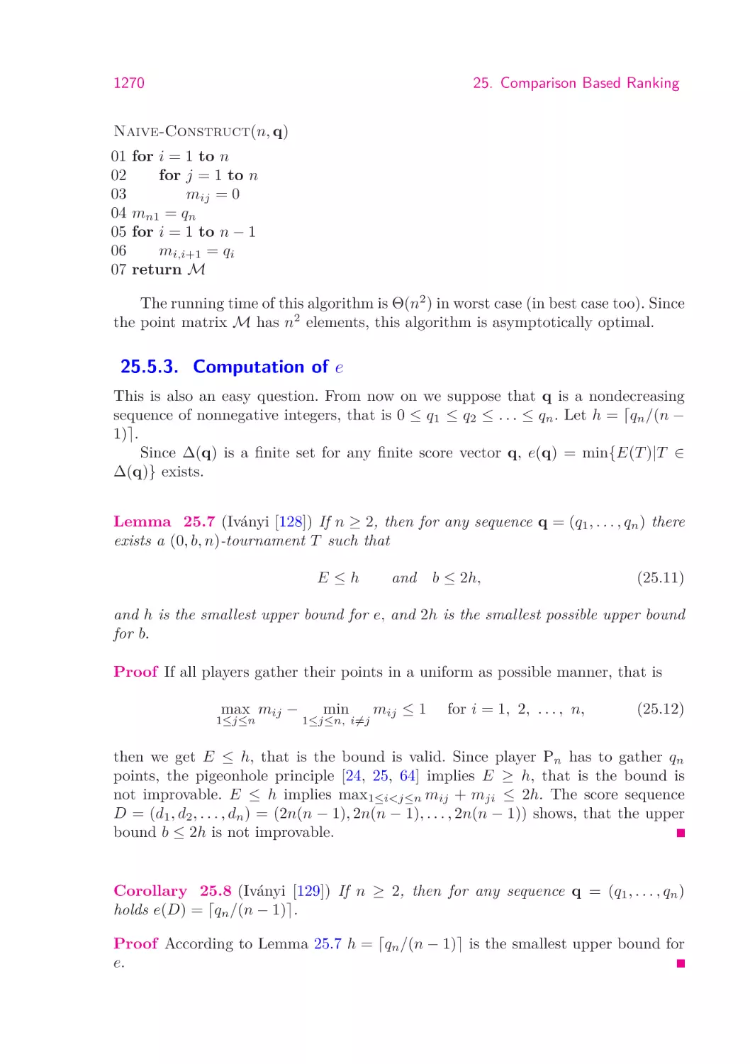
25.5.2. Description of a naive reconstructing algorithm . . . . . .
25.5.3. Computation of e . . . . . . . . . . . . . . . . . . . . . . .
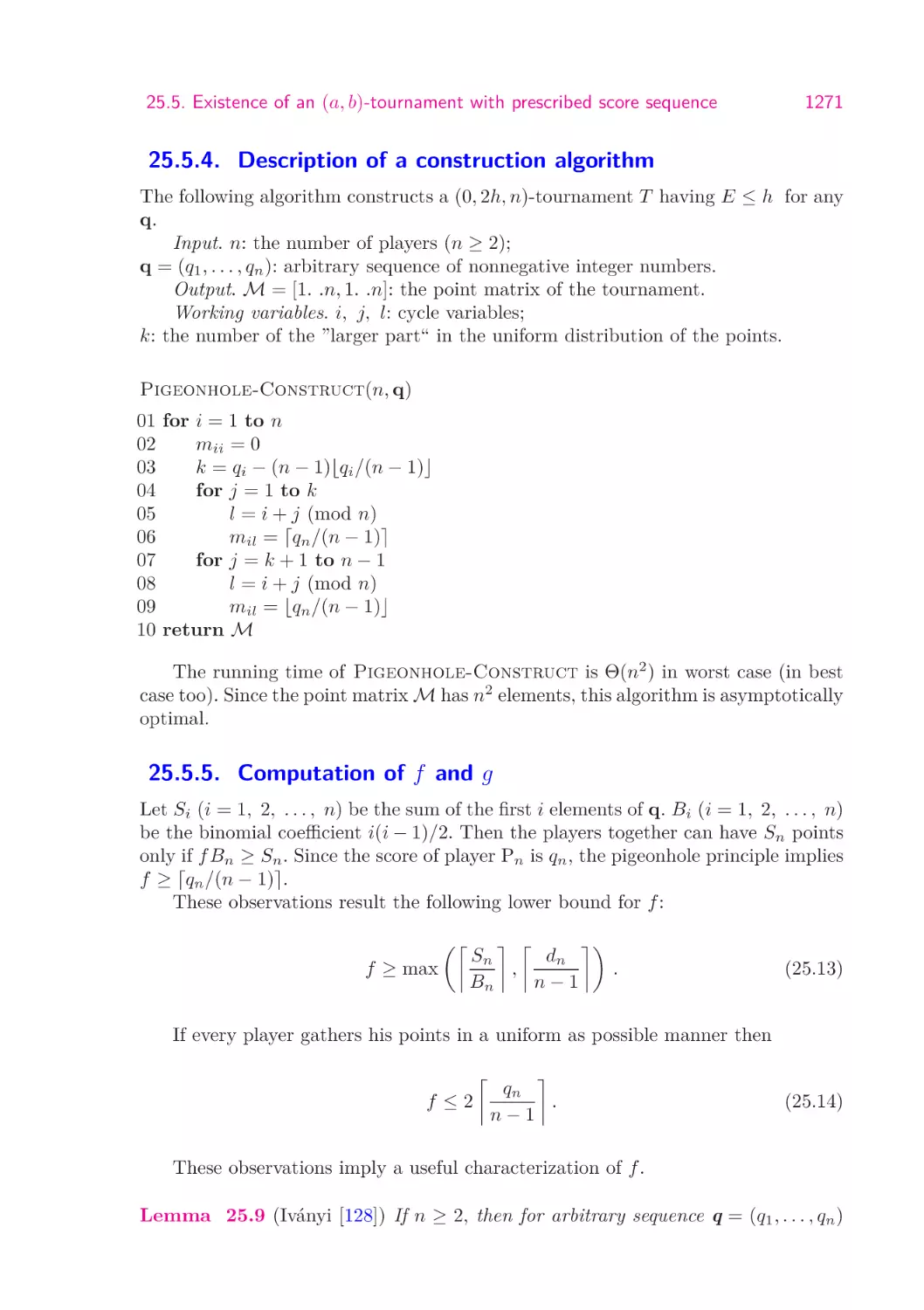
25.5.4. Description of a construction algorithm . . . . . . . . . .
.
.
.
.
.
.
.
.
.
.
1262
1262
1264
1265
1267
1269
1269
1269
1270
1271
1204
Contents
25.5.5. Computation of f and g . . . . . . . . . . . . . . . . . . . .
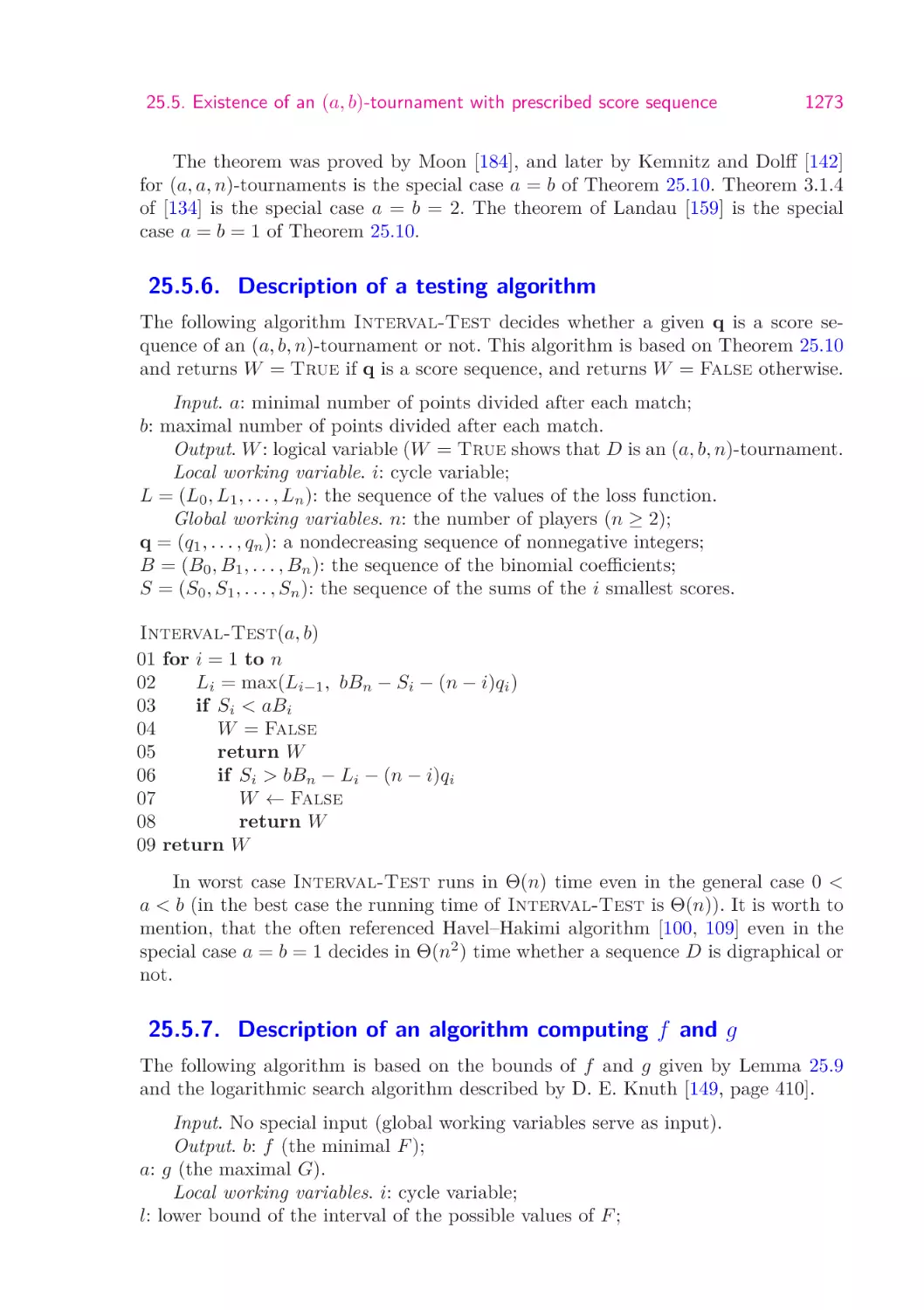
25.5.6. Description of a testing algorithm . . . . . . . . . . . . . . .
25.5.7. Description of an algorithm computing f and g . . . . . . .
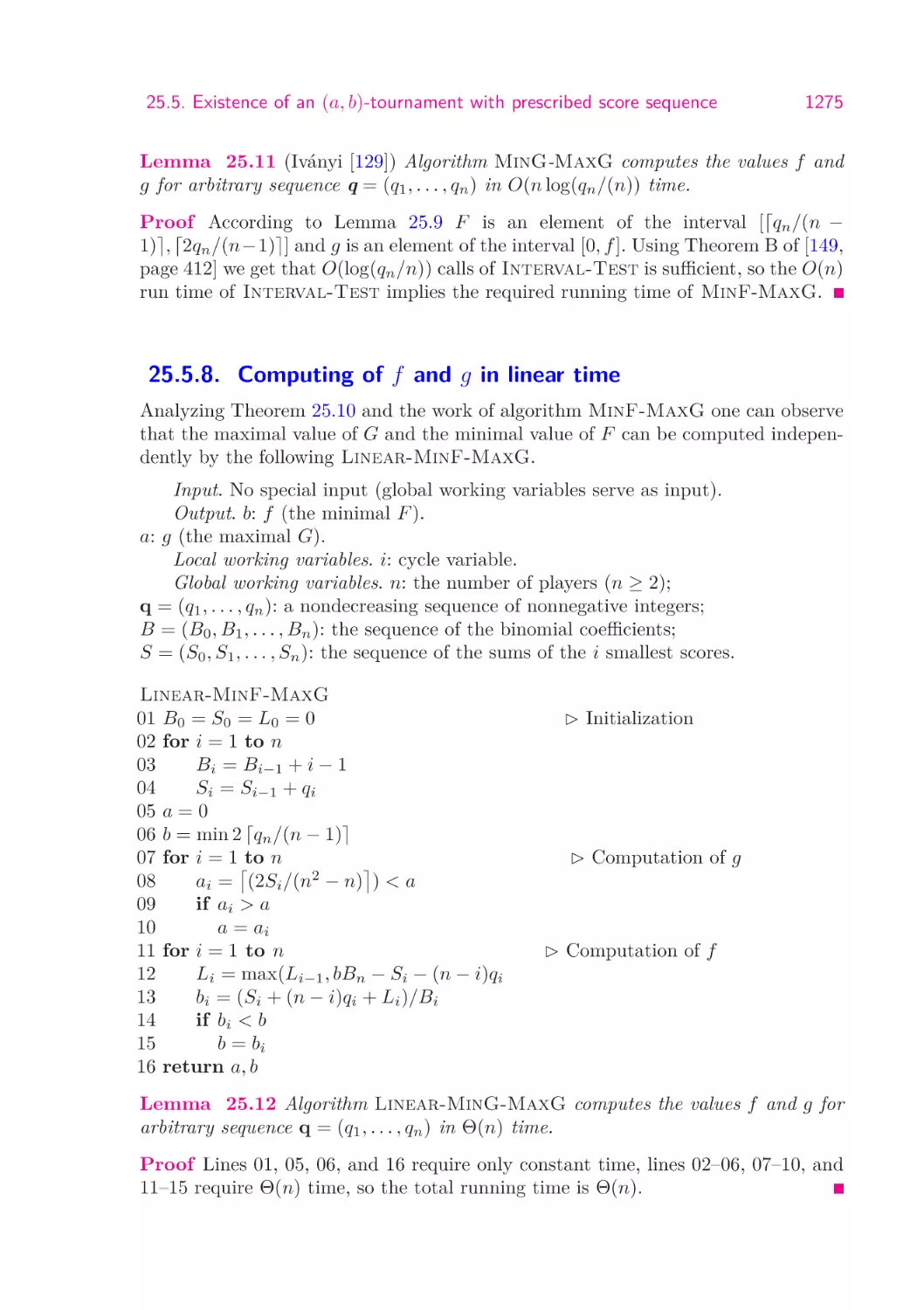
25.5.8. Computing of f and g in linear time . . . . . . . . . . . . .
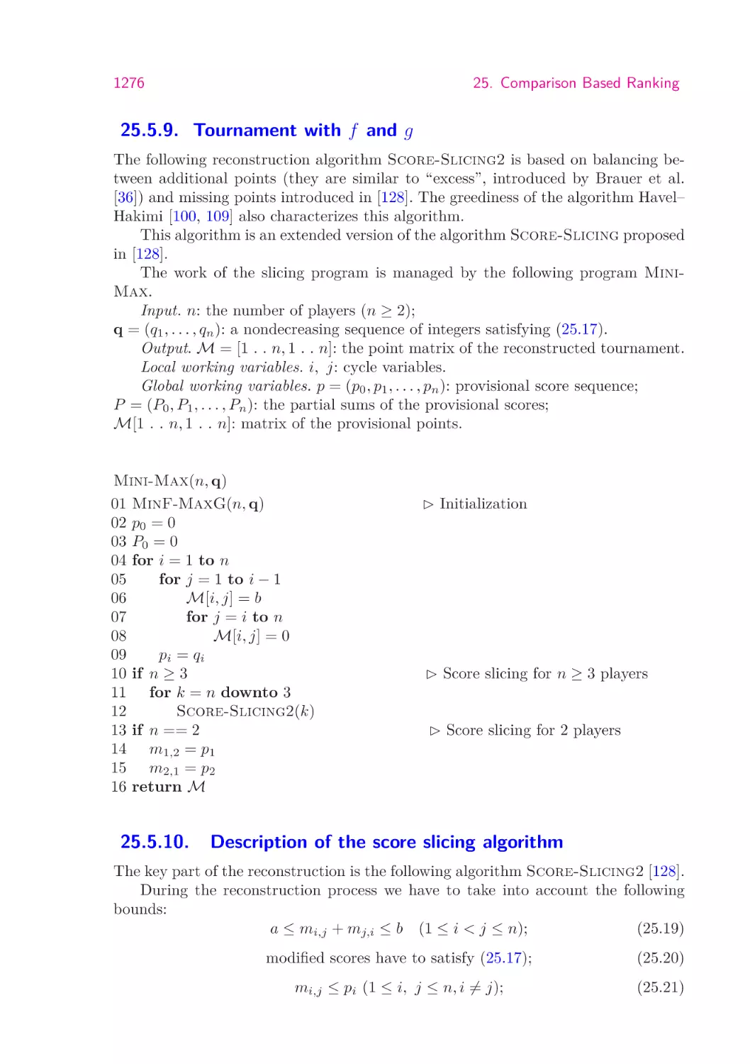
25.5.9. Tournament with f and g . . . . . . . . . . . . . . . . . . .
25.5.10. Description of the score slicing algorithm . . . . . . . . . . .
25.5.11. Analysis of the minimax reconstruction algorithm . . . . . .
25.6. Imbalances in (0, b)-tournaments . . . . . . . . . . . . . . . . . . .
25.6.1. Imbalances in (0, 1)-tournaments. . . . . . . . . . . . . . . .
25.6.2. Imbalances in (0, 2)-tournaments . . . . . . . . . . . . . . .
25.7. Supertournaments . . . . . . . . . . . . . . . . . . . . . . . . . . .
25.7.1. Hypertournaments . . . . . . . . . . . . . . . . . . . . . . .
25.7.2. Supertournaments . . . . . . . . . . . . . . . . . . . . . . .
25.8. Football tournaments . . . . . . . . . . . . . . . . . . . . . . . . . .
25.8.1. Testing algorithms . . . . . . . . . . . . . . . . . . . . . . .
25.8.2. Polynomial testing algorithms of the draw sequences . . . .
25.9. Reconstruction of the tested sequences . . . . . . . . . . . . . . . .
26.Complexity of Words . . . . . . . . . . . . . . . . . . . . . . . . . . . .
26.1. Simple complexity measures . . . . . . . . . . . . . . . . . . . . . .
26.1.1. Finite words . . . . . . . . . . . . . . . . . . . . . . . . . . .
26.1.2. Infinite words . . . . . . . . . . . . . . . . . . . . . . . . . .
26.1.3. Word graphs . . . . . . . . . . . . . . . . . . . . . . . . . .
26.1.4. Complexity of words . . . . . . . . . . . . . . . . . . . . . .
26.2. Generalized complexity measures . . . . . . . . . . . . . . . . . . .
26.2.1. Rainbow words . . . . . . . . . . . . . . . . . . . . . . . . .
26.2.2. General words . . . . . . . . . . . . . . . . . . . . . . . . . .
26.3. Palindrome complexity . . . . . . . . . . . . . . . . . . . . . . . . .
26.3.1. Palindromes in finite words . . . . . . . . . . . . . . . . . .
26.3.2. Palindromes in infinite words . . . . . . . . . . . . . . . . .
27. Conflict Situations . . . . . . . . . . . . . . . . . . . . . . . . . . . . .
27.1. The basics of multi-objective programming . . . . . . . . . . . . . .
27.1.1. Applications of utility functions . . . . . . . . . . . . . . . .
27.1.2. Weighting method . . . . . . . . . . . . . . . . . . . . . . .
27.1.3. Distance-dependent methods . . . . . . . . . . . . . . . . .
27.1.4. Direction-dependent methods . . . . . . . . . . . . . . . . .
27.2. Method of equilibrium . . . . . . . . . . . . . . . . . . . . . . . . .
27.3. Methods of cooperative games . . . . . . . . . . . . . . . . . . . . .
27.4. Collective decision-making . . . . . . . . . . . . . . . . . . . . . . .
27.5. Applications of Pareto games . . . . . . . . . . . . . . . . . . . . .
27.6. Axiomatic methods . . . . . . . . . . . . . . . . . . . . . . . . . . .
28. General Purpose Computing on Graphics Processing Units . . .
28.1. The graphics pipeline model . . . . . . . . . . . . . . . . . . . . . .
28.1.1. GPU as the implementation of incremental image synthesis
28.2. GPGPU with the graphics pipeline model . . . . . . . . . . . . . .
28.2.1. Output . . . . . . . . . . . . . . . . . . . . . . . . . . . . .
1271
1273
1273
1275
1276
1276
1280
1280
1281
1281
1286
1286
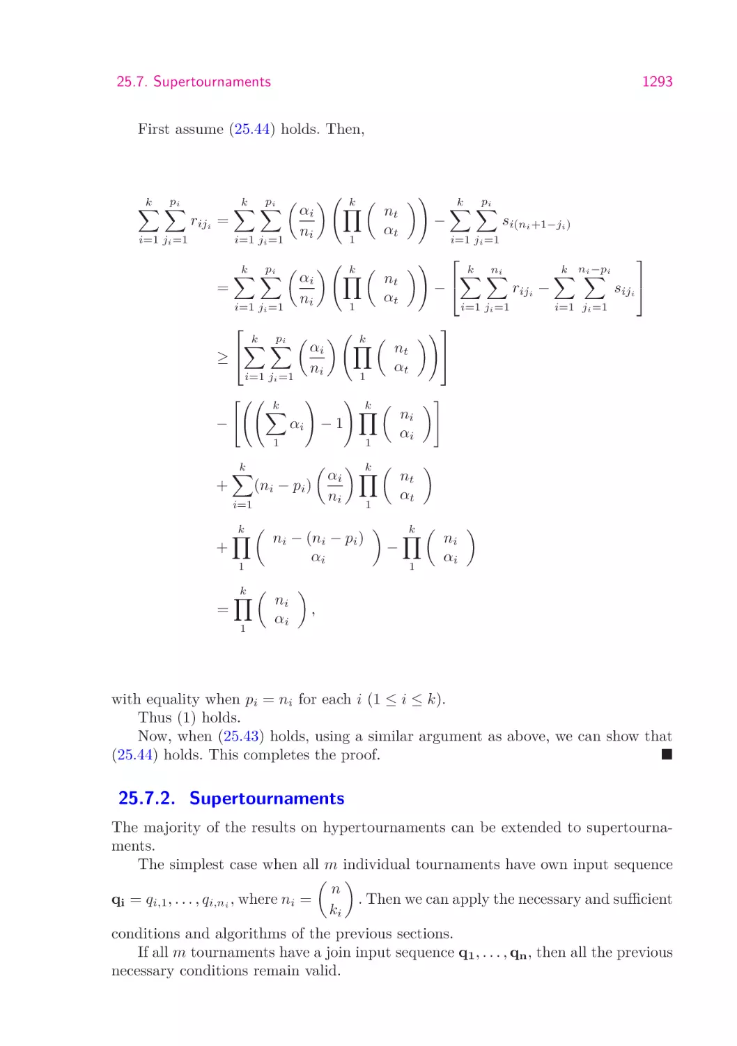
1293
1294
1294
1303
1309
1312
1312
1312
1314
1316
1321
1332
1332
1343
1343
1343
1346
1351
1351
1355
1357
1358
1361
1364
1369
1372
1379
1382
1388
1390
1392
1395
1395
Contents
28.2.2. Input . . . . . . . . . . . . . . . . . . . . . . . . . .
28.2.3. Functions and parameters . . . . . . . . . . . . . .
28.3. GPU as a vector processor . . . . . . . . . . . . . . . . . .
28.3.1. Implementing the SAXPY BLAS function . . . . .
28.3.2. Image filtering . . . . . . . . . . . . . . . . . . . .
28.4. Beyond vector processing . . . . . . . . . . . . . . . . . . .
28.4.1. SIMD or MIMD . . . . . . . . . . . . . . . . . . .
28.4.2. Reduction . . . . . . . . . . . . . . . . . . . . . . .
28.4.3. Implementing scatter . . . . . . . . . . . . . . . . .
28.4.4. Parallelism versus reuse . . . . . . . . . . . . . . .
28.5. GPGPU programming model: CUDA and OpenCL . . . .
28.6. Matrix-vector multiplication . . . . . . . . . . . . . . . . .
28.6.1. Making matrix-vector multiplication more parallel
28.7. Case study: computational fluid dynamics . . . . . . . . .
28.7.1. Eulerian solver for fluid dynamics . . . . . . . . . .
28.7.2. Lagrangian solver for differential equations . . . . .
1205
.
.
.
.
.
.
.
.
.
.
.
.
.
.
.
.
.
.
.
.
.
.
.
.
.
.
.
.
.
.
.
.
.
.
.
.
.
.
.
.
.
.
.
.
.
.
.
.
.
.
.
.
.
.
.
.
.
.
.
.
.
.
.
.
.
.
.
.
.
.
.
.
.
.
.
.
.
.
.
.
1396
1397
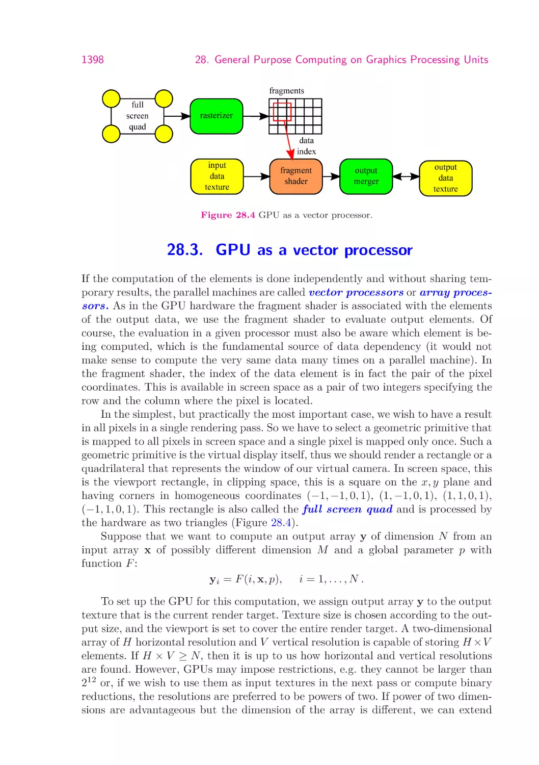
1398
1400
1401
1402
1402
1404
1405
1407
1409
1409
1411
1414
1416
1421
29. Perfect Arrays . . . . . . . . . . . . . . . . . . . . . . . . . . . .
29.1. Basic concepts . . . . . . . . . . . . . . . . . . . . . . . . . .
29.2. Necessary condition and earlier results . . . . . . . . . . . .
29.3. One-dimensional perfect arrays . . . . . . . . . . . . . . . .
29.3.1. Pseudocode of the algorithm Quick-Martin . . . .
29.3.2. Pseudocode of the algorithm Optimal-Martin . . .
29.3.3. Pseudocode of the algorithm Shift . . . . . . . . . .
29.3.4. Pseudocode of the algorithm Even . . . . . . . . . .
29.4. Two-dimensional perfect arrays . . . . . . . . . . . . . . . .
29.4.1. Pseudocode of the algorithm Mesh . . . . . . . . . .
29.4.2. Pseudocode of the algorithm Cellular . . . . . . .
29.5. Three-dimensional perfect arrays . . . . . . . . . . . . . . .
29.5.1. Pseudocode of the algorithm Colour . . . . . . . .
29.5.2. Pseudocode of the algorithm Growing . . . . . . .
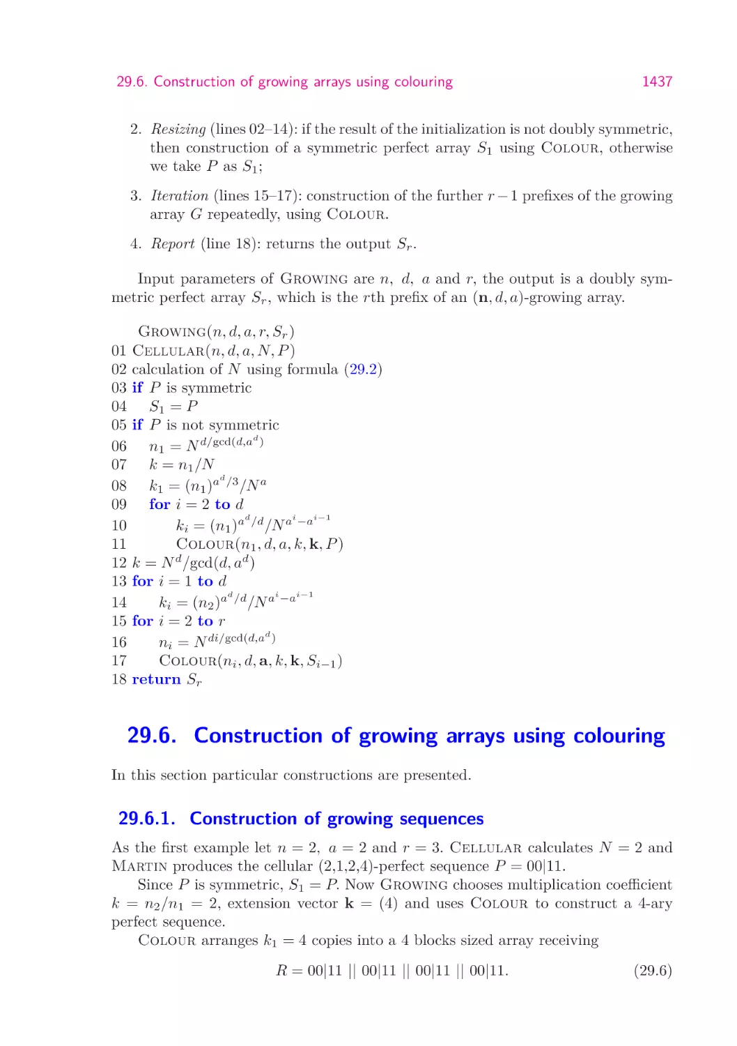
29.6. Construction of growing arrays using colouring . . . . . . .
29.6.1. Construction of growing sequences . . . . . . . . . .
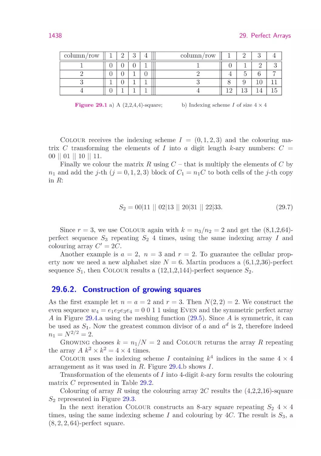
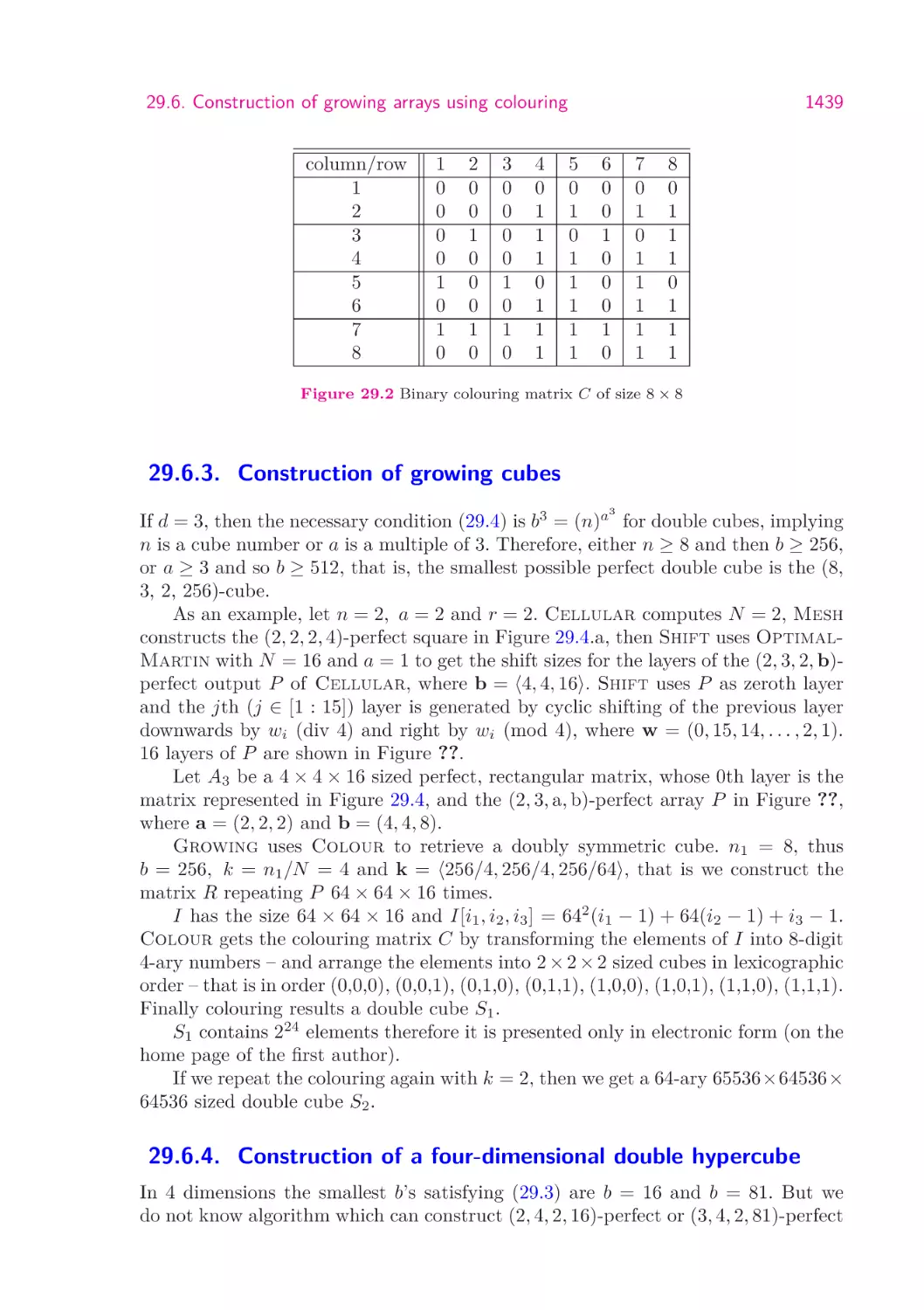
29.6.2. Construction of growing squares . . . . . . . . . . . .
29.6.3. Construction of growing cubes . . . . . . . . . . . . .
29.6.4. Construction of a four-dimensional double hypercube
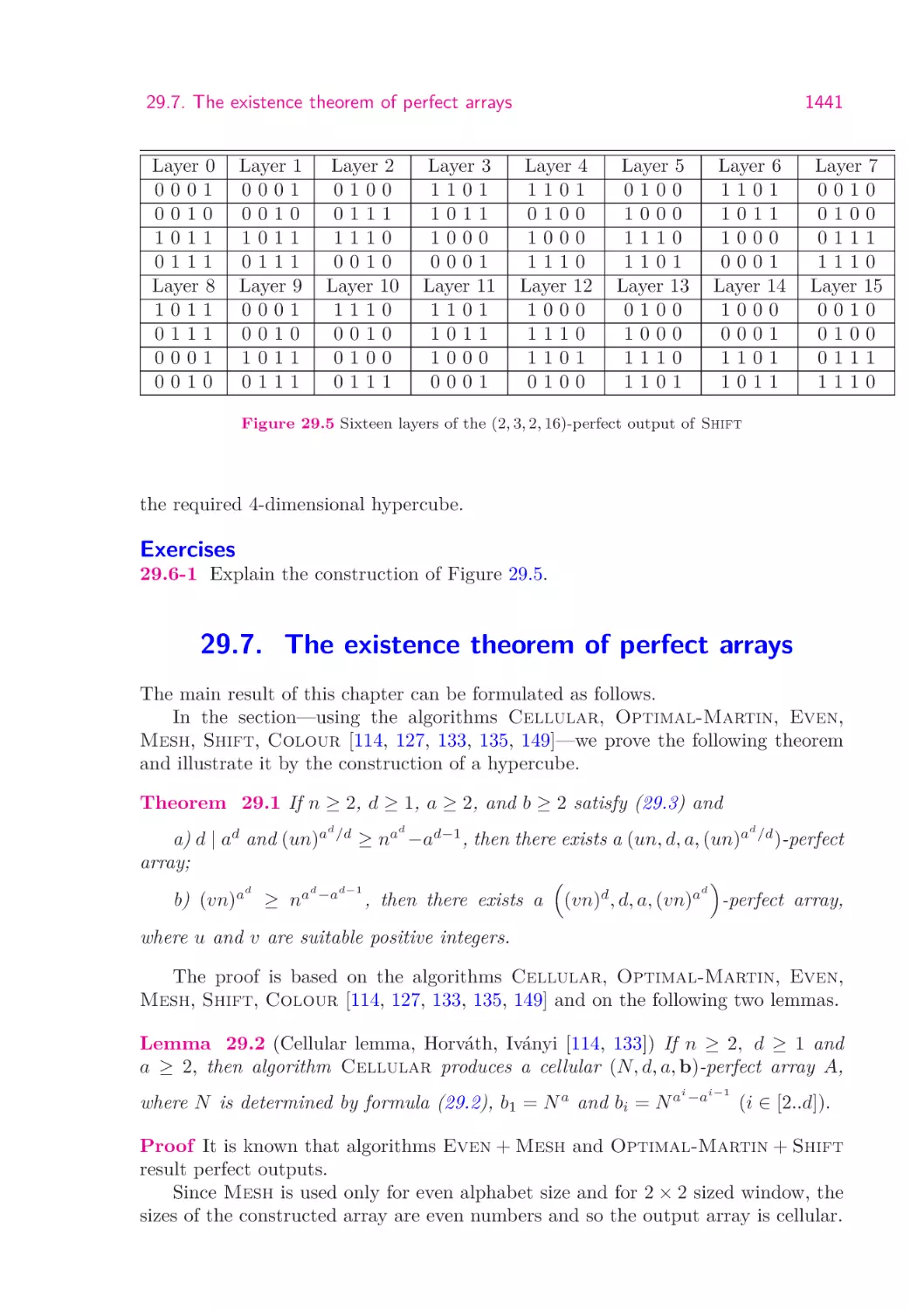
29.7. The existence theorem of perfect arrays . . . . . . . . . . .
29.8. Superperfect arrays . . . . . . . . . . . . . . . . . . . . . . .
29.9. d-complexity of one-dimensional arrays . . . . . . . . . . . .
29.9.1. Definitions . . . . . . . . . . . . . . . . . . . . . . . .
29.9.2. Bounds of complexity measures . . . . . . . . . . . .
29.9.3. Recurrence relations . . . . . . . . . . . . . . . . . .
29.9.4. Pseudocode of the algorithm Quick-Martin . . . .
29.9.5. Pseudocode of algorithm d-Complexity . . . . . . .
29.9.6. Pseudocode of algorithm Super . . . . . . . . . . .
29.9.7. Pseudocode of algorithm MaxSub . . . . . . . . . .
29.9.8. Construction and complexity of extremal words . . .
.
.
.
.
.
.
.
.
.
.
.
.
.
.
.
.
.
.
.
.
.
.
.
.
.
.
.
.
.
.
.
.
.
.
.
.
.
.
.
.
.
.
.
.
.
.
.
.
.
.
.
.
.
.
.
.
.
.
.
.
.
.
.
.
.
.
.
.
.
.
.
.
.
.
.
.
.
.
.
.
.
.
.
.
.
.
.
.
.
.
.
.
.
.
.
.
.
.
.
.
.
.
.
.
.
.
.
.
.
.
.
.
.
.
.
.
.
.
.
.
1428
1428
1431
1431
1431
1432
1432
1433
1433
1434
1434
1435
1435
1436
1437
1437
1438
1439
1439
1441
1443
1443
1444
1446
1448
1450
1450
1451
1451
1452
1206
Contents
29.10.Finite two-dimensional arrays with maximal complexity
29.10.1. Definitions . . . . . . . . . . . . . . . . . . . . . .
29.10.2. Bounds of complexity functions . . . . . . . . . .
29.10.3. Properties of the maximal complexity function .
29.10.4. On the existence of maximal arrays . . . . . . . .
30. Score Sets and Kings . . . . . . . . . . . . . . . . .
30.1. Score sets in 1-tournaments . . . . . . . . . . . .
30.1.1. Determining the score set . . . . . . . . .
30.1.2. Tournaments with prescribed score set . .
30.2. Score sets in oriented graphs . . . . . . . . . . . .
30.2.1. Oriented graphs with prescribed scoresets
30.3. Unicity of score sets . . . . . . . . . . . . . . . .
30.3.1. 1-unique score sets . . . . . . . . . . . . .
30.3.2. 2-unique score sets . . . . . . . . . . . . .
30.4. Kings and serfs in tournaments . . . . . . . . . .
30.5. Weak kings in oriented graphs . . . . . . . . . . .
.
.
.
.
.
.
.
.
.
.
.
.
.
.
.
.
.
.
.
.
.
.
.
.
.
.
.
.
.
.
.
.
.
.
.
.
.
.
.
.
.
.
.
.
.
.
.
.
.
.
.
.
.
.
.
.
.
.
.
.
.
.
.
.
.
.
.
.
.
.
.
.
.
.
1456
1456
1458
1459
1460
.
.
.
.
.
.
.
.
.
.
.
.
.
.
.
.
.
.
.
.
.
.
.
.
.
.
.
.
.
.
.
.
.
.
.
.
.
.
.
.
.
.
.
.
.
.
.
.
.
.
.
.
.
.
.
.
.
.
.
.
.
.
.
.
.
.
1463
1464
1464
1466
1473
1475
1480
1481
1482
1484
1492
Bibliography . . . . . . . . . . . . . . . . . . . . . . . . . . . . . . . . . . . 1504
Subject Index . . . . . . . . . . . . . . . . . . . . . . . . . . . . . . . . . . 1518
Name Index . . . . . . . . . . . . . . . . . . . . . . . . . . . . . . . . . . . . 1524
Introduction
The third volume contains seven new chapters.
Chapter 24 (The Branch and Bound Method) was written by Béla Vizvári
(Eastern Mediterrean University), Chapter 25 (Comparison Based Ranking) by
Antal Iványi (Eötvös Loránd University) and Shariefuddin Pirzada (University of
Kashmir), Chapter 26 (Complexity of Words) by Zoltán Kása, (Sapientia Hungarian University of Transylvania) and Mira-Cristiana Anisiu (Tiberiu Popovici Institute of Numerical Mathematics), Chapter 27 (Conflict Situations) by Ferenc Szidarovszky (University of Arizona) and by László Domoszlai (Eötvös Loránd University), Chapter 28 (General Purpose Computing on Graphics Processing Units) by
László Szirmay-Kalos and László Szécsi (both Budapest University of Technology
and Economics), Chapter 29 (Perfect Arrays) by Antal Iványi (Eötvös Loránd University), and Chapter 30 by Shariefuddin Pirzada (University of Kashmir), Antal
Iványi (Eötvös Loránd University) and Muhammad Ali Khan (King Fahd University).
The LATEX style file was written by Viktor Belényesi, Zoltán Csörnyei, László
Domoszlai and Antal Iványi. The figures was drawn or corrected by Kornél Locher.
and László Domoszlai. Anna Iványi transformed the bibliography into hypertext.
The DOCBOOK version was made by Marton 2001. Kft.
Using the data of the colofon page you can contact with any of the creators of the
book. We welcome ideas for new exercises and problems, and also critical remarks
or bug reports.
The publication of the printed book (Volumes 1 and 2) was supported by Department of Mathematics of Hungarian Academy of Science. This electronic book
(Volumes 1, 2, and 3) was prepared in the framework of project Eastern Hungarian
Informatics Books Repository no. TÁMOP-4.1.2-08/1/A-2009-0046.
This electronic book appeared with the support of European Union and with
the co-financing of European Social Fund.
Budapest, September 2011
Antal Iványi (tony@compalg.inf.elte.hu)
24. The Branch and Bound Method
It has serious practical consequences if it is known that a combinatorial problem is
NP-complete. Then one can conclude according to the present state of science that
no simple combinatorial algorithm can be applied and only an enumerative-type
method can solve the problem in question. Enumerative methods are investigating
many cases only in a non-explicit, i.e. implicit, way. It means that huge majority
of the cases are dropped based on consequences obtained from the analysis of the
particular numerical problem. The three most important enumerative methods are
(i) implicit enumeration, (ii) dynamic programming, and (iii) branch and bound
method. This chapter is devoted to the latter one. Implicit enumeration and dynamic
programming can be applied within the family of optimization problems mainly if all
variables have discrete nature. Branch and bound method can easily handle problems
having both discrete and continuous variables. Further on the techniques of implicit
enumeration can be incorporated easily in the branch and bound frame. Branch and
bound method can be applied even in some cases of nonlinear programming.
The Branch and Bound (abbreviated further on as B&B) method is just a frame of a
large family of methods. Its substeps can be carried out in different ways depending
on the particular problem, the available software tools and the skill of the designer
of the algorithm.
Boldface letters denote vectors and matrices; calligraphic letters are used for
sets. Components of vectors are denoted by the same but non-boldface letter. Capital letters are used for matrices and the same but lower case letters denote their
elements. The columns of a matrix are denoted by the same boldface but lower case
letters.
Some formulae with their numbers are repeated several times in this chapter. The
reason is that always a complete description of optimization problems is provided.
Thus the fact that the number of a formula is repeated means that the formula is
identical to the previous one.
24.1. An example: the Knapsack Problem
In this section the branch and bound method is shown on a numerical example.
The problem is a sample of the binary knapsack problem which is one of the easiest
24.1. An example: the Knapsack Problem
1209
problems of integer programming but it is still NP-complete. The calculations are
carried out in a brute force way to illustrate all features of B&B. More intelligent
calculations, i.e. using implicit enumeration techniques will be discussed only at the
end of the section.
24.1.1. The Knapsack Problem
There are many different knapsack problems. The first and classical one is the binary
knapsack problem. It has the following story. A tourist is planning a tour in the
mountains. He has a lot of objects which may be useful during the tour. For example
ice pick and can opener can be among the objects. We suppose that the following
conditions are satisfied.
•
•
•
•
•
Each object has a positive value and a positive weight. (E.g. a balloon filled with
helium has a negative weight. See Exercises 24.1-1 and 24.1-2) The value is the
degree of contribution of the object to the success of the tour.
The objects are independent from each other. (E.g. can and can opener are not
independent as any of them without the other one has limited value.)
The knapsack of the tourist is strong and large enough to contain all possible
objects.
The strength of the tourist makes possible to bring only a limited total weight.
But within this weight limit the tourist want to achieve the maximal total value.
The following notations are used to the mathematical formulation of the problem:
n
j
wj
vj
b
the
the
the
the
the
number of objects;
index of the objects;
weight of object j;
value of object j;
maximal weight what the tourist can bring.
For each object j a so-called binary or zero-one decision variable, say xj , is
introduced:
1 if object j is present on the tour
xj =
0 if object j isn’t present on the tour.
Notice that
wj xj =
wj
0
if object j is present on the tour,
if object j isn’t present on the tour
is the weight of the object in the knapsack.
Similarly vj xj is the value of the object on the tour. The total weight in the
knapsack is
n
X
j=1
wj xj
1210
24. The Branch and Bound Method
which may not exceed the weight limit. Hence the mathematical form of the problem
is
n
X
vj xj
(24.1)
wj xj ≤ b
(24.2)
max
j=1
n
X
j=1
xj = 0 or 1,
j = 1, . . . , n .
(24.3)
The difficulty of the problem is caused by the integrality requirement. If constraint (24.3) is substituted by the relaxed constraint, i.e. by
0 ≤ xj ≤ 1,
j = 1, . . . , n ,
(24.4)
then the Problem (29.2), (24.2), and (24.4) is a linear programming problem. (24.4)
means that not only a complete object can be in the knapsack but any part of it.
Moreover it is not necessary to apply the simplex method or any other LP algorithm
to solve it as its optimal solution is described by
Theorem 24.1 Suppose that the numbers vj , wj (j = 1, . . . , n) are all positive and
moreover the index order satisfies the inequality
v2
vn
v1
≥
··· ≥
.
w1
w2
wn
(24.5)
Then there is an index p (1 ≤ p ≤ n) and an optimal solution x∗ such that
x∗1 = x∗2 = · · · = x∗p−1 = 1, x∗p+1 = x∗p+2 = · · · = x∗p+1 = 0 .
Notice that there is only at most one non-integer component in x∗ . This property
will be used at the numerical calculations.
From the point of view of B&B the relation of the Problems (29.2), (24.2), and
(24.3) and (29.2), (24.2), and (24.4) is very important. Any feasible solution of the
first one is also feasible in the second one. But the opposite statement is not true.
In other words the set of feasible solutions of the first problem is a proper subset of
the feasible solutions of the second one. This fact has two important consequences:
•
The optimal value of the Problem (29.2), (24.2), and (24.4) is an upper bound
of the optimal value of the Problem (29.2), (24.2), and (24.3).
•
If the optimal solution of the Problem (29.2), (24.2), and (24.4) is feasible in the
Problem (29.2), (24.2), and (24.3) then it is the optimal solution of the latter
problem as well.
These properties are used in the course of the branch and bound method intensively.
24.1. An example: the Knapsack Problem
1211
24.1.2. A numerical example
The basic technique of the B&B method is that it divides the set of feasible solutions
into smaller sets and tries to fathom them. The division is called branching as new
branches are created in the enumeration tree. A subset is fathomed if it can be
determined exactly if it contains an optimal solution.
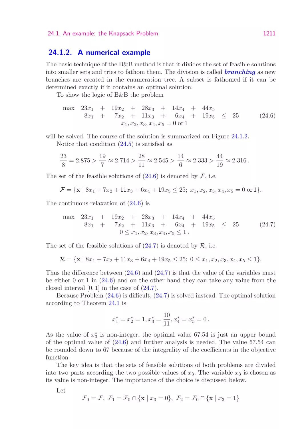
To show the logic of B&B the problem
max
23x1
8x1
+
+
19x2 + 28x3 + 14x4 +
7x2 + 11x3 +
6x4 +
x1 , x2 , x3 , x4 , x5 = 0 or 1
44x5
19x5
≤ 25
(24.6)
will be solved. The course of the solution is summarized on Figure 24.1.2.
Notice that condition (24.5) is satisfied as
19
28
14
44
23
= 2.875 >
≈ 2.714 >
≈ 2.545 >
≈ 2.333 >
≈ 2.316 .
8
7
11
6
19
The set of the feasible solutions of (24.6) is denoted by F, i.e.
F = {x | 8x1 + 7x2 + 11x3 + 6x4 + 19x5 ≤ 25; x1 , x2 , x3 , x4 , x5 = 0 or 1}.
The continuous relaxation of (24.6) is
max
23x1
8x1
+
+
19x2 + 28x3 + 14x4 +
7x2 + 11x3 +
6x4 +
0 ≤ x1 , x2 , x3 , x4 , x5 ≤ 1 .
44x5
19x5
≤ 25
(24.7)
The set of the feasible solutions of (24.7) is denoted by R, i.e.
R = {x | 8x1 + 7x2 + 11x3 + 6x4 + 19x5 ≤ 25; 0 ≤ x1 , x2 , x3 , x4 , x5 ≤ 1}.
Thus the difference between (24.6) and (24.7) is that the value of the variables must
be either 0 or 1 in (24.6) and on the other hand they can take any value from the
closed interval [0, 1] in the case of (24.7).
Because Problem (24.6) is difficult, (24.7) is solved instead. The optimal solution
according to Theorem 24.1 is
x∗1 = x∗2 = 1, x∗3 =
10 ∗
, x = x∗5 = 0 .
11 4
As the value of x∗3 is non-integer, the optimal value 67.54 is just an upper bound
of the optimal value of (24.6) and further analysis is needed. The value 67.54 can
be rounded down to 67 because of the integrality of the coefficients in the objective
function.
The key idea is that the sets of feasible solutions of both problems are divided
into two parts according the two possible values of x3 . The variable x3 is chosen as
its value is non-integer. The importance of the choice is discussed below.
Let
F0 = F, F1 = F0 ∩ {x | x3 = 0}, F2 = F0 ∩ {x | x3 = 1}
1212
24. The Branch and Bound Method
R0
1
67.45
x3 = 0
2
x3 = 1
R1
3
65.26
R2
67.28
x2 = 0
4
x2 = 1
R3
5
65
R4
67.127
x1 = 0
x1 = x3 = x4 = 1
x2 = x5 = 0
6
R5
63.32
x1 = 1
7
R6
−∞
Figure 24.1 The first seven steps of the solution
and
Obviously
R0 = R, R1 = R0 ∩ {x | x3 = 0}, R2 = R0 ∩ {x | x3 = 1} .
Hence the problem
F1 ⊆ R1 and F2 ⊆ R2 .
max 23x1 + 19x2 + 28x3 + 14x4 + 44x5
x ∈ R1
(24.8)
24.1. An example: the Knapsack Problem
1213
is a relaxation of the problem
max 23x1 + 19x2 + 28x3 + 14x4 + 44x5
x ∈ F1 .
(24.9)
Problem (24.8) can be solved by Theorem 24.1, too, but it must be taken into
consideration that the value of x3 is 0. Thus its optimal solution is
x∗1 = x∗2 = 1, x∗3 = 0, x∗4 = 1, x∗5 =
4
.
19
The optimal value is 65.26 which gives the upper bound 65 for the optimal value of
Problem (24.9). The other subsets of the feasible solutions are immediately investigated. The optimal solution of the problem
max 23x1 + 19x2 + 28x3 + 14x4 + 44x5
x ∈ R2
(24.10)
is
6 ∗
, x = 1, x∗4 = x∗5 = 0
7 3
giving the value 67.28. Hence 67 is an upper bound of the problem
x∗1 = 1, x∗2 =
max 23x1 + 19x2 + 28x3 + 14x4 + 44x5
x ∈ F2 .
(24.11)
As the upper bound of (24.11) is higher than the upper bound of (24.9), i.e. this
branch is more promising, first it is fathomed further on. It is cut again into two
branches according to the two values of x2 as it is the non-integer variable in the
optimal solution of (24.10). Let
F3 = F2 ∩ {x | x2 = 0} ,
F4 = F2 ∩ {x | x2 = 1} ,
R3 = R2 ∩ {x | x2 = 0} ,
R4 = R2 ∩ {x | x2 = 1} .
The sets F3 and R3 are containing the feasible solution of the original problems such
that x3 is fixed to 1 and x2 is fixed to 0. In the sets F4 and R4 both variables are
fixed to 1. The optimal solution of the first relaxed problem, i.e.
max 23x1 + 19x2 + 28x3 + 14x4 + 44x5
x ∈ R3
is
x∗1 = 1, x∗2 = 0, x∗3 = 1, x∗4 = 1, x∗5 = 0 .
As it is integer it is also the optimal solution of the problem
max 23x1 + 19x2 + 28x3 + 14x4 + 44x5
x ∈ F3 .
1214
24. The Branch and Bound Method
The optimal objective function value is 65. The branch of the sets F3 and R3 is
completely fathomed, i.e. it is not possible to find a better solution in it.
The other new branch is when both x2 and x3 are fixed to 1. If the objective
function is optimized on R4 then the optimal solution is
x∗1 =
7 ∗
, x = x∗3 = 1, x∗4 = x∗5 = 0 .
8 2
Applying the same technique again two branches are defined by the sets
F5 = F4 ∩ {x | x1 = 0}, F6 = F4 ∩ {x | x1 = 1},
R5 = R4 ∩ {x | x2 = 0}, R6 = R4 ∩ {x | x2 = 1} .
The optimal solution of the branch of R5 is
x∗1 = 0, x∗2 = x∗3 = x∗4 = 1, x∗5 =
1
.
19
The optimal value is 63.32. It is strictly less than the objective function value of the
feasible solution found in the branch of R3 . Therefore it cannot contain an optimal
solution. Thus its further exploration can be omitted although the best feasible
solution of the branch is still not known. The branch of R6 is infeasible as objects
1, 2, and 3 are overusing the knapsack. Traditionally this fact is denoted by using
−∞ as optimal objective function value.
At this moment there is only one branch which is still unfathomed. It is the
branch of R1 . The upper bound here is 65 which is equal to the objective function
value of the found feasible solution. One can immediately conclude that this feasible
solution is optimal. If there is no need for alternative optimal solutions then the
exploration of this last branch can be abandoned and the method is finished. If
alternative optimal solutions are required then the exploration must be continued.
The non-integer variable in the optimal solution of the branch is x5 . The subbranches
referred later as the 7th and 8th branches, defined by the equations x5 = 0 and
x5 = 1, give the upper bounds 56 and 61, respectively. Thus they do not contain
any optimal solution and the method is finished.
24.1.3. Properties in the calculation of the numerical example
The calculation is revisited to emphasize the general underlying logic of the method.
The same properties are used in the next section when the general frame of B&B is
discussed.
Problem (24.6) is a difficult one. Therefore the very similar but much easier
Problem (24.7) has been solved instead of (24.6). A priori it was not possible to
exclude the case that the optimal solution of (24.7) is the optimal solution of (24.6)
as well. Finally it turned out that the optimal solution of (24.7) does not satisfy
all constraints of (24.6) thus it is not optimal there. But the calculation was not
useless, because an upper bound of the optimal value of (24.6) has been obtained.
These properties are reflected in the definition of relaxation in the next section.
As the relaxation did not solved Problem (24.6) therefore it was divided into
24.1. An example: the Knapsack Problem
1215
Subproblems (24.9) and (24.11). Both subproblems have their own optimal solution
and the better one is the optimal solution of (24.6). They are still too difficult to be
solved directly, therefore relaxations were generated to both of them. These problems
are (24.8) and (24.10). The nature of (24.8) and (24.10) from mathematical point of
view is the same as of (24.7).
Notice that the union of the sets of the feasible solutions of (24.8) and (24.10)
is a proper subset of the relaxation (24.7), i.e.
R1 ∪ R2 ⊂ R0 .
Moreover the two subsets have no common element, i.e.
R1 ∩ R2 = ∅ .
It is true for all other cases, as well. The reason is that the branching, i.e. the
determination of the Subproblems (24.9) and (24.11) was made in a way that the
optimal solution of the relaxation, i.e. the optimal solution of (24.7), was cut off.
The branching policy also has consequences on the upper bounds. Let ν(S) be
the optimal value of the problem where the objective function is unchanged and
the set of feasible solutions is S. Using this notation the optimal objective function
values of the original and the relaxed problems are in the relation
ν(F) ≤ ν(R) .
If a subset Rk is divided into Rp and Rq then
ν(Rk ) ≥ max{ν(Rp ), ν(Rq )} .
(24.12)
Notice that in the current Problem (24.12) is always satisfied with strict inequality
ν(R0 ) > max{ν(R1 ), ν(R2 )} ,
ν(R1 ) > max{ν(R7 ), ν(R8 )} ,
ν(R2 ) > max{ν(R3 ), ν(R4 )} ,
ν(R4 ) > max{ν(R5 ), ν(R6 )} .
(The values ν(R7 ) and ν(R8 ) were mentioned only.) If the upper bounds of a certain
quantity are compared then one can conclude that the smaller the better as it is
closer to the value to be estimated. An equation similar to (24.12) is true for the
non-relaxed problems, i.e. if Fk = Fp ∪ Fq then
ν(Fk ) = max{ν(Fp ), ν(Fq )} ,
(24.13)
but because of the difficulty of the solution of the problems, practically it is not
possible to use (24.13) for getting further information.
A subproblem is fathomed and no further investigation of it is needed if either
•
•
its integer (non-relaxed) optimal solution is obtained, like in the case of F3 , or
it is proven to be infeasible as in the case of F6 , or
1216
•
24. The Branch and Bound Method
its upper bound is not greater than the value of the best known feasible solution
(cases of F1 and F5 ).
If the first or third of these conditions are satisfied then all feasible solutions of the
subproblem are enumerated in an implicit way.
The subproblems which are generated in the same iteration, are represented by
two branches on the enumeration tree. They are siblings and have the same parent.
Figure 24.1 visualize the course of the calculations using the parent–child relation.
The enumeration tree is modified by constructive steps when new branches are
formed and also by reduction steps when some branches can be deleted as one of
the three above-mentioned criteria are satisfied. The method stops when no subset
remained which has to be still fathomed.
24.1.4. How to accelerate the method
As it was mentioned in the introduction of the chapter, B&B and implicit enumeration can co-operate easily. Implicit enumeration uses so-called tests and obtains
consequences on the values of the variables. For example if x3 is fixed to 1 then the
knapsack inequality immediately implies that x5 must be 0, otherwise the capacity
of the tourist is overused. It is true for the whole branch 2.
On the other hand if the objective function value must be at least 65, which is
the value of the found feasible solution then it possible to conclude in branch 1 that
the fifth object must be in the knapsack, i.e. x5 must be 1, as the total value of the
remaining objects 1, 2, and 4 is only 56.
Why such consequences accelerate the algorithm? In the example there are 5
binary variables, thus the number of possible cases is 32 = 25 . Both branches 1 and
2 have 16 cases. If it is possible to determine the value of a variable, then the number
of cases is halved. In the above example it means that only 8 cases remain to be
investigated in both branches. This example is a small one. But in the case of larger
problems the acceleration process is much more significant. E.g. if in a branch there
are 21 free, i.e. non-fixed, variables but it is possible to determine the value of one of
them then the investigation of 1 048 576 cases is saved. The application of the tests
needs some extra calculation, of course. Thus a good trade-off must be found.
The use of information provided by other tools is further discussed in Section
24.5.
Exercises
24.1-1 What is the suggestion of the optimal solution of a Knapsack Problem in
connection of an object having (a) negative weight and positive value, (b) positive
weight and negative value?
24.1-2 Show that an object of a knapsack problem having negative weight and
negative value can be substituted by an object having positive weight and positive
value such that the two knapsack problems are equivalent. (Hint. Use complementary
variable.)
24.1-3 Solve Problem (24.6) with a branching strategy such that an integer valued
variable is used for branching provided that such a variable exists.
24.2. The general frame of the B&B method
1217
24.2. The general frame of the B&B method
The aim of this section is to give a general description of the B&B method. Particular
realizations of the general frame are discussed in later sections.
B&B is based on the notion of relaxation. It has not been defined yet. As there
are several types of relaxations the first subsection is devoted to this notion. The
general frame is discussed in the second subsection.
24.2.1. Relaxation
Relaxation is discussed in two steps. There are several techniques to define relaxation
to a particular problem. There is no rule for choosing among them. It depends on
the design of the algorithm which type serves the algorithm well. The different types
are discussed in the first part titled “Relaxations of a particular problem”. In the
course of the solution of Problem (24.6) subproblems were generated which were
still knapsack problems. They had their own relaxations which were not totally
independent from the relaxations of each other and the main problem. The expected
common properties and structure is analyzed in the second step under the title
“Relaxation of a problem class”.
Relaxations of a particular problem
The description of Problem (24.6)
consists of three parts: (1) the objective function, (2) the algebraic constraints, and
(3) the requirement that the variables must be binary. This structure is typical for
optimization problems. In a general formulation an optimization problem can be
given as
max f (x)
(24.14)
g(x) ≤ b
(24.15)
x∈X.
(24.16)
Relaxing the non-algebraic constraints
The underlying logic of generating
relaxation (24.7) is that constraint (24.16) has been substituted by a looser one. In
the particular case it was allowed that the variables can take any value between 0
and 1. In general (24.16) is replaced by a requirement that the variables must belong
to a set, say Y, which is larger than X , i.e. the relation X ⊆ Y must hold. More
formally the relaxation of Problem (24.14)-(24.16) is the problem
max f (x)
(24.14)
g(x) ≤ b
(24.15)
x ∈ Y.
(24.17)
This type of relaxation can be applied if a large amount of difficulty can be eliminated
by changing the nature of the variables.
1218
24. The Branch and Bound Method
Relaxing the algebraic constraints
There is a similar technique such that
(24.16) the inequalities (24.15) are relaxed instead of the constraints. A natural way
of this type of relaxation is the following. Assume that there are m inequalities in
(24.15). Let λi ≥ 0 (i = 1, . . . , m) be fixed numbers. Then any x ∈ X satisfying
(24.15) also satisfies the inequality
m
X
i=1
λi gi (x) ≤
m
X
(24.18)
λ i bi .
i=1
Then the relaxation is the optimization of the (24.14) objective function under the
conditions (24.18) and (24.16). The name of the inequality (24.18) is surrogate
constraint.
The problem
max
23x1
5x1
2x1
1x1
+
+
−
+
19x2 + 28x3 + 14x4
4x2 + 6x3 +
3x4
2x2 − 3x3 +
5x4
5x2 + 8x3 −
2x4
x1 , x2 , x3 , x4 , x5 = 0 or 1
+
+
+
+
44x5
5x5
6x5
8x5
≤ 14
≤ 4
≤ 7
(24.19)
is a general zero-one optimization problem. If λ1 = λ2 = λ3 = 1 then the relaxation
obtained in this way is Problem (24.6). Both problems belong to NP-complete classes.
However the knapsack problem is significantly easier from practical point of view
than the general problem, thus the relaxation may have sense. Notice that in this
particular problem the optimal solution of the knapsack problem, i.e. (1,0,1,1,0),
satisfies the constraints of (24.19), thus it is also the optimal solution of the latter
problem.
Surrogate constraint is not the only option in relaxing the algebraic constraints.
A region defined by nonlinear boundary surfaces can be approximated by tangent
planes. For example if the feasible region is the unit circuit which is described by
the inequality
x21 + x22 ≤ 1
can be approximated by the square
−1 ≤ x1 , x2 ≤ 1 .
If the optimal solution on the enlarged region is e.g. the point (1,1) which is not in
the original feasible region then a cut must be found which cuts it from the relaxed
region but it does not cut any part of the original feasible region. It is done e.g. by
the inequality
√
x1 + x2 ≤ 2 .
A new relaxed problem is defined by the introduction of the cut. The method is
similar to one of the method relaxing of the objective function discussed below.
24.2. The general frame of the B&B method
1219
Relaxing the objective function In other cases the difficulty of the problem is
caused by the objective function. If it is possible to use an easier objective function,
say h(x), but to obtain an upper bound the condition
∀ x ∈ X : h(x) ≥ f (x)
(24.20)
must hold. Then the relaxation is
max h(x)
(24.21)
(24.15)
g(x) ≤ b
(24.16)
x∈X.
This type of relaxation is typical if B&B is applied in (continuous) nonlinear
optimization. An important subclass of the nonlinear optimization problems is the
so-called convex programming problem. It is again a relatively easy subclass. Therefore it is reasonable to generate a relaxation of this type if it is possible. A Problem
(24.14)-(24.16) is a convex programming problem, if X is a convex set, the functions
gi (x) (i = 1, . . . , m) are convex and the objective function f (x) is concave. Thus
the relaxation can be a convex programming problem if only the last condition is
violated. Then it is enough to find a concave function h(x) such that (24.20) is
satisfied.
For example
the single variable function f (x) = 2x2 − x4 is not concave in the
√
√
interval [ −3 3 , 33 ].1 Thus if it is the objective function in an optimization problem
it might √be √
necessary that it is substituted by a concave function h(x) such that
∀x ∈ [ −3 3 , 33 ] : f (x) ≤ h(x). It is easy to see that h(x) = 89 − x2 satisfies the
requirements.
Let x∗ be the optimal solution of the relaxed problem (24.21), (24.15), and
(24.16). It solves the original problem if the optimal solution has the same objective
function value in the original and relaxed problems, i.e. f (x∗ ) = h(x∗ ).
Another reason why this type of relaxation is applied that in certain cases the
objective function is not known in a closed form, however it can be determined in
any given point. It might happen even in the case if the objective function is concave.
Assume that the value of f (x) is known in the points y1 , . . . , yk . If f (x) concave
then it is smooth, i.e. its gradient exists. The gradient determines a tangent plane
which is above the function. The equation of the tangent plane in point yp is2
∇(f (yp ))(x − yp ) = 0.
Hence in all points of the domain of the function f (x) we have that
h(x) = min {f (yp ) + ∇(f (yp ))(x − yp ) | p = 1, . . . , k} ≥ f (x).
Obviously the function h(x) is an approximation of function f (x).
1A
00
continuous function is concave
if itssecond derivative is negative. f (x) = 4 − 12x2 which is
positive in the open interval
2 The
√
√
− 3
, 33
3
.
gradient is considered being a row vector.
1220
24. The Branch and Bound Method
The idea if the method is illustrated on the following numerical example. Assume
that an “unknown” concave function is to be maximized on the [0,5] closed interval.
The method can start from any point of the interval which is in the feasible region.
Let 0 be the starting point. According to the assumptions although the closed formula
of the function is not known, it is possible to determine the values of function and
0
its derivative. Now the values f (0) = −4 and f (0) = 4 are obtained. The general
formula of the tangent line in the point (x0 , f (x0 )) is
0
y = f (x0 )(x − x0 ) + f (x0 ).
Hence the equation of the first tangent line is y = 4x−4 giving the first optimization
problem as
max h
h ≤ 4x − 4
x ∈ [0, 5].
As 4x − 4 is a monotone increasing function, the optimal solution is x = 5. Then
0
the values f (5) = −9 and f (5) = −6 are provided by the method calculating the
function. The equation of the second tangent line is y = −6x + 21. Thus the second
optimization problem is
max h
h ≤ 4x − 4, h ≤ −6x + 21
x ∈ [0, 5].
As the second tangent line is a monotone decreasing function, the optimal solution
is in the intersection point of the two tangent lines giving x = 2.5. Then the values
0
f (2.5) = −0.25 and f (2.5) = −1 are calculated and the equation of the tangent line
is y = −x + 2.25. The next optimization problem is
h ≤ 4x − 4,
max h
h ≤ −6x + 21,
x ∈ [0, 5].
h ≤ −x + 2.25
The optimal solution is x = 1.25. It is the intersection point of the first and third
tangent lines. Now both new intersection points are in the interval [0,5]. In general
some intersection points can be infeasible. The method goes in the same way further
on. The approximated “unknow” function is f (x) = −(x − 2)2 .
The Lagrange Relaxation Another relaxation called Lagrange relaxation.
In that method both the objective function and the constraints are modified. The
underlying idea is the following. The variables must satisfy two different types of
constraints, i.e. they must satisfy both (24.15) and (24.16). The reason that the
constraints are written in two parts is that the nature of the two sets of constraints is
different. The difficulty of the problem caused by the requirement of both constraints.
It is significantly easier to satisfy only one type of constraints. So what about to
eliminate one of them?
24.2. The general frame of the B&B method
1221
Assume again that the number of inequalities in (24.15) is m. Let λi ≥ 0 (i =
1, . . . , m) be fixed numbers. The Lagrange relaxation of the problem (24.14)- (24.16)
is
max f (x) +
m
X
i=1
λi (bi − gi (x))
x∈X.
(24.22)
(24.16)
Notice that the objective function (24.22) penalizes the violation of the constraints,
e.g. trying to use too much resources, and rewards the saving of resources. The first
set of constraints disappeared from the problem. In most of the cases the Lagrange
relaxation is a much easier one than the original problem. In what follows Problem
(24.14)- (24.16) is also denoted by (P ) and the Lagrange relaxation is referred as
(L(λ)). The notation reflects the fact that the Lagrange relaxation problem depends
on the choice of λi ’s. The numbers λi ’s are called Lagrange multipliers.
It is not obvious that (L(λ)) is really a relaxation of (P ). This relation is established by
Theorem 24.2 Assume that both (P ) and (L(λ)) have optimal solutions. Then
for any nonnegative λi (i = 1, . . . , m) the inequality
ν(L(λ)) ≥ ν(P )
holds.
Proof The statement is that the optimal value of (L(λ)) is an upper bound of the
optimal value of (P ). Let x∗ be the optimal solution of (P ). It is obviously feasible
in both problems. Hence for all i the inequalities λi ≥ 0, bi ≥ gi (x∗ ) hold. Thus
λi (bi − gi (x∗ )) ≥ 0 which implies that
f (x∗ ) ≤ f (x∗ ) +
m
X
i=1
λi (bi − gi (x∗ )).
Here the right-hand side is the objective function value of a feasible solution of
(L(λ)), i.e.
ν(P ) = f (x∗ ) ≤ f (x∗ ) +
m
X
i=1
λi (bi − gi (x∗ )) ≤ ν(L(λ)) .
There is another connection between (P ) and (L(λ)) which is also important
from the point of view of the notion of relaxation.
Theorem 24.3 Let xL be the optimal solution of the Lagrange relaxation. If
g(xL ) ≤ b
(24.23)
1222
24. The Branch and Bound Method
and
m
X
i=1
λi (bi − gi (xL )) = 0
(24.24)
then xL is an optimal solution of (P ).
Proof (24.23) means that xL is a feasible solution of (P ). For any feasible solution
x of (P ) it follows from the optimality of xL that
f (x) ≤ f (x) +
m
X
i=1
λi (bi − gi (x)) ≤ f (xL ) +
m
X
i=1
λi (bi − gi (xL )) = f (xL ) ,
i.e. xL is at least as good as x.
The importance of the conditions (24.23) and (24.24) is that they give an optimality criterion, i.e. if a point generated by the Lagrange multipliers satisfies them
then it is optimal in the original problem. The meaning of (24.23) is that the optimal
solution of the Lagrange problem is feasible in the original one and the meaning of
(24.24) is that the objective function values of xL are equal in the two problems, just
as in the case of the previous relaxation. It also indicates that the optimal solutions
of the two problems are coincident in certain cases.
There is a practical necessary condition for being a useful relaxation which is
that the relaxed problem is easier to solve than the original problem. The Lagrange
relaxation has this property. It can be shown on Problem (24.19). Let λ1 = 1,
λ2 = λ3 = 3. Then the objective function (24.22) is the following
(23x1 + 19x2 + 28x3 + 14x4 + 44x5 ) + (14 − 5x1 − x2 − 6x3 − 3x4 − 5x5 )
+3(4 − 2x1 − x2 + 3x3 − 5x4 − 6x5 ) + 3(7 − x1 − 5x2 − 8x3 + 2x4 − 8x5 )
= 47 + (23 − 5 − 6 − 3)x1 + (19 − 1 − 3 − 15)x2 + (28 − 6 + 9 − 24)x3
+(14 − 3 − 15 + 5)x4 + (44 − 5 − 18 − 24)x5
= 47 + 9x1 + 0x2 + 7x3 + x4 − 3x5 .
The only constraint is that all variables are binary. It implies that if a coefficient is
positive in the objective function then the variable must be 1 in the optimal solution
of the Lagrange problem, and if the coefficient is negative then the variable must
be 0. As the coefficient of x2 is zero, there are two optimal solutions: (1,0,1,1,0)
and (1,1,1,1,0). The first one satisfies the optimality condition thus it is an optimal
solution. The second one is infeasible.
What is common in all relaxation?
They have three common properties.
1. All feasible solutions are also feasible in the relaxed problem.
2. The optimal value of the relaxed problem is an upper bound of the optimal
value of the original problem.
24.2. The general frame of the B&B method
1223
3. There are cases when the optimal solution of the relaxed problem is also optimal in the original one.
The last property cannot be claimed for all particular case as then the relaxed problem is only an equivalent form of the original one and needs very likely approximately
the same computational effort, i.e. it does not help too much. Hence the first two
properties are claimed in the definition of the relaxation of a particular problem.
Definition 24.4 Let f, h be two functions mapping from the n-dimensional Euclidean space into the real numbers. Further on let U, V be two subsets of the ndimensional Euclidean space. The problem
max{h(x) | x ∈ V}
(24.25)
max{f (x) | x ∈ U}
(24.26)
is a relaxation of the problem
if
(i) U ⊂ V and
(ii) it is known a priori, i.e. without solving the problems that ν(24.25) ≥ ν(24.26).
Relaxation of a problem class
No exact definition of the notion of problem
class will be given. There are many problem classes in optimization. A few examples
are the knapsack problem, the more general zero-one optimization, the traveling
salesperson problem, linear programming, convex programming, etc. In what follows
problem class means only an infinite set of problems.
One key step in the solution of (24.6) was that the problem was divided into
subproblems and even the subproblems were divided into further subproblems, and
so on.
The division must be carried out in a way such that the subproblems belong
to the same problem class. By fixing the value of a variable the knapsack problem
just becomes another knapsack problem of lesser dimension. The same is true for
almost all optimization problems, i.e. a restriction on the value of a single variable
(introducing either a lower bound, or upper bound, or an exact value) creates a new
problem in the same class. But restricting a single variable is not the only possible
way to divide a problem into subproblems. Sometimes special constraints on a set
of variables may have sense. For example it is easy to see from the first constraint
of (24.19) that at most two out of the variables x1 , x3 , and x5 can be 1. Thus it is
possible to divide it into two subproblems by introducing the new constraint which
is either x1 + x3 + x5 = 2, or x1 + x3 + x5 ≤ 1. The resulted problems are still in the
class of binary optimization. The same does not work in the case of the knapsack
problem as it must have only one constraint, i.e. if a second inequality is added to
the problem then the new problem is out of the class of the knapsack problems.
The division of the problem into subproblems means that the set of feasible
solutions is divided into subsets not excluding the case that one or more of the
subsets turn out to be empty set. R5 and R6 gave such an example.
Another important feature is summarized in formula (24.12). It says that the
1224
24. The Branch and Bound Method
upper bound of the optimal value obtained from the undivided problem is at most
as accurate as the upper bound obtained from the divided problems.
Finally, the further investigation of the subset F1 could be abandoned as R1
was not giving a higher upper bound as the objective function value of the optimal
solution on R3 which lies at the same time in F3 , too, i.e. the subproblem defined
on the set F3 was solved.
The definition of the relaxation of a problem class reflects the fact that relaxation and defining subproblems (branching) are not completely independent. In the
definition it is assumed that the branching method is a priori given.
Definition 24.5 Let P and Q be two problem classes. Class Q is a relaxation of
class P if there is a map R with the following properties.
1. R maps the problems of P into the problems of Q.
2. If a problem (P) ∈ P is mapped into (Q) ∈ Q then (Q) is a relaxation of (P)
in the sense of Definition 29.44.
3. If (P) is divided into (P1 ),. . .,(Pk ) and these problems are mapped into
(Q1 ),. . .,(Qk ), then the inequality
ν(Q) ≥ max{ν(Q1 ), . . . , ν(Qk )}
(24.27)
holds.
4. There are infinite many pairs (P), (Q) such that an optimal solution of (Q) is
also optimal in (P).
24.2.2. The general frame of the B&B method
As the Reader has already certainly observed B&B divides the problem into subproblems and tries to fathom each subproblem by the help of a relaxation. A subproblem
is fathomed in one of the following cases:
1. The optimal solution of the relaxed subproblem satisfies the constraints of
the unrelaxed subproblem and its relaxed and non-relaxed objective function
values are equal.
2. The infeasibility of the relaxed subproblem implies that the unrelaxed subproblem is infeasible as well.
3. The upper bound provided by the relaxed subproblem is less (in the case
if alternative optimal solution are sought) or less or equal (if no alternative
optimal solution is requested) than the objective function value of the best
known feasible solution.
The algorithm can stop if all subsets (branches) are fathomed. If nonlinear programming problems are solved by B&B then the finiteness of the algorithm cannot be
always guaranteed.
In a typical iteration the algorithm executes the following steps.
24.2. The general frame of the B&B method
•
•
•
•
1225
It selects a leaf of the branching tree, i.e. a subproblem not divided yet into
further subproblems.
The subproblem is divided into further subproblems (branches) and their relaxations are defined.
Each new relaxed subproblem is solved and checked if it belongs to one of the
above-mentioned cases. If so then it is fathomed and no further investigation is
needed. If not then it must be stored for further branching.
If a new feasible solution is found which is better than the so far best one, then
even stored branches having an upper bound less than the value of the new best
feasible solution can be deleted without further investigation.
In what follows it is supposed that the relaxation satisfies definition 29.10.1.
The original problem to be solved is
max f (x)
(24.14)
g(x) ≤ b
(24.15)
x ∈ X.
(24.16)
Thus the set of the feasible solutions is
F = F0 = {x | g(x) ≤ b; x ∈ X } .
(24.28)
The relaxed problem satisfying the requirements of definition 29.10.1 is
max h(x)
k(x) ≤ b
x ∈ Y,
where X ⊆ Y and for all points of the domain of the objective functions f (x) ≤ h(x)
and for all points of the domain of the constraint functions k(x) ≤ h(x). Thus the
set of the feasible solutions of the relaxation is
R = R0 = {x | k(x) ≤ b; x ∈ Y} .
Let Fk be a previously defined subset. Suppose that it is divided into the subsets
Ft+1 ,. . . ,Ft+p , i.e.
Fk =
p
[
l=1
Ft+l .
Let Rk and Rt+1 ,. . . ,Rt+p be the feasible sets of the relaxed subproblems. To satisfy
the requirement (24.27) of definition 29.10.1 it is assumed that
Rk ⊇
p
[
l=1
Rt+l .
1226
24. The Branch and Bound Method
The subproblems are identified by their sets of feasible solutions. The unfathomed subproblems are stored in a list. The algorithm selects a subproblem from the
list for further branching. In the formal description of the general frame of B&B the
following notations are used.
ẑ
L
t
F0
r
p(r)
xi
zi
L + Fi
L − Fi
the
the
the
the
the
the
the
the
the
the
objective function value of the best feasible solution found so far
list of the unfathomed subsets of feasible solutions
number of branches generated so far
set of all feasible solutions
index of the subset selected for branching
number of branches generated from Fr
optimal solution of the relaxed subproblem defined on Ri
upper bound of the objective function on subset Fi
operation of adding the subset Fi to the list L
operation of deleting the subset Fi from the list L
Note that yi = max{h(x) | x ∈ Ri }.
The frame of the algorithms can be found below. It simply describes the basic
ideas of the method and does not contain any tool of acceleration.
Branch-and-Bound
1
2
3
4
5
6
7
8
9
10
11
12
13
14
15
16
17
18
19
20
ẑ ← −∞
L ← { F0 }
t ← 0
while L =
6 ∅
do determination of r
L ← L − Fr
determination of p(r)
determination of branching Fr ⊂ R1 ∪ ... ∪ Rp(r)
for i ← 1 to p(r) do
Ft+i ← Fr ∩ Ri
calculation of (xt+i , zt+i )
if zt+i > ẑ
then if xt+i ∈ F
then ẑ ← zt+i
else L ← L + Ft+i
t ← t + p(r)
for i ← 1 to t do
if zi ≤ ẑ
then L ← L − Fi
return x
24.2. The general frame of the B&B method
1227
The operations in rows 5, 7, 8, and 11 depend on the particular problem class and
on the skills of the designer of the algorithm. The relaxed subproblem is solved in
row 14. A detailed example is discussed in the next section. The handling of the list
needs also careful consideration. Section 24.4 is devoted to this topic.
The loop in rows 17 and 18 can be executed in an implicit way. If the selected
subproblem in row 5 has a low upper bound, i.e. zr ≤ ẑ then the subproblem is
fathomed and a new subproblem is selected.
However the most important issue is the number of required operations including the finiteness of the algorithm. The method is not necessarily finite. Especially
nonlinear programming has infinite versions of it. Infinite loop may occur even in the
case if the number of the feasible solutions is finite. The problem can be caused by
an incautious branching procedure. A branch can belong to an empty set. Assume
that that the branching procedure generates subsets from Fr such that one of the
subsets Ft+1 , ..., Ft+p(r) is equal to Fr and the other ones are empty sets. Thus there
is an index i such that
Ft+i = Fr , Ft+1 = ... = Ft+i−1 = Ft+i+1 = ... = Ft+p(r) = ∅ .
(24.29)
If the same situation is repeated at the branching of Ft+i then an infinite loop is
possible.
Assume that a zero-one optimization problem of n variables is solved by B&B
and the branching is made always according to the two values of a free variable.
Generally it is not known that how large is the number of the feasible solutions.
There are at most 2n feasible solutions as it is the number of the zero-one vectors.
After the first branching there are at most 2n−1 feasible solutions in the two first
level leaves, each. This number is halved with each branching, i.e. in a branch on
level k there are at most 2n−k feasible solutions. It implies that on level n there is
at most 2n−n = 20 = 1 feasible solution. As a matter of fact on that level there is
exactly 1 zero-one vector and it is possible to decide whether or not it is feasible.
Hence after generating all branches on level n the problem can be solved. This idea
is generalized in the following finiteness theorem. While formulating the statement
the previous notations are used.
Theorem 24.6 Assume that
(i) The set F is finite.
(ii) There is a finite set U such that the following conditions are satisfied. If a subset
F̂ is generated in the course of the branch and bound method then there is a subset
Û of U such that F̂ ⊆ Û. Furthermore if the branching procedure creates the cover
R1 ∪ . . . ∪ Rp ⊇ F̂ then Û has a partitioning such that
Û = Û1 ∪ · · · ∪ Ûp , Ûi ∩ Ûj = ∅(i 6= j)
F̂ ∩ R̂j ⊆ Ûj (j = 1, . . . , p)
and moreover
1 ≤| Ûj |<| Û | (j = 1, . . . , p) .
(24.30)
(iii) If a set Û belonging to set F̂ has only a single element then the relaxed subproblem solves the unrelaxed subproblem as well.
1228
24. The Branch and Bound Method
Then the Branch-and-Bound procedure stops after finite many steps. If ẑ =
−∞ then there is no feasible solution. Otherwise ẑ is equal to the optimal objective
function value.
Remark. Notice that the binary problems mentioned above with Ûj ’s of type
Ûj = {x ∈ {0, 1}n | xk = δkj , k ∈ Ij } ,
where Ij ⊂ {1, 2, . . . , n} is the set of fixed variables and δkj ∈ {0, 1} is a fixed value,
satisfy the conditions of the theorem.
Proof Assume that the procedure Branch-and-Bound executes infinite many
steps. As the set F is finite it follows that there is at least one subset of F say Fr
such that it defines infinite many branches implying that the situation described in
(24.29) occurs infinite many times. Hence there is an infinite sequence of indices,
say r0 = r < r1 < · · · , such that Frj+1 is created at the branching of Frj and
Frj+1 = Frj . On the other hand the parallel sequence of the U sets must satisfy the
inequalities
| Ur0 |>| Ur1 |> · · · ≥ 1 .
It is impossible because the Us are finite sets.
The finiteness of F implies that optimal solution exists if and only if F is
nonempty, i.e. the problem cannot be unbounded and if feasible solution exist then
the supremum of the objective function is its maximum. The initial value of ẑ is
−∞. It can be changed only in Row 18 of the algorithm and if it is changed then
it equals to the objective function value of a feasible solution. Thus if there is no
feasible solution then it remains −∞. Hence if the second half of the statement is
not true, then at the end of the algorithm ẑ equal the objective function value of a
non-optimal feasible solution or it remains −∞.
Let r be the maximal index such that Fr still contains the optimal solution.
Then
zr ≥ optimal value > ẑ .
Hence it is not possible that the branch containing the optimal solution has been
deleted from the list in the loop of Rows 22 and 23, as zr > ẑ. It is also sure that
the subproblem
max{f (x) | x ∈ Fr }
has not been solved, otherwise the equation zr = ẑ should hold. Then only one option
remained that Fr was selected for branching once in the course of the algorithm. The
optimal solution must be contained in one of its subsets, say Ft+i which contradicts
the assumption that Fr has the highest index among the branches containing the
optimal solution.
If an optimization problem contains only bounded integer variables then the sets
Us are the sets the integer vectors in certain boxes. In the case of some scheduling
problems where the optimal order of tasks is to be determined even the relaxations
have combinatorial nature because they consist of permutations. Then U = R is also
24.3. Mixed integer programming with bounded variables
1229
possible. In both of the cases Condition (iii) of the theorem is fulfilled in a natural
way.
Exercises
24.2-1 Decide if the Knapsack Problem can be a relaxation of the Linear Binary
Optimization Problem in the sense of Definition 29.10.1. Explain your solution regardless that your answer is YES or NO.
24.3. Mixed integer programming with bounded
variables
Many decisions have both continuous and discrete nature. For example in the production of electric power the discrete decision is to switch on or not an equipment.
The equipment can produce electric energy in a relatively wide range. Thus if the
first decision is to switch on then a second decision must be made on the level of
the produced energy. It is a continuous decision. The proper mathematical model of
such problems must contain both discrete and continuous variables.
This section is devoted to the mixed integer linear programming problem with
bounded integer variables. It is assumed that there are n variables and a subset of
them, say I ⊆ {1, . . . , n} must be integer. The model has m linear constraints in
equation form and each integer variable has an explicit integer upper bound. It is also
supposed that all variables must be nonnegative. More formally the mathematical
problem is as follows.
max cT x
(24.31)
Ax = b
(24.32)
∀ j ∈ I : xj ≤ gj
(24.33)
xj ≥ 0 j = 1, . . . , n
(24.34)
∀ j ∈ I : xj is integer ,
(24.35)
where c and x are n-dimensional vectors, A is an m×n matrix, b is an m-dimensional
vector and finally all gj (j ∈ I) is a positive integer.
In the mathematical analysis of the problem below the the explicit upper bound
constraints (24.33) will not be used. The Reader may think that they are formally
included into the other algebraic constraints (24.32).
There are technical reasons that the algebraic constraints in (24.32) are claimed
in the form of equations. Linear programming relaxation is used in the method.
The linear programming problem is solved by the simplex method which needs this
form. But generally speaking equations and inequalities can be transformed into
1230
24. The Branch and Bound Method
one another in an equivalent way. Even in the numerical example discussed below
inequality form is used.
First a numerical example is analyzed. The course of the method is discussed
from geometric point of view. Thus some technical details remain concealed. Next
simplex method and related topics are discussed. All technical details can be described only in the possession of them. Finally some strategic points of the algorithm
are analyzed.
24.3.1. The geometric analysis of a numerical example
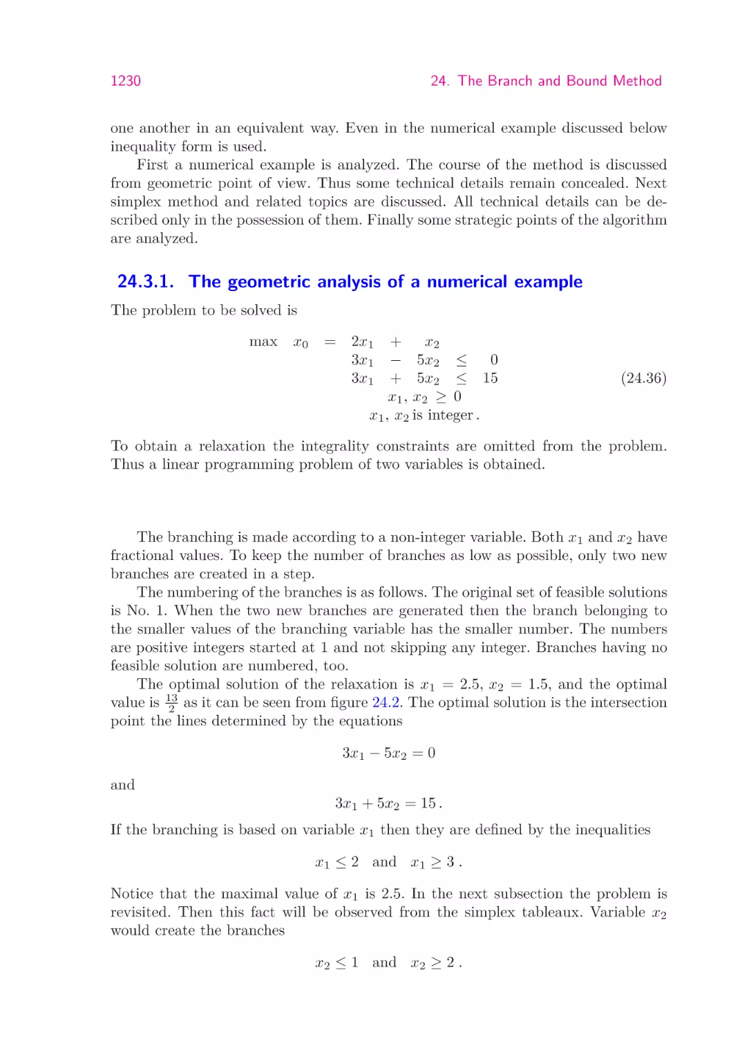
The problem to be solved is
max
x0
=
2x1
3x1
3x1
+ x2
− 5x2 ≤
0
+ 5x2 ≤ 15
x1 , x2 ≥ 0
x1 , x2 is integer .
(24.36)
To obtain a relaxation the integrality constraints are omitted from the problem.
Thus a linear programming problem of two variables is obtained.
The branching is made according to a non-integer variable. Both x1 and x2 have
fractional values. To keep the number of branches as low as possible, only two new
branches are created in a step.
The numbering of the branches is as follows. The original set of feasible solutions
is No. 1. When the two new branches are generated then the branch belonging to
the smaller values of the branching variable has the smaller number. The numbers
are positive integers started at 1 and not skipping any integer. Branches having no
feasible solution are numbered, too.
The optimal solution of the relaxation is x1 = 2.5, x2 = 1.5, and the optimal
value is 13
2 as it can be seen from figure 24.2. The optimal solution is the intersection
point the lines determined by the equations
3x1 − 5x2 = 0
and
3x1 + 5x2 = 15 .
If the branching is based on variable x1 then they are defined by the inequalities
x1 ≤ 2 and x1 ≥ 3 .
Notice that the maximal value of x1 is 2.5. In the next subsection the problem is
revisited. Then this fact will be observed from the simplex tableaux. Variable x2
would create the branches
x2 ≤ 1 and x2 ≥ 2 .
24.3. Mixed integer programming with bounded variables
1231
4
2x1 + x2 =
3
13
2
A
2
B
Feasible region
1
O
1
2
3
4
5
Figure 24.2 The geometry of linear programming relaxation of Problem (24.36) including the
feasible region (triangle OAB), the optimal solution (x1 = 2.5, x2 = 1.5), and the optimal level of
.
the objective function represented by the line 2x1 + x2 = 13
2
None of them is empty. Thus it is more advantageous the branch according to x1 .
Geometrically it means that the set of the feasible solutions in the relaxed problem
is cut by the line x1 = 2. Thus the new set becomes the quadrangle OACD on
Figure 24.3. The optimal solution on that set is x1 = 2, x2 = 1.8. It is point C on
the figure.
Now branching is possible according only to variable x2 . Branches 4 and 5 are
generated by the cuts x2 ≤ 1 and x2 ≥ 2, respectively. The feasible regions of
the relaxed problems are OHG of Branch 4, and AEF of Branch 5. The method
continues with the investigation of Branch 5. The reason will be given in the next
subsection when the quickly calculable upper bounds are discussed. On the other
hand it is obvious that the set AEF is more promising than OHG if the Reader
takes into account the position of the contour, i.e. the level line, of the objective
function on Figure 24.3. The algebraic details discussed in the next subsection serve
to realize the decisions in higher dimensions what is possible to see in 2-dimension.
Branches 6 and 7 are defined by the inequalities x1 ≤ 1 and x1 ≥ 2, respectively.
The latter one is empty again. The feasible region of Branch 6 is AIJF . The optimal
solution in this quadrangle is the Point I. Notice that there are only three integer
points in AIJF which are (0,3), (0,2), and (1,2). Thus the optimal integer solution of
1232
3
2
1
O
24. The Branch and Bound Method
Branch 6
A
Branch 5 I
6
F
Branch 2
- Branch 3; EMPTY
E
J
C
B
D
H
G
1
?
Branch 4
2
3
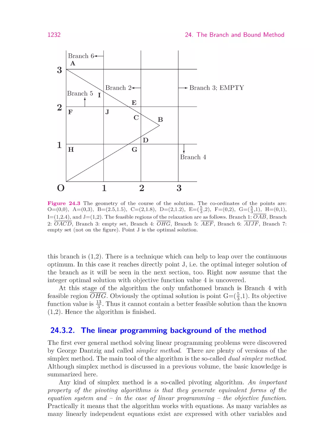
Figure 24.3 The geometry of the course of the solution. The co-ordinates of the points are:
O=(0,0), A=(0,3), B=(2.5,1.5), C=(2,1.8), D=(2,1.2), E=( 35 ,2), F=(0,2), G=( 35 ,1), H=(0,1),
I=(1,2.4), and J=(1,2). The feasible regions of the relaxation are as follows. Branch 1: OAB, Branch
2: OACD, Branch 3: empty set, Branch 4: OHG, Branch 5: AEF , Branch 6: AIJF , Branch 7:
empty set (not on the figure). Point J is the optimal solution.
this branch is (1,2). There is a technique which can help to leap over the continuous
optimum. In this case it reaches directly point J, i.e. the optimal integer solution of
the branch as it will be seen in the next section, too. Right now assume that the
integer optimal solution with objective function value 4 is uncovered.
At this stage of the algorithm the only unfathomed branch is Branch 4 with
feasible region OHG. Obviously the optimal solution is point G=( 53 ,1). Its objective
function value is 13
3 . Thus it cannot contain a better feasible solution than the known
(1,2). Hence the algorithm is finished.
24.3.2. The linear programming background of the method
The first ever general method solving linear programming problems were discovered
by George Dantzig and called simplex method. There are plenty of versions of the
simplex method. The main tool of the algorithm is the so-called dual simplex method.
Although simplex method is discussed in a previous volume, the basic knowledge is
summarized here.
Any kind of simplex method is a so-called pivoting algorithm. An important
property of the pivoting algorithms is that they generate equivalent forms of the
equation system and – in the case of linear programming – the objective function.
Practically it means that the algorithm works with equations. As many variables as
many linearly independent equations exist are expressed with other variables and
24.3. Mixed integer programming with bounded variables
1
1233
6 1/2
x1 ≤ 2
x1 ≥ 3
7/10
2
3
5 4/5
x2 ≤ 1
x2 ≥ 2
4/5
4
−∞
7/15
5
4 1/3
5 1/3
x1 ≤ 1
x1 = 2
4/3
6
4
7
−∞
x1 = 1
x2 = 2
solution
Figure 24.4 The course of the solution of Problem (24.36). The upper numbers in the circuits are
explained in subsection 24.3.2. They are the corrections of the previous bounds obtained from the
first pivoting step of the simplex method. The lower numbers are the (continuous) upper bounds
obtained in the branch.
further consequences are drawn from the current equivalent form of the equations.
If there are inequalities in the problem then they are reformulated by introducing
nonnegative slack variables. E.g. in case of LP-relaxation of Problem (24.36) the
1234
24. The Branch and Bound Method
equivalent form of the problem is
max
x0
=
2x1 + x2
3x1 − 5x2
3x1 + 5x2
x1 , x2 x3 , x4
+ 0x3
+ x3
+ 0x3
≥ 0.
+
+
+
0x4
0x4
x4
=
=
0
15
(24.37)
Notice that all variables appear in all equations including the objective function,
but it is allowed that some coefficients are zeros. The current version (24.37) can be
considered as a form where the variables x3 and x4 are expressed by x1 and x2 and
the expression is substituted into the objective function. If x1 = x2 = 0 then x3 = 0
and x4 = 15, thus the solution is feasible. Notice that the value of the objective
function is 0 and if it is possible to increase the value of any of x1 and x2 and
still getting a feasible solution then a better feasible solution is obtained. It is true,
because the method uses equivalent forms of the objective function. The method
obtains better feasible solution by pivoting. Let x1 and x2 be the two expressed
variables. Skipping some pivot steps the equivalent form of (24.37) is
max
x0
=
0x1
+
0x2
−
7
30 x3
−
13
30 x4
+
13
2
x1
+
0x2
+
1
6 x3
+
1
6 x4
=
5
2
1
x3
0x1 + x2 − 10
x1 , x2 x3 , x4 ≥ 0 .
+
1
10 x4
=
3
2
(24.38)
That form has two important properties. First if x3 = x4 = 0 then x1 = 52 and
x2 = 32 , thus the solution is feasible, similarly to the previous case. Generally this
property is called primal feasibility. Secondly, the coefficients of the non-expressed
variables are negative in the objective function. It is called dual feasibility. It implies
that if any of the non-expressed variables is positive in a feasible solution then that is
worse than the current one. It is true again, because the current form of the objective
function is equivalent to the original one. Thus the current value of the objective
function which is 13
2 , is optimal.
In what follows the sign of maximization and the nonnegativity of the variables
will be omitted from the problem but they are kept in mind.
In the general case it may be assumed without loss of generality that all equations
are independent. Simplex method uses the form of the problem
max x0 = cT x
Ax = b
(24.39)
(24.40)
x ≥ 0,
(24.41)
where A is an m × n matrix, c and x are n-dimensional vectors, and b is an mdimensional vector. According to the assumption that all equations are independent,
A has m linearly independent columns. They form a basis of the m-dimensional
linear space. They also form an m × m invertible submatrix. It is denoted by B.
The inverse of B is B−1 . Matrix A is partitioned into the basic and non-basic parts:
24.3. Mixed integer programming with bounded variables
1235
A = (B, N) and the vectors c and x are partitioned accordingly. Hence
Ax = BxB + NxN = b .
The expression of the basic variables is identical with the multiplication of the equation by B−1 from left
B−1 Ax = B−1 BxB + B−1 NxN = IxB + B−1 NxN = B−1 b,
where I is the unit matrix. Sometimes the equation is used in the form
xB = B−1 b − B−1 NxN .
(24.42)
The objective function can be transformed into the equivalent form
cT x = cTB xB + cTN xN
cTB (B−1 b − B−1 NxN ) + cTN xN = cTB B−1 b + (cTN − cTB B−1 N)xN .
Notice that the coefficients of the basic variables are zero. If the non-basic variables
are zero valued then the value of the basic variables is given by the equation
xB = B−1 b .
Hence the objective function value of the basic solution is
cT x = cTB xB + cTN xN = cTB B−1 b + cTN 0 = cTB B−1 b .
(24.43)
Definition 24.7 A vector x is a solution of Problem (24.39)-(24.41) if it satisfies
the equation (24.40). It is a feasible solution or equivalently a primal feasible
solution if it satisfies both (24.40) and (24.41). A solution x is a basic solution
if the columns of matrix A belonging to the non-zero components of x are linearly
independent. A basic solution is a basic feasible or equivalently a basic primal
feasible solution if it is feasible. Finally a basic solution is basic dual feasible
solution if
cTN − cTB B−1 N ≤ 0T .
(24.44)
The primal feasibility of a basic feasible solution is equivalent to
B−1 b ≥ 0 .
Let a1 , . . . , an be the column vectors of matrix A. Further on let IB and IN be the
set of indices of the basic and non-basic variables, respectively. Then componentwise
reformulation of (24.44) is
∀ j ∈ IN : cj − cTB B−1 aj ≤ 0 .
The meaning of the dual feasibility is this. The current value of the objective function
given in (24.43) is an upper bound of the optimal value as all coefficients in the
equivalent form of the objective function is nonpositive. Thus if any feasible, i.e.
nonnegative, solution is substituted in it then value can be at most the constant
term, i.e. the current value.
1236
24. The Branch and Bound Method
Definition 24.8 A basic solution is OPTIMAL if it is both primal and dual feasible.
It is known from the theory of linear programming that among the optimal
solutions there is always at least one basic solution. To prove this statement is
beyond the scope of the chapter.
In Problem (24.37)
2
1
3 −5 1 0
0
A=
b=
c=
0 .
3
5 0 1
15
0
If the basic variables are x1 and x2 then
1
5 5
1
3 −5
−1
N=
B=
B =
−3
3
0
3
5
30
0
1
cB =
2
1
.
Hence
cTB B−1
B
−1
1
b=
30
5 5
−3 3
1
= (2, 1)
30
0
15
=
5 5
−3 3
75/30
45/30
=
7 13
,
30 30
=
5/2
3/2
, B−1 N = B−1 .
The last equation is true as N is the unit matrix. Finally
7
13
7 13
1 0
T
T −1
.
= − ,−
,
cN − cB B N = (0, 0) −
0 1
30 30
30
30
One can conclude that this basic solution is both primal and dual feasible.
There are two types of simplex methods. Primal simplex method starts from
a primal feasible basic solution. Executing pivoting steps it goes through primal
feasible basic solutions and finally even the dual feasibility achieved. The objective
function values are monotone increasing in the primal simplex method.
The dual simplex method starts from a dual feasible basic solution it goes
through dual feasible basic solutions until even primal feasibility is achieved in the
last iteration. The objective function values are monotone decreasing in the dual
simplex method. We discuss it in details as it is the main algorithmic tool of the
method.
Each simplex method uses its own simplex tableau. Each tableau contains the
transformed equivalent forms of the equations and the objective function. In the
case of the dual simplex tableau the elements of it are derived from the form of the
equations
xB = B−1 b − B−1 NxN = B−1 b + B−1 N(−xN ) ,
where the second equation indicates that the minus sign is associated to non-basic
variables. The dual simplex tableau contains the expression of all variables by the
24.3. Mixed integer programming with bounded variables
1237
negative non-basic variables including the objective function variable x0 and the
non-basic variables. For the latter ones the trivial
xj = −(−xj )
equation is included. For example the dual simplex tableau for (24.37) is provided
that the basic variables are x1 and x2 (see (24.38))
variable
x0
x1
x2
x3
x4
constant
13/2
5/2
3/2
0
0
−x3
−x4
7/30 13/30
1/6
1/6
−1/10
1/10
−1
0
0
−1
Generally speaking the potentially non-zero coefficients of the objective function are
in the first row, the constant terms are in the first column and all other coefficients
are in the inside of the tableau. The order of the rows is never changed. On the
other hand a variable which left the basis immediately has a column instead of that
variable which entered the basis.
The elements of the dual simplex tableau are denoted by djk where k = 0 refers
to the constant term of the equation of variable xj and otherwise k ∈ IN and djk is
the coefficient of the non-basic variable −xk in the expression of the variable xj . As
x0 is the objective function variable d0k is the coefficient of −xk in the equivalent
form (24.42) of the objective function. The dual simplex tableau can be seen on
Figure 24.5.
Notice that dual feasibility means that there are nonnegative elements in the
first row of the tableau with the potential exception of its first element, i.e. with the
potential exception of the objective function value.
Without giving the proof of its correctness the pivoting procedure is this. The
aim of the pivoting is to eliminate the primal infeasibility, i.e. the negative values
of the variables, with the potential exception of the objective function value, i.e.
the elimination of the negative terms from the first column. Instead of that basic
variable xp a non-basic one will be expressed from the equation such that the negative
constant term becomes zero and the value of the new basic variable, i.e. the value
of xk , becomes positive. It is easy to see that this requirement can be satisfied only
if the new expressed variable, say xk , has a negative coefficient in the equation, i.e.
dpk < 0. After the change of the basis the row of xp must become a negative unit
vector as xp became a non-basic variable, thus its expression is
xp = −(−xp ) .
(24.45)
The transformation of the tableau consists of the transformations of the columns such
that the form (24.45) of the row of xp is generated. The position of the (-1) in the
row is the crossing of the row of xp and the column belonging to xk before pivoting.
1238
24. The Branch and Bound Method
objective function value
objective function coefficient
?
d00
d0k+
dj0
djk
6
6
the coefficient of
−xk
in the equation of
constant term in the equation of
xj
xj
Figure 24.5 The elements of the dual simplex tableau.
This column becomes the column of xp . There is another requirement claiming that
the dual feasibility must hold on. Let dj be the column of the non-basic variable xj
including d0 as the column of the constant terms. Then the formulae of the column
transformation are the followings where j is either zero or the index of a non-basic
variable different from k:
dnew
= dold
j
j −
dold
pj
dold
pk
dold
k
(24.46)
and
dnew
=−
p
1 old
dk .
dold
pk
To maintain dual feasibility means that after the change of the basis the relation
new
dnew
≥ 0 must hold for all non-basic indices, i.e. for all j ∈ IN
. It follows from
0j
(24.46) that k must be chosen such that
k = argmax
(
dold
0j
dold
pj
|
dold
pj
)
<0
.
(24.47)
In the course of the branch method in the optimization of the relaxed subproblems
dual simplex method can save a lot of computation. On the other hand what is used
in the description of the method, is only the effect of one pivoting on the value of
24.3. Mixed integer programming with bounded variables
1239
the objective function. According to (24.46) the new value is
old
dnew
00 = d00 −
dold
p0 old
d0k .
dold
pk
old
old
Notice that dold
p0 , dpk < 0 and d0k ≥ 0. Hence the objective function value decreases
by the nonnegative value
dold
p0 old
d0k .
dold
pk
(24.48)
The formula (24.48) will be used if a new constraint is introduced at branching
and it cuts the previous optimal solution. As the new constraint has nothing to do
with the objective function, it will not destroy dual feasibility, but, of course, the
optimal solution of the relaxed problem of the branch becomes primal infeasible.
For example the inequality x1 ≤ 2 is added to the relaxation (24.37) defining a
new branch then it is used in the equation form
x1 + x5 = 2 ,
(24.49)
where x5 is nonnegative continuous variable. According to the simplex tableau
x1 =
1
5 1
+ (−x3 ) + (−x4 ).
2 6
6
Hence
1 1
1
x5 = − − (−x3 ) − (−x4 ) .
2 6
6
(24.50)
(24.49) is added to the problem in the form (24.50). Then the dual simplex tableau
is
variable
x0
x1
x2
x3
x4
x5
constant
13/2
5/2
3/2
0
0
−1/2
−x3
−x4
7/30 13/30
1/6
1/6
−1/10
1/10
−1
0
0
−1
−1/6 −1/6
Only x5 has a negative value, thus the first pivoting must be done in its row. Rule
(24.47) selects x3 for entering the basis. Then after the first pivot step the value of
the objective function decreases by
− 12
7
7
×
=
.
30
10
− 16
If the optimal solution of the relaxed problem is not reached after the first pivoting
1240
24. The Branch and Bound Method
variable
x0
x1
x2
x3
x4
x6
constant
13/2
5/2
3/2
0
0
−1/2
−x3
−x4
7/30 13/30
1/6
1/6
−1/10
1/10
−1
0
0
−1
1/6
1/6
then further decrease is possible. But decrease of 0.7 is sure compared to the previous
upper bound.
Another important property of the cuts is that if it has no negative coefficient
in the form how it is added to the simplex tableau then there is no negative pivot
element, i.e. the relaxed problem is infeasible, i.e. the branch is empty. For example
the cut x1 ≥ 3 leading to an empty branch is added to the problem in the form
x1 − x6 = 3
where x6 is also a nonnegative variable. Substituting the value of x1 again the
equation is transformed to
1
1 1
x6 = − + (−x3 ) + (−x4 ) .
2 6
6
Hence the simplex tableau is obtained. There is a negative value at the crossing point
of the first column and the row of x6 . But it is not possible to choose a pivot element
in that row, as there is no negative element of the row. It means that feasibility can
not be achieved, i.e. that branch is infeasible and thus it is completely fathomed.
24.3.3. Fast bounds on lower and upper branches
The branching is always based on a variable which should be integer but in the
current optimal solution of the linear programming relaxation it has fractional value.
If it has fractional value then its value is non-zero thus it is basic variable. Assume
that its index is p. Remember that I, IB , and IN are the index sets of the integer,
basic, and non-basic variables, respectively. Hence p ∈ I ∩ IB . According to the last
simplex tableau xp is expressed by the non-basic variables as follows:
X
dpj (−xj ) .
(24.51)
xp = dp0 +
j∈IN
As dp0 has fractional value
1 > fp = dp0 − bdp0 c > 0 .
The branch created by the inequality
xp ≤ bdp0 c
(24.52)
24.3. Mixed integer programming with bounded variables
1241
is called lower branch and the inequality
xp ≥ bdp0 c + 1
creates the upper branch.
Let J + and J − be the set of indices of the nonbasic variables according to the
signs of the coefficients in (24.51), i.e.
J + (J − ) = {j | j ∈ IN ; dpj > 0 (dpj < 0)} .
First the lower branch is analyzed. It follows from (24.51) that the inequality
(24.52) is equivalent to
X
dpj (−xj ) ≤ 0.
xp − bdp0 c = fp +
j∈IN
Thus
s = −fp +
X
(−dpj )(−xj )
(24.53)
j∈IN
is a nonnegative variable and row (24.53) can be added to the dual simplex tableau.
It will contain the only negative element in the first column that is the optimization
in the lower branch starts by pivoting in this row. (24.53) can be reformulated
according to the signs of the coefficients as
X
X
s = −fp +
(−dpj )(−xj ) .
(24.54)
(−dpj )(−xj ) +
j∈J −
j∈J +
The pivot element must be negative, thus it is one of −dpj ’s with j ∈ J + . Hence
the first decrease (24.48) of the objective function is
d0j
(24.55)
fp | j ∈ J + .
Plp = min
dpj
In the upper branch the inequality (24.52) is equivalent to
X
dpj (−xj ) ≥ 1 .
xp − bdp0 c = fp +
j∈IN
Again the nonnegative slack variable s should be introduced. Then the row which
can be added to the simplex tableau is
X
X
s = (fp − 1) +
dpj (−xj ) .
(24.56)
dpj (−xj ) +
j∈J +
j∈J −
Thus the pivot element must belong to one of the indices j ∈ J − giving the value
d0j
−
.
(24.57)
(1 − fp ) | j ∈ J
Pup = min
−dpj
1242
24. The Branch and Bound Method
Let ẑ be the upper bound on the original branch obtained by linear programming.
Then the quantities Plp and Pup define the upper bounds of the objective functions
ẑ − Plp and ẑ − Pup on the lower and upper subbranches, respectively. They are not
substituting complete optimization in the subbranches. On the other hand they are
easily computable and can give some orientation to the selection of the next branch
for further investigation (see below).
The quantities Plp and Pup can be improved, i.e. increased. The claim that the
variable s defined in (24.54) is nonnegative implies that
X
− fp ≥
dpj (−xj ) .
(24.58)
j∈J +
In a similar way the nonnegativity of variable s in (24.56) implies that
X
(−dpj )(−xj ) .
fp − 1 ≥
(24.59)
j∈J −
If (24.59) is multiplied by the positive number
fp
1 − fp
then it gets the form
− fp ≥
X
j∈J −
fp
(−dpj )(−xj ) .
1 − fp
(24.60)
The inequalities (24.58) and (24.60) can be unified in the form:
− fp ≥
X
dpj (−xj ) +
X
j∈J −
j∈J +
fp
(−dpj )(−xj ) .
1 − fp
(24.61)
Notice that (24.61) not the sum of the two inequalities. The same negative number
stands on the left-hand side of both inequalities and is greater or equal than the
right-hand side. Then both right-hand sides must have negative value. Hence the
left-hand side is greater than their sum.
0
The same technique is applied to the variable xp instead of xp with
0
xp = xp +
X
µj xj ,
j∈I∩IN
0
where µj ’s are integer values to be determined later. xp can be expressed by the
non-basic variables as
X
X
0
(dpj − µj )(−xj ) +
dpj (−xj ) .
xp = dp0 +
j∈I∩IN
0
j∈IN \I
Obviously xp is an integer variable as well and its current value if the non-basic
24.3. Mixed integer programming with bounded variables
1243
variables are fixed to zero is equal to the current value of dp0 . Thus it is possible to
0
define the new branches according to the values of xp . Then the inequality of type
0
(24.61) which is defined by xp , has the form
−fp ≥
X
j ∈ I ∩ IN
dpj − µj ≥ 0
(dpj − µj )(−xj ) +
X
+
X
j ∈ I ∩ IN
dpj − µj < 0
dpj (−xj ) +
X
fp
(µj − dpj )(−xj )
1 − fp
j ∈ IN \ I
dpj < 0
j ∈ IN \ I
dpj > 0
0
fp
(−dpj )(−xj ) .
1 − fp
0
The appropriate quantities Plp and Pup are as follows:
0
Plp = min{a, b} ,
where
a = min
and
d0j
fp | j ∈ I ∩ IN , dpj − µj > 0
dpj − µj
b = min
further
d0j
fp | j ∈ IN \ I, dpj > 0
dpj
0
Pup = min{c, d} ,
where
c = min
and
d0j (1 − fp )2
| j ∈ I ∩ IN , dpj − µj < 0
(µj − dpj )fp
d0j (1 − fp )2
| j ∈ IN \ I, dpj < 0 .
d = min −
fp dpj
The values of the integers must be selected in a way that the absolute values of the
coefficients are as small as possible, because the inequality cuts the greatest possible
part of the polyhedral set of the continuous relaxation in this way. (See Exercise
24.3-1.) To do so the absolute value of dpj − µj must be small. Depending on its sign
it can be either fj , or fj −1, where fj is the fractional part of dpj , i.e. fj = dpj −bdpj c.
Assume that fj > 0. If dpj + µj = fj then the term
d0j fp
fj
(24.62)
is present among the terms of the minimum of the lower branch. If dpj > 0 then it
obviously is at least as great as the term
d0j fp
,
dpj
1244
24. The Branch and Bound Method
which appears in Plp , i.e. in the right-hand side of (24.55). If dpj < 0 then there is
a term
d0j (fp − 1)
(24.63)
dpj
is in the right-hand side of (24.57) . doj is a common multiplier in the terms (24.62)
and (24.63), therefore it can be disregarded when the terms are compared. Under
the assumption that fj ≤ fp it will be shown that
fp − 1
fp
≥
.
fj
dpj
As dpj is supposed to be negative the statement is equivalent to
dpj fp ≤ (fp − 1)fj .
Hence the inequality
(bdpj c + fj ) fp ≤ fp fj − fj
must hold. It can be reduced to
It is true as bdpj c ≤ −1 and
bdpj c fp ≤ −fj .
−1 ≤
−fj
< 0.
fp
If dpj + µj = fj − 1 then according to (24.57) and (24.61) the term
d0j (1 − fj )2
fp (1 − fj )
is present among the terms of the minimum of the upper branch. In a similar way
it can be shown that if fj > fp then it is always at least as great as the term
d0j (fj − 1)
dpj
which is present in the original formula (24.57).
Thus the rule of the choice of the integers µj ’s is
bdpj c if fj ≤ fp ,
µj =
ddpj e if fj > fp
(24.64)
24.3.4. Branching strategies
The B&B frame doesn’t have any restriction in the selection of the unfathomed
node for the next branching in row 7 of Branch-and-Bound. First two extreme
strategies are discussed with pros and cons. The same considerations have to be
taken in almost all applications of B&B. The third method is a compromise between
the two extreme ones. Finally methods more specific to the integer programming are
discussed.
24.3. Mixed integer programming with bounded variables
1245
The LIFO Rule
LIFO means “Last-In-First-Out”, i.e. one of the branches
generated in the last iteration is selected. A general advantage of the rule is that the
size of the enumeration tree and the size of the list L remains as small as possible. In
the case of the integer programming problem the creation of the branches is based on
the integer values of the variables. Thus the number of the branches is at most gj + 1
if the branching variable is xj . In the LIFO strategy the number of leaves is strictly
less then the number of the created branches on each level with the exemption of
the deepest level. Hence at any moment the enumeration tree may not have more
than
n
X
gj + 1
j=1
leaves.
The drawback of the strategy is that the flexibility of the enumeration is lost.
The flexibility is one of the the main advantage of B&B in solving pure integer
problems.
If the algorithm skips from one branch to another branch far away from the
first one then it is necessary to reconstruct the second branch including not only the
branching restrictions on the variables but any other information which is necessary
to the bounding procedure. In the particular algorithm the procedure determining
the bound is linear programming, more precisely a simplex method. If a new restriction as a linear constraint is added to the problem which cuts off the previous
optimal solution, then the simplex tableau looses the primal feasibility but the dual
feasibility still holds. Thus a dual simplex method can immediately start without
carrying out a first phase. (The purpose of the first phase which itself is a complete
optimization, is to find a primal or dual feasible basic solution depending for primal
or dual simplex method, respectively.) If the B&B method skips to another branch
then to get the new bound by the simplex method will require the execution of the
first phase, too.
A further consideration concerns to the construction of feasible solutions. Generally speaking if good feasible solutions are known in the early phase of the algorithm
then the whole procedure can be accelerated. In the current algorithm branching has
a "constructive nature". It means that the value of the branching variable becomes
more restricted therefore it either becomes integer in the further optimal solutions
in the subbranches of the branch, or it will be restricted further on. Thus it can be
expected that sooner or later a complete integer solution is constructed which might
be feasible or infeasible. On the other hand if the algorithm skips frequently in the
phase when no feasible solution is known then it is very likely that any construction
will be finished only later, i.e. the acceleration will not take place, because of the
lack of feasible solution.
If a LIFO type step is to be done and the branching variable is xp then the lower
branch should be chosen in step 7 of the algorithm, if
zr − Plp ≥ zr − Pup , i.e. Plp ≤ Pup .
1246
24. The Branch and Bound Method
The maximal bound The other extreme strategy is that the branch having the
maximal bound is selected in each iteration. The idea is simple and clear: it is the
most promising branch therefore it worth to explore it.
Unfortunately the idea is not completely true. The bounds of the higher level
branches are not accurate enough. This phenomenon has been discussed during the
analysis of the numerical example in the subsection 24.1.3 in relation (24.12). Thus
a somewhat smaller upper bound in a lower branch can indicate a more promising
branch.
The maximal bound strategy can lead to a very wide enumeration tree which
may cause memory problems. Moreover the construction of feasible solutions will be
slow and therefore the relatively few solutions will be enumerated implicitly, i.e. the
number of steps will be high, i.e. the method will be slow.
Fast bounds and estimates
If the optimal solution of the relaxed problem
is non-integer then it can have several fractional components. All of them must be
changed to be integer to obtain the optimal integer programming solution of the
branch. The change of the value of each currently fractional variable as a certain
cost. The cost of the individual changes are estimated and summed up. The cost
means the loss in the value of the objective function. An adjusted value of the bound
of the branch is obtained if the sum of the estimated individual costs is subtracted
from the current bound. It is important to emphasize that the adjusted value is not
an upper or lower bound of the optimal value of integer programming solution of
the branch but it is only a realistic estimation.
There are two ways to obtain the estimation. The first one uses the crude values
of the fractionality. Let fj and fj0 be the fractional part of variable xj in the current
branch and in the relaxed problem of the original problem, respectively. Further on
let zr , z0 , and ẑ be the optimal value of the relaxed problem in the current branch,
in the original problem, and the value of the best feasible integer solution found so
far. Generally speaking the measure of the fractionality of a real number α is that
how far is α to the closest integer, i.e.
min{α − bαc, dαe − α} .
Hence the estimate is
P
zr − (z0 − ẑ) P
j∈I
j∈I
min{fj , 1 − fj }
min{fj0 , 1 − fj0 }
.
(24.65)
(24.65) takes into account the average inaccuracy of the bounds.
The fast bounds defined in (24.55) and (24.57) can be used also for the same
purpose. They concern to the correction of the fractionality of a single variable in
the current branch. Hence the estimate
X
zr −
min{Plj , Puj }
j∈I
is a natural choice.
24.3. Mixed integer programming with bounded variables
1247
A Rule based on depth, bound, and estimates
The constraints defining
the branches are integer valued lower and upper bounds on the branching variables.
Thus one can expect that these new constraints force the majority of the branching
variables to be integer. It means that the integrality of the optimal solution of the
relaxed problem improves with the depth of the branch. Thus it is possible to connect
the last two rules on the following way. The current bound is abandoned and the
algorithm selects the best bound is the improvement based on estimates is above a
certain threshold.
24.3.5. The selection of the branching variable
In selecting the branching variable again both the fractional part of the non-integer
variables and the fast bounds have critical role. A further factor can be the information obtained from the user.
Selection based on the fractional part
The most significant change can be
expected from that variable which is farthest from integers as the cuts defining the
two new branches cut the most. As the measure of fractionality is min{fj , 1 − fj }
the rule suggest to choose the branching variable xp as
p = argmax{min{fj , 1 − fj } | j ∈ I}
Selection based on fast bounds
Upper bounds are
zr − Plp and zr − Pup
in the lower and upper branches of branch r if the branching variable is xp .
Here are five possible selection criteria:
max max{zr − Plp , zr − Pup }
(24.66)
max min{zr − Plp , zr − Pup }
(24.67)
min max{zr − Plp , zr − Pup }
(24.68)
min min{zr − Plp , zr − Pup }
(24.69)
max{| Plp − Pup |} .
(24.70)
p:
p:
p:
p:
p:
Which one can be offered for a B&B algorithm?
Notice that
max{zr − Plp , zr − Pup }
is a correct upper bound of branch r as it has been mentioned earlier. Thus (24.66)
selects according to the most inaccurate upper bound. It is obviously not good.
(24.68) makes just the opposite it selects the variable giving the most accurate
bound. On the other hand
min{zr − Plp , zr − Pup }
(24.71)
1248
24. The Branch and Bound Method
is the upper bound in the worse one of the two subbranches. The interest of the
algorithm is that it will be fathomed without explicit investigation, i.e. the bound
of this subbranch will be less than the objective function value of an integer feasible
solution. Thus it is good if (24.71) is as small as possible. Hence (24.69) is a good
strategy and (24.67) is not. Finally, (24.70) tries to separate the good and low quality
feasible solutions. The conclusion is that (24.69) and (24.70) are the two best ones
and (24.68) is still applicable, but (24.66) and (24.67) must be avoided.
Priority rule Assume that the numerical problem (24.31)-(24.35) is the model
of an industrial problem. Then the final user is the manager and/or expert who
must apply the decisions coded into the optimal solution. The expert may know
that which factors (decisions) are the most critical ones from the point of view of
the managerial problem and the industrial system. The variables belonging to these
factors may have a special importance. Therefore it has sense if the user may define
a priority order of variables. Then the first non-integer variable of the order can be
selected as branching variable.
24.3.6. The numerical example is revisited
The solution of the problem
max
x0
=
2x1
3x1
3x1
+ x2
− 5x2 ≤
0
+ 5x2 ≤ 15
x1 , x2 ≥ 0
x1 , x2 is integer .
(24.36)
has been analyzed from geometric point of view in subsection 24.3.1. Now the abovementioned methods will be applied and the same course of solution will be obtained.
After introducing the slack variables x3 and x4 the (primal) simplex method
gives the equivalent form (24.38) of the equations and the objective function:
max
x0
=
0x1
+
0x2
−
7
30 x3
−
13
30 x4
+
13
2
x1
+
0x2
+
1
6 x3
+
1
6 x4
=
5
2
1
0x1 +
x2 − 10
x3
x1 , x2 x3 , x4 ≥ 0 .
+
1
10 x4
=
3
2
Hence it is clear that the solution x1 =
optimal dual simplex tableaux:
x0
x1
x2
x3
x4
13/2
5/2
3/2
0
0
5
2
and x2 =
−x3
7/30
1/6
−1/10
−1
0
−x4
13/30
1/6
.
1/10
0
−1
3
2.
(24.38)
(24.38) gives the following
24.3. Mixed integer programming with bounded variables
1249
The first two branches were defined by the inequalities x1 ≤ 2 and x1 ≥ 3. The
second one is an empty branch. The algebraic evidence of this fact is that there is
no negative element in the row of x1 , thus it is not possible to find a pivot element
for the dual simplex method after introducing the cut. Now it will be shown in a
detailed way. Let s be the appropriate slack variable, i.e. the cut introduced in the
form
x1 − s = 3, s ≥ 0 .
The new variable s must be expressed by the non-basic variables, i.e. by x3 and x4 :
3 = x1 − s =
5
1
1
− x3 − x4 − s .
2
6
6
Hence
1
1
1
+ (−x3 ) + (−x4 ) .
2
6
6
When this row is added to the dual simplex tableaux, it is the only row having a
negative constant term, but there is no negative coefficient of any non-basic variable
proving that the problem is infeasible. Notice that the sign of a coefficient is an
immediate consequence of the sign of the coefficient in the row of x1 , i.e. it is not
necessary to carry out the calculation of the row of s and it is possible to conclude
immediately that the branch is empty.
The fractional part f1 equals 21 . Hence the fast bound (24.55) of the lower branch
defined by x1 ≤ 2 is
7 13
7
1
30
=
min 30
.
1 , 1
2
10
6
6
s = −
It means that the fast upper bound in the branch is 13/2-7/10=5.8. The bound can
be rounded down to 5 as the objective function is integer valued.
Let x5 be the slack variable of the cut x1 ≤ 2, i.e. x1 + x5 = 2. Hence
1
1
1
(−x3 ) − −
(−x4 ) .
− −
x5 =
2
6
6
If it is added to the simplex tableaux then the pivot element is d53 . After the first
pivot step the tableaux becomes optimal. It is
x0
x1
x2
x3
x4
x5
29/5
2
9/5
3
0
0
−x5 −x4
7/5 1/5
1
0
−3/5 1/5 .
−6
1
0
−1
−1
0
(24.72)
Notice that the optimal value is 5.8, i.e. exactly the same what was provided by
the fast bound. The reason is that the fast bound gives the value of the objective
function after the first pivot step. In the current case the first pivot step immediately
1250
24. The Branch and Bound Method
produced the optimal solution of the relaxed problem.
x2 is the only variable having non-integer value in simplex tableaux. Thus the
branching must be done according to x2 . The two new cuts defining the branches
are x2 ≤ 1 and x2 ≥ 2. There are both positive and negative coefficients in the row
of x2 , thus both the lower and upper branches exist. Moreover
Pl2 =
4
1 7/5
7
4 1/5
×
= , Pu2 =
×
=
.
5 1/5
5
5 3/5
15
Thus the continuous upper bound is higher on the upper branch, therefore it is
selected first for further branching.
The constraint
x2 − x6 = 2, x6 ≥ 0
are added to the problem. By using the current simplex tableaux the equation
x6 = −
3
1
1
− (−x5 ) + (−x4 )
5
5
5
is obtained. It becomes the last row of the simplex tableaux. In the first pivoting
step x6 enters the basis and x5 leaves it. The first tableaux is immediately optimal
and it is
x0
x1
x2
x3
x4
x5
x6
16/3
5/3
2
5
0
1/3
0
−x6
7/3
5/3
−1
−10
0
−5/3
−1
−x4
2/3
1/3
0
−1
−1
−1/3
0
Here both x1 and x5 are integer variables having non-integer values. Thus branching
is possible according to both of them. Notice that the upper branch is empty in the
case of x1 , while the lower branch of x5 is empty as well. x1 is selected for branching
as it is the variable of the original problem. Now
2
14
7/3 2/3
Pl1 = min
=
,
.
3
5/3 1/3
15
On the other hand the bound can be improved in accordance with (24.64) as d16 > 1,
i.e. the coefficient of −x6 may be 2/3 instead of 5/3. It means that the inequality
x1 + x6 ≤ 1
is claimed instead of
x1 ≤ 1 .
It is transferred to the form
x1 + x6 + x7 = 1 .
24.3. Mixed integer programming with bounded variables
1251
Hence
1
2 2
x7 = − − (−x6 ) − (−x4 ) .
3 3
3
The improved fast bound is obtained from
0
4
2
7
,2 = .
Pl1 = min
3
2
3
It means that the objective function can not be greater than 4. After the first pivoting
the simplex tableau becomes
x0
x1
x2
x3
x4
x5
x6
x7
4
1
2
7
2
1
0
0
−x6 −x7
1
2
1
1
−1
0
−8
−3
2
−3
−1
−1
−1
0
0
−1
giving the feasible solution x1 = 1 and x2 = 2 with objective function value 4.
There is only one unfathomed branch which is to be generated from tableaux
(24.72) by the constraint x2 ≤ 1. Let x8 be the slack variable. Then the equation
9 3
1
1 = x2 + x8 = − (−x5 ) + (−x4 ) + x8
5 5
5
gives the cut
1
4 3
x8 = − + (−x5 ) − (−x4 )
5 5
5
to be added to the tableaux. After two pivoting steps the optimal solution is
x0
x1
x2
x3
x4
x5
x6
13/3
5/3
1
5
5
1/3
0
−x3
−x6
2/3 13/3
1/3
5/3
0
1
−1
0
−1
−10
−1/3 −5/3
0
−1
Although the optimal solution is not integer, the branch is fathomed as the upper
bound is under 5, i.e. the branch can not contain a feasible solution better than the
current best known integer solution. Thus the method is finished.
Exercises
24.3-1 Show that the rule of the choice of the integers µj (24.64) is not necessarily
optimal from the point of view of the object function. (Hint. Assume that variable
xj enters into the basis in the first pivoting. Compare the changes in the objective
function value if its coefficient is −fj and fj − 1, respectively.)
1252
24. The Branch and Bound Method
24.4. On the enumeration tree
One critical point of B&B is the storing of the enumeration tree. When a branch is
fathomed then even some of its ancestors can become completely fathomed provided
that the current branch was the last unfathomed subbranch of the ancestors. The
ancestors are stored also otherwise it is not possible to restore the successor. As
B&B uses the enumeration tree on a flexible way, it can be necessary to store a large
amount of information on branches. It can causes memory problems. On the other
hand it would be too expensive from the point of view of calculations to check the
ancestors every time if a branch becomes fathomed. This section gives some ideas
how to make a trade-off.
The first thing is to decide is that which data are describing a branch. There
are two options. The first one is that all necessary informations are stored for each
branch. It includes all the branching defining constraints. In that case the same
constraint is stored many times, because a branch on a higher level may have many
subbranches. As matter of fact the number of branches is very high in the case of
large scale problems, thus the memory required by this solution is very high.
The other option is that only those informations are stored which are necessary
to the complete reconstruction of the branch. These ones are
•
•
•
•
the
the
the
the
parent branch, i.e. the branch from which it was generated directly,
bound of the objective function on the branch,
index of the branching variable,
branch defining constraint of the branching variable.
For technical reasons three other attributes are used as well:
• a Boolean variable showing if the branch has been decomposed into subbranches,
• another Boolean variable showing if any unfathomed subbranch of the branch
exists,
• and a pointer to the next element in the list of branches.
Thus a branch can be described by a record as follows:
´
record Branch
begin
Parent
Bound
Variable
Value
Decomposition
Descendant
suc
end;
:
:
:
:
:
:
:
Branch;
integer;
integer;
integer;
Boolean;
Boolean;
Branch
The value of the Parent attribute is none if and only if the branch is the initial
branch, i.e. the complete problem. It is the root of the B&B tree. The reconstruction
24.4. On the enumeration tree
1253
of the constraints defining the particular branch is the simplest if it is supposed that
the branches are defined by the fixing of a free variable. Assume that Node is a
variable of type Branch. At the beginning its value is the branch to be reconstructed.
Then the algorithm of the reconstruction is as follows.
Branch-Reconstruction
1 while Node 6= none
2
do x[Node.Variable] ← Node.Value;
3
...
4
Node ← Node.Parent;
5 return Node
The value of a previously fixed variable is set to the appropriate value in row
2. Further operations are possible (row 4). Node becomes its own parent branch in
row 5. If it is none then the root is passed and all fixings are done.
Sometimes it is necessary to execute some operations on all elements of the
list L. The suc attribute of the branches point to the next element of the list.
The last element has no next element, therefore the value of suc is none in this
case. The procedure of changing all elements is somewhat similar to the Branch
Reconstruction procedure. The head of the list L is Tree, i.e. the first element of
the list is Tree.suc.
B&B-List
1 Node ← Tree.suc
2 while Node6=none
3
...
4
Node ← Node.suc
5 return Node
The loop runs until there is no next element. The necessary operations are
executed in row 4. The variable Node becomes the next element of the list in row
5. To insert a new branch into the list is easy. Assume that it is NewNode of type
Branch and it is to be inserted after Node which is in the list. Then the necessary
two commands are:
NewNode.suc ← Node.suc
Node.suc ← NewNode
If the branches are not stored as objects but they are described in long arrays
then the use of attribute suc is superflous and instead of the procedure B&B List
a for loop can be applied.
The greatest technical problem of B&B from computer science point of view
is memory management. Because branches are created in enormous large quantity
the fathomed branches must be deleted from the list time to time and the memory
occupied by them must be freed. It is a kind of garbage collection. It can be done in
three main steps. In the first one value false is assigned to the attribute Descendant
1254
24. The Branch and Bound Method
of all elements of the list. In the second main step an attribute Descendant is changed
to true if and only if the branch has unfathomed descendant(s). In the third step
the unnecessary branches are deleted. It is assumed that there is a procedure Out
which gets the branch to be deleted as a parameter and deletes it and frees the part
of the memory.
Garbage-Collection
1
2
3
4
5
6
7
8
9
10
11
12
13
14
15
16
17
18
19
Node ← Tree.suc
while Node 6= none
Node.Descendant ← False
Node ← Node.suc
Node ← Tree.suc
while Node 6= none
do if not Node.Decomposition and Node.Bound > ẑ
then Pont ← Node.Parent
while Pont 6= none do
Pont.Descendant ← True
Pont ← Pont.Parent
Node ← Node.suc
Node ← Tree.suc
while Node 6= none do
Pont ← Node.suc
if (not Node.Descendant and Node.Decomposition) or Node.Bound ≤ ẑ
then Out(Node)
Node ← Pont
return ???
24.5. The use of information obtained from other
sources
The method can be sped up by using information provided by further algorithmic
tools.
24.5.1. Application of heuristic methods
The aim of the application of heuristics methods is to obtain feasible solutions. From
theoretical point of view to decide if any feasible solution exists is NP-complete as
well. On the other hand heuristics can produce feasible solutions in the case of the
majority of the numerical problems. The methods to be applied depend on the nature
of the problem in question, i.e. pure binary, bounded integer, mixed integer problems
may require different methods. For example for pure integer problems local search
and Lagrange multipliers can work well. Lagrange multipliers also provide upper
bound (in the case of maximization) of the optimal value.
24.6. Branch and Cut
1255
If a feasible solution is known then it is immediately possible to disregard
branches based on their bounds. See row 15 of algorithm Branch and Bound.
There the branches having not good enough bounds are automatically eliminated.
In the case of pure binary problem an explicit objective function constraint can give
a lot of consequences as well.
24.5.2. Preprocessing
Preprocessing means to obtain information on variables and constraints based on
algebraic constraints and integrality.
For example if the two constraints of problem (24.36) are summed up then the
inequality
6x1 ≤ 15
is obtained implying that x1 ≤ 2.
Let
gi (x) ≤ bi
(24.73)
be one of the constraints of problem (24.14)-(24.16). Many tests can be based on the
following two easy observations:
1. If the maximal value of the left-hand side of (24.73) of x ∈ X is not greater
than the right-hand side of (24.73) then the constraint is redundant.
2. If the minimal value of the left-hand side of (24.73) if x ∈ X is greater than
the right-hand side of (24.73) then it is not possible to satisfy the constraint,
i.e. the problem (24.14)-(24.16) has no feasible solution.
If under some further restriction the second observation is true then the restriction
in question can be excluded. A typical example is that certain variables are supposed
to have maximal/minimal possible value. In this way it is possible to fix a variable
or decrease its range.
Lagrange relaxation can be used to fix some variables, too. Assume that the
optimal value of Problem (24.22) and (24.16) is ν(L(λ | xj = δ)) under the further
condition that xj must take the value δ. If ẑ is the objective function value of a
known feasible solution and ẑ > ν(L(λ | xj = δ)) then xj can not take value δ.
Further methods are assuming that the LP relaxation of the problem is solved and
based on optimal dual prices try to fix the values of variables.
24.6. Branch and Cut
Branch and Cut (B&C) in the simplest case is a B&B method such that the a
certain kind of information is collected and used during the whole course of the
algorithm. The theoretical background is based on the notion of integer hull
1256
24. The Branch and Bound Method
Definition 24.9 Let
P = {x | Ax ≤ b}
be a polyhedral set where A is an m × n matrix, x and b are n and m dimensional
vectors. All elements of A and b are rationals. The convex hull of the integer points
of P is called the integer hull of P, i.e. it is the set
conv(P ∩ Z n ) .
The integer hull of the polyhedral set of problem (24.36) is the convex hull of
the points (0,0), (0,3), (1,2), and (1,1) as it can be seen on Figure 24.2. Thus the
description of the integer hull as a polyhedral set is the inequality system:
x1 ≥ 0,
x1 + x2 ≤ 3,
x1 ≤ 1,
x1 − x2 ≤ 0 .
Under the conditions of the definition the integer hull is a polyhedral set, too.
It is a non-trivial statement and in the case of irrational coefficients it can be not
true. If the integer hull is known, i.e. a set of linear inequalities defining exactly the
integer hull polyhedral set is known, then the integer programming problem can be
reduced to a linear programming problem. Thus problem (24.36) is equivalent to the
problem
max
x0
=
2x1
x1
x1
x1
x1
+ x2
+ x2
− x2
≥ 0
≤ 3
≤ 1
≤ 0.
(24.74)
As the linear programming problem easier to solve than the integer programming
problem, one may think that it worth to carry out this reduction. It is not completely
true. First of all the number of the linear constraint can be extremely high. Thus
generating all constraints of the integer hull can be more difficult than the solution
of the original problem. Further on the constraints determining the shape of the
integer hull on the side opposite to the optimal solution are not contributing to the
finding of the optimal solution. For example the optimal solution of (24.74) will not
change if the first constraint is deleted and it is allowed both x1 and x2 may take
negative values.
On the other hand the first general integer programming method is the cutting
plane method of Gomory. Its main tool is the cut which is based on the observation
that possible to determine linear inequalities such that they cut the non-integer
optimal solution of the current LP relaxation, but they do not cut any integer feasible
solution. A systematic generation of cuts leads to a finite algorithm which finds an
optimal solution and proves its optimality if optimal solution exist, otherwise it
proves the non-existence of the optimal solution. From geometrical point of view the
result of the introducing of the cuts is that the shape of the polyhedral set of the last
LP relaxation is very similar to the integer hull in the neighborhood of the optimal
solution.
24.6. Branch and Cut
1257
There is the generalization of Gomory’s cut called Chvátal (or Chvátal-Gomory)
cut. If the two inequalities of (24.36) are summed such that both have weight 61 then
the constraint
x1 ≤ 2.5
is obtained. As x1 must be integer the inequality
x1 ≤ 2
(24.75)
follows immediately. It is not an algebraic consequence of the original constraints.
To obtain it the information of the integrality of the variables had to be used. But
the method can be continued. If (24.75) has weight 52 and the second constraint of
(24.36) has weight 51 then
x1 + x2 ≤ 3.8
is obtained implying
x1 + x2 ≤ 3 .
If the last inequality has weight
then the result is
5
8
and the first inequality of (24.36) has weight
x1 ≤
1
8
15
8
implying
x1 ≤ 1.
Finally the integer hull is obtained. In general the idea is as follows. Assume that a
polyhedral set is defined by the linear inequality system
Ax ≤ b .
(24.76)
Let y ≥ 0 be a vector such that AT y is an integer vector and yT b is a noninteger
¯
value. Then
yT Ax ≤ byT bc
is a valid cut, i.e. all integer points of the polyhedral set satisfy it. As a matter of
fact it can be proven that a systematic application of the method creates a complete
description of the integer hull after finite many steps.
The example shows that Gomory and Chvátal cuts can help to solve a problem.
On the other hand they can be incorporated in a B&B frame easily. But in the very
general case it is hopeless to generate all effective cuts of this type.
The situation is significantly different in the case of many combinatorial problems. There are many theoretical results known on the type of the facet defining
constraints of special polyhedral sets. Here only one example is discussed. It is the
1258
24. The Branch and Bound Method
Traveling Salesperson Problem (TSP). A salesman must visit some cities and at
the end of the tour he must return to his home city. The problem is to find a tour
with minimal possible length. TSP has many applications including cases when the
"cities" are products or other objects and the “distance” among them doesn’t satisfy
the properties of the geometric distances, i.e. symmetry and triangle inequality may
be violated.
The first exact mathematical formulation of the problem is the so-called DantzigFulkerson-Johnson (DFJ) model. DFJ is still the basis of the numerical solutions.
Assume that the number of cities is n. Let dij the distance of the route from city i
to city j (1 ≤ i, j ≤ n, i 6= j). DFJ uses the variables xij such that
1 if the salesman travel from city i to city j
xij =
0 otherwise
The objective function is the minimization on the total travel length:
min
n X
X
dij xij .
(24.77)
i=1 i6=j
The set of the constraints consists of three parts. The meaning of the first part is
that the salesman must travel from each city to another city exactly once:
n
X
xij = 1 i = 1, . . . , n .
(24.78)
j=1,j6=i
The second part is very similar. It claims that the salesman must arrive to each city
from somewhere else again exactly once:
n
X
xij = 1 j = 1, . . . , n .
(24.79)
i=1,i6=j
Constraints (24.78) and (24.79) are the constraints of an assignment problem. Taking
into account that the variables must be binary Problem (24.77)-(24.79) is really an
assignment problem. They don’t exclude solutions consisting of several smaller tours.
For example if n = 6 and x12 = x23 = x31 = 1 and x45 = x56 = x64 = 1 then all
other variables must be zero. The solution consists of two smaller tours. The first
one visits only cities 1, 2, and 3, the second one goes through the cities 4, 5, and 6.
The small tours are called subtours in the language of the theory of TSP.
Thus further constraints are needed which excludes the subtours. They are called
subtour elimination constraints. There are two kinds of logic how the subtours can
be excluded. The first one claims that in any subset of the cities which has at least
two elements but not the complete set of the cities the number of travels must be
less than the number of elements of the set. The logic can be formalized as follows:
X X
∀ S ⊂ {1, 2, . . . , n}, 1 ≤ |S| ≤ n − 1 :
xij ≤ |S| .
(24.80)
i∈S j∈Sj6=i
24.6. Branch and Cut
1259
The other logic claims that the salesman must leave all such sets. Let S̄ =
{1, 2, . . . , n} \ S. Then the subtour elimination constraints are the inequalities
XX
∀ S ⊂ {1, 2, . . . , n}, 1 ≤ |S| ≤ n − 1 :
xij ≥ 1 .
(24.81)
i∈S j∈S̄
The numbers of the two types of constraints are equal and exponential. Although
the constraints (24.78)–(24.80) or (24.78), (24.79), and (24.81) are satisfied by only
binary vectors being characteristic vectors of complete tours but the polyhedral set
of the LP relaxation is strictly larger than the integer hull.
On the other hand it is clear that it is not possible to claim all of the subtour
elimination constraints in the real practice. What can be done? It is possible to
claim only the violated once. The difficulty is that the optimal solution of the LP
relaxation is a fractional vector in most of the cases and that subtour elimination
constraint must be found which is violated by the fractional solution provided that
such constraint exists as the subtour elimination constraints are necessary to the
description of the integer hull but further constraints are needed, too. Thus it is
possible that there is no violated subtour elimination constraint but the optimal
solution of the LP relaxation is still fractional.
To find a violated subtour elimination constraint is equivalent to the finding
of the absolute minimal cut in the graph which has only the edges having positive
weights in the optimal solution of the relaxed problem. If the value of the absolute
minimal cut is less than 1 in the directed case or less than 2 in the non-directed case
then such a violated constraint exists. The reason can be explained based on the
second logic of the constraints. If the condition is satisfied then the current solution
doesn’t leaves at least one of the two sets of the cut in enough number. There are
many effective methods to find the absolute minimal cut.
A general frame of the numerical solution of the TSP is the following. In a B&B
frame the calculation of the lower bound is repeated until a new violated subtour
elimination constraint is obtained, that is the new inequality is added to the relaxed
problem and the LP optimization is carried out again. If all subtour elimination
constraints are satisfied and the optimal solution of the relaxed problem is still noninteger then branching is made according to a fractional valued variable.
The frame is rather general. The violated constraint cuts the previous optimal
solution and reoptimization is needed. Gomory cuts do the same for the general
integer programming problem. In the case of other combinatorial problems special
cuts may work if the description of the integer hull is known.
Thus the general idea of B&C is that a cut is generated until it can be found
and the improvement in the lower bound is great enough. Otherwise branching is
made by a non-integer variable. If the cut generation is made only at the root of the
enumeration tree then the name of the method is Cut and Branch (C&B). If a cut
is generated in a branch then it is locally valid in that branch and in its successors.
The cuts generated at the root are valid globally, i.e. in all branches. In some cases,
e.e. in binary optimization, it is possible to modify it such that it is valid in the
original problem, too.
For practical reasons the type of the generated cut can be restricted. It is the
case in TSP as the subtour elimination constraints can be found relatively easily.
1260
24. The Branch and Bound Method
24.7. Branch and Price
The Branch and Price method is the dual of B&C in a certain sense. If a problem
has very large number of variables then it is often possible not to work explicitely
with all of them but generate only those which may enter the basis of the LP relaxation. This is column generation and is based on the current values of the dual
variables called shadow prices. Similarly to B&C the type of the generated columns
is restricted. If it is not possible to find a new column then branching is made.
Problems
24-1 Continuous Knapsack Problem
Prove Theorem 24.1. (Hint. Let x be a feasible solution such that there are two
indices, say j and k, such that 1 ≤ j < k ≤ n and xj < 1, and xk > 0. Show that
the solution can be improved.)
24-2 TSP’s relaxation
Decide if the Assignment Problem can be a relaxation of the Traveling Salesperson
Problem in the sense of definition 29.10.1. Explain your solution regardless that your
answer is YES or NO.
24-3 Infeasibility test
Based on the the second observation of Subsection 24.5.2 develop a test for the
infeasibility of a linear constraint of binary variables.
24-4 Mandatory fixing
Based on the previous problem develop a test for the mandatory fixing of binary
variables satisfying a linear constraint.
Chapter Notes
The principle of B&B first appears in [158]. It solves problems with bounded integer
variables. The fast bounds were introduced in [22] and [270]. A good summary of the
bounds is [80]. To the best knowledge of the author of this chapter the improvement
of the fast bounds appeared first in [278].
B&B can be used as an approximation scheme, too. In that case a branch can
be deleted even in the case if its bound is not greater than the objective function
value of the current best solution plus an allowed error. [122] showed that there are
classes such that the approximate method requires more computation than to solve
the problem optimally. B&B is very suitable for parallel processing. This issue is
discussed in [43].
Based on the theoretical results of [167] a very effective version of B&C method
was developed for pure binary optimization problem by [250] and independently [14].
Especially Egon Balas and his co-authors could achieve a significant progress. Their
method of lifting cuts means that a locally generated cut can be made globally valid
by solving a larger LP problem and modify the cut according to its optimal solution.
Notes for Chapter 24
1261
The first integer programming method to solve an IP problem with general, i.e.
non-bounded, integer variables is Ralph Gomory’s cutting plane method [93]. In a
certain sense it is still the only general method. Strong cuts of integer programming
problems are discussed in [15]. The surrogate constraint (24.18) has been introduced
by [92]. The strength of the inequality depends on the choice of the multipliers λi .
A rule of thumb is that the optimal dual variables of the continuous problem give a
strong inequality provided that the original problem is linear.
The DFJ model of TSP appeared in [60]. It was not only an excellent theoretical
result, but is also an enormous computational effort as the capacities and speed of
that time computers were far above the recent ones. One important cut of the TSP
polyhedral set is the so-called comb inequality. The number of edges of a complete
tour is restricted in a special subgraph. The subgraph consists of a subset of cities
called hand and odd number of further subsets of cities intersecting the hand. They
are called teeth and their number must be at least three. Numerical problems of TSP
are exhaustively discussed in [238].
A good summary of Branch and Price is [20].
25. Comparison Based Ranking
In practice often appears the problem, how to rank different objects. Researchers
of these problems frequently mention different applications, e.g. in biology Landau
[159], in chemistry Hakimi [100], in networks Kim, Toroczkai, Miklós, Erdős, and
Székely [144], Newman and Barabási [193], in comparison based decision making
Bozóki, Fülöp, Kéri, Poesz, Rónyai and [34, 35, 154], in sports Iványi, Lucz, Pirzada,
Sótér and Zhou [128, 129, 132, 130, 131, 168, 216, 229, 259].
A popular method is the comparison of two—and sometimes more—objects in
all possible manner and distribution some amount of points among the compared
objects.
In this chapter we introduce a general model for such ranking and study some
connected problems.
25.1. Introduction to supertournaments
Let n, m be positive integers, a = (a1 , a2 , . . . , am ), b = (b1 , b2 , . . . , bm ) and k =
(k1 , k2 , . . . , km ) vectors of nonnegative integers with ai ≤ bi (i = 1, 2, . . . , m) and
0 < k1 < k2 < · · · < km .
An (a, b, k, m, n)-supertournament is an x×n sized matrix M, whose columns
correspond to the players of the tournament (they represent the rankable objects)
and the rows correspond to the comparisons of the objects. The permitted elements
of M belong to the set {0, 1, 2, . . . , bmax } ∪ {∗}, where mij = ∗ means, that the
player Pj is not a participants of the match corresponding to the i-th line, while
mij = k means, that Pj received k points in the match corresponding to the i-th
line, and bmax = max1≤i≤n bi .
The sum (dots are taken in the count as zeros) of the elements of the i-th column
of M is denoted by di and is called the score of the ith player Pi :
di =
x
X
mij
(i = 1, . . . , x).
(25.1)
j=1
The sequence d = (d1 , . . . , dn ) is called the score vector of the tournament.
The increasingly ordered sequence of the scores is called the score sequence of the
25.1. Introduction to supertournaments
match/player
P1 -P2
P1 -P3
P1 -P4
P2 -P3
P2 -P4
P3 -P4
P1 -P2 -P3
P1 -P2 -P4
P1 -P3 -P4
P2 -P3 -P4
P1 -P2 -P3 -P4
Total score
1263
P1
1
0
0
*
*
∗
1
1
1
*
3
7
P2
1
*
*
0
0
*
1
0
*
0
1
3
P3
*
2
*
2
*
1
0
*
1
0
1
8
P4
*
*
2
*
2
1
*
2
0
2
1
10
Figure 25.1 Point matrix of a chess+last trick-bridge tournament with n = 4 players.
tournament and is denoted by s = (s1 , . . . , sn ).
Using the terminology of the sports a supertournament can combine the matches
of different sports. For example in Hungary there are popular chess-bridge, chesstennis and tennis-bridge tournaments.
A sport is characterized by the set of the permitted results. For example in tennis
the set of permitted results is Stennis = {0 : 1}, for chess is the set Schess = {0 : 2, 1 :
1}, for football is the set Sfootball = {0 : 3, 1 : 1} and in the Hungarian card game
last trick is Slast trick = {(0, 1, 1), (0, 0, 2). There are different possible rules for an
individual bridge tournament, e.g. Sbridge = {(0, 2, 2, 2), (1, 1, 1, 3)}.
The number of participants in a match of a given sport Si is denoted by ki ,
the minimal number of the distributed points in a match is denoted by ai , and the
maximal number of points is denoted by bi .
If a supertournament consists of only the matches of one sport, then we use a, b
and k instead of vectors a, b, and k and omit the parameter m. When the number
of the players is not important, then the parameter n is also omitted.
If the points can be divided into arbitrary integer partitions, then the given sport
is called complete, otherwise it is called incomplete. According to this definitions
chess is a complete (2,2)-sport, while football isan incomplete (2,3)-sport.
Since a set containing n elements has nk k-element subsets, an (a, b, k, n)
tournament consists of nk matches. If all matches are played, then the tournament
is finished, otherwise it is partial.
In this chapter we deal only with finished tournaments and mostly with complete
tournaments (exception is only the section on football).
Figure 25.1 contains the results of a full and complete chess+last trick+bridge
supertournament.
In this example n = 4, a = b = (2, 2, 6), k = (2, 3, 4), and x =
4
4
4
+
+
4 = 11. In this example the score vector of the given supertournament
3
2
is (7, 3, 8, 10), and its score sequence is (3, 7, 8, 10).
In this chapter we investigate the problems connected with the existence and con-
1264
25. Comparison Based Ranking
struction of different types of supertournaments having prescribed score sequences.
At first we give an introduction to (a, b)-tournaments (Section 25.2), then summarize the results on (1,1)-tournaments (Section 25.3), then for (a, a)-tournaments
(Section 25.4) and for general (a, b)-tournaments (Section 25.5.
In Section 25.6 we deal with imbalance sequences, and in Section 25.7 with supertournaments. In Section 25.8 we investigate special incomplete tournaments (football
tournaments) and finally in Section 25.9 we consider examples of the reconstruction
of football tournaments.
Exercises
25.1-1 Describe known and possible multitournaments.
25.1-2 Estimate the number of given types of multitournaments.
25.2. Introduction to (a, b)-tournaments
Let a, b (a ≤ b) and n (2 ≤ n) be nonnegative integers and let T (a, b, n) be the set
of such generalized tournaments, in which every pair of distinct players is connected
by at least a, and at most b arcs. The elements of T (a, b, n) are called (a, b, n)tournaments. The vector d = (d1 , d2 , . . . , dn ) of the outdegrees of T ∈ T (a, b, n) is
called the score vector of T . If the elements of d are in nondecreasing order, then
d is called the score sequence of T.
An arbitrary vector q = (q1 , . . . , qn ) of nonnegative integers is called multigraphic vector, (or degree vector) if there exists a loopless multigraph whose degree vector is q, and d is called dimultigraphic vector (or score vector) iff there
exists a loopless directed multigraph whose outdegree vector is d.
A nondecreasingly ordered multigraphic vector is called multigraphic sequence, and a nondecreasingly ordered dimultigraphic vector is called dimultigraphic sequence (or score sequence).
In there exists a simple graph, resp. a simple digraph with degree/out-degree
sequence d, then d is called simply graphic, resp. digraphic.
The number of arcs of T going from player Pi to player Pj is denoted by mij (1 ≤
i, j ≤ n), and the matrix M = [1. .n, 1. .n] is called the point matrix or tournament
of the T.
In the last sixty years many efforts have been devoted to the study of both types
of vectors, resp. sequences. E.g. in the papers [27, 71, 86, 96, 100, 103, 101, 109, 131,
132, 130, 140, 204, 248, 251, 259, 263, 273, 281] the multigraphic sequences, while in
the papers [1, 12, 16, 27, 41, 78, 90, 91, 95, 98, 103, 111, 145, 146, 159, 171, 183, 184,
185, 189, 190, 196, 197, 198, 205, 234, 237, 241, 276, 282, 286] the dimultigraphic
sequences have been discussed.
Even in the last two years many authors investigated the conditions when q is
multigraphical (e.g. [21, 31, 40, 53, 82, 83, 87, 84, 116, 117, 137, 144, 147, 148, 174,
178, 212, 215, 239, 271, 277, 279, 283, 284, 289]) or dimultigraphical (e.g. [23, 105,
128, 142, 149, 166, 188, 200, 226, 225, 227, 228, 242, 245, 268, 291]).
It is worth to mention another interesting direction of the study of different kinds
of tournament, the score sets [216]
25.3. Existence of (1, 1)-tournaments with prescribed score sequence
1265
In this chapter we deal first of all with directed graphs and usually follow the
terminology used by K. B. Reid [235, 237]. If in the given context a, b and n are
fixed or non important, then we speak simply on tournaments instead of generalized
or (a, b, n)-tournaments.
The first question is: how one can characterize the set of the score sequences of
the (a, b)-tournaments? Or, with other words, for which sequences q of nonnegative
integers does exist an (a, b)-tournament whose outdegree sequence is q. The answer
is given in Section 25.5.
If T is an (a, b)-tournament with point matrix M = [1. .n, 1. .n], then let
E(T ), F (T ) and G(T ) be defined as follows: E(T ) = max1≤i,j≤n mij , F (T ) =
max1≤i<j≤n (mij +mji ), and g(T ) = min1≤i<j≤n (mij +mji ). Let ∆(q) denote the set
of all tournaments having q as outdegree sequence, and let e(D), f (D) and g(D) be
defined as follows: e(D) = {min E(T ) | T ∈ ∆(q)}, f (q) = {min F (T ) | T ∈ ∆(q)},
and g(D) = {max G(T ) | T ∈ ∆(q)}. In the sequel we use the short notations
E, F, G, e, f, g, and ∆.
Hulett, Will, and Woeginger [117, 285], Kapoor, Polimeni, and Wall [139], and
Tripathi et al. [274, 271] investigated the construction problem of a minimal size
graph having a prescribed degree set [231, 288]. In a similar way we follow a minimax approach formulating the following questions: given a sequence q of nonnegative
integers,
• How to compute e and how to construct a tournament T ∈ ∆ characterized by
e? In Subsection 25.5.3 a formula to compute e, and an in 25.5.4 an algorithm
to construct a corresponding tournament is presented.
• How to compute f and g? In Subsection 25.5.4 we characterize f and g, and
in Subsection 25.5.5 an algorithm to compute f and g is described, while in
Subsection 25.5.8 we compute f and g in linear time.
• How to construct a tournament T ∈ ∆ characterized by f and g? In Subsection
25.5.10 an algorithm to construct a corresponding tournament is presented and
analyzed.
We describe the proposed algorithms in words, by examples and by the pseudocode used in [57].
25.3. Existence of (1, 1)-tournaments with prescribed
score sequence
The simplest supertournament is the classical tournament, in our notation the
(1, 1, n)-tournament.
Now, we give the characterization of score sequences of tournaments which is due
to Landau [159]. This result has attracted quite a bit of attention as nearly a dozen
different proofs appear in the literature. Early proofs tested the readers patience with
special choices of subscripts, but eventually such gymnastics were replaced by more
elegant arguments. Many of the existing proofs are discussed in a survey written by
K. Brooks Reid [234]. The proof we give here is due to Thomassen [268]. Further,
two new proofs can be found in the paper due to Griggs and Reid [95].
1266
25. Comparison Based Ranking
Theorem 25.1 (Landau [159]) A sequence of nonnegative integers q = (q1 , . . . , qn )
is the score vector of a (1, 1, n)-tournament if and only if for each subset I ⊆
{1, . . . , n}
X
|I|
qi ≥
,
(25.2)
2
i∈I
with equality, when |I| = n.
This theorem, called Landau theorem is a nice necessary and sufficient condition,
but its direct application can require the test of exponential number of subsets.
If instead of the nonordered vector we consider a nondecreasingly ordered sequence q = (q1 , . . . , qn ), then due to the monotonity q1 ≤ · · · ≤ qn the inequalities
(25.2), called Landau inequalities, we get the following consequence.
Corollary 25.2 (Landau [159]) A nondecreasing sequence of nonnegative integers
q = (q1 , . . . , qn ) is the score sequence of some (1, 1, n)-tournament, if and only if
k
X
k
qi ≥
2
i=1
(25.3)
for i = 1, . . . , n, with equality for k = n.
Proof Necessity If a nondecreasing sequence of nonnegative integers q is the score
sequence of an (1, 1, n)-tournament T, then the sum of the first k scores in the sequence counts exactly once each arc in the subtournament W induced by {v1 , . . . , vk }
, the number
plus each arc from W to T − W. Therefore the sum is at least k(k−1)
2
of arcs in W . Also, since the sum of the scores of the vertices counts each arc of the
tournament exactly once, the sum of the scores is the total number of arcs, that is,
n(n−1)
.
2
Sufficiency (Thomassen [268]) Let n be the smallest integer for which there is
a nondecreasing sequence s of nonnegative integers satisfying Landau’s conditions
(25.3), but for which there is no (1, 1, n)-tournament with score sequence s. Among
all such s, pick one for which s is as lexicografically small as possible.
First consider the case where for some k < n,
k
X
k
si =
.
2
i=1
(25.4)
By the minimality of n, the sequence s1 = [s1 , . . . , sk ] is the score sequence of
some tournament T1 . Further,
m
X
i=1
(sk+i − k) =
m+k
X
i=1
si − mk ≥
m+k
2
m
k
−
− mk =
,
2
2
(25.5)
for each m, 1 ≤ m ≤ n − k, with the equality when m = n − k. Therefore, by the
25.4. Existence of an (a, a)-tournament with prescribed score sequence
1267
minimality of n, the sequence s2 = [sk+1 −k, sk+2−k , . . . , sn −k] is the score sequence
of some tournament T2 . By forming the disjoint union of T1 and T2 and adding all
arcs from T2 to T1 , we obtain a tournament with score sequence s.
Now, consider the case where each inequality in (25.3) is strict when k < n (in
particular q1 > 0). Then the sequence s3 = [s1 − 1, . . . , sn−1 , sn + 1] satisfies (25.3)
and by the minimality of q1 , s3 is the score sequence of some tournament T3 . Let u
and v be the vertices with scores sn + 1 and s1 − 1 respectively. Since the score of
u is larger than that of v, then according to Lemma 25.5 T3 has a path P from u
to v of length ≤ 2. By reversing the arcs of P, we obtain a tournament with score
sequence s, a contradiction.
Landau’s theorem is the tournament analog of the Erdős-Gallai theorem for
graphical sequences [71]. A tournament analog of the Havel-Hakimi theorem [102,
109] for graphical sequences is the following result.,
Theorem 25.3 (Reid, Beineke [236]) A nondecreasing sequence (q1 , . . . , qn ) of nonnegative integers, n ≥ 2, is the score sequence of an (1, 1, n)-tournament if and only
if the new sequence
(q1 , . . . , qqn , qqn +1 − 1, . . . , qn−1 − 1),
(25.6)
arranged in nondecreasing order, is the score sequence of some (1, 1, n − 1)tournament.
Proof See [236].
25.4. Existence of an (a, a)-tournament with
prescribed score sequence
For the (a, a)-tournament Moon [184] proved the following extension of Landau’s
theorem.
Theorem 25.4 (Moon [184], Kemnitz, Dulff [142]) A nondecreasing sequence of
nonnegative integers q = (q1 , . . . , qn ) is the score sequence of an (a, a, n)-tournament
if and only if
k
X
k
qi ≥ a
,
(25.7)
2
i=1
for i = 1, . . . , n, with equality for k = n.
Proof See [142, 184].
Later Kemnitz and Dulff [142] reproved this theorem.
The proof of Kemnitz and Dulff is based on the following lemma, which is an
extension of a lemma due to Thomassen [268].
1268
25. Comparison Based Ranking
Lemma 25.5 (Thomassen [268]) Let u be a vertex of maximum score in an
(a, a, n)-tournament T. If v is a vertex of T different from u, then there is a directed path P from u to v of length at most 2.
Proof ([142]) Let v1 , . . . , vl be all vertices of T such that (u, vi ) ∈ E(T ), i = 1, . . . , l.
If v ∈ {v1 , . . . , vl } then |P | = 1 for the length |P | of path P. Otherwise if there exists
a vertex vi , 1 ≤ i ≤ l, such that (vi , v) ∈ E(T ) then |P | = 2. If for all i, 1 ≤ i ≤ l
(vi , v) ∈
/ E(T ) then there are k arcs (v, vi ) ∈ T which implies d+ (v) ≥ kl + k > kl ≥
+
d u, a contradiction to the assumption that u has maximum score.
Proof of
Theorem 25.4. The necessity of condition (25.7)
is obvious since
there are a k2 arcs among any k vertices and there are a k2 arcs among all n
vertices.
To prove the sufficiency of (25.7) we assume that the sequence Sn = (s1 , . . . , sn )
is a counterexample to the theorem with minimum n and smallest s1 with that choice
of n. Suppose first that there exists an integer m, 1 ≤ m < n, such that
m
X
k
si = k
.
(25.8)
2
i=1
Because the minimality of n, the sequence (s − 1, . . . , sn ) is the score sequence
of some (1, 1, n)-tournament T1 .
Consider the sequence Rn−m = (r − 1, r2 , . . ., rn−m ) defined by ri = sm+1 − km,
Pm+1
by assumption it follows that
i = 1, . . . , n − m. because of i=1 si ≥ k m+1
2
sm+1 =
m+1
X
i=1
si −
m
X
i=1
si ≥ k
m+1
2
−k
m
2
− km
which implies ri ≥ 0. Since Sn is nondecreasing also Rn−m is a nondecreasing sequence of nonnegative integers.
For each l with 1 ≤ l ≤ n − m it holds that
m
X
l+m
m
l
si −lam ≥ k
si −
−k
(sm+1 −km) =
−lam = k
ri =
2
2
2
i=1
i=1
i=1
i=1
(25.9)
with equality for l = n − m since by assumption
l
X
l+m
X
l
X
l+m
X
i=1
si ≥ a
l+m
2
,
m
X
i=1
si = a
m
2
.
(25.10)
Therefore the sequence Rn−m fulfils condition (25.8), by the minimality of n,
Rn−m is the score sequence of some (a, a, n − m)-tournament T2 . By forming the
disjoint union of T1 and T2 we obtain a (a, a, n)-tournament T with score sequence
Sn in contradiction to the assumption that Sn is counterexample.
Now we consider the case when the inequality in condition (25.8) is strict for
each m, 1 ≤ m < n. This implies in particular s1 > 0.
25.5. Existence of an (a, b)-tournament with prescribed score sequence
1269
The sequence S n = (s − 1, s2 , s3 , . . . , sn−1 , sn ) is a nondecreasing sequence of
nonnegative integers which fulfils condition (25.8). Because of the minimality of Sn ,
S n is the score sequence of some (a, a, n)-tournament T3 . Let u denote a vertex of
T3 with score sn + 1 and v a vertex of T3 with score S1 − 1. Since u has maximum
score in T3 there is a directed path P from u to v of length at most 2 according to
Lemma 25.5. By reversing the arcs of the path P we obtain an (a, a, n)-tournament
T with score sequence Sn . This contradiction completes the proof.
25.5. Existence of an (a, b)-tournament with
prescribed score sequence
In this section we show that for arbitrary prescribed sequence of nondecreasingly
ordered nonnegative integers there exists an (a, b)-tournament
25.5.1. Existence of a tournament with arbitrary degree sequence
Since the numbers of points mij are not limited, it is easy to construct a (0, qn , n)tournament for any q.
Lemma 25.6 If n ≥ 2, then for any vector of nonnegative integers q = (q1 , . . . , qn )
there exists a loopless directed multigraph T with outdegree vector q so, that E ≤ qn .
Proof Let mn1 = dn and mi,i+1 = qi for i = 1, 2, . . . , n − 1, and let the remaining
mij values be equal to zero.
Using weighted graphs it would be easy to extend the definition of the (a, b, n)tournaments to allow arbitrary real values of a, b, and q. The following algorithm,
Naive-Construct works without changes also for input consisting of real numbers.
We remark that Ore in 1956 [196, 197, 198] gave the necessary and sufficient
conditions of the existence of a tournament with prescribed indegree and outdegree
vectors. Further Ford and Fulkerson [78, Theorem11.1] published in 1962 necessary
and sufficient conditions of the existence of a tournament having prescribed lower and
upper bounds for the indegree and outdegree of the vertices. Their results also can
serve as basis of the existence of a tournament having arbitrary outdegree sequence.
25.5.2. Description of a naive reconstructing algorithm
Sorting of the elements of D is not necessary.
Input. n: the number of players (n ≥ 2);
q = (q1 , . . . , qn ): arbitrary sequence of nonnegative integer numbers.
Output. M = [1. .n, 1. .n]: the point matrix of the reconstructed tournament.
Working variables. i, j: cycle variables.
1270
25. Comparison Based Ranking
Naive-Construct(n, q)
01
02
03
04
05
06
07
for i = 1 to n
for j = 1 to n
mij = 0
mn1 = qn
for i = 1 to n − 1
mi,i+1 = qi
return M
The running time of this algorithm is Θ(n2 ) in worst case (in best case too). Since
the point matrix M has n2 elements, this algorithm is asymptotically optimal.
25.5.3. Computation of e
This is also an easy question. From now on we suppose that q is a nondecreasing
sequence of nonnegative integers, that is 0 ≤ q1 ≤ q2 ≤ . . . ≤ qn . Let h = dqn /(n −
1)e.
Since ∆(q) is a finite set for any finite score vector q, e(q) = min{E(T )|T ∈
∆(q)} exists.
Lemma 25.7 (Iványi [128]) If n ≥ 2, then for any sequence q = (q1 , . . . , qn ) there
exists a (0, b, n)-tournament T such that
E≤h
and
b ≤ 2h,
(25.11)
and h is the smallest upper bound for e, and 2h is the smallest possible upper bound
for b.
Proof If all players gather their points in a uniform as possible manner, that is
max mij −
1≤j≤n
min
1≤j≤n, i6=j
mij ≤ 1
for i = 1, 2, . . . , n,
(25.12)
then we get E ≤ h, that is the bound is valid. Since player Pn has to gather qn
points, the pigeonhole principle [24, 25, 64] implies E ≥ h, that is the bound is
not improvable. E ≤ h implies max1≤i<j≤n mij + mji ≤ 2h. The score sequence
D = (d1 , d2 , . . . , dn ) = (2n(n − 1), 2n(n − 1), . . . , 2n(n − 1)) shows, that the upper
bound b ≤ 2h is not improvable.
Corollary 25.8 (Iványi [129]) If n ≥ 2, then for any sequence q = (q1 , . . . , qn )
holds e(D) = dqn /(n − 1)e.
Proof According to Lemma 25.7 h = dqn /(n − 1)e is the smallest upper bound for
e.
25.5. Existence of an (a, b)-tournament with prescribed score sequence
1271
25.5.4. Description of a construction algorithm
The following algorithm constructs a (0, 2h, n)-tournament T having E ≤ h for any
q.
Input. n: the number of players (n ≥ 2);
q = (q1 , . . . , qn ): arbitrary sequence of nonnegative integer numbers.
Output. M = [1. .n, 1. .n]: the point matrix of the tournament.
Working variables. i, j, l: cycle variables;
k: the number of the ”larger part“ in the uniform distribution of the points.
Pigeonhole-Construct(n, q)
01 for i = 1 to n
02
mii = 0
03
k = qi − (n − 1)bqi /(n − 1)c
04
for j = 1 to k
05
l = i + j (mod n)
06
mil = dqn /(n − 1)e
07
for j = k + 1 to n − 1
08
l = i + j (mod n)
09
mil = bqn /(n − 1)c
10 return M
The running time of Pigeonhole-Construct is Θ(n2 ) in worst case (in best
case too). Since the point matrix M has n2 elements, this algorithm is asymptotically
optimal.
25.5.5. Computation of f and g
Let Si (i = 1, 2, . . . , n) be the sum of the first i elements of q. Bi (i = 1, 2, . . . , n)
be the binomial coefficient i(i − 1)/2. Then the players together can have Sn points
only if f Bn ≥ Sn . Since the score of player Pn is qn , the pigeonhole principle implies
f ≥ dqn /(n − 1)e.
These observations result the following lower bound for f :
f ≥ max
dn
Sn
.
,
Bn
n−1
(25.13)
If every player gathers his points in a uniform as possible manner then
f ≤2
qn
.
n−1
(25.14)
These observations imply a useful characterization of f .
Lemma 25.9 (Iványi [128]) If n ≥ 2, then for arbitrary sequence q = (q1 , . . . , qn )
1272
25. Comparison Based Ranking
Player/Player
P1
P2
P3
P4
P5
P6
P1
—
0
0
10
10
10
P2
0
—
0
10
10
10
P3
0
0
—
10
10
10
P4
0
0
0
—
5
5
P5
0
0
0
5
—
5
P5
0
0
0
5
5
—
Score
0
0
0
40
40
40
Figure 25.2 Point matrix of a (0, 10, 6)-tournament with f = 10 for q = (0, 0, 0, 40, 40, 40).
there exists a (g, f, n)-tournament having q as its outdegree sequence and the following bounds for f and g:
max
qn
qn
S
≤f ≤2
,
,
Bn
n−1
n−1
0 ≤ g ≤ f.
(25.15)
(25.16)
Proof (25.15) follows from (25.13) and (25.14), (25.16) follows from the definition
of f.
It is worth to remark, that if qn /(n − 1) is integer and the scores are identical,
then the lower and upper bounds in (25.15) coincide and so Lemma 25.9 gives the
exact value of F.
In connection with this lemma we consider three examples. If qi = qn = 2c(n −
1) (c > 0, i = 1, 2, . . . , n−1), then qn /(n−1) = 2c and Sn /Bn = c, that is Sn /Bn is
twice larger than qn /(n−1). In the other extremal case, when qi = 0 (i = 1, . . . , n−1)
and qn = cn(n − 1) > 0, then qn /(n − 1) = cn, Sn /Bn = 2c, so qn /(n − 1) is n/2
times larger, than Sn /Bn .
If q = (0, 0, 0, 40, 40, 40), then Lemma 25.9 gives the bounds 8 ≤ f ≤ 16. Elementary calculations show that Figure 25.2 contains the solution with minimal f,
where f = 10.
In 2009 we proved the following assertion.
Theorem 25.10 (Iványi [128] For n ≥ 2 a nondecreasing sequence q = (q1 , . . . , qn )
of nonnegative integers is the score sequence of some (a, b, n)-tournament if and only
if
aBk ≤
k
X
i=1
qi ≤ bBn − Lk − (n − k)qk
(1 ≤ k ≤ n),
(25.17)
where
L0 = 0, and Lk = max Lk−1 , bBk −
k
X
i=1
qi
!
(1 ≤ k ≤ n).
(25.18)
25.5. Existence of an (a, b)-tournament with prescribed score sequence
1273
The theorem was proved by Moon [184], and later by Kemnitz and Dolff [142]
for (a, a, n)-tournaments is the special case a = b of Theorem 25.10. Theorem 3.1.4
of [134] is the special case a = b = 2. The theorem of Landau [159] is the special
case a = b = 1 of Theorem 25.10.
25.5.6. Description of a testing algorithm
The following algorithm Interval-Test decides whether a given q is a score sequence of an (a, b, n)-tournament or not. This algorithm is based on Theorem 25.10
and returns W = True if q is a score sequence, and returns W = False otherwise.
Input. a: minimal number of points divided after each match;
b: maximal number of points divided after each match.
Output. W : logical variable (W = True shows that D is an (a, b, n)-tournament.
Local working variable. i: cycle variable;
L = (L0 , L1 , . . . , Ln ): the sequence of the values of the loss function.
Global working variables. n: the number of players (n ≥ 2);
q = (q1 , . . . , qn ): a nondecreasing sequence of nonnegative integers;
B = (B0 , B1 , . . . , Bn ): the sequence of the binomial coefficients;
S = (S0 , S1 , . . . , Sn ): the sequence of the sums of the i smallest scores.
Interval-Test(a, b)
01 for i = 1 to n
02
Li = max(Li−1 , bBn − Si − (n − i)qi )
03
if Si < aBi
04
W = False
05
return W
06
if Si > bBn − Li − (n − i)qi
07
W ← False
08
return W
09 return W
In worst case Interval-Test runs in Θ(n) time even in the general case 0 <
a < b (in the best case the running time of Interval-Test is Θ(n)). It is worth to
mention, that the often referenced Havel–Hakimi algorithm [100, 109] even in the
special case a = b = 1 decides in Θ(n2 ) time whether a sequence D is digraphical or
not.
25.5.7. Description of an algorithm computing f and g
The following algorithm is based on the bounds of f and g given by Lemma 25.9
and the logarithmic search algorithm described by D. E. Knuth [149, page 410].
Input. No special input (global working variables serve as input).
Output. b: f (the minimal F );
a: g (the maximal G).
Local working variables. i: cycle variable;
l: lower bound of the interval of the possible values of F ;
1274
25. Comparison Based Ranking
u: upper bound of the interval of the possible values of F .
Global working variables. n: the number of players (n ≥ 2);
q = (q1 , . . . , qn ): a nondecreasing sequence of nonnegative integers;
B = (B0 , B1 , . . . , Bn ): the sequence of the binomial coefficients;
S = (S0 , S1 , . . . , Sn ): the sequence of the sums of the i smallest scores;
W : logical variable (its value is True, when the investigated D is a score sequence).
MinF-MaxG
01 B0 = S0 = L0 = 0
02 for i = 1 to n
03
Bi = Bi−1 + i − 1
04
Si = Si−1 + qi
05 l = max(dSn /Bn e, dqn /(n − 1)e)
06 u = 2 dqn /(n − 1)e
07 W = True
08 Interval-Test(0, l)
09 if W == True
10 b = l
11 go to 21
12 b = d(l + u)/2e
13 Interval-Test(0, f )
14 if W == True
15 go to 17
16 l = b
17 if u == l + 1
18 b = u
19 go to 37
20 go to 14
21 l = 0
22 u = f
23 Interval-Test(b, b)
24 if W == True
25 a ← f
26 go to 37
27 a = d(l + u)/2e
28 Interval-Test(0, a)
29 if W == True
30 l ← a
31 go to 33
32 u = a
33 if u == l + 1
34 a = l
35 go to 37
36 go to 27
39 return a, b
MinF-MaxG determines f and g.
Initialization
Computation of f
Computation of g
25.5. Existence of an (a, b)-tournament with prescribed score sequence
1275
Lemma 25.11 (Iványi [129]) Algorithm MinG-MaxG computes the values f and
g for arbitrary sequence q = (q1 , . . . , qn ) in O(n log(qn /(n)) time.
Proof According to Lemma 25.9 F is an element of the interval [dqn /(n −
1)e, d2qn /(n−1)e] and g is an element of the interval [0, f ]. Using Theorem B of [149,
page 412] we get that O(log(qn /n)) calls of Interval-Test is sufficient, so the O(n)
run time of Interval-Test implies the required running time of MinF-MaxG.
25.5.8. Computing of f and g in linear time
Analyzing Theorem 25.10 and the work of algorithm MinF-MaxG one can observe
that the maximal value of G and the minimal value of F can be computed independently by the following Linear-MinF-MaxG.
Input. No special input (global working variables serve as input).
Output. b: f (the minimal F ).
a: g (the maximal G).
Local working variables. i: cycle variable.
Global working variables. n: the number of players (n ≥ 2);
q = (q1 , . . . , qn ): a nondecreasing sequence of nonnegative integers;
B = (B0 , B1 , . . . , Bn ): the sequence of the binomial coefficients;
S = (S0 , S1 , . . . , Sn ): the sequence of the sums of the i smallest scores.
Linear-MinF-MaxG
01 B0 = S0 = L0 = 0
02 for i = 1 to n
03
Bi = Bi−1 + i − 1
04
Si = Si−1 + qi
05 a = 0
06 b = min 2 dqn /(n − 1)e
07 for i = 1to n
08
ai = (2Si /(n2 − n) ) < a
09
if ai > a
10
a = ai
11 for i = 1 to n
12
Li = max(Li−1 , bBn − Si − (n − i)qi
13
bi = (Si + (n − i)qi + Li )/Bi
14
if bi < b
15
b = bi
16 return a, b
Initialization
Computation of g
Computation of f
Lemma 25.12 Algorithm Linear-MinG-MaxG computes the values f and g for
arbitrary sequence q = (q1 , . . . , qn ) in Θ(n) time.
Proof Lines 01, 05, 06, and 16 require only constant time, lines 02–06, 07–10, and
11–15 require Θ(n) time, so the total running time is Θ(n).
1276
25. Comparison Based Ranking
25.5.9. Tournament with f and g
The following reconstruction algorithm Score-Slicing2 is based on balancing between additional points (they are similar to “excess”, introduced by Brauer et al.
[36]) and missing points introduced in [128]. The greediness of the algorithm Havel–
Hakimi [100, 109] also characterizes this algorithm.
This algorithm is an extended version of the algorithm Score-Slicing proposed
in [128].
The work of the slicing program is managed by the following program MiniMax.
Input. n: the number of players (n ≥ 2);
q = (q1 , . . . , qn ): a nondecreasing sequence of integers satisfying (25.17).
Output. M = [1 . . n, 1 . . n]: the point matrix of the reconstructed tournament.
Local working variables. i, j: cycle variables.
Global working variables. p = (p0 , p1 , . . . , pn ): provisional score sequence;
P = (P0 , P1 , . . . , Pn ): the partial sums of the provisional scores;
M[1 . . n, 1 . . n]: matrix of the provisional points.
Mini-Max(n, q)
01 MinF-MaxG(n, q)
02 p0 = 0
03 P0 = 0
04 for i = 1 to n
05
for j = 1 to i − 1
06
M[i, j] = b
07
for j = i to n
08
M[i, j] = 0
09
pi = q i
10 if n ≥ 3
11 for k = n downto 3
12
Score-Slicing2(k)
13 if n == 2
14 m1,2 = p1
15 m2,1 = p2
16 return M
25.5.10.
Initialization
Score slicing for n ≥ 3 players
Score slicing for 2 players
Description of the score slicing algorithm
The key part of the reconstruction is the following algorithm Score-Slicing2 [128].
During the reconstruction process we have to take into account the following
bounds:
a ≤ mi,j + mj,i ≤ b (1 ≤ i < j ≤ n);
(25.19)
modified scores have to satisfy (25.17);
(25.20)
mi,j ≤ pi (1 ≤ i, j ≤ n, i 6= j);
(25.21)
25.5. Existence of an (a, b)-tournament with prescribed score sequence
the monotonicity p1 ≤ p2 ≤ · · · ≤ pk has to be saved (1 ≤ k ≤ n);
mii = 0
(1 ≤ i ≤ n).
1277
(25.22)
(25.23)
Input. k: the number of the investigated players (k > 2);
pk = (p0 , p1 , . . . , pk ) (k = 3, 4, . . . , n): prefix of the provisional score sequence p;
M[1 . . n, 1 . . n]: matrix of provisional points;
Output. M : number of missing points
pk : prefix of the provisional score sequence.
Local working variables. A = (A1 , A2 , . . . , An ) the number of the additional
points;
M : missing points: the difference of the number of actual points and the number of
maximal possible points of Pk ;
d: difference of the maximal decreasable score and the following largest score;
y: number of sliced points per player;
f : frequency of the number of maximal values among the scores p1 , p2 ,
. . . , pk−1 ;
i, j: cycle variables;
m: maximal amount of sliceable points;
P = (P0 , P1 , . . . , Pn ): the sums of the provisional scores;
x: the maximal index i with i < k and mi,k < b.
Global working variables: n: the number of players (n ≥ 2);
B = (B0 , B1 , B2 , . . . , Bn ): the sequence of the binomial coefficients;
a: minimal number of points distributed after each match;
b: maximal number of points distributed after each match.
Score-Slicing2(k, pk )
01 P0 = 0
02 for i = 1 to k − 1
Initialization
03
Pi = Pi−1 + pi
04
Ai = Pi − aBi
05 M = (k − 1)b − pk
06 while M > 0 and Ak−1 > 0 There are missing and additional points
07
x=k−1
08
while rx,k == b
09
x=x−1
10
f =1
11
while px−f +1 == px−f
12
f =f +1
13
d = px−f +1 − px−f
14
m = min(b, d, dAx /be, dM/be)
15
for i = f downto 1
16
y = min(b − rx+1−i,k , m, M, Ax+1−i , px+1−i )
17
rx+1−i,k = rx+1−i,k + y
18
px+1−i = px+1−i − y
19
rk,x+1−i = b − rx+1−i,k
1278
25. Comparison Based Ranking
Player/Player
P1
P2
P3
P4
P5
P6
P1
—
1
3
8
9
8
P2
1
—
3
2
9
7
P3
5
4
—
5
5
5
P4
1
2
5
—
7
6
P5
1
0
4
2
—
8
P6
1
2
4
3
2
—
Score
09
09
19
20
32
34
Figure 25.3 The point table of a (2, 10, 6)-tournament T .
Player/Player
P1
P2
P3
P4
P5
P6
P1
—
1
1
3
9
10
P2
1
—
1
3
9
10
P3
1
1
—
3
2
7
P4
6
6
6
—
2
7
P5
1
1
8
8
—
0
P6
0
0
3
3
10
—
Score
9
9
19
20
32
34
Figure 25.4 The point table of T reconstructed by Score-Slicing.
20
M =M −y
21
for j = i downto 1
22
Ax+1−i = Ax+1−i − y
23 while M > 0
No missing points
24
i=k−1
25
y = max(mki + mik − a, mki , M )
26
rki = rki − y
27
M =M −y
28
i=i−1
29 return pk , M
Let us consider an example. Figure 25.3 shows the point table of a (2, 10, 6)tournament T. We remark that the termin point table is used as a synonym of the
termin point matrix.
The score sequence of T is q = (9,9,19,20,32,34). In [128] the algorithm ScoreSlicing resulted the point table reprezented in Figure 25.4.
The algorithm Mini-Max starts with the computation of f . MinF-MaxG called
in line 01 begins with initialization, including provisional setting of the elements of
M so, that mij = b, if i > j, and mij = 0 otherwise. Then MinF-MaxG sets the
lower bound l = max(9, 7) = 9 of f in line 07 and tests it in line 10 Interval-Test.
The test shows that l = 9 is large enough so Mini-Max sets b = 9 in line 12 and
jumps to line 23 and begins to compute g. Interval-Test called in line 25 shows
that a = 9 is too large, therefore MinF-MaxG continues with the test of a = 5 in
line 30. The result is positive, therefore comes the test of a = 7, then the test of
a = 8. Now u = l + 1 in line 35, so a = 8 is fixed, and the control returns to line 02
25.5. Existence of an (a, b)-tournament with prescribed score sequence
Player/Player
P1
P2
P3
P4
P5
P6
P1
—
4
4
7
8
9
P2
4
—
4
7
8
9
P3
4
4
—
1
4
8
P4
1
1
7
—
3
8
P5
0
0
4
5
—
0
P6
0
0
0
0
9
—
1279
Score
9
9
19
20
32
34
Figure 25.5 The point table of T reconstructed by Mini-Max.
of Mini-Max.
Lines 02–09 contain initialization, and Mini-Max begins the reconstruction of
a (8, 9, 6)-tournament in line 10. The basic idea is that Mini-Max successively determines the won and lost points of P6 , P5 , P4 and P3 by repeated calls of ScoreSlicing2 in line 12, and finally it computes directly the result of the match between
P2 and P1 .
At first Mini-Max computes the results of P6 calling calling Score-Slicing2
with parameter k = 6. The number of additional points of the first five players is
A5 = 89 − 8 · 10 = 9 according to line 03, the number of missing points of P6 is
M = 5 · 9 − 34 = 11 according to line 04. Then Score-Slicing2 determines the
number of maximal numbers among the provisional scores p1 , p2 , . . . , p5 (f = 1
according to lines 09–14) and computes the difference between p5 and p4 (d = 12
according to line 12). In line 13 we get, that m = 9 points are sliceable, and P5
gets these points in the match with P6 in line 16, so the number of missing points
of P6 decreases to M = 11 − 9 = 2 (line 19) and the number of additional point
decreases to A = 9 − 9 = 0. Therefore the computation continues in lines 22–27
and m64 and m63 will be decreased by 1 resulting m64 = 8 and m63 = 8 as the
seventh line and seventh column of Figure 25.5 show. The returned score sequence
is p = (9, 9, 19, 20, 23).
In the second place Mini-Max calls Score-Slicing2 with parameter k = 5,
and get A4 = 9 and M = 13. At first P4 gets 1 point, then P3 and P4 get both
4 points, reducing M to 4 and A4 to 0. The computation continues in line 22 and
results the further decrease of m54 , m53 , m52 , and m51 by 1, resulting m54 = 3,
m53 = 4, m52 = 8, and m51 = 8 as the sixth row of Figure 25.5 shows.
In the third place Mini-Max calls Score-Slicing2 with parameter k = 4, and
get A3 = 11 and M = 11. At first P3 gets 6 points, then P3 further 1 point, and
P2 and P1 also both get 1 point, resulting m34 = 7, m43 = 2, m42 = 8, m24 = 1,
m14 = 1 and m41 = 8, further A3 = 0 and M = 2. The computation continues in
lines 22–27 and results a decrease of m43 by 1 point resulting m43 = 1, m42 = 7,
and m41 = 7, as the fifth row and fifth column of Figure 25.5 show. The returned
score sequence is p = (9, 9, 15).
In the fourth place Mini-Max calls Score-Slicing2 with parameter k = 3, and
gets A2 = 10 and M = 9. At first P1 and P2 get 4 points, resulting m13 = 4, and
m23 = 4, and M = 2, and A2 = 0. Then MINI-MAX sets in lines 23–26 m31 = 4
1280
25. Comparison Based Ranking
and m32 = 4. The returned point vector is p = (4, 4).
Finally Mini-Max sets m12 = 4 and m21 = 4 in lines 14–15 and returns the
point matrix represented in Figure 25.5.
The comparison of Figures 25.4 and 25.5 shows a large difference between the
simple reconstruction of Score-Slicing2 and the minimax reconstruction of MiniMax: while in the first case the maximal value of mij + mji is 10 and the minimal
value is 2, in the second case the maximum equals to 9 and the minimum equals to
8, that is the result is more balanced (the given q does not allow to build a perfectly
balanced (k, k, n)-tournament).
25.5.11.
Analysis of the minimax reconstruction algorithm
The main result of this paper is the following assertion.
Theorem 25.13 (Iványi [129]) If n ≥ 2 is a positive integer and q = (q1 , q2 , . . . , qn )
is a nondecreasing sequence of nonnegative integers, then there exist positive integers
f and g, and a (g, f, n)-tournament T with point matrix M such that
f = min(mij + mji ) ≤ b,
g = max mij + mji ≥ a
(25.24)
(25.25)
for any (a, b, n)-tournament, and algorithm Linear-MinF-MaxG computes f and
g in Θ(n) time, and algorithm Mini-Max generates a suitable T in O(qn n2 ) time.
Proof The correctness of the algorithms Score-Slicing2, MinF -MaxG implies
the correctness of Mini-Max.
Lines 1–46 of Mini-Max require O(log(dn /n)) uses of MinG-MaxF, and one
search needs O(n) steps for the testing, so the computation of f and g can be
executed in O(n log(qn /n)) times.
The reconstruction part (lines 47–55) uses algorithm Score-Slicing2, which
runs in O(bn3 ) time [128]. Mini-Max calls Score-Slicing2 n − 2 times with f ≤
2ddn /ne, so n3 qn /n = qn n2 finishes the proof.
The interesting property of f and g is that they can be determined independently
(and so there exists a tournament T having both extremal features) is called linking
property. One of the earliest occurrences appeared in a paper of Mendelsohn and
Dulmage [175]. It was formulated by Ford and Fulkerson [78, page 49] in a theorem
on the existence of integral matrices for which the row-sums and the column-sums lie
between specified bounds. The concept was investigated in detail in the book written
by Mirsky [179]. A. Frank used this property in the analysis of different problems of
combinatorial optimization [81, 85].
25.6. Imbalances in (0, b)-tournaments
A (0, b, n)-tournament is a digraph in which multiarcs multiarcs are permitted, and
which has no loops [97].
At first we consider the special case b = 0, then the (0, b, n)-tournaments.
25.6. Imbalances in (0, b)-tournaments
1281
25.6.1. Imbalances in (0, 1)-tournaments.
A (0, 1, n)-tournament is a directed graph (shortly digraph) without loops and
without multiple arcs, is also called simple digraph [97]. The imbalance of a
−
+
−
vertex vi in a digraph is bvi (or simply bi ) = d+
vi − dvi , where dvi and dvi are
respectively the outdegree and indegree of vi . The imbalance sequence of a
simple digraph is formed by listing the vertex imbalances in nonincreasing order. A
sequence of integers F = [f1 , f2 , . . . , fn ] with f1 ≥ f2 ≥ . . . ≥ fn is feasible if the
sum of its elements is zero, and satisfies
k
X
i=1
fi ≤ k(n − k), for 1 ≤ k < n.
The following result provides a necessary and sufficient condition for a sequence
of integers to be the imbalance sequence of a simple digraph.
Theorem 25.14 (Mubayi, Will, West [187]) A sequence is realizable as an imbalance sequence of a (0, 1, n)-tournament if and only if it is feasible.
The above result is equivalent to saying that a sequence of integers B =
[b1 , . . . , bn ] with b1 ≥ b2 ≥ . . . ≥ bn is an imbalance sequence of a (0, 1, n)-tournament
if and only if
k
X
i=1
bi ≤ k(n − k),
(25.26)
for 1 ≤ k < n, with equality when k = n.
On arranging the imbalance sequence in nondecreasing order, we have the following observation.
Corollary 25.15 A sequence of integers B = [b1 , . . . , bn ] with b1 ≤ b2 ≤ . . . ≤ bn
is an imbalance sequence of a (0, 1, n)-tournament if and only if
k
X
i=1
bi ≥ k(k − n),
for 1 ≤ k < n, with equality when k = n.
Various results for imbalances in different tournaments can be found in [128,
129, 221, 222].
25.6.2. Imbalances in (0, 2)-tournaments
A (0, b, n)-tournament is a digraph in which multiarcs are permitted, and which
has no loops [97]. If b ≥ 2 then a (0, b, n)-tournament is an orientation of a simple
multigraph and contains at most b edges between the elements of any pair of distinct
vertices. Let T be a (0, b, n)-tournament with vertex set V = {v1 , . . . , vn }, and let
1282
25. Comparison Based Ranking
−
d+
v and dv respectively denote the outdegree and indegree of vertex v. Define bvi (or
−
simply bi ) = d+
vi − dui as imbalance of vi . Clearly, −r(n − 1) ≤ bvi ≤ r(n − 1). The
imbalance sequence of D is formed by listing the vertex imbalances in nondecreasing
order.
We remark that (0, b, n)-digraphs are special cases of (a, b)-digraphs containing
at least a and at most b edges between the elements of any pair of vertices. Degree
sequences of (0, b, n)-tournaments have been studied by Mubayi, West, Will [187]
and Pirzada, Naikoo and Shah [221].
Let u and v be distinct vertices in T. If there are f arcs directed from u to v and g
arcs directed from v to u, then we denote this by u(f − g)v, where 0 ≤ f, g, f + g ≤ r.
A double in T is an induced directed subgraph with two vertices u, and v having
the form u(f1 − f2 )v, where 1 ≤ f1 , f2 ≤ r, and 1 ≤ f1 + f2 ≤ r, and f1 is the
number of arcs directed from u to v, and f2 is the number of arcs directed from v
to u. A triple in D is an induced subgraph with tree vertices u, v, and w having
the form u(f1 − f2 )v(g1 − g2 )w(h1 − h2 )u, where 1 ≤ f1 , f2 , g1 , g2 , h1 , h2 ≤ r,
and 1 ≤ f1 + f2 , g1 + g2 , h1 + h2 ≤ b, and the meaning of f1 , f2 , g1 , g2 , h1 , h2
is similar to the meaning in the definition of doubles. An oriented triple in D is an
induced subdigraph with three vertices. An oriented triple is said to be transitive
if it is of the form u(1 − 0)v(1 − 0)w(0 − 1)u, or u(1 − 0)v(0 − 1)w(0 − 0)u, or
u(1 − 0)v(0 − 0)w(0 − 1)u, or u(1 − 0)v(0 − 0)w(0 − 0)u, or u(0 − 0)v(0 − 0)w(0 − 0)u,
otherwise it is intransitive. An r-graph is said to be transitive if all its oriented triples
are transitive. In particular, a triple C in an r-graph is transitive if every oriented
triple of C is transitive.
The following observation can be easily established and is analogue to Theorem
2.2 of Avery [12].
Lemma 25.16 (Avery 1991 [12]) If T1 and T2 are two (0, b, n)-tournaments with
same imbalance sequence, then T1 can be transformed to T2 by successively transforming (i) appropriate oriented triples in one of the following ways, either (a) by
changing the intransitive oriented triple u(1 − 0)v(1 − 0)w(1 − 0)u to a transitive oriented triple u(0−0)v(0−0)w(0−0)u, which has the same imbalance sequence or vice
versa, or (b) by changing the intransitive oriented triple u(1 − 0)v(1 − 0)w(0 − 0)u to
a transitive oriented triple u(0 − 0)v(0 − 0)w(0 − 1)u, which has the same imbalance
sequence or vice versa; or (ii) by changing a double u(1 − 1)v to a double u(0 − 0)v,
which has the same imbalance sequence or vice versa.
The above observations lead to the following result.
Theorem 25.17 (Pirzada, Naikoo, Samee, Iványi 2010 [222]) Among all (0, b, n)tournaments with given imbalance sequence, those with the fewest arcs are transitive.
Proof Let b be an imbalance sequence and let T be a realization of b that is
not transitive. Then T contains an intransitive oriented triple. If it is of the form
u(1 − 0)v(1 − 0)w(1 − 0)u, it can be transformed by operation i(a) of Lemma 25.16
to a transitive oriented triple u(0 − 0)v(0 − 0)w(0 − 0)u with the same imbalance
sequence and three arcs fewer. If T contains an intransitive oriented triple of the form
25.6. Imbalances in (0, b)-tournaments
1283
u(1 − 0)v(1 − 0)w(0 − 0)u, it can be transformed by operation i(b) of Lemma 25.16
to a transitive oriented triple u(0 − 0)v(0 − 0)w(0 − 1)u same imbalance sequence but
one arc fewer. In case T contains both types of intransitive oriented triples, they can
be transformed to transitive ones with certainly lesser arcs. If in T there is a double
u(1 − 1)v, by operation (ii) of Lemma 25.16, it can be transformed to u(0 − 0)v,
with same imbalance sequence but two arcs fewer.
The next result gives necessary and sufficient conditions for a sequence of integers
to be the imbalance sequence of some (0, b, n)-tournament.
Theorem 25.18 (Pirzada, Naiko, Samee, Iványi [222]) A nondecreasing sequence
b = (b1 , . . . , bn ) of integers is an imbalance sequence of a (0, b, n)-tournament if and
only if
k
X
i=1
bi ≥ bk(k − n),
(25.27)
with equality when k = n.
Proof Necessity. A subtournament induced by k vertices has a sum of imbalances
at least bk(k − n).
Sufficiency. Assume that b = (b1 , . . . , bn ) is a nonincreasing sequence of integers satisfying conditions (25.27) but is not the imbalance sequence of any (0, b, n)tournament. Let this sequence be chosen in such a way that n is the smallest possible
and b1 is the least with that choice of n. We consider the following two cases.
Case (i). Suppose equality in (25.27) holds for some k ≤ n, so that
k
X
i=1
bi = bk(k − n),
(25.28)
for 1 ≤ k < n.
By minimality of n, B1 = (b1 , . . . , bk ) is the imbalance sequence of some (0, b, n)tournament T1 with vertex set, say V1 . Let b2 = (bk+1 , bk+2 , . . . , bn ). Consider
f
X
i=1
bk+i =
k+f
X
i=1
bi −
k
X
bi
i=1
≥ b(k + f )[(k + f ) − n] − bk(k − n)
= b(k2 + kf − kn + f k + f2 − f n − k2 + kn)
(25.29)
≥ r(f2 − f n)
= rf (f − n),
for 1 ≤ f ≤ n − k, with equality when f = n − k. Therefore, by the minimality for n,
the sequence b2 forms the imbalance sequence of some (0, b, n)-tournament T2 with
1284
25. Comparison Based Ranking
vertex set, say V2 . Construct a new (0, b, n)-tournament T with vertex set as follows.
Let V = V1 ∪ V2 with, V1 ∩ V2 = ∅ and the arc set containing those arcs which
are in T1 and T2 . Then we obtain the (0, b, n)-tournament T with the imbalance
sequence b, which is a contradiction.
Case (ii). Suppose that the strict inequality holds in (25.27) for some k < n, so that
k
X
i=1
qi > bk(k − n),
(25.30)
for 1 ≤ k < n. Let b1 = (q1 −1, q2 , . . . , qn−1 , qn +1], so that b1 satisfies the conditions
(25.27). Thus by the minimality of b1 , the sequences b1 is the imbalances sequence
of some (0, b, n)-tournament T1 with vertex set, say V1 ). Let bv1 = b1 − 1 and bvn =
an +1. Since bvn > bv1 +1, there exists a vertex vp ∈ V1 such that vn (0−0)vp (1−0)v1 ,
or vn (1 − 0)vp (0 − 0)v1 , or vn (1 − 0)vp (1 − 0)v1 , or vn (0 − 0)vp (0 − 0)v1 , and if these
are changed to vn (0−1)vp (0−0)v1 , or vn (0−0)vp (0−1)v1 , or vn (0−0)vp (0−0)v1 , or
vn (0 − 1)vp (0 − 1)v1 respectively, the result is a (0, b, n)-tournament with imbalances
sequence b, which is again a contradiction. This proves the result.
Arranging the imbalance sequence in nonincreasing order, we have the following
observation.
Corollary 25.19 (Pirzada, Naiko, Samee, Iványi [222]) A nondecreasing sequence
q = (q1 , . . . , qn ) of integers is an imbalance sequence of a (0, b, n)-tournament if and
only if
k
X
i=1
qi ≤ bk(n − k),
for 1 ≤ k ≤ n, with equality when k = n.
The converse of a (0, b, n)-tournament T is a (0, b, n)-graph T 0 , obtained by
reversing orientations of all arcs of T . If q = (q1 , . . . , qn ] with q1 ≤ 2≤ . . . ≤ bn is the
imbalance sequence of a (0, b, n)-tournament T, then q0 = (−qn , −qn−1 , . . . , −q1 ] is
the imbalance sequence of T 0 .
The next result gives lower and upper bounds for the imbalance bi of a vertex
vi in a (0, b, n)-tournament T.
Theorem 25.20 If q = (q1 , . . . , bn ) is an imbalance sequence of a (0, b, n)tournament T, then for each i
b(i − n) ≤ qi ≤ b(i − 1).
(25.31)
Proof Assume to the contrary that qi < b(i − n), so that for k < i,
qk ≤ qi < b(i − n).
(25.32)
q1 < b(i − n), q2 < b(i − n), . . . , bi < b(i − n).
(25.33)
That is,
25.6. Imbalances in (0, b)-tournaments
1285
Adding these inequalities, we get
i
X
k=1
(25.34)
qk < bi(i − n),
which contradicts Theorem 25.18.
Therefore, b(i − n) ≤ qi .
The second inequality is dual to the first. In the converse (0, b, n)-tournament
with imbalance sequence q = (q10 , q20 , . . . , qn0 ) we have, by the first inequality
0
qn−i+1
≥ b[(n − i + 1) − n]
(25.35)
= b(−i + 1).
Since bi = −b0n−i+1 , therefore
qi ≤ −b(−i + 1) = b(i − 1).
Hence, qi ≤ b(i − 1).
Now we obtain the following inequalities for imbalances in (0, b, n)-tournament.
Theorem 25.21 (Pirzada, Naikoo, Samee, Iványi 2010 [222]) If q = (q1 , . . . , qn ) is
an imbalance sequence of a (0, b, n)-tournament with q1 ≥ q2 ≥ . . . ≥ qn , then
k
X
i=1
qi2 ≤
k
X
i=1
(2bn − 2bk − qi )2 ,
(25.36)
for 1 ≤ k ≤ n, with equality when k = n.
Proof By Theorem 25.18, we have for 1 ≤ k ≤ n, with equality when k = n
bk(n − k) ≥
k
X
+ 2(2bn − 2bk)bk(n − k) ≥
k
X
(25.37)
qi ,
i=1
implying
k
X
i=1
qi2
i=1
b2i
+ 2(2bn − 2bk)
k
X
qi ,
i=1
from where
k
X
i=1
qi2 + k(2bn − 2bk)2 − 2(2bn − 2bk)
k
X
i=1
qi ≥
k
X
i=1
qi2 ,
(25.38)
1286
25. Comparison Based Ranking
and so we get the required
q12 + q22 + . . . + qk2 + (2bn − 2bk)2 + (2bn − 2bk)2 + . . . + (2bn − 2bk)2
− 2(2bn − 2bk)q1 − 2(2bn − 2bk)b2 − . . . − 2(2bn − 2bk)bk
≥
k
X
qi2 ,
i=1
(25.39)
or
k
X
i=1
(2bn − 2bk − qi )2 ≥
25.7.
k
X
qi2 .
(25.40)
i=1
Supertournaments
In Section 25.1 we defined the (a, b, k, m, n)-supertournaments.
Now at first we present some results on the special case m = 1, that is on the
hypertournaments.
25.7.1. Hypertournaments
Hypergraphs are generalizations of graphs [27, 28]. While edges of a graph are
pairs of vertices of the graph, edges of a hypergraph are subsets of the vertex set,
consisting of at least two vertices. An edge consisting of k vertices is called a k-edge.
A k-hypergraph is a hypergraph all of whose edges are k-edges. A k-hypertournament
is a complete k-hypergraph with each k-edge endowed with an orientation, that is,
a linear arrangement of the vertices contained in the hyperedge. Instead of scores
of vertices in a tournament, Zhou et al. [291] considered scores and losing scores of
vertices in a k-hypertournament, and derived a result analogous to Landau’s theorem
[159]. The score s(vi ) or si of a vertex vi is the number of arcs containing vi and
in which vi is not the last element, and the losing score r(vi ) or ri of a vertex vi
is the number of arcs containing vi and in which vi is the last element. The score
sequence (losing score sequence) is formed by listing the scores (losing scores) in
non-decreasing order.
The following characterizations of score sequences and losing score sequences in
k-hypertournaments can be found in G. Zhou et al. [292].
Theorem 25.22 (Zhou, Yang, Zhao [292]) Given two non-negative integers n and
k with n ≥ k > 1, a nondecreasing sequence q = [q1 , . . . , qn ] of nonnegative integers
is a losing score sequence of some k-hypertournament if and only if for each j,
j
X
j
qi ≥
,
k
i=1
(25.41)
25.7. Supertournaments
1287
with equality when j = n.
Proof See [292].
Theorem 25.23 (Zhou, Yang, Zhao [292]) Given two positive integers n and k
with n ≥ k > 1, a nondecreasing sequence q = (q1 , . . . , qn ) of nonnegative integers
is a score sequence of some (0, ∞, k, n)k-hypertournament if and only if for each j,
j
X
i=1
qi ≥ j
n−1
k−1
+
n−j
k
−
n
k
,
(25.42)
with equality when j = n.
Proof See [292].
Some more results on k-hypertournaments can be found in [37, 151, 213, 215,
291]. The analogous results of Theorem 25.22 and Theorem 25.23 for [h, k]-bipartite
hypertournaments can be found in [212] and for [α, β, γ]-tripartite hypertournaments
can be found in [223].
Throughout this subsection i takes values from 1 to k and ji takes values from
1 to ni , unless otherwise is stated.
A k-partite hypertournament is a generalization of k-partite graphs (and kpartite tournaments). Given non-negative integers ni and αi , (i = 1, 2, . . . , k) with
ni ≥ αi ≥ 1 for each i, an [α1 , α2 , . . . , αk ]-k-partite hypertournament (or briefly
Pk
k-partite hypertournament) M of order
1 ni consists of k vertex sets Ui with
Pk
|Ui | = ni for each i, (1 ≤ i ≤ k) together with an arc set E, a set of 1 αi tuples
Pk
of vertices, with exactly αi vertices from Ui , called arcs such that any 1 αi subset
P
P
k
k
∪k1 Ui0 of ∪k1 Ui , E contains exactly one of the
1 αi -tuples whose αi entries
1 αi
belong to Ui0 .
Let e = (u11 , u12 , . . . , u1α1 , u21 , u22 , . . . , u2α2 , . . . , uk1 , uk2 , . . . , ukαk ), with uiji ∈
Ui for each i, (1 ≤ i ≤ k, 1 ≤ ji ≤ αi ), be an arc in M and let h < t, we let e(u1h , u1t )
denote to be the new arc obtained from e by interchanging u1h and u1t in e. An arc
containing αi vertices from Ui for each i, (1 ≤ i ≤ k) is called an (α1 , α2 , . . . , αk )-arc.
For a given vertex uiji ∈ Ui for each i, 1 ≤ i ≤ k and 1 ≤ ji ≤ αi , the score
Pk
+
d+
M (uiji ) (or simply d (uiji )) is the number of
1 αi -arcs containing uiji and in
−
which uiji is not the last element. The losing score d−
M (uiji ) (or simply d (uiji )) is
Pk
the number of 1 αi -arcs containing uiji and in which uiji is the last element. By
arranging the losing scores of each vertex set Ui separately in non-decreasing order,
we get k lists called losing score lists of M and these are denoted by Ri = [riji ]njii=1
for each i, (1 ≤ i ≤ k). Similarly, by arranging the score lists of each vertex set Ui
1288
25. Comparison Based Ranking
separately in non-decreasing order, we get k lists called score lists of M which are
denoted as Si = [siji ]njii=1 for each i (1 ≤ i ≤ k).
The following two theorems are the main results of this subsection.
Theorem 25.24 (Pirzada, Zhou, Iványi [229, Theorem 3]) Given k nonnegative
integers ni and k nonnegative integers αi with 1 ≤ αi ≤ ni for each i (1 ≤ i ≤ k),
the k nondecreasing lists Ri = [riji ]njii=1 of nonnegative integers are the losing score
lists of a k-partite hypertournament if and only if for each pi (1 ≤ i ≤ k) with
pi ≤ ni ,
pi
k X
k
X
Y
pi
,
(25.43)
riji ≥
αi
i=1 j =1
i=1
i
with equality when pi = ni for each i (1 ≤ i ≤ k).
Theorem 25.25 (Pirzada, Zhou, Iványi [Theorem 4][229]) Given k nonnegative
integers ni and k nonnegative integers αi with 1 ≤ αi ≤ ni for each i (1 ≤ i ≤ k),
the k non-decreasing lists Si = [siji ]njii=1 of non-negative integers are the score lists
of a k-partite hypertournament if and only if for each pi , (1 ≤ i ≤ k) with pi ≤ ni
pi
k X
X
i=1 ji =1
siji ≥
k
X
αi pi
i=1
ni
!
!
k
Y
ni
i=1
αi
+
k
Y
ni − pi
i=1
αi
k
Y
ni
,
−
αi
i=1
(25.44)
with equality, when pi = ni for each i (1 ≤ i ≤ k).
We note that in a k-partite hypertournament M , there are exactly
arcs and in each arc only one vertex is at the last entry. Therefore,
ni
k X
X
d−
M (uiji ) =
i=1 ji =1
k
Y
ni
i=1
αi
Qk
i=1
ni
αi
.
In order to prove the above two theorems, we need the following Lemmas.
Lemma 25.26 (Pirzada, Zhou, Iványi [Lemma 5][229]) If M is a k-partite hyperPk
tournament of order 1 ni with score lists Si = [siji ]njii=1 for each i (1 ≤ i ≤ k),
then
!
# k
" k
ni
k X
Y ni
X
X
.
(25.45)
siji =
αi − 1
αi
1=1
i=1
i=1 j =1
i
Proof We have ni ≥ αi for each i (1 ≤ i ≤ k). If riji is the losing score of uiji ∈ Ui ,
then
ni
k
k X
Y
X
ni
riji =
.
(25.46)
αi
i=1
i=1 j =1
i
25.7. Supertournaments
1289
The number of [αi ]k1 arcs containing uiji ∈ Ui for each i, (1 ≤ i ≤ k), and
1 ≤ ji ≤ ni is
k
αi Y nt
.
(25.47)
ni t=1 αt
Thus,
ni
k X
X
siji =
k
ni
k X
X
αi Y nt
ni
i=1 ji =1
i=1 ji =1
=
k
X
!
1
k
Y
nt
αt
−
ni
αi
k
Y
ni
−
αi
αt
1
!
# k
" k
Y ni
X
.
=
αi − 1
αi
1
1=1
i=1
αi
1
(25.48)
Lemma 25.27 (Pirzada, Zhou, Iványi [Lemma 6][229]) If Ri = [riji ]njii=1 (1 ≤ i ≤
k) are k losing score lists of a k-partite hypertournament M , then there exists some
h with
k
α1 Y np
r1h <
(25.49)
n1 1 αp
so that R10 = [r11 , r12 , . . . , r1h + 1, . . . , r1n1 ], Rs0 = [rs1 , rs2 , . . . , rst − 1, . . . , rsns ]
(2 ≤ s ≤ k) and Ri = [riji ]njii=1 , (2 ≤ i ≤ k), i 6= s are losing score lists of some kpartite hypertournament, t is the largest integer such that rs(t−1) < rst = . . . = rsns .
Proof Let Ri = [riji ]njii=1 (1 ≤ i ≤ k) be losing score lists of a k-partite hypertour-
nament M with vertex sets Ui = {ui1 , ui2 , . . . , uiji } so that d− (uiji ) = riji for each
i (1 ≤ i ≤ k, 1 ≤ ji ≤ ni ).
Let h be the smallest integer such that
r11 = r12 = . . . = r1h < r1(h+1) ≤ . . . ≤ r1n1
and t be the largest integer such that
Now, let
rs1 ≤ rs2 ≤ . . . ≤ rs(t−1) < rst = . . . = rsns
R10 = [r11 , r12 , . . . , r1h + 1, . . . , r1n1 ],
Rs0 = [rs1 , rs2 , . . . , rst − 1, . . . , rsns
(2 ≤ s ≤ k), and Ri = [riji ]njii=1 , (2 ≤ i ≤ k), i 6= s.
1290
25. Comparison Based Ranking
Clearly, R10 and Rs0 are both in non-decreasing order.
Qk np
1
, there is at least one [αi ]k1 -arc e containing both u1h
Since r1h < α
1
n1
αp
and ust with ust as the last element in e, let e0 = (u1h , ust ). Clearly, R10 , Rs0 and
Ri = [riji ]njii=1 for each i (2 ≤ i ≤ k), i 6= s are the k losing score lists of M 0 =
(M − e) ∪ e0 .
The next observation follows from Lemma 25.26, and the proof can be easily
established.
Lemma 25.28 (Pirzada, Zhou, Iványi [Lemma 7][229]) Let Ri = [riji ]njii=1 , (1 ≤
i ≤ k) be k nondecreasing sequences of nonnegative integers satisfying (25.43. If
nt
α1 Qk
, then there exist s and t (2 ≤ s ≤ k), 1 ≤ t ≤ ns such
r1n1 < n1 1
αt
that R10 = [r11 , r12 , . . . , r1h + 1, . . . , r1n1 ], Rs0 = [rs1 , rs2 , . . . , rst − 1, . . . , rsns ] and
Ri = [riji ]njii=1 , (2 ≤ i ≤ k), i 6= s satisfy (25.43).
Proof of Theorem 25.24. Necessity. Let Ri , (1 ≤ i ≤ k) be the k losing
score lists of a k-partite hypertournament M (Ui , 1 ≤ i ≤ k). For any pi with αi ≤ pi
≤ ni , let Ui0 = {uiji }pjii=1 (1 ≤ i ≤ k) be the sets of vertices such that d− (uiji ) = riji
for each 1 ≤ ji ≤ pi , 1 ≤ i ≤ k. Let M 0 be the k-partite hypertournament formed
by Ui0 for each i (1 ≤ i ≤ k).
Then,
pi
k X
X
i=1 ji =1
riji ≥
pi
k X
X
d−
M 0 (uiji )
i=1 ji =1
(25.50)
k
Y
pt
.
=
αt
1
Sufficiency. We induct on n1 , keeping n2 , . . . , nk fixed. For n1 = α1 , the result is
25.7. Supertournaments
1291
obviously true. So, let n1 > α1 , and similarly n2 > α2 , . . . , nk > αk . Now,
r1n1 =
ni
k X
X
i=1 ji =1
nX
1 −1
riji −
j1 =1
riji
k
k
Y
nt
n1 − 1 Y nt
−
αt
α1
αt
=
2
1
n1
α1
−
n1 − 1
α1
Y
k
n1 − 1
α1 − 1
2
We consider the following two cases.
n1 − 1 Qk nt
.
Case 1. r1n1 =
2
αt
α1 − 1
r1j1 +
i=2 ji =1
j1 =1
≤
=
nX
1 −1
r1j1 +
ni
k X
X
ni
k X
X
riji =
ni
k X
X
i=1 ji =1
i=2 ji =1
=
nt
αt
Y
k
2
.
Then,
riji − r1n1
k
k
Y
nt
n1 − 1 Y nt
−
αt
αt
α1 − 1
1
=
=
nt
αt
(25.51)
2
n1
α1
n1 − 1
α1
−
n1 − 1
α1 − 1
Y
k
2
nt
αt
Y
k
2
nt
αt
(25.52)
.
By induction hypothesis [r11 , r12 , . . . , r1(n1 −1) ], R2 , . . . , Rk are losing score lists
P
k
of a k-partite hypertournament M 0 (U10 , U2 , . . . , Uk ) of order
i=1 ni − 1. ConPk
0
struct a k-partite hypertournament M of order
i=1 ni as follows. In M , let
ni
0
U1 = {u11 , u12 , . . . , u1(n1 −1) }, Ui = {uiji }ji =1 for each i, (2 ≤ i ≤ k). Adding a new
P
k
vertex u1n1 to U10 , for each
i=1 αi -tuple containing u1n1 , arrange u1n1 on the
Pk
n1 − 1 Qk nt
last entry. Denote E1 to be the set of all these
α
i
2
i=1
αt
α1 − 1
tuples. Let E(M ) = E(M 0 ) ∪ E1 . Clearly, Ri for each i, (1 ≤ i ≤ k) are the k losing
1292
25. Comparison Based Ranking
score lists of M .
Case 2. r1n1 <
n1 − 1
α1 − 1
Qk
2
nt
αt
.
Applying Lemma 25.26 repeatedly on R1 and keeping each Ri , (2 ≤ i ≤ k)
0
0
0
, . . . , r1n
] in which now
, r12
fixed until we get a new non-decreasing list R10 = [r11
1
n1 − 1 Qk nt
0
. By Case 1, R10 , Ri (2 ≤ i ≤ k) are the losing score
1n1 =
2
αt
α1 − 1
lists of a k-partite hypertournament. Now, apply Lemma 25.26 on R10 , Ri (2 ≤ i ≤ k)
repeatedly until we obtain the initial non-decreasing lists Ri for each i (1 ≤ i ≤ k).
Then by Lemma 25.27, Ri for each i (1 ≤ i ≤ k) are the losing score lists of a
k-partite hypertournament.
Proof of Theorem 25.25. Let Si = [siji ]njii=1 (1 ≤ i ≤ k) be the k score
lists of a k-partite hypertournament M (Ui , 1 ≤ i ≤ k), where Ui = {uiji }njii=1 with
d+
M (uiji ) = siji , for each i, (1 ≤ i ≤ k).
Clearly,
nt
αi Qk
+
−
, (1 ≤ i ≤ k, 1 ≤ ji ≤ ni ).
d (uiji ) + d (uiji ) = ni 1
αt
Let ri(ni +1−ji ) = d− (uiji ), (1 ≤ i ≤ k, 1 ≤ ji ≤ ni ).
Then Ri = [riji ]njii=1 (i = 1, 2, . . . , k) are the k losing score lists of M . Conversely,
if Ri for each i (1 ≤ i ≤ k) are the losing score lists of M , then Si for each i,
(1 ≤ i ≤ k) are the score lists of M . Thus, it is enough to show that conditions
(25.43) and (25.44) are equivalent provided
siji + ri(ni +1−ji ) =
for each i (1 ≤ i ≤ k and 1 ≤ ji ≤ ni ).
αi
ni
Y
k
1
nt
αt
,
(25.53)
25.7. Supertournaments
1293
First assume (25.44) holds. Then,
pi
k X
X
i=1 ji =1
riji
! X
Y
pi
pi
k X
k
k X
X
αi
nt
−
si(ni +1−ji )
=
αt
ni
1
i=1 ji =1
i=1 ji =1
Y
pi
k X
k
X
αi
nt
=
αt
ni
1
i=1 ji =1
!
ni
k nX
k X
i −pi
X
X
riji −
−
siji
i=1 ji =1
i=1 ji =1
Y
!
pi
k X
k
X
α
n
i
t
≥
αt
n
i
1
i=1 j =1
i
−
+
"
k
X
i=1
+
k
X
1
αi
!
(ni − pi )
#
k
Y
ni
−1
αi
!
αi
ni
Y
k
1
nt
αt
Y
k
k
Y
ni − (ni − pi )
ni
−
αi
αi
1
=
1
1
k
Y
ni
,
αi
1
with equality when pi = ni for each i (1 ≤ i ≤ k).
Thus (1) holds.
Now, when (25.43) holds, using a similar argument as above, we can show that
(25.44) holds. This completes the proof.
25.7.2. Supertournaments
The majority of the results on hypertournaments can be extended to supertournaments.
The simplest case when all m individual tournaments have own input sequence
n
qi = qi,1 , . . . , qi,ni , where ni =
. Then we can apply the necessary and sufficient
ki
conditions and algorithms of the previous sections.
If all m tournaments have a join input sequence q1 , . . . , qn , then all the previous
necessary conditions remain valid.
1294
25. Comparison Based Ranking
25.8.
Football tournaments
The football tournaments are special incomplete (2, 3, n)-tournaments, where the set
of the permitted results is Sfootball = {0 : 3, 1 : 1}.
25.8.1. Testing algorithms
In this section we describe eight properties of football sequences. These properties
serve as necessary conditions for a given sequence to be a football sequence.
Definition 25.29 A football tournament F is a directed graph (on n ≥ 2 vertices) in which the elements of every pair of vertices are connected either with 3
arcs directed in identical manner or with 2 arcs directed in different manner. A
nondecreasingly ordered sequence of any F is called football sequence
The i-th vertex will be called i-th team and will be denoted by Ti . For the
computations we represent a tournament with M, what is an n × n sized matrix, in
which mij means the number of points received by Ti in the match against Tj . The
elements mii , that is the elements in the main diagonal of M are equal to zero. Let’s
underline, that the permitted elements are 0, 1 or 3, so |F| = 3n(n−1)/2 .
The vector of the outdegrees d = (d1 , d2 , . . . , dn ) of a tournament F is called
score vector. Usually we suppose that the score vector is nondecreasingly sorted. The
sorted score vector is called score sequence and is denoted by f = (f1 , . . . , fn ). The
number of football sequences for n teams is denoted by φ(n). The values of φ(n) are
known for i = 1, . . . , 8 [152].
In this subsection at first we describe six algorithms which require Θ(n) time in
worst case, then more complicate algorithms follow.
Linear time testing algorithms
In this subsection we introduce relatively
simple algorithms Boundness-Test, Mono- tonity-Test, Intervallum-Test,
Loss-Test, Draw-Loss-test, Victory-Test, Strong-Test, and Sport-Test.
Testing of boundness
Since every team Ti plays n − 1 matches and receives
at least 0 and at most 3 points in each match, therefore in a football sequence it
holds 0 ≤ fi ≤ 3(n − 1) for i = 1, 2, . . . , n.
Definition 25.30 A sequence q = (q1 , . . . , qn ) of integers will be called n-bounded
(shortly: bounded), if and only if
0 ≤ qi ≤ 3(n − 1)
for i = 1, 2, . . . , n.
(25.54)
Lemma 25.31 (Lucz, Iványi, Sótér [168]) Every football sequence is a bounded
sequence.
Proof The lemma is a direct consequence of Definition 25.29.
The following algorithm executes the corresponding test. Sorting of the elements
of q is not necessary. We allow negative numbers in the input since later testing
25.8. Football tournaments
1295
algorithm Decomposition can produce such input for Boundness-Test.
Input. n: the number of teams (n ≥ 2);
q = (q1 , q2 , . . . , qn ): arbitrary sequence of integer numbers.
Output. W : a logical variable. Its value is True, if the input vector is bounded,
and False otherwise.
Working variable. i: cycle variable.
Boundness-Test(n, q)
01 for i = 1 to n
02
if qi < 0 or qi > 3(n − 1)
03
W = False
04
return W
05 W = True
06 return W
In worst case Boundness-Test runs Θ(n) time, in expected case runs in Θ(1)
time. More precisely the algorithm executes n comparisons in worst case and asymptotically in average 2 comparisons in best case.
Testing of monotonity
sequences.
Monotonity is also a natural property of football
Definition 25.32 A bounded sequence of nonnegative integers q = (q1 , q2 , . . . , qn )
will be called n-monotone (shortly: monotone), if and only if
q 1 ≤ q 2 ≤ · · · ≤ qn .
(25.55)
Lemma 25.33 (Lucz, Iványi, Sótér [168]) Every football sequence is a monotone
sequence.
Proof This lemma also is a direct consequence of Definition 25.29.
The following algorithm executes the corresponding test. Sorting of the elements
of q is not necessary.
Input. n: the number of players (n ≥ 2);
q = (q1 , q2 , . . . , qn ): a bounded sequence of length n.
Output. W : a logical variable. Its value is True, if the input vector is monotone,
and False otherwise.
Working variable. i: cycle variable.
Monotonity-Test(n, q)
01 for i = 1 to n − 1
02
if qi < qi−1
03
W = False
04
return W
05 W = True
06 return W
1296
25. Comparison Based Ranking
In worst case Monotonity-Test runs Θ(n) time, in expected case runs in Θ(1)
time. More precisely the algorithm executes n comparisons in worst case.
The following lemma gives the numbers of bounded and monotone sequences.
Let B(n) denote the set of n-bounded, and M(n) the set of n-monotone sequences,
β(n) the size of B(n) and µ(n) the size of M(n).
Lemma 25.34 If n ≥ 1, then
β(n) = (3n − 2)n
(25.56)
and
µ(n) =
4n − 3
n
(25.57)
.
Proof (25.56) is implied by the fact that an n-bounded sequence contains n elements
and these elements have 3n − 2 different possible values.
To show (25.57) let m = (m1 , m2 , . . . , mn ) be a monotone sequence and let m0 =
(m01 , m02 , . . . , m0n ), where m0i = mi + i − 1. Then 0 ≤ m01 < m02 < · · · < m0n < 4n − 4.
The mapping m → m0 is a bijection and so µ(n) equals to the number of ways of
choosing n numbers from 4n − 3, resulting (25.57).
Testing of the intervallum property
basic idea of Landau’s theorem [159].
The following definition exploits the
Definition 25.35 A monotone nonincreasing sequence q = (q1 , q2 , . . . , qn ) is called
intervallum type (shortly: intervallum), if and only if
X
k
n
k
qi ≤ 3
2
≤
− (n − i)qi
2
2
i=1
(k = 1, 2, . . . , n).
(25.58)
Lemma 25.36 Every football sequence is intervallum sequence.
Proof The left inequality follows from the fact, that the teams T1 , T2 , . . . , Tk play
k
matches and they get together at least two points in each matches.
2
The right inequality
follows from the monotonity of m and from the fact, that
the teams play n2 matches and get at most 3 points in each match.
The following algorithm Intervallum-Test tests whether a monotone input is
intervallum type.
Input. n: the number of teams (n ≥ 2);
q = (q1 , q2 , . . . , qn ): a bounded sequence of length n.
Output. W : a logical variable. Its value is True, if the input vector is intervallum
type, and False otherwise.
Working variables. i: cycle variable;
25.8. Football tournaments
1297
Bk = nk (k = 0, 1, 2, . . . , n): binomial coefficients;
S0 = 0:
Pkinitial value for the sum of the input data;
Sk = i=1 qi (k = 1, 2, . . . , n): the sum of the smallest k input data.
We consider B = (B0 , B1 , . . . , Bn ) and S = (S0 , S1 , . . . , Sn ) as global variables, and therefore they are used later without new calculations. The number of
n-intervallum sequences will be denoted by γ(n).
Intervallum-Test(n, q)
01 B0 = S0 = 0
02 for i = 1 to n
02
Bi = Bi−1 + i − 1
04
Si = Si−1 + qi
05
if 2Bi > Si or Si > 3Bn − (n − i)qi
06
W = False
07
return W
08 W = True
09 return W
In worst case Intervallum-Test runs Θ(n) time. More precisely the algorithm
executes 2n comparisons, 2n additions, 2n extractions, n multiplications and 2 assignments in worst case. The number of the n-intervallum sequences will be denoted
by γ(n).
Testing of the loss property
The following test is based on Theorem 3 of
[128, page 86]. The basis idea behind the theorem is the observation that if the
sum of the k smallest scores is less than 3 k2 , then the teams T1 , T2 , . . . , Tk
have lost at least 3 k2 − Sk points in the matches among others. Let L0 = 0 and
Lk = max(Lk−1 , 3 n2 − Sk ) (k = 1, 2, . . . , n).
Definition 25.37 An intervallum satisfying sequence q = (q1 , q2 , . . . , qn ) is called
loss satisfying, iff
k
X
i=1
qi + (n − k)qk ≤ 3Bn − Lk
(k = 1, 2, . . . , n).
(25.59)
Lemma 25.38 (Lucz, Iványi, Sótér [168]) A football sequence is loss satisfying.
Proof See the proof of Theorem 3 in [128].
The following algorithm Loss-Test exploits Lemma 25.38.
Input. n: the number of teams (n ≥ 2);
q = (q1 , q2 , . . . , qn ): a bounded sequence of length n.
Output. W : a logical variable. Its value is True, if the input vector is Landau
type, and False otherwise.
1298
25. Comparison Based Ranking
Working variables. i: cycle variable;
L = (L0 , L1 , . . . , Ln ): vector of the loss coefficient;
S = (S0 , S1 , . . . , Sn ): sums of the input values, global variables;
B = (B0 , B1 , . . . , Bn ): binomial coefficients, global variables.
Loss-Test(n, q)
01 L0 = 0
02 for i = 1 to n
03
Li = max(Li−1 , 3Bi − Si )
04
if Si + (n − i)qi > 3Bn − Li
05
W = False
06
return W
07 W = True
08 return W
In worst case Loss-Test runs in Θ(n) time, in best case in Θ(1) time. We
remark that L = (L0 , L1 , . . . , Ln ) is in the following a global variable. The number
of loss satisfying sequences will be denoted by λ(n).
Testing of the draw-loss property
In the previous subsection Loss-Test
exploited the fact, that small scores signalize draws, allowing the improvement of
the upper bound 3Bn of the sum of the scores.
Let us consider the loss sequence (1, 2). T1 made a draw, therefore one point is
lost and so S2 ≤ 2B2 − 1 = 1 must hold implying that the sequence (1, 2) is not a
football sequence. This example is exploited in the following definition and lemma.
Let
0
L (0) = 0
and
L0k
= max
L0i−1 , 3Bk
− Sk ,
&P
k
i=1 (qi
− 3bqi /3c)
2
'!
.
(25.60)
Definition 25.39 A loss satisfying sequence q = (q1 , q2 , . . . , qn ) is called draw
loss satisfying, if and only if
k
X
i=1
qk + (n − k)qk ≤ 3Bn − L0k
(k = 1, 2, . . . , n).
(25.61)
Lemma 25.40 (Lucz, Iványi, Sótér [168]) A football sequence is draw loss satisfying.
Proof The assertion follows from the fact that small scores and remainders (mod
3) of the scores both signalize lost points and so decrease the upper bound 3Bn .
The following algorithm Draw-Loss-Test exploits Lemma 25.38.
Input. n: the number of teams (n ≥ 2);
25.8. Football tournaments
1299
q = (q1 , q2 , . . . , qn ): a loss satisfying sequence of length n.
Output. W : a logical variable. Its value is True, if the input vector is Landau
type, and False otherwise.
Working variables. i: cycle variable;
L, S: global variables;
L0 = (L00 , L01 , . . . , L0n ): modified loss coefficients.
Draw-Loss-Test(n, q)
01 L00 = 0
02 for i = 1 to n
P
k
03
L0i = max(Li ),
i=1
(qi −3bqi /3c)
2
04
if Si + (n − i)qi > 3Bn − L0i
05
W = False
06
return W
07 W = True
08 return W
In worst case Draw-Loss-Test runs in Θ(n) time, in best case in Θ(1) time.
We remark that L0 is in the following a global variable.
The number of draw loss satisfying sequences will be denoted by δ(n).
Testing of the victory property
In any football tournament Sn − 2
n
matches end with victory and 3 2 − Sn end with draw.
n
2
Definition 25.41 A loss satisfying (shortly: loss) sequence q = (q1 , q2 , . . . , qn ) is
called victory satisfying, iff
n j k
X
qi
i=1
3
≥ Sn − 2
n
2
(k = 1, 2, . . . , n).
(25.62)
Lemma 25.42 (Lucz, Iványi, Sótér [168]) A football sequence is victory satisfying.
Proof Team Ti could win at most bqi /3c times. The left side of (25.62) is an upper
bound for the number of possible wins, therefore it has to be greater or equal then
the exact number of wins in the tournament.
The following algorithm Victory-Test exploits Lemma 25.42.
Input. n: the number of teams (n ≥ 2);
q = (q1 , q2 , . . . , qn ): a loss sequence of length n.
Output. W : a logical variable. Its value is True, if the input vector is Landau
type, and False otherwise.
Working variables. i: cycle variable;
V = (V0 , V1 , V2 , . . . , Vn ): where Vi is an upper estimation of the number of possible wins of T1 , T2 , . . . , Ti .
1300
25. Comparison Based Ranking
Sn , Bn : global variables.
Victory-Test(n, q, W )
01 V0 = 0
02 for i = 1 to n
03
Vi = Vi−1 + bqi /3c
04 if Vn < Sn − 2Bn
05 W = False
06 return W
07 W = True
08 return W
Victory-Test runs in Θ(n) time in all cases. The number of the victory satisfying sequences is denoted by ν(n).
Victory-Test is successful e.g. for the input sequence (1, 2), but until now we
could not find such draw loss sequence, which is not victory sequence. The opposite
assertion is also true. Maybe that the sets of victory and draw loss sequences are
equivalent?
Testing of the strong draw-loss property
In paragraph ”Testing of the
draw-loss property“ we estimated the loss caused by the draws in a simple way:
supposed that every draw implies half point of loss. Especially for short sequences
is useful a more precise estimation.
Let us consider the sequence (2, 3, 3, 7). The sum of the remainders (mod 3) is
2 + 1 = 3, but we have to convert to draws at least three "packs" (3 points), if we
wish to pair the necessary draws, and so at least six points are lost, permitting at
most Sn = 12.
Exploiting this observation we can sharp a bit Lemma 25.40. There are the
following useful cases:
1. one small remainder (1 pont) implies the loss of (1 + 5 × 3)/2 = 8 points;
2. one large remainder (2 points) implies the loss of (2 + 4 × 3)/2 = 5 points;
3. one small and one large remainder imply the loss of (1 + 2 + 3 × 3)/2 = 6
points;
4. two large remainders imply the loss of (2 + 2 + 2 × 3)/2 = 5 points;
5. one small and two large remainders imply the loss of (2 + 2 + 1 + 3)/2 = 4
points.
According to this remarks let m1 resp. m2 denote the multiplicity of the equality
qk = 1 (mod 3) resp. qk = 2 (mod 3).
Definition 25.43 A victory satisfying sequence q = (q1 , q2 , . . . , qn ) is called
strong, iff
k
X
i=1
qk + (n − k)qk ≤ 3Bn − L00k
(k = 1, 2, . . . , n).
(25.63)
25.8. Football tournaments
1301
Lemma 25.44 (Lucz, Iványi, Sótér [168]) Every football sequence is strong.
Proof The assertion follows from the fact that any point matrix of a football tournament order the draws into pairs.
The following algorithm Strong-Test exploits Lemma 25.8.1.
Input. n: the number of teams (n ≥ 2);
q = (q1 , q2 , . . . , qn ): a loss satisfying sequence of length n
Output. W : a logical variable. Its value is True, if the input vector is Landau
type, and False otherwise.
Working variables. i: cycle variable;
L0 = (L00 , L01 , . . . , Ln ): modified loss coefficients, global variables;
Sn : sum of the elements of the sequence q, global variable;
L00 = (L000 , L001 , . . . , L00n ): strongly modified loss coefficients.
Strong-Test(n, q)
01 m1 = m2 = 0
02 for i = 1 to n
03
if qi == 1 (mod 3)
04
m 1 = m1 + 1
05
if qi == 2 (mod 3)
06
m 2 = m2 + 1
07 L00 = L0
08 if m1 == 1 and m2 = 0
09 L00 = max(L0 , 8)
10 if m1 == 0 and m2 = 1
11 L00 = max(L0 , 5)
12 if m1 == 1 and m2 = 1
13 L00 = max(L0 , 6)
14 if m1 == 0 and m2 = 2
15 L00 = max(L0 , 5)
16 if m1 == 1 and m2 = 2
17 L00 = max(L0 , 4)
18 if Sn < 3Bn − L00
19 W = False
20 return
21 W = True
22 return W
Strong-Test runs in all cases in Θ(n) time.
We remark that L00 is in the following a global variable.
The number of strong sequences will be denoted by τ (n).
Testing of the sport property
One of the typical form to represent a football
tournament is its point matrix as it was shown in Figure 25.3.
Definition 25.45 A victory satisfying sequence q = (q1 , . . . , qn ) is called sport
sequence if it can be transformed into a sport matrix.
1302
25. Comparison Based Ranking
Lemma 25.46 (Lucz, Iványi, Sótér [168]) Every football sequence is a sport sequence.
Proof This assertion is a consequence of the definition of the football sequences.
If a loss sequence q can be realized as a sport matrix, then the following algorithm
Sport-Test constructs one of the sport matrices belonging to q.
If the team Ti has qi points, then it has at least di = qi (mod 3) draws,
vi = max(0, qi − n + 1) wins and li = max(0, n − 1 − qi ) losses. These results
are called obligatory wins, draws, resp. losses. Sport-test starts its work with
the computation of vi , di and li . Then it tries to distribute the remaining draws.
Input. n: the number of players (n ≥ 2);
q = (q1 , q2 , . . . , qn ): a victory satisfying sequence of length n.
Output. W : a logical variable. Its value is True, if the input sequence is sport
sequence, and False otherwise;
Working variables. i: cycle variable;
v, d, l: columns of the sport matrix;
V, D, L : sum of the numbers of obligatory wins, draws, resp. losses;
Bn , SP
n : global variables;
n
Sn = i=1 qi : the sum of the elements of the input sequence;
V F, DF, LF : the exact number of wins, draws, resp. losses.
Sport-Test(n, q)
01 V = D = L = 0
02 for i = 1 to n
03
vi = max(0, qi − n + 1)
04
V = V + vi
05
di = qi (mod 3)
06
D = D + di
07
li = max(0, n − 1 − qi )
08
L = L + li
09 DF = 3Bn − Sn
10 if D > DF or 2DF − D 6= 0 (mod 3)
11 W = False
12 return W
13 V F = Sn − 2Bn
14 LF = V F
15 for i = 1 to n
16
while DF > 0 or V F > 0 or LF > 0
i −di
17
x = min( qi −d3i −3vi , b 3(n−1)−q
c)
6
18
di = di + 3x
19
DF = DF − 3x
i
20
vi = qi −d
3
21
V F = V F − vi
22
li = n − 1 − d i − vi
23
LF = LF − li
25.8. Football tournaments
25
if
26
27
28
if
29
30
28 W = True
29 return W
1303
li 6= vi
W = False
return W
DF 6= 0 or V F 6= 0 or LF 6= 0
W = False
return
Sport-Test runs in Θ(n) time in all cases. The number of the sport sequences
is denoted by σ(n)
Concrete examples
Let us consider short input sequences illustrating the
power of the linear testing algorithms.
4
If n = 2, then according to Lemma 25.34 we have β(2) = 4 = 16 and µ(2) =
5
2 = 10. The monotone sequences are (0, 0), ()0, 1), (0, 2), (0, 3), (1, 1), )1, 2, (1, 3),
(2, 2), (2, 3), (3, 3). Among the monotone sequences there are 4 interval sequences:
(0, 2), (0, 3), (1, 1), and (1, 2), so γ(2) = 4. Loss-Test does not help, therefore
λ(2) = 4. Victory-Test excludes (1, 2), so v(2) = 3. Finally Sport-Test can
not construct a sport matrix for (0, 2) and so it concludes σ(2) = 2. After further
unsuccessful tests Football reconstructs (0 : 3) and (1, 1), proving ϕ(2) = 2.
If n = 3, then according to Lemma 25.34 we have β(3) = 73 = 343 and
µ(3) = 93 = 84. Among the 84 monotone sequence there are 27 interval sequences, and these sequences at the same time have also the loss property, so
γ(3) = λ(3) = 27. These sequences are the following: (0, 2, 4), (0, 2, 5), (0, 2, 6),
(0, 3, 3), (0, 3, 4), (0, 3, 5), (0, 3, 6), (0, 4, 4), (0, 4, 5), (1, 1, 4), (1, 1, 5), (1, 1, 6),
(1, 2, 3), (1, 2, 4), (1, 2, 5), (1, 2, 6), (1, 3, 3), (1, 3, 4), (1, 3, 5), (1, 4, 4), (2, 2, 2),
(2, 2, 3), (2, 2, 4), (2, 2, 5), (2, 3, 3), (2, 3, 4) and (3, 3, 3). From these sequences only
(0, 3, 6), (0, 4, 4), (1, 1, 6), (1, 2, 4), (1, 3, 4), (2, 2, 2), (3, 3, 3) are paired sport sequences, so π(3) = 7. The following tests are unsuccessful, but Football reconstructs the remained seven sequences, therefore ϕ(3) = 7.
If n = 4, then according to Lemma 25.34 we have β(4) = 104 = 10 000 and
= 715. The number of paired sport sequences is π(4) = 40. We now
µ(4) = 13
4
that ϕ(4) = 40, so our linear algorithms evaluate the input sequences correctly up
to n = 4.
If n ≥ 5, then ϕ(5) = 355, but our approximating algorithms end with π(5) =
360, that is the quality of 5 sequences remains open.
25.8.2. Polynomial testing algorithms of the draw sequences
Earlier we used a greedy approach to check whether the necessary number of draws
is allocatable.
Definition 25.47 A sequence 1 ≤ d1 ≤ d2 ≤ · · · ≤ dn ≤ n − 1 is called potential
n-draw sequence. The number of potential n-draw sequences is denoted by π(n).
1304
25. Comparison Based Ranking
Lemma 25.48 (Iványi, Lucz, Sótér [131]) If n ≥ 1, then π(n) =
2n − 2
.
n
Proof The proof is similar to the proof of Lemma 25.34.
Let us suppose we get a potential draw sequence. In this subsection we describe
the testing algorithms Quick-Havel-Hakimi and Linear-Erdős-Gallai.
Quick Havel-Hakimi algorithm
Algorithm Quick-Havel-Hakimi-Test is
based on the following classical theorem [100, 109, 166].
Theorem 25.49 (Havel [109], Hakimi [100]). If n ≥ 3, then a nonincreasing sequence q = (q1 , . . . , qn ) of positive integers is the outdegree sequence of a simple
graph G if and only if q 0 = (q2 − 1, q3 − 1, . . . , qq1 − 1, qq1 +1 − 1, qq1 +2 , . . . , qdn ) is the
outdegree sequence of some simple graph G0 .
Proof See [100, 109].
If G is for example a complete simple graph, then it contains Θ(n2 ) edges and
the direct application of Havel-Hakimi theorem requires Θ(n2 ) time. We make an
attempt to decide in linear time the pairability of a sequence of positive integers.
The first simple observation is the necessity of the condition di ≤ n − 1 for all
i = 1, 2, . . . , n. We have not to test this property since all our draw allocation
algorithms guarantee its fulfilment. Another interesting condition is
Lemma 25.50 (Iványi, Lucz, Sótér [131]) If a nonincreasing sequence d =
(d1 , . . . , dn ) of positive integers is the outdegree sequence of a simple graph G, then
n
X
di
is even.
(25.64)
i=1
and
!
X
n
k
X
k
di
di − min 2
di ≤
,
2
i=1
i=1
k
X
(k = 1, 2, . . . , n).
(25.65)
i=k+1
Proof The draw request of the teams T1 , T2 , . . . , Tk must be covered by inner and
outer draws. The first sum on the right side gives the exact number of usable outer
draws, while the sum of the right side gives the exact number of the reachable inner
draws. The minimum on the left side represent an upper bound of the possible inner
draws.
If we substitute this upper bound with the precise value, then our formula becomes a sufficient condition, but the computation of this value by Havel-Hakimi
theorem is dangerous for the linearity of the method.
25.8. Football tournaments
1305
Let’s take a few example. If n = 2, then we have only one potential drawsequence, which is accepted by Havel-Hakimi algorithm and satisfies (25.64) and
(25.65).
If n = 3, then there are 43 = 4 potential draw sequence: (2,2,2), (2,2,1), (2,1,1)
and (1,1,1). From these sequences Havel-Hakimi algorithm and the conditions of
Lemma 25.48 both accept only (2,2,2)
and (1,1,1).
If n = 4, then there are 64 = 15 potential draw sequences. Havel-Hakimi
algorithm and the conditions of Lemma 25.48 both accept the following 7: (3,3,3,3),
(3,3,2,2), (3,2,2,1), (3,1,1,1), (2,2,2),
(2,2,1,1), and (1,1,1,1).
If n = 5, then there are 85 = 56 potential draw sequences. The methods are
here also equivalent.
From one side we try to find an example for different decisions or try to find an
exact proof of the equivalence of these algorithms.
Linear Erdős-Gallai algorithm
For given nondecreasing sequence q =
(q1 , . . . , qn ) of nonnegative integers the first i elements of the sequence is called
the head of the sequence and last n − i elements are called the tail belonging to the
ith element of the sequence. The sum of the elements of the head P
is denoted by Hi ,
n
while the sum of the element of the tail is denoted by Ti . The sum k=i+1 min(i, bk )
is denoted by Ci and is called the capacity of the tail belonging to qi . If Hn is even,
then q is called even, otherwise the sequence is called odd sequence.
Another classical theorem on the testing of the potential draw sequences whether
they are graphical is the theorem proved by Erdős and Gallai in 1960 [71].
Theorem 25.51 (Erdős, Gallai, [71]) If n ≥ 1, the n-regular sequence (q1 . . . , qn )
is graphical if and only if
Hn is even
(25.66)
and
Hi − i(i − 1) ≤ Ci
(i = 1, . . . , n − 1).
(25.67)
Proof See [52, 71, 251, 272].
Recently we could improve this theorem [131]. The algorithm Erdős-GallaiLinear exploits, that q is monoton. It determines the Ci capacities in constant time.
The base of the quick computation is thesequence m(q) containing pointers.
For given sequence q let m(q) = (m1 , . . . , mn−1 ), where mi points to the element
of qk having the maximal index among such elements of q which are greater or equal
with i.
Theorem 25.52 (Iványi, Lucz, Sótér [131]) If n ≥ 1, the n-regular sequence
(q1 . . . , qn ) is graphical if and only if
Hn
is even
(25.68)
and if i > mi , then
Hi ≤ i(i − 1) + Hn − Hi ,
(25.69)
1306
25. Comparison Based Ranking
further if i ≤ mi , then
Hi ≤ i(i − 1) + i(mi − i) + Hn − Hmi ,
(25.70)
Proof (25.68) is the same as (25.66).
During the testing of the elements of q by Erdős-Gallai-Linear there are two
cases:
•
if i > mi , then the contribution of the tail of q equals to Hn − Hi , since the
contribution Ck of the element qk is only qk .
•
if i ≤ m1 , then the contribution of the tail of q consists of two parts:
Ci+1 , . . . , Cmi equal to i, while Cj = bj for j = mi + 1, . . . , n.
Therefore in the case n − 1 ≥ i > mi we have
Ci = i(i − 1) + Hn − Hi ,
(25.71)
Ci = i(i − 1) + i(mi − i) + Hn − Hmi .
(25.72)
and in the case 1 ≤ i ≤ mi
The following program is based on Theorem ??. It decides on arbitrary n-regular
sequence whether it is graphicakl or not.
Input. n: number of vertices (n ≥ 1);
q = (q1 , . . . , qn ): n-regular sequence.
Output. L: logical variable, whose value is True, if the input is graphical, and
it is False, if the input is not graphical.
Work variables. i and j: cycle variables;
H = (H1 , . . . , Hn ): Hi is the sum of the first i elements of the tested q;
m = (m1 , . . . , mn−1 ): mi is the maximum of the indices of such elements of q, which
are not smaller than i; H0 = 0: help variable to compute of the other elenments of
the sequence H;
q0 = n − 1: help variable to compute the elements of the sequence m.
Linear-Erdős-Gallai(n, b)
01 H0 = 0
02
03
04
05
06
07
08
09
for i = 1 to n
Hi = Hi−1 + qi
if Hn odd
L = False
return
q0 = n − 1
for j = n downto q1 + 1
mj = 0
Line 01: initialization
Lines 02–03: computation of the elements of H
Lines 04–06: test of the parity
Line 07: initialization of b0
Lines 08–09: setting of some pointers
25.8. Football tournaments
10
11
12
15
16
17
18
19
20
21
22
23
24
25
26
27
1307
for i = 1 to n
Lines 10–16: calculation of the pointers
if qi < qi−1
for j = qi−1 downto qi + 1
mj = i − 1
mqi = i
for j = qn − 1 downto 1
Lines 17–18: setting of some pointers
mj = n − 1
for i = 1 to n − 1
Lines 19–25: test of q
if i > mi and Hi > i(i − 1) + Hn − Hi
L = False
return L
if i ≤ mi and Hi > i(i − 1) + Hn − Hi
L = False
return L
L = True
Lines 26–27: the program ends with True value
return L
Theorem 25.53 (Iványi, Lucz [130], Iványi, Lucz, Sótér [131]) Algorithm LinearErdős-Gallai decides in O(n) time, whether an n-regular sequence q = (q1 , . . . , qn )
is graphical or not.
Proof Line 1 requires O(1) time, lines 2–3 O(n) time, lines 4–6 O(1) time, line 07
O(1) time, line 08–09 O(1) time, lines 10–18 O(n) time, lines 19–25 O(n) time and
lines 26–27 O(1) time, therefore the total time requirement of the algorithm is O(n).
Until now the number of good sequences was known only for n = 1, 2, . . . , 23,
see Online Encyclopedia of Integer Sequences [254]. Using the new and quick algorithms we determined γ(n) for n = 24, 25, . . . , 28 too [130, 131, 132]. Figure 25.6
contains the number of good sequences γ(n) for n = 1, . . . , 28, and also γ(n+1)/γ(n)
for n = 1, . . . , 27.
Testing of the pairing sport property at cautious allocation of thedraws
Sport-Test investigated, whether the scores allow to include Sn − 2 n2 draws
into the sport matrix.
Let us consider the sport sequence (2, 3, 3, 9). In a unique way we get the sport
matrix
Here T4 has no partners to make two draws, therefore q is not a football sequence.
Using the Havel-Hakimi algorithm [100, 109, 166] we can try to pair the draws of
any sport matrix. If we received the sport matrix in a unique way, and Havel-Hakimi
algorithms can not pair the draws, then the investigated sequence is not a football
sequence.
Now consider the football sequence f = (66 , 9, 21, 24, 27, . . . , 54, 57, 57, 697 ),
which is the result of a tournament of 7 weak, 14 medium and 7 strong teams.
the weak player play draws among themselves and loss against the medium and
1308
25. Comparison Based Ranking
n
β(n)
ϕ(n)
γ(n)
γ(n + 1)/γ(n)
1
2
3
4
5
6
7
8
9
10
11
12
13
14
15
16
17
18
19
20
21
22
23
24
25
26
27
28
1
2
4
4
31
103
349
1256
4577
17040
63944
242218
922369
3530534
13563764
52283429
202075949
782879161
3039168331
11819351967
???
???
???
???
???
???
???
???
0
2
4
11
31
102
344
1230
4468
16582
62070
234596
891852
3409109
13082900
50380684
194550002
753107537
2921395019
11353359464
???
???
???
???
??
???
???
???
1
2
4
11
31
102
342
1213
4361
16016
59348
222117
836315
3166852
12042620
45967479
176005709
675759564
2600672458
10029832754
38753710486
149990133774
581393603996
2256710139346
8770547818956
34125389919850
132919443189544
518232001761434
2.000000
2.000000
2.750000
2.818182
3.290323
3.352941
3.546784
3.595218
3.672552
3.705544
3.742620
3.765200
3.786674
3.802710
3.817067
3.828918
3.839418
3.848517
3.856630
3.863844
3.870343
3.876212
3.881553
3.886431
3.890907
3.895031
3.897978
???
Figure 25.6 Number of Binomial, fejfelező és good sequences, further the ratio of the numbers of
good sequences for neighbouring values of n.
Team
T1
T2
T3
T4
Wins
3
1
1
0
Draws
0
0
0
2
Losses
0
2
2
1
Points
9
3
3
2
25.1. Table Sport table belonging to the sequence q = (2, 3, 3, 9)
strong teams. The medium teams form a transitive subtournament and loss against
the strong teams. The strong teams play draws among themselves. We perturbate
this simple structure: one of the weak teams wins against the best medium team
25.9. Reconstruction of the tested sequences
1309
instead of to lost the match. There are 42 draws in the tournament, therefore the
sum of the vi multiplicities of the sport matrix has to be 84. A uniform distribution
results vi = 3 for all i determining the sport matrix in a unique way.
Let us consider the matches in the subtournament of T1 , T2 , . . . , T7 . This
subtournament consists of 21 matches, from which at most b 7·3
2 b= 10 can end with
draw, therefore at least 11 matches have a winner, resulting at least 2·10+3·11 = 53
inner points. But the seven teams have only 6 × 6 + 9 = 45 points signalizing that
that the given sport matrix is not a football matrix.
In this case the
concept of inner draws offers a solution. Since f1 + f2 + · · · +
f6 = 36 and 3 62 = 45, the teams T1 , T2 , . . . , T6 made at least 9 draws among
themselves. "Cautious" distribution results a draw sequence (36 ), which can be paired
easily. Then we can observe that f1 + f2 + · · · + f6 + f7 = 45, while 3 · 72 = 63,
so the teams T1 , T2 , . . . , T7 have to made at least 18 draws. Cautious distribution
results a draw sequence (65 , 3, 3). Havel-Hakimi algorithm finishes the pairing with
the draw sequence (2,2), so 2 draws remain unpaired. If we assign a further draw
pack to this subtournament, then the uniform distribution results the draw sequence
(66 , 3) consisting of 13 draw packs instead of 12. Since 3 · 13 = 39 is an odd number,
this draw sequence is unpairable—the subtournament needs at least one outer draw.
???
25.9.
Reconstruction of the tested sequences
The reconstruction begins with the study of the inner draws. Let us consider the
following sequence of length 28: q = (66 , 9, 21, 24, 27, 30, . . . , 54, 57, 57, 697 ). This is
the score sequence of a tournament, consisting of seven weak, 14 medium and 7 strong
teams. The weak teams play only draws among themselves, the medium teams win
against the weak teams and form a transitive subtournament among themselves,
the strong teams win against the weak and medium teams and play only draws
among themselves. Here a good management of obligatory draws is necessary for
the successful reconstruction.
In general the testing of the realizabilty of the draw sequence of a sport matrix is
equivalent with the problem to decide on a given sequence d of nonnegative integers
whether there exists a simple nondirected graph whose degree sequence is d.
Let us consider the following example: q = (64 , 12, 15, 18, 21, 24, 27, 305 , 33). This
is the score sequence of a tournament of 4 ”week“, 8 ”medium“ and 4 ”strong“ teams.
The week teams and also the strong teams play only draws among themselves. The
medium teams win against the weak ones and the strong teams win against the
medium ones. T2 5 wins again T1 , T26 wins against T2 , T27 wins against T3, and
T28 wins against T4 , and the remaining matches among weak and strong teams end
with draw.
In this case the 16 teams play 120 matches, therefore the sum of the scores has
to be between 240 and 360. In the given case the sum is 336, therefore the point
matrix has to contain 96 wins and 24 draws. So at uniform distribution of draws
every team gets exactly one draw pack.
How to reconstruct this sequence? At a uniform distribution of the draw packs
1310
25. Comparison Based Ranking
we have to guarantee the draws among the weak teams. The original results imply
nonuniform distribution of the draws but it seems not an easy task to find a quick
and successful method for a nonuniform distribution.
Exercises
25.9-1 How many monoton sequence is possible in a football tournament with 5
teams?
25.9-2 How many sportmatrix is possible in a football tournament with 5 teams?
Problems
25-1 Football score sequences
Design a program generating all football sequences of length 6. Implement your
program.
25-2 Draw sequences
Design a program which generates all draw sequences of a tournament with n teams.
Chapter Notes
A nondecreasing sequence of nonnegative integers q = (q1 , . . . , qn ) is a score sequence
of a (1, 1, 1)-tournament, if and only if the sum of the elements of q equals to Bn
and the sum of the first i (i = 1, 2, . . . , n − 1) elements of q is at least Bi [159].
q is a score sequence of a (k, k, n)-tournament, iff the sum of the elements of q
equals to kBn , and the sum of the first i elements of D is at least kBi [142, 183].
q is a score sequence of an (a, b, n)-tournament, if and only if (25.17) holds [128].
In all 3 cases the decision whether D is digraphical requires only linear time.
In this paper the results of [128] are extended proving that for any D there exists
an optimal minimax realization T , that is a tournament having D as its outdegree
sequence and maximal G and minimal F in the set of all realization of D.
There are further papers on imbalances in different graphs [141, 187, 213, 214,
211, 244].
Many efforts was made to enumerate the different types of degree and score
sequences and connected with them sequences, e.g. by Ascher [11], Barnes and Savage
[18, 19], Hirschhorn and Sellers [112], Iványi, Lucz and Sótér [132, 131], Metropolis
[176], Rødseth, Sellers and Tverberg [239], Simion [252], Sloane and Plouffe [253,
254, 257, 256, 255].
You can find many references in [128, 129, 131].
Acknowledgement. The author thanks András Frank (Eötvös Loránd University) for valuable advices concerning the application of flow theory, further Péter L.
Erdős (Alfréd Rényi Institute of Mathematics of HAS) and Zoltán Kása (Sapientia
Hungarian University of Transylvania) for the consultation.
The research of the first author was supported by the European Union and the
Notes for Chapter 25
1311
European Social Fund under the grant agreement no. TÁMOP 4.2.1/B-09/1/KMR2010-0003.
26. Complexity of Words
The complexity of words is a continuously growing field of the combinatorics of
words. Hundreds of papers are devoted to different kind of complexities. We try to
present in this chapter far from beeing exhaustive the basic notions and results for
finite and infinite words.
First of all we summarize the simple (classical) complexity measures, giving
formulas and algorithms for several cases. After this, generalized complexities are
treated, with different type of algorithms. We finish this chapter by presenting the
palindrome complexity.
Finally, references from a rich bibliography are given.
26.1. Simple complexity measures
In this section simple (classical) complexities, as measures of the diversity of the
subwords in finite and infinite words, are discussed. First, we present some useful
notions related to the finite and infinite words with examples. Word graphs, which
play an important role in understanding and obtaining the complexity, are presented
in detail with pertinent examples. After this, the subword complexity (as number of
subwords), with related notions, is expansively presented.
26.1.1. Finite words
Let A be a finite, nonempty set, called alphabet. Its elements are called letters or
symbols. A string a1 a2 . . . an , formed by (not necessary different) elements of A,
is a word. The length of the word u = a1 a2 . . . an is n, and is denoted by |u|. The
word without any element is the empty word, denoted by ε (sometimes λ). The set
of all finite words over A is denoted by A∗ . We will use the following notations too:
A+ = A∗ \ {ε},
n
o n
o
An = u ∈ A∗ |u| = n = a1 a2 . . . an | ai ∈ A ,
that is A+ is the set of all finite and nonempty words over A, whilst An is the set of
all words of length n over A. Obviously A0 = {ε}. The sets A∗ and A+ are infinite
26.1. Simple complexity measures
1313
denumerable sets.
We define in A∗ the binary operation called concatenation (shortly catenation). If u = a1 a2 . . . an and v = b1 b2 . . . bm , then
w = uv = a1 a2 . . . an b1 b2 . . . bm ,
|w| = |u| + |v| .
This binary operation is associative, but not commutative. Its neutral element is
ε because εu = uε = u. The set A∗ with this neutral element is a monoid. We
introduce recursively the power of a word:
• u0 = ε
• un = un−1 u, if n ≥ 1.
A word is primitive if it is no power of any word, so u is primitive if
u = v n , v 6= ε
⇒
n = 1.
For example, u = abcab is a primitive word, whilst v = abcabc = (abc)2 is not.
The word u = a1 a2 . . . an is periodic if there is a value p, 1 ≤ p < n such that
ai = ai+p , for all i = 1, 2, . . . , n − p ,
and p is the period of u. The least such p is the least period of u.
The word u = abcabca is periodic with the least period p = 3.
Let us denote by (a, b) the greatest common divisor of the naturals a and b. The
following result is obvious.
Theorem 26.1 If u is periodic, and p and q are periods, then (p, q) is a period too.
The reversal (or mirror image) of the word u = a1 a2 . . . an is uR =
R
an an−1 . . . a1 . Obviously uR = u. If u = uR , then u is a palindrome.
The word u is a subword (or factor) of v if there exist the words p and q such
that v = puq. If pq 6= ε, then u is a proper subword of v. If p = ε, then u is a prefix
of v, and if q = ε, then u is a suffix of v. The set of all subwords of length n of u is
denoted by Fn (u). F (u) is the set of nonempty subwords of u, so
F (u) =
|u|
[
Fn (u) .
n=1
For example, if u = abaab, then
F1 (u) = {a, b}, F2 (u) = {ab, ba, aa}, F3 (u) = {aba, baa, aab},
F4 (u) = {abaa, baab}, F5 (u) = {abaab}.
The words u = a1 a2 . . . am and v = b1 b2 . . . bn are equal, if
• m = n and
• ai = bi , for i = 1, 2, . . . , n .
Theorem 26.2 (Fine–Wilf). If u and v are words of length n, respective m, and if
there are the natural numbers p and q, such that up and v q have a common prefix of
length n + m − (n, m), then u and v are powers of the same word.
1314
26. Complexity of Words
The value n + m − (n, m) in the theorem is tight. This can be illustrated by the
following example. Here the words u and v have a common prefix of length n + m −
(n, m) − 1, but u and v are not powers of the same word.
u = abaab,
v = aba,
m = |u| = 5,
n = |v| = 3,
u2 = abaababaab ,
v 3 = abaabaaba .
By the theorem a common prefix of length 7 would ensure that u and v are powers
of the same word. We can see that u2 and v 3 have a common prefix of length 6
(abaaba), but u and v are not powers of the same word, so the length of the common
prefix given by the theorem is tight.
26.1.2. Infinite words
Beside the finite words we consider infinite (more precisely infinite at right) words
too:
u = u1 u2 . . . un . . . , where u1 , u2 , . . . ∈ A .
The set of infinite words over the alphabet A is denoted by Aω. If we will study
together finite and infinite words the following notation will be useful:
A∞ = A∗ ∪ Aω .
The notions as subwords, prefixes, suffixes can be defined similarly for infinite words
too.
The word v ∈ A+ is a subword of u ∈ Aω if there are the words p ∈ A∗ , q ∈ Aω,
such that u = pvq. If p 6= ε, then p is a prefix of u, whilst q is a suffix of u. Here
Fn (u) also represents the set of all subwords of length n of u.
Examples of infinite words over a binary alphabet:
1) The power word is defined as:
p = 010011000111 . . . 0n 1n . . . = 0102 12 03 13 . . . 0n 1n . . . .
It can be seen that
F1 (p) = {0, 1}, F2 (p) = {01, 10, 00, 11},
F3 (p) = {010, 100, 001, 011, 110, 000, 111}, . . .
2) The Champernowne word is obtained by writing in binary representation
the natural numbers 0, 1, 2, 3, . . .:
c = 0 1 10 11 100 101 110 111 1000 1001 1010 1011 1100 1101 1110 1111 10000 . . . .
It can be seen that
F1 (p) = {0, 1}, F2 (p) = {00, 01, 10, 11},
F3 (p) = {000, 001, 010, 011, 100, 101, 110, 111}, . . .
3) The finite Fibonacci words can be defined recursively as:
f0 = 0, f1 = 01
fn = fn−1 fn−2 , if n ≥ 2.
26.1. Simple complexity measures
1315
From this definition we obtain:
f0 = 0,
f1 = 01,
f2 = 010,
f3 = 01001,
f4 = 01001010,
f5 = 0100101001001,
f6 = 010010100100101001010.
The infinite Fibonacci word can be defined as the limit of the sequence of finite
Fibonacci words:
f = lim fn .
n→∞
The subwords of this word are:
F1 (f ) = {0, 1}, F2 (f ) = {01, 10, 00}, F3 (f ) = {010, 100, 001, 101},
F4 (f ) = {0100, 1001, 0010, 0101, 1010}, . . . .
The name of Fibonacci words stems from the Fibonacci numbers, because the
length of finite Fibonacci words is related to the Fibonacci numbers: |fn | = Fn+2 ,
i.e. the length of the nth finite Fibonacci word fn is equal to the (n + 2)th Fibonacci
number.
The infinite Fibonacci word has a lot of interesting properties. For example, from
the definition, we can see that it cannot contain the subword 11.
The number of 1’s in a word u will be denoted by h(u). An infinite word u is
balanced, if for arbitrary subwords x and y of the same length, we have |h(x) −
h(y)| ≤ 1, i.e.
x, y ∈ Fn (u) ⇒ |h(x) − h(y)| ≤ 1 .
Theorem 26.3 The infinite Fibonacci word f is balanced.
Theorem 26.4 Fn (f ) has n + 1 elements.
If word u is concatenated by itself infinitely, then the result is denoted by uω.
The infinite word u is periodic, if there is a finite word v, such that u = vω. This
is a generalization of the finite case periodicity. The infinite word u is ultimately
periodic, if there are the words v and w, such that u = vwω.
The infinite Fibonacci word can be generated by a (homo)morphism too. Let us
define this morphism:
χ : A∗ → A∗ ,
∀u, v ∈ A∗ .
χ(uv) = χ(u)χ(v),
Based on this definition, the function χ can be defined on letters only. A morphism
can be extended for infinite words too:
χ : Aω → Aω,
χ(uv) = χ(u)χ(v),
∀u ∈ A∗ , v ∈ Aω .
The finite Fibonacci word fn can be generated by the following morphism:
σ(0) = 01, σ(1) = 0 .
In this case we have the following theorem.
1316
26. Complexity of Words
Figure 26.1 The De Bruijn graph B(2, 3).
Theorem 26.5 fn+1 = σ(fn ) .
Proof The proof is by induction. Obviously f1 = σ(f0 ). Let us presume that fk =
σ(fk−1 ) for all k ≤ n. Because
fn+1 = fn fn−1 ,
by the induction hypothesis
fn+1 = σ(fn−1 )σ(fn−2 ) = σ(fn−1 fn−2 ) = σ(fn ).
From this we obtain:
Theorem 26.6 fn = σ n (0) .
The infinite Fibonacci word f is the fixed point of the morphism σ.
f = σ(f ) .
26.1.3. Word graphs
Let V ⊆ Am be a set of words of length m over A, and E ⊆ AV ∩ V A. We define
a digraph, whose vertices are from V , and whose arcs from E. There is an arc from
the vertex a1 a2 . . . am to the vertex b1 b2 . . . bm if
a2 = b1 , a3 = b2 , . . . , am = bm−1 and a1 a2 . . . am bm ∈ E ,
that is the last m − 1 letters in the first word are identical to the first m − 1 letters
in the second word. This arc is labelled by a1 a2 . . . am bm (or a1 b1 . . . bm ).
De Bruijn graphs If V = Am and E = Am+1 , where A = {a1 , a2 , . . . an }, then
the graph is called De Bruijn graph, denoted by B(n, m).
Figures 26.1 and 26.2 illustrate De Bruijn graphs B(2, 3) and B(3, 2).
26.1. Simple complexity measures
1317
Figure 26.2 The De Bruijn graph B(3, 2).
To a walk1 x1 x2 . . . xm , x2 x3 . . . xm xm+1 , . . . , z1 z2 . . . zm in the De Bruijn
graph we attach the label x1 x2 . . . zm−1 zm , which is obtained by maximum overlap
of the vertices of the walk. In Figure 26.1 in the graph B(2, 3) the label attached
to the walk 001, 011, 111, 110 (which is a path) is 001110. The word attached to a
Hamiltonian path (which contains all vertices of the graph) in the graph B(n, m) is
an (n, m)-type De Bruijn word. For example, words 0001110100 and 0001011100
are (2, 3)-type De Bruijn word. An (n, m)-type De Bruijn word contains all words
of length m.
A connected digraph2 is Eulerian3 if the in-degree of each vertex is equal to its
out-degree4 .
Theorem 26.7 The De Bruijn graph B(n, m) is Eulerian.
Proof a) The graph is connected because between all pair of vertices x1 x2 . . . xm and
z1 z2 . . . zm there is an oriented path. For vertex x1 x2 . . . xm there are n leaving arcs,
which enter vertices whose first m − 1 letters are x2 x3 . . . xm , and the last letters in
this words are all different. Therefore, there is the path x1 x2 . . . xm , x2 x3 . . . xm z1 ,
. . . , xm z1 . . . zm−1 , z1 z2 . . . zm .
b) There are incoming arcs to vertex x1 x2 . . . xm from vertices yx1 . . . xm−1 ,
1 In a graph a walk is a sequence of neighbouring edges (or arcs with the same orientation). If the
edges or arcs of the walk are all different the walk is called trail, and when all vertices are different,
the walk is a path.
2 A digraph (oriented graph) is connected if between every pair of vertices there is an oriented path
at least in a direction.
3 A digraph is Eulerian if it contains a closed oriented trail with all arcs of the graph.
4 In-degree (out-degree) of a vertex is the number of arcs which enter (leave) this vertex.
1318
26. Complexity of Words
where y ∈ A (A is the alphabet of the graph, i.e. V = Am ). The arcs leaving
vertex x1 x2 . . . xm enter vertices x2 x3 . . . xm y, where y ∈ A. Therefore, the graph is
Eulerian, because the in-degree and out-degree of each vertex are equal.
From this the following theorem is simply obtained.
Theorem 26.8 An oriented Eulerian trail of the graph B(n, m) (which contains
all arcs of graph) is a Hamiltonian path in the graph B(n, m + 1), preserving the
order.
For example, in B(2, 2) the sequence 000, 001, 010, 101, 011, 111, 110, 100 of
arcs is an Eulerian trail. At the same time these words are vertices of a Hamiltonian
path in B(2, 3).
Algorithm to generate De Bruijn words
Generating De Bruijn words is
a common task with respectable number of algorithms. We present here the wellknown Martin algorithm. Let A = {a1 , a2 , . . . , an } be an alphabet. Our goal is to
generate an (n, m)-type De Bruijn word over the alphabet A.
We begin the algorithm with the word am
1 , and add at its right end the letter ak
with the greatest possible subscript, such that the suffix of length m of the obtained
word does not duplicate a previously occurring subword of length m. Repeat this
until such a prolongation is impossible.
When we cannot continue, a De Bruijn word is obtained, with the length nm +
m − 1. In the following detailed algorithm, A is the n-letters alphabet, and B =
(b1 , b2 , . . .) represents the result, an (n, m)-type De Bruijn word.
Martin(A, n, m)
1
2
3
4
5
6
7
8
9
10
11
12
13
14
15
for i ← 1 to m
do bi ← a1
i←m
repeat
done ← true
k←n
while k > 1
do if bi−m+2 bi−m+3 . . . bi ak 6⊂ b1 b2 . . . bi
Not a subword.
then i ← i + 1
bi ← ak
done ← false
exit while
else k ← k − 1
until done
return B
B = (b,1 b2 , . . . , bnm +m+1 ).
Because this algorithm generates all letters of a De Bruijn word of length (nm +
m−1), and n and m are independent, its time complexity is Ω(nm ). The more precise
characterization of the running time depends on the implementation of line 8. The
26.1. Simple complexity measures
1319
repeat statement is executed nm −1 times. The while statement is executed at most
n times for each step of the repeat. The test bi−m+2 bi−m+3 . . . bi ak 6⊂ b1 b2 . . . bi can
be made in the worst case in mnm steps. So, the total number of steps is not greater
than mn2m+1 , resulting a worst case bound Θ(nm +1). If we use Knuth-Morris-Pratt
string mathching algorithm, then the worst case running time is Θ(n2m ).
In chapter ?? a more efficient implementation of the idea of Martin is presented.
Based on this algorithm the following theorem can be stated.
Theorem 26.9 An (n, m)-type De Bruijn word is the shortest possible among all
words containing all words of length m over an alphabet with n letters.
To generate all (n, m)-type De Bruijn words the following recursive algorithm is
given. Here A is also an alphabet with n letters, and B represents an (n, m)-type De
Bruijn word. The algorithm is called for each position i with m+1 ≤ i ≤ nm +m−1.
All-De-Bruijn(B, i, m)
1 for j ← 1 to n
2
do bi ← aj
3
if bi−m+1 bi−m+2 . . . bi 6⊂ b1 b2 . . . bi−1
4
then All-De-Bruijn(b, i + 1, m)
5
else if length(B) = nm + m − 1
then print B
6
7
exit for
Not a subword.
A De Bruijn word.
The call of the procedure:
for i = 1 to m
do bi ← a1
All-De-Bruijn (B, m + 1, m).
This algorithm naturally is exponential.
In following, related to the De Bruijn graphs, the so-called De Bruijn trees will
play an important role.
A De Bruijn tree T (n, w) with the root w ∈ Am is a n-ary tree defined
recursively as follows:
i. The word w of length m over the alphabet A = {a1 , a2 , . . . , an } is the root of
T (n, w).
ii. If x1 x2 . . . xm is a leaf in the tree T (n, w), then each word v of the form
x2 x3 . . . xm a1 , x2 x3 . . . xm a2 , . . . , x2 x3 . . . xm an will be a descendent of x1 x2 . . . xm ,
if in the path from root to x1 x2 . . . xm the vertex v does not appears.
iii. The rule ii is applied as many as it can.
In Figure 26.3 the De Bruijn tree T (2, 010) is given.
Rauzy graphs
If the word u is infinite, and V = Fn (u), E = Fn+1 (u), then
the corresponding word graph is called Rauzy graph (or subword graph). Figure
1320
26. Complexity of Words
Figure 26.3 The De Bruijn tree T (2, 010).
Figure 26.4 Rauzy graphs for the infinite Fibonacci word.
26.4 illustrates the Rauzy graphs of the infinite Fibonacci word for n = 3 and n = 4.
As we have seen, the infinite Fibonacci word is
f = 0100101001001010010100100101001001 . . . ,
and F1 (f ) = {0, 1}, F2 (f ) = {01, 10, 00},
F3 (f ) = {010, 100, 001, 101}, F4 (f ) = {0100, 1001, 0010, 0101, 1010},
F5 (f ) = {01001, 10010, 00101, 01010, 10100, 00100}.
In the case of the power word p = 01001100011100001111 . . . 0n 1n . . . , where
F1 (p) = {0, 1}, F2 (p) = {01, 10, 00, 11},
F3 (p) = {010, 100, 000, 001, 011, 111, 110},
F4 (p) = {0100, 1001, 0011, 0110, 1100, 1000, 0000, 0001, 0111, 1110, 1111},
the corresponding Rauzy graphs are given in Figure 26.5.
As we can see in Fig, 26.4 and 26.5 there are subwords of length n which can be
26.1. Simple complexity measures
1321
Figure 26.5 Rauzy graphs for the power word.
continued only in a single way (by adding a letter), and there are subwords which
can be continued in two different ways (by adding two different letters). These latter
subwords are called special subwords. A subword v ∈ Fn (u) is a right special
subword, if there are at least two different letters a ∈ A, such that va ∈ Fn+1 (u).
Similarly, v ∈ Fn (u) is left special subword, if there are at least two different
letters a ∈ A, such that av ∈ Fn+1 (u). A subword is bispecial, if at the same time
is right and left special. For example, the special subwords in Figures 26.4 and 26.5)
are:
left special subwords:
right special subwords::
bispecial subwords:
010, 0100 (Figure 26.4),
110, 000, 111, 1110, 0001, 1111, 0011 (Figure 26.5),
010, 0010 ( Figure 26.4),
011, 000, 111, 0111, 1111, 0011 (Figure 26.5)
010 (Figure 26.4),
000, 111, 1111, 0011 (Figure 26.5).
26.1.4. Complexity of words
The complexity of words measures the diversity of the subwords of a word. In this
regard the word aaaaa has smaller complexity then the word abcab.
We define the following complexities for a word.
1) The subword complexity or simply the complexity of a word assigns to
each n ∈ N the number of different subwords of length n. For a word u the number
1322
26. Complexity of Words
of different subwords of length n is denoted by fu (n).
fu (n) = #Fn (u),
u ∈ A∞ .
If the word is finite, then fu (n) = 0, if n > |u|.
2) The maximal complexity is considered only for finite words.
C(u) = max{fu (n) | n ≥ 1, u ∈ A∗ } .
If u is an infinite word, then Cu− (n) is the lower maximal complexity, respectively
Cu+ (n) the upper maximal complexity.
Cu− (n) = min C(ui ui+1 . . . ui+n−1 ),
i
Cu+ (n) = max C(ui ui+1 . . . ui+n−1 ) .
i
3) The global maximal complexity is defined on the set An :
G(n) = max{C(u) | u ∈ An } .
4) The total complexity
nonempty subwords5
for a finite word is the number of all different
K(u) =
|u|
X
fu (i),
i=1
For an infinite word
total complexity:
Ku− (n)
is the lower total complexity, and Ku+ (n) is the upper
Ku− (n) = min K(ui ui+1 . . . ui+n−1 ),
i
u ∈ A∗ .
Ku+ (n) = max K(ui ui+1 . . . ui+n−1 ) .
i
5) A decomposition u = u1 u2 . . . uk is called a factorization of u. If each ui
(with the possible exception of uk ) is the shortest prefix of ui ui+1 . . . uk which does
not occur before in u, then this factorization is called the Lempel-Ziv factorization.
The number of subwords ui in such a factorization is the Lempel-Ziv factorization complexity of u. For example for the word u = ababaaabb the Lempel-Ziv
factorization is: u = a.b.abaa.abb. So, the Lempel-Ziv factorization complexity of u
is lz(u) = 4.
6) If in a factorization u = u1 u2 . . . uk each ui is the longest possible palindrome, then the factorization is called a palindromic factorization, and the number of subwords ui in this is the palindromic factorization complexity. For
u = aababbabbabb = aa.babbabbab.b, so the palindromic factorization complexity of
u is pal(u) = 3.
7) The window complexity Pw is defined for infinite words only. For u =
u0 u1 u2 . . . un . . . the window complexity is
Pw (u, n) = # ukn ukn+1 . . . u(k+1)n−1 k ≥ 0 .
5 Sometimes the empty subword is considered too. In this case the value of total complexity is
increased by 1.
26.1. Simple complexity measures
Subword complexity
1323
As we have seen
fu (n) = #Fn (u),
∀u ∈ A∞ , n ∈ N .
fu (n) = 0, if n > |u|.
For example, in the case of u = abacab:
fu (1) = 3, fu (2) = 4, fu (3) = 4, fu (4) = 3, fu (5) = 2, fu (6) = 1 .
In Theorem 26.4 was stated that for the infinite Fibonacci word:
ff (n) = n + 1 .
In the case of the power word p = 010011 . . . 0k 1k . . . the complexity is:
fp (n) =
n(n + 1)
+ 1.
2
This can be proved if we determine the difference fp (n + 1) − fp (n), which is equal
to the number of words of length n which can be continued in two different ways to
obtain words of length n + 1. In two different ways can be extended only the words
of the form 0k 1n−k (it can be followed by 1 always, and by 0 when k ≤ n − k) and
1k 0n−k (it can be followed by 0 always, and by 1 when k < n − k). Considering
separately the cases when n is odd and even, we can see that:
fp (n + 1) − fp (n) = n + 1 ,
and from this we get
fp (n)
= n + fp (n − 1) = n + (n − 1) + fp (n − 2) = . . .
= n + (n − 1) + . . . + 2 + fp (1) =
n(n + 1)
+ 1.
2
In the case of the Champernowne word
c = u 0 u 1 . . . un . . .
=
=
0 1 10 11 100 101 110 111 1000 . . .
0110111001011101111000 . . . ,
the complexity is fc (n) = 2n .
Theorem 26.10 If for the infinite word u ∈ Aω there exists an n ∈ N such that
fu (n) ≤ n, then u is ultimately periodic.
Proof fu (1) ≥ 2, otherwise the word is trivial (contains just equal letters). Therefore
there is a k ≤ n, such that fu (k) = fu (k + 1). But
fu (k + 1) − fu (k) =
X
# a ∈ A | va ∈ Fk+1 (u) − 1 .
v∈Fk (u)
1324
26. Complexity of Words
It follows that each subword v ∈ Fk (u) has only one extension to obtain va ∈
Fk+1 (u). So, if v = ui ui+1 . . . ui+k−1 = uj uj+1 . . . uj+k−1 , then ui+k = uj+k . Because Fk (u) is a finite set, and u is infinite, there are i and j (i < j), for which
ui ui+1 . . . ui+k−1 = uj uj+1 . . . uj+k−1 , but in this case ui+k = uj+k is true too.
Then from ui+1 ui+2 . . . ui+k = uj+1 uj+2 . . . uj+k we obtain the following equality
results: ui+k+1 = uj+k+1 , therefore ui+l = uj+l is true for all l ≥ 0 values. Therefore
u is ultimately periodic.
A word u ∈ Aω is Sturmian, if fu (n) = n + 1 for all n ≥ 1.
Sturmian words are the least complexity infinite and non periodic words. The
infinite Fibonacci word is Sturmian. Because fu (1) = 2, the Sturmian words are
two-letters words.
From the Theorem 26.10 it follows that each infinite and not ultimately periodic
word has complexity at least n + 1, i.e.
u ∈ Aω, u not ultimately periodic ⇒ fu (n) ≥ n + 1 .
The equality holds for Sturmian words.
Infinite words can be characterized using the lower and upper total complexity
too.
Theorem 26.11 If an infinite word u is not ultimately periodic and n ≥ 1, then
Cu+ (n)
≥
hni
2
+ 1,
Ku+ (n)
n2
+n .
≥
4
For the Sturmian words equality holds.
Let us denote by {x} the fractional part of x, and by bxc its integer part.
Obviously x = bxc + {x}. The composition of a function R by itself n times will
be denoted by Rn . So Rn = R ◦ R ◦ . . . ◦ R (n times). Sturmian words can be
characterized in the following way too:
Theorem 26.12 A word u = u1 u2 . . . is Sturmian if and only if there exists an
irrational number α and a real number z, such that for R(x) = {x + α}
un =
0, if Rn (z) ∈ (0, 1 − α) ,
1, if Rn (z) ∈ [1 − α, 1) ,
un =
1, if Rn (z) ∈ (0, 1 − α) ,
0, if Rn (z) ∈ [1 − α, 1) .
or
√
In the case of the infinite Fibonacci number, these numbers are: α = z = ( 5 + 1)/2.
Sturmian words can be generated by the orbit of a billiard ball inside a square
too. A billiard ball is launched under an irrational angle from a boundary point of
26.1. Simple complexity measures
u
00100011
00100100
00100101
00100110
00100111
00101000
00101001
00101011
01010101
11111111
fu (1)
2
2
2
2
2
2
2
2
2
1
fu (2)
4
3
3
4
4
3
3
4
2
1
1325
fu (3)
5
3
4
5
5
5
4
4
2
1
fu (4)
5
3
4
5
5
5
5
4
2
1
fu (5)
4
3
4
4
4
4
4
4
2
1
fu (6)
3
3
3
3
3
3
3
3
2
1
fu (7)
2
2
2
2
2
2
2
2
2
1
fu (8)
1
1
1
1
1
1
1
1
1
1
Figure 26.6 Complexity of several binary words.
the square. If we consider an endless move of the ball with reflection on boundaries
and without friction, an infinite trajectory will result. We put an 0 in the word if
the ball reaches a horizontal boundary, and 1 when it reaches a vertical one. In such
a way we generate an infinite word. This can be generalized using an (s + 1)-letter
alphabet and an (s + 1)-dimensional hypercube. In this case the complexity is
min(n,s)
fu (n, s + 1) =
X
i=0
n!s!
.
(n − i)!i!(s − i)!
If s = 1, then fu (n, 2) = fu (n) = n + 1, and if s = 2, then fu (n, 3) = n2 + n + 1.
Maximal complexity
For a finite word u
C(u) = max{fu (n) | n ≥ 1}
is the maximal complexity. In Figure 26.6 the values of the complexity function for
several words are given for all possible length. From this, we can see for example
that C(00100011) = 5, C(00100100) = 3 etc.
For the complexity of finite words the following interesting result is true.
Theorem 26.13 If w is a finite word, fw (n) is its complexity, then there are the
natural numbers m1 and m2 with 1 ≤ m1 ≤ m2 ≤ |w| such that
• fw (n + 1) > fw (n),
for 1 ≤ n < m1 ,
• fw (n + 1) = fw (n),
for m1 ≤ n < m2 ,
• fw (n + 1) = fw (n) − 1, for m2 ≤ n ≤ |w|.
From the Figure 26.6, for example, if
w = 00100011, then m1 = 3, m2 = 4,
w = 00101001, then m1 = 4, m2 = 4,
w = 00101011, then m1 = 2, m2 = 5.
1326
26. Complexity of Words
u
000
001
010
011
100
101
110
111
i=1
1
2
2
2
2
2
2
1
fu (i)
i=2
1
2
2
2
2
2
2
1
i=3
1
1
1
1
1
1
1
1
Figure 26.7 Complexity of all 3-length binary words
Global maximal complexity
The global maximal complexity is
G(n) = max{C(u) | u ∈ An } ,
that is the greatest (maximal) complexity in the set of all words of length n on a
given alphabet. The following problems arise:
• what is length of the subwords for which the global maximal complexity is
equal to the maximal complexity?
• how many such words exist?
Example 26.1 For the alphabet A = {0, 1} the Figure 26.7 and 26.8 contain the complexity
of all 3-length and 4-length words.
In this case of the 3-length words (Figure 26.7) the global maximal complexity is 2,
and this value is obtained for 1-length and 2-length subwords. There are 6 such words.
For 4-length words (Figure 26.8) the global maximal complexity is 3, and this value is
obtained for 2-length words. The number of such words is 8.
To solve the above two problems, the following notations will be used:
R(n) = {i ∈ {1, 2, . . . , n} | ∃u ∈ An : fu (i) = G(n)} ,
M (n) = #{u ∈ An : C(u) = G(n)} .
In the table of Figure 26.9 values of G(n), R(n), M (n) are given for length up
to 20 over on a binary alphabet.
We shall use the following result to prove some theorems on maximal complexity.
Lemma 26.14 For each k ∈ N∗ , the shortest word containing all the q k words of
length k over an alphabet with q letters has q k + k − 1 letters (hence in this word
each of the q k words of length k appears only once).
Theorem 26.15 If #A = q and q k + k ≤ n ≤ q k+1 + k, then G(n) = n − k .
Proof Let us consider at first the case n = q k+1 + k, k ≥ 1.
26.1. Simple complexity measures
u
0000
0001
0010
0011
0100
0101
0110
0111
1000
1001
1010
1011
1100
1101
1110
1111
i=1
1
2
2
2
2
2
2
2
2
2
2
2
2
2
2
1
1327
fu (i)
i=2 i=3
1
1
2
2
3
2
3
2
3
2
2
2
3
2
2
2
2
2
3
2
2
2
3
2
3
2
3
2
2
2
1
1
i=4
1
1
1
1
1
1
1
1
1
1
1
1
1
1
1
1
Figure 26.8 Complexity of all 4-length binary words.
From Lemma 26.14 we obtain the existence of a word w of length q k+1 + k which
contains all the q k+1 words of length k +1, hence fw (k +1) = q k+1 . It is obvious that
fw (l) = q l < fw (k + 1) for l ∈ {1, 2, . . . , k} and fw (k + 1 + j) = q k+1 − j < fw (k + 1)
for j ∈ {1, 2, . . . q k+1 − 1}. Any other word of length q k+1 + k will have the maximal
complexity less than or equal to C(w) = fw (k + 1), hence we have G(n) = q k+1 =
n − k.
For k ≥ 1 we consider now the values of n of the form n = q k+1 + k − r with
r ∈ {1, 2, . . . , q k+1 − q k }, hence q k + k ≤ n < q k+1 + k. If from the word w of
length q k+1 + k considered above we delete the last r letters, we obtain a word
wn of length n = q k+1 + k − r with r ∈ {1, 2, . . . , q k+1 − q k }. This word will have
fwn (k + 1) = q k+1 − r and this value will be its maximal complexity. Indeed, it is
obvious that fwn (k +1+j) = fwn (k +1)−j < fwn (k +1) for j ∈ {1, 2, . . . , n−k −1};
for l ∈ {1, 2, . . . , k} it follows that fwn (l) ≤ q l ≤ q k ≤ q k+1 − r = fwn (k + 1), hence
C(wn ) = fwn (k + 1) = q k+1 − r. Because it is not possible for a word of length
n = q k+1 + k − r, with r ∈ {1, 2, . . . , q k+1 − q k } to have the maximal complexity
greater than q k+1 − r, it follows that G(n) = q k+1 − r = n − k.
Theorem 26.16 If #A = q and q k + k < n < q k+1 + k + 1 then R(n) = {k + 1};
if n = q k + k then R(n) = {k, k + 1}.
Proof In the first part of the proof of Theorem 26.15, we proved for n = q k+1 + k,
k ≥ 1, the existence of a word w of length n for which G(n) = fw (k + 1) = n − k.
This means that k + 1 ∈ R(n). For the word w, as well as for any other word w0 of
1328
26. Complexity of Words
n
G(n)
1
2
3
4
5
6
7
8
9
10
11
12
13
14
15
16
17
18
19
20
M (n)
R(n)
1
2
2
3
4
4
5
6
7
8
8
9
10
11
12
13
14
15
16
16
1,
2,
3,
4,
1
1
2
2
2
3
3
3
3
3
4
4
4
4
4
4
4
4
4
5
2
2
6
8
4
36
42
48
40
16
558
718
854
920
956
960
912
704
256
79006
Figure 26.9 Values of G(n), R(n), and M (n).
length n, we have fw0 (l) < fw (k + 1), l 6= k + 1, because of the special construction of
w, which contains all the words of length k + 1 in the most compact way. It follows
that R(n) = {k + 1}.
As in the second part of the proof of Theorem 26.15, we consider n = q k+1 +k −r
with r ∈ {1, 2, . . . q k+1 −q k } and the word wn for which G(n) = fwn (k+1) = q k+1 −r.
We have again k + 1 ∈ R(n). For l > k + 1, it is obvious that the complexity
function of wn , or of any other word of length n, is strictly less than fwn (k + 1).
We examine now the possibility of finding a word w with fw (k + 1) = n − k for
which fw (l) = n − k for l ≤ k. We have fw (l) ≤ q l ≤ q k ≤ q k+1 − r, hence the
equality fw (l) = n − k = q k+1 − r holds only for l = k and r = q k+1 − q k , that is for
w = q k + k.
We show that for n = q k + k we have indeed R(n) = {k, k + 1}. If we start with
the word of length q k + k − 1 generated by the Martin’s algorithm (or with another
De Bruijn word) and add to this any letter from A, we obtain obviously a word v of
length n = q k + k, which contains all the q k words of length k and q k = n − k words
of length k + 1, hence fv (k) = fv (k + 1) = G(n).
Having in mind the Martin algorithm (or other more efficient algorithms),
words w with maximal complexity C(w) = G(n) can be easily constructed for each
n and for both situations in Theorem 26.16.
26.1. Simple complexity measures
1329
Theorem 26.17 If #A = q and q k + k ≤ n ≤ q k+1 + k then M (n) is equal to the
number of different paths of length n − k − 1 in the de Bruijn graph B(q, k + 1).
Proof From Theorems 26.15 and 26.16 it follows that the number M (n) of the
words of length n with global maximal complexity is given by the number of words
w ∈ An with fw (k + 1) = n − k. It means that these words contain n − k subwords
of length k + 1, all of them distinct. To enumerate all of them we start successively
with each word of k + 1 letters (hence with each vertex in B(q, k + 1)) and we add
at each step, in turn, one of the symbols from A which does not duplicate a word of
length k + 1 which has already appeared. Of course, not all of the trials will finish
in a word of length n, but those which do this, are precisely paths in B(q, k + 1)
starting with each vertex in turn and having the length n − k − 1. Hence to each
word of length n with fw (k + 1) = n − k we can associate a path and only one of
length n − k − 1 starting from the vertex given by the first k + 1 letters of the initial
word; conversely, any path of length n − k − 1 will provide a word w of length n
which contains n − k distinct subwords of length k + 1.
M (n) can be expressed also as the number of vertices at level n − k − 1 in the
o
n
set T (q, w) w ∈ Ak+1 of De Bruijn trees.
Theorem 26.18 If n = 2k + k − 1, then M (n) = 22
k−1
.
k−1
Proof In the De Bruijn graph B(2, k) there are 22 −k different Hamiltonian cycles.
With each vertex of a Hamiltonian cycle a De Bruijn word begins (containing all
k-length subwords), which has maximal complexity, so M (n) = 2k · 22
which proves the theorem.
k−1
−k
= 22
k−1
,
A generalization for an alphabet with q ≥ 2 letters:
Theorem 26.19 If n = q k + k − 1, then M (n) = (q!)q
k−1
.
Total complexity The total complexity is the number of different nonempty
subwords of a given word:
K(u) =
|u|
X
fu (i) .
i=1
The total complexity of a trivial word of length n (of the form an , n ≥ 1) is
equal to n. The total complexity of a rainbow word (with pairwise different letters)
of length n is equal to
n(n + 1)
.
2
The problem of existence of words with a given total complexity are studied in
the following theorems.
1330
26. Complexity of Words
Theorem 26.20 If C is a natural number different from 1, 2 and 4, then there
exists a nontrivial word of total complexity equal to C.
Proof To prove this theorem we give the total complexity of the following k-length
words:
K(ak−1 b)
=
k−3
=
=
K(ab
aa)
k−3
K(abcd
)
2k − 1,
4k − 8,
4k − 6,
for k ≥ 1 ,
for k ≥ 4 ,
for k ≥ 3 .
These can be proved immediately from the definition of the total complexity.
1. If C is odd then we can write C = 2k − 1 for a given k. It follows that
k = (C + 1)/2, and the word ak−1 b has total complexity C.
2. If C is even, then C = 2`.
2.1. If ` = 2h, then 4k − 8 = C gives 4k − 8 = 4h, and from this k = h + 2
results. The word abk−3 aa has total complexity C.
2.2. If ` = 2h + 1 then 4k − 6 = C gives 4k − 6 = 4h + 2, and from this
k = h + 2 results. The word abcdk−3 has total complexity C.
In the proof we have used more than two letters in a word only in the case of
the numbers of the form 4h + 2 (case 2.2 above). The new question is, if there exist
always nontrivial words formed only of two letters with a given total complexity.
The answer is yes anew. We must prove this only for the numbers of the form 4h + 2.
If C = 4h + 2 and C ≥ 34, we use the followings:
K(abk−7 abbabb)
K(abk−7 ababba)
=
=
8k − 46,
8k − 42,
for k ≥ 10 ,
for k ≥ 10 .
If h = 2s, then 8k − 46 = 4h + 2 gives k = s + 6, and the word abk−7 abbabb has total
complexity 4h + 2.
If h = 2s + 1, then 8k − 42 = 4h + 2 gives k = s + 6, and the word abk−7 ababba
has total complexity 4h + 2. For C < 34 only 14, 26 and 30 are feasible. The word
ab4 a has total complexity 14, ab6 a has 26, and ab5 aba 30. Easily it can be proved,
using a tree, that for 6, 10, 18 and 22 such words does not exist. Then the following
theorem is true.
Theorem 26.21 If C is a natural number different from 1, 2, 4, 6, 10, 18 and 22,
then there exists a nontrivial word formed only of two letters, with the given total
complexity C.
The existence of a word with a given length and total complexity is not always
assured, as we will prove in what follows.
In relation with the second problem a new one arises: How many words of length
n and complexity C there exist? For small n this problem can be studied exhaustively.
Let A be of n letters, and let us consider all words of length n over A. By a computer
program we have got Figure 26.10, which contains the frequency of words with given
26.1. Simple complexity measures
n=2
C
φn (C)
n=3
C
φn (C)
n=4
C
φn (C)
n=5
C
φn (C)
n=6
C
φn (C)
C
φn (C)
2
2
3
2
3
3
4
0
5
18
6
6
4
4
5
0
6
0
7
36
5
5
6
0
7
0
8
0
8
48
9
60
1331
9
144
10
0
10
24
11
200
12
400
13
1140
14
1200
15
120
6
6
7
0
8
0
9
0
10
0
11
90
12
0
13
0
14
300
15
990
16
270
17
5400
18
8280
19
19800
20
10800
21
720
Figure 26.10 Frequency of words with given total complexity
length and total complexity.
Let |A| = n and let φn (C) denote the frequency of the words of length n over A
having a complexity C. Then we have the following easy to prove results:
φn (C) = 0,
if C < n or C >
n(n + 1)
,
2
φn (n) = n,
φn (2n − 1) = 3n(n − 1),
n(n + 1)
n(n − 1)n!
φn
−1 =
,
2
2
n(n + 1)
= n!
φn
2
As regards the distribution of the frequency 0, the following are true:
If C = n + 1, n + 2, . . . , 2n − 2, then φn (C) = 0 .
If C = 2n, 2n + 1, . . . , 3n − 5, then φn (C) = 0 .
no more 0
The question is, if there exists a value from which up to n(n+1)
2
frequency exist. The answer is positive. Let us denote by bn the least number between
n and n(n + 1)/2 for which
1332
26. Complexity of Words
φn (C) 6= 0 for all C with bn ≤ C ≤
n(n + 1)
.
2
The number bn exists for any n (in the worst case it may be equal to n(n+1)/2):
Theorem 26.22 If ` ≥ 2, 0 ≤ i ≤ `, n =
bn =
`(` + 1)
+ 2 + i, then
2
`(`2 − 1)
+ 3` + 2 + i(` + 1) .
2
26.2. Generalized complexity measures
As we have seen in the previous section, a contiguous part of a word (obtained by
erasing a prefix or/and a suffix) is a subword or factor. If we eliminate arbitrary
letters from a word, what is obtained is a scattered subword, sometimes called
subsequence. Special scattered subwords, in which the consecutive letters are at
distance at least d1 and at most d2 in the original word, are called (d1 , d2 )-subwords.
More formally we give the following definition.
Let n, d1 ≤ d2 , s be positive integers, and let u = x1 x2 . . . xn ∈ An be a word
over the alphabet A. The word v = xi1 xi2 . . . xis , where
i1 ≥ 1,
d1 ≤ ij+1 − ij ≤ d2 , for j = 1, 2, . . . , s − 1,
is ≤ n,
is a (d1 , d2 )-subword of length s of u.
For example the (2, 4)-subwords of aabcade are: a, ab, ac, aba, aa, acd, abd, aae,
abae, ace, abe, ad, b, ba, bd, bae, be, c, cd, ce, ae, d, e.
The number of different (d1 , d2 )-subwords of a word u is called (d1 , d2 )complexity and is denoted by Cu (d1 , d2 ).
For example, if u = aabcade, then Cu (2, 4) = 23.
26.2.1. Rainbow words
Words with pairwise different letters are called rainbow words. The (d1 , d2 )complexity of a rainbow word of length n does not depends on what letters it
contains, and is denoted by C(n; d1 , d2 ).
To compute the (d1 , d2 )-complexity of a rainbow word of length n, let us consider
the word a1 a2 . . . an (if i 6= j, then ai 6= aj ) and the corresponding digraph G =
(V, E), with
V = a1 , a2 , . . . , an ,
E = (ai , aj ) | d1 ≤ j − i ≤ d2 , i = 1, 2, . . . , n, j = 1, 2, . . . , n .
For n = 6, d1 = 2, d2 = 4 see Figure
26.11.
The adjacency matrix A = aij i=1,n of the graph is defined by:
j=1,n
26.2. Generalized complexity measures
1333
Figure 26.11 Graph for (2, 4)-subwords when n = 6.
aij =
1,
0,
if d1 ≤ j − i ≤ d2 ,
otherwise,
for i = 1, 2, . . . , n, j = 1, 2, . . . , n.
Because the graph has no directed cycles, the entry in row i and column j in Ak
(where Ak = Ak−1 A, with A1 = A) will represent the number of k-length directed
paths from ai to aj . If A0 is the identity matrix (with entries equal to 1 only on the
first diagonal, and 0 otherwise), let us define the matrix R = (rij ):
R = A0 + A + A2 + · · · + Ak , where Ak+1 = O (the null matrix).
The (d1 , d2 )-complexity of a rainbow word is then
C(n; d1 , d2 ) =
n
n X
X
rij .
i=1 j=1
The matrix R can be better computed using a variant of the well-known Warshall
algorithm:
Warshall(A, n)
1 W ←A
2 for k ← 1 to n
3
do for i ← 1 to n
do for j ← 1 to n
4
5
do wij ← wij + wik wkj
6 return W
From W we obtain easily R = A0 + W . The time complexity of this algorithms
is Θ(n3 ).
For example let us consider the graph in Figure 26.11. The corresponding adjacency matrix is:
1334
26. Complexity of Words
n=6
d1
d2
1
21
-
1
2
3
4
5
2
46
12
-
3
58
17
9
-
n=7
4
62
19
11
8
-
5
63
20
12
9
7
d1
d2
1
2
3
4
5
6
1
28
-
2
79
16
-
3
110
25
12
-
4
122
30
15
10
-
5
126
32
17
12
9
-
6
127
33
18
13
10
8
Figure 26.12 (d1 , d2 )-complexity for rainbow words of length 6 and 7.
A=
0
0
0
0
0
0
0
0
0
0
0
0
1
0
0
0
0
0
1
1
0
0
0
0
1
1
1
0
0
0
0
1
1
1
0
0
After applying the Warshall algorithm:
W =
0
0
0
0
0
0
0
0
0
0
0
0
1
0
0
0
0
0
1
1
0
0
0
0
2
1
1
0
0
0
2
2
1
1
0
0
,
R=
1
0
0
0
0
0
.
0
1
0
0
0
0
1
0
1
0
0
0
1
1
0
1
0
0
2
1
1
0
1
0
2
2
1
1
0
1
,
and then C(6; 2, 4) = 19, the sum of entries in R.
The Warshall algorithm combined with the Latin square method can be used
to obtain all nontrivial (with length at least 2) (d1 , d2 )-subwords of a given rainbow
word a1 a2 . . . an of length n. Let us consider a matrix A with the elements Aij which
are set of words. Initially this matrix is defined as
Aij =
{ai aj },
∅,
if d1 ≤ j − i ≤ d2 ,
otherwise,
for i = 1, 2, . . . , n, j = 1, 2, . . . , n .
If A and B are sets of words, AB will be formed by the set of concatenation of each
word from A with each word from B:
AB = ab a ∈ A, b ∈ B .
If s = s1 s2 . . . sp is a word, let us denote by 0 s the word obtained from s by erasing
the first character: 0 s = s2 s3 . . . sp . Let us denote by 0 Aij the set Aij in which we
26.2. Generalized complexity measures
1335
erase from each element the first character. In this case 0 A is a matrix with entries
Aij .
Starting with the matrix A defined as before, the algorithm to obtain all nontrivial (d1 , d2 )-subwords is the following:
0
Warshall-Latin(A, n)
1 W←A
2 for k ← 1 to n
3
do for i ← 1 to n
4
do for j ← 1 to n
5
do if Wik 6= ∅ and Wkj 6= ∅
6
then Wij ← Wij ∪ Wik 0 Wkj
7 return W
[
The set of nontrivial (d1 , d2 )-subwords is
Wij . The time complexity
i,j∈{1,2,...,n}
is also Θ(n ).
For n = 7, d1 = 2, d2 = 4, the initial matrix is:
3
A=
∅
∅
∅
∅
∅
∅
∅
∅
∅
∅
∅
∅
∅
∅
∅
∅
{ac}
∅
∅
∅
∅
∅
∅
∅
{ad}
{bd}
∅
∅
∅
∅
∅
∅
{ae}
{be}
{ce}
∅
∅
∅
∅
∅
∅
{bf }
{cf }
{df }
∅
∅
∅
∅
∅
∅
{cg}
{dg}
{eg}
∅
∅
∅
,
and
W=
∅
∅
∅
∅
∅
∅
∅
∅ {ac}
∅
∅
∅
∅
∅
∅
∅
∅
∅
∅
∅
∅
{ad}
{bd}
∅
∅
∅
∅
∅
{ace, ae}
{be}
{ce}
∅
∅
∅
∅
{adf, acf }
{bdf, bf }
{cf }
{df }
∅
∅
∅
{aeg, aceg, adg, acg}
{beg, bdg}
{ceg, cg}
{dg}
{eg}
∅
∅
.
Counting the one-letter subwords too, we obtain C(7; 2, 4) = 30.
The case d1 = 1
In this case instead of d2 we will use d. For a rainbow word,
ai,d we will denote the number of (1, d)-subwords which finish at the position i. For
i = 1, 2, . . . , n
ai,d = 1 + ai−1,d + ai−2,d + . . . + ai−d,d .
(26.1)
1336
26. Complexity of Words
For simplicity, let us denote C(n; 1, d) by N (n, d). The (1, d)-complexity of a
rainbow word can be obtained by the formula
N (n, d) =
n
X
ai,d .
i=1
Because of (26.1) we can write in the case of d ≥ 2
1
ai,d +
=
d−1
1
ai−1,d +
d−1
1
+ · · · + ai−d,d +
d−1
.
Denoting
bi,d = ai,d +
1
,
d−1
and
ci,d = (d − 1)bi,d ,
we get
ci,d = ci−1,d + ci−2,d + . . . + ci−d,d ,
and the sequence ci,d is one of Fibonacci-type. For any d we have a1,d = 1 and
from this c1,d = d results. Therefore the numbers ci,d are defined by the following
recurrence equations:
cn,d = cn−1,d + cn−2,d + . . . + cn−d,d ,
for n > 0,
cn,d = 1,
for n ≤ 0.
26.2. Generalized complexity measures
1337
These numbers can be generated by the following generating function:
Fd (z)
=
X
cn,d z n =
n≥0
=
1 + (d − 2)z − z 2 − · · · − z d
1 − 2z + z d+1
1 + (d − 3)z − (d − 1)z 2 + z d+1
.
(1 − z)(1 − 2z + z d+1 )
The (1, d)-complexity N (n, d) can be expressed with these numbers cn,d by the
following formula:
n
X
1
N (n, d) =
d−1
i=1
!
ci,d − n ,
for d > 1 ,
and
N (n, 1) =
or
N (n, d) = N (n − 1, d) +
n(n + 1)
,
2
1
(cn,d − 1),
d−1
for d > 1, n > 1 .
If d = 2 then
F2 (z) =
1+z
F (z)
1 − z2
=
=
+ F (z) ,
1 − 2z + z 3
1 − z − z2
z
where F (z) is the generating function of the Fibonacci numbers Fn (with F0 =
0, F1 = 1). Then, from this formula we have
cn,2 = Fn+1 + Fn = Fn+2 ,
and
N (n, 2) =
n
X
i=1
Fi+2 − n = Fn+4 − n − 3 .
Figure 26.13 contains the values of N (n, d) for k ≤ 10 and d ≤ 10.
N (n, d) = 2n − 1,
for any d ≥ n − 1.
The following theorem gives the value of N (n, d) in the case n ≥ 2d − 2:
Theorem 26.23 For n ≥ 2d − 2 we have
N (n, n − d) = 2n − (d − 2) · 2d−1 − 2 .
1338
26. Complexity of Words
n \d
1
2
3
4
5
6
7
8
9
10
1
1
3
6
10
15
21
28
36
45
55
2
1
3
7
14
26
46
79
133
221
364
3
1
3
7
15
30
58
110
206
383
709
4
1
3
7
15
31
62
122
238
464
894
5
1
3
7
15
31
63
126
250
494
974
6
1
3
7
15
31
63
127
254
506
1006
7
1
3
7
15
31
63
127
255
510
1018
8
1
3
7
15
31
63
127
255
511
1022
9
1
3
7
15
31
63
127
255
511
1023
10
1
3
7
15
31
63
127
255
511
1023
Figure 26.13 The (1, d)-complexity of words of length n
The main step in the proof is based on the formula
N (n, n − d − 1) = N (n, n − d) − d · 2d−1 .
The value of N (n, d) can be also obtained by computing the number of sequences
of length k of 0’s and 1’s, with no more than d − 1 adjacent zeros. In such a sequence
one 1 represents the presence, one 0 does the absence of a letter of the word in a
given (1, d)-subword. Let bn,d denote the number of n-length sequences of zeros and
ones, in which the first and last position is 1, and the number of adjacent zeros is at
most d − 1. Then it can be proved easily that
bn,d = bn−1,d + bn−2,d + . . . + bn−d,d , for k > 1 ,
b1,d = 1 ,
bn,d = 0, for all n ≤ 0 ,
because any such sequence of length n − i (i = 1, 2, ..., d) can be continued in order
to obtain a similar sequence of length n in only one way (by adding a sequence of
the form 0i−1 1 on the right). For bn,d the following formula also can be derived:
bn,d = 2bn−1,d − bn−1−d,d .
If we add one 1 or 0 at an internal position (e.g at the (n − 2)th position) of each
bn−1,d sequences, then we obtain 2bn−1,d sequences of length n, but from these,
bn−1−d,d sequences will have d adjacent zeros.
The generating function corresponding to bn,d is
Bd (z) =
X
n≥0
bn,d z n =
z(1 − z)
z
=
.
1 − z · · · − zd
1 − 2z + z d+1
By adding zeros on the left and/or on the right to these sequences, we can obtain
the number N (k, d), as the number of all these sequences. Thus
N (k, d) = bk,d + 2bk−1,d + 3bk−2,d + · · · + kb1,d .
26.2. Generalized complexity measures
1339
(i zeros can be added in i + 1 ways to these sequences: 0 on the left and i on the
right, 1 on the left and i − 1 on the right, and so on).
From the above formula, the generating function corresponding to the complexities N (k,
Pd) can be obtained as a product of the two generating functions Bd (z) and
A(z) = n≥0 nz n = 1/(1 − z)2 , thus:
Nd (z) =
X
N (n, d)z n =
n≥0
z
.
(1 − z)(1 − 2z + z d+1 )
The case d2 = n − 1
In the sequel instead of d1 we will use d. In this case the
distance between two letters picked up to be neighbours in a subword is at least d.
Let us denote by bn,d (i) the number of (d, n − 1)-subwords which begin at the
position i in a rainbow word of length n. Using our previous example (abcdef ), we
can see that b6,2 (1) = 8, b6,2 (2) = 5, b6,2 (3) = 3, b6,2 (4) = 2, b6,2 (5) = 1, and
b6,2 (6) = 1.
The following formula immediately results:
bn,d (i) = 1 + bn,d (i+d) + bn,d (i+d+1) +· · ·+ bn,d (n) ,
(26.2)
for n > d, and 1 ≤ i ≤ n − d ,
bn,d (1) = 1 for n ≤ d .
For simplicity, C(n; d, n) will be denoted by K(n, d).
The (d, n − 1)-complexity of rainbow words can be computed by the formula:
K(n, d) =
n
X
bn,d (i) .
(26.3)
bk,d (1) ,
(26.4)
i=1
This can be expressed also as
K(n, d) =
n
X
k=1
because of the formula
K(n + 1, d) = K(n, d) + bn+1,d (1) .
In the case d = 1 the complexity K(n, 1) can be computed easily: K(n, 1) =
2n − 1.
From (26.2) we get the following algorithm for the computation of bn,d (i). The
numbers bn,d (k) (k = 1, 2, . . .) for a given n and d are obtained in the array b =
(b1 , b2 , . . .). Initially all these elements are equal to −1. The call for the given n and
d and the desired i is:
1340
26. Complexity of Words
n
d
1
2
3
4
5
6
7
8
9
10
11
12
1
1
3
7
15
31
63
127
255
511
1023
2047
4095
2
1
2
4
7
12
20
33
54
88
143
232
376
3
1
2
3
5
8
12
18
27
40
59
87
128
4
1
2
3
4
6
9
13
18
25
35
49
68
5
1
2
3
4
5
7
10
14
19
25
33
44
6
1
2
3
4
5
6
8
11
15
20
26
33
7
1
2
3
4
5
6
7
9
12
16
21
27
8
1
2
3
4
5
6
7
8
10
13
17
22
9
1
2
3
4
5
6
7
8
9
11
14
18
10
1
2
3
4
5
6
7
8
9
10
12
15
11
1
2
3
4
5
6
7
8
9
10
11
13
Figure 26.14 Values of K(n, d).
Input (n, d, i)
for k ← 1 to n
do bk ← −1
B(n, d, i)
Output b1 , b2 , . . . , bn
Array b is a global one.
The recursive algorithm is the following:
B(n, d, i)
1
2
3
4
5
6
7
p←1
for k ← i + d to n
do if bk = −1
then B(n, d, k)
p ← p + bk
bi ← p
return
This algorithm is a linear one.
If the call is B(8, 2, 1), the elements will be obtained in the following order:
b7 = 1, b8 = 1, b5 = 3, b6 = 2, b3 = 8, b4 = 5, and b1 = 21.
Lemma 26.24 bn,2 (1) = Fn , where Fn is the nth Fibonacci number.
Proof Let us consider a rainbow word a1 a2 . . . an and let us count all its (2, n − 1)subwords which begin with a2 . If we change a2 for a1 in each (2, n − 1)-subword
which begin with a2 , we obtain (2, n − 1)-subwords too. If we add a1 in front of each
(2, n − 1)-subword which begin with a3 , we obtain (2, n − 1)-subwords too. Thus
bn,2 (1) = bn−1,2 (1) + bn−2,2 (1) .
26.2. Generalized complexity measures
1341
So bn,2 (1) is a Fibonacci number, and because b1,2 (1) = 1, we obtain that bn,2 (1) =
Fn .
Theorem 26.25 K(n, 2) = Fn+2 − 1, where Fn is the nth Fibonacci number.
Proof From equation (26.4) and Lemma 26.24:
K(n, 2)
= b1,2 (1) + b2,2 (1) + b3,2 (1) + b4,2 (1) + · · · + bn,2 (1)
= F1 + F2 + · · · + Fn
= Fn+2 − 1 .
If we use the notation Mn,d = bn,d (1), because of the formula
bn,d (1) = bn−1,d (1) + bn−d,d (1) ,
a generalized middle sequence will be obtained:
Mn,d = Mn−1,d + Mn−d,d , for n ≥ d ≥ 2 ,
M0,d = 0, M1,n = 1, . . . , Md−1,d = 1 .
(26.5)
Let us call this sequence d-middle sequence. Because of the equality Mn,2 =
Fn , the d-middle sequence can be considered as a generalization of the Fibonacci
sequence.
Then next linear algorithm computes Mn,d , by using an array M0 , M1 , . . . , Md−1
to store the necessary previous elements:
Middle(n, d)
1
2
3
4
5
6
7
M0 ← 0
for i ← 1 to d − 1
do Mi ← 1
for i ← d to n
do Mi mod d ← M(i−1) mod d + M(i−d) mod d
print Mi mod d
return
Using the generating function Md (z) =
X
Mn,d z n , the following closed formula
n≥0
can be obtained:
Md (z) =
z
.
1 − z − zd
This can be used to compute the sum sn,d =
n
X
n=1
(26.6)
Mi,d , which is the coefficient of
1342
26. Complexity of Words
z n+d in the expansion of the function
1
z
z
zd
zd
·
+
−
=
.
d
1−z−z 1−z
1 − z − zd
1 − z − zd
1−z
So sn.d = Mn+(d−1),d + Mn,d − 1 = Mn+d,d − 1. Therefore
n
X
i=1
Mi,d = Mn+d,d − 1 .
(26.7)
Theorem 26.26 K(n, d) = Mn+d,d −1, where n > d and Mn,d is the nth elements
of d-middle sequence.
Proof The proof is similar to that in Theorem 26.25 taking into account the equation
(26.7).
Theorem 26.27 K(n, d) =
X n − (d − 1)k
k+1
k≥0
, for n ≥ 2, d ≥ 1 .
1
= 1 + z + z2 + · · · .
1−z
Then, taking into account the equation (26.6) we obtain Md (z) = zG(z + z d ) =
z + z(z + z d ) + z(z + z d )2 + · · · + z(z + z d )i + · · · . The general term in this expansion
is equal to
i
X
i
z i+1
z (d−1)k ,
k
Proof Let us consider the generating function G(z) =
k=1
and the coefficient of z n+1 is equal to
X n − (d − 1)k
.
k
k≥0
The coefficient of z n+d is
Mn+d,d =
X n + d − 1 − (d − 1)k
k
k≥0
.
By Theorem 26.26 K(n, d) = Mn+d,d − 1, and an easy computation yields
K(n, d) =
X n − (d − 1)k
k≥0
k+1
.
(26.8)
26.3. Palindrome complexity
1343
26.2.2. General words
The algorithm Warshall-Latin can be used for nonrainbow words too, with the
remark that repeating subwords must be eliminated. For the word aabbbaaa and
d1 = 2, d2 = 4 the result is: ab, abb, aba, abba, abaa, aa, aaa, bb, ba, bba, baa, and with
a and b we have Caabbbaaa (2, 4) = 13.
26.3. Palindrome complexity
The palindrome complexity function palw of a finite or infinite word w attaches
to each n ∈ N the number of palindrome subwords of length n in w, denoted by
palw (n).
The total palindrome complexity of a finite word w ∈ A∗ is equal to the
number of all nonempty palindrome subwords of w, i.e.:
P (w) =
|w|
X
palw (n) .
n=1
This is similar to the total complexity of words.
26.3.1. Palindromes in finite words
Theorem 26.28 The total palindrome complexity P (w) of any finite word w satisfies P (w) ≤ |w|.
Proof We proceed by induction on the length n of the word w. For n = 1 we have
P (w) = 1.
We consider n ≥ 2 and suppose that the assertion holds for all words of length
n − 1. Let w = a1 a2 . . . an be a word of length n and u = a1 a2 . . . an−1 its prefix of
length n − 1. By the induction hypothesis it is true that P (u) ≤ n − 1.
If an 6= aj for each j ∈ {1, 2, . . . n − 1}, the only palindrome in w which is not in
u is an , hence P (w) = P (u) + 1 ≤ n.
If there is an index j, 1 ≤ j ≤ n − 1 such that an = aj , then P (w) > P (u) if
and only if w has suffixes which are palindromes. Let us suppose that there are at
least two such suffixes ai ai+1 . . . an and ai+k ai+k+1 . . . an , 1 ≤ k ≤ n − i, which are
palindromes. It follows that
ai = an = ai+k
ai+1 = an−1 = ai+k+1
···
an−k = ai+k = an ,
hence ai+k . . . an = ai . . . an−k . The last palindrome appears in u (because of k ≥ 1)
and has been already counted in P (u). It follows that P (w) ≤ P (u) + 1 ≤ n.
1344
26. Complexity of Words
This result shows that the total number of palindromes in a word cannot be
larger than the length of that word. We examine now if there are words which are
‘poor’ in palindromes. In the next lemma we construct finite words wn of arbitrary
length n ≥ 9, which contain
precisely 8 palindromes.
p
Let us denote by w q the fractional power of the word w of length q, which is
the prefix of length p of wp .
n
Lemma 26.29 If wn = (001011) 6 , n ≥ 9, then P (wn ) = 8.
Proof In wn there are the following palindromes: 0, 1, 00, 11, 010, 101, 0110, 1001.
Because 010 and 101 are situated in wn between 0 on the left and 1 on the right,
these cannot be continued to obtain any palindromes. The same is true for 1001 and
0110, which are situated between 1 on the left and 0 on the right, excepting the
cases when 1001 is a suffix. So, there are no other palindromes in wn .
n
Remark 26.30 If u is a circular permutation of 001011 and n ≥ 9 then P (u 6 ) = 8
too. Because we can interchange 0 with 1, for any n there will be at least 12 words
of length n with total complexity equal to 8.
We shall give now, beside the upper delimitation from Theorem 26.28, lower
bounds for the number of palindromes contained in finite binary words. (In the
trivial case of a 1-letter alphabet it is obvious that, for any word w, P (w) = |w| .)
Theorem 26.31 If w is a finite word of length n on a 2-letter alphabet, then
P (w) = n,
7 ≤ P (w) ≤ 8,
8 ≤ P (w) ≤ n,
for 1 ≤ n ≤ 7 ,
for n = 8 ,
for n ≥ 9 .
Proof Up to 8 the computation can be made by a computer program. For n ≥ 9,
Lemma 26.29 gives words vn for which P (vn ) = 8. The maximum value is obtained
for words of the form an , a ∈ A, n ∈ N.
Remark 26.32 For all the short binary words (up to |w| = 7), the palindrome
complexity takes the maximum possible value given in Theorem 26.28; from the words
with |w| = 8, only four (out of 28 ) have P (w) = 7, namely 00110100, 00101100 and
their complemented words.
In the following lemmas we construct binary words which have a given total
palindrome complexity greater than or equal to 8.
Lemma 26.33 If uk,` = 0k 10110` 1 for k ≥ 2 and 1 ≤ ` ≤ k − 1, then P (uk,` ) =
k + 6.
Proof In the prefix of length k of uk,` there are always k palindromes (1, . . . , 1k ).
The other palindromes different from these are 1, 11, 010, 101, 0110 and 10` 1 (for
` ≥ 2), respectively 101101 (for ` = 1). In each case P (uk,` ) = k + 6.
26.3. Palindrome complexity
Lemma 26.34 If vk,` = (0k 1011)
P (vk,` ) = k + 6.
1345
k+`+5
k+4
for k ≥ 2 and k ≤ ` ≤ n − k − 5, then
Proof Since ` ≥ k, the prefix of uk,j is at least 0k 10110k 1, which includes the
palindromes 0, . . . , 0k , 1, 11, 010, 101, 0110 and 10k 1, hence P (vk,` ) ≥ k + 6. The
palindromes 010 and 101 are situated between 0 and 1, while 0110 and 10k 1 are
between 1 and 0 (excepting the cases when they are suffixes), no matter how large
is `. It follows that vk,` contains no other palindromes, hence P (vk,` ) = k + 6.
Remark 26.35 If k = 2, then the word v2,` is equal to w`+7 , with wn defined in
Lemma 26.29.
We can determine now precisely the image of the restriction of the palindrome
complexity function to An , n ≥ 1.
Theorem 26.36 Let A be a binary alphabet. Then
for 1 ≤ n ≤ 7 ,
n ,
7,
8
,
for
n = 8,
P (An ) =
8, . . . , n , for n ≥ 9 .
Proof Having in mind the result in Theorem 26.31, we have to prove only that for
each n and i so that 8 ≤ i ≤ n, there exists always a binary word wn,i of length n
for which the total palindrome complexity is P (wn,i ) = i. Let n and i be given so
that 8 ≤ i ≤ n. We denote k = i − 6 ≥ 2 and ` = n − k − 5.
If ` ≤ k − 1, we take wn,i = uk,` (from Lemma 26.33); if ` ≥ k, wn,i = vk,` (from
Lemma 26.34). It follows that |wn,i | = n and P (wn,i ) = k + 6 = i.
Example 26.2 Let us consider n = 25 and i = 15. Then k = 15−6 = 9, ` = 26−15 = 11.
25
Because ` > k − 1, we use v9,11 = (09 1011) 13 = 09 101109 101, whose total palindrome
complexity is 15.
We give similar results for the case of alphabets with q ≥ 3 letters.
Theorem 26.37 If w is a finite word of length n over a q-letter (q ≥ 3) alphabet,
then
P (w) = n,
for n ∈ {1, 2} ,
3 ≤ P (w) ≤ n, for n ≥ 3 .
Proof For n ∈ {1, 2} it can be checked directly. Let us consider now n ≥ 3 and a
word of length at least 3. If this is a trivial word (containing only one letter n times),
its total palindrome complexity is n ≥ 3. If in the word there appear exactly two
letters a1 and a2 , it will have as palindromes those two letters and at least one of
a21 , a22 , a1 a2 a1 or a2 a1 a2 , hence again P (w) ≥ 3. If the word contains a third letter,
then obviously P (w) ≥ 3. So, the total complexity cannot be less then 3.
1346
26. Complexity of Words
Theorem 26.38 Let A be a q-letter (q ≥ 3) alphabet. Then for
P (An ) =
for 1 ≤ n ≤ 2 ,
n ,
3, . . . , n , for n ≥ 3 .
Proof It remains to prove that for each n and i so that 3 ≤ i ≤ n, there exists always
a word wn,i of length n, for which the total palindrome complexity is P (wn,i ) = i.
n−i+3
3
Such a word is wn,i = ai−3
, which has i − 2 palindromes in its prefix
1 (a1 a2 a3 )
of length i − 2, and other two palindromes a2 and a3 in what follows.
26.3.2. Palindromes in infinite words
Sturmian words The number of palindromes in the infinite Sturmian words is
given by the following theorem.
Theorem 26.39 If u is an infinite Sturmian word, then
palu (n) =
1,
2,
if n is even ,
if n is odd .
Power word Let us recall the power word as being
p = 01001100011100001111 . . . 0n 1n . . . .
Theorem 26.40 The palindrome complexity of the power word p is
palp (n) = 2
jnk
3
+ 1 + ε,
where
ε=
0,
1,
if n divisible by 3 ,
otherwise .
Proof There exist the following cases:
Case n = 3k. Palindrome subwords are:
0i 13k−2i 0i
1i 03k−2i 1i
for i = 0, 1, . . . k ,
for i = 0, 1, . . . k − 1,
so palp (3k) = 2k + 1 .
Case n = 3k + 1. Palindrome subwords are:
0i 13k+1−2i 0i
1i 03k+1−2i 1i
for i = 0, 1, . . . k ,
for i = 0, 1, . . . k,
so palp (3k + 1) = 2k + 2 .
Case n = 3k + 2. Palindrome subwords are:
0i 13k+2−2i 0i
1i 03k+2−2i 1i
for i = 0, 1, . . . k ,
for i = 0, 1, . . . k,
so palp (3k + 2) = 2k + 2 .
26.3. Palindrome complexity
1347
The palindrome subwords of the power word have the following properties:
• Every palindrome subword which contains both 0’s and 1’s occurs only once in the
power word.
• If we use the notations Uiji = 0i 1j 0i and Viji = 1i 0j 1i then there are the unique
decompositions:
p = U111 U121 U232 U242 U353 U363 . . . Uk,2k−1,k Uk,2k,k . . . ,
p = 0V121 V232 V141 V353 V262 V474 V383 . . . Vk+1,2k+1,k+1 Vk,2k+2,k . . . .
Champernowne word The Champernowne word is defined as the concatenation
of consecutive binary written natural numbers:
c = 0 1 10 11 100 101 110 111 1000 1001 1010 1011 1100 . . . .
Theorem 26.41 The palindrome complexity of the Champernowne word is
n
palc (n) = 2b 2 c+ε ,
where
ε=
0, if n is even ,
1, if n is odd .
Proof Any palindrome w of length n can be continued as 0w0 and 1w1 to obtain
palindromes of length n + 2. This theorem results from the following: palc (1) = 2,
palc (2) = 2 and for n ≥ 1 we have
palc (2n + 1) = 2palc (2n − 1) ,
palc (2n + 2) = 2palc (2n) .
The following algorithm generates all palindromes up to a given length of a
Sturmian word beginning with the letter a, and generated by the morphism σ.
The idea is the following. If p is the least value for which σ p (a) and σ p (b) are
both of odd length (such a p always exists), we consider conjugates6 of these words,
which are palindromes (such conjugates always exists), and we define the following
morphism:
π(a) = conj σ p (a) ,
π(b) = conj σ p (b) ,
where conj(u) produces a conjugate of u, which is a palindrome.
The sequences π n (a) n≥0 and π n (b) n≥0 generate all odd length palindromes,
and the sequence π n (aa) n≥0 all even length palindromes.
If α is a word, then 0α0 represents the word which is obtained from α by erasing
its first and last letter. More generally, m0α0m is obtained from α by erasing its first
m and last m letters.
6 If
w = uv then vu is a conjugate of w.
1348
26. Complexity of Words
Sturmian-Palindromes(n)
1
2
3
4
5
6
7
8
9
10
11
12
13
14
15
16
17
18
19
20
21
22
23
24
25
26
if n is even
then n ← n − 1
let p be the least value for which σ p (a) andσ p (b) are both of odd length
let define the morphism: π(a) = conj σ p (a) and π(b) = conj σ p (b)
α←a
while |α| < n
do α ← π(α)
m ← (|α| − n)/2
α ← m0α0m
β←b
while |β| < n
do β ← π(β)
m ← (|β| − n)/2
β ← m0β 0m
repeat print α, β
Printing odd length palindromes.
α ←0α0
β ←0β 0
until α = ε and β = ε
γ ← aa
while |γ| < n + 1
do γ ← π(γ)
m ← (|γ| − n − 1)/2
γ ← m0γ 0m
repeat print γ
Printing even length palindromes.
γ ←0γ 0
until γ = ε
Because any substitution requires no more than cn steps, where c is a constant,
the algorithm is a linear one.
In the case of the Fibonacci word the morphism σ is defined by
σ(a) = ab, σ(b) = a,
and because
σ(a) = ab, σ 2 (a) = aba, σ 3 (a) = abaab, |σ 3 (a)| = |abaab| = 5,
σ(b) = a, σ ( b) = ab, σ 3 (b) = aba, |σ 3 (b)| = |aba| = 3,
both being odd numbers, p will be equal to 3.
The word abaab is not a palindrome, and for the morphism π we will use the
adequate conjugate ababa, which is a palindrome.
In this case the morphism π is defined by
π(a) = ababa,
π(b) = aba.
For example, if n = 14, the following are obtained:
π 2 (a) = ababa aba ababa aba ababa, and then α = aabaababaabaa,
π 2 (b) = ababa aba ababa, and β = ababaabaababa,
π 3 (aa) = ababaabaababaabaababaababaabaababaabaababa, and
Notes for Chapter 26
1349
γ = baababaababaab.
The odd palindromes obtained are:
The even palindromes obtained are:
aabaababaabaa,
abaababaaba,
baababaab,
aababaa,
ababa,
bab,
a,
baababaababaab,
aababaababaa,
ababaababa,
babaabab,
abaaba,
baab,
aa.
ababaabaababa,
babaabaabab,
abaabaaba,
baabaab,
aabaa,
aba,
b,
Problems
26-1 Generating function 1
Let bn,d denote the number of sequences of length n of zeros and ones, in which the
first and last position is 1, and the number of adjacent zeros is at most d − 1. Prove
that the generating function corresponding to bn,d is
Bd (z) =
X
bn,d z n =
n≥0
z(1 − z)
.
1 − 2z + z d+1
Hint. See Subsection 26.2.1.)
26-2 Generating function 2
Prove that the generating function of N (n, d), the number of all (1, d)-subwords of
a rainbow word of length n, is
Nd (z) =
X
n≥0
N (n, d)z n =
z
(1 − z)(1 − 2z + z d+1 )
(Hint. (See Subsection 26.2.1.)
26-3 Window complexity
Compute the window complexity of the infinite Fibonacci word.
26-4 Circuits in De Bruijn graphs
Prove that in the De Bruijn graph B(q, m) there exist circuits (directed cycles) of
any length from 1 to q m .
Chapter Notes
The basic notions and results on combinatorics of words are given in Lothaire’s [162,
163, 164] and Fogg’s books [77]. Neither Lothaire nor Fogg is a single author, they
are pseudonyms of groups of authors. A chapter on combinatorics of words written
by Choffrut and Karhumäki [51] appeared in a handbook on formal languages.
1350
26. Complexity of Words
The different complexities are defined as follows: total complexity in Iványi [125],
maximal and total maximal complexity in Anisiu, Blázsik, Kása [4], (1, d)-complexity
in Iványi [125] (called d-complexity) and used also in Kása [155]), (d, n − 1)complexity (called super-d-complexity) in Kása [157], scattered complexity in Kása
[156], factorization complexity in Ilie [124] and window complexity in Cassaigne,
Kaboré, Tapsoba [46].
The power word, lower/upper maximal/total complexities are defined in Ferenczi, Kása [74]. In this paper a characterization of Sturmian words by upper maximal and upper total complexities (Theorem 26.11) is also given. The maximal complexity of finite words is studied in Anisiu, Blázsik, Kása [4]. The total complexity
of finite words is described in Kása [155], where the results of the Theorem 26.22 is
conjectured too, and proved later by Levé and Séébold [160].
Different generalized complexity measures of words are defined and studied by
Iványi [125] and Kása [155, 157, 156].
The results on palindrome complexity are described in M.-C. Anisiu, V. Anisiu,
Kása [5] for finite words, and in Droubay, Pirillo [65] for infinite words. The algorithm
for palindrome generation in Sturmian words is from this paper too.
Applications of complexities in social sciences are given in Elzinga [69, 68], and
in biology in Troyanskaya et al. [275].
It is worth to consult other papers too, such as [10, 45, 62, 73, 249] (on complexity
problems) and [2, 13, 29, 33, 38, 59, 123] (on palindromes).
27. Conflict Situations
In all areas of everyday life there are situations when conflicting aspects have to
be taken into account simultaneously. A problem becomes even more difficult when
several decision makers’ or interest groups’ mutual agreement is needed to find a
solution.
Conflict situations are divided in three categories in terms of mathematics:
1. One decision maker has to make a decision by taking several conflicting aspects
into account
2. Several decision makers have to find a common solution, when every decision
maker takes only one criterion into account
3. Several decision makers look for a common solution, but every decision maker
takes several criteria into account
In the first case the problem is a multi-objective optimization problem, where the
objective functions make up the various aspects. The second case is a typical problem
of the game theory, when the decision makers are the players and the criteria mean
the payoff functions. The third case appears as Pareto games in the literature, when
the different players only strive to find Pareto optimal solutions instead of optimal
ones.
In this chapter we will discuss the basics of this very important and complex
topic.
27.1. The basics of multi-objective programming
Suppose, that one decision maker wants to find the best decision alternative on the
basis of several, usually conflicting criteria. The criteria usually represent decision
objectives. At first these are usually defined verbally, such as clean air, cheap maintenance, etc. Before the mathematical model is given, firstly, these objectives have
to be described by quantifiable indices. It often occurs that one criterion is described
by more than one indices, such as the quality of the air, since the simultaneous presence of many types of pollution have an effect on it. In mathematics it is usually
1352
27. Conflict Situations
assumed that the bigger value of the certain indices (they will be called objective
functions) means favorable value, hence we want to maximize all of the objective
functions simultaneously. If we want to minimize one of the objective functions, we
can safely multiply its value by (−1), and maximize the resulting new objective
function. If in the case of one of the objective functions, the goal is to attain some
kind of optimal value, we can maximize the deviation from it by multiplying it by
(−1).
If X denotes the set of possible decision alternatives, and fi : X → R denotes the
ith objective function (i = 1, 2, . . . , I), the problem can be described mathematically
as follows:
fi (x) → max
(i = 1, 2, . . . , I) ,
(27.1)
supposing that x ∈ X.
In the case of a single objective function we look for an optimal solution.
Optimal solutions satisfy the following requirements:
(i) An optimal solution is always better than any non-optimal solution.
(ii) There is no such possible solution that provides better objective functions than
an optimal solution.
(iii) If more than one optimal solution exist simultaneously, they are equivalent in
the meaning that they have the same objective functions.
These properties come from the simple fact that the consequential space,
H = {u|u = f (x) for some x ∈ X}
(27.2)
is a subset of the real number line, which is totally ordered. In the case of multiple
objective functions, the
H = {u = (u1 , . . . , uI )|ui = fi (x), i = 1, 2, . . . , I for some x ∈ X}
(27.3)
consequential space is a subset of the I-dimensional Euclidean space, which is only
partially ordered. Another complication results from the fact that a decision alternative that could maximize all of the objective functions simultaneously doesn’t usually
exist.
Let’s denote
fi? = max{fi (x)|x ∈ X}
(27.4)
the maximum of the ith objective function, then the
f ? = (f1? , . . . , fI? )
point is called ideal point. If f ? ∈ H, then there exits an x? decision for which
fi (x? ) = fi? , i = 1, 2, . . . , I. In such special cases x? satisfies the previously defined
(i)-(iii) conditions. However, if f ? ∈
/ H, the situation is much more complicated. In
that case we look for Pareto optimal solutions instead of optimal ones.
27.1. The basics of multi-objective programming
1353
Definition 27.1 An alternative x ∈ X is said to be Pareto optimal, if there is
no x ∈ X such that fi (x) ≥ fi (x) for all i = 1, 2, . . . , I, with at least one strict
inequality.
It is not necessary that a multi-purpose optimization problem has Pareto optimal
solution, as the case of the
H = {(f1 , f2 )|f1 + f2 < 1}
set shows it. Since H is open set, (f1 + 1 , f2 + 2 ) ∈ H for arbitrary (f1 , f2 ) ∈ H
and for a small enough positive 1 and 2 .
Theorem 27.2 If X bounded, closed in a finite dimensional Euclidean space and
all of the objective functions are continuous, there is Pareto optimal solution.
The following two examples present a discrete and a continuous problem.
Example 27.1 Assume that during the planning of a sewage plant one out of two options
must be chosen. The expenditure of the first option is two billion Ft, and its daily capacity
is 1500 m3 . The second option is more expensive, three billion Ft with 2000 m3 daily
capacity. In this case X = {1, 2}, f1 = −expenditure, f2 = capacity. The following table
summarizes the data:
Options
1
2
f1
−2
−3
f2
1500
2000
Figure 27.1 Planning of a sewage plant.
Both options are Pareto optimal, since −2 > −3 and 2000 > 1500.The H consequential
space consists of two points: (−2, 1500) and (−3, 2000).
Example 27.2 The optimal combination of three technology variants is used in a sewage
station. The first variant removes 3,2,1 mg/m3 from one kind of pollution, and 1,3,2 mg/m3
quantity from the another kind of pollution. Let x1 , x2 and 1−x1 −x2 denote the percentage
composition of the three technology variants.
The restrictive conditions:
x1 , x2
≥
0
x1 + x2
≤
1,
the quantity of the removed pollution:
3x1 + 2x2 + (1 − x1 − x2 )
=
2x1 + x2 + 1
x1 + 3x2 + 2(1 − x1 − x2 )
=
−x1 + x2 + 2 .
Since the third term is constant, we get the following two objective-function optimum
problem:
1354
27. Conflict Situations
Figure 27.2 The image of set X.
2x1 + x2 , −x1 + x2 −→ max
provided that
x1 , x2
≥
0
x1 + x2
≤
1.
A H consequential space can be determined as follows. From the
f1
=
2x1 + x2
f2
=
−x1 + x2
equations
x1 =
f1 − f2
f1 − 2f2
and x2 =
,
3
3
and from the restrictive conditions the following conditions arises for the f1 and f2 objective
functions:
x1 ≥ 0
⇐⇒
f1 − f2 ≥ 0
x2 ≥ 0
⇐⇒
f1 + 2f2 ≥ 0
x1 + x2 ≤ 1
⇐⇒
2f1 + f2 ≤ 3 .
Figures ?? and ?? display the X and H sets.
On the basis of the image of the H set, it is clear that the points of the straight section
joining (1, 1) to (2, −1) are Pareto optimal. Point (2, −1) isn’t better than any possible
point of H, because in the first objective function it results the worst possible planes. The
points of the section are not equivalent to each other, either, going down from the point
(1, 1) towards point (2, 1), the first objective function is increasing, but the second one is
27.1. The basics of multi-objective programming
1355
Figure 27.3 The image of set H.
continually decreasing. Thus the (ii) and (iii) properties of the optimal solution doesn’t
remain valid in the case of multi-objection.
As we saw in the previous example, the different Pareto optimal solutions result
in different objective function values, so it is primary importance to decide which one
should be selected in a particular case. This question is answered by the methodology
of the multi-objective programming. Most methods’ basis is to substitute some realvalued
value-function” for the objective functions, that is the preference generated
”˛“
by the objective functions is replaced by a single real-valued function. In this chapter
the most frequently used methods of multi-objective programming are discussed.
27.1.1. Applications of utility functions
A natural method is the following. We assign one utility function to every objective
function. Let ui (fi (x)) denote the utility function of the ith objective function. The
construction of the ui function can be done by the usual manner of the theory
of utility functions, for example the decision maker can subjectively define the ui
values for the given fi values, then a continuous function can be interpolated on the
resulting point. In the case of additive independent utility function additive, whereas
in the case of independent of usefulness utility function additive or multiplicative
aggregate utility function can be obtained. That is, the form of the aggregate utility
function is either
u(f ) =
I
X
i=1
ki ui (fi )
(27.5)
1356
27. Conflict Situations
or
ku(f ) + 1 =
I
Y
kki ui (fi ) + 1 .
(27.6)
i=1
In such cases the multi-objective optimization problem can be rewrite to one
objective-function form:
u(f ) −→ max
(27.7)
provided that x ∈ X, and thus u(f ) means the "value-function".
Example 27.3 Consider again the decision making problem of the previous example. The
range of the first objective function is [0, 2], while the range of the second one is [−1, 1].
Assuming linear utility functions
u1 (f1 ) =
1
1
(f1 ) and u2 (f2 ) = (f2 ) + 1 .
2
2
In addition, suppose that the decision maker gave the
u(0, −1) = 0, u(2, 1) = 1, and the u(0, 1) =
1
4
values. Assuming linear utility functions
u(f1 , f2 ) = k1 u1 (f1 ) + k2 u2 (f2 ) ,
and in accordance with the given values
0
=
k1 0 + k2 0
1
=
k1 1 + k2 1
1
4
=
k1 0 + k2 1 .
By the third equation k2 = 41 , and by the second one we obtain k1 = 43 , so that
u(f1 , f2 ) =
3
1
31
11
5
4
1
u1 (f1 ) + u2 (f2 ) =
(2x1 + x2 ) +
(−x1 + x2 + 1) = x1 + x2 + .
4
4
42
42
8
8
8
Thus we solve the following one objective-function problem:
4
5
x1 + x2 −→ max
8
8
provided that
x1 , x2
≥
0
x1 + x2
≤
1.
Apparently, the optimal solution is: x1 = 1, x2 = 0, that is the first technology must be
27.1. The basics of multi-objective programming
1357
chosen.
Assume that the number of objective functions is n and the decision maker gives
(l)
(l)
N vectors: (f1 , . . . , fn ) and the related u(l) aggregated utility function values.
Then the k1 , . . . , kn coefficients can be given by the solution of the
(l)
k1 u1 (f1 ) + · · · + kn un (fn(l) ) = u(l)
(l = 1, 2, . . . , N )
equation system. We always suppose that N ≥ n, so that we have at least as many
equations as the number of unknown quantities. If the equation system is contradictory, we determine the best fitting solution by the method of least squares. Suppose
that
U=
u11
u21
..
.
···
···
u1n
u2n
..
.
uN 1
···
uN n
The formal algorithm is as follows:
és u =
u(1)
u(2)
..
.
u(N )
.
Utility-Function-Method(u)
1 for i ← 1 to N
2
do for j ← 1 to n
(i)
3
do uij ← uj (fj )
4 k ← (UT U)−1 UT u the vector of solutions
5 return k
27.1.2. Weighting method
Using this method the value-function is chosen as the linear combination of the
original object functions, that is we solve the
I
X
i=1
αi fi (x) −→ max
(x ∈ X)
(27.8)
problem. If we measure the certain objective functions in different dimensions, the
aggregate utility function can’t be interpreted, since we add up terms in different
units. In this case we generally normalize the objective functions. Let mi and Mi
the minimum and maximum of the fi objective function on the set X. Then the
normalized ith objective function is given by the
fi (x) =
fi (x) − mi
M i − mi
1358
27. Conflict Situations
formula, and in the (27.8) problem fi is replaced by fi :
I
X
i=1
αi fi (x) −→ max .
(x ∈ X)
(27.9)
It can be shown, that if all of the αi weights are positive, the optimal solutions of
(27.9) are Pareto optimal with regard to the original problem.
Example 27.4 Consider again the case of Example 27.2. From Figure 27.3, we can see
that m1 = 0, M1 = 2, m2 = −1, and M2 = 1. Thus the normalized objective functions are:
f1 (x1 , x2 ) =
2x1 + x2 − 0
1
= x1 + x2
2−0
2
and
f2 (x1 , x2 ) =
1
1
1
−x1 + x2 + 1
= − x1 + x2 + .
1+1
2
2
2
Assume that the objective functions are equally important, so we choose equivalent weights:
α1 = α2 = 21 , in this way the aggregate objective function is:
1
1 1
1
1
1
1
1
1
(x1 + x2 ) + (− x1 + x2 + ) = x1 + x2 + .
2
2
2 2
2
2
4
2
4
It is easy to see that the optimal solution on set X:
x1 = 0, x2 = 1 ,
that is, only the second technology variant can be chosen.
Suppose that α = (α1 , α2 , . . . , αI ). The formal algorithm is as follows:
Weighting-Method(α)
1 for i ← 1 to I
2
do mi ← (fi (x) −→ min)
3
M ← (fi (x) −→ max)
PI i
4 k ← ( i=1 αi fi −→ max)
5 return k
27.1.3. Distance-dependent methods
If we normalize the objective functions, the certain normalized objective functions
most favorable value is 1 and the most unfavourable is 0. So that 1 = (1, 1, . . . , 1) is
the ideal point and 0 = (0, 0, . . . , 0) is the worst yield vector.
In the case of distance-dependent methods we either want to get nearest to the
vector 1 or get farthest from the point 0, so that we solve either the
%(f (x), 1) −→ min
(x ∈ X)
(27.10)
27.1. The basics of multi-objective programming
1359
or the
%(f (x), 0) −→ max
(x ∈ X)
(27.11)
problem, where % denotes some distance function in RI .
In practical applications the following distance functions are used most frequently:
%1 (a, b) =
I
X
i=1
I
X
%2 (a, b) =
i=1
(27.12)
αi |ai − bi |
αi |ai − bi |2
! 12
(27.13)
%∞ (a, b) = max{αi |ai − bi |}
(27.14)
i
%g (a, b) =
I
Y
i=1
|ai − bi |αi .
(27.15)
The %1 , %1 , %∞ distance functions the commonly known Minkowski distance for p =
1, 2, ∞. The %g geometric distance doesn’t satisfy the usual requirements of distance
functions however, it is frequently used in practice. As we will see it later, Nash’s
classical conflict resolution algorithm uses the geometric distance as well. It is easy
to prove that the methods using the %1 distance are equivalent of the weighting
method. Notice firstly that
%1 (f (x), 1) =
I
X
i=1
αi |fi (x) − 1| =
I
X
i=1
αi |1 − fi (x)| =
I
X
i=1
αi −
I
X
αi fi (x) , (27.16)
i=1
where the first term is constant, while the second term is the objective function of
the weighting method. Similarly,
%1 (f (x), 0) =
I
X
i=1
αi |fi (x) − 0| =
I
X
i=1
αi (fi (x) − 0) =
I
X
αi fi (x)
(27.17)
i=1
which is the objective function of the weighting method.
The method is illustrated in Figures 27.4. and 27.5.
Example 27.5 Consider again the problem of the previous example. The normalized consequences are shown by Figure 27.6. The two coordinates are:
f1 =
Choosing the α1 = α2 =
1
2
f1
f2 + 1
and f2 =
.
2
2
and the %2 distances, the nearest point of H to the ideal
1360
27. Conflict Situations
Figure 27.4 Minimizing distance.
Figure 27.5 Maximizing distance.
point is
f1 =
3
4
, f2 = .
5
5
Hence
f1 = 2f1 = 2x1 + x2 =
6
3
and f2 = 2f1 − 1 = −x1 + x2 = ,
5
5
that is the optimal decision is:
x1 =
4
1
, x2 = , 1 − x1 − x2 = 0 .
5
5
27.1. The basics of multi-objective programming
1361
Figure 27.6 The image of the normalized set H.
Therefore only the first two technology must be chosen in 20% and 80% proportion.
Let’s choose again equivalent weights (α1 = α2 = 12 ) and the %2 distance, but look for
the farthest point of H from the ideal worst point. We can see from Figure 27.5, that the
solution is
f1
f1 =
, f2 = 1 ,
2
so
f1 = 2f1 = 1, f2 = 2f2 − 1 = 1 .
Thus the optimal decision is: x1 = 0 and x2 = 1
The formal algorithm is as follows:
Distance-Dependent-Method(%, f )
1 for i ← 1 to I
2
do mi ← (fi (x) −→ min)
3
Mi ← (fi (x) −→ max)
fi (x) ← (fi (x) − mi )/(Mi − mi )
4
5 k ← (%(f (x), 1) −→ min) or k ← (%(f (x), 0) −→ max)
6 return k
27.1.4. Direction-dependent methods
Assume that we have a f∗ point in set H, on which we’d like to improve. f∗ denotes
the present position, on which the decision maker wants to improve, or at design
1362
27. Conflict Situations
Figure 27.7 Direction-dependent methods.
level we can choose the worst point for the starting one. Furthermore, we assume
that the decision maker gives an improvement direction vector, which is denoted by
v. After that, the task is to reach the farthest possible point in set H starting from
f∗ along the v direction vector. Thus, mathematically we solve the
t −→ max
(f∗ + tv ∈ H)
(27.18)
optimum task, and the related decision is given by the solution of the
f (x) = f∗ + tv
(27.19)
equation under the optimal t value. The method is illustrated in Figure 27.7.
Example 27.6 Let’s consider again the problem of Example 27.2, and assume that f∗ =
(0, −1), which contains the worst possible objective function values in its components. If
we want to improve the objective functions equally, we have to choose v = (1, 1). The
graphical solution is illustrated in Figure 27.8, that
f1 =
1
4
and f2 = ,
3
3
so the appropriate values of the decision variables are the following:
x1 =
1
2
és x2 = .
3
3
A very rarely used variant of the method is when we diminishes the object function values systematically starting from an unreachable ideal point until a possible
solution is given. If f ∗ denotes this ideal point, the (27.18) optimum task is modified
as follows:
t −→ min
(f ∗ − tv ∈ H)
(27.20)
27.1. The basics of multi-objective programming
1363
Figure 27.8 The graphical solution of Example 27.6
Figure 27.9 The graphical solution of Example 27.7
and the appropriate decision is given by the solution of the
f = f ∗ − tv
(27.21)
equation.
Example 27.7 To return to the previous example, consider again that f ∗ = (2, 1) and
v = (1, 1), that is we want to diminish the object functions equally. Figure 27.9 shows the
graphical solution of the problem, in which we can see that the given solution is the same
as the solution of the previous example.
Applying the method is to solve the (27.18) or the (27.20) optimum tasks, and
the optimal decision is given by the solution of the (27.19) or the (27.21) equations.
Exercises
1364
27. Conflict Situations
27.1-1 Determine the consequence space H for the following exercise:
x1 + x2 −→ max
x1 − x2 −→ max
provided that
x1 , x2
3x1 + x2
x1 + 3x2
≥ 0
≤ 3
≤ 3.
27.1-2 Consider the utility functions of the decision maker: u1 (f1 ) = f1 és u2 (f2 ) =
1
2 f2 . Furthermore, assume that the decision maker gave the u(0, 0) = 0, u(1, 0) =
u(0, 1) = 21 values. Determine the form of the aggregate utility function.
27.1-3 Solve Exercise 27.1-1 using the weighting-method without normalizing the
objective functions. Choose the α1 = α2 = 21 weights.
27.1-4 Repeat the previous exercise, but do normalize the objective functions.
27.1-5 Solve Exercise 27.1-1 with normalized objective functions, α1 = α2 = 21
weights and minimizing the
(i) %1 distance
(ii) %2 distance
(iii) %∞ distance.
27.1-6 Repeat the previous exercise, but maximize the distance from the 0 vector
instead of minimizing it.
27.1-7 Solve Exercise 27.1-1 using the direction-dependent method, choosing f∗ =
(0, −1) and v = (1, 1).
27.1-8 Repeat the previous exercise, but this time choose f∗ = ( 32 , 1) and v = (1, 1).
27.2. Method of equilibrium
In this chapter we assume that I decision makers interested in the selection of a
mutual decision alternative. Let fi : X 7→ R denote the objective function of the ith
decision maker, which is also called payoff function in the game theory literature.
Depending on the decision makers relationship to each other we can speak about
cooperative and non-cooperative games. In the first case the decision makers care
about only their own benefits, while in the second case they strive for an agreement
when every one of them are better off than in the non-cooperative case. In this
chapter we will discuss the non-cooperative case, while the cooperative case will be
topic of the next chapter.
Let’s denote Hi (x) for i = 1, 2, . . . , I and x ∈ X, the set of the decision alternatives into which the ith decision maker can move over without the others’ support.
Evidently Hi (x) ⊆ X.
27.2. Method of equilibrium
1365
Definition 27.3 An x∗ ∈ X alternative is equilibrium if for all i and x ∈ Hi (x∗ ),
fi (x) ≤ fi (x∗ ) .
(27.22)
This definition can also be formulated that x∗ is stable in the sense that none
of the decision makers can change the decision alternative from x∗ alone to change
any objective function value for the better. In the case of non-cooperative games,
the equilibrium are the solutions of the game.
For any x ∈ X and i decision maker, the set
Li (x) = {z|z ∈ Hi (x) and for all y ∈ Hi (x), fi (z) ≥ fi (y)}
(27.23)
is called the set of the best answers of the ith decision maker to alternative x. It is
clear that the elements of Li (x) are those alternatives which the ith decision maker
can move over from x, and which ensure the best objective functions out of all the
possible alternatives. According to inequality (27.22) it is also clear that x∗ is an
equilibrium if and only if for all i = 1, 2, . . . , I, x∗ ∈ Li (x∗ ), that is x∗ is mutual
fixed point of the Li point-to-set maps. Thus, the existence of equilibrium can be
traced to the existence of mutual fixed point of point-to-set maps, so the problem
can be solved by the usual methods.
It is a very common case when the collective decision is made up by the personal
decisions of the certain decision makers. Let Xi denote the set of the ith decision
maker’s alternatives, let xi ∈ Xi be the concrete alternatives, and let fi (x1 , . . . , xI )
be the objective function of the ith decision maker. That is the collective decision is
x = (x1 , . . . , xI ) ∈ X1 × X2 × · · · × XI = X. In this case
Hi (x1 , . . . , xI ) = {(x1 , . . . , xi−1 , zi , xi+1 , . . . , xI )|zi ∈ Xi }
and the (27.22) definition of equilibrium is modified as follows:
fi (x∗1 , . . . , x∗i−1 , xi , x∗i+1 , . . . , x∗I ) ≤ fi (x∗i , . . . , x∗I ) .
(27.24)
In the game theory literature the equilibrium is also called Nash-equilibrium.
The existence of an equilibrium is not guaranteed in general. To illustrate this
let’s consider the I = 2 case, when both decision makers can choose between to
alternatives: X1 = {1, 2} and X2 = {1, 2}. The objective function values are shown in
Figure 27.10, where the the first number in the parentheses shows the first, the second
number shows the second decision maker’s objective function value. If equilibrium
exists, it might not be unique, what can be proved by the case of constant objective
functions, when every decision alternative is an equilibrium.
If the X1 , . . . , XI sets are finite, the equilibrium can be found easily by the
method of reckoning, when we check for all of the x = (x1 , . . . , xI ) decision vectors
whether the component xi can be changed for the better of the fi objective function.
If the answer is yes, x is not equilibrium. If none of the components can be changed
in such manner, x is equilibrium. For the formal algorithm, let’s assume that X1 =
{1, 2, . . . , ni }.
1366
27. Conflict Situations
i=2
1
i=1
2
1
(1, 2)
(2, 4)
2
(2, 1)
(0, 5)
Figure 27.10 Game with no equilibrium.
Equilibrium-Search
1 for i1 ← 1 to n1
2
do for i2 ← 1 to n2
..
.
3
4
5
6
7
8
9
10
11
do for iI ← 1 to nI
do key ← 0
for k ← 1 to n
do for j ← 1 to nk
do if fk (i1 , . . . , ik−1 , j, ik+1 , . . . , iI ) > f (i1 , . . . , iI )
then key ← 1 and go to 10
if key = 0
then (i1 , . . . , iI ) is equilibrium
The existence of equilibrium is guaranteed by the following theorem.
Theorem 27.4 Assume that for all i = 1, 2, . . . , I
(i) Xi is convex, bounded and closed in a final dimensional Euclidean space;
(ii) fi is continuous on the set X;
(iii) for any fixed x1 , . . . , xi−1 , xi+1 , . . . , xI , fi is concave in xi .
Then there is at least one equilibrium.
Determination of the equilibrium is usually based on the observation that for all
i, x∗i is the solution of the
fi (x∗1 , . . . , x∗i−1 , xi , x∗i+1 , . . . , x∗I ) −→ max
(xi ∈ Xi )
(27.25)
optimum task. Writing the necessary conditions of the optimal solution (for example the Kuhn-Tucker conditions) we can get an equality-inequality system which
solutions include the equilibrium. To illustrate this method let’s assume that
Xi = {xi |gi (xi ) ≥ 0}
where xi is a finite dimensional vector and gi is a vector-valued function. In this way
(27.25) can be rewritten as follows:
fi (x∗1 , . . . , x∗i−1 , xi , x∗i+1 , . . . , x∗I ) −→ max
(gi (xi ) ≥ 0) .
(27.26)
27.2. Method of equilibrium
1367
In this case the Kuhn-Tucker necessary conditions are:
≥ 0
≥ 0
= 0T
= 0,
ui
gi (xi )
∇i fi (x) + uTi ∇i gi (xi )
uTi gi (xi )
(27.27)
where ∇i denotes the gradient at xi , and ui is a vector which has the same length
as gi . If we formulate the (27.27) conditions for i = 1, 2, . . . , I, we get an equalityinequality system which can be solved by computer methods. It is easy to see that
(27.27) can also be rewritten to an nonlinear optimization task:
PI
uTi gi (xi ) −→ min
ui ≥ 0
gi (xi ) ≥ 0
∇i fi (x) + uTi ∇i gi (xi ) = 0T .
i=1
(27.28)
If the optimal objective function value is positive, the (27.27) system doesn’t have
a solution, and if the optimal objective function value is zero, any optimal solution
is also a solution of the (27.27) system, so the equilibrium are among the optimal
solutions. We know about the sufficiency of the Kuhn-Tucker conditions that if fi is
concave in xi with all i, the Kuhn-Tucker conditions are also sufficient, thus every
solution of (27.27) gives an equilibrium.
The formal algorithm is as follows:
Kuhn–Tucker-Equilibrium
1 for i ← 1 to I
2
do gi ← ∇i fi
3
Ji ← ∇i gi (xi )
4 (x1 , . . . , xI ) ← the solution of the (27.28) optimum task
PI
T
5 if
i=1 ui gi (xi ) > 0
then return "there is no equilibrium"
6
7
else
return (x1 , . . . , xI )
Example 27.8 Assume that I production plant produce some water purification device
sold into households. Let xi denote the quantity
PI produced by the ith production plant, let
ci (xi ) be the cost function of it, and let p( j=1 xj ) be the sale price, which depends on
the total quantity to be put on the market. Furthermore, be Li is the capacity of the ith
production plant. Thus, the possible Xi decision set is the [0, Li ] closed interval, which can
be defined by the
xi
Li − xi
≥
≥
0
0
(27.29)
conditions, so
gi (xi ) =
xi
Li − xi
.
1368
27. Conflict Situations
The objective function of the ith production plant is the profit of that:
fi (x1 , . . . , xn ) = xi p(x1 + · · · + xn ) − ci (xi ) .
(27.30)
Since gi (xi ) is two-dimensional, ui is a two-element vector as well, and the (27.28)
optimum task has the following form:
(1)
PI
(2)
(ui xi + ui (Li − xi ))
(1)
(2)
ui , u i
xi
Li − xi
PI
PI
1
(1)
(2)
p( j=1 xj ) + xi p0 ( j=1 xj ) − c0i (xi ) + (ui , ui )
−1
i=1
(1)
(2)
Let’s introduce the αi = ui −ui
be βi =
(2)
ui ,
PI
i=1
−→
≥
≥
≥
=
min
0
0
0
(27.31)
0.
new variables, and for the sake of notational convenience
then taking account of the last condition, we get the following problem:
PI
(−xi (p(
j=1
PI
xj ) + xi p0 (
j=1
xj ) − c0i (xi )) + βi Li )
βi
xi
xi
−→
≥
≥
≤
min
0
0
Li .
(27.32)
Let’s notice that in case of optimum βi = 0, so the last term of the objective function can
be neglected.
Consider the special case of I = 3, ci (xi ) = ix3i + xi , Li = 1, p(s) = 2 − 2s − s3 . The
(27.32) problem is now simplified as follows:
P3
i=1
xi (2 − 2s − s2 − 2xi − 2xi s − 3ix2i − 1)
xi
xi
x1 + x2 + x3
−→
≥
≤
=
max
0
1
s.
(27.33)
Using a simple computer program we can get the optimal solution:
x∗1 = 0.1077, x∗2 = 0.0986, x∗3 = 0.0919 ,
which is the equilibrium as well.
Exercises
27.2-1 Let I = 2, X1 = X2 = [0, 1], f1 (x1 , x2 ) = x1 + x2 − x21 , f2 (x1 , x2 ) =
x1 + x2 − x22 . Formulate the (27.27) conditions and solve them as well.
27.2-2 Formulate and solve the optimum problem (27.28) for the previous exercise.
27.2-3 Let again I = 2. X1 = X2 = [−1, 1], f1 (x1 , x2 ) = −(x1 + x2 )2 + x1 + 2x2 ,
f2 (x1 , x2 ) = −(x1 + x2 )2 + 2x1 + x2 . Repeat Exercise 27.2-1.
27.2-4 Repeat Exercise 27.2-2 for the problem given in the previous exercise.
27.3. Methods of cooperative games
1369
27.3. Methods of cooperative games
Similarly to the previous chapter let Xi denote again the decision set of the ith
decision maker and let xi ∈ Xi be the concrete decision alternatives. Furthermore,
let fi (x1 , . . . , xI ) denote the objective function of the ith decision maker. Let S be
some subset of the decision makers, which is usually called coalition in the game
theory. For arbitrary S ⊆ {1, 2, . . . , I}, let’s introduce the
v(S) = max min
xi ∈Xi xj ∈Xj
X
fk (x1 , . . . , xI )
k∈S
(i ∈ S, j ∈
/ S)
(27.34)
function, which is also called the characteristic function defined on all of the subsets
of the set {1, 2, . . . , I}, if we add the v(∅) = 0 and
v({1, 2, . . . , I}) = max
xi ∈Xi
I
X
fk (x1 , . . . , xI )
k=1
(1 ≤ i ≤ I)
special cases to definition (27.34).
Consider again that all of the Xi sets are finite for Xi = {1, 2, . . . , ni } , i =
1, 2, . . . , I. Be S a coalition. The value of v(S) is given by the following algorithm,
where |S| denotes the number of elements of S, k1 , k2 , . . . , k|S| denotes the elements
and l1 , l2 , . . . , lI−|S| the elements which are not in S.
Characteristic-Function(S)
1 v(S) ← −M , where M a very big positive number
2 for i1 ← 1 to nk1
..
.
3
4
5
do for i|S| ← 1 to nk|S|
do for j1 ← 1 to nl1
..
.
6
7
8
9
10
11
12
if
13
14 return v(S)
do for jI−|S| ← 1 to nlI−|S|
do Z ← M , where M a very big positive number
P|S|
V ← t=1 fit (i1 , . . . , i|S| , j1 , . . . , jI−|S| )
if V < Z
then Z ← V
Z > v(S)
then v(S) ← Z
Example 27.9 Let’s return
PI to the problem
PI discussed in the previous example, and assume
that I = 3, Li = 3, p( i=1 xi ) = 10 − i=1 xi és ci (xi ) = xi + 1 for i = 1, 2, 3. Since the
cost functions are identical, the objective functions are identical as well:
fi (x1 , x2 , x3 ) = xi (10 − x1 − x2 − x3 ) − (xi + 1) .
1370
27. Conflict Situations
In the following we determine the characteristic function. At first be S = {i}, then
v(S) = max min{xi (10 − x1 − x2 − x3 ) − (xi + 1)}
xi
xj
(j 6= i) .
Since the function strictly decreases in the xj (i 6= j) variables, the minimal value of it is
given at xj = 3, so
v(S) = max xi (4 − xi ) − (xi + 1) = max (−x2i + 3xi − 1) =
0≤xi ≤3
i
5
,
4
what is easy to see by plain differentiation. Similarly for S = {i, j}
v(S) = max min {(xi + xj )(10 − x1 − x2 − x3 ) − (xi + 1) − (xj + 1)} .
i,j
k6=i,j
Similarly to the previous case the minimal value is given at xk = 3, so
v(S) =
max
{(xi + xj )(7 − xi − xj ) − (xi + xj + 2)} = max {x(7 − x) − (x + 2)} =
0≤xi ,xj ≤3
0≤x≤6
= max {−x2 + 6x − 2} = 7
0≤x≤6
where we introduced the new x = xi + xj variable. In the case of S = {1, 2, 3}
v(S) =
max
0≤x1 ,x2 ,x3 ≤3
{(x1 + x2 + x3 )(10 − x1 − x2 − x3 ) − (x1 + 1) − (x2 + 1) − (x3 + 1)} =
= max {x(10 − x) − (x + 3)} = max {−x2 + 9x − 3)} = 17.25 ,
0≤x≤9
0≤x≤9
where this time we introduced the x = x1 + x2 + x3 variable.
Definition (27.34) can be interpreted in a way that the v(S) characteristic function value gives the guaranteed aggregate objective function value of the S coalition
regardless of the behavior of the others. The central issue of the theory and practice
of the cooperative games is how should the certain decision makers share in the maximal aggregate profit v({1, 2, . . . , I}) attainable together. An (φ1 , φ2 , . . . , φI ) division
is usually called imputation, if
φi ≥ v({i})
(27.35)
for i = 1, 2, . . . , I and
I
X
φi = v({1, 2, . . . , I}) .
(27.36)
i=1
The inequality system (27.35)–(27.36) is usually satisfied by infinite number of
imputations, so we have to specify additional conditions in order to select one special
element of the imputation set. We can run into a similar situation while discussing
the multi-objective programming, when we looks for a special Pareto optimal solution
using the concrete methods.
27.3. Methods of cooperative games
1371
Example 27.10 In the previous case a (φ1 , φ2 , φ3 ) vector is imputation if
φ1 , φ2 , φ3
≥
1.25
φ1 + φ2 , φ1 + φ3 , φ2 + φ3
≥
7
φ1 + φ2 + φ3
=
17.2 .
The most popular solving approach is the Shapley value, which can be defined
as follows:
X
(s − 1)!(I − s)!
φi =
(v(S) − v(S − {i})) ,
(27.37)
I!
S⊆{1,2,...,I}
where s denotes the number of elements of the S coalition.
Let’s assume again that the decision makers are fully cooperating, that is they
formulate the coalition {1,2,. . . ,I}, and the certain decision makers join to the coalition in random order. The difference v(S) − v(S − {i}) indicates the contribution to
the S coalition by the ith decision maker, while expression (27.37) indicates the average contribution of the same decision maker. It can be shown that (φ1 , φ2 , . . . , φI )
is an imputation.
The Shapley value can be computed by following algorithm:
Shapley-Value
1 for ∀S ⊆ {1, . . . , I}
2
do v(S) ← Characteristic-Function(S)
3 for i ← 1 to I
4
do use (27.37) for calculating φi
Example 27.11 In the previous example we calculated the value of the characteristic
function. Because of the symmetry, φ1 = φ2 = φ3 must be true for the case of Shapley
value. Since φ1 + φ2 + φ3 = v({1, 2, 3}) = 17.25, φ1 = φ2 = φ3 = 5.75. We get the same
value by formula (27.37) too. Let’s consider the φ1 value. If i ∈
/ S, v(S) = v(S − {i}), so the
appropriate terms of the sum are zero-valued. The non-zero terms are given for coalitions
S = {1}, S = {1, 2}, S = {1, 3} and S = {1, 2, 3}, so
φ1 =
0!2! 5
1!1!
5
1!1!
5
2!0! 69
( − 0) +
(7 − ) +
(7 − ) +
(
− 7) =
3! 4
3!
4
3!
4
3! 4
1 10
23
23
82
138
(
+
+
+
)=
= 5.75 .
6 4
4
3
4
24
An alternative solution approach requires the stability of the solution. It is said
that the vector φ = (φ1 , . . . , φI ) majorizes the vector ψ = (ψ1 , . . . , ψI ) in coalition
S, if
X
X
φi >
ψi ,
i∈S
i∈S
1372
27. Conflict Situations
that is the S coalition has an in interest to switch from payoff vector φ to payoff
vector ψ, or ψ is instabil for coalition S. The Neumann–Morgenstern solution
is a V set of imputations for which
(i) There is no φ, ψ ∈ V , that φ majorizes ψ in some coalition (inner stability)
(ii) If ψ ∈
/ V , there is φ ∈ V , that φ majorizes ψ-t in at least one coalition (outer
stability).
The main difficulty of this conception is that there is no general existence theorem for the existence of a non-empty V set, and there is no general method for
constructing the set V .
Exercises
27.3-1 Let I = 3, X1 = X2 = X3 = [0, 1], fi (x1 , x2 , x3 ) = x1 + x2 + x3 − x2i (i =
1, 2, 3). Determine the v(S) characteristic function.
27.3-2 Formulate the (27.35), (27.36) condition system for the game of the previous
exercise.
27.3-3 Determine the ψi Shapley values for the game of Exercise 27.3-1.
27.4. Collective decision-making
In the previous chapter we assumed that the objective functions are given by numerical values. These numerical values also mean preferences, since the ith decision
maker prefers alternative x to z, if fi (x) > fi (z). In this chapter we will discuss
such methods which don’t require the knowledge of the objective functions, but the
preferences of the certain decision makers.
Let I denote again the number of decision makers, and X the set of decision
alternatives. If the ith decision maker prefers alternative x to y, this is denoted by
x i y, if prefers alternative x to y or thinks to be equal, it is denoted by x i y.
Assume that
(i) For all x, y ∈ X, x i y or y i x (or both)
(ii) For x i y and y i z, x i z.
Condition (i) requires that the i partial order be a total order, while condition (ii)
requires to be transitive.
Definition 27.5 A group decision-making function combines arbitrary individual
(1 , 2 , . . . , I ) partial orders into one partial order, which is also called the collective preference structure of the group.
We illustrate the definition of group decision-making function by some simple
example.
27.4. Collective decision-making
1373
Example 27.12 Be x, y ∈ X arbitrary, and for all i
αi =
(
1,
0,
−1,
ha x i y,
ha x ∼i y,
ha x ≺i y.
Let βi , β2 , . . . , βI given positive constant, and
α=
I
X
βi αi .
i=1
The group decision-making function means:
x y
⇐⇒
α>0
x∼y
⇐⇒
α=0
x≺y
⇐⇒
α < 0.
The majority rule is a special case of it when β1 = β2 = · · · = βI = 1.
Example 27.13 An i0 decision maker is called dictator, if his or her opinion prevails in
group decision-making:
x y
⇐⇒
x i0 y
x∼y
⇐⇒
x ∼i0 y
x≺y
⇐⇒
x ≺i0 y .
This kind of group decision-making is also called dictatorship.
Example 27.14 In the case of Borda measure we assume that α is a finite set and
the preferences of the decision makers is expressed by a ci (x) measure for all x ∈ X. For
example ci (x) = 1, if x is the best, ci (x) = 2, if x is the second best alternative for the ith
decision maker, and so on, ci (x) = I, if x is the worst alternative. Then
x y
⇐⇒
I
X
ci (x) >
⇐⇒
I
X
ci (x) =
⇐⇒
I
X
i=1
I
X
ci (y)
i=1
i=1
x≺y
ci (y)
i=1
i=1
x∼y
I
X
ci (x) <
I
X
ci (y) .
i=1
A group decision-making function is called Pareto or Pareto function, if for
1374
27. Conflict Situations
all x, y ∈ X and x i y (i = 1, 2, . . . , I), x y necessarily. That is, if all the decision
makers prefer x to y, it must be the same way in the collective preference of the
group. A group decision-making function is said to satisfy the condition of pairwise
independence, if any two (1 , . . . , I ) and (01 , . . . , 0I ) preference structure satisfy
the followings. Let x, y ∈ X such that for arbitrary i, x i y if and only if x 0i y,
and y i x if and only if y 0i x. Then x y if and only if x 0 y, and y x if and
only if y 0 x in the collective preference of the group.
Example 27.15 It is easy to see that the Borda measure is Pareto, but it doesn’t satisfy
the condition of pairwise independence. The first statement is evident, while the second
one can be illustrated by a simple example. Be I = 2, α = {x, y, z}. Let’s assume that
x 1 z 1 y
y 2 x 2 z
and
x 01 y 01 z
y 02 z 02 x
.
Then c(x) = 1 + 2 = 3, c(y) = 3 + 1 = 4, thus y x. However c0 (x) = 1 + 3 = 4, c0 (y) =
2 + 1 = 3, so x y. As we can see the certain decision makers preference order between x
and y is the same in both case, but the collective preference of the group is different.
Let RI denote the set of the I-element full and transitive partial orders on
an at least three-element X set, and be the collective preference of the group
which is Pareto and satisfies the condition of pairwise independence. Then is
necessarily dictatorial. This result originated with Arrow shows that there is no
such group decision-making function which could satisfy these two basic and natural
requirements.
Example 27.16 The method of paired comparison is as follows. Be x, y ∈ X arbitrary,
and let’s denote P (x, y) the number of decision makers, to which x i y. After that, the
collective preference of the group is the following:
x y
⇐⇒
P (x, y) > P (y, x)
x∼y
⇐⇒
P (x, y) = P (y, x)
x≺y
⇐⇒
P (x, y) < P (y, x) ,
that is x y if and only if more than one decision makers prefer the x alternative to y.
Let’s assume again that X consists of three elements, X = {x, y, z} and the individual
preferences for I = 3
x 1 y 1 z
z 2 x 2 y
y 3 z 3 x
.
Thus, in the collective preference x y, because P (x, y) = 2 and P (y, x) = 1. Similarly
y z, because P (y, z) = 2 and P (z, y) = 1, and z x, since P (z, x) = 2 and P (x, z) = 1.
Therefore x y z x which is inconsistent with the requirements of transitivity.
27.4. Collective decision-making
1375
Decision makers
1
2
..
.
1
a11
a21
..
.
I
aI1
Alternatives
2
...
a12
...
a22
...
..
.
...
aI2
Weights
N
a1N
a2N
..
.
α1
α2
..
.
aIN
αI
Figure 27.11 Group decision-making table.
The methods discussed so far didn’t take account of the important circumstance
that the decision makers aren’t necessarily in the same position, that is they can
have different importance. This importance can be characterized by weights. In this
generalized case we have to modify the group decision-making methods as required.
Let’s assume that X is finite set, denote N the number of alternatives. We denote
the preferences of the decision makers by the numbers ranging from 1 to N , where
1 is assigned to the most favorable, while N is assigned to most unfavorable alternative. It’s imaginable that the two alternatives are equally important, then we use
fractions. For example, if we can’t distinguish between the priority of the 2nd and
3rd alternatives, then we assign 2.5 to each of them. Usually the average value of the
indistinguishable alternatives is assigned to each of them. In this way, the problem
of the group decision can be given by a table which rows correspond to the decision
makers and columns correspond to the decision alternatives. Every row of the table
is a permutation of the 1, 2, . . . , N numbers, at most some element of it is replaced
by some average value if they are equally-preferred. Figure 27.11 shows the given
table in which the last column contains the weights of the decision makers.
In this general case the majority rule can be defined as follows. For all of the j
alternatives determine first the aggregate weight of the decision makers to which the
alternative j is the best possibility, then select that alternative for the best collective
one for which this sum is the biggest. If our goal is not only to select the best, but
to rank all of the alternatives, then we have to choose descending order in this sum
to rank the alternatives, where the biggest sum selects the best, and the smallest
sum selects the worst alternative. Mathematically, be
f (aij ) =
1,
0
ha aij = 1,
otherwise
(27.38)
and
Aj =
I
X
f (aij )αi
(27.39)
i=1
for j = 1, 2, . . . , I. The j0 th alternative is considered the best by the group, if
Aj0 = max{Aj } .
j
(27.40)
1376
27. Conflict Situations
The formal algorithm is as follows:
Majority-Rule(A)
1 A1 ← 0, A2 ← 0, . . . , AN ← 0, max ← 0
2 for i ← 1 to N
3
do for j ← 1 to I
do if aji = 1
4
5
then Ai ← Ai + αj
6
if Ai > max
then max ← Ai
7
8
ind ← i
9 return ind
Applying the Borda measure, let
Bj =
I
X
(27.41)
aij αi ,
i=1
and alternative j0 is the result of the group decision if
Bj0 = min{Bj } .
(27.42)
j
The Borda measure can be described by the following algorithm:
Borda-Measure-Method(A, α)
1 B1 ← 0, B2 ← 0, . . . , BN ← 0, max ← 0
2 for j ← 1 to N
do for i ← 1 to I
3
4
do Bj ← Bj + aij αi
5
if Bj > max
6
then max ← Bj
7
ind ← j
8 return ind
Applying the method of paired comparison, let with any j, j 0 ∈ X
P (j, j 0 ) =
X
αi
(27.43)
{i|aij <aij 0 }
which gives the weight of the decision makers who prefer the alternative j to j 0 . In
the collective decision
j j 0 ⇐⇒ P (j, j 0 ) > P (j 0 , j) .
In many cases the collective partial order given this way doesn’t result in a clearly
27.4. Collective decision-making
Committee
Members
1
2
3
4
5
6
1377
1
1
2
1
2
3
1
Alternatives
2
3
3
2
1
4
3
2
3
1
1
4
4
2
Weights
4
4
3
4
4
2
3
0.3
0.2
0.2
0.1
0.1
0.1
Figure 27.12 The database of Example 27.17
best alternative. In such cases further analysis (for example using some other
method) need on the
S ∗ = {j|j ∈ X and theres is no such j 0 ∈ X, for which j 0 j}
non-dominated alternative set.
By this algorithm we construct a matrix consists of the {0, 1} elements, where
ajl = 1 if and only if the j alternative is better in all then alternative l. In the case
of draw ajl = 21 .
Paired-Comparison(A)
1 for j ← 1 to N − 1
2
do for l ← j to N
3
do z ← 0
4
for i ← 1 to I
5
do if aij > ail
6
then z ← z + 1
N
if z > 2
7
then ajl ← 1
8
9
if z = N2
10
then ajl ← 12
11
if z < N2
12
then ajl ← 0
13
alj ← ajl
14 return A
Example 27.17 Four proposal were received by the Environmental Authority for the
cleaning of a chemically contaminated site. A committee consists of 6 people has to choose
the best proposal and thereafter the authority can conclude the contract for realizing the
proposal. Figure 27.12 shows the relative weight of the committee members and the personal
preferences.
Majority rule
1378
27. Conflict Situations
Using the majority rule
A1
=
0.3 + 0.2 + 0.1 = 0.6
A2
=
0.2 + 0.1 = 0.3
A3
=
0.1
A4
=
0,
so the first alternative is the best.
Using the Borda measure
B1
=
0.3 + 0.4 + 0.2 + 0.2 + 0.3 + 0.1 = 1.5
B2
=
0.9 + 0.2 + 0.6 + 0.3 + 0.1 + 0.4 = 2.5
B3
=
0.6 + 0.8 + 0.4 + 0.1 + 0.4 + 0.2 = 2.5
B4
=
1.2 + 0.6 + 0.8 + 0.4 + 0.2 + 0.3 = 3.5 .
In this case the first alternative is the best as well, but this method shows equally good the
second and third alternatives. Notice, that in the case of the previous method the second
alternative was better than the third one.
In the case of the method of paired comparison
P (1, 2)
=
0.3 + 0.2 + 0.1 + 0.1 = 0.7
P (2, 1)
=
0.2 + 0.1 = 0.3
P (1, 3)
=
0.3 + 0.2 + 0.2 + 0.1 + 0.1 = 0.9
P (3, 1)
=
0.1
P (1, 4)
=
0.3 + 0.2 + 0.2 + 0.1 + 0.1 = 0.9
P (4, 1)
=
0.1
P (2, 3)
=
0.2 + 0.1 + 0.1 = 0.4
P (3, 2)
=
0.3 + 0.2 + 0.1 = 0.6
P (2, 4)
=
0.3 + 0.2 + 0.2 + 0.1 + 0.1 = 0.9
P (4, 2)
=
0.1
P (3, 4)
=
0.3 + 0.2 + 0.1 + 0.1 = 0.7
P (4, 3)
=
0.2 + 0.1 = 0.3 .
Thus 1 2, 1 3, 1 4, 3 2, 2 4 and 3 4. These references are showed by Figure
27.13. The first alternative is better than any others, so this is the obvious choice.
In the above example all three methods gave the same result. However, in several
practical cases one can get different results and the decision makers have to choose
on the basis of other criteria.
Exercises
27.4-1 Let’s consider the following group decision-making table:
Apply the majority rule.
27.4-2 Apply the Borda measure to the previous exercise.
27.4-3 Apply the method of paired comparison to Exercise 27.4-1.
27.5. Applications of Pareto games
1379
Figure 27.13 The preference graph of Example 27.17
Decision makers
1
1
1
5
4
1
2
3
4
Alternatives
2
3
4
3
2
5
4
5
2
4
1
3
3
2
1
Weights
5
4
3
2
5
3
2
2
1
Figure 27.14 Group decision-making table
Decision makers
1
2
3
4
Alternatives
1
2
3
1
2
3
3
2
1
2
1
3
1
3
2
Weights
1
1
1
1
Figure 27.15 Group decision-making table
27.4-4 Let’s consider now the following group decision-making table:
Repeat Exercise 27.4-1 for this exercise.
27.4-5 Apply the Borda measure to the previous exercise.
27.4-6 Apply the method of paired comparison to Exercise 27.4-4.
27.5. Applications of Pareto games
Let I denote again the number of decision makers but suppose now that the decision makers have more than one objective functions separately. There are several
possibility to handle such problems:
(A) In the application of multi-objective programming, let αi denote the weight of
1380
27. Conflict Situations
the ith decision maker, and let βi1 , βi2 , . . . , βic(i) be the weights of this decision
maker’s objective functions. Here c(i) denote the number of the ith decision
maker’s
objective functions. Thus we can get an optimization problem with the
PI
c(i)
objective function, where all of the decision makers’ all the objective
i=1
functions mean the objective function of the problem, and the weights of the
certain objective functions are the αi βij sequences. We can use any of the
methods from Chapter 27.1. to solve this problem.
(B) We can get another family of methods in the following way. Determine an
utility function for every decision maker (as described in Chapter 27.1.1.),
which compresses the decision maker’s preferences into one function. In the
application of this method every decision maker has only one (new) objective
function, so any methods and solution concepts can be used from the previous
chapters.
(C) A third method can be given, if we determine only the partial order of the
certain decision makers defined on an alternative set by some method instead
of the construction of utility functions. After that we can use any method of
Chapter 27.4. directly.
Example 27.18 Modify the previous chapter as follows. Let’s suppose again that we choose
from four alternatives, but assume now that the committee consists of three people and
every member of it has two objective functions. The first objective function is the technical
standards of the proposed solution on a subjective scale, while the second one are the odds
of the exact implementation. The latter one is judged subjectively by the decision makers
individually by the preceding works of the supplier. The data is shown in Figure 27.16.,
where we assume that the first objective function is judged on a subjective scale from 0
to 100, so the normalized objective function values are given dividing by 100. Using the
weighting method we get the following aggregate utility function values for the separate
decision makers:
1. Decision maker
First alternative:
Second alternative:
Third alternative:
Fourth alternative:
0.9(0.5) + 0.9(0.5)
0.75(0.5) + 0.8(0.5)
0.8(0.5) + 0.7(0.5)
0.85(0.5) + 0.8(0.5)
=
=
=
=
0.9
0.775
0.75
0.825
First alternative:
Second alternative:
Third alternative:
Fourth alternative:
0.85(0.6) + 0.8(0.4)
0.8(0.6) + 0.9(0.4)
0.7(0.6) + 0.8(0.4)
0.9(0.6) + 0.85(0.4)
=
=
=
=
0.83
0.84
0.74
0.88
2. Decision maker
27.5. Applications of Pareto games
Decision maker
1381
Objective function
1
90
0.9
85
0.8
80
0.85
1
2
1
2
1
2
1
2
3
Alternatives
2
3
75 80
0.8 0.7
80 70
0.9 0.8
90 75
0.8 0.9
4
85
0.8
90
0.85
70
0.8
Objective function
weight
0.5
0.5
0.6
0.4
0.7
0.3
Figure 27.16 The database of Example 27.18
3. Decision maker
First alternative:
Second alternative:
Third alternative:
Fourth alternative:
0.8(0.7) + 0.85(0.3)
0.9(0.7) + 0.8(0.3)
0.75(0.7) + 0.9(0.3)
0.7(0.7) + 0.8(0.3)
=
=
=
=
0.815
0.87
0.795
0.73
The preferences thus are the following:
1 1 4 1 2 1 3, 4 2 2 2 1 2 3, and 2 3 1 3 3 3 4 .
For example, in the application of Borda measure
B1
=
1(0.4) + 3(0.3) + 2(0.3) = 1.9
B2
=
3(0.4) + 2(0.3) + 1(0.3) = 2.1
B3
=
4(0.4) + 4(0.3) + 3(0.3) = 3.7
B4
=
2(0.4) + 1(0.3) + 4(0.3) = 2.3
are given, so the group-order of the four alternatives
1 2 4 3.
Exercises
27.5-1 Let’s consider the following table:
Let’s consider that the objective functions are already normalized. Use method
(A) to solve the exercise.
27.5-2 Use method (B) for the previous exercise, where the certain decision makers’
utility functions are given by the weighting method, and the group decision making
is given by the Borda measure.
27.5-3 Solve Exercise 27.5-2 using the method of paired comparison instead of
Borda measure.
Decisi
w
1382
27. Conflict Situations
Decision maker
1
2
3
Objective function
1
2
1
2
1
2
3
Alternatives
1
2
3
0.6 0.8 0.7
0.9 0.7 0.6
0.5 0.3 0.4
0.6 0.8 0.7
0.4 0.5 0.6
0.7 0.6 0.6
0.5 0.8 0.6
Objective function
weight
0.6
0.4
0.5
0.5
0.4
0.4
0.2
Decision make
weight
Figure 27.17
27.6. Axiomatic methods
For the sake of simplicity, let’s consider that I = 2, that is we’d like to solve the
conflict between two decision makers. Assume that the consequential space H is
convex, bounded and closed in R2 , and there is given a f∗ = (f1∗ , f2∗ ) point which
gives the objective function values of the decision makers in cases where they are
unable to agree. We assume that there is such f ∈ H that f > f∗ . The conflict is
characterized by the (H, f∗ ) pair. The solution obviously has to depend on both H
and f∗ , so it is some function of them: φ(H, f∗ ).
For the case of the different solution concepts we demand that the solution
function satisfies some requirements which treated as axioms. These axioms require
the correctness of the solution, the certain axioms characterize this correctness in
different ways.
In the case of the classical Nash solution we assume the following:
(i) φ(H, f∗ ) ∈ H (possibility)
(ii) φ(H, f∗ ) ≥ f∗ (rationality)
(iii) φ(H, f∗ ) is Pareto solution in H (Pareto optimality)
(iv) If H1 ⊆ H and φ(H, f∗ ) ∈ H1 , necessarily φ(H1 , f∗ ) = φ(H, f∗ ) (independence
of irrelevant alternatives)
(v) Be T : R2 7→ R2 such linear transformation that T (f1 , f2 ) = (α1 f1 + β1 , α2 f2 +
β2 ) is positive for α1 and α2 . Then φ(T (H), T (f∗ )) = T (φ(H, f∗ )) (invariant
to affine transformations)
(vi) If H and f∗ are symmetrical, that is f1∗ = f2∗ and (f1 , f2 ) ∈ H ⇐⇒ (f2 , f1 ) ∈
H, then the components of φ(H, f∗ ) be equals (symmetry).
Condition (i) demands the possibility of the solution. Condition (ii) requires
that none of the rational decision makers agree on a solution which is worse than
the one could be achieved without consensus. On the basis of condition (iii) there
0.5
0.25
0.25
27.6. Axiomatic methods
1383
is no better solution than the friendly solution. According to requirement (iv), if
after the consensus some alternatives lost their possibility, but the solution is still
possible, the solution remains the same for the reduced consequential space. If the
dimension of any of the objective functions changes, the solution can’t change. This
is required by (v), and the last condition means that if two decision makers are in the
absolutely same situation defining the conflict, we have to treat them in the same
way in the case of solution. The following essential result originates from Nash:
Theorem 27.6 The (i)-(vi) conditions are satisfied by exactly one solution function, and φ(H, f∗ ) can be given by as the
(f1 − f1∗ )(f2 − f2∗ ) −→ max
f1 ≥ f1∗
f2 ≥ f2∗
((f1 , f2 ) ∈ H)
(27.44)
optimum problem unique solution.
Example 27.19 Let’s consider again the consequential space showed in Figure 27.3 before, and suppose that (f1∗ , f2∗ ) = (0, −1), that is it comprises the worst values in its
components. Then Exercise (27.44) is the following:
f1 (f2 + 1)
−→
max
f2
≤
f1
f2
≤
3 − 2f1
f2
≥
1
− f1 .
2
It’s easy to see that the optimal solution is f1 = f2 = 1.
Notice that problem (27.44) is a distance dependent method, where we maximize
the geometric distance from the (f1∗ , f2∗ ) point. The algorithm is the solution of the
(27.44) optimum problem.
Condition (vi) requires that the two decision makers must be treated equally.
However in many practical cases this is not an actual requirement if one of them is
in stronger position than the other.
Theorem 27.7 Requirements (i)-(v) are satisfied by infinite number of functions,
but every solution function comprises such 0 ≤ α ≤ 1, that the solution is given by
as the
(f1 − f1∗ )α(f2 − f2∗ )1−α
f1
f2
optimum problem unique solution.
−→ max
≥ f1∗
≥ f2∗
((f1 , f2 ) ∈ H)
(27.45)
1384
27. Conflict Situations
Figure 27.18 Kalai–Smorodinsky solution.
Notice that in the case of α = 12 , problem (27.45) reduces to problem (27.44).
The algorithm is the solution of the (27.45) optimum problem.
Many author criticized Nash’s original axioms, and beside the modification of the
axiom system, more and more new solution concepts and methods were introduced.
Without expose the actual axioms, we will show the methods judged to be of the
utmost importance by the literature.
In the case of the Kalai–Smorodinsky solution we determine firstly the ideal
point, which coordinates are:
fi∗ = max{fi |(f1 , f2 ) ∈ H, (f1 , f2 ) ≥ f∗ } ,
then we will accept the last mutual point of the half-line joining f∗ to the ideal point
and H as solution. Figure 27.18. shows the method. Notice that this is an direction
dependent method, where the half-line shows the direction of growing and f∗ is the
chosen start point.
The algorithm is the solution of the following optimum problem.
t −→ max
provided that
f∗ + t(f ∗ − f∗ ) ∈ H .
Example 27.20 In the case of the previous example f∗ = (0, −1) and f ∗ = (2, 1). We
can see in Figure 27.19, that the last point of the half-line joining f∗ to f ∗ in H is the
intersection point of the half-line and the section joining (1, 1) to (2, −1).
The equation of the half-line is
f2 = f1 − 1 ,
while the equation of the joining section is
f2 = −2f1 + 3 ,
27.6. Axiomatic methods
1385
Figure 27.19 Solution of Example 27.20
so the intersect point: f1 = 34 , f2 = 31 .
In the case of the equal-loss method we assume, that starting from the ideal
point the two decision makers reduce the objective function values equally until they
find a possible solution. This concept is equivalent to the solution of the
t −→ min
((f1∗ − t, f2∗ − t) ∈ H)
(27.46)
optimum problem. Let t∗ denote the minimal t value, then the (f1∗ −t∗ , f2∗ −t∗ ) point
is the solution of the conflict. The algorithm is the solution of the (27.46) optimum
problem.
Example 27.21 In the case of the previous example f ∗ = (2, 1), so starting from this point
going by the 45◦ line, the first possible solution is the f1 = 43 , f2 = 13 point again.
In the case of the method of monotonous area the (f1 , f2 ) solution is given by
as follows. The linear section joining (f1∗ , f2∗ ) to (f1 , f2 ) divides the set H into two
parts, if (f1 , f2 ) is a Pareto optimal solution. In the application of this concept we
require the two areas being equal. Figure 27.20 shows the concept. The two areas
are given by as follows:
f1
1
(g(t) − f2∗ )dt − (f1 − f1∗ )(g(f1 ) − f2∗ )
2
f1∗
Z
and
1
(f1 − f1∗ )(g(f1 ) − f2∗ ) +
2
Z
f1∗
f1
(g(t) − f2∗ )dt
where we suppose that f2 = g(f1 ) defines the graph of the Pareto optimal solution.
Thus we get a simple equation to determine the unknown value of f1 .
1386
27. Conflict Situations
Figure 27.20 The method of monotonous area.
The algorithm is the solution of the following nonlinear, univariate equation:
Z
f1
f1∗
(g(t) − f2∗ )dt −
Z
f1∗
f1
(g(t) − f2∗ )dt − (f1 − f1∗ )(g(f1 ) − f2∗ ) = 0 .
Any commonly known (bisection, secant, Newton’s method) method can be used to
solve the problem.
Exercises
27.6-1 Consider that H = {(f1 , f2 )|f1 , f2 ≥ 0, f1 + 2f2 ≤ 4}. Be f1∗ = f2∗ = 0. Use
the (27.44) optimum problem.
27.6-2 Assume that the two decision makers are not equally important in the
previous exercise. α = 13 , 1 − α = 32 . Solve the (27.45) optimum problem.
27.6-3 Use the Kalai–Smorodinsky solution for Exercise 27.6-1
27.6-4 Use the equal-loss method for Exercise 27.6-1
27.6-5 Use the method of monotonous area for Exercise 27.6-1
Problems
27-1 Első feladat címe
Prove that the solution of problem (27.9) is Pareto optimal for any positive
α1 , α2 , . . . , αI values.
27-2 Masodik feladat címe
Prove that the distance dependent methods always give Pareto optimal solution for
%1 . Is it also true for %∞ ?
27-3 Harmadik feladat címe
Find a simple example for which the direction dependent methods give non Pareto
optimal solution.
Notes for Chapter 27
1387
27-4 Negyedik feladat címe
Suppose in addition to the conditions of 27.4. that all of the fi functions are strictly
concave in xi . Give an example for which there are more than one equilibrium.
27-5 Ötödik feladat címe
Prove that the Shapley values result imputation and satisfy the (27.35)–(27.36) conditions.
27-6 Hatodik feladat címe
Solve such a group decision making table where the method of paired comparison
doesn’t satisfy the requirement of transitivity. That is there are such i, j, k alternatives for which i j, j k, but k i.
27-7 Hetedik feladat címe
Construct such an example, where the application of Borda measure equally qualifies
all of the alternatives.
27-8 Nyolcadik feladat címe
Prove that using the Kalai–Smorodinsky solution for non convex H, the solution is
not necessarily Pareto optimal.
27-9 Kilencedik feladat címe
Show that for non convex H, neither the equal-loss method nor the method of
monotonous area can guarantee Pareto optimal solution.
Chapter Notes
Readers interested in multi-objective programming can find addition details and
methods related to the topic in the [260] book. There are more details about the
method of equilibrium and the solution concepts of the cooperative games in the
[79] monograph. The [266] monograph comprises additional methods and formulas
from the methodology of group decision making. Additional details to Theorem
27.6 originates from Hash can be found in [191]. One can read more details about
the weakening of the conditions of this theorem in [107]. Details about the Kalai–
Smorodinsky solution, the equal-loss method and the method of monotonous area
can found respectively in [138], [55] and [3]. Note finally that the [269] summary
paper discuss the axiomatic introduction and properties of these and other newer
methods.
The results discussed in this chapter can be found in the book of Molnár Sándor
and Szidarovszky Ferenc [182] in details.
28. General Purpose Computing on
Graphics Processing Units
GPGPU stands for General-Purpose computation on Graphics Processing Units,
also known as GPU Computing. Graphics Processing Units (GPU ) are highly parallel, multithreaded, manycore processors capable of very high computation and data
throughput. Once specially designed for computer graphics and programmable only
through graphics APIs, today’s GPUs can be considered as general-purpose parallel
processors with the support for accessible programming interfaces and industrystandard languages such as C.
Developers who port their applications to GPUs often achieve speedups of orders of magnitude vs. optimized CPU implementations. This difference comes from
the high floating point performance and peak memory bandwidth of GPUs. This is
because the GPU is specialized for compute-intensive, highly parallel computation—
exactly what graphics rendering is about—and therefore designed such that more
transistors are devoted to data processing rather than data caching and flow control. From the developer’s point of view this means that hardware latencies are not
hidden, they must be managed explicitly, and writing an efficient GPU program is
not possible without the knowledge of the architecture.
Another reason of discussing GPGPU computing as a specific field of computer
science is that although a GPU can be regarded as a parallel system, its architecture
is not a clean implementation of parallel computing models (see Chapter 15 of this
book titled Parallel Computations). Instead, it has the features of many different
models, like pipelines, vector or array processors, Single-Instruction MultipleData (SIMD) machines, stream-processors, multi-processors connected via shared
memory, hard-wired algorithms, etc. So, when we develop solutions for this special
architecture, the ideas applicable for many different architectures should be combined in creative ways.
GPUs are available as graphics cards, which must be mounted into computer systems, and a runtime software package must be available to drive the computations.
A graphics card has programmable processing units, various types of memory and
cache, and fixed-function units for special graphics tasks. The hardware operation
must be controlled by a program running on the host computer’s CPU through Application Programming Interfaces (API ). This includes uploading programs
to GPU units and feeding them with data. Programs might be written and compiled
28. General Purpose Computing on Graphics Processing Units
Graphics API programming model
1389
CUDA programming model
Figure 28.1 GPU programming models for shader APIs and for CUDA. We depict here a Shader
Model 4 compatible GPU. The programmable stages of the shader API model are red, the fixedfunction stages are green.
from various programming languages, some originally designed for graphics (like
Cg [194] or HLSL [177]) and some born by the extension of generic programming
languages (like CUDA C). The programming environment also defines a programming model or virtual parallel architecture that reflects how programmable and
fixed-function units are interconnected. Interestingly, different programming models
present significantly different virtual parallel architectures (Figure 28.1). Graphics
APIs provide us with the view that the GPU is a pipeline or a stream-processor
since this is natural for most of the graphics applications. CUDA [195] or OpenCL
[143], on the other hand, gives the illusion that the GPU is a collection of multiprocessors where every multiprocessor is a wide SIMD processor composed of scalar
units, capable of executing the same operation on different data. The number of
multiprocessors in a single GPU can range nowadays up to a few hundreds and a
single multiprocessor typically contains 8 or 16 scalar units sharing the instruction
decoder.
The total number of scalar processors is the product of the number of multiprocessors and the number of SIMD scalar processors per multiprocessor, which can
be well over a thousand. This huge number of processors can execute the same program on different data. A single execution of the program is called the thread. A
multiprocessor executes a thread block. All processors have some fast local memory, which is only accessible to threads executed on the same processor, i.e. to a
thread block. There is also global device memory to which data can be uploaded
or downloaded from by the host program. This memory can be accessed from mul-
1390
28. General Purpose Computing on Graphics Processing Units
tiprocessors through different caching and synchronization strategies. Compared to
the CPU, this means less transistors for caching, less cache performance in general,
but more control for the programmer to make use of the memory architecture in an
efficient way.
The above architecture favours the parallel execution of short, coherent computations on compact pieces of data. Thus, the main challenge of porting algorithms to
the GPU is that of parallelization and decomposition to independent computational
steps. GPU programs, which perform such a step when executed by the processing
units, are often called kernels or shaders, the former alludes to the parallel data
processing aspect and the latter is a legacy of the fundamental graphics task: the
simulation of light reflection at object surfaces, better known as shading.
GPU programming languages and control APIs have grown pretty similar to each
other in both capabilities and syntax, but they can still be divided into graphics
and GPGPU solutions. The two approaches can be associated with two different
programmer attitudes. While GPGPU frameworks try to add some constructs to
programming languages to prepare regular code for parallel execution, graphics APIs
extend previously very limited parallel shader programs into flexible computational
tools. This second mindset may seem obsolete or only relevant in specific graphicsrelated scenarios, but in essence it is not about graphics at all: it is about the
implicit knowledge of how parallel algorithms work, inherent to the incremental
image synthesis pipeline. Therefore, we first discuss this pipeline and how the GPU
device is seen by a graphics programmer. This will not only make the purpose and
operation of device components clear, but also provides a valid and tried approach
to general purpose GPU programming, and what GPU programs should ideally
look like. Then we introduce the GPGPU approach, which abandons most of the
graphics terminology and neglects task-specific hardware elements in favour of a
higher abstraction level.
28.1. The graphics pipeline model
The graphics pipeline model provides an abstraction over the GPU hardware where
we view it as a device which performs incremental image synthesis [261] (see
Chapter 22 of this book, titled Computer Graphics of this book). Incremental image
synthesis aims to render a virtual world defined by a numerical model by transforming it into linear primitives (points, lines, triangles), and rasterizing these primitives
to pixels of a discrete image. The process is composed of several algorithmic steps,
which are grouped in pipeline stages. Some of these stages are realized by dedicated
hardware components while others are implemented through programs run by GPUs.
Without going into details, let us recap the image synthesis process (Figure 28.2):
•
The virtual world is a collection of model instances. The models are approximated using triangle meshes. This is called .
•
In order to perform shading, the objects have to be transformed into the coordinate system where the camera and lights are specified. This is either the world
space or the camera space.
28.1. The graphics pipeline model
1391
Figure 28.2 Incremental image synthesis process.
•
Triangle vertices are projected on-screen according to the camera settings. Where
a vertex should appear on the screen is found by applying the camera transformation, the perspective transformation, and finally the viewport transformation. In camera space the camera is in the origin and looks at the −z
direction. Rays originating at the camera focus, called the eye position, and
passing through points on the window that represent the pixels of our display
form a perspective bundle. The role of perspective transformation is to convert
this perspective bundle into a parallel bundle of rays, thus to replace perspective projection by a parallel projection. After perspective transformation, the
vertices are in normalized device space where the visible volume is an axis
aligned cube defined by inequalities −1 ≤ x ≤ 1, −1 ≤ y ≤ 1, −1 ≤ z ≤ 1.
Parts of the geometric primitives that are outside of this volume are removed
by clipping. Normalized device space is further transformed to screen space,
where the target image resolution and position are taken into account. Points of
normalized device space coordinates x = −1, y = −1 are mapped to the lower
left corner of the viewport rectangle on the screen. Points of x = 1, y = 1 are
projected to the upper right corner. Meanwhile, the z range of −1 ≤ z ≤ 1 is
converted to [0, 1].
•
In screen space every projected triangle is rasterized to a set of pixels. When an
internal pixel is filled, its properties, including the z coordinate, also called the
depth value, and shading data are computed via incremental linear interpolation from the vertex data. For every pixel, a shading color is computed from
the interpolated data. The shading color of a pixel inside the projection of the
triangle might be the color interpolated from the vertex colors. Alternatively,
we can map images called textures onto the meshes. Texture images are 2D
arrays of color records. An element of the texture image is called the texel.
How the texture should be mapped onto triangle surfaces is specified by texture
coordinates assigned to every vertex.
1392
•
28. General Purpose Computing on Graphics Processing Units
Pixel colors are finally written to the frame buffer that is displayed on the
computer screen. Besides the frame buffer, we maintain a depth buffer (also
called z-buffer or depth stencil texture), containing screen space depth, which
is the z coordinate of the point whose color value is in the frame buffer. Whenever
a triangle is rasterized to a pixel, the color and the depth are overwritten only if
the new depth value is less than the depth stored in the depth buffer, meaning
the new triangle fragment is closer to the viewer. As a result, we get a rendering
of triangles correctly occluding each other in 3D. This process is commonly called
the depth buffer algorithm. The depth buffer algorithm is also an example
of a more general operation, which computes the pixel data as some function
of the new data and the data already stored at the same location. This general
operation is called merging.
28.1.1. GPU as the implementation of incremental image synthesis
The GPU architecture as presented by the graphics API is the direct implementation
of the image synthesis pipeline (left part of Figure 28.1). This pipeline is configured
by the CPU via graphics API calls, and its operation is initiated by the draw call. A
sequence of draw calls during which the configuration of the pipeline does not change
(but the inputs do) is called a pass. A single draw call operates on a sequence of
vertices, the attributes of which are stored in a vertex buffer.
Vertices are expected to be specified in modeling space with homogeneous coordinates. A point of Cartesian coordinates (x, y, z) can be defined by the quadruple
of homogeneous coordinates [xw, yw, zw, w] using an arbitrary, non-zero scalar
w (for more details see Chapter 21 Computer Graphics of this book). This representation owns its name to the fact that if the elements of the quadruple are multiplied
by the same scalar, then the represented point will not change. From homogeneous
quadruple [X, Y, Z, w] the Cartesian coordinates of the same point can be obtained
by homogeneous division, that is as (X/w, Y /w, Z/w). Homogeneous coordinates
have several advantages over Cartesian coordinates. When homogeneous coordinates
are used, even parallel lines have an intersection (an ideal point,) thus the singularity of the Euclidean geometry caused by parallel lines is eliminated. Homogeneous
linear transformations include perspective projection as well, which has an important role in rendering, but cannot be expressed as a linear function of Cartesian
coordinates. Most importantly, the widest class of transformations that preserve
lines and planes are those which modify homogeneous coordinates linearly.
Having set the vertex buffer, vertices defined by their coordinates and attributes
like texture coordinates or color begin their journey down the graphics pipeline,
visiting processing stages implemented by programmable shader processors or fixedfunction hardware elements. We consider these stages one-by-one.
Tessellation If the vertices do not directly define the final triangle mesh, but they
are control points of a parametric surface or define just a coarse version of the mesh,
the first step is the development of the final mesh, which is called tessellation. As
the programmability of this stage is limited and its GPGPU potential is small, we
28.1. The graphics pipeline model
1393
do not discuss this stage further but assume that the vertex buffer contains the fine
mesh that needs no tessellation.
Vertex processing
Objects must be transformed to normalized device space
for clipping, which is typically executed by a homogeneous linear transformation.
Additionally, GPUs may also take the responsibility of illumination computation
at the vertices of the triangle mesh. These operations are executed in the vertex
shader. From a more general point of view, the vertex shader gets a single vertex at
a time, modifies its attributes, including position, color, and texture coordinates, and
outputs the modified vertex. Vertices are processed independently and in parallel.
The geometry shader
The geometry shader stage receives vertex records
along with primitive information. It may just pass them on as in the fixedfunction pipeline, or spawn new vertices. Optionally, these may be written to an output buffer, which can be used as an input vertex buffer in
a consecutive pass. A typical application of the geometry shader is procedural modeling, when a complex model is built from a single point or a
triangle [170].
While vertex shaders have evolved from small, specialized units to general stream
processors, they have kept the one record of output for every record of input scheme.
The geometry shader, on the other hand, works on vertex shader output records
(processed vertices), and outputs a varying (but limited) number of similar records.
Clipping The hardware keeps only those parts of the primitives that are inside
an axis aligned cube of corners (−1, −1, −1) and (1, 1, 1) in normalized device space.
In homogeneous coordinates, a point should meet the following requirements to be
inside:
−w ≤ x ≤ w, −w ≤ y ≤ w, −w ≤ z ≤ w .
This formulation complies to the OpenGL [192] convention. It is valid e.g. in the
Cg language when compiling for an OpenGL vertex shader profile. The last pair of
inequalities can also be defined as 0 ≤ z ≤ w, as Direct3D assumes. This is the
case for Cg Direct3D profiles and in the HLSL standard. The difference is hidden
by compilers which map vertex shader output to what is expected by the clipping
hardware.
Clipping is executed by a fixed-function hardware of the GPU, so its operation
can neither be programmed nor modified. However, if we wish our primitives to
continue their path in further stages of the pipeline, the conditions of the clipping
must be satisfied. In GPGPU, the clipping hardware is considered as a stream
filter. If it turns out that a data element processed by vertex and geometry shader
programs needs to be discarded, vertices should be set to move the primitive out of
the clipping volume. Then the clipping hardware will delete this element from the
pipeline.
After clipping the pipeline executes , that is, it converts homogeneous coordinates
to Cartesian ones by dividing the first three homogeneous coordinates by the fourth
(w). The points are then transformed to where the first two Cartesian coordinates
select the pixel in which this point is visible.
1394
28. General Purpose Computing on Graphics Processing Units
Rasterization with linear interpolation The heart of the pipeline is the nonprogrammable rasterization stage. This is capable of converting linear primitives
(triangles, line segments, points) into discrete fragments corresponding to digital
image pixels. More simply put, it draws triangles if the screen coordinates of the
vertices are given. Pipeline stages before the rasterizer have to compute these vertex
coordinates, stages after it have to process the fragments to find pixel colors.
Even though the base functionality of all stages can be motivated by rasterization, GPGPU applications do not necessarily make use of drawing triangles. Still,
the rasterizer can be seen to work as a stream expander, launching an array of fragment computations for all primitive computations, only the triangles have to be set
up cleverly.
Rasterization works in screen space where the x, y coordinates of the vertices
are equal to those integer pixel coordinates where the vertices are projected. The
vertices may have additional properties, such as a z coordinate in screen space, texture coordinates and color values. When a triangle is rasterized, all those pixels are
identified which fall into the interior of the projection of the triangle. The properties of the individual pixels are obtained from the vertex properties using linear
interpolation.
Fragment shading The fragment properties interpolated from vertex properties
are used to find the fragment color and possibly a modified depth value. The classical
operation for this includes fetching the texture memory addressed by the interpolated
texture coordinates and modulating the result with the interpolated color.
Generally, fragment shader programs get the interpolated properties of the fragment and output the color and optionally modify the depth of the fragment. Like the
vertex shader, the fragment shader is also one-record-in, one-record-out type processor. The fragment shader is associated with the target pixel, so it cannot write
its output anywhere else.
Merging
When final fragment colors are computed, they may not directly be
written to the image memory, but the output merger stage is responsible for the
composition. First, the depth test against the depth buffer is performed. Note that
if the fragment shader does not modify the z value, depth testing might be moved
before the execution of the fragment shader. This early z-culling might improve
performance by not processing irrelevant fragments.
Finally, the output merger blends the new fragment color with the existing pixel
color, and outputs the result. This feature could implement blending needed for
transparent surface rendering (Figure 28.3).
In GPGPU, blending is mainly useful if we need to find the sum, minimum or
maximum of results from consecutive computations without a need of reconfiguring
the pipeline between them.
28.2. GPGPU with the graphics pipeline model
1395
Figure 28.3 Blending unit that computes the new pixel color of the frame buffer as a function of
its old color (destination) and the new fragment color (source).
28.2. GPGPU with the graphics pipeline model
In general purpose programming, we are used to concepts like input data, temporary data, output data, and functions that convert input data to temporary and
finally to output data according to their parameters. If we wish to use the GPU
as presented by a graphics API, our programming concepts should be mapped onto
the concepts of incremental image synthesis, including geometric primitives, vertex/primitive/fragment processing, rasterization, texturing, merging, and final image. There are many different possibilities to establish this correspondence, and their
comparative advantages also depend on the actual algorithm. Here we consider a few
general approaches that have proven to be successful in high performance computing
applications. First, we discuss how our general purpose programming concepts can
be related to GPU features.
28.2.1. Output
GPUs render images, i.e. two-dimensional arrays of pixels. The render target can
be the frame buffer that is displayed or an output texture (in the latter case, the pixel
is often referred to as a texel). In GPGPU the output is usually a texture since texels
can be stored in floating point format unlike the final frame buffer values that are
unsigned bytes. Furthermore, textures can be used later on as inputs of subsequent
computation passes, i.e. the two-dimensional output texture can be interpreted as
one or two-dimensional input texture in the next rendering pass, or as a single layer
of a three-dimensional texture. In older GPUs, a pixel was capable of storing at most
five floating point values since a color is typically identified by red, green, blue, and
opacity values, and hidden surface elimination needed a single distance value, which
is the z coordinate of the point in screen coordinates. Later, with the emergence
of multiple render targets, a pixel could be associated with several, e.g. four
textures, which means that the maximum size of an output record could grow to 17
1396
28. General Purpose Computing on Graphics Processing Units
floats. In current, most advanced Shader Model 5.0 GPUs even this limitation has
been lifted, so a single pixel can store a list of varying number of values.
Which pixel is targeted by the rendering process is determined by the geometric
elements. Each primitive is transformed to screen space and its projection is rasterized which means that those pixels are targeted that are inside the projection. If
more than one element is sent down the pipeline, their projections may overlap, so
the pixel value is calculated multiple times. The merging unit combines these partial results, it may keep only one, e.g. the fragment having minimal screen space z
coordinate if depth testing is enabled, or it may add up partial results using blending.
An important property of the render target is that it can be read directly by none
of the shader processors, and only the fragment shader processor can indirectly write
into it via the possible merging operation. Different fragment shaders are assigned
to different parts of the render target, so no synchronization problem may occur.
28.2.2. Input
In image synthesis the inputs are the geometry stream and the textures used to
color the geometry. As a triangle mesh geometry has usually no direct meaning in
a GPGPU application, we use the geometry stream only as a control mechanism to
distribute the computational load among the shader processors. The real GPGPU
input will be the data stored in textures. The texture is a one-, two- or threedimensional array of color data elements, which can store one, two, three or four
scalars. In the most general case, the color has red, green, blue and opacity channels.
These color values can be stored in different formats including, for example, unsigned
bytes or 32 bit floats. From the point of view of GPGPU, 32 bit floats are the most
appropriate.
A one-dimensional float texture is similar to the linear CPU memory where
the usual data structures like arrays, lists, trees etc. can be encoded. However, the
equivalence of the CPU memory and the GPU texture fails in two important aspects.
In one, the texture is poorer, in the other, it is better than the linear CPU memory.
An apparent limitation is that a texture is parallel read-only for all programmable shaders with the exception of the render target that cannot be read
by the shaders and is accessible only for the merger unit. Read-modify-write cycles,
which are common in the CPU memory, are not available in shader programs. GPU
designers had a good reason not to allow read-modify-write cycles and to classify
textures as parallel read-only and exclusive write-only. In this way, the writes do not
have to be cached and during reads caches get never invalidated.
On the other hand, the texture memory has much more addressing modes than a
linear memory, and more importantly, they are also equipped with built-in texture
filters. With the filters, a texture is not only an array of elements, but also a finite
element representation of a one-, two-, or three-dimensional spatial function (refer
to Section 28.7 to learn more of the relation between finite element representations
and textures).
For one-dimensional textures, we can use linear filtering, which means that if
the texture coordinate u points to a location in between two texels of coordinates U
and U + 1, then the hardware automatically computes a linear interpolation of the
28.2. GPGPU with the graphics pipeline model
1397
two texel values. Let these texels be T (U ) and T (U + 1). The filtered value returned
for u is then
T (u) = (1 − u∗ )T (U ) + u∗ T (U + 1),
where
u∗ = u − U .
Two-dimensional textures are filtered with bi-linear filtering taking the four
texels closest to the interpolated texture coordinate pair (u, v). Let these be T (U, V ),
T (U + 1, V ), T (U + 1, V + 1), and T (U, V + 1). The filtered value returned for (u, v)
is then
T (U, V )u∗ v ∗ + T (U + 1, V )(1 − u∗ )v ∗ + T (U + 1, V + 1)(1 − u∗ )(1 − v ∗ )
+T (U, V + 1)u∗ (1 − v ∗ ),
where u∗ = u − U and v ∗ = v − V .
For three-dimensional textures, tri-linear filtering is implemented.
28.2.3. Functions and parameters
As the primitives flow through the pipeline, shader processors and fixed-function
elements process them, determining the final values in each pixel. The programs of
shader processors are not changed in a single rendering pass, so we can say that each
pixel is computed by the very same program. The difference of pixel colors is due
to data dependencies. So, in conclusion a GPU can be regarded as a hardware that
computes an array of records.
In the GPU, primitives are processed by a series of processors that are either
programmable or execute fixed algorithms while output pixels are produced. It means
that GPUs can also be seen as stream processors. Vertices defining primitives enter
a single virtual stream and are first processed by the vertex shader. With stream
processing terminology, the vertex shader is a mapping since it applies a function
to the vertex data and always outputs one modified vertex for each input vertex. So,
the data frequency is the same at the output as it was at the input. The geometry
shader may change the topology and inputting a single primitive, it may output
different primitives having different number of vertices. The data frequency may
decrease, when the stream operation is called reduction, or may increase, when it
is called expansion. The clipping unit may keep or remove primitives, or may even
change them if they are partially inside of the clipping volume. If we ignore partially
kept primitives, the clipping can be considered as a . By setting the coordinates of
the vertices in the vertex shader to be outside of the clipping volume, we can filter
this primitive out of the further processing steps. Rasterization converts a primitive
to possibly many fragments, so it is an expansion. The fragment shader is also a
mapping similarly to the vertex shader. Finally, merging may act as a selection,
for example, based on the z coordinate or even as an accumulation if blending is
turned on.
Shader processors get their stream data via dedicated registers, which are filled
by the shader of the preceding step. These are called varying input. On the other
hand, parameters can also be passed from the CPU. These parameters are called
uniform input since they are identical for all elements of the stream and cannot
be changed in a pass.
1398
28. General Purpose Computing on Graphics Processing Units
fragments
full
screen
quad
rasterizer
data
index
input
data
texture
fragment
shader
output
merger
output
data
texture
Figure 28.4 GPU as a vector processor.
28.3. GPU as a vector processor
If the computation of the elements is done independently and without sharing temporary results, the parallel machines are called vector processors or array processors. As in the GPU hardware the fragment shader is associated with the elements
of the output data, we use the fragment shader to evaluate output elements. Of
course, the evaluation in a given processor must also be aware which element is being computed, which is the fundamental source of data dependency (it would not
make sense to compute the very same data many times on a parallel machine). In
the fragment shader, the index of the data element is in fact the pair of the pixel
coordinates. This is available in screen space as a pair of two integers specifying the
row and the column where the pixel is located.
In the simplest, but practically the most important case, we wish to have a result
in all pixels in a single rendering pass. So we have to select a geometric primitive that
is mapped to all pixels in screen space and a single pixel is mapped only once. Such a
geometric primitive is the virtual display itself, thus we should render a rectangle or a
quadrilateral that represents the window of our virtual camera. In screen space, this
is the viewport rectangle, in clipping space, this is a square on the x, y plane and
having corners in homogeneous coordinates (−1, −1, 0, 1), (1, −1, 0, 1), (1, 1, 0, 1),
(−1, 1, 0, 1). This rectangle is also called the full screen quad and is processed by
the hardware as two triangles (Figure 28.4).
Suppose that we want to compute an output array y of dimension N from an
input array x of possibly different dimension M and a global parameter p with
function F :
yi = F (i, x, p),
i = 1, . . . , N .
To set up the GPU for this computation, we assign output array y to the output
texture that is the current render target. Texture size is chosen according to the output size, and the viewport is set to cover the entire render target. A two-dimensional
array of H horizontal resolution and V vertical resolution is capable of storing H ×V
elements. If H × V ≥ N, then it is up to us how horizontal and vertical resolutions
are found. However, GPUs may impose restrictions, e.g. they cannot be larger than
212 or, if we wish to use them as input textures in the next pass or compute binary
reductions, the resolutions are preferred to be powers of two. If power of two dimensions are advantageous but the dimension of the array is different, we can extend
28.3. GPU as a vector processor
1399
the array by additional void elements.
According to vector processing principles, different output values are computed
independently without sharing temporary results. As in the GPU hardware the fragment shader is associated with the elements of the output data and can run independently of other elements, we use the fragment shader to evaluate function F. To
find its parameters, we need to know i, i.e. which element is currently computed, and
should have an access to input array x. The simplest way is to store the input array
as an input texture (or multiple input textures if that is more convenient) since the
fragment shader can access textures.
The only responsibility of the CPU is to set the uniform parameters, specify the
viewport and send a full screen quad down the pipeline. Uniform parameters select
the input texture and define global parameter p. Assuming the OpenGL API, the
corresponding CPU program in C would look like the following:
StartVectorOperation( ) {
Set uniform parameters p and arrayX identifying the input texture
glViewport(0, 0, H, V);
glBegin(GL_QUADS);
glVertex4f(-1,-1, 0,
glVertex4f(-1, 1, 0,
glVertex4f( 1, 1, 0,
glVertex4f( 1,-1, 0,
glEnd( );
// Set horizontal and vertical resolutions, H and V
// The next four vertices define a quad
1);
// Vertices assuming normalized device space
1);
1);
1);
}
Note that this program defines the rectangle directly in normalized device space
using homogeneous coordinates passed as input parameters of the glVertex4f functions. So in the pipeline we should make sure that the vertices are not transformed.
For the shader program, the varying inputs are available in dedicated registers
and outputs must also be written to dedicated registers. All of these registers are of
type float4, that is, they can hold 4 float values. The role of the register is explained
by its name. For example, the current value of the vertex position can be fetched
from the POSITION register. Similar registers can store the texture coordinates
or the color associated with this vertex.
The vertex shader gets the position of the vertex and is responsible for transforming it to the normalized device space. As we directly defined the vertices in
normalized device space, the vertex shader simply copies the content of its input
POSITION register to its output POSITION register (the input and output classification is given by the in and out keywords in front of the variable names assigned
to registers):
void VertexShader( in float4 inputPos
out float4 outputPos
{
outputPos = inputPos;
}
: POSITION,
: POSITION )
The geometry shader should keep the rectangle as it is without changing the
vertex coordinates. As this is the default operation for the geometry shader, we do
not specify any program for it. The rectangle leaving the geometry shader goes to
the clipping stage, which keeps it since we defined our rectangle to be inside the
clipping region. Then, Cartesian coordinates are obtained from the homogeneous
ones by dividing the first three coordinates by the fourth one. As we set all fourth
1400
28. General Purpose Computing on Graphics Processing Units
homogeneous coordinates to 1, the first three coordinates are not altered. After homogeneous division, the fixed-function stage transforms the vertices of the rectangle
to the vertices of a screen space rectangle having the x, y coordinates equal to the
corners of the viewport and the z = 0 coordinate to 0.5. Finally, this rectangle is
rasterized in screen space, so all pixels of the viewport are identified as a target, and
the fragment shader is invoked for each of them.
The fragment shader is our real computing unit. It gets the input array and
global parameter p as uniform parameters and can also find out which pixel is being
computed by reading the WPOS register:
float FragmentShaderF(
in float2 index : WPOS,
// target pixel coordinates
uniform samplerRECT arrayX, // input array
uniform float p
// global parameter p
) : COLOR
// output is interpreted as a pixel color
{
float yi = F(index, arrayX, p); // F is the function to be evaluated
return yi;
}
In this program two input parameters were declared as uniform inputs by the
uniform keyword, a float parameter p and the texture identification arrayX. The
type of the texture is samplerRECT that determines the addressing modes how a
texel can be selected. In this addressing mode, texel centers are on a two-dimensional
integer grid. Note that here we used a different syntax to express what the output of
the shader is. Instead of declaring a register as out, the output is given as a return
value and the function itself, and is assigned to the output COLOR register.
28.3.1. Implementing the SAXPY BLAS function
To show concrete examples, we first implement the level 1 functionality of the Basic Linear Algebra Subprograms (BLAS) library (http://www.netlib.org/blas/)
that evaluates vector functions of the following general form:
y = px + y,
where x and y are vectors and p is a scalar parameter. This operation is called
SAXPY in the BLAS library. Now our fragment shader inputs two textures, vector
x and the original version of vector y. One fragment shader processor computes a
single element of the output vector:
float FragmentShaderSAXPY(
in float2 index : WPOS,
// target pixel coordinates
uniform samplerRECT arrayX, // input array x
uniform samplerRECT arrayY, // original version of y
uniform float p
// global parameter p
) : COLOR
// output is interpreted as a pixel color
{
float yoldi = texRECT(arrayY, index);
// yoldi = arrayY[index]
float xi
= texRECT(arrayX, index);
// xi = arrayX[index]
float yi = p * xi + yoldi;
return yi;
}
Note that instead of indexing an array of CPU style programming, here we fetch
the element from a texture that represents the array by the texRECT Cg function.
28.3. GPU as a vector processor
1401
The first parameter of the texRECT function is the identification number of a twodimensional texture, which is passed from the CPU as a uniform parameter, and the
second is the texture address pointing to the texel to be selected.
Here we can observe how we can handle the limitation that a shader can only
read textures but is not allowed to write into it. In the operation, vector y is an input
and simultaneously also the output of the operation. To resolve this, we assign two
textures to vector y. One is the original vector in texture arrayY, and the other one
is the render target. While we read the original value, the new version is produced
without reading back from the render target, which would not be possible.
28.3.2. Image filtering
Another important example is the discrete convolution of two textures, an image and
a filter kernel, which is the basic operation in many image processing algorithms:
L̃(X, Y ) ≈
M
X
M
X
i=−M j=−M
L(X − i, Y − j)w(i, j) ,
(28.1)
where L̃(X, Y ) is the filtered value at pixel X, Y , L(X, Y ) is the original image, and
w(x, y) is the filter kernel, which spans over (2M + 1) × (2M + 1) pixels.
Now the fragment shader is responsible for the evaluation of a single output pixel
according to the input image given as texture Image and the filter kernel stored in
a smaller texture Weight. The half size of the filter kernel M is passed as a uniform
variable:
float3 FragmentShaderConvolution(
in float2 index : WPOS,
// target pixel coordinates
uniform samplerRECT Image, // input image
uniform samplerRECT Weight, // filter kernel
uniform float M
// size of the filter kernel
) : COLOR // a pixel of the filtered image
{
float3 filtered = float3(0, 0, 0);
for(int i = -M; i <= M; i++)
for(int j = -M; j <= M; j++) {
float2 kernelIndex = float2(i, j);
float2 sourceIndex = index + kernelIndex;
filtered += texRECT(Image, sourceIndex) * texRECT(Weight, kernelIndex);
}
}
return filtered;
}
Note that this example was a linear, i.e. convolution filter, but non-linear filters
(e.g. median filtering) could be implemented similarly. In this program we applied
arithmetic operators (*, +=, =) for float2 and float3 type variables storing two
and three floats, respectively. The Cg compiler and the GPU will execute these
instructions independently on the float elements.
Note also that we did not care what happens at the edges of the image, the
texture is always fetched with the sum of the target address and the shift of the
filter kernel. A CPU implementation ignoring image boundaries would obviously be
1402
28. General Purpose Computing on Graphics Processing Units
wrong, since we would over-index the source array. However, the texture fetching
hardware implementing, for example, the texRECT function automatically solves
this problem. When the texture is initialized, we can specify what should happen if
the texture coordinate is out of its domain. Depending on the selected option, we get
the closest texel back, or a default value, or the address is interpreted in a periodic
way.
Exercises
28.3-1 Following the vector processing concept, write a pixel shader which, when a
full screen quad is rendered, quantizes the colors of an input texture to a few levels
in all three channels, achieving a cell shading effect.
28.3-2 Following the gathering data processing scheme, write a pixel shader which,
when a full screen quad is rendered, performs median filtering on an input grayscale
image, achieving dot noise reduction. The shader should fetch nine texel values from
a neighborhood of 3 × 3, outputting the fifth largest.
28.3-3 Implement an anisotropic, edge preserving low-pass image filter with the
gathering data processing scheme. In order to preserve edges, compute the Euclidean
distance of the original pixel color and the color of a neighboring pixel, and include
the neighbor in the averaging operation only when the distance is below a threshold.
28.3-4 Write a parallel Mandelbrot set rendering program by assuming that pixel
x, y corresponds to complex number c = x + iy and deciding whether or not the
2
+ c iteration diverges when started from z0 = c. The divergence may
zn = zn−1
be checked by iterating n = 106 times and examining that |zn | is large enough.
Divergent points are depicted with white, non-divergent points with black.
28.4. Beyond vector processing
Imagining the GPU as a vector processor is a simple but efficient application of the
GPU hardware in general parallel processing. If the algorithm is suitable for vector
processing, then this approach is straightforward. However, some algorithms are not
good candidates for vector processing, but can still be efficiently executed by the
GPU. In this section, we review the basic approaches that can extend the vector
processing framework to make the GPU applicable for a wider range of algorithms.
28.4.1. SIMD or MIMD
Vector processors are usually SIMD machines, which means that they execute not
only the same program for different vector elements but always the very same machine instruction at a time. It means that vector operations cannot contain data
dependent conditionals or loop lengths depending on the actual data. There is only
one control sequence in a SIMD parallel program.
Of course, writing programs without if conditionals and using only constants as
loop cycle numbers are severe limitations, which significantly affects the program
structure and the ease of development. Early GPU shaders were also SIMD type
28.4. Beyond vector processing
1403
processors and placed the burden of eliminating all conditionals from the program
on the shoulder of the programmer. Current GPUs and their compilers solve this
problem automatically, thus, on the programming level, we can use conditionals and
variable length loops as if the shaders were MIMD computers. On execution level,
additional control logic makes it possible that execution paths of scalar units diverge:
in this case it is still a single instruction which is executed at a time, possibly with
some scalar units being idle. Operations of different control paths are serialized so
that all of them are completed. The overhead of serialization makes performance
strongly dependent on the coherence of execution paths, but many transistors of
control logic can be spared for more processing units.
The trick of executing all branches of conditionals with possibly disabled writes
is called predication. Suppose that our program has an if statement like
if (condition(i)) {
F( );
} else {
G( );
}
Depending on the data, on some processors the condition(i) may be true, while
it is false on other processors, thus our vector machine would like to execute function
F of the first branch in some processors while it should evaluate function G of the
second branch in other processors. As in SIMD there can be only one control path,
the parallel system should execute both paths and disable writes when the processor
is not in a valid path. This method converts the original program to the following
conditional free algorithm:
enableWrite = condition(i);
F( );
enableWrite = !enableWrite;
G( );
This version does not have conditional instructions so it can be executed by the
SIMD machine. However, the computation time will be the the sum of computation
times of the two functions.
This performance bottleneck can be attacked by decomposing the computation
into multiple passes and by the exploitation of the feature. The early z-cull compares
the z value of the fragment with the content of the depth buffer, and if it is smaller
than the stored value, the fragment shader is not called for this fragment but the
fragment processor is assigned to another data element. The early z-cull is enabled
automatically if we execute fragment programs that do not modify the fragment’s z
coordinate (this is the case in all examples discussed so far).
To exploit this feature, we decompose the computation into three passes. In the
first pass, only the condition is evaluated and the depth buffer is initialized with the
values. Recall that if the z value is not modified, our full screen quad is on the xy
plane in normalized device space, so it will be on the z = 0.5 plane in screen space.
Thus, to allow a discrimination according to the condition, we can set values in the
range (0.5, 1) if the condition is true and in (0, 0.5) if it is false.
The fragment shader of the first pass computes just the condition values and
stores them in the depth buffer:
float FragmentShaderCondition(
in float2 index : WPOS,
// target pixel coordinates
1404
28. General Purpose Computing on Graphics Processing Units
uniform samplerRECT Input, // input vector
) : DEPTH // the output goes to the depth buffer
{
bool condition = ComputeCondition( texRECT(Input, index) );
return (condition) ? 0.8 : 0.2; // 0.8 is greater than 0.5; 0.2 is smaller than 0.5
}
Then we execute two passes for the evaluation of functions F and G, respectively.
In the first pass, the fragment shader computes F and the depth comparison is set
to pass those fragments where their z = 0.5 coordinate is less than the depth value
stored in the depth buffer. In this pass, only those fragments are evaluated where
the depth buffer has 0.8 value, i.e. where the previous condition was true. Then, in
the second pass, the fragment shader is set to compute G while the depth buffer
is turned to keep those fragments where the fragment’s depth is greater than the
stored value.
In Subsection 28.7.1 we exploit early z-culling to implement a variable length
loop in fragment processors.
28.4.2. Reduction
input data
The vector processing principle assumes that the output is an array where elements
are obtained independently. The array should be large enough to keep every shader
processor busy. Clearly, if the array has just one or a few elements, then only one or
a few shader processors may work at a time, so we loose the advantages of parallel
processing.
In many algorithms, the final result is not a large array, but is a single value
computed from the array. Thus, the algorithm should reduce the dimension of the
output. Doing the in a single step by producing a single texel would not benefit
from the parallel architecture. Thus, reduction should also be executed in parallel,
in multiple steps. This is possible if the operation needed to compute the result from
the array is associative, which is the case for the most common operations, like sum,
average, maximum, or minimum.
thread 4
Σ
thread 2
thread 1
output data
Σ
thread 3
Σ
Σ
Σ
Σ
Σ
Figure 28.5 An example for parallel reduction that sums the elements of the input vector.
Suppose that the array is encoded by a two-dimensional texture. At a single
phase, we downsample the texture by halving its linear resolution, i.e. replacing four
neighboring texels by a single texel. The fragment shaders will compute the operation
28.4. Beyond vector processing
1405
on four texels. If the original array has 2n × 2n resolution, then n reduction steps are
needed to obtain a single 1 × 1 output value. In the following example, we compute
the sum of the elements of the input array (Figure 28.5). The CPU program renders
a full screen quad in each iteration having divided the render target resolution by
two:
Reduction( ) {
Set uniform parameter arrayX to identify the input texture
for(N /= 2 ; N >= 1; N /= 2) { // log_2 N iterations
glViewport(0, 0, N, N);
// Set render target dimensions to hold NxN elements
glBegin(GL_QUADS);
// Render a full screen quad
glVertex4f(-1,-1, 0, 1);
glVertex4f(-1, 1, 0, 1);
glVertex4f( 1, 1, 0, 1);
glVertex4f( 1,-1, 0, 1);
glEnd( );
Copy render target to input texture arrayX
}
}
The fragment shader computes a single reduced texel from four texels as a summation in each iteration step:
float FragmentShaderSum( ) (
in float2 index : WPOS,
// target pixel coordinates
uniform samplerRECT arrayX, // input array x
) : COLOR
// output is interpreted as a pixel color
{
float sum = texRECT(arrayX, 2 * index);
sum += texRECT(arrayX, 2 * index + float2(1, 0));
sum += texRECT(arrayX, 2 * index + float2(1, 1));
sum += texRECT(arrayX, 2 * index + float2(0, 1));
return sum;
}
Note that if we exploited the bi-linear filtering feature of the texture memory,
then we could save three texture fetch operations and obtain the average in a single
step.
28.4.3. Implementing scatter
In vector processing a processor is assigned to each output value, i.e. every processor
should be aware which output element it is computing and it is not allowed to deroute
its result to somewhere else. Such a static assignment is appropriate for gathering
type computations. The general structure of gathering is that we may rely on a
dynamically selected set of input elements but the variable where the output is
stored is known a-priory:
index = ComputeIndex( );
y = F(x[index]);
// index of the input data
Opposed to gathering, algorithms may have scattering characteristics, i.e. a
given input value may end up in a variable that is selected dynamically. A simple
scatter operation is:
index = ComputeIndex( );
y[index] = F(x);
// index of the output data
1406
28. General Purpose Computing on Graphics Processing Units
0 1 2 3 4 5 6
vertex buffer
input data index
vertex
shader
input
data
texture
rasterizer
output
data
index
fragment
shader
output
data
texture
Figure 28.6 Implementation of scatter.
Vector processing frameworks and our fragment shader implementation are unable to implement scatter since the fragment shader can only write to the pixel it
has been assigned to.
If we wish to solve a problem having scattering type algorithm on the GPU,
we have two options. First, we can restructure the algorithm to be of gathering
type. Converting scattering type parallel algorithms to gathering type ones requires
a change of our viewpoint how we look at the problem and its solution. For example,
when integral equations or transport problems are considered, this corresponds to
the solution of the adjoint problem [262]. Secondly, we can move the index calculation
up to the pipeline and use the rasterizer to establish the dynamic correspondence
between the index and the render target (Figure 28.6).
Let us consider a famous scattering type algorithm, histogram generation.
Suppose we scan an input array x of dimension M, evaluate function F for the
elements, and calculate output array y of dimension N that stores the number of
function values that are in bins equally subdividing range (F min, F max).
A scalar implementation of histogram generation would be:
Histogram( x ) {
for(int i = 0; i < M; i++) {
index = (int)((F(x[i]) - Fmin)/(Fmax - Fmin) * N); // bin
index = max(index, 0);
index = min(index, N-1);
y[index] = y[index] + 1;
}
}
We can see that the above function writes to the output array at random locations, meaning it cannot be implemented in a fragment shader which is only allowed
to write the render target at its dedicated index. The problem of scattering will be
solved by computing the index in the vertex shader but delegating the responsibility
of incrementing to the rest of the pipeline. The indices are mapped to output pixels by the rasterization hardware. The problem of read-modify-write cycles might be
solved by starting a new pass after each increment operation and copying the current
render target as an input texture of the next rendering pass. However, this solution
would have very poor performance and would not utilize the parallel hardware at
all. A much better solution uses the arithmetic capabilities of the merging unit.
The fragment shader generates just the increment (i.e. value 1) where the histogram
28.4. Beyond vector processing
1407
needs to be updated and gives this value to the merging unit. The merging unit, in
turn, adds the increment to the content of the render target.
The CPU program generates a point primitive for each input data element.
Additionally, it sets the render target to match the output array and also enables
the merging unit to execute add operations:
ScanInputVector( ) {
Set uniform parameters Fmin, Fmax, N
glDisable(GL_DEPTH_TEST);
// Turn depth buffering off
glBlendFunc(GL_ONE, GL_ONE); // Blending operation: dest = source * 1 + dest * 1;
glEnable(GL_BLEND);
// Enable blending
glViewport(0, 0, N, 1);
// Set render target dimensions to hold N elements
glBegin(GL_POINTS);
// Assign a point primitive to each input elements
for(int i = 0; i < M; i++) {
glVertex1f( x[i] );
// an input element as a point primitive
}
glEnd( );
}
The vertex positions in this level are not important since it turns out later where
this point will be mapped. So we use the first coordinate of the vertex to pass the
current input element x[i].
The vertex shader gets the position of the vertex currently storing the input
element, and finds the location of this point in normalized device space. First, function F is evaluated and the bin index is obtained, then we convert this index to the
[−1, 1] range since in normalized device space these will correspond to the extremes
of the viewport:
void VertexShaderHistogram(
in float
inputPos
: POSITION,
out float4 outputPos : POSITION,
uniform float Fmin,
uniform float Fmax,
uniform float N )
{
float xi = inputPos;
int index = (int)((F(xi) - Fmin)/(Fmax - Fmin) * N); // bin
index = max(index, 0);
index = min(index, N-1);
float nindex = 2.0 * index / N - 1.0;
// normalized device space
outputPos = float4(nindex, 0, 0, 1);
// set output coordinates
}
The above example is not optimized. Note that the index calculation and the
normalization could be merged together and we do not even need the size of the
output array N to execute this operation.
The fragment shader will be invoked for the pixel on which the point primitive
is mapped. It simply outputs an increment value of 1:
float FragmentShaderIncr( ) : COLOR
// output is interpreted as a pixel color
{
return 1; // increment that is added to the render target by merging
}
28.4.4. Parallelism versus reuse
Parallel processors running independently offer a linear speed up over equivalent
scalar processor implementations. However, scalar processors may benefit from rec-
1408
28. General Purpose Computing on Graphics Processing Units
Figure 28.7 Caustics rendering is a practical use of histogram generation. The illumination intensity of the target will be proportional to the number of photons it receives (images courtesy of
Dávid Balambér).
ognizing similar parts in the computation of different output values, so they can
increase their performance utilizing reuse. As parallel processors may not reuse
data generated by other processors, their comparative advantages become less attractive.
GPUs are parallel systems of significant streaming capabilities, so if data that
can be reused are generated early, we can get the advantages of both independent
parallel processing and the reuse features of scalar computing.
Our main stream expander is the rasterization. Thus anything happens before
rasterization can be considered as a global computation for all those pixels that are
filled with the rasterized version of the primitive. Alternatively, the result of a pass
can be considered as an input texture in the next pass, so results obtained in the
previous pass can be reused by all threads in the next pass.
Exercises
28.4-1 Implement a parallel regula falsi equation solver for (2 − a − b)x3 + ax2 +
bx − 1 = 0 that searches for roots in [0, 1] for many different a and b parameters.
The a and b parameters are stored in a texture and the pixel shader is responsible
for iteratively solving the equation for a particular parameter pair. Terminate the
iteration when the error is below a given threshold. Take advantage of the early zculling hardware to prevent further refinement of the terminated iterations. Analyze
the performance gain.
28.4-2 Based on the reduction scheme, write a program which applies simple linear
tone mapping to a high dynamic range image stored in a floating-point texture. The
scaling factor should be chosen to map the maximum texel value to the value of one.
Find this maximum using iterative reduction of the texture.
28.4-3 Based on the concept of scatter, implement a caustics renderer program
(Figure 28.7). The scene includes a point light source, a glass sphere, and a diffuse
square that is visualized on the screen. Photons with random directions are generated
by the CPU and passed to the GPU as point primitives. The vertex shader traces
the photon through possible reflections or refractions and decides where the photon
will eventually hit the diffuse square. The point primitive is directed to that pixel
and the photon powers are added by additive alpha blending.
28.4-4 Based on the concept of scatter, given an array of GSM transmitter tower
28.5. GPGPU programming model: CUDA and OpenCL
1409
coordinates, compute cell phone signal strength on a 2D grid. Assume signal strength
diminishes linearly with the distance to the nearest transmitter. Use the rasterizer
to render circular features onto a 2D render target, and set up blending to pick the
maximum.
28.5. GPGPU programming model: CUDA and
OpenCL
The Compute Unified Device Architecture (CUDA) and the interfaces provide the programmer with a programming model that is significantly different from
the graphics pipeline model (right of Figure 28.1). It presents the GPU as a collection of multiprocessors where each multiprocessor contains several SIMD scalar
processors. Scalar processors have their own registers and can communicate inside
a multiprocessor via a fast shared memory. Scalar processors can read cached
textures having built-in filtering and can read or write the slow global memory. If
we wish, even read-modify-write operations can also be used. Parts of the global
memory can be declared as a texture, but from that point it becomes read-only.
Unlike in the graphics API model, the write to the global memory is not exclusive and atomic add operations are available to support semaphores and data
consistency. The fixed-function elements like clipping, rasterization, and merging are
not visible in this programming model.
Comparing the GPGPU programming model to the graphics API model, we
notice that it is cleaner and simpler. In the GPGPU programming model, parallel
processors are on the same level and can access the global memory in an unrestricted
way, while in the graphics API model, processors and fixed-function hardware form
streams and write is possible only at the end of the stream. When we program
through the GPGPU model, we face less restrictions than in the graphics pipeline
model. However, care should be practiced since the graphics pipeline model forbids exactly those features that are not recommended to use in high performance
applications.
The art of programming the GPGPU model is an efficient decomposition of the
original algorithm to parallel threads that can run with minimum amount of data
communication and synchronization, but always keep most of the processors busy.
In the following sections we analyze a fundamental operation, the matrix-vector
multiplication, and discuss how these requirements can be met.
28.6. Matrix-vector multiplication
Computational problems are based on mathematical models and their numerical
solution. The numerical solution methods practically always rely on some kind of
linearization, resulting in algorithms that require us to solve linear systems of equations and perform matrix-vector multiplication as a core of the iterative solution.
Thus, matrix-vector multiplication is a basic operation that can be, if implemented
1410
28. General Purpose Computing on Graphics Processing Units
efficiently on the parallel architecture, the most general building block in any numerical algorithm. We define the basic problem to be the computation of the result
vector y from input matrix A, vectors x and b, as
y = Ax + b .
We call this the MV problem. Let N × M be the dimensions of matrix A. As every
input vector element may contribute to each of the output vector elements, a scalar
CPU implementation would contain a double loop, one loop scans the input elements
while the other the output elements. If we parallelize the algorithm by assigning
output elements to parallel threads, then we obtain a gathering type algorithm where
a thread gathers the contributions of all input elements and aggregates them to the
thread’s single output value. On the other hand, if we assigned parallel threads to
input elements, then a thread would compute the contribution of this input element
to all output elements, which would be a scatter operation. In case of gathering,
threads share only input data but their output is exclusive so no synchronization
is needed. In case of scattering, multiple threads may add their contribution to the
same output element, so atomic adds are needed, which may result in performance
degradation.
An implementation of the matrix-vector multiplication on a scalar processor
looks like the following:
void ScalarMV(int N, int M, float* y, const float* A, const float* x, const float* b)
{
for(int i=0; i<N; i++) {
float yi = b[i];
for(int j=0; j<M; j++) yi += A[i * M + j] * x[j];
y[i] = yi;
}
}
The first step of porting this algorithm to a parallel machine is to determine
what a single thread would do from this program. From the options of gathering
and scattering, we should prefer gathering since that automatically eliminates the
problems of non-exclusive write operations. In a gathering type solution, a thread
computes a single element of vector y and thus we need to start N threads. A GPU
can launch a practically unlimited number of threads that are grouped in thread
blocks. Threads of a block are assigned to the same multiprocessor. So the next
design decision is how the N threads are distributed in blocks. A multiprocessor
typically executes 32 threads in parallel, so the number of threads in a block should
be some multiple of 32. When the threads are halted because of a slow memory
access, a hardware scheduler tries to continue the processing of other threads, so it
is wise to assign more than 32 threads to a multiprocessor to always have threads
that are ready to run. However, increasing the number of threads in a single block
may also mean that at the end we have just a few blocks, i.e. our program will run
just on a few multiprocessors. Considering these, we assign 256 threads to a single
block and hope that N/256 exceeds the number of multiprocessors and thus we fully
utilize the parallel hardware.
There is a slight problem if N is not a multiple of 256. We should assign the
last elements of the vector to some processors as well, so the thread block number
should be the ceiling of N/256. As a result of this, we shall have threads that are not
28.6. Matrix-vector multiplication
1411
associated with vector elements. It is not a problem if the extra threads can detect
it and cause no harm, e.g. they do not over-index the output array.
Similarly to the discussed vector processing model, a thread should be aware
which output element it is computing. The CUDA library provides implicit input
parameters that encode this information: blockIdx is the index of the thread block,
blockDim is the number of threads in a block, and threadIdx is the index of the
thread inside the block.
The program of the CUDA kernel computing a single element of the output
vector is now a part of a conventional CPU program:
__global__ void cudaSimpleMV(int N, int M, float* y, float* A, float* x, float* b)
{
// Determine element to process from thread and block indices
int i = blockIdx.x * blockDim.x + threadIdx.x;
if(i < N) { // if the index is out of the range of the output array, skip.
float yi = b[i];
for(int j=0; j<M; j++) yi += A[i * M + j] * x[j];
y[i] = yi;
}
}
The global keyword tells the compiler that this function will run not on the
CPU but on the GPU and it may be invoked from the CPU as well. The parameters
are passed according to the normal C syntax. The only special feature is the use of
the implicit parameters to compute the identification number of this thread, which
is the index of the output array.
The kernels are started from a CPU program that sets the parameters and also
defines the number of thread blocks and the number of threads inside a block.
__host__ void run_cudaSimpleMV()
{
int threadsPerBlock = 256; // number of threads per block
int blockNum = (N + threadsPerBlock - 1)/threadsPerBlock; // number of blocks
cudaSimpleMV<<<blockNum, threadsPerBlock>>>(N, M, y, A, x, b);
}
The compiler will realize that this function runs on the CPU by reading the
host keyword. The parallel threads are started like a normal C function call with
the exception of the <blockNum, threadsPerBlock> tag, which defines how many
threads should be started and how they are distributed among the multiprocessors.
28.6.1. Making matrix-vector multiplication more parallel
So far, we assigned matrix rows to parallel threads and computed scalar product
Ai x serially inside threads. If the number of matrix rows is less than the number
of parallel scalar processors, this amount of parallelization is not enough to supply
all processing units with work to do, and the execution of individual threads will be
lengthy. Reformulating the scalar product computation is a well known, but tougher
parallelization problem, as the additions cannot be executed independently, and we
require a single scalar to be written for every row of the matrix. However, parts of
the summation can be executed independently, and then the results added. This is a
classic example of . It is required that the threads whose results are to be added both
finish execution and write their results to where they are accessible for the thread
that needs to add them. Thus, we use thread synchronization and available only
1412
28. General Purpose Computing on Graphics Processing Units
for the threads of the same block.
Let us assume first—unrealistically—that we can have M threads processing a
row and the shared memory can hold M floating point values. Let Q be the vector of
length M residing in shared memory. Then, every thread can compute one element
Qj as Aij xj .. Finally, elements of Q must be reduced by summation. Let us further
assume that M = 2k .. The reduction can be carried out in k steps, terminating
half of the threads, while each surviving thread adds the value in Q computed by
a terminated one to its own. The final remaining thread outputs the value to the
global memory.
#define M THE_NUMBER_OF_MATRIX_COLUMNS
__global__ void cudaReduceMV(int N, float* y, float* A, float* x, float* b)
{
int i = blockIdx.x;
int j = threadIdx.x;
__shared__ float Q[M];
// in the shader memory inside a multiprocessor
Q[j] = A[i * M + j] * x[j];
// a parallel part of matrix-vector multiplication
for(int stride = M / 2; stride > 0; stride >>= 1) // reduction
{
__syncthreads();
// wait until all other threads of the block arrive this point
if(j + stride < M)
Q[j] += Q[j + stride];
}
if(j == 0)
// reduced to a single element
y[i] = Q[0] + b[i];
}
__host__ void run_cudaReduceMV()
{
cudaReduceMV<<< N, M >>>(N, y, A, x, b);
}
For practical matrix dimensions (M > 104 ), neither the number of possible
threads of a single multiprocessor nor the size of the shared memory is enough to
process all elements in parallel. In our next example, we use a single block of threads
with limited size to process a large matrix. First, we break the output vector into
segments of size T . Elements within such a segment are evaluated in parallel, then the
threads proceed to the next segment. Second, for every scalar product computation,
we break the vectors Ai and x into segments of length Z. We maintain a shared
vector Qt of length Z for every row being processed in parallel. We can compute the
elementwise product of the Ai and x segments in parallel, and add it to Qt . As T
rows are being processed by Z threads each, the block will consist of T × Z threads.
From one thread’s perspective this means it has to loop over y with a stride of T,
and for every such element in y, loop over Ai and x with a stride of Z. Also for
every element in y, the contents of Qt must be summed by reduction as before. The
complete kernel which works with large matrices would then be:
__global__ void cudaLargeMV(int N, int M, float* y, float* A, float* x, float* b)
{
__shared__ float Q[T * Z]; // stored in the shared memory inside a multiprocessor
int t = threadIdx.x / Z;
int z = threadIdx.x % Z;
for(int i = t; i < N; i += T)
28.6. Matrix-vector multiplication
1413
{
Q[t * Z + z] = 0;
for(int j = z; j < M; j += Z)
Q[t * Z + z] += A[i * M + j] * x[j];
for(int stride = Z / 2; stride > 0; stride >>= 1)
{
__syncthreads();
if(z + stride < Z)
Q[t * Z + z] += Q[t * Z + z + stride];
}
if(z == 0)
y[i] = Q[t * Z + 0] + b[i];
}
}
__host__ void run_cudaLargeMV()
{
cudaReduceMV<<< 1, T*Z >>>(N, M, y, A, x, b);
}
This can easily be extended to make use of multiple thread blocks by restricting
the outer loop to only a fraction of the matrix rows based on the blockIdx parameter.
The above algorithm uses shared memory straightforwardly and allows us to
align memory access of threads through a proper choice of block sizes. However,
every element of vector x must be read once for the computation of every row. We
can improve on this if we read values of x into the shared memory and have threads
in one block operate on multiple rows of the matrix. This, however, means we can use
less shared memory per line to parallelize summation. The analysis of this trade-off
is beyond the scope of this chapter, but a block size of 64 × 8 has been proposed in
[88]. With such a strategy it is also beneficial to access matrix A as a texture, as
data access will exhibit 2D locality, supported by texture caching hardware.
Even though matrix-vector multiplication is a general mathematical formulation
for a wide range of computational problems, the arising matrices are often large, but
sparse. In case of sparse matrices, the previously introduced matrix-vector multiplication algorithms will not be efficient as they explicitly compute multiplication with
zero elements. Sparse matrix representations and MV algorithms are discussed in
[26].
Exercises
28.6-1 Implement matrix-vector multiplication for large matrices in CUDA. Compare results to a CPU implementation.
28.6-2 Implement an inverse iteration type Julia set renderer. The Julia set is the
2
+c iteration where zn and c are complex numbers. Inverse
attractor of the zn = zn−1
iteration starts from
a
fixed
point of the iteration formula,
√ and iterates
√ the inverse
√
mapping, zn = ± zn − c by randomly selecting either zn − c or − zn − c from
the two possibilities. Threads must use pseudo-random generators that are initialized
with different seeds. Note that CUDA has no built-in random number generator, so
implement one in the program.
1414
28. General Purpose Computing on Graphics Processing Units
function
approximation
1
1
1
1
B1
1
1
B1
1
B2
B3
1
1
Piece-wise constant
B1
B2
1
B2
1
B1
B2
B3
1
B4
Piece-wise linear
B3
Harmonic
1
B3
Haar wavelet
Figure 28.8 Finite element representations of functions. The texture filtering of the GPU directly
supports finite element representations using regularly placed samples in one-, two-, and threedimensions and interpolating with piece-wise constant and piece-wise linear basis functions.
28.7. Case study: computational fluid dynamics
Problems emerging in physics or engineering are usually described mathematically
as a set of partial differential or integral equations. As physical systems expand in
space and time, derivatives or integrals should be evaluated both in temporal and
spatial domains.
When we have to represent a value over space and time, we should use functions
having the spatial position and the time as their variables. The representation of
general functions would require infinite amount of data, so in numerical methods
we only approximate them with finite number of values. Intuitively, these values
can be imagined as the function values at discrete points and time instances. The
theory behind this is the finite element method. If we need to represent function
f (~r) with finite data, we approximate the function in the following finite series form
(Figure 28.8):
f (~r) ≈ f˜(~r) =
N
X
fi Bi (~r),
i=1
where B1 (~r), . . . , BN (~r) are pre-defined basis functions and f1 , . . . , fN are the
coefficients that describe f˜.
A particularly simple finite element representation is the piece-wise linear scheme
that finds possibly regularly placed sample points ~r1 , . . . , ~rN in the domain, evaluates the function at these points to obtain the coefficients fi = f (~ri ) and linearly
interpolates between ~ri and ~ri+1 .
When the system is dynamic, solution f will be time dependent, so a new finite
element representation is needed for every time instance. We have basically two
28.7. Case study: computational fluid dynamics
1415
options for this. We can set sample points ~r1 , . . . , ~rN in a static way and allow only
coefficients fi to change in time. This approach is called Eulerian. On the other
hand, we can also allow the sample points to move with the evaluation of the system,
making also sample points ~ri time dependent. This is the Lagrangian approach,
where sample locations are also called particles.
Intuitive examples of Eulerian and Lagrangian discretization schemes are how
temperature and other attributes are measured in meteorology. In ground stations,
these data are measured at fixed locations. However, meteorological balloons can
also provide the same data, but from varying positions that follow the flow of the
air.
In this section we discuss a case study for GPU-based scientific computation.
The selected problem is computational fluid dynamics. Many phenomena that
can be seen in nature like smoke, cloud formation, fire, and explosion show fluid-like
behavior. Understandably, there is a need for good and fast fluid solvers both in
engineering and in computer animation.
The mathematical model of the fluid motion is given by the Navier-Stokes equation. First we introduce this partial differential equation, then discuss how GPUbased Eulerian and Langrangian solvers can be developed for it.
A fluid with constant density and temperature can be described by its velocity
~v = (vx , vy , vz ) and pressure p fields. The velocity and the pressure vary both in
space and time:
~v = ~v (~r, t),
p = p(~r, t) .
Let us focus on a fluid element of unit volume that is at point ~r at time t. At an
earlier time instance t − dt, this fluid element was in ~r − ~v dt and, according to the
fundamental law of dynamics, its velocity changed according to an acceleration that
is equal to total force F~ divided by mass ρ of this unit volume fluid element:
~v (~r, t) = ~v (~r − ~v dt, t − dt) +
F~
dt .
ρ
Mass ρ of a unit volume fluid element is called the fluid density. Moving the
velocity terms to the left side and dividing the equation by dt, we can express the
substantial derivative of the velocity:
~v (~r, t) − ~v (~r − ~v dt, t − dt)
F~
= .
dt
ρ
The total force can stem from different sources. It may be due to the pressure
differences:
∂p ∂p ∂p
~
~
,
,
,
Fpressure = −∇p = −
∂x ∂y ∂z
~ is the gradient of the pressure field. The minus sign indicates that the
where ∇p
pressure accelerates the fluid element towards the low pressure regions. Here we used
1416
28. General Purpose Computing on Graphics Processing Units
the nabla operator, which has the following form in a Cartesian coordinate system:
~ = ∂ , ∂ , ∂ .
∇
∂x ∂y ∂z
Due to friction, the fluid motion is damped. This damping depends on the viscosity ν of the fluid. Highly viscous fluids like syrup stick together, while lowviscosity fluids flow freely. The total damping force is expressed as a diffusion term
since the viscosity force is proportional to the Laplacian of the velocity field:
2
2
∂ ~v
∂ 2~v
∂ 2~v
~
~
Fviscosity = ν ∇ ~v = ν
+ 2+ 2 .
∂x2
∂y
∂z
Finally, an external force field F~external may also act on our fluid element causing
acceleration. In the gravity field of the Earth, assuming that the vertical direction
is axis z, this external acceleration is (0, 0, −g) where g = 9.8 [m/s2 ].
Adding the forces together, we can obtain the Navier-Stokes equation for the
velocity of our fluid element:
ρ
~v (~r, t) − ~v (~r − ~v dt, t − dt)
~ + ν∇
~ 2~v + F~external .
= −∇p
dt
In fact, this equation is the adaptation of the fundamental law of dynamics for
fluids. If there is no external force field, the momentum of the dynamic system must
be preserved. This is why this equation is also called momentum conservation
equation.
Closed physics systems preserve not only the momentum but also the mass, so
this aspect should also be built into our fluid model. Simply put, the mass conservation means that what flows into a volume must also flow out, so the divergence of
the mass flow is zero. If the fluid is incompressible, then the fluid density is constant,
thus the mass flow is proportional to the velocity field. For incompressible fluids, the
mass conservation means that the velocity field is divergence free:
~ · ~v = ∂vx + ∂vy + ∂vz = 0 .
∇
∂x
∂y
∂z
(28.2)
28.7.1. Eulerian solver for fluid dynamics
The Eulerian approach tracks the evolution of the velocity and pressure fields on
fixed, uniform grid points. The grid allows a simple approximation of spatial derivatives by finite differences. If the grid points are in distances ∆x, ∆y, and ∆z along
the three coordinate axes and the values of scalar field p and vector field ~v at grid
point (i, j, k) are pi,j,k and ~v i,j,k , respectively, then the gradient, the divergence and
the Laplacian operators can be approximated as:
~ ≈
∇p
pi+1,j,k − pi−1,j,k pi,j+1,k − pi,j−1,k pi,j,k+1 − pi,j,k−1
,
,
2∆x
2∆y
2∆x
,
(28.3)
28.7. Case study: computational fluid dynamics
i+1,j,k
vyi,j+1,k − vyi,j−1,k
− vxi−1,j,k
v i,j,k+1 − vzi,j,k−1
~ · ~v ≈ vx
∇
+
+ z
,
2∆x
2∆y
2∆z
1417
(28.4)
i+1,j,k
− 2pi,j,k + pi−1,j,k
pi,j+1,k − 2pi,j,k + pi,j−1,k
~ 2p ≈ p
∇
+
(∆x)2
(∆x)2
+
pi,j,k+1 − 2pi,j,k + pi,j,k−1
.
(∆x)2
(28.5)
The Navier-Stokes equation and the requirement that the velocity is divergence
free define four scalar equations (the conservation of momentum is a vector equation)
with four scalar unknowns (vx , vy , vz , p). The numerical solver computes the current
fields advancing the time in discrete steps of length ∆t:
~v (~r, t) = ~v (~r − ~v ∆t, t − ∆t) +
∆t ~
∆t ~
ν∆t ~ 2
∇ ~v +
Fexternal −
∇p .
ρ
ρ
ρ
The velocity field is updated in several steps, each considering a single term on the
right side of this equation. Let us consider these steps one-by-one.
Advection To initialize the new velocity field at point ~r, we fetch the previous
field at position ~r − ~v ∆t since the fluid element arriving at point ~r was there in the
previous time step [258]. This step computes advection, i.e. the phenomenon that
the fluid carries its own velocity field:
w
~ 1 (~r) = ~v (~r − ~v ∆t, t − ∆t) .
Diffusion
To damp the velocity field, we could update it proportionally to a
diffusion term:
ν∆t ~ 2
∇ w
~1 .
w
~2 = w
~1 +
ρ
However, this type of forward Euler integrator is numerically unstable. The reason of instability is that forward methods predict the future based on the present
values, and as time passes, each simulation step adds some error, which may accumulate and exceed any limit.
Unlike forward integrators, a backward method can guarantee stability. A backward looking approach is stable since while predicting the future, it simultaneously
corrects the past. Thus, the total error converges to a finite value and remains
bounded. Here a backward method means that the Laplacian is obtained from the
future, yet unknown velocity field, and not from the current velocity field:
w
~2 = w
~1 +
ν∆t ~ 2
∇ w
~2 .
ρ
(28.6)
At this step of the computation, the advected field w
~ 1 is available at the grid points,
1418
28. General Purpose Computing on Graphics Processing Units
the unknowns are the diffused velocity w
~ 2i,j,k for each of the grid points. Using (28.5)
to compute the Laplacian of the x, y, z coordinates of unknown vector field w
~ 2 at
grid point (i, j, k), we observe that it will be a linear function of the w
~ 2 velocities
in the (i, j, k) grid point and its neighbors. Thus, (28.6) is a sparse linear system of
equations:
w2 = w1 + A · w2
(28.7)
where vector w1 is the vector of the known velocities obtained by advection, w2 is
the vector of unknown velocities of the grid points, and matrix-vector multiplication
A · w2 represents the discrete form of (ν∆t/ρ)∇2 w
~ 2 (~r).
Such systems are primary candidates for Jacobi iteration (see Chapter 12 of
this book, titled Scientific Computation). Initially we fill vector w2 with zero and
evaluate the right side of (28.7) iteratively, moving the result of the previous step
to vector w2 of the right side. Thus, we traced back the problem to a sequence of
sparse vector-matrix multiplications. Note that matrix A needs not be stored. When
velocity field w
~ 2 is needed at a grid point, the neighbors are looked up and the simple
formula of (28.5) gives us the result.
Updating a value in a grid point according to its previous value and the values of
its neighbors are called image filtering. Thus, a single step of the Jacobi iteration
is equivalent to an image filtering operation, which is discussed in Section 28.3.2.
External force field
grid point:
The external force accelerates the velocity field at each
w
~3 = w
~2 +
∆t ~
Fexternal .
ρ
Projection So far, we calculated an updated velocity field w
~ 3 without considering
the unknown pressure field. In the projection step, we compute the unknown pressure
field p and update the velocity field with it:
~v (t) = w
~3 −
∆t ~
∇p .
ρ
The pressure field is obtained from the requirement that the final velocity field
must be divergence free. Let us apply the divergence operator to both sides of this
equation. After this, the left side becomes zero since we aim at a divergence free
~ · ~v = 0:
vector field for which ∇
∆t ~ 2
∆t ~
~ ·w
~
∇p = ∇
~3 −
∇ p.
0=∇· w
~3 −
ρ
ρ
Assuming a regular grid where vector field w
~ 3 is available, searching the unknown
pressure at grid positions, and evaluating the divergence and the Laplacian with
finite differences of equations (28.4) and (28.5), respectively, we again end up with
a sparse linear system for the discrete pressure values and consequently for the
difference between the final velocity field ~v and w
~ 3 . This system is also solved with
28.7. Case study: computational fluid dynamics
1419
Figure 28.9 A time step of the Eulerian solver updates textures encoding the velocity field.
Advection
Jacobi iteration
Figure 28.10 Computation of the simulation steps by updating three-dimensional textures. Advection utilizes the texture filtering hardware. The linear equations of the viscosity damping and
projection are solved by Jacobi iteration, where a texel (i.e. voxel) is updated with the weighted sum
of its neighbors, making a single Jacobi iteration step equivalent to an image filtering operation.
Jacobi iteration. Similarly to the diffusion step, the Jacobi iteration of the projection
is also a simple image filtering operation.
Eulerian simulation on the GPU The discretized velocity and pressure fields
can be conveniently stored in three-dimensional textures, where discrete variables
are defined at the centers of elemental cubes, called voxels of a grid [106]. At each
time step, the content of these data sets should be refreshed (Figure 28.9).
The representation of the fields in textures has an important advantage when
the advection is computed. The advected field at voxel center ~ri is obtained by
copying the field value at position ~ri − ~vi ∆t. Note that the computed position is
not necessarily a voxel center, but it can be between the grid points. According
to the finite element concept, this value can be generated from the finite element
representation of the data. If we assume piece-wise linear basis functions, then the
texture filtering hardware automatically solves this problem for us at no additional
computation cost.
The disadvantage of storing vector and scalar fields in three-dimensional textures
is that the GPU can only read these textures no matter whether we take the graphics
API or the GPGPU approach. The updated field must be written to the render target
1420
28. General Purpose Computing on Graphics Processing Units
Figure 28.11 Flattened 3D velocity (left) and display variable (right) textures of a simulation.
in case of the graphics API approach, and to the global memory if we use a GPGPU
interface. Then, for the next simulation step, the last render target or global memory
should be declared as an input texture.
In order to avoid write collisions, we follow a gathering approach and assign
threads to each of the grid points storing output values. If GPUs fetch global data
via textures, then the new value written by a thread becomes visible when the pass or
the thread run is over, and the output is declared as an input texture for the next run.
Thus, the computation of the time step should be decomposed to elemental update
steps when the new output value of another grid point is needed. It means that we
have and advection pass, a sequence of Jacobi iteration passes of the diffusion step,
an external force calculation pass, and another sequence of Jacobi iteration passes
of the projection step. With a GPGPU framework, a thread may directly read the
data produced by another thread, but then synchronization is needed to make sure
that the read value is already valid, so not the old but the new value is fetched.
In such cases, synchronization points have the same role and passes or decomposed
kernels.
In case of graphics APIs, there is one additional limitation. The render target can
only be two-dimensional, thus either we flatten the layers of the three-dimensional
voxel array into a large two-dimensional texture, or update just a single layer at
a time. Flattened three-dimensional textures are shown by Figure 28.11. Once the
textures are set up, one simulation step of the volume can be done by the rendering
of a quad covering the flattened grid.
The graphics API approach has not only drawbacks but also an advantage over
the GPGPU method, when the linear systems are solved with Jacobi iteration. The
graphics API method runs the fragment shader for each grid point to update the
solution in the texel associated with the grid point. However, if the neighbor elements of a particular grid point are negligible, we need less iteration steps than in
a grid point where the neighbor elements are significant. In a quasi-SIMD machine
28.7. Case study: computational fluid dynamics
1421
Figure 28.12 Snapshots from an animation rendered with Eulerian fluid dynamics.
like the GPU, iterating less in some of the processors is usually a bad idea. However,
the exploitation of the early z-culling hardware helps to sidestep this problem and
boosts the performance [265]. The z coordinate in the depth value is set proportionally to the maximum element in the neighborhood and to the iteration count.
This way, as the iteration proceeds, the GPU processes less and less number of fragments, and can concentrate on important regions. According to our measurements,
this optimization reduces the total simulation time by about 40 %.
When we wish to visualize the flow, we can also assume that the flow carries a
scalar display variable with itself. The display variable is analogous with some paint
or confetti poured into the flow. The display variable is stored in a float voxel array.
Using the advection formula for display variable D, its field can also be updated
in parallel with the simulation of time step ∆t:
D(~r, t) = D(~r − ~v ∆t, t − ∆t) .
At a time, the color and opacity of a point can be obtained from the display variable
using a user controlled transfer function.
We can use a 3D texture slicing rendering method to display the resulting display
variable field, which means that we place semi-transparent polygons perpendicular
to the view plane and blend them together in back to front order (Figure 28.12). The
color and the opacity of the 3D texture is the function of the 3D display variable
field.
28.7.2. Lagrangian solver for differential equations
In the Lagrangian approach, the space is discretized by identifying , i.e. following
just finite number of fluid elements. Let us denote the position and the velocity of
the ith discrete fluid element by ~ri and ~vi , respectively. We assume that all particles
represent fluid elements of the same mass m, but as the density varies in space and
will be the attribute of the particle, every particle is associated with a different
volume ∆Vi = m/ρi of the fluid. The momentum conservation equation has the
1422
28. General Purpose Computing on Graphics Processing Units
following form in this case:
d~ri
= ~vi ,
dt
m
d~vi
~ ri ) + ν ∇
~ 2~v (~ri ) + F~external (~ri ) ∆Vi .
= −∇p(~
dt
(28.8)
If particles do not get lost during the simulation, the mass is automatically conserved.
However, temporarily this mass may concentrate in smaller parts of the volume,
so the simulated fluid is not incompressible. In Lagrangian simulation, we usually
assume compressible gas.
From the knowledge of the system at discrete points, attributes are obtained at
an arbitrary point via interpolation. Suppose we know an attribute A at the particle
locations, i.e. we have A1 , . . . , AN . Attribute A is interpolated at location ~r by a
weighted sum of contributions from the particles:
A(~r) =
N
X
i=1
Ai ∆Vi W (|~r − ~ri |) ,
where ∆Vi is the volume represented by the particle in point ~ri , and W (d) is a
smoothing kernel, also called radial basis function, that depends on distance
d between the particle location and the point of interest. From a different point of
view, the smoothing kernel expresses how quickly the impact of a particle diminishes
farther away. The smoothing kernel is normalized if smoothing preserves the total
amount of the attribute value, which is the case if the kernel has unit integral over
the whole volumetric domain. An example for the possible kernels is the spiky kernel
of maximum radius h:
W (d) =
15
(h − d)3 , if 0 ≤ d ≤ h and zero otherwise .
πh6
For normalized kernels, the particle density at point ~rj is approximated as:
ρj = ρ(~rj ) =
N
X
i=1
mW (|~rj − ~ri |) .
As each particle has the same mass m, the volume represented by particle j is
∆Vj =
m
1
= PN
.
ρj
rj − ~ri |)
i=1 W (|~
According to the ideal gas law, the pressure is inversely proportional to the volume
on constant temperature, thus at particle j the pressure is
pj =
k
,
∆Vj
28.7. Case study: computational fluid dynamics
1423
where constant k depends on the temperature.
The pressure at an arbitrary point ~r is
p(~r) =
N
X
i=1
pi ∆Vi W (|~r − ~ri |) .
The acceleration due to pressure differences requires the computation of the gradient
of the pressure field. As spatial variable ~r shows up only in the smoothing kernel,
the gradient can be computed by using the gradient of the smoothing kernel:
~ r) =
∇p(~
N
X
i=1
~ (|~r − ~ri |) .
pi ∆Vi ∇W
Thus, our first guess for the pressure force at particle j is:
~ rj ) = −
F~pressure,j = −∇p(~
N
X
i=1
~ (|~rj − ~ri |) .
pi ∆Vi ∇W
However, there is a problem here. Our approximation scheme could not guarantee
to satisfy the physical rules including symmetry of forces and consequently the conservation of momentum. We should make sure that the force on particle i due to
particle j is always equal to the force on particle j due to particle i. The symmetric
relation can be ensured by modifying the pressure force in the following way:
F~pressure,j = −
N
X
pi + pj
i=1
2
~ (|~rj − ~ri |) .
∆Vi ∇W
The viscosity term contains the Laplacian of the vector field, which can be
computed by using the Laplacian of the smoothing kernel:
~ 2~v = ν
F~viscosity,j = ν ∇
N
X
i=1
2
~ W (|~rj − ~ri |) .
~vi ∆Vi ∇
Similarly to the pressure force, a symmetrized version is used instead that makes
the forces symmetric:
F~viscosity,j = ν
N
X
i=1
~ 2 W (|~rj − ~ri |) .
(~vi − ~vj )∆Vi ∇
External forces can be directly applied to particles. Particle-object collisions are
solved by reflecting the velocity component that is perpendicular to the surface.
1424
28. General Purpose Computing on Graphics Processing Units
Figure 28.13 Data structures stored in arrays or textures. One-dimensional float3 arrays store the
particles’ position and velocity. A one-dimensional float2 texture stores the computed density and
pressure. Finally, a two-dimensional texture identifies nearby particles for each particle.
Having computed all forces, and approximating the time derivatives of (28.8) by
finite differences, we may obtain the positions and velocities of each of the particles
in the following way:
~ri (t + ∆t) = ~ri (t) + ~vi (t)∆t ,
~vi (t + ∆t) = ~vi (t) + (F~pressure,i + F~viscosity,i + F~external,i )∆Vi ∆t/m .
Note that this is also a forward Euler integration scheme, which has stability
problems. Instead of this, we should use a stable version, for example, the Verlet
integration [67].
The Lagrangian approach tracks a finite number of particles where the forces
acting on them depend on the locations and actual properties of other particles.
Thus, to update a system of N particles, O(N 2 ) interactions should be examined.
Such tasks are generally referred to as the N-body problem.
Lagrangian solver on the GPU
In a GPGPU framework, the particle attributes can be stored in the global memory as a one-dimensional array or can be
fetched via one-dimensional textures. In graphics API frameworks, particle attributes
can only be represented by textures. The advantage of reading the data via textures
is only the better caching since now we cannot utilize the texture filtering hardware.
A gathering type method would assign a thread to each of the controlled particles,
and a thread would compute the effect of other particles on its own particle. As the
smoothing kernel has finite support, only those particles can interact with the considered one, which are not farther than the maximum radius of the smoothing filter.
It is worth identifying these particles only once, storing them in a two-dimensional
texture of in the global memory, and using this information in all subsequent kernels.
A GPGPU approach would need three one-dimensional arrays representing the
particle position, velocity, density and pressure, and a two-dimensional array for the
neighboring particles (Figure 28.13). In a graphics API approach, these are oneor two-dimensional textures. We can run a kernel or a fragment shader for each of
the particles. In a GPGPU solution it poses no problem for the kernel to output a
complete column of the neighborhood array, but in the fragment shaders of older
GPUs the maximum size of a single fragment is limited. To solve this, we may limit
the number of considered neighbor particles to the number that can be outputted
with the available multiple render target option.
28.7. Case study: computational fluid dynamics
1425
Figure 28.14 A time step of the Lagrangian solver. The considered particle is the red one, and its
neighbors are yellow.
Figure 28.15 Animations obtained with a Lagrangian solver rendering particles with spheres
(upper image) and generating the isosurface (lower image) [115].
The processing of a single particle should be decomposed to passes or kernel
runs when we would like to use the already updated properties of other particles
(Figure 28.14). The first pass is the identification of the neighbors for each particles,
i.e. those other particles that are closer than the support of the smoothing kernel.
The output of this step is a two-dimensional array where columns are selected by
the index of the considered particle and the elements in this column store the index
and the distance of those particles that are close by.
The second pass calculates the density and the pressure from the number and
the distance of the nearby particles. Having finished this pass, the pressure of every
particle will be available for all threads. The third pass computes the forces from the
pressure and the velocity of nearby particles. Finally, each particle gets its updated
velocity and is moved to its new position.
Having obtained the particle positions, the system can be visualized by different
methods. For example, we can render a point or a small sphere for each particle
1426
28. General Purpose Computing on Graphics Processing Units
(upper image of Figure 28.15). Alternatively, we can splat particles onto the screen,
resulting in a rendering style similar to that of the Eulerian solver (Figure 28.12).
Finally, we can also find the surface of the fluid and compute reflections and refractions here using the laws of geometric optics (lower image of Figure 28.15). The
surface of fluid is the isosurface of the density field, which is the solution of the
following implicit equation:
ρ(~r) = ρiso .
This equation can be solved for points visible in the virtual camera by ray marching. We trace a ray from the eye position through the pixel and make small steps
on it. At every sample position ~rs we check whether the interpolated density ρ(~rs )
has exceeded the specified isovalue ρiso . The first step when this happens is the intersection of the ray and the isosurface. The rays are continued from here into the
reflection and refraction directions. The computation of these directions also requires
the normal vector of the isosurface, which can be calculated as the gradient of the
density field.
Exercises
28.7-1 Implement a game-of-life in CUDA. On a two-dimensional grid of cells, every
cell is either populated of unpopulated. In every step, all cell states are re-evaluated.
For populated cells:
•
•
•
Each cell with one or no neighbors dies, as if by loneliness.
Each cell with four or more neighbors dies, as if by overpopulation.
Each cell with two or three neighbors survives.
•
Each cell with three neighbors becomes populated.
For unpopulated cells:
Store cell states in arrays accessible as textures. Always compute the next iteration
state into a different output array. Start with a random grid and display results
using the graphics API.
28.7-2 Implement a wave equation solver. The wave equation is a partial differential
equation:
2
∂2z
∂ z
∂2z
2
,
=
c
+
∂t2
∂x2
∂y 2
where z(x, y, t) is the wave height above point x, y in time t, and c is the speed of
the wave.
Chapter Notes
The fixed transformation and multi-texturing hardware of GPUs became programmable vertex and fragment shaders about a decade ago. The high floating point
processing performance of GPUs has quickly created the need to use them not only
for incremental rendering but for other algorithms as well. The first GPGPU algorithms were also graphics related, e.g. ray tracing or the simulation of natural
Notes for Chapter 28
1427
phenomena. An excellent review about the early years of GPGPU computing can be
found in [199]. Computer graphics researchers have been very enthusiastic to work
with the new hardware since its general purpose features allowed them to implement
algorithms that are conceptually different from the incremental rendering, including the physically plausible light transport, called global illumination [261], physics
simulation of rigid body motion with accurate collision detection, fluid dynamics
etc., which made realistic simulation and rendering possible in real-time systems
and games. The GPU Gems book series [75, 165, 210] and the ShaderX (currently
GPU Pro [70]) series provide a huge collection of such methods.
Since the emergence of GPGPU platforms like CUDA and OpenCL, GPU solutions have showed up in all fields of high performance computing. Online warehouses
of papers and programs are the gpgpu.org homepage and the NVIDIA homepage
[194, 195], which demonstrate the wide acceptance of this approach in many fields.
Without aiming at completeness, successful GPU applications have targeted high
performance computing tasks including simulation of all kinds of physics phenomena, differential equations, tomographic reconstruction, computer vision, database
searches and compression, linear algebra, signal processing, molecular dynamics and
docking, financial informatics, virus detection, finite element methods, Monte Carlo
methods, simulation of computing machines (CNN, neural networks, quantum computers), pattern matching, DNA sequence alignment, cryptography, digital holography, quantum chemistry, etc.
To get a scalable system that is not limited by the memory of a single GPU
card, we can build GPU clusters. A single PC can be equipped with four GPUs and
the number of interconnected PCs is unlimited [290]. However, in such systems the
communication will be the bottleneck since current communication channels cannot
compete with the computing power of GPUs.
29. Perfect Arrays
Sequences of elements of given sets of symbols have a great importance in different
branches of natural sciences. For example in biology the 4-letter set {A, C, G, T } containing the nucleotides (adenine, cytosine, guanine and thymine) and the 20-letter
set {a, c, d, e, f, g, h, i, k, l, m, n, p, q, r, s, t, v, w, z} containing the amino-acids (alanine, cysteine, asparagin-acid, glutamine-acid, phenyl, glycine, histidine, isoleucine,
lysine, leucine, methionine, asparagine, proline, glutamine, arginine, serine, threonine, valine, triptophan, tyrosine) play leading role [125]. Mathematics uses the
10-letter set {0, 1, . . . , 9}, while computer science prefer the binary set {0, 1}.
Arrays with elements from given sets of symbols have various applications, e.g.
Dénes and Keedwell [63] reported on application in frequency allocation of multibeam satellites, Harvit [108] in designing mask configuration for spectrometers,
Mitchell and Paterson [180] in cryptography, Ma [169] in picture coding and processing, Arazi [9] in position recovery of cars.
Complexity is a basic characteristic of arrays of symbols, since affects the cost of
storage and reproduction, and the quantity of information stored in the arrays. The
usual complexity measures are based on the time (or memory) needed for generating
or recognizing them.
Cyclic sequences in which every possible sequence of a fixed length occurs exactly
once have been studied for more than a hundred years [76]. This mathematical
problem was extended to two-dimensional arrays by Reed and Stewart [230] who
gave an example of 4 × 4 sized perfect map. Fan et al. in 1985 [72] proved the
existence of binary perfect maps for larger sizes.
In the first seven sections of this chapter we deal with the existence and construction of perfect arrays. The last three sections superperfect sequences, the subword
complexity and its extension, the d-complexity, are analysed.
29.1. Basic concepts
Let Z be the set of integers. For u, v ∈ Z we denote the set {j ∈ Z | u ≤ j ≤ v}
by [u..v] and the set {j ∈ Z | j ≥ u} by [u..∞]. Let d ∈ [1..∞] and k, n ∈ [2..∞],
bi , ci , ji ∈ [1..∞] (i ∈ [1..d]) and ai , ki ∈ [2..∞] (i ∈ [1..d]). Let a = ha1 , a2 , . . . , ad i,
29.1. Basic concepts
1429
b = hb1 , b2 , . . . , bd i, c = hc1 , c2 , . . . , cd i, j = hj1 , j2 , . . . , jd i and k = hk1 , k2 , . . . , kd i
be vectors of length d, n = hn1 , n2 , . . .i an infinite vector with 2 ≤ n1 < n2 < · · · .
A d-dimensional n-ary array A is a mapping A : [1..∞]d → [0, n − 1].
If there exist a vector b and an array M such that
∀j ∈ [1..∞]d : A[j] = M [(j1 mod b1 ) + 1, (j2 mod b2 ) + 1, . . . , (jd mod bd ) + 1],
then A is a b-periodic array and M is a period of A.
The a-sized subarrays of A are the a-periodic n-ary arrays.
Although our arrays are infinite we say that a b-periodic array is b-sized.
Indexset Aindex of a b-periodic array A is the Cartesian product
Aindex = [1..b1 ] × [1..b2 ] × · · · × [1..bd ] .
A d dimensional b-periodic n-ary array A is called (n, d, a, b)-perfect, if all
possible n-ary arrays of size a appear in A exactly once as a subarray.
Here n is the alphabet size, d gives the number of dimensions of the “window”
and the perfect array M, the vector a characterizes the size of the window, and the
vector b is the size of the perfect array M.
An (n, d, a, b)-perfect array A is called c-cellular, if ci divides bi for i ∈ [1..d].
A cellular array consists of b1 /c1 × b2 /c2 × · · · × bd /cd disjoint subarrays of size c,
called cells. In each cell the element with smallest indices is called the head of the
cell. The contents of the cell is called pattern.
The product of the elements of a vector a is called the volume of the vector
and is denoted by |a|. The number of elements of the perfect array M is called the
volume of M and is denoted by |M |.
If b1 = b2 = · · · = bd , then the (n, d, a, b)-perfect array A is called symmetric.
If A is symmetric and a1 = a2 = · · · = ad , then A is called doubly symmetric. If
A is doubly symmetric and
1. d = 1, then A is called a double sequence;
2. d = 2, then A is called a double square;
3. d = 3, then A is called a double cube.
According to this definition, all perfect sequences are doubly symmetric. In the
case of symmetric arrays we use the notion (n, d, a, b) and in the case of doubly
symmetric arrays we use (n, d, a, b) instead of (n, d, a, b).
The first known result originates from Flye-Sainte who proved the existence of
(2, 1, a, 2a )-perfect sequences for all possible values of a in 1894.
One-dimensional perfect arrays are often called De Bruijn or Good sequences.
Two-dimensional perfect arrays are called also perfect maps or De Bruijn tori.
Even De Bruijn sequences—introduced by Antal Iványi and Zoltán Tóth in
1988—are useful in construction of perfect arrays when the size of the alphabet
is an even number and the window size is 2 × 2. Their definition is as follows.
If n is an even integer then an (n, 1, 2, n2 )-perfect sequence M = (m1 , m2 ,
. . . , mn2 ) is called even, if mi = x, mi+1 = y, x 6= y, mj = y and mj+1 = x
1430
29. Perfect Arrays
imply j − i is even.
Iványi and Tóth in 1988 and later Hurlbert and Isaak in 1994 provided a constructive proof of the existence of even sequences. The later algorithm is stronger
since it constructs a universal infinite sequence whose prefixes are even sequences
for the corresponding alphabet size.
Lexicographic indexing of an array M = [mj1 j2 ...jd ] = [mj ] (1 ≤
ji ≤ bi ) for i ∈ [1..d] means that the index I(mj ) is defined as
I(mj ) = j1 − 1 +
d
X
i=2
(ji − 1)
i−1
Y
bm
m=1
!
.
(29.1)
The concept of perfectness can be extended to infinite arrays in various ways.
In growing arrays introduced by Hurlbert and Isaak in 1994 the window size is
fixed, the alphabet size is increasing and the prefixes grow in all d directions.
Let a and d be positive integers with a ≥ 2 and n = hn1 , n2 , . . .i be a strictly
increasing sequence of positive integers. An array M = [mi1 i2 ...id ] is called (n, d, a)growing, if the following conditions hold:
1. M = [mi1 i2 ...id ] (1 ≤ ij < ∞) for j ∈ [1..d];
2. mi1 i2 ...id ∈ [0..n − 1];
ad /d
3. the prefix Mk = [mi1 i2 ...id ] (1 ≤ ij ≤ nk
ad /d
(nk , d, a, nk
f or j ∈ [1..d]) of M is
)-perfect array for k ∈ [0..∞].
For the growing arrays we use the terms growing sequence, growing square and
growing cube.
For a, n ∈ [2..∞] the new alphabet size N (n, a) is
N (n, a) =
n,
nq,
if any prime divisor of a divides n ,
otherwise ,
(29.2)
where q is the product of the prime divisors of a not dividing n.
Note, that alphabet size n and new alphabet size N have the property that
n | N.
Another possibility for the extension of concept of perfectness is to increase the
window size. Then we get superperfect arrays studied in Section 29.8.
Exercises
29.1-1 Gather one-dimensional examples of the applications of perfect arrays.
29.1-2 Gather two- and three-dimensional examples of the application of perfect
arrays.
29.2. Necessary condition and earlier results
1431
29.2. Necessary condition and earlier results
Since in the period M of a perfect array A each element is the head of a pattern,
the volume of M equals the number of the possible patterns. Since each pattern—
among others the pattern containing only zeros—can appear only once, any size of
M is greater then the corresponding size of the window. So we have the following
necessary condition due to Cock, further Hurlbert and Isaak: If M is an (n, d, a, b)perfect array, then
|b| = n|a|
(29.3)
and
bi > ai for i ∈ [1..d] .
(29.4)
Different construction algorithms and other results concerning one and two dimensional perfect arrays can be found in the fourth volume of The Art of Computer
Programming written by D. E. Knuth [149]. E.g. a (2,1,5,32)-perfect array [149, page
22], a 36-length even sequence whose 4-length and 16-length prefixes are also even
sequences [149, page 62], a (2,2,2,4)-perfect array [149, page 38] and a (4,2,2,16)perfect array [149, page 63].
It is known [42, 149] that in the one-dimensional case the necessary condition
(29.3) is sufficient too. There are many construction algorithms, like the ones of Cock
[56], Fan, Fan, Ma and Siu [72], Martin [172] or any algorithm for constructing of
directed Euler cycles [166].
Chung, Diaconis and Graham [54] posed the problem to give a necessary and
sufficient condition of the existence of (n, 2, a, b)-perfect arrays.
The conditions (29.3) and (29.4) are sufficient for the existence of (2,2,a,b)perfect arrays [72] and (n,2,a,b)-perfect arrays [201]. Later Paterson in [202, 203]
supplied further sufficient conditions.
Hurlbert and Isaak [120] gave a construction for one- and two-dimensional growing arrays.
Exercises
29.2-1 Find the smallest nontrivial solutions of (29.3) for small values of d.
29.3. One-dimensional perfect arrays
In the construction of one-dimensional perfect arrays we use the following algorithms.
29.3.1.
Pseudocode of the algorithm Quick-Martin
Algorithm Martin generates one-dimensional perfect arrays. Its inputs are the alphabet size n and the window size a. Its output is an n-ary perfect sequence of
length na . The output begins with a zeros and always continues with the maximal
permitted element of the alphabet.
A natural implementation of Martin’s algorithm can be found in the chapter
Complexity of words of this book. The following effective implementation of Martin
1432
29. Perfect Arrays
is due to M. Horváth and A. Iványi [114].
Quick-Martin(n, a)
01 for i = 0 to na−1 − 1
02
C[i] = n − 1
03 for i = 1 to a
04
w[i] = 0
05 for i = a + 1 to na
06
k = w[i − a + 1]
for j = 1 to a − 1
07
08
k = kn + w[i − a + j]
09
w[i] = C[k]
10
C[k] = C[k] − 1
11 return w
This algorithm runs in Θ(ana ) time.
29.3.2. Pseudocode of the algorithm Optimal-Martin
The following implementation of Martin algorithm requires even smaller running
time than Quick-Martin.
Optimal-Martin(n, a)
01 for i = 0 to na−1 − 1
02
C[i] = n − 1
03 for i = 1 to a
04
w[i] = 0
05 k = 0
06 for i = a + 1 to na
07
k = k − w[i − a]na−1 + w[i − 1]
08
w[i] = C[k]
09
C[k] = C[k] − 1
10 return w
The running time of any algorithm which constructs a one-dimensional perfect array is Ω(na ), since the sequence contains na elements. The running time of
Optimal-Martin is Θ(na ).
29.3.3. Pseudocode of the algorithm Shift
Algorithm Shift proposed by Cock in 1988 [56] is a widely usable algorithm to
construct perfect arrays. We use it to transform cellular (N, d, a, b)-perfect arrays
into (N, d + 1, a, c)-perfect arrays.
Shift(N, d, a, Pd )
d
1 Optimal-Martin(N a , a − 1)
d
d−1
−1
2 for j = 0 to N a −a
29.4. Two-dimensional perfect arrays
1433
3
4
transform wi to an ad digit N -ary number
produce the (j + 1)-st layer of the output Pd+1 by multiple shifting
the jth layer of Pd by the transformed number (the first a digits
give the shift size for the first direction, then the next a2 − a digits
in the second direction etc.)
5 return Pd+1
d
The running time of Shift is Θ(dN a ).
29.3.4. Pseudocode of the algorithm Even
If N is even, then this algorithm generates the N 2 -length prefix of an even growing
sequence [120].
Even(N )
1 if N == 2
2 w[1] = 0
3 w[2] = 0
4 w[3] = 1
5 w[4] = 1
6 return w
7 for i = 1 to N/2 − 1
for j = 0 to 2i − 1
8
9
w[4i2 + 2j + 1] = j
10
for j = 0 to i − 1
11
w[4i2 + 2 + 4j] = 2i
12
for j = 0 to i − 1
13
w[4i2 + 4 + 4j] = 2i + 1
14
for j = 0 to 4i − 1
15
w[4i2 + 4i + 1 + j] = w[4i2 + 4i − j]
16
w[4i2 + 8i + 1] = 2i + 1
17
w[4i2 + 8i + 2] = 2i
18
w[4i2 + 8i + 3] = 2i
19
w[4i2 + 8i + 4] = 2i + 1
20 return w
The running time of algorithm Even [120] is Θ(N 2 ).
Exercises
29.3-1 Solve the telex problem, that is construct a (2, 1, 5, 32)-perfect array (using
Quick-Martin and Optimal-Martin).
29.4. Two-dimensional perfect arrays
Chung, Diaconis and Graham posed the problem to give a necessary and sufficient
condition of the existence of (n, 2, a, b)-perfect arrays.
1434
29. Perfect Arrays
As Fan, Fan and Siu proved in 1985, the conditions (2) and (3) are sufficient
for the existence of (2,2,a,b)-perfect arrays. Paterson proved the same in 1994 [201]
for (n, 2, a, b)-perfect arrays. Later Paterson [202, 203] supplied further sufficient
conditions.
Hurlbert and Isaak in 1993 gave a construction for one and two dimensional
growing arrays.
29.4.1. Pseudocode of the algorithm Mesh
The following implementation of Mesh was proposed by Iványi and Tóth in 1988.
The input of Mesh is the alphabet size N and an even sequence w. The output is
an (N, 2, 2, N 2 -perfect array. It uses the following meshing function [135]:
Pi,j =
ej ,
ei ,
if i + j is even ,
if i + j is odd ,
(29.5)
Mesh(N, w, S)
1 for i = 1 to N 2
2
for j = 1 to N 2
3
if i + j is even
4
S[i, j] = w[i]
5
else S[i, j] = w[j]
6 return S
29.4.2. Pseudocode of the algorithm Cellular
Algorithm Cellular is an extension and combination of the known algorithms
Shift, Optimal-Martin, Even and Mesh.
Cellular results a cellular perfect array A. Its input data are n, d and a, its
output is an (N, d, a, b)-perfect array, where b1 = N a1 and bi = N a1 a2 ...ai −a1 a2 ...ai−1
for i = 2, 3, . . . , d. Cellular consists of six parts:
1. Calculation (line 1 in the pseudocode): determines the new alphabet size N
using formula (??);
2. Walking (lines 2–3): if d = 1, then construction of a perfect symmetric sequence
S1 using algorithm Optimal-Martin (walking in a De Bruijn graph);
3. Meshing (lines 4–6): if d = 2, N is even and a = 2, then first construct an
N -ary even perfect sequence e = he1 , e2 , . . . , eN 2 i using Even, then construct
an N 2 × N 2 sized N -ary square S1 using meshing function (29.5);
4. Shifting (lines 7–12): if d > 1 and (N is odd or a > 2), then use Martin once,
then use Shift d − 1 times, receiving a perfect array P ;
5. Combination (lines 13–16): if d > 2, N is even and a = 2, then construct an
even sequence with Even, construct a perfect square by Mesh and finally use
of Shift d − 2 times, results a perfect array P.
29.5. Three-dimensional perfect arrays
1435
6. Report (line 17): returns the output A.
01
02
03
04
05
06
07
08
09
10
11
12
13
14
15
16
17
18
Cellular(n, d, a, N )
N = N (n, a)
if d = 1
Optimal-Martin(N, d, a, A)
return A
if d == 2 and a == 2 and N is even
Mesh(N, a, A)
return A
if N is odd or a 6= 2
Optimal-Martin(N, a)
for i = 1 to d − 1
Shift(N, i, Pi )
A = Pd
return A
Mesh(N, a, P1 )
for i = 2 to d − 1
Shift(N, i, Pi )
A = Pd
return A
Exercises
29.4-1 Construct a (4, 2, 2, 16)-perfect array (a binary double square for window
size 2 × 2.
29.5. Three-dimensional perfect arrays
29.5.1. Pseudocode of the algorithm Colour
Colour transforms cellular perfect arrays into larger cellular perfect arrays. Its
input data are
•
d ≥ 1 – the number of dimensions;
•
a – the window size;
•
N ≥ 2 – the size of the alphabet;
•
b – the size of the cellular perfect array A;
•
k ≥ 2 – the multiplication coefficient of the alphabet;
•
A – a cellular (N, d, a, b)-perfect array.
•
(k1 , k2 , . . . , kd ) – the extension vector having the property k |a| = k1 ×k2 ×· · ·×kd .
The output of Colour is
1436
•
29. Perfect Arrays
a (kN )-ary cellular perfect array P of size b = (k1 a1 , k2 a2 , . . . , kd ad ).
Colour consists of four steps:
1. Blocking (line 1) arranging: k |a| copies (blocks) of a cellular perfect array A
into a rectangular array R of size k = k1 ×k2 ×· · · ×kd and indexing the blocks
lexicographically (by 0, 1, . . . , k|a| − 1);
2. Indexing (line 2): the construction of a lexicographic indexing scheme I containing the elements 0, 1, . . . k|a| −1 and having the same structure as the array
R, then construction of a colouring matrix C, transforming the elements of I
into k-ary numbers consisting of |a| digits;
3. Colouring (lines 3-4): colouring R into a symmetric perfect array P using the
colouring array C that is adding the N -fold of the j-th element of C to each cell
of the j-th block in R (considering the elements of the cell as lexicographically
ordered digits of a number).
4. Report (line 5): returns the output A.
The output P consists of blocks, blocks consist of cells and cells consists of elements. If e = P [j] is an element of P, then the lexicographic index of the block
containing e is called the blockindex of e, the lexicographic index of the cell containing e is called the cellindex and the lexicographic index of e in the cell is called
elementindex. E.g. the element S2 [7, 6] = 2 in Table 3 has blockindex 5, cellindex
2 and elementindex 1.
Input parameters are N, d, a, k, k, a cellular (N, d, a, b)-perfect array A, the
output is a (kN, d, a, c)-perfect array P, where c = (a1 k1 , a2 k2 , . . . , ad kd ).
Colour(N, d, a, k, k, A)
1 arrange the copies of P into an array R of size k1 × k2 × · · · × kd blocks
2 construct a lexicographic indexing scheme I containing the elements
d
of [0..k a − 1] and having the same structure as R
3 construct an array C transforming the elements of I into k-ary
numbers of v digits and multiplying them by N
d
4 produce the output P adding the j-th (j ∈ [0..k a − 1]) element of C
to each cell of the j-th block in R for each block of R
5 return P
29.5.2. Pseudocode of the algorithm Growing
Finally, algorithm Growing generates a prefix Sr of a growing array G. Its input
data are r, the number of required doubly perfect prefixes of the growing array G,
then n, d and a. It consists of the following steps:
1. Initialization (line 01): construction of a cellular perfect array P using Cellular;
29.6. Construction of growing arrays using colouring
1437
2. Resizing (lines 02–14): if the result of the initialization is not doubly symmetric,
then construction of a symmetric perfect array S1 using Colour, otherwise
we take P as S1 ;
3. Iteration (lines 15–17): construction of the further r − 1 prefixes of the growing
array G repeatedly, using Colour.
4. Report (line 18): returns the output Sr .
Input parameters of Growing are n, d, a and r, the output is a doubly symmetric perfect array Sr , which is the rth prefix of an (n, d, a)-growing array.
01
02
03
04
05
06
07
08
09
10
11
12
13
14
15
16
17
18
Growing(n, d, a, r, Sr )
Cellular(n, d, a, N, P )
calculation of N using formula (29.2)
if P is symmetric
S1 = P
if P is not symmetric
d
n1 = N d/gcd(d,a )
k = n1 /N
d
k1 = (n1 )a /3 /N a
for i = 2 to d
d
i
i−1
ki = (n1 )a /d /N a −a
Colour(n1 , d, a, k, k, P )
k = N d /gcd(d, ad )
for i = 1 to d
d
i
i−1
ki = (n2 )a /d /N a −a
for i = 2 to r
d
ni = N di/gcd(d,a )
Colour(ni , d, a, k, k, Si−1 )
return Sr
29.6. Construction of growing arrays using colouring
In this section particular constructions are presented.
29.6.1. Construction of growing sequences
As the first example let n = 2, a = 2 and r = 3. Cellular calculates N = 2 and
Martin produces the cellular (2,1,2,4)-perfect sequence P = 00|11.
Since P is symmetric, S1 = P. Now Growing chooses multiplication coefficient
k = n2 /n1 = 2, extension vector k = (4) and uses Colour to construct a 4-ary
perfect sequence.
Colour arranges k1 = 4 copies into a 4 blocks sized array receiving
R = 00|11 || 00|11 || 00|11 || 00|11.
(29.6)
1438
29. Perfect Arrays
column/row
1
2
3
4
1
0
0
1
0
2
0
0
0
1
3
0
1
1
1
4
1
0
1
1
Figure 29.1 a) A (2,2,4,4)-square;
column/row
1
2
3
4
1
0
4
8
12
2
1
5
9
13
3
2
6
10
14
4
3
7
11
15
b) Indexing scheme I of size 4 × 4
Colour receives the indexing scheme I = (0, 1, 2, 3) and the colouring matrix C transforming the elements of I into a digit length k-ary numbers: C =
00 || 01 || 10 || 11.
Finally we colour the matrix R using C – that is multiply the elements of C by
n1 and add the j-th (j = 0, 1, 2, 3) block of C1 = n1 C to both cells of the j-th copy
in R:
S2 = 00|11 || 02|13 || 20|31 || 22|33.
(29.7)
Since r = 3, we use Colour again with k = n3 /n2 = 2 and get the (8,1,2,64)perfect sequence S3 repeating S2 4 times, using the same indexing array I and
colouring array C 0 = 2C.
Another example is a = 2, n = 3 and r = 2. To guarantee the cellular property now we need a new alphabet size N = 6. Martin produces a (6,1,2,36)-perfect
sequence S1 , then Colour results a (12,1,2,144)-perfect sequence S2 .
29.6.2. Construction of growing squares
As the first example let n = a = 2 and r = 3. Then N (2, 2) = 2. We construct the
even sequence w4 = e1 e2 e3 e4 = 0 0 1 1 using Even and the symmetric perfect array
A in Figure 29.4.a using the meshing function (29.5). Since A is symmetric, it can
be used as S1 . Now the greatest common divisor of a and ad is 2, therefore indeed
n1 = N 2/2 = 2.
Growing chooses k = n1 /N = 2 and Colour returns the array R repeating
the array A k 2 × k 2 = 4 × 4 times.
Colour uses the indexing scheme I containing k 4 indices in the same 4 × 4
arrangement as it was used in R. Figure 29.4.b shows I.
Transformation of the elements of I into 4-digit k-ary form results the colouring
matrix C represented in Table 29.2.
Colouring of array R using the colouring array 2C results the (4,2,2,16)-square
S2 represented in Figure 29.3.
In the next iteration Colour constructs an 8-ary square repeating S2 4 × 4
times, using the same indexing scheme I and colouring by 4C. The result is S3 , a
(8, 2, 2, 64)-perfect square.
29.6. Construction of growing arrays using colouring
column/row
1
2
3
4
5
6
7
8
1
0
0
0
0
1
0
1
0
2
0
0
1
0
0
0
1
0
3
0
0
0
0
1
0
1
0
4
0
1
1
1
0
1
1
1
1439
5
0
1
0
1
1
1
1
1
6
0
0
1
0
0
0
1
0
7
0
1
0
1
1
1
1
1
8
0
1
1
1
0
1
1
1
Figure 29.2 Binary colouring matrix C of size 8 × 8
29.6.3. Construction of growing cubes
3
If d = 3, then the necessary condition (29.4) is b3 = (n)a for double cubes, implying
n is a cube number or a is a multiple of 3. Therefore, either n ≥ 8 and then b ≥ 256,
or a ≥ 3 and so b ≥ 512, that is, the smallest possible perfect double cube is the (8,
3, 2, 256)-cube.
As an example, let n = 2, a = 2 and r = 2. Cellular computes N = 2, Mesh
constructs the (2, 2, 2, 4)-perfect square in Figure 29.4.a, then Shift uses OptimalMartin with N = 16 and a = 1 to get the shift sizes for the layers of the (2, 3, 2, b)perfect output P of Cellular, where b = h4, 4, 16i. Shift uses P as zeroth layer
and the jth (j ∈ [1 : 15]) layer is generated by cyclic shifting of the previous layer
downwards by wi (div 4) and right by wi (mod 4), where w = (0, 15, 14, . . . , 2, 1).
16 layers of P are shown in Figure ??.
Let A3 be a 4 × 4 × 16 sized perfect, rectangular matrix, whose 0th layer is the
matrix represented in Figure 29.4, and the (2, 3, a, b)-perfect array P in Figure ??,
where a = (2, 2, 2) and b = (4, 4, 8).
Growing uses Colour to retrieve a doubly symmetric cube. n1 = 8, thus
b = 256, k = n1 /N = 4 and k = h256/4, 256/4, 256/64i, that is we construct the
matrix R repeating P 64 × 64 × 16 times.
I has the size 64 × 64 × 16 and I[i1 , i2 , i3 ] = 642 (i1 − 1) + 64(i2 − 1) + i3 − 1.
Colour gets the colouring matrix C by transforming the elements of I into 8-digit
4-ary numbers – and arrange the elements into 2 × 2 × 2 sized cubes in lexicographic
order – that is in order (0,0,0), (0,0,1), (0,1,0), (0,1,1), (1,0,0), (1,0,1), (1,1,0), (1,1,1).
Finally colouring results a double cube S1 .
S1 contains 224 elements therefore it is presented only in electronic form (on the
home page of the first author).
If we repeat the colouring again with k = 2, then we get a 64-ary 65536×64536×
64536 sized double cube S2 .
29.6.4. Construction of a four-dimensional double hypercube
In 4 dimensions the smallest b’s satisfying (29.3) are b = 16 and b = 81. But we
do not know algorithm which can construct (2, 4, 2, 16)-perfect or (3, 4, 2, 81)-perfect
1440
column/row
1
2
3
4
5
6
7
8
9
10
11
12
13
14
15
16
29. Perfect Arrays
1
0
0
1
0
0
0
1
0
2
0
3
0
2
0
3
0
2
0
0
0
1
2
0
2
1
0
0
0
1
2
0
2
1
3
0
1
1
1
0
1
1
1
2
1
3
1
2
1
3
1
4
1
0
1
1
3
0
3
1
1
0
1
1
3
0
3
1
5
0
0
1
0
0
0
1
0
2
0
3
0
2
0
3
0
6
0
2
0
3
2
2
2
3
0
2
0
3
2
2
2
3
7
0
1
1
1
0
1
1
1
2
1
3
1
2
1
3
1
8
1
2
1
3
3
2
3
3
1
2
1
3
3
2
3
3
9
0
2
1
2
0
2
1
2
2
2
3
2
2
2
3
2
10
0
0
0
1
2
0
2
1
0
0
0
1
2
0
2
1
11
0
3
1
3
0
3
1
3
2
3
3
3
2
3
3
3
12
1
0
1
1
3
0
3
1
1
0
1
1
3
0
3
1
13
0
2
1
2
0
2
1
2
2
2
3
2
2
2
3
2
14
0
2
0
3
2
2
2
3
0
2
0
3
2
2
2
3
15
0
3
1
3
0
3
1
3
2
3
3
3
2
3
3
3
Figure 29.3 A (4,2,2,16)-square generated by colouring
column/row
1
2
3
4
1
0
0
1
0
2
0
0
0
1
3
0
1
1
1
4
1
0
1
1
Figure 29.4 A (2,2,4,4)-square
hypercube. The third chance is the (4, 4, 2, 256)-perfect hypercube. Let n = 2 and a =
2. Cellular calculates N = 2, then calls Optimal-Martin receiving the cellular
(2, 1, 2, 4)-perfect sequence 00|11. Then Cellular calls Mesh which constructs the
cellular (2, 2, 2, 4)-perfect square shown in Figure 29.4.
Now Shift calls Optimal-Martin with n = 1 and a = 1 to get the shift sizes
for the layers of the (2, 3, 2, b)-perfect output P of Cellular, where b = h4, 4, 16i.
Shift uses P as zeroth layer and the jth layer is generated by cyclic shifting of
the previous layer downwards by wi (div 4) and right by wi (mod 4), where w =
h0 15 14 13 1211 10 9 8 7 6 5 4 3 2 1i. The layers of the (2, 3, 2, 16)-perfect array are
shown in Figure 29.5.
Up to this point the construction is the same as in [114], but now d = 4, therefore
we use Shift again to get a (2, 4, 2, 256)-perfect prism, then we fill an empty 256 ×
256 × 256 × 256 cube with 4 × 4 × 16 × 256-sized prisms and finally colouring results
16
1
2
1
3
3
2
3
3
1
2
1
3
3
2
3
3
29.7. The existence theorem of perfect arrays
Layer 0
0001
0010
1011
0111
Layer 8
1011
0111
0001
0010
Layer 1
0001
0010
1011
0111
Layer 9
0001
0010
1011
0111
Layer 2
0100
0111
1110
0010
Layer 10
1110
0010
0100
0111
Layer 3
1101
1011
1000
0001
Layer 11
1101
1011
1000
0001
1441
Layer 4
1101
0100
1000
1110
Layer 12
1000
1110
1101
0100
Layer 5
0100
1000
1110
1101
Layer 13
0100
1000
1110
1101
Layer 6
1101
1011
1000
0001
Layer 14
1000
0001
1101
1011
Layer 7
0010
0100
0111
1110
Layer 15
0010
0100
0111
1110
Figure 29.5 Sixteen layers of the (2, 3, 2, 16)-perfect output of Shift
the required 4-dimensional hypercube.
Exercises
29.6-1 Explain the construction of Figure 29.5.
29.7. The existence theorem of perfect arrays
The main result of this chapter can be formulated as follows.
In the section—using the algorithms Cellular, Optimal-Martin, Even,
Mesh, Shift, Colour [114, 127, 133, 135, 149]—we prove the following theorem
and illustrate it by the construction of a hypercube.
Theorem 29.1 If n ≥ 2, d ≥ 1, a ≥ 2, and b ≥ 2 satisfy (29.3) and
d
a) d | ad and (un)a
array;
d
b) (vn)a
d
≥ na
/d
d
d
≥ na −ad−1 , then there exists a (un, d, a, (un)a
−ad−1
, then there exists a
where u and v are suitable positive integers.
d
(vn)d , d, a, (vn)a
/d
)-perfect
-perfect array,
The proof is based on the algorithms Cellular, Optimal-Martin, Even,
Mesh, Shift, Colour [114, 127, 133, 135, 149] and on the following two lemmas.
Lemma 29.2 (Cellular lemma, Horváth, Iványi [114, 133]) If n ≥ 2, d ≥ 1 and
a ≥ 2, then algorithm Cellular produces a cellular (N, d, a, b)-perfect array A,
i
where N is determined by formula (29.2), b1 = N a and bi = N a
−ai−1
(i ∈ [2..d]).
Proof It is known that algorithms Even + Mesh and Optimal-Martin + Shift
result perfect outputs.
Since Mesh is used only for even alphabet size and for 2 × 2 sized window, the
sizes of the constructed array are even numbers and so the output array is cellular.
1442
29. Perfect Arrays
In the case of Shift we exploit that all prime divisors of a divide the new
i−1
alphabet size N, and bi = N (a−1)(a ) and (a − 1)(ai−1 ) ≥ 1.
Lemma 29.3 (Indexing lemma, Horváth, Iványi [114, 133]) If n ≥ 2, d ≥ 2, k ≥
2, C is a d dimensional a-cellular array with |b| = k |a| cells and each cell of C
contains the corresponding cellindex as an |a| digit k-ary number, then any two
elements of C having the same elementindex and different cellindex are heads of
different patterns.
Proof Let P1 and P2 be two such patterns and let us suppose they are identical. Let
the head of P1 in the cell have cellindex g and head of P2 in the cell have cellindex
h (both cells are in array C). Let g − h = u.
We show that u = 0 (mod k |b| ). For example in Fig. 29.2 let the head of P1 be
(2, 2) and the head of P2 be (2, 6). Then these heads are in cells with cellindex 0 and
2 so here u = 2.
In both cells, let us consider the position containing the values having local value
1 of some number (in our example they are the elements (3,2) and (3,6) of C.) Since
these elements are identical, k|u. Then let us consider the positions with local values
k (in our example they are (3,1) and (3,5).) Since these elements are also identical
so k 2 |u. We continue this way up to the elements having local value k |b| and get
k |b| |u, implying u = 0.
This contradicts to the condition that the patterns are in different cells.
Lemma 29.4 (Colouring lemma) If k ≥ 2, ki ∈ [2..∞] (i ∈ [1..d]), A is a cellular (n, d, a, b)-perfect array, then algorithm Colour(N, d, a, k, k, A, S) produces a
cellular (kN, d, a, c)-perfect array P, where c = hk1 a1 , k2 a2 , . . . , kd ad i.
Proof The input array A is N -ary, therefore R is also N -ary. The colouring array
C contains the elements of [0..N (k − 1)], so elements of P are in [0..kN − 1].
The number of dimensions of S equals to the number of dimensions of P that
is, d.
Since A is cellular and ci is a multiple of bi (i ∈ [1..d]), P is cellular.
All that has to be shown is that the patterns in P are different.
Let us consider two elements of P as heads of two windows and their contents –
patterns p and q. If these heads have different cellindex, then the considered patterns
are different due to the periodicity of R. E.g. in Figure 29.3 P [11, 9] has cellindex
8, the pattern headed by P [9, 11] has cellindex 2, therefore they are different (see
parity of the elements).
If two heads have identical cellindex but different blockindex, then the indexing
lemma can be applied.
Proof of the main theorem. Lemma 29.2 implies that the first call of Colour in
line 10 of Growing results a doubly symmetric perfect output S1 . In every iteration
step (in lines 14–16 of Growing) the zeroth block of Si is the same as Si−1 , since
29.8. Superperfect arrays
1443
the zeroth cell of the colouring array is filled up with zeros.
Thus S1 is transformed into a doubly symmetric perfect output Sr having the
required prefixes S1 , S2 , . . . , Sr−1 .
29.8.
Superperfect arrays
This section deals with the construction of infinite De Bruijn arrays (superperfect
arrays).
Definition 29.5 Let k ≥ 2, m, n, M, N be positive integers (m ≤ M, n ≤
N, M N = k mn ), X = 0, 1, . . . , k − 1. A (k, m, n, M, N )-array (or De Bruijn array)
is a periodic M × N array with elements from X, in which all of the different k-ary
m × n arrays appear exactly ones.
Definition 29.6 Let k ≥ 2, m and M be positive integers, X = {0, 1, . . . , k − 1}.
A (k, m, M )-array (or infinite De Bruijn array) is a k-ary infinite m × ∞ array
with elements from X whose beginning parts of length k mn /M as periodic arrays are
(k, m, n, M, k mn /M )-arrays for n = 1, 2, . . . .
The following theorems [126] give construction results.
Theorem 29.7 (Iványi [126]) For any k ≥ 2, m ≥ 1 and n ≥ 1 there are M and
N such that (k, m, n, M, N )-array P exists.
Proof See [126].
Theorem 29.8 (Iványi [126]) For any odd k ≥ 3 and m ≥ 1 and also for any even
k ≥ 2 and m ≥ 3 there is an M such that a (k, m, M )-array S exists.
Proof See [126].
Theorem 29.8 does not cover the case when k is even and m ≤ 2. No (2, 1, m)and (2, 2, M )-arrays exist [125].
29.9.
d-complexity of one-dimensional arrays
In this section a new complexity measure, d-complexity is studied. This measure is
intended to express the total quantity of information included in a sequence counting
the different d-subsequences (belonging to the given set of sequences) of the investigated sequence. The background of the new complexity measure lies in biology and
chemistry. Some natural sequences, as amino-acid sequences in proteins or nucleotid
sequences in DNA-molecules have a winding structure [61, 66] and some bends can
be cut forming new sequences. The distance parameter d is the bound for the length
1444
29. Perfect Arrays
of bends.
We use the basic concepts and notations of the theory of algorithms [57], formal
languages [240] and graphs [27].
29.9.1.
Definitions
Let n and q be positive integers, A = {a1 , a2 , . . . , aq } be an alphabet, An the set of
n-length words, A∗ the set of finite words and A+ the set of finite nonempty words
over A. The length of a word w is denoted by λ(w).
Let m1 , m2 , . . . , mq be nonnegative integers. Then the multialphabet M =
mq
m2
n
n
1
(A, m1 , m2 , . . . , mq ) is the multiset {am
1 , a2 , . . . , ap ), M the set of words w ∈ A
+
and containing ai ∈ A at most mi times (i = 1, 2, . . . , q), M the set of words
w ∈ Mn containing ai ∈ A+ at most mi times (i = 1, 2, . . . , q). Alphabets can be
considered as special multialphabets with infinite multiplicityes of the letters.
Nonempty sets of words — e.g. An , A+ , Mn , M+ — are called languages. Set
of i-length elements of a language L is denoted by L(i).
Definition 29.9 Let d, r and s be positive integers, u and w words such that
u = u1 u2 . . . ur and w = w1 w2 . . . ws . If r ≥ 2, then u is a d-subword of w (u ⊂d w),
if and only if there exists a sequence i1 , i2 , . . . , ir with 1 ≤ i1 , ir ≤ s, 1 ≤ ij+1 −ij ≤
d (j = 1, . . . , r − 1) such that uj = wij (j = 1, 2, . . . , r). If r = 1, then u is a dsubword of w, if and only if there exists a sequence i with 1 ≤ i ≤ s such that
u1 = wi . If for given u, w and d there exist several such sequences (or indices), then
the sequence belonging to u, w and d is the lexicographically minimal of them. The
differences ij+1 − ij are called jumps. 1-length words contain a jump of size zero.
According to this definition only nonempty words can be d-subwords.
Now we classify the d-subwords of a given word w according to their length,
position of their last letter and the length of their longest jump.
Definition 29.10 Let d and n be positive integers, M a multialphabet, L ⊆ M+
a multilanguage, w = (w1 w2 . . . wn ) ∈ Mn a word, D(w, L, i, d) denote the i-length
subwords of w belonging to L, P (L, w, i, d) denote the d-subwords of w for which the
first appearance ends with wi , U (w, L, i, d) the set of subwords of w for which the
largest jump in its first occurrence in w equals to i (everywhere 0 ≤ i ≤ n). The
d-complexity function C(w, L, i, d) of w is
C(w, L, i, d) = |D(w, L, i, d)|
(i = 1, 2, . . . , n),
(29.8)
H(w, L, i, d) = |P (w, L, i, d)|
(i = 1, 2, . . . , n).
(29.9)
(i = 0, 1, . . . , n − 1),
(29.10)
the d-characteristic function Hd (w, L, i, d) of w is
the djump function J(w, L, i, d) of w is
J(w, L, i, d) = |U (w, L, i, d)|
the total d-complexity T (w, L, d) of w is
T (w, L, d) =
n
X
i=1
C(w, L, i, d) =
n
X
i=1
H(w, L, i, d) =
n−1
X
i=0
J(w, L, i, d).
(29.11)
29.9. d-complexity of one-dimensional arrays
1445
The special case d = 1, L = A+ of C(w, L, i, d) was introduced by M. Heinz
[110] in 1977 and studied later by many authors (see e.g. the papers [4, 74, 249]. The
special case L = A+ of C(w, L, i, d) was introduced in 1984 [118] and studied later
e.g. in [126, 155].
Example 29.1 Let A = {A, E, L, T } be an alphabet, L = A+ , w = (ELT E).
Classification according to the length of the subwords results D(w, L, 1, 1) =
D(w, L, 1, 2) = D(w, L, 1, 3) = {E, L, T }, D(w, L, 2, 1) = {EL, LT, T E}, D(w, L, 2, 2) =
{EL, ET, LT, LE, T E}, D(w, L, 2, 3) = {EL, ET, EE, LT, LE, T E}, D(w, L, 3, 1) =
{ELT , LT E}, D(w, L, 3, 2) = D(w, L, 3, 3) = {ELT , ELE, ET E, LT E}, D(w, L, 4, 1) =
D(w, L, 4, 2) = D(w, L, 4, 3) = {ELT E} and so T (w, L, 1) = 3 + 3 + 2 + 1 = 9, T (w, L, 2) =
3 + 5 + 4 + 1 = 13, T (w, L, 3) = 3 + 6 + 4 + 1 = 14.
Classification
according
to
the
last
letter
gives
P (w, L, 1, 2)
=
{E}, P (w, L, 2, 2)
=
{EL, L}, P (w, L, 3, 2)
=
{ELT, ET, LT, T } and
P (w, L, 4, 2) = {ELT E, ELE, ET E, LE, LT E, T E} and so T (w, L, 2) = 1 + 2 + 4 + 6 = 13.
Classification according to the largest jumps results U (w, A+ , 3, 3)
=
{EE},
U (w, A+ , 2, 3)
=
{ELE, ET, ET E, LE},
U (w, A+ , 1, 3)
=
{E, EL, ELT, ELT E, L, LT, LT E, T, T E} and so T (w, L, 3) = 1 + 4 + 9 = 14.
Let M = (A, 1, 1, . . . , 1), N = M+ . The multisubwords can contain at most one E
and so T (w, N, 3) = 3 + 5 + 2 + 0 < T (w, L, 3) = 14. Decreasing of some complexity values
is natural since bounded multiplicityes exclude some subwords.
Definition 29.11 Let L be a finite language over A = {0, 1, . . . , q −1} and w ∈ A+
be a word. w is a d-covering word of L if and only if w contains all elements of
L as a d-subword. The length of the shortest d-covering word of L is denoted by
γ(L, d). Such words are called minimal. If L = An , then we use g(q, n, d) instead
of γ(L, d).
The special case d = 1 is well-known and widely studied as superstring problem
[287].
Definition 29.12 Let d, q and n be positive integers, A = {0, 1, . . . , q − 1} be
an alphabet and L be a language over A. The maximum of the d-complexities of
the elements of L is denoted by µ(L, d). Words having complexity µ(L, d) are called
maximal. If L = An , then we use f (q, n, d) instead of µ(L, d). Minimal and maximal
words are called extremal.
Definition 29.13 Let F(M) = {L1 , L2 , . . .} be a sequence of languages over some
alphabet multialphabet M with the property Li ⊆ Mi (i = 1, 2, . . .). Such sequences
of languages are called family.
Definition 29.14 Let d, n and q be positive integers, A = {0, 1, . . . , q − 1} an
alphabet, F = {L1 , L2 , . . .} a family of languages and w = (x1 x2 . . .) be a word
over A. w is a d-superminimal word of the family F if and only if the word
(x1 x2 . . . xγ(Lk ,d) ) is a d-covering word of Ln for n = 1, 2, . . . .
Definition 29.15 Let q be a positive integer, A = (0, 1, . . . , q − 1) be an alphabet, d
be a positive integer and w = (x1 x2 . . .) be a word over A. w is d-supermaximal
1446
29. Perfect Arrays
word of the alphabet A if and only if the word x1 x2 . . . xn is a d-maximal word for
n = 1, 2, . . . .
Definition 29.16 The words consisting of identical letters are called homogeneous, the words consisting of different letters are called rainbow and the words
consisting of copies of a given rainbow word (the last copy can be only a prefix) are
called cyclical.
29.9.2.
Bounds of complexity measures
In this section we formulate some simple properties of the investigated complexity
measures.
Lemmas 29.17, 29.18, 29.19 and 29.20 characterize the monotonity properties of
the functions C and H.
Lemmas 29.21, 29.22, 29.23 and 29.24 give some bounds of the functions C, H
and J.
Lemma 29.17 If d is a positive integer, L is a language and w is a word, then
the d-complexity function C(w, L, i, d) is a monotone nondecreasing function of the
distance d, that is
C(w, L, i, d + 1) ≥ C(w, L, i, d)
(i = 1, 2, . . . , λ(w))
(29.12)
and in some cases the equality holds.
Proof D(w, L, i, d) ⊆ D(w, L, i, d + 1) implies the relation. E.g. if λ(w) ≥ 3 and the
first, second and last letters of a word w are identical, then D(w, L, 2, λ(w) − 2) =
D(w, L, 2, λ(w) − 1) and generally if d ≥ λ(w) − 1, then in (29.12) equality holds for
any i.
Lemma 29.18 If d and q are positive integers and A = {0, 1, . . . , q − 1}, then
C(w, A+ , i, d) is a trapezoidal function of i, that is there exist a positive integer
j (1 ≤ j ≤ λ(w)) and a nonnegative integer m such that
C(w, A+ , i, d) < C(w, A+ , i + 1, d) (i = 1, 2, . . . , j − 1),
C(w, A+ , j, d) = C(w, A+ , j + p, d) (p = 0, 1, . . . , m)
(29.13)
(29.14)
and
C(w, A+ , i, d) > C(w, A+ , i + 1, d) (i = j + m, j + m + 1, . . . , λ(w) − 1). (29.15)
Special case d = 1 of this assertion was recently proved by de Luca [Lu]. Since
only words belonging to L are counted as d-subwords, the function C is not always trapezoidal. E.g. if A = {0, 1, . . . , q − 1} an alphabet, m is a nonnegative
integer, L = A1 ∪ A3 ∪ . . . ∪ A2m+1 and w a covering word of A2m+1 , then the
function C(w, L, i, ∞) has k local maxima, since now C(w, L, i, ∞) equals to q i for
i = 1, 3, . . . , 2m + 1 and equals zero otherwise.
29.9. d-complexity of one-dimensional arrays
1447
Lemma 29.19 If L is a language, then the d-characteristic function H(w, L, i, d)
is a nondecreasing function d that is
H(w, L, i, d) ≤ H(w, L, i, d + 1)
(i = 1, 2, . . . , λ(w))
(29.16)
and if L = A+ for some finite alphabet A, then the d-characteristic function H is
an increasing function of i that is
H(w, A+ , i, d) ≤ H(w, A+ , i + 1, d) (i = 1, 2, . . . , λ(w) − 1).
(29.17)
Lemma 29.20 If d is a positive integer, A is an alphabet and L = A+ is a language,
then the cumulated values of the functions C and H are increasing functions of i
that is
i
X
j=1
i
X
j=1
C(w, A+ , j, d) <
+
H(w, A , j, d) <
i+1
X
j=1
i+1
X
j=1
C(w, A+ , j, d) (i = 1, 2, . . . , λ(w) − 1),
(29.18)
H(w, A+ , j, d) (i = 1, 2, . . . , λ(w) − 1).
(29.19)
Proof The corresponding D and P are nonempty sets.
E.g. if L(λ(w)) is empty, then the functions C and H are only nondecreasing
ones.
Lemma 29.21 Let A = {0, 1, . . . , q − 1}, w ∈ A+ and L ⊆ A+ , then
0 ≤ C(w, L, i, d) ≤ min
L(i),
n
i
(i = 1, 2, . . . , n)
(29.20)
(i = 1, 2, . . . , n).
(29.21)
and if w ∈ An , L = An and d ≥ n, then
n
1 ≤ C(w, A+ , i, d) ≤ min q i ,
i
The lower bounds are sharp. The upper bound is sharp if and only if q ≥ n − 1.
Lemma 29.22 Let A = {0, 1, . . . , q − 1}, w ∈ A+ and L ⊆ A+ , then
0 ≤ H(w, L, i, d) ≤ 2i−1
(i = 1, 2, . . . , n)
(29.22)
(i = 1, 2, . . . , n).
(29.23)
and if w ∈ An , L = An and d ≥ n, then
1 ≤ H(w, A+ , i, d) ≤ 2i−1
The lower bounds are sharp. The upper bound is sharp if and only if q ≥ n − 1.
1448
29. Perfect Arrays
Lemma 29.23 Let A = {0, 1, . . . , q − 1}, w ∈ A+ and L ⊆ A+ , then
0 ≤ C(w, L, i, d) ≤ min |(L(i)|, n − i − 1)
(i = 1, 2, . . . , n)
(29.24)
Lemma 29.24 If q is a positive integer and A = {0, 1, . . . , q − 1}, w ∈ An , then
1 ≤ C(w, A+ , i, 1) ≤ min(q i , n − i − 1)
(i = 1, 2, . . . , n).
(29.25)
The lower bound is sharp if and only if w is homogeneous. The upper bound is sharp.
The first proof of Lemma 29.24 is due to Heinz [110]. Shallit [249] has proved
that in the case q = 2 the upper bound can be achieved. M.-C. Anisiu [4] proposed
an algorithm constructing for any positive n an n-length binary word w with the
following property: if 2k + k − 1 ≤ n ≤ 2k+1 + k, then w either contains all k-length
binary words as subword or all of its (k + 1)-length subwords are different.
The jump function characterizes the decreasing of the complexity due to the
decreasing of d.
Lemma 29.25 Let q, n and d be positive integers, A = {0, 1, . . . , q − 1}, w ∈
An , L = A+ . Then
≤ (n − i)2n−i−1
≤ (n − i)2n−i−1 − 1,
J(w, L, i, ∞)
≤ (n − i)2n−i−1 − 7,
≤ (n − i)2n−i−1 − 14,
if
if
if
if
n/2 ≤ i ≤ n − 1,
n/3 ≤ i < n/2 and n = 2i + 1
n/3 ≤ i ≤ n/2 and n = 2i + 2,
n/3 ≤ i ≤ n/2 and n = 2i + 3.
(29.26)
The bounds are sharp if and only if w is a rainbow word.
Proof If n/2 ≤ i ≤ n − 1, then at most one jump of length i is possible. We have
n − i positions to start the jump and can choose or not the remaining (n − i − 1)
letters.
If n = 2i + 1, then we have either two jumps of length i(w1 − wi , wi − w2i+1 ) or
one (wj − wj+i ). Due to the second jump we loss a further subword comparing with
the previous case.
If n = 2i + 2, then we have place also for one or two i-length jumps. The
exponential part of the formula counts 2 subwords containing jumps of length i and
i + 1 and counts twice 5 subwords containing two jumps of length i so we loss 7
subwords.
If n = 2i + 3, then also one or two jumps of length at most i are permitted.
We loss 2 subwords containing jumps of length i and i + 2, 6 subwords containing
jumps of length i and i + 1 and all together 6 subwords containing two jumps both
of length i.
29.9.3.
Recurrence relations
The following recurrence properties of the complexity functions H and J are useful
in the later analysis. In this section always A = {0, 1, . . . , q − 1}, L = An , w =
w1 w2 . . . wn and d ≥ 1, therefore the parameters w, L and d are omitted.
29.9. d-complexity of one-dimensional arrays
1449
Lemma 29.26 If 1 ≤ i ≤ n, then
H(i) ≥ δ(i) +
i−1
X
H(j) .
(29.27)
j=z
where z = min(0, i − d, k), k = max(0, p|wp = wi and 1 ≤ p ≤ i − 1) and
δ(i) =
1,
0,
if
if
∃j (1 ≤ j < i) with wj = wi
@j (1 ≤ j < i) with wj = wi .
(29.28)
Corollary 29.27 If w = (0 1 . . . ) is a crossbow word and i ≥ 1, then
H(i) =
1+
i,
Pi−1
j=1
H(j),
if i > d ,
if 1 ≤ i ≤ d .
(29.29)
Corollary 29.28 If w = (0 1 . . . q − 1)∗ is an infinite cyclical word and d ≥ q,
then
Pi−1
j=1 H(j), if q > d ,
H(i) =
(29.30)
2i ,
if 1 ≤ i ≤ d .
The next three lemmas contain useful results of the theory of linear recurrence
equations. The first one [150] gives the solution of the d-order inhomogeneous recurrence relation, the second one [125] characterizes the roots of the corresponding
characteristic equations and the third one [125] sums the values of the solution function.
Lemma 29.29 If d is a positive integer, then the solution of the inhomogeneous
linear recurrence equation
f (n) =
Pd
a + i=1 f (n − d),
b(n),
if n > d,
if 1 ≤ n ≤ d
(29.31)
is
f (n) = k1 n + k2 +
d
X
i
ci,d ri,d
,
(29.32)
i=1
where the constants k1 , k2 , c1,d , c2,d , . . . , cd,d can be computed using the given initial
values b(n) and the values ri,d can be estimated using the next lemma.
Lemma 29.30 If d ≥ 2, then let r1,d , r2,d , . . . , rd,d be the roots of the d-order
algebraic equation
z d − z d−1 − . . . − z − 1 = 0
(29.33)
1450
29. Perfect Arrays
in decreasing order of their absolute values. Then
2−
1
2d−1
< r1,d < 2 −
1
2d
(29.34)
and
|ri,d | < 1
(i = 2, 3, . . . , d) .
(29.35)
Lemma 29.31 If
f (n) = k1 + k2 n +
d
X
i
ci,d ri,d
,
(29.36)
i=1
then
n
X
f (i) =
i=1
k2 n(n + 1)
c1,d r1,d n
r1,d + k1 n +
+
r1,d − 1
2
d
d
X
X
cj,d rj,d n
ci,d ri,d
n
+
) + O(n2 ) .
rj,d = Θ(r1,d
1
−
r
r
−
1
i,d
j,d
j=2
i=1
29.9.4. Pseudocode of the algorithm Quick-Martin
Algorithm Martin generates one-dimensional perfect arrays. Its inputs are the alphabet size n and the window size a. Its output is an n-ary perfect sequence of
length na . The output begins with a zeros and always continues with the maximal
permitted element of the alphabet.
A natural implementation of Martin’s algorithm can be found in the chapter
Complexity of words of this book. The following effective implementation of Martin
is due to M. Horváth and A. Iványi [114].
29.9.5.
Pseudocode of algorithm d-Complexity
At first we present an algorithm d-Complexity which estimates the d-complexity
of words.
Input: q the size of the alphabet;
d the distance parameter;
n the length of the investigated word;
w[1], w[2], . . . , w[n] the letters of the investigated word.
Output: I[n] the d-complexity of the investigated word.
Working variables: U [0], U [1], . . . , U [q − 1] position of the last occurrence of
letters 0, 1, . . . , q − 1.
z starting index of the summing.
d-Complexity(q, d, n, w)
29.9. d-complexity of one-dimensional arrays
01
02
03
04
05
06
07
08
09
10
11
12
13
1451
for i = 0 to q − 1
U [i] = 0
U [w[1]] = 1
I[0] = 0
for i = 1 to n
H[i] = 0
z = max(0, U [w[i]], i + 1 − d)
for j = z to i
H[i] = H[i] + H[j]
if U [w[i] == 0
H[i] = H[i] + 1
I[i] = I[i − 1] + H[i]
return I
The d-complexity of the investigated word is greater or equal to the output of
this algorithm. If all letters of w are different or if w is a 1-subword of the word
(0 1 . . . q − 1)∗ or d ≥ n − 1, then the output I[n] of the algorithm is the exact
complexity of w.
The running time of this algorithm is O(qn).
29.9.6.
Pseudocode of algorithm Super
The following algorithm produces a superperfect word [125, 126, 280].
Input: nmax the size of the alphabet;
a the length of the window.
Output: an infinite superperfect word w = (w1 , w2 , . . .).
Super(a, nmax )
1n=1
2 w = (0, 1, . . . , n − 1)
3 while n ≤ nmax
4
Continue w to get an Eulerian circuit of De Bruijn graph B(n, a)
5 n=n+1
6 return w
In line 4 of Super we use algorithm Bruijn [126].
29.9.7.
Pseudocode of algorithm MaxSub
Algorithm MaxSub generates a word of given length having maximal subwordcomplexity.
Input: n the length of the word to be generated;
q: the size of the alphabet.
Output: m1 , m2 , . . . mn : the letters of a maximal word M (q, n).
Working variables: C[0], C[1], . . . , C[q n − 1] counters of the vertices of De Bruijn
graph B(q, n).
1452
29. Perfect Arrays
MaxSub(a, nmax )
01 k = blogq nc
02 if n ≤ q k + k − 1
03 k = k − 1
04 Optimal-Martin(q, k)
05 if n == q k + k − 1
06 return M (q, n)
07 Add 0 to the Martin-word and according to the new word draw a path
in the De Bruijn graph B(q, k + 1).
08 Construct cycles in B(q, k + 1) using the remaining edges following
Martin principle.
09 Order these cycles in decreasing order of length. Let |C1 | ≥ |C2 | ≥ . . . ≥ |Cm |.
10 Transform M (q, k) at first into a cyclical De Bruijn word, then back into
a De Bruijn word L ending at the starting vertex of C1 .
11 Add C1 to L receiving the letters mqk +k+2 mqk +k+3 . . . mqk +k+1+|C1 | .
12 if the length of the new word is greater or equal to n
13 return
14 for i = 2 to m
15
Insert Ci in the constructed word.
16
if the length of the new word is greater or equal to n
17
return M (q, n)
The running time of MaxSub is O(anm ax ).
29.9.8.
Construction and complexity of extremal words
Due to the finiteness of the corresponding sets d-extremal words of languages exist in
all cases. Similar assertion does not hold for maximal and minimal words of families
of languages.
Theorem 29.32 and 29.34 contain general bounds of d-complexity, resp. 1complexity. Theorem 29.35 characterizes the maximal d-complexity for medium distance and implies the surprising corollary that binary alphabet is sufficient to get the
same order of maximal subword complexity what can be achieved using an infinite
alphabet.
Theorem 29.37 and 29.38 give the maximal complexity for different values of the
parameters. Theorem 29.40 contains the condition of the existence of 1-superminimal
words. Theorem 29.42 gives the complexity of cyclical words and together with
Theorem 29.37 has the corollary that f (q, n, d) and f (d, n, q) have the same order
of growth. Theorem 29.42 gives that the n-length words can be covered using only
letters needed to cover the words (0n ) (1)n . . . (q − 1)n ) and so illustrates the
decreasing of the length of minimal d-covering words due to the permitted jumps in
the construction.
Theorem 29.32 (Iványi [125]) If d, n and q are positive integers, A = {0, 1, . . . , q−
1} is an alphabet and w ∈ An , then
n ≤ T (w, A+ , d) ≤ 2n − 1 .
(29.37)
29.9. d-complexity of one-dimensional arrays
1453
The lower bound is tight if and only if w is homogeneous. The upper bound is sharp
if and only if w is a rainbow word and d ≥ n − 1.
Proof Since w1 w2 . . . wi ∈ D(w, A+ , i, d) holds for i = 1, 2, . . . , n, the lower bound
is correct and for w = 0n the equality holds. The upper bound can be proved using
n
n
)≤
or directly exploiting that an nequation 29.21 and inequality min(q i ,
i
2
n
element set has 2 −1 nonempty subsets. If q ≥ n and d ≥ n−1, then w = 0 1 . . . n−1
belongs to A+ and contains 2n − 1 different elements of An as a d-subword so the
upper bound is also tight. From the other side if n < k, then w contains repeated
letters and so C(w, A+ , 1, d) < n, and if d < n − 1, then the
first and last letters of
w do not form d-subsequence and so C(w, A+ , 2, d) < n2 .
Corollary 29.33 If d, n and q are positive integers, then
f (1, n, d) = n
(29.38)
f (n, n, d) = f (n, n, n − 1) = 2n − 1 .
(29.39)
and if d ≥ n − 1, then
Theorem 29.34 If q and n are positive integers, A = {0, 1, . . . , q − 1} is an
alphabet and w ∈ Aλ(w) , then
n ≤ T (w, A+ , 1) ≤
n(n + 1)
.
2
(29.40)
The lower bound is sharp if w is homogeneous. The upper bound is sharp if and only
if w is a rainbow word.
Proof We have n + 1 places for the 2 delimiters determining a 1-subword of w. If
q ≥ n, then all 1-subwords of the word u = 0 1 . . . λ(w) − 1 are different. From the
other side if q < n, then w has to contain repeated letters not representing different
1-subwords.
Theorem 29.35 If n and q are positive integers and 1 < q < n − 1, then
f (q, n, 1) =
n(n + 1)
k 2 − k q k+1 − q
− nk +
+
,
2
2
q−1
(29.41)
where k is the unique integer satisfying q k + k − 1 ≤ n < q k+1 + k and so k − 1 <
logq n < k + 1.
Proof Summing the inequalities (29.25) for i = 1, 2, . . . , n results
T (w, A+ , 1) ≤
n
X
i=1
min(q i , n − i + 1) .
(29.42)
1454
29. Perfect Arrays
In the sum for small values of i the exponential part, for large values of i the second
part gives the minimum. Therefore concrete calculations result the formula of the
theorem as a bound. Algorithm MaxSb produces a suitable word for any possible
pair of q − n achieving this bound.
In the binary case Shallit [249] has proved the existence of words with such complexity. Using alphabet containing q ≥ 3 letters and algorithm Super we constructed
[125] infinite words w = w1 w2 . . . with T (w1 w2 . . . wn ) = f (q, n, 1).
Corollary 29.36 If q ≥ 2, then
f (∞, n, 1) = Θ(f (q, n, 1)) =
n(n + 1)
+ n lg n + O(qn) .
2
(29.43)
Theorem 29.37 If d, q and n are positive integers, 1 < d < n − 1 and q ≥ n,
then
d
X
n
ci,d ri,d
.
(29.44)
f (q, n, d) = k1 (q, d)n + k2 (q, d) +
i=1
If d ≤ 4, then computation of the constants in Theorem 29.35 requires only
technical steps, otherwise there are algebraic difficulties. Z. Kása [155] has found
another recurrence relation and gave explicit formulas for d ≥ n/2. Using the jump
function we reprove his result and extend it for some smaller values of d.
Theorem 29.38 (Kása [155]) If d, q and n are positive integers and q ≥ n − 1,
then
n
n
+ c2,2 r2,2
− n − 3,
c1,2 r1,2
n
n
n
− n/2 − 3/2,
+
c3,3 r3,3
+
c
r
c
r
2,3 2,2
1,3 1,3
n
n
n
n
c
r
+
c
r
+
c
r
+
c4,4 r1,4
− n/3 − 1,
1,4 1,4
2,4 2,4
3,4 3,4
f (q, n, d) =
2n − (n − 2 − d)2n−1−d − 2
2n − (n − 2 − d)2n−d−1 − 1,
n
2
− (n − 2 − d)2n−d−1 + 5,
n
2 − (n − 2 − d)2n−d−1 + 14,
if
if
if
if
if
if
if
d=2
d=3
d = 4,
5
n
2 ≤ 2 ≤ d ≤ n − 2,
3 ≤ n = 2d + 1,
4 ≤ n = 2d + 2,
5 ≤ n = 2d + 3.
√
√
√
where√c1,2 = (3/2 + 0, 7 5), c2,2 = (3/2 − 0, 7 5), r1,2 = (1 + 5)/2, r1,2 =
(1 + 5)/2 and so
f (n − 1, n, 2) ≈ 3, 065247.1, 618034n − 0, 065247(−0, 618034)n − n − 3,
f (n − 1, n, 3) ≈ 1, 614776.1, 839287n − n/2 − 3/2 +
0, 737353n .[0, 061034 cos(2, 176234(n + 1)) − 0, 052411 sin(2, 176234(n + 1))].
Proof The formulas for d = 2 and d = 3 appeared in [125], the case d = 4 is a
special case of Theorem 29.35.
If n/2 ≤ d ≤ n − 2, then according to Lemma ?? the sum of the jumping values
29.9. d-complexity of one-dimensional arrays
0
1
2
3
4
5
6
7
8
9
10
n/i
1
2
3
4
5
6
7
8
9
10
1455
1
2
3
4
5
6
7
8
9
1
3
6
10
15
21
28
36
45
1
4
12
25
51
97
176
??
1
4
12
31
73
185
??
1
4
12
32
79
191
1
4
12
32
90
1
4
12
32
1
4
12
1
4
1
2n − 1
1
3
7
15
31
63
127
255
511
1023
Figure 29.6 Values of jumping function of rainbow words of length 1, 2, . . . , 10.
J(w, L, i, ∞) of a rainbow word w for i = n − 1, n − 2, . . . , d + 1 results our formula.
The last 3 formulas also can be derived using Lemma 29.25.
Figure 29.6 shows the values of the jump function for rainbow words. The
first and second columns are computed using the formulas J(1) = n and J(2) =
n(n − 1)/2, the last columns using the formulas for f (q, n, d) and the medium values (printed by bold digits) using the recurrence relation. These data support the
conjecture that the jump function is trapezoidal.
Theorem 29.39 If q is a positive integer, A = {0, 1, . . . , q − 1} is an alphabet,
Ln = An for n = 1, 2, . . . and F = {L1 , L2 , . . .}, then F has a 1-superminimal word
if and only if n 6= 2.
The next theorem shows that the maximal d-complexity is exponential even over
a binary alphabet and d = 2.
Theorem 29.40 Let q ≥ 2 and d ≥ 2 be positive integers and w = w1 w2 . . . =
0 1 . . . q − 1 0 1 . . . q − 1 . . . be an infinite cyclical word over the alphabet A =
{0, 1, . . . , q − 1} and pn = w1 w2 . . . . Then
n
T (pn , A+ , d) = Θ(r1,d
) + O(n),
(29.45)
If q = 2, then
√
√ n
√ n
√
5+2 5 1+ 5
5−2 5 1− 5
T (pn , A , d) =
+
− 2,
2
2
2
2
+
and so
T (pn , A+ , 2) = Θ
√ n !
1+ 5
.
2
(29.46)
(29.47)
1456
29. Perfect Arrays
Proof In this case for the d-characteristic function we get a Fibonacci-type recursion H(w, A+ , i + 2, d) = H(w, A+ , i, d) + H(w, A+ , i + 1, d) with initial values
H(w, A+ , 1, d) = 1 and H(w, A+ , 2, d) = 2. The sum of the corresponding characteristic values gives the total complexity.
Corollary 29.41 If q, n and d are positive integers, q ≥ 2 and d ≥ 2, then
n
Θ(f (q, n, d)) = Θ(f (d, n, q)) = Θ(r1,d
).
(29.48)
Theorem 29.42 If q, n and d are positive integers, d ≥ q, A = {0, 1, , . . . , q − 1)
and L = An , then
g(q, n, d) = qn
(29.49)
and w = (0 1 . . . q − 1)n is a minimal q-covering word of L.
Corollary 29.43 If n and q are positive integers, A = {0, 1, . . . , q − 1}, M =
(A, n, n, . . . , n) and L = Mn , then γ(L, n) = qn and w = (1 2 . . . q)n is a minimal
q-covering word of L.
Exercises
29.9-1 Construct a superperfect word with maximal window size 4 for the alphabet
{0, 1, 2}.
29.10.
Finite two-dimensional arrays with maximal
complexity
The section starts with definitions, then bounds and several further properties of
the complexity functions are given.
29.10.1.
Definitions
Let q ≥ 2 be a positive integer and X = {0, 1, . . . , q − 1} an alphabet. Let X M ×N
denote the set of q-ary M × N arrays (M , N ≥ 1 positive integers), and X ∗∗ =
∪M,N ≥1 X M ×N the set of finite q-ary two-dimensional arrays.
Definition 29.44 Let m and n be positive integers with 1 ≤ m ≤ M and 1 ≤ n ≤
N . A q-ary m × n array B = [bij ]m×n is a subarray of the q-ary M × N array
A = [akl ]M ×N if there exist indices r, s such that r + m − 1 ≤ M , s + n − 1 ≤ N
and B = [auv ]r≤u≤r+m−1,s≤v≤s+n−1 .
According to this definition only nonempty arrays can be (m, n)-subarrays.
We remark that we are dealing with aperiodic q-ary M × N arrays (written on
a planar surface, with all the subarrays situated completely within the borders of
the array). Another point of view is to consider the given array wrapped round on
itself (written on a torus), hence a periodic array. Existence results for periodic and
29.10. Finite two-dimensional arrays with maximal complexity
1457
aperiodic arrays which contain every rectangular subarray of given sizes precisely
once are given by Paterson [201], respectively Mitchell [181].
Notions of complexity similar to those for words can be introduced for arrays.
Let A ∈ X M ×N be a q-ary array and m, n positive integers with 1 ≤ m ≤
M and 1 ≤ n ≤ N . Let DA (m, n) denote the set of different m × n subarrays
of A. The subarray complexity function, or, simply, the complexity function CA :
{1, 2, . . . , M } × {1, 2, . . . , N } → N of A is
CA (m, n) = |DA (m, n)|,
m = 1, 2, . . . , M, n = 1, 2, . . . , N,
(29.50)
and the total complexity function TA of A is
TA =
N
M X
X
m=1 n=1
CA (m, n) .
(29.51)
The one-dimensional complexity and total complexity functions were introduced
by M. Heinz [110] in 1977, and studied later by many authors (see e.g. recent papers
[4, 6, 30, 7, 44, 74, 62, 249]).
Example 29.2 Let X = {0, 1, 2, 3, 4, 5} be an alphabet and
A1 =
000
000
,
A2 =
010
002
,
A3 =
012
345
.
Then TA1 = 6, TA2 = 15, and TA3 = 18.
The q-ary M × N array A is (q, m, n)-extremal if
CA (m, n) =
max
B∈X M ×N
CB (m, n) .
(29.52)
The q-ary M × N array A is (q, m, n)-perfect if it contains each of the possible
m × n q-ary arrays as a subarray exactly once.
The arrays consisting of identical letters are called homogeneous arrays, the
arrays consisting of different letters are called rainbow arrays.
We mention that a q-ary M × N rainbow array exists if and only if q ≥ M N . It
is obvious that (q, m, n)-extremal arrays always exist in X M ×N for arbitrary values
of M , N , while (q, m, n)-perfect arrays can exist only for M , N satisfying q mn =
(M − m + 1) (N − n + 1).
The function Hq,M,N : {1, 2, . . . , M } × {1, 2, . . . , N } → N given by
Hq,M,N (m, n) = min {q mn , (M − m + 1) (N − n + 1)}
(29.53)
is called maximal complexity function.
The q-ary M × N array A is (q, m, n)-maximal if
CA (m, n) = Hq,M,N (m, n);
it is maximal if (29.54) holds for all m = 1, 2, . . . , M, n = 1, 2, . . . , N .
(29.54)
1458
29. Perfect Arrays
29.10.2.
Bounds of complexity functions
We present the natural bounds of the complexity function for q-ary arrays A ∈
X M ×N , as well as those of the total complexity function.
Claim 29.45 (Anisiu, Iványi [8]) For each q-ary M × N array A we have
1 ≤ CA (m, n) ≤ min {q mn , (M − m + 1)(N − n + 1)} ,
m = 1, 2, . . . , M, n = 1, 2, . . . , N .
(29.55)
The lower bound is sharp for homogeneous arrays and the upper bound is sharp for
rainbow arrays. The total complexity of A satisfies the inequality
M N ≤ TA ≤
N
M X
X
Hq,M,N (i, j) .
(29.56)
i=1 j=1
Proof From the definition of the subarray it follows that CA (m, n) ≥ 1, m =
1, 2, . . . , M, n = 1, 2, . . . , N ; for a homogeneous array the equality holds.
It is obvious that the complexity CA (m, n) cannot exceed the total number of subarrays over X, that is q mn ; it also cannot exceed the total number of subarrays of dimension m × n of the given array (possible not all different), namely (M − m + 1)(N − n + 1). It follows that 1 ≤ CA (m, n) ≤
min {q mn , (M − m + 1)(N − n + 1)} , m = 1, 2, . . . , M, n = 1, 2, . . . , N . For
a rainbow array R we have CR (m, n) = (M − m + 1)(N − n + 1) =
min {q mn , (M − m + 1)(N − n + 1)} .
By summing up the inequalities (29.55) we obtain (29.56).
Remark 29.46 In terms of the maximal complexity functions, inequality (29.55)
may be reformulated as
1 ≤ CA (m, n) ≤ Hq,M,N (m, n),
m = 1, 2, . . . , M, n = 1, 2, . . . , N.
It follows that every (q, m, n)-perfect array, as well as any rainbow array, is (q, m, n)maximal.
The values of the complexity and total complexity for homogeneous and rainbow
arrays can be easily computed.
Claim 29.47 (Anisiu, Iványi [8]) If H is a homogeneous M × N array and R is an
M × N rainbow array, then
CH (m, n) = 1,
CR (m, n) = (M − m + 1)(N − n + 1),
m = 1, 2, . . . , M, n = 1, 2, . . . , N
and
TH = M N,
TR =
M (M + 1)N (N + 1)
.
4
(29.57)
29.10. Finite two-dimensional arrays with maximal complexity
1459
Proof The complexity functions CH and CR were given in the proof of Proposition
29.45. Easy calculations give the formulas for TH and TR .
The shape of the complexity function for words was proved in [62, 160, 136, 7]
to be trapezoidal, i. e. it has an ascending part, possibly a horizontal one, and the
last part is a descending line . The main feature is that after becoming constant,
the complexity function of an arbitrary word cannot increase again. The question
for arrays is: for a fixed m0 , is CA (m0 , ·) still trapezoidal? For m0 = 1, the answer
is positive, as a consequence of the mentioned result for words; nevertheless, this is
not true for all the values m0 = 1, 2, . . . , M . The array A in the following example
has the property that CA (2, ·) increases again after becoming a constant.
Example 29.3 For the array A ∈ {0, 1}3×19 given by
A=
1000010000010000001
1111111111111111111
0001111011001010000
!
(29.58)
one has CA (2, 4) = CA (2, 5) = 21, CA (2, 6) = CA (2, 7) = 22 and CA (2, 8) = 21.
29.10.3.
Properties of the maximal complexity function
We shall describe some properties of the function Hq,M,N related to the shape of its
graph, namely its monotonicity and its maximum.
For M = 1 (or N = 1) the arrays are in fact finite sequences (words). It was
shown in [6, 7, 62] that for a given N we have
Hq,1,N (1, n) =
qn , n ≤ k
N − n + 1, k + 1 ≤ n ≤ N ,
(29.59)
where k is the only natural number for which q k + k ≤ N < q k+1 + k + 1. The
maximum of Hq,1,N is equal to N − k and is attained at the unique point k + 1 for
q k + k < N ≤ q k+1 + k + 1 , and at both k and k + 1 for N = q k + k, hence Hq,1,N
is trapezoidal.
In the remaining part of this section we shall consider proper arrays (with
M, N ≥ 2).
Remark 29.48 If both sizes of the array are smaller than the cardinal of the alphabet X (M, N ≤ q), we have
(M − m + 1) (N − n + 1) ≤ q 2 ≤ q mn for mn 6= 1 ,
hence
Hq,M,N (m, n) =
min {q, M N } , m = n = 1
(M − m + 1) (N − n + 1) , otherwise .
1460
29. Perfect Arrays
The maximum will be given by
Hmax = max {min {q, M N } , N (M − 1), M (N − 1)}
and will be attained at one of the points (1, 1), (1, 2) or (2, 1). If q < M N, we have
Hmax = max {q, N (M − 1), M (N − 1)} ; if q ≥ M N, Hmax = M N = h(1, 1).
In what follows we shall consider max{M, N } > q .
Claim 29.49 Anisiu, Iványi [8] Let m0 ∈ {1, ..., M } be fixed; the function
Hq,M,N (m0 , ·) is trapezoidal, the horizontal part containing at most two points; the
last part is a descending line and the maximum of Hq,M,N (m0 , ·) is attained at the
first point dm0 situated on the descending line, or on dm0 − 1.
Proof The values of Hq,M,N (m0 , n), n ∈ {1, ..., N } are given by the minimum of
the values of an increasing exponential and of a descending line. At the beginning,
if (M − m0 + 1) N > q m0 , Hq,M,N (m0 , ·) will be situated on the exponential, and
surely it will end on the descending line. Therefore Hq,M,N (m0 , ·) will have a trapezoidal shape, with a horizontal part with at most two points.
There will be a point dm0 ≤ N which is the least value of n for which
Hq,M,N (m0 , n) is on the descending line, i.e. if dm0 > 1
(M − m0 + 1)(N − dm0 + 1) ≤ q m0 dm0
(M − m0 + 1)(N − dm0 + 2) ≥ q m0 (dm0 −1) .
The maximal value of Hq,M,N (m0 , ·) will be given by
n
o
µm0 = max q m0 (dm0 −1) , (M − m0 + 1)(N − dm0 + 1) .
The maximum of Hq,M,N over {1, ..., M } × {1, ..., N } will be then Hmax = max{µm :
m ∈ {1, ..., M }}.
Remark 29.50 The maximum of Hq,M,N can be attained at a unique point (for
example H2,4,5 (2, 2) = 12) or at several points (H2,4,2 (1, 2) = H2,4,2 (2, 1) =
H2,4,2 (3, 1) = 4).
29.10.4.
On the existence of maximal arrays
In [7] it was proved, using the results in [42, 58, 172, 249] that there exist finite
words with maximal complexity, of any given length; it follows that there are M × 1
and 1 × N maximal arrays for all positive integers M and N . More than that, in
[6] the number of the words with maximal complexity is presented. Nevertheless, if
both M and N are ≥ 2, the situation differs, as the following proposition shows.
Claim 29.51 (Anisiu, Iványi [8]) There are sizes M, N ≥ 2 for which there are no
arrays with maximal complexity.
Notes for Chapter 29
1461
Proof For M = N =
show that the total complexity TA of any 4 × 4
P44 calculations
P4
array is ≤ 69, while i=1 j=1 H2,4,4 (i, j) = 70. It follows that for each 4 × 4 array
A there exists at least one pair (m, n) for which CA (m, n) < H2,4,4 (m, n).
Open question Find the pairs M, N for which there exist maximal arrays in
X ∗∗ .
The result in Proposition 29.51 prevents us from obtaining a q-ary array with
maximal complexity for any M and N ≥ 2. A further question is: given M , N and
m ≤ M, n ≤ N, is there an M × N array Am,n which is (q, m, n)-maximal?
A partial answer is given in [181]: in the binary case, if (M − m + 1)(N − n + 1) =
2mn , there exists a M × N array which is (2, m, n)-maximal (in fact it is (2, m, n)perfect).
Exercises
29.10-1 Design arrays with maximal complexity for different parameters.
Chapter Notes
Cyclic sequences in which every possible sequence of a fixed length occurs exactly
once have been studied for more than a hundred years. The first proof of the existence of (2, 1, a, 2a )-perfect sequences was published by Flye-Sainte [76] in 1894. The
problem was extended to arrays by Fan, Fan, Ma, and Siu in 1985 [72].
One dimensional perfect arrays are often called De Bruijn or Good sequences,
since the papers of De Bruijn [42] and Good [94] make these sequences popular. Two
dimensional perfect arrays were called perfect maps by Reed and Stewart in 1962
[230] and by Paterson in 1996 [202], or De Bruijn tori by Hurlbert and Isaak and
Mitchell in 1993 and later [119, 120, 121].
A good and recent review on the one-dimensional results is given in Chapter
Complexity of words of this volume.
The even De Bruijn sequences were introduced by A. Iványi and Z. Tóth in
1988 [135, 149]. They proposed an algorithm constructing even sequences for arbitrary alphabet size. Later Hurlbert and Isaak [120] provided an universal algorithm
which constructs an infinite sequence whose prefixes are even for the corresponding
alphabet size.
The concept of growing sequences was introduced by G. Hurlbert and G. Isaak
[120].
The necessary conditions (29.3) and (29.4) were formulated at first in papers of
Cock in 1988 [56], and in 1994 of Hurlbert and Isaak [120].
The first growing cubes were constructed by Horváth and Iványi [114], while the
first hypercube by Iványi and Madarász [133].
The most general existence theorem of double symmetric perfect arrays can be
found in [133].
d-complexity was introduced in [125] and extended by Zoltán Kása in [155, 157,
156]
1462
29. Perfect Arrays
Interesting properties of De Bruijn graphs are reviewed by James Bond and
Antal Iványi in [32].
Carla Savage [246] analysed De Bruijn sequences as special Gray codes.
30. Score Sets and Kings
The idea of comparison-based ranking has been discussed earlier in the chapter
Comparison based ranking, where score sequence was introduced as a way of ranking
vertices in a tournament. Oriented graphs are generalizations of tournaments. In fact,
just like one can think of a tournament as expressing the results of a round-robin
competition without ties (with vertices representing players and arrows pointing to
the defeated players), one can think of an oriented graph as a round-robin competition with ties allowed (ties are represented by not drawing the corresponding arcs).
Figure 30.1 shows the results of a round-robin competition involving 4 players a, b, c
Figure 30.1 A round-robin competition involving 4 players.
and d, with (a) ties not allowed and (b) ties allowed. In the first instance there is
always a winner and a loser whenever two players square off, while in the latter case
player a ties with player d and player b ties with player c.
In 2009 Antal Iványi studied directed graphs, in which every pair of different
vertices is connected with at least a and at most b arcs. He named them (a, b, n)tournaments or simply (a, b)-tournament.
If a = b = k, then the (a, b)-tournaments are called k-tournaments. In this chapter we deal first of all with 1-tournaments and (0, 1)-tournaments. (0, 1)-tournaments
are in some sense equivalent with (2, 2)-tournaments. We use the simple notations
1-tournament Tn1 , 2-tournament Tn2 , . . . , k-tournament Tnk , . . . . It is worth mentioning that Tn1 is a classical tournament, while oriented graphs are (0, 1)-tournaments.
If we allow loops then every directed graph is some (a, b, n)-tournament (see the
Chapter ?? (Comparison Based Ranking) of this book).
We discuss two concepts related with (a, b)-tournaments, namely score sets and
kings. A score set is just the set of different scores (out-degrees) of vertices, while a
1464
30. Score Sets and Kings
king is a dominant vertex. We shall study both concepts for 1-tournaments first and
then extend these to the more general setting of oriented graphs.
Although we present algorithms for finding score sets and kings in 1-tournaments
and (0, 1)-tournaments, much of the focus is on constructing tournaments with special properties such as having a prescribed score set or a fixed number of kings. Since
players in a tournament are represented by vertices, we shall use the words player
and vertex interchangeably throughout this chapter without affecting the meaning.
We adopt the standard notation T (V, A) to denote a tournament with vertex set
V and arc set A. We denote the number of vertices by n, and the out-degree matrix
by M, and the in-degree matrix by N. Furthermore, we use the term n-tournament
and the notation Tnk to represent a tournament with n vertices and exactly k arcs
between the elements of any pair of different vertices. In a similar way Rnk and Nn
denote a regular, resp. a null graph. When there is no ambiguity we omit one or
even both indices shall refer to the corresponding tournaments as T, R. and N.
In Section 30.1 the score sets of 1-tournaments are discussed, while Section 30.2
deals with the sore sets of oriented graphs. In Section 30.3 the conditions of the
unique reconstruction of the score sets are considered at first for k-tournaments,
then in more details for 1-tournaments and 2-tournaments. In Section 30.4 and
Section 30.5 results connected with different kings of tournaments are presented.
Some long and accessible proofs are omitted. In these cases the Reader can find
the coordinates of the proof in Chapter notes and Bibliography.
30.1. Score sets in 1-tournaments
In a round-robin competition with no ties allowed, what are the sets of nonnegative
integers that can arise as scores of players? Note that here we are not interested in
the scores of individual players (the score sequence), rather we are looking for the
sets of nonnegative integers with each integer being the score of at least one player
in the tournament. This question motivates the study of score sets of tournaments.
The set of different scores of vertices of a tournament is called the score set
of the tournament. In other words, the score set is actually the score sequence of a
tournament with repetitions removed. For example the tournament given in Figure
30.2 has score sequence [0, 2, 2, 2], whereas the score set of this tournament is {0, 2}.
Figure 30.3 shows the out-degree matrix of the tournament represented on Figure
30.2.
30.1.1. Determining the score set
Determining the score set of a tournament T (V, A) is quite easy. The following
algorithm Set1 takes the data of a tournament T (V, A) as input and returns the
score set S of T.
The procedures of this chapter are written according to the third edition of the
textbook Introduction to Algorithms published by T. H. Cormen, C. E. Leiserson,
R. L. Rivest and C. Stein in 2009.
30.1. Score sets in 1-tournaments
1465
Figure 30.2 A tournament with score set {0, 2}.
vertex/vertex
a
b
c
d
a
—
1
1
1
b
0
—
0
1
c
0
1
—
0
d
0
0
1
—
Score
0
2
2
2
Figure 30.3 Out-degree matrix of the tournament represented in Figure 30.2.
Set1(n, V, A)
1 S=∅
2 for all vertex u ∈ V
3
s=0
4
for all vertex v ∈ V
5
if (u, v) ∈ A
6
s=s+1
7
if s ∈
/S
8
S = S ∪ {s}
9 return S
// is (u, v) an arc of T ?
// is the found score new?
Since the scores of the vertices depend on n(n − 1) out-degrees, any algorithm
determining the score set requires Ω(n2 ) time. Due to the embedded loops in lines
02–08 the running time of Set1 is Ω(n2 ) even in the best case. The precise order of
the running time depends among others on the implementation of the if instruction
in line 07. E.g., if line 07 is implemented by the comparison of the actual score with
the elements of S, then the running time is Θ(n3 ) for a score sequence containing
different elements and is Θ(n2 ) for a regular tournament.
Out-degree matrix Mn×n = [mij ]n×n is a useful tool in the implementation of
graph algorithms. The input of the following algorithm Quick-Set1 is n and M,
and the output is the score sequence s as a nonincreasingly ordered sequence and the
score set S as an increasingly ordered sequence. Quick-Set1 calls the well-known
sorting procedure Insertion-Sort.
1466
30. Score Sets and Kings
Quick-Set1(n, M)
1
2
3
4
5
6
7
8
9
10
11
12
S=∅
for i = 1 to n
si = 0
for j = 1 to n
si = si + mij
S1 = s1
Insertion-Sort(s) if s ∈
/S
for i = 2 to n
if si 6= si−1
Sk = si
k =k+1
return s, S
// score sequence is computed
// sorting of the score vector
Since the embedded loops in lines 02–05 need Θ(n2 ) time, and the remaining
part of the code requires less, the running time of Quick-Set1 is Θ(n2 ) in all cases.
30.1.2. Tournaments with prescribed score set
Constructing a tournament with a prescribed score set is more difficult than determining the score set. Quite surprisingly, if sufficiently many players participate in a
tournament then any finite set of nonnegative integers can arise as a score set. This
was conjectured by K. B. Reid in 1978 and turned out to be a relatively challenging
problem.
Reid proved the result when | S | = 1, 2 or 3, or if S contains consecutive terms
of an arithmetic or geometric progression. That is, Reid showed that any set of one,
two or three nonnegative integers is a score set of some tournament and additionally,
any set of the form {s, s+d, s+2d, . . . , s+pd} for s > 0, d > 1 or {s, sd, sd2 , . . . , sdp }
for s ≥ 0, d > 0, is a score set of some tournament. Hager settled the cases |S| = 4
and |S| = 5 in 1986 and finally in 1987, T. Yao gave an existence proof of the general
Reid’s conjecture based on arithmetic analysis.
Theorem 30.1 (Yao, 1988) Every finite nonempty set S of nonnegative integers is
the score set of some tournament.
Let us try to formulate Reid’s conjecture purely as a statement about numbers. Let S = {s1 , . . . , sp } be an increasing sequence of nonnegative integers. The
conjecture means that there exist positive integers x1 , . . . , xp such that
S = (sx1 1 , . . . , sx2 2 . . . , sxp p )
Pp
is the score sequence of some 1-tournament with i=1 xi = n vertices. By Landau’s
theorem, a = (a1 , . . . , an ), with a1 ≤ · · · ≤ an , is the score sequence of some 1
Pk
Pn
tournament Tn if and only if i=1 ai ≥ k2 , for k = 1, . . . , n−1 and i=1 ai = n2 .
Thus it can be readily seen that Reid’s conjecture is equivalent to the following
statement.
30.1. Score sets in 1-tournaments
1467
For every nonempty set of nonnegative integers S = {s1 , . . . , sp }, where s1 <
· · · < sp , there exist positive integers x1 , . . . , xp , such that
k
X
i=1
p
X
i=1
si xi ≥
Pk
si xi =
Pp
i=1
xi
!
,
xi
.
2
i=1
2
for k = 1, . . . , p − 1 ,
(30.1)
(30.2)
It is this equivalent formulation of Reid’s conjecture that led to Yao’s proof. The
proof is not combinatorial in nature, but uses first of all some results of number
theory. Commenting on Yao’s proof Qiao Li wrote in 2006 in the Annals of New
York Academy of Sciences:
Yao’s proof is the first proof of the conjecture, but I do not think it
is the last one. I hope a shorter and simpler new proof will be coming in
the near future.
However, the prophecized constructive proof has not been discovered yet. This
is in sharp contrast with Landau’s theorem on score sequences, for which several
proofs have emerged over the years. Recently, S. Pirzada and T. A. Naikoo gave
a constructive combinatorial proof of a new special case of Reid’s theorem. Their
proof gives an algorithm for constructing a tournament with the prescribed score
set, provided the score increments are increasing.
Theorem 30.2 (Pirzada and Naikoo, 2008) If a1 , a2 , . . . , ap are nonnegative integers with a1 < a2 < · · · < ap , then there exists a 1-tournament T with score
set
)
(
p
2
X
X
(30.3)
ai , . . . , sp =
S = s1 = a1 , s2 =
ai .
i=1
i=1
Since any set of nonnegative integers can be written in the form of 30.3, the
above theorem is applicable to all sets of nonnegative integers S = {s1 , s2 , . . . , sp }
with increasing increments (i.e., s1 < s2 − s1 < s3 − s2 < · · · < sp − sp−1 .) The
importance of Pirzada-Naikoo proof of Theorem 30.2 is augmented by the fact that
Yao’s original proof is not constructive and is not accessible to a broad audience1 .
The following recursive algorithm is based on Pirzada and Naikoo’s proof of
Theorem 30.2. The algorithm takes the set of increments Ip = {a1 < a2 < · · · < ap }
of the score set S as input and returns a tournament T whose score set is S. Let
Xt = {a1 < a2 < · · · < at } for 1 ≤ t ≤ p. Let Rn denote the regular tournament on
n vertices and let T (1) ⊕T (2) denote the vertex and arc disjoint union of tournaments
1 Yao’s proof originally appeared in Chinese in the journal Kexue Tongbao. Later in 1989, the proof
was published in English in the Chinese Science Bulletin. Unfortunately neither are accessible
through the world wide web, although the English version is available to subscribers of the Chinese
Science Bulletin. In Hungary this journal is accessible in the Library of Technical and Economical
University of Budapest.
1468
30. Score Sets and Kings
Figure 30.4 Construction of tournament T with odd number of distinct scores.
Figure 30.5 Construction of tournament T with even number of distinct scores.
T (1) and T (2) .
Score-Reconstruction1(p, Ip )
1 if p is odd
2
print Odd(p, Ip )
3 else print Even(p, Ip )
This algorithm calls one of the two following recursive procedures ODD and
Even according to the parity of p. The input of both algorithm is some prefix Xt of
the sequence of the increments a1 , a2 , . . . , at , and the output is a tournament having
the score set corresponding to the given increments.
30.1. Score sets in 1-tournaments
1469
Odd(t, Xt )
1 if t == 1
return R2a1 +1
2
(3)
3 else Tt = R(2(at −at−1 +at−2 −at−3 +···+a3 −a2 +a1 )+1)
(2)
4
Tt = R2(at−1 −at−2 +at−3 −at−2 +···+a4 −a3 +a2 −a1 −1)+1
5
t=t−2
(1)
6
Tt = Odd(t, Xt )
(3)
(2)
(1)
7
Tt = Tt ⊕ Tt ⊕ Tt
8
Tt = T + arcs such that
(2)
(1)
9
Tt dominates Tt
(3)
(1)
10
Tt dominates Tt
(3)
(2)
11
Tt dominates Tt
12 return Tt
We can remark that the tournament constructed by the first execution of line 03
of Odd contains the vertices whose score is ap , while the tournament constructed
in line 04 contains the vertices whose score is ap−1 in the tournament appearing as
output. The vertices having smaller scores appear during the later execution of lines
03 and 04 with exception of the vertices having score a1 since those vertices will be
added to the output in line 02.
Even(t, Xt )
(2)
1
Tt = R2(at −at−1 +at−2 −at−3 +···+a4 −a3 +a2 −a1 −1)+1
2
t=t−1
(1)
3
Tt = Odd(t, Xt )
(2)
(1)
4
Tt = Tt ⊕ Tt
(2)
(1)
5
Tt = T + arcs such that Tt dominates Tt
6 return Tt
Since the algorithm is complicated, let’s consider an example.
Example 30.1 Let p = 5 and I5 = {0, 1, 2, 3, 4}. Since p is odd, Score-Reconstruction1
calls Odd in line 02 with parameters 5 and I5 .
(3)
The first step of Odd is the construction of T5 = T2(4−3+2−1+0)+1 = T5 in line 03.
Denoting the vertices of this regular 5-tournament by v1 , v2 , v3 , v4 , v5 and using the
result of Exercise 30.1-1 we get the out-degree matrix shown in Figure 30.6.
(2)
The second step of Odd is the construction of T5 = T2(3−2+1−0−1)+1 = T3 . Let v6 , v7
and v8 be the vertices of this tournament.
The third step of Odd is the recursive call with parameters p = 3 and X3 = {2, 1, 0}.
(3)
The fourth action of Odd is the construction of T3
= T2(2−1+0)+1 = T3 . Let v9 , v10
(2)
and v11 be the vertices of this tournament. The fifth step is the construction of T3 =
T2(2−1+0−1)+1 = T1 . Let v12 be the only vertex of this graph. The sixth action is the call
of Odd with parameters t = 1 and X1 = {0}. Now the number of increments equals to 1,
1470
30. Score Sets and Kings
vertex/vertex
v1
v2
v3
v4
v5
v1
—
0
0
1
1
v2
1
—
0
0
1
v3
1
1
—
0
0
v4
0
1
1
—
—
v5
0
0
1
1
0
Score
2
2
2
2
2
(3)
Figure 30.6 Out-degree matrix of the tournament T5 .
vertex/vertex
v9
v10
v11
v12
v13
v9
—
0
1
0
0
v10
1
—
0
0
0
v11
0
1
—
0
0
v12
1
1
1
—
0
v13
1
1
1
1
—
Score
3
3
3
1
0
(3)
Figure 30.7 Out-degree matrix of the tournament T5 .
v/v
v1
v2
v3
v4
v5
v6
v7
v8
v9
v10
v11
v12
v13
v1
—
1
1
1
1
1
1
1
1
1
1
1
1
v2
0
—
1
1
1
1
1
1
1
1
1
1
1
v3
0
0
—
0
1
1
1
1
1
1
1
1
1
v4
0
0
1
—
0
1
1
1
1
1
1
1
1
v5
0
0
0
1
—
1
1
1
1
1
1
1
1
v6
0
0
0
0
0
—
0
1
1
1
1
1
1
v7
0
0
0
0
0
1
—
0
1
1
1
1
1
v8
0
0
0
0
0
0
1
—
1
1
1
1
1
v9
0
0
0
0
0
0
0
0
—
0
0
1
1
v10
0
0
0
0
0
0
0
0
1
—
0
0
1
v11
0
0
0
0
0
0
0
0
0
1
—
0
0
v12
0
0
0
0
0
0
0
0
1
1
1
—
0
v13
0
0
0
0
0
0
0
0
1
0
1
1
—
Score
0
1
3
3
3
6
6
6
10
10
10
10
10
Figure 30.8 Out-degree matrix of the tournament T5 .
(1)
therefore the algorithm constructs T1 = T1 in line 02.
The seventh step is the construction of T in line 07, then the eighth step is adding new
arcs (according to lines 08–11) to the actual T constructed in line 07 and consisting from
3 regular tournaments having altogether 5 vertices (v13 , v12 , v11 , v10 , v9 ). The result is
shown in Figure 30.7.
Ninth step of Odd is joining the tournaments T5 and T3 to T and the final step is
adding of the domination arcs. The out-degree matrix of the output T5 of Odd is shown
in Figure 30.8.
30.1. Score sets in 1-tournaments
1471
Correctness of the algorithm Let I = {a1 , a2 , . . . , ap } be a set of p nonnegative
integers with a1 < a2 < · · · < ap . Score-Reconstruction1 performs two types
of recursions: first if p is odd and the second if p is even. Assume p to be odd. For
p = 1, the set I contains one nonnegative integer a1 and the algorithm returns the
regular tournament
T2a1 +1 as output. Note that each vertex of T2a1 +1 has score
2a1 +1−1
=
a
,
so
that
score set of T2a1 +1 is S = {s1 = a1 }. This shows that the
1
2
algorithm is correct for p = 1.
If p = 3, then the set of increments I consists of three nonnegative integers
{a1 , a2 , a3 } with a1 < a2 < a3 . Now a3 > a2 , therefore a3 − a2 > 0, so that
a3 −a2 +a1 > 0 as a1 ≥ 0. Let T (3) be a regular tournament having 2(a3 −a2 +a1 )+1
1 )+1−1
vertices. Then each vertex of T (3) has score 2(a3 −a2 +a
= a3 − a2 + a1 .
2
Again, since a2 > a1 , therefore a2 − a1 > 0, so that a2 − a1 − 1 ≥ 0. Let T (2) be
a regular tournament having 2(a2 − a1 − 1) + 1 vertices. Then each vertex of T (2)
has score 2(a2 −a1 2−1)+1−1 = a2 − a1 − 1. Also since a1 ≥ 0, let T (1) be a regular
tournament having 2a1 +1 vertices. Then each vertex of T1 has score 2a1 +1−1
= a1 .
2
If p = 3, Score-Reconstruction1 outputs a tournament T whose vertex set
is the disjoint union of vertex sets of T (1) , T (2) and T (3) and whose arc set contains
all the arcs of T (1) , T (2) and T (3) such that every vertex of T (2) dominates each
vertex of T (1) , and every vertex of T (3) dominates each vertex of T (1) and T (2) .
Thus T has 2a1 + 1 + 2(a2 − a1 − 1) + 1 + 2(a3 − a2 + a1 ) + 1 = 2(a1 + a3 ) + 1 vertices
with score set
S = {a1 , a2 − a1 − 1 + 2a1 + 1, a3 − a2 + a1 + 2(a2 − a1 − 1) + 1 + 2a1 + 1}
)
(
3
2
X
X
ai .
ai ,
= a1 ,
i=1
i=1
This shows that the algorithm is correct for p = 3 too. When the set I of increments consists of an odd number of nonnegative integers, the algorithm recursively
builds the required tournament by using the procedure Odd. To see this, assume
that the algorithm works for all odd numbers upto p. That is, if a1 , a2 , . . . , ap are p
nonnegative integers with a1 < a2 < · · · < ap , then the algorithm outputs a tournaP2
Pp
ment having 2(a1 +a3 +. . .+ap )+1 vertices with score set {a1 , i=1 ai , . . . , i=1 ai }.
Let us call this tournament T (1) .
We now show
constructs a tournament with p+2 vertices with
P2 how the algorithm
Pp+2
score set {a1 , i=1 ai , . . . , i=1 ai }, where a1 , a2 , . . . , ap+2 are p + 2 nonnegative
integers with a1 < a2 < · · · < ap+2 .
Since a2 > a1 , a4 > a3 , . . . , ap−1 > ap−2 , ap+1 > ap . therefore a2 − a1 > 0,
a4 − a3 > 0, . . . , ap−1 − ap−2 > 0, ap+1 − ap > 0, so that ap+1 − ap + ap−1 − ap−2 +
. . .+a4 −a3 +a2 −a1 > 0, that is, ap+1 −ap +ap −1−ap−2 +. . .+a4 −a3 +a2 −a1 −1 ≥ 0.
The procedure Odd constructs T (2) as a regular tournament having 2(ap+1 −
ap + ap−1 − ap−2 + · · · + a4 − a3 + a2 − a1 − 1) + 1 vertices. Each vertex of T (2) has
1472
30. Score Sets and Kings
score
2(ap+1 − ap + ap−1 − ap−2 + . . . + a4 − a3 + a2 − a1 − 1) + 1 − 1
2
= ap+1 − ap + ap−1 − ap−2 + · · · + a4 − a3 + a2 − a1 − 1 .
Again, a3 > a2 , . . . , ap > ap−1 , ap+2 > ap+1 , therefore a3 − a2 > 0, . . . , ap −
ap−1 > 0, ap+2 − ap+1 > 0, so that ap+2 − ap+1 + ap − ap−1 + · · · + a3 − a2 + a1 > 0
as a1 ≥ 0.
The procedure Odd constructs T (3) as a regular tournament having 2(ap+2 −
ap+1 + ap − ap−1 + · · · + a3 − a2 + a1 ) + 1 vertices. Each vertex of T (3) has score
2(ap+2 − ap+1 + ap − ap−1 + · · · + a3 − a2 + a1 ) + 1 − 1
2
= ap+2 − ap+1 + ap − ap−1 + · · · + a3 − a2 + a1 .
Now Score-Reconstruction1 sets T = T (1) ⊕T (2) ⊕T (3) and adds additional
arcs in such a way that every vertex of T (2) dominates each vertex of T (1) , and every
vertex of T (3) dominates each vertex of T (1) and T (2) . Therefore T is a tournament
having
2(a1 + a3 + · · · + ap ) + 1 + 2(ap+1 ap + ap1 ap2 + · · · + a4 a3 + a2 a1 ) + 1
= 2(a1 + a3 + · · · + ap+2 ) + 1
+2(ap+2 ap+1 + ap ap−1 + · · · + a3 a2 + a1 ) + 1
vertices with score set
S=
(
a1 ,
2
X
ai , . . . ,
i=1
p
X
i=1
ai ,
p+1
X
i=1
ai ,
p+2
X
i=1
ai
)
.
Hence by induction, the algorithm is correct for all odd p.
To prove the correctness for even case, note that if p is odd, then p+1 is even. Let
a1 , a2 , . . . , ap+1 be p + 1 nonnegative integers with a1 < a2 < · · · < ap+1 .. Therefore
a1 < a2 < · · · < ap , where p is odd. The procedure Even uses the procedure Odd
to generate a tournament T (1) having 2(a1 + a3 + · · · + ap ) + 1 vertices with score
P2
Pp
set S = {a1 , i=1 ai , . . . ,
i=1 ai }.
Also, since a2 > a1 , a4 > a3 , . . . , ap−1 > ap−2 , ap+1 > ap , the procedure Even
generates a regular tournament T (2) having 2(ap+1 − ap + ap−1 − ap−2 + · · · + a4 −
a3 + a2 − a1 − 1) + 1 vertices such that the score for each vertex is ap+1 − ap + ap−1 −
ap−2 + · · · + a4 − a3 + a2 − a1 − 1.
Finally the algorithm generates the tournament T (1) ⊕ T (2) and adds additional
arcs so that every vertex of T (2) dominates each vertex of T (1) . The resulting tournament T consists of
2(a1 + a3 + · · · + ap−2 + ap ) + 1
+2(ap+1 − ap + ap−1 − ap−2 + · · · + a4 − a3 + a2 − a1 − 1) + 1
= 2(a2 + a4 + · · · + ap+1 )
30.2. Score sets in oriented graphs
1473
vertices and has score set
S = {a1 ,
2
X
ai , . . . ,
i=1
p
X
ai ,
i=1
ap+1 − ap + ap−1 − ap−2 + · · · + a4 − a3 + a2 − a1 − 1
+2(a1 + a3 + · · · + ap−2 + ap ) + 1}
= {a1 ,
2
X
i=1
ai , . . . ,
p+1
X
i=1
ai } .
This shows that the algorithm is correct for even p as well.
Computational complexity The running time of Score-Reconstruction1
depends on the size of the score set |S| as well as the largest increment ap = sp −sp−1 .
The details are left as a problem for the Reader (see Exercise 30.1-1).
Exercises
30.1-1 The out-degree matrix M of a tournament is defined as a 0 − 1 matrix with
(i, j) entry equal to 1 if player vi defeats player vj and 0 otherwise (see (30.13)).
A tournament is completely determined by its out-degree matrix. Write an O(n2 )
algorithm to generate the out-degree matrix of a regular tournament
on n vertices,
ones in each row.
where n is any odd positive integer. Hint. Circularly place n−1
2
30.1-2 Use Exercise 30.1-1 and the discussion in this section to determine the worstcase running time of Score-Reconstruction1.
30.1-3 Obtain the out-degree matrix of a tournament with score set {1, 3, 6}.
How many vertices does this tournament have? Draw this tournament and give
its outdegree-matrix.
30.1-4 Use the tournament obtained in Exercise 30.1-3 to generate the out-degree
matrix of a 1-tournament with score set {1, 3, 6, 10}. Write the score sequence of
your tournament.
30.2. Score sets in oriented graphs
Oriented graphs are generalizations of tournaments. Formally, an oriented graph
D(V, A) with vertex set V and arc set A is a digraph with no symmetric pairs of
directed arcs and without loops. In other words oriented graph is a directed graph in
which every pair of different vertices is connected with at most one arc, or oriented
graphs are (0, 1)-tournaments.
Figure 30.9 shows an oriented graph with score sequence [1, 3, 3, 5] and the
coressponding score set {1, 3, 5}.
Thus tournaments are complete oriented graphs, in the sense that any pair of
vertices in a tournament is joined exactly by one arc. Several concepts defined for
1474
30. Score Sets and Kings
Figure 30.9 An oriented graph with score sequence [1, 3, 3, 5] and score set {1, 3, 5}.
tournaments can be extended in a meaningful way to oriented graphs. For example
score of a player (vertex) in a tournament is defined as its out-degree, as a player
either wins (and earns one point) or looses (earning no points) a two-way clash. In
1991, Peter Avery introduced the score structure for oriented graphs based on the
intuition that in a round-robin competition with ties allowed, a player may earn two,
one or no points in case the player wins, looses or makes a tie respectively.
More precisely, the score of a vertex vi in a k-tournament D with n vertices is
defined as
−
a(vi ) = ai = n − 1 + d+
v i − dv i ,
−
where d+
vi and dvi are the out-degree and in-degree, respectively, of vi . The score
sequence of an oriented graph is formed by listing the vertex scores in non-decreasing
order. If we denote the number of non-arcs in D containing the vertex vi as d∗vi , then
∗
ai = 2d+
v i + dv i .
With this score structure, an oriented graph can be interpreted as the result of a
round-robin competition in which ties (draws) are allowed, that is, the players play
each other once, with an arc from player u to v if and only if u defeats v. A player
receives two points for each win, and one point for each tie.
It is worth to remark that this is a sophisticated score structure comparing with
the simple and natural structure of 2-tournaments.
Avery gave a complete characterization of score sequences of oriented graphs
similar to Landau’s theorem.
Theorem 30.3 (Avery, 1991) A nondecreasing sequence A = [a1 , . . . , an ] of nonnegative integers is the score sequence of an oriented graph if and only if
k
X
i=1
ai ≥ k(k − 1)
(30.4)
for 1 ≤ k ≤ n with equality when k = n.
Proof This theorem is a special case of the theorem proved by Moon in 1963 or
the theorem proved by Kemnitz and Dulff in 1997 (see the theorem and its proof in
30.2. Score sets in oriented graphs
1475
Chapter 25, that is chapter Comparison Based Ranking).
Just as in the case of 1-tournaments, the score set of an oriented graph is
defined as the set of scores of its vertices. It is worth noting that a (0, 1)-tournament
has different score sets under Avery’s and Landau’s score structures. In fact, the score
of a vertex v under Avery’s score structure is twice the score of v under Landau’s
score structure. This is obviously due to Avery’s assumption that a win contributes
2 points to the score.
The score set of an oriented graph can be determined by adapting Quick-Set2
as follows:
Quick-Set2(n, M)
1
2
3
4
5
6
7
8
9
10
11
12
13
14
S=∅
for i = 1 to n
si = 0
for j = 1 to n
si = si + 2mij
if mij==0 and mji == 0
si = si + 1
S1 = s1
k=2
for i = 2 to n
if si 6= si−1
Sk = si
k =k+1
return s, S
// score sequence is computed
// is the found score new?
The running time of Quick-Set2 is Θ(n2 ) since the nested loop in lines 02–07
requires Θ(n2 ) the remaining lines require Θ(n) time.
30.2.1. Oriented graphs with prescribed scoresets
In Section ?? we discussed score sets of tournaments and noted that every non-empty
set of nonnegative integers is the score set of some tournament. In this section we
study the corresponding question for oriented graphs, i.e., which sets of nonnegative
integers can arise as score sets of oriented graphs. Pirzada and Naikoo investigated
this question and gave two sufficient conditions for a set of nonnegative integers to
be the score set of some oriented graph.
Theorem 30.4 (Pirzada, Naikoo, 2008) Let a, d, n nonnegative integers, and S =
{a, ad, ad2 , . . . , adn }, with d > 2 or d = 2 and n > 1. Then there exists an oriented
graph with score set A except for a = 1, d = 2, n > 0 and for a = 1, d = 3, n > 0.
Theorem 30.5 (Pirzada, Naikoo, 2008) If n is a positive integer and a1 , a2 , . . . , an
are nonnegative integers with a1 < a2 < · · · < an , then there exists an oriented graph
1476
30. Score Sets and Kings
with an + 1 vertices and with score set S = {a01 , a02 , . . . , a0n }, where
a0i
=
ai−1 + ai + 1
ai
for i > 1 ,
for i = 1 .
(30.5)
Thus any set of positive integers whose elements form a geometric progression is
the score set of some oriented graph with few exceptions and any set of nonnegative
integers whose elements are of the form (30.5) is also a score set. It follows that every
singleton set of nonnegative integers is the score set of some oriented graph. On the
other hand, for any positive integer n, the sets {1, 2, 22 , . . . , 2n } and {1, 3, 32 , . . . , 3n }
cannot be the score sets of an oriented graph. Therefore, unlike in the case of tournaments, not all sets of nonnegative integers are score sets of oriented graphs. So far
no complete characterization of score sets of oriented graphs is known.
The proof of Theorem 30.4 depends on the following auxiliary assertion.
Lemma 30.6 Naikoo, Pirzada, 2008) The number of vertices in an oriented graph
with at least two distinct scores does not exceed its largest score.
Proof This assertion is the special case k = 2 of Lemma ?? due to Iványi and
Phong.
Here we omit formal proofs of Theorems 30.4 and 30.5 since they can be found
on the internet and since we will implicitly prove these theorems when we check the
correctness of Geometric-Construction and Adding-Construction, respectively.
We first present a recursive algorithm that takes positive integers a, d, and
n, satisfying the condition of Theorem ??, as input and generates a 2-tournament
D(V, A) with score set {a, ad, ad2 , . . . , adn }. Let Np denote the null digraph on p
vertices, i.e., the digraph with n vertices and no arcs.
Geometric-Construction(a, d, n)
1 if a = 0 or n = 0
2
D = Na+1
3
return D
4 else
5
D(1) = Geometric-Construction(a, d, n − 1)
6
U = vertex set of D(1)
7
D = D(1) ⊕ Nadn −2|U |+1
8
Add arcs to D such that
9
Nadn −2|U |+1 dominates D(1)
return D
10
30.2. Score sets in oriented graphs
1477
Geometric-Construction(a, d, n)
1 if n = 0
2
D = Na+1
return D
3
4 if n = 1
4 if n ≥ 2
5
n=n−1
6
D( 1) = Geometric(a,d,n)
6
U = vertex set D( 1)
7
D = D( 1) ⊕ N
Example 30.2 Let a = 2, d = 2 and n = 2. Then the prescribed score set is {2, 4, 8}. The
first step is the call of Geometric with parameters (2, 2, 2).
Algorithm description
If n = 0, then the algorithm returns the null digraph
Na+1 . Note that Na+1 is well-defined as a + 1 > 0. Each vertex of Na+1 has score
a + 1 − 1 + 0 − 0 = a. Therefore the score set of Na+1 is S = {a}. Thus the algorithm
is correct for n = 0.
Now we prove the correctness of Geometric by induction. That is, we show
that if the algorithm is valid for n = 0, 1, . . . , p for some integer p ≥ 1 then it is also
valid for n = p + 1. Let a and d be positive integers with a > 0 and d > 1 such
that for a = 1, d 6= 2, 3. By the induction hypothesis the algorithm can construct an
oriented graph D(1) with score set {a, ad, . . . , adp } and a, ad, . . . , adp are the distinct
scores of the vertices of D(1) . Let U be the vertex set of D(1) .
There are three possibilities:
• a = 1 and d > 3,
•
•
a > 1 and d = 2 or
a > 1 and d > 2.
Obviously, for d > 1 in all the above cases we have adp+1 ≥ 2adp . Also the score set
of D(1) , namely {a, ad, . . . , adp }, has at least two distinct scores for p ≥ 1. Therefore,
by Lemma 30.6 we have |U | ≤ adp . Hence adp+1 ≥ 2|U | so that adp+1 − 2|U | + 1 > 0.
Let Nadp+1 −2|U |+1 be the null digraph with vertex set X.. The algorithm now
generates the vertex and arc disjoint union D = D(1) ⊕Nadp+1 −2|U |+1 and adds an arc
directed from each vertex in Nadp+1 −2|U vert+1 to every vertex of D(1) . The output
D(V, A) of Geometric-Seq-Construction, therefore, has |V | = |U | + adp+1 −
2|U | + 1 = adp+1 − |U | + 1 vertices. Moreover, a + |X| − |X| = a,, ad + |X| − |X| = ad.
ad2 +|X|−|X| = ad2 , . . . , adp +|X|−|X| = adp are the distinct scores of the vertices
in U, while ax = |U | − 1 + |V | − 0 = adp+1 − |V | + 1 − 1 + |V | = adp+1 for all vertices
x ∈ X.
Therefore the score set of D is S = {a, ad, ad2 , . . . , adp , adp+1 } which shows that
the algorithm works for n = p + 1. Hence the algorithm is valid for all a, d and n
1478
30. Score Sets and Kings
satisfying the hypothesis of Theorem ??.
The recursive procedure Geometric runs n times and during its ith run the
procedure adds O(adn+1−i ) arcs to the oriented graph D. The overall complexity of
the algorithm is therefore O(nadn ).
As noted in Theorem ??, there exists no 1-tournament when either a = 1, d =
2, n > 0 or a = 1, d = 3, n > 0. It is quite interesting to investigate these
exceptional cases as it provides more insight into the problem.
Let us assume that S = {1, 2, 22 , . . . , 2n } is a score set of some oriented graph
D for n > 0. Then there exist positive integers, say x1 , x2 , x3 , . . . , xn+1 such that
S1 = [1x1 , 2x2 , . . . , (22 )x3 , . . . , (2n )xn+1
is the score sequence of D. Therefore, by relations (30.4) of score sequences of 1tournaments, we have
2
n
x1 + 2x2 + 2 x3 + · · · + 2 xn+1 =
n+1
X
i=1
xi
!
n+1
X
i=1
!
xi − 1
,
which implies that x1 is even. However, x1 is a positive integer, therefore x1 ≥ 2.
Let the scores be a1 = 1, a2 = 1 and a3 ≥ 1. By inequalities (30.4) a1 + a2 + a3 ≥
3(3 − 1) = 6, or in other words, a3 ≥ 4. This implies that x2 = 0, a contradiction.
The proof of the other exceptional case (S = {1, 3, 32 , . . . , 3n }) is left as an
exercise (Exercise 30.2-1).
The next algorithm takes the set I = {a1 < a2 < · · · < an } consisting of n
nonnegative integers as input and recursively constructs a 2-tournament D(V, A)
the score set S = {a01 , a02 , . . . , a0n } where a0i are of the form 30.5.
Adding-Construction(n, In )
1
2
3
4
5
6
7
8
9
if n = 0
D = Na1 +1
return D
n=n−1
D(1) = Adding-Construction(n, In )
D = D1 ⊕ Nan+1 −an
Add arcs to D such that
Nn dominates D( 1)
return D
30.2. Score sets in oriented graphs
1479
Adding-Construction(n, In )
1 if n = 0
2
D = Na1 +1
3 else
4
D(1) = Adding-Construction(n − 1, In − {an })
5
D = D(1) ⊕ Nan −an−1
7
Add arcs to D such that
8
Nan −an−1 dominates D(1)
9 return D
Algorithm description If n = 1, the algorithm returns the null digraph Na1 +1 .
Each vertex of Na1 +1 has the score a1 + 1 − 1 + 0 − 0 = a1 = a01 . Therefore the score
set of Na1 +1 is S = {a01 } as required.
We prove the correctness of General-Construction in general by induction
on n. Assume that the algorithm is valid for n = 1, 2, . . . , p, for some integer p ≥ 2.
We show that the algorithm is also valid for n = p + 1. Let a1 , a2 , . . . , ap+1 be
nonnegative integers with a1 < a2 < · · · < ap+1 . Since a1 < a2 < · · · < ap , by the
induction hypothesis, the algorithm returns an oriented graph D(1) on ap +1 vertices
with score set {a01 , a02 , . . . , a0p }, where a0i is given by equations (30.5). That is, score
set of D(1) is {a1 , a1 + a2 + 1, a2 + a3 + 1, . . . , ap−1 + ap + 1}. So a1 , a1 + a2 + 1,
a2 + a3 + 1, . . . , ap−1 + ap + 1 are the distinct scores of the vertices of D. Let X be the
vertex set of D(1) so that |X| = ap +1. Since ap+1 > ap , ap+1 −ap > 0, the algorithm
constructs a new oriented graph D = D(1) ⊕ Np+1 with vertex set V = X ∪ Y, where
Y is the vertex set of Np+1 and |Y | = ap+1 − ap . Arcs are added to D such that
there is an arc directed from each vertex in Y to every vertex in X. Thus D has
|V | = |X|+|Y | = ap +1+ap+1 −ap = ap+1 +1 vertices. The distinct score of vertices
in X are a1 + |Y | − |Y | = a1 = a01 , a1 + a2 + 1 + |Y | − |Y | = a1 + a2 + 1 = a02 , a2 + a3 +
1 + |Y | − |Y | = a2 + a3 + 1 = a03 , . . . , ap−1 + ap + 1 + |Y | − |Y | = ap−1 + ap + 1 = a0p ,
while ay = |X| − 1 + |V | − 0 = ap+1 + 1 − 1 + ap + 1 = ap + ap+1 + 1 = a0p+1 for all
y ∈ Y.
Therefore the score set of D is S = {a01 , a02 , . . . , a0p , a0p+1 } which proves the validity of algorithm for n = p + 1. Hence by induction, General-Construction is
valid for all n.
The analysis of computational complexity of General-Construction is left
as an exercise (Exercise 30.2-2).
Exercises
30.2-1 Prove that there exists no oriented graph with score set {1, 3, 32 , . . . , 3n } for
any n > 0.
30.2-2 Adding-Construction is a recursive algorithm. Analyse its running time
and compare its performance with the performance of Geometric-Construction.
30.2-3 Implement Adding-Construction in a suitable programming language
1480
30. Score Sets and Kings
and use it to construct an oriented graph with score set {2, 4, 8}. Write the score
sequence of your oriented graph.
30.2-4 Implement Adding-Construction in a suitable programming language
and use it to construct an oriented graph with score set {1, 4, 6, 9}. Write the score
sequence of your oriented graph.
30.2-5 Give a proof of Lemma 30.6.
30.2-6 For any nonnegative integer n, what is the score set of the regular tournament T2n+1 when considered as an oriented graph.
30.2-7 Determine the score set of the oriented graph D = T3 ⊕ T5 , where T5 dominates T3 , i.e., there is an arc directed from every vertex of T5 to every vertex of T3 .
30.2-8 Write an O(n) algorithm to determine the score set of directed cycles (i.e.,
cycles with directed edges). How can we make this algorithm work for directed wheels
(note that a wheel is a cycle with an additional vertex joined to all the vertices on
the cycle).
30.3. Unicity of score sets
k-tournaments (multitournaments) are directed graphs in which each pair of vertices is connected with exactly k arcs.
Reid formulated the following conjecture in [231].
Conjecture 30.7 Any set of nonnegative integers is the score set of some 1tournament T.
Using Landau’s theorem this conjecture can be formulated in the following arithmetic form too.
Conjecture 30.8 If 0 ≤ r1 < r2 < · · · < rm , then there exist such positive integers
x1 , x2 , . . . , xm , that
j
X
i=1
xi ri ≥
Pj
Pj
( i=1 xi )( i=1 xi − 1)
, j ∈ [1 : m]
2
m
X
Pm
Pm
( i=1 xi )( i=1 xi − 1)
.
2
and
i=1
xi ri =
xm
In this case we say that the sequence s = hs1 , . . . , sn i = hr1x1 , . . . , rm
i realizes
the sequence r = hr1 , . . . , rm i or s is a solution for r.
Reid gave a constructive proof of his conjecture for sets containing one, two or
three elements [231].
Later Hager published a constructive proof for sets with four and five elements
[99] and Yao [288] published the outline of a nonconstructive proof of the general
case.
30.3. Unicity of score sets
1481
A score set is called k-unique, if there exists exactly 1 score sequence of ktournaments generating the given set. In the talk we investigate the following questions:
1. characterization of the unique score sets of 1-tournaments;
2. extension of the Reid’s conjecture to 2-tournaments.
30.3.1. 1-unique score sets
At first we formulate a useful necessary condition.
Lemma 30.9 (Iványi and Phong, 2004) If k ≥ 1, then for any (n, k)-tournament
holds that the sequence s is a solution for r, then in the case m = 1 we have
n = 2r1 + 1
(30.6)
2rm
2r1
+1<n<
+1
k
k
(30.7)
n ≥ rm + 1 .
(30.8)
and in the case m ≥ 2 we have
and
Proof If
This lemma implies the exact answer for the case m = 1.
Corollary 30.10 (Iványi and Phong, 2004) If r = hr1 i, then exactly the sequence
s = hr12r1 +1 i is a solution for r.
Proof Lemma ?? implies that only this solution is acceptable. One can check that
it satisfies the required inequality and equality.
Now we present a useful method of the investigation of the uniqueness. Let
r = ha, a + di. Then according to the Reid-equality we get
2ax + 2(a + d)y = n(n − 1)
implying
y=
n(n − 2a − 1)
.
2d
(30.9)
But here only the values n = 2a + 1 + i (i ∈ [1, 2d − 1]) are permitted where
i ≥ d + 1 − a.
(30.10)
1482
30. Score Sets and Kings
By substitution a = (q − 1)d from (30.9) we get
y=
(2qd − 2d + 2r + 1 + i)i
.
2d
(30.11)
Here y must be an integer, so transform this formula into
y = i(q − d) +
i(2r + 1 + i)
.
2d
(30.12)
Theorem 30.11 If 0 ≤ a < b, then there exist positive integers x and y satisfying
ax ≥
x(x − 1)
2
and
ax + by =
(x + y)(x + y − 1)
.
2
In the following cases there is only one solution:
•
•
•
a = 0;
d = 1;
d = 2.
In the following case there are at least two solutions:
• d is odd and 3 ≤ d ≤ a.
Proof a) Existence of a solution. Let d = b−a and i = 2d−2r−1. Then n = 2(b−r),
y = q(2d − 2r − 1), x = q(2r + 1) satisfy all requirements.
b) Uniqueness. If a = 0, then d = b, q = 1 and y is integer only if i = 2b − 1. So
we get the unique h01 , b2b−1 i solution.
If d = 1, then only i = 1 is permitted, implying the unique solution hab , bb i.
If d = 2 or d is odd, then we also can analyse formula (30.12).
This theorem left open the case when the difference d is odd and the investigated
set is sparse and also the case when the difference is an even number greater then 2.
30.3.2. 2-unique score sets
Now we present a new form of Reid-problem for 2-tournaments.
For a fixed sequence q[m] = hq1 , . . . , qm i with q1 < · · · < qm of positive integers,
we shall denote by G(q[m]) the set G of sequences g = hg1 , . . . , gm i such that
k
X
i=1
qi gi ≥
k
X
i=1
gi
!2
,
k ∈ [1 : m − 1]
30.3. Unicity of score sets
1483
and
m
X
qi gi =
i=1
m
X
i=1
gi
!2
.
Here we also say that g is a solution for q.
We wish to give necessary and sufficient conditions for q[m] to have a solution
that is a nonempty G(q[m]).)
Theorem 30.12 For the sequence q[1] = hq1 i, we have G(q[1]) = hq1 i.
Proof If q[1] = hq1 i, then it is obvious that the solution of q1 g1 = g12 is given in the
form g1 = q1 . Hence we have G(q[1]) = hq1 i.
Theorem 30.13 Let q[2] = hq1 , q2 i be a sequence of positive integers with d =
q2 − q1 > 0. Then G(q[2]) 6= ∅ if and only if either d 6 |(q1 , q2 ) or d|(q1 , q2 ) and there
is a prime p such that p2 |d.
Proof According to the definition of G(q[m]), we need only find positive integers
g1 , g2 such that q1 ≥ g1 and q1 g1 + q2 g2 = (g1 + g2 )2 .
Let q, r be integers for which q2 = qd + r, where 0 ≤ r < d. If d 6 |(q1 , q2 ), then
r 6= 0 and let g1 = rq and g2 = q2 − r(q + 1). Hence we have
g1 = rq = r
q2 − r
q1 − r
=r+r
q2 − q1
q2 − q1
< r + (R1 − r) = R1 ,
g2 = R2 − r(q + 1) =
q2 − (q2 − r)
r
−r
q2 − q1
> q2 − (q2 − r) − r = 0
and
q1 g1 + q2 g2 = q1 rq + q22 − q2 r(q + 1)
= q22 + r(q1 q − q2 q + q2 ) − 2q2 r =
= (q2 − r)2 = (g1 + g2 )2 .
Now assume that d|(q1 , q2 ) and there is a prime p such that p2 |d. In this case r = 0
and we choose g1 , g2 as follows:
g1 :=
q2
d
− 2 and g2 := g1 (p − 1) .
p
p
It is obvious that
g1 > 0, g2 > 0 , g1 ≤ R1
1484
30. Score Sets and Kings
and
q1 g1 + q2 g2 = g1 (q1 + (p − 1)q2 )
= g1 (pq2 − d) =
= g1 p2 (
d
q2
− 2 ) = (g1 p)2 = (g1 + g2 )2 .
p
p
Finally, assume that d = 1 or d|(q1 , q2 ) and d is the product of distinct primes.
If there are positive integers g1 , g2 such that q1 ≥ g1 and q1 g1 + R2 g2 = (g1 + g2 )2 ,
then we have d|g1 + g2 and
1
q1
(g1 + g2 )2 − (g1 + g2 ) = g2 > 0 ,
d
d
R2
1
(g1 + g2 )2 −
(g1 + g2 ) = −g1 < 0 ,
d
d
consequently
q2
q1
g1 + g2
q1
=
+1>
>
.
d
d
d
d
This is impossible.
Theorem 30.14 Iványi, Phong, 2004 Let q[2] =< q1 , q2 > be the sequence of
positive integers with conditions q1 < R2 , (q1 , q2 ) = 1, 2q1 > q2 and d := q2 −R1 has
s distinct prime factors. Then
|G(q[2])| = 2s − 1 .
Proof Since d = q2 − q1 < q1 and (q1 , q2 ) = 1, the congruence x2 ≡ q2 x (mod d)
has 2s − 1 solutions in positive integers less than d. For each solution x we set
g1 = x(q2d−x) and g2 = (d − x) q2d−x . One can check that g1 , g2 satisfy conditions
q1 ≥ g1 and q1 g1 + q2 g2 = (g1 + g2 )2 .
Exercises
30.3-1 How many ?
30.3-2 Design an algorithm
30.4. Kings and serfs in tournaments
Sociologists are often interested in determining the most dominant actors in a social
network. Moreover, dominance in animal societies is an important theme in ecology
and population biology. Social networks are generally modelled as digraphs with
vertices representing actors and arcs representing dominance relations among actors. The concept of “king” is very closely related to dominance in digraphs. Kings
30.4. Kings and serfs in tournaments
1485
Figure 30.10 A tournament with three kings {u, v, y} and three serfs {u, v, x}. Note that z is
neither a king nor a serf and {u.v} are both kings and serfs.
and serfs were initially introduced to study dominance in round-robin competitions.
These concepts were latter extended to more general families of digraphs such as
multipartite tournaments, quasi-transitive digraphs, semicomplete multipartite digraphs and oriented graphs. In this section our focus will be on algorithmic aspects of
kings and serfs in tournaments and their applications in majority preference voting.
A king in a tournament dominates every other vertex either directly or through
another vertex. To make the idea more formal we define a path of length k from
a vertex u to a vertex v in a tournament (or any digraph) as a sequence of arcs
e1 , e2 , . . . , ek where u is the initial vertex of e1 , v is the terminal vertex of ek and the
terminal vertex of ei is the same as the initial vertex of ei+1 , for all 1 ≤ i ≤ k − 1.
If there is a path of length 1 or 2 from a vertex u to a vertex v, then v is said to be
reachable from u within two steps. Analogously, if there is a path of length 1, 2, . . .
or r from u to v then v is said to be reachable from u within r steps. Let T be an
n-tournament. A vertex u in T is called an r-king, where 1 ≤ r ≤ n − 1, if every
other vertex v in the tournament is reachable within r steps from u. A vertex u is
called an r-serf if u is reachable within r if u is reachable within r steps from every
other vertex v in T. In particular, a 2-king is simply called a king and a 2-serf is
called a serf.
S. B. Maurer introduced the dual terms of king and serf in a delightful exposition of a tournament model for dominance in flocks of chicken. In his influential
series of papers on dominance in animal societies, H. G. Landau proved that every
tournament has a king (although he did not use the word king). In fact, he showed
the following.
Theorem 30.15 (Landau, 1953) Every vertex of maximum score in a tournament
is a king.
The proof is quite intuitive. Suppose to the contrary that u is a vertex with maximum
score in a tournament T and u is not a king. Then there exists another vertex v in T
such that v is not reachable from u within 2 steps. But this means that u and all outneighbours of u are reachable from v in 1 step and so s(v) > s(u), a contradiction.
Another classical result by J. W. Moon states that
1486
30. Score Sets and Kings
Theorem 30.16 (Moon, 1968) A tournament without transmitters (vertices with
in-degree 0) contains at least three kings.
It is natural to ask if the bound on the number of kings given in Theorem 30.16
is tight. The answer is yes, as demonstrated by the following example.
Example 30.3 Let T be a tournament with vertex set {v1 , v2 , . . . , v5 }. Let us denote by
(u, v), an arc directed from u to v. Suppose that the arc set of T consists of the arcs
(v3 , v5 ), (v4 , v3 ), all arcs of the form (vj−1 , vj ), with 1 < j ≤ 5 and all arcs of the form
(vj+2 , vj ), (vj+3 , vj ), . . . , (vn , vj ) with j = 1, 2, 4. Then it can be easily verified (Exercise
30.4-2) that T has no transmitters and v2 , v3 and v4 are the only kings in T.
K. B. Reid proved the existence of a tournament with an arbitrary number of
vertices and an arbitrary number of kings, with few exceptions.
Theorem 30.17 (Reid, 1982) For all integers n ≥ k ≥ 1 there exists a tournament
on n vertices with exactly k kings except when k = 2 or when n = k = 4 (in which
case no such n-tournament exists).
Hence no tournament has exactly two kings. The above theorems can be stated
just as well in terms of serfs. To see this, note that the converse T 0 of a tournament
T, obtained by reversing the arcs of T, is also a tournament and that the kings and
serfs of T and T 0 are interchanged.
The king set of a tournament consists of all kings in the tournament. We can
define the serf set analogously. The problem of determining the king set of a tournament is very important both for theoretical and practical considerations. In voting
theory literature, political scientists often refer to the uncovered set in majority preference voting. This uncovered set is actually the king set for the tournament whose
vertices consist of the candidates to be elected and arcs represent the outcomes of
the two-way race between candidates. Here we present a simple polynomial time
algorithm for determining the king set of a tournament. Given an n-tournament T,
let us define an n × n matrix DT+ as
(DT+ )ij
=
1
0
if (vi , vj ) is an arc of T ,
otherwise .
(30.13)
We call DT+ , the out-degree matrix of T. When there is no danger of ambiguity
we will drop the subscript T and simply denote the out-degree matrix by D+ . KingSet takes a tournament T (V, A) as input, calculates the out-degree matrix D+ of T
and uses it to generate the king set K of T. Let O be the n × n zero matrix and let
I be the n × n identity matrix.
30.4. Kings and serfs in tournaments
1487
King-Set(V, A)
1
2
3
4
5
6
7
8
9
9
D+ =
K=∅
for i = 1 to n
for j = 1 to n
if (vi , vj ) ∈ A
(D+ )ij = 1
M = I + D+ + (D+ )2
K = {vi ∈ V |∀vj ∈ V, (M )ij 6= 0}
Nn dominates D( 1)
return K
Algorithm description
The algorithm works on the same principle as the
algorithm for finding the number of paths, from one vertex to another, in a digraph
(Exercise 30.4-1 asks you to derive this algorithm). The (i, j) entry of the matrix
(D+ )2 is equal to the number of paths of length two from vertex vi to vertex vj
(check this!). Therefore, the (i, j) entry of matrix D+ + (D+ )2 counts the number
of paths of length one or two from vi to vj ; and if vertex vi is a king, all entries in
the ith row of I + D+ + (D+ )2 must be non-zero.
The computational complexity of Algorithm King-Set depends on the way
(DT+ )2 is computed. If naive matrix multiplication is used, the algorithm runs in
Θ(n3 ) time. However, using the fast matrix multiplication by Coppersmith and
Winograd, the running time can be reduced to O(n2.38 ). The Reader should note
that by using the duality of kings and serfs, King-Set can be adapted for finding
the serf set of a tournament.
King sets in majority preference voting
Kings frequently arise in political
science literature. A majority preference voting procedure asks each voter to
rank candidates in order of preference. The results can be modeled by a tournament
where vertices represent the candidates and arcs point toward the loser of each two
way race, where candidate u defeats candidate v if some majority of voters prefer
u to v. Political scientists are often interested in determining uncovered vertices in
the resulting tournament. A vertex u is said to cover another vertex v if u defeats v
and also defeats every vertex that v defeats.
The covering relation is clearly transitive and has maximal elements, called uncovered vertices. An uncovered vertex u has the strategically important property
that u defeats any other vertex v in no more than two steps, i.e., either
1. u defeats v or
2. there is some third alternative w such that u defeats w and w defeats v.
Thus an uncovered vertex is actually a king. In fact the uncovered set, consisting of
all uncovered vertices, is precisely the set of all kings (see Exercise 30.4-8).
The idea behind finding kings in a tournament can be easily extended to finding
r-kings for any positive integer r.
1488
30. Score Sets and Kings
rKing-Set(V, A, r)
1
2
3
4
5
6
7
8
9
D+ = 0
K=∅
for i = 1 to n
for j = 1 to n
if (vi , vj ) ∈ A
(D+ )ij = 1
M = I + D+ + . . . + (D+ )r
K = {vi ∈ V |∀vj ∈ V, (M )ij 6= 0}
return K
The above algorithm runs in O(rn3 ) if the matrix multiplications are performed
naively, and in O(rn2.38 ) time if fast matrix multiplication is incorporated.
As we have seen, kings dominate in tournaments. However, there exists a stronger
notion of dominance in tournaments in the form of strong kings. Let us write u → v
to denote that u defeats v in a tournament T, or in other words (u, v) is an arc of T. If
U1 and U2 are disjoint subsets of vertices of T then we write U1 → U2 to denote that
all vertices in U1 defeat all vertices in U2 . We define BT (u, v) = {w ∈ V − {u, v} :
u → w and w → v}, where V denotes the vertex set of T. Let bT (u, v) = |BT (u, v)|.
When no ambiguity arises, we drop the subscript T from the notation.
A vertex u in a tournament T is said to be a strong king if u → v or b(u, v) >
b(v, u) for every other vertex v of T.
Note that bT (u, v) is the number of paths of length two through which v is
reachable from u. Therefore, bT (vi , vj ) = ((DT+ )2 )ij , where DT+ is the out-degree
matrix of T.
Obviously, it is not true that every king is a strong king. For example, Figure
30.11 demonstrates a tournament with three kings, namely x, y and z. However,
only x and y are strong kings as b(z, x) < b(x, z). Figure 30.11 also shows that when
searching for the most dominant vertex in real life applications, a king may not be
the best choice (vertex z is a king, but it defeats only one vertex and is defeated by
all other vertices). Therefore, choosing a strong king is a better option. This intuition
is further confirmed by the fact that, in the probabilistic sense it can be shown that
in almost all tournaments every vertex is a king.
We have already shown that every tournament has a king. We now prove that
every tournament has a strong king.
Theorem 30.18 (???, ????) Every vertex with maximum score in a tournament
is a strong king.
Proof Suppose u is a vertex with maximum score in a tournament T that is not a
strong king. Then there is a vertex v in T such that v → u and b(u, v) ≤ b(v, u). Let
V be the vertex set of T. Define
W = {w ∈ V − {u, v} : u → w and v → w} .
Then s(u) = b(u, v)+|W | and s(v) = b(v, u)+|W |+1. This implies that s(u) < s(v),
30.4. Kings and serfs in tournaments
1489
Figure 30.11 A tournament with three kings and two strong kings
a contradiction.
The problem of finding strong kings is no harder than finding kings in tournaments. Like King-Set, we present a polynomial time algorithm for finding all strong
kings in a tournament using the out-degree matrix D+ .
Strong-Kings(V, A)
1
2
3
4
5
6
7
8
9
D+ = 0
K=∅
for i = 1 to n
for j = 1 to n
if (vi , vj ) ∈ A
+
Dij
=1
+
M = D + (D+ )2
K = {vi ∈ V | ∀j(1 ≤ j ≤ n and j 6= i), Mij > Mji }
return K
Strong-Kings has the same order of running time King-Set.
So far we have been focusing on finding certain type of dominant vertices (like
kings and strong kings) in a tournament. Another very important problem is to
construct tournaments with a certain number of dominant vertices. Maurer posed the
problem of determining all 4-tuples (n, k, s, b) for which there exists a tournament on
n vertices with exactly k kings and s serfs such that b of the kings are also serfs. Such
a tournament is called an (n, k, s, b)-tournament. For example the tournament given
in Figure ?? is a (5, 3, 3, 2)-tournament. Reid gave the following characterization of
such 4-tuples.
Theorem 30.19 Suppose that n ≥ k ≥ s ≥ b ≥ 0 and n > 0. There exists an
(n, k, s, b)-tournament if and only if the following conditions hold.
1. n ≥ k + s − b,
2. s 6= 2 and k 6= 2,
1490
30. Score Sets and Kings
3. either n = k = s = b 6= 4 or n > k and s > b,
4. (n, k, s, b) is none of (n, 4, 3, 2), (5, 4, 1, 0), or (7, 6, 3, 2).
However, the corresponding problem for strong kings has been considered only
recently. For 1 ≤ k ≤ n, a tournament on n vertices is called an (n, k)-tournament if
it has exactly k strong kings. The construction of (n, k)- tournaments follows from
the results proved by Chen, Chang, Cheng and Wang in 2004. The results imply the
existence of (n, k)-tournaments for all 1 ≤ k ≤ n satisfying
k 6= n − 1, when n is odd
k 6= n,
when n is even .
(30.14)
(30.15)
Algorithm nk-Tournament takes positive integers n and k as input satisfying
the constraints (26.2) and (26.3) and outputs an (n, k)-tournament and the set K of
its strong kings. Also for any vertex u of a tournament T, we adopt the notation of
Chen et al. in letting O(u) (respectively, I(u)) denote the set of vertices reachable
from u in one step (respectively, set of vertices from which u is reachable in one
step). Note that O(u) and I(u) are often referred to as the first out-neighbourhood
and first in-neighbourhood of u respectively.
nk−Tournament(n, k)
1
3
4
5
6
7
8
9
10
11
12
13
14
15
16
17
18
19
20
21
22
23
24
25
K=∅
T = null digraph on n verices
if k is odd
T = Tk
K = {v1 , . . . , vk }
if n 6= k
for i = k + 1 to n
V = V ∪ {vi }
A = A ∪ {(u, vi ) : u ∈ V − {vi }}
if k is even
T = Tk−1
V = V ∪ {x, y, z}
K = {v1 , . . . , vk−3 , x}
choose u ∈ V arbitrarily
A = A ∪ {(v, x) : v ∈ O(u)}
A = A ∪ {(x, v) : v ∈ {u, y} ∪ I(u)}
A = A ∪ {(v, y) : v ∈ {u} ∪ I(u) ∪ O(u)}
A = A ∪ {(v, z) : v ∈ {u} ∪ I(u)}
A = A ∪ {(z, v) : v ∈ O(u)}
if n 6= k + 2
for i = k + 1 to n
V = V ∪ {vi }
A = A ∪ {(u, vi ) : u ∈ V − {vi }}
return T, K
30.4. Kings and serfs in tournaments
1491
Figure 30.12 Construction of an (n, k)-tournament with even k.
Algorithm description
The algorithm consists of performing two separate
inductions to generate an (n, k)-tournament, one for odd k and one for even k.. If k
is odd then we start by letting T = Tk , the regular tournament on k vertices (which
always exists for odd k), and inductively add n − k vertices to T that are defeated by
all the vertices of Tk . Thus the resulting tournament has n vertices and k kings (the
vertices of Tk ). The construction for even k is a bit more involved.
We start with
T = Tk−1 . Note that every vertex of Tk−1 has score m = n−4
.
We
then
add three
2
vertices x, y and z and several arcs to Tk−1 such that for a fixed existing vertex u
of Tk−1 .
•
•
•
O(u) → {x} → {u, y} ∪ I(u),
{u} ∪ I(u) ∪ O(u) → {y} → {x, z},
{u} ∪ I(u) → {z} → O(u).
The resulting tournament T (illustrated in Figure 30.12) has k + 2 vertices with
scores s(x) = |I(x)| + 2 = m + 2, s(y) = 2, s(z) = |O(x)| = m and s(v) = m + 2,,
for all vertices v of Tk−1 . Now by Theorem 30.18 all vertices v of Tk−1 and the new
vertex x are strong kings of T, while y and z are not (Exercise 30.4-9). Thus T is a
(k + 2, k)-tournament that can now be extended to an (n, k)-tournament by adding
n − k − 2 more vertices that are defeated by all the existing vertices of T (just like
in the case of odd k).
1492
30. Score Sets and Kings
nk-Tournament runs in quadratic time as it takes O(n2 ) operations to construct a regular tournament and the remaining steps in the algorithm are completed
in linear time.
Exercises
30.4-1 The out-degree matrix D+ of an n-vertex oriented graph is an n × n matrix
whose (i, j) entry is given by dij = number of arcs directed from vi to vj . Describe
an algorithm based on the out-degree matrix for finding the number of paths of
length k < n between any two vertices of the graph.
30.4-2 Draw the tournament discussed in Example 30.3 and show that it has no
transmitters and exactly three kings.
30.4-3 Using the 5-tournament in Example 30.3 give the construction of an ntournament with no transmitters and exactly three kings.
30.4-4 For every odd number n ≥ 3, give an example of an n-tournament, in which
all vertices are serfs.
30.4-5 Prove that any tournament on 4 vertices contains a vertex which is not a
king.
30.4-6 A bipartite tournament is an orientation of a complete bipartite graph. A
vertex v of a bipartite tournament is called a 4-king2 (or simply a king) if there is a
directed path of length 4 from v to every other vertex of the tournament. Derive an
algorithm to obtain all 4-kings in a bipartite tournament and compare its complexity
with the complexity of r-Kings for finding r-kings in ordinary tournaments.
30.4-7 As the name suggests a multipartite tournament is an orientation of a complete multipartite graph. Extend the algorithm obtained in Exercise 30-5 to find all
4-kings in multipartite tournaments. Again compare the performance of your algorithms with r-Kings.
30.4-8 Prove that the uncovered set arising in majority preference voting is exactly
the king set of the majority preference tournament.
30.4-9 Show that when k is even, the output of nk-Tournament has exactly k
kings.
30.5. Weak kings in oriented graphs
In the previous section we studied dominance in tournaments and used the terms
kings and strong kings to describe the dominant vertices in a tournament. However,
in most practical applications the underlying digraph is not a tournament. Rather we
are interested in determining dominant vertices in an oriented graph. For instance,
in a social network, an arc (u, v) denotes that actor u has some relation with actor
v.. Since most social relations (such as hierarchy relations) are irreflexive and asymmetric, a majority of social networks can be modelled as oriented graphs. Therefore,
we would like to generalize the concept of dominance from tournaments to oriented
graphs. In Section ??, we have already defined kings and r-kings in the context of
2 Several bipartite and multipartite tournaments have no 2-king or 3-king. However, a multipartite
tournament with at least one vertex of in-degree zero contains a 4-king. Therefore it is logical to
look for 4-kings in a multipartite tournament.
30.5. Weak kings in oriented graphs
1493
general digraphs. The same definitions are applicable to oriented graphs.
As stated in the beginning of the chapter, oriented graphs can be considered as
round-robin competitions in which ties are allowed. Thus the the classical notion
of king, that is a vertex that defeats every other vertex either directly or through
another vertex, is too strong for oriented graphs. To overcome this difficulty, the
study of the so-called “weak kings” was initiated in 2008 by S. Pirzada and N. A.
Shah. Here we follow their notation. For any two vertices u and v in an oriented
graph D,, one of the following possibilities exist.
1. An arc directed from u to v, denoted by u(1 − 0)v (i.e., u defeats v).
2. An arc directed from v to u , denoted by u(0 − 1)v (i.e., v defeats u).
3. There is no arc from u to v or from v to u , and is denoted by u(0 − 0)v (i.e.,
there is a tie).
A triple in an oriented graph is an induced oriented subgraph with three vertices.
For any three vertices u, v and w, the triples of the form u(1 − 0)v(1 − 0)w(1 − 0)u,
u(1 − 0)v(1 − 0)w(0 − 0)u, u(0 − 0)v(1 − 0)w(1 − 0)u or u(1 − 0)v(0 − 0)w(1 − 0)u
are said to be intransitive, while the triples of the form u(1 − 0)v(1 − 0)w(0 − 1)u,
u(0 − 1)v(1 − 0)w(1 − 0)u, u(1 − 0)v(0 − 1)w(1 − 0)u, u(1 − 0)v(0 − 1)w(0 − 0)u,
u(0 − 1)v(0 − 0)w(1 − 0)u, u(0 − 0)v(1 − 0)w(0 − 1)u, u(1 − 0)v(0 − 0)w(0 − 1)u,
u(0 − 0)v(0 − 1)w(1 − 0)u, u(0 − 1)v(1 − 0)w(0 − 0)u, u(1 − 0)v(0 − 0)w(0 − 0)u,
u(0 − 1)v(0 − 0)w(0 − 0)u, u(0 − 0)v(1 − 0)w(0 − 0)u, u(0 − 0)v(0 − 1)w(0 − 0)u,
u(0 − 0)v(0 − 0)w(1 − 0)u or u(0 − 0)v(0 − 0)w(0 − 1)u are said to be transitive. An
oriented graph is said to be transitive if all its triples are transitive. The converse
D of an oriented graph D is obtained by reversing each arc of D.
Let u and v be vertices in an oriented graph D such that either u(1 − 0)v or
u(0 − 0)v or u(1 − 0)w(1 − 0)v or u(1 − 0)w(0 − 0)v or u(0 − 0)w(1 − 0)v for some
vertex w in D. Then v is said to be weakly reachable within two steps from u. If
either u(1 − 0)v, or u(1 − 0)w(1 − 0)v for some w in D, then v is reachable within
two steps from u.
A vertex u in an oriented graph D is called a weak king if every other vertex
v in D is weakly reachable within two steps from u. A vertex u is called a king if
every other vertex v in D is reachable within two steps from u. A vertex u in an
oriented graph D is called a weak serf if u is weakly reachable within two steps
from every other vertex in D, and a vertex u in D is called a serf if u is reachable
within two steps from every other vertex v in D.
We note that there exist oriented graphs on n vertices with exactly k kings for
all integers n ≥ k ≥ 1, with the exception of n = k = 4. Theorem 30.17 guarantees
the existence of complete oriented graphs (tournaments) with n vertices and exactly
k kings for all integers n ≥ k ≥ 1, with the exceptions k = 2 and n = k = 4.
An oriented graph D with exactly two kings can be constructed as follows. Let
V = {v1 , v2 , . . . , vn } be the vertex set of D, with arcs defined as v1 (1 − 0)vi , for
1494
30. Score Sets and Kings
Figure 30.13 Six vertices and six weak kings.
Figure 30.14 Six vertices and five weak kings.
Figure 30.15 Six vertices and four weak kings.
i = 2, 4, . . . , n; v1 (0 − 1)v3 ; v2 (1 − 0)v3 and v2 (1 − 0)vi , for 4 ≤ i ≤ n; and for all
other i 6= j, vi (0 − 0)vj . The vertices v1 and v3 are the only kings in D (Exercise
30.5. Weak kings in oriented graphs
1495
Figure 30.16 Six vertices and three weak kings.
Figure 30.17 Six vertices and two weak kings.
30.5-1).
There do not exist any complete or incomplete oriented graphs with 4 vertices
and exactly 4 kings. Suppose to the contrary that this is the case and let D be
the incomplete oriented graph with 4 vertices, all of whom are kings. Then D can
be extended to a tournament on 4 vertices by inserting all the missing arcs with
arbitrary orientation. Clearly such a tournament contains 4 kings, which contradicts
Theorem 30.17.
The rest of the section is aimed at investigating weak kings in oriented graphs as
they present a more suitable notion of dominance in oriented graphs. The score of a
vertex in an oriented graph was defined in Section ??. Considering Theorem 30.15,
it is natural to ask if a vertex of maximum score in an oriented graph is a king. The
answer is negative as shown by the following example:
Example 30.4 Consider the oriented graph D shown in Figure 30.18. The scores of vertices
v1 , v2 , v3 and v4 are respectively 2, 3, 3 and 4. Clearly, v4 is a vertex of maximum score
but is not a king as v1 is not reachable within two steps from v4 . However, v4 is a weak
1496
30. Score Sets and Kings
Figure 30.18 Vertex of maximum score is not a king.
king.
Now consider the oriented graph D∗ with vertices u1 ,, u2 , u3 , u4 and u5 , and arcs
defined by u1 (1 − 0)u2 , u2 (1 − 0)ui , for i = 3, 4, q5 and ui (0 − 0)uj for all other i 6= j.
Clearly, s(u1 ) = 5, s(u2 ) = 6, s(u3 ) = 3, s(u4 ) = 3, and s(u5 ) = 3. Evidently, u1 is a king
in D∗ whereas the vertex u2 of maximum score is not a king.
However, we do have the following weaker result.
Theorem 30.20 If u is a vertex with maximum score in a 2-tournament D, then
u is a weak king.
Proof Let u be a vertex of maximum score in D, and let X, Y and Z be respectively
the set of vertices x, y, and z such that u(1 − 0)x, u(0 − 0)y, and u(0 − 1)z. Let
|X| = n1 , |Y | = n2 and |Z| = n3 . Clearly, s(u) = 2n1 + n2 . If n3 = 0, the result is
trivial. So assume that n3 6= 0. We claim that each z ∈ Z is weakly reachable within
two steps from u. If not, let z0 be a vertex in Z not weakly reachable within two
steps from u. Then for each x ∈ X and each y ∈ Y, z0 (1 − 0)x, and z0 (1 − 0)y or
z0 (0 − 0)y. In case z0 (1 − 0)x and z0 (1 − 0)y for each x ∈ X and each y ∈ Y, then
s(z0 ) ≥ 2 + 2n1 + 2n2 = s(u) + n2 + 2 > s(u). which contradicts the choice of u. If
z0 (1 − 0)x and z0 (0 − 0)y for each x ∈ X and each y ∈ Y, then s(z0 ) ≥ 2 + 2n1 + n2 =
s(u) + 2 > s(u), again contradicting the choice of u. This establishes the claim, and
hence the proof is complete.
We now consider the problem of finding all weak kings in an oriented graph (as
kings can be determined by applying Algorithm ??). Let D− and D+ respectively
denote the in-degree and out-degree matrix of an oriented graph D(V, A) with n
vertices. Also let O and J denote the n × n zero matrix and all-ones matrix respectively.
30.5. Weak kings in oriented graphs
1497
Weak-Kings(V, A)
1
2
3
4
5
6
7
8
9
10
11
12
13
14
D+ = 0
D− = 0
K=∅
for i = 1 to n and j = 1 to n
for j = 1 to n
if (vi , vj ) ∈ A
+
Dij
=1
else if (vi , vj ) ∈ A
−
=1
Dij
−
M =J −D
M = D+ + (D+ )2
N = M + M D+ + D+ M
K = {vi ∈ V | ∀vj ∈ V, (N )ij 6= 0}
return K
Algorithm ?? returns the set of all weak kings of an oriented graph. Exercise
30.5-3 asks you to prove that the algorithm works correctly and to determine its
running time.
Indeed, it is also possible to extend Theorem 30.16 to weak kings in oriented
graphs as an oriented graph D without transmitters (vertices of in-degree 0) has at
least three weak kings. To see this let u be a vertex of maximum score in the oriented
graph D. Clearly, by Theorem 30.20, u is a weak king. As D has no transmitters,
there is at least one vertex v such that v(1 − 0)u. Let S be the set of these vertices
v, and let v1 be a vertex of maximum score in S. Let X, Y and Z respectively be the
set of vertices x, y and z, other than u, with v1 (1 − 0)x, v1 (0 − 0)y and v1 (0 − 1)z.
Assume that |X| = n1 , |Y | = n2 , and |Z| = n3 so that s(v1 ) = 2n1 + n2 + 2. We
note that all vertices of Z are weakly reachable within two steps from v1 . If this is
not the case, let z0 be a vertex which is not weakly reachable within two steps from
v1 . Then z0 (1 − 0)u, and (a) z0 (1 − 0)x and (b) z0 (1 − 0)y or z0 (0 − 0)y for each
x ∈ X and each y ∈ Y.
If for each x in X and each y in Y, z0 (1 − 0)x and z0 (1 − 0)y, then s(z0 ) ≥
2n1 + 2n2 + 4 = s(v1 ) + n2 + 2 > s(v1 ). This contradicts the choice of v1 . If for each
x in X and each y in Y, z0 (1 − 0)x and z0 (0 − 0)y, then s(z0 ) ≥ 2n1 + n2 + 4 > s(v1 ),
again contradicting the choice of v1 . This establishes the claim, and thus v1 is also
a weak king.
Now let W be set of vertices w with w(1 − 0)v1 and let w1 be the vertex of
maximum score in W. Then by the same argument as above, every other vertex in
D is weakly reachable within two steps from w1 , and so w1 is a weak king. Since D
is asymmetric, and in D we have w1 (1 − 0)v1 and v1 (1 − 0)u, therefore u, v1 and w1
are necessarily distinct vertices. Hence D contains at least three weak kings.
Although, no oriented graph with 4 vertices and exactly 4 kings exists, it is
possible to generate an oriented graph on n vertices with exactly k weak kings, for
all integers n ≥ k ≥ 1. The following algorithm constructs such an oriented graph.
1498
30. Score Sets and Kings
kWeak-Kings(n, k)
1
2
3
4
5
6
7
8
9
10
11
12
13
14
15
16
17
18
19
20
21
22
23
24
25
26
27
28
V = {x, y, u1 , u2 , . . . , un−2 }
x(0 − 0)y
if k > 2
for i = 1 to n − 2
ui (1 − 0)x
ui (0 − 1)y
for i = n − 3 downto k − 2
un−2 (1 − 0)ui
for i = k − 3 downto 1
un−2 (0 − 0)ui
K = {x, y, un−2 } ∪ {ui | i = 1, . . . , k − 3}
else if k = 2
for i = 1 to n − 2
x(1 − 0)ui
y(1 − 0)ui
for j = 1 to n − 2
if i 6= j
ui (0 − 0)uj
K = {x, y}
else x(1 − 0)ui
u1 (1 − 0)y
for i = 2 to n − 2
u1 (1 − 0)ui
x(1 − 0)ui
y(1 − 0)ui
K = {u1 }
return V, A, K
Algorithm description
When k = n, the algorithm defines the arcs of a 2tournament D with vertex set V = {x, y, u1 , u2 , · · · , un−2 } as
x(0 − 0)y,
ui (1 − 0)x and ui (0 − 1)y for all 1 ≤ i ≤ n − 2,
ui (0 − 0)uj for all i 6= j and 1 ≤ i ≤ n − 2, 1 ≤ j ≤ n − 2,
Clearly, x is a weak king as x(0 − 0)y and x(0 − 0)y(1 − 0)ui for all 1 ≤ i ≤ n − 2..
Also y is a weak king as y(0 − 0)x and y(1 − 0)ui for all 1 ≤ i ≤ n − 2. Finally, every
ui is a weak king, since ui (0−0)uj , for all i 6= j and ui (1−0)x and ui (1−0)x(0−0)y.
Thus D contains exactly n weak kings.
If n = k − 1, the algorithm creates one additional arc un−2 (1 − 0)un−3 in D.
The resulting oriented graph contains exactly n − 1 weak kings, since now un−2 is
not weakly reachable within two steps from un−3 and so un−3 is not a weak king.
If n = k−2 then the algorithm creates two additional arcs in D. namely un−2 (1−
0)un−3 and un−2 (1 − 0)un−4 . Thus D now contains exactly n − 2 weak kings, with
30.5. Weak kings in oriented graphs
1499
un−3 and un−4 not being weak kings.
Continuing in this way, for any 3 ≤ k ≤ n, the algorithm creates new arcs
un−2 (1 − 0)ui in D for all k − 2 ≤ i ≤ n − 3. The resulting graph D contains exactly
k weak kings.
If k = 2, then D is constructed so that x(0 − 0)y, x(1 − 0)ui . y(1 − 0)ui and
ui (0 − 0)uj for all 1 ≤ i ≤ n − 2, 1 ≤ j ≤ n − 2 and i 6= j. Thus D contains exactly
two weak kings x and y.
Finally, D has exactly one weak king if it is constructed such that x(0 − 0)y,
u1 (1 − 0)x, u1 (1 − 0)y and u1 (1 − 0)ui , x(1 − 0)ui and y(1 − 0)ui for all 2 ≤ i ≤ n − 2.
Due to the nested for loops the algorithm runs in O(n2 ) time.
Figure 30.13 shows a 6 vertex oriented graph with exactly 6 weak kings, Figure
30.14 shows a 6 vertex oriented graph with exactly 5 weak kings namely x, y, v1 ,
v2 and v4 , Figure 30.15 shows a 6 vertex oriented graph with exactly 4 weak kings
namely x, y. v1 and v4 . Figure 30.16 shows a 6 vertex oriented graph with exactly
3 weak kings namely x, y and v4 and Figure 30.17 shows a 6 vertex oriented graph
with exactly 2 weak kings namely x and y.
The directional dual of a weak king is a weak serf, and thus a vertex u is a weak
king of an oriented graph D if and only if u is a weak serf of D̄, the converse of
D. So by duality, there exists an oriented graph on n vertices with exactly s weak
serfs for all integers n ≥ s ≥ 1. If n = k ≥ 1, then every vertex in any such oriented
graph is both a weak king and a weak serf. Also if n > k ≥ 1, the oriented graph
described in algorithm kWeakKings contains vertices which are both weak kings
and weak serfs, and also contains vertices which are weak kings but not weak serfs
and vice versa. These ideas give rise to the following problem. For what 4-tuples
(n, k, s, b) does there exist an oriented graph with n vertices, exactly k weak kings,
s weak serfs and that exactly b of the weak kings are also serfs? By analogy with
(n, k, s, b)-tournaments, such oriented graphs are called (n, k, s, b)-oriented graphs.
Without loss of generality, we assume that k ≥ s. The following results by Pirzada
and Shah address this problem.
Theorem 30.21 Pirzada, Shah, 2008 If n > k ≥ s ≥ 0, then there exists no
(n, k, s, s)-oriented graph.
Theorem 30.22 Pirzada, Shah, 2008 There exist (n, k, s, b)-oriented graphs, n ≥
k ≥ s > b ≥ 0 and n > 0, n ≥ k + s − b.
Proof Let D1 be the oriented graph with vertex set {x1 , y1 , u1 , u2 , · · · , uk−b−2 } and
x1 (0 − 0)y1 , ui (1 − 0)x1 , ui (0 − 1)y1 for all 1 ≤ i ≤ k − b − 2, and ui (0 − 0)uj for all
i 6= j.
Take the oriented graph D2 with vertex set {x2 , y2 , v1 , v2 , . . . , vb−2 } and arcs
defined as in D1 . Let D3 be the oriented graph with vertex set {z1 , z2 , . . . , zs−b } and
zi (0−0)zj for all i, j. Let D be the oriented graph D1 ∪D2 ∪D3 (see Figure 30.19) with
zi (1 − 0)y2 for 1 ≤ i ≤ s − b
zi (0 − 0)x2 for 1 ≤ i ≤ s − b
zi (0 − 0)vj for 1 ≤ i ≤ s − b, 1 ≤ j ≤ b − 2
x1 (1 − 0)zi , y1 (1 − 0)zi for 1 ≤ i ≤ s − b
1500
30. Score Sets and Kings
Figure 30.19 Construction of an (n, k, s, b)-oriented graph.
ur (0 − 0)zi for 1 ≤ r ≤ k − b − 2, 1 ≤ i ≤ s − b
x1 (1 − 0)y2 , y1 (1 − 0)y2
vr (1 − 0)y2 for 1 ≤ r ≤ k − b − 2
x1 (0 − 0)x2 , y1 (0 − 0)x2
vr (0 − 0)vj , for 1 ≤ r ≤ k − b − 2, 1 ≤ j ≤ b − 2.
Clearly D contains exactly k weak kings and the weak king set is {x1 , y1 } ∪
{u1 , u2 , . . . , uk−b−2 } ∪ {x2 , y2 } ∪ {v1 , v2 , . . . , vb−2 }. D contains exactly s weak serfs
with the weak serf set as {x2 , y2 } ∪ {v1 , v2 , . . . , vb−2 } ∪ {z1 , z2 , . . . , zs−b }. Also from
these k weak kings, exactly b are weak serfs. The weak king-serf set is {x2 , y2 } ∪
{v1 , v2 , . . . , vb−2 }.
Exercise 30.5-5 asks the reader to derive an algorithm for generating an
(n, k, s, b)-oriented graph when the hypothesis of Theorem 30.22 is satisfied.
Exercises
30.5-1
exactly
30.5-2
30.5-3
30.5-4
30.5-5
Give an algorithm that generates an oriented graph with n vertices and
2 kings. Prove the correctness of your algorithm.
Draw the graph D∗ discussed in Example 30.4.
Prove that Weak-Kings is correct. Also determine its runtime.
Construct an oriented graph with six vertices and exactly one king.
Derive an algorithm that takes a 4-tuple (n, k, s, b) satisfying the hypothesis
Notes for Chapter 30
1501
of Theorem 30.22 as input and generates an (n, k, s, b)-oriented graph. Analyze the
performance of your algorithm.
Problems
30-1 Optimal reconstruction of score sets
In connection with the reconstruction of graphs the basic questions are the existence
and the construction of at least one corresponding graph. These basic questions are
often solvable in polynomial time. In given sense optimal reconstruction is usually a
deeper problem.
a) Analyse Exercise 30.1-1 and try to find a smaller tournament with score set
{0, 1, 3, 6, 10}.
b) Write a back-track program which constructs the smallest tournament whose
score set is {0, 1, 3, 6, 10}.
c) Write a back-track program which constructs the smallest tournament arbitrary given score set.
d) Estimate the running time of your programmes.
Hint. Read Yao’s proof [288].
30-2 Losing set
We define the losing score of a vertex as the in-degree of the vertex. The loosing
score set of a tournament is the set of in-degrees of its vertices.
a) Give an argument to show that any set of nonnegative integers is the loosing
score set of some tournament.
b) Given a set L = {r1 , r2 , . . . , rn } of nonnegative integers with r1 < r2 − r1 <
r3 − r2 < · · · < rn − rn−1 , write an algorithm to generate a tournament with loosing
score set L.
30-3 Imbalance sets and score sets
Compare the existence and construction results of score sets and imbalance sets.
30-4 Unicity of imbalance sets
Find imbalance sets of different types of graphs which determinne the corresponding
score vector in a unique way.
30-5 Score sequences of bipartite graphs
Find a condition for two n-length sequences of nonnegative integers to be the score
sequence pair of an (n, n)-bipartite graph.
Chapter Notes
Many classical ans several contemporary graph theory textbooks are available to
Readers. Such books are e.g. the books of Claude Berge [27] and László Lovász
[166]. However, there is a dearth of books focusing on recent advances in the theory
of digraphs. The book due to Bang-Jensen and Gutin [17] probably comes closest
and the Reader can refer to it for a comprehensive treatment of the theoretical and
algorithmic aspects of digraphs.
1502
30. Score Sets and Kings
The books by Harary, Norman and Cartwright [104], and Chartrand, Lesniak and
Zhang [47, 48], Gross and Yellen [97] present introductory material on tournaments
and score structures. Moon’s book on tournaments [185] is also a good resource but
is now out of print.
The books A. Schrijver [247] and A. Frank [85] contain reach material on optimization problems connected with directed graphs.
The algorithms discussed in this chapter are not commonly found in literature.
In particular the algorithms presented here for constructing tournaments and oriented graphs with special properties are not available in textbooks. Most of these
algorithms are based on fairly recent research on tournaments and oriented graphs.
Majority of the researches connected with score sequences and score sets were
inspired by the work of H. G. Landau, K. B. Reid and J. W. Moon. For classical and
recent results in this area we refer to the excellent surveys by Reid [231, 234, 235].
Landau’s pioneering work on kings and score structure appeared in 1953 [159]. Reid
stated his famous score set conjecture in [231]. Partial results were proved by M.
Hager [99]. Yao’s proof of Reid’s conjecture appeared in English in 1989 [288]. The
comment of Q. Li on Reid’s conjecture and Yao’s proof was published in 2006 [161].
The construction of a new special tournament with a prescribed score set is due
to Pirzada and Naikoo [217]. The score structure for 1-tournaments was introduced
by H. G. Landau [159] and extended for k-tournaments by J. W. Moon in 1963.
This result of Moon later was reproved by Avery for k = 2 and for arbitrary k by
Kemnitz and Dolff [142]. Score sets of 2-tournaments were investigated by Pirzada
and Naikoo in 2008 [220].
Authors of a lot of papers investigated the score sets of different generalized
tournament, among others Pirzada, Naikoo and Chisthi in 2006 (bipartite graphs),
Pirzada and Naikoo in 2006 [218] (k-partite graphs), Pirzada and Naikoo in 2006
[219] (kpartite tournaments@k-partite tournaments).
The basic results on kings are due to K. Brooks Reid [232, 233, 234, 235] and
Vojislav Petrović [37, 206, 207, 208, 209].
The problem of the unicity of score sequences was posed and studied by Antal
Iványi and Bui Minh Phong [134]. Another unicity results connected with tournaments was published e.g. by P. Tetali, J. W. Moon and recently by Chen et al.
[49, 50, 186, 267].
The term king in tournaments was first used by Maurer [173]. Strong kings were
introduced by Ho and Chang [113] and studied later by Chen et al. [49, 50], while
Pirzada and Shah [224] introduced weak kings in oriented graphs. The problems connected with 3-kings and 4-kings were discussed by Tan in [264] and the construction
of tournaments with given number of strong kings by Chen et al. in [50].
The difference of the out-degree and of the in-degree of a given vertex is called
the imbalance of the given vertex. The imbalance set of directed multigraphs were
studied by Pirzada, Naikoo, Samee and Iványi in [222], while the imbalance sets of
multipartite oriented graphs by Pirzada, Al-Assaf and Kayibi [214].
An interesting new direction is proposed by L. B. Beasley, D. E. Brown, and. K.
B. Brooks in [23]: the problem is the reconstruction of tournaments on the base of
the partially given out-degree matrix.
In connection with Problem 1 see Yao’s paper [288] and Chapter Score sets and
Notes for Chapter 30
1503
kings and [168].
To solve Problem 2 you can find some results on losing scores in the paper
Pirzada, Zhou and Iványi [229].
You can find hints for the solution of Problem 3 and Problem 4 in the recent
papers in imbalances [214, 211, 222].
In connection with Problem 5 it is worth to read the paper of Brualdi [39], Gale
[89], Krause [153], Ryser [243] and Sótér, Iványi, and Lucz [259].
Bibliography
[1] P. Acosta, A. Bassa, A. Chaikin, A. Reihl, A. Tingstad, D. J. Kleitman. On a conjecture
of Brualdi and Shen on tournament score sequences. Journal of Graph Theory, 44:215–230,
2003. MR2012804 (2004h:05053). 1264
[2] J.-P. Allouche, M. Baake, J. Cassaigne, D. Damanik. Palindrome complexity. Theoretical
Computer Science, 292:9–31, 2003. 1350
[3] N. Anbarci. Noncooperative foundations of the area monotonic solution. The Quaterly Journal of Economics, 108:245–258, 1993. 1387
[4] M.-C. Anisiu. Finite words with special complexity properties. Pure Mathematics and Applications, 13:31–37, 2002. 1350, 1445, 1448, 1457
[5] M.-C. Anisiu, V. Anisiu, Z. Kása. Total palindrome complexity of finite words. Discrete
Mathematics, 310:109–114, 2010. 1350
[6] M.-C. Anisiu, Z. Blázsik, Z. Kása. Maximal complexity of finite words. Pure Mathematics
and Applications, 13:39–48, 2002. 1457, 1459, 1460
[7] M.-C. Anisiu, J. Cassaigne. Properties of complexity function for finite words. Revue Anal.
Numér. Theor. Approx., 33(2):123–139, 2004. 1457, 1459, 1460
[8] M.-C. Anisiu, A. Iványi. Two-dimensional arrays with maximal complexity. Pure Mathematics and Applications, 17(3–4):197–204, 2006. 1458, 1460
[9] B. Arazi. Position recovery using binary sequences. Electronic Letters, 20:61–62, 1984. 1428
[10] P. Arnoux, C. Mauduit, I. Shiokawa, J. Tamura. Complexity of sequences defined by billiard
in the cube. Bulletin de la Société Mathématique de France, 122(1):1–12, 1994. MR1259106
(94m:11028). 1350
[11] M. Ascher. Mu torere: an analysis of a maori game. Math. Mag., 60(2):90–100, 1987. 1310
[12] P. Avery. Score sequences of oriented graphs. Journal of Graph Theory, 15:251–257, 1991.
MR1111988 (92f:05042). 1264, 1282
[13] M. Baake. A note on palindromicity. Letters in Mathematical Physics, 49(3):217–227, 1999.
1350
[14] E. Balas, S. G. Ceria, G. Cornuéjols. Cutting plane algorithm for mixed 0-1 programs. Mathematical Programming, 58:295–324, 1993. 1260
[15] E. Balas, R. G. Jeroslow. Strengthening cuts for mixed integer programs. European Journal
of Operations Research, 4:224–234, 1980. 1261
[16] Ch. Bang, H. H. Sharp Jr.. Score vectors of tournaments. Journal of Combinatorial Theory
Series A, 26(1):81–84, 1979. MR0525820 (80d:05025). 1264
[17] J. Bang-Jensen, G. Gutin. Digraphs: Theory, Algorithms and Applications (1st edition).
Springer, 2009. MR2472389 (2009k:05001). 1501
Bibliography
1505
[18] T. M. Barnes, C. D. Savage. A recurrence for counting graphical partitions. Electronic Journal of Combinatorics, 2, 1995. R11, 10 pp., MR1329367 (96b:05013). Comment 1 in the same
number, MR1711770. 1310
[19] T. M. Barnes, C. D. Savage. Efficient generation of graphical partitions. Discrete Applied
Math., 78(1–3):17–26, 1997. MR1475813 (98h:05019). 1310
[20] C. Barnhart, E. L. Johnson, G. Nemhauser, M. Savelsbergh, P. Vance. Branch-and-Price:
Column generation for solving huge integer programs. Operations Research, 46:316–329, 1998.
1261
[21] M. Barrus, M. Kumbhat, S. G. Hartke. Graph classes characterized both by forbidden subgraphs and degree sequences. Journal of Graph Theory, 57(1):131–148, 2008. MR2374237
(2008m:05251). 1264
[22] E. Beale, R. Small. Mixed integer programming by a branch-and-bound technique. In W. A.
Kalenich (Ed.), Proceedings of IFIP Congress New York, May 1865, 450–451 pages, 1965.
Spartan Books. 1260
[23] L. B. Beasley, D. E. Brown, K. B. Reid. Extending partial tournaments. Mathematical and
Computer Modelling, 50(1–2):287–291, 2009. MR2542610 (2010i:05141). 1264, 1502
[24] A. Bege. Pigeonhole Principle Problems (Hungarian). Presa Universitară Clujeană, 2007.
MR2499619. 1270
[25] A. Bege, Z. Kása. Algorithmic Combinatorics and Number Theory (Hungarian). Presa Universitară Clujeană, 2006. 1270
[26] N. Bell, M. Garland. Implementing sparse matrix-vector multiplication on throughputoriented processors. In SC’09: Proceedings of the Conference on High Performance Computing Networking, Storage and Analysis, 1–11 pages. ACM, 2009. 1413
[27] C. Berge. Graphs and Hypergraphs (2nd revised edition). North-Holland, 1976. MR0384579
(52 #5453). 1264, 1286, 1444, 1501
[28] C. Berge. Hypergraphs. North-Holland, 1989. North-Holland Mathematical Library, 45.
MR1013569 (90h:05090). 1286
[29] V. Berthé, L. Vuillon. Palindromes and two-dimensional sturmian sequences. Journal of
Automata, Languages and Combinatorics, 6(2):121–138, 2001. 1350
[30] Z. Blázsik, Z. Kása. Dominating sets in De Bruijn graphs. Pure Mathematics and Applications, 13(1–2):79–85, 2002. 1457
[31] F. Boesch, F. Harary. Line removal algorithms for graphs and their degree lists. special issue
on large-scale networks and systems. IEEE Transactions on Circuits and Systems, CAS23(12):778–782, 1976. MR0490474 (58 #9819). 1264
[32] J. Bond, A. Iványi. Modelling of interconnection networks using de bruijn graphs. In A.
Iványi (Ed.), Third Conference of Program Designer, ELTE, Budapest, 75–87 pages, 1987.
1462
[33] J-P. Borel, C. Reutenauer. Palindrome factors of billiard words. Theoretical Computer Science, 340:334–348, 2005. 1350
[34] S. Bozóki, J. Fülöp, A. Poesz. On pairwise comparison matrices that can be made consistent
by the modifcation of a few elements. Central European Journal of Operation Research,
19:157–175, 2011. 1262
[35] S. Bozóki, J. Fülöp, L. Rónyai. On optimal completion of incomplete pairwise comparison
matrices. Mathematical and Computer Modelling, 52(1–2):318–333, 2010. MR2645943. 1262
1506
Bibliography
[36] A. Brauer, I. C. Gentry, K. Shaw. A new proof of a theorem by H. G. Landau on tournament
matrices. Journal of Combinatorial Theory, 5:289–292, 1968. MR0231738 (38 #66). 1276
[37] D. Brcanov, V. Petrović. Toppling kings in multipartite tournaments by introducing new
kings. Discrete Mathematics, 310(19):2250–2554, 2010. MR2669378 (2011e:05094). 1287,
1502
[38] S. Brlek, S. Hamel, M. Nivat, C. Reutenauer. On the palindromic complexity of infinite words.
International Journal of Foundations of Computer Science, 15(2):293–306, 2004. MR2071459
(2005d:68109). 1350
[39] A. R. Brualdi. Short proofs of the gale & ryser and ford & fulkerson characterizations of the
row and column sum vectors of (0, 1)-matrices. mathematical Inequalities and Applications,
4(1):157–159, 2001. 1503
[40] A. R. Brualdi, K. Kiernan. Landau’s and Rado’s theorems and partial tournaments. Electronic Journal of Combinatorics, 16(#N2):6 pp, 2009. MR2475542 (2010b:05076). 1264
[41] A. R. Brualdi, J. Shen. Landau’s inequalities for tournament scores and a short proof of
a theorem on transitive sub-tournaments. Journal of Graph Theory, 38(4):244–254, 2001.
MR1864924 (2002g:05056). 1264
[42] N. G. Bruijn. A combinatorial problem. Nederlandse Akademie van Wetenschappen. Proceedings, 49:758–764, 1946. 1431, 1460, 1461
[43] F. W. Burton, M. Huntbach, G. McKeown, V. Rayward-Smith. Parallelism in branch and
bound algorithms. Technical Reportof Mathematical Algorithms Group-2, Internal Report
CSA/3, University of East Anglia, Norwich, 1983. 1260
[44] A. Carpi, A. de Luca. Words and special factors. Theoretical Computer Science, 254:145–182,
2001. 1457
[45] J. Cassaigne. Complexité et facteurs spéciaux. Bulletin of Bull. Belgian Mathematical Society Simon Stevin, 4(1):67–88, 1997. 1350
[46] J. Cassaigne, I. Kaboré, T. Tapsoba. On a new notion of complexity on infinite words. Acta
Univ. Sapientiae, Mathematica, 2:127–136, 2010. 1350
[47] G. Chartrand, L. Lesniak. Graphs and Digraphs (4th edition). Chapman and Hall/CRC
Press, 2005. MR2107429 (2005g:05001). 1502
[48] G. Chartrand, L. Lesniak, P. Zhang. Graphs and Digraphs (5th edition). Chapman and
Hall/CRC Press, 2010. MR2766107. 1502
[49] A. Chen. The strong kings of tournaments. PhD thesis, National Taiwan University of Science
and Technology, 2007. 1502
[50] A. Chen, J. Chang, Y. Cheng, Y. Wang. The existence and uniqueness of strong kings in
tournaments. Discrete Mathematics, 308(12):2629–2633, 2008. MR2410473 (2009c:05095).
1502
[51] C. Choffrut, J. Karhumäki. Combinatorics of words. In G. Rozemberg (Ed.), Handbook of
Formal Languages, Vol. I-III. Springer, 1997. MR2071459 (2005d:68109). 1349
[52] S. A. Choudum. A simple proof of the Erdős-Gallai theorem on graph sequences. Bull.
Austral. Math. Soc., 33:67–70, 1986. MR0823853 (87c:05100). 1305
[53] F. Chung, R. L. Graham. Quasi-random graphs with given degree sequences. Random Structures Algorithms, 32(1):1–19, 2008. MR2371048 (2009a:05189). 1264
[54] F. Chung, R. L. Graham, P. Diaconis. Universal cycles for combinatorial structures. Discrete
Mathematics, 110(1–3):43–59, 1992. 1431
[55] Y. M. Chun. The equal loss principle for bargaining problems. Economics Letters, 26:103–
106, 1988. 1387
[56] J. C. Cock. Toroidal tilings from de Bruijn cyclic sequences. Discrete Mathematics,
70(2):209–210, 1988. 1431, 1432, 1461
[57] T. H. Cormen, C. E. Leiserson, R. L. Rivest, C. Stein. Introduction to Algorithms 3rd edition.
The MIT Press/McGraw-Hill, 2009. MR2572804 (2010j:68001). 1265, 1444
[58] L. J. Cummings, D. Weidemann. Embedded De Bruijn sequences. Congressus Numer.,
53:155–160, 1986. 1460
Bibliography
1507
[59] D. Damanik, D. Zare. Palindrome complexity bounds for primitive substitution sequences.
Discrete Mathematics, 222:259–267, 2000. 1350
[60] G. Dantzig, D. R. Fulkerson, S. Johnson. Solution of a large-scale traveling salesman problem
to optimality. Operations Research, 2:393–410, 1954. 1261
[61] J. Dassow, V. Mitrana, A. Salomaa. Operations and languages generating devices suggested
by genome evolution. Theoretical Computer Science, 270(1–2):701–708, 2002. MR 1871091
(2003g:68068). 1443
[62] A. de Luca. On the combinatorics of finite words. Theoretical Computer Science, 218(1):13–
39, 1999. MR1687752 (2000g:68123). 1350, 1457, 1459
[63] J. Dénes, A. D. Keedwell. Frequency allocation for a mobile radio telephone system. IEEE
Transactions on Communication, 36:765–767, 1988. 1428
[64] J. A. Dossey, A. Otto, L. Spence, C. Van Den Eynden. Discrete Mathematics. Scott, Foresman and Company, 1987. 1270
[65] X. Droubay, G. Pirillo. Palindromes and Sturmian words. Theoretical Computer Science,
223(1–2):73–85, 1999. MR1704637 (2000g:68122). 1350
[66] W. Ebeling, R. Feistel. Physik der Selbstorganisation und Evolution. Akademie Verlag,
Berlin, 1982. Zbl 0747.92020. 1443
[67] D. Eberly. Game Physics. Morgan Kaufmann Publishers, 2004. 1424
[68] C. H. Elzinga. Complexity of categorial time series. Sociological Methods & Research,
38(3):463–481, 2010. 1350
[69] C. H. Elzinga, S. Rahmann, H. Wang. Algorithms for subsequence combinatorics. Theoretical
Computer Science, 409:394–404, 2008. 1350
[70] W. Engel (Ed.). GPU Pro. A K Peters, 2010. 1427
[71] P. Erdős, T. Gallai. Graphs with prescribed degrees of vertices (Hungarian). Matematikai
Lapok, 11:264–274, 1960. 1264, 1267, 1305
[72] C. T. Fan, S. M. Fan, S. M. Ma, M. K. Siu. On de Bruijn arrays. Ars Combinatoria, 19A:205–
213, 1985. 1428, 1431, 1461
[73] S. Ferenczi. Complexity of sequences and dynamical systems. Discrete Mathematics, 206(1–
3):145–154, 1999. MR1665394 (2000f:68093). 1350
[74] S. Ferenczi, Z. Kása. Complexity for finite factors of infinite sequences. Theoretical Computer
Science, 218:177–195, 1999. MR1687792 (2000d:68121). 1350, 1445, 1457
[75] F. Fernando (Ed.). GPU Gems. Addison-Wesley, 2004. 1427
[76] T. M. Flye-Sainte. Solution of problem 58. Intermediare des Mathematiciens, 1:107–110,
1894. 1428, 1461
[77] N. P. Fogg. Substitutions in dynamics, arithmetics, and combinatorics (Lecture Notes in
Mathematics, Vol. 1794). Springer, 2002. 1349
[78] L. R. Ford, D. R. Fulkerson. Flows in Networks. Princeton Uiversity Press, 2010. First
edition appeared in 1962. MR2729968. 1264, 1269, 1280
[79] F. Forgó, J. Szép, F. Szidarovszky. Introduction to the Theory of Games: Concepts, Methods
and Applications. Kluwer Academic Publishers, 1999. 1387
[80] J. J. H. Forrest, J. P. H. Hirst, J. Tomlin. Practical solution of large mixed integer programming problems with umpire. Management Science, 20:736–773, 1974. 1260
[81] A. Frank. On the orientation of graphs. Journal of the Combinatorial Theory Series B,
28(3):251–261, 1980. MR0579073 (81i:05075). 1280
[82] A. Frank. Connections in combinatorial optimization. I. Optimization in graphs (Hungarian).
Matematikai Lapok, 14(1):20–76, 2008. MR2462485 (2009j:90022). 1264
[83] A. Frank. Connections in combinatorial optimization. II. Submodular optimization and polyhedral combinatorics (Hungarian). Matematikai Lapok, 14(2):14–75, 2008. MR2502046. 1264
1508
Bibliography
[84] A. Frank. Rooted k-connections in digraphs. Discrete Applied Mathematics, 6:1242–1254,
2009. MR2502441 (2010k:05110). 1264
[85] A. Frank. Connections in Combinatorial Optimization. Oxford University Press, 2011. 1280,
1502
[86] A. Frank, A. Gyárfás. How to orient the edges of a graph? In Combinatorics, Vol. 1 (Proc.
Fifth Hungarian Colloquium, Keszthely, 1976), 353–364 pages. North-Holland, 1978. Colloq.
Math. Soc. János Bolyai, Vol. 18. 1264
[87] A. Frank, L. Lap, J. Szabó. A note on degree-constrained subgraphs. Discrete Mathematics,
308(12):2647–2648, 2008. MR2410477 (2009e:05081). 1264
[88] N. Fujimoto. Faster matrix-vector multiplication on geforce 8800gtx. In Parallel and Distributed Processing, IPDPS 2008, 1–8 pages. IEEE, 2008. 1413
[89] D. Gale. A theorem of flows in networks. Pacific Journal of Mathematics, 7:1073–1082, 1957.
1503
[90] S. Gervacio. Score sequences: Lexicographic enumeration and tournament construction.
Discrete Mathematics, 72(1–3):151–155, 1988. (Proceedings of the First Japan Conference
on Graph Theory and Applications, Hakone, 1986). MR0975533 (89k:05040). 1264
[91] S. Gervacio. Construction of tournaments with a given score sequence. Southeast Asian Bulletin of Mathematics, 17(2):151–155, 1993. MR1259991 (95a:05045). 1264
[92] F. Glover. A multiphase-dual algorithm for zero-one integer programming problem.
Operations Research, 13:879–919, 1965. 1261
[93] R. E. Gomory. Outline of an algorithm for integer solutions to linear programs. Bulletin of
American Mathematical Society, 64:275–278, 1958. 1261
[94] I. Good. Normally recurring decimals. Australasian Journal of Combinatorics, 21:167–169,
1946. 1461
[95] J. Griggs, K. B. Reid. Landau’s theorem revisited. Australasian Journal of Combinatorics,
20:19–24, 1999. MR1723857 (2000g:05068). 1264, 1265
[96] J. L. Griggs, D. Kleitman. Independence and the Havel-Hakimi residue. Discrete Mathematics, 127(1–3):209–212, 2004. MR1273603 (95e:05116). 1264
[97] J. Gross, J. Yellen. Handbook of Graph Theory (2nd edition). CRC Press, 2006. MR2181153
(2006f:05001). 1280, 1281, 1502
[98] B. Guiduli, A. Gyárfás, S. Thomassé, P. Weidl. 2-partition-transitive tournaments. Journal
of Combinatorial Theory, Series B, 72(2):181–196, 1998. 1264
[99] M. Hager. On score sets for tournaments. Discrete Mathematics, 58(1):25–34, 1986. 1480,
1502
[100] S. L. Hakimi. On the realizability of a set of integers as degrees of the vertices of a simple
graph. I. Journal of the Society for Applied Mathematics, 10:496–506, 1962. 1262, 1264, 1273,
1276, 1304, 1307
[101] S. Hakimi. On the existence of graphs with prescribed degrees and connectivity. SIAM Journal of Applied Mathematics, 26(1):154–164, 1974. 1264
[102] S. L. Hakimi. On the realizability of a set of integers as degrees of the vertices of a simple
graph. II Uniqueness. Journal of the Society for Applied Mathematics, 11(1):135–147, 1963.
1267
[103] S. L. Hakimi. On the degrees of the vertices of a directed graph. Journal of Franklin Institute,
279:290–308, 1965. 1264
[104] F. Harary, R. Norman, D. Cartwright. An Introduction to the Theory of Directed Graphs.
John Wiley and Sons, Inc, 1965. 1502
[105] H. Harborth, A. Kemnitz. Eine Anzahl der Fussballtabelle. Mathematische Semesterberichte,
29:258–263, 1962. 1264
[106] M. J. Harris, W. V. Baxter, T. Scheuerman, A. Lastra. Simulation of cloud dynamics on
graphics hardware. In Proceedings of the ACM SIGGRAPH/EUROGRAPHICS Conference
on Graphics Hardware, HWWS’03, 92–101 pages, 2003. Eurographics Association. 1419
Bibliography
1509
[107] J. F. Harsanyi, R. Selten. A generalized nash solution for two-person bargaining with incomplete information. Management Science, 12(2):80–106, 1972. 1387
[108] M. Harvit. Spectrometric imager. Applied Optics, 10:1415–1421, 1971. 1428
[109] V. Havel. A remark on the existence of finite graphs (czech). C̆asopis Pĕst. Mat., 80:477–480,
1955. 1264, 1267, 1273, 1276, 1304, 1307
[110] M. Heinz. Zur Teilwortkomplexität für Wörter und Folgen über einem endlichen Alphabet.
Elektronische Informationverarbeitung und Kibernetyk, 13:27–38, 1977. 1445, 1448, 1457
[111] R. Hemasinha. An algorithm to generate tournament score sequences. Math. Comp. Modelling, 37(3–4):377–382, 2003. 1264
[112] M. D. Hirschhorn, J. Sellers. Enumeration of unigraphical partitions. J. Integer Seq., 11(4),
2008. 1310
[113] T. Ho, J. Chang. Sorting a sequence of strong kings in a tournament. Information Processing
Letters, 87(6):317–320, 2003. 1502
[114] M. Horváth, A. Iványi. Growing perfect cubes. Discrete Mathematics, 308:4378–4388, 2008.
1432, 1440, 1441, 1442, 1450, 1461
[115] P. Horváth, D. Illés. Sph-based fluid simulation in distributed environment. In MIPRO 2009:
32nd International Convention on Information and Communication Technology, Electronics
and Microelectronics, 249–257 pages, 2009. 1425
[116] L. Hu, C. Lai, P. Wang. On potentially k5 −h-graphic sequences. Czechoslovak Math. Journal,
59(1):173–182, 2009. 1264
[117] H. Hulett, T. G. Will, , G. J. Woeginger. Multigraph realizations of degree sequences: Maximization is easy, minimization is hard. Operations Research Letters, 36(5):594–596, 2008.
1264, 1265
[118] L. Hunyadvári, A. Iványi. On some complexity measures of words. In I. Peák (Ed.), Automata,
Languages and Mathematical Systems, 7–16 pages. Karl Marx University, Budapest, 1984.
Bbl559.68065. 1445
[119] G. Hurlbert, G. Isaak. On the de Bruijn torus problem. Combinatorial Theory Series A,
164(1):50–62, 1993. 1461
[120] G. Hurlbert, G. Isaak. A meshing technique for de bruijn tori. Contemporary Mathematics,
164(1):50–62, 1994. 1431, 1433, 1461
[121] G. Hurlbert, C. J. Mitchell, K. G. Paterson. On the existence of the Bruijn tori with two by
two window property. Combinatorial Theory Series A, 76(2):213–230, 1996. 1461
[122] T. Ibataki. Computational efficiency of approximate branch-and-bound algorithms. Mathematics of Operations Research, 1:287–298, 1976. 1260
[123] T. I, S. Inenaga, H. Bannai, M. Takeda. Counting and verifying maximal palindromes. In E.
Chavez, S. Lonardi (Eds.), Proceeding of 17th Internatioonal Symposium on String Processing
and Information Retrieval (Los Cabos, Mexico, October 11–79, 2010), Lecture Notes in
Computer Science 6393, 135–146 pages, 2010. Springer-Verlag. 1350
[124] L. Ilie. Combinatorial complexity measures for strings. In Recent Advances in Formal Languages, 149–170 pages. Springer-Verlag, 2006. 1350
[125] A. Iványi. On the d-complexity of words. Annales Universitatis Scientiarum Budapestinensis
de Rolando Eötvös Nominatae, Sectio Computarorica, 8:69–90, 1987. 1350, 1428, 1443, 1449,
1451, 1452, 1454, 1461
[126] A. Iványi. Construction of infinite De Bruijn arrays. Discrete Applied Mathhematics, 22:289–
293, 1988/89. 1443, 1445, 1451
[127] A. Iványi. Construction of three-dimensional perfect matrices. Ars Combinatoria, 29C:33–40,
1990. 1441
1510
Bibliography
[128] A. Iványi. Reconstruction of complete interval tournaments. Acta Universitatis Sapientiae,
Informatica, 1(1):71–88, 2009. 1262, 1264, 1270, 1271, 1272, 1276, 1278, 1280, 1281, 1297,
1310
[129] A. Iványi. Reconstruction of complete interval tournaments. II. Acta Universitatis Sapientiae, Mathematica, 2(1):47–71, 2010. MR2643935. 1262, 1270, 1275, 1280, 1281, 1310
[130] A. Iványi, L. Lucz. Linear Erdős-Gallai test. Combinatorica, 2011. submitted. 1262, 1264,
1307
[131] A. Iványi, L. Lucz, P. Sótér. On Erdős-Gallai and Havel-Hakimi algorithms. Acta Universitatis Sapientiae, Informatica, 3(2), 2011. to appear. 1262, 1264, 1304, 1305, 1307, 1310
[132] A. Iványi, L. Lucz, P. Sótér. Quick Erdős-Gallai algorithm (Hungarian). Alkalmazott Matematikai Lapok, 2011. submitted. 1262, 1264, 1307, 1310
[133] A. Iványi, J. Madarász. Perfect hypercubes. Electronic Notes on Discrete Mathematics, 2011.
(to appear). 1441, 1442, 1461
[134] A. Iványi, B. M. Phong. On the unicity of multitournaments. In Fifth Conference on Mathematics and Computer Science (Debrecen, June 9–12, 2004), 2004. 1273, 1502
[135] A. Iványi, Z. Tóth. Existence of De Bruijn words. In I. Peák (Ed.), Second Conference on
Automata, Languages and Programming Systems (Salgótarján, 1988), 165–172 pages. Karl
Marx University of Economics, 1988. 1434, 1441, 1461
[136] S. Jaeger, R. Lima, B. Mossé. Symbolic analysis of finite words, I: The complexity function.
Bulletin of Brazil Society of Mathematics. New Series, 457–477 pages, 2013. 1459
[137] H. Jordon, R. McBride, S. Tipnis. The convex hull of degree sequences of signed graphs.
Discrete Mathematics, 309(19):5841–5848, 2009. 1264
[138] E. Kalai, M. Smorodinsky. Other solution to Nash’ bargaining problem. Econometrica,
43:513–518, 1975. 1387
[139] S. F. Kapoor, A. D. Polimeni, C. E. Wall. Degree sets for graphs. Fundamenta Mathematica,
95:189–194, 1977. 1265
[140] Gy. O. H. Katona, G. Korvin. Functions defined on a directed graph. In Theory of Graphs
(Proceedings of Colloquium, Tihany, 1966). Academic Press, 1966. 1264
[141] K. Kayibi, M. Khan, S. Pirzada. On imbalances in oriented multipartite graphs. Acta Univ.
Sapientiae, Mathemamatica, 3(1), 2011 (accepted). 1310
[142] A. Kemnitz, S. Dolff. Score sequences of multitournaments. Congressus Numerantium,
127:85–95, 1997. MR1604995 (98j:05072). 1264, 1267, 1268, 1273, 1310, 1502
[143] Khronos. OpenCL overview. 2010. http://www.khronos.org/opencl/. 1389
[144] H. Kim, Z. Toroczkai, I. Miklós, P. Erdős, L. A. Székely. Degree-based graph construction.
Journal of Physics: Mathematical Theory A, 42(39), 2009. No. 392001 (10 pp.). 1262, 1264
[145] D. Kleitman, D. L. Wang. Algorithms for constructing graphs and digraphs with given valences and factors. Discrete Mathematics, 6:79–88, 1973. 1264
[146] D. Kleitman, K. J. Winston. Forests and score vectors. Combinatorica, 1:49–51, 1981. 1264
[147] C. Klivans, V. Reiner. Shifted set families, degree sequences, and plethysm. Electron. Journal
of Combinatorics, 15(1), 2008. R14 (pp. 15). 1264
[148] C. Klivans, B. E. Tenner K. Nyman. Relations on generalized degree sequences. Discrete
Mathematics, 309(13):4377–4383, 2009. 1264
[149] D. E. Knuth. The Art of Computer Programming, Volume 4A. Combinatorial Algorithms.
Addison-Wesley, 2011. 1264, 1273, 1275, 1431, 1441, 1461
[150] D. E. Knuth, R. Graham, O. Patashnik. Concrete Mathematics. Addison-Wesley, Reading,
1997 (second edition). 1449
Bibliography
1511
[151] Y. Koh, V. Ree. On k-hypertournament matrices. Linear Algebra and Applications (Special
[152]
[153]
[154]
[155]
[156]
Issue on the Combinatorial Matrix Theory Conference, Pohang, China, 2002), 373:183–195,
2003. MR2022286 (2004j:05060). 1287
G. Kovács, N. Pataki. Deciding the validity of the score sequence of a football tournament
(hungarian), 2002. Scientific student thesis. Eötvös Loránd University, Budapest. 1294
M. Krause. A simple proof of the gale-ryser theorem. American Mathematical Monthly,
4:335–337, 1996. 1503
G. Kéri. Criterions for matrices of pairwise comparisons (Hungarian). Szigma, 36:139–148,
2005. 1262
Z. Kása. On the d-complexity of strings. Pure Mathematics and Applications, 9:119–128,
1998. 1350, 1445, 1454, 1461
Z. Kása. On scattered subword complexity of finite words. Acta Univ. Sapientiae,
Informatica, 3(1):127–136, 2010. 1350, 1461
[157] Z. Kása. Super-d-complexity of finite words. In H. Pop, A. Bege (Eds.), 8th Joint Conference
on Mathematics and Computer Science MaCS 2010, (July 14–17, 2010, Komárno, Slovakia),
257–266 pages. Novadat, Győr, 2011. 1350, 1461
[158] A. H. Land, A. Doig. An automatic method of solving Discrete Programming problems.
Econometrica, 28:497–520, 1960. 1260
[159] H. G. Landau. On dominance relations and the structure of animal societies. III. The condition for a score sequence. Bulletin of Mathematical Biophysics, 15:143–148, 1953. MR0054933
(14,1000e). 1262, 1264, 1265, 1266, 1273, 1286, 1296, 1310, 1502
[160] F. Levé, P. Séébold. Proof of a conjecture on word complexity. Bulletin of Belgian Mathematical Society Simon Stevin, 8:277–291, 2001. 1350, 1459
[161] Q. Li. Some results and problems in graph theory. Annals of New York Academy of Sciences,
576:336–343, 2006. 1502
[162] M. Lothaire. Applied Combinatorics on Words. Cambridge University Press, 2005. 1349
[163] M. Lothaire. Combinatorics on Words. Cambridge University Press, 1997. 2nd edition. 1349
[164] M. Lothaire. Algebraic Combinatorics on Words. Cambridge University Press, 2002. 1349
[165] H. (Ed.). GPU Gems. Addison-Wesley, 2008. 1427
[166] L. Lovász. Combinatorial Problems and Exercises (2. edtion). AMS Chelsea Publishing, 2007.
First edition: Academic Press, 1979. MR0537284 (80m:05001). 1264, 1304, 1307, 1431, 1501
[167] L. Lovász, A. Schrijver. Cones of matrices and set-functions and 0-1 optimization. SIAM
Journal on Optimization, 1:166–190, 1991. 1260
[168] L. Lucz, A. Iványi, P. Sótér. Testing and enumeration of football sequences. In Abstracts of
[169]
[170]
[171]
[172]
[173]
MaCS 2012, (Siófok, Hungary, February 9-11, 2012). (submitted). 1262, 1294, 1295, 1297,
1298, 1299, 1301, 1302, 1503
S. L. Ma. A note on binary arrays with certain window property. IEEE Transactions on
Information Theory, 30:774–775, 1984. 1428
M. Magdics, G. Klár. Rule-based geometry synthesis in real-time. In W. Engel (Ed.), GPU
Pro: Advanced Rendering Techniques, 41–66 pages. A K Peters, 2010. 1393
E. S. Mahmoodian. A critical case method of proof in combinatorial mathematics. Bulletin
of qhrefunIranian Mathematical Society, 8:1L–26L, 1978. MR0531919 (80d:05046). 1264
M. H. Martin. A problem in arrangements. Bulletin of American Mathematical Society,
40:859–864, 1934. 1431, 1460
S. B. Maurer. The king chicken theorems. Mathematical Magazine, 53:67–80, 1980.
MR0567954 (81f:05089). 1502
[174] D. Meierling, L. Volkmann. A remark on degree sequences of multigraphs. Mathematical
Methods of Operation Research, 69(2):369–374, 2009. MR2491819 (2010c:05031). 1264
1512
Bibliography
[175] N. Mendelsohn, A. Dulmage. Some generalizations of the problem of distinct representatives.
Canadian Journal of Mathematics, 10:230–241, 1958. MR0095129 (20 #1635). 1280
[176] N. Metropolis, P. R. Stein. The enumeration of graphical partitions. European J. Comb.,
1(2):139–153, 1980. MR0587527 (82e:05080). 1310
[177] Microsoft. HLSL. 2010. http://msdn.microsoft.com/en-us/library/bb509561(v=VS.85).aspx.
1389
[178] I. Miklós, P. Erdős, L. Soukup. Towards random uniform sampling of bipartite graphs with
given degree sequence. ?????, 1–33 pages, 2011. submitted. 1264
[179] L. Mirsky. Transversal Theory. An Account of some Aspects of Combinatorial Mathematics.
Mathematics in Science and Engineering, Vol. 75. Academic Press, 1971. 0282853 (44 #87).
1280
[180] C. J. Mitchell, K. G. Paterson. Decoding perfect maps. Designs, Codes and Cryptography,
4:11–30, 1994. 1428
[181] C. J. Mitchell. Aperiodic and semi-periodic perfect maps. IEEE Transactions on Information
Theory, 41(1):88–95, 1995. MR1366746 (97b:94018). 1457, 1461
[182] S. Molnár, F. Szidarovszky. Konfliktushelyzetek megoldási módszerei. SZIE, 2010. 1387
[183] J. W. Moon. On the score sequence of an n-partite tournament. Canadian Journal of Mathematics, 5:51–58, 1962. aaaaaa. 1264, 1310
[184] J. W. Moon. An extension of Landau’s theorem on tournaments. Pacific Journal of Mathematics, 13(4):1343–1346, 1963. MR0155763 (27 #5697). 1264, 1267, 1273
[185] J. W. Moon. Topics on Tournaments. Holt, Rinehart, and Winston, 1963. MR0256919 (41
#1574). 1264, 1502
[186] J. W. Moon. The number of tournaments with a unique spanning cycle. Journal of
Graph Theory, 53(3):303–308, 1982. MR0666798 (84g:05078). 1502
[187] D. Mubayi, T. G. Will, D. B. West. Realizing degree imbalances in directed graphs. Discrete
Mathematics, 41(1):88–95, 1995. MR1850993 (2002e:05069). 1281, 1282, 1310
[188] V. V. Nabiyev, H. Pehlivan. Towards reverse scheduling with final states of sports disciplines.
Applied and Computational Mathematics, 7(1):89–106, 2008. MR2423020 (2009e:90022).
1264
[189] T. V. Narayana, D. H. Bent. Computation of the mumber of tournament score sequences in
round-robin tournaments. Canadian Mathematical Bulletin, 7(1):133–136, 1964. 1264
[190] T. V. Narayana, R. M. Mathsen, J. Sarangi, J.An algorithm for generating partitions and its
application. Journal of Combinatorial Theory, Series A, 11:54–61, 1971. 1264
[191] J. Nash. The bargaining problem. Econometrica, 18:155–162, 1950. 1387
[192] J. Neider, T. Davis, W. Mason. The Official Guide to Learning OpenGL. Addison-Wesley,
1994. http://fly.cc.fer.hr/˜unreal/theredbook/appendixg.html. 1393
[193] M. E. J. Newman, A. L. Barabási. The Structure and Dynamics of Networks. Princeton
University Press, 2006. 1262
[194] NVIDIA. Cg homepage. 2010. http://developer.nvidia.com/page/cg_main.html. 1389, 1427
[195] NVIDIA. CUDA Zone. 2010. http://www.nvidia.com/object/cuda_home_new.html. 1389,
1427
[196] Ø. Ore. Studies on directed graphs. I. Annalen of Mathemathics, 63(2):383–406, 1956.
MR0077920 (17,1116i). 1264, 1269
[197] Ø. Ore. Studies on directed graphs. II. Annalen of Mathemathics, 64(2):142–153, 1956.
MR0079767 (18,143c). 1264, 1269
[198] Ø. Ore. Studies on directed graphs. III. Annalen of Mathemathics, 68(2):526–549, 1958.
MR0100851 (20 #7279). 1264, 1269
Bibliography
1513
[199] J. D. Owens, D. Luebke, N. Govindaraju, M. J. Harris, J. Krüger, A. Lefohn, T. Purcell. A
survey of general-purpose computation on graphics hardware. Computer Graphics Forum,
26(1):80–113, 2007. 1427
[200] D. Palvolgyi. Deciding soccer scores and partial orientations of graphs. Acta Universitatis
Sapientiae, Mathematica, 1(1):35–42, 2009. 1264
[201] K. G. Paterson. Perfect maps. IEEE Transactions on Information Theory, 40(3):743–753,
1994. 1431, 1434, 1457
[202] K. G. Paterson. New classes of perfect maps. i. Combinatorial Theory Series A, 73(2):302–
334, 1996. 1431, 1434, 1461
[203] K. G. Paterson. New classes of perfect maps. ii. Combinatorial Theory Series A, 73(2):335–
345, 1996. 1431, 1434
[204] A. N. Patrinos, S. L. Hakimi. Relations between graphs and integer-pair sequences. Discrete
Mathematics, 15(4):147–358, 1976. 1264
[205] G. Pécsy, L. Szűcs. Parallel verification and enumeration of tournaments. Studia Universitatis
Babeş-Bolyai, Informatica, 45(2):11–26, 2000. 1264
[206] V. Petrović. Bipartite kings. Novi Sad Journal of Mathematics, 98(3):237–238, 1995.
MR1413963 (97d:05135). 1502
[207] V. Petrović. Kings in bipartite tournaments. Discrete Mathematics, 173(1–3):187–196, 1997.
MR1468848 (98g:05067). 1502
[208] V. Petrović, C. Thomassen. Kings in k-partite tournaments. Discrete Mathematics,
98(3):237–238, 1991. MR144406 (92h:05063). 1502
[209] V. Petrović, M. Treml. 3-kings in 3-partite tournaments. Discrete Mathematics, 173(2–
3):177–186, 1998. MR1468848 (98g:05067). 1502
[210] M. Pharr (Ed.). GPU Gems 2. Addison-Wesley, 2005. 1427
[211] S. Pirzada, A. Iványi. On imbalances in digraphs. In Abstracts of MaCS 2012, (Siófok, Hungary, February 9-11, 2012). (submitted). 1310, 1503
[212] S. Pirzada. Degree sequences of k-multi-hypertournaments. Applied Mathematics – Journal
of Chinese Universities, Series B, 31:143–146, 2008. MR2559389 (2011e:05061). 1264, 1287
[213] S. Pirzada. On imbalances in digraphs. Kragujevac Journal of Mathematics, 31:143–146,
2008. MR2478609 (2009m:05079). 1287, 1310
[214] S. Pirzada, A. M. Al-Assaf, K. K. Kayibi. On imbalances in oriented multipartite graphs.
Acta Universitatis Sapientiae, Mathematica, 3(1):34–42, 2011. 1310, 1502, 1503
[215] S. Pirzada, T. A. Chishti, T. A. Naikoo. Score sequences in [h−k]-bipartite hypertournaments
(russian). Discrete Mathematics, 22(1):150–328, 157. MR2676237 (2011f:05132). 1264, 1287
[216] S. Pirzada, M. Khan. Score sets and kings. In A. Iványi (Ed.), Algorithms of Informatics,
1462–1501 pages. AnTonCom, 2011. 1262, 1264
[217] S. Pirzada, T. A. Naikoo. On score sets in tournaments. Vietnam Journal of Mathematics,
34(2):157–161, 2006. 1502
[218] S. Pirzada, T. A. Naikoo. Score sets in oriented k-partite graphs. AKCE International Journal of Graphs and Combinatorics, 3(2):135–145, 2006. 1502
[219] S. Pirzada, T. A. Naikoo. Score sets in oriented k-partite tournaments. Journal of
Applied Mathematics and Computing, 22(1–2):237–245, 2006. 1502
[220] S. Pirzada, T. A. Naikoo. Score sets in oriented graphs. Applicable Analysis and Discrete
Mathematics, 2:107–113, 2008. 1502
[221] S. Pirzada, T. A. Naikoo, U. T. Samee. Imbalances in oriented tripartite graphs. Acta Mathematica Sinica, 27:927–932, 2010. 1281, 1282
[222] S. Pirzada, T. A. Naikoo, U. T. Samee, A. Iványi. Imbalances in directed multigraphs. Acta
Universitatis Sapientiae, Mathematica, 2(2):137–145, 2010. 1281, 1282, 1283, 1284, 1285,
1502, 1503
1514
Bibliography
[223] S. Pirzada, T. A. Naikoo, G. Zhou. Score lists in tripartite hypertournaments. Applicable
Analysis and Discrete Mathematics, 23(4):445–454, 2007. 1287
[224] S. Pirzada, N. A. Shah. Kings and serfs in oriented graphs. Mathematica Slovaca, 58(3):277–
288, 2008. 1502
[225] S. Pirzada, M. Shidiqi, U. Samee. Inequalities in oriented graph scores. II. Bulletin of Allahabad Mathematical Society, 23:389–395, 2008. 1264
[226] S. Pirzada, M. Shidiqi, U. Samee. On mark sequences in 2-digraphs. Journal of Applied
Mathematics and Computation, 27(1–2):379–391, 2008. 1264
[227] S. Pirzada, M. Shidiqi, U. Samee. On oriented graph scores. Mat. Vesnik, 60(3):187–191,
2008. 1264
[228] S. Pirzada, G. A. Zhou. Score sequences in oriented k-hypergraphs. European Journal of
Pure and Applied Mathematics, 1(3):10–20, 2008. 1264
[229] S. Pirzada, G. A. Zhou, A. Iványi. On k-hypertournament losing scores. Acta Univ. Sapientiae, Informatica, 2(2):184–193, 2010. 1262, 1288, 1289, 1290, 1503
[230] I. S. Reed, R. M. Stewart. Note on the existence of perfect maps. IRE Transactions on
Information Theory, 8:10–12, 1962. 1428, 1461
[231] K. B. Reid. Score sets for tournaments. Congressus Numerantium, 21:607–618, 1978. 1265,
1480, 1502
[232] K. B. Reid. Tournaments with prescribed numbers of kings and serfs. Congressus Numerantium, 29:809–826, 1980. MR0608478 (82d:05064). 1502
[233] K. B. Reid. Every vertex a king. Discrete Mathematics, 38(1):93–98, 1982. MR0676524
(84d:05091). 1502
[234] K. B. Reid. Tournaments: Scores, kings, generalisations and special topics. Congressus Numerantium, 115:171–211, 1996. MR1411241 (97f:05081). 1264, 1265, 1502
[235] K. B. Reid. Tournaments. In J. L. Gross, J. Yellen (Eds.), Handbook of Graph Theory, 156–
184 pages. CRC Press, 2004. 1265, 1502
[236] K. B. Reid, L. W. Beineke. Tournaments. In L. W. Beineke, R. Wilson (Eds.), Selected Topics
in Graph Theory, 169–204 pages. Academic Press, 1979. 1267
[237] K. B. Reid, C. Q. Zhang, C. Q.. Score sequences of semicomplete digraphs. Bulletin of
Institute of Combinatorial Applications, 124:27–32, 1998. MR ??? 1264, 1265
[238] G. Reinelt (Ed.). The Traveling Salesman. Lecture Notes in Computer Science. Springer,
2004. 1261
[239] Ø. J. Rødseth, J. A. Sellers, H. Tverberg. Enumeration of the degree sequences of
non-separable graphs and connected graphs. European J. Comb., 30(5):1309–1319, 2009.
MR2514654 (2010b:05086). 1264, 1310
[240] G. Rozenberg, A. Salomaa (Eds.). Handbook of Formal Languages. Vol. 1. Springer-Verlag,
Berlin, 1997. MR98d681. 1444
[241] F. Ruskey, F. Cohen, F. R., P. Eades, A. Scott. Alley cats in search of good homes. Congressus
Numerantium, 102:97–110, 1994. 1264
[242] H. Ryser. Matrices of zeros and ones in combinatorial mathematics. In Recent Advances in
Matrix Theory, 103–124 pages. University of Wisconsin Press, 1964. 1264
[243] H. Ryser. Combinatorial properties of matrices of zeros and ones. Canadian Journal of
Mathematics, 9:371–377, 1994. 1503
[244] U. Samee, T. A. Chishti. On imbalances inoriented bipartite graphs. Eurasian mathematical
Journal, 1(2):136–141, 2010. 1310
[245] U. Samee, F. Merajuddin, P. Pirzada, A. Naikoo. Mark sequences in bipartite 2-digraphs. International Journal of Mathematical Sciences, 6(1):97–105, 2007. MR2472913 (2010b:05078).
1264
[246] C. Savage. A survey of combinatorial gray codes. SIAM Review, 39:605–629, 1997. 1462
[247] A. Schrijver (Ed.). Combinatorial Optimization. Vol A. Paths, Flows, Matchings; Vol.
B. Matroids, Trees, Stable Sets. Vol. C. Disjoint Paths, Hypergraphs. Springer, 2003.
MR1956924 (2004b:90004a), MR1956925 (2004b:90004b), MR1956926 (2004b:90004c). 1502
Bibliography
1515
[248] J. K. Senior. Partitions and their representative graphs. American Journal of Mathematics,
73:663–689, 1951. 1264
[249] J. O. Shallit. On the maximum number of distinct factors in a binary string. Graphs and
Combinatorics, 9:197–200, 1993. 1350, 1445, 1448, 1454, 1457, 1460
[250] H. D. Sherali, W. P. Adams. A hierarchy of relaxations between the continuous and convex
hull representations for zero-one programming problems. SIAM Journal on Discrete Mathematics, 3:411–430, 1990. 1260
[251] G. Sierksma, H. Hoogeveen. Seven criteria for integer sequences being graphic. Journal of
Graph Theory, 15(2):223–231, 1991. 1264, 1305
[252] R. Simion. Convex polytopes and enumeration. Advances Appl. Math., 18(2):149–180, 1996.
1310
[253] N. A. J. Sloane, S. Plouffe. The Encyclopedia of Integer Sequences. With a separately available computer disk. ElsevierAcademic Press, 1995. MR1327059 (96a:11001). 1310
[254] N. A. J. Sloane. Encyclopedia of integer sequences, 2011. http://oeis.org/Seis.html. 1307,
1310
[255] N. A. J. Sloane. The number of bracelets with n red, 1 pink and n − 1 blue beads, 2011.
http://oeis.org/A005654. 1310
[256] N. A. J. Sloane. The number
http://oeis.org/A004251. 1310
of
degree-vectors
for
simple
graphs,
2011.
[257] N. A. J. Sloane. The number of ways to put n + 1 indistinguishable balls into n + 1 distinguishable boxes, 2011. http://oeis.org/A001700. 1310
[258] J. Stam. Stable fluids. In Proceedings of SIGGRAPH 99, Computer Graphics Proceedings,
Annual Conference Series, 121–128 pages, 1999. 1417
[259] P. Sótér, A. Iványi, L. Lucz. On the degree sequences of bipartite graphs. In Abstracts of
MaCS 2012, (Siófok, Hungary, February 9-11, 2012). (submitted). 1262, 1264, 1503
[260] F. Szidarovszky, M. E. Gershon. Techniques for Multiobjective Decision Making in Systems
Management. Elsevier Press, 1986. 1387
[261] L. Szirmay-Kalos, L. Szécsi, M., Sbert. GPU-Based Techniques for Global Illumination Effects. Morgan and Claypool Publishers, 2008. 1390, 1427
[262] L. Szirmay-Kalos, B. Tóth, M. Magdics, D. Légrády, A. Penzov. Gamma photon transport
on the GPU for PET. Lecture Notes on Computer Science, 5910:433–440, 2010. 1406
[263] L. Székely, L. Clark, R. An inequality for degree sequences. Discrete Mathematics,
103(3):293–300, 1992. 1264
[264] B. Tan. On the 3-kings and 4-kings in multipartite tournaments. Discrete Mathematics,
306(21):2702–2710, 2006. MR2263727 (2007f:05079). 1502
[265] N. Tatarchuk, P. Sander, J. L. Mitchell. Early-z culling for efficient GPU-based fluid simulation. In W. Engel (Ed.), ShaderX 5: Advanced Rendering Techniques, 553–564 pages. Charles
River Media, 2006. 1421
[266] A. D. Taylor, A. Pacelli. Mathematics and Politics. Springer-Verlag, 2008. 1387
[267] P. Tetali. A characterization of unique tournaments. Journal of Combinatorial Theory, Ser.
B., 72(1):157–159, 1998. MR1604650 (98h:05086). 1502
[268] C. Thomassen. Landau’s characterization of tournament score sequences. In G. Chartrand
et al. (Ed.), The Theory and Applications of Graphs (Kalamazoo, MI, 1980), 589–591 pages.
John Wiley & Sons, 1981. 1264, 1265, 1266, 1267, 1268
[269] W. Thomson. Cooperative models of bargaining. In R. J. Aumann, S. Hart (Eds.), Handbook
of Game Theory. Elsevier, 1994. 1387
1516
Bibliography
[270] J. Tomlin. An improved branch-and-bound method for integer programming. Operations
Research, 31:1070–1075, 1971. 1260
[271] A. Tripathi, H. Tyagy. A simple criterion on degree sequences of graphs. Discrete Applied
Mathematics, 156(18):3513–3517, 2008. 1264, 1265
[272] A. Tripathi, S. Venugopalan, D. B. West. A short constructive proof of the erdős-gallai
characterization of graphic lists. Discrete Mathematics, 310(4):833–834, 2010. 1305
[273] A. Tripathi, S. Vijay. A note on a theorem of erdős and gallai. Discrete Mathematics, 265(1–
3):417–420, 2003. 1264
[274] A. Tripathi, S. Vijay. On the least size of a graph with a given degree set. Discrete Mathematics, 154(17):530–2536, 2006. 1265
[275] O. G. Troyanskaya, O. Arbell, Y. Koren, G. M. Landau, A. Bolshoy. Sequence complexity profiles of prokaryotic genomic sequences: A fast algorithm for calculating linguistic complexity.
Bioinformatics, 18:679–688, 2002. 1350
[276] R. van den Brink, R Gilles. Ranking by outdegree for directed graphs. Discrete Mathematics,
271(1–3):261–270, 2003. 1264
[277] R. van den Brink, R Gilles. The outflow ranking method for weighted directed graphs. European Journal of Operation Research, 2:484–491, 2009. 1264
[278] B. Vizvári. Integer Programming. Hungarian. Tankönyvkiadó, 1990. 1260
[279] L. Volkmann. Degree sequence conditions for super-edge-connected oriented graphs. J. Combin. Math. Combin. Comput., 68:193–204, 2009. 1264
[280] N. Vörös. On the complexity of symbol sequences. In Conference of Young Programmers
and Mathematicians (ed. A. Iványi), Eötvös Loránd University, Budapest, 43–50 pages, 1984.
1451
[281] C. Wang, G. Zhou. Note on the degree sequences of k-hypertournaments. Discrete Mathematics, 11:2292–2296, 2008. MR2404558 (2009b:05073). 1264
[282] D. L. Wang, D.-J. Kleitman. On the existence of n-connected graphs with prescribed degrees
(n ≥ 2). Networks, 3:225–239, 1973. MR0340118 (49 #4874). 1264
[283] E. W. Weisstein. Degree Sequence, 2011. From MathWorld—Wolfram Web Resource. 1264
[284] E. W. Weisstein. Graphic Sequence, 2011. From MathWorld—Wolfram Web Resource. 1264
[285] T. Will, H. Hulett. Parsimonious multigraphs. SIAM J. Discrete Math., 18(2):241–245, 2004.
MR2112502 (2005h:05053). 1265
[286] K. J. Winston, D.-J. Kleitman. On the asymptotic number of tournament score sequences.
Journal of Combinatorial Theory Series A, 35(2):208–230, 1983. MR0712106 (85b:05093).
1264
[287] E. Yang, Z. The shortest common superstring problem: average case analysis for both exact
and approximate matching. IEEE Transactions on Information Theory, 45(6):1867–1886,
1999. 1445
[288] T. Yao. On Reid conjecture of score sets for tournaments. Chinese Science Bulletin, 10:804–
808, 1989. MR1022031 (90g:05094). 1265, 1480, 1501, 1502
[289] J-M. Yin, G. Chen, J. Schmitt. Graphic sequences with a realization containing a generalized friendship graph. Discrete Mathematics, 24:6226–6232, 2008. MR2464911 (2009i:05065).
1264
[290] F. Zhe, F. Qiu, A. Kaufman, S. Yoakum-Stover. GPU cluster for high performance computing. In Proceedings of the 2004 ACM/IEEE Conference on Supercomputing, SC’04, 47–59
pages, 2004. IEEE Computer Society. 1427
[291] G. Zhou, S. Pirzada. Degree sequence of oriented k-hypergraphs. Journal of Applied Mathematics and Computation, 27(1–2):149–158, 2008. MR2403149 (2009b:05193). 1264, 1286,
1287
[292] G. Zhou, T. Yao, K. Zhang. On score sequences of k-hypertournaments. European Journal
of Combinatorics, 21:993–1000, 2000. MR1797681 (2001k:05153). 1286, 1287
Bibliography
1517
This bibliography is made by HBibTEX. First key of the sorting is the name of the
authors (first author, second author etc.), second key is the year of publication, third
key is the title of the document.
Underlying shows that the electronic version of the bibliography on the homepage
of the book contains a link to the corresponding address.
Subject Index
This index uses the following conventions. Numbers are alphabetised as if spelled out; for
example, “2-3-4-tree" is indexed as if were “two-three-four-tree". When an entry refers to a place
other than the main text, the page number is followed by a tag: exe for exercise, exa for example,
fig for figure, pr for problem and fn for footnote.
The numbers of pages containing a definition are printed in italic font, e.g.
time complexity, 583 .
A
(a, b, k, m, n)-supertournament, 1262, 1286
(a, b, n)-tournament, 1463
(a, b, n)-tournament, 1264
absolute minimal cut, 1259
(a, b)-tournament, 1463
accumulation, 1397
Adding-Construction, 1478, 1479
All-De-Bruijn, 1319
aperiodic array, 1456
API, 1388
Application Programming Interfaces, 1388
Applications of Pareto games, 1379–1381
array processors, 1398
a-sized subarray, 1429
Assignment Problem, 1260pr
assignment problem, 1258
atomic add, 1409
axiomatic methods, 1382–1386
B
B&B-List, 1253
balanced word, 1315
basic dual feasible solution, 1235
basic feasible solution, 1235
Basic Linear Algebra Subprograms, 1400
basic primal feasible solution, 1235
basic solution, 1235
basis functions, 1414
B(n, d, i), 1340
bi-linear filtering, 1397
bipartite graph, 1502
bipartite tournament, 1492exe
BLAS, 1400
blending, 1394
Borda measure, 1373, 1376, 1378, 1387
Borda-Measure-Method, 1376
Boundness-Test, 1295
b-periodic array, 1429
Branch-and-Bound, 1226
Branch and Cut, 1255
Branch and Price method, 1260
branching, 1211
Branch-Reconstruction, 1253
C
camera space, 1390
camera transformation, 1391
Cartesian coordinates, 1392
caustic renderer, 1408exe
cell, 1429
Cellular, 1434, 1435
cellular array, 1429
Cg, 1389
Champernowne word, 1314, 1347
Characteristic-Function, 1369
chess-bridge tournament, 1263
chess-tennis tournament, 1263
circuit, 1349pr
clipping, 1391, 1393
coalition, 1369
collective decision-making, 1372–1379
collective preference structure, 1372
Colour, 1436
comparison based ranking, 1463
complete sport, 1263
Subject Index
complexity, 1322
(d1 , d2 )-complexity, 1332
global maximal, 1322, 1326
lower maximal, 1322
lower total, 1322
maximal, 1322
maximal complexity, 1325
palindrome, 1343
subword, 1322, 1323
total, 1322, 1329
upper maximal, 1322
window, 1322
word, 1322
complexity function, 1457
computational fluid dynamics, 1415
Compute Unified Device Architecture, 1409
1519
Distance-Dependent-Method, 1361
Distance-dependent methods,
distance-dependent methods,
divergence, 1416
d-jump function, 1444
double cube, 1429
double sequence, 1429
double square, 1429
doubly symmetric array, 1429
draw call, 1392
Draw-Loss-Test, 1299
d-supermaximal word, 1446
Conflict situations,
conflict situations,
consequential space, 1352
Continuous Knapsack Problem, 1260pr
continuous relaxation, 1211
CUDA, 1389, 1409
dual feasibility, 1234
dual simplex method, 1232, 1236
Cut and Branch, 1259
cycle, 1480exe
cyclical word, 1446
equal-loss method, 1385
equilibrium, 1365
Equilibrium-Search, 1366
Euclidean distance, 1402exe
Eulerian, 1415
D
d-middle sequence, 1341
(d1 , d2 )-complexity, 1332
d-characteristic function, 1444
d-Complexity, 1450
d-complexity function, 1444
d-covering word, 1445
d-dimensional n-ary array, 1429
De Bruijn
De Bruijn graph, 1316
De Bruijn tree, 1319
De Bruijn word, 1317
De Bruijn graph, 1316fig, 1317, 1329, 1349pr
De Bruijn sequence, 1429
De Bruijn tree, 1319, 1320fig
De Bruijn word, 1317–1319, 1328, 1329
(d1 , d2 )-complexity, 1332
(d1 , d2 )-subword, 1332
depth buffer, 1392
depth buffer algorithm, 1392
depth stencil texture, 1392
depth value, 1391
dictator, 1373
digrahic sequence, 1264
dimultigraphic sequence, 1264
dimultigraphic vector, 1264
directed cycle, 1349pr, 1480exe
directed graph, 1463
directed wheel, 1480exe
direction-dependent methods, 1361–1364
E
early z-culling, 1394, 1403, 1421
Eulerian approach, 1416
Eulerian digraph, 1317, 1318
Eulerian fluid dynamics, 1421fig
Eulerian integration scheme, 1424
Eulerian solver, 1419fig, 1426
Eulerian trail, 1318
Even, 1433, 1469
even sequence, 1305, 1429
expansion, 1397
extremal word, 1445
eye, 1391
F
factorization, 1322
family of languages, 1445
feasible, 1281
feasible solution, 1235
Fibonacci, 1320
word, 1314, 1315, 1323
Fibonacci number, 1340
Fibonacci word, 1320, 1324, 1348
filter kernel, 1401
finished tournament, 1263
finite element, 1396
finite element method, 1414
flattened 3D velocity, 1420fig
fluid density, 1415
football sequence, 1294
football tournament, 1264, 1294
1520
forward Euler integrator, 1417
4-king, 1502
fragments, 1394
frame buffer, 1392
full screen quad, 1398
G
Garbage-Collection, 1254
gathering, 1405
Subject Index
imputation, 1370, 1387
in, 1399
incomplete sport, 1263
incremental image synthesis, 1390
indegree, 1281
in-degree matrix, 1464
infeasibility test, 1260pr
Insertion-Sort, 1465
integer hull, 1255
intervallum sequence, 1296
Interval-Test, 1273
intransitive triple, 1493
Geometric-Construction, 1476, 1477
global, 1411
J
Jacobi iteration, 1418, 1419fig
global maximal complexity, 1322
Gomory cut, 1257, 1259
Good-sequence, 1429
GPGPU, 1388
GPU, 1388
gradient, 1415
Julia set renderer, 1413exe
graph
De Bruijn graph, 1316
Rauzy, 1319
subword, 1319
graphic sequence, 1264
Gray code, 1462
Growing, 1437
growing arrays, 1430
growing sequence, 1461
guaranteed aggregate objective function
value, 1370
H
Hamiltonian cycle, 1329
Hamiltonian path, 1317, 1318
Havel-Hakimi theorem, 1304
head of a cell, 1429
head of a sequence, 1305
histogram generation, 1406
HLSL, 1389
homogeneous array, 1457
homogeneous coordinates, 1392
homogeneous division, 1392, 1393
homogeneous word, 1446
host, 1411
hypergraph, 1286
I
ideal gas law, 1422
ideal point, 1352, 1358, 1392
image filtering, 1418
imbalance, 1281, 1310
imbalance sequence, 1264, 1281
imbalance set, 1502
K
Kalai–Smorodinsky solution, 1384
kernels, 1390
king, 1464, 1493
kings and serfs in 1-tournaments, 1484–1492
king set, 1486
King-Set, 1487
Knapsack Problem, 1216exe, 1229exe
knapsack problem, 1209
k-partite graph, 1502
k-partite hypertournament, 1287
k-tournament, 1463, 1480, 1481
Kuhn–Tucker-Equilibrium, 1367
k-unique score set, 1481
L
Lagrange relaxation, 1220
Lagrangian, 1415
Lagrangian approach, 1421
Lagrangian simulation, 1422
Lagrangian solver, 1424, 1425
Laplacian, 1416
Latin square method, 1334
lexicographic indexing, 1430
Linear-Erdős-Gallai, 1306
Linear-MinF-MaxG, 1275
linking property, 1280
losing score, 1501pr
losing score set, 1501pr
loss satisfying sequence, 1298
Loss-Test, 1298
lower maximal complexity, 1322
M
majority preference voting, 1487
majority rule, 1373, 1375, 1378
Majority-Rule, 1376
Subject Index
mandatory fixing test, 1260pr
Mandelbrot set rendering, 1402exe
mapping, 1397
Martin, 1318, 1328
Martin algorithm, 1318, 1328
maximal complexity, 1350
maximal complexity function, 1457
MaxSub, 1452
1521
obligatory win, 1302
Odd, 1469, 1471, 1472
odd sequence, 1305
one-dimensional perfect array, 1431, 1450
1-tournament, 1463, 1473
OpenCL, 1389, 1409
Optimal-Martin, 1432, 1433exe
merging, 1392
Mesh, 1434
optimal solution, 1352
oriented Eulerian trail, 1318
oriented graph, 1473
method
method
method
method
out, 1399
outdegree, 1281
out-degree matrix, 1464
output merger, 1394
of
of
of
of
equilibrium, 1364–1368
least squares, 1357
monotonous area, 1385
paired comparison, 1374, 1376,
1378
methods of cooperative games, 1369–1372
Middle, 1341
middle sequence, 1341
MinF-MaxG, 1274
minimal cut, 1259
minimal word, 1445
Mini-Max, 1276
momentum conservation equation, 1416
Monotonity-Test, 1295, 1297
multigraphic sequence, 1264
multigraphic vector, 1264
multi-objective programming,
multipartite tournament, 1492exe
multiple render targets, 1395
multitournament, 1480
N
nabla operator, 1416
Naive-Construct, 1270
n-ary perfect sequence, 1431, 1450
Nash-equilibrium, 1365
Nash solution, 1382
Navier-Stokes equation, 1416
N-body problem, 1424
(n, d, a, b)-perfect array, 1429
(n,d, a), 1430
Neumann–Morgenstern solution, 1372
new alphabet size, 1430
nk−Strong-Kings, 1490
(n, k)Weak-Kings, 1498
normalized device space, 1391
P
Paired-Comparison, 1377
pairwise independence condition, 1374
palindrome, 1313
palindrome complexity, 1343
parallel regula falsi equation solver, 1408exe
Pareto function, 1373
Pareto games, 1351
Pareto optimal, 1353, 1358, 1386
Pareto optimal solution, 1351
partial tournament, 1263
particles, 1415, 1421
pass, 1392
pattern, 1429
perfect array, 1428
perfect map, 1428, 1429
period, 1429
periodic word, 1315
ultimately, 1315
perspective projection, 1392
perspective transformation„ 1391
Pigeonhole-Construct, 1271
pivoting, 1251exe
point matrix, 1264, 1278
point table, 1278
POSITION, 1399
power word, 1314, 1320, 1323, 1346, 1350
predication, 1403
primal feasibility, 1234
primal simplex method, 1236
programming model, 1389
Q
(q, m, n)-extremal array, 1457
(q, m, n)-maximal array, 1457
(q, m, n)-perfect array, 1457
O
objective function, 1352
obligatory draw, 1302
obligatory loss, 1302
Quick-Martin, 1431, 1432, 1433exe, 1450
Quick-Set1, 1466
1522
Subject Index
Quick-Set2, 1475
simplex method, 1232
Single-Instruction Multiple-Data, 1388
smoothing kernel, 1422
R
radial basis function, 1422
solution (of linear programming problem),
1235
spiky kernel, 1422
sport sequence, 1301
Sport-Test, 1302
stream filter, 1393, 1397
stream processors, 1397
strong king, 1488
rainbow array, 1457
rainbow word, 1329, 1332, 1446
Rauzy graph, 1319
ray marching, 1426
ray tracing, 1426
Strong-Kings, 1489
reachable vertex, 1485
Strong-Test, 1301
Strurmian word, 1324
realizability, 1309
reduction, 1397, 1404, 1411
relaxation, 1211, 1213, 1214, 1217,
1218–1220
relaxed constraint, 1210
render target, 1395
reuse, 1408
reversal word, 1313
r-king, 1485
rKing-Set, 1488
r-serf, 1485
S
samplerRECT, 1400
SAXPY, 1400, 1401
Sturmian-Palindromes, 1348
Sturmian word, 1324, 1346, 1347, 1350
substantial derivative, 1415
subtour, 1258
subtour elimination constraints, 1258
subword, 1313
(d1 , d2 )-subword, 1332
bispecial, 1321
complexity, 1322
graph, 1319
special, 1321
Super, 1451
superperfect array, 1430
supertournament, 1262–1264, 1286–1293
surrogate constraint, 1218
symmetric array, 1429
scattering, 1405
score, 1262
Score-Reconstruction1, 1468, 1471, 1473
score set, 1264, 1463, 1464
score set of an oriented graph, 1475
score sets in 1-tournaments, 1464–1473
score sets in oriented graphs,
score sets in oriented graphss,
Score-Slicing2, 1277
score vector, 1262, 1264
screen space, 1391, 1393, 1394
serf, 1493
serf set, 1486
Set1, 1465
shaders, 1390
shadow price, 1260
Shapley value, 1371, 1387
Shapley-Value, 1371
shared memory, 1409, 1411
Shift, 1432
SIMD, 1388
simple digraph, 1281
T
tail of a sequence, 1305
telex problem, 1433
tennis-bridge tournament, 1263
tessellation, 1390, 1392
texel, 1391
texRECT, 1400
texture filters, 1396
textures, 1391
the converse of a (0, b, n)-tournament, 1284
the score sequence, 1262
thread, 1389
thread block, 1389
thread synchronization, 1411
3-king, 1502
total complexity, 1322fn
total d-complexity, 1444
total maximal complexity, 1350
transitive oriented graph, 1493
transitive triple, 1493
transparent surface rendering, 1394
trapezoidal shape, 1459
Subject Index
1523
Traveling Salesperson Problem, 1257, 1260pr
tree
De Bruijn tree, 1319
tri-linear filtering, 1397
triple, 1493
Warshall-Latin, 1335
wave equation solver, 1426exe
weak king, 1493
intransitive triple, 1493
transitive triple, 1493
2-tournament, 1463, 1474
weak kings in 2-tournaments, 1492–1501
weak serf, 1493
U
ultimately periodic word, 1315
uncovered vertex, 1487
unicity of score sets, 1480–1484
uniform, 1400
uniform input, 1397
upper maximal complexity, 1322
utility function, 1355–1357
Utility-Function-Method, 1357
V
varying input, 1397
vector processors, 1398
Verlet integration, 1424
vertex buffer, 1392
vertex cover, 1487
Victory-Test, 1300
viewport transformation, 1391
virtual parallel architecture, 1389
viscosity, 1416
volume of an array, 1429
voxels, 1419
W
Warshall, 1333
Warshall algorithm, 1333
Weak-Kings, 1497
weighting method, 1357, 1358
Weighting-Method, 1358
wheel, 1480exe
Wilf–Fine theorem, 1313
window complexity, 1322
word
balanced, 1315
Champernowne, 1347
Champernowne word, 1314
complexity, 1312
De Bruijn word, 1317
factorization, 1322
Fibonacci, 1314, 1315, 1320, 1323
finite, 1312
fractional power, 1344
infinite, 1314
periodic, 1315
power, 1314, 1320, 1323, 1346
prefix, 1313
rainbow, 1329, 1332
reversal, 1313
Sturmian, 1324, 1346
subword, 1313
suffix, 1313
ultimately periodic, 1315
word graph, 1316
world space, 1390
WPOS, 1400
Z
z-buffer, 1392
(0, 1)-tournament, 1473
Name Index
This index uses the following conventions. If we know the full name of a cited person, then we
print it. If the cited person is not living, and we know the correct data, then we print also the year
of her/his birth and death.
A
Acosta, P., 1504
Adams, W. P., 1515
Al-Assaf, Abdulaziz M., 1502, 1513
Allouche, Jean-Paul, 1504
Anbarci, Nejat, 1504
Anisiu, Mira-Cristiana, 1202, 1207, 1350,
1461, 1504
Anisiu, Valeriu, 1350, 1504
Antal, György, 1202
AnTonCom Infokommunikációs Kft., 1202
Arazi, B., 1504
Arbell, Ora, 1516
Arnoux, Pierre, 1504
Arrow, Kenneth Joseph, 1374
Ascher, Marcia, 1310, 1504
Aumann, R. J., 1515
Avery, Peter, 1474, 1475, 1504
B
Baake, M., 1504
Baake, Michael, 1504
Balas, E., 1504
Bang, Ch. M., 1504
Bang-Jensen, Jørgen, 1501, 1504
Bannai, Hideo, 1509
Barabási, A. László, 1512
Barnes, Tiffany M., 1310, 1505
Barnhart, Cynthia, 1505
Barros, M. O., 1505
Bassa, A., 1504
Baxter, William V., 1508
Beale, E. M. L. (1928–1985), 1505
Beasley, LeRoy B., 1502, 1505
Bege, Antal, 1505, 1511
Beineke, L. W., 1267, 1514
Belényesi, Viktor, 1207
Bell, Nathan, 1505
Bent, D. H., 1512
Berge, Claude (1926–2002), 1501, 1505
Berthé, Valerie, 1505
Blázsik, Zoltán, 1350, 1504, 1505
Boesch, F., 1505
Bolshoy, Alexander, 1516
Bond, James, 1462, 1505
Borda, Jean-Charles de (1733–1799), 1373
Borel, Jean-Pierre, 1505
Bozóki, Sándor, 1262, 1505
Brauer, Alfred, 1506
Brcanov, Dejan, 1506
Brlek, Srecko, 1506
Brooks, K. Brooks, 1502
Brown, David E., 1502, 1505
Brualdi, A. Richard, 1503, 1506
Bruijn, Nicolaas Govert, de, 1429, 1506
Burton, F. W., 1506
C
Carpi, A., 1506
Cartwright, D., 1502, 1508
Cassaigne, Julien, 1350, 1504, 1506
Ceria, S., 1504
Chaikin, A., 1504
Champernowne, David Gawen (1912–2000),
1314
Chang, Jou-Ming, 1502, 1506, 1509
Chartrand, Gary, 1502, 1506
Chavez, Edgar, 1509
Chen, Al-Hang, 1502
Chen, An-Hang, 1506
Chen, Gand, 1516
Cheng, Yuwen, 1506
Chishti, T. A., 1310, 1513, 1514
Chisthi, T. A., 1502
Chiu Lau, Lap, 1508
Choffrut, Christian, 1506
Choudum, S. A., 1506
Chun, Youngshub, 1506
Chung, Fan, 1506
Chung, Fan R. K., 1506
Clark, L. H., 1515
Cock, John C., 1431, 1432, 1461, 1506
Cohen, F. R., 1514
Coppersmith, Don, 1487
Cormen, Thomas H., 1464, 1506
Cornuéjols, G., 1504
Cummings, L. J., 1506
Name Index
CS
Csörnyei, Zoltán, 1207
D
Damanik, David, 1504, 1507
Dantzig, George Bernard (1914–2005), 1232,
1258, 1507
Dassow, Jürgen, 1507
Davis, Tom, 1512
De Bruijn, Nicolaas Govert, 1319, 1461
de Luca, Aldo, 1506
Dénes, József, 1428, 1507
Department of Mathematics of Hungarian
Academy of Science, 1207
Descartes, René (Renatus Cartesianus,
1596–1650), 1392, 1393, 1399
Diaconis, Persi Warren, 1506
Doig, A., 1511
Dolff, Susanne, 1510
Domoszlai, László, 1202, 1207
Dossey, John A., 1507
Droubay, Xavier, 1507
Dulff, Susann, 1310
Dulmage, A. L., 1280, 1512
E
Eades, P., 1514
Eastern Hungarian Informatics Books
Repository, 1202, 1207
Ebeling, W., 1507
Eberly, David H., 1507
Elzinga, Cees H., 1350, 1507
Engel, Wolfgang, 1507, 1511, 1515
Entriger, R. C., 1515
Erdős, Pál (= Paul, 1913–1996), 1507
Erdős, Péter László, 1262, 1310, 1510, 1512
Euclid of Alexandria (about B.C. 300), 1392
Euler, Leonhard (1707–1783), 1317, 1415
European Social Fund, 1202, 1207
European Union, 1202, 1207
F
Fülöp, János, 1262, 1505
Fan, C. T., 1428, 1461, 1507
Fan, S. M., 1428, 1461, 1507
Fan, Zhe, 1516
Feistel, R., 1507
Ferenczi, Sébastien, 1507
Fernando, Randima, 1507
Fibonacci, Leonardo Pisano (1170–1250),
1314
Flye-Sainte, T. Marie, 1429, 1461, 1507
Fogg, N. Phyteas, 1507
Ford, L. R., 1280, 1507
Forgó, Ferenc, 1507
Forrest, J. J. H., 1507
Frank, András, 1264, 1280, 1310, 1502, 1507,
1508
Fujimoto, Noriyuki, 1508
Fulkerson, Delbert R., 1280
Fulkerson, Delbert Ray, 1258
Fulkerson, Delbert Ray (1924–1976), 1507
Fulkerson, D. R., 1507
G
1525
Gale, D., 1503, 1508
Gallai, Tibor (1912–1992), 1507
Garland, Michael, 1505
Gaston, Maurice Julia (1893–1978), 1413
Gentry, Ivey C., 1506
Gershon, Mark E., 1515
Gervacio, Severino V., 1508
Gilles, R. P., 1516
Glover, F., 1508
Gomory, Ralph E., 1508
Good, I. J., 1429, 1461, 1508
Govindaraju, Naga, 1513
Graham, Ronald L., 1506
Graham, Ronald Lewis, 1506, 1510
Gray, Frank, 1462
Griggs, J., 1508
Griggs, Jerrold L., 1265, 1508
Gross, Jonathan L., 1508, 1514
Guiduli, B., 1508
Gutin, Gregory, 1501, 1504
Gyárfás, András, 1508
H
Hager, Michael, 1466, 1502, 1508
Hakimi, S. Louis, 1262, 1508, 1513
Hamel, S., 1506
Hamilton, William Rowan (1805–1865), 1317
Harary, Frank, 1502
Harary, Frank (1921–2005), 1505, 1508
Harborth, Heiko, 1508
Harris, Mark J., 1508, 1513
Harsanyi, John F., 1509
Hart, S., 1515
Hartke, S. G., 1505
Harvit, M., 1428, 1509
Havel, Vaclav, 1509
Heinz, Michael, 1445, 1448, 1457, 1509
Hemasinha, R., 1509
Hirschhorn, Michalel D., 1509
Hirst, J. P. H., 1507
Ho, Ting-Yem, 1502, 1509
Hoogeveen, H., 1515
Horváth, Márk, 1432, 1450, 1461, 1509
Horváth, Péter, 1509
Hu, L., 1509
Hulett, H., 1265, 1509, 1516
Huntbach, M. M., 1506
Hunyadvári, László, 1509
Hurlbert, Glenn, 1430, 1431, 1433, 1461,
1509
I
I, Tomohiro, 1509
Ibaraki, Toshihide, 1509
Ilie, Lucian, 1509
Illés, Dávid, 1509
Inenaga, Shunsuke, 1509
Isaak, Garth, 1430, 1431, 1433, 1461, 1509
Iványi, Anna Barbara, 1202, 1207
Iványi, Antal Miklós, 1202, 1207, 1262, 1264,
1294, 1310, 1350, 1428, 1430, 1432, 1434,
1443, 1450, 1454, 1461–1463, 1476, 1481,
1502–1505, 1509–1511, 1513–1516
J
Jacobi, Carl Gustav Jakob (1804–1851), 1420
1526
Jaeger, S., 1510
Jeroslaw, R. G., 1504
Johnson, Ellis L., 1505
Johnson, S. M., 1258, 1507
Jordon, H., 1510
K
Kaboré, Idrissa, 1506
Kahn, Mohammad Ali, 1310
Kalai, Ehud, 1384, 1510
Kalenich, W. A., 1505
Kapoor, S. F., 1265, 1510
Karhumäki, Juhani, 1506
Kása, Zoltán, 1202, 1207, 1350, 1461, 1504,
1505, 1507, 1511
Katona, Gyula O. H., 1510
Kaufman, Arie, 1516
Kayibi, Koko K., 1310, 1502, 1510, 1513
Keedwell, A. Donald, 1428, 1507
Kemnitz, Arnfried, 1310, 1508, 1510
Kéri, Gerzson, 1262, 1511
Khan, Muhammad Ali, 1202, 1207, 1510,
1513
Kiernan, Kathleen, 1506
Kim, Hyunje, 1262, 1510
Klár, Gergely, 1511
Kleitman, Daniel J., 1504, 1508, 1510, 1516
Klivans, C. J., 1510
Knuth, Donald Ervin, 1510
Koh, Youngmee, 1511
Koren, Yair, 1516
Korvin, Gábor, 1510
Kovács, Gábor Zsolt, 1511
Kovács, Gergely, 1202
Krüger, Jens, 1513
Krause, M., 1503, 1511
Kuhn, Harold William, 1366
Kumbhat, M., 1505
L
Lagrange, Joseph-Luis (1736–1813), 1415
Lai, C., 1509
Land, A. H., 1511
Landau, Gad M., 1516
Landau, H. G., 1262, 1265, 1310, 1466, 1475,
1485, 1502, 1511
Laplace, Pierre-Simon (1749–1827), 1416
Lastra, Anselmo, 1508
Lefohn, Aaron E., 1513
Légrády, Dávid, 1515
Leiserson, Charles E., 1464, 1506
Lempel, Abraham, 1322
Lesniak, Linda, 1502, 1506
Levé, Florence, 1350, 1511
Li, Qiao, 1467, 1502, 1511
Lima, R, 1510
Locher, Kornél, 1207
Lonardi, Stefano, 1509
Lothaire, M., 1511
Lovász, László, 1501, 1511
Luca, Aldo de, 1507
Lucz, Lóránd, 1503
Lucz, Loránd, 1262, 1264, 1294, 1310, 1510,
1511, 1515
Luebke, David, 1513
Name Index
M
Ma, M. K., 1507
Ma, S. L., 1428, 1461, 1511
Madarász, János, 1461, 1510
Magdics, Milán, 1511, 1515
Mahmoodian, E. S., 1511
Mandelbrot, benoit (1924–2010), 1402
Martin, M. H., 1318
Martin, Monroe Harnish (1907–2007), 1511
Marton 2001. Kft., 1207
Mason, Woo, 1512
Mathsen, R. M., 1512
Mauduit, C., 1504
Maurer, Stephen B., 1485, 1502, 1511
Mcbride R., 1510
McKeown, 1506
Meierling, D., 1511
Mendelsohn, Nathan S., 1280, 1512
Merajuddin, 1514
Metropolis, N., 1310, 1512
Miklós, István, 1262, 1510, 1512
Minkowski, Hermann (1864–1909), 1359
Mirsky, Leonid, 1280, 1512
Mitchell, Chris J., 1461, 1509, 1512
Mitchell, Jason L., 1515
Mitrana, Victor, 1507
Molnár, Sándor, 1202, 1387, 1512
Moon, John W., 1485, 1502, 1512
Morgenstern, Oskar (1902–1977), 1372
Mossé, B., 1510
Mubayi, D., 1310, 1512
N
Nabiyev, Vasif V., 1512
Naikoo, Tariq A., 1467, 1475, 1502, 1513,
1514
Narayana, T. V., 1512
Nash, John Forbes, 1359
Nash, John Forbes, jr., 1512
Navier, Claude-Louis (1785–1836), 1416
Neider, Jackie, 1512
Nemhauser, George L., 1505
Neumann, János (1903–1957), 1372
Newman, M. E. J., 1512
Nguyen, Hubert, 1511
Nivat, Maurice Paul, 1506
Norman, R. Z., 1502, 1508
Nyman, K. L., 1510
O
Ore, Øystein (1899–1968), 1512
Otto, Alberto, 1507
Owens, John D., 1513
P
Pacelli, Allison M., 1515
Pálvölgyi, Dömötör, 1513
Pareto, Vilfredo Federico Damaso
(1848–1923), 1351, 1373
Pataki, Norbert, 1511
Patashnik, Ore, 1510
Paterson, Kenneth G., 1434, 1461, 1509,
1512, 1513
Patrinos, A. N., 1513
Peák, István (1938–1989), 1509, 1510
Pécsy, Gábor, 1264, 1513
Name Index
Pehlivan, Hüsejin, 1512
Penzov, Anton, 1515
Petrović, Vojislav, 1502, 1506, 1513
Pharr, Matt, 1513
Phong, Bui Minh, 1476, 1481, 1502, 1510
Pirillo, Giuseppe, 1507
Pirzada, Shariefuddin, 1202, 1207, 1262,
1264, 1467, 1475, 1493, 1499, 1502, 1503,
1510, 1513, 1514, 1516
Plouffe, Simon, 1310, 1515
Poesz, Attila, 1262, 1505
Polimeni, A. D., 1265, 1510
Pop, Horia F., 1511
Purcell, Tim, 1513
Q
Qiu, Feng, 1516
R
Rødseth, Øystein J., 1514
Rahmann, Sven, 1507
Rauzy, Gerard, 1319
Rayward-Smith, V. J., 1506
Ree, Sangwook, 1511
Reed, I. S., 1428, 1461, 1514
Reid, K. Brooks, 1265, 1267, 1466, 1486,
1502, 1505, 1508, 1514
Reihl, A., 1504
Reinelt, Gerhard, 1514
Reiner, V., 1510
Rényi, Alfréd (1921–1970), 1310
Reutenauer, Christoffe, 1505, 1506
Rivest, Ronald L., 1464
Rivest, Ronald Lewis, 1506
Rónyai, Lajos, 1262, 1505
Rozemberg, Grzegorz, 1506
Rozenberg, Grzegorz, 1514
Ruskey, Frank, 1514
Ryser, H. J., 1503, 1514
S
Salomaa, Arto, 1507, 1514
Samee, U., 1502
Samee, Uma Tool, 1310, 1513, 1514
Sander, Pedro V., 1515
Sarangi, J., 1512
Savage, Carla, 1462
Savage, Carla D., 1310, 1505, 1514
Savelsbergh, Martin W. P., 1505
Sbert, Mateu, 1515
Scheuermann, Thorsten, 1508
Schmitt, John R., 1516
Schrijver, Alexander, 1502, 1511, 1514
Scott, A., 1514
Séébold, Patrice, 1350, 1511
Sellers, James A., 1509, 1514
Selten, Richard, 1509
Senior, J. K., 1515
Shah, N. A., 1493, 1499, 1502
Shah, Nasir A., 1514
Shallit, O. Jeffrey, 1448, 1454, 1515
Shapley, Lloyd Stowell, 1371
Sharp, H. Jr., 1504
Shaw, Kay, 1506
Shen, Jian, 1506
Sherali, H. D., 1515
1527
Shiddiqi, M., 1514
Shiokawa, Iekata, 1504
Sierksma, G., 1515
Simion, Rodica, 1310, 1515
Siu, M.-K., 1428, 1431, 1434, 1461, 1507
Sloane, Neil A. J., 1310, 1515
Small, R. E., 1505
Smorodinsky, Meir, 1384, 1510
Sótér, Péter, 1262, 1264, 1294, 1310, 1503,
1510, 1511, 1515
Soukup, Lajos, 1512
Spence, L., 1507
Stam, Jos, 1515
Stein, Clifford, 1464, 1506
Stein, P. R., 1310, 1512
Stewart, R. M., 1428, 1461, 1514
Stokes, George Gabriel (1819–1903), 1416
Sturm, Jacques Charles Franşois
(1803–1855), 1324
SZ
Szabó, Jácint, 1508
Szécsi, László, 1202, 1207, 1388, 1515
Székely, László Aladár, 1262, 1264, 1510,
1515
Szép, Jenő (1920–2004), 1507
Szűcs, László, 1264, 1513
Szidarovszky, Ferenc, 1202, 1207, 1387, 1507,
1512, 1515
Szirmay-Kalos, László, 1202, 1207, 1388,
1515
T
Takeda, Masayugi, 1509
TÁMOP-4.1.2-08/1/A-2009-0046, 1202, 1207
Tamura, Jun-Ichi, 1504
Tan, B. P., 1515
Tapsoba, Théodore, 1506
Tatarchuk, Natalya, 1515
Taylor, Alan Dana, 1515
Tenner, B. E., 1510
Tetali, Prasad, 1502, 1515
Thomassé, S., 1508
Thomassen, Carsten, 1264, 1265, 1513, 1515
Thomson, William, 1515
Tingstad, A., 1504
Tipnis, S., 1510
Tomlin, J. A., 1507, 1516
Toroczkai, Zoltán, 1262, 1510
Tóth, Balázs, 1515
Tóth, Zoltán, 1430, 1434, 1461, 1510
Treml, Miroslaw, 1513
Tripathi, Amitabha, 1516
Troyanskaya, Olga G., 1516
Tucker, Albert William (1905–1995), 1366
Tverberg, Heye, 1514
Tyagy, H., 1516
V
Vörös, Nóra, 1451, 1516
Vance, Pamela H., 1505
van den Brink, R., 1516
Van Den Eynden, Charles, 1507
Verlet, Loup, 1424
Vijay, Sujith, 1516
1528
Vizvári, Béla, 1202, 1207, 1516
Volkmann, Lutz, 1264, 1511, 1516
Vuillon, Laurent, 1505
Vvenugopalan, S., 1516
W
Wall, C. E., 1265, 1510
Wang, C., 1516
Wang, D. L., 1510, 1516
Wang, H., 1507
Wang, P., 1509
Wang, Yue-Li, 1506
Warshall, Stephen (1935–2006), 1333
Weidemann, D., 1506
Weidl, P., 1508
Weisstein. E. Wolfram, 1516
West, D. B., 1310, 1516
West, Douglas B., 1512
Will, T. G., 1265, 1509, 1512, 1516
Wilson, R., 1514
Name Index
Winograd, Shmuel, 1487
Winston, K. J., 1510, 1516
Woeginger, Gerhard J., 1265, 1509
Y
Yang, E., 1516
Yao, Tianxing, 1466, 1467, 1502, 1516
Yellen, Jay, 1508, 1514
Yin, Yian-Hua, 1516
Yoakum-Stover, Suzanne, 1516
Z
Zare, Douglas, 1507
Zhang, C. Q., 1514
Zhang, K., 1516
Zhang, Ping, 1502, 1506
Zhang, Z., 1516
Zhou, Guofei, 1262, 1503, 1514, 1516
Ziv, Jacob, 1322