Fundamentals of Statistical and Thermal Physics - Reif F.

Chapter 1: Introduction to Statistical Methods
1.2 The simple random walk problem in one dimension
1.4 Calculation of mean values for the random walk problem
1.5 Probability distribution for large N
1.8 Comments on continuous probability distributions
1.9 General calculation of mean values for the random walk
1.10 Calculation of the probability distribution
1.11 Probability distribution for large N
Suggestions for Supplementary Reading
Problems
Chapter 2: Statistical Description of Systems of Particles
$2.11 Exact and \$
3.2 Reversible and irreversible processes
Thermal Interaction between Macroscopic Systems
3.7 Sharpness of the probability distribution
General Interaction between Macroscopic Systems
3.9 Equilibrium between interacting systems
3.12 Statistical calculation of thermodynamic quantities
Chapter 4: Macroscopic Parameters and Their Measurement
4.6 Consequences of the absolute definition of entropy
Chapter 5: Simple Applications of Macroscopic Thermodynamics
General Relations for a Homogeneous Substance
5.6 Summary of Maxwell relations and thermodynamic functions
Chapter 6: Basic Methods and Results of Statistical Mechanics
6.2 System in contact with a heat reservoir
6.3 Simple applications of the canonical distribution
6.5 Calculation of mean values in a canonical ensemble
Generalizations and Alternative Approaches
6.10 Alternative derivation of the canonical distribution
Chapter 7: Simple Applications of Statistical Mechanics
7.4 Validity of the classical approximation
Kinetic Theory of Dilute Gases in Equilibrium
7.10 Related velocity distributions and mean values
7.11 Number of molecules striking a surface
Chapter 8: Equilibrium between Phases or Chemical Species
8.2 System in contact with a reservoir at constant temperature
8.3 System in contact with a reservoir at constant temperature and pressure
8.4 Stability conditions for a homogeneous substance
8.6 Phase transformations and the equation of state
Systems with Several Components; Chemical Equilibrium
8.8 Alternative discussion of equilibrium between phases
8.9 General conditions for chemical equilibrium
8.10 Chemical equilibrium between ideal gases
Chapter 9: Quantum Statistics of Ideal Gases
9.2 Formulation of the statistical problem
9.8 Quantum statistics in the classical limit
9.10 Evaluation of the partition function
9.11 Physical implications of the quantum-mechanical enumeration of states
9.12 Partition functions of polyatomic molecules
9.14 Nature of the radiation inside an arbitrary enclosure
9.15 Radiation emitted by a body at temperature T
9.17 Quantitative calculation of the electronic specific heat
Chapter 10: Systems of Interacting Particles
10.4 Equation of state and virial coefficients
10.5 Alternative derivation of the van der Waals equation
10.7 Weiss molecular-field approximation
Chapter 11: Magnetism and Low Temperatures
11.3 Measurement of very low absolute temperatures
Chapter 12: Elementary Kinetic Theory of Transport Processes
12.2 Collision time and scattering cross section
Chapter 13: Transport Theory Using the Relaxation-Time Approximation
13.2 Boltzmann equation in the absence of collisions
13.4 Example: calculation of electrical conductivity
13.6 Boltzmann differential equation formulation
13.7 Equivalence of the two formulations
13.8 Examples of the Boltzmann equation method
Chapter 14: Near-Exact Formulation of Transport Theory
14.2 Scattering cross sections and symmetry properties
14.3 Derivation of the Boltzmann equation
14.5 Conservation equations and hydrodynamics
14.6 Example: simple discussion of electrical conductivity
14.7 Approximation methods for solving the Boltzmann equation
14.8 Example: calculation of the coefficient of viscosity
Chapter 15: Irreversible Processes and Fluctuations
15.2 System in contact with a heat reservoir
15.4 Dynamic nuclear polarization; Overhauser effect
15.6 Calculation of the mean-square displacement
15.8 Correlation functions and the friction constant
15.9 Calculation of the mean-square velocity increment
15.10 Velocity correlation function and mean-square displacement
Calculation of Probability Distributions
15.12 Solution of the Fokker-Planck equation
15.17 Nyquist's theorem and equilibrium conditions
General Discussion of Irreversible Processes
Author: Reif F.
Tags: physics
ISBN: 1-57766-612-7
Year: 2009
Similar
Statistical physics of particles
An introduction to thermal physics. Addison Wesley
Nanoscale Energy Transport and Conversion
Condensed Matter Physics
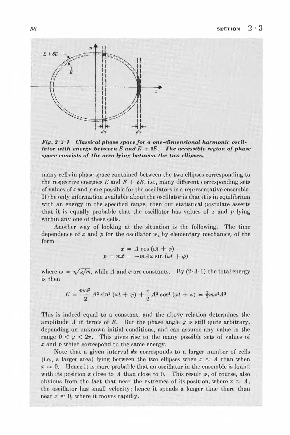
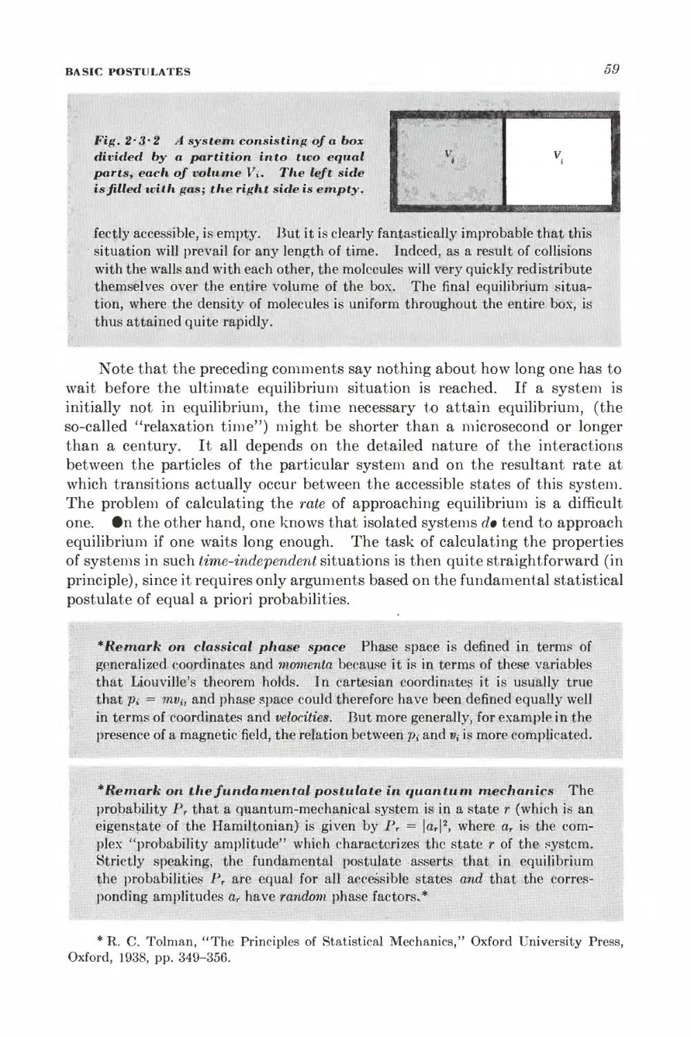
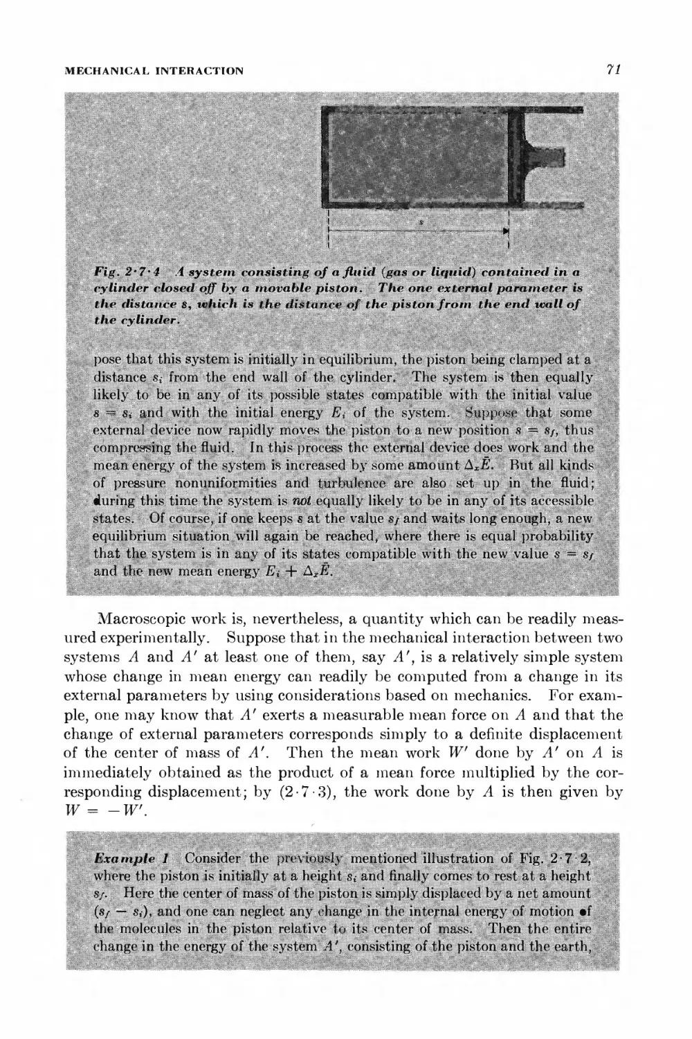
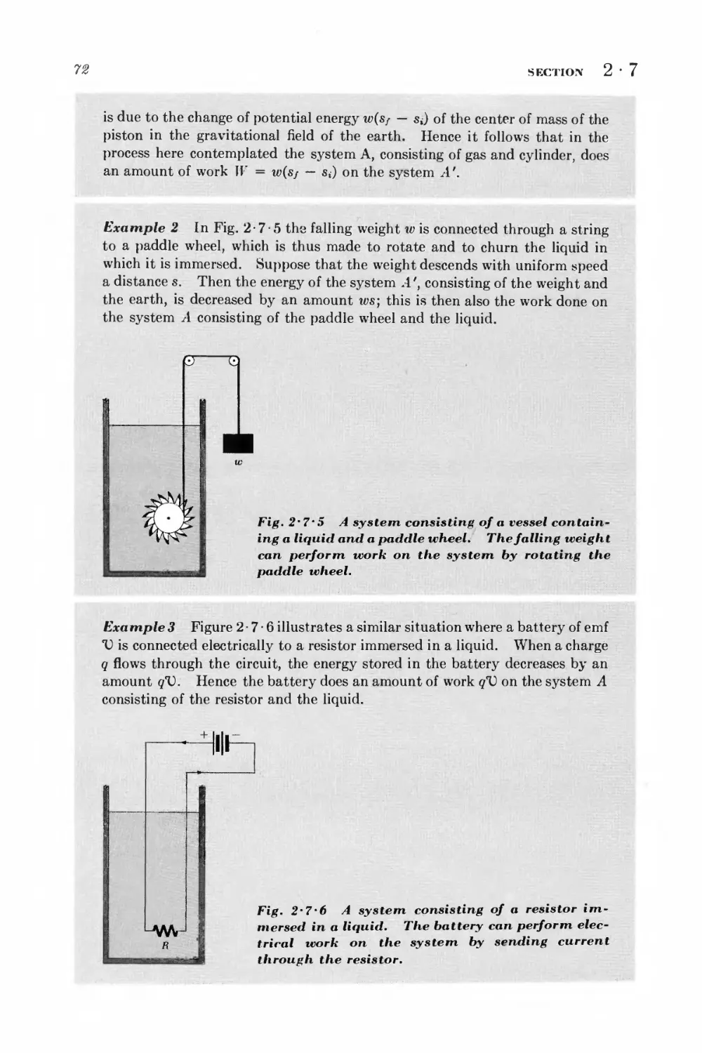
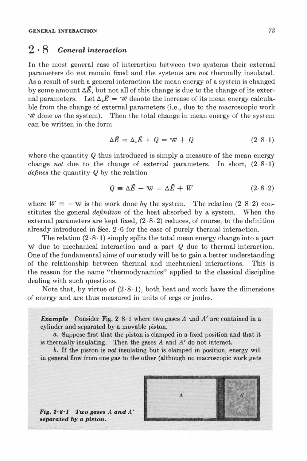
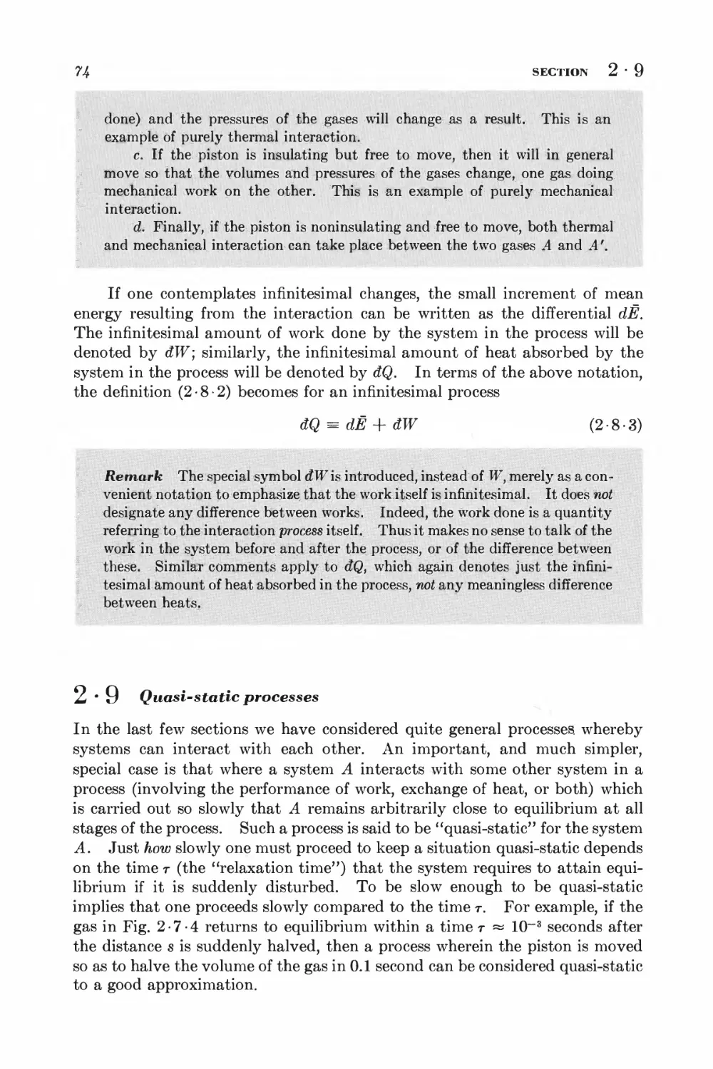
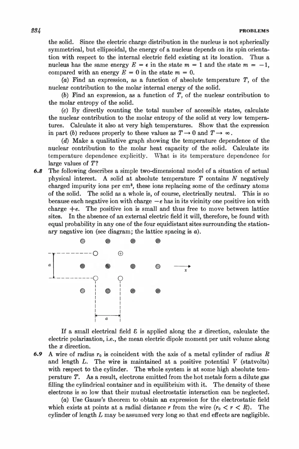
Text
                    - ntals of
ti 1 and
IPH s' S
\
\
I *
X
\ ■ \
F Reif

Fundamentals of
Statistical and
Thermal Physics

Fundamentals of
Statistical and
Thermal Physics
F. Reif
Carnegie Mellon University
WAVELAND
PRESS, INC.
Long Grove, Illinois

For information about this book, contact:
Waveland Press, Inc.
4180 IL Route 83, Suite 101
Long Grove, IL 60047-9580
(847) 634-0081
info@waveland.com
www.waveland.com
Copyright © 1965 by F Reif
Reissued 2009 by Waveland Press, Inc.
10-digit ISBN 1-57766-612-7
13-digit ISBN 978-1-57766-612-7
All rights reserved. No part of this book may be reproduced, stored in a
retrieval system, or transmitted in any form or by any means without
permission in writing from the publisher.
Printed in the United States of America
7 6 5 4 3 2 1

Fundamentals of
Statistical and
Thermal Physics

Preface
this book is devoted to a discussion of some of the basic physical concepts and
methods appropriate for the description of systems involving very many
particles. It is intended, in particular, to present the disciplines of
thermodynamics, statistical mechanics, and kinetic theory from a unified and modern
point of view. Accordingly, the presentation departs from the historical
development in which thermodynamics was the first of these disciplines to
arise as an independent subject. The history of the ideas concerned with heat,
work, and the kinetic theory of matter is interesting and instructive, but it
does not represent the clearest or most illuminating way of developing these
subjects. I have therefore abandoned the historical approach in favor of one
that emphasizes the essential unity of the subject matter and seeks to develop
physical insight by stressing the microscopic content of the theory.
Atoms and molecules are constructs so successfully established in modern
science that a nineteenth-century distrust of them seems both obsolete and
inappropriate. For this reason I have deliberately chosen to base the entire
discussion on the premise tjiat all macroscopic systems consist ultimately of
atoms obeying the laws of quantum mechanics. A combination of these
microscopic concepts with some statistical postulates then leads readily to
some very general conclusions on a purely macroscopic level of description.
These conclusions are valid irrespective of any particular models that might be
assumed about the nature or interactions of the particles in the systems under
consideration; they possess, therefore, the full generality of the classical laws
of thermodynamics. Indeed, they are more general, since they make clear
that the macroscopic parameters of a system are statistical in nature and
exhibit fluctuations which are calculable and observable under appropriate
conditions. Despite the microscopic point of departure, the book thus
contains much general reasoning on a purely macroscopic level—probably about
as much as a text on classical thermodynamics—but the microscopic content
of the macroscopic arguments remains clear at all stages. Furthermore, if one
is willing to adopt specific microscopic models concerning the particles consti-
vii

via
PREFACE
tuting a system, then it is also apparent how one can calculate macroscopic
quantities on the basis of this microscopic information. Finally, the statistical
concepts used to discuss equilibrium situations constitute an appropriate
preparation for their extension to the discussion of systems which are not
in equilibrium.
This approach has, in my own teaching experience, proved to be no more
difficult than the customary one which begins with classical thermodynamics.
The latter subject, developed along purely macroscopic lines, is conceptually
far from easy. Its reasoning is often delicate and of a type which seems
unnatural to many physics students, and the significance of the fundamental
concept of entropy is very hard to grasp. I have chosen to forego the
subtleties of traditional arguments based on cleverly chosen cycles and to substitute
instead the task of assimilating some elementary statistical ideas. The
following gains are thereby achieved: (a) Instead of spending much time discussing
various arguments based on heat engines, one can introduce the student at an
early stage to statistical methods which are of great and recurring importance
throughout all of physics, (b) The microscopic approach yields much better
physical insight into many phenomena and leads to a ready appreciation of
the meaning of entropy, (c) Much of modern physics is concerned with the
explanation of macroscopic phenomena in terms of microscopic concepts. It
seems useful, therefore, to follow a presentation which stresses at all times the
interrelation between microscopic and macroscopic levels of description. The
traditional teaching of thermodynamics and statistical mechanics as distinct
subjects has often left students with their knowledge compartmentalized and
has also left them ill-prepared to accept newer ideas, such as spin temperature
or negative temperature, as legitimate and natural, (d) Since a unified
presentation is more economical, conceptually as well as in terms of time, it permits
one to discuss more material and some more modern topics.
The basic plan of the book is the following: The first chapter is designed to
introduce some basic probability concepts. Statistical ideas are then applied
to systems of particles in equilibrium so as to develop the basic notions of
statistical mechanics and to derive therefrom the purely macroscopic
general statements of thermodynamics. The macroscopic aspects of the
theory are then discussed and illustrated at some length; the same is then done
for the macroscopic aspects of the theory. Some more complicated equilibrium
situations, such as phase transformations and quantum gases, are taken up
next. At this point the text turns to a discussion of nonequilibrium situations
and treats transport theory in dilute gases at varying levels of sophistication.
Finally, the last chapter deals with some general questions involving
irreversible processes and fluctuations. Several appendices contain mostly various
useful mathematical results.
The book is intended chiefly as a text for an introductory course in
statistical and thermal physics for college juniors or seniors. The mimeographed
notes on which it is based have been used in this way for more than two years
by myself and several of my colleagues in teaching such a course,at the
University of California in Berkeley. No prior knowledge of heat or thermo-

PREFACE
IX
dynamics is presupposed; the necessary prerequisites are only the equivalents
of a course in introductory physics and of an elementary course in atomic
physics. The latter course is merely supposed to have given the student
sufficient background in modern physics (a) to know that quantum mechanics
describes systems in terms of quantum states and wave functions, (6) to have
encountered the energy levels of a simple harmonic oscillator and to have seen
the quantum description of a free particle in a box, and (c) to have heard of the
Heisenberg uncertainty and Pauli exclusion principles. These are essentially
all the quantum ideas that are needed.
The material included here is more than can be covered in a one-semester
undergraduate course. This was done purposely (a) to include a discussion of
those basic ideas likely to be most helpful in facilitating the student's later
access to more advanced works, (b) to allow students with some curiosity to
read beyond the minimum on a given topic, (c) to give the instructor some
possibility of selecting between alternate topics, and (d) to anticipate current
revisions of the introductory physics course curriculum which should make
upper-division students in the ne^r future much more sophisticated and better
prepared to handle advanced material than they are now. In actual practice
I have successfully covered the first 12 chapters (omitting Chapter 10 and most
starred sections) in a one-semester course. Chapter 1 contains a discussion of
probability concepts more extensive than is needed for the understanding of
subsequent chapters. In addition, the chapters are arranged in such a way
that it is readily possible, after the first eight chapters, to omit some chapters
in favor of others without encountering difficulties with prerequisites.
The book should also be suitable for use in an introductory graduate
course if one includes the starred sections and the last three chapters, which
contain somewhat more advanced material. Indeed, with students who have
studied classical thermodynamics but have had no significant exposure to the
ideas of statistical mechanics in their undergraduate career, one cannot hope to
cover in a one-semester graduate course appreciably more subject matter than
is treated here. One of my colleagues has thus used the material in our
Berkeley graduate course on statistical mechanics (a course which is, as yet,
mostly populated by students with this kind of preparation).
Throughout the book I have tried to keep the approach well-motivated and
to strive for simplicity of presentation. It has not been my aim to pursue rigor
in the formal mathematical sense. I have, however, attempted to keep
the basic physical ideas in the forefront and to discuss them with care. In the
process the book has become longer than it might have otherwise, for I have
not hesitated to increase the ratio of words to formulas, to give illustrative
examples, or to present several ways of looking at a question whenever I felt
that it would enhance understanding. My aim has been to stress physical
insight and important methods of reasoning, and I advise most earnestly that
the student stress these aspects of the subject instead of trying to memorize
various formulas meaningless in themselves. To avoid losing the reader in
irrelevant details, I have often refrained from presenting the most general case
of a problem and have sought instead to treat relatively simple cases by power-

X
PREFACE
ful and easily generalizable methods. The book is not meant to be
encyclopaedic; it is merely intended to provide a basic skeleton of some fundamental
ideas most likely to be useful to the student in his future work. Needless to
say, some choices had to be made. For example, I thought it important to
introduce the Boltzmann equation, but resisted the temptation of discussing
applications of the Onsager relations to various irreversible phenomena such
as thermoelectric effects.
It is helpful if a reader can distinguish material of secondary importance
from that which is essential to the main thread of the argument. Two devices
have been used to indicate subject matter of subsidiary importance: (a)
Sections marked by a star (asterisk) contain material which is more advanced or
more detailed; they can be omitted (and probably should be omitted in a first
reading) without incurring a handicap in proceeding to subsequent sections.
(b) Many remarks, examples, and elaborations are interspersed throughout the
text and are set off on a gray background. Conversely, black marginal
pointers have been used to emphasize important results and to facilitate
reference to them.
The book contains about 230 problems, which should be regarded as an
essential part of the text. It is indispensable that the student solve an
appreciable fraction of these problems if he is to gain a meaningful understanding of
the subject matter and not merely a casual hearsay acquaintance with it.
I am indebted to several of my colleagues for many valuable criticisms
and suggestions. In particular, I should like to thank Prof. Eyvind H,
Wichmann, who read an older version of the entire manuscript with meticulous
care, Prof. Owen Chamberlain, Prof. John J. Hopfield, Dr. Allan N. Kaufman,
and Dr. John M. Worlock. Needless to say, none of these people should be
blamed for the flaws of the final product.
Acknowledgements are also due to Mr. Roger F. Knacke for providing
the answers to the problems. Finally, I am particularly grateful to my
secretary, Miss Beverly West, without whose devotion and uncanny ability
to transform pages of utterly illegible handwriting into a perfectly typed
technical manuscript this book could never have been written.
It has been said that "an author never finishes a book, he merely abandons
it." I have come to appreciate vividly the truth of this statement and dread
to see the day when, looking at the manuscript in print, I am sure to realize
that so many things could have been done better and explained more clearly.
If I abandon the book nevertheless, it is in the modest hope that it may be
useful to others despite its shortcomings.
F. REIF

Contents
Preface vii
Introduction to statistical methods
RANDOM WALK AND BINOMIAL DISTRIBUTION
1 • 1 Elementary statistical concepts and examples 4
1 • 2 The simple random walk problem in one dimension 7
1 • 3 General discussion of mean values 11
1-4 Calculation of mean values for the random walk problem 18
1 • 5 Probability distribution for large N 17
1 • 6 Gaussian probability distributions 21
GENERAL DISCUSSION OF THE RANDOM WALK
1 • 7 Probability distributions involving several variables 25
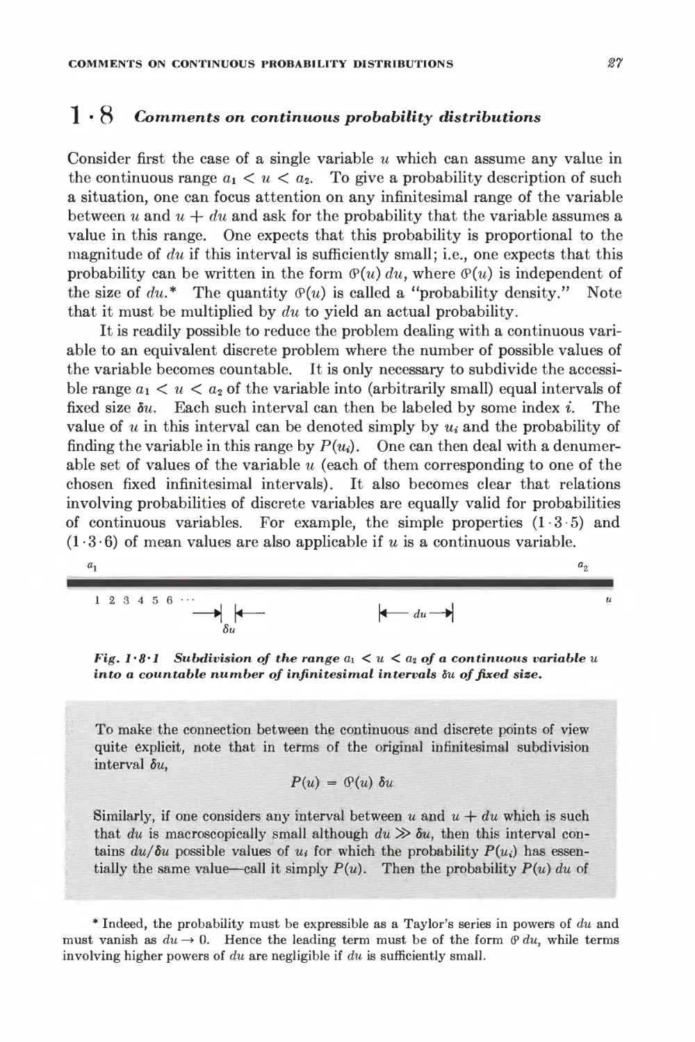
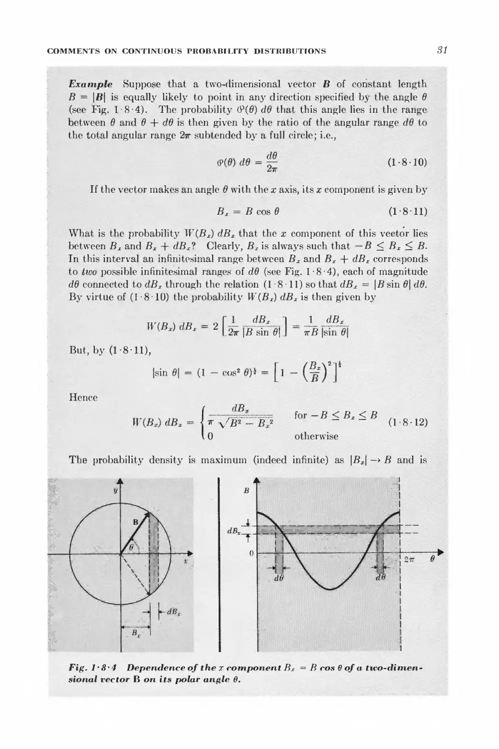
1 • 8 Comments on continuous probability distributions 27
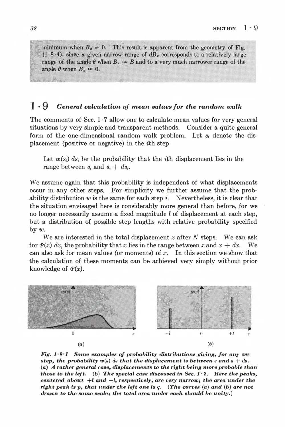
1 • 9 General calculation of mean values for the random walk 82
*1 • 10 Calculation of the probability distribution 85
*1 • 11 Probability distribution for large N 87
Statistical description of systems of particles
STATISTICAL FORMULATION OF THE MECHANICAL PROBLEM
2 • 1 Specification of (he state of a system 48
2 • 2 Statistical ensemble 52
2 • 3 Basic postulates 58
2 • 4 Probability calculations 60
2 • 5 Behavior of the density of states 61

INTERACTION BETWEEN MACROSCOPIC SYSTEMS
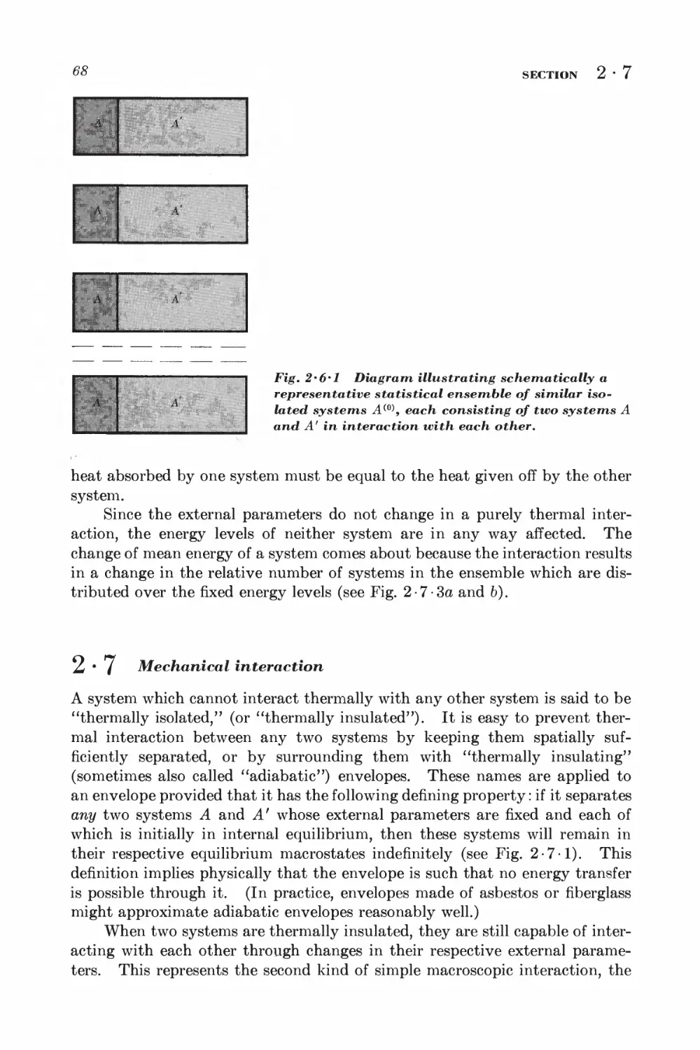
2-6 Thermal interaction 66
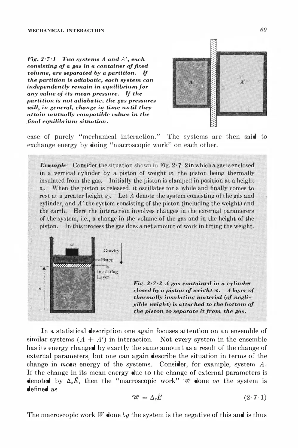
2 • 7 Mechanical interaction 68
2 • 8 General interaction 78
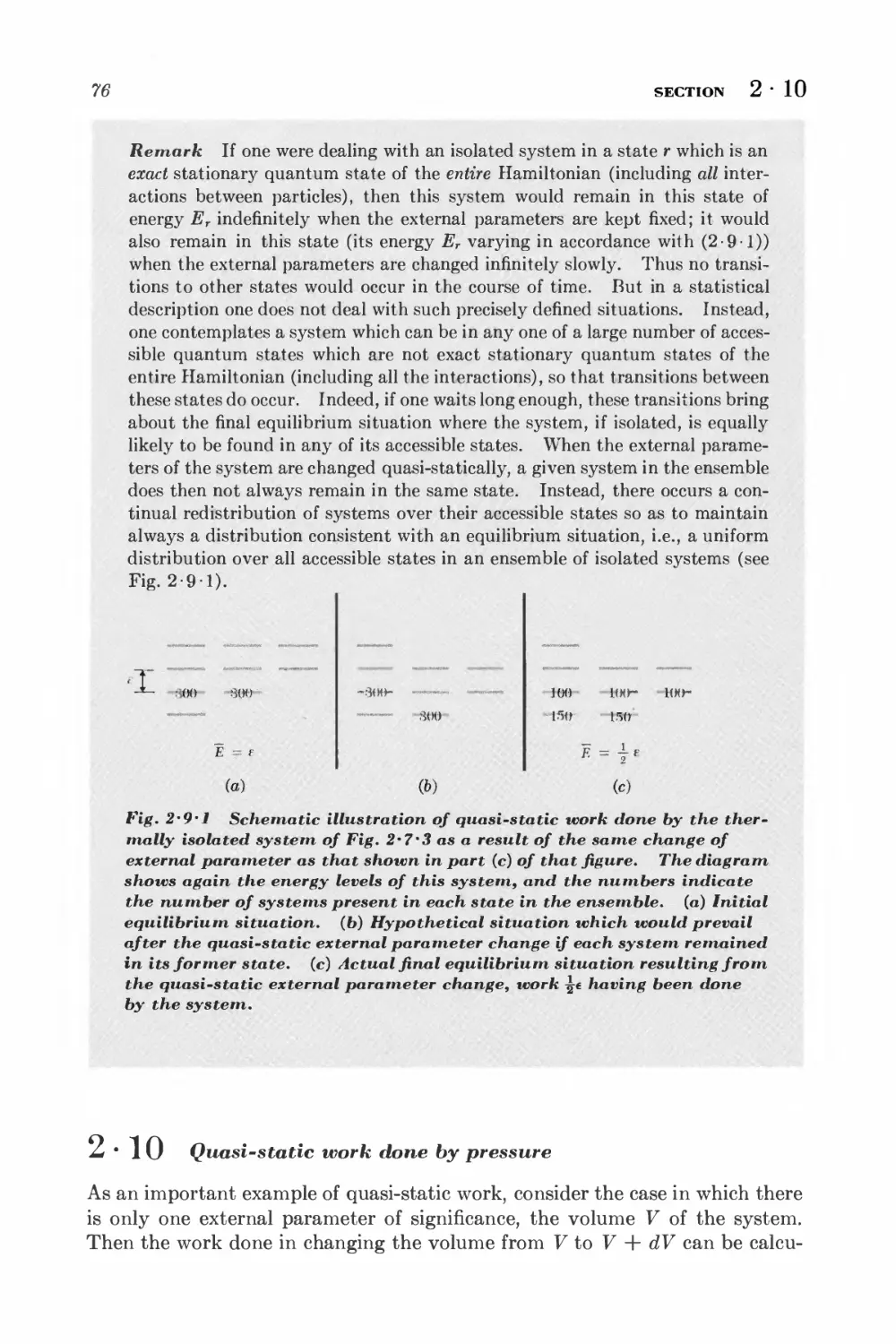
2 • 9 Quasi-static processes 74
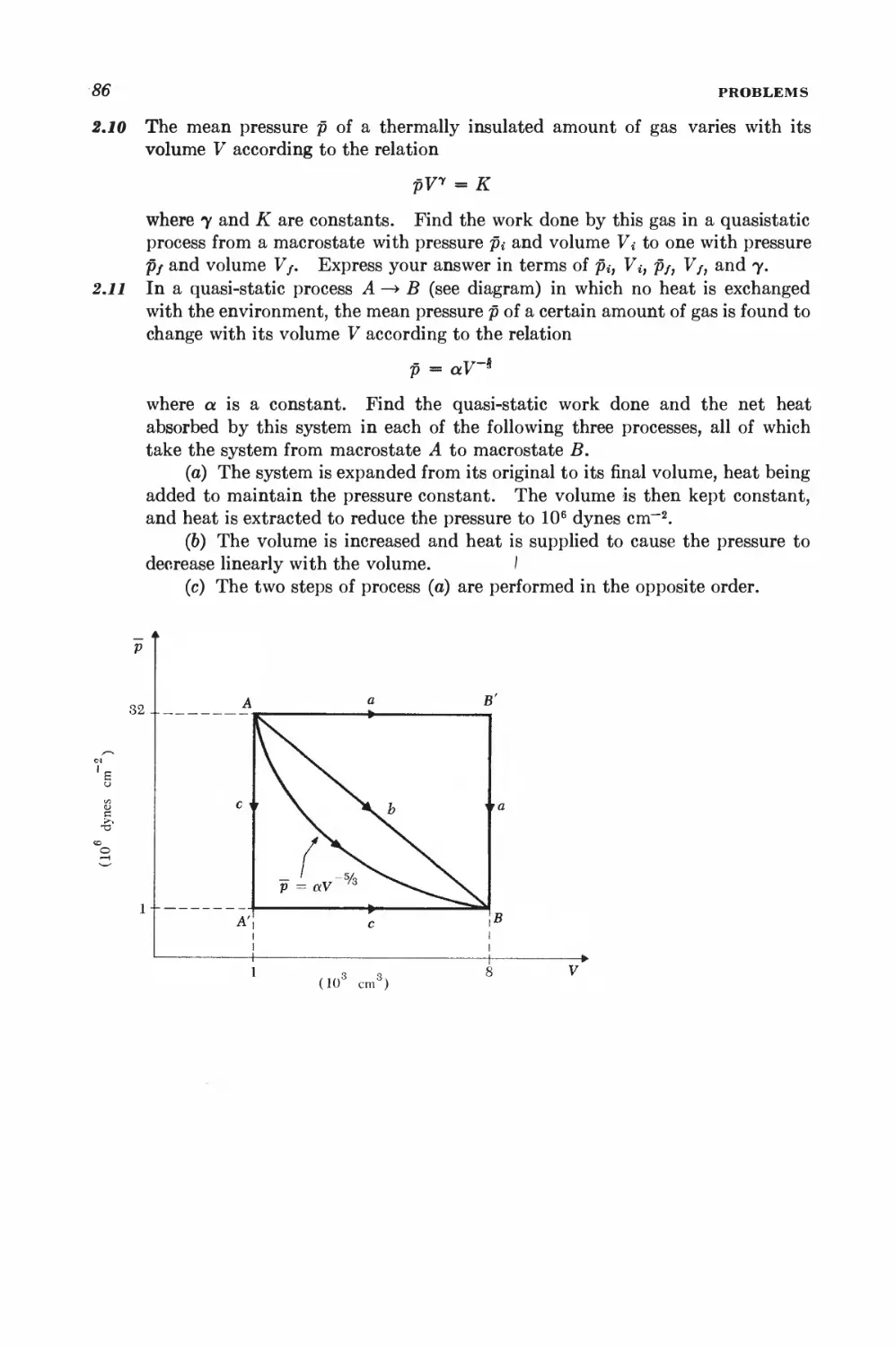
2 • 10 Quasi-static work done by pressure 76
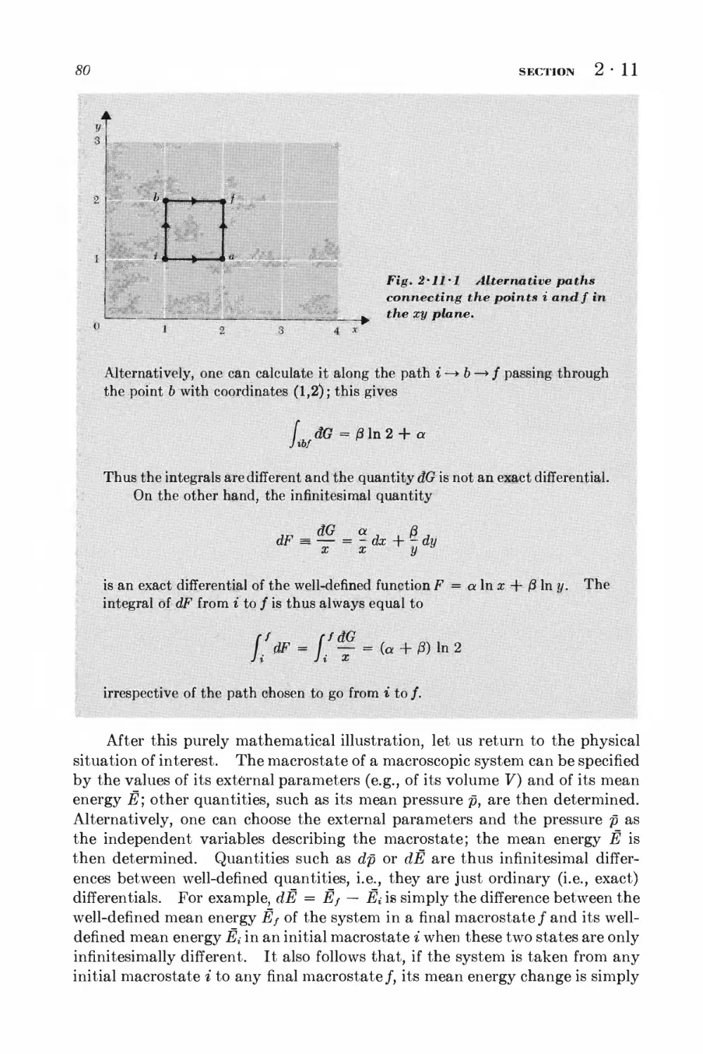
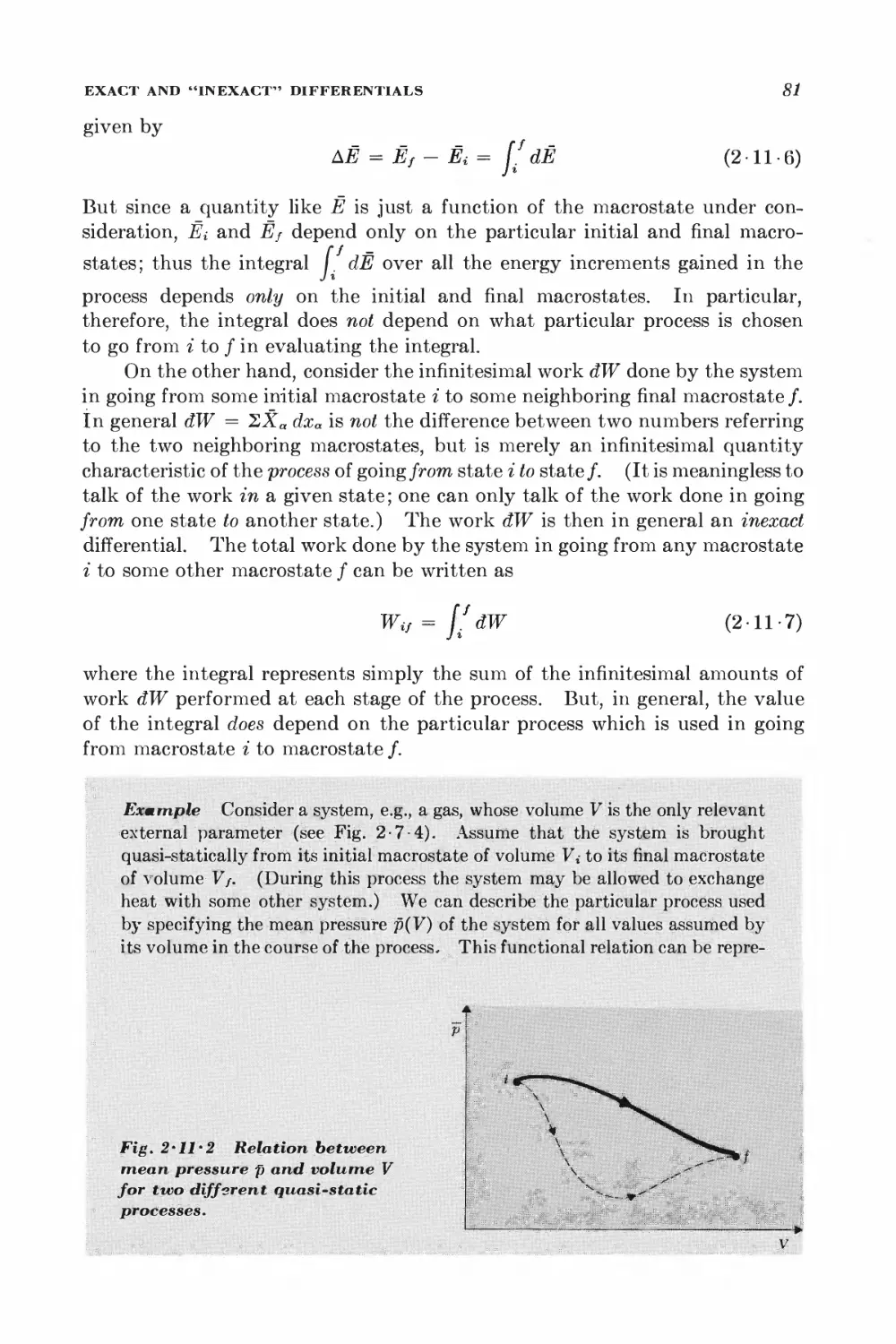
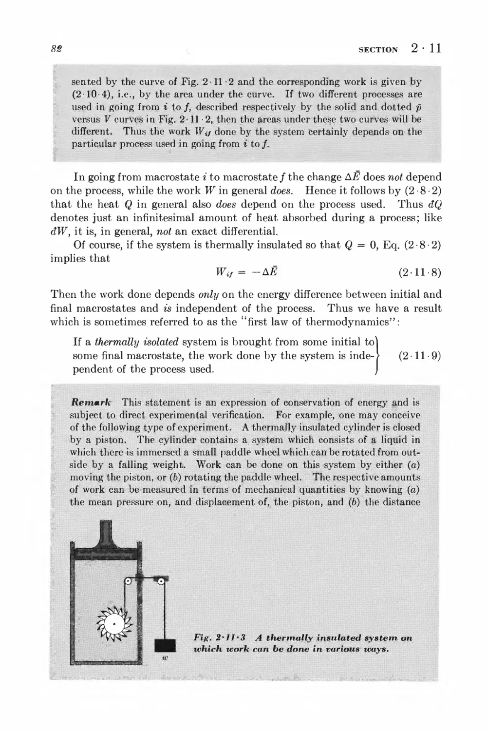
2 11 Exact and "inexact" differentials 78
O Statistical thermodynamics 87
IRREVERSIBILITY AND THE ATTAINMENT OF EQUILIBRIUM
3 • 1 Equilibrium conditions and constraints 87
3 • 2 Reversible and irreversible processes 91
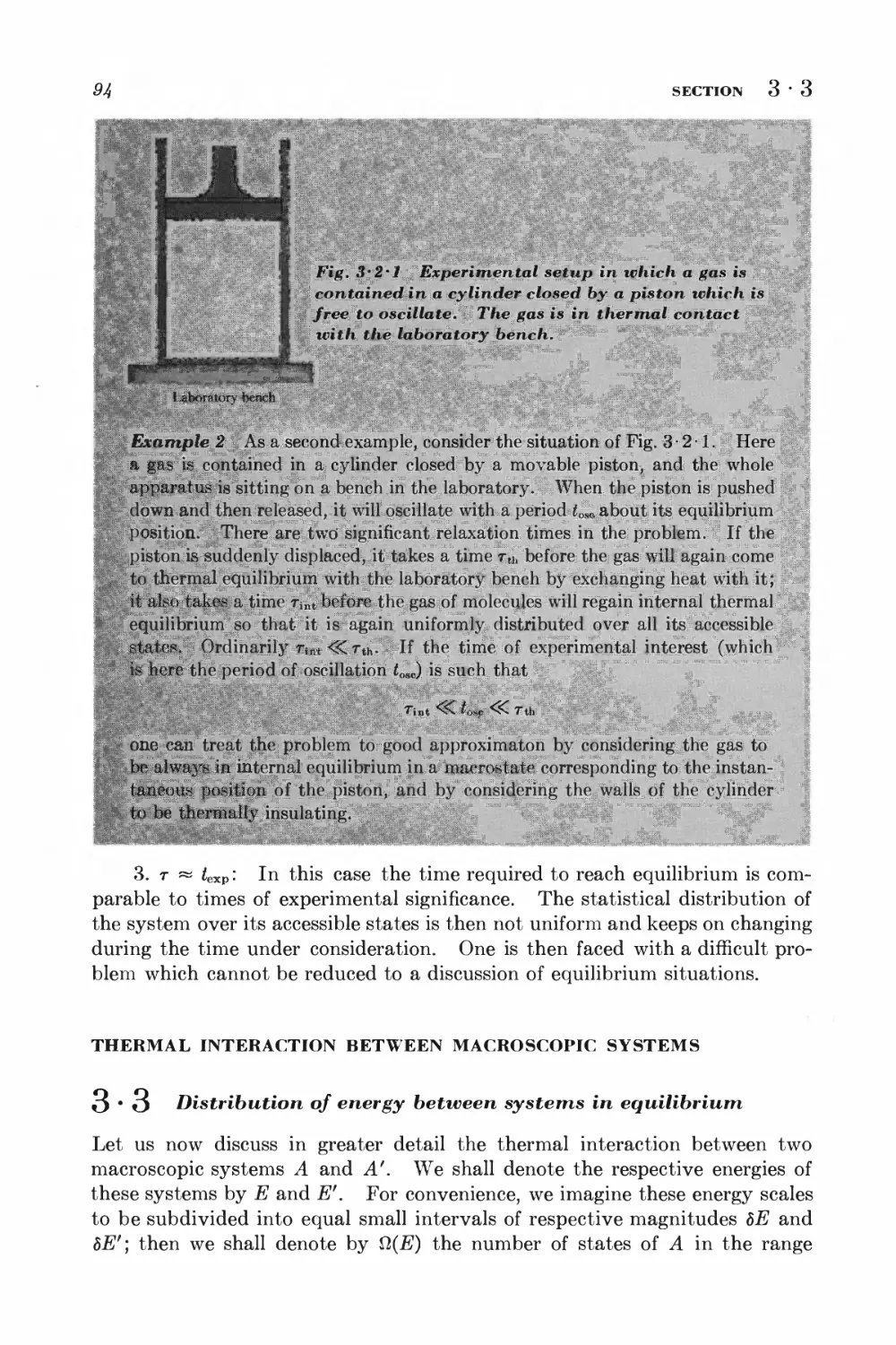
THERMAL INTERACTION BETWEEN MACROSCOPIC SYSTEMS
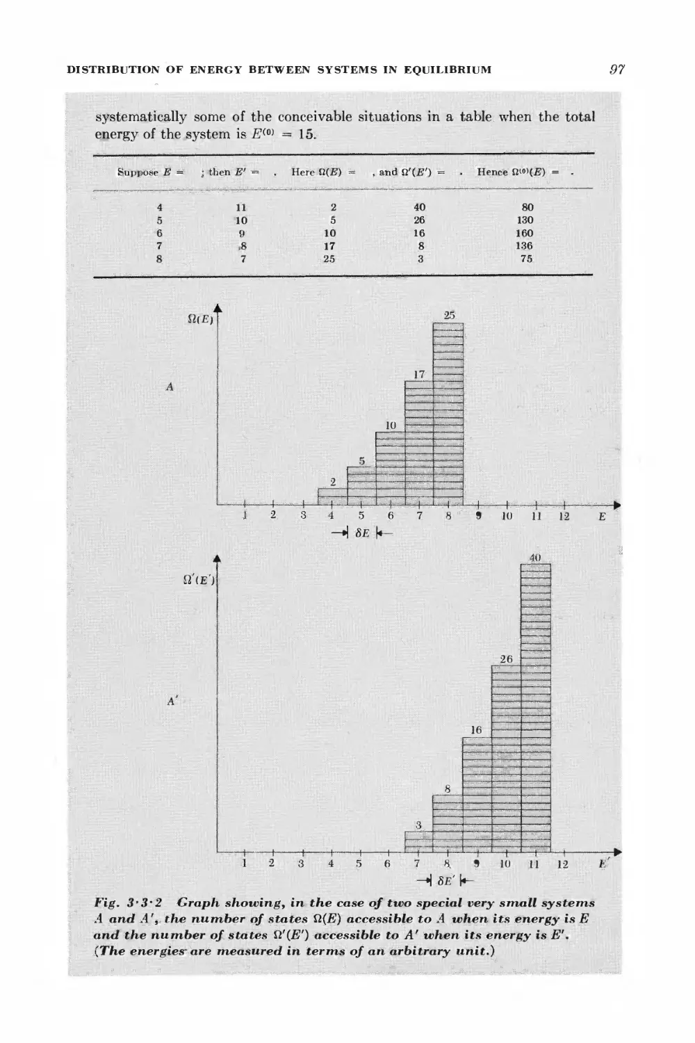
3 • 3 Distribution of energy between systems in equilibrium 94
3-4 The approach to thermal equilibrium 100
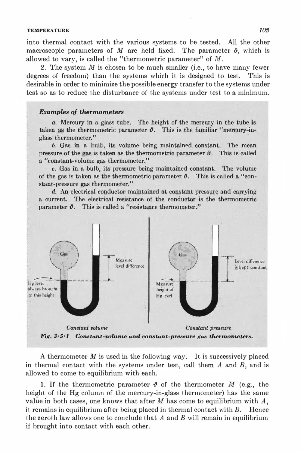
3-5 Temperature 102
3-6 Heat reservoirs 106
3-7 Sharpness of the probability distribution 108
GENERAL INTERACTION BETWEEN MACROSCOPIC SYSTEMS
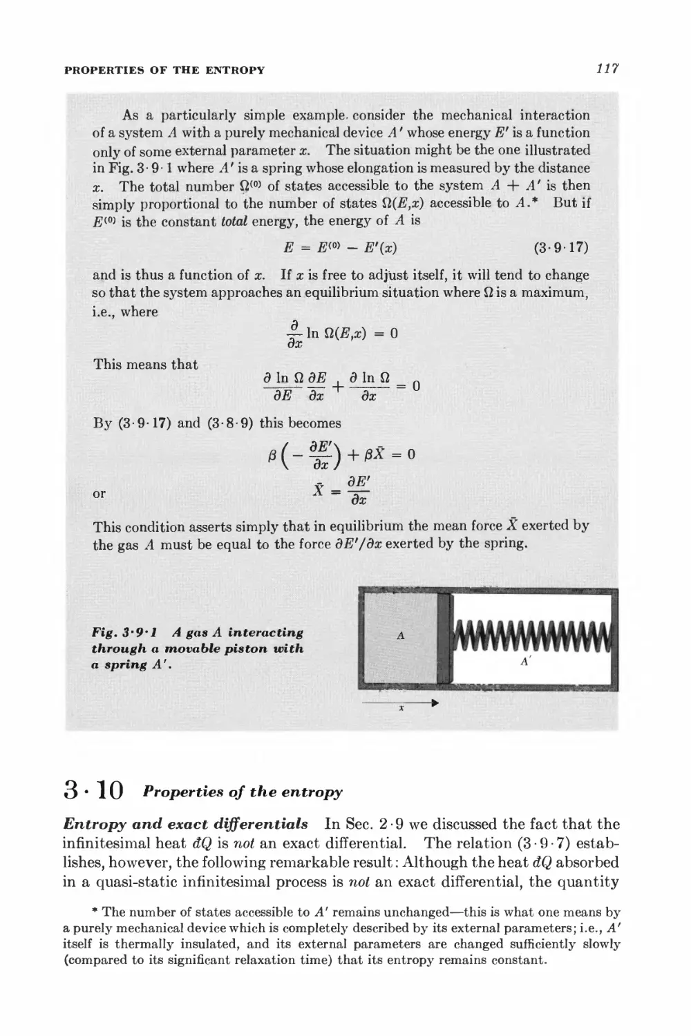
3-8 Dependence of the density of states on the external parameters 112
3-9 Equilibrium between interacting systems 114
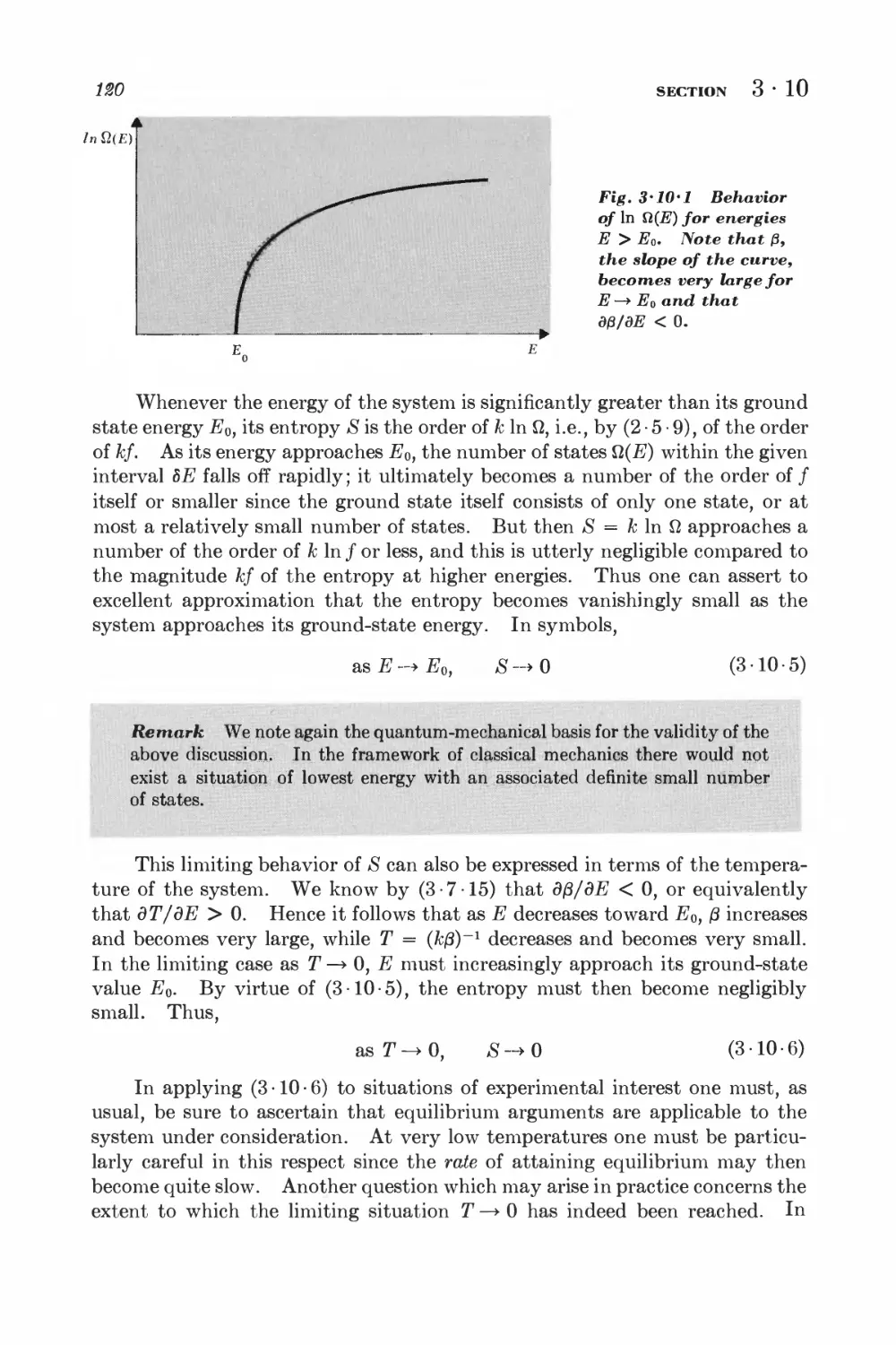
3-10 Properties of the entropy 117
SUMMARY OF FUNDAMENTAL RESULTS
3-11 Thermodynamic laws and basic statistical relations 122
3-12 Statistical calculation of thermodynamic quantities 124
4 Macroscopic parameters and their measurement 128
4 • 1 Work and internal energy 128
4-2 Heat 181
4-3 Absolute temperature 188
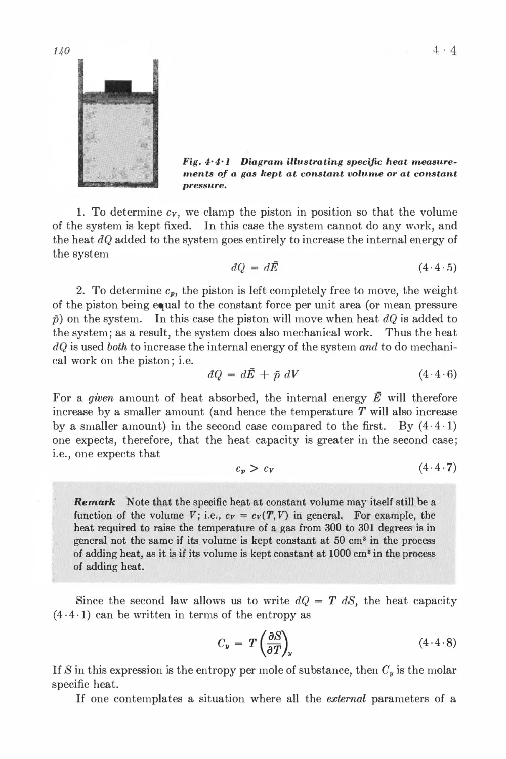
4-4 Heat capacity and specific heat 189
4-5 Entropy 142
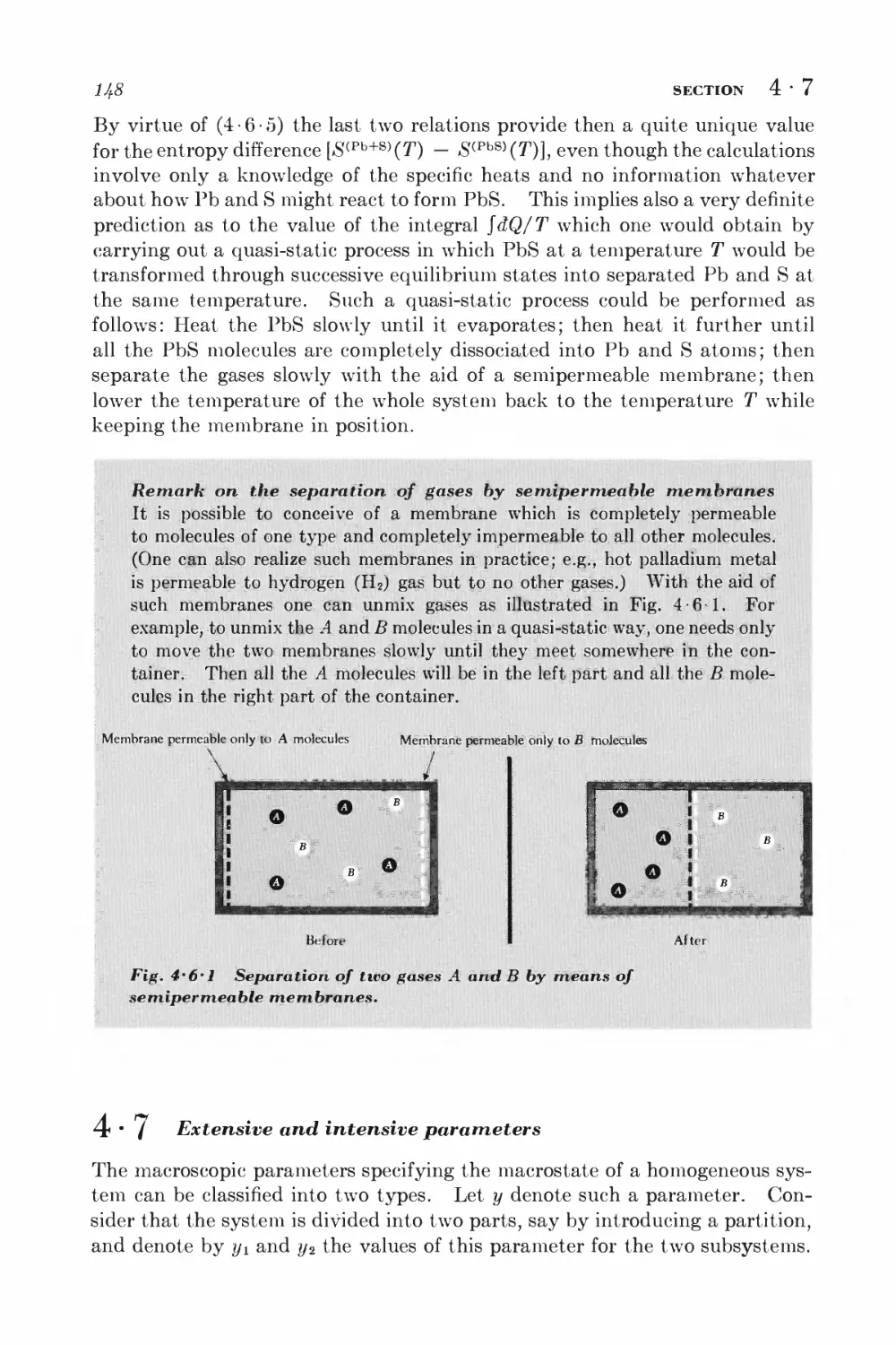
4 • 6 Consequences of the absolute definition of entropy 145
4-7 Extensive and intensive parameters 148
Simple applications of macroscopic thermodynamics 152
PROPERTIES OF IDEAL GASES
5 • 1 Equation of state and internal energy 168
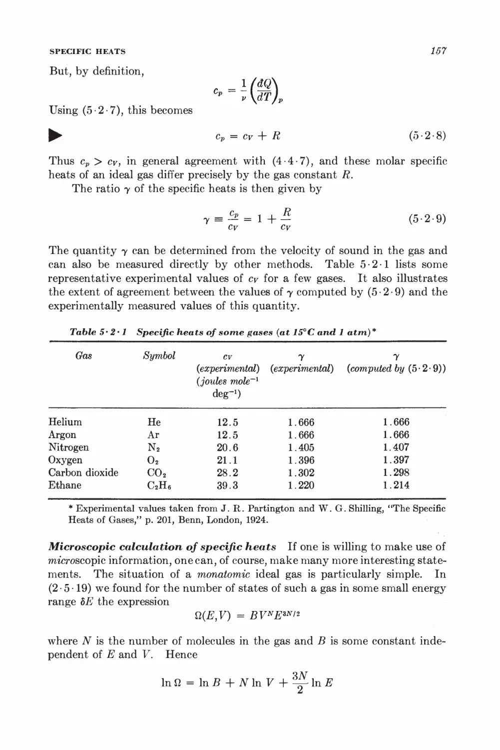
5-2 Specific heats 156

5-3 Adiabatic expansion or compression 158
5-4 Entropy 160
GENERAL RELATIONS FOR A HOMOGENEOUS SUBSTANCE
5-5 Derivation of general relations 161
5 • 6 Summary of Maxwell relations and thermodynamic functions 164
5-7 Specific heats 166
5-8 Entropy and internal energy 171
FREE EXPANSION AND THROTTLING PROCESSES
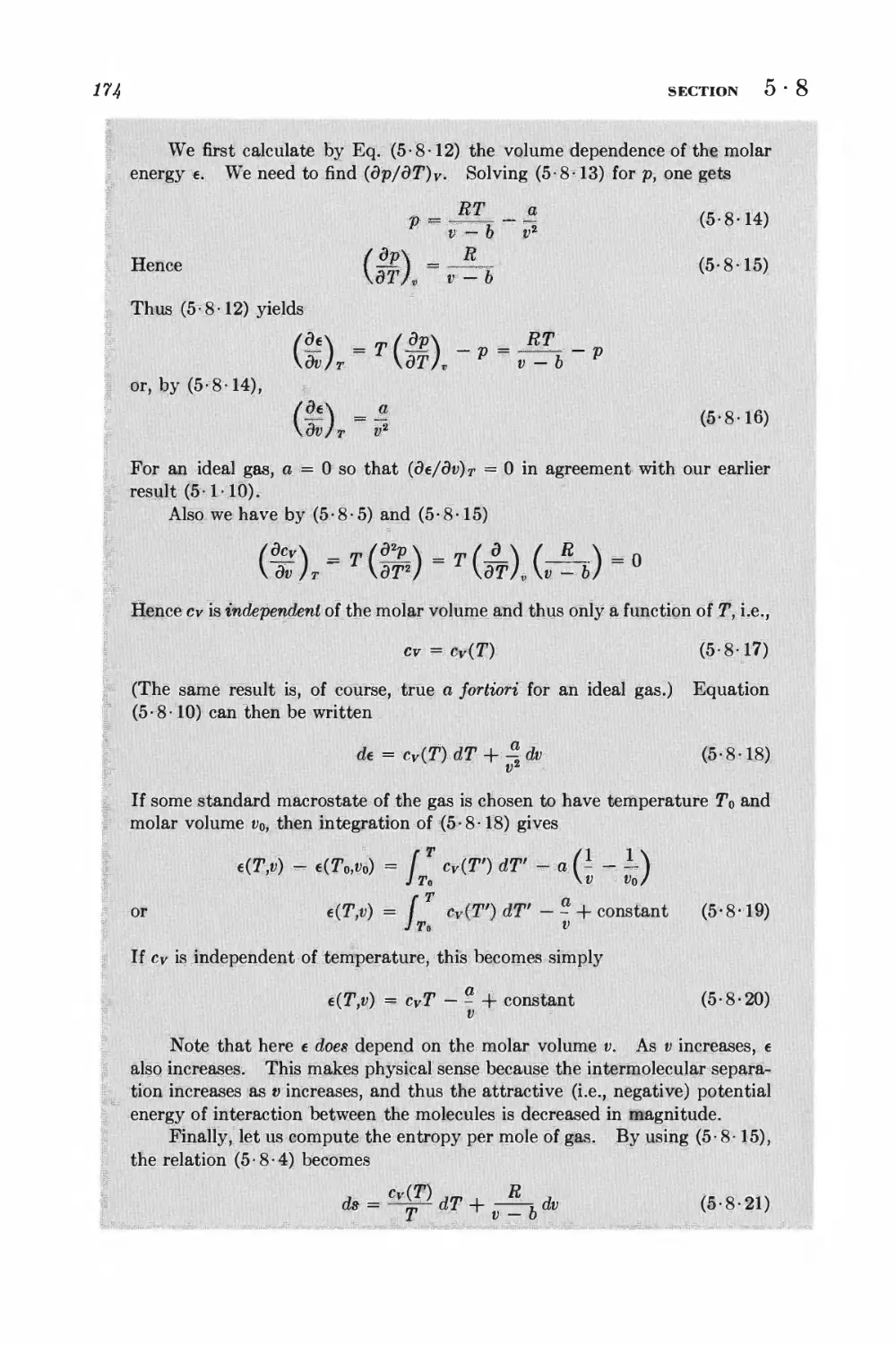
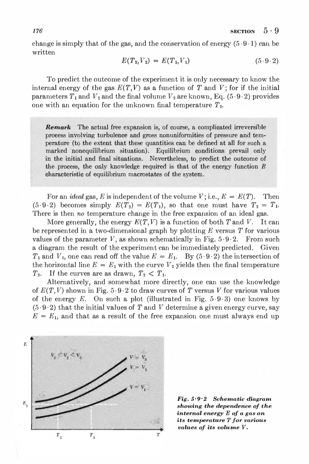
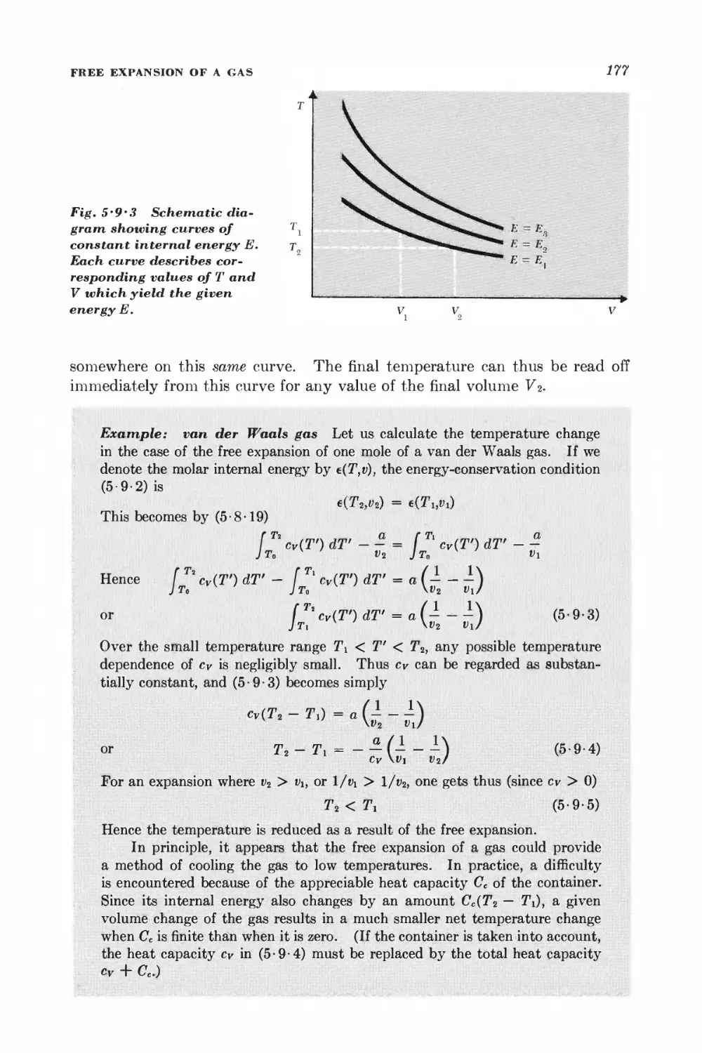
5 • 9 Free expansion of a gas 175
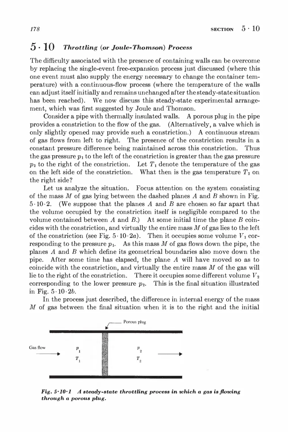
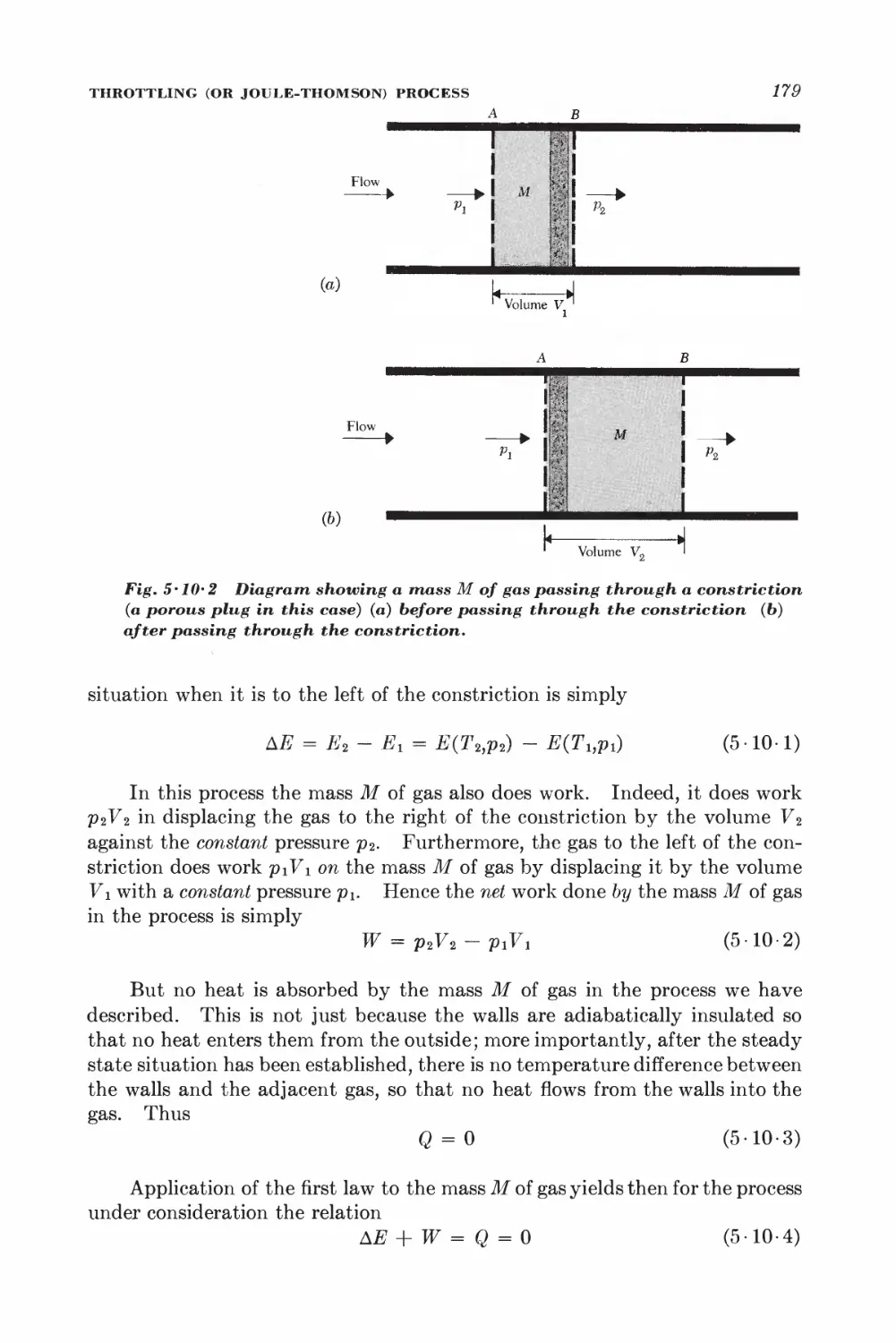
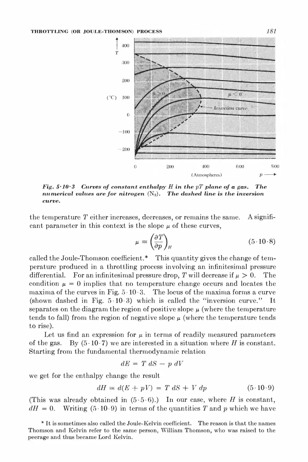
5 10 Throttling (or Joule-Thomson) process 178
HEAT ENGINES AND REFRIGERATORS
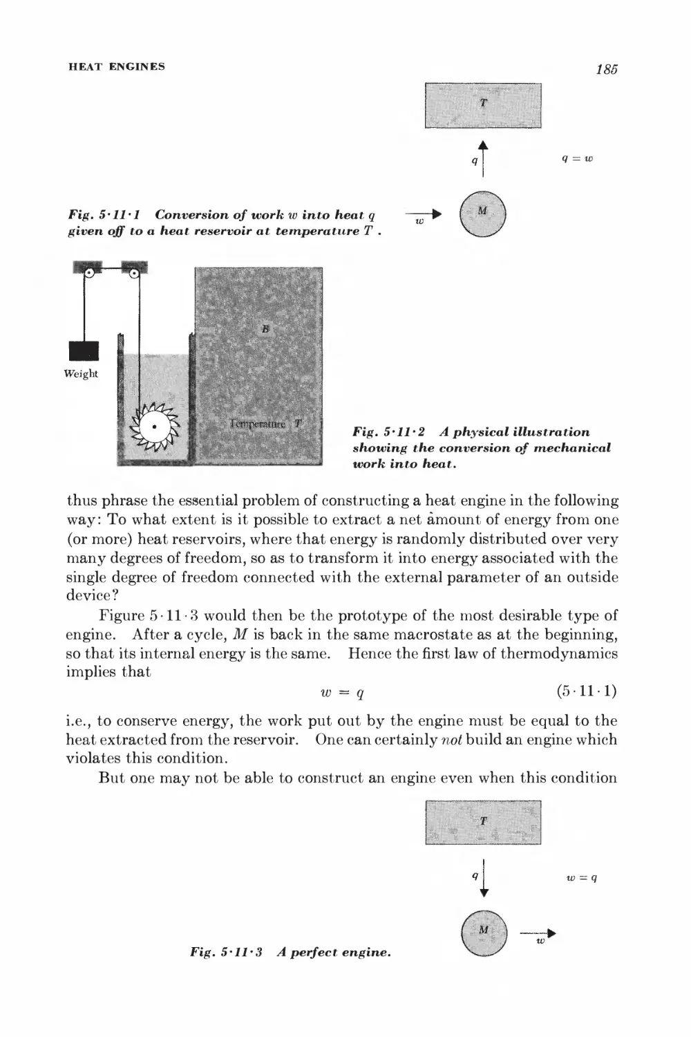
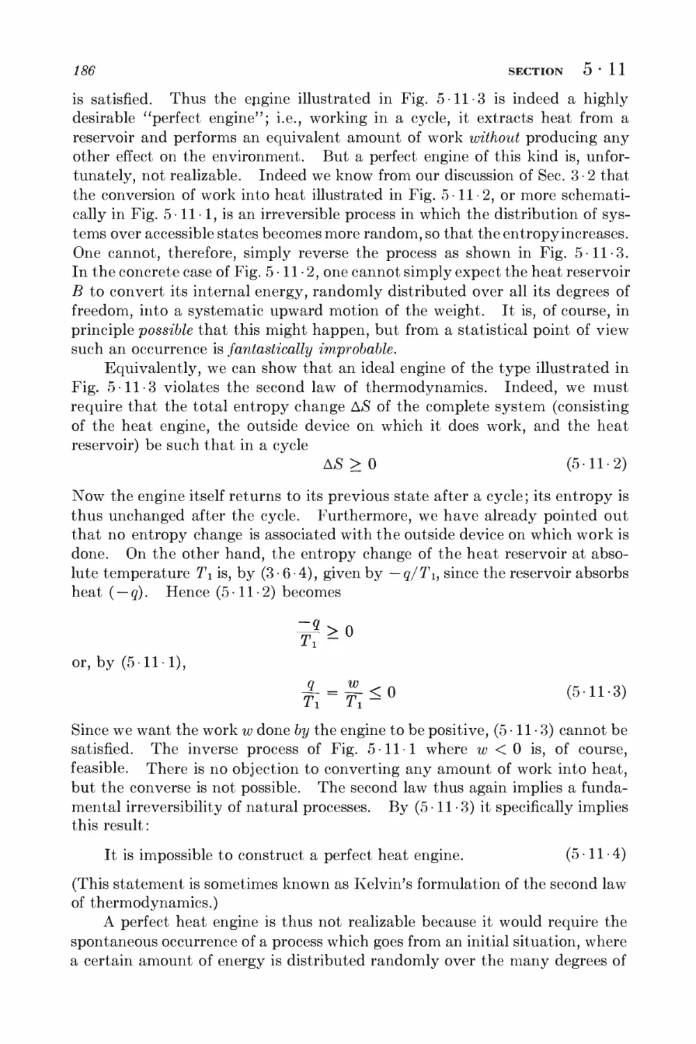
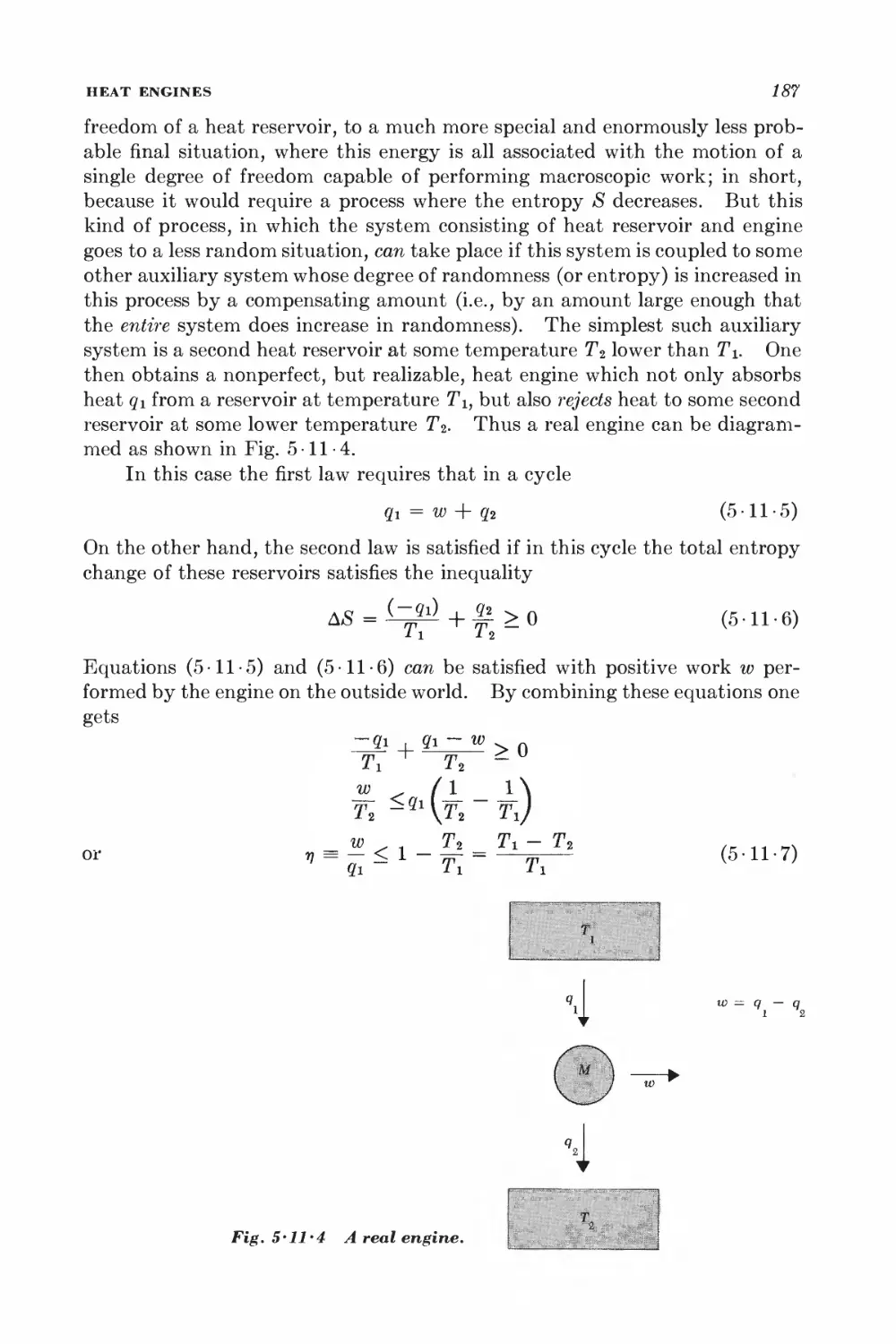
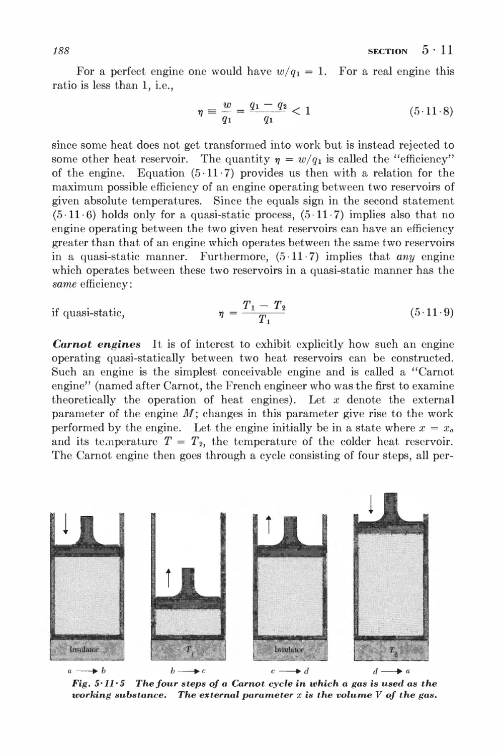
5-11 Heat engines 184
5 12 Refrigerators 190
Basic methods and results of statistical mechanics 201
ENSEMBLES REPRESENTATIVE OF SITUATIONS OF PHYSICAL INTEREST
6 • 1 Isolated system 201
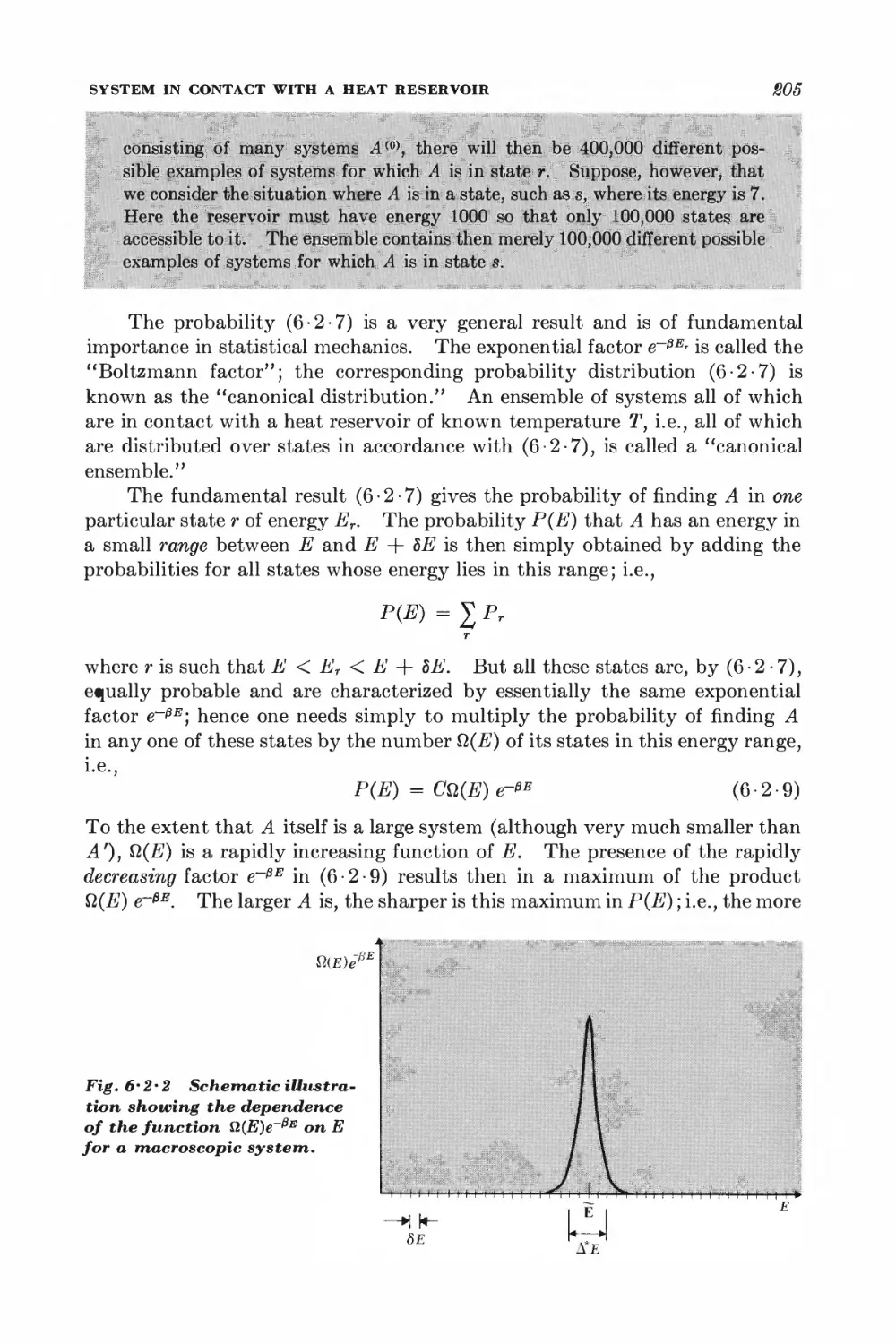
6 • 2 System in contact with a heat reservoir 202
6 • 3 Simple applications of the canonical distribution 206
6-4 System with specified mean energy 211
6 • 5 Calculation of mean values in a canonical ensemble 212
6-6 Connection with thermodynamics 214
APPROXIMATION METHODS
6-7 Ensembles used as approximations 219
*6 • 8 Mathematical approximation methods 221
GENERALIZATIONS AND ALTERNATIVE APPROACHES
*6 • 9 Grand canonical and other ensembles 225
*6-10 Alternative derivation of the canonical distribution 229
Simple applications of statistical mechanics 237
GENERAL METHOD OF APPROACH
7 • 1 Partition functions and their properties 287
IDEAL MONATOMIC GAS
7 • 2 Calculation of thermodynamic quantities 239
7-3 Gibbs paradox 248
7 • 4 Validity of the classical approximation 246

THE EQUIPARTITION THEOREM
7 • 5 Proof of the theorem 248
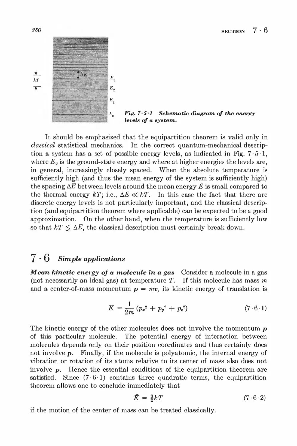
7 • 6 Simple applications 250
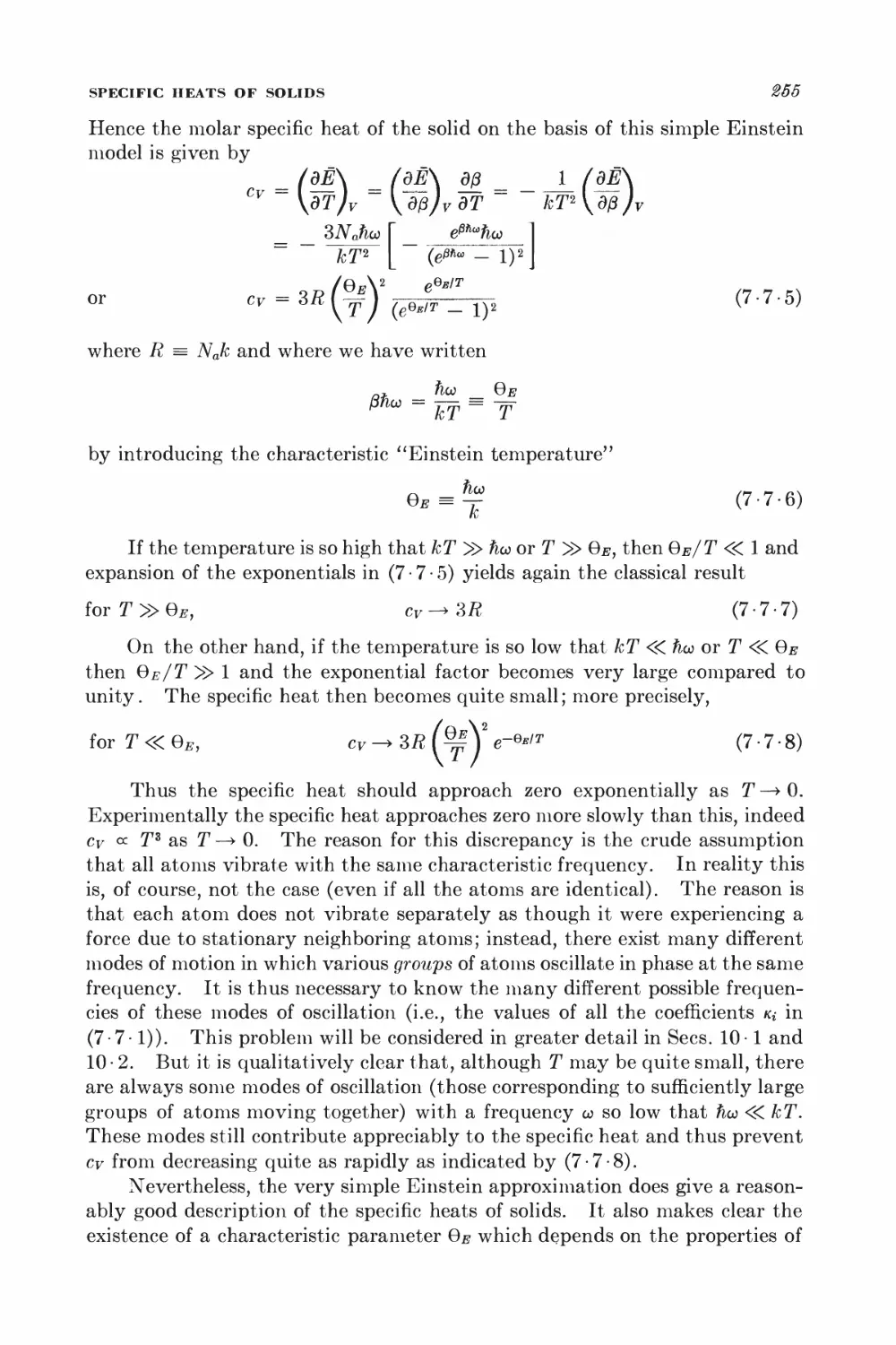
7 - 7 Specific heats of solids 253
PARAMAGNETISM
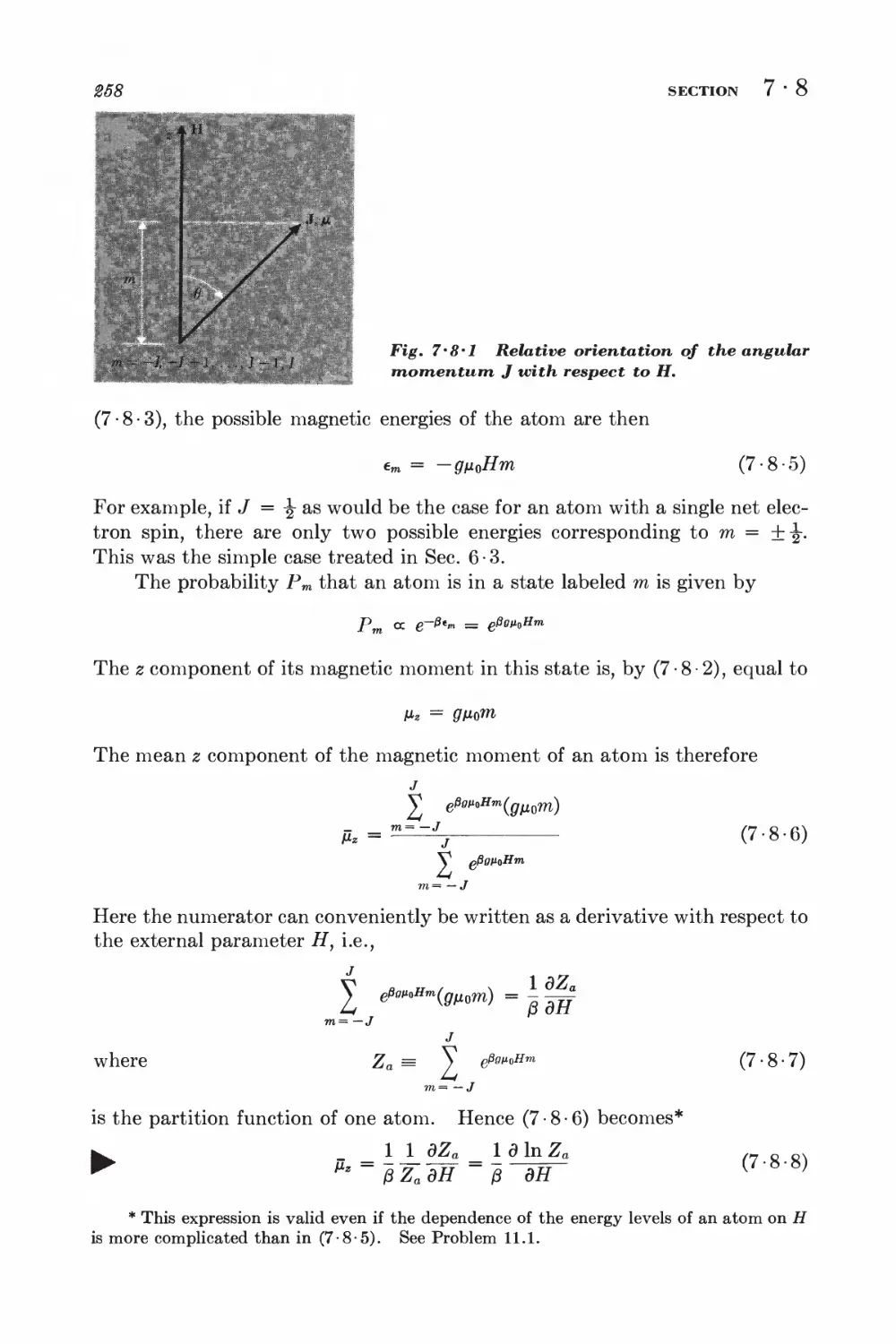
7 • 8 General calculation of magnetization 257
KINETIC THEORY OF DILUTE GASES IN EQUILIBRIUM
7 • 9 Maxwell velocity distribution 262
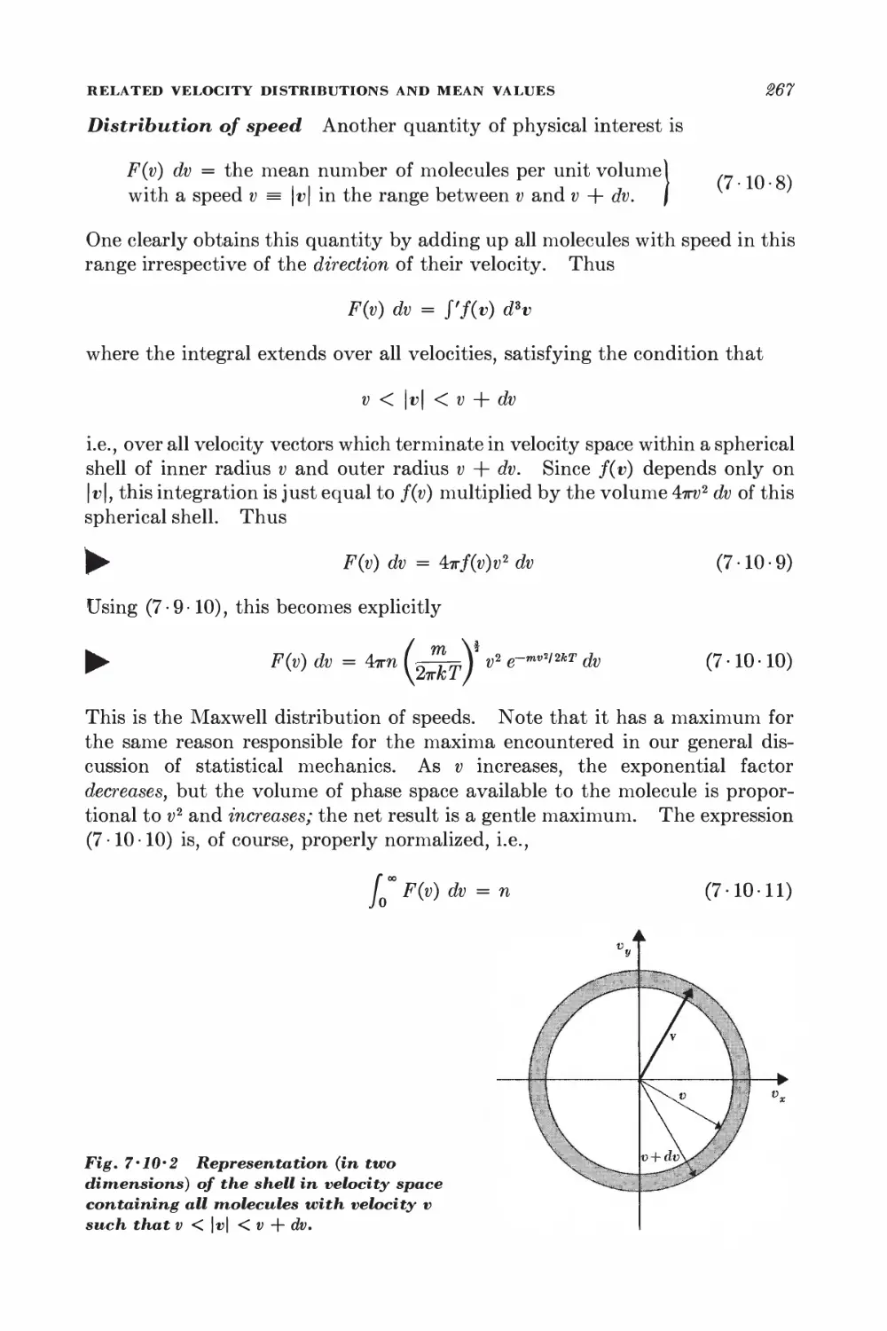
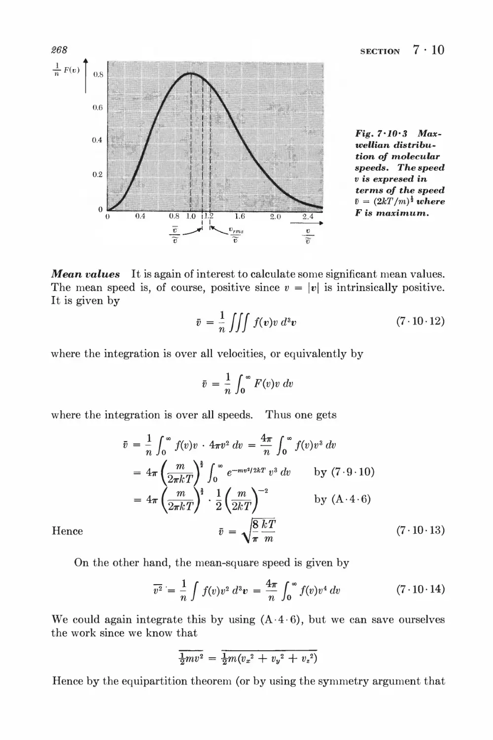
7 • 10 Related velocity distributions and mean values 265
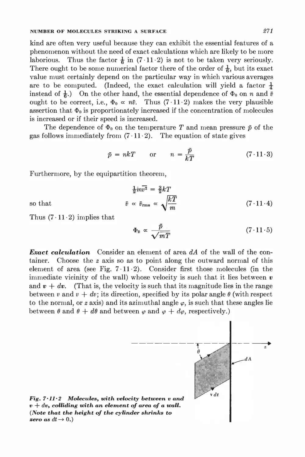
7 11 Number of molecules striking a surface 269
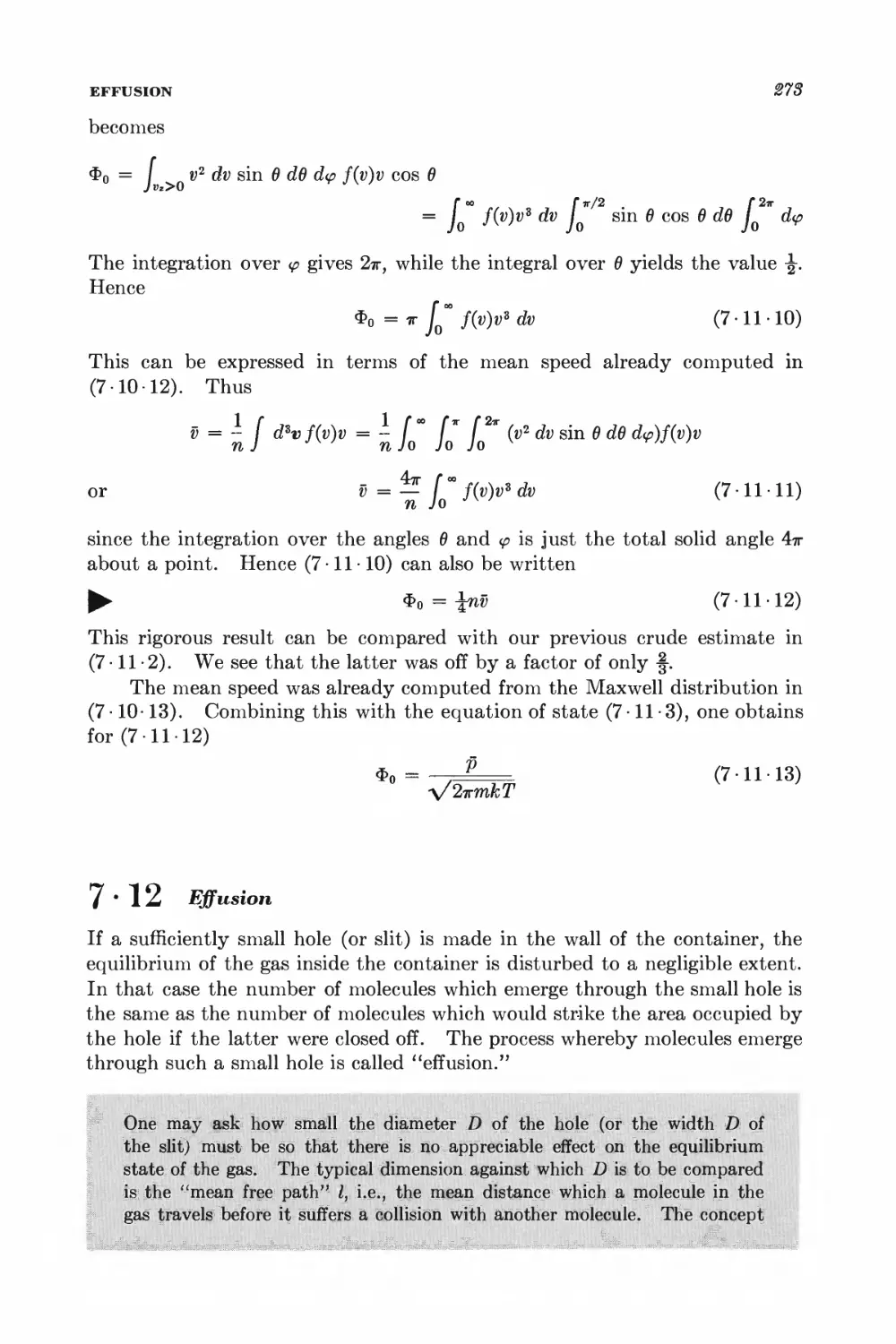
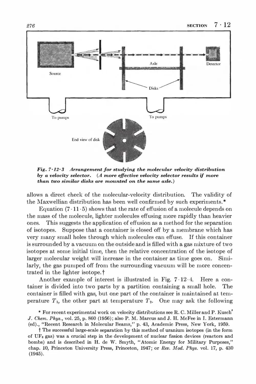
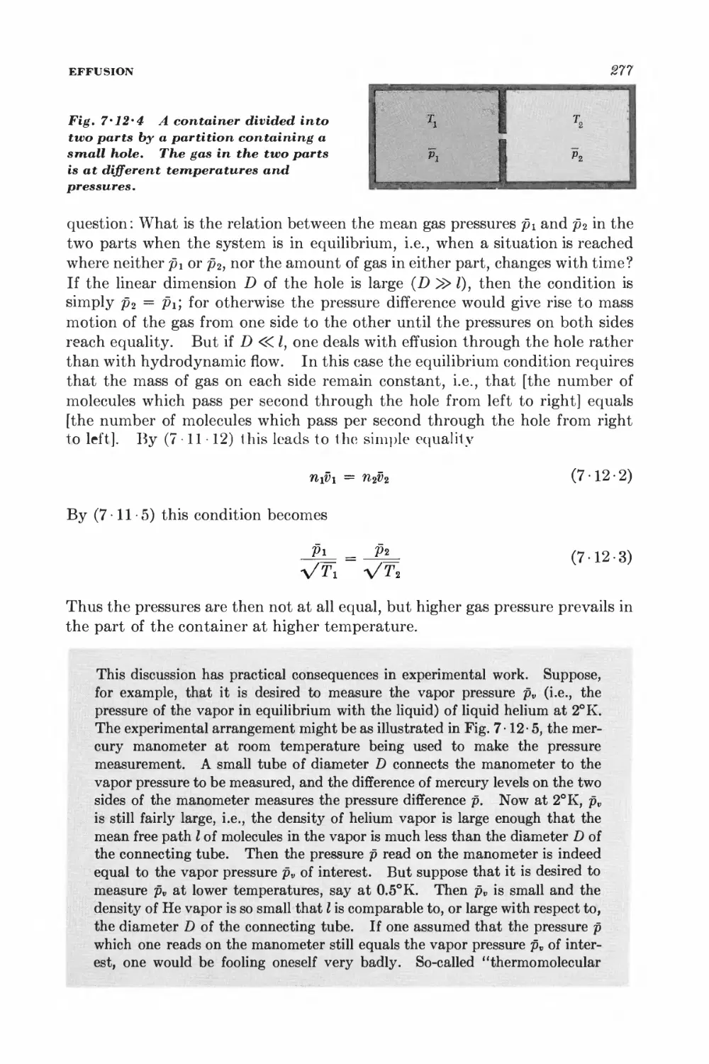
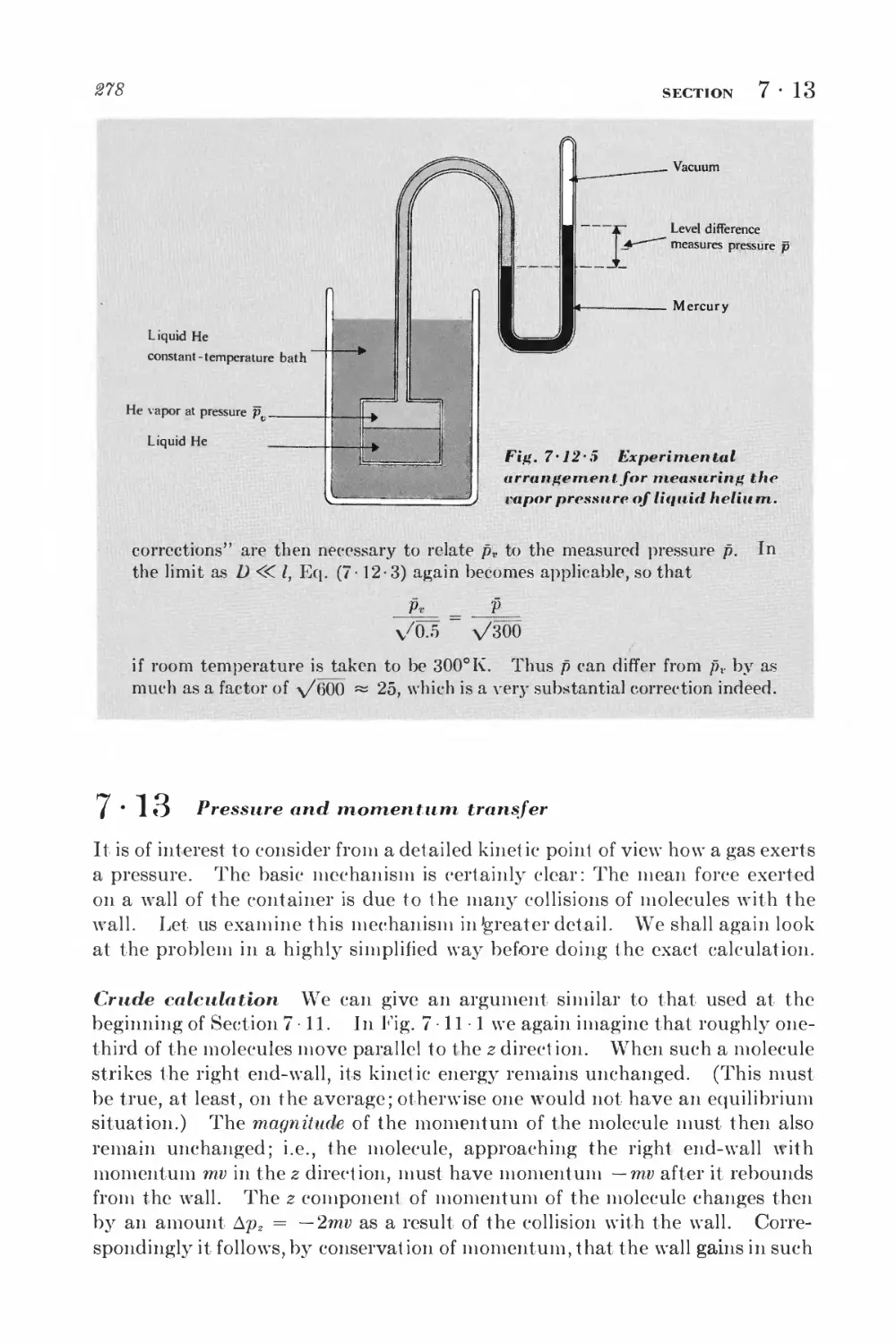
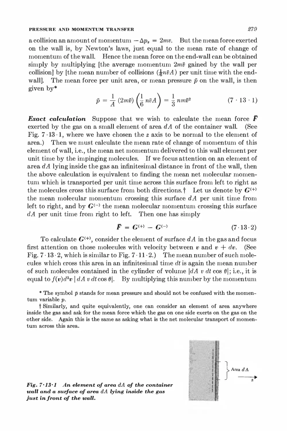
7-12 Effusion 278
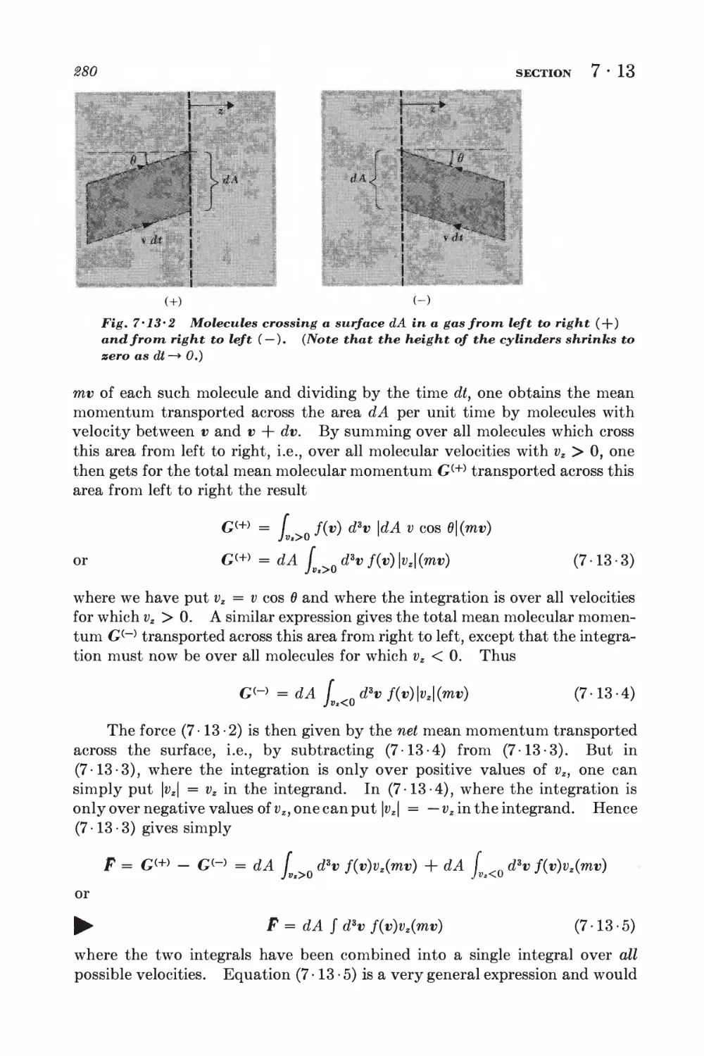
7-13 Pressure and momentum transfer 278
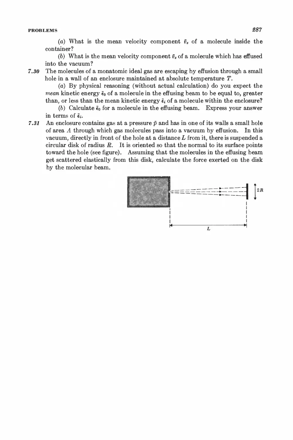
O Equilibrium between phases or chemical species 288
GENERAL EQUILIBRIUM CONDITIONS
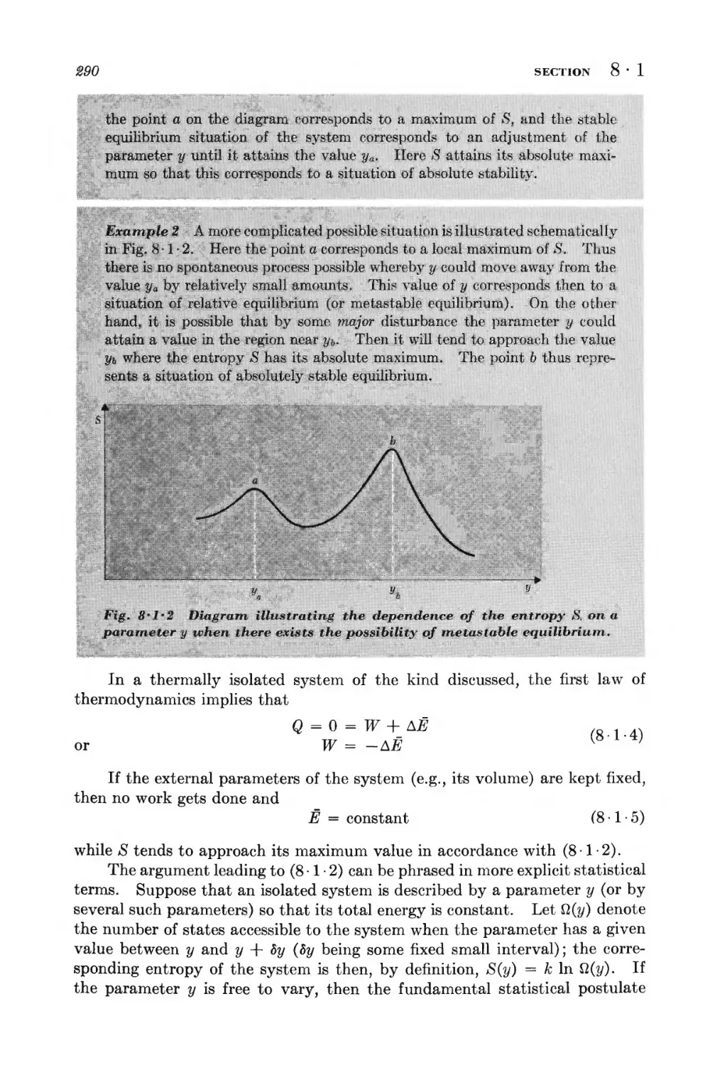
8 • 1 Isolated system 289
8 • 2 System in contact with a reservoir at constant temperature 291
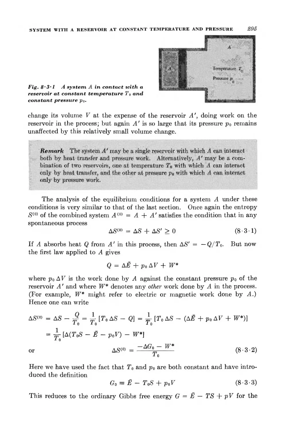
8 • 3 System in contact with a reservoir at constant temperature and
pressure 294
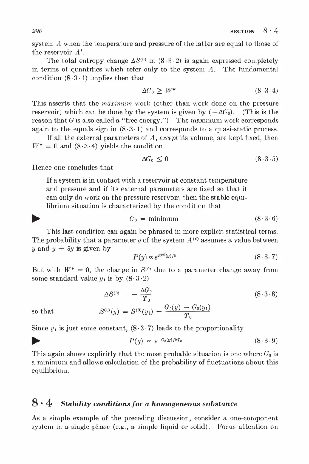
8 • 4 Stability conditions for a homogeneous substance 296
EQUILIBRIUM BETWEEN PHASES
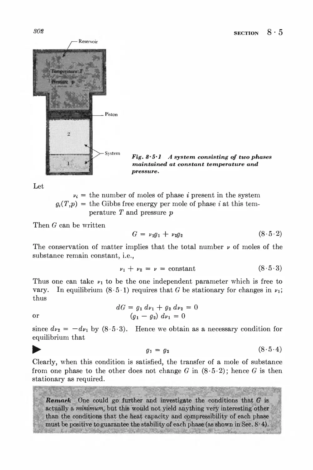
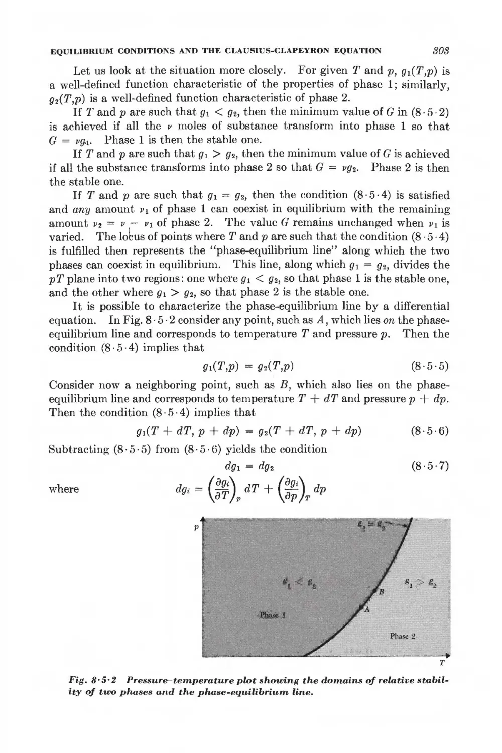
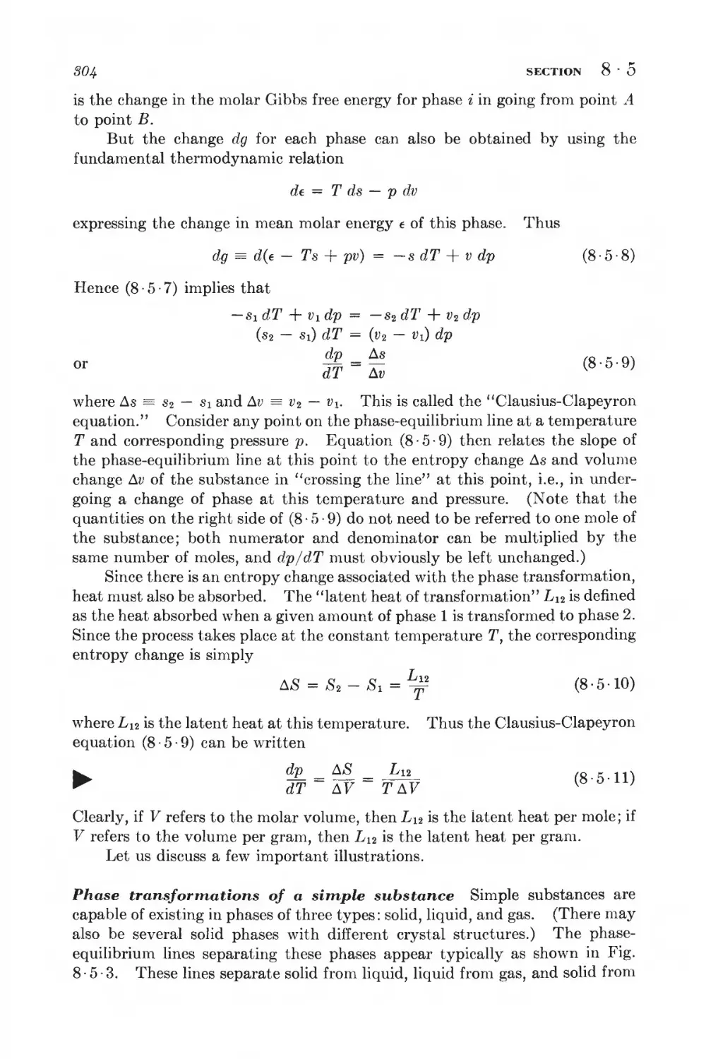
8 • 5 Equilibrium conditions and the Clausius-Clapeyron equation 801
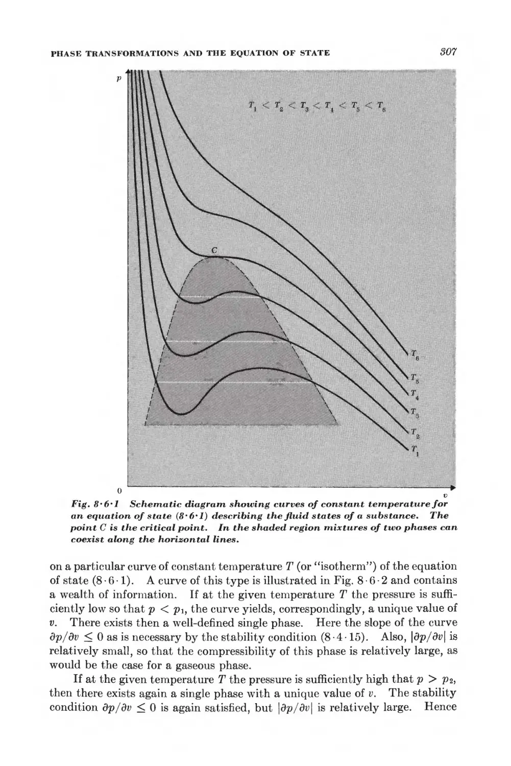
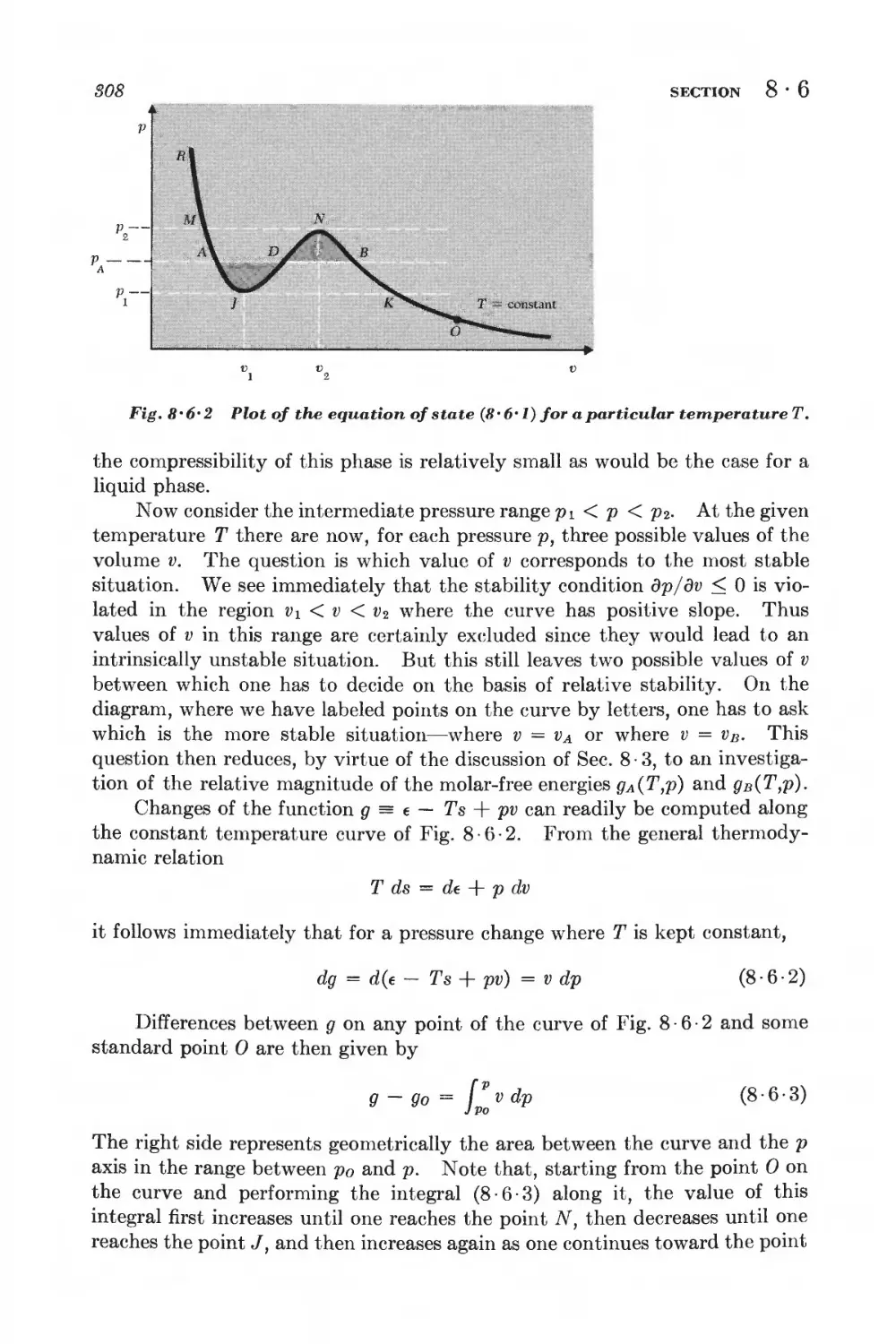
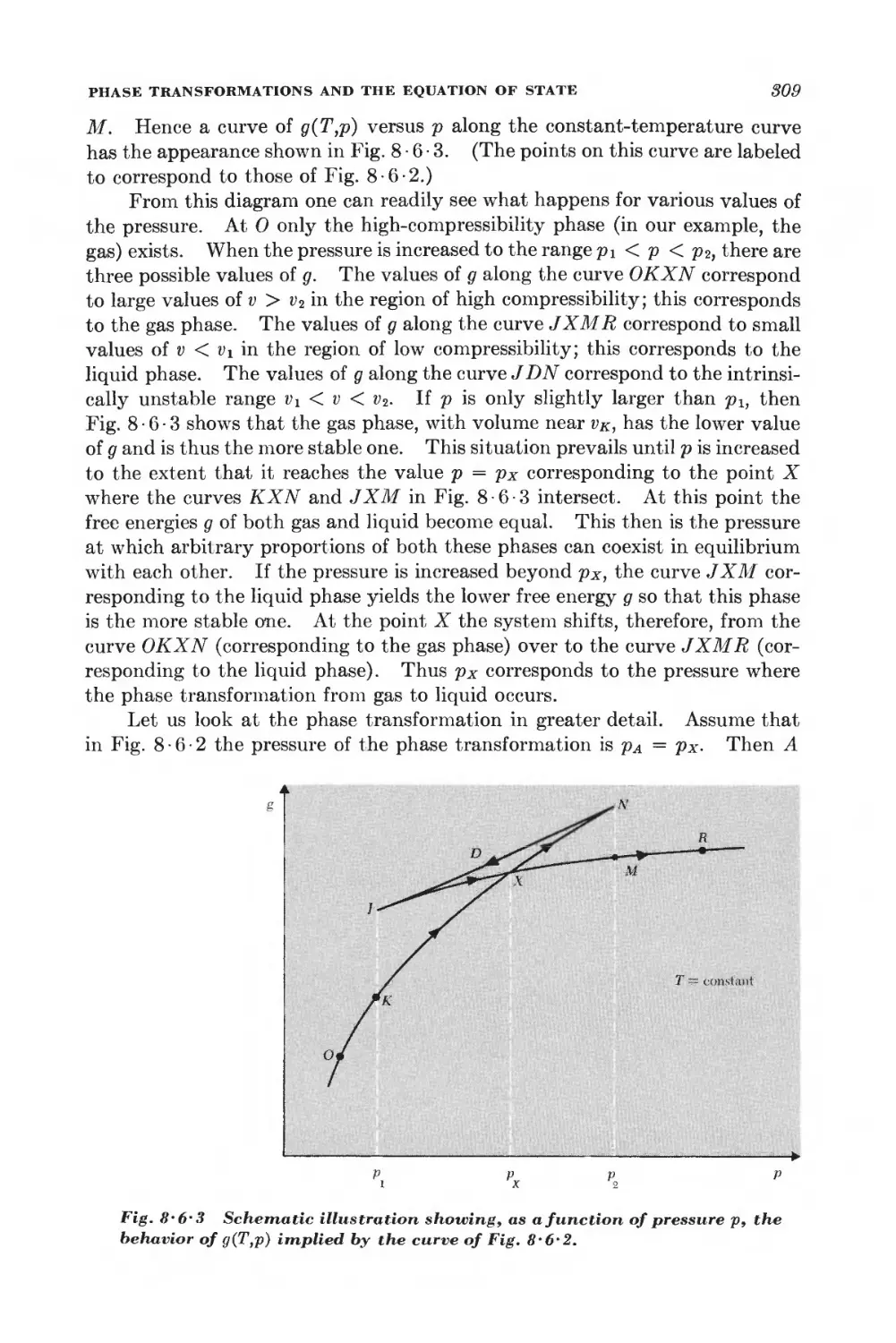
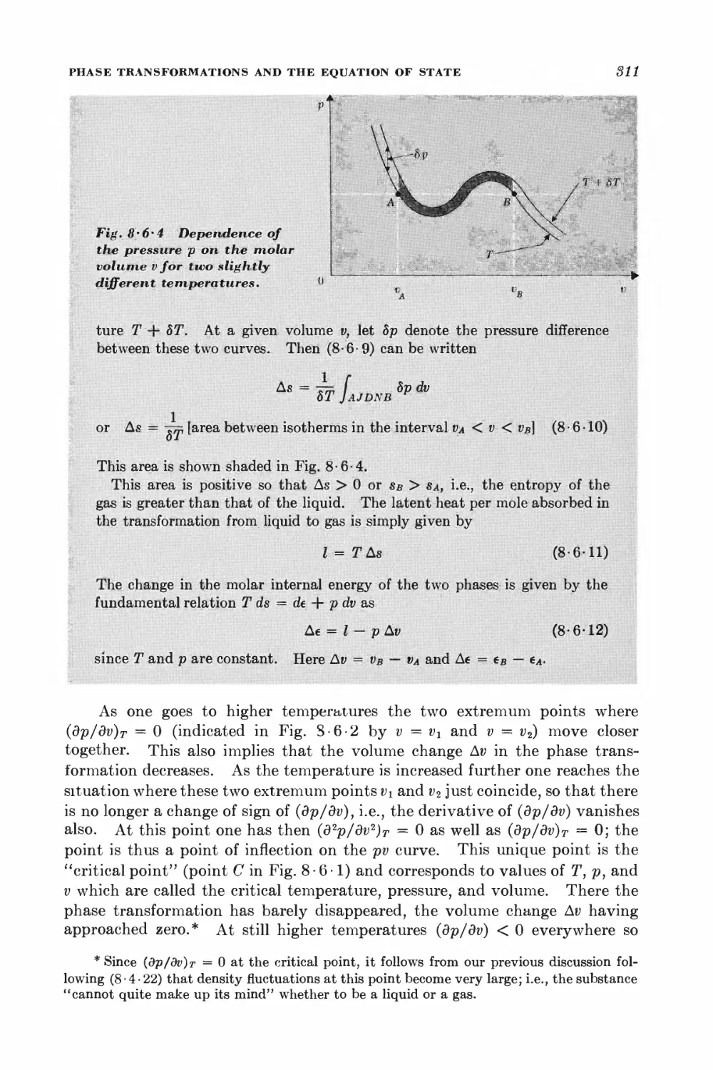
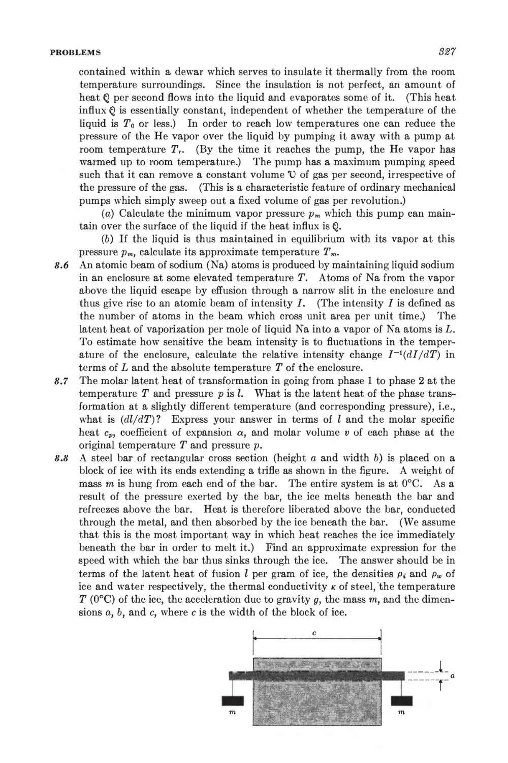
8 • 6 Phase transformations and the equation of state 806
SYSTEMS WITH SEVERAL COMPONENTS; CHEMICAL EQUILIBRIUM
8-7 General relations for a system with several components 812
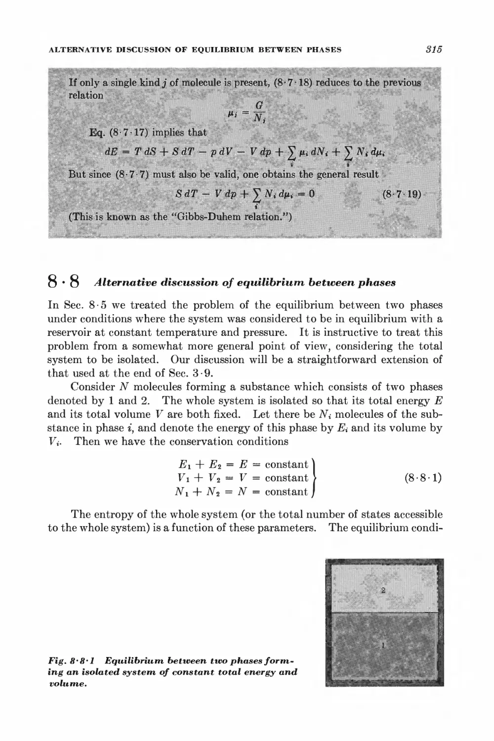
8 • 8 Alternative discussion of equilibrium between phases 815
8 -9 General conditions for chemical equilibrium 817
8 • 10 Chemical equilibrium between ideal gases 819
•7 Quantum statistics of ideal gases 331
MAXWELL-BOLTZMANN, BO SE-EIN STEIN, AND FERMI-DIRAC STATISTICS
9 • 1 Identical particles and symmetry requirements 881
9 • 2 Formulation of the statistical problem 885
9 • 3 The quantum distribution functions 888
9-4 Maxwell-Boltzmann statistics 848
9-5 Photon statistics 845
9 • 6 Bose-Einstein statistics 846
9 • 7 Fermi-Dirac statistics 850
9 • 8 Quantum statistics in the classical limit 851

IDEAL GAS IN THE CLASSICAL LIMIT
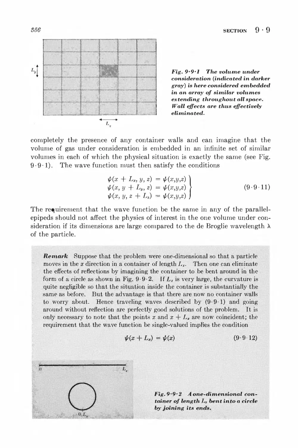
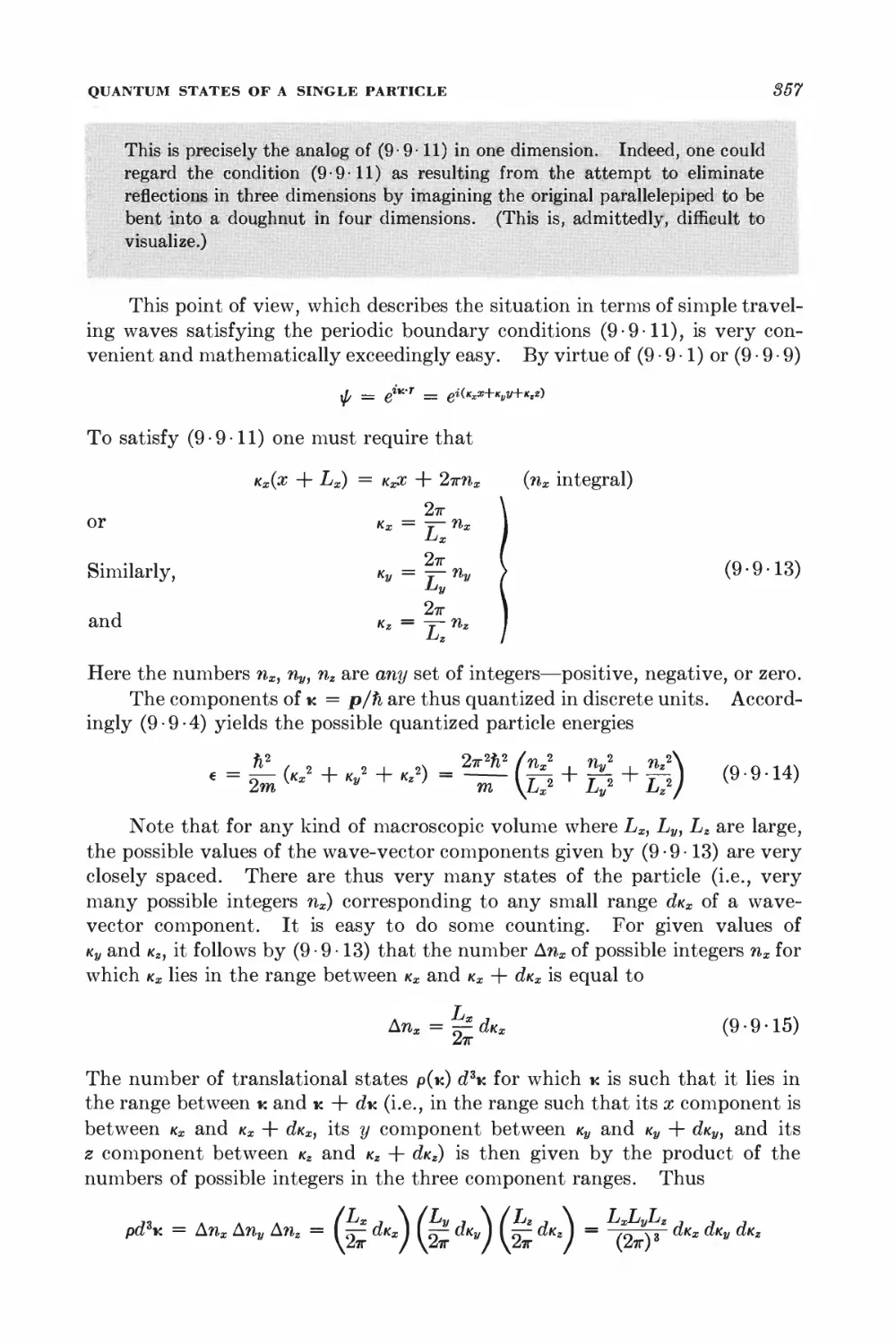
9 • 9 Quantum states of a single particle 353
9 10 Evaluation of the partition function 360
9-11 Physical implications of the quantum-mechanical enumemtion of
states 363
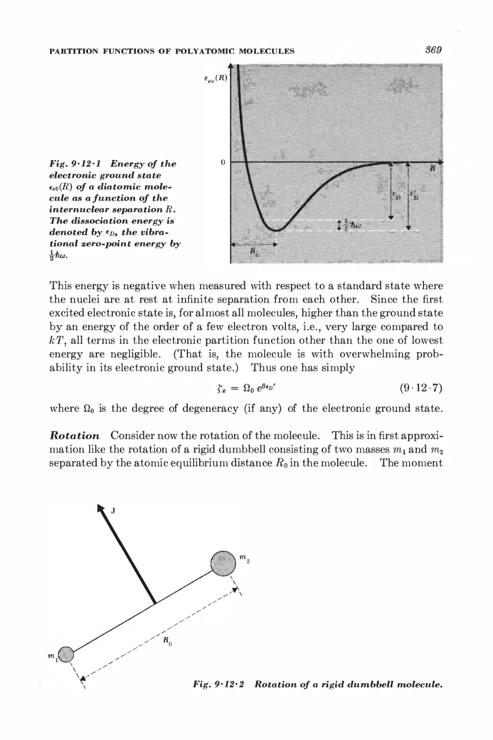
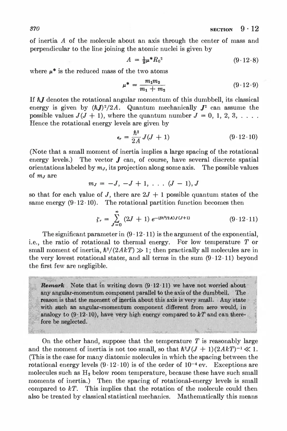
*9 • 12 Partition functions of polyatomic molecules 367
BLACK-BODY RADIATION
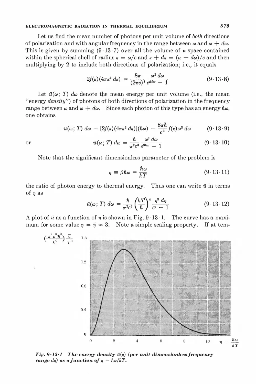
9-13 Electromagnetic radiation in thermal equilibrium inside an
enclosure 373
9-14 Nature of the radiation inside an arbitrary enclosure 378
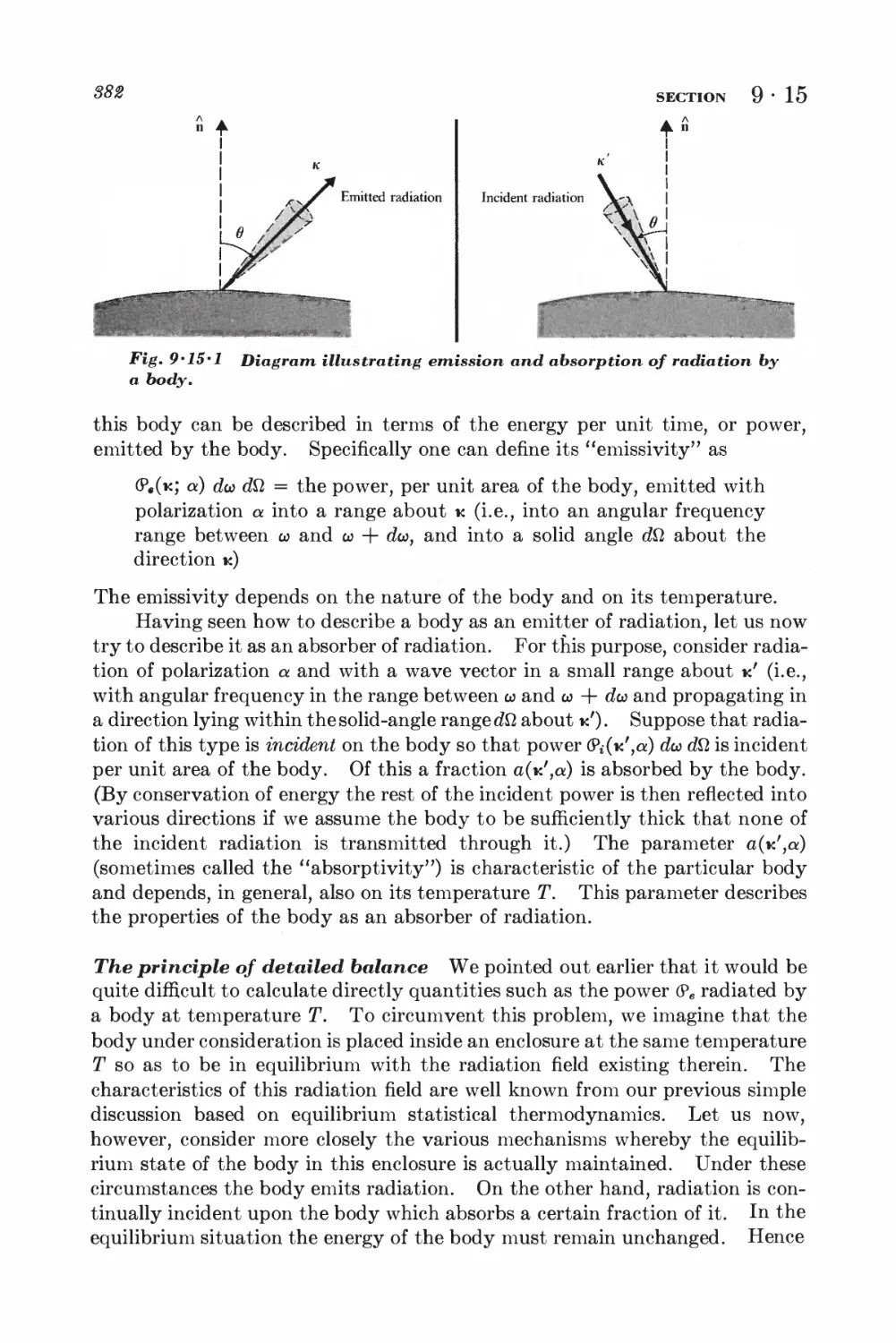
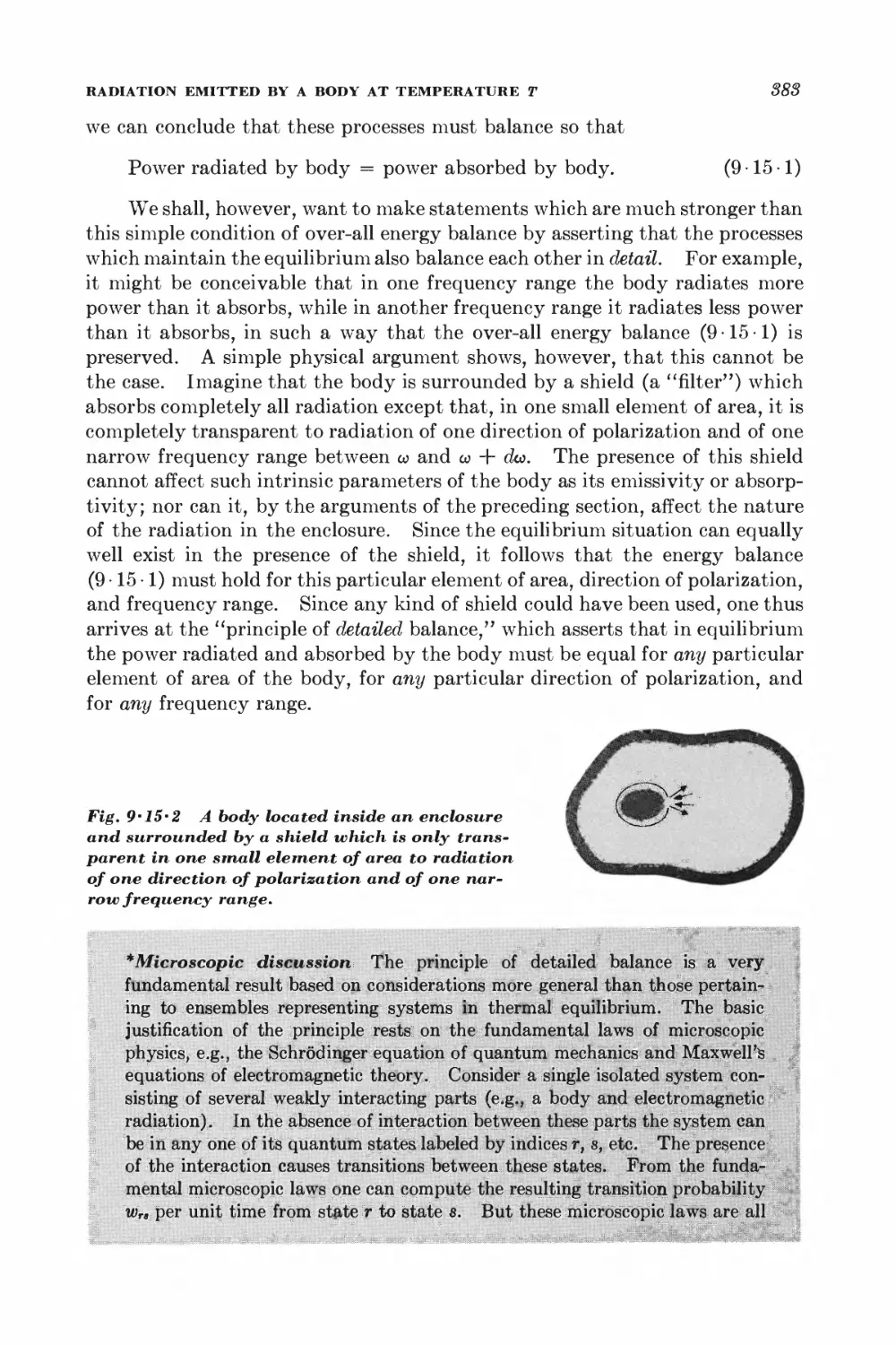
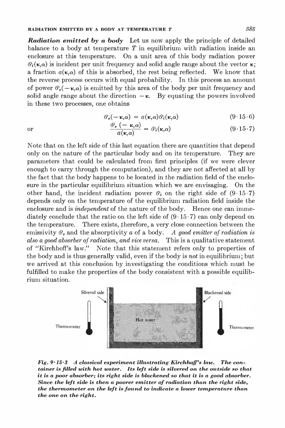
9-15 Radiation emitted by a body at temperature T 381
CONDUCTION ELECTRONS IN METALS
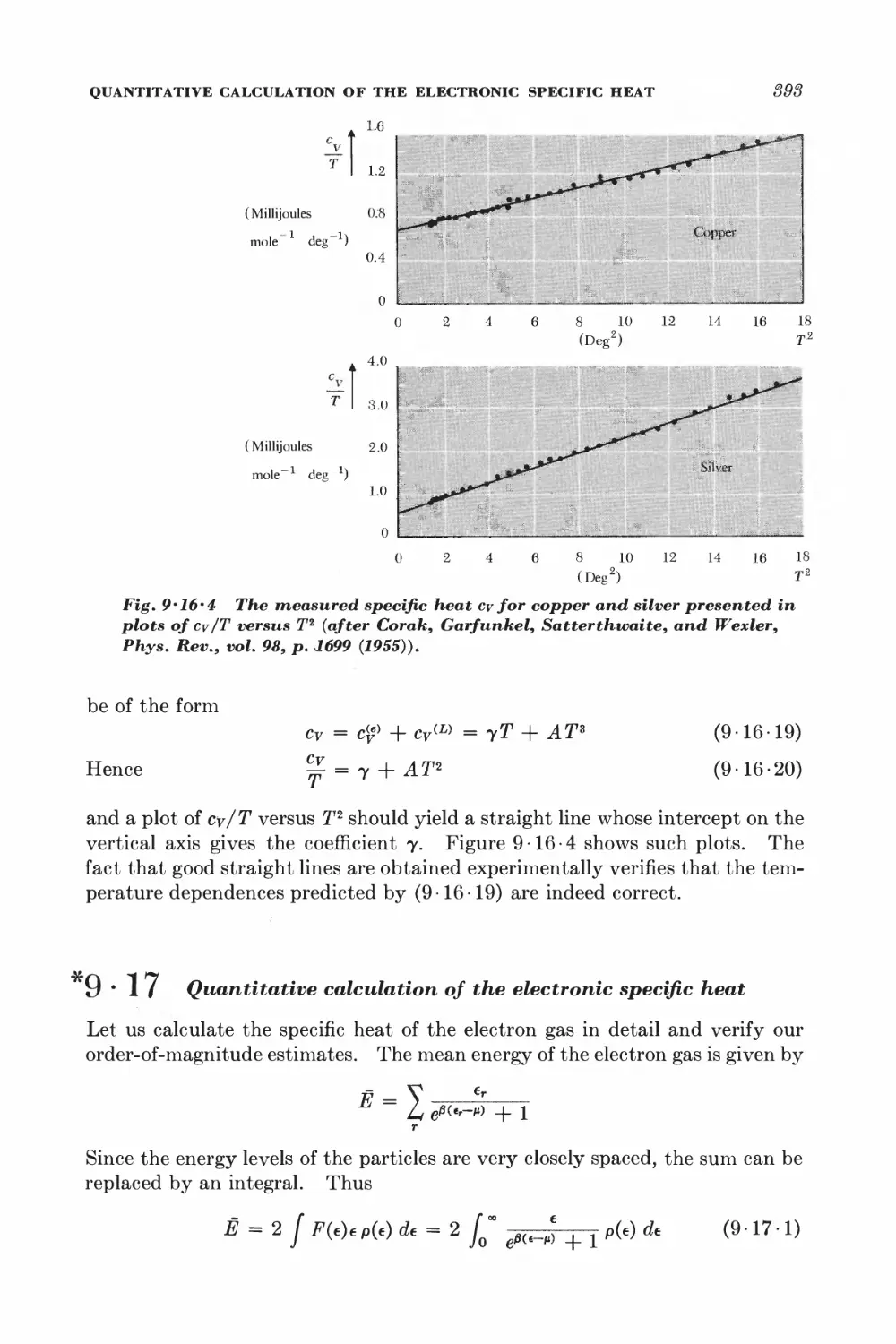
9-16 Consequences of the Fermi-Dirac distribution 388
*9-17 Quantitative calculation of the electronic specific heat 393
10 Systems of interacting particles 404
SOLIDS
10 • 1 Lattice vibrations and normal modes J+07
10-2 Debye approximation I±ll
NONIDEAL CLASSICAL GAS
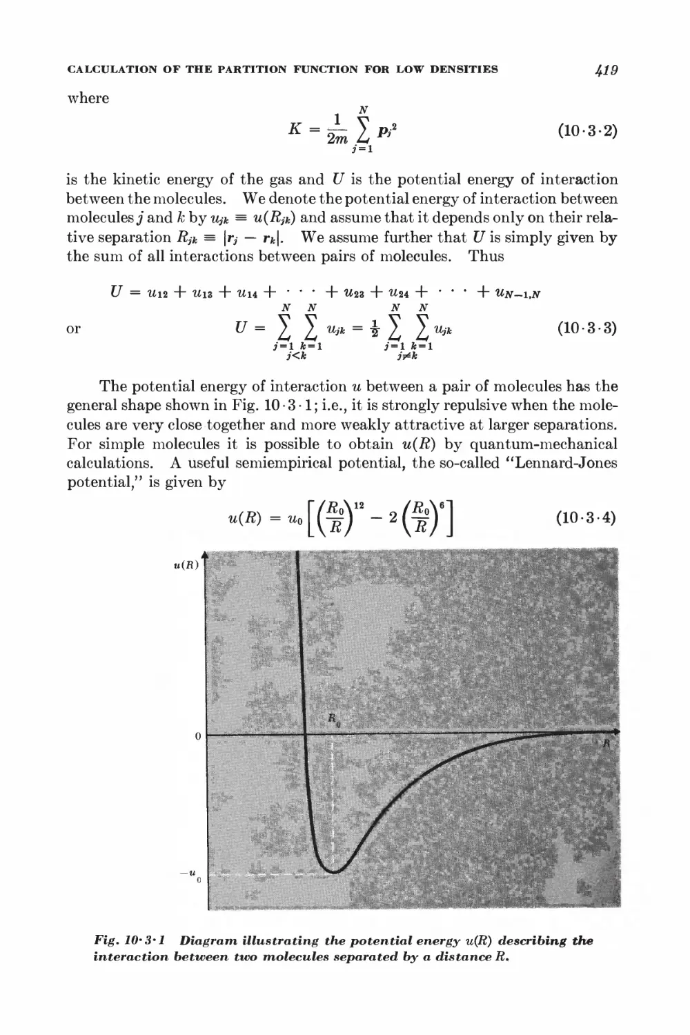
10-3 Calculation of the partition function for low densities 418
10-4 Equation of state and virial coefficients I$2
10-5 Alternative derivation of the van der Waals equation 426
FERROM AGNETISM
10-6 Interaction between spins 428
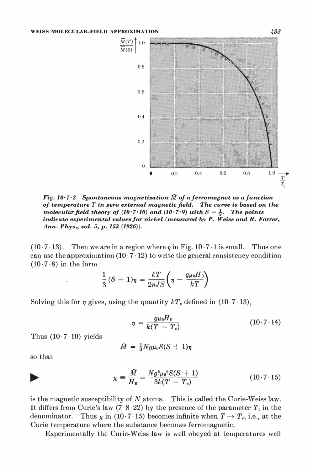
10-7 Weiss molecular-field approximation 430
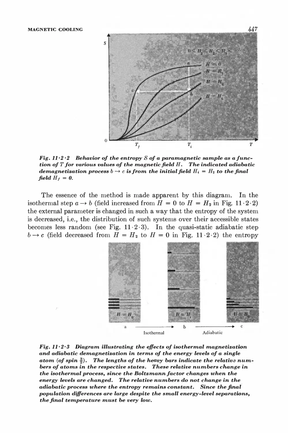
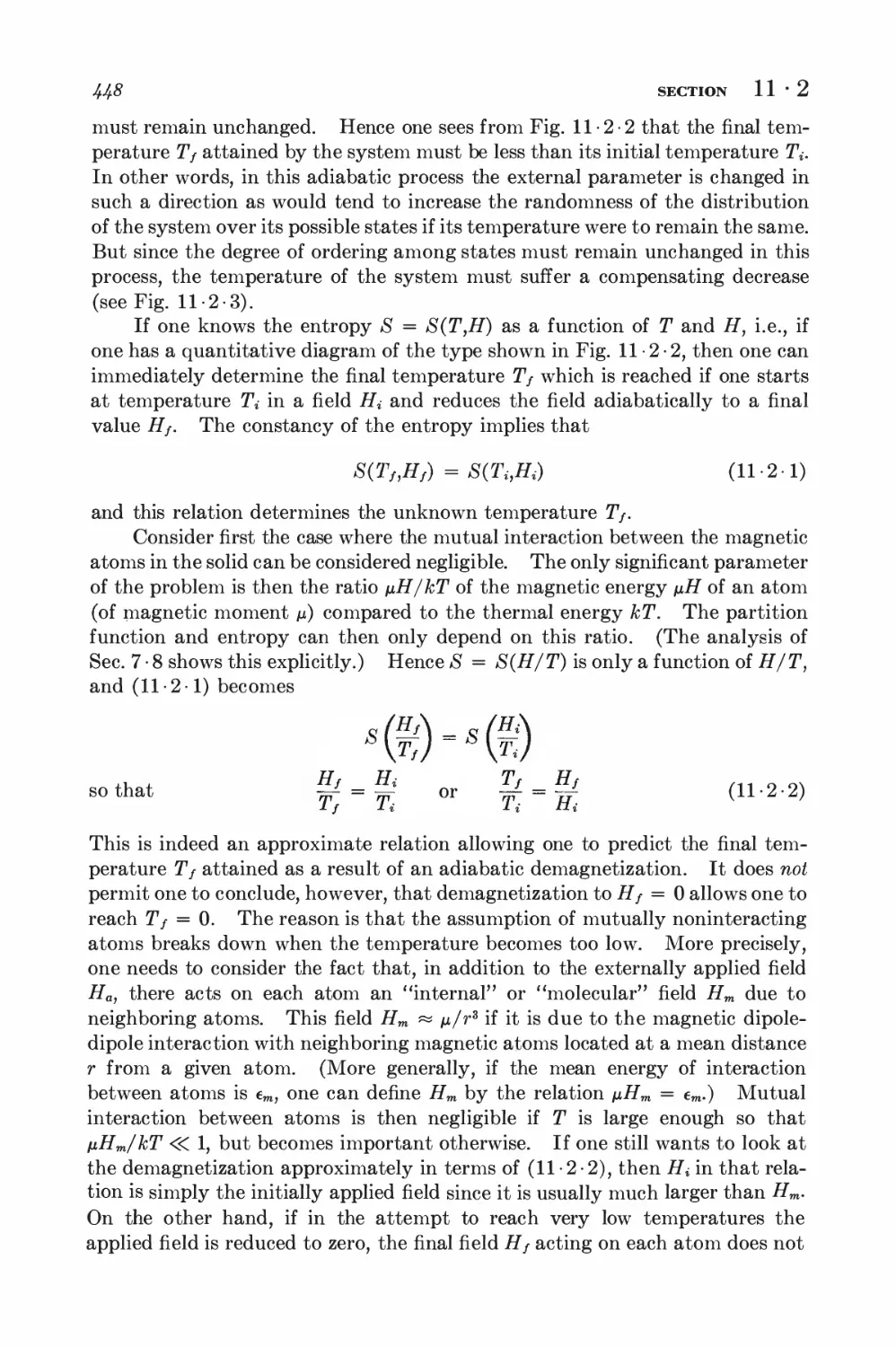
11 Magnetism and low temperatures 438
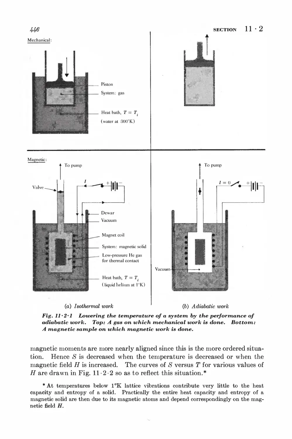
11-1 Magnetic work 489
11-2 Magnetic cooling 44&
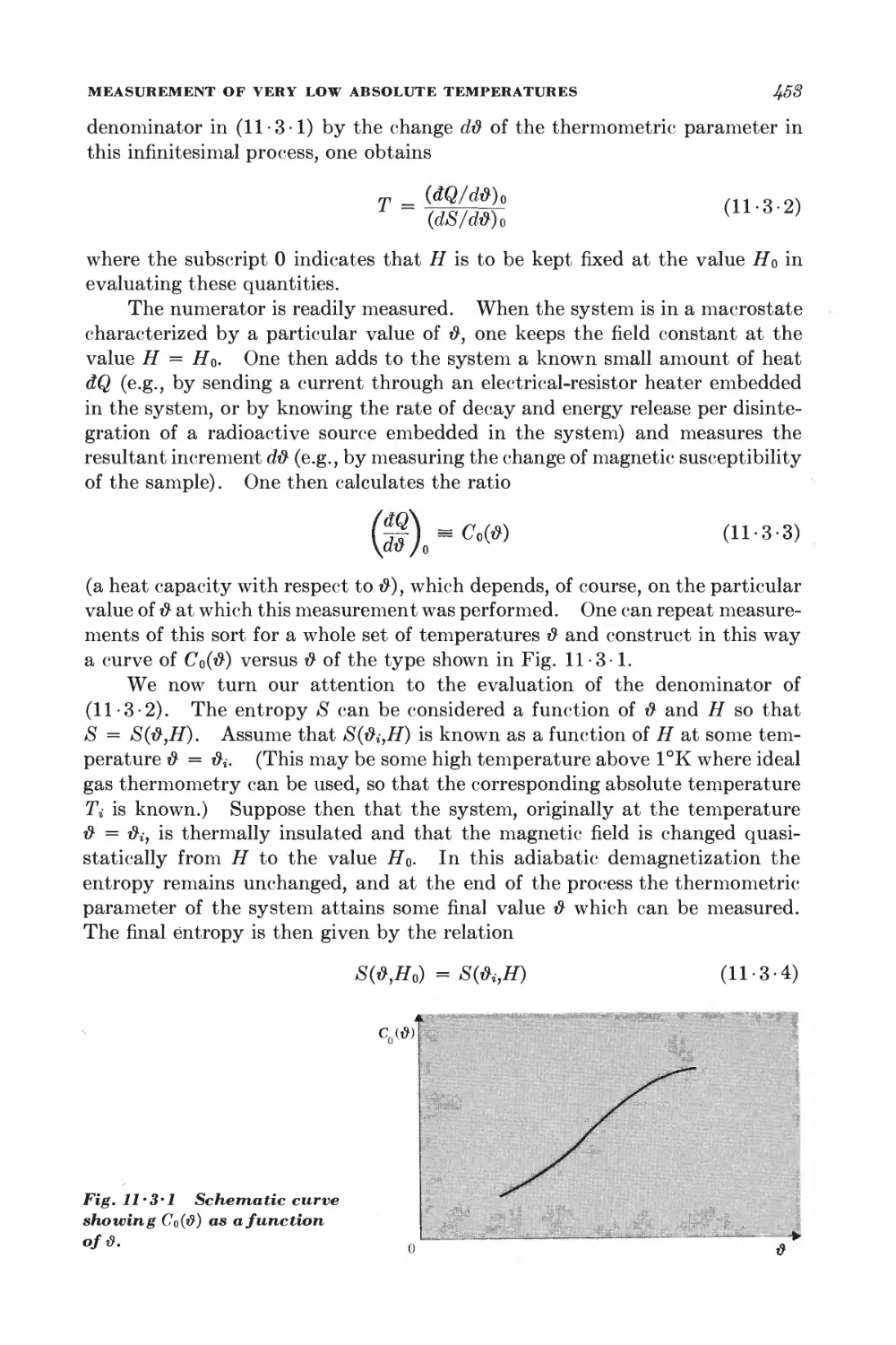
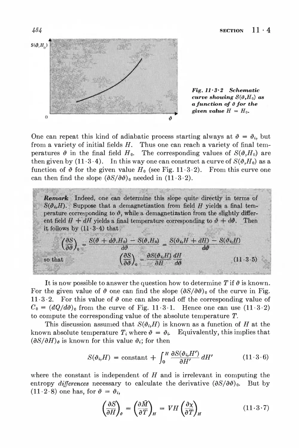
11-3 Measurement of very low absolute temperatures 4&%
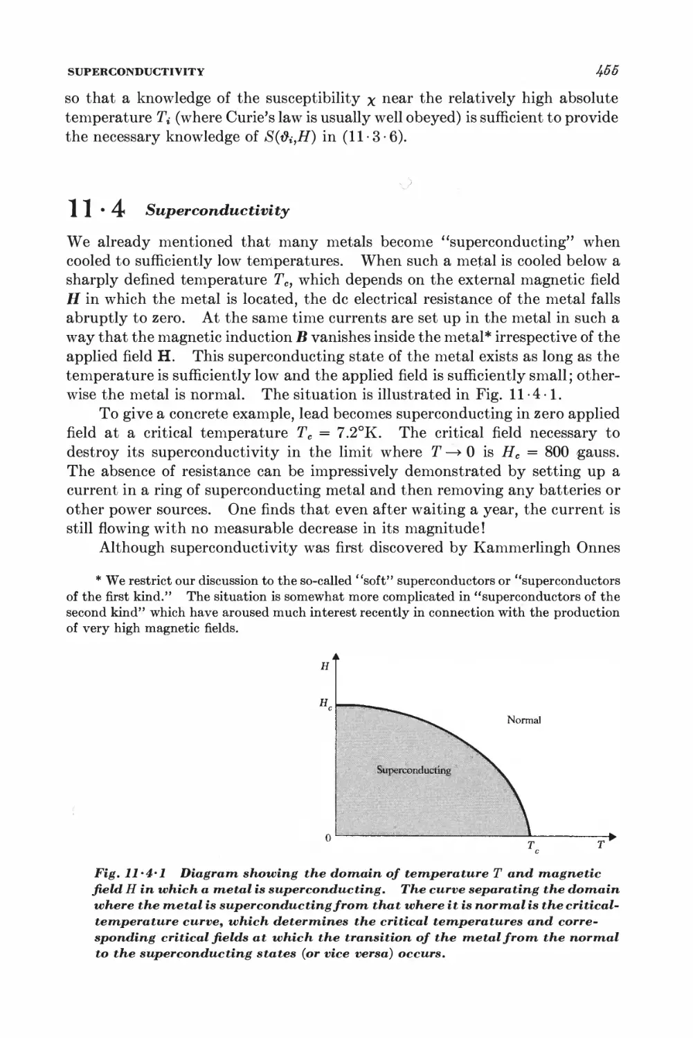
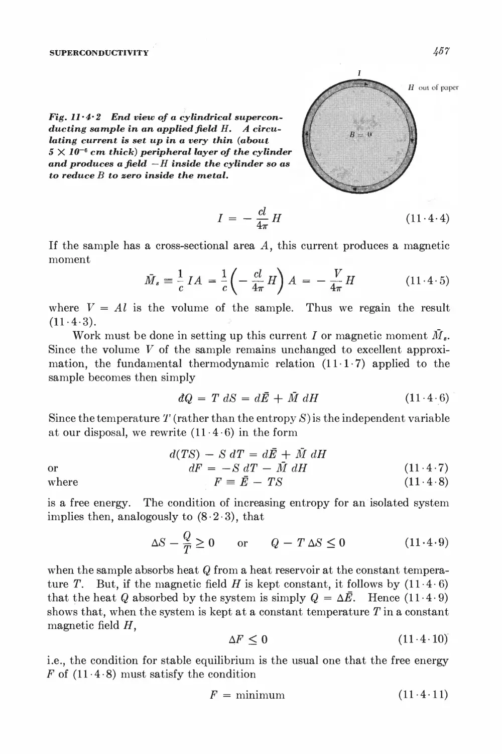
11-4 Superconductivity 4&5
12 Elementary kinetic theory of transport processes 461
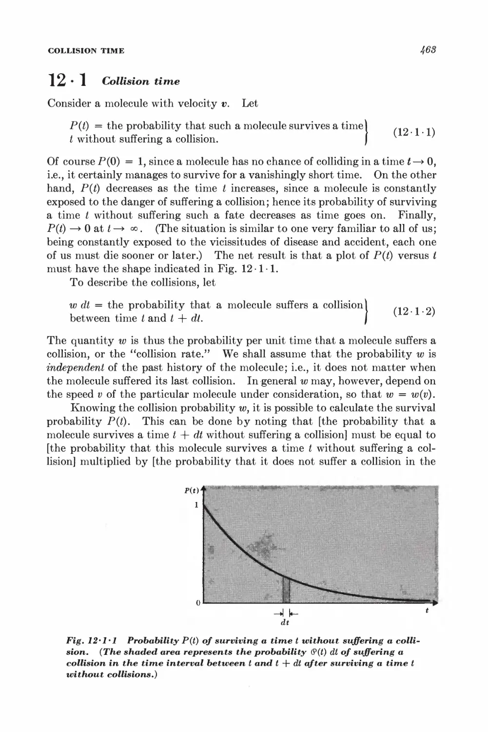
12 • 1 Collision time 468
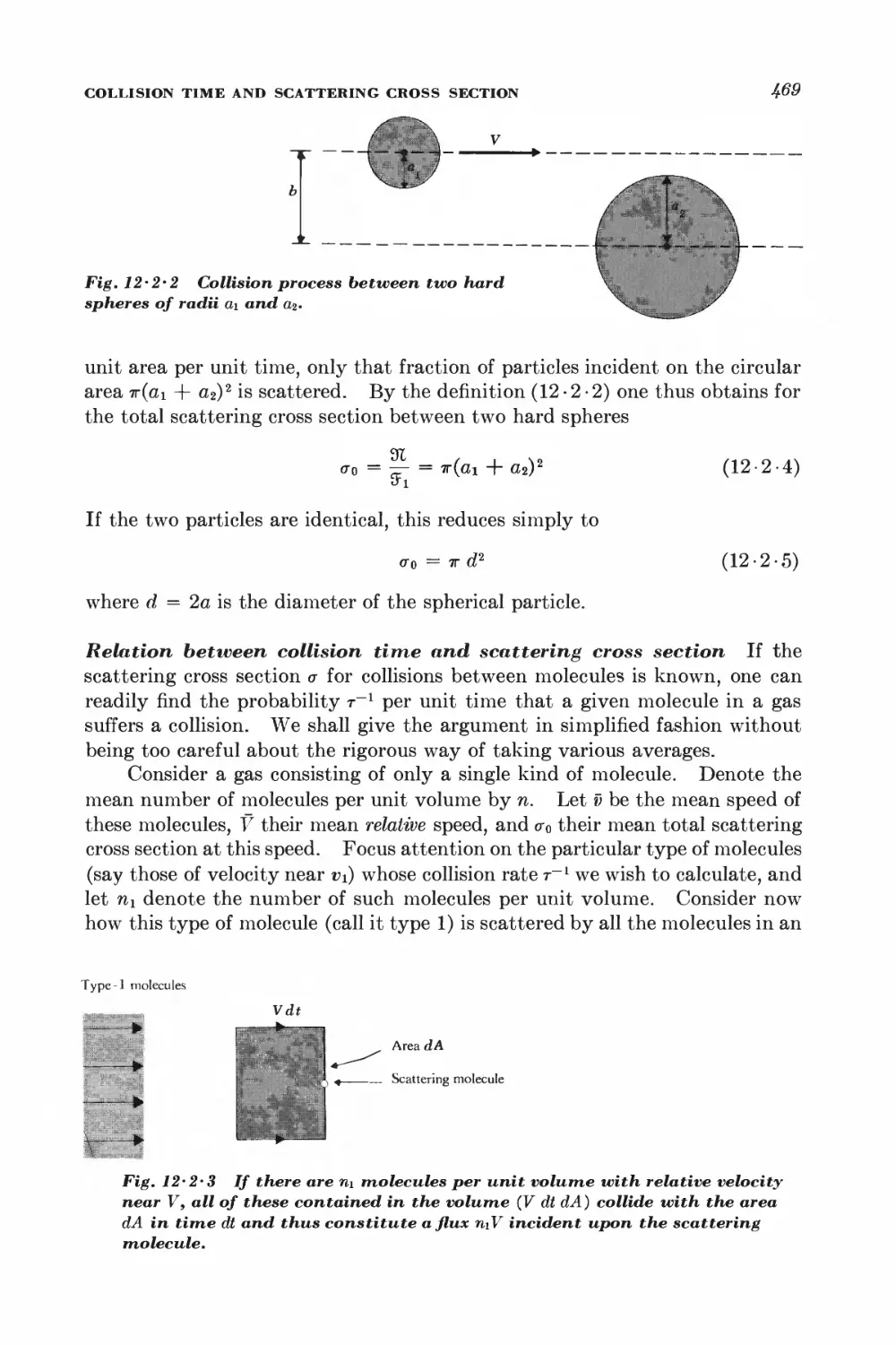
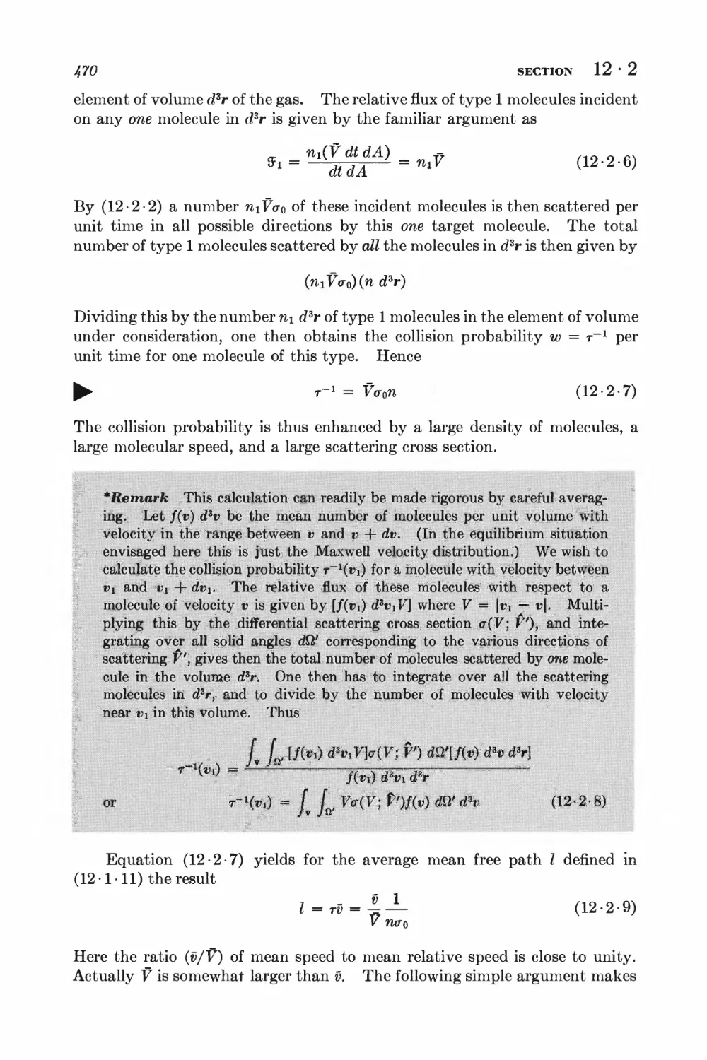
12-2 Collision time and scattering cross section 4^

12-3 Viscosity 471
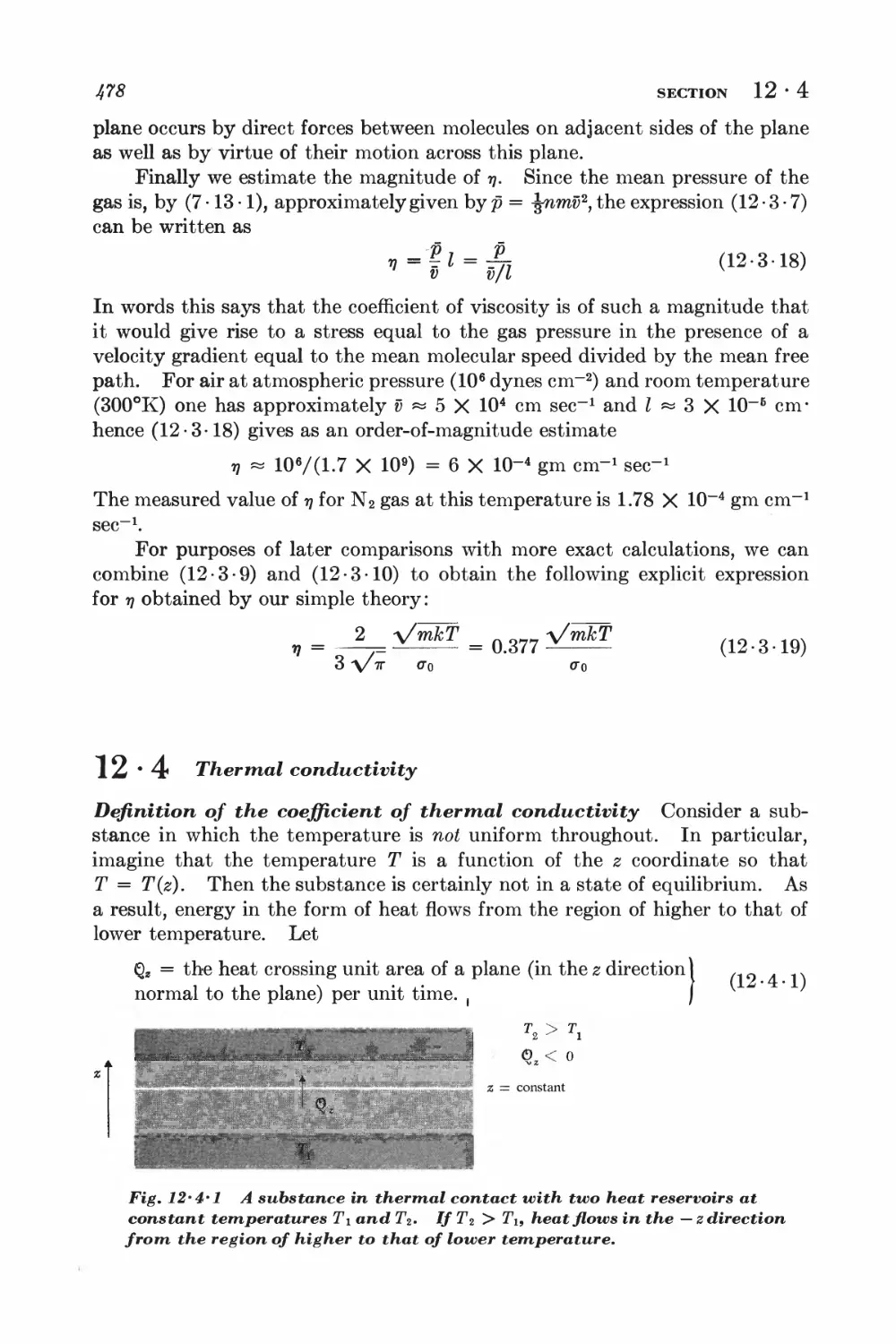
12-4 Thermal conductivity 478
12-5 Self-diffusion 483
12-6 Electrical Conductivity 4^8
13 Transport theory using the relaxation time approximation 494
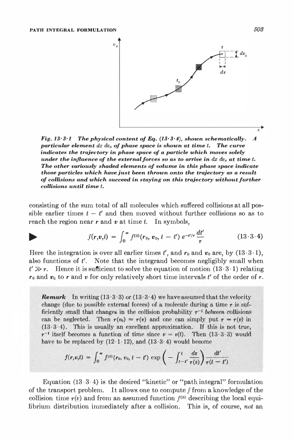
13-1 Transport processes and distribution functions Ift4
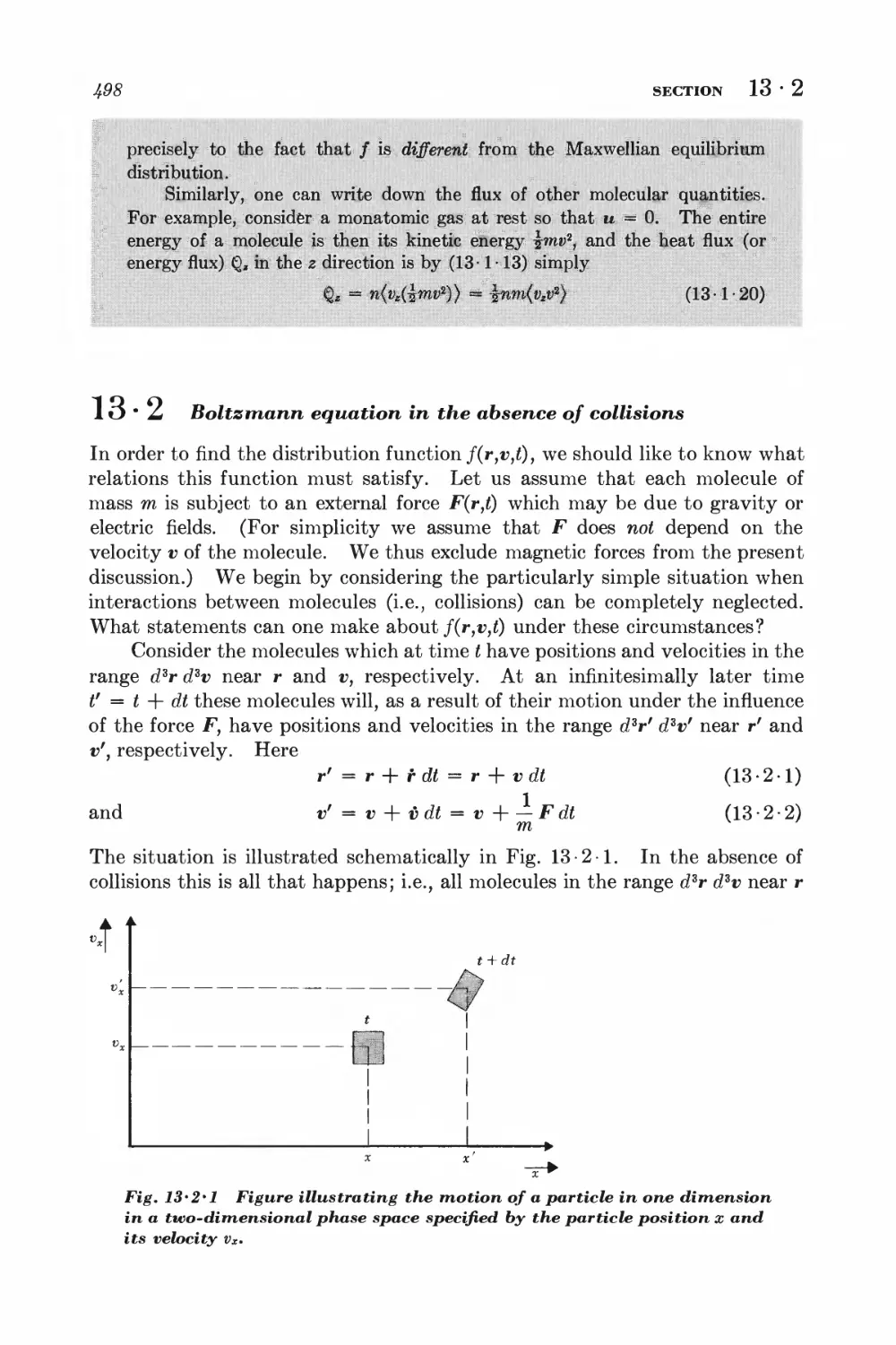
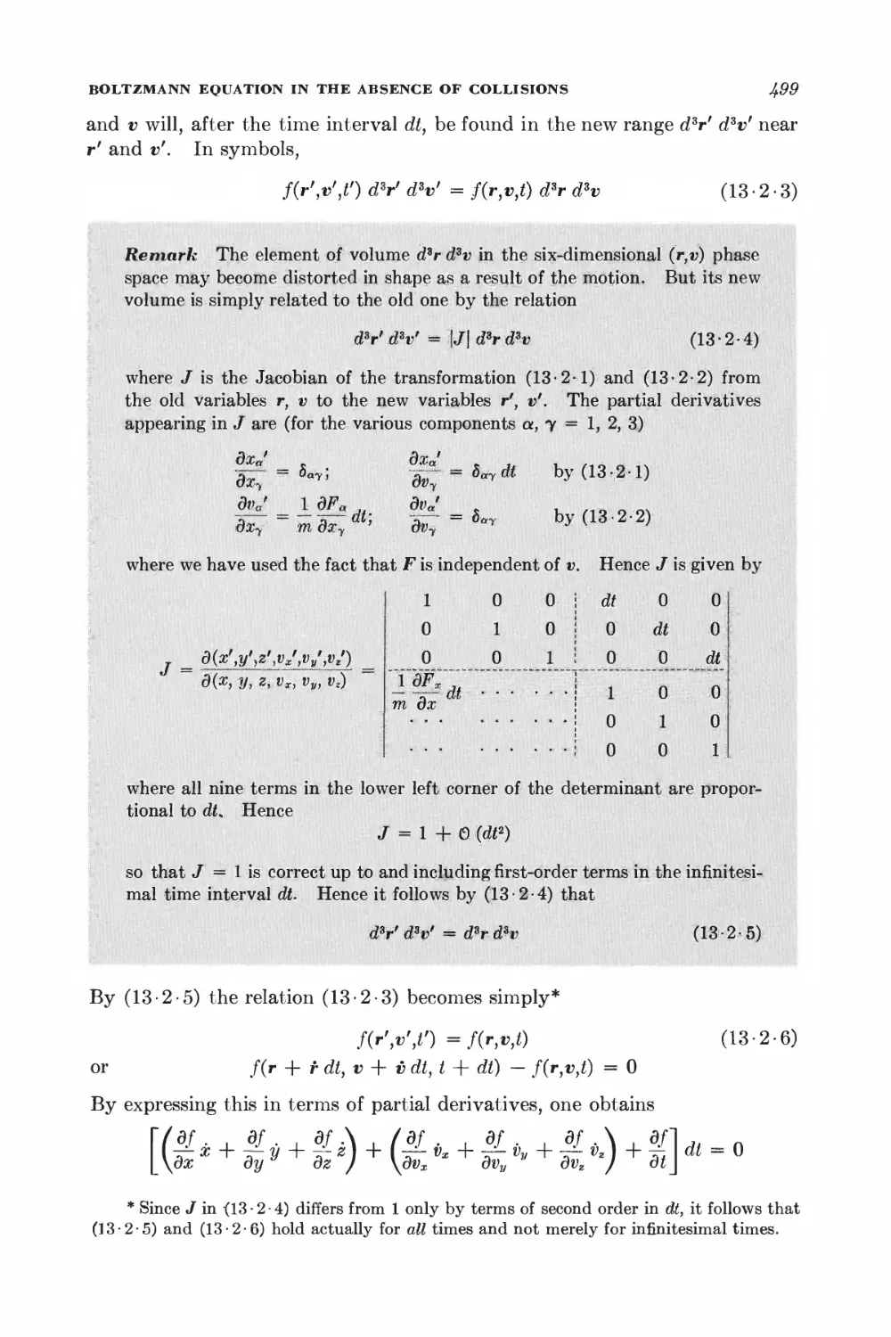
13-2 Boltzmann equation in the absence of collisions 4®8
13-3 Path integral formulation 502
13-4 Example: calculation of electrical conductivity 504
13-5 Example: calculation of viscosity 507
13-6 Boltzmann differential equation formulation 508
13-7 Equivalence of the two formulations 510
13-8 Examples of the Boltzmann equation method 511
14 Near-exact formulation of transport theory 516
14
14
14
14
14
14
14
14
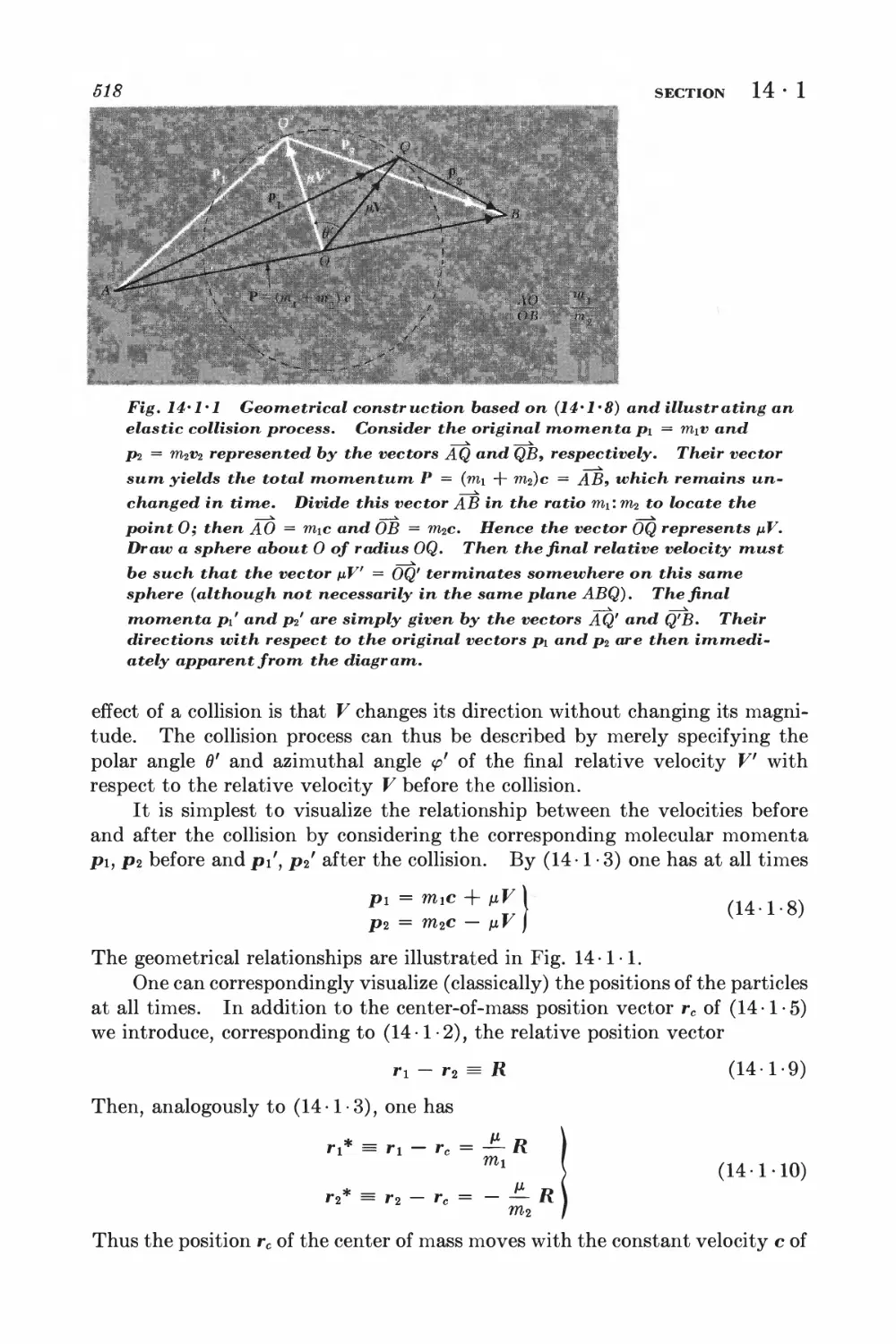
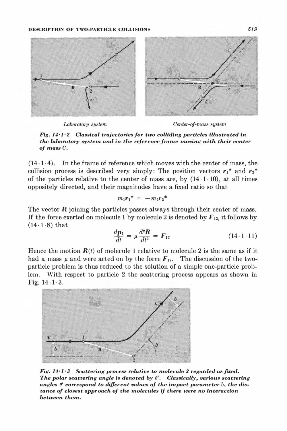
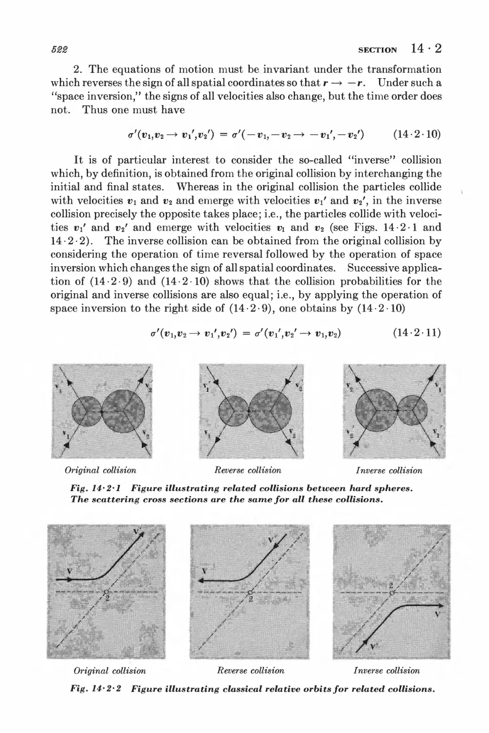
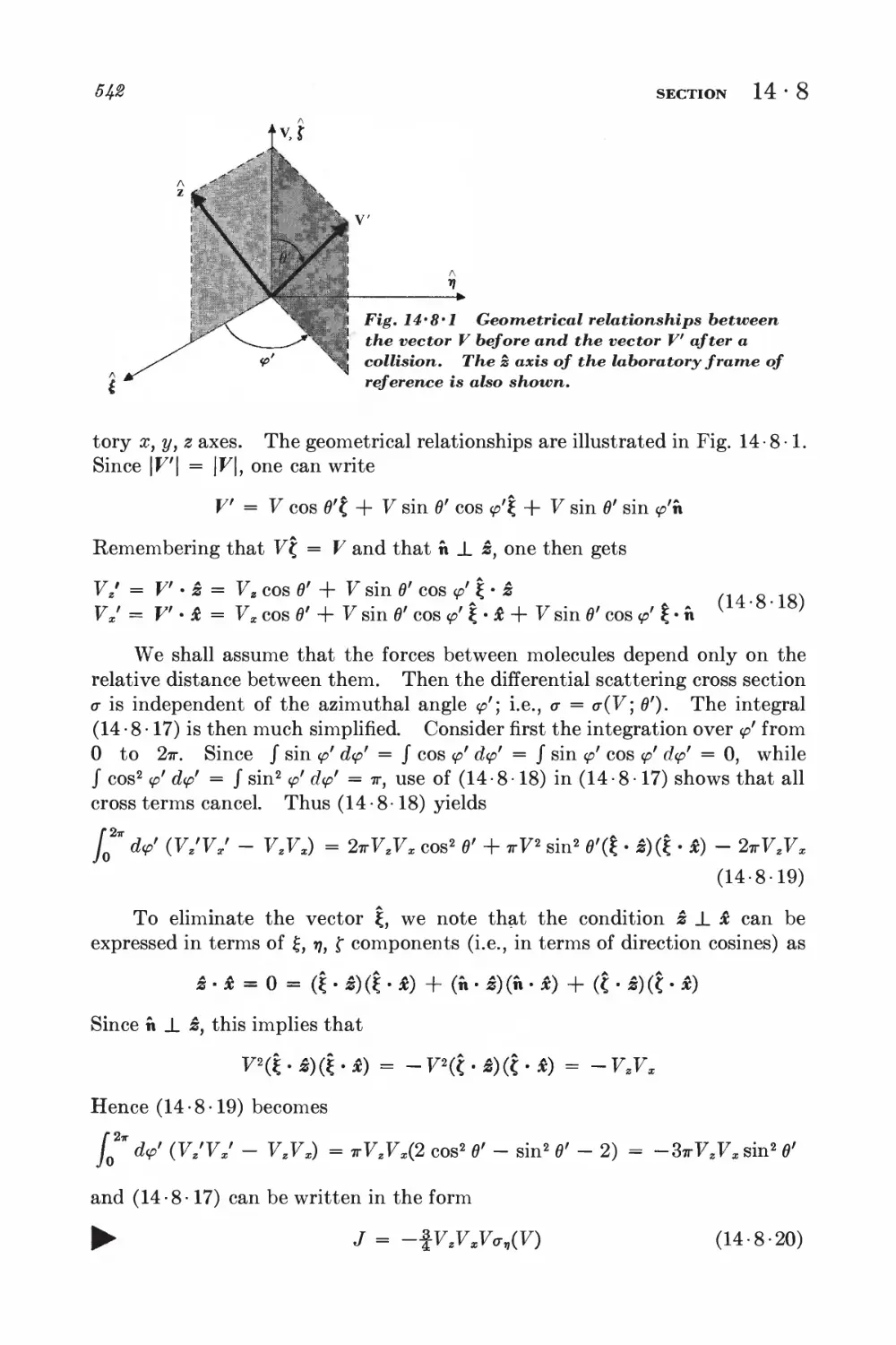
1 Description of two-particle collisions 516
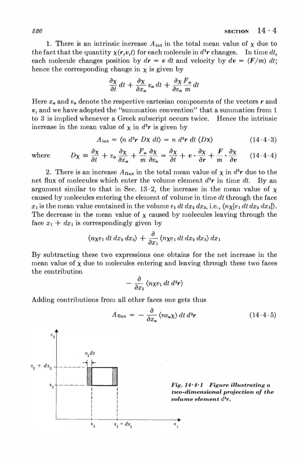
2 Scattering cross sections and symmetry properties 520
3 Derivation of the Boltzmann equation 523
4 Equation of change for mean values 525
5 Conservation equations and hydrodynamics 529
6 Example: simple discussion of electrical conductivity 531
7 Approximation methods for solving the Boltzmann equation 534
8 Example: calculation of the coefficient of viscosity 539
15 Irreversible processes and fluctuations 548
TRANSITION PROBABILITIES AND MASTER EQUATION
15-1 Isolated system 548
15-2 System in contact with a heat reservoir 551
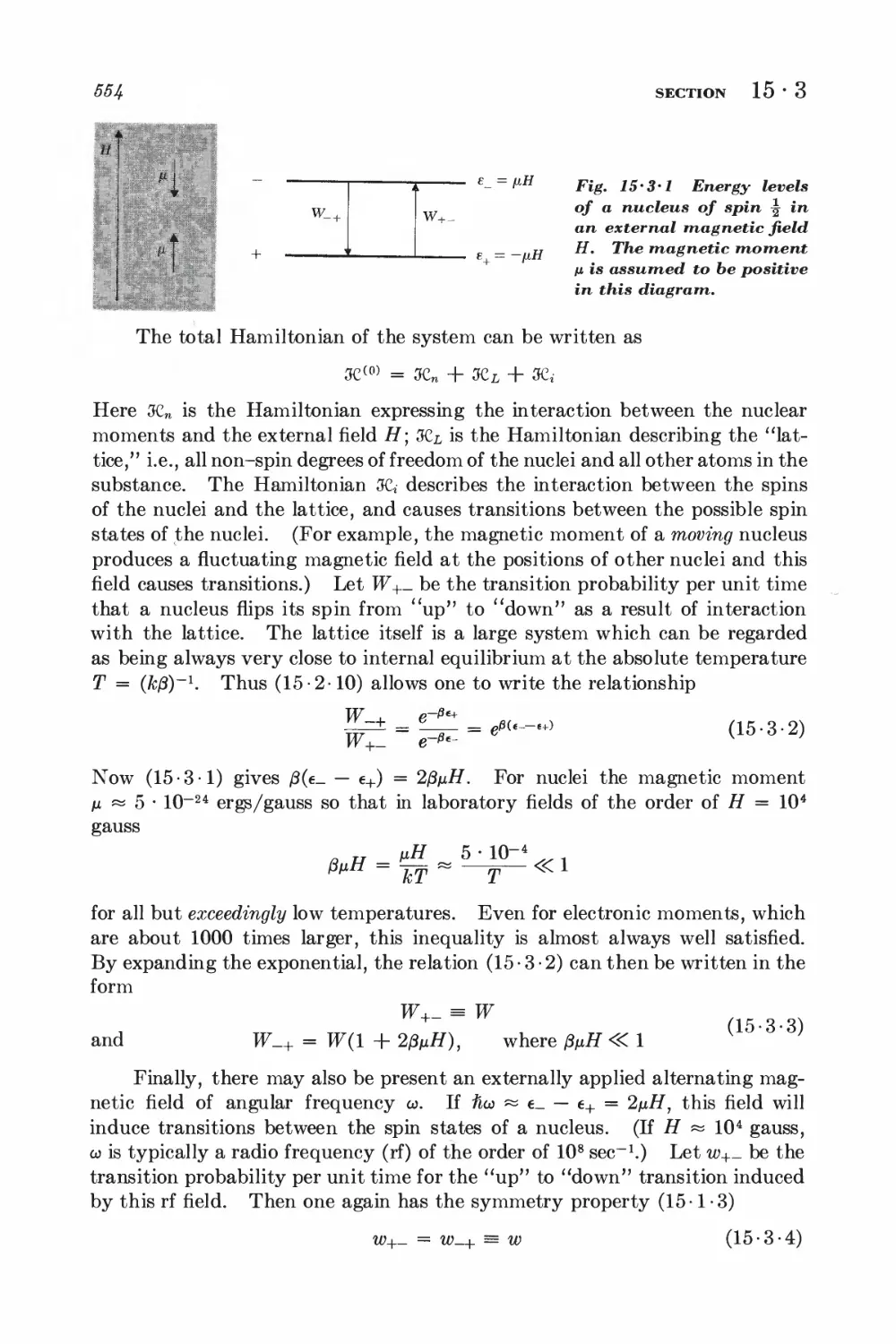
15-3 Magnetic resonance 553
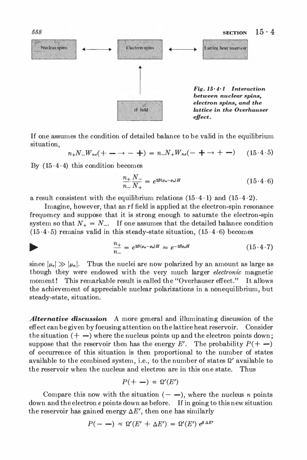
15-4 Dynamic nuclear polarization; Overhauser effect 556
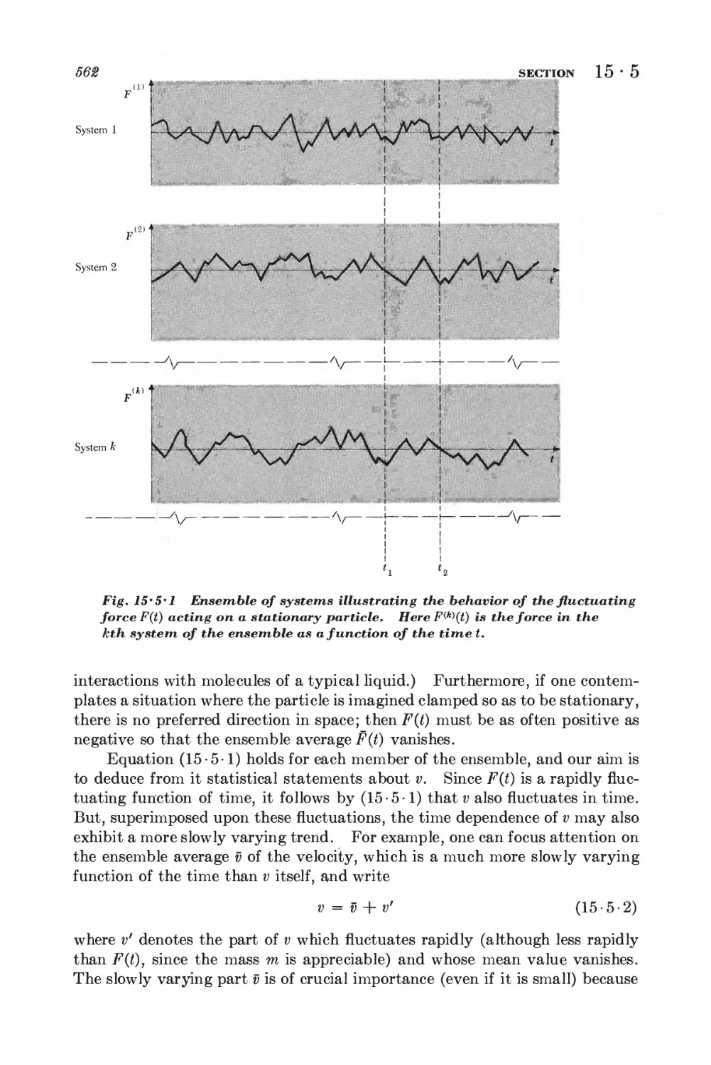
SIMPLE DISCUSSION OF BROWNIAN MOTION
15-5 Langevin equation 560
15-6 Calculation of the mean-square displacement 565
DETAILED ANALYSIS OF BROWNIAN MOTION
15-7 Relation between dissipation and the fluctuating force 567

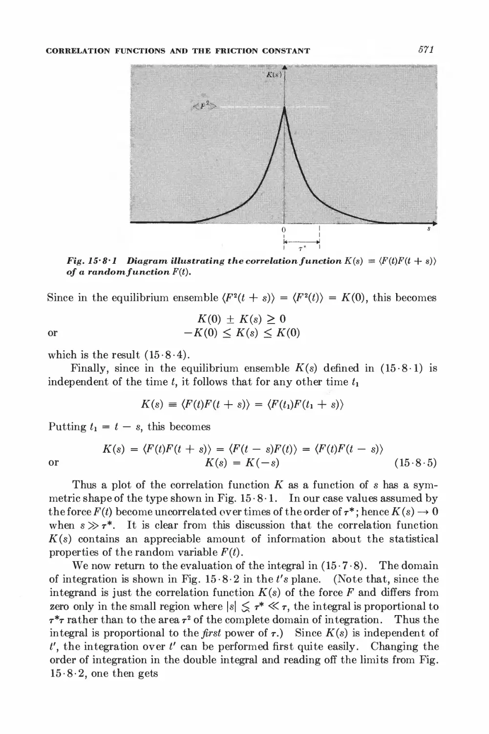
15-8 Correlation functions and the friction constant 570
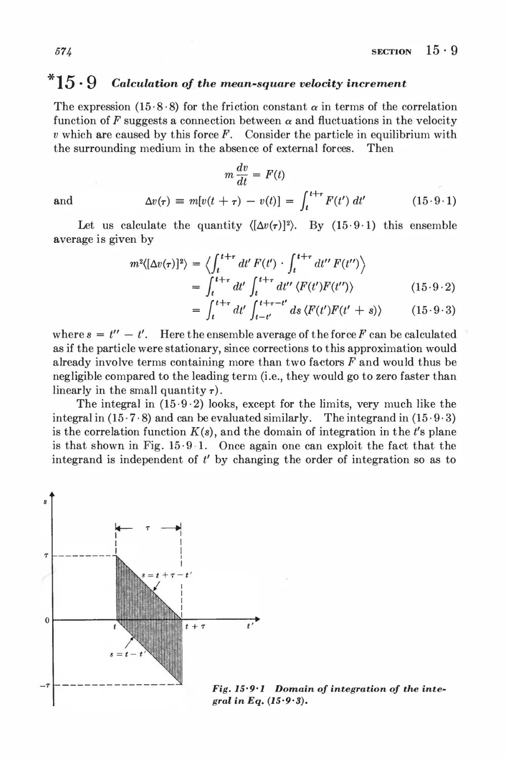
*15 • 9 Calculation of the mean-square velocity increment 574
*15 • 10 Velocity correlation function and mean-square displacement 575
CALCULATION OF PROBABILITY DISTRIBUTIONS
*15 • 11 The Fokker-Planck equation 577
*15-12 Solution of the Fokker-Planck equation 580
FOURIER ANALYSIS OF RANDOM FUNCTIONS
15-13 Fourier analysis 582
15 14 Ensemble and time averages 588
15 15 Wiener-Khintchine relations 585
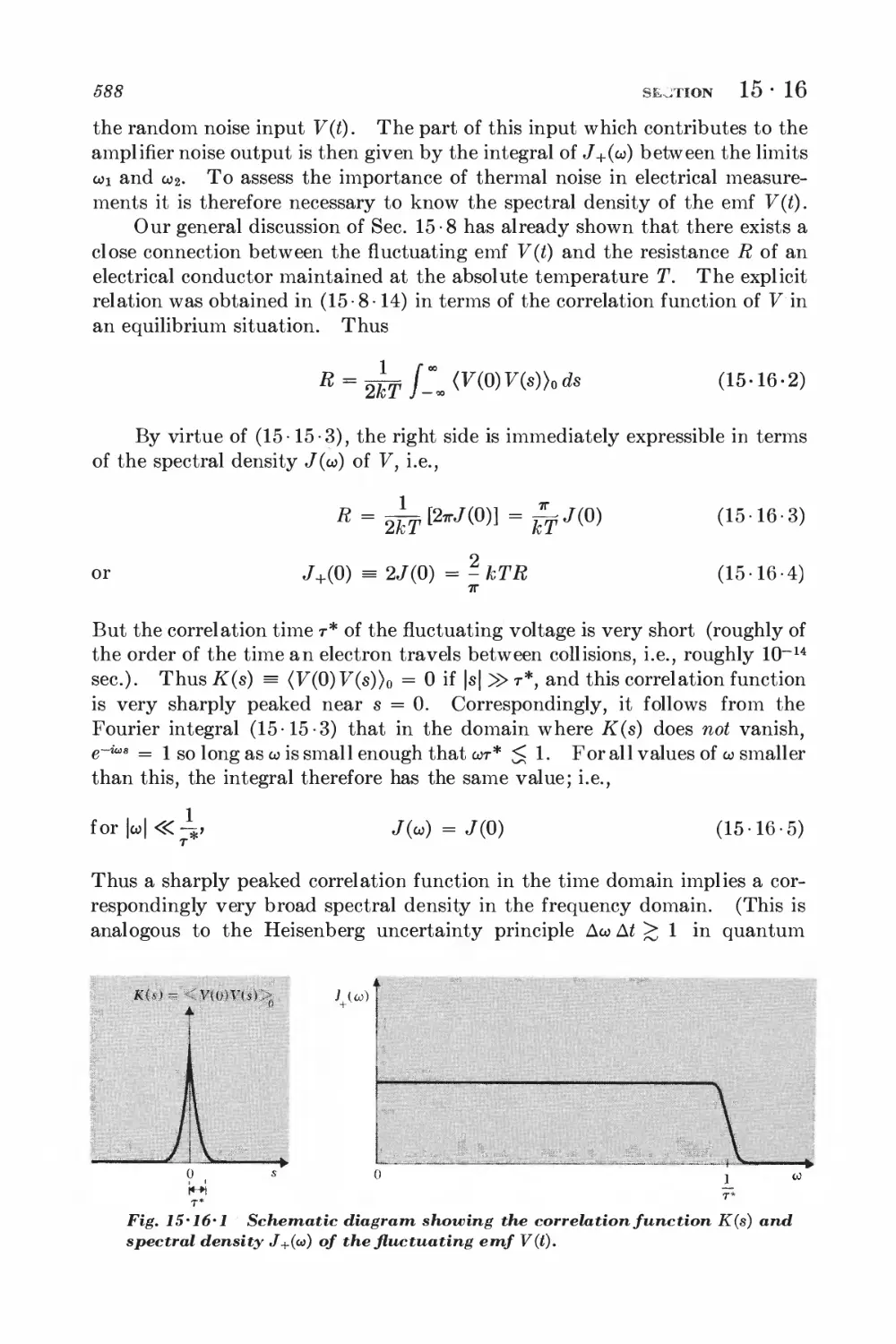
15 16 Nyquist's theorem 587
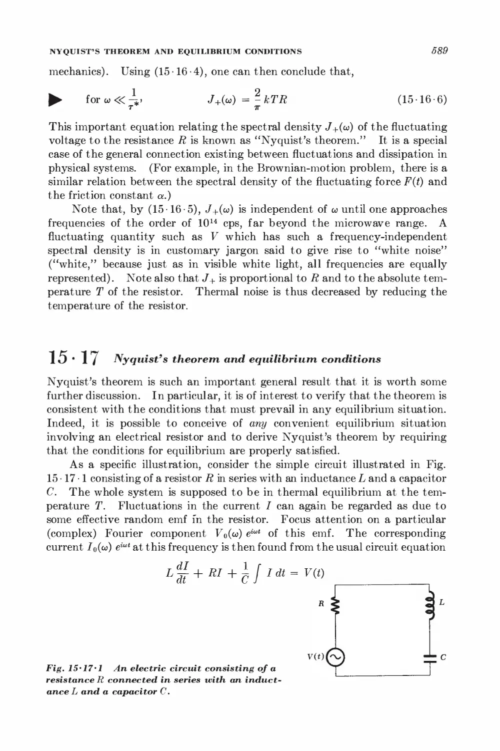
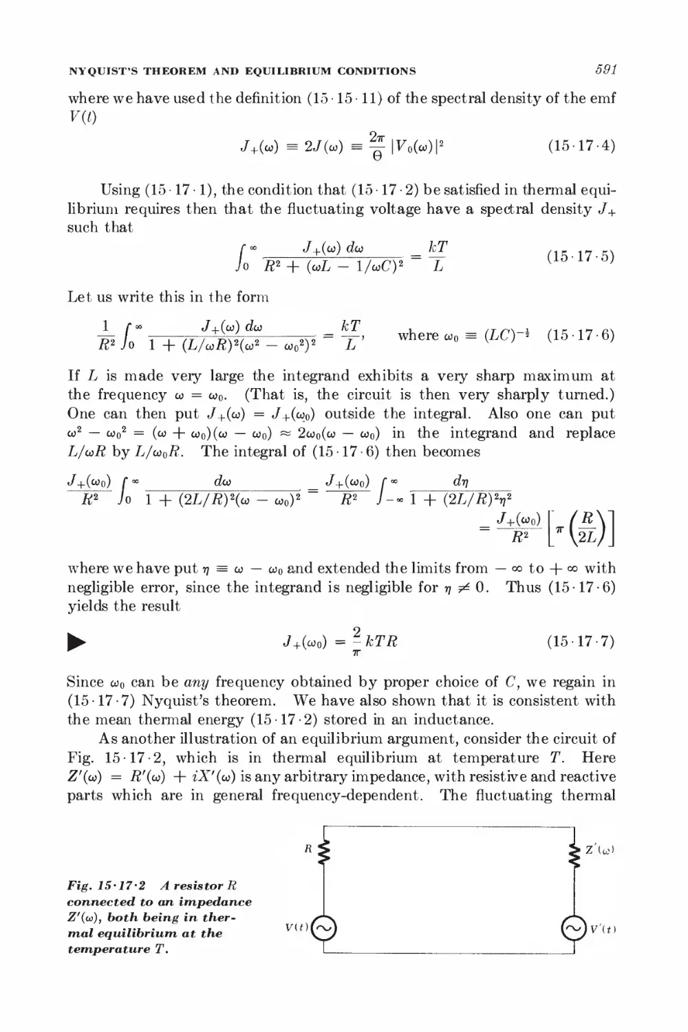
15-17 Nyquist's theorem and equilibrium conditions 589
GENERAL DISCUSSION OF IRREVERSIBLE PROCESSES
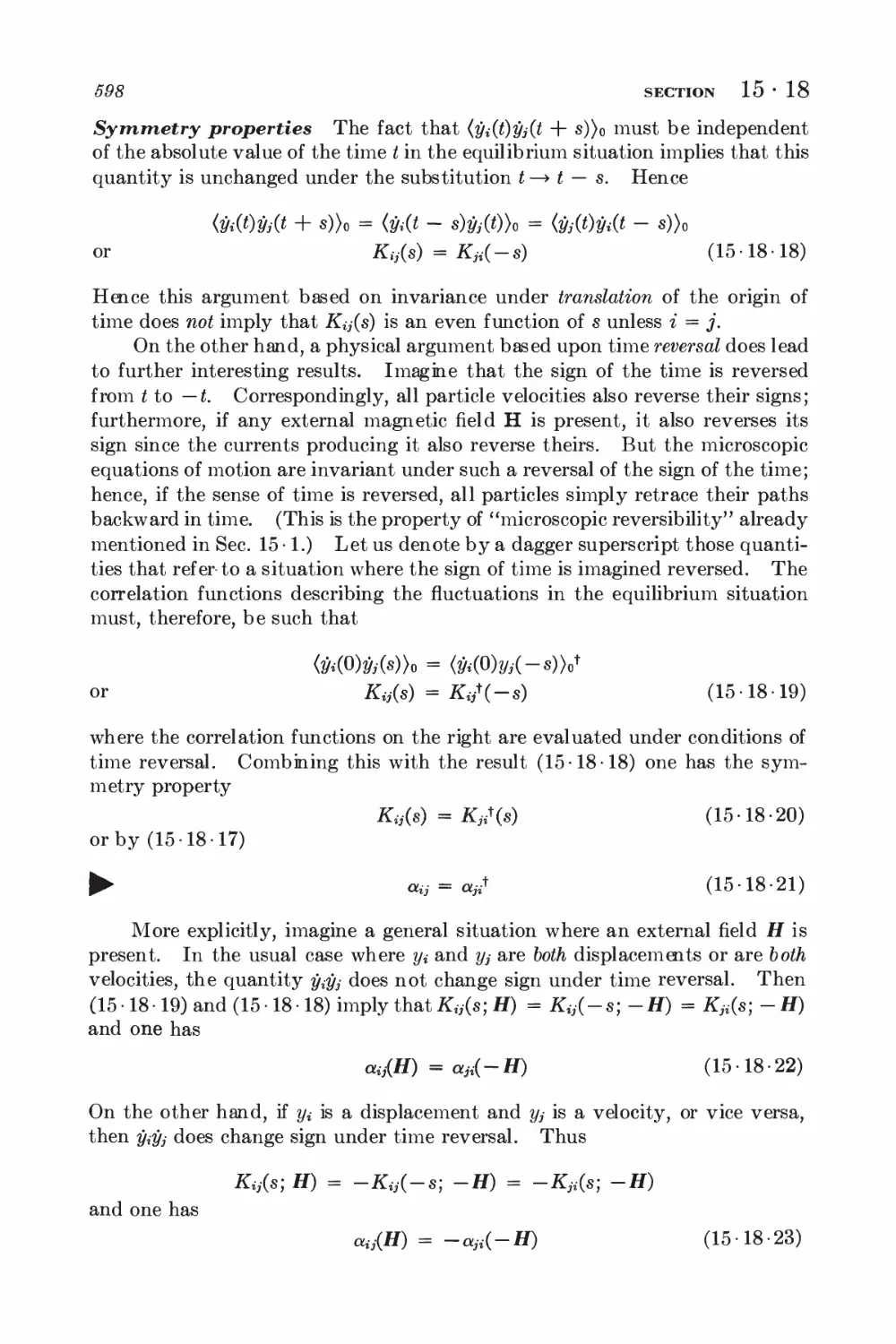
15 18 Fluctuations and Onsager relations 59%
Appendices 605
A.l Review of elementary sums 605
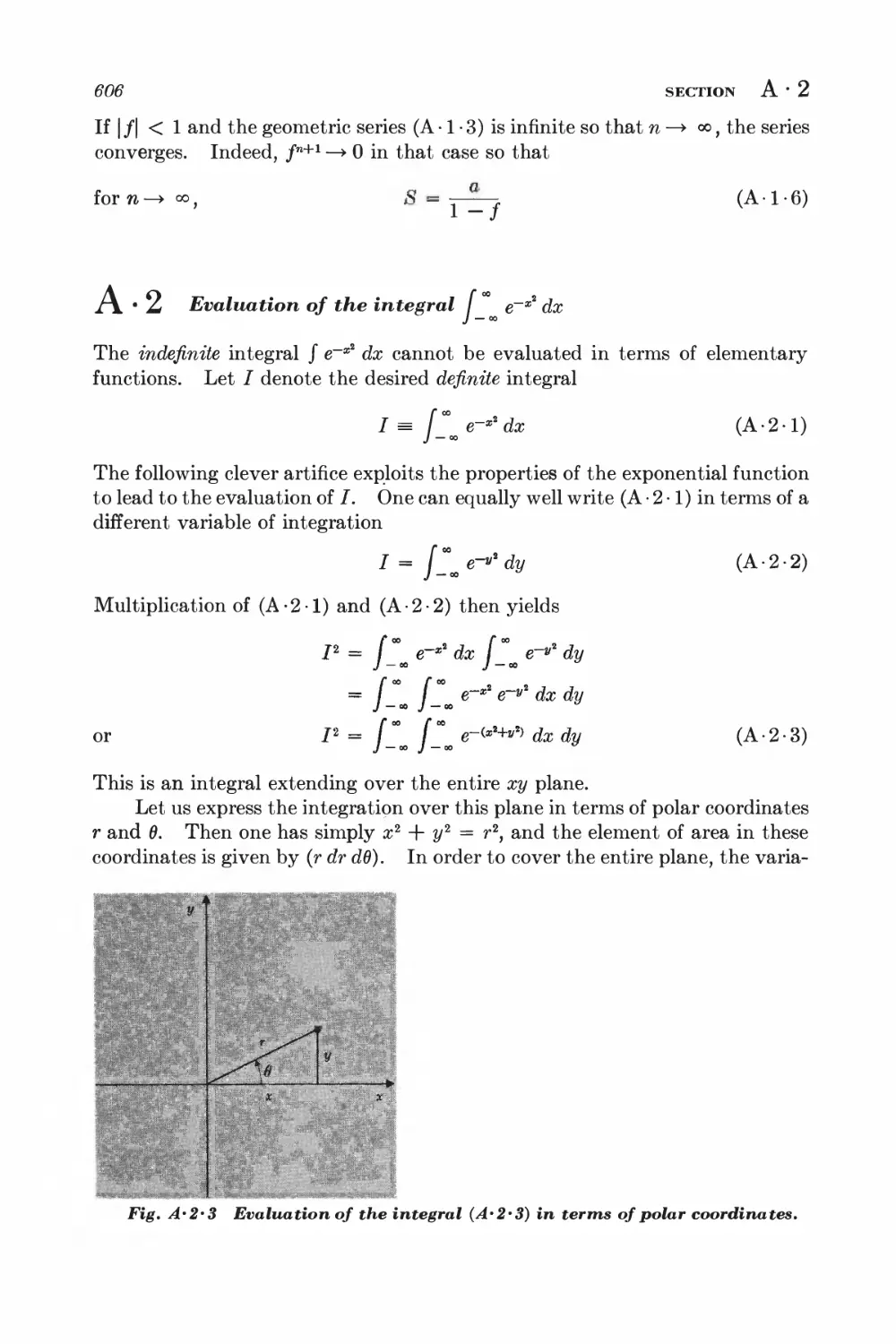
A.2 Evaluation of the integral I e~x* dx 606
A.3 Evaluation of the integral J e~xxn dx 607
A.4 Evaluation of integrals of the form J e~ax2xn dx 608
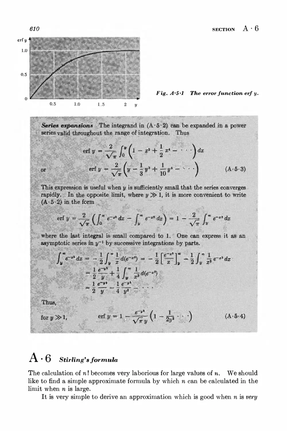
A.5 The error function 609
A.6 Stirling's formula 610
A.7 The Dirac delta function 614
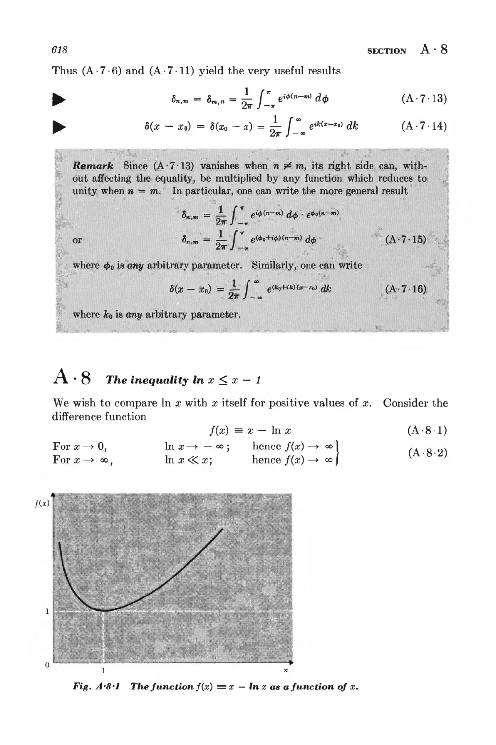
A.8 The inequality In x < x — 1 618
A.9 Relations between partial derivatives of several variables 619
A. 10 The method of Lagrange multipliers 620
A.ll Evaluation of the integral j (ex — l)_1z3 dx 622
A. 12 The H theorem and the approach to equilibrium 624
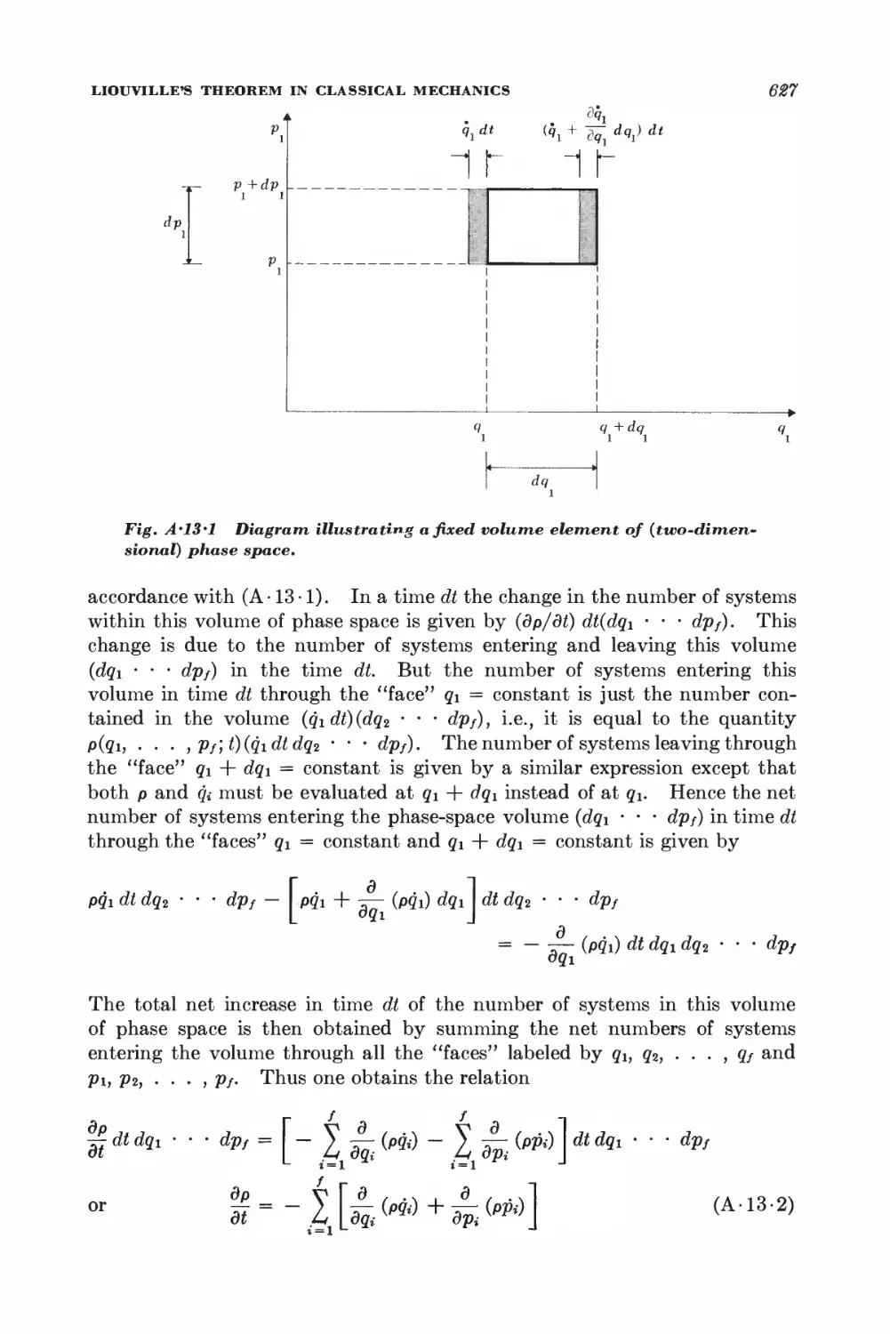
A. 13 Liouvilleys theorem in classical mechanics 626
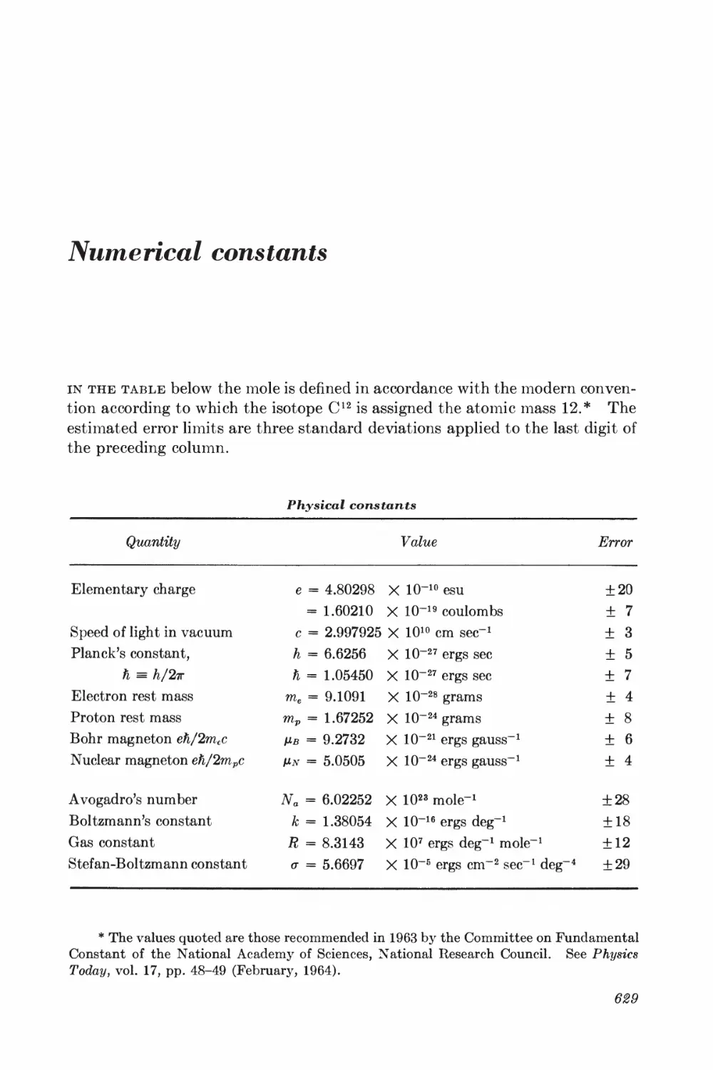
Numerical constants 629
Bibliography 631
Answers to selected problems 637
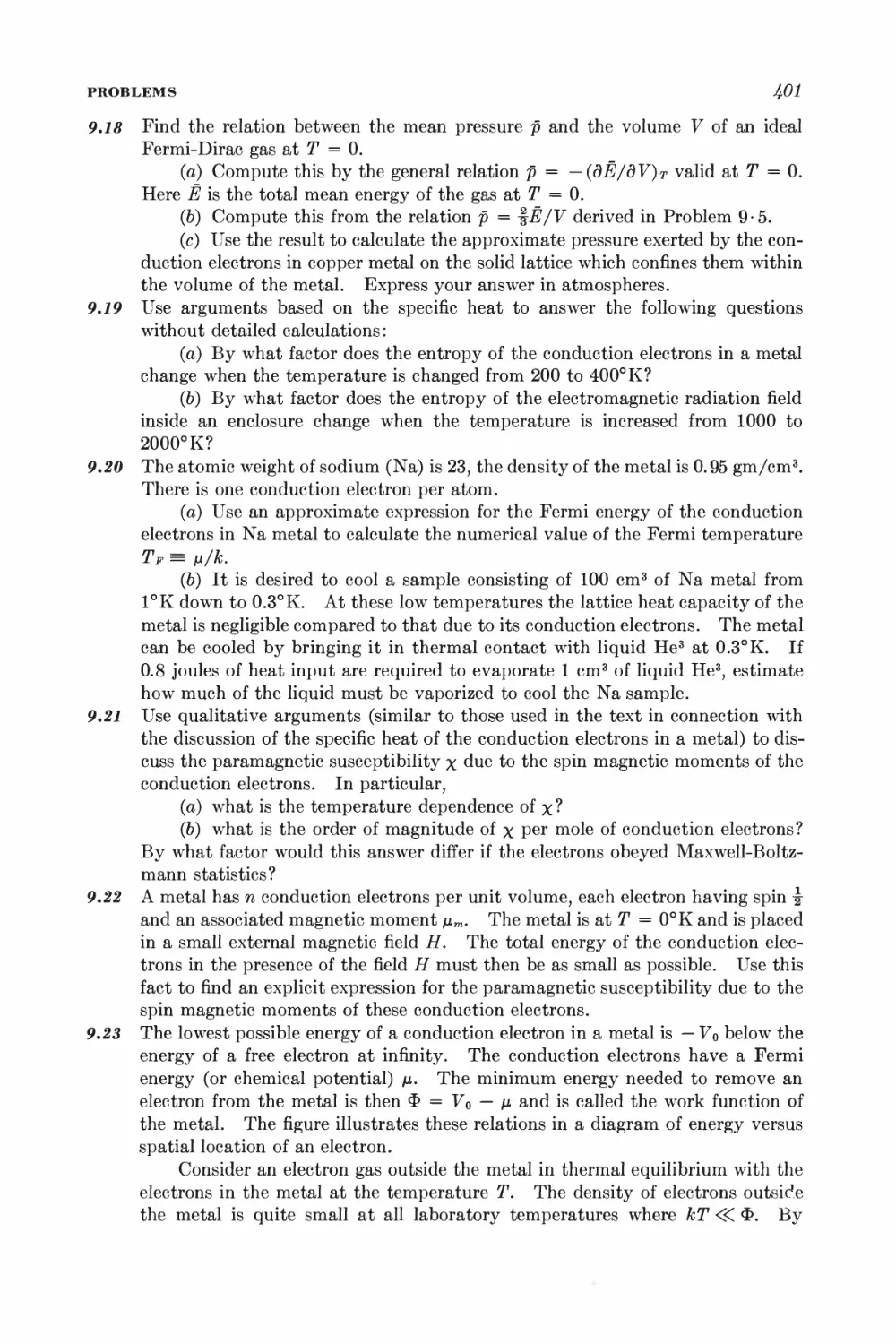
Index
643

Fundamentals of statistical
and thermal physics

Introduction to statistical methods
this book will be devoted to a discussion of systems consisting of very many
particles. Examples are gases, liquids, solids, electromagnetic radiation
(photons), etc. Indeed, most physical, chemical, or biological systems do consist
of many molecules; our subject encompasses, therefore, a large part of nature.
The study of systems consisting of many particles is probably the most
active area of modern physics research outside the realm of high-energy physics.
In the latter domain, the challenge is to understand the fundamental
interactions between nucleons, neutrinos, mesons, or other strange particles. But, in
trying to discuss solids, liquids, plasmas, chemical or biological systems, and
other such systems involving many particles, one faces a rather different task
which is no less challenging. Here there are excellent reasons for supposing that
the familiar laws of quantum mechanics describe adequately the motions of the
atoms and molecules of these systems; furthermore, since the nuclei of atoms
are not disrupted in ordinary chemical or biological processes and since
gravitational forces between atoms are of negligible magnitude, the forces between
the atoms in these systems involve only well-understood electromagnetic
interactions. Somebody sufficiently sanguine might therefore be tempted to
claim that these systems are "understood in principle." This would, however,
be a rather empty and misleading statement. For, although it might be
possible to write down the equations of motion for any one of these systems, the
complexity of a system containing many particles is so great that it may make
the task of deducing any useful consequences or predictions almost hopeless.
The difficulties involved are not just questions of quantitative detail which can
be solved by the brute force application of bigger and better computers.
Indeed, even if the interactions between individual particles are rather simple,
the sheer complexity arising from the interaction of a large number of them can
often give rise to quite unexpected qualitative features in the behavior of a
system. It may require very deep analysis to predict the occurrence of these
features from a knowledge of the individual particles. For example, it is a
striking fact, and one which is difficult to understand in microscopic detail,
I %
I 4
il
<f^!sii*iSf-i«!SSS^
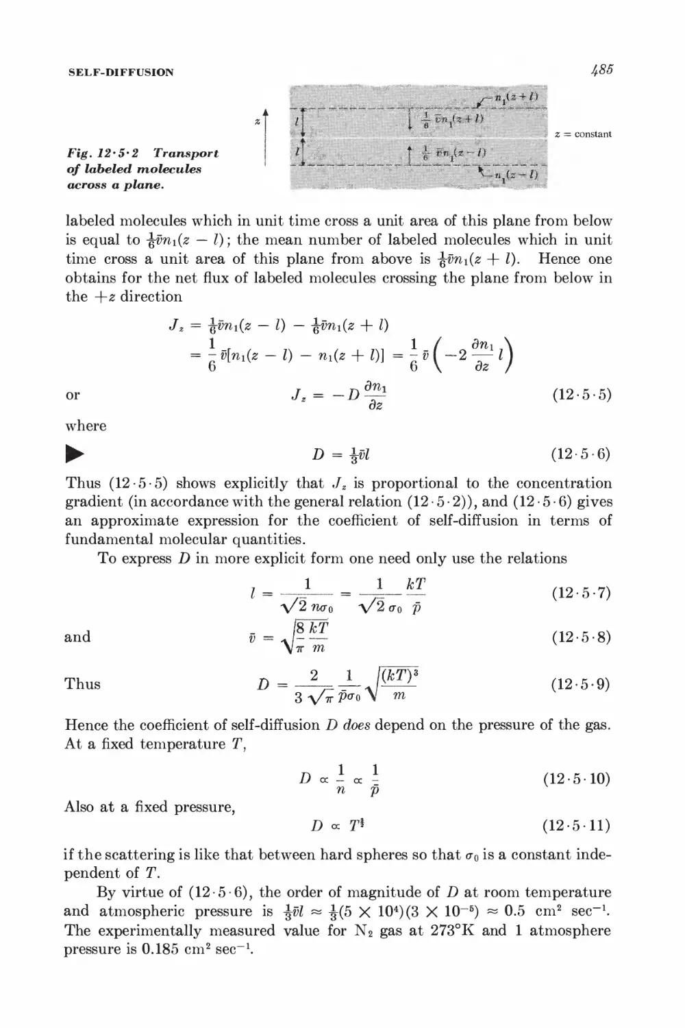
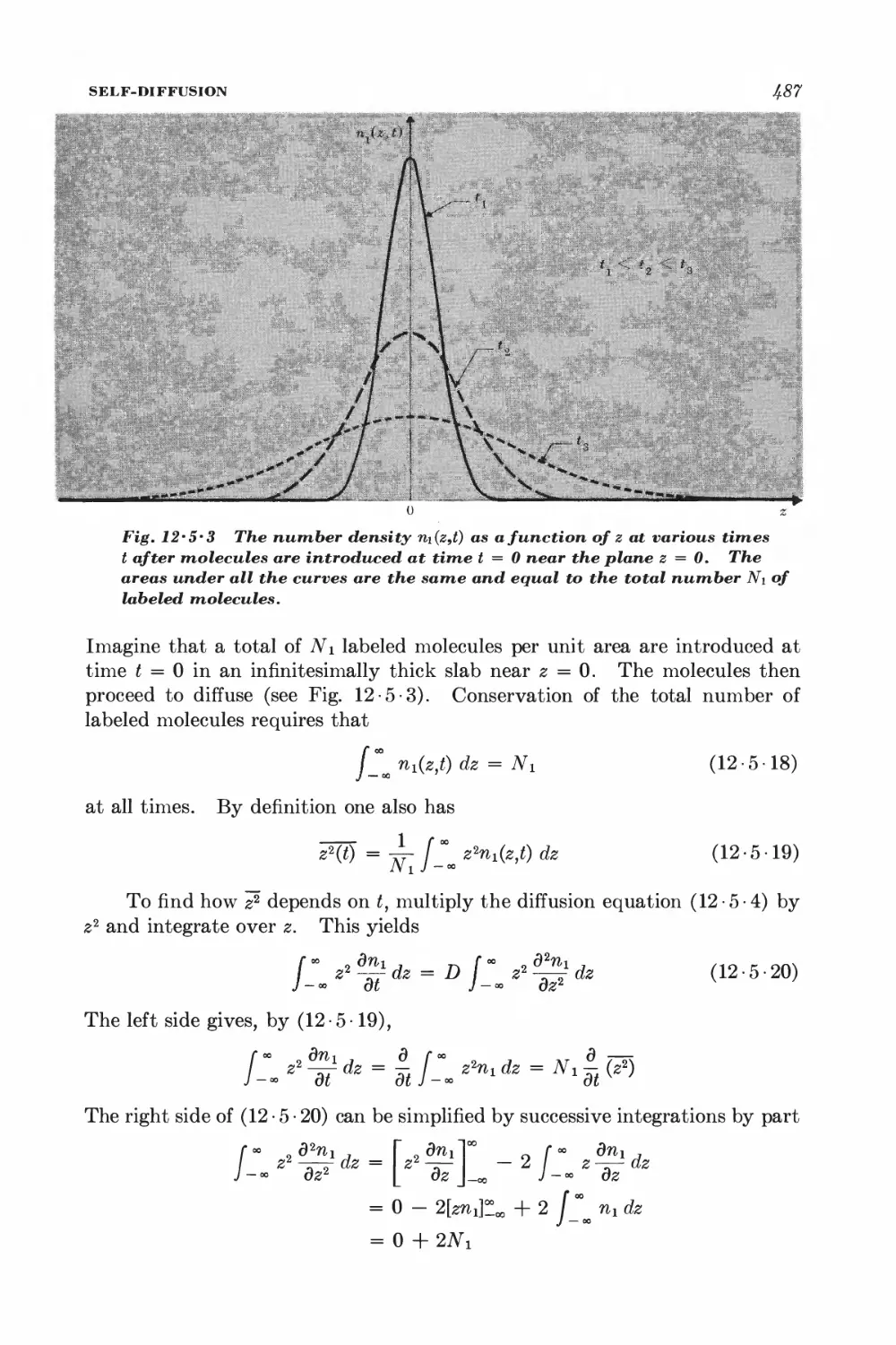
1

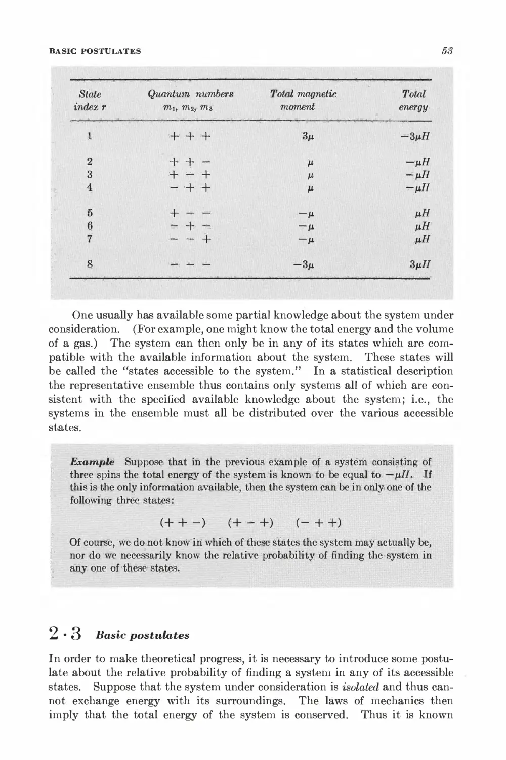
2
INTRODUCTION TO STATISTICAL METHODS
that simple atoms forming a gas can condense abruptly to form a liquid with
very different properties. It is a fantastically more difficult task to attain an
understanding of how aji assembly of certain kinds of molecules can lead to a
system capable of biological growth and reproduction.
The task of understanding systems consisting of many particles is thus
far from trivial, even when the interactions between individual atoms are well
known. Nor is the problem just one of carrying out complicated computations.
The main aim is, instead, to use one's knowledge of basic physical laws to
develop new concepts which can illuminate the essential characteristics of such
complex systems and thus provide sufficient insight to facilitate one's thinking,
to recognize important relationships, and to make useful predictions. When
the systems under consideration are not too complex and when the desired level
of description is not too detailed, considerable progress can indeed be achieved
by relatively simple methods of analysis.
It is useful to introduce a distinction between the sizes of systems whose
description may be of interest. We shall call a system "microscopic" (i.e.
"small scale") if it is roughly of atomic dimensions or smaller (say of the order
of 10 A or less). For example, the system might be a molecule. On the other
hand, we shall call a system "macroscopic" (i.e., "large scale") when it is large
enough to be visible in the ordinary sense (say greater than 1 micron, so that it
can at least be observed with a microscope using ordinary light). The system
consists then of very many atoms or molecules. For example, it might be a
solid or liquid of the type we encounter in our daily experience. When one is
dealing with such a macroscopic system, one is, in general, not concerned with
the detailed behavior of each of the individual particles constituting the system.
Instead, one is usually interested in certain macroscopic parameters which
characterize the system as a whole, e.g., quantities like volume, pressure,
magnetic moment, thermal conductivity, etc. If the macroscopic parameters
of an isolated system do not vary in time, then one says that the system is in
equilibrium. If an isolated system is not in equilibrium, the parameters of the
system will, in general, change until they attain constant values corresponding
to some final equilibrium condition. Equilibrium situations can clearly be
expected to be amenable to simpler theoretical discussion than more general
time-dependent nonequilibrium situations.
Macroscopic systems (like gases, liquids, or solids) began first to be
systematically investigated from a macroscopic phenomenological point of view
in the last century. The laws thus discovered formed the subject of
"thermodynamics." In the second half of the last century the theory of the atomic
constitution of all matter gained general acceptance, and macroscopic systems
began to be analyzed from a fundamental microscopic point of view as systems
consisting of very many atoms or molecules. The development of quantum
mechanics after 1926 provided an adequate theory for the description of
atoms and thus opened the way for an analysis of such systems on the basis
of realistic microscopic concepts. In addition to the most modern methods of
the "many-body problem," there have thus developed several disciplines of
physics which deal with systems consisting of very many particles. Although

INTRODUCTION TO STATISTICAL METHODS
3
the boundaries between these disciplines are not very sharp, it may be useful
to point out briefly the similarities and differences between their respective
methods of approach.
a. For a system in equilibrium, one can try to make some very general
statements concerning relationships existing between the macroscopic
parameters of the system. This is the approach of classical "thermodynamics,"
historically the oldest discipline. The strength of this method is its great
generality, which allows it to make valid statements based on a minimum
number of postulates without requiring any detailed assumptions about the
macroscopic (i.e., molecular) properties of the system. The strength of the
method also implies its weakness: only relatively few statements can be made
on such general grounds, and many interesting properties of the system remain
outside the scope of the method.
b. For a system in equilibrium, one can again try to make very general
statements consistently based, however, on the macroscopic properties of the
particles in the system and on the laws of mechanics governing their behavior.
This is the approach of "statistical mechanics." It yields all the results of
thermodynamics plus sl large number of general relations for calculating the
macroscopic parameters of the system from a knowledge of its microscopic
constituents. This method is one of great beauty and power.
c. If the system is not in equilibrium, one faces a much more difficult task.
One can still attempt to make very general statements about such systems,
and this leads to the methods of "irreversible thermodynamics," or, more
generally, to the study of "statistical mechanics of irreversible processes."
But the generality and power of these methods is much more limited than in
the case of systems in equilibrium.
d. One can attempt to study in detail the interactions of all the particles
in the system and thus to calculate parameters of macroscopic significance.
This is the method of "kinetic theory." It is in principle always applicable,
even when the system is not in equilibrium so that the powerful methods of
equilibrium statistical mechanics are not available. Although kinetic theory
yields the most detailed description, it is by the same token also the most
difficult method to apply. Furthermore, its detailed point of view may tend to
obscure general relationships which are of wider applicability.
Historically, the subject of thermodynamics arose first before the atomic
nature of matter was understood. The idea that heat is a form of energy was
first suggested by the work of Count Rumford (1798) and Davy (1799). It
was stated explicitly by the German physician R. J. Mayer (1842) but gained
acceptance only after the careful experimental work of Joule (1843-1849).
The first analysis of heat engines was given by the French engineer S. Carnot
in 1824. Thermodynamic theory was formulated in consistent form by
Clausius and Lord Kelvin around 1850, and was greatly developed by J. W.
Gibbs in some fundamental papers.(1876-1878).
The atomic approach to macroscopic problems began with the study of
the kinetic theory of dilute gases. This subject was developed through the

4
SECTION 1 ' 1
pioneering work of Clausius, Maxwell, and Boltzmann. Maxwell discovered
the distribution law of molecular velocities in 1859, while Boltzmann formulated
his fundamental integrodifferential equation (the Boltzmann equation) in
1872. The kinetic theory of gases achieved its modern form when Chapman
and Enskog (1916-1917) succeeded in approaching the subject by developing
systematic methods for solving this equation.
The more general discipline of statistical mechanics also grew out of the
work of Boltzmann who, in 1872, succeeded further in giving a fundamental
microscopic analysis of irreversibility and of the approach to equilibrium. The
theory of statistical mechanics was then developed greatly in generality and
power by the basic contributions of J. W. Gibbs (1902). Although the advent
of quantum mechanics has brought many changes, the basic framework of the
modern theory is still the one which he formulated.
In discussing systems consisting of very many particles, we shall not aim
to recapitulate the historical development of the various disciplines dealing
with the physical description of such systems. Instead we shall, from the
outset, adopt a modern point of view based on our present-day knowledge of
atomic physics and quantum mechanics. We already mentioned the fact that
one can make very considerable progress in understanding systems of many
particles by rather simple methods of analysis. This may seem rather
surprising at first sight; for are not systems such as gases or liquids, which consist
of a number of particles of the order of Avogadro's number (1023), hopelessly
complicated? The answer is that the very complexity of these systems
contains within it the key to a successful method of attack. Since one is not
concerned with the detailed behavior of each and every particle in such
systems, it becomes possible to apply statistical arguments to them. But as
every gambler, insurance agent, or other person concerned with the calculation
of probabilities knows, statistical arguments become most satisfactory when
they can be applied to large numbers. What a pleasure, then, to be able to
apply them to cases where the numbers are as large as 1023, i.e., Avogadro's
number! In systems such as gases, liquids, or solids where one deals with very
many identical particles, statistical arguments thus become particularly
effective. This does not mean that all problems disappear; the physics of many-
body problems does give rise to some difficult and fascinating questions. But
many important problems do indeed become quite simple when approached by
statistical means.
RANDOM WALK AND BINOMIAL DISTRIBUTION
11 Elementary statistical concepts and examples
The preceding comments make it apparent that statistical ideas will play a
central role throughout this book. We shall therefore devote this first chapter
to a discussion of some elementary aspects of probability theory which are of
great and recurring usefulness.

ELEMENTARY STATISTICAL CONCEPTS AND EXAMPLES
5
The reader will be assumed to be familiar with the most rudimentary
probability concepts. It is important to keep in mind that whenever it is
desired to describe a situation from a statistical point of view (i.e., in terms of
probabilities), it is always necessary to consider an assembly (or "ensemble")
consisting of a very large number 91 of similarly prepared systems. The
probability of occurrence of a particular event is then denned with respect to this
particular ensemble and is given by the fraction of systems in the ensemble
which are characterized by the occurrence of this specified event. For example,
in throwing a pair of dice, one can give a statistical description by considering
that a very large number 91 (in principle, 91 —> <x>) of similar pairs of dice are
thrown under similar circumstances. (Alternatively one could imagine the
same pair of dice thrown 91 times in succession under similar circumstances.)
The probability of obtaining a double ace is then given by the fraction of these
experiments in which a double ace is the outcome of a throw.
Note also that the probability depends very much on the nature of the
ensemble which is contemplated in denning this probability. For example, it
makes no sense to speak simply of the probability that an individual seed will
yield red flowers. But one can meaningfully ask for the probability that such
a seed, regarded as a member of an ensemble of similar seeds derived from a
specified set of plants, will yield red flowers. The probability depends crucially
on the ensemble of which the seed is regarded as a member. Thus the
probability that a given seed will yield red flowers is in general different if this seed
is regarded as (a) sl member of a collection of similar seeds which are known to
be derived from plants that had produced red flowers or as (b) sl member of a
collection of seeds which are known to be derived from plants that had produced
pink flowers.
In the following discussion of basic probability concepts it will be useful
to keep in mind a specific simple, but important, illustrative example-—the
so-called "random-walk problem." In its simplest idealized form, the problem
can be formulated in the following traditional way: A drunk starts out from a
lamppost located on a street. Each step he takes is of equal length I. The
man is, however, so drunk that the direction of each step-—whether it is to the
right or to the left-—is completely independent of the preceding step. All
one can say is that each time the man takes a step, the probability of its being
to the right is p, while the probability of its being to the left is q = 1 — p.
(In the simplest case p = q, but in general p 5* q. For example, the street
might be inclined with respect to the horizontal, so that a step downhill to the
right is more likely than one uphill to the left.)
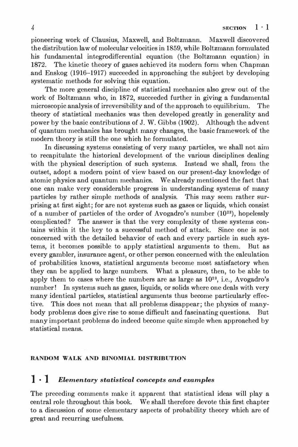
Choose the x axis to lie along the street so that x = 0 is the position of the
0
Lamppost
'u-j """"" " ""*:r" ' " "
/ x
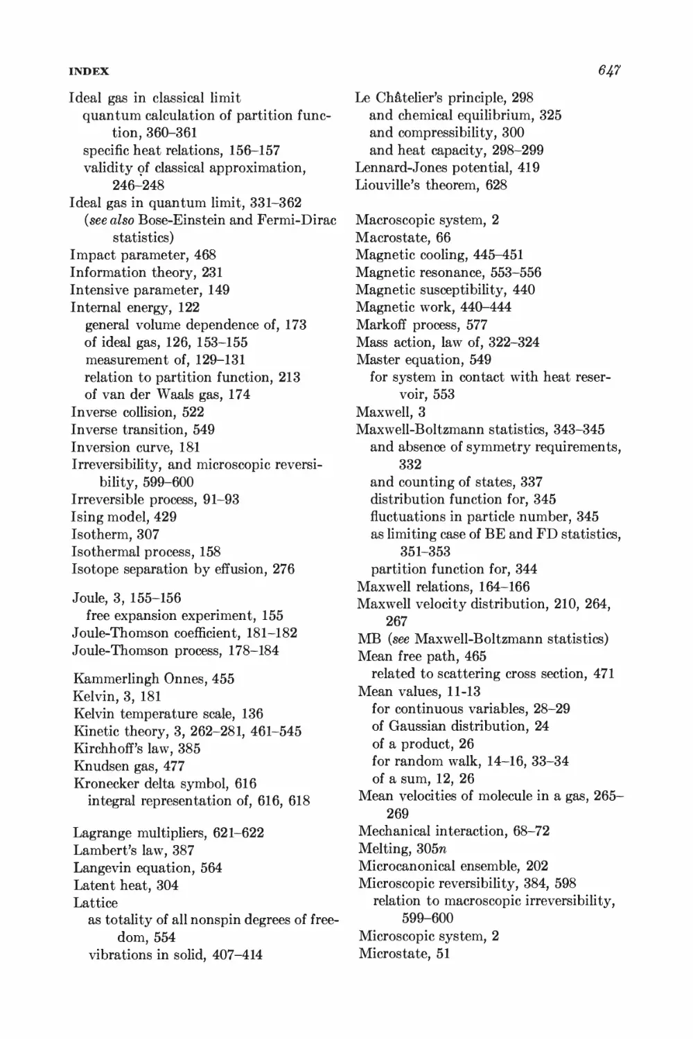
Fig. 1*1*1 The drunkard9s random walk in one dimension.

6
SECTION 1 ' 1
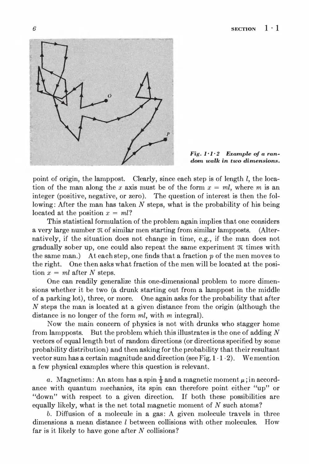
Fig. 1*1'2 Example of a ran-
dom walk in two dimensions.
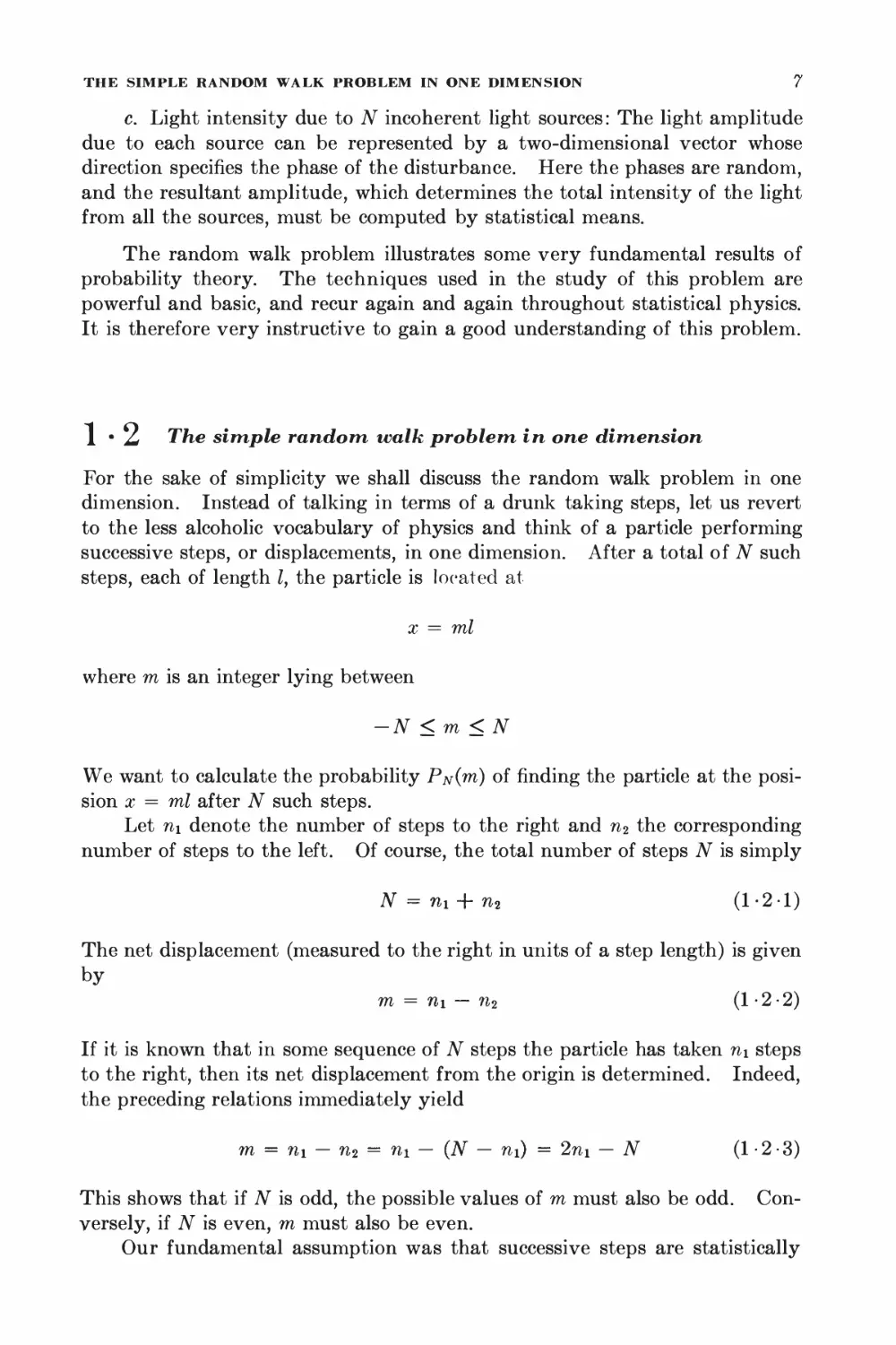
point of origin, the lamppost. Clearly, since each step is of length I, the
location of the man along the x axis must be of the form x = ml, where m is an
integer (positive, negative, or zero). The question of interest is then the
following : After the man has taken N steps, what is the probability of his being
located at the position x = ml?
This statistical formulation of the problem again implies that one considers
a very large number 91 of similar men starting from similar lampposts.
(Alternatively, if the situation does not change in time, e.g., if the man does not
gradually sober up, one could also repeat the same experiment 91 times with
the same man.) At each step, one finds that a fraction p of the men moves to
the right. One then asks what fraction of the men will be located at the
position x = ml after N steps.
One can readily generalize this one-dimensional problem to more
dimensions whether it be two (a drunk starting out from a lamppost in the middle
of a parking lot), three, or more. One again asks for the probability that after
N steps the man is located at a given distance from the origin (although the
distance is no longer of the form ml, with m integral).
Now the main concern of physics is not with drunks who stagger home
from lampposts. But the problem which this illustrates is the one of adding N
vectors of equal length but of random directions (or directions specified by some
probability distribution) and then asking for the probability that their resultant
vector sum has a certain magnitude and direction (see Fig. 1-1-2). We mention
a few physical examples where this question is relevant.
a. Magnetism: An atom has a spin -g- and a magnetic moment pi; in
accordance with quantum mechanics, its spin can therefore point either "up" or
"down" with respect to a given direction. If both these possibilities are
equally likely, what is the net total magnetic moment of N such atoms?
b. Diffusion of a molecule in a gas: A given molecule travels in three
dimensions a mean distance I between collisions with other molecules. How
far is it likely to have gone after N collisions?

THE SIMPLE RANDOM WALK PROBLEM IN ONE DIMENSION 7
c. Light intensity due to N incoherent light sources: The light amplitude
due to each source can be represented by a two-dimensional vector whose
direction specifies the phase of the disturbance. Here the phases are random,
and the resultant amplitude, which determines the total intensity of the light
from all the sources, must be computed by statistical means.
The random walk problem illustrates some very fundamental results of
probability theory. The techniques used in the study of this problem are
powerful and basic, and recur again and again throughout statistical physics.
It is therefore very instructive to gain a good understanding of this problem.
1 • 2^ The simple random walk problem in one dimension
For the sake of simplicity we shall discuss the random walk problem in one
dimension. Instead of talking in terms of a drunk taking steps, let us revert
to the less alcoholic vocabulary of physics and think of a particle performing
successive steps, or displacements, in one dimension. After a total of N such
steps, each of length Z, the particle is located at
x = ml
where m is an integer lying between
-N < m <N
We want to calculate the probability Pn{^) of finding the particle at the posi-
sion x = ml after N such steps.
Let rii denote the number of steps to the right and n2 the corresponding
number of steps to the left. Of course, the total number of steps N is simply
2V = m + w2 (1-2-1)
The net displacement (measured to the right in units of a step length) is given
by
m = ni — n2 (1-2-2)
If it is known that in some sequence of N steps the particle has taken ni steps
to the right, then its net displacement from the origin is determined. Indeed,
the preceding relations immediately yield
m = ni — n2 = ni — (N — ni) — 2ni — N (1-2-3)
This shows that if N is odd, the possible values of m must also be odd.
Conversely, if N is even, m must also be even.
Our fundamental assumption was that successive steps are statistically

8
SECTION 1 ' 2
zv-^&su&mj, s; ssss*« ~&*<r%
p*— :;«r*§*?
%*a&£&*?5$ k&«A&£'vast
n:;"r"".v :f*
f !«£!
fft^J
3
i 2
1
0
0
1
2
3
3 |
1
-1
-3
>
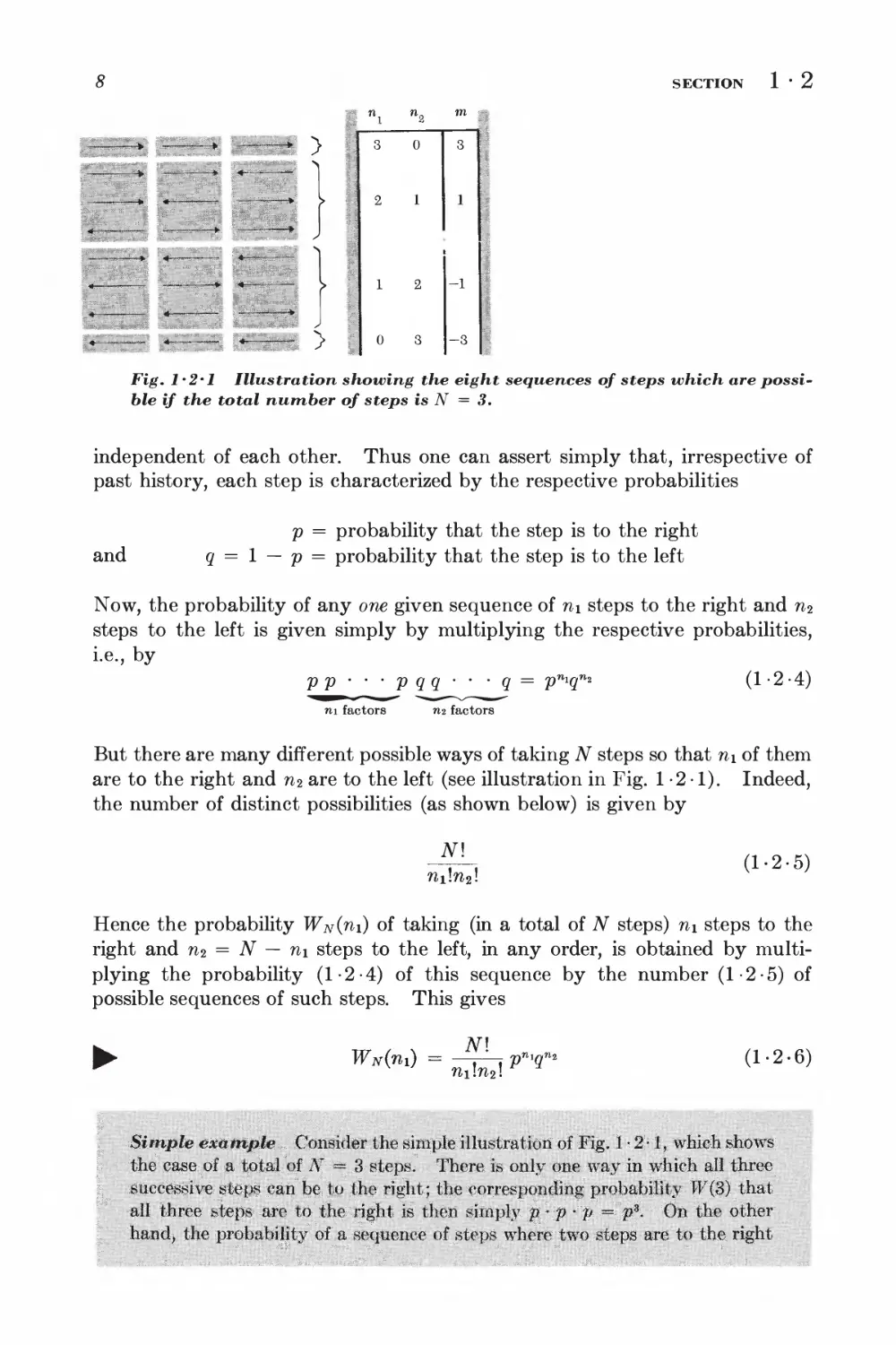
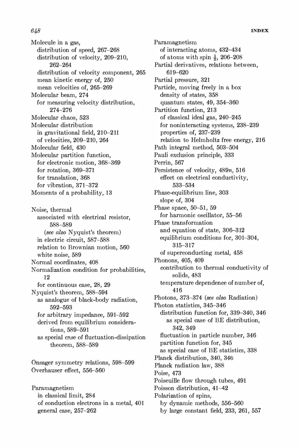
Fig. 1*2*1 Illustration showing the eight sequences of steps which are
possible if the total number of steps is N = 3.
independent of each other. Thus one can assert simply that, irrespective of
past history, each step is characterized by the respective probabilities
p = probability that the step is to the right
and q = 1 — p = probability that the step is to the left
Now, the probability of any one given sequence of n\ steps to the right and n2
steps to the left is given simply by multiplying the respective probabilities,
i.e., by
pp---pqq---q = pniqn* (1 -2-4)
ni factors
712 factors
But there are many different possible ways of taking N steps so that n\ of them
are to the right and n2 are to the left (see illustration in Fig. 1-2 1). Indeed,
the number of distinct possibilities (as shown below) is given by
fti!w2!
(1-2-5)
Hence the probability Wn(tii) of taking (in a total of N steps) n\ steps to the
right and n2 = N — n\ steps to the left, in any order, is obtained by
multiplying the probability (1-2-4) of this sequence by the number (1-2-5) of
possible sequences of such steps. This gives
JMnO =
fti!n2!
p^qn
(1-2-6)
Simple example... Consider the simple illustration of Fig. 1-2-1,, which shows
the case, of a total of N == 3 steps; There is only one way in which all three
successive steps can be to the right; the corresponding probability W($) that
all three steps are to the right is then simply p: p -p =V- 0n the other
hand, the probability of a sequence of steps where two steps are to the right

THE SIMPLE RANDOM WALK PROBLEM IN ONE DIMENSION
while the third step is to the left is p% But there are,fthree such possible
sequences. Thus the total probability of occurrence of a situation where two
steps are to the right and one is to the left is given by 3p2#.
Reasoning leading to Eq. {1-2-5) The problem is to count the number of
distinct ways in which N objects (or steps), of which n*_ are indisMnguishably
of one type and n% of a second type, can be acconan>odated in a total of
N — n\ + n% possible places. In this case
the 1st place can be occupied by any one of the N objects-
the 2nd place can be occupied by any one of the remaining (N
1) objects
the JVth place can be occupied only by the last 1 object ,
Hence all the available places can be occupied in
N(N - 1)(N - 2) • * • i' s£ Ml
possible ways. Thev above enumeration considers each object as
distinguishable. But since the nr objects of the first type are indistinguishable (e.g.,
all are right steps)f all the ?ij permutations of these objects among
themselves lead to the same situation. Similarly/ all the n%\ permutations of
objects of the second type among themselves lead to the same situation.
Hence, by dividing the total number 2V! of arrangements of the objects by
the number nitn2l of irrelevant permutations of objects of each type, one
obtains the total number Nl/nAn^l of distinct ways in which Ar objects can
be arranged if nx are of one type and n% of another type.
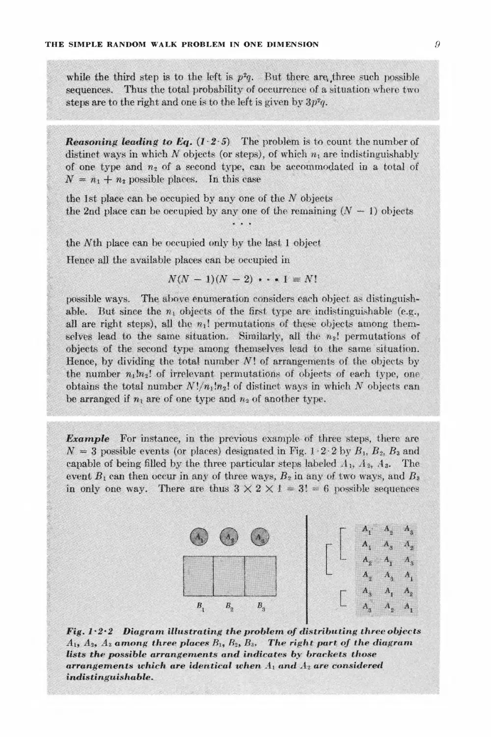
Example For instance, in the pre\rious example of three steps, there are
N — 3 possible events (or places) designated in Fig. 1 -2-2 by Bh B2, B$ and
capable of being filled by the three particular steps labeled Aj, A^ A3. The
event B\ can then occur in any of three ways, B2 in any of two ways, and Bs
in only one way. There are thus 3X2X1= 3! ™ 6 possible sequences
t I
^o A*
Fig. 1*2*2 Diagram illustrating the problem of distributing three objects
Ai, A%9 As among three places Bu Bz> B%. The right part of the diagram
lists the possible arrangements and indicates by brackets those
arrangements which are identical tchen Ai and At are considered
indis tinguis hable.

10
SECTION 1 ' 2
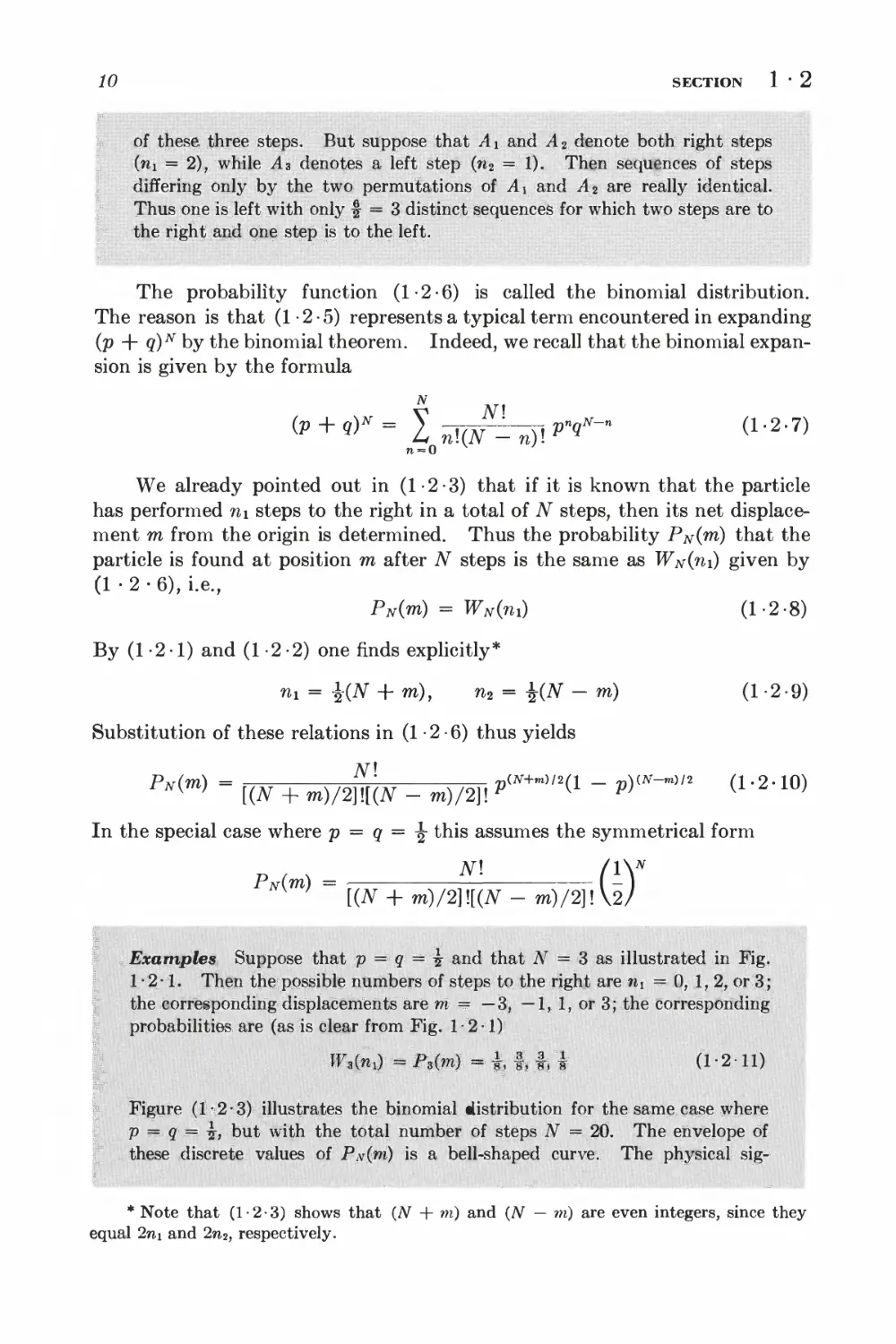
of these three steps. But suppose that A r and A 2 denote both right steps
(rii = 2), while A* denotes a left step (% — 1). Then sequ nces of steps
differing only by the two permutations of AY and A2 are really identical.
Thus one is left with only f — 3 distinct sequences for which two steps are to
the right and one step lis to the left.
The probability function (1-2-6) is called the binomial distribution.
The reason is that (1-2-5) represents a typical term encountered in expanding
(P + Q)N by the binomial theorem. Indeed, we recall that the binomial
expansion is given by the formula
n = 0 v '
We already pointed out in (1-2-3) that if it is known that the particle
has performed n\ steps to the right in a total of N steps, then its net
displacement m from the origin is determined. Thus the probability P^(ra) that the
particle is found at position m after N steps is the same as WN(ni) given by
(1 ' 2 • 6), i.e,
pN(m) = WN(m) (1-2-8)
By (1 -2• 1) and (1 -2 -2) one finds explicitly*
ni = %(N + m), n2 = UN-m) (1-2-9)
Substitution of these relations in (1-2-6) thus yields
AM
rN{ ] [(N + m)/2]l[(N - m)/2]!P U P) U ;
In the special case where p = q = ^ this assumes the symmetrical form
p (m) = m /iy
l(N + m)/2]l[(N - ro)/2]! W
I:
;; Examples Suppose that p = q = ^ and that N = 3 as illustrated in Eig,
f 1-2-1. Then the possible numbers of steps to the right are Wi = 0, 1, 2, or 3;
I the corresponding displacements are m = — 3, — 1, 1, or 3; the corresponding
I probabilities are (as is clear from Fig. 1-2-1)
t W*(nJ - P,(m) - i I |,i (1 2 11)
P
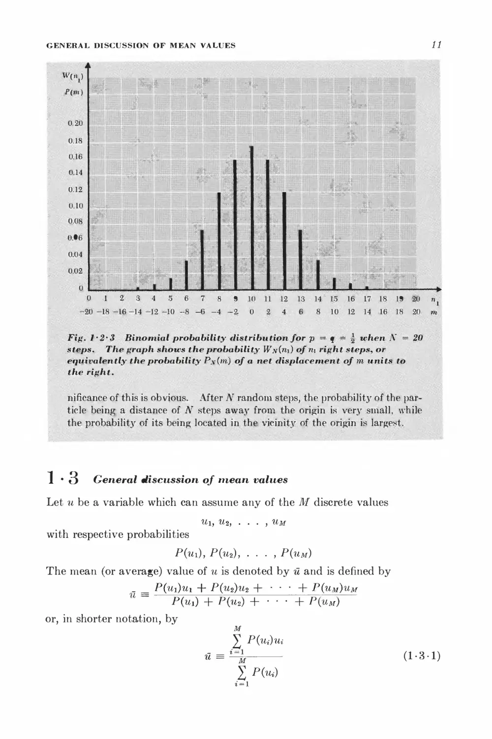
Eigure (1^;2-3) illustrates the binomial distribution for the same case where
I p = q'■■■■= ?, but with the total number of steps N = 20- The envelope of
f =, these discrete values of P,v(m) is a bell-shaped curve. The physical sig-
* Note that (1-2-3) shows that (N + m) and (N — m) are even integers, since they
equal 2n\ and 2n2, respectively.

GENERAL
DISCUSSION OF MEAN VALUES
11
w<*v)
P(m)
0.20
018
016
0:14
0 12
0.10
0.08
o.#6
0.04
0.02
0
jQtf-
;L.
P
llflip
m§
if;
Sibil
^Jfc,,
,?
% ;;j
J
'"'11 i
IK
1111 i
1 ■-■ i
%\
1 *
In ,
p -
lips?
lEi.
„, l
pi
t: If!; j
1 Pi j
* a ij
; " ?
1; * :.
j J J
1* «
if 1
i Pis? :
f 1 j
1
tar
ifi
t -4J
m\
;";:&f
p |£
i; i
r 1
&
IT,
J' 4
o
10 11 12 13 14" .15.' 16 17 18 1? 20 n
-20' -18 -16 -14 -12 -10 -8 -6 -4 -2. 0
i
10 12 14 16 18 20^ m
Fig. i'2*3 Binomial probability distribution for p == q -~ ^ when N ~ 20
steps. The graph shows the probability Wn{ti\) of ri\ right steps, or
eqiiivalehtly the probability P\(m) of a net fHsplacernent of m units to
the right.
riificance of this is obvious. After N random steps, the probability of the
particle being a distance of ..AT steps away from the origin is very small, while
the probability of its being located in the; vicinity of the origin is largest.
1 • O General discussion of mean values
Let u be a variable which can assume any of the M discrete values
Uij u2, . . . , uM
with respective probabilities
P(mi), P(u2), • • • , P(uM)
The mean (or average) value of u is denoted by u and is denned by
_ = P(ui)ui + P(u2)u2 + • • • + P(um)um
U ~ P(ux) + P(u2) + ■ - - + P(uM)
or, in shorter notation, by
£ P(ui)u
M
L
M
(1-3-1)
I PM
i = l

12
SECTION 1 ' 3
This is, of course, the familiar way of computing averages. For example, if u
represents the grade of a student on an examination and P(u) the number of
students obtaining this grade, then Eq. (1-3-1) asserts that the mean grade
is computed by multiplying each grade by the number of students having this
grade, adding this up, and then dividing by the total number of students.
More generally, if f(u) is any function of u, then the mean value oif(u) is
defined by
M
/(«)=*=Tf (1-3-2)
I P(ui)
1=1
This expression can be simplified. Since P(ui) is defined as a probability, the
quantity
M
P(Ul) + P(u2) + • • • + P(uM) = X P(ud
represents the probability that u assumes any one of its possible values and
this must be unity. Hence one has quite generally
M
P> lP(Ui) = l (1-3-3)
i = i
This is the so-called "normalization condition" satisfied by every probability.
As a result, the general definition (1-3-2) becomes
M
^ /(„) = I P(iu)f(ui) (1-3-4)
t'=l
Note the following simple results. If f(u) and g(u) are any two functions
of u, then
f(u) + g(u) = X PWt/M + 9M] - X PW/W + X P(uMui)
i = 1 i = l * = 1
or
► f(u) + g(u) =f(u)+g(u) (1-3-5)
Furthermore, if c is any constant, it is clear that
► qf(SJ = c/(Sy (1-3-6)
Some simple mean values are particularly useful for describing
characteristic features of the probability distribution P. One of these is the mean value
u (e.g., the mean grade of a class of students). This is a measure of the central
value of u about which the various values Ui are distributed. If one measures
the values of u from their mean value u, i.e., if one puts
Au = u — u (1-3-7)
then Au = (u — u) = u — u = 0 (1-3-8)
This says merely that the mean value of the deviation from the mean vanishes.

CALCULATION OF MEAN VALUES FOR THE RANDOM WALK PROBLEM
13
Another useful mean value is
M
(Au)2 = X ?(**)(** - ^)2 > 0 (1-3-9)
which is called the "second moment of u about its mean," or more simply the
"dispersion of u." This can never be negative, since (Au)2 > 0 so that each
term in the sum contributes a nonnegative number. Only if Ui = u for all
values Ui will the dispersion vanish. The larger the spread of values of Ui
about u, the larger the dispersion. The dispersion thus measures the amount
of scatter of values of the variable about its mean value (e.g., scatter in grades
about the mean grade of the students). Note the following general relation,
which is often useful in computing the dispersion:
(u - u)2 = (u2 -2uu + u2) =u~2- 2uu + u2
or
^ (u „ uy = u2 - u2 (1-3-10)
Since the left side must be positive it also follows that
u^^u2 (1-3-11)
One can define further mean values such as (Au)n, the "nth moment of u
about its mean," for integers n > 2. These are, however, less commonly
useful.
Note that a knowledge of P(u) implies complete information about the
actual distribution of values of the variable u. A knowledge of a few
moments, like u and (Au)2, implies only partial, though useful, knowledge of
the characteristics of this distribution. A knowledge of some mean values is
not sufficient to determine P(u) completely (unless one knows the moments (Au)n
for all values of n). But by the same token it is often true that a calculation
of the probability distribution function P(u) may be quite difficult, whereas
some simple mean values can be readily calculated directly without an explicit
knowledge of P(u). We shall illustrate some of these comments in the
following pages.
1 • 4 Calculation of mean values for the random walk problem
In (1-2-6) we found that the probability, in a total of N steps, of making m
steps to the right (and N — ni = n2 steps to the left) is
(For the sake of simplicity, we omit attaching the subscript N to W when no
confusion is likely to arise.)

u
SECTION 1 ' 4
Let us first verify the normalization, i.e., the condition
N
X W(m) = 1 (1-4-2)
ni = 0
which says that the probability of making any number of right steps between
0 and N must be unity. Substituting (1-4-1) into (1 -4-2), we obtain
\ — pn1QN-ni _ /~ _|_ „\n by ^he binomial theorem
Li nil(N — ni)i.
= 1^ = 1 since q = I — p
which verifies the result.
What is the mean number n\ of steps to the right? By definition
N N AM
nlS I W^m- J ■ ^ ^^-m (1-4-3)
m = 0 m = 0 V
If it were not for that extra factor of n i in each term of the last sum, this would
again be the binomial expansion and hence trivial to sum. The factor ni
spoils this lovely situation. But there is a very useful general procedure for
handling such an extra factor so as to reduce the sum to simpler form. Let us
consider the purely mathematical problem of evaluating the sum occurring in
(1 • 4 • 3), where p and q are considered to be any two arbitrary parameters.
Then one observes that the extra factor ni can be produced by differentiation
so that
Hence the sum of interest can be written in the form
I n1l(NN-n1V.P'"qN~n'ni= I ml(Nr-nO\[P^(rFl)]^~"
1=0 ni = 0 U J
5Tn jf} "I by interchanging orae
= V Tp I I nxKJy-nO! pniqN~ni\ 0f summation and dif"
by interchanging order
of summatio
ni=0 " J ferentiation
= V — (v + q)N by the binomial theorem
dp
= pN(p + q)N~i
Since this result is true for arbitrary values of p and q, it must also be
valid in our particular case of interest where p is some specified constant and
q = 1 — p. Then p + q = 1 so that (1-4-3) becomes simply
^ n1 = Np (1-4-4)
We could have guessed this result. Since p is the probability of making
a right step, the mean number of right steps in a total of N steps is simply given

CALCULATION OF MEAN VALUES FOR THE RANDOM WALK PROBLEM 15
by N • p. Clearly, the mean number of left steps is similarly equal to
n2 = Nq (1-4-5)
Of course
wi + n2 = N(p + q) = N
add up properly to the total number of steps.
The displacement (measured to the right in units of the step length I) is
m = wi — n2. Hence we get for the mean displacement
► m = fti — n2 = n\ — n2 = N(p — q) (1-4-6)
If p = q, then m = 0. This must be so since there is then complete symmetry
between right and left directions.
Calculation of the dispersion Let us now calculate (Ani)2. By (1-3-10)
one has
(Am)2 = (ni - ni)2 = V - ni2 (1-4-7)
We already know fi\. Thus we need to compute ni2.
JV
m2 = ^ PT(fti)fti2
m=0
N
7 WAT mPY^I2 (1-4-8)
Lf ni\(N —■ Wi)! ^ *
ni = 0
Considering p and q as arbitrary parameters and using the same trick of
differentiation as before, one can write
Hence the sum in (1-4-8) can be written in the form
N
V Nl ( IX N-
JLoni\(N - nd\\* dp) riq
/ \ N
vfj by interchanging order
pnlqN-nj of summation an(j dif-
ni(N — ni)!
ferentiation
/ d\2
= I p — J (p + q)N by the binomial theorem
= p[N(p + e)""1 + pN(N - l)(p + g)v-2]

16
SECTION 1 ' 4
The case of interest in (1-4-8) is that where p + q = 1. Thus (1-4-8)
becomes simply
n? = p[N + pN(N - 1)]
= Np[l + pN - p]
= (Np)2 + Npq since 1 — p = q
= fli2 + Npq by (1-4-4)
Hence (1 -4-7) gives for the dispersion of ni the result
► (A^)2 = Npq (1-4-9)
The quantity (AnO2 is quadratic in the displacement. Its square root,
i.e., the rms (root-mean-square) deviation A*ni = [(Ani)2]% is a linear measure
of the width of the range over which ni is distributed. A good measure of the
relative width of this distribution is then
A*wi _ \/Npq _ Iq 1
m ~ Np ~ \p y/N
A*m = 1
Note that as N increases, the mean value nx increases like N, but the width
A*ni increases only like iV*. Hence the relative width A*ni/ni decreases with
increasing N like N~*i
One can also compute the dispersion of m, i.e., the dispersion of the net
displacement to the right. By (1-2-3)
m = n\ — n2 — 2n\ — N (1-4-10)
Hence one obtains
Am = m - m = (2m - N) - (2ni - A0 = 2(m - nx) = 2Am (1 -4-11)
and (Am)2 = 4(Aru)2
Taking averages, one gets by (1-4-9)
► (Am)2 = 4(A^P = 4A^g (1-4-12)
In particular,
for p = q = \, (Am)2 = TV
In particular,
for p = q = \,

PROBABILITY DISTRIBUTION FOR LARGE N 17
0 I 2 3 4 5 6 7 8 9 10 11 12 13 14 15 16 17 18 19 20 n}
-20 -18 -16 -14 -12 -10 -8-6-4-2 o 2 4 6 8 10 12 14 16 18 20 m
m = 4 4 -; J< »
,_= Ami Am
A*m = V(Am)2 = 4.38 ^
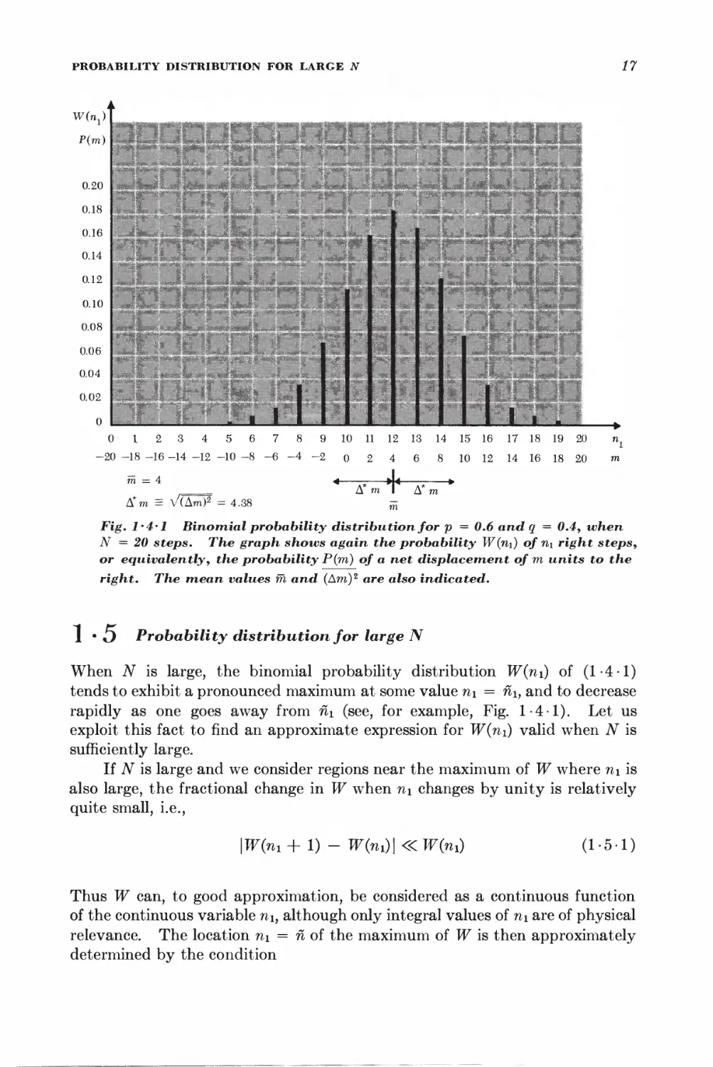
Fig. l'4'l Binomial probability distribution for p = 0.6 and q = 0.4, when
N = 20 steps. The graph shows again the probability W(n\) of n\ right steps,
or equivalently, the probability P(m) of a net displacement of m units to the
right. The mean values m and (Am)2 are also indicated.
1 • O Probability distribution for large N
When iV is large, the binomial probability distribution W(ni) of (1-4-1)
tends to exhibit a pronounced maximum at some value ni = nh and to decrease
rapidly as one goes away from n\ (see, for example, Fig. 1-4-1). Let us
exploit this fact to find an approximate expression for W(ni) valid when N is
sufficiently large.
If N is large and we consider regions near the maximum of W where n\ is
also large, the fractional change in W when n\ changes by unity is relatively
quite small, i.e.,
\W(m + 1) - W(ni)\«W(7n) (1-5-1)
Thus W can, to good approximation, be considered as a continuous function
of the continuous variable ni, although only integral values of ni are of physical
relevance. The location n\ = n of the maximum of W is then approximately
determined by the condition

18 SECTION 1 • 5
dW n • i .1 dlnW n n k o^
-j— = 0 or equivalently —5 = 0 (1-5-2)
where the derivatives are evaluated for n\ = n\. To investigate the behavior
of W(ni) near its maximum, we shall put
m = ni + v (1-5-3)
and expand In W(ni) in a Taylor's series about ii\m The reason for expanding
In Wy rather than W itself, is that In IF is a much more slowly varying function
of n\ than W. Thus the power series expansion for In W should converge much
more rapidly than the one for W.
An example may make this clearer; Suppose one wishes to find an
approximate expression, valid for y <R 1, of the function
/=(i+2/)-*
where N is large. Direct expansion in Taylor's series (or by the binomial
theorem) would give
I /= 1 -Ny + iN(N'±AXy*-.* n
Since N is large, Ny > 1 even for very small values of y and then the above
expansion no longer converges. One can get around this: difficulty % taking
the logarithm first:
In /=== ^N lii (1 -f- y)
Expanding this in Taylor's series, one obtains
ln/^ -A%-^ • • •)
I or §f ==tr-m-tv*'-)
h *.., ... .
which is valid as long as y S 1-
Expanding In W in Taylor's series, one obtains
In W{ni) = In W(fii) + BlV + \Brf + %Bmz + ■ • • (1 5-4)
where Bk = —;—7— (1-5-5)
anf
is the fcth derivative of In W evaluated at n\ = ii\. Since one is expanding
about a maximum, B\ = 0 by (1 • 5 -2). Also, since W is a maximum, it follows
that the term \Btfi1 must be negative, i.e., B2 must be negative. To make this
explicit, let us write B2 = — \B2\. Hence (1 -5-4) yields, putting W = W(ni),
W(ni) = W ehB*^B^'' • = W e-^*2 elB^ "• (1-5-6)
In the region where tj is sufficiently small, higher-order terms in the
expansion can be neglected so that one obtains in first approximation an expression
of the simple form
W(m) = #e-^2 (1-5-7)

PROBABILITY DISTRIBUTION FOR LARGE N 19
Let us now investigate the expansion (1-5-4) in greater detail. By (1 • 4 • 1)
one has
In W(rn) = In AM - lnnj - \n(N - m)\ + n1\np + (N -njlnq (1-5-8)
But, if n is any large integer so that n ^> 1, then In n\ can be considered an
almost continuous function of n, since In n\ changes only by a small fraction of
itself if n is changed by a small integer. Hence
dlnnl ln(n+ 1)! - Inn! ,(71+1)! t , , tx
—3— ~ — i = ln 3 1 = In (n + 1)
an 1 n!
Thus
forn»l, ^-^~lnn (1-5-9)
Hence (1-5-8) yields
dlnW
dn\
-lnni + ln (N - m) + ln p - ln q (1-5-10)
By equating this first derivative to zero one finds the value ni = n\, where
W is maximum. Thus one obtains the condition
or (N — fii)p = fiiq
so that
^ n1 = Np (1-5-11)
since p + q = 1.
Further differentiation of (1-5-10) yields
dni2 ui N — ni
Evaluating this for the value n\ = n\ given in (1-5-11), one gets
R = _ J_ _ 1 = _ 1 (l + I\
2 iVp N - Np N\p^~ q)
or
since 7? + 5 = 1. Thus B2 is indeed negative, as required for W to exhibit
a maximum.
By taking further derivatives, one can examine the higher-order terms in
the expansion (1-5-4). Thus, differentiating (1 -5-12), one obtains
B - 1 _ * = Jul _ Au
3 rh2 (AT -nO2 !!iV2p2 iVV2
l*4 = |^ <p^

20
SECTION 1 * 5
; Similarly, B< - - A - ^^ ~ ~2 (^ + ^)
Thus it is seen that the Mi term in (1*5-4) is smaller in magnitude than
?lk/(Npq)k~x* The neglect of terms beyond 2?2i?2, which leads to (1*5-7), is
therefore justified if n is sufficiently small so that*
V<KNpq (1-5*14)
,,, On the other hand, the factor exp (—ill^l*?2) in (1-5-6) causes W to fall
off very rapidly with increasing values of |i?| if |2?2| is large. Indeed, if
the probability W{nx) becomes negligibly small compared to W{n^„ Hence
it follows that if rj is still small enough to satisfy (1 5*14) up to values of $£\
so large that (1*5/15) is also satisfied, then (1*5*7) provides an excellent
approximation for W throughout the miire region where IF has an appreei*
able magnitude. This condition of simultaneous validity of (1*5* 14) and
(1*5-15) requires that
-y/Mpq «: v <£Np$
V i.e., that 2V>g>>! (1*5*16)
This shows that, throughout the entire domain where the probability W is
not negligibly small, the expression (1 * 5 - 7) provides a very good
approximation to the extent that N is large and that neither p nor q is too small, t
The value of the constant Vf in (1 • 5 • 7) can be determined from the
normalization condition (1-4-2). Since W and n\ can be treated as quasicontinuous
variables, the sum over all integral values of n\ can be approximately replaced
by an integral. Thus the normalization condition can be written
N
£ W(ni) » J W(ni) dnx = j^ W(nx + v) dv = 1 (1-5-17)
ni = 0
Here the integral over rj can to excellent approximation be extended from — oo
to + °°, since the integrand makes a negligible contribution to the integral
wherever |r;| is large enough so that W is far from its pronounced maximum
value. Substituting (1-5-7) into (1-5-17) and using (A-4-2), one obtains
W pm e-*\B*\* dv = W .
= 1
* Note that the condition (1-5-1) is equivalent to \dW/dni\ <3C W, i.e., to |-B2?| =
(Npq)_1\v\ ^ 1 by virtue of (1-5-7) and (1-5-13). Thus it is also satisfied in the domain
(1 • 5 • 14) where W is not too small.
t When p <3C 1 or q <3C 1, it is possible to obtain a different approximation for the
binomial distribution, namely the so-called "Poisson distribution" (see Problem 1.9).

GAUSSIAN PROBABILITY DISTRIBUTIONS
21
Thus (1-5-7) becomes
^ W(ni) = \\M e-hm^-a^ (1.5 • 18)
The reasoning leading to the functional form (1-5-7) or (1-5-18), the
so-called "Gaussian distribution," has been very general in nature. Hence it
is not surprising that Gaussian distributions occur very frequently in statistics
whenever one is dealing with large numbers. In our case of the binomial
distribution, the expression (1-5-18) becomes, by virtue of (1-5-11) and
(1-5-13),
^ W(ni) = (artf W)-* exp [ - ^zNvq^ (1'5'19)
Note that (1-5-19) is, for large values of N and ni, much simpler than
(1-4-1), since it does not require the evaluation of large factorials. Note
also that, by (1-4-4) and (1-4-9), the expression (1-5-19) can be written
in terms of the mean values n, and (Ani)2 as
Win,) = [ar(A^p]-* exp T- ^-I^'l
L 2(A?h)2 J
1 • D Gaussian probability distributions
The Gaussian approximation (1 -5-19) also yields immediately the probability
P(m) that in a large number of N steps the net displacement is m. The
corresponding number of right steps is, by (1-2-9), fti = ^(N + m). Hence
(1-5-19) gives
P(m) = W(^) = pw^exp {- [n^§^1) d-6-1)
since m — Np = %[N + m — 2Np] = ^[m — N(p — q)]. By (1-2-3) one has
m = 2n i — Nf so that m assumes here integral values separated by an amount
Am = 2.
We can also express this result in terms of the actual displacement
variable x,
x = ml (1-6-2)
where / is the length of each step. If I is small compared to the smallest length
of interest in the physical problem under consideration,* the fact that x can
only assume values in discrete increments of 2/, rather than all values
continuously, becomes unimportant. Furthermore, when N is large, the probability
P(m) of occurrence of a displacement m does not change significantly from
* For example, if one considers the random motion (diffusion) of an atom in a solid,
the step length / is of the order of one lattice spacing, i.e., about 10-8 cm. But on the
macroscopic scale of experimental measurement the smallest length L of relevance might be
1 micron = 10-4 cm.

SECTION
1-6
P(m)
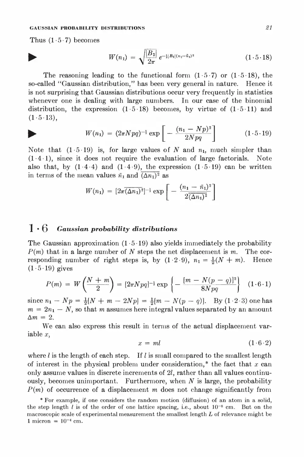
Fig. 1*6*1 The probability P(m) of a net displacement of m units when the
total number N of steps is very large and the step length I is very small.
one possible value of m to an adjacent one; i.e., \P(m + 2) — P(m)\ <<C P(m).
Therefore P(m) can be regarded as a smooth function of x. A bar graph
of the type shown in Fig. 1-4-1 then assumes the character illustrated in
Fig. 1-6-1, where the bars are very densely spaced and their envelope forms
a smooth curve.
Under these circumstances it is possible to regard x as a continuous variable
on a macroscopic scale and to ask for the probability that the particle is found
after N steps in the range between x and x + dx.* Since m assumes only
integral values separated by Am = 2, the range dx contains dx/2l possible values
of m, all of which occur with nearly the same probability P(m). Hence the
probability of finding the particle anywhere in the range between x and x + dx
is simply obtained by summing P(m) over all values of m lying in dx, i.e., by
multiplying P(m) by dx/2l. This probability is thus proportional to dx (as
one would expect) and can be written as
(P(x) dx = P(m)
dx
(1-6-3)
where the quantity (?(x), which is independent of the magnitude of dx, is
called a "probability density." Note that it must be multiplied by a
differential element of length dx to yield a probability.
By using (1-6-1) one then obtains
(P(aO dx =
1
\/2<kc
where we have used the abbreviations
e-C*-M)«/2ff« ^
and
M% = (V ~ q)Nl
o- = 2 V^pq I
(1-6-4)
(1-6-5)
(1-6-6)
* Here dx is understood to be a differential in the macroscopic sense, i.e., dx <<C L, where
L is the smallest dimension of relevance in the macroscopic discussion, but dx ^> I. (In
other words, dx is macroscopic ally small, but microscopically large.)

GAUSSIAN PROBABILITY DISTRIBUTIONS
28
The expression (1-6-4) is the standard form of the Gaussian probability
distribution. The great generality of the argument leading to (1-5-19)
suggests that such Gaussian distributions occur very frequently in probability
theory whenever one deals with large numbers.
Using (1-6-4), one can quite generally compute the mean values x and
(x — x)2. In calculating these mean values, sums over all possible intervals
dx become, of course, integrations. (The limits of x can be taken as — <x> <
x < co , since (?(x) itself becomes negligibly small whenever \x\ is so large as to
lead to a displacement inaccessible in N steps.)
First we verify that (?(x) is properly normalized, i.e., that the probability
of the particle being somewhere is unity. Thus
f " (?(x) dx = ,— fx e~<—m>2/2*
J -00 V27TO- J -M
V27T a J -
dx
e-vw** dy
(L6-7)
= /L V^
a/2tto-
- 1
Here we have put y = x — ix and evaluated the integral by (A-4-2).
Next we calculate the mean value
x = / x(9(x) dx
= L [ °° x e-<*-*>*i2trl dx
V27T a J -°°
= V^T* [/-"-y e~vm°*dy + M /-"- e~ym'2 dy\
Since the integrand in the first integral is an odd function of y, the first integral
9(x)
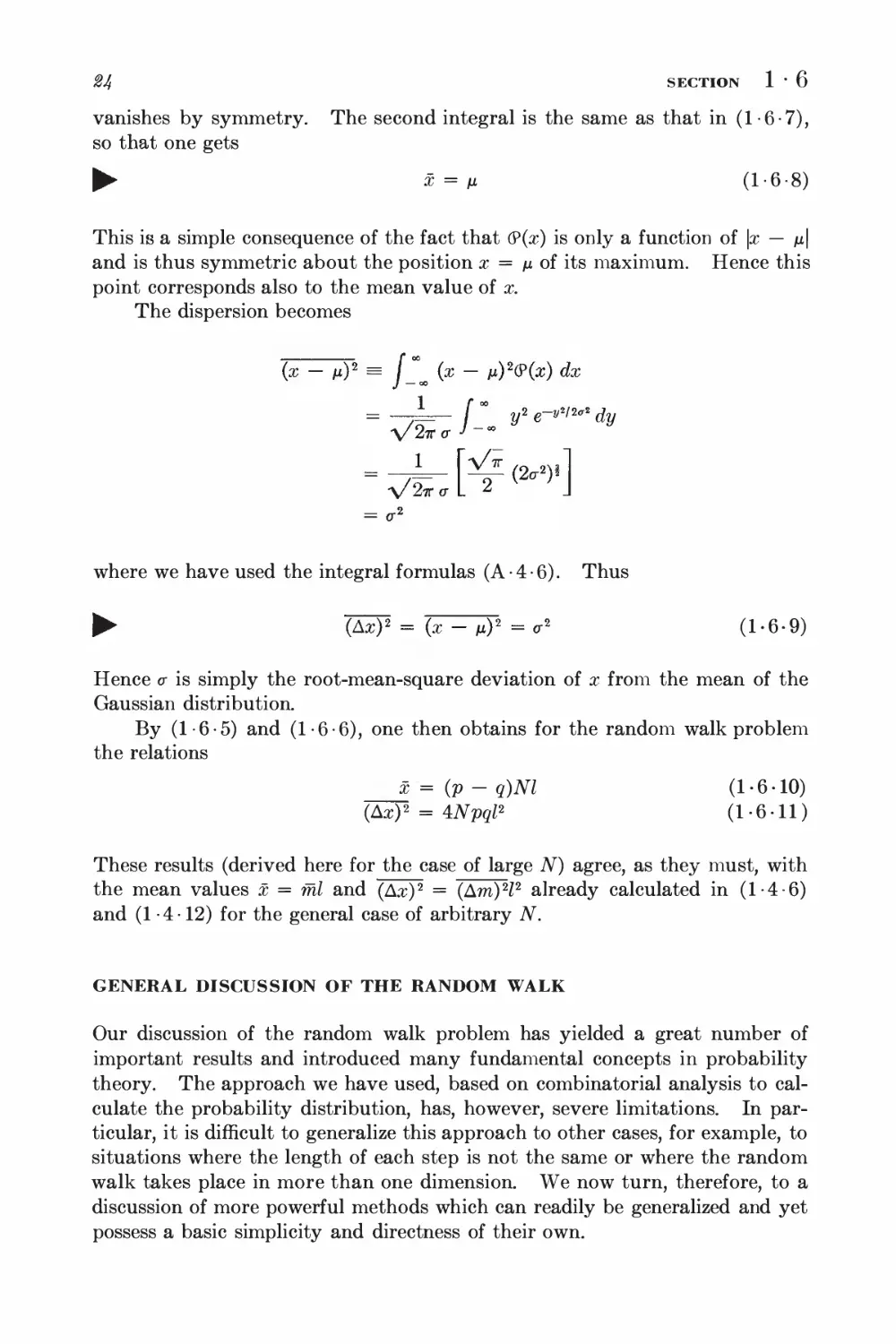
Fig. 1-6'2 The Gaussian distribution. Here (?(x) dx is the area under the
curve in the interval between x and x + dx and is thus the probability that
the variable x lies in this range.

SECTION
1-6
vanishes by symmetry. The second integral is the same as that in (1-6-7),
so that one gets
^ x = /i (1-6-8)
This is a simple consequence of the fact that (?(x) is only a function of \x — /x|
and is thus symmetric about the position x = /i of its maximum. Hence this
point corresponds also to the mean value of x.
The dispersion becomes
(x - M)2 = (^ (x - ij)2(P(x) dx
where we have used the integral formulas (A-4-6). Thus
► jAxJ2 = (x - nY = o-2 (1-6-9)
Hence <r is simply the root-mean-square deviation of x from the mean of the
Gaussian distribution.
By (1-6-5) and (1-6-6), one then obtains for the random walk problem
the relations
x = (p - q)Nl (1-6-10)
(Ax)2 = Wpql2 (1-6-11)
These results (derived here for the case of large N) agree, as they must, with
the mean values x = ml and (Ax)2 = (Am)H2 already calculated in (1-4-6)
and (1 -4-12) for the general case of arbitrary N.
GENERAL DISCUSSION OF THE RANDOM WALK
Our discussion of the random walk problem has yielded a great number of
important results and introduced many fundamental concepts in probability
theory. The approach we have used, based on combinatorial analysis to
calculate the probability distribution, has, however, severe limitations. In
particular, it is difficult to generalize this approach to other cases, for example, to
situations where the length of each step is not the same or where the random
walk takes place in more than one dimension. We now turn, therefore, to a
discussion of more powerful methods which can readily be generalized and yet
possess a basic simplicity and directness of their own.

PROBABILITY DISTRIBUTIONS INVOLVING SEVERAL VARIABLES 25
1 • / Probability distributions involving several variables
The statistical description of a situation involving more than one variable
requires only straightforward generalizations of the probability arguments
applicable to a single variable. Let us then, for simplicity, consider the case of
only two variables u and v which can assume the possible values
Ui where i = 1, 2, . . . , M
and Vj where j = 1, 2, . . . , N
Let P(ui,Vj) be the probability that u assumes the value Ui and that v assumes
the value Vj.
The probability that the variables u and v assume any of their possible
sets of values must be unity; i.e., one has the normalization requirement
M N
I I P{Ui,v3) = 1 (1-7-1)
i = \ 3 = 1
where the summation extends over all possible values of u and all possible
values of v.
The probability Pu(ui) that u assumes the value in, irrespective of the
value assumed by the variable v, is the sum of the probabilities of all possible
situations consistent with the given value of u%) i.e.,
Pu(ui) = f PM (1-7-2)
3 = 1
where the summation is over all possible values of Vj. Similarly, the
probability Pv(vj) that v assumes the value Vj, irrespective of the value assumed by
u, is
M
i = l
Each of the probabilities P« and Pv W> °f course^ properly normalizedr For
example, by (1-7-2) and (1-7 1) one has
I M '" ., M N
I Puirn) = X [ X Piwt] = !' <4--5M),
An important special case occurs when the probability that one variable
assumes a certain value does not depend on the value assumed by the other
variable. The variables are then said to be "statistically independent" or

26 SECTION 1 ' 7
"uncorrected." The probability P{ui,v3) can then be expressed very simply
in terms of the probability Pu{ui) that u assumes the value u{ and the
probability Pv(vj) that v assumes the value vj. Indeed, in this case [the number of
instances in the ensemble where u = Ui and where simultaneously v = v3] is
simply obtained by multiplying [the number of instances where u = ui] by
[the number of instances where v = v3]; hence
P(uitvj) = Pu(ui)Pv(v3) (1-7-5)
if u and v are statistically independent.
Let us now mention some properties of mean values. If F(u,v) is any
function of u and v, then its mean value is defined by
M N
PW) - X 1 P(WiW(w>i) (1-7-6)
i=ii=i
Note that if f(u) is a function of u only, it also follows by (1-7-2) that
JW = X X p(^Mui) = X Puiudfim) (L7-7)
i 3 i
If F and G are any functions of u and v, then one has the general result
WTG - X X P(Vi,Vi)[F(uiM) + GW,-)]
i 3
= X X HuiM)F(ui,v,) + X X p(ui>v>)G(ui>v>)
i j i j
or
^ FR?=F + ff (1-7-8)
i.e., the average of a sum equals simply the sum of the averages.
Given any two functions f(u) and g(v), one can also make a general
statement about the mean value of their product if u and v are statistically
independent variables. Indeed, one then finds
f(u)g{v) = X X p(uiyvj)f(^i)9(^)
i 3
= 11 P«(ui)P.(i*)/(ui)0fo) by (I • 7 • 5)
i j
= [I PuMfiur)] [%P,(vMvi)]
% j
Thus
► 7(uW)=m'g(v) (1-7-9)
i.e., the average of a product equals the product of the averages if u and v are
statistically independent. If u and v are statistically not independent, the
statement (1-7-9) is in general not true.
The generalization of the definitions and results of this section to the case
of more than two variables is immediate.

COMMENTS ON CONTINUOUS PROBABILITY DISTRIBUTIONS 27
1 • O Comments on continuous probability distributions
Consider first the case of a single variable u which can assume any value in
the continuous range a\ < u < 0,2. To give a probability description of such
a situation, one can focus attention on any infinitesimal range of the variable
between u and u + du and ask for the probability that the variable assumes a
value in this range. One expects that this probability is proportional to the
magnitude of du if this interval is sufficiently small; i.e., one expects that this
probability can be written in the form (9{u) du, where (9{u) is independent of
the size of du.* The quantity (P(u) is called a "probability density." Note
that it must be multiplied by du to yield an actual probability.
It is readily possible to reduce the problem dealing with a continuous
variable to an equivalent discrete problem where the number of possible values of
the variable becomes countable. It is only necessary to subdivide the
accessible range a\ < u < a2 of the variable into (arbitrarily small) equal intervals of
fixed size 8u. Each such interval can then be labeled by some index i. The
value of u in this interval can be denoted simply by ui and the probability of
finding the variable in this range by P(ui). One can then deal with a denumer-
able set of values of the variable u (each of them corresponding to one of the
chosen fixed infinitesimal intervals). It also becomes clear that relations
involving probabilities of discrete variables are equally valid for probabilities
of continuous variables. For example, the simple properties (1-3-5) and
(1-3*6) of mean values are also applicable if u is a continuous variable.
1 2 3 4 5 6 •■• u
►[ \i |< du ►]
8u
Fig. 1*8*1 Subdivision of the range a\ < u < a% of a continuous variable u
into a countable number of infinitesimal intervals du of fixed size.
To make the connection between the continuous and discrete points of view
quite explicit, note that in terms of the original infinitesimal subdivision
interval buy
Similarly; if one considers any interval between u and u -|- du which is such
that du is macroscopically small although du ^> 8u, then thin interval con--
tains du/bu possible values of u% for which the probability P(Ui) has
essentially the same value^call it simply P(u)i Then the probability P(w) du of
* Indeed, the probability must be expressible as a Taylor's series in powers of du and
must vanish as du —> 0. Hence the leading term must be of the form (P du, while terms
involving higher powers of du are negligible if du is sufficiently small.

SECTION
1-8
the variable assuming a * value between u and u + du should be given by
multiplying the probability P(ui) for assuming any discrete value in this
range by the number du/Su of discrete values in this range; i.e., one has
> properly
-■<?(*) du - PiUi) ** * ^ d» [l .8-1)
OU oil
Note that the sums involved in calculating normalization conditions or
mean values can be written as integrals if the variable is continuous. For
example, the normalization condition asserts that the sum of the probabilities
over all possible values of the variable must equal unity; in symbols
lP(Ui) = l (1-8-2)
i
But if the variable is continuous, one can first sum over all values of the
variable in a range between u and u + du, thus obtaining the probability (?(u) du
that the variable lies in this range, and then complete the sum (1-8-2) by
summing (i.e., integrating) over all such possible ranges du. Thus (1-8-2)
is equivalent to
f n.%
6>(u)du = 1 (1-8-3)
J a\
which expresses the normalization condition in terms of the probability density
(P(u). Similarly, one can calculate mean values in terms of (P(w). The general
definition of the mean value of a function / was given in terms of discrete
variables by (1-3-4) as
W) =lP(ui)f(ui) (1-8-4)
i
In a continuous description one can again sum first over all values between
u and u + du (this contributes to the sum an amount (P(u) duf(u)) and then
integrate over all possible ranges du. Thus (1-8-4) is equivalent to the
relation
f(u) = fa2(P(u)f(u)du (1-8-5)
J ai
Remark Note that in some cases it is possible that the probability density
(9(u) itself becomes infinite for certain values of^ This does not lead to any *
difficulties as long as the integral f % <P(u) My ^ which measures the proba-
bility that u assumes any value in some arbitrary range between ct and c2,
always remains finite.
The extension of these comments to probabilities involving several
variables is immediate. Consider, for example, the case of two variables u and v
which can assume all values in the continuous respective ranges a\ < u < a2

COMMENTS ON CONTINUOUS PROBABILITY DISTRIBUTIONS
-du *\
Fig. 1'8'2 Subdivision of the continuous variables u and v into small
intervals of magnitude bu and bv.
and b\ < v < 62. One can then talk of the probability <9(u,v) du dv that the
variables lie in the ranges between u and u + du and between v and v + dv,
respectively, where <?(u,v) is a probability density independent of the size of
du and dv. It is again possible to reduce the problem to an equivalent one
involving discrete countable values of the variables. It is only necessary to
subdivide the possible values of u into fixed infinitesimal intervals of size bu
and labeled by i, and those of v into fixed infinitesimal intervals of size bv and
labeled by j. Then one can speak of the probability P(ui,v3) that Ui = u and
that simultaneously v = vjm Analogously to (1-8-1) one then has the
relation
(P(u.v) du dv = Piu.v) -—^r
bu bv
where the factor multiplying P(u,v) is simply the number of infinitesimal cells
of magnitude bu bv contained in the range lying between u and u + du and
between v and v + dv.
The normalization condition (1-7-2) can then be written in terms of
the probability density (?(u,v) as
f °2 f* du dv <P(u,v) = 1
Jaijoi
Analogously to (1-7-7) one can also write
F(u.v) = f°2 [b*dudv6>(u,v)F(u,v)
J a\ Jbi
(1-8-6)
(1.8-7)

SECTION 1 ' 8
Fig. 1*8*3 Illustration showing a function <p(u) which is such that u(<p) is a
double-valued function of <p. Here the range dtp corresponds to u being either
in the range du\ or in the range dit2.
Since the problem can be formulated in discrete as well as continuous terms,
the general properties (1-7-8) and (1-7-9) of mean values remain, of course,
valid in the continuous case.
Functions of random variables Consider the case of a single variable u
and suppose that ip(u) is some continuous function of u. The following
question arises quite frequently. If (P(u) du is the probability that u lies in the
range between u and u + du, what is the corresponding probability W(<p) dip
that ip lies in the range between tp and tp + dtp? Clearly, the latter probability
is obtained by adding up the probabilities for all those values u which are such
that <p lies in the range between (p and (p + dip) in symbols
W(<p) dip = f (P(u) du
J dtp
(1-8-8)
Here u can be considered a function of ip and the integral extends over all those
values of u lying in the range between u(tp) and u(tp + dip). Thus (1-8-8)
becomes simply
W(<p)d<p= fr+d*<P(u)
du
dtp
dip = (P(w)
du
dtp
dip
(1.8-9)
The last step assumes that u is a single-valued function of tp and follows, since
the integral is extended only over an infinitesimal range dtp. Since u = u((p),
the right side of (1-8-9) can, of course, be expressed completely in terms of ip.
If u(<p) is not a single-valued function of <p, then the integral (1-8-8) may
consist of several contributions similar to those of (1-8-9) (see Fig. 1-8-3).
Similar arguments can be used to find the probabilities for functions of
several variables when the probabilities of the variables themselves are known.

COMMENTS ON CONTINUOUS PROBABILITY DISTRIBUTIONS
31
Example Suppose that a two-dimensional vector B of constant length
B - \B\ is equally likely to point in any direction specified b}^ the angle 6
(see Fig. 1-8-4). The probability (P(0) dd that this angle lies in the range
between 6 and 8 + d6 is then given by the ratio of the angular range dd to
the total angular range 2tt subtended by a full circle; i.e.,
<?(0)dd = ^ (1-8-10)
If the vector makes an angle 6 with the x axis, its x component is given by
Bx - B cos 6 (1-8-11)
What is the probability W(BX) dBx that the x component of this vector lies
between Bx and Bx +■ dBJ Clearly, Bx is always such that —B<BX<B.
In this interval an infinitesimal range between Bx and Bx + dBz corresponds
to two possible infinitesimal ranges of dd (see Fig. 1 -8-4), each of magnitude
dd connected to dBT through the relation (18 11) so that dBx = \B sin 6\dd.
By virtue of (1 -8-10) the probability W(BX) dBx is then given by
W(BX) dBx = 2 fi- nr^l = -4 r^T
L2ir\Bs\n6\\ irB |sin 6\
But, by (1-811),
|sin0| = (1 -ooe«0)»= [l -(§)*]
Hence
*B,
lo
for-5 <BX<B
(1-8-12)
otherwise
The probability density is maximum (indeed infinite) as \BX
► B and is
I^:
m
t*
a
t >
|r| t
if«<
if
1
1...
J
$f
a* a
\":
h
J^v
\ v|5h
/. rfj: w
ffivlk-A..=_.fc
^.......,== ,==-..... |,.||...,,L|,..,,,,P
%
v.
:;^
11* /
, *c"H
,, »x :
JHfllp
Fig. 1-8-4 Dependence of the x component Bx = B cos 6 of a
two-dimensional vector B on its polar angle 6.

SECTION
1 -9
i mitiiinum when Bllf= 0. This result is apparent from the geometry of Fig.
(1 ;S>:4), sihce a given narrow range of dBz corresponds to a relatively large
: range of; the angle 6 wlien Bz ~ B and to a very much narrower range of the
angle 0 when Bk ~ 0.
1 • y General calculation of mean values for the random walk
The comments of Sec. 1 • 7 allow one to calculate mean values for very general
situations by very simple and transparent methods. Consider a quite general
form of the one-dimensional random walk problem. Let s»- denote the
displacement (positive or negative) in the ith step
Let w(si) dsi be the probability that the ith displacement lies in the
range between Si and s» + ds^
We assume again that this probability is independent of what displacements
occur in any other steps. For simplicity we further assume that the
probability distribution w is the same for each step i. Nevertheless, it is clear that
the situation envisaged here is considerably more general than before, for we
no longer necessarily assume a fixed magnitude I of displacement at each step,
but a distribution of possible step lengths with relative probability specified
by w.
We are interested in the total displacement x after N steps. We can ask
for (P(x) dx, the probability that x lies in the range between x and x + dx. We
can also ask for mean values (or moments) of x. In this section we show that
the calculation of these moments can be achieved very simply without prior
knowledge of (P(x).
(a)
sr
SSI
Si
+i
(6)
Fig. 1*9*1 Some examples of probability distributions giving, for any one
step, the probability w(s) ds that the displacement is between s and s + ds.
(a) A rather general case, displacements to the right being more probable than
those to the left, (b) The special case discussed in Sec. 1 • 2. Here the peaks,
centered about -\-l and —I, respectively, are very narrow; the area under the
right peak is p9 that under the left one is q. (The curves (a) and (b) are not
drawn to the same scale; the total area under each should be unity.)

GENERAL CALCULATION OF MEAN VALUES FOR THE RANDOM WALK 88
The total displacement x is equal to
N
x = si + s2 + * ' * + sN = ^ Si (1-9-1)
1 = 1
Taking mean values of both sides,
iV N
X
i = \ i = \
= j> = I * (1-9-2)
where we have used the property (1-7-8). But since w(sz) is the same for
each step, independent of i, each mean value st- is the same. Thus (1-9-2)
is simply the sum of N equal terms and becomes
► x = Ns (1-9-3)
where s = Si = j dsw(s)s (1-9-4)
is merely the mean displacement per step.
Next we calculate the dispersion
(Ax)2 = (x - x)2 (1-9-5)
By (1 -9• 1) and (1-9-2) one has
x — x = y (si — s)
N
or
where As = s» — s (1-9-7)
Ax = £ As, (1-9-6)
By squaring (1-9-6) one obtains
N N
(Ax) * = ( £ As,) ( £ ASy) = I (Asi) 2+ II (AaO (As,) (1-9-8)
3=1 i i 3
i9±3
Here the first term on the right represents all the square terms, and the second
term all the cross terms, originating from the multiplication of the sum by
itself. Taking the mean value of (1-9-8) yields, by virtue of (1-7-8),
^ = J(aS3* +JJaSTaS; (1-9-9)
i i j
i*3
In the cross terms we make use of the fact that different steps are statistically
independent and apply the relation (1-7-9) to write for i j* j
(A*)(A*) = (A*) (As,) =0 (1-9-10)
since Asi = s» — s = 0
In short, each cross term vanishes on the average, being as often positive as

3J, SECTION 1 ' 9
negative. Thus (1-9-9) reduces simply to a sum of square terms
N
(Ax)2 = £ (As,)2 (1-9-11)
i = i
Of course, none of these square terms can be negative. Since the probability
distribution w(si) is the same for each step, independent of i, it again follows
that (As,)2 must be the same for each step. Thus the sum in (1-9-11)
consists merely of N equal terms and becomes simply
(Ax)2 = N(As)2 (1-9-12)
where (As)2 = (As*)2 = / ds w(s) (As)2 (1-9-13)
is just the dispersion of the displacement per step.
Despite their great simplicity, the relations (1-9-3) and (1-9-12) are
very general and important results. The dispersion (Ax)2 = (x — x)2 is a
measure of the square of the width of the distribution of the net displacement
about its mean x. The square root A*x = [(Ax)2]*, i.e., the "root-mean-square
(rms) deviation from the mean," thus provides a direct measure of the width of
the distribution of the displacement about the mean x. The results (1-9-3)
and (1-9-12) thus make possible the following interesting statements about
the sum (1-9-1) of statistically independent variables. If s ^ 0 and the
number N of these variables (e.g., of displacements) increases, the mean value
x of their sum tends to increase proportionaly to N. The width A*x of the
distribution about the mean also increases, but only proportionately to NK
Hence the relative magnitude of the width Ax* compared to the mean x itself
decreases like N~*; explicitly, one has by (1-9-3) and (1-9-12), if s ^ 0,
A*x _ A*s 1
where A*s = [(As)2]*. This means that the percentage deviation of the
distribution of values of x about their mean x becomes increasingly negligible as
the number N becomes large. This is a characteristic feature of statistical
distributions involving large numbers.
Example Let us apply the general results (1-9*3)' and (1-9*12) of this
section to the special case of the random walk with fixed step length I
previously discussed in Sec. 1 -2. There the probability of a step to the right
is p, that of a step to the left is q = 1 — p. The mean displacement per step
is then given by
* = Vl + <z(-0 = (P - 0)1 = (2p - 1)1 (1-9-14)
As a check, note that s == 0 if p = qf as required by symmetry.
AISO ? = pp. + g( _|)2 = (p + q)l2 = 12
Hence (As)? = s2 ^ ^2 = 72fl - (2p - l)2]
~ P\l - 4p2 + 4p - 1] = Wp(l - p)
y(As)?^4^2 Jk, (1-9-15)

CALCULATION OF THE PROBABILITY DISTRIBUTION
85
Hence the relations (1-9-3) and (1*9-12) yield
x = (p-q)Nl\ (1.g.16)
(Ax)2 = 4pqNl2 J
Since x = ml, these agree precisely with the previously computed results
(1-4-6) and (1-4-12).
#
1 • 1 (J Calculation of the probability distribution
For the problem discussed in the last section, the total displacement x in N
steps is given by
= I Si (1101)
N
X
We now want to find the probability (P(z) dx of finding x in the range between
x and x + dx. Since the steps are statistically independent, the probability of
a particular sequence of steps where
the 1st displacement lies in the range between Si and Si + dst
the 2nd displacement lies in the range between s2 and s2 + ds2
the iVth displacement lies in the range between sn and sn + dsN
is simply given by the product of the respective probabilities, i.e., by
w(si) ds! • w(s2) ds2 • • • w(sn) dsN
If we sum this probability over all the possible individual displacements which
are consistent with the condition that the total displacement x in (1-10-1)
always lies in the range between x and x + dx, then we obtain the total
probability (P(x) dx, irrespective of the sequence of steps producing this total
displacement. In symbols we can write
□0
(S>(x) dx = //■*"/ w(si)w(s2) • ' • w(sN) dsids2 • • • dsN (1-10-2)
— oo
(dx)
where the integration is over all possible values of the variables Si, subject to
the restriction that
N
x < £ Si<x + dx (1-10-3)
In principle, evaluation of the integral (1-10-2) solves completely the
problem of finding (P(x).

86
SECTION 1 ' 10
In practice, the integral (110-2) is difficult to evaluate because the
condition (1-10-3) makes the limits of integration very awkward; i.e., one
faces the complicated geometrical problem of determining over what subspace,
consistent with (1-10-3), one has to integrate. A powerful way of handling
this kind of problem is to eliminate the geometrical problem by integrating
over all values of the variables st- without restriction, while shifting the
complication introduced by the condition of constraint (110-3) to the integrand.
This can readily be done by multiplying the integrand in (1-10-2) by a
factor which is equal to unity when the st- are such that (1 -10-3) is satisfied,
but which equals zero otherwise. The Dirac 5 function 8(x — z0), discussed in
Appendix A • 7, has precisely the selective property that it vanishes whenever
\x — xq\ > ^ \dx\, while it becomes infinite like (dx)~l in the infinitesimal range
where \x — x0\ < -g- \dx\; i.e., 8(x — x0) dx = 1 in this latter range. Hence
(1-10-2) can equally well be written
oo N
G>(x) dx = 11 • • • / w(si)w(s2) * * * w(sN) 5 (x — \ sA dx\ dsids2 • • • dsN
— 00 1 = 1
(1-10-4)
where there is now no further restriction on the domain of integration. At this
point we can use the convenient analytical representation of the 5 function in
terms of the integral (A-7-14); i.e., we can write
8(x - Zsi) = 1- [ °° dkeik^~* (M0-5)
Ztt J — »
Substituting this result in (1 -10-4) yields:
&(%) = [['''[ w(si)w(s2) ■ • • w(sN) — f"^ dk eiHs*+'*•+**-*> dsx ds2 • • • dsN
or (P(z) = 2~ f* dk e-*x f*^ dsi w(si) eiks* • • • /_^ dsNw(sN) e*'»
(1-10-6)
where we have interchanged the order of integration and used the
multiplicative property of the exponential function. Except for the irrelevant symbol
used as variable of integration, each of the last N integrals is identical and
equal to
^ Q(k) ~ j2m dse**w{s) (1-10-7)
Hence (110-6) becomes
^ (P(x) = ^L p^ dk e~ik*QN(k) (1 -10-8)
Thus the evaluation of two simple (Fourier) integrals solves the problem
completely.

PROBABILITY DISTRIBUTION FOR LARGE N
87
I
Example Let us again apply the present results to the case of equal step
lengths I discussed in Sec, 1' 2. There the probability of a displacement +Z
is equal to p, that of a displacement —I is equal to q = 1 — p; i.e., the
corresponding probability density w is given by
w(s) = p8(s - I) +q8(sj-l)
The quantity (1.10.7) becomes
Q(k) ss «*• = peiM + q e~ikl
Using the binomial expansion, one then obtains
I Q"'(k) = (p eikl + q e~ikl)N
*?* V * AH
I
= \ ' . (fl pikl)n(0 p-ikl\N~n
L n\(N -n)\[Pe } {qe }
n=0
N
X, AM
n}(N-n)\Pq 6
& Thus (1-10-8) yields
i
5 (p(aj) = -L f * dk e~ik*Q*(k)
4TT J — »
i or <?(x) = J -1J^ n);p"g"-»fi[s ~ (2n - tf)q (1 -10• 9)
This says that the probability density (?(x) vanishes unless
x = (2w - A0*, where n = 0, 1, 2, . . . , N
The probability P(2n — AO of finding the particle at such a position is then
given by
i* r (2n-N)l+e AM ...
i P(2n - N) = <?(x) dx = ~~i,,Ar r*\, pnqN~n
where € is some sufficiently small quantity; i.e., P is given by the coefficient
of the corresponding 8 function in (110-9). Thus we regain the result of
Sec. 1 -2 as a special case of the present more general formulation and without
the need to use any combinatorial reasoning.
•3C-
111 Probability distribution for large N
We consider the integrals (110-7) and (110-8) which solve the problem of
finding (?(x) and ask what approximations become appropriate when N is large.
The argument used here will be similar to the method detailed in Appendix
A-6 to derive Stirling's formula.

88
SECTION 1 ' 11
The integrand in (1 • 10 ■ 7) contains the factor eik% which is an oscillatory
function of s and oscillates the more rapidly with increasing magnitude of A:.
Hence the quantity Q(k) given by the integral in (1 • 10-7) tends in general to
be increasingly small as A: becomes large. (See remark below.) If Q is raised to
a large power N, it thus follows that QN(k) tends to decrease very rapidly with
increasing A:. To compute (P(x) by Eq. (110-8), a knowledge of QN(k) for
small values of A: is then sufficient for calculating the integral, since for large
values of A: the contribution of QN(k) to this integral is negligibly small. But
for small values of A:, it should be possible to approximate QN(k) by a suitable
expansion in powers of A:. Since QN(k) is a rapidly varying function of k, it is
preferable (as in Sec. 1-5) to seek the more readily convergent power series
expansion of its slowly varying logarithm In QN(k).
Remark To the extent that w(s) varies slowly over a period of oscillation,
the integral Qfjcj = fdseiksw(s) ~ 0. The reason is that in any range a <
s < b in which w varies slowly so that \dw/ds\{b — a) <<£ w, but which contains
many oscillations so; that (6 — a)k S> 1, the integral
* Combining these two inequalities one can say that
to the extent that k is large enough so that everywhere
dw
\«w
The actual calculation is straightforward. We want first to compute
Q(k) for small values of A:. Expanding eiks in Taylor's series, Eq. (110-7)
becomes
Q(k) = P ds w(s) eiks = 1°°^ ds w(s)(l + iks - ^A:2s2 + ■ ■ ■)
or Q(k) = 1 + isk - i72k2 ■ ■ ■ (1-11-1)
where sn = / dsw(s)sn (1-11-2)
is a constant which represents the usual definition of the nth moment of s.
Here we assume that |w(s)|—>0 rapidly enough as \s\ —* <x> so that these
moments are finite. Hence (1-11-1) yields
lnQ"(A;) = NlnQ(k) = Nln[l + isk - -^A;2 • ■ •] (1-11-3)
Using the Taylor's series expansion valid for y <<C 1,
In (1 + y) = y - iy2 ■ • ■

PROBABILITY DISTRIBUTION FOR LARGE N
39
Eq. (1 • 11 • 3) becomes, up to terms quadratic in k,
In QN = N[isk - %72k2 - i(isk)2 * •
= N[isk - ±(s~2 - s2)A;2 • • •]
= N[isk - ^(Ksyk2 • • •]
where (As)2 = s2 - s2 (1-11-4)
Hence we obtain
QN(k) = eiN~sk-iN~&&k2 (1-11-5)
Thus (1 • 10 • 8) becomes
(P(x) = JL f °° dk e^-M-W^2*2 (1-11-6)
Z7T J — °°
The integral here is of the following form, where a is real and positive:
/_°° du e~au2+bu = f °° du e-a[uZ-(J>la)u^
= J °° du 6-«(«-6/2o)2+62/4a by completing the square
/OO Q
dy e~ay2 by putting y = u — ■=-
- eb2'*a J^ by (A-4-2)
Thus f" du e~au*+bu = J- eb2'*a (1-11-7)
Applying this integral formula to (1-11-6) we get, with b = i(Ns — x) and
a = ^N(As)2, the result
where ^ = Ns
(P(x) = !_ 6-(^)2/2ff2 (1 -11-8)
V2tto-2
(1119)
a2 = N(As)2
Thus the distribution has the Gaussian form previously encountered in Sec.
1-6. Note, however, the extreme generality of this result. No matter what
the probability distribution w(s) for each step may be, as long as the steps are
statistically independent and w(s) falls off rapidly enough as \s\ —■» <x>, the total
displacement x will be distributed according to the Gaussian law if N is
sufficiently large. This very important result is the content of the so-called
"central limit theorem," probably the most famous theorem in mathematical
probability theory.* The generality of the result also accounts for the fact
that so many phenomena in nature (e.g., errors in measurement) obey
approximately a Gaussian distribution.
* A proof of the theorem with attention to fine points of mathematical rigor can be
found in A. I. Khinchin, "Mathematical Foundations of Statistical Mechanics," p. 166,
Dover Publications, New York, 1949.

40 PROBLEMS
We already showed that for the Gaussian distribution (1-6-4)
and (Asp = cr2}
Hence (1-11-9) implies
x = Ns
and (As? = iV(Aip
which agree with the results obtained from our general moment calculations
(1-9-3) and (1-912).
SUGGESTIONS FOR SUPPLEMENTARY READING
Probability theory
F. Mosteller, R. E. K. Rourke, and G. B. Thomas: "Probability and Statistics,"
Addison-Wesley Publishing Company, Reading, Mass., 1961. (An elementary
introduction.)
W. Feller: "An Introduction to Probability Theory and its Applications," 2d ed.,
John Wiley & Sons, Inc., New York, 1959.
H. Cramer: "The Elements of Probability Theory," John Wiley & Sons, Inc., New
York, 1955.
Random walk problem
S. Chandrasekhar: "Stochastic Problems in Physics and Astronomy, Rev. Mod. Phys.,
vol. 15, pp. 1-89 (1943). This article is also reprinted in M. Wax, "Selected Papers
on Noise and Stochastic Processes," Dover Publications, New York, 1954.
R. B. Lindsay: "Introduction to Physical Statistics," chap. 2, John Wiley & Sons,
Inc., New York, 1941. (An elementary discussion of the random walk and related
physical problems.)
PROBLEMS
1.1 What is the probability of throwing a total of 6 points or less with three dice?
1.2 Consider a game in which six true dice are rolled. Find the probability of
obtaining
(a) exactly one ace
(b) at least one ace
(c) exactly two aces
1.3 A number is chosen at random between 0 and 1. What is the probability that
exactly 5 of its first 10 decimal places consist of digits less than 5?
1.4 A drunk starts out from a lamppost in the middle of a street, taking steps of
equal length either to the right or to the left with equal probability. What is
the probability that the man will again be at the lamppost after taking N steps
(1.11-10)

PROBLEMS
u
(a) if N is even?
(b) if N is odd?
1.5 In the game of Russian roulette (not recommended by the author), one inserts
a single cartridge into the drum of a revolver, leaving the other five chambers
of the drum empty. One then spins the drum, aims at one's head, and pulls the
trigger.
(a) What is the probability of being still alive after playing the game N
times?
(b) What is the probability of surviving (N — 1) turns in this game and then
being shot the iVth time one pulls the trigger?
(c) What is the mean number of times a player gets the opportunity of
pulling the trigger in this macabre game?
1.6 Consider the random walk problem with p = q and let m = nx — n2 denote the
net displacement to the right. After a total of N steps, calculate the following
mean values: m, m2, n?, and m*.
1.7 Derive the binomial distribution in the following algebraic way, which does not
involve any explicit combinatorial analysis. One is again interested in finding
the probability W(n) of n successes out of a total of N independent trials. Let
Wi = p denote the probability of a success, w2 = 1 — p = q the corresponding
probability of a failure. Then W(n) can be obtained by writing
2 2 2 2
WW = X X X " " " X w*wiWk ' ' ' wm (1)
i—\j—\ k=\ m—1
Here each term contains N factors and is the probability of a particular
combination of successes and failures. The sum over all combinations is then to be
taken only over those terms involving wx exactly n times, i.e., only over those
terms involving wxn.
By rearranging the sum (1), show that the unrestricted sum can be written
in the form
W(n) = (wi + w2)N
Expanding this by the binomial theorem, show that the sum of all terms in (1)
involving Win, i.e., the desired probability W(n)} is then simply given by the
one binomial expansion term which involves wxn.
1.8 Two drunks start out together at the origin, each having equal probability of
making a step to the left or right along the x axis. Find the probability that
they meet again after N steps. It is to be understood that the men make their
steps simultaneously. (It may be helpful to consider their relative motion.)
1.9 The probability W(n) that an event characterized by a probability p occurs n
times in N trials was shown to be given by the binomial distribution
W(n) = ^why.pn(1 ~ ^^ (1)
Consider a situation where the probability p is small (p <3C 1) and where one is
interested in the case n <C N. (Note that if N is large, W(n) becomes very
small if n —> TV because of the smallness of the factor pn when p <K 1. Hence
W(n) is indeed only appreciable when n <3C N.) Several approximations can
then be made to reduce (1) to simpler form.

42
PROBLEMS
(a) Using the result In (1 — p) « — p, show that (1 — p)^""*1 « e~*p.
(6) Show that N\/(N - n)\ « AT".
(c) Hence show that (1) reduces to
TT(n) = —t e"x (2)
n!
where X = Np is the mean number of events. The distribution (2) is called the
"Poisson distribution."
1.10 Consider the Poisson distribution of the preceding problem.
N
(a) Show that it is properly normalized in the sense that £ wn = I-
n = 0
(The sum can be extended to infinity to an excellent approximation, since Wn
is negligibly small when n > N.)
(b) Use the Poisson distribution to calculate n.
(c) Use the Poisson distribution to calculate (An)2 = JrT^~n)*.
1.11 Assume that typographical errors committed by a typesetter occur completely
at random. Suppose that a book of 600 pages contains 600 such errors. Use
the Poisson distribution to calculate the probability
(a) that a page contains no errors
(6) that a page contains at least three errors
1.12 Consider the a particles emitted by a radioactive source during some time
interval t. One can imagine this time interval to be subdivided into many small
intervals of length At. Since the a particles are emitted at random times, the
probability of a radioactive disintegration occurring during any such time At is
completely independent of whatever disintegrations occur at other times.
Furthermore, At can be imagined to be chosen small enough so that the
probability of more than one disintegration occurring in a time At is negligibly small.
This means that there is some probability p of one disintegration occurring
during a time At (with p <C 1, since At was chosen small enough) and
probability 1 — p of no disintegration occurring during this time. Each such time
interval At can then be regarded as an independent trial, there being a total of
N = t/At such trials during a time t.
(a) Show that the probability W(n) of n disintegrations occurring in a time
t is given by a Poisson distribution.
(b) Suppose that the strength of the radioactive source is such that the
mean number of disintegrations per minute is 24. What is the probability of
obtaining n counts in a time interval of 10 seconds? Obtain numerical values
for all integral values of n from 0 to 8.
1.13 A metal is evaporated in vacuum from a hot filament. The resultant metal
atoms are incident upon a quartz plate some distance away and form there a
thin metallic film. This quartz plate is maintained at a low temperature so that
any metal atom incident upon it sticks at its place of impact without further
migration. The metal atoms can be assumed equally likely to impinge upon
any element of area of the plate.
If one considers an element of substrate area of size b2 (where b is the metal
atom diameter), show that the number of metal atoms piled up on this area
should be distributed approximately according to a Poisson distribution.
Suppose that one evaporates enough metal to form a film of mean thickness
corresponding to 6 atomic layers. What fraction of the substrate area is then not

PROBLEMS
43
covered by metal at all? What fraction is covered, respectively, by metal
layers 3 atoms thick and 6 atoms thick?
1.14 A penny is tossed 400 times. Find the probability of getting 215 heads.
(Suggestion: use the Gaussian approximation.)
1.15 A set of telephone lines is to be installed so as to connect town A to town B.
The town A has 2000 telephones. If each of the telephone users of A were to
be guaranteed instant access to make calls to B, 2000 telephone lines would be
needed. This would be rather extravagant. Suppose that during the busiest
hour of the day each subscriber in A requires, on the average, a telephone
connection to B for two minutes, and that these telephone calls are made at random.
Find the minimum number M of telephone lines to B which must be installed
so that at most only 1 percent of the callers of town A will fail to have immediate
access to a telephone line to B. (Suggestion: approximate the distribution by
a Gaussian distribution to facilitate the arithmetic.)
1.16 Consider a gas of N0 noninteracting molecules enclosed in a container of volume
T0. Focus attention on any subvolume V of this container and denote by TV
the number of molecules located within this subvolume. Each molecule is
equally likely to be located anywhere within the container; hence the
probability that a given molecule is located within the subvolume V is simply equal
to V/V0.
(a) What is the mean number N of molecules located within V? Express
your answer in terms N0, V0, and V.
(b) Find the relative dispersion (N — N)2/N2 in the number of molecules
located within V. Express your answer in terms of N, V, and Vo.
(c) What does the answer to part (b) become when V <3C V0?
(d) What value should the dispersion (N — N)2 assume when V —> V0?
Does the answer to part (b) agree with this expectation?
1.17 Suppose that in the preceding problem the volume V under consideration is
such that 0 <C V/Vo <C 1. What is the probability that the number of
molecules in this volume is between TV and N + dN?
1.18 A molecule in a gas moves equal distances I between collisions with equal
probability in any direction. After a total of TV such displacements, what is the mean
square displacement R2 of the molecule from its starting point?
1.19 A battery of total emf V is connected to a resistor fi;asa result an amount of
power P = V2/R is dissipated in this resistor. The battery itself consists of TV
individual cells connected in series so that V is just equal to the sum of the emf's
of all these cells. The battery is old, however, so that not all cells are in perfec t
condition. Thus there is only a probability p that the emf of any individual
cell has its normal value v; and a probability 1 — p that the emf of any individual
cell is zero because the cell has become internally shorted. The individual cells
are statistically independent of each other. Under these conditions, calculate
the mean power P dissipated in the resistor, expressing the result in terms of
N, v, and p.
1.20 Consider N similar antennas emitting linearly polarized electromagnetic
radiation of wavelength X and velocity c. The antennas are located along the x axis
at a separation X from each other. An observer is located on the x axis at a
great distance from the antennas. When a single antenna radiates, the observer
measures an intensity (i.e., mean-square electric-field amplitude) equal to /.
(a) If all the antennas are driven in phase by the same generator of
frequency v = c/X, what is the total intensity measured by the observer?

u
PROBLEMS
(b) If the antennas all radiate at the same frequency v = c/X but with
completely random phases, what is the mean intensity measured by the observer?
(Hint: Represent the amplitudes by vectors, and deduce the observed intensity
from the resultant amplitude.)
1.21 Radar signals have recently been reflected from the planet Venus. Suppose
that in such an experiment a pulse of electromagnetic radiation of duration r
is sent from the earth toward Venus. A time t later (which corresponds to the
time necessary for light to go from the earth to Venus and back again) the
receiving antenna on the earth is turned on for a time r. The returning echo
ought then to register on the recording meter, placed at the output of the
electronic equipment following the receiving antenna, as a very faint signal of
definite amplitude as. But a fluctuating random signal (due to the inevitable
fluctuations in the radiation field in outer space and due to current fluctuations
always existing in the sensitive receiving equipment itself) also registers as a
signal of amplitude an on the recording meter. This meter thus registers a total
amplitude a = as + an.
Although an = 0 on the average, since an is as likely to be positive 8 s
negative, there is considerable probability that an attains values considerably in
excess of as; i.e., the root-mean-square amplitude (an2)* can be considerably
greater than the signal as of interest. Suppose thit (a^2)* = 1000 as. Then
the fluctuating signal an constitutes a background cf "noise" which makes
observation of the desired echo signal essentially impossible.
On the other hand, suppose that TV such radar pulses are sent out in
succession and that the total amplitudes a picked up at the recording equipment after
each pulse are all added together before being displayed on the recording meter.
The resulting amplitude must then have the form A = As + An, where An
represents the resultant noise amplitude (with An = 0) and A = As represents
the resultant echo-signal amplitude. How many pulses must be sent out before
(An2)* = As so that the echo signal becomes detectable?
1.22 Consider the random walk problem in one dimension, the probability of a
displacement between s and s + ds being
w(s) ds = (27nr2)-* e^-^^ds
After TV steps,
(a) What is the mean displacement x from the origin?
(b) What is the dispersion (x — z)2?
1.23 Consider the random walk problem for a particle in one dimension. Assume
that in each step its displacement is alw»T"» positive and equally likely to be
anywhere in the range between I — 6 a d I -\- b where b < I. After N steps,
what is
(a) the mean displacement x?
(b) the dispersion (x — x)21
1.24 (a) A particle is equally likely to lie anywhere on the circumference of a circle.
Consider as the z axis any straight line in the plane of the circle and passing
through its center. Denote by 6 the angle between this z axis and the straight
line connecting the center of the circle to the particle. What is the probability
that this angle lies between 6 and 6 + dd?
(b) A particle is equally likely to lie anywhere on the surface of a sphere.
Consider any line through the center of this sphere as the z axis. Denote by 6
the angle between this z axis and the straight line connecting the center of the

PROBLEMS Jj.5
sphere to the particle. What is the probability that this angle lies between 6
and 6 + dO?
1.25 Consider a polycrystalline sample of CaS04-2H20 in an external magnetic field
B. in the z direction. The internal magnetic field (in the z direction) produced
at the position of a given proton in the H20 molecule by the neighboring proton
is given by (n/a3) (3 cos2 6 — J) if the spin of this neighboring proton points
along the applied field; it is given by — (n/a3) (3 cos2 6 — 1) if this neighboring
spin points in a direction opposite to the applied field. Here /i is the magnetic
moment of the proton and a is the distance between the two protons, while 6
denotes the angle between the line joining the protons and the z axis. In this
sample of randomly oriented crystals the neighboring proton is equally likely
to be located anywhere on the sphere of radius a surrounding the given proton.
(a) What is the probability W(b) db that the internal field b lies between b
and b + db if the neighboring proton spin is parallel to B?
(b) What is this probability W(b) db if the neighboring proton spin is
equally likely to be parallel or antiparallel to B? Draw a sketch of W(b) as a
function of b.
(In a nuclear magnetic resonance experiment the frequency at which energy
is absorbed from a radio-frequency magnetic field is proportional to the local
magnetic field existing at the position of a proton. The answer to part (b)
gives, therefore, the shape of the absorption line observed in the experiment.)
*1.26 Consider the random walk problem in one dimension and suppose that the
probability of a single displacement between s and s + ds is given by
w(s) ds = - ds
7T S2 + b2
Calculate the probability <9{x) dx that the total displacement after N steps lies
between x and x + dx. Does (P(x) become Gaussian when TV becomes large?
If not, does this violate the central limit theorem of Sec. 1-11?
*1.27 Consider a very general one-dimensional random walk, where the probability
that the ith displacement lies between s» and s» + dsi is given by Wi(si) dsi.
Here the probability density wt characterizing each step may be different and
thus dependent on L It is still true, however, that different displacements are
statistically independent, i.e., w{ for any one step does not depend on the
displacements performed by the particle in any other step. Use arguments similar
to those of Sec. 1-11 to show that when the number TV of displacements becomes
large, the probability (P(x) dx that the total displacement lies between x and
x + dx will still tend to approach the Gaussian form with a mean value x = 2s*
and a dispersion (Ax)2 = S(Asi)2. This result constitutes a very general form of
the central limit theorem.
*1.28 Consider the random walk of a particle in three dimensions and let w(s) d3s
denote the probability that its displacement s lies in the range between s and
s + ds (i.e., that sx lies between sx and sx + dsX) sy between sy and sy + dsyj
and sz between sz and sz + dsz). Let (P(r) d3r denote the probability that the
total displacement r of the particle after TV steps lies in the range between r
and r + dr. By generalizing the argument of Sec. 1-10 to three dimensions,
show that
0,(10 = (i^I-0od3ke~ik'rQN{k)
where Q(k) = J d*s eik'sw(s)

46
PROBLEMS
*1.29 (a) Using an appropriate Dirac-delta function, find the probability density
w(s) for displacements of uniform length Z, but in any random direction of three-
dimensional space. (Hint: Remember that the function w(s) must be such
that SSSW(S) ds = 1 when integrated over all space.)
(b) Use the result of part (a) to calculate Q(k). (Perform the integration
in spherical coordinates.)
(c) Using this value of Q(k)y compute (P(r) for N = 3, thus solving the
random walk problem in three dimensions for the case of three steps.

J 5
.'' k
Statistical description of
systems of particles
now that we are familiar with some elementary statistical ideas, we are ready
to turn our attention to the main subject of this book, the discussion of systems
consisting of very many particles. In analyzing such systems, we shall attempt
to combine some statistical ideas with our knowledge of the laws of mechanics
applicable to the particles. This approach forms the basis of the subject of
"statistical mechanics" and is quite similar to that which would be used in
discussing a game of chance. To make the analogy explicit consider, for
example, a system consisting of 10 dice which are thrown from a cup onto a
table in a gambling experiment. The essential ingredients necessary for an
analysis of this situation are the following:
1. Specification of the state of the system: One needs a detailed method for
describing the outcome of each experiment. For example, in this case a
specification of the state of the system after the throw requires a statement as
to which face is uppermost for each of the 10 dice.
2. Statistical ensemble: In principle it may be true that the problem is
deterministic in the following sense: if we really knew the initial positions and
orientations as well as corresponding velocities of all the dice in the cup at the
beginning of the experiment, and if we knew just how the cup is manipulated
in the act of throwing the dice, then we could indeed predict the outcome of the
experiment by applying the laws of classical mechanics and solving the
resulting differential equations. But we do not have any such detailed information
available to us. Hence we proceed to describe the experiment in terms of
probabilities. That is, instead of focusing our attention on a single
experiment, we consider an ensemble consisting of many such experiments, all carried
out under similar conditions where 10 dice are thrown from the cup. The
outcome of each such experiment will, in general, be different. But we can ask
for the probability of occurrence of a particular outcome, i.e., we can determine
the fraction of cases (in this set of similar experiments) which are characterized
by a particular final state of the dice. This procedure shows how the prob-
i l
47

48
SECTION 2 ' 1
ability is determined experimentally. Our theoretical aim is to predict this
probability on the basis of some fundamental postulates.
3. Basic postulate about a priori probabilities: To make theoretical
progress, we must introduce some basic postulates. Our knowledge of the physical
situation leads us to expect that there is nothing in the laws of mechanics which,
for regular dice of uniform density, would result in the preferred appearance
uppermost of any one face of a die compared to any other face. Hence we may
introduce the postulate that a priori (i.e., based on our prior notions as yet
unverified by actual observations) the probabilities are equal that any of the
six faces of a die land uppermost. This postulate is eminently reasonable and
certainly does not contradict any of the laws of mechanics. That the postulate
is actually valid can only be decided by making theoretical predictions based
on this postulate and checking that these predictions are confirmed by
experimental observations. To the extent that such predictions are repeatedly
verified, the validity of this postulate can be accepted with increasing
confidence.
4. Probability calculations: Once the basic postulate has been adopted,
the theory of probability allows the theoretical calculation of the probability
of the outcome for any experiment with these dice.
In studying systems consisting of a large number of particles, our
considerations will be similar to those used in formulating the preceding problem of
several dice.
STATISTICAL FORMULATION OF THE MECHANICAL PROBLEM
j
£ • I Specification of the state of a system
Consider any system of particles, no matter how complicated (e.g., an assembly
of weakly interacting harmonic oscillators, a gas, a liquid, an automobile).
We know that the particles in any such system (i.e., the electrons, atoms, or
molecules composing the system) can be described in terms of the laws of
quantum mechanics. Specifically, the system can then be described by a wave
function \//(qi, . . . , q/) which is a function of some set of / coordinates
(including possible spin variables) required to characterize the system. The
number / is the "number of degrees of freedom" of the system. A particular
quantum state of the system is then specified by giving the values of some set
of/ quantum numbers. This description is complete since, if ^ is thus specified
at any time t, the equations of motion of quantum mechanics allow prediction
of yp at any other time.
Example 1 Consider a system consisting of a single particle, considered fixed
in position, but having a spin \ (i.e..,,- intrinsic spin angular momentum \h). In
a quantum-mechanical description the state of this particle is specified by the

SPECIFICATION OF THE STATE OF A SYSTEM
49
projection m of its spin along some fixed axis (which we shall choose to call the
z axis). The quantum number m can then assume the two values m = ^ or
m = —-\\ i^e., roughly speaking, one can say that the spin can point either
"up" or "down" with respect to the z axis.
Example 2 Consider a system consisting of N particles considered fixed in
position, but each having spin \. Here TV may be large, say of the order of
Avogadro's number Na ■■= 6 X 1023. The quantum number m of each particle
can then assume the two values \ or —J. The state of the entire system is
then specified by stating the values of the N quantum numbers mh . . . , tun
which specify the orientation of the spin of each particle.
Example 3 Consider a system consisting of a one-dimensional simple
harmonic oscillator whose position coordinate is"■> x. The possible quantum
states of this oscillator can be specified by a quantum number n such that the
energy of the oscillator can be expressed as
En = (n + i)ho)
where co is the classical angular frequency of oscillation. Here the quantum
number n can assume any integral value n = 0, 1, 2, . . . ,.
Example 4 Consider a system consisting of TV weakly interacting one-
dimensional simple harmonic oscillators. The quantum state of this system
can be specified by the set of numbers nly . . , , n*, where the quantum num^
"bet n't refers to the ith oscillator and can assume any value 0, 1, 2, , . . .
Example 5 Consider a system consisting of a single particle (without spin)
confined within a rectangular box (so that the, particle's coordinates lie
within the ranges 0 < x < Lx, 0 < y < Lyj 0 < z < L*).,. but otherwise
subject to no forces. The wave function \p of the particle (of mass, m) must
then satisfy the Schrodinger equation
h2 / d2 d2 d2 \
and, to guarantee confinement of the particle within the box, \f/ must vanish at
the walls. The wave function having these properties has the form
♦ -*(, |f),„(^)si„(,S) (2,,.9
This satisfies (2 ■ Is 1), provided that: the energy E of the particle is related
to- nXi<%, wk fey
Also \f/ = 0 properly when x = Oorx = Lx, when y = 0 or y = Ly, and when
z = 0 or z ■■= Lr, provided that the three numbers nx, nyy nz assume any
discrete integral values. The state of the particle is then specified by stating
the values assumed by these three quantum numbers nx, ny, nz, while Eq.
(2 1- 3) gives the corresponding value of the quantized energy.

50
SECTION 2 ' 1
Comments on the classical description Atoms and molecules are properly
described in terms of quantum mechanics. Throughout this book our
theoretical discussion of systems of many such particles will, therefore, be based
consistently on quantum ideas. A description in terms of classical mechanics,
although inadequate in general, may nevertheless sometimes be a useful
approximation. It is, therefore, worth making a few comments about the
specification of the state of a system in classical mechanics.
Let us start with a very simple case—a single particle in one dimension.
This system can be completely described in terms of its position coordinate q
and its corresponding momentum p. (This specification is complete, since the
laws of classical mechanics are such that a knowledge of q and p at any one
time permits prediction of the values of q and p at any other time.) It is
possible to represent the situation geometrically by drawing cartesian axes
labeled by q and p, as shown in Fig. 211. Specification of q and p is then
equivalent to specifying a point in this two-dimensional space (commonly
called "phase space''). As the coordinate and momentum of the particle
change in time, this representative point moves through this phase space.
In order to describe the situation in terms where the possible states of the
particle are countable, it is convenient to subdivide the ranges of the variables
q and p into arbitrarily small discrete intervals. For example, one can choose
fixed intervals of size 8q for the subdivision of q, and fixed intervals of size 8p for
the subdivision of p. Phase space is then subdivided into small cells of equal
size and of two-dimensional volume (i.e., area)
8q 8p = ho
where ho is some small constant having the dimensions of angular momentum.
The state of the system can then be specified by stating that its coordinate lies
~Pf
^r'^^S-'-ir^H*? ,,"$
%&sm?8u&&&g:&^'&, -fe£
Fig. 2*1*1 Classical phase space for a single particle
in one dimension.
dp
wmemmtcm \
Fig. 2*1*2 The phase of Fig. 2*1*1 is here shown
subdivided into equal cells of volume 8q 8p = ho.

SPECIFICATION OF THE STATE OF A SYSTEM
51
in some interval between q and q + 8q and that its momentum lies in some
interval between p and p + 8p, i.e., by stating that the representative point
(q,p) lies in a particular cell of phase space. The specification of the state of
the system clearly becomes more precise as one decreases the size chosen for
the cells into which phase space has been divided, i.e., as one decreases the
magnitude chosen for /i0. Of course, h0 can be chosen arbitrarily small in this
classical description.
It may be remarked that quantum theory imposes a limitation on the accuracy
with which a simultaneous specification of a coordinate q and its coorespohding
momentum p is possible. Indeed, this limitation; is expressed by the Heisen-
berg uncertainty principle, which states that the uncertainties 8q and 8p in
these two quantities are such that 8q 8p > h, where h is Planck's constant
(divided by 2w.) Thus subdivision of the phase space into cells: of volume
less than h is really physically meaningless j i.e., a choice of ho < h would lead
to a specification of the system more precise than is allowed by quantum
theory.
The generalization of the above remarks to an arbitrarily complex system
is immediate. Such a system can be described by some set of / coordinates
qi, #2, - . . , qj and / corresponding momenta pi, p2, . . . , P/, i.e., by a total
of 2/ parameters. The number / of independent coordinates needed for the
description of the system is called the "number of degrees of freedom" of the
system. (For example, if we are dealing with a system of N point particles,
then each particle is characterized by three position coordinates so that
/ = 3N.) The set of numbers {<?i, ...,<?/, Pi, ..., P/} can again be
regarded as a "point" in a "phase space" of 2/ dimensions in which each
cartesian-coordinate axis is labeled by one of the coordinates or momenta.
(Except for the fact that this space is not so readily visualized by our
provincial three-dimensional minds, this space is completely analogous to the
two-dimensional diagram of Fig. 2-1-1). Once again this space can be
subdivided into little cells (of volume 8qi ■ • • 8qf 8pi ■ ■ • 8pf = /&</ if one
always chooses the interval of subdivision 8qk of the /cth coordinate and 8pk
of the /cth momentum such that 8qk 8pk = h0). The state of the system can
then again be specified by stating in which particular range, or cell in phase
space, the coordinates qi, . . . , qf, pi, . . . , P/ of the system can be found.
Summary The microscopic state, or "microstate," of a system of particles
can be simply specified in the following way:
Enumerate in some convenient order, and label with some index r
(r = 1, 2, 3 . . .), all the possible quantum states of the system. The state
of the system is then described by specifying the particular state r in which the
system is found.
If it is desired to use the approximation of classical mechanics, the
situation is quite analogous. After the phase space for the system has been
subdivided into suitable cells of equal size, one can enumerate these cells in some

52
SECTION 2 • 2
convenient order and label them with some index r (r = 1, 2, 3, . . .). The
state of the system is then described by specifying the particular cell r in which
the representative point of the system is located.
The quantum mechanical and classical descriptions are thus very similar,
a cell in phase space in the classical discussion being analogous to a quantum
state in the quantum-mechanical discussion.
2 • L Statistical ensemble
In principle the problem of a system consisting of many particles is completely
deterministic in the sense that a complete specification of the quantum state \p
of the system at any one time allows calculation of all physical quantities, as
well as prediction of the state \[/ of the system at all other times. (Similarly,
in classical mechanics, complete specification of the state of the system by all
of its coordinates q and momenta p at any one time allows calculation of all
physical quantities, as well as prediction of the coordinates and momenta at
all other times.) But in general we neither have available to us, nor are we
interested in, such a complete specification of the system. Hence we proceed
to a discussion of the system in terms of probability concepts. For this
purpose we consider not an isolated instance of a single system, but instead imagine
attention focused on an ensemble consisting of a very large number of identical
systems, all prepared subject to whatever conditions are specified as known.
The systems in this ensemble will, in general, be in different states and will,
therefore, also be characterized by different macroscopic parameters (e.g., by
different values of pressure or magnetic moment). But we can ask for the
probability of occurrence of a particular value of such a parameter, i.e., we can
determine the fraction of cases in the ensemble when the parameter assumes
this particular value. The aim of theory will be to predict the probability of
occurrence in the ensemble of various values of such a parameter on the basis
of some basic postulates.
Example Consider a system of three fixed particles, each having spin \ so
that each spin can point either up or down (i.e., along or opposite some
direction chosen as the z axis). Each particle has a magnetic moment along the z
axis of /i when it points up, and —/i when it points down. The system is
placed in an external magnetic field H pointing along this z axis.
The state of the particle i can be specified by its magnetic quantum
number m,- which can assume the two values m; = ±^ The state of the
whole system is specified by giving the values of the three quantum numbers
mi} m2, m3. A particle has energy — pH when its spin points up, and energy
IjlH when its spin points down.
We list in the table below all the possible states of the system. We also
list some parameters, such as total magnetic moment and total energy, which
characterize the system as a whole. (For the sake of brevi ty m = \ is denoted
simply by +, and m = — \ by —.)

BASIC POSTULATES 53
State
index r
1
2
3
4
5
6
7
8-
Quantum numbers
mi, m2,:W3
+ + ■+
+ + ~
+ - +
- + +
+ ^ -■■
^ + ^
- - +
^ - ^
Total magnetic
moment
3/x
M
A*
M
~/x
-M
— M
"3/x
Total
energy
-3m#
-fxH
~.HH
^ixH
■VH
»H
SH
ZlxH
One usually has available some partial knowledge about the system under
consideration. (For example, one might know the total energy and the volume
of a gas.) The system can then only be in any of its states which are
compatible with the available information about the system. These states will
be called the "states accessible to the system." In a statistical description
the representative ensemble thus contains only systems all of which are
consistent with the specified available knowledge about the system; i.e., the
systems in the ensemble must all be distributed over the various accessible
states.
Example Suppose that in the previous example of a system consisting of
three spins the total energy of the system is known to be equal to —pH. If
this is the only information available, then the system can be in only one of the
following three states:
(++-> (-+-+) (- ++)
Of course, we do not know in which of these states the system may actually be,
nor do we necessarily know the relative probability of finding the system in
any one of these stated
2 • O Basic postulates
In order to make theoretical progress, it is necessary to introduce some
postulate about the relative probability of finding a system in any of its accessible
states. Suppose that the system under consideration is isolated and thus
cannot exchange energy with its surroundings. The laws of mechanics then
imply that the total energy of the system is conserved. Thus it is known

H
SECTION 2 ' 3
that the system must always be characterized by this value of the energy and
that the states accessible to the system must all have this energy. But there
are usually a great many states of this kind, and the system can be in any one
of them. What can one say about the relative probability of finding the
system in any such state?
One can hope to make some general statements in the simple case where
the isolated system is in equilibrium. Such an equilibrium situation is
characterized by the fact that the probability of finding the system in any one state
is independent of time (i.e., the representative ensemble is the same irrespective
of time). All macroscopic parameters describing the isolated system are then
also time-independent. When one considers such an isolated system in
equilibrium, the only information one has available about the system is that it must
be in one of its accessible states consistent with the constant value of its energy.
But there is nothing in the laws of mechanics which would lead one to expect
that the system should be found more frequently in one of its accessible states
rather than in another. Hence it seems eminently reasonable to assume that
the system is equally likely to be found in any one of its accessible states.
Indeed, one can show explicitly from the laws of mechanics that if one considers
a representative ensemble of such isolated systems where these systems are
distributed uniformly (i.e., with equal probability) over all their accessible states
at any one time, then they will remain uniformly distributed over these states
forever * This fact shows that such a uniform distribution of systems in the
ensemble over their accessible states corresponds indeed to a possible
equilibrium situation which does not change in time. It also suggests that there is
nothing intrinsic in the laws of mechanics which favors some states at the
expense of others, because there exists no tendency to destroy the uniform
distribution by populating some states preferentially while depleting other
states.
The foregoing considerations suggest that all accessible states of an
isolated system have intrinsically the same probability of being occupied by
this system. One is thus led to introduce the following fundamental postulate
of equal a priori probabilities:
^ An isolated system in equilibrium is equally likely to be in any of its
accessible states.
The same postulate is made in classical mechanics where state refers to a
cell in phase space. That is, if phase space is subdivided into small cells of
equal size, then an isolated system in equilibrium is equally likely to be in any
of its accessible cells, f
This fundamental postulate is eminently reasonable and certainly does not
contradict any of the laws of mechanics. Whether the postulate is actually
* This is a consequence of what is called "Liouville's theorem." A proof of this theorem
in classical mechanics is given in Appendix A-13 and discussed more fully in R. C. Tolman,
"The Principles of Statistical Mechanics," chap. 3, Oxford University Press, Oxford, 1938.
A discussion of this theorem in quantum mechanics can be found in chap. 9 of the same book.
t Further comments about the postulate can be found at the end of this section.

BASIC POSTULATES
55
valid can, of course, only be decided by making theoretical predictions based
on it and by checking whether these predictions are confirmed by experimental
observations. A large body of calculations based on this postulate have indeed
yielded results in very good agreement with observations. The validity of
this postulate can therefore be accepted with great confidence as the basis of
our theory.
We illustrate this postulate with a few simple examples.
Example 1 In the previous example of a system of three spins, assume that
the system is isolated. Its total energy is then known to have some constant
value; suppose that it is known to be equal to —jxH. As already mentioned,
the system can then be in any of the following three states
x+ + -) (+-+) (- + +)
The postulate asserts that when the system is in equilibrium it is equally
likely to be found in any of these three states.
Note, incidentally, that it is not true that a given spin is equally likely to
point up or down, i.e., to be in any of its two possible states. (There is,
of course, no paradox here, since a given spin is not an isolated system, but
interacts with the other two spins.) Indeed, it is seen that in the present
example it is twice as probable that a given spin points up (is in a state of
lower energy) than that it points down (is in a state of higher energy).
Example 2 An example more representative of situations encountered in
practice is that of a macroscopic system consisting of N magnetic atoms, where
N is of the order of Avogadro's number. If these atoms have spin ^ and
are placed in an external magnetic field, the situation is, of course, completely
analogous to that of the preceding case of only three spins. But now there
exists, in general, an extremely large number of possible states of the system
for each specified value of its total energy.
Example 3 Consider a one-dimensional harmonic oscillator of mass m and
spring constant k, and let us discuss it in terms of classical mechanics. Denote
the displacement coordinate of the oscillator by x and its linear momentum
by p. Phase space is then two dimensional. The energy E of the oscillator
is given by
*Hs+H (2-3-l)
where the first term on the right is its kinetic, the second term its potential
energy. For a constant energy E, Eq. (2-3-1) describes an ellipse in phase
space, i.e., in the px plane. Suppose one knows that the energy of the
oscillator lies in the small range* between E and E + 8E. Then there are still
* The energy of a system can never be physically known to infinite precision (in quantum
physics not even in principle, unless one spends an infinite amount of time in the
measurement), and working with an infinitely sharply defined energy can also lead to unnecessary
conceptual difficulties of a purely mathematical kind.

56
SECTION 2
E + 8E
Fig, 2-3' 1 Classical phase space for a one-dimensional harmonic
oscillator with energy between E and E -f~ 8E. The accessible region of phase
space consists of the area lying between the two ellipses.
many cells in phase space contained between the two ellipses corresponding to
the respective energies /? and E -f- dE, i.e., many different corresponding sets
of "values' of a; and p are possible for the oscillators in a representative ensemble.
If the only information available about the oscillator is that it is in equilibrium
with an energy in the specified range, then our statistical postulate asserts
that it is equally probable that the oscillator has values of x and p lying
within any one of these cells.
Another way of looking at the situation is the following. The time
dependence of a; and p for the oscillator is, by elementary mechanics, of the
x: = A cos (ait + (p)
p = mn= — mAao sin (ait +■ ip)
where co = \A/ra, while A and <p are constants. By (2- 3 • 1) the total energy
is then
?nw£
E = A2 sin2 (wt + ip) + - JL2 cos2 (at + <p) = i<moozA2
2t Z
This is indeed equal to a constant, and the above relation determines the
amplitude A in termsi of E. But the phase angle (p is still quite arbitrary,
depending on unknown initial conditions, and can assume any value in the
range 0 < <p < 2ir. This gives rise to the many possible sets of values of
x and p which correspond to the same energy.
Note that a given interval dx corresponds to a larger number of cells
(i.e., a larger area) lying between the two ellipses when a; ~ A than when
x ^ 0. Hence it is; more probable that afi oscillator in the ensemble is found
with its position a; close to 4 than close to 0. This result is, of course, also
obvious from the fact that near the extremes of its position, where a; ~ A,
the oscillator has small velocity; hence it spends a longer time there than
near x ~ 0, where it moves rapidly.

BASIC POSTULATES
57
The approach to equilibrium Consider a situation where it is known that
an isolated system is not equally likely to be found in any of the states accessible
to it. Our fundamental postulate asserts that this situation cannot be one
where equilibrium prevails. Thus one expects the situation to change with
time. This means that in the representative statistical ensemble the
distribution of systems over the accessible states will change in time; correspondingly,
the mean values of various macroscopic parameters describing the system will
also change.
Before discussing this nonequilibrium situation in greater detail, it is
worth making a few comments about the nature of the states used in our theory
to describe an isolated system of many particles. These states are not
rigorously exact quantum states of the perfectly isolated system with all
interactions between particles taken into account. * It would be prohibitively
complicated to attempt any such utterly precise description; nor does one have
available sufficiently detailed information about a macroscopic system to make
such a precise description of any experimental interest. Instead one describes
the system in terms of some complete set of approximate quantum states which
take into account substantially all of its predominant dynamical features
without being rigorously exact. When the system is known to be in such a
state at any one time, it will not remain in this state indefinitely. Instead,
there exists a finite probability that the system will at some later time be found
in some of the other approximate states accessible to it, the transitions to these
other states being caused by the presence of small residual interactions between
the particles (interactions not taken into account in denning the
approximate quantum states of the system).
Suppose then that at some initial time t the system is known to be in some
subset of the states actually accessible to it. There are no restrictions which
would prevent the system from being found in any of its accessible states at
some later time since all these states satisfy the conservation of energy and
are consistent with the other constraints to which the system is known to be
subject; nor is there anything in the laws of mechanics which would make any
of these states intrinsically preferable to any other one. It is therefore
exceedingly unlikely that the system remains indefinitely in the restricted subset of
states in which it finds itself at the initial time t. Instead, the system will in
the course of time always make transitions between all its various accessible
states as a result of small interactions between its constituent particles. What
then is the probability of finding the system in any of these states at some much
later time?t
To see what happens it is only necessary to consider a statistical ensemble
* If the system were known to be in such an exact eigenstate at any one time, it would
remain in this state forever.
t In principle, one could ask more detailed questions about subtle correlations existing
between states of the system, i.e., questions about the quantum mechanical phases as well as
amplitudes of the relevant wave functions. But it is generally meaningless to seek such a
precise description in a theory where completely detailed information about any system is
neither available nor of interest.

58
SECTION 2 ' 3
of such systems. Suppose that these systems are initially distributed over
their accessible states in some arbitrary way; e.g., that they are only found in
some particular subset of these accessible states. The systems in the ensemble
will then constantly continue making transitions between the various
accessible states, each system passing ultimately through practically all the states
in which it can possibly be found. One expects that the net effect of these
constant transitions will be analogous to the effect of repeated shufflings of a
deck of cards. In the latter case, if one keeps on shuffling long enough, the
cards get so mixed up that each one is equally likely to occupy any position in
the deck irrespective of how the deck was arranged initially. Similarly, in
the case of the ensemble of systems, one expects that ultimately the systems
will become randomly (i.e., uniformly) distributed over all their accessible
states. The distribution of systems over these states then remains uniform,
i.e., it corresponds to a final time-independent equilibrium situation. In other
words, one expects that, no matter what the initial conditions may be, an
isolated system left to itself will ultimately attain a final equilibrium situation
in which it is equally likely to be found in any one of its accessible states. One
can look upon the expectation discussed in the preceding sentences as a highly
plausible basic hypothesis very well confirmed by experience. From a more
fundamental point of view this hypothesis can be regarded as a consequence
of the so-called "H theorem," which can be established on the basis of the laws
of mechanics and certain approximations inherent in a statistical description.*
Example 1 Consider again the very simple example of an isolated system of
three spins ^ in a large external magnetic field //. The approximate quantum
states of the system can be labeled by the orientation of each spin with
respect to this field ("up" or-"down",). Suppose that this system has been
prepared in such a way that it is known to be in the state (+ + —) at some
initial time; the system is then left to itself. Small interactions exist between
the spins because the magnetic moment of one spin produces a small field Hm
(Hm <C H) with which the moment of some other spin can interact. These;
interactions between the magnetic moments of the spins bring about
transitions in which one spin flips from the "up" direction to the "down" direction
while some other spin does; the reverse; of course, such a mutual spin-flip
leaves the total energy of the system unchanged. The net result is that, after
a sufficiently long time, the system will be found with equal probability in
any of its three accessible states (=+ H ), (H h), and ( h +).
Example 2 Another vivid example is shown in Fig. 2-3-2, in which a gas of
molecules is originally confined to the left half of a box, the right half being
empty. Suppose now that the partition is removed at some initial time t.
Immediately after this act, the molecules are certainly not distributed with
equal probability over all their accessible states, since the molecules are
all localized inthe left half of the box whereas the right half, although now per-
* The interested reader can find a discussion of the H theorem in Appendix A-12.

BASIC POSTULATES
59
Fig. 2-3*2 A system consisting of a box
divided by a partition into two equal
parts, each of volume V'i. The left side
is filled tvith gas; the right side is empty.
fectly accessible, is empty. But it is clearly fantastically improbable that this
situation will prevail for any length of time. Indeed^ as a result of collisions
with the walls and with:each other, the molecules will very quickly redistribute
themselves over the entire volume of the box. The final equilibrium
situation, where the density of molecules is uniform throughout the entire box, is
] s thus attained quite rapidly.
Note that the preceding comments say nothing about how long one has to
wait before the ultimate equilibrium situation is reached. If a system is
initially not in equilibrium, the time necessary to attain equilibrium, (the
so-called "relaxation time") might be shorter than a microsecond or longer
than a century. It all depends on the detailed nature of the interactions
between the particles of the particular system and on the resultant rate at
which transitions actually occur between the accessible states of this system.
The problem of calculating the rate of approaching equilibrium is a difficult
one. #n the other hand, one knows that isolated systems d% tend to approach
equilibrium if one waits long enough. The task of calculating the properties
of systems in such time-independent situations is then quite straightforward (in
principle), since it requires only arguments based on the fundamental statistical
postulate of equal a priori probabilities.
* Re mark on classical phase space Phase space is defined in terms of
generalized coordinates and momenta because it is in terms of these variables
that Liouville's theorem holds. In cartesian coordinates: it is usually true
that Pi — -ffiVif and phase space could therefore have been defined equally well
in terms of coordinates and velocities. But more generally, for example in the
presence of a, magneticrfield, thei relation between 2>i and ^ is more complicated.
* Remark on the fundamental postulate in quantum mechanics The
probability P:r that: a quantum-mechanical system is in a state r (which is an
eigenstate of the Hamiltonian) is given by Pr ==~- \q*\\ where aT is ;the com-
- plex "probability amplitude" which characterizes the state r of the system.
Strictly speaking, the fundamental postulate asserts that in equilibrium
the probabilities Pr are equal for all accessible states and that the
corresponding amplitudes at have random phase factors^*
* R. C. Tolman, "The Principles of Statistical Mechanics/' Oxford University Press,
Oxford, 1938, pp. 349-356.

60
SECTION 2 ' 4
2* • 4 Probability calculations
The postulate of equal a priori probabilities is fundamental to all statistical
mechanics and allows a complete discussion of the properties of systems in
equilibrium. In principle, the calculations are very simple. For purposes of
illustration, consider a system in equilibrium which is isolated so that its total
energy is known to have a constant value in some range between E and
E + 8E. To make statistical predictions, we focus attention on an ensemble
of such systems, all of which satisfy the condition that their total energy lies
in this energy range. Let Q(E) denote the total number of states of the system
in this range. Suppose that there are among these states a certain number
12(E; yk) of states for which some parameter y of the system assumes the value
yk. The parameter might be the magnetic moment of the system, or the
pressure exerted by the system, etc. (We label the possible values which y may
assume by the index k; if the possible values which y can assume are continuous
instead of discrete, we think of successive values of k as corresponding to values
of y which differ by infinitesimal amounts.) Our fundamental postulate tells
us that among the states accessible to the system, i.e., among the 12(E) states
which satisfy the condition that the energy of the system lies in the specified
range, all states are equally likely to occur in the ensemble. Hence we can
simply write for the probability P{yu) that the parameter y of the system
assumes the value yu
Also, to calculate the mean value of the parameter y for this system, we simply
take the average over the systems in the ensemble; i.e.,
lQ(E;yk)yk
-7-:* (2-4-2)
y ~ Q(E)
Here the summation over k denotes a sum over all possible values which the
parameter y can assume.
Calculations of this kind are in principle quite straightforward. It is true
that purely mathematical difficulties of computation may be encountered
unless one is dealing with very simple systems. The reason is that, although
it is quite easy to count states when there are no restrictions, it may be a
formidable problem to pick out only those particular Q(E) states which satisfy
the condition that they have an energy near some specified value E.
Mathematical complications of this sort are, however, not prohibitive and there are
methods for overcoming them quite readily.
Example Let us illustrate these general comments in the case of the
extremely simple example of the system consisting of three spins in equilibrium
in a magnetic field H. If the total energy of this system is known to be — nH}

BEHAVIOR OF THE DENSITY OF STATES
61
then the system is equally likely to be in any of the three states
(++ -) (+-+) (" + +)
Focus attention on one of these spins, say the first. What is the probability
P+ that this spin points up? Since there are two cases where it points up, one
has
p+ = f:
What is the mean magnetic moment &z (in the -\-z direction) of such a spin?
Since the probability of occurrence of each state of the entire system is \t
one has simply
fh ^ fe + S# "t &****) ^ -fat
J, • 5 Behavior of the density of states
A macroscopic system is one which has very many degrees of freedom (e.g.,
a copper block, a bottle of wine, etc.). Denote the energy of the system by E.
Subdivide the energy scale into equal small ranges of magnitude 8E, the
magnitude of 8E determining the precision within which one chooses to measure
the energy of the system. For a macroscopic system, even a physically very
small interval 8E contains many possible states of the system. We shall
denote by Sl(E) the number of states whose energy lies between E and E + 8E.
The number of states Sl(E) depends on the magnitude 8E chosen as the
subdivision interval in a given discussion. Suppose that 8E, while being large
compared to the spacing between the possible energy levels of the system, is
raacroscopically sufficiently small. Then Q(E) must be proportional* to 8E,
i.e., one can write
Q(E) = a>(E)8E (2-5-1)
where w{E) is independent of the size of 8E. Thus w{E) is a characteristic
property of the system which measures the number of states per unit energy
range, i.e., the "density of states." Since all statistical calculations involve
the counting of states, it is worth examining how sensitively tt(E) (or equiva-
lently u(E)) depends on the energy E of a macroscopic system.
We are not interested in any exact results, but rather in a rough estimate
adequate to reveal the essential behavior of 12 as a function of E. A simple
argument can then be given along the following lines. Consider a system of /
degrees of freedom so that / quantum numbers are required to specify each of
its possible states. Let E be the energy of the system measured from its
lowest possible energy (i.e., measured from the energy of its quantum-mechanical
ground state) and let &(E) denote the total number of possible quantum
* The number of states U(E) must vanish when 8E —► 0 and must be expressible as a
Taylor's series in powers of 8E. When 8E is sufficiently small, all terms involving higher
powers of 8E are negligibly small and one is left with an expression of the form (2.5.1).

62
SECTION 2 * 5
states of the system which are characterized by energies less than E Clearly
$(E) increases as the energy E increases. Let us examine how rapidly $(E)
increases.
Consider first one typical degree of freedom of the system. Denote by
$i(e) the total number of possible values which can be assumed by the quantum
number associated with this particular degree of freedom when it contributes
to the system an amount of energy e or less. Again <£>i(e) must clearly increase
as e increases (the smallest value of $i being unity when e has its lowest possible
value). If e is not too small, $i is of the order of e/Ae where Ae denotes the
mean spacing between the possible quantized energies associated with a typical
degree of freedom and may itself depend on the magnitude of e. But without
getting involved in insignificant details, one can say that $i ought to increase
roughly proportionally to e; or in symbols that
$1 cc ea (a « 1) (2-5-2)
where a is some number of the order of unity.
Let us now return to the whole system having an energy E and described
by / quantum numbers {si, s2, . . . , S/}. Then the energy e per degree of
freedom is of the order of
e«| (2-5-3)
and, corresponding to this amount of energy or less, there are roughly $i(e)
possible values which can be assumed by the quantum number describing
this degree of freedom. Corresponding to a total energy of E or less of the
entire system, there are then approximately 3>i(e) possible values which can be
assumed by the quantum number s\ associated with the first degree of freedom,
approximately $i(e) possible values which can be assumed by s2,
approximately $i(e) possible values which can be assumed by s3, etc. Hence the total
number $(E) of possible sets of values of the / quantum numbers is
approximately given by
$(E) « [$i(e)K, where e = j (2-5-4)
This gives the total number of states of the system when it has energy E or less.
The number of states 12(E) in the range between E and E + 8E is then
Q(E) = $>(E + 8E) - $(E) =^ZE (2-5-5)
Thus Sl(E) « f^-1 ^P 4 *E = ^i/_1 ?P*E (2 ■ 5 ■ 6)
de / de
When the energy E of the system increases, the number of states $i per degree
of freedom increases slowly and, by (2-5-3), roughly proportionately to
e = E/f. But when one is dealing with a macroscopic system, / is very large—
of the order of Avogadro's number—so that / « 1024. Since the exponent in
(2-5-6) is so very large, it follows that the number of possible states Sl(E)
accessible to the entire system is an extremely rapidly increasing function of

BEHAVIOR OF THE DENSITY OF STATES
68
the energy E of the system. This is a general characteristic of the number of
states tt(E), or equivalently of the density of states co = SI/8E, of all ordinary
macroscopic systems.
The relation (2-5-6) allows one to make some statements about orders
of magnitude. Thus it implies that
In 12 = (/- 1) ln^x + lnf^S#J (2-5-7)
We recall that 8E is supposed to be large compared to the spacing between the
energy levels of the system. The quantity (d^i/de) 8E is thus of the order of
unity in the widest sense; i.e., it is certainly not greater than/ nor much less
than/-1. Hence its logarithm is certainly of the order of unity in a strict sense
(i.e., it lies between In/ and —In/ or between 55 and —55, if / ~ 1024). On
the other hand, the first term of (2-5-7) is of the order of / itself (if the energy
e of the system is not so very close to its ground-state energy that 3>i = 1 for all
degrees of freedom) and is thus fantastically larger than the second term which
is only of order In/. (That is, In/ < < < /, if / is very large.) Thus to an
excellent approximation, (2-5-7) becomes
In 12 ~/In $i (2-5-8)
and
^ ln!2«0(/) if£>0 (2-5-9)
That is, In 12 is of the order of / if the energy of the system is not too close to
the energy of its ground state. Furthermore, it follows by (2 • 5 • 8) and (2-5-2)
that
^ 12 « QJ oc E' (2-5-10)
This last relation is intended to be only an order-of-magnitude relation showing
roughly how rapidly Sl(E) varies with the energy E of the system. Thus we
have put a = 1 for simplicity, since we are not particularly interested in
whether the exponent in (2 • 5 • 10) should be /, ^/, or any other number of the
order of /.
Special case: ideal gas in the classical limit Consider the case of a gas
of N identical molecules enclosed in a container of volume V. The energy of
this system can be written
E = K+ U + Eint (2-5-11)
Here K denotes the total kinetic energy of translation of the molecules. If
the momentum of the center of mass of the ith molecule is denoted by pit then
K depends only on these momenta and is given by
1 N
K = K(PhP2y . . . jPN) = ^ £ Pi2 (2-5-12)
* = i
The quantity U = U(ri, r2, . . . , r^v) represents the potential energy of

64
SECTION 2 ' 5
mutual interaction between the molecules. It depends on the relative
separations between the molecules, i.e., on their center-of-mass positions r».
Finally, if the molecules are not monatomic, the atoms of each molecule
can also rotate and vibrate relative to its center of mass. Let Qi, Q2, . . . , Qm
and Pi, P2, . . . , Pm denote the coordinates and momenta describing this
intramolecular motion. Then Eint represents the total energy of the system
due to such intramolecular motion; it depends only on the internal coordinates
Qi and internal momenta Pi of all the molecules. Of course, if the molecules
are monatomic, Eint = 0.
A particularly simple case is that where the mutual energy of interaction
between the molecules is negligibly small. Then U « 0 and the molecules are
said to form an "ideal gas." This situation can be achieved physically in the
limit where the concentration N/V of the molecules is made sufficiently small,
for then the mean separation between molecules becomes so large that their
mutual interaction becomes negligibly small.
What is Q(E) for such an ideal gas? Let us consider the situation in the
classical limit, i.e., under circumstances where the energy E of the gas is much
greater than its ground-state energy so that all quantum numbers are large.
A description in terms of classical mechanics is then expected to be a good
approximation. The number of states Q(E) lying between the energies E and
E + 8E is then equal to the number of cells in phase space contained between
these energies; i.e., it is proportional to the volume of phase space contained
therein. In symbols,
-E + 5E f
Q(E) « J . . . J d3n • • • d*rN d*Pl • • • dzpN dQi • • • dQM dPx • • • dPM
(2-5-13)
Here the integrand is simply the element of volume of phase space where we
have used the abbreviations
d3n = dxi dyi dzi
d*pi = dpixdpiydpi2
to express three-dimensional volume elements in terms of the three cartesian
components of the respective position and momentum vectors. The
integration extends over all coordinates and momenta which are such that the total
energy given by (2-5-11) lies in the range between E and E + 8E.
Since U = 0 for an ideal gas, the expression E in (2-5-11) is independent
of the center-of-mass positions n of the molecules.* Hence the integration
over the position vectors n can be performed immediately. Since each integral
over n extends over the volume V of the container, J dzn = V. But there
are iV such integrals. Hence (2-5-13) becomes simply
► Sl(E) oc VNX(E) (2-5-14)
* This is true as long as each molecule remains within the container. Of course, the
walls of the container serve to confine the molecules within its volume by making E —> <»
whenever a molecule tends to penetrate into a wall.

BEHAVIOR OF THE DENSITY OF STATES
65
-E + 8E -
where x(E) * I ' ' ' I dzpi ' ' ' dzpN dQ\ • • • dQM dPi
dPM
(2-5-15)
is independent of V, since neither K nor 2£int in (2-5 11) depend? on the
coordinates r», so that the integral (2-5-15) does not depend on the volume of the
container. The relation (2 • 5 • 14) expresses a physically reasonable result for
noninteracting molecules. It makes the obvious assertion that if the kinetic
energy of each molecule is kept fixed while the volume of the box is doubled,
twice as many states become available to each molecule; the number of states
accessible to the N molecules is then simply increased by a factor 2 X 2 X
2 X 2 • • • =2".
Consider now the particularly simple case where the molecules are mona-
tomic sc that Eint = 0 and no intramolecular coordinates Q* and Pi appear in
the problem. Then (2-5-11) reduces simply to the kinetic energy and becomes
2mE
(2-516)
where the sum contains the square of each momentum component p»a of each
particle (since p»2 = pn2 + p»22 + p*32, denoting x, y, z components by 1, 2, 3,
respectively). The sum in (2-5-16) thus contains 3iV = / square terms. For
E = constant, Eq. (2-5-16) then describes, in the/-dimensional space of the
momentum components, a sphere of radius R{E) = (2mE)*. Hence Sl(E), or
x(E) in (2 • 5 • 15), is proportional to the volume of phase space contained in the
spherical shell lying between the sphere of radius R(E) and that of slightly
larger radius R(E + 8E) (see Fig. 2-5-1). But the volume of a sphere in /
dimensions is proportional to Rfy since it is essentially obtained (just as the
volume of a cube in / dimensions) by multiplying / linear dimensions by each
other. Thus the total number of state $(E) of energy less than E is proportional
Fig. 2*5'1 Illustration in two
dimensions of the "sphere" in momentum
space for a single particle (of mass m)
moving in two dimensions. Here
(2m)~1(px2 + Pv2) = Ej the energy of the
particle. The radius of the shell is
R = (2mE)K
Energy F
Energy £ + 8E

66
SECTION 2 * 6
to this volume, i.e.,
*(E) oc Rf = {2mEy<2 (2-5-17)
The number of states Sl(E) lying in the spherical shell between energies E and
E + 8E is then given by (2-5-5), so that
Q(E) « £(//2)-i oc #(3iW2)-i (2-5-18)
which is properly proportional to Rf~l, i.e., to the area of the sphere in phase
space. Combining this result with (2-5-14) one obtains for the classical
monatomic ideal gas
^ 0(jE) = BVNE™f* (2-5-19)
where B is a constant independent of V and 2£, and where we have neglected
1 compared to N. Note again that since N is of the order of Avogadro's
number and thus very large, Sl(E) is an extremely rapidly increasing function
of the energy E of the system.
INTERACTION BETWEEN MACROSCOPIC SYSTEMS
Z * D Thermal interaction
In describing a macroscopic system it is, in general, possible to specify some
macroscopically measurable independent parameters xi, x2j . . . , xn which are
known to affect the equations of motion (i.e., to appear in the Hamiltonian) of
this system. These parameters are known as the "external parameters" of
the system. Examples of such parameters are the applied magnetic or electric
fields in which the system is located, or the volume V of the system (e.g., the
volume V of the container confining a gas).* The energy levels of the system
depend then, of course, on the values of the external parameters. If a
particular quantum state r of the system is characterized by an energy Er, one
can thus write the functional relation
Er = Er(Xl, 32, ... , Xn) (2'6'1)
The "macroscopic state," or "macrostate," of the system is defined by
specifying the external parameters of the system and any other conditions to
which the system is subject. For example, if one deals with an isolated
system, the macrostate of the system might be specified by stating the values of
the external parameters of the system (e.g., the value of the volume of the
system) and the value of its constant total energy. The representative ensem-
* The volume V enters the equations of motion because the walls of the container are
represented by a potential energy term U which depends on the position coordinates of the
particles in such a way that C/"—> <» whenever the position coordinate of a molecule lies
outside the available volume, i.e., inside the wall itself. For example, in the case of a
single particle, Eq. (2-1-3) shows explicitly that its energy levels depend on the dimensions
of the container; i.e., for a given quantum state, E oc y-S if the volume V of the container is
changed without change of shape.

THERMAL INTERACTION
67
ble for the system is prepared in accordance with the specification of this
macrostate; e.g., all systems in the ensemble are characterized by the given
values of the external parameters and of the total energy. Of course,
corresponding to this given macrostate, the system can be in any one of a very
large number of possible raicrostates (i.e., quantum states).
Let us now consider two macroscopic systems A and A' which can interact
with each other so that they can exchange energy. (Their total energy remains
constant, of course, since the combined system Ai0) consisting of A and A'
is isolated.) In a macroscopic description it is useful to distinguish between
two types of possible interactions between such systems. In one case all the
external parameters remain fixed so that the possible energy levels of the
systems do not change; in the other case the external parameters are changed
and some of the energy levels are thereby shifted. We shall discuss these
types of interaction in greater detail.
The first kind of interaction is that where the external parameters of
the system remain unchanged. This represents the case of purely "thermal
interaction."
Example As a trivial illustration, suppose that a bottle of beer is removed §§
from a refrigerator and placed in the trunk of a car, where it remains for ; k
a while. No external parameters are changed; i.e., neither the volume of the i f
bottle nor that of the air in the trunk is changed. But energy is transferredJgfjj
from the air in the trunk to the beer and results in a change of the latter^ l^jjj
properties (e.g., the beer tastes less good). "1
As a result of the purely thermal interaction, energy is transferred from
one system to the other. In a statistical description where one focuses
attention on an ensemble of similar systems (A + A') in interaction (see Fig.
2-6-1), the energy of every A system (or every A' system) does not change by
precisely the same amount. One can, however, describe the situation
conveniently in terms of the change in mean energy of each of the systems. The
mean energy transferred from one system to the other as a result of purely
thermal interaction is called "heat." More precisely, the change AE of the
mean energy of system A is called the "heat Q absorbed" by this system; i.e.,
Q = AE. This heat can, of course, be negative as well as positive; the
quantity (-Q) is called the "heat given off" by the system. Since the combined
energy of (A + A') is unchanged, it follows that
AE + AE' = 0 (2-6-2)
where AE denotes the change of mean energy of A and AE' that of A'. In
terms of the definition of heat, one can write correspondingly
Q + Q' = 0 or Q = -Q' (2-6-3)
This merely expresses the conservation of energy by the statement that the

68
SECTION
2-7
Fig. 2'6'1 Diagram illustrating schematically a
representative statistical ensemble of similar
isolated systems A^, each consisting of two systems A
and A' in interaction with each other.
heat absorbed by one system must be equal to the heat given off by the other
system.
Since the external parameters do not change in a purely thermal
interaction, the energy levels of neither system are in any way affected. The
change of mean energy of a system comes about because the interaction results
in a change in the relative number of systems in the ensemble which are
distributed over the fixed energy levels (see Fig. 2 • 7 • 3a and b).
2* • / Mechanical interaction
A system which cannot interact thermally with any other system is said to be
"thermally isolated," (or "thermally insulated"). It is easy to prevent
thermal interaction between any two systems by keeping them spatially
sufficiently separated, or by surrounding them with "thermally insulating"
(sometimes also called "adiabatic") envelopes. These names are applied to
an envelope provided that it has the following denning property: if it separates
any two systems A and A' whose external parameters are fixed and each of
which is initially in internal equilibrium, then these systems will remain in
their respective equilibrium macrostates indefinitely (see Fig. 2-7-1). This
definition implies physically that the envelope is such that no energy transfer
is possible through it. (In practice, envelopes made of asbestos or fiberglass
might approximate adiabatic envelopes reasonably well.)
When two systems are thermally insulated, they are still capable of
interacting with each other through changes in their respective external
parameters. This represents the second kind of simple macroscopic interaction, the

MECHANICAL INTERACTION
69
Fig. 2-7*1 Two systems A and Af9 each
consisting of a gas in a container of fixed
volume, are separated by a partition. If
the partition is adiabatic, each system can
independently remain in equilibrium for
any value of its mean pressure. If the
partition is not adiabatic, the gas pressures
will, in general, change in time until they
attain mutually compatible values in the
final equilibrium situation.
case of purely "mechanical interaction." The systems are then said to
exchange energy by doing "macroscopic work" on each other.
Exm tuple Consider the situation shown in Fig. 2 -7 -2 in which a gas is enclosed
in a vertical cylinder by a piston of weight w, the piston being thermally
insulated from the gas. Initially the piston is clamped in positionat a height
Si. When the piston is released, it oscillates for a while and finally comes to
rest at a greater height S/. Let A denote the system consisting of the gas and
cylinder, and Af the system consisting of the piston (including the weight) and
the earth. Here the interaction involves changes in the external parameters
of the system, i.e., a change in the volume of the gas and in the height of the
piston. In this process the gas does a net amount of work in lifting the weight.
Gravity
Insulating
Layer
Fig. 2-7-2 A gas contained in a cylinder
closed by a piston of weight w. A layer of
thermally insulating material (of
negligible weight) is attached to the bottom of
the piston to separate it from the gas.
In a statistical description one again focuses attention on an ensemble of
similar systems (A + A') in interaction. Not every system in the ensemble
has its energy changed by exactly the same amount as a result of the change of
external parameters, but one can again describe the situation in terms of the
change in memn energy of the systems. Consider, for example, system A.
If the change in its mean energy due to the change of external parameters is
denoted by AXE, then the "macroscopic work" "W done on the system is
defined as
-W = AXE (2-7-1)
The macroscopic work W done by the system is the negative of this and is thus

70
SECTION 2 • 7
defined as
W = -%*? s= -AXE (2-7-2)
Whenever we shall use the term "work" without further qualifications, we
shall be referring to the macroscopic work just denned. The conservation of
energy (2-6-2) is, of course, still valid and can be written in the form
W+W = 0 or W = -W (2-7-3)
i.e., the work done by one system must be equal to the work done on the other
system.
The mechanical interaction between systems involves changes in the
external parameters and hence results in changes of the energy levels of the
systems. Note that, even if the energies Er of different quantum states are
originally equal, a change of external parameters usually shifts these energy
levels by different amounts for different states r. In general, the change in
mean energy of a system depends on how the external parameters are changed
and on how rapidly they are changed. When these parameters are changed
in some arbitrary way, the energy levels of the possible states of the system
change; in addition, transitions are produced between various states of the
system. (Thus, if the system is initially in a particular state, it will in general
be distributed over many of its states after the parameter change.) Thus
the situation may be quite complicated while the parameters are changed and
shortly thereafter, even when equilibrium conditions prevail initially and
finally.
„ -20,.
"30" -atr- ""Sb-1*
™^, «^0.. .^To*,
(a) (b) (c)
Fig. 2'7'3 Schematic illustration of heat and work. The diagram shows
the energy levels (separated by an amount e) of a hypothetical system which
can be in any of nine possible states. There are 600 systems in the statistical
ensemble and the numbers indicate the number of these systems in each
state, (a) Initial equilibrium situation, (b) Final equilibrium situation
after the system has given off heat ^e to some other system, (c) Final
equilibrium situation after the system in (a) has (in some arbitrary way) done
work \e on some other system. (The very small numbers used for simplicity
in this illustration are, of course, not representative of real macroscopic
systems.)
'i:
■see- -8«k»»
E = e
^15©"
i90O»
E
«**$©■-'
= i«
Example The complications can be illustrated by the previous example of
Fig. 2 • 7 -2, or perhaps even more directly by the example of Fig. 2-7-4. Sup-

MECHANICAL INTERACTION 71
Macroscopic work is, nevertheless, a quantity which can be readily
measured experimentally. Suppose that in the mechanical interaction between two
systems A and A' at least one of them, say A', is a relatively simple system
whose change in mean energy can readily be computed from a change in its
external parameters by using considerations based on mechanics. For
example, one may know that A' exerts a measurable mean force on A and that the
change of external parameters corresponds simply to a definite displacement
of the center of mass of A', Then the mean work W done by A' on A is
immediately obtained as the product of a mean force multiplied by the
corresponding displacement; by (2-7-3), the work done by A is then given by
W = -W.

SECTION 2
is due to the change of potential energy w(sf — s») of the center of mass of the
piston in the gravitational field of the earth. Hence it follows that in the
process here contemplated the system A, consisting of gas and cylinder, does
an amount of work W = w(s/ — st) on the system A'.
Example 2 In Fig. 2-7-5 the falling weight w is connected through a string
to a paddle wheel, which is thus made to rotate and to churn the liquid in
which it is immersed. Suppose that the weight descends with uniform speed
a distance s. Then the energy of the system A', consisting of the weight and
the earth, is decreased by an amount ws; this is then also the work done on
the system A consisting of the paddle wheel and the liquid.
Fig. 2'7'5 A system consisting of a vessel
containing a liquid and a paddle wheel. The falling weight
can perform work on the system by rotating the
paddle wheel.
Example3 Figure 2-7-6 illustrates a similar situation where a battery of emf
V is connected electrically to a resistor immersed in a liquid. When a charge
q flows through the circuit, the energy stored in the battery decreases by an
amount qV. Hence the battery does an amount of work qV on the system A
consisting of the resistor and the liquid.
"I
Fig. 2-7*6 A system consisting of a resistor
immersed in a liquid. The battery can perform
electrical work on the system by sending current
through the resistor.

GENERAL INTERACTION
73
Z • O General interaction
In the most general case of interaction between two systems their external
parameters do not remain fixed and the systems are not thermally insulated.
As a result of such a general interaction the mean energy of a system is changed
by some amount AE, but not all of this change is due to the change of its
external parameters. Let AXE = *W denote the increase of its mean energy
calculable from the change of external parameters (i.e., due to the macroscopic work
*W done on the system). Then the total change in mean energy of the system
can be written in the form
AE = AXE + Q = W + Q (2-8-1)
where the quantity Q thus introduced is simply a measure of the mean energy
change not due to the change of external parameters. In short; (2-8-1)
defines the quantity Q by the relation
Q = AE-VP = AE+W (2-8-2)
where W = — *W is the work done by the system. The relation (2-8-2)
constitutes the general definition of the heat absorbed by a system. When the
external parameters are kept fixed, (2-8*2) reduces, of course, to the definition
already introduced in Sec. 2-6 for the case of purely thermal interaction.
The relation (2-8-1) simply splits the total mean energy change into a part
*W due to mechanical interaction and a part Q due to thermal interaction.
One of the fundamental aims of our study will be to gain a better understanding
of the relationship between thermal and mechanical interactions. This is
the reason for the name "thermodynamics" applied to the classical discipline
dealing with such questions.
Note that, by virtue of (2-8-1), both heat and work have the dimensions
of energy and are thus measured in units of ergs or joules.
Example Consider Fig. 2-8-1 where two gases A and A' are contained in a
cylinder and separated by a movable piston.
d. Suppose first that the piston is clamped in a fixed position and that it
is thermally insulating. Then the gases A and A! do not interact.
6. If the piston is not insulating but is clamped in position, energy will
in general flow from one gas to the other (although no macroscopic work gets

74
SECTION 2 ' 9
done) and the pressures of the gases will change as a result. This is an
example of purely thermal interaction.
c. If the piston is insulating but free to move, then it will in general
move so that the volumes and pressures of the gases change, one gas doing
mechanical work on the other. This is an example of purely mechanical
interaction.
d. Finally, if the piston is noninsulating and free to move, both thermal
and mechanical interaction can take place between the two gases A and A*.
If one contemplates infinitesimal changes, the small increment of mean
energy resulting from the interaction can be written as the differential dE.
The infinitesimal amount of work done by the system in the process will be
denoted by dW] similarly, the infinitesimal amount of heat absorbed by the
system in the process will be denoted by dQ. In terms of the above notation,
the definition (2-8-2) becomes for an infinitesimal process
dQ^dE + dW (2-8-3)
Remark The special symbol dW is introduced, instead of W, merely as a
convenient notation to emphasize that the work itself is infinitesimal. It does rwl
designate any difference between works. Indeed, the work done is a quantity
referring to the interaction process itself. Thus it makes no sense to talk of the
work in the system before and after the process, or of the difference between
these. Similar comments apply to dQ, which again denotes just the
infinitesimal amount of heat absorbed in the process, not any meaningless difference
between heats.
Z ' y Quasi-static processes
In the last few sections we have considered quite general processes, whereby
systems can interact with each other. An important, and much simpler,
special case is that where a system A interacts with some other system in a
process (involving the performance of work, exchange of heat, or both) which
is carried out so slowly that A remains arbitrarily close to equilibrium at all
stages of the process. Such a process is said to be "quasi-static" for the system
A. Just how slowly one must proceed to keep a situation quasi-static depends
on the time r (the "relaxation time") that the system requires to attain
equilibrium if it is suddenly disturbed. To be slow enough to be quasi-static
implies that one proceeds slowly compared to the time r. For example, if the
gas in Fig. 2-7-4 returns to equilibrium within a time r ~ 10~3 seconds after
the distance s is suddenly halved, then a process wherein the piston is moved
so as to halve the volume of the gas in 0.1 second can be considered quasi-static
to a good approximation.

QUASI-STATIC PROCESSES
75
If the external parameters of a system have values x\, . . . , xn, then the
energy of the system in a definite quantum state r has some value
Er = Er(xh . . . ,xn) (2-9-1)
When the values of the external parameters are changed, the energy of this
state r changes in accordance with the functional relation (2-9-1). In
particular, when the parameters are changed by infinitesimal amounts so that
xa —> xa + dxa for each a, then (2-9-1) gives for the corresponding change in
energy
n
dEr= J df^dxa (2-9-2)
<x = l
The work dW done by the system when it remains in this particular state r is
then denned as
dWr = -dET = 2la,r dxa (2-9-3)
where we have introduced the definition
*..,^-|^ (2-9-4)
OXa
This is called the "generalized force" (conjugate to the external parameter
xa) in the state r. Note that if xa denotes a distance, then Xa is simply an
ordinary force.
Consider now the statistical description where one focuses attention on an
ensemble of similar systems. When the external parameters of the system are
changed quasi-statically, then the generalized forces Xa,r have at any time
well-defined mean values; these are calculable from the distribution of systems
in the ensemble corresponding to the equilibrium situation consistent with the
values of these external parameters at that time. (For example, if the system
is thermally isolated, then the systems in the ensemble are at any time equally
likely to be in any of their accessible states which are compatible with the
values of the external parameters at that time.) The macroscopic work dW
resulting from an infinitesimal quasi-static change of external parameters is
then obtained by calculating the decrease in mean energy resulting from this
parameter change. Calculating the mean value of (2-9-3) averaged over all
accessible states r then gives
n
aw = £ Xadxa (2-9-5)
a = l
where Xa = - ^ (2-9-6)
OXa
is the mean generalized force conjugate to xa. Here the mean values are to
be calculated with the equilibrium distribution of systems in the ensemble
corresponding to the external parameter values xa. The macroscopic work W
resulting from a finite quasi-static change of external parameters can then be
obtained by integration.

76
SECTION 2 * 10
Remark If one were dealing with an isolated system in a state r which is an
exact stationary quantum state of the entire Hamiltonian (including all
interactions between particles), then this system would remain in this state of
energy Er indefinitely when the external parameters are kept fixed; it would
also remain in this state (its energy Er varying in accordance with (2-9 1))
when the external parameters are changed infinitely slowly. Thus no
transitions to other states would occur in the course of time. But in a statistical
description one does not deal with such precisely defined situations. Instead,
one contemplates a system which can be in any one of a large number of
accessible quantum states which are not exact stationary quantum states of the
entire Hamiltonian (including all the interactions), so that transitions between
these states do occur. Indeed, if one waits long enough, these transitions bring
about the final equilibrium situation where the system, if isolated, is equally
likely to be found in any of its accessible states. When the external
parameters of the system are changed quasi-statically, a given system in the ensemble
does then not always remain in the same state. Instead, there occurs a
continual redistribution of systems over their accessible states so as to maintain
always a distribution consistent with an equilibrium situation, i.e., a uniform
distribution over all accessible states in an ensemble of isolated systems (see
Fig. 2-9T).
<r
■w-
(a)
-3t>t>~
300
I5tt
unr-
liny
E =
(b)
(c)
Fig. 2'9'1 Schematic illustration of quasi-static work done by the
thermally isolated system of Fig. 2'7'3 as a result of the same change of
external parameter as that shown in part (c) of that figure. The diagram
shows again the energy levels of this system, and the numbers indicate
the number of systems present in each state in the ensemble, (a) Initial
equilibrium situation, (b) Hypothetical situation which would prevail
after the quasi-static external parameter change if each system remained
in its former state, (c) Actual final equilibrium situation resulting from
the quasi-static external parameter change, work ^e having been done
by the system.
210 Quasi-static work done by pressure
As an important example of quasi-static work, consider the case in which there
is only one external parameter of significance, the volume V of the system.
Then the work done in changing the volume from V to V + dV can be calcu-

QUASI-STATIC WORK DONE BY PRESSURE
77
lated from elementary mechanics as the product of a force multiplied by a
displacement. Suppose that the system under consideration (see Fig. 2-7-4)
is contained in a cylinder. If the system is in state r, let its pressure on the
piston of area A be denoted by pr. The force exerted by the system on the
piston is then prA. The volume of the system is specified by the distance s of
the piston from the end wall of the cylinder; thus V = As. If the distance
s is now changed very slowly by an amount ds, the system remains in the
state r and performs an amount of work
dWr = (prA) ds = pr(A ds) = pr dV (2-10-1)
Since dWr = —dEr, it follows from this that
P'=~W (2-10-2)
Thus pr is the generalized force conjugate to the volume V.
If the volume of the system is changed quasi-statically, the system remains
always in internal equilibrium so that its pressure has a well-defined mean
value p. The macroscopic work done by the system in a quasi-static change of
volume is then, by (2-10-1); related to the mean pressure by the relation*
dW = pdV (2-10-3)
Remark The expression (2*10-3) for the work done is much more general
than the derivation based on the simple cylinder would indicate. To show
this, consider an arbitrary slow expansion of the system from the volume
enclosed by the solid boundary to that enclosed by the dotted boundary in Fig.
2 • 10 • I. If the mean pressure is p, the mean force on an element of area dA is
p dA in the direction of the normal n. If the displacement of this element of
area is by an amount ds in the direction making an angle 0 with the normal,
* When a system is in one definite state r, the work dWr and the corresponding pressure
pr may, in general, depend on just how the volume is changed. (For example, if the system
is in the shape of a rectangular parallelepiped, the work dWr may depend on which wall is
moved and the force per unit area on different walls may be different.) But after averaging
over all the states r, the macroscopic work and mean pressure p become insensitive to the
precise mode of deformation contemplated for the volume.

78
SECTION 2- 11
then the work done by i;he pressure on this area is (p dA} dscos 6 — pdv^
where dy m (dA ds cos 0) is the .volume of the parallelepiped swept out by
themrea element dA in its motion through ds< Summing over all the elements
of area of the boundary surface; gives then for the total work
,dW =2pdv =*p?dv ^pdV
wheredV = %dv is the sum of all the little volumes swept put, i.e^ the increase
in volume of the total system, Thus one regains (2 -10 ■ 3).
Fig, 2m10m2 Dependence of the mean
pressure p on the volume V of a system.
The shaded area under the curve
represents the work done by the system when
its volume changes quasi-statically
from V% to Vj,
Suppose that a quasi-static process is carried out in which the volume is
changed from Vi to Vf. For example, this process might be carried out in
such a way that for all volumes V{ < V < Vf the mean pressure p = p(V)
assumes the values indicated by the curve of Fig. 2-10-2. In this process the
macroscopic work done by the system is given by
WiS = jy' dW = J^ p dV (2-10-4)
Note that this integral represents geometrically just the shaded area contained
below the curve of Fig. 2-10-2.
211 Exact and "inexact" differentials
The expression (2-8-3) relates the differential dE of the energy to the
infinitesimal quantities dW and dQ. It is instructive to examine these infinitesimals
more closely.
Consider the purely mathematical problem where F(xyy) is some function
of the two independent variables x and y. This means that the value of F is
determined when the values of x and y are specified. If one goes to a
neighboring point corresponding to x + dx and y + dy, the function F changes by an
amount
dF = F(x + dxyy + dy) - F(x,y) (2-11-1)
This can also be written in the form

EXACT AND "INEXACT" DIFFERENTIALS
79
dF = A (x,y) dx + B(x,y) dy (2 • 11 • 2)
where A = dF/dx and B = dF/dy. Clearly dF in (2 111) is simply the
infinitesimal difference between two adjacent values of the function F. The
infinitesimal quantity dF is here just an ordinary differential; it is also called
an "exact differential" to distinguish it from other kinds of infinitesimal
quantities to be discussed presently. Note that if one goes from an initial
point i corresponding to {xi,yi) to a final point / corresponding to {xf)yf)y the
corresponding change in F is simply given by
&F = Ff- Fi = j!dF = ftf (A dx + B dy) (211-3)
Since the difference on the left side depends only on the initial and final points,
the integral on the right can only depend on these end points; it thus cannot
depend on the path along which it is evaluated in going from the initial point
i to the final point /.
•n the other hand, not every infinitesimal quantity is an exact differential.
Consider, for example, the infinitesimal quantity
A'(x,y) dx + Bf(x,y) dy = dG (2-11 -4)
where A' and Bf are some functions of x and y, and where dG has been
introduced merely as an abbreviation for the expression on the left side. Although
dG is certainly an infinitesimal quantity, it does not follow that it is necessarily
an exact differential; i.e., it is in general not true that there exists some function
G = G(x,y) whose value is determined when x and y are given, and which
is such that dG = G(x + dx, y + dy) — G(x,y) is equal to the expression
(2-11-4). Equivalently, it is in general not true that, if one sums (i.e.,
integrates) the infinitesimal quantities dG in going from the point i to the point
/ along a certain path, that the integral
JfdG = \f{ (A' dx + B( dy) (2-11-5)
is independent of the particular path used. When an infinitesimal quantity
is not an exact differential it is called an "inexact differential."
k
Example Consider the infinitesimal quantity
P
'§■ X
f dG =■■■ adx -f $ - dy == a dx + fix d(\n y)
f §■
| where a and ft are constants. Let i denote the initial point (1,1) ^nd / the
final point (2;2). In Fig. 2-11-1 one can then, For example, calculate the
f integral of dG along the path i;;^»' a —> f passing through the point a with
coordinates '{% 1 )J this gives
/ ^^«+ 2/3 In 2

80
SECTION 2 11
Fig. 2'11*1 Alternative paths
sflv" connecting the points iandfin
.Tteto^ji. the xy plane.
4 &
Alternatively, one can calculate it along the path i -^ 6 -^ f passing through
the point 6 with coordinates (1,2); this gives
I dG = 0\ri2 + a
J ibf
Thus the integrals are different and the quantity dG is riot an exact differential.
On the other hand, the infinitesimal quantity
dF^^^ + ldy
x z y *
is an exact differential of the well-defined function F = a In x + ft In y. The
integral of dF from i to / is thus always equal to
if cfdG
Ji Ji x
irrespective of the path chosen to go from i to /.
After this purely mathematical illustration, let us return to the physical
situation of interest. The macrostate of a macroscopic system can be specified
by the values of its external parameters (e.g., of its volume V) and of its mean
energy E) other quantities, such as its mean pressure p, are then determined.
Alternatively, one can choose the external parameters and the pressure p as
the independent variables describing the macrostate; the mean energy E is
then determined. Quantities such as dp or dE are thus infinitesimal
differences between well-defined quantities, i.e., they are just ordinary (i.e., exact)
differentials. For example, dE = Ef — Ei is simply the difference between the
well-defined mean energy Ef of the system in a final macrostate / and its well-
defined mean energy Ei in an initial macrostate i when these two states are only
infinitesimally different. It also follows that, if the system is taken from any
initial macrostate i to any final macrostate /, its mean energy change is simply

EXACT AND "INEXACT" DIFFERENTIALS
81
given by
AE = Ef - Et = VdE (211-6)
But since a quantity like E is just a function of the macrostate under
consideration, Ei and Ef depend only on the particular initial and final macro-
states; thus the integral / dE over all the energy increments gained in the
process depends only on the initial and final macrostates. In particular,
therefore, the integral does not depend on what particular process is chosen
to go from i to / in evaluating the integral.
On the other hand, consider the infinitesimal work dW done by the system
in going from some initial macrostate i to some neighboring final macrostate /.
In general dW = 2Xa dxa is not the difference between two numbers referring
to the two neighboring macrostates, but is merely an infinitesimal quantity
characteristic of the process of going from state i to state/. (It is meaningless to
talk of the work in a given state; one can only talk of the work done in going
from one state to another state.) The work dW is then in general an inexact
differential. The total work done by the system in going from any macrostate
i to some other macrostate / can be written as
Wif = ffdW (2-11-7)
where the integral represents simply the sum of the infinitesimal amounts of
work dW performed at each stage of the process. But, in general, the value
of the integral does depend on the particular process which is used in going
from macrostate i to macrostate /.
Exmmple Consider a system, e.g., a gas, whose volume V is the only relevant
external parameter (see Fig. 2-7-4). Assume that the system is brought
quasi-statically from its initial macrostate of volume F» to its final macrostate
of volume Vf. (During this process the system may be allowed to exchange
heat with some other system.) We can describe the particular process used
by specifying the mean pressure p(V) of the system for all values assumed by
its volume in the course of the process, „ This functional relation can be repre-

SECTION 2*11
sented by the curve of Fig. 211-2 and the corresponding work is given by
(2-10-4), i.e., by the area under the curve. If two different processes are
used in going from i to /, described respectively by the solid and dotted p
versus V curves in Fig. 2 11-2, then the areas under these two curves will be
different* Thus the work JFty done by the system certainly depends on the
particular process used in going from i to /.
In going from macrostate i to macrostate / the change &E does not depend
on the process, while the work W in general does. Hence it follows by (2-8-2)
that the heat Q in general also does depend on the process used. Thus dQ
denotes just an infinitesimal amount of heat absorbed during a process; like
dW, it is, in general, not an exact differential.
Of course, if the system is thermally insulated so that Q = 0, Eq. (2-8-2)
implies that
W^ = -AJ? (2-11-8)
Then the work done depends only on the energy difference between initial and
final macrostates and is independent of the process. Thus we have a result
which is sometimes referred to as the "first law of thermodynamics":
If a thermally isolated system is brought from some initial to^
some final macrostate, the work done by the system is inde- \
pendent of the process used. J
(2-11-9)
Remmrk This statement is an expression of conservation of energy and is
subject to direct experimental verification. For example, one may conceive
of the following type of experiment. A thermally insulated cylinder is closed
by a piston. The cylinder contains a system which consists of a liquid in
which there is immersed a small paddle wheel which can be rotated from
outside by a falling weight. Work can be done on this system by either (a)
moving the piston, or (6) rotating the paddle wheel. The respective amounts
of work can be measured in terms of mechanical quantities by knowing (a)
the mean pressure on, and displacement of, the piston, and (6) the distance
Fig* 2'11'3 A thermally insulated system on
which work can be done in various ways.

PROBLEMS
88
Pf by which the known weight descends. By doing such work the system can be
5 brought from its initial macrostate of volume V{ and pressure p» to a final
state of volume V/ and pressure p/. But this can be done in many ways:
e.g., by rotating the paddle wheel first and then moving the piston the required
f amount; or by moving the piston first and then rotating the paddle wheel
I through the requisite number of revolutions; or by performing these two typeg
Jr of work alternately in smaller amounts. The statement (2-11-9) asserts
that if the total work performed in each such procedure is measured, s the
result is always the same.*
Similarly, it follows that if the external parameters of a system are kept
fixed so that it does no work, then dW — 0 and (2-8-3) reduces to
dQ = dE
so that dQ becomes an exact differential. The amount of heat Q absorbed in
going from one macrostate to another is then independent of the process used
and depends only on the mean energy difference between them.
SUGGESTIONS FOR SUPPLEMENTARY READING
Statistical formulation
R. C. Tolman: "The Principles of Statistical Mechanics," chaps. 3 and 9, Oxford
University Press, Oxford, 1938. (This book is a classic in the field of statistical
mechanics and is entirely devoted to a careful exposition of fundamental ideas.
The chapters cited discuss ensembles of systems and the fundamental statistical
postulate in classical and quantum mechanics, respectively.)
Work and heat—macroscopic discussion
M. W. Zemansky: "Heat and Thermodynamics," 4th ed, chaps. 3 and 4, McGraw-Hill
Book Company, New York, 1957.
H. B. Callen: "Thermodynamics," sees. 1.1-1.7, John Wiley & Sons, Inc., New York,
1960. (The analogy mentioned on pp. 19 and 20 is particularly instructive.)
PROBLEMS
2.1 A particle of mass m is free to move in one dimension. Denote its position
coordinate by x and its momentum by p. Suppose that this particle is confined
within a box so as to be located between x = 0 and x = L, and suppose that its
energy is known to lie between E and E + 8E. Draw the classical phase space
* Paddle wheels such as this were historically used by Joule in the last century to
establish the equivalence of heat and mechanical energy. In the experiment just mentioned we
might equally well replace the paddle wheel by an electric resistor on which electrical work
can be done by sending through it a known electric current.

84
PROBLEMS
of this particle, indicating the regions of this space which are accessible to the
particle.
2.2 Consider a system consisting of two weakly interacting particles, each of mass
m and free to move in one dimension. Denote the respective position
coordinates of the two particles by xx and x2, their respective momenta by px and p2.
The particles are confined within a box with end walls located at x = 0 and
x = L. The total energy of the system is known to lie between E and E + 8E.
Since it is difficult to draw a four-dimensional phase space, draw separately the
part of the phase space involving xx and x2 and that involving pi and p2.
Indicate on these diagrams the regions of phase space accessible to the system.
2.3 Consider an ensemble of classical one-dimensional harmonic oscillators.
(a) Let the displacement x of an oscillator as a function of time t be given
by x = A cos (cot + cp). Assume that the phase angle <p is equally likely to
assume any value in its range 0 < <p < 2tt. The probability w(<p) dip that <p
lies in the range between <p and <p + d<p is then simply w(cp) dcp = {2ir)~l dip.
For any fixed time t, find the probability P(x) dx that x lies between x and x + dx
by summing w(<p) d<p over all angles <p for which x lies in this range. Express
P(x) in terms of A and x.
(6) Consider the classical phase space for such an ensemble of oscillators,
their energy being known to lie in the small range between E and E + 8E.
Calculate P(x) dx by taking the ratio of that volume of phase space lying in this
energy range and in the range between x and x + dx to the total volume of phase
space lying in the energy range between E and E + 8E (see Fig. 2 • 3 • 1). Express
P(x) in terms of E and x. By relating E to the amplitude A, show that the
result is the same as that obtained in part (a).
2.4 Consider an isolated system consisting of a large number N of very weakly
interacting localized particles of spin ^. Each particle has a magnetic moment /x
which can point either parallel or antiparallel to an applied field H. The
energy E of the system is then E = — (nx — n2)iJ,H, where nx is the number of
spins aligned parallel to H and n2 the number of spins aligned antiparallel to H.
(a) Consider the energy range between E and E -\- 8E where 8E is very
small compared to E but is microscopically large so that 8E >>> jjlH. What is
the total number of states 12(E) lying in this energy range?
(6) Write down an expression for In 12 (E) as a function of E. Simplify
this expression by applying Stirling's formula in its simplest form (A-6-2).
(c) Assume that the energy E is in a region where 12(E) is appreciable, i.e.,
that it is not close to the extreme possible values ±NjjlH which it can assume.
In this case apply a Gaussian approximation to part (a) to obtain a simple
expression for 12(E) as a function of E.
2.5 Consider the infinitesimal quantity
A dx + B dy = dF
where A and B are both functions of x and y.
(a) Suppose that dF is an exact differential so that F = F(xty). Show that
A and B must then satisfy the condition
dA = dJB
dy dx
(6) If dF is an exact differential, show that the integral {dF evaluated
along any closed path in the xy plane must vanish.

PROBLEMS
85
2.6 Consider the infinitesimal quantity
(x2 — y) dx + xdy = dF
2.7
2.8
2.9
(1)
(a) Is this an exact differential?
(6) Evaluate the integral fdF between the points (1,1) and (2,2) of Fig.
2-11-1 along the straight-line paths connecting the following points:
(1,1)-+
(!,!)-»
(1,1)-»
(1,2) -»
(2,1) -»
(2,2)
(2,2)
(2,2)
(c) Suppose that both sides of (1) are divided by x2. This yields the
quantity dG = dF/x2. Is dG an exact differential?
(d) Evaluate the integral fdG along the three paths of part (6).
Consider a particle confined within a box in the shape of a cube of edges
Lx = Ly = Lz. The possible energy levels of this particle are then given by
(2-1-3).
(a) Suppose that the particle is in a given state specified by particular
values of the three integers nx, nv, and nz. By considering how the energy of
this state must change when the length Lx of the box is changed quasistatically
by a small amount dLx, show that the force exerted by the particle in this state
on a wall perpendicular to the x axis is given by Fx = — 6E/dLx.
(b) Calculate explicitly the force per unit area (or pressure) on this wall.
By averaging over all possible states, find an expression for the mean pressure
on this wall. (Exploit the property that the average values nj = ny2 = nz2
must all be equal by symmetry.) Show that this mean pressure can be very
simply expressed in terms of the mean energy E of the particle and the volume
V = LxLyLz of the box.
A system undergoes a quasi-static process which appears in a diagram of mean
pressure p versus volume V as a closed curve. (See diagram. Such a process is
called "cyclic" since the system ends up in a final macrostate which is identical
to its initial macrostate.) Show that the work done by the system is given by
the area contained within the closed curve.
The tension in a wire is increased quasi-statically from Fx to F2. If the wire has
length L, cross-sectional area A, and Young's modulus F, calculate the work
done.

PROBLEMS
The mean pressure p of a thermally insulated amount of gas varies with its
volume V according to the relation
pVy - K
where 7 and K are constants. Find the work done by this gas in a quasistatic
process from a macrostate with pressure pi and volume Vi to one with pressure
pf and volume Vf. Express your answer in terms of pi} Vi} pf, Vfl and 7.
In a quasi-static process A —> B (see diagram) in which no heat is exchanged
with the environment, the mean pressure p of a certain amount of gas is found to
change with its volume V according to the relation
p = aF"s
where a is a constant. Find the quasi-static work done and the net heat
absorbed by this system in each of the following three processes, all of which
take the system from macrostate A to macrostate B.
(a) The system is expanded from its original to its final volume, heat being
added to maintain the pressure constant. The volume is then kept constant,
and heat is extracted to reduce the pressure to 106 dynes cm-2.
(b) The volume is increased and heat is supplied to cause the pressure to
decrease linearly with the volume. /
(c) The two steps of process (a) are performed in the opposite order.
i
p
S9
1
1
A
c I
A'l
1 >
a I
' \ ^^
p = aV~5/3 ^^^-^/\
c
Y
ra
.
►
(10 cm^)

Statistical thermodynamics
/,'
The fundamental statistical postulate of equal a priori probabilities can be
used as the basis of the entire theory of systems in equilibrium. In addition,
the hypothesis mentioned at the end of Sec. 2 • 3 (and based on the assumed
validity of the H theorem) also makes a statement about isolated systems not in
equilibrium, asserting that these tend to approach ultimate equilibrium
situations (characterized by the uniform statistical distribution over accessible
states which is demanded by the fundamental postulate).
In this chapter we shall show how these basic statements lead to some very
general conclusions concerning all macroscopic systems. The important
results and relationships thus established constitute the basic framework of
the discipline of "equilibrium statistical mechanics" or, as it is sometimes
called, "statistical thermodynamics." Indeed, the major portion of this book
will deal with systems in equilibrium and will therefore be an elaboration of the
fundamental ideas developed in this chapter.
IRREVERSIBILITY AND THE ATTAINMENT OF EQUILIBRIUM
O * 1 Equilibrium conditions and constraints
Consider an isolated system whose energy is specified to lie in a narrow range.
As usual, we denote by 12 the number of states accessible to this system. By
our fundamental postulate we know that, in equilibrium, such a system is
equally likely to be found in any one of these states.
We recall briefly what we mean by "accessible states." There are in
general some specified conditions which the system is known to satisfy. These
act as constraints which limit the number of states in which the system can
possibly be found without violating these conditions. The accessible states
are then all the states consistent with these constraints.
The constraints can be described more quantitatively by specifying the
87

88
SECTION 3 * 1
values of some parameters* yi, y2, • - . , 2/n which characterize the system on a
macroscopic scale. The number of states accessible to the system depends
then on the values of these parameters; i.e., one can write the functional
relation
12 = Q(yh . . . , yn)
for the number of states accessible to the system when each parameter labeled
by a lies in the range between ya and ya + 8ya. For example, a parameter ya
might denote the volume or the energy of some subsystem. We give some
concrete illustrations.
Example 1 Consider the system shown in Fig. 2.3.2 where a box is divided
by a partition into two equal parts, each of volume V'i. The left half of the
box is filled with gas, while the right one is empty. Here the partition acts
as a constraint which specifies that only those states of the system are
accessible for which the coordinates of all the molecules lie in the left half of the box.
In other words, the volume V accessible to the gas is a parameter which has
the prescribed value V = V%>
Example 2 Consider a system Al0) consisting of two subsystems A and A'
separated by a fixed thermally insulating partition (see Fig. 2-7-1). This
partition acts as a constraint which specifies that no energy can be exchanged
between A and A*. Hence only those states of A(0) are accessible which have
the property that the energy of A remains constant at some specified value
E'" = E{, while that of A' remains constant at some other specified value
E' = Ej.
Example 3 Consider the system of Fig. 2: 8 • 1 where a thermally insulated
piston separates two gases A and A*. If the piston is clamped in position,
then this piston acts as a constraint which specifies that only those states
of the total system are accessible which are such that the A molecules lie
within a given fixed volume Viy while the A' molecules lie within a given fixed
volume Vi.
Suppose that the initial situation with the given constraints is one of
equilibrium where the isolated system is equally likely to be found in any of
its Qi accessible states. Consider that some of the constraints are now
removed. Then all the states formerly accessible to the system still remain
accessible to it; but many more additional states will, in general, also become
accessible. A removal of constraints can then only result in increasing, or
possibly leaving unchanged, the number of states accessible to the system.
Denoting the final number of accessible states by ft/, one can write
12/ > ft (3-1-1)
* These are not necessarily external parameters.

EQUILIBRIUM CONDITIONS AND CONSTRAINTS
89
Focus attention on a representative ensemble of systems similar to the
one under consideration and suppose that, when the constraints are removed,
ft/ > ft». Immediately after the constraints are removed, the systems in the
ensemble will not be in any of the states from which they were previously
excluded. But the systems occupy then only a fraction
Pi = ^ (3-1-2)
of the ft/ states now accessible to them. This is not an equilibrium situation.
Indeed, our fundamental postulate asserts that in the final equilibrium
situation consistent with the absence of constraints, it is equally likely that each
of the ft/ states be occupied by the systems. If ft/ ^> ft^7 the particular
situation where the systems are distributed only over the ft; original states becomes
thus a very unlikely one; to be precise, its probability of occurrence is given by
(3-1-2). In accordance with the hypothesis discussed at the end of Sec. 2 ■ 3,
there is then a pronounced tendency for the situation to change in time until
the much more probable final equilibrium situation is reached where the
systems in the ensemble are distributed equally over all the possible ft/ states.
Let us illustrate these statements with the examples mentioned previously.
Example 1 Suppose that the partition in Fig. 2-3-2 is removed. There is
now no longer any constraint preventing a molecule from occupying the
right half of the bbx.: It is therefore exceedingly improbable that all the
molecules will remain concentrated in the left half. Instead, they move
about until they become randomly distributed throughout the entire box.
In this final equilibrium situation each molecule is then equally likely to be
found anywhere inside the box.
Suppose that this final equilibrium situation in the absence of the
partition has been attained. What then is the probability Pi of encountering a
situation where all the molecules are again concentrated in the left half of the
box? The probability of finding one given molecule in the left half of the
box is j. Hence the probability P; of simultaneously finding all TV molecules,
in the left half of the box is; obtained by simply multiplying the respective
probabilities of each molecule being in the left half, i.e.,
Pi - ■(*}*
When N is of the order of Avogadrb's number, so that N ~ 6 X 1023, this:
probability is fantastically small; i.e,,
Pi~ 10
-2X10*3
Exa triple 2 Imagine that the partition in Fig. 2 • 7 1 is made thermally
conducting. This removes the former constraint because the systems A and A'
are now free to exchange energy with each other. The number of states
accessible to the combined system A{0) = A + A' will, in general, be much
greater if A adjusts its energy to some new value (and if Af correspondingly

90
SECTION 3 * 1
adjusts its energy so as to keep the energy of the isolated total system A(0)
unchanged). Hence the most probable final equilibrium situation results
when such an adjustment has taken place by virtue of heat transfer between
the two systems.
Example 3 Imagine that the piston in Fig. 2 • 8■• 1 is undamped so that it is
free to move. Then the number of states accessible to the combined system
A -h A1 is, in general, much increased if the volumes of A and A' assume
new values significantly different from their original ones. Thus a much
more probable final equilibrium situation for the combined system A + A'
is attained if the piston moves so as to bring the volumes of A and A' to
these new values.* As one would expect (and as we shall prove later), this
final equilibrium situation corresponds to one where the mean pressures
of both gases are equal so that the piston is in mechanical equilibrium.
This discussion can be phrased in terms of the relevant parameters
2/i, . . . , 2/n of the system. Suppose that a constraint is removed; for
example, one of the parameters (call it simply y), which originally had the value
y = y^ is now allowed to vary. Since all the states accessible to the system
are a priori equally likely, the equilibrium probability distribution P(y) of
rinding the system in the range between y and y + by is proportional to the
number of states accessible to the system when the parameter lies in this
range; i.e.,
P(y) «*%) (3*1-3)
This probability implies an occurrence of possible values of y, which is, in
general, extremely different from the original situation where all systems in
the ensemble were characterized by the value y = yi (see Fig. 311). In
the absence of constraints the value y = yi of the parameter represents,
therefore, a very improbable configuration. Hence the situation tends to
change in time until the uniform equilibrium distribution of systems over
* The piston may oscillate back and forth several times before settling down in its
final equilibrium position.
Jl. si|p|ir"
"■'"fc$!K:.&*Ssi" ■■■jss^sm ^sMsm"
Fig. 3'1'1 Schematic diagram
showing the number of states il(y)
accessible to a system as a function
of a parameter y. The initial value
of this parameter is denoted by yi.

REVERSIBLE AND IRREVERSIBLE PROCESSES
91
accessible states is attained, i.e., until the various values of y occur with
respective probabilities given by (3-1-3). Usually U(y) has a very
pronounced maximum at some value y. In that case practically all systems in
the final equilibrium situation will have values corresponding to the most
probable situation where y is very close to y. Hence, if initially yi 9^ y, the
parameter y will change after the constraint is removed until it attains values
close to y where 12 is maximum. This discussion can be summarized by the
following statement:
If some constraints of an isolated system are removed, the
parameters of the system tend to readjust themselves in such a way that
12(?/i, . . . , yn) approaches a maximum. In symbols
12(?/i, . . . , yn) —> maximum (3-1-4)
O * L Reversible and irreversible processes
Suppose that the final equilibrium situation has been reached so that the
systems in the ensemble are uniformly distributed over the 12/ accessible final
states. If the constraints are now simply restored, the systems in the ensemble
will still occupy these 12/ states with equal probability. Thus, if 12/ > 12»,
simply restoring the constraints does not restore the initial situation. Once
the systems are randomly distributed over the 12/ states, simply imposing or
reimposing a constraint cannot cause the systems to move spontaneously out
of some of their possible states so as to occupy a more restricted class of states.
Nor could the removal of any other constraints make the situation any better;
it could only lead to a situation where even more states become accessible to
the system so that the system could be found in them as well.
Consider an isolated system (i.e., one which cannot exchange energy in
the form of heat or work with any other system) and suppose that some process
occurs in which the system goes from some initial situation to some final
situation. If the final situation is such that the imposition or removal of constraints
of this isolated system cannot restore the initial situation, then the process is
said to be "irreversible." On the other hand, if it is such that the imposition
or removal of constraints can restore the initial situation, then the process is
said to be "reversible."
In terms of these definitions, the original removal of the constraints in the
case where 12/ > 12; can be said to be an irreversible process. Of course, it is
possible to encounter the special case where the original removal of the
constraints does not change the number of accessible states so that 12/ = 12;. Then
the system, originally in equilibrium and equally likely to be in any of its 12;
states, will simply remain distributed with equal probability over these states.
The equilibrium of the system is then completely undisturbed so that this
special process is reversible.
We again illustrate these comments with the previous examples:

92
SECTION 3 * 2
Example 1 Once the molecules are in equilibrium and uniformly distributed
throughout the box, the simple act of replacing the partition does not change
the essential situation. The 'molecules, still remain uniformly distributed
throughout the box. The original removal of the partition thus constitutes
an irreversible process.
Thisi does not mean that the original situation of this system can never be
restored. It can, provided that the system is hot kept isolated but is allowed
to interact with other systems. For example, in the present situation one
can take a thin piston, which is originally coincident with the right wall of the
box. One can how use some outside device A* (e.g., a falling weight) to move
the piston to the center of the box, thus doing work on the gas in order to
recompress it into the left half against the pressure exerted by the gas. The
volume of the gas has now been restored to its original value Vi and the right
half of the box is empty as before. But the energy of the gas is greater than
originally because of the work done on it during recompression. To restore
the energy of the gas to its previous value, one can now let the gas give off just;
the right amount of heat by bringing it into thermal contact with some
suitable system A". The gas has thus been restored to its original situation, its
volume and energy being the same as initially;
Of course, the isolated system A(0) consisting of the gas and the systems A'
and A" has not been restored to its original situation, since the systems A'
and A" have been changed in the process. The process is still irreversible
for the entire system A(0). Indeed, in releasing the weight to move the piston
and in eliminating the thermal insulation to allow heat exchange with A",
we have removed constraints of A(c) and increased the number of states
accessible to this isolated system.
Example 2 Suppose that thermal interaction between A and A' has taken
place and that the systems are in equilibrium, i Simply making the partition
again thermally insulating does not change the new energies of A and A'.
One cannot restore the system A -\- A' to its original situation by making
heat flow in a direction opposite to the original direction of spontaneous
heat transfer (unless one introduces interaction with suitable outside systems).
The original heat transfer is thus an irreversible process.
Of course, a special case may arise where the initial energies of the systems
A and A* are such that making the partition originally thermally conducting
does not increase the number of states accessible to the combined system
4 -j- A'. Then no net energy exchange takes place between A and A', and
the process is reversible.
Examples Thisi again is, in general, anirreversible process. Simply
clamping the piston in its new position, so that it is again not free to move, does not
restore the initial volumes of the gases.
The discussion of this section can be summarized by the statement that
if some constraints of an isolated system in equilibrium are removed, the num-

REVERSIBLE AND IRREVERSIBLE PROCESSES
98
ber of states accessible to the system can only increase or remain the same, i.e.,
fy > ft.
If £1/ = tii, then the systems in the representative ensemble are already
distributed with equal probability over all their accessible states. The system
remains, therefore, always in equilibrium and the process is reversible.
If tif > fi», then the distribution of systems over the possible states in the
representative ensemble is a very improbable one. The system will therefore
tend to change in time until the most probable final equilibrium situation of
uniform distribution of systems over accessible states is reached. Equilibrium
does not prevail at all stages of the process and the process is irreversible.
Remarks on significant time scales Note that we have nowhere made any
statements about the rate of a process, i.e., about the relaxation time r required
by a system to reach the final equilibrium situation. An answer to this kind
of question could only be obtained by a detailed analysis of the interactions
between particles, since these interactions are responsible for bringing about the
change of the system in time which results in the attainment of the final
equilibrium state. The beauty of our general probability arguments is
precisely the fact that they yield information about equilibrium situations,
without the necessity of getting involved in the difficult detailed analysis of
interactions between the very many particles of a system.
The general probability arguments of statistical mechanics are thus
basically restricted to a consideration of equilibrium situations which do not
change in time. But this limitation is not quite as severe as it might appear at
first sight. The important parameter is really the time texp of experimental
interest compared to the significant relaxation times r of the system under
consideration. There are really three cases which may arise.
1. r « 4xP* In this case the system comes to equilibrium very quickly
compared to times of experimental interest. Hence probability arguments
concerning the resulting equilibrium situation are certainly applicable.
2. r » 4xp" This is the opposite limit where equilibrium is achieved very
slowly compared to experimental times. Here the situation would not be
changed significantly if one imagined constraints to be introduced which would
prevent the system from ever reaching equilibrium at all. But in the presence
of these constraints the system would be in equilibrium; hence it can again be
treated by general probability arguments.
Exa triple 1 Imagine that in Fig, 2 ■ 7 * 1 the partition has a very small thermal
conductivity so that the amount of energy transferred between A and A'
during a time texv of experimental interest is very small. Then the situation
would be substantially the same if the partition were made thermally
insulating; in that case both A and A' can separately be considered to be in
thermal equilibrium and can be discussed accordingly.

94
SECTION
3-3
-fiMfttt
i$^ contained in a cylinder closed by a piston which
!|Jffree, to oscillate.IlIT'he gas is in thermal contact
'-■ j| witlCtheJaborat^-yJyench?^^'' ^P^»r
* 3^2*1^ Experimental setup in which a gas
|E*amp?e2 J As alsecond example, consider the situation of Fig. 3- 2-I. ~ J Here jj
\M gS^te.contained in a cylinder closed by a "movable piston, and the whole"*8
igfti^lp^iis^sitting on .a .bench.in- the.laboratory^ft When the piston is pushed JJ
Jdown and then released, it will oscillate with a period ^ about its equilibrium Si
^position^frThererare two*' significant relaxation times in the problem;^ If the =!|Nf
|piston;is suddenly displaced, ;i1J takes a time ri before the gas wiffagain come jj||
Jt^tlferm^^ laboratory bench by exchanging heat with it; #•(*
f M&9ak$^a; time;: rffl^tehthe gas of molecules will regain internal thermal €
f equilibrium* so that? it isfagain uniformly, distributed over all its^accessible mJ
*! * *e^5!Ordin^rily^iS^ijtK:JS|::If.the time of experimental interest (which &^m
r^he periodjof^bscillatioh ^c) is such that
._ .. .... _. ...j^^^^^-^^f^i^Mi^
Le^eaif treat they problem to: good approximaton by considering;, the gas to
«,
tiptoe
3. t « 4xp: In this case the time required to reach equilibrium is
comparable to times of experimental significance. The statistical distribution of
the system over its accessible states is then not uniform and keeps on changing
during the time under consideration. One is then faced with a difficult
problem which cannot be reduced to a discussion of equilibrium situations.
THERMAL INTERACTION BETWEEN MACROSCOPIC SYSTEMS
q • o Distribution of energy between systems in equilibrium
Let us now discuss in greater detail the thermal interaction between two
macroscopic systems A and A'. We shall denote the respective energies of
these systems by E and E'. For convenience, we imagine these energy scales
to be subdivided into equal small intervals of respective magnitudes 8E and
8E'; then we shall denote by Q(E) the number of states of A in the range

DISTRIBUTION OF ENERGY BETWEEN SYSTEMS IN EQUILIBRIUM
95
Fig. 3'3'1 Two macroscopic systems
A and A' in thermal interaction with
each other.
between E and E + 8E, and by 12'{E() the number of states of Ar in the range
between E( and E( + bE(.
We assume that the systems are not thermally insulated from each other
so that they are free to exchange energy. (The external parameters of the
systems are supposed to remain fixed; thus the energy transfer is in the form of
heat.) The combined system ^4(0) = A + A' is isolated and its total energy
2£(0) is therefore constant. The energy of each system separately is, however,
not fixed, since it can exchange energy with the other system. We assume
always, when speaking of thermal contact between two systems, that the
interaction between the systems is weak so that their energies are simply additive.
Thus we can write
E + Ef = E«» = constant (3-3-1)
! r '"" . T. "\. ^MWW*
Re mark The Hamiltonian (or energy); 3C of the combined system can; always
f be written in the form |~
mMW+Wr+M(i<t>L J rf * *
where JC depends;onlyon the;;variablesdescribing:A;,3C'SnlylonthefHil|i^
describing A^ and the interaction term. JG<iut) oh the; variables;: of both sys-^
terns.* This last term 3C(i^> cannot be zero> because then; the two systems
would not interact at all and would have no; way of exchanginglenergy and
thus coming to equilibrium with each other;: But the assumption of weak
interaction is that; 3C(in^, although finite* is Mgjllffllpiiaiil tcompared to ;JC
and 3C
%&sm£ SfiSSSS;. ..isSiS SSsm
Suppose that the systems A and A' are in equilibrium with each other,
and focus attention on a representative ensemble such as that shown in Fig.
2 ■ 6 ■ 1. Then the energy of A can assume a large range of possible values, but
these values occur by no means with equal probability. Indeed, suppose that
A has an energy E (i.e., more precisely an energy between E and E + 8E.)
Then the corresponding energy of Ar is by (3-3-1) known to be
E' = E«» - E
(3-3-2)
The number of states accessible to the entire system A(0) can thus be regarded
as a function of a single parameter, the energy E of system A. Let lis denote
* For example, for two particles moving in one dimension
3C = f- + f-t + U{x,x')
2m 2m'
where the first terms describe their kinetic energies and the last one describes their potential
energy of mutual interaction which depends on their positions x and x''.

96
SECTION 3 * 3
by S2(0)(2£) the number of states accessible to ^4(0) when A has an energy between
E and E + 8E. Our fundamental postulate asserts that in equilibrium A(0)
must be equally likely to be found in any one of its states. Hence it follows
that the probability P(E) of finding this combined system in a configuration
where A has an energy between E and E + 8E is simply proportional to the
number of states !2(0)(i</) accessible to the total system ^4(0) under these
circumstances. In symbols this can be written
P(E) = CQ«»(E) (3-3-3)
where C is a constant of proportionality independent of E.
More explicitly, this probability could also be written as
where fi^tot denotes: the total number of states accessible to A (.?>.. Of course,
12(b)t0t can be obtained by summing S2(0) (i£) over all possible energies E of the
system A... Similarly, the constant C in (3-3*3) can be determined by the
normalization requirement that the probability P(E) summed over all
possible energies of A must yield unity. Thus
C-* - n<°)tot = 2 a(0)(#)
But when A has an energy E it can be in any one of its 12(E) possible
states. At the same time A' must then have an energy E' = 2£(0) — E so that
it can be in any one of its Q'(E') = Q'(E(0) — E) possible states. Since every
possible state of A can be combined with every possible state of A' to give a
different state of the total system ^4(0), it follows that the number of distinct
states accessible to ^4(0) when A has energy E is simply given by the product
QW(E) = Q(E)Q'(EM - E) (3-3-4)
Correspondingly, the probability (3-3-3) of system A having an energy near
E is simply given by
^ P(E) = «2(£)fl'(#(0) - E) (3-3-5)
Illustrative example with very small numbers Consider the two
systems A and A1 haying the characteristics illustrated in Fig. 3-3*2,
Suppose that the total energy E-W of both systems is, in the arbitrary units used,
equal to 15. One possible situation, for example, would be that E = 4 and
E' — 11. In this case 4 could be any one of its two possible states and A*
in any one of its 40 states. There are then a total of 12(0) = 2 X 40 = 80
different possible states for the combined system A + Af. Let us enumerate

DISTRIBUTION OF ENERGY BETWEEN SYSTEMS IN EQUILIBRIUM
97
systematically some of the conceivable situations in a table when the total
energy of the system is Em =*. 15.
Suppose, E
• then Ee =
Here Q(E) ^ , and: &($')
Hence «"»(#)
4
5
6
7
8
11
10
9
*8
7
2
5
10
17
25
40
26
16
8
3
80
130
160
136
75
siiE'i
2
s-
1 |—| j 1.-J.J
5
Lt_J
10
L4J
17
L^j
25
3 '
! ■ H •■•■!
-H h-—1 |--^'f%--v.>
4 5 6 " 7
10
11 12
4
(E )
i
^-----l I" -- I 1 t- --T—"
8-
8
:|l™ p
^ f ^- f l
16
&
-~
L^J
26
, .qr-:
,o;> :
L^J
40
\*;.
;.-! •
- !
' . •
* * , _.
L-^
"■'
1 l - - ►
10 11
12
1 2 3 4 5 6 7 8, 9
H ■«£' h-
Fig. 3'3'2 Graph showing, in the case of two special very small systems
A and A', the number of states Q(E) accessible to A when its energy is E
and the number of states tl'{E') accessible to A' when its energy is E''.
(The energies' are measured in terms of an arbitrary unit*)

SECTION
3-3
i Note that; it would be most probable in the ensemble to find the combined
i"s^stem in alstate where 4 has energy E = 6 and A' has energy E' — 9. This
[situation would ib(| likely to occur twice as frequently as the situation where
\hmMXM^^^A^.
Let us now investigate the dependence of P(E) on the energy E. Since
A and A' are both systems of very many degrees of freedom, we know by
(2-5-10) that both tt(E) and ttf(Er) are extremely rapidly increasing functions
of their respective arguments. Hence it follows that if one considers the
expression (3-3-5) as a function of increasing energy E, the factor U(E)
increases extremely rapidly while the factor tt'(Ew — E) decreases extremely
rapidly. The result is that the product of these two factors, i.e., the
probability P(E)} exhibits an extremely sharp maximum for some particular value
E of the energy E. Thus the dependence of P(E) on E must show the general
behavior illustrated in Fig. 3-3-3 where the width A*E of the region where
P(E) has appreciable magnitude is such that A*E < < < E.
Fig. 3'3'3 Schematic
illustration of the functional
dependence of the probability
P(E) on the energy E.
jRemark;£More explicitly^ if the number of states exhibits the behavior dis-
Jciissed|nfl(2-5l()) so that ti oc ^/and 12' qc #''', then(3-3-5) gives
InP ~/ln# +/' to (#<°> _ E) + constant
I Thus: In P exhibits! a unique maximum as a function of Ey and this maximum
jof= the logarithm corresponds to & very pronounced maximum of P itself.
| Except; for the fact that this maximum is enormously sharper for these macrp-
jjplfc systems where fl andjfl' are such rapidly varying functions of energy,
J the situation is: analogous to: the simple example discussed above. We shall
Ipostpqneaintil SeC> 3*6 a more quantitative; estimate of the width A*E of the
1 maximum in the case of macroscopic systems,
i: & !fc U \ m !! _ ^_
To locate the position of the maximum of P(E), or equivalently, of the

DISTRIBUTION OF ENERGY BETWEEN SYSTEMS IN EQUILIBRIUM
99
maximum of its logarithm, we need to find the value E = E, where*
dlnP 1 dP
lF = Pi = 0 (3'3'6)
But by (3 -3 -5)
In P(E) = In C + In Q(E) + In Q'(E') (3-3-7)
where E' = #(0) - E. Hence (3-3-6) becomes
a In 0(E) dlnQ'(E') ( _n
dE + dE' { } "
or
^ 0(E) = ?(&) (3-3-8)
where Z? and Z?' denote the corresponding energies of A and Af at the
maximum, and where we have introduced the definition
*> 0(2?) = ^i|° (3-3-9)
with a corresponding definition for /3'. The relation (3-3-8) is the equation
which determines the value E where P(E) is maximum.
By its definition, the parameter ft has the dimensions of a reciprocal energy.
It is convenient to introduce a dimensionless parameter T defined by writing
kT = i (3-3-10)
where k is some positive constant having the dimensions of energy and whose
magnitude can be chosen in some convenient arbitrary way. The parameter T
is then by (3-3-9) denned as
i = || (3-3-11)
where we have introduced the definition
^ S = k\nQ (3-3-12)
This quantity S is given the name of "entropy." The condition of maximum
probability P(E) is then, by (3-3-7), expressible as the condition that the
total entropy
S + S' = maximum (3-3-13)
The condition that this occurs can, by (3 • 3 • 8), be written as
T = T (3-3-14)
* We write this as a partial derivative to emphasize that all external parameters of the
system are considered to remain unchanged in this discussion. The reason that it is
somewhat more convenient to work with In P instead of P itself is that the logarithm is a much
more slowly varying function of the energy E, and that it involves the numbers ft and ft' as a
simple sum rather than as a product.

100
SECTION 3 ' 4
Remark Note that the number 12 of accessible states in the energy range
8E (and hence also the entropy S = k In 12 of (3-3-12)) depends on the size
8E chosen as the fi^ed small energy-subdivision interval in a given discussion.
This dependence of aS is, however, utterly negligible for a macroscopic system
and does not at all affect the parameter )3,
Indeed, by (2-5-1), 12(E) is simply proportional to 8E; i.e., 12(E) =
co(i?) 8E7 where co is the density of states which is independent of 8E. Since 8E
is a fixed interval independent of.E, it follows by (3*3-9) that
0 = ^ (In co + In SE) = 'iM (3-3 15)
which is independent of 8E, Furthermore, suppose that one had chosen
instead of 8E & different energy subdivision interval 8*E. The corresponding
number of-states 12*(1£) in the range between E and E + 8*E would then be
given by
Q*(E) « ffi 8*E
The corresponding entropy defined by''(3-3 12) would then be
S* - k In 12* = S + kin^§ (3-3-16)
oh
Now by (2-5-9), S = k In 12 is of the order -ol.kf, where / is the number of
degrees of freedom of the system; Imagine then an extreme situation
where the interval 8E* would be chosen to be so fantastically different from
8E as to differ from it by a factor as large as / (e.g., by as much as 1024).
Theii the second term on the right side of (3 * 3 16) would at most be of the
order of k In /. But when / is a large number, In / < < < /. (For example,
if /"=f 1024, In/ ==55, tvhich is certainly utterly negligible compared to /
itself.) The last term in (3 • 3 • 16) is therefore completely negligible compared
to Sy so that one has to excellent approximation
S* = S
The value of the entropy S = k In 12 calculated by (3-312) is thus essentially
independent of the interval; 8E chosen for the subdivision of the energy scale.
O ' 4 The approach to thermal equilibrium
We pointed out already that the maximum exhibited by P(E) at the energy
E = E is extremely sharp. There is, therefore, an overwhelmingly large
probability that, in an equilibrium situation where A and Ar are in thermal
contact, the system A has an energy E very close to E, while the system A'
has correspondingly an energy very close to 2£(0) — E = Er. The respective
mean energies of the systems in thermal contact must therefore also be equal
to these energies; i.e., when the systems are in thermal contact,
E = E and Ef = E' (34-1)

THE APPROACH TO THERMAL EQUILIBRIUM
101
Consider then the situation where A and A' are initially separately in
equilibrium and isolated from each other, their respective energies being very
close to Ei and E/. (Their respective mean energies are accordingly Ei = Ei
and Ei = E/.) The systems A and A' are now placed in thermal contact so
that they are free to exchange energy with each other. The resulting situation
is then an extremely improbable one, unless it happens that the systems
initially have energies very close to E and El', respectively. The situation will
therefore tend to change in time until the systems attain final mean energies
Ef and E/ which are such that
Ef = E and E/ = E' (3-4-2)
so that the probability P(E) becomes maximum. By (3-3-8) the /3 parameters
of the systems are then equal, i.e.,
0/ = /V (3-4-3)
where pf = p(Ef) and 0/ = p(E/)
The final probability is maximum and thus never less than the original
one. By virtue of (3-3-7) this statement can be expressed in terms of the
definition (3 ■ 3 ■ 12) of the entropy as
S(Ef) + Sf(E/) > S(Ei) + 8'(Ef) (3-4-4)
When A and A' exchange energy in attaining the final equilibrium, their total
energy is, of course, always conserved. Thus
Ef + E/ = Ei + ES (3-4-5)
Let us denote the entropy changes of the systems by
AS = S,-Si = S(Ef) - S(St) ( 4 .
AS' = S/ - &' = S(E/) - S(E/) ^ D;
Then the condition (3 • 4 • 4) can be written more compactly as
^ AS + AS'>0 (3-4-7)
Similarly, the mean energy changes are, by definition, simply the respective
heats absorbed by the two systems. Thus
Q — Ef — Ei ,„ . „s
Q' - E/ - E/ {6 4 8)
The conservation of energy (3-4-5) can then be written more compactly as
^ Q + Q' = 0 (3-4-9)
Hence Q' = — Q, so that if Q is positive then Q' is negative, and vice versa.
A negative heat absorbed is simply a heat given off, and (3-4-9) expresses the
obvious fact that the heat absorbed by one system must be equal to the heat
given off by the other system.

102
SECTION 3 * 5
By definition, we shall call the system which absorbs heat the ''colder''
system and the system which gives off heat the "warmer," or "hotter,"
system.
There are thus basically two cases which can arise:
1. The initial energies of the system may be such that ft = ft', where
ft = (3(Ei) and ft' = P(E/). Then E{ = E} and the condition of maximum
probability (or entropy) is already fulfilled. (Equation (3-4-7) becomes an
equality.) The systems remain, therefore, in equilibrium. There is then also
no net exchange of energy (i.e., of heat) between the systems.
2. More generally, the initial energies of the systems are such that
ft 5^ ft'. Then Ei ?* E, and the systems are in a very improbable nonequi-
librium situation. (Equation (3-4-7) is an inequality.) This situation will
therefore change in time. Transfer of heat between the systems takes place
until the condition of maximum probability (or entropy) is achieved where
Ef = E and where 0/ = pf.
O • 5 Temperature
In the preceding section we saw that the parameter p (or equivalently, T =
(kp)~Y) has the following two properties:
1. If two systems separately in equilibrium are characterized by the
same value of the parameter, then the systems will remain in equilibrium when
brought into thermal contact with each other.
2. If the systems are characterized by different values of the parameter,
then they will not remain in equilibrium when brought into thermal contact
with each other.
In addition, suppose we have three systems A, B, and C. We know that
if A and C remain in equilibrium when brought into thermal contact, then
Pa = Pc Similarly, we know that if B and C also remain in equilibrium when
brought into thermal contact, then Pb = Pc But then we can conclude that
Pa = Pb, so that systems A and B will also remain in equilibrium when brought
into thermal contact. We thus arrive at the following statement, sometimes
known as the "zeroth law of thermodynamics":
If two systems are in thermal equilibrium with a third sys-^
tern, then they must be in thermal equilibrium with each) (3-5-1)
other. j
This property makes possible the use of test systems, called
"thermometers," which allow measurements to decide whether any two systems will or
will not remain in equilibrium when brought into thermal contact with each
other. Such a thermometer is any macroscopic system M chosen in
accordance with the following two specifications:
1. Among the many macroscopic parameters characterizing the system M,
select one (call it #) which varies by appreciable amounts when M is brought

TEMPERATURE
103
into thermal contact with the various systems to be tested. All the other
macroscopic parameters of M are held fixed. The parameter #, which is
allowed to vary, is called the "thermometric parameter" of M.
2. The system M is chosen to be much smaller (i.e., to have many fewer
degrees of freedom) than the systems which it is designed to test. This is
desirable in order to minimize the possible energy transfer to the systems under
test so as to reduce the disturbance of the systems under test to a minimum.
Examples of thermometers
a. Mercury in a glass tube. The height of the mercury in the tube is
taken Jls the thermometric parameter #. This is the familiar "mercury-in-
glass thermometer."
J 6. Gas in a bulb, its volume being maintained constant. The mean
pressure of the gas is taken as the thermometric parameter #. This is called
a "constant-volume gasthermometer,"
c. Gas in a bulb, its pressure being maintained constant. The volume
of the gas is taken as the thermometric parameter &. This is called a
"constant-pressure gas thermometer."
d* An electrical conductor maintained at constant pressure and carrying
a current. The electrical resistance of the conductor is the thermometric
parameter #. This is called a "resistance thermometer:"
|Hg level
pilways brought
I to this height
Measure
level difference
Measure
height of
Hg level
Level difference
;s kept constant;
Constant volume Constant pressure
Fig. 3'5*1 Constant-volume and constant-pressure gas thermometers.
A thermometer M is used in the following way. It is successively placed
in thermal contact with the systems under test, call them A and B, and is
allowed to come to equilibrium with each.
1. If the thermometric parameter # of the thermometer M (e.g., the
height of the Hg column of the mercury-in-glass thermometer) has the same
value in both cases, one knows that after M has come to equilibrium with A,
it remains in equilibrium after being placed in thermal contact with B. Hence
the zeroth law allows one to conclude that A and B will remain in equilibrium
if brought into contact with each other.

104
SECTION 3 " 5
2. If the thermometric parameter of M does not have the same value in
both cases, then one knows that A and B will not remain in equilibrium if
brought into thermal contact with each other. For suppose they did remain
in equilibrium; then, after M attains thermal equilibrium with A, it would by
the zeroth law have to remain in equilibrium when brought into thermal
contact with B. Thus the parameter # could not change when M is brought into
thermal contact with B.
Consider any thermometer M with any one parameter # chosen as its
thermometric parameter. The value assumed by # when the thermometer M
has come to thermal equilibrium with some system A will, by definition, be
called the "temperature" of the system A with respect to the particular
thermometric parameter d of the particular thermometer M.
According to this definition the temperature can be a length, a pressure,
or any other quantity. Note that, even if two different thermometers have
parameters of the same dimensions, it is in general not true that they will yield
the same value of temperature for the same body. Furthermore, if a body C
has a temperature halfway between the temperatures of bodies A and B when
measured by one thermometer, this statement is not necessarily true with
respect to the temperatures measured by some other thermometer.
Nevertheless, the somewhat arbitrary temperature concept which we have
denned has, according to our discussion, the following fundamental and useful
property:
Two systems will remain in equilibrium when placed in ther-^
mal contact with each other if and only if they have the same > (3-5-2)
temperature (referred to the same thermometer). j
Note that if \p(&) is any single-valued function of $, then it can be used as a
thermometric parameter just as well as # itself. This function ^(#) also
satisfies the property (3-5 2) and can be equally well designated as the
temperature of the system with respect to the particular thermometer chosen for
the measurement.
The temperature concept which we have denned is important and useful,
but is rather arbitrary in the sense that the temperature assigned to a system
depends in an essential way on the peculiar properties of the particular system
M used as the thermometer.
On the other hand, we can exploit the properties of the parameter /3 and
use the particular parameter /3M of the thermometer M as its thermometric
parameter. Then we know that when the thermometer is in thermal
equilibrium with a system A, f}M = Pa- The thermometer measures then, by virtue
of (3-3-9), a fundamental property of the system A, namely, the variation of
its density of states with energy. Furthermore, if one uses any other
thermometer M'j it too will read a value fiMr = Pa when brought into thermal contact
with system A. Thus we see that

TEMPERATURE
105
If the parameter (3 is used as a thermometric parameter, then any
thermometer yields the same temperature reading when used to
measure the temperature of a particular system. Furthermore, this
temperature measures a fundamental property of the density of
states of the system under test.
The parameter p is, therefore, a particularly useful and fundamental
temperature parameter. The corresponding dimensionless quantity T = (k(3)~l
is accordingly called the "absolute temperature." We shall postpone until
later a discussion of practical procedures for finding numerical values of (3 or T
by appropriate measurements.
Some properties of the absolute temperature By (3-3-9) the absolute
temperature is given by
1 din 12 f
kf^^-dE- (3'5'3)
We saw in Sec. 2-5 that to(E) is ordinarily a very rapidly increasing function of
the energy E. Hence (3 • 5 • 3) shows that ordinarily
0 > 0 or T > 0 (3-5-4)
*Remmrk This is-true for all ordinary systems where one takes into account
the kinetic energy of the particles. Such systems have no upper bound on
their possible eiiergy (a lower bound, of course, always exists—namely, the
quantum mechanical ground-state energy of the system); and as we have seen
in Sec. 2-5, £l(E) increases then roughly like E*, where / is the number of
degrees of freedom of the system. Exceptional situations may arise, however,
where one does not want to take into account the translational degrees of
freedom of a system (i.e., coordinates and momenta), but focuses attention
only on its spin degrees of freedom. In that case the system has an upper
bound to its possible energy (e.g., all spins lined up antiparallel to the field)
as well as a lower bound (e.g., all spins lined up parallel to the field).
Correspondingly, the total number of states (irrespective of energy) available to
the system is finite. In this case the number of possible spin states 128pin(£J)
at first increases, as usual, with increasing energy; but then it reaches a
maximum and decreases again. Thus it is possible to get absolute spin
temperatures which are negative as well as positive.
If one disregards such exceptional cases where systems have an upper
bound to their possible total energy, T is always positive and some further
general statements can readily be made. In (2-5-10) it was shown that the
functional dependence of tt(E) is roughly given by
Q(E) oz E'
where / is the number of degrees of freedom of the system and the energy E
is measured with respect to its ground state. Thus
In 12 «* / In E + constant

106
SECTION 3 " 6
Thus, when E = £ « E, one gets
a in q(E)
P dE
and kT « j
(3-5-5)
(3-5-6)
Thus the quantity kT is a rough measure of the mean energy, above the ground
state, per degree of freedom of a system.
The condition of equilibrium (3-3-8) between two systems in thermal
contact asserts that their respective absolute temperatures must be equal.
By virtue of (3-5-6) we see that this condition is roughly equivalent to the
fairly obvious statement that the total energy of the interacting systems is
shared between them in such a way that the mean energy per degree of freedom
is the same for both systems.
In addition, the absolute temperature T has the general property of
indicating the direction of heat flow between two systems in thermal contact.
This is most readily seen in the case where an infinitesimal amount of heat Q is
transferred between two systems A and A\ originally at slightly different
initial temperatures fa and /3/. Using the notation of Sec. 3-3, the condition
that the probability (3-3-7) must increase in the process (or equivalently, the
condition (3-4-7) for the entropy) can be written as
Using the definition of /3 as well as the relations (3-4-8), this becomes
(ft - ft')Q > 0
Thus, if Q > 0, then
and
ft > ft'
Ti < Ti
if Ti and 71/ are positive. Hence positive heat is always absorbed by the
system with higher /3 and given off by the system with lower /3. Or, in the ordinary
case where the absolute temperatures are positive, heat is absorbed by the
system at the lower absolute temperature T and given off by the system at the
higher absolute temperature T. Since the words "colder" and "warmer" were
defined in Sec. 3 • 4 in terms of the direction of heat flow, one can say (in the case
of ordinary positive absolute temperatures) that the warmer system has a
higher absolute temperature than the colder one. (We shall see later that
the same conclusions are true in situations where a finite amount of heat is
transferred.)
O * t) Heat reservoirs
The thermal interaction between two systems is particularly simple if one of
them is very much larger than the other one (i.e., if it has many more degrees

HEAT RESERVOIRS
107
of freedom). To be precise, suppose that Af denotes the large system and A
any relatively small system with which it may interact. The system A' is then
said to act as a "heat reservoir," or "heat bath," with respect to the smaller
system if it is so large that its temperature parameter remains essentially
unchanged irrespective of any amount of heat Q( which it may absorb from the
smaller system. In symbols, this condition says that A' is such that
dE'V
«(3' (3-6-1)
Here dfi( /dE( is of the order of Pf/E', where Ef is the mean energy of A' measured
from its ground state,* while the heat Q( absorbed by A' is at most of the order
of the mean energy E of the small system A above its ground state. Hence
one expects (3-6-1) to be valid if
i.e., if A' is sufficiently large compared to A.
Note that the concept of a heat reservoir is a relative one. A glass of tea
acts approximately as a heat reservoir with respect to a slice of lemon immersed
in it. On the other hand, it is certainly not a heat bath with respect to the
whole room; indeed, the relationship there is the opposite.
If the macroscopic system A' has Sl'(E') accessible states and absorbs heat
Q( = AE', one can express the resulting change in In 12' by a Taylor's expansion.
Thus
In C(B' + Q') - In Q'(m = (^-') Q' + \ (~^) Q'2
+
= M + \%<*> + " ' (3-6-2)
where we have used the definition (3-3-9). But if A' acts as a heat reservoir
so that (3-6-1) is satisfied, then /?' does not change appreciably and higher-
order terms on the right of (3-6-2) are negligible. Thus (3-6-2) reduces
simply to
In &(E' + Q') - lnfi'(£') = P'Q' = $> (3-6-3)
The left side expresses, by the definition (3-3-12), the entropy change of the
heat reservoir. Thus one arrives at the simple result that, if a heat reservoir
at temperature T' absorbs heat Q', its resulting entropy change is given by
^ AS' = 7=7 (for a heat reservoir) (3-6-4)
A similar relation holds for any system which is at absolute temperature
T = (A$)_1 and which absorbs an infinitesimal amount of heat dQ from some
* Indeed, assuming the approximate dependence fi' <* E,f' of (2-5-10), it follows for
W = E' that j8' « (d In tf/dE) « f/E'\ hence \dp/dE'\ « f'/E'* « p/E'.

108 SECTION 3 ' 7
other system at a slightly different temperature. Since dQ <<C E, where E is
the energy of the system under consideration, it follows that
In £2 (E + dQ) - In 0(B) = ^J^^Q = WQ
or, since S = k In 12, that
dS = ^ (3-6-5)
where dS is the increase in entropy of the system.
O * / Sharpness of the probability distribution
In Sec. 3-3 we argued that the probability P(E) that A has an energy E
exhibits a very sharp maximum. Let us now investigate more quantitatively
just how sharp this maximum really is.
Our method of approach is identical to that used in Sec. 1-5. To
investigate the behavior of P(E) near its maximum E = E, we consider the more
slowly varying function In P(E) of (3-3-7) and expand it in a power series of
the energy difference
rj = E - E (3-7-1)
Expanding In U(E) in Taylor's series about E, one gets
lnO(J5) = hQ(*> + (^), + !(*k°),.+ - ■ • (3.7-2)
Here the derivatives are evaluated at E = E. Let us use the abbreviations
»--(^)--(S)
The minus sign has been introduced for convenience since we shall see that the
second derivative is intrinsically negative.
Hence (3-7*2) can be written
In Sl(E) = In Q(E) + fa - iW + * * * (3-7-5)
One can write down a corresponding expression for In Sl'(E') near E' = E'.
By conservation of energy E' = Ei0) — E, so that
E' - E' = -{E - E) = -77 (3-7-6)

SHARPNESS OF THE PROBABILITY DISTRIBUTION
109
Analogously to (3-7-5) one thus obtains
In Q'(F' - In Q'(E') + £'(-17) - iX'(-7/)2 + • • ■ (3-7-7)
where /?' and A' are the parameters (3-7-3) and (3-7-4) correspondingly denned
for system Af and evaluated at the energy E' = E'. Adding (3-7-5) and
'" 7-7) gives
In [Q(E)Q'(E')] = In [Q(E)Q'(E')] + (fi - (3')v - i(A + XV (3-7-8)
At the maximum of Q(E)&(E') it follows by (3-3-8) that 0 = 0', so that the
term linear in 77 vanishes as it should. Hence (3-7-8) yields for (3-3-8) the
•result
In P(E) = In P(E) - ^X0t/2
or
^ P(E) = P(E) e -**•<*-*>■ (3-7-9)
where X0 = X + X' (3-7-10)
Note that X0 cannot be negative, since then the probability P(E) would not
exhibit a maximum value, i.e., the combined system A(0) would not attain a
well-defined final equilibrium situation as, physically, we know it must.
Furthermore, neither X nor X' can be negative. Indeed, one could choose for
A' a system for which X' <C X; in that case X ~ X0 and, since we already argued
that this last quantity cannot be negative, it follows that X > 0. Similar
reasoning shows that X' > 0.*
The same conclusion follows also from the argument that ordinarily
12 oc Ef. Indeed, using the definition (3-7-4), one obtains from (3-5-5)
\=-(-i-\ = -L>0 (3-7-11)
V E*J E2
The preceding discussion leads to several interesting remarks. In Sec.
3 3 we concluded from the general behavior of the densities of states of the
interacting systems that the probability P{E) has a unique maximum at some
energy E. We have now shown more specifically that, for E not too far from
E, the probability P{E) is described by the Gaussian distribution (3-7-9). It
then follows by (1-6-8) that the mean energy E is given by
E = E (3-7-12)
Thus the mean energy of A is indeed equal to the energy E corresponding
to the situation of maximum probability. Furthermore, (3-7-9) shows
that P{E) becomes negligibly small compared to its maximum value when
* The equals sign corresponds to exceptional circumstances. An example might be a
system consisting of a mixture of ice and water in equilibrium. The addition of energy to
this system results in melting some of the ice, but does not change its temperature parameter.
Thus X = -dp/dE = 0.

110
SECTION 3 " 7
%\o(E - E)2» 1, i.e., when \E - E\ » X0~ *. In other words, it is very
improbable that the energy of A lies far outside the range E ± A*E where *
A*E = X<f* (3-7-13)
Suppose now that A is the system with the larger value of the parameter X.
Then
E2 E2
and A*E « -^
Vf
where E is the mean energy of A above its ground state. The fractional width
of the maximum in P(E) is then given by
. A*# 1
E VI
(3-7-14)
If A contains a mole of particles, / « Na ~ 1024 and (A*E/E) « 10"12.
Hence the probability distribution has indeed an exceedingly sharp
maximum when one is dealing with macroscopic systems containing very many
particles. In our example, the probability P(E) becomes already negligibly
small if the energy E differs from its mean value by more than 1 part in-1012!
This is an example of a general characteristic of macroscopic systems. Since
the number of particles is so very large, fluctuations in any macroscopic
parameter y (e.g., energy or pressure) are ordinarily utterly negligible. This means
that one nearly always observes the mean value y of the parameter and tends,
therefore, to remain unaware of the statistical aspects of the macroscopic world.
It is only when one is making very precise measurements or when one is dealing
with very small systems that the existence of fluctuations becomes apparent.
The condition X > 0 implies by (3-7-4) that
. _ d2 In 12 _ dp
or ||<0 (3-7-15)
Using /3 = {kT)~l, the equivalent condition for T becomes
dT dE kT2 dES
Thus H>0 (3-716)
i.e., the absolute temperature of any system increases with its energy.
The relation (3-7-15) allows one to establish the general connection
between absolute temperature and the direction of heat flow. In the situation
of Sec. 3 • 4, suppose that initially ft- ^ ft'. If A absorbs positive heat Q,
* The result (1-6-9) applied to the Gaussian distribution (3-7-9) shows that X0-1 is
indeed the dispersion of the energy.

SHARPNESS OF THE PROBABILITY DISTRIBUTION
111
(3-7-15) implies that its value of /3 must decrease. At the same time, Ar must
give off heat so that its value of 0' must mcrease. Since /3 is a continuous
function of E for each system, the 0 values of the systems change in this way
continuously until they reach the common final value /3/j this must therefore
be such that pf < ft and /3/ > ft'. Thus ft > ft' and the positive heat Q gets
absorbed by the system with the higher value of ft Correspondingly, for
ordinary positive absolute temperatures, positive heat gets absorbed by the
system at the lower absolute temperature 7\*
*Remark dii the total number of accessible states It is of some: interest
to calculate the total number of states fi(0)tot accessible to the entire system
A{0). Since the probability distribution is so sharply peaked, practically all
states lie in a range within a width A*E — \0~* of E (see Fig. 3-3*3). Since ,
the density of states near E = E is equal to W0)(E)/8Ef the total number of
states is approximately given by
nco)tot ^ ^JS a*# i KM® (E) (3 • 7-17)
where K^^ (3-7 18)
o£j
By (3 • 7 • 17) it follows that
In l2«^oi = in flt°>(#) + In K ~ In 0(2?) (3719)
1 The last result is true: to excellent approximation because In K is utterly
t* negligible^ This is another striking consequence of the fact that we are
I dealing with sucMarge numbers. The reason is that; no matter what
reasonable energy subdivision interval we: may choose, the number K in :(3-7-18)
should certainly not be much bigger than f> where / may be of the; order of
^vbgadrb's number AT«r Thus In K is of order In / or lessl On the other
* hand, (2 v5 -s 9) shows that In 12 is some number of the order of /. But when /is
j large, say / ^ Na ~ 1024, / > > > In/ (1024 compared to only 55):. Thus:
J \nK is completely negligible compared to In£l(E). The relation (3-7-19)
asserts then that the probability distribution is so sharply peaked: around its:
maximum that> for purposes of calculating logarithms^ the total number of
fr states is equal to the maximum number of states. From this it also follows
thaty if in analogy to (3-3 • 13), one defines the total entropy of A(0) in terms
|t of the total number of its accessible states so that
t
% S<P> =fcln{2<°>tot
! Then
SW = k In fl<°>(#) - k In [fl(#)fl'(B')] - k In fl(g): + k In ti'0>
[ or S<°> = S(E> + S'(E') (3 • 7 • 20)
I Thus the entropy so defined has the above: simple additive property*
* The statement relating to T is restricted to the ordinary case of positive temperatures,
since otherwise T is not a continuous function of E. Indeed, for spin systems with an upper
bound of possible energies, Q has a maximum, and hence (3 passes continuously through the
value /? — 0. But correspondingly, T = (fc/3)"1 jumps from oo to — oo.

112
SECTION 3 * 8
GENERAL INTERACTION BETWEEN MACROSCOPIC SYSTEMS
O ' O Dependence of the density of states on the
external parameters
Now that we have examined in detail the thermal interaction between systems,
let us turn to the general case where mechanical interaction can also take place,
i.e., where the external parameters of the systems are also free to change. We
begin, therefore, by investigating how the density of states depends on the
external parameters.
For the sake of simplicity, consider the situation where only a single external
parameter x of the system is free to vary; the generalization to the case where
there are several such parameters will be immediate. The number of states
accessible to this system in the energy range between E and E + 8E
will also depend on the particular value assumed by this external parameter;
we shall denote it by Sl(E,x). We are interested in examining how U depends
on x.
When x is changed by an amount dx, the energy Er(x) of each microstate
r changes by an amount (dEr/dx) dx. The energies of different states are, in
general, changed by different amounts. Let us denote by &y(E,x) the number
of those states which have an energy in the range between E and E + 8E when
the external parameter has the value x} and which are such that their derivative
dErldx has a value in the range between Y and Y + 8Y. The total number of
states is then given by
Q(E,x) = %Qy(E,x) (3-8-1)
Y
where the summation is over all possible values of Y.
Consider a particular energy E. When the external parameter is changed,
some states which originally had an energy less than E will acquire an energy
greater than E, and vice versa. What then is the total number of states <r(E)
whose energy is changed from a value less than E to a value greater than E
when the parameter changes from a; to a; + dx? Those states for which dEr/dx
has the particular value Y change their energy by the infinitesimal amount
Y dx. Hence all these states located within an energy Y dx below E will
change their energy from a value smaller to one greater than E (see Fig. 3-8-1).
The number <rY(E) of such states is thus given by the number per unit
Fig. 3*8-1 The shaded area
indicates the energy range
occupied by states with a value of
dEr/dx — Y9 whose energy
changes from a value smaller
than E to one greater than E
when the external parameter is
changed from x to x + dx.
!fg^if!!!ip^-.:-i-!!pM.Mi-1!

DEPENDENCE OF THE DENSITY OF STATES ON THE EXTERNAL PARAMETERS 118
energy multiplied by the energy range Y dx, i.e., by
VT(E)=°I&*LYdx (3-8-2)
Different states have their energy changed by different amounts Y dx (positive
or negative). Hence the total number of states <r(E) whose energy is changed
from a value less to a value greater than E is given by summing (3-8-2) over all
possible values of dEr/dx = F; thus
*W-l*^rd*-^**° (8-8-3)
Y
where we have used the definition
?-wm%Qr{E*)Y (8"8"4)
as the mean value of Y over all accessible states, each state being considered
equally likely. The mean value thus denned is, of course, a function of E and
x, i.e., Y = Y(E,x). Since Y = dEr/dx, one has
Y = ~r= -X (3-8-5)
dx
where X is, by the definition (2-9-6), the mean generalized force conjugate to
the external parameter x.
Let us now consider the total number of states Sl(E,x) between E and
E + 6E (see Fig. 3-8-2). When the parameter changes from x to x + dx,
the number of states in this energy range changes by an amount [dtt(E,x)/dx] dx
which must be due to [the net number of states which enter this range by
having their energy changed from a value less than E to one greater than E]
minus [the net number of states which leave this range by having their energy
changed from a value less than E + 8E to one greater than E + 8E]. In
symbols this can be written
^g^ dx = .(E) - *(E +SE) = -^8E
Using (3-8-3) this becomes
fj--^(°*> (8-8-6)
-^=-eEY-adE
Fig. 3*8'2 The number of t
states in the shaded energy 7? + jrj?
range changes when the
external parameter is varied ^l^tMm %,?P?.
because states enter and leave
this energy range.
^ S-it *s, « . :p.

m
SECTION 3 * 9
By dividing both sides by 12, this can be written
dln!2_ dlnfl ^ dY
~^x~ W Y ~dE {6'*'7)
But for a large system the first term on the right is of the order of (f/E) Y,
since one has approximately 12 oc Ef. On the other hand, the second term on
the right is only of the order of dY/dE « Y/E and is therefore smaller than
the first term by a factor /. For macroscopic systems where / is of the order
of Avogadro's number, the second term on the right is thus utterly negligible.
Hence (3-8-7) becomes to excellent approximation
d In 12 d In 12 T> n - /o n rtX
"to" " " "SB" F " flZ (3'8'8)
where we have used (3-8-5) and the definition (3-3-9) of the temperature
parameter /3.
When there are several external parameters x\, . . . , xn (so that
12 = 12(2£, xi, . . . , xn)) the above relation is clearly valid for each one of them.
One obtains then for each external parameter xa and its corresponding mean
generalized force Xa the general relation
^ d In 12
dxa
= PXa (3-8-9)
O * 5J Equilibrium between interacting systems
Consider two systems A and A' which can interact both by exchanging heat
and by doing work on each other. A specific example might be the situation
illustrated in Fig. 2-8-1 where the piston is free to move and is capable of
conducting heat. System A has energy E and is characterized by some external
parameters xh . . . , xn which are free to vary. Similarly, A' has energy Er
and is characterized by some external parameters Xi,..., xn'. The
combined system A(0) = A + A' is isolated. Hence
E + E' = E«» = constant (3-9-1)
The energy Er of A' is then determined if the energy E of A is known.
Furthermore, if A and A' can interact mechanically, this implies that the parameters
x' are some functions of the parameters x.
Example In Fig, 2-8-1, the gas A is described by one external parameter
f , a^ its volume Fi; similarly, the gas A1 is described by its volume V\ But as
the piston moves, the total volume remains unchanged, i.e.,
J V + V = 7f0> = constant (3-:^ 2)
The total number of states accessible to A(0) is thus a function of E and
of the parameters xa(a = 1, . . . , n). Once again !2(0)(2£; xh . . . , xn) will

EQUILIBRIUM BETWEEN INTERACTING SYSTEMS
115
have a very sharp maximum for some values E = E and xa = xa. The
equilibrium situation corresponds then to the one of maximum probability where
practically all systems Ai0) have values of E and xa very close to E and xa.
The mean values of these quantities in equilibrium will thus be equal to E = E
and xa = xa-
Infinitesimal quasi-static process Consider a quasi-static process in
which the system A, by virtue of its interaction with system A', is brought
from an equilibrium state described by E and xa(a = 1, . . . , n) to an infini-
tesimally different equilibrium state described by E + dE and xa + dxa.
What is the resultant change in the number of states 12 accessible to A ?
Since 12 = tt(E; xi, . . . , xn)j one can write for the resultant change in
In 12 the purely mathematical result
dlnQ = ^dE+ f d~^dxa (3-9-3)
OFj L< dXa
By using the relation (3-8-9), this can be written
d In 12 = (3(dE + %Xa dxa) (3-9-4)
a
By (2-9-5) the last term in the parentheses is just the macroscopic work dW
done by A in this infinitesimal process. Hence (3-9-4) can be written
d In 12 = p(dE + dW) = (3 dQ (3-9-5)
where we have used the definition (2-8-3) for the infinitesimal heat absorbed
by A. Equation (3-9-5) is a fundamental relation valid for any quasi-static
infinitesimal process. By (3 • 3 • 10) and (3 • 3 • 12) it can also be written in the
form
► dQ=TdS = dE + dW (3-9-6)
or equivalently
► dS = ?Q (3-9-7)
Thus the relation (3-6-5) remains valid even if the external parameters of
the system are changed quasi-statically. Note that in the special case when
the system is thermally insulated (i.e., when the process is "adiabatic") the
absorbed heat dQ = 0 and (3-9-7) asserts that
dS = 0
This shows that S, or In 12, does not change even if the external parameters are
varied quasi-statically by a finite amount. Hence one has the important result
that
If the external parameters of a thermally isolated system are
changed quasi-statically by any amount, AS = 0.
(3-9-8)

116
SECTION 3 * 9
Thus the performance of quasi-static work changes the energy of a thermally
isolated system, but does not affect the number of states accessible to it. In
accordance with the discussion of Sec. 3-2, such a process is thus reversible.
It is worth emphasizing that even if a system is thermally isolated so that
it absorbs no heat, its entropy will increase if processes take place which are
not quasi-static. For example, each total system A(0) is thermally isolated in
the three examples discussed at the beginning of Sec. 3 1, yet the number of
states accessible to it, and hence its entropy, increases.
Equilibrium conditions Consider the equilibrium between the systems A
and A' in the simple case where the external parameters are the volumes V
and V of the two systems. The number of states available to the combined
system A(0) is, as in (3-3-5), given by the simple product
12<°>(£,F) = n(E,V)tf(E',V) (3-9-9)
where E' and V are related to E and V by (3■ 9-1) and (3-9-2).
Taking logarithms of (3-9-9), one gets
lnfl<°> = In 12 + In 12' (3-9-10)
or £<°> = S + S' (3-9-11)
The maximum value of S2(0) or aS(0) is then determined by the condition that
dlnG<°> = d(lnG + In 12') = 0 (3-9-12)
for arbitrary changes of dE and dV.
But dlntt = ^^dE + ^^dV = 0dE + QpdV (3-9-13)
dE dV
where we have used (3-8-8) and the generalized force X = —(dEr/dV) is, by
(2-10-2), just the mean pressure p exerted by A. Similarly, one has for A'
d In 12' = 0' dE' + ffp' dV = -0' dE - ffp' dV (3-9-14)
since the conservation conditions (3-9-1) and (3-9-2) imply that dE' = —dE
and dV = —dV, respectively. Hence the condition of maximum entropy
(3-9-12) becomes
(|8 - 00 dE + (pp - p'p') dV = 0 (3-9-15)
Since this must be satisfied for arbitrary values of dE and dV, it follows that
the coefficients of both of these differentials must separately vanish.
Hence 0 - 0' = 0
and pp - ffp' = 0
P-f] (3916)
and p = p'\
As might be expected, these conditions simply assert that the temperatures of
the systems must be equal to guarantee their thermal equilibrium and that
their mean pressures must be equal to guarantee their mechanical equilibrium.

PROPERTIES OF THE ENTROPY
117
As a particularly simple example, consider the mechanical interaction
of a system A with a purely mechanical device A' whose energy E' is a function
only of some external parameter x. The situation might be the one illustrated
in Fig. 3-91 where A' is a spring whose elongation is measured by the distance
x. The total number fi(0) of states accessible to the system A + A' is then
simply proportional to the number of states Q(E,x) accessible to A.* But if
E™ is the constant total energy, the energy of A is
E = #<°> - E'(x)
(3-9-17)
and is thus a function of x. If x is free to adjust itself, it will tend to change
so that the system approaches an equilibrium situation where 12 is a maximum,
i.e., where
dx
In Sl(E,x) = 0
This means that
d In 12 dE ,d In 12
dE dx
dx
= 0
By (3-9-17) and (3-8-9) this becomes
x = —
dx
'(■
This condition asserts simply that in equilibrium the mean force X exerted by
the gas A must be equal to the force dE'/dx exerted by the spring.
Fig, 3m9'l A gas A interacting
through a movable piston with
a spring A'.
O * 1 (J Properties of the entropy
Entropy and exact differentials In Sec. 2-9 we discussed the fact that the
infinitesimal heat dQ is not an exact differential. The relation (3-9-7)
establishes, however, the following remarkable result: Although the heat dQ absorbed
in a quasi-static infinitesimal process is not an exact differential, the quantity
* The number of states accessible to A' remains unchanged—this is what one means by
a purely mechanical device which is completely described by its external parameters; i.e., A'
itself is thermally insulated, and its external parameters are changed sufficiently slowly
(compared to its significant relaxation time) that its entropy remains constant.

118
SECTION 3- 10
dQ/T = dS obtained by dividing dQ by the absolute temperature T of the
system is an exact differential. This is so because the entropy S is a function
characteristic of each macrostate of the system, and dS is simply the difference
between two such functions for adjacent macrostates.
^: Remark If multiplication by a factor converts an inexact differential into
I: an exact differential, then this factor is in mathematical terminology said;
f to be an "integrating factor" for the inexact differential. Thus one can
j: say that the absolute temperature T is characterized by the property that T~l
14, in an integrating factor for dQ-
It follows that, given any two macrostates i and / of a system, the entropy
difference between them can be written as
S'~ S< = HdS = //ir (3101)
where we have used the result (3-9-7) in the last integral. We have labeled
this integral by the subscript "eq" (standing for "equilibrium") to emphasize
explicitly the fact that it is to be evaluated for any process by which the system
is brought quasi-statically through a sequence of near-equilibrium situations
from its initial to its final macrostates. The temperature in the integrand is
thus well denned at all stages of the process. Since the left side of (3-10-1)
refers only to the initial and final macrostates, it follows that the integral on
the right side must be independent of whatever particular quasi-static process
leading from i to / is chosen to evaluate the integral. In symbols,
(eq)
~- is independent of the process (3 • 10 • 2)
Example Consider th two quasi-static processes indicated by the solid and
dashed lines of the p versus V diagram in Fig. 2*11-2. The integral /. dQ ?
giving the total heat absorbed in going from i to/ will be different when evalu-
ated for the two processes. But the integral / (dQ/T) will yield the same
"&■, J*
result when evaluated for these processes.
Let us be clear as to how such an integral is to be evaluated. At any
stage of the process the system is characterized by a certain value of V and
corresponding value p given by the graph. This information is adequate to
determine a definite temperature T for this macrostate of the system. In
going to an adjacent value of V, an amount of heat dQ is absorbed. Hence
one knows both T and dQ, and can sum all the successive quantities dQ/T
as one proceeds to increase the volume from Vi to V/. t

PROPERTIES OF THE ENTROPY
119
Implications of the statistical definition of entropy In (3-3 12) we
denned the entropy in terms of the number 12 of accessible states in the range
between E and E + dE by the relation
S = k\nQ (3-10-3)
It is important to note that if the macrostate of a system is specified, i.e., if
one knows the external parameters and the energy E of the system, then the
number 12 of states accessible to the system is completely determined if the
system is discussed in terms of quantum mechanics. Hence the entropy S has,
by (3-10-3), a unique value calculable from a knowledge of the microscopic
constitution of the system.*
f
Remark This last statement would not :be true if the system were described
in terms of classical mechanics: If the system has /degrees of freedom,
phase space is subdivided (as in Sec. 2-1) into cells of arbitrarily chosen
volume fc/- The total number of cells, or states, available to the system is
then obtained by dividing theaccessible volume of phase; space (contained:
between the energies E and E +■■■ 8E) by the volume per cell. Thus
I
f: & = T-j J • " • / dqy • ■ • dqfdpi - • * dpf
or S = fcln(( • • • fdqi • • • #/V--^lnlo (340-4)^
These relations show that 12 depends in an essential way on the size of the cells
into which phase space is subdivided. Correspondingly, S contains an
additive constant which depends on this cell size. In a classical description
the value of the entropy is thus not unique, but only defined to within an
j arbitrary additive constant. What happens effectively in quantum mechanics
is that there exists a natural unit of cell size according to whichhd isto be put:
equal to Planck's constant; the additive constant becomes then uniquely
J7 determined.
Limiting behavior of the entropy As one goes to lower energy, every
system described by quantum mechanics approaches the lowest possible energy
Eo of its ground state. Corresponding to this energy there exists usually only
one possible state of the system; or there may be a relatively small number of
such states, all of the same energy E0 (the ground state is then said to be
"degenerate"). When one considers energies somewhat greater than E0, the
number of states 12(2?) increases, of course, very rapidly; by (2-5-10), it then
behaves roughly like 12 oc (E — E0)f if / is the number of degrees of freedom
of the system. The general dependence of In 12 on the energy E of the system
is thus of the form sketched in Fig. 3-10-1.
* The value of S is certainly unique for a given choice of the energy subdivision interval
8E. In addition, we showed at the end of Sec. 3-3 that the value of the entropy is also
utterly insensitive to the exact choice of the magnitude of 8E.

SECTION 3 * 10
Fig. 3-10*1 Behavior
of In Q(E) for energies
E > E0. Note that /3,
the slope of the curve,
becomes very large for
E—> E0 and that
dQ/dE < 0.
Whenever the energy of the system is significantly greater than its ground
state energy E0j its entropy S is the order of k In 12, i.e., by (2• 5 ■ 9), of the order
of kf. As its energy approaches E0, the number of states tt(E) within the given
interval dE falls off rapidly; it ultimately becomes a number of the order of /
itself or smaller since the ground state itself consists of only one state, or at
most a relatively small number of states. But then S = k In 12 approaches a
number of the order of k In / or less, and this is utterly negligible compared to
the magnitude kf of the entropy at higher energies. Thus one can assert to
excellent approximation that the entropy becomes vanishingly small as the
system approaches its ground-state energy. In symbols,
as#-~>#0, S-»0 (3-10-5)
Remark We note again the quantum-mechanical basis for the validity of the
above discussion. In the framework of classical mechanics there would not
exist a situation of lowest energy with an associated definite small number
of states.
This limiting behavior of S can also be expressed in terms of the
temperature of the system. We know by (3-7-15) that d/3/dE < 0, or equivalently
that 6T/6E > 0. Hence it follows that as E decreases toward E0, /3 increases
and becomes very large, while T = (fc/3)"1 decreases and becomes very small.
In the limiting case as T —* 0, E must increasingly approach its ground-state
value E0. By virtue of (3-10-5), the entropy must then become negligibly
small. Thus,
as!T-+0, S-+0 (3-10-6)
In applying (3 • 10 • 6) to situations of experimental interest one must, as
usual, be sure to ascertain that equilibrium arguments are applicable to the
system under consideration. At very low temperatures one must be
particularly careful in this respect since the rate of attaining equilibrium may then
become quite slow. Another question which may arise in practice concerns the
extent to which the limiting situation T —-> 0 has indeed been reached. In
no
L

PROPERTIES OF THE ENTROPY
121
other words, how small a temperature is sufficiently small to apply (3 • 10 6) ?
It is only possible to answer this question by knowing something about the
particular system under consideration. A case of very frequent occurrence is
that where the nuclei of the atoms in the system have nuclear spins. If one
brings such a system to some sufficiently low temperature T0, the entropy (or
number of states) associated with the degrees of freedom not involving nuclear
spins may have become quite negligible. Yet the number of states £ls
corresponding to the possible nuclear spin orientations may be very large, indeed just
as large as at very much higher temperatures. The reason is that nuclear
magnetic moments are very small; interactions affecting the spin orientation of
a nucleus are thus also very small. Hence each nuclear spin is ordinarily
oriented completely at random, even at temperatures as low as 7Y
i~
Suppose, for example, that the system consists of atoms having nuclear spin
i (e.g., the system might be a silver spoon). Each spin can have two possible
P orientations. If spin-independent interactions are very small, these two
| orientations do not differ significantly in energy and each spin is equally likely
| to point "up" or "down." If there are N nuclei in the system, there are then
fis = 2N possible spin states accessible to the system, even at a temperature
J as low as T0. Only at temperatures very much less than T0 will the
interactions involving nuclear spins become of significance. For instance, the
J situation where all nuclear spins are aligned parallel to each other ("nuclear
ferromagnetism") may have slightly lower energy than other spin
orientations. The system will then (if it attains equilibrium) settle down at the
very lowest temperatures (T <<< T0) into this one very lowest state where
all nuclei are aligned.
In the case under discussion, where one knows that the nuclear spins are
still randomly oriented at a temperature as low as T0 and do not depart from
this random configuration until one goes to temperatures very much less than
To, one can still make a useful statement. Thus one can assert that as T
decreases towards T0, the entropy approaches a value S0 which is simply given
by the number of possible nuclear spin orientations, i.e., S0 = k In fi^. In
symbols this yields the result that
as77^0+, S-*S0 (3-10-7)
Here T —> 0+ denotes a limiting temperature which is very small, yet large
enough so that spins remain randomly oriented. Furthermore, S0 is a definite
constant which depends only on the kinds of atomic nuclei of which the system
is composed, but which is completely independent of any details concerned
with the energy levels of the system. One can say, in short, that S0 is
independent of all parameters of the system in the widest sense, i.e., independent of
the spatial arrangement of its atoms or of the interactions between them. The
statement (3-10-7) is a useful one because it can be applied at temperatures
which are not prohibitively low.

in
SECTION 3 11
SUMMARY OF FUNDAMENTAL RESULTS
O* 11 Thermodynamic laws and basic statistical relations
The entire discussion of this chapter has been based on the fundamental
statistical postulates of Sec. 2-3. We have elaborated some details and given
various illustrative examples to gain familiarity with the main properties of
macroscopic systems. The main ideas have, however, been quite simple; most
of them are contained in Sees. 3-1,3-3, and 3 • 9. The discussion of this chapter
encompasses, nevertheless, all the fundamental results of classical
thermodynamics and all the essential results of statistical mechanics. Let us now
summarize these results in the form of very general statements and group them
into two categories. The first of these will consist of purely macroscopic
statements which make no reference to the macroscopic properties of the systems,
i.e., to the molecules of which they consist. These statements we shall call
"thermodynamic laws." The other class of statements will refer to the
microscopic properties of the systems and will be designated as "statistical
relations."
Thermodynamic laws The first statement is the fairly trivial one discussed
in Sec. 3-5.
^ Zeroth law: If two systems are in thermal equilibrium with a third system,
they must be in thermal equilibrium with each other.
Next there is a statement expressing the conservation of energy and discussed
in Sec. 2-8.
^ First law: An equilibrium macrostate of a system can be characterized by
a quantity E (called "internal energy") which has the property that
for an isolated system, E = constant (3-11-1)
If the system is allowed to interact and thus goes from one macrostate
to another, the resulting change in E can be written in the form
&E = -W + Q (3-11-2)
where W is the macroscopic work done by the system as a result of the
system's change in external parameters. The quantity Q, defined by
(3-11-2), is called the "heat absorbed by the system."
Next we were led to introduce the entropy S which had the simple properties
discussed in Sees. 3 • 1 and 3 • 9. Thus we obtain the following results:
^ Second law: An equilibrium macrostate of a system can be characterized
by a quantity S (called "entropy"), which has the properties that
a. In any process in which a thermally isolated system goes from one
macrostate to another, the entropy tends to increase, i.e.,
AS > 0
(3-11-3)

THERMODYNAMIC LAWS AND BASIC STATISTICAL RELATIONS 123
b. If the system is not isolated and undergoes a quasi-static
infinitesimal process in which it absorbs heat dQ, then
dS = ^ (3-11-4)
where T is a quantity characteristic of the macrostate of the system. (T
is called the "absolute temperature" of the system.)
Finally, there is a last statement based on (3-10-7).
^ Third law: The entropy S of a system has the limiting property that
as!T^0+, aS-^£o (3-11-5)
where aS0 is a constant independent of all parameters of the particular
system.
Note again that the above four laws are completely macroscopic in content-
We have introduced three quantities (E, S, and T) which are asserted to be
denned for each macrostate of the system, and we have made some statements
about properties relating these quantities. But nowhere in these four laws
have we made any explicit reference to the microscopic nature of the system
(e.g., to the properties of the molecules constituting the system or to the forces
of interaction between them).
Statistical relations There is first the general connection (3*3* 12)
^ S = klnQ (3-11-6)
This allows one to relate the quantities entering in the thermodynamic laws
to one's microscopic knowledge of the system. Indeed, if one knows the nature
of the particles constituting the system and the interactions between them,
then one can in principle use the laws of mechanics to compute the possible
quantum states of the system and thus to find 12.
Furthermore, one can use the fundamental statistical postulate of Sec. 2 • 3
to make statements about the probability P of finding an isolated system in a
situation characterized by certain parameters 2/1, ... , yn. If the
corresponding number of accessible states is 12, then in equilibrium
► P oc 12 oc es/fc (3-11-7)
A large number of conclusions follow from the purely macroscopic
statements which we have called the laws of thermodynamics. Indeed, the whole
discipline of classical thermodynamics assumes these laws as basic postulates
and then proceeds to deduce their consequences in a macroscopic discussion
which never refers to the microscopic description of matter in terms of atoms
or molecules. The approach is sufficiently fruitful to have given rise to a large
body of important results. We shall discuss it further, particularly in Chapter
5. This approach was also historically the oldest, since it could arise in a
context where the atomic constitution of matter was not yet known or sum-

12 J,
SECTION 3 ' 12
ciently understood.* If one does make use of microscopic information and
uses statistical mechanics to calculate 12, one's powers of prediction are, of
course, tremendously increased. Not only can one then calculate
thermodynamic quantities from first principles by using (3 11-6), but one can also
calculate probabilities and thus the fluctuations of physical quantities about
their mean values. Statistical mechanics is thus the more inclusive discipline
which encompasses all of classical thermodynamics; to emphasize this fact it is
sometimes called "statistical thermodynamics."
312 Statistical calculation of thermodynamic quantities
It is worth pointing out explicitly how a knowledge of the number of states
12 = 12(#; ) of a system allows one to calculate important
macroscopic quantities characterizing the system in equilibrium. The quantity 12
is a function of the energy of the system under consideration and of its external
parameters. The relations of particular interest are (3-3-9) and (3-8-9),
namely,
d In 12 ^ Id In 12 /oioi\
0 = -^jT- and x« = a^ (3 12 1)
dh, P dxa
These allow one to compute the absolute temperature and the mean generalized
forces of the system from a knowledge of 12. For example, in the particular
case when xa = V is the volume V of the system, the corresponding mean
generalized force Xa is, by (2-10-2), the mean pressure p given by
The equations (3 12 1) permit one to find relations connecting the
generalized forces, the external parameters, and the absolute temperature
T. Such relations are called "equations of state" and are important since they
relate parameters that are readily measured by experiment. For example, one
can find how the mean pressure p depends on the temperature T and volume
V of the system; the relation p = p(T,V) would be the corresponding "equation
of state."
Remark Note that the relations (3 12 1) are implied by the statement
(3-11-4). The latter yields for an infinitesimal quasi-static process the
entropy change
dS
n
& = -1 (dE + £ Xadx^ (3-12-3)
* See the references at the end of this chapter for books treating the subject entirely
from a macroscopic point of view.

STATISTICAL CALCULATION OF THERMODYNAMIC QUANTITIES
125
But since the; entropy S is a function of the energy and the? externals parame- \
ters> one can also write the purely mathematical result, |
do
-(S)*+2(e)* *►"•«'
Since (3-12-3) and (3* 12-4) must be identically equal for arbitrary values of ; s
dE and dxa, the corresponding coefficients multiplying the differentials must J
be equal. Hence one obtains J
where the derivatives are to be evaluated corresponding to the energy E = Ee
and parameters xa = xa of the equilibrium state under consideration. |The *g
relations (3-12-5) are identical to (3-12-1), since S = k In 12 and T = (*&)-}? *
Let us illustrate the preceding comments by applying them to a very
simple but important system, an ideal gas. In (2 • 5 • 14) we showed that for an
ideal gas of N molecules in a volume V the quantity 12 is of the form
12 oc VNX(E) (3-12-6)
where x(E) is independent of V and depends only on the energy E of the gas.
Hence
In 12 = N In V + In X(E) + constant (3-12-7)
Thus (3-12-2) yields immediately for the mean pressure of the gas the simple
relation
P = ~ = ykT (3-12-8)
or
^ p = nkT (3-12-9)
where n = N/V is the number of molecules per unit volume. This is the
equation of state for an ideal gas. Alternatively one can write N = vNa, where
v is the number of moles of gas present and Na is Avogadro;s number. Then
(3-12-8) becomes
^ pV = vRT (3-12-10)
where R = Na k is called the "gas constant." Note that neither the equation
of state nor the constant R depends on the kind of molecules constituting the
ideal gas.
By (3 • 12 1) and (3 ■ 12 ■ 7) one obtains further
_ d In X(E)
P dE

126
PROBLEMS
evaluated for the mean energy E = E of the gas. Here the right side is only a
function of E, but not of V. Thus it follows that, for an ideal gas 13 = /3(E)
or E = E(T) (3 12 11)
Hence one reaches the important conclusion that the mean energy of an ideal
gas depends only on its temperature and is independent of its volume. This
result is physically plausible. An increase in volume of the container increases
the mean distance between the molecules and thus changes, in general, their
mean potential energy of mutual interaction. But in the case of an ideal gas
this interaction energy is negligibly small, while the kinetic and internal energies
of the molecules do not depend on the distances between them. Hence the
total energy of the gas remains unchanged.
SUGGESTIONS FOR SUPPLEMENTARY READING
The following books give a statistical discussion somewhat similar to the one of this
text:
C. Kittel: "Elementary Statistical Physics," sees. 1-10, John Wiley & Sons, Inc., New
York, 1958.
R. Becker: "Theorie der Warme," sees. 32-35, 45, Springer-Verlag, Berlin, 1955. (A
good book, but in German.)
L. Landau and E. M. Lifshitz: "Statistical Physics," sees. 1-13, Addison-Wesley,
Reading, Mass., 1963.
The following books are good introductions to classical thermodynamics from a
completely macroscopic point of view:
M. W. Zemansky: "Heat and Thermodynamics,'' 4th ed, McGraw-Hill Book Company,
New York, 1957.
E. Fermi: "Thermodynamics,'' Dover Publications, New York, 1957.
H. B. Callen: "Thermodynamics," John Wiley & Sons, Inc., New York, 1960. (More
sophisticated in approach than the preceding books.)
PROBLEMS
3.1 A box is separated by a partition which divides its volume in the ratio 3:1. The
larger portion of the box contains 1000 molecules of Ne gas; the smaller, 100
molecules of He gas. A small hole is punctured in the partition, and one waits
until equilibrium is attained.
(a) Find the mean number of molecules of each type on either side of the
partition.
(6) What is the probability of finding 1000 molecules of Ne gas in the larger
portion and 100 molecules of He gas in the smaller (i.e., the same distribution
as in the initial system) ?

PROBLEMS
127
3.2 Consider a system of N localized weakly interacting particles, each of spin ^ and
magnetic moment pi, located in an external magnetic field H. This system was
already discussed in Problem 2.4.
(a) Using the expression for In U(E) calculated in Problem 2.46 and the
definition /3 = d In 0,/dE, find the relation between the absolute temperature T
and the total energy E of this system.
(b) Under what circumstances is T negative?
(c) The total magnetic moment M of this system is related to its energy
E. Use the result of part (a) to find M as a function of H and the absolute
temperature T.
3.3 Consider two spin systems A and Af placed in an external field H. System A
consists of TV weakly interacting localized particles of spin ^ and magnetic moment
ju. Similarly, system A' consists of N' weakly interacting localized particles of
spin ^ and magnetic moment pi'. The two systems are initially isolated with
respective total energies bN^H and b'N'n'H. They are then placed in thermal
contact with each other. Suppose that \b\ <£C 1 and |6'| «1 so that the simple
expressions of Problem 2.4c can be used for the densities of states of the two
systems.
(a) In the most probable situation corresponding to the final thermal
equilibrium, how is the energy E of system A related to the energy E' of system A'?
(b) What is the value of the energy E of system A?
(c) What is the heat Q absorbed by system A in going from the initial situation
to the final situation when it is in equilibrium with A'?
(d) What is the probability P(E) dE that A has its final energy in the range
between E and E + dE?
(e) What is the dispersion (A*E)2 = (E — E)2 of the energy E of system A in
the final equilibrium situation?
(/) What is the value of the relative energy spread \A*E/E\ in the case when
N'» N?
3.4 Suppose that a system A is placed into thermal contact with a heat reservoir A'
which is at an absolute temperature T' and that A absorbs an amount of heat Q
in this process. Show that the entropy increase AS of A in this process satisfies
the inequality AS > Q/Tf, where the equals sign is only valid if the initial
temperature of A differs infinitesimally from the temperature T' of A'.
3.5 A system consists of iVi molecules of type 1 and iV2 molecules of type 2 confined
within a box of volume V. The molecules are supposed to interact very weakly
so that they constitute an ideal gas mixture.
(a) How does the total number of states 12 (E) in the range between E and
E + 8E depend on the volume V of this system? You may treat the problem
classically.
(b) Use this result to find the equation of state of this system, i.e., to find its
mean pressure p as a function of V and T.
3.6 A glass bulb contains air at room temperature and at a pressure of 1 atmosphere.
It is placed in a chamber filled with helium gas at 1 atmosphere and at room
temperature. A few months later, the experimenter happens to read in a journal
article that the particular glass of which the bulb is made is quite permeable to
helium, although not to any other gases. Assuming that equilibrium has been
attained by this time, what gas pressure will the experimenter measure inside the
bulb when he goes back to check?

Macroscopic parameters / j J
and their measurement ^~—1 XI
section 3-11 contains all the results necessary for an extensive discussion of
systems in equilibrium. We shall begin this discussion by exploring a few of
the purely macroscopic consequences of the theory. The present chapter will
consider briefly some of the parameters which are commonly used in the
description of macroscopic systems. Many of these parameters, such as heat,
absolute temperature, and entropy, have already been introduced. They have been
defined in terms of the macroscopic mechanical concepts applicable to the
particles of a system, and their properties and interrelations have already been
established on the basis of the microscopic theory. But we have yet to
examine how these quantities are to be determined operationally by suitable
macroscopic measurements on a system. An examination of this kind of
question is, of course, essential to any physical theory, since one must show how
theoretical constructs and predictions can be compared with well-defined
experimental measurements. In this chapter we shall discuss how the theory
suggests what quantities are to be studied experimentally and how they are to
be measured. In Chapter 5 we then shall show how the theory is capable of
predicting various important relationships between such measurable
macroscopic quantities.
4 • 1 Work and internal energy
The macroscopic work done by a system is very easily determined, since one
can readily measure the external parameters of the system and the associated
mean generalized forces. For example, if the volume of a system is changed
quasi-statically from Vi to Vf and throughout this process the mean pressure
of the system has the measurable value p(V), the macroscopic work done by
the system is given by calculating the integral (2 • 10 • 4)
W
= jv'p(V)dV (4.1-1)
128

WORK AND INTERNAL ENERGY
129
The determination of the internal energy E of a system is, by (3-11-2),
reducible to a measurement of macroscopic work. If one considers a system
which is thermally insulated so that it cannot absorb any heat, then Q = 0 and
one has simply
&E = -W
or Eb- Ea= -Wab = - T dW (4-1-2)
J a
This relation defines internal energy differences in terms of the macroscopic
work Wab done by the system in going from macrostate a to macrostate b.
Only such energy differences are of physical significance; i.e., the mean energy
is defined only to within an arbitrary additive constant (just as potential energy
in mechanics is denned only to within an arbitrary constant). Thus one can
choose one particular macrostate a of a system as a standard state from which
the mean energy is measured. For example, one can adopt the convention of
putting Ea = 0. To determine the internal energy Eb of any other macrostate
b of the system, it is only necessary to insulate the system thermally and to go
from state a to state b (or conversely, from state b to state a) by the performance
of a suitable amount of macroscopic work. Equation (4-1-2) shows that the
work thus done is independent of the particular process used in going from a to
b. (This was the essential content of the first law of thermodynamics discussed
in Sec. 2-11.) Hence the work thus done by the system is guaranteed to yield
a unique measurable number. The internal energy of macrostate b is thus
uniquely determined by (4-1-2) as
Eb = -Wo, = Wha (4-1-3)
The above procedure can be applied to all macrostates b of the system and
allows one, therefore, to characterize each such state by a definite operationally
measurable value of the internal energy parameter Eh. Note that the units
of energy are the same as those of work, i.e., ergs or joules.
Example 1 Consider a system consisting of a vessel which contains a liquid
and a paddle wheel which is free to rotate (see Fig. 2*7*5). If the system is
kept at fixed pressure, its ipacrostate is completely specified by its internal
I energy Em Equivalently, it can be specified by its temperature # measured
J with respect to any arbitrary thermometer, since S and # are functionally
L related. A falling Weight can do macroscopic work on the system by rotating
the paddle wheel.
! Consider some standard macrostate a, where & = #a and S «= Ea* By
I doing some measurable amount of work %y* on the system one can attain a
j different macrostate characterized by a different temperature # and a larger
internal energy S = Ea + "W, Similarly, one can determine the internal
energy of a macrostate of internal energy lower than £a by starting from this
macrostate, characterized by some temperature &, and measuring the amount
of work "W which must be done on the system to bring its temperature to #a.

180
SECTION 4 ' 1
Fig., 4*1*1 Schematic curve
showing the dependence of
the measured mean energy
Won the arbitrary
temperature: parameter & character*
izing the system of Fig* ?' 7*5.
I
sb;*d£;s la
jThe lenergy of the [initial macrostate: is then E*. —• W. B In this way one can
jOTstruct a curyej of # versus # (see Fig. 4«1 ^ 1 j v The energy Ma. of the
standard estate San,* of course, be; ietgqtial to ;£ero.
ssHMs^msw^^ :^«-gfi&~SL „„..*_.. ,>...
jJfcililpK 2, Consider a system consisting of aii electric resistor: (e.g v a coil of
platinum wirej);^ If thisisystem is fepf ;a| fixed pressure^ ite macrostate can
tagain be: specified completely by an % arbitrary temperature parameter #.
,sfHere one* can determine valuesnof the internal energy of this system corre-
""ilRoSSmg; |p; yariou|;values; -of # jBy;connecting a battery to the:; resistor and
Moingpelectrical Work oil itP Except for the fact that electrical measurements
lare usually more convenient and accurate than mechanical ones, the analysis
MAli'iexamjple (i iiihlbl! to that of the preceding, one;;
*1
Example & Consider the ^system of Fig, -4^1 ■ 2j consisting of a cylinder
containing a gas;. * ^The macrostate pi tiiissystem can be specified by two parame-
iters,, e.g^ its volume :p arid internal energy E* The mean gas pressure p is
thendetermined^ JAlCernatively,!one can specify themacrostate by specifying
*F and ;p as independent variables; the mean energy E is then determined.)
Consider $lstandarcj macrostate a of volume Va and mean pressure pa, where;
SE =§ E^ How would sphe deter mine ^emepi energy Eyqi any other macro-
state b of volume Vb and mean pressure. jfe?
to^;
if **
s#
f 1 ,
III "^
^| f .. Ill LSMI
;•=
Fig. 411*2 A system consisting
of a cylinder containing a gas.
The volume V of the gas is
determined by the position of
the movablepisitorc. The
resistor E can be brought into
thermal contact with this system.

HEAT
131
TST"""" isispT"
,eanpressures describe.
Fi£. 4 -J • 3 Diagram illustrating the volumes and
ing different macrostates of the gas of Fig. 4-1-2^^^^
,#|Each macrostate can be represented by a point on aTf K* diagram*, (see
Fig^ M -3)/j)iie could proceed as follows.^"*" '" 1,Jiittilir^iiplliiitfl
1. Let the gas expand against the piston until its volume changes from
its initial value; ¥a to- its desired final value- Vbf%p& a mJu% thejmean pressure".
of the gas decreases to some value pJflDenote by W£ the^brk done 6^the;gfgl
lis nrocess'"""! fc !"*%iNrr -: :^¥4¥C--^^^^&^^Mm^ *%&St*i
.on^theipistonJnthi^pruu^s. ; „;jiii|^p j^gfcw.-^p^ww^jHurj^
2. Toschange the mean pressure to the('desired'^ fi^al^vlHllp^whiieril
;keeping: the; volume constant; bring the Vstem into''therm^^
another- System^ whose - internal" energy; i|y already, known; .e.g^. bring ^ihes^
system into thermal contact with the electrical resistor%f :the~3precedinel^l
"" ^ ©o electric work V?r on this resistor of anjajnount just sufficient*^
In this process the internal, energy Jif thfej
example
to bring the igas pressure to pfe. _ x T-,--„.
resistor changes,by a measurable amount; Aejand an" amount-'of
^ ^ ^ (in the form of heat) is transferred to the* system of interSl!
The total internal energy of the systelSTin state b iV then^given
4 • 2 Heat
The heat Qab absorbed by a system in going from a macrostate a to another
macrostate b is, by (2-8-2), defined as
Qah = (Eb- Ea) + Wo* (4*2-1)
where PFa6 is the macroscopic work done by the system in this process. Since
we have already discussed how to measure the work Wab and the internal energy
* Since the performance of work on the resistor results in an increase in the pressure of
the gas, the above procedure could not be used if pb < pc. But then one could proceed in
the reverse direction by measuring the work required to go from state b to state a.

182
SECTION 4 ' 2
E} the relation (4-2-1) yields a well-defined number for the heat absorbed.
Note that the units of heat are the same as those of work, i.e., ergs or joules.
In practice, two slightly different methods are commonly used for doing
"calorimetry," i.e., for measuring the heat absorbed by a system.
Direct measurement in terms of work Suppose it is desired to measure
the heat Qab absorbed by a system A with fixed external parameters (e.g., the
gas of Fig. 4-1-2 with piston clamped in position). Then one can bring A into
thermal contact with some other system on which work can be done, e.g., an
electrical resistor (or equivalently, the paddle-wheel system of Fig. 2 • 7 • 5). By
doing a measurable amount of electrical work *W on the resistor, one can bring
A from state a to state b. Since the combined system consisting of A and the
resistor does not exchange heat with any outside system, Eq. (4-2-1) applied to
this combined system yields
<W = AE + Ae
where AE is the change in mean energy of A and Ae is the change in mean energy
of the resistor. Since A itself does no work, the same Eq. (4-2-1) applied to
A implies that
Qab = AE
Hence Qab = V? - Ae (4-2-2)
If the resistor system is sufficiently small compared to A, then Ae « AE
and the term Ae in (4 • 2 • 2) is negligibly small. Otherwise, the internal energy
i of the resistor can be considered known as a function of its macrostate (e.g.
of its temperature d) from prior measurements involving the performance of
electrical work on the isolated resistor system. Equation (4-2-2) thus
determines the heat absorbed by A in going from macrostate a to b.
Comparison method (sometimes called the 66method of mixtures")
While keeping all external parameters fixed, bring the system A into thermal
contact with a reference system B whose internal energy is already known as a
function of its parameters. No work is done in this process. The conservation
of energy for the isolated combined system implies then that in the process of
going [from the initial situation, where the systems are in equilibrium and
isolated from each other] to [the final situation, where the systems are in
equilibrium and in thermal contact], the changes in internal energies satisfy the
condition
AEA + AEB = 0
In terms of the heats absorbed by the two systems, this can be written
Qa + Qb = 0 (4-2-3)
Since QB = AEB is known for the reference system B in terms of the changes
of its parameters in the process, one has thus measured
Qa = -Qb (4-2-4)
A familiar example of this method is that where water is used as the reference

ABSOLUTE TEMPERATURE
133
system B. The system A is immersed in the water. The resulting
temperature change of the water can be measured and determines the internal
energy change of the water. The heat absorbed by A is then known.
4 * O Absolute temperature
We discussed in Sec. 3 • 5 the measurement of temperature with respect to an
arbitrary thermometric parameter of some arbitrary thermometer. We now
want to consider the operational determination of the absolute temperature T
of a system. Compared to an arbitrary temperature parameter, the absolute
temperature has the following two important properties:
1. As discussed in Sec. 3-5, the absolute temperature provides one with
a temperature parameter which is completely independent of the nature of the
particular thermometer used to perform the temperature measurement.
2. The absolute temperature T is a parameter of fundamental significance
which enters all the theoretical equations. Hence all theoretical predictions
will involve this particular temperature parameter.
Any theoretical relation involving the absolute temperature T can be
used as the basis of an experimental determination of T. We can distinguish
between two classes of relations on which such a determination can be
based.
a. Theoretical relations involving macroscopic aspects of the theory.
For example, one can apply statistical mechanics to a particular system to
calculate from microscopic considerations the equation of state of this system.
The equation of state (discussed in Sec. 3 • 12) is a relation between macroscopic
parameters of the system and the absolute temperature T. Hence it can be
used as a basis for measuring T.
b. Theoretical relations based on the purely macroscopic statements
of the theory. For example, the second law states that dS = dQ/T for an
infinitesimal quasi-static process. This relation involves the absolute
temperature T and can thus be used for measuring T. (An example of this
procedure will be discussed in Sec. 11 3.)
The simplest and most important illustration of the first method is
that based on the equation of state for an ideal gas. In (3-12-8) we found
that this equation of state can be written in the form
pV = NkT (4-3-1)
or equivalents, pV = vRT (4-3-2)
where R = Nak (4-3-3)
Here v is the number of moles of gas, and Na is Avogadro's number. In
practice, the ideal gas conditions of negligible interaction between molecules
can be achieved by working with gases in the limit of very high dilution so that
the mean intermolecular separation is large.

134
SECTION 4 ' 3
In the limit of sufficiently high dilution the mean intermolecular separation
also becomes large compared to the mean De Broglie wavelength
corresponding to the mean momentum of a gas molecule. Quantum mechanical effects
thus become unimportant in this limit and the equation of state (4-3-1),
derived on the basis of classical statistical mechanics, must also be valid.
f (The strictly quantum-mechanical derivation of (4-3-1) will be given in
Chapter 9.)
The equation of state (4-3-1) makes some definite predictions. For
example, it asserts that, if the temperature is kept fixed, one has the relation
pV = constant
This result is the familiar and historically important "Boyle's law." Another
consequence of (4-3-1) is that this equation of state is the same irrespective
of the. particular gas considered; e.g., it applies equally well to helium,
hydrogen, or methane, as long as these gases are sufficiently dilute that they can be
considered ideal.
To use the equation of state (4-3-1) as a means for determining the
absolute temperature T, one can proceed as follows. Keep the volume V of
the given amount of gas fixed. Then one has a constant-volume gas
thermometer of the type described in Sec. 3 • 5. Its thermometric parameter is the
pressure p. By virtue of (4-3-1) one knows that p is directly proportional
to the absolute temperature T of the gas. Indeed, once one chooses the value
of the arbitrary constant k still at one's disposal (or equivalently, the value of
the constant R), Eq. (4-3-1) determines a definite value of T. We now
describe how this constant k is conventionally chosen, or equivalently, how
the absolute temperature scale is chosen.
When the constant-volume gas thermometer is brought into thermal
contact with some system A with which it is allowed to come to equilibrium, its
pressure will attain some definite value pA- When it is brought into thermal
contact with some other system B (this may be a system of the same kind but
in some other macrostate) with which it is allowed to come to equilibrium, its
pressure will attain some other definite value pB. By (4-3-1), the pressure
ratio is then given by
w = w (4-3-4)
Vb is
where TA and TB are the absolute temperatures of the systems A and B. Thus
any ideal gas thermometer can be used to measure absolute temperature ratios.
In particular, if system B is chosen as some standard system in some standard
macrostate, then the gas thermometer can be used to measure the ratio of the
absolute temperature T of any system to the temperature TB of this standard
system.

ABSOLUTE TEMPERATURE
185
The relation (4-3-4) is another consequence of the equation of state (4*3*1)
which can be checked experimentally, for it implies that this pressure ratio
ought to be the same no matter what gas is used in the gas thermometer,"
provided that the gas is sufficiently dilute* In symbols,
lim _
constant independent of nature of gas
(4-3-5)
where ":v denotes the number of moles of gas used in the bulb of the
thermometer. , ip ^ : !iS!=y z
This comment also provides an experimental criterion for deciding when a
gas is sufficiently dilute to be considered ideal The pressure ratio Pa/Pb can
be measured with a given amount of gas in the bulb, This measurement
can then be repeated with successively smaller amounts of gas in the bulb;
the ratio Pa/Pb must then, by (4*3-5), reach a limiting constant value.
When this is the case, the gas is known to be sufficiently^ dilute to exhibit
ideal behavior.
By international convention one chooses as the standard system pure
water, and as the standard macrostate of this system the situation where the
solid, liquid, and gas phases of this system (i.e., ice, water, and water vapor)
are in equilibrium with each other. (This macrostate is called the "triple
Water vapor
Water layer
Seal-off
Thermometer bulb
Water
Fig. 4'3'1 Diagram illustrating a triple-point cell designed to calibrate a
thermometer at the triple point of water. A freezing mixture is first
introduced into the central well to produce some of the ice. After the freezing
mixture is removed, the thermometer bulb is placed in the well and the
system is allowed to come to thermal equilibrium.

186
SECTION 4 ' 3
point" of water.) The reason for this choice is that there is only one definite
value of pressure and temperature at which all these three phases can coexist
in equilibrium and, as can readily be verified experimentally, the temperature
of this system is unaffected by any changes in the relative amounts of solid,
liquid, and gas present under these circumstances. The triple point provides,
therefore, a very reproducible standard of temperature. By international
convention one chooses to assign to the absolute temperature Tt of water at its
triple point the value
Tt = 273.16 exactly (4-3-6)
This particular choice was motivated by the desire to keep the modern
temperature scale, adopted by international convention in 1954, as nearly identical
as possible with a historically older temperature scale.
The choice (4-3-6) fixes a scale factor for T which we can indicate by
assigning to T the unit* of "degree K." This stands for "degree Kelvin"
(so named after the famous British physicist of the last century), and is
commonly abbreviated as "°K." Whenever we use the unit "degree" without
further qualifications, we shall always mean "degree K." We mentioned in
Sec. 3-3 that kT has the dimensions of energy. It thus follows that the
constant k has the units of ergs/degree.
Once the above conventions have been adopted, the absolute temperature
TA of any system A is completely determinable by, the gas thermometer. If
the thermometer exhibits pressure pA when in thermal contact with this system,
and pressure pt when in thermal contact with water at the triple point, then
TA = 273.16^ (4-3-7)
Pt
Here the pressure ratio is to be evaluated in the ideal gas limit, i.e., in the limit
when the gas used in the thermometer is made sufficiently dilute. Thus the
absolute temperature of any system can be directly determined by measuring
the pressure of a constant volume gas thermometer. This is in practice a
relatively simple method of measuring the absolute temperature, provided that
the temperature is not so low or so high that the use of gas thermometers
becomes impracticable.
Once the temperature scale has been fixed by (4 • 3 • 6), one can return to the
equation of state (4-3-2) and determine the constant R. Taking v moles of
any gas at the triple-point temperature Tt = 273.16°K, one need only measure
its volume V (in cm3) and its corresponding mean pressure p (in dynes/cm2);
this information permits computation of R by (4 • 3 • 2). Careful measurements
of this type yield for the gas constant the value
R = (8.3143 ± 0.0012) joules mole -1 deg-1 (4-3-8)
* This unit is a unit in the same sense as the degree of angular measure; it does not
involve length, mass, or time.

ABSOLUTE TEMPERATURE
187
(1 joule = 107 ergs). Knowing Avogadro's number ("unified scale," atomic
weight of C12 = 12 exactly)
Na = (6.02252 ± 0.00028) X 1023 molecules mole"1 (4-3-9)
one can use (4-3-3) to find the value of k. This important constant is called
"Boltzmann's constant" in honor of the Austrian physicist who contributed so
significantly to the development of kinetic theory and statistical mechanics.
Its value is found to be*
k = (1.38C54 ± 0.00018) X 10~16 ergs degree"1 (4-3-10)
On the absolute-temperature scale defined by the choice of (4-3-6), an
energy of 1 ev (electron volt) corresponds to an energy kT, where T ^ 11 600°K.
Also, room temperature is approximately 300°K on this scale and corresponds
to an energy k T ~ ^ ev.
Another temperature scale sometimes used is the Celsius (or centigrade)
temperature 6 defined in terms of the absolute temperature T by the relation
6 = T - 273.15 degrees Celsius (4-3-11)
(abbreviated as "°C"). On this scale water at atmospheric pressure freezes
at approximately 0°C and boils at approximately 100°C.
Historical remark We wish to mention briefly the historical context which
motivates the particular choice of numerical value in (4-3-6). The basic
reason was the adoption, before the full significance of the absolute
temperature concept had become clear, of the Celsius (or centigrade) temperature
scale based on two fixed standard temperatures. In this scheme the Celsius
temperature 6 was chosen as a linear function of the thermometric parameter.
For example, in the case of the constant-volume gas thermometer where the
thermometric parameter is the pressure p, the Celsius temperature was taken
to be
■B^ap + b (4-3-12)
where a and b are constants to be determined in terms of the two fixed
standard temperatures. The latter were again based on water as the standard
system, but the two standard macrostates of this substance were chosen as
follows:
1. The state where ice is in equilibrium with air-saturated water at
atmospheric pressure. This is the so-called "ice point" of water. By
definition one assigned to the temperature of this state the value 6 = 0.
2. The state where water is in equilibrium with water vapor at a pressure
of 1 atmosphere. This is the so-called "steam point" of water. By definition
one assigned to the temperature of this state the value 6 = 100.
* The values of these physical constants are those of the least-squares adjustment of
E. R. Cohen and J. W. M. BuMond and approved for adoption by the National Research
Council in April, 1963. See the Table of Numerical Constants at the end of the book.

188
SECTION 4
I
(We note parenthetically that these points are more difficult to: reproduce;
experimentally than the triple point of water, which involves only pure
water (without the presence of air) and needs no specification of the
applied pressure,)
If the pressure readings of the gas thermometer at the ice and steam points
I are denoted by pi and pa, respectively, then Ecj; (4 • 3 • 12) yields the following
two relations when applied to these two standard states:
0 = dpi + b
100 = op9 + b
These two equations can be solved for a and b in terms of pi and ps,} The
relation (4- 3■• 12) then becomes
<?-10of^f (t-3 13)
Fa Hi
Alteriiativelvy this can be used to express p in terms of 0. One finds
V =P«(l+f0) (*3>14)
where 0O = 100 (§-* - 1) * (4 • 3 • 15)
depends only on a pressure ratio and is thus independent of the nature of the-
gas used* Thus 06 is a universal constant for all gases and can be measured
by using a gas thermometer at the ice and steam points. One finds thus
0o= 273.15 (4-3 16)
By (4 • 3 • 14), measurements of two systems at the respective temperatures
6a land 6 b yield for the corresponding; pressure ratio
¥'-rir (4-317)
pB UQ ~V Us
This is of the same form as (4-3-4) if one defines the absolute temperature T
by the: relation
T = 6*+6 (4-3-18)
If the triple point of water is measured oh this temperature scaley one; finds
6 « 0.01°G, or by (4• 3• 18), T ~ 273.16°K approximately.
It is clear that this old-fashioned procedure for establishing a temperature
scale is cumbersome^ logically not very satisfying, and not of the highest
possible accuracy. The modern convention using a single fixed point is far
more satisfactory in all these respects. But by choosing Tt to be exactly
2734.6°K rather than some other number, one gains the convenience that all
the older temperature measurements based on the former temperature scale
will; (within the limits of accuracy with which the triple point of water was
measured on that scale) agree numerically with the values based on the
modern convention.

HEAT CAPACITY AND SPECIFIC HEAT
189
4 * 4 Heat capacity and specific heat
Consider a macroscopic system whose macrostate can be specified by its
absolute temperature T and some other macroscopic parameter (or set of
macroscopic parameters) y. For example, y might be the volume or the mean
pressure of the system. Suppose that, starting with the system at temperature
T, an infinitesimal amount of heat dQ is added to the system while all its
parameters y are kept fixed. The resulting change dT in the temperature of
the system depends on the nature of the system as well as on the parameters T
and y specifying the macrostate of the system. We define the ratio
MA =
\dT)v
Cy (4.4-1)
in the limit as dQ —> 0 (or dT —> 0) as the "heat capacity" of the system. Here
we have used the subscript y to denote explicitly the parameters kept constant
in the process of adding heat. The quantity Cy depends, of course, on the
nature of the system and on the particular macrostate under consideration,
i.e.j in general
Cy = Cy(T,y) (4-2-2)
The amount of heat dQ which needs to be added to produce a given
temperature change dT of a homogeneous system will be proportional to the
quantity of matter contained therein. Hence it is convenient to define a quantity,
the "specific heat," which depends only on the nature of the substance under
consideration, not on the amount present. This can be achieved by dividing
the heat capacity Cy of v moles (or m grams) of the substance by the
corresponding number of moles (or of grams). The "specific heat per mole" or "heat
capacity per mole" is thus defined as
Equivalently, the "specific heat per gram" is defined as
Cy, = ±Cy=±(§) (4-4-4)
v m v m \dT/y
The cgs units of the molar specific heat are, by (4-4-3), ergs degree _1 mole-1.
It should be noted from the operational definition (4-4-1) of the heat
capacity Cy that this quantity does depend on which particular parameters y
of the system are kept constant in the process of adding the heat. Suppose we
consider a substance, e.g., a gas or liquid, whose macrostate can be specified
by two parameters, say the temperature T and the volume V (see Fig. 4-4-1).
When the system is in a given macrostate, we can ask for the following two
quantities: (1) cv, the molar specific heat at constant volume of the system in
this state, and (2) cp, the molar specific heat at constant pressure of the system
in this state.

no
4-4
Fig. 4'4'1 Diagram illustrating specific heat
measurements of a gas kept at constant volume or at constant
pressure.
1. To determine cv, we clamp the piston in position so that the volume
of the system is kept fixed. In this case the system cannot do any work, and
the heat dQ added to the system goes entirely to increase the internal energy of
the system
dQ = dE (4-4-5)
2. To determine cPt the piston is left completely free to move, the weight
of the piston being equal to the constant force per unit area (or mean pressure
p) on the system. In this case the piston will move when heat dQ is added to
the system; as a result, the system does also mechanical work. Thus the heat
dQ is used both to increase the internal energy of the system and to do
mechanical work on the piston; i.e.
dQ = dE + pdV (4-4-6)
For a given amount of heat absorbed, the internal energy E will therefore
increase by a smaller amount (and hence the temperature T will also increase
by a smaller amount) in the second case compared to the first. By (4-4-1)
one expects, therefore, that the heat capacity is greater in the second case;
i.e., one expects that
cp> cv (4-4-7)
Remark Note that the specific heat at constant volume may itself still be a
function of the volume V; i.e., cy ^ cy(T,V) m geheraL For example, the
heat required to raise the temperature of a gas from 300 to 301 degrees is in
general not the same if its volume is kept constant at 50 cm3 in the process
of adding heat, as it is if its volume is kept constant at 1000 cm3 in the process
of adding heat.
Since the second law allows us to write dQ = T dS, the heat capacity
(4-4-1) can be written in terms of the entropy as
C-T(0)w (4-4-8)
If S in this expression is the entropy per mole of substance, then Cy is the molar
specific heat.
If one contemplates a situation where all the external parameters of a

HEAT CAPACITY AND SPECIFIC HEAT
141
system are kept fixed, then the system does no macroscopic work, dW = 0, and
the first law reduces simply to the statement dQ = dE. For example, if the
volume V is the only external parameter, one can write
By virtue of (3 • 7 • 16) it follows that this quantity is always positive.
Measurements of the specific heat involve measurements of heat of the
type discussed in Sec. 4 2. In measuring heat by the comparison method (or
method of mixtures), it used to be popular to select water as the reference
substance. Hence a knowledge of its specific heat was of particular
importance. Such a measurement can be made directly in terms of work and was
first performed by Joule during the years 1843-1849. The specific heat of
water at a pressure of 1 atmosphere and a temperature of 15°C (288.2°K) is
found to be 4.18 joules deg"1 gram"1.
Before the nature of heat as a form of energy was understood, it was
customary to define a unit of heat, the "calorie," as the heat required to raise
the temperature of water at 1 atmosphere from 14.5 to 15.5°C. Joule's
measurement of the heat capacity of water in terms of work allowed expression of
the calorie in terms of absolute energy units. The calorie unit is gradually
becoming obsolete and is now defined in terms of energy units by the relation
1 calorie = 4.1840 joules (4• 4• 10)
Example Let us consider heat measurements by the method of mixtures in
terms of the specific heats of the substances involved. Consider that two
substances A and B, of respective masses mA and mB> are brought into thermal
contact under conditions where the pressure is kept constant. (For example,
a copper block is immersed in water, the pressure being atmospheric.)
Suppose that at this pressure the specific heats per gram of the respective
substances are cA'(T) and cb'(T). Assume that before the substances are
brought into thermal contact their respective equilibrium temperatures are
TA and Tb, respectively. Denote their final common temperature, after
equilibrium is reached, by T}. No work get done in this process, so that the
conservation of energy is expressed by (4-2-3) as
Q* *$.*■.« (4-4-11)
But by (4-4-4) the heat absorbed by a substance when its temperature is
increased by an amount dT is given by dQ = the' dT. Hence the heat
absorbed by A in going from temperature Ta to temperature Tf is given by
Qa - JJAfmACAf(r)dT'
or QA - mACA'(Tf - TA)
if the temperature dependence of cA is negligible. Similar expressions hold

H2 SECTION 4 * 5
r .
1 for B. Hence the fundamental condition (4 • 4• 11) can be written
I"
I Ma f^'c/W + m /*' cBf M' W<| (4-4-12)
in J Ta J Tb
1
This relation allows, for example, computation of the final temperature T/
f if the other quantities are known. The situation is particularly simple if
f the specific heats ca and cb are temperature independent. In this case
J -(4- 4/12) becomes simply
I MAc/iTf - TA)+ mzc/iTf - TB) - P (4*4-13)
f If desired, this can be solved explicitly for the final temperature Tf to give
I? T - mAC,A'^A + mBCB,TB
I f ~ mACA + TfiBCB
4 • 5 Entropy
The entropy can readily be determined by using the second-law statement
(3 11-4) that dS = dQ/T for an infinitesimal quasi-static process. Given any
macrostate b of the system, one can find the entropy difference between this
state and some standard state a by considering any quasi-static process which
carries the system from state a to state b and calculating for this process the
integral
&--S0=/;f (4-5-1)
(eq)
The evaluation of this integral yields, as discussed in Sec. 3 • 10, the same unique
value of Sb — Sa irrespective of what quasi-static process may be chosen to
bring the system from state a to state 6.
Let us emphasize again that the process chosen for calculating the integral
in (4-5-1) must be quasi-static. This means that we must somehow bring the
system from state a to state b by continuously changing its parameters so
slowly (compared to significant relaxation times) that it is at all times very
close to an equilibrium situation. In general, this will require the use of other
auxiliary systems on which the system can do work and from which it can
absorb heat. For example, if we need to change the volume of the system,
we could do it by successively moving a piston by small amounts, proceeding
sufficiently slowly to allow the system to reach equilibrium at all stages. Or,
if we need to change the temperature of the system, we could do it by bringing
the system successively into contact with a large number of heat reservoirs of
slightly different temperatures, again proceeding sufficiently slowly to allow

ENTROPY
US
the system to reach equilibrium at all stages. Clearly, the temperature T is
a well-defined quantity as we go through this succession of equilibrium
situations, and the heat dQ absorbed in going from one macros tate to an adjacent
one is also a measurable quantity. The evaluation of the entropy difference by
(4-5-1) thus presents no conceptual difficulties. Note that the units of entropy
are, by (4-5-1), ergs/degree or joules/degree.
Suppose that the macrostate of a body is only specified by its temperature,
since all its other parameters y (e.g., its volume V or its mean pressure p) are
kept constant. If one knows the heat capacity Cy(t) of the body under these
conditions, then its entropy difference (for the given values of the parameters
y) is given by
s<n)-sm = /;f-/;'<«^ <4.5.2>
In the particular case that CV{T) is independent of T, this becomes simply
S(Tb) - S(Ta) = Cv\np (4 • 5 • 3)
1 a
rn ** -is r — -m- *** i
t# • H - . . ■*" - lift I
|J&&afi^pfe| Consider the example discussed at the end of Sec. 4*4 where, P
f|$F two; systems.- Jj^ancL B\ with; constant specific. heats xx'l andi cb arid originally"" j
|jL3 at respective rtemperatures % arid T£} are brought into thermal contact with s %
H^jeach other, I After the^ systems come to equilibrium^ they reach a common %
jyjf"' final temperature Mu * Wfiat is? the enfropy-change of the entire sysjemjin this, i
r process? /The process which occurred here was certainly not a quasi^staiic one
%m (unless Tb == T"a)j nonequilibrium conditions prevailed between the initial |
Jlif and final situations^ To calculate} the entropy change of system A^ we can |
ty (imagine that it is brought frorri its initial temperature Wa to; its J|g|} tern-
IjLperatureTf by a succession of infinitesimal heat additions whereby theisys- f
jf tern at any intermediate equilibriuin temperature T absorbs from a heat5fi|
§ reservoir at an infinitesimally higher temperature (T + ■&T) a small amount |
% of heat dQ = m^c*' dT. ""** Thus the entropy change of A is: given by m * §
llr *"" * m ^ J**. ., ** ' &*if i
(T Atk » ^f^rt: &§R# « jL... *=r4:.;;;- - ***» af ... i
if*- > . i- J, -"-#:> , ^4 -.^., #,,i |
Ijl j A similar expression holds for System B.:I1 Hence the fntrqpy change of the *» |
" "total system is given by :i!S!" !!> ::? * !? ^ # * * s * a
£& +■ ASi:; ^ mic? In tjt * #^#;ln;tf§ (4 ■ 5 -4); 5L I
1 sll £ ^
^j Since this represents; the total entropy change of the Isolated; vsysjem, 1
% (4 "\ B% we know iby theisecbrid law (3-11 -3) that iihis can riever be negative. s
S To verify this; explicitly, we make use of the simple inequality (proved in
"AppendfeA-a/'' ' _^T ; " - J^__ *__*_/__ l
Ihx.'< # -- 1 (== sign for icl== 1) (4-5-5)
Hence i ^ln x J> — a; ^ 1

144
SECTION 4 ' 5
or, putting y *&■ \/x,
In y > 1 — - (^ sign for y = 1} (4-5-6)
Equation (4 -5 ■ 4) implies, therefore, the inequality
ASa + ASb ^mAcA' (l - ~) + mBcB' (l -f^
- Trl[mAcA'(Tf - 7^) + mBCB'CT7/ - TB)]
= 0 by (4-4-13)
Thus ASA + AS* > 0 (4 • 5 • 7)
The equals sign holds only if TA/Tf = 1 and Ts/Tf^ 1, i.e., if ?* = ?V;
then equilibrium is indeed preserved and no irreversible process occurs after the
systems are brought into thermal contact with each other.
The relation (4-5-2) is actually quite interesting because it gives an
explicit connection between two different types of information about the system
under consideration. On the one hand, (4-5-2) involves the heat capacity
C(T) obtainable from macroscopic measurements of absorbed heat. On the
other hand, it involves the entropy which is related to a microscopic knowledge
of the quantum states of the system and which can be calculated either from
first principles or from experimental information obtainable from spectroscopic
data.
Example As a simple illustration, suppose that one is dealing with a simple
system of iV magnetic atoms, each with spin %. If this system is known to
be ferromagnetic at sufficiently low temperatures, all spins must be completely
aligned as T7—»0 so that the number of accessible states 12 —> 1, or S —
k In 12 —» 0 (in accordance with the third law). But at sufficiently high
temperatures all spins must be completely randomly oriented so that Q ~ 2N
and S — kN In 2. Hence it follows that this system must have a heat
f capacity C(T) which satisfies, by (4-5-2), the equation
Jo 1
This relation must be valid irrespective of the details of the interactions
which bring about ferromagnetic behavior and irrespective of the temperature
dependence of C(T).
These comments should make it apparent that the measuring of heat
capacities is not just a dull activity undertaken to fill up handbooks with data
useful to engineers concerned with the properties of materials. Accurate
measurements of heat capacities may be of considerable interest because they

CONSEQUENCES OF THE ABSOLUTE DEFINITION OF ENTROPY H5
can provide some important information about the nature of the energy levels
of physical systems.
4 * t) Consequences of the absolute definition of entropy
In many applications it is true that only entropy differences, i.e., values of the
entropy measured with respect to some chosen standard state, are of
importance. In this respect the entropy is similar to the internal energy E of a
system, and the entropy of any state with respect to the standard state can be
determined by the integral (4-5-1). But we do know, as discussed in Sec!
3 10, that the entropy S is a completely calculable number and is not merely
defined to within an arbitrary additive constant. This reflects itself in the
third law statement that the entropy approaches, as T —> 0, a definite value
So (usually S0 = 0) independent of all parameters of the system. To obtain
an absolute value of the entropy one can either use statistical mechanics to
calculate the absolute value of the entropy in the standard state, or one can
measure entropy differences from a standard state chosen at T —> 0 where
5 = So is known to have a definite value independent of all parameters of the
system.
The fact that the entropy has a definite value (without any arbitrary
additive constant) makes possible physically significant statements which could
not be made otherwise. The following two examples will serve to illustrate
this point.
Example 1 Consider the case of a solid which can exist in two different
crystal structures. A classical example of this kind is tin, which exists in two
rather different forms: one of these is "white" tin, which is a metal; the other
is "gray" tin, which is a semiconductor. Gray tin is the stable form at
temperatures below To = 292°K, while white tin is the stable form above this
temperature. At the temperature T0 the two forms are in equilibrium with
each other. They can then coexist indefinitely in arbitrary proportions, and a
positive amount of heat Q0 must be absorbed to transform one mole of gray
tin into the white tin modification.
Although white tin is the unstable form at temperatures below T0, the
speed with which the transformation proceeds to the gray form is very slow
compared to times of experimental interest. It is thus very easy to work with
white tin, the ordinary metal, down to very low temperatures. (One is, in
practice, scarcely aware that there is a tendency for the metal to transform to
the gray form.) A sample of white tin readily achieves internal equilibrium,
although it exhibits a negligible tendency to transform to the gray form. One
can thus easily measure the molar specific heat C{w)(T) of white tin in the
temperature range T < T0. There is, of course, no difficulty in working with
a sample of gray tin in this temperature range; one can thus also make
measurements of the molar specific heat C(g)(T) of gray tin at temperatures T < TV*
* All quantities in this discussion refer to measurements at the same constant pressure.

146
SECTION 4 * 6
Since the transformation from the white to the gray form proceeds at a
negligible rate, the situation would not be changed significantly if one imagined
imposing a constraint which would prevent the transformation altogether. In
that case white tin can be considered in a genuine equilibrium situation
statistically distributed over all states consistent with the crystal structure of white
tin; similarly, gray tin can be considered in an equilibrium situation statistically
distributed over all states consistent with the crystal structure of gray tin.
Arguments of equilibrium statistical mechanics can then be applied to each of
these systems. In particular, let us consider the limit as the temperature
T —> 0. By this limit we shall mean a reasonably low temperature (say 0.1°K),
but not one so extremely low (say, less than 10~6°K) that the random spin
orientation of the tin nuclei would be affected.* In accordance with the
discussion of Sec. 3-10, a sample consisting of a mole of white tin approaches, a
ground-state configuration consistent with the white-tin crystal structure.
Correspondingly its entropy S(w) tends to zero except for the contribution
So = k In fts associated with the fts states of possible nuclear spin orientations.
Similarly, a sample consisting of a mole of gray tin approaches a ground state
configuration consistent with the gray tin crystal structure. Correspondingly,
its entropy S(o) also tends to zero except for the contribution due to the possible
nuclear spin orientations. Since one is dealing with the same number of the
same kind of nuclei, there are again fts possible spin states, and this nuclear spin
contribution to the entropy is again So = k In fts. Thus, as T —> 0,
SM(T) -> So and S™(T) -► S0
i.e., S(w)(0) = S(^(0) (4-6-1)
The relation (4-6-1) expresses just the content of the third law that the
entropy approaches, as T —-> 0, a value independent of all parameters of the
system (in this case independent of crystal structure). We shall now show how
this statement can be combined with a knowledge of the specific heats to
calculate the heat of transformation Q0 from gray to white tin at the transition
temperature T0. For suppose that it is desired to calculate the entropy
S(w)(To) of a mole of white tin at T = T0. One can use two different quasi-
static processes in going from T = 0 to the same final macrostate.
1. Bring a mole of white tin quasi-statically from T = 0 to T = T0. This
yields a final entropy
S^(To) = S<">(0) + j^^~P- dT' (4-6-2)
2. Take a mole of gray tin at T = 0 and bring it first quasi-statically to
temperature To. Then transform it quasi-statically (at this equilibrium
transition temperature) to white tin; its entropy change in this transformation is
* The magnetic field H produced by a nuclear moment pi at a neighboring nucleus at an
interatomic distance r is of the order of mA3, i.e., of the order of 5 gauss if /u is a nuclear
magneton (5 X 10~24 ergs/gauss) and r = 10~8 cm. Departures from random nuclear spin
orientation can therefore only be expected at a temperature T low enough so that kT < nHt
the interaction energy between nuclei.

CONSEQUENCES OF THE ABSOLUTE DEFINITION OF ENTROPY H7
simply Qo/To. Hence one can write*
s«(r„) = s«» (o) + foT° ^^ d,r + |? (4-6-3)
Making use of the result (4-6-1), one thus obtains the relation
Q.rf:.C^pdT,_j:.C^pdr (464)
By using the experimental specific heat measurements and performing the
integrations numerically, one finds that the first integral has the value 51.4
joules/deg, while the second integral has the value 44.1 joules/deg. Using
To = 292°K, one then calculates Q0 = (292)(7.3) = 2130 joules, which
compares favorably with the value of 2240 joules obtained by direct measurement
of the heat of transformation. Note that this calculation of Q0 would have
been impossible if the third law had not allowed the comparison (4-6-1)
between the entropies at T = 0.
Example 2 As a second example illustrating the significance of the third law
for calculations of the entropy, consider a system A consisting of a mole of
solid lead (Pb) and a mole of solid sulfur (S) separated by a partition. Consider
also another system B consisting of a mole of the solid compound lead sulfide
(PbS). Although the systems A and B are very different, they consist of the
same atoms. Hence the third law asserts that the entropies of both systems
approach the same value as T —» 0, a value corresponding merely to the number
of possible orientations of the nuclear spins. In symbols,
£(Pb+s)(0) = £(PbS)(0) (4-6-5)
if #(Pb+s)(T) denotes the entropy of system A and #(PbS) denotes the entropy
of system B.
Suppose that the systems A and B are both at atmospheric pressure.
Suppose further that one knows as a function of temperature the heat capacity
per mole (at constant atmospheric pressure) C(Pb) of solid lead, C(S) of solid
sulfur, and C(PbS) of lead sulfide (PbS). Then one can write for the entropy of
the system A consisting of Pb and S separately
^(Pb+s) (^) = ^(Pb+s) (0) + J J C(™(r) dT, + jt CW(T') dT, (4 6 6)
For the entropy of the system B consisting of PbS one can write at the same
temperature
SCPbs)^) = s<Fb8>(o) + jj CVW(T')_ dT, (4-6-7)
* The integrals in (4-6-2) and (4-6-3) must converge properly, since all other
quantities are finite. Hence the specific heats must approach zero as T —> 0. This is a
general property of the specific heats of all substances and one that is well verified
experimentally.

148
SECTION 4 ' 7
By virtue of (4 • 6 • 5) the last two relations provide then a quite unique value
for the entropy difference [£(Pb+S)(T) - £(PbS)(T)], even though the calculations
involve only a knowledge of the specific heats and no information whatever
about how Pb and S might react to form PbS. This implies also a very definite
prediction as to the value of the integral $dQ/T which one would obtain by
carrying out a quasi-static process in which PbS at a temperature T would be
transformed through successive equilibrium states into separated Pb and S at
the same temperature. Such a quasi-static process could be performed as
follows: Heat the PbS slowly until it evaporates; then heat it further until
all the PbS molecules are completely dissociated into Pb and S atoms; then
separate the gases slowly with the aid of a semipermeable membrane; then
lower the temperature of the whole system back to the temperature T while
keeping the membrane in position.
Remark on the separation of gases by semipermeable membranes
It is possible to conceive of a membrane which is completely permeable
to molecules of one type and completely impermeable to all other molecules.
(One can also realize such membranes in practice; e.g., hot palladium metal
is permeable to hydrogen (H2) gas; but to: no other gases.) With the aid of
such membranes one can unmix gases as illustrated in Fig, 4 • 6 1. For
example^ to unmix the A and B molecules in a quasi-static way, one needs only
to move the two membranes slowly until they meet somewhere in the
container; Then all the A molecules will be in the left part and all the B mole^
cules in the right part of the container.
! Membrane permeable only to A molecules
o
Membrane permeable only to B moJecules
o
Before
-if i 1
After
**8E^
Fig. 4m6'l Separation of two gases A and B by means of
semipermeable membranes.
4 * / Extensive and intensive parameters
The macroscopic parameters specifying the macrostate of a homogeneous
system can be classified into two types. Let y denote such a parameter.
Consider that the system is divided into two parts, say by introducing a partition,
and denote by y\ and y2 the values of this parameter for the two subsystems.

EXTENSIVE AND INTENSIVE PARAMETERS 1/^Q
F
r
\l_
S|l:
,,^:,,,„
,!
.„*, 1
1
V.
iiifiiif -'■l--|---r"'"'r:
:|
SU I
1
,r |
Fig. 4'7'1 Division of a homogeneous t
system into two parts by a partition. j
Then two cases can arise:
1. One has yi + y2 = y} in which case the parameter y is said to be
extensive.
2. One has yx = y2 = yy in which case the parameter y is said to be
intensive.
In simple terms one can say that an extensive parameter gets doubled
if the size of the system is doubled, while an intensive parameter remains
unchanged.
Thus the volume V of a system is an extensive parameter, as is the total
mass M of a system. On the other hand, the density p of a system, p = M/V,
is an intensive parameter. Indeed, it is clear that the ratio of any two extensive
parameters is an intensive parameter.
The mean pressure of a system is an intensive parameter, since both parts
of a system, after subdivision, will have the same pressure as before. Similarly,
the temperature T of a system is an intensive parameter.
The internal energy E of a system is an extensive quantity. Indeed,
no work is required to subdivide the system into two parts (if one neglects
the work involved in creating the two new surfaces; this is negligible for
large systems for which the ratio of the number of molecules near the boundary
to the number of molecules in the bulk of the system is very small). Thus
the total energy of the system is the same after subdivision as it was before,
i.e., Ex + E2 = E.
The heat capacity C, being the ratio of an energy increase divided by a
fixed small temperature increment, is similarly an extensive quantity. The
specific heat per mole (or per gram) is, by its definition C/v (where v is the
number of moles in the system), obviously an intensive quantity.
The entropy S is also an extensive quantity. This follows from
the relation AS = fdQ/T, since the heat absorbed dQ = C dT is an
extensive quantity. It also follows from the statistical definition, e.g.,
from (3-7-20).
When dealing with extensive quantities such as the entropy S, it is often
convenient to talk in terms of the quantity per mole S/v which is an intensive
parameter independent of the size of the system. It is sometimes convenient
to denote the quantity per mole by a small letter, e.g., to denote the entropy
per mole by s. Thus S = vs.

160
PROBLEMS
SUGGESTIONS FOR SUPPLEMENTARY READING
Macroscopic discussion of internal energy, heat, and temperature
M. W. Zemansky: "Heat and Thermodynamics," 4th ed., chaps. 1 and 4, McGraw-
Hill Book Company, New York, 1957.
H. B. Callen: "Thermodynamics," chap. 1, John Wiley & Sons, Inc., New York, 1960.
Consequences of the third law
E. Fermi: "Thermodynamics," chap. 8, Dover Publications, New York, 1956.
J. Wilks: "The Third Law of Thermodynamics," Oxford University Press, Oxford,
1961. (A more advanced book.)
PROBLEMS
4.1 (a) One kilogram of water at 0°C is brought into contact with a large heat
reservoir at 100°C. When the water has reached 100°C, what has been the change
in entropy of the water? of the heat reservoir? of the entire system consisting
of both water and heat reservoir?
(6) If the water had been heated from 0°C to 100°C by first bringing it in
contact with a reservoir at 50°C and then with a reservoir at 100°C, what would
have been the change in entropy of the entire system?
(c) Show how the water might be heated from 0°C to 100°C with no change
in the entropy of the entire system.
4.2 A 750-g copper calorimeter can containing 200 g of water is in equilibrium at a
temperature of 20°C. An experimenter now places 30 g of ice at 0°C in the
calorimeter and encloses the latter with a heat-insulating shield.
(a) When all the ice has melted and equilibrium has been reached, what will
be the temperature of the water? (The specific heat of copper is 0.418 joules g_1
deg"1. Ice has a specific gravity of 0.917 and its heat of fusion is 333 joules g"1;
i.e., it requires 333 joules of heat to convert 1 g of ice to water at 0°C.)
(6) Compute the total entropy change resulting from the process of part (a).
(c) After all the ice has melted and equilibrium has been reached, how much
work, in joules, must be supplied to the system (e.g., by means of a stirring rod)
to restore all the water to 20°C?
4.3 The heat absorbed by a mole of ideal gas in a quasi-static process in which its
temperature T changes by dT and its volume V by dV is given by
dQ = c dT + p dV
where c is its constant molar specific heat at constant volume and p is its mean
pressure, p = RT/V. Find an expression for the change of entropy of this
gas in a quasi-static process which takes it from initial values of temperature Ti
and volume F» to the final values Tf and Vf. Does your answer depend on the
process involved in going from the initial to the final state?
4.4 A solid contains N magnetic atoms having spin ^. At sufficiently high
temperatures, each spin is completely randomly oriented, i.e., equally likely to be in
either of its two possible states. But at sufficiently low temperatures the
interactions between the magnetic atoms causes them to exhibit ferromagnetism,

PROBLEMS
151
with the result that all their spins become oriented along the same direction as
T —» 0. A very crude approximation suggests that the spin-dependent
contribution C(T) to the heat capacity of this solid has an approximate temperature
dependence given by
C(T) = d (2 ~ - 1J if ^T7! < T < 7\
= 0 otherwise
The abrupt increase in specific heat as T is reduced below T1 is due to the onset of
ferromagnetic behavior.
Use entropy considerations to find an explicit expression for the maximum
value Ci of the heat capacity.
4.5 A solid contains N magnetic iron atoms having spin S. At sufficiently high
temperatures, each spin is completely randomly oriented, i.e., equally likely to
be in any of its 2S + 1 possible states. But at sufficiently low temperatures the
interactions between the magnetic atoms causes them to exhibit ferromagnetism,
with the result that all their spins become oriented along the same direction as
T —» 0. The magnetic atoms contribute to the solid a heat capacity C(T) which
has, very crudely, an approximate temperature dependence given by
C(T) = d (2 ~ - 1 j if iTx < T < T7!
= 0 otherwise
The abrupt increase in specific heat as T is reduced below Tx is due to the onset of
ferromagnetic behavior.
If one dilutes the magnetic atoms by replacing 30 percent of the iron atoms
by nonmagnetic zinc atoms, then the remaining 70 percent of the iron atoms still
become ferromagnetic at sufficiently low temperatures. The magnetic atoms
now contribute to the solid a heat capacity C(T) with the different temperature
dependence given, very crudely, by
C(T) = C2~ if 0 < T < T2
1 2
= 0 otherwise
Since the interactions between magnetic ions have been reduced, the ferromagnetic
behavior now sets in at a temperature T2 lower than the previous temperature
Th and the heat capacity falls off more slowly below the temperature T2.
Use entropy considerations to compare the magnitude of the specific heat
maximum C2 in the dilute case with the magnitude of the specific heat maximum
Ci in the undiluted case. Find an explicit expression for CJC\.

Simple applications of
macroscopic thermodynamics
in this chapter we shall explore the purely macroscopic consequences of our
theory in order to derive various important relationships between macroscopic
quantities. The whole chapter will be based solely on the general statements,
called "thermodynamic laws," which were derived in Chapter 3 and
summarized in Sec. 3 11. Despite their apparent innocuousness, these statements
allow one to draw an impressive number of remarkable conclusions which are
completely independent of any specific models assumed to describe the
microscopic constituents of a system.
Since the discussion of this chapter will be completely macroscopic,
quantities such as energy E and pressure p will always refer to their respective mean
values. For simplicity, we shall therefore omit the averaging bar symbols
above the letters designating these quantities.
Most of the systems considered in this chapter will be characterized by a
single external parameter, the volume V. The macrostate of such a system can
then be specified completely by two macroscopic variables: its external
parameter V and its internal energy E* The other macroscopic parameters, like
temperature T or pressure p, are then determined. But the quantities V and
E do not always represent the most convenient choice of independent variables.
Any two other macroscopic parameters, e.g., E and p, or T and V, might equally
well be chosen as independent variables. In either case, E and V would then
be determined.
Most of the mathematical manipulations encountered in making
thermodynamic calculations involve changing variables and taking partial derivatives.
To avoid ambiguity, it is customary to indicate explicitly by subscripts which
of the independent variables are kept constant in evaluating a given partial
derivative. For example, if T and V are chosen as independent variables,
(dE/dT)v denotes a partial derivative where the other independent variable
V is kept constant. On the other hand, if T and p are chosen as independent
* These are, of course, the same variables that specify the number of states Q(E,V)
accessible to the system.
152

EQUATION OF STATE AND INTERNAL ENERGY
153
variables, (dE/dT)p denotes a partial derivative where the other independent
variable p is kept constant. These two partial derivatives are, in general, not
equal. If one simply wrote the partial derivative (dE/dT) without a subscript,
it would not be clear which is the other independent variable kept constant in
the differentiation.*
The first law (3 112) applied to any infinitesimal process yields the
relation
dQ = dE + dW
where dE is the change of internal energy of the system under consideration.
If the process is quasi-static, the second law (3 11-2) allows one to express the
heat dQ absorbed by the system in this process in terms of the change of
entropy of the system, i.e., dQ = T dS; furthermore, the work done by the
system when its volume is changed by an amount dV in the process is simply
given by dW = p dV. Hence one obtains the fundamental thermodynamic
relation
^ T dS = dE + pdV
Most of this chapter will be based on this one equation. Indeed, it is usually
simplest to make this fundamental relation the starting point for discussing any
problem.
PROPERTIES OF IDEAL GASES
O • 1 Equation of state and internal energy
Macroscopically, an ideal gas is described by the equation of state relating its
pressure p, volume V, and absolute temperature T. For v moles of gas, this
equation of state is given by
pV = vRT (511)
We derived this relation in (3-12-10) by macroscopic arguments of statistical
mechanics applied to an ideal gas in the classical limit. But from the point
of view of the present macroscopic discussion, Eq. (5 11) merely characterizes
the kind of system we are talking about; thus (5-1 ■ 1) might equally well be
considered as a purely phenomenological relation summarizing experimental
measurements on the system.
An ideal gas has a second important property already proved in (3 ■ 12 ■ 11)
on the basis of microscopic statistical mechanics: its internal energy does not
depend on its volume, but only on its temperature. Thus
E = E(T) independent of V (5-1-2)
This property is actually a direct consequence of the equation of state
(5 11). Thus, even if (5 1-1) were to be considered a purely empirical
equation of state describing a particular gas, the thermodynamic laws would allow
* Further discussion of partial derivatives can be found in Appendix A • 9.

164 SECTION 5 " 1
us to conclude immediately that this gas must satisfy the property (5-1-2).
Let us show this explicitly.
Quite generally, the internal energy E of v moles of any gas can be
considered a function of T and V,
E = E(T,V) (5-1-3)
Thus we can write the purely mathematical statement
a'(lf)rtT + (sf)rdr (514)
But the fundamental thermodynamic relation for a quasi-static continuous
change of parameters can be written as
^ TdS = dQ = dE + pdV (5-1-5)
Using (5-1-1) to express p in terms of V and T, (5*1-5) becomes
or by (5 ■ 1 • 4)
dS = ±dE + v-y dV
dV (5-1-6)
The mere fact that dS on the left side of (5-1-6) is the exact differential of a
well-defined function allows us to draw an important conclusion. We can
consider S dependent on T and V. Thus S = S(T,V), and we can write the
mathematical statement
dS - (lr\dT + (t?ldv <517>
Since this expression must be true for all values of dT and dV, comparison with
(5-1-4) shows immediately that
/ dS\ _1 /dE\
\dT)v T KdT/v
dS\ =±(dE\ V_R
KdV/T T \dV/T V
But the equality of the second derivatives, irrespective of order of
differentiation,
d*S d*S
G
dVdT dTdV
(5-1-9)
implies a definite connection between the expressions on the right side of
(5-1-8). Thus
(±\ (*$\ = (±\ (M\
\dVJT \dTjy \dTjy \dVjT
by (5-1-9), and
T \dV dT/ [ T* \dV/T T \dT dV/] ^

EQUATION OF STATE AND INTERNAL ENERGY
155
using (5-1-8). Since the second derivatives of E are again (analogously to
(5-1-9)) equal irrespective of the order of differentiation, this last relation shows
immediately that
[w)r-° <5110>
(I
This establishes that E is independent of V and completes the proof that
(5-1-2) follows from (511).
Historical remark on the "free expansion" experiment The fact that
the internal energy E of a gas does not depend on its volume (if the gas is
sufficiently dilute that it can be considered ideal) was verified in a classical
experiment by Joule. He made use of the "free expansion" of an ideal gas as
illustrated in Fig. 5-1-1.
A container consisting of two compartments separated by a valve is
immersed in water. Initially, the valve is closed and one compartment is
filled with the gas under investigation, while the other compartment is
evacuated. Suppose that the valve is now opened so that the gas is free to expand
and fill both compartments. In this process no work gets done by the system
consisting of the gas and container. (The container walls are rigid and nothing
moves.) Hence one can say, by the first law, that the heat Q absorbed by
this system equals its increase in internal energy,
Q = AE
(5111)
Assume that the internal energy change of the (thin-walled) container is
negligibly small. Then AE measures simply the energy change of the gas.
Joule found that the temperature of the water did not change in this
experiment. (Because of the large heat capacity of the water, any anticipated
temperature change is, however, quite small; Joule's actual sensitivity of
temperature measurement was, in retrospect, rather inadequate.) Thus the water
absorbed no heat from the gas; consequently, the heat Q absorbed by the gas
Thermometer
Gas Valve
Water
. Vacuum
fS •• ^m.. ..-
g lAm^yl
w
'■fc'-'-SE? ■■»■•' *"i&»*i5&-f-",SKi*'***-. -^m-- ~-
«.^!.S>i ^"sH-SS^i
Fig. 5'1'1 Experimental setup for studying the free expansion of a gas.

156
SECTION 5 " 2
also vanished. All that happens in the experiment is that the temperature
of the gas remains unchanged while its volume changes from its initial value
Vt to its final value Vf. Since Q = 0, Joule's experiment leads by virtue of
(5 111) to the conclusion
E(T,Vf) - E(T,Vi) = 0
which verifies that E(T,V) is independent of the volume V.
5 • L Specific heats
The heat absorbed in an infinitesimal process is given by the first law as
&Q = dE + pdV (5-2-1)
Let us first obtain an expression for the molar specific heat cv at constant
volume. Then dV = 0 and (5-2-1) reduces simply to
dQ = dE
Hence one obtains
= i (*g\ «i (mas
" v \dTjv v \dTj
The specific heat cv may itself, of course, be a function of T, But by virtue
of (5-1-2), it is independent of V for an ideal gas.
Since E is independent of V, so that E is only a function of T, the general
relation (5-1-4) reduces to
dE = l^\ dT (5-2-3)
-(&■
i.e., the change of energy depends only on the temperature change of the gas,
even if the volume of the gas also changes. Using (5-2-2), one can then write
quite generally
dE = vcvdT (5-2-4)
for an ideal gas.
Let us now obtain an expression for the molar specific heat cp at constant
pressure. Here the pressure is constant, but the volume V changes, in general,
as heat is added to the gas. Since the general expression (5-2-4) for dE is still
valid, one can substitute it into (5-2-1) to get
dQ = vcvdT + pdV (5-2-5)
We now want to make use of the fact that the pressure p is kept constant"
By the equation of state (5-1-1), a volume change dV and a temperature
change dT are then related by
p dV = vRdT (5-2-6)
Substituting this into (5-2-5) yields for the heat absorbed at constant pressure
dQ = vcvdT + vRdT (5-2-7)

SPECIFIC HEATS
157
But, by definition,
Cp v \dT)p
Using (5-2-7), this becomes
^ Cp = cv + R (o-2-8)
Thus cp > cv, in general agreement with (4-4-7), and these molar specific
heats of an ideal gas differ precisely by the gas constant R.
The ratio y of the specific heats is then given by
7 = ^ = 1 +- (5-2-9)
Cv Cv
The quantity y can be determined from the velocity of sound in the gas and
can also be measured directly by other methods. Table 5-2-1 lists some
representative experimental values of cv for a few gases. It also illustrates
the extent of agreement between the values of y computed by (5-2-9) and the
experimentally measured values of this quantity.
Table 5m 2m 1 Specific heats of some gases (at 15°C and 1 atm)*
Gas
Helium
Argon
Nitrogen
Oxygen
Carbon dioxide
Ethane
Symbol
He
Ar
N2
o2
co2
C2H6
CV
(experimental)
(joules mole'1
deg"1)
12.5
12.5
20.6
21.1
28.2
39.3
7
(experimental)
1.666
1.666
1.405
1.396
1.302
1.220
7
(computed by (5-2-9))
1.666
1.666
1.407
1.397
1.298
1.214
* Experimental values taken from J. R. Partington and W. G. Shilling, "The Specific
Heats of Gases," p. 201, Benn, London, 1924.
Microscopic calculation of specific heats If one is willing to make use of
microscopic information, one can, of course, make many more interesting
statements. The situation of a monatomic ideal gas is particularly simple. In
(2 • 5 • 19) we found for the number of states of such a gas in some small energy
range bE the expression
Q(E,V) = BVNE™**
where iV is the number of molecules in the gas and B is some constant
independent of E and V. Hence
In 12 = In B + N In V + ~ In E

158
SECTION 5 ' 3
The temperature parameter 0 = (kT)-1 is then given by
d In Q 3AM
P dE 2 E
Thus E = ^ = ™kT (5-210)
This expresses directly the relation between the internal energy and the absolute
temperature of the gas. If Na denotes Avogadro's number, N = vNa and
(5 • 2 ■ 10) can also be written
E = P(Nak)T = \vRT (5-2-11)
where R = Nak is the gas constant.
The molar specific heat at constant volume of a monatomic ideal gas is
then, by (5-2-2) and (5-2-11),
<* = ;(^) =^ (s-2-12>
<dE\ _ 3
KdT/v " 2
By (4-3-8) this has the numerical value
cv = 12.47 joules deg"1 mole"1 (5 ■ 2 ■ 13)
Furthermore, (5-2-8) then gives
Cp = %R + R = -§# (5-2-14)
and 7 = - = f = 1-667 (5-2-15)
cv
These simple microscopic arguments lead thus to very definite quantitative
predictions. The experimental values given in Table 5-2-1 for the monatomic
gases helium and argon show very satisfactory agreement with the theoretical
values (5-2-13) and (5-2-15).
0*0 Adiabatic expansion or compression
Suppose that the temperature of a gas is maintained constant by being kept in
thermal contact with a heat reservoir. If the gas is allowed to expand quasi-
statically under such "isothermal" (i.e., "same temperature") conditions, the
pressure p and volume V satisfy, by virtue of the equation of state (511),
the relation
pV = constant (5-3-1)

ADIABATIC EXPANSION OR COMPRESSION
159
Suppose, however, that the gas is thermally insulated from its
surroundings (i.e., that it is maintained under adiabatic conditions). If the gas is
allowed to expand under these conditions, it will do work at the expense of its
internal energy; as a result its temperature will also change. In a quasi-static
adiabatic process of this kind, how is the pressure p of the gas related to its
volume V?
Our starting point is again the first law (5-2-1). Since no heat is absorbed
in the adiabatic process here contemplated, dQ = 0. Using Eq. (5-2-4) for
an ideal gas, (5-2-1) becomes
0 = vcvdT + pdV (5-3-2)
This relation involves the three variables p, V, and T. By the equation of
state (511), one can express one of these in terms of the other two. Thus
(5-1-1) yields
pdV + V dp = vRdT (5-3-3)
Let us solve this for dT and substitute the result into (5-3-2). This gives
a relation between dp and dV.
0 =^(pdV +Vdp) +pdV = (^ + l\pdV + ^Vdp
or (cv + R)p dV + cvV dp = 0
Dividing both sides of this equation by the quantity cvpV yields the equation
7^ + ^ = 0 (5-3.4)
V p
where, by (5-2-9),
cv + R
Cy Cv
(5-3-5)
Now cv is temperature independent for most gases. In other cases it may be a
slowly varying function of T. Thus it is always an excellent approximation
to assume that the specific heat ratio y is independent of T in a limited
temperature range. Then (5-3-4) can be immediately integrated to give
7 In V + In p = constant
or
^ pVy = constant (5-3-6)
Since y > 1 by virtue of (5 • 3 • 5), p will vary more rapidly with V than in the
isothermal case (5-3-1) where pV = constant.
From (5-3-6) one can, of course, also obtain corresponding relations
between V and T, or between p and T. For example, since p = vRT/V,
(5-3-6) implies that
Vy-*T = constant (5-3-7)

160
SECTION 5 " 4
5 • 4 Entropy
The entropy of an ideal gas can readily be computed from the fundamental
thermodynamic relation (5-1-5) by the procedure of Sec. 4-5. By virtue of
(5-2-4) and the equation of state (5-1-1), the relation (5-1-5) becomes
TdS = vcv(T)dT + v-^dV
dT dV
or dS = vcv{T)^ + vR^y (5-4-1)
This allows one to find, by integration, the entropy of v moles of this gas at any
arbitrary temperature T and volume V compared to the entropy of the gas in
some standard macrostate.
Let us choose as the standard macrostate of this kind of gas one where v0
moles of the gas occupy a volume V0 at the temperature T0. We denote the
molar entropy of the gas in this standard state by s0. To calculate the entropy
S(T,V; v) of v moles of this gas at temperature T and volume V, we need
merely to consider any quasi-static process whereby we bring these v moles of
gas from the standard state to the final state of interest. Let us then first
divide off by a partition v moles of gas in the standard state; these will have
entropy vs0 and occupy a volume Vo(v/v0). Take these v moles of gas and
slowly increase the temperature to the value T while keeping the volume
constant at V0(v/vo) • Then change the volume slowly to the value V while keeping
the temperature constant at T. For the process just described, integration of
(5-4-1) gives the result
WTV. \ « fTcv(T')dT' fv dV'
S(T,V,v)-vso=v JTq ¥, + „ /Fo(„Ao)Tr (5-4-2)
The last integration is immediate:
Ivt / > 1? = [ln F']™-'-> = ln V - ln (Fo -) = In- - In —°
Hence (5-4-2) becomes
S(T,V; v) = v
or S(T,V; v) = v
\ fT—<£^dT'+ Rln- - R\n^ + s0] (5-4-3)
lJ To 1 v Vo J
/ ^fP- dT + R ln V - R ln v + constant 1 (5-4-4)
In this last expression we have lumped all the quantities referring to the
standard state into a single constant. The expressions (5 • 4 • 3) or (5 • 4 • 4) give
the dependence of the entropy S on T, V, and v. In the special case when Cv
is temperature independent, the integral over temperature becomes, of course,
trivial; i.e.,
f^dT' = cvlnT
if cv is constant.

DERIVATION OF GENERAL RELATIONS
161
GENERAL RELATIONS FOR A HOMOGENEOUS SUBSTANCE
3 • 5 Derivation of general relations
We consider a homogeneous system whose volume V is the only external
parameter of relevance. The starting point of our whole discussion is again
the fundamental thermodynamic relation for a quasi-static infinitesimal process
dQ = T dS = dE + pdV (5-5-1)
This equation gives rise to a wealth of other relations which we want to exhibit
presently.
Independent variables S and V Equation (5-5-1) can be written
^ dE = T dS -pdV (5-5-2)
This shows how E depends on independent variations of the parameters S and
V. If these are considered the two independent parameters specifying the
system, then
E = E(S,V)
and one can write the corresponding purely mathematical statement
dE - (g),«+(£).** <55'3>
Since (5-5-2) and (5-5-3) must be equal for all possible values of dS and dV,
it follows that the corresponding coefficients of dS and dV must be the same.
Hence
(-) -T
\dS/y a.'i.A-)
dE\ (5 5 4)
(:
The important content of the relation (5 • 5 • 2) is that the combination of
parameters on the right side is always equal to the exact differential of a
quantity, which in this case is the energy E. Hence the parameters T, S, p,
and V which occur on the right side of (5-5-2) cannot be varied completely
arbitrarily; there must exist some connection between them to guarantee that
their combination yields the differential dE. To obtain this connection, it is
only necessary to note that the second derivatives of E must be independent of
the order of differentiation, i.e.,
d2E d2E
dV dS dS dV
/ a \
or
(dF/sV^A \ds)v\dv)a

162
SECTION 5 " 5
Hence one obtains by (5 -5 • 4) the result
($.--(3),
This useful relation reflects merely the fact that dE is the exact differential of a
well-defined quantity E characteristic of the macrostate of the system.
Independent variables S and p Equation (5*5*2) exhibits the effect of
independent variations of S and V. One might equally well exhibit the effect
of independent variations of S and p. One can easily pass from the expression
p dV, where the variation dV appears, to an equivalent expression where dp
appears by the simple transformation
pdV = d(pV) - V dp
Let us then return to (5 • 5 ■ 2) and transform this into an expression
involving dp rather than dV. We get
dE = T dS - pdV = T dS - d(pV) + V dp
or d(E + pV) = T dS +V dp
We can write this as
dH = T dS+ V dp (5-5-6)
where we have introduced the definition
H = E + pV (5-5-7)
The function H is called the "enthalpy."
Considering S and p as independent variables, one can write
H = H(S,p)
and dH = (^\dS + (™)sdp (558)
Comparison between (5-5-6) and (5-5-8) yields the relations
(:
(SH\
d_H\
dS )P
(5-5-9)
The important aspect of (5-5-6) is again the fact that the combination of
parameters on the right side is equal to the exact differential of a quantity
which we happen to have designated by the letter H. The equality of the
cross derivatives of this quantity, i.e., the equality
dp OS dS dp

DERIVATION OF GENERAL RELATIONS
168
then implies immediately the relation
(sa-(s).
This equation is analogous to (5-5-5) and represents again a necessary
connection between the parameters T, S, p, V. By this time it should be clear
what kind of game one plays to get thermodynamic relations of this sort. All
we need do is play it to the bitter end by performing all other possible changes
of variable in the fundamental equation (5-5-2).
Independent variables T and V We transform (5-5-2) into an expression
involving dT rather than dS. Thus we can write
dE = TdS - pdV = d(TS) - SdT - pdV
or dF = -SdT - pdV (5-5-11)
where we have introduced the definition
F = E - TS (5-5-12)
The function F is called the "Helmholtz free energy."
Considering T and V as independent variables,
F = F(T,V)
Comparison of (5-5-11) with (5-5-13) yields
(5-5-13)
df)v = ~S
dF\
dV)T = ~V
(5-5-14)
Equality of the cross derivatives
d2F d2F
dV dT dT dV
then implies
(dS\ =(dp\
\dVjT \dTjv
(5-5-15)
Independent variables T and p We finally transform (5-5-2) into an
expression involving dT and dp rather than dS and dV. Thus we can write
dE = TdS - pdV = d(TS) - S dT - d(pV) + V dp
or dG = -SdT+ V dp (5-5-16)
where we have introduced the definition
G = E - TS + pV (5-5-17)

164
SECTION 5 * 6
The function G is called the "Gibbs free energy." In terms" of the previous
definitions (5-5-7) or (5-5-12), we could also write G = H — TS, or
G = F + pV.
Considering T and p as independent variables,
G = G(T,p)
and d0-(^)/r + (D,* (5518)
Comparison of (5-5-16) with (5 • 5 • 18) yields
(
\dp/T
ft—
(5-5-19)
Equality of the cross derivatives
d*G d*G
dpdT dT dp
then implies
-(&-(&
O * U Summary of Maxwell relations and thermodynamic
functions
Maxwell relations The entire discussion of the preceding section was based
upon the fundamental thermodynamic relation
^ dE = T dS - pdV (5-6-1)
From this statement we derived the important relations (5-5-5), (5 • 5 • 10),
(5-5-15), and (5 • 5 • 20), which are repeated below:
(®.--(3),
These are known as "Maxwell's relations." They are a direct consequence of
the fact that the variables T, S, p, and V are not completely independent, but
are related through the fundamental thermodynamic relation (5-6-1). All

SUMMARY OF MAXWELL RELATIONS AND THERMODYNAMIC FUNCTIONS 165
the Maxwell relations are basically equivalent;* any one of them can be derived
from any other one by a simple change of independent variables.
It is worth recalling explicitly why there exists this connection between
variables which is expressed by the Maxwell relations. The basic reason is as
follows: It is possible to give a complete macroscopic description of a system in
equilibrium if one knows the number of states Q accessible to the system (or
equivalently, its entropy S = k In il) as a function of its energy E and its one
external parameter V. But both the temperature T and mean pressure p of
the system can be expressed in terms of In Q, or S; in Chapter 3 we found the
explicit expressions (3-12-1) or, equivalently, (3-12-5)
It is the fact that both T and p are expressible in terms of the same function S
which leads to the connection (5 ■ 6 • 1) and hence to the Maxwell relations.
flP^F jl if "jp^~ J-"~ ~ ""■ "*" " Tip
f^JndSedj one hast" i5j|ll $
■*-■ ,
M^M- !by(5^6)
S . .... IP '■;-; .... • a-
|- Trf . .. ,iJP". .. " : ■ f .. ■
tea and the? latter (expression is simply the fundamental relation (5 • 6-1)
$m, ": .1 " ■ ■ ■ " •"" ■-'
Xote that the fundamental relation (5-6 1) involves the variables on the
right side in pairs, one pair consisting of T and Sy the other of p and V. In
these two pairs
(T,S) and (p,F)
the first involves quantities like entropy and temperature which describe the
density of accessible states of the system, whereas the second involves an
external parameter and its corresponding generalized force. The essential
content of the Maxwell relations is the existence of a connection between the
cross derivatives of these two kinds of quantities. Specifically, each of the
Maxwell relations is a statement asserting that [the derivative of a variable of
the first pair with respect to a variable of the second pair] is (except for sign)
equal to [the corresponding derivative of the other variable of the second pair
with respect to the other variable of the first pair].
The above property characterizing the Maxwell relations makes it very
easy to read them off directly from the fundamental relation (5-61). The
proper sign can be obtained in the following way: If the two variables with
respect to which one differentiates are the same variables S and V which occur
as differentials in (5-6-1), then the minus sign that occurs in (5-6-1) also
* They can, for example, all be summarized by the single statement that the Jacobian
determinant d(T,S)/d(p,V) = 1.

166
SECTION 5 " 7
occurs in the Maxwell relation. Any one permutation away from these
particular variables introduces a change of sign.
Example A minus sign occurs in (5-6-2) because the variables £ and V
with respect to which one differentiates are the same as those appearing as
differentials in (5-6-1). On the other hand, in (5-6-3) the derivatives are
with respect to S and p, whereas S and V appear as differentials in (5-6-1).
The switch from p to V implies one sign change with respect to the minus sign
in (5-6-1); hence there is a plus sign in (5-6-3).
Thermodynamic functions The Maxwell relations constitute the most
important result of the last section. It is, however, also worth summarizing
for future reference the various thermodynamic functions that were introduced
in that section. We list them below, together with the most convenient
independent variables used in conjunction with each of these functions (i.e., the
variables in terms of which the fundamental relation (5-6-1) is expressed most
simply):
E E = E(S,V)
H^E + pV H = H(S,p)
F s E - TS F = F(T,V) K }
G=E-TS + pV G = G(T,<p)
Next we summarize the thermodynamic relations satisfied by each of these
functions
dE = TdS - pdV (5-6-8)
dH = TdS+Vdp (5-6-9)
dF = -SdT - pdV (5-6-10)
dG = -SdT + V dp (5-6-11)
The relations (5-5-4), (5-5-9), (5-5-14), and (5-5-19), involving derivatives
of the functions E, H, F, and G, respectively, can immediately be read off from
these equations.
The equations (5-6-9) through (5-6-11) are very simply related to the
fundamental equation (5-6-8) or (5-6-1). It is only necessary to note that
all of them involve the same variable pairs (T,S) and (p,V), the variables
entering as differentials being the independent variables listed in (5 • 6 • 7); and
that any change of variable away from those used in (5-6-8) introduces a
change of sign.
O * § Specific heats
We consider any homogeneous substance whose volume V is the only relevant
external parameter. Let us first investigate the general relation existing
between the molar specific heat cv at constant volume and the molar specific

SPECIFIC HEATS
167
heat cp at constant pressure. This relation has practical importance, since
calculations by statistical mechanics are usually more easily performed for an
assumed fixed volume, while experimental measurements are more readily
carried out under conditions of constant (say atmospheric) pressure. Thus, to
compare the theoretically calculated quantity cv with the experimentally
measured parameter cp, a knowledge of the relation between these quantities
is necessary.
The heat capacity at constant volume is given by
*-(#),-r$), (5-7i)
The heat capacity at constant pressure is similarly given by
MS).-'®.
We seek a general relation between these two quantities.
Experimentally, the parameters which can be controlled most conveniently
are the temperature T and pressure p. Let us consider these as independent
variables. Then S = S(T,p) and one obtains the following general expression
for the heat dQ absorbed in an infinitesimal quasi-static process
W-TdS-T[(0)pdT + (g)rdp\ (5-7.3)
One can use (5-7-2) to write this in the form
dQ = TdS = CpdT + t(^) dp (5-7-4)
\dp/T
If the pressure is maintained constant, dp = 0, and (5-7-4) reduces to (5 • 7 • 2).
But in calculating Cv by (5-7-1), T and V are used as the independent
variables. To express dQ in (5 • 7 • 4) in terms of dT and dV} it is only necessary to
express dp in terms of these differential quantities. This gives
dQ=TdS = CpdT+T(P) \(%) dT + (^\ dv] (5-7-5)
The heat dQ absorbed under conditions when V is constant is then immediately
obtained by putting dV = 0. Dividing this heat by dT gives CV. Thus
C'-r(»),-C' + ''(Dr(*X (5-76)
This is a relation between Cv and Cp, but it involves on the right side
quantities which are not readily measured. For example, what is (dS/dp)^
It is not readily measured, but since it is the derivative of a variable from the
(T,S) pair with respect to a variable from the (p,V) pair, we can use one of the
Maxwell relations. By (5-6-5)
(a-(£),

168
SECTION 5 ' 7
Here the quantity on the right is a readily measured and familiar quantity,
since it is simply the change of volume with temperature under conditions of
constant pressure. Indeed, one defines the intensive quantity
- 1 (dV\
a=v\df)p
(5-7-8)
(:
as the "volume coefficient of expansion" of the substance. Thus
The derivative (dp/dT)v is also not very readily determined, since it implies
a measurement where the volume V is kept constant.* It is usually more
convenient to control the temperature T and pressure p. But we can express
V in terms of T and p. Thus
- = (£)/r+(£)/»
and, under conditions of constant volume where dV = 0, this gives for the
desired ratio dp/dT at constant volume the result
(
(?Y)
W}v (ay\
\dpj
dp\ = _ \9T/P (5-7-10)
(This is simply the result (A • 9- 5), which we could have written down without
rederiving it.) Here the numerator is again related to a by (5-7-8). The
denominator is another familiar quantity, since it measures the change in
volume of the substance with increasing pressure at a constant temperature.
(The change of volume will be negative, since the volume decreases with
increasing pressure.) One defines the positive intensive quantity
as the "isothermal compressibility'J of the substance. Hence (5 • 7 • 10) becomes
Substitution of (5-7-9) and (5-7-12) into (5-7-6) yields then
Cv = CP + T(-Va)(-\
or
r OL
P> Cp- Cv = VT- (5-7-13)
* In the case of solids and liquids a small temperature increase at constant volume tends
to produce a very large pressure increase. This imposes rather severe demands on the
strength of the vessel containing the substance.

SPECIFIC HEATS
169
If Cp and Cv in this expression are the heat capacities per mole, then the
corresponding volume V is the volume per mole.
Equation (5-7-13) provides the desired relation between Cv and Cv in
terms of quantities which can be either readily measured directly or computed
from the equation of state. For solids and liquids the right side of (5-7-13) is
fairly small, so that Cp and CV do not differ very much.
Numerical example Consider the case of copper at room temperature
(298°K) and atmospheric pressure. The density of the metal is 8.9 g cm-3
and its atomic weight is 63.5; hence its molar volume is V = 63.5/8.9 =
7.1 cm3 mole-1. The other observed values* are a = 5 X 10~5 deg-1, k =
4.5 X 10~13 cm2 dyne-1, and cp = 24.5 joules deg-1 mole"1. Then one
computes by (5-7-13) that cp — cv = 1.2 • 107 ergs deg-1 mole-1. Thus cv =
23.3 joules deg^1 mole-1 and 7 = cp/cv = 1.05.
Simple application: ideal gas Let us apply (5-7-13) to the special case
of the ideal gas discussed in Sec. 5 2. Then the equation of state (5-1 • 1) is
pV = vRT (5-7-14)
We calculate first the expansion coefficient a defined by (5-7-8). For
constant p
pdV = vR dT
Hence (%) -J*
\dT/p p
and
1 /vR\ vR 1 ,- 7 ...
We calcaulate next the compressibility k defined in (5-7-11). For constant
T, (5-7-14) yields
p dV + V dp .=; 0
Hence
/dV\ V
\dp/T V
and
Vf V
Thus (5-7-13) becomes
= -U--) =i (5-716)
V \ p) p
or, per mple,
cF-c,-vr^-.^-,s
cp-cv = R (5-7-17)
which agrees with our previous result (5-2-8).
Limiting properties near absolute zero The third law of thermodynamics
(3-11-5) asserts that, as the temperature 71—► 0, the entropy *S of a system
* Data taken from "American Institute of Physics Handbook," 2d ed., McGraw-Hill
Book Company, New York, 1963.

170
SECTION 5 " 7
approaches smoothly some limiting constant value So independent of all
parameters of the system. In symbols*
asT->0, S^So (5-718)
In the limit as T —> 0, the derivatives dS/dT appearing in (5 • 7 • 1) and (5-7-2)
remain thus finite, and one can conclude from these relations that
as!T->0, CV->0 and Cp-+0 (5-7-19)
The argument leading to (5 • 7 • 19) becomes particularly clear if one writes
(5-7*1) or (5-7-2) in integrated form. For example, if the volume is kept
constant,
s(T)-s(o) = [jCiWUdr
But since the entropy difference on the left must be finite, it must be true that
Cv(T) —► 0 as T —> 0 in order to guarantee proper convergence of the integral
on the right. The limiting behavior (5-7-19) of the heat capacities is not
surprising. It merely reflects the fact that as T —> 0, the system tends to
settle down in its ground state. The mean energy of the system then becomes
essentially equal to its ground-state energy, and no further reduction of
temperature can result in a further change of mean energy to a smaller value.
Since the limiting value approached by the entropy as T —> 0 is
independent of all parameters of the system, it is also independent of volume or
pressure variations in this limit. Hence (dS/dp)T —> 0, and the Maxwell
relation (5-7-7) applied to the definition (5-7-8) allows one to make a statement
about the limiting behavior of the coefficient of expansion a; i.e.,
as!T->0, a->0 (5-7-20)
On the other hand, the compressibility k is a purely mechanical property
and a system (e.g., a solid) in its ground state has a well-defined compressibility.
Thus k remains finite as T—> 0.
Since the product Ta2 on the right side of (5 • 7 • 13) approaches zero very
rapidly as T —> 0, it follows that the difference Cp — Cv becomes increasingly
negligible compared to CV itself as one goes to very low temperatures; i.e.,
asT-^O, Cp ~ Cv -> 0 (5-7-21)
Cv
This statement in no way contradicts the relation (5-7-17), according to which
Cp — Cv is a constant for an ideal gas. The reason is that when T —> 0 and
the system approaches its ground state, quantum mechanical effects become
very important. Hence the classical equation of state pV = vRT is no longer
valid, even if the interactions between the particles in a gas are so small that
the gas can be treated as ideal.
* As usual, this low-temperature limit may be understood to be sufficiently high that
the nuclear spin orientations are still completely random.

ENTROPY AND INTERNAL ENERGY
171
5 • O Entropy and internal energy
Consider the temperature T and volume V of a substance as the independent
variables. Then one can write its entropy as
S = S(T,V)
so that dS = (~~) dT + (J~\ dV (5-8-1)
But the first of the derivatives is simply related to the heat capacity at
constant volume, while the second can be reexpressed in terms of a Maxwell
relation. Specifically, by (5-7-1) and (5-6-4) one has
(dS\ =(dp\
\dVjT \dTJv
w)y-?c* <582)
(5-8-3)
Hence (5-8-1) becomes
dS = ^dT + (~^)dV (5-8-4)
T
fv
Note that the right side of (5-8-3) can be evaluated if one knows the
equation of state. The quantity CV is in general a function of both T and V.
Its dependence on V can, however, also be calculated from the equation of
state. Indeed, from its definition,
c'-t(h\
Differentiation at a fixed temperature T then yields
d*S
\dV)T \dv)T[T\dT)v\~T
= T
dV dT
d*S
dT dV
\dTjy \dVjT
= T\dT)r(df)y
by (5-8-3)
Thus
and the right side can be evaluated from a knowledge of the equation of state.
We have already pointed out, most recently in Sec. 5 • 6, that all
thermodynamic properties of a system can be calculated from a knowledge of its entropy.
Let us then ask what experimental knowledge is necessary in order to calculate

172
SECTION 5 ' 8
the entropy S and thus also all other thermodynamic functions. It is readily
seen that what is required is only a knowledge of
1. The heat capacity as a function of T for some one fixed value V = Vi
of the volume
2. The equation of state
For example, the equation of state can be used in (5 ■ 8 • 5) to calculate (dCv/dV)r
as a function of T and V. This information is then sufficient to relate the heat
capacity CV(T,V) at any volume V to the known heat capacity Cv(T,Vi) at the
volume Vi and the same temperature T; i.e., one has simply
CV(T,V) = Cv(T,V0 + f* (dCVw'V))T dV' (5"8"6)
Knowing CV(T,V) and using the knowledge of (dp/6T)v as a function of T and
V which is provided by the equation of state, one can immediately use (5 • 8 • 4)
to find S(T,V) at any temperature T and volume V compared to its value in
some standard state of temperature T0 and volume Vo. One needs only to
integrate (5 • 8 • 4) by writing
S(T,V) - S(T0,Vo) = [S(T,V) - S(T0,V)] + [S(T0,V) - S(T0,V0)] (5-8-7)
where the first term on the right represents the entropy change at the constant
volume V and the second term the entropy change at the constant temperature
To. Thus one gets
s(T,v)-s(W = £g^dr + f*(**wn)vdV' (5'8'8)
* Remark One could, of course, have equally well integrated (5-8-4) in
opposite order by writing, instead of (5- 8-7),
; S(T,V) - S(T0,Vo) = [S(T,V) - S(T,Vo)] + [S(T,V0) - S(T0,V0)]
l =r^qp\^+f^M^ (5.8-9)
1 This expression involves Cv at the volume Vo instead of the volume V, and
t (dp/dT)v at the temperature T instead of the temperature TV Nevertheless
(5-8-9) must yield the result (5-8-8). The reason is, of course, the funda-
f mental one that the entropy is a quantity characteristic of a particular macro-
f state, so that the entropy difference calculated is independent of the process
used to go from the macrostate T0, Vo to that corresponding to T} V.
Let us now turn to the internal energy E of the substance and consider
it as a function of T and V. The fundamental thermodynamic relation asserts
that
dE = TdS - pdV

ENTROPY AND INTERNAL ENERGY
173
By expressing dS in terms of T and V as we already did in (5 • 8 • 4), this can be
written as
dE = CvdT + \^(jf)v ~ v\dV (5-8-10)
Comparing this with the purely mathematical result
we obtain the relations
► (5f)v-C (5.8.11)
(fft-r(£),-' <5'812)
Equation (5 ■ 8 • 12) shows that the dependence of the internal energy on the
volume can again be calculated from the equation of state. A knowledge of this
equation of state and of the heat capacity permits one thus to integrate
(5-8-10) to find E(T,V) at any temperature T and volume V compared to the
energy E(To,V0) of some standard macrostate.
Example: The van der Waals gas Consider a gas whose equation of state
is
(p +J) (*-&) -£5F (5-8-13)
where v =s V/v is the molar volume. This is an empirical equation known as
the van der Waals equation. (With suitable approximations it can also be
derived from statistical mechanics; see Chapter 10.) It represents the
behavior of real gases more accurately than the ideal gas law by introducing
two additional positive constants a and b characteristic of the particular
gas under consideration. (Indeed, it is approximately valid even at
temperatures and molar volumes so low that the gas has become a liquid.)
From a qualitative microscopic point of view, long-range attractive forces
between molecules tend to keep them closer together than would be the
case for noninteracting molecules. These forces thus have the same effect as
a slight compression of the gas; the term a/v2 represents this additional positive
pressure. On the other hand, there are also short-range repulsive forces
between the molecules which keep them apart sufficiently to prevent them
from occupying the same place at the same time. The term b represents the
volume occupied by the molecules themselves and which must thus be
subtracted from the volume available to any one molecule in the container.
For a = 6 — 0, or in the limit where the gas becomes very dilute (so that
v—> oo), Eq. (5-8-13) reduces to the ideal gas equation
pv = RT
as it must.

171) SECTION 5 * 8
| We first calculate by Eq. (5■• 8 •■■12). the volume dependence of the molar
J energy $* We need to find (dp/dT)v. Solving ;(5- 8-13) for p, one gets
Hence (5).-^- <*«-»*
Thus:<5-8 12) yields
/de\ rr(dp\ RT
| or, by(5-8>14),
(de\ _ a,
dv)r *~ v*
(5*8-16)
J For an ideal gas, a = 0 so that (&e/dv)T = 0 in agreement with our earlier
U result (5- U10).
f Also we have by (5 • 8 • 5); and (5-8• 15)
rr
Hence cy is independent of the molar volume and thus only a function of Ty Le.,
1
1 tv^Cv(T) (5-8-17)
I
|i (The pine result is* of course, true a fortiori for an ideal gas.) Equation
I (5 -8 10) can then be written =,
t de = cv(n dT + -9 &' (5* 18)
| If some standard macrostate of the gas is chosen to have temperature TV and
Is molar volume v0, then integration of (5-8-18) gives
e(7» - e(To,Vo) = f * cv{T') dT » a (* - I)
J To \V * Vo/
cy{T) dT ~ - + constant (5-8-19)
To V
- T
To
If cy is independent of temperature, this becomes simply
e(T,v) = cvT - - + constant (5-8-20)
I v
Note that here e does depend on the molar volume v. As v increases, e
I also increases. This makes physical sense because the intermolecular
separate tion increases as v increases, and thus the attractive (i.e., negative) potential
energy of interaction between the molecules is decreased in magnitude.
| Finally, let us compute the entropy per mole of gas. By using (5-8-15),
the relation (5 ■ 8 • 4) becomes
eg ^ ffilE gjy,+ _A_ ^ (?. g. 2i)

FREE EXPANSION OF A GAS
175
I Integrating, one! gets
sm - 3(^0) = j^^^ + fi-ta (£=*) <5,8.22)
If cv is independent of temperature, this can be written
IF
siT'jti) = cvInT + 7?lii,(*. - 6)4- constant (5«8>|3)
FREE EXPANSION AND THROTTLING PROCESSES
5 • 9 Free expansion of a gas
This experiment is one we have mentioned before. Consider a rigid container
which is thermally insulated. It is divided into two compartments separated
by a valve which is initially closed (see Fig. 5-9-1). One compartment of
volume Vi contains the gas under investigation, the other compartment is
empty. The initial temperature of the system is 7Y The valve is now opened
and the gas is free to expand so as to fill the entire container of volume V2.
What is the temperature T2 of the gas after the final equilibrium state has been
reached ?
Since the system consisting of gas and container is adiabatically insulated,
no heat flows into the system; i.e.,
Q = 0
Furthermore, the system does no work in the process; i.e.,
W = 0
Thus it follows by the first law that the total energy of the system is conserved;
i.e.,
AE = 0 (5-9-1)
Assume that the container itself has negligible heat capacity so that the internal
energy of the container itself does not change. (This is a condition difficult to
realize in practice; we shall come back to this point later.) Then the energy

176
SECTION
5-9
change is simply that of the gas, and the conservation of energy (5 • 9 ■ 1) can be
written
E(T2,V2) =E(ThV1) (5-9-2)
To predict the outcome of the experiment it is only necessary to know the
internal energy of the gas E(T,V) as a function of T and V\ for if the initial
parameters 7\ and V\ and the final volume V2 are known, Eq. (5-9-2) provides
one with an equation for the unknown final temperature T2.
Remark The actual free expansion is, of course, a complicated irreversible
process involving turbulence and gross nonuniformities of pressure and
temperature (to the extent that these quantities can be defined at all for such a
marked nonequilibrium situation). Equilibrium conditions prevail only
in the initial and final situations. Nevertheless, to predict the outcome of
the process, the only knowledge required is that of the energy function E
characteristic of equilibrium macrostates of the system.
For an ideal gas, E is independent of the volume V\ i.e., E = E(T). Then
(5-9-2) becomes simply E(T2) = E(TX), so that one must have T2 = Tx.
There is then no temperature change in the free expansion of an ideal gas.
More generally, the energy E(T,V) is a function of both T and V, It can
be represented in a two-dimensional graph by plotting E versus T for various
values of the parameter Vt as shown schematically in Fig. 5-9-2. From such
a diagram the result of the experiment can be immediately predicted. Given
Ti and Vh one can read off the value E = Ex. By (5 ■ 9 • 2) the intersection of
the horizontal line E = Ex with the curve V2 yields then the final temperature
T2. If the curves are as drawn, T2 < T\.
Alternatively, and somewhat more directly, one can use the knowledge
of E(T, V) shown in Fig. 5 ■ 9 • 2 to draw curves of T versus V for various values
of the energy E. On such a plot (illustrated in Fig. 5-9-3) one knows by
(5-9-2) that the initial values of T and V determine a given energy curve, say
E = Eh and that as a result of the free expansion one must always end up
Jifflfl
Fig. 5*9'2 Schematic diagram
showing the dependence of the
internal energy E of a gas on
its temperature T for various
values of its volume V.

FREE EXPANSION OF A GAS
177
Fig. 5*9*3 Schematic
diagram showing curves of
constant internal energy E.
Each curve describes
corresponding values of T and
V which yield the given
energy E.
somewhere on this same curve. The final temperature can thus be read off
immediately from this curve for any value of the final volume V^
Example: van der Waals gas Let us calculate the temperature change
in the case of the free expansion of one mole of a van der Waals gas. If we
denote the molar internal energy by t(T,v), the energy-conservation condition
(5-9*2) is
This becomes by (5 ■ 8 • 19)
f T2 cv{T) dT' - - = f Tl cv(T') dT - -
Hence j* Cv(r) dT - f* cv(T>) dT = « (1 - 1)
f"«**idT>--a(±-£) (5-9.3)
Over the small temperature range Tx < T' < T2, any possible temperature
dependence of cv is negligibly small. Thus cv can be regarded as
substantially constant, and (5-9-3) becomes simply
or
e,(r,-r,)-a(i-i)
(5*9-4)
For an expansion where v2 > vh or l/vv > l/v2, one gets thus (since cv > 0)
T2< T, (5-9-5)
Hence the temperature is reduced as a result of the free expansion.
In principle, it appears that the free expansion of a gas could provide
a method of cooling the gas to low temperatures. In practice, a difficulty
is encountered because of the appreciable heat capacity Cc of the container.
Since its internal energy also changes by an amount CC(T2 — 7\), a given
volume change of the gas results in a much smaller net temperature change
when Cc is finite than when it is zero. (If the container is taken into account,
the heat capacity cv in (5-9-4) must be replaced by the total heat capacity
Cy + Cc.)

178
SECTION 5 ' 10
5*10 Throttling (or Joule-Thomson) Process
The difficulty associated with the presence of containing walls can be overcome
by replacing the single-event free-expansion process just discussed (where this
one event must also supply the energy necessary to change the container
temperature) with a continuous-flow process (where the temperature of the walls
can adjust itself initially and remains unchanged after the steady-state situation
has been reached). We now discuss this steady-state experimental
arrangement, which was first suggested by Joule and Thomson.
Consider a pipe with thermally insulated walls. A porous plug in the pipe
provides a constriction to the flow of the gas. (Alternatively, a valve which is
only slightly opened may provide such a constriction.) A continuous stream
of gas flows from left to right. The presence of the constriction results in a
constant pressure difference being maintained across this constriction. Thus
the gas pressure pi to the left of the constriction is greater than the gas pressure
p2 to the right of the constriction. Let 7\ denote the temperature of the gas
on the left side of the constriction. What then is the gas temperature T2 on
the right side?
Let us analyze the situation. Focus attention on the system consisting
of the mass M of gas lying between the dashed planes A and B shown in Fig.
5-10-2. (We suppose that the planes A and B are chosen so far apart that
the volume occupied by the constriction itself is negligible compared to the
volume contained between A and B) At some initial time the plane B
coincides with the constriction, and virtually the entire mass M of gas lies to the left
of the constriction (see Fig. 5-10 -2a). Then it occupies some volume Vi
corresponding to the pressure pi. As this mass M of gas flows down the pipe, the
planes A and B which define its geometrical boundaries also move down the
pipe. After some time has elapsed, the plane A will have moved so as to
coincide with the constriction, and virtually the entire mass M of the gas will
lie to the right of the constriction. There it occupies some different volume V2
corresponding to the lower pressure p2. This is the final situation illustrated
in Fig. 5 10 2b.
In the process just described, the difference in internal energy of the mass
M of gas between the final situation when it is to the right and the initial
. Porous plug
H
111
Gas flow
►
Fig* 5*10*1 A steady-state throttling process in which a gas is flowing
through a porous plug.

THROTTLING (OR JOULE-THOMSON) PROCESS
179
Flow
(a)
+ \
L J
r Volume Vn
Flow
(b)
M
Volume V0
Fig. 5'10'2 Diagram showing a mass M of gas passing through a constriction
(a porous plug in this case) (a) before passing through the constriction (b)
after passing through the constriction.
situation when it is to the left of the constriction is simply
&E = E2 - Ex = E(T2)p2) - E(T1)Pl)
(5 101)
In this process the mass M of gas also does work. Indeed, it does work
p2V2 in displacing the gas to the right of the constriction by the volume V2
against the constant pressure p2. Furthermore, the gas to the left of the
constriction does work piFi on the mass M of gas by displacing it by the volume
Vi with a constant pressure p\. Hence the net work done by the mass M of gas
in the process is simply
W = p2V2- PlVi (5-10-2)
But no heat is absorbed by the mass M of gas in the process we have
described. This is not just because the walls are adiabatically insulated so
that no heat enters them from the outside; more importantly, after the steady
state situation has been established, there is no temperature difference between
the walls and the adjacent gas, so that no heat flows from the walls into the
gas. Thus
Q = 0 (5103)
Application of the first law to the mass M of gas yields then for the process
under consideration the relation
AE + W = Q = 0 (5-10-4)

180
SECTION 5 * 10
By (5 • 10 • 1) and (5 • 10 • 2) this becomes
(E2 - Ei) + (p2V2 - p1V1) = 0
or Ei + p2V2 = Ex + pxVi (5 ■ 10 ■ 5)
Let us define the quantity
H = E + pV (5-10-6)
This is the so-called "enthalpy" already encountered in (5-5-7). Then
(5 • 10 • 5) can be written
H2 = Hi
or
^ H(T2,p2) =H(Ti,pi) (5-10-7)
Thus we arrive at the result that in a throttling process the gas passes through
the constriction in such a way that its enthalpy H remains constant.
Note that (5-10-7) is analogous to the condition (5-9-2) for the free
expansion case. The difference is that the gas does work in the throttling
process, so that the enthalpy rather than the internal energy is the quantity
which is conserved.
Remark Here again the actual passage of the gas through the constriction
involves complicated irreversible nonequilibrium processes. Equilibrium
situations prevail only to the left and to the right of the constriction. Biit a
knowledge of the enthalpy function H(T,p) characteristic of equilibrium
macrostates of the system is sufficient to predict the outcome of the process.
Suppose that H(T,p) is known as a function of T and p. Then, given Ti
and pi and the final pressure p2, (5-10-7) provides an equation to determine
the unknown final temperature T2. In the case of an ideal gas,
H = E + pV = E(T) + vRT
so that H = H(T) is a function of the temperature only. Then the condition
(5 -10-7) implies immediately
H(Ti) = H(Ti)
so that T2 = Ti. Thus the temperature of an ideal gas does not change in a
throttling process.
In the more general case the method of analysis is similar to that used for
the discussion of the free expansion in Sec. 5 • 9. From a knowledge of H(T,p)
one can construct curves of T versus p for various fixed values of the enthalpy
H (see Fig. 5-10-3). On such a plot the initial values Ti and pi determine
a particular enthalpy curve. By virtue of (5-10-7) one must end up
somewhere on this same curve as a result of the throttling process. The final
temperature T2 can then be read off immediately from this curve for any value of
the final pressure p2.
The curves of Fig. 5 • 10 • 3 do in general exhibit maxima. Thus it is
possible to attain, as a result of a throttling process with p2 < ph conditions where

THROTTLING (OR JOULE-THOMSON) PROCESS 181
0 200 400 600 800
(Atmospheres) p —■—*■*
Fig. 5'10'3 Curves of constant enthalpy H in the pT plane of a gas. The
numerical values are for nitrogen (N2). The dashed line is the inversion
curve.
the temperature T either increases, decreases, or remains the same. A
significant parameter in this context is the slope ^ of these curves,
'-(g). ^
called the Joule-Thomson coefficient.* This quantity gives the change of
temperature produced in a throttling process involving an infinitesimal pressure
differential. For an infinitesimal pressure drop, T will decrease if /i > 0. The
condition ju = 0 implies that no temperature change occurs and locates the
maxima of the curves in Fig. 5 10 - 3. The locus of the maxima forms a curve
(shown dashed in Fig. 5-10-3) which is called the "inversion curve." It
separates on the diagram the region of positive slope ju (where the temperature
tends to fall) from the region of negative slope ju (where the temperature tends
to rise).
Let us find an expression for p in terms of readily measured parameters
of the gas. By (5 -10-7) we are interested in a situation where H is constant.
Starting from the fundamental thermodynamic relation
dE = T dS - pdV
we get for the enthalpy change the result
dH = d(E + pV) = T dS + V dp (5-10-9)
(This was already obtained in (5-5-6).) In our case, where H is constant,
dH = 0. Writing (5-10-9) in terms of the quantities T and p which we have
* It is sometimes also called the Joule-Kelvin coefficient. The reason is that the names
Thomson and Kelvin refer to the same person, William Thomson, who was raised to the
peerage and thus became Lord Kelvin.

182 SECTION 5 " 10
used as independent variables in discussing the throttling process, we get
°-r[($/r+(iH + F*
C,dT + [T(g)r + v]dp = 0
where we have used Cp = T(dS/dT)p. Using this result, valid under
conditions of constant H, to solve for the ratio dT/dp, we get
/an _ _ rwy, + v (5
\OP/H tp
The numerator can be transformed into more convenient form by a
Maxwell relation; by (5-6-5) one has
(%)r = -(jT)r-Va
where a is the coefficient of expansion defined in (5-7-8). Thus (5-10-10)
becomes
^ M = £(r«-1) (5-10-11)
\j p
Of course, this is properly an intensive quantity, since both the volume V and
the heat capacity Cp are extensive quantities.
For an ideal gas we found in (5 • 7 • 15) that a = T~l. Then pi = 0 and, as
mentioned previously, no temperature change results from a throttling process.
More generally, pi > 0 if a > T~l, and conversely n < 0 if a < T~l. The
locus of points in the pT plane, where a is such that a = T_1, gives the
inversion curve.
The Joule-Thomson effect constitutes a practical method for cooling gases
and is often used in processes designed to liquefy gases. In order to achieve a
lower temperature as a result of throttling a gas, it is necessary to work in that
region of pressure and temperature where pi > 0; in particular, the initial
temperature must be less than the maximum temperature on the inversion curve
(see Fig. 5 • 10 • 3). For example, this maximum inversion temperature is 34°K
for helium, 202°K for hydrogen, and 625°K for nitrogen. An attempt to
throttle helium gas starting from room temperature would thus result in an
increase, rather than a decrease, of the gas temperature. To use the Joule-
Thomson effect for cooling helium gas to very low temperatures it is then
necessary to precool it first to temperatures below 34°K. This can be done by
using liquid hydrogen to precool the helium gas. Alternatively, one can keep
the helium gas thermally insulated and let it do mechanical work at the expense
of its internal energy. After this procedure has resulted in a sufficiently large
temperature decrease of the helium gas, the Joule-Thomson effect can be used
as the final stage in the cooling process.
Joule-Thomson effect and molecular forces Neither free-expansion nor
throttling processes result in a temperature change in the case of an ideal gas.

THROTTLING (OR JOULE-THOMSON) PROCESS
183
Both of these processes become interesting only if the gas is not ideal, i.e.,
when the mutual interaction between molecules is of importance. The
equation of state of any gas can be written in the general form of a series
p = kT[n + B2(T)n2 + B3(T)?is • • •] (5-10-12)
which is an expansion in powers of the number of molecules per unit volume
n = N/V. The expression (5-10-12) is called the "virial expansion/' and the
coefficients B2j B^ . . . are called virial coefficients. For an ideal gas
B2 = Bz = - • • = 0. If n is not too large, only the first few terms in
(5-10-12) are important. The first correction to the ideal gas consists of
retaining the term B2n2 and neglecting all higher-order terms. In this case
(5-10-12) becomes
V -%kT{\ +^B*) (51013)
V
One can readily make some qualitative statements about the behavior of
B2 as a function of T on the basis of some simple microscopic considerations.
The interaction between two gas molecules is weakly attractive when their
mutual separation is relatively large, but becomes strongly repulsive when their
separation becomes of the order of a molecular diameter.* At low
temperatures the mean kinetic energy of a molecule is small. The weak long-range
attraction between molecules is then quite significant and tends to make the
mean intermolecular separation less than would be the case in the absence of
interaction. This attraction thus tends to reduce the gas pressure below that
for an ideal gas; i.e., B2 in (5 • 10-13) is then negative. But at higher
temperatures the mean kinetic energy of a molecule becomes so large that the weak
intermolecular attractive potential energy becomes comparatively negligible.
In that case it is the strong short-range repulsive interaction between molecules
which is most significant. This repulsion tends to increase the gas pressure
above that expected for an ideal gas; i.e., B2 is then positive. These qualitative
considerations lead one to expect that B2 is an increasing function of T, being
negative for sufficiently low temperatures and becoming positive at higher
temperatures. (These arguments will be made more quantitative in Sec. 10-4;
they lead to a curve of B2(T) versus T of the type shown in Fig. 10-4-1.)
Let us now apply these considerations to a discussion of the Joule-Thomson
effect by evaluating (5-10-11). Let us use the equation of state (5-10-13) to
express V as a function of T and p. This is most readily done by noting that
the term (N/V)B2 is a correction term which is small compared to unity; hence
one commits negligible error by replacing the ratio N/V in that term by the
value p/(kT) which this ratio assumes in first approximation. Thus (5 • 10 • 13)
becomes
NkT /i,P p\ N fir > n\
V = ~y~ (1 + {TBA = y (kT + pB2)
= n(— + B2\ (5-10-14)
* Figure 10 • 3 • 1 illustrates a curve of potential energy of mutual interaction as a
function of intermolecular distance.

184
SECTION 5 11
Hence (5 -10-11) yields the result
"£KS).-FK.(r£-*) (51015>
The previously discussed temperature dependence of B2 allows us now to draw
some interesting conclusions. Since B2 is an increasing function of T, the
term T(dB2/dT) is positive. At low temperatures where molecular attraction
is predominant, B2 itself is negative; hence (5-10-15) shows that ju > 0 in this
temperature range. But if one goes to sufficiently high temperatures where
molecular repulsion becomes predominent, B2 becomes positive and sufficiently
large to make /* < 0 in (5 • 10-15). The existence of the inversion curve where
[x = 0 reflects, therefore, the competing effects between molecular attraction
and repulsion.
HEAT ENGINES AND REFRIGERATORS
511 Heat engines
Historically, the subject of thermodynamics began with a study of the basic
properties of heat engines. Since the subject has not only great technological
importance (sufficient to have been responsible for the industrial revolution)
but also intrinsic physical interest, we shall devote some time to a discussion of
it.
It is very easy to do mechanical work w upon a device M, and then to
extract from it an equivalent amount of heat q, which goes to increase the
internal energy of some heat reservoir B.* For example, the device M might
be a paddle wheel rotated in a liquid by a falling weight, or an electric resistor
upon which electrical work is done.
The fundamentally significant question is: To what extent is it possible
to proceed in the reverse way, i.e., to build a device (called a "heat engine")
which can extract some of the internal energy from a heat reservoir in the form
of heat and convert it into macroscopic work? The situation would then be as
diagrammed in Fig. 5-11-3.
It is necessary to keep in mind the following points. The work should not
be provided at the expense of the heat engine itself; otherwise one could not'
continue the process of heat-to-work conversion indefinitely. Thus one wants
the engine to be in the same macrostate at the end of the process as it was at the
beginning (i.e., to have gone through a cycle) so that it is ready to start again
converting more heat into work in the next cycle. Clearly, steam engines and
gasoline engines all go through such cycles. Furthermore, the work put out
by the heat engine should be capable of simply changing an external parameter
of some outside device (e.g., of lifting a weight) without doing it at the expense
of affecting the other degrees of freedom (or entropy) of that device. One can
* We use the small letters w and q to denote intrinsically positive amounts of work and
heat.

HEAT ENGINES
185
4
q = w
Fig. 5' 11'1 Conversion of work w into heat q
given off to a heat reservoir at temperature T .
Weight
'^^3-Hsa*** ■«*$*;'' !S5&*
Fig. 5'11'2 A physical illustration
showing the conversion of mechanical
work into heat.
thus phrase the essential problem of constructing a heat engine in the following
way: To what extent is it possible to extract a net amount of energy from one
(or more) heat reservoirs, where that energy is randomly distributed over very
many degrees of freedom, so as to transform it into energy associated with the
single degree of freedom connected with the external parameter of an outside
device?
Figure 5-11-3 would then be the prototype of the most desirable type of
engine. After a cycle, M is back in the same macrostate as at the beginning,
so that its internal energy is the same. Hence the first law of thermodynamics
implies that
w=q (5-11-1)
i.e., to conserve energy, the work put out by the engine must be equal to the
heat extracted from the reservoir. One can certainly not build an engine which
violates this condition.
But one may not be able to construct an engine even when this condition
~%]T
x y „ V'-
w — q
Fig. 5'11'3 A perfect engine.

186
SECTION 5 11
is satisfied. Thus the engine illustrated in Fig. 5 11 -3 is indeed a highly
desirable "perfect engine"; i.e., working in a cycle, it extracts heat from a
reservoir and performs an equivalent amount of work without producing any
other effect on the environment. But a perfect engine of this kind is,
unfortunately, not realizable. Indeed we know from our discussion of Sec. 3-2 that
the conversion of work into heat illustrated in Fig. 5-11-2, or more
schematically in Fig. 5 111, is an irreversible process in which the distribution of
systems over accessible states becomes more random, so that the entropy increases.
One cannot, therefore, simply reverse the process as shown in Fig. 5-11-3.
In the concrete case of Fig. 5 11-2, one cannot simply expect the heat reservoir
B to convert its internal energy, randomly distributed over all its degrees of
freedom, into a systematic upward motion of the weight. It is, of course, in
principle possible that this might happen, but from a statistical point of view
such an occurrence is fantastically improbable.
Equivalently, we can show that an ideal engine of the type illustrated in
Fig. 5 11-3 violates the second law of thermodynamics. Indeed, we must
require that the total entropy change AS of the complete system (consisting
of the heat engine, the outside device on which it does work, and the heat
reservoir) be such that in a cycle
AS > 0 (5-11-2)
Now the engine itself returns to its previous state after a cycle; its entropy is
thus unchanged after the cycle. Furthermore, we have already pointed out
that no entropy change is associated with the outside device on which work is
done. On the other hand, the entropy change of the heat reservoir at
absolute temperature T\ is, by (3-6-4), given by —q/Th since the reservoir absorbs
heat ( — q). Hence (5-11-2) becomes
or, by (5-11-1),
|^ = ^<0 (511-3)
Since we want the work w done by the engine to be positive, (5-11-3) cannot be
satisfied. The inverse process of Fig. 5 111 where w < 0 is, of course,
feasible. There is no objection to converting any amount of work into heat,
but the converse is not possible. The second law thus again implies a
fundamental irreversibility of natural processes. By (5-11-3) it specifically implies
this result:
It is impossible to construct a perfect heat engine. (5-11-4)
(This statement is sometimes known as Kelvin's formulation of the second law
of thermodynamics.)
A perfect heat engine is thus not realizable because it would require the
spontaneous occurrence of a process which goes from an initial situation, where
a certain amount of energy is distributed randomly over the many degrees of

HEAT ENGINES
187
freedom of a heat reservoir, to a much more special and enormously less
probable final situation, where this energy is all associated with the motion of a
single degree of freedom capable of performing macroscopic work; in short,
because it would require a process where the entropy S decreases. But this
kind of process, in which the system consisting of heat reservoir and engine
goes to a less random situation, can take place if this system is coupled to some
other auxiliary system whose degree of randomness (or entropy) is increased in
this process by a compensating amount (i.e., by an amount large enough that
the entire system does increase in randomness). The simplest such auxiliary
system is a second heat reservoir at some temperature T2 lower than 7Y One
then obtains a nonperfect, but realizable, heat engine which not only absorbs
heat qi from a reservoir at temperature Th but also rejects heat to some second
reservoir at some lower temperature T2. Thus a real engine can be
diagrammed as shown in Fig. 5-11-4.
In this case the first law requires that in a cycle
qi = w + q2
(5-11-5)
On the other hand, the second law is satisfied if in this cycle the total entropy
change of these reservoirs satisfies the inequality
AS = ^+f2>0
(5-11-6)
Equations (5-11-5) and (5-11-6) can be satisfied with positive work w
performed by the engine on the outside world. By combining these equations one
gets
w
or
~gi ,Qi
w
w
> 0
\t, rj
<Qi[-7r -nr
(5-11-7)
i
i
Fig. 5'11'4 A real engine.
MMm.

188
SECTION 5 11
For a perfect engine one would have w/qi = 1. For a real engine this
ratio is less than 1, i.e.,
since some heat does not get transformed into work but is instead rejected to
some other heat reservoir. The quantity r\ = w/qi is called the "efficiency"
of the engine. Equation (5-11-7) provides us then with a relation for the
maximum possible efficiency of an engine operating between two reservoirs of
given absolute temperatures. Since the equals sign in the second statement
(5-11-6) holds only for a quasi-static process, (5-11-7) implies also that no
engine operating between the two given heat reservoirs can have an efficiency
greater than that of an engine which operates between the same two reservoirs
in a quasi-static manner. Furthermore, (5-11-7) implies that any engine
which operates between these two reservoirs in a quasi-static manner has the
same efficiency:
rp rp
if quasi-static, ■*} = ^ (5-11-9)
1 i
Carnot engines It is of interest to exhibit explicitly how such an engine
operating quasi-statically between two heat reservoirs can be constructed.
Such an engine is the simplest conceivable engine and is called a "Carnot
engine" (named after Carnot, the French engineer who was the first to examine
theoretically the operation of heat engines). Let x denote the external
parameter of the engine M; changes in this parameter give rise to the work
performed by the engine. Let the engine initially be in a state where x = xa
and its temperature T = T2, the temperature of the colder heat reservoir.
The Carnot engine then goes through a cycle consisting of four steps, all per-
Fig. 5'11'5 The four steps of a Carnot cycle in which a gas is used as the
working substance. The external parameter x is the volume V of the gas.

HEAT ENGINES
189
formed in a quasi-static fashion,
letters a, 6, c, d.
Label macrostates of the engine by small
1. a—> b: The engine is thermally insulated. Its external parameter is
changed slowly until the engine temperature reaches TV Thus xa —> x& such
that T2-^> TV
2. b —> c: The engine is now placed in thermal contact with the heat
reservoir at temperature TV Its external parameter is changed further, the
engine remaining at temperature T\ and absorbing some heat qx from the
reservoir. Thus x& —> xc such that heat qx is absorbed by the engine.
3. c—> d: The engine is again thermally insulated. Its external
parameter is changed in such a direction that its temperature goes back to TV Thus
xc —> Xd such that Ti —> TV
4. d—>a: The engine is now placed in thermal contact with the heat
reservoir at temperature TV Its external parameter is then changed until it
returns to its initial value xa, the engine remaining at temperature T2 and
rejecting some heat q2 to this reservoir. Thus Xd —> xa and heat q2 is given off
by the engine.
The engine is now back in its initial state and the cycle is completed.
Exmmple Let us illustrate a Carnot cycle with a particular kind of system.
Take, for example, a gas (not necessarily ideal) contained in a cylinder
closed off by a piston. The external parameter is the volume V of the gas.|
The four steps of the Carnot cycle are illustrated in Fig. 5 11 • 5. The area
enclosed by the quadrilateral figure in Fig. 5-11 • 6 represents the total work
w
= J*pdV +■ r p dV +■ J* v dV + f°p dV
performed by the engine in a cycle.
1 K=
1: A
t V
F V wv
1 t^Pl!?
Vlgppf
Vflfifl^l
v Vw
v V w
■ \ \m
v \-
a
h
M»*S^
^gp|^ft|fp^|f^^a
!^^B^^^^
*<s^^^^
K^
c
w\ -1
Jl\
§few\
—►
Fig. 5' 11'6 The Carnot cycle of Fig. 5' 11 '5 illustrated on a pV diagram.

190
SECTION 5 " 12
Practical engines, such as steam or gasoline engines, are somewhat more
complicated than Carnot engines. But, like all heat engines, they cannot
be perfect and are well known to have mechanisms (such as condensers or
exhausts) by which they reject heat to some low-temperature reservoir, usually
the surrounding atmosphere.
5 # 1 2d Refrigerators
A refrigerator is a device which, operating in a cycle, removes heat from a
reservoir at lower absolute temperature and rejects it to a reservoir at higher
absolute temperature. It can be represented by the diagram of Fig. 5-12-1,
which is similar to that of Fig. 5 11-4 except that the directions of all the
arrows have been reversed. The first law, applied to the refrigerator of Fig.
5-12-1, requires that
w + q2 = qi (5-12-1)
Since a Carnot engine operates quasi-statically by passing continuously
through a series of near-equilibrium states, one could run it equally well quasi-
statically in the reverse direction. In this case it would operate like a
particularly simple special kind of refrigerator.
Needless to say, Fig. (5 12 1) does not represent the ideal refrigerator
one might like to have. After all, if the two heat reservoirs were placed in
thermal contact with each other, some amount of heat q would flow
spontaneously from the reservoir at higher temperature T\ to the reservoir at lower
temperature TV The "perfect refrigerator" would just reverse the process,
i.e., it would simply remove heat q from the reservoir at lower temperature and
transfer it to the reservoir at higher temperature without affecting the
environment in any other way; i.e., the perfect refrigerator would not require any work
*T
•T
<j, = <j2 + «>
Mfc/Sfc?YU.'38'
•T
4
sSft,:^I#^s^^i
Fig. 5'12'1 A real refrigerator.
Fig, 5'12'2 A perfect refrigerator.

REFRIGERATORS
191
to be done on it and would be represented by the diagram of Fig. 5 12-2.
But a perfect refrigerator would again violate the second law. Indeed, the
total entropy change in Fig. (5-12-2) has to satisfy the inequality
or q(*--l\>o (5-12-2)
\Ti T2)
which is impossible for q > 0 and 7\ > T2. Thus we arrive at the following
statement:
It is impossible to construct a perfect refrigerator. (5 • 12 • 3)
(This statement is sometimes known as the Clausius formulation of the second
law of thermodynamics.)
This result is, of course, only too familiar. Kitchen refrigerators have a
nasty habit of requiring an external source of power.
A real refrigerator is then properly represented by Fig. 5-12-1, where some
amount of work w must be done on the refrigerator to make it function. In
that case one has, by (5 • 12-1),
#2 = q\ — w (5-12-4)
i.e., the heat removed from the colder reservoir is less than that given off to the
warmer reservoir. The second law imposes then the requirement that
g<g (5-12-5)
where the equals sign holds only for a refrigerator operating between the two
reservoirs in a quasi-static manner.
.%\ v " I
Remark It can be shown that the Kelvin and Clausius statements of the ; %
second law are equivalent and that either one implies that there must exist ~~+" ,
a function with the properties of entropy. This was the basis of the historical
macroscopic approach to classical thermodynamics. The interested reader is
referred to the bibliography at the end of this chapter for books developing
this point of view. ;
SUGGESTIONS FOR SUPPLEMENTARY READING
Thermodynamic relations and properties of pure substances
M. W. Zemansky: "Heat and Thermodynamics/' 4th ed., chaps. 6, 11, and 13,
McGraw-Hill Book Company, New York, 1957.
H. B. Callen: "Thermodynamics/' chaps. 5 and 6, John Wiley & Sons, Inc., New York,
1960.

192
PROBLEMS
Practical engines and refrigerators
M. W. Zemansky: "Heat and Thermodynamics,'' 4th ed., sees. 7.2-7.4, 12.1-12.10,
McGraw-Hill Book Company, New York, 1957.
J. K. Roberts and A. R. Miller: "Heat and Thermodynamics," 5th ed., chap. 14,
Interscience Publishers, New York, 1960.
Liquefaction of gases
M. W. Zemansky: "Heat and Thermodynamics," 4th ed., sees. 14.1-14.2, 16.1,
McGraw-Hill Book Company, New York, 1957.
J. K. Roberts and A. R. Miller: "Heat and Thermodynamics," 5th ed., pp. 130-139,
Interscience Publishers, New York, 1960.
Completely macroscopic development of thermodynamics based on the Kelvin or
Clausius statements of the second law; discussion of Carnot engines
M. W. Zemansky: "Heat and Thermodynamics," 4th ed., chaps. 7, 9, and 10, McGraw-
Hill Book Company, New York, 1957.
E. Fermi: "Thermodynamics," sees. 7-13, Dover Publications, New York, 1957.
Jacobian method of manipulating partial derivatives
L. D. Landau and E. M. Lifshitz: "Statistical Physics," sec. 16, Addison-Wesley
Puslishing Company, Reading, Mass., 1958.
F. W. Crawford: "Heat, Thermodynamics, and Statistical Physics," sees. 11.13-11.17,
Harcourt, Brace and World, New York, 1963.
PROBLEMS
5.1 An ideal gas has a temperature-independent molar specific heat cv at constant
volume. Let y = cp/cv denote the ratio of its specific heats. The gas is
thermally insulated and is allowed to expand quasi-statically from an initial
volume Vi at temperature T4- to a final volume Vf.
(a) Use the relation pVy = constant to find the final temperature Tf of
this gas.
(b) Use the fact that the entropy remains constant in this process to find
the final temperature Tf.
5.2 The molar specific heat at constant volume of a monatomic ideal gas is known
to be f R. Suppose that one mole of such a gas is subjected to a cyclic quasi-
static process which appears as a circle on the diagram of pressure p versus
volume V shown in the figure. Find the following quantities:
(a) The net work (in joules) done by the gas in one cycle.
(b) The internal energy difference (in joules) of the gas between state C and
state A.
(c) The heat absorbed (in joules) by the gas in going from A to C via the
the path ABC of the cycle.

PROBLEMS
198
&"*si&:ymg[ m~~
(10 cm )
5.3 An ideal diatomic gas has a molar internal energy equal to E = %RT which
depends only on its absolute temperature T. A mole of this gas is taken quasi-
statically first from state A to state B, and then from state B to state C along the
straight line paths shown in the diagram of pressure p versus volume V.
(a) What is the molar heat capacity at constant volume of this gas?
(b) What is the work done by the gas in the process A —> B —-> C?
(c) What is the heat absorbed by the gas in this process?
(d) What is its change of entropy in this process?
t 1
p]
I
8
6
4
2
0
k5™"-
\ 3?
\k
X-
\f-
-
-" "Tffjf.jr-
if
I
&'■'■
ifAfT
J
„.-:tMS .- -
'"** J^,£f!^^^:"J3t &1"
p
>, £
V';l£&£^
jfv ^
"'-^sfe&l^oSSS -^s" >?■; fef " ^ws^s**?** «.-j
. .^r*-'.
^Y^
_.!..
{#***£
^§§r
, .-i?V**
!-
$ji* j
i
U- j
j
38
1
--?&■ ,„■■ '%
(103 cm3)
5.4 A cylindrical container 80 cm long is separated into two compartments by a thin
piston, originally clamped in position 30 cm from the left end. The left
compartment is filled with one mole of helium gas at a pressure of 5 atmospheres;
the right compartment is filled with argon gas at 1 atmosphere of pressure.

194
PROBLEMS
These gases may be considered ideal. The cylinder is submerged in 1 liter of
water, and the entire system is initially at the uniform temperature of 25°C.
The heat capacities of the cylinder and piston may be neglected. When the
piston is undamped, a new equilibrium situation is ultimately reached with the
piston in a new position.
(a) What is the increase in temperature of the water?
(6) How far from the left end of the cylinder will the piston come to rest?
(c) What is the increase of total entropy of the system?
-'-■a ft tf^.tfW^4^iC^^w^ ■'' '- 'i'v.-"--^'
i
II I
30 cm ' 50 cm
5.5 A vertical cylinder contains v moles of an ideal gas and is closed off by a piston
of mass M and area A. The acceleration due to gravity is g. The molar specific
heat cv (at constant volume) of the gas is a constant independent of temperature.
The heat capacities of the piston and cylinder are negligibly small and any fric-
tional forces between the piston and the cylinder walls can be neglected. The
whole system is thermally insulated. Initially, the piston is clamped in position
so that the gas has a volume V0 and a temperature T0. The piston is now
released and, after some oscillations, comes to rest in a final equilibrium situation
corresponding to a larger volume of the gas.
(a) Does the temperature of the gas increase, decrease, or remain the same?
(b) Does the entropy of the gas increase, decrease, or remain the same?
(c) Calculate the final temperature of the gas in terms of T0, F0, and the
other parameters mentioned in the statement of the problem.
5.6 The following describes a method used to measure the specific heat ratio y =
Cp/cv of a gas. The gas, assumed ideal, is confined within a vertical cylindrical
container and supports a freely moving piston of mass m. The piston and
cylinder both have the same cross-sectional area A. Atmospheric pressure is p0,
and when the piston is in equilibrium under the influence of gravity
(acceleration g) and the gas pressure, the volume of the gas is V0. The piston is now
displaced slightly from its equilibrium position and is found to oscillate about this
position with frequency v. The oscillations of the piston are slow enough that
the gas always remains in internal equilibrium, but fast enough that the gas
cannot exchange heat with the outside. The variations in gas pressure and
volume are thus adiabatic. Express y in terms of m, g} A, p0, Vo, and v.
5.7 Consider the earth's atmosphere as an ideal gas of molecular weight /x in a
uniform gravitational field. Let g denote the acceleration due to gravity.

PROBLEMS
195
(a) If z denotes the height above sea level, show that the change of
atmospheric pressure p with height is given by
where T is the absolute temperature at the height z.
(b) If the decrease of pressure in (a) is due to an adiabatic expansion, show
that
dp _ y dT
V ~ y -1 T
(c) From (a) and (6) calculate dT/dz in degrees per kilometer. Assume
the atmosphere to consist mostly of nitrogen (N2) gas for which y = 1.4.
(d) In an isothermal atmosphere at temperature T, express the pressure
p at height z in terms of the pressure p0 at sea level.
(e) If the sea-level pressure and temperature are p0 and T0y respectively, and
the atmosphere is regarded as adiabatic as in part (6), find again the pressure
p at height z.
5.8 When a sound wave passes through a fluid (liquid or gas), the period of vibration
is short compared to the relaxation time necessary for a macroscopically small
element of volume of the fluid to exchange energy with the rest of the fluid
through heat flow. Hence compressions of such an element of volume can be
considered adiabatic.
By analyzing one-dimensional compressions and rarefactions of the system
of fluid contained in a slab of thickness dx, show that the pressure p(x,t) in the
fluid depends on the position x and the time t so as to satisfy the wave equation
d^p = 2d^p
dt2 U dx2
where the velocity of sound propagation u is a constant given by u = (pKs)~*.
Here p is the equilibrium density of the fluid and ks is its adiabatic
compressibility ks = —V~1(dV/dp)s, i.e., its compressibility measured under conditions
where the fluid is thermally insulated.
5.9 Refer to the results of the preceding problem.
(a) Calculate the adiabatic compressibility ks of an ideal gas in terms of its
pressure p and specific heat ratio y.
(b) Find an expression for the velocity of sound in an ideal gas in terms of y,
its molecular weight ju, and its absolute temperature T.
(c) How does the sound velocity depend on the gas temperature T at a fixed
pressure? How does it depend on the gas pressure p at a fixed temperature?
(d) Calculate the velocity of sound in nitrogen (N2) gas at room temperature
and pressure. Take y = 1.4.
5.10 Liquid mercury at atmospheric pressure and 0°C (i.e., 273°K) has a molar volume
of 14.72 cm3/mole and a specific heat at constant pressure of cp = 28.0 joules
mole-1 deg-1. Its coefficient of expansion is a = 1.81 X 10~4 deg-1, and its
compressibility is k = 3.88 X 10~12 cm2 dyne-1. Find its specific heat cv at
constant volume and the ratio y = cp/cv.
5.11 Consider an isotropic solid of length L. Its coefficient of linear expansion aL
is defined as aL = L~1(dL/dT)p and is a measure of the change in length of this
solid produced by a small change of temperature. By considering an infini-

196
PROBLEMS
tesimal rectangular parallelepiped of this solid, show that the coefficient of
volume expansion a = V~l{dV/3T)V for this solid is simply equal to a = 3aL.
5.12 The following problem arises when experiments are done on solids at high
pressures. If the pressure is increased by an amount Ap, this being done under
circumstances where the sample is thermally insulated and at a sufficiently slow
rate that the process can be regarded as quasi-static, what is the resulting change
of temperature AT7 of the sample? If Ap is fairly small, derive an expression for
AT in terms of Ap, the absolute temperature T of the sample, its specific heat at
constant pressure cp (in ergs g_1 deg-1), its density p (in g/cm3), and its
volume coefficient of thermal expansion a (in deg-1).
5.13 A homogeneous substance at temperature T and pressure p has a molar volume v
and a molar specific heat (measured at constant pressure) given by cp. Its
coefficient of volume expansion a is known as a function of temperature.
Calculate how cp depends on the pressure at a given temperature; i.e., calculate
(dcp/dp)T, expressing the result in terms of T, v, and the properties of a.
5.14 In a temperature range near absolute temperature T, the tension force F of a
stretched plastic rod is related to its length L by the expression
F = aT\L - U)
where a and L0 are positive constants, L0 being the unstretched length of the rod.
When L = L0, the heat capacity Cl of the rod (measured at constant length) is
given by the relation Cl = bT, where b is a constant.
(a) Write down the fundamental thermodynamic relation for this system,
expressing dS in terms of dE and dL.
(b) The entropy S(T,L) of the rod is a function of T and L. Compute
(3S/dL)T.
(c) Knowing S(T0fLo)f find S(T,L) at any other temperature T and length
L. (It is most convenient to calculate first the change of entropy with
temperature at the length L0 where the heat capacity is known.)
(d) If one starts at T = 7\ and L = Li and stretches the thermally insulated
rod quasi-statically until it attains the length Lf, what is the final temperature
Tf? Is Tf larger or smaller than T{?
(e) Calculate the heat capacity Cl(L,T) of the rod when its length is L
instead of L0.
(/) Calculate S(T,L) by writing S(T,L) - S(T0,L0) = [S(T,L) - S(T0,L)]
+ [S(T0,L) — S(T0,Lo)] and using the result of part (e) to compute the first
term in the square brackets. Show that the final answer agrees with that found
in (c).
5.15 The figure illustrates a soap film (shown in gray) supported by a wire frame.
Because of surface tension the film exerts a force 2al on the cross wire. This
force is in such a direction that it tends to move this wire so as to decrease
the area of the film. The quantity a is called the "surface tension" of the film
and the factor 2 occurs because the film has two surfaces. The temperature
dependence of a is given by
a = (To — aT
where a0 and a are constants independent of T or x.
(a) Suppose that the distance x (or equivalently, the total film area 2lx) is
the only external parameter of significance in the problem. Write a relation
expressing the change dE in mean energy of the film in terms of the heat dQ

PROBLEMS
197
5.16
absorbed by it and the work done by it in an infinitesimal quasi-static process in
which the distance x is changed by an amount dx.
(b) Calculate the change in mean energy AE = E{x) — E(0) of the film
when it is stretched at a constant temperature T0 from a length x = 0 to a
length x.
(c) Calculate the work W (0 —> x) done on the film in order to stretch it at
this constant temperature from a length x = 0 to a length x.
Consider an electrochemical cell of the type illustrated in the figure. The cell
can be maintained in equilibrium by connecting a potentiometer across its
terminals in such a way that the emf V produced by the cell is precisely compensated
and no net current flows through the outside circuit. The following chemical
reaction can take place in the cell:
Zn + CuS04 <=± Cu + ZnS04
(1)
Suppose that the equilibrium is shifted quasi-statically by an infinitesimal
amount so that the reaction proceeds from left to right, dN atoms of copper
(Cu) being produced in the process. Then a charge ze dN flows from the Cu to
the zinc (Zn) electrode through the outside circuit (where z = 2 is the valence
of copper) and the cell does an amount of work Vze dN. Expressed in terms of
moles, when dv = dN/Na moles of Cu are produced, the charge transferred is
zeNadv = zf dv (where/ = Nae is called the Faraday constant), and the work
done by the cell is Vzfdv.
rl
* Zn
Porous partition

198
PROBLEMS
The cell can thus be described in terms of the following independent
parameters: its temperature T, the pressure p, and the number of moles v of Cu metal.
The volume change of the material in the cell is negligible. The fundamental
thermodynamic relation for this cell becomes then
TdS = dE + zfO dv (2)
Use this relation to find an expression for the change AE in the mean energy of
the cell at a fixed temperature T and pressure p when one mole of Cu is produced.
Show thereby that &E (which is the heat of reaction involved in the chemical
transformation (1)) can be determined solely by measurements of the emf V
of the cell without the necessity of doing any calorimetry.
5.17 The equation of state of a gas can be written in the form
p = nkT{\ + B2ri)
where p is the mean pressure of the gas, T its absolute temperature, n = N/V
the number of molecules per unit volume, and B2 = B2(T) is the second virial
coefficient. The discussion of Sec. 5-10 showed that B2 is an increasing function
of the temperature.
Find how the mean internal energy E of this gas depends on its volume
V, i.e., find an expression for (dE/dV)T. Is it positive or negative?
5.18 The free expansion of a gas is a process where the total mean energy E remains
constant. In connection with this process, the following quantities are of
interest.
(a) What is (dT/dV)E? Express the resultin terms of p, T, (dp/dT)v,
and CV.
(b) What is (dS/dV)E? Express the result in terms of p and T.
(c) Using the results (a) and (6), calculate the temperature change AT =
T2 — Ti in a free expansion of a gas from volume V\ to volume V2. Give
explicit results for v moles of a van der Waals gas, assuming Cv to be temperature
independent.
5.19 The van der Waals equation for 1 mole of gas is given by (p + av~2)(v — b) =
RT. In general, curves of p versus v for various values of T exhibit a maximum
and a minimum at the two points where (dp/dv)T = 0 (the curves are similar to
those of Fig. 8-61). The maximum and minimum coalesce into a single point
on that curve where (d2p/dv2)T = 0 in addition to (dp/dv)T = 0. This point is
called the "critical point" of the substance and its temperature, pressure, and
molar volume are denoted by T'c, pc, and vc, respectively.
(a) Express a and b in terms of Tc and vc.
(b) Express pc in terms of Tc and vc.
(c) Write the van der Waals equation in terms of the reduced dimensionless
variables
Tc vc pc
This form should involve neither a nor b.
5.20 Find the inversion curve for a van der Waals gas. Express your result in
terms of the reduced variables p' and T\ and find pf as a function of Tf along the
inversion curve. Sketch this curve on a graph of p' versus T7', being sure to
indicate quantitatively the intercepts on the T' axis and the location of the
maximum pressure on this curve.

PROBLEMS
199
5.21 The Joule-Kelvin coefficient is given by
Since it involves the absolute temperature T, this relation can be used to
determine the absolute temperature T.
Consider any readily measurable arbitrary temperature parameter & (e.g.,
the height of a mercury column). All that is known is that & is some (unknown)
function of T; i.e., tf = #(T).
(a) Express (1) in terms of the various directly measurable quantities
involving the temperature parameter & instead of the absolute temperature T,
i.e., in terms of /*' = (d&/dp)H, Cp' = (dQ/d&)p, a' = V-\dV/d&)v, and the
derivative d$/dT.
(b) Show that, by integrating the resulting expression, one can find T for any
given value of & if one knows that & = #0 when T = T0 (e.g., if one knows the
value of & = &o at the triple point where T0 = 273.16).
5.22 Refrigeration cycles have been developed for heating buildings. The procedure
is to design a device which absorbs heat from the surrounding earth or air outside
the house and then delivers heat at a higher temperature to the interior of the
building. (Such a device is called a "heat pump.")
(a) If a device is used in this way, operating between the outside absolute
temperature T0 and an interior absolute temperature Ti} what would be the
maximum number of kilowatt-hours of heat that could be supplied to the
building for every kilowatt-hour of electrical energy needed to operate the device?
(b) Obtain a numerical answer for the case that the outside temperature is
0°C and the interior temperature is 25°C.
5.23 Two identical bodies, each characterized by a heat capacity at constant pressure
C which is independent of temperature, are used as heat reservoirs for a heat
engine. The bodies remain at constant pressure and undergo no change of
phase. Initially, their temperatures are 7\ and T2, respectively; finally, as a
result of the operation of the heat engine, the bodies will attain a common final
temperature Tf.
(a) What is the total amount of work W done by the engine? Express
the answer in terms of C, Th T2, and Tf.
(b) Use arguments based upon entropy considerations to derive an
inequality relating Tf to the initial temperatures 7\ and T2.
(c) For given initial temperatures 7\ and T2, what is the maximum amount
of work obtainable from the engine?
5.24 The latent heat of melting of ice is L per unit mass. A bucket contains a mixture
of water and ice at the ice point (absolute temperature T0). It is desired to use
a refrigerator in order to freeze an additional mass m of water in the bucket.
The heat rejected by the refrigerator goes to warm up a body of constant heat
capacity C and, initially, also at temperature T0. What is the minimum amount
of heat which the refrigerator must reject to this body in the process?
5.25 Consider the physical situation illustrated in Fig. 511-2. Suppose that under
the influence of gravity (g = 980 cm sec-2) the weight, having a mass m = 50
grams, is allowed to descend a distance L = 1 cm before coming to rest on a
platform. In this process the weight turns the paddle wheel and raises the
temperature of the liquid by a slight amount above its original temperature of 25°C.
Calculate the probability that, as a result of a spontaneous fluctuation, the

200
PROBLEMS
water gives off its energy to the weight and raises it again so as to restore it to a
height of 1 cm or more.
5.26 A gasoline engine can be approximately represented by the idealized cyclic
process abed shown in the accompanying diagram of pressure p versus volume
V of the gas in the cylinder. Here a —> 6 represents the adiabatic compression
of the air-gasoline mixture, b —> c the rise in pressure at constant volume due to
the explosion of the mixture, c —> d the adiabatic expansion of the mixture during
which the engine performs useful work, and <2 —» a the final cooling down of the
gas at constant volume.
Assume this cycle to be carried out quasi-statically for a fixed amount of
ideal gas having a constant specific heat. Denote the specific heat ratio by
y = cp/cv. Calculate the efficiency tj (ratio of work performed to heat intake Qi)
for this process, expressing your answer in terms of Vh F2, and y.

Basic methods and results l
of statistical mechanics
one can readily discuss many more important applications based on the
macroscopic aspects of the general theory of Chapter 3. But appreciably
greater insight and power are gained by considering also the microscopic aspects
of the theory. In this chapter we shall therefore turn our attention to the
statistical relations summarized in the latter part of Sec. 3 11. Our aim will
be (1) to derive general probability statements for a variety of situations of
physical interest and (2) to describe practical methods for calculating
macroscopic quantities (such as entropies or specific heats) from a knowledge of the
purely microscopic properties of a system. In Chapter 7 we shall then apply
these methods to a discussion of some important physical situations.
ENSEMBLES REPRESENTATIVE OF SITUATIONS
OF PHYSICAL INTEREST
61 Isolated system
In giving a statistical description of a system, one always has some information
available about the physical situation under consideration. The representative
statistical ensemble is then constructed in such a way that all the systems in the
ensemble satisfy conditions consistent with one's information about the system.
Since it is possible to visualize a variety of physical situations, one is led to
consider a corresponding number of representative ensembles. We shall
describe some of the most important cases in the following sections.
An isolated system represents a situation of fundamental importance, one
which we have discussed at length in Chapters 2 and 3. Indeed, whenever one
is dealing with a situation where a system A is not isolated but is allowed to
interact with some other system A', it is always possible to reduce the situation
to the case of an isolated system by focusing attention on the combined system
A + A'.
201

SECTION
6-2
For the sake of simplicity, suppose that the volume V of the system is its
only relevant external parameter. An isolated system of this kind consists
then of a given number TV of particles in a specified volume V, the constant
energy of the system being known to lie in some range between E and E + bE.
Probability statements are then made with reference to an ensemble which
consists of many such systems, all consisting of this number TV of particles in
this volume V, and all with their energy lying in the range between E and
E + bE. The fundamental statistical postulate asserts that in an equilibrium
situation the system is equally likely to be found in any one of its accessible
states. Thus, if the energy of a system in state r is denoted by Er, the
probability Pr of finding the system in state r is given by
p = /C HE<Er<E + bE (611)
r \ 0 otherwise
where C is a constant. It can be determined by the normalization condition
that 2Pr = 1 when summed over all accessible states in the range between
E and E + bE.
An ensemble representing an isolated system in equilibrium consists then
of systems distributed in accordance with (6 • 1 • 1). It is sometimes called a
"microcanonical" ensemble.
U * L System in contact with a heat reservoir
We consider the case of a small system A in thermal interaction with a heat
reservoir A'. This is the situation already discussed in Sec. 3 • 6 where i «i',
i.e., where A has many fewer degrees of freedom than A'. The system A may
be any relatively small macroscopic system. (For example, it may be a bottle
of wine immersed in a swimming pool, the pool acting as a heat reservoir.)
Sometimes it may also be a distinguishable macroscopic system which can be
clearly identified.* (For example, it may be an atom at some lattice site in a
solid, the solid acting as a heat reservoir.) We ask the following question:
Under conditions of equilibrium, what is the probability Pr of finding the system
A in any one particular microstate r of energy Er?
This question is immediately answered by the same reasoning as was used
in Sec. 3 • 3. We again assume weak interaction between A and A' so that their
energies are additive. The energy of A is, of course, not fixed. It is only the
total energy of the combined system ^4(0) = A + A' which has a constant
value in some range between Em and E(0) + bE. The conservation of energy
can then be written as
Er + E' = E«» (6-2-1)
where E' denotes the energy of the reservoir A'. When A has an energy Er,
* The qualifying remark is introduced because it may not always be possible to label
the identity of an individual atomic particle in a quantum mechanical description.

SYSTEM IN CONTACT WITH A HEAT RESERVOIR 203
the reservoir A' must then have an energy near E' = E(0) — Er. Hence, if A
is in the one definite state r, the number of states accessible to the combined
system ^4(0) is just the number of states Q'(E(0) — Er) accessible to A' when
its energy lies in a range bE near the value E' = E(0) — Er. But, according
to the fundamental statistical postulate, the probability of occurrence in the
ensemble of a situation where A is in state r is simply proportional to the
number of states accessible to ^4(0) under these conditions. Hence
^ I\ = CW(EW _ Er) (6-2-2)
where C is a constant of proportionality independent of r. As usual, it can be
determined from the normalization condition for probabilities, i.e.,
i*-
1 (6-2-3)
where the sum extends over all possible states of A irrespective of energy.
Up to now, our discussion has been completely general. Let us now make
use of the fact that A is a very much smaller system than A'. Then Er <<C E(0)
and (6-2-2) can be approximated by expanding the slowly varying logarithm
of Q'(E') about the value E' = #(0). Thus
In 0'(E«» - Er) = In 0'(S<«) -
j,-\Er ' ' ' (6-2-4)
dW
Since A' acts as a heat reservoir, Er «< E(0) and higher-order terms in the
expansion can be neglected. The derivative
dE'
(6-2-5)
is evaluated at the fixed energy E' = E(0) and is thus a constant independent
of the energy Er of A. By (3-3-10) it is just the constant temperature
parameter ft = (hT)~l characterizing the heat reservoir A'. (Physically, this
means that the reservoir A' is so large compared to A that its temperature
remains unaffected by whatever small amount of energy it gives to A.) Hence
(6-2-4) becomes
In fi'(^(0) - Er) = In Q'(EM) - (3Er
or Q'CE<°> - Er) = Q'(E^) e~^ (6-2-6)
Since Q'(2£(0)) is just a constant independent of r, (6 • 2 • 2) becomes then simply
^ Pr = Ce-eB' (6-2-7)
where C is some constant of proportionality independent of r. Using the
normalization condition (6-2-3), C is determined by the relation
c-i = y e-f*Er

SECTION
6-2
so that (6-2-7) can also be written explicitly in the form
e-PEr
-PEr
(6-2-8)
Let us discuss the results (6-2-2) or (6-2-7) more fully. If A is known to
be in a definite one of its states, the reservoir can be in any one of the large
number Q'(E(0) — Er) of states accessible to it. Remember that ordinarily the
number of states Q'(E') accessible to the reservoir is a very rapidly increasing
function of its energy (i.e., p in (6-2-5) is positive). Thus, if A is in a state r
where its energy Er is higher, the conservation of energy for the total system
implies that the energy of the reservoir is correspondingly lower so that the
number of states accessible to the reservoir is markedly reduced. The
probability of encountering this situation in the ensemble is accordingly very much
less. The exponential dependence of Pr on Er in (6-2-7) just expresses this
state of affairs in mathematical terms.
Example A simple numerical illustration is provided by Fig. 6-2-1 where
the bar graphs show the number of states accessible to A and A' for various
values of their respective energies. Assume that the total energy of the
combined system is known to be 1007. Suppose that A is in one of its states,
call it r, of energy 6. Then the energy of the reservoir A' must be 1001
so that it can be in any one of 400,000 possible states. In an ensemble
Mm
1 1
1 h!2P
3
r
'—f—1
a
s
L+J
1—h ►
■Wi£rr5
■.&*'
1,000,000
Fig. 6*2*1 Schematic illustration (not drawn to scale) showing the
number of states accessible to a system A and to a heat reservoir A' as a
function of their respective energies. (The energy scale is in terms of an
arbitrary unit.)

SYSTEM IN CONTACT WITH A HEAT RESERVOIR
205
^^^SpSsS^^OS^fiSr :* Iprs&sT --'""s&fflppBHS
s^WftiippiijgsiiiiSfpiii! KSg^isjsiSNSffliiE a:
coiisistinjf^f many- systems ^Wf'-there"will tfelubeN.400j0CJ0; difi^fpitupos- j
1 sible pamples of system? for-which A is iiri state r/7; Suppose, however^ Aat
„ we^ consider the^situation where A is in a state, such ass, where its energy is 7,
^, Here the reservoir must have energy 1000 so that only 100.000 states are ft
IL '«accessible to it;s ;The ejjsemble cbntMti$ then merely 100;00(^3iffefeiit possible
JJJ&* examples: of systems for which* A :is: instate s:
The probability (6-2-7) is a very general result and is of fundamental
importance in statistical mechanics. The exponential factor e~&E* is called the
"Boltzmann factor"; the corresponding probability distribution (6-2-7) is
known as the "canonical distribution." An ensemble of systems all of which
are in contact with a heat reservoir of known temperature T, i.e., all of which
are distributed over states in accordance with (6-2-7), is called a "canonical
ensemble."
The fundamental result (6-2-7) gives the probability of finding A in one
particular state r of energy Er. The probability P(E) that A has an energy in
a small range between E and E + dE is then simply obtained by adding the
probabilities for all states whose energy lies in this range; i.e.,
P(E) = £ Pr
r
where r is such that E < Er < E + 5E. But all these states are, by (6 • 2 • 7),
equally probable and are characterized by essentially the same exponential
factor erfiE; hence one needs simply to multiply the probability of finding A
in any one of these states by the number Sl{E) of its states in this energy range,
i.e.,
P(E) = CQ(E)er*B (6-2-9)
To the extent that A itself is a large system (although very much smaller than
A')j Sl(E) is a rapidly increasing function of E. The presence of the rapidly
decreasing factor e~&E in (6-2-9) results then in a maximum of the product
Sl(E) e~&E. The larger A is, the sharper is this maximum in P(E); i.e., the more
^'^f^^K-^^i^
%§* jSWs*"™-&S"*i*|^SS^« is;;=nw ^mSasg &SSm®
fi(E),
Fig, 6'2m 2 Schematic illustra
tion showing the dependence
of the function il{E)e~&E on E
for a macroscopic system.

SECTION
6-3
rapidly ti(E) increases with E, the shaper this maximum becomes. Thus we
arrive again at the conclusions of Sec. 3-7. We emphasize, however, that
(6-2-9) is valid no matter how small A is. It may even be a system of atomic
size, provided that it can be treated as a distinguishable system satisfying the
additivity of energy (6-2-1).
Once the probability distribution (6-2-7) is known, various mean values
can readily be computed. For example, let y be any quantity assuming the
value yr in state r of the system A. Then
I
e-PE*yr
(6-2-10)
where the summation is over all states r of the system A.
D • o Simple applications of the canonical distribution
The canonical distribution (6-2-7) yields a host of conclusions. Here we
mention only a few illustrative applications where the canonical distribution
leads immediately to physically very important results. Most of these will be
discussed more fully in Chapter 7.
Paramagnetism Consider a substance which contains N0 magnetic atoms
per unit volume and which is placed in an external magnetic field H. Assume
that each atom has spin -§- (corresponding to one unpaired electron) and an
intrinsic magnetic moment /z. In a quantum-mechanical description the
magnetic moment of each atom can then point either parallel or antiparallel to the
external field H. If the substance is at absolute temperature T, what is the
mean magnetic moment fxH (in the direction of H) of such an atom? We
assume that each atom interacts only weakly with the other atoms and with
the other degrees of freedom of the substance. It is then permissible to focus
attention on a single atom as the small system under consideration and to
regard all the other atoms and other degrees of freedom as constituting a heat
reservoir.*
Each atom can be in two possible states: the state (+) where its spin
points up (i.e., parallel to H) and the state ( —) where its spin points down (i.e.,
antiparallel to H). Let us discuss these states in turn.
In the (+) state, the atomic magnetic moment y is parallel to H so that
Vh = m- The corresponding magnetic energy of the atom is then e+ = —fxH.
* This assumes that it is possible to identify a single atom unambiguously, an
assumption which is justified if the atoms are localized at definite lattice sites of a solid or if they
form a dilute gas where the atoms are widely separated. In a concentrated gas the
assumption might break down. It would then be necessary to adopt a point of view (which is
always permissible, although more complicated) which considers the entire gas of atoms as a
small microscopic system in contact with a heat reservoir provided by other degrees of
freedom.

SIMPLE APPLICATIONS OF THE CANONICAL DISTRIBUTION
207
The probability of finding the atom in this state is thus
p+ = Ce~e*+ = Ce^H (6-3-1)
where C is a constant of proportionality and /3 = (JcT)~l. This is the state
of lower energy (if /z is positive) and is thus the state in which the atom is more
likely to be found.
In the ( —) state, y is antiparallel to H so that /z# = —/z. The
corresponding energy of the atom is then e_ = +nH. The probability of finding
the atom in this state is thus
P_ = C<r*- = Ce~w (6-3-2)
This is the state of higher energy (if /z is positive) and is thus the state in which
the atom is less likely to be found.
Since the first state where y is parallel to H is more probable, it is clear
that the mean magnetic moment jln must point in the direction of the external
field H. By virtue of (6-3-1) and (6-3-2), the significant parameter in this
problem is the quantity
which measures the ratio of a typical magnetic energy to a typical thermal
energy. It is apparent that if T is very large, i.e., if y <<C 1, the probability
that y is parallel to H is almost the same as that of its being antiparallel. In
this case y is almost completely randomly oriented so that fiH ~ 0. On the
other hand, if T is very small, i.e., if ?/ ^>> 1, then it is much more probable that
V is parallel to H rather than antiparallel to it. In this case JIh ~ m-
All these qualitative conclusions can readily be made quantitative by
actually calculating the mean value UH- Thus we have
P+» + P-(-/x) _ eP»H - e~^H
^ P+ + P- ~ M eP»H + e~^H
or &h = »tanh y^ (6-3-3)
Here we have used the definition of the hyperbolic tangent
A . ev — e~y
tanh y = ;
The "magnetization" M0f or mean magnetic moment per unit volume, is then
in the direction of H and is given by
Mo = N0fiH (6-3-4)
One can easily check that jln exhibits the qualitative behavior already
discussed. If i/ « 1, thene^ = 1 + y + - • • ande™2' = 1 — 7/ + ■ • • . Hence
iory«l, tanhy=(1+y+ ' ' ° ~ (1 ~ y } =y

SECTION 6 " 3
On the other hand, if y » 1, then e* » e-*. Hence
for y y> 1, tanh y = 1
Thus (6-3-3) leads to the limiting behavior that
M2#
for nH/kT<£ 1,
for/u#//cr»l, fe = m
By (6-3-4) and (6-3-5a) it then follows that
if /u#//cT « 1, ^o = x#
where x is a constant of proportionality independent of H. This parameter
X is called the "magnetic susceptibility'' of the substance. Equation (6 ■ 3 ■ 5a)
provides an explicit expression for x in terms of microscopic quantities, i.e.,
(6-3-5a)
(6-3-56)
(6-3-6)
X =
iVo/u2
kT
(6-3-7)
The fact that x « ^_1 is known as Curie's law. On the other hand,
if ixH/kT » 1, Mo -* Nm (6-3-8)
becomes independent of H and equal to the maximum (or "saturation")
magnetization which the substance can exhibit. The complete dependence of the
magnetization M0 on temperature T and magnetic field H is shown in Fig.
6-3-1.
Fig. 6'3'1 Dependence of the magnetisation Mo on magnetic field H and
temperature T for noninteracting magnetic atoms of spin J and magnetic
moment /i.

SIMPLE APPLICATIONS OF THE CANONICAL DISTRIBUTION 209
Molecule in an ideal gas Consider a monatomic gas at absolute
temperature T confined in a container of volume V. Assume that the number of
molecules per unit volume is small enough that the interaction between
molecules is very weak; then the total energy of the gas equals the sum of the
energies of each molecule. We treat the problem classically so that it is
permissible to focus attention on a given distinct molecule (without having to
be concerned about the essential indistinguishability of the molecules in the
gas). All the remaining molecules can then be regarded as a heat reservoir at
temperature T.
The molecule can only be located somewhere inside the container. There
its energy is purely kinetic; i.e.,
E = \mv* = \^ (6-3-9)
where m is the mass of the molecule and v = p/m is its velocity. If the
molecule's position lies in the range between r and r + dr (i.e., if its x
coordinate lies between x and x + dx, its y coordinate between y and y + dy, and its
z coordinate between z and z + dz) and if its momentum lies in the range
between p and p + dp (i.e., if its x component of momentum lies between
px and px + dpx, . . .), then the volume of phase space corresponding to this
range of r and p is
dzr d3p = (dx dy dz) (dpx dpy dpz) (6 • 3 • 10)
To find the probability P{r,p) dzr dzp that the molecule has position lying in
the range between r and r + dr and momentum in the range between p and
p + dp, one need only multiply the number (d*r dsp)/h0* of cells in phase
space corresponding to this range by the probability that the molecule is found
in a particular cell. Thus
(dzr d*p\
P(r,p) d*rd3p cc rraP)e~&(P^m) (6-3-11)
where (3 = (kT)~\
Note that the probability density P does not depend on the position r of
the molecule in the box. This reflects merely the fact that, in the absence of
external forces, the symmetry of the physical situation is such that there can be
no preferred location of a molecule within the box.
To find the probability P(p) d*p that a molecule has momentum lying in
the range between p and p + dp, irrespective of its location r, one need only
sum the probability (6-3-11) over all possible positions r, i.e., integrate it
over the volume of the container
P(p) d*p - f P(r,p) d*r dzp cc <r*a>V2«) &p (6-3-12)
One can equally well express this in terms of the velocity v = p/m. The
probability P'(v) dsv that a molecule has a velocity between v and v + dv is

210
SECTION 6 ' 3
then
P'(„) d*v = P(p) d*p = C e^m^ d*v (6-3-13)
where C is a constant of proportionality which can be determined by the
normalization condition that the integral of the probability (6-3-13) over all
possible velocities of the molecule must be equal to unity. The result (6-3-13)
is the famous "Maxwell distribution'* of molecular velocities.
Molecule in an ideal gas in the presence of gravity Consider the
situation of the preceding example, but suppose now that a uniform gravitational
field acts in the —z direction. Then, instead of (6-3-9), the energy of a
molecule in the gas becomes
E = ^ + mgz (6-3-14)
where g is the constant acceleration due to gravity. Analogously to (6-3-11),
one then has
P(r,p) d*r d*p ex dh>d*P e-PKPV2m)+mgz)
cc d*r d*p c-*<*V2m) e-^gz (6-3-15)
The probability now does depend on the z coordinate of the molecule. The
probability P(p) dzp that a molecule has momentum in the range between jp
and p + dp, irrespective of its location, is given as before by
P(p) d*p = /(r) P(rfp) d*r d*p (6 • 3 • 16)
where the integration over r extends over the volume V of the container.
Since (6-3-15) factors into the product of two exponentials, (6-3-16) becomes
simply
P(p) d*p = C e-ew™ d*p (6 • 3 • 17)
where C is a constant of proportionality. This means that the momentum
distribution function, and thus also the velocity distribution function, is
exactly the same as that obtained in (6 • 3 • 12) in the absence of a gravitational
field.
Finally we can find the probability P(z) dz that a molecule is located at a
height between z and z + dz, irrespective of its momentum or x and y position
components. This is found from (6-3-15) by integration:
P(z) dz = f(xv) fw P(r,p) d*r d*p (6 • 3 ■ 18)
where one integrates over all momenta (from — °o to + °o for each momentum
component) and over all possible x and y values lying within the container,
(i.e., over the cross-sectional area of the container). Again, since (6-3-15)
factors into a product of exponentials, (6 • 3 • 18) becomes simply for a
container of constant cross section
P(z) dz = C" <r*w dz (6 • 3 • 19)

SYSTEM WITH SPECIFIED MEAN ENERGY
211
where C is a constant of proportionality. This implies that
P(z) = P(0)e-m°*ikT (6-3-20)
i.e., the probability of finding a molecule at height z decreases exponentially
with the height. The result (6-3-20) is sometimes called the "law of
atmospheres/ } since it would describe the density variation of the air near the surface
of the earth if the atmosphere were at a constant temperature (which it is not).
D • 4 System with specified mean energy
Another situation of physical interest is that where a system A consists of a
fixed number TV of particles in a given volume V, but where the only
information available about the energy of the system is its mean energy E. This is a
very common situation. Suppose, for example, that a system A is brought to
some final macrostate as a result of interaction with other macroscopic systems.
Then the measurement of the macroscopic work done or the heat absorbed in
the process does not tell one the energy of each system in the ensemble, but
provides information only about the mean energy of the final macrostate of A.
A system A with specified mean energy E is also described by a canonical
distribution. For, if such a system were placed in thermal contact with a heat
reservoir at some temperature (3, the mean energy of the system would be
determined. Thus a proper choice of p would guarantee that the mean energy
of the system assumes the specified value E.
A more direct argument is readily given. Denote the energy of the system
A in state r by Er. Suppose that the statistical ensemble consists of a very
large number a of such systems, ar of which are in state r. Then the
information available to us is that
-Y asEs = E (6-4-1)
a L-f
s
equals the specified mean energy. Thus it follows that
2a8E8 = aE = constant
This implies that the situation is equivalent to one where a fixed total amount
of energy aE is to be distributed over all the systems in the ensemble, each such
system being equally likely to be in any one state. If a system in the ensemble
is in state r, the remaining (a — I) systems must then have a combined energy
(aE — Er). These (a — I) systems can be distributed over some very large
number <£(£") of accessible states if their combined energy is E'. If the one
system under consideration is in state r, the remaining (a — I) systems can then
be with equal probability in any of the $(aE — Er) states accessible to them.
Since Er <<C aE, the mathematical problem is here exactly the same as that of
Sec. 6-2, dealing with a system in thermal contact with a heat reservoir,
except that the role of energy reservoir is now played not by any physical heat

212 SECTION 6 ' 5
reservoir of specified temperature parameter p, but by the totality of all the
other systems in the ensemble. Accordingly, one gets again the canonical
distribution
Pr ex erf>E' (6-4-2)
The parameter p = (d In <t>/d£") does not here have any immediate physical
significance in terms of the temperature of a real heat bath. Rather, it is to be
determined by the condition that the mean energy calculated with the
distribution (6 • 4 • 2) is indeed equal to the specified mean value E, i.e., by the condition
In short, when one is dealing with a system in contact with a heat reservoir
of temperature p = (/cT7)-1, the canonical distribution (6-4-2) is valid and the
mean energy E can be calculated by (6-4-3) from the known value of p. If
one is dealing with a system of specified mean energy E, the canonical
distribution (6-4-2) is again valid, but the parameter p is to be calculated by (6-4-3)
from the known value of E.
D * O Calculation of mean values in a canonical ensemble
When a system A is in thermal contact with a heat reservoir as in Sec. 6-2, or
when only its mean energy is known as in Sec. 6 • 4, the systems in the
representative statistical ensemble are distributed over their accessible states in
accordance with the canonical distribution
Pr = C e-<», = =£-— (6-5-1)
I e~0Er
r
In these physical situations the energy of the system is not precisely specified
and the calculation of important mean values becomes particularly simple.
By (6-5-1) the mean energy is given by
# = -— (6-5-2)
where the sums are over all accessible states r of the system, irrespective of
their energy. The relation (6-5-2) can be reduced to much simpler form by
noting that the sum in the numerator can be readily expressed in terms of the
sum appearing in the denominator. Thus

CALCULATION OF MEAN VALUES IN A CANONICAL ENSEMBLE
218
where
^ Z = ^e-fi*r (6-5-3)
r
is just the sum in the denominator of (6-5-2). Hence one obtains
► *_ 1 dZ _ dlnZ
E-~zw W (6'5'4)
The quantity Z denned in (6-5-3) is called the "sum over states'} or the
"partition function/' (The letter Z is used because the German name is
' 'Zustandsumme. ")*
The canonical distribution implies a distribution of systems over possible
energies; the resulting dispersion of the energy is also readily computed. We
can use the general statistical relation (1-3-10), i.e.,
(AE)2 = (E - E)2 = E2 - 2EE + E2 = E2 - E2 (6-5-5)
2 e-te'Er*
Here W2 = r (6-5-6)
r
But I e->*W = - 1(1 e~^Er) = (- ±)' (£ e-,)
r r x ' r
Hence (6-5-6) becomes
w = lw (6'5'7)
This can be written in a form involving the mean energy E of (6 • 5 • 4). Thus
Hence (6-5-5) yields
► B»Ji--£-*£* <••»•»
Since (AE)2 can never be negative, it follows that dE/d/3 < 0 (or equivalently,
that dE/dT > 0). These results agree with those of (3-7-15) and (3-7-16).
Suppose that the system is characterized by a single external parameter
x. (The generalization of all results to the case when there are several such
parameters will be immediate.) Consider a quasi-static change of the external
parameter from x to x + dx. In this process the energy of the system in state
r changes by the amount
OX
The macroscopic work dW done by the system as a result of this parameter
* Note that since there are in general very many states of the same energy, the sum Z
contains very many terms which are equal.

21b SECTION 6 ' 6
change is then, corresponding to (2-9-5), given by
dw = - ^ (6-5-9)
where the mean value has been calculated with the canonical distribution
(6-5-1). Once again the numerator can be written in terms of Z. Thus
L dx pdx\L, r) $dx
T
and (6-5-9) becomes
dW=^dx = \dJ^Adx (6-510)
pZ dx p dx
Since one can express dW in terms of the mean generalized force X
aw = x dx, x = - ^
1 dx
it follows also, by (6-5-10), that
^ X = lJjRl (6-5-11)
w^ p dx v '
For example, if x = V, the volume of the system, Eq. (6-5-11) provides an
expression for its mean pressure. That is,
or
► p-V-itr (6512)
Now Z is a function of p and V (since the energies Er depend on V). Hence
(6-5-12) is an equation relating p to T = (kp)~l and V, i.e., it gives the
equation of state of the system.
6-6 Connection with thermodynamics
Note that all the important physical quantities can be expressed completely
in terms of In Z. * In particular, the fact that both the mean energy E and the
work dW are expressible in terms of In Z implies immediately the intimate
connection between dSand dW which is the content of the second law of
thermodynamics. To show this explicitly, we recall that Z in (6 • 5 • 3) is a function of both
* The situation is completely analogous to that encountered in (3-12-1), where all
physical quantities could be expressed in terms of In Q,. The physical consequence (the
validity of the second law in the form (6-6-4)) is the same in both cases.

CONNECTION WITH THERMODYNAMICS
215
p and x, since Er = Er(x). Hence one has Z = Z(p}x) and can write for a
small change of this quantity
dlnZ-i^dr+^tf (6-6-1)
dx d/3
Consider a quasi-static process where x and p change so slowly that the system
is always very close to equilibrium and thus always distributed according to the
canonical distribution; then (6-6-1) implies, by virtue of (6 • 5 ■ 4) and (6 • 5 • 10),
the relation
dlnZ = pdW - E dp (6-6-2)
The last term can be rewritten in terms of the change in E rather than the
change in p. Thus
d\nZ = pdW - d(Ep) + pdE
or d (In Z + PE) = p{dW + dE) = P dQ (6-6-3)
where we have used the definition (2-8-3) for the heat dQ absorbed by the
system. Equation (6-6-3) shows again that although dQ is not an exact
differential, an exact differential results when dQ is multiplied by the temperature
parameter p. This is, of course, the content of the second law of
thermodynamics, previously derived in (3-9-5) and expressed there in the form
dS = ^ (6-6-4)
The identification of (6-6-3) and (6-6-4) becomes complete if one puts
^ S=k(\nZ + pE) (6-6-5)
It can readily be verified that this result agrees with the general definition
S ^ kin U(E) introduced in (3- 3-12) for the entropy of a macroscopic system
of mean energy E. The partition function (6-5-3) is a sum over all states r,
& very many of which have the same energy. One can perform the sum by first
JH summing over all the U(E) states in the energy range between E and E + 8E,
and then summing over all such possible energy ranges, Thus
Z - X ^Er * X 0(^) «H» (6-6-6)
% r $
| The summand here is just proportional to the probability (6-2-9) that the
I system A has an energy between E and E + 8E. Since Sl(E) increases very
i; rapidly while e~fiE decreases very rapidly with increasing E7 the summand i
Q(E)e~~PE exhibits a very sharp maximum at some value E of the energy (see
f Fig. 6-2-2)/ The mean value of the energy must then be equal to E (i.e.,
I E = E), and the summand is only appreciable in some narrow range A*E sur- f
l|; rounding E. The subsequent argument is similar to that used in (3-7-17). %
The sum in (6-6-6) must be equal to the value Q(E)e~^ of the summand at

216
SECTION 6 * 6
its maximum multiplied by a number of the order of (£*E/8E)} this being
the number of energy intervals 8E contained in the range A*E. Thus
and In Z = In 0(E) - pE + In -jg
But, if the system has / degrees of freedom, the last term on the right is
at most of the order of In/ and is thus utterly negligible compared to the
other terms which are of the order of/. Hence
\nZ = \nn(E) - 0 (6-6-7)
so that (6- 6* 5) reduces indeed to
S^ k\nQ(:E) (6-6-8)
Since h/3 = T~l, (6-6-5) can be written in the form
TS = kT In Z + E
or
^ F = E -TS = -fcTlnZ (6-6-9)
Thus In Z is very simply related to the Helmholtz free energy F already
encountered in (5-5-12). Indeed, the relations (6-5-12) and (6-5-4) expressing p
and E in terms of derivatives of In Z are equivalent to the relations (5-5-14)
expressing p and S in terms of derivatives of F. They express a connection
between these macroscopic quantities and the partition function Z, which is
calculable from microscopic information about the system. They are thus
analogous to the relations (3 12 1) or (3-12-5) which connect T and E with
the quantity In ft or S.
Let us examine the partition function (6-5-3) in the limit as T —» 0 or
(3~-> cc. Then the only terms of appreciable magnitude in the sum are those
with the lowest possible value of the energy Erj i.e., the £20 states corresponding
to the ground state energy E0. Hence
asT^O, Z^120e-^o
In this limit the mean energy E —» E0, and the entropy S defined in (6-6-5)
becomes,
as T-* 0, S-* fc[(ln fi0 - pE0) + pE0] = k In fi0 (6-6-10)
Thus we regain the statement (known as the "third law of thermodynamics")
that the entropy has the limiting property already discussed in Sec. 3-10; i.e.,
the entropy approaches a value (equal to zero in the absence of randomness of
nuclear spin orientations) independent of all parameters of the system.
Suppose that one is dealing with a system A(0) consisting of two systems
A and A' which are weakly interacting with each other. Let each state of A
be denoted by an index r and its corresponding energy by Er. Similarly, let

CONNECTION WITH THERMODYNAMICS
217
each state of A' be denoted by an index s and its corresponding energy by EJ.
A state of the combined system A{Q) = A + A' can then be denoted by the
pair of indices r,s; since A and A' interact only weakly, the corresponding
energy of this state is simply given by
£rs<°> = Er + E.' (6-6-11)
The partition function of Ai0) is then, by definition,
£<o) = y e-0Erw
r,s
= y e-p(Er+E,>)
r,s
r s
that is,
^ Z<°> = ZZf (6-6-12)
or In Z<°> = In Z + In Z' (6-6-13)
where Z and Z' are the partition functions of A and A', respectively. By virtue
of (6-5-4), the respective mean energies of Ai0\ A, and A' are then related by
5<o) = E + E' (6-6-14)
It then also follows that the respective entropies of these systems are, by virtue
of the definition (6-6-5), related by
S<o) = S + S' (6-6-15)
Hence (6-6-12) or (6-6-13) reflect the obvious fact that the extensive
thermodynamic functions of two weakly interacting systems are simply additive.
Suppose, finally, that two systems A and A' are each separately in internal
equilibrium with specified mean energies, or equivalently, with specified
temperature parameters /3 and /?', respectively. Then the probability Pr of finding
system A in state r and the probability PJ of finding A' in state s are given by
the canonical distributions
p~&Er p-0'Es'
P< = 1^, and Ps = |y^ (6'6'16)
r s
If these systems are placed in thermal contact so that they interact only weakly
with each other, then their respective probabilities are statistically independent
and the probability Prs of finding system A in state r and system s in state s is
given by Prs = PrPs. Immediately after the systems are brought into thermal
contact, it then follows by (6-6-16) that
p-0Er p-0'E,'
Prs = =| =| . (6-6-17)

218
SECTION 6-6
If p — p'} this becomes simply
p-P(Er+Ea')
r s
which is the canonical distribution (corresponding to temperature p)
characterizing the equilibrium of the combined system A + Af whose energy levels
are given by (6-6-11). Hence the systems A and Af do remain in equilibrium
after being joined. On the other hand, if p ^ pf, then (6-6-17) does not
correspond to a canonical distribution of the combined system and thus does not
describe an equilibrium situation. Hence a redistribution of systems over
states tends to occur until an ultimate equilibrium situation is reached where
Pr8 is given by a canonical distribution of the form (6 • 6 • 18) with some common
temperature parameter p. These comments show directly that the parameter
P occurring in the canonical distribution has the familiar properties of a
temperature.
The discussion of this section makes it apparent that the canonical
distribution implies all the thermodynamic relations already familiar from Chapter
3. The particular definition (6 • 6 • 5) of the entropy is actually quite convenient
since it involves a knowledge of In Z rather than of In £1. But a computation
of Z by (6 • 5 • 3) is relatively simple since it involves an unrestricted sum over
all states, whereas a computation of U(E) involves the more difficult problem of
counting only those states lying between the energies E and E + 8E. The
definition (6-6-5) for the entropy of a system at specified temperature p has
the further advantages that it does not depend, even in principle, on the size
dE of any arbitrary energy interval; and that it can be used to define the entropy
of an arbitrarily small system. These are distinct mathematical advantages,
although the physical significance of the original (and, for large systems,
equivalent) definition (6-6-8) of the entropy is more transparent.
*Remark It is instructive to express the physical quantities of interest
directly iii terms of the .canonical probability Pr of (6 • 5-1). By (6 • 5 • 3), one
can write Pr in the form
Pr^1-^- (6- 6-19)
The mean energy of the system is then given by
E = ZPrEt (6- 6- 20)
In a general quasi-static process this energy changes because both Er and Pr
change. Thus
dE ^ ^{ErdPr + Pr dET) (6'6'2I)
The work done by the system in this process is
dW = X P^~dE^ = " X Pr dEr (6-6-22)

ENSEMBLES USED AS APPROXIMATIONS
219
In doing work, the energy of each state, occupied with the given
probability Pr, is thus simply changed by dEr by virtue of the change of external
parameters.
The heat absorbed in this process is, by definition,
tiQ = dE+W
so that dQ ^ %Er4K (6*6- 23)
In absorbing heat, the energy of each state is thus unaffected, but its
probability of occurrence is changed.
The entropy (6 • 6 • 5) can be written
S = k^Z + (3^PrEr]
= kptiZ- ^PMCZPf))
r:':
= k [In Z - In Z (£ Pr) - £ Pr In P/J
" f' &
or
^ S ~ -Jt|] P, In Pr (6• 6-24)
since Y Pr == 1
APPROXIMATION METHODS
D * 7 Ensembles used as approximations
Suppose that one is interested in discussing an isolated system with a given
number N of particles in a given volume V, the energy of the system being
known to lie in the range between E and E + 8E. The physical equilibrium
situation is then such that the system is described statistically in terms of a
microcanonical ensemble where all states in the given energy range are equally
probable. If a parameter y assumes the value yr in state r, then the mean
value of y is given by
Here all summations are subject to the condition that one sums only over those
states for which the energy Er lies in the small range
E < Er < E + 8E (6-7-2)
and Q(E) is the number of states in this particular range. The calculation of
such sums and of il(E) may be quite difficult because of the equation of
constraint (6-7-2). The trouble is that one cannot simply sum indiscriminately

220
SECTION 6 * 7
over all states without restriction as we did in Sec. 6-5 in calculating mean
values with the canonical distribution. Instead, one must pick out only those
particular states which satisfy the restriction (6-7-2). This difficulty can,
however, be readily overcome by the use of quite accurate approximation
methods.
One way of circumventing the difficulties presented by the condition
(6-7-2) is to replace it with the weaker condition that only the mean energy E
of the system is specified, with E chosen to be equal to the given energy E.
Then the canonical distribution (6■ 4-2) is applicable and the probability of the
system being in any one of its tt(Ei) states of energy between Ei and Ei + 8Ei
is given by
P(EJ cc Q^Jr^ (6-7-3)
Since the number of states tt(Ei) for a large system is a very rapidly
increasing function of EY while e~^E^ is rapidly decreasing, the expression (6-7-3) has
the usual very sharp maximum at the energy E = E (see Fig. 6-2-2).
Indeed, the sharpness of this maximum can be explicitly calculated by using
the canonical distribution to compute the dispersion (Ei — E)2 by (6-5-8).
The width A*Ei of the maximum, given by the square root of this dispersion,
is very small relative to E for a macroscopic system. (By the arguments of
(3 ■ 7 ■ 14), A*E/E is ordinarily of the order of /~* where/is the number of degrees
of freedom.) Thus, even if the energy of the system should be so precisely
known that 8E in (6-7-2) is very small (say 8E/E « 10~n), it is yet true that
A*Ei < 8E for a system consisting of a mole of particles. Thus values of the
energy Ex lying outside the range (6-7-2) occur with negligible probability in
the canonical distribution. A specification of the mean energy E is then almost
equivalent to a specification of the total energy E by (6-7-2). Hence one
expects that mean values can be computed with negligible error by using the
canonical distribution; i.e., instead of (6-7-1) one can write
r
where there appears now no further complicating restriction on the domain of
summation, since one sums over all states.
The foregoing comments can be phrased in more physical terms. If a
macroscopic system A is in contact with a heat reservoir, the relative
fluctuations in the energy of A are exceedingly small. Suppose now that A is removed
from contact with the heat reservoir and is thermally insulated; then its total
energy cannot change at all. But the distinction between this situation and
the previous one is so small that it is really utterly irrelevant for most purposes;
in particular, the mean values of all physical quantities (e.g., of the mean
pressure or the mean magnetic moment of A) remain quite unaffected. Hence
it makes no difference whether these mean values are calculated by considering

MATHEMATICAL APPROXIMATION METHODS
221
the system to be isolated so that it has equal probability of being in any one of
its states of accurately specified fixed energy, or by considering it to be in
contact with a heat reservoir so that it is distributed over all its states in
accordance with a canonical distribution. But the latter procedure is
mathematically simpler.
Calculating the dispersion (y — y)2 of some quantity y is a much more
delicate matter. There is no guarantee that the dispersion is the same when
calculated under conditions where E is precisely specified (i.e., 8E —> 0 in
(6-6-2)) or under conditions where only the mean energy E is specified. As a
matter of fact, one would expect the dispersion to be greater in the second case.
In particular, if y were the energy E of the system, its dispersion would vanish
in the first case where E is precisely specified, but would not vanish in the second
case where only the mean value E is specified.
When one is dealing with a macroscopic system of very precisely specified
energy, the mathematical difficulties encountered in the evaluation of (6-7-1)
can therefore be circumvented to excellent approximation. For purposes of
calculating mean values, the situation is quite equivalent to one where the
system is described by a canonical distribution with a mean energy
corresponding to its actual energy.
Mathematical approximation methods
The use of a canonical ensemble as an approximation method for handling the
difficulties caused by the restrictive condition (6-7-2) can also be considered
as a purely mathematical approximation method. This point of view is
instructive both because it makes apparent how to find approximations for
related situations, and because it permits one to make estimates of the errors
involved.
To calculate physical quantities for an isolated system by the relations
(3 • 12 • 1), one needs to know the function In tt(E). Simply counting states is
not very difficult if one can simply proceed in any order and add them up one
at a time to get 1 + 1 + 1 + 1+ • - ■ But the difficulty is that among all
these states one wants to count only those which have an energy Er lying in the
range
E<Er<E+8E (6-8-1)
Thus the sum to be performed is of the form
0(E) = £' ur, ur = 1 for all r (6-8-2)
r
where the prime on 2J denotes that the sum is to be performed subject to the
restriction (6-8-1).
The basic problem is again that of handling the constraint (6 • 8 • 1). There
are several ways of doing this conveniently.

SECTION
6-8
Method 1 This is the mathematical analogue of the physical approximation
used in the preceding section. By virtue of (6 • 8 • 1), the sum (6-8-2) depends
on the particular energy E. If the energy of interest were not E, but Ely the
sum would be quite different. Indeed the sum, i.e., &(2?i), is a very rapidly
increasing function of E\. We wish to calculate it for the particular value
Ei = E. We can exploit the rapidly increasing property of the sum tt(Ei)
by noting that multiplication by the rapidly decreasing function e~&E* produces
a function ti(Ei) e~&Ei with a very sharp maximum near some value E\ = E\.
Here p is some arbitrary positive parameter which (for the time being) has no
connection whatever with temperature. By proper choice of p one can make
the maximum occur at the desired value E\ = E; one need only choose p so that
^ In MEJ en**] = ^gi2 -0-0 (6-8-3)
when Ei = E.
The sharp maximum property of tt(Ei) e~0El implies that when this
quantity is summed indiscriminately over all possible energies £\, only those terms
in some narrow range A*E near E will contribute appreciably. Thus one
selects only those terms of interest; i.e.,
^ 0(#i) e-** = Q(E) er**K, K = J^r
Ei
where the sum is expressed in terms of the value of the summand at the
maximum, multiplied by the number K of terms in the sum contained in the range
A*E (see Fig. 6-2-2). Taking logarithms, one gets
In [£ 0(^0 eH»*»] = In Q(E) - pE
Ei
since In K is utterly negligible compared to the other terms. Hence
^ lnV(E) = In Z + pE (6-8-4)
where Z = £ fi(Ei) e~^ = £ e~^ (6-8-5)
Ei r
The last form on the right is obtained by summing over all individual states,
whereas in the first sum one first groups together all terms with a given energy
E and then sums over all energies. The relation (6-8-4) represents the desired
approximate evaluation of In U in terms of the unrestricted sum Z over all states.
The parameter p is to be determined by the maximum condition (6-8-3)
which is an equation expressing p in terms of E. Thus Z is a function of E
through its dependence on p. By (6-8-4) the condition (6-8-3) becomes for
E\ = E
['-^S+(*S+»)]-
(8 = 0
or dJ±Z + E = Q (6-8-6)
dp

MATHEMATICAL APPROXIMATION METHODS
Using (6-8-5), this equation for determining /3 is simply
-:= = £ (6-8-7)
r
It is clear from (6-8-3) that the parameter p introduced in this
approximation method is just the temperature of the system. Similarly, the entropy can
be calculated by (6-8-4) as
S = klnQ = A;(In Z + pE)
where the sum Z defined in (6-8-5) is simply the partition function already
encountered in (6 • 5 • 3).
Method 2 It is possible to handle the restrictive condition in the sum
(6-8-2) in a very straightforward fashion by a method similar to that used in
Sec. 1 • 10. Let us shift the complication introduced by the restriction from the
summation to the summand by multiplying each term in the sum by the
function 8(Er — E) 8E, which is equal to unity whenever Er lies in a range 8E about
E, but which vanishes otherwise. By Appendix A • 7 the function 8(Er — E)
is just the Dirac 8 function. Then one can write
q(E) = £ 8(Er - E) 8E (6-8-8)
r
where the sum is now over all states without any restriction, but where the 8
function in the summand guarantees that only those terms in (6-8-8) which
satisfy the condition (6-8-1) contribute to the sum.
But at this point one can make use of the simple analytic representation
for the 8 function given in (A-7-16). Thus
8(E - Er) = ±- f °° dp' e*E-Ew e^E~E^
or in more compact form
8(E - Er) = ^- r d0'e<M'>S (6-8-9)
Zw J — °°
where p = p + ip' (6-8-10)
is complex, the integration is only over its imaginary part, and p is an arbitrary
parameter which can be chosen at will.
The sum (6-8-8) is now readily evaluated. One has simply
Q(E) =—"? f"„ dp' e^E~E^
r
or Q(E) = ^ y_"a tftS' e»EZ(Q (6-811)
where Z(0) = V e~iE' = Y e-0s+tf')B, (6-8-12)

SECTION
6-8
This last sum is over all states without restriction and is thus relatively simple
to evaluate.
These results are exact. We note that if 0' = 0, all the terms in the sum
(6 • 8 • 12) are positive. On the other hand, if f}' y± 0, the oscillatory factors
e-ifi'Er cause the terms in the sum not to add in phase, but to add with more or
less random signs in the real and imaginary parts. Since there are so very
many terms in the sum, the result is that the absolute value \e-EZ(ff) | is very
much larger for $' = 0 than for p' t± 0. Because of this very sharp maximum,
only the region of integration near /?' = 0 contributes appreciably to the integral
(6-811). Hence we expect that the integral is very well approximated by
Q(E) = K'ePEZ{P) (6-8-13)
where Kr is some constant which is certainly small compared to the number of
degrees of freedom. Thus
^ In Q(E) = pE + In Z((3) (6 • 8 • 14)
since In Kr is negligibly small compared to the other terms which are of order
/. Thus we regain the result (6-8-4).
It is worth doing the argument leading to (6-8 13) more carefully.
Because the integrand in (6 • 8 • 11) is only appreciable for 0' ~. 0, one can in the
significant domain of integration expand its logarithm in a power series about
ff^lO, Thus
:ln[rf*Ztf)r=£F-+--ln.Z(«-
= {0: + iff)E ■+■ In Z(0) -}- Mi$$ + iMi$')* + ' ' '
or
In [<&*Z(P)] = m ■+■ In Z(P) + i(E + #0/3' - $B$'* + . * - (6-8-15)
r "D f dk In Z ~| d* In Z Ya Q , a.
where Bk - ™^ =* ^Zf <6*8*16)
L d/3* V=o d(3k
Hence
&*m$ ** ^0^m^^m^Mm^ (6 • 8-17)
The parameter 0 is still at our disposal; and we pan choose it so as to
optimize our approximation. Irrespective of the choice of J3, we already
know (and (6-8-17) shows this explicitly) that ]e^Z(J$)\ is always maximum
for 0' =*■ 0. We should like the integrand to contribute most significantly
to the integral in the immediate vicinity of §' ~ 0 where the expansion
(6-8-15) is most nearly valid. Because of the oscillatory behavior of the
integrand e^Z((3) caused by the imaginary part #', this integrand contributes
to the integral most importantly in that region where it oscillates least rapidly;
i.e., where

GRAND CANONICAL AND OTHER ENSEMBLES
so that the integrand is stationary with respect to the phase /3'. Choosing
the: region of least rapid oscillation to lie at P' = 0 means choosing # so that
E + £1 - 0
or E + ^^ = Q (6*8-18)
Then (6- 8-17) reduces to
e^ZX$) = edEZ(p) e-^'* (6- 8-19)
The argument which led us to expect a sh-rp maximum of e£EZ(&) at
$' = o implies that B2 must be such that Bi >>> 1. Hence (6:i=8:; 11) becomes
simply
4tt / — *
or G(=g) = e^Z(/3) - jE^ (6- 8- 20)
V27rE?
Thus In fl(#) ~ 02? + In Z
These are the results (6-8 13) and (6-8-14). Note also that the condition
(6- 8-18) which determines j?: is the same as that of (6-8- 6)> i.e., it is again
equivalent to (6*8- 7). *
GENERALIZATIONS AND ALTERNATIVE APPROACHES
D * 9 Grand canonical and other ensembles
System with an indefinite number of particles The discussion of the last
few sections can be readily generalized to a variety of other situations.
Consider, for example, the case where a system A of fixed volume V is in contact
with a large reservoir A' with which it can exchange not only energy, but
particles (see Fig. 6-9-1). Then neither the energy E of A nor the number TV
of particles in A are fixed, but the total energy E{0) and the total number of
particles N(0) of the combined system A{0) = A + A' are fixed; i.e.,
E + E' = £<°> = constant
N + N' = AT(o) = constant
(6-9-1)
where E' and N' denote the energy and number of particles in the reservoir A'.
In this situation one can ask for the probability in the ensemble of finding the
* This method based on the integral (6-8-11) and its approximate evaluation by the
method of stationary phase is equivalent to the so-called "Darwin-Fowler" method which
employs contour integration in the complex plane and the method of steepest descents.
See, for example, R. H. Fowler, "Statistical Mechanics," 2d ed., chap. 2, Cambridge
University Press, Cambridge, 1955, or E. Schrodinger, "Statistical Thermodynamics," 2d ed.,
chap. 6, Cambridge University Press, Cambridge, 1952.

SECTION
6-9
Fig. 6*9*1 A small system A separated
from a much larger system A' by a
perforated partition. The systems
can exchange both energy and
particles.
system A in any one particular state r where it contains Nr particles and has an
energy Er.
The argument which answers this question is identical to that of Sec. 6-2.
Let £l'(E' ,N') denote the number of states accessible to the reservoir A' when
it contains N' particles and has an energy in the range near E'. If A is in the
particular state r, the number of states accessible to the combined system ^4(0)
is just the number of states accessible to the reservoir. The probability Pr of
finding A in this state is then proportional to this; i.e.,
Pr(Er,Nr) OC fi'(#(0> - Er, WV - Nr)
(6-9-2)
where we have used the conservation equations (6-9-1). Since A is very small
compared to A', Er « E™ and Nr « iV<0). Thus
In 0'(B<» - Er, W» - Nr) = In Q'(E^, N™) - [^J^l & - [^£l Nr
Here the derivatives are evaluated for E' = 2£(0) and N' = iV(0); they are,
therefore, constants characterizing the reservoir A'. Denote them by
Then
and
p = L"aF"J0 and a " ["a^Jo
Q'(EW - Er, W® - Nr) = Qf(E^\ N™} e~^~aNr
(6-9-3)
Pr <x er$Er-
•aNr
(6-9-4)
This is called the "grand canonical" distribution. An ensemble of systems
distributed according to this probability distribution is called a "grand
canonical ensemble." The parameter p is, by (6-9-3), the temperature parameter
of the reservoir; thus T = (/c/3)"1 is the absolute temperature of the reservoir.
The quantity /z = —kTa is called the "chemical potential" of the reservoir.
It is obvious from the discussion of Sec. 6 • 4 that if one considers a physical
situation where only the mean energy E and the mean number N of particles
of a system A are known, the distribution over systems in the ensemble is
again described by a grand canonical distribution of the form (6-9-4). But
then the parameters p and a no longer characterize any reservoir. Instead,
they are to be determined by the conditions that the system A has the specified

GRAND CANONICAL AND OTHER ENSEMBLES
mean energy E and mean number N of particles, i.e., by the equations
E =
TV
£ e-0Er-aNrEr
_r
V e-(3Er-aNr
r
£ e-fiEr~aNrNr
_r
V e-0Er-aNr
(6-9-5)
Here the sums are over all possible states of the system A irrespective of its
number of particles or of its energy.
When A is a macroscopic system in contact with a reservoir as illustrated
in Fig. 6 9 1, it is again clear that the relative fluctuations of its energy about
its mean energy 5, and of its number of particles about its mean number N,
are very small. Thus the physical properties of A would not be appreciably
affected if it were removed from contact with the reservoir so that both its
energy and number of particles would be rigorously fixed. Thus, for purposes
of calculating mean values of physical quantities, it makes no noticeable
difference whether a macroscopic system is isolated, or in contact with a reservoir
with which it can only exchange energy, or in contact with a reservoir with
which it can exchange both energy and particles. Hence these mean values
can equally well be calculated by considering the system to be distributed with
equal probability over all states of given energy and number of particles
(microcanonical distribution), or to be distributed according to the canonical
distribution (6-2-7) over all its states with a given number of particles
irrespective of energy, or to be distributed according to the grand canonical distribution
(6-9-4) over all its states irrespective of energy and number. In some
problems where the constraint of a fixed number of particles is cumbersome, one
can thus readily circumvent the complication by approximating the actual
situation with one where only the mean number of particles is fixed, i.e., by
using the grand canonical distribution (6-9-4). This is sometimes a useful
procedure in practical calculations.
System in macroscopic motion Up to now we have always been careful to
satisfy the condition of conservation of total energy for an isolated system.
But what about other constants of motion like the total linear momentum or
total angular momentum? The reason that we have not paid attention to
these quantities is that we have always effectively considered the system A of
interest to be enclosed in a container A' of very large mass. This container can
take up arbitrary amounts of momentum from the system A with negligible
effect on the velocity of its center of mass. The system A can thus have
arbitrary amounts of momentum, and one need not be concerned about
satisfying any momentum conservation conditions for it. What is effectively
specified in the problem is then the velocity t?0 of the container A', and we have
chosen v0 = 0 with respect to the laboratory. The system A itself can then

SECTION
6-9
have arbitrary momentum; the condition of equilibrium is only that its mean
velocity be the same as the specified velocity v0 of the container.
These comments show that the system A' acts like a momentum reservoir
with a mass M' much larger than that of A. The analogy to the case of energy
reservoirs discussed in Sec. 6-2 is apparent. It is, indeed, of some interest to
discuss briefly the situation where the combined system A{0) = A + A' is in
macroscopic motion with respect to the laboratory. Consider the case where
A can exchange both energy and momentum with the much larger system A'.
If A is in a state r where its total energy is er and its momentum is pr, then the
conservation conditions for the combined system A(0) of total energy e0 and
momentum p0 are
er + e' = eo = constant /a n a,
i / + + (6-9-6)
pr + p = />o = constant
Here e' denotes the total energy and p' the total momentum of the reservoir A'.
Up to now we have always considered systems whose center of mass is at
rest with respect to the laboratory; then the total energy e of a system consists
only of the internal energy E of particle motion with respect to the center of
mass. In the present problem the situation is different. The number of
states Q'(E') accessible to A' depends on its internal energy E' with respect to
its center of mass. Since the latter moves with velocity p'/M', the internal
energy of A' differs from its total energy e' by the macroscopic kinetic energy
of center-of-mass motion. Thus
e' = *'-4m> (6'9-7)
When A is in state r, it follows by (6-9-6) that the internal energy of A' is
E' = e0 ~ er — 27^r (po ~ Pr^2
_ PO2 iPO'Pr Pr2
- e0 ~ er — j^rjn -f
or E
2Mf ' M' 2M'
' ~(eo-lff}-(er-v<>.pr) (6-9-8)
Since M' is very large, we have neglected the term pr2/Mf. Also Mf is then
nearly the mass of the combined system A(0) so that vo = po/Mf is the velocity
of the center of mass of the total system ^4(0) (or equivalently, of A').
The probability Pr that A is in state r is
Pr cc fl'(E')
with E' given by (6 • 9 • 8). Expanding In Q'(E') in the usual way this becomes
^ Pr CC e-P(*r-V0-Pr) (6 ' 9 ' 9)
where p = d In Q'/dE' is the temperature parameter of the reservoir evaluated
when its internal energy E' = e0 — po2/2M'.

ALTERNATIVE DERIVATION OF THE CANONICAL DISTRIBUTION
229
Example Consider a molecule A in an ideal gas A', the center of mass of the
whole gas moving with constant velocity vo. Suppose that A is in a state
with momentum between p and p +'■ dp, or velocity between v and v + dv,
where p — mv and m is the mass of the molecule. Then
■€r — i>b *pr — imt?2 — wo-::i m« = im(i; — t?Q)2 — imi;0s
Since vo is just a constant, it follows by (6- & 9) that the probability of the
molecule's velocity being in the range between v arid ir+ cto is simply
This is, of course, what one would expect. The molecule has simply a Max~
wellian velocity distribution relative to the frame of reference moving with the
constant velocity v0.
Alternative derivation of the canonical distribution
The canonical distribution is so important that it is worth deriving it by an
alternative method. Although this derivation is more cumbersome than the
one given in Sec. 6-4, it has some instructive features.
We use the notation introduced in Sec. 6-4 and consider a system A of
constant specified mean energy E. The representative ensemble is supposed
to consist of a very large number a of such systems, ar of which are in state r.
Then we know that
i
ar = a (6-10-1)
while -Y arEr = E (6-10-2)
a Li
The number T(ait a2, . . .) of distinct possible ways of selecting a total of a
distinct systems in such a way that ai of them are in state r = 1, ai in state
r = 2 etc., is given by the same combinatorial reasoning as that used in Sec.
1-2, i.e., by
r=~r-7^j ■ (6-10-3)
oi!a2!a3! • • ■
Thus In T = In o! - ^ In or! (6-10-4)
r
Since the representative ensemble is supposed to consist of a very large number
of systems, all the numbers a and ar are very large so that Stirling's
approximation can be used in its simplest form (A • 6 • 2):
In ar\ = (ir In ar — ar

280
SECTION 6 * 10
Hence (6-10-4) becomes
In T = a In a — a — V ar In ar + V ar
r r
or In T = a In a — Sar In ar (6 • 10 • 5)
where we have used (610 1). We can now ask: For what distribution of
systems over the possible states will the total number T of possible ways of
achieving this distribution be a maximum? That is, for what set of numbers
Oi, a2, a3, . . . , subject to conditions (6-10-1) and (6-10-2), will r (or In r)
be a maximum?
The condition that In T has an extremum is that for small changes* 8ar of
the various numbers there is no change in T. Thus we require that
5 In r = - £ (8ar + In ar 8ar) = 0 (6-10-6)
r
subject to the conditions (6-10-1) and (6-10-2), i.e.,
£5ar = 0 (6-10-7)
r
and
£ Er bar = 0 (6-10-8)
r
By virtue of (6 • 10 • 7) the condition (6 • 10 • 6) becomes
2) In ar 8ar = 0 (6-10-9)
r
In (6 • 10 • 9) all the changes 8ar are not independent of each other since they
must satisfy the equations of constraint (6 10- 7) and (6-10-8). The situation
is most expeditiously handled by the method of Lagrange multipliers (see
Appendix A-10). Thus one can multiply (6-10-7) by a parameter a. and
(6-10 • 8) by a parameter p and then add these equations to (6 • 10 • 9) to obtain
£ (In ar + a + pEr) 8ar = 0 (6 • 10 • 10)
r
With a proper choice of a and 0, all the 8ar in (6 • 10 • 10) can now be regarded
as independent. Hence we can conclude that each coefficient of 8ar must
separately vanish. If we denote by ar the value of ar when r is maximum, we
have then
In ar + a + pEr = 0
or ar = e~ae~PEr (6-10-11)
Here the parameter a is to be determined by the normalization condition
* The numbers ar are integers, but they are so large that even a change 8aT of many
integer units is negligibly small compared to ar itself and can be considered infinitesimal.
Thus differential calculus methods are applicable.

ALTERNATIVE DERIVATION OF THE CANONICAL DISTRIBUTION
231
(6-10-1); i.e.,
e~a = 0,(2 e-Wr)-
The parameter p is
relation
Putting
►
we have in (6 • 10 ■ 13) regained the canonical distribution (6 • 4 • 2) as
corresponding to that distribution of systems in the ensemble which makes the number T
of possible configurations a maximum.
In terms of the probability Pr = ar/a, the expression (6 10- 5) for T can
be written
In T = a In a — V aPr In (aPr)
r
= a In a — a V Pr(ln a + In Pr)
= a In a — a In a (Y Pr) — a Y Pr In Pr
r
or In T = -a £ Pr In Pr (6-10-14)
r
since SPr = 1. (Note that the right side is properly positive, since 0 < Pr < 1,
so that In Pr < 0.)
Hence the canonical distribution Pr is characterized by the fact that
it makes the quantity — V Pr In Pr a maximum subject to a given value
r
2PrEr = E of the mean energy. Comparison with the expression (6-6-24)
for the entropy in terms of the canonical distribution shows that
lnf =|S (6-10-15)
An increase in In r reflects a more random distribution of systems over the
available states, i.e., a loss of specific information about the distribution of
systems over the available states. The maximum possible value of r gives,
by (6-10-15), the entropy of the final equilibrium state.
The quantity —In r, i.e., the function V Pr In Pr, can be used as a measure
r
of nonrandomness, or information, available about systems in the ensemble.
This function plays a key role as a measure of information in problems of
communication and general "information theory."*
* See, for example, L. Brillouin, "Science and Information Theory," 2d ed., Academic
Press, New York, 1962; or J. R. Pierce, "Symbols, Signals, and Noise," Harper, New York,
1961. Statistical mechanics is considered from the point of view of information theory by
E. T. Jaynes in Phys. Rev., vol. 106, p. 620 (1957).
to be determined by the condition (6-10-2), i.e., by the
X e-eB'Er
2 e-w
= E (6-10-12)
ar e-PEr
PT = ?l = JL (6-10-13)

PROBLEMS
Remark One can easily check that T is indeed a maximum byexpanding
(6-10-5) about the value ar. Thus
In T = a In a ^ 2(ar + 8ar) In (ar + 8ar) (6 10-16)
But
In (fir. + 5ar) ^ In ar + In (l + -g) - In ar + -g - | (^ • - •
Then (6-10-16) becomes
In T — a In a — ) ar In ar — ) (1 + In aT) ddr — ^ « ^r^
The terms jn ga^ vanis]^ as they must for an extfemum, since
2 In aT dar = -2(a + £#r) 5ar = 0
by (6• 10• 7) and (6 10-8). Hence one is left with
In T = (a In a - £ ar In ar) - \ J ^
r-r^t-lga^]' ,6,0.,,,
r
The argument of the exponential function is a very large positive number
unless practically all the bar vanish. Hence T exhibits a very sharp maximum.
SUGGESTIONS FOR SUPPLEMENTARY READING
C. Kittel: "Elementary Statistical Physics/' sees. 11-14, John Wiley & Sons, Inc.,
New York, 1958.
T. L. Hill: "An Introduction to Statistical Thermodynamics," chaps. 1 and 2, Addison-
Wesley Publishing Company, Reading, Mass., 1960.
E. Schrodinger: "Statistical Thermodynamics/' 2d ed., chaps. 2 and 6, Cambridge
University Press, Cambridge, 1952.
R. Becker: "Theorie der Warme," sees. 36-41, 46, Springer-Verlag, Berlin, 1955.
PROBLEMS
6.1 A simple harmonic one-dimensional oscillator has energy levels given by En =
(w + i)h&, where co is the characteristic (angular) frequency of the oscillator and
where the quantum number n can assume the possible integral values n = 0,
1, 2, ... . Suppose that such an oscillator is in thermal contact with a heat
reservoir at temperature T low enough so that kT/(hco) <K 1.
(a) Find the ratio of the probability of the oscillator being in the first
excited state to the probability of its being in the ground state.

PROBLEMS
233
(b) Assuming that only the ground state and first excited state are
appreciably occupied, find the mean energy of the oscillator as a funcion of the
temperature T.
6.2 Consider again the system of Problem 3.2, i.e., N weakly interacting particles,
each of spin \ and magnetic moment n, located in an external field H. Suppose
that this system is in thermal contact with a heat reservoir at the absolute
temperature T. Calculate its mean energy E as a function of T and H. Compare
the result with the answer to Problem 3.2a.
6.3 A solid at absolute temperature T is placed in an external magnetic field H =
30,000 gauss. The solid contains weakly interacting paramagnetic atoms of spin
\ so that the energy of each atom is + fxH.
(a) If the magnetic moment fx is equal to one Bohr magneton, i.e., n =
0.927 X 10-20 ergs/gauss, below what temperature must one cool the solid so
that more than 75 percent of the atoms are polarized with their spins parallel to
the external magnetic field?
(b) Suppose that one considered instead a solid which is free of
paramagnetic atoms but contains many protons (e.g., paraffin). Each proton has spin \
and a magnetic moment fx = 1.41 X 10-23 ergs/gauss. Below what temperature
must one cool this solid so that more than 75 percent of the protons have their
spins aligned parallel to the external magnetic field?
6.4 A sample of mineral oil is placed in an external magnetic field 77. Each proton
has spin \ and a magnetic moment fx; it can, therefore, have two possible energies
e = +nH, corresponding to the two possible orientations of its spin. An
applied radio-frequency field can induce transitions between these two energy
levels if its frequency v satisfies the Bohr condition hv = 2fxH. The power
absorbed from this radiation field is then proportional to the difference in the
number of nuclei in these two energy levels. Assume that the protons in the
mineral oil are in thermal equilibrium at a temperature T which is so high that
[iU <K kT. How does the absorbed power depend on the temperature T of
the sample?
6.5 Consider an ideal gas at the absolute temperature T in a uniform gravitational
field described by acceleration g. By writing the condition of hydrostatic
equilibrium for a slice of the gas located between heights z and z + dz, derive
an expression for n(z), the number of molecules per cm3 at height z. Compare
this with Eq. (6-3-20), which was derived from statistical mechnics.
6.6 A system consists of N weakly interacting particles, each of which can be in either
of two states with respective energies ei and e2, where ei < e2.
(a) Without explicit calculation, make a qualitative plot of the mean
energy E of the system as a function of its temperature T. What is E in the
limit of very low and very high temperatures? Roughly near what
temperature does E change from its low to its high temperature limiting values?
(b) Using the result of (a), make a qualitative plot of the heat capacity Cv
(at constant volume) as a function of the temperature T.
(c) Calculate explicitly the mean energy E{T) and heat capacity Cv(T)
of this system. Verify that your expressions exhibit the qualitative features
discussed in (a) and (6).
6.7 The nuclei of atoms in a certain crystalline solid have spin one. According to
quantum theory, each nucleus can therefore be in any one of three quantum
states labeled by the quantum number m, where m = 1, 0, or —1. This
quantum number measures the projection of the nuclear spin along a crystal axis of

PROBLEMS
the solid. Since the electric charge distribution in the nucleus is not spherically
symmetrical, but ellipsoidal, the energy of a nucleus depends on its spin
orientation with respect to the internal electric field existing at its location. Thus a
nucleus has the same energy E = e in the state m = 1 and the state m = — 1,
compared with an energy E = 0 in the state m = 0.
(a) Find an expression, as a function of absolute temperature T> of the
nuclear contribution to the molar internal energy of the solid.
(6) Find an expression, as a function of T7, of the nuclear contribution to
the molar entropy of the solid.
(c) By directly counting the total number of accessible states, calculate
the nuclear contribution to the molar entropy of the solid at very low
temperatures. Calculate it also at very high temperatures. Show that the expression
in part (6) reduces properly to these values as T —> 0 and T —> oo.
(d) Make a qualitative graph showing the temperature dependence of the
nuclear contribution to the molar heat capacity of the solid. Calculate its
temperature dependence explicitly. What is its temperature dependence for
large values of T?
The following describes a simple two-dimensional model of a situation of actual
physical interest. A solid at absolute temperature T contains N negatively
charged impurity ions per cm3, these ions replacing some of the ordinary atoms
of the solid. The solid as a whole is, of course, electrically neutral. This is so
because each negative ion with charge — e has in its vicinity one positive ion with
charge -f-e. The positive ion is small and thus free to move between lattice
sites. In the absence of an external electric field it will, therefore, be found with
equal probability in any one of the four equidistant sites surrounding the
stationary negative ion (see diagram; the lattice spacing is a).
-O ©
-o o
If a small electrical field £ is applied along the x direction, calculate the
electric polarization, i.e., the mean electric dipole moment per unit volume along
the x direction.
A wire of radius r0 is coincident with the axis of a metal cylinder of radius R
and length L. The wire is maintained at a positive potential V (statvolts)
with respect to the cylinder. The whole system is at some high absolute
temperature T. As a result, electrons emitted from the hot metals form a dilute gas
filling the cylindrical container and in equilibrium with it. The density of these
electrons is so low that their mutual electrostatic interaction can be neglected.
(a) Use Gauss's theorem to obtain an expression for the electrostatic field
which exists at points at a radial distance r from the wire (r0 < r < R). The
cylinder of length L may be assumed very long so that end effects are negligible.

PROBLEMS
285
(b) In thermal equilibrium, the electrons form a gas of variable density
which fills the entire space between the wire and cylinder. Using the result
of part (a), find the dependence of the electric charge density on the radial
distance r.
6.10 A dilute solution of macromolecules (large molecules of biological interest) at
temperature T is placed in an ultracentrifuge rotating with-angular velocity co.
The centripetal acceleration coV acting on a particle of mass m may then be
replaced by an equivalent centrifugal force mco2r in the rotating frame of
reference.
(a) Find how the relative density p(r) of molecules varies with their radial
distance r from the axis of rotation.
(b) Show quantitatively how the molecular weight of the macromolecules
can be determined if the density ratio Pi/p2 at the radii n and r2 is measured by
optical means.
6.11 Two atoms of mass m interact with each other by a force derivable from a mutual
potential energy of the form
«-"•[©"-»©']
where x is the separation between the two particles. The particles are in
contact with a heat reservoir at a temperature T low enough so that kT <$C U0,
but high enough so that classical statistical mechanics is applicable. Calculate
the mean separation x(T) of the particles and use it to compute the quantity
1 dx
a = xdf
(This illustrates the fundamental procedure for calculating the coefficient of
linear expansion of a solid.) Your calculation should make approximations
based on the fact that the temperature is fairly low; thus retain only the lowest
order terms which yield a value of a ^ 0. (Hint: Expand the potential function
about its minimum in a power series in x. To evaluate some of the integrals, use
approximations similar to those used in evaluating the integral (A- 6-12).)
6.12 Consider a rectangular box with four walls and a bottom (but no top). The total
area of the walls and bottom is A. Find the dimensions of the box which give a
maximum volume using
(a) the methods of straightforward calculus;
(b) Lagrange multipliers (see Appendix A-10).
*6.13 Suppose that the expression
S = -k%Pr\nPr
r
is accepted as the general definition of the entropy of a system. The following
problems illustrate that the entropy so defined has indeed some very interesting
properties showing that S is a measure of disorder or randomness in a system.
Imagine that a system Ai has probability Pr(1) of being found in a state r
and a system A2 has probability Ps(2) of being found in a state s. Then one has
Si= -k X Pra) In P/d and S2 = ~k X P*{2) In i\(2)
r s
Each state of the composite system A consisting of Ax and A2 can then be labeled
by the pair of numbers r, s; let the probability of A being found in this state be

PROBLEMS
denoted by Prs. Then its entropy is defined by
S = -k%%Prs\nPrs
r s
If Ai and A2 are weakly interacting so that they are statistically
independent, then Prs = Pr(1)Ps(2). Show that under these circumstances the entropy is
simply additive, i.e., S = Si + S2.
In the preceding problem, assume that Ax and A2 are not weakly interacting so
that Prs 5* Pr{1)Ps{2). One has, of course, the general relations
Fr(1) =XPr, and iV2> = £/\s
s r
Furthermore, all the probabilities are properly normalized so that
X Pr™ - 1, 2 ^(2) = 1, 2 D **» = 1
r s r s
(a) Show that
v-s /P (DP (2)\
S- (Si + Sj =k^Prs\n(^r p* )
(6) By using the inequality of Appendix A-8, — \nx > — x + 1, show that
£ < £i + S2
where the equals sign holds only if Prs = Pr(1)Ps(2) holds for all r and s. This
means that the existence of correlations between the systems, due to the
interaction between them, leads to a situation less random than that where the
systems are completely independent of each other.
Consider a system distributed over its accessible states r in accordance with an
arbitrary probability distribution Pr and let its entropy be defined by the relation
S = — h }j Pr In Pr. The distribution is properly normalized so that L,Pr = 1.
r r
Compare this distribution with the canonical distribution
P/0) = q^, Z = V e-0Er
z 7
corresponding to the same mean energy E, i.e.,
ZPr^Er = VPrEr = E
The entropy for this canonical distribution is given
r
(a) Show that
S - So = k S [-Pr In Pr + Pr In P/0) - Pr In iV°> + Pr(0) In P/°)]
r
p,<°>
-*2*
ln>,
(6) Using again the inequality In a; < x — 1 of Appendix A • 8, go on to
show that So > S, the equals sign holding only if Pr = iV0) for all states r.
This shows (in agreement with the discussion of Sec. 6-10) that, for a
specified value of the mean energy, the entropy S is a maximum for the canonical
distribution.

Simple applications of
statistical mechanics
the discussion of the preceding chapter dealt with some detailed microscopic
aspects of the general theory of Chapter 3. As a result of this discussion, we
have acquired some very powerful tools for calculating the macroscopic
properties of any system in equilibrium from a knowledge of its microscopic
constituents. The range of applicability of these conceptual tools is very wide
indeed. In the present chapter, we shall illustrate their usefulness by
discussing some rather simple, but very important, physical situations.
GENERAL METHOD OF APPROACH
/ • 1 Partition functions and their properties
The procedure for calculating macroscopic properties by statistical mechanics
is; in principle, exceedingly simple. If the system under consideration is at a
specified temperature T7, i.e., if it is in thermal contact with some heat reservoir
at this temperature, then one need only calculate the partition function Z of
(6-5-3). Other physical quantities such as E, p, S, or even dispersions such as
(AE)2, can then be immediately obtained from the relations of Sec. 6-5 by
simply taking suitable derivatives of In Z. Nor is the situation significantly
different if the system is not in contact with a heat reservoir. Even if the
system is isolated and has fixed energy, the mean values of the macroscopic
parameters of the system are still related to its temperature T as though it were
in thermal contact with a heat reservoir of this temperature. Thus the
calculation is again reduced to the evaluation of the partition function Z.
Thus one arrives at the near-universal prescription for calculating
macroscopic properties by statistical mechanics: evaluate the partition function*
Z = £ *""**' (7-1-1)
r
* An alternative prescription would, of course, be to evaluate ti(E) and then to use
relations such as (3-12-1) to find other quantities. But, for reasons already discussed, a
direct calculation of ti(E) is in general more difficult than a calculation of Z.
287

SECTION
7- 1
This is an unrestricted sum over all states of the system. If one knows the
particles which constitute the system and the interactions between them, it
is possible to find the quantum states of this system and to evaluate the sum
(711). The statistical mechanical problem is then solved. In principle
there is no difficulty in formulating the problem, no matter how complex the
system may be. The difficulties are reduced to the mathematical ones of
carrying out these prescriptions. Thus it is an easy task to find the quantum
states and the partition function for an ideal gas of noninteracting atoms; but
it is a formidable task to do the same for a liquid where all the molecules interact
strongly with each other.
If the system can be treated in the classical approximation, then its energy
E(qi, . . . , <?/, Ph • • • , Pf) depends on some / generalized coordinates and /
momenta. If phase space is subdivided into cells of volume h0f, the partition
function in Eq. (711) can be evaluated by first summing over the number
(dqi • • • dqf dpi • • • dpf)/h0f of cells of phase space which lie in the element of
volume (dqi • • • dqfdpi • • • dpf) at the point {#i, . . . , gy, pi, . . . , pf] and
which have nearly the same energy E(qu . . . , qf, pi, . . . , pf); and then
summing (or integrating) over all such elements of volume. Thus one obtains
in the classical approximation
dq± • • ■ dpf
= J . . . J^c ,/ft'fty **' (7-1-2)
It is worth keeping in mind the following remarks concerning the partition
function Z. The first remark pertains to the energy scale used in evaluating Z.
The energy of a system is only denned to within an arbitrary additive constant.
If one changes by a constant amount e0 the standard state with respect to
which the energy is measured, the energy of each state r becomes Er* = Er + e0.
Correspondingly, the partition function becomes
z* = £ e~0tEr+to) = €~0*o £ e-pEr = e~^z (7-1-3)
r r
or In Z* = In Z - 0eo
Thus the partition function is also changed. By (6 ■ 5 ■ 4) the new mean energy
is then given by
pt _ dlnZ* _ dlnZ p
i.e., it is properly shifted by the amount e0. On the other hand, the entropy is
properly unchanged, since by (6-6-5)
S* = fc(ln Z* + PE*) = fc(ln Z + 0) = S
Similarly, all expressions for generalized forces (i.e., all equations of state) are
unchanged, since they involve only derivatives of In Z with respect to an external
parameter.
The second remark concerns the decomposition of the partition function
for a system A when the latter consists of two parts A' and A" which interact

CALCULATION OF THERMODYNAMIC QUANTITIES
289
only weakly with each other. If the states of A' and A" are labeled
respectively by r and s, then a state of A can be specified by the pair of numbers
r,s and its corresponding energy Ers is simply additive, i.e.,
E„ = Erf + ES" (7-1-4)
Here A' and A" may refer to two different distinguishable groups of particles
which interact weakly with each other (e.g., He and Ne molecules in an ideal-gas
mixture of these two gases). Alternatively, they may refer to two different
sets of degrees of freedom of the same group of particles (e.g., in a diatomic gas,
they may refer to (1) the degrees of freedom describing the translational motion
of the centers of mass of the molecules and (2) the degrees of freedom describing
the rotation of these molecules about their respective centers of mass).
The important point is only the additivity of the energies in (7 • 1 ■ 4); for
then the partition function Z for the total system A is a sum over all states
labeled by rs, i.e.,
Z = £ e-MES+E") = £ e-w e-w = (£ e~W) (£ e~W)
r,s r,s r s
Thus Z = Z'Z" (7-1-5)
and In Z = In Z' + In Z" (7-1-6)
where Z' and Z" are the partition functions of A' and A", respectively. Thus
we have shown that if a system consists of distinct noninteracting parts, the
partition function factors into a simple product.* This is a useful result and
one which clearly is equally valid when one is dealing with more than two
weakly interacting parts.
IDEAL MONATOMIC GAS
/ * L Calculation of thermodynamic quantities
Consider a gas consisting of N identical monatomic molecules of mass m
enclosed in a container of volume V. Denote the position vector of the ith
molecule by i\-, its momentum by pi. Then the total energy of the gas is given by
N
E= £gj+ U(rlt rt, . . . ,rN) (7-2-1)
Here the first term on the right represents the total kinetic energy of all the
molecules. The term U represents the potential energy of interaction between
the molecules. If the gas is sufficiently dilute that the interaction between
molecules is negligible, U —> 0 and we obtain the simple case of an ideal gas.
* We already established this result in (6-6-13) where we showed that it implies the
additivity of all extensive thermodynamic functions.

2W
SECTION 7 ' 2
In writing (7-2-1), we assume the constraining condition that all the position
vectors i\ lie inside the volume of the container.
Let us treat the problem classically; the validity of this approximation will
be examined in Sec. 7-4. Then we can immediately use (7-1-2) to write the
classical partition function (denote it by Z')
Z' = f exp j- /S ^~ W + ■ ■ ■ +PN2) + U(ru . . . , r„)]j
d*rx • • - d3rN d*pi • • • d*pN
or
Z' = ~^f e-W2m»l2d*Pl • • • j e-W2m»»sd*pN
f e-W* r*>d8ri • • • d*nr (7-2-2)
where the second expression follows from the first by using the multiplicative
property of the exponential function. Since the kinetic energy is a sum of
terms, one for each molecule, the corresponding part of the partition function
breaks up into a product of N integrals, each identical except for the irrelevant
variable of integration, and equal to
[-„ e~W2mWd*p
Since U is not in the form of a simple sum of terms for individual molecules,
the integral over the coordinates rh . . . , rN is very difficult to carry out.
This is why the treatment of nonideal gases is complicated. But if the gas is
sufficiently dilute to be ideal, then U = 0 and the integral becomes trivial; i.e.,
JcPri • • • d*rN = ld*rifd*r2 • ■ ■ Jd*rN = VN
since each integration extends over the volume of the container. Then Z'
factors into a simple product
Z' = £N (7-2-3)
or InZ' = iVlnf (7-2-4)
v r°°
where f=J_^e- w/2m)p* dzp (7-2-5)
is the partition function for a single molecule.
Remark It would be possible to formulate this problem in a slightly
different way by not imposing the condition that the position coordinate r of
each molecule lie within the container. In that case, to write down an
expression for the total energy valid everywhere, one would have to add to (7-2-1)
a term

CALCULATION OF THERMODYNAMIC QUANTITIES
841
where w(rt) represents the potential energy of a molecule due to the container,
i.e.,
0 if r lies inside the container
1 — if r lies outside the container
In this case the partition function (7-2-2) would contain a factor e~&u' which
would equal unity whenever all molecules are within the container and would
equal zero whenever any one molecule is outside the container. Thus the
integration over all coordinates without restriction would again immediately
reduce to the form (7-2-2) of integration over the volume of the
container only.
The integral in (7-2-5) is readily evaluated.
oo
f°° e-W/2m)p* tfp = fff e-(0l2m)(Px*+pv*+pS) dpx dpy dpz
— oo
= f " e-W2"''3"2 dpx f " e-W2m)p>* dpy f " e-W2m)3'.2 dpz
by (A-4-2)
=(m
and lnZ' = tf|W-|ln/S+|lnfcY] (7-2-7)
From this partition function one can immediately calculate a host of other
physical quantities. By (6-5-12) the mean gas pressure p is given by
_ = 1 ainZ; = 1 N
P p dV pV
Thus
^ pV = NkT (7-2-8)
and one regains the equation of state already derived in (3-12-8) under more
general conditions (gas not necessarily monatomic).
By (6-5-4), the total mean energy of the gas is
£ = -^z' = lj = m <7-2-9>
where
► e = %kT (7-2-10)
is the mean energy per molecule. The heat capacity at constant volume of the
gas is then given by
Cv = (^\ =-Nk = -vNak (7-2-11)
\dT/v 2 2

SECTION
7-2
where v is the number of moles and Na is Avogadro's number. Hence the
molar specific heat at constant volume of a monatomic gas is
cv = %R (7-2-12)
where R — Nak is the gas constant. These results agree with those already
obtained in (5 ■ 2 • 10) and (5-2 12).
Remark on fluctuations The fluctuation in the total energy of the gas in
contact with a heat reservoir at temperature T can also be readily calculated.
By (6-5-8) the dispersion in energy is given by :
BE
Here the volume V is, of course, kept constant in taking the derivative.
Putting: jS. = (kT)~x, this becomes
w~- (SU-«■(£),
or
I* (AE)* = kT*Cv (7-2 13)
Thus the fluctuation in energy of any system is quite generally related to its
heat capacity at constant volume. In the particular case of a monatomic
ideal gas consisting of N molecules one obtains, by (7-2-11),
-(Alp - $N#T* (7-2-14)
The root-mean-square fluctuation in energy A*E = [(A2<7)2]* can be compared
to the mean energy E of the gas. Thus
- I±
A*B = VjWP , ^ ,_-_ (?.2,15)
E %Nl
This lis very small when N is of the order of Avogadro's number,
The entropy of the gas can be calculated by (6-6-5). Using (7-2-7)
and (7-2-9) one obtains
S = fcfln Z' + 0) = Nk Tin V - | In 0 + | In (^\ + |1
or S = 7W;[ln V + f In T + a] (7-2-16)
, 3, /2wmk\ , 3
where „ . _ h ^__ j + _
is a constant independent of T, V, or N. This expression for the entropy is,
however, not correct.

GIBBS PARADOX
248
( * 3 Gibbs paradox
The challenging statement at the end of the last section suggests that the
expression (7 • 2 • 16) for the entropy merits some discussion. First, note that
our calculation was carried out within the framework of classical mechanics
which certainly is not valid at very low temperatures where the system is in
the (relatively few) states of very low energy close to the quantum-mechanical
ground state and where a quantum description is certainly needed. Hence the
circumstance that Eq. (7-2-16) yields S-> - °o as T-> 0 (in apparent
contradiction to the third law of thermodynamics) is no cause for alarm. In
accordance with its classical derivation, (7 ■ 2 ■ 16) is not expected to be valid at
such low temperatures.
Nevertheless, the expression (7 • 2 • 16) for S is clearly wrong since it implies
that the entropy does not behave properly as an extensive quantity. Quite
generally, one must require that all thermodynamic relations remain valid if
the size of the whole system under consideration is simply increased by a scale
factor a, i.e., if all its extensive parameters are multiplied by the same factor a.
In our case, if the independent extensive parameters V and N are multiplied
by a, the mean energy E in (7-2-9) is indeed properly increased by this same
factor, but the entropy S in (7 • 2 • 16) is not increased by a because of the term
TV In V.
Indeed, (7-2-16) asserts that the entropy S of a fixed volume V of gas is
simply proportional to the number N of molecules. But this dependence on N
is not correct, as can readily be seen in the following way. Imagine that a
partition is introduced which divides the container into two parts. This is a
reversible process which does not affect the distribution of systems over
accessible states. Thus the total entropy ought to be the same with, or without, the
partition in place; i.e.,
S = S' + S" (7-3-1)
where S' and S" are the entropies of the two parts. But the expression
(7-2-16) does not yield the simple additivity required by (7-3-1). This
is easily verified. Suppose, for example, that the partition divides the gas
into two equal parts, each containing N' molecules of gas in a volume V.
Then the entropy of each part is given by (7 • 2 • 16) as
S' = S" = N'k[ln V' + $hiT + <r]
while the entropy of the whole gas without partition is by (7-2-16)

w
SECTION 7 ' 3
S = 2N'k[ln (2V) + f In T + cr]
Hence ,S - 2,S" = 2N'k In (2T') - 2,V'/c In V = 2N'k hi 2 (7 -3-2)
and is not equal to zero as required by (7-3-1).
This paradox was first discussed by Gibbs and is commonly referred to
as the "Gibbs paradox." Something is obviously wrong in our discussion; the
question is what. Did we not prove quite generally in (6-6-15) that the
entropies of two weakly interacting systems are additive? How then can we
fail to satisfy the condition (7-3-1)? The answer is quite simple. Our
general argument in Sec. 6-6 was based on the premise that the external
parameters of each subsystem remain the same. If we brought the two gases
in our example together and left them separated by a partition, then the
volume V of each subsystem would remain the same and their entropies would
satisfy the additivity (7-3-1). But we did more than that—we also removed
the partition. In that case Eq. (6 • 6 • 11) is no longer valid because the energies
EJ and E8" are both calculated with the volume V as the external parameter,
while for the combined system (with partition removed) the possible states of
energy Er8 are to be calculated with total volume 2Vr as the external parameter.
The act of removing the partition has thus very definite physical
consequences. Whereas before removal of the partition a molecule of each
subsystem could only be found within a volume V, after the partition is removed
it can be located anywhere within the volume V = 2V. If the two
subsystems consisted of different gases, the act of removing the partition would
lead to diffusion of the molecules throughout the whole volume 2V and
consequent random mixing of the different molecules. This is clearly an irreversible
process; simply replacing the partition would not unmix the gases. In this
case the increase of entropy in (7-3-2) would make sense as being simply a
measure of the irreversible increase of disorder resulting from the mixing of
imlike gases.
But if the gases in the subsystems are identical, such an increase of entropy
does not make physical sense. The root of the difficulty embodied in the
Gibbs paradox is that we treated the gas molecules as individually
distinguishable, as though interchanging the positions of two like molecules would lead to a
physically distinct state of the gas. This is not so. Indeed, if we treated the
gas by quantum mechanics (as we shall do in Chapter 9), the molecules would,
as a matter of principle, have to be regarded as completely indistinguishable.
A calculation of the partition function would then automatically yield the
correct result, and the Gibbs paradox would never arise. Our mistake has
been to take the classical point of view too seriously. Even though one may
be in a temperature and density range where the motion of molecules can be
treated to a very good approximation by classical mechanics, one cannot go so
far as to disregard the essential indistinguishability of the molecules; one
cannot observe and label individual atomic particles as though they were
macroscopic billiard balls. If one does want to use the classical approximation, then
the indistinguishability of the molecules must be taken into account explicitly
in calculating the partition function (7-2-2). This can be done by noting

GIBBS PARADOX
245
that the AM possible permutations of the molecules among themselves do not
lead to physically distinct situations, so that the number of distinct states over
which one sums in (7-2-2) is too large by a factor of AM. The correct partition
function Z, which does take into account the essential indistinguishability of
the molecules and does not lead to the Gibbs paradox difficulties, is then given
by dividing (7-2-3) by this factor, i.e.,
Zf tN
Z = AM = AM (7-3-3)
Note that in a strictly classical description it would be permissible to consider
every particle as distinguishable. If one agrees to consider identical
molecules as essentially indistinguishable so as to avoid the Gibbs paradox, then
the following question arises: Just how different must molecules be before
they should be considered distinguishable (i.e., before their mutual mixing
leads to a finite, instead of no, increase of entropy) ? In a classical view of
nature two molecules could, of course, differ by infinitesimal amounts (e.g.,
the nuclei of two atoms could have infinitesimally different masses). In a
quantum description this troublesome question does not arise because of the
quantized discreteness of nature (e.g., the nuclei of two isotopes differ by at
least one nucleon mass). Hence the distinction between identical and non-
identical molecules is completely unambiguous in a quantum-mechanical
description. The Gibbs paradox thus foreshadowed already in the last
century conceptual difficulties that were resolved satisfactorily only by the
advent of quantum mechanics.
By (7-3-3) one then gets
InZ = A^lnf- In AM
or In Z = N In f-N In N + N (7-3-4)
where we have used Stirling's formula. Equation (7-3-4) differs from the
corresponding expression (7-2-4) only by the additive term (—N\nN + N).
Since the pressure p and energy E depend only on derivatives of In Z with
respect to V or /3, the previous results (7-2-8) and (7-2-9) for these quantities
are unaffected. But the expression for S, which does involve In Z itself rather
than only its derivatives, is changed by this additive term. Thus (7-3-4)
yields, instead of (7-2-16), the result
S = kN[\n V + f In T + cr] + k(-N \n N + N)
or
^ S = fciNrTln^ + llnr + crol (7-3-5)
where *0 - a + 1 = \ In fc?*) + | (7-3-6)
It is apparent that the extra term involving In A^ avoids the difficulties of
the Gibbs paradox. The entropy S in (7-3-5) behaves properly like an

246
SECTION 7 * 4
extensive quantity; i.e., it does get multiplied by a factor a if both V and TV are
multiplied by a.
Since h0 is an arbitrary constant in the present classical calculation, cr0 is
some arbitrary additive constant in the entropy. Note that (7-3-5) agrees
exactly with the entropy expression derived by macroscopic reasoning in
(5 • 4 • 4). It is only necessary to put TV = vNa, where v is the number of moles
of gas, and to use the relation (7-2-12), according to which cy = %Nak for a
monatomic ideal gas.
/ * 4 Validity of the classical approximation
We saw that the essential indistinguishability of identical molecules cannot be
disregarded even if the motion of the molecules can be treated by classical
mechanics. But to what extent is the latter procedure itself valid? That is,
to what extent is it permissible to evaluate the partition function (7-2-2) hi
terms of coordinates i\- and momenta pt which can be simultaneously specified ?
An approximate criterion for the validity for this classical description can
be obtained by appealing to the Heisenberg uncertainty principle
AqAp>h (7-4-1)
This relates the uncertainties Aq and Ap introduced by quantum effects in any
attempt at simultaneous specification of a position q and corresponding
momentum p of a particle. Suppose that one tries to describe the motion of
the gas molecules by classical mechanics. Denote the magnitude of the mean
momentum of a molecule by* p and the mean separation between molecules by
R. Then one would certainly expect a classical description to be applicable if
Rp»h (7-4-2)
when (7-4-1) implies that quantum mechanical effects are not important.
Equivalently (7-4-2) expresses the condition that
► fi»X (7-4-3)
i.e., that the mean separation between particles is much greater than their
mean de Broglie wavelength
X = 2tt-_ = h (7-4-4)
V V
When (7-4-3) is satisfied so that R » X, the quantum description ought to be
equivalent to the motion of wave packets describing individual particles which
move independently in a quasi-classical manner. In the opposite limit, where
R <5C X, a state of the whole gas will be shown in Chapter 9 to be described by a
single wave function which cannot be decomposed in any simple way; it thus
* The symbol p should not be confused with the mean pressure of the gas. We shall
denote the latter quantity by capital P later in this section.

VALIDITY OF THE CLASSICAL APPROXIMATION #4'
results in correlations between the motions of the particles even if no forces
exist between them.
The mean intermolecular separation R can be estimated by imagining
each molecule at the center of a little cube of side R, these cubes filling the
available volume V. Then
R*N = V
or R = f|Y (7-4-5)
The mean momentum p can be estimated from the known mean energy e of a
molecule in the gas at temperature T. By (7-2 10)
Thus
Hence
2m
p «
X «
\ the condition (7-4-3) becomes
/FV
2
\J%mkT
h
\/3mkT
h
(7-4-6)
» , " (7-4-7)
V* / \/ZmkT
This shows that the classical approximation ought to be applicable if the
concentration N/V of molecules in the gas is sufficiently small, if the temperature
T is sufficiently high, and if the mass of the molecules is not too small.
Numerical estimates Consider, for example, helium (He) gas at room
temperature and pressure. Then one has
mean pressure P = 760 mm Hg ~ 106 dynes/cm2
temperature T « 300°K; hence A T « 4 X 10~14 ergs
molecular mass m = 7——^77^ ~7X 10~24 grams
6 X lu2d
The equation of state gives
N P
Y? = Tm = 2.5 X 1019 molecules/cm3
V k 1
Thus R « 34 X 10-8cm by (7-4-5)
and X « 0.6 X 10~8 cm by (7 • 4 • 6)
Here the criterion (7-4-3) is quite well satisfied, and the classical evaluation of
the partition function ought to be a very good approximation if the indis-
tinguishability of the particles is taken into account. Most gases have larger
molecular weights and thus smaller de Broglie wavelengths; the criterion
(7-4-3) is then even better satisfied.
On the other hand, consider the conduction electrons in a typical metal.
In a first approximation, interactions between these electrons can be neglected

248
SECTION 7 * 5
so that they can be treated as an ideal gas. But the numerical values of the
significant parameters are then quite different. First, the mass of the electron
is very small, about 10~27 g or 7000 times less than that of the He atom. This
makes the de Broglie wavelength of the electron much longer,
X « (0.6 X 10"8) V7000 « 50 X 10"8 cm
In addition, there is about one conduction electron per atom in the metal.
Since there is roughly one atom in a cube 2 X 10~8 cm on a side,
R « 2 X 10"8 cm
This is much smaller than for the He gas case; i.e., the electrons in a metal form
a very dense gas. Hence the criterion (7-4-3) is certainly not satisfied.
Thus there exists no justification for discussing electrons in a metal by classical
statistical mechanics; indeed, a completely quantum-mechanical treatment is
essential.
THE EQUIPARTITION THEOREM
*J • O Proof of the theorem
In classical statistical mechanics there exists a very useful general result which
we shall now establish. As usual, the energy of a system is a function of some/
generalized coordinates qk and corresponding / generalized momenta pk; i.e.,
E = E(qly . . . , qf,Pl, . . . , pf) (7-5-1)
The following is a situation of frequent occurrence:
a. The total energy splits additively into the form
E = ei{p%) +E'(qly . . . ,pf) (7-5-2)
where u involves only the one variable pi and the remaining part E' does not
depend on p^
b. The function u is quadratic in pi, i.e., it is of the form
ei(Pi) = by? (7-5-3)
where b is some constant.
The most common situation is one where pi is a momentum. The reason
is that the kinetic energy is usually a quadratic function of each momentum
component, while the potential energy does not involve the momenta.
If in assumptions (a) and (b) the variable were not a momentum pi but a
coordinate qi satisfying the same two conditions, the theorem we want to
establish would be exactly the same.
We ask the question: What is the mean value of ei in thermal equilibrium
if conditions (a) and (b) are satisfied?
If the system is in equilibrium at the absolute temperature T = (/c/3)_1, it
is distributed in accordance with the canonical distribution; the mean value

PROOF OF THE THEOREM 2J+9
h is then, by definition, expressible in terms of integrals over all phase space
[" e-fis<9l---"pt)6idqi • • • dpf
g, = Liz (7-5-4)
Loo e~pmqi' ""Pf) dqi - - - dpf
By condition (a) this becomes
. f ^^6, dqi • ■ ■ dp/
€l" / *-*<•**'> dgi • • • dpf
— / €-&uti dpi f e~&E> dqi • - - dpf
f e~&ti dpi f er®E' dqi - - - dpf
where we have used the multiplicative property of the exponential function
and where the last integrals in both numerator and denominator extend over
all terms q and p except pi. These integrals are equal and thus cancel; hence
only the one-dimensional integrals survive:
This can be simplified further by reducing the integral in the numerator to that
in the denominator. Thus
--^(fe-^dpi)
ii =
/ e-P'i dpi
dp
or u = - j- In (|^ er*« dPi) (7-5-6)
Up to now we have made use only of the assumption (7 • 5 • 2). Let us now
use the second assumption (7-5-3). Then the integral in (7-5-6) becomes
fl„ e~^ dVi = ["„ e'&hVi2 dp, = /H ( ^ e~hy2 dy
where we have introduced the variable y = ffipim Thus
In [^ e-e** dp{ = -\ In (3 + In ["^ e~^2 dy
But here the integral on the right does not involve /3 at all. Hence (7-5-6)
becomes simply
= [ - -\n(3) = —
d/3\ 2 V 2/3
2/3
or
► u = ±kT (7-5-7)
Note the great generality of this result and that we obtained it without
needing to evaluate a single integral.
Equation (7-5-7) is the so-called "equipartition theorem" of classical
statistical mechanics. In words it states that the mean value of each
independent quadratic term in the energy is equal to \kT\

250
SECTION 7 " 6
Fig. 7'5ml Schematic diagram of the energy-
levels of a system.
It should be emphasized that the equipartition theorem is valid only in
classical statistical mechanics. In the correct quantum-mechanical
description a system has a set of possible energy levels, as indicated in Fig. 7-5-1,
where E0 is the ground-state energy and where at higher energies the levels are,
in general, increasingly closely spaced. When the absolute temperature is
sufficiently high (and thus the mean energy of the system is sufficiently high)
the spacing AE between levels around the mean energy E is small compared to
the thermal energy kT; i.e., AE <<C kT. In this case the fact that there are
discrete energy levels is not particularly important, and the classical
description (and equipartition theorem where applicable) can be expected to be a good
approximation. On the other hand, when the temperature is sufficiently low
so that kT < AE, the classical description must certainly break down.
/ * D Simple applications
Mean kinetic energy of a molecule in a gas Consider a molecule in a gas
(not necessarily an ideal gas) at temperature T. If this molecule has mass m
and a center-of-mass momentum p = rat;, its kinetic energy of translation is
K = 2k(p*2 + w + p-2) (7'61)
The kinetic energy of the other molecules does not involve the momentum p
of this particular molecule. The potential energy of interaction between
molecules depends only on their position coordinates and thus certainly does
not involve p. Finally, if the molecule is polyatomic, the internal energy of
vibration or rotation of its atoms relative to its center of mass also does not
involve p. Hence the essential conditions of the equipartition theorem are
satisfied. Since (7-6-1) contains three quadratic terms, the equipartition
theorem allows one to conclude immediately that
K = \kT (7-6-2)
if the motion of the center of mass can be treated classically.

SIMPLE APPLICATIONS
251
For an ideal monatomic gas the entire energy is kinetic, so that the mean
energy per mole of gas is simply
E = Na(%kT) = %RT
The molar specific heat at constant volume is then
Brownian motion Consider a macroscopic particle of mass m immersed in a
liquid at temperature T. Let the z axis point in the direction of the
gravitational field (if one is present) and focus attention on vx, the x component of the
center-of-mass velocity of the particle. The mean value of vx must vanish by
symmetry; i.e.,
vx - 0
But it is, of course, not true that vx itself is always found to vanish if one
observes a collection of such particles; velocity fluctuations do occur. Indeed,
the equipartition theorem can be applied to the center-of-mass energy terms
just as in the preceding example; thus one can conclude that
hnvx^ = hkT or vx2 = —
m
The dispersion vx2 in this velocity component is thus negligibly small when
m is large. For example, when the particle is the size of a golf ball, fluctuations
in its velocity are essentially unobservable and the particle appears to be at
rest. But when m is small (e.g., when the particle has a diameter of about a
micron), vx2 becomes appreciable and velocity fluctuations can readily be
observed under a microscope. The fact that small particles of this kind
perpetually move about in a random manner was first observed by Brown, a
botanist, in the last century. The phenomenon is, therefore, called "Brownian
motion.'' It was explained theoretically by Einstein in 1905 on the basis of
the intrinsic thermal fluctuations resulting from the interaction of the small
particle with the heat bath, i.e., from the random collisions of the particle with
the molecules of the liquid. The phenomenon was historically important in
helping to gain acceptance for the atomic theory of all matter and for the
validity of the statistical description thereof.
Harmonic oscillator Consider a one-dimensional harmonic oscillator which
is in equilibrium with a heat reservoir at absolute temperature T. The energy
of such an oscillator is given by
E = £ + l«* (7-6-4)
where the first term on the right is the kinetic energy involving the momentum
p and mass m, and the second term on the right is the potential energy involv-

252 SECTION 7 * 6
ing the position coordinate x and spring constant k0. Each of these terms is
quadratic in the respective variable. Hence the equipartition theorem leads
immediately to the following conclusions, valid in the classical approximation:
mean kinetic energy = —— p2 = \kT
2ra
mean potential energy = ^kox2 = \kT
Hence the mean total energy is
E = \kT + ±JcT = kT (7-6-5)
It is instructive to treat this example by quantum mechanics as an
illustration of the limits of validity of the classical description. According to quantum
mechanics the possible energy levels of the harmonic oscillator are given by
En = (n +i)ftco (7-6-6)
where the possible states of the oscillator are labeled by the quantum number
n which can assume all integral values
n = 0, 1, 2, 3, . . .
Here h is Planck's constant (divided by 2ir) and
= J- (7-6-7)
i m
is the classical angular frequency of oscillation of the oscillator. The mean
energy of the oscillator is then given by
CO
E = ^ = l|f=_*inZ (7.6.8)
I e-0*.
71=0
co co
where Z= £ e~»E* = £ e-(n+hm» (7-6-9)
n=0 n=0
co
Or Z = e~^hu V e~nPhu — e-hPha>n _|_ e-$hu _|_ e-Whw _|_ . . .)
n = 0
This sum is just an infinite geometric series where each term is obtained from
the preceding one as a result of multiplication by e~^hu. The sum can thus
immediately be evaluated to give
Z = c-tf** L— (7 • 6 • 10)
or In Z = -$0ha> - In (1 - e~^) (7-6-11)
Thus one obtains, by (7-6-8),

SPECIFIC HEATS OF SOLIDS
253
or
►
^^G+^i)
Let us now investigate some limiting cases. When
hco
(3hco
kT
« 1
(7-6-12)
(7-6-13)
the temperature is so high that the thermal energy kT is large compared to the
separation hco between energy levels. Then one expects the classical
description to be a good approximation. Indeed, if (7 • 6 • 13) is valid, the exponential
function can be expanded in Taylor's series so that (7-6-12) becomes
E = hco
1
1 +
2 ^ (1 + /3hco +
')
i]~h"[l+(L]
i-1
hco \
or
E
1
(3hi
kT
by virtue of (7-6 13)
in agreement with the classical result (7-6-5).
On the other hand, at low temperatures where
flhco = j^ » 1
one has e$hw ^> 1, so that (7-6-12) becomes
E = hco(% + e-^«)
(7-6-14)
(7-6-15)
(7-6-16)
This is quite different from the equipartition result (7 • 6 • 5) and approaches
properly the ("zero point") energy \hco of the ground state as T —» 0.
7 * 7 Specific heats of solids
Consider any simple solid with Avogadro's number 7Va of atoms per mole.
Examples might be copper, gold, aluminum, or diamond. These atoms are free
to vibrate about their equilibirum positions. (Such vibrations are called
"lattice vibrations.") Each atom is specified by three position coordinates
and three momentum coordinates. Since the vibrations are supposed to be
small, the potential energy of interaction between atoms can be expanded about
their equilibrium positions and is therefore quadratic in the atomic
displacements from their equilibrium positions. The net result is that the total energy
of lattice vibrations can be written (when expressed in terms of appropriate
"normal mode coordinates") in the simple form
E
(7-7-1)

254
SECTION 7 ' 7
Here the first term is the total kinetic energy involving the 3A^a (normal-mode)
momenta of the atoms, while the second term is the total potential energy
involving their ?>Na (normal-mode) coordinates. The coefficients k; are positive
constants. Thus the total energy is the same as that of 3iVa independent one-
dimensional harmonic oscillators. If the temperature T is high enough so that
classical mechanics is applicable (and room temperature is usually sufficiently
high for that), application of the equipartition theorem allows one to conclude
immediately that the total mean energy per mole is
E = 3Na[(±kT) X 2]
or E = 3NakT = 3RT (7-7-2)
Thus the molar specific heat at constant volume becomes
► °V = (I*)v = 3* (773)
This result asserts that at sufficiently high temperatures all simple solids have
the same molar specific heat equal to 3R (25 joules mole-1 deg-1). Historically,
the validity of this result was first discovered empirically and is known as the
law of Dulong and Petit. Table 7-7-1 lists directly measured values of the
molar specific heat cp at constant pressure for some solids at room temperature.
The molar specific heat cv at constant volume is somewhat less (by about 5
percent, as calculated in the numerical example of Sec. 5-7).
Table 7 • 7 • 1 Values* of cp (joules mole-1 deg~l) for some solids at T = 298°K
Solid
Copper
Silver
Lead
Zinc
cP
24.5
25.5
26.4
25.4
Solid
Aluminum
Tin (white)
Sulfur (rhombic)
Carbon (diamond)
cP
24.4
26.4
22.4
6.1
* "American Institute of Physics Handbook," 2d ed., McGraw-Hill Book Company,
New York, 1963, p. 4-48.
Of course, the preceding arguments are not valid for solids at appreciably
lower temperatures. Indeed, the third law leads to the general result (5-7-19),
which requires that cv must approach zero as T —> 0. One can obtain an
approximate idea of the behavior of cv at all temperatures by making the crude
assumption (first introduced by Einstein) that all atoms in the solid vibrate
with the same angular frequency co. Then k; = raco2 for all terms i in (7-7-1),
and the mole of solid is equivalent to an assembly of 3Na independent one-
dimensional harmonic oscillators. These can be treated by quantum
mechanics so that their total mean energy is just 3Na times that of the single oscillator
discussed in (7-6-12); i.e.,
£ = 3JV0ft«(!+iSCL_) (7-7-4)

SPECIFIC HEATS OF SOLIDS
Hence the molar specific heat of the solid on the basis of this simple Einstein
model is given by
/dE\ = (dE\ d£ = 1_ /dE\
\dT/v \ d/3/v ST ~ kT2 \ dp )v
cv
kT* I
(e(Sho> _ 1)2
(ee£7TT7i)2
cv = 2R 0?)2 ,„«:;- 1X-, (7-7-5)
where R = Nak and where we have written
., hco BE
mco = kf = T
by introducing the characteristic "Einstein temperature"
QE = ^ (7-7-6)
If the temperature is so high that kT » hco or T ^> Be, then Be/T <£ 1 and
expansion of the exponentials in (7 • 7 • 5) yields again the classical result
fovT»BE, cv-^SR (777)
On the other hand, if the temperature is so low that kT <£ hco or T <&Be
then BE/T » 1 and the exponential factor becomes very large compared to
unity. The specific heat then becomes quite small; more precisely,
for T « BE, cv -> 3fl feV e~^T (7 7 8)
Thus the specific heat should approach zero exponentially as T —> 0.
Experimentally the specific heat approaches zero more slowly than this, indeed
cv oc Tz as T —> 0. The reason for this discrepancy is the crude assumption
that all atoms vibrate with the same characteristic frequency. In reality this
is, of course, not the case (even if all the atoms are identical). The reason is
that each atom does not vibrate separately as though it were experiencing a
force due to stationary neighboring atoms; instead, there exist many different
modes of motion in which various groups of atoms oscillate in phase at the same
frequency. It is thus necessary to know the many different possible
frequencies of these modes of oscillation (i.e., the values of all the coefficients K{ in
(77.1)). This problem will be considered in greater detail in Sees. 10-1 and
10 ■ 2. But it is qualitatively clear that, although T may be quite small, there
are always some modes of oscillation (those corresponding to sufficiently large
groups of atoms moving together) with a frequency co so low that hco <K kT.
These modes still contribute appreciably to the specific heat and thus prevent
cv from decreasing quite as rapidly as indicated by (7 7 8).
Nevertheless, the very simple Einstein approximation does give a
reasonably good description of the specific heats of solids. It also makes clear the
existence of a characteristic parameter 9# which depends on the properties of

256
3R
SECTION 7 * 7
Fig. 7*7*1 Temperature dependence of cv according to the Einstein model.
The points are experimental values of Cv for diamond, the fit to the curve
being achieved by choosing Oe — 1320°K (after A. Einstein9 Ann. Physik, vol.
22, p. 186 (1907)).
the solid under consideration. For example, if a solid has atoms of low
molecular weight and is hard (i.e., relatively incompressible), this implies that
each oscillator has a small mass m and a large spring constant k0 (i-e., the
spring is stiff). Then (7-6-7) shows that the angular frequency of vibration
co of the atoms is large, or that Se defined in (7-7-6) is large. Thus one must
go to higher temperatures before the classical limit cv — 3R is reached. This
explains why a solid such as diamond, which consists of relatively light carbon
atoms and is quite hard, has at room temperature a specific heat Cv which is
still considerably smaller than the classical value 3R (see Table 7-7-1). Thus
for diamond a reasonably good fit with experiment can be obtained by
choosing SE = 1320°K (see Fig. 7-7-1). For most other solids SE lies closer to
Se ~ 300°K. This corresponds to a frequency of vibration co/2tt ^ fc6^/(27r^)
of about 6 X 1012 cycles/sec, i.e., to a frequency in the infrared region of the
electromagnetic spectrum.
Before Wm introduction of quantum ideas it was not possible to
understand why the molar specific heats of solids should fall below the classical
equipartitibn value 37^ at low temperatures. In 1907; Einstein's theory
clarified the mystery and helped to gain acceptance for the new quantum
concepts;

GENERAL CALCULATION OF MAGNETIZATION
257
PARAMAGNETISM
/ • o General calculation of magnetization
We have considered a simple example of paramagnetism in Sec. 6-3. Here
we shall discuss the general case of arbitrary spin.
Consider a system consisting of N noninteracting atoms in a substance at
absolute temperature T and placed in an external magnetic field H pointing
along the z direction. Then the magnetic energy of an atom can be written as
6 = -v.tf (7-8-1)
Here y. is the magnetic moment of the atom. It is proportional to the total
angular momentum hj of the atom and is conventionally written in the form
It = £MoJ (7-8-2)
where m0 is a standard unit of magnetic moment (usually the Bohr magneton
Mo = eh/(2mc)y m being the electron mass) and where g is a number of the
order of unity, the so-called g factor of the atom.*
Remark Strictly speaking the magnetic field H used in (7-8-1) is the local
|l magnetic field acting on the atom. It is not quite the same as the external
f magnetic field since it includes also the magnetic field produced by all the
% other atoms. Suitable corrections for the difference can be made by standard
arguments of electromagnetic theory. The distinction between external and
local field becomes increasingly unimportant when the concentration of
•: ^magnetic atoms is kept smaJJ.
By combining (7-8-1) and (7-8-2) one obtains
e= -gnoJ-H = -g»oHJs (7-8-3)
since H points in the z direction. In a quantum-mechanical description the
values which Jz can assume are discrete and are given by
Jz = m
where m can take on all values between —J and +«/ in integral steps; i.e.,
m = -J, -J + 1, -J + 2, . . . , J - 1, J (7-8-4)
Thus there are 2 J + 1 possible values of m corresponding to that many possible
projections of the angular momentum vector along the z axis. By virtue of
* In the case of atoms having both electronic spin and orbital angular momentum, g
would be the Lande g factor.

SECTION
7-8
Fig. 7'8ml Relative orientation of the angular
momentum J with respect to H.
(7 • 8 • 3), the possible magnetic energies of the atom are then
em = —gn0Hm (7-8-5)
For example, if J = \ as would be the case for an atom with a single net
electron spin, there are only two possible energies corresponding to m = +-J.
This was the simple case treated in Sec. 6-3.
The probability Pm that an atom is in a state labeled m is given by
Pm a e-P** = e0e^Hm
The z component of its magnetic moment in this state is, by (7-8-2), equal to
txz = giitfn
The mean z component of the magnetic moment of an atom is therefore
j
Hz =
m= —J
V efignoHm
(7-8-6)
Here the numerator can conveniently be written as a derivative with respect to
the external parameter H, i.e.,
^ eteoffm(^om) = __^
m= —J
J
where Za = T e^«Hm (7-8-7)
m= —J
is the partition function of one atom. Hence (7-8-6) becomes*
1 1 dZa 1 a In Za
V* = o'v"
t3ZadH 13 dH
(7-8-8)
* This expression is valid even if the dependence of the energy levels of an atom on H
is more complicated than in (7-8-5). See Problem 11.1.

GENERAL CALCULATION OF MAGNETIZATION 259
To calculate Za, introduce the abbreviation
* ^ l^off = £gj? (7-8-Q)
which is a dimensionless parameter which measures the ratio of the magnetic
energy gn$Hy which tends to align the magnetic moment, to the thermal
energy kT, which tends to keep it randomly oriented. Thus (7-8-7) becomes
j
-j
Za = V e*™ = e~^J + e-^-D + • . • + e*J
which is simply a finite geometric series where each term is obtained from the
preceding one as a result of multiplication by e*. This can immediately be
summed to give
Za — -\ "
1 — e*
This can be brought to more symmetrical form by multiplying both numerator
and denominator by e"1,/2. Then
£ = . „„—_
e~^ — e*v
or
sinh jp)
where we have used the definition of the hyperbolic sine
pv p—y
sinh y = e 26 (7.8-11)
Thus In Za = In sinh (J + ^)rj ~ In sinh ^ (7 • 8 • 12)
By (7-8-8) and (7-8-9) one then obtains
Hence
or
►
where
►
Id
flz = gf^o
In Za Id In Za drj d In Za
dH ~ 0 ^77 d# ~ m dv
~(J + j)cosh(J + ±)ri
sinh (,/ + ^)t)
&z = gnoJBj(r))
*'\\(
J + ~ J coth (J + \ ) v
^ cosh ^rf\
sinh ^77 J
1 iM
- - coth - rj
(7-8-13)
(7-8-14)

260 SECTION 7 • 8
The function Bj(rj) thus defined is sometimes called the "Brillouin
function.' ' Let us investigate its limiting behavior for large and small values of
the parameter 17.
The hyperbolic cotangent is defined as
,, cosh y ey + e~v /« „ -.-x
coth y = -t-t-^ = - (7 • 8 • 15)
u sinh y ev — e~y v '
For y» 1, erv«&> and coth y = 1 (7 8 16)
Conversely, for ^«1, both ey and e-*' can be expanded in power series.
Retaining all terms quadratic my, the result is
1 + h2 + * ' '
coth y = - 1
For?/«l, cothy = -+^y (7-817)
Applying these results to the function Bj(i)) denned in (7-8-14) yields
for r, » 1, B.r(v) = j [(j + 0 - ij = 1 (7 8-18)
In the opposite limit where 77 <3C 1,
For 77 « 1, fl .,(*) = <^±i> ,7 (7-8 19)
Figure 7-8-2 shows how Bj(rj) depends on 77 for various values of ./.
If there are N0 atoms per unit volume, the mean magnetic moment per
unit volume (or magnetization) becomes by (7-8-13)
► Mz = JVofe = NofmJBjin) (7 ■ 8 • 20)
If 77 <<C 1, (7-8-19) implies that Mz oc ^ oc H/T. #ne can write this relation

GENERAL CALCULATION OF MAGNETIZATION
261
Fig. 7-8-2 Dependence of
the Brillouin function
Bj(v) on its argument rj for
various values of J.
in the following form:
for^oi///c77«l,
Mz = XH
(7-8-21)
where the constant' of proportionality, i.e., the susceptibility x, is given by
► x-«.f*W.+ 1> (7-8.22)
Thus x a T~\ a result known as Curie's law. In the other limiting case
when gnoH/kT » 1, Mz -» N0g»oJ (7 • 8 • 23)
One gets then saturation behavior where each atom has the maximum z
component of magnetic moment, g^oJ, that it can possibly have.
Although the general results (7-8-20) and (7-8-21) are quite important,
all the physical ideas are exactly the same as those already discussed in Sec. 6 • 3
for the special simple case of J = %. Note that our discussion is equally valid
if the total angular momentum J and magnetic moment y of the atom are due
to unpaired electrons of the atom (e.g., a gadolinium or iron atom); or if the
atom has no unpaired electrons and / and y are due solely to the nucleus of the
atom (e.g., a He3 atom or fluorine F~ ion). The difference is one of
magnitudes. In the first case /z is of the order of a Bohr magneton. But in the
second case the magnetic moment is smaller by approximately the ratio of the
electron to the nucleon mass; i.e., it is of the order of a nuclear magneton,
about 1000 times smaller than the Bohr magneton. Nuclear paramagnetism
is thus about 1000 times smaller than electronic paramagnetism.
Correspondingly, it requires an absolute temperature about 1000 times smaller to
achieve the same extent of preferential nuclear spin orientation along an
applied magnetic field as it does to achieve this extent of orientation for an
electronic spin (see Problem 6.3).

At
7.00
6.00
5.00
4.00
3.00
2.00
1.00
SECTION
7-9
(Gauss/deg)
10"" M.
Fig. 7'8'B Plots of the mean magnetic moment fxz of an ion (in units of the
Bohr magneton ju0) as a function of H/T. The solid curves are Brillouin
functions. The experimental points are those for (I) potassium chromium alum9
(II) iron ammonium alum, and (III) gadolinium sulfate octahydrate. In all
cases, J = S9 the total electron spin of the ion9 and g — 2. Note that at 1.3°K
a field of 509000 gauss is sufficient to produce more than 99.5 percent
magnetic saturation (after W. E. Henry9 Phys. Rev. vol. 88, p. 561 (1952)).
KINETIC THEORY OF DILUTE GASES IN EQUILIBRIUM
/ • JJ Maxwell velocity distribution
Consider a molecule of mass m in a dilute gas. The gas may possibly consist
of several different kinds of molecules; the molecule under consideration may
also be polyatomic. Let us denote the position of the center of mass of this
molecule by r and the momentum of its center of mass by p. If external force
fields (e.g., gravity) are neglected, the energy e of this molecule is equal to
e = S- +e<int> (7-9-1)
2m

MAXWELL VELOCITY DISTRIBUTION
263
where the first term on the right is the kinetic energy of the center of mass
motion; the second term, which arises only if the molecule is not monatomic,
designates the internal energy of rotation and vibration of the atoms with
respect to the molecular center of mass. Since the gas is supposed to be
sufficiently dilute to be considered ideal, any potential energy of interaction with
other molecules is supposed to be negligible; thus e does not depend on r.
The translational degrees of freedom can be treated classically to an
excellent approximation if the gas is dilute and the temperature is not too low;
the internal degrees of freedom must usually be treated by quantum mechanics.
The state of the molecule can be described by specifying that the position of
the center of mass of the molecule lies in the range (r; dr), i.e., in a volume
element of magnitude d3r = dx dy dz near the position r; that the momentum of
its center of mass lies in the range (p; dp), i.e., within the momentum space
volume d3p = dpx dpy dpz near the momentum p; and that the state of internal
motion of the molecule is labeled by some quantum numbers s with
corresponding internal energy es(int). This particular molecule is in weak interaction with
all the other molecules which act, therefore, as a heat reservoir at the
temperature T of the gas. If the gas is sufficiently dilute, it is also permissible to
think in classical terms and to focus attention on the particular molecule as a
distinguishable entity. Then the molecule satisfies all the conditions of a
distinct small system in contact with a heat reservoir and obeys, therefore, the
canonical distribution. Hence one obtains for the probability Ps(r,p) d*r d*p
of finding the molecule with center-of-mass variables in the ranges (r; dr) and
(p; dp) and with internal state specified by s the result
Ps(r,p) d*r d*p cc e-**/2m+«™] d*r d*p
oc e-pp7/2me-^nt)d"rd"p (7-9-2)
The probability P(r,p) d3r d3p of finding the molecule with center-of-mass
variables in the ranges (r; dr) and (p; dp), irrespective of its internal state, is
obtained by summing (7-9-2) over all possible internal states s. The sum
over the factor exp (— ^int)) contributes then only a constant of
proportionality, so that the result of summing (7-9-2) is simply
P(ryp) d*r d*p o: e-WV2-0 dzr dsp (7-9-3)
This is, of course, identical with the result (6-3-11) derived previously under
less general conditions.
If one multiplies the probability (7-9-3) by the total number TV of
molecules of the type under consideration, one obtains the mean number of
molecules in this position and momentum range. Let us express the result in terms
of the velocity v = p/m of the molecule's center of mass. For the type of
molecule under consideration, we define
f(r,v) d*r d*v = the mean number of molecules with center \
of mass position between r and r + dr, and velocity between v > (7-9-4)
and v + dv. J

264
SECTION 7 ' 9
Then (7-9-3) gives
j\r,v) <Pr <l'Av = ae-e(mvi'"2> (Pr d*v (7-9-5)
where C is a constant of proportionality which can be determined by the
normalization condition
LfMf(r>v)d3rd3v = N (7'96)
That is, summing over molecules with all possible velocities v from — oo to oo
and with all possible positions r anywhere in the volume V of the container
must yield the total number of molecules. Substituting (7-9-5) in (7-9-6)
thus gives
C f f e-p(mv2/2) d*v d*r = N (7-9-7)
J(r) J(v)
Since / does not depend on r, the integration over this variable yields simply
the volume V. The rest of the integration is similar to that leading to (7 2 0).
Thus (7-9-7) reduces to
C-n(f?Y, »-^ (7-9-8)
where n is the total number of molecules (of this type) per unit volume. Hence
(7-9-5) becomes
f(v) d*r dzv = n (OP) c - W»* d*r dzv (7-9-9)
f(v) d*r d*v = n ( o^nrY e-*»V**T d3r d*v (7 • 9• 10)
or
Here we have omitted the variable r in the argument of/since/does not depend
on r. This condition must, of course, be true from symmetry considerations
since there is no preferred position in space in the absence of external force
fields. Furthermore one sees that / depends only on the magnitude of v; i.e.,
/(»)=/(») (7-911)
where v = \v\. Again this is obvious by symmetry, since there is no preferred
direction in a situation where the container, and thus also the center of mass of
the whole gas, is considered to be at rest.
If (7 • 9 • 10) is divided by the element of volume dzr, one obtains
f(v) ddv = the mean number of molecules per unit volume\
with center-of-mass velocity in the range between v and? (7-9-12)
v + dv. j
Equation (7 • 9 • 10) is the Maxwell velocity distribution for a molecule of a
dilute gas in thermal equilibrium.

RELATED VELOCITY DISTRIBUTIONS AND MEAN VALUES
7 * 10 Related velocity distributions and mean values
Distribution of a component of velocity Various other distributions of
physical interest follow immediately from (7-9-10). For example, one may
be interested in the quantity
g(vx) dvx = the mean number of molecules per unit volume]
with x component of velocity in the range between vx and (
vx + dvx, irrespective of the values of their other velocity (
components.
(7-10-1)
Clearly, one obtains this by adding up all molecules with x component of
velocity in this range; i.e.,
g(vx)dvx = fMfMf(*)d*v
(7-10-2)
where one sums over all possible y and z velocity components of the molecules.
By (7 • 9 • 10) this becomes
g-(m/2*T)V dVy /^" g-(m/S*r)«.» dt),
n\2irkT) e aVxJ-
or
►
— ml m \ p-mvxV2kT fa I ^ '. i
n\2irkT/ e aVx\\ m J
(m V
2^t)
e-mvJ>l*kT fa
(7-10-3)
Fig. 7 m10'l Maxwellian distribution of a molecular velocity component.

266
SECTION 7 ' 10
Of course, this expression is properly normalized so that
J"„g(v,) dvx = n (7-10-4)
Equation (7 • 10 ■ 3) shows that each component of velocity is distributed with a
Gaussian distribution symmetric about the mean value
vx = 0 (7-10-5)
It is physically clear that vx = 0 by symmetry, since the x component of velocity
of a molecule is as likely to be positive as negative. Mathematically this
result follows, since
*>z = - I g(vx) vx dvx
n y-»
Here the integrand is an odd function of vx (i.e., reverses its sign when vx
reverses sign) because g(vx) is an even function of vx (i.e., does not reverse its
sign under this operation, since it depends only on vx2). Thus contributions to
the integral from +vx and — vx cancel each other. A similar argument shows
immediately that
if k is any odd integer, vj = 0 (7-10-6)
Of course, vx2 is intrinsically positive and is, by virtue of (7-10-5), the
dispersion of vx. By direct integration, using (7-10-3), or by recalling the
properties of the Gaussian distribution already studied in (1 • 6 • 9), it follows that
^ = ~ /_! 9MV*S dv* = *§ (7-10-7)
The same result follows, of course, also immediately from the equipartition
theorem, according to which
\mv2 = %kT
Thus the root-mean-square width of the Gaussian (7 • 10 • 3) is given by
A*vx = y/kT/m. The lower the temperature, the narrower will be the width
of the distribution function g(vx).
Needless to say, exactly the same results hold for vy and vz, since all velocity
components are, by the symmetry of the problem, completely equivalent.
Note also that, since v2 = vx2 + vy2 + v2, Eq. (7-9-10) factors so that
it can be written in the form
f(v) d3v = \g{vx) dvxl \g{vy) dvyl [g(vz) dvz
n [ n \[ n \[ n
This means that the probability that the velocity lies in the range between v
and v + dv is just equal to the product of the probabilities that the velocity
components lie in their respective ranges. Thus the individual velocity
components behave like statistically independent quantities.

RELATED VELOCITY DISTRIBUTIONS AND MEAN VALUES
267
Distribution of speed Another quantity of physical interest is
F{v) dv = the mean number of molecules per unit volume)
with a speed v = \v\ in the range between v and v + dv. \
(7-10-8)
One clearly obtains this quantity by adding up all molecules with speed in this
range irrespective of the direction of their velocity. Thus
F(v) dv = J'f(v) dzv
where the integral extends over all velocities, satisfying the condition that
v < \v\ < v + dv
i.e., over all velocity vectors which terminate in velocity space within a spherical
shell of inner radius v and outer radius v + dv. Since f(v) depends only on
|t?|, this integration is just equal to f(v) multiplied by the volume Airv2 dv of this
spherical shell. Thus
^ F(v) dv = ^irf(v)v2 dv
Using (7 • 9 • 10), this becomes explicitly
^ F(v) dv = 4wn C^ff ^ e~m^2kT dv
(7-10-9)
(7 10 10)
This is the Maxwell distribution of speeds. Note that it has a maximum for
the same reason responsible for the maxima encountered in our general
discussion of statistical mechanics. As v increases, the exponential factor
decreases, but the volume of phase space available to the molecule is
proportional to v2 and increases; the net result is a gentle maximum. The expression
(7 10 10) is, of course, properly normalized, i.e.,
/ °° F(v) dv = n
(71011)
Fig. 7'10'2 Representation (in two
dimensions) of the shell in velocity space
containing all molecules with velocity v
such that v < \v\ < v + dv.
f* =/
1 * i
W; \
x^jS
i
^H
k
/v
u + dA^XT
V\
|y4
IQI
^.
W
Vx

SECTION 7 ' 10
7TF(»)
Fig. 7-10-3 Max-
wellian
distribution of molecular
speeds. The speed
v is expresed in
terms of the speed
V = (2kT/m)h where
F is maximum.
Mean values It is again of interest to calculate some significant mean values.
The mean speed is, of course, positive since v = \v\ is intrinsically positive.
It is given by
where the integration is over all velocities, or equivalently by
1 f °°
v = - / F(v)v dv
n Jo w
where the integration is over all speeds. Thus one gets
1 r °o 47T f °o
v = - f(v)v • £tv2 dv = — / f(v)v* dv
n Jo Jy J n Jo Jy J
= 4?r (z!m)' /o" e~mvi,2kT v* dv by (7 • 9 • 10)
— A ( m Y ^ ( m V
" \2rifeT/ ' 2 \2kf)
Hence
by (A-4-6)
v =
}SkT
On the other hand, the mean-square speed is given by
-«• i r ,, x o ™ 4?r
V2 = i f fu\v2 tfv = — f °° /(u)?;4
n J y ' n Jo
dv
(7 10 12)
(7-10-13)
(7-10-14)
We could again integrate this by using (A-4-6), but we can save ourselves
the work since we know that
\mv2 = ^m(vx2 + vy2 + v2)
Hence by the equipartition theorem (or by using the symmetry argument that

NUMBER OF MOLECULES STRIKING A SURFACE 269
w? = V = ^?> so that ^2 = 3vz2> a quantity already computed in (7-10-7)),
we get
\rr^ = f/cT7
or *,2 = £^ (71015)
m
The root-mean-square speed is thus
vTms = VP = ^^ (7-10-16)
Finally, one can ask for the most probable speed v of the molecule, i.e.,
the speed for which F(v) in (7 • 10 • 10) is a maximum. This is given by the
condition
dv
«i-m°)
i.e., 2v e~mv2/2kT + v2 [ - p~ v ] e-mv2l2kT = 0
or y2 =
m
Hence v is given by
V = yJ^zr (7-10-17)
m
All these various speeds are proportional to (kT/m)h. Thus the molecular
speed increases when the temperature is raised; and, for a given temperature,
a molecule with larger mass has smaller speed. The various speeds we have
calculated are such that their ratios
^rmS : v : v \
Is - (
are proportional to \/3 : A/- :\/2 > (7 10 18)
\7T I
or to 1.224:1.128: 1 /
For nitrogen (N2) gas at room temperature (300°K) one finds by (7 10 16),
using m = 28/(6 X 1023) g, that
?W « 5 X 104 cm/sec « 500 m/sec (7 10 19)
a number of the order of the velocity of sound in the gas.
/ * 1 1 Number of molecules striking a surface
It is possible to discuss a number of interesting physical situations by
considering the motion of individual molecules in detail. Detailed arguments of this
kind constitute the subject matter of what is usually called "kinetic theory."
Since we shall for the present restrict ourselves to equilibrium situations, our
considerations will be very simple.

270
SECTION 7*11
Let us focus attention on a dilute gas enclosed in a container and ask the
following question: How many molecules per unit time strike a unit area of the
wall of this container? This question is very closely related to another
question of physical interest: If there is a very small hole in the wall of the container,
how many molecules will stream out of this hole per unit time?
Crude calculation To understand the essential features of the situation, it
is adequate to adopt a highly simplified approximate point of view. Imagine
that the container is a box in the form of a parallelepiped, the area of one end-
wall being A. How many molecules per unit time strike this end-wall?
Suppose that there are in this gas n molecules per unit volume. Since they all
move in random directions, we can say roughly that one-third of them, or n/3
molecules per unit volume, have their velocities in a direction predominantly
along the z axis (chosen to be normal to the end-wall under consideration as in
Fig. 7 111). Half of these molecules, i.e., n/6 molecules per unit volume,
have their velocity in the +z direction so that they will strike the end-wall
under consideration. If the mean speed of the molecules is v, these molecules
cover in an infinitesimal time dt a mean distance v dt. Hence all those molecules
with velocity v in the z direction which lie within a distance v dt from the end-
wall, will, within a time dt, strike the end-wall; those which lie further than a
distance v dt from the end-wall will not. Thus we arrive at the result that
[the number of molecules which strike the end-wall of area A in time dt] is
equal to [the number of molecules having velocity v in the z direction and
contained in the cylinder of volume Av dt]; i.e., it is given by
(Avdt) (7 111)
The total number <£0 of molecules which strike unit area of the wall per unit
time (i.e., the total molecular "flux") is then given by dividing (7 111) by
the area A and the time interval dt. Thus
*o ~inv (7-11-2)
We emphasize that this result was obtained by a very crude argument in
which we did not consider in any detail the velocity distribution of the
molecules, either in magnitude or in direction. Nevertheless, arguments of this
©

NUMBER OF MOLECULES STRIKING A SURFACE
271
kind are often very useful because they can exhibit the essential features of a
phenomenon without the need of exact calculations which are likely to be more
laborious. Thus the factor -g- in (7-11-2) is not to be taken very seriously.
There ought to be some numerical factor there of the order of -g-, but its exact
value must certainly depend on the particular way in which various averages
are to be computed. (Indeed, the exact calculation will yield a factor \
instead of -g-.) On the other hand, the essential dependence of $o on n and v
ought to be correct, i.e., $o °c nv. Thus (7-11-2) makes the very plausible
assertion that $o is proportionately increased if the concentration of molecules
is increased or if their speed is increased.
The dependence of <£0 on the temperature T and mean pressure p of the
gas follows immediately from (7-11-2). The equation of state gives
p = nkT or n =
kT
(7-11-3)
Furthermore, by the equipartition theorem,
so that
Thus (7-11-2) implies that
%mv2 = \kT
[kT
V cc vTm8 oc
$0 <*
VmT
(7-11-4)
(7-11-5)
Exact calculation Consider an element of area dA of the wall of the
container. Choose the z axis so as to point along the outward normal of this
element of area (see Fig. 7-11-2). Consider first those molecules (in the
immediate vicinity of the wall) whose velocity is such that it lies between v
and v + dv. (That is, the velocity is such that its magnitude lies in the range
between v and v + dv; its direction, specified by its polar angle 6 (with respect
to the normal, or z axis) and its azimuthal angle <p, is such that these angles lie
between 6 and 6 + dd and between <p and <p + d<p, respectively.)
Fig. 7'11'2 Molecules, with velocity between v and
v + dv9 colliding with an element of area of a wall.
(Note that the height of the cylinder shrinks to
zero as dt —» 0.)

272
SECTION 7*11
Molecules of this type suffer a displacement v dt in the infinitesimal time
interval dt. Hence all molecules of this type which lie within the infinitesimal
cylinder of cross-sectional area dA and of a length v dt making an angle 6 with
the z axis will strike the wall within the time interval dt] the molecules lying
outside this cylinder will not.* The volume of this cylinder is dA v dt cos 0,
while the number of molecules per unit volume in this velocity range isf(v) d*v.
Hence [the number of molecules of this type which strike the area dA of the
wall in time dt] = [f(v) dsv][dA v dt cos 0]. Dividing this by the area dA and
the time interval dt, we get for
$(v) d*v = the number of molecules, with velocity between^
v and v + dv, which strike a unit area of the wall per unit > (7-11-6)
time. j
the expression
^ $(t>) d*v = dsv f(v)v cos 0 (7-11-7)
Let 3>0 = the total number of molecules which strike a unit
area of the wall per unit time.
This is simply given by summing (7-11-7) over all possible velocities which a
molecule can have and which will cause it to collide with the element of area.
This means that we have to sum over all possible speeds 0 < v < °°, all possible
azimuthal angles 0 < <p < 2-k, and all angles 0 in the range 0 < 6 < 7r/2.
(Those molecules for which tt/2 < 6 < tt have their velocity directed away
from the wall and hence will not collide with it.) In other words, we have to
sum over all possible velocities v subject to the restriction that the velocity
component vz = v cos 6 > 0 (since molecules with vz < 0 will not collide with
the element of area). Thus we have
$0 = f d*v f(v)v cos 6 (7-11-9)
The results (7-11-7) and (7-11-9) are generally valid even if the gas is not in
equilibrium (although / might then also be a function of r and t). But if we
consider a gas in thermal equilibrium, f(v) = f(v) is only a function of |t?|. The
element of volume in velocity space can be expressed in spherical coordinates
dsv = v2 dv (sin 6 dd dip)
where sin 6 dd d<p = dQ, is just the element of solid angle. Hence (7-11-9)
* Note that since the length v dt of the cylinder can be considered arbitrarily small, only
molecules located in the immediate vicinity of the wall are involved in this argument.
Furthermore, since v dt can be made much smaller than the mean distance / traveled by a
molecule before it collides with another molecule, collisions between molecules need not be
considered in this argument; i.e., any molecule located in the cylinder and traveling toward
the wall will indeed strike the wall without being deflected by a collision before it gets there.
(7-11-8)

EFFUSION
becomes
$o = / nv2 dv sin 6 dd dtp f(v)v cos 0
f oo fir/2 f 2tt
= L f(v)vz dv sin 0 cos 0 dd J dtp
The integration over <p gives 27r, while the integral over 0 yields the value ^.
Hence
$0 = T J J f(v)v*dv (7-11-10)
This can be expressed in terms of the mean speed already computed in
(7 10 -12). Thus
If 1 f oo f ir f 2ir
~V = n J d"vf(v> = nlo Jo Jo (V' dv sin 6 d6 d<p)f(v)v
v = ^ f~mv*dv (7-11-11)
or
since the integration over the angles 6 and <p is just the total solid angle 47r
about a point. Hence (7 11-10) can also be written
^ ^o = i«w (7-11-12)
This rigorous result can be compared with our previous crude estimate in
(7-11-2). We see that the latter was off by a factor of only -§-.
The mean speed was already computed from the Maxwell distribution in
(7-10-13), Combining this with the equation of state (7-11-3), one obtains
for (7 11 12)
$o = , P (7-11-13)
7*1^ Effusion
If a sufficiently small hole (or slit) is made in the wall of the container, the
equilibrium of the gas inside the container is disturbed to a negligible extent.
In that case the number of molecules which emerge through the small hole is
the same as the number of molecules which would strike the area occupied by
the hole if the latter were closed off. The process whereby molecules emerge
through such a small hole is called "effusion."
i i
ps One may ask how small the diameter D of the hole (or the width D of
v the slit) must be so that there is no appreciable effect on the equilibrium
state of the gas. The typical dimension against which D is to be compared
f: is the "mean free path" I, i.e., the mean distance which a molecule in the
| gas travels before it suffers a collision with another molecule. The concept

274
SECTION 7 ' 12
|r of mean free path will be discussed in greater detail in Chapter 12. Here it-^ #
if -a- will suffice to make the obvious comment that, at a given temperature, I is
fr inversely proportional to the number of molecules per unit volume. (At
f room temperature and atmospheric pressure, I » 10~& cm in a typical gas.) ^
ffr If D <3C I, the hole can be considered as very small. ' In that case, molecules
|#f will now and then emerge from the hole if their velocities happen to be in the
fj right direction.^" When a few molecules escape through the hole, the remain-
I ing molecules in the container are then scarcely affected since I is so large,
p This is the case of "effusion." ~ % '
|;; On the other hand, if D ^> Z, molecules suffer frequent collisions with each
ft, other within distances of the order of the hole size. When some molecules
j, emerge through this hole (see Fig. 7 12 1), the molecules behind them are
f in an appreciably different situation. They no longer continue colliding with
| the molecules on the right which have just escaped through the hole, but
i|E they still suffer constant collisions with the molecules on the left. The net
| result is that the molecules near the hole experience, by virtue of these con-
|f tinuous molecular impacts, a net force to the right which causes them to
J5w acquire a drift velocity in the direction toward the hole. ™ The resultant
I collective motion of all these molecules moving together is then analogous to p
ps the flow of water through the hole of a tank. In this case one has not effusion,
jb but "hydrodynamic flow.'' i
Let us consider the situation when the hole is sufficiently small so that
molecules emerge through the hole by effusion. If a vacuum is maintained
outside the container, the effusing molecules can be collimated further by
additional slits so that one is left with a well-defined "molecular beam." Such
molecular beams have been extensively used in experimental physics
investigations because they provide one with the possibility of studying individual
molecules under circumstances where interactions between them are negligible.
The number of molecules which have speed in the range between v and v + dv
and which emerge per second from a small hole of area A into a solid angle
range dtt in the forward direction 6 ~ 0 is given by (711-7) as
A$(v) d*v cr A[f(v)v cos 6](v2 dv dti)
oc f(v)v* dv dti oc e~rnv*iuTvs fa dn (7 -12-1)
Note that this expression involves the factor v5, rather than the factor v2 which
occurs in the Maxwellian speed distribution (7-10-10).
Experiments on such a molecular beam can provide a direct test of the
Maxwell velocity distribution by checking the prediction (7 12 1). Figure

EFFUSION
275
To pumps To pumps
Fig. 7*12*2 A molecular-beam apparatus for studying the velocity
distribution of silver (Ag) atoms. The Ag atoms stick to the drum surface upon
impact.
7 12-2 shows one experimental arrangement which has been used. Silver (Ag)
atoms are produced by evaporation in an oven and emerge through a narrow
slit to form a molecular beam. A rotating hollow cylindrical drum, with a
slit in it, revolves rapidly about its axis and is located in front of the beam.
When molecules enter the slit in the drum, they require different times to reach
the opposite side of the drum, a fast molecule requiring less time than a slow
one. Since the drum is rotating all the time, the Ag molecules deposited on the
opposite inside surface of the drum get spread out on this surface in accordance
with their velocity distribution. Thus a measurement of the thickness of the
Ag deposit as a function of distance along the drum surface provides a
measurement of the molecular velocity distribution.
A more accurate method for determining the velocity distribution involves
the use of a velocity selector similar in principle of operation to those used in
neutron time-of-flight spectroscopy or for determining the velocity of light
(Fizeau wheel). In this method the molecular beam emerges from a hole and
is detected by a suitable device at the other end of the apparatus. The velocity
selector is placed between the source and the detector and consists, in the
simplest case, of a pair of disks mounted on a common axle which can be
rotated with known angular velocity. Both disks are identical and have
several slots cut along their periphery; thus the rotating disks act as two
shutters which are alternately opened and closed. When the disks are properly
aligned and not rotating, all molecules can reach the detector by passing
through corresponding slots in both disks. But when the disks are rotating,
molecules passing through a slot in the first disk can only reach the detector if
their velocity is such that [the time of flight required for them to travel to the
second disk] is equal to [the time required for the next slot of this disk to rotate
to the location of the original slot]. Otherwise they will strike the solid part
of the second disk and be stopped. Hence different angular velocities of
rotation of the disks allow molecules of different speeds to reach the detector.
Measurement of the relative number of molecules arriving there per second then

276
SECTION 7 ' 12
Source
u
To pumps
Detector
u
To pumps
End view of disk
V
'" ^--k f
Fig. 7m12m3 Arrangement for studying the molecular velocity distribution
by a velocity selector. (A more effective velocity selector results if more
than two similar disks are mounted on the same axle.)
allows a direct check of the molecular-velocity distribution. The validity of
the Maxwellian distribution has been well confirmed by such experiments.*
Equation (7-11-5) shows that the rate of effusion of a molecule depends on
the mass of the molecule, lighter molecules effusing more rapidly than heavier
ones. This suggests the application of effusion as a method for the separation
of isotopes. Suppose that a container is closed off by a membrane which has
very many small holes through which molecules can effuse. If this container
is surrounded by a vacuum on the outside and is filled with a gas mixture of two
isotopes at some initial time, then the relative concentration of the isotope of
larger molecular weight will increase in the container as time goes on.
Similarly, the gas pumped off from the surrounding vacuum will be more
concentrated in the lighter isotope, f
Another example of interest is illustrated in Fig. 7-12-4. Here a
container is divided into two parts by a partition containing a small hole. The
container is filled with gas, but one part of the container is maintained at
temperature Ti, the other part at temperature TV One may ask the following
* For recent experimental work on velocity distributions see R. C. Miller and P. Kusch'
J. Chem. Phys., vol. 25, p. 860 (1956); also P. M. Marcus and J. H. McFee in I. Estermann
(ed)., "Recent Research in Molecular Beam's," p. 43, Academic Press, New York, 1959.
t The successful large-scale separation by this method of uranium isotopes (in the form
of UF6 gas) was a crucial step in the development of nuclear fission devices (reactors and
bombs) and is described in H. de W. Smyth, "Atomic Energy for Military Purposes,"
chap. 10, Princeton University Press, Princeton, 1947; or Rev. Mod. Phys. vol. 17, p. 430
(1945).

EFFUSION 277
Fig. 7'12'4 A container divided into I :2j
two parts by a partition containing a
small hole. The gas in the two parts
is at different temperatures and
pressures. r ^ry^:-?;- -- -v^rrj-:- ■-,^^k^--^-
question: What is the relation between the mean gas pressures pi and p2 in the
two parts when the system is in equilibrium, i.e., when a situation is reached
where neither pi or p2y nor the amount of gas in either part, changes with time?
If the linear dimension D of the hole is large (D ^> I), then the condition is
simply p2 = p\\ for otherwise the pressure difference would give rise to mass
motion of the gas from one side to the other until the pressures on both sides
reach equality. But if D <C I, one deals with effusion through the hole rather
than with hydrodynamic flow. In this case the equilibrium condition requires
that the mass of gas on each side remain constant, i.e., that [the number of
molecules which pass per second through the hole from left to right] equals
[the number of molecules which pass per second through the hole from right
to left]. By (7 ■ 11 ■ 12) this leads to the simple equali1y
nidi = n2v2 (7 12- 2)
By (7*11-5) this condition becomes
Pi __ 7>2
VTi Vt2
(7-12-3)
Thus the pressures are then not at all equal, but higher gas pressure prevails in
the part of the container at higher temperature.
This discussion has practical consequences in experimental work. Suppose,
for example, that it is desired to measure the vapor pressure pv (i.e., the
pressure of the vapor in equilibrium with the liquid) of liquid helium at 2°K.
The experimental arrangement might be as illustrated in Fig. 7-12- 5, the
mercury manometer at room temperature being used to make the pressure
measurement. A small tube of diameter D connects the manometer to the
vapor pressure to be measured, and the difference of mercury levels on the two
sides of the manometer measures the pressure difference p. Now at 2°K, pv
is still fairly large, i.e., the density of helium vapor is large enough that the
mean free path I of molecules in the vapor is much less than the diameter D of
the connecting tube. Then the pressure p read on the manometer is indeed
equal to the vapor pressure pv of interest. But suppose that it is desired to
measure pv at lower temperatures, say at 0.5° K. Then pv is small and the
density of He vapor is so small that I is comparable to, or large with respect to,
the diameter D of the connecting tube. If one assumed that the pressure p
which one reads on the manometer still equals the vapor pressure pv of
interest, one would be fooling oneself very badly. So-called "thermomolecular

278
SECTION 7- 13
Liquid He
constant-temperature bath
He vapor at pressure pt
Liquid He
Vacuum
Level difference
measures pressure p
Mercury
Fig. 7* 12-5 Experimental
arrangement for measuring the
vapor pressure of liquid heliu m.
corrections" are then necessary to relate pv to the measured pressure p. In
the limit as D <3C /, Ya\. (7 12-3) again becomes applicable, so that
Pv
V
v/0.o V300
if room temperature is taken to be 300°K. Thus p can differ from pr by as
much as a factor of \/600 ~ 25, which is a very substantial correction indeed.
/ * 1 O Pressure and momentum transfer
It is of interest to consider from a detailed kinetic point of view how a gas exerts
a pressure. The basic mechanism is certainly clear: The mean force exerted
on a wall of the container is due to the many collisions of molecules with the
wall. Let us examine this mechanism in'greater detail. We shall again look
at the problem in a highly simplified way before doing the exact calculation.
Crude calculation We can give an argument similar to that used at the
beginning of Section 7-11. In Fig. 7-11-1 we again imagine that roughly one-
third of the molecules move parallel to the z direction. When such a molecule
strikes the right end-wall, its kinetic energy remains unchanged. (This must
be true, at least, on the average; otherwise one would not have an equilibrium
situation.) The magnitude of the momentum of the molecule must then also
remain unchanged; i.e., the molecule, approaching the right end-wall with
momentum mv in the z direction, must have momentum — mv after it rebounds
from the wall. The z component of momentum of the molecule changes then
by an amount Ap2 = —2mv as a result of the collision with the wall.
Correspondingly it follows, by conservation of momentum, that the wall gains in such

PRESSURE AND MOMENTUM TRANSFER 279
a collision an amount of momentum — Apz = 2mv. But the mean force exerted
on the wall is, by Newton's laws, just equal to the mean rate of change of
momentum of the wall. Hence the mean force on the end-wall can be obtained
simply by multiplying [the average momentum 2mv gained by the wall per
collision] by [the mean number of collisions (^nvA) per unit time with the end-
wall]. The mean force per unit area, or mean pressure p on the wall, is then
given by*
p = -j (2mv) I- nvA ) = « nmv2 (7 • 13 • 1)
Exact calculation Suppose that we wish to calculate the mean force F
exerted by the gas on a small element of area dA of the container wall. (See
Fig. 7 • 13 • 1, where we have chosen the z axis to be normal to the element of
area.) Then we must calculate the mean rate of change of momentum of this
element of wall, i.e., the mean net momentum delivered to this wall element per
unit time by the impinging molecules. If we focus attention on an element of
area dA lying inside the gas an infinitesimal distance in front of the wall, then
the above calculation is equivalent to finding the mean net molecular
momentum which is transported per unit time across this surface from left to right as
the molecules cross this surface from both directions.! Let us denote by G(+)
the mean molecular momentum crossing this surface dA per unit time from
left to right, and by G(_) the mean molecular momentum crossing this surface
dA per unit time from right to left. Then one has simply
F = G<+> - G<"> (7-13-2)
To calculate G(+), consider the element of surface dA in the gas and focus
first attention on those molecules with velocity between v and v + dv. (See
Fig. 7-13-2, which is similar to Fig. 7-11-2.) The mean number of such
molecules which cross this area in an infinitesimal time dt is again the mean number
of such molecules contained in the cylinder of volume \dA v dt cos 0|; i.e., it is
equal to f(v)dsv \ dA v dt cos 0|. By multiplying this number by the momentum
* The symbol p stands for mean pressure and should not be confused with the
momentum variable p.
t Similarly, and quite equivalently, one can consider an element of area anywhere
inside the gas and ask for the mean force which the gas on one side exerts on the gas on the
other side. Again this is the same as asking what is the net molecular transport of
momentum across this area.
%
Fig. 7m13ml An element of area dA of the container
wall and a surface of area dA lying inside the gas
just in front of the wall.
s
A
"Z I
?l
Area dA
►

9.RC) SECTION 7- 13
(+) <->
Fig. 7-13-2 Molecules crossing a surface dA in a gas from left to right (+)
and from right to left (-). (Note that the height of the cylinders shrinks to
zero as dt —> 0.)
mv of each such molecule and dividing by the time dt, one obtains the mean
momentum transported across the area dA per unit time by molecules with
velocity between v and v + dv. By summing over all molecules which cross
this area from left to right, i.e., over all molecular velocities with vz > 0, one
then gets for the total mean molecular momentum G(+) transported across this
area from left to right the result
G(+) = f >Q f(v) dzv \dA v cos 6\(mv)
or G™ = dA Jvt>Qd*vf(v)\vz\(mv) (7-13-3)
where we have put vz = v cos 6 and where the integration is over all velocities
for which vz > 0. A similar expression gives the total mean molecular
momentum G(-} transported across this area from right to left, except that the
integration must now be over all molecules for which vz < 0. Thus
G<"> = dA I nd*v f(v)\vz\(mv) (7-13-4)
JVz<.\)
The force (7-13-2) is then given by the net mean momentum transported
across the surface, i.e., by subtracting (7-13-4) from (7-13-3). But in
(7-13-3), where the integration is only over positive values of vz, one can
simply put \vz\ = vz in the integrand. In (7-13-4), where the integration is
only over negative values of vz, one can put \vz\ = — vz in the integrand. Hence
(7-13-3) gives simply
F = G<+) - G(-> = dA jv>0 d*v f(v)vz(mv) + dA J^<0 d*v f(v)vz(mv)
or
^ F= dA fd*v f(v)vz(mv) (7-13-5)
where the two integrals have been combined into a single integral over all
possible velocities. Equation (7 • 13 ■ 5) is a very general expression and would

PRESSURE AND MOMENTUM TRANSFER
281
be valid even if the gas is not in equilibrium, i.e., even if / is completely
arbitrary.
If the gas is in equilibrium, then f(v) is only a function of v = \v\. Note
first that
Fz = dA mf dzv f(v)vzvx = 0 (7-13-6)
since the integrand is odd, having opposite signs for +vz and — vz. Equation
(7 13-6) expresses the obvious fact that there can be no mean tangential force
on the wall in an equilibrium situation. The mean normal force does, of
course, not vanish. Measured per unit area it gives the mean pressure, which
is thus, by (7-13-5), equal to
V = jj = j d*vf(v)mv2
or p = ntrw2 (7 13- 7)
Here we have used the definition
v? = lj d*vf(vW
By symmetry, V2 = vf = ^7 so that
v2 — vx2 + vy2 + vz2 = 3vz2
Hence (7-13-7) can be written equivalently as
► p = ^nmv2 (7-13-8)
This agrees substantially with our crudely derived result (7 13 1) (except that
the averaging is now done carefully so that what appears is v2 rather than v2).
Since v2 is related to the mean kinetic energy K of a molecule, (7 -13-8) implies
the general relation
p - fn(^m^) - %nK (7-13-9)
i.e., the mean pressure is just equal to f- the mean kinetic energy per unit
volume of the gas.
Up to now we have not yet made use of the fact that the mean number
density of molecules f(v) d*v is given by the Maxwell velocity distribution.*
This information allows us to calculate explicitly v2 and is equivalent to using
the equipartition theorem result that K = %kT. Then (7-13-9) becomes
p = nkT (7-13-10)
so that one regains the equation of state of a classical ideal gas.
* The expressions (7-13-7) through (7-13-9) are thus equally valid even if / is given
by the quantum-mechanical Fermi-Dirac or Bose-Einstein equilibrium distributions to be
discussed in Chapter 9.

282
PROBLEMS
SUGGESTIONS FOR SUPPLEMENTARY READING
J. F. Lee, F. W. Sears, and D. L. Turcotte: "Statistical Thermodynamics," chaps. 3
and 5, Addison-Wesley Publishing Company, Reading, Mass., 1963.
N. Davidson: "Statistical Mechanics," chaps. 10 and 19, McGraw-Hill Book Company,
New York, 1962.
R. D. Present: "Kinetic Theory of Gases," chaps. 2 and 5, McGraw-Hill Book
Company, New York, 1958.
PROBLEMS
7.1 Consider a homogeneous mixture of inert monatomic ideal gases at absolute
temperature T in a container of volume V. Let there be vY moles of gas 1,
v2 moles of gas 2, . . . , and vk moles of gas k.
(a) By considering the classical partition function of this system, derive
its equation of state, i.e., find an expression for its total mean pressure p.
(b) How is this total pressure p of the gas related to the pressure pi which the
ith gas would produce if it alone occupied the entire volume at this temperature?
7.2 An ideal monatomic gas of N particles, each of mass m, is in thermal equilibrium
at absolute temperature T. The gas is contained in a cubical box of side L,
whose top and bottom sides are parallel to the earth's surface. The effect of the
earth's uniform gravitational field on the particles should be considered, the
acceleration due to gravity being g.
(a) What is the average kinetic energy of a particle?
(b) What is the average potential energy of a particle?
7.3 A thermally insulated container is divided by a partition into two compartments,
the right compartment having a volume b times as large as the left one. The left
compartment contains v moles of an ideal gas at temperature T and pressure p.
The right compartment also contains v moles of an ideal gas at the temperature
T. The partition is now removed. Calculate
(a) the final pressure of the gas mixture in terms of p;
(b) the total change of entropy if the gases are different;
(c) the total change of entropy if the gases are identical.
7.4 A thermally insulated container is divided into two parts by a thermally
insulated partition. Both parts contain ideal gases which have equal constant heat
capacities cv. One of these parts contains v\ moles of gas at a temperature 7\
and pressure p\\ the other contains v2 moles of gas at a temperature T2 and
pressure p2. The partition is now removed and the system is allowed to come to
equilibrium.
(a) Find the final pressure.
(b) Find the change AS of total entropy if the gases are different.
(c) Find AS if the gases are identical.
7.5 A rubber band at absolute temperature T is fastened at one end to a peg, and
supports from its other end a weight W. Assume as a simple microscopic model
of the rubber band that it consists of a linked polymer chain of N segments
joined end to end; each segment has length a and can be oriented either parallel
or antiparallel to the vertical direction. Find an expression for the resultant
mean length I of the rubber band as a function of W. (Neglect the kinetic

283
energies or weights of the segments themselves, or any interaction between the
segments.)
7.6 Consider a gas which is not ideal so that molecules do interact with each other.
This gas is in thermal equilibrium at the absolute temperature T. Suppose that
the translational degrees of freedom of this gas can be treated classically. What
is the mean kinetic energy of (center-of-mass) translation of a molecule in this gas?
7.7 Monatomic molecules adsorbed on a surface are free to move on this surface
and can be treated as a classical ideal two-dimensional gas. At absolute
temperature T, what is the heat capacity per mole of molecules thus adsorbed on a
surface of fixed size?
7.8 The electrical resistivity p of a metal at room temperature is proportional to the
probability that an electron is scattered by the vibrating atoms in the lattice,
and this probability is in turn proportional to the mean square amplitude of
vibration of these atoms. Assuming classical statistics to be valid in this
temperature range, what is the dependence of the electrical resistivity p on the
absolute temperature T?
7.9 A very sensitive spring balance consists of a quartz spring suspended from
a fixed support. The spring constant is a, i.e., the restoring force of the spring
is — ax if the spring is stretched by an amount x. The balance is at a
temperature T in a location where the acceleration due to gravity is g.
(a) If a very small object of mass M is suspended from the spring, what is
the mean resultant elongation x of the spring?
(b) What is the magnitude (x — x)2 of the thermal fluctuations of the object
about its equilibrium position?
(c) It becomes impracticable to measure the mass of an object when the
fluctuations are so large that [(x — x)2]* = x. What is the minimum mass M
which can be measured with this balance?
.10 A system consists of N very weakly interacting particles at a temperature T
sufficiently high so that classical statistical mechanics is applicable. Each
particle has mass m and is free to perform one-dimensional oscillations about its
equilibrium position. Calculate the heat capacity of this system of particles at
this temperature in each of the following cases:
(a) The force effective in restoring each particle to its equilibrium position is
proportional to its displacement x from this position.
(b) The restoring force is proportional to x3.
.11 Assume the following highly simplified model for calculating the specific heat of
graphite, which has a highly anisotropic crystalline layer structure. Each
carbon atom in this structure can be regarded as performing simple harmonic
oscillations in three dimensions. The restoring forces in directions parallel to a
layer are very large; hence the natural frequencies of oscillations in the x and y
directions lying within the plane of a layer are both equal to a value coy which is
so large that hcan >£> 300&. On the other hand, the restoring force perpendicular
to a layer is quite small; hence the frequency of oscillation coL of an atom in the
z direction perpendicular to a layer is so small that hcc± <^C 300&. On the basis of
this model, what is the molar specific heat (at constant volume) of graphite at
300°K?
12 Consider a solid of compressibility k. Assume that the atoms in this solid are
arranged on a regular cubic lattice, the distance between their nearest neighbors
being a. Assume further that a restoring force — k0 Aa acts on a given atom
when it is displaced by a distance Aa from its nearest neighbor.

PROBLEMS
(a) Use simple reasoning to find an approximate relation between the spring
constant k0 and the compressibility k of this solid. (Consider the force needed
to decrease the length of one edge of a solid parallelepiped by a small amount.)
(b) Estimate roughly the order of magnitude of the Einstein temperature
Qe for copper (atomic weight = 63.5) by assuming that it is a simple cubic
structure with density 8.9 g cm-3 and compressibility 4.5 X 10-13 cm2 dyne-1.
7.13 Show that the general expression (7-8-13) for ~jxz becomes identical to the
simple expression (6-3-3) in the case where J = ?.
7.14 Consider an assembly of N0 weakly interacting magnetic atoms per unit volume
at a temperature T and describe the situation classically. Then each magnetic
moment |* can make any arbitrary angle 6 with respect to a given direction (call
it the z direction). In the absence of a magnetic field, the probability that
this angle lies between 6 and 6 + dd is simply proportional to the solid angle
2?r sin 6 dd enclosed in this range. In the presence of a magnetic field H in the
z direction, this probability must further be proportional to the Boltzmann
factor e~&E, where E is the magnetic energy of the moment |* making this angle 6
with the z axis. Use this result to calculate the classical expression for the mean
magnetic moment Mz of these No atoms.
7.15 Consider the expression (7-8-20) for Mz in the limit where the spacing between
the magnetic energy levels is small compared to kT, i.e., where tj = giioJ/kT <<C 1.
Assume further that the angle 6 between J and the z axis is almost continuous,
i.e., that / is so large that the possible values of cos 6 = m/J are very closely
spaced; to be specific assume that / is large enough that Jrj >>> 1. Show that in
this limit the general expression (7-8-20) for Mz does approach the classical
expression derived in the preceding problem.
7.16 An aqueous solution at room temperature T contains a small concentration of
magnetic atoms, each of which has a net spin £ and a magnetic moment /x. The
solution is placed in an external magnetic field H pointing along the z direction.
The magnitude of this field is inhomogeneous over the volume of the solution.
To be specific, H = H(z) is a monotonic increasing function of z, assuming a
value Hi at the bottom of the solution where z = z\ and a larger value H2
at the top of the solution where z = z2.
(a) Let n+(z) dz denote the mean number of magnetic atoms whose spin
points along the z direction and which are located between z and z + dz. What
is the ratio n+(z2)/n+(z{) ?
(b) Let n(z) dz denote the total mean number of magnetic atoms (of both
directions of spin orientation) located between z and z + dz. What is the ratio
n(z2)/n(zi)? Is it less than, equal to, or greater than unity?
(c) Make use of the fact that jjlH <<C kT to simplify the answers to the
preceding questions.
7.17 What fraction of the molecules of a gas have x components of velocity between
— v and +v, where v is the most probable speed of the molecules? (Suggestion:
consult a table of the error function; see Appendix A- 5.)
7.18 Use the results of Problem 5.9 to express the velocity of sound in an ideal gas
in terms of the most probable speed v of the molecules in the gas and the specific
heat ratio y = cv/cv of that gas.
In the case of helium (He) gas, what fraction of the molecules have molecular
speeds less than the speed of sound in this gas?
7.19 A gas of molecules, each of mass m, is in thermal equilibrium at the absolute
temperature T. Denote the velocity of a molecule by v, its three cartesian com-

PROBLEMS
285
ponents by vx, vy, and vz, and its speed by v. What are the following mean
values:
(a) vx (d) vxsvv
(b) vx2 (e) (vx + bvy)2 where 6 is a constant
(c) v2vx (/) vx2vv2
(If you need to calculate explicitly any integrals in this problem, you are the
kind of person who likes to turn cranks but does not think.)
7.20 An ideal monatomic gas is in thermal equilibrium at room temperature T so
that the molecular velocity distribution is Maxwellian.
(a) If v denotes the speed of a molecule, calculate (l/v). Compare this
with l/v.
(b) Find the mean number of molecules per unit volume whose energy lies
in the range between e and e + de.
7.21 What is the most probable kinetic energy £ of molecules having a Maxwellian
velocity distribution? Is it equal to \mv2, where v is the most probable speed of
the molecules?
7.22 A gas of atoms, each of mass m, is maintained at the absolute temperature T
inside an enclosure. The atoms emit light which passes (in the x direction)
through a window of the enclosure and can then be observed as a spectral line
in a spectroscope. A stationary atom would emit light at the sharply defined
frequency v0. But, because of the Doppler effect, the frequency of the light
observed from an atom having an x component of velocity vx is not simply equal
to the frequency v0, but is approximately given by
where c is the velocity of light. As a result, not all of the light arriving at the
spectroscope is at the frequency v0; instead it is characterized by some intensity
distribution I(v) dv specifying the fraction of light intensity lying in the
frequency range between v and v + dv. Calculate
(a) The mean frequency v of the light observed in the spectroscope.
(6) The root-mean square frequency shift (A^)rms = \{v — i>)2]* (measured
from the mean frequency) of the light observed in the spectroscope.
(c) The relative intensity distribution I(v) dv of the light observed in the
spectroscope.
7.23 In a molecular beam experiment, the source is a tube containing hydrogen
at a pressure ps = 0.15 mm of mercury and at a temperature T = 300°K. In
the tube wall is a slit 20 mm X 0.025 mm, opening into a highly evacuated
region. Opposite the source slit and one meter away from it is a second detector
slit parallel to the first and of the same size. This slit is in the wall of a small
enclosure in which the pressure p can be measured.
(a) How many H2 molecules leave the source slit per second?
(6) How many H2 molecules arrive at the detector slit per second?
(c) What is the pressure pd in the detector chamber when a steady state
has been reached so that pd is independent of time?
7.24 A thin-walled vessel of volume V, kept at constant temperature, contains a gas
which slowly leaks out through a small hole of area A. The outside pressure is
low enough that leakage back into the vessel is negligible. Find the time

286
PROBLEMS
required for the pressure in the vessel to decrease to 1/e of its original value.
Express your answer in terms of A, V, and the mean molecular speed v.
7.25 A spherical bulb 10 cm in radius is maintained at room temperature (300° K)
except for one square centimeter which is kept at liquid nitrogen temperature
(77°K). The bulb contains water vapor originally at a pressure of 0.1 mm of
mercury. Assuming that every water molecule striking the cold area condenses
and sticks to the surface, estimate the time required for the pressure to decrease
to 10-6 mm of mercury.
7.26 A vessel is closed off by a porous partition through which gases can pass by
effusion and then be pumped off to some collecting chamber. The vessel itself
is filled with a dilute gas consisting of two types of molecules which differ because
they contain two different atomic isotopes and have correspondingly masses
mi and ra2. The concentrations of these molecules are C\ and c2, respectively,
and are maintained constant inside the vessel by constantly replenishing the
supply of gas in it by a steady slow flow of fresh gas through the vessel.
(a) Let c\ and c2' denote the concentrations of the two types of molecules
in the collecting chamber. What is the ratio c2'/ci?
(b) By using the gas UF6, one can attempt to separate U235 from U238,
the first of these isotopes being the one useful in the initiation of nuclear-fission
reactions. The molecules in the vessel are then U238F619 and U235F619. (The
concentrations of these molecules, corresponding to the natural abundance of the
two uranium isotopes, are c238 = 99.3 percent and c235 = 0.7 percent.)
Calculate the corresponding ratio c^/c^s oi the molecules collected after effusion in
terms of their original concentration ratio cm/cm.
7.27 A container has as one of its walls a membrane containing many small holes.
If the container is filled with gas at some moderate pressure po, gas will escape
by effusion into the vacuum surrounding the container. It is found that when
the container is filled with He gas at room temperature and at pressure po,
the pressure will have fallen to ^po after one hour.
Suppose that the container is filled at room temperature and at total
pressure po with a mixture of helium (He) and neon (Ne), the atomic concentrations
of both species being 50 percent (i.e., 50 percent of the atoms are He and 50
percent of them are Ne). What will be the ratio nNe/ftHe of the atomic
concentrations of Ne to He after one hour? Express your answer in terms of the atomic
weights MNe of neon and nae of helium.
7.28 A box of volume V containing an ideal gas of molecular weight m at temperature
T is divided into two equal halves by a partition. Initially the pressure on the
left side is pi(0) and that on the right side is p2(0). A small hole of area A is now
introduced in the partition by opening a valve so that the molecules can effuse
through the resulting hole in the (thin) partition.
(a) Find the pressure pi(t) of the gas in the left side of the box as a function
of time.
(6) Calculate the change of entropy AS of the whole gas after the final
equilibrium has been reached.
7.29 An enclosure contains a dilute gas at temperature T. Some molecules can
escape into a vacuum by effusing through a small hole in one of the walls of the
container. Choose the z direction so as to point along the outward normal to
the plane of this hole. Let the mass of a molecule be m and the z component
of its velocity be denoted by vz.

PROBLEMS
287
(a) What is the mean velocity component vz of a molecule inside the
container?
(b) What is the mean velocity component vz of a molecule which has effused
into the vacuum?
7.30 The molecules of a monatomic ideal gas are escaping by effusion through a small
hole in a wall of an enclosure maintained at absolute temperature T.
(a) By physical reasoning (without actual calculation) do you expect the
mean kinetic energy e0 of a molecule in the effusing beam to be equal to, greater
than, or less than the mean kinetic energy u of a molecule within the enclosure?
(b) Calculate e0 for a molecule in the effusing beam. Express your answer
in terms of e,-.
7.31 An enclosure contains gas at a pressure p and has in one of its walls a small hole
of area A through which gas molecules pass into a vacuum by effusion. In this
vacuum, directly in front of the hole at a distance L from it, there is suspended a
circular disk of radius R. It is oriented so that the normal to its surface points
toward the hole (see figure). Assuming that the molecules in the effusing beam
get scattered elastically from this disk, calculate the force exerted on the disk
by the molecular beam.
I I
I i

Equilibrium between phases
or chemical species
the last several chapters have elaborated both the macroscopic and the
microscopic aspects of the basic theory of Chapter 3. We are thus well
prepared to use this theory to discuss a number of important physical situations.
Up to now we have dealt almost exclusively with systems consisting of a
single "component" (i.e., of a single type of molecule or chemical species) and
a single "phase" (i.e., a single spatially homogeneous state of aggregation).
But the situations of greatest interest are often more complicated. For
example, one may be interested in a single-component system consisting of
several phases (e.g., ice and water in equilibrium, or a liquid and its vapor in
equilibrium). Alternatively, one may be interested in a single-phase system
consisting of several components (e.g., a gas consisting of several types of
molecules which may react chemically with each other). Or, in the case of
greatest generality, one may be interested in systems consisting of several
components in several phases.
In this chapter we shall show how such more complicated systems can be
treated by the methods of statistical thermodynamics. Most of our
considerations will be independent of any particular microscopic models and will lead
to a number of very general results. These yield much valuable insight into
many systems of common occurrence. In addition, they are useful both in
establishing important relationships between various macroscopic quantities
and in furnishing suitable starting points for detailed microscopic calculations.
GENERAL EQUILIBRIUM CONDITIONS
The following sections will amplify the discussion of Sec. 3 • 1 with the aim of
examining equilibrium conditions for systems in various physical situations.
288

ISOLATED SYSTEM 289
81 Isolated system
Consider a thermally isolated system A. From our discussion of Sec. 3-1,
as summarized in the second law of thermodynamics, we know that any
spontaneously occurring process is such that the entropy of the system tends to
increase. In statistical terms this means that the system tends to approach
a situation of larger intrinsic probability. In any such process the spontaneous
change of entropy satisfies thus the condition
AS > 0
(8-1-1)
It follows that if a stable equilibrium situation has been attained where no
further spontaneous processes (other than ever-present random fluctuations)
can take place, then this is a situation where S is maximum; i.e., it is the most
probable situation for the system subject to the given constraints. Hence one
can make the following statement.
For a thermally isolated system, the stable equilibrium
situation is characterized by the fact that
S
maximum
(8-1-2)
This means that if one goes away from the situation where S = /Smax is
maximum, then for very small departures from this equilibrium situation S does not
change (dS = 0 for an extremum), but for larger departures S must decrease.
That is, the change of entropy AmS measured from a stable equilibrium
situation is such that
AmS = S - Sm*x <0 (8-1-3)
Example 1 Let us illustrate the situation schematically (see Fig. 8-1*1).
Suppose that the system is characterized by a parameter y (or by several such
parameters) which is free to vary. (For example, the system might consist of
ice and water, and y might denote the relative concentration of ice.) Then
Fig. 8*1*1 Diagram iltiistrating tlMj i^^E»**fcdfeifJ€«-- -<^T *fee- lej^^P&^j^- -:jS:: -oj* w-
parameter y*

290
SECTION 8 ' 1
p^s^Plf^|lig2^^
wr
"%L<
Ull^he point a on the diagram, corresponds to a maximum of S9 and the stable .
^| equihbrium.'situation-'of the; system corresponds'to'5'an adjustment of the
|jll' parameter y- until it attains the value y*. Here S attains its absolute maxi-
&l-limm so that this corresponds to a situation of absolute stability.
I5 A more complicated possible situation is illustrated schematically
pi hr Fig, I* 1:2; % Here the, point a corresponds to a local maximum of S. Thus"
fc|i;there is no spontaneous process possible whereby y could move away from the.
ifii^value ^ by relatively small amounts; .This value of y corresponds then to a
[JJsito (or metastable equilibrium);' On the other '
p| hand; it is possible that by some major disturbance the parameter y could
jr« attain a value in the region near ^r^Then it will tend to approach the value
|: • y* where the entropy S has. its absolute maximum. The point b thus repre-
f , Jenfe a situation of absqfutely^Mable equilibrium*
™..-9ksh!.;5b. S
| ^Flgr-.'-tf'I-.B Diagram illustrating the dependence of the entropy & on a
Jk!^!^^e^er ^ whenttiere exists the possibility of metastable equilibrium.
In a thermally isolated system of the kind discussed, the first law of
thermodynamics implies that
or
Q = o = W + AE
W = -AE
(8-1-4)
If the external parameters of the system (e.g., its volume) are kept fixed,
then no work gets done and
E = constant (8*1-5)
while S tends to approach its maximum value in accordance with (8-1-2).
The argument leading to (8 ■ 1 • 2) can be phrased in more explicit statistical
terms. Suppose that an isolated system is described by a parameter y (or by
several such parameters) so that its total energy is constant. Let Q(y) denote
the number of states accessible to the system when the parameter has a given
value between y and y + by {by being some fixed small interval); the
corresponding entropy of the system is then, by definition, S(y) = k In Q(y). If
the parameter y is free to vary, then the fundamental statistical postulate

SYSTEM IN CONTACT WITH A RESERVOIR AT CONSTANT TEMPERATURE 291
asserts that in an equilibrium situation the probability P(y) of finding the
system with the parameter between y and y + by is given by
P> P(y) oz Q(y) = esM*k (8-1-6)
Equation (8-1-6) shows explicitly that if y is left free to adjust itself, it
will tend to approach a value y where P(y) is maximum, i.e., where S(y) is
maximum. In equilibrium the relative probability of the occurrence of a
fluctuation where y ^ y is then given by (8-1-6) as
^M = e^slk (8-1-7)
where AmS = S(y) — Sm&*.
The relations (8-1-6) or (8-1-7) provide more quantitative statements
than the assertion (8-1-2) because they imply not only that the system tends
to approach the situation where S = Smax, but they also allow one to calculate
the probability of occurrence of fluctuations where S ^ Smax-
8 ' 2 System in contact with a reservoir at constant temperature
Knowing the equilibrium conditions for an isolated system, one can readily
deduce similar conditions for other situations of physical interest. For
example, much experimental work is done under conditions of constant
temperature. Thus we should like to investigate the equilibrium conditions for a

.■■.=Sfe^ffi,-»V?^ft™.rS-Vi«--,Wi
fix m , ;;
SECTION
8-2
Fig. 8'2ml A system A in contact with a
heat reservoir at temperature To.
system A in thermal contact with a heat reservoir A' which is at the constant
absolute temperature T0.
The combined system ^.(0) consisting of the system A and the heat
reservoir A' is an isolated system of the type discussed in Sec. 8 1. The
entropy £(0) of A(0) then satisfies the condition (8 11) that in any spontaneous
process
AS«» >0 (8-2-1)
But this condition can readily be written in terms of quantities which refer
only to the system A of interest. Thus
A£<°> = AS + AS'
(8-2-2)
where AS is the entropy change of A and AS' that of the reservoir A' in the
process under consideration. But if A absorbs heat Q from the reservoir
Af in this process, then A' absorbs heat ( — Q) and suffers a corresponding
entropy change
(-Q)
AS' =
To
since it remains in internal equilibrium at the constant temperature T0.
Furthermore, the first law gives
Q = AE + W
where AE is the internal energy change of A and W the work done by A
in the process under consideration. Thus (8-2-2) can be written
AS«» =AS-^ = T»AS- i^E + W) = AjTpS - E) - W
1 o 1 o 1 o
or
A£(°>
-AF0 - W
(8-2-3)
where we have used the fact that T0 is a constant and have introduced the
definition
F0 = E - T0S (8-2-4)
This reduces to the ordinary Helmholtz free energy F = E — TS of the system
A if the latter has a temperature T equal to that of the heat reservoir A'. Of

SYSTEM IN CONTACT WITH A RESERVOIR AT CONSTANT TEMPERATURE 298
course, in the general case when A is not in equilibrium with A', its
temperature T is not necessarily equal to TV
The total entropy change A#(0) in (8 • 2 • 3) is expressed completely in terms
of quantities that refer only to the system A of interest. The fundamental
condition (8-2-1) then allows us to draw some interesting conclusions. Since
To is in all ordinary cases positive, one gets
-AF0>W (8-2-5)
This relation implies that the maximum work which can be done by a system
in contact with a heat reservoir is given by ( — AFo). (This is the reason for
the name "free energy" given to F.) The maximum work corresponds, of
course, to the equals sign in (8-2-1) and is obtained when the process used is a
quasi-static one (so that A is always in equilibrium with Ar and T = T0).
Equation (8 • 2 • 5) should be compared with the rather different relation (8-1-4)
which holds for the work done by an isolated system.
If the external parameters of the system A (e.g., its volume) are kept
fixed, then W = 0 and (8 • 2 • 5) yields the condition
AF0 < 0 (8-2-6)
This equation is analogous to Eq. (811) for an isolated system. It implies
that if a system in thermal contact with a heat reservoir, its free energy tends
to decrease. Thus we arrive at the statement:
If a system, whose external parameters are fixed, is in thermal
contact with a heat reservoir, the stable equlibrium situation is
characterized by the condition that
^ Fq = minimum (8-2-7)
This last condition can again be phrased in more explicit statistical terms.
Consider the external parameters of A to be fixed so that W = 0, and suppose
that A is described by some parameter y. The thermodynamic functions of
A (e.g., S and E) have definite values S(yi) and E(yi) when y has a given value
y = y\. If the parameter changes to any other value y, these functions change
by corresponding amounts AS = S(y) — S(yi) and AE = E(y) — E(yi) = Q.
The entropy of the heat reservoir A' also changes since it absorbs some heat,
and the corresponding change in the total entropy of A(0) is given by (8-2-3)
(with W = 0) as
AS<°> = ~^f-° (8-2-8)
J- o
But in an equilibrium situation the probability P(y) that the parameter lies
between y and y + by is proportional to the number of states 12(0)(z/) accessible
to the total isolated system A(0) when the parameter lies in this range. Thus
one has, analogously to (8-1-6),
P(y) cc Q<°>(3/) = esm^ik
(8-2-9)

294 SECTION 8 ' 3
But by (8-2-8)
SC«<y) = S™(yd ~*P = S^(yO - Fo(v) I f o(yi)
1 o i o
Since ?/i is just some arbitrary constant value, the corresponding constant terms
can be absorbed in the constant of proportionality of (8-2-9) which then
becomes
► P(y) « <rF*<*MT. (8-2-10)
This relation shows directly that the most probable situation is one where
Fq is a minimum. Of course, if E is a constant independent of y (as it would be
for an isolated system), then F0 = E — TGS(y) and (8 ■ 2 -10) reduces properly
to the relation (8-1-6) which involves only the entropy.
Retrmth The relation (8 2-IQ) is, of course, akin to the canonical
distribution. According to the latter the desired probability is given by
rPi&\ * %***, ,ft» - (k$fSr* (8-> 11)
r
where the sum extends over all states r for which the parameter lies between
y and y + hy* If fi(2£; y) denotes the number of states for which the
parameter lies between y and y + By and whose energy lies between E and E + §E,
the relation (8-2-11) becomes
E
where the sum is now to be taken over all possible energy intervals. The sum-
mand has as a function of E the usual very sharp maximum near some value
E(y) which depends on y and which is equal to the mean energy of the system
for this value of y. Hence only terms near this maximum contribute
appreciably to the sum and
O * O System in contact with a reservoir at constant temperature
and pressure
Another case of physical interest is that where a system A is maintained under
conditions of both constant temperature and constant pressure. This is a
situation of frequent occurrence in the laboratory, where one may carry out an
experiment in a thermostat at, say, atmospheric pressure. A situation such
as this implies that the system A is in thermal contact with a heat reservoir
A* which is at a constant temperature T0 and at a constant pressure po. The
system A can exchange heat with the reservoir A'\ but the latter is so large
that its temperature T0 remains unchanged. Similarly, the system A can

SYSTEM WITH A RESERVOIR AT CONSTANT TEMPERATURE AND PRESSURE
Fig. 8*3*1 A system A in contact with a
reservoir at constant temperature TQ and
constant pressure p0.
l%essuM%;s^
ismmmmi&g&'v
change its volume V at the expense of the reservoir Af, doing work on the
reservoir in the process; but again Af is so large that its pressure p0 remains
unaffected by this relatively small volume change.
1 Remark The system A* may be a single reservoir with which A can interact
Imv both by heat transfer and pressure work. Alternatively* A' may be a com-
I bination of two reservoirs, one at temperature TG with which A can interact
I only by heat transfer, and the other at pressure p$ with which A can interact
% only by pressure work.
The analysis of the equilibrium conditions for a system A under these
conditions is very similar to that of the last section. Once again the entropy
S(0) of the combined system Ai0) = A + A' satisfies the condition that in any
spontaneous process
AS™ = AS + AS' > 0 (8-3-1)
If A absorbs heat Q from Af in this process, then AST = —Q/Tq. But now
the first law applied to A gives
Q = ae + p0AV + W*
where p0 AV is the work done by A against the constant pressure p0 of the
reservoir A' and where W* denotes any other work done by A in the process.
(For example, W* might refer to electric or magnetic work done by A.)
Hence one can write
A£<°> = AS
1
^ = i- [r0 AS - Q] = ±- [TQ AS - (AE + p0 AV + W*)]
1 o i o i o
= jr [HToS -E- pBV) - W*}
or
ASW
-AGo - W*
(8-3-2)
Here we have used the fact that T0 and po are both constant and have
introduced the definition
Go = E-T0S + poV (8-3-3)
This reduces to the ordinary Gibbs free energy G = E — TS + pV for the

296
SECTION 8 * 4
system A when the temperature and pressure of the latter are equal to those of
the reservoir A'.
The total entropy change A$(0) in (8-3-2) is again expressed completely
in terms of quantities which refer only to the system A. The fundamental
condition (8-3-1) implies then that
-A<70 > W* (8-3-4)
This asserts that the maximum work (other than work done on the pressure
reservoir) which can be done by the system is given by ( — AGo). (This is the
reason that G is also called a "free energy.") The maximum work corresponds
again to the equals sign in (8-3-1) and corresponds to a quasi-static process.
If all the external parameters of A, except its volume, are kept fixed, then
W* = 0 and (8-3-4) yields the condition
A(?0<0 (8-3-5)
Hence one concludes that
If a system is in contact with a reservoir at constant temperature
and pressure and if its external parameters are fixed so that it
can only do work on the pressure reservoir, then the stable
equilibrium situation is characterized by the condition that
^ Go = minimum (8-3-6)
This last condition can again be phrased in more explicit statistical terms.
The probability that a parameter y of the system A(0) assumes a value between
y and y + by is given by
P(y)ocesmMik (8-3-7)
But with W* = 0, the change in Si0) due to a parameter change away from
some standard value y^ is by (8-3-2)
AS(0> = - ^-° (8-3-8)
J o
so that S«»(j,) = S«»(yd - Go(y) ~ Go{yi)
1 0
Since yx is just some constant, (8-3-7) leads to the proportionality
^ P(y) oc e-G0toikT0 (8-3-9)
This again shows explicitly that the most probable situation is one where G0 is
a minimum and allows calculation of the probability of fluctuations about this
equilibrium.
O • 4 Stability conditions for a homogeneous substance
As a simple example of the preceding discussion, consider a one-component
system in a single phase (e.g., a simple liquid or solid). Focus attention on

STABILITY CONDITIONS FOR A HOMOGENOUS SUBSTANCE
<**<-
Fig. 8m4'l A small portion A of a
homogeneous substance is singled out for
consideration to examine the conditions for stable
equilibrium.
"V.
"X-.
y
■ -'*T¥SKtel_„ W
some small, but macroscopic, part A of this system where A consists of some
fixed number of particles. The rest of the system is then relatively very large
and acts like a reservoir at some constant temperature T0 and constant pressure
Pa. By (8-3-5) the condition for stable equilibrium applied to A is that for
this system the function
Go = E — T0S + PqV = minimum
(8-4-1)
Stability against temperature variations Let T and V be the two
independent parameters specifying the macrostate of A. Consider first a situation
where V is considered fixed but where the temperature parameter T is allowed
to vary. Suppose that the minimum of Go occurs for T = f when Go = Gmin-
Expanding G about its minimum and writing AT = T — T, one obtains
Am(rn
fl-°--(^X4i,+K^Xw,+ ---(842)
Here all derivatives are evaluated at T = f. Since G is a minimum, its
stationary character at this point implies that AmG = 0 in a first approximation;
i.e., the first-order terms proportional to AT must vanish so that
<dGo\
Kdf)v
0
for T = T
(8-4-3)
The fact that Go is not only stationary but a minimum at T = T requires that
in next approximation, when terms in (AT)2 become important, one has
or
(d*G0\
\dT*)v
AmGo > 0
> 0 for T = f
(8-4-4)
Fig. 8'4-2 Schematic dependence
of Go(T9V) on the temperature T
at a fixed volume V.

298
SECTION 8 ' 4
Using (8-4-1), the condition (8-4-3) that G0 be stationary becomes, when
V is kept constant,
But by the fundamental thermodynamic relation
T dS = dE + p dV
it follows that for V constant, dV = 0, and
(as\ _(aS\
\dTjv \dTjv
Thus (8-4-5) becomes
\df)v = \l " y) \df)v
Setting this equal to zero where T = T, one gets simply
T = To
Hence we arrive at the obvious conclusion that a necessary condition for
equilibrium is that the temperature of the subsystem A is the same as that of the
surrounding medium.
Now we proceed to the second-order terms to satisfy the condition (8-4-4),
which guarantees that Go is actually a minimum. By (8-4-7),
(ejGo\ _T,(aB\ +/1_r.\/w*\ >0
\6T*/v T* \dT/v \ T) \dT*Jv ~
When this is evaluated at the minimum of G, where T = T0 by virtue of
(8-4-8), the second term vanishes and one obtains simply
(§\>0 (849)
But this derivative is just the heat capacity CV at constant volume. Thus
^ CV>0 (8-4-10)
The condition (8-4-9) or (8-4-10) was already derived previously in (3-7-16)
and in (6-5-8). It is a fundamental condition required to guarantee the
intrinsic stability of any phase.
This condition is physically very reasonable. Indeed, the following
statement, known as "Le Chatelier's principle/' must be true quite generally:
^ If a system is in stable equilibrium, then any spontaneous change of
its parameters must bring about processes which tend to restore the
system to equilibrium.
If this statement were not true, any slight fluctuation leading to a deviation
from equilibrium would result in an increase of this deviation so that the
system would clearly be unstable. To illustrate the principle in the present
(8-4-5)
(8-4-6)
(8-4-7)
(8-4-8)

STABILITY CONDITIONS FOR A HOMOGENOUS SUBSTANCE 299
example, suppose that the temperature T of the subsystem A has increased
above that of the surroundings Af as a result of a spontaneous fluctuation.
Then the process brought into play is heat transfer from the system A at the
higher temperature to the surroundings A', and a resulting decrease in the
energy E of A (i.e., AE < 0). But the stability condition expressed by
Le Chatelier's principle requires that this process, induced by the original
temperature increase, is such that the temperature is again decreased (i.e.,
AT < 0). Hence it follows that AE and AT must have the same sign, i.e.,
that dE/dT > 0 in agreement with (8-4-9).
Stability against volume fluctuations Suppose that the temperature of
the subsystem A is considered fixed at T = Tq, but that its volume V is
allowed to vary. Then one can write
Am(?0 = Go - Gmia = (§)r AV + | (fg)r (AV)' +■■■ (8-4-11)
where AV = V — V, and the expansion is about the volume V = V where
(to is minimum. The condition that (to is stationary demands that
Using the definition (8-4-1)
(w)T = (w)T- To(w)T + Po
But, by virtue of (8-4-6),
since T = TQ. The condition (8-4-12) then implies that at equilibrium, where
G is minimum and V = V, the corresponding value of the pressure p is such
that
p=Po (8-4-14)
Again this is a rather obvious result which asserts merely that in equilibrium
the pressure of the subsystem A must be equal to that of the surrounding
medium.
The condition that G is actually a minimum is that AjGo > 0; or by
(8*4 11), that the second derivative of Go is positive. By (8-4 13) this yields
the condition

800
SECTION 8 ' 4
In terms of the isothermal compressibility defined by
*=-Hw\ (84i6)
the condition (8 • 4 • 15) is equivalent to
^ k>Q (8-4-17)
The stability condition (8-4-15) is again a physically quite reasonable
result consistent with Le CMtelier's principle. Suppose that the volume of
the subsystem A has increased by an amount AV as a result of a fluctuation.
The pressure p of A must then decrease below that of its surroundings (i.e.,
Ap < 0) to guarantee that the net force exerted on A by its surroundings is of
a direction such that it tends to reduce its volume to its former value.
Density fluctuations The preceding considerations permit one also to
calculate the fluctuation in the volume V of the small subsystem A. The most
probable situation is that where V = V is such that G0 is a minimum,
G0(V) = Crmin. Let (P(F) dV denote the probability that the volume of A lies
between V and V + dV. Then one has by (8-3-9)
(P(V) dV oc e-G*<r>*kTdV (8-4-18)
But when AV = V — V is small, the expansion (8-4-11) is applicable. By
virtue of (8-4-12) and (8-4-15) it yields
go(v) = (?min - \ (0)r (aw = (?min + <U£
where we have used the definition (8-4-16) in the last step. Thus (8-4-18)
becomes
(V(- VY~
(P(V) dV = B exp
2JcTqVk
dV (8-4-19)
where we have absorbed Gmin into the proportionality constant B. This
constant can, of course, be determined by the normalization requirement that the
integral of (8-4 • 19) over all possible values of the volume V is equal to unity.*
The probability (8-4 19) is simply a Gaussian distribution with a
maximum at the volume V = V. Thus V is also equal to the mean volume V and
the general result (1-6-9) implies that (8-4-19) yields a dispersion of the
volume equal to
(AV)* s (F - F)2 = kToVK (8-4-20)
The presence of such volume fluctuations in a small amount of material
containing a fixed number iV of molecules implies, of course, corresponding
fluctuations in the number n = N/V of molecules per unit volume (and thus
* This integral can be extended from V = — «j to V = +<*>, since the integrand
(8-4-19) becomes negligible when V differs appreciably from the value V where (P is
maximum.

EQUILIBRIUM CONDITIONS AND THE CLAUSIUS-CLAPEYRON EQUATION SOI
also in the mass density of the substance). The fluctuations in n are centered
about the value n = N/V, and for relatively small values of An = n — n one
has An = -(N/V2) AV = -(n/V) AV. Hence (8-4-20) implies for the
dispersion in the number density n the result
= ^JWr = n^(^K\ (8-4-21)
(An)'
(;
Note that this depends on the size of the volume V under consideration.
An interesting case arises when
at),-*0 (8'4-22)
Then k —> oo and the density fluctuations become very large. * The conditions
of temperature and pressure which are such that (dp/dV)T = 0 define the
so-called "critical point" of the substance. The very large density
fluctuations at this point lead to a very large scattering of light. As a result a
substance, which is ordinarily transparent, will assume a milky white appearance
at its critical point (e.g., liquid C02 when it approaches its critical point at a
temperature of 304°K and pressure of 73 atmospheres). This impressive
phenomenon is known as "critical point opalescence.''
Remark The result (8-4 19), proved under conditions of constant
temperature, can he shown to remain valid even if both V arid T are allowed to
vary simultaneously (see Problem 8.1). Hence this discussion of density
fluctuations is applicable to the actual case of experimental interest.
EQUILIBRIUM BETWEEN PHASES
O " O Equilibrium conditions and the Clausius-Clapeyron equation
Consider a single component system which consists of two phases which we
shall denote by 1 and 2. For example, these might be solid and liquid, or
liquid and gas. We suppose that the system is in equilibrium with a reservoir
at the constant temperature T and constant pressure p so that the system
itself has always a temperature T and a mean pressure p. But the system can
exist in either of its two possible phases or in a mixture of the two. Let us
begin by finding the conditions which must be satisfied so that the two phases
can coexist in equilibrium with each other.
In accordance with the discussion of Sec. 8-3, the equilibrium condition
is that the Gibbs free energy G of the system is a minimum,
G = E - TS + pV = minimum (8-5-1)
* They do not become infinite, since the approximations which allowed us to neglect in
(8-4-11) terms beyond (AF)2 are then no longer justified.

SOS
SECTION
8-5
1
Piston
System
Fig. 8- 5-1 A system consisting of two phases
maintained at constant temperature and
pressure.
Let
vi — the number of moles of phase i present in the system
gi(T,p) = the Gibbs free energy per mole of phase i at this
temperature T and pressure p
Then G can be written
G = i/tfi + v2g2 (8-5-2)
The conservation of matter implies that the total number v of moles of the
substance remain constant, i.e.,
v\ + V2 = v — constant (8-5-3)
Thus one can take ^i to be the one independent parameter which is free to
vary. In equilibrium (8-5-1) requires that G be stationary for changes in v\\
thus
dG = gri dvi + 02 dv2 = 0
or (gi - g2) dvi = 0
since dvi = —dv\ by (8-5-3). Hence we obtain as a necessary condition for
equilibrium that
► g^ = g2 (8-5-4)
Clearly, when this condition is satisfied, the transfer of a mole of substance
from one phase to the other does not change G in (8 • 5 • 2); hence G is then
stationary as required.
J RcmorfelTCGne could go: further and investigate the conditions that & is
uacj;uallyva/r^tSM,i but this 'would Jnbtiyigld Anything very- inte^sting^othexJ
f than™ the conditions that the heap capacity and cjpnpfessibility of each phase j
Kmust be positive to guarantee theistabilityiof each phase: (asishowndn: Sec. 81* 4)jf
""" UJtBB&MF" " "" " '""" "" "

EQUILIBRIUM CONDITIONS AND THE CLAUSIUS-CLAPEYRON EQUATION
803
Let us look at the situation more closely. For given T and p, gi(Tfp) is
a well-defined function characteristic of the properties of phase 1; similarly,
g2(T,p) is a well-defined function characteristic of phase 2.
If T and p are such that Q\ < g2, then the minimum value of G in (8 • 5 • 2)
is achieved if all the v moles of substance transform into phase 1 so that
Q = vfa. Phase 1 is then the stable one.
If T and p are such that g\ > g2j then the minimum value of G is achieved
if all the substance transforms into phase 2 so that G = vg2. Phase 2 is then
the stable one.
If T and p are such that gi = g2j then the condition (8-5-4) is satisfied
and any amount vi of phase 1 can coexist in equilibrium with the remaining
amount v2 = v — vx of phase 2. The value G remains unchanged when vx is
varied. The locus of points where T and p are such that the condition (8-5-4)
is fulfilled then represents the "phase-equilibrium line" along which the two
phases can coexist in equilibrium. This line, along which g± — g2) divides the
pT plane into two regions: one where g\ < g2, so that phase 1 is the stable one,
and the other where gi > g2, so that phase 2 is the stable one.
It is possible to characterize the phase-equilibrium line by a differential
equation. In Fig. 8-5-2 consider any point, such as A, which lies on the phase-
equilibrium line and corresponds to temperature T and pressure p. Then the
condition (8-5*4) implies that
gi(T,p) =gt(T,p) (8-5*5)
Consider now a neighboring point, such as B, which also lies on the phase-
equilibrium line and corresponds to temperature T + dT and pressure p + dp.
Then the condition (8-5-4) implies that
gi(T + dT,p + dp) - g2(T + dT,p + dp) (8-5-6)
Subtracting (8-5-5) from (8-5-6) yields the condition
dgt = dg2 (8-5-7)
where
*-(£),"+(£X*
.-!'*<*>» ?t*r'*e\il
t ^ ^
*y
J,&
$>&%m I?
Fig, 8'5m2 Pressure-temperature plot showing the domains of relative
stability of two phases and the phase-equilibrium line.

804
SECTION 8 * 5
is the change in the molar Gibbs free energy for phase i in going from point A
to point B.
But the change dg for each phase can also be obtained by using the
fundamental thermodynamic relation
de = T ds — p dv
expressing the change in mean molar energy e of this phase. Thus
dg = d(e - Ts + pv) = -sdT + v dp (8-5-8)
Hence (8-5-7) implies that
— Si dT + Vi dp = — s2 dT + v2 dp
(s2 — Si) dT = (v2 — Vi) dp
dp As ,0 „ m
d? = Av (8°'9)
where As h= s2 — si and Av = v2 — vx. This is called the "Clausius-Clapeyron
equation." Consider any point on the phase-equilibrium line at a temperature
T and corresponding pressure p. Equation (8-5-9) then relates the slope of
the phase-equilibrium line at this point to the entropy change As and volume
change A^ of the substance in "crossing the line,J at this point, i.e., in
undergoing a change of phase at this temperature and pressure. (Note that the
quantities on the right side of (8 • 5 • 9) do not need to be referred to one mole of
the substance; both numerator and denominator can be multiplied by the
same number of moles, and dp/dT must obviously be left unchanged.)
Since there is an entropy change associated with the phase transformation,
heat must also be absorbed. The "latent heat of transformation" L12 is denned
as the heat absorbed when a given amount of phase 1 is transformed to phase 2.
Since the process takes place at the constant temperature T, the corresponding
entropy change is simply
AS - S2- Sx =*f (8-5-10)
where L12 is the latent heat at this temperature. Thus the Clausius-Clapeyron
equation (8*5-9) can be written
► dp _ AS _ Ll2 /o.x.iiN
dT ~ AV ~ ¥AV (8 D U)
Clearly, if V refers to the molar volume, then LV2 is the latent heat per mole; if
V refers to the volume per gram, then Li2 is the latent heat per gram.
Let us discuss a few important illustrations.
Phase transformations of a simple substance Simple substances are
capable of existing in phases of three types: solid, liquid, and gas. (There may
also be several solid phases with different crystal structures.) The phase-
equilibrium lines separating these phases appear typically as shown in Fig.
8-5-3. These lines separate solid from liquid, liquid from gas, and solid from

EQUILIBRIUM CONDITIONS AND THE CLAUSIUS-CLAPEYRON EQUATION
305
Fig. 8'5'3 Phase diagram for a
simple substance. Point A is the
triple point, point C the critical
point.
' Solid
gas.* The three lines meet at one common point A, called the "triple point";
at this unique temperature and pressure arbitrary amounts of all three phases
can therefore coexist in equilibrium with each other. (This is the property
which makes the triple point of water so suitable as a readily reproducible
temperature standard.) At point C, the so-called "critical point/7 the liquid-
gas equilibrium line ends. The volume change AV between liquid and gas has
then approached zero; beyond C there is no further phase transformation, since
there exists only one "fluid" phase (the very dense gas has become
indistinguishable from the liquid).
In going from solid (s) to liquid (I) the entropy of the substance (or degree
of disorder) almost always increases.! Thus the corresponding latent heat Lsi
is positive and heat gets absorbed in the transformation. In most cases the
solid expands upon melting, so that AV > 0. In that case the Clausius-
Clapeyron equation (8*5-11) asserts that the slope of the solid-liquid
equilibrium line (i.e., of the melting curve) is positive. There are some substances, like
water, which contract upon melting so that AF < 0. For these the slope of
the melting curve must thus be negative (as drawn in Fig. 8-5*3).
Approximate calculation of the vapor pressure The Clausius-Clapeyron
equation can be used to derive an approximate expression for the pressure of a
vapor in equilibrium with the liquid (or solid) at a temperature T. This
pressure is called the "vapor pressure" of the liquid (or solid) at this temperature.
By (8-5-11)
dp __ _J
If " YXv
(8-5-12)
* The gas phase is sometimes also called the "vapor phase." The transformation from
solid to liquid is called "melting," that from liquid to gas is called "vaporization," and that
from solid to gas is called "sublimation."
t An exceptional case occurs for solid He3 in a certain temperature range where the
nuclear spins in the solid are randomly oriented while those in the liquid are aligned anti-
parallel to each other so as to satisfy the quantum-mechanical Fermi-Dirac statistics.

306
SECTION 8 ' 6
where I s= ln is the latent heat per mole and v is the molar volume. Let 1
refer to the liquid (or solid) phase and 2 to the vapor. Then
Av = v2 — Vi » v2
since the vapor is much less dense than the liquid, so that v2 » Vi. Let us also
assume that the vapor can be adequately treated as an ideal gas, so that its
equation of state is simply
pv2 = RT
Then Av - RT/p and (8-5-12) becomes
pdT = ~RT* (8-5-13)
Assume that I is approximately temperature independent. Then (8 • 5 -13) can
be immediately integrated to give
In p — — j^~ + constant
or p = p0e~lfRT (85 14)
where p0 is some constant. This shows that the vapor pressure p is a very
rapidly increasing function of T7, the temperature dependence being determined
by the magnitude of the latent heat of vaporization.
O • O Phase transformations and the equation of state
Consider a single-component system. Suppose that the equation of state for a
mole of this substance
p-p(v,T) (8-6-1)
is assumed known (by theoretical considerations or from empirical information)
for the range of variables where the substance is a gas or a liquid. For example,
the equation of state might be the van der Waals equation mentioned in
(5-8-13), i.e.,
(p+5)(v -b)"RT
The equation of state (8-6-1) can be represented in a two-dimensional diagram
by drawing a set of curves of mean pressure p versus the molar volume v for
various values of the temperature T. Such a diagram is illustrated
schematically in Fig. 8-6-L*
Consider the system described by (8-6-1) to be in contact with a reservoir
at given temperature T and pressure p. The intensive parameters T and p can
then be regarded as the independent variables of the problem. Focus attention
* Upon multiplication by v%> the van der Waals equation is seen to be cubic in v. Thus
it also gives rise to S-shaped curves of the type illustrated in Fig. 8*6*1.

PHASE TRANSFORMATIONS AND THE EQUATION OF STATE 307
Fig. 8*6'1 Schematic diagram showing curves of constant temperature for
an equation of state (8'6'1) describing the fluid states of a substance. The
point C is the critical point. In the shaded region mixtures of two phases can
coexist along the horizontal lines.
on a particular curve of constant temperature T (or "isotherm") of the equation
of state (8-6-1). A curve of this type is illustrated in Fig. 8-6-2 and contains
a wealth of information. If at the given temperature T the pressure is
sufficiently low so that p < piy the curve yields, correspondingly, a unique value of
v. There exists then a well-defined single phase. Here the slope of the curve
dp/dv < 0 as is necessary by the stability condition (8-4-15). Also, |dp/dt>| is
relatively small, so that the compressibility of this phase is relatively large, as
would be the case for a gaseous phase.
If at the given temperature T the pressure is sufficiently high that p > pi,
then there exists again a single phase with a unique value of v. The stability
condition dp/dv < 0 is again satisfied, but \dp/dv\ is relatively large. Hence

308 SECTION 8 " 6
~$£ " ™ 3«*w^^-^ar^Mii«3S-ffiS-jsa-- at!-*** sum >.-*
Fig. 8 '6- 2 Plot of the equation of state (8*6*1) for a particular temperature T,
the compressibility of this phase is relatively small as would be the case for a
liquid phase.
Now consider the intermediate pressure range pi < p < p2. At the given
temperature T there are now, for each pressure p, three possible values of the
volume v. The question is which value of v corresponds to the most stable
situation. We see immediately that the stability condition dp/dv < 0 is
violated in the region V\ < v < v2 where the curve has positive slope. Thus
values of v in this range are certainly excluded since they would lead to an
intrinsically unstable situation. But this still leaves two possible values of v
between which one has to decide on the basis of relative stability. On the
diagram, where we have labeled points on the curve by letters, one has to ask
which is the more stable situation—where v — vA or where v = vB. This
question then reduces, by virtue of the discussion of Sec. 8-3, to an
investigation of the relative magnitude of the molar-free energies gA(T,p) and gB(T,p).
Changes of the function g = e — Ts + pv can readily be computed along
the constant temperature curve of Fig. 8-6-2. From the general
thermodynamic relation
T ds = de + p dv
it follows immediately that for a pressure change where T is kept constant,
dg = d(e - Ts + pv) =v dp (8-6-2)
Differences between g on any point of the curve of Fig. 8-6*2 and some
standard point 0 are then given by
9 - Qo = fPvdp (8-6-3)
The right side represents geometrically the area between the curve and the p
axis in the range between p0 and p. Note that, starting from the point 0 on
the curve and performing the integral (8-6-3) along it, the value of this
integral first increases until one reaches the point N, then decreases until one
reaches the point J, and then increases again as one continues toward the point

PHASE TRANSFORMATIONS AND THE EQUATION OF STATE 309
M. Hence a curve of g(T,p) versus p along the constant-temperature curve
has the appearance shown in Fig. 8-6-3. (The points on this curve are labeled
to correspond to those of Fig. 8-6-2.)
From this diagram one can readily see what happens for various values of
the pressure. At 0 only the high-compressibility phase (in our example, the
gas) exists. When the pressure is increased to the range pi < p < p2, there are
three possible values of g. The values of g along the curve OKXN correspond
to large values of v > v2 in the region of high compressibility; this corresponds
to the gas phase. The values of g along the curve JXMR correspond to small
values of v < vY in the region of low compressibility; this corresponds to the
liquid phase. The values of g along the curve JDN correspond to the
intrinsically unstable range Vi < v < v2. If p is only slightly larger than ph then
Fig. 8-6-3 shows that the gas phase, with volume near vk, has the lower value
of g and is thus the more stable one. This situation prevails until p is increased
to the extent that it reaches the value p = px corresponding to the point X
where the curves KXN and JXM in Fig. 8-6-3 intersect. At this point the
free energies g of both gas and liquid become equal. This then is the pressure
at which arbitrary proportions of both these phases can coexist in equilibrium
with each other. If the pressure is increased beyond px, the curve JXM
corresponding to the liquid phase yields the lower free energy g so that this phase
is the more stable one. At the point X the system shifts, therefore, from the
curve OKXN (corresponding to the gas phase) over to the curve JXMR
(corresponding to the liquid phase). Thus px corresponds to the pressure where
the phase transformation from gas to liquid occurs.
Let us look at the phase transformation in greater detail. Assume that
in Fig. 8-6-2 the pressure of the phase transformation is pA = px. Then A
g ..'AT
fi
/ T-zz constant
04
P P p P
I X 2
Fig. 8'6m 3 Schematic illustration showing, as a function of pressure p, the
behavior of g(T,p) implied by the curve of Fig. 8'6'2.

810
SECTION 8 * 6
and B both correspond to the point X in Fig. 8-6-3. Furthermore vB is the
molar volume of the gas and vA that of the liquid at the pressure and
temperature of the phase transformation. If under these circumstances a fraction £
of the mole of substance is in the gaseous phase, then the total molar volume
*>tot is given by
^tot = &b + (1 - Qva (8-6-4)
In the course of the phase transformation the total molar volume changes
continuously from the value vB for the gas to the value vA for the liquid as the
fraction £ changes continuously from 1 to 0. In this process there will, of
course, be a change of entropy and an associated latent heat. In Fig. 8-6-2
the horizontal line BDA along which the phase transformation occurs is
characterized by the fact that
Qb = 0a (8-6-5)
or, by virtue of (8-6-3), by the fact that the integral
hnjA'*-0 (8-66)
when evaluated along the curve BNDJA in Fig. 8-6-2. This integral can be
broken up into several parts giving contributions of different signs:
[N [D tJ [A
Jb vdP + Jn vdP + JDvdP + Jj vdp = Q
(/zf v dp - Id v dp) + ( " L vdp + L v dp) = °
or area (DNB) - area (AJD) = 0
where area (DNB) denotes the area enclosed by the straight line DB and the
curve DNB, and similarly, where area (AJD) denotes the area enclosed by the
straight line AD and the curve AJD. Thus we have the result that the
location of the phase-transformation line ADB in Fig. 8-6-2 is determined by the
condition that
f ii (Consider the given curve for temperatureUT arid :;a neighboring onei fortempera-

PHASE TRANSFORMATIONS AND THE EQUATION OF STATE 311
ture T ■+= 8T. At a given volume v, jet 5p denote the pressure difference
between these two curves. Then (8-6- 9) can be written
T As = ttf, / $p dv
I 8T Jajdnb k
or As = ^ [area between isotherms in the interval va < v < vB] (8:- 6 10)
I Qi
This area is shown shaded in Fig. 8- 6- 4.
This area is positive so that As > 0 or sb > sa, i.e., the entropy of the
gas is greater than that of the liquid. The latent heat per mole absorbed in
the transformation from liquid to gas is simply given by
{ l^TAs (8.6-11)
The change in the molar internal energy of the two phases: is given by the
fundamental relation T ds — de +■ p dv as
Ae = l-pAv (8-6-12)
since T and p are constant. Here At> = Vb — va and Ae := eB — e4.
As one goes to higher temperatures the two extremum points where
(dp/dv)T = 0 (indicated in Fig. 8-6-2 by v = Vi and v = v2) move closer
together. This also implies that the volume change At; in the phase
transformation decreases. As the temperature is increased further one reaches the
situation where these two extremum points Vi and v2 just coincide, so that there
is no longer a change of sign of (dp/dv), i.e., the derivative of (dp/dv) vanishes
also. At this point one has then (d2p/dv2)T = 0 as well as (dp/dv)T = 0; the
point is thus a point of inflection on the pv curve. This unique point is the
"criticalpoint" (point C in Fig. 8-6-1) and corresponds to values of T, p, and
v which are called the critical temperature, pressure, and volume. There the
phase transformation has barely disappeared, the volume change Av having
approached zero.* At still higher temperatures (dp/dv) < 0 everywhere so
* Since (dp/dv)r = 0 at the critical point, it follows from our previous discussion
following (8-4-22) that density fluctuations at this point become very large; i.e., the substance
"cannot quite make up its mind" whether to be a liquid or a gas.

SECTION
8-7
that there is no phase transformation. One then deals always with a single
fluid phase with no sharp distinction between gas and liquid. As the pressure
is raised one then goes continuously from the situation of large molar volume v
and high compressibility to the situation of small v and low compressibility.
SYSTEMS WITH SEVERAL COMPONENTS; CHEMICAL EQUILIBRIUM
O * / General relations for a system with several components
Consider a homogeneous system, of energy E and of volume V, which consists
of m different kinds of molecules. Let Ni be the number of molecules of type i.
Then the entropy of the system is a function of the following variables:
S = S(E,V,NhNh . . . ,Nm) (8-7-1)
These variables can, of course, all change in a general process. For example,
the numbers of molecules of each species may change as a result of chemical
reactions. In a completely general infinitesimal quasi-static process the
entropy change is then given by*
* - (a)„ « + (£)„<"' +1, (mU * »•*•»
Here the subscript N denotes the fact that all the numbers {Ni, . . . , Nm]
are kept constant in taking the partial derivative. In the case of a derivative
such as (SS/dNi), the subscript N denotes the fact that all the numbers
{Nh . . . , Ni-iy Ni+it . . . , Nm}, except the one number Ni with respect to
which the derivative is taken, are kept constant in taking the partial derivative.
Equation (8-7-2) is a purely mathematical statement. But in the simple
case when all the numbers N% are kept fixed, the fundamental thermodynamic
relation asserts that
dS = f = dE+/dV (8-7-3)
Under these circumstances dNi = 0 for all i in Eq. (8-7-2); comparison of
the coefficients of dE and dV in (8-7-2) and (8-7-3) then yields
(**\ =1
W" T (8-7-4)
(dA\ =p
\dVjE,N T
* The system is, in general, interacting with some other systems. The variables in
(8-7-2) and subsequent relations are to be evaluated for the equilibrium (or most probable)
situation when the values of these variables are essentially equal to their mean values,
E, V, Ni, p, and so on. We shall, however, omit writing the averaging bars over these
symbols.

GENERAL RELATIONS FOR A SYSTEM WITH SEVERAL COMPONENTS SIS
Let us introduce the abbreviation
"m-T(wX.T» (8"7-5)
The quantity ju? is called the "chemical potential per molecule" of the jth
chemical species and has been defined so that it has the dimensions of energy.
Then (8-7-2) can be written in the form
1 jf. V
or
dS = ~dE + ^dV ~ J^-dNi (8-7-6)
m
^ dE = TdS -pdV + £ fiidNi (8*7-7)
i = l
This is just a generalization of the fundamental relation dE = T dS — p dV to
the case where the numbers of particles are allowed to vary.
Note that the chemical potential & can be written in many forms
equivalent to (8-7-5). For example, suppose that all the independent variables
other than Nj are kept constant in (8 ■ 7 • 7). Then dS = dV = 0, dNi = 0 for
i 9^ j, and (8-7-7) yields the relation
"' " Uv^.
(8-7-8)
Alternatively, one can write (8-7-7) in the form
d(E - TS) = dF = -SdT - p dV + J^^dNi (8-7-9)
i
If all independent variables other than Nj are kept constant, it follows
immediately that
"-(w\.r* <8710)
One can also write (8-7-7) in terms of the Gibbs free energy; thus
d(E - TS + pV) = dG = -SdT +Vdp+ 2wdNi (8-711)
i
Hence one can also write
» = (wX,., <8712)
If there is only one chemical species present, say species j, then
G = G(T,p,N,)
But G must be an extensive quantity. Thus, if all the independent extensive
parameters are multiplied by a scale factor a, i.e., if Nj is multiplied by a, then
G must be multiplied by the same factor a. Thus G must be proportional to
Nj and can be written in the form
G{T,p,N,) = Njg'(T,p)

814
SECTION 8 ' 7
(8-7-13)
where g'{T,<p) does not depend on JV>. Then
"'= (wX* = e'(T'p)
i.e., the chemical potential per molecule is just equal to the Gibbs free energy
g' = G/Nj per molecule.
When several components are present, then G = G(T, p, Ni, . . . , Nm)
and in general
Cj| i?cmarfc sfi;The: requiremeni fe quantities] scale' properly leads JIB|
no we ver, to the folio wing general conclusions^1* Consider/ for example/ the ! jj
|jjjj total energy tf~~™ig * *""*" "**"* r,! m -^ ,s"; ** -ja * * ;;! *
yr.,3piir^dfeSfe- - ii?«j
'(lf":ll)g
L jpff OTfihcrepeslall extensive variables by;theiiimllkMeiamb'r:,;; Eff .* (8 -7:-;14;): *
Iginust:regain,valid,^hat-gif " " ^fi^*i"aft.-^> ^■■?' . ^ J
™^Miit,
life-* J 1iRi% " B*
I ^Cjthen one; must; also ^havej^&'S^*; Thus; % is
lii
1 „ Jyjjft,, ji Bite ™ ;i :~K7::i ^««»» ^p11*
j:where; ||*f! <k IftLShln thelleft side of (8?7 < 15); becomes: E{S #^ T^4f ^V 1,
^K&Wiy fV.); which ■cm^e^;expanded^bout:its vjprt^ E^^^r^
- where -y 3O.iliThus (8- 7• 15) implies the; r^irelnent that *
%£i|#Ki:;„.
|ii|fr;rtl|ut ttej^derivative'p ;are: precisely ;giveii :by the ^resp^tivew.coeffici6nts^
&f dSi: c?^y an(i^ in (8• 7-7),|Hence,(8<7^ 16) is;equivalent to the relationlii^
Kjsasss^f-* fe ;~ ■• ■ ■■■■/ ji ' ■ „,
,jyiiks: raf: ap .„. :s::i 111
;(8-7jl7)
* This purely mathematical consequence of (8 • 7 • 15) is commonly referred to as "Euler's
theorem for homogeneous functions."

ALTERNATIVE DISCUSSION OF EQUILIBRIUM BETWEEN PHASES
315
[If only a single kind j of molecule is present, (8*7-18) reduces to the previous]
trelation JiJL j^^ * "
rNA
i-7* 17) implies that
(8-7-7) must also ^v *c*^, ^^ v-^^ «x^ g
s;: s ., mi_. ^JKr^Wsfe*-; t&£' & -:
*-. (This is known as the "Gibbs-Duhem relation.")
7i - v dv^v dp -b-y w <w< + Y Ntdtii^
o be* valid, one obtains the general result i^85
vJllPL '= /ft. 7
^iE^wSfe.* rfJl SM^sfe ^lil^
*M*mr#**M*
O • O Alternative discussion of equilibrium between phases
In Sec. 8-5 we treated the problem of the equilibrium between two phases
under conditions where the system was considered to be in equilibrium with a
reservoir at constant temperature and pressure. It is instructive to treat this
problem from a somewhat more general point of view, considering the total
system to be isolated. Our discussion will be a straightforward extension of
that used at the end of Sec. 3 ■ 9.
Consider N molecules forming a substance which consists of two phases
denoted by 1 and 2. The whole system is isolated so that its total energy E
and its total volume V are both fixed. Let there be Ni molecules of the
substance in phase i, and denote the energy of this phase by Ei and its volume by
Vi. Then we have the conservation conditions
Ei + E2 = E — constant \
Vi + V2 — V = constant >
Ni + N2 = N = constant)
(8-8-1)
The entropy of the whole system (or the total number of states accessible
to the whole system) is a function of these parameters. The equilibrium condi-
Fig. 8*8* 1 Equilibrium between two phases
forming an isolated system of constant total energy and
volume.

316
SECTION 8 ' 8
tion corresponding to the most probable situation is that the entropy is a
maximum, i.e., that
S = S(EhVhNi; E2,V2,N2) = maximum (8-8-2)
But S = S^VuN!) + S2(E2,V2,N2)
where Si is the entropy of phase i. Thus the maximum condition (8-8-2)
yields
dS = dSx + dS2 = 0 (8-8-3)
subject to the conditions (8-8-1), which become, in differential form,
dE1 + dE2 = 0]
dVl + dV2 = o[ (8-8-4)
dtfi + dN2 = OJ
By using the relation (8-7-6) for each phase, (8-8-3) gives
dS = {jxdE, + ||dF! - y/1*1) + (hdE2 + Y2dV2~ T2dN2) = °
or
ds=(i-i)^+(f:-f;)dv>-(f:-f;)^-° (885)
where we have used the conservation conditions (8-8-4). Since (8 • 8 ■ 5) is to
be valid for arbitrary variations dEh dVh dNi, it follows that the coefficients
of all these differentials must separately vanish. Thus one obtains
or
1
T1
Pi
Ml
Ti
-K-
-fi"°
--£ = 0
T2
t1 = t;
Pi = Pi
Ml = M2 ,
(8-8-6)
These are the necessary conditions for equilibrium between two phases; they
reflect the respective conservation equations (8-8-1). The relations (8-8-6)
assert that the temperatures and mean pressures of the phases must be equal,
as one would expect. The condition that the chemical potentials must also
be equal may seem less familiar. But since each phase consists of only a single
component, it follows by (8-7-13) that /*» = g/ is the chemical potential per
molecule of phase i. The last relation of (8-8-6) is then equivalent to
gi' = 02; (8-8-7)
Thus we regain the condition (8*5-4).

GENERAL CONDITIONS FOR CHEMICAL EQUILIBRIUM
317
Remark In Sec. 85 we used the Gibbs free energy g per mole; thus g% —
Nag/ where Na is Ayogadro's number. In the same way, it is sometimes useful
to define a chemical potential per mole. This is given by the relation (dG/dpi);
since *>,- = Ni/Na, it is Na times larger than the corresponding chemical
potential per molecule (dG/dNi).
One could readily extend the arguments of this section to treat the
equilibrium between phases containing several components, or to calculate the
fluctuations in the number of particles present in each phase.
Finally it is worth noting the microscopic implications of our discussion.
One can take the equilibrium condition (8-8-6) or (8-8-7) and write it in the
form
Mi(2» = pt(T,p) (8-8-8)
where we have expressed the chemical potentials in terms of T and p. Now
we know, at least in principle, how to use statistical mechanics to calculate
thermodynamic functions such as the entropy S for each phase. We can then
go on to calculate for each phase the chemical potential fx (say, by its definition
(8-7-5)) and we can express it in terms of T and p. The result is an equation
of the form (8-8-8) which can be solved to find p as a function of T. In
this way one can, for example, start from first principles to compute the vapor
pressure of a substance at a given temperature. The only difficulty in such a
calculation is the evaluation of the partition function for each phase. We shall
illustrate such a vapor-pressure calculation in the next chapter.
O * 9 General conditions for chemical equilibrium
Consider a homogeneous system (consisting of a single phase) which contains
m different kinds of molecules. Let us designate the chemical symbols of
these molecules by Biy B2, . . . , Bm. Assume that there exists the possibility
of one chemical reaction occurring between these molecules whereby molecules
can get transformed into each other. This chemical transformation must be
consistent with the conservation of the total number of atoms of each kind. A
properly balanced chemical equation expresses precisely these conservation
conditions.
Example Suppose that the system consists of H2, 02, and H20 molecules
in the gas phase. There exists the possibility of transformation of molecules
into each other through the chemical reaction
2H2-f 02 <=> 2H20
This chemical equation is properly balanced so that the total number of H
atoms is the same on the left and right sides, as is the total number of O
atoms.

S18
SECTION 8-9
Let bi denote the coefficient of Bi in the chemical equation; thus 6t- is some
small integer designating the number of Bi molecules involved in the chemical
transformation. For convenience we adopt the convention that, if the
chemical reaction is regarded arbitrarily as proceeding in a given direction, one
considers 6t- positive for any "product" molecule formed as a result of the
chemical reaction, and one considers bi negative for any "reactant" molecule
disappearing as a result of the reaction. For example, the reaction
2H2 + 02 -> 2H20
would be written in standard form as
-2H2 - 02 + 2H20 = 0 (8-9-1)
A general chemical equation can then be written in the form
m
^ £&A = 0 (8-9-2)
Let Ni denote the number of Bi molecules in the system. The numbers
Ni can change as a result of the chemical reaction between molecules. But
they cannot change in arbitrary ways because the conservation of atoms
requires that the chemical equation (8-9-2) be satisfied. The changes in the
numbers Ni must therefore be proportional to the numbers of molecules
appearing in the balanced chemical equation (8-9-2); i.e.,
dNi = \bi for all i (8-9-3)
where X is a constant of proportionality. Here dN% > 0 for molecules formed
as a result of the reaction, and dN% < 0 for molecules disappearing as a result of
the reaction.
Consider now an equilibrium situation where molecules confined within an
isolated enclosure of volume V can react chemically with each other in
accordance with the reaction (8-9-2). Let E denote the total energy of the system.
The equilibrium condition then is that
S = S(E, V,Nh . . . ,Nm) = maximum (8-9-4)
or dS = 0 (8-9-5)
Under the assumed conditions of constant V and E, this condition becomes, by
virtue of (8-7-6),
m
%»idNi = 0 (8-9-6)

CHEMICAL EQUILIBRIUM BETWEEN IDEAL GASES
S19
Using the fact that the variations dNi must satisfy the chemical equation
(8-9-2), i.e., the restriction (8-9-3), the condition (8-9*6) then becomes
simply
m
k. 2^ = 0 (8-9-7)
This is the general condition for chemical equilibrium.
The chemical potentials m are functions of the variables describing the
system. For example, w =w (E, V,Nh . . . , Nm), if E and F are chosen as
independent variables, or w = /«(T, F, ATi, . . . , Nm) if 7 and F are chosen
as independent variables. Hence the condition (8-9-7) implies in an
equilibrium situation a definite connection between the mean numbers Ni of
molecules of each kind. Since statistical thermodynamics allows one to calculate
thermodynamic functions like the entropy S, it also makes it possible to
calculate the chemical potentials m and thus to deduce explicitly the
connection between the numbers Nh . . . , Nm implied by the condition (8-9-7).
We shall illustrate such a calculation in the next section.
O " 10 Chemical equilibrium between ideal gases
Consider that the chemical reaction (8-9-2) can occur between m different
types of molecules. Suppose that these form gases which can be considered
ideal and that they are confined in a container of volume F at an absolute
temperature T. What is the relationship between the mean numbers of the
reacting molecules in the equilibrium situation?
The question is readily answered by exploiting the condition (8-9-7)
explicity. In other words, suppose that one knows the free energy
F = F(T,V,Nt, . . . ,Nm)
of this mixture of gases. If at the constant specified temperature T and
volume F one imagines a transformation in which, in accordance with the
chemical equation (8-9-2), |b»-| of each of the reactant molecules are
transformed into bt of each of the product molecules, then the corresponding small
free-energy change AF in the reaction is given by
*'-i(wX,,b'-z*A <8101)

SECTION 8'10
Here *"(^;)™ (8102)
is, in accordance with the relation (8-7 10), just the chemical potential
of a molecule of type i and is, like F itself, a function of the variables
T7, F, Ni, . . . , Nm. In equilibrium the free energy F is a minimum, so that
(8-10-1) yields the familiar condition (8 ■ 9 ■ 7):
AF = ^^ = 0 (8-10-3)
The remaining task is then merely that of calculating^, and hence the chemical
potentials &, of this mixture of gases.
Calculation of the chemical potential We again consider the gases to be
at sufficiently high temperature and sufficiently low density that their transla-
tional motion can be treated classically.
Let the possible states of the kih molecule in the gas be labeled by $k and
let €k(sk) denote the energy of the molecule in this state. Since there is
negligible interaction between the molecules, the total energy of the gas in
one of its possible states can always be written as a sum
E = ei(si) + e2(s2) + €3(s3) + ■ ■ •
with a number of terms equal to the total number of molecules. Hence the
partition function becomes (treating all molecules as distinguishable)
Z1 = V e-0[«ifci)+«j(«2)+--*]
where the summation is over all the states of each molecule. As usual this
factors into the form
Z' = QV*<'i>) QV*«<'i>) • • • (8-10-4)
Si S2
In this product there will be Ni equal factors for all molecules of type i} each of
these factors being equal to
ft = £eHM») (8-10-5)
8
where the sum is over all the states s and corresponding energies of one
molecule of type i. Thus (8-10-4) becomes simply
Z' = riW- ' • ■ UN- (8-10-6)
Here we have counted as distinct states of the gas all those which differ only
by permutations of like molecules. As we saw in Sec. 7 • 3, it would be erroneous
(Gibbs paradox) and inconsistent with the essential indistinguishability of the
molecules in quantum mechanics to count these gas states as distinct. To get
the correct partition function Z, the expression (8 10- 6) must therefore be
divided by the (Ni\N2\ • * * Nm\) possible permutations of like molecules
among themselves. Thus we get
z - %,£.■ ■ ■ • n,< <8-10-7>

CHEMICAL EQUILIBRIUM BETWEEN IDEAL GASES 321
This can also be written
^ Z = ZxZ2 • • Zm (8-10-8)
where
► Zl = K (8-10-9)
is the partition function of a gas of Ni molecules occupying the given volume V
by itself in the absence of all other gases.
A variety of important results follow from (8* 10-8), i.e., from the relation
InZ = pnZ* (8*10-10)
i
These results all reflect the fact that the molecules are weakly interacting so
that the thermodynamic functions are simply additive. For example, since
the mean energy of a system is given quite generally by E ~ (— d In Z/d/3),
it follows from (8-10-10) that
E(T,V) = ^Ei{T,V) (8-10-11)
i
where Ei is the mean energy of the ith gas occupying the given volume by
itself. Also, since the mean pressure of a system is given quite generally by
p = 0-x(d In Z/dV), it follows from (8* 10-10) that
p = lp, (8-10-12)
i
where pi is the mean pressure that would be exerted by the ith gas if it occupied
the given volume V by itself. This quantity pi is called the "partial pressure
of the ith gas."
Now we have already derived the equation of state for a single gas; i.e.,
for gas i occupying the volume V by itself
Pi = mkT, ni^~ (8*10-13)
Hence (8 • 10 • 12) gives us immediately the equation of state for the gas mixture
m
p = nkT, where n = £ nz (8-10 14)
t=i
Since the Helmholtz free energy is given quite generally by the relation
F = -kT In Z, it follows from (8-10-10) that
F(T,V) = ^Fi{TJ) (8-10-15)
i
where Fi is the free energy of the ith gas by itself. Since F — E — TS,
(8-10-11) and (8-10-14) also establish the additivity of the entropies
S(T,V) = 2Si(T,V) (8-10-16)
where Si is the entropy of the ith gas occupying the given volume by itself.

SECTION 8 ' 10
Let us now proceed to calculate the chemical potential. By (8-10-9),
In Z{ - Nilnfr-In Nil
where fo = $i{T,V) is the partition function (8-10-5) for a single molecule and
thus does not involve Ni. Using (6-6-9) and (8 ■ 10 • 10), one then obtains
F = ~kT In Z = -kT £ (Ni In ft - In tf<!)
or *■ = -JfcrJJV.-Clnfi-lnJVi+l) (8-10-17)
where we have used Stirling's formula In AT! — N InN — N. Since
d In (AH)
[dN
InN
(a result already encountered in (1-5-9)), it then follows by (8-10-2) that the
chemical potential of the jth kind of molecule is simply given by
» = $)„« =-kT<>» i'-1*™
or
^ /iy = -icThx-Hjr (8-10-18)
N)
Law of mass action By (8-10-1), the free-energy change in the reaction is
then equal to
AF = -kT £ bi (In f,- - In A^) = A^0 + &T £ 6,- In AT,- (8-10-19)
i
where AF0 - - k T £ 6,- In U (8 10- 20)
t
is a quantity (the so-called "standard free-energy change of the reaction")
which depends only on T and Vt but not on the numbers Ni of molecules
present. The equilibrium condition (8-10-3) then becomes
AF = AF0 + kT^ bi In Ni = 0
i
£ ]nNfi = In (A^-A^ • • • #„*-) = - ^
i
or
^ WM2^ • • • JV> - Kiv(r,F) (8-10-21)
where
^ i^(7\F) s c-a^./w = fl&lf262 . . . fm&m (8-10-22)
The quantity ifjv is independent of the numbers of molecules present and is
called the "equilibrium constant"; it is a function only of T and V through
the dependence of the molecular partition functions f,- on these quantities.

CHEMICAL EQUILIBRIUM BETWEEN IDEAL GASES
828
Equation (8-10-21) is the desired explicit relation between the mean numbers
of molecules present in equilibrium; it is called the "law of mass action" and is
likely to be familiar from elementary chemistry.
I =: -c
| Example Consider the reaction (8-9-1) in the gas phase
- 2H2 - 02 + 2H20 - 0
The law of mass action (8-10-21) then becomes
JVHS-%rWH!o2 = kn
'jiSfc-^™
^,^,„M ms^^m^sf^md
Note that (8 ♦ 10 ♦ 22) gives an explicit expression for the equilibrium
constant Kn in terms of the partition functions f»for each type of molecule. Hence
Kn can be calculated from first principles if the molecules are sufficiently
simple so that fr in (8 • 10 ■ 5) can be evaluated from a knowledge of the quantum
states of a single molecule. Even when the molecules are more complex, it is
still possible to use spectroscopic data to deduce their energy levels and thus
to calculate f »• and the equilibrium constant Kn.
% " - rli
k Remark Note that the factor Nil, present in (8-10-9) to take proper ;|
! account of the indistinguishability of the molecules, is absolutely essential to
*' the whole theory. If this factor were not present, one would simply have
In Z = UNi In f,-, so that the chemical potential would become'/*,♦ = —&71 In f ,-,T
independent of Nj. Hence (8-10-3) would give us no relationship between .»jj
numbers at all! Thus the classical difficulties exemplified by the Gibbs I
£ paradox lead to nonsense all down the line. i
It is worth noting the simplifying property that £i(V,T) is, as in (7-2-6),
simply proportional to F. Indeed (8 ■ 10 • 5) can be written
f.- o: j d*r j (Pp e~fip2/2m £ e-*
(int)
where we have calculated the translational part of the partition function
classically. (The remaining sum is over the states of internal motion, both
vibration and rotation, if the molecule is not monatomic.) Here the center of
mass position r occurs only in the integral } dzr which yields the volume V.
Thus one can write
MV,T) = 7f/(T) (8-10-23)
where f / depends only on T. Hence the chemical potential (8 • 10 • 18) becomes
ixj = - JcTlntL (8-10-24)
nj
where nj = Nj/V is the number of molecules of type j per unit volume.

824 SECTION 8 * 10
The fundamental equilibrium condition (8 10- 3) can then be written
more simply
£ bi In ni = Y, bi In f/
i i
or
^ nxW2 ' * • nm6- = Kn(T) (8-10-25)
where
^ Kn(D = f^f*"* " * ' r»6- (8-10-26)
and the equilibrium constant Kn{T) depends onto/ on the temperature.
By (8-10-22) and (8-10-26) one has the relation
m
KN(T,V) = VbKn(T), where 6 = £ fc (8-10-27)
i = l
Remark The law of mass action (8-10*25) can be given a detailed kinetic
interpretation. Write the reaction (8 9-2) in the form
■bi'Bi +-6/Ba-+ ■•=•• + bkBk±^bk^Bk+1 +...,+ &w£w (8-10-28)
where t = 1, . . .■ , k refers to the k kinds of reactant molecules (with &;' =
—bi > 0) and where £ = fc -f 1, , . . , m refers to the remaining (m — k) kinds
of product molecules. The probability P+ per unit time that the reaction
(8-10-28) occurs from left to right should be proportional to the probability
of simultaneous encounter in a given element of volume of 6/ Bi-molecules,
b2' #2-molecules, . . . , bk' /^-molecules. Since molecules in an ideal gas
are statistically independent, the probability of molecule i being in the
volume element is simply proportional to w,-f and the probability P+ becomes
P+ - K^T)n^'rki** • • * nif*
where K+(T) is a constant of proportionality which can depend on T.
Similarly, the probability P- per unit time that the reaction (8 • 10 ■ 28) occurs from
right to left should be proportional to the probability of simultaneous
encounter of bk+i Z?fc+i-molecules, . . . , bm Z?™-molecules, i.e.,
P- = K.(T)nk+1b^nk+2bk+2 ' ' ' nmb>»
In equilibrium one must have
Hence it follows that
nk+ib*+lnk+2bk+2 - - - nmbm = K+(T)
' n&'hj* • ■ • nkbk' K-XT)
which is identical in form with (8-10-25).
Temperature dependence of the equilibrium constant The relation
(8-10-22) gives explicitly
In KN(T,V) = ~^r° (8-10-29)

CHEMICAL EQUILIBRIUM BETWEEN IDEAL GASES 325
*™ F&l - ~(*),(&) - - &)„£ »■»■»)
The last expression follows by (8 10 19), since AF and AF0 differ only by an
expression involving the numbers Ni and since these numbers are supposed to
be held constant, as indicated, in the differentiation of AF/kT. Hence
/dhiKA 1 1 /dAF\
{~W-)V = kf>AP ~kf\-6T)VtN (810'31)
But
- ®»- -1 u) {§,.) - - ? (4) ® - m - - **
Here we have used the general relation, implied by (8*7-9), that
and have denoted by AS the entropy change of the reaction when \bi\ of each
of the reactant molecules are transformed into hi of each of the product
molecules. Hence (8 ■ 10 • 31) becomes
(^-), = ^(AF + T AS) = ^ (81032)
since F z= E — TS] thus Ai£ = A(F + TVS) is simply the mean energy increase
in the reaction. Since the reaction is carried out at constant volume, AE is also
the heat absorbed in the reaction when \bi\ of each of the reactant molecules
are transformed into bi of each of the product molecules.
Since Kn differs from Ky only by a factor involving the volume V,
(8-10-32) implies equivalently that
If AE > 0, (8-10-32) asserts that KN increases as T is increased. This
result is again in accord with what would be expected from Le Chatelier's
principle. When E > 0, heat is absorbed as a result of the reaction. If the
temperature T increases, more molecules must then be produced in order to
absorb heat and thus to restore the original temperature. Thus KN must
increase.
SUGGESTIONS FOR SUPPLEMENTARY READING
Stability conditions
H. B. Callen: "Thermodynamics," chap. 8, John Wiley & Sons, Inc., New York, 1960.
Fluctuations of thermodynamic quantities
L. D. Landau and E. M. Lifshitz: "Statistical Physics," sees. 109-111, Addison-Wesley
Publishing Company, Reading, Mass., 1959.

326
PROBLEMS
Phase transformations
M. W. Zemansky: "Heat and Thermodynamics," 4th ed., chap. 15, McGraw-Hill Book
Company, New York, 1957.
W. P. Allis and M. A. Herlin: "Thermodynamics and Statistical Mechanics," sees.
33-36, McGraw-Hill Book Company, New York, 1952.
H. B. Callen: "Thermodynamics," chap. 9, John Wiley & Sons, Inc., New York, 1960.
A. B. Pippard: "The Elements of Classical Thermodynamics," chaps. 8 and 9,
Cambridge University Press, Cambridge, 1957. (Includes a good discussion of "higher-
order" phase transformations.)
Chemical equilibrium
M. W. Zemansky: "Heat and Thermodynamics," 4th ed., chaps. 17 and 18, McGraw-
Hill Book Company, New York, 1957.
H. B. Callen: "Thermodynamics," chap. 12, John Wiley & Sons, Inc., New York, 1960.
T. L. Hill: "An Introduction to Statistical Thermodynamics," chap. 10, Addison-
Wesley Publishing Company, Reading, Mass., 1960.
J. F. Lee, F. W. Sears, and D. L. Turcotte: "Statistical Thermodynamics," chap. 13,
Addison-Wesley Publishing Company, Reading, Mass., 1963.
PROBLEMS
8.1 In some homogeneous substance at absolute temperature T0 (e.g., a liquid or
gas) focus attention on some small portion of mass M. This small portion is in
equilibrium with the rest of the substance; it is large enough to be macroscopic
and can be characterized by a volume V and temperature T. Calculate the
probability (?(V,T) dV dT that the volume of this portion lies between V and
V + dV and that its temperature lies between T and T + dT. Express your
answer in terms of the compressibility k of the substance, its density po, and its
specific heat per gram cv at constant volume.
8.2 The vapor pressure p (in millimeters of mercury) of solid ammonia is given by
In p = 23.03 - 3754/T and that of liquid ammonia by In p = 19.49 - 3063/77.
(a) What is the temperature of the triple point?
(b) What are the latent heats of sublimation and vaporization at the triple
point?
(c) What is the latent heat of melting at the triple point?
8.3 A simple substance of molecular weight fx has its triple point at the absolute
temperature T0 and pressure p0. At this point the densities of the solid and
liquid are ps and pi, respectively, while the vapor can be approximated by a
dilute ideal gas. If at this triple point the slope of the melting curve is (dp/dT)m
and that of the liquid vaporization curve is (dp/dT)Vj what is the slope (dp/dT)s
of the sublimation curve of the solid?
8.4 Helium remains a liquid down to absolute zero at atmospheric pressure, but
becomes a solid at sufficiently high pressures. The density of the solid is, as
usual, greater than that of the liquid. Consider the phase-equilibrium line
between the solid and liquid. In the limit as T —> 0, is the slope dp/dT of this
line positive, zero, or negative?
8.5 Liquid helium boils at a temperature T0 (4.2°K) when its vapor pressure is equal
to po = 1 atmosphere. The latent heat of vaporization per mole of the liquid
is equal to L and approximately independent of temperature. The liquid is

PROBLEMS
327
contained within a dewar which serves to insulate it thermally from the room
temperature surroundings. Since the insulation is not perfect, an amount of
heat Q per second flows into the liquid and evaporates some of it. (This heat
influx Q is essentially constant, independent of whether the temperature of the
liquid is T0 or less.) In order to reach low temperatures one can reduce the
pressure of the He vapor over the liquid by pumping it away with a pump at
room temperature Tr. (By the time it reaches the pump, the He vapor has
warmed up to room temperature.) The pump has a maximum pumping speed
such that it can remove a constant volume V of gas per second, irrespective of
the pressure of the gas. (This is a characteristic feature of ordinary mechanical
pumps which simply sweep out a fixed volume of gas per revolution.)
(a) Calculate the minimum vapor pressure pm which this pump can
maintain over the surface of the liquid if the heat influx is Q.
(b) If the liquid is thus maintained in equilibrium with its vapor at this
pressure pm, calculate its approximate temperature Tm.
8.6 An atomic beam of sodium (Na) atoms is produced by maintaining liquid sodium
in an enclosure at some elevated temperature T, Atoms of Na from the vapor
above the liquid escape by effusion through a narrow slit in the enclosure and
thus give rise to an atomic beam of intensity /. (The intensity / is defined as
the number of atoms in the beam which cross unit area per unit time.) The
latent heat of vaporization per mole of liquid Na into a vapor of Na atoms is L.
To estimate how sensitive the beam intensity is to fluctuations in the
temperature of the enclosure, calculate the relative intensity change I~x{dI/dT) in
terms of L and the absolute temperature T of the enclosure.
8.7 The molar latent heat of transformation in going from phase 1 to phase 2 at the
temperature T and pressure p is I. What is the latent heat of the phase
transformation at a slightly different temperature (and corresponding pressure), i.e.,
what is (dl/dT)? Express your answer in terms of I and the molar specific
heat cp, coefficient of expansion a, and molar volume v of each phase at the
original temperature T and pressure p.
8.8 A steel bar of rectangular cross section (height a and width b) is placed on a
block of ice with its ends extending a trifle as shown in the figure. A weight of
mass m is hung from each end of the bar. The entire system is at 0°C. As a
result of the pressure exerted by the bar, the ice melts beneath the bar and
refreezes above the bar. Heat is therefore liberated above the bar, conducted
through the metal, and then absorbed by the ice beneath the bar. (We assume
that this is the most important way in which heat reaches the ice immediately
beneath the bar in order to melt it.) Find an approximate expression for the
speed with which the bar thus sinks through the ice. The answer should be in
terms of the latent heat of fusion I per gram of ice, the densities p» and pw of
ice and water respectively, the thermal conductivity k of steel, the temperature
T (0°C) of the ice, the acceleration due to gravity g, the mass m, and the
dimensions a, b, and c, where c is the width of the block of ice.

328 PROBLEMS
8,9 Careful measurements were made of the vapor pressure of liquid pentane as a
function of temperature. The temperature was measured very precisely in terms
of the emf of a thermocouple whose reference junction was maintained at the
triple point of water. Thus one determined the curve of vapor pressure p versus
measured thermocouple emf </>. Also measured as a function of </> along the
vapor pressure curve were the latent heat of vaporization L per gram of liquid
pentane, and the volume change AV per gram of pentane in going from liquid to
vapor. Show that this information is sufficient to calibrate the thermocouple;
i.e., write an explicit expression (in terms of an integral) for the absolute
temperature T when the measured thermocouple emf is </>.
8.10 Consider any substance in equilibrium in the presence of externally applied forces
due to gravitational or electromagnetic fields. Focus attention on any two
volume elements of this substance, both of fixed size and infinitesimally small on a
macroscopic scale. By using the fact that the total entropy of the substance
must remain stationary if a small amount of energy or a small number of
particles, or both, are transferred from one of these volume elements to the other,
show that the temperature T and the chemical potential jli must each have a
constant value throughout the substance.
8.11 Consider a classical ideal gas in thermal equilibrium at temperature T in a
container of volume V in the presence of a uniform gravitational field. The
acceleration due to gravity is g and directed along the —z direction.
(a) Calculate the chemical potential fx of an element of volume of such a gas
as a function of the pressure p, the temperature T, and the height z.
(b) Show that the requirement that fx is constant implies immediately the
law of atmospheres which gives the dependence of p on T and z.
8.12 At a fixed temperature T = 1200°K, the gases
C02 + H2 +± CO + H20
are in chemical equilibrium in a vessel of volume V. If the volume of this vessel
is increased, its temperature being maintained constant, does the relative
concentration of C02 increase, decrease, or remain the same?
8.13 An experiment on iodine (I) atoms is carried out in a molecular beam apparatus.
The beam is obtained by effusion of molecules from a small slit in an oven
containing, as a result of thermal dissociation, a mixture of I2 molecules and I atoms.
If the temperature of the oven is kept the same but the total gas pressure within
it is doubled, by what factor is the intensity of I atoms in the beam changed?
8.14 Consider the following chemical reaction between ideal gases:
w
£ biBi = 0
i=i
Let the temperature be T, the total pressure be p. Denote the partial pressure of
the iih. species by p*. Show that the law of mass action can be put into the form
PiblP2b* ' ' ' pmb™ = KP(T)
where the constant KP(T) depends only on T.
8.15 Show that if the chemical reaction of the preceding problem is carried out under
conditions of constant total pressure, the heat of reaction per mole (i.e., the heat
which must be supplied to transform \b%\ moles of each of the reactants to \bi\
moles of each of the reaction products) is given by the enthalpy change
AH = Zbihi

PROBLEMS
829
where hi is the enthalpy per mole of the ith gas at the given temperature and
pressure.
8.16 Show that
din Kp ^ AH
df ' Rf*
where R is the gas constant per mole.
8.17 Suppose that v0 moles of H20 gas are introduced intt a container of fixed vol-
ume Fata temperature low enough so that virtually all the gas remains undis-
sociated in the form of H20 vapor. At higher temperatures dissociation can
take place according to the reaction
2H20 --» 2H2 + 02
Let £ denote the fraction of H20 molecules which are dissociated at any
temperature T corresponding to a total gas pressure p. Write an equation relating
£ to p and KP(T).
8.18 In the preceding problem the degree of dissociation £ at atmospheric pressure and
at various temperatures T is experimentally found to have the following values:
T (°K) £
1500 L97 X 10~4
1705 1.2 X 103
2155 1.2 X 10-2
What is the heat required to dissociate one mole of water vapor at 1 atmosphere
into 02 and H2 at a temperature of 1700°K?
8.19 The partition function for an ideal gas of molecules in a volume V can be written
in the form
z - m < w
where Vf' is the partition function for a single molecule (involving its kinetic
energy, plus internal energy if it is not monatomic) and f' depends only on the
absolute temperature T.
When these molecules are condensed so as to form a liquid, the crudest
approximation consists of treating the liquid as if the molecules still formed a
gas of molecules moving independently, provided that (1) each molecule is
assumed to have a constant potential energy — rj due to its average interaction
with the rest of the molecules; and (2) each molecule is assumed free to move
throughout a total volume Nv0, where v0 is the (constant) volume available per
molecule in the liquid phase.
(a) With these assumptions, write down the partition function for a liquid
consisting of Ni molecules.
(b) Write down the chemical potential \iQ for Ng molecules of the vapor in a
volume Vg at the temperature T. Treat it as an ideal gas.
(c) Write down the chemical potential fjn for Ni molecules of liquid at the
temperature T.
(d) By equating chemical potentials, find an expression relating the vapor
pressure to the temperature T where the gas is in equilibrium with the liquid.

sso
PROBLEMS
(e) Calculate the molar entropy difference between gas and liquid in
equilibrium at the same temperature and pressure. From this calculate the molar
heat of evaporation L. Show that L = Nav if r)^> kT.
(/) The boiling point Tb is that temperature where the vapor pressure is
1 atmosphere. Express the ratio L/RTb in terms of v0 and the volume vg per
molecule in the vapor phase at one atmosphere at the temperature Tb.
(g) Estimate the order of magnitude of L/RTb and show that it is a
number of the order of 10 for all ordinary liquids. (This result is called "Trouton's
rule.")
(h) Compare this simple theory with experiment by looking up the densities
and molecular weights of some liquids, computing L/Tb, and comparing with the
experimental ratio of L/Tb. Data can be found in the "Handbook of Physics
and Chemistry" (Chemical Rubber Publishing Company, Cleveland, Ohio).
Try nitrogen and benzene, for example.

Quantum statistics of
ideal gases
this chapter will be devoted to a discussion of systems consisting of particles
with negligible mutual interaction, i.e., of "ideal gases." But we shall now
treat these systems from a completely quantum-mechanical point of view.
This will allow us to discuss problems involving gases at low temperatures or
high densities and to avoid the problems encountered in Sec. 7 • 3 in connection
with the indistinguishability of the particles. It will also permit us to calculate
unique values of entropies, to make absolute calculations of vapor pressures
or chemical-equilibrium constants, and to treat distinctly nonclassical gases
such as photons or conduction electrons in metals.
MAXWELL - BOLTZMANN, BOSE - EINSTEIN,
AND FERMI - DIRAC STATISTICS
9-1 Identical particles and symmetry requirements
Consider a gas consisting of N identical structureless particles enclosed within
a container of volume V. Let Qi denote collectively all the coordinates of the
zth particle (e.g., its three cartesian position coordinates and its spin coordinate,
if any). Let Si be an index labeling the possible quantum states of this single
particle (e.g., each possible value of Si corresponds to a specification of the
three momentum components of the particle and of its direction of spin
orientation; we postpone more detailed discussion to Sec. 9-9). The state of the
whole gas is then described by the set of quantum numbers
{si, 82, ... , sN} (9-1-1)
which characterize the wave function >F of the gas in this state.
^ = *(........*i(<2i, 02, • • • ,Qn) 0-1-2)
Let us now discuss the various cases of interest.
SSI

882
ECTION 9 ' 1
"Classical" case (Maxwell-Boltzmann statistics) In this case the particles
are considered to be distinguishable, and any number of particles can be in the
same single-particle state s. This "classical" description imposes no symmetry
requirements on the wave function when two particles are interchanged. The
particles are then said to obey "Maxwell-Boltzmann statistics" (abbreviated
"MB statistics"). This description is not correct quantum mechanically, but
is interesting for purposes of comparison.
Quantum mechanics The quantum-mechanical description is, of course,
the one which is actually applicable. But when quantum mechanics is applied
to a system of identical particles, it imposes definite symmetry requirements on
the wave function (9-1-2) under interchange of any two identical particles.
The net result is that one does not obtain a new state of the whole gas by simply
interchanging two such particles. When counting the distinct possible states
accessible to the whole gas, the particles must thus be considered as intrinsically
indistinguishable. In enumerating these possible states of the gas, it does then
not matter which particle is in which particle state, but only how many particles
there are in each single-particle state s.
The symmetry requirements can be regarded as fundamental quantum-
mechanical postulates* and are intimately connected with the spin of the
particles. There are two possible cases which may arise: either (a) the
particles have integral spin or (b) the particles have half-integral spin.
a. Particles with integral spin (Bose-Einstein statistics):
This is the case where each particle has a total spin angular momentum
(measured in units of h) which is integral, i.e., 0, 1, 2, . . . (examples might be
He4 atoms or photons). Then the fundamental quantum-mechanical
symmetry requirement is that the total wave function ^ be symmetric (i.e., that it
remain unchanged) under interchange of any two particles (i.e., interchange of
both their spatial and spin coordinates). In symbols,
*(• • • Qi • • • Qi • • 0 =*(■ • • Qi • • • Qj • • •) (9-1-3)
(Here we have omitted the subscript {si, . . . , sN} in (9-1 -2) for the sake of
brevity.) Thus interchange of two particles does not lead to a new state of
the whole gas. The particles must, therefore, be considered as genuinely
indistinguishable in enumerating the distinct states of the gas. Note that
there is no restriction on how many particles can be in any one single-particle
state s. Particles satisfying the symmetry requirement (9-1-3) are said to
obey "Bose-Einstein statistics" (abbreviated "BE statistics") and are
sometimes called "bosons."
b. Particles with half-integral spin (Fermi-Dirac statistics):
This is applicable when each particle has a total spin angular momentum
(measured in units of h) which is half-integral, i.e., -^-, |-, . . . (examples might
* These postulates can, however, be derived (as was first done by Pauli) from a much
more profound point of view which examines the requirements for a consistent description
of the particles in terms of quantum field theory.

IDENTICAL PARTICLES AND SYMMETRY REQUIREMENTS SSS
be electrons or He3 atoms). Then the fundamental quantum-mechanical
symmetry requirement is that the total wave function ^ be antisymmetric (i.e., that
it change sign) under interchange of any two particles. In symbols
¥(• • • Qi • • • Qi • • •) = -*(• • • Qi • • • Qi • • •) (9-1-4)
Once again, interchange of two particles does not lead to a new state of the gas.
Hence the particles must again be considered as genuinely indistinguishable in
enumerating the distinct states of the gas. But the change of sign in (9-1-4)
does imply one additional consequence: Suppose that two particles i and j, both
in the same single-particle state s, are interchanged. In that case one obviously
has
*(■ • Qj • Qi ')=*(• Qi • • Qi ' ' ') (9-1-5)
But since the fundamental symmetry requirement (9-1-4) must also be valid,
(9-1-4) and (9-1-5) together imply that
^ = 0 when particles i and j are in the same state s (9-1-6)
Thus in the Fermi-Dirac case there exists no state of the whole gas for which
two or more particles are in the same single-particle state. This is the so-called
"Pauli exclusion principle." * In enumerating the distinct states of the gas one
must then keep in mind the restriction that there can never be more than one
particle in any given single-particle state. Particles satisfying the
antisymmetry requirement (9-1-4) are said to obey Fermi-Dirac statistics (abbreviated
"FD statistics") and are sometimes called "fermions."
Illustration A very simple example should help to make these general
ideas much clearer. Consider a "gas" of only two particles; call them A and B.
Assume that each particle can be in one of three possible quantum states,
s = 1, 2, 3. Let us enumerate the possible states of the whole gas. This is the
same as asking in how many distinct ways one can put two particles (A and B)
into three single-particle states (labeled 1, 2, 3).
Maxwell-Boltzmann statistics: The particles are to be considered
distinguishable. Any number of particles can be in any one state.
1 2 S
AB
A
B
A
B
. . .
AB
B
A
. . .
• • •
A
B
AB
. . .
B
A
B
A
* This principle should be familiar since it applies to the important case of electrons
(which have spin ^) and accounts for the periodic table of the elements.

334
SECTION 9 * 1
Each of the two particles can be placed in any one of the three states. Hence
there exist a total of 32 = 9 possible states for the whole gas.
Bose-Einstein statistics: The particles are to be considered indistinguishable.
Any number of particles can be in any one state. The indistinguishability
implies that B = A, so that the three states in the MB case which differed only
in interchange of A and B are now no longer to be counted as distinct. The
enumeration is then as follows:
1 2 S
AA
AA
AA
A A
A • ■ ■ A
A A
There are now three distinct ways of placing the particles in the same state.
There are three distinct ways of placing the particles in different states. Hence
there exist a total of 3 + 3 = 6 possible states for the whole gas.
Fermi-Dirac statistics: The particles are to be considered as
indistinguishable. No more than one particle can be in any one state. The three states in
the BE case where two particles were in the same state must be eliminated in
this case. One is thus left with the following enumeration:
1 2 S
A A
A • • * A
A A
There exist now only a total of 3 possible states for the whole gas.
This example shows one further qualitative feature of interest. Let
_ probability that the two particles are found in the same state
~~ probability that the two particles are found in different states
Then we have for the three cases
£mB = 6" = 2"
£be = ■§• = 1
£fd = % = 0
Thus in the BE case there is a greater relative tendency for particles to bunch
together in the same state than in classical statistics. On the other hand, in
the FD case there is a greater relative tendency for particles to remain apart
in different states than there is in classical statistics.

FORMULATION OF THE STATISTICAL PROBLEM 335
tM Discussion in terms of wave functions The same simple example can be
(f discussed equivalently in terms of the possible; wave functions for the whole
| j gas. Let
tg \p8(Q) = the one-particle wave function for a single
J1 particle (with coordinate Q) in state s
fS As before, let >F be the wave function for the whole gas. Since the particles
| are noninteracting, ^ can be written as a simple product of single-particle
jKf wave functions, or of proper linear combinations thereof. Let us again discuss
i the cases in turn.
!; Maxwell-Boltemann statistics: There is no particular symmetry require-
J: ment on ^ under particle interchange. Apart from normajjzation, a com-
P plete set of wave functions ^ for the gas are then the 3X3 = 9 functions
jf of the form
jf where i = 1, 2, 3 and j = 1, 2, 3.
|y* Bose-Einstein statistics: Here ^ must be symmetric under interchange of
f\ the two particles. From the nine wave functions listed above one can con-
Bf struct only six symmetric ones. A complete (unnormalized) set of distinct
f wave functions are then the three functions of the form
where i = 1, 2, 3 and the three functions of the form
where j > i; again i = 1, 2, 3 and j = 1, 2, 3.
i Fermi-Dirac statistics: Here >F must be antisymmetric under interchange ;;
C of the two particles. From the nine wave functions listed under the MB case
% one can construct only three antisymmetric ones. ^ A complete (unnormalized)
j" set of distinct wave functions are then the three functions of the form
I MQaWMb) - UQb)UQa)
&t where j > i; again i = 1, 2, 3 and j = 1, 2, 3.
JJ • L Formulation of the statistical problem
We consider a gas of identical particles in a volume V in equilibrium at the
temperature T. We shall use the following notation:
Label the possible quantum states of a single particle by r (or s).
Denote the energy of a particle in state r by er>
Denote the number of particles in state r by nr.
Label the possible quantum states of the whole gas by R.

SECTION 9 ' 2
The assumption of negligibly small interaction between the particles allows
us to write for the total energy of the gas, when it is in some state R where
there are n\ particles in state r = 1, n2 particles in state r = 2, etc., the
additive expression
ER = Wiei + n2e2 + rises + ' ' ' = £ Wr€r (9-2-1)
r
where the sum extends over all the possible states r of a particle. Furthermore,
if the total number of particles in the gas is known to be N, one must have
%nr = N (9-2-2)
r
In order to calculate the thermodynamic functions of the gas (e.g., its entropy),
it is necessary to calculate its partition function
Z = V <r+B* = £ e-*(nii+n"*+ * * *) (9-2-3)
R R
Here the sum is over all the possible states R of the whole gas, i.e., essentially
over all the various possible values of the numbers rii, n2, nz, . . . .
Since exp [ — 0(ni€i + n2C2 +""")] is the relative probability of finding
the gas in a particular state where there are %i particles in state 1, n2 particles
in state 2, etc., one can write for the mean number of particles in a state s
I
n8e
,—0(nifi+ns«H )
Hence
or
►
* = «
* V g-/3(n1«1+n,e,+ -.)
^ = i|(-rai:)e"'(niei+n"+*'0
IdlnZ
(9-2-4)
l3Zdes
(9-2-5)
Thus the mean number of particles in a given single-particle state s can also be
expressed in terms of the partition function Z.
Calculation of the dispersion One can similarly write down an expression
for the dispersion of the number of particles in state s. One can use the
general relation
(AJO* = (n# _ra§)i = 5^5 _ ft#i (9-2-6)
But for n,8 one can write, by definition,
J£ _ * (9-2-7)
\ e-j3(ni€i+nf€l+ • • •)
Hence n? = i Y(- IA) f-i <L) *-*»,,+.«,+ -> = 1 (- J*V z

FORMULATION OF THE STATISTICAL PROBLEM
337
f or n?-wM (92-8)
This can be put into a more convenient form involving n« in (9-2- 5). Thus
Thus (9^2-6) becomes
j1 or by (9-2-5),
; ^ ^^=^|S; (9-2-10)
Calculation of all physical quantities of interest thus requires simply the
evaluation of the partition function (9-2-3). Let us now be very specific
about what we mean by the sum over all possible states R of the gas. In
accordance with the discussion of Sec. 91 we mean the following:
Maxwell-Boltzmann statistics: Here one must sum over all possible
numbers of particles in each state, i.e., over all values
nr = 0, 1, 2, 3, . . . for each r (9-2-11)
subject to the restriction (9-2-2) of a fixed total number of particles
£n, - N (9-2-12)
r
But the particles have also to be considered as distinguishable. Thus any
permutation of two particles in different states must be counted as a distinct
state of the whole gas even though the numbers {nh n2, n3, . . .} are left
unchanged. This is so because it is not enough to specify how many particles
are in each single-particle state, but it is necessary to specify which particular
particle is in which state.
Bose-Einstein and photon statistics: Here the particles are to be considered
as indistinguishable, so that mere specification of the numbers [rti, n2, n3, • • •}
is enough to specify the state of the gas. Thus it is necessary only to sum over
all possible numbers of particles in each single-particle state, i.e., over all
possible values
nr = 0, 1, 2, 3, . . . for each r (9-2-13)
If the total number of particles is fixed, these numbers must satisfy only
the restriction (9-2-2)
£nr = N (9-2-14)

SS8
SECTION 9 ' 3
A simpler special case is that where there is no requirement fixing the total
number of particles. This is the case, for example, when one considers the
particles to be photons enclosed in a container of volume V, since the photons
can be readily absorbed and emitted by the walls. There is then no equation
of constraint (9 • 2 • 14) to be satisfied, and one obtains the special case of
"photon statistics."
Fermi-Dirac statistics: Here the particles are again to be considered as
indistinguishable, so that mere specification of the numbers {wi, n2, n3, . . .} is
enough to specify the state of the gas. Thus it is necessary only to sum over
all possible numbers of particles in each single-particle state, remembering
that there can be no more than one particle in any one such state; i.e., one has
to sum over the two possible values
nr = 0, 1 for each r (9-2-15)
If the total number of particles is fixed, these numbers must satisfy only
the restriction (9-2-2)
£nr = N (9-2-16)
JJ * O The quantum distribution functions
Before turning to a systematic calculation of the partition functions in the
various cases of interest, we shall devote this section to a simple discussion of
the essential features of the quantum theory of ideal gases. We begin by
noting that there is a profound difference between gases obeying BE statistics
and those obeying FD statistics. This difference becomes most striking in the
limit as T —-> 0, when the gas as a whole is in its state of lowest energy.
Consider a gas consisting of a fixed number N of particles, and suppose
that the state of lowest energy of a single particle has an energy ei. (This
corresponds to a state where the particle has essentially zero momentum.) In
the case of BE statistics, where there is no restriction on how many particles
can be placed in any one single-particle state, the lowest energy of the whole
gas is then obtained if all the N particles of the gas are put into their lowest-
lying state of energy ei (e.g., all particles are in their state of zero momentum).
This then describes the situation at T = 0.
But in the case of FD statistics one cannot put more than one particle
into any one single-particle state. If one is interested in obtaining the lowest
energy of the whole gas, one is then forced to populate single-particle states of
increasing energy; i.e., one can start from the state of lowest energy ei and
must then fill up single-particle states of successively higher energies, one at a
time, until all the N particles have been accommodated. The net result is
that, even when T = 0 and the gas as a whole is in its state of lowest possible
energy, there are particles in the gas which have a very high energy compared

THE QUANTUM DISTRIBUTION FUNCTIONS 889
to €1; similarly, the gas as a whole has an energy considerably greater than the
energy Nei which it would have if the particles obeyed BE statistics. The
Pauli exclusion principle thus has very pronounced consequences.
Let us now consider the case of arbitrary temperature T and calculate,
for the several cases of interest, the mean number of particles n8 in a particular
state s. We can proceed directly from the expression (9-2-4) for this mean
value, i.e.,
V n e~0(ni'i+n*'2+ • • • +ns«s+ • • •)
ne = ^^ — (9-3-1)
711,712, . . .
By summing first over all possible values of n8, using the multiplicative
property of the exponential function, and rearranging the order of summation,
(9-3-1) can also be written in the form
%nsi
-j3wses
«. = -==! w^;r- (9-3-2)
ni.ns, . .
Here the last sums in the numerator and denominator omit from consideration
the particular state s (this is indicated by the superscript s on the summation
symbol).
Photon statistics This is the case of BE statistics with an unspecified total
number of particles. In accordance with the discussion of the last section, the
numbers ni, n2, . . . assume here all values nr = 0, 1, 2, 3, . . . for each r,
without any further restriction. The sums 2(s) in the numerator and
denominator of (9-3-2) are then identical and cancel. Thus one is left simply with
3>-
-/3ng«s
n. = *^—; (9-3'3)
e
,—/3ns«,
The rest of the calculation is straightforward. The result (9-3-3) becomes
But the last sum is just an infinite geometric series which can be summed.
Thus
V e~/ws = l + g-*. + e-2*. +
1 - e~e**
n* = 0
Hence (9-3-4) gives

BJfi
SECTION 9 ' 3
or
This is called the "Planck distribution."
Fermi-Dirac statistics Let us now turn to cases where the total number N
of particles is fixed. This restriction makes the calculation slightly more
complicated. We discuss first the case of FD statistics, since it is somewhat
simpler. In accordance with the discussion of Sec. 9-2, the sums in (9-3-2)
range here over all values of the numbers nh n2, . . . such that nr = 0 and 1
for each r; but these numbers must always satisfy the restriction
^nr = N (9-3-6)
r
This restriction implies, for example, that if one particle is in state s, the
sum 2(s) in (9 • 3 • 2) extends only over the remaining (N — 1) particles which can
be put into the states other than s. Let us then introduce for the sum 2(s),
extended over all states except s, the convenient abbreviation
ZS(N) = £(a) eH»(»i-,+»,«H-• ■) (9-3-7)
ni,n2, . . •
if N particles are to be distributed over these remaining states, i.e., if
V(s) nr = A^ (state s omitted from this sum)
r
By performing explicitly the sum over n8 ~ 0 and 1, the expression (9-3-2)
becomes then
0 + e-e*'Z.(N - 1)
Z.(N) + e-e*Z.(N - 1)
(9-3-8)
°r n* " [Zs(N)/Z8(N - 1)] e*. + 1 (9"3"9)
This can be simplified by relating Z8(N — 1) to Z8(N). Thus one can
write quite generally, if AiV <K Nt
In ZS(N - AN) = In Z.(N) -
or Z8(N - AN)
where a8 =
But since Z8(N) is a sum over very many states, one expects that the variation
of its logarithm with the total number of particles iV should be very insensitive
as to which particular state s has been omitted from the sum (9 • 3 • 7). Let us
then introduce the approximation (whose validity can be verified later) that
a8 is independent of s, so that one can write simply
^ AN = In Z.(N) -
= Z.(N) e-°>AN
dlnZs
dN
- asAN
(9-3-10)
(9-3-11)
as = a
(9-3-12)

THE QUANTUM DISTRIBUTION FUNCTIONS 3^1
for all s. The derivative (9-3-11) can then also be expressed approximately
in terms of the derivative of the full partition function Z(N) (over all states)
which occurs in the denominator of (9-3-1) or (9-3-8); i.e.,
«-^ (9.3-18)
Using (9-3-10) with AN = 1 and the approximation (9-3-12), the result
(9-3-9) becomes then
► «. = ^+l (9-3-14)
This is called the "Fermi-Dirac distribution."
The parameter a in (9 • 3 ■ 14) can be determined from the condition (9-3-6),
which demands that the mean values must satisfy the relation
£nr = N (9-3-15)
r
V 1
or
l^^ri = N (9316)
Note that since the free energy F = — kT In Z, the relation (9 • 3 • 13) is
equivalent to
where p is the chemical potential per particle defined in (8 • 7 • 10). The result
(9 • 3 * 14) can thus also be written in the form
*- = efl(J) + x (9-3-18)
Note that n8 —> 0 if e8 becomes large enough. On the other hand, since
the denominator in (9 • 3 ■ 14) can never become less than unity no matter how
small e8 becomes, it follows that n8 < 1. Hence
0 < n8 < 1
a relation which reflects properly the requirement imposed by the Pauli
exclusion principle.
Remark concerning the validity of the approximation The partition
function given by the denominator of (9- 3 •■ 1) or (9- 3 -8) is related to Z8(N) by
Z(N) = Z8(N) +--er*«Z.(N - 1) = Z8(N)(1 + e-«-P<>)
■ or In Z « In Z6 + In (1 + e~a-^
where we have used (9-3• 10) and (9-3 12). Hence
dlnZ _ frln.Z. _ e-«-P* da
dN ~ dN 1 + (r«~~0«dN
da
or a = a9 — n,^

SECTION
9-3
!
The: assumption (9- 3 • 12) is then satisfied if
I §§*■-«" (9-3.19)
jj| or; for FD statistics where n8 < 1, if da/dN <C a; i.e., if the number of par-
jg tides iV is large enough so that the chemical potential does not change appreci*
C aibly up)bn addition of one more particle to the system.
Bose-Einstein statistics The discussion here is very similar to that just
given in the case of FD statistics. Here the sums in (9-3-2) range over all
values of the numbers n\, n^ . . . such that nr = 0, 1, 2, 3, . . . for each r;
but the situation differs from the case of photons because these numbers must
always satisfy the restriction (9-3-6) of a fixed total number N of particles.
Performing explicitly the sum over n8, Eq. (9-3-2) then becomes
- _ 0 + er+*Z.(N - 1) + 2<r*«Z.(N - 2) + - - -
n° Z8(N) + e-^Zs(N - 1) + e~^Zs(N - 2) + • - ■ &'*'*»
where Z8(N) is denned as in (9-3-7). Using (9 • 3 • 10) and the approximation
(9-3-12), the result (9-3-20) becomes
. Z8(N)[0 + e-0* e~a + 2e~2^ e~2a + • • •]
Us Z8(N)[1 + e~^e~a + e~2^e-2a + ■ • •]
or ns = -i= (9-3-21)
But this simple expression is similar to (9-3-3), except that /3es in that
expression is replaced by (a + (3e8). The remainder of the calculation is then
identical to that leading to (9-3*4) and yields therefore
► «--F^3T (9'3'22)
This is called the "Bose-Einstein distribution." Note that n8 can become very
large in this case. The parameter a can again be determined by the condition
(9-3-15), i.e., by the relation
r
It is again related to the chemical potential n by the relation a = —/3/la of
(9-3-17), so that (9-3-22) can also be written in the form
1
e0(«,-M) _ I
(9-3-24)
In the case of photons, the sums are to be performed without any
restriction as to the total number N of particles, so that Z(N) [or Z8(N)] does not
depend on N. Thus a = 0 by (9-3-13), and the Bose-Einstein distribution
(9 • 3 • 22) reduces properly to the special case of the Planck distribution (9-3-5).

MAXWELL-BOLTZMANN STATISTICS
848
Remark In the case of photons (or other particles whose total number is
not fixed) es denotes the unambiguously defined energy necessary to create one
particle in state s (e;gr| e8 = hco8 if cos iii the angular frequency of the photon).
Suppose that the energy scale i&shifted by an arbitrary constant 77, so that the
ground state of the photon gas (the situation when nt = n2 = n$ = • • • =0)
has energy 77 instead of zero energy. Then the energy of the gas in a particular
state becomes E = 2nrer + 77. But the constant 77 cancels in (9- 3-1), so that
the Planck distribution (9-3-5) is properly unaffected.
In the case of ordinary gases with a fixed number N of particles, e8 denotes
the energy level of a particle in state s. Suppose that the energy scale is
shifted by an arbitrary constant. Then all single-particle energy levels are
shifted by the same constant 77' and the energy of;all states of the whole gas is
shifted by the constant rj = Ny'. Once again this additive qonstant cancels 1
in (9- 3• 1); thus the FD and BE distributions (9-3-18) and (9; 3 • 24) are
properly unaffected (the chemical potential n being also shifted by 77'),
This completes the discussion of the essential features of the quantum
statistics of ideal gases. It is, however, worth looking at the various cases in
greater detail with the aim of calculating not only the distribution functions
n8, but also thermodynamic functions (e.g., the entropy) and the magnitude of
fluctuations in the number of particles in a given state. We shall, therefore,
devote the next few sections to calculate systematically the partition function
Z for each case of interest, i.e., to find an explicit expression for Z in terms of
the energy levels of a single particle. The remainder of the calculation will
then involve only the simple problem of finding explicitly the energy levels of a
single particle.
9 • 4 Maxwell-Boltzmann statistics
For purposes of comparison, it is instructive to deal first with the strictly
classical case of Maxwell-Boltzmann statistics. Here the partition function is
Z = V e-/3(niei+n2e2+ - - ■) (9-4-1)
R
where the sum is to be evaluated, as described at the end of Sec. 9-2, by
summing over all states R of the gas, i.e., by summing over all possible values of
the numbers nr and taking into account the distinguishability of the particles.
If there is a total of N molecules, there are, for given values of {wi, n^ . . .},
AM
ni\n2l • * *
possible ways in which the particles can be put into the given single-particle
states, so that there are ni particles in state 1, ni particles in state 2, etc. By
virtue of the distinguishability of the particles, each of these possible arrange-

344 section 9 • 4
ments corresponds then to a distinct state for the whole gas. Hence (9*4-1)
can be written explicitly as
Z = y , ^! e--3(«i«.+n2*s+ ■ ■ ■) (9-4-2)
„ r nx\n2\ • • •
ni,ri2t... *
where one sums over all values nr = 0, 1, 2, . . . for each r, subject to the
restriction
lnr = N (9-4-3)
r
But (9-4*2) can be written
„ r* wi w2 • ■ •
Wl,?l2, ■ ' ■
which, by virtue of (9 • 4 • 3), is just the result of expanding a polynomial. Thus
Z = (e-*i + e-*9^ + • • *)*
or
^ In Z = JV In (J er*r) (9-4-4)
r
where the argument of the logarithm is simply the partition function for a
single particle.
Alternative method One may equally well write the partition function of
the whole gas in the form
Z * £ eXP [-£(€,, + €r, + * • ' + €r*)J (9/4'5)
where the summation is now over all the possible states of each individual
particle. Clearly, this way of summing considers particles as distinguishable
and produces distinct terms in the sum when [particle 1 is in state n and
particle 2 is in state r^] and when [particle 2 is in state ri and particle 1 is in
staterji. Now (9-4-5) immediately factors to give
Z- £ exp (-^cri) exp (-^€r8) • • ■
~ [^exp^-iSer,)] [£expi-p€j] • ♦ •
Thus one regains the result (9 • 4 • 4).
By applying (9*2-5) to the partition function (9*4-4), one obtains, by
differentiating with respect to the one term involving €8,
- = _ lainZ = _ 1 N -g er*«

PHOTON STATISTICS
345
or
^ n, = N^- (9-4-7)
r
This is called the "Maxwell-Boltzmann distribution." It is, of course, just
the result we encountered previously in a classical approach where we applied
the canonical distribution to a single particle.
Calculation of the dispersion By combining the general result (9 2 10)
with (9-4-7) one obtains
v * - 0de, 0 L 2e"^ (2e"*02 J
= fl>- AT
of (A^> = rc8 (l - ^) « *. "(94•§)
This last step follows since na ^C N unless the temperature T is exceedingly
low. The relative dispersion is then
«&-h
9 * O Photon statistics
The partition function is given by
Z = V e-0(n1*,+n1f,+ • • •) (9-5-1)
R
where, in accordance with the discussion at the end of Sec. 9 ■ 2, the summation
is simply over all values nr — 0, 1, 2, 3, . . . for each r, without further
restriction. Thus (9-5-1) becomes explicitly
Z = V e-0ni«i e~Pn*€* e~0n3«8 • • •
7ll,?t2, • • •
or Z = ( £ <r*ni«i) ( £ c-***) ( f) e"^3^) • • • (9-5-2)
711=0 «2=0 Jl3 = 0
But each sum is just an infinite geometric series whose first term is 1 and where
the ratio between successive terms is e~fit*. It can thus be immediately
summed. Hence (9-5-2) becomes
Z = \l - e-+y \1 - e-ey \l - <r*y
or
^ In Z = - £ln (1 - e-*0 (9-5-3)

846 SECTION 9 ' 6
By applying (9-2-5) to (9-5-3), differentiation with respect to the one
term involving e8 yields
- = _ JdlnZ e-*«.
U* " 0 de8 " 1 - eH»*
or
Thus we regain the Planck distribution previously derived in (9 ■ 3 ■ 5).
Calculation of the dispersion The dispersion in ns can be calculated by
applying (9 • 2 • 10) to (9 -5-4). Thus
h
1 dns
I
(Arcs)2 - ^ a€s - (c/3?_i)2
One can use (9-5-4) to write this in terms of n8. Thus
_ {&& - 1) + 1
Hence (Aris)2 = ^(1 + ?i8) (9-5-5)
or
I ** "IT "a,*1 (9'5'6)
ji Note that this dispersion is greater than in the MB case of Eq. (9*4• 8). In
dealing with photons, therefore, the relative dispersion does not become
arbitrarily small even if ns ^> 1.
y • O Bose-Einstein statistics
The partition function is again given by
Z = £ e-^(niei+n2e2+ • • • ) (9-6-1)
R
where, in accordance with the discussion of Sec. 9 • 2, the summation is over all
values
nr = 0, 1, 2, . . . for each r (9-6-2)
Unlike the photon case, however, these numbers must now satisfy the
restrictive condition
£nr = N (9-6-3)
r
where N is the total number of particles in the gas. If it were not for the
equation of constraint (9-6-3), the sum (9-6-1) could be easily evaluated just as in
the last section. But the condition (9-6-3) introduces a complication.

BOSE-EINSTEIN STATISTICS
84?
There are various ways of handling the problem presented by the
condition (9-6-3). Let us use an approximation method similar to that described
in Sec. 6-8. As a result of (9-6-3), Z depends on the total number N of
particles in the system. If the number of particles were N' instead of N, the
partition function would have some other value Z(N'). Indeed, since there
are so many terms in the sum (9-6-1), Z(N') is a very rapidly increasing
function of Nr. But, by virtue of (9 • 6 • 3), we are interested only in the value of Z
for N' = N. We can, however, exploit the rapidly increasing property of
Z(N') by noting that multiplication by the rapidly decreasing function e~aN'
produces a function Z(N')e~aN' with a very sharp maximum which can be
made to occur at the value Nf = N by proper choice of the positive parameter
a. A sum of this function over all possible numbers Nf thus selects only those
terms of interest near N' = N, i.e.,
i
Z(N') e~«N' = Z(N) e~«N A*N' (9-6-4)
where the right side is just the maximum value of the summand multiplied by
the width A*iV of its maximum (where A*iV <<C N).
Let us introduce the abbreviation
^ Z = V Z(N')e-«N' (9-6-5)
N'
Taking the logarithm of (9 • 6 • 4) one then obtains to an excellent approximation
^ In Z(N) = aN + In Z (9-6-6)
where we have neglected the term In (A*iV) which is utterly negligible
compared to the other terms which are of order N. Here the sum (9 • 6 • 5) is easily
performed, since it extends over all possible numbers without any restriction.
(The quantity Z is called a "grand partition function.")
Let us evaluate Z. By (9-6-1) this becomes
X = V e-/3(nxex+n2e2+ • • •) e-a(n!+n2+ • • •) (9 • 6 ' 7)
where the sum is over all possible numbers (9-6-2) without restriction. By
regrouping terms one obtains
ni,n2, . . .
00 00
= / V r(a+j3«,)nA / y e-(a+/3e2)nA . . .
m=0 n2 = 0
This is just a product of simple geometric series. Hence
Z = I 1 _ e-C«+/3ei) ) I l _ e-(a+0e2)J
or InZ = - £ In (1 - <r"-e*<) (9-6-8)

848 SECTION 9 ' 6
Equation (9-6-6) then yields
^ In Z = aiV -- £ In (1 - e~a~^) (9-6-9)
r
Our argument assumed that the parameter a is to be chosen so that the
function Z{N')e-aN' has its maximum for N' = N, i.e., so that
^ [In Z(N') - aN'] = 9lndZN(N) ~ « = 0 (9-6-10)
Since this condition involves the particular value N' = N, a itself must be a
function of N. By virtue of (9-6-6), the condition (9-6-10) is equivalent to
[■+(*+^&]—°
AT . d In Z d In Z /n c 11 \
or AH — = —— =0 (9-611)
da da
Using the expression (9-6-9), the relation (9-6-11) which determines a is then
^ z-rr = 0
-Si
or
► I **£=!-" (96'12)
By applying (9-2-5) to (9-6-9) one obtains then
1 d In Z
1 [_ frr*-e* d In Zdal
j8 de8 13
The last term takes into account the fact that a is a function of e8 through the
relation (9-6-12). But this term vanishes by virtue of (9 • 6 • 11). Hence one
has simply
► ^ = ^-1 A"6-13)
Thus one regains the Bose-Einstein distribution already derived previously in
(9-3-22). Note that the condition (9-6-12) which determines a is then
equivalent to
£ nr = N (9-6-14)
r
the obvious requirement needed to satisfy the conservation of particles (9 • 6 • 3).
The chemical potential of the gas is given by
dF lrTdlnZ

BOSE-EINSTEIN STATISTICS
S49
where we have used (9 • 6 • 10). Thus the parameter
a - -fti (9-6-15)
is directly related to the chemical potential of the gas. In the case of photons,
where there is no restriction on the total number of particles, Z is independent
of N; then a — 0, and all our relations reduce to those of the preceding section.
Calculation of the dispersion By applying (9*2-10) to (9*6-13) one
obtains
(An.) - g des - ^ (6a+pca _ 1)2 y- + PJ
n ♦ *ri** - -(6tt4** ~ 1} + * - - j. - 2
|, = - ut :(e«+/9<> - l)2 "" (e«+0* - l)2 " ™s i""n"
Hence ^)~2 = n,(l ■+ n.) (l + 41^) ~ -rt.(l + n>) (9-6-16)
and
► ^-i.+« <•■•■")
where we have neglected the term da/de8. This term is usually very small,
since a is to be determined by (9-6-11) and (unless the temperature T = (k(3)^1
is so low that only a very few terms in the sum have appreciable magnitude)
a small change of one energy e, leaves the sum (and hence a) essentially
unchanged.
Note that the relation (9-6-17) is exactly the same as that of (9-5- 6) for
photons. The relative dispersion is again greater than in the MB case of
(9- 4 -9). Thus the relative dispersion does not become arbitrarily small even
when n8 ]£> 1.
The correction term in (9-6-16) can, of course, be evaluated explicitly by
taking (9- 6-12), which determines a, and differentiating it with respect to e8.
Thus
T
or -0(n. + *.*) - [£ (*, + «r2) ] |j = 0
t
Hence jg = -0 -*'<* + ^
and
<S^ = n8(l + n.) [ 1 -w'(yt-,-n^ 1 (9■ 6 • 18)
[ 2<nr(i+?ir)j
The dispersion is thus slightly smaller than if the last term in the square
brackets were neglected. But if one goes to the limit where T-+0, then
all the particles tend to be in the one single-particle state s = 1 of lowest
energy, so that nx » N while na » 0 for all other states. The correction
term in (9-6-18) is then important since it predicts properly that the
fluctuation in the number of particles in the ground state s = 1 goes to zero.

350
SECTION 9 ' 7
9 • / Fermi-Dirac statistics
The discussion here is very similar to that for Bose-Einstein statistics. The
problem is again to evaluate the partition function (9-6-1). But, in accord
with the discussion of Sec. 9-2, the summation is only over the two values
nr = 0 and 1 for each r (9-7-1)
where these numbers must again satisfy the restrictive condition (9 • 6 • 3).
The problem can be handled in a manner identical to that used in the
last section for BE statistics. The unrestricted sum Z of (9 • 6 • 5) becomes
^ — \ g—/3(n1e14-n2«2+ ' * *)— «(ni+n24- ■ ■ ')
1 1
= ( X e-<a+^)n0 ( X e-(*+/3e')n2) ■ • • (9-7-2)
Here each sum consists, by virtue of (9-7-1), of only two terms and is thus
trivial. Hence
Z = (1 + e-*-^)(l + e—-*») • • •
or In Z = X ln (! + e-*"*0 (9-7-3)
r
Hence (9-6-5) becomes
^ ln Z = aN + X In (1 + er*-e*r) (9-7-4)
r
Except for some important sign changes, this expression is of the same form
as (9-6-9) for the BE case. The parameter a is again to be determined from
the condition (9-6-11). Thus
da Z 1 + e-*"^
or
► l^hn = N <9-7-5>
r
By applying (9-2-5) to (9-7-4), one obtains
lainZ 1 #r*-0*
or
► *.-j*£+i (9-7-8)
Thus one regains the Fermi-Dirac distribution derived previously in (9 • 3 • 14).
The relation (9-7-5) which is used to determine a is again just the condition
(9 • 6 • 14) and the parameter a is again related to the chemical potential ju by
the relation (9-6-15).

QUANTUM STATISTICS IN THE CLASSICAL LIMIT 851
B3?pK~8S
Calculation of the dispersion By applying ^2:*lfl|Btosftjf*!^iafi
obtains;
7KPT2 ~ - I Bi -4 ■■-^- , f & V g\ *&
l6«-tf« (e<rl*«. -)-: J) _ J!. ,:*|, —•• ,jmf
and .•■«.
HK-A-il
' 2
Note that the relative dispersion ils smaller than in the MB case discussed in li
Eo^ (9- 4-9). For example, if %-* i, the maximum value it can ifem ihj
accordance with the exclusion principle, then the dispersion vanishes. J There
is no fluctuation in ft* for states which are comrjetely filled, 'jjfE iiiiP
m-«. ..sBSssSjagssss^ps. 3wss^»l'a^?»
9 • O Quantum statistics in the classical limit
The preceding sections dealing with the quantum statistics of ideal gases can
be summarized by the statements that
► *-s=»£±-i (981)
where the upper sign refers to FD and the lower one to BE statistics. If the
gas consists of a fixed number N of particles, the parameter a is to be
determined by the condition
► l**-l**hri-N (98-2)
r r
The partition function Z of the gas is given by
^ In Z = aN ± J In (1 ± ir«-*0 (9-8-3)
r
Let us now investigate the magnitude of a in some limiting cases.
Consider first the case of a gas at a given temperature when its concentration is
made sufficiently low, i.e., when N is made sufficiently small. The relation
(9*8-2) can then only be satisfied if each term in the sum over all states is
sufficiently small, i.e., if nT <<C 1 or exp (a + /for) » 1 for all states r. Similarly,
consider the case of a gas with some fixed number N of particles when its
temperature is made sufficiently large, i.e., when ($ is made sufficiently small. In
the sum of (9-8-2) the terms of appreciable magnitude are those for which
$*r <K a; hence it follows that as 0—► 0, an increasing number of terms with
large values of er contribute substantially to this sum. To prevent this sum
from exceeding N, the parameter a must become large enough so that each

SECTION
9-8
term is sufficiently small; i.e., it is again necessary that exp (a + /3er) »1 or
fir«l for all states r. Thus one arrives at the conclusion that, if the
concentration is made sufficiently low or if the temperature is made sufficiently high,
a must become so large that,
for all r, e«+*- » i (9-8-4)
Equivalently this means that the occupation numbers become then small
enough so that,
for all r, nr « 1 (9-8-5)
We shall call the limit of sufficiently low concentration or sufficiently high
temperature where (9-8-4) or (9-8-5) are satisfied the "classical limit."
In this limit it follows by (9-8-4) that for both FD and BE statistics
(9-81) reduces to
nr = er"-e<r (9-8-6)
By virtue of (9-8-2), the parameter a is then determined by the condition
or
= iV(£e-^)_1 (9-8-7)
Thus rir^N^r^- (9-8-8)
r
Hence it follows that in the classical limit of sufficiently low density or
sufficiently high temperature the quantum distribution laws, whether FD or BE,
reduce to the MB distribution.
The present conclusion is in agreement with our discussion of Sec. 7-4,
where we estimated more quantitatively just how low the concentration and
how high the temperature must be for classical results to be applicable.
Let us now consider the partition function of (9-8-3). In the classical
limit, where (9 • 8 • 4) is satisfied, one can expand the logarithm in (9 • 8 • 3) to get
In Z = aN ± J (±e-«-e<r) = aN + N
r
But by virtue of (9-8-7)
a = - In N + In (£ e~^)
r
Hence In Z = -N In N + N + N In (£ er*+) (9-8-9)
r
Note that this does not equal the partition function ZMb computed in Eq.
(9-4-4) for MB statistics
In ZMB = iVln (J «-**) (9 • 8 • 10)
Indeed In Z = In ZMB - (N In N - N)
Thus In Z = In ZMB - In AH
or Z = 7ff (9-811)

QUANTUM STATES OF A SINGLE PARTICLE
S5S
where we have used Stirling's formula since N is large. Here the factor Nl
corresponds simply to the number of possible permutations of the particles,
permutations which are physically meaningless when the particles are identical.
It was precisely this factor which we had to introduce in an ad hoc fashion in
Sec. 7-3 to save ourselves from the nonphysical consequences of the Gibbs
paradox. What we have done in this section is to justify the whole
discussion of Sec. 7-3 as being appropriate for a gas treated properly by quantum
mechanics in the limit of sufficiently low concentration or high temperature.
The partition function is automatically correctly evaluated by (9*8-9), there
is no Gibbs paradox, and everything is consistent.
A gas in the classical limit where (9-8-6) is satisfied is said to be "non-
degenerate." On the other hand, if the concentration and temperature are such
that the actual FD or BE distribution (9-8-1) must be used, the gas is said to
be "degenerate."
IDEAL GAS IN THE CLASSICAL LIMIT
y • y Quantum states of a single particle
Wave function To complete the discussion of the statistical problem it is
necessary to enumerate the possible quantum states s and corresponding
energies e8 of a single noninteracting particle. Consider this particle to be
nonrelativistic and denote its mass by ra, its position vector by r, and its
momentum by p. Suppose that the particle is confined within a container of
volume V within which the particle is subject to no forces. Neglecting for the
time being the effect of the bounding walls, the wave function ^(r,t) of the
particle is then simply described by a plane wave of the form
^ = Ae**'*-"* = iKr) e-**f (9-9-1)
which propagates in a direction specified by the "wave vector" k and which
has some constant amplitude A. Here the energy e of the particle is related
to the frequency to by
e=hu (9-9-2)
while its momentum is related to its wave vector
P = flK
Thus one has
= p2 hV
2m 2m
1
I The basic justification for these statements is, of course, the fact that
p & must satisfy the Schrodinger equation
$ %h&£ =3C* (995)
■S
k by the de Broglie relation
(9-9-3)
(9-9-4)

354
SECTION 9 * 9
f% §FSfiJ°Secan choose the; potential energy to be zero inside the container, the
j| H fflmiltonian JC: reduces there to the kinetic energy alone; i.e.,
ilflPwhi£&
:Mliiii"
_™ ^ _^ j9^
(9-9'6)
J^lwBem^db^rirofc.dep^d/on.^rffie; (S-9-5) reduces to the time-mdependent
ji^I Sbhrodihger equation
fc or*' W*SJPfs«G (99-8)
BT ?<*ua*io11 ^"®-"'^ shows that e corresponds to the possible values of JC and is
n thus the energy of the;particle; The wave equation (9- 9 ;8) has solutions of
j the general form
"'""""'" ' HAL* B . * !3iE+ **
^vhere k is the constant f'wave: vector" with components ;% *„, k*. By sub-
ititvrtio^Qfpyg* 9)nnto (9> 9-8) one finds that the latter equation is satisfied if
(9-9-9)
Ifhuf
jftg
= 0
(9-910)
J and i is 00% a;function of the magnitude k = \k\ of *s Since
— ■>*;«" * " ' • ■ »
|onej obtains then $he relations (9-:9-3) andu(9'9-4);
Up to now we have considered only the translational degrees of freedom.
If the particle also has an intrinsic spin angular momentum, the situation is
scarcely more complicated; there is then simply a different function ^ for each
possible orientation of the particle spin. For example, if the particle has
spin i (e.g., if it is an electron), then there are two possible wave functions
\p± corresponding to the two possible values m =- ±| of the quantum number
specifying the orientation of the particle's spin angular momentum.
Boundary conditions and enumeration of states The wave function
\p must satisfy certain boundary conditions. Accordingly, not all possible
values of k (or p) are allowed, but only certain discrete values. The
corresponding energies of the particle are then also quantized by virtue of (9 ■ 9 ■ 4).
The boundary conditions can be treated in a very general and simple
way in the usual situation where the container enclosing the gas of particles is

QUANTUM STATES OF A SINGLE PARTICLE
355
large enough that its smallest linear dimension L is much greater than the
de Broglie wavelength X = 27t/|k| of the particle under consideration.* It is
then physically clear that the detailed properties of the bounding walls of the
container (e.g., their shape or the nature of the material of which they are
made) must become of negligible significance in describing the behavior of a
particle located well within the container.f To make the argument more
precise, let us consider any macroscopic volume element which is large
compared to X and which lies well within the container so that it is everywhere
removed from the container walls by distances large compared to X. The
actual wave function anywhere within the container can always be written as a
superposition of plane waves (9-9-1) with all possible wave vectors k. Hence
one can regard the volume element under consideration as being traversed by
waves of the form (9-9-1) traveling in all possible directions specified by k, and
with all possible wavelengths related to the magnitude of k. Since the
container walls are far away (compared to X), it does not really matter just how
each such wave is ultimately reflected from these walls, or which wave gets
reflected how many times before it passes again through the volume element
under consideration. The number of waves of each kind traversing this
volume element should be quite insensitive to any such details which describe
what happens near the container walls and should be substantially unaffected
if the shape or properties of these walls are modified. Indeed, it is simplest if
one imagines these walls moved out to infinity, i.e., if one effectively eliminates
the walls altogether. One can then avoid the necessity of treating the problem
of reflections at the walls, a problem which is really immaterial in describing
the situation in the volume element under consideration. It does not matter
whether a given wave enters this volume element after having been reflected
somewhere far away, or after coming in from infinity without ever having been
reflected at all.
The foregoing comments show that, for purposes of discussing the
properties of a gas anywhere but in the immediate vicinity of the container walls, the
exact nature of the boundary conditions imposed on each particle should be
unimportant. One can therefore formulate the problem in a way which makes
these boundary conditions as simple as possible. Let us therefore choose the
basic volume V of gas under consideration to be in the shape of a rectangular
parallelepiped with edges parallel to the x, y, z axes and with respective edge
lengths equal toLXyLyyLz. Thus V = LxLyLz. The simplest boundary
conditions to impose are such that a traveling wave of the form (9-9-1) is indeed an
exact solution of the problem. This requires that the wave (9-9-1) be able to
propagate indefinitely without suffering any reflections. In order to make the
boundary conditions consistent with this simple situation, one can neglect
* This condition is ordinarily very well satisfied for essentially all molecules of a gas
since a typical order of magnitude, already estimated in Sec. 7-4, is X » 1 A for an atom of
thermal energy at room temperature.
t Note that the fraction of particles near the surface of the container, i.e., within a
distance X of its walls, is of the order of \L2/LS = X/L and is thus ordinarily utterly negligible
for a macroscopic container.

856
SECTION 9 ' 9
Fig. 9*9m1 The volume under
consideration {indicated in darker
gray) is here considered embedded
in an array of similar volumes
extending throughout all space.
Wall effects are thus effectively
eliminated.
completely the presence of any container walls and can imagine that the
volume of gas under consideration is embedded in an infinite set of similar
volumes in each of which the physical situation is exactly the same (see Fig.
9 ■ 9 • 1). The wave function must then satisfy the conditions
jP(x + Lx, y, z) = \p(x,yyz) \
+(x,y + Lyyz) = +(x,y,z) | (9-9-11)
\//(x, y,z + Lz) - yp(x,V,z) J
The requirement that the wave function be the same in any of the
parallelepipeds should not affect the physics of interest in the one volume under
consideration if its dimensions are large compared to the de Broglie wavelength X
of the particle.
Remark Suppose that the 'problem were one-dimensional so that a particle
moves in the z direction in a container of length Lx. Then one can eliminate
the effects of reflections by imagining the container to be bent around in the
form of a circle as shown in Fig. 9-9-2. If Lx is very large; the curvature is
quite negligible so that the situation inside the container is substantially the
same as before. But the advantage is that there are now no container walls
to worry about. Hence traveling waves described by (9-9-1) and going
around without reflection are perfectly good solutions of the problem. It is
only necessary to note that the points x and x + Lx are now coincident; the
requirement that the wave function be single-valued implies the condition
$(x+Lx) ^#(x) (9-9 12)

QUANTUM STATES OF A SINGLE PARTICLE
357
This is precisely the analog of (9 ■ 9 ■ 11) in one dimension. Indeed, one could
regard the condition (9-9-11) as resulting from the attempt to eliminate
reflections in three dimensions by imagining the original parallelepiped to be
bent into a doughnut in four dimensions. (This is, admittedly, difficult to
visualize.)
This point of view, which describes the situation in terms of simple
traveling waves satisfying the periodic boundary conditions (9-9-11), is very
convenient and mathematically exceedingly easy. By virtue of (9 • 9 • 1) or (9 • 9 • 9)
To satisfy (9-9-11) one must require that
kx(x + Lx) = kxx + 2irnx (nx integral)
2tt
or kx = j- nx
Lx
Similarly, kv = y~ nv } (9-9-13)
Ly
a 27r
and kz = -j-nz
L>z
Here the numbers nx, ny, nz are any set of integers—positive, negative, or zero.
The components of k = p/h are thus quantized in discrete units.
Accordingly (9-9-4) yields the possible quantized particle energies
= ^L
€ 2m
W+*. + ^-?^(g + jg+g) (99-14)
Note that for any kind of macroscopic volume where Lx, Ly, Lz are large,
the possible values of the wave-vector components given by (9-9-13) are very
closely spaced. There are thus very many states of the particle (i.e., very
many possible integers nx) corresponding to any small range dKx of a wave-
vector component. It is easy to do some counting. For given values of
Ky and kZ} it follows by (9-9 13) that the number Anx of possible integers nx for
which kx lies in the range between kx and kx + dKx is equal to
Anx = 7^dKx (9-9-15)
The number of translational states p(k) cPk for which k is such that it lies in
the range between k and k + dv. (i.e., in the range such that its x component is
between kx and kx + dKX} its y component between kv and kv + day, and its
z component between kz and kz + dKz) is then given by the product of the
numbers of possible integers in the three component ranges. Thus
pdzK = Anx Any Anz — ( ?p dKx ) f 9^ dny ) («r^ dKz J = ?L \% dKx dKy dKz

858
SECTION 9 " 9
or
p cPk =
(2tt);
d3*
(9-9-16)
where ddK ^ dKx dKy dKz is the element of volume in "k space." Note that the
density of states p is independent of k and proportional to the volume V under
consideration; i.e., the number of states per unit volume, with a wave number k
(or momentum p = hn) lying in some given range, is a constant independent of
the magnitude or shape of the volume.
Remark Note that (9-9-3) yields for the number of translational states
pp&p in the; momentum range between p and p -f- dp the expression
PP dfp £= p dzK
(2tt)8 W ~ K V
(9-9-17)
where h =* 2irh is the ordinary Planck's constant. Now V dzp is the volume
of the classical six-dimensional phase space occupied by a particle in a box of
volume V and with momentum between p and p + dp. Thus (9-9-17)
shows that subdivision of this phase space into cells of size h* yields the
correct number of quantum states for the particle.
Various other relations can be deduced from the result (9-9-16). For
example, let us find the number of translational states pK dK for which k is such
that its magnitude |k| lies in the range between k and k + dK. This is obtained
by summing (9 • 9 • 16) over all values of k in this range, i.e., over the volume in
k space of the portion of spherical shell lying between radii k and k + dK. Thus
r dK
<2r)!
(4ti
<2 dK) = r—_ K2 dK
(9-9-18)
Remark Since e depends only on =*"= |k|, (9-9^18) gives immediately;
corresponding to this range of k, the corresponding number of translational
states: p«; de for which the energy of the particle lies between e arid e + de.
From the equality of states one has
ir
|p€ de\ = \pK dK\ = pK
de
de
By (9- 9-4) one then obtains
V 2
P<de = ^K
dtc\ _
de \de " 4ir*
V (2m)t
»•
■*&
(9-9-19)
Alternative discussion It is, of course, possible to adopt a slightly more
complicated point of view which does take into account explicitly reflections
occurring at the walls of the container. Since the exact boundary conditions

QUANTUM STATES OF A SINGLE PARTICLE
859
are immaterial let us, for simplicity, assume that the container is in the shape
of a rectangular parallelepiped with walls located at x = 0 and x = LX) y = 0
and y =iJjV} and z = 0 and z = Lz. Let us further assume that these walls
are perfectly reflecting, i.e., that the potential energy U of the particle equals
U = 0 inside the box and U = oo outside the box. Then the wave
function yp must satisfy the requirement that
{whenever x = 0 or Lz
y = OorLy (9-9-20)
z = 0 or L£
The particular solution \p = etKT of (9-9-9) represents a traveling wave
and does not satisfy the boundary conditions (9-9-20). But one can
construct suitable linear combinations of (9-9*9) (all of which automatically also
satisfy the Schrodinger equation (9-9-8)) which dp satisfy the boundary
conditions (9-9-20). What this means physically is that in this box with
perfectly reflecting parallel walls standing waves are set up which result from the
superposition of traveling waves propagating back and forth.*
Mathematically, since eiKzX is a solution of (9-9-8), so is e~iK% The combination
(etUw- _ g-iir*») <x gin KxX (9-9-21)
vanishes properly when x = 0. It can also be made to vanish for x = Lz,
provided one chooses kx so that
where nx is "any integer. Here the possible values nx should be restricted to
the positive set
fix = lj *>] *J, ■ ■ ■
since a sign reversal of nx (or kx) just turns the function (9-9- 20) into
sin (—kx)% — — sin kxx
which is not a distinct new wave function. Thus a standing wave solution is
specified completely by \kx\.
Forming standing waves analogous to (9-9-21) also for the y and z
directions, one obtains the product wave function
if/ — A (sin kxx) (sin Kyy) (sin kzz) (9 • 9 • 22)
where A is some constant. This satisfies the Schrodinger equation (9*9*8)
and also the boundary conditions (9-9*20) provided that
n*K %™ T~%» tftf.f-y-Wj, (9-9-23) s
* Simple standing waves of the form (9-9-21) would not be set up if the walls of the
container were not exactly parallel. Hence our previous discussion in terms of traveling
waves criss-crossing the volume in all directions, in a manner insensitive to the precise
boundary conditions, affords a more convenient and general point of view.

360
SECTION 9 * 10
where nxr nv, nz are any -positive integers. The possible energies of the particle
are then given by
ft2
2m
For given values of k^, and k2> the number of translational states with kx in the
range between kx and kx + dKx is now equal to
:M-x~A4Kz (9-9-24)
W
The number of translational states with k in the range between k and k + dv.
is then given by
pd*K —AnxArty Ans ==. I—* dkA ( —- dKv J f —? dtcg\
or pd?K = |d3K (9-9-25)
The number of translational states pK die for which k is such that its magnitude
lies in the range between k and k + dK is obtained by summing (9 ■ 9 • 25) over
all values of k in this range, i.e., over the volume in k space of the portion of
spherical shell lying between radii k and k + dK and located in the first octant
where kx, kv, kz > 0 so as to satisfy (9-9-23). Thus (9-9-25) yields
**.£(***)-£,,* (9.9.26)
This is the same result as was obtained in (9-9-18). The reason is simple.
By (9-9- 24) there are, compared to (9-9-15), twice as many states lying in a
given interval dKX} but since only positive values of kx are now to be counted,
the number of such intervals is decreased by a compensating factor of 2.
By (9-9-26) it also follows that p« de is the same as in (9-9-19). This
just illustrates the result (which can also be established by rather elaborate
general mathematical arguments)* that this density of states should be the
same irrespective of the shape of the container or of the exact boundary
conditions imposed on its surface, so long as the de Broglie wavelength of the
particle is small compared to the dimensions of the container.
9-10 Evaluation of the partition function
We are now ready to calculate the partition function Z of a monatomic ideal
gas in the classical limit of sufficiently low density or sufficiently high
temperature. By (9-8-9) one has
In Z = N(\n f - In N + 1) (9-10-1)
where f = £ e~^ (9-10-2)
* See, for example, R. Courant and D. Hilbert, "Methods of Mathematical Physics,''
vol. I, pp. 429-445, Interscience Publishers, New York, 1953.

EVALUATION OF THE PARTITION FUNCTION
861
is the sum over all states of a single particle. The expression (9-10 1) is
identical to the result (7 • 3 • 3); i.e.,
z = jf] (9-10-3)
Since we have just enumerated the possible states of a single particle, the
sum (9 • 10 • 2) is readily evaluated. By (9 • 9 • 14)
f = ^ exP [- f~ (**2 + Kv2 + k*2)] (9-10-4)
Kx,Ky,Kz
where the sum is over all possible values of kx, kv, kz given by (9*9-13). Since
the exponential function factors, f becomes the product of three similar sums
j- = fYe-<0h*l2mUS\ (Y e-tfA*/2m)«1,»\ /y g-03ft«/2m)^\ (9 • 10 • 5)
tor Ky Kz
Successive terms in a sum like that over kx = (2ir/Lx)nx correspond to a
very small increment Akx = 2tt/Lx in kx and differ, therefore, very little from
each other; i.e.,
_ [e-(Pfta/2m)^«j / ™L j <^ e-my2m)KX^ (9 • 10 • 6)
Provided that this condition is satisfied, it is an excellent approximation to
replace the sums in (9-10-5) by integrals. A small range between kx and
kx + dKx contains then, by (9 -9* 15), Anx = (Lx/2tt) cIkx terms which have
nearly the same magnitude and can be grouped together. Summing over all
possible ranges of kx completes the sum. Thus
Kx = — » ^ '
Lx /27rmV Lx /2wm\* , f A . ox
= tAw) =^h\~r) by (A42)
Hence (9 10-5) becomes
Note that this is the same result as that obtained by the classical calculation in
(7-2-6), provided that we set the arbitrary parameter h0 (which measures the
size of a cell in classical phase space) equal to Planck's constant h.
It then follows, by (9-10-1), that
lnZ = AT^ln|-|ln^ + |ln^ + l) (9-10-8)
N 2 H ' 2 h2
Hence E = - ^-- = |^ = lNkT (9-10-9)
up Z p Zi

862 SECTION 9 • 10
and
^ S = t(lnZ + pE) = Nk An-^ + | In T + (r0J (91010)
where
°"0 s 2 ~P~~ + 2 (9-10-11)
These results are exactly the same as those we obtained in (7 • 3 • 5), with one
important difference. Since we have now treated the problem by quantum
mechanics, the constant <r0 has a definite value in terms of Planck's constant h
(unlike the classical case where ho was an arbitrary parameter). The fact that
the entropy does not involve any arbitrary constants has important physical
consequences which we shall discuss in Sec. 9 11. All quantities such as E or
the mean pressure p, which depend only on derivatives of S are, of course, the
same as those calculated in Sec. 7*2.
§|
jjL Let us verify that the condition (9-10-6) justifying the replacement of the |
|fs sum over statesby an integral is indeed satisfied. This condition requires that
^k*~I «1 (9-10-12)
m Lx\
fp&
But the mean value of kx can be estimated from (9-10-9)? or the equi-^
partition theorem. Thu&
ft<? _ 1 hy _ 1 kf
2m, 3 2m 2
if or hkx ~ sfrnkT ^
§ Hence (9 • 10 • 12) becomes;
1 mkT L% x/mkTL*
| or approximately \<&LZ (9-10-13)
fm% where X = h/p is the mean de Broglie wavelength of the particle, ,
flj Thus (9* 10-12) demands only that X is smaller than the smallest dimen--
jjjsion L of the container. On the other hand, we saw in Sec. 74 that the
| requirement for the very applicability of the classical approximation is that
jf g X be smaller than the mean interparticle separation, i.e.,
t X«4 (9 10-14)
p which is a much more stringent condition than (9*10-13). %
Finally, let us point out what happens if each particle has also an intrinsic
spin angular momentum J. The possible orientations of this spin are specified
by its projection rrtj = —J, —J + ly . . . , J — 1, J. There are then
(2J + 1) possible states of the same energy associated with each possible
translational state of a particle. The net result is that the sum over states f
simply is multiplied by (2 J + 1), so that the entropy is increased by the
constant Nk In (2 J + 1).

PHYSICAL IMPLICATIONS OF QUANTUM-MECHANICAL ENUMERATION OF STATES 868
y • 1 1 Physical implications of the quantum-mechanical
enumeration of states
Although the results of the quantum-mechanical calculation of Z are virtually
the same-as those of the semiclassical calculation in Sec. 7-3, there are two
significant differences:
a. The correct dependence (9 10-1) of In Z on N (i.e., the factor iV! in
(9-10-3)) is an automatic consequence of the theory. Thus the Gibbs paradox
does not arise, and In Z in (9 • 10 • 8) behaves properly like an extensive quantity
under simultaneous change of scale of N and V.
b. There are no arbitrary constants occurring inZor the entropy S derived
therefrom; instead Z is a well-defined number involving Planck's constant h.
These differences reflect the fact that we have now unambiguously counted
the number of quantum states available to the gas. We should expect this
enumeration to be particularly important in cases involving transfer of
particles from one phase to another (or from one component to another), since
in these cases a calculation of the equilibrium situation must compare the
actual number of states available in one phase with that in another (or for one
type of molecule with that for another). Mathematically, this is manifested
by the properties of the chemical potential
In the last chapter we saw that the chemical potential is the important
parameter determining the equilibrium conditions between phases or chemical
components. On the other hand, it is clear from (9 111) and (9-10 • 1) that
M = -*Tln^ (9-11-2)
does depend on N and the various constants, such as Planck's constant,
involved in f. Thus the quantum-mechanical calculation of Z in terms of
these constants allows one to make predictions completely outside the realm of
any theory based on classical statistical mechanics. We shall give two
representative illustrations.
Thermal ionization of hydrogen atoms Suppose that H atoms are
enclosed in a container of volume Fata high temperature T.* There then
exists the possibility of ionization into a hydrogen ion H+ and an electron e_.
This can be described in terms of the reaction
H<=±H+ + e- (9-11-3)
Let e0 denote the energy necessary to ionize the atom, i.e., its "ionization
potential.'' This means that the ground state of the H atom has an energy
(— eo) relative to the state where the proton H+ and the electron e~ are at rest
* We assume that this temperture is high enough that the number of H2 molecules is
negligible, practically all of them being dissociated into H atoms.

864
SECTION 9*11
separated by an infinite distance from each other. * Viewing (9-11-3) as a
chemical equilibrium of the type discussed in Sec. 8-9, we can write it in the
standard form
-H + H+ + e- = 0
so that the law of mass action (8-10-21) becomes
N+N.
N;
H
= KN (9-11-4)
where KN = £±L (9-11-5)
sh
Here N denotes the mean number of particles of each kind and the subscripts
+, —, and H refer to the H+ ion, the electron, and the H atom, respectively.
We are now in a position to calculate the quantities f from first principles.
It is only necessary to be sure, for the sake of consistency, that all energies in
the problem are measured from the same standard state. We shall choose
this standard state to be the one where the electron and proton are at rest at
infinite separation from each other. Furthermore, we shall assume that the
H+ and e~ concentrations are relatively small. The classical limit is then
applicable at these high temperatures, and any coulomb attraction between
the separated protons and electrons can be neglected.
Thus one can use (9 • 10 • 7) to write for the electron of mass m,
f_ = 2p(27rm/cT)* (9-11-6)
Here the factor of 2 is introduced, since the electron has spin \ and, therefore,
has two possible spin states for each translational state. Similarly, for the
freely moving proton of mass M, one obtains
U = 2^(2irMkT)i (9-11-7)
Here the factor of 2 is introduced, because the nuclear spin of the proton is
-3-, so that there are two possible nuclear spin orientations for each translational
state of the proton.
The H atom has a mass M + m ~ M, since m <3C M. Its internal energy
measured with respect to our chosen standard state is ( — e0), since practically
all H atoms are in their ground state at the temperature under consideration, t
Hence one can write for the H atom
fH = 4 ^ (fcrilf*T)* e**kT (9-11-8)
* From atomic physics we know that eo = ^(e2/a0), where a0 = fi2/me2 is the Bohr
radius. Numerically eo = 13.6 electron volts. (This is about three times larger than the
energy necessary to dissociate a H2 molecule.)
t The first excited state has an energy — ^eo, so that the relative probability of finding an
atom in this state rather than in the ground state is
which is very small, even if T = (fc/3)"1 = 10,000°K.

PHYSICAL IMPLICATIONS OF QUANTUM-MECHANICAL ENUMERATION OF STATES 865
Here the factor of 4 is introduced, since there are four possible states of the
atom for each translation state: two states of possible electron spin orientation,
and for each of these, two states of possible nuclear spin orientation.
Combining these various expressions, one obtains, by (9-11-5),
KN = ~ {2irmkTY e-*°ikT (9-11-9)
which is the desired expression for the equilibrium constant. Note that all the
statistical weighting factors due to the existence of spin have cancelled.
What (9-11-4) and (9-11-9) say physically is that the large ionization
potential e0 tends to favor the existence of the H atom since this is the system
of lowest energy. On the other hand, many more states become accessible to
the system, i.e., its entropy tends to be greater, if one deals with two separate
particles. The equilibrium situation represents the compromise between these
two tendencies. More generally speaking, the most probable situation is that
where the free energy F = E — TS is minimum. At low temperatures where
F ~ E this favors the situation of low energy, i.e., the H atom. On the other
hand, when T becomes large, F can become small if the entropy S is large, and
this favors dissociation.
Suppose that a number N0 of H atoms are present in the container at some
temperature low enough that iV_ = N+ ~ 0, and that the temperature is then
raised to the value T. Let £ denote the fraction of atoms dissociated at this
temperature, i.e.,
«-£ (9-11-10)
But by virtue of (911-3)
N+ = JV_ = Not
and NH = No- Not = N0(l - $) » iV0
since £ « 1. Then the law of mass action (9-11-4) gives, by (9-11-9),
so that the degree of dissociation can be readily calculated. Note that
Planck's constant appears quite explicitly in this relation.
Vapor pressure of a solid Consider a solid consisting of monatomic
molecules, e.g., solid argon. If it is in equilibrium with its vapor the equilibrium
condition is, by (8-8-8),
Ml = M2 (9-11-12)
where mi is the chemical potential of the vapor and ju2 that of the solid. Unless
the temperature is exceedingly high, the vapor is not too dense and can be
treated as an ideal gas. Then for the chemical potential of iVi atoms of vapor
in a volume Vu (9-11-2) and (9-10-7) give
„.--M'l„[I;(^)'] (91113)

866
SECTION 9 11
Here we have assumed, for simplicity, that the atoms of mass m have no spin
degrees of freedom.
Let us now turn to a discussion of the solid. If it consists of N2 atoms
and has a volume V2y its chemical potential is related to its partition function
»-(&X.--"-($rk
Although we could try to calculate Z by using a model such as the Einstein
model of Sec. 7 • 7, let us keep the discussion more general and relate Z directly
to specific heat information. The mean energy of the solid is related to Z by
««-(!|-Vh'(tI
This can be integrated immediately to give
In.
Z(T) - In Z(T0) = f* ^p? dT' (9-11 • 15)
Here we shall choose T0 —» 0.
Since the solid is almost incompressible, its volume V2 is very nearly
constant, and its thermodynamic functions are essentially only functions of T.
Let us denote by c(T) the specific heat per atom of the solid. (It matters little
whether it is measured at constant volume or constant pressure, since the solid
is nearly incompressible.) Since (dE/dT)v = N2c, we can express E(T) in
terms of the specific heat. Thus
E(T) = -N2V + N2 JJ c(T") dT" (9-11-16)
Here we have put E(0) ss — N2-q. This is simply the ground-state energy of
the solid measured from the same standard state as that of the vapor, i.e., from
the state where all atoms are at rest at very large distances from each other.
Thus 7} is the latent heat of sublimation per atom at T = 0.
Finally we note that as T —► 0 or /? —> <x>
Z = 2 e-+Er -> fi0 <r*<-*«*>
or lnZ(T0)=^ asT0-*0 (9-11-17)
Kl 0
since the number of states fi0 accessible to the solid in its ground state is of the
order of unity.* (The atoms were assumed to have no spin degrees of freedom
which might lead to many states at T0 = 0.) Using (9 • 11 • 16) and (9 • 11 • 17)
in (9-11-15), and putting T0—■> 0, one obtains
In Z(T) =^ + N2 JJ ^ JJ' c(T") dT" (9-1118)
Hence (9 11 14) yields
M2(T) = -V-T fj ^ JJ' c(T") dT" (9 11 19)
* That is, the entropy S = k In Q of the solid vanishes as T —> 0, in accordance with the
third law.

PARTITION FUNCTIONS OF POLYATOMIC MOLECULES
867
The equilibrium condition (9 11 12) becomes then
In I - fe™**Y'
[ Vj /2vmi
kT
(911-20)
7 J
To find the vapor pressure p, one needs only to use the ideal gas equation of
state pV\ = NikT for the vapor. Thus (9-11-20) becomes
In
m
Hence In p = In [^^ (kT)*
and p(T) = ^^(ftD'exp
h2 ) | kT
^ kT
-*-i/.r^r^«"]
(911.21)
This is the desired expression for the vapor pressure. Note that it again
involves Planck's constant in an essential way.
The specific heat of the solid can be obtained either from microscopic
calculation by some model (e.g., the Einstein model of Sec. 7-7) or from
experimental measurements. The double integral in (9-11-21) is seen to be a
positive increasing function of T\ it converges without difficulty, since c —> 0
sufficiently rapidly as T —> 0.
Note that if we had tried to compute the vapor pressure by means of the
Clapeyron equation in a manner similar to that used at the end of Sec. 8-5, we
could not have determined the constant of integration, i.e., all the constants on
the right side of (9-11-21).
#i
y • \2d Partition functions of polyatomic molecules
Let us sketch briefly how one goes about calculating the partition function for
an ideal gas consisting of JV polyatomic molecules. In the classical limit where
the mean de Broglie wavelength X associated with the momentum of the
center-of-mass motion is small compared to the mean separation of the
molecules one has again
Here f = £e-^w (9 12-2)
«
is the partition function for an individual molecule, the summation being over
all the quantum states s of the molecule. To a good approximation one can
write the Hamiltonian of a molecule in the additive form
5C = 3C* + 5Ce + 5Cr + 3C, (9-12-3)
and correspondingly the energy levels of the molecule in the form
e(s) = et(st) + ee(se) + er(sr) + ev(sv) (9-12-4)

868
SECTION 9 * 12
3C« denotes the Hamiltonian describing the translational motion of the
center of mass of the molecule; et(st) denotes the corresponding translational
energy of the translational state labeled st.
3Ce denotes the Hamiltonian describing the motion of the electrons about
the nuclei assumed in a fixed configuration; ee(se) denotes the corresponding
electronic state labeled se.
3Cr denotes the Hamiltonian describing the rotation of the nuclei of the
molecule about their center of mass; er(sr) denotes the corresponding rotational
energy of the rotational state labeled sr.
3CV denotes the Hamiltonian describing the vibrational motion of the
nuclei of the molecule relative to each other; ev(sv) denotes the corresponding
vibrational energy of the vibrational state labeled by sv.
The additivity of (9 • 12 • 4) implies immediately that the partition function
f factors into a product; i.e.,
f = V e~0Ut(st)+€e(se)+eA8r)+ev(as)}
St,Se, . . .
= (Ve-^W) (Ye-^W) (Ve-^£^A (Y e-^BA
St Se Sr Su
or t = ttUA'v (9 12-5)
where £t is the partition function for the translational motion of the center of
mass, feis the partition function for electronic motion, etc.
Let us discuss these partition functions specifically for a diatomic molecule
with atoms of masses mx and m2.
Translational motion of the center of mass The center of mass moves
like a particle of mass mx + m2. Thus
5C(f)
p*
2 (mi + ra2)
where p denotes the linear momentum of the center of mass. Using the mass
mi + m2, the translational states are then the same as those discussed in
connection with the monatomic gas. Hence the sum over translational states
gives by comparison with (9 • 10 • 7)
ft = ~ ^(m! + mi)kT]$ (9 • 12 • 6)
Electronic motion We turn next to the internal motion of the atoms
relative to the center of mass. Consider first the possible electronic states of the
molecule. For fixed nuclei the electronic ground-state energy ee0 can be
calculated as a function of the internuclear separation R and yields a curve of the
type shown in Fig. 9-12-1.
The minimum of this curve determines, for the electronic ground state of
the molecule, the equilibrium internuclear separation R0, where ee0 = — €d'.

PARTITION FUNCTIONS OF POLYATOMIC MOLECULES 369
Fig. 9-12-1 Energy of the
electronic ground state
€eo(R) of a diatomic
molecule as a function of the
internuclear separation R.
The dissociation energy is
denoted by *d9 the
vibrational zero-point energy by
This energy is negative when measured with respect to a standard state where
the nuclei are at rest at infinite separation from each other. Since the first
excited electronic state is, for almost all molecules, higher than the ground state
by an energy of the order of a few electron volts, i.e., very large compared to
kT, all terms in the electronic partition function other than the one of lowest
energy are negligible. (That is, the molecule is with overwhelming
probability in its electronic ground state.) Thus one has simply
f« = fio^' (9-12-7)
where fi0 is the degree of degeneracy (if any) of the electronic ground state.
Rotation Consider now the rotation of the molecule. This is in first
approximation like the rotation of a rigid dumbbell consisting of two masses mi and m2
separated by the atomic equilibrium distance R0 in the molecule. The moment
Fig. 9*12-2 Rotation of a rigid dumbbell molecule.

S70
SECTION 9 * 12
of inertia A of the molecule about an axis through the center of mass and
perpendicular to the line joining the atomic nuclei is given by
A =in*Ro2 (9-12-8)
where n* is the reduced mass of the two atoms
„*=-»_ (9-12-9)
If hj denotes the rotational angular momentum of this dumbbell, its classical
energy is given by (hJ)2/2A. Quantum mechanically J2 can assume the
possible values J (J + 1), where the quantum number J = 0, 1, 2, 3, ....
Hence the rotational energy levels are given by
ft2
er = £IJ(J + 1) (9-12-10)
(Note that a small moment of inertia implies a large spacing of the rotational
energy levels.) The vector J can, of course, have several discrete spatial
orientations labeled by mj, its projection along some axis. The possible values
of mj are
mj = -J, -J + 1, . . . (J - 1), J
so that for each value of J, there are 2*7 + 1 possible quantum states of the
same energy (9-12-10). The rotational partition function becomes then
00
fr = X (2J + 1) e-(^S/2A)J(J+1) (9-12-11)
J = 0
The significant parameter in (9-12-11) is the argument of the exponential,
i.e., the ratio of rotational to thermal energy. For low temperature T or
small moment of inertia, h2/(2AkT) » 1; then practically all molecules are in
the very lowest rotational states, and all terms in the sum (9-12-11) beyond
the first few are negligible.
Remark Note that in writing down (9>12-11) we: have not worried about
any angujar^mpmentum component parallel to thejaxis of the dumbbell, * The»
reasoniis that the moment of inertia about this axis is very small. I Any istate 1
with such an angular-momentum component different from zero would, in
analogy to ^*; 12^10), have very high energy compared! to J? arid caii there*»
Is! fore be neglected J
„« SJL™« w
■^Is^-su ^a™.^-^.-^™™ ^l.^sSss^g*™™:
On the other hand, suppose that the temperature T is reasonably large
and the moment of inertia is not too small, so that h2J(J + \)(2AkT)~l <C 1.
(This is the case for many diatomic molecules in which the spacing between the
rotational energy levels (9-12-10) is of the order of 10~4 ev. Exceptions are
molecules such as H2 below room temperature, because these have such small
moments of inertia.) Then the spacing of rotational-energy levels is small
compared to kT. This implies that the rotation of the molecule could then
also be treated by classical statistical mechanics. Mathematically this means

PARTITION FUNCTIONS OF POLYATOMIC MOLECULES
871
that successive terms in the sum (9-12-11) differ from each other by relatively
small amounts so that this sum can be approximated by an integral. Thus one
can write, putting u = J (J + 1),
2A
-/;
till p-(W2i)« =
aU6 0h*
r,~^ (912-12)
If the two nuclei of the molecule are identical, then we must again be
concerned about their essential indistinguishability (just as we were concerned
about the factor AT! in the translational partition function). In the classical
limit, where (9-12-12) is valid, the indistinguishability is easily handled.
Turning the molecule end-for-end is the same as interchanging the two identical
nuclei. We have counted such a turning over by 180° as a distinct state in
calculating (9-12 12), and properly so for unlike nuclei. But it is not to be
counted as a distinguishable state for like nuclei; in this case (9-12-12) is too
large by a factor of 2. Hence one should generally put
fr = ^ (9-12-13)
, _ f 1 if the nuclei are unlike ,Q 19 1 ..
\ 2 if they are identical
In the case where the quasi-classical treatment of rotation is not applicable
(e.g., for H2 at low temperatures) the situation is more complicated and leads
to the involvement of nuclear spins with the rotation in a very intimate way.
We shall forego discussing the interesting peculiarities arising in such cases.
Remark In the classical limit where (9 12 13) is applicable
In f r — -*■ In /? + constant
Hence the mean energy of rotation is given by
er = ■=■: |~ In fr - | = kT (942.15)
This is indeed! what one would get from the classical equipartition theorem
applied to the two degrees of freedom which represent classical rotation>;
namely, rotation about the two orthogonal principal axes which are perpen^
dicular to the line joining the two nuclei. (We already mentioned in our
last remark that the rotation about the line joining the nuclei cannot be
treated in the classical limit.)
Vibration Finally, the nuclei are also free to vibrate relative to each other
about their equilibrium separation R0. The potential energy of the nuclei as a
function of their separation R is given by the electronic ground-state energy
ee0(R) of Fig. 9-12-1. Near its minimum it can be expanded in the form
€e0(£) = -eD' + ±bit2 (9-12-16)

872
SECTION 9 " 12
where b s *' €^fo) and £ = R - R0 (9-12-17)
The kinetic energy of vibration of the nuclei relative to their center of mass is
given by
K = ^*fl2 = i^2 (9-12-18)
By (9 12 16) and (9-12-18), one would obtain classically simple harmonic
motion of angular frequency
""V?
(9-12-19)
Quantum mechanically, (9-12-16) and (9-12-18) yield the Hamiltonian of a
simple harmonic oscillator whose possible vibrational energy levels are given by
ev = hu(n +-J) (9-12-20)
Here the possible quantum states are labeled n, which can assume all values
n = 0, 1, 2, 3, . . . .
Hence the vibrational partition function is
00
f. = 2 e-**»<«+*) (9-12-21)
n = 0
We already evaluated this simple geometric series in (7-6-10). Thus
p—h&hv
For most diatomic molecules at ordinary temperatures ha> is so large (of the
order of 0.1 ev) that (3hco ^> 1. In that case (9 12-21) reduces to its first term
The vibrational degrees of freedom can then certainly not be treated classically.
Remark Note that even at T = 0 the nuclei still have a zero-point energy i
%ho) in their lowest vibrational state. Hence €d' in Fig. 9-12-1 is not equal '
to the dissociation energy €z> which must be provided at T = 0 to dissociate
the molecule into two atoms at rest at an infinite distance from each other.
Instead, one has (see Fig. 9-12-1)
€D » €Dr**j&6!. (9* 12- 23)
We have now calculated all the essential ingredients necessary for the
evaluation of the partition function (9-12-5) for an ideal gas of diatomic
molecules. (Some examples of applications will be found in the problems.) If the
nuclei of the molecules have spin, then f in (9-12-5) must also be multiplied
by the possible number of nuclear-spin states. If one deals with molecules
consisting of more than two atoms, the decomposition (9-12-4) or (9-12-5) is

ELECTROMAGNETIC RADIATION IN THERMAL EQUILIBRIUM
878
in general still valid, but the rotational and vibrational partition functions
fr and f„ become more complicated.
BLACK - BODY RADIATION
9 13 Electromagnetic radiation in thermal equilibrium inside
an enclosure
Let us consider the electromagnetic radiation (or in quantum-mechanical
language, the assembly of photons) which exists in thermal equilibrium inside
an enclosure of volume V whose walls are maintained at the absolute
temperature T. In this situation photons are continuously absorbed and reemitted
by the walls; it is, of course, by virtue of these mechanisms that the radiation
inside the container depends on the temperature of the walls. But, as usual,
it is not at all necessary to investigate the exact mechanisms which bring about
the thermal equilibrium, since the general probability arguments of statistical
mechanics suffice to describe the equilibrium situation.
Let us regard the radiation as a collection of photons. These must, of
course, be considered as indistinguishable particles. The total number of
photons inside the enclosure is not fixed, but depends on the temperature T of
the walls. The state s of each photon can be specified, in a manner discussed
below, by the magnitude and direction of its momentum and by the direction
of polarization of the electric field associated with the photon. The radiation
field existing in thermal equilibrium inside the enclosure is completely described
if one knows the mean number ns of photons in each possible state. The
calculation of this number is precisely the problem already solved in (9-3-5). The
result is the Planck distribution
*- = *r=ri (9131)
where es is the energy of a photon in state s.
To make this result more concrete we have to consider in greater detail
how the state of each photon is specified. Since we are dealing with
electromagnetic radiation, the electric field £ (or each component thereof) satisfies
the wave equation
** = ?*? (913-2)
This is satisfied by (the real part of) plane wave solutions of the form
g = A e*(K.r-«e) = £0(r) e-**t (9-13-3)
(where A is any constant), provided that the wave vector k satisfies the
condition
K = -f k s |k| (9-13-4)

374
SECTION 9 ' 13
f Remark Note that the spatial part £0(r) on the right side of (9 • 13 3)
|i satisfies the time independent wave equation
I which is, for each component of £0, of exactly the same form as the time-
H independent:Schrpdihger equation (9-9-8) for a nohrelatiyistic particle.
If the electromagnetic wave is regarded as quantized, then the associated
photon is described in the familiar way as a relativistic particle of energy e and
momentum p given by the familiar relations
•:£) <9"35>
Thus (9-13-4) implies that
P
\p\=^ (9-13-6)
Since an electromagnetic wave satisfies the Maxwell equation V • £ = 0,
it follows by (9-13-3) that k • £ = 0, i.e., that £ is transverse to the direction
of propagation determined by the vector k. For each k, there are thus only
two possible components of £, perpendicular to k, which can be specified. In
terms of photons this means that, for each k, there are two possible photons
corresponding to the two possible directions of polarization of the electric
field £.
As in the case of the particle discussed in Sec. 9 ■ 9, not all possible values of
k are allowed, but only certain discrete values depending on the boundary
conditions. Let us again take the enclosure to be in the form of a paralellepiped
with edges LXf Lyy Lz in length. We suppose that the smallest of these lengths,
call it L, is so large that L^>\ where X = 2tt/k is the longest wavelength of
significance in the discussion. Then we can again neglect effects occurring near
the walls of the container and can describe the situation in terms of simple
traveling waves of the form (9-13-3). To eliminate wall effects it is only
necessary to proceed as in Sec. 9 ■ 9 by imposing the periodic boundary
conditions (9-9-11). The enumeration of possible states is then exactly identical to
that in Sec. 9-9, the possible values of k being those given by (9-9-13).
Let /(k) dsv. = the mean number of photons per unit volume, with
one specified direction of polarization, whose wave vector lies between
k and k + dr..
There are, by virtue of (9-9-16), (2tt)~3 dsv. photon states of this kind per unit
volume. Each of these has an energy e = hco = hoc. Since the mean number
of photons with one definite value of k in this range is given by (9-13-1),
► /« ** = i^I (ga (9-13-7)
Obviously /(k) is only a function of |k|.

ELECTROMAGNETIC RADIATION IN THERMAL EQUILIBRIUM
875
Let us find the mean number of photons per unit volume of both directions
of polarization and with angular frequency in the range between co and co + dco.
This is given by summing (9-13-7) over all the volume of k space contained
within the spherical shell of radius k = w/c and k + die = (co + dco)/c and then
multiplying by 2 to include both directions of polarization; i.e., it equals
dca
2/W(W^)=^elfi—f
(9-13-8)
Let u(u; T) da denote the mean energy per unit volume (i.e., the mean
"energy density") of photons of both directions of polarization in the frequency
range between co and w + da>. Since each photon of this type has an energy ftco,
one obtains
u(a>; T) dco = [2/M(4™2 d*)](M = ^/M"3 da
or
u(co; T) da =
h
dco
tt2c3 e&fm - 1
Note that the significant dimensionless parameter of the problem is
ha>
(9-13-9)
(9 13 10)
rj = phco =
kT
(9-13 11)
the ratio of photon energy to thermal energy. Thus one can write u in terms
of 7} as
(9 13 12)
-, tw h (kT\ *dr}
A plot of u as a function of t? is shown in Fig. 9-13-1. The curve has a
maximum for some value ?? = r) ~ 3. Note a simple scaling property. If at tem-
2 3 3
7] =
Fig. 9'13'1 The energy density u(v) (per unit dimensionless frequency
range drj) as a function of rj = fiu/kT.

S76
SECTION 9 " 13
perature T\ the maximum occurs at the angular frequency coi, and at some other
temperature T2 the maximum occurs at co2, then one must have
h&i _ ha)2 _ ~
wx~ w2~v
or T1=Y2 (91313)
This result is known as "Wien's displacement law."
The mean total energy density u0 in all frequencies is given by
u0(T) = fj u(T; w) da
By (9-13-11) this becomes
The definite integral here is just some constant. Hence one is left with the
interesting result that
► u0(T) cc T4 (9-13-15)
This statement is called the Stefan-Boltzmann law.
The integral (9 13 14) can easily be integrated numerically. Although
this has no physical importance, it can also be evaluated exactly (see Appendix
A-11). The result is
Uq{
i.
Thus one obtains the explicit expression
^-Sw (913"17)
THe proportionality (9-13-15) is an obvious result reflecting the fact that
space is three-dimensional. This can be seen by the following simple
argument. At a temperature T most of the photons must have an energy of the
order of kT or less, i.e., they must be photons with wave vector k of magnitude
less than k' corresponding to an energy
W = — « kT
c
But in three-dimensional space, the number of photon states with |k| less k' is
proportional to the volume in k space contained within a sphere of radius «'.
Hence the total mean number N of photons at temperature T must be
proportional to
AT «: Kn cc T73 (9-13-18)
The typical energy of these photons is of the order of kT. Hence it follows
that the mean energy density w0 satisfies the proportionality
wo ex N(kT) ex T' (9-13-19)

ELECTROMAGNETIC RADIATION IN THERMAL EQUILIBRIUM
877
Calculation of radiation pressure It is of interest to calculate the mean
pressure p exerted by the radiation on the walls of the enclosure. The pressure
contribution from a photon in state s is given by — des/dV; hence the mean
pressure due to all the photons is*
p = In°(-w) (91320)
where ns is given by (9-13-1). To evaluate — des/dV, consider for simplicity
that the enclosure is a cube of edge lengths Lx = Ly = Lz = L so that its
volume is V = L3. With the possible values of k given by (9-9-13), one has
for a state s specified by the integers
es = hco = hcK = hc(Kx2 + kv2 + kz2)% = he I y- 1 (nx2 + ny2 + nz2)^
or es = CL-1 = CV-%, where C = constant (9 13 -21)
Hence |* = -\cV~* = - \~ (91322)
Thus (9-13-20) becomes
s x / s
or
^ p = iuo (9-13-23)
The radiation pressure is thus very simply related to the mean energy density
of the radiation.
It is also instructive to calculate the radiation pressure by detailed kinetic
arguments similar to those used in Sec. 7-13 for computing the mean pressure
exerted by a classical gas of particles. Photons impinging upon an element of
area dA of the container wall (normal to the z direction) impart to it in unit
time a mean z component of momentum G(z+). In equilibrium, an equal
number of photons leaves the wall and gives rise to an equal momentum flow
—Gl+) in the opposite direction. Hence the net force per unit area, or pressure
on the wall, is related to the mean rate of change of momentum by
* - ii ^ ~ (-G^i = lr
Consider, in Fig. 9-13-2, all photons with wave vector between k and k + dr..
There are 2/(k) d3K photons of this kind (of both possible polarizations) per
unit volume. Since photons travel with speed c, all photons contained in the
cylindrical volume c dt dA cos 6 strike the area dA in time dt and carry z
component of momentum Hkz. The total photon momentum arriving at dA per
unit time is then
<?£+> = 1 f [2/(k) dzK](c dt dA cos 0)(hicz)
at Jkz>o
* The same result could be obtained from the general relation p = /3_1(d In Z/dV) by
using the partition function for photons in (9-5-3).

378
SECTION 9 ' 14
.#CJ?
cdt
Area dA
Hence
Fig. 9'13'2 Photons impinging upon
a wall.
p = 2ch f [2/(k) d**}^
J Kz>0 K
where we have put cos 6 = kz/k. But /(k) depends only on |k|, so that the
integrand is an even function of kz. Thus one can extend the integration over
all values of k and write
p = ch |[2/M d*«] ~^ = \ch /[2/(k) d»K] (k*2 + ">* + K'8)
where the last result follows by symmetry, since all directions are equivalent.
Since kx2 + %2 + kz2 = /c2, one then obtains
P = i/[2/(K)rf»K](c*K) =iuo
since cft/c is simply the energy of a photon of wave vector k.
9-14 Nature of the radiation inside an arbitrary enclosure
The full generality of the results of the preceding section can be made apparent
by a few simple physical arguments. Consider an enclosure which has an
arbitrary shape and which may contain several bodies within it. Its walls,
which may consist of any material, are maintained at an absolute temperature
T. The enclosure thus acts as a heat reservoir. From our general arguments
of statistical thermodynamics we know that the equilibrium situation of
greatest probability, or entropy, is the one where the radiation, as well as the
bodies inside the enclosure, are all characterized by the same temperature T.
The nature of the radiation field existing at this temperature T inside the
enclosure can be described in terms of

NATURE OF THE RADIATION INSIDE AN ARBITRARY ENCLOSURE
879
T
Fig. 9'14'1 Electromagnetic radiation in %^ ^~ I
equilibrium inside an enclosure of arbitrary ^'^V^r^^... #
shape. The radiation must be homogeneous. "^^^i^"
/a(K,r) d3K = the mean number of photons per unit volume at the
point r, with wave vector between k and k + dv. and with polarization
specified by the index a (i.e., by some unit vector ba ±_ k)
As usual we assume that the dimensions of the enclosure are large compared
to the wavelengths X = 2ttk~1 of interest.
If the enclosure is in equilibrium, one can immediately make several general
statements about /.
1. The number / is independent of r; i.e., the radiation field is
homogeneous.
Argument: Suppose that /«(*,**) were different at two positions in the
enclosure. Consider what would happen if two identical small bodies at
temperature T were placed at these positions. (Imagine these to be surrounded by
filters which transmit only frequencies in the specified range co = co(k) and
which transmit only radiation of the specified direction of polarization a.)
Since different amounts of radiation would be incident on the two bodies, they
would absorb different amounts of energy per unit time and their temperatures
would therefore become different. This would contradict the equilibrium
condition of maximum entropy according to which the temperature must be
uniform throughout the enclosure. Hence
/a(K,r) = /«(k) independent of r
2. The number / is independent of the direction of k, but depends only
on |k|; i.e., the radiation field is isotropic.
Argument: Suppose that/a(K) did depend on the direction k, e.g., that/
is greater if k points north than if it points east. We could again imagine that
two identical small bodies at temperature T (and surrounded by the same
filters as before) are introduced into the enclosure as shown in Fig. 9-14-2.
Then the body on the north side would have more radiation incident on it and
Fig. 9'14'2 The radiation in equilibrium
inside the enclosure is isotropic.

380 SECTION 9 • 14
thus absorb more power than the body on the east side. This would again lead
to a nonpermissible temperature difference being produced between these
bodies. Hence we can conclude that
/«(*) = /«(«), where k = |k|
3. The number/ is independent of the direction of polarization of the
radiation, i.e., the radiation field in the enclosure is unpolarized.
Argument: Suppose that/«(/c) did depend on the direction of polarization
specified by a. Then we could imagine that two identical small bodies at the
temperature T are introduced side by side into the enclosure and are surrounded
by niters which transmit different directions of polarization. Hence different
amounts of radiation would be incident upon these bodies, and a temperature
difference would be developed between them in contradiction to the equilibrium
condition. Hence
/ito = /2«
is independent of the polarization index.
4. The function / does not depend on the shape nor volume of the
enclosure, nor on the material of which it is made, nor on the bodies it
may contain.
Argument: Consider two different enclosures, both at the temperature T,
and suppose that the fractions /^(k) and j£2)(/c) describing their radiation fields
were different. Imagine that we connect the two enclosures through a small
hole (containing a filter which transmits only radiation in a narrow frequency
range about w(/c) and of the specified direction of polarization). This would
represent an equilibrium situation if both enclosures are at the same
temperature T. But if /(1) > /(2), more radiation per unit time would pass from
enclosure 1 into enclosure 2 than in the opposite direction, A temperature
difference would then develop between the two enclosures, in contradiction to
the equilibrium condition of uniform temperature. Hence one concludes that
/?'(«) = /S"W
T
Fig. 9'14'3 Two different enclosures at the same temperature
joined through a small hole.

RADIATION EMITTED BY A BODY AT TEMPERATURE T
881
Thus we arrive at the result that in thermal equilibrium /«(*) depends
only on the temperature T of the enclosure. In particular, it also follows that
/ is the same for an arbitrary cavity as it is for the rectangular parallellepiped
cavity which we used for simplicity in the discussion of Sec. 9-13.
9 15 Radiation emitted by a body at temperature T
In the preceding sections we considered the very simple equilibrium situation of
electromagnetic radiation confined within an enclosure at absolute temperature
T. We arrived at a set of interesting results on the basis of very general
arguments of statistical mechanics without having to be concerned about the
detailed mechanisms of absorption or emission of radiation by the walls. The
results of this equilibrium discussion can, however, serve as a basis for treating
much more general cases. Consider, for example, a body maintained at some
elevated absolute temperature T; as a concrete example, think of the hot
filament of a light bulb hanging from the ceiling. We know that this body
emits electromagnetic radiation, and we may be interested in how much energy
per unit time (or power) (Pe(co) dco this body emits by radiation in the frequency
range between co and to + dto. The situation envisaged here is certainly not
one of equilibrium; the walls of the room are at a much lower temperature than
the light-bulb filament, and there is a continuous transfer of energy by radiation
from the hot filament to the colder walls. It might seem, therefore, that we can
no longer use the methods of equilibrium statistical mechanics to discuss this
problem and that we need to undertake a detailed investigation of the processes
whereby the atoms in the body emit radiation. This would indeed be a
formidable problem in quantum mechanics and electromagnetic theory! It is
possible, however, to circumvent completely such an analysis by reverting to very
clever general arguments based on the equilibrium situation. The method of
approach consists of imagining the radiating body to be in an equilibrium
situation inside an enclosure containing radiation at this temperature T, and then
investigating the conditions that must prevail so that the equilibrium is indeed
maintained. The fundamental argument used here is one of "detailed
balance"; i.e., one argues that if the body is to remain in equilibrium, then each
process of emission by the body must be balanced by an inverse process of
absorption of incident radiation. But the radiation incident on the body in an
equilibrium situation is easily calculated from the results of the preceding
sections dealing with the simple case of an ideal gas of photons. Thus one can
immediately find the power emitted in such a process without engaging in the
vastly more complicated calculation of how a collection of interacting atoms in
the body emit radiation. Now that we have outlined the general nature of the
arguments to be used, let us make them more precise.
Bodies as emitters and absorbers of radiation Consider an arbitrary
body at absolute temperature T. The electromagnetic radiation emitted by

9 15
Emitted radiation
^■•■>m,^wtys^.mmm^-^m0m fe.:
Incident radiation
t.
Fig. 9m15ml Diagram illustrating emission and absorption of radiation by
a body.
this body can be described in terms of the energy per unit time, or power,
emitted by the body. Specifically one can define its "emissivity" as
(P,(k; a) dco dtt = the power, per unit area of the body, emitted with
polarization a into a range about k (i.e., into an angular frequency
range between co and co + da>, and into a solid angle dtt about the
direction k)
The emissivity depends on the nature of the body and on its temperature.
Having seen how to describe a body as an emitter of radiation, let us now
try to describe it as an absorber of radiation. For this purpose, consider
radiation of polarization a and with a wave vector in a small range about k' (i.e.,
with angular frequency in the range between co and co + da> and propagating in
a direction lying within the solid-angle range eft2 about k'). Suppose that
radiation of this type is incident on the body so that power 6\(K',a) doo dti is incident
per unit area of the body. Of this a fraction a(v!,a) is absorbed by the body.
(By conservation of energy the rest of the incident power is then reflected into
various directions if we assume the body to be sufficiently thick that none of
the incident radiation is transmitted through it.) The parameter a(^f,a)
(sometimes called the "absorptivity") is characteristic of the particular body
and depends, in general, also on its temperature T. This parameter describes
the properties of the body as an absorber of radiation.
The principle of detailed balance We pointed out earlier that it would be
quite difficult to calculate directly quantities such as the power (Pe radiated by
a body at temperature T. To circumvent this problem, we imagine that the
body under consideration is placed inside an enclosure at the same temperature
T so as to be in equilibrium with the radiation field existing therein. The
characteristics of this radiation field are well known from our previous simple
discussion based on equilibrium statistical thermodynamics. Let us now,
however, consider more closely the various mechanisms whereby the
equilibrium state of the body in this enclosure is actually maintained. Under these
circumstances the body emits radiation. On the other hand, radiation is
continually incident upon the body which absorbs a certain fraction of it. In the
equilibrium situation the energy of the body must remain unchanged. Hence

RADIATION EMITTED BY A BODY AT TEMPERATURE T 383
we can conclude that these processes must balance so that
Power radiated by body = power absorbed by body. (9 • 15 • 1)
We shall, however, want to make statements which are much stronger than
this simple condition of over-all energy balance by asserting that the processes
which maintain the equilibrium also balance each other in detail. For example,
it might be conceivable that in one frequency range the body radiates more
power than it absorbs, while in another frequency range it radiates less power
than it absorbs, in such a way that the over-all energy balance (9-15-1) is
preserved. A simple physical argument shows, however, that this cannot be
the case. Imagine that the body is surrounded by a shield (a "filter") which
absorbs completely all radiation except that, in one small element of area, it is
completely transparent to radiation of one direction of polarization and of one
narrow frequency range between co and co + dco. The presence of this shield
cannot affect such intrinsic parameters of the body as its emissivity or
absorptivity; nor can it, by the arguments of the preceding section, affect the nature
of the radiation in the enclosure. Since the equilibrium situation can equally
well exist in the presence of the shield, it follows that the energy balance
(9 • 15 • 1) must hold for this particular element of area, direction of polarization,
and frequency range. Since any kind of shield could have been used, one thus
arrives at the "principle of detailed balance," which asserts that in equilibrium
the power radiated and absorbed by the body must be equal for any particular
element of area of the body, for any particular direction of polarization, and
for any frequency range.
Fig. 9'15'2 A body located inside an enclosure
and surrounded by a shield which is only
transparent in one small element of area to radiation
of one direction of polarization and of one
narrow frequency range.
* Microscopic discussion The principle of detailed balance is a very-
fundamental result based on considerations more general than those pertain- ;*
ing to ensembles representing systems in thermal equilibrium! j The basic
justification of the principle rests on the fundamental laws of microscopic
physics, e.g., the Schrodinger equation of quantum mechanics and Maxwell's _
equations of electromagnetic theory. Consider a single isolated system
consisting of several weakly interacting parts (e.g., a body and electromagnetic ?*
radiation). In the absence of interaction between these parts the system can
be in any one of its quantum states labeled by indices r, s, etc. The presence^
of the interaction causes transitions between these states. From the funda- * ^j
mental microscopic laws one can compute the resulting transition probability JIIM
wn per unit time from state r to state 8. But these microscopic laws are all &j

SECTION 9 " 15
w invariant under reversal of the time from i to -*& Under such a time reversal
| a state r goes over into a state r% etc, (e.g., a state of a particle labeled by its
momentum p =* hv. goes over into one labeled by'momentum —p). If we
I call the "reverse" transition the one from state s* to x*, then the invariance
j" of the microscopic laws under time reversal implies that
%
L w,v « w„ (9-15-2)
?' This expresses the "principle of microscopic reversibility." For example,
t, consider the process of emission of a photon with wave vector k. The reverse
I process obtained by reversing the sign of the time t is the absorption of a
| photon of wave vector —k. The microscopic reversibility (9-15-2) asserts
W that these two processes occur with equal probability.
Once one knows the transition probability for the occurrence of a process
in a single system, one can readily calculate the rate of occurrence of this
process when one deals with a statistical ensemble of such systems. Let us
consider the process of transition from a set A of states labeled by r to some
set B of states labeled by s. s Let Pr denote the probability in the ensemble
r that the system is in state r. Then the probability Wab of occurrence of the
I process A —> B in the ensemble is given by
PrWre (9*15*3)
ft r s
jir jjere one sums over all the initial states r in the set A from which the system
can start out, each of these states being weighted by the probability that the
system is found in this state; then one sums this probability over all the possi-
i ble set B of final states s. Similarly, onja can write for the rate of occurrence
of the reverse process
WE
-5^f.#.*r* (9-154)
But our fundamental statistical postulate asserts thaty in an equilibrium sitii--
ation, an isolated system is found with equal probability in any accessible state
of the ensemble. All the probabilities Pr are then equal to the same value P.
Hence one obtains by (9-15*2)
WB*A* = P \ X W»*r* = P X X Wrt
so that WB*A* = Wab (9-15-5)
This is the principle of detailed balance. In words it asserts that in the
statistical ensemble representing a system in equilibrium, the probability of
occurrence of any process must be equal to the probability of occurrence of
the reverse process. By a process we mean transitions from one set of states
of the system to another such set of states, the probability of the process
being proportional to the number of such transitions occurring per unit time.
The reverse process is the one that would result if the sign of the time were
reversed, in particular, if all velocities were reversed so that everything went
backward in time.

RADIATION EMITTED BY A BODY AT TEMPERATURE T
885
Radiation emitted by a body Let us now apply the principle of detailed
balance to a body at temperature T in equilibrium with radiation inside an
enclosure at this temperature. On a unit area of this body radiation power
G\(K,a) is incident per unit frequency and solid angle range about the vector k;
a fraction a(^ya) of this is absorbed, the rest being reflected. We know that
the reverse process occurs with equal probability. In this process an amount
of power (Pe( —k,«) is emitted by this area of the body per unit frequency and
solid angle range about the direction — k. By equating the powers involved
in these two processes, one obtains
or
(Pe( —K,a) = a(K,a)G>i(K,a)
a(Kya)
= (P.-(K,a)
(9-15-6)
(9-15-7)
Note that on the left side of this last equation there are quantities that depend
only on the nature of the particular body and on its temperature. They are
parameters that could be calculated from first principles (if we were clever
enough to carry through the computation), and they are not affected at all by
the fact that the body happens to be located in the radiation field of the
enclosure in the particular equilibrium situation which we are envisaging. On the
other hand, the incident radiation power G\- on the right side of (9-15-7)
depends only on the temperature of the equilibrium radiation field inside the
enclosure and is independent of the nature of the body. Hence one can
immediately conclude that the ratio on the left side of (9 • 15 • 7) can only depend on
the temperature. There exists, therefore, a very close connection between the
emissivity (Pe and the absorptivity a of a body. A good emitter of radiation is
also a good absorber of radiation, and vice versa. This is a qualitative statement
of "Kirchhoff's law." Note that this statement refers only to properties of
the body and is thus generally valid, even if the body is not in equilibrium; but
we arrived at this conclusion by investigating the conditions which must be
fulfilled to make the properties of the body consistent with a possible
equilibrium situation.
Silvered side
Thermometer
I Blackened side
Hot water ^
^b
i
Thermometer
Fig. 9' 15'3 A classical experiment illustrating Kirchhojf's law. The
container is filled with hot water. Its left side is silvered on the outside so that
it is a poor absorber; its right side is blackened so that it is a good absorber.
Since the left side is then a poorer emitter of radiation than the right side9
the thermometer on the left is found to indicate a lower temperature than
the one on the right.

%-fei
SECTION 9- 15
I Remark > Kirchhoff 's law is a reasonable result by virtue of the following
microscopic considerations. Focus attention on a pair of energy levels of the
body; transitions between these give rise to emission or absorption of
radiation at some frequency w. If transitions between these levels are readily
J| produced (i.e., if the transition probability is large), then the electric field in
]||| the incident radiation can readily induce absorption in transitions from the
p| lower to the upper level; but then the thermal agitation can also readily induce
jlT emission in transitions from the upper to the lower level.
^-^3S>;;-ffi;™;^5Ss;P|i:„.„S„..jsm „,
A particularly simple case arises if a(K,a) = 1 for all polarizations,
frequencies, and directions of the incident radiation. A body having this property
is a perfect absorber of radiation and is called a "black body." (The reason
for the name is clear, since a body which absorbs all radiation incident on it
would look black.) For a black body (9-15-6) becomes simply
(Pe6(-K,oO = (?i(K,a) (9-15-8)
Substances such as lampblack are reasonable approximations to black bodies,
but by no means perfectly so, since they do not absorb all radiation at all
frequencies. The best approximation to a black body is a small hole in the
wall of some enclosure. Consider such a hole. Any radiation incident on this
hole from outside gets trapped inside the enclosure with negligible probability
of escaping through the hole as a result of several reflections. Thus the hole
acts like a perfect absorber of all radiation incident on it, i.e., like a black body.
By (9 • 15 • 8) the power emitted by any black body has the same characteristics.
In particular, the hole cut in the enclosure can serve (and in practice does serve)
as the prototype of a black body emitter. The emission characteristics of this
hole are, of course, particularly easily calculated. The problem here is simply
that of "effusion" of photons from the enclosure through the hole (analogous to
the effusion of molecules discussed in Sec. 7 12).
Let us now put (9 • 15 • 6) into more quantitative form by calculating
explicitly the power (?;(*,«) incident per unit area of a body in an enclosure at
temperature T. This is readily done in terms of the mean number /(k) d3K
of photons per unit volume and of a given polarization, the quantity found in
E^qjosprie •* Incident radiation
IV
Fig. 9'15'4 A small hole in an enclosure
acts like a black body.

RADIATION EMITTED BY A BODY AT TEMPERATURE T
887
(9 • 13 • 7). Referring to Fig. 9-13-2, the familiar argument demonstrates that
(c dt cos 0)/(k) dsK photons of this kind strike a unit area of the body in time dt.
Since each photon carries energy hoo one obtains
(P»(K,a) dco dtt = (hoo)(c cos 6 /(«) d*v)
Expressing the volume element dsK in spherical coordinates and using the
relation k = oo/c, one has
CO2
dzv. = k2 dn dti = -r doo dti
c3
Hence <P.<K,a) = ^ /(*) cos (9 (9-15-9)
This is independent of the direction of polarization a, since / does not depend
on it, but does depend on the angle 6 of the direction of incidence with respect
to the normal to the surface.
From the detailed balance argument (9-15-6) one thus obtains for the
power emitted by a body in the direction k' = — k
(P6(k» da dQ = a(-K» ^/(/c) cos 6 da dQ (9-15-10)
If the body absorbs isotropically so that a(—k',«) is independent of the
direction of k', this shows that the power emitted is proportional to cos 6, where 6 is
the angle between the direction of emission and the normal to the surface.
This result is known as "Lambert's law."
Let us now find the total power (Pe(co) dco emitted per unit area into the
frequency range between co and co + dco for both directions of polarization.
Then one must integrate (9 ■ 15 • 10) over all possible directions of emission, i.e.,
over all solid angles in the polar angle range 0 < 6 < tt/2 and azimuthal angle
range 0 < <p < 2tt. Then one must multiply by 2 to include both directions
of polarization. Assume, for simplicity, that the absorptivity a = a(co) is
independent of the direction and polarization of the incident radiation. Since
dQ = sin 6 dd d<p, one then obtains
(Pe(co) doo = 2 f (P6(k» dco dQ
= a(co) —^-/(/c) doo (2tt IJ 2 cos 6 sin 6 dd\
or (Pe(co) doo = a(oo) ^^-'/W da (9-15-11)
Here the right side is proportional to (hoo)f(K) d3K, i.e., to the mean radiation
energy density u(oo) doo inside an enclosure. Thus it can be expressed explicitly
in terms of u(oo) by (9-13-9) to yield the simple result
► (?e(oo) doo = a(oo)[icu(oo) doo] (9-15-12)
Using the equilibrium relation (9-13-7) for /(/c), or equivalently, the relation

888 section 9-16
(9 • 13 • 10), one thus obtains
^ ($».(„) dc = a(c) ^ ^^ (9-15-13)
For a black body a(co) = 1, and this becomes the famous Planck law for the
spectral distribution of black-body radiation. By virtue of (9-15-12), the
frequency and temperature dependence of (Pe(co) is then the same as that
illustrated in Fig. 9 13 1.
The total power (P*0) emitted per unit area of the body is obtained by
integrating (9-15-13) over all frequencies. If a(co) has a constant value a in
the frequency range where (Pe(co) is not negligibly small, then the integral is the
same as that encountered in obtaining (9 13-17). Thus one gets simply
^ <p(o> = a(icu0) = a(aT*) (9-15-14)
where a = 1^— (9 15 15)
The relation (9-15-14) is called the Stefan-Boltzmann law, and the coefficient
a is called the Stefan-Boltzmann constant. Its numerical value is
a = (5.6697 ± 0.0029) X 10~5 erg sec"1 cm"2 deg~4 (9-15-16)
In the case of a black body, a = 1. If one is dealing with radiation in the
infrared region, a ~ 0.98 for a substance such as lampblack; on the other hand,
a ~ 0.01 for a metal such as gold with a well-polished surface.
CONDUCTION ELECTRONS IN METALS
JJ • 1D Consequences of the Fermi-Dirac distribution
It is possible to neglect, to a first approximation, the mutual interaction of the
conduction electrons in a metal. These electrons can therefore be treated as
an ideal gas. Their concentration in a metal is, however, so high that they
cannot be treated at ordinary temperatures by the approximation of classical
statistics. This conclusion was made apparent by the numerical example at the
end of Sec. 7-4. Hence the appropriate Fermi-Dirac statistics must be used
to discuss conduction electrons in a metal.
In (9 • 3 • 14) we found for the mean number of particles in state s the FD
distribution
1 1
"- e«+3<, + i e^-M) + i
Here we have used the definition
(9-16-1)
/i s - | = -kTa (9-16-2)
The quantity jjl is called the "Fermi energy'' of the system. (Incidentally, we
showed in (9-3-17) that jjl is also the chemical potential of the gas). The

CONSEQUENCES OF THE FERMI-DIRAC DISTRIBUTION
parameter a or n is to be determined by the condition that
i
ne
= S
L, eM^ + 1
= N
(9-16-3)
where N is the total number of particles in the volume V. By virtue of
(9-16-3), ju is then a function of the temperature.
Let us look at the behavior of the "Fermi function"
F(e) - ^(€_M) + x
(9-16-4)
as a function of e, this energy being measured above its lowest possible value
e = 0. If /x is such that ft* <C 0, then e0<«-M) ^> 1 and F reduces to the Maxwell-
Boltzmann distribution. In the present case, however, we are interested in
the opposite limit where
ft* =
kT
»1
(9-16-5)
In this case, if e <C m, then /3(e — ^) <C 0 so that F(e) = 1. On the other hand,
if e » fi, then /3(e — m) » 0 so that F(e) = e^~~<> falls off exponentially like a
classical Boltzmann distribution. If e = ju, then i^7 = -J. The transition
F(e)
k *™
-*
|
"- - **"**""r
*
^r-TrfS*:-™, rt^rfM
fi ^
&>.-
*"* ■" *r'
\K
^ylijM^^--1
s&Sfcfflf.sS-iSS'B.-s*
1
1
—►
n
H H-
2Jtr
Fig. 9'16ml The Fermi function at a finite temperature T.
i
«0
1
0
.;.—*.—^
v%
i!i. :g-;
^ «
: "
^r^"K^S"--^e?TOSS^S«i^^M»^!SSW
»»Si%^R!?iJ^t'!»I?'s.Si«SS*.SK?;3i;-
l!
w**,™*™*.
1
1
s
1
i
I
1
'™'#
Fig. 9-16-2 The Fermi function at T = 0.

890
SECTION 9 16
region in which F goes from a value close to 1 to a value close to zero corresponds
to an energy interval of the order of kT about e = n (see Fig. 9-16-1). In the
limit when T —> 0 (or /3 —> «d ) this transition region becomes infmitesimally
narrow. In this case F = 1 for e < n and F = 0 for e > ju, as illustrated in
Fig. 9-16-2. This is an obvious result for the absolute-zero situation where
the gas is in its ground state of lowest energy. Since the exclusion principle
requires that there be no more than one particle per single-particle state, the
lowest energy of the gas is obtained by piling all particles into the lowest
available unoccupied states until all the particles are accomodated. The last
particle thus added to the pile has quite a considerable energy ju, since all the
lower energy states have already been used up. Thus one sees that the
exclusion principle implies that a FD gas has a large mean energy even at absolute
zero.
Let us calculate the Fermi energy n = ju0 of a gas at T = 0. The energy
of each particle is related to its momentum p = hv. by
2ra
2m
(9-16-6)
At T = 0 all states of lowest energy are filled up to the Fermi energy \x, which
corresponds to a "Fermi momentum" of magnitude pF = hicF such that
Mo
Pf£
2m
wkf*
2m
(9-16-7)
Thus at T = 0 all states with k < kf are filled, all those with k > kf are empty.
The volume of the sphere of radius kf in k space is (-^ttkf3). But, by virtue of
(9-9-16), there are (27r)~3F translational states per unit volume of k space.
The "Fermi sphere" of radius kf contains therefore (27r)_3F (-§ttkf3)
translational states. The total number of states in this sphere is twice as large, since
each electron with a spin of i|- has two spin states for each translational state.
Since the total number of states in this sphere must at T = 0 be equal the
total number of particles accomodated in these states, it follows that
V
(2*y
(hKF*)
- N
Fig. 9'16'3 The Fermi sphere in k space. At
T — 0 all states with K < kf ore completely occupied
by particles, those with K > kf are completely empty.

CONSEQUENCES OF THE FERMI-DIRAC DISTRIBUTION
391
or
^ kf = (zt*^\ (9 16*8)
Thus x,-£-^(0 (9.16-9)
This means that the de Broglie wavelength \F corresponding to the Fermi
momentum is of the order of the mean interparticle separation (V/N)K All
particle states with de Broglie wavelength X = 2ttk~1 > \F are occupied at
T = 0, all those with X < \F are empty.
By (9-16-7) one obtains for the Fermi energy at T = 0
K)'
ft2 h2 / AfV
"-L^-L^'vl (91610)
Numerical estimate Let us calculate the Fermi energy at T = 0 of
I copper, a typical metal. Its density is 9 grams/cm3 and its atomic weight is
|, 63.5. There are then 9/(63.5) = 0.14 moles of Cu per cm3 or, with one con-
} duction electron per atom, NJV = 8.4 X 1022 electrons/cm3. Taking the
y
i-
electron mass m « 10~27 grams, one obtains, by (9-16-10),
TV = ^ «■ 80,000°E (9-16 11)
Ir
| The quantity TV is called the "Fermi temperature.'' For a metal such as Cu
J it is seen to be much greater than any temperature T of the order of room tem-
ltjs perature (T « 300°K). Hence even at such relatively high temperatures the ., s
C electron gas is highly degenerate. The Fermi distribution at room temper-
| ature has then the appearance of Fig. 9-16-1 where kT <3£ /x, and the Fermi
I energy /u differs only slightly from its value Mo at T = 0, i.e.,
|, M ** Mo ,
Since in a metal there are so many electrons with e <3C m, all of which are in
completely filled states, these electrons have in many cases very little effect on
the macroscopic properties of the metal. Consider, for example, the
contribution of the conduction electrons to the specific heat of the metal. The heat
capacity CV at constant volume of these electrons can be computed from a
knowledge of their mean energy E(T) as a function of T} i.e.,
= (:
If the electrons obeyed classical MB statistics, so that F oc e~Pt for all electrons,
then the equipartition theorem would give, classically,
E = f NkT and Cv = £i\T* (9 ■ 16 ■ 13)
But in the actual situation where the FD distribution has the form shown in
Fig. 9 16 1, the situation is very different. A small change of T does not

SECTION
9- 16
affect the many electrons in states with e <3C m> since all these states are
completely filled and remain so when the temperature is changed. The mean
energy of these electrons is therefore unaffected by temperature so that these
electrons contribute nothing to the heat capacity (9-16-12). On the other
hand, the small number A^ff of electrons in the small energy range of order kT
near the Fermi energy ^ do contribute to the specific heat. In the tail end of
this region F °c e~^ behaves as a MB distribution; hence, in accordance with
(9-16-13), one expects that each electron in this region contributes roughly an
amount -§& to the heat capacity. If p(e) de is the number of states in the energy
range between e and e + de, the effective number of electrons in this region is
JVeff ~ P(»)kT (9 16 14)
Hence one obtains for the heat capacity
Cy ** NM(p) « fi'pGO T (9 16-15)
More roughly still, one can say that only a fraction kT/y of the total electrons
are in the tail region of the FD distribution so that
iVeff « (—)# (9 16 16)
and Cv ~ | Nk (~~\ = v \ R (J-) (9-16-17)
Since T/TF is quite small, the molar specific heat cv of the electrons is
very much less than their classical specific heat -ffl. This is a welcome result
because it accounts for the fact that the molar heat capacity of metals is about
the same as that of insulators (at room temperature, approximately 3R by
virtue of the vibrations of the atoms in the lattice). Before the advent of
quantum mechanics the classical theory predicted incorrectly that the presence
of conduction electrons should raise the heat capacity of metals by 50 percent
(i.e., by -ffl) compared to insulators.
Note also that the specific heat (9-16-17) is not temperature-independent
as it would be classically. Using the superscript e to denote the electronic
specific heat, the molar specific heat is of the form
cv(e) = yT (9-16-18)
where 7 is a constant of proportionality. At room temperature cv(e) is
completely masked by the much larger specific heat cy(L) due to lattice vibrations.
But at very low temperatures cv(L) = A T3y where A is a constant of
proportionality,* and approaches, therefore, zero much faster than the electronic
contribution (9 16 18) which approaches zero only proportionally to T. Thus
it follows that low temperature experiments on metals permit measurements of
the magnitude and the temperature dependence of the electronic specific heat.
Indeed, the total measured specific heat of a metal at low temperatures should
* This result will be derived theoretically in Sec. 10 • 2.

QUANTITATIVE CALCULATION OF THE ELECTRONIC SPECIFIC HEAT
(Millijoules
mole" cleg""1)
1.2
0:8
0.4
0
.™„™ Ss~s^*
*■'-"'p-ki"~**
: *ft- .
* l***-^
Z™'1' $"=&
" --! S
™"
^•ffc-J> ^
r:
;--
%..
"""""^ """
—-^«
11'
s?'^
,. k
™"~" .'.' «J*««*>,"Wf,"
~w
Cppp^r £„-..
*"...,
(Deg2)
10 12
14
16 18
4.0
( Millijoules
mole""1 deg-1)
3.0
2.0
1.0
0
Ut .:«?—" ■*■■
r
>%J***>
•""v^
•'-—& »«"—»
F
^"ZT ^
%
.mi
IS-
**^i
'"8»fi*
!jt^
= ~*z
»
•^
* Silver
i:
—
j
J
t
10 12
14
(Deg2)
16 18
T2
Fig. 9'16'4 The measured specific heat cv for copper and silver presented in
plots of cv/T versus T2 (after Corah, Garfunkel9 Satterthwaite, and Wexler,
Phys. Rev., vol. 98, p. 1699 (1955)).
be of the form
Hence
cv = 4e) + cv(L) = yT + AT*
(9-16-19)
(9-16-20)
and a plot of cv/T versus T2 should yield a straight line whose intercept on the
vertical axis gives the coefficient y. Figure 9-16-4 shows such plots. The
fact that good straight lines are obtained experimentally verifies that the
temperature dependences predicted by (9-16-19) are indeed correct.
#i
917 Quantitative calculation of the electronic specific heat
Let us calculate the specific heat of the electron gas in detail and verify our
order-of-magnitude estimates. The mean energy of the electron gas is given by
E
L &i+-*> + l
Since the energy levels of the particles are very closely spaced, the sum can be
replaced by an integral. Thus
E = 2 f F(e)ep(e)de = 2 fj
e««-(i> + 1
p(«) de
(9-17-1)

394
SECTION 9*17
where p(e) de is the number of translational states lying in the energy range
between e and e + de. The factor of 2 in (9 • 17 • 1) accounts for the two possible
spin states which exist for each translational state. Here the Fermi energy n
is to be determined by the condition (9-16-3), i.e.,
2 / F(6)p(a) da = 2 J" ^ + t p(e) de = N (9-17-2)
Evaluation of integrals All these integrals are of the form
Jj F(e)<p(e) de (9-17-3)
where i^(e) is the Fermi function (9-16-4) and <p(e) is some smoothly varying
function of e. The function F(e) has the form shown in Fig. 9-16-1, i.e., it
decreases quite abruptly from 1 to 0 within a narrow range of order kT about
e = m, but is nearly constant everywhere else. This immediately suggests
evaluating the integral (9-17-3) by an approximation procedure which exploits
the fact that F'(e) = dF/de = 0 everywhere except in a range of order kT near
e = m where it becomes large and negative. Thus one is led to write the
integral (9-17-3) in terms of F' by integrating by parts.
Let *(e) ss j*vW)de' (9-17-4)
Then |Q" F(eMe) de = [F(e)+(e)]; - fj F'(e)f(e) de
But the integrated term vanishes, since F( oo) = 0, while ^(0) = 0 by (9 • 17 • 4).
Hence
/0" F(eMe) de = - f~ F'(*)+(*) de (9 -17 • 5)
Here one has the advantage that, by virtue of the behavior of F'(e), only the
relatively narrow range of order kT about e = m contributes appreciably to the
integral. But in this small region the relatively slowly varying function \p can
4
I
F(e)
mr
Fig. 9'17'1 The derivative F'(e) of the Fermi function as a function of e.

QUANTITATIVE CALCULATION OF THE ELECTRONIC SPECIFIC HEAT 395
be expanded in a power series
where the derivatives are evaluated for e = ju. Hence (9-17-5) becomes
m = 0 L JP
But /o" F>(e)(< - „)- & - - /o- (eggr+ i). (« - ")m *
/ee £*
-ft* (e* + l)2
where z = 0(€ — M) (9-17-7)
Since the integrand has a sharp maximum for e = /x, (i.e., for £ = 0) and since
/3m ^> 1, the lower limit can be replaced by — <x> with negligible error. Thus
one can write
f~ F'(e) (c - M)m de = - (fcr)«/m (9-17-8)
where /m = f*5 _i__ ^m ^ (9-17-9)
Note that
€s 1
(c*+ l)2 (e* + l)(c~* + 1)
is an even function of x. If m is odd, the integrand in (9 • 17 • 9) is then an odd
function of x so that the integral vanishes; thus
Im = 0 if mis odd (9-17-10)
Also /o = r ,x e*,,2dx = - l^r-A" = 1 (91711)
./— (6* + l)2 |_e* + 1 J — oo
By using (9-17-8), the relation (9-17-6) can then be written in the form
+ ■ • •
(9-17-12)
The integral 72 can readily be evaluated (see Problems 9.26 and 9.27).
One finds

896 SECTION 9*17
Hence (9-17-12) becomes
^ f* F(eM<) de = f* <p(e) de + £ (*T)« [g ^ + ■ • • (9 • 17 ■ 13)
Here the first term on the right is just the result one would obtain for T —> 0
corresponding to Fig. 9 16-2. The second term represents a correction due to
the finite width (~ kT) of the region where F decreases from 1 to 0.
Calculation of the specific heat We now apply the general result (9 • 17 • 13)
to the evaluation of the mean energy (9-17-1). Thus one obtains
E = 2 /o" ep(e) de + |* (kT) * [| (eP) ^ (9 17 14)
Since for the present case, where kT/jd <3C 1, the Fermi energy jjl differs only
slightly from its value ju0 at T = 0, the derivative in the second small correction
term in (9-17-14) can be evaluated at ju = /jl0 with negligible error.
Furthermore one can write
2 Jo ep(e) de = 2 JQ ep(e) de + 2 J^ ep(e) de = #0 + 2ju0p(mo)(m - Mo)
since the first integral on the right is by (9-17-1) just the mean energy E0 at
T = 0. Since
de (ep) = P + *P ' P = de"
Eq. (9-17-14) becomes
E = E0 + 2Mop(mo)(m - mo) + ^ (*r)- [pfcio) + mop'(mo)] (9-17-15)
Here we still need to know the change (ju — ju0) of the Fermi energy with
temperature. Now ju is determined by the condition (9-17-2) which becomes, by
(9-17-13),
2 j» p(e) de + |2 (fcD V(M) = tf (9 • 17 • 16)
Here the derivative in the correction term can again be evaluated at juo with
negligible error, while
2 j* p(e) de = 2 J" p(e) de + 2 f* p(e) de = A^ + 2p(Mo)(M ~ Mo)
since the first integral on the right side is just the condition (9-17-2) which
determined ju0 at T = 0. Thus (9-17-16) becomes
2p(mo)(m - mo) +12 (fcrjvu) = o
or (m-mo) = -£(*r)8^ (9-17-17)

QUANTITATIVE CALCULATION OF THE ELECTRONIC SPECIFIC HEAT
Hence Eq. (9 17 15) becomes
897
E = ^o - ! (*T) W'(Mo) + \ (W[p(Mo) + Mop'(mo)]
E - E0 + ~ (fcT)2p(/*o) (9-17-18)
since terms in p' cancel. The heat capacity (at constant volume) becomes then
or
(h
dE = 2^
dT 3
k2P(»o)T
(9-17-19)
This agrees with the simple order of magnitude calculation of Eq. (9-16-15).
The density of states p can be written explicitly for the free-electron gas by
(9-919):
But
Hence
/ w V (a *d*j\ V (2m)§ * , /n 17
£2 / ]\T\l
20)
pfoo) = V
2*%'
H)'
(9-17-21)
Equivalently this can be written in terms of N and jjl0 by eliminating the volume
V between the last two equations. Thus, one obtains
p(Mo) =
Hence (9 17 19) gives
or, per mole,
►
2W^H[^(3*w)?~
A Mo ^ Mo
3 „ (^ kT\
_ 3N
4 mo
= ^~ (9-17-22)
(9-17-23)
(9-17-24)
SUGGESTIONS FOR SUPPLEMENTARY READING
D. K. C. MacDonald: "Introductory Statistical Mechanics for Physicists," chap. 3,
John Wiley & Sons, Inc., New York, 1963.
C. Kittel: "Elementary Statistical Physics," sees. 19-22, John Wiley & Sons, Inc.,
New York, 1958.
L. D. Landau and E. M. Lifshitz: "Statistical Physics," chap. 5, Addison-Wesley
Publishing Company, Reading, Mass., 1958.
J. E. Mayer and M. G. Mayer: "Statistical Mechanics," chap. 16, John Wiley & Sons,
Inc., New York, 1940. (Detailed discussion of degenerate gases.)
T. L. Hill: "An Introduction to Statistical Thermodynamics," chaps. 4, 8, 10, Addison-
Wesley Publishing Company, Reading, Mass., 1960. (Ideal gases in the classical
limit.)

898
PROBLEMS
PROBLEMS
9.1 Consider a system consisting of two particles, each of which can be in any one of
three quantum states of respective energies 0, e, and 3e. The system is in
contact with a heat reservoir at temperature T = (&/3)-1.
(a) Write an expression for the partition function Z if the particles obey
classical MB statistics and are considered distinguishable.
(b) What is Z if the particles obey BE statistics?
(c) What is Z if the particles obey FD statistics?
9.2 (a) From a knowledge of the partition function Z derived in the text, write an
expression for the entropy S of an ideal FD gas. Express your answer solely in
terms of nr, the mean number of particles in state r.
(b) Write a similar expression for the entropy S of a BE gas.
(c) What do these expressions for S become in the classical limit when
nr«l?
9.3 Calculate the partition function of a monatomic gas in the classical limit by
considering the particles enclosed in a rectangular box with perfectly reflecting walls
and describing each particle in terms of the wave function \// of (9-9-22) which
vanishes at the walls. Show that the result is identical to that obtained in
(9 • 10 • 7) by using the description in terms of traveling waves.
9.4 (a) An ideal gas of N atoms of mass m is contained in a volume V at absolute
temperature T. Calculate the chemical potential ix of this gas. You may use
the classical approximation for the partition function, taking into account the
indistinguishability of the particles.
(b) A gas of N' such weakly interacting particles, adsorbed on a surface of
area A on which they are free to move, can form a two-dimensional ideal gas on
such a surface. The energy of an adsorbed molecule is then (p2/2m) — e0, where
p denotes its (two-component) momentum vector and e0 is the binding energy
which holds a molecule on the surface. Calculate the chemical potential /x' of
this adsorbed ideal gas. The partition function can again be evaluated in the
classical approximation.
(c) At the temperature T, the equilibrium condition between molecules
adsorbed on the surface and molecules in the surrounding three-dimensional gas
can be expressed in terms of the respective chemical potentials. Use this
condition to find at temperature T the mean number n' of molecules adsorbed per
unit area of the surface when the mean pressure of the surrounding gas is p.
9.5 Consider a nonrelativistic free particle in a cubical container of edge length L
and volume V = L3.
(a) Each quantum state r of this particle has a corresponding kinetic energy
er which depends on V. What is er(V)?
(b) Find the contribution to the gas pressure pr = —(der/dV) of a particle
in this state in terms of er and V.
(c) Use this result to show that the mean pressure p of any ideal gas of
weakly interacting particles is always related to its mean total kinetic energy E by
p = %E/Vy irrespective of whether the gas obeys classical, FD, or BE statistics.
(d) Why is this result different from the relation p = iE/V valid for a gas
of photons?
(e) Calculate the mean pressure p by using a semi classical kinetic theory
calculation which computes p from the momentum transfer resulting from the

PROBLEMS
899
molecular impacts with a wall. Show that the result thus obtained is consistent
with that derived in (c) in all cases.
9,6 Consider an ideal gas of N very weakly interacting ordinary nonrelativistic
particles in equilibrium in a volume V at the absolute temperature T. By continuing
to reason along lines similar to those used in the preceding problem, establish the
following results, irrespective of whether the gas obeys classical, FD, or BE
statistics.
(a) Calculate the dispersion (Ap)2 of the gas pressure, and show that it is
quite generally directly related to the dispersion (AE)2 of the total gas energy.
(b) By using the expressions for E and (AE)2 in terms of the partition
function Z, express p and (Ap)2 in terms of Z. Show that
(c) In the case of this gas in the classical limit, calculate explicitly the
fractional dispersion of the pressure (Ap)2/p2.
*9,7 What is the molar specific heat at constant volume of a diatomic gas at room
temperature T0? Use the fact that for practically all diatomic molecules the
spacing between rotational energy levels is small compared to kT0, while that
between their vibrational energy levels is large compared to kT0.
*9,8 Suppose that N molecules of HD gas are put into a flask and kept at a
temperature T until complete equilibrium has been established. The flask will then
contain H2 and D2 molecules in addition to some mean number n of HD
molecules. Calculate the ratio n/N. Express your answer in terms of T, the mass m
of a hydrogen atom, the mass M of a deuterium atom, and the (angular)
vibrational frequency coo of the HD molecule. You may assume that T is about room
temperature, so that the rotational degrees of freedom of the molecules can be
treated as classical, while hco0» kT, so that all the molecules are essentially in
their lowest vibrational state.
9,9 Electromagnetic radiation at temperature Ti fills a cavity of volume V. If the
volume of the thermally insulated cavity is expanded quasistatically to a
volume 8V, what is the final temperature Tf? (Neglect the heat capacity of the
cavity walls.)
9.10 Apply the thermodynamic relation T dS = dE + p dV to a photon gas. Here
one can write that E = Vu where u(T), the mean energy density of the radiation
field, is independent of the volume V. The radiation pressure p = -J-il.
(a) Considering S as a function of T and V, express dS in terms of dT and
dV. Find (dS/dT)v and (dS/dV)T.
(b) Show that the mathematical identity (d2S/dVdT) = (d2S/dTdV) gives
immediately a differential equation for u which can be integrated to yield the
Stefan-Boltzmann law u oc TA.
9.11 A dielectric solid has an index of refraction n0 which can be assumed to be
constant up to infrared frequencies. Calculate the contribution of the black-body
radiation in the solid to its heat capacity at a temperature T = 300°K.
Compare this result with the classical lattice heat capacity of SR per mole.
9.12 It has been reported that a nuclear fission explosion produces a temperature of
the order of 106°K. Assuming this to be true over a sphere 10 cm in diameter,
calculate approximately

PROBLEMS
(a) the total rate of electromagnetic radiation from the surface of this
sphere ;
(b) the radiation flux (power incident per unit area) at a distance of 1 km;
(c) the wavelength corresponding to the maximum in the radiated power
spectrum.
9.13 The surface temperature of the sun is T0 (= 5500°K); its radius is R (= 7 X 1010
cm) while the radius of the earth is r ( = 6.37 X 108 cm). The mean distance
between the sun and the earth is L ( = 1.5 X 1013 cm). In first approximation
one can assume that both the sun and the earth absorb all electromagnetic
radiation incident upon them.
The earth has reached a steady state so that its mean temperature T does
not change in time despite the fact that the earth constantly absorbs and emits
radiation.
(a) Find an approximate expression for the temperature T of the earth in
terms of the astronomical parameters mentioned above.
(b) Calculate this temperature T numerically.
9.14 What is the total number 31 of molecules that escape per unit time from a unit
area of the surface of a liquid which is at temperature T, where its vapor
pressure is p? Use detailed balance arguments by considering a situation where the
liquid is in thermal equilibrium with its vapor at this temperature and pressure.
Treat the vapor as an ideal gas, and assume that molecules striking the surface
of the liquid are not appreciably reflected.
Calculate the number 31 of molecules escaping per unit time from unit area
of the surface of water in a glass at 25°C. The vapor pressure of water at this
temperature is 23.8 mm Hg.
9.15 To measure the vapor pressure of a metal (e.g., nickel) at some elevated
temperature T, one can enclose a wire of this metal in an evacuated glass envelope.
By passing a current through the wire, one can bring it to the desired
temperature T for a time t. (This temperature can be measured by optical means by
observing the wavelength distribution of the emitted radiation.) All the
molecules of the vapor emitted from the wire and striking the glass envelope
condense there, since this envelope is at a much lower temperature. By weighing
the wire before and after the experiment, one can measure the small loss of mass
AM per unit length of this wire. The radius r of the wire can also be measured.
(It changes only by a negligible amount during the experiment.) The metal is
known to have a molecular weight /i.
Derive an explicit expression showing how the vapor pressure p(T) of the
metal at the temperature T can be determined from these experimentally
measured quantities. (Assume that when the metal is in equilibrium with its vapor,
every molecule of the vapor striking the surface of the metal condenses.)
9.16 An ideal Fermi gas is at rest at absolute zero and has a Fermi energy fi. The mass
of each particle is m. If v denotes the velocity of a molecule, find vx and vx2.
9.17 Consider an ideal gas of N electrons in a volume V at absolute zero.
(a) Calculate the total mean energy E of this gas.
(b) Express E in terms of the Fermi energy fi.
(c) Show that E is properly an extensive quantity, but that for a fixed
volume V, E is not proportional to the number N of particles in the container.
How do you account for this last result despite the fact that there is no
interaction potential between the particles?

PROBLEMS
Jfil
9.18 Find the relation between the mean pressure p and the volume V of an ideal
Fermi-Dirac gas at T = 0.
(a) Compute this by the general relation p = — (dE/dV)T valid at T = 0.
Here E is the total mean energy of the gas at T = 0.
(b) Compute this from the relation p = %E/V derived in Problem 9-5.
(c) Use the result to calculate the approximate pressure exerted by the
conduction electrons in copper metal on the solid lattice which confines them within
the volume of the metal. Express your answer in atmospheres.
9.19 Use arguments based on the specific heat to answer the following questions
without detailed calculations:
(a) By what factor does the entropy of the conduction electrons in a metal
change when the temperature is changed from 200 to 400° K?
(b) By what factor does the entropy of the electromagnetic radiation field
inside an enclosure change when the temperature is increased from 1000 to
2000°K?
9.20 The atomic weight of sodium (Na) is 23, the density of the metal is 0.95 gm/cm3.
There is one conduction electron per atom.
(a) Use an approximate expression for the Fermi energy of the conduction
electrons in Na metal to calculate the numerical value of the Fermi temperature
TV = v/k.
(b) It is desired to cool a sample consisting of 100 cm3 of Na metal from
1°K down to 0.3°K. At these low temperatures the lattice heat capacity of the
metal is negligible compared to that due to its conduction electrons. The metal
can be cooled by bringing it in thermal contact with liquid He3 at 0.3°K. If
0.8 joules of heat input are required to evaporate 1 cm3 of liquid He3, estimate
how much of the liquid must be vaporized to cool the Na sample.
9.21 Use qualitative arguments (similar to those used in the text in connection with
the discussion of the specific heat of the conduction electrons in a metal) to
discuss the paramagnetic susceptibility x due to the spin magnetic moments of the
conduction electrons. In particular,
(a) what is the temperature dependence of x?
(b) what is the order of magnitude of x per mole of conduction electrons?
By what factor would this answer differ if the electrons obeyed Maxwell-Boltz-
mann statistics?
9.22 A metal has n conduction electrons per unit volume, each electron having spin ^
and an associated magnetic moment \im. The metal is at T = 0°K and is placed
in a small external magnetic field H. The total energy of the conduction
electrons in the presence of the field H must then be as small as possible. Use this
fact to find an explicit expression for the paramagnetic susceptibility due to the
spin magnetic moments of these conduction electrons.
9.23 The lowest possible energy of a conduction electron in a metal is — V0 below the
energy of a free electron at infinity. The conduction electrons have a Fermi
energy (or chemical potential) fi. The minimum energy needed to remove an
electron from the metal is then $ = V0 — m and is called the work function of
the metal. The figure illustrates these relations in a diagram of energy versus
spatial location of an electron.
Consider an electron gas outside the metal in thermal equilibrium with the
electrons in the metal at the temperature T. The density of electrons outside
the metal is quite small at all laboratory temperatures where kT <3C <i>. By

PROBLEMS
equating chemical potentials for the electrons outside and inside the metal, find
the mean number of electrons per unit volume outside the metal.
i
iHBi
Hi
r
Outside
Metal
Outside
9.24 Calculate the number of electrons emitted per second per unit area from the
surface of a metal at temperature T. Hence calculate the resultant electron
current density. Use detailed balance arguments by considering the situation
when such a metal is in thermal equilibrium with an electron gas outside the
metal as; discussed in the last problem. Assume that a fraction r of the
electrons striking the metal is reflected.
9.25 Write an expression for /(k) d3K, the mean number of conduction electrons per
unit volume which are inside the metal and which have a particular direction of
spin orientation and a wave vector k (or momentum p = v./h) lying in the range
between k and k + dv.. Use this result and detailed kinetic arguments to
calculate how many of the electrons inside the metal strike unit area of its surface per
unit time with enough energy to emerge from the metal. Assume that a
fraction r of these electrons are reflected back into the metal without emerging from
it. Compare your answer with that obtained in the preceding problem.
9.26 (a) Show that the integral I2, defined in (9-17-9), can by integration by parts,
be written in the form
A f" xdx
(b) By expanding the integrand in powers of e~x and integrating term by
term, show that I2 can be expressed as an infinite series.
(c) By summing this series by a method similar to that used in Appendix
A-11, show that h = tt2/3.
9.27 The calculations involving Fermi-Dirac statistics give rise to the integrals Im
denned in (9-17-9).
(a) Show that all these integrals can be obtained if it is possible to evaluate
the single integral
/(*)■/• ^,e±^ a)
J — a
since power series expansion of J(k) yields the result
J(k) = £
(iky
(2)
(b) Evaluate the integral J(k) by putting z = z, where z is a complex
variable, and using contour integration. In order to exploit the periodicity of the
exponential function ee, compare the integral along the real axis (where z = x)
with the integral along the parallel line a distance 2tt above the real axis (where
z = x + 2iri). These paths can be distorted into each other if one bypasses the
singularity at z = wr.

PROBLEMS
408
(c) By expanding J(k) and comparing the coefficients of k2 on both sides of
(2), obtain in particular the value of I2.
*9.28 Consider a gas of weakly interacting particles obeying BE statistics and
maintained at a temperature T. The total number of particles is not specified exactly,
but only their mean total number N is given. The whole gas can then be
described in terms of the grand canonical distribution of (6- 9- 4).
(a) Use this distribution to calculate the mean number of particles ns in the
single-particle state s. Compare your answer with (9-6-13).
(b) Use this distribution to calculate the dispersion (Ans)2. Show that this
result agrees with (9- 6-17), but does not include the correction terms contained
in (9-618). _
(c) Use the grand canonical distribution to calculate ns and ns2 if the
particles obey FD statistics.
*9.29 The partition function (9-61) subject to the condition (9-6-3) can be written
in the form
Z = y e-e^+n^+' '• > 1^: J* exp [(V - Y nr\ (a + ia') 1 da'} (1)
r
Here the factor in braces has, by (A-7-15), the property that (irrespective of
the value assumed by the parameter a) it equals unity when (9-6-3) is satisfied,
but vanishes otherwise. Hence the sum in (1) can be performed over all possible
values nr = 0, 1, 2, 3, . . . for each r, without any further restriction.
By using arguments similar to those of method 2 in Sec. 6-8, derive an
explicit approximate expression for In Z and show how the value of a is to be
determined. In this way, rederive the results (9-6-9) and (9-6-12).

Systems of interacting
particles
statistical mechanics has been used repeatedly in the preceding chapters to
calculate the equilibrium properties of systems on the basis of a knowledge of
their microscopic constituents. Up to now we have, however, restricted
ourselves to simple situations where the systems consist of particles which interact
with each other to a negligible extent. The calculations are then, of course,
quite easy. But most systems in the real world are more complicated than
ideal gases and consist of many particles which do interact with each other
appreciably (e.g., liquids and solids). In principle, the discussion of the
equilibrium properties of such a system requires again only a calculation of its
partition function. But, although the problem is thus very well defined, it
can become both complex and subtle. Indeed, some of the most fascinating
and difficult questions explored in present-day research concern systems of
interacting particles.
An important and frequently occurring situation arises when one is dealing
with a system at a sufficiently low absolute temperature. In this case the
probability that the system is in any one of its states is appreciable only if it is
a state of low energy. There is therefore no need to examine all the possible
quantum states of the system; an investigation of the relatively few quantum
states of energy not too far above the ground-state energy of the system is
sufficient to discuss the problem. The analysis is thereby greatly facilitated. The
general procedure consists in trying to simplify the dynamical problem by
introducing new variables in terms of which the low-lying excited states of the
system can be described most simply. These excited states represent then
particularly simple possible modes of motion ("collective modes") of the system
as a whole, rather than of the individual particles. To be specific, one attempts
to choose the new variables so that the Hamiltonian of the system, when
expressed in terms of these variables, becomes identical in form to the
Hamiltonian of an assembly of weakly interacting particles. (These are commonly
called "quasi-particles" to avoid confusion with the actual particles constituting
404

SYSTEMS OF INTERACTING PARTICLES
405
the system.) If the dynamical problem of reducing the Hamiltonian to this
simple form can be solved, then the whole problem becomes equivalent to
that of an ideal gas of quasi-particles; the statistical problem thus becomes
trivial.
Let us mention a few illustrations of the above method of analysis in terms
of collective modes. Consider, for example, a solid, i.e., a system where the
interaction between particles is sufficiently strong that they become arranged
in a lattice of definite crystal structure. If the temperature is not too high,
the amplitudes of vibration of the individual atoms are relatively small. The
collective modes of motion involving many atoms are then the possible sound
waves which can propagate through the solid. When these sound waves are
quantized, they exhibit particlelike behavior and act like weakly interacting
quasi-particles called "phonons." (The situation is analogous to light waves,
which exhibit particlelike behavior when quantized, the quasi-particles being
the familiar photons.) Another example might be a ferromagnet at very low
temperatures. Here all the spins and associated magnetic moments interact
strongly with each other and all point in one particular direction at T = 0.
Small deviations from perfect alignment constitute low-lying excited states of
somewhat higher energy. These deviations can propagate through the
ferromagnet like waves (they are called "spin waves") and, when quantized, have
particlelike properties (they are then called "magnons"). Other systems, such
as liquid helium near T = 0, can similarly be described in terms of quasi-
particles. These general remarks are admittedly rather vague (although the
detailed discussion of solids in Sec. 10-1 will illustrate the method of approach
quite specifically in a simple case). They should, however, be sufficient to
indicate that it is often possible to reduce a problem of interacting particles
near T = 0 to a trivial equivalent problem of essentially noninteracting
particles.
Another situation which is relatively simple to treat is the opposite limit,
where the temperature T of the system is high enough that &T7 is large
compared to the mean energy of interaction of a particle with the other particles of
the system. Since the interaction between particles is then relatively small,
it can be taken into account by systematic approximation methods (like
appropriate power series expansions). These yield the correction terms which
describe the extent to which the properties of the system depart from those
which would exist if interactions between particles were absent. One instance
where such approximation methods are applicable is an ordinary gas which is
sufficiently dilute and at a sufficiently high temperature that its behavior does
not differ excessively from that of an ideal gas, although it may differ from it
significantly. Another illustration is a system of interacting spins at a
temperature much higher than that below which ferromagnetism occurs; departures
of the susceptibility from Curie's law then do occur, but the correction terms
are relatively small.
The two situations described in the preceding paragraphs represent
extremes of comparative simplicity. In the limit of sufficiently low
temperature the systems are almost completely ordered (e.g., the lattice of a solid is

406
SECTION 10 ' 1
almost rigid, or the spins of a ferromagnet are almost perfectly aligned); the
small departures from perfect order can then be discussed fairly readily. In
the other limit of sufficiently high temperature the systems are almost
completely disordered (e.g., the motions of individual molecules in a gas are almost
completely uncorrelated, or the spins of a spin system point in almost random
directions); the small departures from perfect randomness can then be readily
discussed. It is the intermediate situation which is the most difficult and
fascinating, for it raises the question of how a system does make the transition
from a disordered to an ordered configuration as its temperature is reduced.
The ordering can be expected to take place at some temperature T which is
such that A; T7 is of the order of the mean interaction energy of a particle with the
other particles in the system. But just how rapidly does the system become
ordered when its temperature is lowered? The answer is that the ordering, or
at least the onset of ordering, can occur very abruptly at a sharply defined
critical temperature Tc. For example, a gas at a fixed pressure turns suddenly
into a liquid at a sharply defined temperature; or an assembly of spins becomes
suddenly ferromagnetic below a well-defined critical temperature. The reason
for the suddenness of these transitions is that the presence of appreciable
interactions between particles can lead to "cooperative" behavior involving all the
particles; i.e., when a few particles become locally ordered, this facilitates the
ordering of some more particles further away, with the net result that the order
propagates through the entire system (like a row of collapsing dominoes). For
example, when a few gas molecules condense to form a liquid, this process helps
other molecules to condense; or when a few spins become oriented in the same
direction, they produce an effective magnetic field which induces neighboring
spins also to line up in this direction. Since such cooperative effects involve
correlations between all the particles, they are very difficult to discuss
theoretically. In principle it is, of course, true that the exact partition function Z
would describe all these phenomena, including the occurrence of abrupt phase
transitions whose existence would be manifested by a singularity of the function
Z as a function of T at a critical temperature Tc. But the theoretical problem
is precisely the circumstance that it is very difficult to calculate Z when the
correlated motions of all particles must be taken into account. Only the most
trivial problems can be discussed exactly (with great mathematical ingenuity),
and it is a challenging task to develop approximation methods which are
powerful enough to treat physically important situations. It is characteristic of
these methods that they become least satisfactory at a temperature close
to Tc where the correlations resulting in cooperative behavior become most
significant.
In this chapter we shall discuss only some simple, but important, systems
consisting of interacting particles and shall treat them by the simplest methods.
We shall discuss a solid as an example of an almost ordered system at
comparatively low temperatures; a slightly nonideal gas as an example of an almost
random system at comparatively high temperatures; and the case of ferromag-
netism as an example of cooperative ordering.

LATTICE VIBRATIONS AND NORMAL MODES
407
SOLIDS
101 Lattice vibrations and normal modes
Consider a solid consisting of N atoms. Denote the position vector of the ith
atom of mass m»- by i\, its corresponding cartesian coordinates by xu, #»2, %iz',
denote the equilibrium position of this atom by r/0). Each atom is free to
vibrate with relatively small amplitude about its equilibrium position. To
measure displacements from the equilibrium position, introduce the variable
iia = Xi« ~ xfa\ where a = 1, 2, or 3 (10 • 1 • 1)
The kinetic energy of vibration of the solid is then
N 3 N 3
K = £ X X m^«2 = £ X X m^«2 (10-1-2)
i=la=l i=la=l
where £;a = &« denotes the a component of velocity of the ith atom.
The potential energy V = V(xu, x12, . . . , xnz) can be expanded in
Taylor's series since the displacements £ia are small. Thus one gets
v = v°+l[£\j<° + l21 [i£kl^+ ■ ■ ■ (1°-1'3)
Here the sums over i and j are from 1 to JV; the sums over a and y are from
1 to 3. The derivatives are all evaluated at the equilibrium positions of the
atoms where (0) for all i and a. These derivatives are therefore
simply constants. In particular, V0 is merely the potential energy in the
equilibrium configuration of the atoms. Since V must be a minimum in this
equilibrium configuration, [dV/dXia]o = 0, i.e., the force acting on any atom
must then vanish. Introducing as an abbreviation the constants
-IV^-1 dO-1-4)
L "*^ta OXjy J 0
(10-1-3) becomes thus, neglecting terms of order higher than quadratic in J,
V = Vo + i X A*-iyt*by (10-1-5)
Hence the total Hamiltonian, or energy, associated with the vibrations of the
atoms in the solid assumes the form
w = ^o + £ X ™*fc2 + i X A«.iTfc*T (10"x'6)
The kinetic energy term is simple since it involves a sum of terms each of which
refers only to a single coordinate. The potential energy term is
complicated, however, since it involves all possible products of different coordinates.
This reflects, of course, just the fact that the atoms interact so that they do not
behave like independent particles.
■A-iccjy

408
SECTION 10 * 1
Since the potential energy is quadratic in the coordinates, the problem
presented by (10 -1-6) can, however, immediately be reduced to much simpler
form by a change of variables which eliminates the cross-product terms in the
potential energy (10 -1-5) without destroying the simple form (10 -1-2) of the
kinetic energy. (The procedure is analogous to that of rotating the coordinate
axes in such a way as to reduce the general equation of an ellipsoid to the simple
standard form which involves only the square of each coordinate but no cross-
product terms). Indeed, it can readily be shown* that it is always possible to
go from the 3 N old coordinates &« to some new set of 3N generalized coordinates
qr by a linear transformation of the form
SN
fc« = X B^qr (10-1-7)
r=l
such that a proper choice of the coefficients BiatT transforms 3C in (10-1-6) to
the simple form
SN
K=V0+±l «r2 + C*V) (10-1-8)
r = l
Here the coefficients cor2 are positive constants, and there are no cross terms
involving products of two different variables. The new variables qr are called
the "normal coordinates" of the system. In terms of these variables the
Hamiltonian (10-1-8) is simply a sum of 3N independent terms each of which
refers to only a single variable. Indeed (10 18) is identical in form to the
Hamiltonian of 3N independent one-dimensional harmonic oscillators, the
oscillator of coordinate qr having an angular ("normal mode") frequency cor.
The change of variable (10-1 • 7) has thus reduced the complicated problem of
N interacting atoms to the equivalent problem of 3 iVnoninter acting harmonic
oscillators. The discussion of the latter problem is, of course, very simple.
To give the quantum-mechanical discussion, consider iirst the simple one-
dimensional harmonic oscillator Hamiltonian
5Cr = W + a*V) (10-1-9)
involving the single variable qr. The possible quantum states of this oscillator
are labeled by the quantum number nr which can assume the values
nr = 0, 1, 2, 3, 4, . . . (10-1-10)
The corresponding energies are given by
er = (Wr + i)ftWr (10-1-11)
One can then write immediately the solution for the complete Hamiltonian
(10-1-8) of a system of 3N independent harmonic oscillators. The quantum
state of the whole system is specified by the set of 3N quantum numbers
{wi, 7&2, . . . , n$N} each of which can assume any of the integral values listed
* See, for example, H. Goldstein, "Classical Mechanics," chap. 10, Addison-Wesley
Publishing Company Reading, Mass., 1950; or K. R. Symon, "Mechanics," 2d ed., sees.
12rl-12-3, Addison-Wesley Publishing Company, Reading, Mass., 1960.

LATTICE VIBRATIONS AND NORMAL MODES
409
in (10-1-10). The corresponding total energy is simply the sum of the one-
dimensional oscillator energies, i.e.,
3N
Enx,... ,nSN = F0 + J (nr + i)ha>r (10 • 1 -12)
r = l
This can be written in slightly different form as
3JV
^ ^ niN = ~Nr,+ £ flrfe* (10 ' 1 ' 13)
r = l
where — iVr/ = F0 + i £ ftwr (10 • 1 • 14)
r
is a constant independent of the quantum numbers nr. By (10113), —Nrj
represents the lowest possible energy of the atoms measured with respect to a
standard state where they are at rest at an infinite separation from each other.
(Note that this quantity differs from V0 by the "zero-point energy77 jf2hcor.)
Thus rj represents the binding energy per atom in the solid at absolute zero.
Remark We have arrived at the result that the state of the system is
completely specified by the set of integers [nr, , . . , ws//}. with a corresponding
energy given by (10-1 • 13). Note that this result is exactly the same as if
one were dealing with a system of particles each of which can be in any one
of the SN states labeled by r = 1, ■» . v , SN with respective energies Tkoi,
ho)2, . . r , fy»)%N; there being ni particles present in state 1, n2 particles in
state 2, . . . , and n3jy particles in state SN, From this point of view the
state of the system would be specified by stating the numbers nr of particles
of each type r; Only these numbers are important, i.e., there is no mention
of any distiriguishability of particles, and, therefore, it does not matter which
particular particle is in which state. Furthermore, any number of particles
(nr = 0y 1, 2, 3, . *= .) can be in any one state r, and the total number |.H-r
of particles is not fixed in any way. These particles would theii obey Bbse-
Einstein statistics. One can summarize these comments by noting that a
quantum-mechanical discussion of the harmonic-oscillator Hamiltonian
(10 • 1 -8) giv^s rise to a specification of the system in terms of iritegraj
quantum numbers riv, and that the results can then be interpreted as if one dealt
with a system of indistinguishable particles where these integers specify the
number of particles in each state. This is, of course, merely an
interpretation of the results in terms of particles. To emphasize this fact we shall
refer to these "particles" as "quasi-partides" to avoid confusion with the real
particles of the problem, i.e., the atoms which form the solid. This
interpretation in terms of quasi-particles represents a very useful point of view. In
the present case the quantization of the lattice vibrations leads to quasi-
particles which are called "phonons" (since they are basically quantized sound
waves). The situation is completely analogous to the case where one
quantizes electromagnetic radiation; the quasi-particles which arise in that problem
are called "photons" and have the familiar particlelike properties of light.

410
SECTION 10 • 1
The calculation of the partition function with (10-113) is immediate.
One has
or
7ll,7l2,WS • . •
00 00
z = •w,(r=7*=i) " ' ' (i - !-^^) (10115)
since this is simply the product of one-dimensional harmonic-oscillator
partition functions which are geometric series.
SN
Thus In Z = pNri - £ In (1 - e~^r) (10-1 • 16)
r = l
The possible normal mode frequencies cor are closely spaced, and it is convenient
to define the quantity
o-(co) dco = the number of normal modes with angular
frequency in the range between co and co + dco.
(10-1-17)
A curve of o-(co) versus co might have the kind of shape shown in Fig. 10-1-1.
In terms of the definition (10-1-17), In Z in (10-1-16) can be expressed as an
integral
In Z = pNrj - JJ In (1 - r-^Mw) da (10-1 • 18)
(Arbitrary units)
0 0.1 0.2 0.3 0.4 0.5 0.6 0.7 0.8 0.9 1.0
(2w x 1013 sec l) [*>D <omax
Fig. lO'l'l The normal-mode vibrational frequency distribution a-(co) for
aluminum. The solid curve is a measured curve deduced from X-ray
scattering measurements at 300°K (after C. B. Walker, Phys. Rev., vol. 103, p. 547
(1956)). The dashed curve represents the Debye approximation of Sec. 10'2
with a value 9d = 382°K deduced from the specific heat.

DEBYE APPROXIMATION
ill
Thus the mean energy of the solid becomes
E= --^-= -NV+ ]o ji^—jvi^du (10119)
Its heat capacity at constant volume is then
or
r * pfJhu
► Cv = hh («w - 1)' (^)M«) &> (10-1-20)
The statistical problem is thus very simple. The entire complication of
the problem revolves about the transformation of the Hamiltonian from
(10-1-6) to (10-1-8); i.e., one must solve a mechanics problem to find the
actual normal mode frequencies of the solid so as to determine the function
o-(co) for the solid under consideration.
Irrespective of the exact shape of o-(co), one can make general statements
about the high temperature limit. The significant dimensionless parameter
occurring in (10 1 18) is fihto = hco/kT. Let comax denote the maximum
frequency of the normal mode spectrum, i.e., let comax be such that
er(co) =0 if (10-1-21)
If 77 is large enough so that /3ftcomax « 1, ihen fihu « 1 throughout the range of
integration of the integral (10-1-20), so that one can write
ef**» = 1 + phu + • • •
Thus (10 • 1 • 20) becomes simply,
for kT » ftaw, Cv = k Jj cr(co) da = ZNk (10 • 1 • 22)
since the integral equals simply the total number of normal modes, i.e.,
fj (r(co)dco = 3JV (10-1-23)
The relation (10 • 1-22) is simply the Dulong and Petit law already obtained in
Sec. 7 • 7 by applying the equipartition theorem in the classical
high-temperature limit.
10-2 Debye approximation
The calculation of the number o-(co) of normal-mode frequencies is a complicated
problem. Although fairly good calculations of o-(co) can be made for solids
of simple structure, it is useful to employ less laborious methods to obtain
approximate estimates of o-(co).
Consider a solid consisting of N atoms whose masses are not too dissimilar.
The approximation method used by Debye proceeds by neglecting the dis-

412
SECTION 10-2
creteness of the atoms in the solid and treating the latter as if it were a
continuous elastic medium. Each normal mode of vibration of this elastic
continuum is characterized by a wavelength X. Let a denote the mean interatomic
separation in the solid. If X y> a, neighboring atoms in the solid are displaced
by nearly the same amount. In this case the fact that atoms are at a finite
separation a from each other is not very significant, and the normal modes of
vibration of the elastic medium are expected to be very nearly the same as
those of the actual solid. On the other hand, those modes of vibration of the
elastic continuum for which X becomes comparable to a correspond to markedly
different displacements of neighboring atoms. The discrete spacing of atoms
is then quite important, and the actual normal modes of vibration of the atoms
are consequently quite different from those of the elastic continuum. In
short, treating the real solid as though it were an elastic continuum should be a
good approximation for modes of long wavelength X >2> a. Equivalently, this
means that for low frequencies co the density of modes ac(co) for the continuous
elastic medium should be very nearly the same as the mode density o-(co) for
the actual solid. For shorter wavelengths, or higher frequencies, o-(co) and
ac(co) differ increasingly. Finally, when X < a, o-(co) and <rc(co) are completely
different; indeed the real solid has no modes at such high frequencies (i.e.,
o-(co) = 0 for co > comax), while there is no limitation on how short a wavelength
or how high a frequency a continuous medium can have.
Let us then investigate the normal modes of vibration of the solid
considered as an isotropic elastic continuous medium of volume V, Let u(r,t)
denote the displacement of a point in this medium from its equilibrium
position. (In the limit of long wavelengths, the a component of the atomic
displacement %ia denned in (10-1-1) is then approximately given by &a(0 ~
ua(rii0),t).) The displacement u must then satisfy a wave equation which
describes the propagation through the medium of sound waves traveling with
some effective velocity c8. The analysis of normal modes is then completely
analogous to that in Sec. 9-9. A sound wave of wave vector k corresponds to
an angular frequency w = csk, and the number of possible wave modes with
frequency between a and co + dco (corresponding to a magnitude of k between
k and k + die) is given analogously to (9-9 18) by
<rc(to) da = 3 ~-z (4tt/c2 &) = 3 ^r3 co2 dco (10-2-1)
where the factor of 3 accounts for the fact that there are three possible
directions of polarization of u (one longitudinal one, as well as two transverse ones)
for each wave vector k.
The analysis can readily be made more detailed. The displacement u can
quite generally be written in the form
u = ut + ui (10-2-2)
where div ut = 0 (10-2-3)
and curia, =0 (10-2-4)

DEBYE APPROXIMATION
418
Elasticity theory shows* that the vectors ut and ui then satisfy, with different
velocities of propagation ct and ci, respectively, the wave equations
Ut c,2 dt2
\ £ (10'2-5)
T72 l d Ul
Here c* and _c£ can be expressed in terms of the elastic constants of the medium
by the relations
where p is the density of the medium, 11 its' shear modulus, and 6 its bulk
modulus (the reciprocal of its compressibility).
Equations (10 • 2-5) have plane wave solutions of the form
Ut = >!>(«■•'-«'>, |«4 =*.§' (10-2-7)
Ui ■«* =4? rfM^y |ri| ^ S (10 • 2 • 8)
where At and Ai are constants; By virtue of (10-2- 3)
v.t • ut = 0, so that ut _L k« (10-2-9)
Hence ut represents a displacement which is perpendicular to the direction of
propagation of the wave, so that ut in (10-2-7) represents the propagation
of a sound wave polarized transversely to the direction of propagation. Simi^
larly, it follows from (10-2-4) that
ki X ut = 0, so that ui||ki- (10-2-10)
Hence ui represents a displacement which is parallel to the direction of
propagation of the wave, so that ut in (10-2-8) represents the propagation of a
sound wave polarized longitudinally to the direction of propagation.
By (9-9-18) the number of longitudinal wave modes in the frequency
range between to and co + dco corresponding to a wave vector of magnitude
between ki and ki + diciis then
F T
a™(co) do) = — Zttki2 dm - — co2 dco (10-2-11)
(2tt)3 2tT2C*3
For the number of transverse wave modes in the frequency range between co
arid co + dco one obtains a similar result except for multiplication by a factor
of 2, since there are two possible components of the transverse displacement ut.
Thus
<xf (co) doo = 2 -3— co2 cfco (10 ■ 2 • 12)
2ir2ctz
* See, for example, L. Page, "Introduction to Theoretical Physics," 3d ed., p. 195,
D. Van Nostrand Company, Inc. New York, 1953.

AH
SECTION
10-2
fj Hence; the total number of modes of the elastic continuum in this frequency
range is given by
c£(a>) dco = [creW(«) '+ (rc«>(co)] dco = 3 —— cu2 rfco (10- 2-13)
27T2C83
|Ji where we have defined an effective sound velocity c8 by the relation
A—:i+-^ (1Q214)
fc"
Ci°
c*rf
."■WW- « " ^ » • ,:r
so that c, reduces simply to the velocity of sound if ct = ct. Except for the
fact that (10- 2-14) and (10- 2*6) express c8 directly in terms of the measured
Irsound velocities or elastic constants, (10-2-13) is, of course, identical to
& i(10-21).
The Debye approximation consists in approximating o-(co) by <rc(co) not
only at very low frequencies where these should be nearly the same, but for
all the 3N lowest-frequency modes of the elastic continuum. Specifically,
Debye approximates o-(co) by the distribution o-d(co) denned by
cd (to) =
c(w)
0
for co < cod
for co > cod
(10-2-15)
where the "Debye frequency" cod is chosen so that <td(co) yields the correct
total number of 3N normal modes (just as a does in (10-1 -23)); i.e.,
/ (Td(co) d,03 = I (Tc(co) dtO = 3N
(10-2-16)
A plot of ctd(u) versus cj is shown in Fig. 10-2-1 and is compared with a real
frequency spectrum o-(co) in Fig. 10 • 1 • 1.
Substitution of (10-2-1) into (10-2-16) yields
37 r«D . , V
2TT2Ct
"Wo "
2dco =
2tt2c8!
COD3 = ZN
(10-2-17)
an(«)
Fig, 10'2'1 The Debye frequency spectrum.

DEBYE APPROXIMATION
416
or
K)
^ cod = CslWyj (10-2-18)
Thus the Debye frequency depends only on the sound velocities in the solid
and on the number of atoms per unit volume. It is approximately such that
the corresponding wavelength 2ttcs/cob is of the order of the interatomic spacing
a ~ (V/N)K Since cs ~ 5 • 105 cm/sec and a ~ 10~8 cm, cod ~ 1014 sec-1 is
typically a frequency lying in the infrared region of the electromagnetic
spectrum.
Using the Debye approximation (10-2 15), the heat capacity (10-1-20)
becomes
Cv = k , Rh —~ 0 9 , co2 dco (10-2-19)
Jo (ePhu — l)2 2tt2cs3 v f
In terms of the dimensionless variable x = phco this gives
c-=*d^rD^V4<fe (i°-2-2o)
To facilitate comparison with the classical result CV = 3iVA;, the volume V can
be expressed in terms of TV by (10-2-17), giving
V = fawC^Y (10-2-21)
Thus (10-2-20) can be written in the form
^ Cv = aNkfadttuD) = ZNkfD (^\ (10 - 2 ■ 22)
where we have defined the "Debye function" /d(?/) by
► ^ s I /„" ^&jy x'dx (10 • 2 • 23)
and have further defined the "Debye temperature" 9D to be such that
► keD = haD (10-2-24)
At high temperatures where T y> 0d, Jd(^d/T) —> 1 by the general arguments
at the end of Sec. 10-1. Indeed, for small y, one can put ex = 1 + x in the
integrand of (10-2-22) so that
forj/->0, fD(y)-+^fJx*dx = 1 (10-2-25)
The more interesting limiting case is that of very low temperatures. Then
pha> ^>> 1 for relatively low frequencies where co <£ cod. Physically this means
that only oscillators of low frequency co are then thermally excited to an
appreciable extent and contribute to the heat capacity. Mathematically
this means that the exponential factors are such that the integrand in (10 • 1 • 20)
is appreciably only for small values of co. In this case a knowledge of o-(co) for

416
SECTION 10 " 2
v
Fig, 10*2*2 Temperature dependence of the heat capacity Cv according to
the Debye theory (10'2'22). The dashed curve shows, for comparison, the
temperature dependence according to the simple Einstein model of Sec* 7*7,
with Qe = 6d.
low frequencies w is sufficient to calculate CV at low temperatures, and it is
precisely in this region that the Debye approximation of replacing the solid by
an elastic continuum is best.
In this low-temperature region the upper limit f3hcoD = Qd/T of the
integral (10 • 2 • 20) can be replaced by oo so that this integral becomes simply a
constant. Hence it follows immediately that for T <3C QD,
► CV « $-* « T* (10-2-26)
Remark At sufficiently low temperatures normal modes of frequencies as
high as cod are not excited. Hence it becomes irrelevant that an upper cutoff
frequency cod exists in this problem and the situation becomes completely
analogous to that of electromagnetic waves, where all frequencies are permissible.
The remarks made in (9-13 • 18) in connection with photons are thus equally
applicable in this case of "phqnons" or normal modes of sound. The mean
number of pjionons in our three-dimensional problem is thus given by
N cc co3 « Tz (10-2-27)
and correspondingly their mean energy by
E « N(kT) oc T*
Hence it follows that
dT
(1.0-: 2- 28)
(10-2-29)
The Tz relation of (10-2-26) therefore reflects simply the fact that we are
dealing with a three^dimensiQnal solid.
The result (10-2*26) can easily be made more quantitative. Since the
upper limit in (10-2-20) can be replaced by oo? we note that Cv becomes

DEBYE APPROXIMATION
417
independent of the precise value chosen for the upper cutoff frequency coD-
The resulting integral was already encountered in our discussion of black-body
radiation in (9 13 16); it can be evaluated numerically or can be computed
exactly (see Appendix A-11). Thus one finds
f °° ex f«
Jo (ex - I)2 Jo
1)
1 dX " 15
(10-2-30)
where the second integral is obtained by integration by parts. Equivalently,
this implies that
4tt4 1
for y y> 1,
Hence (10-2-20) becomes
My) =
5 yz
(10-2-31)
cv =
2x2
Vk
/kTV
\Ceh/
Alternatively, this can also be expressed in terms of the quantity wD or QD
given by (10-2-18) and (10-2-24). Using (10-2-21), or using (10-2-22) and
(10-2-23), one obtains
Cv =
12ir4
Nk
(0
(10-2-32)
The fact that the specific heat of solids is proportional to T3 at sufficiently
low temperatures is quite well verified experimentally, although it may be
necessary to go to temperatures low enough so that T < 0.02eD (see Figs.
9-16-4 and 10-2-3). The Debye temperature QD can be obtained from such
low-temperature specific-heat measurements by comparison with the coefficient
of T3 in (10 • 2 • 32). Theoretically, GD should be given by (10 • 2 • 18) so that it
can be computed from the elastic constants of the solid, either from the known
6.0
4.0
2.0
— 0
' fc=4L
'd?**
^
%„*
:* .
'Z,::J
% "'
1
^y&l
\.~&
-~3£----
%w*
;il .
"It
4
; r:{ :;
a
*-Jfe
L
■J
.
, „
is
~^ik
4*
* 1
1
3?
J
i:
5 10
(Deg2)
15
20
Fig. 10-2-3 A curve of Cv/T versus T2 for KCl showing the validity of the
Ts law at low temperatures. (The experimental points are those of P. H.
Keesom and N. Pearlman9 Phys. Rev., vol. 91, p. 1354 (1953).)

418
SECTION 10-3
3fl
(DegK) T
Fig. 10'2'4 The molar specific heat of copper: Debye theory with 9d = 309°K
and experimental points. (After P. Debye, Ann. Physik, vol. 39, p. 789 (1912).)
velocities of sound ci and ct, or by (10-2-6) from the known elastic moduli.
The agreement is fairly good, as shown in Table 10-2-1.
The Debye theory (10-2-22) also provides in many cases a fairly good,
although not perfect, representation of the temperature dependence of the
specific heat over the entire temperature range. Figure 10-2-4 shows an
example taken from Debye's original paper.
Table 10 • 2 • 1 Comparison of Debye temperatures obtained from low-
temperature specific-heat measurements and calculated from
elastic constants*
Solid
QDfrom specific heat (°K) Qd from elastic constants (°K)
NaCl
KC1
Ag
Zn
308
230
225
308
320
246
216
305
* Compilation taken from C. Kittel "Introduction to Solid State Physics," 2d ed.,
p. 132, John Wiley & Sons, Inc., New York, 1956.
NONIDEAL CLASSICAL GAS
10-3 Calculation of the partition function for low densities
Consider a monatomic gas of JV identical particles of mass m in a container of
volume V at temperature T. We assume that T is sufficiently high and the
density n = N/V is sufficiently low that the gas can be treated by classical
statistical mechanics. The energy, or Hamiltonian, of this system can be
written in the form
5C = K + U (10-3-1)

CALCULATION OF THE PARTITION FUNCTION FOR LOW DENSITIES
419
where
K =
2ra
N
I-
3 = 1
(10-3-2)
is the kinetic energy of the gas and U is the potential energy of interaction
between the molecules. We denote the potential energy of interaction between
molecules,/ and k by Ujk = u(Rjk) and assume that it depends only on their
relative separation Rjk = |ry — r^|. We assume further that U is simply given by
the sum of all interactions between pairs of molecules. Thus
U = Ul2 + Uu + Uu + * * * + ^23 + U24 +
N N N N
+ UN-i,i
or
U = I I ujh = i I I
Ujk
(10-3-3)
j=l k = l
The potential energy of interaction u between a pair of molecules has the
general shape shown in Fig. 10 • 3 • 1; i.e., it is strongly repulsive when the
molecules are very close together and more weakly attractive at larger separations.
For simple molecules it is possible to obtain u(R) by quantum-mechanical
calculations. A useful semiempirical potential, the so-called "Lennard-Jones
potential," is given by
■w—[(§)"-*(§)'] (10'3'4)
«(B)
Fig. 10'3'1 Diagram illustrating the potential energy u(R) describing the
interaction between two molecules separated by a distance R*

SECTION
10-3
«(R)
i
Fig. 10-3-2 Graph
illustrating the potential energy
u(R) ofEq. (10*3-5) as a
function of R.
This has the general shape shown in Fig. 10-3-1. The two constant
parameters —uo and Ro denote, respectively, the minimum value of u and the
separation at which this minimum occurs. The fact that u oc R~* when R is large
has theoretical justification (see Problem 10.6).
A different potential which is a less realistic approximation, but
mathematically slightly simpler, is of the form
u(R)
Uq
m
for R < R0
for R > R0
(10-3-5)
The fact that u ~~> oo for R < R0 means that the minimum possible separation
between molecules is RG} i.e., the molecules act like weakly attracting hard
spheres of radius \R$. The choice of exponent s = 6 is usually most
appropriate. This potential is illustrated in Fig. 10-3-2.
To discuss the equilibrium properties of the gas, it is then necessary to
calculate the classical partition function
- mil ■
= WW\S
I
e-(J(K+U)
d*Pl
d*pN d3rx
d3rN
h*N
f e~^K^ **>d*pi • • • d*pN
d*rN (10-3-6)
where K and U are given by (10 -3-2) and (10 -3-3). The factor N\ takes into
account the indistinguishability of the particles, and we have set ho = h in
accordance with our discussion of Sec. 9 • 10. The first integral over the
momenta is very simple and identical to that evaluated in (7-2-6) for the ideal
gas. Denote the second integral by
Zu^f
JerW<rf-"rx>d*ri
dzrN
(10-3-7)

CALCULATION OF THE PARTITION FUNCTION FOR LOW DENSITIES
m
Then (10-3-6) becomes
The evaluation of the integral Zu, where each ry ranges over the volume V of
the container, is quite complicated because U in (10-3-3) does not involve the
coordinates one at a time. The calculation of Zu constitutes thus the essential
difficulty in the discussion of nonideal gases. Of course, Zu becomes simple in
the limiting case when the gas is ideal so that U —> 0, or when the
temperature is so high that /3 -> 0; for then e~Pu -> 1 and Zu -> VN.
If the gas density n is not too large, it is possible to develop systematic
approximation procedures for evaluating the partition function Zu. These
procedures involve essentially a series expansion in successively higher powers
of the density n. For low densities the first terms in the expansion are then
sufficient to give an accurate description of the gas. Indeed, the first
approximation to Zu can be easily obtained by energy considerations alone. The
mean potential energy of the gas is given by
^ = ^!^^=-J>^ (10-3-9)
} e pu ddri • • • dzrN d/3
Hence In Zu(0) = N In V - J* U(f3f) d/3' (10-3-10)
since Zu(0) = VN for f} = 0. But by Eq. (10-3-3) the mean potential energy
of the ^N(N — 1) pairs of molecules is simply
U = ±N(N - \)u « ±N2u (10-3-11)
since N ^> 1. Furthermore, when the gas is sufficiently dilute, one can assume
in first approximation that the motion of any pair of molecules is not correlated
appreciably with the motion of the remaining molecules which act, therefore,
simply like a heat reservoir at temperature T. The probability that molecule j
is located at a position R = ry — rk relative to molecule k is then proportional
to e~$u(R) dzR. Hence the mean potential energy u between this pair of
molecules is given by
u - ~c—. 7S„ = — — In / e~&u dzR (10-3-12)
where the integration is over all possible values of the relative position R, i.e.,
essentially over the whole volume V of the container. Since u ~ 0 and
e-pu ~ i practically everywhere except when R is small, it is convenient to
write the integral in the form
f e-e* dm = J [1 + (e~^ - 1)] dm = V + I = V (l + y\ (10-3-13)
where
^ 7(/3) eee J (eH»« - 1) dm = j~ (e~$u - 1)4*R* dR (10-3-14)

SECTION 10 4
is relatively small so that I « V. By using (10 -3-13) in (10 -3-12), one then
obtains
fi=_A-[,„F + ln(1 + ^],0-|(I+.-.)
Thus (10-3-11) becomes
or u=-Y- (10-315)
Tl = - I **1 d-L
2 V dp
Hence (10-3-10) yields simply, since I = 0 for 0 = 0,
2 V
^ In Z„tf) = AT In V + \ ^ 1(0) (10-3• 16)
10-4 Equation of state and virial coefficients
The equation of state can readily be obtained from the partition function by
the general relation
ldlnZ 1 a In Zu /iA . iN
v = e^r = ]3^v- (1041)
since only Zv in (10 -3-8) involves the volume V. Hence (10 -3-16) yields the
result
v N IN2
n-tit-lr-lW (10-4-2)
This is of the general form
^ = n + B2(T)n* + Bz{T)n* + • • • (10-4-3)
where n = N/V is the number of molecules per unit volume. Equation
(10-4-3) is an expansion in powers of n which is the so-called "virial
expansion" already mentioned in (5-10-12). The coefficients B2, Bh . . . are
called the "virial coefficients." For the ideal gas B2 = Bz = * • * = 0. If
n is not too large, only the first few terms in (10-4-3) are appreciable. We
have evaluated the first correction to Z when terms .in n2 become important.
Hence we have found the second virial coefficient B2; by identification with
(10-4-2) and reference to (10-3-14) it is simply given by
B,
= -\I = -2tt |o°° (<r*> - \)R2dR (10-4-4)
A knowledge of the intermolecular potential u allows therefore an immediate
evaluation of the first correction term to the ideal-gas equation of state.
Keeping in mind the general behavior of the intermolecular potential
illustrated in Fig. 10-3-1, it is easy to discuss the temperature dependence of
B2. Consider the dependence of the integrand in (10 -4-4) as a function of R.

EQUATION OF STATE AND VIRIAL COEFFICIENTS
1 2 5 10 20 50 100
uo
Fig. 10'4' 1 Dimensionless plot showing the dependence of B2 on the
temperature T. The curve labeled "classical" shows the result of the classical
calculation using the Lennard-Jones potential (10*3m4). The other two
curves indicate, for comparison, calculated curves for He and Hz gas if
quantum-mechanical effects are taken into account. (It is seen that
quantum effects for these light gases become important at low temperatures.)
The points indicate experimental results for several gases (after J. O.
Hirschfelder, C. F. Curtiss, and R. B. Bird, "Molecular Theory of Gases and
Liquids," p. 164, John Wiley & Sons, Inc., New York, 1954).
When R is small, u is large and positive so that (e_/3w — 1) is negative; in this
region the integrand in (10-4-4) thus makes a positive contribution to B2.
But for larger values of Ry u is negative so that (e_/3w — 1) is positive and larger
for larger values of fi (i.e., for smaller values of T); in this region the integrand
thus makes a negative contribution to B2. At low temperatures this negative
contribution is predominant so that B2 is negative; but at high temperatures it
is of minor significance so that B2 is positive. At some intermediate
temperature B2 must then vanish. The temperature dependence of B2 exhibits,
therefore, the behavior shown in Fig. 10-4-1.
One can understand this behavior in more physical terms. At low
temperatures where kT < uo, the molecules are most likely to be in configurations
of lowest mutual energy where the intermolecular forces are attractive. This

m
SECTION 10 * 4
attraction tends to reduce the pressure of the gas below that of an ideal gas,
i.e., B2 is negative. At higher temperatures, where kT > Uo, the molecules
are scarcely affected by the presence of the potential minimum, and it is the
strong repulsive interaction whose influence is predominant. This repulsion
increases the pressure of the gas above that of an ideal gas, i.e., B2 is positive.
Finally, when T is very large, the molecular kinetic energy becomes so large
that the molecules can also overcome some of their repulsive potential energy
to come closer together than at lower temperatures. Thus, at sufficiently high
temperatures, there is a slight tendency for the pressure, and hence for B2y to
decrease again.
All these qualitative features are exhibited in Fig. 10-4-1, which illustrates
the result of an explicit calculation of B2 by using (10-4-4) with the Lennard-
Jones potential (10-3-4). Note that this potential is of the general form
u(R) = Uo<t>(jQ (10-4-5)
where Uo and Ro are two parameters and <t> is some function of the relative
separation R/Ro. Thus (10-4-4) can be written
B2 = -2<jrRo* fj (e-^o*(«o _ i)R'*dR'}
or B2' = -2tt f~ (e-*(*'W _ \)Rn dR>
where B2' s A and T = — = -^
/to3 Uo Uo/k
Hence the potential (10-4-5) implies that, when expressed in terms of these
dimensionless variables, B2 is the same universal function of Tf for all gases.
This function is shown in Fig. 10 • 4 • 1 for the Lennard-Jones potential (10-3-4).
Experimental measurements of the equation of state provide points which can
be plotted on such a graph, the question being how good a fit with the
theoretical curve can be obtained by using only the two adjustable parameters
Ro and Uo. Figure 10-4-1 shows that rather good agreement can be obtained.
The values of Ro and Uo which give the best fit then yield information about
the inter molecular potential. For example, for argon one thus obtains*
Ro = 3.82 A and u0/k = 120°K.
The van der Waals equation Let us illustrate the calculation of B2 for a
special simple case. Suppose that the potential u can be adequately
represented by (10-3-5). Then (10-4-4) becomes
B2 - 2tt [** R2 dR - 2tt /"" («r*« - 1)#2 dR (10-4-8)
J0 J Ro
* Values for some other gases can be found summarized in T. L. Hill, "Introduction to
Statistical Thermodynamics," p. 484, Addison-Wesley Publishing Company, Reading,
Mass., 1960.
R'
R_
Ro
(10-4-6)
(10-4-7)

EQUATION OF STATE AND VIRIAL COEFFICIENTS J^25
Assume that the temperature is high enough that
0wo«l (10-4-9)
Then e~&u ~ 1 — /3u in the second integral and (10-4-8) becomes
B2 = y Ro' - 2x/3w„ f~ (jf)' R* dR
or B2 =
2k
3
"O-rhS)
where we have assumed that s > 3 so that the integral converges. Thus
B2 assumes the form
B* = V-£f (10-410)
where
6's^fi08 and a> = (-A-^\b'uo (10-4-11)
The equation of state (10-4-3) becomes then, neglecting terms of order higher
than n2}
Fr = n + (b'-Fr)ni <1(M-12>
Hence p = nkT + (Jb'kT - a')n2
or p + a'n2 = nkTQ. + b'n) « t-^4t" (10-4-13)
1 — bn
In the last step we have made the approximation that
b'n«l (10-4-14)
i.e., that the density of the gas is low enough that the mean volume n~l = V/N
available per molecule in the container is large compared to the volume of the
hard-sphere core of the molecule. Thus (10-4-13) becomes
(p + a'n*) (± - b'\ = kT (10-4-15)
which is essentially the van der Waals equation. One can write this in more
familiar form in terms of the molar volume v = V/v} where v is the number of
moles of gas. Thus
_ N _ vNa _ Na
n " V " V ~ v
where Na is Avogadro's number. Thus (10-4-15) becomes
(p + S)(v~h) = RT (10-4-16)
where R = Nak is the gas constant and
a s Na2af and b s Nab' (10 • 4 • 17)
By virtue of (10 -4-11), the van der Waals constants a and b are then expressed
in terms of the parameters describing the intermolecular potential (10-3-5).

426
SECTION 10 ' 5
IU • 5 Alternative derivation of the van der Waals equation
It is instructive to discuss the problem of the nonideal gas in an alternative
way which, though very crude, does not specifically assume that the gas is
dilute. One proceeds by focusing attention on a single molecule and
approximates the situation by assuming that this molecule moves in an effective
potential Ue(r) due to all the other molecules (which are assumed to remain
unaffected by the presence of the molecule under consideration). The
partition function for the system reduces then to that for a system of N independent
particles, each with kinetic energy (2m)_1p2 and potential energy Ue. In this
approximation one has classically
Z - m [if e-™>^d^J (10-51)
where the factor Nl again takes into account the indistinguishability of the
molecules. The integral over momentum is identical to that evaluated in
(7-2-6) for the ideal gas. Thus (10-5-1) becomes
'-mffiYU""^ <106'2)
This remaining integral extends over the volume F of the container. To make
further progress, we note that there are regions where Ue —> °° because of the
strong repulsion between molecules. Thus the integrand vanishes in these
regions of total volume Vx. In the remaining volume (F — Vx), where Ue does
not vary too rapidly with the intermolecular separation, we shall replace it by
some effective constant average value Ue> Thus (10-5-2) becomes
z = m [(w)*(F ~ Vx) e"'*f (10'5'3)
It remains to estimate the values of the parameters Ue and Vx by some
self-consistency requirements. The total mean potential energy of the
molecules is given by NUe. But since there are ^N(N — 1) ~ ^N2 pairs of
molecules, it follows by (10-3-3) that their total mean potential energy is also
given by %N2u. Equating these expressions one requires that NUe = ^N2u,
i.e., that
U. = %Nu (10-5-4)
To estimate the mean potential energy u between a pair of molecules, let us
assume that the potential (10-3-5) is an adequate representation of reality.
Focusing attention on a given molecule j, one can say in the crudest
approximation that any other molecule is equally likely to be anywhere in the container
if it is at distance R greater than R0 from molecule j. The probability of its
being at a distance between R and R + dR is then (^wR2 dR)/V so that

ALTERNATIVE DERIVATION OF THE VAN DER WAALS EQUATION
427
We again assume that s > 3, i.e., that u(R) falls off sufficiently rapidly for the
integral to converge properly. Then (10-5-4) becomes
Ue = ^Nu = -a'^ (10-5-5)
where a1 = -^- fi03I _ ^ j u0 (10-5-6)
3
By (10-3-5) the distance of closest approach between molecules is R0.
In each encounter between a pair of molecules there is thus a volume excluded
to one molecule by virtue of the presence of the other molecule, this volume
being that of a sphere of radius R0 (see Fig. 10-5-1). Since there are
%N(N — 1) ~ ^N2 pairs of molecules, the total excluded volume is iN2(4prRod).
But, for the sake of self-consistency, this must be equal to NVX, since Vx was
understood to be the volume excluded per molecule. Thus it follows that
Vx = VN (10-5-7)
where V = | B0» = 4 [^ 0J-0)3] (10-5-8)
is just four times the volume of a hard-sphere molecule.
This completes our crude evaluation of the partition function. One can
now calculate the equation of state by the general relation (6 • 5 • 12). Applied
to (10 • 5 • 3) this gives
Using (10-5-5) and (10-5-7), this becomes
kTN . N'
— a
or
y V -b'N V-
(p + a'v^)(^-b') = kT (1059)
Thus we regain the van der Waals equation (10-4-15).
The arguments used in this section to derive the equation of state (10-5-9)
have been quite crude. They have, however, been more general than those of
the preceding section, since they did not assume specifically that the gas is of
low density. Hence one expects that, although the van der Waals equation
(10-5-9) is only a very approximate equation of state, it retains also some
Fig. 10'5'1 Illustration showing that the presence of
a molecule k makes a spherical volume of radius R0
inaccessible to molecule j. The molecules are
considered hard spheres of radius ^Rq.

m
SECTION 10 * 6
rough measure of validity even when used to describe the dense liquid state.
It should thus be permissible to use this equation to discuss approximately the
occurrence of the gas-liquid phase transformation by the arguments of Sec. 8 • 6.
FERROMAGNETISM
10-6 Interaction between spins
Consider a solid consisting of N identical atoms arranged in a regular lattice.
Each atom has a net electronic spin S and associated magnetic moment y.
Using a notation similar to that of Sec. 7 • 8, the magnetic moment of an atom is
then related to its spin by*
U = 9»oS (10-6-1)
where m0 is the Bohr magneton and the g factor is of order unity. In the
presence of an externally applied magnetic field Ho along the z direction, the
Hamiltonian 5C0 representing the interaction of the atoms with this field is then
N N
3Co = -<7Mo X $ ' H» = - W?o X $. (10-6-2)
3 = 1 3 = 1
In addition, each atom is also assumed to interact with neighboring
atoms. This interaction is not just the magnetic dipole-dipole interaction due
to the magnetic field produced by one atom at the position of another one.
This interaction is in general much too small to produce ferromagnetism. The
predominant interaction is usually the so-called "exchange" interaction. This
is a quantum-mechanical consequence of the Pauli exclusion principle. Since
electrons cannot occupy the same state, two electrons on neighboring atoms
which have parallel spin (i.e., which cannot occupy the same orbital state)
cannot come too close to each other in space (i.e., cannot occupy the same
orbital state); on the other hand, if these electrons have antiparallel spins, they
are already in different states, and there is no exclusion-principle restriction on
how close they can come to each other. Since different spatial separations of
the electrons give rise to different electrostatic interactions between them, this
qualitative discussion shows that the electrostatic interaction (which can be of
the order of 1 ev and can thus be much larger than any magnetic interaction)
between two neighboring atoms does also depend on the relative orientations
of their spins. This is the origin of the exchange interaction, which for two
atoms j and k can be written in the form
3C,-fc - ~2JSrSk (10-6-3)
Here J is a parameter (depending on the separation between the atoms) which
measures the strength of the exchange interaction. If J > 0, the interaction
* In Sec. 7-8 we used the symbol J instead of S, but the latter notation is customary in
discussions of ferromagnetism; it also avoids confusion with the conventional use of J to
designate the exchange energy in (10-6-3).

INTERACTION BETWEEN SPINS 429
energy 3Cjk is lower when the spins are parallel than when they are antiparallel.
The state of lowest energy will then be one which favors parallel spin
orientation of the atoms, i.e., one which tends to produce ferromagnetism. Note also
that, since the exchange interaction depends on the degree to which electrons
on the two atoms can overlap so as to occupy approximately the same region in
space, J falls off rapidly with increasing separation between atoms; hence the
exchange interaction is negligible except when the atoms are sufficiently close
to each other. Thus each atom will interact appreciably only with its n nearest
neighbor atoms.
Remark Let us show explicitly that the magnetic interaction between atoms
is far too small to account for ordinary ferromagnetism. Since an atom
produces a magnetic field: at a distance r of the order of /Liq/r3, the magnetic
interaction of an atom with its n neighboring atoms at a distance r is approximately
(ftftoVr3). Taking n ^ 12, fi0 ~ l(r~?0 ergs gauss""1 (the Bohr magneton), and
r ■=■■ 2 • 10~8 cm-j this gives for the interaction energy 1.5 X 10^16 ergs or,
dividing by k, about i°K. This magnitude of interaction energy might well
produce ferromagnetism below 1°K, but certainly not in the region below
100G°K where metallic iron is ferromagnetic!
To simplify the interaction problem, we shall replace (10-6-3) by the
simpler functional form
Wjk = ~2JSjzSks (10-6-4)
This approximate form leaves the essential physical situation intact and avoids
the complications introduced by the vector quantities. (The simpler form
(10-6-4) is called the "Ising model".)
The Hamiltonian 3C' representing the interaction energy between the
atoms can then be written in the form
3C' = $(-2J | I SizSkz) (10-6-5)
3=1 k=l
where J is the exchange constant for neighboring atoms and the index k refers
to atoms in the nearest neighbor shell surrounding the atom j. (The factor -^ is
introduced because the interaction between the same two atoms is counted
twice in performing the sums).
The total Hamiltonian of the atoms is then
3C = 3Co + 3C' (10-6-6)
The problem is to calculate the thermodynamic functions of this system, e.g.,
its mean magnetic moment M, as a function of the temperature T and the
applied field H0. The presence of interactions makes this task quite
complicated despite the extreme simplicity of (10-6-5). Although the problem has
been solved exactly for a two-dimensional array of spins when H0 = 0, the
three-dimensional problem is already so difficult that it has up to now defied

480
SECTION 10 ' 7
exact solution. We shall therefore attack the problem by the simplest method
of approximation, the molecular-field theory of Pierre Weiss.
1 (J * 7 Weiss molecular-field approximation
Focus attention on a particular atomj, which we shall call the "central atom."
The interactions of this atom are described by the Hamiltonian
3C,- = -g»oH0Sjz - 2JSjz £ Skz (10- 71)
The last term represents the interaction of this central atom with its n nearest
neighbors. As an approximation we replace the sum over these neighbors by
its mean value, i.e., we put
2J £ Skz = gn0Hm (10-7-2)
where Hm is a parameter defined so as to have the dimensions of a magnetic
field. It is called the "molecular" or "internal" field and is to be determined in
such a way that it leads to a self-consistent solution'of the statistical problem.
In terms of this parameter (10-7-1) becomes just
3Cj = - <7mo(#o + Hm)Sjz (10-7-3)
The effect of neighboring atoms has thus simply been replaced by an effective
magnetic field Hm. The problem presented by (10 • 7 • 3) is just the elementary
one of a single atom in an external field (Ho + Hm), a problem discussed in
Sec. 7-8. The energy levels of the central jth atom are then
Em = -gno(H0 + Hm)m8, ms = -£, (-S + 1), . . . , S (10-7-4)
From this one can immediately calculate the mean z component of spin of
this atom. One has by (7 • 8 • 13)
SZ = SBs(n) (10-7-5)
where v s pg^(H0 + Hm), /3 = (kT)-1 (10 • 7 • 6)
and Bs(r]) is the Brillouin function for spin S defined in (7-8-14).
The expression (10-7-5) involves the unknown parameter Hm. To
determine it in a self-consistent way, we note that there is nothing which
distinguishes the central jih atom from any of its neighboring atoms. Hence any
one of these neighboring atoms might equally well have been considered as the
central atom of interest and its mean value of Sz must also be given by (10 • 7 • 5).
To obtain self-consistency we must then require that (10-7-2) reduce to
2JnSBs(v) - g^Hm (10-7-7)
Since rj is related to Hm by (10-7-6), the condition (10-7-7) is an equation

WEISS MOLECULAR-FIELD APPROXIMATION J^gl
which determines Hm and thus completes the solution of the entire problem.
Expressing Hm in terms of 77, (10-7-7) becomes
kT / _ gnoH0\
Bs(v) = ih(ri-~TT-j
which determines 77 and thus H„
(10-7-8) becomes,
for Ho = 0,
(10-7-8)
In particular, in the absence of external field
^(77)=2W^
(10-7-9)
The solution of the equations (10 • 7 • 8) or (10 • 7 • 9) can readily be obtained
by drawing on the same graph (as shown in Fig. 10-7-1) both the Brillouin
function y = B8(rj) and the straight line
kT / flxoff0\
y 2nJS\v kT )
and finding the point of intersection 77 = 77' of these two curves.
Once the molecular field parameter Hm is determined, the total magnetic
moment of the sample is of course known. One has by (10 • 7 • 5) simply
M = gno J S* = NgnoSBs(v) (10 • 7 • 10)
3
Consider now the case when the external field #0 = 0. It is then always
true that 77 = 0 is a solution of (10 • 7 • 9) so that the molecular field Hm vanishes.
But there exists also the possibility of a solution where 77 ^ 0 so that Hm
%^^^^%^^^s^!fs»sm7^«s^mms^^
Fig. 10-7-1 Graphical solution of Eq. (10-7-8) determining the molecular
field Hm corresponding to the intersection of the curves at rj = 77'. The
dashed straight line corresponds to the case where the external field H0 = 0.

482
SECTION 10 * 7
assumes a finite value; correspondingly, there exists then a magnetic moment
given by (10-7-10). The presence of such spontaneous magnetization in the
absence of an external field is, of course, the distinguishing characteristic of
ferromagnetism. To have such a solution where 77 ^ 0 it is necessary that
the curves in Fig. 10-71 intersect at a point 77 ?± 0 when both curves start
out at the origin. The condition for this to occur is that the initial slope of the
curve y = Bs(rj) is larger than that of the straight line, i.e., that
[fL>IOT <107">
But when rj <3C 1, Bs assumes the simple form given by (7-8-19)
Bb(v) « &S + l)v (10-7 12)
Hence (10 -711) becomes
or T < Tc
where
kTc^2nJSiS±J} (10.7.13)
Thus there exists the possibility of ferromagnetism below a certain critical
temperature Tc, called the "Curie temperature/' given in terms of J by
(10-7-13). This ferromagnetic state where all spins can exploit their mutual
exchange energy by being preferentially aligned parallel to each other has
lower free energy than the state where rj = Hm = 0. At temperatures below
Tc the ferromagnetic state is therefore the stable one.*
As the temperature T is decreased below Tc, the slope of the dashed straight
line in Fig. 10-7-1 decreases so that it intersects the curve y = Bs(y) at
increasingly large values of rj corresponding to increasingly large values of y.
For T —> 0, the intersection occurs for rj —> oo where Bs(rj) —* 1; then (10 • 7 • 10)
gives M —> NgnoSy the magnetic moment when all spins are aligned
completely parallel. For all these temperatures one can, of course, use (10 -7-10)
to compute M(T) corresponding to the various values of rj. One then obtains
a curve of the general shape shown in Fig. 10-7-2.
Finally we investigate the magnetic susceptibility of the solid in the
presence of a small external field at temperatures above the Curie temperature
* This does not mean that a macroscopic sample in zero external field necessarily has a
net magnetic moment. To minimize the energy stored in the magnetic field, the sample
tends to become subdivided into many domains, each magnetized along a definite direction,
but with these directions differing from one domain to another. (See C. Kittel,
"Introduction to Solid State Physics," 2d ed., chap. 15, John Wiley & Sons, Inc., New York, 1956.)
Our discussion thus applies to a single domain.

WEISS MOLECULAR-FIELD APPROXIMATION
Fig. 10*7'2 Spontaneous magnetization M of a ferromagnet as a function
of temperature T in zero external magnetic field. The curve is based on the
molecular field theory of (10*7*10) and (10*7*9) with S = -J-. The points
indicate experimental values for nickel (measured by P. Weiss and R. Forrer,
Ann. Phys., vol. 5, p. 153 (1926)).
(10 • 7 • 13). Then we are in a region where rj in Fig. 10 • 7 • 1 is small. Thus one
can use the approximation (10•7• 12) to write the general consistency condition
(10 -.7 -8) in the form
Solving this for rj gives, using the quantity kTc defined in (10-7-13),
Thus (10-7-10) yields
so that
V k(T - Te)
M = iNgnoS(S + lh
(10-7-14)
M_ NgWSjS + 1)
Ho 3k(T - Tc)
(10-7-15)
is the magnetic susceptibility of N atoms. This is called the Curie-Weiss law.
It differs from Curie's law (7 • 8 • 22) by the presence of the parameter Tc in the
denominator. Thus x in (10-7-15) becomes infinite when T—> Tc, i.e., at the
Curie temperature where the substance becomes ferromagnetic.
Experimentally the Curie-Weiss law is well obeyed at temperatures well

4$4 SECTION 10 * 7
(DegK) ~T*
Fig. 10'7-3 Plot of x"1 versus T per gram of gadolinium metal above its
Curie temperature. The curve is (except for some slight departures at high
temperatures) a straight line, in accord with what would be expected from
the Curie-Weiss law (10*7'15). The intercept of the line with the
temperature axis gives Tc = 310°K. The metal becomes ferromagnetic below 289°K.
(Experimental data of S. Arajs and R. V. Colvin, J. Appl. Phys., vol. 32
(suppl.)9p. 336 (1961).)
above the Curie temperature. It is, however, not true that the temperature
Tc occurring in (10-7-15) is exactly the same as the Curie temperature at
which the substance becomes ferromagnetic. Furthermore, the shape of the
magnetization curve calculated by the Weiss molecular-field theory in Fig.
10-7-2 is quantitatively not quite correct. One of the most serious
discrepancies of the present theory concerns the behavior of the specific heat at
the Curie temperature in zero external field. Experimentally, the specific heat
has a very sharp discontinuity at that temperature, whereas the theory just
discussed predicts a much less abrupt change. The existence of these
discrepancies is not surprising in view of the drastic approximations used in this
simple theory which replaced all spins by some average effective field and
neglected the existence of any correlated fluctuations in the orientations of
different spins. The simple theory is, nevertheless, remarkably successful in
exhibiting all the main features of ferromagnetism. Needless to say, more
refined approximation methods have been devised which improve agreement
with experiment considerably.*
* One of the simplest of these, the so-called Bethe-Peierls-Weiss approximation (the
Weiss involved here being a different person from Pierre Weiss, who introduced the concept
of the molecular field), is a straightforward generalization of the method used in this section.
It simply treats a central atom and its nearest neighbors exactly and replaces all the other
atoms by an effective molecular field. See P. R. Weiss, Phys. Rev., vol. 74, p. 1493 (1948).

PROBLEMS
485
SUGGESTIONS FOR SUPPLEMENTARY READING
Solids
C. Kittel: "Introduction to Solid State Physics/' 2d ed., chaps. 5 and 6, John Wiley &
Sons, Inc., New York, 1956.
J. F. Lee, F. W. Sears, and D. L. Turcotte: "Statistical Thermodynamics," chap. 12,
Addison-Wesley Publishing Company, Reading, Mass., 1963.
R. Becker: "Theorie der Warme," chap. 5, Springer-Verlag, Berlin, 1955. (In German.)
M. Blackman: "The Specific Heats of Solids," in "Handbuch der Physik," vol. 7/1,
pp. 325-382, Springer-Verlag, Berlin, 1955. (In English.)
(The last two references give more detailed discussions of lattice vibrations.)
Nonideal Gases
T. L. Hill: "An Introduction to Statistical Thermodynamics,'' chaps. 15 and 16,
Addison-Wesley Publishing Company, Reading, Mass., 1960.
: "Statistical Mechanics," chap. £>, McGraw-Hill Book Company, New York,
1956. (An advanced discussion.)
N. G. Van Kampen: Physica, vol. 27, p. 783 (1961). (Simple derivation of the virial
expansion.)
R. Brout: Phys. Rev., vol. 115, p. 824 (1959). (An alternative moderately simple
derivation of the virial expansion.)
Ferro magnetis m
C. Kittel: "Introduction to Solid State Physics," 2d ed., chap. 15, John Wiley & Sons,
Inc., New York, 1956. (A simple discussion, including domain formation.)
G. H. Wannier: "Elements of Solid State Theory," chap. 4, Cambridge University
Press, 1959. (The Ising model and other cooperative phenomena.)
P. R. Weiss: Phys. Rev., vol. 74, p. 1493 (1948). (Improved approximation method for
treatment of ferromagnetism.)
R. Brout: "Phase Transitions," W. A. Benjamin, Inc., New York, 1965. (A general
discussion of types of cooperative behavior leading to various kinds of phase
transformations.)
PROBLEMS
10.1 For the quantized lattice waves (phonons) discussed in connection with the
Debye theory of specific heats, the frequency co of a propagating wave is related
to its wave vector k by co = ck, where k = |k| and c is the velocity of sound.
On the other hand, in a ferromagnetic solid at low temperatures quantized waves
of magnetization (spin waves) have their frequency co related to their wave
number k according to co = An2, where A is a constant. At low temperatures, find
the temperature dependence of the heat capacity due to such spin waves.
10.2 Use the Debye approximation to find the following thermodynamic functions of
a solid as a function of the absolute temperature T:
(a) In Z, where Z is the partition function
(6) the mean energy E
(c) the entropy S

436
PROBLEMS
Express your answers in terms of the function
3 fy x3dx
and in terms of the Debye temperature QD = hcom&x/k.
10.3 Evaluate the function D(y) in the limits when y ^> 1 and y <<C 1. Use these
results to express the thermodynamic functions In Z, E, and S calculated in the
preceding problem in the limiting cases when T <£QD and when T ^> 9z>.
10.4 In the expression for the energy E of (10-1-13) both 77 and the normal mode
frequencies depend, in general, on the volume V of the solid. Use the Debye
approximation to find the equation of state of the solid; i.e., find the pressure p
as a function of V and T. What are the limiting cases valid when T <<C 9z> and
when T » 9z>? Express your answer in terms of the quantity
= V dOn
7 ~ eD dv
10.5 Assume that 7 is a constant, independent of temperature. (It is called the
Grtineisen constant.) Show that the coefficient of thermal expansion a is then
related to 7 by the relation
_ 1(§X\ _ (dp\ _ Cv
a~ V \dT/p " * \dT/v ~ Ky V
where Cv is the heat capacity of the solid and k is its compressibility.
10.6 As an electron moves in a molecule, there exists at any instant of time a
separation of positive and negative charge in the molecule. The latter has,
therefore, an electric dipole moment pi which varies in time.
(a) How does the electric field due to this dipole vary with the distance R
from the molecule? (Here R is assumed to be much larger than the molecular
diameter.)
(6) If another molecule of polarizability a is located at a distance R from
the first molecule, how does the dipole moment p2 induced in this molecule by
the first depend on the distance #?
(c) How does the interaction energy between px and p2 depend on #?
Show that this is the distance dependence of the "van der Waals potential/'
i.e., of the long-range part of the Lennard-Jones potential.
10.7 Show that the molar entropy of a monatomic classical nonideal gas at absolute
temperature T, and with a density corresponding to n atoms per unit volume,
can in first approximation be written in the form
S(T,n) = S0(T,n) + A(T)n
where So(T,ri) is the entropy of the gas at this temperature and density if it
were ideal (i.e., if the intermolecular interaction potential u{R) = 0). Show that
the coefficient A(T) is always negative (as expected since correlations ought to
decrease the degree of randomness in the gas) and find an explicit expression for
A(T) in terms of u.
10.8 An adsorbed surface layer of area A consists of N atoms which are free to move
over the surface and can be treated as a classical two-dimensional gas. The
atoms interact with each other according to a potential u(R) which depends only
on their mutual separation R. Find the film pressure, i.e., the mean force per
unit length, of this gas (up to terms involving the second virial coefficient).

PROBLEMS
437
10.9 Consider an assembly of N magnetic atoms in the absence of an external field
and described by the Hamiltonian (10- 6-5). Treat this problem by the simple
Weiss molecular-field approximation.
(a) Calculate the behavior of the mean energy of this system in the limiting
cases where T <K Tc, where T ~ Tc, and where T^> Tc. Here Tc denotes the
Curie temperature.
(b) Calculate the behavior of the heat capacity in the same three
temperature limits.
(c) Make a sketch showing the approximate temperature dependence of the
heat capacity of this system.

Magnetism and low
magnetic intekactions are of considerable interest throughout much of
physics; they are of particular importance in the study of matter at low
temperature and provide also the means for attaining extremely low temperatures.
Before leaving the subject of systems in thermal equilibrium, we shall therefore
devote some attention to the application of thermodynamic ideas to these
topics.
The study of a macroscopic system at very low temperatures provides an
opportunity for investigating this system when it is in its ground state and in
the quantum states which lie very close to it. The number of such states
accessible to the system, or its corresponding entropy, is then quite small.
The system exhibits, therefore, much less randomness, or a much greater
degree of order, than it would at higher temperatures. The low temperature
situation is thus characterized by a fundamental simplicity* and by the
possibility that some systems may exhibit in striking fashion a high degree of order
on a macroscopic scale. An example of such order is provided by a system of
spins all of which, at sufficiently low temperatures, become aligned parallel to
each other, thus giving rise to ferromagnetism. A more spectacular example is
provided by liquid helium, which remains a liquid down to absolute zero
(provided that its pressure is not increased above 25 atmospheres). Below a
critical temperature of 2.18°K (the so-called "lambda point") this liquid
becomes "superfluid"; it then exhibits completely frictionless flow and can pass
through extremely small holes with the greatest of ease. Another set of
spectacular examples is provided by many metals (e.g., lead or tin) which
become "superconducting" below characteristic sharply defined critical
temperatures. The conduction electrons in these metals then exhibit completely
frictionless flow with the result that the metals become perfect conductors of
electricity (with strictly zero dc electrical resistivity) and manifest striking
magnetic properties. We refer the interested reader to the references at the
* There is at least simplicity in principle, since the task of understanding the nature of
the ground state of a many-particle system may, at times, be far from trivial.
temperatures

MAGNETIC WORK
489
end of this chapter for more detailed discussions of these remarkable
properties. The foregoing comments should, however, be sufficient to indicate why
the field of low temperature physics has become a well-developed active field
of current research.
It is worth inquiring just how close to its ground state a macroscopic
system can be brought in practice, i.e., to how low an absolute temperature it
can be cooled. The technique is to insulate the system at low temperatures
from its room temperature surroundings by enclosing it in a "dewar." (This is
a glass or metal vessel which provides thermal insulation by a double-walled
construction; a vacuum maintained between these walls minimizes heat
conduction by residual gases and proper polishing of the walls minimizes heat
influx due to radiation.)* Helium is the gas which liquefies at the lowest
temperature, at 4.2°K under atmospheric pressure. The temperature of the
liquid can be readily reduced further to about 1°K simply by pumping away
the vapor over the liquid and thus reducing its pressure to the lowest
practically feasible value. | Thus it is quite easy by modern techniques to bring
any substance to 1°K simply by immersing it in a heat bath consisting of
liquid helium. By using liquid He3, the liquid consisting entirely of the rare
isotope He3 (normally constituting less than 1 part in 106 of ordinary helium,
which consists almost entirely of He4), one can apply similar methods to attain
fairly readily temperatures down to 0.3°K. Appreciably greater effort and
different techniques are necessary in order to work at still lower temperatures.
By using a method (to be discussed in Sec. 11-2) which involves the
performance of magnetic work by a thermally isolated system of spins, it is feasible to
attain temperatures as low as 0.01°K or even 0.001°K. Extensions of this
method have even made it possible to reach 10~6°K!
After these general remarks' about low-temperature physics and some of
its connections with magnetism, we are ready to turn to a specific discussion
of magnetic systems. Any subject involving electromagnetism raises
immediately the question of choice of units. Since we are discussing problems in
physics rather than in electrical engineering, we shall use the units which are
currently in most common use in the physics journals of all countries, namely
Gaussian cgs units. We recall that in these units all electrical quantities
(such as current and voltage) are measured in electrostatic units, while
magnetic quantities (such as magnetic field or magnetization) are measured in
gauss.
1 1 * 1 Magnetic work
We consider a system of volume V in an externally applied field Ha. The
system might, for example, be a sample consisting of a magnetic solid. In
* An ordinary thermos bottle is a familiar example of a dewar.
t The principle of the method should be familiar to any hiker ambitious enough to have
cooked out of doors. The boiling point of water on a mountain top is reduced below that
at sea level because of the reduced atmospheric pressure.

440 SECTION 11 * 1
Ha »
Fig. ll'l'l A long cylindrical sample in the presence of an externally
applied magnetic field Ha. Here H = Ha and M0 = xH.
order to avoid uninstructive complications and problems of detail which are
predominantly in the realm of electromagnetic theory, we shall focus attention
on a physically simple situation. We assume that the externally applied field
Hay even when it varies in space, is substantially uniform over the volume of
the relatively small sample. We further assume that the sample is in the
shape of a cylinder which is very long compared to its cross-sectional
dimensions, and that it is always kept oriented parallel to the direction of Ha. Then
the mean magnetic moment per unit volume M0 = M/V is essentially uniform
throughout the sample and parallel to Ha. (These properties would also be
true for any ellipsoidal sample.) In addition, if H denotes the magnetic field
inside the sample, H = Haby virtue of the boundary condition that tangential
components of H must be continuous. We also recall that quite generally the
magnetic induction B is related to H by the relation
B = H+AwMo (11-1-1)
Outside the sample where M0 = 0, B = Ha. The magnetic susceptibility x per
unit volume of the sample is defined by the ratio x = Mo/H so that (1111)
can also be written
B = v'H = (1 + 4ttX)H (11-1-2)
where // is called the magnetic permeability of the sample.
The starting point for applying macroscopic arguments of statistical
thermodynamics to such a magnetic system is again the fundamental relation
(3-9-6)
dQ = T dS = dE + dW (11-1-3)
valid for any quasi-static process. Here the system is, in general, characterized
by two external parameters, the volume V and the applied magnetic field Ha.
Hence the total work dW done by the system includes not only the mechanical
work p dV done by the pressure in a volume change dV but also the magnetic
work dW(m) associated with changes in Ha. We proceed to derive an expression
for this magnetic work.
To keep the geometry simple by making the problem one dimensional, we
suppose that the applied magnetic field Ha points in the z direction and that the
cylindrical sample is always oriented parallel to this direction. Then the
magnetic field H inside the sample (and its magnetic moment M) also points
in the z direction and H = Ha. Suppose then that the sample is in a particular
state r, where its total magnetic moment is Mr, and that the external magnetic
field Ha = H at the position of the sample is changed slowly by a small amount.
The work done in this process cannot depend on just how the field is changed.

MAGNETIC WORK
ui
Let us therefore imagine that the magnitude of the applied field is not quite
uniform in space, but that it vanishes at infinity and varies gradually so as to
attain the value Ha in the region of experimental interest. The magnetic field
then exerts on the sample a force having a component Fx = Mr(dH/dx) in the
x direction (see Fig. Ill- 2). The magnetic field at the position of the sample
can now be changed by moving the sample slowly from a position x where
H = H(x) to a neighboring position x + dx where H = H(x + dx). In this
process one must exert on the sample a force — Fx in the x direction and must do
on the sample an amount of work dV?lm) which goes to increase the energy of
the sample in this state by an amount dEr. Thus
or*
Thus
#Wi»> = dEr = (-F.) dx = (-Mr^pj
dV?(rm) = dEr = -MrdH
dEr
dx
Mr = -
dH
(11-1-4)
(111-5)
i.e., the magnetic moment is the "generalized force" conjugate to the magnetic
field regarded as an external parameter. Taking the statistical average of
(111-4) over an equilibrium statistical ensemble of similar systems, one then
obtains for the macroscopic magnetic work dW(m) done by the sample when the
field in which it is located changes by an amount dH the result
dW™ = -<rw<"> = MdH
(11-1-6)
* Note that this expression justifies the familiar result Er = —MrH for the energy of a
magnetic moment of fixed size in an external field H.
H(x) in z direction
^Fx=l-Idy{H+dJLdx)
Fig, 11*1*2 Diagram illustrating the force exerted by a magnetic field H
on a magnetic moment represented by a small rectangular current loop.
There is a net x component of force given by Fx = c~lI dy (dH/dx) dx =
M(BH/dx), where I is the current and M = c~l I(dx dy) is the magnetic
moment of the loop. The force on a large sample can be regarded as due
to the superposition of forces on many such infinitesimal moments.

SECTION
11 1
where M is the total mean magnetic moment of the sample,
damental thermodynamic relation (11-1-3) can be written
^ T dS = dE + pdV + MdH
Hence the fun-
(11-1-7)
where the last two terms represent the total work done by the sample in a
general infinitesimal quasi-static process.
The relation (11-1-7) can, as usual, be rewritten in a variety of other forms.
For example, if it is desired to consider M rather than H as an independent
variable, one can write M dH = d(MH) — H dlif, so that (11-1-7) becomes
T dS = dE* + p dV - H dM (11-1-8)
where E* ss E + MH is the analog of some kind of enthalpy. The
thermodynamic consequences of (11-1-8) or (11 1-7) are, of course, equivalent; the
essential content of these relations is that both dE and dE* are exact
differentials of well-defined quantities characteristic of the macro state of the system.
Alternative point of view There is another way in which one can calculate
the magnetic work. Imagine that the sample is placed inside a close-fitting
solenoid whose length I and area A are then equal to those of the sample so
that IA = V, the volume of the sample. The solenoid is supposed to consist of
N turns of wire and to have negligible electrical resistance. 11 can be connected
to a source of emf (e.g., a battery) as shown in Fig. 11-1-3. Work must be
done by the source of emf on the system consisting of the coil and sample in
order to produce the desired magnetic field. The reason is that, in trying to
change the magnetic field inside the coil, a counter-emf V is induced across the
coil. The source of emf must then provide an emf V to overcome this induced
emf. If the current in the circuit is /, the magnetic work cfW'(m) thus done by
the source in time dt is
(fW'(m) = VI dt (11-1-9)
Let us now express V and / in terms of the fields B and H inside the solenoid.
Since the magnetic flux passing through each turn of the solenoid is BA, the
magnitude of the induced emf is given by Faraday's law as
V
\Ni^
(11110)
Fig. 11*1*3 A magnetic sample placed inside
a solenoid.

MAGNETIC WORK
443
13)
where the constant c is the velocity of light (since we use Gaussian units) and
where B is expressed in gauss and V in statvolts. Also, by Ampere's circuital
theorem, H inside the solenoid satisfies the relation
HI = —(NI) (11111)
c
Hence (111-9) becomes
or cFW'W =^-HdB (11112)
Using (1111) and M = VMq this becomes
aw'to = ?- H(dH + 4tt dMQ) = d (^g~) + H dM (11-1
This expression represents the work necessary to magnetize the sample and to
establish the magnetic field; i.e., it is the work done on the system consisting
of the sample plus the magnetic field. On the other hand, (111-6) represents
the work done on the sample in some given magnetic field, i.e., it is the work
done on the system consisting of the sample alone. It is, of course, equally
legitimate to consider either the sample alone, or the sample plus
electromagnetic field, as the system of interest.
The following analogy may serve to clarify the situation. Consider a gas
and a spring contained in a cylinder, as shown in Fig. 11-1-4. It is possible
to consider the gas as the system of interest. In this case the spring is part
of the environment capable of doing work on this system. Alternatively, one
can consider the gas plus the spring as the system of interest. The potential
energy of the spring is then part of the internal energy of this system.
Fig. 11 • i • 4 A gas and a
spring contained within a
cylinder closed by a movable
piston.
If one adopts the point of view that the system of interest consists of
sample plus field, the thermodynamic relation (11-1-3) becomes, using for
the magnetic work dW'(m) = —dVP,(m) done by this system the expression
(111-13),
TdS = d(E' ~^) +pdV - HdM (111
14)
where 2?'denotes the mean energy of this system. Putting £?* = E1 — VH2/8tt,
this relation is identical with (11-1-8) and thus equivalent to (111-7). This

444 section 11
shows explicitly that the thermodynamic consequences of our discussion are
same irrespective of which system one chooses to consider.
*Remark It is instructive to exhibit in detail the equivalence of the
expressions (11 -1 - 6) and (11 -1 -13) for magnetic work. To show this explicitly,
consider the situation illustrated in Fig. 11-1-3. Suppose one starts with
H = 0 and an unmagnetized sample with M =■ 0. What then is the work V?
which one must do to reach the final situation where the field is HQ and the
magnetic moment of the sample is M(HQ) ? By using the reasoning leading to
(11113), one gets
W = «^ + / H dM (11-115)
07T JO
Let us now look at the problem from a different point of view. Imagine
that one starts with H = 0, and that the sample with M — 0 is located at
infinity. The final situation can then be brought about in the following steps:
1. Turn on the field H0 inside the coil.
2. Bring the sample from infinity into the coil, magnetizing it in the
process. This requires work for two reasons:
o. Work must be done, forced current h in the coil (i.e., for fixed H0),
to move the sample into the coil against the forces exerted on it by
the field.
b. Work must be done by the battery to keep the current IQ
constant even though an emf is induced in this coil by the moving
magnetized sample which produces a changing flux through the coil.
By (11 ■ 1 • 13) the work done in step (1) is simply
The work done on the sample in step (2a) is given by (11 • 1 • 6) so that
W = - f^ M(H) dH (111-17)
Finally in step (26), where H ■= HQ is maintained constant, the work
done by the batter^ is given by (II • 1 • 12)
•W =^Ho(Bf-Bi) (11118)
where B\ is the initial and Bf the final value of the magnetic induction inside
the coil. But when the sample is initially at infinity, Bi = H0; when the
sample is finally inside the coil, (11-11) yields Bf «=H0 + AirM(H0)/V.
Hence (111-18) becomes
W = I H0^^i = H0M(H0) (11119)
Adding the three works (li-1-16), (111-17) and (11-1-19), one gets then
W = ^-P- - 1 M(H) dH + M(Ho)HQ (11 • 1 -20)
o7T 7 0
Integration by parts shows that this is indeed identical to (11-1 • 15).

MAGNETIC COOLING
US
I I • 2d Magnetic cooling
Since it is possible to do work on a sample by changing the applied magnetic
field, it is also possible to heat or cool a thermally insulated sample by changing
a magnetic field. This provides a commonly used method to attain very low
temperatures. The nature of this method can be made clearer by comparing
it with a more familiar mechanical analogue. Suppose that it is desired to cool
a gas by means of mechanical work. One can proceed in the manner illustrated
in the top part of Fig. 11-2 1. The gas is initially in thermal contact with a
heat bath at temperature Tiy e.g., with a water bath. One can now compress
the gas to a volume Vim In this process work is done on the gas, but it can give
off heat to the bath and thus remains at the temperature 7\ after equilibrium
has been reached. The gas is then thermally insulated (e.g., by removing the
water bath) and is allowed to expand quasi-statically to some final volume Vf.
In this adiabatic process the gas does work at the expense of its internal energy
and, as a result, its temperature falls to some final value Tf less than Ti.
The method of magnetic cooling is very similar and is illustrated in the
bottom part of Fig. 112 1. The system of interest is a magnetic sample
initially in thermal contact with a heat bath at temperature Ti. In practice
this heat bath is liquid helium near 1°K, thermal contact of the sample with
the bath being established by heat conduction through some helium gas at low
pressure. One can now switch on a magnetic field until it attains some value
Hi. In this process the sample becomes magnetized and work is done, but the
sample can give off heat to the bath and thus remains at the temperature Ti
after equilibrium has been reached. The sample is then thermally insulated
(e.g., by pumping off the helium gas which provided the thermal contact with
the bath) and the magnetic field is reduced quasi-statically to a final value Hf
(usually Hf = 0).* As a result of this ''adiabatic demagnetization" the
temperature of the sample falls to some final value Tf less than Ti. In this way
temperatures as low as 0.01°K can readily be attained. Indeed, temperatures
close to 10_6°K have been achieved by elaboration of this method.
Let us now analyze the method in greater detail in order to understand how
the temperature reduction comes about. The first step is an isothermal
process: here the system is kept at a constant temperature Ti while it is brought
from some macrostate a to some other macrostate 6 by a change of external
parameter. The second step is an adiabatic process: here the system is
thermally isolated and is then brought quasi-statically from the macrostate 6 to a
macrostate c by a change of external parameter. The entropy S of the system
therefore remains constant in this last step. The whole method is then most
conveniently illustrated in a diagram of entropy S versus temperature T.
Such a diagram is shown schematically in Fig. 11-2-2 for a paramagnetic
sample where the significant external parameter is the magnetic field H. For
such a sample the entropy S becomes smaller when the individual atomic
* Internal equilibrium is usually attained rapidly enough that reducing the field to zero
in a few seconds is sufficiently slow to be considered quasi-static.

446
Mechanical:
Piston
System: gas
Heat bath, T = T.
i
(water at 300°K)
SECTION
11-2
" ^
Magnetic:
To pump
Magnet coil
System: magnetic solid
Low-pressure He gas
for thermal contact
Heat bath, T = T.
i
(liquid helium at 1°K)
To pump
Vacuu
(a) Isothermal work ' (6) Adiabatic work
Fig. 11*2*1 Lowering the temperature of a system by the performance of
adiabatic work. Top: A gas on which mechanical work is done. Bottom:
A magnetic sample on which magnetic work is done.
magnetic moments are more nearly aligned since this is the more ordered
situation. Hence S is decreased when the temperature is decreased or when the
magnetic field H is increased. The curves of S versus T for various values of
H are drawn in Fig. 11-2-2 so as to reflect this situation.*
* At temperatures below 1°K lattice vibrations contribute very little to the heat
capacity and entropy of a solid. Practically the entire heat capacity and entropy of a
magnetic solid are then due to its magnetic atoms and depend correspondingly on the
magnetic field H.

MAGNETIC COOLING
Fig. 11 '2 *2 Behavior of the entropy S of a paramagnetic sample as a
function of T for various values of the magnetic field H. The indicated adiabatic
demagnetization process b —> c is from the initial field Hi = H2 to the final
field Hf = 0.
The essence of the method is made apparent by this diagram. In the
isothermal step a—> b (field increased from H = 0 to H = H2 in Fig. 11-2-2)
the external parameter is changed in such a way that the entropy of the system
is decreased, i.e., the distribution of such systems over their accessible states
becomes less random (see Fig. 11-2-3). In the quasi-static adiabatic step
b-+ c (field decreased from H = H2 to H = 0 in Fig. 11-2-2) the entropy
a p. k p, c
Isothermal Adiabatic
Fig. 11'2'3 Diagram illustrating the effects of isothermal magnetization
and adiabatic demagnetization in terms of the energy levels of a single
atom {of spin f). The lengths of the heavy bars indicate the relative
numbers of atoms in the respective states. These relative numbers change in
the isothermal process, since the Boltzmann factor changes when the
energy levels are changed. The relative numbers do not change in the
adiabatic process where the entropy remains constant. Since the final
population differences are large despite the small energy-level separations,
the final temperature must be very low.

U8
SECTION 11 ' 2
must remain unchanged. Hence one sees from Fig. 11-2-2 that the final
temperature Tf attained by the system must be less than its initial temperature 7\.
In other words, in this adiabatic process the external parameter is changed in
such a direction as would tend to increase the randomness of the distribution
of the system over its possible states if its temperature were to remain the same.
But since the degree of ordering among states must remain unchanged in this
process, the temperature of the system must suffer a compensating decrease
(see Fig. 11-2-3).
If one knows the entropy S = S(T,H) as a function of T and H, i.e., if
one has a quantitative diagram of the type shown in Fig. 11-2-2, then one can
immediately determine the final temperature Tf which is reached if one starts
at temperature 7\ in a field Hi and reduces the field adiabatically to a final
value Hf. The constancy of the entropy implies that
S(Tf,Hf) = S(TiyHi) (11-2-1)
and this relation determines the unknown temperature Tf.
Consider first the case where the mutual interaction between the magnetic
atoms in the solid can be considered negligible. The only significant parameter
of the problem is then the ratio \xHjkT of the magnetic energy \xH of an atom
(of magnetic moment /x) compared to the thermal energy kT. The partition
function and entropy can then only depend on this ratio. (The analysis of
Sec. 7 • 8 shows this explicitly.) Hence S = S(H/T) is only a function of H/T,
and (11-2-1) becomes
sothat T,-T, "' T.-TT, (" 2'2)
This is indeed an approximate relation allowing one to predict the final
temperature Tf attained as a result of an adiabatic demagnetization. It does not
permit one to conclude, however, that demagnetization to Hf = 0 allows one to
reach Tf = 0. The reason is that the assumption of mutually noninteracting
atoms breaks down when the temperature becomes too low. More precisely,
one needs to consider the fact that, in addition to the externally applied field
Haj there acts on each atom an "internal" or "molecular" field Hm due to
neighboring atoms. This field Hm « /x/r3 if it is due to the magnetic dipole-
dipole interaction with neighboring magnetic atoms located at a mean distance
r from a given atom. (More generally, if the mean energy of interaction
between atoms is em, one can define Hm by the relation ^Hm = em.) Mutual
interaction between atoms is then negligible if T is large enough so that
liHm/kT <3C 1, but becomes important otherwise. If one still wants to look at
the demagnetization approximately in terms of (11-2-2), then Hi in that
relation is simply the initially applied field since it is usually much larger than Hm.
On the other hand, if in the attempt to reach very low temperatures the
applied field is reduced to zero, the final field Hf acting on each atom does not

MAGNETIC COOLING
449
vanish but becomes equal to Hm. Thus one has approximately
n^TTi (11'23)
In order to achieve very low temperatures, it is therefore necessary to use
magnetic samples in which the interaction between magnetic atoms is small.
It is thus helpful to use as samples solids in which the concentration of magnetic
atoms is not too large. Typically, one uses salts containing paramagnetic
ions separated by many other atoms. An example is iron ammonium alum
(FeNH4(S04)2-12 H20) which contains magnetic Fe3+ ions; the interactions
between these ions are such that, starting at about 1°K in a field Hi « 5000
gauss, one can attain final temperatures of about 0.09°K. In a salt such as
cerium magnesium nitrate (Ce2Mg3(N03)i2-24 H20) the internal interactions
affecting the magnetic cerium ions are considerably smaller so that one can
attain a final temperature of less than 0.01°K under similar conditions. In
attempting to minimize interactions between magnetic atoms one can also try
to reduce their concentration by substituting nonmagnetic atoms (such as Zn)
for an appreciable fraction of magnetic atoms (such as Fe) in a crystal lattice.
Of course, one cannot push this process of dilution too far because then the heat
capacity associated with the magnetic atoms becomes too small. If this heat
capacity becomes smaller than the small but finite heat capacity associated
with lattice vibrations, then it is impossible to reduce appreciably the
temperature of the sample (consisting of spins plus lattice).*
The degrees of freedom associated with the possible orientations of the
spins of the magnetic atoms constitute a "spin system," which is in thermal
interaction with the degrees of freedom of translational motion of all the
atoms which constitute the "lattice system." (The interaction between the
two systems occurs because the translational motion of the magnetic atoms
produces fluctuating magnetic fields which can reorient their magnetic
moments and associated spins.) The external magnetic field acts on the
spin system alone, but if this field is not changed too rapidly, the lattice
and spin systems remain always in equilibrium with each other. Thus the
temperature of the lattice is reduced to the same extent as that of the spin
system. Furthermore, the total heat capacity of the sample consists of that
of the spin system plus that of the lattice.
Thermodynamic analysis The method of adiabatic demagnetization
illustrated in Fig. 11 2 2 can readily be discussed in general terms by considerations
very similar to those used in discussing the Joule-Thomson effect in Sec. 5 • 10.
The volume V of the solid sample remains essentially constant in these
experiments. Only magnetic work is then done and the parameters T and H can be
taken to specify completely the macrostate of the sample. The entropy
* It is impossible to cool the water in a swimming pool appreciably by putting it in
thermal contact with a golf ball, no matter how cold this golf ball may be.

460 SECTION 11 • 2
S(TjH) remains constant during the quasi-static adiabatic demagnetization.
A field change dH in this process is then related to the corresponding
temperature change dT by the condition
dS = (^\dT + (m)rdH = ° (11-24)
^-(d-T\ __WA m.2.5)
But t(0)b = Ch(T,H) (11-2-6)
is the heat capacity of the sample measured under conditions of constant
magnetic field. To simplify the numerator in (11-2-5) one can use the
fundamental thermodynamic relation (11-1-7), with dV = 0:
dS = T dS - M dH (11-2-7)
Here the variable pairs (T,S) and (M,H) occur on the right side, and (6S/dH)T
is a derivative of a variable from one pair with respect to a variable of the other
pair. Hence (11-2-7) suggests immediately a Maxwell relation of the type
(dS\ (dM\
\dHjT \dTjH
(11-2-8)
f The rigorous proof follows by writing (11 -2 * 7) in the form
j|J dF ** -&&T.-&&H
§t where the quantity F \m E ^ TS can be considered a function of T and H-.
t The relation
■Sl#" s "...
1 d2F dW
dH dT " ST dH
flpfcfteii immediately implies (11*2-8).
Writing M = VXH (11-2-9)
where x = x(T}H) is the magnetic susceptibility per unit volume of the sample,
(11-2-5) becomes then
Thus a knowledge of x{T,H) (i.e., of the magnetic equation of state of the
system) and of the heat capacity CH{T,H) is sufficient to calculate* (6T/dH)s.
* Note that this derivative is analogous to the Joule-Thomson coefficient (dT/dp)H
defined in (5-10-8).

MAGNETIC COOLING
451
Actually, the dependence of CH on H can also be found from a knowledge
of x(T,H). Proceeding as in (5-8-5), one obtains
\dH)T-{dH)T[T{tf)H\-T
By (11-2-8) this becomes
d*S _ d2S
dHdT dTdH
T \dTjH \dHJ7
(#X-r(£).-™(£). <"•*••»
An integration over H for a fixed value of T then yields the relation
CH(T,H) = CB(Tfi) + VT fQH (d2xllf'))H H> dH' (11 • 2 -12)
Hence a knowledge of the heat capacity CH(Tfi) in zero magnetic field plus a
knowledge of x(T,H) is sufficient to compute CH(T,H) for all fields H and to
find the quantity (dT/dH)s in (11-2*10).
Ewmpk As a very Special case; suppose that in a certain rangeof teiS-
perature and magnetic field the susceptibility x is approximately given by
1 Curie's law * *' : iisa * "
is &_ ^
X - rp j
where o is constant. Suppose further that: in zero magnetic; field the sample 1
has a heat capacity (owing predominantly to interaction between magnetic!
atoms) which assumes in this temperature ra^ *"" 1
where b is another constant. Then it fbllbws by (11 ;2 ;12) that'
Furthermore^ by virtue of (11 2- 8) and (ll-2-;9)>
Hence (11- 2 ■ 4) becomes %
Hi
or, "f- ^ ;^:^2 ? i <* !In (6 +::: ^'1 l,|r i|Jjl;
Ttae,
of
by integration

1>52
SECTION 11 * 3
11-3
Measurement of very low absolute temperatures
Measurements of the absolute temperature in the region below 1°K present
some difficulties. Since gases have condensed to become liquids or solids,
thermometers using ideal gases are not available. Other theoretical
relationships (for example, Curie's law according to which x ^ T~l) may be useful in
determining T7, but their range of validity is limited. We shall now show how
the second law of thermodynamics can be used to establish the absolute
temperature scale in this region.
Before proceeding with this discussion, it may be worth pointing out that
the actual measurement of absolute temperatures in this range is sufficiently
important in physical investigations to warrant considerable effort. First, it
should be kept in mind that the range below 1°K is not a "small" temperature
range. What counts in physical phenomena, and what appears in the Boltz-
mann factor, is the ratio of k T to significant energies in the systems under
consideration. Thus it is temperature ratios which tend to be important, and the
range from 0.001°K to 1°K can span a variety of physical phenomena
comparable to that between 1°K and 1000°K. Second, all theoretical predictions
involve the absolute temperature T. Hence no comparison between theory
and experiment would be possible if one could not determine the absolute
temperature at which a particular experiment is carried out.
It is not difficult to measure a temperature. One needs only to proceed as
in Sec. 3 -5 by choosing an arbitrary macroscopic parameter & of some system
as a thermometric parameter while keeping all its other macroscopic
parameters fixed. For example, the system used as thermometer might be a
paramagnetic solid maintained at a fixed pressure. Its magnetic susceptibility x can
readily be determined, by measuring the inductance of a coil surrounding the
solid, and can be used as its thermodynamic paramater #. This parameter & is
some unknown function of the absolute temperature T, i.e., & = &(T). The
problem is how to use a knowledge of & based on such an arbitrary thermometer
to obtain the corresponding value of the absolute temperature T.
The second law of thermodynamics is a general relation involving T and
provides the starting point of the discussion. The law states that in an
infinitesimal quasi-static process the heat absorbed dQ and the corresponding
entropy change of a system are related by dS = dQ/T. Hence
T-§ (11.3-1)
This relation can be applied to the system used as thermometer. Assume
that the infinitesimal process envisaged in (11-3-1) is one where the external
parameters of the system are kept fixed. To be specific, consider the case
where the system used as a thermometer is a paramagnetic solid and where
the applied magnetic field H is the one external parameter of significance.
Then the infinitesimal process envisaged in (11 -3-1) is one where H is kept
fixed so that H = Ho (ordinarily Ho = 0). Dividing both the numerator and

MEASUREMENT OF VERY LOW ABSOLUTE TEMPERATURES
458
denominator in (11-3-1) by the change d& of the thermometric parameter in
this infinitesimal process, one obtains
T = (tiQ/d&)o
(dS/d&)o
(11-3-2)
where the subscript 0 indicates that H is to be kept fixed at the value H0 in
evaluating these quantities.
The numerator is readily measured. When the system is in a macrostate
characterized by a particular value of #, one keeps the field constant at the
value H = H0. One then adds to the system a known small amount of heat
dQ (e.g., by sending a current through an electrical-resistor heater embedded
in the system, or by knowing the rate of decay and energy release per
disintegration of a radioactive source embedded in the system) and measures the
resultant increment d& (e.g., by measuring the change of magnetic susceptibility
of the sample). One then calculates the ratio
(dQ\
V»/o
W)
(11-3-3)
(a heat capacity with respect to #), which depends, of course, on the particular
value of # at which this measurement was performed. One can repeat
measurements of this sort for a whole set of temperatures & and construct in this way
a curve of Co(d) versus # of the type shown in Fig. 11-3-1.
We now turn our attention to the evaluation of the denominator of
(11-3-2). The entropy S can be considered a function of # and H so that
S = S(&,H). Assume that S(&i,H) is known as a function of H at some
temperature # = &i. (This may be some high temperature above 1°K where ideal
gas thermometry can be used, so that the corresponding absolute temperature
Ti is known.) Suppose then that the system, originally at the temperature
# = &i, is thermally insulated and that the magnetic field is changed quasi-
statically from H to the value H0. In this adiabatic demagnetization the
entropy remains unchanged, and at the end of the process the thermometric
parameter of the system attains some final value # which can be measured.
The final entropy is then given by the relation
S(&,H0) = SfaH)
(11-3-4)
cntf)
Fig. ll'3'l Schematic curve
showing C0(#) as a function
of'a.
$ ^^^■^WttS'i^**-4S5»«gSSSKiu«?ii^'!isS^fJ
«s^^»r-y^s^^||™
-«r™3&iMr"'
m
fibH
JLltCiu^

454
SW,H„)
■^^m^j«sm^ff^p^^wmsM^n&^^^^.m^&^
SECTION
11-4
Fig. 11-3*2 Schematic
curve showing S(t),Ho) as
a function of & for the
given value H ~ H0.
One can repeat this kind of adiabatic process starting always at # = #*, but
from a variety of initial fields H. Thus one can reach a variety of final
temperatures # in the final field HG. The corresponding values of S($,Ho) are
then given by (11 -3 • 4). In this way one can construct a curve of S(&,HG) as a
function of & for the given value H0 (see Fig. 11-3-2). From this curve one
can then find the slope (dS/d&)0 needed in (11-3-2).
|L s Henaar&J Indeed1! one; c&ii: "determine this slope; quite directly- :in termf of
jjp S(&i;jH)!w S'uppo3enthat: a demagnetization from fiel<$ H yields a find tem-
|l s; perature; corresponding tor#, whilem demagnetization from the slightly differ-
Ill; J ent 'field H # dM yMdsNa final temperature-corresponding "to ;#; # M, T^hen
|Hfl it, follows by (11 ;==§■■# that 1
. l&I.:^JS>.s.lttfl)'
m^mm^^s&^&&.^^^^^^ms^ir..
s (11 -3-5);
.4ilsf^™3^^ESp98!affiiiM^«MasPSii
It is now possible to answer the question how to determine T if # is known.
For the given value of & one can find the slope (dS/d&)G of the curve in Fig.
11-3-2. For this value of # one can also read off the corresponding value of
Co = (dQ/d&)G from the curve of Fig. 11-3-1. Hence one can use (11-3-2)
to compute the corresponding value of the absolute temperature T.
This discussion assumed that S(&i,H) is known as a function of H at the
known absolute temperature Ti where & = #*. Equivalently, this implies that
(dS/dH)& is known for this value #*; for then
S(&iyH) = constant + \H dS^^ dH' (11-3-6)
Jo otL
where the constant is independent of H and is irrelevant in computing the
entropy differences necessary to calculate the derivative (dS/d&)0. But by
(11-2-8) one has, for # = #*,
\dHjo
(^ =VH
JT)H
\bt)h
(11-3-7)

SUPERCONDUCTIVITY
455
so that a knowledge of the susceptibility x near the relatively high absolute
temperature Ti (where Curie's law is usually well obeyed) is sufficient to provide
the necessary knowledge of S($i,H) in (11-3-6).
11*4 Superconductivity
We already mentioned that many metals become "superconducting" when
cooled to sufficiently low temperatures. When such a metal is cooled below a
sharply defined temperature Tc, which depends on the external magnetic field
H in which the metal is located, the dc electrical resistance of the metal falls
abruptly to zero. At the same time currents are set up in the metal in such a
way that the magnetic induction B vanishes inside the metal* irrespective of the
applied field H. This superconducting state of the metal exists as long as the
temperature is sufficiently low and the applied field is sufficiently small;
otherwise the metal is normal. The situation is illustrated in Fig. 11-4 1.
To give a concrete example, lead becomes superconducting in zero applied
field at a critical temperature Tc = 7.2°K. The critical field necessary to
destroy its superconductivity in the limit where T —> 0 is Hc = 800 gauss.
The absence of resistance can be impressively demonstrated by setting up a
current in a ring of superconducting metal and then removing any batteries or
other power sources. One finds that even after waiting a year, the current is
still flowing with no measurable decrease in its magnitude!
Although superconductivity was first discovered by Kammerlingh Onnes
* We restrict our discussion to the so-called "soft" superconductors or "superconductors
of the first kind." The situation is somewhat more complicated in "superconductors of the
second kind" which have aroused much interest recently in connection with the production
of very high magnetic fields.
H
Fig. ll'4'l Diagram showing the domain of temperature T and magnetic
field H in which a metal is superconducting. The curve separating the domain
where the metal is superconducting from that where it is normal is the critical-
temperature curve, which determines the critical temperatures and
corresponding critical fields at which the transition of the metal from the normal
to the superconducting states (or vice versa) occurs.
Normal

456
SECTION 11 * 4
in 1911, it was only in 1957 (after years of immense efforts) that a successful
microscopic theory of this remarkable phenomenon was finally proposed. The
essence of the microscopic explanation is that a very weak interaction between
the conduction electrons of a metal can, at sufficiently low temperatures, lead
to quantum states characterized by a highly correlated motion of all these
electrons. The theory is complicated precisely because it must give a proper
quantum-mechanical description of the correlated motion of very many
particles obeying Fermi-Dirac statistics. The reader is referred for further details
to the references at the end of this chapter. In the present section we shall
only want to make use of the fundamental property that
B = 0 inside a superconducting metal (11 -41)
Both the normal and the superconducting states of the metal can be
treated as well-defined thermodynamic macrostates of the metal. The
transition from one to the other is completely analogous to a phase transformation
like that between a liquid and a solid. Thus the superconducting transition
can be readily discussed by similar thermodynamic reasoning.
Consider a metal in the form of a long cylinder placed parallel to an
externally applied field H as shown in Fig. 1111. When the metal is normal, its
magnetic moment M = 0 to a very good approximation, since its susceptibility
X is very small (of the order of 10-6). On the other hand, when the metal is
superconducting, the property (11-4 1) implies that the sample has a large
magnetic moment. Indeed, since H inside the metal is the same as the applied
field, it follows by (1111) that inside the superconducting metal
B = H + 4tt~- = 0 (11-4-2)
Hence the total magnetic moment Ms of the superconducting sample is
Ms = -%-H (11-4-3)
47T
There is another more direct way of obtaining this result. We adopt a
microscopic point of view so that there is no distinction between B and H.
Then B = H is produced by all currents, both those that are macroscopically
applied and those microscopic currents that are responsible for the
magnetization of the sample. In the presence of an externally applied field H a
circulating current / must then be set up (along the periphery of the superconducting
metal) of such a direction and magnitude that it cancels this applied field so as
to make the net field B = 0 inside the metal. By Ampere's circuital theorem
this current / generates a field Hi given by Ujl = (47r/c)7, where I is the length
of the sample. The condition that the total field inside the sample must
vanish becomes then
H + Hj = H + ^ / = 0
cl
The current flowing along the periphery of the sample has thus a magnitude

SUPERCONDUCTIVITY
457
Fig. 11' 4' 2 End view of a cylindrical
superconducting sample in an applied field H. A
circulating current is set up in a very thin (about
5 X 10~6 cm thick) peripheral layer of the cylinder
and produces afield —H inside the cylinder so as
to reduce B to zero inside the metal.
cl
H out of paper
4?r
(11-4-4)
If the sample has a cross-sectional area A, this current produces a magnetic
moment
M>
s^^IA=-(-^h)a = -~H (11-4-5)
c c \ 4?r / 4?r
where V = Al is the volume of the sample. Thus we regain the result
(11-4-3).
Work must be done in setting up this current / or magnetic moment M8.
Since the volume V of the sample remains unchanged to excellent
approximation, the fundamental thermodynamic relation (11-1-7) applied to the
sample becomes then simply
dQ = T dS = dE + MdH
(11-4-6)
Since the temperature T (rather than the entropy S) is the independent variable
at our disposal, we rewrite (11-4-6) in the form
or
where
d(TS) - SdT = dE + M dH
dF = -SdT - M dH
F = E - TS
(11-4-7)
(11-4-8)
is a free energy. The condition of increasing entropy for an isolated system
implies then, analogously to (8-2-3), that
Q
AS
>0 or Q- TAS<0
(11-4-9)
when the sample absorbs heat Q from a heat reservoir at the constant
temperature T. But, if the magnetic field H is kept constant, it follows by (11-4-6)
that the heat Q absorbed by the system is simply Q = AE. Hence (11-4-9)
shows that, when the system is kept at a constant temperature T in a constant
magnetic field H,
AF<0 (11-4-10)
i.e., the condition for stable equilibrium is the usual one that the free energy
F of (11-4-8) must satisfy the condition
F = minimum
(11-4-11)

458
SECTION 11 * 4
The problem of the equilibrium between the normal and superconducting
phases of a metal is then quite analogous to the ordinary phase transformations
discussed in Sec. 8-5. To satisfy the minimum property (11-4-11), F must
be stationary if one transforms the metal from the normal to the
superconducting state. Hence the condition of equilibrium between the normal and
superconducting phases at a given temperature T and magnetic field H is
Fn = F8 (11-4 12)
where Fn and Fe are the respective free energies of the two phases. On the
other hand, if Fn < Fs, the normal phase of the metal is the more stable one;
if Fs < Fn, the superconducting phase is the more stable one.
The condition (11-4-12) is satisfied everywhere along the phase
transformation (i.e., critical temperature) curve of Fig. 11-4-1. Proceeding as in
the derivation of the Clausius-Clapeyron equation (8-5-9), the relation
(11 4 12) applied to a particular point (T,H) on the critical temperature curve
yields
FH(T,H) = FS(T,H)
At a neighboring point on this critical temperature curve one has similarly
Fn(T + dT,H + dH) = FS(T + dT, H + dH)
Subtracting these two relations, one gets
dFn = dFs (11-4-13)
Here dF, whether in the normal or superconducting phases, is given by (11 • 4 • 7).
Hence (11-4-13) becomes
-Sn dT - MndH = -Ss dT - Ms dH
where the subscripts n and s denote functions in the normal and
superconducting phases respectively. Thus
(Sn - Ss) dT = -{Mn- Ms) dH
Since Mn ~ 0, while Ms is given by (11-4-3), this becomes
^ Sn-S,= -^H^ (11-4-14)
This is the analog of the Clausius-Clapeyron equation (8-5-9); it relates
the entropy difference to the slope of the transition temperature curve.
Since dH/dT < 0, it follows that Sn > Ss. Thus the superconducting
state of the metal has lower entropy (i.e., is more ordered) than the normal
state. Associated with this entropy difference, there is a latent heat
L = T(Sn - Ss) (11-4-15)
which must be absorbed by the metal in the transformation from the
superconducting to the normal state. Note that Sn — Ss = 0 when the transition takes
place in zero external field so that H = 0. In that case there is no latent heat
associated with the transition. When T —-> 0, the third law of thermodynamics
requires that Sn — Ss —-> 0. The latent heat must then also vanish as T —-> 0.
In addition, Eq. (11 -4 14) implies then that (dH/dT) -* 0 as T -* 0, i.e., the

PROBLEMS
459
transition curve in Fig. 11-41 must start out at T = 0 with zero slope. All
these conclusions are in agreement with experiment.
SUGGESTIONS FOR SUPPLEMENTARY READING
Magnetic work
C. Kittel: "Elementary Statistical Physics," sec. 18, John Wiley & Sons, Inc., New
York, 1958.
H. B. Callen: "Thermodynamics," chap. 14 and sec. 4-10, John Wiley & Sons, Inc.,
New York, 1960.
General references on low-temperature physics
D. K. C. MacDonald: "Near Zero," Anchor Books, New York, 1961. (A very
elementary survey.)
M. W. Zemansky: "Heat and Thermodynamics," 4th ed., chap. 16, McGraw-Hill Book
Company, New York, 1957.
K. Mendelssohn: "Cryophysics," Interscience Publishers, New York, 1960.
L. C. Jackson: "Low-temperature Physics," 5th ed., John Wiley & Sons, Inc., New
York, 1962.
C. T. Lane: "Superfluid Physics," McGraw-Hill Book Company, New York, 1962.
(Superfluid helium and superconductivity.)
E. M. Lifshitz: "Superfluidity," Scientific American, June, 1958.
F. Reif: "Superfluidity and Quasi-particles," Scientific American, November, 1960.
(The last two articles give simple accounts of superfluid liquid helium.)
Magnetic cooling
F. E. Simon, N. Kurti, J. F. Allen, and K. Mendelssohn: "Low-temperature Physics,"
Pergamon Press, London, 1952. (The second chapter, by Kurti, presents a good
elementary discussion of adiabatic demagnetization.)
N. Kurti: Physics Today, vol. 13, pp. 26-29, October, 1960. (Popular account
describing the attainment of temperatures close to 10~6°K.)
Super conduc tivity
E. A. Lynton: "Superconductivity," John Wiley & Sons, Inc., New York, 1962. (A
good modern introduction.)
J. E. Kunzler and M. Tanenbaum: "Superconducting Magnets," Scientific American,
June, 1962.
T. A. Buchhold: "Applications of Superconductivity," Scientific American, March,
1960.
(The last two articles describe practical applications of superconductivity.)
PROBLEMS
11.1 Suppose that the energy of a system in state r is given by Er(H) when the
system is in a magnetic field H. Then its magnetic moment Mr in this state is

PROBLEMS
quite generally given by (11-1-5), so that Mr = —dEr/dH. Use this result to
show that when the system is in equilibrium at the temperature T, its mean
magnetic moment is given by M = /3-1 d In Z/dH, where Z is the partition
function of this system.
11.2 The magnetic susceptibility per unit volume of a magnetic solid is given by
X = A/(T — 6) where A and 6 are constants independent of magnetic field.
How much does the entropy per unit volume of this solid change if, at the
temperature T, the magnetic field is increased from H = 0 to H = HQ?
11.3 The magnetic susceptibility per mole of a substance containing interacting
magnetic atoms is given by the Curie-Weiss law, x = A/(T — 6), where A and 6 are
constants independent of temperature and of magnetic field. The parameter 6
depends, however, on the pressure p according to the relation 6 = 60(1 + ap)
where 0O and a are constants. Calculate the change in molar volume of this
substance when, at a fixed temperature and pressure, the magnetic field is
increased from H = 0 to the value H = H0.
11.4 (a) Show that for a fixed temperature, the entropy of a metal is independent of
magnetic field in both its superconducting and its normal states. (The magnetic
susceptibility in the normal state is negligibly small.)
(6) Given the critical field curve H = H(T) for a superconductor, find a
general expression for the difference (Cs — Cn) between the heat capacities of the
metal in the superconducting and normal states at the same temperature T.
(c) What is the answer to part (b) at the transition temperature T = Tcl
11.5 At these low temperatures the temperature dependence of the heat capacity Cn
in the normal state is to a good approximation given by
Cn = aT + bT3
where a and b are constants. In the superconducting state the heat capacity
Cs —> 0 as T —> 0 more rapidly than T; i.e., Cs/T —> 0 as T —> 0. Assume that
the critical field curve has the parabolic shape H = Hc[l — (T/Tc)2]. What is
the temperature dependence of Cs?
11.6 Consider a metal in zero magnetic field and at atmospheric pressure. The heat
capacity of the metal in the normal state is Cn = yT; in the superconducting
state it is approximately Cs = olTz. Here y and a are constants; T is the
absolute temperature.
(a) Express the constant a in terms of y and the critical temperature Tc.
(6) Find the difference between the internal energy of the metal in the
normal and superconducting states at T = 0. Express the answer in terms of
7 and Tc.
(Remember that the entropy of the normal and superconducting states is the
same both at T = 0 and at T = Tc.)
11.7 The heat capacity Cn of a normal metal at low temperatures T is given by
Cn = yT, where 7 is a constant. But, if the metal is superconducting below
the transition temperature Tc, then its heat capacity Cs in the superconducting
state in the temperature range 0 < T < Tc is approximately given by the
reflation Cs = olTz, where a is some constant. The entropies Sn and Ss of the metal
in the normal and superconducting states are equal at the transition
temperature T = Tc; it also follows by the third law that Sn = S8 as T —> 0. Use the
above information to find the relation between Cs and Cn at the transition
temperature Tc.

Elementary kinetic theory
of transport processes
i i /1 1
f I
1
™s?% -C,
in the preceding chapters our concern has been almost exclusively with
equilibrium situations. General statistical arguments were quite sufficient to treat
problems of this sort, and there was no need to investigate in detail the
interaction processes which bring about the equilibrium. Many problems of great
physical interest deal, however, with nonequilibrium situations.
Consider, for example, the case where the two ends of a copper rod are
maintained at different temperatures. This is not an equilibrium situation,
since the entire bar would then be at the same temperature. Instead, energy
in the form of heat flows through the bar from the high- to the low-temperature
end, the rate of this energy transfer being measured by the "thermal
conductivity" of the copper bar. A calculation of the coefficient of thermal
conductivity thus requires a more detailed consideration of the nonequilibrium
processes whereby energy is transported from one end of the bar to the other.
Calculations of this sort can become quite complicated, even in the rather
simple case of ideal gases which we shall treat in these next chapters. It is
therefore very valuable to develop simple approximate methods which yield
physical insight into basic mechanisms, which elucidate the main features of
phenomena in a semiquantitative way, and which can be extended to the
discussion of more complicated cases where more rigorous methods might become
hopelessly complex. Indeed, it is very often found that simple approximate
calculations of this sort lead to the correct dependence of all significant
parameters, like temperature and pressure, and to numerical values which differ by
no more than 50 percent from the results of rigorous calculations based on the
solution of complicated integrodifferential equations. In this chapter,
therefore, we shall begin by discussing some of the simplest approximate methods
for dealing with nonequilibrium processes. Although we shall treat the case of
dilute gases, the same methods are useful in more advanced work, e.g., in
discussing transport processes in solids in terms of "dilute gases'' of electrons,
"phonons" (quantized sound waves with particlelike properties), or
"magnolia" (quantized waves of magnetization).
461

462
SECTION 12-1
In a gas, molecules interact with each other through collisions. If such a
gas is initially not in an equilibrium situation, these collisions are also
responsible for bringing about the ultimate equilibrium situation where a Maxwell-
Boltzmann velocity distribution prevails. We shall discuss the case of a gas
which is dilute. The problem is then relatively simple because of the following
features:
a. Each molecule spends a relatively large fraction of its time at distances
far from other molecules so that it does not interact with them. In short, the
time between collisions is much greater than the time involved in a collision.
6. The probability of more than two molecules coming close enough to each
other at any time so as to interact with each other simultaneously is negligibly
small compared to the probability of only two molecules coming sufficiently
close to another to interact. In short, triple collisions occur very rarely
compared to two-particle collisions. Thus the analysis of collisions can be reduced
to the relatively simply mechanical problem of only two interacting particles.
c. The mean de Broglie wavelength of molecules is small compared to the
mean separation between molecules. The behavior of a molecule between
collisions can then be described adequately by the motion of a wave packet or
classical particle trajectory, even though a quantum-mechanical calculation
may be necessary to derive the scattering cross section describing a collision
between two molecules.
Finally, it is worth adding a very general comment about the distinction
between equilibrium and steady-state situations. An isolated system is said
to be in equilibrium when none of its parameters depends on the time. It is,
however, also possible to have a nonequilibrium situation where a system A,
which is not isolated, is maintained in such a way that all of its parameters are
time-independent. The system A is then said to be in a "steady state/' but
this situation is not one of equilibrium, since the combined isolated system A(0)
consisting of A and its surroundings is not in equilibrium, i.e., since the
parameters of A' vary in time.
J Example Consider a copper rod A connecting two heat reservoirs B\ and B2
at different temperatures 7\ and T2. A steady-state situation would be one
where the temperatures Tx and T2 at the two ends of the rod are maintained
*f constant and where one has waited a sufficiently long time so that the local
temperature in each macroscopically small region of the rod has attained a
constant value. If Bx and Z?2 are sufficiently large, the temperatures Tx and
Ti will vary very slowly, despite the transfer of heat from one reservoir to the
: other; but Bx and B2 are certainly not in equilibrium, and their temperatures
will gradually change and reach equality if one waits long enough to attain
JK the final equilibrium situation. Similarly, if one constantly does work on one
reservoir and uses a refrigerator on the other reservoir to keep their respective
J, temperatures strictly constant* the environment of A i§ most certainly not in
f; equilibrium.

COLLISION TIME
463
12 1 Collision time
Consider a molecule with velocity v. Let
P(t) = the probability that such a molecule survives a time|
t without suffering a collision. J
(12-11)
Of course P(0) = 1, since a molecule has no chance of colliding in a time t —> 0,
i.e., it certainly manages to survive for a vanishingly short time. On the other
hand, P(t) decreases as the time t increases, since a molecule is constantly
exposed to the danger of suffering a collision; hence its probability of surviving
a time t without suffering such a fate decreases as time goes on. Finally,
P(t) —> 0 at t —> oo. (The situation is similar to one very familiar to all of us;
being constantly exposed to the vicissitudes of disease and accident, each one
of us must die sooner or later.) The net result is that a plot of P(t) versus I
must have the shape indicated in Fig. 12-1-1.
To describe the collisions, let
w dt = the probability that a molecule suffers a collision \
between time t and t + dt. \
(12-1-2)
The quantity w is thus the probability per unit time that a molecule suffers a
collision, or the Collision rate." We shall assume that the probability w is
independent of the past history of the molecule; i.e., it does not maiter when
the molecule suffered its last collision. In general w may, however, depend on
the speed v of the particular molecule under consideration, so that w = w(v).
Knowing the collision probability w, it is possible to calculate the survival
probability P(t). This can be done by noting that [the probability that a
molecule survives a time t + dt without suffering a collision] must be equal to
[the probability that this molecule survives a time t without suffering a
collision] multiplied by [the probability that it does not suffer a collision in the
Fig. 12ml'l Probability P(t) of surviving a time t without suffering a
collision. {The shaded area represents the probability (9(t) dt of suffering a
collision in the time interval between t and t + dt after surviving a time t
without collisions.)

464
SECTION 12 * 1
subsequent time interval between t and t + dt]. In symbols, this statement
becomes
P(t + dt) = P(t) (1 - w dt) (12 1 3)
dP
Hence P(t) + ^- dt = P(t) - P(t)w dt
P7ST=-W (1214)
Between collisions (i.e., in a time or the order of w~x) the speed v of a molecule
does not change at all; or, if the molecule is subject to external forces due to
gravity or electromagnetic fields, its speed changes usually only by a relatively
small amount in the short time w~l. Hence the probability w, even if it is a
function of v, can ordinarily be considered essentially a constant independent of
time. The integration of (12 ■ 1 -4) is then immediate and gives
In P = —wt + constant
or P = C e-^1
Here the constant of integration C can be determined by the condition that
P(0) = 1. Thus one obtains C = 1 and
^ P(t) = e~wt (12-1-5)
Multiplication of (12 1 1) by (12 1 2) gives then
(P(t) dt = the probability that a molecule, after surviving^
without collisions for a time t, suffers a collision in the time > (12 -1-6)
interval between t and t + dt. )
Thus
^ (P(t) dt = e~wtw dt (12 1 7)
Remark One could also find ®(t) dt by arguing that it must be equal to [the
probability of surviving a time t] minus [the probability of surviving a time
t + dt].
dP
Thus <P(0 dt = P(t) - P(t + dt) = - — dt
dt
By using (12-1 • 5), this yields again the relation (12-1 -7).
The probability (12-1-7) should be properly normalized in the sense that
dt = 1 (12-1-8)
/; m
This asserts simply that there is probability unity that a molecule collides at
some time. Indeed, by (12 -1-7), one finds
J °° e-wtw $t = Jj e~y dy = 1
so that the normalization condition (12-1-8) is verified.

COLLISION TIME £65
Let t = t be the mean time between collisions. This is also called the
"collision time" or "relaxation time" of the molecule. By (12 • 1 • 7) one can
write
T = t=[~ (P(t) dt t
e~wtw dt t
1 foe 1
= — / e~yy ay = —
w Jo u u w
since the integral is of the type evaluated in (A • 3 • 3). Thus
1
T = —
w
(12-1-9)
and (12-1-7) can equally well be written in the form
^ (?(t)dt = e-«r- (12-110)
Since in general w = w(v),t may depend on the speed v of the molecule. The
mean distance traveled by such a molecule between collisions is called the
"mean free path" I of the molecule. One has thus
l(v) = VT(V) (12-1-11)
A gas of molecules can then conveniently be characterized by the average
collision time, or the average mean free path, of the molecules traveling with a
mean speed v.
Remark If w depends on the speed v and the latter does change appreciably
in times of the order of vr1, then w on the right side of (12-1-4) becomes a
function of the time L The integration would then give, instead of (12-1*7),
(P(t) dt = jexp [ - r w(t') dt'] } w(t) dt (121 • 12)
Remarks on the similarity to a game of chance The problem of molecular
collisions formulated in the preceding paragraphs is similar to a simple game of
chance. The molecule in danger of a collision is analogous to a man who keeps
on throwing a die in a game where he has to pay $100 whenever the throw of the
die results in the "fatal event" of a 6 landing uppermost. (The game of
Russian roulette described in Problem 1.5, might be a more bloody analogue.)
Let
p = the probability that the fatal event occurs in a given trial.
This probability p is assumed to be independent of the past history of occurrence
of fatal events. Then
q = 1 — p = the probability that the fatal event does not occur in a
given trial.

466 SECTION 12 * 1
The probability Pn of surviving n trials without a fatal event is thus given by
Pn = (1 -V)n (12113)
The probability (Pn of surviving (n — 1) trials without a fatal event and then
suffering the fatal event at the nth trial is then
6>n = (1 - v)n~lv = qn~lv (12-1-14)
This probability is properly normalized so that the probability of suffering the
fatal event at some time is unity, i.e.,
00
X <P« = 1 (12115)
tt = l
This can be verified by using (12-1-14); thus
00 00
X #n = X ?n_1P = P(l + Q + <f + ' ' ")
n=l n=l
By summing the geometric series, we obtain properly
L ^ l-q V
The mean number of trials is given by
n = A ^ = A ^n_1??71 = - 2 f^ (12-1-16)
n=\ n=\ n=\
By considering q as an arbitrary parameter one can write
00 00
lqnn = qlq Iqn
n = l
d
= q
= q
dq \1 - q)
(1 ~ q) + q
(1 - qY (1 - qY
Hence (12-116) becomes, putting q = 1 — p,
n= n V m=-2 = ~ (12-1-17)
(1 — qY V V
All these results are analogous to those obtained in discussing a molecule.
To make the correspondence exact, consider time to be divided into fixed
infinitesimal intervals of magnitude dt. Each such interval represents a "trial"
for the molecule in its game of chance. The fatal event is, of course, the
suffering of a collision. In terms of the collision rate w of (12 • 1 • 2), the probability p
is then given by
p = wdt (12-1-18)

COLLISION TIME AND SCATTERING CROSS SECTION 467
Furthermore, the number of trials experienced by a molecule in a time t is
given by
n=l (12-1.19)
Note that as dt —-> 0, p —-> 0 and n —> oo in such a way that
pn = wt (12 -1-20)
By (12 •1•13) the survival probability is then given by
P(t) = (l - vy
Since p <<C 1, this can be approximated by writing
In P = n In (1 — p) ~ — np
Hence P(t) = e~n^ = e~wt (12-1-21)
where we have used (12 • 1 • 20). Thus we regain (12 -1-5).
Similarly, one obtains by (12 • 1 • 14)
(P(t) dt = (1 - pY~lp = e~wtw dt (12-1-22)
which agrees with (12 • 1 • 7). Finally (12 • 1 • 19) gives
t = n dt
which becomes, by (12 • 1 • 17),
T =ldt = JL I (12-1-23)
p w dt w
and agrees thus with (12-1-9).
12-2 Collision time and scattering cross section
Scattering cross section An encounter (or collision) between two particles
is described in terms of a "scattering cross section*' which can be computed by
the laws of mechanics if the interaction potential between the particles is
known. Consider two particles of respective masses m^ and ra2. Denote their
respective position vectors by rx and r2, and their respective velocities by vi
and t?2. View the situation from a frame of reference fixed with respect to
particle 2; the motion of particle 1 relative to 2 is then described by the relative
position vector R = rx — r2, and the relative velocity V = vi — t?2. In this
frame of reference where the "target*' particle 2 is at rest, consider that there
is a uniform flux of $i type 1 particles per unit area per unit time incident with
relative velocity V on the target particle 2. As a result of the scattering process
a number d$l of particles of type 1 will emerge per unit time at large
distances from the target particle with final velocity in the range between V and
V + dV. This defines a small solid angle range d£l' about the direction
V' = V'/\V'\ of the scattered beam. (If the collision process is elastic so that

468 SECTION 12 2
Classical particle trajectory
SSI*i
Fig. 12'2'1 Scattering process viewed from the frame of reference where
the target particle 2 is at rest.
energy is conserved, \V'\ = \V\.) This number d$l is proportional to the
incident flux £Fi and to the solid angle d&. One can then write
d9l = (Fiffffi' (12-2-1)
where the factor of proportionality a is called the "differential scattering cross
section." It depends in general on the magnitude V of the relative velocity of
the incident particle and on the particular direction V' (specified by the polar
angle 6f and azimuthal angle <pr) of the scattered beam relative to the incident
direction V. This differential scattering cross section a = <r(V; V') can be
computed by classical or quantum mechanics if the interaction potential
between the particles is known. Note that a has the dimensions of an area,
since the flux £Fi is expressed per unit area.
The total number 91 of particles scattered per unit time in all directions is
obtained by integrating (12-2-1) over all solid angles. Thus
91 = J& ^kt dtt' = ^kto (12 -2-2)
where a0(V) = Jn,*(V; V) dQ' (12-2-3)
is called the "total scattering cross section." In general o-0 depends on the
relative speed V of the incident particles.
The calculation of scattering cross sections for various types of forces
between particles is a problem discussed in courses on mechanics. Let us here
recall only briefly the very simple result obtained in classical mechanics for
the total scattering cross section between two "hard spheres" of respective
radii a\ and a2. (This means that the interaction potential V(R) between the
particles is a function of the distance R between their centers such that
V(R) = 0 when R > (<n + a2) and V(R) -► oo when R < (ai + a2).) The
relative initial motion of the two spheres is indicated in Fig. 12-2-2. Note that
scattering takes place only if the distance b (called the "impact parameter") is
such that b < (ai + a2). Hence, out of an incident flux of $i particles per

COLLISION TIME AND SCATTERING CROSS SECTION
469
unit area per unit time, only that fraction of particles incident on the circular
area ir(ai + a2)2 is scattered. By the definition (12-2-2) one thus obtains for
the total scattering cross section between two hard spheres
°» = i1 = Hai + a2)2 (12-2-4)
*J 1
If the two particles are identical, this reduces simply to
<ro^ird2 (12-2-5)
where d = 2a is the diameter of the spherical particle.
Relation between collision time and scattering cross section If the
scattering cross section a for collisions between molecules is known, one can
readily find the probability r_1 per unit time that a given molecule in a gas
suffers a collision. We shall give the argument in simplified fashion without
being too careful about the rigorous way of taking various averages.
Consider a gas consisting of only a single kind of molecule. Denote the
mean number of molecules per unit volume by n. Let v be the mean speed of
these molecules, V their mean relative speed, and c0 their mean total scattering
cross section at this speed. Focus attention on the particular type of molecules
(say those of velocity near i?i) whose collision rate r_1 we wish to calculate, and
let ni denote the number of such molecules per unit volume. Consider now
how this type of molecule (call it type 1) is scattered by all the molecules in an
Type-l molecules
Fig. 12'2'3 If there are n\ molecules per unit volume with relative velocity-
near V9 all of these contained in the volume (V dt dA) collide with the area
dA in time dt and thus constitute a flux n\V incident upon the scattering
molecule.

470
SECTION 12 * 2
element of volume dzr of the gas. The relative flux of type 1 molecules incident
on any one molecule in dzr is given by the familiar argument as
■-sJarafa-'' <I2'2«
By (12-2 2) a number uiVgq of these incident molecules is then scattered per
unit time in all possible directions by this one target molecule. The total
number of type 1 molecules scattered by all the molecules in dzr is then given by
(niVa0)(n dzr)
Dividing this by the number n\ dzr of type 1 molecules in the element of volume
under consideration, one then obtains the collision probability w = t~1 per
unit time for one molecule of this type. Hence
^ r~i = f<r0n (12-2-7)
The collision probability is thus enhanced by a large density of molecules, a
large molecular speed, and a large scattering cross section.
J *Remark This calculation can readily be made rigorous by careful averag-
| ing. Let f(v) dzv be the mean number of molecules per unit volume "with
velocity in the range between v and v + dv. (In the equilibrium situation
j^lfe, envisaged here this is just the Maxwell velocity distribution.) We wish to
f calculate the collision probability r_1(t?i) for a molecule with velocity between
t?i and t?i + dvi. The relative flux of these molecules with respect to a
molecule of velocity v is given by [/(t?i) d*viV\ where V = |t?i — t?|.
Multiplying this by the differential scattering cross section c(V; V'), and
integrating over all solid angles dW corresponding to the various directions of
scattering V', gives then the total number of molecules scattered by one mole-
--;•• cule in the volume d*r. One then has to integrate over all the scattering
i molecules in d*r, and to divide by the number of molecules with velocity
J near t?i in this volume. Thus
J; jv fa \f(vr) d^VMV; F') dQ>[f(v)'dH cPr]
r ::-: T-KtH) m - — /(^) &vi d*r ""
f or r- l(t?i) - jy JQf V<r(t; P')/W ** dfo (12 - 2 ■ 8)
¥ „i"
Equation (12-2-7) yields for the average mean free path I defined in
(12-1-11) the result
I =Tv = Z— (12-2-9)
V mro
Here the ratio (v/V) of mean speed to mean relative speed is close to unity.
Actually V is somewhat larger than v. The following simple argument makes

VISCOSITY
471
this clear. Consider two different molecules with velocities vY and v2. Their
relative velocity is then given by
V = vi — vz
Hence V2 = t?i2 + v22 - 2t?i • v2 (12 • 2 • 10)
If one takes the average of both sides of this equation, v\ • v2 =0, since the
cosine of the angle between vY and v2 is as likely to be positive as negative for
molecules moving in random directions. Thus (12 -2-10) becomes
Y2 = v? + v?
Neglecting the distinction between root-mean-square and mean values, this
can be written
V « vV + ttf (12 2 11)
When the molecules in the gas are all identical, vY = v2 and (12-2-11) becomes
V « V2v (12-2-12)
Then (12-2-9) becomes
^ Z « —pi— (12-2-13)
^ V 2 7l(7o
Although this fact is not too interesting, it may be remarked parenthetically
that a suitable average of (12-2-8) over the Maxwell velocity distribution
yields for hard-sphere collisions precisely the result (12-2-13).
It is of interest to estimate the mean free path for a typical gas at room
temperature (~ 300°K) and atmospheric pressure (106 dynes cm-2). The
number density n can be calculated from the equation of state. Thus
V 106
n = kf= (1.4 X 10-")(300) = 2A X 1019 molecules/cm3
A typical molecular diameter d might be 2 X 10~8 cm. Hence (12 • 2 • 5) gives
(To « tt(2 X 10"8)2 « 12 X 10"16 cm2 and (12-2-13) yields the estimate
^3X 10"5 cm (12 • 2 • 14)
Thus I » d (12 • 2 • 15)
so that our approximations based on relatively infrequent encounters between
molecules are justified. If the gas is nitrogen, the mean speed of a N2 molecule
is, by (7 • 10 • 19), of the order of v ~ 5 X 104 cm/sec. Its mean time r between
collisions is then roughly r ~ l/v ~ 6 X 10~10 sec. Thus its collision rate is
r_1 ~ 2 X 109 sec-1, which is a frequency in the microwave region of the
electromagnetic spectrum.
iZ * O Viscosity
Definition of the coefficient of viscosity Consider a fluid (liquid or gas).
Imagine in this fluid some plane with its normal pointing along the z direction.

47* SECTION 12 • 3
_%SS^|^«*.^^3SS*?«S?®'h&%^
'I ,J#m$-iJ&^< .w^grf^J
- - - paw w, .s,,^ *. m> «r. tfwww* *»». «
Fig. 12*3*1 A plane z = constant in a fluid. The fluid below the plane exerts
a force Pz on the fluid above it.
Then the fluid below this plane (i.e., on the side of smaller z) exerts a mean
force Pz per unit area (or "stress") on the fluid above the plane. Conversely,
it follows by Newton's third law that the fluid above the plane exerts a stress
— Pz on the fluid below the plane.
The mean force per unit area normal to the plane, i.e., the z component of
Pz, measures just the mean pressure p in the fluid; to be precise, Pzz = p.
When the fluid is in equilibrium, so that it is at rest or moving with uniform
velocity throughout, then there is no mean component of stress parallel to the
plane. Thus Pzx = 0. Note that the quantity Pzx is labeled by two indices,
the first of them designating the orientation of the plane and the second the
component of the force exerted across this plane.*
Consider now a nonequilibrium situation where the liquid does not move
with the same velocity throughout. To be specific, consider the case where
the fluid has a constant mean velocity ux in the x direction, the magnitude of
ux depending on z so that ux = ux(z). This kind of situation could be produced
if the fluid is enclosed between two plates a distance L apart, the plate at z = 0
being stationary and the plate at z = L moving in the x direction with constant
velocity u0. The layers of fluid adjacent to the plates assume, to a good
approximation, the velocities of the plates, so that there is no relative velocity
of slip between the fluid and the plates. Layers of fluid between the plates
have then different mean velocities ux varying in magnitude between 0 and uq.
In this case the fluid exerts a tangential force on the moving plate, tending to
slow it down so as to restore the equilibrium situation.
More generally, any lftyer of fluid below a plane z = constant exerts a
tangential stress Pzx on the fluid above it. We already saw that Pzx = 0 in
the equilibrium situation where ux(z) does not depend on z. In the present
nonequilibrium case where dux/dz ^ 0 one expects, therefore, that Pzx should
* The quantity Pay (where a. and y can denote x, y, or z) is called the "pressure tensor.''
z = constant
f"™^'^-
!ik
^■■■^^M
M*=Mo -*
#* ::
"••■"ir'Tn -•'••-• - r ———i
tL. ™J
1
- - J" ■ -■ - --'■
u = 0 ux= 0
X
Fig. 12*3*2 A fluid contained between two plates. The lower plate is at
rest while the upper one moves with velocity Uo; there thus exists a velocity
gradient (dux/dz) in the fluid.

VISCOSITY
478
be some function of derivatives of ux with respect to z such that it vanishes
when ux is independent of z. But if dux/dz is assumed to be relatively small,
the leading term in a power-series expansion of this function should be an
adequate approximation, i.e., one expects a linear relation of the form
^ P„=-v^± (12-31)
Here the constant of proportionality 77 is called the "coefficient of viscosity."
If ux increases with increasing 2, then the fluid below the plane tends to slow
down the fluid above the plane and thus exerts on it a force in the — x direction.
That is, if dux/dz > 0, then Pzx < 0. Hence the minus sign was introduced
explicitly in (12 ■ 3 ■ 1) so as to make the coefficient 77 a positive quantity. The
cgs unit of 77 is, by (12-3-1), that of gm cm-1 sec-1. (It is also commonly
called a "poise" in honor of the physicist Poiseuille.) The proportionality
implied by (12-3-1) between the stress Pzx and the velocity gradient dux/dz is
experimentally well satisfied by liquids and gases if the velocity gradient is not
too large.
Note the various forces which act in the x direction in Fig. 12-3-2. The
fluid below the plane z = constant exerts a force Pzx per unit area on the fluid
above it. Since the fluid between this plane and the plate at z = L moves
without acceleration, this plate must exert a force — Pzx per unit area on the
fluid adjacent to it. By Newton's third law, the fluid must then also exert on
the plate at z = L a force per unit area + PZX, given by (12-3-1).
Calculation of the coefficient of viscosity for a dilute gas In the simple
case of a dilute gas, the coefficient of viscosity can be calculated fairly readily
on the basis of microscopic considerations of kinetic theory. Suppose that
the mean fluid velocity component ux (which is assumed to be very small
compared to the mean thermal speed of the molecules) is a function of z. How does
the stress Pzx come about in this situation? The qualitative reason is that in
Fig. 12-3-2 molecules above the plane z = constant have a somewhat larger
x component of momentum than molecules below this plane. As molecules
cross back and forth across this plane they carry this x component of
momentum with them. Hence the gas below the plane gains momentum in the x
direction from the molecules coming from above the plane; conversely, the gas
above the plane loses momentum in the x direction by virtue of the molecules
arriving from below the plane. Since the rate of change of momentum of a
system is, by Newton's second law, equal to the force acting on the system, it
follows that the gas above the plane is acted on by a force due to the gas below
the plane. More precisely,
Pzx = mean increase, per unit time and per unit area of the
plane, of the x component of momentum of the gas above the
plane due to the net transport of momentum by molecules
crossing this plane.
(12-3-2)

474
SECTION 12-3
fr Remark ,. An analogy may make this mechanism of viscosity by momentum
transfer clearer. Suppose two railroad trains move side by side along parallel
{Ml tracks, the speed of one train being greater than that of the other. Imagine
f that workers on each train constantly pick up sandbags from their train and
|j* throw them onto the other train. Then there is a transfer of momentum
jj between the trains so that the slower train tends to be accelerated and the
f 3 faster train to be decelerated.
Let us now give an approximate simple calculation of the coefficient of
viscosity. If there are n molecules per unit volume, roughly one-third of
them have velocities along the z direction. Half of these, or -jtn molecules
per unit volume, have mean velocity v in the +z direction; the other half have
a mean velocity v in the —z direction. On the average there are, therefore,
i^nv) molecules which in unit time cross a unit area of the plane z = constant
from below; similarly, there are (^nv) molecules which in unit time cross a unit
area of this plane from above. But molecules which cross the plane from
below have, on the average, experienced their last collision at a distance
I (I = mean free path) below the plane. Since the mean velocity ux = ux(z)
is a function of 2, the molecules at this position (z — I) had on the average a
mean x component of velocity ux(z — I). Thus each such molecule of mass m
transports across the plane a mean x component of momentum [mux(z — I)].
Hence one concludes that
The mean x component of momentum transported per unit^
time per unit area across the plane in the upward direction = > (12-3-3)
(%nv)[mux(z — I)]. )
Similarly, the mean x component of momentum transported^
per unit time per unit area across the plane in the downward > (12-3-4)
direction = (^nv) [mux(z + I)], j
By subtracting (12-3-4) from (12-3-3) one obtains the net molecular transport
of x component of momentum per unit time per unit area from below to above
the plane, i.e., the stress Pzx described in (12-3-2). Thus
Pzx = (^nv)[mux(z — I)] — (^nv)[mux(z + I)]
or Pzx = jrnvm[ux(z — I) — ux(z + I)] (12-3-5)
Here ux(z) can be expanded in Taylor's series and higher-order terms can be
neglected, since the velocity gradient dux/dz is assumed to be small (i.e., small
Fig. 12'3m3 Momentum transport by molecules crossing a plane.

VISCOSITY
475
enough that the mean velocity ux does not vary appreciably over a distance of
the order of I). Thus
du
ux(z + I) = ux(z) + -j~ I • - -
du
ux(z — I) = ux{z) ~ I • ■ •
Hence P2X = - nvm (-2 — l) = -„ — (12-3-6)
6 \ dz / dz
where
^ v=±nvml (12-3-7)
Thus Pzx is indeed proportional to the velocity gradient dux/dz (as expected by
(12-3-1)), and (12-3-7) provides an explicit approximate expression for the
viscosity coefficient tj in terms of the microscopic parameters characterizing
the molecules of the gas.
Our calculation has been very simplified and careless about the exact way
various quantities ought to be averaged. Hence the factor -J- in (12-3-7) is
not to be trusted too much; the constant of proportionality given by a more
careful calculation might be somewhat different. On the other hand, the
essential dependence of t\ on the parameters n, v, m, and I ought to be correct.
Discussion The result (12-3-7) leads to some interesting predictions. By
(12-2-13)
Z« 1— (12-3-8)
\/2 7l(7o
Thus the factor n cancels in (12-3-7), and one obtains
1 m _
— _v
V 2 °o
But the mean molecular speed, given by (7 ■ 10 13) as*
"-VV57S <12-3'9>
/8-
\7r m
(12-3-10)
depends only on the temperature but not on the gas density n. Hence (12-3-9)
is independent of the gas density n, or equivalently, of the gas pressure
p = nkT.
This is a remarkable result. It asserts that in the situation illustrated in
Fig. 12-3-2, the viscous retarding force exerted by the gas on the moving
upper plate is the same whether the pressure of the gas between the two plates
is, for example, equal to 1 mm Hg or is increased to 1000 mm Hg. At first
sight such a conclusion seems strange, since a nai've intuition might lead one
* In the approximate calculations of this chapter one could just as well replace the mean
speed v by the rms speed -\/SkT/m obtained from the equipartition theorem.

476
SECTION 12 ' 3
to expect that the tangential force transmitted by the gas should be
proportional to the number of gas molecules present. The paradox is resolved by
noting that if the number of gas molecules is doubled, there are indeed twice
as many molecules available to transport momentum from one plate to the
other; but the mean free path of each molecule is then also halved, so that it
can transport this momentum only half as effectively. Thus the net rate of
momentum transfer is left unchanged. The fact that the viscosity -q of a gas
at a given temperature is independent of its density was first derived by
Maxwell in 1860 and was confirmed by him experimentally.
It is clear, however, that this result cannot hold over an arbitrarily large
density range of the gas. Indeed, we made two assumptions in deriving the
relation (12-3-7):
1. We assumed that the gas is sufficiently dilute that there is negligible
probability that more than two molecules come simultaneously so close together
as to interact appreciably among themselves. Thus we were allowed to
consider only two-particle collisions. This assumption is justified if the density n
of the gas is sufficiently low so that
l»d (12-3-11)
where d ~ V^o is a measure of the molecular diameter.
2. On the other hand, we assumed that the gas is dense enough that the
molecules collide predominantly with other molecules rather than with the
walls of the container. This assumption implies that n is sufficiently large that
l«L (12-3-12)
where L is a measure of the smallest linear dimension of the containing vessel
(e.g., L is the spacing between the plates in Fig, 12-3-2).
If the gas is made so dilute that the condition (12-3-12) is violated, then
the viscosity rj must decrease, since in the limiting case when n —> 0 (perfect
vacuum) the tangential force on the moving plate in Fig. 12-3-2 must clearly
go to zero. (Indeed, in this limit the mean free path I in (12-3-7) must
approach the container dimension L.) Note, however, that the range of
densities where both (12-3-11) and (12-3-12) are simultaneously satisfied is quite
large, because L ^> d in usual macroscopic experiments. Thus the coefficient
of viscosity rj of a gas is independent of its pressure over a very considerable
range.
Remark The foregoing comments can be made somewhat more
quantitative. The total probability per unit time to7'1 that a molecule suffers a
collision can be written as the sum of two probabilities
to"1 ^T-i+r^™1 (12-3 13)

VISCOSITY
477
where r"1 is the probability per unit time that the molecule collides with
other molecules and tw~1 is the probability per unit time that the molecule
collides with the walls of the container. But by (12-2-7)
r-i « Vnao « j (12-3 14)
where I ~ (\/2 nco)-1 is the mean free path due to collisions with other
molecules. On the other hand, the mean time tw required to cross the smallest
dimension L of the container is of the order of L/v so that
^■^|, (12^3.15)
Hence (12-3-13) gives for the resultant mean free pathh — t0v the relation
l=\+t-~ V^wdo-fj (12-3^16)
It is this value of l0 which should be used in (12- 3-7) if approximate account
is to be taken of collisions with the walls. When the density n becomes
sufficiently small, U —»L and rj & n. It should be pointed out, however, that
in the very low density limit where I ^> L (a gas satisfying this condition is
called a " Kniidseh gas") the concept of coefficient of viscosity tends to lose its
meaning. The reason is that molecular collisions with the walls are then of
overwhelming importance so that geometrical factors involving the shape of
the container have to be considered in detail.
Let us now discuss the temperature dependence of rj. If the scattering of
molecules is similar to that of hard spheres, then the cross section <r0 is by
(12-2-5) a number independent of T. Then it follows by (12-3-9) that the
temperature dependence of rj is the same as that of v; i.e., for hard-sphere
scattering,
n cc I* (12-3-17)
More generally, <t0 — <r${V) depends on the mean relative speed of the
molecules. Since V « T% o-0 becomes then also temperature dependent. The
result is that rj tends to vary with temperature more rapidly than in (12 • 3 • 17),
somewhat more like T0-7. This can be qualitatively understood since there
exists not only a repulsive but also a longer-range attractive interaction
between the molecules. This latter interaction tends to increase the scattering
probability of a molecule and becomes more effective at low temperatures,
where the molecules have low velocities and are thus more readily deflected.
Hence the scattering cross section o-0 tends to decrease with increasing
temperature. As T increases, the viscosity y & T*/<tq tends, therefore, to increase
with temperature more rapidly than T*.
Note that the viscosity of a gas increases as the temperature is raised.
This behavior is quite different from that of the viscosity of liquids, which
generally decreases rapidly with increasing temperature. The reason is that
in a liquid, where molecules are close together, momentum transfer across a

b78
SECTION 12 * 4
plane occurs by direct forces between molecules on adjacent sides of the plane
as well as by virtue of their motion across this plane.
Finally we estimate the magnitude of 77. Since the mean pressure of the
gas is, by (7 • 13 • 1), approximately given by p = j^nrnv2, the expression (12 • 3 • 7)
can be written as
v =tl =$ (12-3-18)
v v/l v
In words this says that the coefficient of viscosity is of such a magnitude that
it would give rise to a stress equal to the gas pressure in the presence of a
velocity gradient equal to the mean molecular speed divided by the mean free
path. For air at atmospheric pressure (106 dynes cm-2) and room temperature
(300°K) one has approximately v « 5 X 104 cm sec-1 and i«3X 10~B cm*
hence (12-3-18) gives as an order-of-magnitude estimate
77 ~ 106/(L7 X 109) = 6 X 10"4 gm cm"1 sec"1
The measured value of 77 for N2 gas at this temperature is 1.78 X 10-4 gm cm-1
sec-1.
For purposes of later comparisons with more exact calculations, we can
combine (12-3-9) and (12-3-10) to obtain the following explicit expression
for 77 obtained by our simple theory:
„ = 2 V«*r _ 0.377^™ (12-3-19)
3 V 7T (70 CO
1^*4 Thermal conductivity
Definition of the coefficient of thermal conductivity Consider a
substance in which the temperature is not uniform throughout. In particular,
imagine that the temperature T is a function of the z coordinate so that
T = T(z). Then the substance is certainly not in a state of equilibrium. As
a result, energy in the form of heat flows from the region of higher to that of
lower temperature. Let
Qz = the heat crossing unit area of a plane (in the z direction \ /19 a n
normal to the plane) per unit time. , )
..--.- .-.=.:.-,...■ -=v-■ = =■■■ S^ -iljiji ■"- ^#?** *: f-««W»..W^| T > T
z = constant
Fig. 12'4m 1 A substance in thermal contact with two heat reservoirs at
constant temperatures T\ and T%. If T2 > Ti9 heat flows in the —z direction
from the region of higher to that of lower temperature.

THERMAL CONDUCTIVITY ^Q
The quantity 0Z is called the "heat flux" in the z direction. If the temperature
were uniform, 0Z = 0. If it is not uniform, one expects that Oz should to good
approximation be proportional to the temperature gradient dT/dz if the latter
is not too large. Thus one can write
► ®z=~KJz~ (12-4-2)
The constant of proportionality k is called the "coefficient of thermal
conductivity" of the substance. Since heat flows from the region of higher to
that of lower temperature, 0Z < 0 if dT/dz > 0. The minus sign was
introduced explicitly in (12 • 4 • 2) so as to make k a positive quantity. The relation
(12 • 4 • 2) is found to be well obeyed in practically all gases, liquids, and isotropic
solids.
Calculation of the coefficient of thermal conductivity for a dilute gas
In the simple case of a dilute gas the coefficient of thermal conductivity can be
readily calculated by simple microscopic arguments similar to those used in
discussing the viscosity of a gas. Consider a plane z = constant in the gas
where T = T(z). The mechanism of heat transport is due to the fact that
molecules cross this plane from above and below. But if dT/dz > 0, a
molecule coming from above has a mean energy e(T) which is larger than that of a
molecule coming from below. Thus there results a net transport of energy
from the region above the plane to that below it. More quantitatively, there
are again roughly ^nv molecules which in unit time cross unit area of this plane
from below and an equal number of molecules which cross it from above.*
Here n is the mean number of molecules per unit volume at the plane
z = constant, and v is their mean speed. Now molecules which cross this
plane from below have, on the average, experienced their last collision at a
distance I (I = mean free path) below the plane. But the mean energy l of a
molecule is a function of T and, since T = T(z) in the present case,
consequently a function of z so that e = e(z). Hence the molecules crossing the
plane from below carry with them a mean energy e(z — I) corresponding to the
* Since the thermal conductivity of a gas is measured under steady-state conditions
where there is no convective motion of the gas, the number of molecules crossing unit area
of any plane per second from one side must always be equal to the number of molecules
crossing the plane in the opposite direction. It is therefore unnecessary in this simple
discussion to worry about the fact that the temperature gradient causes n and v to be slightly
different above and below the plane. (Such questions can be investigated more carefully
by the methods of the next chapters.)

480
SECTION 12 * 4
mean energy assumed by them at their last collision at the position (z — I).
Thus one obtains
Mean energy transported per unit time per unit area across! ( . .
the plane from below = jrnve(z — I). I
Similarly, in considering molecules coming from above the plane where they
suffered their last collision at (z + l), one obtains
(12-4-4)
or
Mean energy transported per unit time per unit area across!
the plane from above = jrnve(z + I). j
By subtracting (12-4-4) from (12-4-3) one then obtains the net flux of
energy Qz crossing the plane from below in the +z direction
Qz = %nv{i(z- I) - e(z + l)\
-H*>-£]-[*>+,s]}
since I depends on z through the temperature T. Let us introduce the
abbreviation
c^~ (12-4-6)
which is the specific heat per molecule. Then (12-4-5) becomes
&=-*^ (12-4-7)
where
^ K = ±nvcl (12-4-8)
The relation (12-4-7) shows that Q2 is indeed proportional to the temperature
gradient (as expected by (12-4-2)), and (12-4-8) provides an explicit
expression for the thermal conductivity k of the gas in terms of fundamental molecular
quantities.
Once again the precise factor -J in (12-4-8) is not to be trusted too much
in this simplified calculation, but the dependence on the other parameters
ought to be correct. Since I oc n~ly the density n again cancels; i.e., using
(12-3-8), the thermal conductivity (12-4-8) becomes
1 C v (12-4-9)
3\/2(7o
which is independent of the pressure of the gas. This result is due to the
same reasons mentioned in connection with the similar property of the viscosity
coefficient rj and is again valid in a density range where d <Kl <C L.
Note that for a monatomic gas the equipartition theorem gives e = ^kT
so that the specific heat per molecule is simply given by c = ^k.

THERMAL CONDUCTIVITY
481
Since ?5 oc p and since c is usually temperature independent, (12-4-9)
gives for hard-sphere interaction between molecules
k oz T* (12-4-10)
More generally, a0 also tends to vary with the temperature in the manner
discussed in the last section in connection with the viscosity. As a result,
ac increases again somewhat more rapidly with increasing temperature than is
indicated by (12-4-10).
An estimate of the order of magnitude of k for a gas at room temperature
can readily be obtained by substituting typical numbers into (12-4-8). A
representative value is the measured thermal conductivity of argon at 273°K,
namely k = 1.65 X 10~4 watts cm-1 deg-1.
By using the result (12-3-10) for v, the approximate expression (12-4-9)
for the thermal conductivity becomes explicitly
2 c jkT
3 \Zir a0 \ m
£
(12-411)
Finally, comparison between the expressions (12-4-8) for the thermal
conductivity k and (12-3-7) for the viscosity 77 shows that these are quite
similar in form. Indeed, one obtains for their ratio the relation
- = — (12-4-12)
t) m
Equivalently, multiplying both numerator and denominator by Avogadro's
number Na,
- = ^ (12-4-13)
where cv = Nac is the molar specific heat of the gas at constant volume and
where y. = Nam is its molecular weight. Thus there exists a very simple
relation between the two transport coefficients k and 77, a relation which can
readily be checked experimentally. One finds that the ratio (k/tj) (c/ra)^1 lies
somewhere in the range between 1.3 and 2.5 instead of being unity as predicted
by (12 • 4 • 12). In view of the very simplified nature of the arguments leading
to these expressions for rj and k, there is greater justification for being pleased
by the extent of agreement with experiment than there is cause for surprise at
the discrepancy. Indeed, part of the latter is readily explained by the mere
fact that our calculation did not take into account effects due to the
distribution of molecular velocities. Thus faster molecules cross a given plane more
frequently than slower ones. In the case of thermal conductivity these faster
molecules also transport more kinetic energy; but in the case of viscosity they
do not carry any greater mean x component of momentum. Thus the ratio
ac/t; should be increased to a value larger than that given by (12-4-12).
* Application to nonclassical gases It is worth pointing out that the
simple considerations of this section are applicable to a much wider class of
physical situations. Consider, for example, the thermal conductivity of a

482
SECTION 12 * 4
metal. Heat in such a metal is predominantly transported by the conduction
electrons. The latter would travel through a perfect periodic crystal lattice
without being scattered (since the electrons have wave properties in a quantum
description). They do, however, get scattered because every metal contains
some impurities or other lattice imperfections, and because at a finite
temperature the lattice vibrates (i.e., the perfect periodicity of the lattice is then
disturbed by thermally excited sound waves, or phonons, traveling through the
lattice).
In order to apply (12-4-8) to the conduction electrons which form a
highly degenerate Fermi-Dirac gas, we note first that only those electrons
lying within a range of the order of kT around the Fermi energy /x, i.e., only
the fraction kT/n of electrons which contribute to the electronic specific heat
(an amount -§k per electron) contribute to the thermal conductivity k. Hence
the product nc in (12-4-8) involves only these effective electrons; thus it
becomes approximately n(kT/n)(%k), i.e., it is proportional to T. All these
electrons move nearly with the Fermi velocity vF', thus v ~ Vf in (12-4-8), and
this is essentially temperature independent. If the temperature is low enough,
the number np of thermally excited phonons per unit volume becomes
sufficiently small compared to the number m of impurities per unit volume that
impurity scattering of the electrons is predominant. But since ru is a fixed
number independent of T, the electron mean free path I oc nc1 is independent of
T (assuming the electron-impurity scattering cross section to be essentially
constant). Hence (12-4-8) predicts that, for impurity scattering,
Ki oc T (12-4-14)
This proportionality is experimentally found to be well satisfied for metals
(and alloys, which are, of course, very impure) at sufficiently low temperatures.
At higher temperatures, scattering by phonons becomes predominant. If
the temperature is still sufficiently low that all thermally excited phonons (or
lattice vibrations) have large wavelengths compared to the interatomic spacing
(i.e., if T is still appreciably less than the Debye temperature of Sec. 10-2),
then the problem is quite analogous to that of photons, and the mean number
of phonons per unit volume np oc Tz> (see (10-2-27)). Hence the electron
mean free path due to collision with phonons is given by I oc np~l <* T~z
(assuming an essentially constant electron-phonon scattering cross section).
The temperature dependence of k in (12-4-8) then becomes, for phonon
scattering,
*p«r(^) « ± (12-415)
More generally, the electrons are scattered independently by both
impurities and phonons at the same time. Hence the thermal resistivities (i.e., the
reciprocals of the respective conductivities) due to these processes simply add.
The resultant thermal conductivity k must then be given by a relation of the
form
i = - + - =^ + 6T2 (12-4-16)
K Ki Kp J.

SELF-DIFFUSION
483
where Ki and kp are given by (12-4-14) and (12-4-15), and where a and b are
two constants. The temperature dependence (12-4-16), with its
characteristic maximum as a function of T7, is experimentally well verified.
Let us finally consider the thermal conductivity of an insulating solid at
low temperatures. Since there are no conduction electrons, the thermal
conductivity is low and is entirely due to heat transport by lattice vibrations, i.e.,
by phonons. In order to apply (12-4-8) to these phonons, we note that
np oc T* if T is sufficiently low. The speed v of a phonon is the velocity of
sound, which is essentially temperature-independent. The mean energy I of a
phonon is of the order of kT, so that c = de/dT is of the order k and
temperature-independent. If T is sufficiently low, the mean free path of a phonon is
essentially limited by scattering from the boundaries of the specimen; thus I is
of the order of the specimen dimensions and therefore
temperature-independent. Hence one obtains for an insulator at low temperature simply
k oc T73 (12-4-17)
This temperature dependence is experimentally found to be approximately
correct.
1 Z * O Self-diffusion
Definition of the coefficient of self-diffusion Consider a substance
consisting of similar molecules, but assume that a certain number of these
molecules are labeled in some way. For example, some of the molecules might be
labeled by the fact that their nuclei are radioactive. Let n\ be the mean
number of labeled molecules per unit volume. In an equilibrium situation the
labeled molecules would be distributed uniformly throughout the available
volume, so that rti is independent of position. Now suppose that their
distribution is not uniform, so that rti does depend on position, e.g., rti = 711(2),
even though the total mean number n of molecules per unit volume remains
constant. (This constancy guarantees that there is no mass motion of the
whole substance.) This is not an equilibrium situation and thus there will be
a motion of labeled molecules tending to increase the entropy, i.e., tending to
make the concentration n\ more nearly uniform. Let the flux of labeled
molecules be denoted by J, i.e., let
Jz = the mean number of labeled molecules crossing unit!
area of a plane (in the z direction normal to the plane) per/ (12-5-1)
unit time. j
If rti were uniform, Jz = 0. If nY is not uniform one expects that Jz should to
good approximation be proportional to the concentration gradient of labeled
molecules. Thus one can write
Jz = -D^ (12-5-2)

m
SECTION 12 * 5
Fig. 12'5'1 Diagram illu8trat~
^^SJSi^!^ in^ the conservation of the
" l^iC:?f- j number of molecules during
diffusion.
Area A
The constant of proportionality D is called the "coefficient of self-diffusion" of
the substance. If dnY/dz > 0, the flow of labeled particles is in the — z
direction so as to equalize the concentration, i.e., Jz < 0. Hence the minus sign
was introduced explicitly in (12-5-2) to make D a positive quantity. The
relation (12-5-2) is found to describe quite adequately the self-diffusion* of
molecules in gases, liquids, or isotropic solids.
It is useful to point out that the quantity n\ satisfies, by virtue of the
relation (12-5-2), a simple differential equation. Consider a one-dimensional
problem where rii(z,t) is the mean number of labeled molecules per unit volume
located at time t near the position z. Focus attention on a slab of substance of
thickness dz and of area A. Since the total number of labeled molecules is
conserved, one can make the statement that the [increase per unit time in the
number of labeled molecules contained within the slab] must be equal to [the
number of labeled molecules entering the slab per unit time through its surface
at z] minus [the number of labeled molecules leaving the slab per unit time
through its surface at z + dz]. In symbols,
-~ (niA dz) = AJz(z) — AJz(z + dz)
ot
dz = Jz(z) — Jz(z) + ~ dz
dni
In
Thus ^i=_^ (12-5-3)
dt dz
This equation expresses just the conservation of the number of labeled
molecules. Using the relation (12-5-2), this becomes
This is the desired partial differential equation, the "diffusion equation/'
satisfied by rii(zyt).
Calculation of the coefficient of self-diffusion for a dilute gas In the
simple case of a dilute gas, the coefficient of self-diffusion can readily be
calculated by mean-free-path arguments similar to those used in the last two
sections. Consider a plane z = constant in the gas. The mean number of
* One speaks of se//-diffusion if the diffusing molecules are, except for being labeled,
identical to the remaining molecules of the substance. The more general and complicated
situation would be that of mutual diffusion where the molecules are unlike, e.g., the diffusion
of He molecules in argon gas.

Fig. 12-5-2 Transport
SELF-DIFFUSION 485
f ▼ si" j.-,t^< — Si z — constant
of labeled molecules ~" ™^."-\r -,; ^\""*:" ^=- '-"\^.. X;™ Jv^
across a plane. .„v«^? „,-/??, .,., ...^—^ ^^^.^ix^i^. „„, oJ^^
labeled molecules which in unit time cross a unit area of this plane from below
is equal to ^vrti(z — I); the mean number of labeled molecules which in unit
time cross a unit area of this plane from above is ^vni(z + I). Hence one
obtains for the net flux of labeled molecules crossing the plane from below in
the -\-z direction
or
where
►
Jz = ^vnx(z -
6
- 0 — ^vrti{z + I)
- 1) - m(z + I)]
dz
D = pi
+™-M-'S')
(12-5-5)
(12-5-6)
Thus (12-5-5) shows explicitly that Jz is proportional to the concentration
gradient (in accordance with the general relation (12-5-2)), and (12-5-6) gives
an approximate expression for the coefficient of self-diffusion in terms of
fundamental molecular quantities.
To express D in more explicit form one need only use the relations
I = —A = _L_-^ (12-5-7)
V 2 nao y2 <rQ p
iSkT
v = x
\7r m
and v = J-— (12-5-8)
Thus D = —?L _L /Ml3 (12-5-9)
Hence the coefficient of self-diffusion D does depend on the pressure of the gas.
At a fixed temperature T,
Also at a fixed pressure,
D oc I oc - (12-5-10)
n p
D <x 7H (12-511)
if the scattering is like that between hard spheres so that o-0 is a constant
independent of T.
By virtue of (12-5*6), the order of magnitude of D at room temperature
and atmospheric pressure is jfil ~ ^(5 X 104)(3 X 10™6) ~ 0.5 cm2 sec-1.
The experimentally measured value for N2 gas at 273°K and 1 atmosphere
pressure is 0.185 cm2 sec-1.

486
SECTION 12 * 5
Comparison between (12 -5-6) and the coefficient of viscosity rj in (12 • 3 • 7)
yields the relation
2- J- -I (12-5-12)
rj nm p v '
where p is the mass density of the gas. Experimentally, one finds that the
ratio (Dp/r]) lies in the range between 1.3 and 1.5 instead of being unity as
predicted by (12 -5-12). In view of the crude nature of our simple calculations
this extent of agreement between theory and experiment can be regarded as
quite satisfactory.
Diffusion regarded as a random walk problem It is possible to look
upon the diffusion problem as a random walk executed by the labeled molecule.
Assume that successive displacements suffered by the molecule between
collisions are statistically independent and denote by ft the z component of the
ith displacement of the molecule. If the molecule starts at z = 0, the z
component of its position vector after a total of N displacements is then given by
N
z = X ^ (12-5-13)
We calculate mean values as in Sec. 1- 9. By virtue of the random direction
of each displacement, ft = 0 so that z = 0. On the other hand, one obtains
for the dispersion
^ = %T? + ZZ'Mi (12-5-14)
i i j
Now, by virtue of the statistical independence, ftft = ftft = 0 so that (12-5-14)
reduces simply to
z2 = Nf2 (12-5-15)
The mean-square displacement f2 per step can readily be computed. The
z component of this displacement in time t is f = vzt. Hence
But, by symmetry, vz2 = j$v2
* = jo e~
Hence
Since each displacement between collisions requires a mean time r, the total
number N of displacements suffered in a time t is equal to t/r. Hence
(12-5-15) yields for the mean-square z component of displacement of a
molecule in time t the result
► F(0 = OFr)* (12-5-17)
On the other hand, one can also calculate the mean-square displacement
z2(t) by purely macroscopic reasoning based on the diffusion equation (12-5-4).
'2.
Hr
f2
= vzW
Furthermore,
■ *.,
T
f2
=<-i:
= f*v
one has by (12 • 1
e~u u2 du = 2t2
•10)
(12-
5
■16)

SELF-DIFFUSION 4&7
Fig. 12-5-3 The number density ni(z,t) as a function of z at various times
t after molecules are introduced at time t = 0 near the plane z = 0. The
areas under all the curves are the same and equal to the total number Ni of
labeled molecules.
Imagine that a total of Ni labeled molecules per unit area are introduced at
time t = 0 in an infinitesimally thick slab near z = 0. The molecules then
proceed to diffuse (see Fig. 12-5-3). Conservation of the total number of
labeled molecules requires that
f^n&fidz = N1 (12-5-18)
at all times. By definition one also has
J^) = * f °° z2nx(z,t) dz (12 • 5 • 19)
To find how ? depends on t, multiply the diffusion equation (12-5-4) by
z2 and integrate over z. This yields
/:.■■$*-'>/:.•'£* (,2520)
The left side gives, by (12-5-19),
/:.'^*-5/-".-'*-w's5,>
The right side of (12 • 5 • 20) can be simplified by successive integrations by part
= 0 - 2[znlZ„ + 2 !_"_ nx dz
= 0 + 2JVi

488
SECTION 12 * 6
since rii and (dnx/dz) —> 0 as \z\ —> oo. Thus (12-5-20) becomes
j(?) = 2D (12-5-21)
or
^ z~2 = 2Bi (12-5-22)
where the constant of integration has been set equal to zero, since z2 = 0 for
t = 0 by virtue of the initial condition that all molecules start at z = 0.
By comparing (12-5-22) with the random walk result (12-5-17) one
obtains
D = ffir (12-5-23)
or D = ±vl (12-5-24)
if one neglects the distinction between v2 and v2 and sets vt = I. Thus one
regains the result (12-5-6).
12-6 Electrical conductivity
Consider a system (liquid, solid, or gas) containing charged particles which are
free to move. If a small uniform electric field 8 is applied in the z direction,
a nonequilibrium situation results in which an electric current density jz is set
up in this direction. By definition
jz = the mean electric charge crossing a unit area (perpen-1 ,19 ^
dicular to the z direction) per unit time. J
If the electric field 8 is sufficiently small, one expects that
h = ^ei8 (12-6-2)
where the constant of proportionality <rei is called the "electrical conductivity"
of the system. The relation (12-6-2) is called "Ohm's law."
Consider now a dilute gas of particles having mass m and charge e and
interacting with some other system of particles by which they can get scattered
with collision time r. A particularly simple case would be that of a relatively
small number of ions (or electrons) in a gas where these ions are predominantly
scattered by collisions with the neutral gas molecules.
Remark Another example would be that of the conduction electrons in a
metal where the electrons are scattered by the atoms of the solid. This case
involves, however, some subtleties by virtue of the Fermi-Dirac statistics
obeyed by the electrons. It will be considered more specifically in Chapter 13.
When an electric field 8 is applied in the z direction, it gives rise to a mean
z component of velocity vz of the charged particles. The mean number of such

ELECTRICAL CONDUCTIVITY
489
particles crossing a unit area (perpendicular to the z direction) per unit time is
then given by nvz if n is the mean number of charged particles per unit volume.
Since each particle carries a charge e, one thus obtains
jz = nevz (12-6-3)
It only remains to calculate vz. Let us measure time from the instant
t = 0 immediately after the particle's last collision. The equation of motion
of the particle between this collision and the next one is
dvz
m—-=e£>
at
Hence vM = — t + 0,(0) (12-6-4)
m
In order to calculate the mean value vZf we assume that as a result of each
collision the particle is, at least on the average, restored to thermal
equilibrium; its velocity i?(0) has then random direction and vz(0) = 0 irrespective
of the particle's past history before that collision.* Taking the mean value of
(12-6-4) over all possible times t between collisions, as given by the
probability (12 • 1 10), we then obtain
1 = 1 f>*j = *r (12-6-5)
m Jo T m
that is, we have just used the familiar result that the mean time t between
collisions is equal to r. We have also treated the collision probability r_1 per unit
time as a constant, even though it may depend on the particle speed. This is
justified because the electric field 8 was assumed to be sufficiently small that
the increment in the particle's speed produced by 8 between successive
collisions is negligibly small compared to the thermal speed of the particles.
By using (12-6-5) in (12-6-3), one obtains
j* = ^rS (12-6-6)
or jM=va& (12-6-7)
where
► <rei = —r (12-6-8)
m
Thusjz is indeed proportional to 8 (as expected by (12-6-2)) and (12-6-8)
provides an explicit expression for the electrical conductivity o-ei in terms of
microscopic parameters of the gas.
If the conductivity is due to a relatively small number of ions in a gas,
the collisions limiting the mean free path are predominantly those between
* One can expect this to be a very good approximation if the charged particle suffers
collisions with particles of much larger mass. Otherwise the charged particle retains after
each collision some memory of the z component of velocity it had before that collision. For
the time being we neglect corrections due to such "persistence-of-velocity" effects.

490
PROBLEMS
ions and neutral gas molecules.* Suppose that the total scattering cross
section of an ion by a molecule is <rim and that there are, per unit volume,
rii molecules of mass mi» m. The thermal speed of the ions is then much
greater than that of the molecules, and the mean relative speed of an ion-
molecule encounter is simply the mean ion speed v. Thus the collision rate of
an ion is approximately equal to
/8kT\
T~l « n\V<Tim — U\ I J (Tim
and *-~Ji ^7=r^ (1269)
SUGGESTIONS FOR SUPPLEMENTARY READING
R. D. Present: "Kinetic Theory of Gases," chap. 3, McGraw-Hill Book Company,
New York, 1958. (See also sees. 8-1-8-2 on collision dynamics.)
J. F. Lee, F. W. Sears, and D. L. Turcotte: "Statistical Thermodynamics/' chap. 4,
Addison-Wesley Publishing Company, Reading, Mass., 1963.
C. Kittel: "Introduction to Solid State Physics," 2d ed., pp. 138=153, John Wiley &
Sons, Inc., New york, 1956. (Applications to the thermal conductivity of solids.)
PROBLEMS
12.1 A large number of throws are made with a single die.
(a) What is the mean number of throws between the appearances of a six?
At any stage of the process what is the mean number of throws
(6) before the next appearance of a six;
(c) since the last appearance of a six?
12.2 Let I denote the mean free path of a molecule in a gas. Suppose that such a
molecule has just suffered a collision. What is the mean distance
(a) it travels before it suffers the next collision;
(6) it has traveled since it suffered the last collision?
(c) What is the mean distance traveled by the molecule between two
successive collisions?
12.3 An ion of mass m and electric charge e is moving in a dilute gas of molecules
with which it collides. The mean time between collisions suffered by the ion
is r. Suppose that a uniform electric field 8 is applied in the x direction.
(a) What is the mean distance x (in the direction of 8) which the ion
travels between collisions if it starts out with zero x component of velocity
after each collision?
(6) In what fraction of cases does the ion travel a distance x less than x?
12.4 Calculate the differential scattering cross section a for the scattering of a hard
* Actually, even if ion-ion collisions occurred frequently, they would not affect the
electrical conductivity, since the colliding ions would, effectively, simply exchange roles in
carrying the electric current. This will be shown in greater detail in Sec. 14-6.

PROBLEMS
491
sphere of radius Oi by a stationary hard sphere of radius o2. How does the
result depend on the angle of scattering 0'? (Use classical mechanics.)
12.5 The total scattering cross section for an electron-air molecule collision is about
10-15 cm2. At what gas pressure will 90 percent of the electrons emitted from
a cathode reach an anode 20 cm away? (Assume that any electron scattered
out of the beam does not reach the anode; i.e., neglect multiple scattering.)
12.6 Estimate the magnitude of the coefficient of viscosity rj of argon gas at 25°C
and 1 atmosphere pressure. To estimate the dimension of an argon atom,
consider the atoms as hard spheres which, in the solid at low temperatures, form a
close-packed structure having a density of 1.65 gm/cm3. The atomic weight
of Ar is 39.9. Compare your estimate with the experimentally observed value
of rj = 2.27 X 10~4 gm cm"1 sec-1.
12.7 In the Millikan oil-drop experiment, the terminal velocity with which the oil
drop falls is inversely proportional to the viscosity of the air. If the
temperature of the air increases, does the terminal velocity of the drop increase,
decrease, or remain the same? What happens when the atmospheric pressure
increases?
12.8 It is desired to measure the coefficient of viscosity rj of air at room
temperature, since this parameter is essential for determining the electronic charge by
Millikan's oil-drop experiment. It is proposed to perform the measurement in
a viscometer consisting of a stationary inner cylinder (of radius R and length L)
supported by a torsion fiber, and an outer cylinder (of slightly larger inner
radius R + 8) rotating slowly with angular velocity oo. The narrow annular
region of thickness 5(5 <C R) is filled with the gas under consideration and one
measures the torque G on the inner cylinder.
(a) Find the torque G in terms of rj and the parameters of this
experimental apparatus.
(b) To determine what quartz fiber is needed, estimate the magnitude of
the viscosity of air from first principles, and use this result to estimate the
magnitude of the torque which has to be measured in an apparatus of this kind.
Take as dimensions R = 2 cm, 8 = 0.1 cm, L = 15 cm, and co = 2ir radians/
second.
12.9 Suppose that the molecules of a gas interact with each other through a
radial force F which depends on the intermolecular separation R according to
F = CR~S, where s is some positive integer and C is a constant.
(a) Use arguments of dimensional analysis to show how the total
scattering cross section o-0 of the molecules depends on their relative speed V. Assume
a classical calculation so that <t0 can only depend on V, the molecular mass m,
and the force constant C.
(b) How does the coefficient of viscosity rj of this gas depend on the
absolute temperature T?
12.10 A fluid of viscosity rj flows through a tube of length L and radius a as a result
of a pressure difference, the pressure being px at one end and p2 at the other
end of the tube. Write the conditions necessary to ensure that a cylinder of
fluid of radius r moves without acceleration under the influence of the pressure
difference and the shearing force due to the viscosity of the liquid. Hence
derive an expression for the mass M of fluid flowing per second through the tube
for the following two cases:
(a) The fluid is an incompressible liquid of density p.
(b) The fluid is an ideal gas of molecular weight /x.

PROBLEMS
(These results are Poiseuille's flow formulas.) Assume that the layer of fluid in
contact with the walls of the tube is at rest. Note also that the same mass of
fluid must cross any cross-sectional area of the tube per unit time.
12.11 Consider a general situation where the temperature T of a substance is a
function of the time t and the spatial coordinate z. The density of the substance
is p, its specific heat per unit mass is c, and its thermal conductivity is k. By
macroscopic reasoning similar to that used in deriving the diffusion equation
(12-5-4), obtain the general partial differential equation which must be
satisfied by the temperature T(z,t).
12.12 A long cylindrical wire of radius a and electrical resistance R per unit length
is stretched along the axis of a long cylindrical container of radius b. This
container is maintained at a fixed temperature To and is filled with a gas having
a thermal conductivity k. Calculate the temperature difference AT between
the wire and the container walls when a small constant electrical current / is
passed through the wire, and show that a measurement of AT provides a means
for determining the thermal conductivity of the gas. Assume that a steady-
state condition has been reached so that the temperature T at any point has
become independent of time. (Suggestion: Consider the condition which must
be satisfied by any cylindrical shell of the gas contained between radius r and
radius r + dr.)
12.13 Consider a cylindrical dewar vessel (e.g., thermos bottle) of the usual double-
walled construction. The outer diameter of the inner wall is 10 cm, the inner
diameter of the outer wall is 10.6 cm. The dewar contains a mixture of ice and
water; the outside of the dewar is at room temperature, i.e., at about 25°C.
(a) If the space between the two walls of the dewar contains He gas at
atmospheric pressure, calculate approximately the heat influx (in watts per cm
height of the dewar) due to heat conduction by the gas. (A reasonable
estimate for the radius of a helium atom is about 10~8 cm.)
(6) Estimate to what value (in mm Hg) the pressure of the gas between
the walls must be reduced before the heat influx due to conduction is reduced
below the value calculated in part (a) by a factor of 10.
12.14 The coefficient of viscosity of He gas at T = 273° K and 1 atmosphere is 771, that
of Ar gas is 772. The atomic weights of these gases are /xi and /x2, respectively.
(a) What is the ratio <j2/g\ of the Ar-Ar atom total scattering cross section
a2 as compared to that of the He-He atom total scattering cross section o"i?
(6) What is the ratio k2/ki of the thermal conductivity k2 of argon gas
compared to the thermal conductivity k\ of He gas when T = 273° K?
(c) What is the ratio D2/Di of the diffusion coefficients of these gases
when T = 273°K?
(d) The atomic weights of He and A are respectively /xi = 4 and /x2 = 40.
The measured viscosities at 273° K are respectively 771 = 1.87 X 10~4 and
rj2 = 2.105 X 10~4 gm cm-1 sec-1. Use this information to calculate
approximate values of the cross sections <j\ and a2.
(e) If the atoms are considered to scatter like hard spheres, estimate the
diameter d\ of a He atom and the diameter d2 of an Ar atom.
12.15 It is desired to do an experiment on an isotopic mixture of N2 gas. For this
purpose one takes a spherical storage vessel, 1 meter in diameter, containing
N214 gas at room temperature and atmospheric pressure, and introduces through
a valve at one side of the container a small amount of N215 gas. In the absence
of any convection in the gas, make a rough estimate of how long one has to wait

PROBLEMS
498
before one can be reasonably sure that the N214 and N218 molecules are
uniformly mixed throughout the container.
12.16 A satellite, in the form of a cube of edge length L, moves through outer space
with a velocity V parallel to one of its edges. The surrounding gas consists of
molecules of mass m at a temperature T, the number n of molecules per unit
volume being very small, so that the mean free path of the molecules is much
larger than L. Assuming that collisions of the molecules with the satellite are
elastic, calculate the mean retarding force exerted on the satellite by the
interplanetary gas. You can assume that V is small compared to the mean speed
of the gas molecules. If the mass of the satellite is M and it is not subject to
external forces, after how long a time will the velocity of the satellite be reduced
to half its original value?

Transport theory using
the relaxation-time
app roximation
in the preceding chapter we presented a highly simplified discussion of non-
equilibrium transport processes in dilute gases. Although this discussion was
valuable and illuminated the main physical processes at play, it was quite
crude; e.g., no attempt whatever was made to take into account the
distribution of molecular velocities. In this chapter we shall treat the theory of
transport phenomena from a somewhat more sophisticated point of view. Our
main aim will be to gain insight into how the velocity distribution of the
molecules is actually modified when nonequilibrium conditions prevail. We shall
then use this information to investigate the resulting transport processes. Up
to a point we shall thus set up the problem quite correctly, taking proper
account of the distribution of molecular velocities and acquiring a better
understanding of the significant parameters involved. Nevertheless, we shall
still use some fairly drastic approximations in order to avoid the complications
involved in a detailed analysis of molecular collisions. The resulting
theoretical approach is thus still fairly simple and very useful in practice, especially
in more complicated problems. On the one hand it has the advantage,
compared to the most elementary theory, that it provides a systematic way of
formulating a problem and that it isolates clearly the essential assumptions in
a calculation; on the other hand, it is often tractable even when the more
rigorous theory proves excessively difficult. In the next chapter we shall then
show how this theoretical approach can be extended so as to yield a more
nearly exact theory.
131 Transport processes and distribution functions
The general theory of transport processes is based on the following observation.
Suppose that one knows for a given situation, which is in general not an
equilibrium situation, the actual molecular distribution function/(r,t?,0- As usual,
this is defined so that
494

TRANSPORT PROCESSES AND DISTRIBUTION FUNCTIONS
495
f(r,v,t) dzr dzv = the mean number of molecules whose cen-\
ter of mass at time t is located between r and r + dr and > (13•1 • 1)
has a velocity between v and v + dv. )
The function f(r,v,t) provides a complete description of the macroscopic state
of the dilute gas (neglecting possible nonequilibrium perturbations of the
internal degrees of freedom of the molecules) and should therefore permit
calculation of all quantities of physical interest, e.g., of viscosity coefficients or
thermal conductivities. Hence any transport problem can be solved by
attempting to calculate the actual distribution function f(r,v,t) for the physical
situation of interest.
To elaborate these comments, let us point out a few general relations
involving the distribution function f(r,v,t). Let
n(r,t) dzr = the mean number of molecules (irrespective of
velocity) which at time t are located between r and r + dr.
Then one has by the definition (13 11)
n(r,t) = j d*vf(r,v,t) (13-1-3)
where the integration is over all possible velocities. Furthermore, let x(r,v,t)
be any function that denotes a property of a molecule located at time t near r
with a velocity near v. For example, x might denote the energy e of the
molecule; or it might denote a vector quantity like the momentum p of the
molecule. The mean value of x at time t at the position r will be denoted
interchangeably either by a bar or by angular brackets and is defined by
(x(r,0) - X(r,0 - ^ / d'vf(r,v,t)X(r,v,t) (13-1-4)
In particular, the mean velocity u(r,t) of a molecule at position r and time t
is defined by
u(r,t) - (v(r,t)) = ^ / d*vf(r,v,t)v (13-1-5)
This velocity u(r,t) describes the mean velocity of flow of the gas at a given
point. (This is just the "hydrodynamic velocity" of the fluid described by
macroscopic hydrodynamics.) It is useful to measure the velocity v of a
molecule with respect to this mean velocity. We shall therefore define the
"peculiar velocity" U of a molecule by the relation
U= v - u (13-1-6)
Thus it follows, by the definition (13-1-5), that
(U) = (v) - u = 0 (13-1-7)
In considering transport phenomena, one is interested in calculating the
fluxes of various quantities. Consider at time t and at the point r an
infinitesimal element of area dA whose normal is denoted by the unit vector A.
This element of area divides the gas into two regions, a (+) region on the side
(13-1-2)

496 SECTION 13 ' 1
Fig. 13'1'1 The element of area dA with normal h divides the gas into a
( + ) and ( — ) region and moves with velocity u. The figure illustrates
molecules crossing the element of area in time dt from the (—) to the ( + ) side
(left diagram), and from the (+) to the ( — ) side (right diagram).
toward which n points and a ( —) region on the other side. If the mean
molecular velocity u(r,t) does not vanish, we imagine that the element of area
moves along with the fluid, i.e., that it moves without change of orientation
with the velocity u(r,t). Because of their random velocities U about the mean
velocity u, molecules move back and forth across this element of area. Each
such molecule carries the property x with it. One then defines &n(r,t), the A
component of the flux of x across this element of area, by the statement that
&n(r,t) = the net amount of x which is transported per unitl
time per unit area of an element of area (oriented with its> (13-1-8)
normal along A) from its (—) to its (+) side. j
Referring to Fig. 13 • 1 • 1, it is easy to calculate this flux by familiar methods.
Consider molecules at time t located near r with a velocity near v. Their
velocity relative to dA is given by U = v — u. If Un = A • U > 0, these
molecules will cross the element of area from the ( —) to the (+) side. The
number of such molecules crossing dA in the infinitesimal time dt is the number
of such molecules contained in the infinitesimal cylinder of area dA and of
length \Udt\ i.e., of corresponding height \n* Udt\. Since its volume is
\h" UdtdA\, it contains thus/(r,t?,<) dzv \h» Udt dA\ such molecules. Since
each such molecule carries the property x(r,*M)> the total amount of x carried
by the molecules across the area dA in time dt from the ( —) to the (+) side is
given by
h.u>of(*>">$ <**v\A-UdtdA\ x(r,v,t) (13-1-9)
where the integration is over all velocities v for which n • U > 0.
The analysis for molecules crossing dA from the (+) to the ( —) side is
similar. These are the molecules for which Un = n • U < 0. The total
amount of x carried by these molecules across the area dA in time dt from the
(+) to the ( —) side is then given by the corresponding integral
Lu<oKr>v>t)d3v\A' UdtdA\x(r,v,t) (13-1-10)

TRANSPORT PROCESSES AND DISTRIBUTION FUNCTIONS Jf.97
To obtain the net flux of x from the ( —) to the (+) side one needs then only
subtract (13 1 10) from (13 1 9) and to divide by dt dA. Thus
*"(r>l) = Lu>od*vftA' Ul* ~ Lu<od3vf\A' U\* (13-1-11)
In the first integral |ft • U\ = ft • U since ft • U is positive. But in the second
integral |ft • U\ = — ft • U since ft • U is negative. Hence the integrand in the
second integral assumes a net positive sign, and the two integrals combine to
give a single integral over all possible velocities:
► $n(r,t) = f d*v /ft • UX (13 • 1 • 12)
In terms of the definition (13-1-4) this can be written
^ 5n(r,t) = n<ft. f/x) (13-1 13)
Thus $Fn can be regarded as the ft component of a flux sector $F such that
tfn = ft-ff (13-1-14)
where ff = n(t/x> (13-1-15)
Examples In calculating the viscosity of a gas (as we did in Sec. 12; 3),
one is interested in finding Pza, the a component of the mean stress exerted,
on a unit area of surface with normal oriented along the z axis, by the fluid
below this surface on the fluid above this surface. The corresponding rate of
change of momentum is given by the net flux of or component of molecular
momentum transported from below to above the surface, The quantity
transported is thus x — w^, while h • Ur = Uz. Hence this stress, or
momentum flux, is by (13 • 1 • 13)
P^=nm(U:*Va) (13 • 116)
This can also be written in the form
Pza - rnn(Ug(ua + Ua)$ = nm{ua(UJ + (Up*)]
or Pz(t = rvm(UeUa) (13 '■■ 1 •17)
since Wa(r,0 does not depend on v and (Uj) = 0.
For Instancej in the physical situation illustrated in Fig. 12- 3-2, one has
ux t* 0 and uz ^ 0. Then Uz == vz, and (13 • 1 • 16) becomes simply
Pm ~ mrt^&ii ■» mj ffiv:pzV& (13 ■ 1 • 18)
The mean pressure p is just the stress exerted normal to the surface, i.e., in the
z direction. Hence one has
p - P« = nm(^) (13-1-19)
This result agrees with that of Eq. (7-13-7) and is, of course, always a positive
quantity. In calculating Pza in (13-1 • 18) one must use the actual function
/(r,v,0 for the nonequilibrium situation. If / were simply the equilibrium
distribution function for a gas at rest, / would depend only on |t?|. In
calculating PZXj the integrand in (13-1 • 18) would then be an odd function of v2 and
vx so that the integral over all velocities would vanish by symmetry. The
existence of a shearing stress Pzx 7* 0 in the situation of Fig. 12-3-2 is due

498
SECTION 13 ' 2
precisely to the fact that / is, different from the Maxwellian equilibrium
distribution.
Similarly, one can write down the flux of other molecular quantities.
For example, consider a monatomic gas at rest so that u = 0. The entire
energy of a molecule is then its kinetic energy \mv2, and the heat flux (or
energy flux); Qa in the z direction is by (13-1 • 13) simply
Q* « n{vt{fan&)) « faim(p*tfi) (13 • 1 • 20)
13-2 Boltzmann equation in the absence of collisions
In order to find the distribution function f(r,v,t), we should like to know what
relations this function must satisfy. Let us assume that each molecule of
mass m is subject to an external force F(r,t) which may be due to gravity or
electric fields. (For simplicity we assume that F does not depend on the
velocity v of the molecule. We thus exclude magnetic forces from the present
discussion.) We begin by considering the particularly simple situation when
interactions between molecules (i.e., collisions) can be completely neglected.
What statements can one make about f(r,v,t) under these circumstances?
Consider the molecules which at time t have positions and velocities in the
range dzr dzv near r and v, respectively. At an infinitesimally later time
t' = t + dt these molecules will, as a result of their motion under the influence
of the force F, have positions and velocities in the range d V d V near r' and
t/, respectively. Here
r' = r + rdt = r + v dt (13-2-1)
and v1 = v + v dt = v + — Fdt (13-2-2)
m
The situation is illustrated schematically in Fig. 13 2 1. In the absence of
collisions this is all that happens; i.e., all molecules in the range d3r d3t? near r
4
t + dt
3
Fig. 13*2*1 Figure illustrating the motion of a particle in one dimension
in a two~dimensional phase space specified by the particle position x and
its velocity vx.

BOLTZMANN EQUATION IN THE ABSENCE OF COLLISIONS
499
and v will, after the time interval dt, be found in the new range dV d*v' near
r' and t/. In symbols,
f(r\vf,tf) d*r' dsv' = f(r,v,t) d*r dzv
(13-2-3)
Remark The element of volume d*rd3v in the six-dimensional (r,v) phase
space may become distorted in shape as a result of the motion. But its new
volume is simply related to the old one by the relation
i¥W =\J\ <Fr0n
(13-2-4)
where J is the Jacobian of the transformation (13-21) and (13-2-2) from
the old Variables r, v to the new variables rf, vf. The partial derivatives
appearing in J are (for the various components or, 7 = I, 2, 3)
dxj
dxy
dVa' 1 3Fa
dxd
SVy
dPa'
dl
^*. ■ " « A* "^ A>< ~~ °<
dx<
mdxy
SVy
by (13-2vl)
by (13-2-2)
where we have used the fact that F is independent of v. Hence J is given by
d(x',y',z',vx',vy',vj)
d(x, y, z, vrt vy, v2)
1
0
0
TdF7"
7T- at
m ax
0
1
0
dt
0
£
1
0
0
0
dt
JL
0
1
0
where all nine terms in the lower left corner of the determinant are
proportional to dt* Hence
j = 1 + e(dt*)
so that J = 1 is correct up to and including first-order terms in the
infinitesimal time interval dt. Hence it follows by (13 ■ 2 • 4) that
W m& = d?rWv
(13-2.5)
By (13-2-5) the relation (13-2-3) becomes simply*
/(r>'/) = f(r,v,t)
or f(r + rdt,v + v dt, t + dt) - f(r,v,t) = 0
By expressing this in terms of partial derivatives, one obtains
(13-2-6)
[(££*+!»+£')+(£*
^ toy " ^ dV.
*) + m\*-°
* Since J in -(13-2-4) differs from 1 only by terms of second order in dt, it follows that
(13-2-5) and (13-2-6) hold actually for all times and not merely for infinitesimal times.

500
SECTION 13 ' 2
More compactly, this can be written
^ Df=0 (13-27)
where ty = % + * . *f + * . g = % + v . g + £. £ (13.2-8)
' dt dr dv dt dr m dv v
Here df/dr denotes the gradient with respect to r, i.e., the vector with
components df/dx, df/dy, df/dz. Similarly, df/dv denotes the gradient with
respect to v, i.e., the vector with components df/dvx, df/dvy, df/dvz.
Equation (13-2-7) is a linear partial differential equation satisfied by /.
The relations (13-2-6) or (13-2-7) assert that / remains unchanged if one
moves along with the molecules in phase space. (This is a special case of
Liouville's theorem proved in Appendix A-13.) Equation (13-2-7) is the
Boltzmann equation without collisions. (In plasma physics it is sometimes
called the "Vlasov equation.")
* Alternative derivation Instead of following the motion of an element of
volume of phase space as we did in Fig. (13-2-1), one can focus attention on a
fixed element of volume. Thus, consider a given range of molecular positions
between r and r + dr and of velocities between v and v + dv (see Fig. 13 • 2 • 2).
The number of molecules in this element of volume d8r d3v of phase space
changes as the positions and velocities of the molecules change. The increase
in the number of molecules in this range in time dt is given by (df/dt) d3r d3v dt.
This change is due to the number of molecules entering and leaving this range
dzr dzv as a result of their motion.
In the absence of collisions, the molecular positions and velocities change
simply in accordance with (13-2-1) and (13-2-2). The number of molecules
entering the "volume" d8r d3v in time dt through the "face" x = constant is
then just the number contained in the volume (x dt) dy dz dvx dvy dvz, i.e.,
equal to f(x dt) dy dz dvx dvy dvz. The number leaving through the "face"
dv?
vr 4- dv.
dt
Wl
11
(i+$JLdx)dt
dx
H- -I
x + dx
dx
Fig. 13m 2m 2 Figure illustrating a fixed element of volume of phase space for
a particle moving in one dimension and specified by its position x and
velocity vx.

BOLTZMANN EQUATION IN THE ABSENCE OF COLLISIONS
501
x + dx = constant is given by a similar expression except that both / and x
must be evaluated at x + dx instead of at x. Hence the net number of
molecules entering the range d*r d*v in time dt through the faces x and x + dx is
fx dt dy dz dvx dvy dvz — \fx + — (fx) dx \ dt dy dz dvx dvy dvz
dx
= - ^ (fx) dt d*r d*v
Summing similar contributions for molecules entering through the faces labeled
by V, z, vx, vv, and vz, one obtains
where xx = x, x2 = y, x3 = z
and vi = vXj v2 = vv, v3 = vz
But p = p = 0
since the variables t? and r are independent, and
dt;a m dva
since F does not depend on velocity. Hence the last bracket in (13-2-9)
vanishes so that this equation reduces to
3£ + , */ + , a/_o
dt or dv
which is identical to (13-2-7).
*ft.emark This last derivation is, of course, similar to that used in the
derivation of Liouville's theorem in Appendix A 13. This also suggests how
one would generalize the discussion to include magnetic forces which are veloc^-
ity dependent. Since the force could still be derived from a Hamiltonian 3C,
one could introduce a distribution function/'(r,p,t) involving the momentum p
instead of the velocity v. By Liouville's theorem this would satisfy the
equation
dt+r'dr+P'dp °
(Here p == mv + (e/c)A if the magnetic field is given in terms of a vector
potential A.)

602
SECTION 13 ' 3
lo • O Path integral formulation
The investigation of transport processes requires a consideration of the effects
of molecular collisions. We are interested in finding f(r,v,t). Suppose that
there were no collisions. A molecule with position r and velocity v at time t
would then at any earlier time t0 = t — t' have a position r0 and velocity v0 which
could be calculated from the equations of motion for the particle under the
influence of the force F, Both r0 and v0 depend thus on the elapsed time t'
and on the values of r and v at the time t. In symbols,
r« = r(t°) = r0(t; r,v)\
vo = v(to) = v0(t; r,v)l
In the absence of collisions, Df = 0, so that / remains unchanged in any finite
time interval, i.e.,
f(r,v,t) = f(r0,v0,to) (13-3-2)
Let us now consider the effects of collisions. We assume, as in Sec. 12 • 1,
that the probability that such a molecule suffered a collision in the time
interval between t0 = t — t' and t0 — dt1 = to — (tr + dt'), and then continued
to move without further collisions during the time t', is given by
— est* (13-3-3)
T
Let us suppose that the number of molecules near r0 and t?0 which have just
suffered a collision at time to is given by f(0)(r0}vo,to) d3r0 d3v0. To avoid a
detailed analysis of collision processes, we must introduce some assumption
concerning the functional form of /(0). We shall thus assume that the effect
of collisions is simply to restore the distribution function to one describing
equilibrium conditions existing locally near the particular point at the
particular time. For example, if the molecules obey Maxwell-Boltzmann
statistics, we assume that /(0) has the form.
/(0)(ro,tVo) = n (j£j e-^»o-u)>
where the parameters n, 0, and u may be functions of r0 and £0 (though not
of vo) and represent respectively the local number density, temperature
parameter, and mean velocity of the molecules. * It follows, by (13 • 3 • 2), that if there
were no collisions, all the /(0)(ro,vo,£o) d3r0 d3v0 molecules near r0 and t?0 would
arrive near r and v at time t. Because of collisions only a fraction (13-3-3)
of these manage to survive so as to arrive near r and v at time t. Hence it
follows that the number of molecules near r and v at time t can be regarded as
* If externally applied forces or temperature gradients are not too large, collisions may
readily be effective in bringing about equilibrium conditions within any macroscopically
small volume element. But the existence of such local equilibria does not imply that the
various volume elements are in equilibrium with each other; i.e., that there exists global
equilibrium throughout the whole gas.

PATH INTEGRAL FORMULATION
503
:i>*
Fig. 13'3'1 The physical content of Eq. (13* 3'4), shown schematically. A
particular element dx dvx of phase space is shown at time t. The curve
indicates the trajectory in phase space of a particle which moves solely
under the influence of the external forces so as to arrive in dx dvx at time t.
The other variously shaded elements of volume in this phase space indicate
those particles which have just been thrown onto the trajectory as a result
of collisions and which succeed in staying on this trajectory without further
collisions until time t.
consisting of the sum total of all molecules which suffered collisions at all
possible earlier times t — t' and then moved without further collisions so as to
reach the region near r and v at time t. In symbols,
^ f(r,v,t) = fj /C)(r„, „0, t - V) <r** ^ (13-3-4)
Here the integration is over all earlier times tf, and r0 and v0 are, by (13-3-1),
also functions of t'. Note that the integrand becomes negligibly small when
V ^> r. Hence it is sufficient to solve the equation of motion (13 3 1) relating
r0 and t*0 to r and v for only relatively short time intervals tf of the order of r.
Remark In writing (13*3*3) or (13 * 3 * 4) we have assumed that the velocity
change (due to possible external forces) of a molecule during a time r is
sufficiently small that changes in the collision probability r^1 between collisions
can be neglected. Then r(v0) « x(t>) and one can simply put r = r{v) in
(13 • 3 -4). This is usually ah excellent approximation. If this is not true,
t^1 itself becomes a function of time since v ■= v(t). Then (13-3-3) would
have to be replaced by (12-1 • 12), and (13-3>4) would become
/(,.,.) = /0-/.»(,,^i-o«,p(-y;'„±)^
Equation (13-3-4) is the desired "kinetic" or "pathintegral" formulation
of the transport problem. It allows one to compute / from a knowledge of the
collision time t(v) and from an assumed function /(0) describing the local
equilibrium distribution immediately after a collision. This is, of course, not an

504
SECTION VS ' 4
exact prescription for calculating/. It assumes the existence of a collision time
t{v) which can be approximately calculated from the scattering cross section by
(12-2-8). Furthermore, it assumes that the same distribution /(0) is always
restored after collisions; hence it does not take into account "persistence-of-
velocity" effects, i.e., the fact that a molecule after a collision has a velocity
that is not independent of its velocity just before the collision. Nevertheless,
(13-3-4) is a very useful approximation. * It has the great virtue of simplicity
so that it can be used to discuss complex physical situations without
encountering prohibitive mathematical difficulties.
%.
*Remark Some care must be taken to verify that the function / calculated |
by (13 • 3 • 4) is not inconsistent with the distribution /(0) assumed immediately
|^ after a collision. For example, as a result of a collision, the velocity v of a I
J molecule can change by arbitrarily large amounts in an infinitesimal time,
§, but its position cannot change instantaneously. Hence the number n(r,t) of
|" molecules per unit volume must be the same immediately before or after a
|l collision; i.e., one must require that s
i J d*v f(r,v,t) = / d*v /<« (r,v,t) *
Finally, it is worth pointing out that (13-3-4) can be written in a
convenient alternative form. Let us write f(0)[t'] to denote the complete time
dependence of /(0), including that contained in r0 and t?0. Then (13-3-4) can
be integrated by parts to give
f(r,v,t) = - /0"/(0)[<'] d(C""/0 = -[fm[t')e->'<r}« + f^^'4'
The first integrated term on the right becomes /(0) [0] = /(0)(^^,0- Hence we
obtain
P. A/ s f(r,v,t) - P»(r,v,t) = fj ^P it*" dt> (13-3-5)
This has the advantage that it yields directly the (usually small) departure of
/ from the distribution function /(0).
13-4 Example: calculation of electrical conductivity
We illustrate the path-integral method by treating two particular situations of
physical interest. The first of these is the case of electrical conductivity
already discussed by the simplified arguments of Sec. 12 • 6. We again consider
a gas of particles of mass m and charge e in the presence of a constant uniform
* This path-integral formulation has become popular in recent years, particularly in
solid-state physics. See R. G. Chambers, Proc. Phys. Soc. London, vol. 65A, p. 458 (1952);
also V. Heine, Phys. Rev. vol. 107, p. 431 (1957); Cohen, Harrison, and Harrison, Phys. Rev.
vol. 117, p. 937 (I960).

EXAMPLE: CALCULATION OF ELECTRICAL CONDUCTIVITY
505
external electric field 8 in the z direction. The particles might be ions in a gas
which are scattered by the molecules of the gas; or they might be electrons in a
metal which are scattered by the atoms of the lattice.
We assume that collisions lead to a local equilibrium distribution of the
form
PHwt) = g(e), e = imv* (13-4-1)
Here ^(e) for the ions in a gas is just the equilibrium Maxwell-Boltzmann
distribution, i.e.,
/m/3V
0(«)=»(sf) e~e' (13-4-2)
where n is the number of particles per unit volume.
Consider a particle with position r and velocity v at time t. One can find
its position r(t0) and velocity v(t0) (and thus also its energy e(to)) at any other
time t0 from the equations of motion. These are in this case
(13-4-3)
t0 and using (13 • 4 • 3),
(13-4-4)
since de/dvz = mvz. We assume that 8 is sufficiently small that vz does not
change appreciably in a time of the order of r; i.e., we assume that
(dvz/dt)r = (e8/m)r <<C v, where v is the mean thermal velocity of the particles.
Then dg/de and vz in the integral of (13-3-5) can to good approximation be
evaluated at the time t instead of at the earlier time to = t — t'. Thus (13-3-5)
becomes
dg
dvx _ dvy _
dto dto
dvz
dto
To calculate/ by (13-3-5) we note that, with t' =
ff(o) = <y(o) = dg dVz =
dt' dto dvz dto
Thus ^=-<*M=-e&v,dJ>
dt m dvz de
= t — t0 £
dg eZ
dvz m
A/= -eSvM I" e-''*dt'
J de JO
or
► f(r,v,t) = g(e) - e&rv.^ (13-4-5)
The current density jn in the n direction is the flux of charge through an
element of area directed along n. Thus
jn = e f d*vfvn (13-4-6)
Note that, since both r and g depend only on |t?|, the integral / dzv gvn has an
odd integrand for every velocity component vn so that it vanishes. This is,
of course, an obvious result, since j must be zero in the equilibrium situation in
the absence of an electric field.

506
SECTION 13 * 4
By symmetry j must be in the direction of the electric field 8; thus only
ja does not vanish. By (13-4-5) and (13-4-6) one obtains
8
= - e2 f d*v^rv.* (13-4-7)
The ratio jz/& = <rei is, by definition, the electrical conductivity of the particles.
As one would expect for the case of sufficiently low electric fields, (13-4-7)
shows that jz °c 8.
When g is the Maxwell-Boltzmann distribution of (13 • 4 • 2), as it would be
for ions or for (sufficiently dilute) electrons in a gas,
% = -Pg (13-4-8)
Then (13-4-7) becomes
<rel = /3e2 j dHgrv2 (13-4-9)
To evaluate the integral one requires a knowledge of r as a function of v. This
could be calculated by (12-2-8), but the result is rather complicated. If one
makes the approximation of replacing t(v) by some constant mean value f and
takes it outside the integral, one obtains
/3e2f / dzvgvz2 = /3e2f(nvz2)
Here the average is calculated with the equilibrium function g so that the
equipartition result \mv* = ^kT applies. Thus
(Tel = — f (13-410)
m
which agrees with our previously derived result (12-6-8).
If it is desired to apply (13-4-7) to the calculation of the conductivity of
electrons in a metal, then g(e) is given by the Fermi distribution so that
g cc (e0(«-M) + i)-i. Since this gas is highly degenerate, dg/de differs from zero
only when e « n, the Fermi energy (see Sec. 9 • 16). Hence (13 -4-7) shows that
only the electrons with energy close to the Fermi energy contribute to the
conductivity of the metal. Correspondingly, only the value of r = tf for electrons
near the Fermi energy is needed to compute the integral. Thus (13-4-7)
becomes
dg
Cel
- -eVF f d*vj-vz2 (13-411)
J de
This integral can, however, again be expressed in terms of the total number n
of electrons per unit volume. Since dg/dvz = (dg/de) (de/dvz) = mvz{dg/de),
7 -» de 7 -» dvzm m * m J - »
where we have performed an integration by parts. The first term on the right
vanishes since g = 0 for vz = + oo. Hence (13-4-11) becomes
o-ei
= _6vF(-I [ <Pvg\ =—rF (13-4-12)
\ m J *) m

EXAMPLE: CALCULATION OF VISCOSITY
507
since the integral is simply equal to n. The relation (13-4-12) is similar to
(13-4• 10). But here we have not introduced any approximations concerning
the velocity dependence of r, since only the value of r for electrons near the
Fermi energy is of relevance. Note, however, that n in (13-4-12) is the total
number of. electrons per unit volume.
13-5 Example: calculation of viscosity
We treat again the physical situation illustrated in Fig. 12-3-2, where the mean
velocity component ux(g) of the gas does not vanish and depends on z. We
assume that collisions tend to produce a local equilibrium distribution relative
to the gas moving with a mean velocity ux at the location of the collision.
Thus
/<°>(r,t>,0 = g[vt - ux(z), vy,vz] = g(Ux,UyiUz) (13-5-1)
where Ux = vx — ux(z), Uy = vV} Uz = vz (13-5-2)
and g is simply the Maxwell distribution
g(V.,U»V.) = g(U) = n ^?Ye-tf»D» (13-5-3)
Since there are no external forces acting on a molecule between collisions,
the molecular velocity remains constant between collisions. Consider such a
molecule which at time t is located at z and has a velocity component vz. Then
as a function of the time tG this molecule moves simply so that
^ = ».(<<>) = ». (13-5-4)
By (13-5-1) we note that fm[t'] depends on the time t' = t — h only through
the time dependence of z. Thus
df^ = _^P> = _ J^dUx= _ _cty/_ du*\ dz{U)
dt' dt0 dUx dt0 SUX\ dz) dt0
or by (13-5-4)
dt> ~ dUxJz~Vz {lS 5 5)
This expression is independent of t' so that (13-3-5) becomes simply
► f-^+^w." (13-5-6)
We now calculate the stress compoent Pzx. By (13 • 1 • 17) this is
P« = m f d3vfUzUx (13-5-7)
Since /(0) = g(U) is only a function of |l/|, the integral / d*v f0)UzUx = 0 by

508 SECTION 13 ' 6
symmetry, since the integrand is an odd function of Uz and of Ux. Hence
(13-5-7) becomes simply, since vz = Ue by (13-5-2),
P-- -1^= (13-58)
where
^ v= -m J d*U-^L U2Uxr (135-9)
The coefficient rj in (13-5-8) is, by defiiiition, the coefficient of viscosity, and
(13-5-9) represents the expression derived for it on the basis of the present
formulation of the theory.
If we again make the approximation of replacing t(v) by a suitable mean
value f so that it can be taken outside the integral, further simplifications
become possible. Thus one gets
v = -mr Jf dUv dU9 U,2 j~m dUx~^r Ux
Integrating by parts
/-co dU*Wm Ux = lgUx]~Z " /-co dUxg = ° " /-co dU*g
Hence v = mff d*UgUz2 = mfnU? (13 • 5 • 10)
where the mean value is calculated for the Maxwell distribution (13-5-3) so
that the equipartition result %mUz2 = %kT applies. Hence
^ rj = nkTf (13-5-11)
By symmetry one can also write IT? = jfU* so that (13-5-11) becomes
rj - %nmfZP (13-5-12)
If one puts approximately U2 ~ t/2, then rU = I, the mean free path. If one
considers further the case where ux is small so that £7 ~ £, then (13-5-12)
reduces to ^nmlv, the expression (12-3-7) derived by simple mean-free-path
arguments.
13-6 Boltzmann differential equation formulation
It is possible to formulate the problem of calculating /(r,t?,0 by an alternative
approach which is equivalent to the path-integral method of Sec. 13-3.
Proceeding as in Sec. 13 • 2, focus attention on the molecules which at time t have
position and velocity in a range dzr dzv near r and v. Consider then the
situation at an infinitesimally later time t + dt. If there were no collisions, these
particles would simply move, under the influence of the external force, to a

BOLTZMANN DIFFERENTIAL EQUATION FORMULATION
509
position near r' = r + r dt and to a velocity near v' = v + v dt so that Eq.
(13-2-3) would be valid. But if collisions also take place, the number of
molecules in the range d8r d8v can also change by virtue of collisions. The
reason is that, as a result of collisions, molecules originally with positions and
velocities not in this range dzr dzv can be scattered into this range; conversely,
molecules originally in this range can be scattered out of it. Let Dcf dzr dzv
denote the net increase per unit time in the number of molecules in the range
d*r d*v as a result of such collisions. Then one can assert, instead of (13 • 2 • 3),
that [the number of molecules which at the time t + dt are in the range near
(r + r dt) and (v + v dt)] must be equal to [the number of molecules which
were at time t in the range near r and v and thus moved to (r + r dt) and
(v + v dt) as a result of the external force] plus [the net change in the number
of molecules in this range caused by collisions in the time interval dt]. In
symbols,
f(r + rdt,v + vdt,t + dt) dV dV = f(r,v,f) d*r d*v + Dcf d*r d*v dt
Using (13-2-5), this becomes with the definition (13-2-8)
P> Df=Dcf (13-6-1)
This is called the "Boltzmann Equation.''
The compact form (13 -6 1) hides a complicated equation. In particular,
one can write down an explicit expression for Dcf in terms of integrals involving
/ and describing properly the rate at which molecules enter and leave the range
d*r d*v as a result of collisions. The Boltzmann equation (13 • 6 • 1) is then an
"integrodifferentiaP' equation, i.e., both partial derivatives of / and integrals
over / enter in this equation for the unknown function /. This equation is the
basis of the more exact transport theory to be discussed in the next chapter.
For the present we want to avoid excessive complications by means of
suitable approximations for Dcf. Let us then simply assume that the effect
of collisions is always to restore a local equilibrium situation described by the
distribution function fi0)(r,v,t). Let us further assume that, if the molecular
distribution is disturbed from the local equilibrium so that the actual
distribution f{r,v,t) is different from /(0), then the effect of the collisions is simply to
restore/ to the local equilibrium value/(0) exponentially with a relaxation time
to which is of the order of the time between molecular collisions. In symbols
this assumption for Dcf reads
Dcf = -J *— (13-6-2)
TO
According to (13-6-2), Dcf = 0 if / = /(0); also for fixed r and i;,/changes as
a result of collisions according to f(t) = /(0)(0 + [/(0) - /(0)(0)] exp (-t/ro).
With the assumption (13-6-2), Eq. (13-6-1) becomes
► Qf.S + v.g + E.Z.-LzrH (13.6-3)
^ dt dr m dv to

610
SECTION 13 * 7
This is simply a linear partial differential equation for / and is the Boltzmann
equation with the relaxation-time assumption.
10 • / Equivalence of the two formulations
We now want to show that the special Boltzmann equation (13-6-3) is
completely equivalent to the path integral (13 • 3 • 4). Indeed, the latter integral is
just an integrated form of the partial differential equation (13 • 6 • 3). Thus it is
quite immaterial whether a given transport problem is discussed in terms of the
path-integral method of Sec. 13-3 or by the Boltzmann equation method of
Sec. 13 • 6. For more complicated problems the path-integral method is usually
easier, since it provides already an expression in integrated form so that no
partial differential equation needs to be solved.
To show the equivalence, we consider f(r,v,t) as given by (13 -3-4) and ask
what differential equation / satisfies. Remember that in (13 • 3 • 4) the variables
r and v are related to the corresponding variables r0 and t?0 via the equations
of motion (13 • 3 • 1). That is, r0 and v0 are the values assumed by the position
and velocity of a molecule at time tG = t — t' if the molecule has position and
velocity r and v at time t. Or conversely, r and v are the values assumed by
the position and velocity at time t = tG + t' if the corresponding values are r0
and t?0 at time t0. Consider then a molecule with given values of r0 and t?0 at
time tG = t — t'. The equations of motion (13 -3 1) under the influence of the
external force then imply a connection such that at time t the molecule has
position r and velocity v, and that at the time t + dt it has position r + r dt
and velocity v + v dt. Now by (13-3-4)
f(r,v,t) = /J /<°>(r0, t>o, t - t') e-*'* y (13-7-1)
Similarly, one must have
f(r + tdt,v + vdt,t + dt)= f /<°)(r0, v0, t + dt - t') tr** — (13 • 7 • 2)
JO T
Subtracting (13-7-1) from (13-7-2), one obtains
f(r + rdt,v + vdt,t + dt) - f(r,v,t)
JO dt T X
Since we are considering a situation with fixed given values of r0 and t?0, we can
write
d/«»(ro, t?0> t - if) = a/(0)(r0, t?0> t - if)
dt dt'
Dividing both sides of (13-7-3) by dt then gives
Df =-\f; W^'lf-^e-^dt' (13-7-4)

EXAMPLES OF THE BOLTZMANN EQUATION METHOD 511
Here the left side is just the quantity Df denned in (13 -2-8). Integrating
(13-7-4) by parts, one gets
1 T 1 °° 1 r * rftf
= - M /c«(r0, »o, t - O e->',r \ - i L /(°>(r0, »„, t - f) e-'* =L
T [ JO T J™ T
Df
T T
since the remaining integral is just the one occurring in (13-7-1). Hence one
obtains
£/ = -(/(0) -/) (13-7-5)
T
which is identical with the Boltzmann equation (13-6-3), provided that the
relaxation time r0 introduced there is identified with the ordinary mean time r
between molecular collisions. We shall therefore henceforth write r0 = r in
the Boltzmann equation (13-6*3).
13-8 Examples of the Boltzmann equation method
In order to apply the Boltzmann equation (13-6-3) to the discussion of
transport problems, further approximations are usually needed to achieve a solution
of this partial differential equation. A frequently occurring situation is that
where the departures from the equilibrium situation are relatively small. The
approximation procedures exploit this fact.
Suppose that the situation is one of complete equilibrium. Then/ = /(0)
is the actual equilibrium distribution which ought also, therefore, to satisfy
the Boltzmann equation (13-6-3). Indeed this is the case. The collision
term Dcf <* (/ — /(0)) on the right side vanishes then. Furthermore, the left
side Df of (13 -6-3) also vanishes as a special case of Liouville's theorem.
Remark For example, for a gas at rest one knows by statistical mechanics
that/(0) = /(0)(e) is only a function of the energy e of the molecule.
Specifically, e = \mv2 + V(r) where V(r) is the potential energy from which the
force is derived so that F = -(dV/dr). Then df^/dt = 0. Also the term '
Sfm df^de d/<°> „
v* -5— = v • -5— -zr =; ^: ^^ v • F
or oe or oe
. , f d/<°> f dfwde amr
just cancels the term — • -^ = — • -^ -^ === -!^ —- * mv
m ov m oe ov oe m
Thus Df™ = 0 so that the left side of (13 6-3) vanishes.
Consider now a situation slightly removed from equilibrium. Then one
can write / = /(0) + /(1), where /(1) <<C /(0). The collision term on the right
side of (13 • 6 - 3) becomes just — /(1)/r. The left side is then also small and can
be evaluated approximately by neglecting terms in /(l). This perturbation

512
SECTION 13 * 8
procedure is best illustrated by some examples. We shall, therefore, apply the
Boltzmann equation method to the same two cases already discussed by the
path-integral method in Sees. 13-4 and 13-5.
Electrical conductivity The physical situation is the one described in Sec.
13 • 4. In the absence of an external electric field 8, the distribution function
is given by
/(o) = g(e)9 € ^imy2 (13-8-1)
where g(e) is the MB distribution (13-4-2) in the case of ions or the FD
distribution in the case of electrons in a metal. If a spatially uniform time-
independent electric field 8 is applied in the z direction, one expects that the
new distribution function f(r,v,t) will still be independent of r and t. Then
the Boltzmann equation (13-6-3) becomes simply, since F = eZ has only a
z component,
«=_/_^ (13.8-2)
m dvz t
Let us assume that 8 is quite small. Then one expects that / differs only
slightly from /(0) = g. Thus we put
f=g + /(1), where /<*> « g (13 • 8• 3)
Then (13-8-2) becomes in first approximation
*£--£? (13.8-4)
m dvz t
Here we have neglected on the left side the term involving /(1), since it is of the
order of the product of the two small quantities 8 and /(1). Thus (13-8-4)
becomes
/a, =/_s/=_£§li£=_e8Ty^ (13-8-5)
J J y m dvz de
which is identical with (13-4-5). The rest of the discussion proceeds then as
in Sec. 13-4.
By (13-8-3), the above approximations are valid if f(1) <Kg. Since
dg/de = —Pg, this condition becomes by (13-8-5) e8>rvzfi = e8>(rvz)/kT <<C 1.
This means that the electric field 8 must be sufficiently small that the energy
acquired by the particle from the field 8 in a mean free path vzt is appreciably
less than its mean thermal energy.
Viscosity The physical situation here is the one discussed in Sec. 13-5.
In the absence of a mean velocity gradient, the equilibrium distribution for a
fluid moving with constant mean velocity ux in the x direction is simply
/(0) = g(vx - ux,vy,vz) = g(Ux,Uy,Uz), (13-8-6)
the Maxwellian distribution (13-5-3) relative to the moving fluid. This

PROBLEMS
618
satisfies the Boltzmann equation (13 • 6 • 3). If there is a mean velocity gradient
in the gas so that ux in (13-8-6) is a function of z such that dux/dz ^ 0, then
(13-8-6) no longer satisfies the equation (13-6-3). Since the situation is
time-independent, / does not depend on t. But / will depend on z, since this
is the direction of the velocity gradient. Here there is no external force, i.e.,
F = 0, so that the Boltzmann equation (13-6-3) becomes simply
v,jf = -f~ /(0> (13-8-7)
OZ T
Again we assume that dux/dz is sufficiently small, and hence df/dz is sufficiently
small, that / differs from /(0) only by a small amount. Putting again
/ = /(0) + /(1), with /(» « /<»> (13-8-8)
(13-8-7) becomes then
df(o) f(i)
vz%~ = -J— (13-8-9)
dz t
where we have neglected terms in /(1) on the left side. Thus
/<»=/- r = -«>'^r=«>'ffi-xi£ (13 •8 •10)
which agrees again with our previous expression (13-5-6).
SUGGESTIONS FOR SUPPLEMENTARY READING
C. Kittel: "Elementary Statistical Physics," sees. 40, 41, 43, John Wiley & Sons, Inc.,
New York, 1958.
S. Chapman and T. G. Cowling: "The Mathematical Theory of Non-uniform Gases,"
2d ed., chap. 2, Cambridge University Press, Cambridge, 1952. (Discussion of
distribution functions and fluxes.)
PROBLEMS
13.1 Since the relaxation time r is only a function of |u| (or of e = ^mv2), show by
performing the integrations over angles in (13-4-7) that the expression for the
electrical conductivity can be written in the form
G'i = -h2ftTVid3v
3 Jo de
where g = g(t) = gd?mtP) is the equilibrium distribution function.

514 PROBLEMS
13.2 Suppose that the particles in the preceding problem obey Maxwell-Boltzmann
statistics. Show that their electrical conductivity can be written in the
convenient form
ne2
<rel = — <r>„
where (t)0 is a suitably weighted average of t(v) over the velocity distribution
and is defined by
8 f °°
(t)* = -—7= L dse-°*s4T(vs)
3 \Ar yo
Here v = (2kT/m)* is the most probable speed of the particle in equilibrium
and s = v/v is a dimensionless variable expressing molecular speeds in terms of
this most probable speed. The average (r)^ has been defined in such a way
that it reduces to r when this quantity is independent of v.
13.3 Show that the expression (13-5- 9) for the viscosity can be written in the form
<--s/«-g^
where g = g(e) = g(^mU2) is the equilibrium distribution function.
13.4 If the molecules obey Maxwell-Boltzmann statistics, show that their coefficient
of viscosity can be written in the form
rj = nkT{r\
where (r), is a mean collision time defined by
<T>„ =
16 f™
——r-\0 dse-°*s«T(vs)
15 \Ztt jv
and where the notation is similar to that used in Problem 13.2. If t(v) is
independent of v, (r), again reduces to r.
13.5 Assume that (r), in the last problem (or in (13-5-11)) can be approximated by
a constant value r = l/v = (V 2 tutqv)'1 where a0 is the constant total
scattering cross section between rigid-sphere molecules. Calculate rj in terms of a0t T,
and the molecular mass m. Compare the result with the simplest mean-free-
path calculation (12-3-19) and with the result of the rigorous calculation
(14-8-33).
13.6 A dilute gas of monatomic molecules of mass m is enclosed in a container and
maintained in the presence of a small temperature gradient dT/dz in the z
direction. It is desired to find an expression for the thermal conductivity of this gas
at the temperature T. If Maxwell-Boltzmann statistics are applicable, find,
in first approximation, the distribution function / of the molecules in the
presence of this temperature gradient by using the path-integral method. Assume
that the molecular collision time r is independent of molecular speed.
Suggestion: Assume that the distribution function immediately after
collision is of the local equilibrium form
9 = n y^) exp (-ifimv*)
where the temperature parameter f$ = {kT)~l and the local density n are both
functions of z. Since the experimental conditions are such that no macroscopic

Problems
515
mass motion of the gas is allowed, the condition that vl = 0 yields a relation
between n and ft. What does this relation say about the pressure in the gas?
13.7 Find the molecular distribution function in the preceding problem by solving
the Boltzmann equation.
13.8 Use the results of the preceding problems to calculate the thermal conductivity
of the gas. Show that it can be written in the form
bnk*T
2 m
where r is the constant collision time.
13.9 Compare the result obtained in the calculation of the preceding problem with
the simplest mean-free-path calculation k = incvl of (12-4-8) for a monatomic
gas. Assume a constant relaxation time r s I/v.
13.10 Assuming that the collision time r can be taken as a constant, use the results of
Problems 13.4 and 13.8 to find the ratio k/tj of thermal conductivity to
viscosity. Compare this with the value of this ratio obtained by the simplest
mean-free-path calculations. Does the more refined calculation improve the
agreement of this ratio with experiment?
13.11 The conduction electrons of a metal are primarily responsible for the thermal
conductivity of the metal. Calculate the thermal conductivity k due to these
conduction electrons, remembering that these form a highly degenerate Fermi-
Dirac gas. In setting up the calculation (either from the point of view of the
path integral or the Boltzmann equation method), remember that the thermal
conductivity is measured under open-circuit conditions where no electric
current flows through the metal. Hence in the presence of the thermal gradient,
a slight redistribution of the conduction electrons must occur so as to set up
in the metal an electric field 8 of just the right amount to reduce the mean drift
velocity of the electrons to zero. Express your final answer for k in terms of
the temperature T of the metal, the total number n of conduction electrons per
unit volume, the electron mass m, and the collision time tf of the electrons
having an energy near the Fermi energy.
13.12 Use the result of the preceding problem and that of Eq. (13-4-12) to compute
the ratio k/o-6i of the thermal conductivity k to the electrical conductivity ae\ of
a metal. Show that this ratio depends only on the temperature T and on the
fundamental constants e and k, but is independent of the mass of the electrons,
their number density, or their collision times in the particular metal. (This
result is known as the Wiedemann-Franz law.)
Calculate the value of this ratio numerically at 0°C (T = 273°K).
Compare this value with the experimentally measured ratio for the following metals:
silver, gold, copper, lead, platinum, tin, tungsten, and zinc. (The
experimentally measured values k and <7ei for these metals can be found, for example, in
the "Handbook of Physics and Chemistry" (Chemical Rubber Publishing
Company) or in the "American Institute of Physics Handbook/' 2d ed. (McGraw-
Hill Book Company, 1963).)

Near-exact formulation
of transport theory
our treatment of transport processes in the preceding chapter left much to be
desired. We assumed the existence of a relaxation time r and had only
approximate means of calculating this quantity. More important, we did not treat
the effects of collisions in a detailed way. Thus we neglected correlations
between molecular velocities before and after a collision, i.e., persistence of
velocity effects. We shall now formulate the problem in a more rigorous and
satisfactory way without using the concept of a relaxation time. The procedure
will be to write down an equation for the distribution function /(r,t;,2) directly
in terms of the scattering cross section a for binary collisions between the
molecules. The solution of this equation provides, in principle, a solution of the
physical problem. Since the equation is quite complicated, the task of solving
it is not easy, and approximation methods must again be used. Nevertheless,
despite increased complexity, there is an important advantage in formulating
the problem in this way. The reason is that the point of departure of the
theory is an equation which is fairly rigorous. Hence general theorems can be
proved and systematic approximation procedures developed. On the other
hand, if one starts from the simpler formulations of the preceding chapter, it is
difficult to estimate the errors committed and to know how to correct for
certain effects (like persistence of velocities) in a systematic way.
14 • 1 Description of two-particle collisions
We begin our discussion by considering in detail collisions between two
molecules. Throughout this chapter we shall assume that if the molecules are not
monatomic, their states of internal motion (e.g., rotation or vibration) are
unaffected by the collisions. Thus the two molecules under consideration can
be treated as simple particles with respective masses rrti and m2, position vectors
ri and r2, and velocities v\ and v2. The interaction between these particles
depends then in some way on their relative positions and velocities. (If the
516

DESCRIPTION OF TWO-PARTICLE COLLISIONS
517
particles also have spins, we assume for the sake of simplicity that their
interaction does not depend on their spins.)
The collision problem can be much simplified by an appropriate change of
variables. Conservation of the total momentum implies the relation
mivi + m2v2 = P = constant (14-11)
Thus the velocities vi(t) and v2(t) are not independent, but must always satisfy
the relation (14-11). The other quantity of physical interest is the relative
velocity
Vl- V2= V (14-1-2)
One can then use (14-1-1) and (14-1-2) to express vi and v2 in terms of P
and V. Thus
(mi + m2)vi = P + m2V ]
(mi + m2)v2 = P — rtiiV j
or v\ = c +
v2
JLV)
m2 }
(14-1-3)
where c = p-— = ; (14-1-4)
mi + m2 mi + m2
is the time-independent velocity of the center of mass; i.e.,
drc
C dt
i vnir\ + m2r2 t .
where rc = ; (14-1-5)
mi + m2
is the position vector of the center of mass. In addition, we have introduced
the quantity
mim2
M =
mi + m2
(14-1-6)
which is called the "reduced mass" of the particles.
The total kinetic energy K of the particles becomes by (14-1-3)
K = imitV + im2v2* = i(mi + m2)c* + \»V* (14-1-7)
Consider now a collision process. Denote the velocities of the two
particles before they interact with each other in the collision process by v\ and v2\
denote their respective velocities after the collision by v\ and v2 . In terms of
the new variables the situation is described in a particularly simple way. The
center-of-mass velocity c remains unchanged as a consequence of conservation
of momentum. The relative velocity changes from the value V before the
collision to the value V after the collision. We assume the collisions to be
elastic so that the internal energies of the molecules remain unchanged. Then
the kinetic energy K remains unchanged in a collision, and it follows, by
(14-1-7), that V2 also remains unchanged so that \V'\ = \V\. Hence the only

518
SECTION 14*1
Fig. 14'1*1 Geometrical construction based on {14'1'8) and illustrating an
elastic collision process. Consider the original momenta pi = m\V and
P2 = miVi represented by the vectors AQ and QB9 respectively. Their vector
sum yields the total momentum P = (mi + m^c = AB9 which remains
unchanged in time. Divide this vector AB in the ratio mi'.w,2 to locate the
point 0; then AO = mic and OB = tyiic. Hence the vector OQ represents fxV.
Draw a sphere about 0 of radius OQ. Then the final relative velocity must
be such that the vector yV = OQ' terminates somewhere on this same
sphere {although not necessarily in the same plane ABQ). The final
momenta pi and pi' are simply given by the vectors AQ' and Q'B. Their
directions with respect to the original vectors pi and pi are then
immediately apparent from the diagram.
effect of a collision is that V changes its direction without changing its
magnitude. The collision process can thus be described by merely specifying the
polar angle 6' and azimuthal angle <p' of the final relative velocity V with
respect to the relative velocity V before the collision.
It is simplest to visualize the relationship between the velocities before
and after the collision by considering the corresponding molecular momenta
Pi, Pi before and pi', p2' after the collision. By (14 1-3) one has at all times
pi = m\c + [xV
P2 = m2c — [xV
(14-1-8)
The geometrical relationships are illustrated in Fig. 14-1 • 1.
One can correspondingly visualize (classically) the positions of the particles
at all times. In addition to the center-of-mass position vector rc of (14-1-5)
we introduce, corresponding to (14-1-2), the relative position vector
n - r2 = R (14-1-9)
Then, analogously to (14 -1-3), one has
ri* = ri-rc = ±R
rrti
r2* = r2 - rc = - -^ R
m2
Thus the position rc of the center of mass moves with the constant velocity c of
(14-1-10)

DESCRIPTION OF TWO-PARTICLE COLLISIONS
519
+-&-«—>
V-
: -.-as, ^ ..-TSU..8S& ..,..%
KiL -V, A'^SKS
,^S!Sfe^'iS'-*SS=SS ^S^:SB?*:^^,^S^^^^jS!^^--B^,jI^^Wi»^,:?^J»tJW»f-sssS
Laboratory system
Center-of-mass system
Fig. 14'1'2 Classical trajectories for two colliding particles illustrated in
the laboratory system and in the reference frame moving with their center
of mass C.
(14 1-4). In the frame of reference which moves with the center of mass, the
collision process is described very simply: The position vectors ri* and r2*
of the particles relative to the center of mass are, by (14-1-10), at all times
oppositely directed, and their magnitudes have a fixed ratio so that
min"
-mirf
The vector R joining the particles passes always through their center of mass.
If the force exerted on molecule 1 by molecule 2 is denoted by Fi2, it follows by
(14-1-8) that
dpi = d2R
dt M dt2
= F,
(14111)
Hence the motion R(t) of molecule 1 relative to molecule 2 is the same as if it
had a mass fx and were acted on by the force Fi2. The discussion of the two-
particle problem is thus reduced to the solution of a simple one-particle
problem. With respect to particle 2 the scattering process appears as shown in
Fig. 14-1-3.
!
fu
Fig. 14'1'3 Scattering process relative to molecule 2 regarded as fixed.
The polar scattering angle is denoted by 6'. Classically, various scattering
angles Q' correspond to different values of the impact parameter b9 the
distance of closest approach of the molecules if there were no interaction
between them.

520
SECTION 14 * 2
14 * 2i Scattering cross sections and symmetry properties
Molecules having initially velocities vi and t?2 can get scattered in their relative
motion through various angles Bf and <p' (depending classically on the value of
the initial impact parameter b). If the only information available are these
initial velocities vi and v2 (and quantum mechanically this is all the information
one can possibly have, since simultaneous determination of the impact
parameter b would be impossible in principle), then the outcome of the scattering
process must be described in statistical terms. This can be done in terms of
the quantity c' defined so that
o"'(t?i,t?2—> v\\v2) d3vi dzv2 = the number of molecules per\
unit time (per unit flux of type 1 molecules incident with/
relative velocity V upon a type 2 molecule) emerging after) (14-2-1)
scattering with respective final velocities between n' and\
vi + dvi and between v2 and v2 + dv2. }
Analogously to (14-1-3), one has
Vl' = c' +i-F and v2f = c! - — V (14-2-2)
nti m2
where, by virtue of conservation of momentum and energy, c' = c and
\V'\ = \V\. Thus <t' must vanish unless v\ and v2 are such that these
conditions are satisfied. Indeed, in terms of the variables c and F, the scattering
process is completely described in terms of the equivalent one-body problem of
relative motion of Fig. 14-1-3, where V is specified completely in terms of the
polar and azimuthal angles 6' and <p' with respect to V. Hence one can define
a simpler but less symmetrical quantity, the differential scattering cross section
o- already introduced in (12-2-1), by the statement that
(t(V) d£l' = the number of molecules per unit time (per unit
flux of type 1 molecules incident with relative velocity V
upon a type 2 molecule) emerging after scattering with final (14 -2-3)
relative velocity V with a direction in the solid-angle range
dtt' about the angles 6' and <pr.
Here a depends in general on the relative speed \V\ = \V'\ and on the angles
0' and <p'; i.e., it depends on the magnitude and direction of V. By the
definitions (14-2-3) and (14-2-2), a is related to a' by
<r(P) cB2' - jc, jy, *'(vhv2 -► t?i>2') dW d*v2' (14 • 2 • 4)
where the integration is over all values of c' and of \V'\. (The integration is,
of course, trivial, since <r' = 0 unless c' = c and \V'\ = \V\.)

SCATTERING CROSS SECTIONS AND SYMMETRY PROPERTIES
521
Remark It is useful to express the velocity range dH\ d3v2 in terms of the
variables c and V. One has
dVd1!*; = \J'\dzcdW (14-2-5)
where J' is the Jacobian of the transformation (14-1 * 3), But
■dv%* dv2x — \( X\r\ dc* dVx — \ "** j dcx dV*
1
1
JL
mi
_ JL1
ra2
== —ii\-~—I- — ) dcx dVx = — dc±
dVt
where we have used (14-1-6). The transformation (14-2-5) is just the
absolute value of a product of three such terms, corresponding to x, y,-.-and
z components. Hence one gets simply
*»* d»wB:™ #c d?f (14-2-6)
Similarly, one has
2W dW = #e' #F' (14-2-7)
Now c' = c; furthermore V and F differ only in direction but not in
magnitude, arid since volume elements remain unchanged under simple rotations of
coordinates, dW = d3V. Hence (14-2-6) and (14-2-7) also imply
,dW ##s' ■=* <2%i d*v% (14-2-8)
The probability <r' has various useful symmetry properties which imply
connections between a given collision process and related processes. The
interactions between the molecules are basically electromagnetic in origin.
The equations of motion must therefore have the following very general
properties:
1. The equations of motion must be invariant under reversal of the sign
of the time from t—>—t. Under such a time reversal, which implies of course
a corresponding reversal of all the velocities, one obtains the "reverse" collision
in which the particles simply retrace their paths in time. Thus one must have
the following relation between scattering probabilities
o-'(vi,t?2—> vi,v2') dsvi ddv2f = ar( — vi,, — v2,-J> — vh — v2) dzvi dzv2
or by (14-2-8)
<r'(vhv2-> t?i>2#) = er'(-t?i',-i?2'-> -t?i,-t?2) (14-2-9)
* Remark If the particles had spin and the interaction between them were
spin-dependent, then time reversal would also necessitate simultaneous
reversal of all spins. Equation (14 • 2 - 9) would therefore not be valid as it stands,
but would still hold if averaged over all possible directions of the initial and
final spins.

522
SECTION 14 * 2
2. The equations of motion must be invariant under the transformation
which reverses the sign of all spatial coordinates so that r -^ —r. Under such a
"space inversion,'' the signs of all velocities also change, but the time order does
not. Thus one must have
<rf(vhv2 -> Vi',Vi') = <r'( - vh - v2 -> - Vl', - v2') (14-2-10)
It is of particular interest to consider the so-called "inverse" collision
which, by definition, is obtained from the original collision by interchanging the
initial and final states. Whereas in the original collision the particles collide
with velocities vi and v2 and emerge with velocities v\ and v2', in the inverse
collision precisely the opposite takes place; i.e., the particles collide with
velocities vi' and v2' and emerge with velocities vi and v2 (see Figs. 14-2-1 and
14-2-2). The inverse collision can be obtained from the original collision by
considering the operation of time reversal followed by the operation of space
inversion which changes the sign of all spatial coordinates. Successive
application of (14-2-9) and (14-2-10) shows that the collision probabilities for the
original and inverse collisions are also equal; i.e., by applying the operation of
space inversion to the right side of (14-2-9), one obtains by (14-2-10)
er'(t>i,t>2-> t>i',t>2') = o'(v1',Vt'-+Vi,vi) (14-2-11)
Original collision Reverse collision Inverse collision
Fig. 14'2'1 Figure illustrating related collisions between hard spheres.
The scattering cross sections are the same for all these collisions.
Original collision Reverse collision Inverse collision
Fig. 14*2'2 Figure illustrating classical relative orbits for related collisions.

DERIVATION OF THE BOLTZMANN EQUATION
528
14 * O Derivation of the Boltzmann equation
We are now in a position to make use of our knowledge of molecular collisions
to derive an explicit expression for Dcf in the Boltzmann equation (13 -6-1),
Df= Dcf (14-31)
In order to calculate Dcf, the rate of change of / caused by collisions, we shall
make the following assumptions:
a. The gas is sufficiently dilute that only two-particle collisions need be
taken into account.
b. Any possible effects of the external force F on the magnitude of the
collision cross section can be ignored.
c. The distribution function /(r,t?,£) does not vary appreciably during a
time interval of the order of the duration of a molecular collision, nor does it
vary appreciably over a spatial distance of the order of the range of inter-
molecular forces.
d. When considering a collision between two molecules one can neglect
possible correlations between their initial velocities prior to the collision. This
fundamental approximation in the theory is called the assumption of
"molecular chaos.'' It is justified when the gas density is sufficiently low. Then the
mean free path I is much greater than the range of inter molecular forces, and
two molecules originate before their encounter at a relative separation which is
of the order of I and thus sufficiently large that a correlation between their
initial velocities is unlikely.
Focus attention on molecules located in the volume element dzr located
between r and r + dr, and consider the collisions which occur there in the time
between t and t + dt. (Here dr is taken to be large compared to the range of
intermolecular forces and dt to be large compared to the duration of a collision.
Nevertheless, they can be considered infinitesimally small with respect to
variations in/ by virtue of the assumption (c).) We are interested in
calculating how collisions cause a net change Dcf{r,v}t) dzr dzv dt in the number of
such molecules with velocity between v and v + dv. First, the molecules in
dzr can be thrown out of this velocity range by virtue of collisions with other
molecules; we denote the resulting decrease in time dt of the number of such
molecules by DcH/(r,t;,0 dzr dzv dt. Second, molecules in dzr whose velocity
is originally not in the range between v and v + dv can be thrown into this
velocity range by virtue of collisions with other molecules; we denote the
resulting increase in time dt of the number of molecules thus scattered into
this velocity range by Dc(+)f(r,v,t) d3r d3v dt. Hence one can write
Dcf = - Dc^f + Dc™f (14 • 3 • 2)
To calculate Dc(-)/, we consider in the volume element d8r molecules with
velocity near v (call these A molecules) which are scattered out of this velocity
range by virtue of collisions with other molecules (call them Ai molecules)
which are in the same volume element dzr and which have some velocity t?i.

524
SECTION 14 * 3
The probability of occurrence of such a collision where an A molecule changes
its velocity from v to one near t/, while an Ai molecules changes its velocity
from vi to one near v\ is by (14-2-1) described in terms of the scattering
probability <r'(v,vi —> v',vi) dV d8t?i'. To obtain the total collision-induced
decrease Dc(_)/ dzr dHv dt in time dt of the number of molecules located in dzr
with velocity between v and v + dv one must first multiply <r' dzv' d*v\ by
the relative flux \v — vi\f(r,v,t) dzv of A molecules incident upon an A\
molecule and must then multiply this by the number of A \ molecules/(r,t?i,£) dzr dzv\
which can do such scattering. Then one has to sum the result over all possible
initial velocities vi of the A\ molecules with which A can collide and over all
possible final velocities v' and v\ of the scattered A and A\ molecules. Thus
one obtains:
Dc™f(r,v,t) d*r d8v dt = \ ,\ A
J Vl' J V 'J VI
[\v - vi\f(r,v,t) d*v][f(r,vht) d*r d*Vi][<r'(v,vi -> t/,tV) dV dW) (14-3-3)
Here we have used the fundamental assumption (d) of molecular chaos in
writing for the probability of simultaneous presence in d8r of molecules with
respective velocities near v and vi an expression proportional to the simple
product
f(r,v,t) d3v • f(r,vi,t) d3V!
which assumes the absence of any correlations between the initial velocities v
and t?i, so that these are statistically independent.
We now turn to the calculation of Dc(+)f. Considering again the same
volume element d3r, we ask how many molecules will end up after collisions
with a velocity in the range between v and v + dv. But this involves precisely
a consideration of what we called "inverse collisions'7 in Sec. 14-2. Namely,
we should like to consider all molecules in dzr with arbitrary initial velocities
v' and v\ which are such that, after collision, one molecule acquires a velocity
in the range of interest between v and v + dv, while the other acquires some
velocity between vi and vi + dv\. This scattering process is described by the
scattering probability a'(v',vi —> t?,t?i). The relative flux of molecules with
initial velocity near v' is \v' — t;i'|/(r,t/,2) d8v', and these molecules get scattered
by thef(r,vi',t) dzr dzv\ molecules with velocity near v\. Hence one can write
for the total increase in time dt of the number of molecules located in dzr with
velocity between v and v + dv the expression
DcMf(r,v,t) d*r d8v dt = f f , f,
J VI J VI JV
[\vf - vi'\f(r,t?,t) dV][/(r,tV,£) d*r dW][<7'(t;>i' -♦ v,vi) d'v d*vi] (14-3-4)
where the integrations are over all the possible initial velocities v' and v\ of
the molecules, and over all possible final velocities v\ of the other molecule whose
velocity does not end up in the range of interest near v.
By (14 • 3 • 2), Dcfis then obtained by subtracting (14 • 3 • 3) from (14-3-4).
Note the following simplifying features. By (14-2-11) the probabilities for
inverse collisions are equal so that
v'iv'jVi —» v,vi) = er'(v,i7i —> v',vi)

EQUATION OF CHANGE FOR MEAN VALUES 525
Furthermore, we can introduce the relative velocities
V=v-vu V = v' - vi' (14-3-5)
Then the conservation of energy for elastic collisions implies that
in = \v\ = v
In order to save writing, it is also convenient to introduce the abbreviations
/ = f(r,v,f), /i = f(r,vht) ni n fiv
Then (14-3-2) becomes
Dcf = L L L> (/,// ~ //l} v*'(v>vi -> *W) d't>i dV <W (14 - 3 • 7)
One can use (14-2-4) to express this result in terms of V and the solid-angle
range d£l' about this vector. Using (13 • 2 • 8), the Boltzmann equation (14-3-1)
for f(r,v,i) can then be written in the explicit form
where <r = <r(V).
14-4 Equation of change for mean values
Consider any function x{ryvyt) which describes a property of a molecule that
has a position r and a velocity v at time t As in (13 1-4), the mean value of
X is denned by
where n(r,t) is the mean number of molecules per unit volume. We should
like to derive an equation which describes how (x) varies as a function of t and r.
This can be done in two ways, either by analyzing the situation directly from
the beginning, or by starting from the Boltzmann equation (14-3-8). Since
both approaches are instructive, we shall illustrate them in turn.
Direct analysis Consider the fixed volume element d3r, located between r
and r + dr} which contains n(r}t) d3r molecules. In a time interval between
t and t + dt the total mean value (n d3r x) of the quantity x for all molecules
in d3r increases by an amount
jt <nx> d*r dt = Aint + An** + Acoi (14-4-2)
Note that n can always be taken outside the averaging brackets, since it does
not depend on v. The quantities A represent various contributions to be
described presently.

526
SECTION 14 • 4
1. There is an intrinsic increase ^4int in the total mean value of x due to
the fact that the quantity x(**,u,2) for each molecule in d8r changes. In time dt,
each molecule changes position by dr = v dt and velocity by dv = (F/m) dt;
hence the corresponding change in x is given by
at dxa ava m
Here xa and va denote the respective cartesian components of the vectors r and
u, and we have adopted the "summation convention" that a summation from 1
to 3 is implied whenever a Greek subscript occurs twice. Hence the intrinsic
increase in the mean value of x in d3r is given by
Aint = (n d*r Dx dt) = n d8r dt (Dx)
Fa dx = dx
m dva
where
Dx = dt+V«dx-a +
= -£+v
dt
dx , F
-I .
or m
dx
dv
(14-
(14-
•3)
•4)
2. There is an increase ^4fiux in the total mean value of x in d8r due to the
net flux of molecules which enter the volume element dzr in time dt. By an
argument similar to that in Sec. 13-2, the increase in the mean value of x
caused by molecules entering the element of volume in time dt through the face
xi is the mean value contained in the volume V\ dt dxi dxz, i.e., (nx[vi dt dxi dx$).
The decrease in the mean value of x caused by molecules leaving through the
face xi + dxi is correspondingly given by
(nxvi dt dx2 dxz) + -— (nxvi dt dx2 dx3) dx\
OX\
By subtracting these two expressions one obtains for the net increase in the
mean value of x due to molecules entering and leaving through these two faces
the contribution
~ ^— (nxvi dt d*r)
ox i
Adding contributions from all other faces one gets thus
A fiux = — -—(nvax)dtdzr
OXa
(14-4-5)
S + dX2
t\. dt
Fig. 14*4*1 Figure illustrating a
two-dimensional projection of the
volume element d3r.

EQUATION OF CHANGE FOR MEAN VALUES 527
3. Finally, there is an increase ^4coi in the total mean value of x in d8r
because of collisions between molecules in this volume element. In such a
collision where a molecule with velocity v collides with another one of velocity
t?i, and the molecules then emerge with respective final velocities v' and t?i', the
change in x is equal to
Ax = x' + xi'-x-xi (14-4-6)
where
X = x(r,v,t), Xi = x(r,vht) (
X' = x(rJ,t), Xi'^xMV) U^-4-O
The number of such collisions is again given by
[\v - V!\f(r,v,t) d*v][<r' dV d'v!'][f(r,vi,t) d*r d*vx]
where we have used the assumption of molecular chaos. Thus Aco\ is obtained
by multiplying this number by Ax and summing over all possible initial
velocities v and v\ of the molecules and over all their possible final velocities.
This result must then be divided by 2, since in the above sums over molecular
velocities each colliding pair of molecules is counted twice. Thus one has
Acol = i d*r dt //// d*v d*v, dV dWffiVv' AX (14 - 4 - 8)
By (14-4-3), (14-4-5) and (14-4-8), Eq. (14-4-2) then becomes
► jt (nx) = n(Dx) - ^- (nvaX) + e(x) (14-4-9)
where e(x) denotes the rate of change of x per unit volume due to collisions;
by (14-4-8) and (14-2-4) it can be written
^ e(x) = Jtdt = 2 /// d%V d*Vl d®'fflV(T Ax (144-10)
Note again that n can always be taken outside the averaging angular brackets
since it does not depend on v. Equation (14-4-9) is sometimes called
"Enskog's equation of change."
Analysis based on the Boltzmann equation To find the equation
satisfied by (x) denned in (14-4-1), we multiply both sides of the Boltzmann
equation (14-3-8) by x and then integrate over all velocities v. Thus we get
Jd'vDfx = Jd'vDcfx (14-4-11)
where f d*v Dfx = f d*v%x + f d*v v ■ $ x + f d*v~ • ^ x (14-4-12)
J J dt J or J m ov
and where e(x) = / d*v Dcf X = /// d*v d'vi dff (/'// - //,) VaX (14 - 4 ■ 13)
Let us now transform the integrals in (14-4-12) into quantities which are
averages, i.e., into integrals which involve/ itself rather than its derivatives.
Thus we have
/*•!* - /"[sew -'*]'b/"*-/*■>£

528 SECTION 14*4
since the order of differentiation with respect to t and integration over v can be
interchanged. Hence
/<*![*-£<"<*>>-w\t> (14414>
The second integral in (14-4-12) can be similarly rewritten. To avoid
confusion, we express the vector quantities in terms of their cartesian components
denoted by Greek subscripts and again use the summation convention.
Keeping in mind that r, v, t are to be considered as independent variables, one has
!**-%* = k{n{v°x)) - n(v"t}/ <i4-4i5)
or
Finally, since we assumed the force F to be independent of velocity, one gets
J m av J m dva
Since/—-> 0 as |^«| —> °°, this becomes simply
/>^.§fx=_^n/|x) (14.4.16)
J m dv m \dvj
Hence (14-4-12) is obtained by adding the expressions (14-4-14) through
(14-4 16). The result is
^ | d*vDfx- | (n<x» + ^ (n<t;«x» - n(Dx) (14-4-17)
where D\ is denned in (14-4-4).
We now turn to the evaluation of the collision term (14-4-13). This is
by (14-2-4) most symmetrically written in the form
<5(x) = ////d^d^idVd^x' (/'// -ffdVi/ivw-tv'tvAxirnt) (14-4-18)
The high symmetry of this expression can be exploited by interchanging v and
t?i as well as v' and v\. This leaves a' unchanged so that one obtains
<5(x) = Iff! d*v <Pv! d V dW (/'// ~ //i) tVX(r,t>i,fl (14 ■ 4 • 19)

CONSERVATION EQUATIONS AND HYDRODYNAMICS 529
Adding (14-4-18) and (14-4-19) then yields
e(x) = ±J J J J d*v d»t>i d V dW (/'// - //i) V*'[x + xi] (14 • 4 • 20)
with x and xi denned in (14-4-7).
But one can exploit a further symmetry by interchanging v and t/, as
well as t?i and tV. This leads to the inverse collision which leaves o-' also
unchanged. Thus one can write
//// d*v d*v, dV dWffi'Vv [X + Xi]
= HII d'vd'vid'v'dWffiVa'lx' + Xi'] (14-4-21)
where x' and xi are denned in (14-4-7).
Substituting (14-4-21) in (14-4-20) then yields
<5(x) = i//// d'v d*Vi dV dWffiVa' AX
or
► e(x) = if J J ^ d8»i dO' //iFff Ax (14 • 4 ■ 22)
where Ax = x' + xi ~ X ~ Xi is the total change in the quantity x in the
collision between two molecules. Substitution of (14-4-17) and (14-4-22)
into (14 • 4 • 11) leads then again to Eq. (14 • 4 • 9).
14-5 Conservation equations and hydrodynamics
The equation of change (14-4-9) becomes particularly simple if x refers to a
quantity which is conserved in collisions between molecules so that Ax = 0.
Then e(x) = 0 and Eq. (14-4-9) reduces simply to*
ft {nx) + a^ {nVaX) = n{Dx} (14-5-1)
The fundamental quantities which are conserved in a collision are, first, any
constant, in particular the mass m of a molecule. Furthermore, each
component of the total momentum of the colliding molecules is conserved. Finally,
assuming the internal energies of all molecules to remain unchanged in
collisions, the total kinetic energy of the colliding molecules is also conserved.
These conservation laws lead then to five corresponding cases where Ax = 0
in (14-4-6). These are
conservation of mass x = ^ (14-5-2)
conservation of momentum x = ™>vy, y = 1, 2, 3 (14-5-3)
conservation of energy x = ^mv2 (14-5-4)
One then obtains by (14-5-1) five corresponding conservation laws satisfied by
the gas.
* This equation and all subsequent considerations of this section are very general.
They depend only on the conservation laws, not on the assumption of molecular chaos and
the consequent special form (14.4.10) of <?(x) involving//i as a simple product.

580 SECTION 14'5
Conservation of mass Putting x = w, Eq. (14-51) leads immediately to
— (nm) + — (nmva) = 0 (14-5-5)
Here n is independent of v and can be taken outside the angular averaging
brackets. Also by (13 • 1 • 5), (v) = u, the mean velocity of the gas.
Furthermore, the mass density of the gas, i.e., its mass per unit volume, is given by
p(r,t) = mn(r,t) (14-5-6)
Hence (14-5-5) becomes simply
or using the vector notation of the divergence,
^t + V-(pu) =0 (14-5-8)
This is the so-called "equation of continuity" of hydrodynamics. It expresses
the macroscopic condition necessary to guarantee the conservation of mass.
Conservation of momentum By (14-5-3) we put x = ww7 so that Eq.
(14-5-1) becomes
— (nrrtVy) + -— (nmvaVy) = n(m Dvy) (14-5-9)
ot oxa
By the definition (14-4-4),
Dv =^^l=^s' =^
m dva m m
Hence (14-5-9) becomes, using (14-5-7),
d / n _l d
(Puy) + £- (P(vavy)) = pF,' (14 - 5 • 10)
where F' = — (14-5-11)
m
is the force per unit mass of the fluid.
The second term in (14-5-10) is usefully expressed in terms of u and the
peculiar velocity U. By (13-1-6),
v = u+U
and (vavy) = ((ua + Ua)(uy + Uy)) = (uauy + UaUy + uaUy + Uauy)
or (vavy) = uauy + (UaUy) (14 • 5 • 12)
since (uaJJy) = ua(JJy) = 0
Furthermore, we define the "pressure tensor" Pay by
Pay s p(U*Uy), Pya = Pay (14-5 • 13)

EXAMPLE: SIMPLE DISCUSSION OF ELECTRICAL CONDUCTIVITY
581
This definition agrees with that of (13-1-7). By (14-5-12) and (14-5-13),
Eq. (14-5-10) then becomes
I(pUy) + ~ix~a (pUaUy) = ~ l£f + p/v (14'5'14)
This is the Euler equation of motion of macroscopic hydrodynamics. It can
be put into more transparent form by rewriting the left side of (14-5-14) as
dp . duy . d , N , duy
[dp d , A \duy . duyl n . duy
M + 3ara(pu°)\ + p[-M+u°*cra\ = 0 + piu
Here the first square bracket vanishes by the equation of continuity (14 • 5 • 7);
furthermore, we have defined the "substantial derivative" of any function
4>(r,t) by
at dt dxa
This measures the rate of change of the function $ if one considers oneself
moving along with the mean velocity u of the fluid. Hence (14 • 5 • 14) becomes
^ duy dPay + pFj (14-5-16)
P
dt dxa
This expresses physically the fact that the rate of change of mean momentum
of any element of fluid is due to the stress forces (including the ordinary
pressure) of the surrounding fluid, as well as to the external forces acting on
the fluid.
We could, similarly, go on to use (14-5-4) to derive the hydrodynamic
equation for energy conservation, but we shall not do this here.
The conservation equations (14-5-7) and (14-5-16) are rigorous
consequences of the Boltzmann equation (14-3-8). Nevertheless it is clear
that, in order to obtain from them practical hydrodynamic equations, one must
find explicit expressions for quantities such as the pressure tensor Pay. Of
course, (14-5-13) provides a prescription for calculating this quantity in terms
of molecular quantities, but this requires finding the actual distribution
function/ which is a solution of the Boltzmann equation (14 • 3 • 8). Hydrodynamic
equations can thus be obtained to various orders of approximation. Details
are discussed in the references.
14-6 Example: simple discussion of electrical conductivity
Before turning to detailed applications of the theory of this chapter to the
solution of problems of physical interest, we shall show how the present
formulation of the theory can also be useful in discussing situations in less
rigorous terms. As an example, we shall give a semiquantitative treatment of

582
SECTION 14 * 6
electrical conductivity which, although almost as simple as the elementary
arguments of Chapter 12, will bring out several new features of physical
significance.
Consider the case of ions of mass m and charge e which move in a neutral
gas consisting of molecules of mass mx. Let the number of ions per unit
volume be n, the number of neutral molecules per unit volume be n\. The
temperature is T, and a small uniform electric field 8 is applied in the z
direction. We should like to find the electrical conductivity <rei of the ions.
This situation was already discussed in Sees. 12 • 6, 13 • 4, and 13 • 8. Here
we shall consider the collision processes in somewhat greater detail. We are
interested in finding the electrical current density of the ions
jz = enuz (14-6-1)
Since 8 depends on neither r nor t, it follows that neither n nor the mean ion
velocity u depends on position r or on the time t once a steady-state situation
has been reached. One can immediately write the equation for the mean
momentum balance for the ions contained in a unit volume by using the
equation of change (14-4-9). The direct physical argument is that the [rate of
change of mean momentum of these ions] must be equal to [the mean external
force exerted on these ions by the electric field] plus [the mean rate of
momentum gain of these ions due to collisions]. In symbols
nm -^7 = ne& + C(m^)
at
In the steady state duz/dt = 0 so that this condition becomes simply
neZ + e(mvz) = 0 (14-6-2)
To calculate the mean rate of ion-momentum gain caused by collisions,
we note first that, when two ions collide, their total momentum is conserved.
Hence there is no mean change of ion momentum caused by collisions between
ions. Thus C(mvz) is due entirely to momentum changes suffered by ions in
collisions with neutral molecules.
The mean number of such ion-molecule collisions per unit time is
approximately given by
r-1 - ?<ru*ni (14-6-3)
where V is the mean relative speed between an ion and a molecule and aim is
the total scattering cross section for scattering of an ion by a molecule. Here
one can put approximately, as in (12-2-11),
V2 « V2 = v2 + vx2
SkT(±- + ±-\ = *¥L (14-6-4)
where we have used the equipartition theorem and introduced the reduced
mass
_a^i_ (14.6.5)
m + mi

EXAMPLE: SIMPLE DISCUSSION OF ELECTRICAL CONDUCTIVITY 5SS
We calculate next the mean momentum gain (p) of an ion in an
ion-molecule collision. By (14-1-3) we can write the ion velocity v in terms of the
velocity V of an ion relative to the molecule with which it collides and the
velocity c of their center of mass. Thus p = mv = mc + /jlV. The
momentum change of the ion in this collision is then
Ap = m(v' - v) = n(y* - V) = Mf(cos 0' - 1)V + Vx'] (14-6-6)
Here we have resolved V into components parallel and perpendicular to V.
The relative velocity V after collision is such that \V'\ = \V\ and that it makes
an angle 6' with respect to V. On the average, V will have no components
perpendicular to V so that (V±f) = 0. Furthermore, if the collision is like
that between hard spheres, all scattering angles 6' are equally probable so that
cos 6' = 0 on the average. (See Problem 12.4.) Hence on the average
(14-6-6) gives, for the mean momentum gain of an ion per collision,
(Ap) = -n(V) = -fx(v - v,)
or (Ap) = -juu (14-6-7)
if we assume that the neutral molecules are at rest with respect to the container
walls so that their mean velocity u\ = 0.
It is of interest to compare (Ap) with the mean momentum mu of the ions.
(In the present problem, u has, of course, only a nonvanishing component in
the z direction.) Then (14-6-7) can be written
(Ap)=-£mu, f s ± = ™x (14-6-8)
m m + mi
where £ denotes the fractional mean momentum loss of an ion per collision.
This shows that if w « mj, then £ « 1; the ion loses then, on the average,
practically all its forward momentum in each collision with the much heavier
molecule. On the other hand, if m ^> mh then £ « nti/m; the ion loses then,
on the average, only a relatively small fraction rai/ra of its forward momentum
in each collision with the much lighter molecule. In the latter case, collisions
with molecules are, of course, not very effective in reducing the electrical
conductivity of the ions. The factor £ of (14-6-8) shows that an ion after a
collision may have a velocity which depends strongly on its velocity before the
collision, particularly if m » mi. Hence this factor takes into account the
persistence of velocity effects which we ignored in the preceding two chapters.
The mean rate of collision-induced momentum gain of an ion can then be
computed by multiplying the mean number r_1 of ion-molecule collisions per
unit time by the mean momentum gain (Ap) per collision. By (14-6-8) the
momentum balance (14-6-2) becomes simply
e8 - T-l(Zmuz) =0 (14-6-9)
Hence uz =-78
m £

584
SECTION 14 ' 7
By (14-6-1) the electrical conductivity is then
-4 = ^i] (14-610)
This differs from the previous expressions (12 • 6 • 8) or (13 • 4 • 10) by the factor £
which takes into account the persistence-of-velocity effects. Using (14-6-3)
and (14-6-8) one gets explicitly
o-ei
ne2[ \ZkT I"1 (m\
ne2 1
or *el = ^ attt* (14-6-11)
Note that this depends only on the reduced mass of the ion and molecule. If
m«mi so that persistence-of-velocity effects are negligible, then fx = m and
(14-6-11) reduces essentially to (12-6-9). But in the opposite limit, where
m ^>> mi, one gets /jl = mh and <rei becomes independent of the mass of the ion.
The relation (14-6-11) exhibits the correct dependence on the various
parameters of the problem. In particular, it takes into account persistence-
of-velocity effects and shows properly that ion-ion collisions have no
appreciable effect on the electrical conductivity. A more careful evaluation of the
momentum-balance equation would lead to numerically more accurate results.
We leave this as an exercise in one of the problems at the end of the chapter.
14-7 Approximation methods for solving the
Boltzmann equation
To apply the transport theory developed in this chapter to a quantitative
discussion of situations of physical interest, it is necessary to find approximate
solutions of the Boltzmann equation
Df= Dcf (14-7-1)
written out explicitly in (14 -3-8). Our aim will not be to find the most exact
solutions accessible by means of elaborate approximation procedures, but to
show how results of good accuracy can be obtained by relatively simple
methods.
To find the distribution function f(ryv,t) which satisfies (14-7-1), we
assume again that we are dealing with a physical situation which is not too far
removed from equilibrium conditions. Then one expects that/(r,t;,£) does not
differ too much from a Maxwell distribution /(0)(r,t;,£), which describes local
equilibrium conditions near a particular place and time; i.e.,
fv(r,v,t) = n (^y e-^v-*2 (14-7-2)
where n, /3, and u may all be slowly varying functions of r and t, but do not
depend on v. Since the dependence of/(0) on v is thus the same as that for a
genuine equilibrium distribution, and since the collision term in the Boltzmann

APPROXIMATION METHODS FOR SOLVING THE BOLTZMANN EQUATION 585
equation involves only integrations over velocities, it follows that /(0) has the
same property as a genuine equilibrium distribution of remaining unchanged
under the influence of collisions; i.e.,
Dcf0) = 0 (14-7-3)
Remark This can be readily verified by showing that, for any r and t,
fm^fm^ -* f^{vfMmW) (14 tf • 4)
so that the integrand on the right side of (14-3-8) vanishes. Equivalently,
it is necessary to show that
In /«»(t>) + In fW(vi) =■ In f™(v') -f In .p^/)
f or by (14-7-2) that
%m(v - u)2 + |m(r! - u)2 = $m(v' - u)2 + iro(iV - u)2 (14-7-5)
But the left side of (14 ■ 7 • 5) can be written simply as
(^mv2 -f- ^mvi2) — (mv + mv\) • u + mu2
which involves, besides constants, only the total kinetic energy arid the total
momentum of the particles before collision. Since the right side of (14-7- 5)
is of the same form, except for referring to velocities after the collision, the
conditions of conservation of total kinetic energy and of total momentum in a
collision imply immediately the validity of (14-7-5) and hence of (14-7-3).
Of course, /(0) does not in general reduce the left side of the Boltzmann
equation (14 - 7 • 1) to zero. That is, Z)/(0) ^ 0, unless n, (3, and u are
independent of r and t. Only then would /(0) be a genuine, rather than merely a local,
equilibrium distribution function satisfying the Boltzmann equation (14-7-1).
To exploit the assumption that the situation is not far removed from
equilibrium, one can write / in the form
/ = /(o>(i+$)j where $« 1 (14-7-6)
In the Boltzmann equation (14-7-1), the contribution of the correction term
y(o)<£ t0 the left side can then be neglected compared to the contribution of/(0).
Thus
Df ~ Dp® (14-7-7)
The right side of (14-7-1) is given by (14-3-8) as
Dcf = J J d*Vl dV U'Si ~ ffi) V* (14-7-8)
Using (14-7-6), one has
fh =/(0)/i(0)(l +$ + $i)
where we have neglected the small quadratic term 3>3>i. Similarly, one has
/'// =/(0)/l(0)(1 + <£>' + <£>/)
where we have used (14-7-4) to put/^'/^' = /<°>/i<0>.
Substituting these relations into (14-7-8), and using the fact that terms
involving only /(0)'s lead to a vanishing contribution to the integral (since

586 SECTION 14*7
Dc/co) = 0 by (14-7-3)), one obtains
where Dcf = £$ (14-7-9)
^ £<S> = // d«t? da'fMfiWV* A$ (14 • 7 • 10)
with A$ = $'+ $/-$-<*>i (14-7-11)
In terms of these abbreviations the Boltzmann equation (14-7-1) is then, by
(14-7-7) and (14-7-9), reduced to the approximate form
^ D/(°> = £$ (14-7-12)
The functional form of /(0) is known by (14-7-2); hence the left side of
(14 • 7 • 12) is a known function. The unknown function <£ appears in (14 -7-12)
only in the integrand of the right side. Finding the functional form of <S> which
satisfies the integral equation (14 • 7 • 12) is still not a trivial task. On the other
hand, this equation is linear in <S> and very much simpler than the original
Boltzmann equation (14 • 7 • 1).
Remark We can impose one physical requirement which helps to place some
restriction on the possible form of <i>. Let us require that the actual function
f(r,v,t) be such that the quantities n{r,t), u(r,t)y and @(r,t) ss (kT)~l in
I (14-7-2) preserve their usual meaning of denoting respectively the mean
I number of particles per unit volume, their mean velocity, and their mean
thermal kinetic energy. In more mathematical terms this means that we
require the following relations, true in the equilibrium situation when % u,
and T are independent of r and t, to remain valid even if these parameters
do depend on r and t:
1 | / dHrf [| mfc ~ *#*] - «te# J
■i r By (14 -7 - 6)r the first term /^ by itseff satisfies al thesfe r4atiio» Hence it
follows that, to satisfy (14 • 7 • 13)> the function $ must be such that
? J #t>/«»# # 0 \
; j #t?/<°>#t? = o \ (W-7'i#
To determine the function <S> which satisfies (14-7-12), one can assume
that it has some reasonable functional form which depends on q parameters
Ai, A 2, As, . . . ,Aq. For example, one could assume that <S> is a function of
U = v — u of the form
3 3
*= X axC/x+ t ^UxU,+ ■ ■ ■ (14-7-15)
X = l X,(« = l

APPROXIMATION METHODS FOR SOLVING THE BOLTZMANN EQUATION SS7
where the coefficients ax and a\M are parameters. If one takes this assumed
form of 3> and substitutes it into (14-7-12), one will in general find that £<£ is
not the same function of v as the left-hand side Z)/(0). Hence no choice of the
parameters Ah . . . ,Aq will really fulfill the requirement that (14-7-12) be
satisfied for all values of v. Nevertheless, one's guess as to the functional
form of 3> may not be too bad, provided that one makes an optimum choice of
the parameters Aj, . . . ,Aq. One systematic way of making this choice is to
replace the task of satisfying Eq. (14-7-12) by the weaker requirement of
satisfying it only in an average sort of way. For example, if ^r(v) is any
function of v, then it follows by (14-7-12) that
f dzv * DfW = J d*vV £<f> (14 • 7 ■ 16)
Since one has integrated over v, both sides of this equation are independent of
v. Although (14-7-12) implies (14-7-16), the converse is, of course, not true;
i.e., if <£ satisfies (14-7-16) for a given choice of the function ^, it does not
necessarily satisfy the original equation (14-7-12). Only if (14-7-16) were
satisfied for all possible functions ^, could one conclude that (14-7-16) is
equivalent to (14-7-12). Nevertheless, if one chooses some set of q functions
^i, . . . , ^q and tries to satisfy the resulting q equations (14-7-16) for all of
these, then one obtains q simple algebraic equations for the q unknown
parameters A i . . . Aq. One would then expect that this choice of the .4's would
give a reasonably good solution of (14 7-12). Of course, the larger the
number q of parameters at one's disposal (and the corresponding number of
^s used to obtain independent algebraic equations (14-7-16)), the better can
one expect the solution to approximate the real solution of (14-7-12). If one
assumes the functional form (14-7-15) for <£, then the various "test functions"
^ are most conveniently chosen to be functions of the form U\, U\Utiy ....
The method just described is then called the "method of moments."
Note that (14-7-16) is equivalent to (14-4-11); thus the condition
(14-7-16) implies physically the requirement that the mean value (%r) satisfies
the correct equation of change (14-4-9).
■■*Solution by use of a variational principle A particularly powerful
method of solving (14-7-12) is provided by the use of a suitable variational
principle. Note that the integral in (14- 7 12) is linear in <£; i.e., for any two
functions <£ and SF
£($ + *)=£$+£* (14-717)
Note also that the integral in (14-7-16) has a lovely degree of symmetry.
Using (14-7-10) and (14-2-4) it can be written in the symmetric form
, fd*v*£$> = /;/;d*vd^ dWdWfwfiWVv'tep***■ v\t>/)* a$ (h• i• is)
:." One can now proceed as we did in transforming the expression (14 4-18) into
(14 • 4* 22). First interchange v and t?i, as well as v' and :t?i'. Then cr' as well

588
SECTION 14 ' 7
as A<£ are unchanged. Thus (14-7-8) becomes (we omit the volume elements
in the integrals for the sake of brevity)
/ *£$ = /////(0)/i(0)F<r'*i A<£>
Adding this to (14-7-18) then gives
/ * £$ =i /////(0>/i(0>F<t'[* + *i] A$ (14-7-19)
Interchanging v and v' as well as vi and t?/ (i.e., passing to the inverse
collision) leaves <r' unchanged and changes the sign of A<£. Also by (14-7-4),
fwj^oy = po)flv»m Hence (14-7-19) becomes
Adding this to (14-7-19) yields the symmetrical form
/*£$ = -ini//(0)/i(fl)ya'A^A$ (14-7-20)
where A^ = ^' + ¥/ - ^ - ^i.
The result (14-7-20) implies two important properties. First it yields
the symmetry relation
► J^<£$ = f$£V (14-7-21)
Second, if ^ = <£, then the integrand in (14-7-20) is positive so that
► f <$>£<$> <0 (14-7-22)
Let us now compare the actual solution $ of (14-7-12) with any other
function <£' = $ + 6$. If we multiply both sides of (14-7-12) by <£, we obtain
the expressions /<££<£ and /<£ D/(0). Using instead the function <£' and
exploiting (14-7-21), these expressions become, respectively,
/ <£>'£<£>' = /(<£> + 6$) £(<£> + 6$) = / <£>£<£> + 2/ 6$£<£> + / 6<£>£ 6$
(14-7-23)
and
/ $' £>/(o) = /(<£> + 6$) Dp> = / $ D/(°> + / 6$ D/<°> (14-7-24)
Hence, if one considers the expression
^ jtf =/ d3t> <£>£<£>- 2 / d3t> $ Dj(0) = j dsv $(£$ _ 2 £/«») (14- 7• 25)
and the corresponding expression M' calculated with the function <£', one finds
by (14-7-23) and (14-7-24) that
M' - M = / S<£>£ 6$ < 0 (14-7-26)
where we have deliberately defined M so that, by virtue of (14-7-12), terms
linear in 6$ vanish in (14 • 7 • 26). Hence M does not change for small changes
6$-in the function <£, but is always negative for larger values of 6$. Thus we
arrive at the "variational principle":
The expression M assumes its maximum value for that particular
function <£ which is a solution of the Boltzmann equation (14 7-12).

EXAMPLE: CALCULATION OF THE COEFFICIENT OF VISCOSITY
589
This provides one with a very powerful method of finding approximate
solutions of the Boltzmann equation (14-7-12). If one assumes a functional
form for «£ which contains several parameters, then the optimum choice of
these parameters which provides one with the best solution to (14-7*12) is
that which makes the expression M a maximum. One can also quite
systematically find increasingly better approximations to the real solution of
(14-7-12) by successively modifying one's first guess of the function <£ in such
a way as to make M greater and greater.
As the simplest example, assume that $ is of the form <f> = A<j>f where
<j> is some function of v and A is a parameter. Then (14-7-25) gives
M - %A? / <j> £4* -= 24 / * Z>/^-
The dptimuift choice of A is obtained by maximizing M't i.e*, by putting
H - 0 * 2A j <j>&4> ~ 2 f $ Df™
so that A « ^Mt (*4 • 7 - 27)
14-8 Example: calculation of the coefficient of viscosity
Consider again the physical situation illustrated in Fig. 12-3-2 where the gas
has a mean velocity ux(z) in the x direction and a gradient dux/dz ^ 0. We are
interested in calculating the shearing stress Pzx.
This situation is time-independent and only ux depends on z. Hence the
local equilibrium distribution is simply that already used in (13•8-6); i.e.,
/(0)(r,t>,0 = n (^\ e'^m^-uM]
Z+VyZ+Vz*}
where /3 and n are just constants. More compactly one can write this in the
form
f<Hr,v,t) = g(U) (14-8-1)
where Ux(z) = vx — ux(z), Uy = vy, Uz = vz (14-8-2)
and g{ U) = n (^Y «rtf»»» (14-8-3)
Since there are no external forces so that F = 0, one has simply
^-^-^(-S)-**^.
dux
~dz
where we have put vz = Uz by (14-8-2). Hence the Boltzmann equation
(14-7-12) becomes, using (14-8-3),
(pm^\g(U)UMUx = // d^altf g(U)g(U1)V<r A$ (14-8-4)

540
SECTION 14 • 8
It remains to determine how <£ depends on v, or equivalently on 17, so
that it yields upon integration the left side of (14-8-4). This left side
transforms under rotation of coordinate axes like the product of the vector
components UZUX. The right side must, therefore, behave similarly. Thus we
are led to expect that <£ has the form
$ = AUZUX (14-8-5)
where A, in general, might be some function of \U\. We shall, however,
assume that to a first approximation A is simply independent of \U\. To
determine the value of this one parameter A which gives the best solution, we
proceed by the method of (14 • 7 • 16). We shall multiply both sides of (14 -8-4)
by the test function UZUX, integrate over v (or equivalently U), and try to
satisfy the resulting equation by proper choice of A. This means that we are
trying to satisfy, instead of (14-8-4), the equation
pm~? f d*Ug(U)Uz*Ux* = A fff d*Ud*Uidtf g(U)g(Ui)V<rU.UxA(U.Ua)
(14-8-6)
(Note that this choice of A is exactly equivalent to that given by the
variational principle in (14-7-27).)
The integral on the left is by (14-8-6) simply
f d*Ug(U)Uz*Ux*
e-twsdUy /^ ertf-rfv [7,2 dUz J^ e-Wmux> U%2 dUx
fd*Ug(U)Uz2UJ = nU?U? = n C^-Y (14-8 7)
where the bars denote equilibrium values calculated with the equilibrium
function g; these can therefore be obtained by the equipartition theorem without
need of explicit calculation.
In the integral on the right side of (14 • 8 • 6) we shall first integrate over all
angles of scattering, i.e., over all dQ,'y and then integrate over U and Ui. Thus
we write this integral in the form
/ = ff d*Ud*U1g(U)g(U1)UzUxJ(U,U1) (14-8-8)
where J(l/,l/i) = / dtf V* A(UZUX) (14-8-9)
Using (14-8-7), Eq. (14-8-6) then becomes simply
► »(%)%-AI <14-8-10>
Before evaluating /, note that the function <£ of (14-8-5) satisfies, by
symmetry, the conditions (14-7-14). Note also that the pressure tensor Pzx can
be immediately calculated from (14 -8-5). By (13 • 1 • 17)
Pzx = mjd8vfUzUx = mfd'Ug(U)(l + $)UZUX
= 0 + mfd8Ug$UzUx = Amf d*U gUz2Ux2
-(0)7:

EXAMPLE: CALCULATION OF THE COEFFICIENT OF VISCOSITY
541
where we have used the fact that the integral involving g(U) alone vanishes by
symmetry. Since the last integral is just that of (14-8-7), one obtains
m
P* Pzx = nml—\A (14-8-11)
Thus the calculation is completed once the integral / is evaluated, since A is
then known by (14-8-10).
Evaluation of the collision integral I We first evaluate the integral /
of (14-8-9). Since the integrand involves V directly as well as in the cross
section c(F), we express U in terms of the relative velocity V and the center-of-
mass velocity c. Thus
V=v-v1 = U-U1 (14-8-12)
Also, since all molecules have the same mass m,
mv + mv\ 1
c = = - (t? + t?i)
2m 2
or C= c - u = i(U + 170 (14-8-13)
where C is the center-of-mass velocity measured relative to the mean velocity u
of the gas. By (14 • 8 • 12) and (14 • 8 • 13) one finds, analogously to (14 • 1 • 3),
U = C + %V, Ui = C-\V (14-8-14)
After the collision one has similarly
U' = C + \V\ U1 = C - \V (14-8-15)
since C remains constant. Now, by (14-7-11),
A(UZUX) = U.'UJ + Uu'Ulx' - UZUX - UlzUlx
Using (14-8-14), one obtains
UZUX + UuUu* = (C. + ±F.)(C, + iVx) + (C. - ±K.)(C, - ±VX)
= 2CZCX + \VZVX
Hence A(UZUX) = i(Vz'Vx' - VZVX) (14-8-16)
Thus (14-8-9) becomes
J = i /0* P sin 0' <«' dip' V*[VZ'VX' - VZVX] (14-8-17)
where 6' and <?' are the polar and azimuthal angles of V measured with respect
to V as polar axis. This vector V is, of course, fixed in the integration
(14-8-17) which is over the various directions of V. Imagine that V is taken
to be along the f axis of a cartesian coordinate system £, 77, f. Without loss
of generality one can then choose the £ axis, from which the angle <pf is
measured, to lie in the (V,z) plane. Here £, n, ( denote unit vectors directed along
the £, rj, f axes; similarly xy y, z denote unit vectors directed along the labora-

54^
SECTION 14 ' 8
Fig. 14*8*1 Geometrical relationships between
the vector V before and the vector V after a
collision. The z axis of the laboratory frame of
reference is also shown.
tory x, y, z axes. The geometrical relationships are illustrated in Fig. 14-8-1.
Since |F'| = |F|, one can write
V = V cos 6't + V sin 6' cos <p'% + V sin 6' sin cp'h
Remembering that F( = V and that n JL z, one then gets
Vz* = V z = Vz cos 6' + V sin 6' cos <p' £ • z
VJ = V'x = F.cos^ + Fsin^cos^e-^+Fsin^cos^l-n t14'*'1^
We shall assume that the forces between molecules depend only on the
relative distance between them. Then the differential scattering cross section
o- is independent of the azimuthal angle cp'; i.e., <r = <r(V\ 6'). The integral
(14 -8 17) is then much simplified. Consider first the integration over <p' from
0 to 2ir. Since / sin <p' d<p' = / cos <p' d<p' = / sin <p' cos <p' dip' = 0, while
/ cos2 <p' dip' = / sin2 tp' dip' = tt, use of (14-8-18) in (14-8-17) shows that all
cross terms cancel. Thus (14-8-18) yields
P dip' (Vz'Vxf - VZVX) = 2wVzVx cos2 6' + ttF2 sin2 6'(% .*)(£.*)- 2wVzVx
(14-8-19)
To eliminate the vector £, we note that the condition z JL x can be
expressed in terms of £, rj, f components (i.e., in terms of direction cosines) as
* . x = 0 = (* • £)($ • *) + (n • z)(n . *) + (C • z)(l • x)
Since n JL z} this implies that
V\% ■ z)(\ .£) = - V*(i ■*)(?•*) = - F2F,
Hence (14-8-19) becomes
f**d<p' (V.'VX' - V,VX) = tVzVx(2 cos2 B' - sin2 0' - 2) = -3i-F,7,sin* 0'
and (14-8-17) can be written in the form
► J = -iV.V.Vv^V)
(14-8-20)

EXAMPLE: CALCULATION OF THE COEFFICIENT OF VISCOSITY 548
where
^ av(V) ss 2tt fj<r(V,d') sin3 0' d0' (14-8-21)
can be interpreted as the total effective scattering cross section which enters
the viscosity calculation.
One can now return to the integral (14-8-8), which becomes
I = ~Hf dzUdzVlg(U)g(U1)UzUxVzVxVcrri(V)
or by (14-8-3)
^Y ff d*Ud*Ui «r**"«™-«™ V.V.V.V.V^V) (14 • 8 • 22)
' — oo
This integral depends again on the relative velocity V. Hence we again make
the transformation (14-8-14) to the variables V and C. Analogously to
(14-2-6), one has dzUdzUt = dzCdzV. Then (14-8-22) becomes
/ = _ ?n2^V J! dZC dZV g-fimtCHVn
(czCx + ^ VZVX + l- CZVX + i C,F.) VzVxVav
= - | n2 ( ^Y |_°°w d3C e-^^2 |_°°w tf3F <*-*""* \CZCXV,VX + J F,2F,2
+ i C^F*2 + i C*F,2F^ ttr,( V)
By symmetry it is clear that three of the terms in the parentheses are odd
functions of Vz or Vx and lead therefore, by symmetry, to a vanishing result upon
integration over V. Thus one is left with
/ = _ A U2 g?Y 1^ dzC e-pmc> 1^ dW e-^ViVzWxW<rv(V) (14-8-23)
By Appendix A • 4 one has simply
/l dZC e~Pm°2 = ^ /0°° e~Pm°2 °2 dC = feY (14-8-24)
Expressing V in terms of spherical coordinates with z as polar axis, one has
Vz = V cos 0, Vx = V sin 0 cos <p, and dzV = F2 dF sin 0 dd d<p. Thus one gets
I dzV e-^mV2Vz2Vx2<Tv(V) = U dV e-^mV2V7(rv(V) fc dd sin3 0 cos2 0
[2* 7
/ a^> cos2 <p
(14-8-25)

544 SECTION 14 " 8
where we have introduced the dimensionless variable
which physically expresses the relative speed V in terms of the most probable
speed v of the gas in equilibrium. If (tv did not depend on the relative speed of
the molecules, then the integral in (14 • 8 • 25) would, by Appendix A • 4, be equal
to 3(7,. More generally, let us define a mean effective cross section by
► ff'(r)-I/o"*^v'(:^b) (14826)
Then (14-8-25) becomes
<r»-vV.*Va*V<r,(V) = ^ j^jfr (14-8-27)
Substituting (14-8-27) and (14-8-24) into (14-8-23) yields then
► j___?4 w,(*ry,, (14.8.28)
Evaluation of the coefficient of viscosity Using (14 • 8 • 28), the parameter
A is now given by (14-8-10) as
f dW
5 y/ir 1 / m V dux
^--^shfe)'^ <14829)
Then one obtains by (14-8-11)
*zx — ~rj ——
dz
where
► , = ^^ (14-8-30)
This completes the calculation. It is, of course, apparent by (14-8-30)
that rj depends only on the temperature, but not on the pressure.
Note that it is the cross section gv of (14 -8-21), rather than the total cross
/■2tt
section o-0 = 2ir I <r sin 6' dd', which enters this viscosity calculation. The
extra sin2 6' factor in the integrand implies that scattering angles near 90° are
weighted most heavily. The physical reason is clear; scattering through such
angles is most effective in cutting down the rate of momentum transfer
responsible for the viscosity.
I Example Let us evaluate (14-8 30) for the special case where the molecules
can be considered hard spheres of radius a. Then the total scattering cross
section is
(To - ^(2a)2 - 4?ra2 (14-:8- 31)
The differential scattering cross, section for hard spheres does not depend; on
the scattering angle 6f (see Problem 12.4). Thus

PROBLEMS
545
cr — -— — er
Then one finds, by (14-8-21),
2
"-*(£K>?'*"H9-
-„.
M& Since this is independent of V, (14-8-26) gives simply
p <r„ ~<rv = f<r0 (14-8-32)
f Thus (14-8-30) becomes
J. = 5j^5 VmkT _ a553 Vrf (14.8-33)
|p 16 (7o (70
: This is actually a very good value for the hard-sphere model. More refined
approximations would only increase this result by 1.6 percent.
It is of interest to note that (14-8-33) is larger than the result of the
1 most elementary mean-free-path calculation (12-3-19) by a factor of 1.47;
SUGGESTIONS FOR SUPPLEMENTARY READING
Relatively elementary discussions
R. D. Present: "Kinetic Theory of Gases," chaps. 8 and 11, McGraw-Hill Book
Company, New York, 1958.
E. A. Guggenheim: "Elements of the Kinetic Theory of Gases," Pergamon Press,
New York, 1960.
A. Sommerfeld: "Thermodynamics and Statistical Mechanics," chap. 5, Academic
Press, New York, 1956.
E. M. Kennard: "Kinetic Theory of Gases," chap. 4, McGraw-Hill Book Company,
New York, 1938.
More advanced books
K. Huang: "Statistical Mechanics," chaps. 3, 5, and 6, John Wiley & Sons, Inc., New
York, 1963.
K. M. Watson, J. W. Bond, and J. A. Welch: "Atomic Theory of Gas Dynamics,"
Addison-Wesley Publishing Company, Reading, Mass., 1965.
S. Chapman and T. G. Cowling: "The Mathematical Theory of Non-uniform Gases,"
2d ed., Cambridge University Press, Cambridge, 1952.
J. 0. Hirschf elder, C. F. Curtiss, and R. B. Byrd, "Molecular Theory of Gases and
Liquids," chaps. 7 and 8, John Wiley & Sons, Inc., New York, 1954.
PROBLEMS
14.1 Consider the physical situation envisaged in Sec. 14-6 where there are n ions per
unit volume, each having charge e and mass m. These ions are free to move in
a gas containing m neutral molecules of mass wii in unit volume. Assume, for

PROBLEMS
the sake of simplicity, that the scattering of an ion by a molecule can be
approximated by the scattering of hard spheres of total cross section erim. The neutral
gas has zero drift velocity, since it is at rest with respect to the container. By
carrying out the momentum balance argument of Sec. 14-6 exactly, derive an
expression for the electrical conductivity of the ions in this gas.
14.2 Consider again the physical situation described in Problem 13.6 where a
monatomic dilute gas at temperature T is enclosed in a container and is maintained
in the presence of a small temperature gradient in the z direction. The
molecular mass is m, and the differential scattering cross section describing collisions
between molecules is o-(F,0').
(a) Obtain an approximate form of the molecular distribution function.
Refer to the suggestion in Problem 13-6 and note again that the physical
situation of no mass motion requires that ve = 0.
(b) Find an approximate solution of the Boltzmann equation and use this
result to find the coefficient of thermal conductivity of this gas. Express your
answer in terms of T, m, and the effective total cross section &„(T) defined in
(14-8-26).
(c) If the molecules can be considered hard spheres of total scattering cross
section Co, calculate the thermal conductivity of this gas in terms of <tq.
14.3 By comparing the general expressions derived in the case of a monatomic dilute
gas for its thermal conductivity k in Problem 14.2 and for its viscosity
coefficient rj in (14-8-30), show that the ratio k/tj is a constant independent of the
nature of the interactions between the molecules.
(a) Find the numerical value of this ratio.
(b) Compare this value with the value which would be computed on the
basis of the simplest mean-free-path arguments.
(c) Compare the value of this ratio predicted by the exact theory with
experimental values obtained for several monatomic gases. Appended are a few
values of atomic weights /x, viscosity rj (in gm cm-1 sec-1), and thermal
conductivity k (in ergs cm"1 sec"1 deg"1) at T = 373° K
Gas n rj k
Neon 20.18 3.65 X 10"4 5.67 X 103
Argon 39.95 2.70 X 10~4 2.12 X 103
Xenon 131.3 2.81 X 10"4 0.702 X 103
14.4 The general expression (6-6-24) for the entropy of a system suggests that the
quantity H defined in terms of the distribution function f(r,v,t) by
H ss jdsvf\nf
is related to the entropy of the gas. By using for / the equilibrium Maxwell
velocity distribution verify that H = —S/k, where S is the entropy per unit
volume of a monatomic ideal gas.
14.5 Use the definition
H = fd*vf\nf
to obtain a general expression for the time derivative dH/dt. Make use of the
Boltzmann equation satisfied by /, and exploit the symmetry of the resulting

PROBLEMS
547
expression in a manner similar to that employed in evaluating the collision term
at the end of Sec. 14-4.
(a) In this manner show that
§ - - i /// #* d^<& ^(In/'// - In//,)(/'// - //,)
(b) Since for any y and x,
(In y — In x)(y — x) > 0
(the equal sign being valid only when y = x), show that dH/dt < 0 and that the
equals sign holds if, and only if, /'// = //1. This is the so-called "Boltzmann
H theorem," which proves that the quantity H always tends to decrease (i.e.,
the generalized entropy defined as —H/k tends to increase).
(c) Since in equilibrium it must be true that dH/dt = 0, show that when
equilibrium has been reached /'// = //1.
14.6 The equilibrium condition/'// = //1 is equivalent to
ln/' + ln// = ln/ + ln/i
i.e., the sum of quantities before a collision must be equal to the sum of the
corresponding quantities after the collision. The only quantities thus
conserved are, besides a constant, the three momentum components of a molecule
and its kinetic energy. Thus the equilibrium condition can only be satisfied
by an expression of the form
In / = A + Bxmvx + Bymvy + Bzmvz + CQmv2)
where the coefficients A> BXy Byy Bzy and C are constants. Show that this implies
that / must, therefore, be the Maxwellian velocity distribution (for a gas whose
mean velocity does not necessarily vanish).

Irreversible processes
and fluctuations
in this final chapter we shall attempt to make some general statements about
systems which are not necessarily in equilibrium. Thus we shall examine how
equilibrium is approached and how rapidly it is approached. We shall also
want to gain an understanding of the frictional effects (like those due to viscous
forces or to electrical resistance) which lead to dissipation of energy in many
systems of interest. Finally, we shall investigate the fluctuations exhibited
by certain parameters of systems in thermal equilibrium. Although these
various questions may at first sight seem unrelated, our discussion will show
that they are actually very intimately connected.
TRANSITION PROBABILITIES AND MASTER EQUATION
151 Isolated system
Consider an isolated system A. Let its Hamiltonian (or energy) be
3C0 = 3C + 3d (151-1)
where 3C is the main part of the Hamiltonian and 3d <<C 3C is a small additional
part describing some weak interactions not included in 5C. (For example, in
the case of a dilute gas, 3d might contain all the kinetic energy terms of the
molecules, while 3d might describe the small interactions between the
molecules.) Let the quantum states of 3d be denoted by r and their corresponding
energy levels by Er. If 3d = 0, these states would be quantum states of the
total Hamiltonian so that the system A would remain in any such state
indefinitely. The presence of the additional interaction 3d makes this no longer
true, since 3d is capable of inducing transitions between the various
unperturbed states r. If 3d is small, if there is a nearly continuous distribution of
548

ISOLATED SYSTEM
549
accessible energy levels,* and if one considers time intervals which are not too
small, then there exists a well-defined transition probability Wr8 per unit time
from the unperturbed state r to the unperturbed state s of system A. By
conservation of energy Wrs is such that
ifErj*E„ Wr8=0 (15-1-2)
Furthermore, there is a symmetry property relating this transition to the
inverse transition* from state s to state r,
► W„ = W„ (15-1-3)
* Remark This follows from the fact that by quantum mechanics
where (s|X»|r) is the matrix element of 3Ct- between state r and state s. Since
JCi is heriiiitiah, so that (s|3Cy|ir) — ^-iJCyfs)*-, the relation (15-1-3) follows
immediately. Note also that this symmetry property relating inverse
transitions is not quite the same as the symmetry property between reverse
transitions discussed in (9 • 15 • 2).
Let Pr(t) denote the probability that system A is found in state r at time t.
Then Pr tends to increase with time because systems in other states make
transitions to the given state r, and it tends to decrease because systems in this
state r make transitions to other states s. The time dependence of Pr can thus
be described by the equation
^r = £ p8w8r - ^ PrWrs (15-1-4)
8 8
or
► If = X(PsWsr -PrWrs) (151'5)
8
If there are N states, one can write N such equations in the corresponding
number of unknowns Pr. Hence a knowledge of the transition probabilities
Wr8 allows one to compute the probabilities Pr as a function of time.
Equation (15-1-5) is called the "master equation." Note that all terms
in it are real and that the time t enters linearly in the first derivative. Hence
the master equation does not remain invariant as the sign of the time t is
reversed from t to —t. This equation describes, therefore, the irreversible
behavior of a system. It is thus quite unlike the detailed microscopic equations
of motion, e.g., the Schrodinger equation, which provide a description which
* This can be the case because the energy levels are very closely spaced, or because one
considers an ensemble of systems not all of which have exactly the same energy levels. (An
example of the latter situation might be an assembly of nuclei located in slightly different
local magnetic fields.)

550
SECTION 15 " 1
is invariant under time-reversal.* Although the master equation is related to
the Schrodinger equation, the precise approximations which lead to the
derivation of the master equation are subtle and involve the interesting question of
how one passes from reversible microscopic equations to a description which
exhibits irreversibility.! We shall discuss this question in somewhat greater
detail in Sec. 15-7. In the present context the approximations involved are
those, already mentioned, which lead to the existence of well-defined transition
probabilities per unit time and those implied by a discussion which concerns
itself only with the probability Pr that the system is in a given state r. (The
complete quantum-mechanical specification of the state of the system at all
times involves the complex probability amplitude ar(t), where Pr = |ar|2. The
present discussion thus involves approximations which disregard all
information contained in the phases of the amplitudes ar.)
If the isolated system A is in equilibrium, the fundamental statistical
postulate of equal a priori probabilities asserts that, for all r and s,
Pr = Ps (151-6)
By the symmetry property (15 1-3) the right side of (15 1 • 5) gives then
PsW8r - PrWr8 = P8(Wsr - Wr8) = 0 (15-1-7)
so that (15-1-5) yields dPr/dt = 0 for all r. Thus Eq. (15-1-5) does then
describe correctly an equilibrium situation.
The relation (15-1-7) expresses a condition of detailed balance according
to which the rate of occurrence of any transition equals the corresponding rate
of occurrence of the inverse transition; i.e., states of the same energy (for which
Wr8 9^ 0) are connected by the relation
PrWrs = PsWsr (15-18)
This is certainly a sufficient condition to guarantee that dPr/dt = 0 for all r;
it is not, however, a necessary condition. As we have just shown, the condition
(15 • 1 • 8) is satisfied in equilibrium. It may, however, be possible to encounter
nonequilibrium steady-state situations, defined by the fact that dPr/dt = 0
for all r, in which the condition (15-1-8) is not satisfied.J
Note that if it is assumed that the condition of detailed balance holds in an
equilibrium situation where Pr = P8, then one can immediately conclude from
(15-1-8) that W8r = Wr8. Since the transition probabilities W are dynamical
quantities which do not depend on whether the system is in equilibrium or not,
it then follows that the relation W8r = Wr8 must be quite generally valid even
if A is not in equilibrium. Thus one arrives again at the result (15 -1-3).
* For a discussion of time-reversal in variance, see R. C. Tolman, "The Principles of
Statistical Mechanics," sees. 37 and 95, Oxford University Press, Oxford, 1938.
tFor a discussion of such derivations and further references, see R. W. Zwanzig in
University of Colorado "Lectures in Theoretical Physics," vol. 3, pp. 106-141, Interscience
Publishers, New York, 1961.
t See, for example, M. J. Klein, Phys. Rev. vol. 97, p. 1446 (1955).

SYSTEM IN CONTACT WITH A HEAT RESERVOIR
551
15*^ System in contact with a heat reservoir
Consider a system A in thermal contact with a much larger system A'. The
total Hamiltonian of the combined system Am = A + A' is
X(0) = 3C + 3C' + 3C*
where 3C is the Hamiltonian of A, 3C' is that of the heat reservoir A', and 3C* is
very small and describes the weak interaction between A and A'. In the
absence of interaction when 3C* = 0, denote the energy of A in state r by Er,
and the energy of A' in state r' by E'r>. The presence of the interaction 3Ct
induces transitions between these states and is responsible for bringing about
equilibrium between A and A'.
Let Pr be the probability that A is in state r, and P'r> the corresponding
probability that A' is in state r'. The state of the combined system ^4(0) is
described by the pair of numbers r and r'\ the probability of Aw being in this
state is P$ = PrPy- In this combined system the interaction 3d causes
transitions between states. Under assumptions similar to those of the last
subsection, there exists a well-defined transition probability Ww(rr' —* ss') per
unit time from state rr' to state ss'. By conservation of energy,
if Er + E'r. *E8 + E'8>, W^(rr' -+ ss') =0 (15-2-1)
In addition, (15-1-3) yields for the isolated system A(0) the symmetry condition
W«»(ss' -^rr') = W«»(rr'-+ss') (15-2-2)
Let us first recall the relations valid in equilibrium. Then Pr is
proportional to the total number of states available to A(c) when A is known to be in
the given state r; thus, by the reasoning of Sec. 6-2,
Pr <x l'Q'(E«» - Er) <x e-f*Er (15-2-3)
where tt'(E') is the number of states available to A' when its energy is E'',
i</(0) is the constant total energy of Aw, and 0 = 5 In tt'/dE' (evaluated for
2£' = E(0)) is the temperature parameter of the reservoir A'.
One can also obtain the canonical distribution (15-2-3) for system A by
assuming that the condition of detailed balance prevails in equilibrium and that
the interaction between A and A' causes transitions between all states of A.
Then one can write
PrP'r>WW(rr' -> ss') = P8P'8>WW(ss' -* rr') (15 • 2 • 4)
where W(0) ?* 0. Using the equality (15-2-2) this becomes
P P'\
W = W (1525)
But 4' itself satisfies the canonical distribution, since the equilibrium of A' is
undisturbed when it is placed in contact with a heat reservoir at temperature
/3. Hence P/ oc exp ( — f$E'r') and (15-2-5) becomes
Pr e~
fT0S'rs
= e-^v-i?v) (15-2-6)

552 SECTION 15'2
Application of the conservation of energy to (15-2-4) requires that
Er + K> = ES + E's, or E'j - E'r, = ~(E8 - Er)
Hence (15-2-6) becomes
£l = p-fS(Er-Es) _ *
(15-2-7)
and one regains the canonical distribution (15-2-3) for system A.
Suppose now that we consider a general nonequilibrium situation, but
assume that the heat reservoir A' is so large that, irrespective of what A does,
A' always remains in internal equilibrium. Thus, no matter what total energy
A' may have at any one time, A' is always supposed to be distributed according
to a canonical distribution with the constant temperature parameter p. Under
these circumstances, let us ask for the net transition probability Wrs per unit
time of the subsystem A from its state r to its state s. It should be clear that
Wr8 7* Wsr) Fig. 15-2-1 illustrates how this comes about.
The transition probability Wrs can be obtained by multiplying the
transition probability W(0)(rr' —* ss') for the combined system A(0) by the probability
P'r* that A' is in the particular state r' and then summing over all possible
initial states r' in which A' can be found and all the possible final states s' in
which it can end up. Thus
Wr,
= £ Pr'W«»(rr' -* ss') = C £ er^^W^ (rr9 -* ss') (15-2-8)
rV
since P'T* = C exp (—/3E'rr), where C is some constant. Similarly,
W8r = C £ e-fiE'<WM(88' -> rr') (15-2-9)
ll'r J:
kdi™
arrw««;5^E?W«»"^!epi3^
'if
Hi
Fig. 15'2'1 Diagram illustrating a system A in thermal contact with a heat
reservoir A'. The lines indicate the energy levels for states r and s of A, and
states r' and sr of A'. Since A' remains always in thermal equilibrium, A' is
more likely to be in the lower state s' (marked by the heavy line) than in
the upper state r'. As a result, transitions of the type ssr —> rr'', illustrated
in the left diagram, occur more frequently than those of type rr' —» ssr,
illustrated on the right. Hence Wsr > Wrs* These transitions tend thus to pro-
duce the thermal equilibrium distribution where A is more likely to be in
state r than in state s.

MAGNETIC RESONANCE
558
But the energy conservation (15-2 • 1) implies that E'j = E'r* + Er — E8.
Using the symmetry relation (15-2-2), the expression (15-2-9) becomes then
Wsr = C V erf**' e-KBr-EM)ww(rr'^> ss') = e~^Er-E.)Wr8
Thus
► fe-^MJ-s <15-2-10>
In the ordinary case where fi > 0, W8r > Wr8 if E8 > Er. In the system A
transitions to states of lower energy are thus more probable than transitions
in the opposite direction. This is, of course, what is required to bring about
the thermal equilibrium distribution in A. Indeed, if it is assumed that the
condition of detailed balance prevails at equilibrium, then
PrWr8 = P8Wsr (15-211)
The canonical distribution (15-2-7) then implies immediately the relation
(15-2-10) between transition probabilities.
It is convenient to make the relationship (15-2-10) apparent by
introducing a quantity \r8 = \8r denned by
e-e*.W„ = er+SrWr, s \r8 = \sr
Then one can write
W„ = e^-Kr, Wrs - ePi'K. (15-2-12)
and (15-2 10) follows automatically since \8r = \r8.
The probabilities for system A satisfy again the master equation (15-1-5)
dPr = y (p8Wsr _ PrWrs) = V Xsr(ps ew> _ Pr ewr) (15.2 • 13)
Once again, if equilibrium prevails so that the canonical distribution (15-2-3)
holds for system A, then the right side of (15-2-13) vanishes and dPr/dt = 0
for all r, as it should.
15-3 Magnetic resonance
An instructive and important example of the ideas developed in the preceding
sections is that of magnetic resonance. Consider a substance containing N
noninteracting nuclei (or electrons) of spin \ and magnetic moment /*. If the
substance is placed in an applied magnetic field Hy each spin can point either
"up" (i.e., parallel to H) or "down." We denote the corresponding states by
+ and —, respectively. The two possible energies of each nucleus are then
€± = +M# (15-3-1)
Let w+ be the mean number of spins pointing up and n_ be the mean number of
spins pointing down. Clearly, n+ + n_ = N.

554
SECTION 15 * 3
W_.
w+
fiH
-/jlH
Fig. 15'3'1 Energy levels
of a nucleus of spin \ in
an external magnetic field
H. The magnetic moment
fx is assumed to be positive
in this diagram.
The total Hamiltonian of the system can be written as
3C(0) = 3Cn + 3CL + 3Ct-
Here 3Cn is the Hamiltonian expressing the interaction between the nuclear
moments and the external field H\ 3CL is the Hamiltonian describing the
"lattice," i.e., all non-spin degrees of freedom of the nuclei and all other atoms in the
substance. The Hamiltonian 3Ct describes the interaction between the spins
of the nuclei and the lattice, and causes transitions between the possible spin
states of the nuclei. (For example, the magnetic moment of a moving nucleus
produces a fluctuating magnetic field at the positions of other nuclei and this
field causes transitions.) Let W+- be the transition probability per unit time
that a nucleus flips its spin from "up" to "down" as a result of interaction
with the lattice. The lattice itself is a large system which can be regarded
as being always very close to internal equilibrium at the absolute temperature
T = (fc/3)-1. Thus (15-2-10) allows one to write the relationship
+ e °'' " (15-3-2)
TT+_
-P«-
= fiPU
-«+)
Now (15-3-1) gives /3(e_ — e+) = 2/3nH. For nuclei the magnetic moment
ix ~ 5 • 10~24 ergs/gauss so that in laboratory fields of the order of H = 104
gauss
foH =
M# _ 5 • 10-4
kT T
«1
for all but exceedingly low temperatures. Even for electronic moments, which
are about 1000 times larger, this inequality is almost always well satisfied.
By expanding the exponential, the relation (15 -3-2) can then be written in the
form
TT+_ s W
and TT_+ = W(\ + 2foH), where foH« 1
(15-3-3)
Finally, there may also be present an externally applied alternating
magnetic field of angular frequency o>. If /ko « e_ — e+ = 2/jlH, this field will
induce transitions between the spin states of a nucleus. (If H « 104 gauss,
a) is typically a radio frequency (rf) of the order of 108 sec-1.) Let w+- be the
transition probability per unit time for the "up" to "down" transition induced
by this rf field. Then one again has the symmetry property (15-1-3)
W+- = W-+ = W
(15-3-4)

MAGNETIC RESONANCE 555
Here w = w(oi) is only appreciable if co satisfies the resonance condition
fla ~ 2/z#.
The master equations for n+(t) and n-(t) then become
^j[± = n_(T7_+ + w) - n+(W+. + w)
°^ = n+(W+- + w)- n_(T7_+ + w)
(15-3-5)
By subtracting the second equation from the first, one obtains
j (n+ - w_) = -2n+(W+- + w) + 2n_(TF_+ + w) (15-3-6)
Introducing the population difference
n = n+ — n_ (15-3-7)
and using (15-3-3), the relation (15-3-6) becomes
Zjl = -2(W + w)n + 2foHWN (15-3-8)
Here we have put AfoHWri- = AfoHW (£ N — n) ~ 2foHWN, since one
always has n <<C TV in the temperature range of interest.
Let us now investigate various cases of interest. Consider first the
equilibrium situation in the absence of an applied rf field, i.e., with w = 0. Then
dn/dt = 0, and (15-3-8) yields for the equilibrium excess number of spins
nG = N^H (15-3-9)
This is, of course, the result which follows from the canonical distribution
according to which one has in equilibrium
*± = V + f^ ~ * ^~ = 2^(1 ± ^H)
so that n0 = n+ — n_ assumes the value (15-3-9)
Hence (15-3-8) can be written in the form
^ *?: = -2T7(n - n„) - 2wn (15-3-10)
In the absence of a rf field when w = 0, this yields upon integration
n(t) = n0 + [n(0) - n„] e~2Wt (15-3-11)
where n(0) is the population difference at the initial time t = 0. Thus n(t)
approaches its equilibrium value n0 exponentially with a characteristic
"relaxation time" (2W)~1. Obviously, the larger the interaction W of the spins with
the lattice heat reservoir, the shorter the relaxation time.
Suppose now that the interaction of the spins with the lattice is very weak,

556
SECTION
15-4
ippp|fii|
Fig. 15'3'2 Net energy flow in a steady-state resonance
absorption experiment.
so that W ~ 0, and that a rf magnetic field is applied. Then (15-3-10)
becomes
dn
-77 = — 2wn
at
so that
n(t) = n(0) e~2wt
(15-3-12)
The population difference then becomes exponentially zero within a
characteristic time (2w)~1 which is inversely proportional to the strength of the interaction
with the applied rf field. The reason for this is quite clear. Since there are
more nuclei in the lower state of Fig. 15-3-1 than in the upper state, the
transitions induced by the rf field result in a net absorption of power equal to
(n+ — nJ}w(2/jLH). The nuclear spin system is essentially isolated since
W « 0; hence the energy absorbed from the rf field goes to increase the energy
and hence the "spin temperature Ts" of the spins until T8 approaches infinity.
At this point n+ = n_, the population difference n = 0, and there is no further
absorption of rf power. The spin system is then said to be "saturated.''
If one does want to observe absorption of rf power in a steady state
situation, there must be adequate contact between the spin system and the lattice
heat reservoir. In that case the power absorbed by the spin system is in turn
given off to the lattice (which, being a system of very large heat capacity,
experiences only an infinitesimal increase in temperature). In the steady state
dn/dt = 0 so that (15-3-10) becomes
W(n — n0) = —wn
or
n =
n0
1 + (w/W)
(15-3-13)
Thus n is less than the equilibrium value n0 by an amount which depends on
the ratio w/W of the transition probabilities. If w <<C W7 n—>n0; but if
w ^> W, n —* 0 and one gets saturation.
154 Dynamic nuclear polarization; Overhauser effect
Nonequilibrium methods for achieving nuclear polarization (the so-called
"Overhauser eff ect" being one such method) provide a particularly illuminating
illustration of the ideas presented in the last few sections. Consider a
substance containing both nuclei of spin ^ and magnetic moment junj and also
unpaired electrons of spin ^ and magnetic moment [xe (ixe < 0). The substance
is placed in an external magnetic field H pointing in the z direction. Suppose

DYNAMIC NUCLEAR POLARIZATION; OVERHAUSER EFFECT
557
that the principal interaction of a nucleus is with an electron through "hyperfine
interaction/' i.e., through the magnetic field produced by the electron at the
position of the nucleus. (This interaction is described by a Hamiltonian of the
form 3Cne = al • S where / is the nuclear and 5> the electronic spin angular
momentum.) Since no z component of external torque acts on the system
consisting of nucleus and electron (i.e., since the total Hamiltonian of this
system is invariant under rotations about the z direction), the total 2component
of angular momentum (Iz + Sz) of this system is a constant of the motion.
Thus the transitions induced by the interaction between a nucleus and an
electron must always be such that whenever the nucleus flips its spin from "up"
to "down," the electron must flip its spin from "down" to "up," and vice
versa. We shall denote the transition probability per unit time due to this
interaction by PPne(H > h) where + and — indicate up and down
orientations of the nucleus w, and + and — up and down orientations of the
electron e.
The nuclei interact then predominantly with the electron spins, which in
turn interact appreciably with the lattice heat reservoir. It is through this
chain of interactions that the nuclear spins attain the thermal equilibrium
situation corresponding to the lattice temperature T = (kp)~l. Let n+ and ri-
denote the mean number of nuclear "up" and "down" spins; let N+ and N-
denote the mean number of electron "up" and "down" spins. In thermal
equilibrium one then obtains, for the nuclei of energy e± = +nnH,
l!± = _r _ P2fonH M5-4-1}
Also for the electrons of energy E± = + ixeH,
N+ _ e^H
N- e~^H
= e2^H (15-4-2)
The degree of polarization of the nuclei and electrons can be measured by the
respective ratios denned by
*-'7^nL and t^N^TNl (15'4'3)
Each £ lies in the range — 1 < £ < 1. Since |/xe| ~ 1000|jun|, it is clear by
(15-4-1) and (15-4-2) that £n <<C £e. Even if one goes to such high applied
fields H and low temperatures T that the electrons are appreciably polarized,
the degree of nuclear polarization is thus still very small, in particular much too
small to do nuclear physics experiments on polarized nuclei.
From the point of view of the transition probabilities one can regard the
combined system (n + e) of nucleus and electron as being in thermal contact
with the lattice heat reservoir. It then follows by (15 • 2 • 10) that the transition
probabilities must satisfy the relation
Wne(- +-* + -) 6 e l° j

558
SECTION 15 ' 4
!; Kudoac-spins
f - Bieetron/spihs-
tf m$;:
Lattice heat reservoir:
Fig. 15'4'1 Interaction
between nuclear spins,
electron spins, and the
lattice in the Overhauser
effect.
If one assumes the condition of detailed balance to be valid in the equilibrium
situation,
n+NJVne(+ -^ - +) = n-N+Wne(- + -* + -) (15-4-5)
By (15-4-4) this condition becomes
n-N+
= e2PiHn-H.)H
(15-4-6)
a result consistent with the equilibrium relations (15-4-1) and (15-4-2).
Imagine, however, that an rf field is applied at the electron-spin resonance
frequency and suppose that it is strong enough to saturate the electron-spin
system so that N+ = 2V_. If one assumes that the detailed balance condition
(15-4-5) remains valid in this steady-state situation, (15-4-6) becomes
!± = e2fiiixn-ii.)H ~ e-20neH
(15-4-7)
since |/xe| ^> \nn\. Thus the nuclei are now polarized by an amount as large as
though they were endowed with the very much larger electronic magnetic
moment! This remarkable result is called the "Overhauser effect." It allows
the achievement of appreciable nuclear polarizations in a nonequilibrium. but
steady-state, situation.
Alternative discussion A more general and illuminating discussion of the
effect can be given by focusing attention on the lattice heat reservoir. Consider
the situation (H ) where the nucleus points up and the electron points down;
suppose that the reservoir then has the energy E'. The probability P(-\ )
of occurrence of this situation is then proportional to the number of states
available to the combined system, i.e., to the number of states Q,' available to
the reservoir when the nucleus and electron are in this one state. Thus
P(+ —) oc Q'(E')
Compare this now with the situation ( ), where the nucleus n points
down and the electron e points down as before. If in going to this new situation
the reservoir has gained energy Ai£', then one has similarly
P( ) oc &(E' + AE') = Q'(E') ePAE'

DYNAMIC NUCLEAR POLARIZATION; OVERHAUSER EFFECT
559
where we have expanded In 12' about E' in the last term and where
dm 12'
P== BE'
is the temperature parameter of the reservoir. Hence
p(+-) - e-^
p(- -)
or, equivalently,
n+N-
n„N-
(15-4-8)
(15-4-9)
We now want to calculate AE'. According to the interactions illustrated
in Fig. 15-4 1, the situation ( ) must be visualized as arising from the
preceding situation (H ) in two stages, as shown in Fig. 15-4-2. (a) The
first stage involves a mutual spin flip of n and e caused by the mutual interaction
of nucleus and electron, (b) The second stage involves interaction between
the electron and the lattice (or the rf field) whereby the electron spin alone is
flipped. Let Ene = denote the total energy of the system (n + e) consisting
of nucleus and electron. Then the change AEne of this energy in the two stages
is
AaEne = (e_ - €+) + (E+ - EJ) = 2nnH - 2»eH = 2(Mn - Me)#
(15-4-10)
AtEne = (E- - E+) = 2ixeH (15-4-11)
Stage a:
Stage b:
By addition, the total change in energy of the system (n + e) is then
AEne = 2fxnH (15-4-12)
Consider first the case of thermal equilibrium in the absence of an rf field.
Conservation of energy requires then that the total energy change (15-4-12)
is provided by the lattice heat reservoir so that
AE' - -AEne = -2ixnU
Hence it follows, by (15-4-9), that
V± -
= e^nH
(15-4-13)
(15-4-14)
in agreement with (15-4-1).
Consider now, by contrast, the steady-state situation where the applied rf
*%*
Fig. 15*4*2 Interactions leading from the situation where the nucleus n
points up and the electron e points down to the situation where n points
down and e points down as before.

560
SECTION 15 * 5
field keeps the electron-spin system saturated. Since the interaction of the
electron-spin system with the rf field is then much stronger than its interaction
with the lattice, the electron-spin flip of stage b is in this case achieved by
interaction with the rf field; the requisite energy for this process is thus provided by
this externally applied field and not by the lattice. The total energy supplied
by the heat reservoir is then only that for stage a. Thus
AE' = -AaEne = -2(M„ - »e)H (15-4-15)
Hence it follows by (15-4-9) that
V± = e2/J<M»-ft>ir » e-2fi*H (15-4-16)
n-
Thus we obtain again the Overhauser effect predicted in (15-4-7).
SIMPLE DISCUSSION OF BROWNIAN MOTION
15-5
Langevin equation
A sufficiently small macroscopic particle immersed in a liquid exhibits a random
type of motion. This phenomenon, already mentioned in Sec. 7-6, is called
"Brownian motion" and reveals very clearly the statistical fluctuations which
occur in a system in thermal equilibrium.
There are a variety of important situations which are basically similar.
Examples are the random motion of the mirror mounted on the suspension
fiber of a sensitive galvanometer, or the fluctuating current existing in an electric
resistor. Thus Brownian motion can serve as a prototype problem whose
analysis provides considerable insight into the mechanisms responsible for the
existence of fluctuations and "dissipation of energy.'' This problem is also of
great practical interest because such fluctuations constitute a background of
"noise" which imposes limitations on the possible accuracy of delicate physical
measurements.
For the sake of simplicity we shall treat the problem of Brownian motion
in one dimension. We consider thus a particle of mass m whose center-of-mass
coordinate at time t is designated by x(t) and whose corresponding velocity is
v = dx/dt. This particle is immersed in a liquid at the absolute temperature
T. It would be a hopelessly complex task to describe in detail the interaction
of the center-of-mass coordinate x with all the many degrees of freedom other
than x (i.e., those describing the internal motion of the atoms in the
macroscopic particle, as well as those describing the motion of the molecules in the
surrounding liquid). But these other degrees of freedom can be regarded as
constituting a heat reservoir at some temperature T, and their interaction
with x can be lumped into some net force F(t) effective in determining the time
dependence of x. In addition, the particle may also interact with some external
systems, such as gravity or electromagnetic fields, through a force denoted by

LANGEVIN EQUATION
561
$(t). The velocity v of the particle may, in general, be appreciably different
from its mean value in equilibrium.*
Focusing attention on the center-of-mass coordinate x, Newton's second
lav/ of motion can then be written in the form
TOj| = £($) +F(t) (15-5-1)
Here very little is known about the force F(t) which describes the interaction of
x with the many other degrees of freedom of the system. Basically, F(t) must
depend on the positions of very many atoms which are in constant motion.
Thus A t) is some rapidly fluctuating function of the time t and varies in a
highly irregular fashion. Indeed, one cannot specify the precise functional
dependence of F on t. To make progress, one has to formulate the problem
in statistical terms. One must, therefore, envisage an ensemble of very many
similarly prepared systems, each of them consisting of a particle and the
surrounding medium. For each of these the force F(t) is some random function
of t (see Fig. 15-5-1). One can then attempt to make statistical statements
about this ensemble.
For example, looking at a given time h, one can ask for the probability
P(Fi,ti) dF\ that the force F in the ensemble assumes at this time a value
between Fx and Fx + dFx. Or, picking two specific times h and t2l one can
ask for the joint probability P(F\ti'yF2t2) dFx dF2 that at time t\ the force lies
between Fx and Fi -+- dFlt and that at time t2 it lies between F2 and F2 + dF2.
Similarly*-, one can compute various averages over the ensemble, Thus the
mean value of F at time ti is
M
£&)=! 2Fmm
where the sum is over all the N systems, labeled by k, contained in the
ensemble.
The following descriptive comments can be made about F(t). The rate
at which F(t) varies can be characterized by some "correlation time" r* which
measures roughly the mean time between two successive maxima (or minima)
of the fluctuating function F(t). This time r* is quite small on a macroscopic
scale. (It ought to be roughly of the order of a mean intermolecular separation
divided by a mean molecular velocity, e.g., about 10~13 sec if F(t) describes
* Indeed, the following question is of interest. Suppose that 3 = 0 and that at some
initial time the particle has a velocity v different from its thermal mean value v = 0. (This
could be the result of a spontaneous fluctuation; alternatively, this velocity might have been
produced by the application of some external force which is then switched off.) How
rapidly does the particle's velocity then approach the mean value corresponding to thermal
equilibrium ?

1
I
! I
i i
'l *2
Fig. 15'5'1 Ensemble of systems illustrating the behavior of the fluctuating
force F(t) acting on a stationary particle. Here F^(t) is the force in the
kth system of the ensemble as a function of the time t.
interactions with molecules of a typical liquid.) Furthermore, if one
contemplates a situation where the particle is imagined clamped so as to be stationary,
there is no preferred direction in space; then F(t) must be as often positive as
negative so that the ensemble average F(t) vanishes.
Equation (15-5-1) holds for each member of the ensemble, and our aim is
to deduce from it statistical statements about v. Since F(t) is a rapidly
fluctuating function of time, it follows by (15-5-1) that v also fluctuates in time.
But, superimposed upon these fluctuations, the time dependence of v may also
exhibit a more slowly varying trend. For example, one can focus attention on
the ensemble average v of the velocity, which is a much more slowly varying
function of the time than v itself, and write
v = v + v' (15-5-2)
where v' denotes the part of v which fluctuates rapidly (although less rapidly
than F(i), since the mass m is appreciable) and whose mean value vanishes.
The slowly varying part v is of crucial importance (even if it is small) because

LANGEVIN EQUATION
56S
it is of primary significance in determining the behavior of the particle over
long periods of time. To investigate its time dependence, let us integrate
(15-5-1) over some time interval r which is small on a macroscopic scale, but
large in the sense that r ^> r*. Then one gets
m[v(t + r) - v(t)] = $(t)r + ftt+TF(t') dt' (15-5-3)
where we have assumed that the external force tf is varying slowly enough that
it changes by a negligible amount during a time r. The last integral in (15 • 5 • 3)
ought to be very small since F(t) changes sign many times in the time r. Hence
one might expect that any slowly varying part of v should be due only to the
external force ^j i.e., one might be tempted to write
m^§- = S (15-5-4)
dt
But this order of approximation is too crude to describe the physical
situation. Indeed, the interaction with the environment expressed by F(t)
must be such that it always tends to restore the particle to the equilibrium
situation. Suppose, for example, that the external force tf = 0. The
interaction expressed by F must then be such that, if v ?± 0 at some initial time, it
causes v to approach gradually its ultimate equilibrium value v = 0. But
(15-5-4) fails to predict this kind of trend of v toward its equilibrium value.
The reason is that we were too careless in treating the effects of F in (15-5-3).
Thus we did not consider the fact that the interaction force F must actually be
affected by the motion of the particle in such a way that F itself also contains
a slowly varying part F tending to restore the particle to equilibrium. Hence
we shall write, analogously to (15-5-2),
F = F + F' (15-5-5)
where F' is the rapidly fluctuating part of F whose average value vanishes.
The slowly varying part F must be some function of v which is such that
F(v) = 0 in equilibrium when v = 0. If v is not too large, F(v) can be expanded
in a power series in v whose first nonvanishing term must then be linear in v.
Thus F must have the general form
F = -av (15-5-6)
where a is some positive constant (called the "friction constant") and where
the minus sign indicates explicitly that the force F acts in such a direction that
it tends to reduce v to zero as time increases. Our present arguments do not
permit us to make any statements about the actual magnitude of a. W^ can,
however, surmise that a must in some way be expressible in terms of F itself,
since the frictional restoring force is also caused by the interactions described
byF(t).

564
SECTION 15 ' 5
In the general case the slowly varying part of (15-5 1) becomes then
m^ = $ + F = $-av (15-5-7)
If one includes the rapidly fluctuating parts v' and F' of (15 • 5 • 2) and (15 • 5 • 5),
Eq. (15-5-1) can be written
^ m^ = $ - aV + F'(t) (15-5-8)
where we have put av « av with negligible error (since the rapidly fluctuating
contribution av' can be neglected compared to the predominant fluctuating
term F'(t)). Equation (15-5-8) is called the "Langevin equation." It differs
from the original equation (15-5-1) by explicitly decomposing the force F(t)
into a slowly varying part —av and into a fluctuating part F'(t) which is "purely
random/' i.e., such that its mean value always vanishes irrespective of the
velocity or position of the particle. The Langevin equation (15-5-8) describes
in this way the behavior of the particle at all later times if its initial conditions
are specified.
Since the Langevin equation contains the frictional force —av, it implies
the existence of processes whereby the energy associated with the coordinate
x of the particle is dissipated in the course of time to the other degrees of
freedom (e.g., to the molecules of the liquid surrounding the particle). This is,
of course, in accord with our macroscopic experience where frictional forces are
commonplace. Nevertheless, one deals here with an example of an interesting
and conceptually difficult general problem. Consider a system A in contact
with some large system B. The macroscopic equations governing the fLotion
of the combined system (A + B) do not involve any frictional forces. The
total energy is conserved, and the motion is reversible. (That is, if the sign
of the time t were reversed, the equations of motion would be essentially
unchanged and all particles would (classically) retrace their paths in time.)
But if one focuses attention on A, its interaction with the heat reservoir B can
be adequately described by equations of motion involving frictional forces.
There is thus dissipation of energy from A to the heat reservoir B and the
motion of A is not reversible. The question is to understand in detail how
this situation comes about, what conditions must be satisfied for this
description to be approximately valid, and how the modified equations of motion for A
are derivable from the microscopic equations. A discussion of such questions
in abstract generality is beyond the scope of this book. We shall, however,
return in Sec. 15-7 to a more detailed investigation of the approximations
which lead to the irreversible Langevin equation (15-5-8).
Finally, it is useful to point out the analogous electrical problem of an
electrical conductor of self-inductance L carrying a current /. Let the applied
electromotive force (emf) be V(t). The current / carried by the electrons is
affected by the interactions of these electrons with the atoms of the conductor.
The net effect of these interactions on the current / can be represented by some
effective fluctuating emf V(t). The latter can be decomposed into a slowly

CALCULATION OF THE MEAN-SQUARE DISPLACEMENT 565
varying part — RI (where R is some positive constant) and into a rapidly
fluctuating part V'(t) whose mean value vanishes. The analogue of the Langevin
equation (15-5-8) then becomes
L~-t =V - RI + V'(t) (15-5-9)
The friction constant R is here simply the electrical resistance of the conductor.
15-6 Calculation of the mean-square displacement
Let us assume the validity of Langevin's equation as an adequate phenomeno-
logical description of Brownian motion and illustrate how it can be applied to
the calculation of quantities of physical interest. In the absence of external
forces (15-5-8) becomes
m~~= -av + F'(t) (15-6-1)
One can go further and calculate the frictional force by applying purely
macroscopic hydrodynamic reasoning to the motion of a macroscopic spherical
particle of radius a moving with velocity v through a liquid of viscosity rj. This
calculation yields a frictional force —av where
a = Qirrja (15-6-2)
This is known as "Stokes's law."*
Consider the situation of thermal equilibrium. Clearly the mean
displacement x of the particle vanishes (i.e., x = 0) by symmetry, since there is no
preferred direction in space. To calculate the magnitude of the fluctuations,
we now use (15-6-1) to calculate the mean-square displacement (x2) = x2 of
the particle in a time interval t. (We shall indicate ensemble averages
interchangeably by bars or angular brackets.) Equation (15-6-1) contains the
quantities v = x and dv/dt = dx/dt. Multiplying both sides of (15-61) by
x, one thus gets
mXTt= m\jt ^Xx) " ±2\ = ~aXX + xF'(l) (15-6-3)
One can now take the ensemble average of both sides of (15 -6-3). As pointed
out in connection with the Langevin equation (15-5-8), the mean value of
the fluctuating force F' always vanishes, irrespective of the value of v or x.
Hence (xFr) = (x)(Ff) = 0. Furthermore, the equipartition theorem yields
%m(x2) = %kT. Thus (15-6-3) becomes
m\-f. (zz)) = m-T.(zx) = kT — a(xx) (15-6-4)
* See Problem 15.1. For the rigorous hydrodynamic derivation see, for example, L.
Page, "Introduction to Theoretical Physics," 3d ed., p. 286, D. Van Nostrand Company,
Princeton, N.J., 1952; or G. Joos, "Theoretical Physics," 3d ed., p. 218, Hafner Publishing
Company, N.Y., 1958.

566
SECTION 15-6
Remark The operations of taking a time derivative and taking an
ensemble average commute. Indeed, suppose that a quantity y assumes at time t
the value yik)(t) in the kth system of an ensemble consisting of N systems.
f; Then
If i- (y) - * /I § u<m\ -1 Y ^ - /^\
II eftW dt \N h V -V N I dt \dt I
since one can interchange the order of differeiitiatiqii and summation.
The relation (15- 6-4) is a simple differential equation which can
immediately be solved for the quantity (xx) = ^(d(x2)/'dt). Thus one obtains
JcT
(xx) = C<r" + — (15-6-5)
ot
where C is a constant of integration. Here we have introduced the definition
7 = - (15-6-6)
m
so that 7_1 denotes a characteristic time constant of the system. Assuming
that each particle in the ensemble starts out at t = 0 at the position x = 0, so
that x measures the displacement from the initial position, the constant C in
(15-6-5) must be such that 0 = C + kT/a. Hence (15-6-5) becomes
1 d IcT
(x±) = i jt (x*) = ^ (1 - e-*) (15-6-7)
Integrating once more one obtains the final result
p. <X2) = 2*T [t _ 7-i(1 _ e-yt)] (15-6-8)
Note two interesting limiting cases. If t < 7_1, then
e-v' = 1 - yt + -1-72*2 - ■ • •
Thus
hT
for £ « 7-1, (x*) = —t2 (15-6-9)
m
The particle then behaves during a short initial time interval as though it were
a free particle moving with the constant thermal velocity v = (kT/m)*.
On the other hand, if t » 7_1, e~^1 —> 0. Thus (15-6-8) becomes simply
for t » 7-1, <rr2> = —t (15-6-10)
a
The particle then behaves like a diffusing particle executing a random walk so
that (x2) « £. Indeed, since the diffusion equation leads by (12-5-22) to the
relation (x2) = 2Dt, comparison with (15-6-10) shows the corresponding diffu-

RELATION BETWEEN DISSIPATION AND THE FLUCTUATING FORCE
567
sion coefficient to be given by
D = — (15-611)
a
By using (15-6-2), the relation (15-6-10) yields the explicit result
kT
<**> = — * (15-6-12)
Observations of particles executing Brownian motion allowed Perrin
(ca. 1910) to measure (x2) experimentally. Indeed, knowing the size and
density of the particles as well as the viscosity of the medium, Perrin was able
to deduce from these observations a reasonably good value for Boltzmann's
constant k and thus, with a knowledge of the gas constant R, the value of
Avogadro's number.
A problem intimately related to the one discussed in this section is that of
the behavior of the particle in an external force field. If the particle carries
an electric charge e and is placed in a uniform electric field 8, the Langevin
equation (15-5-8) becomes
m~ = e8,-av+ F\t)
Taking the mean values of both sides and considering the steady-state situation
where dv/dt = 0, this yields
e& — av = 0
This shows that v oc 8. The "mobility" [x = v/Z is then given by
M-| = - (15-6-13)
Thus the mobility [x and the diffusion coefficient D in (15-6-11) are both
expressible in terms of a. There exists therefore an intimate connection
between these two coefficients, namely,
► %-m (156-14)
This is known as the "Einstein relation."
DETAILED ANALYSIS OF BROWNIAN MOTION
15-7 Relation between dissipation and the fluctuating force
In order to gain a better understanding of the frictional force, we shall now
return to Eq. (15-5-1) and attempt to analyze it in somewhat greater detail.
Let us again consider a time interval r which macroscopically is very small, but
which is large on a microscopic scale so that
r^>r*

668
SECTION 15 ' 7
where t* is a correlation time which is of the order of the mean period of
fluctuations of the force F(t). (This time r* measures also the relaxation time
required for the degrees of freedom responsible for the force F to come to
internal equilibrium when disturbed by a sudden small change of x.) We again
assume that the external force $ is slowly varying, and we shall be interested in
finding the slowly varying part of the velocity v. Here we call quantities
slowly varying if they change by negligible amounts in a time interval r.
Focus attention on an ensemble of similarly prepared systems each of
which satisfies Eq. (15-5-1). By considering this equation in its integrated
form (15-5-3) and taking the ensemble average of both sides, one obtains
m(v(t + r) - v(t)) = 5(i)r + f^ {F(t')) dt' (15 -7 • 1)
If one neglected completely any effect of the particle's motion on the force F
exerted on it by the environment, the mean value (F) would be the same as the
mean value (F% = 0 that prevails in a static equilibrium situation where the
particle is somehow clamped so as to be stationary with respect to its
environment. This is, of course, not the actual situation. Indeed, as was pointed out
in Sec, 15 • 5, an order of approximation that would simply put (F) = (F)0 = 0
in (15-7-1) would be inadequate, since it would not yield a slowly varying
velocity tending to restore the particle to thermal equilibrium. One therefore
needs to estimate how (F) is affected as the velocity v of the particle changes.
To make an approximate analysis of the situation, we can proceed as
follows. Let us focus attention on the small system A described by x and the
other degrees of freedom with which this coordinate interacts through the force
F (e.g., the particle itself and the molecules of the liquid in the immediate
vicinity of the particle). All the many other degrees of freedom (e.g., the bulk
of the liquid) then constitute a large heat bath B. The temperature T = {kfi)~l
of this heat bath is essentially constant, irrespective of any small changes in its
energy. For a given value of v, considered as a parameter, the possible states
of A can be labeled r; in such a state, the force F assumes some value Fr.
Suppose that at some arbitrary time t the particle has a velocity v(t). In
first approximation, the system A at this time can be assumed to be in an
equilibrium situation where (F) = 0 and where the probability of A being in
state r is denoted by Wr(0). In the next approximation one must, however,
investigate how (F) is affected by the motion of the particle. Consider then
the situation at a slightly later time t' = t + r' when the particle has a velocity
v(t + t'). The motion of the particle affects its environment and, if r' is
sufficiently short, the mean force (F(t')) depends on the situation at the earlier
time t. Indeed, as the particle's velocity changes, the internal equilibrium of
the environment is disturbed. But after a time of the order of r* (i.e., of the
order of the time between molecular collisions) the interactions between
molecules will have reestablished equilibrium conditions consistent with the new
value of the parameter v = v(t + r'). This means that the heat bath B will
again be found with equal likelihood in any one of its 12 accessible states.
Suppose then that in a time interval r' > r* the velocity of the particle

RELATION BETWEEN DISSIPATION AND THE FLUCTUATING FORCE
569
changes by Av(t') and that correspondingly the energy of B changes from E' to
E' + AE'{t'). The number of states accessible to B changes accordingly from
ti(E') to Q,(E' + AE'). Since in a situation of equilibrium the probability of
occurrence of a given state r of A is proportional to the corresponding number
of states accessible to the heat bath B, it is then possible to compare the
probability of occurrence of the same configuration r at the times t and t + r'.
If the latter probability is denoted by Wr(t + r'), one has simply
WT(t + r') _ Q(E' + AE')
Wrw Q(E')
(15-7-2)
where /? = (d In 0,/dE') is the temperature parameter of the heat bath B.
Physically, this means that the likelihood that system A is found in a given state
at a somewhat later time is increased if more energy becomes available to the heat
reservoir. Thus
Wr(t + t') = Wrm e^E' « Wrwil + 0 AE') (15-7-3)
At the slightly later time V = t + t' the mean value of F is then given by
<F> = £ Writ + r')Fr = £ W>(1 +pAE')Fr = ((1 + 0 AE')F)e
r r
where the last mean value is to be computed with the equilibrium probability
TTr(0>. Since <^)0 = 0, this gives
^ (F) = p(F AE')0 (15-7-4)
which, in general, does not vanish.
These approximate considerations can now be used in (15-7-1), where
t^>t*. The integral in that expression extends then over a time interval
sufficiently long that r' = V — t^>r* over practically the whole range of
integration, making it possible to use the approximation (15-7-4) in the
integrand.
The energy increase of B in the time t' — t is simply the negative of the
work done by the force F on the particle. Thus
AE' = - J* v(t")F(t") dt" « -v(t) J*'F(t") dt" (15-7-5)
where we have made the approximation, consistent with (15-7-1), that v(t)
does not vary appreciably over times of the order of r. Hence one can use
(15-7-4) to write for the integrand in (15-7-1) the expression
(F(t')) = -p{F(t')v(t) j*F(t") dt"\ = -fr(t) J*' dt" (F(t')F(t")), (15-7-6)
Here we have first averaged separately over v(t), since it varies much more
slowly than F(t). It is useful to write (15-7-6) in terms of the physically
significant time difference
s = t" - V (15-7-7)

570 SECTION 15 • 8
Equation (15- 7 1) then becomes
m{v(t + t) - v{t)) = S(t)r - Pv(t) //*' dt' ft°_f ds(F(t')F(t' + s)% (15-7-8)
The last term on the right is slowly varying and leads to "dissipation," i.e., to
the fact that in the absence of external forces, when $ = 0, the mean velocity
v goes to zero with increasing time.
15 ' O Correlation functions and the friction constant
The ensemble average which occurs in (15-7-8), i.e.,
K(s) ^ {F{t')F{t"))o = (F(t')F(t' + s))0 (15-8-1)
is called the "correlation function" of the function F(t). The ensemble average
is here taken in the equilibrium situation where the distribution of systems in
the ensemble is independent of the absolute value of the time. Hence this
average is independent of the time t' and depends only on the time difference s.
Correlation functions occur quite frequently in statistical physics and
have several general interesting properties. In the following we can consider
F(j) to be any random function of t and shall, for convenience, write t instead of
t' and drop the subscript from the averaging brackets. Then one has
K(0) = (F(t)F(t)) = (F2(t)} > 0 (15-8-2)
Thus if (0) is equal to the mean square value of the fluctuating function F, i.e.,
to its dispersion if (F) = 0. (Of course (F2(t)) is independent of the value of
the time t in this equilibrium situation.)
If s becomes sufficiently large, then F(t) and F(t + s) must become
uncorrected, i.e., the probability that F assumes a certain value at time t + s must
be independent of the value it assumed at the much earlier time /. Thus one
has
for s -* oo, K(s) -* (F(t))(F(t + «)>
i.e., for «-> oo, K(s)-+0 if (F) = 0 (15-8-3)
Quite generally one can also show that
\K(s)\ <K(fi) (15-8-4)
This follows from the obvious relation that
([F(t) ± F(t + *)]»> > 0
Thus (F\t) + F\t + s) ± 2F(t)F(t + «)> > 0
or (F*(t)) + {F\t + «)> ± 2(F(t)F(t + «)> > 0

CORRELATION FUNCTIONS AND THE FRICTION CONSTANT 571
f
I'
f\
I
i
I
X
Fig. 15'8'1 Diagram illustrating the correlation function K(s) = {F(t)F(t + s))
of a random function F(t).
Since in the equilibrium ensemble (F2(t + s)) = (F2(t)) = if (0), this becomes
K(0) ± K(s) > 0
or ~K(0) < K(s) < K(0)
which is the result (15 • 8 • 4).
Finally, since in the equilibrium ensemble K(s) denned in (15-8-1) is
independent of the time ty it follows that for any other time ti
K(s) = (F(t)F(t + *)> = (FMFih + *)>
Putting t\ = t — s, this becomes
K(s) = (F(t)F(t + 8)) = (F(t - s)F(t)) = (F(t)F(t - *)>
or K(s) = K(-s) (15-8-5)
Thus a plot of the correlation function if as a function of s has a
symmetric shape of the type shown in Fig. 15 • 8 • 1. In our case values assumed by
the force F(t) become uncorrected over times of the order of r*; hence K(s) —> 0
when s^2>t*. It is clear from this discussion that the correlation function
K(s) contains an appreciable amount of information about the statistical
properties of the random variable F(t).
We now return to the evaluation of the integral in (15 • 7 • 8). The domain
of integration is shown in Fig. 15-8-2 in the t's plane. (Note that, since the
integrand is just the correlation function K(s) of the force F and differs from
zero only in the small region where \s\ < r* <C r, the integral is proportional to
t*t rather than to the area r2 of the complete domain of integration. Thus the
integral is proportional to the first power of r.) Since K(s) is independent of
V\ the integration over V can be performed first quite easily. Changing the
order of integration in the double integral and reading off the limits from Fig.
15-8-2, one then gets

57%
SECTION 15-8
Fig. 15'8'2 Domain of integration of the integral in Eq. (15'7'8).
jt^T dt' ft°_t, ds K(s) = /_°t ds f^J dtf K(s) = |_°t ds K(s)(r + s)
Since r ^> r*, while K(s) —> 0 when \s\ ^> r*, one can neglect s compared to r in
the entire range where the integrand is appreciable; furthermore, the lower limit
in the last integral can be replaced by — °o with negligible error. Hence one
obtains simply
ftt+T*dt' jt°_t,dsK(s) - t f\ dsK(s) = ir pw dsK(s) (15-8-6)
where we have used the symmetry property (15-8-5) in the last step. Thus
(15-7-8) can be written
m(v(t + t) - v(t)) = $(t)r - av(t)r (15-8-7)
where the constant a is given explicitly by
= ^f-JF^F^ds
(15-8-8)
The last term in (15-8-7) is thus seen to be proportional to r in the same
way as the term involving the external force 5\ Since we assumed that
v = (v) varies only slowly over time intervals of the order of r, the left side of
(15-8-7) is relatively small. Hence one can express (15-8-7) in terms of the
("coarse-grained") time derivative
<ti _ (v(t + r)) - (v(t)) = (v(t + r) - v(t))
dt T T
Thus
dv
m— = $ —av
dt
When tf = 0, this yields upon integration
v(t) = v(0) e-v,
7 =
m
(15-8-9)
(15-8-10)
so that v approaches its equilibrium value v = 0 with a time constant y x.
Since we assumed that v is slowly varying, so that (dv/dt)r <3C v, this assump-

CORRELATION FUNCTIONS AND THE FRICTION CONSTANT
578
tion demands, by (15-8-10), that yr « 1 or, by (15-7-1), that
7"1»r* (15-8-11)
The discussion leading to (15-8-9) shows that frictional forces arise in the
dynamic description of a system when the surroundings with which it interacts
come to internal equilibrium very quickly compared to the smallest time scale
of interest in the description of this system. The result (15-8-9) agrees with
the previously discussed phenomenological equation (15-5-7) and thus leads
again to a description of fluctuations in terms of the Langevin equation
(15-5-8). But our present analysis has provided us with greater insight into
how the frictional force — av arises from the fluctuating force. In particular,
the relation (15-8-8), which is sometimes called the "fluctuation-dissipation
theorem," provides us with an explicit expression for the friction constant a in
terms of the correlation function of the fluctuating force F(t) in the
equilibrium situation. It is plausible that this kind of connection should exist.
Indeed, suppose that the interaction of the system (e.g., of the particle) with
its surrounding heat reservoir is strong. Then the force F(t) producing
fluctuations in the system must be large. But, if the interaction with the heat
reservoir is strong, the system will also attain equilibrium with the
surrounding heat reservoir quite quickly if it is not in equilibrium initially; i.e., the
parameter a describing the rate of approach to equilibrium must then also be
large.
Remark on the analogous electrical problem It was pointed out at the
end of Sec. 15-5 that the problem of an electrical conductor of
self-inductance L and carrying a current / is analogous to the Brownian-motion
problem. Indeed, if V denotes an applied emf and V(t) the effective fluctuating
emf representing the interaction of the conduction electrons with all the other
degrees of freedom, the current / satisfies the equation
L¥ =V(t) + V(t) (15-8-12)
This is analogous to (15- 5-1) with L = m, / = v, and V(t) = F(t). If V is a
relatively slowly varying function of time, an analysis similar to that leading
to (15-8-9) then gives the equation
L^jt = V - RI (15-8-13)
This equation is, of course, simply the conventional electric circuit
equation for a conductor of inductance L and electrical resistance R. But the
present analysis has examined more closely how the frictional effects
represented by this resistance come about and provides, through the analogue of
(15-8-8), the following explicit expression for R in terms of the fluctuating
emf:
R
= 2^/-l <F(°)F(s)>ods (15-8-14)

574
SECTION 15 • 9
lO * 9 Calculation of the mean-square velocity increment
The expression (15-8-8) for the friction constant a in terms of the correlation
function of F suggests a connection between a and fluctuations in the velocity
v which are caused by this force F. Consider the particle in equilibrium with
the surrounding medium in the absence of external forces. Then
mTt=F(t)
and Av(t) = m[v(t + r) - v(t)] = j^~F(t') dt' (15-9-1)
Let us calculate the quantity ([Av(t)]2). By (15-9-1) this ensemble
average is given by
m*([Av(r)]2) = (ftt+T dt' F(tf) • Jtt+r dt" F(t"j)
= j^T dt' j^Tdt" (F(t')F(t")) (15-9-2)
= //+T<fc' j^~l'ds(F(t')F(t' + 8)) (15-9-3)
where s = t" — t'. Here the ensemble average of the force F can be calculated
as if the particle were stationary, since corrections to this approximation would
already involve terms containing more than two factors F and would thus be
negligible compared to the leading term (i.e., they would go to zero faster than
linearly in the small quantity r).
The integral in (15-9-2) looks, except for the limits, very much like the
integral in (15 • 7 • 8) and can be evaluated similarly. The integrand in (15 • 9 • 3)
is the correlation function K(s), and the domain of integration in the 2's plane
is that shown in Fig. 15-9-1. Once again one can exploit the fact that the
integrand is independent of t' by changing the order of integration so as to
Fig. 15'9'1 Domain of integration of the
integral in Eq. (15-9-3).

VELOCITY CORRELATION FUNCTION AND MEAN-SQUARE DISPLACEMENT 575
integrate first over t'. Thus one gets, with limits determined from Fig.
15-91,
l*+T dt' ft-J~'' ds K(s) = lo ds !t + ~8 dt' K^ + l-r ds I!-, dt' K(s)
= fj dsK(s)(t - s) + /_°r ds K(s)(t + s)
Since t 2> t*, while K(s) —> 0 when \s\ i£> t*, the term s can again be neglected
compared to r in the integrand; also t in the limit of integration can be replaced
by oo with negligible error. Thus (15-9-3) gives
m2<[A?)(T)]2) = t f* ds K(s) + t jl^ ds K(s) = r j"a ds K(s)
or ([Av(t)Y) = —2 f" (F(0)F(s))0ds (15-9-4)
Hence ([Ay]2) is directly proportional to r. Comparison with (15-8-8) shows
that this can be expressed in terms of the friction constant a. Thus
► <[At>(r)P> = ^ (2kTa) = ^ yr (15-9-5)
where y = a/m.
In (15-8-7) we found that, for <F = 0,
^ (Av(t)) = - -vr = -vyr (15-9-6)
Hence (15-9-5) implies the relation
<[Mt)p) = _?m:^> (15.9.7)
m v
*1510 Velocity correlation function and
mean-square displacement
As an example of the use of correlation functions, let us compute the mean-
square displacement (x2(t)) of the particle in time t by a more direct method
than that used in Sec. 15-6. We consider the equilibrium situation in the
absence of external forces. Let x(0) = 0 at t = 0. Since x = v, one has
x(t) = J^v(t')dt' (15-10-1)
Thus one obtains
(x2(t)) = \/0f v(t') dt' \l v(t") dt") = £ dt' £ dt" (v(l')v(t")) (15-10-2)
In this time-independent problem the velocity correlation function Kv can
depend only on the time difference s = t" — t', so that
(v(t')v(t")) = (v(0)v(s)) s Kv(s) (15 -10-3)

576 SECTION 15 • 10
The integral (15 10-2) is essentially the same as the one occurring in (15 -9-2).
With a change of limits similar to that in Fig. 15-9-1 one then obtains
(x*(t)) = J* ds |o'~S dt' Kv(s) + J°_% ds fl_s dt' Kv(s)
= J* ds Kv(s)(t - s) + j°_t ds Kv(s)(t + s)
If we put s—-> — s in the second integral and use the symmetry property
Kv( — s) = Kv(s) of (15-8-5), this becomes simply
^ (X*(Q) = 2 /J ds (t - s)(v(0)v(s)) (15 -10 - 4)
A calculation of (x2(t)) then requires only a knowledge of the velocity
correlation function (15-10-3).
Since our information about v relates its derivative to F, it is easiest to
find a differential relation for the desired correlation function Kv. One
approach consists in starting from the Langevin equation (15-5-8)
m^- = -av +F'(t) (15-10-5)
Then v(s + r) - v(s) = -yv(s)r + - fs+T F'(t') dt' (15-10-6)
where y = a/m and t^> t* is macroscopically small. Multiplying both sides
by v(0) and taking the ensemble average gives
(v(0)v(s + r)> - (v(0)v(s))
= -y(v(0)v(s))r + - (v(0) fs+TF'(tf) dt') (15-10-7)
TTt J8
In taking the ensemble average, the fluctuating force F' can here be treated as
purely random and independent of v, since any dependence on the motion of
the particle has already been explicitly included in the friction term av of
(15-10-5). Thus one has simply
(v(o) /;+t F'(f) df) ~ <»(o» {/;+i F'(f) df) = o
Equation (15 -10-7), which is valid for r > 0, becomes then to a good
approximation
(v(0)v(s + r)> - (v(0)v(s)) _ d_{v(0)v(s)) = _y{v(0)v(s)) (15.10.8)
By integration this gives for s > 0
(v(0)v(s)) = (v2(0))e-v*
By virtue of the symmetry property (v(0)v( — s)) = (v(0)v(s)}, this yields for
all values of s the expression
fc> (v(0)v(s)) = (v\0)) e-y\'\ = VL e-t\.\ (15-10-9)

THE FOKKER-PLANCK EQUATION
577
where we have used the equipartition theorem result (^mv2(0)) = \hT. This
correlation function has the functional dependence illustrated in Fig. 15-8-1.
Note that the values assumed by the velocity are only correlated over a time
interval of the order of y~l. This time interval is shorter the larger the
magnitude of the friction constant.
By using (15-10-9) in the relation (15-10-4) one obtains
<**(«)> = ^ /0 ds(t - s) e-" (15 • 10 • 10)
If t ^> 7~\ e~ys —> 0 when s ^> y~l) i.e., e~ys —* 0 for values of s that are much
less than t. Hence one can put t — s ~ t in the integrand and put t—-> oo in
the upper limit of (15 • 10 • 10) with negligible error. Thus (15 • 10 • 10) becomes
for t» 7-i, (x2(t)) = — f°° dst e-y* = —t (15-10-11)
' N w/ m Jo my v y
More generally, the evaluation of (15-10-12) for arbitrary y yields
or <x*(0> = ^ [< - \ (1 - er«) ] (15 • 10 • 12)
which agrees with (15-6-8).
CALCULATION OF PROBABILITY DISTRIBUTIONS
The Fokker-Planck equation
Consider the Brownian-motion problem in the absence of external forces.
Instead of inquiring simply how the mean value of the velocity v changes with
time t, let us now ask the more detailed question concerning the time
dependence of the probability P(v,t) dv that the particle's velocity at time t lies
between v and v + dv. One expects that this probability does not depend on
the entire past history of the particle, but that it is determined if one knows
that v = Vq at some earlier time to. (This assumption characterizes what is
known as a "Markoff process.") Hence one can write P more explicitly as a
conditional probability which depends on v0 and t0 as parameters; i.e.,
Pdv = P(vt\v0t0)dv (15-11-1)
is the probability that the velocity is between v and v + dv at time t if it is
known that the velocity is v0 at the earlier time t0. Since nothing in this
problem depends on the origin from which time is measured, P can actually only
depend on the time difference s = t — t0. Thus one can simply write
P(vt\v0t0) dv = P(v,s\v0) dv (15-11-2)

578
SECTION 15 # 11
to denote the probability that, if the velocity has the value vG at any one time,
it assumes a value between v and v + dv after a time s. If s —> 0, one knows
that v = v0. Thus
for s -> 0, P(v,s\v0) -> 8(v - v0) (15 • 11 • 3)
where the Dirac 5 function on the right side vanishes unless v = v0.
On the other hand, if s—> <», the particle must come to equilibrium with
the surrounding medium at temperature T, irrespective of its past history.
Hence P then becomes independent of vG and also independent of the time;
i.e., it reduces to the canonical distribution. Thus
fors-> oo, P(v,s\v0)dv-+ f^j er****dv (15-11-4)
One can readily write down a general condition that must be satisfied by
the probability P(y,s\vo). In any small time interval r, the [increase in the
probability that the particle has a velocity between v and v + dv] must be
equal to the [decrease in this probability owing to the fact that the particle,
originally with velocity between v and v + dv, has a probability P(vhr\v) dvx of
changing its velocity to any other value between V\ and Vi + dvi] plus the
[increase in this probability owing to the fact that the particle, originally with
a velocity in any range between ^i and Vi + dvh has a probability P(v,ti\v{) dv
of changing its velocity to a value in the original range between v and v + dv].
In symbols this condition becomes
— dvr= — f P(v,s\v0) dv - P(vhr\v) dvY + / P(vhs\v0) dvx • P(v}t\vx) dv
OS Jvi Jvi
(15-11-5)
where the integrals extend over all possible velocities V\. In the first integral
P(v,s \vq) does not depend on vh while
fviP(vhr\v)dv1 = 1 (15-11-6)
since P(vhr\v) is a properly normalized probability. Putting v± = v — £,
Eq. (15-11-5) then becomes
()P r *
2-r= -P(v,8\vo) + ]_ooP(v- Z,8\vo)P(v,t\v- t)dt (15-11-7)
Note that Eq. (15-11-5) is equivalent to the general master equation
(15 -1-5) and is also similar to the Boltzmann equation (14 • 3 • 8). In the latter
equation a molecule can change its velocity abruptly by a very large amount
as a result of a collision with another molecule. But in the present case the
velocity v of the macroscopic particle can only change by a small amount during
the small time interval r. Hence one can assert that the probability
P(v} t\v — f) can only be appreciable when |£| = \v — Vi\ is sufficiently small.
A knowledge of the integrand of (15 • 11 • 7) for small values of £ should then be
sufficient for evaluating the integral. Hence it should be permissible to
expand this integrand in a Taylor's series in powers of £ about the value

THE FOKKER-PLANCK EQUATION
579
P(v,s\v0)P(v + £, t\v) and to retain only the lowest-order terms. This
expansion becomes
00
P(V - i, s\v,)P{v, r\v - {) = 2 {-^ ^ [P(v,s\v«)P(v + *, r\v)\
n = 0
Hence (15-11-7) becomes
00 _
n = 0 L -J
(15-11-8)
The term n = 0 in the sum is simply P(v,s\vG) by virtue of the normalization
condition (15 • 11 • 6). As for the other terms, it is convenient to introduce the
abbreviation
Mn = - l" dit*P(v + £,t\v) = ^(r)]n) (15-11-9)
T J — °° T
where ([Ay(r)]n) = ([v(t) — v(0)]n) is the nth moment of the velocity increment
in time r. Equation (15-11-8) then becomes
dP(v,s\vo) V (-l)w dn r f ,
3^ = Z "TT" w lMnP(vM (15-11-10)
n = l
But when r —> 0, ((A# )n) —> 0 more rapidly than r itself if n > 2 (see Problem
15.11). When r is macroscopically infinitesimal (although r » r*) the terms
involving Mn with n > 2 can therefore be neglected in (15-11-10). Hence
this equation for P(y,s|y0) reduces to
This is the so-called "Fokker-Planck equation." It is a partial differential
equation for P and involves as coefficients only the two moments Mx and M2 of
P evaluated for a macroscopically infinitesimal time interval. These moments
have already been calculated for the Brownian motion problem in sections
15-8 and 15-9. Alternatively they can also be easily deduced from the
Langevin equation (see Problem 15.11). The relations (15 -9-5) and (15 -9-6)
give
Mi = -(Av(t)) = -yv
T
and M2 = -<Mr)]2> = — y\
t v J m '
Hence (15 11 11) becomes
(15 11 12)
or
dP d , m . kTd*P
-=7- (VP) +7 r-r- (15 ' 11 ' 13)
ds dv v ' r m dv2 v J
dP _ , dP . kTd2P ,1R „ 1A,
— = yP + yv — + 7 — -t-t (15-11-14)

580
SECTION 15 ' 12
Alternative method The condition satisfied by the probability P(vtt\vo,to)'-
can also be formulated quite generally to express the fact that P provides a
complete probability ■description- for the problem, Thus consider any time ii,
with to < ti < t, and denote the velocity at this time by t%. The particle
must have arrived at the final velocity v at time i by passing through any
of its possible velocities V\ at the intermediate time tr.: Now the probability
that a particle starting at time to with velocity v0 attains at time h a velocity
between vx and Vi + dvl7 and then ends up at time J with a velocity between
v and v + dv, is given by P(vt\viti) dv • Piv\t\\voio) dv\. Hence one must have
the general relation
P(vt\v0to) dv = P Pivtlvth) dv ■ Pivihlvoto) dvi (15-11-15)
where the integration is over all possible values of the intermediate velocity Vi.
Let us introduce the time differences
S: fs % ■*-<• to arid r m 1- -^ %
Then t ^ tf0 == s + r, arid (15 • 11 • 15) can be written in terms of the simpler
notation of (15-11- 2) as
^ P(v, s + t\v0) - |_"w P(i>,t|^)P(M^q) d^x (15 • 11 • 16)
This is an integral equation (called the "Smoluchowski equation"), which
must be satisfied by the probability P\
To convert (15 • 11 • 16) into a differential equation, it is only necessary to
consider t to be small. Putting v\ m. v — £r (15 • 11 16) then becomes
%W + ffr **- j~m iW'l* - OP(v - f, s\vo)M (15-11-17)
where P(v,t\v — £) is only appreciable when £ is small. Equation (15-11 • 17)
is identical with (15-11-7) so that one regains the Fokker-Planck equation
(151111).
•15-12 Solution of the Fokker-Planck equation
To find P(vys\v0), it is only necessary to solve the Fokker-Planck equation
(15-11 • 14), subject to the initial condition (15-11-3) which requires that
for s -^ 0, P(v,s\vo) -> 5(v - v0) (15 -12-1)
We outline briefly the method of solution. Consider first the simpler
equation obtained by putting d2P/dv2 = 0 in (15-11 14). Then one gets
£-*"£ = *p (15122)

SOLUTION OF THE FOKKER-PLANCK EQUATION 581
This looks similar to the perfect differential expression
-r- ds -\ dv = dP
ds dv
Multiplying (15-12 • 2) by the integrating factor \(v,s), the identification would
be complete if
ds = X, dv = — \yv, dP = XyP
i.e., if -7- = — yv and -=— = yP
7 ds ds
or v = u e-ys and P = Q e7s
where u and Q are constants.
This result suggests using the method of variation of parameters by
considering Q and u as variables and trying to simplify the original equation
(15 • 11 • 14) by a substitution of the form
P(v,s) = eysQ(u,s), where u = ve^s (15-12-3)
Then one calculates
dv du
dv2 du2
dQ+ udQ~
ds du
Thus (15 11 14) reduces to
f = y«Le^2 (15.12.4)
ds m du2 v
To eliminate the factor e27S, one can introduce a new time scale 8 defined so
that dt = e~2-*s dd, or
^^i-(627S _ x) (15-12-5)
Then (15-12-5) becomes simply
~ww = C-r~y withC = 7— (15-12-6)
d6 du2 m v
This is the standard diffusion equation with a solution
Q = (4ttC0)-* e-(—o)2/4C0 (15 -12-7)
which satisfies the condition that Q —> 8(u — uo) as 8 —> 0. In terms of the
original variables one obtains then
PMvg) = [*rkT(l - <r*")\ exP [" 2kT(l - e-^)\ (15'12'S)
Note that for s—> 007 this approaches properly the Maxwell distribution
(15-11-4). Note also that at any arbitrary time (15-12-8) is a Gaussian

582
SECTION 15- 13
distribution with a mean value v(s) = ^o e~ys] this result is in accord with
(15-8-10).
FOURIER ANALYSIS OF RANDOM FUNCTIpNS
15-13 Fourier analysis
When dealing with a random function of time y(t), it is very often convenient
to consider its frequency components obtained by Fourier analysis. This has
the advantage that it is commonly easier to focus attention on the amplitudes
and phases of simple sinusoidally varying functions than on the very
complicated variation in time of the random function y(i). In addition, suppose that
y(t) is a quantity which is used as the input to a linear system (e.g., an electrical
voltage which is used as input to an electrical circuit involving resistors,
inductors, and capacitors); then it is quite easy to discuss what happens to
each frequency component passing through the system, but it would be
very difficult to analyze the situation without resolving y(t) into Fourier
components.
The quantity y(t) has statistical properties described by a representative
ensemble similar to that illustrated in Fig. 15-5-1 for the function F(t). We
want to represent y(t) within the very large time interval — G < t < G in
terms of a superposition of sinusoidally varying functions of time. (We can
ultimately go to the limit where G —> °o.) To avoid possible convergence
difficulties, we shall then try to find the Fourier representation of the modified
function ye(t) which is identical with y(t) in the entire domain — G < t < G,
but which vanishes otherwise. Thus ye(i) is defined by
-Ho(0 SLL<,<e <«■»■»
We make use of the result (A-7 14) that the complex exponential function
satisfies the ("orthogonality") property
J_ f eM*-«') do> = 8(t - if) (15-13-2)
Z7T J — °°
where 8(t — t') is the Dirac 8 function. For any one system of the ensemble, we
can then write the function ye(t) in the form
ye(t) = pM dt' 8(t - t')yQ(t')
or
► Ve(t) = pM C(«) eiut da> (15 -13-3)
where C(w) = k~ [ " ye(tf) e~iut' dt'
Z7T J — °°

ENSEMBLE AND TIME AVERAGES
588
or
► C(«) = ^ /_6e y(tf) <r** dt' (15 • 13 • 4)
and where we have used the definition (15-13-1) in the last step. The
relation (15-13-3) is the desired "Fourier integral" representation of the function
ye(t) in terms of a superposition of complex exponential functions of different
frequencies co; the coefficient C(co) is then determined by (15-13-4). Since
y(t) is real, its complex conjugate satisfies the relation
y*(t) =y(t) (15-13-5)
Hence it follows by (15-13-4) that
C*(co) = C(-co) (15-13-6)
In any one system k of the ensemble, the function y(k)(i) can thus be
represented by its corresponding Fourier coefficient C(A;)(co) given by (15-13-4).
15 " 14 Ensemble and time averages
There are two types of averages that are of interest. The first of these is the
ordinary statistical average of y at a given time over all systems of the ensemble.
This ensemble average, which we denote interchangeably by y or (y), is defined
by
V(t) = <3l(t))=jf X ym{t) (15-14-1)
fc = l
where y(k) (t) is the value assumed by y(t) in the kth system of the ensemble and
where N is the very large total number of systems in the ensemble.
The second average of interest is the average of y for a given system of the
ensemble over some very large time interval 29 (where 6 —> °o). We shall
denote this time average by {y} and define it for the kth system of the ensemble
by
WHO) - ^ /_Ge Vik)(t + t') dt' (15-14-2)
(In more pictorial terms illustrated by Fig. 15-5-1, the ensemble average is
taken vertically for a given t, while the time average is taken horizontally for a
given k.)
Note that the operations of taking a time average and taking an ensemble
average commute. Indeed
N
(\y™(t)\) = J, y \~ /_ee ?<*>« + 0 dt']
" h /-e [F I y'^ + '>] dt' = £§ /-e W + '» df
or <{yw«)}> = \(y(t))} (15-14-3)

584
SECTION 15 " 14
Consider now a situation which is "stationary" with respect to y. This
means that there is no preferred origin in time for the statistical description of
y) i.e., the same ensemble ensues when all member functions y(k)(t) of the
ensemble are shifted by arbitrary amounts in time. (In an equilibrium
situation this would, of course, be true for all statistical quantities.) For such
stationary ensembles there is an intimate connection between ensemble and time
averages if one assumes that (with the possible exception of a negligible number
of exceptional systems in the ensemble) the function y(k)(t) for each system of
the ensemble will in the course of a sufficiently long time pass through all the
values accessible to it. (This is called the "ergodic" assumption.) One can
then imagine that one takes, for example, the /cth system of the ensemble and
subdivides the time scale into very long sections (or intervals) of magnitude
29, as shown in Fig. 15-14-1. Since G is very large, the behavior of y(k)(t) in
each such section will then be independent of its behavior in any other section.
Some large number of M such sections should then constitute as good a
representative ensemble of the statistical behavior of y as the original ensemble.
Hence the time average should be equivalent to the ensemble average.
More precisely, in such a stationary ensemble the time average of y taken
over some very long time interval G must be independent of the time t.
Furthermore, the ergodic assumption implies that the time average must be the
#\*)*
m%ww^
e
'20
se
40
•50
60
70
Fig. 15'14'1 The time dependence of i/(fc)W in
the kth member of a stationary ergodic
ensemble. The time scale is shown broken up into
sections of very long duration 26. These
sections are shown rearranged vertically in the
bottom part of the figure to form another
representative ensemble equivalent to the original
one. (Here y^t') = y^(2je + t')9 with
-e < t' < e.)

WIENER-KHINTCHINE RELATIONS 585
same for essentially all systems of the ensemble. Thus
{2/<*>(t)} = {y} independent of k (15• 14• 4)
Similarly, it must be true that in such a stationary ensemble the ensemble
average of y must be independent of time. Thus
(y(t)) = (y) independent of t (15-14-5)
The general relation (15-14-3) leads then immediately to an interesting
conclusion. By taking the ensemble average of (15-14-4), one gets simply
(ivw(M) = iv\
Furthermore, taking the time average of (15-4-5) gives simply
\(y(t))) = (y)
Hence (15-14-3) yields, for a stationary ergodic ensemble, the important result
\y)=(y) (15-14-6)
1515 Wiener-Khintchine relations
Consider the random function y(t), which is stationary. Its correlation
function is then, by definition,
K(s) = (y(t)y(t + s)) (15-15-1)
and is independent of t since y(t) is stationary. Note that K(0) = (y2) gives
the dispersion of y if (y) = 0.
The correlation function of y can, like any other function of time and like
y itself, also be expressed as a Fourier integral. Analogously to (15 -13-3) one
can then write
► K(s) = f^ J(co) e™ da> (15 • 15 • 2)
where the coefficient J (a) is called the "spectral density" of y. From
(15-15-2) it follows that J(a>) can conversely be expressed in terms of K(s).
One thus obtains, analogously to (15-13-4),
fc> J(co) = ^- l~ K(s) e-^'ds (15-15-3)
Remark This follows explicitly from (15-15*2) by multiplying both sides
of that relation by e~iu's and then integrating over s. Thus
/ ds K(s) eriw's = f * ds f°° du J(u>) e««-*'>«
J — oo J — oo J — oo
=■ 2w V_^ du J. (ial 8(to - «')
= JW)
which is identical to (15-15-3) if one puts a/ — oo.

586 SECTION 15 * 15
The correlation function K(s) is real and satisfies the symmetry property
(15-8-5). Thus
K*(s) = K(s) and K(-s) = K(s) (15-15-4)
Hence it follows by (15-15-3) that J(co) is also real and satisfies similar
symmetry properties, i.e.,
If
I
?
r
§.
J*(w) = «/(«) and J(-co) = J(co) (15-15-5)
Remark The proofs are immediate since, by virtue of (15-15-3) and
(15-15-4), I
I and J(-co) =7T j" K(*> e<" ds = T /_" K(s) e_,'M"ds = J(co>
where we have changed the variable of integration from s to —s in the second
f set of integrals.
Note that (15-15-2) implies the particularly important result that
(y2) = K(0) = j~m J(co) du> = fj J+(co) dw (15-15-6)
where J+(co) = 2J(co) (15-15-7)
is the spectral density for positive frequencies.
The Fourier integrals (15-15-2) and (15-15-3) are known as the Wiener-
Khintchine relations. They can also be written in explicitly real form by
putting e±ius = (cos cos ± i sin cos) and noting that, by virtue of (15 ■ 15 • 4) and
(15-15-5), the part of the integrand involving sin cos is odd and leads to a
vanishing integral. Thus (15-15-2) and (15-15-3) become
K(s) = /_* J(co) cos cos dco = 2 J °° J(co) cos cos da (15 • 15 • 8)
1 r oo \ r oo
J(°>) = h~ / K(s) cos cos ds = - I K(s) cos cos ds (15-15-9)
Zt J -°° tt JO
It is of interest to express K(s) and J(co) directly in terms of the Fourier
coefficients C(co) of the original random function y(f). If y(t) is stationary and
ergodic, K(s) is independent of time, and the ensemble average can be replaced
by a time average over any system of the ensemble. Hence (15 15 1) can
be written
K(s) = (y(0)y(s)) = {y(0)y(s)\
or K(s) = ^ j°J? y(t')y(s + t')
where we have used the definition (15-14-2). By replacing y(t') by the modi-

NYQUIST'S THEORM 587
fied function ye(t') of (15 13 1), this becomes
K(s) = ^ f^ dt' ye(t')ye(s + t) (15 • 15 • 10)
(Replacement of the function y(s + tr) by ye(s + tf) in the integrand is
permissible since it causes an error only of the order of s/0, which is negligible in
the assumed limit 0—> oo). By using the Fourier expansion (15 13-3), the
last expression can then be written
K(s) =~ f°° dt' fw da' C(co')e*''' [~ do C(o) e*w>
20 J — * J — °° 7 — °°
= :k [°° do/ /*°° dco C(co')C(co) e-s /*°° <ft'e«tt'+tt>*'
= ^ f " dw /"" d«' C(»')C(«) e*"^ «(«' + «)]
= £ /"" dwC(-co)C(co)ei»8
U J""
= 5 /" dco|C(co)|2e^ by (15-13-6)
(3 J — °°
or if (s) = I" J(u) 6iws ds
w
here
^ J(co) = g |C(co)|2 (15-15-11)
Hence one also obtains
(y*) = X(0) = | /^ |C(») |2 ^ (15 -15 • 12)
The relation (15 • 15 • 11) provides an expression for the spectral density J(co) in
terms of the Fourier coefficient C(co) of any system in the ensemble. It also
shows explicitly that J(<a) can never be negative.
15-16
Nyquist's theorem
Suppose that an electrical resistor R is connected across the input terminals of
a linear amplifier which is tuned so as to pass (angular) frequencies in the range
between a>i and o>2. The fluctuating current 1(f) due to the random thermal
motion of electrons in the resistor gives rise to a random output signal (or
"noise") in the amplifier. The interactions responsible for this random current
can be represented by an effective fluctuating emf V(t) in the resistor. If this
emf V(f) is expressed in terms of Fourier components, then one can write
(V2) = f~J+(w)da (15-16-1)
where J+(<a) is the spectral density of the emf V(f). Since J+(co) is
intrinsically nonnegative, it provides an appropriate measure of the magnitude of

588
SECTION 15 " 16
the random noise input V(t). The part of this input which contributes to the
amplifier noise output is then given by the integral of J+(co) between the limits
coi and co2. To assess the importance of thermal noise in electrical
measurements it is therefore necessary to know the spectral density of the emf V(t).
Our general discussion of Sec. 15-8 has already shown that there exists a
close connection between the fluctuating emf V(t) and the resistance R of an
electrical conductor maintained at the absolute temperature T. The explicit
relation was obtained in (15-8-14) in terms of the correlation function of V in
an equilibrium situation. Thus
fl =
2%T f"jV(Q)V(s))ods
(15-16-2)
By virtue of (15-15-3), the right side is immediately expressible in terms
of the spectral density J(co) of V, i.e.,
or
fl = ^[W(0)] = ^J(0)
J+(0) = 27(0) = - kTR
IT
(1516-3)
(15-16-4)
But the correlation time r* of the fluctuating voltage is very short (roughly of
the order of the time an electron travels between collisions, i.e., roughly 10~14
sec). Thus K(s) = (V(0)V(s))0 = 0 if |s| ^> r*, and this correlation function
is very sharply peaked near s = 0. Correspondingly, it follows from the
Fourier integral (15-15-3) that in the domain where K(s) does not vanish,
6-i«s = l go long as co is small enough that cot* < 1. For all values of co smaller
than this, the integral therefore has the same value; i.e.,
for M«3,
J(w) = j(0)
(15-16-5)
Thus a sharply peaked correlation function in the time domain implies a
correspondingly very broad spectral density in the frequency domain. (This is
analogous to the Heisenberg uncertainty principle Act At > 1 in quantum
K<*>«.'<V(0)V(&3&f
%li "' a
1
1"
3 * J
!
r /
- /
'■'^»--~/l
L "
\
\
IV *
rs>'
-*-»►
JL(w)
life!!
Fig. 15*16*1 Schematic diagram showing the correlation function K(s) and
spectral density J+(oi) of the fluctuating emf V{t).

NYQUIST'S THEOREM AND EQUILIBRIUM CONDITIONS
589
mechanics). Using (15 16-4), one can then conclude that,
fe> for w « \> J+(co) = - kTR (15 -16-6)
T 7T
This important equation relating the spectral density J+(co) of the fluctuating
voltage to the resistance R is known as "Nyquist's theorem.'' It is a special
case of the general connection existing between fluctuations and dissipation in
physical systems. (For example, in the Brownian-motion problem, there is a
similar relation between the spectral density of the fluctuating force F(f) and
the friction constant a.)
Note that, by (15-16-5), J+(u) is independent of o> until one approaches
frequencies of the order of 1014 cps, far beyond the microwave range. A
fluctuating quantity such as V which has such a frequency-independent
spectral density is in customary jargon said to give rise to "white noise''
("white," because just as in visible white light, all frequencies are equally
represented). Note also that J+ is proportional to R and to the absolute
temperature T of the resistor. Thermal noise is thus decreased by reducing the
temperature of the resistor.
10 * 1 / Nyquist's theorem and equilibrium conditions
Nyquist's theorem is such an important general result that it is worth some
further discussion. In particular, it is of interest to verify that the theorem is
consistent with the conditions that must prevail in any equilibrium situation.
Indeed, it is possible to conceive of any convenient equilibrium situation
involving an electrical resistor and to derive Nyquist's theorem by requiring
that the conditions for equilibrium are properly satisfied.
As a specific illustration, consider the simple circuit illustrated in Fig.
15 • 17 • 1 consisting of a resistor R in series with an inductance L and a capacitor
C. The whole system is supposed to be in thermal equilibrium at the
temperature T. Fluctuations in the current I can again be regarded as due to
some effective random emf in the resistor. Focus attention on a particular
(complex) Fourier component V0(w) eiut of this emf. The corresponding
current Io(<a) eiut at this frequency is then found from the usual circuit equation
L§+Ri+UIdt = nt)
Fig, 15'17ml An electric circuit consisting of a
resistance R connected in series with an induct'
ance L and a capacitor C.
v(O0

590
SECTION 15 ' 17
This gives, for the particular frequency co,
J0(w) = Y^±, where Z(«) = R + i(uL - — \ (15-17-1)
Zj (co ) y cocy
is the impedance of the circuit.
General statistical arguments applied to this circuit in thermal
equilibrium require, however, that the mean energy stored in the inductance be given
by
&LP) = ikT (15-17-2)
The circuit equation (15-17-1) must therefore be consistent with this result.
|,3 It is not immediately obvious that (15-17-2) follows immediately from the
a classical equipartition theorem.* One can, however, regard the current / as
J a macroscopic parameter of the system and consider the free energy F of the
f circuit as a function of i". Then the probability P(I) dl that this current
f has a value between / and I + dl when the circuit is in thermal equilibrium
% with a heat reservoir at temperature T is, by (8-2-10), proportional to
I exp (—AF/kT), Here AF is its free energy measured from the situation
I? where 1=0. But a bodily motion of all the charges, setting up a current /
g but leaving their relative state of motion unchanged, should have negligible
I effect on their entropy S. Thus AS = 0 and AF = AE - T AS = AE so that
|, P(I) dl oc e-*EikT dl oc e-hLiVkT dl (15-17-3)
% since the energy change is that associated with the inductance, i.e., AE = \.LP.
JJ The functional form (15-17-3) implies that
? /1 \ r P(I)dIP 1
\2 ' / P(I)dI 2
£ J — » ^
J is just given by the equipartition theorem result. A similar argument shows
that, if the voltage across a capacitor C is Vc, the mean energy (?CVc2)
J stored in this capacitor in thermal equilibrium ought also to be equal to \.kT.
Returning now to the circuit of Fig. 15-17-1, the mean energy stored
in the inductance L can be expressed in terms of Fourier components by
(15-15-12). Thus
\2 / 2 eJ-«|0WI 2 e-/— |Z(co)|2
1 r- •(«) 1 r
|Z(«)|* 2 J° |Z(«)|»
* In order to satisfy the conditions of applicability of this theorem, it would be necessary
to show that it is possible to write the total energy of all the particles in the circuit in the
form \hl% plus other terms which involve generalized coordinates and momenta of all these
particles but not I.

NYQUIST'S THEOREM AND EQUILIBRIUM CONDITIONS
591
where we have used the definition (15 •15•11) of the spectral density of the emf
V(l)
/+(«) = 2J(a) ^ ^ |F0(co)|2 (15-17-4)
Using (15 • 17 • 1), the condition that (15 -17-2) be satisfied in thermal
equilibrium requires then that the fluctuating voltage have a spectral density J+
such that
Jo R> + (coL - 1/coC)2 " ^ ( j
Let us write this in the form
ji T i -u /, /+PWd" FS-X' where Wo - (LC)- (15-17-6)
K2 JO 1 + (L/Cj0R)2(o)2 — COO2) ^
If L is made very large the integrand exhibits a very sharp maximum at
the frequency co = co0. (That is, the circuit is then very sharply turned.)
One can then put J+(<a) = «/+(co0) outside the integral. Also one can put
co2 — co02 = (co + co0)(co — coo) ~ 2coo(co — coo) in the integrand and replace
L/mR by L/u0R. The integral of (15 17-6) then becomes
J+(coq) /*« dco _ J+(coq) f « drj
~W~ Jo 1 + (2L/#)2(co - coo)2 " R2 J— 1 + (2L/R)V
where we have put 77 = co — co0 and extended the limits from — 00 to + 00 with
negligible error, since the integrand is negligible for 77 ^ 0. Thus (15-17-6)
yields the result
^ J+(a>0) = -kTR (15-17-7)
Since co0 can be any frequency obtained by proper choice of C, we regain in
(15-17-7) Nyquist's theorem. We have also shown that it is consistent with
the mean thermal energy (15-17-2) stored in an inductance.
As another illustration of an equilibrium argument, consider the circuit of
Fig. 15-17-2, which is in thermal equilibrium at temperature T. Here
Z'(co) = R'(w) + iX'(ui) is any arbitrary impedance, with resistive and reactive
parts which are in general frequency-dependent. The fluctuating thermal
Fig. 15-17-2 A resistor R
connected to an impedance
Z'(co)j both being in
thermal equilibrium at the
temperature T.
Z U
V(t)(^\ (^V(t

592
SECTION 15 " 17
emf s associated with the resistor R and the impedance Z' are represented by
V(t) and V'(t), respectively. In the equilibrium situation illustrated in Fig.
15-17-2, the [mean power (?' absorbed by the impedance Z' due to the
random emf V(t) associated with R] must be equal to the [mean power (P absorbed
by the resistance R due to the random emf V'(t) associated with Z']. Thus
(?' = <? (15-17-8)
Focus attention on a narrow frequency range between co and co + dw. The
equality (15 17-8) must be valid in any such range if it is to be valid in general.*
But the frequency component V0(o)) of the emf V(t) produces in the circuit a
current I0 = V0/(R + Z'); the mean power (?' consequently absorbed by Zf is
given by
2R' (15-17-9)
Similarly, the frequency component F0'(co) of the emf V'(t) produces in the
circuit a current 1V = V0'/(R + Z'); the mean power (P consequently absorbed
by R is given by
2R (151710)
with the same constant of proportionality as in (15-17-9). Hence it follows
by (15-17-8) that
\V*\W = |F0'|2#
or J+(a)R'(u) = J+'(a>)R (15-17-11)
where /+ is the spectral density of V(t) and J+' that" of V'(t). Hence it follows
by (15-17-7) that
J+'(w) = ^M (I kTR\ = - kTR\u>) (15-17-12)
K \7T J IT
This shows that the spectral density of the thermal fluctuating voltage of any
impedance is always associated with its resistive part (at the particular
frequency) in accordance with Nyquist's theorem*.
Finally, it is instructive to present Nyquist's original derivation of his
theorem by noting that the problem of the resistor R can be viewed as a simple
one-dimensional case of black-body radiation. One need only consider an
ideal (lossless) one-dimensional transmission line of great length L which is
terminated on both ends by resistances R (see Fig. 15-17-3), the whole system
being in equilibrium at the temperature T. The particular transmission line
is chosen so that its characteristic impedance is equal to R. Then any voltage
wave propagating along the transmission line is completely absorbed by the
terminating resistor R without reflection. The resistor is then indeed the
* This is an argument of detailed balance. Indeed, one could always conceive that a
suitable filter of pure reactance Xf is inserted in the circuit so as to pass current only in this
frequency range. This reactance Xf can be imagined added to the reactance X' in the
following discussion.
<?'
2R' =
Fo
R + Z'
<P <* \h'\2R =
R + Z'\

NYQUIST'S THEOREM AND EQUILIBRIUM CONDITIONS
R
\(t)t
>(£
Fig. 15'17m3 A long transmission line of length L terminated at both ends
by equal resistances R equal to its characteristic impedance.
analogue of a black body in one dimension. A voltage wave of the form
V = V0 exp [i(kx — cot)] propagates along the transmission line with a velocity
d = co//c. To count the possible modes, one can consider the domain between
x = 0 and x = L and impose the boundary condition V(LX) = F(0) on the
possible propagating waves. Then kL = 2im, where n is any integer, and
there are An = (l/2ir) dk such modes per unit length of the line in the frequency
range between co and co + dco. The mean energy in each mode is given by
(9131) as
e(co) = -gJ^_ -> kT forha>«kT (15 17 13)
One can now resort to the familiar detailed balance argument by equating
(in any small frequency range between co and co + dco) the power absorbed by a
resistor to the power emitted by it. Since there are (27r)~1(dco/c/) propagating
modes per unit length in this frequency range, the mean energy per unit time
incident upon a resistor in this frequency range is
<* = C (± ^ e(co) = ~ e(co) dco (15 • 17 • 14)
2tt
This is the power absorbed by the resistor. By the principle of detailed balance
this must be equal to the power emitted by the resistor in this frequency range.
But if the thermal emf generated by a resistor is V, this voltage sets up a
current / = V/2R in the line. Hence the mean power emitted down the line
and absorbed by the resistor at the other end is
^ = fi©4f^&
or (4:R)~1J+ dco in the "requency range between co and co + dco. Equating this
to (15-17-14) then gives
£g J+(w) dco = — e(co) du
Thus J+(co)=?e^_K (15-17-15)
which is the correct Nyquist result if quantum-mechanical corrections are
taken into account. Since at ordinary temperatures nco <<C kT up to frequencies

59 i SECTION 15*18
well beyond the microwave range, (15-17-15) becomes,
for /ko « kT, J+(co) = - kTR
which agrees with (15 16-6) or (15 • 17•7).
GENERAL DISCUSSION OF IRREVERSIBLE PROCESSES
13 • 10 Fluctuations and Onsager relations
We shall conclude this chapter by showing that the arguments used in Sec. 15 • 7
to study the Brownian-motion problem can be extended on a more abstract
level to lead to general results of very wide applicability.
Consider an isolated system A described macroscopically by n parameters
{yly . . . , yn\. Imagine that the possible values of each parameter yi are
subdivided into small ranges of magnitude 8yi, and denote by 0(yly . . . , yn)
the number of states accessible to A when the parameters lie in the small range
near [yh . . . , yn}. Then S = k In ft is, by definition, the corresponding
entropy of A. It may be helpful in this general discussion to keep in mind
some specific simple examples, e.g., the situation illustrated in Fig. 15 18 1
where the single parameter y denotes the position of the weight, or the
Brownian-motion problem where y denotes the velocity v of the particle.
In the equilibrium situation the probability in the representative ensemble
of finding A with its parameters in the range near {y\ . . . yn) is given by
P(yh . . . , yn) cr Q(yh . . . , yn) = e*» *«>* (15-18-1)
The most probable situation is that in which S has its maximum value S, and
this occurs for values of the parameters yi = yi. Then
m-
foralH (15-18-2)
where the square bracket denotes that the derivatives are evaluated when
Weight
Fig. 15'18'1 An isolated system where a weight
suspended from a spring is immersed in a
viscous oil.

FLUCTUATIONS AND ONSAGER RELATIONS
595
yj = ijj for all j. The fact that S is a maximum implies then, by Taylor's series
expansion, that for small values of \yi — y^,
S(yh . . . , yn) - S(yh . . . , yn) = i£Cik(yi - yi)(yk - yk) (15-18-3)
ik
where C, = CK - [^] (15-18-4)
Suppose now that one or more parameters yi are known to be different
from yi. This situation may have arisen as a result of external intervention
(e.g., clamping the weight in position), or as a result of spontaneous fluctuations
in the system. If the parameters are now left free to adjust themselves, A
will be in a highly improbable situation. One expects therefore that the
parameters yi will change in time until A approaches the most probable
situation. Our present interest is to examine this more difficult nonequilibrium
problem and to arrive at some statements about the rate at which the
parameters change.
Purely phenomenologically one may reason as follows. Quantities such
as yi = dyi/dt and dS/dyi are very rapidly fluctuating functions of time. Let
us therefore focus attention on their ensemble averages, which are slowly
varying functions of time and which describe the macroscopically readily observable
quantities. If dS/dyi = 0 for all i, the system is by virtue of (15-18-2) in
equilibrium; then the mean values yi of all parameters remain unchanged; i.e.,
dyi/dt = 0 for all i. On the other hand, when all the quantities dS/dyi do not
vanish, the system is not in equilibrium. One expects then that
^f = /(?!, ?,,..., ?.), where Y{ = ^ (15-18-5)
and where / is some function such that / = 0 in the equilibrium situation when
Yi = 0 for all i. If the situation is not too far removed from equilibrium, then
the quantities Yi are small and the parameters yi change relatively slowly in
time. One can then expand (15-18-5) in a Taylor's series and obtain for the
lowest order nonvanishing terms a linear relationship of the form
► II =\ ai>?j (15-18-6)
3 = 1
where the "friction coefficients" en, are constants. By (15-18-3)
► ^; = H = £ cjk(m - yk) (15-18-7)
k
If yk = yk for all /c, the "driving forces" Y, vanish; the relation (15 -18-6) then
properly describes the equilibrium situation where dyi/dt = 0. Jn the more
general nonequilibrium case, the quantities yi must change in such a direction
that the entropy S increases.
Let us now treat the situation by more detailed statistical arguments
similar to those used in Sec. 15-7 to discuss the Brownian-motion problem.

596
SECTION 15 ' 18
Each parameter yi can be regarded as a random variable which fluctuates
rapidly in time. Its rate of fluctuation is given by yi = dyi/dt and can be
characterized by some correlation time r* which measures the time between
successive maxima (or minima) of the function yi. The time r* is also of the
order of the relaxation time necessary for the system to return to equilibrium
after some sudden small disturbance away from equilibrium. This time r*
is very short on a macroscopic scale, and our interest is in describing the
behavior of yi over time intervals very much greater than r*. We introduce,
therefore, a time interval r which is microscopically large in the sense that
t^>t*, but which is macroscopically so small that (for each i) the ensemble
average yi = (yt) changes only very little during such a time r. We then
consider the statistical ensemble and shall try to find the "coarse-grained" time
derivative of (^), i.e., the value of
- (Vi(t + r) - yiit)) = - T+T (yi(tf)) dt' (15 -18-8)
T T Jt
In the first approximation one can assume that the value of (yi) at time t is
the same as if the parameters g,- of A did not change in time, i.e., that (g;(0) = 0
as it would be in an equilibrium situation. But, to make the approximation
adequate, one must take into account the fact that, when the parameters of
the system change in time, the values assumed by yi in the ensemble at any
subsequent time t' do depend on how the parameters y, themselves change in
time. Let us assume that the parameters change in a small time interval
t (r' > t*) by small amounts from yj(t) to yj (t + r') = yj(t) + Ayj(rf). Since
r' > t*, the system A can then reestablish internal equilibrium so that it is
again equally likely to be found in any of its ft accessible states consistent with
these new values of the parameters. In the time r' the number of accessible
states ft (or, equivalently, the entropy S = k In ft of the system) therefore
changes by an amount
AS(t') = k In Q[Vl(t + t'), y*(t + r'), * ' ']
- k\nQ[yi(t)fy^t)f • • •] (15-18-9)
Suppose that the system has a probability Wr of being found in some
configuration r where the value of yt is (yi)r- When the system is in internal
equilibrium this probability is proportional to the number of states accessible
to the system under these circumstances. Hence one can compare the
respective probabilities that the system is found in the same configuration r at time t
and time t + t' by writing
or Wr(t + t') « Writ) \ 1 + \ AS(t') 1 (15 18 11)
where A/S(t') is the entropy change of the system in the time t'. The mean

FLUCTUATIONS AND ONSAGER RELATIONS 597
value of iji at the time t' = t + rf is then given by
<fc(0> = J) ^ + T')(^)r = (** [l + £ A5(r') j)o
where the last average is to be computed with the original probability Wr(t)
at time t where we assumed an equilibrium situation so that (i/t-)0 = 0. Hence
(^')>=J(|/i(OAS(r')>. (15 18 12)
Here one can expand AS in (15-18-9) and write
AS(r') = S[yi(t + r'), • • .] - S[yi(t), . . .] = £ —Ay/T') (15 18 13)
Since r » t', it is permissible to use the result (15 • 18 • 12) in the integrand
of (15-18-8). A calculation analogous to that of Sec. 15-7 then gives
(Vi(t + r) - yf(t)) = I f(i+r (Uf) *S(t' - t))0 dt'
= 11 l!+T dt' {unYAD //' dt" un\
3
~ i X YAt) Jti+r dt' f* dt" (Ht')Ut"))»
3
where we have put Y3 = dS/dyj and have averaged separately over this more
slowly varying function. Putting s = I" — tf and using the same change of
variable as in (15-8-6) then gives
(Vi(t + t) - Vi(t)) = \%Y3- |_° ds f^J dt' Kits) =12 *> /!. ds K*M
(151814)
where K^s) = <fr(0fo(* + *)>o = <0i(O)ft(*))o (15 • 18 • 15)
is the "cross-correlation" function relating yi and ijj in equilibrium. Thus
(15 • 18 • 14) gives, after division by t, the coarse-grained time derivative
► li-t^t (151816)
3
where
^ a.. = 1 J^ ds K..(S) (15.18• 17)
Equation (15-18-16) is identical to (15 18-7), but the friction coefficients an
are now given explicitly in terms of correlation functions of the quantities y
in the equilibrium situation. Equation (15-18-17) is a general form of the
fluctuation-dissipation theorem.

598
SECTION 15 " 18
Symmetry properties The fact that {yi{t)y3{t + s))o must be independent
of the absolute value of the time t in the equilibrium situation implies that this
quantity is unchanged under the substitution t—>t — s. Hence
<fc(0fc(< + «)>o = (frit - s)y3(t))0 = (yj(t)yi(t - «)>0
or Kh{s) = K3i(-s) (15-18-18)
Hence this argument based on in variance under translation of the origin of
time does not imply that Kij(s) is an even function of s unless i = j.
On the other hand, a physical argument based upon time reversal does lead
to further interesting results. Imagine that the sign of the time is reversed
from t to —t. Correspondingly, all particle velocities also reverse their signs;
furthermore, if any external magnetic field H is present, it also reverses its
sign since the currents producing it also reverse theirs. But the microscopic
equations of motion are invariant under such a reversal of the sign of the time;
hence, if the sense of time is reversed, all particles simply retrace their paths
backward in time. (This is the property of "microscopic reversibility" already
mentioned in Sec. 15 • 1.) Let us denote by a dagger superscript those
quantities that refer to a situation where the sign of time is imagined reversed. The
correlation functions describing the fluctuations in the equilibrium situation
must, therefore, be such that
<fc(0)fc(*)>o = (HO)y3{-s)W
or Ky(s) = Ki*(-s) (15-18-19)
where the correlation functions on the right are evaluated under conditions of
time reversal. Combining this with the result (15 18 18) one has the
symmetry property
Ki3{s) = KjHs) (15-18-20)
or by (15 18 17)
► oi5 = aj* (15-18-21)
More explicitly, imagine a general situation where an external field H is
present. In the usual case where yi and y3 are both displacements or are both
velocities, the quantity yiy3 does not change sign under time reversal. Then
(15 • 18 • 19) and (15 • 18 • 18) imply that Ki3(s; H) = Ki3{-s; - H) = K3i(s; - H)
and one has
ai3(H) = ah{-H) (15-18-22)
On the other hand, if yt is a displacement and y3 is a velocity, or vice versa,
then ijiy3 does change sign under time reversal. Thus
Ki3(s; H) = -Ki3{-s; -H) = -K3i(s; -H)
and one has
ai3(H) = -a3i(-H) (15-18-23)

FLUCTUATIONS AND ONSAGER RELATIONS
599
The symmetry relations (15 18-21) (or more specifically (15-18-22) and
(15-18-23)) are known as the "Onsager reciprocal relations." Together with
the equations (15 18 16) they form the basis for the entire discipline of
macroscopic irreversible thermodynamics. A discussion of this subject and its
applications to phenomena such as thermoelectric effects would take us too far
afield in this book. The interested reader is referred to the references at the
end of this chapter.
Finally, it is worth pointing out that the macroscopic reversibility in no
way contradicts the fact that in a macroscopic description all parameters
always tend to change in time so as to approach some equilibrium value and
thus to exhibit irreversible behavior. Consider a variable y whose fluctuations
in an equilibrium situation are illustrated schematically in Fig. 15 -18-2. For
simplicity we assume that there is no magnetic field present and that y is some
quantity, e.g., a displacement, which is invariant under time reversal. If,
starting at some time t = t0, one looks into the future at times t0 + s where
s > 0, or into the past at times t0 — s where s > 0, the situation is then quite
indistinguishable. Or, phrasing this in more picturesque terms, suppose that
one took a moving picture of the fluctuating variable y. Then a spectator
watching the movie run through the projector could not distinguish whether the
movie is run through the projector forward or backward. This illustrates
concretely the microscopic reversibility of the process under consideration.
On the other hand, suppose that one knows that the parameter lies in the small
range between y\ and y\ + 8y, where y\ is appreciably different from the mean
value y about which y fluctuates. Then y must lie near one of the very few
peaks like A, which correspond to such improbably large fluctuations that y
attains a value near y\ (see Fig. 15-18-2). But then y, being near a maximum
like A, will decrease as time goes on. (As a matter of fact, it would also
decrease if one went backward in time.) The situation where y has a value
near y\ and yet increases would correspond to the occurrence of a peak like B,
which is even larger than A; on the rising side of this peak, y would indeed
increase. But the occurrence of peaks as large as B is enormously less probable
than the already very improbable occurrence of peaks as large as A. Hence, if
y is known to be as large as yi, one can conclude that it will practically always
decrease and thus approach closer to y.
Does the preceding argument, however, not contradict the fact that y has
A 4S» S3t*8-'¥2>si5&GS-s3 ftsK SB--W "ess ■e^sar -KM .-ssSS&S "feSs sssi«k' r:* 'sSSS "" v«V.~ ;- 'S*s«™fi-s:<isC5s i--^:^VrJi!^^:fe*^<^^^
Fig. 15'18*2 Diagram illustrating the time dependence of a fluctuating
parameter y(t) in equilibrium.

600
SECTION 15 ' 18
to increase in the first place in order to attain a value as large as y\ as a result of
spontaneous fluctuations? The answer is that there is no contradiction
because if \yx — y\ is at all appreciable, it would take an unimaginably long
time before a fluctuation as large as this actually did occur; i.e., spontaneously
occurring peaks as large as A are a fantastically rare occurrence if \yi — y\ is
not small. Indeed, in this case the only practical hope of observing what
happens when y has a value near yi is to bring it to this value by external
intervention. If one then removes the external constraint, the situation will
be just the same as if y had attained the value yi as a result of prior spontaneous
fluctuations, and y will practically always decrease toward y.
SUGGESTIONS FOR SUPPLEMENTARY READING
Fluctuation phenomena
C. Kittel: "Elementary Statistical Physics," sees. 25-32, John Wiley & Sons, Inc.,
New York, 1958.
R. Becker: "Theorie der Warme," chap. 6, Springer-Verlag, Berlin, 1955.
D. K. C. MacDonald: "Noise and Fluctuations: An Introduction," John Wiley & Sons,
Inc., New York, 1962.
M. Wax (ed.): "Selected Papers on Noise and Stochastic Processes," Dover
Publications, New York, 1954. (See particularly the paper of S. Chandrasekhar,
reprinted from Rev. Mod. Physics, vol. 15, pp. 1-89 (1943), which gives an
extensive discussion of Brownian-motion problems.)
C. W. McCombie: Fluctuation Theory in Physical Measurements, Reports on Progress
in Physics, vol. 16, pp. 266-320 (1953).
Fluctuation theory in applied physics
A. van der Ziel: "Noise," Prentice-Hall, Englewood Cliffs, N.J., 1954.
J. J. Freeman: "Principles of Noise," John Wiley & Sons, Inc., New York, 1958.
W. N. Davenport and W. L. Root: "Random Signals and Noise," McGraw-Hill Book
Company, New York, 1958.
Advanced discussions of the relation between fluctuation and dissipation
H. B. Callen and T. A. Welton: Irreversibility and Generalized Noise, Phys. Rev.,
vol. 83, p. 34 (1951); also J. L. Jackson, Phys. Rev., vol. 87, p. 471 (1952).
H. B. Callen: "The Fluctuation-dissipation Theorem and Irreversible
Thermodynamics," in D. Ter Haar (ed.): "Fluctuations, Relaxation, and Resonance in Magnetic
Systems," pp. 15-22, Oliver and Boyd, London, 1962.
Irreversible thermodynamics
C. Kittel: "Elementary Statistical Physics," sees. 33-35, John Wiley & Sons, Inc.,
New York, 1958.
R. Becker: "Theorie der Warme," chap. 6, Springer-Verlag, Berlin, 1955.
J. F. Lee, F. W. Sears, D. L. Turcotte: "Statistical Thermodynamics," chap. 15,
Addison-Wesley Publishing Company, Reading, Mass., 1963.
S. R. DeGroot: "Thermodynamics of Irreversible Processes," Interscience Publishers,
New York, 1951.

PROBLEMS
601
PROBLEMS
15.1 A sphere or radius a moves with uniform speed v through a fluid of viscosity
77. The frictional retarding force / acting on the sphere must then be some
function of a, v, and 77. (It cannot depend on the density of the fluid since the
inertial properties of the fluid are of no consequence in the absence of
acceleration.) Use arguments of dimensional analysis to find (except for a constant of
proportionality) the dependence of the frictional force / on these parameters.
Show that the result agrees with Stokes's law in (15-6-2).
15.2 W. Pospisil (Ann. Physik, vol. 83, p. 735 (1927)) observed the Brownian motion
of soot particles of radius 0.4 • 10~4 cm. The particles were immersed in a
water-glycerin solution having a viscosity of 0.0278 gm cm*"1 sec"1 at the
temperature of 18.8°C of the experiment. The observed mean square x component
of displacement in a 10-second time interval was x* = 3.3 • 10~8 cm2. Use
these data and the known value of the gas constant to calculate Avogadro's
number.
15.3 Consider a system of particles (each having a charge e) confined within some
finite volume. The particles might, for example, be ions in a gas or ions in a
solid like NaCl. The particles are in thermal equilibrium at the temperature
T in the presence of an electric field 8 in the z direction.
(a) Denote the mean number of particles per unit volume at the
position z by n(z). Use the results of equilibrium statistical mechanics to relate
n(z + dz) to n(z).
(b) Suppose that the particles can be characterized by a diffusion coefficient
D. By using the definition of this coefficient, find the flux JD (the number of
particles crossing unit area per unit time in the z direction) due to the
concentration gradient calculated in (a).
(c) Suppose that the particles are also characterized by a mobility y
relating their drift velocity to the applied field 8. Find the particle flux Jp
resulting from the drift velocity produced by the field 8.
(d) By making use of the fact that in equilibrium the net particle flux
Jd + Jfi must vanish, find a relation between D and p. The result thus obtained
constitutes a very general derivation of the Einstein relation (15-6-14).
15.4 Consider the Langevin equation
where the first term on the right is a phenomenological expression for the slowly
varying part of the interaction force, whose rapidly fluctuating part is
denoted by F'(t). If Ff is neglected, the solution of the resulting equation is
v = u exp ( — yt) where u is a constant. In the general case where F' 5* 0,
assume a solution of the same form with u = u(t) and show that the solution of
the Langevin equation gives for the velocity at time t the result
v = v0 e~y* + - e-y* f * eV' F'(t') dV (2)
m Jo
where v0 = v(0).
15.5 To exploit the fact that the correlation time r* of the fluctuating force Ff is very
short, consider a time r such that r ^> t*, but which is macroscopically very

602
PROBLEMS
short in the sense that r <£ y_1. The force F' is then not correlated in
successive intervals of length r (all correlations due to the slowly varying interaction
force having already been explicitly absorbed in the term — yv of the Langevin
equation). By dividing the time interval t into Ar successive intervals r so
that t = Arr, show that in the preceding problem the solution of the Langevin
equation can be written in the form
A7-l
v - v0 e-y* = Y = £ yk (1)
k = 0
where yk = e_*>" e^Krk = e-rT(N-k)Gk (2)
and Gk = - fT F'(kr + s) ds (3)
fti Jo
Since t^> r*y the statistical properties of Gk are the same in each interval of
length r. Furthermore, the quantities yk (or Gk) are statistically independent
of each other.
15.6 Show that the results of the preceding problem can also be obtained directly
from the Langevin equation (1) of Problem 15.4 by integrating the latter
over the small time interval r so as to relate the velocity vk at time Jct to the
velocity vk-i at the time (k — l)r. Successive application of this result then
allows one to relate vn to v0.
15.7 Use the results of Problem 15.5 to relate Y to (?, the ensemble average of Gk
which is independent of k. Show that the result G = 0, expected from the
property that W = 0, is consistent with the equilibrium value v = 0 which must
be attained when t —> oo.
15.8 Use the results of Problem 15.5 to relate Y2 to G2 for all times t. Show that
G2 can then be determined since it is known that, when t —> oo, the velocity must
be given by the equilibrium Maxwell distribution, so that ^mv2 = \kT. Find
thus the explicit value of (p. Hence find also an explicit expression for Y2
valid at all times.
15.9 The central limit theorem in its general form (see Problem 1.27) can be applied
to Eq. (1) of Problem 15.5 to find for large TV the probability distribution of
Y = 2yk since this quantity is a sum of statistically independent variables. By
combining this result with the value of Y2 found in Problem 15.8, find the
probability P(v,t\v0) dv for the velocity v after any time interval t. Show that
the result thus obtained agrees with the solution (15 • 12 • 8) of the Fokker-Planck
equation.
15.10 Express G2 in terms of the correlation function K(s) = {F'(t)F'(t + s)) of the
random force and use the result of Problem 15.8 to rederive in this way the
fluctuation-dissipation theorem (15-8-8) relating the friction constant to K(s).
15.11 Integrate the Langevin equation (1) of Problem 15.4 directly over the small
time interval r to find Av = v(t) — v0.
(a) Use this result to express Av and (Av)2 in terms of G and G2. Show
that these moments are proportional to r and find their explicit values by using
the results of Problems 15.7 and 15.8.
(b) Express (Av)3 and (Av)A in terms of moments of G; show that these
quantities are proportional to r2.
(c) Find an explicit expression for (Av)3.
15.12 Use the solution (2) of Problem 15.4 to find the velocity correlation function
(v(0) v(t)). Express the result in terms of T7, m, y, and L

PROBLEMS
60S
15.13 Use the solution (2) of Problem 15.4 to calculate directly v2(t) for any time
t ^> r* without explicitly breaking up the range of integration of the integral
into discrete intervals as was done in Problem 15.5. Use the fact that t* <K 7~*
so that the correlation function (F'(O)F'(s)) is appreciable only when ys <£ 1.
Show that the result thus obtained agrees with that derived previously. Show
also that this result yields immediately the general fluctuation-dissipation
theorem (15-8- 8) if one makes use of the requirement that \iml ~ \hT in the final
equilibrium situation when t —> 00.
15.14 Consider the Langevin equation (1) of Problem 15.4.
(a) Write Ff and v in terms of Fourier integrals, and show how their
Fourier coefficients must be related to satisfy the Langevin equation. Express
the spectral density of the velocity in terms of the spectral density of the
force F'(t).
(b) Use the Wiener-Khintchine relations to find the spectral density of the
velocity v from the known correlation function (15-10-9) of this quantity.
(c) By combining the preceding results of this problem, find an explicit
expression for the spectral density of the force Ff in terms of 7. This
constitutes another derivation of Nyquist's theorem.

Appendices
J\ • 1 Review of elementary sums
If f(x) denotes a function of a variable x which can assume the discrete vah;
X\, X2, . . • , xm, then the sum
in
/(sO + f(x,) + • • • + f(xm) = I f(Xi) (A-1-1)
i = l
is conveniently abbreviated by the compact notation on the right. The
distributive property of addition permits one to rearrange the terms of a sum in
convenient ways; e.g.,
in n in n
I 2*i"=(2>) (2» (A-i-2)
i = l y = i i = i y = i
Here the right side is obtained by summing first over all values of y for a given
value of x, and then summing the resulting products over all values of x.
A frequently occurring sum is that of a "geometric series''
S = a + af+af*+ • • • +af» (A-l-3)
where each term is obtained from the preceding one as a result of multiplication
by /. This factor / may be real or complex. To evaluate the sum (A-1 • 3),
multiply both sides by / to obtain
fS = af+ af + • • • + af« + a/^1 (A-1-4)
Subtracting (A • 1 • 4) from (A • 1 • 3) then yields
(1 - f)S = a - af"*1
1 _ fn+l
so that S *= a J_ , (A-1-5)
606

606
SECTION
A-2
If | /| < 1 and the geometric series (A • 1 • 3) is infinite so that n —* <», the series
converges. Indeed, fn+1 —> 0 in that case so that
for n-
S =
1-/
(A-1-6)
J\ • Z Evaluation of the integral / e~x* dx
The indefinite integral J e~x* dx cannot be evaluated in terms of elementary
functions. Let / denote the desired definite integral
/->■*
dx
(A-2-1)
The following clever artifice exploits the properties of the exponential function
to lead to the evaluation of /. One can equally well write (A • 2 • 1) in terms of a
different variable of integration
I = j"„<r*dy (A-2-2)
Multiplication of (A-2-1) and (A-2-2) then yields
P = f^ e-* dx j"^ e-*2 dy
= f"^ ["^ e~x* e~v* dx dy
or P = f^ px e-<*2+*s> dx dy (A-2-3)
This is an integral extending over the entire xy plane.
Let us express the integration over this plane in terms of polar coordinates
r and 0. Then one has simply x2 + y2 = r2, and the element of area in these
coordinates is given by (r dr dd). In order to cover the entire plane, the varia-
Fig. A-2-3 Evaluation of the integral (A-2-3) in terms of polar coordinates.

EVALUATION OF THE INTEGRAL / e x Xn dx 607
bles 0 and r must range over the values 0 < 6 < 2w and 0 < r < oo. Hence
(A-2-3) becomes
p = J J j^ e-r* rdrdd = 2ir fj e~r* r dr (A • 2 • 4)
since the integration over 0 is immediate. But the factor r in this integrand
makes the evaluation of this last integral trivial. Thus
P = 1* Jj (-i)d(e-r>) = -7r[e-a- = -*(0 - 1) = x
or I = y/v
Thus
► /T. e~**dx = ^ (A-2-5)
Note that since e~x* is an even function (i.e., since it assumes the same value
for x and —x)
["^ e~x* dx = 2 Jo°° e~x* dx
Hence
^ fj e-*2dx = iV* (A-2-6)
/\ • o Evaluation of the integral I e x xn dx
For n = 0, the evaluation is trivial.
|o°° e-*<fe = -[e~x]; = -[0 - 1] = 1 (A-3-1)
More generally, the integral can be simplified by integration by parts. Thus,
for n > 0,
t » t 00
/ 6_x xn dx = — I xnd(e~x)
= — [xn6~x]^ + n / xn~l e~x dx
Since the first term on the right vanishes at both limits, one obtains the
recurrence relation
/ e~x xn dx = n J e~x xn~l dx (A-3-2)
If n is a positive integer, one can apply Eq. (A-3-2) repeatedly to get
f~ e~x xn dx = n(n - l)(n - 2) • • • (2)(1)
or
► Jj e~xxndx = n\ (A-3-3)

608 SECTION A • 4
% Actually the integral is also well defined if n is nonintegral and n > — 1.
s Quite generally the "gamma function" is defined by the relation
T(n) m (J e~* a:"-1 dx j(A-3> 4)'
By (A 3 -3) it thus follows that if n is a positive integer
L r(n)=(n-W (A3- 5)
Equation (A-3-2) implies the general relation
r(n)"2 (n - 1) T(n- 1) (A.3-6)
By (A-3-1) it follows that
1 T(l) = 1 (A-3-7)
Note also that €L
T(|) jp, A" e"x a:* da; = 2 f* e"^ %
"where we have put x = 2/2, Thus (A-2-6) yields
T(i) - V^ (A-3,8)
**i
/\ " 4 Evaluation of integrals of the form I e~ax* xn dx
Let
I(n) = /°° e-ax2 zn dx, where n > 0 (A-4-1)
Putting x = arty, we note that for n = 0
7(0) - a-* |Q" e-"8 dy - ^ a~* (A ■ 4 - 2)
where we have used (A-2-6). Also for n = 1
7(1) = a"* /o°° e~"2 2/ dy = a^[-± «r*T = frr1 (A-4-3)
All integrals 7(n) with integral values n > 1 can then be reduced to the integrals
7(0) or 7(1) by differentiation with respect to a considered as a parameter.
Indeed, one can write (A-4-1) in the form
/(») = _ A(7" e—«s-'d^ = - a/(?l~2) (A-4-4)
da \J0 y da
which gives a recurrence relation which can be applied as often as necessary.
For example,

THE ERROR FUNCTION 609
Alternatively one can put x = (w/a)* in (A ■ 4 • 1). Then dx = ^crhfl du,
and the integral assumes the form
I{n) = £«-*<•>+•> jQ°° er» MK»+i) dM
By virtue of the definition (A-3-4) of the r function, this can then be written
^ I(n) = J J e-«*> xn dx = I r fc^) «-(«+«/* (A-4-5)
Using the property (A-3-6) of the r function and the values r(0) and r(ij-)
given in (A-3-7) and (A-3-8), one can apply (A-4-5) to construct a small
table of integrals. Thus one obtains explicitly
HO) = i V* «-*
7(1) = i«-i
/(2) = i(iV^)«-f = iV*«-*
7(3) = i(l)a-2 = i_a-2
7(4) = i(f X i >A)c*-S = fV* cH
7(5) = ^(2 X l)a-3 = a"3
(A-4-6)
A-5
77ie error function
The integral / e~*2 cfo cannot be evaluated in terms of elementary functions,
although we have seen in Appendix A-2 that the definite integral between 0
and oo has the simple value
[a e~*2dx = ^ (A-5-1)
Jo 2
Since the indefinite integral occurs frequently, it is useful to define the following
function of y by the relation
eriy =-^- fvV*2dx (A-5-2)
This is called the "error function." The integral can be evaluated numerically
for various values of y and is tabulated in many books.* By its definition
(A-5-2), erf y is a monotonically increasing function of y since the integrand
in (A-5-2) is positive. Obviously erf 0 = 0. The factor in front of the
integral (A-5-2) has been chosen so that, by virtue of (A-5-1), erf y —> 1 as
y —> oo. The behavior of erf y is illustrated in Fig. A-5-1.
* See, for example, B. O. Peirce and R. M. Foster, "A Short Table of Integrals," 4th
ed., Ginn and Company, Boston, 1956.

610
SECTION
A-6
Fig. A-5'l The error function erf y.
integrand in (A ■ 5 • 2) can be expanded in a power
range of integration. Thus
Ida:
(A'5*3)
useful when y is sufficiently small that the series converges
limit, where y 2> 1, it is more convenient to write
^ >^t;^
' <iK"'f! .1. K>a#v
iL
:{A<5*4)
dJ _ f - e-x» dx \ » "! 1_ ' - 'I " -jr-* %
small compared to 1.1 One can express it as an s
successive integrations by parts. *
1
A-6 Stirling9 s formula
The calculation of n\ becomes very laborious for large values of n. We should
like to find a simple approximate formula by which n can be calculated in the
limit when n is large.
It is very simple to derive an approximation which is good when n is very

STIRLING'S FORMULA
611
Fig. A'6'l Behavior of In n as a
function of n.
large. By its definition
Thus
nIslX2X3X-"X(n-l)Xn
n
Inn! = In 1 + In 2 + • • • + In ft = £ In m (A-6-1)
One can approximate this sum (given by the area under the steps of Fig.
A-6-1) by an integral (the area under the continuous curve of Fig. A-6-1).
This replacement by an integral is increasingly good in the range where m is
large, since In m then varies only slightly when m is increased by unity. With
this approximation (A-6-1) becomes
In n! ~ / In x dx = [x In x — x]\
or
In n! ^ n In n — n
(A-6-2)
since the lower limit is negligible when n ^> 1.
In most applications of statistical mechanics the numbers of interest are
so large that (A-6-2) is an adequate approximation. It is, however, readily
possible to obtain a much better approximation by a method which is of very
general utility. As a starting point one needs a convenient analytic expression
for ft!. The integral formula of (A-3• 3) provides one such convenient
expression, namely,
n\ = jj xne~xdx (A-6-3)
Consider the integrand F = xne~x when n is large. Then xn is a rapidly
increasing function of x, while e~x is a rapidly decreasing function of x. Hence
the product F = xne~x is a function which exhibits a sharp maximum for some
value x = x0 and falls off rapidly for x appreciably removed from x0. Let us
locate the position x0 of this maximum of the integrand F. It is equivalent
and more convenient to work with the logarithm of F. (Since In F is a mono-

612
SECTION A " 6
vn ~x
F = xne
5 £ J^M
. ifSf!!"
S'VSTfejK!
■ Sff1 « -r
SjT :
S;::i
Jl)]
it j
::, Vifts^*
1
1
i
i
Fig, A'6'2 Behavior of the integrand F(x) = xn e x as a function of x for
large values of n.
tonically increasing function of F, a maximum in In F corresponds, of course,
to a maximum of F.) To find this maximum, put
dlnF =
dx
or -j- (n In x — x) = 1=0
dx x
Hence xG = n (A-6-4)
But, to the extent that the maximum of the integrand F is very sharp, only
values of x in the vicinity of xG — n contribute appreciably to the integral
(A ■ 6 ■ 3). Hence a knowledge of the integrand F in the vicinity of n is adequate
for an evaluation of the integral. But convenient power-series expansions
exist which represent F adequately in this region. Hence one is led to a
convenient approximate evaluation of the integral.
To find an expression for F valid near x = n, write
x = n + £, where % <Kn (A • 6 • 5)
and expand In F in a Taylor's series in £ about the point x = n.
I Remark We expand In 7? rather than F directly because F has a sharp
maximum and is therefore a very rapidly varying function of x; hence it is
difficult to expand it in a power series valid over an appreciable range. On
the other hand, for F ^> 1, In F is a much more slowly varying function of a
than F itself and can therefore readily be expanded. This comment is
similar to that discussed at the beginning of Sec. 1 - 5.
Then In F = n In x - x - n In (n + £) - (n + £) (A-6-6)
But, expanding the logarithm in Taylor's series,
In (n + i) = In n + In (1 + ^ = In n + ^ - J^ + ■ • ■ (A-6-7)
Substituting this in (A • 6 ■ 6), the first-order term linear in £ vanishes, of course,

STIRLING'S FORMULA SIS
since one is expanding In F about its maximum. Thus
H2
In T'7 = ft In ft — ft
2 n
or
F = nne-ne-H?ln) (A • 6 • 8)
The last exponential term shows explicitly that F has a maximum for £ = 0 and
that it becomes quite small when |£| ^> \/n. If ft is large, \/n <3C ft and the
maximum is very sharp (see Fig. A • 6 • 2). By (A ■ 6 • 8) the integral (A • 6 • 3)
then becomes
U\ = P nn e~n e-U?ln) ^ = n« e~n J~^ <>-*(*%) ^ (A • 6 • 9)
In the last integral we have replaced the lower limit —ft by — oo, since for
values £ < — ft the integrand is already negligibly small. By (A-4-6) this
last integral equals \/2irn. Thus (A • 6 • 9) yields the result
^ ft! = V^m ftn e~n for ft » 1 (A • 6 • 10)
This is known as Stirling's formula. It can also be written in the form
In ft! = ft In ft - ft + ^ln (2?™) (A-6-11)
If ft is very large, In n <3C ft. (For example, if n = 6 X 1023, Avogadro's
number, then In ft = 55.) In that case (A-6-11) reduces properly to the simple
result (A-6-2).
Accuracy of Stirling's formula To investigate this question, one heeds
only to go systematically to the next higher approximation in expanding In F.
Then ;(A; 6-7) gives
M„+e=ln„+.i_i(i)'+.(i)'..(i)'+...
1 £2 1 £3 1 £4
so that In F = n In n — n — - — +0^7 — 7—0
2 ft 3 ft2 4 ft8
The integral (A- 6- 9) becomes then
w!-^e-Aexp('l?)expGS-iS>dt (A612)
Here one can make one further approximation to evaluate the integral. The
factor exp (—^£2/ft) is the predominant one which makes the integrand
negligibly small when |£| > n*. Hence a knowledge of the second factor in the
integrand is required only in the significant range where £ < n*. There this
factor can be expanded in a Taylor's series, since

614
SECTION A ' 7
i.e., all these terms are much less than unity when n is large. Hence (A • 6 ^ 12)
I can be approximated by
«**vrf**r«W[i *<§|-||)+(||+ - ■ $*G d-*
m
where we have used the expansion
and have been careful to retain all terms of order n~* and re1. (Note that
£6/^4 S n3/n4 ~ ft"1 is still of order rr1.) Here the second integral
involving £3 vanishes by symmetry, since the integrand is an odd function of £. The
remaining three integrals can be evaluated by the results of Appendix A-4.
Hence
.! = «» r [V^Tn + 0 - ± [| Vx (a»)l] + JL [^ Vx (*)■])
Thus
^ %! - V^n"e^Jl+^4- • —1 (A-6-14)
This shows the next correction term for Stirling's formula. Thus, even when
n is as small as 10, Stirling's formula is already accurate to better than
1 percent.*
J\ • / The Dirac delta junction
The Dirac 5 function is a very convenient "function" (or more exactly, the
limiting case of a function) having the property of singling out a particular
value x = xq of a variable x. The function is characterized by the following
properties:
8(x — Xq) = 0 for x 9^ x0
but 8(x — xo) —► oo for x —> x0
in such a way that, (
for any e > 0, / 8(x — x0) dx = 1
That is, the function 8(x — x0) has a very sharp peak at x = #0, but the area
under the peak is unity. It follows that, given any smooth function f(x), one
* More rigorous estimates of the maximum error committed in using Stirling's formula
can be found in R. Courant, "Differential and Integral Calculus/' p. 361, Interscience
Publishers, New York, 1938; also in R. Courant and D. Hilbert, "Methods of Mathematical
Physics, vol. I, p. 522, Interscience Publishers, New York, 1953.

THE DIRAC DELTA FUNCTION
8{x
Fig. A'7'l Schematic plot of 8(x — Xq) as a function of x.
has
r b r b
JA f(x)8(x — x0) dx = f(x0) JA 8(x — x0) dx
since 8(x — x0) 5* 0 only when x = x0, and there f(x) = f(x0). Hence
i.
mKx -*><*-( ^ "11*: < B (A-7-2)
0
otherwise
The property (A-7-2) implies all the characteristics of (A-7-1) and can be
taken as the definition of the function 8(x — x0).
The 8 function is a mathematical representation of a very common physical
approximation, the "physical point." (An example is the electron considered
as a point charge.) It corresponds to a finite physical quantity (e.g., an
electrical charge) concentrated in a region much smaller than all other
dimensions relevant in a physical discussion. Subtle questions concerned with
limiting processes involving mathematical points are therefore usually
irrelevant in discussions of physical problems.*
The following are examples of various analytical representations of the
8 function. In all of these the positive parameter y is taken in the limit 7 —> 0.
(This is a physical limit where 7 is smaller than all other relevant dimensions.)
«(,)-(£ tov-l<x<l (A.7.3)
I 0 otherwise
Example 1:
Example 2:
Example 3:
8(x) = -
8(x) =
TX2 + 72
1
V2tt'
e—32/272
(A-7-4)
(A-7-5)
The most convenient and important representation is, however, one involving
an integral.
* The reader interested primarily in questions of mathematical rigor is referred to M. J.
Lighthill, "Introduction to Fourier Analysis and Generalized Functions," Cambridge
University Press, Cambridge, 1958.

616
SECTION
A-7
Integral representation of the 8 function The periodic character of the
complex exponential function yields the familiar result
( 2tt for n = 0
/:
pin<f>
d<j> =
[(±D-(±1)]
= 0 for n ^ 0
i.e.
8 -I1
(A-7-6)
(A-7-7)
in in
where the right-hand side is a shorthand notation defined by
if n = m
if n ?£ m
This useful symbol is called the "Kronecker delta symbol." It is obviously the
analog, for discrete variables, of the definition of the Dirac 8 function 8(x — x0)
for continuous variables.
To make the connection between the discrete and continuous cases explicit,
choose a very large number L so that
27Tft
X =
(A-7-8)
covers essentially all possible values of the continuous variable x as n assumes
all possible integral values.* The relation (A-7-8) associates with each
integer n the range of x lying between
T(n--)<x<T(n + -)
i.e., a range of magnitude
Ax = % (A-7-9)
Li
which becomes infinitesimally small as L —•> oo.
* The factor 2-n- in (A-7-8) is introduced purely for convenience so that trigonometric
functions such as cos Nx (where TV is any integer) remain unchanged when x changes by L.
1 &&
J) g™»^ ™? £*""''?;
I^^SPICJ^S
kit "I
fife i;
f A It**!!-;;
flUi'SfiJ
Fig. A'7'2 The Kronecker delta
symbol dn,o as a function of the
continuous variable x = 2-irn/L.
-6
-&

THE DIRAC DELTA FUNCTION
617
According to the definition (A • 7 • 7) it then follows that
_ f 1 when —-J- Ax < x < ^ Ax
n,° } 0 otherwise
By (A -7 -3) one can then write for the 5 function the expression
8(x) = lim ^-°
Hence 8(x) = lim
Ax->0 ™
(A-7-10)
— f* e
Ax J-*
in<£
d<t>
p(iLxf2Tr)<f>
d<j>
using (A-7-6)
using (A-7-8) and (A-7-9)
Let
so that
Then
►
d<j> = ^-dk
Li
'<*>-5f/-*>
dfc
(A-7-11)
This is the desired integral representation of the 5 function, a very useful result.
|BemorMfMt,; usf verify^^eci^'liM^-i^M. representation ^(A* 7* 11) iihas,: iMjjiJ
-desired properties:of the d function.^We;see that for x j* 0^ the integrand in ll|^
I (A-7 -11) isi a rapidly oscillating f unctioniso that the integral vanishes; also for j
*jXj ==;j0,s:e^ffe 1|::iso%;that"thefintegraL- ^poaches infini^1 ffi^ffiore detail, Ji
P introduce in the integrand the; factor €TJ*'*! (^yhere 7s is infinitesimally smallJ^
jjfiand.. positive}to avoid convergence ambiguities,for \k\ --» ::mfl||Then^ ^ |JL
sil&ii-f 4k'S»t29- h-.vMUH^
^il;^: |;&~- TJiiSiS fe+jYjf.
Sit Ji::;::
"* *Sfifi fej"j
*
11,
^^BStJ
if** where y^tfy|jh s. ^
^(fflWi!2);j
PiJiMhis m thl"sajne:^as;; thelSpresenMipn' (A>,7;^ 4) "mentioned previbusly.'lP JSotoJ
jfphat^for x^ '%^m^^fm^^^^^^%hm s @i?y),-^.a^AB:ihe|
lit JI integral of ?(A? 7 ? 1/2)? is.:
■/ ■-*=! ^rtt !# '" »*« 7T1 -" *' ^ii tJ.: ^«=" - *r i:L;2:; "w \, 27 J |p™s
i" as: required
s,diy^i

618
SECTION
A-8
Thus (A-7-6) and (A-7-11) yield the very useful results
^ dn,m = 8m,n = ^ f^ e^~^ d<f>
^ 8(x - xo) = d(x0 - x) = — f ^ e^-^o) dfc
t^ihark Since (A; 7'• 13) vanishes when" n $& m, its right [side: can, witjft
out affecting lie equality^ be multiplied by any function which reduces: to: %
unity^ when n = m. In particular^ one can write; the more: general result
(A-713)
(A-7-14)
h**im ~4xf- ^^^ -^^^
2ttJ -
e(^o+t*)(n-m) (fa
P whereto is any arbitrary parameter. Similarly, one can write \
Sfc - z0) = £- f °° e<*°+ifc) <*"*<>> dfc
where #0 Ss <wy arbitrary parameter.
;(A*i5)f*iJ
:(A-7*16>
A-8
The inequality In x < x — 1
We wish to compare In x with x itself for positive values of x. Consider the
difference function
f{x) = x -\nx (A-8-1)
For x —> 0, In # —> — oo ; hence f(x) —> oo)
For x —> oo,
In x <K x;
hence /(#) —> oo j
(A-8-2)
Fig. A'8'l The function f(x) = x — Inx as a function of x.

RELATIONS BETWEEN PARTIAL DERIVATIVES OF SEVERAL VARIABLES 619
To investigate the behavior of f(x) between these limits, we note that
^ = 1 - - = 0 forz = 1 (A-8-3)
ax x
when / = 1. Since f(x) is a continuous function of x satisfying (A • 8 • 2) and
having a single extremum given by (A • 8 • 3), it follows that f(x) must have the
appearance shown in Fig. A • 8 • 1 with a minimum at x = 1. Hence
f(x) > /(l) = 1 (= sign if x = 1) (A-8-4)
or, by (A-8 1),
In x < x — 1 (= sign if x = 1) (A • 8 • 5)
J\ • y Relations between partial derivatives of several variables
Consider three variables x, y, z, two of which are independent. Then there
exists a functional relationship of the form
z = z(x,y) (A-9-1)
if one considers x and y as the independent variables. Given infinitesimal
changes in x and y, the corresponding change in z can then be written
dz=(^\dx + (^ldy (A-92)
where the subscripts indicate explicitly the variables held constant in taking
the partial derivatives.
Alternatively, one might wish to consider y and z as the independent
variables and to use (A • 9 • 1) to express x in terms of these; then
x = x(y,z) (A-9-3)
Analogously to (A-9-2), infinitesimal changes in the variables would then be
related by
dx - (!)>+(I)/2 (A94)
We should like to express the partial derivatives occurring in (A • 9 • 4) in terms
of the partial derivatives of (A-9-2) which involve x and y as independent
variables.
Evaluation of (dx/dy)z Here one is asked to keep z constant and find the
ratio of the increment dx associated with an increment dy. But if z is kept
constant in (A-9-2), one has dz = 0, so that
°-®.*+(S).*
Thus J - - jfe^>-
dy (dz/dx)y

620
SECTION A * 10
Since z was kept constant, this yields the result
^ \dy/z (dz/dx)v
Evaluation of (dx/dz)y Here one is asked to keep y constant and find the
ratio of the increment dx associated with an increment dz. But if y is kept
constant in (A • 9 • 2), one has dy = 0 so that
Thus
dz = (t-J dx
\dx/y
dx 1
dz (dz/dx)y
or
w \dz/v (dz/dx)v
(A-9-6)
A 10 The method of Lagrange multipliers
Suppose that it is desired to find the extremum (maximum or minimum) of the
function
f(xh x2j . . • , xn) (A-10 1)
where the n variables xi, x2, . . . , xn satisfy the equation of constraint
g(xh x2, . . . , xn) = 0 (A-10-2)
If/is to have an extremum for a given set of values {^i(0), . . . , x„(0)), then
there can be no change in / for any infinitesimal departure of the variables
from this set; i.e.,
df = -r- dx! + ^-dx2+ • • • +-j¥-dxn = 0 (A-10-3)
uXi 0X2 OXn
Here the derivatives are to be evaluated at the (n-dimensional) "point"
{Zl<°>, . . . , Xn™).
Furthermore, since the relation (A 10-2) is always to be satisfied, one
must require that for any small departure from the extremum point
dg = ^-dx1 + ^-dx2+ • • • +p-dxn = 0 (A-10-4)
dX\ 6X2 dXn
where the derivatives are again to be evaluated at the extremum point
{Zl<°>, . . . ,Xn™}.
Now, if all the variables xi, x2, . . . ,xn were completely independent, then
one could in (A • 10 • 3) choose each dx to be zero except a particular one, say

THE METHOD OF LAGRANGE MULTIPLIERS 621
dxk. One could then immediately conclude from (A 10 3) that (df/dxk) = 0
for all k.
But all the variables xi, x2, . . . , xn are not independent, since they are
interrelated by the condition (A • 10 • 2). Since one equation connects the
variables, one of the variables, say, xn, can by (A 10 2) be expressed in terms
of the other (n — 1) variables; these may then be chosen quite independently
without further restrictions. In other words, one must solve (A • 10 • 3) subject
to the relation (A • 10 • 4). The straightforward (and difficult) way of doing this
is to use (A 10 4) to solve dxn in terms of the differentials dxh . . . , dxn-i.
Substituting this value in (A • 10 • 3) would then give a linear relation
involving only the (n — 1) differentials dxly . . . , dxn-i which are now completely
independent. Putting all these (except dxk) equal to zero, would
immediately give an equation to be satisfied as a result of the extremum condition
(A-10-3). Since k = 1, 2, . . . , n — 1, there would be a total of (n — 1)
such equations.
The above method is perfectly correct and feasible, but it is complicated
because it spoils the symmetry of the problem. A much easier procedure of
accomplishing the same task is due to Lagrange. In this method one
introduces a parameter X, to be determined later, by which one multiplies the
restrictive condition (A • 10 • 4). One then adds the result to (A ■ 10 • 3) to obtain
dXi/ \dx2 dX2/ \dxn dxn/
(A-10-5)
Here, of course, only (n — 1) of the differentials dxi are independent, e.g.,
dxly . . . , dxn-i. But the value of the parameter X is still at one's disposal.
Choose it so as to eliminate the coefficient of dxn, e.g., choose X so that
(Note that X is a constant characteristic of the particular extremum point
{^i(0), . . . , xni0)\, since the derivatives in (A 10-3) are evaluated at this
point.) But with this one term in (A-10-5) eliminated, all the remaining
differentials dxly . . . , dxn-i are independent. Since any one of these can be
set equal to zero, one can immediately conclude that
^ + x|^ = 0 for* = 1, . . . ,n- 1
dxk dxk
The net result of this argument is that one can write
^- + \P- = 0 for all k = 1, ... ,n (A-10-6)
dxk dxk
This means that, after the "Lagrange multiplier'J X has been introduced, the
expression (A-10-5) can be treated as if all differentials dxk were mutually

622 SECTION A '11
independent. The awkward constraining condition (A 10-4) has thus been
handled very elegantly.
Of course, the constraint has not disappeared; all one has done is to
postpone the complications introduced by it to a later stage of the problem where
it is more readily handled. For, after solving Eq. (A • 10 • 6), the solutions will
still be in terms of the unknown parameter X. This parameter can then be
determined by requiring that the solution satisfies the original restrictive
condition (A-10-2).
The method can readily be generalized to the case when there are m
equations of constraint. In that case only (n — m) of the variables are independent,
and the problem can be handled by introducing m Lagrange parameters,
Xi, . . . , Xm, one for each equation of constraint.
All Evaluation of the integral jj (e* - l)1 x* dx
Let /
["JL^L (A-111)
JO €x — 1 V '
This can be evaluated by expanding the integrand in a series. Since e~x < 1
throughout the range of integration, one can write
ex — 1 1 — e
= \ e~nxxd
n = l
Hence (A • 11 • 1) becomes
oo oo
/ = Y j °° e~nxx* dx = / ™4 / °° e~vVz dy
n = 1 n = 1
00
or J = 6 y \ (A-11-2)
n = l
since the integral equals 3! = 6 by virtue of (A-3-3). This series converges
rapidly and can thus be easily evaluated numerically; alternatively, its exact
value can also be found analytically to be
2i=iS <A-n-8>
n = l
Hence
► I = ^5 (A-11-4)

EVALUATION OF THE INTEGRAL
/.'
(e* - l)"1 s8 dx
lisps
The exact value can be found in straightforward ffishionj by contour
integration in the complexE plane;* fl The sum (All- 2) suggests a sum of resi- *
dues; at all integral values. Since the; function (tan itz)r} has simple poles:;
at all integral values^ it; lollops that the sum :(A; 11 >= 2) can be expressed in
CI terms of a pTOtour integral along the jp$th & of Fig,;-: A-:l 1;- la, i.e., *
,**■!
II:: Jiy:ws |i f
:: ^^ -55Bf .«***&-*
IS1 *
fe& wi
:(A*ffl-5)
where the mtegrand vanishes as 2—t <»;cf Since tKe sum is unchanged if
n ^ "i* n> it can be equally well expressed; in terms of; an identical integral
sffialengjCfi; Thus (&«lJH6)]$agi be written
^IMl^
:§^|$ji|e 6
(A 11-8)
s * asi"" ^
|L where the integrand is understood to be that, of (A 11 -5). In the last; step
III j#e; ha^e ^completed the f)ath of integptionr along! the semicircles at infinity *
It:1 (see Fig All 16) since |he integrand vanishes; there. Since the resulting;
p * enclosed area contains no Singularities except at z ^ 10, we have then shrunk
S f this contour d6wnI to the infinitesimal circle (?b surrounding the origin (see
L Fig;ilA.10 thfe tot; integraUs limp^
ill in powers 6f z about z jp 0,s only the term involving 2~V contributes to the
pN§ integral while; other powers; of )z do not* Thus one gets m^-
1^
i4 tan ttz ~~ z&z ■+- Sirfe* ^ ^6^ ^ r
^'":^— 4- other powers of z :
lllk;
ir-i-H*'!-^*
:n
(d): IVie contours G aridC1'"(closed at infinity)): (6) The contours
C ahdC' closed by the se mitircles a tii^ra ty * (c) Tlie contour in (6) shrunk
|I down to an infinitesimal circleiC^ about the origin.
* This general method of summing series can be found described in P. M. Morse and H.
Feshbach, "Methods of Theoretical Physics," vol. I, p. 413, McGraw-Hill Book Company,
New York, 1953.

684 SECTION A * 12
■P ■■■- -feSj, ->-•?--* SB*iJb
w
|l Hence (A • 11 • 6) becomes
!p r^ $H 1 „ / -■ «-3v /ir4\
2i ) rr4 = - (-2*1) ( - —) = 2i f ^-)
Z, 2V 'V 45/ V90/
i;
j; which yields the result (A* 11 -4).
}" Alternatively, the integral J of (A-11 • 1) can be extended from — <*>: to op
f after integration by parts. Thus
| ^ 1 r°o x*ez dx
|L -~ 8./— (e* - l)2
I This integral can then be evaluated directly, without series expansion, by using
|L contour integration in a manner similar to that outlined in Problem 9.27.
A 12
The H theorem and the approach to equilibrium
We consider in greater detail the situation described at the end of Sec. 2-3.
Let us denote the approximate quantum states of an isolated system by r
(or s). The most complete description of interest to us in considering this
system is one which specifies at any time t the probability Pr(t) of finding this
system in any one of its accessible states r. This probability is understood to
be properly normalized so that summation over all accessible states always
yields
2^(0 = 1 (A-12-1)
r
Small interactions between the particles cause transitions between the
accessible approximate quantum states of the system. There exists
accordingly some transition probability Wrs per unit time that the system originally
in a state r ends up in some state s as a result of these interactions. Similarly,
there exists a probability W8r per unit time that the system makes an inverse
transition from the state s to the state r. The laws of quantum mechanics
show that the effect of small interactions can to a good approximation be
described in terms of such transition probabilities per unit time, and that these
satisfy the symmetry property*
Wsr= Wrs (A 12-2)
The probability Pr of finding the system in a particular state r increases
with time because the system, having originally probability Ps of being in any
other state s} makes transitions to the given state r; similarly, it decreases
because the system, having originally probability Pr of being in the given
state r, makes transitions to all other states s. The change per unit time in
the probability PT can, therefore, be expressed in terms of the transition prob-
* The conditions necessary for the validity of this description in terms of transition
probabilites and the symmetry property (A • 12 - 2) are discussed more fully in connection with
Eq. (15-1-3).

THE H THEOREM AND THE APPROACH TO EQUILIBRIUM 625
abilities per unit time by the relation
dP,
or
^ = 1 Wrs(P8 - Pr) (A-12-3)
8
where we have used the symmetry property (A-12-2).*
Consider now the quantity H defined as the mean value of In Pr over all
accessible states; i.e.,
H = El\ = %Prln Pr (A-12-4)
r
This quantity changes in time since the probabilities Pr vary in time.
Differentiation of (A •12•4) then gives
dt
r x ' r
or IT = 11 Wra{P° ~ Pr)(ln Pr + 1} (A'12'5)
r s
where we have used (A • 12 • 3). Interchange of the summation indices r and s
on the right side does not affect the sum so that (A-12• 5) can equally well be
written
W = II Wsr(Pr " Ps)(lnPs + 1} (A-12-6)
r s
Using the property (A-12-2), dH/dt can then be written in very symmetrical
form by adding (A • 12 • 5) and (A-12-6). Thus one gets
fr = " \22Wrs(Pr - Ps)(\nPr - In P.) (A-12-7)
But since In Pr is a monotonically increasing function of Pr, it follows that if
Pr > Ps, then In Pr > In Ps, and vice versa. Hence
(Pr - Ps) (In Pr - In Ps) > 0 (= sign only if Pr = Ps) (A • 12 • 8)
Since the probability Wrs is intrinsically positive, each term in the sum
(A-12-7) must be positive or zero. Hence one can conclude that
► f^° <A-12-9>
where the equals sign holds only if Pr = Ps for all states r and s between which
transitions are possible (so that Wrs ^ 0), i.e., for all accessible states. Thus
~7T — 0 only if Pr = C for all accessible states (A • 12 • 10)
* Note that the relation (A-12-3) is just the "master equation" discussed in (15-1-5).

626
SECTION A ' 13
where C is some constant independent of the particular state r. The result
(A-12-9) is called the "H theorem" and expresses the fact that the quantity
H always tends to decrease in time.*
An isolated system is not in equilibrium when any quantity, and in
particular the quantity H, changes systematically in time. Now (A • 12 • 7) shows
that, irrespective of the initial values of the probabilities Pr, the quantity H
tends always to decrease as long as not all of these probabilities are equal.
It will thus continue to decrease until H has reached its minimum possible
value when dH/dt = 0. This final situation is, by (A-12-10), characterized
by the fact that the system is then equally likely to be found in any one of its
accessible states. This situation is clearly one of equilibrium, since any
subsequent change in the probabilities Pr could only make some probabilities
again unequal and thus again increase Hy a possibility ruled out by (A-12-9).
The final equilibrium situation is thus indeed consistent with the postulate of
equal a priori probabilities, t
A 13
Liouville's theorem in classical mechanics
Consider an isolated system specified classically by / generalized coordinates
and momenta {qi, . . . , qf, pi, . . . , pf}. In a statistical ensemble of such
systems let
Pfaii • • • > Qf> Ph • • • i Pf] t) dqi - - - dqf dpi - - - dpf = the
number of systems in the ensemble which, at time t, have positions
and momenta in the element of volume (dqi • • • dqf dpi • • • dpf) of
phase space lying between qi and qx + dqh qi and q2 + dq2, . . . , P/
and pf + dpf.
Every system in the ensemble moves in time according to its classical equations
of motion which are
qi=*T-> Pi=~T~ (A-13-i)
dpi * dqi
where 3C = 3C(gi, . . . , q/, pi, . . . , ps) is the Hamiltonian of the system.
As a result of this motion the density p of systems in phase space changes in
time. We are interested in finding dp/dt at a given point of phase space.
Focus attention on any given fixed element of volume of phase space
located between qi and qx + dqi, qi and q2 + dq2, . . . , p/ and py + dps (see
Fig. A-13-1). The number of systems located in this volume (dqi • • • dqf
dpi - - - dpf) changes as the coordinates and momenta of the systems vary in
*Note that, by (6-6-24), S = -kH. Thus (A-12-9) expresses the fact that the
entropy tends to increase.
t More elaborate and critical discussions of the H theorem can be found in R. C. Tol-
man, "The Principles of Statistical Mechanics," chap. 12, Oxford University Press, Oxford,
1938; also in D. ter Haar, Rev. Mod. Phys., vol. 27, p. 289 (1955). The H theorem was first
proved, in somewhat special form, by Boltzmann in 1872.

LIOUVILLE'S THEOREM IN CLASSICAL MECHANICS
627
dp
A
P
1
J +dp
i l
P
l
9
i*
ir
¥'
1
dqr
(^i+ a^ dV d/
ir
►
^+^
dq
Fig. A'13'l Diagram illustrating a fixed volume element of
{two-dimensional) phase space.
accordance with (A • 13 • 1). In a time dt the change in the number of systems
within this volume of phase space is given by (dp/dt) dt(dqi • • • dpf). This
change is due to the number of systems entering and leaving this volume
(dqi • • • dpf) in the time dt. But the number of systems entering this
volume in time dt through the "face" q\ = constant is just the number
contained in the volume (qidt)(dq2 • * • dpf), i.e., it is equal to the quantity
p(Qh • • • , Pf',t)(qidtdq2 • • • dpf). The number of systems leaving through
the "face" q\ + dq\ = constant is given by a similar expression except that
both p and <fc must be evaluated at qi + dqY instead of at qx. Hence the net
number of systems entering the phase-space volume (dqi • • • dpf) in time dt
through the "faces" q\ = constant and q\ + dqi = constant is given by
pqi dt dq2 • • • dpf — pqi + — (pqi) dqi \dt dq2 • • • dpf
?\
= — t— (ptfi) dt dqi dq2 • • • dpf
The total net increase in time dt of the number of systems in this volume
of phase space is then obtained by summing the net numbers of systems
entering the volume through all the "faces" labeled by qh q2, . . . , <?/ and
pi} p2, . . . , pf. Thus one obtains the relation
^ dtdqi ■ • • dpf = - ^ — (pqi) - ^ — (ppi) \dtdqi • ■ • dpf
(A-13-2)

628
SECTION A ' 13
This can be written
dp
Bt
=-j,[(s*+^)+<t+i)] <*■"■•>
But, by virtue of the equations of motion (A-13-1) it follows that
(A-13-4)
Hence (A-13-3) reduces simply to
dqi .dpi = d25C _ d25C = Q
dqi dpi dqidpi dpidqi
i = 1 N '
or equivalently to
► £-ff+?(!*+&*)-° <*•»••>
where dp/d£ is the totoZ time derivative of p(q1} . . . , p/'y t); it measures the
rate of change of p if one moved along in phase space with the point
representing a system. By (A • 13 • 1) one can also write (A • 13 • 5) as
*E = _ V /^—- i£*£\ (A-13-7)
The relation (A 13 -5) or (A 13 -6) is known as LiouvihVs theorem.
Suppose that at any one time t, p is a constant (i.e., the systems are
uniformly distributed over all of phase space). Or, more generally, suppose that
p is at time t only a function of the energy E of the system, this energy being, of
course, a constant of the motion. Then*
ap = apa^ = 0 and _^p=^p^==0
dqi dE dqi dpi dE dpi
and LiouvihVs theorem (A 13-5) implies that dp/dt = 0. This means that
the distribution of systems over states remains then unchanged in time, i.e.,
one has an equilibrium situation. In particular, a specification such as that
of the microcanonical ensemble (where p = constant when EG < E < EG + BE,
but p = 0 otherwise) is then indeed consistent with an equilibrium situation.
In quantum mechanics an equivalent discussion can be given in terms of
the density matrix pmn instead of the classical phase-space density p. This
discussion is actually simpler than the classical one for someone familiar with
elementary quantum mechanics. The interested reader is referred to the
references, t
* The same result would hold if p is only a function of any set of parameters «i, . . . , amt
which are constants of the motion.
t See C. Kittel, "Elementary Statistical Physics," sec. 23, John Wiley & Sons, Inc.,
New York, 1958; also R. C. Tolman, "The Principles of Statistical Mechanics," chap. 9,
Oxford University Press, Oxford, 1938.

Numerical constants
in the table below the mole is denned in accordance with the modern
convention according to which the isotope C12 is assigned the atomic mass 12.* The
estimated error limits are three standard deviations applied to the last digit of
the preceding column.
Physical constants
Quantity Value Error
Elementary charge
Speed of light in vacuum
Planck's constant,
h = h/2w
Electron rest mass
Proton rest mass
Bohr magneton eh/2mcc
Nuclear magneton eh/2mvc
Avogadro's number
Boltzmann's constant
Gas constant
Stefan-Boltzmann constant
e
c
h
h
me
mp
»B
Vn
Na
k
R
a
= 4.80298
= 1.60210
X 10-10 esu
X 10-19 coulombs
= 2.997925 X 1010 cm sec"1
= 6.6256
= 1.05450
= 9.1091
= 1.67252
= 9.2732
= 5.0505
= 6.02252
= 1.38054
= 8.3143
= 5.6697
X 10-27 ergs sec
X 10-27 ergs sec
X 10-28 grams
X 10-24 grams
X 10-21 ergs gauss-1
X 10-24 ergs gauss-1
X 1023 mole-1
X 10-16 ergs deg-1
X 107 ergs deg-1 mole-1
X 10-5 ergs cm-2 sec-1 deg-4
±20
± 7
± 3
± 5
± 7
± 4
± 8
± 6
± 4
±28
±18
±12
±29
* The values quoted are those recommended in 1963 by the Committee on Fundamental
Constant of the National Academy of Sciences, National Research Council. See Physics
Today, vol. 17, pp. 48-49 (February, 1964).
629

680
NUMERICAL CONSTANTS
Conversion factors
Quantity
Value
Error
Triple point of water
Celsius temperature
= 273.16° K
X°C= (273.15 + X)°K
1 atmosphere = 760 mm Hg
1 joule
1 thermochemical calorie
1 electron volt
1 kilocalorie/mole
= 1.013250 X 106 dynes cm"2
= 107 ergs
= 4.1840 joules
= 1.60210 X 10~12ergs
= 1.16049 X 104OK
= 6.94726 X 10"14 ergs/molecule
= 4.33634 X 10"2 ev/molecule
by definition
by definition
by definition
by definition
by definition
±7
±16
±32
±28
Approximate temperature T corresponding to various frequencies v {kT = hv)
v = 106 cycles sec-1
v = 1010 cycles sec-1
v = 1013 cycles sec-1
v = 1015 cycles sec-1
T = 4.80 X 10"5°K
T = 0.48 °K
T = 480°K
T = 4.8 X 104OK
(radio-wave photon)
(microwave photon)
(infrared photon)
(visible photon)

Bibliography
This bibliography includes references to works appreciably more advanced than the
present book, but is not meant to be exhaustive.
General textbooks
Allis, W. P., and M. A. Herlin: "Thermodynamics and Statistical Mechanics,"
McGraw-Hill Book Company, New York, 1952.
Crawford, F. H.: "Heat, Thermodynamics, and Statistical Physics," Harcourt, Brace
and World, Inc., New York, 1963.
King, A. L.: "Thermophysics," W. H. Freeman & Company, San Francisco, 1962.
Lee, J. F., F. W. Sears, and D. L. Turcotte: "Statistical Thermodynamics,"
Addison-Wesley Publishing Company, Reading, Mass., 1963.
Morse, P. M.: "Thermal Physics," rev. ed., W. A. Benjamin, New York, 1964.
Sears, F. W.: "Thermodynamics, the Kinetic Theory of Gases, and Statistical
Mechanics," 2d ed., Addison-Wesley Publishing Company, Reading, Mass., 1953.
Sommerfeld, A.: "Thermodynamics and Statistical Mechanics," Academic Press,
New York, 1956.
Soo, S. L.: "Analytical Thermodynamics," Prentice-Hall Publishing Company,
Englewood Cliffs, N.J., 1962.
Probability theory
Crame>, H.: "The Elements of Probability Theory," John Wiley & Sons, Inc., New
York, 1955.
Feller, W.: "An Introduction to Probability Theory and Its Applications," 2d ed.,
John Wiley & Sons, Inc., New York, 1957.
Hoel, P. G.: "Introduction to Mathematical Statistics," 3d ed., John Wiley & Sons,
Inc., New York, 1962.
Mosteller, F., R. E. K. Rourke, and G. B. Thomas: "Probability and Statistics,"
Addision-Wesley Publishing Company, Reading, Mass., 1961. (An elementary
introduction.)
Munroe, M. E.: "The Theory of Probability," McGraw-Hill Book Company, New
York, 1951.
Parzen E.: "Modern Probability Theory and Its Applications," John Wiley & Sons,
Inc., New York, 1960.
681

682
BIBLIOGRAPHY
Macroscopic thermodynamics
Callen, H. B.: "Thermodynamics," John Wiley & Sons, Inc., New York, 1960. (A
modern sophisticated introduction.)
Fermi, E.: "Thermodynamics," Dover Publications, New York, 1957. (A good
introduction.)
Guggenheim, E. A.: "Thermodynamics," 4th ed., Interscience Publishers, New York,
1960.
Kirkwood, J. G., and 1. Oppenheim: "Chemical Thermodynamics," McGraw-Hill
Book Company, New York, 1961.
Pippard, A. B.: "The Elements of Classical Thermodynamics," Cambridge University
Press, Cambridge, 1957.
Zemansky, M. W.: "Heat and Thermodynamics," 4th ed., McGraw-Hill Book
Company, New York, 1957. (A careful exposition of fundamental ideas and good
introduction.)
Statistical mechanics
Andrews, F. C: "Equilibrium Statistical Mechanics," John Wiley & Sons, Inc., New
York, 1963. (A readable elementary introduction.)
Becker, R.: "Theorie der Warme," Springer-Verlag, Berlin, 1955. (A good
introduction to statistical mechanics and fluctuation phenomena.)
Brillouin, L.: "Science and Information Theory," 2d ed., Academic Press, New York,
1962. (Discusses the connection with information theory and some paradoxes
such as "Maxwell's demon".)
R. Brout: "Phase Transitions," W. A. Benjamin, New York, 1965.
Chisholm, J. S. R., and A. H. Border "An Introduction to Statistical Mechanics,"
Pergamon Press, New York, 1958.
Davidson, N.: "Statistical Mechanics," McGraw-Hill Book Company, New York, 1962.
Eyring, H., D. Henderson, B. J. Stover, and E. M. Eyring: "Statistical Mechanics and
Dynamics," John Wiley & Sons, Inc., New York, 1963.
Fowler, R. H.: "Statistical Mechanics," 2d ed., Cambridge University Press,
Cambridge, 1955. (Treatise based on the Darwin-Fowler method.)
Fowler, R. H., and E. A. Guggenheim: "Statistical Thermodynamics," rev. ed.,
Cambridge University Press, Cambridge, 1949. (A less theoretical treatise than the
previous one, but also based on the Darwin-Fowler method.)
Frenkel, J. I.: "Statistische Physik," Akademie-Verlag, Berlin, 1957.
Hill, T. L.: "An Introduction to Statistical Thermodynamics," Addison-Wesley
Publishing Company, Reading, Mass., 1960. (An introduction oriented toward
chemistry.)
Hill, T. L.: "Statistical Mechanics," McGraw-Hill Book Company, New York, 1956.
(A good exposition of more advanced and modern topics.)
Huang, K.: "Statistical Mechanics," John Wiley & Sons, Inc., New York, 1963.
(Treats advanced topics xsi interest to physicists.)
Kittel, C: "Elementary Statistical Physics," John Wiley & Sons, Inc., New York, 1958.
Khinchin, A. I.: "Mathematical Foundations of Statistical Mechanics," Dover
Publications, New York, 1949.
Landau, L. D., and E. M. Lifshitz: "Statistical Physics," Addison-Wesley Publishing
Company, Reading, Mass., 1959.
Lee, J. F., F. W. Sears, and D. L. Turcotte: "Statistical Thermodynamics," Addison-
Wesley Publishing Company, Reading, Mass., 1963. (A readable elementary
introduction.)

BIBLIOGRAPHY
688
Lindsay, R. B.: "Introduction to Physical Statistics," John Wiley & Sons, Inc., New
York, 1941.
MacDonald, D. K. C: "Introductory Statistical Mechanics for Physicists," John
Wiley & Sons, Inc., New York, 1963.
Mayer, J. E., and M. G. Mayer: "Statistical Mechanics," John Wiley & Sons, Inc.,
New York, 1940.
Munster, A.: "Statistische Thermodynamik," Springer-Verlag, Berlin, 1956.
: "Prinzipien der Statistischen Mechanik," in "Handbuch der Physik," vol.
III/2, pp. 176-412, Springer-Verlag, Berlin, 1959.
Muto, T., and Y. Takagi: "Order-Disorder in Alloys," in "Advances in Solid-state
Physics," vol. 1, pp. 194-282; Academic Press, New York, 1955. (Discussion of
cooperative phenomena.)
Rushbrooke, G. S.: "Introduction to Statistical Mechanics," Oxford University Press,
Oxford, 1949.
Schrodinger, E.: "Statistical Thermodynamics," 2d ed., Cambridge University Press,
Cambridge, 1952. (A concise and clearly written book.)
Ter Haar, D.: "Foundations of Statistical Mechanics," Rev. Mod. Phys., vol. 27, p.
289 (1955).
: "Elements of Statistical Mechanics," Holt, Rinehart and Winston, New York,
1954.
Tolman, R. C: "The Principles of Statistical Mechanics," Oxford University Press,
Oxford, 1938. (A careful exposition of the fundamental concepts and a classic
in the field.)
Tribus, M.: "Thermostatics and Thermodynamics," D. Van Nostrand & Company,
New York, 1961. (Written by an engineer from the point of view of information
theory.)
Wilks, J.: "The Third Law of Thermodynamics," Oxford University Press, Oxford,
1961.
Wilson, A. H.: "Thermodynamics and Statistical Mechanics," Cambridge University
Press, Cambridge, 1957.
Kinetic theory
Chapman, S., and T. G. Cowling: "The Mathematical Theory of Non-uniform
Gases," Cambridge University Press, Cambridge, 1952. (A standard advanced
work.)
Guggenheim, E. A.: "Elements of the Kinetic Theory of Gases," Pergamon Press,
New York, 1960. (An elementary introduction to (xact transport theory.)
Hirschfelder, J. O., C. R. Curtiss, and R. B. Bird: "The Molecular Theory of Gases
and Liquids," John Wiley & Sons, Inc., New York, 1954. (An advanced book.)
Jeans, J.: "An Introduction to the Kinetic Theory of Gases," Cambridge University
Press, Cambridge, 1952.
: "Kinetic Theory of Gases," Cambridge University Press, Cambridge, 1946.
Kennard, E. H.: "Kinetic Theory of Gases," McGraw-Hill Book Company, New York,
1938.
Loeb, L. B.: "The Kinetic Theory of Gases," 2d ed., McGraw-Hill Book Company,
New York, 1934.
Patterson, G. N.: "Molecular Flow of Gases," John Wiley & Sons, Inc., New York,
1956.
Present, R. D.: "Introduction to the Kinetic Theory of Gases," McGraw-Hill Book
Company, New York, 1958. (A good introduction.)

684
BIBLIOGRAPHY
Sommerfeld, A.: "Thermodynamics and Statistical Mechanics," Academic Press, New
York, 1956. (Chapters 3 and 5 contain a good discussion of kinetic theory.)
Waldman, L.: "Transporterscheinungen in Gasen von mittlerem Druck," in "Handbuch
der Physik," vol. XII, pp. 295-514, Springer-Verlag, Berlin, 1958.
Watson, K. M., J. W. Bond, and J. A. Welch: "Atomic Theory of Gas Dynamics,"
Addison-Wesley Publishing Company, Reading, Mass., 1965. (An advanced
modern treatment.)
Fluctuations and irreversible processes
Becker, R.: "Theorie der Warme," Springer-Verlag, Berlin, 1955. (Chapter 6 gives a
good discussion of fluctuation phenomena.)
Chandrasekhar, S.: "Stochastic Problems in Physics and Astronomy," Rev. Mod.
Phys.j vol. 15, pp. 1-89 (1943). (A good discussion of Brownian motion and
random walk problems.)
Cohen, E. D. G. (ed.): "Fundamental Problems in Statistical Mechanics," John
Wiley & Sons, Inc., New York, 1962.
Cox, R. T.: "Statistical Mechanics of Irreversible Change," Johns Hopkins Press,
Baltimore, Md., 1955.
Denbigh, K. G.: "Thermodynamics of the Steady State," John Wiley & Sons, Inc.,
New York, 1951.
DeGroot, S. R.: "Thermodynamics of Irreversible Processes," Interscience Publishers,
New York, 1951.
DeGroot, S. R., and P. Mazur: "Non-equilibrium Thermodynamics," Interscience
Publishers, New York, 1962.
Eisenschitz, R.: "Statistical Theory of Irreversible Processes," Oxford University
Press, Oxford, 1958.
Kirkwood, J. G., and J. Ross: "The Statistical Mechanical Basis of the Boltzmann
Equation," in I. Prigogine (ed.), "International Symposium on Transport
Processes in Statistical Mechanics," p. 1, Interscience Publishers, New York,
1958.
Kubo, R.: "Some Aspects of the Statistical Mechanical Theory of Irreversible
Processes," in University of Colorado, "Lectures in Theoretical Physics," vol. I, pp.
120-203; Interscience Publishers, New York, 1959.
McCombie, C. W.: "Fluctuation Theory of Physical Measurements," Reports on
Progress in Physics, vol. 16, pp. 266-320 (1953).
MacDonald, D. K. C: "Noise and Fluctuations: an Introduction," John Wiley & Sons,
Inc., New York, 1962.
Prigogine, I.: "Introduction to Thermodynamics of Irreversible Processes," 2d ed.,
John Wiley & Sons, Inc., New York, 1962.
Rice, S. A., and H. Frisch: "Some Aspects of the Statistical Theory of Transport,"
Ann. Review of Phys. Chem., vol. 11, pp. 187-272 (1960). (A review article on
irreversible statistical mechanics.)
Ross, J.: "Contribution to the Theory of Brownian Motion," J. Chem. Phys.j vol. 24, p.
375 (1956). (A detailed derivation of the Fokker-Planck equation.)
Wax, M. (ed.): "Selected Papers on Noise and Stochastic Processes," Dover
Publications, New York, 1954.
Zwanzig, R. W.: "Statistical Mechanics of Irreversibility," in University of Colorado,
"Lectures in Theoretical Physics," vol. 3, pp. 106-141, Interscience Publishers,
New York, 1961.

BIBLIOGRAPHY
6S5
History
Broda, E.: "Ludwig Boltzmann," Franz Deuticke, Vienna, 1955. (In German.)
Holton, G., and D. H. D. Roller: "Foundations of Modern Physical Science," chaps. 19,
20, and 25, Addison-Wesley Publishing Company, Reading, Mass., 1958.
Koenig, F. O.: "On the History of Science and of the Second Law of Thermodynamics,"
in H. M. Evans (ed.), "Men and Moments in the History of Science," University
of Washington Press, Seattle, 1959.
Roller, D.: "The Early Development of the Concepts of Temperature and Heat,"
Harvard University Press, Cambridge, Mass., 1950.
Wheeler, L. P.: "Josiah Willard Gibbs," Yale University Press, 1951 (paperback
edition, 1962).

Answers to selected problems
CHAPTER 1
1.2 (a) 0.402; (b) 0.667; (c) 0.020 1.5 (a) (fp~; (b) (IKf)^1; (c) 6
i.6 m = 0; m2 = AT; m3 = 0; m4 = 3N2 - 2,V 1.8 [(2iV)!/(Ar!)2][|]2Ar
1.11 (a) 0.37; (b) 0.08 i.i5 0.003; 0.086; 0.162 1.15 85 1.18 Nl2
1.19 (NW2/R)p*[\ + (1 - p)AVp] i.25 (a) ATZ; (6) Nb*/3
1.25 (a) A(fi/a* + &)~* d&, where .1 = | \/a8/3/tx
(6) i^(M/a3 - &)"* <Z6, if - 2M/a3 < 6 < - juA*3;
|^[(M/a3 - 6)"* + (mA*3 + 6)"*] d&, if - m/«3 < 6 < mA*3;
iA(M/a3 + 6)"* db if mA*3 < 6 < 2M/a3
i.26 N& da; [tt(x2 + AW)]"1
i.29 (87TZ3)-1 if 0 < r < I; (31 - r)(167rZ3r)-1 if I < r < 31; 0 if r > 31
CHAPTER 2
dx 9A ( \ El ^L
(a) tt(A2 - x*Y* (a) [(N/2) - (E/2»H)]\[(N/2) + {E/2pH)]\ 2»E
2.7 (b) p = %E/V 2.10 (pfVf - ViVi)/(l - 7)
2.11 (a) W = 22,400 joules, Q = 11,800 joules
CHAPTER 3
3.2 (a) E = -NnH tanh (fiH/kT); (b) E > 0; (c) M = N» tanh (nH/kT)
3.3 (a) E/^N = E'/»'*N'; (b) n*N(bNnH + b'N'n'H'^N + ju'W)-1;
(c) AW'ff(6'/txV - bn'*n)(n2N + m'2^')"1;
(d) P(E) dE = (2tto-2)~^ exp [- (E - 5)2/2o-2] dE,
where <r = w'H[NN''/(»2N + /u'W)]*; (e) cr2; (/) »'/{&'&)
637

688
ANSWERS TO SELECTED PROBLEMS
CHAPTER 4
4.1 (a) ASw = 1310 joules deg_1, A&e8 = -1120 joules deg-1,
AStot = 190 joules deg"1; (6) 102 joules deg"1
4.3 AS = c In (Tf/Ti) + R In (Vf/Vi) 4.4 2.27 Nk
CHAPTER 5
5.1 (a) Tf = TiiVf/ViY-y 5.2 (a) 314 joules; (6) 600 joules; (c) 1157 joules
5.4 (c) 3.24 joules deg"1 5.5 (c) [T0 + (mgV0/vcvA)](l + fl/cr)"1
5.6 7 = ^2v2mV0(poA2 + m^A)"1 5.12 aT Ap/pcp
5.13 ctHT - vT(da/dT)
5.14 (c) ^(L,?7) = S(Lo,T0) + b(T - T0) - a7\L - L0)2;
(e) Cl(L,T)^J>T - a7\L - L0)2
5.15 (6) 2fo0z; (c)-2&rs 5.15 (a) -(l/Cv)[T(dp/dT)v - p]
5.19 (c) (p' + 3/v'*)(v' - £) = f T' 5.20 p' = 9 - 12(V^ - Vs)2
5.21 (b) To exp JU [a' d#'/(l + n'CJ/V)]} 5.22 (a) 7V(7\- - T0)
5.23 (a) C(Ti + T2 - 2T,); (6) T, > V^; (c) C(V^ - V^)2
5.25 exp(-1018) 5.26 1 - (Fi/T^-1
CHAPTER 6
6.1 (a) g-ft-zw; (6) (feo/2)(l + 3c"^/fcr)(l + «-*«/*r)-i 6.4 77"1
6.6 (c) 2? = AT(Cl + €*r<«-«i>'*r)(l + «-(«-«i)/*r)-i
6.7 (6) 5 = #«& In (1 + 2<r«'*r) + (2tf «€/De~€/*r(l + 2<r«/*r)-1
6.8 (Nea/2) tanh (ega^fcT7)
6.10 (a) p(r) = p(0) exp (mu*r*/2kT)\ (b) ju = [2i\Ufc7y«*(ri* - r22)] In [p(ri)/p(r.)]
6.11 a = 0.15&/t/o 6.12 (A/3)*, (A/3)*, |(A/3)*
CHAPTER 7
7.2 (b) kT + mgrL(l — emeLlkT)-i
7.3 (a) 2p(l + 6)-1; (6) *># In [(1 + &)7&]; (c) *># In 1(1 + 6)2/46]
7.5 Natsaih(Wa/kT) 7.9 (a) Ma/a; (b) kT/a; (c) y/kTa/g1

ANSWERS TO SELECTED PROBLEMS 689
7.10 (b) fATfc 7.12 (b) 164°K 7.14 Mz = iVoM [coth inH/kT) - (kT/nH)]
7.16 (c) 1 + i(p/kT)*(II2*- Hf) 7.17 0.843
7.18 u = (7/2)^; 37 percent have speed less than u.
7.20 (6) 2Trn{<irkT)~hh-*/kT de 7.22 (c) h exp [-mc\v - v0)2/(2kTv02)] dv
7.23 (a) 1.1 X 1018; (b) 1.7 X 1011; (c) 2.4 X 10-8 mm of Hg
7.24 4V/vA 7.27 2<1-vW«*>
7.28 (a) £[Pl(0) + p,(0)] + i[pi(0) - p2(0)]e-^;
w 5? [*(0) ln pl(o^(o) + »(0) lnvJ)Tv,(0)} 7M <»**
7.31 pA 1 - cos3 (sin"1 f ) -> f M (|T if # « L
CHAPTER 8
8.1 (S>{V,T)dVdT
= _L ( Cvp° V
~ 2tt \k2T*K/
8.2 (a) 195°K; (6) Z = 31,220 joules mole"1 for sublimation, I = 25,480 joules
mole-1 for vaporization; (c) 5740 joules mole-1
8.5 (a) QRTr/LV; (b) T0[l - (T0R/L) ln {vJv»)]~l 8.6 T^[{L/RT) - *]
«.7 (cP2 - cPl) + (^/TXl - [T(a2v2 - am)]/(v2 - vx)}
8.8 (2mgkT/abcl2Pi)[(l/pi) - (1/p*)]
tf.ii (a) §kT + m^ - kT[\n (kT/p) + f ln T + o-0]
#.i5 2, for small dissociation #.i7 ^(T7) = p£3(l - £)-2(2 + £)-1
S.i9 (d) p/ZbT7 = e-P*/evo; (/) L/#n = ln (v0/v0)
CHAPTER 9
9.2 5 = -k J) [nr ln nr ± (1 + nr) ln (1 + nr)] (upper sign for FD, lower for BE)
r
9.4 (c) M(27rm)-H/c77)-i exp (eo/ZcT7) 9.6 (c) 2/3N 9.7 f #
9.# 1
^
(m + M)2
mM
exp
~ 2/cTV " [2(m + M)]*/J
9.75 (a) To \/R/2L 9.15 p(t) = (AM/rt) VRT/2w
9.16 ^ = 2M/5m 9.18 (a) [(3ir*)*/b]{hym){N'/V)* 9.22 x = 3riMm2Ax

6Jfi ANSWERS TO SELECTED PROBLEMS
9.23 (2/h3)(2irmkT)k-*lkT 9.24 [47rme(l - r)/h*]{kTye-*lkT
00
9.26 (b) 12 = 4 £ (-l)V(w + l)2 9.27 (6) J(A;) = Trfc/sinh tt/c
M = 0
CHAPTER 10
10.2 (a) In Z = (Nrj/kT) - 3N In (1 - e^*7) + ND(eD/T);
(b) E = -Nr) + 3NkTD(GD/T);
(c) S = Nk[-3 In (1 - e-*>iT) + 4D(BD/T)]
10.3 For T « 0D, In Z = (Mj/fcT7) + (Nt*T*/5Bd*),
E = -Nr) + (Swi/5)(NkT'/eD^),
S = (4w*/5)Nk(T/eD)*;
for T» Bz), In Z = (AV/bT7) + N[~3 In (G^/T7) + 1],
E = -Nr) + 3NkT, S = Nk[-3 In (QD/T) + 4]
10.4 p = N(dr)/dV) + (3yNkT/V)D(QD/T)
10.7 -|/b / °° [1 - <H0«(1 + |Su)]47r^2 dig
70.9 (a) E = -2nNS2J, if T « T7,,;
^ __ 5NS(S±l)NkT\ __ 3A;?7 1 _ .
£2 + £+l [ 2nJ>S(>S+ 1)JJ c'
C = 0 if T7» Te
CHAPTER 11
77.2 AS = — .4/fo2/2(77 - 0)2 11.3 Av = -A6oaH0*/2[T - 0O(1 + af>)Y
11.4 (b) C8- Cn = (VT/4w)(dH/dT)* + (VTH/4ir)(d*H/dT*);
(c) (VTc/4w)(dH/dTy 11.6 (a) a = 3y/Tc*; (b) ~yTc2/4
CHAPTER 12
12.3 (a) (eS/m)r2; (6) 0.757 12.4 £(ai + a2)2 J2.# (a) G = 2tt#3LW$
12.9 (b) 7) CC r(.+8)/2(.-l)
72.70 (a) (ir/8)(paA/riL)(pi - p2);
(6) (7r/16)(MaV^TL)(Pl2 - p22)
72.77 d!T/d* = (K/pc)(d2T/dz2)
12.12 (PR/2ttk) In (b/a)
12.15 t « 3 hours
72.76 ff = unvVL2, t = M In 2/mnvL2

ANSWERS TO SELECTED PROBLEMS
641
CHAPTER 13
13.6 vz = 0 gives (l/n)(dn/dz) = (l/PHdP/dz),
f = g + {gvzT/T){dT/dz)[§ - \{mv2/kT)}
13.11 k = (7r2/S)(nk2T/m)rF 13.12 K/ael = (ir2/3)(k/e)2T
CHAPTER 14
14.1 (Tei = (3Tr?/8)(ne2/rii(Tim(0))(2iJLkT)-?, where m = mxm/{mx + m)
14.2 (b) k = f|(/c/5>) y/wkT/m; (c) k = H(k/a0) y/irkT/m
14.3 k/V = 15/c/4m
CHAPTER 15
N-l
15.7 f = X e~7TiN~k)& = ° **•* G2 = 2kTyr/m, Y2 = (kT/m){\ - e~2^)
15.10 y = (2mkT)-1 ("^ K(s) ds
15.11 (a) Av = -yv0T, (Av)2 « G2 = 2kTyr/m;
(b) (Avy = -3twG2, (AvY = GA\ (c) (Az;)3 = -6kTy2T2v0/m
15.13 i^i) = t^e-2?' + [(1 - 6-2T')/27m2] f~ K(s) ds
15.14 (a) Jf'(co) = m2(72 + co2)J,(co);
(b) J,(co) = (/cT/Trm)^/^2 + co2)];
(c) JF'(+)(co) = {2/ir)mkTy

Index
Absolute temperature (see Temperature,
absolute)
Absorptivity, 382
Accessible states, 53, 87
Adiabatic demagnetization, 445-451
Adiabatic isolation, 68
Adiabatic expansion of ideal gas, 158-159
Adsorbed molecules in equilibrium with a
gas, 398
Atmospheres, law of, 211
BE (see Bose-Einstein statistics)
Binomial distribution, 10
Black body, 386
radiation by, 386-388
Boltzmann, 4, 635
Boltzmann constant, 137
Boltzmann equation, 525
in absence of collisions, 500
in presence of collisions, 509
in complete form, 525
linearized, 536
solution by moments, 536-537
solution by variational principle,
537-539
with relaxation time approximation,
509
Boltzmann factor, 205
derivation of, 202-204
Bose-Einstein statistics, 346-349
and counting of states, 337-338
distribution function for, 342, 348
fluctuation in particle numbers, 349
Bose-Einstein statistics
nature of ground state, 338
partition function for, 348
and symmetry requirements, 332
Bosons, 332
Boyle's law, 134
Brillouin function, 260
Brownian motion, 251, 560
Langevin equation, 564
mean-square displacement, 567,
575-577
mean-square velocity increment, 575,
602
mean velocity increment, 571, 602
probability distribution for velocity, 581
Calorie, 141
Calorimetry (see Heat, measurement of)
Canonical distribution, 205
calculation of mean values, 212-214
derivation by combinatorial argument,
229-231
Carnot, 3
Carnot engine, 188-190
Celsius temperature scale, 137
Center-of-mass motion, 517-519
Central limit theorem, 39
Chemical equilibrium, 317r325
between ideal gases, 319^-325
equilibrium constant, 322-324
general equilibrium conditions for, 317-
319
law of mass action, 322-324
standard free energy change, 322
648

6U
INDEX
Chemical potential, 313
and Fermi energy for FD gas, 388
of ideal gas, 322
and Planck's constant, 363
relation to Gibbs free energy, 313-314
Clausius, 3
Clausius-Clapeyron equation, 304
and slope of melting curve, 305
and vapor pressure, 305-306
Coefficient of linear expansion, 195-196
Coefficient of volume expansion, 168
behavior as T -* 0, 170
of ideal gas, 169
Cold
definition of, 102
relation to absolute temperature, 106
Collision probabilities, 463-465
(see also Collision time)
Collision time, 465
related to scattering cross section,
469-470
Compressibility, 168
of ideal gas, 169
positive sign of, 300
Conservation equations of
hydrodynamics, 529-531
Constraints, 87-91
Continuity, equation of, 530
Cooperative behavior, 406
Correlation function, 570
for cross-correlation, 597
properties of, 570-571
of velocity in Brownian motion, 576,
602
Correlation time, 562
Critical point, 198, 305, 311
fluctuations near, 301
opalescence at, 301
Curie's law, 208
in general case, 261
Curie temperature, 432
Curie-Weiss law, 433
Cyclic process, 85, 184
D drift derivative operator, 500
Dc collision operator, 509
explicit expression for, 525
Darwin-Fowler method, 225n
De Broglie relation, 353
Debye frequency, 415
Debye function, 415
Debye normal mode distribution, 414
Debye specific heat of solids, 415
in low temperature limit, 416-417
Debye temperature, 415
Debye theory of solids, 411-418
Degenerate gas, 353
Degrees of freedom, 51
Degrees Kelvin, 136
Delta function, 614-615
integral representation of, 617-618
Delta symbol, Kronecker, 616
Density of states, 61
effect of changing external parameters,
112-114
for a free particle in a box, 358
general properties of, 61, 63
for ideal gas, 63-66
Detailed balance, principle of, 381,
382-383
and evaporation, 400
microscopic discussion of, 383-384
and Nyquist's formula, 591-594
and radiation by hot bodies, 385-388
Detailed balance conditions, 550
Dewar, 439
Differentials, exact and inexact, 79
Differential scattering cross section
(see Scattering cross section)
Diffusion, 483-484
coefficient for dilute gas, 485
related to viscosity, 486
coefficient related to friction constant,
567
coefficient for self-diffusion, 484
equation for concentration, 484
mean-square displacement in, 486-488
as a random walk, 486-487
related to mobility, 567
Dirac delta function
(see Delta function)
Dispersion, 13 (see also Fluctuations)
of Gaussian distribution, 24
for the random walk, 16, 34
Dissociation energy of a molecule, 372
Dissociation of H atom, 363-365
Distribution function for molecules, 263,
495
Doppler broadening, 285
Dulong and Petit law, 254, 411

INDEX
645
Efficiency of heat engine, 188
Effusion, 273-278
Einstein relation between diffusion and
mobility, 567, 601
Einstein temperature, 255
Einstein theory of specific heat of solids,
254-256
Elastic waves, 412-414
Electrical conductivity, 488
of charged particles in a dilute gas, 489
calculation by momentum
arguments, 532-534, 545-546
calculation in terms of r, 504-506
of electrons in metals, 506-507
Electrochemical cell, 197-198
Electromagnetic radiation (see Radiation)
Electrons in metals, 388-393
paramagnetism of, 401
specific heat of, 391-393, 397
thermal conductivity of, 482-483
Emissivity, 382
Energy fluctuation, 109-110, 213
of ideal gas, 242
Engine
Carnot, 188-189
perfect, 184-186
quasi-static, 188
Ensemble, 5
canonical, 205
grand canonical, 225-227
micro canonical, 202
for system with indefinite number of
particles, 225-227
for system in uniform motion, 227-229
Ensemble average, 561, 583
Enskog equation of change, 527
Enthalpy, 162
in throttling process, 180
Entropy
additivity of, 111, 217
and heat capacity, 140-141
of ideal gas, 160
implications of third law, 145-148
limiting behavior as T7—> 0, 119-121
measurement of, 142-143
of mixing, 243-244, 282
of monatomic ideal gas, 245
and probability, 123
related to absorbed heat, 108, 115, 118
related to partition function, 215
Entropy
statistical definition of, 99, 119
thermodynamic calculation of, 172
Equation of state, 124
calculated from partition function, 214
for ideal classical gas, 125
for slightly nonideal gas, 422
van der Waals, 173
virial expansion, 183
Equilibrium, 54
metastable, 290
Equilibrium conditions
between chemical components, 317-391
under conditions of constant T, 291-294
under conditions of constant T and p,
294-296
for homogeneous substance, 296-300
for isolated system 284-291
between phases, 301-306, 315-317
Equilibrium constant, 322-324
calculation from first principles,
363-365
temperature dependence of, 325
Equipartition theorem, 249
Ergodic ensemble, 584
equality of ensemble and time average,
585
Error function, 609-610
Euler equation of hydrodynamics, 531
Exchange interaction, 428
Exclusion principle, 33
application to homonuclear molecules,
371
and exchange energy, 428
and ground state of FD gas, 338-339
Extensive parameter, 149
External parameter, 66
FD (see Fermi-Dirac statistics)
Fermi energy, 388, 391
Fermi function, 389-390
integrals involving, 393-396
Fermi momentum, 390
Fermi sphere, 390
Fermi temperature, 391
Fermi-Dirac statistics, 350-351
and conduction electrons in metals,
388-393
and counting of states, 338

646
INDEX
Fermi-Dirac statistics
distribution function for, 341, 350
fluctuation in particle numbers, 351
nature of ground state, 339, 390
partition function for, 350
and symmetry requirements, 332-333
Fermions, 333
Ferromagnetism, 428-434
Curie temperature for, 432
and exchange interaction, 428-429
Weiss molecular field theory of, 430-434
First law of thermodynamics, 82, 122
Fluctuation
near critical point, 301
of density, 300-301
of energy, 109-110, 213, 242
of ideal gas, 242
of gas pressure, 399
of particle number, 336-337
for BE statistics, 349
for FD statistics, 351
for MB statistics, 345
for photons, 346
of volume, 300
Fluctuation-dissipation theorem, 572-573,
603
general case, 597
and Nyquist theorem, 588-589
Flux
of molecular quantities, 495-497
of molecules, 270-273
Fokker-Planck equation, 579
solution for Brownian motion, 580-581
Fourier analysis of random functions,
582-583
Free energy
Gibbs, 164
Helmholtz, 163
related to partition function, 216
Free expansion
of an arbitrary gas, 175-177
of an ideal gas, 155
Friction constant, 563
expressed in terms of fluctuating force,
572
Gamma function, 608
Gas constant, 136
Gasoline engine, 200
Gaussian distribution, 21-24
as general limiting case, 37-40
as limiting case of binomial distribution,
17-21
Gaussian integral, 607
Generalized force, 75
Geometric series, sum of, 605-606
Gibbs, 3, 4, 635
Gibbs-Duhem relation, 315
Gibbs free energy, 164
Gibbs paradox, 243-245
Grand canonical distribution, 226
Grand partition function, 347
Griineisen constant, 436
//-theorem
for dilute gas, 546-547
general case, 624-626
Harmonic oscillator
classical phase space for, 55-56
energy levels of, 49
mean thermal energy of, 251-253
Heat, 67, 73
measurement of, 131-133
Heat bath (see Heat reservoir)
Heat capacity, 139-141
(see also Specific heat)
Heat engines, 184-190
Heat pump, 199
Heat reservoir, 107
Helmholtz free energy, 163
Hot, definition of, 102
Hydrogen atom, thermal ionization of,
363-365
Hyperfine interaction, 557
Ideal gas in classical limit, 64
adiabatic processes, 158-159
classical partition function, 239-241,
245
density of states, 64-66
entropy, 160
quantum expression for, 362
equation of state, 125, 241
internal energy, 126, 153-156
mixture of several species
chemical potential, 322
equation of state, 321
partition function, 321

INDEX
647
Ideal gas in classical limit
quantum calculation of partition
function, 360-361
specific heat relations, 156-157
validity of classical approximation,
246-248
Ideal gas in quantum limit, 331-362
(see also Bose-Einstein and Fermi-Dirac
statistics)
Impact parameter, 468
Information theory, 231
Intensive parameter, 149
Internal energy, 122
general volume dependence of, 173
of ideal gas, 126, 153-155
measurement of, 129-131
relation to partition function, 213
of van der Waals gas, 174
Inverse collision, 522
Inverse transition, 549
Inversion curve, 181
Irreversibility, and microscopic
reversibility, 599-600
Irreversible process, 91-93
Ising model, 429
Isotherm, 307
Isothermal process, 158
Isotope separation by effusion, 276
Joule, 3, 155-156
free expansion experiment, 155
Joule-Thomson coefficient, 181-182
Joule-Thomson process, 178-184
Kammerlingh Onnes, 455
Kelvin, 3, 181
Kelvin temperature scale, 136
Kinetic theory, 3, 262-281, 461-545
Kirchhoff's law, 385
Knudsen gas, 477
Kronecker delta symbol, 616
integral representation of, 616, 618
Lagrange multipliers, 621-622
Lambert's law, 387
Langevin equation, 564
Latent heat, 304
Lattice
as totality of all nonspin degrees of
freedom, 554
vibrations in solid, 407-414
Le Chatelier's principle, 298
and chemical equilibrium, 325
and compressibility, 300
and heat capacity, 298-299
Lennard-Jones potential, 419
Liouville's theorem, 628
Macroscopic system, 2
Macrostate, 66
Magnetic cooling, 445-451
Magnetic resonance, 553-556
Magnetic susceptibility, 440
Magnetic work, 440-444
Markoff process, 577
Mass action, law of, 322-324
Master equation, 549
for system in contact with heat
reservoir, 553
Maxwell, 3
Maxwell-Boltzmann statistics, 343-345
and absence of symmetry requirements,
332
and counting of states, 337
distribution function for, 345
fluctuations in particle number, 345
as limiting case of BE and FD statistics,
351-353
partition function for, 344
Maxwell relations, 164-166
Maxwell velocity distribution, 210, 264,
267
MB (see Maxwell-Boltzmann statistics)
Mean free path, 465
related to scattering cross section, 471
Mean values, 11-13
for continuous variables, 28-29
of Gaussian distribution, 24
of a product, 26
for random walk, 14-16, 33-34
of a sum, 12, 26
Mean velocities of molecule in a gas, 265-
269
Mechanical interaction, 68-72
Melting, 305n
Microcanonical ensemble, 202
Microscopic reversibility, 384, 598
relation to macroscopic irreversibility,
599-600
Microscopic system, 2
Micros tate, 51

648
INDEX
Molecule in a gas,
distribution of speed, 267-268
distribution of velocity, 209-210,
262-264
distribution of velocity component, 265
mean kinetic energy of, 250
mean velocities of, 265-269
Molecular beam, 274
for measuring velocity distribution,
274-276
Molecular chaos, 523
Molecular distribution
in gravitational field, 210-211
of velocities, 209-210, 264
Molecular field, 430
Molecular partition function,
for electronic motion, 368-369
for rotation, 369-371
for translation, 368
for vibration, 371-372
Moments of a probability, 13
Noise, thermal
associated with electrical resistor,
588-589
(see also Nyquist's theorem)
in electric circuit, 587-588
relation to Brownian motion, 560
white noise, 589
Normal coordinates, 408
Normalization condition for probabilities,
12
for continuous case, 28, 29
Nyquist's theorem, 588-594
as analogue of black-body radiation,
592-593
for arbitrary impedance, 591-592
derived from equilibrium
considerations, 589-591
as special case of fluctuation-dissipation
theorem, 588-589
Onsager symmetry relations, 598-599
Overhauser effect, 556-560
Paramagnetism
in classical limit, 284
of conduction electrons in a metal, 401
general case, 257-262
Paramagnetism
of interacting atoms, 432-434
of atoms with spin |, 206-208
Partial derivatives, relations between,
619-620
Partial pressure, 321
Particle, moving freely in a box
density of states, 358
quantum states, 49, 354-360
Partition function, 213
of classical ideal gas, 240-245
for noninteracting systems, 238-239
properties of, 237-239
relation to Helmholtz free energy, 216
Path integral method, 503-504
Pauli exclusion principle, 333
Perrin, 567
Persistence of velocity, 489n, 516
effect on electrical conductivity,
533-534
Phase-equilibrium line, 303
slope of, 304
Phase space, 50-51, 59
for harmonic oscillator, 55-56
Phase transformation
and equation of state, 306-312
equilibrium conditions for, 301-304,
315-317
of superconducting metal, 458
Phonons, 405, 409
contribution to thermal conductivity of
solids, 483
temperature dependence of number of,
416
Photons, 373-374 (see also Radiation)
Photon statistics, 345-346
distribution function for, 339-340, 346
as special case of BE distribution,
342, 349
fluctuation in particle number, 346
partition function for, 345
as special case of BE statistics, 338
Planck distribution, 340, 346
Planck radiation law, 388
Poise, 473
Poiseuille flow through tubes, 491
Poisson distribution, 41-42
Polarization of spins,
by dynamic methods, 556-560
by large constant field, 233, 261, 557

INDEX
649
Postulate of equal a priori probabilities,
54-56
Pressure
calculated by statistical mechanics, 125,
241
exerted by degenerate Fermi-Dirac gas,
401
exerted by a gas, 398-399
of gas mixture, 282
kinetic evaluation of, 278-281
related to momentum transfer, 278-281
Pressure tensor, 472n
Probability, 5
density, 22, 27-32
of several variables, 25-26
of statistically independent variables, 26
Product molecule, 318
Quantum states
of free particle, 49, 354-360
of harmonic oscillator, 49
Quasi-particles, 404-405, 409
Quasi-static process, 74-76
Radiation in equilibrium, 378-381
energy density of, 375-376
general properties of, 378-381
photon distribution for, 374
pressure of, 377-378
Radiation emitted by a body, 381-388
and black bodies, 386
Planck radiation law for, 388
Radioactive decay, 42
Random walk, 5-40
with arbitrary step lengths, 32-40
mean values, 33-34
probability distribution, 35-36
probability distribution for large N,
37-40
and diffusion, 486-488
with equal step lengths, 7-11
for large N, 17-21
Reactant molecule, 318
Reduced mass, 517
Refrigerators, 190-191
perfect, 190
Relaxation rates, 93-94
Relaxation time, 59
in Boltzmann equation, 509
Relaxation time
for spin system, 555
as time between molecular collisions,
465
Reverse collision, 521-522
Reverse transition, 384
Reversible process, 91-93
Rigid rotator, 369-371
Rotation of molecule, 369-371
Saturation
in magnetic resonance, 556
of magnetization for large H/T, 208
Scattering cross section, 467-468
differential, 468, 520
effect of time reversal and space
inversion, 521-522
total, 468
for hard spheres, 469
Second law of thermodynamics, 122-123
and canonical distribution, 215
Clausius statement of, 191
Kelvin statement of, 186
Self-diffusion (see Diffusion)
Semipermeable membrane, 148
Smoluchowski equation, 580
Sound, velocity of, 195
Space inversion, effect on scattering cross
section, 522
Specific heat, 139
behavior as 7^0, 170
of conduction electrons in metals,
391-393
exact calculation of, 396-397
of diatomic molecules, 399
general relation between cp and cv,
166-168
of monatomic ideal gas, 157-158,
241-242, 251
positive sign of, 298
of solids, 253-256
in classical limit, 253-254, 411
Debye theory, 415
Einstein approximation, 254-255
general expression, 411
volume dependence of, 171
Spectral density, 585
Stationary ensemble, 584
Statistical independence, 25-26
Statistical mechanics, 3

650
INDEX
Steady state, 462
Stefan-Boltzmann constant, 388
Stefan-Boltzmann law for radiation
energy density, 376, 388
thermodynamic derivation of, 399
Stirling's formula, 613
including correction terms, 614
to lowest approximation, 611
Stokes's law, 565, 601
Stress in fluid, 472
Sublimation, 305n
Substantial derivative, 531
Summation convention, 526
Superconductivity, 438, 455-459
critical field, 455
critical temperature, 455
entropy and latent heat, 458-459
magnetic moment, 456-457
slope of critical temperature curve, 458
Superfluid liquid helium, 438
Surface tension, 196-197
Survival probability, 463
Susceptibility, magnetic, 208
in general case, 261
Temperature, 102-106
Temperature, absolute, 105
measurement of, 133-137
measurement at very low temperatures,
452-455
negative, 105
properties of, 105-106
spin, 105, 556
statistical definition of, 99
Temperature as arbitrary thermometric
parameter, 104
Thermal conductivity, 478-479
coefficient of, 479
of conduction electrons in metals, 515
of dilute gas, 479-481
calculation in terms of r, 514-515
related to viscosity, 481
rigorous calculation, 546
of solids, 482-483
Thermal insulation, 68
Thermal interaction, 66-68
Thermionic emission of electrons, 402
Thermodynamics, 3, 152-191
Thermodynamic functions, 166
Thermodynamic laws, 122-123
Thermodynamic relations, 164-166
for several components, 312-315
Thermometers, 102-105
Thermometric parameter, 103
Thermomolecular effects, 276-278
Third law of thermodynamics, 119-121,
123
applications of, 145-148
application to specific heats, 170
related to partition function, 216
Thomson, William (see Kelvin)
Throttling process, 178-184
Time average, 583
relation to ensemble average, 583-585
Time reversal, 383-384
invariance of scattering cross section,
521
Tin, white and gray, 145-147
Transition probabilities between states,
548-549
relation to inverse transition
for isolated system, 549
for system in contact with heat
reservoir, 553
relation to reverse transition, 383-384
Triple point, 305
of water, 135-136
Trouton's rule, 330
Van der Waals equation, 173, 198
derivation of, 424-428
Van der Waals force, 436
Vapor pressure, 305
approximate temperature dependence,
305-306
calculation from first principles,
365-367
Vaporization, 305n
Variation principle for Boltzmann
equation, 537-539
Velocity, peculiar, 495
Velocity distribution of molecules
experimental measurement of, 274-276
for gas in macroscopic motion, 229
Maxwellian, 210
Velocity selector, 275-276
Virial coefficients, 183, 422
scaling properties for different gases, 424
theoretical expression for second
coefficient, 422

INDEX
651
Virial equation of state, 183, 422
Viscosity, 471-473
coefficient of, 473
of dilute gas, 473-478
calculation in terms of r, 508, 513
independence of pressure, 475-477
rigorous result, 544-545
temperature dependence, 477-478
Viscous flow through tubes, 491
Warm
definition of, 102
Warm
relation to absolute temperature, 106
Wave function of free particle, 354
Wave vector, 353
Weiss molecular field, 430
Wiedemann-Franz law, 515
Wien's displacement law, 376
Wiener-Khintchine relations, 585-586
Work, 69-70
done by pressure, 76-78
magnetic, 440-444
Zeroth law of thermodynamics, 102, 122

Fundamentals of
Statistical and
Thermal Physics
All macroscopic systems consist ultimately of atoms obeying the laws
of quantum mechanics. That premise forms the basis for this
comprehensive text, intended for a first upper-level course in statistical and
thermal physics. Reif emphasizes that the combination of microscopic
concepts with some statistical postulates leads readily to conclusions
on a purely macroscopic level. The author's writing style and
penchant for description energize interest in condensed matter
physics as well as provide a conceptual grounding with information
that is crystal clear and memorable.
Reif first introduces basic probability concepts and statistical methods
used throughout all of physics. Statistical ideas are then applied to
systems of particles in equilibrium to enhance an understanding of
the basic notions of statistical mechanics, from which derive the
purely macroscopic general statements of thermodynamics. Next, he
turns to the more complicated equilibrium situations, such as phase
transformations and quantum gases, before discussing nonequilib-
rium situations in which he treats transport theory and dilute gases at
varying levels of sophistication. In the last chapter, he addresses some
general questions involving irreversible processes and fluctuations.
Waveland Press, Inc.
www. waveland. com
ISBN 13: 978-1-57766-612-7
ISBN 10:1-57766-612-7
9V81577ll666127l