Graduate Studies
in Mathematics
Volume 5
Algebraic Curves and
Riemann Surfaces
Rick Miranda
ill "iTSTp M American Mathematical Society

Editorial Board
James E. Humphreys
Robion C. Kirby
Lance W. Small
1991 Mathematics Subject Classification. Primary 14-01, 14Hxx; Secondary 14H55.
Abstract. This text is an introduction to the theory of algebraic curves defined over the complex
numbers. It begins with the definitions and first properties of Riemann surfaces, with special
attention paid to the Riemann sphere, complex tori, hyperelliptic curves, smooth plane curves,
and projective curves. The heart of the book is the treatment of divisors and rational functions,
culminating in the theorems of Riemann-Roch and Abel and the analysis of the canonical map.
Sheaves, cohomology, the Zariski topology, line bundles, and the Picard group are developed after
these main theorems are proved and applied, as a bridge from the classical material to the modern
language of algebraic geometry.
Library of Congress Cataloging-in-Publication Data
Miranda, Rick, 1953-
Algebraic curves and Riemann surfaces / Rick Miranda.
p. cm. —(Graduate studies in mathematics, ISSN 1065-7339; v. 5)
Includes bibliographical references (p. - ) and index.
ISBN 0-8218-0268-2 (acid-free)
1. Curves, Algebraic. 2. Riemann surfaces. I. Title. II. Series.
QA565.M687 1995
516.3'52-dc20 95-1947
CIP
Copying and reprinting. Individual readers of this publication, and nonprofit libraries acting
for them, are permitted to make fair use of the material, such as to copy a chapter for use
in teaching or research. Permission is granted to quote brief passages from this publication in
reviews, provided the customary acknowledgment of the source is given.
Republication, systematic copying, or multiple reproduction of any material in this publication
(including abstracts) is permitted only under license from the American Mathematical Society.
Requests for such permission should be addressed to the Manager of Editorial Services, American
Mathematical Society, P.O. Box 6248, Providence, Rhode Island 02940-6248. Requests can also
be made by e-mail to reprint-permission8math.anis.org.
The owner consents to copying beyond that permitted by Sections 107 or 108 of the U.S.
Copyright Law, provided that a fee of $1.00 plus $.25 per page for each copy be paid directly to
the Copyright Clearance Center, Inc., 222 Rosewood Drive, Danvers, Massachusetts 01923. When
paying this fee please use the code 1065-7339/95 to refer to this publication. This consent does
not extend to other kinds of copying, such as copying for general distribution, for advertising or
promotional purposes, for creating new collective works, or for resale.
Copyright 1995 by the American Mathematical Society. All rights reserved.
The American Mathematical Society retains all rights
except those granted to the United States Government.
Printed in the United States of America.
@ The paper used in this book is acid-free and falls within the guidelines
established to ensure permanence and durability.
Ct Printed on recycled paper.
This publication was typeset by the author, with editorial assistance
from the American Mathematical Society, using Aj\/\S-\&T&.,
the American Mathematical Society's TfjX macro system.
10 9 8 7 6 5 4 3 2 1 99 98 97 96 95

Contents
Preface
Chapter I. Riemann Surfaces: Basic Definitions 1
1. Complex Charts and Complex Structures 1
Complex Charts 1
Complex Atlases 3
The Definition of a Riemann Surface 4
Real 2-Manifolds 5
The Genus of a Compact Riemann Surface 6
Complex Manifolds 6
Problems I.I 7
2. First Examples of Riemann Surfaces 7
A Remark on Defining Riemann Surfaces 7
The Projective Line 8
Complex Tori 9
Graphs of Holomorphic Functions 10
Smooth Affine Plane Curves 10
Problems 1.2 12
3. Projective Curves 13
The Projective Plane P2 13
Smooth Projective Plane Curves 14
Higher-Dimensional Projective Spaces 16
Complete Intersections 17
Local Complete Intersections 17
Problems 1.3 18
Further Reading 19
Chapter II. Functions and Maps 21
1. Functions on Riemann Surfaces 21
Holomorphic Functions 21
Singularities of Functions; Meromorphic Functions 23
Laurent Series 25
The Order of a Meromorphic Function at a Point 26

x CONTENTS
C°° Functions 27
Harmonic Functions 27
Theorems Inherited from One Complex Variable 28
Problems II. 1 30
2. Examples of Meromorphic Functions 30
Meromorphic Functions on the Riemann Sphere 30
Meromorphic Functions on the Projective Line 31
Meromorphic Functions on a Complex Torus 33
Meromorphic Functions on Smooth Plane Curves 35
Smooth Projective Curves 36
Problems II.2 38
3. Holomorphic Maps Between Riemann Surfaces 38
The Definition of a Holomorphic Map 38
Isomorphisms and Automorphisms 40
Easy Theorems about Holomorphic Maps 40
Meromorphic Functions and Holomorphic Maps to the Riemann
Sphere 41
Meromorphic Functions on a Complex Torus, Again 42
Problems II.3 43
4. Global Properties of Holomorphic Maps 44
Local Normal Form and Multiplicity 44
The Degree of a Holomorphic Map between Compact Riemann Sur-
Surfaces 47
The Sum of the Orders of a Meromorphic Function 49
Meromorphic Functions on a Complex Torus, Yet Again 50
The Euler Number of a Compact Surface 50
Hurwitz's Formula 52
Problems II.4 53
Further Reading 54
Chapter III. More Examples of Riemann Surfaces 57
1. More Elementary Examples of Riemann Surfaces 57
Lines and Conies 57
Glueing Together Riemann Surfaces 59
Hyperelliptic Riemann Surfaces 60
Meromorphic Functions on Hyperelliptic Riemann Surfaces 61
Maps Between Complex Tori 62
Problems III.l 65
2. Less Elementary Examples of Riemann Surfaces 66
Plugging Holes in Riemann Surfaces 66
Nodes of a Plane Curve 67
Resolving a Node of a Plane Curve 69
The Genus of a Projective Plane Curve with Nodes 69

CONTENTS xi
Resolving Monomial Singularities 71
Cyclic Coverings of the Line 73
Problems III.2 74
3. Group Actions on Riemann Surfaces 75
Finite Group Actions 75
Stabilizer Subgroups 76
The Quotient Riemann Surface 77
Ramification of the Quotient Map 79
Hurwitz's Theorem on Automorphisms 82
Infinite Groups 82
Problems III.3 83
4. Monodromy 84
Covering Spaces and the Fundamental Group 84
The Monodromy of a Finite Covering 86
The Monodromy of a Holomorphic Map 87
Coverings via Monodromy Representations 88
Holomorphic Maps via Monodromy Representations 90
Holomorphic Maps to P1 91
Hyperelliptic Surfaces 92
Problems III.4 93
5. Basic Projective Geometry 94
Homogeneous Coordinates and Polynomials 94
Projective Algebraic Sets 95
Linear Subspaces 95
The Ideal of a Projective Algebraic Set 96
Linear Automorphisms and Changing Coordinates 97
Projections 98
Secant and Tangent Lines 99
Projecting Projective Curves 101
Problems III.5 102
Further Reading 103
Chapter IV. Integration on Riemann Surfaces 105
1. Differential Forms 105
Holomorphic 1-Forms 105
Meromorphic 1-Forms 106
Denning Meromorphic Functions and Forms with a Formula 107
Using dz and dz 108
C°° 1-Forms 109
1-Forms of Type A,0) and @,1) 110
C°° 2-Forms 110
Problems IV.l 111
2. Operations on Differential Forms 112

xii CONTENTS
Multiplication of 1-Forms by Functions 112
Differentials of Functions 113
The Wedge Product of Two 1-Forms 113
Differentiating 1-Forms 114
Pulling Back Differential Forms 114
Some Notation 115
The Poincare and Dolbeault Lemmas 117
Problems IV.2 117
3. Integration on a Riemann Surface 118
Paths 118
Integration of 1-Forms Along Paths 119
Chains and Integration Along Chains 120
The Residue of a Meromorphic 1-Form 121
Integration of 2-Forms 122
Stoke's Theorem 123
The Residue Theorem 123
Homotopy 124
Homology 126
Problems IV.3 126
Further Reading 127
Chapter V. Divisors and Meromorphic Functions 129
1. Divisors 129
The Definition of a Divisor 129
The Degree of a Divisor on a Compact Riemann Surface 129
The Divisor of a Meromorphic Function: Principal Divisors 130
The Divisor of a Meromorphic 1-Form: Canonical Divisors 131
The Degree of a Canonical Divisor on a Compact Riemann Surface 132
The Boundary Divisor of a Chain 133
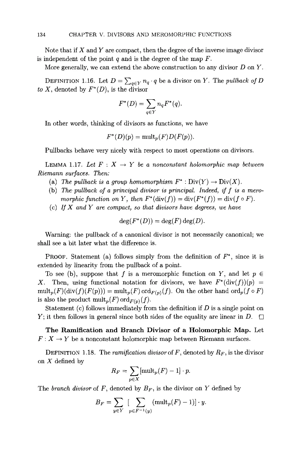
The Inverse Image Divisor of a Holomorphic Map 133
The Ramification and Branch Divisor of a Holomorphic Map 134
Intersection Divisors on a Smooth Projective Curve 135
The Partial Ordering on Divisors 136
Problems V.I 137
2. Linear Equivalence of Divisors 138
The Definition of Linear Equivalence 138
Linear Equivalence for Divisors on the Riemann Sphere 140
Principal Divisors on a Complex Torus 140
The Degree of a Smooth Projective Curve 142
Bezout's Theorem for Smooth Projective Plane Curves 143
Pliicker's Formula 143
Problems V.2 145
3. Spaces of Functions and Forms Associated to a Divisor 145

CONTENTS xiii
The Definition of the Space L{D) 145
Complete Linear Systems of Divisors 147
Isomorphisms between L(Z?)'s under Linear Equivalence 148
The Definition of the Space L^(D) 148
The Isomorphism between L^(D) and L(D + K) 149
Computation of L{D) for the Riemann Sphere 149
Computation of L(D) for a Complex Torus 150
A Bound on the Dimension of L(D) 151
Problems V.3 152
4. Divisors and Maps to Projective Space 153
Holomorphic Maps to Projective Space 153
Maps to Projective Space Given By Meromorphic Functions 154
The Linear System of a Holomorphic Map 155
Base Points of Linear Systems 157
The Hyperplane Divisor of a Holomorphic Map to P" 158
Defining a Holomorphic Map via a Linear System 160
Removing the Base Points 160
Criteria for <po to be an Embedding 161
The Degree of the Image and of the Map 164
Rational and Elliptic Normal Curves 165
Working Without Coordinates 166
Problems V.4 166
Further Reading 167
Chapter VI. Algebraic Curves and the Riemann-Roch Theorem 169
1. Algebraic Curves 169
Separating Points and Tangents 169
Constructing Functions with Specified Laurent Tails 171
The Transcendence Degree of the Function Field M(X) 174
Computing the Function Field M(X) 177
Problems VI. 1 178
2. Laurent Tail Divisors 178
Definition of Laurent Tail Divisors 178
Mittag-Leffler Problems and H1 (D) 180
Comparing H1 Spaces . 181
The Finite-Dimensionality of H1 (D) 182
Problems VI.2 184
3. The Riemann-Roch Theorem and Serre Duality 185
The Riemann-Roch Theorem I 185
The Residue Map 186
Serre Duality 188
The Equality of the Three Genera 191
The Riemann-Roch Theorem II 192

xiv CONTENTS
Problems VI.3 193
Further Reading 193
Chapter VII. Applications of Riemann-Roch 195
1. First Applications of Riemann-Roch 195
How Riemann-Roch implies Algebraicity 195
Criterion for a Divisor to be Very Ample 195
Every Algebraic Curve is Projective 196
Curves of Genus Zero are Isomorphic to the Riemann Sphere 196
Curves of Genus One are Cubic Plane Curves 197
Curves of Genus One are Complex Tori 197
Curves of Genus Two are Hyperelliptic 198
Clifford's Theorem 198
The Canonical System is Base-Point-Free 200
The Existence of Meromorphic 1-Forms 200
Problems VII. 1 202
2. The Canonical Map 203
The Canonical Map for a Curve of Genus at Least Three 203
The Canonical Map for a Hyperelliptic Curve 203
Finding Equations for Smooth Projective Curves 204
Classification of Curves of Genus Three 205
Classification of Curves of Genus Four 206
The Geometric Form of Riemann-Roch 207
Classification of Curves of Genus Five 209
The Space L(D) for a General Divisor 210
A Few Words on Counting Parameters 211
Riemann's Count of 3g — 3 Parameters for Curves of Genus g 212
Problems VII.2 215
3. The Degree of Projective Curves 216
The Minimal Degree 216
Rational Normal Curves 216
Tangent Hyperplanes 217
Flexes and Bitangents 219
Monodromy of the Hyperplane Divisors 221
The Surjectivity of the Monodromy 222
The General Position Lemma 224
Points Imposing Conditions on Hypersurfaces 225
Castelnuovo's Bound 228
Curves of Maximal Genus 230
Problems VII.3 232
4. Inflection Points and Weierstrass Points 233
Gap Numbers and Inflection Points of a Linear System 233
The Wronskian Criterion 234

CONTENTS xv
Higher-order Differentials 236
The Number of Inflection Points 238
Flex Points of Smooth Plane Curves 241
Weierstrass Points 241
Problems VII.4 243
Further Reading 245
Chapter VIII. Abel's Theorem 247
1. Homology, Periods, and the Jacobian 247
The First Homology Group 247
The Standard Identified Polygon 247
Periods of 1-Forms 247
The Jacobian of a Compact Riemann Surface 248
Problems VIII. 1 249
2. The Abel-Jacobi Map 249
The Abel-Jacobi Map A on X 249
The Extension of A to Divisors 250
Independence of the Base Point 250
Statement of Abel's Theorem 250
Problems VIII.2 250
3. Trace Operations 251
The Trace of a Function 251
The Trace of a 1-Form 252
The Residue of a Trace 253
An Algebraic Proof of the Residue Theorem 253
Integration of a Trace 254
Proof of Necessity in Abel's Theorem 255
Problems VIII.3 256
4. Proof of Sufficiency in Abel's Theorem 257
Lemmas Concerning Periods 257
The Proof of Sufficiency 260
Riemann's Bilinear Relations 262
The Jacobian and the Picard Group 263
Problems VIII.4 264
5. Abel's Theorem for Curves of Genus One 265
The Abel-Jacobi Map is an Embedding 265
Every Curve of Genus One is a Complex Torus 265
The Group Law on a Smooth Projective Plane Cubic 266
Problems VIII.5 267
Further Reading 267
Chapter IX. Sheaves and Cech Cohomology 269
1. Presheaves and Sheaves 269

xvi CONTENTS
Presheaves 269
Examples of Presheaves 269
The Sheaf Axiom 272
Locally Constant Sheaves 273
Skyscraper Sheaves 273
Global Sections on Compact Riemann Surfaces 275
Restriction to an Open Subset 276
Problems IX. 1 276
2. Sheaf Maps 278
Definition of a Map between Sheaves 278
Inclusion Maps 278
Differentiation Maps 279
Restriction or Evaluation Maps 279
Multiplication Maps 280
Truncation Maps 281
The Exponential Map 281
The Kernel of a Sheaf Map 282
1-1 and Onto Sheaf Maps 282
Short Exact Sequences of Sheaves 284
Exact Sequences of Sheaves 286
Sheaf Isomorphisms 286
Using Sheaves to Define the Category 288
Problems IX.2 289
3. Cech Cohomology of Sheaves 290
Cech Cochains 291
Cech Cochaih Complexes 291
Cohomology with respect to a Cover 292
Refinements 293
Cech Cohomology Groups 295
The Connecting Homomorphism 297
The Long Exact Sequence of Cohomology 298
Problems IX.3 300
4. Cohomology Computations 301
The Vanishing of Hl for C°° Sheaves 302
The Vanishing of H1 for Skyscraper Sheaves 303
Cohomology of Locally Constant Sheaves 304
The Vanishing of H2 (X, Ox [D]) 304
De Rham Cohomology 305
Dolbeault Cohomology 306
Problems IX.4 308
Further Reading 308
Chapter X. Algebraic Sheaves 309

CONTENTS xvii
1. Algebraic Sheaves of Functions and Forms 309
Algebraic Curves 309
Algebraic Sheaves of Functions 309
Algebraic Sheaves of Forms 310
The Zariski Topology 311
Problems X.I 312
2. Zariski Cohomology 312
The Vanishing of Hl {XZar, T) for a Constant Sheaf T 313
The Interpretation of Hl (D) 314
GAGA Theorems 315
Further Computations 316
The Zero Mean Theorem 317
The High Road to Abel's Theorem 319
Problems X.2 320
Further Reading 321
Chapter XL Invertible Sheaves, Line Bundles, and H1 323
1. Invertible Sheaves 323
Sheaves of O-Modules 323
Definition of an Invertible Sheaf 324
Invertible Sheaves associated to Divisors 325
The Tensor Product of Invertible Sheaves 326
The Inverse of an Invertible Sheaf 328
The Group of Isomorphism Classes of Invertible Sheaves 329
Problems XI. 1 330
2. Line Bundles 331
The Definition of a Line Bundle 331
The Tautological Line Bundle for a Map to Pn 333
Line Bundle Homomorphisms 334
Denning a Line Bundle via Transition Functions 335
The Invertible Sheaf of Regular Sections of a Line Bundle 337
Sections of the Tangent Bundle and Tangent Vector Fields 340
Rational Sections of a Line Bundle 342
The Divisor of a Rational Section 343
Problems XI.2 344
3. Avatars of the Picard Group 345
Divisors Modulo Linear Equivalence and Cocycles 345
Invertible Sheaves Modulo Isomorphism 348
Line Bundles Modulo Isomorphism 351
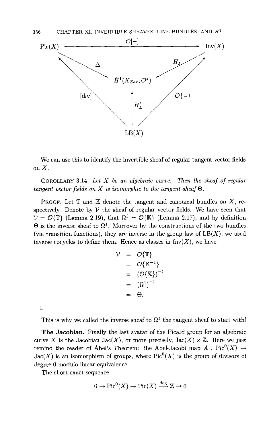
The Jacobian 356
Problems XI.3 357
4. H as a Classifying Space 357
Why u\o*) Classifies Invertible Sheaves and Line Bundles 357

xviii CONTENTS
Locally Trivial Structures 359
A General Principle Regarding H 360
Cyclic Unbranched Coverings 360
Extensions of Invertible Sheaves 361
First-Order Deformations 364
Problems XI.4 368
Further Reading 369
References 371
Index of Notation 377

Preface
This text has evolved from lecture notes for a one-semester course which I have
taught 5 times in the last 8 years as an introduction to the ideas of algebraic
geometry using the theory of algebraic curves as a foundation.
There are two broad aims for the book: to keep the prerequisites to a bare
minimum while still treating the major theorems seriously; and to begin to con-
convey to the reader some of the language of modern algebraic geometry.
In order to present the material of Algebraic Curves to an initially relatively
unsophisticated audience I have taken the approach that Algebraic Curves are
best encountered for the first time over the complex numbers. Therefore the
book starts out as a primer on Riemann surfaces, with complex charts and mero-
morphic functions taking center stage. In particular, one semester of graduate
complex analysis should be sufficient preparation, and it is not assumed that the
reader has any serious background in either algebraic topology or commutative
algebra. But I try to stress that the main examples (from the point of view
of algebraic geometry) come from projective curves, and slowly but surely the
text evolves to the algebraic category, culminating in an algebraic proof of the
Riemann-Roch theorem. After returning to the analytic side of things for Abel's
theorem, the progression is repeated again when sheaves and cohomology are
discussed: first the analytic, then the algebraic category.
The proof of Riemann-Roch presented here is an adaptation of the adelic
proof, expressed completely in terms of solving a Mittag-Leffler problem. This
is a very concrete approach, and in particular no cohomology or sheaf theory is
used. However, cohomology groups clandestinely appear (as obstruction spaces
to solving Mittag-Leffler problems), motivating their explicit introduction later
on.
The other goal is to begin to convey, as much as possible, the language of
modern algebraic geometry to the student. This language is that of rational
functions, divisors, bundles, sheaves, cohomology, and the Zariski topology, to
name some of the highlights presented here. I hope that a student who has
read the later chapters of this book will be prepared to understand at least the
first few minutes of a modern colloquium talk discussing algebraic curves and

xx PREFACE
algebraic geometry. I consider the treatment of sheaves and cohomology given
here to be rather gentle; for example, most of the sheaves which are used as
the initial examples were introduced in a natural way much earlier in the text.
Hence by the time a sheaf is even defined the reader will actually have a decent
understanding of what the technicalities entail. In addition, the zero-th and first
cohomology groups will already have been seen in the proof of the Riemann-Roch
theorem (without them being called that of course).
The first three chapters are introductory, discussing the basic definitions of
Riemann surfaces and holomorphic maps between them. Of the 12 sections in
these chapters, 5 are devoted entirely to examples of one sort or another. The
main theorems here are that the sum of the orders of a meromorphic function on
a compact Riemann surface is zero, and Hurwitz's Formula relating the genera
of compact Riemann surfaces given a map between them. The fourth chapter
on integration is meant to get to the Residue Theorem in a direct manner.
Chapters 5-8 form the technical heart of the text. Divisors and how they are
used to organize forms, functions, and maps are introduced in Chapter 5, and
in Chapter 6 the Riemann-Roch Theorem and Serre Duality are proved, after
introducing the concept of an algebraic curve, which is denned here as a compact
Riemann surface whose field of global meromorphic functions separates points
and tangents. Chapter 7 is devoted to applications of Riemann-Roch. Here is
found the classification of curves of low genus, Clifford's Theorem, the analysis
of the canonical map, and Riemann's count of 3g — 3 parameters for curves of
genus at least two. A section on the degree of a projective curve culminates in
Castelnuovo's bound on the genus. It is here most of all that the reader will
feel an urge to learn more algebraic geometry, and in particular some higher-
dimensional theory. The final section concerns inflection points of linear systems
and Weierstrass points in particular. In Chapter 8 Abel's Theorem is proved;
along the way the algebraic proof of the Residue Theorem is indicated. The final
section discusses the group law on a smooth cubic curve.
The last three chapters introduce sheaves and Cech cohomology. Initially the
classical topology is used, focusing in on the standard sheaves of holomorphic
and meromorphic functions and forms. The Zariski topology and the algebraic
sheaves are brought into the picture next, and the obstruction space for solving
a Mittag-Leffler problem (seen in the proof of the Riemann-Roch Theorem) is
here realized as an H1 of an algebraic sheaf.
The last chapter is organized around the Picard group of an algebraic curve
and its many manifestations: as the group of divisors modulo linear equivalence,
as the group of line bundles modulo isomorphism, as the group of invertible
sheaves modulo isomorphism, as the first cohomology group with values in the
nowhere zero regular functions, and as the Jacobian (extended by Z). Here there
is an opportunity to explain why Hl is useful to classify locally trivial objects in
general, and the text closes with first-order deformations, with Riemann's count
of 3g — 3 parameters enjoying a reprise.

PREFACE xxi
At the end of each chapter I have included some suggestions for further read-
reading. These are not meant to be completely comprehensive, but simply indicate
some of the sources that I am aware of which I have found illuminating.
I would like to thank Bruce Crauder, David Hahn, Luisa Paoluzzi, John
Symms, and Caryn Werner for commenting on various sections; also I am greatly
indebted to Ciro Ciliberto and Peter Stiller who each read through substantial
portions of the text and offered many valuable suggestions.
It has been my great privilege to have been given the opportunity to study
algebraic geometry in my professional life. There is no doubt that the theory of
algebraic curves is the richest and deepest of the field's various roots, and I hope
I have conveyed some of the special pleasure obtained in visiting this material,
which serves simultaneously as one of the great jewels of classical mathematics
and one of the most vital areas of modern research.
Rick Miranda
October 1994
Fort Collins, Colorado

Chapter I. Riemann Surfaces: Basic Definitions
1. Complex Charts and Complex Structures
The basic idea of a Riemann surface is that it is a space which, locally, looks
just like an open set in the complex plane. In this section we make this precise.
Complex Charts. Let X be a topological space. In order to make X look,
locally, like an open set in the complex plane, we want to have a local complex
coordinate at every point of the space; this local coordinate can then be used to
define all the local notions of functions of one complex variable. Now a coordinate
on a space is simply a function from the space to the standard space, in this case
the complex plane. This leads to the following definition.
Definition 1.1. A complex chart, or simply chart, on X is a homeomorphism
0 : U —> V, where U C X is an open set in X, and V C C is an open set in
the complex plane. The open subset U is called the domain of the chart (/>. The
chart <j> is said to be centered at p ? U if (p(p) = 0.
We think of a chart on X as giving a local (complex) coordinate on its domain,
namely z = <f>(x) for x e U.
Example 1.2. Let X = M2, and let U be any open subset. Define (j>u{x, y) =
x + iy from U (considered as a subset of R2) to the complex plane. This is a
complex chart on M2.
Example 1.3. Again let X = K2. For any open subset U, define
y
These are also complex charts onl2.
Example 1.4. Let <j> : U —» V be a complex chart on X. Suppose that
U\ C U is an open subset of U. Then <f>\u1 : U\ —> (j){U\) is a complex chart on
X. This restriction of <j> is called a sub-chart of <j>.

2 CHAPTER I. RIEMANN SURFACES: BASIC DEFINITIONS
Example 1.5. Let <j> : U —> V be a complex chart on X. Suppose that
ij) : V —> W is a holomorphic bijection between two open sets of the complex
plane. Then the composition ip o <j> : U —>W/isa complex chart on X. If we
think of <j> as giving a complex coordinate on U, we can view this operation as a
change of coordinates.
We do not want to think of a simple change of coordinates as imposing an
essentially different structure on the open set in question. In other words, with
the above notation, the two charts <j> and ip o <j> should not produce different
answers when we get around to asking questions about local functions and forms
on the domain. A careful analysis of the "difference" between these two charts
leads us to the following definition.
Definition 1.6. Let fa ¦. U\ —> Vi and fa> : U2 —> Vi be two complex charts
on X. We say that fa and </>2 are compatible if either U\C\U2— 0, or
fa o fa'1 ¦ faiUi n u2) -> <h(Ui n u2)
is holomorphic.
Note that the definition is symmetric: if 4>2°fa~l is holomorphic on fa{Uif\U2),
then fa o 0 will be holomorhic on ^2(^1 n U2). The function T = <fi2 ° ^j
is called the transition function between the two charts; it is a bijection in any
case. Transition functions enjoy the following property.
Lemma 1.7. Let T be a transition function between two compatible charts.
Then the derivative T" is never zero on the domain ofT.
PROOF. Let S denote the inverse to T, so that S o T is the identity on the
domain of T, i.e., S{T{w)) = w for all w. Taking the derivative of this equation
gives S'(T(w))T'(w) = 1, so that T'{w) cannot be zero. ?
Suppose that T is the transition function between the charts <j> and ip, with
a point p in their common domain. Denote by z = cf>(x) and w = ip(x) the two
local coordinates, with z0 — <j>{p) and Wo = ipip)- The above lemma implies
that the power series expansion of the transition function T — <j> o ip (which
expresses z as a power series in w) must be of the form
z = T(w) = z0 + ^2 an(w - wo)n,
ith ai ^ 0.
Example 1.8. Referring to the situation of Example 1.5, let <fi : U —> V be
a complex chart on X, and let ip : V —> W be a holomorphic bijection between
two open sets of the complex plane. Then the charts <f> and ip o <j> are compatible.
Moreover, ip o 0 will be compatible with any chart which is compatible with fa
Example 1.9. Any two sub-charts of a complex chart are compatible.

1. COMPLEX CHARTS AND COMPLEX STRUCTURES 3
Example 1.10. Any two charts in Example 1.2 are compatible.
Example 1.11. Any two charts in Example 1.3 are compatible.
EXAMPLE 1.12. No chart of Example 1.2 is compatible with any chart of
Example 1.3 (unless the domains are disjoint).
A more serious example is given by the following.
EXAMPLE 1.13. Let S2 denote the unit 2-sphere inside R3, i.e.,
S2 = {(x,y,w)GR3 \x2+y2+w2 = l}.
Consider the w = 0 plane as a copy of the complex plane C, with (x, y, 0) being
identified with z = x + iy. Let 0i : S2 - {@,0,1)} —* C be denned by projection
from @,0,1). Specifically,
The inverse to (j>\ is
X 11
>i(x,y,w) = +i- .
1 - w 1 - w
2Im(z) \z\2-l
Define <j>2 ¦ S2 - {@,0,-1)} -»• C by projection from @,0,-1) followed by a
complex conjugation:
X V
4>2{x,y,w) = — i
1 + w
i.
1 + w 1 + w
The inverse to <j>2 is
! 2Re(^) 2Im(g) 1 \*
<t>2 { (
+1 \z\ +1 \z\ +1
The common domain is S2 — {@,0, ±1)}, and is mapped by both <j>\ and <j>2
bijectively onto C* = C — {0}. The composition fa ° </>j~1(z) = 1/z, which is
holomorphic. Thus the two charts are compatible.
Complex Atlases. Note that in Example 1.13, every point of the sphere lies
in at least one of the two complex charts. Therefore we have a local complex
coordinate at each point of the sphere. This, of course, is our ultimate goal.
For X to look locally like the complex plane everywhere, we must have com-
complex charts around every point of X. Moreover, we want these charts to be
compatible. This is the notion of a complex atlas.
Definition 1.14. A complex atlas (or simply atlas) A on X is a collection
A — {4>a : Ua —» Va} of pairwise compatible complex charts whose domains
cover X, i.e., X = \JaUa.

4 CHAPTER I. RIEMANN SURFACES: BASIC DEFINITIONS
Note that the charts defined in Example 1.2 form a complex atlas on M2, as
do the charts in Example 1.3. Also, the two charts defined on the 2-sphere in
Example 1.13 define a complex atlas on S2.
Example 1.15. If A = {4>a : Ua —> Va} is an atlas on X, and Y c X is
any open subset, then the collection of sub-charts Ay = {4>a\Ynua '¦ Y (~)Ua —>
4>a(Y fl Ua)} is an atlas on Y.
It may well be the case that two different atlases give the same local notions
of complex analysis on a Riemann surface; in particular, this will happen when
every chart of one atlas is compatible with every chart of the other atlas. This
notion gives an equivalence relation on atlases:
DEFINITION 1.16. Two complex atlases A and B are equivalent if every chart
of one is compatible with every chart of the other.
Note that two complex atlases are equivalent if and only if their union is also
a complex atlas. An easy Zorn's lemma argument will show that every complex
atlas is contained in a unique maximal complex atlas; moreover, two atlases are
equivalent if and only if they are contained in the same maximal complex atlas.
Definition 1.17. A complex structure on X is a maximal complex atlas on
X, or, equivalently, an equivalence class of complex atlases on X.
Note that any atlas on X determines a unique complex structure. This is the
usual way that complex structures are defined: by giving an atlas.
The Definition of a Riemann Surface. Recall that a topological space
X is said to be Hausdorff \i, for every two distinct points x, y in X, there are
disjoint neighborhoods U and V of x and y, respectively. X is said to be second
countable if there is a countable basis for its topology.
Definition 1.18. A Riemann surface is a second countable connected Haus-
Hausdorff topological space X together with a complex structure.
The second countability condition is a technical one, meant to exclude certain
pathological examples; any Riemann surface found "in nature" (i.e., as a subset of
C n for example) will be second countable. In particular, if the complex structure
may be defined by a countable atlas, then X must be second countable.
Example 1.19. Let X be C itself, considered topologically as R2, with the
complex structure induced by the atlas of Example 1.2. This Riemann surface
is called the complex plane.
Example 1.20. Let X be the 2-sphere, with complex structure given by the
two-chart atlas of Example 1.13. Note that the sphere is Hausdorff and con-
connected. This Riemann surface is called the Riemann Sphere. Note that if one
chart of the Riemann Sphere has as coordinate z, then the other chart has the
coordinate 1/z, and there is only one point which is not in the z-chart. The

1. COMPLEX CHARTS AND COMPLEX STRUCTURES 5
Riemann Sphere is often written as Cqq or CUoo, with the complex plane C
representing one chart, with the "point at infinity" oo being the single extra
point. The Riemann Sphere is a compact Riemann surface.
Example 1.21. Any connected open subset of a Riemann surface is a Rie-
Riemann surface; use the atlas on the subset as described in Example 1.15.
Real 2-Manifolds. The reader who has seen some of the theory of manifolds
will recognize in every detail the definitions and constructions. In essence, a
Riemann surface is simply a connected complex manifold of dimension one (this
is one complex dimension, remember).
It is convenient to sometimes "forget" the complex structure of a Riemann
surface, and to consider it simply as a 2-manifold. Let us then briefly recall the
relevant definitions. Let X be a Hausdorff topological space.
Definition 1.22. An n-dimensional real chart on X is a homeomorphism
<f> : U —> V, where U C X is an open set in X, and V C M.n is an open set in
B™. Two such real charts <j>\ and fa are C°° -compatible if either the intersection
of their domains is empty, or
fa o <t>~1: <j>x{ux n U2) -> fa{Ux n U2)
is a C°° diffeomorphism, i.e., it and its inverse have partial derivatives of all
orders at every point. A C°° atlas on X is a collection of real charts on X, which
are pairwise C°°-compatible, and whose domains cover X. Two such atlases are
equivalent if their union is an atlas. A C°° structure on X is an equivalence class
of C°° atlases. A C°° real manifold is a second countable connected Hausdorff
space X together with a C°° structure.
Since holomorphic maps of a complex variable z — x + iy are C°° in the
real variables x and y, we immediately see that every Riemann surface is a 2-
dimensional C°° real manifold (which we often abbreviate and refer to simply as
a -manifold").
Let us make a few remarks concerning the topology of Riemann surfaces.
Firstly, for manifolds, connectedness and path-connectedness are equivalent; thus
we have that every Riemann surface is path-connected.
Next, note that a holomorphic map between two subsets of the complex plane
preserves the orientation of the plane. Indeed, the familiar conformal property of
holomorphic functions implies that all local angles are preserved by holomorphic
maps, and in particular right angles are preserved; therefore the local notions of
"clockwise" and "counterclockwise" for small circles are preserved. Since giving
an orientation on a surface can be viewed as equivalent to having consistent local
choices for "clockwise", holomorphic maps preserve the orientation of the plane.
Therefore, if we induce a local orientation at each point of a Riemann surface
by "pulling back" the orientation via some complex chart containing that point,
this local orientation is well denned, independent of the choice of complex chart.

6 CHAPTER I. RIEMANN SURFACES: BASIC DEFINITIONS
These local orientations induce a global orientation on the Riemann surface;
hence we have that every Riemann surface is orientable. The reader may consult
[Armstrong83], [Munkres84], or [Massey67] for further details concerning
orientation.
The Genus of a Compact Riemann Surface. These remarks are enough
to completely determine compact Riemann surfaces, as far as their C°° struc-
structure goes. For this we appeal to the classification of compact orientable 2-
manifolds; each of these is a g-holed torus for some unique integer g > 0. (See
[Armstrong83], [Massey67], or [Sieradski92] for example.) When g — 0,
we have no holes and the surface is topologically the 2-sphere. When g = 1,
there is one hole, and the surface is a simple torus, topologically homeomorphic
to S1 x S1. For g > 2, the surface is obtained by attaching g "handles" to a
2-sphere. This integer g is called the topological genus of the compact Riemann
surface, and is a fundamental invariant. Thus:
Proposition 1.23. Every Riemann surface is an orientable path-connected 2-
dimensional C°° real manifold. Every compact Riemann surface is diffeomorphic
to the g-holed torus, for some unique integer g > 0.
We have only seen one example so far of a compact Riemann surface, namely
the Riemann Sphere (Example 1.20). It has topological genus 0.
Complex Manifolds. As was seen above, the definition of a Riemann surface
and the definition of a C°° real manifold are in all ways parallel. The reader
should also be aware that higher-dimensional analogues of Riemann surfaces
also exist, defined in exactly the same spirit. Here we just give the definitions,
since we will rarely need to work with complex manifolds of higher dimension.
Definition 1.24. Let X be a Hausdorff topological space. An n-dimensional
complex chart on X is a homeomorphism (f> : U —> V, where U C X is an open
set in X, and V C C" is an open set in C™. Two such n-dimensional complex
charts <f>i and <f>2 are compatible if either the intersection of their domains is
empty, or
0a o fc1: <Ai(f/i n U2) -> <h(Ui n U2)
is holomorphic, i.e., is holomorphic in each of the n variables separately at every
point. An n-dimensional complex atlas on X is a collection of n-dimensional
complex charts on X, which are pairwise compatible, and whose domains cover
X. Two such atlases are equivalent if their union is an atlas. An n-dimensional
complex structure on X is an equivalence class of n-dimensional complex atlases.
An n-dimensional complex manifold is a connected Hausdorff space X together
with an n-dimensional complex structure.

2. FIRST EXAMPLES OF RIEMANN SURFACES 7
Problems I.I
A. Let fa : Ui -+ Vi, i = 1,2, be complex charts on X with U\ n[/2 / 0. Suppose
that <f>2 o <j>^1 : 4>\{U\ fl U2) —* fa(Ui n ^2) is holomorphic. Show that it is
bijective, with inverse <f>i o c^1 : faiUi n U2) —> <^»i(C/i n C/2), proving that
<^j o^1 is also holomorphic.
B. Let <j> : U —» V be a complex chart on X, and let V : V ~> ^ be a
holomorphic bijection between two open sets in C. Show that ip o <f>: U —» VF
is a complex chart on X. Show that ip o </> is compatible with any chart on
X which is compatible with <j>.
C. Verify that any two sub-charts of a complex chart are compatible (Example
1.9 of the text).
D. Verify that any two charts in Example 1.2 are compatible.
E. Verify that any two charts in Example 1.3 are compatible.
F. Check that no chart of Example 1.2 is compatible with any chart of Example
1.3 of the notes.
G. In Example 1.13, where an atlas of the Riemann Sphere is defined, check
that indeed fa o <f>^1 sends z to 1/z as stated.
H. Show that equivalence of complex atlases is an equivalence relation.
I. Equivalent atlases may be partially ordered by inclusion. Show that any
atlas is equivalent to a unique maximal atlas.
J. Show that holomorphic bijections between open sets in the complex plane
preserve the local orientation.
2. First Examples of Riemann Surfaces
In this section we'll present some easy examples of Riemann surfaces, espe-
especially of compact Riemann surfaces. These include the projective line, complex
tori, and smooth plane curves.
A Remark on Defining Riemann Surfaces. To define a Riemann surface,
it would appear that one needs to start with a topological space X, second
countable, connected and Hausdorff, and then define a complex atlas on it; in
other words, one needs to have the topology first, and then one can impose the
complex structure. This is not completely accurate; one can often use the data
denning an atlas to also define the topology.
This observation is based on the following remark: if an open cover {Ua} of
a topological space X is given, then a subset U C X is open in X if and only if
each intersection U n Ua is open in Ua.
More generally, if any collection {Ua} of subsets of a set X is given, and
topologies are given for each subset Ua, then one can define a topology on X by
declaring a set U to be open if and only if each intersection U C\Ua is open in
Ua.
Now suppose we are given a collection of subsets {Ua} of a set X, which cover
X (so that X = (J Ua), and a set of bijections <f>a : Ua —» Va where each Va is

8 CHAPTER I. RIEMANN SURFACES: BASIC DEFINITIONS
an open subset of C. Each Va has its topology as a subset of C, and so using
the (f>a, we can transport this topology to every Ua: we simply declare a subset
U of Ua to be open if and only if <j>a{U) is open in Va (or, equivalently, open in
C).
Now we can define a topology on all of X, again by declaring a set U to be
open in X if and only if each intersection U n Ua is open in Ua.
This prescription gives a topology on X such that each Ua is an open set
if and only if for each a and /3, the subset Ua n Up is open in Ua. From the
definition of the topology on the C/Q's, this condition is equivalent to asking that
4>a(Ua fl Up) is open in Va (or, equivalently, open in C).
Thus we may take the following route to define a Riemann surface:
• Start with a set X.
• Find a countable collection of subsets {Ua} of X, which cover X.
• For each a, find a bisection <f>a from Ua to an open subset Va of the
complex plane.
• Check that for every a and /?, <f>a(Ua l~l Up) is open in Va. At this point
we have, by the above remarks, a topology denned on X, such that each
Ua is open; moreover by definition, each <f>a is a complex chart on X.
• Check that the complex charts <f>a are pairwise compatible.
• Check that X is connected and Hausdorff.
The Projective Line. Let C P* denote the complex projective line, that is,
the set of 1-dimensional subspaces of C 2. If (z, w) is a nonzero vector in C 2, its
span is a point in CP1; we will denote the span of (z,w) by [z : w]. Note that
every point of CP1 can be written in this form, as [z : w], with z and w not
both zero; moreover,
[z : w] = [Xz : Xw]
for any nonzero A € C *.
We will use the method outlined above for defining a complex structure on
Let Uo = {[z : w] | z / 0}, and Ux = {[z : w] \ w ^ 0}. Note that Uo and U\
cover CP1. Define <f>0 : Uo —> C by <t>0[z : w] — w/z\ similarly define fa : U\ —» C
by <f>i[z : w] = z/w. Both </>0 and fa are bijections, so we have the data required
above. Note that (f>i(U0 <~)Ui) = C*, which is ope"n in C. The composition
fa ° do1 sends s to 1/s, and therefore these two charts are compatible. Since •
both Uo and U\ are connected, and have nonempty intersection, their union C P1 [
is connected. Finally we show CP1 is Hausdorff. Take two points p and q in j
C P1. If both p and q are in either Uq or Ui, we can separate them by open !
sets, since the Ui are Hausdorff. Therefore we may assume that p S Uo - U\ [
and q € U\ - Uo; this forces p = [1 : 0] and q = [0 : 1]. These are separated by
(^^(D) and fa~1(D), where D is the open unit disc in C.
We will usually denote C P1 by simply P1; it is called the complex projective
line. Note that P1 is the union of the two closed sets ^1(?>) and ^^(D), where

2. FIRST EXAMPLES OF RIEMANN SURFACES 9
D is the closed unit disc in C. Since D is compact, we see that the projective
line is compact.
Complex Tori. Fix u>i and u>2 to be two complex numbers which are linearly
independent over R. Define L to be the lattice
L = Zwi + Za>2 = {miwi + m2u;2 \mi,m^ E Z}.
The lattice L is a subgroup of the additive group of C Let X = C/L be the
quotient group, with projection map n :C —> X. Note that via tt, we can impose
the quotient topology on X, namely, a set U C X is open if and only if 7r~1(t7)
is open in C. This definition makes n continuous, and since C is connected, so
isX.
Every open set in X is the image of an open set in C, since if U is open in X,
U — n(n~1(U)). A more serious remark is that n is an open mapping, that is, n
takes any open set of C onto an open set in X. Indeed, if V is open in C, then
to check that n(V) is open in X we must show that 7r~1Gr(y)) is open in C; but
= \J(lu
is a union of translates of V, which are all open sets in C.
For any z 6 C, define the closed parallelogram
Pz = {z + Ai^i + A2w2 I \ € [0,1]}.
Note that any point of C is congruent modulo L to a point of Pz. Therefore the
projection map tt maps Pz onto X. Since Pz is compact, so is X.
The lattice L is a discrete subset of C, so there is an e > 0 such that |u;| > 2e
for every nonzero lj ? L. Fix such an e, and fix a point zq € C. Consider the
open disc D = D(z0, e) of radius e about zQ. This choice of e insures that no two
points of D{zq, e) can differ by an element of the lattice L.
We claim that for any z$, and for any such e, the restriction of the projection
¦k to the open disc D maps D homeomorphically onto the open set tt(-D). Clearly
tv\d '¦ D —> n(D) is onto, continuous, and open (since tt is). Therefore we need
only check that it is 1-1; this follows from the choice of e.
We are now ready to define a complex atlas on X. Again fix e as above. For
each zq € C, let DZo = D{zq, e), and define <j)Zo : tt(DZo) —* DZo to be the inverse
of the map k\dzo ¦ By the above claim, these (f>'s are complex charts on X.
To finish the construction, we must check that these charts are pairwise com-
compatible. Choose two points z\ and Z2, and consider the two charts <f>i = (f>Zl :
ir(Dzl) -» DZ1 and fo = <f>Z2 : ir(DZ2) -» DZ2. Let U = ir(Dtl) n v{DX2). If U
is empty, there is nothing to prove. If U is not empty, let T(z) = ^2(<A^1(^)) =
4>2{k{z)) for z € <t>i(U); we must check that T is holomorphic on <t>i(U). Note
that 7r(T(z)) = tt(z) for all z G fa{U), so T{z) -z = u(z) E L for all z € <fa{U).
This function u> : fa (U) —¦ L is continuous, and L is discrete; hence u is locally
constant on fa(U). (It is constant on the connected components of U.) Thus,

10 CHAPTER I. RIEMANN SURFACES: BASIC DEFINITIONS
locally, T(z) = z + w for some fixed w€i, and is therefore holomorphic. Hence
the two charts <f>\ and (f>2 are compatible, and the collection of charts {<pz \ z € C}
is a complex atlas on X.
Hence X is a compact Riemann surface. In fact it has topological genus one;
topologically, X is a simple torus. This is most easily seen by considering X
as the image of the parallelogram Po; under the map n\p0, the opposite sides
are identified together, and no other identifications are made, giving the familiar
construction of the torus. These Riemann surfaces (which depend of course on
the lattice L) are called complex tori.
Graphs of Holomorphic Functions. Let V c C be a connected open
subset of the complex plane, and let jbea holomorphic function defined on all
of V. Consider the graph X of g, as a subset of C2:
X = {(z,g{z))\zeV}.
Give X the subspace topology, and let tt : X —» V be the first projection; note
that 7T is a homeomorphism, whose inverse simply sends the point z ? V to the
ordered pair (z,g(z)). Thus n is a complex chart on X, whose domain covers
all of X. Hence we have a complex atlas on X, composed of a single chart; this
gives X the structure of a Riemann surface.
This example can be immediately generalized to any finite collection of holo-
holomorphic functions gi,...,gnonV; simply take X to be the graph in Cn+1:
X = {(z,9l(z),...,gn(z))\zeV}.
Smooth Affine Plane Curves. This is a further generalization of the graph
construction introduced above. We would like to consider a locus X cC2 which
is locally a graph, but perhaps not globally. The most natural way to do this is
to define a locus X by requiring a complex polynomial of two variables f(z,w)
to vanish. Morally speaking, this should cut the complex dimension down by
one, and we have a chance of producing a Riemann surface this way.
One needs a mild condition on the polynomial / for this to work, essentially
insuring that X is locally a graph. This condition is based on the Implicit
Function Theorem:
Theorem 2.1 (The Implicit Function Theorem). Let f(z,w) e C[z,w]
be a polynomial, and let X = {(z,w) € C2 | f(z,w) — 0} be its zero locus. Let
p — (zq,Wo) be a point of X, i.e., p is a root of f. Suppose that df/dw(p) ^ 0.
Then there exists a function g(z) defined and holomorphic in a neighborhood of
zq, such that, near p, X is equal to the graph w = g(z). Moreover g' = — gf/g~
near z®.
Of course, if df/dw(p) = 0, it may still be true that df/dz(p) ^ 0, and X
will still be, locally, a graph near p, using the other variable. This motivates the
following.

2. FIRST EXAMPLES OF RIEMANN SURFACES 11
Definition 2.2. An affine plane curve is the locus of zeroes in C 2 of a poly-
polynomial /(z, w). A polynomial f(z, w) is nonsingular at a root p if either partial
derivative df/dz or df /dw is not zero at p. The affine plane curve X of roots
of / is nonsingular at p if / is nonsingular at p. The curve X is nonsingular, or
smooth, if it is nonsingular at each of its points.
We can obtain complex charts on a smooth affine plane curve by using the
Implicit Function Theorem to conclude that the curve is locally a graph, and
then making the construction analogously to that for a graph.
Specifically, let X be a smooth affine plane curve, defined by a polynomial
f(z,w). Let p = (zo,wo) € X. If df/dw{p) ^ 0, find a holomorphic function
gp(z) such that in a neighborhood U of p, X is the graph w — gP{z). Thus the
projection irz : U —» C (mapping (z, w) to z) is a homeomorphism from U to its
image V, which is open in C. This gives a complex chart on X.
If instead df/dz(p) / 0, then we make the identical construction using the
other projection nw, sending (z,w) to w near p.
Since X is smooth, at least one of these partials must be nonzero at each
point, and so the domains of these complex charts cover X.
Let us check that any two of these charts are compatible. Suppose first that
both charts are obtained using nz. Then, if there is nonempty intersection with
their domains, the composition of the inverse of one with the other is the identity,
which is certainly holomorphic. The same holds if both charts are obtained using
TTW.
Therefore assume that one chart is ttz and the other is irw. Choose a point
p = (zq, Wq) in their common domain U. Assume that near p, X is locally of the
form w = g(z) for some holomorphic function g. Then on irz(U) near z0, the
inverse of tt2 sends z to (z,g(z)). Thus the composition ttw ottJ1 of nw with the
inverse of tvz sends z to g{z), which is holomorphic.
This completes the proof that any two of the charts are compatible, and gives
a complex atlas on X.
The space X is certainly second countable and Hausdorff, as a subspace of C 2.
Thus to see that X is a Riemann surface, we must only check that it is connected.
This is not automatic; for example, if the polynomial / defining X is the product
of two linear factors with the same slope (e.g., f(z,w) = (z + w)(z + w — 1)) then
X is the union of two complex lines which do not meet; each line is a Riemann
surface itself (being a graph), but the union is not connected.
One possible assumption on the polynomial / for X to be connected is that
f(z, w) be an irreducible polynomial; that is, that / cannot be factored nontriv-
ially as / = g(z,w)h(z,w), where both g and h are nonconstant polynomials:
Theorem 2.3. If f(z,w) is an irreducible polynomial, then its locus of roots
X is connected. Hence if f is nonsingular and irreducible, X is a Riemann
surface.

12 CHAPTER I. RIEMANN SURFACES: BASIC DEFINITIONS
The locus of roots of an irreducible polynomial f(z, w) is called an irreducible
affine plane curve.
The proof of the connectedness of X if / is irreducible is not elementary, but
requires some of the machinery of algebraic geometry. We will not present a
proof here; see [Shafarevich77], for example. Granting this, we see that: every
smooth irreducible affine plane curve is a Riemann surface.
EXAMPLE 2.4. Let h(z) be a polynomial in one variable which is not a perfect
square. Then the polynomial /(z, w) = w2 — h(z) is irreducible. Moreover, if h(z)
has distinct roots, then / is nonsingular, and its locus of roots X is a Riemann
surface. (Prove this for yourself: Problem G below.)
A slight generalization will be useful later. If f(z,w) is an irreducible poly-
polynomial, then the points on its locus of roots X where / is singular forms a finite
set. (This is nontrivial! But let's go on.) If we delete these points, then the
resulting open subset of X is a Riemann surface, using the same charts as given
above. This is referred to as the smooth part of the afHne plane curve X, and in
general, if / is an irreducible polynomial, the smooth part of its zero locus is a
Riemann surface.
No affine plane curve is compact: as a subset of C2 = R4, it is not a bounded
set, since for any fixed z0, there will be roots w to the polynomial f(zo,w) = 0.
Problems 1.2
A. Verify that if any collection of subsets {Ua} of a set X are given, and topolo-
topologies are given for each subset Ua, then a topology can be denned on X by
declaring that a subset U C X is open in X if and only if U n Ua is open in
Ua for every a.
B. Suppose, in problem A, that each Ua is connected. Form a graph with one
vertex (called va) for each Ua, and with vertex va connected by an edge to
V/3 if and only if Ua n Up ^ 0. Prove or disprove: X is connected if and only
if the graph is connected.
C. Check that the function from P1 to S2 sending [z : w] to
BRe(iuf),2Im(f *), \w\2 - |z|2)/(|ti;|2 + l*|2)
is a homeomorphism onto the unit sphere in R3. Therefore the projective
line is a compact Riemann surface of genus zero.
D. Show that any lattice L = Zwi + Zw2 in C with u>\ and u>2 linearly indepen-
independent over R is a discrete subset of C.
E. Show that a complex torus has topological genus one by constructing an
explicit homeomorphism to the product S1 x S1 of two circles.
F. Show that the group law of a complex torus X is divisible: for any point
p ? X and any integer n > 1 there is a point q S X with n ¦ q = p. Indeed,
show that there are exactly n2 such points q.

3. PROJECTIVE CURVES 13
G. Show that the polynomial f(z, w) = w2 — h(z) is an irreducible polynomial
if and only if h(z) is a polynomial which is not a perfect square. Show that
f(z, w) is a nonsingular polynomial if and only if h(z) has distinct roots.
H. Let X be an affine plane curve of degree 2, that is, defined by a quadratic
polynomial f(z,w). (Such a curve is called an affine conic.) Suppose that
f(z, w) is singular. Show that in fact / factors as the product of two linear
polynomials, so that X is therefore the union of two intersecting lines. Give
an example of a smooth affine plane conic.
I. Give an example of a smooth irreducible affine plane curve of arbitrary de-
degree. Make sure you check the irreducibility!
J. Let <f> be holomorphic in a neighborhood of p € C. Assume that <f>'(p) ^ 0.
Prove (using the Implicit Function Theorem) that there exists a neighbor-
neighborhood U of p such that <f>\u is a chart on C.
3. Projective Curves
The Projective Line Px is the first in a series of examples which encompass the
most important and interesting compact Riemann surfaces. These are surfaces
which are embedded in projective space. We first discuss the case of projective
plane curves.
The Projective Plane P 2. We will make a construction very similar to that
made for the projective line PJ.
Definition 3.1. The projective plane P 2 is the set of 1-dimensional subspaces
ofC3.
If (x, y, z) is a nonzero vector in C 3, its span is denoted by [x : y : z] and is a
point in the projective plane; every point in the projective plane may be written
in this way. Note that
[x : y: z] = [Xx : Xy: Xz]
for any nonzero number A; indeed, P2 can be viewed as the quotient space of
C 3 — {0} by the multiplicative action of C *. In this way it inherits a Hausdorff
topology, which is the quotient topology coming from the natural map from
C3-{0}ontoP2.
The entries in the notation [x : y : z] are called the homogeneous coordinates of
the corresponding point in the projective plane. The homogeneous coordinates
are not unique, as noted above; however whether they are zero or not is well
denned.
The space P 2 can be covered by the three open sets
Uo = {[x : y : z] \ x ? 0};^ = {[x : y : z] \ y ? 0};[/2 = {[x : y : z] \ z^ 0}.
Each open set Ui is homeomorphic to the affine plane C 2. The homeomorphism
on [70 is given by sending [a; : y : z] G P2 to (y/x, z/x) € C2; its inverse sends

14 CHAPTER I. RIEMANN SURFACES: BASIC DEFINITIONS
(a,b) € C2 to [l : a : b] 6 P2. On the other two open sets the map is similar,
dividing by y for U\ and by z for L^-
We note here that the projective plane is compact: it may be covered by three
compact sets, namely the closed unit poly-disks in the three open sets [/, above.
Smooth Projective Plane Curves. A polynomial F is homogeneous if
every term has the same degree in the variables; this degree is the degree of the
homogeneous polynomial. For example, x2y — 2xyz + 3z3 is homogeneous of
degree 3 in the variables x,y,z.
Let F(x, y, z) be a homogeneous polynomial of degree d. It does not make
sense to evaluate Fata point of the projective plane; if [xq : yo : Zo] € P2, then
F(xo,yo,zo) is not well denned, because the homogeneous coordinates a;0, yo,
and zq are themselves not well denned. In particular, one sees easily that
F(\x0, Xyo, Az0) = XdF(x0, y0, z0)
but as noted above [Xx0 : Ay0 : Xz0] and [x0 ¦ yo ¦ Zo] are the same point in the
projective plane. However this computation shows that whether F is zero or not
does make sense. Therefore the locus
X = {[x:y.z}eF2\F(x,y,z)=0}
is well denned. Moreover it is a closed subset of P2. The intersection Xi of X
with the open sets Ui is exactly an affine plane curve when transported to C2.
For example, in Uo where x ^ 0, we have after transporting to C2 that
which is the affine plane curve described by the polynomial f(a,b) — 0, where
f(a,b)=F(l,a,b).
We want to show that under a nonsingularity assumption on F, the locus X
is a Riemann surface. In any case X is called the projective plane curve defined
byF.
Definition 3.2. A homogeneous polynomial F(x,y, z) is nonsingular if there
are no common solutions to the system of equations
C-3) F=~dx~ = ~dy~ = ~dz~={)
in the projective plane P 2.
This condition is equivalent to requiring that there be no nonzero solutions
to the above system in C3.
Before proceeding, we note that any homogeneous polynomial F (in any num-
number of variables x,) satisfies Euler's Formula:
C.4) F =

3. PROJECTIVE CURVES 15
where d is the degree of F. To see this, it suffices to prove it when F is a
monomial, since both sides are additive; for a monomial it is trivial.
LEMMA 3.5. Suppose that F(x, y, z) is a homogeneous polynomial of degree d.
Then F is nonsingular if and only if each Xi is a smooth affine plane curve in
C2.
Proof. Suppose first that one of the X; is not smooth; we may assume by
symmetry that Xo is not smooth. Define f(u,v) — F(l,u,v), so that Xo is
defined by / = 0 in C2. Since Xo is not smooth, there is a common solution
(uo, vq) G C2 to the set of equations
f=l = l=0
We claim then that [1 : u0 : v0] is a common solution to the system C.3), and
thus F is singular. For this we note that
F[l:uo:vo] = f(uo,vo)=0,
— [1 : u0 : «o] = •q-(uo,vo)=0,
— [l:uo:v0] = -jj- (uo,v0) = 0, and
dF OF dF
— [l:uo:vo] - (dF-u0- vo-^)[l : u0 : v0] = 0,
where the last computation of dF/dx uses Euler's formula C.4).
We leave the converse, which follows the same lines of computation, to the
reader. ?
Now suppose we do have that F(x, y, z) is a nonsingular homogeneous polyno-
polynomial, denning the projective plane curve X. It is a basic theorem, again a little
deeper than what we can do here, that a nonsingular homogeneous polynomial
is automatically irreducible. Let us simply accept this, and then note that each
of the three open subsets Xi of X are smooth irreducible affine plane curves, and
hence are Riemann surfaces by Theorem 2.3. Recall that the coordinate charts
on the Xi are simply the projections, which in our case are easy to describe:
they are the functions y/x and z/x for Xo, and are ratios of the other variables
for the other pieces.
Thus to see that the complex structures given on the Xi separately are com-
compatible, one needs to check statements like the following. Consider a point p € X
which is in both Xo and X\: p = [x : y : z] with x,y / 0. Suppose that <f>o = y/x
is a chart near p for Xo, and <j)\ = z/y is a chart near p for Xi. We must show
that 4>\0(f>Ql is holomorphic. Now ^{w) = [1 : w : h(w)] for some holomorphic
function h (locally, X is the graph of h). Hence <j>\ o ^^(w) = h(w)/w which is
holomorphic since w ^ 0 (p is in Xi).

16 CHAPTER I. RIEMANN SURFACES: BASIC DEFINITIONS
Similar checks with all other possible chart combinations show that the com-
complex structures on the Xi are all compatible, and thus induce a complex structure
onl.
PROPOSITION 3.6. Let F(x,y,z) be a nonsingular homogeneous polynomial.
Then the projective plane curve X which is its zero locus in P2 is a compact
Riemann surface. Moreover at every point of X one can take as a local coordinate
a ratio of the homogeneous coordinates.
We have indicated above why X is a Riemann surface; we need only show
that it is compact. However it is a closed subset of P2, which is compact. Such a
Riemann surface is called a smooth projective plane curve; its degree is the degree
of the denning polynomial.
Higher-Dimensional Projective Spaces. The opportunity exists to find
Riemann surfaces in higher-dimensional projective space, which we now briefly
describe.
Definition 3.7. The set of 1-dimensional subspaces of Cn+1 is called pro-
projective n-space and is denoted by P".
The span of the vector (xo,x\,... ,xn) ? Cn+1 is denoted by [x] — [x0 : x\ :
¦ ¦ ¦ : xn]; these are the homogeneous coordinates of the corresponding point of
P". We have
Pn = (C+1 -{0})/C*
which induces a Hausdorff topology on projective space.
Projective n-space is covered by the n+1 open sets
Ui = {[x] \x
for i = 0,..., n. Each Ui is isomorphic to C n, via the map sending the n+1 ho-
homogeneous coordinates [x0 : x\ : ¦ ¦ ¦ : xn] to the n-tuple (xo/xi, x\/xi,..., xn/xi)
(with Xi/xi deleted). These maps from Ui to Cn are n-dimensional complex
charts on Pn, and together they form an n-dimensional complex atlas, inducing
an n-dimensional complex structure on Pn. Therefore Pn is an n-dimensional
complex manifold.
It is easy to see that Pn is compact, either by mapping the unit sphere in
C n+1 onto it, or by writing it as the union of the n+1 compact sets in each Ui
where all of the coordinates are at most 1.
If F(x0,... ,xn) is a homogeneous polynomial, then its values in Pn are not
well defined, but whether F is zero or not is; the locus of zeroes of F is called a
hypersurface in P n.

3. PROJECTIVE CURVES 17
Complete Intersections. Since P" is a complex manifold of dimension n,
it is locally isomorphic to an open set in C n. Every time we impose an equation,
we intuitively cut down the complex dimension by one. Thus to find a Riemann
surface in projective n-space P™ one would first look at the common zeroes
of n — 1 homogeneous polynomials, that is, one would try to intersect n — 1
hyper surf aces. In order to obtain a Riemann surface this way, one needs to have
the analogue of the nonsingularity condition.
This is based (as in the original case of plane curves) on a higher-dimensional
version of the Implicit Function Theorem. Without going into the details, we
will just state the final result.
Definition 3.8. Let Fi,..., Fn_i be n- 1 homogeneous polynomials in n+l
variables xq,. .. ,xn. Let X be their common zero locus in Pn. We say X is a
smooth complete intersection curve in P" if the (n— 1) x (n + l) matrix of partial
derivatives (dFi/dxj) has maximal rank n — 1 at every point of X.
PROPOSITION 3.9. A smooth complete intersection curve iuP" is a compact
Riemann surface. Moreover at every point ofX one can take as a local coordinate
a ratio Xi/xj of the homogeneous coordinates.
The condition on the matrix of partials is the hypothesis of the multi-variable
Implicit Function Theorem, which insures that X is locally the graph of a set
of n — 1 holomorphic functions. Charts on X are then afforded by the ratios of
appropriate coordinates.
Local Complete Intersections. Not all Riemann surfaces which one finds
in projective n-space are smooth complete intersection curves. One example is
the image of the function H : P1 —» P3 sending [x : y] to [a;3 : x2y : xy2 : y3].
The image is a curve X in P3 which requires not 2 but 3 equations to cut it out.
The three equations are
x0x3 = xix2, x0x2 = x\, and Xix3 = x\.
This is the twisted cubic curve in P3. It is not easy to see that it is not a complete
intersection curve, but let us leave that off for the moment.
The way to see that X is a Riemann surface is to notice that at any point of
the curve, only two of the three equations are actually necessary; for example,
near [1:0:0:0], the curve is cut out by the two equations
\
x0x3 = x\x2 and xox2 — x\
since the third equation x\x3 = x\ is a consequence of these two if one assumes
that x0 ^ 0, which it is not near this point.
The problem is that no single pair of the three will work at every point of X.
This situation then motivates the following definition.

18 CHAPTER I. RIEMANN SURFACES: BASIC DEFINITIONS
Definition 3.10. A local complete intersection curve in projective n-space is
a locus X c P" given by the vanishing of a set {Fa} of homogeneous polyno-
polynomials, such that near each point p € X, X is actually described by n — 1 of the
polynomials
Fai = Fa2 — ¦ ¦ ¦ = FQn_! = 0
satisfying the nonsingularity condition that the (n — 1) x (n +1) matrix of partial
derivatives (dFaJdxj) has maximal rank n — 1 at the point p.
Since the charts on a complete intersection curve are locally denned by the
Implicit Function Theorem, this local condition on the common zeroes of a set
of homogeneous polynomials is enough to insure that the curve is a Riemann
surface:
Proposition 3.11. Every connected local complete intersection curve X in
P n is a compact Riemann surface. Moreover at every point of X one can take
as a local coordinate a ratio Xi/xj of the homogeneous coordinates.
It is an interesting and important theorem in algebraic geometry that every
Riemann surface which is holomorphically embedded in projective space is a
local complete intersection curve. (We will define "holomorphically embedded"
a bit later!)
Problems 1.3
A. Let (pi : Ui —> C2 for i = 0,1,2 be the maps described in the text, e.g.,
<f>o[x : y : z] = (y/x,z/x) and similarly for <f>i and fa. Show that the
</>i's are homeomorphisms, where Ui has its subspace topology from P2,
whose topology is given by the quotient topology from C3. Show that P2
is Hausdorff. Show further that P2 is covered by the three compact sets
4>~X(D), where D = {(z,w) \ \\z\\ < 1 and ||u;|| < 1}, and is therefore
compact.
B. Show that the locus of zeroes of a homogeneous polynomial F(x, y, z) in the
projective plane is well defined.
C. Prove Euler's formula for a homogeneous polynomial F(x) of degree d in any
number of variables x — (x0, Xi,..., xn):
A OF
a .=o ox,
D. Prove the other half of Lemma 3.5: if a homogeneous polynomial F(x, y, z)
is singular, then at least one of the affine plane curves Xi is not smooth.
E. A degree one curve in the projective plane, defined by a homogeneous poly-
polynomial in x, y, z of degree one, is called a line. Any such polynomial F is of

FURTHER READING 19
the form ax + by + cz. One may write this polynomial in vector form as
(x\
F(x, y, z) = ax + by + cz — RV = (a b c) \y
where R is the row vector of coefficients and V is the column vector of
variables. Use this description to prove that any two distinct lines in the
projective plane meet at a unique point. Give a formula for the point of
intersection in terms of the coefficients of the lines.
F. Show that the curve in P3 defined by the two equations x0x3 = X\x<i and
Xq + x\ + x\ + x\ = 0 is a smooth complete intersection curve. What is its
topological genus?
G. Show that no pair of the three equations given in the text which define the
twisted cubic curve X suffice to define X. Show however that near any
point of X, X is defined (locally) by two equations. Hence it is a local
complete intersection curve and a compact Riemann surface. What is its
topological genus?
Further Reading
It will come as no surprise that the subject of Riemann surfaces goes back
to Riemann [Riemannl892]; Klein's exposition [Kleinl894] followed in the
last century. The first modern treatment of Riemann surfaces dates from Weyl's
landmark text [Weyl55], first published in 1913. The third edition, published in
1955, was reworked considerably, and Weyl's approach there was foreshadowed
by Chevalley a few years earlier [Chevalley51].
The literature on Riemann surfaces is often referred to as "vast", but this
word is almost an understatement. For the basic definitions [Springer57],
[Pfluger57], [Bers58], and [AS60] are still useful; these are in a slightly older
style but have especially strong treatments of the topological issues. More re-
recent are [Gunning66], [S-N70], [G-N76], [Gunning76], [FK80], [Forster81],
[Grifflths89], [Reyssat89], [Yang91], [Buser92], and [Narasimhan92], all
of which are solid and relatively complete in what they do. As an excellent
survey the reader may wish to consult [Shokurov94]. The texts [Beardon84],
[JS87] and [Kirwan92] are somewhat more elementary. Especially delightful is
Clemens' scrapbook [Clemens80], which is informal yet substantial.
We have downplayed the topological questions which arise in the study; the
reader could consult any number of good texts for the basic material on man-
manifolds. In the text are mentioned [Massey67], [Massey91], [Munkres75],
[Armstrong83], [Munkres84], and [Sieradski92]; the analysis on manifolds
is very well done in [Munkres91], and [Buser92] has a solid discussion of the
topological questions arising specifically for Riemann surfaces.
As to preliminary material, namely the basics on functions of one complex
variable, the author has taught or taken courses using [Ahlfors66], [Conway78],

20 CHAPTER I. RIEMANN SURFACES: BASIC DEFINITIONS
[Lang85], and [Boas87] as texts, and all have their strengths.
Complex manifolds of higher dimension is the subject of [K-M71].

Chapter II. Functions and Maps
1. Functions on Riemann Surfaces
Let X be a Riemann surface, p a point of X, and / a function on X denned
near p. To check whether / has any particular property at p (for example
to check/define / being holomorphic at p), one would use complex charts to
transport the function to the neighborhood of a point in the complex plane, and
check the property there. In this section we make this precise for a variety of
properties.
The only thing to be careful of is that the property one is checking must be
independent of coordinate changes, so that it does not matter what chart one
uses to check the property.
Holomorphic Functions. Let X be a Riemann surface, let p be a point of
X, and let / be a complex-valued function denned in a neighborhood W of p.
Definition 1.1. We say that / is holomorphic at p if there exists a chart
<f> : U —* V with p € U, such that the composition / o <f>~1 is holomorphic at
4>{p). We say / is holomorphic in W if it is holomorphic at every point of W.
We have some immediate remarks, which are embodied in the following.
Lemma 1.2. Let X be a Riemann surface, let p be a point of X, and let f be
a complex-valued function defined in a neighborhood W of p. Then:
a. / is holomorphic at p if and only if for every chart <f> : U —» V with
p (EU, the composition f o (f>~1 is holomorphic at 4>{p);
b. / is holomorphic in W if and only if there exists a set of charts [<f>i :
Ui —> Vi} with W C (Jj Ui, such that /o^ is holomorphic on </>i(Wr\Ui)
for each i;
c. if f is holomorphic at p, f is holomorphic in a neighborhood of p.
Proof. To prove the first statement, let <f>\ and fa be two charts whose
domains contain p, and suppose that / o i^j is holomorphic at <f>i(p)- We must
check that f ° 4>2l IS holomorphic at fa (p) • But
21

22 CHAPTER II. FUNCTIONS AND MAPS
which shows that / o ^"] is the composition of holomorphic functions, and is
therefore holomorphic.
The second statement follows immediately from the first. The third statement
follows from the corresponding statement for functions on open sets in C ?
The reader should check that the following examples all give holomorphic
functions as claimed.
Example 1.3. Any complex chart, considered as a complex-valued function
on its domain, is holomorphic on its domain.
Example 1.4. Let / be a complex-valued function on an open set in C. Then
the above definition of holomorphic (considering C as a Riemann surface, see
Example 1.19) agrees with the usual definition.
Example 1.5. Suppose / and g are both holomorphic at p e X. Then f ±g
and fg are holomorphic at p. If g(p) / 0, then f/g is holomorphic at p.
Example 1.6. Let / be a complex-valued function on the Riemann Sphere
Cqo denned in a neighborhood of oo. Then / is holomorphic at oo if and only
if f(l/z) is holomorphic at z = 0. In particular, if / is a rational function
f(z) = p(z)/q(z), then / is holomorphic at oo if and only if deg(p) < deg(qf).
EXAMPLE 1.7. Consider the projective line Pl with homogeneous coordinates
[z : w\. Let p(z, w) and q(z, w) be homogeneous polynomials of the same degree.
Assume that q(zo,wo) / 0. Then f([z : w]) = p(z,w)/q(z,w) is a well defined
holomorphic function in a neighborhood of [zq : wq].
Example 1.8. Consider a complex torus C/L, with quotient map n : C —»
C/L. Let / : W —» C be a complex-valued function on an open subset W C C/L.
Then / is holomorphic at a point p 6 W if and only if there is a preimage z of
p in C such that / o n is holomorphic at z. In addition, / is holomorphic on W
if and only if / o n is holomorphic on tt~1(W).
Example 1.9. Let X be an affine plane curve which is defined by a nonsin-
gular polynomial f(z,w) — 0. Then the two projections (onto the z- and w-
axes) are holomorphic functions on X. Any polynomial function g(z,w), when
restricted to the smooth affine plane curve X, is a holomorphic function.
Example 1.10. Let X be a projective plane curve which is defined by a non-
singular polynomial F(x,y, z) = 0. Let p = [x0 : yo : z0] be a point on X with
x0 ^ 0. Then the two ratios y/x and z/x are holomorphic functions on X at p.
Any polynomial function g(y/x,z/x), when restricted to the smooth projective
plane curve X, is a holomorphic function at p. Note that such a polynomial
function may be written as a ratio G(x, y, z)/xd, where G is the homogenization
of the polynomial g, of degree d. More generally, if G(x, y, z) is a homogeneous
polynomial of degree d, and H(x, y, z) is a homogeneous polynomial of the same

1. FUNCTIONS ON RIEMANN SURFACES 23
degree d which does not vanish at p, then the ratio G/H is a holomorphic func-
function on X at p.
Example 1.11. The previous example generalizes immediately to smooth lo-
local complete intersection curves X inside Pn. In particular, if G(x0, ¦.. ,xn)
is a homogeneous polynomial of degree d, and H(xq, ... ,xn) is a homogeneous
polynomial of the same degree d which does not vanish at p ? X, then the ratio
G/H is a holomorphic function on X at p.
It is useful to introduce the following notation.
Definition 1.12. If W c X is an open subset of a Riemann surface X, we
will denote the set of holomorphic functions on W by Ox (W) (or simply O(W)):
OX{W) = O{W) = {/ : W -> C | / is holomorphic }.
We note that O{W) is a C-algebra.
Singularities of Functions; Meromorphic Functions. Let X be a Rie-
Riemann surface, let p be a point of X, and let / be a complex-valued function
denned and holomorphic in a punctured neighborhood of p. (A punctured neigh-
neighborhood of a point p is a set of the form U — {p}, where U is a neighborhood of p.)
The concept of the type of singularity (removable, pole, essential) for functions
of a single complex variable extends readily to functions on a Riemann surface.
Definition 1.13. Let / be holomorphic in a punctured neighborhood of p €
X.
a. We say / has a removable singularity at p if and only if there exists a
chart </>:[/—> V with p ? U, such that the composition / o (j)~l has a
removable singularity at 4>(p)-
b. We say / has a pole at p if and only if there exists a chart <f> : U —* V
with p ? U, such that the composition / o (f>~1 has a pole at (f>(p).
c. We say / has an essential singularity at p if and only if there exists a
chart <j>: U —^ V with p ? U, such that the composition / o <f>~1 has an
essential singularity at 4>{p).
We have the following analogue of Lemma 1.2, which we leave to the reader.
Lemma 1.14. With the above notations, f has a removable singularity (re-
(respectively pole, essential singularity) if and only if for every chart <f> : U —* V
with p ? U, the composition f o 0 has removable singularity (resp. pole, es-
essential singularity) at <j>{p).
We note that if / is defined and holomorphic in a punctured neighborhood of
p, then one can decide which kind of singularity / has at p by investigating the
behaviour of f(x) for x near p.

24 CHAPTER II. FUNCTIONS AND MAPS
a) If \f(x)\ is bounded in a neighborhood of p, then / has a removable
singularity at p. Moreover, in this case the limit limx_»p f(x) exists, and
if we define f(p) to be this limit, / is holomorphic at p.
b) If \f(x)\ approaches oo as x approaches p, then / has a pole at p.
c) If |/(x)| has no limit as x approaches p, then / has an essential singu-
singularity at p.
Definition 1.15. A function / on X is meromorphic at a point p ? X if it
is either holomorphic, has a removable singularity, or has a pole, at p. We say /
is meromorphic on an open set W if it is meromorphic at every point of W.
As was the case with the examples of holomorphic functions, we leave to the
reader to check that the following examples all give meromorphic functions as
claimed.
Example 1.16. Let / be a complex-valued function on an open set in C
Then the above definition of meromorphic (considering C as a Riemann surface,
see Example 1.19) agrees with the usual definition.
Example 1.17. Suppose / and g are both meromorphic at p ? X. Then
/ ± g and fg are meromorphic at p. If g is not identically zero, then f/g is
meromorphic at p.
Example 1.18. Let / be a complex-valued function on the Riemann Sphere
Coo defined in a neighborhood of oo. Then / is meromorphic at oo if and only
if /A/z) is meromorphic at z = 0. In particular, any rational function f(z) =
p(z)/q(z) is meromorphic at oo; indeed, any rational function is meromorphic
on all of the Riemann Sphere.
Example 1.19. Let / and g be holomorphic functions on a Riemann surface
X at p. Then the ratio f/g is a meromorphic function at p, as long as g is
not identically zero in a neighborhood of p. Indeed, any function h which is
meromorphic at a point p € X is locally the ratio of two holomorphic functions.
EXAMPLE 1.20. Consider the projective line P1 with homogeneous coordi-
coordinates [2 : u>]. Let p(z, w) and q(z, w) be homogeneous polynomials of the same
degree (with q not identically zero). Then f([z : w]) = p(z,w)/q(z,w) is a well
denned meromorphic function onP1.
Example 1.21. Consider a complex torus C/L, with quotient map tt : C —>
C/L. Let / : W —¦ C be a complex-valued function on an open subset W C C/L.
Then / is meromorphic at a point p € W if and only if there is a preimage z
of p in C such that / o tt is meromorphic at z. In addition, / is meromorphic
on W if and only if / o n is meromorphic on ir~l(W). Note that g = f o n is
always L-periodic, that is, g(z + u) = g(z) for every z S C and every u S L\
in fact, there is a 1-1 correspondence between functions on C/L and L-periodic
functions on C. A meromorphic i-periodic function on C is called an elliptic

1. FUNCTIONS ON RIEMANN SURFACES 25
function. Thus the above correspondence induces a 1-1 correspondence between
elliptic functions on C and meromorphic functions on C/L.
Example 1.22. Let X be a projective plane curve which is defined by a non-
singular polynomial F(x, y, z) = 0. Let G(x, y, z) be a homogeneous polynomial
of degree d, and H(x, y, z) a homogeneous polynomial of the same degree d which
does not vanish identically on X. Then the ratio G/H is a meromorphic function
onX.
Example 1.23. Again the previous example generalizes to smooth local com-
complete intersection curves X inside Pn. In particular, if G(x0,.. ¦ ,xn) is a homo-
homogeneous polynomial of degree d, and H(x0,..., xn) is a homogeneous polynomial
of the same degree d which does not vanish identically on X, then the ratio G/H
is a meromorphic function on X.
Definition 1.24. If W C X is an open subset of a Riemann surface X,
we will denote the set of meromorphic functions on W by M\ (W) (or simply
M{W))\
MX(W) = M{W) = {/ : W -> C | / is meromorphic }.
Laurent Series. Let / be denned and holomorphic in a punctured neigh-
neighborhood of p € X. Let <j) '¦ U —* V be a chart on X with p € U. Thinking of
z as the local coordinate on X near p, so that z = 4>{x) for x near p, we have
that / o (f)~l is holomorphic in a neighborhood of Zq = <p(p). Therefore we may
expand / o cf>~1 in a Laurent series about z0;
A.25)
This is called the Laurent Series for f about p with respect to <f> (or with respect
to the local coordinate z). The coefficients {cn} of the Laurent series are called
the Laurent coefficients.
The Laurent series definitely depends on the choice of local coordinate, that
is, the choice of chart <f>.
One can use Laurent series however to check the nature of the singularity of
/ at p. This is just based on the usual criterion for functions of one complex
variable, and we leave it to the reader:
Lemma 1.26. With the above notation, f has a removable singularity at p if
and only if any one of its Laurent series has no negative terms. The function f
has a pole at p if and only if any one of its Laurent series has finitely many (but
not zero) negative terms. The function f has an essential singularity at p if and
only if any one of its Laurent series has infinitely many negative terms.

26 CHAPTER II. FUNCTIONS AND MAPS
The Order of a Meromorphic Function at a Point. Not only can one
decide the nature of a singularity from a Laurent series, but, for meromorphic
functions, one can extract the order of the zero or pole from any Laurent series.
DEFINITION 1.27. Let / be meromorphic at p, whose Laurent series in a local
coordinate z is J2n cn(z ~ zo)n- The order of f at p, denoted by ordp(/), is the
minimum exponent actually appearing (with nonzero coefficient) in the Laurent
series:
ordp(/) = min{n | cn ^ 0}.
We need to check that ordp(/) is well denned, independent of the choice of
local coordinate used to define the Laurent series.
Suppose that ip : U' —> V is another chart with p ? U', giving local coor-
coordinate w = 4>{x) for x near p. Suppose further that ip(p) = wq. Consider the
holomorphic transition function T(w) = <j> o i\)~x, which expresses z as a holo-
morphic function of w. Since T is invertible at wq, we must have T'(wq) ^ 0
(Chapter I, Lemma 1.7). If we write the power series for T, it will therefore be
of the form
Z - T(w) - Z0
with the linear term coefficient ai ^ 0.
Suppose now that cno(z - zo)n° + (higher order terms) is the Laurent series
for / at p in terms of the coordinate z, with cno ^ 0, so that the order of /
computed via z is no- To obtain the Laurent series for / in terms of w, we
simply compose the above Laurent series with the above power series expression
z — Zq — 5Zn>! an(w — Wo)n. We see immediately that the term of lowest possible
order in the variable w—wq of the composition is Cn^ (w — u>o)n° • Since neither
cno nor a\ is zero, this term is actually present and the order of / computed via
w is also no. Thus the order of / at p is well defined.
We have the following, which we leave to the reader.
Lemma 1.28. Suppose f is meromorphic at p. Then f is holomorphic at p if
and only if ordp(/) > 0. In this case f(p) = 0 if and only ifovdp(f) > 0. / has
a pole at p if and only ifordp(f) < 0. / has neither a zero nor a pole at p if and
only ifoTdp(f) = 0.
We say that / has a zero of order n at p if ordp(/) = n > 1. We say / has a
pole of order n at p if ordp(/) — —n < 0.
The order function behaves well with respect to products, but is more unruly
with respect to sums:
Lemma 1.29. Let f andg be nonzero meromorphic functions atp € X. Then:
a. OTdp{fg) = ordp(/) + ordp(ff).
b. ordpif/g) = ordp(/) - ordp(g).
c. ordp(l//) = -ordp(/).

1. FUNCTIONS ON RIEMANN SURFACES 27
d. ordp(/ ±g)> min{ordp(/), ordp{g)}.
Again we leave these simple computations to the reader.
Any rational function f(z) can be considered as a meromorphic function on
the Riemann Sphere (Example 1.18). The order of such functions at any point
can be obtained quite readily; we leave the details as a problem for the reader.
Example 1.30. Let f(z) = p(z)/q(z) be a nonzero rational function of z,
considered as a meromorphic function on the Riemann Sphere as in Example
1.18. We may factor p and q completely into linear factors and write / uniquely
as
where c is a nonzero constant, the Aj's are distinct complex numbers, and the
exponents ej are integers. Then ordz^ (/) = e; for each i. Moreover, ordoo(/) =
deg(gr) - deg(p) = ~Y^iei- Finally, ordx(f) = 0 unless x = oo or x is one of the
points z = Xi. Note that
? ordx(f) = 0,
which as we will see is a general phenomenon for meromorphic functions on
compact Riemann surfaces.
C°° Functions. A real-valued function of a complex variable z = x + iy is C°°
at a point Zq if, as a function of x and y, it has continuous partial derivatives of
all orders at z0. A complex-valued function of z is C°° if its real and imaginary
parts are. This concept transfers immediately to a Riemann surface using the
same construct as for holomorphic functions: a function / denned on a Riemann
surface X is C°° at a point p if there is a chart <f>: U —> V on X with p € U such
that / o (f>~1 is C°° at <j>(p). To check that a function is C°°, any chart can be
used. If / is defined on all of X, then for / to be C°° it suffices to check locally
using any atlas of charts on X.
Harmonic Functions. Harmonic functions play a central role in the analytic
theory of Riemann surfaces. Although we will not stress this point of view, it is
good to know what that aspect of the theory is about.
Definition 1.31. A real-valued C°° function h(x,y) of two real variables x
and y denned on an open set V C M.2 is harmonic if
dx2 + dy2
identically onV. A complex-valued function is harmonic if and only if its real
and imaginary parts are harmonic.

28 CHAPTER II. FUNCTIONS AND MAPS
The real and imaginary parts of any holomorphic function of z = x + iy are
harmonic as functions of x and y; this follows immediately from the Cauchy-
Riemann equations. Hence holomorphic functions are harmonic.
We transport harmonicity to a Riemann surface X via charts in the usual
way. Suppose h is a C°° at a point p on X. We say that h is harmonic at p if
there is a chart </>:[/—> V with p 6 U such that ho(f>~1 is harmonic near <fr(p).
This is independent of the choice of chart in fact:
Lemma 1.32. Suppose h is a C°° function defined near p ? X. Let <f>\ and fa
be two charts near p. Then /io^j" is harmonic near <j>\{p) if and only ifhocfi^1
is harmonic near fa (p)-
Proof. Let z = x + iy be the local coordinate for fa, and let w = u + iv be
the local coordinate for fa. We know that the change of coordinates function
w = T(z) = fa(fa~ {z)) is holomorphic; writing this as u = u(x,y) and v —
v(x,y), we conclude that these functions satisfy the Cauchy-Riemann equations
ux — vy and uy = —vx.
Suppose /12 = ho<f>^1 is harmonic in u and v. We must show that h\ = hocf)^1
is harmonic in x and y; this will suffice, by symmetry. But
hi(x,y) = h{^l(x,y)) = h((f>21(u(x,y),v{x,y))) = h2(u(x,y),v{x,y));
so the chain rule gives
(hi)x = (h2)uux - (h2)vuy and {hx)y = {h2)uuy + (h2)vux
using the Cauchy-Riemann equations. Then
(hi)xx = (h2)uuul - {h2)uvuxuy + {h2)uuxx - {h2)vuuyux + {h2)vvu2y - {h2)vuyx,
and
(h)yy = {hi)uuu2y + (h2)uvuyux + (h2)uuyy + {h2)vuuxuy + (h2)vvu2x + (h2)vuxy.
Therefore
(hl)xx + (hl)yy = ((hl)uu + (M^X^ $
In the above expression, the first term is zero since h2 is harmonic as a function
of u and v, and the second term is zero since u is harmonic as a function of x
and y. Q
Theorems Inherited from One Complex Variable. Certain theorems
concerning holomorphic and meromorphic functions are inherited immediately
from the corresponding theorems concerning functions denned on open sets in
the complex plane. We collect some of them here.

1. FUNCTIONS ON RIEMANN SURFACES 29
Theorem 1.33 (Discreteness of Zeroes and Poles). Let f be a mero-
morphic function defined on a connected open set W of a Riemann surface X.
If f is not identically zero, then the zeroes and poles of f form a discrete subset
ofW.
The above theorem has an immediate implication for compact surfaces.
COROLLARY 1.34. Let f be a meromorphic function on a compact Riemann
surface, which is not identically zero. Then f has a finite number of zeroes and
poles.
Theorem 1.35 (The Identity Theorem). Suppose that f and g are two
meromorphic functions defined on a connected open set W of a Riemann surface
X. Suppose that f = g on a subset S cW which has a limit point in W. Then
f — g on W.
Theorem 1.36 (The Maximum Modulus Theorem). Let f be holomor-
phic on a connected open set W of a Riemann surface X. Suppose that there is
a point p E W such that \f(x)\ < \f(p)\ for all x e W. Then f is constant on
W.
We have the following corollary of the Maximum Modulus Theorem, which is
a theorem truly about Riemann surfaces, in that there is no precise counterpart
for functions on complex domains.
THEOREM 1.37. Let X be a compact Riemann surface. Suppose that f is
holomorphic on all of X. Then f is a constant function.
Proof. Since / is holomorphic, its absolute value |/| is a continuous function;
therefore, since X is compact, |/| achieves its maximum value at some point of
X. By the Maximum Modulus Theorem, / must then be constant on X, since
X is connected. ?
The closest thing to the above theorem for functions on complex domains
is Liouville's Theorem, which states that a bounded entire function must be
constant. This can in fact be reformulated in terms of functions on the Riemann
Sphere.
Harmonic functions also satisfy a maximum principle; the statement is prac-
practically the same as for holomorphic functions.
Theorem 1.38. Suppose that f is harmonic on a connected open set W of a
Riemann surface X. Suppose that there is a pointp G W such that \f(x)\ < \f(p)\
for all x € W. Then f is constant on W. In particular, if X is a compact
Riemann surface then any harmonic function on X is constant.

30 CHAPTER II. FUNCTIONS AND MAPS
Problems II. 1
A. Check that all of the functions of Examples 1.3 through 1.11 are holomorphic
as claimed.
B. Check that all of the functions of Examples 1.16 through 1.23 are meromor-
phic as claimed.
C. Let L be a lattice in C and let X be the torus C/L. Let n : C -> X be the
quotient map. Show that a function / on X is meromorphic if and only if
the composition fn is a meromorphic function on C.
D. Prove Lemma 1.26.
E. Prove Lemma 1.28.
F. Prove Lemma 1.29.
G. Verify all of the statements of Example 1.30.
H. Prove Liouville's Theorem (that a bounded entire function on C is constant)
by showing that a bounded entire function extends to a holomorphic function
on the (compact) Riemann Sphere Coo.
I. Prove without invoking the Maximum Modulus Theorem that any rational
function which is holomorphic at every point of the Riemann Sphere C^ is
in fact a constant.
2. Examples of Meromorphic Functions
Meromorphic Functions on the Riemann Sphere. We have seen in
Example 1.18 that any rational function r{z) = p(z)/q(z) is meromorphic on the
whole Riemann Sphere. In fact, the converse is true:
Theorem 2.1. Any meromorphic function on the Riemann Sphere is a ratio-
rational function.
Proof. Let / be a meromorphic function on the Riemann Sphere Coo. Since
Coo is compact, it has finitely many zeroes and poles. Let {Aj} be the set of zeroes
and poles of / in the finite complex plane C, and assume that ordz=xi(f) = e^.
Consider the rational function
which has the same zeroes and poles, to the same orders, as / does, in the finite
plane (see Example 1.30). Let g(z) = f/r(z); g is a meromorphic function on
Coo, with no zeroes or poles in the finite plane. Therefore, as a function on C,
it is everywhere holomorphic, and has a Taylor series
n=0

2. EXAMPLES OF MEROMORPHIC FUNCTIONS 31
which converges everywhere on C. Note however that g is also meromorphic at
z = oo; in terms of the coordinate w = 1/z at oo, we have
oo
g{w) = Ylcnw~n
and so for this to be meromorphic at w = 0 it must be the case that g has only
finitely many terms, that is, g is a polynomial in z.
If the polynomial g is not constant, then it will have a zero in C, which is a
contradiction. Hence the ratio f/r is constant, and / is a rational function. ?
COROLLARY 2.2. Let f be any meromorphic function on the Riemann Sphere.
Then
Proof. We have already seen in Example 1.30 that this is true for rational
functions. Since any meromorphic function on Coo is rational by the above
theorem, we are done. ?
Recall that for a meromorphic function /, the order is positive at the zeroes
and negative at the poles. Therefore the statement above that the sum of the
orders is zero says exactly that / has the same number of zeroes and poles, if
we count them according to their order. This is a recurring theme in the theory:
one gets very nice answers to formulas which count things (like the number of
zeroes, etc.) if one "counts properly". In this case, counting properly means
counting according to the order.
Meromorphic Functions on the Projective Line. Let Px be the projec-
tive line. We have claimed in Example 1.20 that ratios of homogeneous poly-
polynomials of the same degree give meromorphic functions onP1. This example is
important enough to go through the details in the text, which we will now do.
Note that we can view P1 as the quotient space
P1 = (C2-{0})/C\
where A 6 C* acts on a nonzero vector (z,w) € C2 by sending it to (Xz,Xw).
The orbit of (z,w) is exactly the point [z : w] G P1. Thus to construct functions
onP1 we try to define functions on C2 which are invariant under the action of
C *; such a function will descend to the quotient P1, and we can check at the
end whether or not it is meromorphic. One such function is the function sending
{z,w) to z/w. This is the prototype for all the examples, in fact.
A polynomial p(z, w) is said to be homogeneous if each of its terms has the
same total degree; this degree is the degree of p. Thus a homogeneous polynomial

32 CHAPTER II. FUNCTIONS AND MAPS
of degree d can be written uniquely as
d
p(z,w) = y^jaiziwd~\
i=0
Note that if p(z, w) is a homogeneous polynomial of degree d, then p(Xz, Xw) =
\dp(z,w). Hence p is not invariant under the action of C*, but at least it
transforms in a very controlled way.
What is now obvious is that if p(z, w) and q(z, w) are both homogeneous
polynomials of the same degree, with q not identically zero, then the ratio
r(z, w) = p(z, w)/q(z, w) will be invariant under the action of C*.
Indeed, consider the special function u = z/w, which is C "-invariant. Let
r(u) be any rational function of u; then r is also C "-invariant. If we multiply
the numerator and denominator of r by the appropriate power of w, we will
obtain a ratio of homogeneous polynomials of the same degree.
Lemma 2.3. Ifp(z,w) andq(z,w) are homogeneous of the same degree, with
q not identically zero, then r(z,w) = p(z,w)/q(z,w) descends to a meromorphic
function onP1.
Proof. Let <f> : {w ^ 0} —> C be one of the two standard charts of P1, so
that 4>([z : w}) — z/w. Note that 4>~l{u) = [u : 1]. To check that the function
r([z : w]) — p(z,w)/q(z,w) is meromorphic on {w ^ 0}, we must show that
r o (f>~1 is meromorphic on C. But
r(r1(u))=r([u:l])=p(u,l)/q(u,l)
is a rational function of u, and is certainly meromorphic. The same computation
for the other chart (sending [z : w] to w/z) finishes the computation. ?
Every homogeneous polynomial of positive degree in z, w factors completely
into linear factors; homogeneous polynomials in two variables behave like or-
ordinary polynomials in a single variable in this respect. Therefore a ratio of
homogeneous polynomials of the same degree can always be written in the form
B.4) r(z,w)
where we may assume the different factors are relatively prime. It is easy to see
that with this notation, ord[at.6i](r) = e; when we consider r as a meromorphic
function onP1. With this remark, it is easy to show the following analogue of
Theorem 2.1; moreover the proof is essentially the same.
THEOREM 2.5. Every meromorphic function onP1 is a ratio of homogeneous
polynomials in z, w of the same degree.

2. EXAMPLES OF MEROMORPHIC FUNCTIONS 33
Proof. Let / be a meromorphic function on P1 which is not identically zero.
Since Pl is compact, / has finitely many zeroes and poles, which we may list as
{[a» : bi]}. Assume that ord[a..(,.](/) = ej, and consider the ratio
r{z,w) = w
where n is chosen simply to make r a ratio of homogeneous polynomials of the
same degree: n = — X^ie»- The ratio g = f/r has no zeroes or poles, except
possibly at the point [1 : 0] where w = 0. We would like to show that g is
constant.
If g has a pole at [1:0], then since g has no zeroes, \jg has no poles. Hence
1/g is constant since P1 is compact; but 1/g has a zero at [l : 0], which gives a
contradiction since 1/g = r/f is not identically zero.
Therefore we may assume that g does not have a pole at [1:0]. Hence g is
holomorphic on all of P1, so g is constant since P1 is compact. ?
Note that since r is a ratio of polynomials of the same degree, when we write
r as in B.4) we have J2; e* = 0; therefore we see that, as with rational functions
on the Riemann Sphere, we have 5Zordp(r) — 0. By the above theorem, every
meromorphic function onP1 is of this form. Therefore:
Corollary 2.6. Let f be any nonconstant meromorphic function on P1.
Then
Meromorphic Functions on a Complex Torus. Fix r in the upper half-
plane, and consider the lattice L = Z + Zt. Form the complex torus X = C/L.
Just like P1, C/L is a quotient space, and so one may construct meromorphic
functions on C/L by taking L-periodic meromorphic functions on C. One's first
instinct is to build such functions by taking ratios of L-periodic holomorphic
functions on C. The problem is that there are (essentially) no such things: any
L-periodic holomorphic function on C would descend to a holomorphic function
on C/L, which would then be constant because C/L is compact.
Therefore we fall back to relying on ratios of holomorphic functions which are
not separately L-periodic, but which transform in a highly controlled manner
upon translation by lattice points. By a careful choice of the numerator and
denominator, we can arrange the extra factor to cancel and obtain a true L-
periodic function.
The entire story from this point of view is similiar to the construction of mero-
meromorphic functions onP1, as ratios of homogeneous polynomials. The homoge-
homogeneous polynomials are not invariant under the action of C *, but transform very
nicely (p(z,w) of degree d transforms under the action of A € C* to Xdp(z,w)).
A homogeneous polynomial is a product of homogeneous linear polynomials,

34 CHAPTER II. FUNCTIONS AND MAPS
and the analogue of homogeneous linear polynomials in our torus situation is
the theta-function.
Fix a r with 7m(r) > 0, and define
This series converges absolutely and uniformly on compact subsets of C.
Hence 9(z) is an analytic function on all of C.
Note that 6(z + 1) = 6{z) for every z in C, so that 9 is periodic. (The series
given above is its Fourier series.) We need to investigate how 9 transforms under
translation by r. An easy series computation shows that
9{z + T) = e~^T+2^9(z)
for every z in C.
It follows directly that Zq is a zero of 9 if and only if zq + m + nr is a zero of
9 for every m and n in Z. Moreover the order of zero of 9 at zq is the same as
the order of zero at zq -f- m + m.
An integral computation easily shows that the only zeroes of 9 are at the
points A/2) + (t/2) + m + tit, for integers m and n, and that these zeroes are
all simple.
Consider then the translate
9W(z) = 9(z-A/2)-(t/2)-x)
which has simple zeroes at the points x + L. Note that
9(-x)(z + 1) = 9(x)(z) and 9(x\z + t) = -e~2ni(-z-x)9{x)(z).
Now consider a ratio
R(z] _ UiWiz)
R{z) ~ w^r
This function R(z) is certainly meromorphic on C, and is periodic, i.e., R(z+l) =
R(z). Therefore it will be L-periodic if and only if R(z + r) = R(z). But
R(z
= /^\m-n e-2ni[(m-n)z+YJj Vj-J^i Xi^ R(z)
Thus we need the extra factor
/ i \m-n

2. EXAMPLES OF MEROMORPHIC FUNCTIONS 35
to be identically 1 for all z. This forces m = n, and if so, this number is 1 if and
only if
* 3
We have therefore proved the following.
PROPOSITION 2.7. Fix a positive integer d, and choose any two sets ofd com-
complex numbers {xi} and {j/j} such that Y,i xi~Hj Vj *s an integer. Then the ratio
of translated theta functions
R(z) _ Ui^Hz)
is a meromorphic L-periodic function on C, and so descends to a meromorphic
function on C/L.
We note that since 6^ has a simple zero at each of the points of x + L, the
above ratio R has zeroes at the points Xi + L and poles at the points yj + L of
C/L.
We will be able to prove later that every meromorphic function on C/L is of
this form, namely a ratio of translated theta-functions. Moreover in the next
section we will see that every lattice L may be put into the form Z -f- Zt, so this
seemingly special case is in fact the general one.
Meromorphic Functions on Smooth Plane Curves. Let f(x,y) = 0
define a smooth affine plane curve X C C2. We have seen in Example 1.11
that the coordinate functions x and y are both holomorphic functions on X, and
hence so is any polynomial g(x, y). Therefore any ratio of polynomials r(x, y) =
g(x,y)/h(x,y) is a meromorphic function on X, as long as the denominator
h(x,y) does not vanish identically on X.
If the denning polynomial f(x, y) divides this denominator h(x, y), then clearly
h will vanish everywhere on X. A basic theorem of polynomial algebra and al-
algebraic geometry guarantees that this is the only case when h could vanish
identically on X. This is Hilbert's Nullstellensatz, and for our purposes it can
be stated as follows:
Theorem 2.8 (Hilbert's Nullstellensatz). Suppose h is a polynomial
vanishing everywhere an irreducible polynomial f vanishes. Then f divides h.
See [Shafarevich77], for example. Therefore the only condition on a ratio
of polynomials g/h to obtain a meromorphic function on the affine plane curve
described by / = 0 is that / not divide the denominator h.
The situation is very similar in the protective case. Here we have homogeneous
coordinates [x : y : z], with the plane curve X defined by the vanishing of an
irreducible nonsingular homogeneous polynomial F(x,y,z).
We no longer can take ratios of holomorphic functions, since there are no
nonconstant holomorphic functions on X. But we may still take ratios: if

36 CHAPTER II. FUNCTIONS AND MAPS
G(x,y,z) and H(x,y,z) are both homogeneous of the same degree, then the
ratio R(x, y, z) = G/H is a well denned complex-valued function everywhere in
the plane P2 away from the zeroes of H.
We claim that such a ratio determines a meromorphic function on the smooth
projective plane curve X denned by F = 0, as long as the denominator H does
not vanish identically. Moreover, an easy extension of Hilbert's Nullstellensatz
says that this can happen only if F divides H.
Indeed, since a projective plane curve has the same charts as a smooth affine
curve, we may check that such a ratio R is meromorphic by checking on the
affine charts of P2. To check it for example on the C2 where z ^ 0, we simply
set z = 1 in the equation F to obtain the affine equation f(x, y) = F(x, y, 1) for
X, and also set z = 1 in the homogeneous polynomials G and H. Thus we see
that the function R is, in this C2 where z ^ 0, equal to the ratio of ordinary
polynomials g(x,y)/h(x,y) — G(x,y, 1)/H(x,y, 1). Hence it is meromorphic at
all points of X in this C2, since it is a ratio of holomorphic functions there. ;
Similar arguments in the other two C2's of P2 show that R is meromorphic :
on all of X. \
Therefore: j
Proposition 2.9. Let X be a smooth affine plane curve defined by an ir- |
reducible nonsingular polynomial f(x,y) = 0. Then any ratio of polynomials
r = g(x,y)/h(x,y) is a meromorphic function on X as long as f does not divide
the denominator h.
In the projective case, let X be a smooth projective plane curve defined by an
irreducible nonsingular homogeneous polynomial F(x,y,z) = 0. Then any ratio
of homogeneous polynomials R = G(x,y,z)/H(x,y,z) where G and H have the
same degree is a meromorphic function on X as long as F does not divide the
denominator H.
Smooth Projective Curves. It is time to make a proper definition of a
general Riemann surface found in a higher-dimensional projective space. The
idea is exactly motivated by the requirement that the above Proposition still be
true, namely that the ratios of homogeneous polynomials will give meromorphic
functions.
Definition 2.10. Let Ibea Riemann surface, which is a subset of a pro-
projective space Pn. We say that X is holomorphically embedded in Pn if for every
point p on X there is a homogeneous coordinate Zj such that:
a. zj # 0 at p;
b. for every k, the ratio Zk/zj is a holomorphic function on X near p; and
c. there is a homogeneous coordinate Zi such that the ratio Zi/zj is a local
coordinate on X near p.
A Riemann surface which is holomorphically embedded in projective space is
called a smooth projective curve.

2. EXAMPLES OF MEROMORPHIC FUNCTIONS 37
Let X be a smooth projective curve. If we fix a point p on X, and let Zj
be the homogeneous coordinate with the above properties near p, then note
that any ratio of homogeneous coordinates Zi/zk is meromorphic at p, since
zi/zk = izi/zj)/{zk/zj) is a ratio of holomorphic functions defined near p. (This
works at least when the coordinate Zk is not identically zero on X.) Since the
ratios of the coordinates are meromorphic functions on X, so will any rational
function of these ratios. A rational function of these ratios can always be written
itself as a ratio of homogeneous polynomials of the same degree, by clearing
denominators; therefore we have immediately the statement corresponding to
the previous Proposition:
Proposition 2.11. Let X be a smooth projective curve in Pn. Then any
ratio of homogeneous polynomials R — G(zo, z\,..., zn)/H(zo, z\,...,zn) where
G and H have the same degree is a meromorphic function on X as long as the
denominator H does not vanish identically on X.
It is easy to verify that all of the examples of Riemann surfaces which we have
found in projective space so far are holomorphically embedded:
Proposition 2.12. The projective line F1 is a smooth projective curve. Any
smooth projective plane curve IcF2 is a smooth projective curve. Any com-
complete intersection curve, and more generally any local complete intersection curve,
is a smooth projective curve.
Proof. Suppose X is a local complete intersection curve in Pn. Fix a point
ponl. Then near p, X is locally the graph of a set of n — 1 holomorphic
functions of a complex variable z, and therefore we may write X as the locus
\l:z:g2{z) :••• : gn(z)]
near p (after rearranging the coordinates if necessary). Here the homogeneous
coordinate zq is nonzero at p, and the ratio z = Z\ /zq is a local coordinate at p;
finally all the ratios Zi/z0 are holomorphic at p. Since this is true for all points
p, X is holomorphically embedded. ?
For a Riemann surface X to be holomorphically embedded in P n is essentially
equivalent to the above local form, namely that X is locally a graph of n - 1
holomorphic functions. Indeed, if we fix a point p, and for example assume that
z0 is the homogeneous coordinate which is nonzero at p, with the ratio z = z^/zq
being a local coordinate on X near p, then it is clear that near p, X is the graph
[1 : z :s2(z) : ••• ¦ 9n{z)\
where 9k{z) — zk/zo is holomorphic.
There are essentially two ways to find smooth projective curves X. The
first we have seen: find X as the locus of common zeroes of a suitable set of
homogeneous polynomials. This leads to the local complete intersection idea,
which we have introduced earlier. The second we will see a bit later: take

38 CHAPTER II. FUNCTIONS AND MAPS
a known Riemann surface X and find a suitable map from X into projective
space.
Problems II.2
A. Consider the projective line P:. Fix a point pgP1, and a finite set S C P1
with p ? S. Show that there exists a meromorphic function /onP1 with a
simple zero at p and no zeroes or poles at any of the points of S.
B. Show that the series defining the theta-function converges absolutely and
uniformly on compact subsets of C
C. Show that 9(z + 1) = 9(z) for every z in C.
D. Show that 6{z + r) = e-^T+2^6(z) for every z in C.
E. Show that zq is a zero of 6 if and only if zq + m + m is a zero of 6 for every
m and n in Z. Moreover the order of zero of 6 at Zq is the same as the order
of zero at zq + m + nr.
F. Show that the only zeroes of 6 are at the points A/2) + (t/2) +m + nr, for
integers m and n, and that these zeroes are simple. (Hint: integrate 8'/6
around a fundamental parallelogram.)
G. Let {pi} and {qi} be two sets of d points on a complex torus X = C/L
(repetitions are allowed). Show that there exist numbers {xi} and {j/^} in
C such that Tr(xi) = pi and 7r(j/i) = <& for every i with J2i xi — 12i Vi $ an^
only if ^2iPi = J2i It in tne quotient group law of X.
H. Consider the complex torus X = C/L. Fix a point p ? X, and a finite set
S c X with p $. S. Show that there exists a meromorphic function / on X
with a simple zero at p and no zeroes or poles at any of the points of S.
3. Holomorphic Maps Between Riemann Surfaces
The Definition of a Holomorphic Map. Modern geometric philosophy
holds firmly to the notion that the first thing one does after defining the objects
of interest is to define the functions of interest. In our case the objects are
Riemann surfaces, and we have already addressed complex-valued functions on
Riemann surfaces. However "functions" are to be taken also in the sense of
mappings between the objects; once we define such mappings, we will have a
category of Riemann surfaces.
In the case of Riemann surfaces, which have local complex coordinates, the
natural property of a mapping is to be holomorphic. Let X and Y be Riemann
surfaces.
DEFINITION 3.1. A mapping F : X —> Y is holomorphic at p € X if and only
if there exists charts </>i : U\ —» V\ on X with p 6 U\ and </>2 : U2 —> V2 on Y
with F(p) ? U2 such that the composition </>2 o F o 0 is holomorphic at </>i(p).
If F is defined on an open set W C X, then we say F is holomorphic on W if
F is holomorphic at each point of W. In particular, F is a holomorphic map if
and only if F is holomorphic on all of X.

3. HOLOMORPHIC MAPS BETWEEN RIEMANN SURFACES 39
EXAMPLE 3.2. The identity mapping id : X —> X is holomorphic for any
Riemann surface X.
As is the case with holomorphic functions, one can check the holomorphicity
of a map with any pair of charts. Specifically, we have the following.
Lemma 3.3. Let F : X —> Y be a mapping between Riemann surfaces.
a. F is holomorphic at p if and only if for any pair of charts <f>i : U\ —*
V\ on X with p € U\ and fc : U% —> V-i on Y with F(p) ? U?, the
composition foo F o cf>~1 is holomorphic at 4>i(p).
b. F is holomorphic on W if and only if there are two collections of charts
{</>« : U^ -> Vll)} on X with W C U U^ and {^ ; [/20) -> V^}
1
on Y with F(W) C (J,- U^ such that 4>Bj) o F o ^i)-1 is holomorphic
for every i and j where it is defined.
Example 3.4. If Y is the complex plane C, then a holomorphic map F : X —>
Y is simply a holomorphic function on X.
Holomorphic maps behave quite well with respect to composition. We leave
the following to the reader.
Lemma 3.5.
a. // F is holomorphic, then F is continuous and C°°.
b. The composition of holomorphic maps is holomorphic: if F : X —> Y
and G : Y —> Z are holomorphic maps, then G o F : X —> Z is a
holomorphic map.
c. The composition of a holomorphic map with a holomorphic function is
holomorphic: if F : X —> Y is holomorphic arid g is a holomorphic
function on an open set W C Y, then g o F is a holomorphic function
onF-\W).
d. The composition of a holomorphic map with a meromorphic function is
meromorphic: if F : X —> Y is holomorphic and g is a meromorphic
function on an open set W C Y, then g o F is a meromorphic function
on F~1(W). (There is one mild proviso here: the image F(X) must not
be a subset of the set of poles of g.)
The second property, along with Example 3.2, insures that Riemann surfaces,
with holomorphic mappings, form a category.
The last properties above are often expressed as follows. Let F : X —> Y be a
holomorphic map between Riemann surfaces. Then for every open set W <Z Y,
F induces a C-algebra homomorphism

40 CHAPTER II. FUNCTIONS AND MAPS
defined by composition with F: F*(g) = g o F. We have the same notion for
meromorphic functions, and the map is also called F*:
F* : MY(W) -» MX{F-\W))
is again defined as composition with F, if F is not constant.
If F : X —> Y and G : Y —> Z are holomorphic maps, then it is trivial that
F*oG* = {GoF)*.
Isomorphisms and Automorphisms. When are two Riemann surfaces to
be considered the same? The answer is of course the natural one.
Definition 3.6. An isomorphism (or biholomorphism) between Riemann sur-
surfaces is a holomorphic map F : X —* Y which is bijective, and whose inverse
.F : Y —> X is holomorphic. A self-isomorphism F : X —> X is called an
automorphism of X. If there exists an isomorphism between X and Y, we say
that X and Y are isomorphic (or biholomorphic).
Lemma 3.7. The Riemann Sphere CM and the protective line P1 are isomor-
isomorphic.
PROOF. The function from P1 to the Riemann Sphere sending [z : w] to
BRe(ziD), 21m(zw), \z\2 - M2)/(|;z|2 + |tu|2) G S2
is an isomorphism onto Coo • ?
Easy Theorems about Holomorphic Maps. Several theorems concerning
holomorphic maps are immediate consequences of the corresponding theorems
concerning holomorphic functions. We collect some of them here.
The first is the Open Mapping Theorem for holomorphic maps.
Proposition 3.8 (Open Mapping Theorem). Let F : X —> Y be a non-
constant holomorphic map between Riemann surfaces. Then F is an open map-
mapping.
Next is the fact that the inverse of a holomorphic map is automatically holo-
holomorphic.
Proposition 3.9. Let F : X —> Y be'.a 1-1 holomorphic map between Rie-
Riemann surfaces. Then F is an isomorphism between X and its image F(X).
We have the analogue of the Identity Theorem.
Proposition 3.10 (Identity Theorem). Let F and G be two holomorphic
maps between Riemann surfaces X and Y. If F = G on a subset S of X with a
limit point in X, then F — G.
The next proposition has no analogue in the theory of holomorphic functions,
since it deals with holomorphic maps with compact domain.

3. HOLOMORPHIC MAPS BETWEEN RIEMANN SURFACES 41
Proposition 3.11. Let X be a compact Riemann surface, and let F : X —>Y
be a nonconstant holomorphic map. Then Y is compact and F is onto.
PROOF. Since F is holomorphic and X is open in itself, F(X) is open in Y
by the open mapping theorem. On the other hand, since X is compact, F(X) is
compact; since Y is Hausdorff, F(X) must be closed in Y. Hence F(X) is both
open and closed in Y, and since Y is connected, it must be all of Y. Thus F is
onto, and Y is compact. ?
Proposition 3.12 (Discreteness of Preimages). Let F : X —> Y be a
nonconstant holomorphic map between Riemann surfaces. Then for every y € Y,
the preimage F~x(y) is a discrete subset of X. In particular, if X and Y are
compact, then F~1(y) is a nonempty finite set for every y ?Y.
Proof. Fix a local coordinate z centered at y E Y, and for a point x €
F~l{y) choose a local coordinate w centered at x. Then the map F, written in
terms of these local coordinates, is a nonconstant holomorphic function z = g(u>);
moreover g has a zero at the origin, since x (which is w = 0) goes to y (which is
z = 0). Since zeroes of nonconstant holomorphic functions are discrete, we see
that, in some neighborhood of x, x is the only preimage of y. This proves that
i?~1(j/) is a discrete subset of X. The second statement follows since F must be
onto (Proposition 3.11) and discrete subsets of compact spaces are finite. ?
Meromorphic Functions and Holomorphic Maps to the Riemann
Sphere. We have noted above in Example 3.4 that any holomorphic function /
on a Riemann surface X can be viewed as a holomorphic map to the complex
plane C A similar construction may be made for meromorphic maps.
Let / be a meromorphic map on X. The values which / can take are complex
numbers, away from the poles of /. At a pole of /, the natural "value" is oo. To
make this precise, we define a function F ; X —> Coo by
I f(x) € C if x is not a pole of /
|^oo if a; is a pole of /.
It is easy to see that this mapping F is a holomorphic map. Moreover, we
have the following correspondence, which we leave to the reader to verify.
PROPOSITION 3.13. The above construction induces a 1-1 correspondence be-
between
holomorphic maps
> and <
meromorphic functions f
which are not identically oo
Of course, the constant functions correspond to the constant maps.
Since C^ is isomorphic to P1, there is of course a correspondence between
meromorphic functions and maps to P1; it should be clear what the precise
statement is. Let us simply write down the formula.

42 CHAPTER II. FUNCTIONS AND MAPS
Suppose that / is a meromorphic function on X, and consider a point p 6
X. In a neighborhood of p, f may be written as the ratio of two holomorphic
functions / = g/h. The corresponding map to P1, in this neighborhood of p,
sends a point x to [g{x) : h(x)}.
A meromorphic function cannot be globally written as a ratio of holomorphic
functions in general, so this representation for the map to P2 is generally possible
only locally, in a neighborhood of each point. However we do see that any
holomorphic map to P1 can be locally written in this form: x goes to \g{x) : h(x)},
where g and h are holomorphic functions.
This correspondence between meromorphic functions and holomorphic maps
to the Riemann Sphere makes it possible to make geometric arguments (namely,
arguments about maps between Riemann surfaces) in order to draw conclusions
about holomorphic and meromorphic functions. This is in fact a central tool in
the theory.
Meromorphic Functions on a Complex Torus, Again. Let us give an
example of the kind of arguments which are possible by exploiting the correspon-
correspondence between meromorphic functions and holomorphic maps to the Riemann
Sphere. In particular, let us prove the analogue to Corollary 2.6 for meromorphic
functions on a complex torus.
Lemma 3.14. Let f be any nonconstant meromorphic function on a complex
torus X = C/L. Then
Proof. We'll give a proof in the case that L = Z + Zt, with Im(T) > 0; this
is in fact the general case (see Problem K below).
Let / be a meromorphic function on X. The statement says that, counting via
order, / has exactly as many zeroes as poles. Suppose this is false; by replacing
/ by 1// if necessary we may assume that / has more poles than zeroes. Let
Pi,...,pn be the zeroes of /, and let q\,..., qm be the poles of /, with n < m;
repetitions are allowed in these lists if the zero or pole is of order higher than
one.
Add Pn+i, ¦ ¦ ¦ ,Pm to the list of zeroes in an arbitrary way, with the only
condition that ^Pi = ^2qi in the quotient group law of X. Lift each Pi to
Xi G C and each q3 to r/j € C, in such a way that Yl Xi = J2 Vi in C. (See
Problem II.2,G.) Form the ratio of translated theta-functions as in Proposition
2.7: R(z) = H.iO{Xi\z)/Hje{yj)(z)- Since R is meromorphic and L-periodic,
we may consider R as a meromorphic function onl = C/L. As such, it has
zeroes exactly at the pt's and poles at the qi's, for every i = 1,..., m.
Therefore the ratio g — R/f has no poles, with only zeroes at the points
Pn+i, ¦ ¦ ¦ ,pm- But X is compact; therefore g is constant. Since g has zeroes, it
must be identically zero, which is nonsense since R is not.
This contradiction proves the lemma. ?

3. HOLOMORPHIC MAPS BETWEEN RIEMANN SURFACES 43
We will be able to give a proof of the above statement for an arbitrary compact
Riemann surface shortly, along slightly different lines.
Problems II.3
A. Verify Example 3.4: if Y is the complex plane C, prove that a holomorphic
map F : X —> Y is simply a holomorphic function on X.
B. Prove all the statements of Lemma 3.5.
C. Show that under the isomorphism between P1 and the Riemann Sphere Coo,
the points [z : 1] are sent to the finite points z, and the point [1 : 0] is sent
to oo.
D. Explicitly write down the inverse holomorphic map to the isomorphism from
P1 to Coo given in the proof of Lemma 3.7. Check everything necessary.
E. Let 7T : C —> X = C/L be the natural projection map defining a complex
torus X. Let Y be a Riemann surface. Show that a map F : X —> Y is
holomorphic if and only if F o tt : C —> Y is holomorphic. Deduce that the
projection map n is a holomorphic map.
F. Let f(z,w) and g(z, w) be homogeneous polynomials of the same degree
with no common factor, and not both identically zero. Show that the map
F : P1 —> P1 defined by sending [z : w] to [f(z,w) : g(z,w)] is well defined
and holomorphic. What if / and g have a common factor?
fa b
G. Let A = , I be an invertible 2-by-2 matrix over C. Show that the map
\c d)
Fa '¦ Pl —* P1 sending [z : w] to [az + bw : cz + dw] is an automorphism of
P1. For which matrices A is Fa the identity? Show that FAb = Fa° Fb-
H. Show that after identifying Pl with Coo, the automorphism Fa defined above
takes z G Coo to {az + b)/(cz + d); hence it is a linear fractional transforma-
transformation.
I. Let X be a compact Riemann surface and / a nonconstant meromorphic
function on X. Show that / must have a zero on X, and must have a pole
onl.
J. Prove that, given a meromorphic function / on a Riemann surface X, the
associated map F : X —> Coo is holomorphic. Verify the 1-1 correspondence
of Proposition 3.13.
K. Recall that a lattice L c C is an additive subgroup generated (over Z) by two
complex numbers u\ and UJ2 which are linearly independent over R. Thus
L = {mwi + nw2 | m, n G Z}.
1. Suppose that L C V are two lattices in C. Show that the natural map
from C/L to C/L' is holomorphic, and is biholomorphic if and only if
L = L'.
2. Let L be a lattice in C and let a be a nonzero complex number. Show
that aL is a lattice in C and that the map
<f>: C/L -v C/(aL)

44 CHAPTER II. FUNCTIONS AND MAPS
sending the coset z + L to (az) + (aL) is a well defined biholomorphic
map.
3. Show that every torus C/L is isomorphic to a torus which has the
form C/(Z + Zr), where r is a complex number with strictly positive
imaginary part.
4. Global Properties of Holomorphic Maps
Local Normal Form and Multiplicity. It may seem strange to have the
first part of a section on global properties dealing with a completely local con-
concept. However, most global properties actually state that some function of local
invariants is constant. This is the case in our situation, and so we must introduce
the local invariant before proceeding.
A holomorphic map between two Riemann surfaces has a standard normal
form in some local coordinates: essentially, every map looks like a power map.
This we now present.
Proposition 4.1 (Local Normal Form). Let F : X —> Y be a holomor-
holomorphic map defined atp € X, which is not constant. Then there is a unique integer
m > 1 which satisfies the following property: for every chart fa : Ui —> V2 on Y
centered at F{p), there exists a chart fa : U\ —> V\ on X centered atp such that
PROOF. Fix a chart fa on Y centered at F(p), and choose any chart ip
U —> V on X centered at p. Then the Taylor series for the function T(w)
fa(F(tp~1(w))) must be of the form
with cm # 0, and m > 1 since T@) = 0. Thus we have T(w) = wmS(w) where
S(w) is a holomorphic function at w = 0, and 5@) ^ 0. In this case there
exists a function R(w) holomorphic near 0 such that R(w)m — S(w), so that
T(w) = {wR(w))m. Let T](w) = wR(w); since ?/@) 7^ 0, we see that near 0
the function v is invertible (by the Implicit Function Theorem), and of course
holomorphic. Hence the composition fa = v o tp is also a chart on X defined and
centered near p. If we think of v as denning a new coordinate z (via z = rj(w)),
we see that z and w are related by z = wR(w). Thus
= T(w)
= (wR(w))
= zm.

4. GLOBAL PROPERTIES OF HOLOMORPHIC MAPS 45
The uniqueness of m comes from noticing that, if there are local coordinates
at p and F(p) such that the map F has the form z <-> zm, then near p, there
are exactly m preimages of points near F (p). Thus this exponent m can be
detected solely by studying the topological properties of the map F near p, and
is therefore independent of the choices of the local coordinates. ?
Definition 4.2. The multiplicity of F at p, denoted multp(F), is the unique
integer m such that there are local coordinates near p and F(p) with F having
the form z h-> zm.
Example 4.3. Let <f> : U —» V be a chart map for X, considered as a holo-
morphic map to C. Then <f> has multiplicity one at every point of U.
Note that multp(F) > 1 always. There is a simple way to compute the
multiplicity without having to find local coordinates which put the map F into
local normal form, or even to have local coordinates which are centered at the
point in question and its image. Take any local coordinates z near p and w near
F(p); say that p corresponds to zq and F(p) to wq. In terms of these coordinates,
the map F may be written as w = h(z) where h is holomorphic. Then of course
w0 = h(z0).
Lemma 4.4. With the above notation, the multiplicity multp(F) of F at p is
one more than the order of vanishing of the derivative h'(zo) of h at zq:
mM\tp(F) = 1 + ordZo(dh/dz).
In particular, the multiplicity is the exponent of lowest strictly positive term of
the power series for h: if h(z) = h(zo) + Yl^m ci(z ~~ zoY with m > 1 and
cm # 0, then mu\tp(F) — m.
Proof. We saw in the proof of the Local Normal Form Proposition 4.1 that
the multiplicity was the lowest term appearing in the power series T for F when
centered local coordinates are used at p and at the image point F{p). With the
above notation, z — z0 and w — wq are such centered local coordinates; therefore
since w — Wo = h(z) — h(zo), we see that the multiplicity is the lowest term
appearing in the power series expansion for h(z) — h(zo) about z = zq. By
Taylor's Theorem, this is one more than the order of the derivative of h at zq,
as stated. ?
The above lemma shows that the points of the domain where F has multiplic-
multiplicity at least two form a discrete set. Indeed, such points correspond to zeroes of
the derivative of a local formula h for F, and since h is holomorphic, the zeroes
of its derivative are discrete. One can also check this by the local normal form.
Definition 4.5. Let F : X —> Y be a nonconstant holomorphic map. A
point p € X is a ramification point for F if multp(i?) > 2. A point y € Y is a
branch point for F if it is the image of a ramification point for F.

46 CHAPTER II. FUNCTIONS AND MAPS
Thus the ramification points and branch points for a holomorphic map form
discrete subsets of the domain and range respectively.
Let us do an example concerning smooth plane curves. Suppose that X is a
smooth affine plane curve denned by f(x, y) = 0. Define ir: X —> C by projection
onto the x-axis: ir(x,y) = x. We claim that n is ramified at p = {xo,yo) G X if
and only if (df/dy)(p) =0.
Suppose first that (df/dy)(p) =? 0. Then tt is a chart map for X near p, and
so certainly has multiplicity one.
Conversely, suppose that {df/dy){p) = 0. Then since X is smooth at p,
we must have (df/dx)(p) ^ 0, and so the function y is a chart map for X
near p. By the Implicit Function Theorem, near p, X is locally the graph of a
holomorphic function g(y). Hence f(g(y),y) is identically zero in a neighborhood
of yo- Taking the derivative with respect to y, we see that (Of /dx)g'(y)+{df /dy)
is identically zero near p. By assumption the second term is zero at p, and so
since (df/dx)(p) =?¦ 0, we must have g'(yo) = 0.
But g(y) is exactly the local formula for the map tt. Hence by the derivative
criterion Lemma 4.4, n is ramified at p.
The same remark holds for a smooth projective plane curve X. Suppose that
X is defined by a homogeneous polynomial F(x, y, z) = 0. Consider the map
G : X —> P1 denned by projection to the y — 0 line: G[x : y : z] — [x : z\. Then
G is ramified at p G X if and only if (dF/dy)(p) = 0. This follows directly from
the above analysis, only noting that locally, X is the affine plane curve defined
by f(x,y) = F(x,y, 1) = 0. (One has to check the chart where x = 1 also; one
gets the same answer.)
These statements will be useful enough to collect them below:
Lemma 4.6. Let X be a smooth affine plane curve defined by f(x,y) = 0.
Define ir : X —> C by n(x, y) = x. Then n is ramified at p G X if and only if
(df/dy)(p) = 0.
Let X be a smooth projective plane curve defined by a homogeneous polynomial
F(x,y,z) — 0; consider the map G : X —> P1 defined by G[x : y : z] = [x : z].
Then G is ramified at p e X if and only if (dF/dy)(p) = 0.
Finally let us remark on a relationship between the multiplicity (which is
defined for a holomorphic map between Riemann surfaces) and the order (which
is defined for a meromorphic function). There ought to be some relationship, by
the correspondence given in Proposition 3.13. Let / be a meromorphic function
on a Riemann surface X, and let F : X —> C^ be the associated holomorphic
map to the Riemann Sphere.
Suppose p e X is not a pole of /; let zq = f(p). Then the function / - z0 has
a zero at p, and by Lemma 4.4, we see that multp(F) = ordp(/ - f{p)).
Suppose that p is a pole of /; then the order of / at p is negative, and p is a
zero of 1//; we obviously have mu\tp(F) = — ordp(/) in this case. Let us collect
these remarks in the following.

4. GLOBAL PROPERTIES OF HOLOMORPHIC MAPS 47
Lemma 4.7. Let f be a meromorphic function on a Riemann surface X, with
associated holomorphic map F : X —> C^.
a. If p ? X is a zero of f, then multp(F) = ordp(/).
b. Ifp is a pole of f, then multp(F) = -ordp(/).
c. If p is neither a zero nor a pole of f, then multp(F) = ordp(/ — f(p)).
The Degree of a Holomorphic Map between Compact Riemann Sur-
Surfaces. Holomorphic maps between compact Riemann surfaces exhibit several
beautiful properties, of which the most important is the following.
Proposition 4.8. Let F : X —> Y be a nonconstant holomorphic map be-
between compact Riemann surfaces. For each y E Y, define dy(F) to be the sum
of the multiplicities of F at the points of X mapping to y:
dy(F)= Y, multp(F).
Then dy(F) is constant, independent of y.
PROOF. The idea of the proof is to show that the function y \—> dy(F) is
a locally constant function from Y to the integers Z. Since Y is connected, a
locally constant function must be constant, and we will be done.
Before proceeding, consider the open unit disc D = {z G C | ||z|| < 1} and
the map / : D —> D given by f(z) = zm for some integer rn > 1. This map /
is of course holomorphic and onto; the only ramification point for / is at z — 0,
where the multiplicity is m. All other points have multiplicity one. For any
w G D, if w =?¦ 0 there are exactly m preimages (the m mth roots of w), each of
multiplicity one; if w = 0, the only preimage is z = 0, which has multiplicity m.
Therefore this local normal form map / satisfies the constancy condition above:
the sum of the multiplicities of the preimage points is constantly rn.
Clearly if one has a disjoint union of such maps, that is, a map from the
disjoint union of several such disks to D (each possibly with a different power
m), the constancy condition is still satisfied. Our goal is then to show that for
any holomorphic nonconstant map F as in the Proposition, F is locally (above
a neighborhood of any point y in the target) exactly a disjoint union of these
power maps.
Fix then a point y 6 7, and let {x\,... ,xn} be the inverse image of y under
F. Choose a local coordinate w onY centered at y. By the Local Normal Form
Proposition 4.1, we may choose coordinates {zi} on X, with Zi centered at Xi
for each i = 1,... ,n, such that in a neighborhood of xi the map F sends Zi to
w = z™\ Therefore, if we look at these neighborhoods of the Xi, we have exactly
the desired disjoint union description of F.
What is left to prove is that, near y, there are no other preimages left unac-
unaccounted for which are not in the neighborhoods of the x^s. This is where we use
the compactness of X.

48 CHAPTER II. FUNCTIONS AND MAPS
Suppose that, arbitrarily close to y, there are preimages which are not in any
of the above neighborhoods of the x^s. With this assumption we may find a
sequence of points of X, none of which lie in any of the neighborhoods of the
Xj's, such that the images of these points under F converge to y G V. Since X
is compact, we may extract a convergent subsequence, say {pn}', this sequence
then has the property that it converges (say to a point i?X) and the sequence
of images F(pn) converges to y. Since F is continuous, the limit point x must
lie over y: F(x) — y. Hence by assumption x is one of the a^'s; and so we obtain
a contradiction, since none of the pn's lie in the neighborhoods of the XiS.
This proves that there are no other unaccounted preimages in a neighborhood
of y, and finishes the proof. ?
The above Proposition motivates the following definition.
Definition 4.9. Let F : X —> Y be a nonconstant holomorphic map between
compact Riemann surfaces. The degree of F, denoted deg(F), is the integer dy (F)
for any y € Y.
This is another example of how "counting properly" gives a nice formula.
Here we are counting preimages for holomorphic maps, and Proposition 4.8 says
that if we count with multiplicity, the number of preimages is constant, equal to
the degree of the map (by definition).
Note that when F has degree one, then it is 1-1. Therefore we obtain the
following immediately from Proposition 3.9:
Corollary 4.10. A holomorphic map between compact Riemann surfaces is
an isomorphism if and only if it has degree one.
For example, suppose that X is a compact Riemann surface, p is a point of
X, and / is a meromorphic function on X with a simple pole at p and no other
poles. Then the corresponding map F : X —* C^ has multiplicity one at p, and
p is the only point mapping to oo; hence F has degree one, and is, by the above
Corollary, an isomorphism. Therefore we have shown the following simple but
useful fact:
Proposition 4.11. If X is a compact Riemann surface having a meromor-
meromorphic function f with a single simple pole, then X is isomorphic to C^.
Suppose that F : X —* Y is a nonconstant holomorphic map between compact
Riemann surfaces. If we delete the branch points (in Y) of F, and all of their
preimages (in X), we obtain a map F : U —> V between 2-manifolds which is
a covering map in the sense of topology: every point of the target V has an
open neighborhood N c V such that the inverse image of N under F breaks
into a disjoint union of open sets M; C U with the map F sending each M%
homeomorphically onto N.

4. GLOBAL PROPERTIES OF HOLOMORPHIC MAPS 49
Because of this, a map F as above is sometimes called a branched covering. It
is a covering map away from finitely many points (the branch points), and over
these branch points the map has a very controlled behaviour.
The Sum of the Orders of a Meromorphic Function. We are now
in a position to prove the general statement concerning the sum of the orders
of a nonconstant meromorphic function on a compact Riemann surface. This
generalizes what we have already seen for functions on the Riemann Sphere
(Corollary 2.6) and functions on a complex torus (Lemma 3.14). In these cases,
the proofs were based on the ready availability of a wealth of meromorphic
functions (rational functions in the case of the Riemann Sphere, and ratios of
translated theta-functions in the case of a complex torus).
Now we can give a proof in general based on the theory of the degree.
PROPOSITION 4.12. Let f be a nonconstant meromorphic function on a com-
compact Riemann surface X. Then
PROOF. Let F : X —> Coo be the associated holomorphic map to the Riemann
Sphere. Let {xi} be the points of X mapping to 0, and let {yj} be the points of
X mapping to oo; the xt 's are exactly the zeroes of /, and the yj's are its poles.
Let d be the degree of the mapping F.
By the definition of the degree, we have that
d = 2_, multXj (F) and d = 2_. mult^ (F).
i j
Now the only points of X where / has nonzero order are at its zeroes and
poles, which are these points {xi} and {yj}. By Lemma 4.7, we have that
mxAtXi{F) = ovdx,(f) and mult^F) = -ordw(/).
Hence
= 0
since both sums are equal to the degree d. ?

50 CHAPTER II. FUNCTIONS AND MAPS
Meromorphic Functions on a Complex Torus, Yet Again. As an ap-
application of the degree theory for a holomorphic map, we can now characterize
all meromorphic functions on a complex torus.
Proposition 4.13. Any meromorphic function on a complex torus is given
by a ratio of translated theta-functions.
Proof. Let X be a complex torus, and / a nonconstant meromorphic func-
function on X. We have seen that / has as many zeroes as poles (Lemma 3.14); let
{Pi}, i = 1,..., n be the zeroes and {q{\, % = 1, ¦ ¦., n be the poles of /, with
repetitions allowed for zeroes and poles of higher order.
We will show below that in fact ]T^ pi = Y^i 1i in the quotient group law of
X. If this is true, then we may finish the argument by lifting each Pi to xt 6 C
and each (/; to y, ? C with ^ a;, = Yli Vi (see Problem II.2,G). Then the ratio of
translated theta-functions R(z) = Ylt ^XtHz) / Ylj ^v^{z) has the same zeroes
and poles as / does, to the same orders. Hence f/R has no zeroes or poles, so
must be constant since X is compact.
Now suppose that YliPi ^ Ylili m the quotient group law of X. Choose
points po and q§ in X such that Y17=oPi = 'Y^i=o1i m ^- Form the ratio
of translated theta-functions R{z) = Ud=o0(Xi)(z)/Il]=o9{vj)(z) as above, and
consider the meromorphic function g = R/f on X. Note that g has exactly one
zero (at po) and one pole (at 50), both of order one, since all other zeroes and
poles are cancelled away.
Let G : X —> Coo be the holomorphic map to the Riemann Sphere which
corresponds to the meromorphic function g. Since g has a single simple zero,
and a single simple pole, we see that as a holomorphic map, G has degree one.
Hence G is an isomorphism, by Corollary 4.10. But X has genus one and the
Riemann Sphere has genus zero; there certainly can be no isomorphism between
them.
This contradiction shows that we must have had ^2i p, = ^2i qi in the quotient
group law of X after all, completing the proof. ?
The Euler Number of a Compact Surface. Let S be a compact 2-
manifold (possibly with boundary). A triangulation of S is a decomposition
of S into closed subsets, each homeomorphic to a triangle, such that any two
triangles are either disjoint, meet only at a single vertex, or meet only along a
single edge.
Definition 4.14. Let S be a compact 2-manifold, possibly with boundary.
Suppose a triangulation of S is given, with v vertices, e edges, and t triangles.
The Euler number of S (with respect to this triangulation) is the integer e(S) =
v — e + t.
Please forgive the double use of the notation e; no confusion will arise if the
reader is awake.

4. GLOBAL PROPERTIES OF HOLOMORPHIC MAPS 51
The main fact about Euler numbers is that they do not depend on the par-
particular triangulation one uses to compute them. These ideas properly belong to
a course in topology, and we will only sketch the proof of the following.
Proposition 4.15. The Euler number is independent of the choice of trian-
triangulation. For a compact orientable 2-manifold without boundary of topological
genus g, the Euler number isi-ig.
PROOF. [Sketch] First we must introduce the notion of a refinement of a
triangulation. Suppose one has a triangulation of a surface; let T be one of the
triangles. One obtains a "finer" triangulation by adding a vertex somewhere
in the interior of T, and adding three edges from that new vertex to the three
original vertices of T. This essentially replaces T with three, triangles, adding a
net of one vertex, three edges, and two triangles. Note that the Euler number is
unchanged by this operation.
Another way to refine the triangulation is to take two neighboring triangles
which meet along a common edge E. Then one adds a vertex somewhere in the
interior of E, and two edges to each of the opposite vertices of the two triangles.
This essentially bisects each of the two triangles, adding a net of one vertex,
three edges, and two triangles again.
If the 2-manifold has a boundary, one may simply bisect a single triangle along
an edge which forms part of the boundary. This adds a net of one vertex, two
edges, and one triangle.
These three operations are called elementary refinements; note that none of
them change the Euler number. A general refinement is obtained by making a se-
sequence of elementary refinements. Therefore a triangulation and any refinement
give the same Euler number for the surface.
Now comes the main theorem concerning triangulations: any two triangula-
tions of a compact 2-manifold (even with boundary) have a common refinement.
(To see this, simply superimpose both triangulations on the surface, then add
lots of vertices and edges to make the union a triangulation; finally note that
doing this is a refinement of either one.)
This is now enough to show that the Euler number is well denned: since the
Euler number is constant under refinement, and any two triangulations have
a common refinement, we see that any two triangulations give the same Euler
number.
Now make a specific computation with any triangulation you wish, and dis-
discover that a sphere has Euler number 2; this is the genus zero case. Also check
that a cylinder has Euler number 0, and that a closed disk has Euler number 1.
Now to increase the genus of a surface by one, one removes two disks, and
attaches a cylinder along the two bounding circles. Removing the two disks
drops the Euler number by one each, so by two total; adding the cylinders does
not change the Euler number. Therefore the Euler number decreases by two if
the genus increases by one.

52 CHAPTER II. FUNCTIONS AND MAPS
Since the Euler number of a sphere (with genus zero) is 2, by induction we
see that a surface of genus g has Euler number 2 — 2g. ?
Note that we have swept under the rug an important theorem concerning
compact Riemann surfaces: they can all be triangulated. This we leave to the
reader to either look up or prove by induction.
Hurwitz's Formula. The constancy of the degree for a holomorphic map
between compact Riemann surfaces, combined with the theory of the Euler num-
number, gives an important formula relating the genera of the domain and range with
the degree and ramification of the map. This is known as Hurwitz's formula,
and its use is ubiquitous in the theory of compact Riemann surfaces.
Theorem 4.16 (Hurwitz's Formula). Let F : X —> Y be a nonconstant
holomorphic map between compact Riemann surfaces. Then
2g(X) - 2 = deg(F)Bg(Y) - 2) + ? [multp(F) - 1].
Proof. Note that since X is compact, the set of ramification points is finite,
so that the sum (which may be restricted to the ramification points of F) is a
finite sum.
Take a triangulation of Y, such that each branch point of F is a vertex.
Assume there are v vertices, e edges, and t triangles. Lift this triangulation to
X via the map F, and assume there are v' vertices, e' edges, and if triangles on
X. Note that every ramification point of F is a vertex on X.
Since there are no ramification points over the general point of any triangle,
each triangle of Y lifts to deg(F) triangles in X. Thus t' = deg(F)t. Similarly
e' = deg(F)e. Now fix a vertex q E Y. The number of preimages of q in X is
I^H?)!) which we can rewrite as
i^wi = E l
p6F-i(Q)
= deg(F)+ ? [1 - multp(F)].
Therefore the total number of preimages of vertices of Y, which is the number
v' of vertices of X, is
E (deg(^)+ E
vertex , of r
E [1 - multp(F)])
= deg(F)v- E E [multp(F)-l]
vertex q of Y
= deg(F)v- E [multP(F) -1].
vertex P of X

4. GLOBAL PROPERTIES OF HOLOMORPHIC MAPS 53
Therefore
2g(X)-2 = -e(X)
= —v' + e' — t'
= - deg(F)v + ^2 [multp(F) - 1] + deg(F)e - deg(F)f
vertex p of x
= -deg(F)e(y)+ ^ [multp(F) -1]
vertex p of X
= deg(F)Bg(Y) - 2) + ? [multp(F) - 1],
the last equality holding because every ramification point of F is a vertex of
X. ?
We may view this proof as resolving two different ways of computing preim-
ages. If we "count properly", we take into account the ramification of the map
and all of the multiplicities. If we count "naively", we get a computation of the
Euler number. Putting these two things together gives Hurwitz's formula.
Problems II.4
A. Verify the statement in Example 4.3 that chart maps have constant multi-
multiplicity one. Is the converse true? (I.e., is every holomorphic map from an
open set in X to an open set in C with constant multiplicity one, a chart
map?)
B. Let F be a holomorphic map between Riemann surfaces. Prove that the set
of points p with multp(F) > 2 forms a discrete subset of the domain by using
the Local Normal Form.
C. Let F : X —> Y and G : Y —* Z be two nonconstant holomorphic maps
between Riemann surfaces. Show that if p ? X, then multp(G o F) =
ma\tp(F) multF(p)(G). Show that if / is a meromorphic function on Y, then
ordp(/ o F) = multp(F) ordF(p)(/).
D. Explicitly triangulate the sphere, the disk, and the cylinder and verify that
they have Euler numbers 2, 1, and 0 respectively.
E. Show that if / is a holomorphic function at p, and multp(/) = 1 (considering
/ as a holomorphic map locally to C), then / is a local coordinate function
at p.
F. Let / be a global meromorphic function on a compact Riemann surface X.
Show that / is a local coordinate at all but finitely many points of X.
G. Let f(z) = z3/(l — z2), considered as a meromorphic function on the Rie-
Riemann Sphere Coo. Find all points p such that ordp(/) ^ 0. Consider the
associated map F : C^ —* Coo. Show that F has degree 3 as a holomorphic
map, and find all of its ramification and branch points. Verify Hurwitz's
formula for this map F.

54 CHAPTER II. FUNCTIONS AND MAPS
H. Let f(z) = 4z2(z — l) /Bz — l) , considered as a meromorphic function
on the Riemann Sphere Coo- Find all points p such that ordp(/) ^ 0.
Consider the associated map F : C^ —> Coo • Show that F has degree 4 as a
holomorphic map, and find all of its ramification and branch points. Verify
Hurwitz's formula for this map F.
I. Let F : X —* Y be a nonconstant holomorphic map between compact Rie-
Riemann surfaces.
1. Show that if Y = P1, and F has degree at least two, then F must be
ramified.
2. Show that if X and Y both have genus one, then F is unramified.
3. Show that g(Y) < g(X) always.
4. Show that if g(Y) = g(X) > 2, then F is an isomorphism.
J. Let X be the projective plane curve of degree d denned by the homogeneous
polynomial F(x, y, z) = xd + yd + zd. This curve is called the Fermat curve
of degree d. Let it : X —> PJ be given by n[x : y : z] = [x : y].
1. Check that the Fermat curve is smooth.
2. Show that n is a well denned holomorphic map of degree d.
3. Find all ramification and branch points of tt.
4. Use Hurwitz's formula to compute the genus of the Fermat curve: you
should get
K. Let U be the affine plane curve denned by x2 = 3 +10?4 + 3i8. Let V be the
affine plane curve denned by w2 = z6 — 1. Show that both curves are smooth.
Show that the function F : U -* V denned by z = A + *2)/(l - t2) and
w = 2tx/(l — t2) is holomorphic and nowhere ramified whenever t =fi ±1.
Further Reading
The basic material on singularities of complex functions is standard fare in all
texts on complex variables; each of the texts mentioned at the end of Chapter I
have plenty on this, and also sections on harmonic functions, which are sometimes
given short shrift in a first course.
Many authors introduce meromorphic functions on a torus (also known as
elliptic functions) via the Weierstrass P-function; this is the approach taken for
example in [Ahlfors66], [JS87], [Lang85], and [Lang87]. We have taken the
approach of theta-functions, to emphasize the analogy between ratios of theta-
functions (on a torus) and ratios of homogeneous polynomials (on the projective
line); this is also the approach of [Clemens80]. For (much) more depth on
theta-functions, see [R-F74], [Gunning76], and [Mumford83].
We have mentioned Shafarevich's text [Shafarevich77] for the Nullstellen-
satz; there are many other references, many in texts in algebra, for example,
[Z-S60], [AM69], [Hungerford74], and [Lang84]; students just starting out
may find the treatment in [Artin91] less steep. The Nullstellensatz is at the

FURTHER READING 55
heart of algebraic geometry, and it is mentioned in all elementary texts, but of-
often not proved; see [Fulton69], [Mumford76], [Hartshorne77], [Kendig77],
[Reid88], [Harris92], and [C-L-O92] for variety.
The Hurwitz Formula is a fundamental result, surely the centerpiece of this
chapter. Another proof may be had without the topological arguments, using
differential forms; with this approach the formula is a consequence of Riemann-
Roch. It is sometimes referred to as the Riemann-Hurwitz Formula. The ap-
approach we have taken is similar to that in [Reyssat89], [JS87], and [Kirwan92],
while [Narasimhan92] and [Forster81] take the differential forms route.

Chapter III. More Examples of Riemann Surfaces
1. More Elementary Examples of Riemann Surfaces
Lines and Conies. Special examples of smooth projective plane curves are
the curves of low degree. Curves of degree one are lines, curves of degree two
are conies, curves of degree three are cubics, etc.
Lines are relatively easy to understand:
Lemma 1.1. Any line in P2 is nonsingular and is isomorphic to P1.
PROOF. Let [x : y : z] be the homogeneous coordinates of P2. Then any line
X is given by an equation F(x, y, z) = ax + by + cz = 0, where the coefficients
a, b, c are not all zero. These coefficients are exactly the three partial derivatives
of F, and therefore F is nonsingular.
To see that X is isomorphic to P1, we may assume that a ^ 0. Then an
isomorphism from P1 to X is given by sending [r : s] to [-(br + cs)/a :r:s}. ?
Conies are more interesting, and of course have been one of the favorite objects
of study for geometers for millenia. Conies are defined by quadratic equations
of the form
F(x, y, z) = ax1 + Ibxy + lexz + dy2 + leyz + fz2,
where a, b, c, d, e, / are complex constants, not all zero. We have inserted the
factor of 2 in the coefficients so that we may write F conveniently in matrix
form
(a b c\ /x\
b d e]\y]= VTAFV,
c e fj \zj
where V is the column vector of variables. We see that F determines and is
determined by a 3-by-3 symmetric matrix Af-
Lemma 1.2. The quadratic polynomial F is nonsingular if and only if the
matrix Af is invertible.
57

58 CHAPTER III. MORE EXAMPLES OF RIEMANN SURFACES
PROOF. The vector of 3 partial derivatives of F is exactly 2AFV. Hence for
F to be singular there must exist a point in P2 (represented by a nonzero column
vector Vo) such that 2AFV0 = 0. This happens if and only if AF is a singular
matrix. ?
Now suppose that T is a nonsingular 3-by-3 matrix. Let FA be the quadratic
equation denned by the symmetric matrix A. Note that B = TTAT is also
symmetric; let Fb be the quadratic equation denned by B.
Lemma 1.3. The map T, defined by sending V to TV, gives an isomorphism
from the curve Xb defined by FB to the curve Xa defined by Fa ¦
Proof. Clearly if the point V lies on XB, so that VT{TTAT)V = 0, then
(TV)TA(TV) = 0, so that the point TV lies on the curve XA- Therefore T
maps Xb to Xa, and by symmetry the inverse map T~l maps Xa back onto
Xb- One now checks that T is holomorphic to complete the proof; we leave this
to the reader. ?
Now we appeal to some linear algebra: over the complex numbers, any in-
vertible symmetric matrix A may be factored as A = TrT for some invertible
T. We conclude the following:
Corollary 1.4. Any smooth protective plane conic is isomorphic to the conic
defined by the identity matrix, which is the conic given by x2 + y2 + z2 = 0. In
particular, any two smooth protective plane conies are isomorphic. Moreover,
there is an isomorphism of the form V h-> TV, where T is an invertible 3-by-3
matrix.
Thus to study conies up to isomorphism, we can pick any one and study it. It
is convenient to pick the conic X denned by F = xz - y2, which is nonsingular.
Define a map G : P1 —> X by sending [r : s] to [r2 : rs : s2}; check that this
is a holomorphic map. Moreover it is an isomorphism: the inverse map sends
[x : y : z] on X to the point [x : y] in P1 (if one of x or y is nonzero) or to the
point [y : z] (if one of y or z is nonzero). Note that this is well defined: if both
conditions are satisfied, then [x : y] = [y : z] in P1, since xz = y2. Therefore:
Corollary 1.5. Any smooth projective plane conic is isomorphic to P1. In
particular, it has topological genus zero.
The isomorphism described above is actually geometrically inspired. Let L
be the line in the plane denned by z = 0, and let p be the point [0:0:1] which
is on the conic X (but not on the line L). For any point ? ? L, one can form the
line Me joining I to p; this line will meet X at p and at one other point xe. The
map sending I to xi is G.
Conversely, given x ^ p on the conic X, form the line joining x to p, and
intersect that with L; this gives the map H from the conic back to the line.

1. MORE ELEMENTARY EXAMPLES OF RIEMANN SURFACES 59
One usually hears this isomorphism as being given by "projection from a point
on the conic".
Now let us use a bit more symmetric linear algebra; the precise statement we
need is that two symmetric matrices A and B are related by an invertible matrix
T with B = TTAT if and only if they have the same rank. Therefore quadratic
equations are classified (up to these changes of coordinates given by the action
of the matrix T) simply by the rank, which can be 0, 1, 2, or 3. The rank zero
case is a bit silly: it means that the matrix A is identically zero, and therefore
so is the equation Fa- In the case of rank one, the equation can be put into the
form F — x2, and in general F is the square of a linear form. One calls this kind
of conic a double line: the linear form defines a line, and the "double" structure
comes from the squaring. In the case of rank two, the equation can be put into
the form F = xy, and in general F is the product of two distinct linear forms.
One says that this conic consists of two lines. Finally the case of rank three is
the case of a smooth conic which we have described above.
Glueing Together Riemann Surfaces. The preferred method to describe
a Riemann surface is to give a set or space Z and then give the charts, whose
domains are then subsets of Z. The chart domains are themselves Riemann
surfaces, being open sets in Z. We may a posteriori think of Z as the union of
the chart domains.
In several circumstances it is convenient to be able to give the open subsets
abstractly, without defining the entire set Z all at once at the beginning of the
process. Such a method would then start by taking a collection of Riemann
surfaces (which are intended ultimately to be open subsets of the final Riemann
surface) and "glue" these individual Riemann surfaces together.
The topologists have thought about these things already for us, and have
provided us with the proper notion of glueing. Let us briefly describe this, in the
special case where just two subsets are glued together. Suppose that X and Y
are topological spaces, with open subsets U C X and V C Y. Suppose further
that a homeomorphism 4>: U —> V is given.
Form the disjoint union X ]J Y, and partition this disjoint union into the
following three types of subsets:
• Singleton sets {x} where x G X — U;
• Singleton sets {y} where y G Y — V;
• Doubleton sets {u,<f>(u)} where u G U.
Let Z be the set of these subsets; thus there is one point of Z for every point
of X - U and for every point of Y - V, and one point of Z for every pair of
corresponding points of U and V. Clearly there is an onto map from .XTJY to
Z, sending a point (in either X or V) to the subset which it is in. If one gives Z
the quotient topology for this map tt, which declares a subset W C Z to be open
if and only if n~1(W) is open in X]JY, we obtain a topological space which
is the glueing of X and Y along U and V via 4>. The space Z is denoted by

60 CHAPTER III. MORE EXAMPLES OF RIEMANN SURFACES
X]\Y/4,.
Note that the natural inclusions of X and Y into Z are continuous. Moreover,
if A C X is an open set, then its image in Z is also open; indeed, the image is
homeomorphic to A under the inclusion.
Our interest is when all the spaces in sight are Riemann surfaces, and the
map cj) is an isomorphism; we conclude under a mild hypothesis that the glueing
is a Riemann surface.
Proposition 1.6. Let X and Y be Riemann surfaces. Suppose that U C X
and V C Y are nonempty open sets, and there is given an isomorphism 4>: U —>
V between them. Then there is a unique complex structure on the identification
space Z = X \J Yl4> such that the natural inclusions of X and Y into Z are
holomorphic. In particular, if Z is Hausdorff, it is a Riemann surface.
Proof. Define a complex structure on Z as follows. Let jx ¦ X —> Z and
jy : Y —* Z be the natural inclusions. For every chart ip : Ua —> %fj(Ua) on
X, take the open set jx(Ua) C Z, and define a chart map on jx{Ua) by using
ipojx1. Make similar charts on Z for the charts of Y. This gives a set of charts
whose domains cover Z, which are easily checked to be pairwise compatible.
Hence we have an induced complex structure on Z.
If we desire the natural inclusions of X and Y into Z to be holomorphic,
these charts are forced on us; hence the complex structure is unique with this
condition.
Finally, since X and Y are both connected, so is Z; therefore Z is a Riemann
surface if it is Hausdorff. ?
One can construct the Riemann Sphere Coo by glueing together two copies
of the complex plane C. We let X = Y = C, U = V = C*, and the map 4> is
denned by 4>{z) = \jz.
Hyperelliptic Riemann Surfaces. Let h(x) be a polynomial of degree 2g+
1 + e, where e is either 0 or 1, and assume that h(x) has distinct roots. Form
the smooth affine plane curve X by the equation y2 = h(x). Let U = {(x,y) G
X | x ^ 0}; U is an open subset of X.
Let k(z) = z2g+2h(l/z); note that k(z) is a polynomial in z, and also has
distinct roots since h does. Form the smooth affine plane curve Y by the equation
w2 = k(z). Let V = {{z, w) e Y | z ^ 0}; V is an open subset of Y.
Define an isomorphism <f>: U —* V by
Let Z be the Riemann surface obtained by glueing X and Y together along U
and V via (f>.
Lemma 1.7. With the above construction, Z is a compact Riemann surface
of genus g. The meromorphic function x on X extends to a holomorphic map
,

1. MORE ELEMENTARY EXAMPLES OF RIEMANN SURFACES 61
n : Z —> Coo which has degree 2. The branch points ofir are the roots of h (and
the point oo if h has odd degree).
Proof. One checks readily that Z is Hausdorff, and hence is a Riemann
surface. Z is compact, since it is the union of the two compact sets
{(x,y) 6 X | ||a;|| < 1} and {(z,w) € Y \ \\z\\ < 1}.
The map n obviously has degree 2, and so the inverse image of any point under
7T is either two points with multiplicity one, or one point with multiplicity two.
The latter type gives a ramification point, and occurs exactly over the 1g + 2
roots of h (if h has even degree), or over the 2g + l roots of h and over oo (if h has
odd degree). Such a point contributes 1 to the sum in the Hurwitz formula; thus
the total contribution to the sum in the Hurwitz formula is 2<? + 2. Therefore we
see that
2g(Z)-2 = degGr)B<?(C0C)-2) + B<? + 2)
= 2(-2) + 2<? + 2 = 2<? - 2.
Thus g{Z) = g as claimed. ?
Definition 1.8. A compact Riemann surface constructed in this way is called
a hyperelliptic Riemann surface.
Note that any hyperelliptic surface Z denned by y2 = h(x) has an automor-
automorphism a : Z —> Z, namely
cr{x,y) = {x,-y).
Note that a is an involution, that is, a o a = id. This involution is called the
hyperelliptic involution on X. It commutes with the projection map tt : X —> C^
is the sense that ix o a = tt.
Meromorphic Functions on Hyperelliptic Riemann Surfaces. Using
the hyperelliptic involution a, we can describe all meromorphic functions on a
hyperelliptic Riemann surface X, defined by an equation y2 = h(x).
For any meromorphic function / on X, the pullback function a*f = foais
also meromorphic on X, since a is a holomorphic map. Since a1 — id, the sum
/ + a*f is cT*-invariant: a*(f + a*/) = / + a*f.
Now the basic example of a (r*-invariant function is one which is pulled back
from Coo. This is a function g of the form g = ir*r = r o n for some meromorphic
function r on Coo- The next lemma shows that these are in fact all of the
cr*-invariant functions on X.
Lemma 1.9. Let g be a meromorphic function on X such that a*g = g. Then
there is a unique meromorphic function r on C^ such that </ = 7r*r = ro7r.

62 CHAPTER III. MORE EXAMPLES OF RIEMANN SURFACES
Proof. One simply defines r(p) for p ? C^ by choosing a preimage q ? X
for p (so that ir(q) — p) and setting r(p) = g(q). The cr*-invariance of g implies
that r is well defined; then one needs to check that r is meromorphic, which is
straightforward, and is left as an exercise. ?
Therefore, given any meromorphic function / on X, the cr*-invariant part
/+ — (l/2)(/ + a*f) is pulled back from a function r on C^: f+ = r o n.
Note that of the two coordinate functions x and y on X, the function x is
a*-invariant, and the function y is not. However y does enjoy an anti-invariance:
<r*y = —y. This anti-invariance holds for the function /~ = (l/2)(/ — cr*f)
also, for any meromorphic function / on X. Therefore the ratio f~/y is again
a*-invariant, and we conclude that there exists a meromorphic function s on Coo
such that /~ = ys.
Since / = /+ + /~, and all meromorphic functions on Coo are rational by
Theorem 2.1 of Chapter II, we have the following.
Proposition 1.10. Every meromorphic function f on a hyperelliptic Rie-
mann surface X defined by y2 = h(x) can be written uniquely as
f = r(x) + ys(x),
where r(x) and s(x) are rational functions of x.
Maps Between Complex Tori. Suppose that L and M are lattices in C,
defining complex tori X = C/L and Y = C/M. Fix any complex number
a ? C, and consider the translation map z >—> z + a. This map descends to a
holomorphic map Ta ¦ Y —* Y; moreover, Ta depends only on a mod M, which
is a point q ? Y, and Ta is an automorphism of Y with inverse T_a. Such an
automorphism, which is usually denoted simply by Tq, is called a translation of
Y: it sends y € Y to y + q (where the sum is understood to be that of the
quotient group law in Y).
Now let F : X —> Y be a holomorphic map. By composing F with a suitable
translation on Y we may assume that F@) = 0.
Note that F is unramified by Hurwitz's formula. Hence F : X —> Y is a
covering map in the sense of topology, and hence so is the composition F o n :
C —> X —* Y. Since the domain is simply connected, this must be isomorphic as
a covering to the universal covering of Y, which is tt : C —> Y. Therefore there
is a map G : C —> C and a commutative diagram
c -
7T |
X -
u c
'U Y
Note that the map G must be holomorphic, since all other maps in the diagram
are holomorphic and unramified. Moreover, since F@) = 0, G must send 0 to

1. MORE ELEMENTARY EXAMPLES OF RIEMANN SURFACES 63
a lattice point; we may assume in fact that G@) = 0, since composing with
translation by a lattice point does not affect the projection map n.
Now G is a holomorphic map which must send the lattice L to the lattice
M. Indeed, for any complex number z, and any element ? ? L, we must have
G(z + ?) = G(z) mod M; hence there is a lattice point w(z,?) G M such that
u(z, ?) — G(z + ?)- G(z). But M is a discrete set, and C is connected; therefore
for fixed ? we see that lj(z, ?) is independent of z.
Taking the derivative with respect to z, we have that lj'(z,?) = 0. But
this says that G'(z + ?) = G'(z), so that the derivative G' is invariant under
translation by lattice points. Hence the values of G' all occur in a fundamental
parallelogram for L; since such a parallelogram is compact, the values of G' are
bounded. Therefore G' is a bounded entire function; hence it is constant, and so
G is linear. Since G@) = 0, there is a complex constant 7 such that G(z) = 72.
Since G sends the lattice L into the lattice M, we must have that 7L C M.
This implies in particular that the induced map F is a group homomorphism.
Therefore we have shown the following:
Proposition 1.11. Let X and Y be two complex tori given by lattices L and
M respectively. Then any holomorphic map F : X —> Y is induced by a linear
map G : C —* C of the form G{z) = 72: + a, where 7 is a constant such that
jL C M. The constant a may be taken to be zero if and only if F sends 0 to
0; in this case the map F is a homomorphism of groups. The holomorphic map
F is an isomorphism if and only if 7L = M. In general, the degree of F is the
index \M/fL\ of'7L inside M.
Only the last two statements require any more argument, but the first is
rather obvious; if 7L = M, then 7-1M = L, and so the map H(z) = 7 (z - a)
induces a holomorphic map from Y to X which is an inverse for F. We leave
the final statement to the reader as an exercise.
Using these ideas we may easily determine all of the automorphisms of a
complex torus. Again we assume that an automorphism F : X —> X sends 0 to
0 (else we may compose with a translation to achieve this). F is then induced
by a linear map G of the form G(z) = 72, for some 7 such that 7L = L.
This forces ||7|| = 1, and in fact 7 must be a root of unity. We see the
obvious values 7 = ±1 as possibilities; these correspond to F being the identity
map and the inverse map, respectively. Every complex torus has these two
automorphisms.
Assume then that 7 is not real. Let ? be a number of minimal length in
L — {0}; then so is y?, and ? and ~f? must generate L over Z.
Now 72? is also in L, and so we may write -y2? = m^j?-\-n? for some integers m
and n. Dividing by ? we see that 7 satisfies the quadratic equation z2 — mz — n =
0. The only roots of unity which satisfy quadratic equations are the 4th and 6th
roots of unity. Therefore we may assume that 7 = i or that 7 = exp(?ri/3). In the
first case the lattice L is a square lattice (which has orthogonal generators of the

64 CHAPTER III. MORE EXAMPLES OF RIEMANN SURFACES
same length) and in the second case L is an hexagonal lattice (with generators
of the same length separated by an angle of tt/3).
Let us summarize:
Proposition 1.12. Let X = C/L be a complex torus. Then any holomorphic
map F : X —> X fixing 0 is induced by multiplication by some 7 G C, and is
therefore a homomorphism of the group structure on X. Moreover if F is an
automorphism, then either:
a. L is a square lattice and 7 is a 4th root of unity;
b. L is an hexagonal lattice and 7 is a 6th root of unity; or
c. L is neither square nor hexagonal and 7 = ±1.
Therefore if we set Auto(X) to be the automorphisms of X fixing 0, we have
that
Auto(X) S Z/4 if L is square;
AutoPO - Z/6 if L is hexagonal;
AutoPO - z/2 otherwise.
In particular: the complex torus defined using a square lattice is not iso-
morphic to a complex torus denned using an hexagonal lattice. Thus there
are nonisomorphic complex tori (and hence nonisomorphic Riemann surfaces of
genus one)! Of course two Riemann surfaces with different genera cannot be iso-
morphic, but the complex tori have given us the first example of nonisomorphic
Riemann surfaces with the same genus.
We will be able to show later that every Riemann surface of genus zero is
isomorphic to Px, so our first chance at finding this phenomenon is in genus one.
In fact for every genus g > 1 there are nonisomorphic Riemann surfaces (and
lots of them).
We can be a bit more precise in the case of complex tori using the methods
above. First we note that every complex torus is isomorphic to a complex torus
XT denned by a lattice LT generated by 1 and r, where r is a complex number
with positive imaginary part. Indeed, if L is generated by w\ and u>2, then using
7 = 1/wi maps L into the lattice generated by 1 and u^/wi. If this ratio is in
the upper half-plane, then this is r; otherwise we may take r = — u>2/wi equally
well as a generator.
Now we ask the question: when are XT and XT> isomorphic? For this we must
have a complex number 7 such that ^LT = LTi; this is equivalent to having the
two numbers 7 and fr generating LTi. In order that they lie in LT*, there must
be integers a, b, c, and d such that 7 = c + dr' and 7T = a + br'. Eliminating 7
from these equations gives that t = (a + br')/(c + dr'). Moreover for 7 and 7T
to generate LT>, we must have the determinant ad — be equal to ±1. In fact it
must equal 1, since both r r' lie in the upper half-plane. These conditions are
also clearly sufficient, and we have proven the following:

1. MORE ELEMENTARY EXAMPLES OF RIEMANN SURFACES 65
Proposition 1.13. Two complex tori XT and XT, are isomorphic if and only
if there is a matrix I ) in SL2(Z) such that t = (a + bT')/(c + dr').
\c a)
The group SL2(Z) acts on the upper half-plane El (the matrix sends r to
(a + br')/{c + dr')) and so we see that isomorphism classes of complex tori
are in 1-1 correspondence with points of the orbit space H/SL2(Z). This orbit
space is in fact isomorphic to the complex numbers, via the so-called j-function.
The interested reader should consult [Serre73] or [Lang87] for rather complete
treatments. But in any case we see that there are uncountably many isomorphism
classes of complex tori, and that they vary with essentially one parameter (the
lattice generator r).
Problems III.l
A. Verify that the isomorphism T between two conies described in the text is
indeed a holomorphic map. Verify that the map from P1 to the conic xz = y2
sending [r : s] to [r2 : rs : s2] is a holomorphic map.
B. Check that the charts on the glueing space Z = XJJY/0 denned in the
proof of Proposition 1.6 are pairwise compatible.
C. Show that if one glues together C and C along C* and C* via the glueing
map (p{z) = z, the resulting space is not Hausdorff.
D. Let h(x) be a polynomial of degree 2g + l+e (with e € {0,1}) having distinct
roots and let U — {(x, y) e C2 | y2 = h(x) and x ^ 0}. As in the text let
k(z) = z2g+2h{l/z) and let V = {{z,w) 6 C2 | w2 = k{z) and z ^ 0}.
Show that the mapping 4> '¦ U —> V defined by {z,w) = (l/x,y/x9+1) is an
isomorphism of Riemann surfaces.
E. Check that the function r denned in the proof of Lemma 1.9 is meromorphic.
F. Let X be the compact hyperelliptic curve defined by x2 = 3 + lOt4 + 3i8.
Let Y be the compact hyperelliptic curve denned by w2 = ze — 1. Let U
and V be the corresponding affine plane curves, which are the complements
in X and Y respectively of the points at infinity. Show that the function
F : U -c V defined by z = A+ ?2)/(l - t2) and w = 2te/(l - t2f extends
to a holomorphic map from X to Y of degree 2, which is nowhere ramified.
What is the genus of X and of Y?
G. Let X be a complex torus. Show that any translation map of X, which is
induced from a translation in the complex plane, is a holomorphic map.
H. Let X be a complex torus. Show that the full group of automorphisms of X
is a semidirect product of the group of translations with the group Auto(X)
of automorphisms fixing 0.
I. Let X be a complex torus, and let F be a nontrivial automorphism of X.
Show that if F is not a translation, then F has a fixed point.
J. Let X and Y be complex tori denned by lattices L and M respectively, and
F : X —* Y be a holomorphic map induced by a linear map G(z) =70 + 0
with 7L C M. Show that the degree of F is the index of 7L inside M.

66 CHAPTER III. MORE EXAMPLES OF RIEMANN SURFACES
2. Less Elementary Examples of Riemann Surfaces
Plugging Holes in Riemann Surfaces. If one takes a Riemann surface
and deletes one point, one still has a Riemann surface, albeit with a "hole" in it.
The process can be reversed if we define a "hole" properly. Defining something
which isn't supposed to be there requires some care, but is not too troublesome
after all.
Definition 2.1. Let X be a Riemann surface. A hole chart on X is a complex
chart (f> : U —* V on X such that V contains an open punctured disc Do =
{z | 0 < \\z — Zq\\ < e} with the closure inX of (f>~1(D0) inside U, and this closure
is transported via <f> to the punctured closed disc D\ = {z | 0 < \\z — zo\\ < e}.
In other words, a hole chart has a hole in it: the closure of Dq in C has zq
in it, but the closure of the corresponding open set <j>~1(Do) in X does not have
any point corresponding to Zq.
Now suppose that X is a Riemann surface with a hole chart cf> : U —> V on
it. Let Do be the open punctured disc as above, and let D be simply the open
disc D = {z | \\z — zo\\ < e}. Note that D is a Riemann surface in its own
right, and Do is an open subset of D, which is isomorphic to the open subset
4>~1{Dq) C X via the chart map <f> suitably restricted. Form the identification
space Z = X\\D/(j); the assumption on the closure of 4>~l(D$) exactly implies
that Z is Hausdorff. Thus Z is a Riemann surface, which we refer to as the
surface obtained from X by plugging the hole in the hole chart <fi.
Compactifications of certain Riemann surfaces may be effected by means of
plugging holes. Suppose that X is a Riemann surface with a finite number
of disjoint hole charts <j>i : Ui —> Vi. Let Gt be the open subset <$>~X{D^) in
X. Suppose that X — UjG, is compact. Then the surface obtained from X by
plugging the holes in these hole charts is compact, since it can be decomposed
as the union of finitely many compact sets (namely X — U,G, and the closures
of the discs which are glued in to plug the holes).
The simplest example of this is the compactification of C to the Riemann
Sphere Coo. The hole chart on C is the function <f>(z) = \/z, denned for z ^ 0.
A more sophisticated example is the compactification of the smooth afnne
plane curve given by the hyperelliptic equation y2 = h(x), where h is a poly-
polynomial with distinct roots. We have already produced a compactification above
by glueing together two such Riemann surfaces. However we can also obtain the
same compact Riemann surfaces by plugging the holes.
Assume first that h has odd degree 2g + 1. Then the chart <f> defined by
<j>(x,y) = y/x9+1 is defined for ||a;|| large, and is a hole chart on X; the "hole" is
the point at infinity. Plugging this hole gives a compact Riemann surface.
If h has even degree 2g + 2, then we know that X has two points at infinity.
As x approaches oo, y/x9+1 approaches one of the two square roots of a =
lim^tx, h(x)/x'29+2. (The number a is just the top coefficient of h.) The two

2. LESS ELEMENTARY EXAMPLES OF RIEMANN SURFACES 67
hole charts are fa i = 1,2, where fa(x,y) = 1/x for both i, but fa is defined
for ||a;|| large and y/x9+1 near +y/a, and fa> is defined for ||a;|| large and y/x9+1
near —y/a. Plugging these two holes gives a compact Riemann surface.
Nodes of a Plane Curve. Certain types of plane curves which are not
smooth everywhere (and hence are not Riemann surfaces) can give rise to Rie-
Riemann surfaces with the following construction. First assume that X is an affine
plane curve given by f(z, w) = 0, such that at all but finitely many points of
X, at least one of the partials df/dz or df/dw is nonzero. Therefore if we
delete these finitely many points, where / = df/dz = df/dw = 0, we obtain a
Riemann surface using charts afforded by the Implicit Function Theorem as in
Chapter I, Section 2.
The deletion of these points gives a Riemann surface with holes in it, and
under some mild hypotheses it is not hard to discover the hole charts.
Definition 2.2. A point p on an affine plane curve X defined by f(z, w) — 0
is called a node of the plane curve X if p is a singular point of X (i.e., f(p) =
df/dz(p) = df/dw(p) = 0), but the Hessian matrix of second partials
/ d2f/dz2 d2f/dzdw\
\d2f/dwdz d2f/dw2)
is nonsingular at p, i.e.,
In terms of the coefficients for /, this condition means that if we expand
/ about the point p — (zo,wo), the constant term is zero (since f(p) — 0), the
linear terms are zero (since df/dz(p) = df/dw(p) = 0), and the quadratic terms
are of the form
a(z - zqJ + b(z - zo){w - w0) + c(w - w0J
where the homogeneous quadratic equation ax2 + bxy + cy2 factors into distinct
homogeneous linear factors Ii(x,y)l2{x,y).
The Implicit Function Theorem applied to a smooth point of f(z, w) — 0 can
be interpreted as saying that near a smooth point, the locus of roots X of / looks
very much like the tangent line to X at p. In other words, if f(p) = 0 and one
of the derivatives of / is not zero at p, then X is locally the graph of a function,
which of course is locally like its tangent line. Note that the tangent line at a
point is exactly the zeroes of the linear part of /, expanded about that point.
The same principle can be applied here, to one higher order: if X has a node
at p, then locally near p the curve should look like the zeroes of its quadratic
part. We can make this precise as follows:

68 CHAPTER III. MORE EXAMPLES OF RIEMANN SURFACES
Lemma 2.3. Suppose the locus of roots X of f(z,w) has a node at p =
(zo,u?o). Factor the quadratic term of f as above, writing
f(z,w) = l\(z — zq,w — wqI2(z — zq,w — wq) + higher order terms,
where the ^ are distinct homogeneous linear polynomials. Then as a power
series, f itself factors as f = gh, where
g{z,w) = ?\(z — zq,w - w0) + higher order terms, and
h(z, w) = ?2 {z — zq, w — wq) + higher order terms.
Proof. This is a simple version of a general factoring principle known as
Hensel's Lemma: if the lowest order terms of a power series factors into distinct
factors, then the entire power series factors compatibly.
In this special case the lemma is easy to see. For sanity change coordinates
to x = ?i(z — zo,w - wo) and y = ?2B — zq,w — wo), and write
f(x,y) = xy +
i=3
where fi is homogeneous of degree i in x and y. We seek power series g =
x + J2i>2 & and h = y + Yli>2 ^» sucn tnat / = S^, where we have gx and ht
homogeneous of degree i. We note first that imposing f = gh forces
B.4) fi = xhi-i + ygi-i + ^2 9jh
3=2
t-2
9jh-j
for each i > 3. For i — 3, this requires simply that fa = xh2 + yg2, and clearly
for any /3 of degree 3 one can solve this for 52 and /12.
One now proceeds by induction on i. Suppose that all gj and h3 have been
found for j < i — 1, and we want to determine <?i_i and/ij_i. Then the constraint
B.4) gives the condition that
i-2
xhi-i + ygt-i = fi -^gjhj-j,
j=2
and the right-hand side is, by induction, a known homogeneous polynomial of
degree i. Clearly one can solve for <?j_i and /ii_1 in this case. This recursive
procedure produces the power series g and h, factoring /. ?

2. LESS ELEMENTARY EXAMPLES OF RIEMANN SURFACES 69
Resolving a Node of a Plane Curve. It is an easy exercise to show that
these power series g and h must converge near the node point p, since / does (/
is a polynomial, after all). Thus near p, the locus X of zeroes of / is the locus
of zeroes of gh, which is simply the union of the locus Xg of zeros of g and the
locus Xh of zeroes of h.
These separate loci Xg and Xh are, near p, Riemann surfaces! Using the
change of coordinates as in the proof above, we see for example that
g(x, y) = x + (higher order terms in x and y)
and so dg/dx(p) = 1 ^ 0. Therefore the Implicit Function Theorem gives that
near p, Xg is the graph of a function of y, and so is a Riemann surface. The
same remarks hold of course for Xh-
Now let us return to the singular curve X defined by / = 0 at p, and delete the
point p, producing a Riemann surface Y (at least near p). This surface Y, near
p, is equal to the union of Xg — {p} and Xh — {p} ¦ Let Ug and Uh be the open sets
on Y which are equal separately to Xg — {p} and Xh — {p}, respectively. Then
Y has two obvious hole charts on it: one is the composition of the isomorphism
of Ug with Xg — {p} with a chart on Xg near p, and the other is the same for
Uh- Plugging these two hole charts is called resolving the node of X at p.
This entire process is really local to the singularity at p. It can be performed
equally well on a projective plane curve with nodes; after all, a projective plane
curve is locally an affine plane curve, and the concept of a node transfers im-
immediately. Since a projective plane curve, whether singular or not, is certainly
compact (it is a closed subset of the projective plane, which is compact), the
result of resolving the nodes of a projective plane curve is a compact Riemann
surface, if it is connected. As with affine plane curves, the resolution is connected
if and only if the homogeneous polynomial defining the projective plane curve is
irreducible. Therefore:
Proposition 2.5. Let F(x,y,z) be an irreducible homogeneous polynomial
of degree d, defining the locus of roots IcP2. Assume that at all but finitely
many points of X, F is a nonsingular polynomial, that is, at least one of its first
partials, is nonzero. Assume further that these finitely many singular points are
nodes of X. Then the Riemann surface obtained by resolving these nodes of X
is a compact Riemann surface.
The Genus of a Projective Plane Curve with Nodes. We have seen in
previous examples that smooth projective plane curves of degree either one or
two (i.e., lines and conies) have genus zero. Moreover, the Fermat curve of degree
d (denned by xd + yd + zd = 0) has genus g=(d-l){d- 2)/2. (Problem II.4,
G.) This is indeed the formula in general for a smooth projective plane curve of
degree d, although it is a bit beyond us now to prove this.
There are two approaches to the proof which can be outlined now, although
neither can be executed just yet. The first is'to write down a suitable meromor-

70 CHAPTER III. MORE EXAMPLES OF RIEMANN SURFACES
phic function on the curve X, say a ratio of linear homogeneous polynomials.
Considering this function as a holomorphic map F to P1, one then tries to com-
compute the ramification and degree of F, and then apply the Hurwitz formula. In
other words, one does the same computation as was done in the special case of
the Fermat curve, for the general smooth curve.
The second is to show that the genus does not change when one varies the
coefficients of the homogeneous polynomial: essentially one wants to show that
the genus is locally constant as a function of the coefficients. Then one shows
that the space of coefficients for smooth plane curves is connected. Since the
formula is true for the Fermat curve, the result follows.
There are other approaches, which involve the theory of algebraic surfaces,
but these require more theory than can be stated concisely at this point.
What about a projective plane curve whose only singularities are nodes? Let
us argue in the spirit of the second approach, and consider "nearby" curves
whose coefficients differ only slightly from that of the nodal curve. At a node,
we locally have a curve of the form xy = 0; the nearby curve looks locally like
xy = t for some small parameter t. Topologically, as t approaches zero, a small
circle (homeomorphic to S1) is becoming contracted to the node point. Therefore
the Euler number of the nearby smooth curve and the Euler number of the nodal
curve differs by exactly one, which is the difference between the Euler number
of a circle @) and of the nodal point A). Thus after resolving the node (which
replaces one point by two), we see that the resolution curve has an Euler number
which is two greater than that of the nearby smooth curve.
This same analysis holds at each node; hence if there are n nodes to the curve,
the Euler number increases by 2n in going from the nearby smooth curve to the
resolution of the nodes. Since the Euler number is equal to 2 - 2g, an increase
of 2n in the Euler number implies a decrease of n in the genus. We therefore
arrive at the formula for the genus of a projective plane curve with nodes, which
is called Pliicker's formula:
Proposition 2.6 (Plucker's Formula). LetX be a projective plane curve
of degree d with n nodes and no other singularities. Then the genus g of X is
g=(d-l){d-2)/2-n.
We will return to Plucker's formula and give a proper proof later, along the
lines of the first approach described above.
The point of bringing this all up now is simply to point out that every Riemann
surface can be obtained as a projective plane curve with nodes. Indeed, if a
Riemann surface of genus g is not hyperelliptic, then it can be obtained as a
projective plane curve of degree 2g — 2 with exactly 2g2 — 8g + 6 nodes! This too
is beyond us now, but it feels good to have at least a minimal understanding of
every Riemann surface.

2. LESS ELEMENTARY EXAMPLES OF RIEMANN SURFACES 71
Resolving Monomial Singularities. It is a basic fact of plane curve ge-
geometry that any type of singularity can be suitably resolved. Although a general
analysis of plane curve singularities is not appropriate now, there is a type of
singularity which is very similar to the node, whose resolution involves really no
further ideas, and which will come up shortly. These are singularities which are
locally of the form zn — wm, for positive integers n and m.
What does it mean for a singularity to be locally of this form? Consider the
plane curve f(x, y) = 0, and assume that it is singular at the origin.
Definition 2.7. The singularity of f(x,y) = 0 at the origin is said to be
(n,m)-monomial if there are power series g(x,y) and h(x,y), each having no
constant term, and having linearly independent linear terms, such that f(x, y) =
g(x, y)n — h(x, y)m as power series in two variables.
First note that if either n or m is 1, then the curve is not singular at the
origin. Hence we may assume that both n and m are at least two.
Note that a node is a B,2)-monomial singularity; if it is given by xy — 0
locally, when we set g = {x + j/)/2 and h = (x — y)/2, we have xy = g2 — h2.
Now let us turn to resolving a monomial singularity. The existence of the
power series g and h gives a second pair of local analytic coordinates z = g(x, y)
and w = h(x,y) on the plane. Therefore we may consider the equation zn = wm
as the prototype.
First assume that n and m are relatively prime; choose integers a and b
such that an + bm = 1. Consider the function r(t) — (z,w) — (tm,tn); define
s(z,w) = t = zbwa. Note that r and s are inverse maps between a neighborhood
of t — 0 and a neighborhood of the monomial singularity on the singular curve.
This function s then gives a hole chart on the curve with the singular point
deleted; plugging this one hole resolves the singularity.
Next assume that n = m. If we let ? = expB7ri/n) be a primitive nth root of
unity, then the equation zn — wn factors completely into linear factors:
n-l
zn-wn = Y[(z-Cw).
1=0
Each of the factors obviously defines a smooth curve; they just all pass through
the origin, which is of course the singular point. Therefore removing the origin
gives a space which decomposes into n smooth curves, each with a hole in it.
Plugging these n holes resolves the singularity in this case.
Finally assume that n < m and (n, m) = k with 1 < k < n. The resolution of
this singularity simply combines features of the previous two cases. Write n = ka
and m = kb; then (a, b) = 1. Note now that if C = expB7ri/fc), the equation now
factors as
fc-i
i=0

72 CHAPTER III. MORE EXAMPLES OF RIEMANN SURFACES
Each of the factors we know how to resolve; this was our first case, up to a
harmless constant, and we have seen that there is one hole to plug for each
factor. Doing this for each factor gives a resolution of the curve with k plugged
holes.
Summarizing, we have:
Lemma 2.8. A plane curve singularity which is (n,m)-monomial is resolved
by the above process, which involves removing the singular point and plugging the
resulting k — (n, m) holes.
Special names are traditionally given to certain monomial singularities. We
have already seen that a B,2)-monomial singularity is a node. A B,3)-monomial
singularity is an ordinary cusp. A B,4)-monomial singularity is a tacnode.
A B,5)-monomial singularity is called a higher-order cusp, as are all B,m)-
monomial singularities with m > 5 and odd. A B,6)-monomial singularity is
called a higher-order tacnode, as are all B, m)-monoinial singularities with m > 6
and even. In general, a B,m)-monomial singularity is said to be of type om_i.
A C,3)-monomial singularity is an ordinary triple point, or of type dj. A C,4)-
monomial singularity is said to be of type e^. A C,5)-monomial singularity is
said to be of type e8. A C,6)-monomial singularity is an infinitely near triple
point.
A (n, n)-monomial singularity is an ordinary n-fold point. It is only a special
type of one, however:
Definition 2.9. A plane curve singularity f(x,y) = 0 at the origin is an
ordinary n-fold point if the lowest term of / is the degree n term, and this term
(which is a homogeneous polynomial of degree n in x and y) factors completely
into distinct linear factors.
The n-fold analogue of Hensel's Lemma then insures that the entire polyno-
polynomial f(x, y) factors compatibly into n power series, each of which is smooth at
the origin. Therefore we can resolve an ordinary n-fold point by removing the
singular point and plugging the n holes in the resulting n factors.
Finally, suppose that the polynomial f(x, y) locally factors as / = gh, with
each of the curves g = 0 and h = 0 having a monomial singularity. Then we
see immediately how to resolve the singularity of /: remove the singular point,
and separately plug the holes in the g = 0 and h = 0 curves. Examples of this
are the singularities of type dn, n > 4, which have local equations of the form
f(x,y) = x(y2 — xn~2). (Note that when n = 3 this is just a tacnode and when
n = 4 this is an ordinary triple point.) Also the missing singularity of type e-i
has the equation x(x2 — y3).
The singularities of types an (n > 1), dn (n > 4), and en (n — 6,7,8) are called
simple plane curve singularities; they are important especially in the theory of
algebraic surfaces.

2. LESS ELEMENTARY EXAMPLES OF RIEMANN SURFACES 73
Cyclic Coverings of the Line. There is a construction which is very sim-
similar in spirit to the construction of hyperelliptic surfaces, and gives many new
examples of Riemann surfaces with especially simple equations describing them.
These are the cyclic coverings of a line. Choose an integer d and a polynomial
h(x) of degree k with distinct roots. Consider the affine plane curve X defined
by the equation
the assumption that h has distinct roots implies that X is smooth.
Let us show that X has finitely many holes at infinity; when these holes are
plugged, we will obtain a compact Riemann surface Y.
We attempt the same sort of change of coordinates which was used in the
hyperelliptic analysis. Let x = 1/z, so that yd — h(l/z). Write k = di — e,
where 0 < e < d, and multiply the equation through by zde to obtain (yze) =
zMh(l/z) = z*(zkh{l/z)).
Now we let w — yze and g(z) = zkh(l/z); note that g is a polynomial with
a nonzero constant term c, and near x = oo the curve X is described by the
equation wd — z€g(z) with z near 0.
If e = 0, as z approaches 0 we see that w can approach any of the d dth roots
of the constant term c. Moreover the projection to z gives d hole charts on X
near x = oo; plugging these gives a compact Riemann surface Y.
If e / 0 then as z approaches 0, so does w. By choosing an eth root of g(z) we
may absorb the function g into the ze, and note that the curve is then described
by a monomial singularity equation wd = ze. This we have seen how to resolve to
produce a Riemann surface in the previous section: we must remove the singular
point (if e > 2) and plug the resulting (d, e) holes.
This completes the analysis; we have compactified X to a compact Riemann
surface Y by plugging certain holes at x = oo; moreover we have been led to
resolving certain monomial singularities.
Now however we see that the assumption that h(x) has distinct roots was
unnecessary: if h has a multiple root at x — Xq, then one simply obtains a
monomial singularity, which we are prepared to resolve. To see this, assume for
simplicity that x0 — 0, so that h has a root of order n at 0. Then the equation
for X is yd = xnr(x), where r has a nonzero constant term. Taking the nth root
of r and absorbing this into the xn factor, we see the monomial form yd = xn.
We simply resolve this, and any other singularities of X coming from multiple
roots of h in a similar way, to produce the compact Riemann surface Y (after
plugging the holes at x = oo).
Any Riemann surface obtained this way, by resolving and compactifying a
plane curve denned by yd = h(x), is called a cyclic covering of the line.
There is a natural projection map tt : Y —> P1 induced by sending (x, y) to x;
this is of course a holomorphic map.
The "cyclicity" of these curves comes from the existence of an automorphism

74 CHAPTER III. MORE EXAMPLES OF RIEMANN SURFACES
a generalizing the hyperelliptic involution. Choose a dth root of unity (, and
consider the map a : X —> X sending (x, y) to (x,(,y). This map is of order d,
and extends to an automorphism of order d of the compact Riemann surface Y.
Moreover a commutes with the projection map it, in the sense that it o a = it.
Problems III. 2
A. Let X be the smooth affine plane curve defined by the equation y2 = h(x),
where h(x) is a polynomial of degree 2g + 1 with distinct roots. Show that
the map 4>(x,y) — y/x9+1 defines a hole chart on X for ||a;|| large.
B. Convince yourself that the "difference" (topologically speaking) between the
locus xy — t and the locus xy = 0 for small t, near the origin, is exactly that
the node of xy = 0 is deforming into a circle. (Remember that this is all
happening in C2 = R4!)
C. Use Pliicker's formula to show that a projective plane curve of degree 2g-2
with exactly 2g2 -8g + 6 nodes has a resolution of genus g.
D. Let Y be the Riemann surface denned by the equation yd = h(x), a cyclic
covering of the line. Let it be the projection map and a the cyclic automor-
automorphism.
1. Show that ?r is a holomorphic map of degree d from Y to P1.
2. Check that the cyclic map <r of a cyclic covering of the line is an au-
automorphism of the compact Riemann surface Y as claimed. Show that
every fiber of the projection map it : Y —> P1 is an orbit of a.
3. Show that above a root of h of order n, there are (d, n) points of Y,
each of multiplicity d/(d,n) for the projection map it.
4. Given the degree of h and the orders of its roots, give a formula for the
genus of Y using Hurwitz's formula.
E. Let y be the Riemann surface defined by the equation yd = h(x), a cyclic
covering of the line. Let tt be the projection map and a the cyclic automor-
automorphism; let ? = expB?n/d) be a primitive dth root of unity.
Note that given any meromorphic function / on Y, the composition a* f =
/ o a is also meromorphic. For each i = 0,..., d - 1, let Mi be the space of
those meromorphic functions fonY such that <r*f = C f ¦
1. Show that x € Mo and y e M\.
2. Show that every / in Mo is of the form n*r, for some meromorphic
function r on Coo.
3. Show that every / in Mx is of the form ylir*r, for some meromorphic
function r on C^.
4. Show that every meromorphic function / can be written uniquely in
the form f = J2ifn where f% G Mi for each i.
5. Conclude that the field of meromorphic functions on Y is the field of
all functions of the form
d-l
i=0

3. GROUP ACTIONS ON RIEMANN SURFACES 75
where r{{x) is a rational function of x for each i.
3. Group Actions on Riemann Surfaces
A basic construction for Riemann surfaces is to take a known Riemann surface
and divide it by the action of a group. In this section we develop the first ideas
of this theory.
Finite Group Actions. Let G be a group and X a Riemann surface. We
will assume that G is a finite group for most of this section; at the end we will
make some remarks about the infinite case.
An action of G on X is a map GxI-»I, which we will denote by {g,p) i->
g ¦ p, which satisfies
a. (gh) ¦ p = g ¦ (h ¦ p) for g, h € G and pel, and
b. e • p = p for p ? X, where e € G is the identity.
Technically, this is called a left action of G on X. To denote that G acts on
X, we write G : X.
Note that if we fix g G G, the map sending p to g ¦ p is a bijection; its inverse
is the map sending p to g~l ¦ p.
The orbit of a point p € X is the set G ¦ p = {g ¦ p | g € G}. If A C X is any
subset, we denote by G ¦ A the set of orbits of points in A: G ¦ A = {g • a \ g €
G and a € A}.
The stabilizer of a point pelis the subgroup Gp = {g € G \ g ¦ p = p}. The
stabilizer is often called the isotropy subgroup of p.
Note that points in the same orbit have conjugate stabilizers: indeed, Gg.p =
gGvg~x. Moreover if G is a finite group, then the order of the orbit times the
order of the stabilizer equals the order of the group:
\G-p\ \GP\ = \G\.
The kernel of an action of G on X is the subgroup K = {geG\g-p =
p for all p € X}. It is the intersection of all stabilizer subgroups. It is not hard
to see that the kernel is a normal subgroup of G, and that the quotient group
G/K acts on X with trivial kernel and identical orbits to the G action. Therefore
we usually may assume that the kernel is trivial; this is called an effective action.
The action is continuous, respectively holomorphic, if for every g e G, the
bijection sending p to g • p is a continuous, respectively holomorphic, map from
X to itself. If it is holomorphic, it will necessarily be an automorphism of X.
The quotient space XjG is the set of orbits. There is a natural quotient map
it : X —> X/G sending a point to its orbit. We give a topology to X/G by
declaring a subset U C X/G to be open if and only if 7r"(C7') is open in X; this
is the quotient topology on X/G. Clearly the quotient map tt is continuous; it is
an open mapping if the action is continuous, in particular, if it is holomorphic.
Our goal is to put a complex structure on X/G so that the quotient map tt is
a holomorphic map.

76 CHAPTER III. MORE EXAMPLES OF RIEMANN SURFACES
Stabilizer Subgroups. The first step in the process is to understand the
stabilizers more precisely.
PROPOSITION 3.1. Let G be a group acting holomorphically and effectively on
a Riemann surface X, and fix a point p € X. Suppose that the stabilizer subgroup
Gp is finite. Then in fact Gp is a finite cyclic group.
In particular, if G is finite, all stabilizer subgroups are finite cyclic subgroups.
Proof. Fix a local coordinate z centered at p. For any g € Gp, write g(z) =
Sn=i an{9)zn'i this power series has no constant term since g(p) = p. Moreover
note that a\ (g) ^ 0, since g is an automorphism of X and hence has multiplicity
one at every point, in particular at p.
Consider the function a± : Gp —> Cx. Note that it is a homomorphism of
groups: a\(gh) is calculated by computing the power series for g(h(z)), and this
is
00
g{h{z)) - g(Y^an{h)zn)
n=l
oo oo m
ro=l n=l
= a\{g)a\{h)z + higher order terms
so that ai(gh) = ai(g)ai(h).
To finish the proof, we will show that this homomorphism is 1-1. This suffices,
since the only finite subgroups of Cx are cyclic.
To see that a\ is 1-1, consider a group element g in the kernel of a\. This
means that g(z) = z + higher order terms. In order to show that the kernel is
trivial, we must show that in fact g(z) = z, i.e., that all higher order terms of g
are zero.
Suppose not; let m > 2 be the exponent of the first nonzero higher order term
of g. Therefore g(z) = z + azm mod zm+1 with a / 0.
Now it is elementary to check, by induction, that gk (z) = z+kazm mod zm+l.
But since the stabilizer subgroup is finite, this element g must have finite order.
Hence for some k, gk is the identity, i.e., gk{z) = z. Therefore for some k, ka
must be zero, forcing a = 0. This contradiction shows that in fact g is the
identity, and completes the proof. ?
Proposition 3.2. Let G be a finite group acting holomorphically and effec-
effectively on a Riemann surface X. Then the points of X with nontrivial stabilizers
are discrete.
Proof. Suppose that there is a sequence {pn} converging to p such that
each Pi has a nontrivial element gi fixing it. Since G is finite, we may pass to
a subsequence and assume that each p, is fixed by the same nontrivial element
g. Since g is continuous, it must fix the limit point p also. However, since g is

3. GROUP ACTIONS ON RIEMANN SURFACES 77
a holomorphic automorphism of X, the Identity Theorem implies that g is the
identity. This contradiction proves that points with nontrivial stabilizers cannot
accumulate, and in particular they form a discrete set. ?
The Quotient Riemann Surface. In order to put a complex structure on
the quotient surface X/G, we must find complex charts. The following proposi-
proposition is fundamental.
Proposition 3.3. Let G be a finite group acting holomorphically and effec-
effectively on a Riemann surface X. Fix a point p s X. Then there is an open
neighborhood U of p such that:
(a) U is invariant under the stabilizer Gp, i.e., g ¦ u e U for every g € Gp
and u ? U;
(b) UH{g-U)=9 for every g ? Gp;
(c) the natural map a : U/Gp —> X/G, induced by sending a point in U to
its orbit, is a homeomorphism onto an open subset of X/G;
(d) no point of U except p is fixed by any element of Gp.
Proof. Let G — Gp = {gi,... ,gn} be the elements of G not fixing p. Since
X is Hausdorff, for each i, we may find open neighborhoods Vt of p and Wi of
gi -p with Vi l~l Wi = 0. Note that g~l ¦ Wi is an open neighborhood of p for each
i. Let Ri = Vi n (g^1 ¦ Wi), let R = f]i Ri, and let
U= fl g R.
geGp
Clearly each Ri is an open neighborhood of p, and hence so is R and U.
Moreover g • U = U for g 6 Gp; the terms of the intersection defining U are
simply permuted upon applying g. This proves (a).
To prove (b), note that Ri H (ffi • Ri) C Vi f) Wi = 0; hence Rr\(gi-R) = 9
and U n {gi ¦ U) = 0 for each i.
Finally, the map a : U/Gp —* X/G is obviously 1-1. It is continuous and open
since the composition with the quotient map from U to U/Gp gives the quotient
map n\u, which is continuous and open. Hence it is a homeomorphism onto its
image in X/G.
Finally, (d) follows by the discreteness of the set of points with nontrivial
isotropy: simply shrink U if necessary. ?
The above Proposition points the way towards denning charts on X/G: we
define charts on U/Gp and transport these to X/G via the map a.
Choose a point p € X/G, and suppose that p is the orbit of a point p € X.
Suppose first that \GP\ — 1, so that the stabilizer of p is trivial. Then Proposition
3.3 implies that there is a neighborhood U of p such that tt|[/ : U —> W C X/G
is a homeomorphism onto a neighborhood W of p. By shrinking U if necessary,
we may assume that U is the domain of a chart <j> : U —* V on X. We take as

78 CHAPTER III. MORE EXAMPLES OF RIEMANN SURFACES
a chart on X/G the composition ip = <t> ° 7r|^J1 : W —> V. Since both <f> and tt|c/
are homeomorphisms, this is a chart on X/G.
In order to form a chart near a point p with m = \Gp\ > 2, we must find an
appropriate function from a neighborhood of p to C. Again using Proposition
3.3, choose a Gp-invariant neighborhood U of p such that the natural map a :
U/Gp —> W c X/G is a homeomorphism onto a neighborhood W of p. Moreover
we may assume that the map U —> U/Gp is exactly m-to-1 away from the point
P-
We seek a mapping <fi : W —» C to serve as a chart near p. The composition
of such a map with a and the quotient map from U to f//Gp would be a Gp-
invariant function ft : U —> U/Gp ^> W —> C on a neighborhood of p. We will
find ^ by first finding this function ft.
Let z be a local coordinate centered at p. For each g 6 Gp, we have the
function 3B), which has multiplicity one at p. Define
h(z) = H g(z).
g€Gp
Note that ft has multiplicity m = |GP| at p, and is defined in some Gp-invariant
neighborhood of p\ we may shrink U to this neighborhood if necessary, and
assume that h is defined on U.
Clearly h is holomorphic and Gp-invariant: applying an element of Gp simply
permutes the factors in the definition of h. Therefore h descends to a continuous
function h : U/Gp —> C. Moreover, since h is open, so is h.
Finally we claim that ft is 1-1. This is simply because the holomorphic map
h has multiplicity m, and hence is m-to-1 near p; so is the map from U to U/Gp
away from p. Therefore ft is 1-1.
Since ft is 1-1, continuous, and open, it is a homeomorphism; composing it
with the inverse of a : U/Gp —> W gives a chart map <f> on W:
4>-.w^ u/Gp i,ycc.
Note that the first case of multiplicity one is really a special case of the second
case: if m = 1, then h(z) = z, and we recover the charts described in the first
case.
THEOREM 3.4. Let G be a finite group acting holomorphically and effectively
on a Riemann surface X. Then the above construction of complex charts on X/G
makes X/G into a Riemann surface. Moreover the quotient map n : X —> X/G
is holomorphic of degree \G\, and multpGr) = |GP| for any point p € X.
Proof. These complex charts certainly cover X/G. We must check that they
are all compatible, and give a complex atlas on X, and hence a complex structure.
Since the points with nontrivial stabilizers are discrete, we may assume that no
two chart domains, constructed in the m > 2 case, meet; hence there is nothing
to check there.

3. GROUP ACTIONS ON RIEMANN SURFACES 79
Suppose next that the two charts are both constructed in the m = 1 case.
Then they are compatible, since the original charts on X are compatible.
Finally suppose that we have one chart (j>\ : U\ —> V\ constructed in the
m = 1 case, and one 4>2 : Ui —> V2 constructed in the m > 2 case. Let U\ and
U2 be the open sets in X used to construct these charts. Choose a point f in the
intersection UiC\Ui of the domains of the two charts; lift r to r in U\ flL^. (If J/i
and U2 do not intersect, replace U\ by a translate under the group which does
intersect U2.) Let w be the local coordinate in U\ and z the local coordinate in
U2. The local coordinate in U\ is also «;, and the local coordinate in C/2 is h(z),
constructed as above. Since h is a holomorphic function, and since z and w are
themselves compatible, we see that (f>\ and (f>2 are compatible.
Since G is finite and X is Hausdorff, so is X/G; since X is connected and
n : X —> X/G is onto, X/G is also connected. Therefore these charts make X/G
into a Riemann surface.
That 7T is holomorphic is immediate from the definitions of the charts on X/G.
Clearly the degree of n is the order of the group |G|. Finally, the multiplicity of
n at a point p is exactly the multiplicity of the function h(z) constructed above,
and this is precisely \GP\. ?
The above analysis gives the following interesting Corollary for the way a
finite group can act on a Riemann surface, locally. It may be thought of as a
version of the Local Normal Form.
Corollary 3.5 (Linearization of the Action). Let G be a finite group
acting holomorphically and effectively on a Riemann surface X. Fix a point
p € X with nontrivial stabilizer of order m. Let g G Gp generate the stabilizer
subgroup. Then there is a local coordinate z on X centered at p such that g(z) =
Xz, where X is a primitive mth root of unity. (By replacing g by a different
generator of Gp, we may obtain X = expB7ri/m).j
Proof. Choose a local coordinate w on X/G near G ¦ p. The Local Normal
Form Proposition 4.1 gives the existence of a local coordinate z on X near p such
that w = zm is the formula for tt in these coordinates. The preimages of points
corresponding to small nonzero values of w exactly differ by mth roots of unity
in the ^-coordinate. However these preimages are also orbits under the action
of elements of the stabilizer subgroup Gp. Therefore, for small z, this Gp-orbit
consists of exactly the points {expB7rife/m)z |0<fc<m — 1}. This forces
g(z) = Xz for some A = expB7rife/m) as stated. D
Ramification of the Quotient Map. Let G be a finite group acting holo-
holomorphically and effectively on a compact Riemann surface X, with quotient
Y = X/G. Suppose that y G Y is a branch point of the quotient map tt : X —> Y.
Let Xi,...,x3 be the points of X lying above y; they form a single orbit for the
action of G on X. Since the Xi's are all in the same orbit, they all have conjugate
stabilizer subgroups, and in particular each stabilizer subgroup is of the same

80 CHAPTER III. MORE EXAMPLES OF RIEMANN SURFACES
order, say r. Moreover the number s of points in this orbit is the index of the
stabilizer, and so is equal to |G|/?\ These remarks prove the following.
Lemma 3.6. Let G be a finite group acting holomorphically and effectively on
a compact Riemann surface X, with quotient map tt : X —> Y = X/G. Then for
every branch point y € Y there is an integer r > 2 such that it~1(y) consists of
exactly \G\/r points of X, and at each of these preimage points tt has multiplicity
r.
We therefore have the following, applying Hurwitz's formula (Theorem 4.16)
for the genus:
Corollary 3.7. Let G be a finite group acting holomorphically and effec-
effectively on a compact Riemann surface X, with quotient map tt : X —> Y = X/G.
Suppose that there are k branch points yi,..-,yk inY, with tt having multiplicity
ri at the \G\/ri points above yi. Then
2g(X)-2 = J
The quantity 5Z^=1A — ;fr) is clearly of some importance in studying actions
of finite groups on compact Riemann surfaces. In particular, the value of 2
is interesting, given the above formula. The following Lemma is completely
elementary, and we leave it to the reader.
LEMMA 3.8. Suppose that k integers r\,...,Tk with r< > 2 for each i are
given. Let R = ?t*=1(l - j-).
k = 1, any r\\
k = 2, any r\,r2\ or
k = 3, {n} = {2,2, any r3}; or
k = 3,{rt} = {2,3,3}, {2,3,4}, or {2,3,5}.
(a)
(b) « = 2^fc>{ri} = (* = 3'{r<}3={2'3'6}'{2'4'4}' °r{3'3'3}; °r
W >W \fc = 4,{ri} = {2,2,2,2}.
(c) If R > 2 then in fact R>2±.
Let us apply these results towards computing the possible finite groups which
can act on the Riemann Sphere. Suppose then that G is a finite group acting
holomorphically and effectively on C^. Since Coo has genus zero, so must Coo/G,
and so the Hurwitz formula in this case says that

3. GROUP ACTIONS ON RIEMANN SURFACES 81
where as above R — 5Zi=1(l — 7-)- In particular, we see that if G ^ {1} then
R ^ 0 and there must be ramification, i.e., k > 1; in addition we must have
R < 2, and solving for \G\ we see that
11 2-R
Note that we cannot have k = 1 in fact. Just numerically, this makes R =
1 - 1/r for some r>2, soO<fi<l and 2 > 2 - R > 1; hence |G| = 2/B - R)
will not be an integer.
A more topological argument is that if k = 1, there is only one branch point
for the quotient map n. Hence n is unramified over Coo — one point, which is
simply connected and has no nontrivial coverings. Therefore n would have to
have degree one, which it does not.
Not all of the possibilities of Lemma 3.8(a) in case k = 2 can occur, either.
In fact if k = 2 then rx and r2 must be equal. To see this suppose that the
branch points are at j/i and yi- Consider a small loop 7 in C^/G around j/i,
which starts and ends at a point j/o. This loop 7 may be lifted to a curve in C^
starting at any of the \G\ points in the fiber of n over j/o- The permutation of
this fiber of n given by sending a point p in the fiber to the endpoint of the lift
of 7 which starts at p, is of order ri.
Similar considerations apply to a small loop around j/2i giving a permutation
which is of order r^. However since Coo/G = Coo these two loops are homotopic;
hence the permutations must have the same order, so T\ — T2 — r, say. Note
that \G\ = 2/B - R) = r in this case. Indeed, this case is achieved by a cyclic
group of order r, acting on Coo by multiplying the coordinate z by rth roots of
unity.
In case k — 3, we see that:
if {r,} = 2,2,r, then \G\ = 2r;
if {ri} = 2,3,3, then \G\ = 12;
if {r;} = 2,3,4, then \G\ = 24;
if {ri} = 2,3,5, then \G\ = 60.
The first case is achieved by the action of a dihedral group. The latter cases
are achieved by actions of A4, 54, and A5. These are the famous "platonic solid
actions", which are groups acting on the sphere leaving either a tetrahedron (the
2,3,3 case), a cube and an octahedron (the 2,3,4 case), or a dodecahedron and
an icosahedron (the 2,3,5 case) invariant.
Let us finish this subsection by briefly mentioning finite group actions on
Riemann surfaces of genus one. Suppose X has genus one, and G is a finite group
acting holomorphically and effectively on X. Then XjG has genus at most one.
If X/G has genus one, then we see from Corollary 3.7 that 0 = \G\R, so R = 0

82 CHAPTER III. MORE EXAMPLES OF RIEMANN SURFACES
and there is no ramification for the map ir. Hence none of the automorphisms
of X given by the action of group elements of G have any fixed points. This
forces them all to be translations of X, and so G is a finite abelian group of
translations of X.
If X/G has genus 0, then we see that 0 = |G|(-2 + R), so R = 2 and we have
the four cases of Lemma 3.8(b) for the ramification possibilities.
Hurwitz's Theorem on Automorphisms. For Riemann surfaces of genus
2 or more, Corollary 3.7 leads to a bound on the order of the group G which
can act holomorphically and effectively. This was first proved by Hurwitz, and
is known as Hurwitz' Theorem.
Theorem 3.9 (Hurwitz' Theorem). Let G be a finite group acting holo-
holomorphically and effectively on a compact Riemann surface X of genus g > 2.
Then
Proof. Corollary 3.7 gives that
2g-2 = \G\[2g(X/G)-2 + R],
where as above R = $^A ~ I/7"*)-
Suppose first that g(X/O) > 1. If R = 0, so there is no ramification to the
quotient map, then g(X/G) > 2, which implies that \G\ < g - 1. If R ^ 0, this
forces R > 1/2. Then 2g(x/G) -2 + R> 1/2, so we have \G\ < 4(g - 1). This
finishes the case that g{X/G) > 1.
Assume then that g{X/G) = 0. Then the above reduces to
2g-2 = \G\[-2 + R],
which forces R > 2. Lemma 3.8(c) then implies that R - 2 > 1/42. Therefore
|G| < 84E - 1) as claimed. ?
In fact, the group of all automorphisms of a compact Riemann surface of
genus at least two is a finite group. This is a bit beyond us now; but it implies
that for such a Riemann surface, we have
|Autp0|<84Ep0-l)
since the full group Aut(X) of automorphisms certainly acts holomorphically
and effectively on X. We will prove the finiteness in Chapter VII.
Infinite Groups. In the above discussion we have concentrated on the ac-
actions of finite groups; however the reader should be aware that the construction
of the complex structure on X/G can be easily made for a certain class of actions
of infinite groups.

3. GROUP ACTIONS ON RIEMANN SURFACES 83
Definition 3.10. Let G be a discrete group acting effectively on a Hausdorff
space X. We say that G acts properly discontinuously if for each pair of points
(p, q) in X there exist neighborhoods U and V of x and y respectively such that
{g G G | (g ¦ U) n V ^ 0} is finite.
This forces the quotient space to be Hausdorff. Moreover, if X is a Riemann
surface and G acts properly discontinuously on X, then points of X with non-
trivial stabilizers form a discrete set, and all stabilizers are finite cyclic groups.
Indeed the analogue of Proposition 3.3 holds verbatim. (See [tomDieck.87,
Chapter I, Section 3] for the basic theory.) This allows one to put a complex
structure on X/G in the same manner as outlined above.
The first example of the case of an infinite group action is the action of Z x Z
on C given by translation in two linearly independent directions. The quotient
space is a complex torus.
The second and primary example is a discrete group of automorphisms of the
complex disc. This is of fundamental importance, since the universal covering
of any compact Riemann surface of genus at least two is the disc, so the deck
transformations of the universal covering give a holomorphic and effective action
of a discrete group, with quotient the given compact Riemann surface. A recent
introduction to this can be found in [JS87, Chapter 5] and [FK80, Chapter IV].
Problems III.3
A. Let G be a finite group, acting on a set X. For p G X, show that the order
of the orbit of p times the order of the stabilizer subgroup of p equals the
order of the group G:
\G-p\ \GP\ = \G\.
B. Show that the kernel K of an action of G on X is a normal subgroup of G,
and that the quotient group G/K acts on X with trivial kernel and identical
orbits to the G action.
C. Assume that G acts continuously on X. Show that the quotient map tt :
X —> X/G is an open mapping.
D. Suppose that g(z) = z + azm mod zm+l with a ^ 0. Check that gk(z) =
z + kazm mod zm+1.
E. Let G CCX be a finite subgroup of order n. Show that G consists of exactly
the n nth -roots of unity: G = {expBnik/n) |0<fc<n-l}.
F. Let G act continuously on a topological space X, and let Y be a topological
space. Show that a map a : X/G —> Y is continuous if and only if qott : X —>
Y is continuous and G-invariant. Show that there is a 1-1-correspondence
between
. ( G-invariant
continuous maps ,1
vis-, -i, f and < continuous maps
a:X/G-,Y J |
which associates to a the map /? = a o tt.

84 CHAPTER III. MORE EXAMPLES OF RIEMANN SURFACES
G. Prove Lemma 3.8. With the notation of that Lemma, show that R — 2^ if
and only if k = 3 and {r-;} = {2,3,7}.
H. Show that the group of automorphisms of C^ generated by the two au-
automorphisms sending z to expB7ri/riJ and sending z to \jz is a dihedral
group of order 2r, which acts holomorphically and effectively on Coo. Show
that there are three branch points to the quotient map, with ramification
numbers 2,2, r.
I. Define holomorphic and effective actions of A4, S4, and A§ on Coo such
that the quotient map has 3 branch points with ramification numbers 2,3,3,
2,3,4, and 2,3,5 respectively. Compute the ramification points, and show
that when they are represented as points on the two-sphere S2 cl3, one of
the three orbits form the vertices of a regular solid.
J. Define holomorphic and effective actions of finite groups on Riemann surfaces
of genus one which have genus zero quotient, and realize the four cases of
Lemma 3.8(b).
K. Show that the "Klein curve" X defined by xy3 + yz3 + zx3 = 0 is a smooth
protective plane curve. Since it has degree 4, X has genus 3. Show that it
realizes the Hurwitz bound by finding 168 automorphisms of X.
4. Monodromy
In this section we will introduce the concept of monodromy for a holomorphic
map between compact Riemann surfaces, and show how the monodromy may be
used to recover the map itself. We will assume that the reader is familiar with the
basic ideas about the fundamental group of a real manifold, and the relationship
between the fundamental group and covering spaces. There are many good refer-
references for this elementary material; see for example [Munkres75], [Massey67],
or [Armstrong83].
We will at least define everything so there is no confusion about terminology.
Covering Spaces and the Fundamental Group. Let V be a connected
real manifold, and fix a base point q e V. A path on V is a continuous map
7 : [0,1] —> V. A loop based at q is a path on V such that 7@) =7A) = q.
Two loops 71 and 72 are said to be homotopic if there is a continuous map
G : [0,1] x [0,1] -> V such that G{0,t) = 71 (t) and G{l,t) = 72(t) for all t, and
G(s, 0) = G(s, 1) = q for all s. Homotopy is an equivalence relation on the set of
all loops based at q. The fundamental group of V is the set of homotopy classes of
loops based at q, and is denoted by iri(V,q). The operation of concatenation of
loops gives a group structure to •K\(V,q). A connected space is simply connected
if its fundamental group is trivial.
A covering space of V is a continuous map F : U —> V such that F is onto, and
for each point v € V there is a neighborhood W of v in V such that F~1(W) con-
consists of a disjoint union of open sets Ua, each mapping via F homeomorphically
onto W.

4. MONODROMY 85
A covering space F : U —> V enjoys the path-lifting property: for any path
7 : [0,1] —> V and any preimage p of 7@) there is a path 7 on U such that
7@) = p and F o 7 = 7. In other words, one can lift the path 7 to a path on U,
starting at any preimage of the starting point of 7.
There is a straightforward notion of isomorphism of covers: two covers Fi :
Ui —> V and F2 : ?/2 —> V are isomorphic if there is a homeomorphism G : U\ —>
C/2 such that F2 o G = Fi.
There exists a universal covering space Fo : Uo —> V such that C/o is simply
connected; moreover Fq : Uq —> V is unique up to isomorphism. The universal
property of the universal cover is that if F : U —> V is any other connected
covering space of V, then F factors through Fo uniquely, in the sense that there
is a unique covering map G : Uo —> U such that Fo = F o G.
The fundamental group iti(V,q) acts on the universal cover Fo : Uo —> V as
follows. Fix a point p € Uo which maps to the base point q € V. Choose a loop
7 on V based at 9, and a point ueU. Choose a path a on U starting at u and
ending at p. Then Fo o a is a path on V, starting at Fo(u) and ending at q. Its
reverse, -Fo o a, starts at q and ends at F0(u). Consider the unique lift 7 of the
loop 7 which starts at p, and the unique lift /? of the reverse path —Fq oa which
starts at the endpoint 7A) of 7. The endpoint /3A) of this last path /3 lies over
the point F0(u).
There is a lot to check here, but the bottom line is that this point /3A) depends
only on the point u and the homotopy class [7] of the loop 7; call the point [7] -u.
This gives an action of ^i(V,q) on the universal cover Fo : Uq —> V, and the
action preserves the fibers of the covering map Fo. Moreover, the orbit space
Uo/ki(V,q) is naturally homeomorphic to the original space V.
Given any subgroup H C tti(V, q) of the fundamental group, the above action
may be restricted to an action of H on the universal cover. The orbit space Uq/H
maps to V, and is a covering space of V. Moreover every connected covering
space of V occurs this way; two such orbit spaces are isomorphic (as coverings
of V) if and only if the subgroups are conjugate subgroups of the fundamental
group. Therefore there is a 1-1 correspondence
isomorphism classes of "j ( conjugacy classes
connected coverings } «-> { of subgroups
F-.U-+V
As noted above, given the subgroup H C tti(V, q), the covering is obtained
by taking the orbit space Uq/H, where Uq is the universal covering space. Con-
Conversely, given a connected covering F : U —> V, choose a point p € U lying over
the base point q, and take the subgroup H C ni(V,q) to be those homotopy
classes [7] such that [7] ¦ p — p. This subgroup depends on the point p, but its
conjugacy class does not. The degree of the covering (that is, the number of
preimages of a point of V) is exactly the index of the subgroup H inside the
fundamental group.

86 CHAPTER III. MORE EXAMPLES OF RIEMANN SURFACES
Example 4.1. Let X = C/L be a complex torus. Then the natural quotient
map 7T : C —» X is the universal cover of X. The fundamental group of X is a
free abelian group on two generators, isomorphic to the lattice L. The action of
L on the universal cover C is by translation.
Example 4.2. Let V be the punctured unit disc {z ? C | 0 < \z\ < 1}. Let
H be the upper half plane {z € C | lm{z) > 0}. The map F : H -» V defined
by F(z) = expB7ri,z) is the universal cover of V. The fundamental group of V
is an infinite cyclic group, generated by any loop in V with winding number one
about the origin. The action of the fundamental group on the universal cover HI
is by translation by integers: z is sent toz + n for an integer n.
If we identify the fundamental group ir\{V,q) with Z, we see that the only
subgroups are those generated by a nonnegative integer N > 0: NZ. When
N = 0, we have the trivial subgroup, and this corresponds to the universal cover
H —> V, which has infinite degree. When N = 1, we have the entire fundamental
group, and this corresponds to the trivial covering of V by itself (via the identity).
For N > 2, the covering space corresponds to the quotient of the universal cover
H by the translation z i-> z + N; this quotient is also a punctured disc Djv,
and the quotient map ttn '¦ H —» Djv sends z to exp{2niz/N). If we denote the
coordinate in the disc Djv by wjv, we see that the covering map may be expressed
as wn = expBmz/N), where z is the coordinate in H. In particular the original
coordinate in the space V is wi, and the covering Fn : Dn —» V is given by
w\ = Wx. Therefore these intermediate coverings are simply the punctured disc
again, and the covering map is a power map, of degree TV.
The Monodromy of a Finite Covering. Let F : U —> V be a connected
covering space of finite degree d, so that all points have exactly d preimages. If
F corresponds to a subgroup H C m(V, q), then the degree d is the index of the
subgroup H.
Consider the fiber F~l(q) over q. Denote the d points in this fiber by
{x\,..., Xd\. Every loop 7 in V based at q can be lifted to d paths 71, • • •,7d,
where 7; is the unique lift of 7 which starts at Xi. In other words, 7i@) = Xi for
every i.
Next consider the endpoints 7»A); these also lie over q, and indeed form the
entire preimage set F~i(q). Hence each is an Xj for some j; we denote 7i(l) by
This function a is a permutation of the indices {1,..., d}, and it is easy to see
that it depends only on the homotopy class of the loop 7. Therefore we have a
group homomorphism
where Sd denotes the symmetric group of all permutations on d indices.
Definition 4.3. The monodromy representation of a covering map F : U —>
V of finite degree d is the group homomorphism p : tti (V, q) -* Sd denned above.

4. MONODROMY 87
The connectedness of the domain U gives the following property to the mon-
monodromy representation. We say that a subgroup H C Sd is transitive if for any
pair of indices i and j there is a permutation a in the subgroup H which sends
i to j: a(i) = j.
Lemma 4.4. Let p : tti(V, <?) —> 5^ 6e i/ie monodromy representation of a
covering map F : U —> V of finite degree, with U connected. Then the image of
p is a transitive subgroup of Sd.
PROOF. With the notation introduced above, fix two indices i and j, and
consider the two points x^ and Xj in the fiber of F over q. Since U is connected,
we may find a path 7 on U starting at Zj and ending at Xj. Let 7 = F o 7 be
the image of 7 in V; note that 7 is a loop in V based at q, since both Xj and Xj
map to q under F. Then by construction we have that p([y]) is a permutation
which sends i to j. ?
Example 4.5. Let ixN : DN —> V = D\ be the covering map of punctured
unit discs given by the Nth power map: if w, is the coordinate in D^ then the
map is given by w\ = w^ . Let q = 1/2W be the base point in D\. If we let
C = expBiri/N) be a primitive Nth root of unity, then the preimages of q are the
points Xi — 0/2, for i = 1,..., TV. The generator 7 for the fundamental group
iri(V,q) is given by the loop Wi(t) — expBirit)/2N for t ? [0,1]. This loop lifts
to the loops 7; given by wN(t) = 0 expBirit/N)/2 for ? ? [0,1], whose starting
point is at 0/2 and whose ending point is at 0+1/2- Therefore the monodromy
representation p for this covering sends the generator [7] of the fundamental
group to the cyclic permutation which sends i to i + 1 (modulo N) for each i.
The Monodromy of a Holomorphic Map. Let us apply this theory of
covering spaces, the fundamental group, and monodromy representations to the
case of a holomorphic nonconstant map F : X —> Y between compact Riemann
surfaces. Because of ramification, F is not in general a covering map. Let R C X
be the finite set of ramification points of F, and let B = F(R) C Y be the finite
set of branch points. Let V = Y - B and let U = X - F~l(B). Note that we
are removing all of the branch points from Y, and all of the ramification points
from X; but in addition from X we are also removing any point which maps to
a branch point, that is, any point in the same fiber of F as a ramification point.
These need not all be ramification points.
Note that for any v G V, the preimage set F-1(u) consists of d distinct
points, each having multiplicity one for the holomorphic map F. Therefore the
restriction F\u : U —> V is a true covering map, of degree d.
This covering therefore has a monodromy representation p : iri(V,q) —> 5^; it
is called the monodromy representation of the holomorphic map F. Since X is
connected, so is the open subset U, and hence the image is a transitive subgroup
oiSd.

88 CHAPTER III. MORE EXAMPLES OF RIEMANN SURFACES
For each branch point b gY, choose a small open neighborhood W of b in V;
the punctured open set W - {&} is an open subset of V, isomorphic to a small
punctured disc. Denote by ui,... ,Uk the k preimages of b in X; the number k
will be less than the degree d of F since 6 is a branch point, so that at least one
of the Uj's are ramification points.
We choose W small enough so that F~1(W) decomposes as a disjoint union of
open neighborhoods Ui,...,Uk of the points ui,...,Uk respectively. Set rrij =
multu (F) to be the multiplicity of F at these preimage points; by the Local
Normal Form, there are coordinates Zj on the Uj 's and z on W so that the map
F has the form z = z™3 on Uj ¦
Now consider Uj — {uj}; Uj — {uj} is isomorphic to a punctured disc, and the
map F sends Uj - {uj} to W - {b} via the to*-'1 power map. Choose a path a
from the base point q to a point qo inW — {b}, and a loop /? in W — {b} based at
go with winding number one around the branch point b. Then the path or1 (la
(composing paths from right to left) is a loop 7 on V based on q. We call such
a loop on V a small loop on V around b.
In analyzing how the small loop 7 lifts to the covering F : U —> V, it is clear
that traversing the path a simply gives an identification of the fiber of F over
q with the fiber of F over qo; following the reverse path a gives the inverse
identification. Therefore the permutation a of the fiber of F over q which is
induced (via the monodromy representation p) by the small loop 7 around b is
actually determined up to this identification by the loop /3 around the branch
point b.
Above the open set W — {b} we have k punctured discs Uj — {uj}, each
mapping to W — {b} via a power map. This situation was analyzed in Example
4.5; the monodromy for each cover Uj — {uj} —> W — {b} is a cyclic permutation
of those rrij preimages of qo which lie in Uj. In fact the loop /? induces a cyclic
permutation of these points, and therefore the loop 7 also maps to a cyclic
permutation of the corresponding identified points in the fiber above the base
point q. Therefore we know the cycle structure of the permutation a, and we
have proved the following.
Lemma 4.6. Suppose that above the branch point b G Y there are k preim-
preimages ui,...,«fc, with multUj.(F) = mj. Then with the above notation the cycle
structure of the permutation a representing a small loop around b (after the
identification via the path a) is (mi,... ,mfc).
Coverings via Monodromy Representations. Suppose a connected real
manifold V is given, with a chosen base point q. Suppose further that we have
a group homomorphism p : ¦n\{V,q) —> Sd, from the fundamental group of V
to a symmetric group Sd, with a transitive image. Fix an index, say 1. Let
H C tti (V, q) be the subgroup consisting of those homotopy classes [7] such that

4. MONODROMY 89
p(py]) fixes the index 1:
Then H has index d in tt^V, g), and by the general theory induces a connected
covering space Fp : Up —> V. Moreover this covering has the property that its
monodromy representation is exactly the given homomorphism p of course.
This process essentially gives an inverse to the mapping which sends a covering
to its monodromy representation; the only caveat is that this only works for
coverings of finite degree. Hence we have the following: for a connected real
manifold V, there is a 1-1 correspondence
isomorphism classes of ^ ( group homomorphisms
connected coverings I I p : ni(V,q) —> Sd
F :U —> V f | with transitive image
of degree d ) \ (up to conjugacy in Sd)
The reason for the conjugacy in Sd is easy to see: this simply reflects a
relabeling of the points in the fiber of the covering over the base point.
Now further assume that V is a Riemann surface. It is a general principle that
coverings of Riemann surfaces are Riemann surfaces. We have seen this principle
at work before in discussions concerning complex tori; chart maps on the covering
space are given by composing the covering map with chart functions on the target
Riemann surface. Moreover this way of putting charts on the covering space is
forced if you want the covering map to be holomorphic. Therefore:
LEMMA 4.7. Let F : U —> V be a connected covering map of a Riemann
surface V. Then there is a unique complex structure on U such that F is a
holomorphic map.
If the reader is interested he or she may supply the details of the proof of the
lemma quite easily. In particular the universal cover of any Riemann surface is
a Riemann surface.
Combining this with the previous 1-1 correspondence gives us the following.
Corollary 4.8. Let V be a Riemann surface. Then there is a 1-1 correspon-
correspondence
isomorphism classes °f \ [ group homomorphisms
unramified holomorphic maps I I p : iri(V,q) —> Sd
F : U -^ V I I with transitive image
of degree d ) \ (up to conjugacy in Sd)

90 CHAPTER III. MORE EXAMPLES OF RIEMANN SURFACES
Holomorphic Maps via Monodromy Representations. We want to ap-
apply the constructions given above to construct branched coverings of Riemann
surfaces, that is, holomorphic maps with ramification. Of course such a map is
not a covering map in the sense of topology, so we must finesse this somehow.
Let Y be a compact Riemann surface, and let B C Y be a finite subset. Let
V = Y - B be the complement of B, which is an open subset of Y and is also
a Riemann surface. Fix a base point q € V. Suppose that one has a group
homomorphism p : ni(V,q) —> Sd, with transitive image. Let Fp : Up —> V be
the covering map induced by p; the space Up is a Riemann surface and the map
Fp is a holomorphic map of degree d, by the previous discussion.
Let us focus attention on a point b e B which has been removed from Y to
create the open set V. Let W be a small open neighborhood of b in Y, so that
W - {b} is isomorphic to a punctured disc. If W is small enough, the preimage
F~1(W — {&}) will decompose into a disjoint collection Uj of covers of W — {b}.
Now recall that finite degree covers of a punctured disc have been classified: they
are all punctured discs, and the covering map is a power map. We may therefore
suppose that each Uj is a punctured disc also, and that the map Fp restricted
to Uj is a power map; say that the power for the domain Uj is m,j.
We may further shrink W if necessary and assume that W is completely
contained in a chart domain for Y. Then we see that on each Uj we have a hole
chart for Up, since Uj is isomorphic to a punctured disc. Hence we may plug each
of these holes in Up; moreover when we do this (for each branch point and for
each hole chart) the resulting surface Xp maps holomorphically to Y, extending
the covering map Fp : Up —> V. The reason for the existence of the extension is
simple: on each Uj the map Fp is the mf1 power map from Uj to W - {b}, and
the power map from one punctured disc to another extends to the unpunctured
discs. Therefore if the disc which plugs the hole of Uj is denoted by Uj, we have
a unique extension of the holomorphic map Fp from Uj to W. These all combine
to extend the map Fp to a map Fp : Xp —> Y.
Note lastly that the Riemann surface Xp obtained by plugging all these holes
is compact. Indeed, if we delete each W from Y we obtain a compact subset,
and its preimage Z in Xp is also compact (a finite covering of a compact set is
compact). Since Xp is the union of Z and the closures of all of the Uj's (over all
of the branch points), we see that Xp is a union of finitely many compact sets
and is therefore compact.
Finally note that if we remove B from Y and its preimage from Xp, we obtain
a covering map with monodromy representation p.
Note that Fp : Xp —> Y has as its branch points at most the finite set B; at
all other points Fp is unramified. We may compute the multiplicities of Fp at
the points lying above a point b € B by considering the cycle structure of a small
loop 7 in V around b constructed as in the proof of Lemma 4.6. Such a loop 7
must be of the form a /3a, where a is a path from the base point q to a point

4. MONODROMY 91
near b, and j3 is a small loop winding once around b. Then if the cycle structure
of /0Q7]) is (mi,..., nik), then there are k preimages u\,..., Uk of b in Xp, and
multUj. (Fp) = rrij.
We see that it is not necessary that each point b of B be a branch point for
the map Fp: in particular, if the cycle structure above is A,1,..., 1), then above
b we will have d preimages, each having multiplicity one, and so there will be no
ramification above b.
Summarizing, we have the following.
Proposition 4.9. Let Y be a compact Riemann surface, let B be a finite
subset ofY, and let q be a base point ofY—B. Then there is a 1-1 correspondence
isomorphism classes of \ , , , .
, , ( group homomorphisms
holomorphic maps .,. _ . _
F-.X^Y U p:«i(Y-B,q)^Sd
I with transitive image
of deqree d . . _ .
,,.,,.. D I. (up to conjugacy m Sd)
whose branch points he in B )
Moreover at a point beBjif^isa small loop inY — B around b based at q, and
tf P{[l\) has cycle structure (mi,... ,mk), then there are k preimages U\,... ,Uk
ofb in the corresponding cover Fp : Xp —> Y, with m.ultUj(Fp) = md for each j.
Holomorphic Maps to P1. The previous proposition is especially useful in
constructing Riemann surfaces together with holomorphic maps to the projective
line P*. Fix n points bi,... ,bn in Px and a base point q (which is not one of
the ftj's). Let V = P1 - {&i,... ,bn}; V is a Riemann surface, and since P1 is
topologically a sphere, we have that the fundamental group of V is a free group
on n generators [71],..., [7^], subject to the single relation that
[7l]M-"[7n] = l
in iri(V,q). Indeed, each [fi] is the homotopy class of a small loop on V around
bi.
Therefore a group homomorphism p : ir\ (V, q) —> Sd is determined by choosing
n permutations o~i — pd'yi]), subject only to the condition that
cr1cr2---an = 1
in Sd- The image of p will be the subgroup generated by the ct;'s.
Applying Proposition 4.9, we have the following.

92 CHAPTER III. MORE EXAMPLES OF RIEMANN SURFACES
Corollary 4.10. Fix a finite set B = {61;... ,bn} C P1. Then there is a
1-1 correspondence
isomorphism classes of
holomorphic maps
F:X ^P1
of degree d
whose branch points
lie in B
conjugacy classes of n-tuples
(crit...,crn) of permutations in
such that o~x ¦ ¦ ¦ o~n — 1
and the subgroup
generated by the $i 's
is transitive
Moreover if o~i has cycle structure (mi,... ,m,k), then there are k preimages
«i,..., Wfc of bi in the corresponding cover F : X —> Y, with multUj (F) = rrij
for each j.
Hyperelliptic Surfaces. Recall that a hyperelliptic curve is a compact Rie-
mann surface X denned by an equation of the form y2 = h(x), where h is a
polynomial with distinct roots. The coordinate function x induces a holomor-
holomorphic map F : X —> P1 which has degree 2.
Using the monodromy theory developed above, we can prove a sort of converse
to this statement:
Proposition 4.11. Let X be a compact Riemann surface. Suppose that F :
X —> P1 is a holomorphic map of degree 2. Then X is a hyperelliptic curve.
PROOF. Let g be the genus of X; by Hurwitz's formula we have that the
number of branch points of F is 2g+2, and since the degree of F is 2, each branch
point has as its preimage a single ramification point with multiplicity two. Let
B = {bi,..., b2g+2} be the set of branch points of F, and let V = P 1 - B; the
monodromy representation for F is a group homomorphism p : ix\ (V) —> S2 and
we denote by o~i the image under p of the homotopy class of a small loop in V
around bi.
Since there is one point of multiplicity two lying above bi for each i, the cycle
structure of 0* must be B) for each i; this forces ctj to be the transposition A2) €
52 for each i. Hence once the branch points {61,..., 629+2} are chosen, there is
no choice for the permutations ctj, and the Riemann surface X is determined up
to isomorphism by the branch points alone.
On the other hand, if z is an affine coordinate onP1, and none of the branch
points bi is the point at infinity, then the hyperelliptic curve Y defined by the
equation y2 = IT^=t (z - h) also covers P1 with the same branch points by a
map of degree 2 (given by the function z). Therefore this covering z : Y —> P1
has the same branch points and the same monodromy as does the given map
F : X —> P1. By the 1-1 correspondence, we must have that these coverings are
isomorphic, and so X = Y.
If one of the branch points, say &2g-i-2> is the point at infinity, simply consider
instead the hyperelliptic curve defined by the equation y2 = Il^t^2 ~~ ^»)» tne
argument proceeds in the same manner. ?

4. MONODROMY 93
This Proposition is often used as the denning property of a hyperelliptic curve:
a hyperelliptic curve is one which has a map of degree two onto the projective
line.
Problems III.4
A. Let L be a lattice in C and let it : C —> X — C/L be the natural quotient map.
Show that if M C L is a sublattice of L, then the covering of X corresponding
to the subgroup M is the complex torus C/M, and the covering map is the
natural map sending C/M to C/L.
B. Let L be a lattice generated by 1 and r, with Ini(r) > 0. Let H be the
subgroup of L generated by 1; that is, H is the integers. Show that the
covering of X = C/L corresponding to the subgroup H is isomorphic to C *,
and write down the covering maps.
C. Let V = C*. Show that the universal covering of V is C, and find the
universal covering map. Show that the fundamental group of V is infinite
cyclic. Determine all connected coverings of V up to isomorphism.
D. Suppose that a connected covering Fp : Up —> V is denned via a group
homomorphism p : Kiiy, q) —> Sd with transitive image as in the text. Show
that the monodromy representation of Fp is p.
E. Prove Lemma 4.7.
F. Suppose that a holomorphic map F : X —> P1 of degree d is defined by the
correspondence of Corollary 4.10, that is, a set of branch points {b\,..., bn}
in P -1 are chosen, and a set of corresponding permutations <j\,..., an in Sd
are given, which generate a transitive subgroup of Sd and whose product is
1. Suppose that the permutation a* is a product of fcj disjoint cycles. Show
that the genus g of the compact Riemann surface X is
G. Let f(z) = zs/(l - z2) define a holomorphic map of degree 3 from P1 to
itself. Find all of the branch points, and the corresponding permutations in
S3.
H. Let f(z) = 4z2(z — lJ/Bz — IJ define a holomorphic map of degree 4 from
P1 to itself. Show that there are three branch points, and that the three
corresponding permutations in S± are o\ = A2)C4), ct2 = A3)B4), and
ct3 = A4)B3) up to conjugacy.
I. Let X denote the Fermat curve of degree d in P2, defined by the homo-
homogeneous polynomial xd + yd + zd = 0. Let F : X —> P1 be defined by
F([x : y : z]) = [x : y]. Show that F has d branch points, and find the d
corresponding permutations.
J. Let G be the dihedral group of order 2r acting on P1, with three branch
points bi,b2,bs for the quotient map it : P1 —> P1; moreover assume that for
each i = 1,2,3 the map n has multiplicity r; at each of 2r/r^ points lying
above bt, with {r^} = {2,2,r}. Find the three corresponding permutations

94 CHAPTER III. MORE EXAMPLES OF RIEMANN SURFACES
in S^r-
K. Do the same computation as above, for the groups of order 12, 24, and 60
which act on P1; here the {rj numbers are {2,3,3}, {2,3,4}, and {2,3,5}
respectively.
L. Let Y be a Riemann surface of genus g > 1. The fundamental group of Y
is a free group on 2g generators oi,..., ag, b\,..., bg subject to the single
relation that
ai6ioj~16^1a262^16^1 • • • dgbgd^bg1 — 1.
Therefore an unramified covering F : X —> Y of degree two is determined by
giving 2g permutations in 52 satisfying the above relation, which generate a
transitive subgroup. For the permutations to generate a transitive subgroup
is easy: not all of the permutations should be the identity. Show that the
number of nonisomorphic unramified coverings of Y is 22g — 1. In the case
of g = 1, assume that Y is a complex torus given by a lattice L in C; find
the three sublattices of L corresponding to the three nonisomorphic covers.
5. Basic Projective Geometry
In this section we will develop somewhat further the basic notions of projective
n-space Pn.
Homogeneous Coordinates and Polynomials. Recall that Pn is the set
of 1-dimensional subspaces of Cn+1. If (xo, ¦ ¦ ¦, xn) is a nonzero vector in Cn+1,
its span, which is a 1-dimensional subspace, is denoted by [x0 : ¦ ¦ ¦ : xn] € Pn.
Every point of Pn may be written in this way; moreover
[x0 ¦¦¦¦¦¦¦ xn] = [\x0 : • • • : \xn] for any A € C, A / 0
and if [xo : ¦ ¦ ¦ ; xn\ — [yo : ¦ ¦ ¦ : yn] then there is a nonzero complex number A
such that yt = \xi for each i.
The a;,'s are called the homogeneous coordinates onP". We note that their
values are not determined at a point p € Pn, but whether Xj is zero or not does
make sense.
Similarly, suppose that F{x0,..., xn) is a homogeneous polynomial. Then we
cannot evaluate Fata point p ? ?n (by writing p = [a0 : • • • : an] and forming
the number F(p) = F(do,..., on)) but again whether this number F(p) is zero
or not does make sense.
A projective space may be constructed from any finite-dimensional complex
vector space V, by taking the 1-dimensional subspaces of V. This is called the
projectivization of V, and is denoted by PV. If v G V is a nonzero vector, then
its span is a point of PV, denoted by [v]. If V has dimension n + 1, and one
chooses a basis for V, (which essentially gives an explicit isomorphism of V with
Cn+1), then we see that PV is "isomorphic" to Pn.

5. BASIC PROJECTIVE GEOMETRY 95
Projective Algebraic Sets. The subsets of projective space which we are
most interested in are the smooth projective curves. We have mentioned pre-
previously that every such subset is a local complete intersection curve, defined
by the vanishing of a set of homogeneous polynomials (with the extra Jacobian
condition). We take this idea as the definition of an "algebraic" subset of Pn:
Definition 5.1. A subset Z c P" is an algebraic set if there is a set of ho-
homogeneous polynomials {Fa} such that Z = {p ? Pn | Fa(p) = 0 for every a}.
Denote by k[x\ the ring of polynomials k[xo,... ,xn]. If S is a set of homoge-
homogeneous polynomials, we will denote by Z(S) the set of common zeroes in Pn of
the polynomials in S.
The two "extreme" cases of projective algebraic sets are the largest ones and
the smallest ones. Intuitively speaking, the largest ones should be the common
zeroes of the smallest sets of polynomials: the singletons. A hypersurface. in
Pn is an algebraic subset which is the zeroes of a single polynomial F, i.e., an
algebraic subset of the form Z({F}). It is obvious that every algebraic set is
an intersection of hypersurfaces, and indeed that a subset of Pn is an algebraic
subset if and only if it is an intersection of hypersurfaces.
At the other extreme, the smallest possible algebraic subset would be a single
point, and it is true that a single point is an algebraic set. To see this, suppose
that p = [a0 : ¦ ¦ ¦ : an] 6 Pn; then p is the only common zero of the set of linear
polynomials Fij = a^Xj — ajXi. Alternatively, suppose that a0 = 1 (which we
may assume by reordering the variables and scaling the coordinates); then p is
the only common zero of the set of linear polynomials Gj = Xj — ajXo-
In fact, any finite subset of Pn is algebraic; this is a consequence of the
following lemma, which we leave to the reader.
Lemma 5.2. Any intersection of algebraic subsets offn is an algebraic subset.
Any finite union of algebraic subsets ofPn is an algebraic subset.
We see therefore that one has a topology on P" whose closed sets are the
algebraic subsets; this topology is called the Zariski topology on P".
Linear Subspaces. Probably the most important algebraic subsets other
than the hypersurfaces and the finite sets are the linear subspaces of Pn. These
are exactly the subsets described by a set of homogeneous polynomials, which
all have degree one.
An alternate way of viewing a linear subspace is afforded by considering the
original vector space Cn+1. Suppose that W C Cn+1 is a vector subspace. Then
the 1-dimensional subspaces of W forms a linear subspace of P n, and every linear
subspace of Pn is obtained in this way, for a unique vector subspace.
This is nicely expressed without coordinates: if PV is the projectivization of
a vector space V, and W C V is a vector subspace, then ?W C PV is a linear
subspace of PV.

96 CHAPTER III. MORE EXAMPLES OF RIEMANN SURFACES
Note that the intersection of any collection of linear subspaces is a linear
subspace.
The dimension of a linear subspace L C P n is defined to be one less than the
dimension of the vector subspace W to which L = FW corresponds:
Note that with this convention, the empty set (which is P{0}) has dimension
Linear subspaces of dimension zero are the points; a linear subspace of di-
dimension one is called a line. In general, a linear subspace of dimension k is
called a k-plane. A hyperplane is a linear subspace of codimension one, that is,
of dimension 1% — 1 in P n.
Suppose that Z C Vn is any subset. We define the span of Z, denoted by
span(Z), to be the intersection of all linear subspaces containing Z. If L =
span(Z), we might also say that Z spans L. We say that Z is nondegenerate if
Z spans all of Pn.
If Z is a finite set of points Z = {pi,---,pr}, then we say that Z is linearly
independent if the dimension of the span of Z is maximal, i.e., if dimspan(Z) =
#{Z) — 1. The finite set Z is dependent if not.
Thus two distinct points are always independent and span a line. Three points
either are independent (and span a 2-plane) or are dependent and span a line.
Points lying on a line are said to be collinear.
We have the following dimension formula, which follows easily from the cor-
corresponding formula for vector subspaces of a vector space:
Lemma 5.3. If L and M are two linear subspaces ofVn, then
dim(span(L U M)) = dim(L) + dim(M) - dim(L n M).
We leave the proof to the reader.
The Ideal of a Projective Algebraic Set. Suppose that Z C P" is a
subset. Since homogeneous polynomials are the only "functions" which we have
available to work with in Pn, it is natural to ask which ones vanish at all the
points of Z. We define
I(Z) = the ideal of k[x]
generated by all homogeneous polynomials F vanishing on Z;
I(Z) is called the homogeneous ideal of the subset Z.
The study of projective algebraic sets and their ideals is the main topic of the
field of algebraic geometry. We will not delve too deeply into this in this text,
but the reader should be aware of some of the language.

5. BASIC PROJECTIVE GEOMETRY
97
Linear Automorphisms and Changing Coordinates. Suppose that T :
Cn+1 —¦> Cn+1 is a C-linear isomorphism. Then T transports subspaces to sub-
spaces, preserving dimension; in particular it sends each 1-dimensional subspace
to another. Hence T induces a map T : Pn —> Pn; such a map is called a linear
automorphism of P n.
In terms of homogeneous coordinates, suppose that we think of C™+1 as
column vectors in the usual way, so that applying the map T is equal to multi-
multiplication by an invertible square matrix At = (fly) of size n + 1:
\
\
= A7
\
Hence the same formulas are used for transforming the homogeneous coordinates
of points in Pn under T:
n
T[x0 :¦¦¦: xn] = []T
anjXj].
j=o
3=0
Often the application of an invertible linear transformation T on projective
space is called changing the coordinates, or choosing coordinates. This is perhaps
more apt when thinking about the projectivization PV of a vector space V of
dimension n + 1 over C. A choice of basis v0,.. .,vn for V gives "coordinates"
on V: the coordinates of ^ CjVj are the c^'s. This choice of basis is equivalent
to giving a C-linear isomorphism <j> : Cn+1 —> V, which send the standard ith
basis vector of C n+1 to vc, using <f> we obtain a corresponding isomorphism from
Pn to PV, putting homogeneous coordinates on PV. The formalism is the same:
the homogeneous coordinates of the point E- CjVj] € PV are [cq : ¦ ¦ ¦ : cn].
Choosing another basis gives a different isomorphism, and different homogeneous
coordinates.
More generally, if V and W are two vector spaces, and T : V —¦ W is an
isomorphism between them, the T induces a map T : PV —> ?W; such a map is
called a linear isomorphism of the projective spaces.
One of the most common uses of changing coordinates is to take some collec-
collection of subsets of Pn and choose coordinates so that the subsets are described
either by simple equations or by simple coordinates. Some examples are given
in the lemma below, which we leave to the reader to check.
Lemma 5.4. Let Pn be projective n-space.
a. Given any point p G Pn, there are coordinates so that
p = [1 : 0 : 0 : • • • : 0].

98 CHAPTER III. MORE EXAMPLES OF RIEMANN SURFACES
b. Given any point p ? ?n, and any hyperplane HcP" not containing p,
there are coordinates so that p = [1 : 0 : 0 : • • • : 0] and H is described by
xo=0.
c. Given any n + 1 linearly independent points {po,Pi, ¦ ¦ ¦ ,pn} of?n, there
are coordinates so that
p0 = [1 : 0 : 0 : • • • : 0]
Pl = [0:1:0: •••:()]
pn = [0:0:0: ---I].
d. Given any n + 2 points {po,pi,... ,pn,pn+i} of ?n, such that any n + 1
of them are linearly independent, there are coordinates so thatpo,... ,pn
are as above, and pn±i = [1 : 1 : • • • : 1].
e. Given a k-plane LcP", there are coordinates so that L is described by
Xk+1 = Xk+2 = ¦ ¦ ¦ = Xn = 0.
f. Given a k-plane L C P™, and an (n - k - l)-plane M C ?n, which are
disjoint, there are coordinates so that L is described by xk+i — xk+2 —
• • • = xn — 0 and M is described by xq, = X\ = ¦ ¦ ¦ = xk = 0.
Two disjoint linear subspaces L and M as in Lemma 5.4.f above are said to
be complementary linear subspaces.
Projections. Let L C Pn be a fc-plane and M C Pn be an (n - k - l)-plane
which are disjoint (and hence complementary) subspaces. Note that L and M
together span all of Pn.
Suppose p is a point not in L. Then the span of L U {p} is a linear subspace
L\ which has dimension one more than that of L: L\ is a (k + l)-plane. Hence
by the dimension formula (Lemma 5.3), we see that
dim(Li C\M) = dim(Lx) + dim(M) - dimspan(Li U M)
= (fc + 1) + (n - fc - 1) - (n) = 0,
so that L\ n M is a single point, in M of course.
Definition 5.5. The projection from L to M is the mapping
7T: (?n-L) ->M
defined by sending a point p ^ L to the intersection point of span(L U {p}) with
M:
ir(p) = span(L U {p}) D M.
The subspace L is called the center of projection.

5. BASIC PROJECTIVE GEOMETRY 99
Note the odd use of the word: the projection from L is exactly not defined on
L\
It is easy to see that if L is denned by Xk+i = Xk+2 — ¦ ¦ ¦ — xn — 0 and M is
described by Xq = x\ = ¦ • ¦ = Xk = 0, then
tt[x0 : ¦ ¦ • : xn] = [0 : 0 : • • • : 0 : xk+i : Xk+2 ¦ •¦¦ • xn].
One often suppresses the choice of the target subspace M in the language, and
refers to 7r simply as "the projection from L". The reason for this is that if M\
and Mi are two complementary subspaces to L, with projections tt\ from L to
M\ and ixi from L to Mi, then the restriction of tt2 to M\ is a linear isomorphism
<j>: Mi —> M2, and
<f> OITi = 7T2.
So for most purposes it doesn't matter which subspace one is projecting to.
In abstract terms, projections may be defined as follows. Suppose that W
is a vector subspace of V, and L — PW is the corresponding linear subspace
of PV. Then the quotient space V/W is a vector space, and the quotient map
it : V -> V/W induces the projection map it : (PV - L) -> P(V/W).
This point of view makes it even clearer that the target space of a projection
is not so important: in the above formulation, it is not even a subspace!
Probably the most common use of projections is when the center of projection
is a single point p. Then the projection from p maps Pn - {p} to a hyperplane,
isomorphic to a P".
Projections send linear subspaces to linear subspaces; the dimension of the
image depends on how much the subspace meets the center of the projection.
Projections compose nicely: if L\ c L2 C Pn are linear subspaces, and if tt^
is the projection from Li, then %i is the composition of m with projection from
the image of L2. In particular, any projection may be viewed as a composition
of projections, each of which is a projection from a single point.
Projection maps are always onto, and never 1-1. It is an exercise to check
that if 7T is the projection from L, and p / q are distinct points not in L, then
ir(p) = ir(q) if and only if the line joining p and q meets L.
Secant and Tangent Lines. Let us return now to a smooth projective curve
X cVn. Suppose that p and q are distinct points on X. The line joining p and
q is called a secant line to X, and in general any line of P™ which meets X in
at least two distinct points is called a secant line to X. The line through two
points p and q is often denoted by pq.
Let L C P n be a linear subspace, with a complementary space M, and suppose
that L is disjoint from X. If it is the projection with center L, then n\x maps
X to the lower-dimensional linear space M.
If p and q are distinct points of X, then the projection ir(p) = ir(q) if and
only if the secant line through p and q meets the center of projection L. Hence
7r|x will be 1-1 if L is disjoint from the union of the secant lines.

100 CHAPTER III. MORE EXAMPLES OF RIEMANN SURFACES
More interesting, and slightly more difficult to define, are the tangent lines to
X. Fix a point p ? X. Since X is holomorphically embedded, we may choose
coordinates in Pn such that p — [1 : 0 : 0 : • • ¦ : 0] and X is, near p, defined by
the locus
[1 :z:g2(z) :••¦ :jn(z)j,
where z is a local coordinate centered at p and g2, ¦.., gn are holomorphic func-
functions of z, with gi@) = 0 for every i.
Define a point q by taking the derivative of the above local parametrization
of A":
.= [0:i:fe@) = ...:%@)l.
Definition. 5.6. The tangent line to X at p is the line joining p and q.
It is an exercise to check that the tangent line is well defined, independent of
the choices made in the local parametrization of X.
If X is a straight line in Pn, then X is its own tangent line at any of its points.
Returning to the situation of a projection it from a center L, restricted to
the Riemann surface X, we ask the question: given a point p, when does tt\x
map a neighborhood of p isomorphically onto a Riemann surface in the target
projective space? We have already seen above that in order for ix\x to be 1-1,
the center L must be disjoint from all of the secant lines.
This is not enough for the image to be a holomorphically embedded Riemann
surface, however. Consider the twisted cubic curve ICP3, which is the image
of the mapping from P1 to P3 which locally sends z to [1 : z : z2 : z3]. Let L be
the single point [0:1:0:0]; projection from L, restricted to X, locally sends z
to [1 : z2 : z3] € P2. This is not a holomorphically embedded Riemann surface
near z = 0.
The problem with the above example is that the tangent line to X at the
point [1:0:0:0] (corresponding to z = 0) is the line joining [1 : 0 : 0 : 0] to
[0:1:0:0], and this line then meets the center of projection L. If this does not
happen, then the image is locally a Riemann surface:
Proposition 5.7. Let X cVn be a smooth projective curve. Let L C Pn be
a linear space disjoint from X. Suppose that L does not meet any secant line to
X, so that the projection n from L, when restricted to X, is 1-1. Fix a point
p 6 X. Then there is a neighborhood U of p such that tt(U) is a holomorphically
embedded Riemann surface (in the complementary space to L) if and only if the
tangent line to X at p does not meet L.
Proof. We may choose coordinates so that the fc-plane L is defined by x0 =
Xi = • • • = Xn-k-i = 0, and that p = [1 : 0 : • ¦ • : 0]. In this case, since X is
holomorphically embedded, there is a local coordinate z centered at p such that
X is locally parametrized near p by [1 : g\{z) : g2(z) : • • • : gn(z)}, where the

5. BASIC PROJECTIVE GEOMETRY 101
gi's are holomorphic functions of z, <7i@) = 0 for each i, and at least one gi has
nonvanishing derivative at 0 (so that this gi is a local coordinate also at p).
The projection it, in terms of the local coordinate z, sends z to [1 : g\ (z) :
• • • : gn~k-i{z)\. This is also a holomorphically embedded Riemann surface if
and only if one of the g^s with i < n — k — 1 is a local coordinate at the image
of p, i.e., one of the g^s with i < n - k — 1 has a nonvanishing derivative at 0.
Now the tangent line to X at p is the line joining p to the point [0 : g[@) :
g'2@) ¦.-••: g'n@)]. This line meets L if and only if this point is in L, and so the
tangent line meets L if and only if g'^0) = 0 for every i < n — k — 1.
Hence the tangent line to X at p meets L if and only if the projection 7r(X),
near ir(p), is not a holomorphically embedded Riemann surface. ?
Projecting Projective Curves. The discussion above immediately gives
us the following.
Corollary 5.8. Suppose that IcP" is a smooth projective curve. Let L
be a linear space disjoint from X, which is the center of the projection ir. Then
n\x is 1-1 and ir(X) is a smooth projective curve if and only if L does not meet
any secant or tangent line to X. In this case ir\x ¦ X —> ft(X) is an isomorphism
of Riemann surfaces-
Can we find a linear subspace L disjoint from any secant or tangent line? This
is basically a matter of determining dimensions. Fix a smooth projective curve
X and consider the space
of triples of points whose first and second point are different, and lie on X, and
whose third point lies on the secant line through the first two points. The space
J is clearly a 3-dimensional complex manifold: If z is a local coordinate near p,
and w is a local coordinate near q, and r = p + Xq, then J is parametrized locally
near {p,q,r) by {z,w,X).
The function a : J —¦ Pn sending (p,q,r) to r is a continuous map, and has
image equal to the union of all the secant lines to X. We conclude that if n > 4,
then a cannot be an onto map; therefore there is a point po € Pn which does
not lie on any secant line.
Similarly consider the space
J = {{p,r) \ r lies on the tangent line to X at p}.
Again, it is easy to see that J is a 2-dimensional complex manifold: if z is a
local coordinate near p, and if we choose coordinates so that X is described near
p as the locus [I : z : g2{z) : ¦¦ ¦ : gn{z)], then we may write r = p + A[0 : 1 :
#2@) : ''' : 9n@)]> and we see that (z, A) parametrizes J near the point (p,r).
The function /? : J —> P ™ sending (p, r) to r is a continuous map, and has
image equal to the union of all the tangent lines to X. We conclude that if n > 3,

102 CHAPTER III. MORE EXAMPLES OF RIEMANN SURFACES
then C cannot be onto; therefore there is a point p0 € P n which does not lie on
any tangent line.
Putting the two constructions together, we see that if n > 4, there is a point p0
which does not lie on any secant or tangent line to -X". Therefore, by Corollary
5.8, the projection from po maps X isomorphically onto a smooth projective
curve inP"^1.
We may therefore proceed recursively, continuing to project the curve X until
we reach P3. Therefore:
Proposition 5.9. Let X be a smooth projective curve in P™ with n > 4.
Then there is a projection to P3 which maps X isomorphically onto a smooth
projective curve in P3.
One can refine this argument and show the following.
Proposition 5.10. Let X be a smooth projective curve in Pn with n > 3.
Then there is a projection to P2 which maps X isomorphically onto a smooth
projective plane curve with nodes.
We leave the details to the reader; the idea is that since there are points not
on any tangent lines, we can project to P2, and locally we have an isomorphism
onto the image, which is a Riemann surface. But globally, since the projecting
point may lie on some secants, two different points may be mapped to the same
point in the plane, creating nodes on the image.
Problems III.5
A. Let p = \xq : •¦- : xn] and q = [y0 : • • • : yn] be points of Pn given by
homogeneous coordinates. Show that p = q if and only if for every i and j,
B. Show that if S\ C S2 C k[x] then Z(S2) C Z{S\) C P".
C. Show that if S C k[x] generates the ideal / c k[x], then Z(S) = Z(I).
D. Prove Lemma 5.2.
E. If L and M are two linear subspaces of Pn, show that
dim(span(L U M)) = dim(L) + dim(M) - dim(L n M).
F. Show that any four distinct points on the twisted cubic curve in P3 are
linearly independent.
G. Show that the homogeneous ideal I(X) of the plane conic curve X denned
by F(x, y, z) — xz — y2 = 0 is the principal ideal generated by F,
H. Show that the homogeneous ideal of the twisted cubic is generated by the
three quadratic equations F\ = x\ - xox2, F2 = x\ — X1X3, and F3 =
X0X3 — X\Xz which cut it out.
I. Let p and q be distinct points in Pn. Find a map F -.P1 —>Pn which sends
0 to p, 00 to q, and has image equal to the line joining p and q.

FURTHER READING 103
J. Show that given any degree d, and any finite set of points of Pn, there is a
hypersurface of degree d not containing any of the points of the set.
K. Prove Lemma 5.4.
L. Suppose that W\ and W2 are vector subspaces of V, so that FWi and FW2
are linear subspaces of PV. Show that FW\ and FW2 are complementary
(i.e., they are disjoint and the sum of their dimensions is one less than the
dimension of PV) if and only if the vector space V is the internal direct sum
of Wi and W2.
M. Check that if L is defined by xk+\ = xk+2 = ¦ ¦ ¦ — xn — 0 and M is described
by x0 = x\ = ¦ ¦ ¦ = xk = 0, then the projection it from L to M has the
formula
¦k[x0 ; ¦ ¦ ¦ : xn] = [0 : 0 : • • • : 0 : xk+1 : xk+2 :¦¦¦•¦ Xn}.
N. Show that if n :Fn — L ^> M is the projection from L to M, and p / q are
distinct points not in L, then n(p) = ir(q) if and only if the line joining p
and q meets L.
O. Suppose that it is a projection with center L, and that V is another linear
subspace. Show that the image tt(L') is a linear subspace of the target space,
and that
dim7r(Z/) = dim(L') - dim(L n L') - 1.
P. Let X be a smooth projective plane curve denned by F(x, y, z) = 0, where
F is a nonsingular homogeneous polynomial. Show that if p = [xo : yo : z0]
is a point on X, then the tangent line to X at p is the line defined by
OF. . dF. dF. .
-r^{xo,yo,zo)x+-Q-{xo,yo,zo)y+—{xo,yo,zo)z = 0.
Q. Show that the complement of an algebraic set in Pn is path-connected.
Further Reading
The discussion about lines and conies is de rigueur for any book on curve
geometry; [Reid88] and [Clemens80] are recent books with sections devoted
to conies in particular. For further reading on maps between complex tori,
[JS87] and [Serre73] are fine; all books devoted to elliptic curves treat this, in
particular [Lang87], [Silverman86], and [Husemoller87] among many others
take off from here.
The singularities of projective plane curves are discussed in [Walker50],
[S-K59], [Seidenberg68], [Fulton69], [Samuel69] [O-O81], [Brieskorn86],
and [Kirwan92]; an older viewpoint is taken in [Coolidge31]. This is a clas-
classical subject, and its literature may be as large as that on Riemann surfaces
themselves.
Forming quotients of manifolds and algebraic varieties by actions of groups is
also a subject unto itself. Eventually an expert will want to read [Mumford65],
but not right away.

104 CHAPTER III. MORE EXAMPLES OF RIEMANN SURFACES
The brief section above on Projective Geometry is meant only to scratch
the surface and whet the reader's appetite for more algebraic details, leading
to Algebraic Geometry. A sampler of relatively recent books might include
[Mumford76], [Kendig77], [Shafarevich77], [Hartshorne77], [G-H78],
[Iitaka82], [Namba84], [Reid88], [C-L-O92], and [Harris92]. For the previ-
previous generation [H-P47] and [S-R49] were widely read and are still valuable.

Chapter IV. Integration on Riemann Surfaces
1. Differential Forms
As you know from a first course in one complex variable, the basic tool and,
indeed, the motivation for much of the subject is contour integration. In order to
transport the theory of integration to Riemann surfaces, we need to have objects
to integrate. These objects are called forms, and they come in various flavors.
Holomorphic 1-Forms.
Definition 1.1. A holomorphic 1-form on an open set V C C is an expression
ui of the form
w = f{z)dz
where / is a holomorphic function on V. We say that w is a holomorphic 1-form
in the coordinate z.
This is the basic object which we would like to transport up to a general
Riemann surface via complex charts. When we do this, we will require some
compatibility condition whenever two charts have overlapping domains. This
motivates the following.
Definition 1.2. Suppose that u>i = f{z)dz is a holomorphic 1-form in the
coordinate z, defined on an open set V\. Also suppose that W2 = g(w)dw is
a holomorphic 1-form in the coordinate w, defined on an open set V2. Let
z = T(w) define a holomorphic mapping from the open set V2 to V\. We say
that uj\ transforms to cjq under T if g(w) = f(T(w))T'(w).
Note that the above definition is cooked up exactly so that the expression for
uj\ transforms into the expression for W2 when one sets dz = T'(w)dw (as one
should!).
Also note that if T is invertible with inverse function 5, then uj\ transforms
to u>2 under T if and only if W2 transforms to uj\ under 5.
Given the above notation, we are ready to transport this construct to a Rie-
Riemann surface:
105

106 CHAPTER IV. INTEGRATION ON RIEMANN SURFACES
Definition 1.3. Let X be a Riemann surface. A holomorphic 1-form on X
is a collection of holomorphic 1-forms {w^}, one for each chart <j>: U —> V in the
coordinate of the target V, such that if two charts </>, : Ui —> V* (for i = 1,2) have
overlapping domains, then the associated holomorphic 1-form u)^1 transforms to
w^2 under the change of coordinate mapping T = fa o <f±l.
To define a holomorphic 1-form on a Riemann surface, one does not need to
actually give a holomorphic 1-form on every chart, but only the charts of some
atlas:
LEMMA 1.4. Let X be a Riemann surface and A a complex atlas on X. Sup-
Suppose that holomorphic 1-forms are given for each chart of A, which transform to
each other on their common domains. Then there exists a unique holomorphic
1-form on X extending these holomorphic 1-forms on each of the charts of A-
Proof. Let ip be a chart of X not in the atlas; our task is to define the
holomorphic 1-form with respect to ip or, equivalently, in terms of the local
coordinate w of ip. Fix a point p in the domain of ip, and choose chart <f> in
the atlas containing p in its domain; let z be the associated local variable. Let
f(z)dz be the holomorphic 1-form with respect to <j>. Then simply define the
holomorphic 1-form with respect to ip as f(T(w))T'(w)dw, where z = T(w)
describes the change of coordinates <f> o ip~1.
Now one checks that this definition is independent of the choice of (f>, and
gives a 1-form with respect to ip at every point of the domain. Next one checks
that all of these holomorphic 1-forms transform to each other, and thus define a
holomorphic 1-form on X. This 1-form is obviously unique. ?
Meromorphic 1-Forms. In the same spirit as above we may define mero-
morphic 1-forms, as expressions which are locally of the form f(z)dz where / is
meromorphic:
Definition 1.5. A meromorphic 1-form on an open set V C C is an expres-
expression u> of the form
w = f{z)dz
where / is a meromorphic function on V. We say that w is a meromorphic 1-form
in the coordinate z.
The compatibility condition for meromorphic 1-forms is identical to that for
holomorphic 1-forms:
Definition 1.6. Suppose that uj\ = f(z)dz is a meromorphic 1-form in the
coordinate z, defined on an open set V\. Also suppose that W2 = g(w)dw is
a meromorphic 1-form in the coordinate w, defined on an open set V^- Let
z = T(w) define a holomorphic mapping from the open set V2 to Vi- We say
that uj\ transforms to w2 under T if g(w) = f(T(w))T'(w).

1. DIFFERENTIAL FORMS 107
Transporting the notion of meromorphic 1-forms from the complex plane to
a Riemann surface is now done in the same way also:
Definition 1.7. Let X be a Riemann surface. A meromorphic 1-form on X
is a collection of meromorphic 1-forms {lo^}, one for each chart <j>: U —> V in the
variable of the target V, such that if two charts ^ :{/»—> Vi (for i = 1,2) have
overlapping domains, then the associated meromorphic 1-form lj^ transforms
to w^2 under the change of coordinate mapping T = <fii o (p^1 ¦
As is the case for holomorphic 1-forms, we may define a meromorphic 1-form
using only the charts in a given atlas; we leave this to the reader.
Lemma 1.8. Let X be a Riemann surface and A a complex atlas on X. Sup-
Suppose that meromorphic 1-forms are given for each chart of A, which transform to
each other on their common domains. Then there exists a unique meromorphic
1-form on X extending these meromorphic 1-forms on each of the charts of A.
Let a; be a meromorphic 1-form denned in a neighborhood of a point p. Choos-
Choosing a local coordinate centered at p, we may write u> = f(z)dz where / is a
meromorphic function at z = 0.
Definition 1.9. The order ofu at p, denoted by ordp(o;), is the order of the
function / at 0.
It is easy to see that ordp(u;) is well defined, independent of the choice of
local coordinate. A meromorphic 1-form lj is holomorphic at p if and only if
ordp(w) > 0.
We say p is a zero of lj of order n if ordp(a;) — n > 0. We say p is a pole of u>
of order n if ordp(u;) = —n < 0. The set of zeroes and poles of a meromorphic
1-form is a discrete set.
Defining Meromorphic Functions and Forms with a Formula. The
definition of a meromorphic or holomorphic 1-form w suggests that in order to
define u ona Riemann surface X, one must give local expressions for lj (of
the form f(z)dz) in each chart of an atlas for X. In fact, one can define u> by
giving a single formula in a single chart. This is sufficient to determine lo by
the Identity Theorem for meromorphic functions and forms: if two meromorphic
1-forms agree on an open set, they must be identical.
Of course, this way of defining a form does not guarantee that the form actu-
actually exists on all of X. It may well happen that if one has a meromorphic local
expression f(z)dz in one chart, then when one transforms this local expression
to another chart it may fail to be meromorphic. For example, the meromorphic
1-form exp(z)dz on the finite chart C of C^ does not extend to a meromorphic
1-form in a neighborhood of oo.
A second problem may arise, namely that the local expression does not trans-
transform uniquely to the other points of X. For example, consider the meromorphic
1-form y/zdz defined on the complex plane with the negative real axis removed,

108 CHAPTER IV. INTEGRATION ON RIEMANN SURFACES
where the branch of the square root is chosen so that \/I = 1. This can be
extended to the negative real axis, but not uniquely. Hence we do not obtain a
meromorphic 1-form on all of C *.
However, it is very convenient to simply use a single formula in one specified
chart to define a meromorphic 1-form u>, and to let the burden fall to the reader
to check that the formula transforms uniquely to give a meromorphic 1-form on
all of X. This way of denning meromorphic 1-forms is employed systematically.
The same remarks hold also for meromorphic functions: they can be deter-
determined by a single formula in a single chart.
Using dz and dz. We can relax the holomorphic or meromorphic conditions
for 1-forms and obtain a notion of C°° 1-forms. These should locally be expres-
expressions of the form f(x, y)dx + g{x, y)dy, where x and y are the local real variables
(i.e., z = x + iy).
However it is useful to abandon completely the use of the real and imaginary
parts x and y of the complex variable z, and instead depend solely on z and its
complex conjugate ~z. This is possible, since
x = (z + z)/2 and y = (z - z)/2i,
and
z — x + iy and ~z = x — iy,
so that any function expressible in terms of x and y is expressible in terms of z
and z, and vice-versa. Furthermore, the same holds for the differentials:
dx = (dz + dz)/2 and dy = (dz - dz)/2i,
since
dz = dx + idy and dz = dx - idy.
Thus any expression one would like to construct of the form f(x, y)dx +
g(x,y)dy can be written instead in the form r(z,z)dz + s(z,z)dz. This we will
do religiously.
This principle is carried over to partial derivatives also. Given a C°° function
f(x,y), we have
0/ = dj_dx_ d?dy
dz dx dz dy dz
10/ 19/
2 dx 2i dy'
and
0/ = d?dx d?dy
dz dxdz dydz
2dx 2idy'

1. DIFFERENTIAL FORMS 109
Thus we can define the differential operators d/dz and d/dz by
d_ = 1 d_ _ .d_
8z 2[dx l8y'
and
d_ = \,d_ .d_
dz ~ 2[dx+tdy>'
With this notation, we note that a C°° function / is holomorphic on an open
set V if and only if
? = ••
dz
since this condition is exactly the Cauchy-Riemann equations for /.
C°° 1-Forms. With the dz and dz notation at hand, we can easily develop
the notion of C°° 1-forms.
Definition 1.10. A C°° 1-form on an open set V C C is an expression w of
the form
ijj = f(z, ~z)dz + g(z, z)dz
where / and g are C°° functions on V. We say that a; is a C°° 1-form in the
coordinate z.
The transformation rule is the following:
Definition 1.11. Suppose that wi = fi(z,~z)dz+gi(z,~z)d~z isaC°° 1-form in
the coordinate z, defined on an open set Vi. Also suppose that uJ = fi {w, w)dw+
g2(w,w)dw is a C°° 1-form in the coordinate w, defined on an open set V2.
Let z = T(w) define a holomorphic mapping from the open set V2 to Vj. We
say that wi transforms to U2 under T if h{w,w) — fi(T(w),T(w))T'(w) and
92(w, w) = gi{T(w),T{w))T'{w).
Note that the definition is made in this way because of the differential formula
for the chain rule: if z = T(w), then dz = T'(w)dw, and d~z = T'(w)dw, Also
note that the dz part of the expression transforms into the dw part, and the dz
part into the du;: there is no "mixing" of the two halves of the expression upon
changes of coordinates. This is the real reason to use z and ~z instead of x and
y here; in an x, y formulation, there are cross-terms everywhere.
We use the same method as before to transport these ideas to a Riemann
surface:
Definition 1.12. Let X be a Riemann surface. A C°° 1-form on X is a
collection of C°° 1-forms {^4,}, one for each chart <\> : U —» V in the variable of
the target V, such that if two charts fc : Ui —¦> Vi (for i = 1,2) have overlapping
domains, then the associated C°° 1-form u^ transforms to u>^ under the change
of coordinate mapping T = 4>\ ° 4>2~X¦

110 CHAPTER IV. INTEGRATION ON RIEMANN SURFACES
We have the same remark concerning denning a C°° 1-form only on the charts
of an atlas, which we again leave to the reader:
Lemma 1.13. Let X be a Riemann surface and A a complex atlas on X.
Suppose that C°° 1-forms are given for each chart of A, which transform to each
other on their common domains. Then there exists a unique C°° 1-form on X
extending these C°° 1-forms on each of the charts of A.
1-Forms of Type A,0) and @,1). Since, under transformation by holomor-
phic changes of coordinates, the dz and dz parts of a C°° 1-form are preserved,
we may split the definition of a C°° 1-form into two separate definitions, namely
of C°° 1-forms with only dz parts, and ones with only dz parts.
Definition 1.14. A C°° 1-form is of type A,0) if it is locally of the form
f(z,~z)dz. It is of type @,1) if it is locally of the form g(z, z)dz.
Since the transformation rules for C°° 1-forms preserve the dz part and the
dz part, this definition is well defined: if a form looks like a form of type A,0)
in one chart, it will in any other chart on the common domain.
Note that any holomorphic 1-form is of type A,0). A meromorphic 1-form
would be of type A,0) if it was C°° (which it is not at its poles).
C°° 2-Forms. One introduces 1-forms in order to have something to integrate
around paths, which we will see later. Similarly, one often has a desire to perform
a surface integral over a suitable 2-dimensional piece of a Riemann surface. The
appropriate integrand in this case is a 2-form.
Definition 1.15. A C°° 2-form on an open set V C C is an expression rj of
the form
rj = /(z,z)dz Adz
where / is a C°° function on V. We say that rj is a C°° 2-form in the coordinate
z.
These types of differentials for surface integrals behave formally as follows.
Firstly, one has
dz A dz = -dz A dz
since changing the order in the wedge product corresponds to reversing the orien-
orientation of the surface over which the integration is being performed (thus changing
the sign of the integral). Secondly,
dz A dz = dz A dz = 0
since one cannot have a surface integral using only one variable!
The transformation rule is the following:

1. DIFFERENTIAL FORMS 111
Definition 1.16. Suppose that rji - f(z,~z)dz A dz is a C°° 2-form in the
coordinate z, defined on an open set V\. Also suppose that 1J — g(w,w)dw AduJ
is a C°° 2-form in the coordinate w, defined on an open set V2. Let z = T(w)
define a holomorphic mapping from the open set V2 to V\. We say that 771
transforms to rJ under T if g(w,w) = f{T{w),T(w))\\T'{w)\\2.
The above definition comes exactly from making the change of coordinates
both in the function parts and the dz and dz parts of the expression, and then
using the rules given above for simplifying and cancelling, noting that ||T'(w)||2 =
T'(w)T'(w).
Again the same method is used to transport these ideas to a Riemann surface:
Definition 1.17. Let X be a Riemann surface. A C°° 2-form on X is a
collection of C°° 2-forms {774,}, one for each chart </> : U —> V in the variable of
the target V, such that if two charts fa : Ui —* Vi (for i = 1,2) have overlapping
domains, then the associated C°° 2-form rj(p1 transforms to n^ under the change
of coordinate mapping T = <fi\ o (p^1.
Finally the same atlas remark holds again:
Lemma 1.18. Let X be a Riemann surface and A a complex atlas on X.
Suppose that C°° 2-forms are given for each chart of A, which transform to each
other on their common domains. Then there exists a unique C°° 2-form on X
extending these C°° 2-forms on each of the charts of A.
Problems IV. 1
A. Let X be the Riemann Sphere Coo, with local coordinate z in one chart and
w = 1/z in the other chart. Let u be a meromorphic 1-form on X. Show
that if u = f(z)dz in the coordinate z, then / must be a rational function
of z. Show further that there are no nonzero holomorphic 1-forms on Coo-
Where are the zeroes and poles, and the orders, of the meromorphic 1-form
defined by dz? Of the 1-form dz/z?
B. Let L be a lattice in C, and let n : C —> X = C/L be the natural quotient
map. Show that the local formula dz in every chart of C/L is a well defined
holomorphic 1-form on C/L. Show that this 1-form has no zeroes. Show
that the local formula dz in every chart of C/L is a well defined C°° 1-form
on C/L.
C. Let X be a smooth affine plane curve defined by f(u,v) = 0. Show that
du and dv define holomorphic 1-forms on X, as do p(u, v)du and p(u, v)dv
for any polynomial p(u, v). Show that if r(u,v) is any rational function,
then r(u, v)du and r(u,v)dv are meromorphic 1-forms on X. Show that
(df/du)du = —(df/dv)dv as holomorphic 1-forms on X.
D. Let X be a smooth protective plane curve defined by a homogeneous poly-
polynomial F(x,y,z) = 0. Let f{u,v) = F(u, v,l) define the associated smooth
affine plane curve. Show that du and dv define meromorphic 1-forms on all

112 CHAPTER IV. INTEGRATION ON RIEMANN SURFACES
of X, as do r(u, v)du and r(u, v)dv for any rational function r. Show that
(df/du)du — —(df/dv)dv as meromorphic 1-forms on X.
E. With the notation of the previous problem, suppose that F(x,y, z) has degree
d > 3. Show that if p(u, v) is any polynomial of degree at most d — 3, then
du
p{u,v)
df/dv
defines a holomorphic 1-form on the compact Riemann surface X.
Suppose that X is a projective plane curve of degree d with nodes, defined
by the affine equation f(u, v) = 0. Show that if p(u, v) is any polynomial of
degree at most d — 3, which vanishes at the nodes of X, then
du
p{u,v)
df/dv
defines a holomorphic 1-form on the resolution X of the nodes.
G. Let X be a compact hyperelliptic Riemann surface defined by y2 = h(x),
where h has degree 2g +1 or 2g + 2 (so that X has genus g). Show that dx/y
is a holomorphic 1-form on X if g > 1. Show that p(x)dx/y is a holomorphic
1-form on X if p(x) is a polynomial in x of degree at most g — 1.
H. Let X be a cyclic cover of the line denned by yd = h(x). Show that r(x, y)dx
defines a meromorphic 1-form on X. Give criteria for when r(x,y)dx is a
holomorphic 1-form.
I. Let L be a lattice in C, and let n : C —> X = C/L be the natural quotient
map. Show that dz Adz is a well defined C°° 2-form on C/L,
J. Prove Lemma 1.8.
2. Operations on Differential Forms
There are several operations which one can perform with forms to produce
other forms. We briefly describe them here, and we will leave the details of most
of the constructions to the reader.
Multiplication of 1-Forms by Functions. Suppose that h is a C°° function
on a Riemann surface X, and a; is a C°° 1-form on X. We may define a C°° 1-
form hw locally, by writing w = fdz + gd~z and declaring hw to be hfdz + hgdz.
It is an immediate check that this gives a well defined 1-form hw on X. The
properties listed below are all obvious:
• If uj is of type A,0), then so is hw.
• If u; is of type @,1), then so is hw.
• If u; is holomorphic and h is holomorphic, so is hu>.
• If a; is meromorphic and h is meromorphic, so is hw.
• If h and lj are meromorphic at p then ordp(hu)) = ovdp(h) + ordp(w).
One can also multiply a C°° 2-form rj by a function h, obtaining a C°° 2-form
hrj defined locally in the obvious way: if r\ = f{z,~z)dz A d~z with respect to a

2. OPERATIONS ON DIFFERENTIAL FORMS 113
coordinate z, then hrj = h{z,~z)f(z,~z)&z A dz with respect to that coordinate.
Differentials of Functions. Let / be a C°° function defined on a Riemann
surface. Then one can define the C°° 1-forms d/, df, and df on X by the
following rule. Let </>: U —> V be a chart on X giving a local coordinate z. Write
/ on U in terms of the local coordinate as f(z,~z). Define
and
Lemma 2.1. The above local recipe gives well defined C°° 1-forms df, df, and
df on X. A C°° function f is holomorphic if and only if df = 0. The operators
d, d, and d are C-linear and satisfy the product rules
d(fg) = fdg + gdf; d(fg)=fdg + gdf; d(fg) =
A C°° 1-form w is said to be exact on an open set U if there is a C°° function
/ defined on U such that df = w on U.
Recall that every meromorphic function / on a Riemann surface can be used
as a local coordinate at a point p where / is holomorphic and ordp(/ — f(p)) = 1;
moreover this is the case at all but a discrete set of points p. Therefore if such an
/ is given, we may write any meromorphic 1-form u with an expression g(z)df
for a suitable meromorphic function g. This is a convenient method for giving
formulas for meromorphic 1-forms without having to be too explicit about where
the formula is valid.
The Wedge Product of Two 1-Forms. The formalism used in the def-
definition of 2-forms can be extended, by the use of linearity, to define a wedge
product of two 1-forms. The wj and ^2 be two C°° 1-forms on X. Choosing a
local variable z we may write wi = f\dz + g^dz and uj2 = /adz + g2<l~z. Define
with respect to this local variable the C°° 2-form u>i A U2 by
(/i02 - h9i)&z A dz.
Lemma 2.2. The above definition gives a well defined C°° 2-form on X.

114 CHAPTER IV. INTEGRATION ON RIEMANN SURFACES
Differentiating 1-Forms. Let u be a C°° 1-form on a Riemann surface X.
Then one can define the C°° 2-forms du;, du, and dw on X by the following rule.
Let 4> : U —* V be a chart on X giving a local coordinate z. Write w on U in
terms of the local coordinate as f(z,~z)dz + g(z,~z)d~z. Define
du = —dz A dz, eta = —-—dz A dz,
az oz
and
du> = du+~Blj = (tt - %)dz A dz.
dz oz
Lemma 2.3. The above local recipe gives well defined C°° 2-forms da;, du, and
du on X. A C°° 1-form u> of type A,0) is holomorphic if and only if du> = 0.
The operators d, d, and d are C -linear and satisfy the product rules
d(fuj) =dfAuj + fdu; d(fuj) = dfAuj + fduj; d(fu) = df A w + fduj ¦
if f is a C°° function and w a C°° 1-form. In addition, we have
for any C°° function f.
Note also that
ddf= -ddf
for a C°° function /.
A C°° function / is said to be harmonic on an open set U if ddf = 0 on U.
A C°° 1-form w is said to be d-closed (or simply closed) if du; = 0; it is d-closed
if dcj = 0 and d-closed if duj = 0.
Note that since ddf = 0, every exact form is closed; the converse is not
generally true. Similar remarks hold for d-exact and d exact forms.
The following is a simple consequence of applying the Cauchy-Riemann equa-
equations.
Lemma 2.4. If lj is a holomorphic 1-form, then u> is d-closed: du = 0. Con-
Conversely, if u) is of type A,0) and is d-closed, then u> is holomorphic.
Pulling Back Differential Forms. Let F : X —* Y be a nonconstant
holomorphic map between two Riemann surfaces. Let u> be a C°° 1-form on Y.
We can define a C°° 1-form F*w on X using the following rule. Fix a chart
4> : U —> V on X such that F(U) is contained in the domain U' of a chart
ip : U' —> l^' on 7. This gives local coordinates z on U' and w on U, and in
terms of these local coordinates the holomorphic map F has the form z = h(w)
for some holomorphic function h.
Assume that w is equal to f(z,~z)dz + g(z,~z)d~z in the variable z. We define
the 1-form F*u> with respect to the variable w by setting
= f{h(w),h{w))ti(w)dw + g(h{w),h(w))h'(w)dw.

2. OPERATIONS ON DIFFERENTIAL FORMS 115
LEMMA 2.5. The above prescription gives a well defined C°° 1-form F*uj on
X.
The form F*uj is called the pullback of u> via F. The following are immediate:
• If u; is holomorphic, so is F*w.
• If u; is meromorphic, so is F*w.
• If a; is of type A,0), so is F*w.
• If a; is of type @, l), so is F*uj.
Recall that we may also pull back functions: if / is a function on Y, then F*f
is simply the function / o F.
A completely analogous idea allows us to pull back 2-forms also, using the
local formula
F*(f{z,z)dz A dz) = f{h(w),h(w))\\ti(w)\\dw A d«J.
The operation of F* commutes with all three types of differentiation, at all
levels. Specifically, if / is a C°° function and a; is a C°° 1-form, we have
• F*(df) = d(F*f) and F*{dw) = d{F*w).
• F*(df) = d(F*f) and F*(duj) = d(F*u).
• F*Ef) = d{F*f) and F*(dw) = d{F*J).
The pullback of a meromorphic 1-form enjoys an order formula relating the
order of the form and the multiplicity of the map to the order of the pullback:
Lemma 2.6. Suppose that F : X —>Y is a holomorphic map between Riemann
surfaces, and u> is a meromorphic 1-form on Y. Fix a point p G X. Then
ordp{F*Lj) = A + ordF(p)(w)) multp(F) - 1.
Proof. We may choose local coordinates w at p and z at F(p) such that near
p, F has the form z = wn, where n = multp(.F). With respect to the variable
z, the form w equals (czk + higher order terms in z)dz, where k = ordF(p)(o>).
Thus the form F*u> equals (cwnk + higher order terms in iw)(nwn~1)dw with
respect to this variable w. We see immediately then that the order of F*w is
nk + n — 1 as claimed. ?
Some Notation. Fix an open set U on a Riemann surface X. It is convenient
to be able to speak of the space of fe-forms of various types defined on U alone.

116 CHAPTER IV. INTEGRATION ON RIEMANN SURFACES
We employ the following notation, most of which is quite standard.
?(U) = ?@) A7) = {C°° functions / : U -» C}.
E{l){U) = {C°°l-forms defined on U}.
?(.W(u) = {C°° 1-forms of type A,0) defined on U}.
?(°>V(U) = {C°° 1-forms of type @,1) denned on U}.
S{2){U) = {C°° 2-forms denned on U}.
O(U) — { holomorphic functions /:?/—> C}.
fI(C/) = { holomorphic 1-forms denned on U}.
M(U) = M^°\U) = { meromorphic functions / denned on ?/}.
^ = { meromorphic 1-forms defined on ?/}.
All of these sets are complex vector spaces. Moreover, the spaces ?(U), O(U),
and M(U) are rings (in fact, C-algebras); if U is connected then O(U) is an in-
integral domain and M(U) is a field. The usual multiplication makes the spaces
?W{U), ?{1'0){U), ?W>{U), and ?^(U) into modules over the ring ?(U); simi-
similarly the spaces fi1([7) and M^(U) are modules over O(U) and if U is connected
MS^iJJ) is a vector space over M(U).
We have the obvious relationships
O{U) c ?(U),
0{U) C M(U),
Sl^U) c ?(l'°\U),
^(U) C M{l)(U), and
Note that if V C U are open sets, then for all of these spaces there are natural
"restriction" maps from the space of forms over U to the corresponding space
over V. All such maps are denoted by py. We always have
p% = id and p^ o pv = pvw if W C V C U.
If F : X —> Y is a holomorphic map, and V C Y is an open set, then we have
for each i = 0,1,2, and similarly for all of the other spaces mentioned above. The
fact that F* commutes with the various forms of differentiation can be expressed
by the commutativity of the obvious squares.
F* also commutes with the restriction maps, as do all forms of differentiation.

2. OPERATIONS ON DIFFERENTIAL FORMS 117
The Poincare and Dolbeault Lemmas. The Poincar6 and Dolbeault Lem-
Lemmas address the question: when is a function equal to the derivative of another
function, at least locally? More precisely, when is a 1-form w equal to df or df,
locally? Clearly since ddf = 0, a necessary condition for w = df is that du = 0;
since df has type @,1), a necessary condition for w = df is that w be of type
@,1).
It turns out that these conditions are sufficient as well. We will not use these
results in an important way, and so will not give proofs; they can be found in
many texts.
Proposition 2.7 (Poincare's Lemma). Let w be a C°° 1-form on a Rie-
mann surface X. Suppose that du — 0 identically in a neighborhood of a point
p in X. Then on some neighborhood U of p there is a C°° function f defined on
U with u) = df on U.
A proof can be found in [Munkres91]; the idea is to use path integration
(which we will discuss in the next section) and show that the function f(z) — J u>
is well defined (using dio = 0) and satisfies df = w (by the fundamental theorem
of calculus).
Dolbeault's Lemma is not as elementary.
Proposition 2.8 (Dolbeault's Lemma). Let lj be aC°° @,1)-form on a
Riemann surface X. Then on some neighborhood U of p there is a C°° function
f defined on U with w = df onU.
In the real analytic category a proof is elementary, and goes as follows. Write
w = g(z,~z)$z. We seek a function / such that df/dz = g. If g is real analytic,
then it can be expanded in a series and we may write g = J^i ^ CijZ%W. Then we
may integrate term-by-term, and set f = J2ij CijZlJj+l/(j + 1).
See for example [Forster81] for a general proof.
Problems IV.2
A. Check that if w is a C°° 1-form and h is a C°° function, then hw denned as
in the text is a C°° 1-form.
B. Prove Lemma 2.1.
C. Prove Lemma 2.2, i.e., that the wedge product of two 1-forms is a well defined
2-form.
D. Prove Lemma 2.3.
E. Prove Lemma 2.4.
F. Prove Lemma 2.5, i.e., that the pullback of a 1-form is well defined.
G. Prove that the pullback of a 2-form is well defined.
H. Let a holomorphic map F : C^ —> Coo be denned by the formula w = zN for
some integer N > 2, where we use z as an affine coordinate in the domain
and w as an affine coordinate in the range. Compute the pullback F*(dw)

118 CHAPTER IV. INTEGRATION ON RIEMANN SURFACES
of the form (l/w)dw. Compute the orders of F*(dw) at all of its zeroes and
poles.
I. Let X be a hyperelliptic curve defined by y2 = h(x). Let it : X —> Px be the
double covering map sending (x,y) to x. Let w — ir*{dx/h(x)). Compute
the orders of lj at all of its zeroes and poles.
3. Integration on a Riemann Surface
We are now in a position to describe contour integration for a Riemann surface.
Paths. The concept of a 1-form is specifically designed to provide an inte-
integrand for a "contour integral" on a Riemann surface. The other ingredient of
such an integral is the contour itself. This we now develop briefly; these ideas
should be quite well known.
Definition 3.1. A path on a Riemann surface X is a continuous and piece-
wise C°° function 7 : [a, b] —> X from a closed interval in R to X. The points
7@) and 7F) are the end-points of the path G@) is sometimes called the initial
point). We say the path 7 is closed if 7@) = 7F).
There are several obvious remarks to make.
Example 3.2. Let 7 : [a, b] —> X be a path on X. Suppose that a : [c,d\ —>
[a, b] is a continuous and piecewise C°° function sending c to a and d to b. Then
7 o a is a path on X. This is referred to as a reparametrization of the path 7.
Any path 7 may be reparametrized so that its domain is [0,1].
EXAMPLE 3.3. Let 7 : [a, b] —> X be a path on X. The reversal of 7, denoted
by —7, is the path defined by sending t € [a, b] to 7@ + b — t). Its initial point
is the endpoint of 7, and its endpoint is the initial point of 7.
EXAMPLE 3.4. If F : X —* Y is a C°° map (in particular if it is a holomorphic
map), then F o 7 is a path on Y. The path F o 7 is often denoted by F*7.
Example 3.5. Let p be a point of a Riemann surface X, and let S be a subset
of X whose closure does not contain the given point p. Then there is a closed
path 7 on X with the following properties:
• 7 is 1-1 and the image of 7 lies completely inside the domain U of a
chart </>: U -> V on X.
• The closed path ^07 on V has winding number 1 about the point 4>(p).
• No point of S which lies in the domain U is mapped to the interior of
00 7, i.e., for every s G S n U, the winding number of <\> o 7 about 4>(s)
is zero.
We say that such a path is a small path enclosing p and not enclosing any point
ofS.
We note that this definition is independent of which coordinate chart is used.
One can also arrange, by suitable choice of the coordinate chart, that

3. INTEGRATION ON A RIEMANN SURFACE 119
• the chart <j> is centered at p,
• the domain of 7 is [0,2n], and
• the closed path </> o 7 on V is exactly the path z(t) = rexp(zt) for some
real number r > 0, in the local coordinate z of V.
Finally we note that the interior of a small path enclosing p is well defined:
it is the connected component of X — imaged) containing p.
Example 3.6. Suppose 71 and 72 are two paths on X with the endpoint of
71 being the same as the initial point of 72. Then there is a path 7 on X with
domain [0,1] such that 7| [0,1/2] and 7I [1/2,1] are reparametrizations of 71 and 72
respectively. This is the process of concatenation of the two paths. It can be
extended in the obvious way to any finite number of paths.
The above construction can be trivially reversed: if 7 is a path on X with
domain [a, b], then any partition a = ao < ai < ... < an = b of the interval gives
a decomposition of 7 into n paths, of which 7 is the concatenation. One calls
this a partitioning of the path 7.
The following is immediate using the compactness of a closed interval.
LEMMA 3.7. Let 7 be a path on a Riemann surface X. Then 7 may be par-
partitioned into a finite number of paths {¦Ji}, such that each 7, is C°°, with image
contained in a single chart domain of X.
Note that any two such partitionings have a common refinement. Thus any
quantity defined via a partition of a path which is invariant under refinement is
actually a function of the path itself, not the partition.
Integration of 1-Forms Along Paths. We are now prepared to define the
integral of a C°° 1-form along a path. Let a; be a C°° 1-form on a Riemann surface
X. Let 7 be a path on X. Choose a partition {7^} of 7 so that each 7* is C°°
on its domain [flj-i, a,] and has image contained in the domain Ui of a chart fa.
With respect to each chart fa, write the 1-form wasw = fi(z, ~z)dz + gi(z, z)dz.
Consider the composition fa o 7^ as defining the function z = z(t) for t in the
domain of 7*.
Definition 3.8. With the above notation, we define the integral of w along
7 to be the complex number
Note that if the image of 7 is contained in the domain of a single chart
(f>: U —* V, and if uj = fdz + gdz in this chart, then
/ u) = I fdz + gdz
where the integral on the right is the usual contour integral of the path <jyy in V.

120 CHAPTER IV. INTEGRATION ON RIEMANN SURFACES
It is an immediate check that the above definition is independent of the choice
of coordinate charts; this is exactly the motivation for the definition of how a
1-form transforms under change of coordinates. Moreover, it is invariant under
a refinement of the partition. Therefore, as noted above, the integral is well
defined, depending only on the path 7 and the 1-form w.
The following lemma contains some immediate remarks, which we leave to
the reader.
Lemma 3.9. (a) The integral is independent of the choice of parametriza-
tion. In other words,
/ LJ = I U)
J 7a J-y
if a is any reparametrization of the domain of the path 7.
(b) The integral is C-linear in u>:
/ (Awi + nuJ) = A / u)\ + n / w2.
Jy Jy J-y
(c) The fundamental theorem of calculus holds: if f is a C°° function defined
in a neighborhood of the image of 7 : [a, b] —> X, then
f df =
- f(l(a)).
(d) The integral is linear under partition of the path, i.e., if'7 is partitioned
into paths {¦ji}, then
(e) // one reverses the direction of a path, the sign of the integral changes:
I u> = — / w.
J—y Jj
(f) If F : X —» y is a holomorphic map between Riemann surfaces, then the
operation of F* on paths is adjoint to the operation of F* on 1-forms.
In other words, if 7 is a path on X and u) is a 1-form on Y, then
F*uj.
Chains and Integration Along Chains. It is useful to employ a summa-
summation notation for the partitioning of a path, and also in other situations. The
proper setting for this is the notion of a chain.
Definition 3.10. A chain on a Riemann surface X is a finite formal sum of
paths, with integer coefficients.

3. INTEGRATION ON A RIEMANN SURFACE 121
The set of all chains on X forms a free abelian group CH(X), with basis the
set of paths on X. Every chain can be uniquely written in the form 7 = ? • no-
nowhere the rij's are integers (positive or negative) and the 7j's are paths on X.
Given a chain 7 = ?\ n^, and a C°° 1-form w, we can define the integral of
u> over 7 by extending the path integrals by linearity.
/ ^ =
J-f
OJ.
Note that if 7 is partitioned into paths {7^}, we may write 7 = X^7>
not get into trouble with the integration conventions. Similarly, the notation —7
for a reversal of a path 7 now has two meanings (as the reversed path and also
the chain (-1) • 7), but integration cannot see the difference between these two
meanings, so we will not fuss about it.
With this notation, we now have that integration is a bilinear operation, C-
linear in the 1-forms as has been mentioned above, and now Z-linear in the
chains.
The Residue of a Meromorphic 1-Form. Let w be a 1-form on a Riemann
surface X which is meromorphic at a point p € X. Choosing a local coordinate
z centered at p, we may write w via a Laurent series as
00
ui = f(z)az = ( y cnz )(xz
n=-M
where C-m ^ 0, so that ordp(u;) = -M.
Definition 3.11. The residue of cj at p, denoted by Resp(u;), is the coefficient
c_i in a Laurent series for u> at p.
We note that a Laurent series is certainly not well defined; it is our task to
show that at least this one coefficient c_i is, however. This will follow from the
next lemma.
Lemma 3.12. Let u> be a meromorphic 1-form defined in a neighborhood of
p € X. Let 7 be a small path on X enclosing p and not enclosing any other pole
of ui. Then
Proof. Let 4>: U —> V be a chart on X centered at p containing the image
of 7, so that 7 satisfies the conditions of the definition of small path enclosing
p with respect to this chart. Write u = f(z)dz in the local coordinate z on V,
and assume that f(z) has a Laurent series Y^n cnZn- Then
f(z)dz,

122 CHAPTER IV. INTEGRATION ON RIEMANN SURFACES
which is equal to 2iric-i by the ordinary Residue Theorem in the complex
plane. ?
Corollary 3.13. The residue of a meromorphic 1-form is a well defined
complex number.
This follows from the previous lemma, since the integral is independent of the
chart, and hence of the local coordinate used to expand the 1-form in a Laurent
series.
Lemma 3.14. Suppose f is a meromorphic function atp&X. Then df/f is
a meromorphic 1-form atp, and
Resp(d///) = ordp(/).
Proof. Choose a chart centered at p, giving a local coordinate z, and assume
that ordp(/) = n. Then we may write / = czn + higher order terms near
p, with c / 0. Note that then 1// = c~1z~n + higher order terms near p.
In this case df = (nczn~l + higher order terms )dz near p, so that df/f =
(n/z + higher order terms )dz; this clearly has residue n = ordp(/) at p. D
Integration of 2-Forms. Let T be a triangle on a Riemann surface X, that
is, the homeomorphic image of a triangle in C. Suppose that T is contained
completely inside the domain of a chart 4> : U —> V. Then if 77 is a C°° 2-form
on X, we may write 77 = f(z,~z)dz A dz in this chart. With this set-up, we may
define
111 = ff f(z,z)dzAdz
= // (-2i)f(x + iy,x - iy)dx Ady
J J<b(T)
where this last integral is the usual surface integral in C = R2.
Note that if 77 is contained in the domain of two charts, then the integral is
well defined: this amounts to simply a change of variable in the double integral.
In general, suppose that D C X is a triangulable closed set. Then we may
define JJD 77 by first triangulating D so that each triangle is contained in a single
chart domain, and then adding the separate integrals over the triangles together.
Since any two triangulations of D will have a common refinement, one need
only show that the definition is well denned under a refinement of a triangulation.
This boils down to simply showing that if a single triangle is subdivided, the
integral does not change. But this is simply the addition formula for integrating
over the union of two closed sets. Thus:
LEMMA 3.15. The above prescription gives a well defined integral JJD rj when-
whenever D is a triangulable closed set of X and 77 is a C°° 2-form on X.

3. INTEGRATION ON A RIEMANN SURFACE 123
We note here a useful construction. If T is any triangle on X completely
contained in some chart domain, we can construct a path dT by traversing the
boundary of T counterclockwise, parametrized by arc-length. (The initial point
can be taken to be any one of the vertices, fix one to be specific, it will never
matter.) This gives a closed path dT on X. If D is any triangulable closed set
on X, we may decompose D into triangles {T{\, and set dD = ^2idTi, which
is a chain on X, called the boundary chain of D, This chain depends on the
triangulation, but only up to some mild transformations, essentially replacing
paths by partitions and reparametrizations. Since we only use this construction
of dD in order to integrate over dD, and since integration is unaffected by
partitioning and reparametrizing, we do not need to pay too much attention to
the choices made.
Stoke's Theorem. We now have all the ingredients to write down the Rie-
Riemann surface version of Stoke's Theorem:
Theorem 3.16 (Stoke's Theorem). Let D be a triangulable closed set on
a Riemann surface X, and let w be a C°° 1-form on X. Then
du.
dD J JD
Proof. Since both sides are additive with respect to the triangles composing
a triangulation of D, we may assume D is a triangle which is contained inside
some chart domain. At this point we may transfer both integrals to the complex
plane via the chart map, and then notice that the theorem is simply Green's
Theorem in the plane. ?
The Residue Theorem. In the standard first course in complex variables,
one inevitably comes across the Residue Theorem, which states that the sum
of the residues is equal to some integral. The Riemann surface version is even
simpler:
Theorem 3.17 (The Residue Theorem). Let w be a meromorphic 1-form
on a compact Riemann surface X. Then
p(w) = 0.
Pex
Proof. Note of course that since the poles of w form a discrete set in X, the
sum is actually finite since X is compact. Let Pi,p2, ¦ ¦ ¦ ,Pn be the poles of lj.
For each pole pi, choose a small path 7* on X enclosing pi and no other pole of
w, and let ?/j be the interior of 7,. Note that by the usual residue theorem in
the plane, we have
o = 2m ResPi (w)
by Lemma 3.12.

124 CHAPTER IV. INTEGRATION ON RIEMANN SURFACES
Let D = X - UiUu then D is triangulable, and dD = - J2i H as a chain on
X. Therefore
= -i
2™ JdD
= —: / / dw by Stoke's Theorem
27™ J Jd
= 0
since du = 0 in a neighborhood of D, where u> is holomorphic. ?
One cannot stress too much the importance of the Residue Theorem in the
theory of Riemann Surfaces. The Residue Theorem can be taken to be the basis
for the proof of the Riemann-Roch Theorem, which describes rather precisely
the space of meromorphic functions with prescribed poles on a compact Riemann
surface.
There is also an algebraic proof of the Residue Theorem which avoids the use
of integration; this will be described later.
As a first application, applying the Residue Theorem to df/f, and using
Lemma 3.14, we have the following.
Corollary 3.18. Let f be a nonconstant meromorphic function on a com-
compact Riemann surface X. Then
Recall that we have previously proved this statement (as Proposition 4.12 of
Chapter II) using the theory of the degree of a holomorphic map.
Homotopy. The concept of homotopic paths extends readily to Riemann
surfaces. Let F : [a, b] x [0, l] —> X be a continuous function. For each s € [0,1],
define 7S : [a, b] —> X by 75(t) = F(t, s). Assume that each 7S is a path on X.
Assume further that all of these paths have the same initial point and the same
endpoint; in other words, the map F is constant on the two sets {a} x [0, l] and
{6}x[0,l].
Definition 3.19. A map F as above defines a homotopy between the paths 70
and 71 on X. We say that the two paths 70 and 71 are homotopic, or homotopic
via F.
Note that homotopic paths necessarily have the same initial points and the
same endpoints.

3. INTEGRATION ON A RIEMANN SURFACE 125
The basic theorem concerning homotopy of paths carries over verbatim from
the theory of contour integration in the complex plane. In our context, it is the
following.
Proposition 3.20. Suppose 70 and 71 are homotopic paths on a Riemann
surface X. Then ifu> is any closed 1-form on X (i.e., duj = 0), then
/ u> = / u.
Jy0 Jf!
Proof. The point is that if D is the image of the rectangle under the ho-
homotopy, then D is triangulable and dD = 71—70 up to partitioning and
reparametrization. Therefore
/ uj= u> = dcj =
Jfi—Co JdD JJd
since w is closed. ?
Note that any holomorphic 1-form is closed, so the above proposition applies
immediately to integrals of holomorphic 1-forms: the integrals depend only on
the homotopy class of the path of integration, not on the path itself.
Let iTi(X,p) be the fundamental group of X, consisting of homotopy classes
of closed paths starting and ending at p ? X. The above proposition implies
that for any closed 1-form to, the map
denned by sending the homotopy class of the closed path 7 to J w, is well denned,
independent of the choice of particular path 7 in the homotopy class.
Moreover, this map, for fixed a;, is a group homomorphism from the funda-
fundamental group to C. Since C is an abelian group, this group homomorphism must
factor through the abelianization of iri(X,p).
In other words, we note that every commutator aba~1b~1 of 7ti(X,p) is sent to
zero by this group homomorphism, and thus the commutator subgroup [tti,^]
(which is generated by such commutators) is in the kernel of this integration
map. Thus a fundamental theorem for group homomorphisms implies that inte-
integration of to induces a well defined group homomorphism from the abelianization
TTi^p)/^!,^] toC.
The quotient group ni(X,p)/[Tri,n{\ is denoted by H\{X), and is called the
first homology group of X. If X is a compact orientable 2-manifold of genus g,
which is the case for a compact Riemann surface, then H\(X) is a free abelian
group of rank 2g.

126 CHAPTER IV. INTEGRATION ON RIEMANN SURFACES
Homology. There is another viewpoint on homology of which it is useful to
be aware. Consider the group CH(X) of chains on X. Each chain is a finite
formal sum
where each rii is an integer and ¦ji is a path on X. To each chain we can
associate a finite formal sum of points on X, by mapping each path ji to the
formal difference of its endpoints, and extending by linearity. This gives a group
homomorphism from the group of all chains CR(X) to the free abelian group
on the set of points of X. The kernel of this homomorphism is the set of chains
which has every endpoint of a path 7,, canceled by an initial point of another.
We denote this kernel by CLCH(X), the set of closed chains on X.
Now it is trivial that if D is a triangulable closed set in X, then the chain dD
is a closed chain; this follows since the boundary dT of any triangle is closed*
Such a closed chain is called a boundary chain on X. The subgroup of CLCH(X)
- generated by all boundary chains dD is denoted by BCH(X).
Definition 3.21. The quotient group CLCH(X)/BCH(X) is called the first
homology group of X, and is denoted by H\{X).
It is a basic theorem in homotopy and homology theory for manifolds that
the definition given above for H\ (X) in terms of closed chains modulo boundary
chains gives the same answer as that given in the previous subsection, as the
abelianization of ni(X). The precise statement is that the natural map from the
set of based paths on X to CLCH(X) (sending a path 7 to itself) induces an
isomorphism between ¦7Ti(X)/{7Ti,tti} and CLCH(X)/BCH(X).
With respect to integration, suppose that a; is a closed 1-form. Then integra-
integration of u> gives a group homomorphism from the group of closed chains CLCH(X)
to C. By Stoke's theorem,
JdD
for any boundary chain dD on X; therefore this group homomorphism from
CLCH(X) to C has all of BCH(X) in its kernel, and so induces a homomorphism
lj : H, (X) -> C.
This homomorphism J_ w associated to w is called the period mapping for
w. One can consider its domain to be either the homology group Hi{X) or the
fundamental group ni(X), as needs arise.
Problems IV.3
A. Check the assertions made in Examples 3.2 - 3.6.
B. Prove Lemma 3.7.

FURTHER READING 127
C. Check that the definition of the integral of a C°° 1-form along a path is inde-
independent of the choice of coordinate charts and is invariant under refinement
of the chosen partition.
D. Prove Lemma 3.9.
E. Let L be a lattice in C, and let tt : C —> X = C/L be the natural quotient
map.
a. Let zq 6 L be a lattice point. Define the curve 7 : [0,1] —> C by
7(t) = tzo- Show that 7:7 is a closed path on C/L.
b. Compute J^ dz.
d. Compute JJX dz A dz.
F. Let t be a complex number with strictly positive imaginary part. Let h be
a meromorphic function on C which is (Z + Zr)-periodic; in other words,
h(z + 1) = h(z + t) = h(z) for all z. For any point p in C, let 7P be the path
which is the counterclockwise boundary of the parallelogram with vertices
p,p+l,p + T + l,p + T,p (in that order). Assume p is chosen so that there
are no zeroes or poles of h on 7P. Show that
27Ti Jlp
is an element of the lattice (Z + Zt).
G. Check by direct computation that if r(z) is a rational function of z, then the
meromorphic 1-form r(z)dz on the Riemann Sphere Coo satisfies the Residue
Theorem. (Hint: write r(z) in partial fractions.)
H. Check that if L is a lattice in C and h(z) is an L-periodic meromorphic
function, then the meromorphic 1-form to = h(z)dz, considered as a form on
the complex torus C/L, satisfies the Residue Theorem.
Further Reading
We have taken what might be called a "low road" approach to differential
forms; the "high road" is to define a form as a section of a bundle, or a sheaf.
For an introduction to forms on real manifolds, see [B-T82].
The most important, and maybe the only, result in this chapter is the Residue
Theorem; the rest is mainly definitions of what should be familiar objects, in the
Riemann surface setting. The proof we have given is the standard analytic one,
found in many texts, e.g., [Forster81], [Narasimhan92], [G-H78]. There is
an algebraic proof, which we will discuss later; see [Serre59] for this approach.

Chapter V. Divisors and Meromorphic Functions
1. Divisors
Divisors are, at first, a way of organizing into one package the zeroes and
poles of a meromorphic function or 1-form. It turns out that a seemingly simple
idea has many other applications, however.
The Definition of a Divisor. Let X be a Riemann surface. We will denote
by Zx the group of all functions from X to the integers, which is a group under
pointwise addition. Given a function D : X —» Z, the support of D is the set of
points p € X where D(p) ^ 0.
Definition 1.1. A divisor on X is a function D : X —» Z whose support is a
discrete subset of X. The divisors on X form a group under pointwise addition,
denoted by Div(X).
It follows immediately that if X is a compact Riemann surface, then a function
D : X —* Z is a divisor if and only if it has finite support; therefore the group
Div(X) for compact X is exactly the free abelian group on the set of points of
X.
We usually denote a divisor D by using a summation notation, and write
where the set of points p such that D(p) ^ 0 is discrete.
The Degree of a Divisor on a Compact Riemann Surface. The finite-
ness of the support of a divisor on a compact Riemann surface allows us to take
the formal sum in the notation for a divisor and make an actual sum:
Definition 1.2. The degree of a divisor Dona compact Riemann surface is
the sum of the values of D:
deg(?>) = ? D(p).
129

130 CHAPTER V. DIVISORS AND MEROMORPHIC FUNCTIONS
The degree function deg : Div(X) —» Z is a group homomorphism. Its kernel
is the subgroup Divo(X) consisting of divisors of degree 0.
The Divisor of a Meromorphic Function: Principal Divisors. Let X
be a Riemann surface and let / be a meromorphic function on X which is not
identically zero.
Definition 1.3. The divisor of f, denoted by div(/), is the divisor defined
by the order function:
p
Any divisor of this form is called a principal divisor on X. The set of principal
divisors on X is denoted by PDiv(X).
We note that by Lemma 1.29 of Chapter II, we have the following:
Lemma 1.4. Let f and g be nonzero meromorphic functions on X. Then:
(a) div(/ff)=div(/)+div($).
(b) div(//0)=div(/)-div(p).
(c) di
The above lemma shows that the set PDiv(X) of principal divisors on X forms
a subgroup of Div(X). In fact it is a subgroup of Divo(X) when X is compact:
Lemma 1.5. If f is a nonzero meromorphic function on a compact Riemann
surface, then deg(div(/)) = 0.
This statement is exactly Proposition 4.12 of Chapter II (and Corollary 3.18
of Chapter III): the sum of the orders of a meromorphic function on a compact
Riemann surface is zero.
Example 1.6. Let X be the Riemann Sphere Coo, with coordinate z in the
finite plane C. Let f(z) be any rational function, which we can then factor
completely and write as
where the e; are integers and the Xi are distinct complex numbers. Then
* (J>) ¦ oo.
t=l i=l
Example 1.7. Let 8(z) be the standard theta-function, which is holomorphic
on all of C, and has simple zeroes at the points A/2) + (t/2) + ?, for all lattice
points ? e Z + Zr. Then
div@)= Y, 1 • A/2) + (t/2) + m + tit.
This divisor on C does not have finite support.

1. DIVISORS 131
Occasionally it is useful to focus on only the zeroes or only the poles of a
meromorphic function /.
Definition 1.8. The divisor of zeroes of f, denoted by divo(/), is the divisor
divo(/)= Yl ordp(/)-p.
p with ordj,(/)>0
Similarly, the divisor of poles of f, denoted by divoo(/), is the divisor
divoo(/)= Yl (-ordp(/)).p.
p with ordp(/)<0
Note that both of these divisors are nonnegative functions, with disjoint sup-
support, and
A.9) div(/) = divo(/) - divoo(/).
The Divisor of a Meromorphic 1-Form: Canonical Divisors. Let X
be a Riemann surface and let w be a meromorphic 1-form on X which is not
identically zero.
Definition 1.10. The divisor of w, denoted by div(w), is the divisor defined
by the order function:
div(w) = Y^ ordp(w) • p.
p
Any divisor of this form is called a canonical divisor on X. The set of canonical
divisors on X is denoted by KDiv(X).
Example 1.11. Let uj be the 1-form dz on the Riemann Sphere C^. Then
div(w) = —2 • oo, since u has no zeroes, and has a double pole at oo. More
generally, if uj — f(z)dz, where / = c?\ [z — \i)ei is a rational function of z,
then
div(w) =^ei-A,- B +
In particular, all such meromorphic 1-forms on Coo have degree —2.
We have the formula
div(/w) = div(/) + div(w)
when / is a nonzero meromorphic function and uj is a nonzero meromorphic
1-form on X.
The above formula shows that if one adds a principal divisor to a canonical
divisor, the result is a canonical divisor. There is a stronger version of this, based
on the following lemma.
Lemma 1.12. Letui andu2 be two meromorphic l-forms on a Riemann sur-
surface X, with uj\ not identically zero. Then there is a unique meromorphic func-
function f on X with u>2 = fu)\ ¦

132 CHAPTER V. DIVISORS AND MEROMORPHIC FUNCTIONS
Proof. Choose a chart (j) : U —> V on X giving local coordinate z. Write
w* = gi(z)dz for meromorphic functions gt on V. Let h = 52/ffi be the ratio of
these functions, which is also a meromorphic function on V. Now define / — h°<l>,
a meromorphic function on U.
It is easy to check that / is well defined, independent of the choice of coordi-
coordinate chart. This is the desired function. ?
Corollary 1.13. The set KDivpf) of canonical divisors is exactly a coset
of the subgroup PDiv(X) of principal divisors. In other words, the difference of
any two canonical divisors is principal.
Therefore we have that
KDiv(X) = div(w) + PDiv(X)
for any nonzero meromorphic 1-form u>.
Finally we note that we also have the concept of the divisor of zeroes divo(w)
and the divisor of poles divoo(w) of a meromorphic 1-form, defined in exactly
the same way as for a meromorphic function.
The Degree of a Canonical Divisor on a Compact Riemann Surface.
Let X be a compact Riemann surface of genus g. Suppose that / is a mero-
meromorphic function on X; consider / as a holomorphic map F : X —> Coo. Let us
assume F has degree d. Then by Hurwitz's formula, we see that
-l]=2g-2 + 2deg(F).
Consider the meromorphic 1-form u> on C^ of degree —2, defined by ui — dz;
it has a double pole at 00, and no other poles or zeroes. Let r\ — F*(to) be the
pullback of u> to X. It is not hard to see, using Hurwitz's formula and Lemma
2.6 of Chapter IV, that the degree of div(?7) is 2g - 2:

1. DIVISORS 133
deg(div(r/)) = ^ ordp(rj)
pex
pex
= ' XI [A +ordF(p)(w))multp(F) - 1]
[multp(F) - 1] + 2^ (- multp(F) - 1)
2multp(F)
2deg(F)-2deg(F)
This computation shows the following:
PROPOSITION 1.14. If X is a compact Riemann surface which has a noncon-
nonconstant meromorphic function, then there is a canonical divisor on X of degree
The assumption that X has a nonconstant meromorphic function will be dis-
dispensed with later: every compact Riemann surface has one, and in fact has many.
However this is highly nontrivial!
The Boundary Divisor of a Chain. Suppose 7 = J^ n^ is a chain on
X. Assume for simplicity that each of the paths 7* is defined on [0,1]. Since the
sum is finite, we see that the boundary
is also a finite sum, and we may consider it then as a divisor on X. This
divisor dj, which was briefly introduced in Section 3 of Chapter IV, is called the
boundary divisor of the chain 7. It obviously has degree 0, and it is easy to see
since X is path-connected that any divisor of degree 0 is the boundary divisor
of some chain on X.
Note that a chain is closed if and only if its boundary divisor is zero.
The Inverse Image Divisor of a Holomorphic Map. Let F : X —> Y
be a nonconstant holomorphic map between Riemann surfaces.
Definition 1.15. Let q be a point of Y. The inverse image divisor of q,
denoted by F*(q), is the divisor
F*(q)= ]T multp(F)-p.

134 CHAPTER V. DIVISORS AND MEROMORPHIC FUNCTIONS
Note that if X and Y are compact, then the degree of the inverse image divisor
is independent of the point q and is the degree of the map F.
More generally, we can extend the above construction to any divisor D on Y.
Definition 1.16. Let D = ^2qeY nq- qbe a divisor on Y. The pullback of D
to X, denoted by F*(D), is the divisor
qEY
In other words, thinking of divisors as functions, we have
F*(D)(p) = mn\tp(F)D(F(p)).
PuUbacks behave very nicely with respect to most operations on divisors.
Lemma 1.17. Let F : X —> Y be a nonconstant holomorphic map between
Riemann surfaces. Then:
(a) The pullback is a group homomorphism F* : Div(Y") —> Div(X).
(b) The pullback of a principal divisor is principal. Indeed, if f is a mero-
morphic function on Y, then F*(div(/)) = div(F*(/)) = div(/ o F).
(c) // X and Y are compact, so that divisors have degrees, we have
Warning: the pullback of a canonical divisor is not necessarily canonical; we
shall see a bit later what the difference is.
Proof. Statement (a) follows simply from the definition of F*, since it is
extended by linearity from the pullback of a point.
To see (b), suppose that / is a meromorphic function on Y, and let p ?
X. Then, using functional notation for divisors, we have F*(div(/))(p) =
multp(F)(div(/)(F(p))) = multp(F) ordF(p)(/). On the other hand ordp(/ o F)
is also the product xmi\tp(F)ordF^(f).
Statement (c) follows immediately from the definition if D is a single point on
Y; it then follows in general since both sides of the equality are linear in D. ?
The Ramification and Branch Divisor of a Holomorphic Map. Let
F : X —> Y be a nonconstant holomorphic map between Riemann surfaces.
Definition 1.18. The ramification divisor of F, denoted by Rp, is the divisor
on X denned by
RF = ^[mnltp(F) - 1} ¦ p.
Pex
The branch divisor of F, denoted by BF, is the divisor on Y defined by
yEY

1. DIVISORS 135
Note that if X and Y are compact, then these sums are finite, and the rami-
ramification divisor has the same degree as the branch divisor. The degree of these
divisors in this case is exactly the error term in Hurwitz's formula relating the
genus of X and Y; this formula can therefore be written as
2g(X) - 2 = deg(F)Bg(Y) - 2) + deg(RF).
A more precise version of the Hurwitz formula relates the pullback of a canon-
canonical divisor on Y to a canonical divisor on X. The result is the following, whose
proof we leave as an exercise.
Lemma 1.19. Let F : X —> Y be a nonconstant holomorphic map between
Riemann surfaces. Let uj be a meromorphic l-form on Y, not identically zero.
Then the difference between the pullback of the divisor of u and the divisor of
the pullback of uj is the ramification divisor of the map F:
dw(F*u) = F*(div(w)) + RF.
If X and Y are compact, and one takes the degree of both sides of this
equation, one recovers the Hurwitz formula.
Intersection Divisors on a Smooth Projective Curve. Let X be a
smooth projective curve, that is, a Riemann surface holomorphically embed-
embedded in projective space Pn. We will write the homogeneous coordinates in P™
as [xq '¦ xi : • • • : xj. Fix a homogeneous polynomial G(xq, ¦ ¦ ¦, xn) which is not
identically zero on X.
We want to define the intersection divisor div(G) on X, which records the
points where G = 0 on X. Of course there are multiplicities (i.e., orders of
vanishing) and we must take these into account.
Fix a point pel where G vanishes, and choose a homogeneous polynomial
H of the same degree as G, which does not vanish at p. (One way to do this is
to choose a coordinate xt which is not zero at p, and use H = xf.)
In this case the ratio G/H is a meromorphic function on X, which vanishes at
p. We define the integer div(G)(p) to be the order of this meromorphic function
at p. Note that since G vanishes at p and H does not, this order is strictly
positive.
At points q where G^Owe set div(G)(q) = 0.
Lemma 1.20. This divisor div(G) does not depend on the choice of the non-
vanishing homogeneous polynomial H, and is therefore well defined.
Proof. If another polynomial H' is used, then the meromorphic function
G/H changes to G/H', which is just G/H multiplied by the nonzero function
H/H'. Since multiplication by a meromorphic function having order 0 does not
change the order, we see that the order of G/H and of G/H' is the same, and is
determined only by G. D

136 CHAPTER V. DIVISORS AND MEROMORPHIC FUNCTIONS
Definition 1.21. The divisor div(G) is called the intersection divisor of G
onX.
Note that
A.22) div(GiG2) = div(d) + div(G2)
if G\ and G2 are both homogeneous polynomials.
Of particular importance is when G has degree one. In this case the intersec-
intersection divisor is called a hyperplane divisor.
There is a nice relationship between intersection divisors and principal divi-
divisors. Suppose that G\ and G2 are two homogeneous polynomials of the same
degree. Then we may form the meromorphic function / = G\ /G2 on the smooth
protective curve X.
Lemma 1.23. With the above notation, if G\ and G2 are homogeneous poly-
polynomials of the same degree, then the divisor of f = Gi/G2 is the difference of
the two intersection divisors:
div(/) = div(Gi) - div(G2).
Proof. Given a point p ? X, choose a homogeneous polynomial H of the
same degree as G\ and G2 which does not vanish at p. Then div(Gi)(p) and
div(G2)(p) are equal to the order of the functions Gi/H and G2/H at p. Since
/ = G1/G2 = {Gi/H)/{G2/H), we have ordp(/) = ordp(Gi/#) - ordp(G2/#)
as required. ?
In particular, we see that the difference between any two hyperplane divisors
is a principal divisor.
The Partial Ordering on Divisors. Let D be a divisor on a Riemann
surface. We write D > 0 if D(p) > 0 for all p (thinking of D as a function).
We write D > 0 if D > 0 and D ^ 0. We write Dl > D2 if D\ - D2 > 0, and
similarly for >. Similarly we have the notion of < and < for divisors. This puts
a partial ordering on the set Div(X) of divisors on X.
Note that every divisor D can be uniquely written in the form
D = P-N,
where P and N are nonnegative divisors with disjoint support. We have already
seen an example of this decomposition in A.9) for the divisor of a meromorphic
function.
If / is a meromorphic function on X, then / is holomorphic if and only if
div(/) > 0. The same remark applies to divisors of meromorphic 1-forms.
There is also the notion of the minimum of a (finite) set of divisors, which is
taken to be the function which is the minimum value among all the values of the
given divisors at each point:
min{A, • • -,Dn}(p) = min{?>i(p),. ..,D

2. LINEAR EQUIVALENCE OF DIVISORS 137
Note that if / and g are nonzero meromorphic functions such that / + g is
nonzero, then
div(/ + g) > min{div(/), divE)}
since the same holds true for the order function.
Problems V.I
A. Let X be the hyperelliptic surface denned by y2 = x5 - x. Note that x and
y are meromorphic functions on X. Compute the principal divisors div(a;)
and div(y).
B. Show that the ratio of two meromorphic 1-forms on a Riemann surface is
a well denned meromorphic function, independent of the coordinate chart
used to define it as in Lemma 1.12.
C. Let X = C/L be a complex torus. Show that the form dz on X is a well
defined nowhere zero holomorphic 1-form on X. Conclude that 0 is a canon-
canonical divisor on X. Conclude that on a complex torus, every canonical divisor
is principal and vice versa.
D. Let / be a nonconstant meromorphic function on a Riemann surface X, and
let F : X —> Cqo be the associated map to the Riemann Sphere. Show that
the divisor of zeroes divo(/) of / is the same as the inverse image divisor
F*@). Similarly show that divrXl(f) = F*(oo) as divisors on X.
E. Let X be the hyperelliptic surface defined by y2 = h(x), where h(x) is a
polynomial in x with distinct roots of even degree. Let n : X —•» Coo be the
double covering map sending (x, y) to x. Show that the ramification divisor
Rn of n is the divisor of zeroes divoB/) of the meromorphic function y. What
goes wrong if h has odd degree?
Compute the branch divisor Bn. Show that the pullback of the branch
divisor 7r*(S7r) is equal to twice the ramification divisor Rn: 7r*(S7r) = 2Rn.
F. Prove Lemma 1.19, using Lemma 2.6 of Chapter IV.
G. Show that if X is a smooth projective curve, then div(GiG2) = div(Gi) +
div(G2) if G\ and Gi are homogeneous polynomials.
H. Let X be the smooth projective plane cubic curve defined by y2z — x3 — xz2.
Compute the intersection divisors of the lines defined by x = 0, y = 0, and
z = 0 with X.
I. Show that if X is a line in the projective plane, then the intersection divisor of
any other line with X has degree one. In general, show that the intersection
divisor of a homogenous polynomial G of degree d with a line X has degree
d.
3. Let X be the projective plane conic defined by xy = z2. Then if G =
ax + by + cz is a homogeneous polynomial of degree one, the intersection
divisor div(G) on X has degree two. Give criteria (in terms of the coefficients
of G) for this divisor div(G) to be of the form 2 • p for some point p G X.

138 CHAPTER V. DIVISORS AND MEROMORPHIC FUNCTIONS
2. Linear Equivalence of Divisors
One notices that in many of the natural constructions of divisors, it is often
the case that any two of the divisors differ by a principal divisor. For example,
the difference between any two canonical divisors is a principal divisor. This
seemingly harmless idea will become the primary way in which divisors are or-
organized.
The Definition of Linear Equivalence. The relationship of "differing by
a principal divisor" is important enough to be extracted and given a name:
Definition 2.1. Two divisors on a Riemann surface X are said to be linearly
equivalent, written D\ ~ D2, if their difference is a principal divisor, i.e., if their
difference is the divisor of a meromorphic function.
There are several elementary remarks to be made:
Lemma 2.2. Let X be a Riemann surface. Then:
(a) Linear equivalence is an equivalence relation on the set Div(X) of divi-
divisors on X.
(b) A divisor is linearly equivalent to 0 if and only if it is a principal divisor.
(c) If X is compact, then linearly equivalent divisors have the same degree:
ifDi ~ D2 then deg(?>i) = deg(?>2)-
Proof. Statement (b) is practically the definition of linear equivalence: D ~
0 if and only if D - 0 = D is a principal divisor. Statement (a) then follows
immediately, since we see that linear equivalence is simply the relation of being
in the same coset for the subgroup PDiv(X) of principal divisors. A linear
equivalence class is therefore exactly a coset for PDiv(X).
If X is compact, then principal divisors have degree 0 (Lemma 1.5). Therefore
if D1 = div(/) + D2, then deg(?>i) = deg(div(/)) + deg(?>2) = deg(?>2), which
proves (c). ?
We have the following examples of linearly equivalent divisors, all taken from
the examples of the last section.
Lemma 2.3. Let X be a Riemann surface. Then:
(a) // / is a meromorphic function on X which is not identically zero, then
the divisor of zeroes of f is linearly equivalent to the divisor of poles of
/:div0(/)~divoo(/).
(b) Any two canonical divisors on X are linearly equivalent, and any divisor
linearly equivalent to a canonical divisor is a canonical divisor.
(c) If X is the Riemann Sphere C^, then any two points on X are linearly
equivalent.
(d) // F : X —> Y is a holomorphic map, and D\ and D2 are linearly
equivalent divisors on Y, then the pullbacks F*(D\) and F*(D2) are
linearly equivalent divisors on X.

2. LINEAR EQUIVALENCE OF DIVISORS 139
(e) // F : X —> Coo is a holomorphic map, then the inverse image divisors
F*(X) are all linearly equivalent.
(f) If X is a smooth projective curve, and G\ and Gi are two homogeneous
polynomials in the ambient variables of the same degree, then their in-
intersection divisors div(Gi) and div(G2) are linearly equivalent. In par-
particular, any two hyperplane divisors on X are linearly equivalent.
Proof. Statement (a) is immediate from the equation A.9), which says that
for a meromorphic nonzero function /, div(/) = divo(/) — divoo(/). Statement
(b) is the content of Corollary 1.13.
To see (c), let Ai and A2 be two points in C^o, neither equal to 00. Then
f(z) = (z — \\)/{z - A2) is a meromorphic function with div(/) = 1 • Ai — 1 • A2.
If A2 = 00, then simply use f(z) = z — Ai.
To prove (d), suppose that Di - D2 = div(/) on Y, for some meromorphic
function / on Y. Then by Lemma 1.17, F*(D1) - F*{D2) = div(F*(/)), where
F*(f) = f o F is the composition of / with the map F. Statement (e) now
follows immediately from (c) and (d).
Finally (f) is immediate from Lemma 1.23. ?
The linear equivalence class of the canonical divisors is called the canonical
class of divisors.
The terminology of linear equivalence comes from property (e) above; A is
varying on a line (which the Riemann Sphere is considered to be for this purpose).
If we have a principal divisor D, we may write D = div(/) as D — P — N,
where both P and N are nonnegative with disjoint support. Thus P is the
divisor of zeroes of / and JV is the divisor of poles of /. We see immediately
from the definition that P and N are linearly equivalent. Now view / not as
a meromorphic function but as a holomorphic map F from X to the Riemann
Sphere. The divisor P is the inverse image divisor F*(Q), and N is the inverse
image divisor F*(oo). One can imagine "interpolating" between P and N by the
other inverse image divisors F*(X) as A passes from 0 to 00. This gives a family
of divisors on X, varying with A 6 Coo.
If we combine these examples given in the above lemma with the remark that
for a compact Riemann surface linearly equivalent divisors have the same degree,
we obtain the following corollary.
Corollary 2.4. Let X be a compact Riemann surface. Then:
(a) If f is a meromorphic function on X which is not identically zero, then
deg(div0(/)) = deg(divoo(/)).
(b) Any two canonical divisors on X have the same degree. If X has genus
g and has a nonconstant meromorphic function, then the degree of any
canonical divisor is 2g — 2.
(c) If X is a smooth projective curve, and G\ and Gi are two homogeneous
polynomials in the ambient variables of the same degree, then their in-

140 CHAPTER V. DIVISORS AND MEROMORPHIC FUNCTIONS
tersection divisors div(Gj) and div(G2) have the same degree. In par-
particular, any two hyperplane divisors on X have the same degree.
Statement (a) of the above corollary is another restatement of the by-now-
familiar property that the sum of the orders of a meromorphic function on a
compact Riemann surface is zero. Statement (b) follows from the linear equiv-
equivalence between any two canonical divisors, and the computation of Proposition
1.14.
Linear Equivalence for Divisors on the Riemann Sphere. On a com-
compact Riemann surface X, any principal divisor has degree 0. For the Riemann
Sphere, this turns out also to be a sufficient condition for a divisor to be principal.
Proposition 2.5. A divisor D on the Riemann Sphere is a principal divisor
if and only if deg(D) = 0.
Proof. We have already seen that the condition is necessary. For the suffi-
sufficiency, suppose that deg(D) — 0, and write
: • Xi + eoo • oo
where the Xi are points of C and eoo = — 53ie*- Then D = div(/), where
a
We leave the following two corollaries to the reader.
Corollary 2.6. Let D\ and D^ be two divisors on the Riemann Sphere.
Then D\ <~ D2 if and only ifdeg(Di) = deg(?>2).
Corollary 2.7. Let D be a divisor with deg(D) > 0 on the Riemann Sphere.
Then D is linearly equivalent to a nonnegative divisor. If deg(D) > 0 then for
any given point p there is a strictly positive divisor E linearly equivalent to D
without p in its support.
Principal Divisors on a Complex Torus. The problem of determining
the principal divisors on a complex torus X — C/L, where L is a lattice Z + Zr,
introduces a new element into the situation. Note that X itself is a group, with
group structure inherited from the addition in C. This allows us to define a
group homomorphism
A : Div(X) -> X
by sending a formal sum ?\ ni ¦ Pi to the actual sum in the group of X. This
map is called the Abel-Jacobi map for the complex torus X.
Theorem 2.8 (Abel's Theorem for a Torus). A divisor D on the com-
complex torus X = C/L is principal if and only if deg(D) = 0 and A(D) = 0.

2. LINEAR EQUIVALENCE OF DIVISORS 141
Proof. Let us first check that the conditions are necessary. Suppose that
D = div(/) for some meromorphic nonzero function / on X. Of course deg(?>) =
0. Let ir: C —> X be the quotient map, and let h = f o tt be the pullback of / to
an L-periodic meromorphic function h on C. For any point p ? C, denote by 7P
the parallelogram with vertices p, p + 1, p+ 1 + t, and p + t. Since the zeroes
and poles of h are discrete, we may choose a point p such that h has no zeroes or
poles on 7P. Therefore the zeroes and poles of / on X are in 1-1 correspondence
with the zeroes and poles of h inside 7P, with the same orders. Now the integral
L
is easily seen by explicit computation over the four edges of 7P to be an element of
the lattice L. (See Problem IV.3F.) On the other hand, by the ordinary residue
theorem in the complex plane, the value of this integral is exactly
\J ordz{h)z.
z inside jp
Hence modding by L gives
[ ordx(f)x = 0 inX,
xex
showing that A(div(f)) = 0.
Conversely, assume that D has degree 0 and A(D) = 0. Write D = Y2i(Pi~Qi)i
where the pi and q\ need not be distinct, although no Pi equals any qj. Lift each
Pi to Zi G C, and similarly lift each g, to u>i. Since A(D) = 0, we have that
^2i(zi — u>i) is an element of the lattice L. By altering z\, we may assume then
that in fact X^f^i ~ wi) — 0- I*1 *n^s case ^ne ratio of theta-functions
is an L-periodic meromorphic function on C which descends to a meromorphic
function / on X with div(/) = D. ?
The following is now immediate.
Corollary 2.9. Let D\ and D2 be two divisors on a complex torus. Then
?>i ~ D2 if and only ifdeg(Di) = deg(?>2) and A(Di) = A(D2).
We have the following analogue of Corollary 2.7. Note the differences, how-
however; they are significant.
Corollary 2.10. Let D be a divisor with deg(?>) > 0 on a complex torus X.
Then D is linearly equivalent to a positive divisor. If deg(D) = 1 then D <~ q
for a unique point q € X. Ifdeg(D) > 1 then for any given point x € X there is
a positive divisor E linearly equivalent to D without x in its support.

142 CHAPTER V. DIVISORS AND MEROMORPHIC FUNCTIONS
Proof. Let deg(?>) = d > 0, and consider the divisor E = D-(d—l)-p-q
for p and q arbitrary points on X. E has degree 0, and by choosing the point
q = A(D — (d — 1) • p) we may arrange A(E) — 0. Therefore E is a principal
divisor, and D is linearly equivalent to (d — 1) • p + q. If deg(?>) — 1, then of
course the point q is determined by q = A(D). If deg(?>) > 1, then by varying
the point p we may avoid any given point of X. ?
The Degree of a Smooth Projective Curve. We are now in a position
to define the degree of a smooth projective curve X, which is a fundamental
invariant.
Definition 2.11. Let X be a smooth projective curve. The degree of X,
denoted by deg(X), is the degree of any hyperplane divisor on X.
This is well defined, since any two hyperplane divisors on X are linearly
equivalent by Lemma 2.3(f); since X is compact, these hyperplane divisors will
then have the same degree.
We already have a notion of degree for smooth projective plane curves X,
defined by the vanishing of a homogeneous polynomial F(x,y, z); we have taken
the degree of X to be the degree of the polynomial F. Let us check that these
two definitions of degree coincide.
For this, let X be defined by F(x, y, z) = 0, where F has degree d. Let G be a
homogeneous degree one polynomial defining the hyperplane divisor div(G) on
X.
To compute the degree of div(G), we may change coordinates and assume
that G(x,y,z) = x, and that [0 : 0 : 1] is not a point of X. Consider the
linear polynomial y; since [0 : 0 : 1] ^ X, x and y never vanish simultaneously
on X. Therefore the meromorphic function h = x/y can be used to determine
div(a;); indeed, the intersection divisor div(a;) is exactly the divisor of zeroes of
the function h: div(a;) = divg(/i) = divo(x/y).
Let H : X —> Cqo be the associated holomorphic map to h. The divisor of
zeroes of the function h is exactly the inverse image divisor H* @) (see Problem
V.1D.) Therefore the degree of div(a;) is the degree of H*@), which is the same
as the degree of the map H, by Lemma 1.17(c).
What is the degree of the map HI Fix a general A S C For H(p) to equal A,
we must have p = [x : y : z] with x = \y\ moreover p lies on the curve X, and
hence satisfies F = 0. If A ^ 0, then neither x nor y can be zero, again since
[0 : 0 : 1] is not on X. Therefore all points of H~1(X) can be written in the form
[A : 1 : w] with F(\, l,w) = 0. For a general fixed A, this is a polynomial in w
of degree d, and has d solutions. Moreover for a general A, these solutions are
distinct, and the map H has multiplicity one at all of them, since this is the case
for any A which is not a branch point of H. Hence we see that for general A,
H~1(X) has cardinality d; this implies that H has degree exactly d. We conclude
that the intersection divisor div(a;) has degree d.

2. LINEAR EQUIVALENCE OF DIVISORS 143
Summarizing, we have proved the following.
Proposition 2.12. Let X be a smooth protective plane curve defined by the
vanishing of a homogeneous polynomial F(x, y, z) = 0, where F has degree d.
Then X has degree d, in the sense that any hyperplane divisor on X has degree
d.
Bezout's Theorem for Smooth Projective Plane Curves. Let X be
a smooth projective curve in Pn of degree d. Suppose that G(xq, ... ,xn) is a
homogeneous polynomial of degree e, defining the intersection divisor div(G).
Intuitively, this intersection divisor records the number of points of intersection
between X and the hypersurface defined by G — 0 (counted of course with some
multiplicities). Bezout's Theorem tells us the degree of this intersection divisor,
and so tells us how many points of intersection there are.
Theorem 2.13 (Bezout's Theorem). Let X be a smooth projective curve
of degree d and let G be a homogeneous polynomial of degree e which does not
vanish identically on X. Then the degree of the intersection divisor div(G) on
X is the product of the degrees of X and ofG:
deg(div(G)) = deg(X) deg(G) = de.
Proof. Let H be a homogeneous polynomial of degree one, denning a hy-
hyperplane divisor div(H) on X. Note that He has degree e, which is the same as
the degree of G. Therefore by Corollary 2.4(c), the intersection divisors div(He)
and div(G) on X have the same degree since X is compact.
Since divGfe) = ediv(H), we have deg(div(iJe)) = edeg(divGf)). Moreover
deg(div(#)) = deg(X) = d by the definition of the degree of X. Hence we have
that deg(G) = de as claimed. ?
There are more general forms of Bezout's Theorem which apply even when
X is not a smooth curve, and even when X is not a curve at all, but a higher-
dimensional subset of projective space.
Pliicker's Formula. Bezout's Theorem allows us to give a proof of Pliicker's
formula for the genus of a smooth plane curve.
The proof is based on the following, which is a more precise version of Lemma
4.6 of Chapter II.
Lemma 2.14. Let X be a smooth projective plane curve defined by a homo-
homogeneous polynomial F(x,y,z) = 0; consider the map it : X —> P1 defined by
n[x : y : z] = [x : z\. Note that dF/dy is also a homogeneous polynomial. In this
case the intersection divisor div(dF/dy) on X is exactly the ramification divisor
Rn ofn:
div{dF/dy) = Rn.

144 CHAPTER V. DIVISORS AND MEROMORPHIC FUNCTIONS
Proof. The earlier lemma simply noted that these two divisors have the same
support, that is, a point p e X is ramified for tt if and only if (dF/dy)(p) = 0.
Therefore the lemma above is a quantitative version of the earlier qualitative
statement.
It is sufficient to prove the statement in the open set where z ^ 0; in the
other open sets the argument is similar. Here X is isomorphic to the affine
plane curve defined by f(x,y) = 0, where f(x,y) = F(x,y,l); moreover tt is
simply the projection map sending (x,y) to x. Suppose p = (?0,2/0) is a point
of ramification for n, which is therefore also a zero of df/dy. Then df/dx is
nonzero at p, since X is smooth at p; hence y is a local coordinate for X near p.
By the Implicit Function Theorem, near p, X is locally the graph of a holo-
morphic function g(y). Hence f(g(y),y) is identically zero in a neighborhood of
2/o- Taking the derivative with respect to y, we see that (df/dx)g'{y) + (df/dy)
is identically zero on X near p; so
Of/dy = -(df/dx)g'(y)
on X near p.
Now g{y) is exactly the local formula for the projection map tt. Hence the
order of g(y) is the multiplicity of the map tt. The order drops by one upon
taking a derivative, so the order of g'{y) is one less than the multiplicity of tt.
Since (df/dx) ^ 0 at p, the order of g'(y) is the same as the order of df/dy.
Hence
ovdp(df/dy) = multpGr) - 1.
The number on the left is the value of the intersection divisor dvv(dF/dy) at p;
the number on the right is the value of the ramification divisor Rn at p. ?
Once we understand the ramification of tt, we can recover the genus of X
using Hurwitz's formula.
Proposition 2.15 (Plucker's Formula). A smooth protective plane curve
of degree d has genus g — (d - l)(d — 2)/2.
Proof. Let X be a smooth projective plane curve of degree d, defined by
the vanishing of the homogeneous polynomial F. Consider the holomorphic map
n : X —» P1 defined by ir[x : y : z] = [x : z]. This map tt has degree d, and
has ramification divisor equal to the intersection divisor div (dF/dy) by Lemma
2.14. By Bezout's Theorem (Theorem 2.13) this intersection divisor has degree
d(d — 1), since dF/dy has degree d — 1. Therefore Hurwitz's formula yields
20 - 2 = d(-2) + d(d - 1)
for the genus g of X; solving for g give g = (d — l)(d — 2)/2 as claimed. ?
This method can also be extended to provide the Pliicker formula for the
genus of a projective plane curve with nodes. One needs to define and check
several things. Firstly, one defines the intersection divisor div(G) in this case

3. SPACES OF FUNCTIONS AND FORMS ASSOCIATED TO A DIVISOR 145
and checks that Bezout's Theorem still holds. Secondly, assume for simplicity
that none of the node points lift to ramification points for the projection map
tt; this can always be achieved after a change of coordinates. In this case one
now checks that if X is defined by F = 0, then dF/dy vanishes at all the nodes,
and the intersection divisor has value exactly one at both of the points on the
Riemann surface corresponding to the node. Since these points then occur in the
intersection divisor but not in the ramification divisor, the ramification divisor
is equal to the intersection divisor minus the divisor of points corresponding to
nodes; there are two such points for each node. Therefore the degree of the
ramification divisor is equal to d(d — 1) — 2n, where n is the number of nodes.
Plugging this into Hurwitz's formula gives 2g - 2 = d(—2) + d(d - 1) - 2n, and
solving for g gives
Problems V.2
A. Prove Corollary 2.6, that two divisors on the Riemann Sphere C^ are linearly
equivalent if and only if they have the same degree.
B. Prove Corollary 2.7.
C. Let X be the projective plane cubic defined by the equation y2z = x3 — xz2.
Let po = [0 : 1 : 0], pi = [0 : 0 : 1], j>2 = [1 : 0 : 1], and p3 = [-1 : 0 : 1].
Show that 2p0 ~ 2pi for each i. Show that p\ + p2 + P3 ~ 3pc
D. Prove the following converse to Lemma 2.3(e). Suppose E\ and Ei are
two divisors which are both nonnegative and have disjoint support on a
Riemann surface X. Show that if E\ ~ E2, then there is a holomorphic map
F : X -> Coo such that Ei = F*@) and E2 = F*(oo).
E. Prove Corollary 2.9.
F. Show that the "twisted cubic curve" in P3 defined by xw = yz, xz = y2,
and yw = z2 has degree three, by computing the (degree of the) hyperplane
divisor div(:r). Also compute div(y) on the twisted cubic.
G. Check what needs to be checked in the outline of the proof of Pliicker's
formula given in the text for a projective plane curve with nodes.
3. Spaces of Functions and Forms Associated to a Divisor
One of the primary uses of divisors is to organize the meromorphic functions
on a Riemann surface. This is done by employing the order function, as we will
see below. For this purpose it is convenient to define
ordp(/) = 00
if / is identically zero in a neighborhood of p. We also use the convention that
00 > n for any integer n.
The Definition of the Space L(D). Let D be a divisor on a Riemann
surface X.

146 CHAPTER V. DIVISORS AND MEROMORPHIC FUNCTIONS
DEFINITION 3.1. The space of meromorphic functions with poles bounded by
D, denoted by L(D), is the set of meromorphic functions
L(D) = {fe M(X) | div(/) > -?>}.
It is immediate from the definition that L(D) is a complex vector space.
The reason for the terminology is the following. Suppose that D{p) = n > 0.
Then if / G L(D), we must have ordp(/) > — n, which means that / may have
a pole of order n at p, but no worse. Similarly, if D(p) — —n < 0, then if
/ G L(D), we must have ordp(/) > n, forcing / to have a zero of order n at p.
Hence the conditions imposed on a meromorphic function / to get into a space
L(D) are one of two types: either poles are being allowed (to specified order and
no worse), or zeroes are being required (to at least some specified order), at a
discrete set of points of X.
Another way to say the above definition is to use Laurent series. Write D =•
^2 rip ¦ p. For any point p, choose a local coordinate z centered at p. Then any
meromorphic function / on X has a local Laurent series with respect to this
local coordinate. The condition that / G L(D) is equivalent to saying that at all
points p, the local Laurent series has no terms lower than z~np.
If D\ < D2, then any functions with poles bounded by D\ has poles certainly
bounded by D2; thus we see that
C.2) if D\ < D2, then L{D1) C L{D2).
Recall that a meromorphic function is holomorphic if and only if div(/) > 0;
thus
C.3) 1@) = O(X) = {holomorphic functions on X}.
In particular, we see that
C.4) if X is compact, then L@) = { constant functions on X} = C
since the only holomorphic functions on a compact Riemann surface are the
constant functions.
We have the following easy but important criterion, when X is compact, for
when L{D) = {0}.
Lemma 3.5. Let X be a compact Riemann surface. If D is a divisor on X
with deg(D) < 0, then L(D) = {0}.
Proof. Suppose that / G L(D) and / is not identically zero. Consider the
divisor E = div(/) + D. Since / G L{D), E>0,so certainly deg{E) > 0. How-
However since deg(div(/)) = 0, we have deg(iJ) = deg(D) < 0. This contradiction
proves the result. ?

3. SPACES OF FUNCTIONS AND FORMS ASSOCIATED TO A DIVISOR 147
Complete Linear Systems of Divisors. Suppose that D is a divisor on
X.
Definition 3.6. The complete linear system of D, denoted by \D\, is the set
of all nonnegative divisors E > 0 which are linearly equivalent to D:
\D\ = {E e Div(X) | E ~ D and E > 0}.
Note that any of the divisors in a complete linear system can define that linear
system; they are all linearly equivalent to each other. We have the easy remark
that
if X is compact and deg(D) < 0, then |D| = 0.
There is a geometric/algebraic structure to a complete linear system \D\ which
is related to the vector space L(D). Recall the projectivization P(V) for a
complex vector space V; it is the set of 1-dimensional subspaces of V, and if
V has dimension n + 1, then P(V) can be put into 1-1-correspondence with
projective n-space P™.
Take the vector space F(L(D)). Define a function
5 : P(L(D)) -> |?>|
by sending the span of a function / G L(D) to the divisor div(/) + D. Since
div(A/) = div(/) for any constant A, the above map S is well denned.
Lemma 3.7. If X is a compact Riemann surface, the map S defined above is
a 1-1 correspondence.
Proof. Take a divisor E 6 \D\. Since E ~ D, there is a meromorphic
function / on X such that E = div(/) + D; moreover, since E > 0, the function
/ € L(D). Clearly S(f) = E, showing that S is onto.
Suppose that S(f) = S(g); they are exactly the same divisor. This implies
after cancelling the D's that div(/) = div(g). Therefore div(f/g) — 0, so that
f/g has no zeroes or poles on X. Since X is compact, f/g must be a nonzero
constant A; hence / and g have the same span in L(D). This shows that S is
1-1. ?
Thus for a compact Riemann surface, complete linear systems have a natural
projective space structure.
A general linear system is a subset of a complete linear system |D|, which
corresponds (via the map S) to a linear subspace of ?(L(D)). The whole space
is a linear subspace obviously, so any complete linear system is a linear system.
The dimension of a linear system is the dimension of the linear subspace of \D\
considered as a projective space. A linear system of dimension one is a pencil; a
linear system of dimension two is a net, and of dimension three is a web.

148 CHAPTER V. DIVISORS AND MEROMORPHIC FUNCTIONS
Isomorphisms between L(.D)'s under Linear Equivalence. If two divi-
divisors are linearly equivalent, then the associated spaces of meromorphic functions
are naturally isomorphic.
Proposition 3.8. Suppose that Di and D2 are linearly equivalent divisors on
a Riemann surface X. Write D\ = D2 + div(/i) for some nonzero meromorphic
function h. Then multiplication by h gives an isomorphism of complex vector
spaces
Hh ¦ L{DX) % L(D2).
In particular, if Di ~ D2, then dimL(D\) = dimL(?>2)-
PROOF. Suppose that / ? L{D\), so that div(/) > -?>i. Then div(hf) =
div(h) + div(/) > div(/i) — Di = D2, so that the function hf = ^h{f) is indeed
in L(D2). Thus \ih maps L{D\) to L(D2), and by symmetry H\/h maps L{D2)
back to L{D\). Since these are inverse linear maps, ^ is an isomorphism. D
The Definition of the Space L^(D). The same constructions used above
in defining spaces of functions with poles bounded by a divisor can be used to
define spaces of meromorphic 1-forms.
Definition 3.9. The space of meromorphic 1-forms with poles bounded by D,
denoted by L^(D), is the set of meromorphic 1-forms
= {w € M{1){X) | div(w) > -D}.
It is immediate from the definition that L^(D) is a complex vector space.
We have
the space of global holomorphic 1-forms on X.
There is the following analogue of Proposition 3.8.
PROPOSITION 3.10. Suppose that D\ and ?>2 are linearly equivalent divisors
on a Riemann surface X. Write D\ = D2 + div(/i) for some nonzero mero-
meromorphic function h. Then multiplication by h gives an isomorphism of complex
vector spaces
In particular, if Dx ~ D2, then dimL^^Di) = dimL^{D2),
The same proof given above for the spaces L(D) works in this setting.

3. SPACES OF FUNCTIONS AND FORMS ASSOCIATED TO A DIVISOR 149
The Isomorphism between L^\D) and L(D + K). The construction of
the spaces L^(D) can actually be directly related to the spaces L(D). Fix a
canonical divisor K = div(w) (where u is a meromorphic 1-form) and another
divisor D. Suppose that / is a meromorphic function in the space L(D + K);
this means that div(/) + D + K > 0. Consider the meromorphic 1-form /w;
note that div(/w) — div(/) + div(w) = div(/) + K. Hence div(/w) + D > 0, so
fcj € L^\D). Therefore multiplication by w gives a C-linear map
Lemma 3.11. With the above notation, the multiplication map ^iu is an iso-
isomorphism of vector spaces. In particular, dim L^(D) = dim L(D + K).
PROOF. The map is obviously linear and injective. To see that it is surjective,
choose a 1-form J G L^(D), so that div(w') + D > 0. By Lemma 1.12, there
is a meromorphic function / such that u/ = fw. Note that
div(/) + D + K = div(/) +D + div(w) = div(/w) + D = div(w') + D > 0,
so / € L(D + K). Clearly then ^(/) = J. ?
Computation of L(D) for the Riemann Sphere. Suppose that D is a
divisor on the Riemann Sphere with deg(D) > 0. Write
-P = ^2 d ¦ A, + ex ¦ oo
with Xi distinct in C, such that ^Zi ei + eoo > 0. Consider the function
Proposition 3.12. With the above notations, the space L(D) is exactly the
space
L(D) = {g(z)fo(z) | g(z) is a polynomial of degree at most deg(D)}.
PROOF. Fix a polynomial g(z) of degree d; note that div(<?) > -d ¦ oo. Now
the divisor of fo is exactly
and so
div{g(z)fD{z)) + D = div(s) + div( fD) + D
which is at least 0 if d < deg(D). This proves that the given space is a subspace
afL(D).

150 CHAPTER V. DIVISORS AND MBROMORPHIC FUNCTIONS
Now take any nonzero h e L(D), and consider g = h/fD. We have
=div(ft)-div(/D) > ~D-div{fD) = (-J^-e^-oo = -deg(I>)-oo,
which shows that g can have no poles in the finite part C, and can have a pole of
order at most deg(D) at oo. This forces g to be a polynomial of degree at most
deg(D). ?
This explicit computation gives immediately the dimension of the space L(D):
Corollary 3.13. Let D be a divisor on the Riemann Sphere. Then
if deg(D) < 0, and
dim L{D)= ,
1 ' ~x if deg(D) > 0.
Computation of L(D) for a Complex Torus. Let X = C/L be a complex
torus. Let us compute the dimension of L(D) for any divisor D on X.
Proposition 3.14. Let X = C/L be a complex torus, and let D be a divisor
onX.
a) //deg(.D) < 0, then L{D) = {0}.
b) Ifdeg(D) = 0 and D ~ 0 then dim L(D) = 1.
c) Ifdeg(D) = 0 and D / 0 then L{D) = {0}.
d) Ifdeg(D) > 0 then dimL{D) = deg(D).
Proof. The first statement has been noticed already. We leave statements
(b) and (c) as exercises; they are in fact true for any compact Riemann surface.
To prove statement d), first let us show that it is true if deg(D) = 1. By
Corollary 2.10, we know that D is linearly equivalent to a positive divisor, so we
may assume that D = p for some point p € X. Clearly the constant functions
are in L(D), so L(D) has dimension at least one. On the other hand, suppose
that L(D) contains a nonconstant meromorphic function /. This function /
must then have a pole; however the poles of / are bounded by p, so / has a
simple pole at p and no other pole. Therefore the associated map F : X —> Coo
has degree one, and is therefore an isomorphism, which is absurd. Hence L(D)
consists of only the constant functions and has dimension one if deg(D) — 1.
To finish the proof, we may proceed by induction on D; assume then that
deg(D) = d > 1. Write D = D\ + p for some divisor Di of degree d — 1 and
some point p. By the induction step we know that dimL{D\) = d — 1.
Find a positive divisor E ~ D, which does not have p in its support; this is
possible by Corollary 2.10. Let / be a meromorphic function on X with div(/) =
E-D; notice that / <= L{D). Also we have div(/) + D1=E-D + D1=E-p
which is not nonnegative; hence / ^ L(Di). This proves that L(D\) ^ L(D),
and so dim L(D) > d since L{D{) C L(D).
To see that the dimension of L{D) is exactly d, choose a local coordinate z
centered at p, and suppose that D(p) = n. Then every / e L(D) has a Laurent

3. SPACES OF FUNCTIONS AND FORMS ASSOCIATED TO A DIVISOR 151
series in z whose lowest possible term is the z~n term. Consider the linear map
r : L(D) —> C sending / to the coefficient of the z~n term of its Laurent series
in 2. The kernel of r is exactly L{D — p) = L{D]). Hence L(D) has dimension
at most one more than dimi(D1). Since they are not equal, we must have
dimL(D) =dimL(D1) + l = d. ?
A Bound on the Dimension of L(D). Part of the argument used above
in the computation of L{D) for a complex torus can be applied to any Riemanii
surface. This will lead to a bound on the dimension of L(D) for a compact
Riemann surface, and in particular prove that these spaces are finite-dimensional.
Lemma 3.15. Let X be a Riemann surface, let D be a divisor on X, and let
p be a point of X. Then either L(D — p) = L(D) or L(D — p) has codimension
one in L(D).
PROOF. Choose a local coordinate z centered at p, and let n = —D(p).
Then every function / in L(D) has a Laurent series at p of the form czn +
higher order terms . Define a map a : L(D) —+ C by sending / to the coefficient
of the zn term in its Laurent series. Clearly a is a linear map, and the kernel of
a is exactly L(D — p). If a is the identically zero map, then L(D — p) = L(D).
Otherwise a is onto, and so L(D — p) has codimension one in L(D). Q
On a compact Riemann surface, we can use this lemma to prove the following
bound on the dimension of L(D):
Proposition 3.16. Let X be a compact Riemann surface, and let D be a
divisor on X. Then the space of functions L{D) is a finite-dimensional complex
vector space. Indeed, if we write D = P' — N, with P and N nonnegative divisors
with disjoint support, then dim L(D) < 1 4- deg(P). In particular, if D is a
nonnegative divisor, then dimJL(D) < 1 -t-deg(D).
Proof. Note that the statement is true for D = 0: on a compact Riemann
surface, L@) consists of only the constant functions and therefore has dimension
one. We go by induction on the degree of the positive part P of D. If deg(P) = 0,
then P = 0, so that dimL(P) = 1; since D < P, we see that L(D) C L(P), so
that dimL(D) < dim L(P) = 1 = 1 + deg(P) as required.
Assume then that the statement is true for divisors whose positive part has
degree k — 1, and let us prove it for a divisor whose positive part has degree k > 1.
Fix such a divisor D, and write D = P — N as above, with deg(P) = k. Choose
a point p in the support of P, so that P(p) > 1. Consider the divisor D — p; its
positive part is P - p, which has degree k - 1. Hence the induction hypothesis
applies, and we have that dim L(D - p) < deg(P - p) + 1 = deg(P). Now we
apply the codimension statement Lemma 3.15, and conclude that dim L(D) <
1 + dimL(D - p). Hence dim L{D) < deg(P) + 1 as claimed. D

152 CHAPTER V. DIVISORS AND MEROMORPHIC FUNCTIONS
The finite-dimensionality of the spaces L(D) implies the same for the spaces
L^(D), given the isomorphism between L^\D) and L(D + K) for a canonical
divisor K. Therefore:
Corollary 3.17. Let X be a compact Riemann surface. Then for any divisor
D on X, the spaces l/1) (D) are finite-dimensional.
Problems V.3
A. Show that the space L(D) is a complex vector space.
B. Let F •. X —> C^ be a nonconstant holomorphic map. Show that the divisors
F* (q) for q € C^ form a pencil.
C. Let D be a divisor of degree 0 on a compact Riemann surface X. Show
that if D ~ 0, then L(D) is one-dimensional. Show that if D / 0, then
L(D) = {0}.
D. Let X be a compact Riemann surface of genus g, and assume that X has a
meromorphic function, so that by Proposition 1.14 canonical divisors have
degree 2g - 2. Prove that if deg(D) < 2 - 2g, we must have L^(D) - 0.
This is the 1-form analogue of Lemma 3.5.
E. Prove Proposition 3.10.
F. Let L = Z+Zr, where t is a complex number with strictly positive imaginary
part. Let X = C/L be the associated quotient torus, and let tt : C —> X be
the natural quotient map. Finally let p0 = tt(O) be the origin of the group
law on X.
1. Recall that for any meromorphic function / on a Riemann Surface, and
any meromorphic 1-form w, the product fw is also a meromorphic 1-
form. Use this to show that if h is any meromorphic function on the
torus X, then hdz is a meromorphic 1-form on X.
2. Suppose h is a meromorphic function on X in the space L(np0) for some
integer n. Show that Respo(/idz) = 0.
3. Let z be a local coordinate on X centered at pQ. Suppose that for some
integer n, his & meromorphic function on X in L(npQ), with a Laurent
series expansion J2iL-n ciz'• Show that if c; — 0 for every i < 0, then
the meromorphic function h is identically 0.
4. Suppose that h is in LBp0). Show that h(x) = h{-x) for all x in X.
(This is equivalent to the Laurent series for h (in a coordinate z centered
at po) having only even degree terms.)
5. Show that no nonconstant function h in LBpo) is the square of any
meromorphic function on X.
6. Show that there exists a unique function / € LBpo) such that the
Laurent series for / (in a coordinate z centered at Po) has the form
f(z) = -j + a2z2 + a4z4 + ... .

4. DIVISORS AND MAPS TO PROJECTIVE SPACE 153
7. Show that there exists a unique function g € LCp0) such that the
Laurent series for g (in a coordinate z centered at po) has the form
1
g(z) = —^
zA
8. Show that g(x) = —g(—x) for all x in X. (This is equivalent to the
Laurent series for g (in a coordinate z centered at po) having only odd
degree terms.) Hence the Laurent series for g actually has the form
g(z) = ^+blZl+b3z3 + ... .
9. Find the Laurent series for f2, f3, and g2 (up through the V term) in
terms of the above-written Laurent series for / and g,
10. Show that g2 = f3 + Af + B for some constants A and B.
11. Show that the polynomial w3 + Aw + B has no double roots. (Hint:
suppose that a is a double root. Show that the meromorphic function
g/(f — a) is a square root of a function in LBp0).)
G. Show that given any two meromorphic functions / and g on X, there is a
divisor D such that / and g are both in L{D).
H. Suppose that X is a compact Riemann surface and D > 0 is a strictly positive
divisor on X such that dimL(D) = 1 + deg(D). Conclude that there exists
a point p € X such that dim L(p) = 2. Conclude that X is isomorphic to
the Riemann Sphere.
I. Let X be a Riemann surface, and let E be any divisor on X. Suppose that
D is a nonnegative divisor with finite support. Show that L(E) C L(E + D)
has codimension at most deg(D).
4. Divisors and Maps to Projective Space
One of the primary ways of understanding Riemann surfaces is to map them
into a projective space. If we can exhibit a Riemann surface X as holomorphically
embedded in a projective space, that is, as a smooth projective curve, the tools
of algebraic geometry can come into play, in particular the use of hyperplane
divisors, etc. Therefore, via intersections, embeddings of X into projective space
give rise to divisors; the converse is also true, as we will see.
Holomorphic Maps to Projective Space. The first task is to understand
what is meant by a holomorphic map to P™. The condition is local on the
domain.
Definition 4.1. Let X be a Riemann surface. A map <j> : X —> Pn is holo-
holomorphic at a point p € X if there are holomorphic functions g0, g\,..., gn defined
on X near p, not all zero at p, such that <f>{x) — [go(x) : gi(x) : ¦ ¦ ¦ : gn(x)] for x
near p. We say <f> is a holomorphic map if it is holomorphic at all points of X.

154 CHAPTER V. DIVISORS AND MEROMORPHIC FUNCTIONS
Note that if one of the g^s is nonzero at p, then it will be nonzero in a
neighborhood of p, and so the map <j>{x) = \go(x) ¦ gi(x) : • • • : gn(x)] will be
well defined for x near p.
Maps to Projective Space Given By Meromorphic Functions. On
a compact Riemann surface, there are no nonconstant holomorphic functions.
Therefore one cannot expect to use the same holomorphic functions gi at all
points of X to define a holomorphic map </>. In fact, one can use meromorphic
functions as we now discuss.
Let X be a Riemann surface. Choose n + 1 meromorphic functions / =
(/o) /i) • • •! fn) on X, not all identically zero. Define <j>f : X —> P" by setting
Note that a priori, (f>f is defined at p if
• p is not a pole of any ft, and
• p is not a zero of every fi.
Moreover <j>f is a holomorphic map at all such points p where it is defined.
We claim that even at points which violate the above conditions, <f>f can be
denned, in such a way that <f)f is holomorphic. This is due to the fundamental
property of homogeneous coordinates of projective space, namely that
[x0 : xi : • • • : xn] = [\x0 : Xxi : • • ¦ : Xxn]
for any nonzero number A.
Lemma 4.2. // the meromorphic functions {fi} are not all identically zero,
then the map <j>f : X —> Pn given above extends to a holomorphic map defined
on all of X.
Proof. Fix a point p e X, and let n = miniordp(/i). The problem comes
exactly when n ^ 0: if p is a pole of some ft, then n < 0, and if p is a zero of
every fi, then n > 0.
Now in a neighborhood of p, we may assume that no ft has a pole other than
possibly at p, and there are no common zeroes to the /j's, other than possibly
at p. Hence if we choose a local coordinate z on X centered at p, then every
fi(z) is holomorphic for z near 0 but z ^ 0, and there is no z near 0 which is a
common root to every fi. Hence for z/Owe may multiply each fi(z) by z~n,
without changing the value of <j>f. Thus if we set gi(z) = z~nfi(z) for each i, we
have
0/B) = [fo(z):fi(z):---:fn(z)]forz^0
= [z-nf0(z) : z~nMz) : ¦ • • : z~n fn(z)} for z ± 0
= \go{z) ¦ 9\{z) ¦•••: 9n{z)\.
Now this last expression for 4>f{z) has every coordinate holomorphic near 0, and
has at least one coordinate nonzero at 0. Therefore the value of <j>f is well defined

4. DIVISORS AND MAPS TO PROJBCTIVE SPACE 155
at z = 0, namely it is [<?o(O) : ffi@) : • • • : <?n@)]. This process extends <j>f to all
of X, in a holomorphic way. ?
It is a basic result that every holomorphic map (j> : X —> Pn can be defined
this way.
Proposition 4.3. Lei <j> : X —> Pn 6e a holomorphic map. Then there is an
(n + l)-tuple of meromorphic functions f = (/o, /i, • •., /n) on X suc/i that <f> =
0/. Moreover if two (n + I)-tuples f = (f0, }\,..., /„) and g = (g0,ffi,..., gn)
of meromorphic functions induce the same map, so that <j>f = <f>g as holomorphic
maps to Pn, then there is a meromorphic function X on X such that gt — Xfi
for every i.
Proof. Fix the holomorphic map <f> : X —> P™. Let [x0 : ¦ • ¦ : xn] be the
homogeneous coordinates of P™. By reordering the variables we may assume
that x0 is not identically zero on the image <j>(X). Define /» on X to be the
composition of <f> with the function Xijxo on P™. The function /0 is the constant
function 1 in this case.
We claim that /, is a meromorphic function on X. To see this, fix a point
p € X, and write 0 in a neighborhood of p as <j)(z) = \ga(z) : g\{z) : ¦ • ¦ : gn(z)]
for holomorphic functions gi of a local coordinate z centered at p. Note that
go is not identically zero near p, by assumption. Then clearly fi{z) = gi/go is
meromorphic at p, since it is a ratio of holomorphic functions.
Finally it is clear that <f> = <j>f, where / = A, /i, /2, • • •, fn)-
To prove the uniqueness statement, suppose that <j>f = (f>g with the notation
above. Let us assume for simplicity that none of the functions fi or gi are
identically zero; if so, these must simply be omitted from the discussion. At all
points p except the finitely many zeroes and poles of the functions fa and <?i, we
have [fo(p) ¦•¦¦¦¦ fn(p)] = [9o(p) •¦¦¦¦ 9n(p)] as points in projective space, and
none of these coordinates are zero. Therefore there is a nonzero \(p), depending
on p, such that gi(p) = fi(p)X(p) for every i. We see that A is a holomorphic
function at these points, since it is equal to gi/fi for every i. Moreover this also
shows that A is meromorphic on all of X, since it is a ratio of global meromorphic
functions at all but finitely many points. D
Recall that M{X) is the field of global meromorphic functions on X. The
above proposition then gives a 1-1 correspondence between the set of holomorphic
maps from X to P" and the projective space PJtux) (which is the set of 1-
dimensional subspaces of the (n + l)-dimensional vector space M{X)n+l defined
over the field M{X)).
The Linear System of a Holomorphic Map. Let 4> : X —> Pn be a
holomorphic map to projective space. To every such holomorphic map <j> we can
associate a linear system, which we now describe.

156 CHAPTER V. DIVISORS AND MEROMORPHIC FUNCTIONS
Write <j> = [fo ¦ f\ '¦¦¦•'¦ fn] where each /$ is a meromorphic function on X.
Let D = — mkii{div(/i)} be the inverse of the minimum divisor of the divisors
of the functions. Therefore, for p €. X, we have that —D{p) is the minimum
among the orders of the /, at p, and so —D(p) < ordp(/j) for each i.
Therefore — D < div(/j) for each i, and we have that /; € L(D) for every i.
Hence if we let Vf be the C-linear span of the functions {/i}, that is, the set of
all linear combinations ^ difi with <n ? C, we have that Vf C L(D) is a linear
subspace of L(D).
Therefore the set of divisors ](/>] — {div(g) + D | g € Vf} forms a linear system
on X, a subsystem of the complete linear system \D\ of all positive divisors
linearly equivalent to D.
Clearly the construction of D depends on the choice of the meromorphic
functions {f{\ used to define (f>. But in fact the linear system depends only on
Lemma 4.4. The linear system \<p\ defined above is well defined, independent
of the choice of the functions {/j} used to define <j>.
Proof. Suppose that (j> is also denned by <j> — [g0 : ¦ ¦ ¦ : gn] for meromorphic
functions gt on X. By Proposition 4.3 there is a meromorphic function A on X
such that <?i = Xfi for each i. Since div(gj) = div(A) + div(/j), the minimum of
the divisors of the g^s will differ from the minimum of the divisors of the /i's by
exactly the divisor div(A). Hence if we call D the negative of the minimum for
the /i's as above, and D' the negative of the minimum for the gi's, we have that
D' = D — div(A). In particular, D ~ D' and so the complete linear systems are
the same: |D| = \D'\.
Now it is clear also that the linear systems \<j>f\ and \</)g\, defined as above
using the /i's and the pi's respectively, are also the same. Indeed, a typical
member of \<j>g\ is a divisor of the form div(^ aigi) + D', and since
this is a general element of \(/>f\ also. Hence the two linear systems are the same
and the definition of \(f>\ is well defined. Q
DEFINITION 4.5. Given a holomorphic map </>: X —> Pn with nondegenerate
image, the linear system \<j>\ defined above is called the linear system of the map
With a linear system of divisors naturally associated to a holomorphic map
(/>, one might be tempted to define the degree of the map <j> to be the degree

4. DIVISORS AND MAPS TO PROJECTIVE SPACE 157
of the divisors in the associated linear system |0|. This agrees with the prior
notion of the degree of a map to Px, but in general is too dangerous a use of the
terminology. The reason for this, as we will see later, is that if <j> maps X onto
a smooth projective curve Y inside Pn, then we have two different definitions
of the degree of (f>; one coming from the old definition of the degree of the map
(p : X —+ Y, and the one coming from the degree of the divisors in the linear
system \(f>\, and these do not agree in general.
Note also that if <j> maps XtoP" with nondegenerate image (which is equiv-
equivalent to having the coordinate functions {/$} linearly independent), then the
dimension of the linear system \<p\ is exactly n, since the dimension of the asso-
associated vector space of functions is n + 1.
A linear system of dimension n whose divisors all have degree d is often called
a ug%". A natural question now arises: which g%'s can be the linear systems of
holomorphic maps? There is one property which can be singled out, that the.
linear system \(p\ enjoys:
Lemma 4.6. Let (j> : X —> Pn be a holomorphic map. Then for every point
p E X there is a divisor E € \cf>\ which does not have p in its support. In other
words, there is no point of X which is contained in every divisor of the linear
system \<j>\.
Proof. Fix p ? X, and write <j> = [f0 : ¦ ¦ ¦ : /„] for meromorphic functions /».
Recall that we define D — - minj{div(/;)}. Suppose that the minimum order of
the /i's at p is k; assume that this minimum is achieved with the function fj, so
that ordp(/j) = k. Then D{p) = —k, and E — div(/j) + D is an element of the
linear system \<j>\. But E(p) = ordp(/j) + D(p) = k - k = 0, so E does not have
p in its support. ?
Base Points of Linear Systems. The property above will turn out to be
the only restriction on a linear system, in order that it occurs as the linear system
of a holomorphic map. It is important enough to discuss it on its own.
Definition 4.7. Let Q be a linear system (that is, Q is a gr) on a Riemann
surface X. A point p is a base point of the linear system Q if every divisor E € Q
contains p (i.e., every E e Q satisfies E > p). A linear system Q is said to be
base-point-free (or simply free) if it has no base points.
The simplest example of a linear system which is base-point-free is the system
101 consisting of divisors of holomorphic functions. If X is compact, this system
just has the single divisor 0 in it.
We have seen above that if 0 is a holomorphic map to P n with nondegenerate
image, then the associated linear system \<f>\ is base-point-free.
One can express the property of being a base point using spaces of functions.
Suppose that Q <z \D\ is a linear system, a subsystem of a complete linear system
|D|. Let V C L(D) be the vector subspace which corresponds to Q, so that the

158 CHAPTER V. DIVISORS AND MEROMORPHIC FUNCTIONS
divisors in the linear system Q are exactly those of the form div(/) + D for
/GV-.
Now for every / € L(D), and for every point p € X, we have D(p) +ordp(/) >
0. So p is a base point of Q if and only if for every / 6 V, we have D(p) +
ordp(/) > 1. Since / is already in L(D), this condition on / exactly says that
/ € L(D — p). Hence we are led to the following criterion:
Lemma 4.8. A point p e X is a base point of the linear system Q C |D|
defined by the vector subspace V C L(D) if and only if V C L{D — p). In
particular p is a base point of the complete linear system \D\ if and only if
L(D-p)=L(D).
We adopt the convention, which is consistent with the above, that if \D\ is
empty, then every point is a base point.
Another way to express the above is that p is not a base point of Q if and
only if there is a function / € V with ordp(/) = —D(p) exactly.
Combining Lemma 4.8 and Proposition 3.16 we arrive at the following.
Proposition 4.9. Let D be a divisor on a compact Riemann surface X. Then
a point p € X is a base point of the complete linear system \D\ if and only if
dimL(Z) — p) = dimL(Z)). Hence \D\ is base-point-free if and only if for every
point p e X, dim L(D - p) = dimL(D) - 1.
The following examples come from our rather complete knowledge of the di-
dimensions of the spaces L(D) for the Riemann Sphere and for a complex torus.
Example 4.10. Every divisor of nonnegative degree on the Riemann Sphere
has a base-point-free complete linear system.
Example 4.11. Suppose X is a complex torus. Then any divisor of degree
at least 2 has a base-point-free complete linear system.
The Hyperplane Divisor of a Holomorphic Map to P™. Let <t> : X —>
Pn be a holomorphic map. We have seen above that we may associate to <f> a
linear system \<j>\ of divisors on X, by considering a set of n + 1 meromorphic
functions which define (p.
There is another, more geometric, way of obtaining a linear system from the
holomorphic map (f>, which is inspired by the construction of a hyperplane divisor
for a smooth projective curve.
Suppose that H C Pn is a hyperplane, defined by the vanishing of a single
homogeneous polynomial of degree one. Suppose that X does not lie entirely
inside H. We will define a divisor <j>*(H) associated to this hyperplane.
Fix a point p e X, and suppose that L is the homogeneous linear equation
for H. Since X does not lie inside H, the equation L does not vanish identically
onX.
Choose another homogeneous linear equation M which is not zero at 4>(p),
and consider the function h = (L/M) o cf>, denned in a neighborhood of p. This

4. DIVISORS AND MAPS TO PROJECTIVE SPACE 159
is a holomorphic function near p, since if we choose a local coordinate z centered
at p and write (f> near p as cj>(z) = [go(z) : g\{z) : ¦ ¦ ¦ : gn(z)] for holomorphic
functions gi, not all 0 at z — 0, the function h is a ratio of one linear combination
of gi's divided by another, with the denominator not zero at p.
We set 4>*(H)(p) to be the order ordp(/i) of h at p; since h is holomorphic, this
is a nonnegative integer. Moreover it is strictly positive if and only if <j>{p) € H.
Definition 4.12. The above construction defines a divisor 4>*{H) on X, and
is called a hyperplane divisor for the map (f>.
One must check that this is well denned, but this goes exactly like the argu-
argument which shows that an intersection divisor on a smooth projective curve is
well denned; we leave it to the reader. Indeed, it is possible to define, for any
homogeneous polynomial G in the ambient variables, a divisor <j>*{G), using the
same ideas.
In any case we note that the hyperplane divisor 4>*{H) depends only on the
hyperplane H, and not on its equation L: if one multiplies the equation by a
constant, one does not change the order of the function which defines <jf{H){p).
We want to show that the set of hyperplane divisors {(p*(H)} forms exactly the
linear system \<j>\ for the map <f>. This relies on the following simple observation:
Lemma 4.13. Suppose that the homogeneous coordinates o/Pn are [x0 : ¦ ¦ ¦ :
xn], and that H is defined by the linear equation L = ^^aiXi — 0. Let the
holomorphic map <j> be defined by <j> — [fo : ¦ ¦ ¦ : fn], and setD = — minj{div(/i)}.
If 4>{X) is not contained in the hyperplane H, then
Proof. Fix a point p € X, and choose j such that ordp(/j) = — D{p) is
the minimum order. In this case the coordinate Xj will not vanish at p, so
we may take M = Xj in denning the hyperplane divisor <j>*(H). The function
h = (L/M) o 0 is then h — (^2i a-ifi)/fj), and does not vanish identically near p
since X does not lie inside H. Hence
ordp(h) = ordp(^a,/,) - ordp(/j) = ordp(^ai/i) + D{p)
i i
as claimed. ?
Now the desired statement is immediate.
Corollary 4.14. Let <j> : X —> P™ be a holomorphic map. Then the set of
hyperplane divisors {(j>*(H)} forms the linear system \<j>\ of the map.
We see in particular another quick proof that the linear system \<j>\ of a holo-
holomorphic map has no base points. This is clear from the description of this linear

160 CHAPTER V. DIVISORS AND MEROMORPHIC FUNCTIONS
system as the set of hyperplane divisors: a point p is in the support of a hyper-
plane divisor <j>*{H) if and only if <j>(jp) e H, and given any point of projective
space, one can find a hyperplane which does not contain that point.
Defining a Holomorphic Map via a Linear System. We will now prove
that the base-point-free property of the linear system of a holomorphic map in
fact characterizes such systems.
Proposition 4.15. Let Q C |D| be a base-point-free linear system of (projec-
(projective) dimension n on a compact Riemann surface X. Then there is a holomorphic
map (f> : X —> P™ such that Q = \<j>\. Moreover <j> is unique up to the choice of
coordinates in P n.
Proof. We have been running around these ideas enough now that the proof
of the Proposition is almost easier than the statement. Suppose that the linear
system Q corresponds to a vector subspace V C L(D), so that the divisors of Q
are those of the form div(/) + D, for / € V. Choose a basis /o,..., fn for V.
Then the holomorphic map <j> — [/0 : • • • : /„] has Q = \<f>\ as desired.
To see the uniqueness statement, suppose that <j>' = [go : ¦ ¦ • : gn] also has
Q = \(j>'\. The divisors of \(j>'\ are then of the form div(g) + D' where g is a
general linear combination of the g,'s, and D' is the inverse of the minimum of
the divisors of the gi's. In any case since \(f>\ = \<j>'\, we may change coordinates
in the <j>' map and assume that for each i, div(/i) + D = div(</t) + D'. If we set
hi = fi/gt, we see that div(hi) = D' — D is constant, independent of i\ since all
of these ratios have the same divisor, they must all be equal (up to a constant
factor). By adjusting the g^s further by constant factors, we may then assume
that there is a single meromorphic function h on X such that h — fi/gi- At this
point we have that <j> = <j>', and so <j> is unique, up to the changes of coordinates
in Pn which were applied in the proof. ?
Therefore we have a 1-1 correspondence
base-point-free \ ( holomorphic maps i^:X->Pn
linear systems f ^ { with nondegenerate image,
of dimension n on X J \ up to linear coordinate changes
Removing the Base Points. The most important case of the construction
of holomorphic maps via linear systems is to use complete linear systems \D\.
One immediate problem is that in general complete linear systems may well have
base points. However this is not fatal, as we now discuss.
Suppose that the complete linear system \D\ has base points. Let F =
mm{E | E e |D|} be the minimum of all of the divisors in the linear sys-
system; the divisor F is the largest divisor that occurs in every divisor of |D|. It is
obvious that the complete linear system \D — F\ then has no base points, and
moreover \D\ = F + \D - F\, that is, every divisor of |D| is F plus a divisor in
\D — F\ and conversely.

4. DIVISORS AND MAPS TO PROJECTIVE SPACE 161
The divisor F is called the fixed part, or fixed divisor, of the linear system \D\.
The complete linear system \D — F\ is called the moving part of |D|.
As far as choosing functions in order to define a holomorphic map <j> goes,
one loses nothing by passing to the moving part of \D\, by the following simple
observation:
Lemma 4.16. If F is the fixed divisor of the complete linear system \D\, then
L(D-F)=L{D).
Proof. Clearly since F > 0, we have that D- F < D and so L(D - F) C
L(D). To see the reverse inclusion, let / € L{D), so that div(/) + D > 0.
Therefore div(/) + D e \D\, and we may write div(/) + D = F + D' for some
nonnegative divisor D'. Then div(/) + {D - F) = D' > 0, so that / € L(D -
F). D
In any case we see that base points of \D\ allow us to "shrink" the divisor
without affecting the space of functions. We therefore lose nothing by restricting
attention to holomorphic maps denned by complete linear systems which are
base-point-free.
Given a divisor D with |D| base-point-free, we denote by (f>o the holomorphic
map associated to the complete linear system |D|.
Criteria for (f>o to be an Embedding. The results given above allow us to
restrict attention to holomorphic maps (f>o where |D| is a complete linear system
without base points. We first ask the question: when is </>?> a 1-1 map? We need
the following preliminary lemma.
Lemma 4.17. Let X be a compact Riemann surface, and let D be a divisor on
X with \D\ base-point-free. Fix a point p e X. Then there is a basis /o, /i, • •., fn
for L(D) such that ordp(/0) = —D(p) and ordp(/j) > -D(p) for i > 1.
Proof. Consider the codimension one subspace L(D - p) of L(D), and let
/i, • ¦ ¦ ,fn be a basis for L(D - p). Extend this to a basis for L(D) by adding a
function f0 in L(D) - L(D-p). Then ordp(/i) > -D(p) + 1 > -D(p) for every
i> 1.
If in addition ordp(/0) > -D(p), then /0 € L(D-p), which is a contradiction.
Therefore ordp(/0) = —D(p) as required. D
The above lemma provides a convenient tool in studying whether the map
cpD is 1-1- We have the following criterion for this, expressed in terms of the
function spaces.
Proposition 4.18. Let X be a compact Riemann surface, and let D be a
divisor on X with \D\ base-point-free. Fix distinct points p and q in X. Then
<Pd(p) = <pD(q) if and only if L(D - p - q) = L(D - p) = L(D — q). Hence
<f>E) is 1-1 if and only if for every pair of distinct points p and q on X, we have
dim L(D - p - q) = dim L(D) - 2.

162 CHAPTER V. DIVISORS AND MEROMORPHIC FUNCTIONS
Proof. Since changing the basis for L(D) only gives a linear change of co-
coordinates for the map 4>d, we may certainly check whether 4>d(p) = 4>d{q)
using any basis. Choose the basis given by the previous lemma. With this ba-
basis, note that <j>d{p) = [1 : 0 : 0 : • • • : 0]. Therefore <J>d{<1) — <Pd(p) if and
only if <j>D (q) = [1 : 0 : 0 : ¦ • ¦ : 0] also, which is clearly equivalent to having
ord9(/o) < ordq(/j) for each i > 1, by the construction of the map <j>d = <j>f-
Since q is not a base point of |D|, this happens if and only if ord?(/o) = —D{q)
and ord,(/i) > -D{q) for each i>\. This happens if and only if {/i,..., /n} is
a basis for L(D — q). However this basis was chosen exactly so that {/i,..., /„}
was a basis for L(D - p); therefore the above criterion is equivalent to having
L(D - p) equal to L(D - q).
This says that every function / in L(D) with ordp(/) > —D(p) also satisfies
ordg(/) > -D(q). Hence L(D - p) C L(D - p - q), since p and q are distinct.
Thus we see that the condition is equivalent to having the three spaces L(D —p),
L(D — q), and L(D — p — q) all equal, which proves the first statement.
Since |D| is base-point-free, we have that dim L(D — p) — dim L(D — q) =
dimJL(D)-l. Therefore dim L(D-p-q) is either dimL(?>)-l or dimL(D)-2,
by Lemma 3.15. If <j>d is 1-1, then by the first part we see that L(D —p — q) is a
proper subspace of L(D - p) for all p and q, and so must have dimension equal
todimL(D) -2.
Conversely, if the dimension always does drop by 2, then the tower of sub-
spaces L(D —p — q) C L{D — p) C L(D) must all be distinct for every p and q,
so that <j>D is 1-1. ?
Having <f>?, 1-1 is not completely satisfying. The problem is that the image of
<j>D, even if it is 1-1, may not be a holomorphically embedded Riemann surface.
The prototype for this phenomenon is the map from C to P 2 given by sending
z to [1 : z2 : z3]. In the relevant chart Uo = C 2 of P 2 where the first coordinate
is nonzero, this map sends z to (z2,z3). This image cannot possibly be a holo-
holomorphically embedded Riemann surface, since if it were, the composition of the
map 4>o with a chart map near @,0) for the image would be a 1-1 holomorphic
map between Riemann surfaces, hence would be a biholomorphism. But the
derivative of (po is zero at the origin, and so by the chain rule the derivative of
the composition would be zero, which is a contradiction.
Another way to see that the image in this example is not holomorphically
embedded in P 2 is to notice that at z = 0 none of the coordinates of the map is
a local coordinate on the curve. What is necessary and sufficient is that, if we
choose a basis fo, fi,. ¦ ¦, fn f°r L(D) as above to use as the coordinates of the
map 4>D, where /0 has minimum order -D(p) at p and all other /» have order
strictly greater, then we require that at least one of the /» with i > 1 have order
exactly —D(p) + 1 and no more. This will have the effect that, using a local
coordinate z near p, and after scaling by z~D(jp\ the zeroth coordinate will not
vanish at p, all other coordinates will vanish at p, and at least one of the other

4. DIVISORS AND MAPS TO PROJECTIVE SPACE 163
coordinates will have a simple zero at p.
This is the condition which allows us to apply the Implicit Function Theorem,
and to conclude that the image is a holomorphically embedded Riemann surface.
(Essentially, if ft has order exactly — D(p) + l at p, then /,//o is a local coordinate
on the image.)
Hence, if we assume that 4>d is 1-1, then the image is a Riemann surface and
4>d is an isomorphism onto its image if and only if there is a function in L(D—p)
but not in L(D - 2p). This function is the desired fc having order -D(p) + 1
and no more. Therefore we have shown the following.
Lemma 4.19. Let X be a compact Riemann surface, and let D be a divisor
on X with \D\ base-point-free. Assume that <j>D is 1-1. Fix a point p in X.
Then the image of <j>o is a holomorphically embedded Riemann surface near
<j>D (p) (and hence <j>D is an isomorphism onto its image near p) if and only if
L(D-2p)?L(D-p).
Again, on a compact Riemann surface, we may rephrase this using dimension.
The codimension of L(D - 2p) inside L(D-p) is either 0 or 1, and we need it to
be 1 for the above criterion. However we have seen that when |D| is base-point-
free, then L(D — p) has codimension 1 in L(D). Thus the above condition boils
down to having dimL(D — 2p) = dimL(D) — 2.
Note that this is the same condition as the 1-1 condition, simply allowing
q = p. Therefore the whole analysis can be expressed as follows.
Proposition 4.20. Let X be a compact Riemann surface, and let D be a
divisor on X whose linear system \D\ has no base points. Then (po is a 1-1
holomorphic map and an isomorphism onto its image (which is a holomorphically
embedded Riemann surface in Fn), if and only if for every p and q in X, we
have dim L(D — p — q) — dim L(D) — 2. (The case p — q is explicitly required
here!)
When the map <j>d is an isomorphism onto its image, we say that it is an
embedding. One thinks of <j>D as just including X inside a projective space.
A divisor D such that \D\ has no base points and <j)o is an embedding is called
a very ample divisor. This terminology is horrible but standard.
Example 4.21. Every divisor D of positive degree on the Riemann Sphere is
very ample.
Example 4.22. Suppose X is a complex torus. Then any divisor of degree
at least 3 is very ample.

164 CHAPTER V. DIVISORS AND MEROMORPHIC FUNCTIONS
The Degree of the Image and of the Map. Note that hyperplane divisors,
which were introduced previously for smooth projective curves holomorphically
embedded in projective space, are now defined for any Riemann surface mapping
to projective space. This is a significant generalization, and illustrates a general
principle in modern algebraic geometry: if you can define something for an
object, you probably can (and should) define it for a map too.
In the case of hyperplane divisors, if the mapping is a holomorphic embedding,
the two notions coincide.
Hyperplane divisors were used for smooth projective curves to define their
degree. Suppose now that <j> : X —> Pn is a holomorphic map, and suppose
further that the image Y = <j>(X) is a smooth projective curve. Then Y has a
degree, the degree of a hyperplane divisor of Y. The map <f> : X —> Y has a
degree also, the number of preimages of a general point of Y. Finally we have
the degree of the hyperplane divisors of the map <f>. These degrees are related as
follows:
Proposition 4.23. Suppose <p : X —>Fn is a holomorphic map with a smooth
projective curve Y as the image. Let H be a hyperplane ofFn. Then
where in the above formula deg@) denotes the degree of the map <f> : X —> Y.
In particular, if D is a very ample divisor on X, so that <j>o is a holomorphic
embedding of X into P n, then
deg(</>(X)) = deg(D).
Proof. The degree formula is based on the following: if we fix a point p € X,
and H is defined by L = 0, then
where div(L) is the hyperplane divisor of I on F. The above is exactly the
equation ordp(/io <j)) = multp@) • ord^,(p)(/i) for a meromorphic function h on Y
(see Problem II.4C), applied to the meromorphic function h = L/M, where M
is a linear homogeneous polynomial not vanishing at p.

4. DIVISORS AND MAPS TO PROJECTIVE SPACE 165
Then
p€X
p€X
• div(L)fa)
= deg@)deg(div(Z,)),
which proves the degree formula. D
EXAMPLE 4.24. Let X be the hyperelliptic curve of genus 2 denned by the
equation v2 = u6 — 1. Consider the map (f> : X —> P2 given by <f> — [1 : u : u2].
The image of this map is the smooth conic curve Y denned by xz = y2. The
map (j) : X —> Y has degree 2. The hyperplane divisors of (j> have degree 4.
Rational and Elliptic Normal Curves. Consider the Riemann Sphere
Coo, and let D be the divisor n- oo for some n > 1. This divisor is very ample by
the criterion given above, since dim L(D) = n + 1 but dim L(D — p — q)=n — l
for any p and q. The embedding <j>d maps the Riemann Sphere to Pn, and the
image is called a rational normal curve.
If we choose a local coordinate z on C, so that z — oo is the point at infinity,
then a basis for L(n • oo) is {1, z, z2,...,zn}. Hence the map (/>?> to Pn, using
this basis, sends z to [1 : z : z2 : • • • : zn\. The point at infinity is sent to
[0:0: ¦•• :0:l].
Note that when n = 1, the map is the standard isomorphism between C^
and P:.
When n = 2, the map sends the Riemann Sphere isomorphically onto the
conic curve given by the homogeneous polynomial equation XZ = Y2 in terms
of the homogeneous coordinates [X : Y : Z] of P2. When n = 3, the map sends
the Riemann Sphere isomorphically onto the twisted cubic in P 3.
These maps (from Px or C^ to Pn given by a basis for all the space of all
polynomials of a certain degree) are called Veronese maps.
Let X be a complex torus. Then any divisor D of degree d > 3 or more is
very ample, and gives a holomorphic embedding. Since dimL(D) = deg(D) = d
in this case, we see that (po maps X to Pd~x, onto a smooth curve of degree d.
The image is called an elliptic normal curve of degree d.
When d = 3, we have an embedding of X into the plane. This embedding
maps X to a smooth cubic curve in the plane.

166 CHAPTER V. DIVISORS AND MEROMORPHIC FUNCTIONS
Working Without Coordinates. Let V be a complex vector space. Re-
Recall that the projectivization of V, denoted by PV, is the set of 1-dimensional
subspaces of V.
There is a dual construction which is useful to be aware of.
Definition 4.25. The dual projective space (PV)* is the set of codimension
one subspaces of V.
Note that any codimension one subspace W of V induces a hyperplane FW C
PV; indeed, the dual space (PV)* may be identified with the set of hyperplanes
inPV.
We leave the following to the reader.
Lemma 4.26. There is a natural bijection between P(V*) and (PV)* given by
associating to the span of a nonzero functional f : V —> C the codimension one
subspace which is the kernel of f.
In the situation we are currently in, of analysing linear systems |D| on a
Riemann surface X and their induced maps <j>D, codimension one subspaces
arise quite naturally. Suppose that \D\ is a base-point-free linear system on X
of dimension at least one. Then for any point p e X, the subset {E e \D\ \ E >
p} is a hyperplane in |D|; indeed, under the bijection of |D| with P(L(D)), it
corresponds exactly to the codimension one subspace ?(L(D —p))-
This remark allows us to give a coordinate-free description of the map </>?>.
Proving the following is elementary, only an exercise in unraveling the notation,
and we leave it to the reader.
Proposition 4.27. The map 4> : X —> \D\* sending a point p e X to {E e
\D\ | E > p) is, with suitable coordinates, the map <j>d-
Problems V.4
A. Let / be a meromorphic function on a Riemann surface X. Show that the
holomorphic map <j>: X —* P1 defined by <j>(p) = [1 : f(p)} is, after identifying
P1 with Coo, exactly the holomorphic map F : X —> Coo associated to /.
B. Verify the statements of Examples 4.10 and 4.11.
C. Verify the statements of Examples 4.21 and 4.22.
D. Note that a hyperplane in P1 is just a single point. Show that if q € P1,
then the hyperplane divisor for a holomorphic map <j> '¦ X —> P1 is the same
as the inverse image divisor <j>*[q).
E. Assume that <j>: X —> Fn is an embedding onto the projective curve Y c?n.
Show that the hyperplane divisors on X, denned in this Section, correspond
(via the isomorphism between X and Y) to the hyperplane divisors on Y
denned in Section 1.
F. We recall the notation of Problem F, Section 3. Let D = 3 • pQ and let
{l,f,g} be the basis of L(D) discussed there. Show that with this basis,

FURTHER READING 167
4>D is an embedding of C/L onto the smooth cubic curve denned by Y2Z =
X3 + AXZ2+BZ3.
G. Prove Lemma 4.26.
H. Prove that the subset {E e \D\ \ E > p} is exactly the set p+\D-p\. Prove
that it is a hyperplane in \D\, and under the bijection of \D\ with P(L(D)),
it corresponds exactly to F(L(D —p)).
I. Prove Proposition 4.27.
J. Generalize Example 4.24 to any hyperelliptic curve: show that if v2 = h(u)
defines a hyperelliptic curve of genus g, then <f> = [1 : u : u2 : • • • : ug~1]
defines a degree 2 map onto a rational normal curve of degree g—\ in P^1,
and that the hyperplane divisors of (f> have degree 2g — 2.
K. Let Q be a linear system without base points. Show that for any finite set of
points {pi,... ,pn} there is a divisor D in Q without any Pi in its support.
Further Reading
No book on algebraic curves or Riemann surfaces can avoid divisors; the
treatment given here is the standard one.
Bezout's Theorem generalizes to many settings. For a thorough discussion
of the local intersections of plane curves and their contribution to the product
of the degrees, see [Fulton69]. More general statements are discussed in all
texts in algebraic geometry, e.g., [Mumford76], [Hartshorne77], [G-H78],
and [Shafarevich77].
Pliicker's Formula also has more general versions, which apply to nonsmooth
curves, and give information relating flexes and bitangents, nodes and cusps. See
[G-H78] for a thorough discussion.
Rational normal curves have fascinated geometers for centuries, beginning
with conies; they have a multitude of minimizing properties both in the algebraic
and the differential categories. See [G-H78] or [Harris92] for lots more. Elliptic
normal curves is the subject of the monograph [Hulek86].

Chapter VI. Algebraic Curves and the Riemann-Roch
Theorem
1. Algebraic Curves
Throughout this section X will be a compact Riemann surface of genus g.
Separating Points and Tangents. It is a basic and highly nontrivial result
that a compact Riemann surface has nonconstant meromorphic functions on it.
However, almost all Riemann surfaces which one stumbles across in nature have
plenty of them. The theory involved in producing meromorphic functions for an
unknown compact Riemann surface X is rather technical analysis and functional
analysis. After one has access to meromorphic functions, however, the theory is
completely algebraic, or at least can be made so. Therefore to get an overview of
the subject we may be excused if we simply assume that the Riemann surfaces
under discussion have a decent supply of meromorphic functions.
Let us say that a meromorphic function / on a Riemann surface X has multi-
multiplicity one at a point p G X if either / is holomorphic at p and ovdp(f-f(p)) = 1,
or / has a simple pole at p. This is exactly equivalent to the associated map F
from X to the Riemann Sphere having multiplicity one at p.
With this terminology, let us make a specific definition for having "lots" of
meromorphic functions.
Definition 1.1. Let S be a set of meromorphic functions on a compact Rie-
Riemann surface X. We say that S separates points of X if for every pair of distinct
points p and q in X there is a meromorphic function / 6 S such that f(p) ^ /(<?)•
We say that S separates tangents of X if for every point p ? X there is a mero-
meromorphic function / e S which has multiplicity one at p. A compact Riemann
surface X is an algebraic curve if the field Ai(X) of global meromorphic functions
separates the points and tangents of X.
We want to explicitly allow poles in the functions considered above. This
means that if / has a pole at p and not at q, then /(p) ^ f(q)-
The terminology of "separating points" needs no explanation; that of "sepa-
"separating tangents" is a bit more obscure. The idea comes from calculus of several
169

170 CHAPTER VI. ALGEBRAIC CURVES AND RIEMANN-ROCH
variables, and is more suggestive when working with higher-dimensional varieties
than simply curves. Recall that given a map F between manifolds, the deriva-
derivative F' is naturally, at each point p, a map from the tangent space at p to the
tangent space at F(p). To say that F "separates tangents" should mean that the
derivative F' is a 1-1 map on the tangent vectors. In our case of a meromorphic
function / on X defined at a point p, we may consider it as a holomorphic map
F from X to the Riemann Sphere, which in local coordinates can be written as
a holomorphic function g from C to C, sending 0 to 0. Here the tangent space is
1-dimensional, and the derivative map at 0 is simply multiplication by the num-
number g'{0). Hence we should say that / separates the tangents at p if g'@) / 0;
and this exactly says that multp(i7') = 1.
Also note that when ordp(/ — f(p)) = 1, / may be used as a local coordinate
near p. Therefore the separating tangents condition is equivalent to saying that,
at every point p ? X, there is a local coordinate which extends to a meromorphic
function on all of X.
We have actually seen these conditions in a slightly different guise in Section
4 of Chapter V. The conditions that a map <j>D to projective space be a holomor-
holomorphic embedding imply that the space L(D) generates a field of functions which
separates the points and tangents of X.
Finally note that if X is an algebraic curve, then for every p G X we can find
a global meromorphic function g on X such that ordp(<7) — 1: take a function
/ exhibiting the separation of tangents at p, and use either g = f - f(p) if / is
holomorphic at p or g = 1// if / has a simple pole at p.
The reader should check the following examples. The first uses the rational
functions on C^.
Example 1.2. The Riemann Sphere C^ is an algebraic curve.
Using ratios of theta-functions, we have the following.
Example 1.3. Any complex torus C/L is an algebraic curve.
Using ratios of homogeneous polynomials of the same degree, one can check
the next three examples.
Example 1.4. Any smooth projective plane curve is an algebraic curve.
Example 1.5. Any smooth projective curve in Pn is an algebraic curve.
Example 1.6. The Riemann surface obtained by resolving the nodes of a
projective plane curve with nodes is an algebraic curve.
Given a hyperelliptic surface, or more generally any cyclic covering of the line,
which is given by an equation of the form yd = h(x), one has available as a global
meromorphic function any rational function of x and y. These are enough to
prove that these surfaces are algebraic.
Example 1.7. Any hyperelliptic Riemann surface is an algebraic curve.

1. ALGEBRAIC CURVES 171
Example 1.8. Any cyclic covering of the line is an algebraic curve.
The basic analytic result from which we will proceed is the following.
Theorem 1.9. Every compact Riemann surface is an algebraic curve.
As noted above, this is a rather deep theorem, using tools of analysis and
functional analysis. Indeed, it is not easy to see that a compact Riemann surface
has any nonconstant meromorphic functions at all! We will say a little more
about this later. For now, our basic point of view will be to take the algebraicity
as an assumption and proceed from there. We will head towards a proof of the
Riemann-Roch Theorem in this chapter, which gives some quantitative infor-
information about meromorphic functions (it describes the dimension of the space
of functions L{D)). We will see that, given the Riemann-Roch Theorem for a
compact Riemann surface, it is easy to prove that it is an algebraic curve. Thus
the "qualitative" information that a Riemann surface is an algebraic curve is
seen to be equivalent to the more quantitative statement of Riemann-Roch.
As a consequence of the Riemann-Roch Theorem, we will be able to show
that any algebraic curve can be holomorphically embedded into projective space.
Moreover, we will see that any global meromorphic function on a smooth pro-
projective curve is a rational function. Therefore the entire field M(X) of global
meromorphic functions on X consist entirely of rational functions, given some
projective embedding of X. For this reason the field M.{X) is sometimes called
the rational function field, or simply the function field, of X.
Constructing Functions with Specified Laurent Tails. Our first job is
to parlay the existence of meromorphic functions for an algebraic curve X into
slightly more specific statements, which will be useful later. This we now do in
a series of lemmas.
Lemma 1.10. Let X be an algebraic curve, and let p G X. Then for any
integer N there is a global meromorphic function f on X with ordp(/) = N.
Proof. We have already remarked that we can produce a global meromor-
meromorphic function g on X such that ordp(g) = 1, using the hypothesis that M.(X)
separates tangents. The function / = gN then has order TV at p. D
A Laurent polynomial r(z) = YlT=n c^z% ls caued a Laurent tail of a Laurent
series h(z) if the Laurent series starts with r(z), i.e., if the series h — r has all of
its terms higher than the top degree term of r.
We next note that on an algebraic curve we can produce a global meromorphic
function / with any given Laurent tail at a point p.
Lemma 1.11. Let X be an algebraic curve. Fix a point p on X and a local
coordinate z centered at p. Fix any Laurent polynomial r(z) in z. Then there
exists a global meromorphic function f on X whose Laurent series at p has r(z)
as a Laurent tail.

172 CHAPTER VI. ALGEBRAIC CURVES AND RIEMANN-ROCH
Proof. Write r(z) = YlT=n c^z% w^^ Cn an<^ c™ nonzero. Therefore r has
m — n + 1 terms. We will proceed by induction on the number of terms. If r
has a single term czm, then all that is being required (up to a constant factor)
is that the function / have order m at p. This is possible by Lemma 1.10.
Now suppose that r = Y^iLn CiZ% ^^ a^ least two terms, with lowest term
cnzn. Again, by Lemma 1.10 (or by the previous single term case), we can find
a global meromorphic function h with cnzn as a Laurent tail. Let s(z) be the
Laurent polynomial which is the tail of the Laurent series of h — r at p, up
through the zm term; note that s(z) has fewer terms than r(z). Therefore by
induction there is a global meromorphic function g whose Laurent series at p has
s as a tail. Then the function f = h — g has r as a Laurent tail. ?
The above lemma is a kind of approximation result: any Laurent series at
a single point can be approximated (up to arbitrary order) by a global mero-
meromorphic function. We now begin to analyze what is possible simultaneously at
several points.
Lemma 1.12. Let X be an algebraic curve. Then for any two points p and q
in X, there is a global meromorphic function f on X with a zero at p and a pole
at q.
Proof. Since A4(X) separates points of X, we see that there is a global
meromorphic function g on X such that g(p) ^ g(q). By replacing g by \/g if
necessary, we may assume that p is not a pole of g; by replacing g by g — g(p),
we may assume in fact that g(p) = 0. If q is a pole of gy we are done; if not, then
/ = 9/(9A) — 9) has the required properties. ?
This can be extended to any number of points by a simple induction.
Lemma 1.13. Let X be an algebraic curve. Then for any finite number of
points p,qi,... ,qn in X, there is a global meromorphic function f on X with a
zero at p and a pole at each qi.
Proof. This goes by induction on the number n of g's. The n = 1 case is
the previous lemma. Suppose n > 2. Let g be a global meromorphic function
on X with a zero at p and a pole at qi,...,qn-i, which exists by the induction
assumption. Let h be a global meromorphic function on X with a zero at p and
a pole at qn. Then for large m, the function / — g + hm has the required zeroes
and poles.
Indeed, / certainly has a zero at p. Fix one of the q^s with i < n — 1, so that
g has a pole there; then if h is holomorphic at q^, then / has a pole at qi for every
m. If h also has a pole at qi: then for large m the pole of hm will be of larger
order than the pole of g, and so the sum will have a pole. Finally, consider qn,
where h has a pole. Then no matter what behaviour g has at qn, for large m, f
will have a pole there. ?

1. ALGEBRAIC CURVES 173
In fact, we can be more specific about achieving various values (with orders)
at collections of points.
Lemma 1.14. Let X be an algebraic curve. Then for any finite number of
points p,qi,... ,qn in X, and any N > 1, there is a global meromorphic function
f on X with ordp(/ - 1) > N and ord?i(/) > N for each i.
Proof. Let g be a global meromorphic function with a zero at p and a pole
at each <fr. Then / = 1/A + gN) has the required properties. ?
This in turn can be generalized, to produce a single function which approxi-
approximates any given behaviour at a finite set of points. By this we essentially mean
that we can find a single function which agrees with a collection of given func-
functions up to arbitrary order at a finite set of points. This generalizes Lemma 1.11
to any finite set.
Lemma 1.15 (Laurent Series Approximation). Suppose thatX is an al-
algebraic curve. Fix a finite number of points pi,...,pn in X, choose a local
coordinate zi at each pi, and finally choose Laurent polynomials u(zi) for each
i. Then there is a global meromorphic function f on X such that for every i, f
has ri as a Laurent tail at Pi.
Proof. Fix an integer N larger than every exponent of every term of every
n. Extend each r, by adding zero terms, and consider each r; as a Laurent
polynomial with terms of degree less than N. We will find an / that agrees with
Ti up through the terms of order less than N. For / to have ri as a Laurent tail
at pi is equivalent to the inequality ordPi (/ — r;) > N. By Lemma 1.11, there are
global meromorphic functions gi on X such that gi has rj as a Laurent tail at p;.
Let M be the minimum of the orders ordPi (n), which is the same as the minimum
of the orders ordPi(<?i). By Lemma 1.14, there are global meromorphic functions
hi on X such that for each i, ovdPi(hi - 1) > N - M and ordPj.(hi) > N - M
for j j? i.
Consider then the function / = ?^ /lift. At a point p^, the term /ijft has r^
as its Laurent tail; all terms at the other points are zero up through order N — 1.
Therefore at Pi, f has ri as its Laurent tail, and is the desired function. ?
We actually will only require the following, which is a much simpler statement:
that we can achieve any given set of orders at a finite set of points.
Corollary 1.16. Let X be an algebraic curve. Fix a finite number of points
Pi,...,pn in X, and a finite number of integers ml. Then there exists a global
meromorphic function f on X such that ordPi = rrii for each i.
The Laurent Series Approximation Lemma can be formulated in a purely
algebraic setting, and as such forms the basis for the algebraic study of func-
function fields. There are analogues for number fields (that is, finite extensions of

174 CHAPTER VI. ALGEBRAIC CURVES AND RIEMANN-ROCH
Q) as well. The reader may wish to consult the first sections of [Lang82] or
[Deuring73] for a purely algebraic treatment.
The Transcendence Degree of the Function Field M(X). The simple
bound on the dimension of the spaces L(D) given above leads directly to a bound
on the transcendence degree for the function field Ai(X) on an algebraic curve
X.
Proposition 1.17. Let X be an algebraic curve. Then the function field
A4(X) is a finitely generated extension field o/C of transcendence degree exactly
one.
Proof (transcendence degree). The statement that the transcendence
degree is one is the more elementary one. Since X is an algebraic curve, there
is a nonconstant element of Ai(X); so the transcendence degree of M.(X) must
be at least one. Suppose that it is at least two; let / and g be algebraically
independent elements of Ai(X). Let D be a nonnegative divisor on X such that
/ and g are both in L(D). (Choosing D to be greater than the divisors of poles
divoo(/) of / and divooE) suffices.) Note then that for any i and j at least zero,
we have
flgj e L(nD) if i + j < n.
Hence L(nD) has every monomial of degree at most n in / and g in it, and these
monomials are linearly independent since / and g are algebraically independent.
Therefore
dim L{nD) > (n2 + 3n + 2)/2,
which is the number of these monomials. On the other hand, since D (and nD)
are positive divisors, we have the crude bound
dim L(n.D) < 1 + deg(n?>) = 1 + deg(?>)n.
For large n we obtain a contradiction: the dimension is L(nD) is not growing
fast enough. ?
The finite generation is slightly more involved. First choose a nonconstant
meromorphic function / on X. Denote by C(/) the field of all rational expres-
expressions in the function /; C(/) is isomorphic to the field C(?) of rational functions
in one variable t, where a rational function r(t) corresponds to the rational ex-
expression r(f). We then have a chain of fields
C C C(f) C M(X);
in order to show that Ai(X) is finitely generated over C it suffices to show that
A4(X) is a finite algebraic extension of C(/).
We require a lemma.

1. ALGEBRAIC CURVES 175
Lemma 1.18. Let A be a divisor on a compact Riemann surface X, and let
D = divoo(/) be the divisor of poles of some nonconstant meromorphic function
f on X. Then there is an integer m > 0 and a meromorphic function g on X
such that A — div(g) < mD. Moreover, g can be taken to be a polynomial in f:
g = r(/) for some polynomial r(t) ? C[t].
Proof (of the lemma). Let pi,- ¦ -,Pk be the points in the support of A
which are not poles of /, and which have A(pi) > 1. Then f(pi) is a number in
C, and so / - f(pi) has a zero at Pi, to at least order one; moreover, its poles are
the same as the poles of /. Hence (f — f(pi)) has a zero at p; to at least
order A{pt), and (/ - f{p))A<"Pi^ has no poles other than the poles of /. Taking
the product over all these points pt, which are not poles of /, of these factors
gives a meromorphic function g which is a polynomial in / such that A — div(<?)
is positive only at the poles of/.
Therefore for some integer m, A — div(<?) < mD, where D is the divisor of
poles of /. ?
By applying this lemma with A = — div(/i) for meromorphic h on X, we
immediately obtain the following:
COROLLARY 1.19. Let X be a compact Riemann surface, and let f and h be
nonconstant meromorphic functions on X. Then there is a polynomial r{i) € C[t]
such that the function r(f)h has no poles outside of the poles of f. In this case
there is an integer m such that r(f)h ? L(mD), where D = divco(/) is the
divisor of poles of f.
This in turn gives the following lower bound on the dimension of the space
L(mD) for large m:
Lemma 1.20. Fix a meromorphic function f on a compact Riemann surface,
and let D = divoo(/). Suppose that [M(X) : C(/)] > k. Then there is a constant
mo such that for all m > tuq,
dim L(mD) > (m — tuq + l)fc
Proof. Suppose that ffi,...,<?& are elements of Ai(X) which are linearly
independent over C(/). By the previous corollary, for each i there is a nonzero
polynomial ri(t) such that the poles of hi — ri(f)gi occur only at the poles of /.
Note that the functions hi,...,hk are also linearly independent over C(/), and
there is an integer m$ such that hi G L(m,oD).
Now for any integer m > mo, the functions phj are in L(mD) as long as
i < m - m0, since / ? L(D). These are all linearly independent over C, so
dim L(mD) > (m — mo + l)fc
for m > mo as claimed. ?
We can now finish the proof of Proposition 1.17.

176 CHAPTER VI. ALGEBRAIC CURVES AND RIEMANN-ROCH
Proof (finite generation of M{X) over C). In fact it is the case that
[M(X) : C(/)] < deg(D), where D = divoo(/). Suppose on the contrary that
\M(X) : C(/)] > 1 + deg(D). By the above lemma, we have that there is an
integer too such that for all to > mo,
dim L(mD) > (to -m0 + 1)A + deg(?>)).
However the crude bound for L(mD) gives that
dim L(mD) < 1 + deg(m?») = 1 + mdeg(?»),
so that
1+rodegCD) > (to -to0 + 1)A + deg(D))
which is silly for large to. D
In fact we can be more precise concerning the index of C(/) in M(X). This
uses the Laurent Series Approximation Lemma (it actually just uses its Corollary
1.16).
Proposition 1.21. Let f be a nonconstant meromorphic function on an al-
algebraic curve X. Then
[M(X) : C(/)] = deg(D),
where D is the divisor div^/) of poles of f.
Proof. We have just seen above that the index is at most deg(D), so we
must only show the other inequality. Write the polar divisor as D = J2iniPi>
with each nt > 1, and consider functions gtj, where gij has a pole at pi to order
j, and no zero or pole at any of the other pk's. This is possible using Corollary
1.16.
We claim that {g^ \ 1 < j < n^} are linearly independent over C(/). This
will suffice to complete the proof.
Suppose to the contrary that there is a linear relation
with coefficients rational functions of /. By clearing denominators we may as-
assume that in fact the Cij's are polynomials in /. Therefore the only poles of
dj (/) are at the points pk, and if Cij has degree d, then c,j (/) has a pole of order
exactly dnk at Pk-
Choose iq and jo such that the degree do of Ciojo is maximal (and in case of a
tie choose the highest j). Renumber so that i0 — 1, and divide through by Ciojo
to produce a relation
with d\j0 = 1 and all other dij 's being rational functions of / whose denomina-
denominators have degree at least as large as the numerators. In particular, all of these
functions have nonnegative order at the poles {pi} of /, and these orders are all

1. ALGEBRAIC CURVES 177
multiples of the order of /, that is, ordPi(dij(f)) is a nonnegative multiple of rn
for each i and j.
Look at the order of this expression at the point px. First consider the terms
with i ^ 1. Then gtj has order 0 at p\, and dij as nonnegative order; so all of
these terms have nonnegative order.
Next consider the terms with i = 1. Since the orders of the di/s are nonneg-
nonnegative multiples of n\ at p\, and the order of g^ is —j, which is between —n\ and
—1, the only way a term can have negative order is if dy has order 0, and in this
case the term will have order —j. Such a term does exist, namely the lj0 term:
the term dyo<7ijo = gij0 has order exactly — j0 at p\. The g^s have distinct
orders, so if we consider the maximum j among all those with ordPl(dij) = 0,
we see that we have a term with a pole of order j, which cannot be cancelled by
any other term in the entire sum. Since the sum is supposed to be identically
zero, this is a contradiction. ?
Computing the Function Field A4(X). This precise result concerning
the function field M(X) for an algebraic curve allows us to compute M(X) in
most cases of interest. To see how this goes, we need to remark that all of the
statements made in this section about M(X) in fact hold for any field of global
meromorphic functions which separates points and tangents of X; this is all that
was ever used in the proofs. In particular, this holds for the index statement
above, and we can conclude the following:
If T is any field of global meromorphic functions on X con-
containing the constant functions, which separates the points and
tangents of X, then for every nonconstant / G J7, we have
[F : C(/)] = deg(diVoo(/)).
On the other hand, this is true for M(X) also, and T C M(X). Therefore
we must have T — M(X), and we have proved the following.
Proposition 1.22. Suppose that X is an algebraic curve, and T is any field
of global meromorphic functions on X containing the constant functions, which
separates the points and tangents of X. Then T — Ai(X). In particular, if S
is any set of global meromorphic functions on X which separates the points and
tangents of X, then S generates the function field M(X) as a field extension of
We have the following corollary, which we leave to the reader to check.
Corollary 1.23.
(i) The function field of the Riemann Sphere C^ is the field generated by
the affine coordinate z.
(ii) The function field of a complex torus C/L is generated by ratios of theta-
functions.

178 CHAPTER VI. ALGEBRAIC CURVES AND RIEMANN-ROCH
(iii) The function field of a smooth projective curve or of the resolution of a
projective plane curve with nodes is the field of rational functions. That
is, if X is embedded in projective space P™, with coordinates [xo : Xi :.
• • • : xn], then the ratios Xi/xj generate M.{X).
(iv) The function field of a hyperelliptic Riemann surface, and more generally
of a cyclic covering of the line defined by yd = h(x), is generated by x
and y.
Problems VI. 1
A. Let D be a very ample divisor on a compact Riemann surface X. Show
that the field generated by the functions in L{D) separate the points and
tangents of X.
B. In Problem A, is it true that the functions in L(D) separate the points and
tangents of XI
C. Show that the Riemann Sphere C^ is an algebraic curve.
D. Show that a complex torus C/L is an algebraic curve.
E. Show that a smooth projective curve is an algebraic curve.
F. Show that a hyperelliptic Riemann surface is an algebraic curve.
G. Show that the Riemann surface obtained by resolving the nodes of a projec-
projective plane curve with nodes is an algebraic curve.
H. Show that a cyclic covering of the line is an algebraic curve.
I. Let X be an algebraic curve. Show, using the compactness of X, that there
are a finite number of global meromorphic functions on X which separate
the points and tangents of X.
J. Show that if the conclusion of Corollary 1.16 holds for a compact Riemann
surface X, then X is an algebraic curve.
K. Prove Corollary 1.23.
L. Let G be a finite group acting effectively on an algebraic curve X.
i. Show that G acts on the function field M(X).
ii. Show that the function field of the quotient Riemann surface XjG is
the field of invariants M(X)G.
iii. Show that XjG is an algebraic curve.
2. Laurent Tail Divisors
In the Laurent Series Approximation Lemma, we saw the need for having a
collection of Laurent tails defined at a finite set of points of X. It is useful to
make a group out of this kind of data.
Definition of Laurent Tail Divisors. Let X be a compact Riemann sur-
surface. For each point p in X, choose once and for all a local coordinate zp centered
at p. This allows us to associate, to each meromorphic function defined near p,
a Laurent series in the coordinate zp.

2. LAURENT TAIL DIVISORS 179
Definition 2.1. A Laurent tail divisor on X is a finite formal sum
where rp(zp) is a Laurent polynomial in the coordinate zp, that is, a Laurent
series with a finite number of terms. The set of Laurent tail divisors on X forms
a group under formal addition, and will be denoted by T(X).
Note the similarity with the concept of ordinary divisors, where a simple
integer is associated to finitely many points of X.
We use ordinary divisors to "filter" the group of Laurent tail divisors in the
following way. Given an ordinary divisor D on I, we may consider the subgroup
T[D] (X) — (S2 rp ' V I f°r au V with rp ^ 0, the top term of rp
p
has degree strictly less than - D(p)}.
As an example, take the trivial ordinary divisor D = 0. Then T{0](X) is
the group of Laurent tail divisors ^ rp ¦ p such that every term of each rp has
strictly negative degree.
There is a natural truncation map from T(X) to T[D\ (X) which simply takes
each Laurent polynomial rp and removes all terms of degree -D{p) and higher.
Similarly, if D\ and D<i are two divisors with D\ < D2, then there is a natural
truncation map
t = t%:T[D1](X)->T[D2](X)
defined by removing from each rp all terms of degree — -D2(p) and higher.
Given a meromorphic function /, and any divisor D, we can define a multi-
multiplication operator
»f = nf: T[D](X) -> T[D - div(/)](X)
defined by sending ^2 rp-p to the suitable truncation of ^2{frp) -p. Note that p^
is an isomorphism, with inverse equal to /j,1,. . This isomorphism is related
to the isomorphism between L(D) and L(D — div(/)) discussed in Section 3 of
Chapter V.
There is a Laurent tail version of the divisor function. This requires fixing a
given ordinary divisor D on X; then we have the map
aD : M{X)-* T[D](X)
defined by sending the meromorphic function / to the sum JZP rp ¦ p, where rp is
the truncation of the Laurent series f(zp) of / in terms of zp, removing all terms
of order —D(p) and higher.

180 CHAPTER VI. ALGEBRAIC CURVES AND RIEMANN-ROCH
Note that aD commutes with the truncation maps, in the following sense. If
D\ < I?2, then the composition of a?,l with t^1 is just old2'-
aD2 : M(X) ^ TID^X) H T[D2](X).
This divisor map ao is compatible with the multiplication operators fi in the
following sense: if / and g are meromorphic functions on X then
B-2) M/(«Li(ff)) = aD_div(/)(/ff)
for any divisor D.
If D(p) = 0, then ao(f) is a Laurent tail divisor whose Laurent polynomial
at p has only strictly negative degree terms; it is exactly the strictly negative
terms of the Laurent series for / at p. In particular, this term of «?>(/) is zero
if and only if / is holomorphic at p.
The space L(D) of global meromorphic functions on X with poles bounded'
by D has a nice interpretation using this circle of ideas. For a function / to
get into L(D), it may have no terms of order less than —D(p) at each p. This
exactly says that upon truncating at the —D(p) level and higher, we get zero at
every point. Thus
L{D) = ker(aD).
Mittag-Leffler Problems and H1(D). If we take a Laurent tail divisor
Z G T[D](X), we may ask whether it is in the image of ao, i.e., whether
there is a global meromorphic function on X with precisely those tails. We
have addressed a similar question before, in the Laurent Series Approximation
Lemma; there we saw that we can have any combination of Laurent tails at a
finite set of points, but we had no control over what happens at all other points
of X.
Note that if a point p has rp = 0 in Z and D(p) = 0 (which happens for all but
finitely many points p), then a preimage of Z under ao must be holomorphic at p.
Therefore we see that the construction of a preimage under aD to a Laurent tail
divisor Z is much harder than the Laurent Series Approximation Lemma might
suggest; we are requiring that a global function / not only have specified Laurent
tails at a finite number of points, but also that it be holomorphic everywhere
else.
This problem of constructing functions with specified Laurent tails at a finite
number of points, and no other poles, is called the Mittag-Leffler Problem for
the Riemann surface X. It is clearly of fundamental importance in the function
theory of X.
As an example, again consider the case D = 0; a Laurent tail divisor in
T[0](X) is determined by giving a Laurent polynomial r-j at a finite number of
points {pi}, all of whose terms have strictly negative degree. A preimage of this
Laurent tail divisor under ao is a global meromorphic function / such that / - rt
is holomorphic at each pi, and / is holomorphic everywhere else. The strictly

2. LAURENT TAIL DIVISORS 181
negative part of a Laurent series is sometimes called the principal part of the
series; thus this Mittag-Leffler problem is often referred to as "specifying a finite
number of principal parts".
Algebraically, the Mittag-Leffler problem of constructing preimages to ac is
measured by the cokernel. We give this cokernel a special notation:
Hl{D) := coker(ar>) = T[JD](X)/image(aD).
By definition, a Laurent tail divisor Z G T[D] (X) is in the image of ap if and
only if its class in H1(D) is zero. Hence this space measures the failure of being
able to solve Mittag-Leffler problems on X.
It would be nice to know that this space is finite-dimensional; this we will see
shortly.
The definition and further analysis of the space Hl(D) is facilitated by the
use of exact sequences. Recall that a sequence of C-linear maps
between complex vector spaces is said to be exact at V if kerF) = image(a). A
longer sequence of maps is exact if it is exact at each interior space. A short
exact sequence is an exact sequence of five spaces and four maps such that the
first and last spaces are both {0}.
We see immediately from the definitions that for any ordinary divisor D on
X, we have an exact sequence
0 -» L(D) -» M(X) -2?» T[D}(X) -» H\D) -+ 0,
which we can write as a short exact sequence
0 -> M(X)/L(D) ^ T[D](X) -» Hl{D) -> 0.
Comparing H1 Spaces. Suppose that D\ <D2, so that the truncation map
t: T[Di](X) -> T[D2](X) is defined. In this case we also have L(D{) C L(D2).
Since the truncation commutes with the a maps, we obtain an induced map
between the short exact sequences
M(X)/L(D1)
i
M(X)/L(D2)
—> T[D
t
™2 T[D,
i](X)
i
i](X)
- H\D,)
i
- HHD2)
where the two squares in the diagram commute. The vertical maps in this
diagram are all onto, so by the snake lemma we obtain a short exact sequence
for the kernels of these vertical maps. Let us analyze these kernels.
Firstly, the kernel of the map on the left from M{X)/L{DX) to M(X)/L(D2)
is simply L{D2)/L(D\); therefore
dimker(.M(X)/?(?>!) -> M{X)/L(D2)) = dimL(D2) - dimL(Di).

182 CHAPTER VI. ALGEBRAIC CURVES AND RIEMANN-ROCH
Secondly, the kernel of the truncation map t : T[Di](X) —> T[D2](X) is the
space of those Laurent tail divisors JZp rp ¦ p such that the top term of rp has
order less than -D\{p) and the bottom term has order at least -D2{p) for each
p. Hence we obtain exactly D2 (p) — D\ (p) possible monomials in zp which are
allowed to appear in an element of the kernel, namely those monomials z? with
—D2(p) < k < —D\(p). The conditions at each p are independent, and so the
total dimension of the kernel of t is Y^pi^iP) — D\(p)), which is exactly the
difference of the degrees of the two divisors:
dimker(i : T^X) -> T[D2](X)) = deg(?>2) - deg^).
Thirdly, let us denote by Hl{D\ID2) the kernel of the induced map on the
right from if^Di) to Hl(D2). Since the snake lemma gives us a short exact
sequence of kernels
0 -» L(D2)/L(D1) -> ker(t) -> H^D^D^ -> 0,
and we have seen that ker(i) is finite-dimensional, we have immediately that
H1(Di/D2) is also finite-dimensional. Moreover, by the computations of the
dimensions above we have proved the following.
Lemma 2.3. Suppose that D\ and D2 are ordinary divisors on a compact
Riemann surface X, with D\ < D2. Then
dimH1{D1/D2) = [deg(D2) -dimL(D2)} - [deg(Di) -dimi(Di)].
Note that we can expand the sequence of kernels above and obtain a "long
exact sequence" of spaces
0 -> L(Di) -» L(D2) -> ker(t) ^ Cdeg(D2-Dl) -» H1^) -> Hl{D2) -> 0.
The Finite-Dimensionality of HX(D). Our next order of business is to
prove that the spaces Hl(D) for an algebraic curve X are finite-dimensional.
Thus there are only finitely many linear conditions on a given Laurent tail divisor
Z to be able to solve the Mittag-Leffier problem for Z.
We have already seen that when D\ < D2, the space Hl(Di/D2) is finite-
dimensional; this space measures the "difference" between H1(D\) and H1{D2).
Therefore if either one of these spaces is finite-dimensional, so is the other. The
approach is then to prove that for some single divisor D the space Hl(D) is
finite-dimensional, and then deduce that all such spaces are finite-dimensional
using this trick.
We begin with a lemma.
Lemma 2.4. Fix a nonconstant global meromorphic function f on an algebraic
curve X, and let D be its divisor of poles: D = divoo(/). Then for large m the
dimension of Hl{Q/mD) is constant, independent of m.

2. LAURENT TAIL DIVISORS 183
Proof. Applying Lemma 2.3 with D1 = 0 and D2 = mD, we obtain
dimH^O/mD) = mdeg(?») - dimi(mD) + 1,
using the fact that X is compact so dimi(O) = 1. Recall that by Proposition
1.21, [M(X) : C(/)] = deg(D) as field extensions; then by Lemma 1.20, we see
that there is an integer Too such that
dim L{mD) > (m - m0 + 1) deg(?>)
for m > mo- Using this in the above formula gives
dimH^O/mD) <mdeg{D)- {m - m0 + 1) deg(D) + 1 = 1+deg(D)(m0 - 1),
which is independent of to and gives a uniform bound for dimHl@/mD) for
large to.
Now if 0 < m\ < m2, we have 0 < m\D < tti2.D, so that Hl(Q) maps onto
^(miD), which maps onto Hl(m,2D). The composition of these maps is of
course the natural one from i?1@) to H1(m2D); hence the kernel i/1@/m1D)
of the map from H1@) to Hl{m\D) is contained in the kernel i?1@/m2I?) of
the map to H1(m2D):
H^O/mxD) C H1@/m2D).
Thus we see that dim if 1{0/mD) is nondecreasing as m increases. Since we have
just seen that it is uniformly bounded, it must stabilize eventually. ?
Fixing a meromorphic function / and its divisor of poles D, we see that there
is a constant M (depending only on D) such that
deg(m?») - dim L(m.D) < M
for all to > 0, since this is simply dim Hl@/mD) -1. This statement generalizes
to any divisor.
Lemma 2.5. For any algebraic curve X, there is an integer M such that
deg(A)-dimL(A) <M
for every divisor A on X.
PROOF. Fix a meromorphic function / on X and let D = divoo(/) be its
divisor of poles. Let M be such that
deg(m?») - dim L(m.D) < M
for all to > 0; such an M exists as noted above.
Now let A be any divisor on X. By Lemma 1.18, there is a meromorphic
function g on X and an integer to such that B = A- div(g) < mD. Note that

184 CHAPTER VI. ALGEBRAIC CURVES AND RIEMANN-ROCH
deg(S) = deg(A) and L(B) ^ L(A), so that deg(A) - dimL(A) = deg(S) -
dim. L(B). Therefore
deg(A) - dim L{A) = deg(S) - dim L(B)
- [deg(mD) - dim L(m.D)] - dim ^(B/mD)
< deg (mD) — dim L {mD)
< M
as desired. D
Hence there is a divisor AQ on X such that deg(A0) - dimL(Ao) is maximal.
Lemma 2.6. For this divisor AQ, we have ^(Aq) = 0.
Proof. Suppose that Hl(AQ) ^ 0. Then there is a Laurent tail divisor Z
in T[A0](X) which is not auo(/) for any meromorphic function / on X. By
increasing Ao to a divisor B we may truncate Z to 0, i.e., t(Z) = 0 in T[B](X).
Therefore the class of t(Z) in i?1E) is certainly zero. Hence the class of Z in
Hx(Aq) is in fact in the kernel Hl{AQIB); thus this kernel is nonzero. But by
Lemma 2.3,
1 < dim JJ^o/B) = [deg(B) - dimL(B)] - [deg^o) - dimL(A0)],
which is nonpositive by the maximality of deg(j4o) — dimi(j4o). This is a con-
contradiction, proving the lemma. ?
This is the critical step in finite-dimensionality.
Proposition 2.7. For any divisor D on an algebraic curve X, H1(D) is a
finite-dimensional vector space over C.
Proof. Let Ao be as above, and write D — Ao = P — N, where P and
N are nonnegative divisors. Then H1(AQ) surjects onto Hl(A0 + P), so that
H^Ao + P) = 0 also. Therefore Hl{A0 + P - N) ? H\A0 + P - N/Ao + P),
which is finite-dimensional. Since D = Ao + P — N, we are done. ?
Problems VI.2
A. Given a meromorphic function /, and any divisor D, show that the multi-
multiplication operator
fif = M? •• T[D](X) - T[D - div(/)](X),
denned by sending YLrp ' P ^° ^ne suitable truncation of XX/rj>) ' Pi is an
isomorphism. Show that its inverse is Mi// •
B. Show that if / and g are global meromorphic functions on X, and D is
an ordinary divisor on X, then M/(c*?)(<7)) = »D-div(/)(/3) as elements of

3. THE RIEMANN-ROCH THEOREM AND SERRE DUALITY 185
C. Show that if D1 < D2, then
ud2 = t%\ o aDl.
D. If you have never heard of the snake lemma, prove from first principles that
if one has two short exact sequences, and onto maps from the spaces of one
to the spaces of the other, such that the two obvious squares commute, then
the kernels of the maps form a short exact sequence.
E. Let X be the Riemann Sphere C^. Show that H1 @) = 0 by explicitly finding
a preimage under ao for any Laurent tail divisor Z in T[0] (X). (Hint: use
partial fractions.)
F. Let X be the Riemann Sphere Coo, and let p be the point z — 0. Considering
p as an ordinary divisor on X, show that ff1(—p) = 0, again by explicitly
finding preimages under a_p.
G. With the same notation as in the previous problem, consider the Laurent
tail divisor Z = z ¦ p; note that Z e T[—2p](X). Show that Z is not in the
image of a_2p, and conclude that H1(—2p) ^ 0.
H. Let X — C/L be a complex torus, and let p be the zero of the group law on
X. Let z be the local coordinate on X at p, and consider the Laurent tail
divisor Z = z~l -p; note that Z G T[0](X). Show that Z is not in the image
of a0, and conclude that H1^) ^ 0 for a complex torus.
I. Let X be a complex torus. Fix a finite number of points pi on X, with local
coordinate Zi at pi. Consider the Laurent tail divisor Z = ?\ CjZ -p,; note
that it is in T[0](X). Show that Z — ao(f) for some global meromorphic
function / on X if and only if J]i Ci — 0.
J. Show that if Dx ~ D2, then H^Di) ^ Hl(D2), by showing that an iso-
isomorphism is induced from an appropriate multiplication operator on the
corresponding Laurent tail spaces.
3. The Riemann-Roch Theorem and Serre Duality
In this section we will prove the Riemann-Roch Theorem, which is the founda-
foundation of the theory of algebraic curves, giving a precise answer for the dimension
of the space L(D).
The Riemann-Roch Theorem I. The finite-dimensionality of the ^(Dj's
allows us to split the dimension of the kernels Hl\D\ j'D?) as
dim H1{D1/D2) = dimff1^) - dimtf1^)
if D\ < D-i- By plugging this into the formula given by Lemma 2.3 and re-
rearranging a bit we see that
dimL(JD1) - deg(?>x) - dimff^Di) = dimL(?>2) - deg{D2) - dimH1(D2)
if D\ < D2. Noting that any two divisors have a common maximum, we conclude
that this quantity
dim L{D) - deg(D) - dim H1 (D)

186 CHAPTER VI. ALGEBRAIC CURVES AND RIEMANN-ROCH
is constant over all divisors D. When D = 0, this quantity is simply 1 —
dim H1 @). Thus we obtain the following.
Theorem 3.1 (The Riemann-Roch Theorem: First Form). Let D be a
divisor on an algebraic curve X. Then
dim L(D) - dim H1 (D) = deg(D) + 1 - dim if1 @).
The problem of computing the dimension of the space L(D) of meromorphic
functions on X with poles bounded by D is called the Riemann-Roch Problem.
It is of fundamental importance in the theory of Riemann surfaces. It was solved
by Riemann and Roch in the last century.
The above description of dim L(D) is somewhat unsatisfying, since we have
simply traded our problem to the computation of the dimension oiH1(D) (and of
Hl@)). Since as we have noted above H1 spaces are also directly related to the
existence of meromorphic functions, it is fair to say that we have no surprises
yet. The real power of the Riemann-Roch Theorem comes after adequately
identifying the H1 's. This is afforded by the Serre Duality Theorem, which we
discuss next.
The Residue Map. The space Hl (D) measures whether a Laurent tail divi-
divisor Z can be the truncation of a meromorphic function / on X. There is another
measure we can make concerning this question, which is based on the Residue
Theorem. For illustration suppose we have a Laurent tail divisor Z = J2 rP • p in
T[0](X), so that the terms rp of Z have only negative exponents appearing. To
ask whether Z — ao(f) is exactly to ask whether there is a meromorphic func-
function / on X such that at each point p G X, the negative terms in the Laurent
series for / form exactly the Laurent tail rp. Thus we are trying to specify the
Laurent tails at all poles of /.
Suppose that such an / exists, and we are given a holomorphic 1-form u) on
X. Then fui can have poles only at the poles of /, and the negative terms in
the Laurent series for the meromorphic 1-form fu> are determined just by the
negative terms in the Laurent series for / (and u; of course). In other words, the
negative terms of the Laurent series for fu> at p are just the negative terms of
the Laurent series for rpo>, if ao(/) = J2rp ' P-
Now the Residue Theorem comes into play; it states that
which reduces by the above analysis to
C.2) ^Resp(rpu;)=0
p
if cto{f) = 53rp • p as desired. Therefore C.2) is a necessary condition on the
Laurent tail divisor Z = J]rp • p for Z to be ao(/) for some /.

3. THE RIEMANN-ROCH THEOREM AND SERRE DUALITY 187
The Serre Duality Theorem says that these conditions, suitably generalized
for any divisor D, are necessary and sufficient for the existence of the function
/; moreover linearly independent w's give independent conditions. Therefore the
space H1 (D) can be identified with a space of 1-forms (or, more precisely, the
dual of such a space).
To get started, suppose that D is a divisor on X and u is a meromorphic
1-form on X in the space L^(—D). Therefore by definition div(u;) > D, i.e.,
ordp(u;) > D(p) for all p e X. Therefore we may write
in the local coordinate zp at p, for every p.
Next suppose that / is a meromorphic function on X. Write /
near p. Computing the residue of fui at p, we find that
Resp(fLj) = coefficient of (l/zp)dzp in j
k n=D(p)
n=D(p)
so that this residue depends only on those coefficients a^ for / with i < —D(p).
Saying this another way, we see that the residue depends only on the Laurent
tail divisor ao(f), which simply encodes the truncations of the Laurent series
for / at every point, at exactly this exponent.
Therefore we may define a residue map
: T[D](X) ~* C for u G L{1)(-D)
by setting
p • p) -
What we have just seen above is that
sp(/w) = Resw(aD(/)) when u e
p
Since ^2 Resp(/a>) = 0 by the Residue Theorem, we have that
Resw(ai3(/)) = 0 when u G L{1)(-D).
In other words, Res^, vanishes on the image of old when u> G L^(-D). Hence
descends to a linear functional
Resw :

188 CHAPTER VI. ALGEBRAIC CURVES AND RIEMANN-ROCH
which we then think of as an element of the dual space H1 (D)*. Thus we obtain
a linear map, also called the residue map,
Res:LA)(-?>) -> Hl(D)*
sending u e L^(—D) to the linear functional Resw on Hl(D).
Serre Duality. The Duality Theorem of Serre states that this is an isomor-
isomorphism.
Theorem 3.3 (Serre Duality). For any divisor D on an algebraic curve
X, the map
is an isomorphism of complex vector spaces. In particular, for any canonical
divisor K on X,
dimH\D) = dim Lw(-D) = dimL(K - D).
The proof naturally breaks into showing that Res is injective, and then sur-
jective. The injectivity is the easier part.
Proof (injectivity of Res). Suppose that u> e LA)(-D), w ^ 0, such
that Res(a>) is the identically zero map on Hl{D). This means that
rpw) = 0
for every JZrp ' P ? ^"[¦^l- Fix a point p with local coordinate z = zp; since
w G L^(—D), we must have ordp(w) > D(p). Write k = ordp(w); hence
-1 - k < —D(p) and so the Laurent tail divisor z~1~k ¦ p is in T[D](X). But if
we write
\n=k
where the lowest coefficient c\. ^ 0, then
oo
Resu,B-1-fc • p) = RespB-1-fc ^ cnzndz)
n=k
= Cfc,
which is not zero. This contradiction shows that Res(u;) cannot be the identically
zero map on HX(D) unless w = 0. D
The surjectivity follows from two lemmas. Before proceeding to them, let
us note that the dual space H1^)* to Hl{D) can be identified with the space
of linear functionals on T[D](X) which vanish on the image (xd(M{X)) of the
meromorphic functions. This allows us to pull our computations back to the
T[D](X) level, which is convenient.

3. THE RIEMANN-ROCH THEOREM AND SERRE DUALITY 189
Note that if 0 : T[D](X) —> C is linear and vanishes on ccd(M(X)), and /
is any meromorphic function, then 0 o /j,f : T[D + div(f)](X) —* C is also linear
and vanishes on a[)+div^^(A4(X)), since
(j>(tif{aD+div(f){g))) = 4>{aD{fg)) = 0
using B.2).
Lemma 3.4. Suppose that 0i and 02 are two linear functionals on H1 (A) for
some divisor A. Then there is a positive divisor C and nonzero meromorphic
functions f\, fi in L(C) such that
4>i°tA
as functionals on H1(A — C). In other words, the two maps on T\A — C](X) in
the diagram
h
T[A-C](X) C
T[A-C-dW(f2)](X) ±T[A](X)
are equal for some C and some /i, /2 € L(C) - {0}.
Proof. Suppose no such divisor C and functions fi exist. Then for every
divisor C, the C-linear map
L{C)
defined by sending a pair (fu f2) to 01oi^-c'"div(/l) oM/l -
is injective. Therefore for every C, we must have
C.5) dim H1 (A - C) > 2 dim L(C).
Now for C large and positive, the Riemann-Roch Theorem applied to the divisor
A — C gives
dim H1 (A - C) = dim L(A - C) - deg{A - C) - 1 + dim H1 @)
< dim L{A) - deg(A) - 1 + dim if1 @) + deg(C),
which for fixed A grows at most like a + deg(C) for some constant a. On the
other hand, Riemann-Roch for the divisor C implies that
dim L(C) > deg(C) + 1 - dim if1 @),
so 2 dimL(C) grows at least like 6 + 2deg(C) for a constant b. These two growth
rates are incompatible with C.5), giving a contradiction. ?

190 CHAPTER VI. ALGEBRAIC CURVES AND RIEMANN-ROCH
At first blush the above lemma seems miraculous: one can make any two
functionals look the same after pulling them back far enough. But the key lies
in the use of the multiplication operators /i/j and /i/2 above. We are trying
to prove that the i/1(?>) spaces are isomorphic (after dualizing) to spaces of 1-
forms. If we recall that given any two meromorphic 1-forms wi and W2, there is a
meromorphic function / such that w2 = fuJ\, then it is much less surprising that
given any two functionals on Hl{D), they "differ" by appropriate multiplication
operators.
The second lemma is more elementary.
Lemma 3.6. Suppose that D\ is a divisor on X with u> € L^\—D\), so that
Resw : T[Di](X) —* C is well defined. Suppose that Di > D\ and that Resw van-
vanishes on the kernel oft: T[Di](X) -> T[D2]{X). Then in fact w e LA)(-?>2).
Proof. Suppose on the contrary that lj is not in L^(—D2); this means that
there is a point p ? X with fc = ordp(w) < Z?2(p)- Consider the Laurent tail
divisor Z = ^fc -p. Then Z € ker(t), but Resw(Z) ^ 0. This contradiction
proves the lemma. ?
Finally we note that the map Resw is compatible with the multiplication map
(if in the following sense. Suppose that / is a meromorphic function on X and
u e L^{-D). Then fu e L^(-D - div(/)) and
Resw
as functionals on T[D + div(/)].
We can now finish the proof of the Serre Duality Theorem.
Proof (surjectivity Of Res). Fix a divisor D on X and a nonlinear func-
functional (j) : Hl(D) —» C, which we consider as a functional on T[D](X), zero
on aD(M(X)). Choose any nonzero meromorphic differential form lj, and
let K = div(tu). Find a divisor A such that A < D and A < K. Note
then that w € L^(-A), so Resw is well defined on T[A](X). Denote by
cj)A = (j) o t : T[A](X) —» C the composition of 0 with the truncation map
from T[i4](X) to T[D](X). Thus 4>a and Resw are both linear functionals on
T[A](X). Hence by Lemma 3.4, there is a positive divisor C and meromorphic
functions f\, $1 ? L(C) such that
(t>AotA U1> onh = ReswotA u'ofj,h
as functionals on Hl(A — C). Now Res^, otA~ ~ ]v^2> is simply the functional
Resw, acting on T[A - C - div(/2)](X); and Res^ o(ih is exactly Res/2W on
T[A - C]{X). Therefore we have that

3. THE RIEMANN-ROCH THEOREM AND SERRE DUALITY 191
as functionals on T[A — C](X). Composing with /ii//i; which is the inverse of
fifl, we find that
4>A o tAA-C-div{h) = Res/2
as functionals on T[A - C - div(/i)](X). Note that (/2//i)w €
C + div(/i)), and the above shows that Res(/2//1)u, vanishes on the kernel of
t = f^c^div(/l). Therefore by Lemma 3.6, we see that (/2//i)w <E L^(-A),
and so <f>A = Res(/2//1)u;. Noting that (f>A = </> o tp, we see that Res(y2/y1)w
vanishes on the kernel of tp, so that in fact (Jijfi)u/ 6 L^(—D) and <j> —
/i)w). D
If we fix a canonical divisor K = div(w) for some meromorphic 1-form w on
X, then using the isomorphism of Lemma 3.11 of Chapter V, we see that
dimLA)(-D) = dimL(K - D),
which, combined with the isomorphism of the Residue map between L^(—D)
and the dual of H1 (D), proves that dim H1 (D) is equal to the above dimensions;
this checks the final statement of the Serre Duality Theorem.
The Equality of the Three Genera. The first application of Serre Duality
is to identify the term dim H1 @) appearing in the first form of the Riemann-Roch
Theorem.
First we note that for any canonical divisor K on an algebraic curve of genus
g, we have
C.7) deg(tf) = 2g-2,
by Proposition 1.14 of Chapter V.
Secondly, applying Serre Duality to a canonical divisor K, we see that
C.8) dim^1(A') = l,
since ^(K) is Serre dual to L(K — K) = L@), which has dimension one.
Moreover we also have that
C.9) dim if1 @) = dim ?,(#),
since these spaces are also Serre dual to each other.
Finally we apply Riemann-Roch to a canonical divisor K, obtaining
dimL(tf) - dim H1 {K) = deg(K) + 1 - dim if1 @),
which using C.9), C.7), and C.8) we write as
2dimif1@) = deg(/0 + l + dimff1(/0 = {2g-2) + l + l = 2g.
Therefore
C.10) dim if1 @) = dimLA)@) = dimL(K) = g.

192 CHAPTER VI. ALGEBRAIC CURVES AND RIEMANN-ROCH
Note that (at least) two statements are being made here. Firstly, the topo-
logical genus g is exactly the mystery term dim if1 @) in the Riemann-Roch
Theorem. This mystery term is sometimes referred to as the arithmetic genus of
X; such a term always appears in generalizations of the Riemann-Roch Theorem
to higher dimensions.
Secondly, since the space L^@) is exactly the space Q}(X) of global holo-
morphic 1-forms on X, we see that the dimension of this space is also exactly
g. The dimension of this space is a priori an analytic invariant, depending very
much on the complex structure. Some authors call dimfi1^) the analytic genus
olX.
Thus we see that all three genera, namely
• the topological genus g,
• the arithmetic genus dim if1 @), and
• the analytic genus dim ft1 (X) = dimLA)@) = dim L(K)
are all equal; this generalizes in higher dimensions to a theorem called the
Hirzebruch-Riemann-Roch Theorem.
The Riemann-Roch Theorem II. Rolling all of these things together we
obtain the most useful form of the Riemann-Roch Theorem.
Theorem 3.11 (The Riemann-Roch Theorem: Second Form). Let X
be an algebraic curve of genus g. Then for any divisor D and any canonical
divisor K, we have
dim L(D) - dim L(K - D) = deg(D) + l-g.
It was Riemann's theorem that
and then Roch provided the error term.
The Riemann-Roch Theorem is often expressed in terms of the dimension of
the complete linear system \D\ rather than the dimension of the space L(D). In
this form it becomes
dim \D\ - dim \K - D\ = deg(D) + l-g,
where here we must adopt the convention that if a linear system is empty, its
dimension is — 1.
When the degree of D is large enough, then the degree of K—D is small enough
so that L(K — D) is automatically zero. This gives the following computation
for such "big" divisors:
Corollary 3.12. Let D be a divisor of degree at least 2g — l on an algebraic
curve X. Then Hl(D) - 0 and
dimL(D) = deg(D) + 1 - g.

FURTHER READING 193
Problems VI.3
A. Check that the map Resw is compatible with the multiplication map (if in
the following sense. Suppose that / is a meromorphic function on X and
lj e LW(-D). Then fw e L^{-D - div(/)) and
Resw
as functionals on T[D + div(/)](X).
B. Show that if D is a positive divisor of degree at least g + 1, then there is a
nonconstant function in L{D).
C. Let D be a divisor on an algebraic curve X of genus g, such that deg(?>) =
2g - 2 and dim L(D) = g. Show that D is a canonical divisor.
D. Let X be an algebraic curve and D a divisor on X with deg(D) > 0. Show
that ff1 (AT + .D) =0.
E. Check the Riemann-Roch Theorem in the case when X is the Riemann
Sphere, and when X is a complex torus.
F. Show that if the Riemann-Roch Theorem is true for a divisor D, then it is
true for the divisor K — D.
G. Show that if g > 2 and m > 2 then
diml(mA') = (g - l)Bm - 1).
H. Show that if X is a hyperelliptic curve of genus g defined by y2 — h(x), then
the space ^(X) of holomorphic 1-forms on X is
dr
fi1W = {p(a:)—|deg(p)<5-l}.
(See Problem IV. 1G.)
I. Show that if X is a smooth projective plane curve of degree d, defined by an
affine equation f(u, v) = 0, then
= {p(u, v)^~ | deg(p) < d - 3}.
(See Problem IV.IE.)
J. Show that on an algebraic curve of genus one, there is a nowhere zero holo-
holomorphic 1-form w, which is unique up to a constant factor.
K. Show that if D > 0 then deg(D) - g < dim |D| < deg(D).
Further Reading
The definition of an algebraic curve given here is somewhat nonstandard;
most introductory texts take an "embedded" point of view and define an alge-
algebraic curve as a projective curve. This has the immediate advantage of applying
directly to any ground field, not just the complex numbers. Our definition gen-
generalizes well to higher dimensions; the fundamental paper discussing these ideas
is [Moishezon67].

194 CHAPTER VI. ALGEBRAIC CURVES AND RIEMANN-ROCH
The Laurent series approximation results follow very closely [Lang82]; see
also [Deuring73].
The construct of Laurent tail divisors is a poorly disguised version of adeles,
first introduced for these purposes in [Weil38]. This method of approaching the
Riemann-Roch theorem is taken in [Lang82] and [Serre59], where the adeles
are called repartitions. The reader may also want to compare this approach with
that taken in [Mumford76].
We have seen in this chapter that the function field M.(X) has taken center
stage, with the curve X itself retreating somewhat. Taken to its logical conclu-
conclusion, in fact the curve X may be dispensed with altogether: it can be recovered
from the field M(X). Moreover the reader eager for generalizations sees quickly
that this approach permits an arbitrary ground field. There are good sections in
[Hartshorne77] and [Lang82] with this more general point of view.

Chapter VII. Applications of Riemann-Roch
1. First Applications of Riemann-Roch
In this section we collect some of the more elementary, yet basic, applications
of the Riemann-Roch Theorem.
How Riemann-Roch implies Algebraicity. Note that on a very basic
level, the Riemann-Roch Theorem can be seen to simply guarantee the existence
of nonzero meromorphic functions on X; if deg(D) > g, then dimL(D) > 1
so there is a nonconstant function in L(D). In fact, Riemann-Roch implies
algebraicity in the following sense:
Proposition 1.1. If X is a compact Riemann surface which satisfies the
Riemann-Roch Theorem for every divisor D, then X is an algebraic curve.
Proof. First we show that M(X) separates the points of X. Fix two points
p and q on X, and consider the divisor D — (g +1) -p. By Riemann's inequality,
we see that dimL(D) > deg(D) + l-g = 2; hence there is a nonconstant function
/ e L(D). This function / must have a pole, and the only poles allowed are at
p, so / has a pole at p and no other poles. In particular / does not have a pole
at g, and / then separates p and q.
Secondly we show that M.(X) separates the tangents of X. Fix a point p ? X,
and consider the divisors Dn — n • p. For large n, dim L(Dn) = n + 1 — g by
Corollary 3.12 of Chapter VI; hence there are functions in L(Dn+i) which are
not in L(Dn) for large n. This implies that for large n, there are functions /„
with a pole of order exactly n at p and no other poles. The ratio /„//„+1 then
has a simple zero at p. ?
Criterion for a Divisor to be Very Ample. Using the Riemann-Roch
Theorem, we can give a cheap criterion in terms of the degree of a divisor D for
the map (J)d to projective space to be an embedding.
Proposition 1.2. Let X be an algebraic curve of genus g. Then any divisor
D with deg(.D) > 2g + 1 is very ample, that is, the complete linear system \D\
has no base points and the associated holomorphic map 4>d to projective space
195

196 CHAPTER VII. APPLICATIONS OF RIEMANN-ROCH
is a holomorphic embedding onto a smooth projective curve of degree equal to
deg(?>).
Proof. We need to check that dim L(D — p — q) = dimL(D) — 2 for any
points p and q on X. Since both D and D — p — q have degree at least 2g — 1,
we have that H1 (D) = H1 (D - p - q) = 0 by Corollary 3.12 of Chapter VI, and
dimL(D) = deg(D) + l-g and dimL(D -p - q) = deg(Z) -p-q) + l-g-
Since the degrees differ by two, the result follows. ?
Every Algebraic Curve is Projective. Here we just want to remark that
the basic example of an algebraic curve, namely that of a smooth projective
curve, is in fact the "only" example:
Proposition 1.3. Every algebraic curve X can be holomorphically embedded
into projective space.
The proof simply requires constructing a very ample divisor D on X, and by
Proposition 1.2, we only need to find a divisor of degree at least 2g + 1, where g
is the genus of X. Pick any point p, and use D — Bg + 1) • p.
Actually, using this divisor proves somewhat more. Recall that if a complete
linear system \D\ is used to define a holomorphic map <$>d to projective space
P", then the set of hyperplane divisors is exactly the complete linear system
(Corollary 4.14 of Chapter V). In particular, if D = Bg + l) -p for some point p,
then there is a hyperplane H such that (f>*D(H) — Bg+l)-p. Set-theoretically, this
implies that the inverse image of H is just the point p; therefore the complement
X — p is embedded via <f>o into Pn — H, which is isomorphic to Cn. Hence:
Proposition 1.4. If X is an algebraic curve and p e X, then X — p can be
embedded into affine space C n.
Curves of Genus Zero are Isomorphic to the Riemann Sphere. We
are now in a position to answer some basic questions concerning possible complex
structures on 2-manifolds. In particular, we can now show that there is only one
complex structure on the 2-sphere. The basis for this is the following, which is
a reworking of Proposition 4.11 of Chapter II.
Lemma 1.5. Let X be a compact Riemann surface. Suppose that for some
point p ? X, L(p) has dimension greater than one. Then X is isomorphic to the
Riemann Sphere.
Proof. The hypothesis implies that there is a nonconstant meromorphic
function / in L(p). This function must have poles, but the only pole which
is allowed is a simple pole at p. Therefore / has a simple pole at p and no other
poles. In this case the associated holomorphic map F : X —* C^ has degree one,
and is therefore an isomorphism. ?
The contrapositive statement is the form in which this is most used:

1. FIRST APPLICATIONS OF RIEMANN-ROCH 197
Corollary 1.6. If X is a compact Riemann surface of genus at least one,
then the space of functions L(p) consists only of constant functions, for any point
peX.
Lemma 1.5 is the basis for the "classification" of curves of genus zero.
PROPOSITION 1.7. Let X be an algebraic curve of genus 0. Then X is iso-
isomorphic to the Riemann Sphere Cx.
Proof. Fix any point p 6 X. Since the canonical divisor K on X has degree
2g — 2 = —2, then the divisor K — p has degree —3. This is strictly negative, so
L(K — p) = 0. Applying Riemann-Roch to the divisor p, we find that
dimL(p) = deg(p) + l-g + dim I, (A" - p) = 2.
We conclude using Lemma 1.5 that X is isomorphic to the Riemann Sphere. ?
Curves of Genus One are Cubic Plane Curves. If we apply the criterion
of Proposition 1.2 to an algebraic curve X of genus one, we see that any divisor
of degree 3 is very ample. Since by Riemann-Roch, dim L(D) = 3 if deg(D) = 3,
we see that the holomorphic map <f>D would map X to the plane P2. Since
deg(I>) = 3, the hyperplane divisor is of degree 3, and so the image is a smooth
cubic curve. Therefore:
Proposition 1.8. Every algebraic curve of genus one is isomorphic to a
smooth projective plane cubic curve.
Curves of Genus One are Complex Tori. Our other example of a curve
of genus one is given by a complex torus, and we are now in a position to prove
that every curve of genus one is a complex torus. Since we will return to this in
Chapter VIII, we will only sketch the construction.
Let X be a curve of genus one, and let n : Y —> X be its universal covering
space. We know from topology that as a topological space Y = R2 and the
fundamental group Z x Z of X acts on Y by two independent translations. We
need only show that Y = C, as a Riemann surface.
Using Riemann-Roch, specifically C.7) and C.10), we see that if Ko = div(u/0)
is a canonical divisor on X, then deg(K) = 0 and dimL(K0) = 1. If / € ?(#0),
then lj = fuj0 is a holomorphic 1-form, and still div(w) has degree 0; therefore
div(w) = 0 and lj has no zeroes or poles.
We use ui to define an isomorphism </> : Y —> C. Consider the pullback n*u;
note that this is a holomorphic 1-form on Y with no zeroes. Fix a point po € Y,
and for p € Y, choose a path jp from po to p. Set
4>{p) = I tt'uj.
J~Yp

198 CHAPTER VII. APPLICATIONS OF RIEMANN-ROCH
Since Y is simply connected and tt*ui is holomorphic, this integral depends only
on the endpoints, and so is well denned. Moreover it is clear that <f> is holomor-
holomorphic: integrals depend holomorphically on their endpoints. The map <fi is the
desired isomorphism between Y and C:
Proposition 1.9. Every algebraic curve of genus one is isomorphic to a com-
complex torus.
Curves of Genus Two are Hyperelliptic. Let X be an algebraic curve
of genus g = 2. Consider a canonical divisor K, which has degree 2g - 2 = 2.
Since dim L(K) — g = 2, we may assume that K > 0; moreover we conclude
that there is a nonconstant function / € L(K). The associated holomorphic map
F : X -> Coo has degree 2. Therefore:
PROPOSITION 1.10. Every algebraic curve of genus two is hyperelliptic.
Clifford's Theorem. Most of the easy applications of the Riemann-Roch
Theorem give some criterion for Hl (D) to be zero, and therefore we get a formula
for dim L(D). When both of these spaces are nonzero, the problem of computing
them becomes harder. A divisor D such that D > 0 (so that dim L(D) > 1) and
Hl{D) ^ 0 is called a special divisor, the dimension of Hl{D) was called the
index of speciality when the subject was younger.
Note that D is a special divisor if and only if both dim L(D) > 1 and
dim L(K — D) > 1, where K is a canonical divisor.
Riemann-Roch says that the difference of these numbers is deg(?>) + 1 — g.
Given that they are both strictly positive, we can develop an inequality for their
sum, and deduce an inequality for dimL(D) itself. We require a lemma.
Lemma 1.11. Let D\ and D2 be two divisors on a compact Riemann surface
X. Then
dimI(D2) < dimL(min{Dr,D2}) + dimL(max{Di,D2}).
Proof. By the definition of these spaces, we see immediately that
L(A) n L(D2) = L(min{D1,D2}).
Since A < max{Di, D2}, we have that L{DX) C L(max{D\, D2}) for both i, so
that
L(Di) + L{D2) C L(max{Di, D2}).
If W\ and W2 are two subspaces of a vector space, we know that
dim(Wi) + dim(W2) = dim(Wi + W2) + dim(Wri n W2)\
applying this in our situation gives
= dim(L(I>i) + L{D2)) + dim(L(Di) nL(D2))
< dimL(max{Di,D2})+diinL(inin{Di,D2})

1. FIRST APPLICATIONS OF RIEMANN-ROCH 199
which is the desired inequality. ?
This simple remark is what we will apply to D and K - D.
Lemma 1.12. Let D be a divisor on an algebraic curve X of genus g. Suppose
that dim L(D) > 1 and dim L(K - D) > 1. Then dimL(D) + dim L(K - D) <
l + g.
Proof. To say that dim L(D) ^ 0 is equivalent to having the complete linear
system \D\ nonempty; we may therefore choose a positive divisor D\ ~ D.
Similarly choose a positive divisor D2 ~ K — D. Since both ?>i and D2 are
positive, so is their minimum; i.e., 0 < min{?>i, D2}- Moreover their maximum
is bounded by their sum, i.e., max{?>i, D2} < D\ + ?>2-
If the maximum was exactly equal to the sum, and the minimum equal to
zero, then we would have
dimL(D)+dimL(K-D) = dimL^) + dimL(D2)
Di,Aj) +
I>2)+dimL@)
and this would finish the proof.
Now the maximum is the sum and the minimum is zero exactly when D\
and I>2 have disjoint support. This we will arrange with a slightly more careful
construction.
Choose D2 arbitrarily in \K - D\ as above. Write \D\-F+\M\, where F
is the fixed part of |D| and the linear system \M\ has no base points. Since \M\
has no base points, there is a divisor D3 ? \M\ whose support is disjoint from
D2. Moreover dimL(D3) — dimL(M) — dimL(I>). Furthermore D3 + D2 <
F + D3 + D2 ~ D + (K - D) = K, so that dimL(?>3 + D2) < dimL(K) = g.
Therefore we have, arguing as above, that
dimL{D)+dim L{K-D) = dimL(D3) +dimL(D2)
< dimL(max{I>3,I>2}) + dimL(min{I>3,I>2})
< g + l.
D
Adding this inequality for the sum dim L(D)+ dim L(K-D) to the Riemann-
Roch equality for the difference dim L(D) - dim L(K - D) we obtain Clifford's
Theorem:
Theorem 1.13 (Clifford's Theorem). Let D be a special divisor on an
algebraic curve X, that is, both L(D) and L(K - D) are nonzero. Then
2dimL(D) < deg(D) + 2.

200 CHAPTER VII. APPLICATIONS OF RIEMANN-ROCH
Clifford's Theorem is often expressed in terms of the dimension of the complete
linear system \D\; recall that \D\ is naturally a projective space of dimension one
less than dim L(D). Therefore if D is a special divisor we have
dim|D|<ideg(D).
The Canonical System is Base-Point-Free. Let \K\ be the canonical
linear system on an algebraic curve X, that is, \K\ consists of the divisors of the
holomorphic 1-forms on X. If X has genus 0, this system is empty. For higher
genera, we can show that the canonical system has no base points.
Lemma 1.14. The canonical linear system \K\ on an algebraic curve X of
genus g > 1 is base-point-free.
Proof. Fix a point p ? X. We must show that L(K — p) ^ L(K), and for.
this it suffices to show that dim L(K — p) = dim L(K) — 1 = g — 1.
Now since dimL(p) = 1 by Corollary 1.6, we have using Riemann-Roch that
1 = dimL(p) = dimL(K -p) + deg(p) + 1 - g,
which gives dim L(K - p) — g — 1 as desired. ?
The Existence of Meromorphic 1-Forms. The Riemann-Roch and Serre
Duality Theorems are directed towards answering questions concerning the ex-
existence of meromorphic functions. What about meromorphic 1-forms? It should
come as no surprise, since 1-forms are used as the basic tool in the proof of these
theorems, that with a bit of thought the existence of meromorphic 1-forms can
be analyzed.
Suppose one wants to study 1-forms in the same spirit as functions: prescribe
certain zeroes and poles, in the data of a divisor D, and study the meromorphic
1-forms with poles bounded by D. This is exactly the space L^X\D), and can
be directly related to a space of functions via a canonical divisor K: L^l\D) =
L(D + K). So this type of question is a bit too easy at this point.
More interesting is to specify, in addition to prescribed poles, also prescribed
residues. Let us consider the case when we seek a meromorphic 1-form with
prescribed simple poles, with prescribed residues, and no other poles.
To fix notation, choose a finite set of points {pi} and a corresponding set of
complex numbers {n}. Does there exist a meromorphic 1-form with simple poles
at the pi's, with residue r* at pt, and no other poles? Clearly by the Residue
Theorem we must have J2i ri = 0- I*1 f&ct tms *s a sufficient condition.
Proposition 1.15. Given an algebraic curve X, a finite set of points {pi}
on X, and a corresponding set of complex numbers {r;}, there is a meromorphic
1-form u on X with simple poles at the pi's, no other poles, and ResPi(w) = r-j
for each i, if and only if ^ r, = 0.

1. FIRST APPLICATIONS OF RIEMANN-ROCH 201
PROOF. We will assume that the genus g > 1; if g = 0, then X is the Riemann
Sphere, and one can write down the 1-form w explicitly in this case.
Let D be the divisor D = 5^iP» °f the desired poles. Since g > 1, the
canonical linear system is base-point-free by Lemma 1.14; hence we may choose
a nonnegative canonical divisor K which has none of the p;'s in its support.
Let w0 be a meromorphic 1-form on X whose divisor is K; since K > 0, w0 is
in fact holomorphic. We will find our desired 1-form w as fuo, for a suitable
meromorphic function /.
Choose a local coordinate z, at each pi. For each i, we may write wo =
(cj + Zigi)dzi where gi{z{) is holomorphic in zt, and moreover c^ ^ 0 (else p^
would be a zero of wq, and hence would appear in K). Consider the Laurent tail
divisor Z which is supported at the Pi's, and whose value at pi is the Laurent
tail (ri/ci)z~l. We may consider this Laurent tail divisor Z as being in the
truncated space of Laurent tail divisors T[K] (X).
We claim that a solution to our problem is exactly given by a global mero-
meromorphic function / such that ax{f) = Z. Such an / clearly will have no poles
except at the p^'s and the points in the support of K. However at any point q
in the support of K, the order of pole allowed in / is no more than the order of
zero of ujq; hence the 1-form fuj0 will not have any pole at such a q. Moreover,
the pole of / at Pi will be simple, as will the pole of ftuo; and the residue of fu>o
will be exactly ri as required.
Now we may solve this Mittag-Leffler problem and find the desired function
/ if and only if the class of Z is zero in KX(K). We have seen in Equation C.8)
of Chapter VI that this is a 1-dimensional space. Therefore there is exactly one
linear condition on such Z's for the function / to exist. We already know one
such linear condition: the sum of the residues r, must be zero. Hence this is
the only linear condition, and it is sufficient for the existence of / (and also of
w). ?
One could take a more theoretical point of view with this proof at the expense
of introducing a new space of Laurent tails. This is the space of Laurent tail 1-
form divisors, which are defined exactly as the space of Laurent tail divisors,
but with additional appropriate dz's everywhere. Let us denote this space by
Tl[D\(X). There is a natural divisor map from the space M1(X) of meromor-
meromorphic 1-forms on X; its kernel is the space L^(D) of 1-forms with poles bounded
by D.
Choosing a meromorphic 1-form w$ whose canonical divisor is K, we have
a natural map from T[K](X) to Tx[0](X), induced by multiplication by u>q.
Indeed, the diagram below
0 -> L(K) -> M(X) -> T[K]{X)
i i i
- MHX) ^

202 CHAPTER VII. APPLICATIONS OF RIEMANN-ROCH
has exact rows, and the vertical maps are all isomorphisms, given by multiplica-
multiplication by u)q.
Since the right map on the top row has a 1-dimensional cokernel i/1(K), so
does the right map on the bottom row. But this map sends a meromorphic
l-form to the negative parts of its Laurent series at every point. Therefore we
see that there is exactly one linear condition on a Laurent tail l-form divisor
in T1 [0] (X) to be the set of Laurent tails of a global meromorphic l-form; this
condition is of course that the sum of the residues is zero.
Problems VII. 1
A. Let X be an algebraic curve and D a divisor on X with deg(?>) > 0. Recall
that dim L(D) < 1 + deg(-D). Show that equality holds if and only if X has
genus zero. (This has been given before as Problem V.3H; if you didn't do
it then, do it now.)
B. Let X be an algebraic curve of genus g > 2 and D a divisor on X with
deg(D) > 0. Show that if deg(D) < 2g - 3 then dimL(D) < g - 1. Show
that if deg(?>) = 2g — 2, then dimL(D) < g. Therefore we see that among
divisors of degree 2g - 2, the canonical divisors have the most sections.
C. Let X be an algebraic curve of genus g. Show that if g > 3, then mK is
very ample for every m > 2. Show that if g = 2, then mK is very ample for
every m > 3. Show that if g = 2, then fan maps X to a smooth projective
plane conic, and that this map has degree 2.
D. Let X be an algebraic curve of genus g > 1. Prove that equality holds in
Clifford's Theorem if D is either a principal divisor or a canonical divisor.
E. Show that if X is hyperelliptic of genus g, it : X —* Pl is the double covering
map, and D = n*{E) for any positive divisor E of degree at most g — 1 on
P1, then D is special and equality holds in Clifford's Theorem for D. Does
equality hold when E has larger degree?
F. Show that the previous two problems encompass all cases of equality in
Clifford's Theorem. (Hint: use induction on the degree of D.)
G. Show that given an algebraic curve X, and a point p 6 X, there is a global
meromorphic l-form u> on X with a double pole at p and no other poles.
Conclude that if z is a local coordinate on X centered at p, there is a mero-
meromorphic l-form wonl whose Laurent series at p has the form dz/z2 with
no other terms of negative degree, and no other poles other than at p.
H. Generalize the previous problem: given an algebraic curve X, an integer
n > 2, a point p & X, and a local coordinate z at p, show that there is a
meromorphic l-form lj on X with a pole of order n at p, no other poles,
and whose Laurent series at p has the form dz/zn with no other terms of
negative degree.
I. Using the previous problem, and Proposition 1.15, show that given an al-
algebraic curve X, a finite set of points pi, (with local coordinates Zj), and a
finite set of Laurent tails ri(zi) all of whose terms are negative, show that

2. THE CANONICAL MAP 203
there is a meromorphic 1-form lj on X whose Laurent series has r;(z,)dz; as
its terms of negative degree for each i if and only if the sum of the coefficients
of the z~l&Zi terms are zero.
2. The Canonical Map
The Canonical Map for a Curve of Genus at Least Three. Let X be
an algebraic curve of genus 3 or more. Let Kbea canonical divisor on X. Note
that the complete linear system \K\ is exactly the set of divisors of holomorphic
1-forms on X.
We have seen in Lemma 1.14 that \K\ is base-point-free; hence the associated
holomorphic map
<pK :X->Fg-1
is denned. This map, undoubtedly the most important map for the theory of
algebraic curves, is called the canonical map for X. A basic question arises:
when is the canonical map an embedding? There is no chance unless the genus
is at least 3, so we assume this.
We have seen in Proposition 4.20 of Chapter V that <f>K will fail to be an
embedding if and only if there are points p and q on X (q = p is possible) such
that dim L(K-p-q) ^ dimL(K)-2. This can only happen if dim L(K-p-q) —
dim L(K) — 1 = g — 1 since \K\ has no base points. Using Riemann-Roch we
have that
dim L(K - p - q) — deg(K -p-q) + 1 — g + dimL(p + q) = g-3 + dimL(p + q).
Hence the canonical map will fail to be an embedding if and only if there exist
two points p and q such that dim L(p + q) — 2.
If this happens, then any nonconstant function / e L(p + q) gives a degree
2 map to the Riemann Sphere, and so X is hyperelliptic by Proposition 4.11 of
Chapter III. Conversely, if X is hyperelliptic and n : X —> C^ is the degree 2
mapping, then the inverse image divisor p+q of oo has degree 2 and dim L(p+q) —
2. Therefore we have proved the following.
Proposition 2.1. Let X be an algebraic curve of genus g > 3. Then the
canonical map is an embedding if and only if X is not hyperelliptic. If X is
not hyperelliptic, the canonical map embeds X into P9^1 as a smooth projective
curve of degree 2g — 2.
The only additional remark necessary is to note that since deg(K) = 2g — 2
by C.7) of Chapter VI, then the degree of the image of the canonical map is also
2g - 2, by Proposition 4.23 of Chapter V.
The Canonical Map for a Hyperelliptic Curve. For a hyperelliptic curve
X of genus g > 2, the canonical linear system \K\ still has no base points, and
so the canonical map 0x is still defined. However, as we saw above, <f>K is not
an embedding. We can easily see what (J>k is in this case.

204 CHAPTER VII. APPLICATIONS OF RIEMANN-ROCH
Suppose that X is defined by y2 — h(x), where h(x) is a polynomial of degree
2g + 1 or 2g + 2 with distinct roots. We have seen (Problem VI.3H) that the
space of holomorphic 1-forms on X is
dr
tf(X) = {p(x)-\deg(p)<g-l}.
y
In particular, if we use the canonical divisor K = div(d:r/2/), then a basis for the
space L(K) is {l,x, x2,..., a:9^1}. Hence the canonical map is given by
<j>K = [1 :x:x2: ¦¦¦ : x9'1}.
If we denote by n : X —> Pl the double covering map, sending (x, y) to x, we
see that the canonical map (J>k is the composition of the double covering map tt
with the holomorphic Veronese map i/9_i : P1 —> P9 given by a basis for the
functions in L((g — 1) • oo). The image of this Veronese map vg-\ is a rational
normal curve (of degree g — 1 in P9^1). We have shown the following:
Proposition 2.2. For a hyperelliptic curve X of genus g > 2, the canonical
map 4>k is the composition of the double covering map and a Veronese map. In
particular, the image of <$>k is a rational normal curve Y of degree g— 1 in P9,
and the map <\>k '¦ X —» Y has degree 2.
The above also shows that
the double covering map for a hyperelliptic curve of genus g > 2 is unique
since is it the canonical map after all.
Finding Equations for Smooth Projective Curves. Suppose that D is
a very ample divisor on an algebraic curve, inducing the holomorphic embedding
<j>D '¦ X —» Pn. The image (which we will also call X) is a smooth projective
curve. We are now in a position to be precise about the hypersurfaces (defined
by the vanishing of homogeneous polynomials F = 0) on which X might lie.
It is convenient to introduce the notation V(n, k) for the vector space of
homogeneous polynomials of degree fc in the n +1 homogeneous variables of Pn.
Note that
B.3) dimV{n,k)(
Fix a degree fc, and a homogeneous polynomial Fq of degree k such that Fq is
not identically zero on X. Consider the intersection divisor div(Fo) on X. Since
the hyperplane divisors on X are exactly the divisors in the linear system |D|
(by Corollary 4.14 of Chapter V), we see that div(F0) ~ kD since Fo has degree
fc.

2. THE CANONICAL MAP 205
Suppose then that F is another homogeneous polynomial of degree fc, so that
the ratio / = F/Fo is a meromorphic function on X. It is clear that / has poles
bounded by div(F0); hence we obtain a C-linear map
Rk :P(n,k)-*L(kD)
denned by sending a homogeneous polynomial F to the ratio F/Fo. (Here we
are suppressing the use of the isomorphism between L(div(F0)) and L(kD) for
notational convenience.) The map Rk should be thought of as a restriction map;
we are taking a ratio F/Fo and restricting it to a function on X when we map
F to L(kD).
In any case we see that a polynomial F is in the kernel of Rk if and only if F
vanishes identically on X. Therefore the kernel of Rk is formed by the equations
of the hypersurfaces in Pn containing X.
Now as the degree k grows, by B.3), the dimension of the space P(n, fc) grows
like kn/n\. By Riemann-Roch, the dimension of L(kD) equals deg(.D)A; + 1 — g.
Clearly for fc large we will have lots of equations in the kernel!
For a local complete intersection curve, which is defined by the vanishing of
certain polynomials F\,..., F^, one obtains for free many equations which vanish
on X: any linear combination J^ GiFi for example, where the degree of Gt is
chosen so that all the degrees of the products GiFi are the same. What we
are seeing above is the first step in showing that any projective curve is a local
complete intersection: in any case we have lots of equations which vanish.
Note that when A; = 1, the restriction map R\ is always 1-1. This is because
X is a nondegenerate curve in P", and lies inside no hyperplane.
For a specific divisor D about which we know the dimensions of the spaces
L(kD), we can be quite precise, since the dimension of the kernel of Rk is at least
the difference between the dimension of V(n,k) and the dimension of L(kD).
For example, if deg(D) > g, then deg(fc?>) > kg > 2g — 1 if fc > 2, so that
H^kD) = 0 for fc > 2 by Corollary 3.12 of Chapter VI. Therefore:
Lemma 2.4. Suppose that D is a very ample divisor on an algebraic curve X
of degree at least g. Then for every fc > 2,
dimker(i?fc) > ( n + k \ - deg(D)k -1+g
Classification of Curves of Genus Three. Let us apply the above analysis
of equations to classify, via the canonical embedding, curves of low genus. We
begin with a nonhyperelliptic curve X of genus 3, where the canonical map </>^-
maps X into P2 as a smooth curve of degree 4.
We should fully expect X to be the zeroes of a polynomial F of degree 4, and
we can discover F by the method outlined above. Indeed, by Lemma 2.4, we see

206 CHAPTER VII. APPLICATIONS OF RIEMANN-ROCH
that
dimker(-R4) > ( 2 ^ J - 4deg(X) -1 + 3 = 15-16+ 2 = 1
so that there is indeed a quartic polynomial F vanishing on X. This polynomial
must be irreducible, since no polynomial of degree less than four can vanish on
X, for degree reasons.
There cannot be two independent polynomials of degree 4 vanishing on X;
the zeroes of two independent polynomials would form a finite set in P 2. So we
conclude that ker(i?4) is one-dimensional, generated by the quartic equation F
vanishing on X.
If F vanishes on X, then so does any multiple GF for any homogeneous
polynomial of degree k — 4. This gives, for fc > 5, a subspace of \er{Rk) of
dimension dim'PB, fc — 4) = (fc — 2)(/c — 3)/2. Moreover this is also the lower
bound given by Lemma 2.4:
dimker(-Rfc) > (k + 2)(k + l)/2 - 4k + 2 = (fc - 2)(fc - 3)/2.
Finally we note that this must be all of ker(-Rfc): if a polynomial H vanished
on X, and was not a multiple of F, then either H and F have a common factor
(of degree less than four) which must vanish on X, or their common zero locus
is a finite set. In either case this is a contradiction.
Therefore we conclude that every polynomial vanishing on X is a multiple of
the quartic polynomial F.
The analysis of precisely which polynomials vanish on a subset of projective
space is practically the defining problem of algebraic geometry.
We have shown:
Proposition 2.5. Let X be an algebraic curve of genus 3. Then either X is
hyperelliptic (defined by an equation of the form y2 = h(x) where h has degree 7
or 8) or the canonical map <j>k for X embeds X into the projective plane P2 as
a smooth plane quartic curve defined by the vanishing of a quartic polynomial.
Actually, we obtain slightly more from the computations above. We have
shown that dimker(iifc) is exactly the lower bound given by Lemma 2.4. This
means that the map R^ : VB, fc) —> L(kK) must be surjective. Passing to the
linear systems, we see that any pluricanonical divisor in \kK\ is an intersection
divisor div(G) for some homogeneous polynomial G of degree fc. Therefore the
system of intersection divisors for any degree fc is complete.
Classification of Curves of Genus Four. Let X be a nonhyperelliptic
curve of genus 4, whose canonical map (J>k embeds X into P3 as a curve of
degree 6.

2. THE CANONICAL MAP 207
From Lemma 2.4, we see that
dimker(i?2) > ( \ ) - 2-6 - 1 + 4 = 1
\ ^ /
and
dimker(i?3) >(M-3-6-l + 4 = 5.
Hence our first conclusion is that there is a quadratic polynomial F vanishing on
X, since ker(i?2) / 0. In fact F is unique, up to a constant multiple. Suppose on
the contrary that there were two independent quadratics F and F\ vanishing on
X. Choose a general hyperplane H = P2, and restrict to H. The polynomials
F and F± restrict to quadratics in the variables of H, and by Bezout's theorem
(which is elementary in the case of two conies, even if they are singular) the
common zeroes of F and -F\ in H consists of at most 4 points. However the
intersection of X with H consists of 6 points; so X cannot be contained in the
zeroes of both F and Fi.
Since F vanishes on X, so do the cubic polynomials xF, yF, zF, and wF,
where [x : y : z : w] are the variables of P3. In other words, for any linear
polynomial L, the cubic polynomial LF will vanish on X and hence lie in ker(i?3).
This gives an obvious 4-dimensional subspace of ker(J?3), but we have seen above
that dimker(i?3) > 5. Hence there must be a cubic polynomial G, not a multiple
of F, which vanishes on X.
Again, intersecting with a general hyperplane H, it is easy to see that F and
G have 6 zeroes on H; since X intersects H in 6 points, and X is contained in
the common zeroes of F and G, we see that X must equal the common zeroes of
F and G, at least on the general hyperplane H. Making a more delicate analysis
in case there are fewer than 6 points in the intersection of H with X one can see
that in fact X must equal the common zeroes of F and G in P 3. Therefore we
have proved:
Proposition 2.6. Let X be an algebraic curve of genus 4. Then either X is
hyperelliptic (defined by an equation of the form y2 = h(x) where h has degree 9
or 10,) or the canonical map <j>k for X embeds X into P3 as a smooth curve of
degree 6 defined by the vanishing of a quadratic and a cubic polynomial.
A more careful analysis shows that the canonical curve X is the complete
intersection of the quadratic F and the cubic G, and that every polynomial
vanishing on X is a linear combination of F and G.
The Geometric Form of Riemann-Roch. The Riemann-Roch Theorem
has a beautiful expression when interpreted in terms of points on the canonical
curve. Let X be a nonhyperelliptic curve of genus g, canonically embedded
in P9. Fix a positive divisor D = Pi + ¦ ¦ ¦ + Pd of degree d (there may be
repetitions among the points pi). If the points pi are distinct, their span is a

208 CHAPTER VII. APPLICATIONS OF RIEMANN-ROCH
linear subspace of P9, which may be expressed, if it is not the whole space, as
the intersection of the hyperplanes containing all of the points.
It is this way of thinking of the span which generalizes to the case when the
points are not distinct. We say that a hyperplane H contains the divisor D if
div(?T) > D. Hence if D(p) = 0, there is no condition on H at p; if D(p) = 1, H
must pass through p; and if D(p) > 2, not only must H pass through p, but the
order of the function h defining div(H) must be at least D{p). Note that this
definition depends on the curve X, not just the points of D in canonical space.
For an arbitrary divisor D on the canonical curve X, we therefore define the
span of D, denoted span(?>), to be the intersection of the hyperplanes H C P9^1
such that H contains D, i.e., div(H) > D; if there are no such hyperplanes, the
span of D is taken to be the whole space P9.
For the canonical embedding, the hyperplane divisors are exactly the divisors
in the canonical linear system \K\. For a hyperplane divisor to contain a given
divisor D is a set of linear conditions on the hyperplane, and so for fixed D the
hyperplane divisors containing D form a linear subsystem of \K\. Since every
one of these divisors is at least ?), we see that D is in the fixed part of this linear
system. So after removing D, we have a linear system of divisors in \K — D\.
Conversely, given any divisor E in \K — D\, we see that D + E is a canonical
divisor, and hence corresponds to a hyperplane H which obviously contains D.
Therefore we have a 1-1 correspondence between hyperplanes containing D and
the linear system \K — D\.
The set of hyperplanes containing D is the same as the set of hyperplanes
containing the span of D, and this set forms a linear space inside the dual
projective space (P9) parametrizing all the hyperplanes. The dimension of
this linear space (of hyperplanes containing span(Z))) is complementary to the
dimension of the span of D; since this linear space of hyperplanes is isomorphic
to the linear system \K — D\, we see that
dim \K - D\ + dimspan(D) = g - 2.
(In this formula the dimension of the empty set must be taken to be — 1.) By
Serre Duality this also has an interpretation in terms of H1(D):
dim iJ^D) =g-l- dimspan(D).
These remarks are the basis for the "geometric" version of the Riemann-Roch
Theorem:
Theorem 2.7 (The Riemann-Roch Theorem: Geometric Form). Let
X be a nonhyperelliptic algebraic curve of genus g, canonically embedded inP9.
Fix a positive divisor D on X, considered as a divisor on the canonical curve.
Then
dim |D| = deg(D) - 1 - dimspan(D),

2. THE CANONICAL MAP 209
or, equivalently,
dim L{D) = deg(D) - dimspan(-D).
Classification of Curves of Genus Five. Let X be a nonhyperelliptic
curve of genus 5, whose canonical map <j>k embeds X into P4 as a curve of
degree 8.
From Lemma 2.4, we see that
dimker(i?2) ^
so that there are at least 3 linearly independent quadratics F\, F2, and F3
vanishing on X. Now the precise analysis is starting to get too advanced to give
a proper proof, but the bottom line is that most of the time X is the complete
intersection of these three quadrics.
The case when X is not a complete intersection of the three quadrics is now
easy to understand, given the Geometric Form of the Riemann-Roch Theorem.
Suppose that there is a linear system Q of dimension one and degree 3 on X;
recall that such a linear system Q is called a g\. Suppose that D = p + q + r is
a divisor in the linear system. By the Geometric Form of Riemann-Roch, we see
that
dimspan(p + q + r) = deg(?>) - 1 - dim \D\ = 3 - 1 - 1 = 1,
so that the three points p, q, and r are collinear, and so lie on a line i in canonical
space P4.
Hence any quadratic polynomial vanishing on all of X restricts to a quadratic
polynomial on the line ?, which vanishes at the three points p, q, and r; since
the quadratic on the line can have at most two roots if it is nonzero, it must be
identically zero on the line. We conclude that any polynomial vanishing on all
of X also vanishes on the line. Moreover there is a 1-dimensional family of such
lines, since the linear system Q has dimension one. The union of these lines is
called a scroll.
A nonhyperelliptic algebraic curve which has a g\ is called a trigonal curve.
The precise statement for curves of genus 5 is as follows:
Proposition 2.8. Let X be an algebraic curve of genus 5. Then either X is
hyperelliptic (defined by an equation of the form y2 = h(x) where h has degree
11 or 12^ or the canonical map <Pk for X embeds X into P4 as a smooth curve
of degree 8. If X is not trigonal, then X is a complete intersection defined by
the vanishing of three independent quadratic polynomials. If X is trigonal, then
X lies on a scroll which is the intersection of the quadrics containing X.

210 CHAPTER VII. APPLICATIONS OF RIEMANN-ROCH
The Space L{D) for a General Divisor. The Geometric Form of the
Riemann-Roch Theorem is quite useful in understanding the dimension of L(D)
for a "general" divisor D. What do we mean here by the word "general"?
Unfortunately, there is no strict definition: the precise use of the word changes
from one lemma to the next. However there is a principle at work in using the
word; let us try to explain it.
In the Geometric Form of the Riemann-Roch Theorem, the dimension of L(D)
is expressed in terms of the dimension of the span of D. If D is a positive divisor
of degree d, consisting of d distinct points, then its span can have dimension at
most d — 1 (or g — 1, if d > g): two points span a line, three at most a 2-plane,
etc. Moreover one sees immediately that if one chooses the points at random,
so to speak, they will span the maximum dimension possible: for points to be
linearly dependent, some equations need to be satisfied among their coordinates.
To be more precise, we may consider a positive divisor D of degree d as being
associated to a point in Xd (if we order the points appearing in D). The space
Xd becomes a parameter space for all divisors of degree d, up to a choice of the
ordering of the points. We say a statement about divisors of degree d is true
for a "general" divisor of degree d if it is true for all divisors parametrized by a
dense open set in Xd.
It is an exercise to show that, since the canonical curve spans P^, the
property that a divisor of degree d on the canonical curve has a span of the
maximum dimension d — 1 (or g — 1, if d > g) is true for a general divisor.
The language is most often used in the following way: one says that "the
general divisor of degree d satisfies Property P", and by this it is meant that the
subset of Xd parametrizing those divisors which have the Property P (whatever
it is) is a dense open subset of Xd.
With all of this said, we have the following immediate corollary of the Geo-
Geometric Form of Riemann-Roch.
Corollary 2.9. Let X be a nonhyperelliptic curve of genus g.
a. For a general positive divisor D of degree d < g, dimL(D) = 1 and
dim H^D) = g - d, so that dim \D\ = 0 and \D\ = {?>}.
b. For a general positive divisor D of degree d > g, Hl{D) — 0 and
dimi(D) — d + 1 — g, so that dim \D\ = d — g.
Therefore we see that "special" positive divisors, i.e., those divisors D > 0
with H1 (D) ^ 0, are actually general if d < g, so beware! On the other hand,
the above corollary states that special divisors of degree d > g are not general.
The word "special" has a definite precise meaning for divisors (while the word
"general", as we have seen does not); the opposite of "special" is nonspecial.
An application to automorphisms is the
Corollary 2.10. Suppose that X is a nonhyperelliptic algebraic curve of
genus g. Then any nontrivial automorphism of X has at most 2g + 2 fixed

2. THE CANONICAL MAP 211
points.
Proof. By Corollary 2.9, we may choose g +1 general points Pi, ¦ ¦ ¦ ,pg+i on
X, and find a meromorphic function / on X with simple poles at each Pi and
no other poles. If a ? Aut(X) and is not the identity, then g — f — f o a has at
most 1g + 2 poles, namely the p^s and the a~1(pi)'s. Therefore g has at most
2g + 2 zeroes also. But any point fixed by a is a zero of g. ?
A Few Words on Counting Parameters. Given a complex manifold M,
one of the first questions one asks is: what is the dimension of Ml If M is a
parameter space whose points correspond to some given objects, the dimension
of M is said to be the number of parameters for the given objects. Another use
of the terminology is to say that the given objects depend on k parameters, if
the dimension of the parameter space is k.
For example, if one wants to classify divisors of degree d on an algebraic curve
X, then we have seen above that a reasonable parameter space to choose is the
d-fold product Xd. This actually parametrizes divisors whose points are ordered,
so we would say that divisors on X of degree d whose points are ordered depend
on d parameters.
Finding the number of parameters on which a set of objects or a given set of
constructions depend is called "counting parameters", and it can be a pleasant
hobby; moreover the skill of counting parameters is occasionally quite useful.
There is really one basic tool for counting parameters, namely a dimension
formula relating the dimension of two manifolds if there is a map between them.
It is the following.
Theorem 2.11 (Dimension Theorem). Suppose M and N are connected
complex manifolds and F : M —> N is a C°° onto map such that the fibers
F~1(n) for n ? N are also complex manifolds, all of the same dimension. Then
dim(M) = dim(A0 + dimF^)
for n ? N.
Probably the simplest proof, conceptually, relies on a bit of differential geom-
geometry (or differential topology). There are some technicalities, but the sketch is as
follows. Pick a general point p ? M; then the differential DF of the map F sends
the tangent space TP(M) to M at p linearly to the tangent space Tq(N) to N
at q = F(p), and DF is onto (since F is) with kernel equal to the tangent space
to the fiber F~1(q). Since the tangent spaces are vector spaces with the same
dimension as the manifolds, the dimension theorem follows from linear algebra.
The hypotheses may be relaxed significantly if the map is holomorphic; then
one needs only to know the dimension of the general fiber of F. The reader may
see [Shafarevich77] for a discussion in the algebraic category.
As an example, let us compute the number of parameters for straight lines
in P". Part of the fun of counting parameters is that you can do it without

212 CHAPTER VII. APPLICATIONS OF RIEMANN-ROCH
constructing the parameter space at all! The approach is to assume a space
exists, and then find what its dimension must be.
The space parametrizing lines in P" is called a Grassmann variety, and is
denoted by G(l,n). The points of G(l,n) are in 1-1 correspondence with the
lines of P™. If ? is a line of P", let us denote by [?] the point of the Grassmann
corresponding to ?.
Consider the space of triples
I = {([?],p,q) | p,q el and p ^ q} cG(l,n) x P" xP".
If we denote by A the diagonal inside P™ x Pn, we have the two obvious projec-
projections
I
/ TTl 7T2 \
l) P"XP"-A
and since any line contains two points, and any pair of distinct points lies on a
line, both projections are onto.
Now dim(P " x P " — A) = 2n; moreover the fibers of tt2 are all singletons, since
through two distinct points there passes a unique line. Hence by the Dimension
Theorem, dim(J) = 2ra.
The fiber of -K\ over a "point" [?] are those triples ([?],p,q) with p and q
coming from ?; this is isomorphic to ? x ? - (the diagonal of ?), and so since ? is
a line, this fiber has dimension 2.
Hence by the Dimension Theorem one more time, we see that
B.12) dim(G(l,n)) = 2n-2,
and so we would say that lines in?n depend on2n — 2 parameters.
The space I used in the count of parameters above is called an incidence
space; there is no strict definition of an incidence space, but it always is a space
of pairs, triples, or in general n-tuples of objects, some of which meet or lie in
the others.
Riemann's Count of 3g - 3 Parameters for Curves of Genus g. With-
Without further ado let us proceed directly to the mother of all parameter counts: on
how many parameters do algebraic curves of genus g depend? For low genus we
can count parameters without much technique. For example, for j = 0we have
seen that the only algebraic curve is the Riemann Sphere, up to isomorphism;
hence there are no parameters.
For genus one, we have seen that complex tori depend on one parameter,
namely r in the upper half-plane H, up to the action of the discrete group
SLB, Z). Since the action of the group is discrete, the orbit space which actually
parametrizes complex tori has dimension equal to the dimension of the upper
half-plane, which is one.

2. THE CANONICAL MAP 213
Before proceeding to the count of parameters for general curves of genus
g, let us count the parameters for unordered sets of k distinct points on the
Riemann Sphere, up to automorphisms. Since the automorphism group acts
triply transitively on the sphere (i.e., any three points may be taken to any
other by an automorphism), there are no parameters if k < 3. If we denote
by Pfc the space parametrizing unordered sets of k distinct points in C^ up to
automorphisms, we see that there is a natural map
(where A is the set of (k - 3)-tuples for which there is some duplication) which
sends a (k — 3)-tuple (pi,... ,Pk-z) of distinct points to the unordered set
{0, l,oo,pi,... ,Pk-z}, up to automorphisms. Since any three points may be
taken to 0, 1, and oo by an automorphism, we see that 4> is an onto map. More-
Moreover the fibers of cp are finite: given an unordered set of k points, there are
only finitely many ways to order the set, and for each ordering there is a unique
automorphism sending the first three points to 0, 1, and oo. We conclude that:
the number of parameters
B.13) for k > 3 unordered points in C^ (or P1),
up to automorphisms, is k — 3.
We may immediately apply the above count of parameters in the case of curves
of genus two. Every such curve is hyperelliptic, in a unique way (the double
covering map is the canonical map). The double covering tt is determined, by
the monodromy argument, simply by the six branch points in P1. Moreover these
branch points are unordered, and are only defined up to a choice of coordinate
in P1, or equivalently, up to automorphism. Therefore curves of genus 2 depend
on 3 parameters.
In general, the same argument shows that hyperelliptic curves of genus g > 2
depend on 1g — 1 parameters; the canonical double covering has 2g + 2 branch
points.
We can use the monodromy construction now to count the number of param-
parameters for branched coverings of Px. Fix an integer g, and consider holomorphic
maps F : X —> P1 of degree 2g — 1, branched at Sg — 4 points, over each of
which there is a single ramification point of multiplicity 2. Let us denote by
{F : X —> f'1}g the space of such maps. By Hurwitz's formula, the curve X
will have genus g. Moreover such maps F : X —> P1 are determined, up to the
choice of permutations, by the branch points. In other words, since the branch
points are unordered, and since we have not chosen a coordinate on P1, there is
a map
a:{F:X^Pl}g^P6g-4
sending a map to its set of branch points. By the monodromy construction, this
is onto, with finite fibers: if one fixes the branch points, then there are only

214 CHAPTER VII. APPLICATIONS OF RIEMANN-ROCH
finitely many ways to choose the permutations. Therefore these spaces have the
same dimension:
dim{F :X ^P^g =6g-7.
There are maps of degree 2g — 1 which are branched over fewer points, either
with a higher multiplicity ramification point or with a branch point having more
than one ramification point lying above it. It is easy to see that these maps
depend on fewer parameters, however, and in fact they are in some sense "limits"
of the more general maps described above. We will ignore these in what follows.
Now there is another description of the space {F : X —> P1}^, given by the
alternate way of constructing a holomorphic map to P *, namely by using linear
systems. A map from a curve X to P1 of degree 1g — 1 is given by a base-
point-free pencil Q of degree 2g — 1, that is, a base-point-free linear system Q of
dimension 1 and degree 2g - 1. (This linear system Q would be a glg-i-) Let us
denote by {(X, glg-i)} the space of pairs whose first coordinate is an algebraic •
curve X of genus g and whose second is a g2g~i on X. Since the g\g-i pencil Q
gives a map F : X —> P1, and vice versa, we see that
dim^X,^)} = dim{F : X - P1}, = 6g - 7
also.
Recall that a pencil Q is a linear subspace inside a complete linear system
\D\ of dimension one. If Q has degree 1g — 1, then so does D of course, and so
by Riemann-Roch, we have that dim \D\ = deg(-D) — g = g — 1. Let us denote
by {(X, fffc^-i)} the space parametrizing pairs (X, \D\), where X is an algebraic
curve of genus g and \D\ is a complete linear system of degree 1g — 1 on X. We
have a natural map
sending a pencil to its complete linear system. This is an onto map, and the
fiber of j3 over a pair (X, \D\) is the set of pairs (X,Q) where Q C \D\ is a
pencil. Therefore the fiber is a Grassmann variety, parametrizing the lines in the
projective space \D\. Since dim \D\ = g — 1, by B.12) we see that the fibers of C
have dimension 1g — 4. Hence by the dimension theorem, we have that
dim{(X, g%\)} = F3 - 7) - Bg - 4) = Ag - 3.
Next consider the space {(X, D2g-i)} of pairs (X, D) where X is an algebraic
curve of genus g and D is a divisor of degree 2g — 1 on X. The natural map
sending a divisor to its complete linear system is of course onto, and the fiber
of 7 over a point (X, \D\) is the set of pairs (X, E) with E G \D\\ since \D\ is a
projective space of dimension g — 1, this fiber has dimension g — 1. Therefore
dim{(X, D2g^)} = {Ag - 3) + (g - 1) = 5g - A.

2. THE CANONICAL MAP 215
Finally consider the space {Xg} of curves of genus g. We have the projection
map
sending a pair (X, D) to X, which is of course onto. The dimension of the fiber
over a "point" X the space of divisors on X of degree 2g - 1, and this space has
dimension 2g — 1. Therefore
dim{Xg} = E*7 - 4) - Bg - 1) = 3g - 3,
or, using the other language,
B.14) the number of parameters for curves of genus g > 2 is 3g — 3.
Pictorially, we have arrived at the count of 3g — 3 parameters by analyzing
the spaces and maps
F2^-i)} - iF : x -> p ^s (coo - {0,1, oo}N9~7
/ 2ff - 4 \ 0 / 0
where we have written the dimensions of the fibers next to the maps.
We have ignored in the above all questions concerning the constructions of
the appropriate spaces; this is in fact nontrivial. The space {Xg} parametrizing
curves of genus g is usually denoted by Mg, and is called the moduli space for
curves of genus g.
Problems VII.2
A. Check that for a smooth plane curve of degree 4, the bound given by Lemma
2.4 for the dimension of the space of polynomials of degree k vanishing on
X is trivial for k < 3.
B. Prove that the common zeroes of two polynomials F and G in P2 forms a
finite set, unless F and G have a common factor. (You may have to consult
a book on Algebra for this.)
C. Let X c P" be a smooth nondegenerate projective curve, i.e., X does not
lie in a hyperplane. Show that the general divisor D of degree d on X has
dimspan(?>) = min{d - 1, n}.
D. Let G(k,n) be the Grassmann variety parametrizing fc-planes in P". Com-
Compute the dimension of G(k,n) in the same spirit as was done above for
G(l,n); the answer is (k + l)(n - k).
E. Compute the dimension of the space of trigonal curves. For which genera
does one expect all curves to be trigonal?
F. Count parameters for curves of degree 4 in P2 and show that, up to linear
automorphisms of P2, they depend on 6 parameters as they should.

216 CHAPTER VII. APPLICATIONS OF RIEMANN-ROCH
G. Count parameters for the intersection of a quadric and a cubic surface in
P3, and show that up to linear automorphisms of P3 they depend on 9
parameters.
H. Count parameters for the intersection of three general quadrics in P4 and
show that up to linear automorphisms these curves depend on 12 parameters.
I. Fix the genus g. What is the lowest integer k such that for every curve X
of genus g there is a holomorphic map F : X —* Pl of degree k?
3. The Degree of Projective Curves
Given a smooth projective curve X c P™, we have available three discrete
invariants: the genus g of X (which is intrinsic to the curve X), the degree d
of X (which depends on the embedding of X into projective space), and the
dimension n of the ambient projective space. In this section we will develop the
first ideas needed to understand how these invariants are related.
The Minimal Degree. We assume that X is a nondegenerate subset of
P™, i.e., X lies in no hyperplane. If we let H be a hyperplane of P", and
write D = div(H) as its hyperplane divisor, we have that the set of hyperplane
divisors on X forms a linear system Q, which is a subsystem of its complete linear
system \D\. The dimension of the linear system Q is then the ambient dimension
n; hence we have that dim |D| > n. Expressed in terms of the dimension of the
vector space L(D), we have that dim L(D) > n + 1.
Moreover the degree d of X is the degree of any hyperplane divisor, and
so d = deg(.D). Since D is a positive divisor, we have the basic bound that
dim L(D) < d + 1. Therefore:
Proposition 3.1. // X c P" is a nondegenerate smooth projective curve,
then
deg(X) > n.
This fits well with what we know about plane curves, where n = 2: if the
degree of X is less than two, X must be a line, and therefore be degenerate!
In P3, we see that the minimum degree is 3, and this is achieved by the
twisted cubic curve. Any curve of degree 2 in P 3 must lie in a plane: conies are
fundamentally planar objects.
Rational Normal Curves. Recall that a rational normal curve is, up to
changes of coordinates in P", the image of the holomorphic map un : P1 —> P"
sending [s : t] to [sn : sn~lt : ¦ • • : si" : ?"]. This is a nondegenerate smooth
projective curve of degree n in Pn, and therefore has minimal possible degree.
Suppose that X C P" is nondegenerate and has degree d = n. Then, analyz-
analyzing the argument above, we see that the inequalities in
n - dim(Q) < dim |?>| = dim L(D) - 1 < d

3. THE DEGREE OF PROJECTIVE CURVES 217
must be equalities. Therefore the linear system Q of hyperplane divisors is the
complete linear system \D\ (so that n = dim(Q) = dim \D\) and also dimL(D) —
l + deg(D).
This latter equality implies that X has genus zero, and is therefore isomorphic
to P1. The first equality says that any divisor of degree n is a hyperplane divisor,
and in particular that we may choose the hyperplane H so that its divisor is
D — n ¦ oo. In this case a basis for L(D) is {l,z,z2,... ,zn} using an affine
coordinate z; and then the associated map to Pn is exactly the map giving the
rational normal curve. We have proved the following.
PROPOSITION 3.2. Suppose X is a nondegenerate smooth projective curve in
P" of minimal degree n. Then X is a rational normal curve.
This is just one of the many extremal properties of rational normal curves.
The genus of the curve X does not enter into the bound on the degree, but as
we have seen, curves achieving the bound have genus zero. Therefore the bound
is better for curves of positive genus: if g > 1 then d> n + 1. This simple line
of reasoning is exhausted rather quickly, but it suggests that we can do better
by somehow incorporating the genus into the analysis. This turns out to be a
bit involved, but leads to a wonderful bound, discovered by Castelnuovo, which
is sharp for all genera.
In order to get to this, we must understand a bit about tangent hyperplanes.
Tangent Hyperplanes. Suppose that X c P" is a nondegenerate smooth
curve, and H is a hyperplane in P". We know that if p is a point on the curve
X, then H passes through p if and only if div(H) > p, i.e., if and only if the
point p is in the support of the hyperplane divisor.
Definition 3.3. We say that the hyperplane H is tangent to X at p if
div(#) > 2 • p.
The following justifies the use of this terminology.
Lemma 3.4. A hyperplane H is tangent to X at p if and only if H contains
the tangent line to X at p.
Proof. We may choose coordinates in P" so that p = [1 : 0 : 0 : • • ¦ : 0] and
the tangent line is spanned by p and q = [0 : 1 : 0 : 0 : • • • : 0]. In this case there
is a local coordinate z centered at p such that near p, X has a parametrization
of the form [1 : z : g2(z) : ¦ ¦ ¦ : gn(z)] where each gi{z) is holomorphic in z, and
9i@) = g'i(o) = o.
Suppose now that H is a hyperplane through p, and is defined by the equation
Y^,7=icixi = 0 (tne xo term is zero since we assume that H contains p). To
compute the value of the hyperplane divisor div(i?) at p, we choose the auxiliary
polynomial Xq (which does not vanish at p), form the ratio h = (XT=i cixi)/xo,
and take ordp(h).

218 CHAPTER VII. APPLICATIONS OF RIEMANN-ROCH
In the local coordinate z, we see that
71
h{z) = ciz ¦
since each gl vanishes at 0 to order at least two, h will have order at least two
at p if and only if ci =0.
Therefore div(H)(p) > 2 if and only if ci = 0, and this in turn is equivalent
to having the point q € H. Since p is already in H, then q G H if and only if
the tangent line pq C H. O
A hyperplane which is not tangent to X at any point is called a transverse
hyperplane to X. Most hyperplanes are transverse:
Lemma 3.5. Suppose that IcP" is a nondegenerate smooth curve. Then
the general hyperplane H is transverse to X (in the sense that the set of trans-
transverse hyperplanes is an open dense subset of the dual projective space of all
hyperplanes).
Proof. Clearly the property of being tangent to X is a closed condition. We
will show that the set of transverse hyperplanes forms an open dense set in the
dual projective space of hyperplanes of P". The first job is to show that there
is a transverse hyperplane.
Choose two hyperplanes Hi and i?2 such that Hi (IX is disjoint from H2OX.
Let Q be the pencil generated by Hi and H2, which therefore has no base points.
The pencil Q corresponds to a holomorphic map F : X —> Px, and the inverse
image divisors of F are exactly the divisors in the pencil Q. If we choose a point
p € P1 which is not one of the finitely many branch points of F, then the inverse
image divisor D = -F^) will consist of d distinct points, each with multiplicity
one. Since D is a member of the pencil Q, D is also a hyperplane divisor, and
the hyperplane H such that div(H) = D is transverse to X.
Therefore the open set of transverse hyperplanes is nonempty. To see that it
is dense, let Hi be a tangent hyperplane. Choose another hyperplane H2 such
that Hi fl X is disjoint from H2 n X. Make the same construction as above:
we saw that all but finitely many hyperplane divisors in the pencil generated by
div(Hx) and div(H2) come from transverse hyperplanes. Therefore Hi is a limit
of transverse hyperplanes, and the set of transverse hyperplanes is dense. ?
We can be a bit more precise:
Lemma 3.6. Suppose that X c P" is a nondegenerate smooth curve. Then
through every point p of X there is a transverse hyperplane. Hence the general
hyperplane o/P" through p is transverse to X. Moreover for fixed p there are
only finitely many points q G X such that no hyperplane through p and q is
transverse to X.

3. THE DEGREE OF PROJECTIVE CURVES 219
PROOF. The argument is very similar to that given above, although we apply
it to two hyperplanes Hi and H2 which only have p in their common support.
Then the pencil Q generated by H\ and H2 has only p as a base point, so
removing this base point gives a linear system Q—p without base points. By the
argument given above, using the associated map to Pl, we may find a divisor D
of Q - p consisting of d - 1 distinct points, none of which are p. Then D + p
is a hyperplane divisor, and the associated hyperplane is transverse to X and
contains p.
This proves all but the final statement, which follows since the divisor D above
may be chosen to be any inverse image divisor of a nonbranch point of the map
toP1. ?
Flexes and Bitangents. We need to dig a bit deeper into these sorts of
issues, and show that the general hyperplane which is tangent to X is not more
tangent than it needs to be. To be more precise, we will say that a hyperplane
H meets Xatp with multiplicity k if div(H)(p) = k. The hyperplane H is said
to be transverse to X at p if H meets X at p with multiplicity one, and is said
to be simply tangent to X at p if it meets X at p with multiplicity two. A point
p 6 X is called an inflection point, or a flex point, if every tangent hyperplane
to X at p meets X at p with multiplicity at least three: there are no simply
tangent hyperplanes at p.
LEMMA 3.7. Suppose that X C P" is a nondegenerate smooth curve (with
n > 2). Then X has only finitely many flex points.
Proof. The assumption that n > 2 is meant only to exclude the straight
line, which is its own tangent at all points, with infinite multiplicity!
We will show that the set of flex points on X is discrete; since X is compact,
the finiteness follows.
Suppose that po is a flex point of X. Choose coordinates so that po = [1 :
0 : • • • : 0] and the tangent line to X at p0 is spanned by p0 and q = [0 : 1 :
0 : 0 : • • • : 0]. Then there is a local coordinate zonl centered at p0 such
that X is parametrized near p0 by [1 : z : g2(z) : • • • : gn(z)], where each gt{z)
is holomorphic. Moreover we have that for each i > 2, ^(O) = 0 (since z — 0
corresponds to po), and we may assume that <7,'@) = 0 (by the choice of the
tangent line) and that #f @) = 0 (since we assume that pQ is a flex point).
If the homogeneous coordinates of P n are [xq : ¦ ¦ ¦ : xn], and if H is a hyper-
hyperplane defined by J3 cixi = 0, then for H to be tangent to X at the point pa with
coordinate z = awe must have
n
CQ + cia + 2 9i{a)ct = 0 and
z=2
i=2

220 CHAPTER VII. APPLICATIONS OF RIEMANN-ROCH
the first equation says that H passes through the point pa, and the second that
H is tangent to X at pa- We may solve these equations for cq and c\, and deduce
that the hyperplanes tangent to X at pa are parametrized by the homogeneous
coordinates \c^ : ¦ • • : cn].
The multiplicity of the tangency is determined by the order of vanishing of
the holomorphic function
h(z) = Co + C\Z +
i=2
i=2 i=2 i=2 i=2
8 = 2
at z = a. By construction, ft, vanishes at z = a to order at least 2: iJ is tangent
to X at the point pa.
If we set f(z) = 2"=2 3»('s)ci' we see' usmS the Taylor series expansion of /,
that h vanishes at z = a to order three or more if and only if f"(a) — 0.
Hence if there are flex points arbitrarily close to po, we conclude that for
every choice of Ci's, the function /" has zeroes arbitrarily close to 0; since it is
holomorphic, we must have that /" is identically zero near 0, and hence / is
linear. This being true for all choices of the Cj's, we then conclude that gi{z) is
linear for each i. But then X is a straight line! This contradiction proves the
lemma. ?
A hyperplane H is said to be bitangent to X if it is tangent to X at two (or
more) distinct points. For a hyperplane to be bitangent at two points p and q
on X, it must be the case that p and q have the same tangent line. As with flex
points, this is a rare occurrence:
Lemma 3.8. Suppose that X c P™ is a nondegenerate smooth curve (with
n > 2). Then there are only finitely many pairs of distinct points p and q with
the same tangent line.
PROOF. Again it suffices to show the discreteness of the set of points p whose
tangent line is also tangent at another point of X. For this we begin as with
the flex points. Suppose that po and Qo share a tangent line to X. Choose
coordinates so that p0 = [1 : 0 : • ¦ • : 0] and q0 = [0 : 1 : 0 : 0 : ¦ • • : 0],
so that the tangent line to X at po is spanned by po and <?o- Then there is a
local coordinate z on X centered at po such that X is parametrized near p0 by
[1 : z : g2{z) : • ¦ • : gn(z)], where each gi(z) is holomorphic. Moreover we have
that for each i > 2, gi@) = 0 (since z = 0 corresponds to po), and we may
assume that ^@) = 0 (by the choice of the tangent line).

3. THE DEGREE OF PROJECTIVE CURVES 221
For a point pa near p, parametrized by z — a, its homogeneous coordinates
are pa = [1 : a : g2(a) : ¦ ¦ ¦ : gn(a)]. We assume that there are arbitrarily small
values of a for which pa is a bitangent point. Let ta = [0:1 : g'2(a) : ¦ ¦ ¦ : g'n(a)]
be the derivative point, so that pa and ta span the tangent line to X at pa. We
are assuming that there is another point qa € X having this tangent line; if so,
we must have qa = ta + w(a)pa for some (holomorphic) function w, and so we
may write qa = [w(a) : 1 + w(a)a : g'2(a) + w{a)g2{a) : • • ¦ : g'n(a) + w(a)gn{a)\.
The tangent to X at qa is spanned by qa and its derivative point
ra = [w'(a) : w(a) + w'(a)a : g'2'(a) + w'(a)g2(a) + w(a)g'2(a) :
¦¦¦: g'M + w'(a)gn{a) + w{a)g'n{a)}.
That this tangent line is the same as that for pa means that this point is a linear
combination of pa and ta, and so we may write ra = X(a)pa +fi(a)ta for constants
A and n, which depend on a.
Equating the first two coefficients gives, up to scaling, that A = w'(a) and
(i = w(a). Then equating further coefficients we see that <?"(a) + w'(a)gi(a) +
w(a)g'i(a) = w'(a)gi(a) + w(aK-(a), which forces g"{a) to be identically zero.
Therefore, as in the previous lemma, we conclude that each function & is linear,
so that X is a straight line, contradicting the nondegeneracy. ?
The above lemmas combine to give the following.
COROLLARY 3.9. Suppose that X c P" is a nondegenerate smooth curve of
degree d (with n > 2).
a. The general hyperplane H infn is such that its divisor div(H) consists
of d distinct points {pi}, each having div(H)(pi) = 1 (i.e., the general
hyperplane is transverse to X).
b. For all but finitely many points p of X, the general tangent hyperplane
H to X at p is such that div(H) = 2 • p + q^ + • • • + qd with all qi distinct
and unequal to p (i.e., H is neither a flexed tangent nor a bitangent
hyperplane).
Monodromy of the Hyperplane Divisors. Given a smooth projective
curve X of degree d, and a transverse hyperplane H, its divisor div(H) — pi +
¦ • • + Pd consists of d points, each having multiplicity one in the hyperplane
divisor. We may consider these points as an unordered set of d points on X, and
a priori they have no particular structure to them, in the sense that there is no
obvious way to partition this set into any meaningful subsets.
If fact our goal is now to prove that there is no extra structure to be found
among the points of a general hyperplane divisor on X. For this we make a mon-
monodromy construction similar in spirit to that discussed in Section 4 of Chapter
III.

222 CHAPTER VII. APPLICATIONS OF RIEMANN-ROCH
Let (Pra)* be the dual space parametrizing all the hyperplanes of Pn. By
Lemma 3.5, inside (Pn)* is the open dense subset T of transverse hyperplanes.
Fix a transverse hyperplane Ho e T, and let div(H0) = p1 +p2 + \-pd.
As one varies the hyperplane Ho, the points of intersection p% also vary; if one
has a path 7 in T starting at Hq, then in fact each point pi may be followed as
the hyperplanes vary along the path. To be explicit, define the space
% = {{H,plt... ,pd) I H € T and div(ff) =
whose points parametrize transverse hyperplanes together with an ordering of
the points in their divisors.
It is straightforward to check that the projection
sending (H,pi,... ,pd) to H is a covering space, in the sense of topology, of
degree d\. Note that although it is easy to see that it is a covering space, it is
not obvious at all that Td is connected. This is one of our main goals in fact.
By the path-lifting property of covering spaces, any loop in T based at HQ
may be lifted to a path in Td. If 7 is such a loop, then the lift of 7 which starts
at the point (H0,pi,... ,pd) will end at a point (H0,pa^,... ,pa(d)) for some
permutation a of the indices on the points.
This permutation depends only on the homotopy class of the loop 7, and so
we obtain a group homomorphism
from the fundamental group of T to the symmetric group Sd, called the hyper-
hyperplane monodromy representation of the curve XcP".
The Surjectivity of the Monodromy. The image of the hyperplane mon-
monodromy representation is the group of permutations of the points pi,..., pd which
can be achieved by varying the hyperplane Hq around a loop in the space T.
Suppose that some subset R C {pi,... ,pd} of points enjoyed some special prop-
property, which distinguished R from all other subsets. Suppose further that as
we varied the hyperplane, that special property was preserved as we follow the
points of the subset. Then, given any loop in T, the permutation corresponding
to that loop would have to preserve the subset R. Hence the image of the hyper-
hyperplane monodromy representation would be contained in the subgroup consisting
of those permutations which preserved the indices of R.
Similar considerations would apply if there were some set of subsets, all of
which enjoyed some distinguishing property, and that property was preserved
under variation: the image of the hyperplane monodromy representation would
fail to be the full symmetric group, but would be contained in a subgroup con-
consisting of those permutations which preserved the set of subsets.

3. THE DEGREE OF PROJECTIVE CURVES 223
Thus the fact that there can be no meaningful way to consistently partition the
set of points of a general hyperplane divisor may be expressed by the following
mathematical statement.
Proposition 3.10. Let IcP" be a smooth nondegenerate curve of degree
d. Then the hyperplane monodromy representation
is surjective.
The proof of the proposition proceeds in several steps. The first is to choose
a simply tangent hyperplane H, whose divisor is of the form div(H) — 2p + qs +
• ¦ • + <ld, with p and the q,'s distinct points of X. We may further assume that
neither p nor any of the q^s are equal to any point pt appearing in the divisor
of Ho, i.e., that div(H) and div(Ho) have disjoint supports.
Consider the line V joining H and Ho in the dual projective space; this is a
pencil of hyperplanes, without base points, and therefore gives a map F : X —»
Px. The point of P1 corresponding to Hq is not a branch point of F, while
the point b corresponding to H is a branch point. By Lemma 4.6 of Chapter
III, the cycle structure of the permutation representing a small loop around b is
B,1,1,..., 1), i.e., this permutation is a simple transposition. Therefore:
Lemma 3.11. There is a simple transposition in the image of the hyperplane
monodromy representation p.
This is a good start, but of course we need more. We mentioned above that the
space Td is connected, but that this was not obvious. In fact the connectedness of
Td is equivalent to the surjectivity of the hyperplane monodromy representation
p: if Td is connected, then for any permutation a, we could find a path 7 in
Td joining (H0,pi,... ,Pd) to {HQ,pa{l),... ,pa(d)), and the image 7 in T of this
path would be a loop for which p([7]) — <?¦
We will settle for a bit less for now, which will in the end also suffice to prove
the surjectivity of p. Let
T2 = {(H,Pl,p2) I H e T and Pl +p2 < div(J?)}
be the space whose points parametrize transverse hyperplanes together with two
ordered points in their divisors. We have the second projection tt2 : T2 —> X x X
sending (H,Pl,p2) to (pi,p2).
Lemma 3.12. The image of the second projection tt2 is connected.
Proof . Suppose we fix (p\, p2) in the image of k2 . Consider the points {p\, p),
as p varies in X; for this pair to be in the image of tt2, there must be a transverse
hyperplane H through p\ and p. By Lemma 3.6, we conclude that for all but
finitely many p's, the pair (pi,p) is in the image of ir2.

224 CHAPTER VII. APPLICATIONS OF RIEMANN-ROCH
If we consider the map a : imageGr2) —> X sending (pi,P2) to p\, we see that
a is onto (since through every point there is a transverse hyperplane) and that
the fibers of a are connected. Therefore the image of tt2 is connected. ?
After dealing with the image of tt2, we now turn to its fibers.
LemMA 3.13. The fibers of 7r2 are connected.
Proof. Fix a pair (pi,P2) in the image of 1x2; then the fiber tt^HpiiK)
consists of the set of transverse hyperplanes H which contain p\ and p2. This is
a nonempty set by assumption, and the property of being transverse is general,
so this fiber is an open dense set in the linear space of all hyperplanes through
Pi andp2-
To show connectedness, assume that H\ and H2 are both transverse hyper-
hyperplanes containing p\ and p2- We argue as in the proof of Lemma 3.6. Consider
the pencil Q generated by Hi and H2. Let F be the fixed part of Q, which since
Hi is transverse, is a divisor of the form pi + p2 + qi + ¦ ¦ ¦ + qk with all points
distinct. Consider the pencil Q - F, and the associated map to P1; for all but
finitely many points AgP1, the inverse image divisor D\ will be such that the
divisor D\ +F is the divisor of a transverse hyperplane. Therefore there are only
finitely many hyperplanes in the pencil Q which are not transverse to X, and so
Hi and H2 may be connected by a path which in fact lies inside this pencil. ?
We now have all the tools at hand to address the surjectivity of the hyperplane
monodromy representation.
Proof (of Proposition 3.10). By the previous two lemmas, we see that
iT2 '¦ T2 —> X x X has connected image and connected fibers; therefore the
domain T2 is connected. Therefore for any four indices i,j,k,?, there is a path
7 in T2 joining (Ho,Pi,Pj) to (H0,pk,pe)- The image 7 in T is a loop based at
Ho, such that /5Q7]) sends i to k and j to ?. We conclude that the image of p is
doubly transitive: any two indices may be sent to any other two.
By Lemma 3.11, there is a transposition (ij) in the image of p. If k and ?
are any two indices, by the double transitivity there is a permutation a in the
image of p such that a(i) = k and a(j) = ?. Then the permutation a(ij)cr~1 is
the transposition (k?) switching k and ?, and is in the image of p. We conclude
ihat the image of p contains every such transposition (k?).
Since every permutation in Sd may be written as a product of transpositions,
p is surjective. ?
The Gefieral Position Lemma. Our primary application of the surjectivity
of the hyperplane monodromy representation is to prove that there can be no
nontrivial, dependencies among the points of a general hyperplane divisor.
We say that a set of points {pi,--. ,Pd} in P" are in general position if any
subset of ti or fewer points are linearly independent.

3. THE DEGREE OF PROJECTIVE CURVES 225
Lemma 3.14 (The General Position Lemma). Let X be a nondegenerate
smooth projective curve inPn. Then for a general hyperplane H ofPn, the
points of H H X are in general position in the projective space H.
Proof. Let pi,..., p<* be the points of H n X, and write pi = [a^o : a,i : • • • :
ajn] for each i. If we form the matrix A = (a^), we see (since all the points lie in
the hyperplane H) that every determinant of a minor of size n+1 must vanish.
In order that the points Pix,..., pin be linearly independent, we must have
that there is a determinant of a minor of size n, using the rows indexed by
ii,...,in, which is not zero.
To be explicit, if i = {ii,..., in} is a subset of the indices for the points and
j = {j\, ¦ ¦ ¦ ,jn} is a subset of the indices for the coordinates, let us denote by
d(i,j) the determinant of the corresponding minor of size n. Hence the points
Pii, • • •, Pin are dependent in H if and only if for all j_, we have d(i, j) = 0.
Denote by Z; the set of elements (H,pi,... ,pd) G 7^ such that {pi1,... ,pin}
are dependent. This subset Zt is denned by the vanishing of all the determinants
d(i, j) as j varies, and therefore is a closed subset of 7^. Since the coordinates
of the points Pi vary holomorphically with the coefficients of the hyperplane H,
these determinants are also holomorphic functions of these coefficients; hence if
Zj is not the whole space, its complement is open and dense in 7^.
Hyperplanes H for which the points of HDX are in general position are those
parametrized by the intersection of the complements of the subsets Z^. To prove
the General Position Lemma, we must show that this intersection is open and
dense. By the above, this would follow if the intersection is nonempty.
Suppose on the contrary that the intersection is empty. Since the complements
are open and dense if nonempty, for the intersection to be empty it must be the
case that one or more of the subsets Z» is the whole space 7^.
On the other hand it must be the case that at least one of the Z^s is not
the whole space: since X is nondegenerate, we can find points p^,... ,pin on X
which are linearly independent, and the hyperplane H they lie in will not have
(H,pi,...,pn) in Zi.
Therefore we may choose a hyperplane HQ to use as a base point for T with
the following property for its points pi, • •. ,Pd of intersection with X: there is
a subset A = {pi^, ¦ ¦ ¦ ,Pkn} of points which are linearly independent in H, and
another subset B = {pi1,. ¦. ,Pin} of points such that Z^ is the whole space 7^.
Then no loop in T based at Hq can take the set B to the set A: following the
points of B, one always obtains dependent points.
This violates the surjectivity of the hyperplane monodromy representation,
and proves the General Position Lemma. ?
Points Imposing Conditions on Hyper surfaces. Suppose thatpi,... ,pd
are distinct points in projective space P", which has homogeneous coordinates
[xi : ¦ • • : xn\. (We are using projective space of dimension n — 1 here simply to

226 CHAPTER VII. APPLICATIONS OF RIEMANN-ROCH
apply the notation to a hypersurface in P ".) Consider the vector space V(n—1, k)
of homogeneous polynomials of degree k in the n variables X\,..., xn.
For a homogeneous polynomial F to vanish at a point p is a single linear con-
condition on the coefficients of F: if p = [ai : • ¦ • : an] and F — Ecn>-¦¦,inx\1 '' 'xn"'
then F(p) — 0 if and only if the coefficients Cilt...,»„ satisfy the linear equation
Ecii,...,.-X1"-<B=o-
The vanishing of F at a point is of course equivalent to having the hypersurface
defined by F — 0 pass through that point. It is more common to use the
hypersurface language than the polynomial language.
More generally, the vanishing of F at the set of points pi,•• ¦, Pd is d linear
equations on the coefficients of F. These linear equations may or may not be
independent. To determine the amount of independence precisely, let us define
V{n — 1, k)(-pi — p2 — ¦ ¦. — pd) to be the subspace of V(n - 1, k) consisting
of those homogeneous polynomials of degree k which vanish at all of the points
Definition 3.15. We say that the set of points {pi,... ,pd] imposes r con-
conditions on hyper surfaces of degree k if the codimension of the linear subspace
V(n — 1, k)(— p\ — p2 — ¦ ¦ ¦ — pd) of polynomials of degree k which vanish at the
points, in the space V{n — 1, fc), is r. We say that the set of points {pi,... ,pd}
imposes independent conditions on hypersurfaces of degree k if they impose the
maximum of d conditions.
Of course the number of conditions imposed by a set of points in projective
space is one of the first pieces of information one would like to know about the
homogeneous ideal of that set of points.
We introduce these ideas now in order to apply them to obtain Castelnuovo's
inequality relating the degree and genus of a smooth projective curve XcP".
Fix a hyperplane H, with hyperplane divisor D = div(H). The idea is to es-
estimate the number dim L(mD) in two ways: first by analyzing the number of
conditions imposed by the points of D, and secondly by applying the Riemann-
Roch theorem.
By the General Position Lemma, we may assume that the points of D =
Pi + • ¦ • +Pd are m general position in the hyperplane H. This allows us to apply
the following estimate.
Lemma 3.16. Suppose that p\, ¦ ¦. ,Pd ore. points in general position in pn-1.
Then the number r of conditions imposed by p\,... ,pd on hypersurfaces of degree
k is at least
l + fc(n-l) if 1 + k(n - 1) < d, or
d ifl + k(n-l)> d.
Proof. Let s = min{d, 1 + k(n — 1)}; we are claiming that the number of
conditions imposed is at least s. Choose s of the points, and renumber them

3. THE DEGREE OF PROJECTIVE CURVES 227
so that they are pi,-..,ps- Fix homogeneous coordinates for these pj's so that
evaluation of homogeneous polynomials is possible. Define the evaluation map
by sending a homogeneous polynomial F to (F(pi),..., F(ps)).
This is a linear map, and clearly the subspace V(n — 1, k)(— p\ — ¦ • ¦ — pd),
consisting of those polynomials vanishing at all of the points, is contained in the
kernel of the map E. Therefore the number of conditions imposed is at least the
codimension of the kernel of E, which is exactly the dimension of the image of
E. Therefore it suffices to show that E is surjective.
There are at most k(n — 1) points in the set pi,... ,ps-i\ therefore we may
partition them into k subsets A\,..., Ak, each of which has at most n — 1 points.
Since the points are in general position, for each i we may find a hyperplane Hi
passing through the points of the subset Ai and not through ps. If Hi is defined
by the linear equation Fi, then the product F = i<\ • • ¦ Fk is a polynomial of
degree k vanishing at all the points pi,... ,ps-i, and not at ps. Therefore after
appropriately scaling F, we see that E(F) is the standard basis vector in Cs
which has a 1 in the sth spot and zeroes elsewhere.
But the choice of the point ps among the s points was arbitrary; by symmetry
we see each standard basis vector of Cs is in the image of E, and so E is surjective
as desired. ?
We apply the above lemma to the points of a hyperplane divisor to obtain the
following result.
Proposition 3.17. Let X be a nondegenerate smooth projective curve in P"
of degree d. Let D be a hyperplane divisor on X. Then
1) «^+ «"-!) <d
Proof. Since the dimension of the spaces L(?D) are the same for all hyper-
hyperplane divisors D, we may assume that D is the divisor of a transverse hyperplane
Ho and the d points of D are in general position in Ho. We may choose coordi-
coordinates in P" so that Ho is denned by the linear equation x0 = 0.
Given a homogeneous polynomial F 6 V(n, k), consider the ratio F/xq. This
is a ratio of homogeneous polynomials of the same degree, and so is a meromor-
phic function on X; moreover it has poles bounded by D. Therefore we obtain
a linear map
C : V(n, k) -* L{kD)
denned by /3(F) = F/zg.
At a point pi of the divisor D, we see that div(/3(F))(pj) — div(F)(pi) - k;
hence j3{F) has a pole of order exactly k at p* if (and only if) F does not vanish
at pi. Therefore if we consider the subspace L((k - l)D) C L(D), its preimage

228 CHAPTER VII. APPLICATIONS OF RIEMANN-ROCH
under /? is exactly the subspace V(n, k)(—D) of homogeneous polynomials which
vanish at all the points of D.
Hence by the First and Second Isomorphism Theorems for vector spaces, we
have
V(n, k)/V(n, k)(-D) * image(/3)/(image(/3) D L{{k -
C.18) * (image(/3) + L({k -
C L(kD)/L((k -
and therefore
dimL(kD) - dimi((fc - l)D) > dimV(n, k) - dimV(n, k)(-D).
To finish, we use the map
C:V{n,k)-+P(n-l,k),
which simply sets x0 equal to zero in a polynomial: ((F(xo,Xi,... ,xn) =
F@,Xi,... ,xn). This is an onto linear map, and using the same notation
as above, the preimage ?~1(V(n - l,k)(~D)) of the subspace of polynomials
in the variables of H which vanish at the points of D contains the subspace
V(n,k)(-D). Therefore
dimV{n,k)-dimP(n,k)(-D) >
= d\mV(n-l,k)-dimV(n-l,k)(-D).
Now the result follows from the previous lemma. ?
Castelnuovo's Bound. It is more convenient to express the bound of the
previous Proposition in terms of the multiple k directly. To this end define
m =
and note that with this definition, we have that
Id if k > m.
Now for large i we form the telescoping sum
dimL(?D) - dimL(O) = ^[dimL(fcJD) - dimi((fc -
k=\

3. THE DEGREE OF PROJECTIVE CURVES 229
and the inequality on the differences, combined with knowing that dim 1,@) = 1,
gives
m t
dimL{?D) > 1 + ]T[1 + A:(n-1)] + ]T d
fc=l fc=m+l
= 1 +m+ (n- l)m(m+ l)/2+ d(l-m).
Now (finally!) we can apply Riemann-Roch: for large ?, H1(?D) = 0 so that
6imL(W) = dt + l-g
where g is the genus of X. If we write
d - 1 = m(n - 1) + e, with 0 < e < n - 1,
then combining this with the above gives
g = d? + 1 - dim L(?D)
{n- l)m(m + l)/2 + d(? - m)\
= -m - (n - l)m(m + l)/2 + [1 +m(n - 1) + e]m
= (n — l)m(m — l)/2 + me,
which is the classical bound of Castelnuovo:
Theorem 3.19. Let X be a nondegenerate smooth projective curve inVn of
degree d and genus g. Write
d — 1 = m(n — 1) + ? with m > 1 and 0 < e < n — 1.
Then
m(m- 1)
5< (n1)^^
A surprisingly large number of curves which we have encountered up to now
actually achieve the Castelnuovo bound for the genus and degree. We leave the
following computations to the reader to check.
Example 3.20. Suppose that X is a smooth plane curve of degree d. Then
g = (d-l)(d-2)/2 by Pliicker's formula, which achieves the Castelnuovo bound
(with n = 2, m = d — 1, and e = 0).
Example 3.21. Any rational normal curve of degree n in P" achieves the
Castelnuovo bound (with g = 0, m = 1, and e = 0). Any elliptic normal curve
of degree n + 1 in Pn achieves the Castelnuovo bound (with g — 1, m = 1, and
e = 1 if n > 3; if n = 3 then m — 2 and ? = 0).

230 CHAPTER VII. APPLICATIONS OF RIEMANN-ROCH
Example 3.22. Suppose that X is an algebraic curve of genus g, and D is a
divisor on X of degree d > 2g +1. Then D is very ample and the associated map
4>o maps X isomorphically onto a smooth projective curve in Pd~9 of degree
d. The image is a curve achieving the Castelnuovo bound (with n — d — g, and
m=l,e = gtid>2g + l, while m = 2, e = 0 if d = 2# + 1).
Example 3.23. Suppose that X is a nonhyperelliptic curve of genus g > 3.
Then the canonical image of X in P9^1 achieves the Castelnuovo bound (with
d = 2g - 2, n = g — 1, m = 2, and e = 1).
Curves of Maximal Genus. Smooth projective curves achieving the Castel-
Castelnuovo bound are sometimes called Castelnuovo curves, or Castelnuovo extremal
curves; they are the curves with maximum possible genus for their degree, or
minimal possible degree for their genus.
The examples above show that there are several important classes of curves,
including canonical curves, which do have maximal genus. For such curves one
ought to be able to say something specific, by analyzing the inequalities in the
proof of the Castelnuovo bound: all these inequalities must be equalities for
curves of maximal genus.
Let us focus on the inequalities of Proposition 3.17: that these are equalities
leads to the following conclusion.
Proposition 3.24. Let XcP" be a smooth projective curve achieving the
Castelnuovo bound for the maximum genus. Fix a hyperplane divisor D =
div(H) on X, where we choose coordinates so that the hyperplane H is defined
by xq =0. Then for every k > 0, the natural map
j3k :V(n,k)^L(kD)
defined by Ck (F) — F/xq is onto.
Proof. The proof proceeds by induction on k, and for k = 0 the result is
trivial: both V(n,k) and L@) are the constant functions, and f30 is the identity.
Assume then that (ik-i is onto. Reading the proof of Proposition 3.17, we see
that the inclusion
(imaged) + L((k - 1)D))/L({k - l)D)) C L(kD)/L((k - l)D)
of C.18) must be an equality. Hence every function / € L(kD) is equal to
Pk{F) (for some F G V(n, k)) modulo an element of L((k — 1)D); this element,
by induction, may be written as Ck-i(G) for some G G V(n,k — 1). Hence
/ = /3k{F) + /3k-i(G) = /3k(F + x0G) is in the image of Ck. U
Applying this with k = 1, we see that every function in L{D) is of the form
L/xq for some linear homogeneous polynomial L. In terms of the corresponding
hyperplane divisors, this gives that these curves are embedded by complete linear
systems:

3. THE DEGREE OF PROJECTIVE CURVES 231
Corollary 3.25. Let X C P" be a smooth projective curve achieving the
Castelnuovo bound for the maximum genus. If D is a hyperplane divisor for
X, then the hyperplane linear system is the complete linear system \D\: every
divisor in D is a hyperplane divisor.
That this is true for the canonical curves, and curves already embedded by
complete linear systems, is obvious. It is not for plane curves however.
Moving to higher degree k, recall that if / € L{k\D) and g € L(fc2-D) then
fg € L((ki + k,2)D). In particular, by induction, if /i,..., fn are all in L(D),
then any homogeneous polynomial in the /j's of degree k is in L(kD).
The usual notation for the vector space of homogeneous polynomial expres-
expressions of degree k in arbitrary vectors from a vector space V is Symmfc(V). We
then have the following:
Corollary 3.26. Let X c Pn be a smooth projective curve achieving the
Castelnuovo bound for the maximum genus. If D is a hyperplane divisor for X,
then for all k > 1 the natural map
Symmk(L(D)) -> L(kD)
(sending a polynomial expression in functions in L(D) to the actual function it
represents in L(kD)) is onto.
In general, a curve with this property is called protectively normal. That this
is true for a canonical curve is a theorem of Max Noether:
Corollary 3.27. Let X c P9 be a canonical curve. Then for all k > 1
the natural map
Symmfc(L(K)) -> L(kK)
is onto.
The kernel of this map is of course those polynomial expressions which vanish
on X: this is the kth homogeneous piece of the homogeneous ideal of X, because
the canonical curve is embedded by the functions in L(K). Since the dimension
of L(K) is g, then
dimSymmfc(L(i0)= ( 9 ~ !, +
by B.3), while for k > 2, dim L(kK) = {2k - l)(g - 1) by Riemann-Roch.
Therefore we see that, in the k = 2 case, for example, a canonical curve of genus
g lies on exactly g(g + l)/2 - 3(g - 1) — (g - 2)(g - 3)/2 linearly independent
quadric hypersurfaces. This sharpens the inequality we had in Lemma 2.4.
A deeper analysis, in fact using these quadrics through the curve, leads ulti-
ultimately to a complete classification of curves of maximal genus. Even to state the
classification requires some knowledge of the theory of algebraic surfaces, and we
will forego this. The reader may consult [ACGH85] for a complete treatment.

232 CHAPTER VII. APPLICATIONS OF RIEMANN-ROCH
Problems VII.3
A. Let X be a nondegenerate smooth projective curve in Pn of degree d. Show
that if the hyperplane divisor D is a special divisor, then d > 2n.
B. Let X be a nondegenerate smooth projective curve in P™. Show that the
property of being tangent to X is a closed condition on the dual space of
hyperplanes.
C. Suppose that X is a smooth projective plane curve of degree d defined by
F(x,y,z) =0. Define the Hessian Up of F to be the polynomial
/ d2F/dx2 d2F/dxdy d2F/dxdz
HF(x,y,z) = detl d2F/dydx d2F/dy2 d2F/dydz
\ d2F/dzdx 02F/dzdy 02F/dz2
Show that div(Hp) is supported at the flex points of X; moreover if p € X
and div(HF)(p) ~ k, then the tangent line ? to X at p meets X exactly k + 2
times at p, in the sense that div(?)(p) = k + 2.
D. Check that the projection tti : 7^ —> T is a covering space in the sense of
topology of degree d\.
E. For k <d, define the space
% = {{H,Pl,. •. ,pk) | H ? T and Pl + ¦ ¦ ¦ +Pk < div(H)}
be the space whose points parametrize transverse hyperplanes together with
k ordered points in their divisors. Show that 7& is connected.
F. Show that the coordinates of the points of intersection of a hyperplane H
with a smooth projective curve X c P™ vary holomorphically with the
coefficients of H. (That is, if we fix all but one coefficient of H, then the
coordinates depend holomorphically on that last coefficient.)
G. 1. Show that two points always impose two conditions on hypersurfaces of
any degree.
2. Show that three points impose three conditions on hypersurfaces of
degree k > 2, and impose three conditions on hyperplanes if and only
if the three points are not collinear.
3. Show that four points in the plane impose independent conditions on
conies if and only if they are not collinear.
4. Show that five points in the plane impose independent conditions on
conies if and only if no four are collinear.
5. Show that d points in Pn impose independent conditions on hypersur-
hypersurfaces of large enough degree.
H. Check that the curves of Examples 3.20-3.23 achieve the Castelnuovo bound
as claimed.
I. Show that for every d>n>2, there are smooth projective curves of degree
d in Pn achieving the Castelnuovo bound for the maximum genus.
J. Assume that X c P™ is a smooth projective curve of degree d achieving the
Castelnuovo bound for the maximum genus. Fix a positive integer k such

4. INFLECTION POINTS AND WEIERSTRASS POINTS 233
that s = l + k(n — 1) < d. Suppose that D = J2i Pi 1S a general hyperplane
divisor on X, and that F is a polynomial of degree k in the n — 1 variables of
the hyperplane vanishing on s of the points of D. Show that F must vanish
at all d points of D.
K. Assume that X c P3 is a smooth projective curve of degree d achieving
the Castelnuovo bound for the maximum genus. Show that its genus g is
(d/2 - IJ if d is even, and is (d- l)(d-3)/2 if d is odd. Show that if d > 7
then X lies on a unique quadric surface.
4. Inflection Points and Weierstrass Points
Recall that, given a smooth projective curve ICP" and a point p ? X, a
hyperplane H through p is said to be tangent to X at p if div(H) > 2 ¦ p. We
call H a flexed tangent hyperplane if in fact div(H) >3p, and p a flex point of
X if every tangent hyperplane is in fact flexed.
These ideas can be considerably refined, and in this section we indicate how
this goes.
Gap Numbers and Inflection Points of a Linear System. For a smooth
projective curve X embedded in projective space by a complete linear system
\D\, the hyperplanes passing through a point p € X correspond to the subspace
L(D —p) C L(D). Those tangent to X at p correspond to L(D — 2p), and those
flexed to X at p correspond to L(D — 3p).
Therefore the study of tangent and flexed hyperplanes may be reduced to the
study of the subspaces L(D — kp) C L(D). Subspaces of L(D) for a fixed divisor
D are linear systems, and with this point of view, we may formulate the problem
for any linear system Q <z \D\ on an algebraic curve X. We assume that Q is
nonempty, so that the vector subspace V C L(D) corresponding to Q is nonzero.
In this case, for any point p ? X, we have the nested sequence of subspaces
V(-np) = VnL{D-np)={feV\ ordp(/) > -D(p) + n}.
Clearly
V(-np)CV(-(n-l)p)
and the sequence of subspaces eventually arrives at {0}: if k > deg(D) then
L(D — kp) — 0. Moreover the subspaces V(-np) C V(—(n - l)p) are either
equal or differ in dimension by exactly one. The linear system corresponding
to V(—np) will be denoted by Q(—np); these are those elements D of Q which
satisfy D > np.
Definition 4.1. An integer n > 1 is said to be a gap number for Q at p if
V(-np) ^ V(—(n — l)p), or, equivalently, if dimV(-np) = dimV(—(n—l)p) — l.
The set of gap numbers for Q at p is denoted by GP(Q).
Of course the dimension criteria can be expressed in terms of the linear systems
too: n e GP(Q) if and only if dimQ(-np) = dim<3(-(n - l)p) — 1.

234 CHAPTER VII. APPLICATIONS OF RIEMANN-ROCH
Recall that a linear system Q is called a grd if dim Q = r and deg(Q) = d. We
leave the following elementary remarks to the reader.
Lemma 4.2. Let Q be a nonempty grd on an algebraic curve X, and fix a point
p&X. Then:
a. The set of gap numbers GP(Q) is a finite set, and #GP(Q) = 1 + r.
b. Gp(Q)c {1,2,... ,1 + d}.
c. The point p is a base point of Q if and only if 1 ^ GP{Q).
d. 1 + d e GP(Q) if and only if d ¦ pE Q.
e. Gp(|0|) = {1} for every point p.
Imposing an extra order of zero on the functions of V is a single linear condi-
condition; therefore one might expect that these conditions are in general independent,
and that each subspace V(—kp) is indeed smaller than the previous subspace,
until of course we reach the zero space. This phenomenon happens exactly when
the set of gap numbers GP(Q) is equal to the set {1,2,3,..., r + 1}. We will say
that p is an inflection point for the linear system Q if GP(Q) is not equal to this
set of the first r + 1 integers.
The filtration of the space V by the subspaces V(—np) can be used to give a
basis for V. Suppose that r = dimQ, so that r + 1 — dim(V) and we write the
gap numbers for Q at p in increasing order as GP(Q) = {n\ < n^ < ¦ ¦ ¦ < ?v+i}-
Then for each i = 1,..., r + 1 we may choose a function ft G V(—(n* — l)p) —
V(-njp), which must therefore satisfy ordp(/t) = m — 1 — D(p). The set of /j's
then give a basis for V, and any basis for V with these orders at p is called an
inflectionary basis for V with respect to p.
If 2 is a local coordinate centered at p, and we set & = zD^ fi, then a local
formula for the holomorphic map 4>q : X —> P r associated to the linear system Q
is given by 4>q{z) = [gi : g2 : ¦ ¦ ¦ : gr+i], which, after multiplying by appropriate
constants, has the form
Moreover if p is not a base point of Q, then the first gap number n\ — 1 and the
above formula is defined at p, not just in a punctured neighborhood.
In any case we see that p is not an inflection point for Q if there is a basis
{/i> • • •) fr+i} for V such that ordp(/;) — i — I - D(p) for each i. (This will
necessarily be an inflectionary basis for V with respect to p.)
The Wronskian Criterion. Fix a local coordinate z centered at p, and any
basis {/ifc} for V. Set g\. = zD^hk for each k, so that every g^ is holomorphic at
p. In order that p not be an inflection point for Q, it is necessary and sufficient
that we be able to find a linear combination ^fc c^g^ having order i - 1 at p for
each i = 1,..., r + 1: then the corresponding linear combinations of the /ifc's will
be a basis {fi} for V, and will satisfy ordp(/j) — i — 1 — D(p) for every i.

4. INFLECTION POINTS AND WEIERSTRASS POINTS
235
By Taylor's Theorem, the Laurent series for g^ at z = 0 (which is a Taylor
series) has the form
In order that we be able to form a linear combination of the g^s to achieve any
order between 0 and r at z = 0, it is necessary and sufficient that the square
matrix
Si@) g[@) g^]@) ... g[r)@) N
ff22)@) •¦¦ 9ir\0)
be invertible.
The reader familiar with the elementary theory of ordinary differential equa-
equations will recognize the above matrix as the Wronskian of the set of functions
5i, • • • ,5r+i, evaluated at z = 0. To be specific, if we have r + 1 functions
9ii ¦ • • i ffr+i; we define their Wronskian to be the function
= det
\
which is holomorphic if every gi(z) is holomorphic. The subscript on the W is
meant to indicate what variable one is taking all the derivatives with respect to.
The above discussion allows us to conclude the following.
Lemma 4.3. Let X be an algebraic curve and Q a linear system on X, corre-
corresponding to a subspace V C L(D). Then a point p € X with local coordinate z
is an inflection point for Q if and only if for any basis {/1,..., fr+\} for V, the
Wronskian Wz(zD^fu..., zD^fr+i) is zero at p.
Just as in the theory of O.D.E's, the Wronskian may be used to determine if
a set of functions are linearly dependent.
Lemma 4.4. If gi,¦ ¦ ¦ ,gr+i are linearly independent holomorphic functions
defined in a neighborhood of z = 0, then the Wronskian Wz(gi,... ,gr+\)(z) is
not identically zero near z = 0.
We indicate a proof in the Problems.
Corollary 4.5. For a fixed linear system Q on an algebraic curve X, there
are only a finite number of inflection points.

236 CHAPTER VII. APPLICATIONS OF RIEMANN-ROCH
PROOF. As usual, we prove finiteness by proving discreteness. Fix a point p ?
X; then there is a neighborhood U ofp such that for all q € [/, we have D(q) = 0
if q j^ p. Fix a basis {<7i,..., gr+i} for V. By the above analysis, we have that q
is an inflection point for Q if and only if the Wronskian Wz {g\,..., gr+\) is zero
at q. Since the g^s are linearly independent, this Wronskian is not identically
zero; and since it is holomorphic, it has discrete zeroes. Hence after shrinking U
there will be no inflection points in U — {p}. D
Higher-order Differentials. The natural question immediately arises: how
many inflection points does a linear system Q have? This is a global matter,
and to get to a satisfactory answer we must understand how the Wronskian
globalizes.
Now the Wronskian is built up from the derivatives of the functions involved,
and so one might expect forms to enter into the picture. However the derivatives
in the Wronskian are of higher order than one, and so we should be suspicious
that 1-forms are the right tool.
In fact the correct approach is to define higher-order forms on a Riemann
surface. This we now briefly do, leaving all of the details to the reader.
Definition 4.6. A meromorphic n-fold differential on an open set V C C is
an expression /j of the form
M = f(z)(dz)\
where / is a meromorphic function on V. We say that \x is a meromorphic n-fold
differential in the coordinate z.
The language of "differentials" is used instead of "forms" to avoid confusion
between the idea of n-fold differentials and n-forms.
The compatibility condition for meromorphic n-fold differentials is as follows:
Definition 4.7. Suppose that /zi — f(z)(dz)n is a meromorphic n-fold dif-
differential in the coordinate z, defined on an open set V\. Also suppose that
jU2 = g(w)(dw)n is a meromorphic n-fold differential in the coordinate w, defined
on an open set V2 ¦ Let z = T(w) define a holomorphic mapping from the open
set V2 to V\. We say that fi\ transforms to ^2 under T if g{w) = f(T(w))T'{w)n.
Transporting the notion of meromorphic n-fold differentials from the complex
plane to a Riemann surface is now done in the usual way:
Definition 4.8. Let X be a Riemann surface. A meromorphic n-fold dif-
differential on X is a collection of meromorphic n-fold differentials {/U^}, one for
each chart (j> : U —> V in the variable of the target V, such that if two charts
<t>i '¦ Ui ^> Vi (for i = 1,2) have overlapping domains, then the associated mero-
meromorphic n-fold differential /xi transforms to /X2 under the change of coordinate
mapping T = (p\ o <f>^ ¦

4. INFLECTION POINTS AND WEIERSTRASS POINTS 237
Of course as always it is enough to give a collection of meromorphic n-fold
differentials on the charts of a single atlas for X.
Note immediately that a 1-fold differential is just a 1-form. More generally, if
ui\,..., (jjn are meromorphic 1-forms, we may define their product /x = w\ ¦ ¦ ¦ u)n
locally by the formula
where u>i = fi(z)dz locally. In particular if ui is a meromorphic 1-form, its power
ujn is a meromorphic n-fold differential.
As promised, the Wronskian provides the main example of these objects.
Lemma 4.9. Let X be an algebraic curve, and let gi,... ,gt be meromorphic
functions on X. Then
Wz(9l(z),...,ge(z))(dzfe-1)/2
defines a meromorphic ?(? — 1)/2-fold differential on X.
Proof. Since each gi is meromorphic, so is the Wronskian Wz(gi,... ,ge);
hence we certainly have a meromorphic ?(? — l)/2-fold differential locally. We
must only check that these local formulas transform to each other as meromor-
meromorphic n-fold differentials under changes of coordinates. Suppose that the change
of coordinates mapping is z = T(w). One can show easily by induction that for
any k,
where the functions ajk(z) are holomorphic functions. Therefore the matrix
(dfcgi(T(w))/dwk), whose determinant is the Wronskian Ww in the w coordi-
coordinate, can be brought via column operations to the matrix (T'(w)kdkgi(z)/dzk).
Factoring out from each column the factor T'(w)k, we are left with the matrix
whose determinant is the Wronskian Wz in the z coordinate. The total number
of T'(w) factors is 0 + 1 + ¦ • • + (? - 1) = ?(? - l)/2, and so
Ww =
) = TM detD) = Tiwy
dw dz
proving the result. ?
This meromorphic differential defined locally by the Wronskian will be de-
denoted by W(gi,... ,ge), without the subscript.
As is the case for meromorphic functions and meromorphic 1-forms, at any
point p the order of a meromorphic n-fold differential is well defined, by
ordp(f(z)(dz)n)=ordp(f(z)).

238 CHAPTER VII. APPLICATIONS OF RIEMANN-ROCH
Moreover the same language of zeroes and poles is used as usual. This allows us
to define the divisor div(/x) of a meromorphic n-fold differential \x to be
For any divisor D on X, we denote by L^ (D) the vector space of meromor-
meromorphic n-fold differentials whose poles are bounded by D:
— {meromorphic n-fold differentials \x | div(/x) > --D}.
We will need to know in which of these spaces the Wronskian lies.
Lemma 4.10. Let X be an algebraic curve, D a divisor on X, and let fi,..., fe
be meromorphic functions in L(D). Then the meromorphic n-fold differential
W(f\, ¦ ¦ ¦ ,fe) has poles bounded by ID:
PROOF. This lemma is simply based on the remark that if all the g^s are holo-
morphic, so is the Wronskian. Fix a point p € X with local coordinate z. Then
for each i, ordp(<?i) > -D(p), so that zD^gi is holomorphic at p. Hence the
Wronskian Wz(zD^gi,... ,zD(-p^ge) is holomorphic at p. But the Wronskian
is multilinear, so that Wz(zD^g1:... ,zD^ge) = zeD^Wz(gi(z),... ,ge(z)).
Since this is holomorphic at p, we have that ordp(W(gi(z),..., ge(z)) > -lD(p)
as claimed. ?
The Number of Inflection Points. Returning to the problem of computing
inflection points of a linear system Q C \D\, assume that dimQ = r and that
{/ii• • • > fr+i} is a basis for the corresponding subspace V C L(D).
Consider the Wronskian W(f\,..., /r+i)- If one changes the basis of V, then
the Wronskian changes by the determinant of the change of basis matrix, and
so the Wronskian is well defined (up to scalar constant) by the linear system Q
itself, and not by the choice of basis. We will therefore denote it by W(Q) when
convenient; Lemma 4.10 then implies that
if r = dim Q.
Counting the zeroes and poles of W(Q) is based on the following remark,
which is the analogue of Lemma 3.11 of Chapter V.
Lemma 4.11. Let X be an algebraic curve, D a divisor on X, and K = div(u;)
a canonical divisor. Then the multiplication map
< : L(D + nK) -> L(n) (D)
defined by ?(/) = fun is an isomorphism of vector spaces.

4. INFLECTION POINTS AND WEIERSTRASS POINTS 239
Proof. Of course since u is a meromorphic 1-form, and / is a meromorphic
function, then fun is a meromorphic n-fold differential. Moreover the multipli-
multiplication map is clearly linear in /, and is 1-1.
To show that fcjn has poles bounded by D, fix a point p ? X and a local
coordinate z at p, and write u> = g{z)dz. Then ujn = g(z)n(dz)n, so that
ordp(/u;n) = ordp'(/) + nordp(g) = ordp(/) + nK(p) > -D{p)
if / G L(D + nK); hence we see that C does map L(D + nK) to ?<")(?>).
Finally to see that ? is onto, we note that if \x = h(z)(dz)n e L{n\D), and
u) = g(z)dz, then / = h/gn is a meromorphic function in L(D + nK), which is
defined globally. ?
This allows us to compute the sum of the orders of the Wronskian:
Corollary 4.12. Let X be an algebraic curve and Q a linear system on X
with r = dim Q. Then
= r(r + l)(g - 1).
Proof. Let n = r(r + l)/2, so that by Lemma 4.10 we have that the Wron-
Wronskian differential W(Q) is an element of the space L^n\{r + 1)D). Then by
Lemma 4.11 there is a meromorphic 1-form to and a meromorphic function /
such that W(Q) = fun. Then
nordp(u;)
( since Y^ordp(/) = 0)
= n{2g-2)=r(r
using the fact that deg(div(u;)) = 2g - 2. ?
In order to obtain a good formula, we must have a computation of the order
ordp(W(Q)), and relate this to the gap numbers for an inflection point. Fix a
point p ? X, with a local coordinate z. If {/i,..., /r+i} is a basis for V, recall
that by Lemma 4.3, p is an inflection point for \D\ if and only if the Wronskian
Wz{zD{p)fi,..., zD{-p)fr+i) is zero at p. Since
D.13) = (r
we have a clean link between the order of vanishing of Wz(zD(~p^fi,... ,
(which measures inflectionary behaviour) and ordp(W^Q)), for which we have a
global formula.

240 CHAPTER VII. APPLICATIONS OF RIEMANN-ROCH
The final ingredient is provided by the
< n2 < ¦ ¦ ¦ < nr+i}, and {fa,. ..,fr+1} is a
Lemma 4.14. If GP(Q) =
basis for V, then
1=1
PROOF. To compute the order of the Wronskian, we may choose any basis for
V, and it is convenient to choose an inflectionary basis; hence we may assume
that for each i, fa = zni-l~D(p) + ...; setting gi = zD^ fi, then it is the order
of
which we must compute.
The lowest term of the Taylor series for the determinant which computes this
Wronskian may be obtained by considering the determinant of the lowest terms
of the entries only, if this determinant is not zero. In other words, if
has its lowest possible term nonzero, then this lowest term is also the lowest term
of W{z).
Expanding the determinant for Y(z) into the usual sum of products over
permutations, one sees readily that that every term of the sum is a monomial
whose exponent is X)i=i(n» ~ *)• Hence the determinant for Y(z) is a single
monomial, and moreover the coefficient of this monomial is itself a determinant,
of the matrix N whose jth column Nj is
\
\){n0 - 2)
It is a standard exercise to show that N is invertible when all of the integers n*
are distinct; the matrix N is a relative of a Vandermonde matrix, and we leave
the details to the reader. Therefore the determinant of N is nonzero, proving
that the lowest term of W(z) is the term whose exponent is YZ=l(ni ~ *)> which
proves the result. ?
With this in hand, it is natural to define the inflectionary weight of a point p
with respect to a linear system Q to be the sum
r+l
wJQ) =

4. INFLECTION POINTS AND WEIERSTRASS POINTS 241
where the gap numbers are GP(Q) = {ni < 77.2 < • ¦ • < nr+\\. We note that the
inflectionary weight is positive exactly when the point is an inflection point.
Putting everything together yields the following.
Theorem 4.15. Let X be an algebraic curve of genus g, and let Q be a grd on
X, that is, a linear system on X of degree d, with r = dimQ. Then
PROOF. Choose a basis /i,..., /r+i for the subspace V of L(D) corresponding
to Q. We compute
5>P(Q) = 5>rdp(W^D(p>/i,---,2D(p)/r+i)) ( by Lemma 4.14)
(using D.13))
p
= (r + l)d + r(r + l)(g - 1) = (r + l)(d + rg-r)
using Corollary 4.12. ?
Flex Points of Smooth Plane Curves. We can use the inflectionary weight
formula of Theorem 4.15 to compute the number of flex points to a smooth
projective plane curve X of degree d. Recall that a line H in P2 is said to meet
X at p with multiplicity k if div(H)(p) = k.
This multiplicity is related to the inflectionary weight as follows. Let Q be the
hyperplane linear system, which is a g\ on X. For any point p ? X, since p is not
a base point of Q, we have n\ = 1. Moreover since the general line through p is
not tangent to X at p, we have 77.2 = 2. The linear subsystem Q(—p) consists of
the divisors of the lines through p, and the system Q(—2p) consists of the single
divisor of the tangent line to X at p. If that tangent line H meets X at p with
multiplicity k, then div(tf) ? Q(-kp) but div(#) ? Q(-{k + l)p): Q{-(k + l)p)
is the empty linear system. We conclude that the 3 gap numbers of GP(Q) must
be ni = 1, 77.2 — 2, and 77.3 = k + 1.
Therefore the inflectionary weight wp(Q) = k - 2. Recalling that Pliicker's
formula says that g = (d— l)(d - 2)/2, Theorem 4.15 now gives the following.
Corollary 4.16. Let X be a smooth projective plane curve of degree d. Then
X has exactly 3d(d — 2) flex points, where a flex point p whose tangent line meets
X at p with multiplicity k is counted k — 2 times.
Weierstrass Points. There is of course one linear system on any algebraic
curve which enjoys a special position, and that is the canonical linear system. To
study the inflectionary behaviour of points for the canonical system is to study
the tangent hyperplanes to the canonical curve, at least when the curve is not
hyperelliptic.

242 CHAPTER VII. APPLICATIONS OF RIEMANN-ROCH
Inflection points for the canonical linear system have a special name: they are
called the Weierstrass points for the curve. The weight of a Weierstrass point is
its inflectionary weight for the canonical linear system. Since dim \K\ = g — 1,
each point p E X has exactly g gap numbers for the canonical linear system.
Since the canonical linear system has dimension g — 1 and degree 2g — 2,
Theorem 4.15 gives immediately a count for the number of Weierstrass points:
Corollary 4.17. Let X be an algebraic curve of genus g > 1. Then there
are
g3 -9 = 9(9-i)(s + i)
Weierstrass points on X, each counted according to their weight.
The Weierstrass points are a set of marked points on X; they have properties
which the other points of X do not. This is because no choices are necessary
to construct the canonical linear system on X. The matter perhaps becomes'
clearer after applying Riemann-Roch, which we now explain.
Fix a point p e X. Then an integer n is a gap number for \K\ at p if and only
if L(K - np) / L(K - (n - l)p). By Riemann-Roch, we have
dimL{K - Ip) = Bg - 2 - i) + 1 - g + dimL(lp) = g-l-? + dimL{?p)
for every (.. Therefore
&mL(K-{n-l)p)-&mL(K-np) = [g - 1 - (n - 1) + dimL((n - l)p)}
— [g — 1 — n + dim L(np)}
= 1 + dim L((n — l)p) — dim L(np),
so that n is a gap number for \K\ at p if and only if L((n — l)p) = dim.L(np).
Therefore the gap numbers for \K\ at p may be computed by looking at the
nested sequence of vector spaces of meromorphic functions
{0} C L@) C Up) C LBp) C-.-C L({n - l)p) C L(np) C ¦ ¦ ¦ .
At each stage, passing from L((n — l)p) to L(np), the dimension either stays the
same, or increases by 1. When it stays the same, n is a gap number for \K\ at
p. Therefore we see that n is a gap number for \K\ at p if and only if there is no
meromorphic function / with a pole of order exactly n at p and having no other
poles.
Eventually, indeed for n > 2g — 1, Hl(np) = 0 and dim L(np) = n + 1 — g, so
that the dimensions increase by one from then on. They start with dimL@p) =
1, so that there are exactly g integers where the dimension does not increase,
and these are the set of gap numbers GP(|X|) for \K\ at p.
In any case we see that p is a Weierstrass point on X if and only if the
set of gap numbers GP(\K\) is not equal to the set {1,2,... ,g} of the first g
integers. This exactly means that there is no increase all the way from L@) to

4. INFLECTION POINTS AND WEIERSTRASS POINTS 243
L(gp). Hence a point p is a Weierstrass point on X if and only if L(gp) has a
nonconstant function in it, or, equivalently, if and only if dim L(gp) > 2.
The set of gap numbers for the canonical system enjoys the following special
property: their complement (inside the natural numbers) forms a semigroup
under addition. That is, if n and m are not gap numbers in GP(\K\), then
neither is their sum n + m. This is a result of the interpretation in terms of
the existence of meromorphic functions: if n and m are not gap numbers, then
there are functions / and g with poles of order exactly n and m respectively and
having no other poles. Then the product fg has a pole of order n + m at p and
no other poles, so that n + mis not a gap number.
Weierstrass points, since they are intrinsic to the curve, must be permuted by
any automorphism. This remark is the basis for the
THEOREM 4.18. An algebraic curve X of genus at least two has only finitely
many automorphisms.
PROOF. We will only sketch the proof, leaving the details to the interested
reader. First one shows separately that if X is hyperelliptic, then any automor-
automorphism must commute with the canonical double covering n : X —> P1, and so
descend to an automorphism of P * which permutes the 2g -\- 2 branch points.
Therefore we obtain a homomorphism p : Aut(X) —> S2g+2, it is easy to see that
the kernel has order two, generated by the canonical involution for n.
If X is not hyperelliptic, then it is an exercise to check that there must be
k > 2g + 6 Weierstrass points. Any automorphism must permute these, and
so again there is a homomorphism p : Aut(X) —> S^- Any automorphism in
the kernel fixes the k Weierstrass points. Hence by Corollary 2.10, the kernel is
trivial, and so Aut(X) is finite. ?
Problems VII.4
A. Prove Lemma 4.2.
B. Show that if D is very ample, then 2 e GP(\D\).
C. If D is very ample, inducing the holomorphic embedding 4>d '¦ X —> Pn,
show that p is a flex point of the image curve if and only if 3 ^ GP(\D\).
D. If X has genus zero, and deg(D) = d, show that Gp(|?>|) = {1,2,..., d+ 1}.
E. If X has genus one, and deg(?>) = d, show that GP(\D\) = {1,2,...,d}
unless d ¦ p ~ D; in this case, show that GP(\D\) = {l,2,...,d — l,d+l}.
Show that there are exactly d2 such points on X.
F. Let X be a hyperelliptic curve, with the canonical double covering map
F : X —> Pl. Let D be an inverse image divisor of F, of degree 2. Show that
GP(\D\) = {1,2} if multp(F) = 1, while GP{\D\) = {1,3} if multp(F) = 2.
Note that there are exactly 2# + 2 such points on X.
G. Show that Wz(hgu..., hgt) = heWz(gi,.. .,gt).
H. Let gi,...,gebe holomorphic, and for integers ni,...,ne, define the function

244 CHAPTER VII. APPLICATIONS OF RIEMANN-ROCH
D(ni,...,ne) to be the determinant
= det
\
(ni)
a(nt) ,
9e I
Note then that the Wronskian is Wz(gi,. ¦¦,ge) = D@,1,2,...,(.- 1). Show
the following "product rule": the derivative of the function D(ni,..., ne) is
the sum
I. Assume that the functions gi are all holomorphic and that the Wronskian
Wz(gi,... ,gi) is identically zero in a neighborhood of z = 0. Then all
derivatives of Wz must be zero at z = 0. Use the product rule above to
conclude that all of the vectors
</in)(o) \
K.
Vn =
\
)
must lie in a (? — l)-dimensional subspace of Ce.
Continuing with the previous problem, conclude that there are constants
such that J2i ci9i @) = 0 for every n > 0. Conclude that g(z) = J2
J2i
is identically zero, so that the functions {gi} are linearly dependent.
Check that if a>i,... ,un are meromorphic 1-forms, defined locally by Wj
fi(z)dz, then their product \x = wi ¦ • ¦ wn defined locally by the formula
is a meromorphic n-fold differential.
L. Check that if A is an invertible matrix of constants and (fi, ¦ ¦ ¦, fe) =
Ei,.. .,9t)A, then W(A, ...,//)= det(j4)W(ffl) ...,gt).
L. Check the details of the proof of Lemma 4.14.
M. Show that for a base-point-free pencil Q (that is, a g\), defining a holo-
holomorphic map 4>q : X —* P1, we have wp(Q) = multp(^Q) — 1. Show that
Theorem 4.15 gives exactly Hurwitz's formula in this case.
N. Show that if Q is a grd on an algebraic curve X, such that wp(Q) = 0 for
all points p, then X has genus zero, r = d + 1, and Q is the complete
linear system of divisors of degree d. Hence the only curve X c Pd with
no inflection points (for the hyperplane linear system) is the rational normal
curve of degree d.

FURTHER READING 245
O. Show that a smooth plane cubic curve has exactly 9 inflection points, each of
whose tangent line meets it with multiplicity 3. Find these inflection points
for the curve given by y2z = x3 — xz2.
P. Show that if a linear system Q has the divisor F as its fixed part, and if
p € X, then the first gap number for Q at p is n\ = F(p) + 1.
Q. Consider the projective line X = P1, and the complete linear system of
divisors of degree 3 on X. Suppose that Q is a linear subsystem of dimension
r, that is, Q is a g% on P1.
1. If r = 3 show that there are no inflection points for Q.
2. If r = 2 and Q is base-point-free show that there are either three inflec-
inflection points, each with gap numbers {1,2,4}, or two inflection points,
one with gap numbers {1,2,4} and one with gap numbers {1,3,4}.
Show that in the first case the associated holomorphic map 4>q maps
P1 onto a cubic plane curve with a single node, and in the second case
onto a cubic plane curve with a single cusp.
3. If r = 1 and Q is base-point-free show that there can be either 2, 3,
or 4 inflection points, with inflectionary weights 1 or 2, summing to 4.
Give examples of all the numerical possibilities.
4. What can happen if Q has base points?
R. Let X be an algebraic curve of genus g > 2.
1. Show that n e GP(\K\) if and only if there is a holomorphic 1-form u
on X with ordp(w) = n — 1.
2. Show that 2 ? GP(\K\) if and only if X is hyperelliptic and p is a
ramification map for the double covering n : X —> P1. If so, show that
Gp(|#|) = {1,3,5,..., 29-l}.
3. Conversely, show that if X is hyperelliptic, then there are exactly 2g +
2 Weierstrass points on X, each having this set (of the first g odd
numbers) as the set of gap numbers.
S. Let X be a nonhyperelliptic curve of genus g > 3. Write Gp(\K\) = {ni <
n2 < ¦¦¦ < ng}.
1. Show that ni = 1-
2. Show that m < 2i - 2 for every i > 2.
3.1 Conclude that the canonical inflectionary weight w(p) = Yli=i(ni ~~ *)
is at most (g - l)(g - 2)/2.
4. Show that there are at least 2g + 6 Weierstrass points on X.
Further Reading
All of the "elementary" applications of Riemann-Roch given in the first sec-
section are completely standard and are discussed in most texts. There are several
proofs of Clifford's Theorem; the reader may want to compare the one here
with those in [Hartshorne77], [G-H78], and [ACGH85]. For more on count-
counting parameters, leading to Riemann's count of 3g — 3 parameters for curves of
genus g, see [G-H78]. The dimension theorem for complex manifolds is proved

246 CHAPTER VII. APPLICATIONS OF RIEMANN-ROCH
there; in the algebraic category it is proved for example in [Hartshorne77] and
[Shafarevich77], and in the real category one may consult [Warner71].
One's education in the subject of curves is not complete without having spent
some time with Mumford's excellent monograph [Mumford78]; in the first two
lectures are discussed curves and moduli spaces.
We have approached the Castelnuovo theory from the same point of view as
in [ACGH85]; it is also discussed in [G-H78], [Harris80], [Harris82], and
[Narasimhan92]. The "primary" reference is [Castelnuovo 1889]. This has
become a very active area of current research, and the literature is beginning to
be quite large. It is not an overstatement to say that more has been done in
Castelnuovo theory in the last 15 years than in the previous 85.
Most of the discussion of inflection points does not require the Riemann-Roch
Theorem; only in the application to Weierstrass points is it used. A proof of the
finiteness of automorphisms can be read in [G-H78] or [ACGH85], for example.

Chapter VIII. Abel's Theorem
1. Homology, Periods, and the Jacobian
The First Homology Group. Recall from Chapter III the definition of the
first homology group of a compact Riemann surface X, as the quotient of the
group of closed chains on X modulo the subgroup of boundary chains:
Hi{X,Z) = CLCH(X)/BCH(X).
For a compact Riemann surface X of genus g, this is a free abelian group of rank
2g. A standard set of generators for this group can be obtained using a certain
represention of X as a polygon with Ag sides, appropriately identified in pairs.
The Standard Identified Polygon. Let V = Vg be a polygon with Ag
sides, labeled (in counterclockwise order) as 0,1,^,0,'^^ as i runs from 1 to g.
Direct these sides so that a; and bi are directed counterclockwise, and a[ and b'{
clockwise, for each i. A compact orientable 2-manifold of genus g is obtained by
identifying the sides a^ with a[ and bi with b[ for every i, in the given directions.
We call this representation of a surface of genus g the standard identified polygon
representation.
Note that all Ag vertices on the boundary of V are identified to one point of X.
Therefore the curves a^ and bi considered on X are closed paths. These closed
paths, considered as closed chains on X, freely generate the first homology group
#i(X,Z).
Periods of 1-Forms. Let w be a closed C°° 1-form on X. If D is any
triangulated subset of X, then using Stoke's theorem we have
/ u = [[ dw = [f 0 = 0.
JdD JJD JJD
Therefore the integral of u> around any boundary chain is 0. Hence the integrals
of uj around any closed chain only depends on the homology class of the chain,
and so for any homology class [c] € H\(X,Z), the integral
/ u — I uj
J\c] Jc
247

248 CHAPTER VIII. ABEL'S THEOREM
is well defined.
In particular, since every holomorphic 1-form is closed, we see that integrals
of holomorphic 1-forms around homology classes in Hi(X,Z) are well denned.
Hence for every homology class [c], we obtain a well defined functional on the
space ^(X) of holomorphic 1-forms, given by integration around c:
he]
Definition 1.1. A linear functional A : Q}(X) —> C is a period if it is Jj, for
some homology class [c] ? Hi(X,Z).
We note that the set A of periods forms a subgroup of the dual space O1(X)*.
The Jacobian of a Compact Riemann Surface. The quotient space of
functional on ^(X) modulo the period subgroup is of fundamental importance
in the study of compact Riemann surfaces.
Definition 1.2. Let X be a compact Riemann surface. The Jacobian of X,
denoted by Jac(X), is the quotient group
A
of functionals on the space of holomorphic 1-forms modulo periods.
We can be more down-to-earth and describe the Jacobian using bases. Let
u!\,..., ujg be a basis for O1(X). This allows us to identify the dual space fi1(X)*
with the space of column vectors C 9, by associating a functional A to the column
vector (A(u;i),..., X(ug))T. In particular, every period is associated to such a
vector: the period corresponding to the homology class of a closed chain c is the
vector (Jcuji,. .., Jcujg)T. In this way we have
C9
Jac(X) <* —,
where here A is the subgroup of C9 associated to the periods.
In any case, we note that Jac(X) is an abelian group.
Example 1.3. The Jacobian of the Riemann Sphere is trivial: Jac(Coo) =
{0}. Indeed, the space of holomorphic 1-forms fi^Coo) is trivial.
The next example is more serious; we leave it to the reader to check the
details.
Example 1.4. Let X be a complex torus C/L. Then Jac(X) S X.

2. THE ABEL-JACOBI MAP 249
Problems VIII. 1
A. Show that all Ag vertices on the boundary of the standard identified polygon
V are identified to a single point.
B. Show that the Jacobian of a complex torus X = C/L is isomorphic to X by
explicitly showing that the subgroup of periods A C C is a lattice which is
homothetic to the defining lattice L for X, i.e., there is a nonzero complex
number y such that /iA = L.
C. Let X be a hyperelliptic curve given with a degree 2 holomorphic map F :
X —> Pl. Let bx and b2 be two of the branch points of F in Pl, and let 7
be a path in P1 starting at 61 and ending at 62) not passing through any
other branch points of F. If r\ and r<z are the points of X lying above b\ and
62 respectively, then the path 7 lifts to two paths 71 and 72 from r\ to ri-
Hence 71 - 72 is a closed chain on X. Show that such closed chains generate
the first homology group Hx(X,Z).
D. Using the ideas of the previous problem, compute the subgroup of periods
of the genus two hyperelliptic curve denned by y2 = x6 - 1.
2. The Abel-Jacobi Map
In order to fully exploit the construction of the Jacobian of an algebraic curve
X, we need to more explicitly relate the Jacobian to X itself. This is provided
by the Abel-Jacobi map.
The Abel-Jacobi Map A on X. Choose a base point po on the compact
Riemann surface X. For each point pgX, choose a path 7P on X from po to p.
Define the map
by sending p to the functional given by integration along 7p:
f
This function is not well defined: if one chooses a different path 7^ from po to p,
then the value of A(p) changes by the functional which is integration around the
closed chain 7p — 7^. In other words, A(p) is well defined modulo the subgroup
of periods. Therefore we do obtain a well defined map
A : X -v Jac(JC).
This map is called the Abel-Jacobi map for X. It depends on the base point p0.
If we choose a basis {u>i} for $V(X), we may consider the Abel-Jacobi map A
as mapping to C9/A, by the formula
rP rP
A(p) = ( / wi>->/ ug) mod A.
In this setting recall that A is the subgroup of periods in C9.

250 CHAPTER VIII. ABEL'S THEOREM
The Extension of A to Divisors. We may extend the Abel-Jacobi map
from X to the group Div(X) of divisors on X, by denning
This gives us a group homomorphism, also called the Abel-Jacobi map, and also
denoted by A:
A : Div(X) -> Jac(X).
Of more immediate importance is the restriction of this map to the subgroup
of divisors of degree 0 on X:
o :
Jac(X).
Independence of the Base Point. The following lemma shows that the
choice of base point in the definition of the Abel-Jacobi map is irrelevant for Ao ..
LEMMA 2.1. The Abel-Jacobi map Ao defined on divisors of degree 0 is inde-
independent of the chosen base point po on X.
Proof. Suppose a new base point p'o is chosen. Let 7 be a path from p0 to
p'o on X. Then in the formula for A(p), if we change the base point from p0
to Po, we see that the image vector changes exactly by j = (/ u>i,..., J u>g)r
mod A. This element j € Jac(JC) is independent of p; hence if J2np — 0, then
) npp) changes by ? npj = j ? np = 0. ?
Statement of Abel's Theorem. We are now in a position to state the main
theorem of this chapter. Recall that if / is a meromorphic function on a compact
Riemann surface X, then its divisor div(/) ( a principal divisor) has degree 0.
We have seen that in general this is not a sufficient condition however for a
divisor to be a principal divisor. Abel's Theorem gives us the sharp criterion.
Theorem 2.2 (Abel's Theorem). Let X be a compact Riemann surface of
genus g. Let D be a divisor of degree 0 on X. Then D is the divisor of a
meromorphic function on X if and only if A${D) = 0 in Jac(JC).
The proof of Abel's theorem will occupy the rest of this chapter.
Problems VIII.2
A. Show that the Abel-Jacobi map A : X —> Jac(X) is an isomorphism of groups
when X is a complex torus C/L, and when the base point p0 is chosen to be
0 mod L, by explicitly computing the integrals.
B. Reconcile the statement given above for Abel's Theorem in general with the
versions of Abel's Theorem previously stated for the Riemann Sphere and a
complex torus.
C. Show that the chosen base point po is sent by the Abel-Jacobi map A to the
origin of Jac(X).

3. TRACE OPERATIONS 251
D. Suppose that A : X —> Jac(X) is defined with a base point po, and A' : X —>
Jac(X) is defined with a base point pr0. Show that A' = to A, where r is the
translation (in the group law of the Jacobian Jac(X)) by the element A(p'o):
r(j)= j-A(p'o) for j
3. Trace Operations
Let F : X —> Y be a nonconstant holomorphic map between compact Riemann
surfaces. Given any kind of function or form on Y, say a, there is a very natural
notion of "pullback" which constructs a corresponding function or form F*a on
X.
In this section we will develop a converse operation, associating to a function
or form on X its trace on Y.
The Trace of a Function. Let h be a meromorphic function on X. Suppose
that q ? Y, which is not a branch point of F. If F has degree d, then there
are exactly d preimages of q in X; call them pi,... ,Pd- Moreover, since the
multiplicity of F at each Pi is one, there is a chart domain U containing q
such that F~X{U) is the disjoint union of chart domains V\,..., Vd, with F\v,
biholomorphic for each i.
Let 4>i : U —> Vi be the inverse of F|v;- Define a function Tr(h) on U, called
the trace of h, by
d d
Tr(h) = J2ho& = X>?MvJ.
i=l i=\
In other words, the trace function evaluated at a point q ? Y is simply the sum
over the preimages of the original function on X:
h(p);
this at least is true if /i has no poles at the preimages of q. We note that if h is
holomorphic at each pit then Tr(/i) is holomorphic at g.
We leave it as an exercise to check that this gives a well defined meromorphic
function Tr(h) on the complement of the branch locus in Y.
What happens at the branch points of Fl By the classification of singularities,
we have that Tr(/i) has either an essential singularity, a pole, or a removable
singularity at the branch points. The claim is that the branch points are at
worst poles of Tr(/i), and if h is holomorphic at each preimage point, then again
Tr(/i) is holomorphic.
The critical computation to make is to assume that the branch point q has a
single preimage p, with multiplicity m. By the local normal form for F, we may
choose a local coordinate z centered at q and w centered at p such that the map
F has the form z = wm.
Assume then that h has a Laurent series ]Tn cnwn at p. Let C — expB7ri/m).
Then for nonzero z's, the value of Tr(/i)(z) is obtained by summing the values

252 CHAPTER VIII. ABEL'S THEOREM
of the preimages, as noted above. The preimages of any nonzero z = wm are the
points Cwi for i = 0,..., m — 1. Hence
ro-l
Tr(h)(z)=Tv(h)(wm) = ?>
i=0
ro-l
i=0 n
ro-l
i=0
Now if m divides n, every ?m is 1. However if m does not divide n, the sum of
these roots of unity is zero. Therefore only the terms with n = km survive; we
obtain
This formula shows that if fa is meromorphic at p, then Tr(/i) is meromorphic
at q; and if h is holomorphic at p, then Tr(fa) is holomorphic at q.
Now in the general case that q has more than one preimage point, the func-
function Tr(/i) is simply the sum of the traces obtained from neighborhoods of each
preimage point. Hence again we see that Tr(ft) is holomorphic (respectively
meromorphic) if h is holomorphic (respectively meromorphic) at each preimage
point.
The Trace of a 1-Form. The same principles used above in the construction
of the trace of a meromorphic function can be applied to construct the trace of
a meromorphic 1-form also. Let u> be a meromorphic 1-form on X. For a point
q ? Y which is not a branch point of F, use the same notation as above and get
a chart domain U containing q whose inverse image is a disjoint union of chart
domains V$, on which F is an isomorphism. Again let fa be the inverse of F\vt-
Then define Tr(u;) on U by
This defines a meromorphic 1-form at all nonbranch points of Y.
To see that Tr(u>) extends nicely across the branch points, we make a compu-
computation similar to what we did above for the functions. Again we may assume that
q has a single preimage p, with multiplicity m, and we may choose centered coor-
coordinates z and w such that F has the form z = wm. We then write u> = h(w)dw,
where h has a Laurent series ]Tn cnwn. Note that dz = mu;m"'1du;, so we may

3. TRACE OPERATIONS 253
write u! = [h(w)/mwm~1\dz. We have the formula (valid for nonzero z = wm)
m-l
Tr(w) - E ft(Ci«')/m(Ciio)ro~1dz
i=0
m-l
i=0 n
m-l
n i=0
This time the only terms which survive are those with m dividing n — m + 1,
i.e., those with n = km — 1 for some k. Therefore we have
C.1) Tr(uj)
which shows that Tr(u;) is also meromorphic at q, and indeed is holomorphic if
ui is holomorphic at the preimages of q.
If there is more than one preimage of q, a sum is taken over those preimages.
This gives a local definition of the 1-form Tr(w) in all situations; we leave to
the reader to check that these local definitions all transform to one another, and
therefore define a global meromorphic 1-form.
This 1-form Tr(o;) is called the trace of u>.
The Residue of a Trace. The formula above for the trace of a meromorphic
1-form allows us to conclude the following.
Lemma 3.2. Let F : X —> Y be a nonconstant holomorphic map between
compact Riemann surfaces. Let w be a meromorphic 1-form on X. Then for
any point q 6Y,
Resq(Tr(a;)) =
PROOF. It suffices to check that the residues are equal if the preimage of q
is a single point p, with multiplicity m. Using the notation above, we have that
Resp(u>) = c_i, the coefficient of w in the Laurent series for u>. By C.1), this
is also the coefficient of z~x in the Laurent series for Tv(uj). ?
An Algebraic Proof of the Residue Theorem. The notion of the trace
operation for meromorphic 1-forms can be used to give a different proof of the
Residue Theorem for algebraic curves. The proof is more algebraic, in the sense
that it does not utilize the theory of integration. Indeed, it can be adapted to
give a proof of the Residue Theorem in more general settings (i.e., for algebraic
curves over arbitrary fields).
We want to show that for any meromorphic 1-form u> on an algebraic curve X,
the sum of the residues of to is zero. The idea is very simple: find a nonconstant

254 CHAPTER VIII. ABEL'S THEOREM
holomorphic map F from X to the Riemann Sphere, verify the Residue Theorem
for Tr(o;), and finally show that the Residue Theorem for Tr(w) implies it for w.
The first part is immediate when X is an algebraic curve; simply choose
any nonconstant meromorphic function / on X and let F be the associated
holomorphic map to C^. The assumption that X is algebraic is used simply to
guarantee the existence of a single such /.
Now consider the meromorphic 1-form Tr(w) on Coo- As we have seen, we
may choose an affine coordinate z and write
Tr(w) = r(z)dz,
where r(z) is a rational function of z. Any rational function of z may be expanded
into partial fractions, and so we may write r(z) as a sum of terms, each of the
form c(z — a)n (where n may be positive or negative, and a,c S C). To show
that the sum of the residues of Tr(o;) is zero, it suffices to show this for each of
these terms.
So consider the meromorphic 1-form c(z — a)ndz on Coo- If ti < —2, then this
has a unique pole at the point a, with residue zero. If n = —1, then this has a
simple pole at a with residue c and a simple pole at oo with residue —c, and no
other poles. If n > 0, then this has a unique pole at oo (of order at least 2) with
residue zero. Therefore in every case the sum of the residues of c(z — a)ndz is
zero, and this proves the Residue Theorem for Tr(o;).
Finally Lemma 3.2 is all that is required to lift the Residue Theorem from
Tr(u>) to u>. This simply involves organizing the points of X into the fibers of F:
pex qeCoc
^^ Resq(Tr(o;)) using Lemma 3.2
— 0 by the Residue Theorem for Tr(u>).
This finishes the "algebraic proof" of the Residue Theorem.
Integration of a Trace. Let 7 be a path on Y, and let wbea meromorphic
1-form on X whose poles do not lie on the preimage of the points of 7. In this
case the integral of Tr(u;) along 7 is well defined. One can relate this to an
integral of u> as follows.
Away from the branch points of F, one has exactly d preimages of every point
on Y, and F is a local homeomorphism. Therefore, at all but finitely many points
of 7, we may lift 7 to exactly d paths 71,... ,7d- These paths come together at
ramification points of F which lie above any branch points lying on 7; but in
any case we may take the closure of these lifted paths and obtain d lifts which
we also denote by 7*.
Definition 3.3. The pullbackoi a path 7 on Y is the chain F*j = 71H

3. TRACE OPERATIONS 255
Extending by linearity, we may define the pullback of any chain on Y. With
this construction, we have the following formula for the integral of a trace:
Lemma 3.4. Let F : X —> Y be a nonconstant holomorphic map between
compact Riemann surfaces. Let w be a holomorphic 1-form on X. Let 7 be a
chain on Y. Then
f
uj —
r
Proof. The integrals in question do not "see" the branch points of F, and
we may assume that 7 is a path not through any branch point. In this case the
left side of the equation is a sum of integrals of w, adding up the integrals along
the lifted curves 7;. The right side of the equation is an integral of the sum. of
the appropriate u/s. These are clearly the same. D
Proof of Necessity in Abel's Theorem. We are now in a good position
to prove one half of Abel's Theorem.
Proof (Necessity). Suppose that D — div(/) is the divisor of a noncon-
nonconstant meromorphic function on the compact Riemann surface X. Let F : X —>
Coo be the corresponding holomorphic map of degree d to the Riemann Sphere.
On the sphere, choose a path 7 from 00 to 0, not passing through any branch
points of F (other than possibly 00 and 0). In this case the pullback chain
F*7 = Yn=i li is a sum °f paths, each joining a pole of / to a zero of /. Write
It — 7i@) and Pi = 7;A), so that YLiPi ls the divisor of zeroes of / and J2i g; is
the divisor of poles of /; in particular, we may write the divisor D of / as
D =
Choose a basis u\,...,ug for f21(X), and choose a base point x € X. For
each i, choose a path an from x to pi and a path /3j from x to q{. Then the
Abel-Jacobi mapping Ao applied to D is exactly
A0(D) = V( / Wl). • ¦ / wg)T - ( / u>w ¦ ¦ f ug)T mod A.
t = l J"* Ja> J Pi J&
For each i, let rji be the closed path a^ — 7$ — /%. Since this is a closed path,
the vector

256 CHAPTER VIII. ABEL'S THEOREM
is a period in A for each i. Therefore, we may subtract it from the above formula
for Aq(D), and obtain
A0(D) = ]T(/ ui,--- f tJg)T mod A
i=l A. •'li
= (/ wi,--- I ujg)T
mod A.
Now consider the jth coordinate of this vector, which is the integral /F. ljj.
Using Lemma 3.4, we see that this is equal to / Tt(ujj). Since ljj is holomorphic
on X, Tr(o;j) is holomorphic on the Riemann Sphere Coo- But since C^ has
genus 0, there are no nonzero holomorphic 1-forms on Coo- Hence Tr(o;j) = 0
for each j, and the integral in question is then also 0. Therefore Aq(D) = 0
in Jac(JC), and we have proved the necessity of this condition for D to be a
principal divisor. ?
Problems VIII.3
A. Check that if F : X —* Y is a nonconstant map between compact Riemann
surfaces, and h is a meromorphic function on X, then the prescription given
above for defining Tr(/i) makes Tr(/i) into a meromorphic function on the
complement of the branch locus in Y. (The only serious part is to check that
Tr(/i) is well defined.)
B. Suppose that F : X —> Y is a nonconstant holomorphic map between com-
compact Riemann surfaces. Show that Tr : M(X) —> M(Y) is a group homo-
morphism.
C. Let X be a hyperelliptic curve denned by the equation y2 = h(x), and let
¦k : X —> Coo be the hyperelliptic double covering sending (a;, y) e X to x.
Consider the meromorphic function r(x) + s(x)y on X, where r and s are
rational functions of x. Compute its trace on Coo •
D. Suppose that F : X —> Y is a nonconstant holomorphic map of degree
d between compact Riemann surfaces. Show that if g is a meromorphic
function on Y, then Tr(F*(g)) — dg. More generally show that if g is
meromorphic on Y and h is meromorphic on X then Tt(F*(g)h) = gTt(h).
Hence if we make M{X) into a ,M(y)-vector space via F*, then Tr is M(Y)-
linear.
E. Show that the definition of Tr(o;) at a nonbranch point of Y is well defined.
F. Suppose that F : X —> Y is a nonconstant holomorphic map of degree
d between compact Riemann surfaces. Show that if a; is a meromorphic
1-form on Y, then Tr(F*(w)) = du>. More generally show that if a; is a
meromorphic 1-form on Y and ft is a meromorphic function on X then
G. Let X be a hyperelliptic curve defined by the equation y1 = h(x), and let
¦k : X —> Cqo be the hyperelliptic double covering sending (x,y) S X to x.

4. PROOF OF SUFFICIENCY IN ABEL'S THEOREM 257
Consider the meromorphic 1-form (r(x) + s(x)y)dx on X, where r and s are
rational functions of x. Compute its trace on Coo-
4. Proof of Sufficiency in Abel's Theorem
Lemmas Concerning Periods. Recall the description of the compact Rie-
mann surface X of genus g as the standard identified polygon V with its Ag sides
{ai,bi,a'i,b'i}^=1. Recall that <n and a'{ are identified in X to a closed path a,,
and bi and b't are also identified in X to a closed path bi. Around the polygon V
appear the directed sides in the order: a^, bi, a't backwards, then b\ backwards.
For any 1-form a on X, we set
AAa) =
i(a) — / a and Bi(a) = / .
Ja.i Jbi
to be the values of the integrals of cr along these closed paths on X. For a fixed
1-form a, these 2<? numbers are called the periods of a. Note the dual use of
the word. The numbers Ai are called the a-periods, and the Bi are called the
b-periods.
Let a be any closed C00 1-form on X. This form may be considered as a form
on V, also. Choose a base point x in the interior of V. For any point p S V}
define
IAp) =
where the integral is taken on any path from x to p which lies entirely inside
V. This function is well defined on V since cr is closed, and so integrals are
independent of path since V is simply connected.
We note that the function fa is C°° on V, and indeed dfa — a by the Fun-
Fundamental Theorem of Calculus. In particular, if cr is holomorphic, then so is
Lemma 4.1. Let a and r be closed C°° 1-forms on X. Then
Here dV = Yli=i(ai + ^» ~ at ~ K) as a chain. The equality holds even if r is a
meromorphic 1-form on X with no poles along any of the curves a^ or b^.
Proof. For any point p on the side at, denote by p' the corresponding point
on a\ which is to be identified with p in X. Let ap be a path inside V from p to
p'. Then
P')= fPa- fP a = - f a,
Jx Jx Jap
since integrals of a around closed paths are zero. Now on X, the path ap is a
closed path, which is homotopic to the path bi. Therefore, since a is closed, we

258 CHAPTER VIII. ABEL'S THEOREM
have
faip) - fa(p') = --Bi(cr) for every p e o».
Make a similar analysis for a point q on hi. Let q' be the corresponding point
on b't, and let f3q be a path inside V from q to q'. Then
exactly as above. Now this time the curve f3q, considered on X, is homotopic to
o^, which is — o^; hence
fa{q) ~ /ate') = Ai(a) for every 5 e bt.
Finally note that since r is a 1-form on X, its values along o^ and a't are equal,
and similarly for bi and 6^. Hence
JdV ~{ Ja,i Ja\ Jbi Jb'.
as promised. ?
The above lemma is used in the following.
Lemma 4.2. Suppose that to is a nonzero holomorphic 1-form on X. Then
Proof. Locally, write u> = f(z)dz, so that u; = f(z)dz. Then u> A u>
\f\2dz A dz = -2i|/|2dx A dy. Hence
Im
Now use Lemma 4.1 with a = u) and r = U. We note that
/ fuu - d(fuu>) by Stoke's Theorem
JdV JJv
- /x*
/
dV JJV
{df A uJ +

4. PROOF OF SUFFICIENCY IN ABEL'S THEOREM 259
since dfw — u and duJ — 0 (uj is holomorphic). We conclude using Lemma 4.1
that
g
Jj)BAZ3)-Ai(Z3)Bi{w)\<Q.
Let z0 = x0 + iyo be the sum ^2iAl(u))B1(tj). Since Ai(u) — Ai(w) and the
same for the B^s, the Sum above is simply Zq — ~Zq = 2iyo- Therefore yo < 0 as
desired. ?
Corollary 4.3. Suppose that w is a holomorphic 1-form on X with A{{w) =
0 for every i. Then ui = 0. The same conclusion holds if Bi(w) = 0 for every i.
PROOF. If Ai(u>) = 0 for every i, then the sum above is clearly 0; this is a
contradiction if w / 0. The same argument is used if Bi{w) = 0 for each i. ?
Several properties of the a- and b-periods of holomorphic 1-forms can be nicely
expressed by introducing the following matrices. Let u>i,..., u>g be a basis for
the space Q1(X) of holomorphic 1-forms on X. Let A be the jxj matrix whose
ijth entry is the a-period Ai(wj). Similarly let B be the g x g matrix whose
ijth entry is the b-period Bi(ujj). These matrices are called the period matrices
of X (relative to this choice of basis for $V(X) and this choice of paths {a,i,bi}
generating Hi{X,Z)).
Lemma 4.4. Both A and B are nonsingular matrices.
PROOF. Suppose that A is singular, and let c = (ci,... ,cg)T be a nonzero
vector such that Ac = 0. Let u — ^ CjVj', this is a nonzero holomorphic 1-form
on X. But then
Ai(u>) = 2_]CjAi(u>j) = 0 for each i,
j
since it is the ith entry of the product Ac. This is a contradiction by Corollary
4.3, since u ^ 0.
The proof for the B matrix is identical. ?
These period matrices satisfy a symmetry property also.
Lemma 4.5. The period matrices satisfy the identity ATB = BTA.
PROOF. Fix indices j and k, and apply Lemma 4.1 with a = ujj and r = u>k-
Note that
/ Lj^k= // d{fUjuJk) = //
JdV JJV JJV
since u>j Au>k = 0 (both are of type A,0)) and du>k — 0 (u>k is holomorphic, hence
closed). Therefore we conclude using Lemma 4.1 that
i=\ i=\

260 CHAPTER VIII. ABEL'S THEOREM
The left side is the jkth entry of ATB, and the right side is the jkth entry of
BTA. ?
The Proof of Sufficiency. We are now in a position to prove the other half
of Abel's Theorem. One more lemma is required.
LEMMA 4.6. Let D be a divisor of degree 0 on a compact Riemann surface X,
such that Aq{D) = 0 in Jac(X). Then there is a meromorphic 1-form to on X
such that
• <jj has simple poles at the points where D / 0, and has no other poles.
• Resp(o;) = D(p) for each point p 6 X.
• The a- and b-periods of u> are integral multiples of 2iri.
PROOF. Since the only condition that a meromorphic 1-form exist with simple
poles and prescribed residues is that the sum of the residues is zero (Proposition
1.15 of Chapter VII), we see that there is a meromorphic 1-form satisfying the
first two conditions, since D has degree 0. Let r be such a form. Note that
for any constants Cj, the form w = r — 2f=i ciwi wu^ a^so satisfy the first two
conditions. We therefore seek constants c» such that u> also satisfies the third
condition.
We may assume that no point where D{p) / 0 lies on any of the curves a; or
h.
For each k = 1,..., g define
Using Lemma 4.1, we see that
Pk = 9~ / Yl
2™ Jdv ?? pex
using the ordinary Residue Theorem for integrals of meromorphic functions on
complex domains. Since fUk is holomorphic, and r has simple poles exactly
at the points where D(p) ^ 0, with residue D(p), we see that Resp(/Wfcr) =
/Wfc(p)-D(p). Hence
p p JPo
where po is the chosen base point on X. By definition, this is exactly the kth
coordinate of the Abel-Jacobi map applied to the divisor D. By assumption,
A0{D) = 0; we therefore conclude that the vector (pi,... ,pg)T is a period
vector in A.
Hence we may write
g 9
(Pi, •¦¦,Pg) =

4. PROOF OF SUFFICIENCY IN ABEL'S THEOREM 261
for some integers n; and m^ i.e., there are integers ni,rrn such that
Pk =
for every k. On the other hand by definition we have
Aj{t)
EBi(r)
Comparing these two we see that
9
for each k. Let a be the vector with ith coordinate Ai(r) — 27rm;, and let b
be the vector with iih coordinate Sj(r) — 2-irimi. The above equation can be
expressed succinctly as
ATb = BTa.
Now consider the sequence of linear transformations
cq "> c2g ^» cq
where in terms of matrices
/ a\
'=(BT -AT).
Since both A and B are nonsingular, both a and j3 have maximal rank g. More-
Moreover, by the symmetry property of Lemma 4.5, we have that f3 o a = 0. We
conclude by dimension reasons that the sequence is exact, i.e. that ker(/3) =
image(a:).
What we have seen above is that the 2g-dimensional vector (?) is in the
kernel of f3. Therefore it is in the image of a, and there is a vector c such that
Ac — a and Be = b.
This is the desired vector to use to alter the given 1-form r. Let Cj be the jth
coordinate of c, and let w = r - ]T\ CjUj. Compute the periods of w:
Ai{uj) = Ai(r) - '^2/cJAi{wj) = Ai(t) - [ ith coordinate of Ac = a]
3
j] =2nirii,
and
Bi{uj) = Bi(r) - Y^ c3Bi{uj) = Bi(r) - [ ith coordinate of Be = b]
i
= Bi(r) - [Bi(r) - 2nirrii] =
Thus w satisfies the required conditions. ?

262 CHAPTER VIII. ABEL'S THEOREM
The above lemma is really the heart of the matter; from here on the proof
is rather formal. Suppose that D is a divisor of degree 0 with AQ(D) — 0 in
Jac(X). Let u> be the meromorphic 1-form satisfying the conditions of Lemma
4.6. Fixing a base point po ? X, define the function
fip) = exp( /
Jpo
Note that since the periods of w are integral multiples of 27ri, and the residues
of lj are integers, the function / is well denned, independent of the path chosen
from po to p. Moreover / is clearly holomorphic wherever u> is, that is, away
from the support of the divisor D.
We will show that / is meromorphic, and D — div(/). Suppose that p is in
the support of D, with D(p) = n / 0. Then near p, in terms of a local coordinate
z centered at p, u> may be written as
u = -+9(z)
where g(z) is holomorphic. Hence near p, the integral Jz u> has the form n ln(z) +
h(z) for a holomorphic function h. Therefore / has the form
f(z) = zneh^
which is clearly meromorphic. Moreover ordp(/) = n, and so div(/) — D.
This proves the sufficiency of the condition stated in Abel's theorem, and
completes the proof.
Riemann's Bilinear Relations. Lemma 4.5 is the first of two relations on
the period matrices A and B which together are known as the Riemann bilinear
relations. The first was a consequence of Lemma 4.1, and the second follows
from Lemma 4.2.
We note that since the a-period matrix A is nonsingular, we may change the
basis w\,...,wg for f21(JC) and achieve A = I. Such a basis for Q}{X) is said to
be normalized (with respect to the generators {aj,6,} for Hi(X,Z)). If such a
basis is used, the b-period matrix is said to be normalized.
Lemma 4.7. Any normalized b-period matrix B is symmetric and has positive
definite imaginary part.
PROOF. If A = I, the symmetry of B follows from Lemma 4.5. Fix real
numbers c\,...,cg, not all zero, and let w = ^Z ¦ CjWj. By Lemma 4.2, we have
Expanding this, and noting that Ai(u>) = Ci, we obtain
Im^2CiCjB^Wj) <0

4. PROOF OF SUFFICIENCY IN ABEL'S THEOREM 263
since each Cj is real. Writing c = (ci,... ,cg) , and dispensing with the conju-
conjugation, we have that
Im(cTBc) > 0,
which exactly says that ImB is a positive definite real matrix. ?
COROLLARY 4.8. The 2g columns of the period matrices A and B are linearly
independent over M.
PROOF. It suffices to show this after changing to a normalized basis, in which
case A — I and B is a normalized matrix of b-periods. Suppose that the columns
are not linearly independent over M.. Then there are real g-dimensional vectors
a and b such that
(I B) (*)=<>,
i.e, a + Bb — 0. Taking imaginary parts, we see that Im Bb = 0, forcing b = 0
by Lemma 4.7. Then a = 0 is immediate. ?
The Jacobian and the Picard Group. Note that the columns of the pe-
period matrices form a basis for the subgroup of periods AcC9. Since they are
linearly independent over M., they form a lattice in C9. We may take the columns
of the period matrices as a real basis for C9 over M, and then conclude that, as
an abelian group, Jac(JC) is isomorphic to 2<? copies of the circle group M/Z. In
particular Jac(X) is compact.
We see then that Jac(X) is a g-dimensional generalization of a complex torus
C/(Z + Zr).
Definition 4.9. A group of the form C9/A, where A is a subgroup of C9
generated by 2g vectors which are independent over R, is called a g-dimensional
complex torus.
Thus the Jacobian of a compact Riemann surface of genus g is a g-dimensional
complex torus.
It is a theorem of Jacobi, which we will not prove here, that the Abel-Jacobi
mapping Ao : Divo(X) —> Jac(X) is surjective. Abel's Theorem states that the
kernel of A$ is exactly the subgroup PDiv(X) of principal divisors. Therefore
we obtain the isomorphism
The group of divisors modulo principal divisors is called the Picard group of X,
and is denoted by Pic(X):
Pic(X) = Div(X)/PDiv(X).

264 CHAPTER VIII. ABEL'S THEOREM
If we denote by Pic°(X) the subgroup of Pic(JC) given by classes of divisors of
degree 0, then the above isomorphism is exactly that
This is often how Abel's Theorem is stated.
Problems VIII.4
A. Let a be any closed C°° 1-form on X, considered as a 1-form on the standard
identified polygon V. Fix a base point x in the interior of V, and for any
point p € V, define
where the integral is taken on any path from x to p which lies entirely inside
V'. Show that fa is well denned and C°° on V. Show that dfa = a. Show
that if a is holomorphic, then so is fa.
B. Let w be a meromorphic 1-form on X whose periods are all integral multiples
of 27ri, and whose residues are all integers. Fixing a base point p0 € X, define
the function
rp
f(p) = exp( / u).
Jpo
Show that / is well defined, independent of the path chosen from j>o to p.
Show that / is holomorphic wherever to is.
C. Let X be a compact Riemann surface of genus at least one. Show that the
Abel-Jacobi map A : X —> Jac(X) is 1-1.
D. For any divisor D on X, show that A~X(A(D)) is the linear equivalence class
oiD.
E. Let DivJ(JC) denote the set of nonnegative divisors of degree d on X. Note
that Divo"(JC) = {0} and that DivJ(X) = X. Consider the restriction Ad of
the Abel-Jacobi map to DivJ(JC):
Show that for any nonnegative divisor D of degree d, the fiber A^1 (Ad{D))
is the complete linear system |D|. (Hence the fiber is a projective space, of
dimension equal to dim |D|.)
F. Let X be a curve of genus 2 with a positive canonical divisor K. Show
that the fiber of A2 : Div^X) —> Jac(JC) over A2{K) is isomorphic to a
projective line,.but that all other nonempty fibers are singletons. Generalize
this to other hyperelliptic curves of higher genus.
G. Show that the derivative of the Abel-Jacobi map A : X —> Jac(X) is the
canonical map for X, in the following sense. Fix a point pel, and con-
consider A as a map between two complex manifolds. Let Tp(X) denote the
1-dimensional tangent space to X at p. Let C9 be the (/-dimensional tan-
tangent space to Jac(X). Show that the derivative dA of A, at the point p,

5. ABEL'S THEOREM FOR CURVES OF GENUS ONE 265
maps TP(X) to C9 and is 1-1. This then gives a 1-dimensional subspace of
C9 for every point p € X; and hence a map from X to P9. This map is
the canonical map for X.
5. Abel's Theorem for Curves of Genus One
The Abel-Jacobi IVJap is an Embedding. An immediate consequence of
Abel's Theorem is that the Abel-Jacobi mapping embeds a compact Riemann
surface X into its Jacobian:
Proposition 5.1. Let X be a compact Riemann surface ofgenus g > 1. Then
the Abel-Jacobi mapping A : X —> Jac(JC) is 1-1.
PROOF. Suppose that A(p) — A(q), with p / q. Then on the divisor level,
A(p - q) = 0 in Jac(X), so that p — q is a principal divisor. Hence there is a
meromorphic function / on X with a simple zero at p, a simple pole at q, and
no other poles. The associated holomorphic map F : X —> C^ would then be a
nonconstant map of degree one, and hence an isomorphism. Since g > 1, this is
a contradiction. ?
Every Curve of Genus One is a Complex Torus. Now suppose X has
genus one. Then Jac(JC) is itself a complex torus of dimension one, and is
therefore a Riemann surface of genus one also. Moreover the Abel-Jacobi map
A : X —> Jac(X) is a holomorphic map. This follows from the local definition
of the map as integration: locally, A sends p to Jp uj, where a; is a holomorphic
1-form on X, and this is a holomorphic function of p.
Therefore the Abel-Jacobi map for a curve of genus one is a 1-1 holomorphic
map between compact Riemann surfaces. Hence it is an isomorphism; and the
choice of a base point j>o is the only choice made in the definition of A. This
proves the following, which we sketched in Section VII.1.
Proposition 5.2. Every compact Riemann surface of genus one is isomor-
phic to a complex torus. Moreover given any point po S X there is an isomor-
isomorphism A of X with the complex torus Jac(JC) such that A(po) = 0.
In particular, we see that every curve of genus one is an abelian group, the
group law being induced by the Abel-Jacobi isomorphism. Any point on the
curve may serve as the origin of the group law.
Note that the isomorphism A : X —> Jac(JC) induces the group homomor-
phism Div(X) —> Jac(X) which sends a divisor D to the sum in Jac(X) of its
points. When Jac(X) is identified with X, we simply obtain the map sending a
formal sum ^ np ¦ p to the actual sum ]T npp in the group law of X. This is the
most common formulation of the Abel-Jacobi mapping for a curve of genus one:
the map A : Div(X) —> X sending a formal sum to the actual sum.

266 CHAPTER VIII. ABEL'S THEOREM
The Group Law on a Smooth Projective Plane Cubic. Consider a
smooth projective plane cubic curve X, which necessarily has genus one by
Pliicker's formula. By the above Proposition, X is isomorphic to a complex
torus, and so is an abelian group.
Let us denote the origin of the group law by po; this can be an arbitrary point
of X, and the choice of p0 essentially determines the group law, as we shall now
see.
Consider a linear homogeneous polynomial H{X, Y, Z) = aX + bY + cZ in the
variables of the projective plane. Since X is a cubic curve, the hyperplane divisor
div(H) has degree 3, and we may write it as a formal sum div(H) = P1+P2+P3
for three points p\, j>2, and Ps on X. If the Pi's are distinct, then we say the line
given by H = 0 is transverse to X: otherwise we say that the line is tangent to
X. If all three Pi are equal, then H = 0 is a flexed tangent to X, and the point
is a flex point of X.
Define (.{H) = Pi -\- P2 + Pz to be the sum of the three points, in the group
law of X; 1{H) is a point of X.
We claim that this point is the same for all lines H. Indeed, if H' is another
homogeneous linear polynomial, then the two divisors div(H) and div(H') are
linearly equivalent by Lemma 2.3 of Chapter V. Therefore the divisor D =
div(H) - div(H') is a principal divisor, and so by Abel's Theorem A(D) — p0 in
group law of X. But A{D) = ?{H) - i{H'), so that ?{H) = ?(H') as points of
X.
Let us denote this point by ?; we will call this special point the collinearity
point of the plane cubic. The collinearity point is the sum, in the group law of
X, of any three collinear points on X.
Suppose that p & X and 3p = ? in the group law. (By the description of X as
a complex torus, we know that there are exactly 9 such points on X.) Consider
the tangent line L to X at p: the intersection divisor for this tangent line must
have the form p + p + q for some point q S X. But then 2p + q = ? = 2>p in the
group law, forcing p = q; we conclude that p is a flex point of X.
Conversely, any flex point p clearly satisfies 3p = ? in the group law. Hence
we have shown:
Lemma 5.3. There are exactly 9 flex points on a smooth projective cubic curve
X, given by the nine solutions p to the equation 2>p = ? in the group law of X.
We knew the number of flexes already, from Corollary 4.16 of Chapter VII.
What is this mystery point I on XI Take the tangent line to the cubic X at
the origin point p0. This line has intersection divisor P0+P0 + Q for some point
q, since it is tangent to X at p0. Therefore 2p0 + q — ?; since p0 is the origin of
the group law, we see that q = I. Thus
The collinearity point ? is the third point of intersection of the
tangent line at the origin point po with the cubic X.

FURTHER READING 267
Now suppose we are lucky enough to have chosen one of the 9 flex points as
the origin point. Then the point I is also po, and the entire analysis simplifies;
the description of the group law is particularly nice.
Proposition 5.4. Suppose that X is a smooth protective plane cubic curve
whose origin po is a flex point. Then three points on X are collinear if and only
if they sum to zero in the group law of X. The inverse law in the group of X has
the form: —p is the third point of intersection of the line joining p$ and p with
X. The group law itself has the form: p + q is the inverse of the third point of
intersection of the line joining p and q with X. When p = q, this law becomes:
2p is the inverse of the third point of intersection of the tangent line to X at p
with X.
PROOF. Since the origin po is a nex point, the collinearity point I is po; the
collinear condition in general is that three points are collinear (that is, form the
intersection divisor of X with a line) if and only if they sum to I in the group
law. This proves the first statement.
To check the inverse law, note that p + q = 0 in the group if and only if
V + 1 + Po = 0 in the group, since po = 0. This happens if and only if p, q, and
Po are collinear.
To check the sum law, we note that p + q + r = 0in the group if and only
if r is the inverse of p + q. Since this is also the condition that the points be
collinear, we are done.
Finally the doubling law is similar to the above, with p = q. ?
Problems VIII.5
A. Show that if X has genus one, then the Abel-Jacobi map A : X —> Jac(JC)
is holomorphic.
B. Suppose a smooth cubic curve X is given by the equation Y2Z = X3 +
aXZ2 + bZ3, for constants a and b, with 4o3 + 27b2 ^ 0 (to insure smooth-
smoothness). Use the flex point po = [0 : 1 : 0] as the origin of the group law on X.
Find the formula for p + q in the group law of X, given the homogeneous
coordinates of p and q. Find the formula for 2p, also. (Hint: use this exercise
to get friendly with a symbolic algebra package.)
C. The hyperelliptic curve X defined by y2 = x4 + 1 has genus one. Choose a
convenient point and write down the group law on X in terms of the affine
coordinates x and y. Read Fermat's proof that this curve has no points (x, y)
with x and y both rational numbers; show that his infinite descent argument
is essentially "dividing by 2" in the group law.
Further Reading
Again, the monograph [Mumford78] cannot be recommended too much at
this point, especially lecture III. There is a good guide to the existing liter-
literature there also. Most other recent texts cover this material, and some go

268 CHAPTER VIII. ABEL'S THEOREM
somewhat deeper, e.g. [Gunning72], [R-F74], [Gunning76], [Reyssat89]
and [Narasimhan92].
There are good sections for this material also in [G-H78] and [ACGH85];
the latter especially is an excellent source for further material.
The reader will want to also look at the article [Smith89] for a nice continu-
continuation of the theory.

Chapter IX. Sheaves and Cech Cohomology
The ideas of sheaves have become pervasive in modern geometry. Although
the language of sheaves takes some getting used to, one can get quite far by
thinking of a sheaf as a way of organizing functions and forms which satisfy local
properties. With this point of view, we will see that virtually all of the sheaves
which will be introduced in this section have been introduced before without
using the sheaf language.
1. Presheaves and Sheaves
A sheaf is most naturally defined as something called a presheaf, with an extra
condition to be explained later.
Presheaves. If one wants to organize together the functions or forms which
satisfy some local property, the first step is to define, for each open set U, those
objects which satisfy the property. This is most conveniently done by employing
the language of a presheaf, which is the first ingredient in the definition of a
sheaf.
Definition 1.1. Let X be a topological space. A presheaf of groups T on
X is a collection of groups J-{U), one for every open set U, and a collection of
group homomorphisms py : !F{U) —* !F{V) whenever V C [/, such that
• ^"@) is the trivial group with one element,
• Py =id on F{U), and
• ifWCVCU, then puw = p^ o Pv.
The homomorphisms py are called the restriction maps for the presheaf.
One has the notion of a presheaf of rings also: each group J-{U) is in fact a
ring, and the restriction maps are ring homomorphisms.
The elements of J-{U) are commonly called the sections of J- over U.
The elements of J-{X), which are the sections of J- over the entire space X,
are called the global sections of T.
Examples of Presheaves. The basic example of a presheaf on a space X
is to take a group G and define a presheaf Gx on X by setting GX{U) for any
269

270 CHAPTER IX. SHEAVES AND CECH COHOMOLOGY
nonempty open set U to be the set of all functions from U to G:
GX{U) = Gu = {f : U -» G} for U / 0.
There are no conditions on the functions here at all. The set Gx (U) is given
the group structure of pointwise multiplication: (/ • g) (x) = f(x) ¦ g{x). The
restriction maps are given by the usual restriction of functions. If we set Gx @) =
{0} by fiat, the conditions of a presheaf are clearly satisfied.
If we take a ring R instead of a group G, then the same construction gives a
presheaf of rings Rx on X.
Now arbitrary functions into a group are usually not very interesting geomet-
geometrically; no attempt is made to respect the topology of X, after all. One usually
incorporates the topology by requiring the functions to be at least continuous;
this of course requires putting a topology on the group G (or the ring R).
Our favorite example of a ring with a topology is the complex numbers C, so
let us start from there. In order to define a presheaf of complex-valued functions
on a space X, one needs only to specify the additional properties you want
the functions to satisfy, and check that under restriction these properties are
preserved. Then the presheaf axioms will be automatic, and a presheaf will be
defined.
What additional properties (besides continuity) will be interesting to us? As
you may have suspected, differentiability and analyticity are of primary concern.
All of these properties can be defined at a point; then they hold for an open set
U if and only if they hold at each point of U.
Suppose that V is a property of functions, which is denned initially at points;
i.e., a function / defined in a neighborhood of a point p has property V at p if
and only if some condition holds at the point p. We usually extend the definition
to having the property on open sets by declaring that a function / has property
V on U if and only if / has property V at every point of U.
If this is the case, then clearly such a property will be preserved under restric-
restriction to a smaller open set: if the property holds at all points of U, and V C U,
then obviously the property will hold at all points of V. Hence in this situation
we will always get a presheaf of functions Tv, defined by setting Fv(U) to be
those functions defined on U and satisfying property V on U.
The reader can easily check that many of the examples below are of this type.
Example 1.2. Let C^(U) be the set of all C°° functions / : U -> C. This is
a presheaf of rings C^ (or simply C°°) on X.
Example 1.3. Let X be a Riemann surface. Let Ox(U) be the set of all
holomorphic functions / : U —> C. This is a presheaf of rings Ox (or simply O)
onX.
Example 1.4. Let X be a Riemann surface. Let OX(U) be the set of all
nowhere zero holomorphic functions / : U —> C *. This is a presheaf of groups

1. PRESHEAVES AND SHEAVES 271
Ox (or simply O*) on X; the group action is pointwise multiplication.
Example 1.5. Let X be a Riemann surface. Let Mx{U) be the set of all
meromorphic functions on U. This is a presheaf of rings Mx (or simply A4) on
X. Note that if U is connected, then M.(U) is actually a field.
Example 1.6. Let X be a Riemann surface. Let M*X{U) be the set of all
meromorphic functions on U which are not identically zero on any connected
component of U. This is a presheaf of groups M*x (or simply A4*) on X, under
multiplication. If U is connected, then M*(U) is simply the multiplicative group
of the field M{U).
Example 1.7. Let X be a Riemann surface. Let Hx(U) be the set of all
harmonic functions on U. This is a presheaf of groups Hx (or simply H) on X.
Example 1.8. Let X be a Riemann surface, and let D be a divisor on X.
Let Ox [D] (U) be the set of all meromorphic functions on U which satisfy the
condition that
ordp(/) > -D(p) for all p e U.
This is a presheaf of groups OX[D] (or simply O[D\) on X. Note that Ox[0] is
exactly the presheaf Ox of holomorphic functions on X.
Example 1.9. Let X be a topological space, and let G be a group. Let
Gx{U) be the group G, for every nonempty open set U Q X. Continuing
with the function terminology, we can consider Gx(U) as the set of all constant
functions from U to G. Every restriction map is the identity, unless the subset is
the empty set, in which the restriction map is zero. This is a presheaf of groups
on X, called a constant presheaf.
We can generalize all of this to forms instead of functions immediately. Essen-
Essentially all properties of forms which have been introduced survive after restriction,
so we immediately obtain presheaves. These include:
• ?x : Sl{U) = {C°° 1-forms on U}.
• S1/ : ?1<°{U) = {C°° (l,0)-forms on U}.
• ?°XA : ?°^{U) = {C°° @, l)-forms on U}.
• Qx: Q1(Lr) = {holomorphic 1-forms on U}.
• flx: fl (U) = {complex conjugates of holomorphic 1-forms on U}.
(These are locally of the form f(z)dz where / is holomorphic in z.)
• Mx : M^(U) = {meromorphic 1-forms on U}.
fi1 [D](U) = {meromorphic 1-forms on U with poles bounded by D}.
That is, we require ordp(u;) > —D{p) for all p 6 U.
?x:?2(y) = {C°° 2-forms on U}.

272 CHAPTER IX. SHEAVES AND CECH COHOMOLOGY
As we have done above, it is common to drop the subscript denoting the
surface if there is no possibility of confusion.
The Sheaf Axiom. We have seen above that one obtains a presheaf anytime
one has a property of a function or form defined on an open set which survives
under restriction to any open subset. In other words, if we have that whenever
the property holds for an open set U, then it also holds for any open subset
V C U, then we have a presheaf of functions or forms.
The sheaf axiom essentially states the converse: a property should hold if and
only if it holds on the subsets. To be precise, let us say that a property P is local
if whenever {Ui} is an open cover of an open set U, then the property holds on
U if and only if it holds on each Ui. The following axiom captures this idea for
general presheaves.
Definition 1.10 (The Sheaf Axiom). Suppose T is a presheaf on X, U is
an open subset of X, and {Ui} is an open covering of U. We say that T satisfies
the sheaf axiom for U and {Ui} if whenever one has elements st € T(Ui) which
"agree on the intersections" in the sense that the restrictions to intersections are
equal, i.e.,
Puinu (si) = Puinu (sj) for every i alld •?>
then these sections S, patch together uniquely to give a section on U; that is,
there is a unique s 6 J-{U) such that
We say that T is a sheaf if it satisfies the sheaf axiom for every open set U and
every open covering {Ui} of U.
The uniqueness of the section s € F(U) guaranteed by the sheaf axiom can
be phrased quite usefully as follows. Suppose that s and t are two sections in
J-{U) which agree on the open sets Ui for every i, that is,
PUi (s) = Put (*) for everY i-
Then we conclude using the sheaf axiom that s = t.
This is often used simply to conclude that a section s of a sheaf is zero: it is
zero if its restriction to an open cover gives zero on each subset.
If one has a presheaf of functions or forms on X which is denned by some
property P which is a local property in the sense given above, then the presheaf
is automatically a sheaf. This is because the agreement of the functions or forms
on the overlap intersections automatically gives a well denned unique function
or form on the open set U, and one must only check that it satisfies the property
P. This is exactly what the "local" aspect of the property P insures.
All of the presheaves defined above are sheaves, except for the "constant"
presheaf. This is because all of the properties denning the functions or forms
in these presheaves are local in the sense above. Specifically, the property of a

1. PRESHEAVES AND SHEAVES 273
function or form being C°°, harmonic, holomorphic, or meromorphic are clearly
local. The type of a 1-form is a local property. Finally, having poles bounded
by a given divisor D is a local property for meromorphic functions or 1-forms.
Locally Constant Sheaves. Note however that the property of being con-
constant is not a local property for a function. Specifically, if an open set is discon-
disconnected into two open disjoint subsets, then a function may be constant on each
of the subsets, but with different values; it is then not constant on the whole set.
Thus a constant presheaf is never a sheaf, unless the group is trivial or the space
enjoys the property that any two open sets intersect.
It should not be a surprise that we can remedy this by considering the func-
functions which are locally constant. If U C X is an open subset of the space X,
and G is an arbitrary group, then a function / : U —> G is locally constant if for
every p eU there is a neighborhood V of p with V cU such that / is constant
on V. Note that this is equivalent to asking for an open covering {[/,} of U such
that / is constant on each Ui.
It is immediate that the property of being locally constant is local in the sense
above. Therefore the locally constant functions into a group G forms a sheaf,
which is usually denoted by G. The most commonly used groups are actually
all rings: the integers, the reals, and the complexes. The associated sheaves of
locally constant functions are denoted by
Z, 1, and C
respectively.
It is common to call these sheaves simply constant sheaves; the reader is
expected to recall that a constant sheaf actually consists of locally constant
functions.
Skyscraper Sheaves. Suppose that one gives, for each point p E X, a, differ-
different group Gp. Then to any open set U of X, one may assign the direct product
of all groups Gp for p 6 U to U:
peu
One has the restriction maps given by the natural projections. It is elementary
to check that this gives a sheaf on X. Since there is absolutely no requirement
that the different groups at different points be related in any way, we might call
such a sheaf a totally discontinuous sheaf.
An example of this is to use the same group G at every point of X. Then
one simply obtains the sheaf of all functions from X to G, which we have seen
before and denoted by Gx.
One of the most common types of totally discontinuous sheaves is obtained by
giving a single group Gat a single point p, and assigning the trivial group {0}
to all other points of X. This kind of sheaf is also called a skyscraper sheaf (out

274 CHAPTER IX. SHEAVES AND CECH COHOMOLOGY
of the drab skyline the group G rises majestically at the chosen point p). Such
a skyscraper sheaf would be denoted by Gp. Note that this type of skyscraper
sheaf has
c,(t0_/<°> *>*"
P \G iipGU.
For example, the skyscraper sheaf Cp is the complex numbers at the point p,
and is {0} at all other points.
Given a totally discontinuous sheaf <S, a section s ? S(U) may be "evaluated"
at a point p in U by setting s(p) equal to the pth coordinate of s (which is an
element of the group Gp associated to the point p). The support of a section
s € S(U) is the set of points p ? U such that s(p) / 0. In general, a totally
discontinuous sheaf can have sections with arbitrary support sets.
Notice that the sections of the skyscraper sheaf Gp can only have the point p
(or the empty set) for support.
A slight variation of the Gp construction is actually more useful in many
instances, and is also referred to as a skyscraper sheaf. Again one gives a group
Gp for every point p ? X, but to each open set U one assigns only the subgroup
of the above direct product consisting of sections with discrete support. That
is, the sections are those {/-tuples {gp E Gp : p E U) such that the set of p € U
with gp / 0 forms a discrete set. This also forms a sheaf, and this case arises
more often in practice.
Here it is not so much that the sheaf itself resembles a skyscraper on the
landscape, but each section of the sheaf does!
Note that a totally discontinuous sheaf is a skyscraper sheaf if and only if one
uses the trivial group at all but a discrete set of points of X. In particular, the
skyscraper sheaf Gp is a skyscraper sheaf in this second sense.
A more complicated example is given by assigning the group of integers to
every point of a Riemann surface. Then to every open set U one obtains the
group of functions from U to Z, which are discretely supported. Such a function
is exactly a divisor on U\ Therefore we obtain the (skyscraper) sheaf of divisors
Vivx-
Another particular case of a skyscraper sheaf is given by the Laurent tail
divisor construction. Fix an ordinary divisor D on a Riemann surface X, and
choose a local coordinate zp at every point p E X. To each p associate the group
of Laurent tails truncated at -D(p), that is, the group of Laurent polynomials
in zp whose top term has degree strictly less than —D(p). We will denote by
Tx[D\ the skyscraper sheaf with these groups at each point.
A relative version of this can be made in case one has two ordinary divisors D\
and Z?2 on X with D\ < D2 ¦ Then for each p we associate the group of Laurent
polynomials in zp whose top term has degree strictly less than —D\ (p) and whose
lowest term has degree at least — D2(p)- The skyscraper sheaf associated to this
choice at each point is denoted by Tx\Di/D2\-

1. PRESHEAVES AND SHEAVES 275
Global Sections on Compact Riemann Surfaces. Let X be a compact
Riemann surface. In this case many of the sheaves introduced above have well-
understood groups of global sections.
If G is any group, then GX(X) is the group of all functions from X to G.
Similarly, C°°{X) is the ring of all C°° complex-valued functions on X. Simi-
Similarly for the other C°° sheaves of forms. (These examples do not use that X is
compact.)
Since every holomorphic or harmonic function on a compact Riemann surface
is constant, we have that
OX(X) = HX(X) = C and O*X(X) = C*.
Since X is connected, the global sections of the sheaf of meromorphic functions
Mx forms a field: this is exactly the field of meromorphic functions on X, which
we have been denoting by M.{X). The global sections of M.x is the multiplicative
group of this field.
If we fix a divisor D on X, then the global sections of the sheaf Ox[D] of
meromorphic functions with poles bounded by D is exactly the space L(D):
OX[D){X)=L{D).
The connectivity of X insures that the global sections of any of the locally
constant sheaves is simply the group itself. Thus
Z(X) = Z, R(X) = R, and C(X) = C.
Turning to 1-forms, we see that the global sections of Qx of the sheaf of
holomorphic 1-forms is the space of global holomorphic 1-forms, which we have
been denoting by fI(X). Similarly, if D is a divisor on X, then
is the space of global meromorphic 1-forms with poles bounded by D.
A totally discontinuous sheaf <S with groups Gp at each point p has the direct
product of all of the groups as the group of global sections:
gp.
pex
In particular, the skyscraper sheaf Gp constructed with a single group G at the
point p and the group {0} at all other points has global sections equal to the
group G. For example,
For a skyscraper sheaf T formed by taking the sections of a totally discontin-
discontinuous sheaf which have discrete support, the group of global sections are those
X-tuples with discrete support. If X is compact, then we must have only finite

276 CHAPTER IX. SHEAVES AND CECH COHOMOLOGY
support; therefore the group of global sections in this case is the direct sum of
the point groups:
T(X) = 0 Gp if X is compact.
pex
The global sections of the sheaf T>ivx of divisors is simply the group of divisors
Div(X) on X.
In the case of the discrete skyscraper sheaf of Laurent tail divisors Tx [D],
the space of global sections on a compact Riemann surface is simply the space
T[D]{X) introduced in Chapter VI, Section 2. The relative version Tx[Di/D2]
has as its space of global sections the space of Laurent polynomials which at every
point p has terms of degree at least —Z>2(p) and strictly less than — D\(p). This
leaves only D2(p) — Di{p) possible monomials; therefore on a compact Riemann
surface the space of global sections of this sheaf is a vector space of dimension
deg(?>2)-deg(?>i)-
Restriction to an Open Subset. Let ^"bea sheaf on a space X, and let
Y C X be an open set. Then it is easy to check that by only taking open subsets
inside of Y, we obtain a sheaf T\y on Y; if U C Y is open, then U is also open
in X, and we set
We only note that if we restrict the sheaf of holomorphic functions Ox on X
to the open subset Y, we obtain Vs sheaf of holomorphic functions; that is,
Ox\y=Oy.
Problems IX. 1
A. Check that the presheaves of functions Cg, Ox, Ox, Mx, M*x, ~Hx, and
Ox[D] are all indeed sheaves on a Riemann surface X.
B. Check that the presheaves of forms ?x, S]f', ?x'1, flx, Ux, Mx, O.X[D],
and ?x are all indeed sheaves on a Riemann surface X.
C. Let 5 and T be two sets, and suppose for each index i there is given a
function fa : S —> T. Also suppose that a set R is given, with a function
g : R—> S. We say that the diagram
r _L» 5 Jl+ T
is exact if fa o g — fj o g for every pair of indices i and j, and if s € S with
fi(s) = fj(s) for every pair of indices i and j, then s = g(r) for some r e R.
Express the sheaf axiom in terms of exactness of such a diagram of sets.

1. PRESHEAVES AND SHEAVES 277
D. Show that if G is a group, and X is a topological space in which every pair
of nonempty open sets intersect, then the constant presheaf G\ (denned by
setting Gx(U) — G for every nonempty open subset U C X) is indeed a
sheaf on X.
E. Check that the general skyscraper construction produces a sheaf.
F. Prove that a totally discontinuous sheaf is a skyscraper sheaf if and only if
the trivial group is used at all but a discrete set of points of X.
G. Let T and Q be two sheaves of abelian groups on X. Define the direct sum
sheaf T (B Q by setting
for an open set U C X. Define the restriction maps for J- (B Q using the
restriction maps of T and of Q, and show that J- (B Q is a sheaf on X.
H. Prove that if X is a Riemann surface and Y is an open subset, then
OX
Y =
In general, show that if Z and Y are both open subsets, with Z c Y c X,
and T is a sheaf on X, then
{T\v)\z=T\z-
I. Let J- be a sheaf on X, and fix a point p & X. Consider the disjoint union set
D = Uu3pJr(U) (note that the union is only over the open neighborhoods of
p). Define an equivalence relation on D as follows: if / € F{U) and g € F{V)
then we declare / ~ g if there is an open neighborhood W of p contained in
U nV such that p^ (/) = p^ (g). Show that this is an equivalence relation
on D. The set of equivalence classes is called the stalk of T at p, and is
denoted by Tp. Note that there is a natural map tt : T(U) —> Tp for any
open neighborhood U of p, sending a section of T over U to its equivalence
class in the stalk.
J. Show that given any two elements Si and s^ in the stalk !FP, there is an open
neighborhood U of p such that both st are represented by sections of T over
U.
K. Show that if T is a sheaf of groups, then the stalk Tp inherits the group
structure in the following way: if s\ and s2 are two elements of Tp, then find
an open neighborhood U of p and sections /x and f2 in T{U) representing
s\ and S2 respectively; then set S\ + S2 to be the equivalence class of /j + f2
in T{U). Show this is well denned and gives a group structure on the stalk.
Show that for any U the map n : T(U) —> Tp is a homomorphism.
L. Show that the stalks of a locally constant sheaf G_ are all isomorphic to the
group G.
M. If X is a Riemann surface, show that the stalks of the sheaf Ox of holomor-
phic functions on X are all isomorphic (after a choice of local coordinate) to
the ring of convergent power series C{^} in one variable over C.

278 CHAPTER IX. SHEAVES AND CECH COHOMOLOGY
N. What are the stalks of a totally discontinuous sheaf? What are the stalks of
a skyscraper sheaf?
O. Define the sheaf of meromorphic n-fold differentials on a Riemann surface
X.
2. Sheaf Maps
The concept of a sheaf assigns algebraic objects to geometric ones. No al-
algebraic construction is complete until the maps between the algebraic objects
are described. In the case of sheaves the maps are called sheaf maps, or sheaf
homomorphisms.
Definition of a Map between Sheaves. Let T and Q be two sheaves on
a space X.
Definition 2.1. A sheaf map, or sheaf homomorphism, from T to Q is a
collection of homomorphisms
<t>u ¦ HU) - G(U),
for every open set U C X, which commute with the restriction maps p for the
two sheaves, that is,
^ Q{U)
Puvl iPuv
^ g(v)
commutes whenever V C U is an open subset. (Note that the restriction maps
on the left are those for the sheaf J7, and those on the right are for the sheaf Q.)
The sheaf map is denoted by <j>.
If T and Q are sheaves of groups, then the maps <f>u must be group homomor-
homomorphisms. If they are sheaves of rings, then the maps must be ring homomorphisms.
We remark that the identity map id : T —> T is always a sheaf map, and that
the composition of sheaf maps is a sheaf map.
Inclusion Maps. The first kind of sheaf maps one encounters are inclusions.
These arise simply when, for every open set U, the group T(U) is a subgroup of
the group Q{U). The requirement of commutativity with the restriction maps is
usually immediate in these situations.
Let us simply list the inclusions among the sheaves we have introduced so far.
• Constant sheaves: Z C K C C.
• Holomorphic/Meromorphic sheaves: C C Ox C M.x-
• Nonzero Holomorphic/Meromorphic sheaves: Ox C M*x-

2. SHEAF MAPS
279
• Sheaves of C°° 1-forms: Q,x c ?x° c ?x and
• Sheaves of functions with bounded poles: if D\ < D2 are divisors on X,
then Ox[Di] C OX[D2).
• Sheaves of C°° functions: Ox C Hx C Cg.
d ^ C ^ C ?x.
• Sheaves of meromorphic 1-forms: fi^ C M^, ttx[D] C .M^' for any
divisor D, and ft^I-Di] C ftx[-D2] whenever ?>i < D2.
• Sheaves of Laurent Tail Divisors: if Di < D2 then T[?>2] C T\D{\ and
Differentiation Maps. The second type of map which arises immediately is
induced by differentiation, in all of its varied forms. Such maps always commute
with restriction, and give sheaf maps. We have encountered all of these maps
before, but without the sheaf terminology. We have:
• Differentiation of functions:
d
d
a
dd
d(=d)
d
d(=d)
• Differentiation of 1-forms:
d
d(=d)
d{=d)
Ox-
Hx -
Mx
?.1,0
CX '
?¦0,1
Z>X '
nx,
^
cx
, and
1,0
Restriction or Evaluation Maps. The most general type of restriction
map takes a function or form on X and suitably restricts it to a closed subset.
In the case of Riemann surfaces, the most natural closed subset is simply a single
point. In this case restriction maps tend to be simply evaluation maps of some
form.
The simplest type of restriction is to take a nonzero meromorphic function on
a Riemann surface X and attach at every point its order. This gives an integer at
every point, which is zero outside of a discrete set; therefore we have a sheaf map
div from the sheaf of nonzero meromorphic functions to the sheaf of divisors:
div : MX
x

280 CHAPTER IX. SHEAVES AND CECH COHOMOLOGY
Fix a point p on a Riemann surface X, and denote by Cp the skyscraper sheaf
supported at p, with ring the complex numbers C at p, and {0} at all other
points.
The first form of evaluation simply takes a function / and evaluates it at p.
This gives a sheaf map
evalp : C% -> Cp,
which on any open set U containing p sends the C°° function / defined on U to
the constant f(p). On an open set not containing p the sheaf map is identically
zero.
More generally, fix a divisor D on X. Locally near the point p, the sections of
Ox [D] are meromorphic functions whose order is at least —D(p) at p. Therefore
the Laurent series for such a function in terms of a local coordinate z at p can
have terms no lower that the z~D^ term. Therefore we can assign to such a
function the coefficient of its lowest possible term, giving a sheaf map
evalp :OX[D]^CP
sending / = En>-D(P) cnz" to the coefficient c_?>(P)- Note that this map de-
depends on the choice of local coordinate, unless D(p) = 0, in which case it is
simply the evaluation map given above.
Finally, taking the residue of a meromorphic 1-form at a point p can be phrased
as a sheaf map. Specifically, we have
Res : M{x] -» Cp
defined on an open set U containing p by sending a meromorphic 1-form ui on
U to the residue Resp(u;). This residue map can also be defined on any of the
sheaves iVf-D].
Multiplication Maps. There are several maps between sheaves which are
defined by fixing a single global function or form, and multiplying by that func-
function or form. These by their very nature always commute with restriction and
give a map of sheaves.
For example, fix a global meromorphic function / on a Riemann surface X.
Then for any open set U C X, multiplication by / gives a group homomorphism
from M(U) to itself, which commutes with restriction; we obtain a sheaf map
Hf : Mx -^ Mx-
This multiplication map can be applied to various subsheaves of M. Fix
a divisor D; then if div(g) > —D on an open set U, we will have div(/5) =
div(/) + div(g) > div(/) — D on U. Hence multiplication by / gives a natural
map
lif:Ox[D]->Ox[D-div(f)}.

2. SHEAF MAPS 281
We can also multiply forms by /; if we do this with meromorphic 1-forms we
obtain a sheaf map
and if D is any divisor on X, we similarly have the sheaf map
Now fix a global meromorphic 1-form wonl. Clearly sending a meromorphic
function / to fw gives a sheaf map
Again we may look at subsheaves; fixing a divisor D, we see that we have
Hv : OX[D]-> nx[D - dxv(u>)}
using a computation identical to that given above.
Truncation Maps. Suppose that D is an ordinary divisor on a Riemann
surface X. Choosing a local coordinate zp at each point p, we have the discrete
skyscraper sheaf of Laurent Tail divisors Tx [D] on X constructed by taking at
each p the group of those Laurent polynomials in zp whose top term has degree
strictly less than —D(p). If / is meromorphic on an open set U, then at each
point p we may write the Laurent series for / in terms of zp and truncate this
series at the —D(p) terms and higher. This gives a Laurent tail divisor, and this
assignment gives a sheaf map
aD : Mx-> TX[D]
for each D.
If D\ < D2, we may truncate the Laurent tail divisors in 7x[-Di] at the
—D2{p) level for each p; this gives a sheaf map
Finally, if D\ < D2, then we may take any meromorphic function whose poles
are bounded by D2 and truncate its Laurent series at the —D\ level and higher;
this gives a sheaf map
aDl/D2:Ox[D2}^Tx[D1/D2}.
The Exponential Map. Given a holomorphic function / on an open set
U of a Riemann surface X, the function expB7ri/) is also holomorphic, and
nowhere zero on U. This exponentiation commutes with restriction, and is a ho-
momorphism from the additive group Ox{U) to the multiplicative group OX(U);
therefore we obtain the exponential map of sheaves
expB7rH : Ox -> Ox.

282 CHAPTER IX. SHEAVES AND CECH COHOMOLOGY
The Kernel of a Sheaf Map. Suppose that <f> : T —> Q is a sheaf map
between two sheaves of groups on X. Define a subsheaf K. C T, called the kernel
of </>, by declaring that
IC(U) = ker(&/),
that is, the group associated to the open set U is exactly the kernel of the group
homomorphism <f>u '¦ F(U) —> G(U). Note that if p denotes the restriction map
for T, and if / € IC(U), then for any open subset V C U, the restriction Py{f)
is in the group JC(V), since
It is immediate that, using the restriction maps from T, the kernel K. is a presheaf
onX
Lemma 2.2. The kernel presheaf is a sheaf.
PROOF. We must check that the sheaf axiom holds. Let {Ui} be a collection
of open sets of X, and let U = UiUi be their union. Suppose that s» ? JC(Ui)
are given, such that for each i and j, the restrictions agree on the overlaps:
Since J7 is a sheaf, there exists a unique element s of T{U) such that p^ (s) — Si
for each i. We must show that this element s is actually in the kernel K.(U). For
this we must check that <j>u{s) — 0 in G(U).
Let U = p^j. ((pu(s)) be the restriction to Ui of this section <f>u{s) of G(U). By
the commutativity of </> with the restriction maps, we have that
U = 4>Ui{PUi{s)) = 4>Ux{si) = ° for each h
since s» are sections of the kernel sheaf. Now we use the sheaf axiom for Q to
conclude that, since ti is zero for each i, the original section <j>u{s) is zero too. ?
1-1 and Onto Sheaf Maps. Since sheaves are built to encode local prop-
properties of functions and forms, various properties of sheaf maps are also defined
using local ideas only. The properties of being injective and surjective are of this
type. Let cp : J- —* Q be a sheaf map.
Definition 2.3. We say that <j> is 1-1, or injective, if for every point p and
every open set U containing p, there is an open subset V <ZU containing p such
that <j>v is 1-1.
We say that <j> is onto, or surjective, if for every point p and every open set U
containing p, there is an open subset V C U containing p such that 4>v is onto.
Note that we don't require all the maps <f>u to be either 1-1 or onto, but only
"eventually" 1-1 or onto, in the sense above.
Actually, the definition for 1-1 can be considerably shortened:
Lemma 2.4. The following are equivalent for a sheaf map 4>: T —> Q:

is 1-1,
which
it then
proves
suffices to
<?Vp(Sp) =
the result.
show
: 4>vp d
?
that i
oUvp{s)
(Sp)
Pi
= 0. But
@t/(«)) =
2. SHEAF MAPS 283
(i) <t> is 1-1.
(ii) (/>[/ is 1-1 for every open subset U c X.
(iii) The kernel sheaf for <j> is the identically zero sheaf.
PROOF. Clearly (ii) and (iii) are equivalent and (ii) implies (i); hence we need
only show that (i) implies (ii). Let U be an arbitrary open set, and let s € J-(U)
with (j>u{s) = 0 in Q(U). We must show that s = 0.
For this it suffices to show that pv(s) is zero in .F(V) for each subset V of an
open covering of U, by the sheaf axiom.
For every point p 6 U, since <f> is 1-1, by definition there is an open subset
Vp C U containing p such that <j>vp is 1-1. Let sp = pv (s) be the restriction of s
to Vp. Since the Vp's cover U it suffices to show that each sp is zero. Since 4>vp
= 0,
The analogous lemma is not true for onto maps of sheaves. Think of a sheaf
map (p : J- —» Q as defining some operator on functions or forms (e.g., differen-
differentiation). To say that <f>u is onto for a particular open set U is to say that one
can always solve the equation (j>u(f) = 9 for any g € G(U), with some / e F(U)
(depending of course on g).
To say that the sheaf map </> is onto however means that one may not be able
to solve all such equations on the open set U; it means exactly that one can solve
the equation on a possibly smaller neighborhood of any point p E U.
The prototype for this concept is the exponential mapping
expB7i7-) : Ox -> Ox
on a Riemann surface X. Suppose for example that X is the complex plane
with the origin removed, i.e., X = C*. Consider the function g(z) — 1/z,
which is nowhere zero on X and is therefore an element of O*(X). There is no
holomorphic function f(z) such that expBirif) ¦= 1/z; hence the exponential
mapping is not onto for the open set X. However, at any point p 6 C *, there is
a branch of the logarithm InB) defined near p, and f(z) — (—l/27ri)ln(z) is a
solution to the desired equation near p.
What we have just shown is that the exponential sheaf map is onto in this
case. Indeed, since a branch of the logarithm exists at any nonzero point, the
exponential sheaf map is onto for any Riemann surface.
Other examples of onto sheaf maps are given below.
Example 2.5. Locally, any holomorphic 1-form may be written as df, for a
holomorphic function /. Therefore the sheaf map d : O —> fi1 is onto.
Example 2.6. Let K, be the kernel of the sheaf map d : ?l —> S2, that is,
K, is the sheaf of enclosed 1-forms. Then since ddf = 0 for any C°° function /,

284 CHAPTER IX. SHEAVES AND CECH COHOMOLOGY
we have that d maps the sheaf of C°° functions into K.. This map is onto by
Poincare's Lemma.
Example 2.7. Locally, any C°° function g can be written as df; this is Dol-
beault's Lemma. Therefore the sheaf map d : C°° —> S0'1 is onto. Applying
conjugation gives that the sheaf map d : C°° —> ?1>0 is onto. At the 1-form level,
this implies that the maps d : ?10 —> ?2 and d : ?0I —> ?2 are both onto. Hence
also d : ?l —> ?2 is onto, and dd : C°° —> ?2 is onto.
Example 2.8. One can always write down a convergent Laurent series with
any given order and any given lowest coefficient. Therefore the sheaf map evalp :
O[D] —> Cp is onto for any divisor D and any point p.
Example 2.9. Similarly, locally one can write down a meromorphic 1-form
with an arbitrary residue at a given point. Therefore the sheaf map Res : M^ —>
Cp is onto for any point p. If D is any divisor such that D(p) > 1, then the sheaf
map Res : ?ll[D] —> Cp is onto. It is the identically zero map if D(p) < 0: one is
not allowing any pole of the 1-form at p, and so certainly the residue at p will
be zero.
Example 2.10. Since any Laurent polynomial can be realized by a meromor-
meromorphic function locally, the sheaf map ao ¦ Mx —> Tx[D] is onto for a Riemann
surface X. For the same reasons, if D\ < D2, the sheaf map aDl/D2 : Ox [D2] —*
Tx [D\ /D2] is onto. In particular, any possible order for a meromorphic function
can be locally achieved; therefore the divisor map div from the sheaf of nonzero
meromorphic functions M*x to the sheaf of divisors Vivx is onto.
Example 2.11. If D\ < D2 are two ordinary divisors on a Riemann surface
X, then the truncation map t^ : Tx[Di] —> Tx\B^\ is an onto map of sheaves.
Short Exact Sequences of Sheaves. As is the case with the theory of
vector spaces and modules in general, there is a notion of a short exact sequence
of sheaves which is quite useful. Recall that a short exact sequence of abelian
groups is a sequence
where the map <f> from B to C is onto, and the map from A to B is an isomorphism
onto the kernel of (f>. We could in fact take A to simply be the kernel of <f>, and
then the map from A to B is an inclusion. This formulation is good enough for
the sheafincation of this concept.
Definition 2.12. We say that a sequence of sheaf maps
is a short exact sequence of sheaves if the sheaf map </> is onto, and the sheaf K.
is the kernel sheaf of </>.

2. SHEAF MAPS 285
Thus one obtains a short exact sequence of sheaves anytime one has an onto
sheaf map for which you can identify the kernel.
Example 2.13. On a Riemann surface, the sequence
0 -» C -» O d=? Q1 -* 0
is exact, since the kernel of d in this setting is exactly the constant functions.
Example 2.14. The sequence
o^z-,oexp(-l")o*-,o
is exact, since the kernel of the exponential map is exactly the integer-valued
functions.
Example 2.15. The sequence
0 _» o -> C°° ? S0'1 -> 0
is exact, since a function / is holomorphic if and only if the Cauchy-Riemann
equations are satisfied, and this is exactly that df = 0.
Example 2.16. Similarly, the sequence
0 _> ft1 -» S1'0 -^> ?2 -» 0
is exact.
Example 2.17. The sequence
is exact, by the definition of the harmonic functions.
Example 2.18. The sequence
is exact.
EXAMPLE 2.19. The sequence
0 _* c -» C°° -^ ker(d : ?l -> ?2) -> 0
is exact, since the kernel of d in this setting is exactly the constant functions.
Example 2.20. For any divisor D and any point p, the sequence
0 -» O[D -p] - O[D] ^ Cp -+ 0
is exact.

286 CHAPTER IX. SHEAVES AND CECH COHOMOLOGY
Example 2.21. For any divisor D and any point p with D(p) = 1, the se-
sequence
0 -» Ql[D - p] -> ^[D] ?S? Cp -> 0
is exact.
Example 2.22. Since a meromorphic function whose divisor is trivial has no
zeroes or poles, the sequence
0 -> O*x -* M*x ^ Vivx -> 0
is exact.
Example 2.23. For any divisor D, the sequence
0^Ox[D]->Mxa-ZTx[D}->Q
is exact. If D\ < D2, then the sequence
o - ox[a] -» ox[?>2] Q°4°2 r* [a/As] - o
is exact.
Example 2.24. For any two divisors D\ < D2, the sequence
0 - TxlDt/Di] -» T* [At] - TX[A>] -» 0
is exact.
Exact Sequences of Sheaves. The general definition of an exact sequence
of sheaves will really not arise too often, but it is worth remarking on. We take
our cue from the definition of a 1-1 or onto sheaf map.
Definition 2.25. Let A ^* B —> C be a sequence of sheaf maps. This se-
sequence is exact at B if, firstly, the composition of the maps is zero; and secondly,
for every open set U and every point p € U and every section b ? B(U) which is
in the kernel of <f>u, there is an open subset V <zU containing p such that py(b)
is in the image of ay-
The reader should check that a short exact sequence of sheaf maps is exact
at the three possible positions.
Sheaf Isomorphisms. Before leaving the subject of sheaf maps, we must
make sure we know what the isomorphisms are in this category. Let <j> : T —> Q
be a sheaf map. Taking our cue from algebra, we would declare <j> to be an
isomorphism if it is both 1-1 and onto; taking our cue from category theory,
we would require <j> to have an inverse sheaf map ip : Q —> T (such that the
composition either way is the identity sheaf map).
Luckily, these give equivalent definitions.
Lemma 2.26. A sheaf map </> : T —> Q is both 1-1 and onto if and only if it
has an inverse sheaf map.

2. SHEAF MAPS 287
Proof. Suppose that an inverse sheaf map ip exists. Then ipu is an inverse
to (f>u for every open set U; hence each (j>u is an isomorphism, and clearly then
(/> is both 1-1 and onto.
Suppose then that <f> is both 1-1 and onto. It suffices to show that for every
open set, the map <j>u is an isomorphism; then the collection of inverses will
define the inverse sheaf map ifi to <j>. Since <fr is 1-1, every <f>u is 1-1 by Lemma
2.4.
Fix an open set U. We must now show (f>u is onto. To this end fix a section
g G Q{U). Since the sheaf map <f> is onto, for every point p e U, there is an open
neighborhood Vp of p contained in U such that gp = py (g) is in the image of
4>vp- Let fp ? P(VP) be a preimage of gp for each p.
The open subsets {Vp} cover U. We will use the sheaf axiom to patch together
the local sections {/p} to obtain a section /, which will map to the original section
g. The first step is to check that the restrictions of different /p's agree on the
intersections. Therefore fix p / q, and let W — Vp n Vq\ we must show that
PwUp) = PwUq)- Since </> is 1-1, so is <j>w; hence to check this equality, it
suffices to check it after applying <f>w ¦ But
and similarly with q: 4>w(pw(fq)) = Pw(9) also- Hence they are equal to each
other, and the collection of sections {/p} patch together (using the sheaf axiom
for J7) to give a section / G F{U).
Finally we must check that <t>u{S) — 9- Again by the sheaf axiom, this can
be checked locally, on each Vp. Making the computation
shows that (pu{f) and g do agree on each member of the open cover {V^,} of U,
and hence are equal by the sheaf axiom. ?
Note that in the above proof of the surjectivity of 4>u, we needed to use the
injectivity of <j>\ as we remarked earlier, it is not the case in general that a sheaf
map is onto only when all of the homomorphisms (j>u are onto.
Definition 2.27. A sheaf map </>: T —* Q is an isomorphism if it is both 1-1
and onto, or, equivalently, if it has an inverse sheaf map.
There are several natural isomorphisms among the sheaves we have introduced
so far. These are usually induced by multiplication. In particular, if / is a global
meromorphic function on a Riemann surface X which is not identically zero,
then
and for a fixed divisor D
(if : Ox[D] -^OX[D- div(/)] and N : Vx[D] - Qx[D - di

288 CHAPTER IX. SHEAVES AND CECH COHOMOLOGY
are all sheaf isomorphisms; the inverse in each case is given by multiplication by
!//¦
If w is a nonzero global meromorphic 1-form on X, then the sheaf map
and (for any divisor D) the sheaf map
^ : OX[D] ^ tfxlD - div(uj)}
are both sheaf isomorphisms. Note that the first map /j,^ : M.x —> -Mx is only
an isomorphism of sheaves of abelian groups; the sheaf Mx is also a sheaf of
rings, which Mx IS not-
Using Sheaves to Define the Category. Our first application of the lan-
language of sheaves is to use them to define a Riemann surface. Recall what a
Riemann surface is: a second countable connected Hausdorff topological space
with an atlas of compatible complex charts. We've seen above that if X is a
Riemann surface, then X has a natural sheaf of rings on it, namely the sheaf
Ox of holomorphic functions.
Now suppose that X is any second countable connected Hausdorff topological
space, with a sheaf TZ of rings of complex-valued functions on X (that is, for
each open subset U C X, the ring TZ(U) consists of a ring of functions from U
toC).
Fix any open set U C X, and a function / : U —> V, where V C C is
an open subset of the complex plane. Composition with / then gives a ring
homomorphism
{C-valued functions on ^4} -^-> {C-valued functions on f~1(A)}
for any open subset A c V. Note that
Oy(A) C {C-valued functions on ^4}
and by assumption
Tl{f-l{A)) c {C-valued functions on
It is in this setting that we can formulate the definition of a Riemann surface
in terms of sheaves.
PROPOSITION 2.28. Let X be a second countable connected Hausdorff topo-
topological space, with a sheaf 1Z of rings of complex-valued functions on X. Suppose
an open cover {Ui} of X is given, and homeomorphisms fi : U{ —¦> V{ C C are
given for each i, satisfying the following two conditions:
(a) As complex-valued functions on Ui, each fi is a section of the sheaf TZ:
ft E 11A1,) for each i;

2. SHEAF MAPS 289
(b) Composition with fi carries Oyi isomorphically as a sheaf onto 1Z\ut for
each i, in the sense that
is a ring isomorphism for every open AcVi-
Then the homeomorphisms fi are compatible chart maps on the space X and
define a complex structure on X, making X into a Riemann surface.
PROOF. Since the /i's are already homeomorphisms, they are certainly chart
maps; the only thing to check is the compatibility. Fix two such, say /i : f7i —» V\
and fi : U2 -*• V2. Let W = Ui n U2. We must show that h = f2 o f~l -.
fi(W) —> f2{W) is holomorphic. The function h is defined on fi(W), which is
a subset of V\. Therefore to check that it is holomorphic, we must show that
it is in Ov1{fi{W)); by condition (b) above it then suffices to check that after
composing with fi we obtain a function in 7?.(W). But h o /x — f2\w, which by
condition (a) is a section of TZ(W). ?
Thus we see that a Riemann surface can be defined as a certain type of
space with a special sheaf of functions defined on it. It would be hard to argue
that this approach is simpler than the original. However this same approach
may be generalized to many other categories, and is nowadays the "highbrow"
approach to defining lots of geometric categories, including topological manifolds,
differentiable manifolds, projective varieties, and schemes. We will not pursue
this point of view much further, but it is worth being aware of.
Problems IX. 2
A. Prove that the identity map is a sheaf map, and that the composition of two
sheaf maps is a sheaf map.
B. Check that the sheaf maps described in Examples 2.5 through 2.11 are indeed
onto as claimed.
C. Check that the sequences of sheaf maps described in Examples 2.13 through
2.24 are indeed short exact sequences of sheaves as claimed.
D. Check that a short exact sequence of sheaves is exact at the three possible
positions. Check that a sheaf map (j> : T —> Q is 1-1 if and only if the
sequence
is exact at T\ check that <j> is onto if and only if the sequence
is exact at Q.
E. Suppose that a global C°° 2-form 77 is given on a Riemann surface X. Show
that multiplication by 77 is a sheaf map from the sheaf of C°° functions C"x
on X to the sheaf of C°° 2-forms ?\ on X. Show that this multiplication
map is an isomorphism if and only if 77 is nowhere zero.

290 CHAPTER IX. SHEAVES AND CECH COHOMOLOGY
F. Let u be a global meromorphic 1-form on X, which is not identically zero.
Show that for any divisor D on X, multiplication by u>
is a sheaf isomorphism.
G. Let <f> : T —> Q be a sheaf map, and fix a point p G X. Define a map
4>p '¦ 3~p ~* GP on the stalks as follows. For an element / e Tp, represent /
by a section s € J-{U) for some neighborhood ?/ of p, and define 4>p(f) = g,
where g is represented by <f>u(s) ? ^(^)- Show that this map <f>p is well
defined, and is a homomorphism.
H. Show that a sheaf map <j> is onto if and only if every stalk map <j>p is onto.
Prove the same statement for 1-1 sheaf maps. Formulate and prove a crite-
criterion for a sequence of sheaf maps to be exact in terms of the stalk maps.
3. Cech Cohomology of Sheaves
Cohomology is a way of attaching ordinary groups to sheaves of groups (or
rings to sheaves of rings, etc.) which measure the more global aspects of a sheaf.
Sheaves are designed to make all local statements easy to formulate, and this
is because in many instances local statements are easy to come by. However in
geometry one is usually interested in global information.
The prototype for this phenomenon is the sheaf Ox [D] on a Riemann surface
X. Locally, it is trivial to find meromorphic functions with poles bounded by a
divisor D; if D(p) = k, and z is a local coordinate centered at p, then z~kh(z) for
any holomorphic function h will be a local section of Ox[D\. However, asking
for a global meromorphic function with this property is a quite different matter;
we have seen that this is exactly the content of the Riemann-Roch problem, and
its solution may be rather tricky.
So in general we are left with the following situation: we can solve our prob-
problems locally easily, by finding sections of some sheaf; but we really want to solve
problems globally, by finding global sections of that sheaf. The sheaf construc-
construction does offer some help in this direction, because the sheaf axiom itself insures
that global sections will exist if local sections exist which agree on the overlap
domains.
The cohomology construction turns the agreement condition into an algebraic
one, by writing down a suitable homomorphism whose kernel is the set of sections
which agree on their overlap domains. It not only provides a space of solutions,
but in many cases a space of obstructions to finding solutions.
The technicalities of properly constructing the cohomology groups of a sheaf
and the rather formidable notation involved should not be taken too seriously at
one's first encounter with the theory. For many geometers, cohomology theory is
applied mathematics: something to be appreciated and actively used more than
studied and analyzed in its own right. Its use may be likened to driving a car:
you can easily get a license to drive (and most people do) without being able to

3. CECH COHOMOLOGY OF SHEAVES 291
build an engine.
For this reason we will take an abbreviated approach to cohomology, checking
some but not all of the statements necessary to make a complete theory.
Cech Cochains. Let T be a sheaf of abelian groups on a topological space
X. Let U = {Ui} be an open covering of X, and fix an integer n > 0. For every
collection of indices («o, i\, ¦ ¦ ¦, in), we denote the intersection of the correspond-
corresponding open sets by
tfio.i!,...,^ =uionuiln---nuin.
The deletion of one of the indices is indicated with the use of a " ik ": the open
set U. . ~ . is exactly f7io,i1,...,ifc_1,ifc+1,...,in. Note that we always have
TT /— TT
iA0,n,...,in i= ui0,iu-,ik,-,in'
Definition 3.1. A Cech n-cochain (or simply n-cochain) for the sheaf T over
the open cover U is a collection of sections of !F, one over each t/io,ti,...,in- The
space of Cech n-cochains for T over U is denoted by Cn(U, J7); thus
Thus a Cech 0-cochain is simply a collection (/j € F{Ui))\ that is, one gives a
section of T over each open set in the cover. Similarly, a 1-cochain is a collection
of sections of T over every double intersection of open sets in the cover; typical
notation for a 1-cochain is (fij), where fy G F(Ui ("I Uj) for every pair of indices
i and j.
In general, an n-cochain would be denoted by (/io,...,in).
We note that if <f> : T —» Q is a sheaf map, then there is an induced map on
cochains
4>-.cn(u^)-^cn(u,g)
for any open covering U, sending a cochain (/io,...,in) to @(/io,...,in))-
Cech Cochain Complexes. Define a "coboundary operator"
by setting
where
n+l
fc=0
In the above formula p denotes the restriction map for the sheaf T corresponding
to the subset ?/in i ,, CU. . -r-
At the 0 level, d sends a 0-cochain (/;) to the 1-cochain (gij) where
9ij = fj - h,

292 CHAPTER IX. SHEAVES AND CECH COHOMOLOGY
suitably restricted of course. (We will often abuse the notation and drop the
explicit mention of the suitable restriction map p.) We see here the algebraic
patching condition: if d{fi) = 0 as a 1-cochain, i.e., if every g^ — fj — fi s zero,
then the fi's agree on the overlap of their domains, and will patch together by
the sheaf axiom to give a global section of the sheaf.
At the 1 level, d sends a 1-cochain (fij) to the 2-cochain (gijk), where
9ijk — fjk - fik + fij-
Any n-cochain c with dc — 0 is called an n-cocycle; the space of n-cocycles is
denoted by Zn(U, J7). This is simply the kernel of d at the nth level.
Any n-cochain which is in the image of d (coming out of the space of (n - 1)-
cochains) is called an n-coboundary; the space of n-coboundaries is denoted
by !?"¦(?¦/, .F). Note that since there are no (—l)-cochains, there are no 0-
coboundaries; i.e., B°(U,F) = 0 always.
It is elementary to check that d o d = 0; you should at least check this at the
0 level. Thus we have a Cech cochain complex
0 -» C°{U,F) ± &{U,F) ± C2{U,7) ^ ...
(In general, a complex is a sequence of homomorphisms such that the compo-
composition of any two in a row gives the zero map.)
The coboundary operator commutes with the map on cochains coming from
a map of sheaves.
Cohomology with respect to a Cover. The fact that d o d = 0 implies
that every n-coboundary is an n-cocycle:
Bn{U,T) CZn(U,T).
Definition 3.2. The nth cohomology group En(JA,T) of T with respect to
the open cover U is the quotient group
Hn{U,T) = Zn(U,T)/Bn{U,T)
of n-cocycles modulo n-coboundaries.
We have an immediate interpretation of H°:
Lemma 3.3. For any open covering U, the 0th cohomology group of a sheaf J-
is isomorphic to the group of global sections of T:
PROOF. Since there are no 0-coboundaries, H° is simply Z°, the space of
0-cocycles. Define the map a : T{X) —> C° by sending a global section / to the
0-cochain (/,), where fi = p* (/) is the restriction of / to f7j. Then d(/i) = {gij),
where g^ = fj — fi\ this is zero for every i and j, since both fi and fj are just
the restrictions of /. Therefore a maps T{X) to the space of 0-cocycles Z°, and
hence to H°.

3. CECH COHOMOLOGY OF SHEAVES 293
That q is 1-1 and onto is exactly the content of the sheaf axiom. ?
Since the coboundary map commutes with any map induced by a map of
sheaves, such a map sends cocycles to cocycles and coboundaries to coboundaries;
hence there is an induced map on cohomology groups:
4>: T -» G induces 0* : Hn{U, T) -» Hn(U, Q).
Refinements. We would like to associate, to every sheaf T, a cohomology
group which does not depend on the choice of any open covering. For this we
need to compare the cohomology groups denned above for different coverings;
this requires the following notion.
Definition 3.4. Let U = {Ui}iei and V — {Vj}jeJ be two open coverings of
X. We say that V is a refinement of U, denoted by V -< U, if for every open set
Vj from the covering V there is an open set Ui from the covering U with V, C [/$.
One also says that V is finer than U if it is a refinement. Any choice of such
a Ui for every Vj can be viewed as a function r : J —> / on the index sets for
the two coverings, such that Vj C Ur^ for every j. Such a function is called a
refining map for the coverings. The refining map is not unique.
Note that the concept of refining gives a partial ordering on the set of all
coverings of X.
We leave to the reader to check the following examples.
Example 3.5. Any subcovering of an open covering is a refinement. In par-
particular, note that if one takes an open covering and simply adds more open sets,
the original covering is finer than the one with the added open sets. This is a
bit counterintuitive, so beware.
Example 3.6. Let X be any topological space in which points are closed, and
let U be an open cover of X. Then for any point p in X there is a refinement V
of U such that p is in only one open set of V.
EXAMPLE 3.7. Let X be any Riemann surface. Then any open covering has
a refinement consisting entirely of chart domains.
Example 3.8. Any two open coverings have a common refinement.
Suppose now that V = {Vj}j^j is a refinement of U = {Ui}i^i. Let r : J —> /
be a refining map. Then r induces a map on n-cochains f : Cn(U, J-) —* Cn(V, J-)
by the formula
H(fio,..,iJ) = (9,0 >J.
where
9jo, — ,jn = /r(jo),...,r(jn)'
restricted to VjOi...jn.

294 CHAPTER IX. SHEAVES AND CECH COHOMOLOGY
The following is an immediate check which we leave to the reader.
Lemma 3.9. With the above notations, the map f on n-cochains sends n-
cocycles to n-cocycles and n-coboundaries to n-coboundaries. Therefore f induces
a map
H{r):Hn{U,T)-^Hn(V,F)
for every n.
We remark that H(r) on the 0 level is the identity, once Hn(U,!F) and
Hn(V, T) are identified with the space of global sections F{X).
We see that having a refining map r gives a way of comparing the cohomology
spaces associated to two covers, one of which is finer than the other. In fact the
particular refining map is irrelevant:
Lemma 3.10. The map H(r) on the cohomology groups is independent of the
refining map r, and depends only on the two coverings U and V.
Proof. Suppose that r and r' are both refining maps for the refinement
V -< U. We must show that H(r) = H(r'). This is clear for n = 0, so assume
that n > 1.
Fix a cohomology class h € .&"(?¦/, .F), and represent h by an n-cocycle
(/io,...,tn)- Then H(r)(h) is represented by the n-cocycle (gjo,...jn), and H{r')(h)
is represented by the n-cocycle (g'j0 jn), where
9jo,...,jr> = fr(jo),-,rUn) aIld 9'jB,...,jn = fr'(jo),...,r'{jn)
for every set of n + 1 indices jo,...,jn- We must show that the difference
(9' jo,--,jn ~ 9jo,--,3n) ls zero m cohomology, i.e., that it is a coboundary.
Form the (n - l)-cochain (hgOj.../n_x) defined by
ra-l
/lfo,.-A-i =/2(~l) fr(eo),...,r(ek),r'(ek),...,r'(en-1)-
fc=0
A computation (using the fact that (/iOi...)in) is a cocycle) yields that
Therefore these two cocycles differ by a coboundary, and we conclude that
H(r)(h) = H(
We will therefore denote this refining map on the cohomology level simply by
nv.
Note that if W -< V -< U are three covers, each finer than the next, then
ttV „ ttU __ xtU
Also, these refining maps commute with any map <f>* induced by a map of
sheaves.
LEMMA 3.11. The map Hy on the cohomology groups is 1-1 at the H1 level.

3. CECH COHOMOLOGY OF SHEAVES 295
Proof. Let (fab) ? ZX{U,T) represent a class in El(U,T) which goes to
zero in Hl{V, J7) under the map H\j. This means that the 1-cocycle (/r(i)r(j)) is
a coboundary; so there is a 0-chain (<%) 6 C°(V,J-) such that fT(i)r(j) = 9j ~ 9i
for every index i and j for the V covering. To prove that Hy is 1-1, we must
show that in fact (fab) is a coboundary.
Fix an index k for the U covering, and note that since (fab) is a cocycle,
9j ~ 9i = fr(i)r(j) = fkr(j) ~ /fcr(i) »n V* D Vj D Uk\
therefore for every i and j,
9j ~ fkr(j) =9i- fkr(i) on V n Vj n Uk.
As we vary i, we obtain a covering of Uk by the sets V^nf/fe. Hence the sheaf axiom
for T implies that there is a unique section hk € ^{Uk) such that hk = 9i~ fkr(i)
We claim that d((hk)) = {fab), so that (/afc) is in fact a coboundary and its
cohomology class is zero. For this we must show that fab = hi, — ha on Ua H Ub
for every pair of indices a, b for the IA covering.
If we fix an index k for the V covering, we see that on Ua D C4 PI Vfc
/ab = /or(fc) ~ fbr(k) = far(k) ~ 9k ~ fbr(k) + 9k = K — ha.
As we vary k, we obtain a covering of Ua ("I !7b by the sets Ua D Ut, Ci Vk; hence
the sheaf axiom allows us to conclude that fat, = hi, — ha as required. ?
Cech Cohomology Groups. We are now in a position to define a series
of cohomology groups which do not depend on a covering. This involves the
direct limit concept. Suppose a partially ordered index set A is given, and a
group Ga is given for each a G A. (In our application the index set is the set
of all coverings, and to each covering U we will associate the group ^(U,^).)
Suppose that a map H^ : Gb —> Ga is given for every pair of comparable indices
a < b, satisfying H% ° H^ = Rca if a < b < c. Finally assume that for every pair
of indices a and b there is an index c with c < a and c < b. (Such a collection of
groups and maps are called a direct system of groups.)
In this situation the direct limit of the system of groups {Ga \ a ? A} exists;
this is a group, denoted by
L = lim Ga,
aeA
together with maps ha : G'a —> L for every a, such that ha o H* = hb for every
a < b. Moreover L is universal with respect to this property, in the sense that if
any other group V receives a map h'a;Ga-+ L' from every group Ga, such that
h'a o Hba — h'b for every a < b, then there is a unique homomorphism / : L —> V
such that / o ha = h'a for every a.
In case all of the groups Ga are subgroups of some fixed larger group G, and
all of the maps are inclusions, then the direct limit is simply the union of the
subgroups Ga.

296 CHAPTER IX. SHEAVES AND CECH COHOMOLOGY
Definition 3.12. Fix a sheaf T on X and an integer n > 0. The nth Cech
cohomology group of T on X is the group
Hn(X,F) = \imHn(U,F).
u
Since at the H° level, all of the groups are isomorphic to !F(X) and all of
the maps Hy are compatible isomorphisms, the direct limit is also isomorphic
to^(X):
At the H1 level, we have seen that all of the maps are 1-1; in this case one
can imagine that all of the cohomology groups are subgroups of a fixed space
with the maps being inclusions. If this were true then
u
We can achieve this with a bit of set-theoretic trickery as follows. Form the
disjoint union A of all the Cech cohomology groups
Define an equivalence relation « on A by declaring hi G Hl {U\, T) equivalent
to hi ? H1(U2, J-) if there is a common refinement V of IA\ and U2 such that
H^1 (hi) = H%2 (h2) in H1 (V, T). The set of equivalence classes B = A/ « has as
natural subsets the isomorphic images Bu of the groups H1 (U, J-), and inherits a
group structure from them; moreover B is their union. Thus we have artificially
constructed a single group B with the cohomology groups as subgroups, and it
is not hard to see that B is the direct limit.
In this case the following is clear:
Corollary 3.13. For any sheaf T on X, Hl(X,T) = 0 if and only if
Hl(U,T) = 0 for every open covering U.
Using the maps given in the direct limit, we have natural maps from every
Hn(U,!F) to Hn(X, J7). Thus every n-cocycle for any covering gives a class in
Hn(X,F). This class is zero if and only if there is a refinement of the covering
such that the class is zero in the cohomology group for the refinement; that is,
it is zero if and only if it is a coboundary after some refinement.
By the universal property of direct limits, if <j> : T —* Q is a sheaf map, then
the collection of (/>* 's on the cohomology groups for the coverings induces a map
on the limit group, which is also called <pt:
This map is functorial in the sense that id* = id and (<f> o tp)^ — <?„ o ipt.
To read more about the direct limit construction, see [AM69] or [Lang84].

3. CECH COHOMOLOGY OF SHEAVES 297
The Connecting Homomorphism. Suppose that <p : T -+ Q is an onto
map of sheaves. Let /C be the kernel sheaf for <f>. Let us define a map, called the
connecting homomorphism
as follows. Take g ? Q(X). Since <p is onto, for every point p there is a neigh-
neighborhood Up of p such that g = (f>(fp) on Up for some /p € J-{Up). Note that the
collection W = {C/p} is an open cover of X; let /ipg = fq — fp € ^{UpCiUg). It
is clear that (/ipg) is a 1-cocycle for the sheaf T; moreover 4>(hpq) = 0, since the
difference is essentially g — g. Therefore (hpq) is a 1-cocycle for the kernel sheaf
/C, and represents a cohomology class in ^1(W,/C). Its image in Hl(X,K) will
be denoted by A(g).
Lemma 3.14. This construction of A(g) is independent of the choice of cov-
covering U and the choice of preimages fp.
Proof. Fix an open covering U = {U{\ and let us first check the indepen-
independence of the choice of preimages. Suppose that on each Ui, there are two sections
fi and // in F{Ui) such that 4>{f%) = <P(fi) = 9\ut for every i. Set hpq = fq - fp
and h'pq = f'q — fp; we must show that (hpq) and {h'pq), which are both 1-cocycles
for the kernel sheaf /C, differ by a 1-coboundary. Define K = fa - f[ € F{Ui);
note that in fact ki € K(Ui) for every i, so that (A^) is a 0-cochain for the kernel
sheaf /C. Moreover d(ki) = (?pq), where
lpq — Kq — Kp = \fq — fq) — (fp — fp) = npq — npq.
Therefore the difference {hpq) - {h'pq) — (?pq) is a coboundary, and we have
produced the same element in the cohomology group Hl(U, /C); in particular, we
have the same element in the direct limit group Hl{X, K).
To check the independence of the choice of coverings, we may assume that one
of the coverings is finer than the other (since any two coverings have a common
refinement). Suppose then that V -< U, and let fi e J~(Ui) be preimages of g\ut
for each i. If r is a refining map for the comparison between V and U, then
note that on Vj, we may set /j = fr(j)\vj and obtain preimages of g on the sets
Vj. Since we have already proven that for a fixed covering, the construction of
A(<7) does not depend on the choice of preimage, we may compare the use of the
coverings U and V using the preimages fl and /j.
But in this case, the 1-cocycle (fi) exactly maps to the 1-cocycle (/j) under
the map H(r) which induces the map Hy in cohomology. Therefore in the direct
limit group Hl(X,1C), these two cocycles are the same. ?
The purpose of the connecting homomorphism A is to give a criterion for
when a given global section g G Q{X) is hit by a global section of T:
Lemma 3.15. Suppose g e G(X) is a global section of Q. Then there is a
global section s € T{X) of T such that (j)(s) = g if and only if A(g) = 0.

298 CHAPTER IX. SHEAVES AND CECH COHOMOLOGY
Proof. Suppose that <p(s) = g for some s e F{X). Then, in the definition
of the connecting homomorphism given above, We may choose Up = X for every
point p, and fp = s. Using the notation above, we then have hpq = 0 for every
p and q, so this is the identically zero 1-cocycle, which of course induces the 0
element in cohomology.
Conversely, suppose that A(g) = 0 in Hl{X,K). Using the above notation,
this means that the 1-cocycle (hpq) is a coboundary, and we may write hpq =
kq — kp for some 0-cochain (kp) for the kernel sheaf K. Set sp = fp — kp, where
fp is the preimage of g under <f> locally on the set Up.
On the overlap UpP\Uq, we have
Sp — Sq = [Jp — kp) — (Jq — kg) = \kq — kp) — (fq — fp) = kq — kp — hpq = 0,
and so by the sheaf axiom the sections {sp} patch together to give a global
section s e F{X).
We claim that <j>(s) = g. By the sheaf axiom, it is enough to see this locally
on each Up. But on each Up, we have
9\up = <t>(fp) = <t>(fP - kp) = <p(sp) = <f>(s\Up) = </»(s)|t/p,
so we are done. D
Corollary 3.16. Let <j>: J- —> Q be an onto map of sheaves with kernel sheaf
K. Then the map on global sections <p : F{X) —> Q{X) is onto if Hl(X,K) — 0.
One should view this as follows: if this Hl vanishes, then we can solve an
equation globally on X. This is always important information.
The Long Exact Sequence of Cohomology. The property expressed in
Lemma 3.15 can be viewed as saying that the sequence of maps
is an exact sequence of groups. This little exact sequence is part of a long exact
sequence of cohomology groups:
Proposition 3.17 (The Long Exact Sequence in Cohomology). Let
<p : J- —> Q be an onto map of sheaves with kernel sheaf K. Then the sequence
0 -» K(X)'™ F{X) ^g{X)^ H1 {X, K) ^ Hl (X, F) H H1 {X, Q)
is exact at every step.
Here "inc" is the inclusion map of the kernel sheaf /C into T¦
PROOF. The exactness at IC(X) and at J-{X) is just the definition of the
kernel sheaf. The exactness at Q{X) is, as mentioned above, exactly the content
of Lemma 3.15.
To see that image(A) c ker(inc»), suppose that g € G{X). The first step in
defining A(g) is to choose an open covering {Ui} and find elements fa € J-{Ui)

3. CECH COHOMOLOGY OF SHEAVES 299
with (f>Ui(fi) — d\ui', then A(g) is defined by the 1-cocycle fi - fj for the sheaf
K. But this cocycle is obviously a coboundary in the sheaf T.
To finish the exactness at H1 (X, /C), we must check that ker(inc*) C image(A).
Suppose that (k^) is a 1-cocycle for the sheaf /C which represents a class in the
kernel of inc*. Then (kij) is a coboundary, considered as a 1-cocycle for the sheaf
T, and so there is a 0-cochain (/;) such that kij = fj — fi on U{ n Uj for every i
and j. Consider the 0-cochain (gt) for Q, where gi = <f>(fi). Note that
& - 9j = Hfa ~ fj) = <P(kji) = 0
on Ui n Uj, so by the sheaf axiom for Q there is a global section g ? Q(X) such
that g\ui = Qi for every i. It is clear from the definition of A that A(^) is the
class of (kij).
Finally we must check the exactness at HX(X,J-). It is clear that inc* o<p* =
0, so we only need to check that ker((/>*) C image(inc*). Let c be a class in
ker@,), and represent c by a 1-cocycle (fij) with respect to some open covering
U. Since 0*(c) = 0, we have that the 1-cocycle ((j>{fij)) represents 0 in Hl(X, Q).
Therefore it is a coboundary; there is a 0-cochain (gi) with respect to the cover
U such that <f>(fij) = 9j ~ 9i for every i and j in J. After refining U further we
may assume, since <p is an onto map of sheaves, that each gi is equal to <p(fi) for
some element fi € F(Ui).
Let hij = fij — fj + fi € T{Ui n Uj); this is clearly a 1-cocycle since (fij) is.
Applying (j>, we see that
<f>(hij) = (j>(fij) - gj +9i=0,
so that (h^) is actually a 1-cocycle for the kernel sheaf K. Since it differs from
the cocycle (fij) by the coboundary of the 0-cochain (fi), it also gives the original
class c in cohomology. Thus c is in the image of inc,. ?
The above proposition is usually expressed as saying that "a short exact se-
sequence of sheaves gives a long exact sequence in coholomogy". The sequence
continues under certain hypotheses. An open covering of a space is locally finite
if every point has a neighborhood which intersects only finitely many of the open
sets in the covering. A space is paracompact if it is Hausdorff and every open
covering has a locally finite refinement. Every Riemann surface is paracompact;
indeed, any manifold is paracompact (see [Munkres75]). Paracompactness is
the property which insures that the long exact sequence of cohomology continues
past the H1 level. We will not prove this here; see [Serre55, section25].
Theorem 3.18. Let X be a paracompact space (e.g., a Riemann surface) and
let
be a short exact sequence of sheaves on X. Then there are connecting homomor-
phisms A : Hn(X,Q) —> Hn+1(X,K.) for every n > 0 such that the sequence of

300 CHAPTER IX. SHEAVES AND CECH COHOMOLOGY
cohomology groups
0 -» H°(X,tC) ^ #°(X,.F) ^ H°(X,Q)
-* H\X,K) '"' Hl{X,F) h Hl{X,Q)
-¦ H2{X,K) ^ H2{X^) h H2{X,g)
is exact.
Problems IX.3
A. Show that the coboundary operator d commutes with the map on cochains
coming from a map of sheaves.
B. Check that the map a : F{X) —> Z° defined by sending a global section /
of T to the 0-cocycle (/i) (where each /, is simply the restriction of / to Ui)
is a bijection, by using the sheaf axiom for T.
C. Show that refinement gives a partial ordering on the set of all open coverings
of a space X.
D. Verify Example 3.6: for any space X in which points are closed, and any
open cover U of X, and for any point p in X, there is a refinement V of U
such that p is in only one open set of V.
E. Verify Example 3.7: any open covering of a Riemann surface X has a refine-
refinement consisting entirely of chart domains.
F. Show that any two open coverings of a space X have a common refinement,
by taking intersections.
G. Show that a refining map r for comparing two coverings induces a map f on
cochains which sends cocycles to cocycles and coboundaries to coboundaries.
Conclude that H(r) is a well defined map on cohomology. Check that on
the 0 level, H(r) is always an isomorphism, which is the identity on global
sections after making the identification of the two H°'s with the group of
global sections.
H. Show that the (n - l)-cochain (/ito,...,in_1) defined in the proof of Lemma
3.10 does indeed satisfy
d((K <n-l)) = (ff'jo jn -9jo,.;jn)
as claimed.
I. Show that if W -< V -< U are three covers, each finer than the next, then
TjV - TjU TjU
tlyy O Yiy — Hyy.
J. Show that the refining maps H\j commute with any map <j>* induced by a
map of sheaves, in the following sense. Suppose that <j>: F —> G is & map of
sheaves on X, and U and V are two open coverings of X with V finer than

4. COHOMOLOGY COMPUTATIONS 301
U. Then for any n, the diagram
Hn(U,F) ^ Hn{U,Q)
) -^ Hn{V,Q)
commutes.
K. Show that if a family of subgroups {Ga} of a fixed group G is given, with
the property that any two are both contained in a third, then the union
L — UaGa is a subgroup of G, which satisfies the universal property for the
direct limit of the subgroups. (Here the maps between the subgroups are
the inclusion maps when one is contained in another.)
L. Show that if a direct system of groups {Ga} and maps H^ are given, such
that every map Hba is an isomorphism, then the direct limit L of the system
of groups is also isomorphic to each, and in fact the natural map ha : Ga —> L
is an isomorphism. (Use the universal property of the direct limit.)
M. Let X be the Riemann Sphere Coo, and let Uo = X - {0} and U\ = X - {oo}
be the standard open covering U of X. Compute H1^,Ox[n • oo]) for all
n explicitly by writing down the spaces of relevant cochains, computing the
1-cocycles and 1-coboundaries, and taking the quotient group. Show that
this cohomology group is a complex vector space.
N. Let (fi0 in) be an n-cocycle for a sheaf T. Show that if any two of the
indices are equal, then /io,...,in = 0. Showthat if all of the indices are distinct,
and <t is a permutation of the indices, then /CT(i0),.,.,CT(in) = sign(<r)/i0>...,»„.
4. Cohomology Computations
As mentioned in the previous sections of this chapter, most of the time one is
primarily interested in computing the group of global functions or forms satisfy-
satisfying some local conditions. Cohomologically speaking, this is always some H° of
a sheaf on the space in question.
Short exact sequences of sheaves give precise relationships between different
sheaves, and the computation of global sections can, by appealing to the long
exact sequence in cohomology, often be reduced to some computation of an Hl.
These in turn can be related to i?2's, etc. So eventually all the cohomology
groups can get involved.
It is most useful to have general statements that with certain sheaves or types
of sheaves, higher cohomology groups automatically vanish. If so, then whenever
such sheaves appear in a short exact sequence of sheaves, we will have that every
third term of the long exact sequence will vanish, which is great information
relating the cohomology of the other two sheaves.
We will begin this section by proving that the higher cohomology of the C°°
sheaves and the skyscraper sheaves do vanish, and then proceed to draw conclu-
conclusions concerning cohomology of other sheaves by using the long exact sequence.

302 CHAPTER IX. SHEAVES AND CECH COHOMOLOGY
There are at least three basic ways to use vanishing of cohomology groups to
make conclusions about other cohomology groups, using the long exact sequence.
The most trivial is if, in the long exact sequence, one has two vanishing groups
A and C separated by a single group B:
One concludes that B = 0 in this situation.
A second is if one has two vanishing groups A and D separated by two groups
B and C:
0 = A->B^C-+D = 0.
In this case one concludes that the map from B to C is an isomorphism, and in
particular that B = C.
A third is if one shows that in a short exact sequence of sheaves
the H1 (X, J7) of the middle sheaf is zero. One then concludes that
A remark on notation: often one simply writes Hn(Jr) for the cohomology
group of a sheaf T on a space X, when the space X is by the context obvious.
The Vanishing of H1 for C°° Sheaves. Recall that the support of a con-
continuous function <f> on a topological space X is the closure of the subset {x G
X | tp(x) 7^ 0}. On any paracompact space, such as a Riemann surface, one has
partitions of unity for any open covering U = {Ui}. This is a set of C°° functions
{ifi} such that
• every point in X has a neighborhood meeting only finitely many of the
support sets of the <pi,
• for every point p € X, J2t fiip) = 1> and
• Supp((/?i) C Ui for every i.
The existence of partitions of unity is the key ingredient in proving the fol-
following vanishing result.
Proposition 4.1. Let X be a Riemann surface. Then for any n > 1,
a. Hn{X,C'x) = 0,
b. Hn{x,e1) = o,
c. Hn{X,S1'°) = 0,
d. Hn{X,8®>l) = 0, and
e. Hn(X,?2)=0.
PROOF. We will only show that Hl(U,C°°) = 0 for every open covering U —
{Ui} on X, by showing that every 1-cocycle is a coboundary. This will imply
that H^X^00) = 0, by Corollary 3.13. The vanishing of the H1 for the other

4. COHOMOLOGY COMPUTATIONS 303
C°° sheaves is proved in an identical manner. Also, the proof for the higher
cohomology groups varies only in that there are more indices to keep track of.
Fix a covering U, and let (fa) be a 1-cocycle for the sheaf C°° on this covering.
Consider the C°° function <Pjfij; extend it by zero outside of Supp(<pj) and
consider it as a C°° function denned on all of Ui. Set gi — — Y2j fjfii'i this is
also a C°° function defined on Ut. (The sum is finite for any point, by the local
finiteness of the partition of unity.) Then, using that (fij) is a 1-cocycle, we have
9j ~9i =
k k k k
so that (fij) = d(gi) is a coboundary. ?
The Vanishing of H1 for Skyscraper Sheaves. A variant of the partition
of unity argument given above for the C°° sheaves can be used to show that any
skyscraper sheaf has a vanishing Hl.
This is based on an integer-valued version of a partition of unity:
Lemma 4.2. Let X be a space, and letU = {Ui} be an open cover of X. Then
there is a collection of integer-valued functions {fi} on X satisfying
• every point p in X lies in only finitely many of the support sets of the
• for every point p € X, J2iifi(p) = 1 > an^
• Supp(</Ji) C Ui for every i.
PROOF. Take the open covering {Ui} and totally order the index set. Then
define
10 otherwise.
This collection of functions works. ?
These functions are generally discontinuous of course. But if / is a section of
a skyscraper sheaf T on an open set U, and ip is any Z-valued function denned
on U, then <pf is also a section of T on U. Hence these are possible functions to
use in partition of unity arguments involving skyscraper sheaves.
Proposition 4.3. Let X be a space, and let T be a skyscraper sheaf on X.
Then for any n > 1, Hn(X,T) = 0.
Proof. Again we will only give the proof for the H1. It suffices to show that
HX(U,J-) = 0 for every open covering U = {Ui) on X. We mimic in every detail
the proof of Proposition 4.1.
Fix a covering U, and let {ipi} be an integer-valued partition of unity as
described above for U. Let (fa) be a 1-cocycle for the sheaf T on this covering.
Consider the section <fijfij: extend it by zero outside of Supp(</3i) and consider
it as a section of T denned on U{. Set gi — ~2,- fjfij', this is also a section

304 CHAPTER IX. SHEAVES AND CECH COHOMOLOGY
of T defined on [/j. Then, using that (fa) is a 1-cocycle, we have 9j - 9i = fij
exactly as before, so that (fij) = d(gi) is a coboundary. ?
COROLLARY 4.4. Let X be a Riemann surface. Then:
a. for any point peX, Hn(X, Cp) = 0 forn> 1;
b. Hn(X,Vivx) = 0 forn> 1;
c. for any divisor D on X, Hn(X,Tx[D\) = 0 forn>l;
d. for any pair of divisors Z>i < D2, Hn(X,Tx[Di/D2}) = 0 for n > 1.
Cohomology of Locally Constant Sheaves. Suppose we have a group G
and we consider the locally constant sheaf G of locally constant functions from X
to G. Clearly all of the cohomological constructions made for this sheaf depend
only on the topology of X; if X is a Riemann surface, then the C°° structure on
X and certainly the complex structure is irrelevant.
It is a basic result in algebraic topology that the Cech cohomology groups
for the locally constant sheaves agree with the simplicial cohomology for any
triangulable space. (See [Munkres84, Section 73].) For contractible spaces,
these groups are mostly zero; for compact Riemann surfaces, these are in any case
well-known groups. Thus we obtain the following computations from algebraic
topology:
Proposition 4.5. Let X be a contractible Riemann surface (e.g., the disc or
the plane C), and let G be an abelian group. Then
a. H°(X,G)*G, and
b. Hn(X,G) = 0forn> 1.
PROPOSITION 4.6. Let X be a compact Riemann surface of genus g. Let G
be an abelian group. Then
a. H°(X,G)*G,
b. Hl(X,G)*G29,
c. H2(X,G)*G, and
d. Hn(X,G) = 0forn>3.
The Vanishing of H2(X,Ox[D]). We may use the long exact sequence of
cohomology and the vanishing results above to prove the following.
PROPOSITION 4.7. Let X be a Riemann surface and let D be a divisor on X.
Then Hn(X,OX[D}) = 0forn>2.
Proof. First let us check this for D = 0. The short exact sequence
0 _» O -> C°° -^ e0'1 ->0
gives exact sequences
iT1^0'1) A Hn+1(O) -* Hn+\C°°)

4. COHOMOLOGY COMPUTATIONS 305
for every n > 0. Since the two spaces at the ends vanish for n > 1, the result
follows.
The general case follows by using the sequence
0 - Ox[Di] -> OX[D2] aD^°2 Tx[Dl/D2\ - 0
which exists and is exact whenever D\ < D2. This induces in the long exact
sequence
Hn-1{TX[D1/D2\) - #"@X[A]) - Hn(Ox[D2}) - F
and the two spaces at the ends vanish for n > 2 since the sheaf Tx[D\/D2] is a
discrete skyscraper sheaf. Therefore
Hn{Ox[D{\) s Hn(Ox[D2}) for n > 2
if Di < D2. Writing a divisor D as D = P - N with P,N>0, we see that
Hn{Ox[D}) a i7n@A:[P]) since ?><P
S Hn(Ox) since 0 < P
= 0
by the result for D = 0, i.e., for Ox- ?
Let w be a meromorphic 1-form on a Riemann surface, with canonical divisor
K. Then for any divisor D on X, we have an isomorphism of sheaves
given by multiplication by w. This remark, with the above Proposition, gives
the following.
Corollary 4.8. Let X be a Riemann surface and let D be a divisor on X.
Then Hn{X, Clx[D}) = 0 /or n > 2.
De Rhatn Cohomology. The De Rham cohomology groups are defined
using C°° forms and noting that the operator d satisfies d o d = 0. Therefore
any C°° fe-form w which is d-exact, i.e., which is drj for some C°° (k - l)-form rj
certainly is d-closed: du = 0.
Definition 4.9. Let X be a differentiable manifold. The kth De Rham coho-
cohomology group, denoted by H§(X), is the quotient space of d-closed C°° fc-forms
modulo the image of d:
k _ {C°° fe-forms u | dw = 0}
{dTjhisaC^^lHorm}"
Note that H%(X) S C is the space of constant functions on X.
Proposition 4.10. Let X be a Riemann surface. Then for any n > 0,

306 CHAPTER IX. SHEAVES AND CECH COHOMOLOGY
PROOF. The result is clear for n = 0 (both are the space of constant functions
on X) and for n > 3 (both spaces are 0).
To understand H\ (X), recall the short exact sequence
D.11) 0->C->C°° -i/C->0
where K is the kernel sheaf for the sheaf map d : E1 —> E2. We see that H\{X)
is exactly the cokernel of the map d on global sections:
Since ff^A^C00) = 0, this cokernel is isomorphic to HX(X,C), using the long
exact sequence. Note also that
for every n > 1, since the higher cohomology groups for the sheaf C°° vanish.
The analysis of the H\ is similar. By Poincare's Lemma, the sheaf map
d : E1 —> E2 is onto with kernel K. We then have a long exact sequence in
cohomology; this gives that
and
0 -» K(X) -» ^(X) 4 52(X) - H\X,K) -» 0
since the higher cohomology groups of the two C°° sheaves are 0. Thus we have
that
HJ{X) ? Hl(X,K) ^ ^(X.C).
D
Note that by Propositions 4.5 and 4.6, we have that H\(X) and Hj(X) are
both zero if X is contractible; if X is a compact Riemann surface of genus g,
then dimHl(X) = 2g and dimHj(X) = 1.
Dolbeault Cohomology. Let X be a Riemann surface. The Dolbeault co-
cohomology groups are denned similarly to the De Rham groups, using the operator
d instead of d.
Definition 4.12. The Dolbeault cohomology group of X (of type (p, q)) is the
group Ht'i(X) denned by
image 5 : ?w-l{X) -» ?*><<i{X)

4. COHOMOLOGY COMPUTATIONS 307
In the above definition we set ?°<° to be the sheaf C00 of C00 functions, ?u =
?2 to be the sheaf of C°° 2-forms, and ?p'q = 0ifp + g>2or;p = 2or<jf = 2.
We have in particular only 4 possible groups here:
= O(X),
? ' (X)
imaged :C~
image5 : ?^°{X) ^ ?%X)'
The first two groups are adequately described above. The second two have
interpretations using Cech cohomology. Consider the short exact sequence
0 _> O -> C°° -^ ?0A -> 0
which gives the long exact sequence
0 _» O(X) -» C°°(X) -^ f0'1^) -> ^(X, O) -» 0.
We see immediately that
Similarly, consider the short exact sequence
0 _> fii _> f i.o _* 5
which gives the long exact sequence
0 -> n\x) -+ s°'l{x) -^ ?2{x)
Therefore we have
If we adopt the notation that a function is a 0-form, and use fi^ for the sheaf
of holomorphic functions Ox, then all four Dolbeault groups can be expressed
via Cech cohomology as
D.13)

308 CHAPTER IX. SHEAVES AND CECH COHOMOLOGY
Problems IX.4
A. Show that if T is a skyscraper sheaf on AT, U is an open set in X, and
tp is any integer-valued function on U, then for every / e F(U), we have
ipf e ?{U) also.
B. Let X be a Riemann surface. Analyze the long exact sequence in cohomology
for the short exact sequence
and say as much as you can about the terms involved.
C. Show that on a Riemann surface X, we have
Show that Hn(X,H) = 0 for n > 2.
D. Let D be a divisor on a Riemann surface X, and let p be a point on X. Show
that if Hl{X,Qx[D-p\) = 0, then H^X^xiD]) = 0. Use induction to
show that if Dx < D2 and Hl(X, Ox[Di]) = 0, then Hl(X,Ox[D2}) = 0.
Further Reading
There are more complete treatments of sheaf and Cech cohomology theory
in [Hirzebruch66], [Warner71], and [G-H78]. Serre's monograph [Serre55]
is still hard to beat, and there the point of view of the e"tale space is brought
forward. In [Hartshorne77] the construction of the derived functor cohomology
theory is explained. The reader may also profit from [Gomez-Mont89] and
[Godement58], which is probably the most complete.
For De Rham and Dolbeault cohomology, the reader may consult [K-M71],
[Warner71], [B-T82], [Wells73], [Hartshorne76], and [G-H78].

Chapter X. Algebraic Sheaves
1. Algebraic Sheaves of Functions and Forms
Algebraic Curves. Recall that an algebraic curve is a compact Riemann
surface whose field of meromorphic functions separates points and tangents. Any
projective curve is algebraic, as we have noted. Indeed, it is a fundamental
tneorem in the anafyti'caf part of tne tneory tnat any compact iliemann surface
is an algebraic curve.
Since any projective curve X is algebraic, and the global meromorphic func-
functions on X are all rational functions, the field M{X) of global meromorphic
functions on X is often called the rational function field of X. Similarly, the
vector space M^(X) of global meromorphic 1-forms on X is called the space
of rational 1-forms,
We have introduced sheaf theory as a tool to organize functions and forms
satisfying local properties, and Cech cohomology to extract global information
from local (i.e. sheaf) data. The usual definition of the important sheaves of
functions and forms associates to every open set U in X the set of all holomorphic
or meromorphic functions or forms of the desired type, defined on that open set
U. Most of these functions will not extend to all of X. Hence it seems inefficient
to use them at every stage of the constructions, only to have them disappear at
the end when one tries to draw global conclusions.
This is the main idea of introducing the sheaves of algebraic functions and
forms: Stay with the globally defined objects all the way.
Algebraic Sheaves of Functions. Let X be an algebraic curve, and let
M(X) be the field of rational functions on X. Define a sheaf Ox,aig on X by
setting
Ox,aig(u) = {/ e M{X) | / is holomorphic at all points of U).
Thus for every U, we have Ox,aig(U) is a subring of the fixed rational function
field M(X). This sheaf is called the sheaf of regular functions on X.
Note that there is a natural inclusion map
OX,al9 ^ Ox
309

310 CHAPTER X. ALGEBRAIC SHEAVES
since every one of these functions is by definition holomorphic.
The use of the word "regular" is simply meant to replace "holomorphic",
when this whole idea is generalized to fields other than C. Similarly, the word
"rational" is more commonly used than "meromorphic", when working with the
algebraic sheaves. This, as noted above, is because for a projective curve, every
global meromorphic function is the restriction of a rational function.
More generally, given a divisor D on 1, we construct the algebraic analogue
of the sheaf of meromorphic functions with poles bounded by D:
Ox,aig[D}(U) = {/ 6 M(X) | div(/) > -D at all points of U}.
This is called the sheaf of rational functions with poles bounded by D on X. Note
that of course Ox,aig[0] = Ox,aig- Again there is a natural inclusion
Finally we have the analogue of the sheaf of meromorphic functions itself.
This is the sheaf of rational functions on X, defined by
Mx,aig{U) = M(X){U)
for every U, i.e., the locally constant sheaf of locally constant functions from U
to the discrete group M{X). Of course we again have an inclusion of sheaves
MX,alg ^ Mx-
We feel free to drop the subscript X in the notation when there is no chance
of confusion.
Algebraic Sheaves of Forms. The same constructions made above for func-
functions can be made for 1-forms. We let M^\X) denote the group of rational
1-forms on X. It is a 1-dimensional vector space over the rational function field
M{X), generated by any nonzero rational 1-form.
We have the sheaf of regular 1-forms on X, defined by
tix,aig{U) = {w? MW(X) | lj is holomorphic at all points of U}.
Given a divisor D, we have the sheaf of rational 1-forms with poles bounded
by D, defined by
tix,aig\D\(u) = {w S M{l){X) I div(w) > -D at all points of U};
again we have ^x,aigi^ = ax,aig'
Finally we have the locally constant sheaf of rational 1-forms on X:
for every U, i.e., the sheaf of locally constant functions from U to the discrete
group

1. ALGEBRAIC SHEAVES OF FUNCTIONS AND FORMS 311
We also have the corresponding inclusions of sheaves:
Slx[D], and M^alg ^ Mx].
Again the subscript X is often omitted from the notation.
The Zariski Topology. The construction of the algebraic sheaves above is
all well and good, but the real utility of these sheaves comes when we not only
restrict the sheaves but also restrict the open sets on which we build the sheaves.
Recall that a cofinite subset of X is a subset whose complement is finite. All
such sets are of course open sets of X, and these are the open sets to which we
will focus our attention. The motivation for looking at the cofinite sets comes
from the following observation.
LEMMA 1.1. For any divisor D, consider the algebraic sheaf Ox, alg[D] defined
above. Then for any open set U, and any f 6 Oaig[D](U), there is cofinite set
V with U CV C X such that the restriction map
hits the function f. The same statement is true for any of the sheaves of rational
l-formsQXalg[D}.
PROOF. Since / is a global meromorphic function, it has a finite number of
poles, and in particular a finite number of poles outside of U. Let pi,... ,pn be
the poles of / outside of U. Since D has finite support, there are finitely many
points <ji,..., qm with D(qi) < 0 outside of U.
Let V be the complement of the sets of p's and </'s. Then div(/) > -D on
all of V, since it is on all of G, and at any point p of V - U, div(/)(p) > 0 and
D(p) > 0. Hence / e Oalg[D](V).
The same proof works for the sheaf ^lx^aig[D\ of rational 1-forms with poles
bounded by D. ?
The moral of the above lemma is that, as far as the sections of the algebraic
sheaves go, one does not need all of the open sets, just the cofinite sets. In effect,
every section of every one of these sheaves over any open set actually lives as
a section over a cofinite open set. Luckily, these sets are enough to define a
topology on X.
Definition 1.2. Let X be a compact Riemann surface. The Zariski topology
on X is the topology whose open sets are the cofinite sets (and the empty set,
of course).
When we explicitly want to refer to X with its Zariski topology, we will write
We note several immediate points:
is not a Hausdorff space.

312 CHAPTER X. ALGEBRAIC SHEAVES
• Xzar is compact, in the sense that every open cover has a finite subcover.
(This property is sometimes referred to as quasi-compactness, when the
space is not Hausdorff; some authors reserve compactness to imply also
that the space is Hausdorff.)
• Any two nonempty open sets of XZar intersect. (A space with this
property is said to be irreducible.)
Since any Zariski open set is a classical open set, the Zariski topology is a
subtopology of the classical topology. In particular, every sheaf on X (using the
classical topology) induces a sheaf on Xzan simply by only considering the sheaf
on the Zariski open sets.
This is usually only done for the algebraic sheaves, in which case one obtains
sheaves
OxZar,aig[D], nXzarMg[D}, MxZar,aig, and M{?arMg
of algebraic functions and forms on Xzar ¦ Note that the sheaves
r,aig and Mx]zalg
are actually constant sheaves, since every two open sets intersect in Xzar- The
first has sections equal to the field of global meromorphic functions M{X) for
every open set; the second has the group M^(X) of global meromorphic 1-forms
as sections over each open set.
Problems X.I
A. Note that in the text we defined the various algebraic sheaves of functions
and forms by giving only a presheaf. Check that the presheaf Ox,aig of
regular functions on an algebraic curve X (and more generally the presheaves
Ox,aig[D}) satisfy the sheaf axiom (with the classical topology).
B. Repeat Problem A. for the algebraic sheaves of forms.
C. Verify that the Zariski topology is a topology.
D. Show that the stalk Ox,aig,P of the sheaf Ox,aig at a point p e X is the sub-
ring of the rational function field M{X) consisting of those rational functions
which are holomorphic at the point p.
E. Show that if if is a canonical divisor on an algebraic curve X, then
2. Zariski Cohomology
Since the Zariski topology is a topology on X, one can use this topology
to define Cech cohomology groups on XZar for any sheaf on Xzar- The same
identical formalism is used as in the construction of the Cech cohomology groups
for sheaves on X with the classical topology.

2. ZARISKI COHOMOLOGY 313
For every Zariski open covering U = {Ui}, we may form the Cech cochain
group
and there are coboundary maps
defined by setting
where
n+l
just as before. We still have d o d = 0, and so we obtain the Cech groups with
respect to the cover U, defined by taking the kernel of d modulo the image of d.
Again taking the limit over all covers gives the Cech cohomology group
Hn(XZar,f)
for any sheaf on Xzar ¦
The Vanishing of Hl(XZar,^) for a Constant Sheaf T. As we have
seen, both of the sheaves Maig and Mal are constant sheaves on Xzar> A
general result allows us to conclude that the higher cohomology of these sheaves
vanish.
Proposition 2.1. Let G be a constant sheaf (constantly equal to the group
G) on Xzar- Then for every n > 1, Hn(XZar,G) = 0.
Proof. We will give the proof for H1; the proof in general only involves more
indices, not more ideas. Let c denote a cohomology class in Hl{XzanG), and
represent c as a 1-cocycle (fa) with respect to some covering U = {U^}, which
we may take to be finite since Xzar is quasi-compact. Choose an ordering of the
open sets Ui, so that we have Uq, Ui, ..., Un for some n. The cocycle condition
on the /y's implies that fa = 0 for every i and /^ = —fa for every i jt j.
Therefore the cocycle is determined by the elements /,j with i < j.
In fact, the cocycle is determined by the elements fi^+i for each i. This is
because if i < j < k, then fik = fij + fjk by the cocycle condition, and all of
these elements make sense since every two open sets intersect. Moreover it is
easy to see that if fij+i are chosen arbitrarily in G, then one recovers the cocycle
by setting
fc=t
for every i < j.

314 CHAPTER X. ALGEBRAIC SHEAVES
Now set go — d and for i > 1 set <?» = YD^o fk,k+i- Then fa) is a 0-cochain
for the sheaf G, and clearly fa = gj — gi for i < j. Therefore the 1-cocycle (fa)
is a coboundary, so its cohomology class c is zero in Hl. D
COROLLARY 2.2. If X is a compact Riemann surface, then for n > 1,
H"(XZar,Xa;s) = Hn{XZaT)M{aig) = 0.
The Interpretation of H1 (D). If one has a short exact sequence of sheaves
on Xzar, one may not have a complete long exact sequence in cohomology, since
Xzar is not paracompact. However one always has the long exact sequence up
through the H1 level, and this is enough for our purposes at the moment.
Recall the sheaf of Laurent tail divisors Tx [D] whose sections over a classical
open set U is the set of Laurent tail divisors with terms bounded above by
—D. Using the classical topology, the definition of a Laurent tail divisor implied
that the set of points where the divisor was nontrivial was a discrete subset of
the open set. Therefore on the entire compact Riemann surface, a Laurent tail
divisor had to have finite support.
In the algebraic setting, we simply require every Laurent tail divisor to have
finite support, i.e., it must be a global Laurent tail. This exactly mimics the
definition of the algebraic sheaves: take only the global objects satisfying the
required condition. This give us a sheaf Tx,aig[D} for every divisor flonl.
We still have a map old in the algebraic setting, sending a global meromorphic
function to its suitably truncated Laurent tail. This gives now a map of sheaves
On Xzar"
> Tx,alg[D}.
Lemma 2.3. For every divisor D on X, the map a.D,aig is an onto map of
sheaves on Xzar with kernel Ox,aig[D\. Hence we have a short exact sequence
0 - Ox,a,g[D} - Malg aD^ls Tx,alg{D] - 0.
PROOF. Clearly the algebraic sheaf Ox,aig[D] is the kernel of ao,aig\ the
surjectivity of aD aig is the real question. We will show that ao,aig is surjective
on any open set U which is not the entire surface X. This will suffice to show
that ocD,aig is an onto map of sheaves.
Fix a point p in the complement of U. Let Z be a finite Laurent tail divisor
supported on U) with terms bounded above by —D, so that Z e Tx,aig\D](U).
Consider the divisor Dn = D + n-p. For large n we have Hl(Dn) = 0 (recall that
this is the cokernel of the global map a^ : M(X) —> T[Dn\(X), see Chapter
VI, Section 2). Indeed, using Corollary 3.12 of Chapter VI, it is enough to have
deg(Dn) > 2g - 1 where g is the genus of X.
Therefore for large n the global map aon is surjective. Note that the finite
Laurent tail divisor Z is in the space of global Laurent tail divisors T[Dn](X),
since Z does not have p in its support. Hence there is a global meromorphic

2. ZARISKI COHOMOLOGY 315
function / with aDn(f) = Z. This function /, when restricted to the original
open set U, is a preimage of Z also. ?
The above proof amounts to saying that if one allows an arbitrarily bad pole
at some point outside the set U, then one can arrange any finite set of Laurent
tails inside U.
By Corollary 2.2, the long exact sequence for this short exact sequence starts
out as
0 _ L(D) - M(X) ^ T[D](X) - H\XZar,Ox,alg[D]) -> 0.
We therefore conclude that H1(Xzar,?>x,aig[D}) is isomorphic to the cokernel
of the global map ao- In other words, we have proved the following.
Proposition 2.4. If D is any divisor on an algebraic curve X, then
Finally the mystery behind the H1 notation for this cokernel is solved!
GAGA Theorems. With now two different ways of taking cohomology, a
natural problem arises, namely to compare them. For sanity we will write Xan
for the Riemann surface X with the classical, or analytic, topology, and also we
will write Ox,an[D] for the sheaves of meromorphic functions on Xan with poles
bounded by D. Specifically one wants to compare the groups Hn(Xan, Ox,an[D])
andHn(XZar,OXMg[D}).
Recall that the algebraic sheaf Ox,aig[D] is a subsheaf of the analytic sheaf
Ox [D], both considered as sheaves on X with the classical topology. Hence for
every n there is an induced map
h : Hn(Xan,Ox,aig{D]) - Hn(Xan,Ox,an[D}).
Furthermore, since any Zariski open set is classically open, any Zariski open
covering is a classical open cover; hence any cochain for the Zariski topology is
a cochain for the classical topology. This induces a map on cohomology
j2 ¦ Hn(XZar,Ox,aig[D}) - Hn{Xan,Ox,ai9\D\)-
The composition 22 with j\ gives a natural comparison map
j : Hn(XZar,Ox,aig[D}) - Hn(Xan,Ox,an[D}).
The same constructions may be used to obtain a comparison map for the
sheaves of 1-forms also. This is then a map
31 : Hn(XZar,QXMg[D}) -> Hn(Xan,Slx,
Now it is a fundamental result that these comparison maps j and jl are
isomorphisms of groups. This type of theorem is called a GAGA theorem, after
the article of Serre [Serre56] in which such theorems are first proved. "GAGA"
is an acronym for "Geometrie Analytique et Geometrie Algebrique", which is

316 CHAPTER X. ALGEBRAIC SHEAVES
the title of Serre's paper. The proof of the GAGA theorems are beyond us at
this moment; but for the sheaves we have seen the statement is the following.
THEOREM 2.5 (GAGA). Let X be an algebraic curve. Then for any divisor
D, the comparison maps
j : Hn(Xzar,OX,alg[D]) -> Hn(Xan,OX,an[D])
j1 : Hn(XZar,ClXtalg[D}) - Hn(Xan,QXtan[D})
are group isomorphisms for all n.
In addition to Serre's original paper, one may consult [GA74] for the full
statements and proofs.
Note that it is not being claimed that any sheaf has the same cohomology
using either of the topologies. A good example where they diverge is the locally
constant sheaves. By Proposition 2.1, Hl{Xzar,G) — 0; but we have seen that
H1 (Xan,G) is isomorphic to G crossed with itself 2g times. The GAGA theorem
therefore is more subtle than simply a statement about comparing cohomology
with different topologies; the sheaf counts also.
Further Computations. The GAGA Theorem, which relates the Zariski
cohomology groups of the algebraic sheaves to the cohomology of the analytic
sheaves, and the interpretation of the cokernel space H1(D) as a Zariski coho-
cohomology group, allows us to give some precise computations of the cohomology
of the analytic sheaves. This in turn gives us some insight into several analytic
theorems.
The following is a direct consequence of the GAGA Theorem, Proposition 2.4,
and the results on H1(D) in Chapter VI, Section 3.
Proposition 2.6. Let X be an algebraic curve of genus g. Let D be a divi-
divisor on X. Then the spaces H^Xan^aniD}) and Hl(Xan,Q,lan[D\) are finite-
dimensional. Moreover,
dimH\Xan)Oan) = g
and
<timH1{Xan,Q,1an) = l.
Ifdeg(D) >2g-l, then Hl(Xan,Oan[D}) = 0.
Let us now turn to the short exact sequence
which gives the long exact sequence
0 -¦ C(X) -» O(X)
:) -> h\x,o)
:) -> o.

2. ZARISKI COHOMOLOGY 317
If we assume that X is an algebraic curve of genus g, then the first two spaces
are 1-dimensional, as are the last two spaces. Therefore the sequence breaks,
leaving a short exact sequence
0 -¦ Q^X) -* H1{X,C) -+ H1{X,O) -* 0.
The first and last space here have dimension g, and the middle space has di-
dimension 2g. This sequence is called the Hodge filtration on the middle space
H1(X,C).
Now consider the sheaf sequence
0 -> OX[D] ^Mxa-3 TX[D] -> 0
which gives the long exact sequence
0 - O[D](X) - M(X) aD^X) TX[D](X) ->
-> H\X,OX[D\) - H\X,Mx) - 0
since TX[D] is a skyscraper sheaf and hence H1(X, Tx[D]) = 0. Now we have
seen above that when the degree of D is large enough, H1 (X, Ox [D]) — 0. Hence
we conclude, independently of D, that
which is the same result as we had for the Zariski cohomology of the correspond-
corresponding algebraic sheaf in Corollary 2.2.
The Zero Mean Theorem. Let X be an algebraic curve. Consider the
short exact sequence of sheaves
B.7) 0 -> H -> C°° ™ 82 -> 0;
from this we see that
We also have the sequence
o -> c -> h 4 nl © n1 -> o.
The long exact sequence of cohomology groups is then
0 -» C -»
c) —> it yA.^ri) —> ±1 \Jv,\l ) t±7 -tl yA.,ii> ) —*
:) -¦ o.
The first two spaces are simply the constant functions, by the maximum modulus
theorem for harmonic functions. Therefore these two break off, giving the exact

318 CHAPTER X. ALGEBRAIC SHEAVES
sequence
o -+ n1{X)®n\x) -*
-> #2(X,C) -> 0.
Now J71(X) has dimension g over C, hence dimension 2g over K; its conjugate
space also has dimension 2g over R, since they are isomorphic (via conjugation
of course) over M. The second space in the sequence above has dimension 2g over
C, hence dimension 4g over R. Therefore the first map above is an isomorphism,
and these two spaces also break off the sequence, giving the short exact sequence
o -» h1{x,h) -> H1(x,Q1)®iil(x,n1) -»#2(x,c) -> o.
We have that H1(X,Cl1) is 1-dimensional over C, hence 2-dimensional over M;
the same is true of H1 (X, Q ). Therefore the middle space here is 4-dimensional
over R. The last space H2{X, C) is 1-dimensional over C, hence 2-dimensional
over R; we conclude that H1 (X, H) is 2-dimensional over R. Since it is a complex
space, we see that
dimcH1(X,n) = l.
Returning to the short exact sequence B.7), we have a long exact sequence
0 -> H(X) -> C°°{X) ^ ?2(X) A Hl(X, H) -> 0,
which shows that
?2(X)/dd(C°°(X)) S H\X,H) ^ C.
One interprets this as saying that there is one linear condition on a C°° 2-
form j] for it to be ddf for some C°° function /. One can write down this linear
condition immediately in terms of integration: by Stoke's theorem, we have
for any C°° function /. Therefore:
Proposition 2.8 (The Zero Mean Theorem). Let n be aC°° 2-form on
an algebraic curve X. Then there exists a C°° function f on X such that ddf = r\
if and only if
1L
77 = 0.
X
M. Cornalba refers to this theorem as the "cornerstone of the theory of Rie-
mann surfaces" in his highly recommended notes on the Riemann-Roch and Abel
Theorems [Cornalba89]. It can be proved without resorting to the GAGA theo-
theorems and the algebraic computation of H1 (D) using a bit of functional analysis.
The reader may consult Cornalba's notes or Warner's text [Warner71] for a
proof in this spirit. If one does this, the entire theory may be reversed in a

2. ZARISKI COHOMOLOGY 319
sense, and one can recover all of the major theorems simply from the Zero Mean
Theorem.
The High Road to Abel's Theorem. Consider the exponential sequence
O^Z^Ox ~^O*X -» 0
for an algebraic curve X, which induces the long exact sequence
0 -> Hl{X,Z) -> Hl{X, Ox) -» H\X, O*x) -» #2(X,Z).
Also consider the sequence
0 -^ O*x -> .M^ -> Vivx -> 0
which, on the right side, sends a meromorphic function to its divisor. The long
exact sequence here starts out as
0 _¦ C* -> M{X)* -» Div(X) -¦ H\X,O*X).
Now recall that H2(X, Z) — Z; in fact there is an isomorphism such that the
composition map
Div(X) -> tf^X.C^) -> H2(X,Z) ^ Z
is exactly the degree mapping, sending a divisor .D to its degree. Moreover
the image of M{X)* —> Div(X) is exactly the subgroup PDiv(X) of principal
divisors on X. Therefore we may build the diagram
0
I
PDiv(X)
1
Divo(X)
I
0
1
= PDiv(X)
1
-> Div(X) dAs
I
Z -^ 0 .
II
0 - H1{X,OX)/H1{X,Z) -^ H\X,O*X) dAg H2(X,Z)
The vertical sequence on the left side of this diagram shows that we have an
alternate criterion for when a divisor of degree 0 is a principal divisor: D is
principal if and only if D goes to 0 in the quotient group Hl(X, Ox)/H1{X,Z).
Actually, this quotient group is isomorphic to the Jacobian Jac(X) of X, and
the map is of course the Abel-Jacobi mapping. At this point let us be content
with remarking that, due to Serre Duality and the GAGA theorems, we have a
natural isomorphism
between the numerator of this quotient group and the dual space to the space
of holomorphic 1-forms. Moreover, the cohomology group H1(X,Z) is a free
abelian group of rank 2g, where g is the genus of X. Its image in J71(X)* is
exactly the period lattice, and we have the Jacobian of X.

320 CHAPTER X. ALGEBRAIC SHEAVES
This cohomological point of view can be taken from the beginning to prove
Abel's theorem. One gets the criterion immediately, and then one has to identify
all the maps and the spaces. The more pedestrian approach taken in Chapter
VIII defines the maps and spaces at the outset, and then the work is done in
verifying the theorem.
Problems X.2
A. Give a proof that H2(Xzar,G) = 0 for a constant sheaf G on an algebraic
curve X.
B. Verify that aD:<llg : Maig —> Tx,aig[D\ is a map of sheaves on XZar.
C. Why is it enough to show that if a map a of sheaves is onto for every open
set which is not the whole space X, then a is an onto map of sheaves?
Generalize this statement.
D. By analyzing the long exact sequence associated to the short exact sequence
whenever D\ < ?>2, prove the first form of the Riemann-Roch Theorem.
E. Assuming that the Zero Mean Theorem holds for any compact Riemann
surface X (which it does of course), show that if w is any C°° 1-form on X,
then there exists a C°° function / on X such that ddf = du>. Conclude that
if a is a @, l)-form on X, then there exists a C°° function / on X such that
ddf = da.
F. Let X be a compact Riemann surface. Define a mapping Bar : Q1(X) —>
H2-'l{X) by sending a holomorphic 1-form u> to the Dolbeault cohomology
class of the conjugate form w. Show that Bar is C-anti-linear, and is 1-1.
Show that if one assumes that the Zero Mean Theorem holds for X, then
Bar is onto.
G. Let X be a compact Riemann surface. Show that the natural map from
HUX) to Hld'l{X), sending the Dolbeault cohomology class of a C°° 2-form
77 to its De Rham cohomology class, is an isomorphism of complex vector
spaces, using the Zero Mean Theorem.
H. Show that for a compact Riemann surface X, the following sequence is exact:
0 - ^(X) A Hd(X) *> H°/{X) Z Hl/{X) ? H}(X) -> 0,
where A and C are the obvious maps, B is induced by projection of a 1-form
onto its @,1) part, and D is induced by the differentiation operator d.
Continuing with the sequence of the previous problem, now assume that the
Zero Mean Theorem holds for X. Conclude that dim fi1 (X) = ± dim H\ (X).
Finally note that since the operator d is denned purely in terms of the C°°
structure, the De Rham cohomology group H\{X) has the same dimension
for all X of the same topological genus; all such X are diffeomorphic. There-
Therefore we conclude that dim fi1 (X) depends only on the genus g of X, and not
on X itself. One concludes that dimCl1 (X) = g by explicitly computing the

FURTHER READING 321
space of holomorphic 1-forms on a single surface of genus g, say a hyperel-
liptic surface.
This series of problems illustrate how the Zero Mean Theorem is used to
begin the computations of cohomology spaces in the theory of compact Rie-
mann surfaces.
J. Show that the exact sequence of the previous problem corresponds to part
of the long exact sequence in cohomology for the short exact sequence of
sheaves
using the De Rham and Dolbeault isomorphisms.
Further Reading
The final algebraic nail has now been driven in, by introducing the alge-
algebraic sheaves and the Zariski topology. The move to working over an arbitrary
field is almost complete; a text taking this point of view from the beginning is
[Hartshorne77].
The Zariski topology may be defined for any algebraic variety of arbitrary
dimension: the closed sets are the algebraic subsets. This has been generalized
further to the spectrum of commutative rings (see [AM69]), and then to schemes
(see [E-H92] for an introduction). A professional will eventually have need of
the encyclopedic [Grothendieck].
The GAGA theorems appear in [Serre56]; see also [GA74].

Chapter XI. Invertible Sheaves, Line Bundles, and Hl
The Picard group Pic(X) of an algebraic curve X has been defined as the group
of divisors on X modulo the subgroup of principal divisors; in other words, it
classifies divisors up to linear equivalence. It turns out that the Picard group
classifies many things, which a priori are unrelated, but in the end share a very
close relationship. These are "invertible" sheaves, defined to be sheaves on X
which are locally isomorphic to Ox, and "line bundles", about which more will be
said later. In addition, the Picard group can also be represented as a cohomology
group.
These four aspects of the Picard group bind the theory together in an espe-
especially intricate way, and the language and notation used by working algebraic
geometers reflects this; it is common parlance that a linear equivalence class of
divisors is called a "bundle", and a cohomology class will be referred to as an
"invertible sheaf". It is part of the study to get used to these abuses.
In this chapter we will lay out these other ways of thinking about Pic(X),
and work through all the relationships.
We will work in this chapter in the algebraic category, taking as the underlying
topology the Zariski topology and taking the algebraic sheaves as the fundamen-
fundamental tools. The interested reader will have no trouble translating the definitions
into the analytic category if it is desired.
1. Invertible Sheaves
Sheaves of O-Modules. The importance of the Picard group comes from
its ability to classify locally trivial objects of a special type; this is not so clear
from the divisor-mod-linear equivalence viewpoint, but it is obvious from the
invertible-sheaf and line-bundle viewpoints. Before defining an invertible sheaf,
we must understand the concept of a sheaf of modules.
Definition 1.1. Let X be an algebraic curve (with its Zariski topology), and
denote simply by O the sheaf Ox,alg of regular functions on X. A sheaf T on
X is a sheaf of O-modules (or simply an O-module) if
(i) for every open set U C X, the group F(U) is an O(C/)-module;
323

324 CHAPTER XI. INVERTIBLE SHEAVES, LINE BUNDLES, AND H1
(ii) whenever V C U, then the restriction map py : F{U) —> F(V) is O-
linear in the sense that if r € O(U) and / ? F{U) then Py(r ¦ /) =
Of course in the algebraic category, where every ring O(U) is a subring of the
rational function field M(X), the restriction maps are all inclusions, and making
the appropriate identifications the last condition is more naturally written simply
as pv(r ¦ f) = r ¦ py(f), i.e., that py is O-linear.
A sheaf map <f> : T —» Q between two (9-modules is simply a sheaf map such
that for every U, 4>u ¦ F(U) —> Q(U) is a homomorphism of O(t/)-modules. The
kernel of a sheaf map of O-modules is a sheaf of O-modules.
The main examples of O-modules are the sheaves Ox,aig [D] of rational func-
functions with poles bounded by a divisor D, the sheaves ilx ai [D] of rational 1-forms
with poles bounded by D, and the (constant) sheaf Mx,aig of rational functions
on X.
Definition of an Invertible Sheaf. We can now state the definition of an
invertible sheaf, which is expressed in terms of restricted sheaves. Recall that if
T is a sheaf on X, and Y C X is an open set, then we may define a sheaf T\y
on Y by setting ^yifJ) = F{U) for any open subset U CY (which is then also
an open subset of X).
Definition 1.2. Let X be an algebraic curve, and let T be a sheaf of O-
modules. We say that T is invertible if for every p ? X there is an open neigh-
neighborhood U of p, such that T\u = O\u as sheaves of O|[/-modules on the space
U.
Thus invertible sheaves are "locally free rank one" O-modules. An isomor-
isomorphism <j>(/ : O\u —> T\u is called a trivialization of T over U.
An equivalent way of giving the invertible definition is to require that there
is an open cover {Ui} of X such that for each i, Jr\ul = O\Ut as sheaves of
O|ui-modules on Ui-
It is sometimes convenient to express the invertibility property in terms of
generators for the modules F{V). Suppose that U is an open subset of X on
which T\u — O\u as sheaves of O-modules. In this case we have an isomorphism
of sheaves (f> : O\y —> T\u, which exactly means that there are isomorphisms
<py : O(V) —> T(V) for all open V C U; moreover each map (f>y is a map of
O(V)-modules, and these isomorphisms commute with the restriction maps. In
particular, there is an isomorphism <fru : O(U) —> T{U) on the entire open subset
U.
Let fu € F{U) be the image of 1 G O(U), which is then a generator for
the free module T(U) over O(U). Note that if we define fv = py(fu) for
every open V C [/, then fy is also a generator of the free module ^(V), since
fv = Pv(fu) = Py(-Ml)) = 4>v(Py(l)) = Ml).

1. INVERTIBLE SHEAVES 325
Thus the element fu is not only a generator for T{U), but it restricts to
generators fy for T{V) for every open V C U.
It is easy to express the fact that T{V) is free of rank one over O(V) using a
generator fy; we simply require that fy generate T{V) over O(V), and that it
has a trivial annihilator in O(V); that is, if r ? O(V) and r ¦ fv =0 then r = 0.
So we are led to the following criterion for T\y to be isomorphic to O\\j\ there
should be a section fv ? T(U) such that for every open V C U, the restriction
fv = py(fu) generates T(V) and has a trivial annihilator. This proves the
following:
Lemma 1.3. Let X be an algebraic curve, and let T be a sheaf of O-modules.
Then J- is invertible if and only if for every p ? X there is an open neighbor-
neighborhood U of p and a section fu ? J~{U) such that for all V C U, the restricted
section fv = Pyifu) generates the module T{V) over O(V), and has a trivial
annihilator.
Such an element fu will be called a local generator for the invertible sheaf T
at the point p. Hence we may loosely say that a sheaf T is invertible if it has a
local generator at every point of X.
Example 1.4. Let X be an algebraic curve. Then the sheaf fi1 = Q,x al of
regular 1-forms on X is invertible. A local generator for Q1 in a neighborhood
of a point p is the 1-form dz, where z is any rational local coordinate for X
centered at p (that is, z is a rational function with a simple zero at p).
Invertible Sheaves associated to Divisors. The first (and as we will see,
the "only") example of an invertible sheaf is afforded by the sheaf of rational
functions whose poles are bounded by a divisor D on X.
Lemma 1.5. Let X be an algebraic curve, and let D be a divisor on X.
Then the sheaf Ox,aig\D\ is an invertible sheaf. Moreover, a local generator
for Ox,aig[D] at a point p ? X is z~D^p\ where z is any rational function on X
with a simple zero at p.
PROOF. Fix a point p ? X, and let z ? Ai(X) be a rational function with a
simple zero at p. (Such a global function exists since X is an algebraic curve.)
Then z can be taken as a local complex coordinate on X at p. Let U be the
Zariski open subset of X defined by removing all zeroes and poles of z (except
for p) and all points q with D{q) ^ 0 (except for p). This is a cofinite subset of
X, and for every q ? U with q ^ p we have ordq(z) = D{q) = 0.
Let n = D(p); we claim that fu = z~n is a local generator for Qx,aig[D\ at
p. Firstly, by the choice of U, we have that fu ? Ox,atg[D](U), and so we may
define fy ? Ox,aig[D]{V) for every open subset V C U. Of course each of these
sections fy has trivial annihilator; it is nonzero, and the multiplication is all
happening in the rational function field M(X).

326 CHAPTER XI. INVERTIBLE SHEAVES, LINE BUNDLES, AND H1
To finish the proof, using Lemma 1.3, we must check that fv generates
Ox,aig[D](V) over O{V) for every open V C U. Let g e 0x,a,g[?>](V); since
V C U, we have that at all points q € V with q ^ p, ordq(g) > 0, and at p we have
ordp(<7) > —n. Now the purported generator fv = z~n satisfies ordQ(/y) = 0
for all q ^ p, and ordp(/v) = —n. Therefore the ratio r = g//y has ordQ(r) > 0
for every q ? V (including q = p), and hence r € O(V). Hence g = r ¦ fv, and
so fv does generate Ox,aig[D\{V) over O(V). ?
The same proof, using rational 1-forms instead of rational functions, gives the
following.
Lemma 1.6. Let X be an algebraic curve, and let D be a divisor on X,
Then the sheaf flx al [D] is an invertible sheaf. Moreover, a local generator
for Qlx aig[D] at a point p ? X is z~D^dz, where z is any rational function on
X with a simple zero at p.
Instead of copying the proof, one could instead appeal to the isomorphism of
sheaves Clx a[g[D] = Ox,aig[K + D\ where K is a canonical divisor on X; then
the above lemma becomes a direct corollary of Lemma 1.5.
The Tensor Product of Invertible Sheaves. If F and G are two free
modules of rank one over a ring R, generated by / and g respectively, then the
tensor product F ®r G is also free of rank one over R, generated by / ® g. It
is possible to "sheafify" this remark and define a tensor product operation on
invertible sheaves.
Let T and Q be two invertible sheaves on an algebraic curve X. One's first
instinct in trying to define T ®o Q is to set
A.7) T®g{U) = T{U)®o(u)Q{U),
which does produce a presheaf of O-modules on X. However it does not in
general satisfy the sheaf axiom. This is a big disappointment, since A.7) is an
attractively simple definition.
The sheaf axiom states that if {Ui} is an open cover of X, and T is any sheaf
on X, then the natural map
n Ui) I s^unutnuj = s^unu^u, for all i,j}
is an isomorphism of groups. (The map sends a section s to the collection
of restrictions of s to U n [/,.) We can reverse our point of view and take this
property as the definition of !F{U) if we know enough about the groups T(Uf\Ui).
Suppose then that U is an open set on which both invertible sheaves T and
Q have trivializations. In other words, we have compatible isomorphisms from
O(V) to both F(V) and Q(V) for every open V C U. In this case we should be
satisfied with the definition of J-®oQ given in A.7), not only for U but for every

1. INVERTIBLE SHEAVES 327
open subset of U; this produces a free rank one module for every open subset,
and the compatibility conditions ensure that in fact with this definition we have
{F®oG)\u=O\u.
With this in mind we follow the dictates of the sheaf axiom to define Jr®oG(U)
for any open U, as follows. Let {?/»} be the collection of all open subsets of X
on which both T and Q may be trivialized. This forms an open covering of X.
For any open subset U of X, define
A.8) F® Y[
i
Uj for all
LEMMA 1.9. The definition given in A.8) defines an invertible sheaf on X,
denoted by T ®o G, o,nd is called the tensor product of the invertible sheaves T
and Q.
PROOF. It is clear that A.8) defines a presheaf. Let us check the sheaf axiom.
For this choose an open set U and an open covering {Vjj} of U. Suppose that
sections (s, ) in T %o G{Vk) are given for each k, which agree on Vk n Ve for
every k,?. We must show that this collection of sections comes from a unique
section of T ®o G(U).
Note that for every i and jfc, we have s[k) G T{Vk n Ui) ®O(vknUi) G(Vk n Ui).
Let fi € ^F{Ui) be a generator over O(Ui), and let & € Q(Ui) be a generator
over O(Ui). We note that for every open subset of Ui, fx and <?, are generators
of the corresponding modules, by restriction. In particular, we have that fi ® 9i
is a generator of T(Ui) ®o(Ui) Q{Ui) and of the corresponding module over any
open subset of Ui. Hence we may write
for some unique r\ ? O(Vk D Ui), for every k and i.
Since the collections (s\ ) agree on the overlaps, we have for every k, ?, and
i that r\ \vknvtrdJ, — r\ \vknvlnut- Therefore since O satisfies the sheaf axiom
these ring elements patch together to give a unique ri € O{U n Ui) such that
n\vknUi = r^ for every k.
In this case we set s, = r» • fi® gt ? T(U n Ui) ®o(unut) G{U n Ui). We then
have that the collection (si) is a section of T ®o G over U, and restricts to the
collections (s\ ) for every k.
The uniqueness of the section (s^ comes from the uniqueness of the r^'s. This
finishes the proof that T ®o G is a sheaf.
To see that it is invertible, fix an index i, and consider the local generators fi
and </i fovTlu, a,ndQ\Ut respectively. If for every j we set Sj = fi\u3nUi®9i\Ujnu,,
we see that the collection (sj) is a section of T®o G over Ui. Moreover it is clear

328 CHAPTER XI. INVERTIBLE SHEAVES, LINE BUNDLES, AND H1
that it is a local generator, since fi and gi are local generators. This finishes the
proof of the lemma. ?
The last paragraph of the proof shows that if T and Q are both trivializable
over an open set U, then so is T ®o Q- Indeed, a local generator is induced by
the tensor product of the local generators for T and Q.
In the definition of T ®o G, we used every open set Ui on which both T and
Q could be trivialized. We remark here that this is not really necessary; if we
use any collection of such C/j's which cover X, we will obtain a sheaf isomorphic
to the one above. We leave it to the reader to check this statement.
Using all of these open sets was only done to avoid having to make a choice
of such a covering, which would have necessitated showing that the result was
independent of the choice of covering, up to isomorphism.
The proof of the following easy lemma is left to the reader.
Lemma 1.10. Let X be an algebraic curve.
(i) If J- is an invertible sheaf on X, then O ®o T =¦ T.
(ii) If T and Q are invertible sheaves on X, then T <8>e> Q — Q <8e> ?'¦
(iii) // T, Q, and H. are invertible sheaves on X, then [T ®o Q) ®o 7~L —
The Inverse of an Invertible Sheaf. If F is a free module of rank one
over a ring R, generated by /, then the dual module F = RomR(F, R) is also
free of rank one over R, generated by the functional which sends / to 1. It is
possible to "sheafify" this remark and define a dualizing operation on invertible
sheaves.
Let T be an invertible sheaf on an algebraic curve X. One's first instinct in
trying to define Jr~1 is to set
A-11) r-\U) = Homo{u)(r{U),0(U)),
which does produce a presheaf of O-modules on X. However again it does not
in general satisfy the sheaf axiom.
One can recover in the same manner as above; this time we will leave all the
details to the reader. Let {Ui} be the collection of all open subsets of X on
which T may be trivialized. This is an open covering of X. For any open subset
U of X, define
A.12) 7-\U) = {(s^H^
i
Lemma 1.13. The definition given in (\-\1) defines an invertible sheaf on X,
denoted by T"x, and is called the inverse of the invertible sheaf T.

1. INVERTIBLE SHEAVES 329
In addition, if T is trivializable over an open set U, then so is the inverse
sheaf T~x. If / is a local generator for T on U, then a local generator for T~x
is induced by the functional sending / to 1.
One of the most important examples of an inverse sheaf construction is to take
the inverse sheaf to the invertible sheaf 01 of regular 1-forms on X. This sheaf
is called the tangent sheaf, and is often denoted by Ox (or simply Q). More will
be said later concerning the tangent sheaf.
The Group of Isomorphism Classes of Invertible Sheaves. For an
algebraic curve X, we have seen that the tensor product gives a binary operation
on the class of invertible sheaves. We form a group from the isomorphism classes
as follows.
Denote by Inv(X) the set of isomorphism classes of invertible sheaves on X.
If T is an invertible sheaf, its isomorphism class will be denoted by [J7]. Define
It is clear that this is well defined, depending only on the isomorphism classes of
the invertible sheaves and not on the sheaves themselves. Moreover by Lemma
1.10, this binary operation on Inv(X) has O as an identity, and is commutative
and associative.
We claim that the class of the inverse invertible sheaf gives an inverse for this
operation. To see this, we must check that for an invertible sheaf T on X, we
have
Such an isomorphism is to be expected, by analogy with the free rank one module
situation: if F is a free rank one module over a commutative ring R with identity,
then F <g># Homft(F, R) = R. Moreover the isomorphism sends / <g> <f> to <p(f)-
We need to "sheafify" this isomorphism.
Let {Ui} be an open cover of X such that over each Ui there is a local generator
fi for the invertible sheaf T- Then by definition we have for any open subset U
oiX,
T®oF-l(U) = {(si)e'[[jr{Ur\Ul)®o(unuiKr~1(UnUi) |
i
UiDUj for all i, j}.
On U n Ui, T{U n Ui) is a free rank one module over O(U n Ut), generated
by fi\unUi- Similarly, T~l(U f)Ui) is also free of rank one, generated by the
functional fa which sends /; to 1. Therefore for every i we may write s; =
fi' fi® 4>ii f°r some unique r^ ? O(U H Ui). The compatibility condition for the
Sj's ensures that r^u^UinUj = rj\unUinUj', therefore this collection of r,'s patch
together to give a section r ? O(U). This prescription defines a sheaf map

330 CHAPTER XI. INVERTIBLE SHEAVES, LINE BUNDLES, AND H1
and we must now check that $ is an isomorphism.
The inverse ^ to $ is readily defined. Fix an open set U, and a section
r € O(U). Define *(r) to be the collection (s,), where s, = r\unu, •fi®4>i- This
defines a sheaf map, and we leave it to the reader to check that $ and \P are
inverses of one another.
This proves the following.
Proposition 1.14. Let X be an algebraic curve. Then the set Inv(X) of
isomorphism classes of invertible sheaves on X forms an abelian group whose
operation is induced by the tensor product. The identity is the class of the sheaf
O of regular functions on X. The inverse of the class of an invertible sheaf is
the class of the inverse invertible sheaf.
We will see in Section 3 that the map sending a divisor D to the invertible
sheaf O[D] induces an isomorphism from the Picard group Pic(X) of divisors
modulo linear equivalence, to the group Inv(X) of invertible sheaves. For this
reason all algebraic geometers refer to Inv(X) as the Picard group of X.
Problems XI. 1
A. Show that the kernel of a sheaf map of O-modules is an 0-module.
B. Show that Ox,aig[D], ?lx,aig[D]> anc^ -Mx,aig are sheaves of O-modules.
C. Show that if T is a sheaf of 0-modules, then for every point p € X, the stalk
Tp is a module over the stalk Op.
D. Prove or disprove: a sheaf T of 0-modules is invertible if and only if for
every point p € X, the stalk Tv is a free rank one Op-module.
E. Show that the presheaf denned by A.7) may not satisfy the sheaf axiom, by
considering the Riemann Sphere X, a point p € X (say p = oo), and the two
invertible sheaves Ox,aig[-p] and Ox,aig\p]- Specifically, show that there is
an open cover of X and sections of the presheaf over each open set in the
cover, which agree on the intersections, but which do not come from a global
section of the presheaf.
F. Show that if {(/»} is any open covering of X such that both T and Q are
trivialized over each Ui, and we define a sheaf T on X by setting
T(U) = {(s>)?'[[jr(UnUi)®o(unut)G(UnUi) I
i
Si\unutnu, = Sjlunu.nUj for all i,j},
then the sheaf T is isomorphic to the tensor product sheaf T ®o G-
G. Prove Lemma 1.10.
H. Show that the presheaf defined by A.11) may not satisfy the sheaf axiom,
by considering the Riemann Sphere X, a point p ? X (say p = oo), and the
invertible sheaf Ox,aig[—p]- Specifically, show that there is an open cover of
X and sections of the inverse presheaf over each open set in the cover, which
agree on the intersections, but which do not come from a global section of
the inverse presheaf.

2. LINE BUNDLES 331
I. Prove Lemma 1.13.
2. Line Bundles
A line bundle on an algebraic curve X is essentially the assignment of a
complex line to each point pel. (By "complex line" we mean a one-dimensional
complex vector space.) The prototype for this is projective space itself; a point
p G Pn is defined to be a 1-dimensional subspace Lp of Cn+1. Hence assigning
the subspace Lp (considered as a vector space) to itself (considered as the point
p in Pn) gives a line bundle onP".
Since Pn has this most natural line bundle on it, anything that maps to Pn
will have an induced line bundle: if <f> : X —> Pn is a function, we may assign to
a point x ? X the complex line given by <j>(x).
In this way line bundles are ubiquitous, once you know what they are. In
this section we will speak only of line bundles on algebraic curves, although the
reader should have no trouble transferring the ideas to other categories.
The Definition of a Line Bundle. Let X be an algebraic curve. In assign-
assigning a one-dimensional complex vector space Lp (a complex line) to every point
p of X, we want to include an extra condition that roughly speaking makes the
complex lines vary continuously with the points of X. In fact, the best one
can hope for is that the dependence on the point is locally trivial. The model
for this should be C x U, for an open set U C X; the second projection map
pr2 ¦ C x U —> U sending (X,p) to p has the property that pr^ip) = C x {p} is
naturally a complex line, and as one varies p the line varies "trivially".
The concept is somewhat similar to the definition of a Riemann surface itself.
There we had a topological space which was locally biholomorphic to an open
subset of C; these isomorphisms were given by the complex charts.
Transferring this idea in our context leads to the following definition.
Definition 2.1. Let X be an algebraic curve, let L be a set, and let n : L —>
X be a function. A line bundle chart for L (or for n) is a bijection <f> : ir~l(U) —>
C x U for some open set U C X, such that pr2 o <f> — n on 7r—1(f7).
The open set U is called the support of the line bundle chart. Note that if
4> : 7r~1({7) —> C x U is a line bundle chart for L, then we automatically have
that the fibers Lp = it~l{p) for each point p in U are complex lines, with a vector
space structure: via <f>, Lp is carried exactly onto C x {p}, and we can transport
the addition and scalar multiplication via <f>. Explicitly, we have
for A G C and v G Lp, and
v + w = 4>~1{pri((j){v)) + pri(<f>(w)),p)
for v and w in Lp.

332 CHAPTER XI. INVERTIBLE SHEAVES, LINE BUNDLES, AND H1
If <f> : n~1(U) —> C x U is a line bundle chart for L, a complex coordinate z
in the first component C of the target is called the fiber coordinate of the line
bundle L with respect to this chart </>.
Now we will have to define what it means for two line bundle charts to be
compatible. The reader will see that we are recapitulating the idea of a Riemann
surface in its entirety.
The additional complication for line bundle charts is that we want to preserve
the vector space structure in the fibers Lp of the map n.
Suppose that <f>\ : tt~1(C/1) —» U\ and (jJ : n (U2) —> U2 sxe two line bundle
charts on L, and p G U\ D U2- Note that we have two separate identifications of
the fiber Lp = n~1(p) with C x {p}, given by <fri and </>2; we demand first that
the composition <j>2 o (p'1 be a linear isomorphism of vector spaces. Since these
are just one-dimensional spaces, the map must be obtained by scaling by some
nonzero number r(p). Secondly, we should demand that this scaling factor vary
holomorphically with the point p. Since we are in the algebraic category here,
we in fact demand that it vary as a global meromorphic function. This gives the
following.
Definition 2.2. Let X be an algebraic curve, let L be a set, and let tt : L —>
X be a function. Suppose that 4>\ ¦ 7r~1(i7i) —> CxUi and </>2 : 7r~1({/2) —> Cx{/2
are two line bundle charts on L. We say that <f>i and <f>2 are compatible if either
U\ D U2 = 0 or the map
<j>2 o (j)'1 : C x (Ui fl[/2)^Cx {Ui n U2)
has the form
(v,p) h-> (r(p)-v,p)
for some regular nowhere zero function r G O(U\ D G2).
The regular nowhere zero function r is called the transition function between
the two line bundle charts.
The form of the map above is expressed conveniently in terms of the fiber
coordinates of the two line bundle charts: if Zi is the fiber coordinate for L with
respect to <f>i, then these fiber coordinates must be related by an equation of the
form
z2=r ¦ zi
for some regular nowhere zero function r G O(Ui C\ U2)-
This notion of compatibility ensures that the vector space structures induced
on the fiber Lp via the two different line bundle charts are in fact exactly the
same.
We can now finish the definition of a line bundle in a rather formal way, again
taking our cue from the Riemann surface definition.

2. LINE BUNDLES 333
Definition 2.3. Let X be an algebraic curve, let L be a set, and let tt : L —>
X be a function. A line bundle atlas for L (or for tt) is a collection of pairwise
compatible line bundle charts for L whose supports cover X. Two line bundle
atlases for L are equivalent if every line bundle chart of one is compatible with
every line bundle chart of the other. A line bundle structure for L (or for tt) is
a maximal line bundle atlas for L, or, equivalently, an equivalence class of line
bundle atlases for L. A line bundle on X is a map n : L —> X which has a line
bundle structure.
The first example of a line bundle on an algebraic curve X is the trivial line
bundle, defined to be simply the product L = C x X, with the map n being the
second projection. Here a line bundle atlas consists of a single line bundle chart.
The Tautological Line Bundle for a Map to P". As mentioned above,
one of the most important examples of a line bundle on an algebraic curve X
comes from a holomorphic map to a projective space. Choose n + 1 rational
functions /0, /i, ...,/„ on X which are not all identically zero. These functions
define a mapping
by sending p € X to [fo(p) '¦ fi{p) '¦¦¦¦'¦ fn{p)}', see Chapter V, Section 4.
Consider the subset LcC n+1 x X defined by
L = {(v,p) &Cn+1xX\v€ *(p)} = (J (*(p) x {p}),
where we of course are identifying the point $(p) in projective space with the cor-
corresponding one-dimensional subspace of C"+1. Note that the second projection
gives a function it : L —> X, and the fiber Lp = ir~l(p) is naturally isomorphic
to the complex line associated to $(p) (it is in fact $(p) x {p}).
Let Ui C X be the open subset of X where the ith coordinate of $ is not zero;
hence
Ui = ^({[zo : ¦ • • : Zi-i : 1 : zl+l : ¦ • • : zn] \ Zi € C}).
For any point p € Ui, we may write $(p) uniquely as [z$ : ¦ ¦ ¦ : Zi-i : 1 : 2,+i :
• • • : zn\\ these coordinate functions zk = fk/fi (which are of course functions
of p) are regular functions on Ui. (In fact, [/, may be denned to be the Zariski
open subset of X obtained by removing all the poles of the rational functions
fk/fi, as k varies.)
Hence for any (v,p) G TT~1(Ui), define fa : TT~l(Ui) —> C x Ui by setting
where Vi is just the ith coordinate of the vector v. The inverse mapping sends a
pair (s,p) to the pair (v,p), where v — (szo,..., sz,_i, s, szj+i, ..., szn). It is an
exercise to check that fa is a line bundle chart for L.

334 CHAPTER XI. INVERTIBLE SHEAVES, LINE BUNDLES, AND H1
Let us check that ^ and <f>j are compatible. For a point p ? Ui (~)Uj, write
*(/>) =[zo ¦ ¦¦¦ Zi-i ¦ 1 : Zi+i ¦¦•¦¦¦ zn]s& above. Then if (s,p) eCxfC/jll Uj),
we have
= (szj,p) = (sfj/fi,p);
since fj/fc is a regular function on Ui, this has the correct form for the compat-
compatibility condition.
Since the C/j's cover X, the 0,'s give a line bundle atlas for L, and hence
induce a line bundle structure on L. This line bundle is called the tautological
line bundle for the map $.
Line Bundle Homomorphisms. In any algebraic construction, it is never
enough to give the objects without giving the maps between the objects. The
case of line bundles is no exception, if for no other reason than to be able to
speak of isomorphisms between different line bundles.
Essentially, a line bundle homomorphism should be a map between the line
bundles which sends fibers to fibers and is linear on each fiber. Moreover the
linear map should vary in a regular way. This leads to the following.
Definition 2.4. Let X be an algebraic curve and suppose that n\ : L\ —> X
and tt2 : L2 —> X are two line bundles on X. A function a : L\ —> L2 is a line
bundle homomorphism if
(i) tt2 o a = tti, and
(ii) for every pair of line bundle charts <f>i : 7rf1({/1) —> C x Ui and fo :
7r2~1(^2) —> C x U2 for L\ and L2 respectively, the composition
fooacp-1 :Cx{U1nU2)^Cx {Ux n U2)
has the form
{s,p)^ (fip)s,p)
for some regular function / on U\ fl U2 ¦
It is an exercise to check that it suffices to check condition (ii) only for pairs
of line bundles charts coming from two line bundle atlases for L\ and L2.
The composition of two line bundle homomorphisms is a line bundle homo-
homomorphism; the identity map for a line bundle is of course a line bundle homo-
homomorphism. A line bundle isomorphism is a line bundle homomorphism which has
an inverse. Two line bundles are said to be isomorphic if there is a line bundle
isomorphism between them.
We denote by LB(X) the set of isomorphism classes of line bundles on X.

2. LINE BUNDLES 335
Defining a Line Bundle via Transition Functions. Recall in Chapter
III, Section 1 we introduced the notion of glueing Riemann surfaces together
to obtain other Riemann surfaces. A similar idea can be developed to define
line bundles on an algebraic curve X, by "glueing" trivial line bundles on open
sets {Ui} together. The required glueing data is exactly the set of transition
functions.
Suppose then that an open covering {Ui} of an algebraic curve X is given.
Let us give, for each pair (i,j) of indices, a regular nowhere zero function t^ on
the intersection U% ClUj. We consider the trivial line bundle C x Ui over each {/».
In order to "glue" these line bundles together, whenever a point p is in both Ui
and Uj, we need to identify the complex line C x {p} C C x Ui with the complex
line C x {p} C C x Uj. This is of course done via the transition function tij: we
identify (s,p) € C x Uj with (tijS,p) ? C x [/,.
To be more precise and explicit, let L be the disjoint union
L = ]J(C x Ux).
i
Define a partition of L by declaring (s,p) € C x Uj to be in the same partition
subset as {UjS,p) € C x Ui whenever p € Ui O Uj. Let L be the set of partition
subsets; there is a natural map from L to L, sending an element to its partition
subset.
Under some mild hypotheses, L will be a line bundle over X, and the natural
maps from C x Ui to L will be inverses of line bundle charts for L. What is
required is essentially that we not identify too much. For example, if i = j, we
do not want to make any nontrivial identifications at all; hence we will insist
that
B.5) tu = 1 on Ui
for each i.
Similarly, if i ^ j, we will have that (s, p) ? C x Uj is identified with (ttJ s, p) ?
C x Ui, which is in turn identified back with (tjitijS,p) € C x Uj\ hence we will
demand that
B.6) tjiUj Elon(/,fl Uj
for every i and j.
Finally, if i, j, and k are three indices, by starting at {s,p) G C x C/fc and
moving to the Uj, then to the Ui, and back to the Uk products, we see that
B.7) tkiUjtjk = 1 on Ui D Uj n Uk
is necessary for every i, j, and k.
These three properties B.5)-B.7) are called the cocycle conditions on the
transition functions t^; compare them with the conditions for a 1-cochain to be
a 1-cocycle. More will be said about this later.

336 CHAPTER XI. INVERTIBLE SHEAVES, LINE BUNDLES, AND H1
Note that the cocycle conditions imply by induction that itio,ii,...,in is any
sequence of indices, then
B.8) tloln = U0lltili2 ¦ ¦¦tin_lln on Ul0 n • • • n Uin.
Therefore any point (s,p) € C x U3 is identified exactly with the points
(UjS,p) € C x Ui for those i such that p € Ui, and with no other points. In
particular, the composition
is injective.
Let Li be the image of C x Ui in L, so that the above composition gives a
bijection between C x Ui and L*; denote by fa: Li —> C x Ui the inverse of this
bijection; it is a line bundle chart on L.
Finally we check the compatibility of these line bundle charts. Fix two indices
i and j, and an ordered pair (s,p) € C x Uj. Then fa(faJ1(s,p)) is the point in
C x Ui which is identified with (s,p) in L; this is by our construction exactly the
point (tijS,p). Therefore since t^ is a regular nowhere zero function on Ui C\ Uj
by assumption, the mapping fa o faj1 has the required form and the two line
bundle charts are compatible.
Since the f/;'s form an open cover of X, we have constructed a line bundle
atlas for L, inducing a line bundle structure.
This proves the following.
Proposition 2.9. Let X be an algebraic curve, {Ui} an open cover of X, and
for each pair i,j of indices, suppose that tij is a nowhere zero regular function
on Ui D Uj, such that the collection {Uj} satisfies the cocycle conditions B.5)-
B.7). Then there is a line bundle L, unique up to isomorphism, with line bundle
charts having the Ui's as supports, and having the functions tij as the transition
functions. In terms of fiber coordinates Zi for these line bundle charts, we have
the equation
holding over Ui D Uj for every i and j.
The only point which we leave to the reader is to check the uniqueness of L.
Example 2.10. As an example of the previous construction, consider the
algebraic curve P1, with its two charts [70 = {[1 : z] | z € C} and U\ = {[w :
1] | w e C}. On the overlap of course we have w = 1/z. Define a set of transition
functions by
?oo = ?n = 1) ^oi = z", t\o = wn.
This set satisfies the cocycle conditions, and defines a line bundle denoted by Ln
onP1.

2. LINE BUNDLES 337
Example 2.11. The above construction works both in the analytic setting
(for a Riemann surface with the classical topology) and in the algebraic setting
(for an algebraic curve with the Zariski topology). Let us give an example in the
analytic setting.
Let X be any compact Riemann surface, and suppose that A = {<j>i ¦ Ui —> V*}
is an atlas on X. For every i and j, the charts fa and <f>j are compatible, and so
the composition Tij = fa o faj1 is a biholomorphic function from <pj(Ui fl Uj) to
fa(Ui n Uj). Moreover by Lemma 1.7 of Chapter I, the derivative T(j is nowhere
zero. Let t^ = T[j o fa\utnUj'i this is a nowhere zero holomorphic function on
Ui D Uj, and the collection (tij) satisfies the cocycle conditions.
The line bundle which this set of transition functions defines, constructed as
above, is called the tangent bundle Tx (or simply T) on X. We will see later
that it depends only on the complex structure of X, not on the particular atlas
chosen to define it.
Example 2.12. Let X be any compact Riemann surface; with the same no-
notation as above, we may use as transition functions not the derivatives T^, but
the reciprocal functions 1/T^-. Since we have that Tij °Tji is the identity, in fact
Tji = 1/T!j. In any case if we let Uj = Tjj o faluinUj, we obtain a nowhere zero
holomorphic function on Ui n Uj, and the collection (tij) satisfies the cocycle
conditions.
The line bundle which this set of transition functions defines, constructed as
above, is called the canonical bundle Kx (or simply K) on X. It also depends
only on the complex structure of X, not on the particular atlas chosen to define
it.
The Invertible Sheaf of Regular Sections of a Line Bundle. The way
that line bundles and invertible sheaves are directly related is via the notion of
a section of a line bundle.
Definition 2.13. Let n : L —> X be a line bundle over an algebraic curve
X, and let U C X be an open subset of X. A regular section of L over U is a
function s : U —> L such that
(i) for every p € U, s(p) lies in the fiber of L over p, i.e.,
7T o s = idjy;
and
(ii) for every line bundle chart <f>: ?r~1(y) —> C x V for L, the composition
pr\ o <j> o s\unv '¦ U n V —> C
is a regular function on U D V.
It is an exercise to check that if a function s exists satisfying (i), then one
does not need to check (ii) for every line bundle chart for L, but just for the line
bundle charts in some line bundle atlas for L.

338 CHAPTER XI. INVERTIBLE SHEAVES, LINE BUNDLES, AND H1
We denote by Oxtaig{L}(U) (or simply O{L}(U) if no confusion is possible)
the set of regular sections of L over U. Our aim is to show that this construction
gives an invertible sheaf on X.
First we note that whenever V C U there is a natural restriction map from
O{L}(U) to O{L}(V). Secondly, by using the addition in each fiber of L, we
see immediately that the set of regular sections forms a group under pointwise
addition: if si and S2 are regular sections over U, then «i +S2 (defined by sending
a point p to si(p) + S2(p), the sum being computed in the fiber of L over p) is
a regular section of L over U. Thirdly, if s is a regular section of L over U and
/ is a regular function on U, then the product / • s (denned by sending a point
p ? U to the vector f(p) ¦ s(p) in the fiber of L over p) is also a regular section of
L over U; moreover it is clear that the required distributive laws hold. Therefore
the set O{L}(U) is a module over the ring O(U); since the restriction map is
compatible with this module structure, we have a presheaf of O-modules.
To check the sheaf axiom, fix an open set U and an open covering {Vi} of U.
Suppose that regular sections s$ of L over V* are given for each i, such that Si
and Sj agree on the intersections Vi (~\ Vj for every pair i,j. Define s : U —* L by
setting s(p) = Sj(p) if p 6 V^; this is well defined, and satisfies n o 5 = idjj. We
must check the regularity condition.
Fix a line bundle chart <f> : n~1(W) —> C x W for L, and for each i let
f{ = pn o(f>o Silvinw '¦ Vi Pi W —> C; by assumption, each /» is a regular function
on Vi fl W. Since the s,'s agree on the double intersections, we have that fi — fj
on Vi fl Vj: n W for every i,j. Hence since O is a sheaf, the fa's patch together to
give a regular function / on U n W. This regular function / is, by construction,
equal to pr\ o <j>o s\unw, and so s is a regular section of L over U.
This finishes the proof that O{L} is a sheaf of O-modules. Finally to check
that it is invertible, fix a line bundle chart <f>: tt~1(G) —> C x U for L. Then for
any regular function / on any open subset V C U of U, we may define a regular
section Sf for L over y by setting
Conversely, given a regular section s for L over V, we obtain a regular function
fs on V by
/« = Pn ° 4> ° s.
The reader can check that these correspondences give inverse O-module isomor-
isomorphisms between O{V) and O{L}(V) for every such V; moreover everything is
compatible with the restriction maps and so we in fact obtain a sheaf isomor-
isomorphism between O\v and O{L}\jj. Hence O{L} is invertible, and we have shown
the following.
Proposition 2.14. Let X be an algebraic curve and it : L —> X a line bundle
on X. Then the presheaf O{L} of regular sections of L is an invertible sheaf on
X.

2. LINE BUNDLES 339
The construction above induces a function O{-} from the set LB(X) of iso-
isomorphism classes of line bundles on X to the group Inv(X) of isomorphism
classes of invertible sheaves on X. We will see later that this is a bijection.
Regular sections can be conveniently described in terms of fiber coordinates
and transition functions if one has a line bundle atlas for tt : L —> X. Specifically,
suppose that {</>i : 7r~1(Lri) —> C x Ui} is a line bundle atlas for L, with fiber
coordinates Zi and transition functions t^ satisfying the equations
zi HjZj
for every i and j. Suppose that on each Ui a regular function Sj is given. We may
view Si as the first coordinate of a section Si on the trivial bundle C x Ui —> Ui,
by defining 5,(p) = {si(p),p). Then we may transfer these sections Si to iK~1{Ui)
via the line bundle chart maps, and define regular sections Si for L over Ui, by
§i(p) = <fr~1(Sl(p)). If these agree on the intersections UiDUj, we will be able to
define a global regular section S of L over X by setting S(p) = Si(p) if p € Ux.
Note that the definition of Si is essentially that Zi = Si(p); hence the compat-
compatibility condition for agreement of the sections is exactly that
Si = UjSj on Ui HUj
for every i and j. We may go through this construction for describing regular
sections over any open set U C X, and we have therefore shown the following:
Lemma 2.15. Suppose that L is a line bundle on X having transition functions
{tij} with respect to a line bundle atlas having as support the open sets {Ui}.
Then a regular section of L over an open set U C X is given by a collection of
regular functions Si ? O(UC\Ui) satisfying the compatibility condition
Si = tijSj on U DUid Uj
for every i and j.
Example 2.16. Let us take the canonical bundle K defined in Example 2.12,
via a complex atlas A = {<j>i : Ui —> Vi}, and transition functions tij defined
there. Let Zi be the local coordinate for the chart (pi. Suppose that a; is a
holomorphic 1-form on an open set U C X. With respect to <f>i we may write ui
locally as Sidz;; we may consider Si as a holomorphic function on U PI Ui. If we
have Zi = Tij(zj) on Ui D Uj, then dzj = T^dzj] hence the condition that ui be
well defined on all of U is that s{T[j = Sj, or, equivalently, that
Si — tij Sj,
since with a mild abuse of notation we have t^ — 1/1^-. This shows that
LO induces a section of the canonical bundle over U. Conversely, a section of
the canonical bundle over U induces a holomorphic 1-form w, by reversing the
construction.

340 CHAPTER XI. INVERTIBLE SHEAVES, LINE BUNDLES, AND H1
In fact this correspondence holds over any open set; we leave the following to
the reader:
Lemma 2.17. // K is the canonical bundle on X, then its sheaf of regular
sections O{K} is isomorphic to the sheaf fi1 of regular 1-forms on X.
Sections of the Tangent Bundle and Tangent Vector Fields. We can
also give some meaning to the sections of the tangent bundle, after introducing
what a tangent vector field is. We will be brief; the analogue with the construc-
construction of forms should make it evident how to make rigorous definitions.
If a manifold is embedded in an ambient linear space, one may define the
tangent vectors to the manifold at a point p to be the linear subspace of the
ambient space most closely approximating the manifold. This is admittedly
vague, but since we want to define tangent vectors at points of an arbitrary
(unembedded) curve, we do not want to use this as a definition anyway.
Another approach to tangent vectors at a point p on a manifold is to take the
space of all tangent vectors to curves passing through the given point p. Since
we are trying to define tangent vectors to curves in the first place, this also seems
circular (although it could be successfully pursued).
We prefer to think of a tangent vector as giving a directional derivative at
a point. If one has local coordinates {z\,... zn) at a point, the tangent vector
v_ = [v\, ¦ ¦ ¦, vn) induces the directional derivative operator
on functions of the variables Zi. Note that the operator Dy_ is a derivation, in
the sense that it satisfies the three conditions
(i) Dy[c) = 0 for all constant functions c;
(ii) Dy(f + g) = Dy{f) + Dy{g) for all functions / and g; and
(iii) Dy(fg) — fD^(g) + gDy(f) for all functions / and g.
Moreover it is not hard to check that all derivations have the directional deriva-
derivative form given above.
In one dimension, which is our situation, a tangent vector will then correspond
to a derivation of the the form Xd/dz for a local coordinate z centered at p, and
some constant A. If we desire a tangent vector field, i.e., giving a tangent vector
at each point in an open set with local coordinate z, then the constant A would
then vary with the point, giving an operator of the form D = f(z)d/dz. We
take this to be our basic definition of a holomorphic tangent vector field (with
respect to a local coordinate, i.e., with respect to a chart on X); we require the
coefficient function / to be holomorphic.
Suppose that z and w are two local coordinates near p, and that w = T(z) is
the transition function. Let f(z)d/dz and g(w)d/dw be two holomorphic tangent
vector fields with respect to these local coordinates. Since for any function h,

2. LINE BUNDLES 341
we have
,. .dh ., .dhdw ., ... . dh
these two derivations are equal exactly when g(w) = f(z)T'(z); expressing this
all in terms of the same variable z gives the compatibility condition
B.18) g(T(z)) = f(z)T'(z).
With analogy to the definition of 1-forms, we therefore define a holomorphic
tangent vector field on X to be a collection of holomorphic tangent vector fields
fid/dzi with respect to local coordinates Zi on a complex atlas for X, which are
pairwise compatible in the above sense. We can also of course define holomorphic
tangent vector fields on any open set U C X in the same way.
We leave it to the reader to check that if one has a holomorphic tangent vector
field with respect to all the charts of one complex atlas for X, then one obtains
unique holomorphic tangent vector fields with respect to every complex chart of
X (this is the case for 1-forms, see Lemma 1.4 of Chapter IV).
The whole construction can be made in the algebraic category also; the local
coordinates are taken to be rational, as are the coefficient functions. One then
gets a definition of a regular tangent vector field on X.
A regular (or holomorphic) tangent vector field on an open set U can be
naturally restricted to open subsets of U. In this way we obtain a sheaf of
regular tangent vector fields, which in a natural way is a sheaf of O-modules. In
fact it is clearly invertible: a local generator is d/dz if z is a local coordinate.
We now can state the analogue of Lemma 2.17.
Lemma 2.19. 7/T is the tangent bundle on X, then its sheaf of regular sec-
sections O{T} is isomorphic to the invertible sheaf of regular tangent vector fields
onX.
Proof. We will show that the local generators for the two sheaves have the
same transition functions. Suppose that a complex atlas on X is given, with
local coordinates Zi and transition functions T^, so that z, = Tij(zj). By the
definition given above, a regular tangent vector field on X is given by operators
fi{zi)d/dzi satisfying the compatibility condition B.18), which is
This is precisely the condition that the local functions f patch together to give
a section of the tangent bundle T.
The same computation can be made over any open set U of X, and proves
the lemma. ?
We will see below that the sheaf of regular tangent vector fields on X is
isomorphic to the tangent sheaf ©, which by definition is the inverse sheaf to the
sheaf fi1 of regular 1-forms on X.

342 CHAPTER XI. INVERTIBLE SHEAVES, LINE BUNDLES, AND H1
Rational Sections of a Line Bundle. Just as there are regular and rational
functions on an algebraic curve, so can there be regular and rational sections of
a line bundle. These would be regular sections at all but finitely many points;
at those point a "pole" is allowed.
Definition 2.20. Let ¦k : L —> X be a line bundle over an algebraic curve X.
A rational section of L is a regular section s : U —> L on a Zariski open subset U
of X. In other words, there is a finite set P C X, and a function s : X — P —> L,
such that
(i) for every p ? X — P, s(p) lies in the fiber of L over p, i.e.,
7T o s = idx-Pi
and
(ii) for every line bundle chart <f> : n~1(V) —> C x V for L, the composition
pr\ o <f>o s\v : V —> C
is a rational function.
As one might expect, rational sections are much easier to come by than regular
sections. In fact, the rational sections of L are in 1-1 correspondence with the
rational function field M(X). To see this, fix a line bundle chart <f> : ?r~1(y) —»
C x V for L, and let / be any rational function on X. Then the formula
defines a rational section of L. Conversely, if s is a rational section, then prio<j>os
is a rational function.
This correspondence between rational sections and rational functions depends
completely on the choice of the line bundle chart, and is not natural in any way.
If we change line bundle charts, the rational function corresponding to a given
rational section will of course get multiplied by the transition function (which is
again a rational function); the resulting product is the rational function obtained
using the new line bundle chart.
As with regular sections, rational sections may also be given locally, satisfying
a compatibility condition identical to that given in Lemma 2.15. We leave the
proof of the following to the reader.
Lemma 2.21. Suppose that L is a line bundle on X having transition functions
{tij} with respect to a line bundle atlas having support the open sets {Ui}. Then
a rational section of L over X is given by a collection of rational functions
Si € M.{Ui) = M{X) satisfying the compatibility condition
Si — tijSj on Ui fl Uj
for every i and j.

2. LINE BUNDLES 343
The Divisor of a Rational Section. The relationship between line bundles
and divisors is afforded by defining the divisor of a rational section of a line
bundle. We first define the order of a rational section.
Definition 2.22. Let X be an algebraic curve, let tt : L —> X be a line
bundle on X, and fix a rational section s of L. The order of s at a point p € X,
denoted by ordp(s), is the order of the rational function / = pr\ o (f>o s where
<j): 7T~1(C/) —> C x U is any line bundle chart for L whose support U contains p.
We must check that this is well defined, independent of the choice of line
bundle chart. However if another line bundle chart <f>' : n~1{V) —> C X V is used,
with a nowhere zero regular transition function t between the two line bundle
charts, then the rational function /' = pri o <f>' o s is exactly tf; hence
ordp(/') = ordp(t/) = ardp(t) + ordp(/) = ordp(/)
since ordp(t) = 0. Therefore ordp(s) is well defined.
Moreover since we are in the algebraic category, all but finitely many points
p of X will have ordp(s) = 0. We define the divisor div(s) of the rational section
s to be the divisor whose value at p is ordp(s):
div(s) = ^2 ordp(s) • p.
If L has transition functions i^, and the rational section s is given by a
collection of rational functions Si satisfying s; = UjSj (see Lemma 2.21), then
the divisor of s restricted to Ui is the divisor of Si restricted to {/,.
The fundamental remark which we are striving for here is that these divisors
are all linearly equivalent:
Proposition 2.23. Let L be a line bundle on an algebraic curve X. Suppose
that «i and S2 are two rational sections of L. Then div(si) ~ div(s2).
Proof. Fix a line bundle chart <j> : tt"(C/) —> C x U for L, and let ft =
pr\ o <j> o Si be the corresponding rational functions to the two sections. Let
9 = fl/f2-
Now for any other line bundle chart 0' : tt~1(C/') —> C x U' for L, denote the
transition function from <f> to <f>' by t. Then the rational function f[ = pr\ o<p' osi
is exactly tfi for each i. In particular, we also have that g = f[/f'2\ so the
rational function g obtained by taking the ratio of the local rational functions
corresponding to the S;'s is independent of the choice of line bundle chart used
to define the rational functions.
Hence if p e U n U', we have
ordp(s2) = ordp(/^) = ordp(#) + ordp(/{) = ordp(#) + or

344 CHAPTER XI. INVERTIBLE SHEAVES, LINE BUNDLES, AND H1
Since as noted above the function g does not change when we change line bundle
charts, this formula in fact holds for all p in X. Hence div(s2) = div(#) + div(si),
proving that div(s2) is linearly equivalent to div(si). D
We therefore obtain a function from the set LB(X) of isomorphism classes of
line bundles on X to the Picard group Pic(X) of divisors modulo linear equiva-
equivalence, by sending the class of a line bundle L to the divisor of any of its rational
sections. We will see in the next section that this is a bijection.
Problems XI.2
A. Check that the additions and scalar multiplications induced on the fiber Lp
of a line bundle L over a point p by two different compatible line bundle
charts are in fact the same.
B. Check that the functions <f>i used to define the tautological line bundle for a
map to projective space are indeed line bundle charts.
C. As a projective space, the algebraic curve P1 has a tautological line bundle
L. Show that L may be denned by an atlas with two line bundle charts,
supported over the two standard charts of P1. Find the transition functions
for L.
D. Show that the composition of two line bundle homomorphisms is a line bun-
bundle homomorphism.
E. Check that the line bundle L constructed in the proof of Proposition 2.9 is
unique.
F. Show that the tautological line bundle on P1 is one of the line bundles Ln
denned in Example 2.10. Which n is it?
G. Suppose that L is a line bundle on an algebraic curve X, U is an open subset
of X, s is a function from U to L satisfying tt o s = idjj, and suppose that
s satisfies condition (ii) of Definition 2.13 for all line bundle charts in some
line bundle atlas for L. Show that s is a regular section of L over U, i.e.,
that s satisfies the condition (ii) for all line bundle charts for L.
H. Let I be a line bundle on an algebraic curve X. Show that a line bundle
homomorphism a : C x X —> L from the trivial line bundle to L induces a
global regular section sa of L, by setting sa(p) = a(l,p) for each p € X.
Show that every global regular section of L is obtained from a unique such
line bundle homomorphism a.
I. Show that if L is the trivial line bundle on X, then the invertible sheaf 0{L}
is isomorphic to the sheaf O of regular functions on X.
J. Let a : L\ —> L2 be a line bundle homomorphism. Show that a induces a
sheaf map from O{L{\ to O{L2} by sending a regular section s of L over U
to the composition a o s.
K. Show that if K is the canonical bundle on X, then the sheaf 0{K} of regular
sections of K is isomorphic to the sheaf of regular 1-forms Q1.
L. Prove Lemma 2.21.
M. Define the degree of a line bundle L on an algebraic curve to be the degree

3. AVATARS OF THE PICARD GROUP 345
of a divisor of any rational section of L. Show that this is well defined.
Compute the degree of the line bundles Ln on P1 denned in Example 2.10.
N. Show that a line bundle L on an algebraic curve X is isomorphic to the trivial
line bundle if and only if there is a nowhere zero regular global section of L.
O. Suppose that D is the divisor of a rational section of a line bundle L on
X. Show that any divisor D' linearly equivalent to D is the divisor of some
rational section of L. In particular, if L has a nonzero regular section s0,
with div(so) = Do, show that
Z?o I — {div(s) | s is a regular section of L}.
P. Start with an algebraic curve X and a very ample divisor D on X. Embed
X into projective space with the rational functions in L{D). Consider the
tautological bundle L for X with this map to Pn. Compare the divisor of a
rational section of L to the original divisor D; are they in the same linear
equivalence class?
3. Avatars of the Picard Group
In the previous sections we have introduced invertible sheaves and line bundles
on an algebraic curve X. We now want to explain how these ideas are related;
we will see that there are in fact five different groups of objects which a priori
look different, but which in the end turn out to be essentially the same. We
begin with recalling the Picard group of an algebraic curve, and relate this to a
cohomology group.
Divisors Modulo Linear Equivalence and Cocycles. Recall that the
definition of the Picard Group Pic(X) for an algebraic curve X is
Pic(JC) = Div(X)/PDiv(X),
the group of divisors on X modulo the subgroup of principal divisors. We usually
say that the Picard group is the group of divisors modulo linear equivalence, since
two divisors are linearly equivalent exactly when their difference is a principal
divisor.
Our first goal is to develop a cohomological interpretation for the Picard
group. For this we need to introduce the sheaf of divisors on X, and since we are
working in the algebraic category (where the philosophy is that all local objects
should in fact be global) let us define the sheaf T>ivx,aig by
T^ivx,aig(U) — { divisors with finite support contained in U}.
This contrasts with the analytic sheaf of divisors, which consists of all divisors
supported on U; there the support simply had to be a discrete subset, not a
finite subset.
There is a divisor map, taking a rational function on U (which is not identically
zero) and sending it to the part of its divisor supported on U; this gives a sheaf

346 CHAPTER XI. INVERTIBLE SHEAVES, LINE BUNDLES, AND Hl
map
. div : ^*X,ala ~* ViVX,alg-
(Recall that M*x a[ is a constant sheaf on X, namely the constant sheaf of
not-identically-zero rational functions.)
Lemma 3.1. For an algebraic curve X, with the Zariski topology, the divisor
map div : M*x alg —> Vivx,aig is an onto map of sheaves.
Proof. Fix a Zariski open set U containing a point pel, and a finitely
supported divisor D on U. If D{p) — 0, consider the Zariski open subset V of
U obtained by deleting the support of D; on V, the divisor D restricts to 0,
and so is the divisor of the rational function 1. Hence we have lifted D after a
restriction to a smaller neighborhood.
Suppose now that n = D(p) ^ 0. Since X is algebraic, we have a rational
function z on X with ordp(z) = 1. Now form the Zariski open subset V of U
obtained by deleting the support of D, except for p, and the zeroes and poles of
the rational function z, except for p; on V, the divisor D restricts to n ¦ p, and
so is the divisor of the rational function zn. Hence again we have lifted D after
a restriction to a smaller neighborhood. ?
What is the kernel of this sheaf map div? Clearly it is the sheaf of those
rational functions which have a trivial divisor, and this is exactly the sheaf of
rational functions which are both regular (no poles) and nowhere zero (no zeroes).
We use the notation Ox alg for this sheaf:
Ox,aig{U) = {/ ? Ox,aig(U) | / has no zeroes on U}.
This is a sheaf on X, with the group operation being multiplication of functions.
In the rest of this chapter we will often write simply O* for the sheaf O*x al .
We therefore have a short exact sequence of sheaves
0 - O*Xtalg - Mx,alg d^ Vivx,alg -+ 0
which induces the long exact sequence in cohomology
C.2)
0 - OXtalg(X) -* Mx>alg{X) d4 Vivx,alg(X) - H\XZaT, OXtalg) - 0,
where the last term here is zero because M*x alg is a constant sheaf on X and
we are using the Zariski topology, so that Hl {Xzar, M*Xalg) = 0 by Proposition
2.1 of Chapter X.
Now O*x al (X) are the global regular nowhere zero functions on X; all such
are constant, so this group is isomorphic to C*. Similarly M*Xalg(X) is just
the multiplicative group of the rational function field M(X), which is simply

3. AVATARS OF THE PICARD GROUP 347
M(X) - {0}. Finally the group Vivx,aig(x) is the group Div(X) of global
divisors on X. Therefore the sequence C.2) is
0 _* C * - M(X) - {0} ^ Div(A-) -* HHXzar, O*XMg) -* 0,
which realizes the cohomology group Hl{XzariO*x aig) as the cokernel of the
global divisor map. Of course the image of the global divisor map is exactly the
subgroup PDiv(X) of principal divisors on X. We conclude that the quotient is
isomorphic to this H1, and have proved the following.
Proposition 3.3. The Picard group Pic(X) of an algebraic curve X is iso-
isomorphic to the first cohomology group of the sheaf O*x al , via the map A induced
by the connecting homomorphism:
Let us be explicit and go through the exercise of computing a cocycle for the
linear equivalence class of a divisor D. Write D as a finite sum
N
for integers m and points p; on X. By Corollary 1.16 of Chapter VI, there
is a rational function / on X with ordPi — m for each i — 1,...,N. Let
qi,..., qM be the set of zeroes and poles of / disjoint from the set of pi's, and
let C/i = X - {qi,...,qM}; let U2 = X - {Pl,...,pN}. Then {UUU2} is a
Zariski open covering of X, on which the divisor D lifts: on U\, D = div(/i)
with /i = /, and on U2, D — 0, so that if we set f2 = 1, then D = div(/2) on
U2.
The prescription for computing the connecting homomorphism says to lift
locally, then take differences; in our multiplicative situation we would then take
ratios. Hence we define a 1-cochain (tij) with respect to the cover {Ui,U2} by
setting
hi = *22 = 1, *i2 = /2//1 = 1//, and t2i = fi/f2 = f.
The element tu is defined on U\, and ^22 is defined on U2; the elements ?12 and
t2\ are denned on U\C\U2. On these sets these elements are sections of the sheaf
O*, and form a 1-cocycle. The class of this cocycle in Hl{Xzar, O*x alg) is the
image of the divisor class of D.
Beware: some authors define the cocycle using the convention that t^ = fi/fj
(see for example [Kodaira86]); this differs from the above exactly in getting the
inverse of the cocycle we defined.
The construction given above shows that the cohomology class for a divisor
D can be represented using an open covering with only two open sets. But
Proposition 3.3 implies that every cohomology class is the class corresponding
to a divisor. Hence we obtain the following useful corollary:

348 CHAPTER XI. INVERTIBLE SHEAVES, LINE BUNDLES, AND H1
Corollary 3.4. Let X be an algebraic curve. Then every cohomology class
in Hl(Xzar, O*x alg) can be represented by a cocycle (tij) with respect to an open
covering U = {C/j, U2} having only two open sets.
Invertible Sheaves Modulo Isomorphism. Recall that given a divisor D
on an algebraic curve X, the sheaf O\D] is invertible. Moreover, if Z?i and D2
are linearly equivalent, then the sheaves O[Di] and O[L>2] are isomorphic; the
isomorphism is given by multiplication by the function whose divisor is D\ — D2 ¦
Therefore we have a well defined map
O[-\ : Pic(X) -» Inv(X);
we will show that this is a group isomorphism.
First let us check that the map is a homomorphism; this is equivalent to
checking the isomorphism
O[Di + D2] ^ O[D{\ ®o O[D2]
for any two divisors Di and D2 on X.
To check this, recall that O[D] is locally generated by a rational function
/ with div(/) = — D (see Lemma 1.5). Choose an open covering {Ui} for X,
such that on each Ui both of the sheaves O[D\] and O[D2] are trivialized; let
f> and f\ be local generators for these two sheaves on Ui respectively; hence
div(/|j)) = -Dj on Ui.
Therefore div(/f]f[2)) = -?>i - D2 on U% for every i, and so /fVf) is a
local generator for O[Di + D2] on Ui.
Now there is a bilinear map induced by multiplication from O[.Di] x O[L>2] to
O[D\ + D2]; this bilinear map descends to the tensor product, giving a natural
sheaf map
H : O[Di] ®o O[D2] -> O[Di + D2).
A local generator for the tensor product over Ui is f\ ® f> , this local gener-
generator maps (via the multiplication map (i) to the product f\ f( , which as we
noted above is a local generator for O[D\ + D2\. Hence the sheaf map /j, is an
isomorphism, since it sends the local generator to the local generator over each
Ui.
This proves that O[—] is a homomorphism of groups.
PROPOSITION 3.5. Let X be an algebraic curve. Then the map
O[-\ : Pic(A-) -»Inv(X)
is an isomorphism of groups.
Proof. The identity for the group law in Inv(X) is the sheaf O. Suppose
then that O[D] = O as sheaves of O-modules. The invertible sheaf O has a
global generator, namely the function 1; hence we conclude that O[D] will have
a global generator. Call that global generator /; therefore / generates the free

3. AVATARS OF THE PICARD GROUP 349
rank one module O[D](U) over O for every open set U. Hence O[D\{U) consists
exactly of the multiples of / by elements of O(U), for every U. We conclude
that as a sheaf
0[?>]=0[-div(/)],
since both sides are the multiples of / by regular functions, locally. Note that
this is an equality of sheaves, not an isomorphism.
This is enough to conclude that D = — div(/). The more general statement is
that if O[D\\ = O[D2\ as subsheaves of M, then D\= D2. To see this, suppose
that D\ (p) < D2 (p) for some point p. Let z be a rational function having order
one at p. Then in a Zariski neighborhood U of p, z~°2^ will be in O[D2]{U)
but not in O[Di](U). This contradiction proves that D\{p) > D2(p) for all p,
so that D\ > D2; reversing the argument shows the other inequality and we
conclude that D\ = D2.
Applying this in our case yields that D = - div(/), and is therefore principal,
so that the class of D in Pic(X) is zero. Therefore we have proved that the
kernel of the group homomorphism O[—] is trivial, so that O\—\ is 1-1.
To show that the map is onto, we must recover a divisor class from an invertible
sheaf. If the invertible sheaf was 0[-D], the way to recover D is to choose a
covering {Ui} on which the sheaf trivializes, and choose local generators fi\ then
we have D(p) = — ordp(fl) if p € Ui.
Let J7 be an arbitrary invertible sheaf on X, and let {(/,} be a covering of X
such that for every i, F\ut is trivial. Let /, be a local generator for !F\ui, namely
a generator of the module !F(Ui) over O{Ui).
These elements /$ are not functions; we have no control over what they are.
However for every pair i, j we have a regular nowhere zero function tij on Ui f] Uj
such that fi = Ujfj on Ui n Uj, since over this set both /, and fj are local
generators, and hence they "differ" by a unit in the ring O(Ui n Uj). (We see
here the cocycle of the divisor before we are seeing the divisor!) Note that the
collection (tij) satisfies the cocycle conditions.
Fix an index, say i = 0, and consider the functions t,0 f°r every i; this is
regular and nowhere zero on UoC\Ui. However it may have zeroes or poles on
Ui — (Uo H Ui), and we will form a divisor D on X by setting
D(p) = -oTdp(Uo) if p?Ui.
Note that this is well defined: if p ? UiDUj, then t,o = Ujtjo, so that ordp(tio) =
ordp(tjo) since ordp(tjj) = 0 for any p e UiDUj. Note that D(p) = 0 for all
p e Uo, since too = 1-
We remark at this point that O[D] is also trivializable over each {/,; in fact
Uo is a local generator.
Finally we must check that with this divisor D, we have O[D] = T. For this
we must define isomorphisms O[D](U) —> !F{U) for every open set U, which
are compatible with the restriction maps. However it suffices to define such

350 CHAPTER XI. INVERTIBLE SHEAVES, LINE BUNDLES, AND H1
isomorphisms for all U which are subsets of the t/j's; by the sheaf axiom we will
obtain isomorphisms for all U.
Indeed, it suffices to define the isomorphisms only for the Ui, since both O[D]
and T are trivializable over each Ui. The compatibility with the restriction maps
will be ensured if we check that for an open subset U C Ui n U3¦, the map for U
defined by restricting the map on Ui is the same as that defined by restricting
the map on Uj.
Now on Ui, simply send the local generator ti0 of O[D] to the local generator
fi of T, and extend 0(f7;)-linearly. This is compatible with the restriction maps
precisely because the Uj's satisfy the cocycle condition. If U C Ui D Uj, then
using the Ui map we see that the local generator ijo is sent to /$; using the Uj
map we see that the local generator tj0 is sent to fj, These differ by Uj both
before and after applying the map, and so induce the same map on U.
This proves that O[D] = T, and hence the group homomorphism O\—\ is
onto, finishing the proof of the Proposition. ?
We saw in the proof above the cocycle of the divisor rearing its head for a
moment. Following that construction to its conclusion gives an isomorphism
between Inv(X) and H1(Xzar> O*)\ let us go through this for completeness.
Let T be an invertible sheaf on X, let U = {Ui} be an open cover of X such
that T trivializes over each Ui, and let fi be a local generator of T over Ui.
For each pair i,j, define Uj G O*(Ui D Uj) by writing /, = U3f3 in T(UX C\Uj).
Then the collection (Uj) is a 1-cocycle for the sheaf O*, with respect to the open
coveringU, and hence induces a class in Hl{U, O*), and further in ^(Xzar, O*).
Call this class
Lemma 3.6. The class Hi(F) G Hl(XZar,O*Xalg) is well defined, indepen-
independent of the choice of local generators and of the choice of open covering.
PROOF. First, suppose that different local generators {gt} are taken for the
sheaf T over each Ui. Then for every i there is a regular nowhere zero function
Si such that g^ = Sifi. Hence on Ui flUj we have gi = Sj/j = SiUjfj = SiUjSj1gj
so that the cocycle computed via the generators {gi} differs from the cocycle
computed via the {ft} by the coboundary (sl/sj). Hence the cohomology class
is the same in H1 (li, O*), and so of course in H1 (XZar, O*).
To check that the cohomology class is independent of the choice of open
covering it suffices to check that it is invariant under refinement, since any two
open coverings have a common refinement. But if V = {Vk} is a refinement
of U, with refining map r (so that Vfc C Ur(k) for every index k), then we may
choose as a local generator over each Vk the local generator fr^) for T over Ur(k) ¦
Then the cocycle H(T) computed via the covering U maps (via the cohomology
refining map H(r)) to the cocycle computed via the covering V. Hence they are
equal in the limit group i/1(X^ar,O*). ?
We can now close the loop on this circle of ideas.

3. AVATARS OF THE PICARD GROUP 351
PROPOSITION 3.7. Let X be an algebraic curve. Then the map Hi : lnv(X) —>
r,®*) is an isomorphism of groups. Moreover the composition
Pic(X) °±} InvpO -^ H\XZar,O*)
is the isomorphism A induced by the connecting homomorphism as in Proposition
3.3.
Proof. It is enough to check the last statement, that the composition is A,
since we already know that both A and O\—\ are isomorphisms of groups. For
this we must show that for a divisor D, #/(?>[?>]) = A(D).
Fix D; we compute A(D) as indicated in the discussion after Proposition 3.3.
For this we found a Zariski open covering {U\, U2} for X such that the support of
D was contained entirely in U\, and D = div(/) on U\\ we had D = 0 = div(l)
on U^. Then a cocycle representing A(?)) was (?;j), where ?12 = 1//- (This
determines all the tij by the cocycle conditions.)
The invertible sheaf O[D] is trivialized over each Uf, we have as local genera-
generators /1 = 1// on U\ and /2 = 1 on J72. On the intersection we have
*12 = <12 ¦ 1 = *12/2 = /l = 1//,
determining the cocycle representing Hj(O[D]). This is the same as that for
A(D), proving the proposition. ?
Line Bundles Modulo Isomorphism. Let L be a line bundle on X. In the
previous section we have described several constructions which assign invertible
sheaves and divisor classes to L. We want to weave this all together in the same
spirit as was done for invertible sheaves.
Let LB(X) denote the set of isomorphism classes of line bundles on X. In
the last section we saw that the sheaf O{L} of regular sections of L is invertible;
this gives a function
O{-} : LB(Jf) -> Inv(X).
In addition, if s is any rational section of L, then its divisor div(s) is defined,
and by Proposition 2.23, the linear equivalence class of div(s) depends only on
L, not on s; hence we obtain a "divisor class" map, which we will denote by
[div], to the Picard group:
[div] : LB(X) -> Picpf).
Finally the transition functions for a line bundle atlas for L gives a 1-cocycle
for the sheaf O*Xalg, and we want to show that this gives a function
To be explicit, if ¦n : L —> X is the line bundle map, and {fa : ¦n{Ui) —> C x U^
is a line bundle atlas for L, then the compatibility of the line bundle charts

352 CHAPTER XI. INVERTIBLE SHEAVES, LINE BUNDLES, AND H1
implies that for every i,j, the map
fa o <t>~1 :Cx([/,n Uj) -> c x (Ui n Uj-)
has the form
(v,p) h-> (Uj(p)-v,p)
for some regular nowhere zero function tij € O(Ui n E/j). If we use Zj for the
coordinate in the "fiber" C for the jth line bundle chart, this equation is expressed
by
In any case, the collection (Uj) satisfies the cocycle conditions and gives a
1-cocycle for the sheaf O*. If we denote by Li the open covering of X by the
supports {Ui} of the line bundle atlas, the cohomology class of this 1-cocycle lies
in HX(U, O*), and hence induces a class in Hl(Xzar, O*). We denote this class
by HL(L).
Lemma 3.8. For a line bundle L on an algebraic curve X, the cohomology
class Hl(L) in Hl(Xzar-,O*x aig) *s we^ defined, independent of the line bundle
atlas used to define it.
PROOF. The proof is quite similar to that of Lemma 3.6; we will only sketch
it.
Firstly, one shows that the class depends only on the open covering {Ui},
not on the particular line bundle charts. This is because if one uses, instead of
the line bundle charts fa, alternate line bundle charts fa[ : tt^) —> C x [/,
(with the same support sets Ui), then the compatibility of fa with fa\ for each
i gives a regular nowhere zero function Sj on Ui for each i, and the 1-cocycle
denned using the fa\ charts will differ from that denned using the fa charts by the
coboundary (st/sj). Hence we obtain the same class in Hl(li, O*), so certainly
mH\XZar,O*).
Secondly one remarks that since any two open coverings have a common
refinement, it suffices to show that we get the same cohomology class using two
line bundle atlases where one open covering is finer than the other.
Finally one checks that if V = {Vfc} is a refinement of li, with refining map
r (so that Vfc C Ur(k) for every index k), then we may use the same line bundle
charts (suitably restricted) for each for the {Vfc} covering, i.e., define the line
bundle chart with support Vfc to be the restriction of the line bundle chart with
support t/r(fc). Then the cocycle Hl(L) computed via the covering U maps (via
the cohomology refining map H(r)) to the cocycle computed via the covering V.
Hence they are equal in the limit group Hl(Xzar,O*)- ?
Our next task is to show that the cohomology class determines the line bundle
(up to isomorphism). In fact:

3. AVATARS OF THE PICARD GROUP 353
Lemma 3.9. The mapping
HL:LB(X)^H1(XZar,O*) ¦
is a bijection.
PROOF. We showed in the last section that given a collection of transition
functions (i^) satisfying the cocycle conditions, there was a line bundle with
those transition functions; moreover the line bundle was unique up to isomor-
isomorphism. The cocycle conditions are exactly the conditions necessary for the col-
collection (tij) to be a 1-cocycle for the sheaf O*; hence the construction of the line
bundle from the transition functions exactly gives that the map Hl is onto.
We must show that Hi is 1-1. Suppose that two line bundles ttj : L\ —> X
and 7T2 : L2 —> X map to the same cohomology class under HL. This means
that there are coverings {U[ } and {UJ } supporting atlases {<j>\¦ } and {<j>j }
for L\ and Li respectively, such that the transition functions for the <pi 's and
the </>j 's give cocycles which are equal in cohomology. By passing to a common
refinement we may assume that we have a single open covering U = {Ui}, so
that the two cocycles both live in Hl{U,O*). Since the cohomology classes of
the cocycles are equal in Hl{Xzar, O*), we may pass to a possibly finer covering
(which we will also denote by U = {Ui}) and assume that the cocycles differ by
a coboundary.
This means that there are regular nowhere zero functions sz on Ui for each i
such that if (t- ) is the collection of transition functions for the <j>\ ''s, and (t\-')
is the collection of transition functions for the <j>\ s, then t\ Si/sj = t\j for
every i and j.
For each i, define the line bundle automorphism Si : C x [/, -> C x [/, by
Si(zi,p) = {slzi,p). Consider the line bundle chart <f)> : ix~l{Ui) -»Cx[/,
denned by setting
Note that these alternate line bundle charts are compatible with the line bundle
charts {(f>\ }, and so give an alternate line bundle atlas for L\. Moreover by
construction the transition functions for L\ with respect to this alternate set of
line bundle charts are exactly t\"'' = t\, Si/sj = t\j ¦
What we have shown then is that there are line bundle atlases for both L\
and Z/2 with exactly the same open covering for the supports of the line bundle
charts, and exactly the same transition functions. We conclude that L\ = L2,
by the uniqueness statement of Proposition 2.9. ?
The lemma above has a surprising corollary, when we combine it with Corol-
Corollary 3.4:
Corollary 3.10. Let L be a line bundle on an algebraic curve X. Then
there is a line bundle atlas for L consisting of only two line bundle charts.

354 CHAPTER XI. INVERTIBLE SHEAVES, LINE BUNDLES, AND H1
Using the bijection Hl, we can put an abelian group structure on LB(X)
by transferring the group operation from Hl(Xzar, O*). Tautologically we then
have that H^ is a group isomorphism.
Since all of these groups are abelian groups, the map sending an element to
its inverse is a group isomorphism. In particular, we may define an alternate
group isomorphism
H'L:LB(X)^H1(XZar,O*)
by setting H'L(L) = 1/Hl(L). We only do this because of the following analogue
of Proposition 3.7.
Proposition 3.11. For an algebraic curve X, the maps H'L : LB(X) —>
iil(Xzar^*) and [div] : LB(X) —> Pic(X) are isomorphisms of groups. More-
Moreover the composition
LB(X) !^J Picpf) ^ H\XZar,O*)
is the isomorphism H'L obtained by composing the isomorphism Hl with inver-
inversion. In other words, if L is a line bundle on X,then A([div](L)) =
PROOF. As noted above, the fact that H'L is an isomorphism is by defini-
definition. If we show the last statement, then the function [div] will be equal to the
composition A o Hl, and will therefore also be an isomorphism of groups.
It remains then to show that 1/H^ = A o [div]. Using Corollary 3.10, we
may find a line bundle atlas for L consisting of two line bundle charts fc having
supports Ui for i = 1,2. Let t\2 = / be the transition function; this determines
all the Uj by the cocycle conditions. Moreover the cohomology class of (Uj) is
exactly the class of Hl{L).
Define a rational section for L by setting s\ = f and s% = 1; this satisfies
Si = tijSj for all possible pairs i and j (the only one that really counts is i = 1
and j = 2), and hence induces a global rational section s by Lemma 2.21. The
divisor of this section is the divisor D with
D\Ux = div(/)|c/l and D\U2 = div(l)|[/2 = 0.
So this divisor is the divisor of meromorphic functions /1 = / over U\ and fi — \
over U2-
The cocycle (t^-) = A(D) for this divisor is determined by the function
fi2 = /2//1 = !//•
Since we have that t'12 = 1/<12, this cocycle for A(D) is the inverse of the cocycle
(Uj) for L. Hence A o [div] = l/HL = H'L as stated. ?
Finally we want to get the function O{—} into the act.

3. AVATARS OF THE PICARD GROUP 355
Proposition 3.12. For an algebraic curve X, the map O{-} : LB(X) —>
lnv(X) is an isomorphism of groups. Moreover the composition
LB(X) °-^} Inv(A-) -^ Hl{XZar,O*)
is the isomorphism H'L obtained by composing the isomorphism Hl with inver-
inversion. In other words, if L is a line bundle on X,then Hi{O{L}) = l/HL{L).
PROOF. Let I be a line bundle on L; we may again assume that L has an
atlas consisting of two charts (f>i and (f>2 over open sets U\ and U2 covering X.
If z% is the fiber coordinate with respect to <fo, and we have
for every i and j, then the collection (tij) is a 1-cocycle representing the coho-
mology class Hl{L).
The invertible sheaf O{L} is also trivialized over the two open sets Ui, and
local generators for O{L}(Ui) are given by the sections Si defined by setting
Zi = 1 identically. We obtain the cocycle representing Hj(O{L}) by writing the
local generator over t/2 as a multiple of the local generator over U\. When z2 = 1
(which defines S2), we have that z\ = tyi; this is ?12 times the section s\ (which
is defined by z\ = 1). Hence
so that the cocycle (i^) representing Hj{O{L}) has t'2i = ?12- This is the inverse
of the cocycle for HL(L); hence Hj(O{L}) = 1/Hl{L) as claimed.
This then implies that O{—} is an isomorphism of groups, since both Hj and
Hl are. ?
Corollary 3.13. Let X be an algebraic curve. Then the composition of
group isomorphisms
is the isomorphism O{ —} : LB(X) —> lnv(X).
Proof. We have
O{-} = HJloH'L by Proposition 3.12
= O[-} o A o H'L by Proposition 3.7
= O[-\ o [div] by Proposition 3.11,
which is the statement to be proved. ?
Thus all four of these groups are connected by isomorphisms in a "commuting
tetrahedron":

356 CHAPTER XI. INVERTIBLE SHEAVES, LINE BUNDLES, AND Hl
Pic(X)
Inv(X)
LB(X)
We can use this to identify the invertible sheaf of regular tangent vector fields
onX.
Corollary 3.14. Let X be an algebraic curve. Then the sheaf of regular
tangent vector fields on X is isomorphic to the tangent sheaf 0.
Proof. Let T and K denote the tangent and canonical bundles on X, re-
respectively. Denote by V the sheaf of regular vector fields. We have seen that
V = O{T} (Lemma 2.19), that O1 = O{K} (Lemma 2.17), and by definition
6 is the inverse sheaf to O1. Moreover by the constructions of the two bundles
(via transition functions), they are inverse in the group law of LB(X); we used
inverse cocycles to define them. Hence as classes in lnv(X), we have
V = 0{T}
= e.
?
This is why we called the inverse sheaf to O1 the tangent sheaf to start with!
The Jacobian. Finally the last avatar of the Picard group for an algebraic
curve X is the Jacobian Jac(X), or more precisely, Jac(X) x Z. Here we just
remind the reader of Abel's Theorem: the Abel-Jacobi map A : Pic°(X) —>
Jac(X) is an isomorphism of groups, where Pic°(X) is the group of divisors of
degree 0 modulo linear equivalence.
The short exact sequence
0 -> Pic°(X) -> Pic(X) ^ Z -> 0

4. H1 AS A CLASSIFYING SPACE 357
splits, although not canonically. A splitting is afforded by choosing a specific
divisor of degree one, and this is commonly taken to be a single point p0 on X.
Then the splitting map takes a divisor D of degree d to the divisor D — d- p0 of
degree 0. Composing this with the Abel-Jacobi map A to Jac(X) and adding the
degree information back in via a second coordinate gives a group isomorphism
A : Pic(X) -> Jac(X) x Z,
sending the class of a divisor D to the pair (A(D — d ¦ po), deg{D)). Therefore
we have five different groups, all isomorphic to one another:
• the Picard group of divisors modulo linear equivalence: Pic(X);
• the isomorphism classes of invertible sheaves: Inv(X);
• the isomorphism classes of line bundles: LB(X);
• the cohomology group Hl(XZar,OXalg);
• the Jacobian (extended by Z): Jac(X) x Z.
Only the Jacobian suffers from having a noncanonical isomorphism; for the other
four the maps in the commuting tetrahedron are all natural.
Problems XI.3
A. Check that the presheaf Vivx,aig defined above is in fact a sheaf in the
Zariski topology for X.
B. Show that the presheaf O* denned above is a sheaf on X.
C. Let D = n ¦ oo be a divisor on P1 supported at the single point oo. Explicitly
compute a cocycle representing the class of A(?)) in Hl(PZar, O*Xalg).
D. Suppose an explicit cocycle (fa) G Hl(JA,O*x al ) is given, where U is a
given open covering of X. How would you compute a divisor D such that
A(D) is represented by that cocycle?
E. Show that for the standard open covering U of Pl, the group H1 (U, Ox al )
is infinite cyclic.
F. Show that if s is a rational section of the canonical bundle on an algebraic
curve X, then div(s) is a canonical divisor on X.
4. H as a Classifying Space
In this section we want to give an explanation for the occurrence of the coho-
cohomology group Hl(Xzar, O*) among the avatars of the Picard group. Taking a
slightly broader viewpoint, one realizes that the construction of H1 for various
sheaves will give groups which classify a diverse set of objects.
Why H^O*) Classifies Invertible Sheaves and Line Bundles. Both
line bundles and invertible sheaves are examples of locally trivial objects. A
line bundle is locally isomorphic (as a line bundle) to the trivial bundle C x
X; an invertible sheaf is locally isomorphic (as a sheaf of 0-modules) to the
trivial invertible sheaf of regular functions Ox ¦ What makes a line bundle or an
invertible sheaf nontrivial is not its local structure, but its global structure.

358 CHAPTER XI. INVERTIBLE SHEAVES, LINE BUNDLES, AND Hl
It is therefore not a surprise that Cech cohomology, which is designed precisely
to organize information which is locally simple but globally complicated, can
be used to attack problems of classification for line bundles and for invertible
sheaves.
Taking up the case of line bundles first, we see that line bundle charts exactly
give the local triviality of a line bundle. The compatibility condition for two line
bundle charts exactly says that on the intersection, the composition of the inverse
of one line bundle chart with the other line bundle chart is an automorphism of
the trivial line bundle chart.
What is an automorphism of a trivial line bundle? Take the trivial line bundle
Tu = C x U. A line bundle homomorphism a :Tu —> Tv must have the form
u{z,p) = {f{p)-z,p)
for some regular function / on U. For a to be an automorphism, one must have
that the regular function / be nowhere zero on U, so that the inverse line bundle
homomorphism
a^,^) = {w/f(p),p)
exists. Moreover we see immediately that there is a 1-1 correspondence between
the group of line bundle automorphisms of Tv and the group O*(U) of nowhere
zero regular functions on U; this correspondence is a group isomorphism. There-
Therefore:
Lemma 4.1. For an algebraic curve X, the sheaf of automorphisms of the
trivial line bundle is isomorphic to the sheaf O*.
The case of invertible sheaves is similar: a local generator exactly gives an
isomorphism with O, locally. Two different local generators / and g give different
isomorphisms with O; the composition of one with the inverse of the other gives
an automorphism of O on the intersection. Specifically, this automorphism is
exactly given by multiplication by the nowhere zero regular function h such that
f = h-g.
In any case, an automorphism of a ring (as a module over itself) is always
given by multiplication by a unit in the ring. Since the units in the rings O(U)
form precisely the group O*(U), we have that:
Lemma 4.2. For an algebraic curve X, the sheaf of automorphisms of the
trivial invertible sheaf O is isomorphic to the sheaf O*.
Now it is because of Lemmas 4.1 and 4.2 that H1(Xzar,O*) classifies both
line bundles and invertible sheaves: the sheaf O* is the sheaf of automorphisms
of the trivial object (to which these objects are locally isomorphic) in both cases.
Specifically, cohomology classes get into the act via the transition functions in
the case of line bundles (the map Hl constructed in the previous section) and
via the ratios of the local generators in the case of invertible sheaves (the map
Hi).

4. H1 AS A CLASSIFYING SPACE 359
A collection of trivializations for an invertible sheaf, or a line bundle atlas
for a line bundle, gives naturally a 1-cocycle for the sheaf O* for a particular
covering U of X. Changing the trivializations of the sheaf over the open sets
of the covering, or changing the line bundle atlas (but retaining the same open
sets as supports) changes the 1-cocycle by a coboundary. Passing to a finer
covering in the cohomology is equivalent to using a finer set of trivializations
for the invertible sheaf, or a finer line bundle atlas. Therefore the limit group
H1(Xzar,O*) classifies isomorphism classes of both invertible sheaves and of
line bundles.
The reader should check the proofs of Lemmas 3.6 and 3.8 to be reminded
how these arguments went in each case.
Locally Trivial Structures. One can apply the principles used in the con-
construction of the bijections Hi and Hl to essentially arbitrary locally trivial
objects. One only requires a proper definition of the "trivial" object T; then
a locally trivial object is denned to be an object S such that there is an open
covering U — {Ui} of X with S\u, = T\ui for every i.
Of course one sees immediately that one needs to know not only what the
object is, but what its sheaf of automorphisms is; otherwise one cannot decide
whether S\v = T\v. This is part of the "proper definition".
In the case of invertible sheaves, the trivial object is the sheaf O; in the case
of line bundles, the trivial object is the product bundle C x X. In both cases
the sheaf of automorphisms of the trivial object is isomorphic to O*.
We will give several examples below of locally trivial structures. As an ini-
initial example, consider simply two disjoint copies of a Riemann surface X, both
mapping via the identity to X:
We take as the local automorphisms only the identity mapping on the disjoint
union, together with the map which switches the two copies of X.
With this definition, a locally trivial object is a curve Y together with a map
¦n :Y -^ X such that there is an open covering li = {Ui} of X and isomorphisms
4>i : tt (Ui) —» Ui ]J Ui for every i (making the obvious diagram commute), such
that for every pair i, j the composition </>., o cfr'1 is either the identity map or the
switching map on (Ui D Uj) ]J(Ui C\Uj).
It is common to call these objects locally trivial double coverings of X.
We see that locally there are only two automorphisms for the trivial object;
the identity and the switching map. Therefore the sheaf of automorphisms of
the trivial object is the constant sheaf Z/2Z.
We give this example explicitly for a Riemann surface, using the classical
topology. We will see below that with the Zariski topology the only locally
trivial object is the trivial object.

360 CHAPTER XI. INVERTIBLE SHEAVES, LINE BUNDLES, AND Hl
A General Principle Regarding H . Suppose we are in the situation
described above, with a proper definition of a trivial object T together with its
sheaf of automorphisms Aut(T). We have the following.
Proposition 4.3. The set of isomorphism classes of locally trivial objects is
in 1-1 correspondence with H1 (X, Aut(T)).
PROOF. The proof is completely formal, simply mimicking what was done for
invertible sheaves and line bundles in the previous sections.
Let 5 be an object locally isomorphic to T. One obtains a cohomology class
H(S) as follows: choose an open covering U = {Ui}, and trivializations <f>i :
S\ui —> T\ui for each i. The compositions a,ij = 4>iO(j>~.1 then are automorphisms
of TutnUj> and form a 1-cocycle for the sheaf Aut(T). The class of this 1-cocycle
in Hl{X, Aut(T)) is denoted by H(S).
The proof that H(S) is well denned, independent of the choice of open covering
and of trivializations, goes exactly like the proofs of Lemmas 3.6 and 3.8. The
proof that every 1-cocycle is of the form H(S) for some locally trivial object 5
involves a glueing procedure identical to the construction of line bundles from
transition functions; see the proof of Proposition 2.9. If two different objects Si
and 52 have H(Si) = H(S2), then one concludes that Si and 52 are isomorphic,
using the same argument as was given in Lemma 3.9. ?
To continue with the example of locally trivial double coverings of X given
above, where the trivial object is X]JX, we see that the locally trivial double
coverings of X are classified by the group Hl (X, Z/2Z).
Cyclic Unbranched Coverings. We can easily generalize the double cover-
covering situation to coverings of higher degree, maintaining the cyclicity. Specifically,
define the trivial object T over X to be N disjoint copies of X, each mapping
via the identity to X:
We now allow only those automorphisms which act cyclically. Specifically, there
are exactly N such automorphisms locally, one for each integer k modulo N: the
kth automorphism sends a point in the ith X to itself in the (i + kI X.
A locally trivial object in this setting will be called a locally trivial cyclic
covering of X of degree N.
We have as a sheaf of local automorphisms the constant sheaf Z/JVZ. Hence:
PROPOSITION 4.4. The isomorphism classes of locally trivial cyclic cover-
coverings of X of degree N are in 1-1 correspondence with the cohomology group
Hl{X,Z/NZ).

4. H1 AS A CLASSIFYING SPACE 361
Let us compute this group for a Riemann surface X (using the classical topol-
topology) . We have a short exact sequence of constant sheaves
0 -> jVZ -> Z -> Z/iVZ -> 0
(where the map on the right is induced by sending an integer to its class modulo
N). The kernel sheaf NZ is isomorphic to Z; under this isomorphism the map
on the left is given by multiplication by N. Hence the long exact exact sequence
in cohomology is
0 -> Z -> Z -> Z/NZ ->
-> Hl(X,Z) ->
H2(X,Z) -» H2(X,Z/NZ) ->...
The sequence is exact at the #° level; moreover the groups Hl(X,Z) are free
abelian groups (of rank 2<? when i = 1 and of rank one when i = 2). Hence the
multiplication-by-./V maps are all injective, and we see that
Hl(X,Z/NZ) ^ {Z/NZf9.
Thus in particular there are TV29 nonisomorphic cyclic coverings of X of degree
N.
Note that if we use the Zariski topology instead of the classical topology, we
get that Hl{X,Z/NZ) = 0 by Proposition 2.1 of Chapter X. Intuitively, since
all of the open sets of the Zariski topology are so large, if a covering S splits into
a disjoint union over a Zariski open set, it must split globally, and be the trivial
object.
Let us remark that one can take locally trivial coverings and remove the
cyclic hypothesis; one may allow any permutation of the sheets of the covering.
This leads to automorphisms which are sections of the constant sheaf Sn_ of all
permutations, and so these will be classified by JJ1(JX", Sn)-
The problem with this is that since Sn is not abelian for N > 3, we have here
a sheaf of nonabelian groups. For such things the Cech cohomology produces
only a set, not a group. However the general principle is still valid.
Extensions of Invertible Sheaves. As a next example, let us fix two in-
vertible sheaves T and Q, and take as the trivial object their sheaf direct sum
T © Q. This is simply the sheaf whose sections over an open set U is the direct
sum T(U) © G(U)¦ We fix as part of the data the inclusion map of T into T © Q
and the projection map of T © Q onto Q.
Fixing these two maps means that we want the local automorphisms to pre-
preserve these maps. We therefore define a local automorphism (over an open set
U of X) to be a sheaf automorphism $ from (T © Q)\u to itself, making the
diagram
- G(V)
||
- G{V)

362 CHAPTER XI. INVERTIBLE SHEAVES, LINE BUNDLES, AND H1
commute for all V C U.
Objects which are locally trivial with these definitions of triviality are called
extensions of Q by T.
Let's compute the sheaf of local automorphisms. Suppose that T and Q are
both trivialized over an open set U, with local generators / and g. Then locally
T © Q is isomorphic to O © O as an O-module. The group of automorphisms as
an 0-module (ignoring the commuting diagram condition) is therefore just the
group of nonsingular 2-by-2 matrices with entries in O(U): we denote this group
by GL2@(?7)). A matrix I I acts on a pair (af,Cg) by sending it to the
\c d)
pair {{aa + b/3)f, {ca + dC)g).
Now we can add in the condition that the diagram commutes. In order that
the square on the right commute (i.e., the automorphism commutes with the
projection to Q) we must have that ca + dC = C for all a and /?; this requires
c = 0 and d = 1. In order that the square on the left commute we must have
that a — 1. Therefore the automorphism must locally have the form
1 b
0 1
for some regular function b € O(U).
We claim that this function b is actually a section of an invertible sheaf. To
see this, let U = {Ui} be an open covering on which both T and Q trivialize; let
fi and gi be local generators respectively. Suppose that transition functions for
T are tij and for Q are s^, so that on Ui H Uj we have
fi = Ujfj and gi = s^gj
for every i and j.
Suppose now that $ is a global automorphism of the trivial direct sum object
above. Then on each Ui there is a regular function bi such that $ui has the form
or, equivalently given our restrictions, that
(O.SiI-* (bifi,9i
On the intersection with Uj, we also have that
On the other hand, using the change of generators via the transition functions,
we see that

4. H1 AS A CLASSIFYING SPACE 363
which must be equal to Fj/j,^j). Hence we see that we have the compatibility
condition
Let g[ be a local generator for the inverse sheaf g 1, which is dual to ^; note
that g\ = s~^gj for every i and j. Set h% = btfi <8> g[, which is a local section of
.F <?>o g1'¦ On the intersection UiHUj, we have
so that by the sheaf axiom the local sections hi patch together to give a global
section of the sheaf T ®o g1 ¦
This same computation holds not only for global sections, but also for sections
over any open set. Hence we have shown:
Lemma 4.5. The sheaf of local automorphisms of the trivial extension ofg by
T is isomorphic to the sheaf T' ®o ?-1 •
What are the locally trivial objects here? The answer should not be unex-
unexpected, and we leave it to the reader:
Proposition 4.6. An extension ofg by T is a short exact sequence of sheaves
of O-modules
Two such extensions (with middle sheaves Ti\ and IH.2) are isomorphic if and
only if there is an isomorphism h : 7i\ —> H2 of sheaves of O-modules making
the diagram
t - Ux -> g
II lh ||
t -> n2 - g
commute.
Such sequences come up frequently in the study of algebraic curves on alge-
algebraic surfaces.
In any case, our general principle immediately gives the following:
Proposition 4.7. If T and g are invertible sheaves on an algebraic curve X,
the set of isomorphism classes of extensions of g by T is in 1-1 correspondence
with the cohomology group Hl(X, Jr®g~l).

364 CHAPTER XI. INVERTIBLE SHEAVES, LINE BUNDLES, AND H1
First-Order Deformations. How about using these ideas to classify Rie-
Riemann surfaces themselves? After all, a Riemann surface is some kind of locally
trivial object, where the local triviality is expressed exactly by the existence of
complex charts. (For this example we will work in the analytic category, with
the classical topology.) This seems like a promising train of thought, but to put
the problem into the framework of the classifying theory above we need to define
a "trivial" object, and a sheaf of local automorphisms which are allowed.
Right away one sees that the trivial object, being one of the objects to be
classified after all, should be a Riemann surface; the first difficulty comes in
deciding which one. There is no natural choice here, and we get bogged down
right at the start.
There are constructions of a space Mg which classifies all Riemann surfaces
of genus g, but they do not proceed along these lines.
If we insist on pursuing this, we must fall back on choosing a Riemann surface
Xq, and try to describe those Riemann surfaces which are "near" to Xq. These
should be other Riemann surfaces which occur in a family of Riemann surfaces
depending on some parameter t, which when t — 0 gives our chosen Xo, and for
t ^ 0 gives "nearby" Riemann surfaces (at least when t is "near" 0).
A good example to keep in mind would be a family of genus one curves, defined
by an equation of the form
y2 =x3 -a(t)x + b(t),
where a(t) = 1 + oi(t) +... and b(t) = b\t + bit1 + ¦¦¦ are holomorphic functions
of t with a@) = 1 and 6@) = 0. For this family the chosen curve is Xo defined
by y2 = x3 - x; as t varies we obtain other curves Xt of genus one.
To define a family of curves depending on a parameter properly requires the
idea of a complex 2-manifold. We do not want to develop all of the theory of
complex 2-manifolds for this example, but you can easily imagine the definition:
it is just a second countable Hausdorff space X, with chart functions <f> :U —> V
for all U in some open covering of X, which are homeomorphisms onto open sets
in C2, and which are compatible in the sense that the compositions 0 o ip~l for
two such charts <j> and ip are biholomorphic on the domain (which is an open
subset of C2).
Now a family of Riemann surfaces depending on t € V C C is a complex 2-
manifold X together with an onto map ¦n : X —> V whose fibers are all Riemann
surfaces; if we want the dependence on t to be holomorphic, we require that tt
be a holomorphic function.
We can now make a provisional definition: a deformation of a Riemann surface
Xq over an open neighborhood V of 0 in C is a complex 2-manifold X together

4. H1 AS A CLASSIFYING SPACE 365
with a commuting diagram
x0
i
0
C
€
X
1 7T ,
V
where ¦n is a holomorphic map, all of whose fibers Xt = tt x (t) for ( g V are
Riemann surfaces.
The trivial deformation over V is simply the product X = Xo x V, with the
mapping ¦n being the second projection. With this trivial object, what we would
be classifying would be locally trivial deformations of Xq over V.
The local triviality of a deformation n : X —> V comes from requiring that for
every point p & Xq, there is a neighborhood U of p in Xo and a neighborhood U
of p € tt^) C <-f in # such that li = U xV\ moreover the isomorphism should
make the diagram
UxV = W
V = V
commute.
What are the local automorphisms of the trivial object? These will be iso-
isomorphisms $:[/xF->[/xFfor open sets U C X preserving the commuting
diagram above; in other words, we require that the diagram
u -->
1
V =
u
xV
It
V
A UxV
I*
V
commute, and that the map from U to the second UxV also be the inclusion.
Such a function $ must be of the form
*{z,t) = @{z,t),t)
for some holomorphic function 8 of two variables, if the right side of the diagram
is to commute; moreover we must also have
6(z,0) = z
in order that the map preserve the inclusion of U into UxV.
There are two problems with this which now appear. Firstly, this group of
local automorphisms is highly nonabelian, and so we will not have a sheaf of
abelian groups. Secondly, the sheaf depends on V in a serious way: if V is
larger, then there may well be fewer automorphisms (due essentially to the fact
that the relevant holomorphic function 6 may not converge for larger t values).
With these issues in mind let us retreat and only consider the linearization of
the local automorphism 3>. In other words, if we concentrate on just the first-
order terms of a Taylor series for 6, can we arrive at a more tractable set of local
automorphisms?

366 CHAPTER XL INVERTIBLE SHEAVES, LINE BUNDLES, AND Hl
To this end expand the function 8 as a power series in t to obtain
because 8(z,0) = z.
Let us define the first-order part of the local automorphism $ to be the holo-
morphic function 6^(z), which is the coefficient of the linear term of the first
coordinate 8 of $. Two local automorphisms are equal to first order if they have
the same first-order part. We define the sheaf of first-order automorphisms of
the trivial deformation Xq x V —> V to be the sheaf of local automorphisms up
to first order.
Evidently this sheaf is invertible, since a local section $ of this sheaf is com-
completely determined by the coefficient 9^(z), which can be any holomorphic func-
function a priori. We are now in business! Let us determine the transition functions
for this invertible sheaf.
Choose a complex atlas (f>i : Ui —> C on Xq, with local coordinates Zi and
transition functions T^, so that Zi = Tij(zj). Suppose that we have a first-order
automorphism $ for Xq x V, which then restricts to first-order automorphisms
$i : Ui x V —> Ui x V which can be written (up to first order) as
where we write « for equality up through the linear terms.
In order that the automorphisms 3>i patch together to give 3>, we must have
that <&i(p,t) — <&j(p,t) whenp ? Ui CiUj. If p has coordinate Zj in the Uj chart,
then (p, t) is mapped via 3>j to
In this case in the Ui chart the coordinate of p is Zi = Tij(zj); it is then mapped
via <?; to
(zl + e^)(zi)t,t).
These must be the same to first order; hence we must have
Tij(zj+ef)(zj)t) = zi + el1)(zi)t
to first order. But using Taylor's theorem we have that
Hence the condition that the 3>i 's patch together to first order is that
"i \zi) — 1ij(zj)V] \zj),
which exactly means that the local functions d\ patch together to give a section
of the bundle whose transition functions are the derivatives T't-.

4. H1 AS A CLASSIFYING SPACE 367
This is exactly the tangent bundle (see Example 2.11)! Hence by Lemma
2.19 and Corollary 3.14, the sheaf of first-order automorphisms of the trivial
deformation of Xo (over any base V) is the tangent sheaf 6.
The locally trivial objects with this notion of automorphism are clearly the
locally trivial deformations of Xq up to first order. (These are usually called
first-order deformations of Xo.) Hence applying our general principle we have:
Proposition 4.8. First-order deformations of a Riemann surface are classi-
classified by Hl{X, 6).
The dimension of this cohomology group can be computed for any curve X:
Lemma 4.9. Let X be an algebraic curve of genus g. Then
ifg = 0;
ifg = 1; and
3 ifg>2.
Proof. Recalling that 6 is the inverse sheaf to O1 = O(K) for a canonical
divisor K, we see by Serre Duality that
^, 6) = dim#°(X, O{2K)).
If g = 0, IK has degree —4, which is negative; hence this space is 0. If g = 1, then
K is a principal divisor, as is 2K; hence OBK) = O and the space has dimension
one. If g > 2, then 2K has degree 4p—4, which is larger than 2#—1; hence we may
use Riemann-Roch to calculate the dimension to be Dg — 4) +1 — g = 3g — 3. ?
Corollary 4.10. Every first-order deformation of the protective line P1 is
trivial.
This is perhaps not surprising; after all, all curves of genus zero are isomorphic,
so it is not possible to construct families of curves of genus zero which actually
vary up to isomorphism.
How should we interpret these other numbers? Suppose that we had succeeded
in our original goal to construct a space Mg which classified all Riemann surfaces
of genus g. Such a space is called a moduli space for curves of genus g. Let us be
optimistic and assume that the moduli space Mg is a complex manifold. If we
have a locally trivial deformation ¦n : X —> V of Xq over V, we could then define
a function F : V —> Mg sending a point t to the point in Mg which classified the
Riemann surface Xt = n~1(t). We could be even more optimistic and assume
that F is a holomorphic map. We thus obtain a complex "arc" on Mg, namely
the image F(V).
Conversely, if we had a holomorphic map F : V —> Mg, we could conceivably
build a family ¦n : X —> V of curves, by setting tt^) to be the curve Xt which
the point F(t) classified.

368 CHAPTER XI. INVERTIBLE SHEAVES, LINE BUNDLES, AND H1
We are somewhat out on a limb here, with lots of assumptions; but let us
continue to speculate. If we believe the correspondence outlined above, that
deformations of Xo over V correspond to maps F : V —> Mg, then given such a
deformation, its first-order part will naturally correspond to the tangent vector
to Mg in the direction of the curve F(V) on Mg. Hence we arrive at the following
heuristic:
First-order deformations of Xq correspond to tangent vectors to the moduli
space Mg at the point corresponding to Xo-
Now if the moduli space Mg is really a complex manifold, then the dimension
of its tangent space at a point would be equal to its dimension as a manifold.
We are therefore led to the following guess: the moduli space, if it exists, has
dimension equal to dimH1(X,Q). This line of argument is supported by the
count of 3g — 3 parameters for Riemann surfaces made in Section 2 of Chapter
VII for Riemann surfaces of genus g > 2.
The program of properly constructing the space Mg and verifying all the
properties required to make this heuristic argument rigorous has been carried
out. The famous number 3<? — 3, which is the number of parameters necessary
to describe curves of genus g (for g > 2), was first computed by Riemann.
Problems XI.4
A. Show that P1 has no locally trivial cyclic coverings of any degree N > 2.
B. Let X be the Riemann surface of genus one denned by the equation y2 =
x3 — x. Find all three nontrivial locally trivial cyclic coverings of degree 2.
C. Let A and B be two sheaves of abelian groups on X. Show that the direct
sum sheaf denned by
{A®B)(U)=A{U)®B{U)
is a sheaf on X. Show that if A and B are sheaves of O-modules, then so is
A®B.
D. Let 1 be P1, let p = [1 : 0], and let O[n] = O[n ¦ p]. Show that if n < m + 1,
the only extension of O[n] by O[m] is the trivial one.
E. With the notation as above, write down a nontrivial extension of O[0] by
O[-2).
F. Let X be the curve of genus one denned by y2 = x3 — x. Write down a
nontrivial extension of O by itself.
G. Prove Proposition 4.6.
H. Define Hl (X, S) for a sheaf of nonabelian groups S. Why is this not a group
in general?
I. Define vector bundles of rank n on an algebraic curve X. (These should
be locally isomorphic to C x X, with automorphisms being linear trans-
transformations in the fibers.) Show that the set of isomorphism classes of vec-
vector bundles of rank n on X is is 1-1 correspondence with Hl(X,GLn(O)),

FURTHER READING 369
where GLn@) is the sheaf whose sections over an open set U is the group
GLn(O(U)).
Further Reading
The natural extensions of invertible sheaves are the locally free sheaves, and
then the coherent sheaves, in the algebraic category; see [Serre55] and also
[Hartshorne77].
For line bundles, and more generally vector bundles, [G-H78] has a good
section, as well as [Kodaira86]; see also [Husemoller94].
For deformation theory, [Kodaira86] has the analytic point of view, while
[Artin76] and [Sernesi86] are good introductions in the algebraic category
(which really requires and exploits the theory of schemes). See also [E-H92].
The construction of the moduli space Mg for curves of genus g as a projective
variety (or, more precisely, as a Zariski open subset of a projective variety) is
due to Mumford, see [Mumford65]. The reader interested further in moduli
questions will want to investigate [D-M69], [Mumford77], and [Newstead78];
an introduction to these papers is found in [Morrison89].

References
[Ahlfors66] L.V. Ahlfors: Complex Analysis. McGraw-Hill A966)
[AS60] L.V. Ahlfors and L. Sario: Riemann Surfaces. Princeton Univer-
University Press A960)
[ACGH85] E. Arbarello, M. Cornalba, P.A. Griffiths, and J. Harris: Geom-
Geometry of Algebraic Curves. Grundlehren der mathematishen Wis-
senschaften 267, Springer-Verlag, New York A985)
[Armstrong83] M.A. Armstrong: Basic Topology. Undergraduate Texts in Math-
Mathematics, Springer-Verlag, New York A983)
[Artin76] M. Artin: Deformations of Singularities. TATA Lecture Notes,
Vol. 54 A976)
[Artin91] M. Artin: Algebra. Prentice-Hall A991)
[AM69] M. Atiyah and I.G. Macdonald: Commutative Algebra. Addison-
Wesley Publishing Company A969)
[Beardon84] A. F. Beardon: A Primer on Riemann Surfaces. London Mathe-
Mathematical Society Lecture Note Series, Vol. 78, Cambridge Univer-
University Press A984)
[Bers58] L. Bers: Riemann Surfaces. Courant Institute of Mathematical
Sciences, NYU, New York A958)
[Boas87] R.P. Boas: Invitation to Complex Analysis. Random House
A987)
[B-T82] R. Bott and L. W. Tu: Differential Forms in Algebraic Topology.
Graduate Texts in Mathematics, No. 82, Springer-Verlag A982)
[Brieskorn86] E. Brieskorn: Plane Algebraic Curves. Birkhauser Verlag A986)
[Buser92] P. Buser: Geometry and Spectra of Compact Riemann Surfaces.
Progress in Mathematics, Vol. 106, Birkhauser Verlag A992)
[Castelnuovol889] G. Castelnuovo: "Ricerche di geometria sulle curve alge-
briche". Atti R. Accad. Sci. Torino, Vol. 24 A889), 196-223.
[Chevalley51] C. Chevalley: Introduction to the Theory of Algebraic Functions
of One Variable. Mathematical Surveys VI, American Mathemat-
Mathematical Society A951)
[Clemens80] C. H. Clemens: A Scrapbook of Complex Curve Theory. The Uni-
University Series in Mathematics, Plenum Press A980)
371

372
REFERENCES
[Conway78] J.B. Conway: Functions of One Complex Variable, 2nd edition.
Graduate Texts in Mathematics, No. 11, Springer-Verlag A978)
[Coolidge31] J. L. Coolidge: A Treatise on Algebraic Plane Curves. Dover
Publications A959)
[Cornalba89] M. Cornalba: "The Theorems of Riemann-Roch and Abel".
In: Lectures on Riemann Surfaces, Edited by M. Cornalba, X.
Gomez-Mont, and A. Verjovsky; Proceedings of the College on
Riemann Surfaces, ICTP, Trieste, Italy, 1987; World Scientific
A989), 302-349.
[C-L-092] D. Cox, J. Little, and D. O'Shea: Ideals, Varieties, and Algo-
Algorithms. Undergraduate Texts in Mathematics, Springer-Verlag
A992)
[D-M69] P. Deligne and D. Mumford: "The Irreducibility of the Space
of Curves of Given Genus". Publ. Math. IHES, Vol. 36 A969),
75-100.
[Deuring73] M. Deuring: Lectures on the Theory of Algebraic Functions of
One Variable, Lecture Notes in Mathematics, Vol. 314, Springer-
Verlag A973)
[E-H92] D. Eisenbud and J. Harris: Schemes: The Language of Modern
Algebraic Geometry. Wadsworth and Brooks-Cole A992)
[FK80] H.M. Farkas and I. Kra: Riemann Surfaces, 2nd edition. Gradu-
Graduate Texts in Mathematics, No. 71, Springer-Verlag A992)
[Forster81] O. Forster: Lectures on Riemann Surfaces. Graduate Texts in
Mathematics, No. 81, Springer-Verlag A981)
[Fulton69] W. Fulton: Algebraic Curves. W. A. Benjamin, New York A969)
[Godement58] R. Godement: Topologie alge'brique et Theorie des Faisceaux.
Hermann, Paris A958)
[Gomez-Mont89] X. Gomez-Mont: "Merornorphic Functions and Cohomology
on a Riemann Surface". In: Lectures on Riemann Surfaces,
Edited by M. Cornalba, X. Gomez-Mont, and A. Verjovsky;
Proceedings of the College on Riemann Surfaces, ICTP, Trieste,
Italy, 1987. World Scientific A989), 245-301
[Griffiths89] P. Griffiths: Introduction to Algebraic Curves. Translations of
Mathematical Monographs, vol. 76, American Mathematical So-
Society A989)
[GA74] P. Griffiths and J. Adams: Topics in Algebraic and Analytic Ge-
Geometry. Mathematical Notes, Princeton University Press, Prince-
Princeton, NJ A974)
[G-H78] P. Griffiths and J. Harris: Principles of Algebraic Geometry. Wi-
Wiley Interscience A978)
[Grothendieck] A. Grothendieck (with J. Dieudonne): Elements de Geometrie
Algebrique. Publ. Math. IHES, Vols. 4, 8, 11, 17, 20, 24, 28, 32
A960-67)

REFERENCES 373
[G-N76] J. Guenot and R. Narasimhan: Introduction a la Theorie des
Surfaces de Riemann. Monographies de L'Enseignement Mathe-
matique No. 23 A976)
[Gunning66] R. C. Gunning: Lectures on Riemann Surfaces. Princeton Uni-
University Press A966)
[Gunning72] R. C. Gunning: Lectures on Riemann Surfaces: Jacobi Varieties.
Princeton University Press A972)
[Gunning76] R. C. Gunning: Riemann Surfaces and Generalized Theta Func-
Functions. Ergebnisse der Mathematik und Ihrer Grenzgebiete, New
Series, Vol. 91, Springer-Verlag, Berlin A976)
[Harris80] J. Harris: "The genus of space curves". Math. Annalen, Vol. 249
A980), 35-68.
[Harris82] J. Harris: Curves in Protective Space. Les Presses de L'Universite
de Montreal A982)
[Harris92] J. Harris: Algebraic Geometry - A First Course. Graduate Texts
in Mathematics, No. 133, Springer-Verlag A992)
[Hartshorne76] R. Hartshorne: "On the De Rham cohomology of algebraic va-
varieties", Publ. Math. IHES, No. 45 A976), 5-99
[Hartshorne77] R. Hartshorne: Algebraic Geometry. Graduate Texts in Mathe-
Mathematics, No. 52, Springer-Verlag A977)
[Hirzebruch66] F. Hirzebruch: Topological Methods in Algebraic Geometry.
Grundlehren der mathematishen Wissenschaften 131, Springer-
Verlag A986)
[H-P47] W. V. D. Hodge and D. Pedoe: Methods of Algebraic Geometry.
Cambridge University Press A947)
[Hulek86] K. Hulek: Protective Geometry of Elliptic Curves. Asterisque
Vol. 137, Societe Mathematique de France A986)
[Hungerford74] T. W. Hungerford: Algebra. Graduate Texts in Mathematics,
No. 73, Springer-Verlag A974)
[Husemoller87] D. Husemoller: Elliptic Curves. Graduate Texts in Mathematics,
No. Ill, Springer-Verlag A987)
[Husemoller94] D. Husemoller: Fibre Bundles, 3rd Edition. Graduate Texts in
Mathematics, No. 20, Springer-Verlag A994)
[Iitaka82] S. Iitaka: Algebraic Geometry - An Introduction to Birational
Geometry of Algebraic Varieties. Graduate Texts in Mathemat-
Mathematics, No. 76, Springer-Verlag A982)
[JS87] G.A. Jones and D. Singerman: Complex Functions - An al-
algebraic and geometric viewpoint. Cambridge University Press,
Cambridge A987)
[Kendig77] K. Kendig: Elementary Algebraic Geometry. Graduate Texts in
Mathematics, No. 44, Springer-Verlag A977)
[Kirwan92] F. Kirwan: Complex Algebraic Curves. London Math. Soc. Stu-
Student Texts No. 23, Cambridge University Press A992)

374
REFERENCES
[Kleinl894] F. Klein: Riemannschen Fldchen, Vol. I and II. Gottingen A894)
[Kodaira86] K. Kodaira: Complex Manifolds and Deformation of Complex
Structures. Grundlehren der mathematishen Wissenschaften 283,
Springer-Verlag, New York A986)
[K-M71] K. Kodaira and J. Morrow: Complex Manifolds. Holt, Rhinehart
and Winston A971)
[Lang82] S. Lang: Introduction to Algebraic and Abelian Functions, 2nd
edition. Graduate Texts in Mathematics, No. 89, Springer-Verlag
A982)
[Lang84] S. Lang: Algebra, 2nd edition. Addison-Wesley Publishing Com-
Company A984)
[Lang85] S. Lang: Complex Analysis, 2nd edition. Graduate Texts in Math-
Mathematics, No. 103, Springer-Verlag A985)
[Lang87] S. Lang: Elliptic Functions, 2nd edition. Graduate Texts in Math-
Mathematics, No. 112, Springer-Verlag A987)
[Massey67] W. Massey: Algebraic Topology: An Introduction. Harcourt,
Brace, and World, Inc., New York A967)
[Massey91] W. Massey: A Basic Course in Algebraic Topology. Graduate
Texts in Mathematics, No. 127, Springer-Verlag A991)
[Moishezon67] B. G. Moishezon: "On n-dimensional compact varieties with
n algebraically independent meromorphic functions". American
Mathematical Society Translations, Vol. 63 A967), 51-177.
[Morrison89] I. Morrison: "Constructing the moduli space of stable curves".
In: Lectures on Riemann Surfaces, Edited by M. Cornalba, X.
Gomez-Mont, and A. Verjovsky; Proceedings of the College on
Riemann Surfaces, ICTP, Trieste, Italy, 1987; World Scientific
A989), 201-244.
[Mumford65] D. Mumford: Geometric Invariant Theory. Ergebnisse der Math-
ematik und Ihrer Grenzgebiete, New Series, Vol. 34, Springer-
Verlag, Berlin A965)
[Mumford76] D. Mumford: Algebraic Geometry I - Complex Protective Va-
Varieties. Grundlehren der mathematishen Wissenschaften 221,
Springer-Verlag, New York A976)
[Mumford77] D. Mumford: "Stability of Projective Varieties". L'Ens. Math.,
Vol. 23 A977), 39-100.
[Mumford78] D. Mumford: Curves and Their Jacobians. The University of
Michigan Press A974)
[Mumford83] D. Mumford: Tata Lectures on Theta I. Progress in Mathematics
Vol. 28, Birkhauser Boston A983)
[Munkres75] J. R. Munkres: Topology - A First Course. Prentice-Hall, New
' Jersey A975)
[Munkres84] J. R. Munkres: Elements of Algebraic Topology. Benjamin-
Cummings, Menlo Park, CA A984)

REFERENCES 375
[Munkres91] J. R. Munkres: Analysis on Manifolds. Addison-Wesley, Reading,
MA A991)
[Namba84] M. Namba: Geometry of Protective Algebraic Curves. Mono-
Monographs and textbooks in pure and applied mathematics, Vol. 88,
M. Dekker A984)
[Narasimhan92] R. Narasimhan: Compact Riemann Surfaces. Lectures in Math-
Mathematics, ETH Zurich, Birkhauser Verlag A992)
[Newstead78] P. E. Newstead: Introduction to Moduli Problems and Orbit
Spaces. Tata Institute of Fundamental Research Lecture Notes,
Springer-Verlag A978)
[0-081] G. Orzech and M. Orzech: Plane Algebraic Curves: An Intro-
Introduction via Valuations. Pure and Applied Mathematics, Vol. 61,
M. Dekker A981)
[Pfluger57] A. Pfluger: Theorie der Riemannschen Fldchen. Springer-Verlag
A957)
[R-F74] H. E. Rauch and H. M. Farkas: Theta-Functions with Appli-
Applications to Riemann Surfaces. Williams and Wilkins, Baltimore
A974)
[Reid88] M. Reid: Undergraduate Algebraic Geometry. London Math. Soc.
Student Texts No. 12, Cambridge University Press A988)
[Reyssat89] E. Reyssat: Quelques Aspects des Surfaces de Riemann. Progress
in Mathematics, Vol. 77, Birkhauser Press A989)
[Riemannl892] B. Riemann: Gesammelte Mathematische Werke, 2nd edition.
Teubner A892; Dover reprint 1953)
[Samuel69] P. Samuel: Lectures on Old and New Results on Algebraic Curves.
Lectures on Mathematics and Physics, Mathematics Vol. 36, Tata
Institute of Fundamental Research A969)
[Seidenberg68] A. Seidenberg: Elements of the Theory of Algebraic Curves.
Addison-Wesley A968)
[S-K59] J. G. Semple and G. T. Kneebone: Algebraic Curves. Oxford
Clarendon Press A959)
[S-N70] L. Sario and M. Nakai: Classification Theory of Riemann
Surfaces. Grundlehren der mathematishen Wissenschaften 164,
Springer-Verlag A970)
[S-R49] J. G. Semple and L. Roth: Introduction to Algebraic Geometry.
Oxford University Press A949)
[Sernesi86] E. Sernesi: Topics on Families of Protective Schemes. Queen's
Papers in Pure and Applied Mathematics, No. 73 A986)
[Serre55] J. P. Serre: "Faisceaux algebriques coherents", Ann. of Math. 61
A955) 197-278.
[Serre56] J. P. Serre: "Geometrie Algebrique et Geometrie Algebrique",
Ann. Inst. Fourier, Vol. 6. A956), 1-42
[Serre59] J. P. Serre: Groupes Algebriques et Corps de Classes. Hermann

376
REFERENCES
A959); English Translation: Algebraic Groups and Class Fields.
Graduate Texts in Mathematics, No. 117, Springer-Verlag A988)
[Serre73] J. P. Serre: A Course in Arithmetic. Graduate Texts in Mathe-
Mathematics, No. 7, Springer-Verlag A973)
[Shafarevich77] I. R. Shafarevich: Basic Algebraic Geometry. Springer-Verlag,
Berlin A977)
[Shokurov94] V. V. Shokurov: "Riemann Surfaces and Algebraic Curves". In:
Algebraic Geometry I, edited by I. R. Shafarevich. Encyclopedia
of Mathematical Sciences, Vol. 23, Springer-Verlag A994)
[Sieradski92] A. Sieradski: An Introduction to Topology and Homotopy, PWS-
Kent Publishing Company A992)
[Silverman86] J. H. Silverman: The Arithmetic of Elliptic Curves. Graduate
Texts in Mathematics, No. 106, Springer-Verlag A986)
[Smith89] R. Smith: "The Jacobian Variety of a Riemann Surface and its
Theta Geometry". In: Lectures on Riemann Surfaces, Edited by
M. Cornalba, X. Gomez-Mont, and A. Verjovsky; Proceedings
of the College on Riemann Surfaces, ICTP, Trieste, Italy, 1987.
World Scientific A989), 350-427
[Springer57] G. Springer: Riemann Surfaces. Chelsea Publishing Company
A957)
[tomDieck87] T. torn Dieck: Transformation Groups, De Gruyter Studies in
Mathematics, No. 8. Walter De Gruyter and Co., Berlin A987)
[Walker50] R. J. Walker: Algebraic Curves. Dover Publications A950)
[Warner71] F.W. Warner: Foundations of Differentiable Manifolds and Lie
Groups. Scott-Foresman A971)
[Weil38] A. Weil: "Sur les fonctions algebrique a corps de constantes fi-
finis". Comptes Rendus, Vol. 210, A940), 129-133.
[Wells73] R. O. Wells: Differential Analysis on Complex Manifolds.
Prentice-Hall A973)
[Weyl55] H. Weyl: The Concept of a Riemann Surface, 3rd edition.
Addision-Wesley Publishing Company, A955)
[Yang91] K. Yang: Complex Algebraic Geometry: An Introduction to
Curves and Surfaces. Monographs and Textbooks in Pure and
Applied Mathematics, vol. 149, M. Dekker A991)
[Z-S60] O. Zariski and P. Samuel: Commutative Algebra. Van Nostrand
A960)

Index of Notation
C the field of complex numbers
C * the group of nonzero complex numbers
R the field of real numbers
Q the field of rational numbers
Z the ring of integers
S2 the unit 2-sphere inR3
Coo The Riemann Sphere
Pl the projective line
[x : y] homogeneous coordinates in P1
P 2 the projective plane
[x : y : z] homogeneous coordinates in P 2
P" projective n-space
[x0 : ¦ ¦ ¦ : xn] homogeneous coordinates in P ™
Ox(W) the ring of holomorphic functions on open set W C X
Mx(W) the ring of meromorphic functions on open set W C X
ordp(/) the order of a meromorphic function / at a point p
6(z) theta function
multp(F) the multiplicity of a holomorphic map Fata point p
dy(F) the sum of the multiplicities of F at F~1(y)
deg(F) the degree of a holomorphic map F between compact
Riemann surfaces
e(S) the Euler number of a compact manifold S
X]JY the disjoint union of X and Y
X JJ Y/4> glueing together X and Y via <j>
Auto(X) the group of automorphisms of a torus X fixing 0
G : X a group G acting on a set X
G ¦ p the orbit of a point p under the action of G
Gp the stabilizer of a point p under the action of G
X/G the quotient of X under the action of G
Aut(X) the group of automorphisms of a Riemann surface X
377

378
INDEX OF NOTATION
8{U)
f(i) (V)
f(i,o)(j7)
?B) (jj)
M(U)
J to
JJD rj
iri{X,p)
Hi(X)
CLCH(X)
BCH(X)
Div(-X)
deg(D)
div(/)
divo(/)
divoo (/)
div(w)
divo(w)
divoo (w)
PDiv(-X)
KDiv(X)
F*(f)
F* (to)
F* (D)
RF
Bf
div(G)
Di ~ D<x
deg(-X)
A
L(D)
\D\
4>f
grd
the order of a meromorphic 1-form a; at a point p
C°° functions / : U -> C
C°° 1-forms denned on U
c°° 1-forms of type A,0) defined on U
C°° 1-forms of type @,1) denned on U
Coo 2_forms denned on U
holomorphic 1-forms on U
meromorphic functions / denned on U
meromorphic 1-forms defined on U
the integral of a 1-form to along a path 7
the residue of a meromorphic 1-form to at a point p
the (double) integral of a 2-form over a triangulable set D
the first homotopy group of X with base point p
the first homology group of X
the group of closed chains on X
the subgroup of boundary chains on X
the group of divisors on X
the degree of a divisor D
the group of divisors of degree 0 on X
the divisor of a meromorphic function /
the divisor of zeroes of a meromorphic function /
the divisor of poles of a meromorphic function /
the divisor of a meromorphic 1-form u>
the divisor of zeroes of a meromorphic 1-form u>
the divisor of poles of a meromorphic 1-form w
the subgroup of principal divisors on X
the set of canonical divisors on X
the pullback of a function /
the pullback of a form w
the pullback of a divisor D
the ramification divisor of a holomorphic map F
the branch divisor of a holomorphic map F
the intersection divisor of a homogeneous polynomial G
linear equivalence of two divisors D\ and Di
the degree of a projective curve X
the Abel-Jacobi mapping for a complex torus X
the space of meromorphic functions with poles bounded by D
the complete linear system of a divisor D
the space of meromorphic 1-forms with poles bounded by D
the holomorphic map to Pn, given by /= (/o, ...,/„)
the linear system of a holomorphic map to Pn
a linear system of dimension r and degree d

INDEX OF NOTATION
379
FV
(PV)',P(V)
T(X)
T[D](X)
t
D2
H\D)
Res
span(D)
Symmfc(y)
W(Q)
A
Jac(X)
A
B
Pic(X)
the holomorphic map to P", given by a basis for L(D)
the hyperplane divisor of a holomorphic map to P n
the projectivization of a vector space V
the dual projective space
the group of Laurent tail divisors on X
the group of Laurent tail divisors whose top terms are bounded
by-?>
the truncation map on groups of Laurent tail divisors
the multiplication isomorphism of groups of Laurent tail
divisors
the Laurent tail divisor map
the cokernel of old
the kernel of the natural map Hl{D{) —> H1(D2) when ?>i <
D2
the linear functional on Hl{D) if w G L^{-D)
the Serre Duality isomorphism from L^l\—D) to Hl(D)*
the span of a divisor on a smooth projective curve
the Grassmann variety of lines in P n
the Grassmann variety of /c-planes in P ™
homogeneous polynomial expressions of vectors in V
set of gap numbers
the Wronskian determinant
space of n-fold differentials with poles bounded by D
the Wronskian n-fold differential of the linear system Q
inflectionary weight
the integration map from $V(.X) to C.
the subgroup of periods inside $V(.X)*
the Jacobian of X, = Ql(X)*/A
the Abel-Jacobi map from X or Div(X) to Jac(X)
the Abel-Jacobi map from Divo(.X) to 3ac(X)
the trace of a meromorphic function h
the trace of a meromorphic 1-form u>
the pullback of a path 7
an a-period of a 1-form a
a b-period of a 1-form a
the matrix of a-periods
the matrix of b-periods
the Picard group of divisors on X mod linear equivalence
the Picard group of degree 0 divisors mod linear equivalence
the sections of a sheaf or presheaf T over an open set U
the restriction map in a sheaf or presheaf

380 INDEX OF NOTATION
the global sections of a sheaf T on X
Gx the presheaf of all functions from X to a group G
CjJ? the sheaf of C°° functions on X
Ox the sheaf of holomorphic functions on X
Ox the sheaf of nowhere zero holomorphic functions on X
M.x the sheaf of meromorphic functions on X
M*x the sheaf of nonzero meromorphic functions on X
Hx the sheaf of harmonic functions on X
Ox [D] the sheaf of meromorphic functions on X with poles bounded
by-D
Gx for a group G, the constant presheaf GX{U) = G for every U
?x the sheaf of C°° 1-forms on X
?x'° the sheaf of C°° A,0)-forms on X
?0/ the sheaf of C°° @, l)-forms on X
Qx the sheaf of holomorphic 1-forms on X
Qx the sheaf of complex conjugates of holomorphic 1-forms on X
Mx the sheaf of meromorphic 1-forms on X
Qx [D] the sheaf of meromorphic 1-forms on X with poles bounded
by?>
?x the sheaf of C°° 2-forms on X
G_ the sheaf of locally constant G-valued functions
Z the sheaf of locally constant Z-valued functions
R the sheaf of locally constant R-valued functions
C the sheaf of locally constant C-valued functions
Cp the skyscraper sheaf C supported at a single point p
Vivx the sheaf of divisors on X
Tx [D] the sheaf of Laurent tail divisors on X bounded above by — D
Tx[Dx/D2] the sheaf of Laurent tail divisors on X with terms between
—Di and —D\
Uio,iu...tin the intersection of [/»„,..., ?/»„
Cn{JA,T^) the Cech cochain group
Zn(U, J7) the Cech cocycle group
Bn{U,T) the Cech coboundary group
Hn(U, T) the Cech cohomology group with respect to a covering U.
4>t the induced map on cohomology given a map 0 on sheaves
V -< U the covering V is finer than U
r the induced map on cochains for a refining map r
H(r) the induced map on cohomology for a refining map r
H\j the map on cohomology when V is finer that U.
lim - Ga the direct limit of a direct system of groups

INDEX OF NOTATION 381
Hn(X, T) the nth cohomology group of T on X
A the connecting homomorphism in the long exact sequence
H%(X) the kth DeRham cohomology group
ifZ'9 (X) the (p, q) Dolbeault cohomology group
Ox,aig the sheaf of regular functions on an algebraic curve X
Ox,aig[D] the sheaf of rational functions on X with poles bounded by D
Mx,aig the (locally constant) sheaf of rational functions
Qx al the sheaf of regular 1-forms on an algebraic curve X
^x,aig[D} the sheaf of rational 1-forms on X with poles bounded by D
•Mx aig the (locally constant) sheaf of rational 1-forms
Xzar an algebraic curve X with the Zariski topology
Hn{XZar, F) the Cech cohomology group for a sheaf in the Zariski topology
T~x,aig[D\ the sheaf of global Laurent tails
ao,aig the map sending a rational function to its Laurent tail divisor
F ®r G the tensor product of two modules F and G over a ring R
T ®o Q the tensor product of two invertible sheaves
T~x the inverse, or dual, of an invertible sheaf
Qx the tangent sheaf on an algebraic curve X
Inv(X) the group of isomorphism classes of invertible sheaves on X
[J7] the isomorphism class of an invertible sheaf T
LB(X) the group of isomorphism classes of line bundles on X
Ln a line bundle onP1
Tx the tangent bundle on X
Kx the canonical bundle on X
O{L} the invertible sheaf of regular sections of a line bundle L
ordp(s) the order of a rational section s of a line bundle
div(s) the divisor of a rational section s of a line bundle
'DivXidig the algebraic sheaf of finite divisors on X
A the isomorphism from Pic(X) to Hl{XZa.r, O*)
Hi the isomorphism from Inv(X) to Hl{XZar, O*)
HL the isomorphism from LB(X) to Hl(XZar, O*)
H'L the composition of Hl with inversion

Index of Terminology
1-1 sheaf map, 282
a-period, 257, 259, 262
Abel's Theorem, 247, 250, 263, 266, 356
for a torus, 140
for curves of genus one, 265
for the Riemann Sphere, 140
proof of necessity, 255
proof of sufficiency, 257, 260
the high road, 319, 320
Abel-Jacobi map, 249, 250, 255, 260, 319,
356, 357
for a curve of genus one, 265
for a torus, 140
has canonical map as derivative, 264
independent of the base point, 250
is 1-1 on X, 264, 265
is holomorphic, 265, 267
is surjective, 263
on divisors, 250
on divisors of degree d, 264
on points, 249
Afnne conic, 13
Afnne plane curve, 11, 14, 15, 144
1-forms on, 111
irreducible, 12
meromorphic functions on, 35, 36
node of, 67
of degree 2, 13
projections are holomorphic, 22
ramification of projection, 46
smooth part, 12
Algebraic curve, 169, 195, 254, 309, 325
complex torus, 170
computing the function field, 177
existence of 1-forms, 200, 202, 203
function field has tr. deg. one, 174
hyperelliptic, 170
is projective, 196
of genus 0, 197
of genus 1, 197
of genus 2, 198
of genus 3, 206
of genus 4, 207
of genus 5, 209
Riemann Sphere, 170
smooth projective curve, 170
trigonal, 209
Algebraic set, 95
Analytic genus, 192
Arithmetic genus, 192
Atlas, 3, 341
C°°, 5
n-dimensional complex, 6
equivalence of, 4
line bundle, 333, 336, 339, 352-355
on Pn, 16
on X/G, 78
on a graph, 10
on a smooth affine plane curve, 11
on a torus, 9
Automorphism, 40
168, 84
first-order, 366
group is finite, 82, 243
linear, 97
number of fixed points, 210
of P1, 43
of Ox, 358
of a torus, 64, 65
of a trivial extension, 363
of the trivial line bundle, 358
b-period, 257, 259
normalized matrix, 262
Base point
canonical system has none, 200
gap number criterion, 234
of a linear system, 157
of fundamental group, 84
removing from a linear system, 160
Base-point-free linear system, 157
Bezout's Theorem, 143
Biholomorphism, 40
Bitangent hyperplane, 220
Boundary chain, 123, 126
group, 126, 247
Boundary divisor of a chain, 133
Branch divisor, 134
Branch point, 45
and monodromy, 88, 91
behaviour of the trace, 251
of a quotient map, 80
of hyperelliptic projection, 61
Branched covering, 49
number of parameters for, 213
Canonical bundle, 337
sheaf of sections, 340
Canonical class, 139
383

384
INDEX OF TERMINOLOGY
Canonical divisor, 131
Hl has dimension one, 191
from a section of the canonical bundle,
357
has degree 2g - 2, 133, 139, 191
on a torus, 137
pullback formula, 135
Canonical map, 203
for a curve of genus 3, 206
for a curve of genus 4, 207
for a curve of genus 5, 209
for a hyperelliptic curve, 204
for a nonhyperelliptic curve, 203
is the derivative of Abel-Jacobi, 264
Castelnuovo curves, 230
Castelnuovo's bound, 229
Cech coboundary, 292
Cech cochain, 291
Cech cocycle, 292
Cech cohomology, 296
for C°° sheaves, 302
for constant sheaves, 304
for skyscraper sheaves, 303
long exact sequence, 298, 299
with respect to a cover, 292
Zariski topology, 313
Center of projection, 98
Chain, 120
Chart
centered at a point, 1
complex, 1
complex n-dimensional, 6
defining a Riemann surface, 8
domain, 1
hole, 66
line bundle, 331
onP1, 8
onP", 16
on a covering, 89
on a quotient, 78
on a smooth affine plane curve, 11
on a torus, 9
on the Riemann Sphere, 3
real, 5
C°° function, 27
C°° real manifold, 5
C°° structure, 5
Closed 1-form, 114
Closed chain, 126
Closed path, 118
Coboundary operator, 291
Cocycle conditions, 335
Collinear, 96
Collinearity point, 266
Compact Riemann surface, 6
Compatibility
of complex charts, 2, 6
of line bundle charts, 332
of real charts, 5
Complete linear system, 147
as a fiber of Abel-Jacobi, 264
is a projective space, 147
Complex manifold, 6
Complex plane, 4
Complex structure, 4
n-dimensional, 6
Complex torus, 9
g-dimensional, 263
Abel's Theorem, 140
automorphisms, 64
canonical divisor is principal, 137
elliptic normal curve, 165
every curve of genus one is, 198, 265
function field, 177
has divisible group law, 12
is an algebraic curve, 170
isomorphic to C/(Z + Zt), 44
meromorphic functions on, 25, 35, 42,
50
Concatenation of paths, 119
Conic, 57, 58
affine, 13
is isomorphic toP1, 58
is planar, 216
Connecting homomorphism, 297
Constant presheaf, 271
Constant sheaf, 273
Cech cohomology, 304, 313
Continuous action, 75
Covering map, 48
Covering space, 84
cyclic unbranched, 360
Cubic, 57
group law, 267
Cusp, 72
Cyclic covering, 73
unbranched, 360
De Rham cohomology, 305, 320
Deformation, 364
first-order, 367
locally trivial, 365
trivial, 365
Degree
invariant under linear equivalence, 138
minimal, 216
of a canonical divisor is 1g — 2, 133,
139
of a covering map, 86
of a divisor, 129

INDEX OF TERMINOLOGY
385
of a holomorphic map, 48
of a homogeneous polynomial, 14
of a line bundle, 345
of a principal divisor is zero, 130
of a projective curve, 142
of a smooth projective plane curve, 16
of the image of a map to P", 164
Differential
n-fold, 236
form, see form
of a function, 113
Dimension of a linear system, 147
Dimension of a subspace, 96
Dimension theorem, 211
Direct limit, 295
Direct system, 295
Divisor, 129
boundary divisor of a chain, 133
branch, 134
canonical, 131
complete linear system of, 147
degree, 129
fixed, 161
general, 210
hyperplane, 136, 142, 159
intersection, 136
inverse image, 133
invertible sheaf of, 271, 325
linear equivalence, 138
map, 279, 319, 346
of a meromorphic 1-form, 131
of a meromorphic n-fold differential,
238
of a meromorphic function, 130
of a rational section of a line bundle,
343
of Laurent tails, 179
of poles, 131, 132
of zeroes, 131, 132
partial ordering, 136
principal, 130
pullback, 134
ramification, 134
skyscraper sheaf, 274
space of forms with poles bounded by,
148
space of functions with poles bounded
by, 146
span, 208
special, 198
very ample, 163, 195
Dolbeault cohomology, 306
Dolbeault's Lemma, 117, 284
Elliptic function, 25, 54
Elliptic normal curve, 165
achieves the Castelnuovo bound, 229
Embedding, 163
Endpoint, 118
Equivalence of atlases, 5, 6
Equivalence of line bundle atlases, 333
Essential singularity, 23
Euler number, 50, 70
Euler's Formula, 14
Exact 1-form, 113
Exact sequence, 181
Exact sequence of sheaves, 286
Exponential map, 281
Extensions of invertible sheaves, 362
Fermat curve, 54, 69, 93
Fiber coordinate, 332
First homology group, 125, 126, 247
Fixed part of a linear system, 161
Flex point, 219, 233, 241, 266
nine on a cubic, 266
Flexed tangent line, 266
Form, see one-form,two-form
Free linear system, 157
Function field, 171, 177, 309
has tr. deg. one, 174
separating points and tangents, 169
Fundamental group, 84, 125
abelianization is homology, 125
of P 1 minus n points, 91
of a curve of genus g, 94
of a punctured disc, 86
of a torus, 86
GAGA Theorem, 316
Gap number, 233
General divisor, 210
General Position Lemma, 225
Genus
analytic, 192
arithmetic, 192
of a plane curve, 70
topological, 6, 192
Global sections, 269
Glueing
line bundles, 335
locally trivial objects, 360
Riemann surfaces, 59
g?, 157, 234
Graph of a function, 10
Grassmann variety, 212
Group action, 75
Group law on a cubic, 267
Effective action, 75
Harmonic function, 27, 114

386
INDEX OF TERMINOLOGY
Hausdorff, 4
Hessian, 232
Higher-order cusp, 72
Higher-order tacnode, 72
Hodge filtration, 317
Hole chart, 66
Holomorphic
action, 75
embedding in Pn, 36
function, 21
is constant on a compact surface, 29
of several variables, 6
on an affine plane curve, 22
preserves orientation, 5
sheaf, 270
map, 38
1-1 criterion, 161
between tori, 63
branch divisor, 134
branch point, 45
defined by a linear system, 160
defined by monodromy, 91
degree, 48
degree of the image, 164
embedding, 163
embedding criterion, 163
has discrete preimages, 41
hyperplane divisor, 159
inverse image divisor, 133
is an isomorphism if 1-1, 40
is an isomorphism if degree one, 48
linear system of, 156
local normal form, 44
monodromy representation, 87
multiplicity, 45
ramification divisor, 134
ramification point, 45
the canonical map, 203
toP1, 166
toP™, 153
to the Riemann Sphere, 41
Veronese map, 165
without coordinates, 166
one-form, 105, 106
on a hyperelliptic curve, 193
on a projective plane curve, 193
on a torus, 193
period of, 248
sheaf, 271
tangent vector field, 341
Homogeneous coordinates, 13, 94
Homogeneous ideal, 96
Homogeneous polynomial, 14, 31
Homomorphism
of line bundles, 334
of sheaves, 278
Homotopic loops, 84
Homotopy of paths, 124
Hurwitz formula, 52, 135, 244
Hurwitz's theorem on automorphisms, 82
Hyperelliptic involution, 61
Hyperelliptic surface, 61, 92, 167
Abel-Jacobi fibers, 264
and equality in Clifford, 202
automorphisms, 243
function field, 178
homology generators, 249
is an algebraic curve, 170
meromorphic function on, 62
one-form on, 193
one-forms on, 112
the canonical map, 204
Weierstrass points and gap numbers,
245
Hyperplane, 96
bitangent, 220
containing a divisor, 208
divisor, 136
form the linear system, 159
monodromy of, 222
of a holomorphic map, 159
flexed, 233
general, 221
monodromy representation, 222
tangent, 217, 233
transverse, 218, 219
Hypersurface, 16, 95, 226
containing the canonical curve, 204
Identity Theorem, 29, 40
Implicit Function Theorem, 10
Imposing conditions on hypersurfaces, 226
Imposing independent conditions, 226
Incidence space, 212
Index of speciality, 198
Infinitely near triple point, 72
Inflection point, 219, 234
counting, 241
Wronskian criterion, 235
Inflectionary basis, 234
Inflectionary weight, 240
Initial point, 118
Integral
around a closed chain, 248
depends holomorphically on the end-
points, 198
of a 1-form along a chain, 121
of a 1-form along a path, 119
of a 2-form, 122
of a trace, 255

INDEX OF TERMINOLOGY
387
Intersection divisor, 136
Inverse image divisor, 133
Inverse of an invertible sheaf, 328
Invertible sheaf, 324
cocycle for, 350
extensions, 362
group, 330
inverse, 328
is locally trivial, 358
local generator, 325
of a divisor, 325, 348
of sections of a line bundle, 338, 355
of tangent vector fields, 341, 356, 367
tensor product, 327
trivialization, 324
Irreducible polynomial, 11
Isomorphism
between L(D)'s, 148
between L«(D) and L(D + K), 149
between L^(D)'s, 148
of covering spaces, 85
of line bundles, 334
of Riemann surfaces, 40
of sheaves, 287
Isotropy subgroup, 75
Jacobian, 248, 264, 319, 356
Kernel of a sheaf map, 282
Kernel of an action, 75
Lattice, 9, 43
hexagonal, 64
homothetic to Z + Zt, 44
inC», 263
square, 63
Laurent series, 25
Laurent Series Approximation, 173
Laurent tail, 171
Laurent tail 1-form divisors, 201
Laurent tail divisor, 179
Line, 8, 18, 57, 96, 241
flexed, 266
secant, 99
tangent, 100, 241, 266
transverse, 266
Line bundle, 333
atlas, 333
automorphism, 358
canonical bundle, 337, 339
chart, 331
compatibility of charts, 332
defined by transition functions, 336
fiber coordinate, 332
glueing, 335
group, 351
homomorphism, 334
rational section, 342
regular section, 337
structure, 333
support of a chart, 331
tangent bundle, 337, 341
tautological, 334
transition function, 332
trivial, 333
Linear equivalence, 138
Linear isomorphism of projective spaces,
97
Linear subspace of F™, 95
Linear system, 147
base-point-free, free, 157
canonical, 200
complete, 147
denning a holomorphic map, 160
dimension, 147
fixed part/divisor, 161
gap number, 233
moving part, 161
of a holomorphic map, 156
Linearly dependent subset of Fn, 96
Linearly independent subset of Pn, 96
Local complete intersection curve, 18, 37,
205
Local generator for an invertible sheaf, 325
Local Normal Form, 44
Locally constant sheaf, 273
Locally finite covering, 299
Long exact sequence, 298, 299
Loop, 84
Maximum Modulus Theorem, 29
Meromorphic
ra-fold differential, 236
function, 24
divisor of, 130
Laurent tail divisor of, 179
multiplicity one, 169
onP1, 24, 32
on a cyclic covering of the line, 74
on a hyperelliptic curve, 62
on a projective curve, 25, 36, 37
on a torus, 25, 35, 50, 150
on an affine plane curve, 36
on the Riemann Sphere, 24, 30, 149
order, 26
separating points, 169
separating tangents, 169
sheaf, 271
sum of the orders is zero, 31, 33, 42,
49, 124

388
INDEX OF TERMINOLOGY
trace, 251
with poles bounded by D, 146
with prescribed Laurent tails, 173
with prescribed orders, 173
one-form, 106, 107
divisor of, 131
on a cyclic covering of the line, 112
on a hyperelliptic curve, 112
on an affine plane curve, 111
on an projective plane curve, 112
on an projective plane curve with
nodes, 112
on the Riemann Sphere, 111
order, 107
product, 237
pullback order formula, 115
ratio of two is a function, 131
residue, 121
sheaf, 271
sum of the residues is zero, 123
trace, 252
with poles bounded by D, 148
with prescribed Laurent tails, 200
Minimum of a set of divisors, 136
Mittag-Leffler Problem, 180
Moduli space for curves, 215, 367
Monodromy representation
defining a covering space, 89
defining a holomorphic map, 91
of a covering map, 86
of a holomorphic map, 87
of hyperplane divisors, 222
surjectivity, 223
Monomial singularity, 71
Moving part of a linear system, 161
Multiplicity of a holomorphic map, 45
and the order, 47
derivative formula, 45
Multiplicity of a hyperplane meeting a pro-
projective curve, 219, 241
Multiplicity one function, 169
Net, 147
Node of a plane curve, 67, 102, 144
meromorphic one-form, 112
resolving, 69
Nonsingular polynomial, 11
Nonspecial divisors, 210
Nullstellensatz, 35
One-form
C°°, 109
9-closed, 114
9-closed, 114
closed, 114
defined with an atlas, 106, 107, 110
differential of, 114
exact, 113
holomorphic, 105, 106
integral along a chain, 121
integral along a path, 119
meromorphic, 106, 107
of type @,1), 110
of type A,0), 110
pullback, 115
rational, 309
with bounded poles, 310
regular, 310
residue, 121
wedge product, 113
Onto sheaf map, 282
Open Mapping theorem, 40
Orbit, 75
Order
of a meromorphic 1-form, 107
of a meromorphic n-fold differential,
237
of a meromorphic function, 26
of a rational section of a line bundle,
343
Ordinary cusp, 72
Ordinary plane curve singularity, 72
Ordinary triple point, 72
Orientable, 6
Paracompact, 299
Partition of a path, 119
Partition of unity, 302
Path, 84, 118
Path-connected, 5
Path-lifting property, 85
Pencil, 147
Period, 248, 257
mapping, 126
matrix, 259
Picard group, 263, 345
and the Jacobian, 356
as the group of invertible sheaves, 348
as the group of line bundles, 354
isomorphic to H1(X, O*), 347
Pliicker's Formula, 70
Plflcker's formula, 144
fc-plane, 96
Plane curve
affine, see Affine plane curve
projective, see Projective plane curve
Plugging a hole, 66
Poincare's Lemma, 117, 284, 306
Pole, 23
of a meromorphic 1-form, 107

INDEX OF TERMINOLOGY
389
of a meromorphic n-fold differential,
238
of a meromorphic function, 26
of a meromorphic function is isolated,
29
Presheaf, 269
constant, 271
Principal divisor, 130
Principal part, 181
Projection, 98
Projective n-space, 16, 94
dual, 166
holomorphic embedding in, 36
holomorphic map to, 153
Projective algebraic set, 95
Projective curve, 36
Projective line, 8
automorphism, 43
has no deformations, 367
holomorphic map to, defined by mon-
odromy, 91
isomorphic to the Riemann Sphere, 40
meromorphic function, 24, 32
Projective plane, 13
Projective plane curve, 14
Projectively normal, 231
Projectivization of a vector space, 94, 147,
166
Properly discontinuous action, 83
Pullback of a 1-form, 115
Pullback of a divisor, 134
Pullback of a path, 254
Ramification divisor, 134
Ramification point, 45
Rational function field, see Function field
Rational normal curve, 165, 216
achieves the Castelnuovo bound, 229
has no inflection points, 245
is the canonical image of a hyperellip-
tic curve, 204
Rational section of a line bundle, 342
divisor of, 343
order of, 343
Refinement of a triangulation, 51
common refinements exist, 51
elementary, 51
Refinement of an open covering, 293
Refining map, 293
Regular
function, 309
one-form, 310
section of a line bundle, 337
tangent vector field, 341, 356
Removable singularity, 23
Reparametrization of a path, 118
Residue, 121
of a trace, 253
Residue map, 188
Residue Theorem, 123, 186, 200
algebraic proof, 253
Resolving a node, 69
Restriction maps, 116, 269
Reversal of a path, 118
Riemann bilinear relations, 262
Riemann Sphere, 4
as a rational normal curve, 165
computation of L(D), 149
finite groups acting on, 80
function field, 177
has trivial Jacobian, 248
holomorphic maps to, 41
is an algebraic curve, 170
is the only curve of genus zero, 197
isomorphic to P *, 40
linear equivalence on, 140
meromorphic function on, 24, 30
meromorphic one-form, 111
Riemann surface, 4
Riemann-Roch problem, 186
motivating Cech cohomology, 290
Riemann-Roch Theorem, 186, 192
Geometric Form, 208
implies algebraicity, 195
Scroll, 209
Secant line, 99
Second countable, 4
Section
global, 269
of a line bundle, 337
of a presheaf, 269
of the canonical bundle, 339
of the tangent bundle, 341
rational, of a line bundle, 342
Separates points, 169
Separates tangents, 169
Serre Duality, 188
Sheaf, 272
algebraic, 309
axiom, 272
constant, 273
direct sum, 277
homomorphism, 278
invertible, 324
isomorphism, 287
locally constant, 273
map, 278
1-1, 282
induces a cochain map, 291

390
INDEX OF TERMINOLOGY
induces a cohomology map, 293, 296
kernel, 282
onto, 282
short exact sequence, 284
of C°° functions, 270
of 0-modules, 323
of forms, 271
of harmonic functions, 271
of holomorphic functions, 270
of meromorphic functions, 271
of meromorphic functions with poles
bounded by D, 271
of nonzero holomorphic functions, 271
of not identically zero meromorphic
functions, 271
of rational 1-forms, 310
of rational functions, 310
of regular functions, 309
of regular one-forms, 310
restriction to an open subset, 276
skyscraper, 273
stalk, 277
totally discontinuous, 273
Short exact sequence, 181
Short exact sequence of sheaves, 284
Simple plane curve singularities, 72
Simple tangency, 219
Simply connected, 84
Singularity, 23
Skyscraper sheaf, 273
Small loop around a point, 88
Small path enclosing a point, 118
Smooth complete intersection curve, 17
Smooth projective curve, 36
Smooth projective plane curve, 16
Span of a divisor, 208
Special divisor, 198
Stabilizer, 75
Stalk, 277
Standard identified polygon, 247
Stoke's Theorem, 123
Subchart, 1
Support of a divisor, 129
Support of a function, 302
Support of a line bundle chart, 331
Tacnode, 72
Tangent bundle, 337, 341, 367
Tangent hyperplane, 217
Tangent line, 100, 241, 266
Tangent sheaf, 329
Tangent vector field, 341
Tautological line bundle, 334
Tensor product of invertible sheaves, 327
Theta-function, 34, 50
Totally discontinous sheaf, 273
Trace
of a 1-form, 253
of a function, 251
Transform
of a2-form, 111
of a C°° 1-form, 109
of a holomorphic 1-form, 105
of a meromorphic 1-form, 106
of a meromorphic n-fold differential,
236
Transition function between charts, 2
Transition function for line bundle charts,
332
cocycle conditions, 335
defining a line bundle, 336
for the canonical bundle, 337
for the tangent bundle, 337
Transverse hyperplane, 218, 219
Transverse line, 266
Triangulation, 50
Trigonal algebraic curve, 209
Triple point, 72
Trivialization of an invertible sheaf, 324
Twisted cubic curve, 17, 100, 102, 145,
165, 216
Two-form
C°°, 110
defined with an atlas, 111
integral, 122
on a Riemann surface, 111
pullback, 115
sheaf, 271
transform of, 111
Universal cover, 85
of a compact Riemann surface with
9 > 2, 83
of a torus, 62
Veronese map, 165, 204
Very ample divisor, 163, 195
Web, 147
Wedge product, 113
Weierstrass points, 242
Zariski topology, 95, 311
Zero
of a meromorphic 1-form, 107
of a meromorphic n-fold differential,
238
of a meromorphic function, 26
of a meromorphic function is isolated,
29
Zero Mean Theorem, 318