/


Author: Lang S.
Tags: mathematics mathematical physics springer publisher linear algebra graduate texts in mathematics
ISBN: 0-387-95327-2
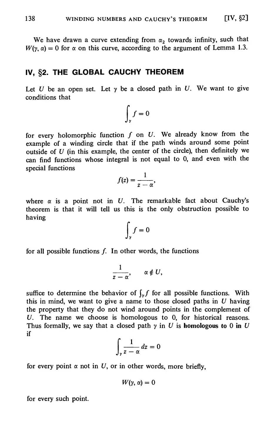
Year: 2002

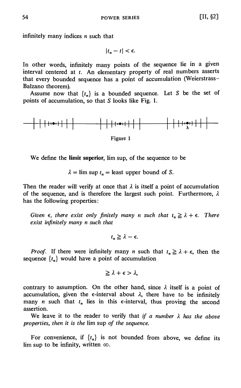
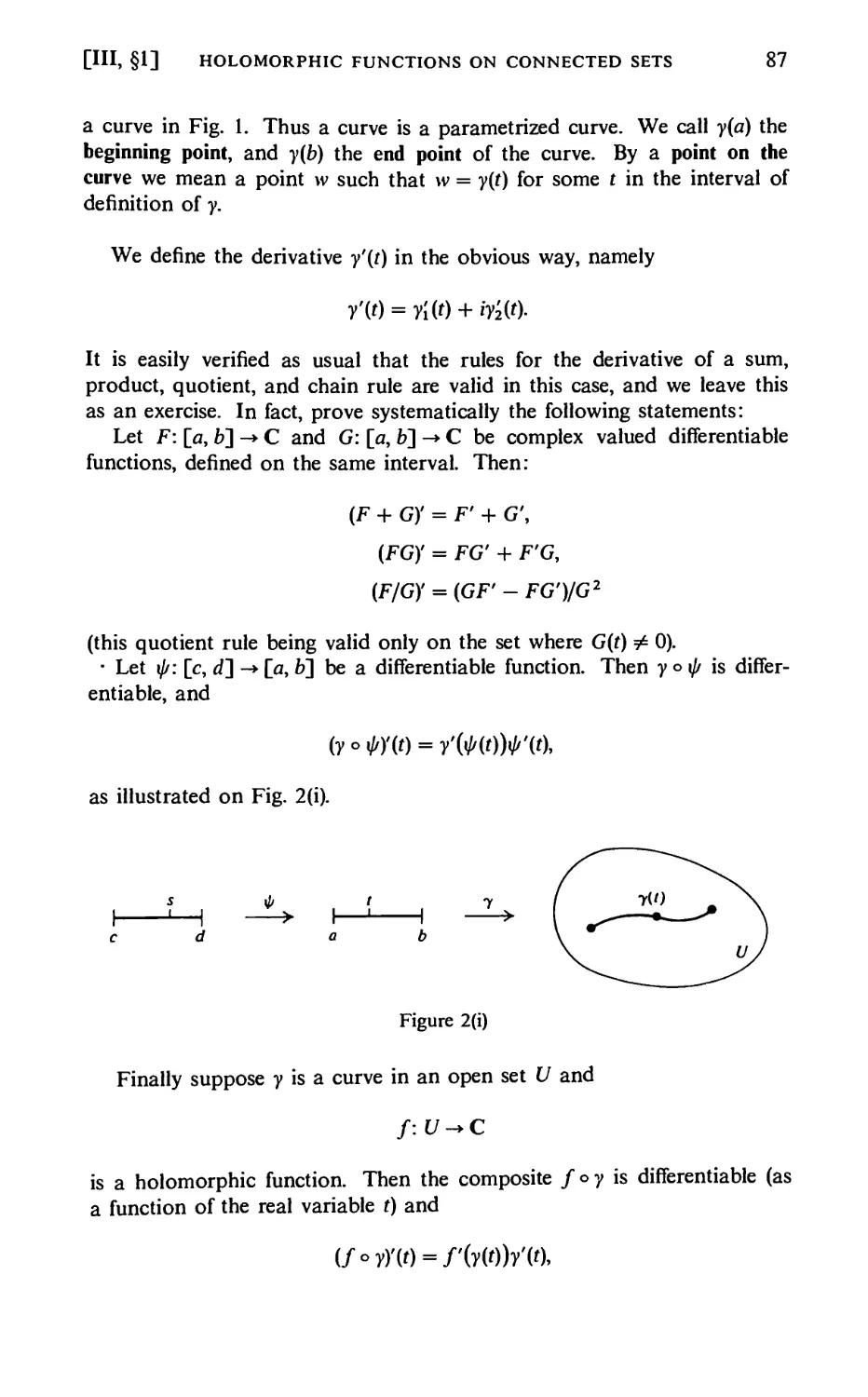
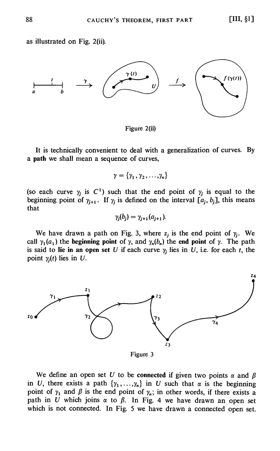
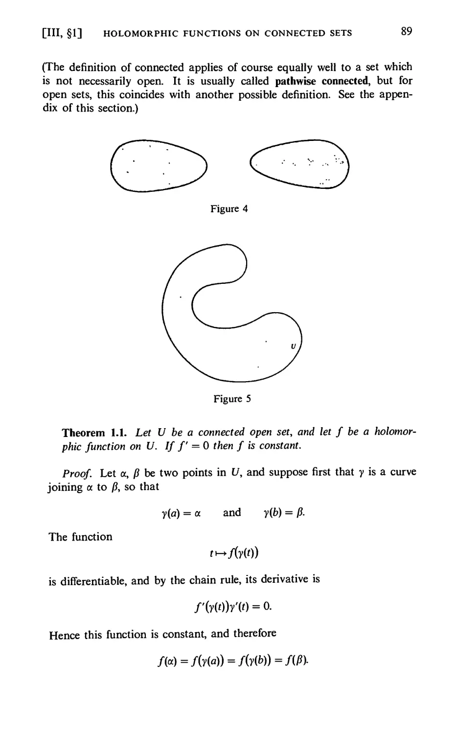
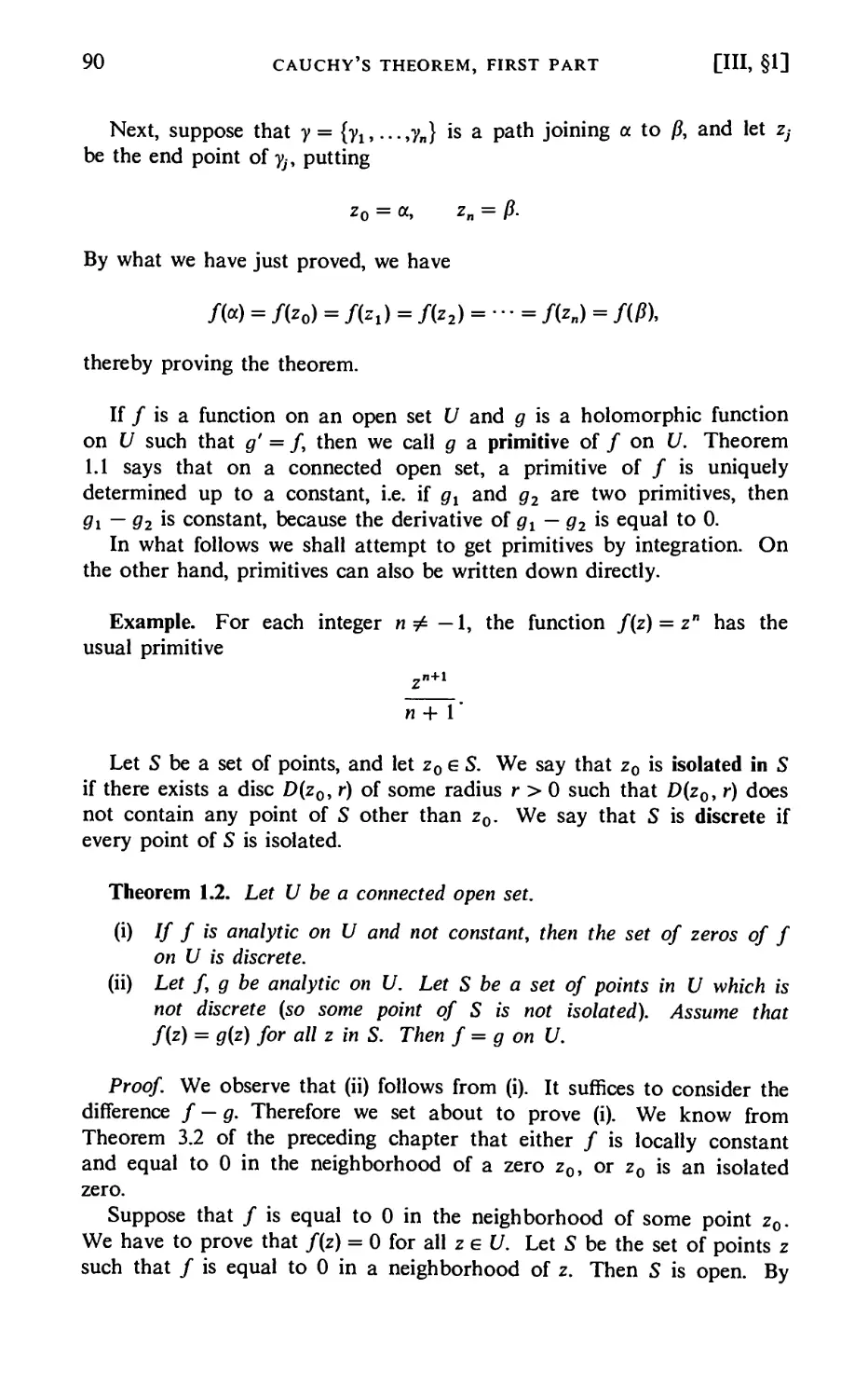
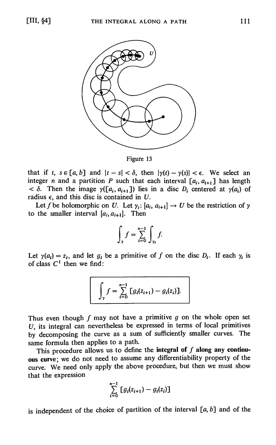
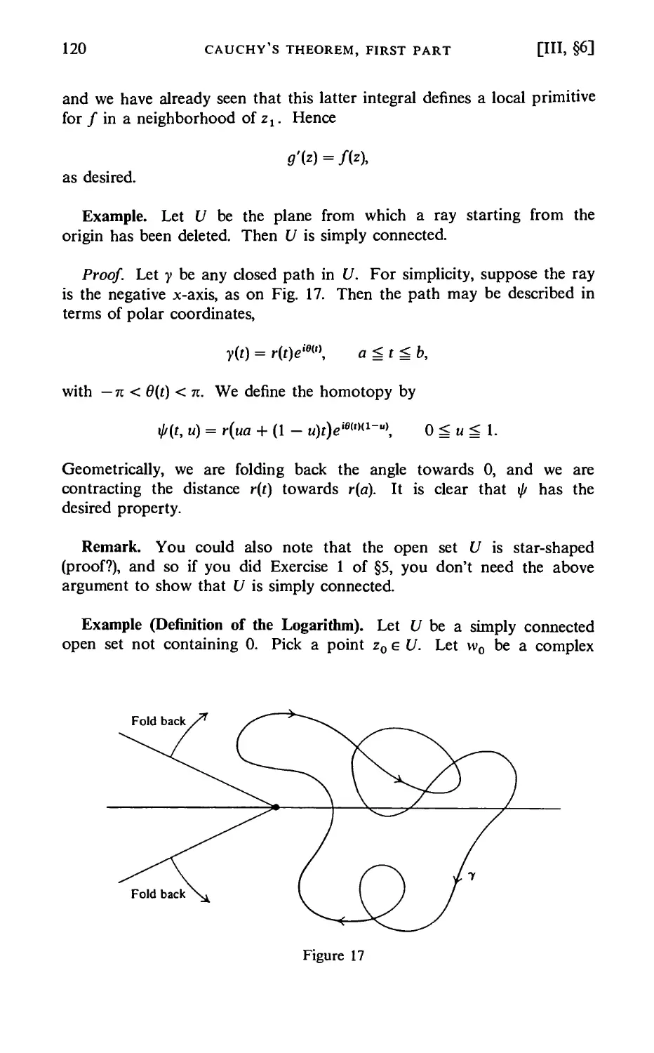
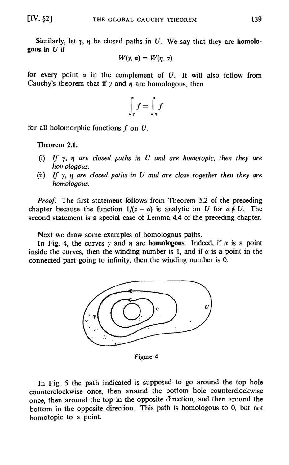
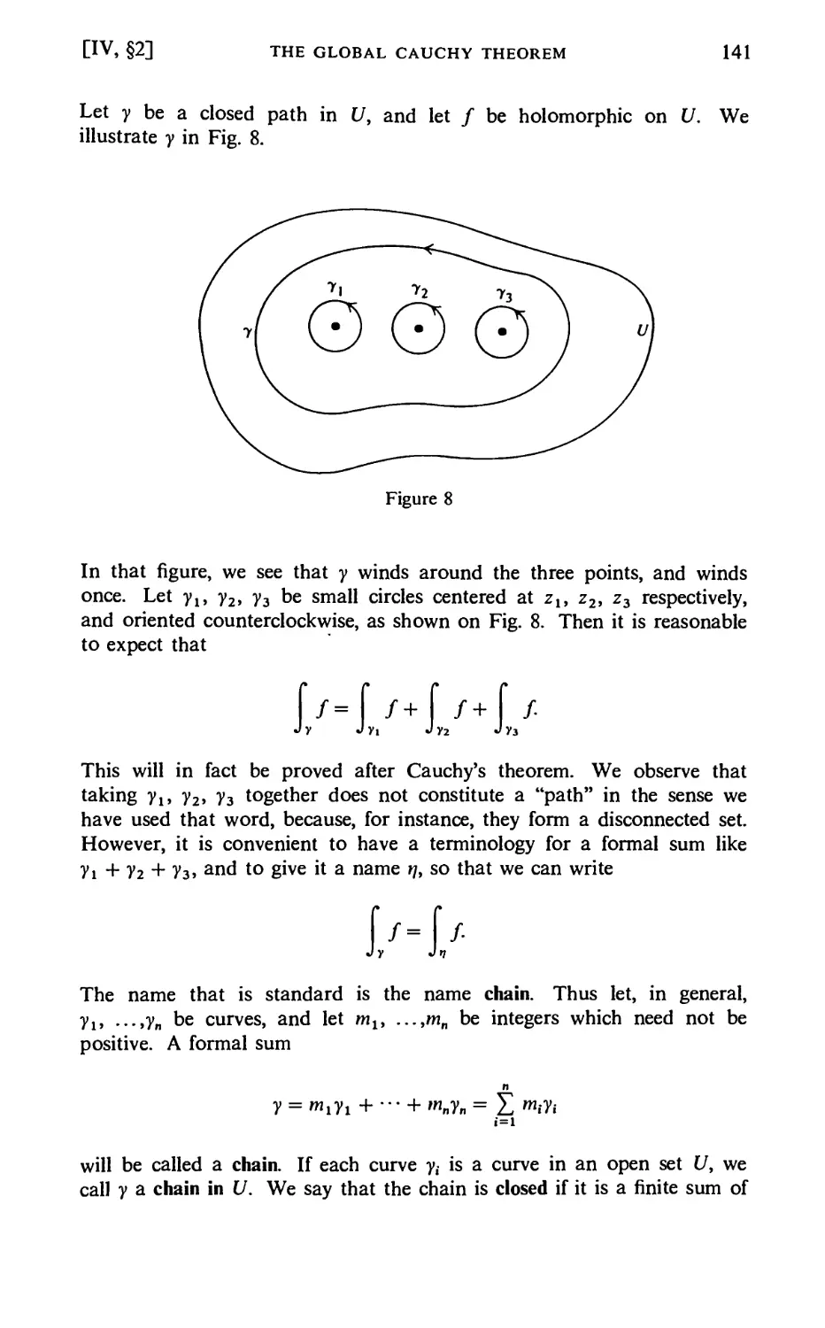
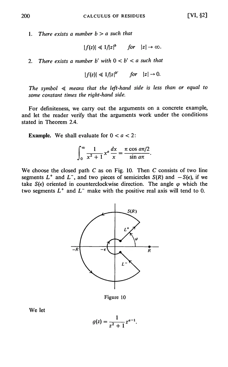
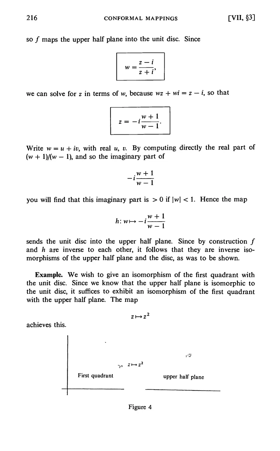
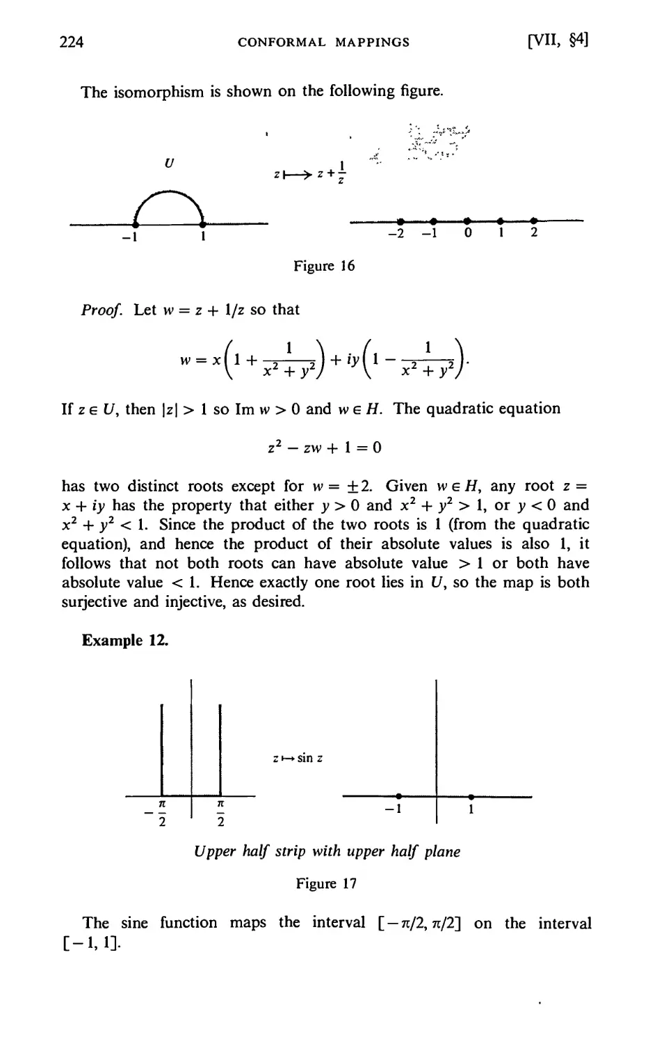
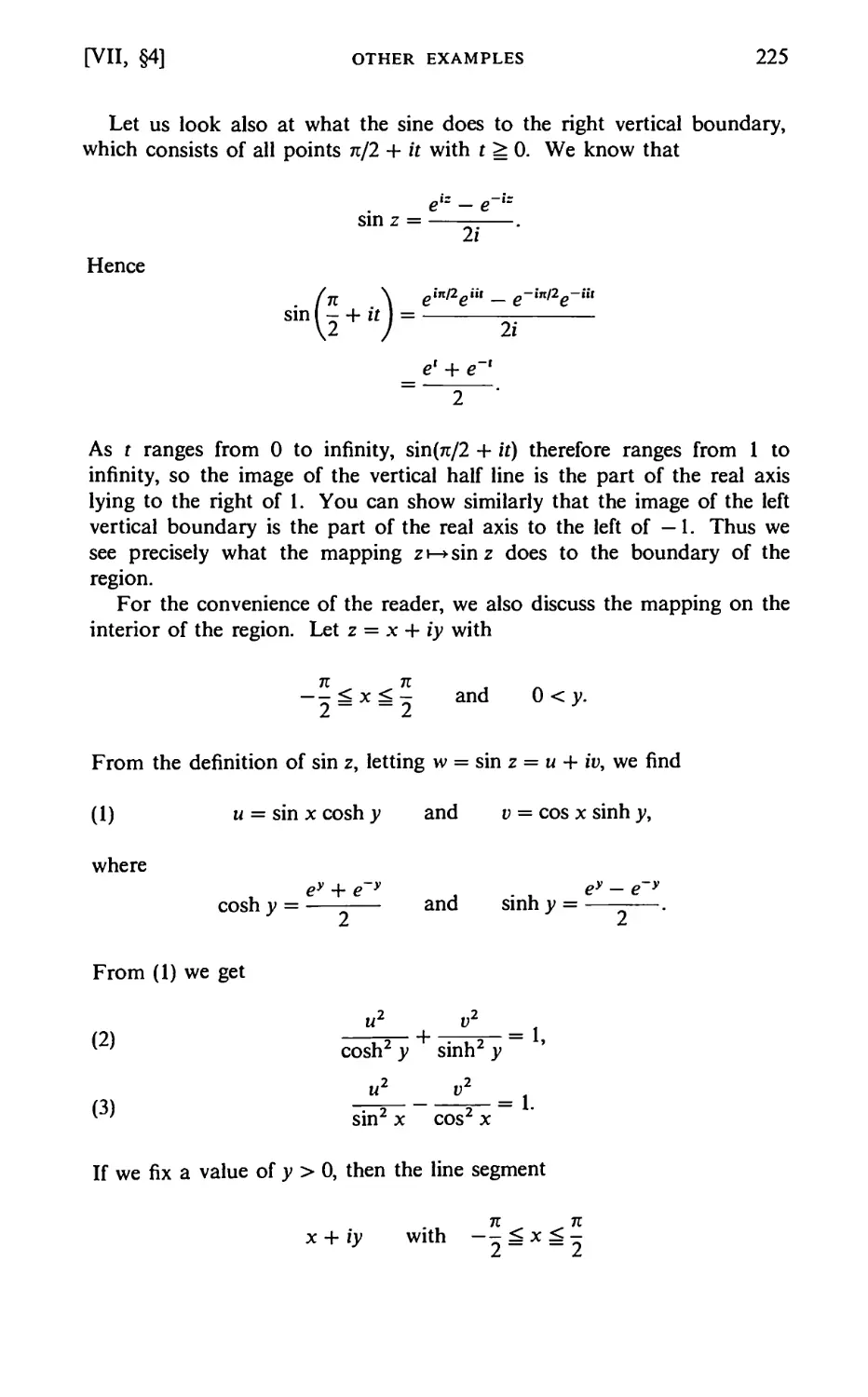
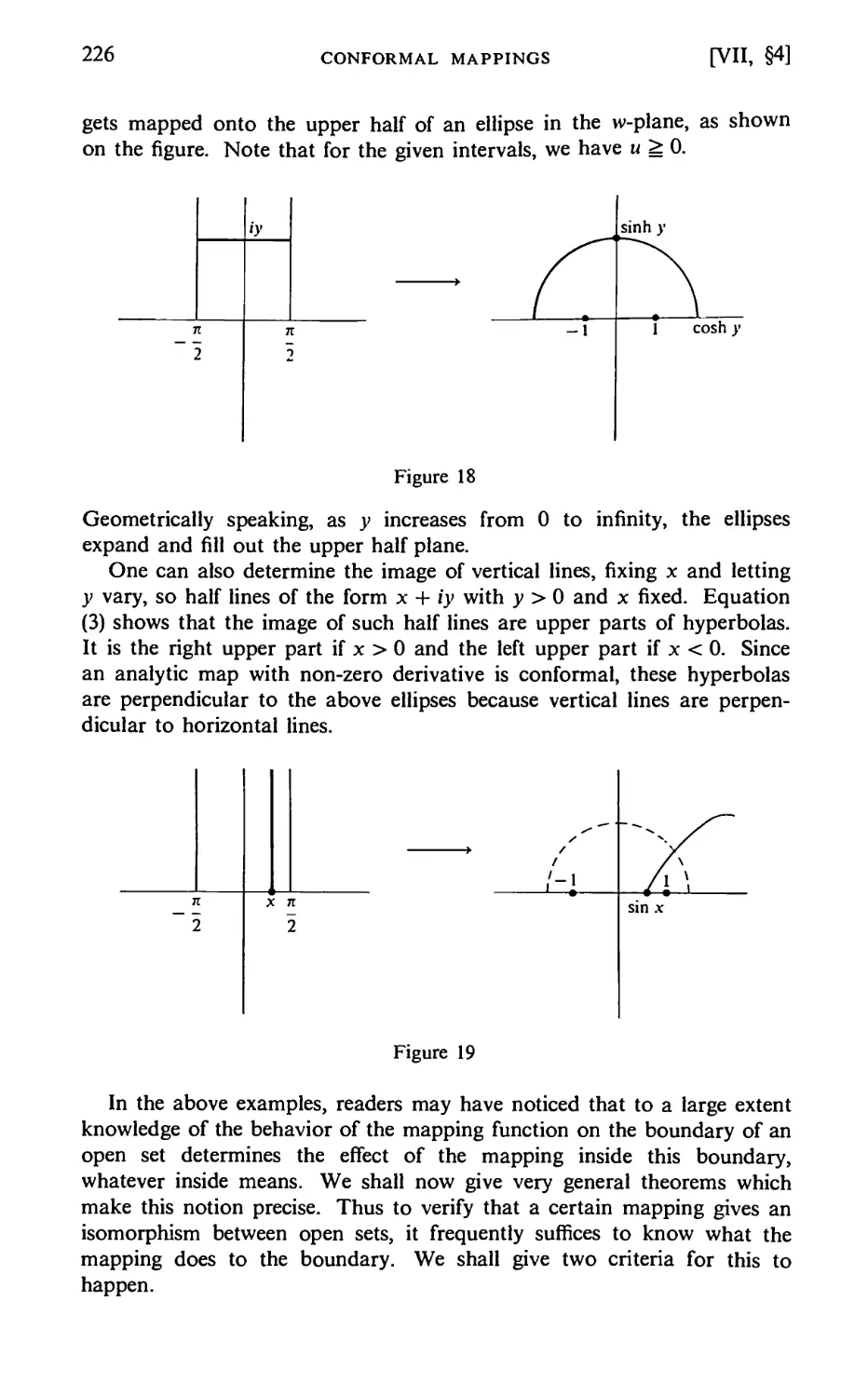
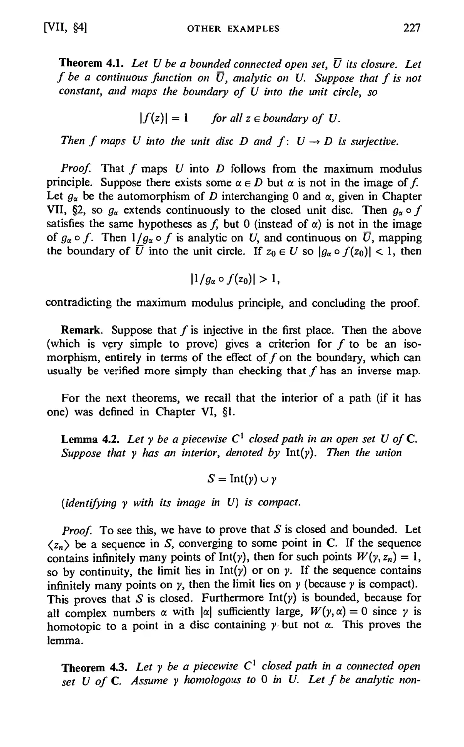
Text
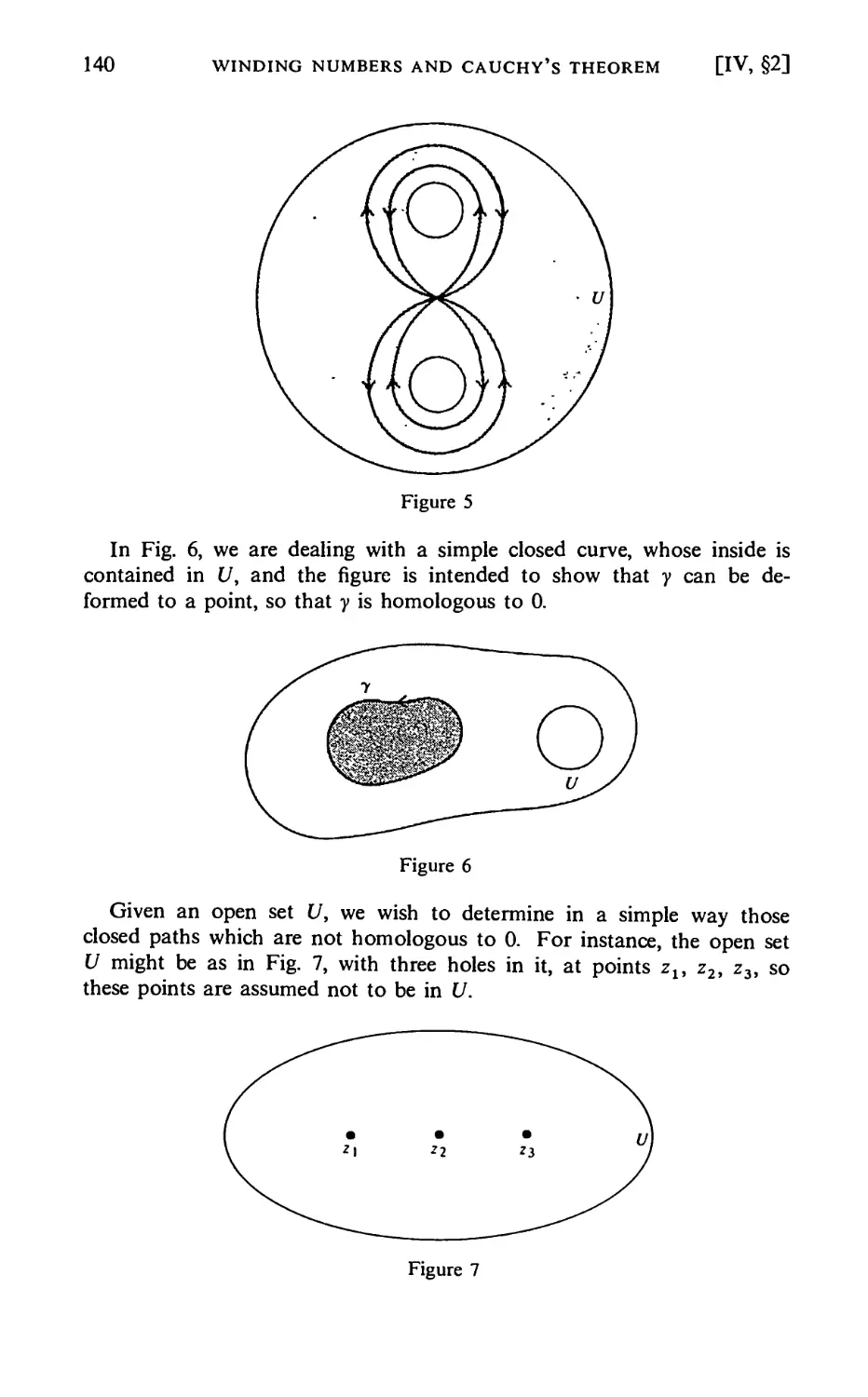
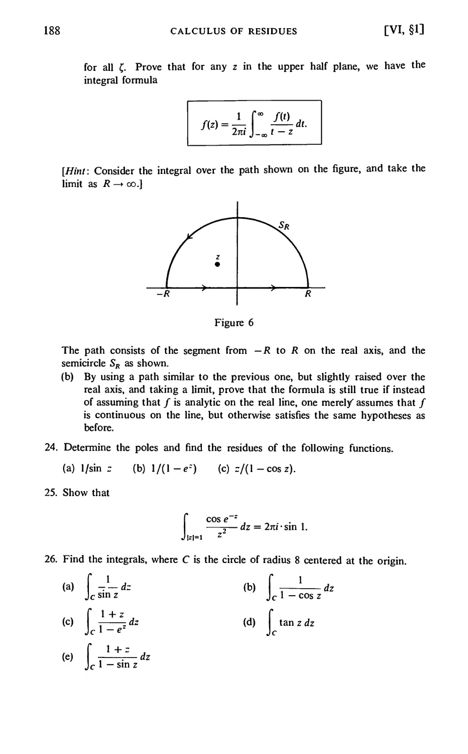
Serge Lang
Complex
Analysis
Fourth Edition
Springer
Graduate Texts in Mathematics
Editorial Board
S. Axler F.W. Gehring K.A. Ribet
Springer
Books of Related Interest by Serge Lang
Short Calculus
2002, ISBN 0-387-95327-2
Calculus of Several Variables, Third Edition
1987, ISBN 0-387-96405-3
Undergraduate Analysis, Second Edition
1996, ISBN 0-387-94841-4
Introduction to Linear Algebra
1997, ISBN 0-387-96205-0
Math Talks for Undergraduates
1999, ISBN 0-387-98749-5
Other Books by Lang Published by
Springer-Verlag
Math! Encounters with High School Students • The Beauty of Doing Mathematics
• Geometry: A High School Course • Basic Mathematics • Short Calculus • A First
Course in Calculus • Introduction to Linear Algebra • Calculus of Several
Variables • Linear Algebra • Undergraduate Analysis • Undergraduate Algebra •
Complex Analysis • Math Talks for Undergraduates • Algebra • Real and
Functional Analysis • Introduction to Differentiable Manifolds • Fundamentals of
Differential Geometry • Algebraic Number Theory • Cyclotomic Fields I and II •
Introduction to Diophantine Approximations • SL2(R) • Spherical Inversion on
SLn(R) (with Jay Jorgenson) • Elliptic Functions • Elliptic Curves: Diophantine
Analysis • Introduction to Arakelov Theory • Riemann-Roch Algebra (with
William Fulton) • Abelian Varieties • Introduction to Algebraic and Abelian
Functions • Complex Multiplication • Introduction to Modular Forms • Modular
Units (with Daniel Kubert) • Introduction to Complex Hyperbolic Spaces •
Number Theory III • Survey on Diophantine Geometry
Collected Papers I-V, including the following: Introduction to Transcendental
Numbers in volume I, Frobenius Distributions in GL2-Extensions (with Hale
Trotter in volume II, Topics in Cohomology of Groups in volume IV, Basic
Analysis of Regularized Series and Products (with Jay Jorgenson) in volume V
and Explicit Formulas for Regularized Products and Series (with Jay Jorgenson) in
volume V
THE FILE • CHALLENGES
Serge Lang
Complex Analysis
Fourth Edition
With 139 Illustrations
Springer
Serge Lang
Department of Mathematics
Yale University
New Haven, CT 06520
USA
Editorial Board
S. Axler F.W. Gehring K.A. Ribet
Mathematics Department Mathematics Department Mathematics Department
San Francisco State East Hall University of California at
University University of Michigan Berkeley
San Francisco, CA 94132 Ann Arbor, MI 48109 Berkeley, CA 94720-3840
USA USA USA
Mathematics Subject Classification (2000): 30-01
Library of Congress Cataloging-in-Publication Data
Lang, Serge, 1927-
Complex analysis I Serge Lang.—4th ed.
p. cm.—(Graduate texts in mathematics; 103)
Includes bibliographical references and index.
ISBN 0-387-98592-1 (alk. paper)
1. Functions of complex variables. 2. Mathematical analysis.
I. Title. II. Series
QA331.7.L36 1999
515'.9—dc21 98-29992
ISBN 0-387-98592-1
Printed on acid-free paper.
© 1999 Springer Science+Business Media, Inc.
All rights reserved. This work may not be translated or copied in whole or in part without the
written permission of the publisher (Springer Science+Business Media, Inc., 233 Spring Street,
New York, NY 10013, USA), except for brief excerpts in connection with reviews or scholarly
analysis. Use in connection with any form of information storage and retrieval, electronic
adaptation, computer software, or by similar or dissimilar methodology now know or hereafter
developed is forbidden.
The use in this publication of trade names, trademarks, service marks and similar terms, even
if the are not identified as such, is not to be taken as an expression of opinion as to whether or
not they are subject to proprietary rights.
Printed in the United States of America by Sheridan Books.
9 8 7 6 5
springeronline.com
Foreword
The present book is meant as a text for a course on complex analysis at
the advanced undergraduate level, or first-year graduate level. The first
half, more or less, can be used for a one-semester course addressed to
undergraduates. The second half can be used for a second semester, at
either level. Somewhat more material has been included than can be
covered at leisure in one or two terms, to give opportunities for the
instructor to exercise individual taste, and to lead the course in whatever
directions strikes the instructor's fancy at the time as well as extra
reading material for students on their own. A large number of routine
exercises are included for the more standard portions, and a few harder
exercises of striking theoretical interest are also included, but may be
omitted in courses addressed to less advanced students.
In some sense, I think the classical German prewar texts were the
best (Hurwitz-Courant, Knopp, Bieberbach, etc.) and I would recommend
to anyone to look through them. More recent texts have emphasized
connections with real analysis, which is important, but at the cost of
exhibiting succinctly and clearly what is peculiar about complex analysis:
the power series expansion, the uniqueness of analytic continuation, and
the calculus of residues. The systematic elementary development of
formal and convergent power series was standard fare in the German texts,
but only Cartan, in the more recent books, includes this material, which
I think is quite essential, e.g., for differential equations. I have written a
short text, exhibiting these features, making it applicable to a wide
variety of tastes.
The book essentially decomposes into two parts.
The first part, Chapters I through VIII, includes the basic properties
of analytic functions, essentially what cannot be left out of, say, a one-
semester course.
v
Vi FOREWORD
I have no fixed idea about the manner in which Cauchy's theorem is
to be treated. In less advanced classes, or if time is lacking, the usual
hand waving about simple closed curves and interiors is not entirely
inappropriate. Perhaps better would be to state precisely the homologi-
cal version and omit the formal proof. For those who want a more
thorough understanding, I include the relevant material.
Artin originally had the idea of basing the homology needed for
complex variables on the winding number. I have included his proof for
Cauchy's theorem, extracting, however, a purely topological lemma of
independent interest, not made explicit in Artin's original Notre Dame
notes [Ar 65] or in Ahlfors' book closely following Artin [Ah 66]. I
have also included the more recent proof by Dixon, which uses the
winding number, but replaces the topological lemma by greater use of
elementary properties of analytic functions which can be derived directly
from the local theorem. The two aspects, homotopy and homology, both
enter in an essential fashion for different applications of analytic
functions, and neither is slighted at the expense of the other.
Most expositions usually include some of the global geometric
properties of analytic maps at an early stage. I chose to make the preliminaries
on complex functions as short as possible to get quickly into the analytic
part of complex function theory: power series expansions and Cauchy's
theorem. The advantages of doing this, reaching the heart of the subject
rapidly, are obvious. The cost is that certain elementary global geometric
considerations are thus omitted from Chapter I, for instance, to reappear
later in connection with analytic isomorphisms (Conformal Mappings,
Chapter VII) and potential theory (Harmonic Functions, Chapter VIII).
I think it is best for the coherence of the book to have covered in one
sweep the basic analytic material before dealing with these more
geometric global topics. Since the proof of the general Riemann mapping
theorem is somewhat more difficult than the study of the specific cases
considered in Chapter VII, it has been postponed to the second part.
The second and third parts of the book, Chapters IX through XVI,
deal with further assorted analytic aspects of functions in many
directions, which may lead to many other branches of analysis. I have
emphasized the possibility of defining analytic functions by an integral
involving a parameter and differentiating under the integral sign. Some
classical functions are given to work out as exercises, but the gamma
function is worked out in detail in the text, as a prototype.
The chapters in Part II allow considerable flexibility in the order they
are covered. For instance, the chapter on analytic continuation, including
the Schwarz reflection principle, and/or the proof of the Riemann
mapping theorem could be done right after Chapter VII, and still achieve
great coherence.
As most of this part is somewhat harder than the first part, it can easily
be omitted from a one-term course addressed to undergraduates. In the
FOREWORD Vii
same spirit, some of the harder exercises in the first part have been
starred, to make their omission easy.
Comments on the Third and Fourth Editions
I have rewritten some sections and have added a number of exercises. I
have added some material on harmonic functions and conformal maps, on
the Borel theorem and Borel's proof of Picard's theorem, as well as D.J.
Newman's short proof of the prime number theorem, which illustrates
many aspects of complex analysis in a classical setting. I have made more
complete the treatment of the gamma and zeta functions. I have also
added an Appendix which covers some topics which I find sufficiently
important to have in the book. The first part of the Appendix recalls
summation by parts and its application to uniform convergence. The
others cover material which is not usually included in standard texts on
complex analysis: difference equations, analytic differential equations, fixed
points of fractional linear maps (of importance in dynamical systems),
Cauchy's formula for C00 functions, and Cauchy's theorem for locally
integrable vector fields in the plane. This material gives additional insight
on techniques and results applied to more standard topics in the text.
Some of them may have been assigned as exercises, and I hope students
will try to prove them before looking up the proofs in the Appendix.
I am very grateful to several people for pointing out the need for a
number of corrections, especially Keith Conrad, Wolfgang Fluch, Alberto
Grunbaum, Bert Hochwald, Michal Jastrzebski, Jose Carlos Santos, Ernest
C. Schlesinger, A. Vijayakumar, Barnet Weinstock, and Sandy Zabell.
Finally, I thank Rami Shakarchi for working out an answer book.
New Haven 1998
Serge Lang
Prerequisites
We assume that the reader has had two years of calculus, and Has some
acquaintance with epsilon-delta techniques. For convenience, we have
recalled all the necessary lemmas we need for continuous functions on
compact sets in the plane. Section §1 in the Appendix also provides
some background.
We use what is now standard terminology. A function
f:S-+T
is called injective if x ^ y in S implies f(x) ^ f{y). It is called surjective if
for every z in T there exists xe S such that f{x) = z. If f is surjective,
then we also say that f maps S onto T. If f is both injective and
surjective then we say that f is bijective.
Given two functions f, g defined on a set of real numbers containing
arbitrarily large numbers, and such that g(x) ^ 0, we write
f <£ g or f(x) < g(x) for x -+ oo
to mean that there exists a number C > 0 such that for all x sufficiently
large, we have
l/MI ^ Cg(x).
Similarly, if the functions are defined for x near 0, we use the same
symbol < for x -»0 to mean that there exists C > 0 such that
|/(x)| ^ Cg(x)
ix
X PREREQUISITES
for all x sufficiently small (there exists 5 > 0 such that if \x\ < S then
l/MI = Cg(x)). Often this relation is also expressed by writing
fix) = 0(g(x)),
which is read: f{x) is big oh of g{x), for x -> oo or x -> 0 as the case
may be.
We use ]a, b[ to denote the open interval of numbers
a < x < b.
Similarly, [a, b\_ denotes the half-open interval, etc.
Contents
Foreword v
Prerequisites ix
PART ONE
Basic Theory 1
CHAPTER I
Complex Numbers and Functions 3
§1. Definition 3
§2. Polar Form 8
§3. Complex Valued Functions 12
§4. Limits and Compact Sets 17
Compact Sets 21
§5. Complex Differentiability 27
§6. The Cauchy-Riemann Equations 31
§7. Angles Under Holomorphic Maps 33
CHAPTER II
Power Series 37
§1. Formal Power Series 37
§2. Convergent Power Series 47
§3. Relations Between Formal and Convergent Series 60
Sums and Products 60
Quotients 64
Composition of Series 66
§4. Analytic Functions 68
§5. Differentiation of Power Series 72
xi
Xli CONTENTS
§6. The Inverse and Open Mapping Theorems 76
§7. The Local Maximum Modulus Principle 83
CHAPTER III
Cauchy's Theorem, First Part 86
§1. Holomorphic Functions on Connected Sets 86
Appendix: Connectedness 92
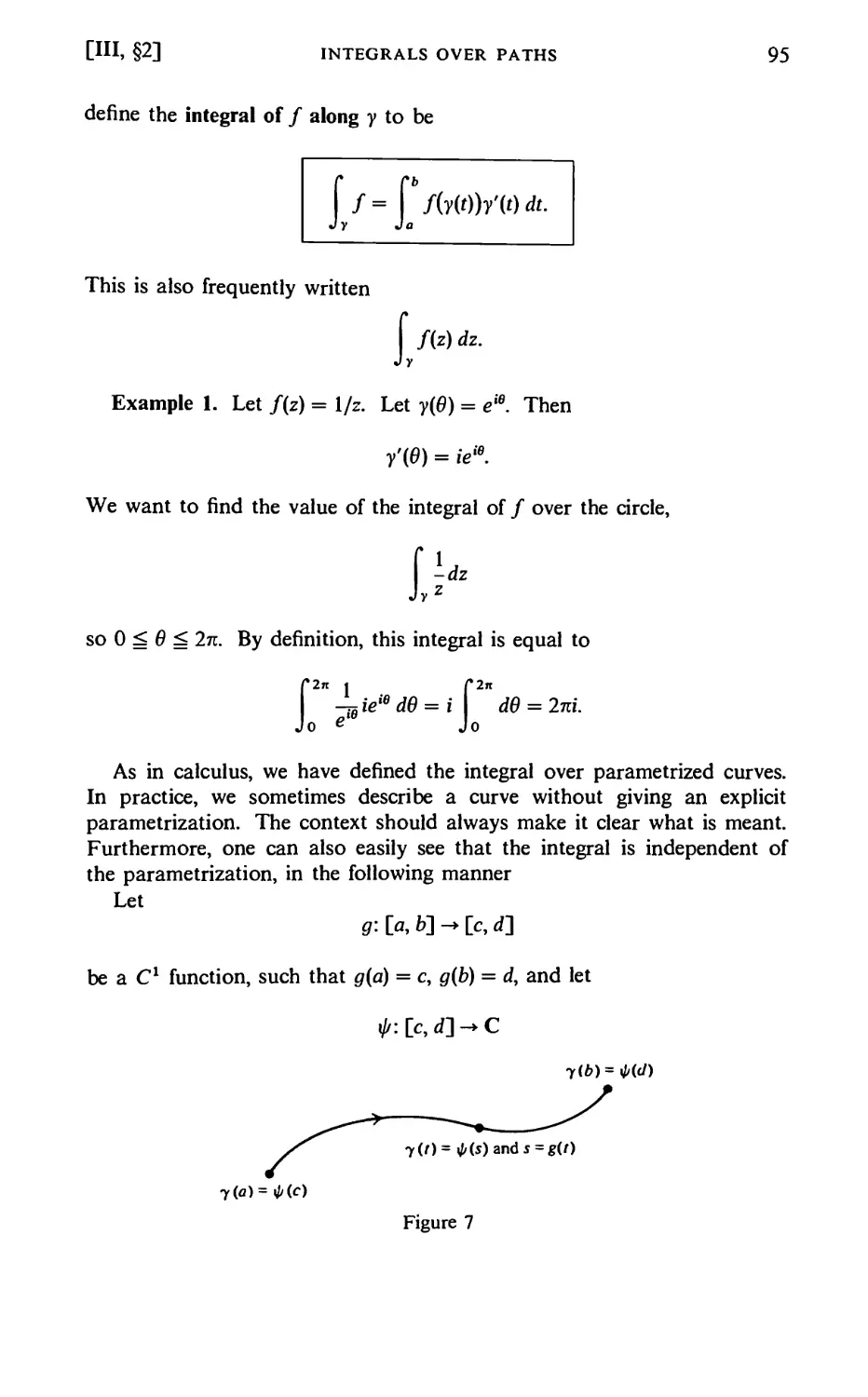
§2. Integrals Over Paths 94
§3. Local Primitive for a Holomorphic Function 104
§4. Another Description of the Integral Along a Path HO
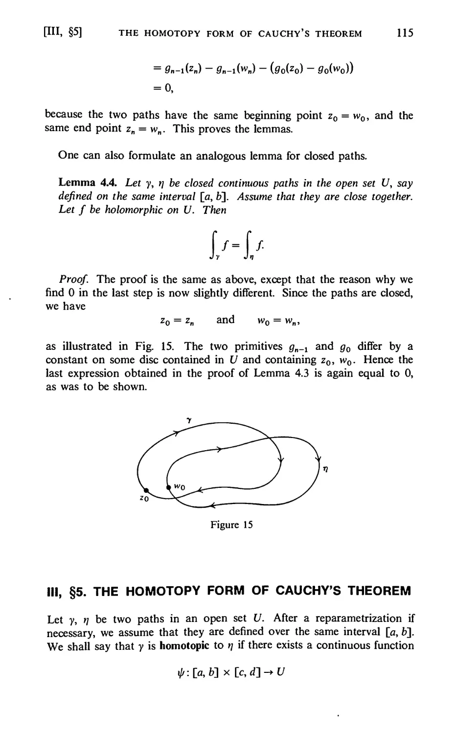
§5. The Homotopy Form of Cauchy's Theorem 115
§6. Existence of Global Primitives. Definition of the Logarithm 119
§7. The Local Cauchy Formula 125
CHAPTER IV
Winding Numbers and Cauchy's Theorem 133
§1. The Winding Number 134
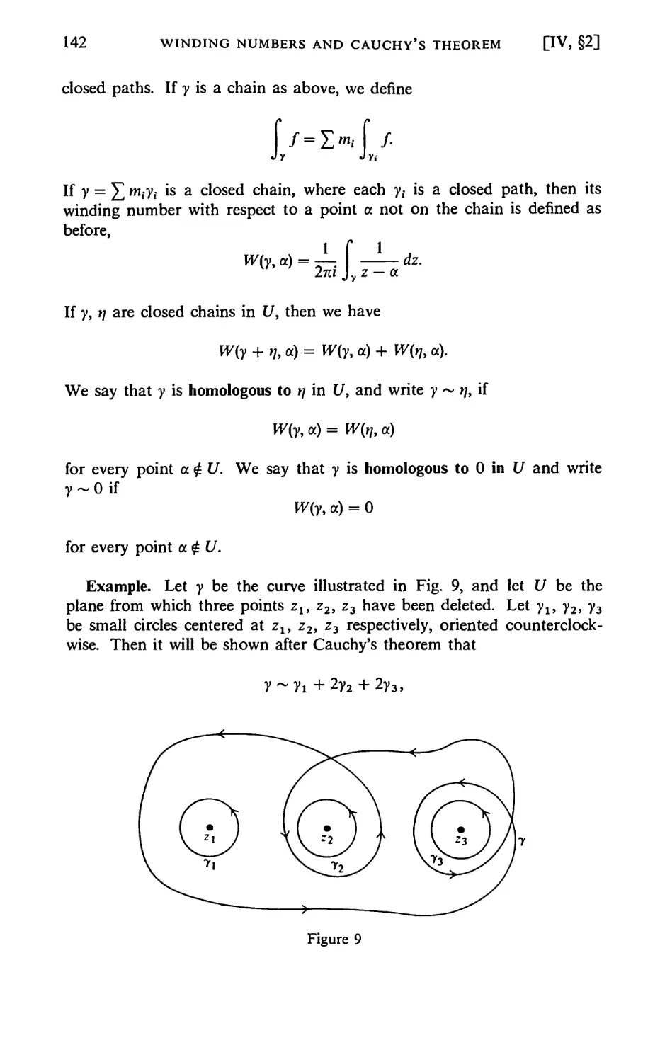
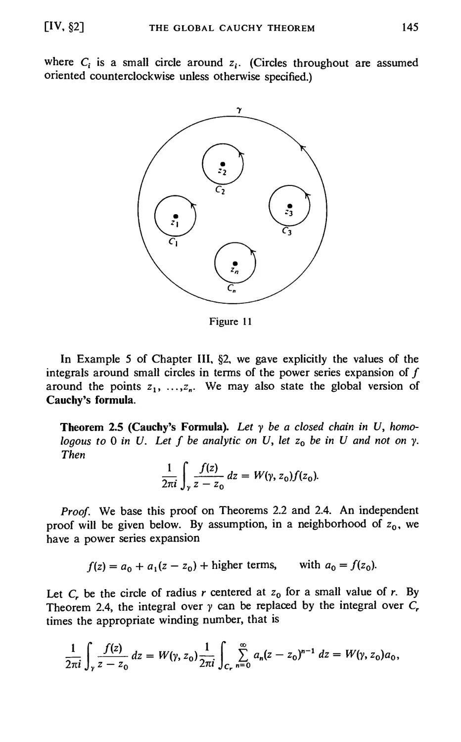
§2. The Global Cauchy Theorem 138
Dixon's Proof of Theorem 2.5 (Cauchy's Formula) 147
§3. Artin's Proof 149
CHAPTER V
Applications of Cauchy's Integral Formula 156
§1. Uniform Limits of Analytic Functions 156
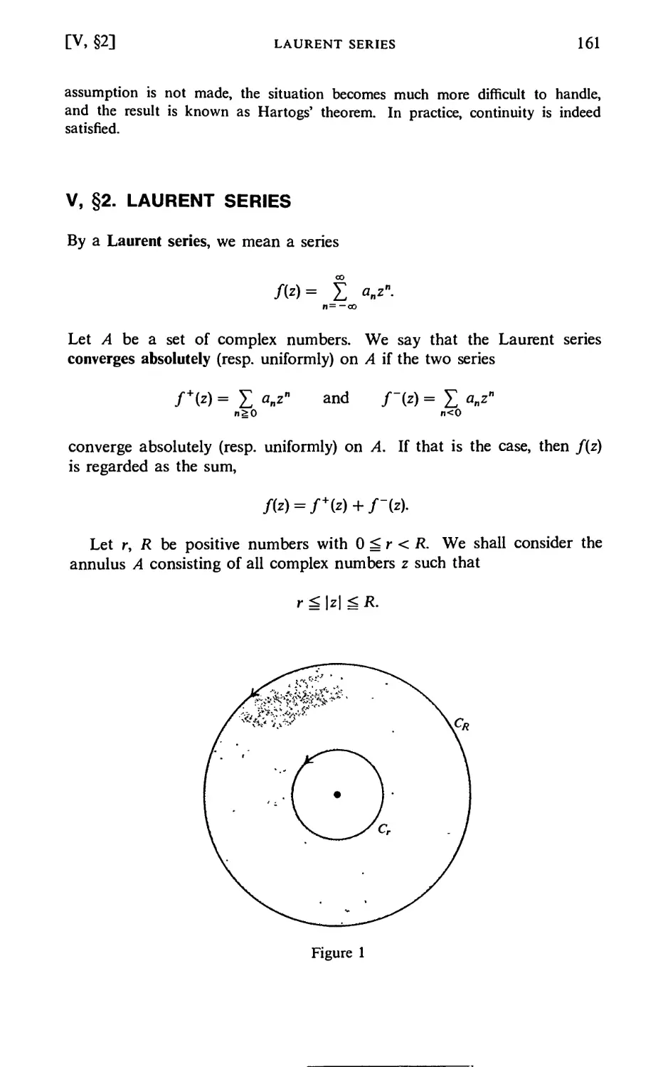
§2. Laurent Series 161
§3. Isolated Singularities 165
Removable Singularities 165
Poles 166
Essential Singularities 168
CHAPTER VI
Calculus of Residues 173
§1. The Residue Formula 173
Residues of Differentials 184
§2. Evaluation of Definite Integrals 191
Fourier Transforms 194
Trigonometric Integrals 197
Mellin Transforms 199
CHAPTER VII
Conformal Mappings 208
§1. Schwarz Lemma 210
§2. Analytic Automorphisms of the Disc 212
§3. The Upper Half Plane 215
§4. Other Examples 220
§5. Fractional Linear Transformations 231
CONTENTS Xlii
CHAPTER VIII
Harmonic Functions 241
§1. Definition 241
Application: Perpendicularity 246
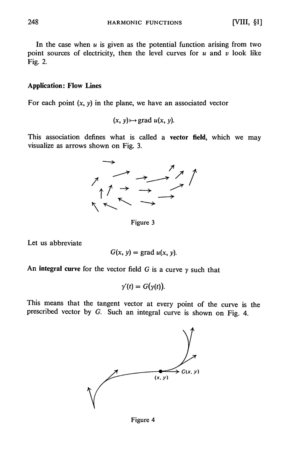
Application: Flow Lines 248
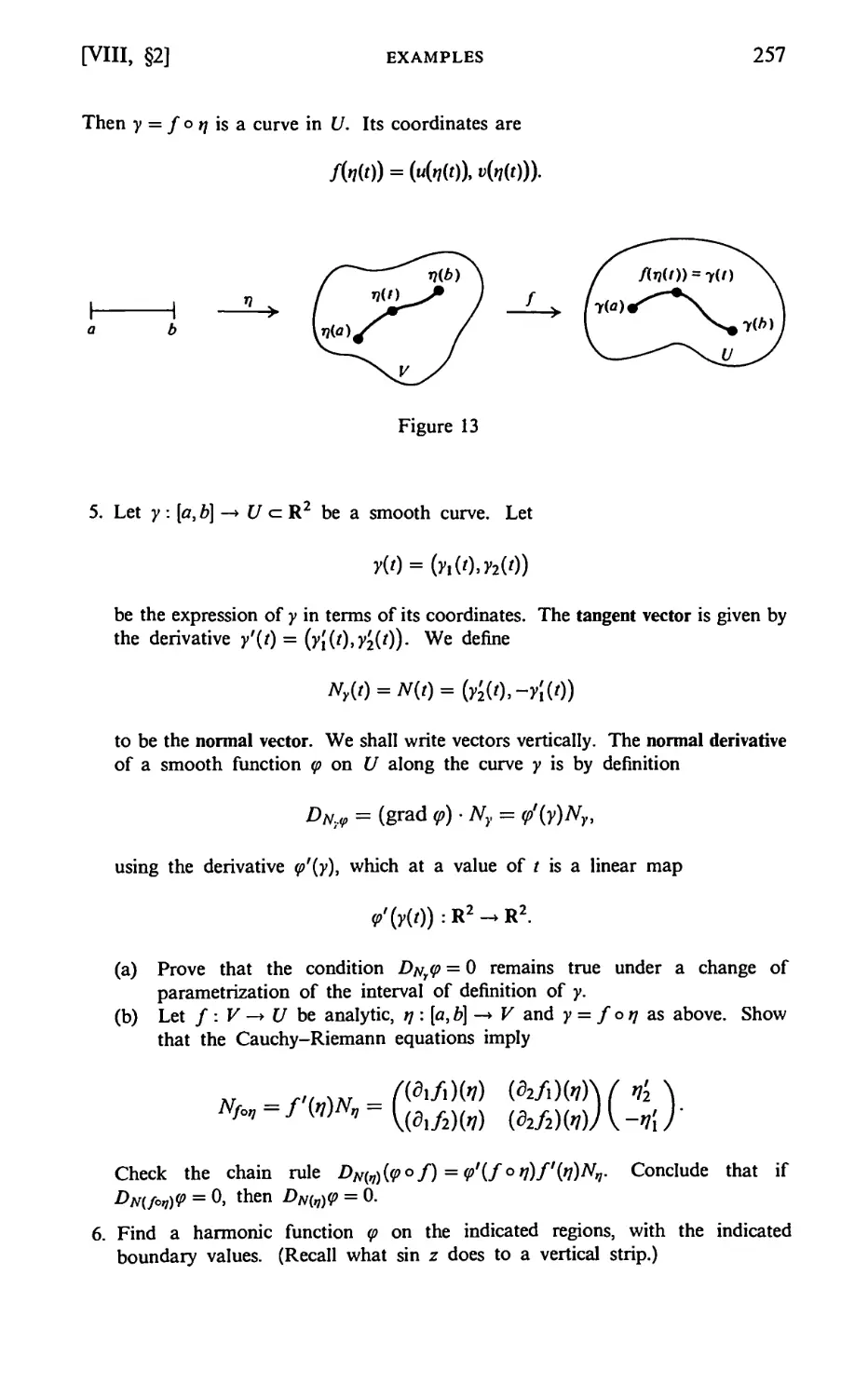
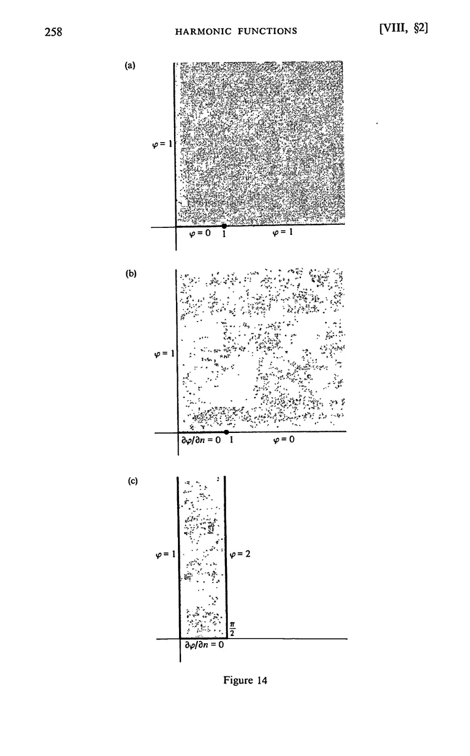
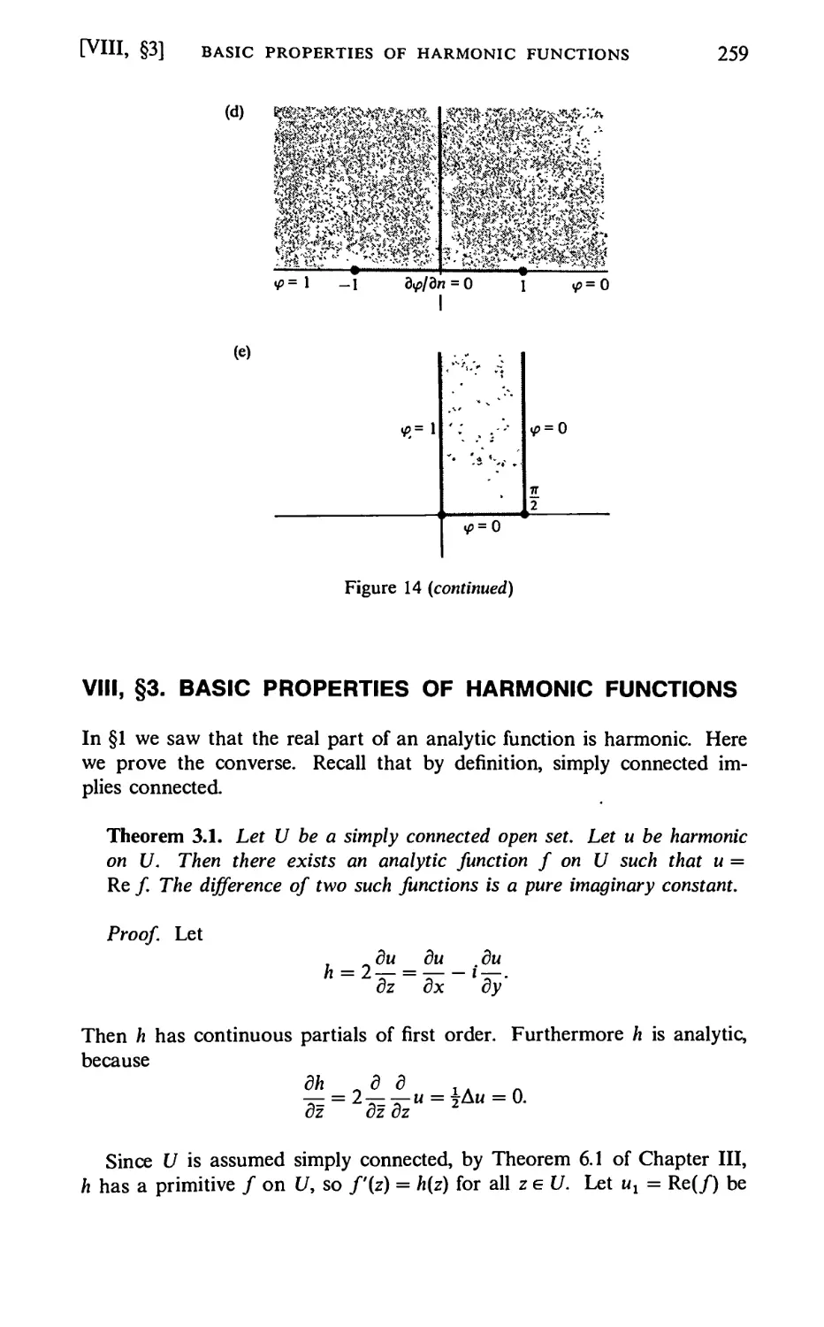
§2. Examples 252
§3. Basic Properties of Harmonic Functions 259
§4. The Poisson Formula 271
The Poisson Integral as a Convolution 273
§5. Construction of Harmonic Functions 276
§6. Appendix. Differentiating Under the Integral Sign 286
PART TWO
Geometric Function Theory 291
CHAPTER IX
Schwarz Reflection 293
§1. Schwarz Reflection (by Complex Conjugation) 293
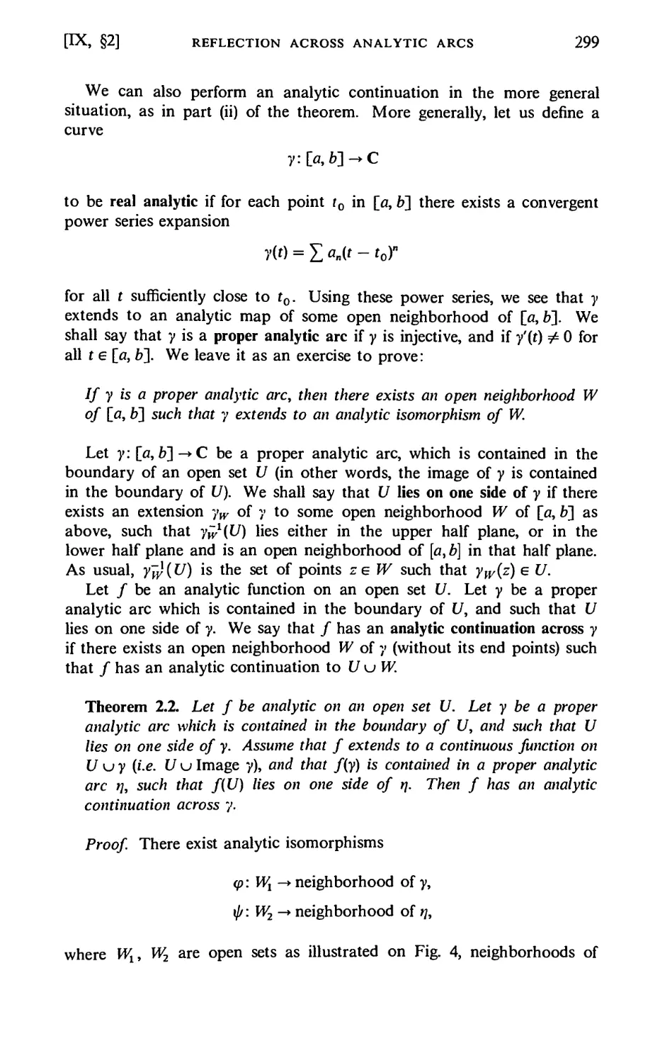
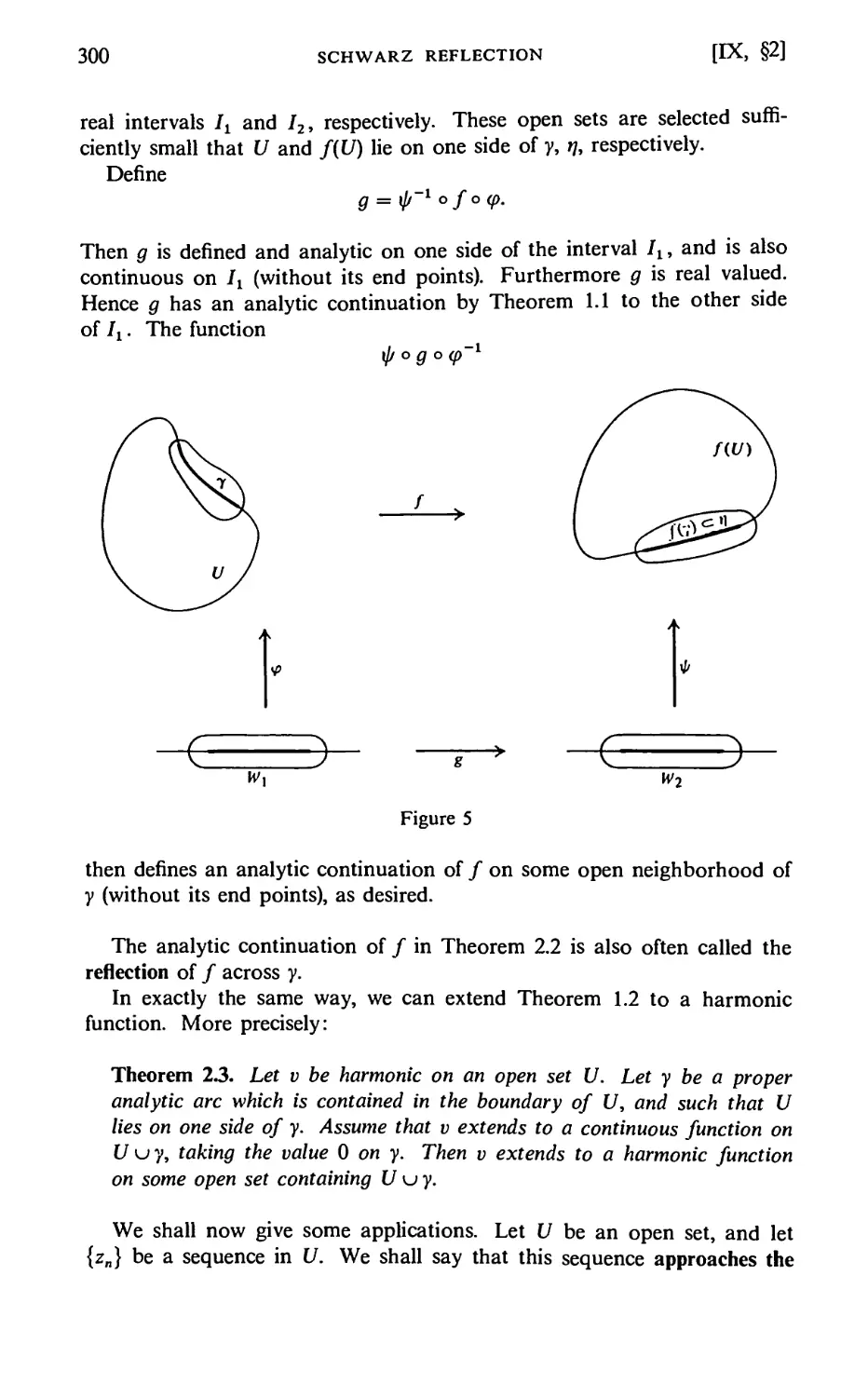
§2. Reflection Across Analytic Arcs 297
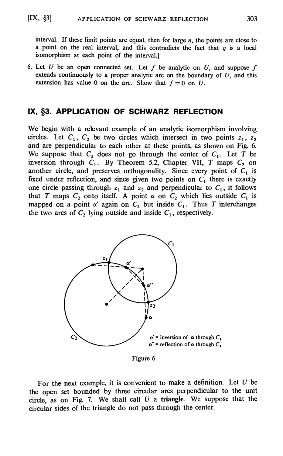
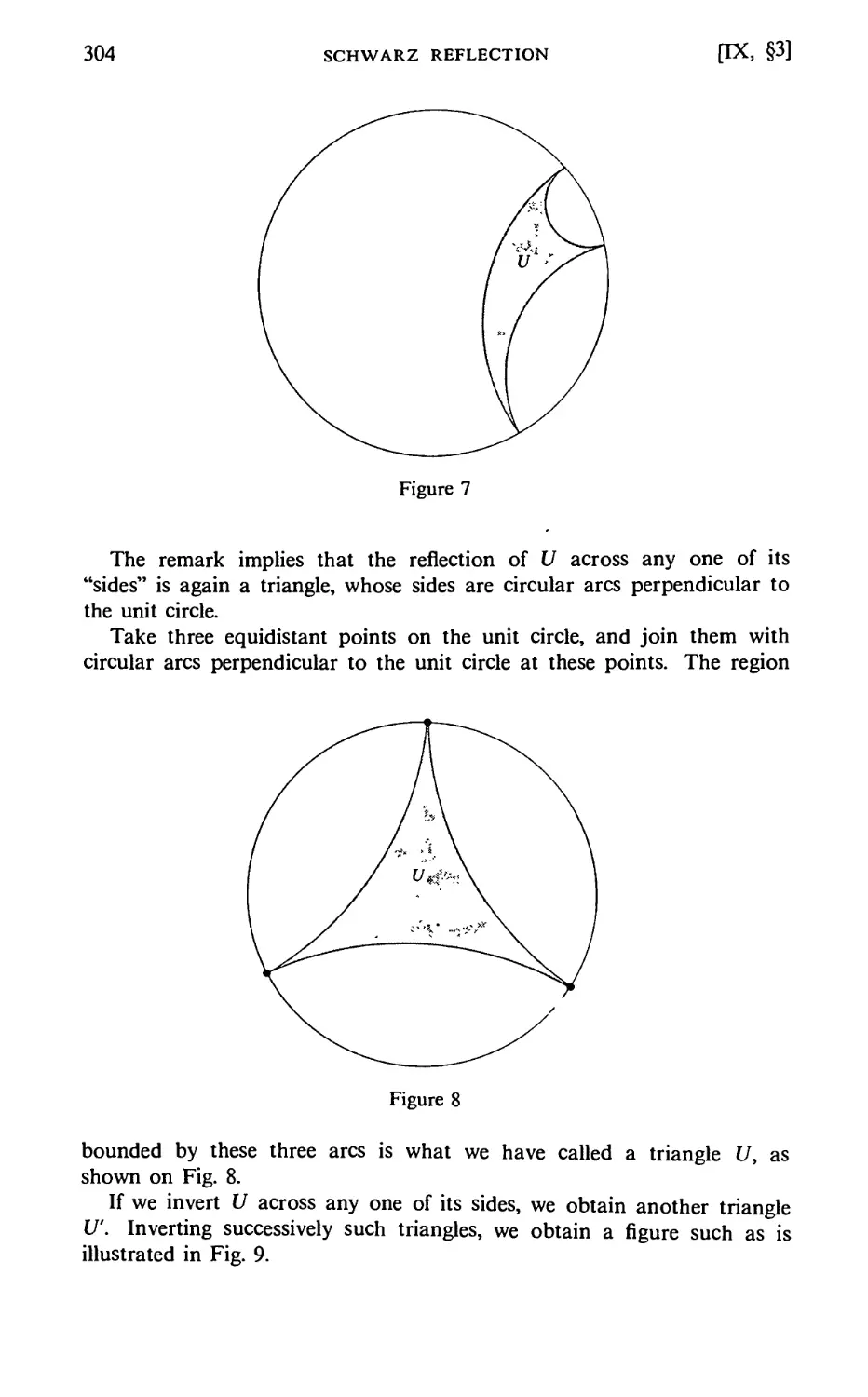
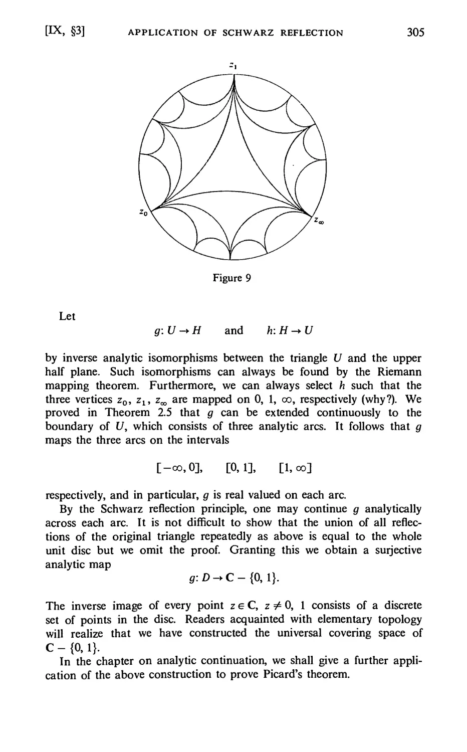
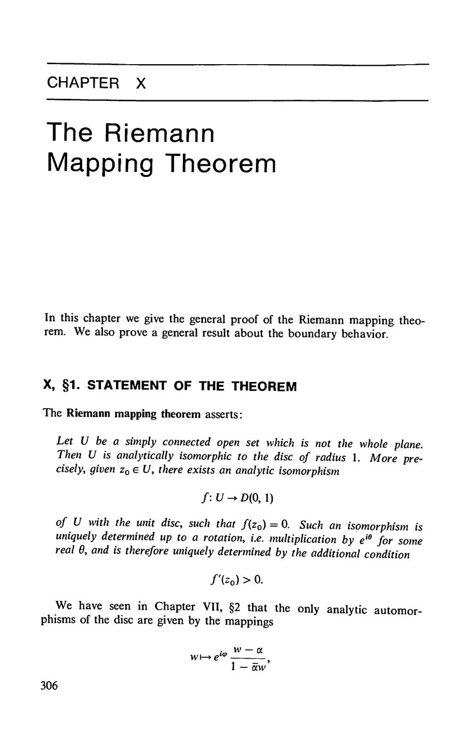
§3. Application of Schwarz Reflection 303
CHAPTER X
The Riemann Mapping Theorem 306
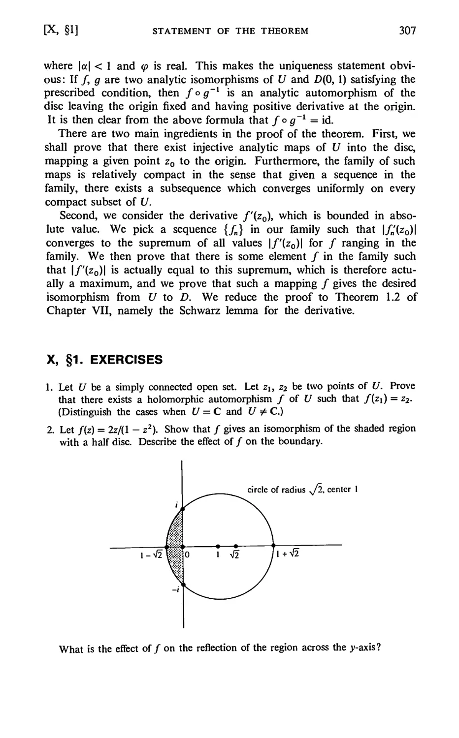
§1. Statement of the Theorem 306
§2. Compact Sets in Function Spaces 308
§3. Proof of the Riemann Mapping Theorem 311
§4. Behavior at the Boundary 314
CHAPTER XI
Analytic Continuation Along Curves 322
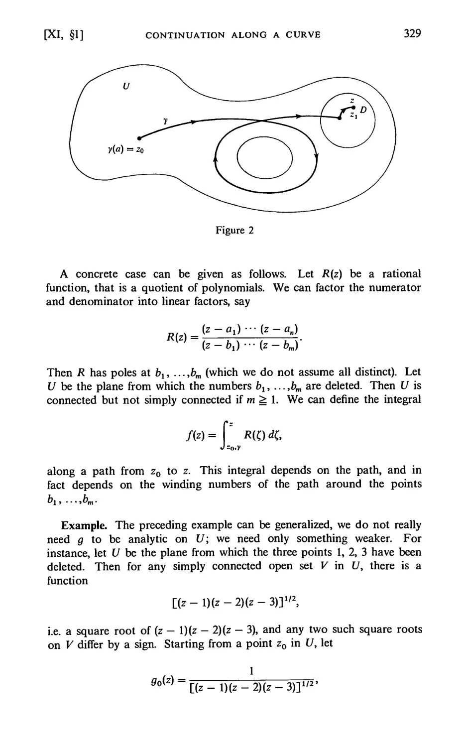
§1. Continuation Along a Curve 322
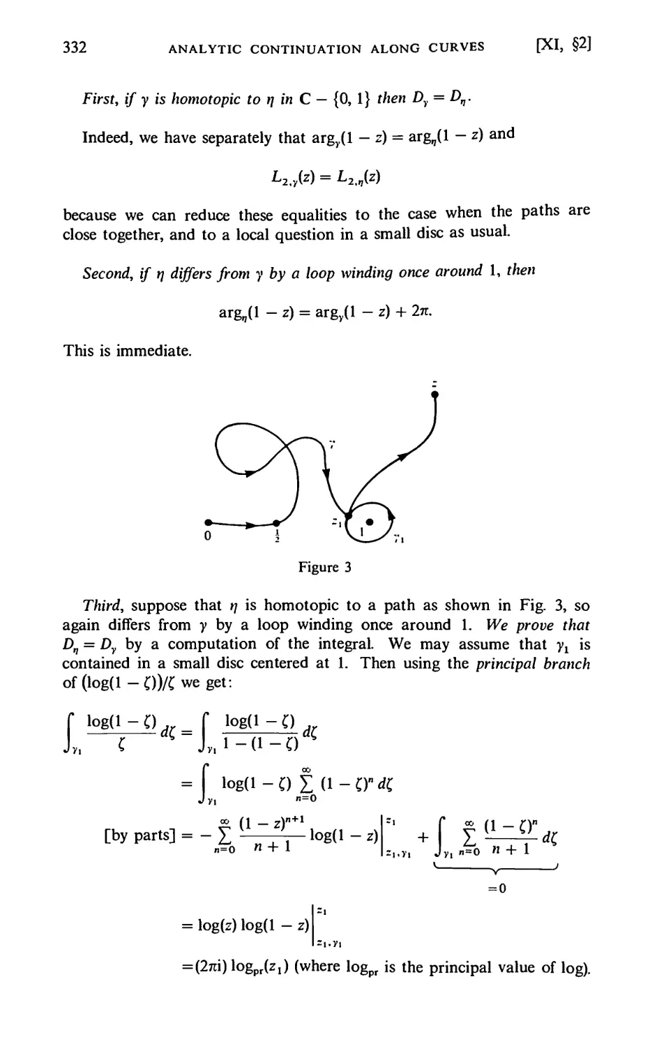
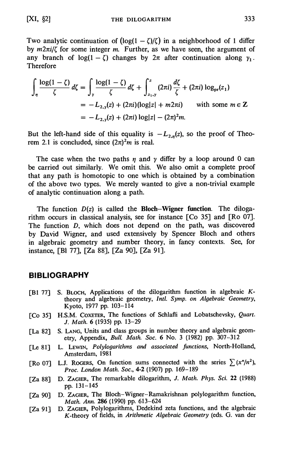
§2. The Dilogarithm 331
§3. Application to Picard's Theorem 335
PART THREE
Various Analytic Topics 337
CHAPTER XII
Applications of the Maximum Modulus Principle and Jensen's Formula 339
§1. Jensen's Formula 340
§2. The Picard-Borel Theorem 346
§3. Bounds by the Real Part, Borel-Caratheodory Theorem 354
§4. The Use of Three Circles and the Effect of Small Derivatives 356
Hermite Interpolation Formula 358
§5. Entire Functions with Rational Values 360
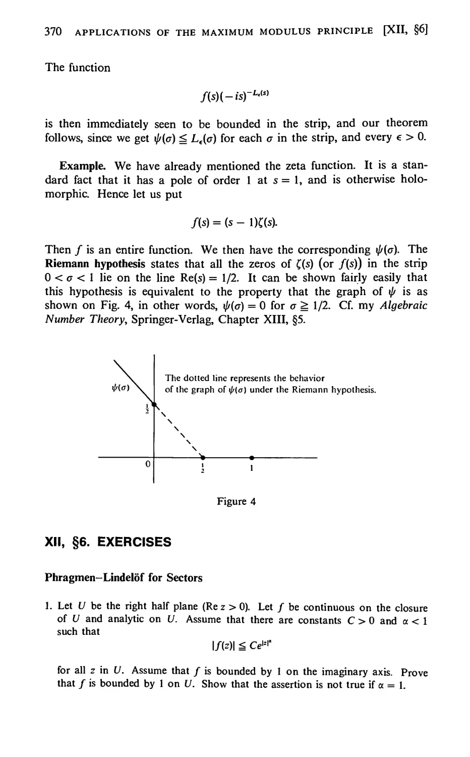
§6. The Phragmen-Lindelof and Hadamard Theorems 365
Xiv CONTENTS
CHAPTER XIII
Entire and Meromorphic Functions 372
§1. Infinite Products 372
§2. Weierstrass Products 376
§3. Functions of Finite Order 382
§4. Meromorphic Functions, Mittag-Leffler Theorem 387
CHAPTER XIV
Elliptic Functions 391
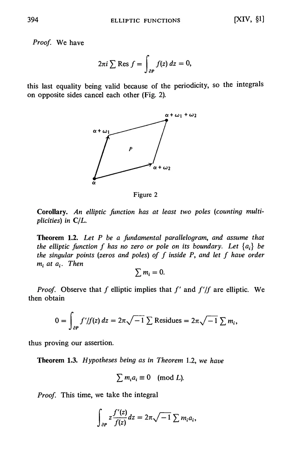
§1. The Liouville Theorems 391
§2. The Weierstrass Function 395
§3. The Addition Theorem 400
§4. The Sigma and Zeta Functions 403
CHAPTER XV
The Gamma and Zeta Functions 408
§1. The Differentiation Lemma 409
§2. The Gamma Function 413
Weierstrass Product 413
The Gauss Multiplication Formula (Distribution Relation) 416
The (Other) Gauss Formula 418
The Mellin Transform 420
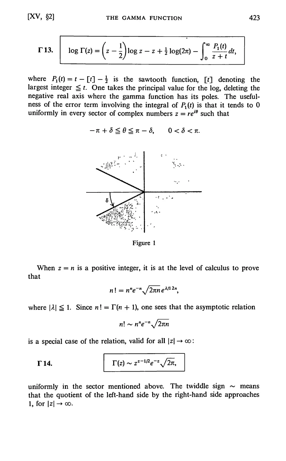
The Stirling Formula 422
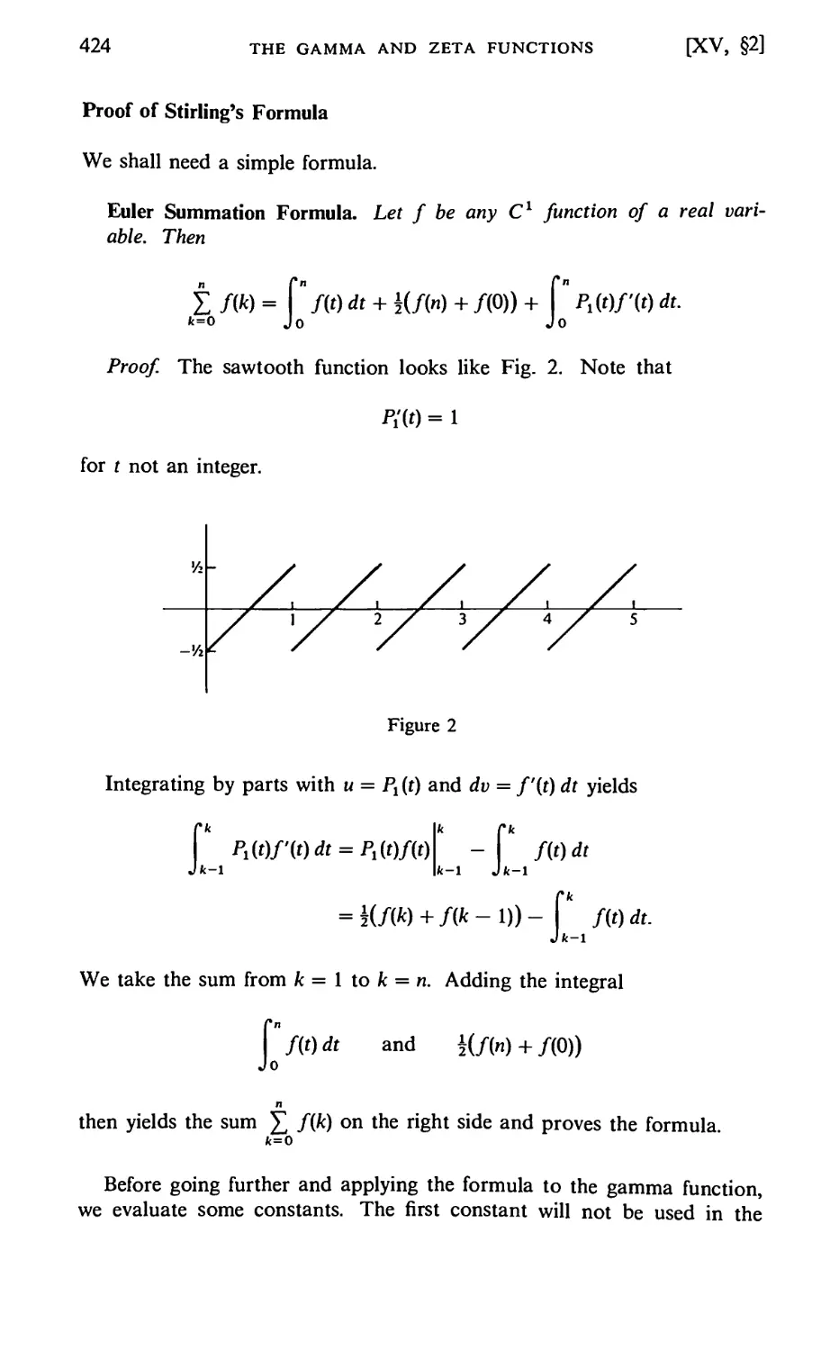
Proof of Stirling's Formula 424
§3. The Lerch Formula 431
§4. Zeta Functions 433
CHAPTER XVI
The Prime Number Theorem 440
§1. Basic Analytic Properties of the Zeta Function 441
§2. The Main Lemma and its Application 446
§3. Proof of the Main Lemma 449
Appendix 453
§1. Summation by Parts and Non-Absolute Convergence 453
§2. Difference Equations 457
§3. Analytic Differential Equations 461
§4. Fixed Points of a Fractional Linear Transformation 465
§5. Cauchy's Formula for C°° Functions 467
§6. Cauchy's Theorem for Locally Integrable Vector Fields 472
§7. More on Cauchy-Riemann 477
Bibliography 479
index 481
PART ONE
Basic Theory
CHAPTER I
Complex Numbers
and Functions
One of the advantages of dealing with the real numbers instead of the
rational numbers is that certain equations which do not have any
solutions in the rational numbers have a solution in real numbers. For
instance, x2 = 2 is such an equation. However, we also know some
equations having no solution in real numbers, for instance x2 = — 1, or
x2 = —2. We define a new kind of number where such equations have
solutions. The new kind of numbers will be called complex numbers.
I, §1. DEFINITION
The complex numbers are a set of objects which can be added and
multiplied, the sum and product of two complex numbers being also a
complex number, and satisfy the following conditions.
1. Every real number is a complex number, and if a, P are real
numbers, then their sum and product as complex numbers are
the same as their sum and product as real numbers.
2. There is a complex number denoted by i such that i2 = -1.
3. Every complex number can be written uniquely in the form a + bi
where a, b are real numbers.
4. The ordinary laws of arithmetic concerning addition and
multiplication are satisfied. We list these laws:
If a, (], y are complex numbers, then {aP)y = a(0y), and
(a + P) + y = a + (P + y).
3
4 COMPLEX NUMBERS AND FUNCTIONS [I, §1]
We have a(0 + y) = a.p + ay, and (0 + y)a = fia. + ya.
We have a/? = /to, and a + /? = /? + a.
If 1 is the real number one, then la = a.
If 0 is the real number zero, then Oa = 0.
We have a + (-l)a = 0.
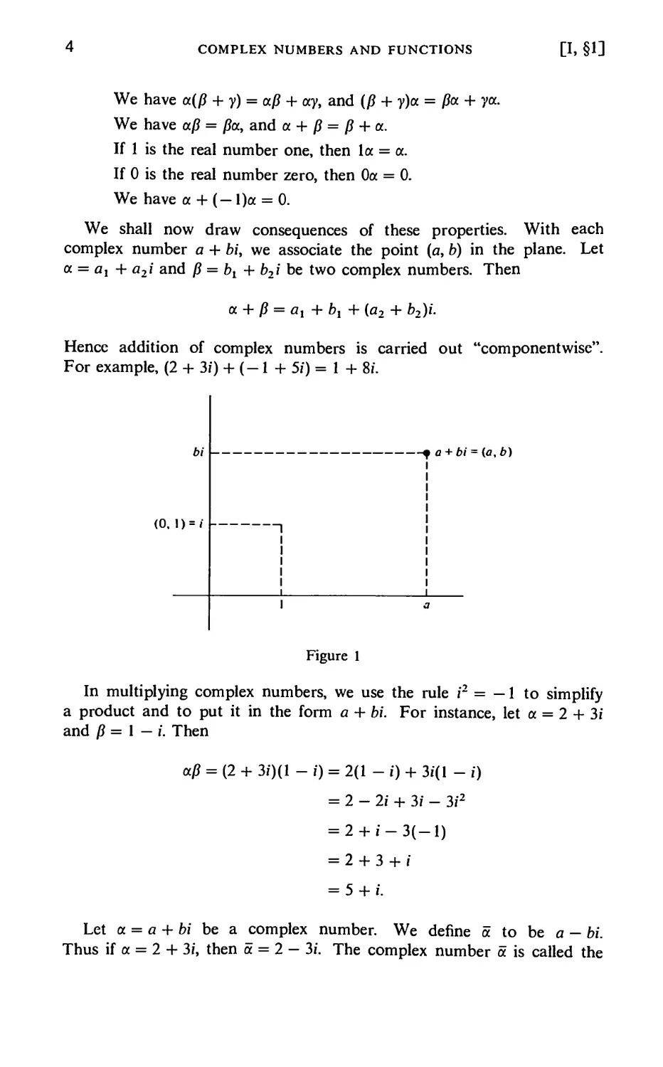
We shall now draw consequences of these properties. With each
complex number a + bi, we associate the point {a, b) in the plane. Let
a = a, + a2i and P = bt + b2i be two complex numbers. Then
a + P = ax + bx + (a2 + b2)i.
Hence addition of complex numbers is carried out "componentwise".
For example, (2 + 3/) + (-1 + 5/) = 1 + 8/.
(0.1) = /
p a + bi = (a, b)
Figure 1
In multiplying complex numbers, we use the rule r = — 1 to simplify
a product and to put it in the form a + bi. For instance, let a = 2 + 3f
and p = 1 - i. Then
afi = (2 + 3/)(1 - i) = 2(1 - i) + 3/(1 - i)
= 2-2/ + 3/ - 3r
= 2 + /-3(-1)
=2+3+/
= 5 + /.
Let a = a + fei be a complex number. We define a to be a — bi.
Thus if a = 2 + 3/, then a = 2 - 3/. The complex number a is called the
6 COMPLEX NUMBERS AND FUNCTIONS [I, §1]
The real number b is called the imaginary part of a, and denoted by
Im(a).
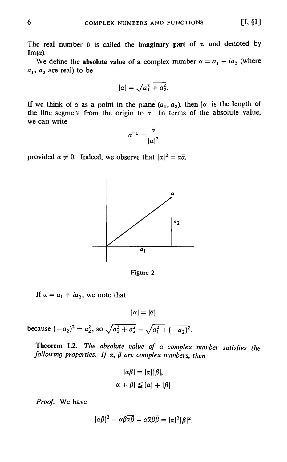
We define the absolute value of a complex number a = ax + ia2 (where
fli, a2 are real) to be
l«| = y/aj + a\.
If we think of a as a point in the plane (alt a2), then |a| is the length of
the line segment from the origin to a. In terms of the absolute value,
we can write
provided a ^ 0. Indeed, we observe that |a|2 = aa.
jS r2
f °~\
Figure 2
If a = ax + ia2, we note that
M = 1*1
because (-a2)2 = aj, so y/aj + a\ = >/a2+(-a2)2.
Theorem 1.2. The absolute value of a complex number satisfies the
following properties. If a, /? are complex numberst then
Proof We have
Wp\2 = ap^p = aapp = \a\2\p\2.
[I, §1]
DEFINITION
7
Taking the square root, we conclude that |a||/?| = |a/?|, thus proving
the first assertion. As for the second, we have
|oc + p\2 = (a + P)(a + Q) = (« + £)(« + ft
= aa + 0a + a/? + pfi
= |a|2 + 2 Re(05) + |0|2
because oip = Pa. However, we have
2 Re(05) ^ 2|0a|
because the real part of a complex number is ^ its absolute value.
Hence
1« + P\2 ^ l«l2 + 2|05| + \p\2
^\a\2 + 2\p\\a\ + \p\2
= (W\ + \P\)2.
Taking the square root yields the second assertion of the theorem.
The inequality
\« + P\^\«\ + \P\
is called the triangle inequality. It also applies to a sum of several terms.
If zu ...,zn are complex numbers then we have
\ZX +-~ + ZH\£M + — + \Zn\-
Also observe that for any complex number z, we have
|-z|H4
Proof?
I, §1. EXERCISES
1. Express the following complex numbers in the form x + iyt where x, y are
real numbers.
(a) (-1 + 30-1 (b) (1+0(1-0
(c) (1+/)/(2-/) (d) (/-1)(2-0
(e) (7 + 7ti)(n + i) (0 (2i + l)ni
(g) (y/2i)(n + 3i) (h) (/+1)(/-2)(/ + 3)
2. Express the following complex numbers in the form x + iy, where x, y are
real numbers.
8 COMPLEX NUMBERS AND FUNCTIONS [I, §2]
(a) (1 + 0"1 (b) jL, (c) |ij (d) —
3. Let a be a complex number # 0. What is the absolute value of a/a? What
is a?
4. Let a, p be two complex numbers. Show that op = ap and that
oT^Tp = a + p.
5. Justify the assertion made in the proof of Theorem 1.2, that the real part of a
complex number is =" its absolute value.
6. If a = a + ib with a, b real, then b is called the imaginary part of a and we
write b = Im(a). Show that a — a = 2/ Im(a). Show that
Im(a) =" |Im(a)| =" |a|.
7. Find the real and imaginary parts of (1 + i)100-
8. Prove that for any two complex numbers z, w we have:
(a) |z|£|z:-W| + M
(b) |z|-|wU|z-w|
(c) \z\-\w\^\z + w\
9. Let a = a + ib and z = x + iy. Let c be real > 0. Transform the condition
|z-a| = c
into an equation involving only x, y, a, b, and c, and describe in a simple
way what geometric figure is represented by this equation.
10. Describe geometrically the sets of points z satisfying the following conditions,
(a) \z-i + 3| = 5 (b) |z-i+3|>5
(c) |z-i + 3|^5 (d) |z + 2i| = l
(e) lmz>0 (f) lmz = 0
(g) Rez>0 (h) Rez = 0
I, §2. POLAR FORM
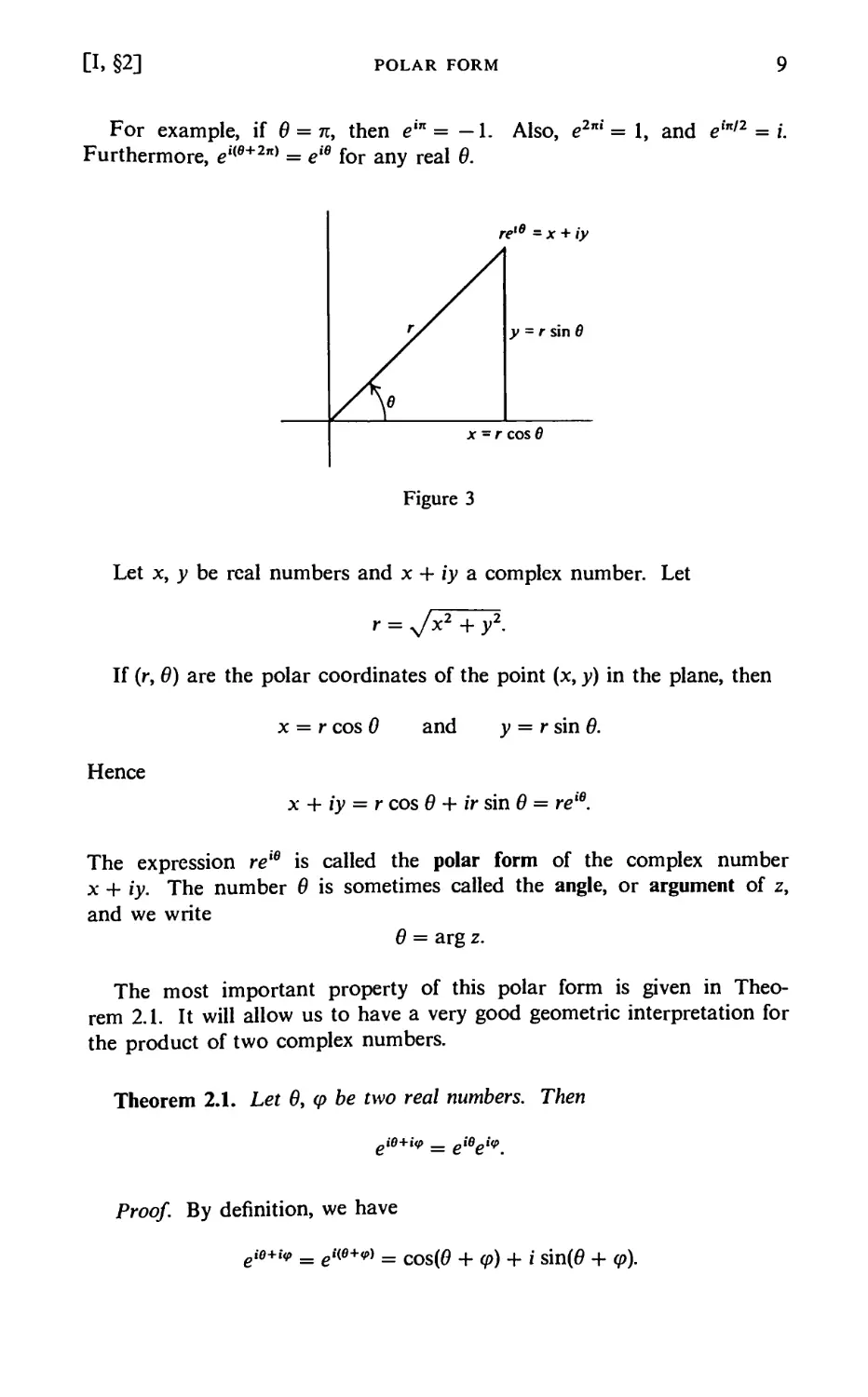
Let (x, y) = x + iy be a complex number. We know that any point in
the plane can be represented by polar coordinates (r, 6). We shall now
see how to write our complex number in terms of such polar coordinates.
Let 6 be a real number. We define the expression eie to be
eie = cos 0 + i sin 6.
Thus eie is a complex number.
[I, §2]
POLAR FORM
9
For example, if 0 = n, then ein = -1. Also, e2ni = 1, and ein'2 = i.
Furthermore, eilB+2n) = eie for any real 6.
Figure 3
Let x, y be real numbers and x + iy a complex number. Let
r = Jx2 + y2.
If (r, 6) are the polar coordinates of the point (x, y) in the plane, then
x = r cos 0 and y = r sin 6.
Hence
x + iy = r cos 0 + ir sin 0 = reie.
The expression re'e is called the polar form of the complex number
x + iy. The number 6 is sometimes called the angle, or argument of z,
and we write
6 = arg z.
The most important property of this polar form is given in
Theorem 2.1. It will allow us to have a very good geometric interpretation for
the product of two complex numbers.
Theorem 2.1. Let 6, q> be two real numbers. Then
piO+i<p _ pi6pi<p
Proof. By definition, we have
eie+i9 = ew+v) = cos(0 + (p) + i Sin(0 + </>).
10 COMPLEX NUMBERS AND FUNCTIONS [I, §2]
Using the addition formulas for sine and cosine, we see that the
preceding expression is equal to
cos 6 cos q> — sin 6 sin q> + i'(sin 6 cos q> + sin cp cos 6).
This is exactly the same expression as the one we obtain by multiplying
out
(cos 6 + i sin 0)(cos q> + i sin </>).
Our theorem is proved.
Theorem 2.1 justifies our notation, by showing that the exponential
of complex numbers satisfies the same formal rule as the exponential of
real numbers.
Let a = ax + ia2 be a complex number. We define ea to be
e°leia\
For instance, let a = 2 + 3i. Then ea = e2e3i.
Theorem 2.2. Let a, /? be complex numbers. Then
ea+P = eaep.
Proof. Let a = ax + ia2 and /? = bx + ib2. Then
e<*+P _ e(al+bl)+i(a2+b2) _ ^i+b^iiaj+bj)
= eaiebleia2+ib2.
Using Theorem 2.1, we see that this last expression is equal to
ealebleia2eib2 _ e"leio2ebleib2
By definition, this is equal to eaefi, thereby proving our theorem.
Theorem 2.2 is very useful in dealing with complex numbers. We shall
now consider several examples to illustrate it.
Example 1. Find a complex number whose square is 4ein/2.
Let z = 2einl*. Using the rule for exponentials, we see that z2 = 4ein/2.
Example 2. Let n be a positive integer. Find a complex number w
such that wn = eiK'2.
[I, §2]
POLAR FORM
11
It is clear that the complex number vv = einl2n satisfies our requirement.
In other words, we may express Theorem 2.2 as follows:
Let zx = r^16* and z2 = r2ei62 be two complex numbers. To find the
product zlz2, we multiply the absolute values and add the angles. Thus
ziz2 = r^e**1**2*.
In many cases, this way of visualizing the product of complex numbers
is more useful than that coming out of the definition.
Warning. We have not touched on the logarithm. As in calculus, we
want to say that ez = w if and only if z = log w. Since e2nik = 1 for all
integers k, it follows that the inverse function z = log w is defined only
up to the addition of an integer multiple of 27«. We shall study the
logarithm more closely in Chapter II, §3, Chapter II, §5, and Chapter III, §6.
I, §2. EXERCISES
1. Put the following complex numbers in polar form.
(a) 1+/ (b) l+i\/2 (c) -3 (d) 4/
(e) l-iy/2 (f) Si (g) -7 (h) -1-/
2. Put the following complex numbers in the ordinary form x + iy.
(a) eiin (b) e2in'3 (c) 3<?''"/4 (d) ne-'"*3
(e) e2ni'6 (f) e~in'2 (g) e~in (h) e~5inf*
3. Let a be a complex number ^ 0. Show that there are two distinct complex
numbers whose square is a.
4. Let a + bi be a complex number. Find real numbers x, y such that
(x + iy)2 = a + bi,
expressing x, y in terms of a and b.
5. Plot all the complex numbers z such that z" = I on a sheet of graph paper,
for n = 2, 3, 4, and 5.
6. Let a be a complex number ^0. Let n be a positive integer. Show that
there are n distinct complex numbers z such that z" = a. Write these complex
numbers in polar form.
7. Find the real and imaginary parts of /1/4, taking the fourth root such that its
angle lies between 0 and n/2.
8. (a) Describe all complex numbers z such that ez = 1.
(b) Let w be a complex number. Let a be a complex number such that
e" = w. Describe all complex numbers z such that ex = w.
12 COMPLEX NUMBERS AND FUNCTIONS [I, §3]
9. If ez = ew, show that there is an integer k such that z = w + 2nki.
10. (a) If 0 is real, show that
n e'e + e~'e J . n ew-e
cos 8 = and sin 0 = ——
(b) For arbitrary complex z, suppose we define cos z and sin z by replacing
6 with z in the above formula. Show that the only values of z for which
cos z = 0 and sin z = 0 are the usual real values from trigonometry.
. Prove that for any complex number z^l we have
z"+1 —
I + z + --- + z" = -
12. Using the preceding exercise, and taking real parts, prove:
n 1 sin[(n + £)0]
1 + cos 8 + cos 26 + ---+ cos nd = - -\
2 sin-
2
for 0 < 0 < In.
13. Let z, w be two complex numbers such that zw ^= 1. Prove that
| z — w |
< 1 if \z\ < 1 and \w\ < 1,
11 — zw\
I z — w I
1 — zw\
if \z\ = 1 or |w|= 1.
(There are many ways of doing this. One way is as follows. First check that
you may assume that z is real, say z = r. For the first inequality you are
reduced to proving
(r — w)(r — vv) < (1 — rw)(l — rvv).
Expand both sides and make cancellations to simplify the problem.)
I, §3. COMPLEX VALUED FUNCTIONS
Let S be a set of complex numbers. An association which to each
element of S associates a complex number is called a complex valued
function, or a function for short. We denote such a function by symbols
like
f: S - C.
[I, §3] COMPLEX VALUED FUNCTIONS 13
If z is an element of S, we write the association of the value f(z) to z by
the special arrow
z.-/(z).
We can write
f(z) = u(z) + iv(zl
where u(z) and v{z) are real numbers, and thus
z i—> u(z), z i—> v(z)
are real valued functions. We call u the real part of f, and v the
imaginary part of/.
We shall usually write
z = x + iy,
where x, y are real. Then the values of the function f can be written in
the form
f(z) = f(x + iy) = u(x, y) + iv(x, y),
viewing w, v as functions of the two real variables x and y.
Example. For the function
f(z) = x3y + i sin(x + y),
we have the real part,
m(x, y) = x3y,
and the imaginary part,
v(x> y) = sm(* + y)-
Example. The most important examples of complex functions are the
power functions. Let n be a positive integer. Let
Rz) = z\
Then in polar coordinates, we can write z = reie, and therefore
f{z) = r"einB = r"(cos n6 + i sin n0).
For this function, the real part is r"cosn0, and the imaginary part
is r" sin n6.
14 COMPLEX NUMBERS AND FUNCTIONS [I, §3]
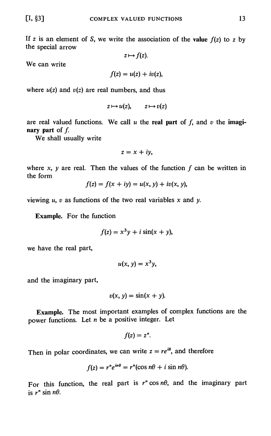
Let D be the closed disc of radius 1 centered at the origin in C. In
other words, D is the set of complex numbers z_such that \z\ ^ 1. If z is
an element of D, then z" is also an element of D, and so z\-^z" maps D
into itself. Let S be the sector of complex numbers reie such that
0^0^ 2701,
as shown on Fig. 4.
Figure 4
The function of a real variable
maps the unit interval [0, 1] onto itself. The function
#!-► ne
maps the interval
[0, 2n/ri] -> [0, 2tQ.
In this way, we see that the function f(z) = z" maps the sector S onto the
full disc of all numbers
w = fe'>
with 0 ^ t ^ 1 and 0 ^ cp ^ 2n. We may say that the power function
wraps the sector around the disc.
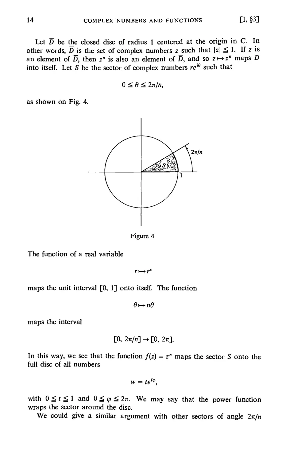
We could give a similar argument with other sectors of angle 2n/n
[I, §3]
COMPLEX VALUED FUNCTIONS
15
as shown on Fig. 5. Thus we see that z\-^z" wraps the disc n times
around.
Figure 5
Given a complex number z = reie, you should have done Exercise 6
of the preceding section, or at least thought about it. For future
reference, we now give the answer explicitly. We want to describe all
complex numbers vv such that vv" = z. Write
Then
_ *n_in<p
= tV
0<t.
If vv" = z, then t" = r, and there is a unique real number t ^ 0 such that
t" = r. On the other hand, we must also have
which is equivalent with
irup = i6 + Inik,
where k is some integer. Thus we can solve for cp and get
6 Ink
The numbers
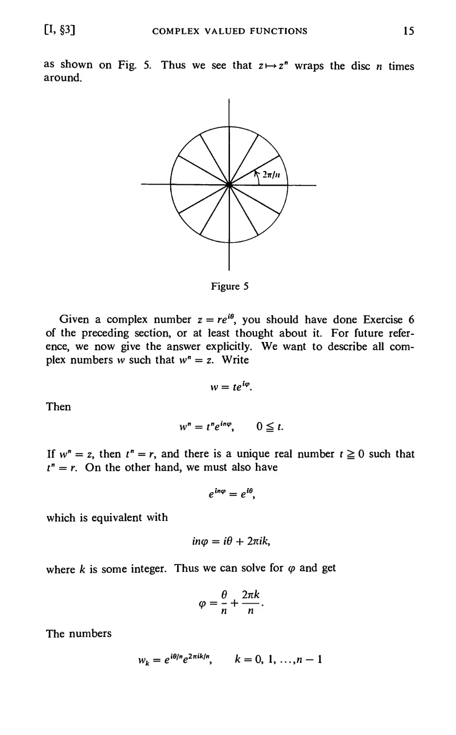
wfc
= eie/ne2nik/n, k = 0, 1,...,/1-1
16 COMPLEX NUMBERS AND FUNCTIONS [I, §3]
are all distinct, and are drawn on Fig. 6. These numbers wk may be
described pictorially as those points on the circle which are the vertices
of a regular polygon with n sides inscribed in the unit circle, with one
vertex being at the point ewl".
Figure 6
Each complex number
Ck = e2nik,n
is called a root of unity, in fact, an n-th root of unity, because its /i-th
power is 1, namely
(rk)n = e2nik"i" = e2nik = i
The points wk are just the product of elB,n with all the /i-th roots of unity,
wk = eie,nCk.
One of the major results of the theory of complex variables is to
reduce the study of certain functions, including most of the common
functions you can think of (like exponentials, logs, sine, cosine) to power
series, which can be approximated by polynomials. Thus the power
function is in some sense the unique basic function out of which the others
are constructed. For this reason it was essential to get a good intuition
of the power function. We postpone discussing the geometric aspects
of the other functions to Chapters VII and VIII, except for some simple
exercises.
[I. §4]
LIMITS AND COMPACT SETS
17
I, §3. EXERCISES
1. Let f{z) = 1/z. Describe what f does to the inside and outside of the unit
circle, and also what it does to points on the unit circle. This map is called
inversion through the unit circle.
2. Let f(z) = 1/z. Describe f in the same manner as in Exercise 1. This map is
called reflection through the unit circle.
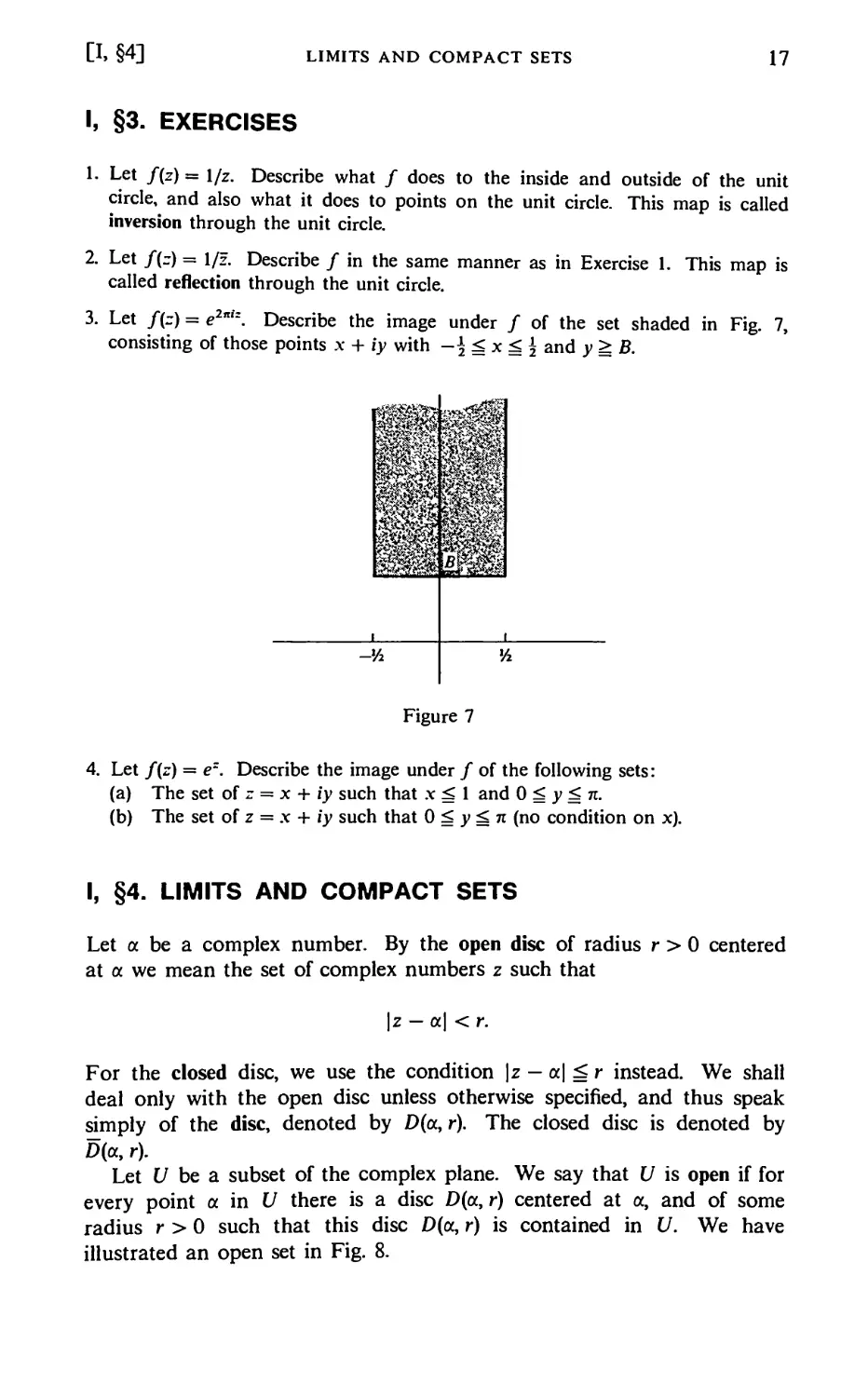
3. Let f(z) = e2niz. Describe the image under f of the set shaded in Fig. 7,
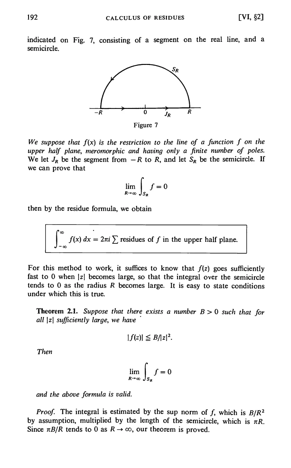
consisting of those points x + iy with — \£ x ^ \ and y^B.
Figure 7
4. Let f{z) = ez. Describe the image under f of the following sets:
(a) The set of z = x + iy such that x ^ 1 and 0 ^ y ^ n.
(b) The set of z = x + iy such that 0 ^ y ^ n (no condition on x).
I, §4. LIMITS AND COMPACT SETS
Let a be a complex number. By the open disc of radius r > 0 centered
at a we mean the set of complex numbers z such that
\z - a\ < r.
For the closed disc, we use the condition \z — a| ^ r instead. We shall
deal only with the open disc unless otherwise specified, and thus speak
simply of the disc, denoted by D(a, r). The closed disc is denoted by
D(a, r).
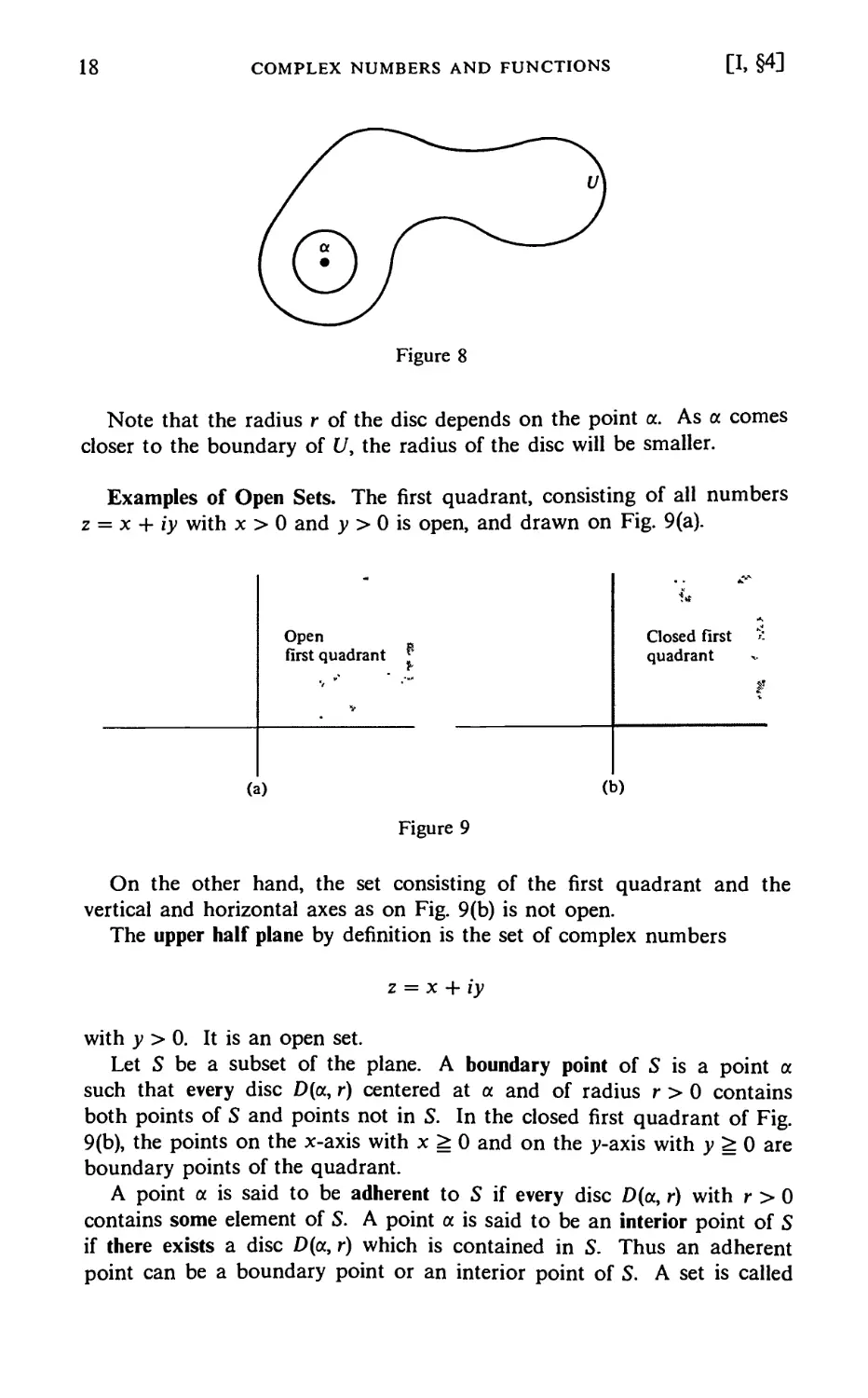
Let U be a subset of the complex plane. We say that U is open if for
every point a in U there is a disc D(a, r) centered at a, and of some
radius r > 0 such that this disc D(a, r) is contained in U. We have
illustrated an open set in Fig. 8.
18 COMPLEX NUMBERS AND FUNCTIONS [I, §4]
Figure 8
Note that the radius r of the disc depends on the point a. As a comes
closer to the boundary of U, the radius of the disc will be smaller.
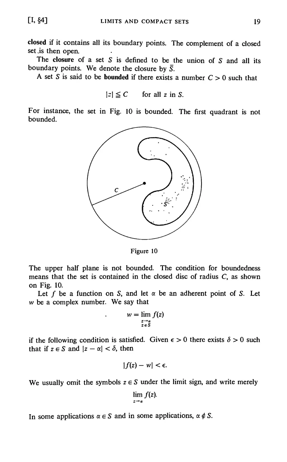
Examples of Open Sets. The first quadrant, consisting of all numbers
z = x + iy with x > 0 and y > 0 is open, and drawn on Fig. 9(a).
Closed first *:
quadrant
?
Open
first quadrant p
(a) (b)
Figure 9
On the other hand, the set consisting of the first quadrant and the
vertical and horizontal axes as on Fig. 9(b) is not open.
The upper half plane by definition is the set of complex numbers
z = x + iy
with y > 0. It is an open set.
Let S be a subset of the plane. A boundary point of S is a point a
such that every disc D(a, r) centered at a and of radius r > 0 contains
both points of S and points not in S. In the closed first quadrant of Fig.
9(b), the points on the x-axis with x ^ 0 and on the y-axis with y ^ 0 are
boundary points of the quadrant.
A point a is said to be adherent to S if every disc D(a, r) with r > 0
contains some element of S. A point a is said to be an interior point of S
if there exists a disc D(a, r) which is contained in S. Thus an adherent
point can be a boundary point or an interior point of S. A set is called
[I. §4]
LIMITS AND COMPACT SETS
19
closed if it contains all its boundary points. The complement of a closed
set js then open.
The closure of a set S is defined to be the union of S and all its
boundary points. We denote the closure by S.
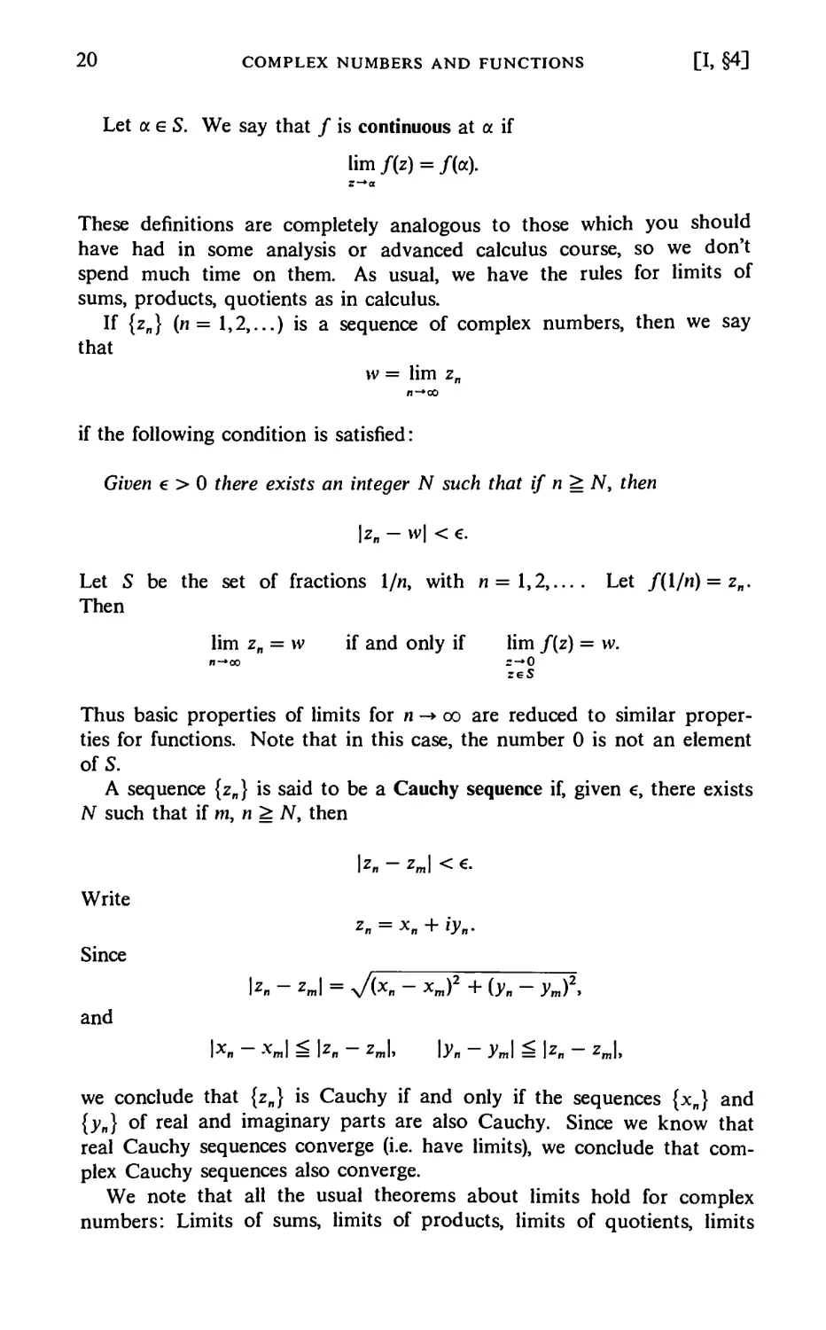
A set S is said to be bounded if there exists a number C > 0 such that
|r| ^ C for all z in S.
For instance, the set in Fig. 10 is bounded. The first quadrant is not
bounded.
Figure 10
The upper half plane is not bounded. The condition for boundedness
means that the set is contained in the closed disc of radius C, as shown
on Fig. 10.
Let f be a function on S, and let a be an adherent point of S. Let
vv be a complex number. We say that
w = lim f(z)
if the following condition is satisfied. Given € > 0 there exists 5 > 0 such
that if z e S and \z - a\ < S, then
1/(2)-w|<€.
We usually omit the symbols zeS under the limit sign, and write merely
lim /(z).
In some applications aeS and in some applications, a $ S.
20 COMPLEX NUMBERS AND FUNCTIONS [I, §4]
Let a e S. We say that f is continuous at a if
lim/(z) = /(a).
z — a
These definitions are completely analogous to those which you should
have had in some analysis or advanced calculus course, so we don't
spend much time on them. As usual, we have the rules for limits of
sums, products, quotients as in calculus.
If {z„} (n = 1,2,...) is a sequence of complex numbers, then we say
that
vv = lim z„
n-»oo
if the following condition is satisfied:
Given € > 0 there exists an integer N such that if n^. N, then
\z„ — W\ < €.
Let S be the set of fractions 1/n, with /1 = 1,2,.... Let f(l/n) = z„.
Then
lim z„ = vv if and only if lim f(z) = vv.
n-»oo =-»0
Thus basic properties of limits for n -> oo are reduced to similar
properties for functions. Note that in this case, the number 0 is not an element
ofS.
A sequence {z„} is said to be a Cauchy sequence if, given €, there exists
N such that if m, n^ N, then
\z„ - zm\ < €.
Write
Zn = Xn + iy„-
Since
k - *J = x/(*„ - *J2 + (yn - ym)2,
and
|x. - xm\ ^ \zn - zj, \y„ - ym\ ^ \zn - zm\,
we conclude that {z„} is Cauchy if and only if the sequences {x„} and
{y„} of real and imaginary parts are also Cauchy. Since we know that
real Cauchy sequences converge (i.e. have limits), we conclude that
complex Cauchy sequences also converge.
We note that all the usual theorems about limits hold for complex
numbers: Limits of sums, limits of products, limits of quotients, limits
[I. §4]
LIMITS AND COMPACT SETS
21
of composite functions. The proofs which you had in advanced calculus
hold without change in the present context. It is then usually easy to
compute limits.
Example. Find the limit
lim
„-oo 1 + nz
for any complex number z.
If z = 0, it is clear that the limit is 0. Suppose z^O. Then the
quotient whose limit we are supposed to find can be written
1 +nz 1
- + z
But
lim
im ( - + z ) = ;
Hence the limit of the quotient is z/z = 1.
Compact Sets
We shall now go through the basic results concerning compact sets. Let
S be a set of complex numbers. Let {z„} be a sequence in S. By a point
of accumulation of {z„} we mean a complex number v such that given €
(always assumed > 0) there exist infinitely many integers n such that
\zn — V\ <€.
We may say that given an open set U containing v, there exist infinitely
many n such that z„ e U.
Similarly we define the notion of point of accumulation of an infinite
set S. It is a complex number v such that given an open set U
containing v, there exist infinitely many elements of S lying in U. In particular,
a point of accumulation of S is adherent to S.
We assume that the reader is acquainted with the Weierstrass-Bolzano
theorem about sets of real numbers: If S is an infinite bounded set of real
numbers, then S has a point of accumulation.
We define a set of complex numbers S to be compact if every sequence
of elements of S has a point of accumulation in S. This property is
equivalent to the following properties, which could be taken as alternate
definitions:
(a) Every infinite subset of S has a point of accumulation in S.
22 COMPLEX NUMBERS AND FUNCTIONS [I, §4]
(b) Every sequence of elements of S has a convergent subsequence
whose limit is in S.
We leave the proof of the equivalence between the three possible
definitions to the reader.
Theorem 4.1. A set of complex numbers is compact if and only if it is
closed and bounded.
Proof Assume that S is compact. If S is not bounded, for each
positive integer n there exists z„ e S such that
kl > n.
Then the sequence {z„} does not have a point of accumulation. Indeed,
if v is a point of accumulation, pick m>2|i>|, and note that |u|>0.
Then
\zm-v\*\zm\-\v\*m-\v\>\v\.
This contradicts the fact that for infinitely many m we must have zm close
to v. Hence S is bounded. To show S is closed, let v be in its closure.
Given n, there exists z„ e S such that
\z„ — v\ < 1//1.
The sequence {z„} converges to u, and has a subsequence converging to
a limit in S because S is assumed compact. This limit must be u, whence
veS and S is closed.
Conversely, assume that S is closed and bounded, and let B be a
bound, so \z\ ^ B for all z e S. If we write
z = x + iy,
then \x\ ^ B and \y\ ^ B. Let {z„} be a sequence in S, and write
Zn = Xn + ^n •
There is a subsequence {zn|} such that {xn|} converges to a real number
a, and there is a sub-subsequence {z„2} such that {yn2} converges to a
real number b. Then
converges to a + ib, and S is compact. This proves the theorem.
Theorem 4.2. Let S be a compact set and let Si => S2 => • • • be a
sequence of non-empty closed subsets such that S„ => S„+l. Then the
intersection of all S„ for all n = 1, 2, ... is not empty.
[I, §4]
LIMITS AND COMPACT SETS
23
Proof. Let z„eS„. The sequence {z„} has a point of accumulation
in S. Call it v. Then i> is also a point of accumulation for each
subsequence {zk} with k ^ w, and hence lies in the closure of S„ for each n,
But S„ is assumed closed, and hence veS„ for all n. This proves the
theorem.
Theorem 4.3. Let S be a compact set of complex numbers, and let f be
a continuous function on S. Then the image of f is compact.
Proof. Let {w„} be a sequence in the image of f so that
vv„ = f(z„) for z„ g S.
The sequence {z„} has a convergent subsequence {z„J, with a limit v in
S. Since f is continuous, we have
lim w = lim f(z ) = f{v).
Hence the given sequence {w„} has a subsequence which converges in
f(S). This proves that f(S) is compact.
Theorem 4.4. Let S be a compact set of complex numbers, and let
/:S-R
be a continuous function. Then f has a maximum on S, that is, there
exists v g S such that f(z) ^ f(v) for all z g S.
Proof. By Theorem 4.3, we know that f(S) is closed and bounded.
Let b be its least upper bound. Then b is adherent to f(S), whence in
f{S) because f{S) is closed. So there is some veS such that f(v) = b.
This proves the theorem.
Remarks. In practice, one deals with a continuous function f: S -*■ C
and one applies Theorem 4.4 to the absolute value of f, which is also
continuous (composite of two continuous functions).
Theorem 4.5. Let S be a compact set, and let f be a continuous
function on S. Then f is uniformly continuous, i.e. given € there exists S
such that whenever z, weS and \z — w\ < <5, then \f{z) — f(w)\ < e.
Proof. Suppose the assertion of the theorem is false. Then there exists
€, and for each n there exists a pair of elements z„, w„eS such that
\z„ - w„| < l//i but \f(z„) - f(w„)\ > c.
24 COMPLEX NUMBERS AND FUNCTIONS [I, §4]
There is an infinite subset J1 of positive integers and some veS such
that z„ -> v for n -> oo and neJl. There is an infinite subset J2 of Jx and
ueS such that vv„ -► u for n -> oo and neJ2. Then, taking the limit for
n -+ oo and nsJ2 we obtain |w — v\ = 0 and w = v because
\v — u\ ^ \v — z„\ + \z„ — w„\ + \w„ — u\.
Hence f(v) — f(u) = 0. Furthermore,
1/(¾) " /(W„)l ^ 1/(2.) - /(W)| + 1/(^) - /(M)| + |/(M) - /(W„)|.
Again taking the limit as n -*■ oo and neJ2i we conclude that
/fe.)-./K)
approaches 0. This contradicts the assumption that
I/(Z„) -/K)|>€,
and proves the theorem.
Let A, B be two sets of complex numbers. By the distance between
them, denoted by d(A, B), we mean
d(A, B) = g.l.b.|z - vv|,
where the greatest lower bound g.l.b. is taken over all elements z e A and
vv g B. If B consists of one point, we also write d{A, w) instead of d{A, B).
We shall leave the next two results as easy exercises.
Theorem 4.6. Let S be a closed set of complex numbers, and let v be a
complex number. There exists a point we S such that
d(S, v) = | vv — v\.
[Hint: Let £ be a closed disc of some suitable radius, centered at v,
and consider the function zi-> \z — v\ for z e S n £.]
Theorem 4.7. Let K be a compact set of complex numbers, and let S be
a closed set. There exist elements z0e K and w0 e S such that
d(K,S) = \z0-w0\.
[Hint: Consider the function z\-+d{S, z) for z e K.]
[I, §4]
LIMITS AND COMPACT SETS
25
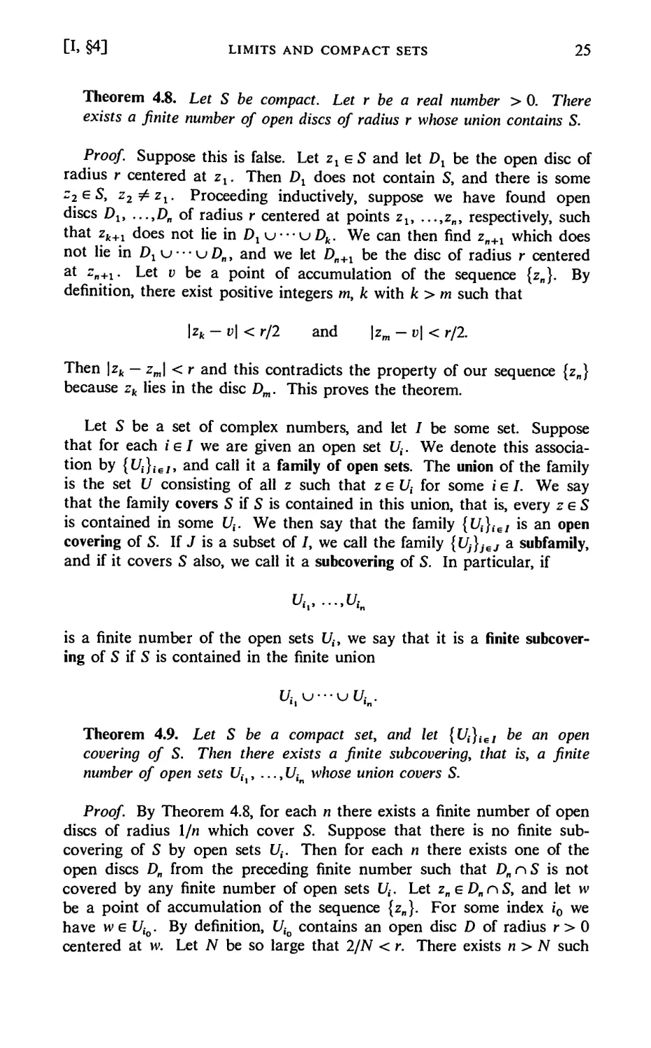
Theorem 4.8. Let S be compact. Let r be a real number > 0. There
exists a finite number of open discs of radius r whose union contains S.
Proof Suppose this is false. Let zleS and let Dx be the open disc of
radius r centered at z1. Then Dl does not contain S, and there is some
z2 e S, 22^zi- Proceeding inductively, suppose we have found open
discs Dlt ...,D„ of radius r centered at points zx, ...,z„, respectively, such
that zk+1 does not lie in Dlw-<jDk. We can then find zn+1 which does
not lie in Dl u • • • u D„, and we let Dn+1 be the disc of radius r centered
at zn+l. Let d be a point of accumulation of the sequence {z„}. By
definition, there exist positive integers m, k with k> m such that
\zk -v\< r/2 and \zm - v\ < r/2.
Then \zk — zm\ <r and this contradicts the property of our sequence {z„}
because zk lies in the disc Dm. This proves the theorem.
Let S be a set of complex numbers, and let I be some set. Suppose
that for each iel we are given an open set U{. We denote this
association by {Ui}ieI, and call it a family of open sets. The union of the family
is the set U consisting of all z such that z e t/£ for some i e J. We say
that the family covers S if S is contained in this union, that is, every zeS
is contained in some V,. We then say that the family {Ut}teI is an open
covering of S. If J is a subset of I, we call the family {Uj}jeJ a subfamily,
and if it covers S also, we call it a subcovering of S. In particular, if
^-,.--.¾
is a finite number of the open sets U{, we say that it is a finite
subcovering of S if S is contained in the finite union
Theorem 4.9. Let S be a compact set, and let {Ui}ieI be an open
covering of S. Then there exists a finite subcovering, that is, a finite
number of open sets Uix, ...,Uin whose union covers S.
Proof By Theorem 4.8, for each n there exists a finite number of open
discs of radius \/n which cover S. Suppose that there is no finite sub-
covering of S by open sets U{. Then for each n there exists one of the
open discs D„ from the preceding finite number such that D„nS is not
covered by any finite number of open sets U(. Let z„ e D„nS, and let w
be a point of accumulation of the sequence {z„}. For some index i0 we
have we Uio. By definition, Uio contains an open disc D of radius r > 0
centered at w. Let N be so large that 2/N < r. There exists n> N such
26 COMPLEX NUMBERS AND FUNCTIONS [I, §4]
that
k - w| ^ l/N.
Any point of D„ is then at a distance ^ 2/N from w, and hence D„ is
contained in D, and thus contained in Uio. This contradicts the
hypothesis made on D„, and proves the theorem.
I, §4. EXERCISES
1. Let a be a complex number of absolute value < 1. What is lim a"? Proof?
2. If |a| > 1, does lim a" exist? Why?
3. Show that for any complex number z ^ 1, we have
- 1
L + z + • • • + z" =
:- 1
If \z\ < 1, show that
lim (1 + z + ••■ + z") = -—
n-co 1 —
4. Let f be the function defined by
m = lim :
„-„ 1 + n2z
Show that f is the characteristic function of the set {0}, that is, /(0) = 1, and
/(z) = 0 if z * 0.
5. For \z\ ,* 1 show that the following limit exists:
f(z) = lim (
Is it possible to define /(z) when |z| = 1 in such a way to make / continuous?
6. Let
f(z) = lim ^-n.
(a) What is the domain of definition of / that is, for which compiex numbers
z does the limit exist?
(b) Give explicitly the values of /(z) for the various z in the domain of /
7. Show that the series
[I, §5]
COMPLEX DIFFERENTIABILITY
27
converges to 1/(1 - z)2 for \z\ < 1 and to l/z(l - z)2 for \z\ > 1. Prove that
the convergence is uniform for \z\ g c < 1 in the first case, and \z\ ^ b > 1 in
the second. [Hint. Multiply and divide each term by 1 - z, and do a partial
fraction decomposition, getting a telescoping effect.]
I, §5. COMPLEX DIFFERENTIABILITY
In studying differentiate functions of a real variable, we took such
functions defined on intervals. For complex variables, we have to select
domains of definition in an analogous manner.
Let U be an open set, and let z be a point of U. Let f be a function
on U. We say that f is complex differentiate at z if the limit
exists. This limit is denoted by f'(z) or df/dz.
In this section, differentiable will always mean complex differentiable.
The usual proofs of a first course in calculus concerning basic
properties of differentiability are valid for complex differentiability. We shall
run through them again.
We note that if f is differentiable at z then f is continuous at z
because
Mm(fiz + h)-M) = UmfiZ + hl-f{Z)h
/>-o /.-0 n
and since the limit of a product is the product of the limits, the limit on
the right-hand side is equal to 0.
We let f, g be functions defined on the open set U. We assume that
f, g are differentiable at z.
Sum. The sum f + g is differentiable at z, and
(f + g),(z) = f'(z) + 9'(z\
Proof. This is immediate from the theorem that the limit of a sum is
the sum of the limits.
Product. The product fg is differentiable at z, and
{fg)'{z) = f'{z)g{z) + f{z)g'{z).
28 COMPLEX NUMBERS AND FUNCTIONS [I, §5]
Proof. To determine the limit of the Newton quotient
f(z + h)g(z + h)-f(z)g(z)
h
we write the numerator in the form
f(z + h)g(z + /i)- f{z)g{z + h) + f(z)g(z + h) - Rz)g{z).
Then the Newton quotient is equal to a sum
f{z + h)-f(z) , M , „,9(z + h)-g(z)
g(z + h) + f(z) ^ .
Taking the limits yields the formula.
Quotient. If g(z) j^ 0, then the quotient f/g is differentiable at z, and
Proof. This is again proved as in ordinary calculus. We first prove
the differentiability of the quotient function l/g. We have
1 1
g(z + h) g(z)
h
Taking the limit yields
g(z + h) - g(z) 1
h g(z + h)g{z)
-i#9'(z)'
which is the usual value. The general formula for a quotient is obtained
from this by writing
fl9=f-\l9,
and using the rules for the derivative of a product, and the derivative of
i/g.
Examples. As in ordinary calculus, from the formula for a product
and induction, we see that for any positive integer n,
!Tz=nz •
[I, §5]
COMPLEX DIFFERENTIABILITY
29
The rule for a quotient also shows that this formula remains valid when
n is a negative integer.
The derivative of z2/(2z - 1) is
(2z - l)2z - 2z2
(2z - 1)2 "
This formula is valid for any complex number z such that 2z — 1 ^ 0.
More generally, let
f(z) = P(z)/Q{z),
where P, Q are polynomials. Then f is differentiable at any point z
where Q(z) ^ 0.
Last comes the chain rule. Let U, V be open sets in C, and let
f: U -> V and g: V -* C
be functions, such that the image of f is contained in V. Then we can
form the composite function go f such that
(gof){z) = g(f{z)).
Chain Rule. Let w = f{z). Assume that f is differentiable at z, and g is
differentiable at w. Then g ° f is differentiable at zy and
{gofnz) = g'(f{z))f\z).
Proof. Again the proof is the same as in calculus, and depends on
expressing differentiability by an equivalent property not involving
denominators, as follows.
Suppose that f is differentiable at z, and let
Then
(1) f{z + h) - f(z) = f'{z)h + hcp(h),
and
(2) lim q>(h) = 0.
30 COMPLEX NUMBERS AND FUNCTIONS [I, §5]
Furthermore, even though </> is at first defined only for sufficiently small
h and h ^ 0, we may also define </>(0) = 0, and formula (1) remains valid
for /i = 0.
Conversely, suppose that there exists a function q> defined for
sufficiently small h and a number a such that
(1') f(z + h)-f(z) = ah + hq>(h)
and
(2) lim </>(/i) = 0.
/.-0
Dividing by h in formula (T) and taking the limit as /i->0, we see that
the limit exists and is equal to a. Thus f'{z) exists and is equal to a.
Hence the existence of a function q> satisfying (T), (2) is equivalent to
differentiability.
We apply this to a proof of the chain rule. Let w = f(z), and
k=f(z + h)-f(z),
so that
9(f(z + h)) - g{f(z)) = g(w + k) - g(W).
There exists a function \J/{k) such that lim \}/{k) = 0 and
fc-0
g(w + k) - g(w) = g'{w)k + kij/{k)
= 9»(f(z + *) - m) + (f(z + h)- f(z))iP(k).
Dividing by h yields
gof{z + h)-gof{z) f{z + h)-f{z) f{z + h)-f(z) ,
-h = g (w) -h + s *(k).
As h -> 0, we note that k -> 0 also by the continuity of f, whence \J/(k)^>0
by assumption. Taking the limit of this last expression as h -> 0 proves
the chain rule.
A function f defined on an open set U is said to be differentiable if it
is differentiable at every point. We then also say that f is holomorphic
on U. The word holomorphic is usually used in order not to have to
specify complex differentiability as distinguished from real differentiability.
[I> §6] THE CAUCHY-RIEMANN EQUATIONS 31
In line with general terminology, a holomorphic function
f:U-+V
from an open set into another is called a holomorphic isomorphism if
there exists a holomorphic function
g.V^U
such that g is the inverse of f, that is,
g°f=idu and fog = idv.
A holomorphic isomorphism of U with itself is called a holomorphic
automorphism. In the next chapter we discuss this notion in connection
with functions defined by power series.
I, §6. THE CAUCHY-RIEMANN EQUATIONS
Let f be a function on an open set V, and write f in terms of its real
and imaginary parts,
f{x + iy) = u(x, y) + iv(x, y).
It is reasonable to ask what the condition of differentiability means in
terms of u and v. We shall analyze this situation in detail in Chapter
VIII, but both for the sake of tradition, and because there is some need
psychologically to see right away what the answer is, we derive the
equivalent conditions on u, v for f to be holomorphic.
At a fixed z, let f'(z) = a + bi. Let w = h + ik, with h, k real. Suppose
that
f(z + w) - f(z) = f'(z)w + (J(W)W,
where
lim (t(w) = 0.
Then
f'(z)w = (a + bi){h + ki) = ah - bk + i(bh + ak).
On the other hand, let
F: U -+ R2
32 COMPLEX NUMBERS AND FUNCTIONS [I, §6]
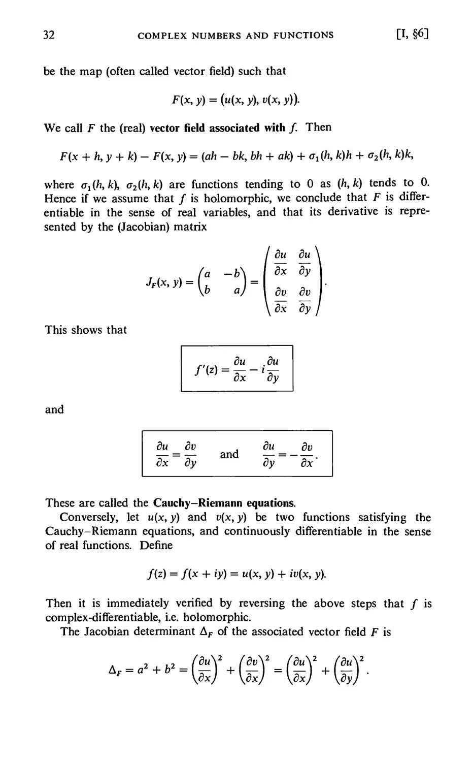
be the map (often called vector field) such that
F{x, y) = (u{x, y), v{x, y)).
We call F the (real) vector field associated with f. Then
F{x + h,y + k)- F{x, y) = (ah - bk, bh + ak) + ox(K k)h + a2{h, k)k,
where gx(K k), a2{h,k) are functions tending to 0 as (h,k) tends to 0.
Hence if we assume that f is holomorphic, we conclude that F is
differentiate in the sense of real variables, and that its derivative is
represented by the (Jacobian) matrix
This shows that
and
M*, y)
du
_fa -b\_\ dx
~\b a)~ 1 dv
.,. , du .du
f{z) = dx-%
du dv du
dx dy dy
du\
dv J
YyJ
dv
dx'
These are called the Cauchy-Riemann equations.
Conversely, let u{x, y) and v(x, y) be two functions satisfying the
Cauchy-Riemann equations, and continuously differentiable in the sense
of real functions. Define
f(z) = f(x + iy) = u(x, y) + iv{x, y).
Then it is immediately verified by reversing the above steps that f is
complex-differentiable, i.e. holomorphic.
The Jacobian determinant Af of the associated vector field F is
w*-(§' +
fev\2 feu\2 /Bu\2
[I, §7] ANGLES UNDER HOLOMORPHIC MAPS 33
Hence Af ^ 0, and is ^0 if and only if f'(z) ^ 0. We have
Af(x,>;) = |/'(z)|2.
We now drop these considerations until Chapter VIII.
The study of the real part of a holomorphic function and its relation
with the function itself will be carried out more substantially in Chapter
VIII. It is important, and much of that chapter depends only on
elementary facts. However, the most important part of complex analysis at the
present level lies in the power series aspects and the immediate
applications of Cauchy's theorem. The real part plays no role in these matters.
Thus we do not wish to interrupt the straightforward flow of the book
now towards these topics.
However, the reader may read immediately the more elementary parts
§1 and §2 of Chapter VIII, which can be understood already at this
point.
I, §6. EXERCISE
1. Prove in detail that if u, v satisfy the Cauchy-Riemann equations, then the
function
f(z) = f(x + iy) = u(x, y) + iv(x, y)
is holomorphic.
I, §7. ANGLES UNDER HOLOMORPHIC MAPS
In this section, we give a simple geometric property of holomorphic
maps. Roughly speaking, they preserve angles. We make this precise as
follows.
Let U be an open set in C and let
y:[a,b]^U
be a curve in U, so we write
y(t) = x(t) + iy(t).
We assume that y is differentiate, so its derivative is given by
/(0 = x'(0 + iy'(t).
34 COMPLEX NUMBERS AND FUNCTIONS [I, §7]
Let f: U -> C be holomorphic. We let the reader verify the chain rule
jtf(y(t)) = f'(y(t))y'(t).
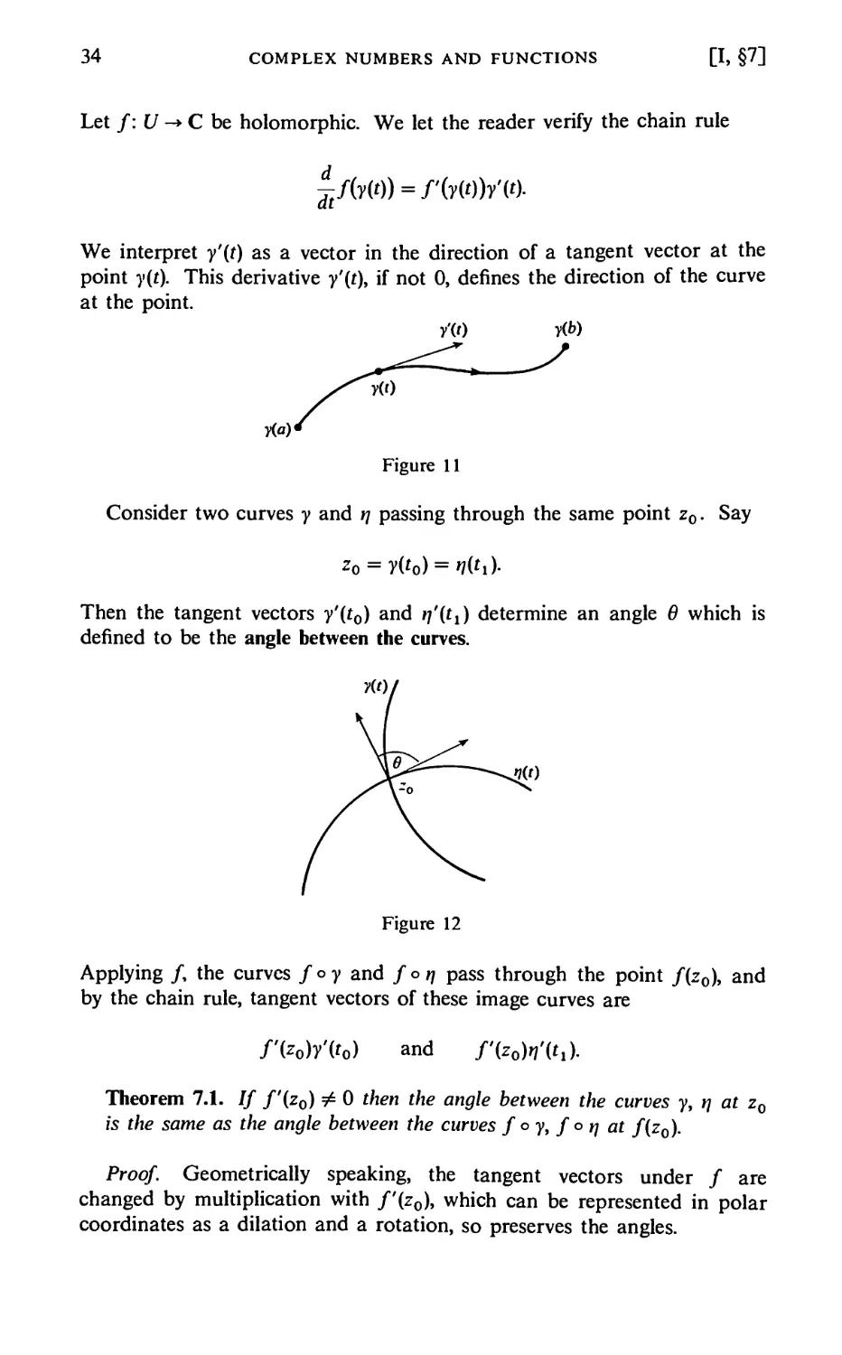
We interpret y'{t) as a vector in the direction of a tangent vector at the
point y(t). This derivative y'(t), if not 0, defines the direction of the curve
at the point.
/(0 y(b)
y(a)
Figure 11
Consider two curves y and n passing through the same point z0. Say
Zo = y(h) = tl(h)-
Then the tangent vectors y'{t0) and n'(ti) determine an angle 6 which is
defined to be the angle between the curves.
Figure 12
Applying f the curves foy and f o n pass through the point f(z0), and
by the chain rule, tangent vectors of these image curves are
f'(zo)y'{t0) and /'(zoWi^).
Theorem 7.1. If f'(z0) ^ 0 then the angle between the curves y, n at z0
is the same as the angle between the curves f ° y, f ° n at f{z0).
Proof. Geometrically speaking, the tangent vectors under f are
changed by multiplication with f'(z0), which can be represented in polar
coordinates as a dilation and a rotation, so preserves the angles.
[X §7] ANGLES UNDER HOLOMORPHIC MAPS 35
We shall now give a more formal argument, dealing with the cosine
and sine of angles.
Let z, w be complex numbers,
z = a + bi and w = c + di,
where a, b, c, d are real. Then
zw = ac + bd + i(bc — ad).
. Define the scalar product
(1) <z, w> = Re(zw).
Then <z, \v> is the ordinary scalar product of the vectors {a, b) and (c, d)
in R2. Let 6(z, w) be the angle between z and w. Then
(2) cos0(z,W) = ^^.
|z|M
Since sin 6 = cos ( 6 - ^ ), we can define
<z, — iw>
l*IM
*H).
(3) sin 6{z, w) =
This gives us the desired precise formulas for the cosine and sine of an
angle, which determine the angle.
Let f'(z0) = a. Then
(4) <az, a\v> = Re(azavv) = aa Re(zvv) = |a|2<z, w>
because aa = |a|2 is real. It follows immediately from the above formulas
that
(5) cos 6(az, aw) = cos 6(z, w) and sin 6(az, aw) = sin 6(z, w).
This proves the theorem.
A map which preserves angles is called conformal. Thus we can say
that a holomorphic map with non-zero derivative is conformal. The
complex conjugate of a holomorphic map also preserves angles, if we
disregard the orientation of an angle.
In Chapter VII, we shall consider holomorphic maps which have
inverse holomorphic maps, and therefore such that their derivatives are
36 COMPLEX NUMBERS AND FUNCTIONS [I, §7]
never equal to 0. The theorem proved in this section gives additional
geometric information concerning the nature of such maps. But the
emphasis of the theorem in this section is local, whereas the emphasis in
Chapter VII will be global. The word "conformal", however, has become
a code word for this kind of map, even in the global case, which explains
the title of Chapter VII. The reader will notice that the local property of
preserving angles is irrelevant for the global arguments given in Chapter
VII, having to do with inverse mappings. Thus in Chapter VII, we shall
use a terminology which emphasizes the invertibility, namely the
terminology of isomorphisms and automorphisms.
In this terminology, we can say that a holomorphic isomorphism is
conformal. The converse is false in general. For instance, let U be the
open set obtained by deleting the origin from the complex numbers.
The function
/:[/->[/ given by z i—► z2
has everywhere non-zero derivative in U, but it does not admit an
inverse function. This function f is definitely conformal. The invertibility
is true locally, however. See Theorem 5.1 of Chapter II.
CHAPTER II
Power Series
So far, we have given only rational functions as examples of holomorphic
functions. We shall study other ways of defining such functions. One
of the principal ways will be by means of power series. Thus we shall see
that the series
z2 z3
1+Z+2! + 3!+'"
converges for all z to define a function which is equal to e~. Similarly,
we shall extend the values of sin z and cos z by their usual series to
complex valued functions of a complex variable, and we shall see that
they have similar properties to the functions of a real variable which you
already know.
First we shall learn to manipulate power series formally. In
elementary calculus courses, we derived Taylor's formula with an error term.
Here we are concerned with the full power series. In a way, we pick up
where calculus left off. We study systematically sums, products, inverses,
and composition of power series, and then relate the formal operations
with questions of convergence.
II, §1. FORMAL POWER SERIES
We select at first a neutral letter, say T. In writing a formal power series
£ anTn = a0 + axT + a2T2 + ---
n=0
37
38
POWER SERIES
[II, §1]
what is essential are its "coefficients" a0, alt a2, ... which we shall take
as complex numbers. Thus the above series may be defined as the
function
n\-^an
from the integers ^ 0 to the complex numbers.
We could use other letters besides T, writing
/(r) = L<Vn,
/(*) = 5>„z".
In such notation, f does not denote a function, but a formal expression.
Also, as a matter of notation, we write a single term
anT"
to denote the power series such that ak = 0 if k ^ n. For instance, we
would write
5T3
for the power series
o + or + or2 + 573 + or4 + •••,
such that a3 = 5 and ak = 0 if k ^ 3.
By definition, we call a0 the constant term of/.
If
f = YJ°nTn and g = l,bnT"
are such formal power series, we define their sum to be
f + 9 = Zc„7n, where c„ = an + bn.
We define their product to be
/0 = Zd„:rn, where d„ = £ afcbn_fc.
The sum and product are therefore defined just as for polynomials. The
first few terms of the product can be written as
fg = a0b0 + {a0bx +0^0)^ + (^0^2 + «1^1 + a2b0)T2 + •"•
[II, §1]
FORMAL POWER SERIES
39
If a is a complex number, we define
«/ = E(«a„)r"
to be the power series whose n-th coefficient is aan. Thus we can
multiply power series by numbers.
Just as for polynomials, one verifies that the sum and product are
associative, commutative, and distributive. Thus in particular, if f, g, h
are power series, then
f(9 + h)=fg + fh (distributivity).
We omit the proof, which is just elementary algebra.
The zero power series is the series such that an = 0 for all integers
/i^O.
Suppose a power series is of the form
f = arT' + ar+lT'+l + --,
and ar ¥" 0. Thus r is the smallest integer n such that an ^ 0. Then we
call r the order of f, and write
r = ord f.
If ord g = s, so that
g = bsTs + bs+1Ts+1+ ---,
and bs ^ 0, then by definition,
fg = arbsTr+s + higher terms,
and arbs j± 0. Hence
ord fg = ord f + ord g.
A power series has order 0 if and only if it starts with a non-zero
constant term. For instance, the geometric series
I + T+T2 + T3 + •-•
has order 0.
Let f=YJanTn be a power series. We say that g = YjbnTn is an
40 POWER SERIES [II, §1]
inverse for f if
/0=1-
In view of the relation for orders which we just mentioned, we note that
if an inverse exists, then we must have
ord f = ord g = 0.
In other words, both f and g start with non-zero constant terms. The
converse is true:
If f has a non-zero constant term, then f has an inverse as a power
series.
Proof. Considering a^f instead of f, we are reduced to the case
when the constant term is equal to 1. We first note that the old
geometric series gives us a formal inverse,
= 1 + r + r2 + • • •.
1 — r
Written multiplicatively, this amounts to
(1 - r)(l +r + r2 + ■■■)= I +r + r2 + ■•• -r{\ +r + r2 + ■••)
= 1 +r + r2 + ----r-r2----
= 1.
Next, write
/=l-/i, where h = -(axT + a2T2 + •••).
To find the inverse (1 — /i)"1 is now easy, namely it is the power series
(*) </> = l +h + h2 + h3 + ---.
We have to verify that this makes sense. Any finite sum
1 +h + h2 + --- + hm
makes sense because we have defined sums and products of power series.
Observe that the order of hn is at least n, because hn is of the form
(-\)na1Tn + higher terms.
[II, §1]
FORMAL POWER SERIES
41
Thus in the above sum (*), if m > n, then the term hm has all coefficients
of order ^ n equal to 0. Thus we may define the n-th coefficient of q> to
be the n-th coefficient of the finite sum
1 +h + h2 + ••• + /!".
It is then easy to verify that
(1 - h)q> = (1 - /i)(l +h + h2 + h3 + •••)
is equal to
1 + a power series of arbitrarily high order,
and consequently is equal to 1. Hence we have found the desired inverse
for/.
Example. Let
cos 7=1-^ + ^--
be the formal power series whose coefficients are the same as for the
Taylor expansion of the ordinary cosine function in elementary calculus.
We want to write down the first few terms of its (formal) inverse,
1
cos T'
Up to terms of order 4, these will be the same as
\ -(11-II \ ~ \2i" 4!~ + "V
H2!-4!+-JH
f2 <Tr4 "TT4
= 1+ 2!"" 4!" + """ + (2!p + "
= 1 + X- T2 + (— + 4 J T4 + higher terms.
This gives us the coefficients of 1/cos T up to order 4.
42
POWER SERIES
[II, §1]
The substitution of h in the geometric series used to find an inverse
can be generalized. Let
f=T"„T"
be a power series, and let
h(T) = c1T+--
be a power series whose constant term is 0, so ord h ^ 1. Then we may
"substitute" h in f to define a power series /o/ior f(h), by
(foh){T) = f(h(T)) = foh = a0 + aih + a2h2 + a3h3 + ■■■
in a natural way. Indeed, the finite sums
are defined by the ordinary sum and product of power series. If m > n,
then amhm has order > n; in other words, it is a power series starting
with non-zero terms of order > n. Consequently we can define the
power series f o h as that series whose «-th coefficient is the /i-th coefficient
of
a0 + ath + ••■ + anhn.
This composition of power series, like addition and multiplication,
can therefore be computed by working only with polynomials. In fact,
it is useful to discuss this approximation by polynomials a little more
systematically.
We say that two power series f = YjanTn and g = YJbnTn are
congruent mod TN and write f = g (mod TN) if
an = bn for « = 0, ...,7V- 1.
This means that the terms of order ^ N — 1 coincide for the two power
series. Given the power series f, there is a unique polynomial P(T) of
degree ^ N — 1 such that
f(T) = P(T) (mod TN),
namely the polynomial
P(T) = a0 + 0lT + ••■ + cin^T'
[", §1]
FORMAL POWER SERIES
43
V fi = f2 and gl=g2 (mod TN), then
fi+9i=f2 + 9i and flSl = f2g2 (mod TN).
U h\> h2 are power series with zero constant term, and
hx=h2 (mod T"),
then
fAhAT)) = h(h2{Tj) (mod 7").
Proof. We leave the sum and product to the reader. Let us look
at the proof for the composition fxohx and f2°h2. First suppose h
has zero constant term. Let Px, P2 be the polynomials of degree TV - 1
such that
fx = Px and f2 = P2 (mod TN).
Then by hypothesis, Px = P2 = P is the same polynomial, and
f,(h) = P,(h) = P2(h) = /2(/i) (mod TN).
Next let Q be the polynomial of degree N — 1 such that
th(T)^h2(T) = Q(T) (mod 7").
Write P = a0 + ax T + ■ ■ ■ + aN_x TN~l. Then
^(/11) = 00 + ^1 + --- + ^-1^-1
= a0 + aiQ + --- + ^-1^-1
= a0 + axh2 + ••■ + aN.th^~l
= P{h2) (mod TN).
This proves the desired property, that fx 0 /i1 = f2 0 h2 (mod TN).
With these rules we can compute the coefficients of various operations
between power series by reducing the computations to polynomial
operations, which amount to high-school algebra. Indeed, two power series
f, g are equal if and only if
f=g (mod TN)
for every positive integer TV. Verifying that f = g (mod TN) can be
44
POWER SERIES
[II, §1]
done by working entirely with polynomials of degree < N.
If f\> /2 are power series, then
(/1+/2)(/0=/1(/1) + /2(/0,
(/1/2)(/1) = /i(/0/2(/0> and (fjf2)(h) = /^/2)//2(/2)
if ord /2 = 0. If g, h have constant terms equal to 0, then
f{g(h)) = (fog)(h).
Proof In each case, the proof is obtained by reducing the statement
to the polynomial case, and seeing that the required properties hold for
polynomials, which is standard. For instance, for the associativity of
composition, given a positive integer N, let P, Q, R be polynomials of
degree _: N - 1 such that
f=P, g=Q, h = R (mod TN).
The ordinary theory of polynomials shows that
P(Q(R)) = (P ° QW)-
The left-hand side is congruent to f(g(h)), and the right-hand side is
congruent to (f°g)(h) (mod TN) by the properties which have already
been proved. Hence
f(g(h)) = (fog)(h) (mod 7").
This is true for each N, whence f(g(h)) = (/0 g)(h), as desired.
In applications it is useful to consider power series which have a finite
number of terms involving 1/z, and this amounts also to considering
arbitrary quotients of power series as follows.
Just as fractions m/n are formed with integers m, n and n ^ 0, we can
form quotients
f/9 =f(T)/g(T)
of power series such that g ^0. Two such quotients f/g and fjgt are
regarded as equal if and only if
f9i =fig,
which is exactly the condition under which we regard two rational num-
pi. §1]
FORMAL POWER SERIES
45
bers m/n and ml/nl as equal. We have then defined for power series all
the operations of arithmetic.
Let
/(7) = amTm + am+lTm+l + ■■■ = £ anTn
be a power series with am ^ 0. We may then write f in the form
f = amTm(l + h(T)),
where /i(7) has zero constant term. Consequently 1// has the form
" amTm 1 + h{T)
We know how to invert 1 + h{T), say
(1 +/1(7))-1 = 1 +^7- + ^7^ + ---.
Then 1//(7) has the shape
1// = ^^5 + ^^1^5=1 + --
It is a power series with a finite number of terms having negative powers
of 7 In this manner, one sees that an arbitrary quotient can always be
expressed as a power series of the form
//» = yS + Y2=r + - + co + cir + c2r2 + -
= I cnT\
If c_m ^0, then we call —m the order of f/g. It is again verified as for
power series without negative terms that if
q> = f/g and <p, =fjglf
then
ord </></>! = ord </> + ord q>x.
Example. Find the terms of order ^ 3 in the power series for 1/sin 7
By definition,
sin7=7-73/3! + 75/5!----
= 7(1 -72/3! + 74/5!-•••)•
46
POWER SERIES
[II, §1]
Hence
1 _ 1 1
sin T ~ f 1 - T2/V.+ T*/5\ + •••
= ^(1 + T2/3\ - T4/5\ + (T2/3\)2 + higher terms
= — + — T + \ * 73 + higher terms.
T 3! V(3!)2 5!/
This does what we wanted.
II, §1. EXERCISES
We shall write the formal power series in terms of z because that's the way they
arise in practice. The series for sin r, cos z, ez, etc. arc to be viewed as formal
series.
1. Give the terms of order ^ 3 in the power series:
(a) e: sin z (b) (sin z)(cos z) (c)
e- — cos z
(d) :
sin z
(g)
cos z
(e)
cos z
(h) <?r/sin z
(f)
cos z
sin z
2. Let J\z) = £>„--". Define f(-z) = ^a^-zf = 2>n(-l)V. We define f{z) to
be even if an = 0 for n odd. We define f(z) to be odd if an = 0 for n even.
Verify that f is even if and only if f(— z)=f{z) and f is odd if and only if
f(-z) = -f(z).
3. Define the Bernoulli numbers B„ by the power series
Prove the recursion formula
B0 Bj
n!0! (ii-l)!
ez —
H + -
1 io»!
• , B-
' 1!(«-1)!
Then B0 = 1. Compute B,, B2, B3, B4. Show that Bn = 0 if n is odd ^ 1.
4. Show that
2 <r* _ e-/2 n% (2„)
[II, §2] CONVERGENT POWER SERIES 47
Replace z by 2niz to show that
00 (2n)2"
nzcotnz=YJ(-irTr^B2nz2".
n=o (2m)!
5. Express the power series for tan z, z/sin z, z cot z, in terms of Bernoulli
numbers.
6. (DifiFerence Equations). Given complex numbers a0, a\, u\, u-> define a„ for
n ^ 2 by
a„ = u1an_l + M2an_2-
If we have a factorization
T2 -u1T-u2 = (T-a)(T-a'\ and a # a',
show that the numbers a„ are given by
a„ = Aa" + Ba'n
with suitable A, B. Find /1, B in terms of a0, a,, a, a'. Consider the power
series
F(T) = £ fl„T".
n=0
Show that it represents a rational function, and give its partial fraction
decomposition.
7. More generally, let a0, ...,ar.1 be given complex numbers. Let u,, ...,ur be
complex number such that the polynomial
P(T) = Tr - (uxTr~x +--- + ^)
has distinct roots a,, ...,ar. Define a„ for n ^ r by
«„ = "i«„-i +••• + «ra„-r-
Show that there exist numbers Alt...,Ar such that for all n,
an = A^" + ••• + ATa?.
II, §2. CONVERGENT POWER SERIES
We first recall some terminology about series of complex numbers.
Let {zn} be a sequence of complex numbers. Consider the series
00
Ev
n = l
48
POWER SERIES
[II, §2]
We define the partial sum
n
S„= Z Zk = Zl + Z2 + ■•■ + *„•
fc = l
We say that the series converges if there is some w such that
lim sn = w
n-»oo
exists, in which case we say that w is equal to the sum of the series, that
is,
n=l
If A = Z«„ and B = £/?„ are two convergent series, with partial sums
sn= £ a* and tn= £ &,
fc=i fc=i
then the sum and product converge. Namely,
A + B = £(an + pn)
AB = lim sntn
n-»co
Let {cn} be a series of real numbers cn ^ 0. If the partial sums
are bounded, we recall from calculus that the series converges, and that
the least upper bound of these partial sums is the limit.
Let Zan be a series of complex numbers. We shall say that this series
converges absolutely if the real positive series
converges. If a series converges absolutely, then it converges. Indeed, let
n
S* = Z a*
fc=l
be the partial sums. Then for m ^ n we have
sn - sm = am+l + ■•• + an
[H» §2] CONVERGENT POWER SERIES 49
whence
k=m + l
Assuming absolute convergence, given e there exists N such that if n,
m ^ N, then the right-hand side of this last expression is < €, thereby
proving that the partial sums form a Cauchy sequence, and hence that
the series converges.
We have the usual test for convergence:
Let Yj cnbe a series of real numbers ^ 0 which converges. If |aj ^ cn
for all n, then the series £an converges absolutely.
Proof. The partial sums
fc=i
are bounded by assumption, whence the partial sums
*c=i *c=i
are also bounded, and the absolute convergence follows.
In the sequel we shall also assume some standard facts about
absolutely convergent series, namely:
(i) If a series Yl a« w absolutely convergent, then the series obtained by
any rearrangement of the terms is also absolutely convergent, and
converges to the same limit.
(ii) If a double series
00 / 00 \
eeJ
„=i v,=i /
is absolutely convergent, then the order of summation can be
interchanged, and the series so obtained is absolutely convergent, and
converges to the same value.
The proof is easily obtained by considering approximating partial
sums (finite sums), and estimating the tail ends. We omit it.
We shall now consider series of functions, and deal with questions of
uniformity.
Let S be a set, and f a bounded function on S. Then we define the
50
POWER SERIES
[II, §2]
sup norm
\\fh= 11/11= SUP |/(Z)|,
= eS
where sup means least upper bound. It is a norm in the sense that for
two functions /, g we have ||/ + g\\ ^ ||/|| + \\g\\, and for any number c
we have ||c/|| = \c\ ||/||. Also / = 0 if and only if ||/|| = 0.
Let {/„} (n = 1,2,...) be a sequence of functions on S. We shall say
that this sequence converges uniformly on S if there exists a function / on
S satisfying the following properties. Given €, there exists N such that if
n _ N, then
11/--/11 <€■
We say that {/„} is a Cauchy sequence (for the sup norm), if given €,
there exists N such that if m, n _ N, then
ll/»-/JI<€.
In this case, for each ze S, the sequence of complex numbers
converges, because for each z g S, we have the inequality
|/n(z)-/„(z)| = ||/n-/J|.
Theorem 2.1. If a sequence {/„} of functions on S is Cauchy, then it
converges uniformly.
Proof For each z e S, let
/(z)= Km/B(z).
Given €, there exists N such that if m, n _ TV, then
l/n(z) - fm(z)\ < €, for all Z E S.
Let /i = N. Given zgS select m = TV sufficiently large (depending on 2)
such that
l/W- fM)\ <€■
Then
1/(2) " /„(*)! = 1/(2) " /M(2)| + \fJZ) -/n(2)|
<€+||/M-/J|
<2€.
[II, §2]
CONVERGENT POWER SERIES
51
This is true for any z, and therefore \\f — fn\\ <2e, which proves the
theorem.
Remark. It is immediately seen that if the functions fn in the theorem
are bounded, then the limiting function f is also bounded.
Consider a series of functions, £/„. Let
*„= £/*=/1+/2+ ■■■+/»
*c=i
be the partial sum. We say that the series converges uniformly if the
sequence of partial sums {sn} converges uniformly.
A series £/„ is said to converge absolutely if for each z e S the series
El/-(*)l
converges.
The next theorem is sometimes called the comparison test.
Theorem 2.2. Let {cn} be a sequence of real numbers ^ 0, and assume
that
converges. Let {/„} be a sequence of functions on S such that \\fn\\ ^ cn
for all n. Then £/„ converges uniformly and absolutely.
Proof Say m^n. We have an estimate for the difference of partial
sums,
ik-*ji= i 11/* 11= i ck.
k=m + l k=m+l
The assumption that £cfc converges implies at once the uniform
convergence of the partial sums. The argument also shows that the convergence
is absolute.
Theorem 2.3. Let S be a set of complex numbers, and let {/„} be a
sequence of continuous functions on S. If this sequence converges
uniformly, then the limit function f is also continuous.
Proof. You should already have seen this theorem some time during a
calculus course. We reproduce the proof for convenience. Let aeS.
Select n so large that ||/ —/n|| < €• For this choice of n, using the
continuity of fn at a, select <5 such that whenever \z — a\ <5 we have
\fn{2) -/„(«)!<€.
52 POWER SERIES [II, §2]
Then
\m - m\ ^ \/{z) - fn(Z)\ + !/„(*) -/„(«)! +i/» - /(«)i-
The first and third term on the right are bounded by \\f — fn\\ < €. The
middle term is < €. Hence
Lflz)-/(a)|<3€,
and our theorem is proved.
We now consider the power series, where the functions fn are
/»(2) = «„*".
with complex numbers an.
Theorem 2.4. Let {an} be a sequence of complex numbers, and let r be
a number > 0 such that the series
converges. Then the series £ ^n2" converges absolutely and uniformly
for \z\ ^ r.
Proof Special case of the comparison test.
Example. For any r > 0, the series
converges absolutely and uniformly for \z\ ^r. Indeed, let
cn = rn/n\.
Then
cn+1 _ rn+1 n\ r
cn ~ {n + 1)! rn ~ n + 1"
Take n ^ 2r. Then the right-hand side is ^ 1/2. Hence for all n
sufficiently large, we have
Therefore there exists some positive integer n0 such that
c„ ^ C/2n~n<>,
[II, §2]
CONVERGENT POWER SERIES
53
for some constant C and all n = n0. We may therefore compare our series
with a geometric series to get the absolute and uniform convergence.
The series
exp(z) = JT z"/n!
n=0
therefore defines a continuous function for all values of z. Similarly, the
series
73 _5 oo „2n + l
sinz = z-- + -----= y {-\y~
3! 5! „V ' (2n + l)!
and
z2 z4 °° z2n
coSZ = i-- + --.= io(-,r_
converge absolutely and uniformly for all \z\ ^ r. They give extensions of
the sine and cosine functions to the complex numbers. We shall see later
that exp(z) = ez as defined in Chapter I, and that these series define the
unique analytic functions which coincide with the usual exponential, sine,
and cosine functions, respectively, when z is real.
Theorem 2.5. Let £a„z" be a power series. If it does not converge
absolutely for all z, then there exists a number r such that the series
converges absolutely for \z\ <r and does not converge absolutely for \z\ > r.
Proof Suppose that the series does not converge absolutely for all z.
Let r be the least upper bound of those numbers s ^ 0 such that
l\an\s»
converges. Then £ |a„IMn diverges if \z\ > r, and converges if \z\ <r by
the comparison test, so our assertion is obvious.
The number r in Theorem 2.5 is called the radius of convergence of the
power series. If the power series converges absolutely for all z, then we
say that its radius of convergence is infinity. When the radius of
convergence is 0, then the series converges absolutely only for z = 0.
If a power series has a non-zero radius of convergence, then it is
called a convergent power series. If D is a disc centered at the origin and
contained in the disc D(0, r), where r is the radius of convergence, then
we say that the power series converges on D.
The radius of convergence can be determined in terms of the
coefficients. Let t„ be a sequence of real numbers. We recall that a point of
accumulation of this sequence is a number t such that, given €, there exist
54
POWER SERIES
[II, §2]
infinitely many indices n such that
\tn~t\<€.
In other words, infinitely many points of the sequence lie in a given
interval centered at r. An elementary property of real numbers asserts
that every bounded sequence has a point of accumulation (Weierstrass-
Balzano theorem).
Assume now that {tn} is a bounded sequence. Let S be the set of
points of accumulation, so that S looks like Fig. 1.
| |H'"ii 11 11 H"'ii| | 1 |n-;'ii| 1
Figure 1
We define the limit superior, lim sup, of the sequence to be
X = lim sup tn = least upper bound of S.
Then the reader will verify at once that X is itself a point of accumulation
of the sequence, and is therefore the largest such point. Furthermore, X
has the following properties:
Given €, there exist only finitely many n such that tn ^ X + €. There
exist infinitely many n such that
tn^X-e.
Proof. If there were infinitely many n such that tn ^ X + €, then the
sequence {tn} would have a point of accumulation
^ X + € > X,
contrary to assumption. On the other hand, since X itself is a point of
accumulation, given the €-interval about X, there have to be infinitely
many n such that tn lies in this €-interval, thus proving the second
assertion.
We leave it to the reader to verify that if a number X has the above
properties, then it is the lim sup of the sequence.
For convenience, if {tn} is not bounded from above, we define its
lim sup to be infinity, written oo.
[II, §2]
CONVERGENT POWER SERIES
55
As an exercise, you should prove:
Let {tn}, {s„} be sequences of real numbers ^ 0. Let
t = lim sup tn and s = lim sup sn.
Then
lim sup(tn + sn) S t + s.
If t * 0, then
lim sup(£nsn) ^ ts.
If lim tn exists, then t = lim tn.
n —co n —oo
This last statement says that if the sequence has an ordinary limit, then
that limit is the lim sup of the sequence.
The second statement is often applied in case one sequence has a
lim sup, and the other sequence has a limit ^ 0. The hypothesis t ^ 0 is
made only to allow the possibility that s = oo, in which case ts is
understood to be oo. If s ^ oo, and t ^ oo, and lim tn exists, then it is true
unrestrictedly that
lim sup(tnsn) = ts.
Theorem 2.6. Let £ onzn be a power series, and let r be its radius of
convergence. Then
- = limsup|aj1/n.
If r = 0, this relation is to be interpreted as meaning that the sequence
{|aj1/n} is not bounded. If r = oo, it is to be interpreted as meaning
that limsup|aj1/n = 0.
Proof. Let t = lim sup|aj1/n. Suppose first that t ^ 0, oo. Given € > 0,
there exist only a finite number of n such that |aj1/n ^ t + e. Thus for all
but a finite number of n, we have
IflJ =(t + €)",
whence the series Yjanz" converges absolutely if \z\ < \/{t + e), by
comparison with the geometric series. Therefore the radius of convergence r
satisfies r ^ l/(t + e) for every € > 0, whence r ^ \/t.
56
POWER SERIES
[II, §2]
Conversely, given e there exist infinitely many n such that |a„|1/n ^ t — €,
and therefore
Hence the series £ anzn does not converge if \z\ = \/(t-e), because its
«-th term does not even tend to 0. Therefore the radius of convergence r
satisfies r ^ l/(t - e) for every € > 0, whence r ^ l/t. This concludes the
proof in case t ^0, oo.
The case when t = 0 or oo will be left to the reader. The above
arguments apply, even with some simplifications.
Corollary 2.7. If lim \an\1,n = t exists, then r = l/t.
Proof. If the limit exists, then t is the only point of accumulation of
the sequence |aj1/n, and the theorem states that t ■— l/r.
Corollary 2.8. Suppose that £«„2" nas a radius of convergence greater
than 0. Then there exists a positive number C such that if A > l/r then
\an\ ^ CAn for all n.
Proof. Let s = I/A so 0 < s < r at the beginning of the proof of the
theorem.
In the next examples, we shall use a weak form of Stirling's formula,
namely
n\ = nne~nun where lim uj/n = 1.
You can prove this estimate by comparing the integral
f"
log x dx = n log n — n + I
with the upper and lower Riemann sums on the interval [1, ri], using the
partition consisting of the integers from 1 to n. This is a very simple
exercise in calculus. Exponentiating the inequalities given by the
Riemann sums yields the weak form of Stirling's formula.
Let {an}, {bn} be two sequences of positive numbers. We shall write
an = bn for n -> oo
if for each n there exists a positive real number un such that lim uj,,n = 1,
and an = bnun. If lim a}nln exists, and an = bnt then lim bn1/n exists and is
equal to lim aj,,n. We can use this result in the following examples.
[II, §2] CONVERGENT POWER SERIES 57
Example. The radius of convergence of the series £ n! zn is 0. Indeed,
we have n\ = nne~n and (n!)1/n is unbounded as n -> oo.
Example. The radius of convergence of £(l/n!)zn is infinity, because
1/«! = en/nn so (l/«!)1/n ->0 as n -> oo.
Example. The radius of convergence of £(n!/nn)zn is e, because
n\/nn = e~n, so lim{n\/nn)l'n = e'1.
Ratio Test. Let {an} be a sequence of positive numbers, and assume that
lim a»+i/a„ =A^0. Then lim alJn = A also.
Proof Suppose first A > 0 for simplicity. Given e > 0, let no be such
that A — e ^ an+\/an ^ A + e if n ^ no. Without loss of generality, we can
assume c < A so A-e>0. Write
,, tfjfc , x tfjfc
Jfc=l * it=«o
Then by induction, there exist constants Ci(c) and C2(e) such that
Cx{e)(A - €)"-"<> ^an^ C2(e)(A + c)-1*,
Put C1,(e) = C1(c)(^-cr/,° and Q(c) = C2(c)(>4 +c)n°. Then
C((C)1/n(^( - e) ^ *y" ^ C^)1^ + €).
There exists N ^ no such that for n^N we have
C/fc)1/M = 1 + Si(#i) where ft (w)| ^ £/(.4 - c),
and similarly Cj(c)1/n = 1+^(w) with \82(n)\^el(A + e). Then
,4 - e + 8x(n)(A - e) ^ axJn ^A + e + S2(n){A + e).
This shows that \a„ — A\ ^ 2c, and concludes the proof of the ratio test
when A > 0. If A = 0, one can simply replace the terms on the left of the
inequalities by 0 throughout.
Example (The Binomial Series). Let a be any complex number ^ 0.
Define the binomial coefficients as usual,
/cA g(g-l) — (g-fi+ 1)
W" n\
58
POWER SERIES
[II, §2]
and the binomial series
<i + 7r-ftm-£^)7--.
By convention,
The radius of convergence of the binomial series is 1 if a is not equal to
an integer ^ 0.
Proof Under the stated assumption, none of the coefficients an are 0,
and we have
i / i \a~n\
The limit is 1 as n -> oo, so we can apply the ratio test.
Warning. Let r be the radius of convergence of the series f{z).
Nothing has been said about possible convergence if \z\ = r. Many cases
can occur concerning convergence or non-convergence on this circle. See
Exercises 6 and 8 for example.
II, §2. EXERCISES
1. Let |a| < 1. Express the sum of the geometric series £®=1 a" in its usual
simple form.
2. Let r be a real number, 0 ^ r < 1. Show that the series
£ r"eine and £ rMeine
converge (8 is real). Express these series in simple terms using the usual
formula for a geometric series.
3. Show that the usual power series for log(l + z) or log(l — z) from elementary
calculus converges absolutely for \z\ < 1.
4. Determine the radius of convergence for the following power series,
(a) ]>■*■ (b) £>"/«"
(c) £2V (d) £(logH)V
(e) I2"V (f) £>V
, * V"! - /m V("!)3 -
(g) Z^ <h) Zj3-jy*
[II, §2]
CONVERGENT POWER SERIES
59
5. Let f(z) = £ a„z" have radius of convergence r > 0. Show that the following
series have the same radius of convergence:
(a) Y,na„z" (b) £ n2a„z"
(c) Yj "Jflnz" f°r any positive integer d (d) £ na„z"~l
nil
6. Give an example of a power series whose radius of convergence is 1, and
such that the corresponding function is continuous on the closed unit disc.
IHint: Try £ z"/n2.]
7. Let a, b be two complex numbers, and assume that b is not equal to any
integer ^ 0. Show that the radius of convergence of the series
^b(b+ 1)---(6 + n)Z
is at least 1. Show that this radius can be oo in some cases.
8. Let {a„} be a decreasing sequence of positive numbers approaching 0. Prove
that the power series £ a„z" is uniformly convergent on the domain of z such
that
|z|^l and |z-l|^<5,
where S > 0. [Hint: For this problem and the next, use summation by parts,
see Appendix, §1.]
oo
9. (Abel's Theorem). Let £ a„z" be a power series with radius of convergence
n=0
oo
^ 1. Assume that the series J] a„ converges. Let 0 ^ x < 1. Prove that
n=0
lim £ a„x" = J a„.
x-l n=0 n=0
Remark. This result amounts to proving an interchange of limits. If
s„(x) = £ akxk,
k=l
then one wants to prove that
lim lim s„(x) = lim lim s„(x).
n—oo x-l x—1 n—oo
Cf. Theorem 3.5 of Chapter VII in my Undergraduate Analysis, Springer-
Verlag, 1983.
10. Let £ a„z" and £ b„z" be two power series, with radius of convergence r and
s, respectively. What can you say about the radius of convergence of the
series:
(a) 2>n + fcn)zn (b) 2>Azn?
11. Let a, fi be complex numbers with |a| < \p\. Let
/(z) = X(3an-5/J'V'.
60
POWER SERIES
[II, §3]
Determine the radius of convergence of f(z).
12. Let {«„} be the sequence of real numbers defined by the conditions:
a0= 1, at = 2, and a„ = an_, + fl„_2 for n ^ 2.
Determine the radius of convergence of the power series
00
n = 0
[Hint: What is the general solution of a difference equation? Cf. Exercise 6
of§l.]
13. More generally, let u,, u2 be complex numbers such that the polynomial
P(T) =T2-UlT-u2 = (T- ai)(T-«2)
has two distinct roots with |aj| < |a2|. Let a0, a, be given, and let
an = Uian-1 + Ulan-1 for tl^.2.
What is the radius of convergence of the series £anT"?
II, §3. RELATIONS BETWEEN FORMAL AND
CONVERGENT SERIES
Sums and Products
Let f = f{T) and g = g{T) be formal power series. We may form their
formal product and sum, f + g and fg. If f converges absolutely for
some complex number z, then we have the value f(z), and similarly for
gW-
Theorem 3.1. Iff, g are power series which converge absolutely on the
disc D(0, r), then f + g and fg also converge absolutely on this disc. If a
is a complex number, af converges absolutely on this disc, and we have
(f + g)iz) = f{z) + g(z), (fg){z) = f(z)g(z),
(af)(z) = af(z)
for all z in the disc.
Proof We give the proof for the product, which is the hardest. Let
/ = 5>„:rn and g = bnTn,
[II, §3] RELATIONS BETWEEN FORMAL AND CONVERGENT SERIES 61
so that
fa = Z c*Tn, where c„ = £ akb„_k.
k=0
Let 0 < s < r. We know that there exists a positive number C such that
for all n,
M ^ Qs" and \bn\ ^ C/s".
Then
k=0 sK s" k s"
Therefore
lc,|-<<!±^.
S
But lim (« + l)1/nC1/n = 1. Hence
n-»x
lim sup|cn|1/n ^ 1/s.
This is true for every s<r. It follows that lim sup|cj1/n ^ 1/r, thereby
proving that the formal product converges absolutely on the same disc.
We have also shown that the series of positive terms
t t kJkn-*lkl"
n=0 fc=0
converges.
Let
fN(T) = a0 + aiT + - + aNTN,
and similarly, let gN{T) be the polynomial consisting of the terms of
order ^ N in the power series for g. Then
f{z) = lim fN(z) and g{z) = lim gN{z).
N N
Furthermore,
K/flfMz) - fN(*)gN(z)\ ^ I I M \K.k\ kl".
n=N+l k=0
In view of the convergence proved above, for N sufficiently large the
right-hand side is arbitrarily small, and hence
f(z)g(z) = lim fN(z)gN{z) = (fg)(z),
N
62
POWER SERIES
[II, §3]
thereby proving the theorem for the product.
The previous theorem shows that a formal power series determines a
function on the disc of absolute convergence. We can raise the question:
If two formal power series /, g give rise to the same function on some
neighborhood of 0, are they equal as formal power series? Subtracting g
from /, this amounts to asking: If a power series determines the zero
function on some disc centered at the origin, is it the zero series, i.e. are
all its coefficients equal to 0? The answer is yes. In fact, more is true.
Theorem 3.2.
(a) Let f(T) = Y^anTn be a non-constant power series, having a
nonzero radius of convergence. Iff(0) = 0, then there exists s > 0 such
that f(z) ^ 0 for all z with \z\ S s, and z ^ 0.
(b) Let f{T) = ^2anTn and g{T) = ^2bnTn be two convergent power
series. Suppose that f(x) = g(x) for all points x in an infinite set
having 0 as a point of accumulation. Then f(T) = g(T), that is
an = bn for all n.
Proof. We can write
f(z) = amzm + higher terms, and am ^ 0
= amzm{\ +blZ + b2z2 + ---)
= amzm(\ + h(z))t
where h(z) = bxz + b2z2 + ■■■ is a power series having a non-zero radius
of convergence, and zero constant term. For all sufficiently small \z\, the
value \h(z)\ is small, and hence
1 + h{z) * 0.
If z j± 0, then amzm j± 0. This proves the first part of the theorem.
For part (b), let h{t) = f(T) - g(T) = £>„ - bn)T". We have h(x) = 0
for an infinite set of points x having 0 as point of accumulation. By part
(a), this implies that h(T) is the zero power series, so a„ = b„ for all n,
thus proving the theorem.
Example. There exists at most one convergent power series f(T) =
^an7n such that for some interval [—€,€] we have f{x) = ex for all x in
[-€, €]. This proves the uniqueness of any power series extension of the
exponential function to all complex numbers. Similarly, one has the
uniqueness of the power series extending the sine and cosine functions.
[H, §3] RELATIONS BETWEEN FORMAL AND CONVERGENT SERIES 63
Furthermore, let exp(z) = £ z"/n!. Then
exp(iz) = £ (iz)7« ! •
Summing over even n and odd n, we find that
exp(iz) = C{z) + iS{z),
where C{z) and S(z) are the power series for the cosine and sine of z
respectively. Hence eie for real 6 coincides with exp(i"0) as given by the
power series expansion.
Quite generally, if g{T), h(T) are power series with 0 constant term, then
exp{g(T) + h(T)) = (exp g(T)) (exp h(T)).
Proof. On one hand, by definition,
exp^nw)) = t{e{T)V{T)r
/i=0 "•
and on the other hand,
=£m±m: qed.
In particular, for complex numbers z, w we have
exp(r + w) = (exp z) (exp u'),
because we can apply the above identity to g{T) = zT and h(T) = wT, and
then substitute T = 1. Thus we see that the exponential function ez defined
in Chapter I has the same values as the function defined by the usual power
series exp(z). From now on, we make no distinction between ez and exp(z).
Theorem 3.2 also allows us to conclude that any polynomial relation
between the elementary functions which have a convergent Taylor
expansion at the origin also holds for the extension of these functions as
complex power series.
Example. We can now conclude that sin2r + cos2r = 1, where sinr =
S{z), cosz = C(z) are defined by the usual power series. Indeed, the
power series S(z)2 + C(z)2 has infinite radius of convergence, and has
value 1 for all real z. Theorem 3.2 implies that there is at most one series
having this property, and that is the series 1, as desired. It would be
disagreeable to show directly that the formal power series for the sine and
64
POWER SERIES
[II, §3]
cosine satisfy this relation. It is easier to do it through elementary calculus
as above.
Example. Let m be a positive integer. We have seen in §2 that the
binomial series
with a = \fm has a radius of convergence ^ 1, and thus converges
absolutely for \z\ < 1. By elementary calculus, we have
B(x)m = \+x
when x is real, and |x| < 1 (or even when |.\| is sufficiently small).
Therefore B{T)m is the unique formal power series such that
B(x)m = \ + x
for all sufficiently small real .x, and therefore we conclude that
B(T)m =l + T.
In this manner, we see that we can take m-th roots
(1+2)^
by the binomial series when |r| < 1.
Quotients
In our discussion of formal power series, besides the polynomial
relations, we dealt with quotients and also composition of series. We still
have to relate these to the convergent case. It will be convenient to
introduce a simple notation to estimate power series.
Let f(T) = £ anTn be a power series. Let
cp(T) = YJcnTn
be a power series with real coefficients cn ^ 0. We say that f is
dominated by </>, and write
f<cp or f(T)<cp(n
if \an\ ^ cn for all n. It is clear that if </>, \}/ are power series with real co-
[II, §3] RELATIONS BETWEEN FORMAL AND CONVERGENT SERIES 65
efficients = 0 and if
f<q>, 0<«A,
then
f + 9 < q> + 4> and fg< cpij/.
Theorem 3.3. Suppose that f has a non-zero radius of convergence, and
non-zero constant term. Let g be the formal power series which is inverse
to f that is, fg = 1. Then g also has a non-zero radius of convergence.
Proof. Multiplying f by some constant, we may assume without loss
of generality that the constant term is 1, so we write
f= 1 +aiT + a2T2 + --- = 1 -h(T\
where h{T) has constant term equal to 0. By Corollary 2.8, we know
that there exists a number A > 0 such that
\an\ = ,4", n = 1.
(We can take C = 1 by picking A large enough.) Then
1 1
AT) 1 - h(T)
But
= 1 +h(T) + h(T)2 + ---.
oo Af
Therefore 1//(7) = g(T) satisfies
,™ , AT (AT)2
1 -AT (1 -AT)2 AT
1 -AT
But
l- = (1 -,47)(1 +2,47 + (2,47^ + ---)
,47
1 -AT
<(1 +,47)(1 +2,47 + (2,47)2 + •••)•
Therefore g(T) is dominated by a product of power series having
nonzero radius of convergence, whence #(7) itself a non-zero radius of
convergence, as was to be shown.
66 POWER SERIES [II, §3]
Composition of Series
Theorem 3.4. Let
f(z) = I anzn and h{z) = £ bnzn
be convergent power series, and assume that the constant term of h is 0.
Assume that f{z) is absolutely convergent for \z\ ^ r, with r > 0, and
that s> 0 is a number such that
llbjs^r.
Let g = f{h) be the formal power series obtained by composition,
9(T)= IJan(fJbkTk)n.
n£0 \k=l J
Then g converges absolutely for \z\ ^ s, and for such z,
g(z) =f(h(z)).
Proof Let g{T) = YJcnTn. Then g(T) is dominated by the series
9(T)<t Wn\(l\bk\Tk)n
n=0 \k=l J
and by hypothesis, the series on the right converges absolutely for \z\ ^ s,
so g(z) converges absolutely for \z\ ^ s. Let
/^) = 00 + ^+-- + ^-1^-1
be the polynomial of degree ^ N — 1 beginning the power series f Then
f(HT))-fN(h(T))< I \an\(t \bk\Tk)\
and f(h(T)) = g{T) by definition. By the absolute convergence we
conclude: Given e, there exists N0 such that if N ^ N0 and \z\ ^ s, then
\g(z)-fN(h(z))\<e-
Since the polynomials fN converge uniformly to the function f on the
closed disc of radius r, we can pick N0 sufficiently large so that for
[II, §3] RELATIONS BETWEEN FORMAL AND CONVERGENT SERIES 67
N =■ N0 we have
\fN(Hz))-AHz))\<€.
This proves that
\g(z)-f(h(z))\<2e,
for every e, whence g(z) - f(h(z)) = 0, thereby proving the theorem.
Example. Let m be a positive integer, and let h{z) be a convergent
power series with zero constant term. Then we can form the m-th root
(1 + h(z))lfm
by the binomial expansion, and this m-th root is a convergent power
series whose m-th power is 1 + h{z).
Example. Define
/(^)=1(-1)^-.
n = l "
Readers should immediately recognize that the series on the right is the
usual series of calculus for log(l + w) when w = x and x is real. This
series converges absolutely for |iv| < 1. We can therefore define logz for
\z-\\ < 1 by
logz =f{z- 1).
We leave it as Exercise 1 to verify that exp log z = z.
II, §3. EXERCISES
1. (a) Use the above definition of log z for \z — 1| < 1 to prove that exp log z = z.
[Hint: What are the values on the left when z = x is real?]
(b) Let z0 ^ 0. Let a be any complex number such that exp(a) = z0. For
\z - z0\ < \z0\ define
to«-->rS-I)+a-/(Sr)+'t
Prove that exp log z = z for \z — z0\ < \z0\.
■ Warning. The above definitions in parts (a) and (b) may differ by a
constant. Since you should have proved that exp log z = z in both cases,
and since exp(vvi) = exp(u>2) if and only if there exists an integer k such
68 POWER SERIES [II, §4]
that w\ = w2 + 2nik, it follows that if we denote the two logs by logj and
log2, respectively, then log^z) = log2(z) + 2nik.
2. (a) Letexp(r)=^=0r"/«!andlog(l + r) = E?=i(-l)A_13nA'A'- Show that
exp log(l + T) = \+T and log exp(r) = T.
(b) Let h\(T) and h2(T) be formal power series with 0 constant terms. Prove
that log((l + Ai(D)(l +h2(T))) = log(l + /,,(7¾ +log(l +/i2(r)).
(c) For complex numbers a, fi show that log(l +T)a = a log(l + T) and
(1+ r)a(l+ 7/ = 0+ ?T+/?-
3. Prove that for all complex z we have
etz + e~xz , . e': — e~tz
cos z = and sinz= — .
2 2/
4. Show that the only complex numbers z such that sin z = 0 are z = kn, where k
is an integer. State and prove a similar statement for cos z.
5. Find the power series expansion of f(z) = l/(z + l)(z + 2), and find the radius
of convergence.
6. The Legendre polynomials can be defined as the coefficients P„(a) of the series
expansion of
/(r) = (l-2az + z2)1/2
= 1 + P,(a)z + P2(a)z2 + •• + P„(a)z" + ■■•.
Calculate the first four Legendre polynomials.
II, §4. ANALYTIC FUNCTIONS
So far we have looked at power series expansions at the origin. Let f be
a function defined in some neighborhood of a point z0. We say that f is
analytic at z0 if there exists a power series
00
Z fln(z - Z0)"
n = 0
and some r > 0 such that the series converges absolutely for \z — z0\ < r,
and such that for such z, we have
f(z) = £ an(z - z0)\
n = 0
[II, §4] ANALYTIC FUNCTIONS 69
Suppose f is a function on an open set U. We say that f is analytic on
U if f is analytic at every point of U.
In the light of the uniqueness theorem for power series, Theorem 3.2,
we see that the above power series expressing f in some neighborhood of
z0 is uniquely determined. We have
f(z0) = 0 if and only if a0 = 0.
A point z0 such that f{z0) = 0 is called a zero of f. Instead of saying
that f is analytic at z0, we also say that f has a power series expansion
at z0 (meaning that the values of f{z) for z near z0 are given by an
absolutely convergent power series as above).
If S is an arbitrary set, not necessarily open, it is useful to make the
convention that a function is analytic on S if it is the restriction of an
analytic function on an open set containing S. This is useful, for
instance, when S is a closed disc.
The theorem concerning sums, products, quotients and composites of
convergent power series now immediately imply:
V /> 9 are analytic on (/, so are f + g, fg. Also f/g is analytic on the
open subset of z e U such that g{z) j± 0.
If g: U -+ V is analytic and f: V -+ C is analytic, then fog is analytic.
For this last assertion, we note that if z0 e U and g{z0) = w0, so
g(z) = w0 + J2b"(z-zo)" and f{w) = Y^a„(w- w0)"
for w near vi>o, then g(z) — \v0 is represented by a power series h{z — z0)
without constant term, so that Theorem 3.4 applies: We can "substitute"
f(9(z)) = IJan(g(z)-WoY
to get the power series representation for f(g(z)) in a neighborhood of
z0.
The next theorem, although easy to prove, requires being stated. It
gives us in practice a way of finding a power series expansion for a
function at a point.
Theorem 4.1. Let f{z) = £ anzn be a power series whose radius of
convergence is r. Then f is analytic on the open disc D(0, r).
Proof. We have to show that f has a power series expansion at an
arbitrary point z0 of the disc, so \z0\ < r. Let s > 0 be such that
70
POWER SERIES
[II, §4]
\z0\ + s < r. We shall see that f can be represented by a convergent
power series at z0, converging absolutely on a disc of radius s centered
at z0.
Figure 2
We write
so that
Then
z = z0 + (z - z0)
zn = (z0 + {z- z0))n.
If \z — z0\ < s then \z0\ + \z — z0\ < r, and hence the series
£ \an\(\z0\ + \z-z0\T= f \an\\t f?Vrorfclz-zolfcl
n=0 n=0 \_k=0 \K/ J
converges. Then we can interchange the order of summation, to get
which converges absolutely also, as was to be shown.
Example. Let us find the terms of order ^ 3 in the power series
expansion of the function
f(z) = z2/(z + 2)
[II, §4]
ANALYTIC FUNCTIONS
71
at the point z0 = 1. We write
z = 1 + (z - 1), z + 2 = 3 + (z - 1).
Let = denote congruence mod(z - 1)4 (so disregard terms of order > 3).
Then
z2 = 1 + 2(z - 1) + (z - 1)2
: + 2 = 3(l +^-1))
1 1
•+2 ]i+i(,-.,
-K
i-^-i) + i(z-l)2-i(z-i)3 + -
Hence
-^- = (1 + 2(z - 1) + (z - 1)2)
z + I
xK1_5(z_1)+?(z"1)2"i(z~1)3)
These are the desired terms of the expansion.
Remark. Making a translation, the theorem shows that if f has a
power series expansion on a disc D(z0, r), that is,
f(z) = YJan(z-z0T
for |z — z0| < r, then / is analytic on this disc.
II, §4. EXERCISES
1. Find the terms of order ^ 3 in the power series expansion of the function
f(z) = z2/(z - 2) at z = 1.
2. Find the terms of order ^ 3 in the power series expansion of the function
f(z) = (z - 2)/(z + 3)(z + 2) at z = 1.
72
POWER SERIES
[II, §5]
II, §5. DIFFERENTIATION OF POWER SERIES
Let D(0, r) be a disc of radius r > 0. A function f on the disc for which
there exists a power series £ anzn navm8 a radius of convergence ^ r
and such that
for all z in the disc is said to admit a power series expansion on this disc.
We shall now see that such a function is holomorphic, and that its
derivative is given by the "obvious" power series.
Indeed, define the formal derived series to be
Yj nanzn~l = ax + 2a2z + 3a3z2 + •••.
Theorem 5.1. If f{z) = £ anzn has radius of convergence r, then:
(i) The series £ nanzn~l has the same radius of convergence.
(ii) The function f is holomorphic on D(0, r), and its derivative is equal
Proof By Theorem 2.6, we have
limsup|aj1/n= 1/r.
But
lim sup|«aj1/n = lim sup n1/n|a„|1/n.
Since lim «1/n = 1, the sequences
|«aj1/n and |aj1/n
have the same lim sup, and therefore the series £ anzn and £ nanzn have
the same radius of convergence. Then
£ nanzn~l and £ nanzn
converge absolutely for the same values of z, so the first part of the
theorem is proved.
As to the second, let \z\ < r, and 6 > 0 be such that \z\ + S < r. We
consider complex numbers h such that
I'll < <5-
We have
f(z + h) = YJan(z + h)n
= I an(zn + nzn~lh + h2Pn(z, /2)),
[II, §5] DIFFERENTIATION OF POWER SERIES 73
where Pn{z, h) is a polynomial in z and /2, with positive integer
coefficients, in fact
Note that we have the estimate:
|P„(z, /2)| ^ ^ (^5k~2\zrk = Pn(\z\, S).
Subtracting series, we find
f(z + /2)- f(z) - £ naHz"-lh = h2 £ anPn(z, /2),
and since the series on the left is absolutely convergent, so is the series
on the right. We divide by /2 to get
f(z + h)-f(z) „_,
£ Z "fl«z = h £ anP„(z, h).
For I/21 < 5, we have the estimate
This last expression is fixed, independent of h. Hence
IhZaM^m^lhlZlaJPMzlS)-
As /2 approaches 0, the right-hand side approaches 0, and therefore
1^1/2^^(^)1 = 0.
/.-0
This proves that f is differentiable, and that its derivative at z is given by
the series £ nanzn~1, as was to be shown.
Remark. Conversely, we shall see after Cauchy's theorem that a
function which is differentiable admits power series expansion—a very
remarkable fact, characteristic of complex differentiability.
From the theorem, we see that the k-th derivative of f is given by the
series
f™(z) = k\ak + hk(z\
74
POWER SERIES
[II, §5]
where hk is a power series without constant term. Therefore we obtain
the standard expression for the coefficients of the power series in terms of
the derivatives, namely
/<»>(0)
If we deal with the expansion at a point z0, namely
f{z) = a0 + ax{z - z0) + a2{z - z0)2 + •■■,
then we find
/""fro)
It is utterly trivial that the formally integrated series
00 Q
n=0 " + 1
has radius of convergence at least r, because its coefficients are smaller in
absolute value than the coefficients of f. Since the derivative of this
integrated series is exactly the series for / it follows from Theorem 6.1
that the integrated series has the same radius of convergence as f.
Let f be a function on an open set U. If g is a holomorphic function
on U such that g' = / then g is called a primitive for / We see that a
function which has a power series expansion on a disc always has a
primitive on that disc. In other words, an analytic function has a local
primitive at every point.
Example. The function 1/z is analytic on the open set U consisting of
the plane from which the origin has been deleted. Indeed, for z0 ^ 0, we
have the power series expansion
1 _ 1 1 1
2 Z0 + Z-Z0 Z0 (1 + (Z - Z0)/Z0)
Zo\ z0 J
converging on some disc \z — z0\ < r. Hence 1/z has a primitive on such
a disc, and this primitive may be called log z.
[II, §5] DIFFERENTIATION OF POWER SERIES 75
II, §5. EXERCISES
In Exercises 1 through 5, also determine the radius of convergence of the given
series.
Let
Prove that f"(z) = f{z).
2. Let
^ = ¾
/^=1^2-
^o (m!)
Prove that
z2f"(z) + zf\z) = 4z2f(z).
3. Let
z" z$ z?
/(z) = z__ + ___ + -...
Show that f'{z) = l/(z2 + 1).
4. Let
Prove that
z2J"(z) + zJ'(z) + z2J(z) = 0.
5. For any positive integer k, let
r/i V (-1)" fzY"+k
Prove that
z2JZ(z) + zJi(z) + (z2 - k2)Jk(z) = 0.
6. (a) For \z — 1| < 1, show that the derivative of the function
log z = iog(i + (z - d) = £ (- ir1 ^-^-
=i n
is 1/z.
(b) Let z0 * 0. For |z - z0\ < 1, define f(z) = £(- l)"_1((z " ^o)Ao)7m. Show
that /'(z) = 1/z.
76
POWER SERIES
[II, §6]
II, §6. THE INVERSE AND OPEN MAPPING THEOREMS
Let f be an analytic function on an open set (/, and let /((/) = V. We
shall say that f is an analytic isomorphism if V is open and there exists
an analytic function
g:V->U
such that fog = idv and g of = id^, in other words, f and g are inverse
functions to each other.
We say that f is a local analytic isomorphism or is locally invertible at
a point z0 if there exists an open set U containing z0 such that f is an
analytic isomorphism on (/.
Remark. The word "inverse" is used in two senses: the sense of §1,
when we consider the reciprocal 1// of a function f and in the current
sense, which may be called the composition inverse, i.e. an inverse for the
composite of mappings. The context makes clear which is meant. In this
section, we mean the composition inverse.
Theorem 6.1.
(a) Let f{T) = axT + higher terms be a formal power series with
fl^O. Then there exists a unique power series g(T) such that
f(g{T)) = T This power series also satisfies g(f{T)) = T
(b) If f is a convergent power series, so is g.
(c) Let f be an analytic function on an open set U containing z0.
Suppose that f'{z0) ^ 0. Then f is a local analytic isomorphism at
z0.
Proof We first deal with the formal power series problem (a), and we
find first a formal inverse for /(7). For convenience of notation below
we write /(T) in the form
f{T) = axT- t anTn.
n = 2
We seek a power series
g{T)= tbnTn
n=l
such that
f(9(T)) = T
The solution to this problem is given by solving the equations in terms
[II, §6] THE INVERSE AND OPEN MAPPING THEOREMS 77
of the coefficients of the power series
a,g{T) - a2g{T)2 ---=7.
These equations are of the form
a\K - Pn{a2,...,0,,,^,...,b„-i) = 0, and 01^ = 1 for n = 1,
where Pn is a polynomial with positive integer coefficients (generalized
binomial coefficients). In fact, one sees at once that
P„(a2,...,a„, &!,..., &„_!)
= 02^2.-(^1..-^-1) + - + 0-^(^1,.-^-1^
where again Pfc „ is a polynomial with positive coefficients. In this
manner we can solve recursively for the coefficients
since b„ appears linearly with coefficient ax ¥" 0 in these equations, and
the other terms do not contain bn. This shows that a formal inverse
exists and is uniquely determined.
Next we prove that g(f(T)) = 7 By what we have proved already,
there exists a power series h{T) = clT + higher terms with q^O such
that g(h(T)) = 7 Then using f(g{T)) = T and g(h{T)) = 7, we obtain:
g(f(T)) = g(f(g(HT)))) = g(h(T)) = 7,
which proves the desired formal relation.
Assume next that f is convergent.
We must now show that g{z) is absolutely convergent on some disc.
To simplify the number of symbols used, we assume that ax = 1. This
loses no generality, because if we find a convergent inverse power series
for a1lf{z), we immediately get the convergent inverse power series for
f{z) itself.
Let _
/*(7) = 7 - X a*T"
n^2
be a power series with a* real ^ 0 such that \an\ ^ a* for all n. Let (/)(7)
be the formal inverse of/*(7), so
cp(T)=YJcnT\ c1 = l.
Then we have
78
POWER SERIES
[II, §6]
^-/^1,...,^,^,...,^) = 0
with those same polynomials Pn as before. By induction, it therefore
follows that c„ is real = 0, and also that
\K\^cn,
since bn = Pn{a2,...,bn-x). It suffices therefore to pick the series /* so
that it has an easily computed formal inverse q> which is easily verified to
have a positive radius of convergence.
It is now a simple matter to carry out this idea, and we pick for /* a
geometric series. There exists A > 0 such that for all n we have
picking A sufficiently large.)
A2T2
1 -AT
= 7, namely
which is equivalent with the quadratic equation
(A2 + A)qy(T)2 -(1 + AT)q>(T) + T = 0.
This equation has the solution
= l + AT-y/(l+ AT)2 - 4T(A2 +^4)
9( ] 2(A2 + A)
The expression under the radical sign is of the form
and its square root is given by
We use the binomial expansion to find the square root of a series of the
(We can omit a constant C in front of An by
Then
f*(T)= T- X AnTn = T-
The power series cp{T) is such that f*(q>{T)) =
,T, A2cp(T)2
1 - Aq>{T)
[II, §6] THE INVERSE AND OPEN MAPPING THEOREMS 79
form 1 + h{T) when h{T) has zero constant term. It is now clear that
(/)(71) is obtained by composition of convergent power series, and hence
has a non-zero radius of convergence. This proves that the power series
g{T) also converges.
Finally, for (c), suppose first that z0 = 0 and f(z0) = 0, so f is analytic
on an open set containing 0. This means that f has a convergent power
series expansion at 0, so we view f as being defined on its open disc of
convergence
/:D->C.
Let V0 be an open disc centered at 0 such that V0 is contained in the disc
of convergence of g, and such that g(V0) c D. Such a neighborhood of 0
exists simply because g is continuous. Let U0 =f~l{V0) be the set of all
ze D such that f{z) c V0. Let
be the restriction of f to U0. We claim that f0 is an analytic
isomorphism. Note that g( V0) c U0 because for weV0 we have f(g{w)) = w by
Theorem 3.4, so we consider the restriction g0 of g to V0 as mapping
g0: V0-^U0.
Again by Theorem 3.4, for zeU0 we have g0(f0{z)) = z, which proves
that f0 and g0 are inverse to each other, and concludes the proof of
Theorem 6.1(c) in case z0 = 0 and f(z0) = 0.
The general case is reduced to the above case by translation, as one
says. Indeed, for an arbitrary /, with f(z) = £ an(z — z0)n, change
variables and let
w = z - z0, F(w)= f{z) - f{z0) = £ anwn.
n=l
Then we may apply the previous special case to F and find a local
inverse G for F. Let w0 = /(z0), and let
g{w) = G{w - w0) + z0.
Then g is a local inverse for /, thus finishing the proof of Theorem 6.1.
There are (at least) four ways of proving the inverse function theorem.
1. The way we have just gone through, by estimating the formal
inverse to show that it converges.
80
POWER SERIES
[II, §6]
2. Reproducing the real variable proof for real functions of class C1.
By the contraction principle, (shrinking lemma), one first shows that the
map is locally surjective, and one constructs a local inverse, which is
shown to be differentiable, and whose derivative satisfies, for w = f{z\ the
relation
g'(W) = l/f'iz).
The reader should be able to copy the proof from any standard book on
analysis, (certainly from my Undergraduate Analysis [La 83]).
3. Assuming the theorem for C00 real functions. One can show (and
we shall do so later when we discuss the real aspects of an analytic
function) that an analytic function is C00, as a function of (x, y), writing
z = x + iy.
The hypothesis f'{z0) j± 0 (namely ax ^ 0) is then seen to amount to the
property that the Jacobian of the real function of two variables has
nonzero determinant, whence f has a C00 inverse locally by the real theorem.
It is then an easy matter to show by the chain rule that this inverse
satisfies the Cauchy-Riemann equations, and is therefore holomorphic,
whence analytic by the theory which follows Cauchy's theorem.
4. Giving an argument based on more complex function theory, and
carried out in Theorem 1.7 of Chapter VI.
AH four methods are important, and are used in various contexts
in analysis, both of functions of one variable, and functions of several
variables.
Let U be an open set and let f be a function on U. We say that f is
an open mapping if for every open subset V of U the image f{U') is
open.
Theorem 6.1 shows that the particular type of function considered
there, i.e. with non-zero first coefficient in the power series expansion, is
locally open. We shall now consider arbitrary analytic functions, first at
the origin.
Let
f(z) = Yjanz"
be a convergent non-constant power series, and let m = ord f, so that
f(z) = amzm + higher terms, am j± 0.
= amzm(\ + h(z)\
[II, §6] THE INVERSE AND OPEN MAPPING THEOREMS 81
where h{z) is convergent, and has zero constant term. Let a be a
complex number such that am = am. Then we can write f{z) in the form
f(z) = (az(\+hl(z)))m,
where hx{z) is a convergent power series with zero constant term,
obtained from the binomial expansion
(1 +/1(2))^=1+/1^),
and
Mz) = az(\ + hx{z)) = az + azhx{z)
is a power series whose coefficient of z is a ^ 0. Theorem 6.1 therefore
applies to /\(z), which is therefore locally open at the origin. We have
f(z) = Mz)m.
Let U be an open disc centered at the origin on which fx converges.
Then f^U) contains an open disc V. The image of V under the map
YVI—> Wm
is a disc. Hence f(U) contains an open disc centered at the origin.
Theorem 6.2. Let f be analytic on an open set U, and assume that for
each point of U, f is not constant on a given neighborhood of that
point. Then f is an open mapping.
Proof We apply the preceding discussion to the power series
expansion of f at a point of U, so the proof is obvious in the light of what we
have already done.
The construction in fact yielded the following statement which it is
worthwhile extracting as a theorem.
Theorem 6.3. Let f be analytic at a point z0,
f(z) = a0 + £ an{z - z0)\
with m ^ 1 and am ^ 0. Then there exists a local analytic isomorphism
cp at 0 such that
f(z) = a0 + cp{z - z0)m.
82
POWER SERIES
[II, §6]
We interpret Theorem 6.3 as follows. Let
ty:U-+V
be an analytic isomorphism. We write w = \J/(z). We may view ^ as a
change of coordinates, from the coordinate z to the coordinate w. In
Theorem 6.3 we may therefore write
f(z) = a0 + w"\
where w = q>{z - z0). The expansion for f in terms of the coordinate
w is therefore much simpler than in terms of the coordinate z.
We also get a criterion for a function to have an analytic inverse on a
whole open set.
Theorem 6.4. Let f be analytic on an open set U, and assume that f is
injective. Let V = f(U) be its image. Then f:U-*V is an analytic
isomorphism, and f'(z) ^ 0 for all ze U.
Proof. The function f between U and V is bijective, so we can define
an inverse mapping g: V -*■ U. Let z0 be a point of U, and let the power
series expansion of f at z0 be as in Theorem 6.3. If m > 1 then we see
that f cannot be injective, because the m-th power function in a
neighborhood of the origin is not injective (it wraps the disc m times around).
Hence m = 1, and Theorem 6.1 now shows that the inverse function g is
analytic at/(z0). This proves the theorem.
Example 1. Let f(z) = 3 — 5z + higher terms. Then /(0) = 3, and
/'(0) = ^ = -5^0.
Hence f is a local analytic isomorphism, or locally invertible, at 0.
Example 2. Let f{z) = 2 - 2z + z2. We want to determine whether f
is locally invertible at z = 1. We write the power series expansion of/ at
1, namely
/(2)= l+(z-l)2 = l+a2(z-l)2.
Here we have ax = 0. Hence / is not locally invertible at z = 1.
Example 3. Let f{z) = cos z. Determine whether / is locally invertible
at z = 0. In this case,
z2
f(z) = 1 — — + higher terms,
so a, = 0 and / is not locally invertible.
[II, §7] THE LOCAL MAXIMUM MODULUS PRINCIPLE 83
Example 4. Let f(z) = z3. Then f'(z) = 3z2 and /'(0) = 0. Thus f is
not locally invertible at 0. On the other hand, f'{z) ^ 0 if z # 0. Hence
if z0 ^ 0 then f is locally invertible at z0. However, let U be the open
set obtained by deleting the origin from C. Then f is not invertible on
U. (Why?)
II, §6. EXERCISES
Determine which of the following functions are local analytic isomorphism at the
given point. Give the reason for your answer.
1. f(z) = ez at z = 0.
2. f{z) = sin(z2) at z = 0.
3. f(z) = (z - l)/(z - 2) at z = 1.
4. f(z) = (sin z)2 at z = 0.
5. f(z) = cos z at z = n.
6. Linear Differential Equations. Prove:
Theorem. Let a0(z), ...,ak(z) be analytic functions in a neighborhood of 0.
Assume that ao(0) ^ 0. Given numbers c0, ...,ck_j, f/iere exists a unique
analytic function f at 0 swc/i f/iaf
0-/(0) = c„ /or m = 0, ...,*-1
and such that
aQ(z)Dkf(z) + a, (z)Dk~1f(z) + ••• + ak(z)f(z) = 0.
[Hint: First you may assume a0{z) = 1 (why?). Then solve for / by a formal
power series. Then prove this formal series converges.]
7. Ordinary Differential Equations. Prove:
Theorem. Let g be analytic at 0. There exists a unique analytic function f at 0
satisfying
/(0) = 0, and f\z) = g{f(z)\
{Hint: Again find a formal solution, and then prove that it converges.]
[Note: You will find the above two problems worked out in the Appendix, §3,
but please try to do them first before looking up the solutions.]
II, §7. THE LOCAL MAXIMUM MODULUS PRINCIPLE
This principle is an immediate application of the open mapping theorem,
and so we give it here, to emphasize its direct dependence with the
preceding section. On the other hand, we wait for a later chapter for less
84
POWER SERIES
[II, §7]
basic applications mostly for psychological reasons. We want to
alternate the formal operations with power series and the techniques which
will arise from Cauchy's theorem. The later chapter could logically be
read almost in its entirety after the present section, however.
We say that a function f is locally constant at a point z0 if there exists
an open set D (or a disc) containing z0 such that f is constant on D.
Theorem 7.1. Let f be analytic on an open set U. Let z0e U be a
maximum for \f\, that is,
l/(z0)l ^1/(2)1, for all zeU.
Then f is locally constant at z0.
Proof The function f has a power series expansion at z0,
f{z) = a0 + at(z - z0) + •••.
If f is not the constant a0 = f{z0), then by Theorem 6.2 we know that f
is an open mapping in a neighborhood of z0, and therefore the image of
f contains a disc D(a0, s) of radius s > 0, centered at a0. Hence the set
of numbers \f{z)\, for z in a neighborhood of z0, contains an open
interval around a0, so \f{z)\ > \f{z0)\ for some z. Hence
l/(*o)l = kol
cannot be a maximum for f a contradiction which proves the theorem.
Corollary 7.2. Let f be analytic on an open set U, and let z0 e U be a
maximum for the real part Re f that is,
Re f(z0) ^ Rcf{z), for all zeU.
Then f is locally constant at z0.
Proof The function e/(r) is analytic on U, and if
f{z) = u{z) + iv{z)
is the expression of f in terms of its real and imaginary parts, then
|g/(=)| = g«M
Hence a maximum for Re/ is also a maximum for |e/(r)|, and the
corollary follows from the theorem.
[II, §7] THE LOCAL MAXIMUM MODULUS PRINCIPLE 85
The theorem is often applied when f is analytic on an open set U
and is continuous at the boundary of U. Then a maximum for \f{z)\
necessarily occurs on the boundary of U. For this one needs that U
is connected, and the relevant form of the theorem will be proved as
Theorem 1.3 of the next chapter.
We shall give here one more example of the power of the maximum
modulus principle, and postpone to a later chapter some of the other
applications.
Theorem 7.3. Let
f{z) = a0 + a,z + ••• + adzd
be a polynomial, not constant, and say ad ^ 0. Then f has some
complex zero, i.e. a number z0 such that f(z0) = 0.
Proof. Suppose otherwise, so that \/f(z) is defined for all z, and
defines an analytic function. Writing
\adzd adzd J
one sees that
lim \/f(z) = 0.
1=1-00
Let a be some complex number such that /(a) # 0. Pick a positive
number R large enough such that |a| < R, and if \z\ ^ R, then
1 1
Uw\<\Jw'
Let S be the closed disc of radius R centered at the origin. Then S is
closed and bounded, and \/\f{z)\ is continuous on S, whence has a
maximum on S, say at z0. By construction, this point z0 cannot be on the
boundary of the disc, and must be an interior point. By the maximum
modulus principle, we conclude that l/f{z) is locally constant at z0. This
is obviously impossible since f itself is not locally constant, say from the
expansion
f(z) = b0 + bl(z-z0) + --- + bd{z - z0)d,
with suitable coefficients b0, ...,bd and bd # 0. This proves the theorem.
CHAPTER III
Cauchy's Theorem, First Part
III, §1. HOLOMORPHIC FUNCTIONS ON
CONNECTED SETS
Let [a, b] be a closed interval of real numbers. By a curve y (defined on
this interval) we mean a function
y: [a, b] -> C
which we assume to be of class C1.
Figure 1
We recall what this means. We write
y(t) = yl(t) + iy2(t),
where yx is the real part of y, and y2 is its imaginary part. For instance,
the curve
y{0) = cos 6 + i sin 0, 0^0^ 2tc,
is the unit circle. Of class C1 means that the functions yx(t), y2{t) have
continuous derivatives in the ordinary sense of calculus. We have drawn
86
[HI, §1] HOLOMORPHIC FUNCTIONS ON CONNECTED SETS 87
a curve in Fig. 1. Thus a curve is a parametrized curve. We call y(a) the
beginning point, and y{b) the end point of the curve. By a point on the
curve we mean a point w such that w = y{t) for some t in the interval of
definition of y.
We define the derivative y'(t) in the obvious way, namely
fit) = y[(t) + iy&).
It is easily verified as usual that the rules for the derivative of a sum,
product, quotient, and chain rule are valid in this case, and we leave this
as an exercise. In fact, prove systematically the following statements:
Let F: [a, b~\ -> C and G: [a, b] -> C be complex valued differentiable
functions, defined on the same interval. Then:
(F + G)' = F' + G',
(FG)' = FG' + F'G,
(F/G)' = {GF' - FG')/G2
(this quotient rule being valid only on the set where G{t) # 0).
• Let \p: [c, d~\ -> [a, b~\ be a differentiable function. Then y o ^ is
differentiable, and
(y o W(t) = y'(iP(t))nt),
as illustrated on Fig. 2(i).
Figure 2(i)
Finally suppose y is a curve in an open set U and
f:U->C
is a holomorphic function. Then the composite foy is differentiable (as
a function of the real variable t) and
(f°y)'(t) = f'(y(t))y'(t),
88 cauchy's theorem, first part [III, §1]
as illustrated on Fig. 2(ii).
I L-H —^
a b
Figure 2(ii)
It is technically convenient to deal with a generalization of curves. By
a path we shall mean a sequence of curves,
y = {yi,y2.---.Vn}
(so each curve y} is C1) such that the end point of y} is equal to the
beginning point of yj+l. If y} is defined on the interval [a,-, fy], this means
that
yjibj) = yj+i(aj+l).
We have drawn a path on Fig. 3, where z} is the end point of y,. We
call y^flx) the beginning point of y, and y„(b„) the end point of y. The path
is said to lie in an open set U if each curve y} lies in U, i.e. for each t, the
point yj(t) lies in U.
Figure 3
We define an open set U to be connected if given two points a and /?
in t/, there exists a path {yi,...,y„} in t/ such that a is the beginning
point of yt and ft is the end point of y„; in other words, if there exists a
path in U which joins a to /?. In Fig. 4 we have drawn an open set
which is not connected. In Fig. 5 we have drawn a connected open set.
[Ill, §1] HOLOMORPHIC FUNCTIONS ON CONNECTED SETS 89
(The definition of connected applies of course equally well to a set which
is not necessarily open. It is usually called pathwise connected, but for
open sets, this coincides with another possible definition. See the
appendix of this section.)
Figure 4
Figure 5
Theorem 1.1. Let U be a connected open set, and let f be a holomor-
phic function on U. If f = 0 then f is constant.
Proof. Let a, /? be two points in U, and suppose first that y is a curve
joining a to /?, so that
y(a) = a and y{b) = p.
The function
t^f(y(t))
is differentiable, and by the chain rule, its derivative is
f'{y(t))y'(t) = 0.
Hence this function is constant, and therefore
f(«)=f(y(a)) = f(y(b))=f(p).
90 CAUCHY'S THEOREM, FIRST PART [III, §1]
Next, suppose that y = {yl9...,yn} is a path joining a to /?, and let Zj
be the end point of y,, putting
z0 = «> Zn = P-
By what we have just proved, we have
/(«) = f(z0) = Rzx) = f(z2) = ■■■= f(z„) = f(p\
thereby proving the theorem.
If f is a function on an open set U and g is a holomorphic function
on U such that g = f then we call g a primitive of f on U. Theorem
1.1 says that on a connected open set, a primitive of f is uniquely
determined up to a constant, i.e. if gx and g2 are two primitives, then
0i — 9i ^ constant, because the derivative of gx — g2 is equal to 0.
In what follows we shall attempt to get primitives by integration. On
the other hand, primitives can also be written down directly.
Example. For each integer n ^ — 1, the function f(z) = z" has the
usual primitive
z"+l
n+\'
Let S be a set of points, and let z0 e S. We say that z0 is isolated in S
if there exists a disc D(z0, r) of some radius r > 0 such that D{z0, r) does
not contain any point of S other than z0. We say that S is discrete if
every point of S is isolated.
Theorem 1.2. Let U be a connected open set.
(i) If f is analytic on U and not constant, then the set of zeros of f
on U is discrete.
(ii) Let f g be analytic on U. Let S be a set of points in U which is
not discrete {so some point of S is not isolated). Assume that
f(z) = g(z) M all z in S. Then f = g on U.
Proof. We observe that (ii) follows from (i). It suffices to consider the
difference f — g. Therefore we set about to prove (i). We know from
Theorem 3.2 of the preceding chapter that either f is locally constant
and equal to 0 in the neighborhood of a zero z0, or z0 is an isolated
zero.
Suppose that f is equal to 0 in the neighborhood of some point z0.
We have to prove that f{z) = 0 for all z e U. Let S be the set of points z
such that f is equal to 0 in a neighborhood of z. Then S is open. By
[Ill, §1] HOLOMORPHIC FUNCTIONS ON CONNECTED SETS 91
Theorem 1.6 below, it will suffice to prove that S is closed in U. Let zx
be a point in the closure of S in U. Since f is continuous, it follows that
f(zi) = 0- If *\ is not in S, then there exist points of S arbitrarily close
to zx, and by Theorem 3.2 of the preceding chapter, it follows that f is
locally equal to 0 in a neighborhood of zx. Hence in fact zx eS, so S is
closed in U. This concludes the proof.
Remarks. The argument using open and closed subsets of U applies
in very general situations, and shows how to get a global statement on a
connected set U knowing only a local property as in Theorem 3.2 of the
preceding chapter.
It will be proved in Chapter V, §1, that a function is holomorphic if
and only if it is analytic. Thus Theorem 1.2 will also apply to
holomorphic functions.
The second part of Theorem 1.2 will be used later in the study of
analytic continuation, but we make some comments here in anticipation.
Let f be an analytic function defined on an open set U and let g be an
analytic function defined on an open set V. Suppose that U and V have
a non-empty intersection, as illustrated on Fig. 6. If U, V are connected,
and if f(z) = g(z) for all ze U n K i.e. if f and g are equal on the
intersection U n V, then Theorem 1.2 tells us that g is the only possible
analytic function on V having this property. In the applications, we shall
be interested in extending the domain of definition of an analytic
function f, and Theorem 1.2 guarantees the uniqueness of the extended
function. We say that g is the analytic continuation of f to V.
Figure 6
It is also appropriate here to formulate the global version of the
maximum modulus principle.
Theorem 1.3. Let V be a connected open set, and let f be an analytic
function on V. If z0eU is a maximum point for \f\, that is
\f(z0)\ ^ 1/001
for all ze U, then f is constant on U.
92 CAUCHY'S THEOREM, FIRST PART [III, §1]
Proof. By Theorem 6.1 of the preceding chapter, we know that f is
locally constant at z0. Therefore f is constant on U by Theorem 1.2(H)
(compare the constant function and f). This concludes the proof.
Corollary 1.4. Let U be a connected open set and Uc its closure. Let f
be a continuous function on Uc, analytic and non-constant on U. If z0
is a maximum for f on Uc, that is, \f{z0)\ ^ \f(z)\ for all z e Uc, then z0
lies on the boundary of Uc.
Proof. This comes from a direct application of Theorem 1.3.
Remark. If Uc is closed and bounded, then a continuous function has
a maximum on Uc, so a maximum for f always exists in Corollary 1.4.
Appendix: Connectedness
The purpose of this appendix is to put together a couple of statements
describing connectedness in various terms. Essentially we want to prove
that two possible definitions of connectedness are equivalent. For
purposes of this appendix, we use the words pathwise connected for the
notion we have already defined. Let U be an open set in the complex
numbers. We say that U is topologically connected if U cannot be
expressed as a union U = VvW, where V, W are open, non-empty, and
disjoint. We start with what amounts to a remark. Let S be a subset of
U. We say that S is closed in U if given ze U and z in the closure of S,
then zeS.
Lemma 1.5. Let S be a subset of an open set U. Then S is closed in U
if and only if the complement of S in U is open, that is, U — S is open.
In particular, if S is both open and closed in U, then U — S is also open
and closed in U.
Proof. Exercise 1.
Theorem 1.6. Let U be an open set. Then U is pathwise connected if
and only if U is topologically connected.
Proof of Theorem 1.6. Assume that U is pathwise connected. We
want to prove that U is topologically connected. Suppose not. Then
U = VkjW where V, W are non-empty and open. Let zx g V and z2eW.
By assumption there exists a path y: [a, b~\ -> V such that y(a) = zv and
y{b) = z2. Let T be the set of t e [a, b] such that y(t) e V. Then T is not
empty because a e T, and T is bounded by b. Let c be the least upper
[Ill, §1] HOLOMORPHIC FUNCTIONS ON CONNECTED SETS 93
bound of T. Then c # b. By definition of an upper bound, there exists a
sequence of real numbers tn, with c < t„ ^ b such that y{t„)e W, and t„
converges to c. Since y is continuous, it follows that y(c) = lim y{t„), and
since W is closed in U, it follows that y(c) e W. On the other hand, by
definition of a least upper bound, there exists a sequence of real numbers
sn with a ^s„^c such that sn converges to c, and y{sn) e K Since y is
continuous, it follows that y(c) = lim y(s„), and since V is closed in t/, it
follows that y(c) e V, which is a contradiction proving that t/ is
topological^ connected.
Conversely, assume U is topologically connected. We want to prove
that U is pathwise connected. Let z0 e U. Let V be the set of points in
U which can be joined to z0 by a path in U. Then F is open. Indeed,
suppose that there is a path in U joining z0 to zx. Since U is open,
there exists a disc Dfz^r) of radius r>0 contained in t/. Then every
element of this disc can be joined toz, by a line segment in the disc, and
can therefore be joined to z0 by a path in U, so V is open. We assert
further that V is closed. To see this, let {z„} be a sequence in V
converging to a point u in U. Since U is open, there exists a disc D(u, r) of
radius r > 0 contained in U. For some n the point z„ lies in D{u, r).
Then there is a line segment in D(w, r) joining w and z„, and so w can be
joined by a path to z0. This proves that V is closed. Hence V is both
open and closed, and by assumption, V = U. This proves that U is
pathwise connected, and concludes the proof of Theorem 1.6.
Warning. The equivalence of the two notions of connectedness for
open sets may not be valid for other types of sets. For instance, consider
the set consisting of the horizontal positive x-axis, together with vertical
segments of length 1 above the points 1, 1/2, 1/3, ..., 1/«, ... and also
above 0. Now delete the origin. The remaining set is topologically
connected but not pathwise connected. Draw the picture! Also compare
with inaccessible points as in Chapter X, §4.
Ill, §1. EXERCISES
1. Prove Lemma 1.5.
2. Let (/ be a bounded open connected set, {/„} a sequence of continuous
functions on the closure of t/, analytic on V. Assume that {/„} converges
uniformly on the boundary of U. Prove that {/„} converges uniformly on U.
3. Let «j, ...,«„ be points on the unit circle. Prove that there exists a point z on
the unit circle so that the product of the distances from z to the as is at least
1. (You may use the maximum principle.)
94 cauchy's theorem, first part [III, §2]
III, §2. INTEGRALS OVER PATHS
Let F: [a, b~\ -> C be a continuous function.
Write F in terms of its real and imaginary parts, say
F(t) = u(t) + iv(t).
Define the indefinite integral by
F{t) dt = u(t) dt + i\ v{t) dt.
Verify that integration by parts is valid (assuming that F' and G' exist
and are continuous), namely
I F(t)G'(t) dt = F(t)G{t)
{G(t)F'{t)dt.
(The proof is the same as in ordinary calculus, from the derivative of a
product.)
We define the integral of F over [a, b~] to be
[ F{t) dt = I u{t) dt + il v{t) dt.
Ja Ja Ja
Thus the integral is defined in terms of the ordinary integrals of the real
functions u and v. Consequently, by the fundamental theorem of calculus
the function
> F{s) ds
is differentiable, and its derivative is F{t), because this assertion is true if
we replace F by u and v, respectively.
Using simple properties of the integral of real-valued functions, one
has the inequality
lfH=f
\F(t)\ dt.
Work it out as Exercise 11.
Let f be a continuous function on an open set U, and suppose that y
is a curve in U, meaning that all values y(t) lie in U for a ^ t ^ b. We
[Ill, §2] INTEGRALS OVER PATHS 95
define the integral of f along y to be
\ f = ^f(y(t))y'(t)dt.
This is also frequently written
| f(z)dz.
Example 1. Let f{z) = 1/z. Let y(0) = eie. Then
/(0) = ieie.
We want to find the value of the integral of f over the circle,
J>
so 0 ^ 6 ^ 2n. By definition, this integral is equal to
J. 5-^*-']. d6 = 2nL
As in calculus, we have defined the integral over parametrized curves.
In practice, we sometimes describe a curve without giving an explicit
parametrization. The context should always make it clear what is meant.
Furthermore, one can also easily see that the integral is independent of
the parametrization, in the following manner
Let
be a C1 function, such that g{a) = c, g(b) = d, and let
y(b) = <MJ)
7(fl)= ^/(c)
Figure 7
96 cauchy's theorem, first part [III, §2]
be a curve. Then we may form the composed curve
y(t) = Mg(t)\
We find:
j f = jbf(y(t))y'(t)dt
= ^bf(Hg(t)))r(g(t))gV)dt
= \df^(s))ns)ds
-j'
J*
Thus the integral of f along the curve is independent of the parametriza-
tion.
If y = {ft,...,)'„} is a path, then we define
\f-i f/■
Jy l-l J y,.
to be the sum of the integrals of f over each curve yt of the path.
Theorem 2.1. Let f be continuous on an open set U, and suppose that f
has a primitive g, that is, g is holomorphic and g' = f. Let a, /? be two
points of U, and let y be a path in U joining a to p. Then
J f = g(P)-g(«\
and in particular, this integral depends only on the beginning and end
point of the path. It is independent of the path itself
Proof Assume first that the path is a curve. Then
J f(z)dz = ^ g>(y(t))y'(t)dt.
By the chain rule, the expression under the integral sign is the derivative
>o).
[HI, §2]
INTEGRALS OVER PATHS
97
Hence by ordinary calculus, the integral is equal to
g(y(t))
= g{y(b)) - g(y(a)l
which proves the theorem in this case. In general, if the path consists of
curves yt, ...,yn, and z, is the end point of yJy then by the case we have
just settled, we find
f = gtei) - g(z0) + g(z2) - g(*i) + • • • + g(z„) - g(z„-i)
= g(zn) - g{z0),
which proves the theorem.
Example 2. Let f(z) = z3. Then f has a primitive, g{z) = z*/4. Hence
the integral of f from 2 + 3i to 1 — i over any path is equal to
(1-i)4 (2 + 3/)4
Example 3. Let f(z) = ez. Find the integral of f from 1 to in taken
over a line segment. Here again f'(z) = f(z), so f has a primitive. Thus
the integral is independent of the path and equal to ein — e1 = — 1 — e.
By a closed path, we mean a path whose beginning point is equal to
its end point. We may now give an important example of the theorem :
If f is a continuous function on U admitting a holomorphic primitive g,
and y is any closed path in V, then
{/=»■
Example 4. Let f{z) = zn, where n is an integer #-1. Then for any
closed path y (or any closed path not passing through the origin if n is
negative), we have
zndz = 0.
This is true because zn has the primitive zn+1/{n + 1). [When n is
negative, we have to assume that the closed path does not pass through the
origin, because the function is then not defined at the origin.]
98 cauchy's theorem, first part [III, §2]
Putting this together with Example 1, we have the following
tabulation. Let Cr be the circle of radius R centered at the origin oriented
counterclockwise. Let n be an integer. Then:
JCr [2m if/i=-l.
Of course, in Example 1 we did the computation when R = 1, but you
can check that one gets the same value for arbitrary R. In the exercises,
you can check similar values for the integral around a circle centered
around any point z0.
We shall see later that holomorphic functions are analytic. In that
case, in the domain of convergence a power series
Za^z-ZoT
can be integrated term by term, and thus integrals of holomorphic
functions are reduced to integrals of polynomials. This is the reason why
there is no need here to give further examples.
Theorem 2.2. Let U be a connected open set, and let f be a continuous
function on U. If the integral of f along any closed path in U is equal
to 0, then f has a primitive g on U, that is, a function g which is
holomorphic such that g' = f
Proof Pick a point z0 in U and define
gW = f" f
where the integral is taken along any path from z0 to z in U. If y, /7 are
two such paths, and //"is the reverse path of // (cf. Exercise 9), then
{>', //"} is a closed path, and by Exercise 9 we know that
Therefore the integral defining g is independent of the path from z0 to z,
and defines the function. We have
iz) l r-+h
[HI, §2]
INTEGRALS OVER PATHS
99
and the integral from z to z + h can be taken along a segment in U from
z to z + h. Write
f(0=f(z) + (p(0,
where lim </>(£) = 0 (this can be done by the continuity of/ at z). Then
1 f=+" l f=+" l f=+"
-J /(CMC = ^ J /fcMC + j-J </>(CMC
1 f=+"
= /U) + ^J </>(0<*C
The length of the interval from z to z + h is \h\. Hence the integral on
the right is estimated by (see below, Theorem 2.3)
~\h\ max MC)|,
I'll
where the max is taken for C on the interval. This max tends to 0 as
h -> 0, and this proves the theorem.
Remarks. The reader should recognize Theorems 2.1 and 2.2 as being
the exact analogues for (complex) differentiable functions of the standard
theorems of advanced calculus concerning the relation between the
existence of a primitive (potential function for a vector field), and the
independence of the integral (of a vector field) from the path. We shall see
later that a holomorphic function is infinitely complex differentiable, and
therefore that f itself is analytic.
Let y be a curve, y: [a, fc]-> C, assumed of class C1 as always. The
speed is defined as usual to be \y'(t)\, and the length L(y) is defined to be
the integral of the speed,
L{y) = j* 1/(01 dt.
If y = {)»!, ...,yn} is a path, then by definition
Liy) = t Ufil
i=i
Let f be a bounded function on a set S. We let ||/|| be the sup norm,
100 cauchy's theorem, first part [III, §2]
written ||/||s if the reference to S needs to be made for clarity, so that
ll/H = SUp |/(Z)|
zeS
is the least upper bound of the values \f(z)\ for ze S.
Let / be continuous on an open set U. By standard results of
elementary real analysis, Theorem 4.3 of Chapter I, the image of a curve or a
path y is closed and bounded, i.e. compact. If the curve is in U, then the
function
t^f(y(t))
is continuous, and hence / is bounded on the image of y. By the
compactness of the image of y, we can always find an open subset of U
containing y, on which / is bounded. If y is defined on [a, b], we let
||/||y = max |/(y(f))|.
iGffl.b]
Theorem 2.3. Let f be a continuous function on U. Let y be a path in
U. Then
\l
^ /|£||/||yL(y).
Proof. If y is a curve, then
f(y(t))y'(t)dt
\f(y(t))\\y'(t)\dt
\\yL(y),
ii/i-if-
4.
as was to be shown. The statement for a path follows by taking an
appropriate sum.
Theorem 2.4. Let {/„} be a sequence of continuous functions on U,
converging uniformly to a function f Then
V YjL is a series of continuous functions converging uniformly on U,
[HI, §2]
INTEGRALS OVER PATHS
101
then
j>.-Ej>
Proof. The first assertion is immediate from the inequality.
If/„- f/U \\fn-f\£\\fn-f\\L(y).
IJ y J y I J y
The second follows from the first because uniform convergence of a series
is defined in terms of the uniform convergence of its partial sums,
*„=/i+•■■+/„.
This proves the theorem.
Example 5. Let f be analytic on an open set containing the closed
disc D(0, R) of radius R centered at the origin, except possibly at the
origin. Suppose f has a power series expansion
f(z) = ^r + '" + ^jL + axz + - + anzn + •••
possibly with negative terms, such that the series with non-negative terms
00
n=0
has a radius of convergence > R. Let CR be the circle of radius R
centered at the origin. Then
f{z)dz = liiia-x.
JcR
This is a special case of Theorem 2.4 and Example 4, by letting
fn(z)= t akz\
k=—m
Each fn is a finite sum, so the integral of fn is the sum of the integrals of
the individual terms, which were evaluated in Example 4.
102 cauchy's theorem, first part [III, §2]
III, §2. EXERCISES
1. (a) Given an arbitrary point z0, let C be a circle of radius r > 0 centered at
z0, oriented counterclockwise. Find the integral
(z-z0)"dz
for all integers n, positive or negative,
(b) Suppose f has a power series expansion
f(z)= £ ak(z-z0)\
k=-m
which is absolutely convergent on a disc of radius > R centered at z0.
Let CR be the circle of radius R centered at z0. Find the integral
I Mdz.
2. Find the integral of f{z) = e= from —3 to 3 taken along a semicircle. Is this
integral different from the integral taken over the line segment between the
two points?
3. Sketch the following curves with 0 ^ r ^ 1.
(a) y(t) = 1 + it
(b) y(0 = e-""
(c) y(t) = e«"
(d) y(t) =l+it + t2
4. Find the integral of each one of the following functions over each one of the
curves in Exercise 3.
(a) f(z) = z2
(b) f(z) = z
(c) /(z)=l/z
5. Find the integral
zez~ dz
(a) from the point i to the point — i + 2, taken along a straight line
segment, and
(b) from 0 to 1 + i along the parabola y = x2.
6. Find the integral
sin z dz
from the origin to the point 1 + i, taken along the parabola
y = x2.
[HI, §2]
INTEGRALS OVER PATHS
103
7. Let a be a vertical segment, say parametrized by
a(t) = z0 + ire, -1 g t ^ 1,
where z0 is a fixed complex number, and c is a fixed real number > 0. (Draw
the picture.) Let a = z0 + x and a' = z0 — x, where x is real positive. Find
lim[U L-)d,
x-oJa\z-a z~a'J
(Draw the picture.) Warning: The answer is not 0!
8. Let x > 0. Find the limit:
Hm I ( — —)dt.
b-« J -b V + ix l ~ ixJ
9. Let y: [a, fc] -> C be a curve. Define the reverse or opposite curve to be
such that y~{t) = y(a + b — t). Show that
[--[<
10. Let [a, fc] and [c, d] be two intervals (not reduced to a point). Show that
there is a function g(t) = rt + s such that g is strictly increasing, g{a) = c and
g(b) = d. Thus a curve can be parametrized by any given interval.
11. Let F be a continuous complex-valued function on the interval [a, b~\. Prove
that
lfH=f
\m\dt.
[Hint: Let P = [a = a0, a,, ...tan = b] be a partition of [a,b]. From the
definition of integrals with Riemann sums, the integral
rb n-l
F(t) dt is approximated by the Riemann sum J] F(ak)(ak+l — ak)
Ja *=°
whenever max(ak+, — ak) is small, and
ft n-l
|F(r)|dt is approximated by £ lF(flfc)Kfl*+i - fl*)-
Ja *=°
The proof is concluded by using the triangle inequality.]
104 cauchy's theorem, first part [III, §3]
III, §3. LOCAL PRIMITIVE FOR A
HOLOMORPHIC FUNCTION
Let [/ be a connected open set, and let f be holomorphic on U. Let
z0 g U. We want to define a primitive for f on some open disc centered
at z0, i.e. locally at z0. The natural way is to define such a primitive by
an integral,
g(*)= ["/(C)rfC,
taken along some path from z0 to z. However, the integral may depend
on the path.
It turns out that we may define g locally by using only a special type
of path. Indeed, suppose U is a disc centered at z0. Let ze U. We
select for a path from z0 to z the edges of a rectangle as shown on
Fig. 8.
Figure 8
We then have restricted our choice of path to two possible choices as
shown. We shall see that we get the same value for the integrals in the
two cases. It will be shown afterwards that the integral then gives us a
primitive.
By a rectangle R we shall mean a rectangle whose sides are vertical or
horizontal, and R is meant as the set of points inside and on the
boundary of the rectangle, so R is assumed to be closed. The path describing
the boundary of the rectangle taken counterclockwise will be also called
the boundary of the rectangle, and will be denoted by
dR.
If S is an arbitrary set of points, we say that a function f is
holomorphic on S if it is holomorphic on some open set containing S.
[Ill, §3] LOCAL PRIMITIVE FOR A HOLOMORPHIC FUNCTION 105
Theorem 3.1 (Goursat). Let R be a rectangle, and let f be a function
holomorphic on R. Then
{/ = 0.
JdR
Proof Decompose the rectangle into four rectangles by bisecting the
sides, as shown on Fig. 9.
1 * 1
. 0
' 0
>
< 1
0 '
0,
>
Figure 9
Then
Consequently,
f /-if j
JdR «=1 JdRi
If /l=^lf 'I-
and there is one rectangle, say R(1), among Rt, R2, R3, R^ such that
If I 1| f I
f =4 A'
\JdR<» | ^\jdR I
Next we decompose Rll) into four rectangles, again bisecting the sides
of Rll) as shown on Fig. 10.
For one of the four rectangles thus obtained, say R(2\ we have the
similar inequality
If /|*-|f
/
106 cauchy's theorem, first part [III, §3]
.Rt2)
Figure 10
We continue in this way, to obtain a sequence of rectangles
such that
Then
If /|*-lf /I-
II H\\ 4
On the other hand, let L„ be the length of dRln). Then
so that by induction,
L„+1=-L„
Ln = ^L0
where L0 = length of dK.
We contend that the intersection
00
n=l
consists of a single point z0. Since the diameter of Rln) tends to 0 as n
becomes large, it is immediate that there is at most one point in the
intersection. Let a„ be the center of Rln). Then the sequence {an} is a
[Ill, §3] LOCAL PRIMITIVE FOR A HOLOMORPHIC FUNCTION 107
Cauchy sequence, because given €, let N be such that the diameter of
RlN) is less than €. If n, m ^ N, then a„, am lie in RlN) and so
|an - a J ^ diam RlN) < e.
Let z0 = lim an. Then z0 lies in each rectangle, because each rectangle
is closed. Hence z0 lies in the intersection of the rectangles RlN) for
N = 1, 2, ..., as desired. (See also Theorem 4.2 of Chapter I.)
Since f is differentiable at z0, there is a disc V centered at z0 such
that for all z e V we have
m = Rz0) + f'(z0)(z - z0) + (z- z0)h(z),
where
lim h{z) = 0.
If n is sufficiently large, then Rln) is contained in V, and then
[ f(z) dz = [ f(z0) dz + f'(z0) [ (z - z0) dz
J<\F
(z - z0)h{z) dz.
By Example 4 of §2, we know that the first two integrals on the right of
this equality sign are 0. Hence
I '"J '
(z - z0)/i(z) dz,
Jew
and we obtain the inequalities
-fjf /1^1 f /Ulf (z-z0)h{z)dz
4 \JdR I Ua/?<"' I IJcW">
^iL0diam i^(n) sup|/i(z)l,
where the sup is taken for all zeRln). But diam Rln) = (1/2") diam R.
This yields
If.
/ ^ L0 diam /? sup|/i(z)|.
108 cauchy's theorem, first part [III, §3]
The right-hand side tends to 0 as n becomes large, and consequently
{/ = 0,
JdR
as was to be shown.
We carry out the program outlined at the beginning of the section to
find a primitive locally.
Theorem 3.2. Let U be a disc centered at a point z0. Let f be
continuous on U, and assume that for each rectangle R contained in U
we have
J /-a
JdR
For each point z, in the disc, define
9(*i)= f"7,
Jz0
where the integral is taken along the sides of a rectangle R whose
opposite vertices are z0 and zx. Then g is holomorphic on U and is a
primitive for f namely
Proof We have
f=,+/.
9(zi+h)-g(Zl)= f(z)dz
Z\ +/1
h2
r
4
1
•
''>
Figure 11
[Ill, §3] LOCAL PRIMITIVE FOR A HOLOMORPHIC FUNCTION 109
The integral between zx and zx + h is taken over the bottom side /i, and
vertical side h2 of the rectangle shown in Fig. 11. Since f is continuous
at z,, there exists a function \j/{z) such that
lim \p(z) = 0
Z — Zi
and
/00=/(^) + ^(4
Then
rz,+h rZl+h
g{zx +/i)- g(Zl) = I f(zt) dz + ijj(z) dz
= hf{zx)+ [l+h\{z)dz.
Jzi
We divide by h and take the limit as h -> 0. The length of the path from
zx to zx + /i is bounded by |/it| + \h2\. Hence we get a bound
^(1*11 +1^21) SUP|^(Z)|,
where the sup is taken for z on the path of integration. The expression
on the right therefore tends to 0 as h -> 0. Hence
limg(z1 + >0-g(z,)=/(zi)>
as was to be shown.
Knowing that a primitive for f exists on a disc (/ centered at z0, we
can now conclude that the integral of f along any path between z0 and z
in U is independent of the path, according to Theorem 2.1, and we find:
Theorem 3.3. Let U be a disc and suppose that f is holomorphic on U.
Then f has a primitive on U, and the integral of f along any closed
path in U is 0.
Remark. In Theorem 7.2 we shall prove that a holomorphic function
is analytic. Applying this result to the function g in Theorem 3.2, we
shall conclude that the function f in Theorem 3.2 is analytic. See
Theorem 7.7.
i r
\j/(z) dz
110 CAUCHY'S THEOREM, FIRST PART [III, §4]
III, §4. ANOTHER DESCRIPTION OF THE
INTEGRAL ALONG A PATH
Knowing the existence of a local primitive for a holomorphic function
allows us to describe its integral along a path in a way which makes no
use of the differentiability of the path, and would apply to a continuous
path as well. We start with curves.
Lemma 4.1. Let y: [a, b~\ -> U be a continuous curve in an open set U.
Then there is some positive number r>0 such that every point on the
curve lies at distance ^ r from the complement of U.
Figure 12
Proof The image of y is compact. Consider the function
q>{t) = min \y(t) - w\,
where the minimum is taken for all vv in the complement of U. This
minimum exists because it suffices to consider vv lying inside some big
circle. Then cp(t) is easily verified to be a continuous function of t,
whence </> has a minimum on [a, fc], and this minimum cannot be 0
because U is open. This proves our assertion.
Let P = [a0,...,an] be a partition of the interval [a, b]. We also write
P in the form
a = a0^al ^ a2 ^--- ^ an = b.
Let {D0,...,Dn} be a sequence of discs. We shall say that this sequence
of discs is connected by the curve along the partition if D, contains the
image y([as, a,+i]). The following figure illustrates this.
One can always find a partition and such a connected sequence of
discs. Indeed, let e > 0 be a positive number such that € < r/2 where r is
as in Lemma 4.1. Since y is uniformly continuous, there exists 5 such
[Ill, §4] THE INTEGRAL ALONG A PATH 111
Figure 13
that if t, se[a,b] and \t - s\ < 5, then \y(t) - y{s)\ < e. We select an
integer n and a partition P such that each interval [a,-, a£+1] has length
< <5. Then the image y(\ait aI+1]) lies in a disc D, centered at y{a{) of
radius €, and this disc is contained in U.
Let/be holomorphic on U. Let y{: [a{, ai+i] -* U be the restriction of y
to the smaller interval [0,-,0,+1]. Then
f/-"f f/•
Let y(a,) = z£, and let gt be a primitive of f on the disc D£. If each y, is
of class C1 then we find:
Jy £=0
Thus even though / may not have a primitive g on the whole open set
U, its integral can nevertheless be expressed in terms of local primitives
by decomposing the curve as a sum of sufficiently smaller curves. The
same formula then applies to a path.
This procedure allows us to define the integral of f along any
continuous curve; we do not need to assume any differentiability property of the
curve. We need only apply the above procedure, but then we must show
that the expression
"£[0l(*!+l)-0lfo)]
i=0
is independent of the choice of partition of the interval [a, b~] and of the
112 cauchy's theorem, first part [III, §4]
choices of the discs Dt containing y([a,-, al+1]). Then this sum can be
taken as the definition of the integral
I/
The reader interested only in applications may omit the following
considerations. First we state formally this independence, repeating the
construction.
Lemma 4.2. Let y: [a, b] -> U be a continuous curve. Let
o0 = a = ai = a2 = "" * = an = b
be a partition of [a, b] such that the image y([a;, a,+i]) is contained in
a disc Dh and D{ is contained in U. Let f be holomorphic on U and let
gx be a primitive of f on D{.
Let z{ = y(at). Then the sum
"£[0l(2|+l)-0l(*l)]
i=0
is independent of the choices of partitions, discs Dt, and primitives gx on
D£ subject to the stated conditions.
Proof First let us work with the given partition, but let B{ be another
disc containing the image y([aj, al+l~\\ and B{ contained in U. Let ht be
a primitive of f on B{. Then both gh /i; are primitives of f on the
intersection f^nD;, which is open and connected. Hence there exists a
constant Q such that & =/¾ + C) on BjnD,-. Therefore the differences
are equal:
9i(Zi+i) ~ 9i(zi) = htei+i) ~ hi(Zi).
Thus we have proved that given the partition, the value of the sum is
independent of the choices of primitives and choices of discs.
Given two partitions, we can always find a common refinement, as in
elementary calculus. Recall that a partition
G = [*o,.-A.]
is called a refinement of the partition P if every point of P is among the
points of Q, that is if each a} is equal to some bx. Two partitions always
have a common refinement, which we obtain by inserting all the points
of one partition into the other. Furthermore, we can obtain a refinement
of a partition by inserting one point at a time. Thus it suffices to prove
[HI, §4]
THE INTEGRAL ALONG A PATH
113
that if the partition Q is a refinement of the partition P obtained by
inserting one point, then Lemma 4.2 is valid in this case. So we can
suppose that Q is obtained by inserting some point c in some interval
[flfc, flfc+J for some k, that is Q is the partition
[a0,...,afc,c,afc+1,...,an].
We have already shown that given a partition, the value of the sum as in
the statement of the lemma is independent of the choice of discs and
primitives as described in the lemma. Hence for this new partition Q, we
can take the same discs D-t for all the old intervals [a;, ai+1] when i ^ k,
and we take the disc Dk for the intervals [ak,c] and [c, ak+l\ Similarly,
we take the primitive gt on D{ as before, and gk on Dk. Then the sum
with respect to the new partition is the same as for the old one, except
that the single term
is now replaced by two terms
9k(zk+l) - gk(y{c)) + 9k(y(c)) - gk{zk).
This does not change the value, and concludes the proof of Lemma 4.2.
For any continuous path y: [a, b] -*■ U we may thus define
f f= I [»i(y(fli+i))-»i(y(fli))]
Jy i = 0
for any partition [a0tal1...,a„'] of [a, b] such that y([flj, ai+1]) is
contained in a disc D;, Dt cz U, and g{ is a primitive of f on D{. We have
just proved that the expression on the right-hand side is independent of
the choices made, and we had seen previously that if y is piecewise C1
then the expression on the right-hand side gives the same value as the
definition used in §2. It is often convenient to have the additional
flexibility provided by arbitrary continuous paths.
Remark. The technique of propagating discs along a curve will again
be used in the chapter on holomorphic continuation along a curve.
As an application, we shall now see that if two paths lie "close
together", and have the same beginning point and the same end point, then
the integrals of f along the two paths have the same value. We must
define precisely what we mean by "close together". After a repara-
metrization, we may assume that the two paths are defined over the same
interval [a, b]. We say that they are close together if there exists a
partition
a = a0^ax £a2^~--£an = b,
114 cauchy's theorem, first part [III, §4]
and for each i = 0, ...,n — 1 there exists a disc Dt contained in U such
that the images of each segment [a„ al+l~\ under the two paths y, n are
contained in D,, that is,
yfe, a,+i]) <= % and n{[a„ ai+1]) c= D;.
Lemma 4.3. Let y, ^/ be two continuous paths in an open set U, and
assume that they have the same beginning point and the same end point.
Assume also that they are close together. Let f be holomorphic on U.
Then
Jv Ji
/•
Proof. We suppose that the paths are defined on the same interval
[a, b], and we choose a partition and discs D{ as above. Let gx be a
primitive of/ on D,. Let
zi = yfai) and wi = *l(ai)-
We illustrate the paths and their partition in Fig. 14.
2n = 7 (b) = 77 (b) = wn
zo = 7 (a) = t? (a) = w0
Figure 14
But g,-+1 and g{ are primitives of f on the connected open set Di+1nDi,
so gi+i-gi is constant on Dl+1nDj. But Di+lnDi contains zi+1 and
wi+1. Consequently
Qi+iUi+i) ~ 9i+i(wi+i) = g-Azi+i) - 0,(wi+1).
Then we find
/-/=1 l9i(zi+i) ~ 9i(Zi) ~ (0/(>vi+1) - 0f(W|))]
Jy J »7 »-0
= I [foifo+i) - 0iK+1)) - ($,(*,) - $,(*,))]
[Ill, §5] THE HOMOTOPY FORM OF CAUCHY'S THEOREM 115
= 0„-i(z„) - gn-iM - (goko) - 0oK))
= 0,
because the two paths have the same beginning point z0 = w0, and the
same end point zn = wn. This proves the lemmas.
One can also formulate an analogous lemma for closed paths.
Lemma 4.4. Let y, n be closed continuous paths in the open set U, say
defined on the same interval [a, b]. Assume that they are close together.
Let f be holomorphic on V. Then
Proof. The proof is the same as above, except that the reason why we
find 0 in the last step is now slightly different. Since the paths are closed,
we have
z0 = zn and w0 = w„,
as illustrated in Fig. 15. The two primitives gn_x and g0 differ by a
constant on some disc contained in U and containing z0, w0. Hence the
last expression obtained in the proof of Lemma 4.3 is again equal to 0,
as was to be shown.
Figure 15
III, §5. THE HOMOTOPY FORM OF CAUCHY'S THEOREM
Let y, r\ be two paths in an open set U. After a reparametrization if
necessary, we assume that they are defined over the same interval [a, b].
We shall say that y is homotopic to n if there exists a continuous function
ip:la,b] x [c,d-\-*U
116 CAUCHY'S theorem, first part [III, §5]
defined on a rectangle [a, b] x [c, d\ such that
ijj{t, c) = y(t) and ip(t, d) = rj(t)
for all t g [a, b~\.
For each number s in the interval [c, d\ we may view the function ij/s
such that
as a continuous curve, defined on [a, b\ and we may view the family of
continuous curves i}/s as a deformation of the path y to the path n. The
picture is drawn on Fig. 16. The paths have been drawn with the same
end points because that's what we are going to use in practice. Formally,
we say that the homotopy i}/ leaves the end points fixed if we have
\J/(a, s) = y(a) and \J/(b, s) = y{b)
for all values of s in [c, d~\. In the sequel it will be always understood that
when we speak of a homotopy of paths having the same end points, then
the homotopy leaves the end points fixed.
Similarly, when we speak of a homotopy of closed paths, we assume
always that each path t//5 is a closed path. These additional requirements
are now regarded as part of the definition of homotopy and will not be
repeated each time.
Theorem 5.1. Let y, n be paths in an open set U having the same
beginning point and the same end point. Assume that they are homo-
topic in U. Let f be holomorphic on U. Then
Jy Jn
Theorem 5.2. Let y, n be closed paths in U, and assume that they are
Figure 16
[Ill, §5] THE HOMOTOPY FORM OF CAUCHY'S THEOREM 117
homotopic in U. Let f be holomorphic on U. Then
In particular, if y is homotopic to a point in U, then
I/-a
Either of these statements may be viewed as a form of Cauchy's
theorem. We prove Theorem 5.2 in detail, and leave Theorem 5.1 to the
reader; the proof is entirely similar using Lemma 4.3 instead of Lemma
4.4 from the preceding section. The idea is that the homotopy gives us a
finite sequence of paths close to each other in the sense of these lemmas,
so that the integral of f over each successive path is unchanged.
The formal proof runs as follows. Let
¢: [a, b] x [c, <*]-►(;
be the homotopy. The image of \\f is compact, and hence has distance
> 0 from the complement of V. By uniform continuity we can therefore
find partitions
a = a0 = ax = • ■ ■ = an = b,
c = Co = ci = "' = cm = d
of these intervals, such that if
Su = small rectangle [a,-, al+1] x [c,, cJ+1]
then the image ^(¾) is contained in a disc Di} which is itself contained
in U. Let ij/j be the continuous curve defined by
^j(f) = M,C;), 7 = 0, ...,m.
Then the continuous curves i}/j, ^J+1 are close together, and we can apply
the lemma of the preceding section to conclude that
Since ij/0 = y and i/^ = n, we see that the theorem is proved.
Remark. It is usually not difficult, although sometimes it is tedious, to
exhibit a homotopy between continuous curves. Most of the time, one
118 cauchy's theorem, first part [III, §5]
can achieve this homotopy by simple formulas when the curves are given
explicitly.
Example. Let z, vv be two points in the complex numbers. The
segment between z, vv, denoted by [z, vv], is the set of points
z + t{w-z), O^t^l,
or equivalently,
(1 - t)z + tw, 0^1½ 1.
A set S of complex numbers is called convex, if, whenever z, vv e S, then
the segment [z, vv] is also contained in S. We observe that a disc and a
rectangle are convex.
Lemma 5.3. Let S be a convex set, and let y, n be continuous closed
curves in S. Then y, n are homotopic in S.
Proof. We define
ij/(t, s) = sy(t) + (1 -s)n(t).
It is immediately verified that each curve \j/s defined by i}/s(t) = i}/{t, s) is a
closed curve, and ij/ is continuous. Also
W, 0) = fi{t) and M, 1) = y(t),
so the curves are homotopic. Note that the homotopy is given by a
linear function, so if y, n are smooth curves, that is C1 curves, then each
curve \j/s is also of class C1.
We say that an open set U is simply connected if it is connected and if
every closed path in U is homotopic to a point. By Lemma 5.3, a
convex open set is simply connected. Other examples of simply
connected open sets will be given in the exercises. Simply connected open
sets will be used in an essential way in the next section.
Remark. The technique used in this section, propagating along curves,
will again be used in the theory of analytic continuation in Chapter XI, §1,
which actually could be read immediately as a continuation of this section.
Ill, §5. EXERCISES
1. A set S is called star-shaped if there exists a point z0 in S such that the line
segment between z0 and any point z in S is contained in S. Prove that a
star-shaped set is simply connected, that is, every closed path is homotopic to
a point.
[Ill, §6] EXISTENCE OF GLOBAL PRIMITIVES 119
2. Let U be the open set obtained from C by deleting the set of real numbers
^ 0. Prove that U is simply connected.
3. Let V be the open set obtained from C by deleting the set of real numbers
^ 0. Prove that V is simply connected.
4. (a) Let U be a simply connected open set and let f be an analytic function
on V. Is /(1/) simply connected?
(b) Let H be the upper half-plane, that is, the set of complex numbers
z = x + iy such that y > 0. Let f(z) = e2nis. What is the image /(/f)? Is
f{H) simply connected?
Ill, §6. EXISTENCE OF GLOBAL PRIMITIVES.
DEFINITION OF THE LOGARITHM
In §3 we constructed locally a primitive for a holomorphic function by
integrating. We now have the means of constructing primitives for a
much wider class of open sets.
Theorem 6.1. Let f be holomorphic on a simply connected open set U.
Let z0 g U. For any point z e U the integral
g(z) = ^ AQdt
is independent of the path in U from z0 to z, and g is a primitive for f
namely g'{z) = f{z).
Proof Let yx, y2 be two paths in U from z0 to z. Let y^ be the
reverse path of y2, from z to z0. Then
y = {yi>y2"}
is a closed path, and by the first form of Cauchy's theorem,
f /+ f /= f/ = o.
Jyi Jvl Jy
Since the integral of / over y2" is the negative of the integral of f over
y2, we have proved the first assertion.
As to the second, to prove the differentiability of g at a point zlt if z
is near zlt then we may select a path from z0 to z by passing through
zj, that is
9(z) = 9(zi)+ /
120 CAUCHY'S THEOREM, FIRST PART [III, §6]
and we have already seen that this latter integral defines a local primitive
for f in a neighborhood of zx. Hence
as desired.
Example. Let U be the plane from which a ray starting from the
origin has been deleted. Then U is simply connected.
Proof. Let y be any closed path in U. For simplicity, suppose the ray
is the negative x-axis, as on Fig. 17. Then the path may be described in
terms of polar coordinates,
y(t) = r{t)eim, a^t^b,
with — n < 6(t) < n. We define the homotopy by
ijj{t, u) = r(ua + (1- u)t)ei0U){1-"\ 0 S " S 1.
Geometrically, we are folding back the angle towards 0, and we are
contracting the distance r(t) towards r{a). It is clear that i}/ has the
desired property.
Remark. You could also note that the open set U is star-shaped
(proof?), and so if you did Exercise 1 of §5, you don't need the above
argument to show that U is simply connected.
Example (Definition of the Logarithm). Let U be a simply connected
open set not containing 0. Pick a point z0 e U. Let vv0 be a complex
Figure 17
[HI, §6] EXISTENCE OF GLOBAL PRIMITIVES 121
number such that
e — z0.
(Any two such numbers differ by an integral multiple of 27«.) Define
log z = w0 +
(>
Then log z (which depends on the choice of z0 and w0 only) is a
primitive for 1/z on (/, and any other primitive differs from this one by a
constant.
Let L0(l + vv) = £( — l)""1w7w be the usual power series for the log
in a neighborhood of 1. If z is near z0, then the function
F(z) = vv0 + L0(l + (z - z0)/z0)
defines an analytic function. By Exercise 6 of Chapter II, §5, we have
F'(z) = \/z. Hence there exists a constant K such that for all z near z0
we have log z = F(z) + K. Since both log z0 = w0 and F(z0) = w0, it
follows that K = 0, so
log z = F{z) for z near z0.
Consequently, by Exercise 1 of Chapter II, §3, we find that
eiogr _ z for z near z0.
Furthermore, given zl e U, we have
*/Zq «/ Zq tll|
so by a similar argument, we see that log z is analytic on U. The two
analytic functions elogz and z are equal near z0. Since U is connected,
they are equal on U by Theorem 1.2(H), and the equation elogz = z
remains valid for all ze U.
If L{z) is a primitive for 1/z on U such that eL(z) = z, then there exists
an integer k such that
L{z) = log z + 2nik.
Indeed, if we let g{z) = L(z) - log z, then e9is) = 1, so g{z) = 2nik for some
integer k.
122 cauchy's theorem, first part [III, §6]
Example. Let V be the open set obtained by deleting the negative real
axis from C, and write a complex number ze V in the form
z = reie with —n<6<n.
We can select some z0 e V with
For a positive real number r we let log r be the usual real logarithm, and
we let
logz0 = logr0 + i"0o.
Then V is simply connected, and for all z e V we have
log z = log r + i6 with —n<6<n.
For a numerical example, we have
I - i = reie = V2e!^4\
so
log(l-i) = ilog2-^.
Example. On the other hand, let U be the open set obtained by
deleting the positive real axis from C, i.e. U = C — Rg0- Take 0 < 6 < 2n.
For this determination of the logarithm, let us find log(l — i). We write
1-/ = reiQ = y/2eilnf\
Then
log(l-«) = ilog2 + ^.
We see concretely how the values of the logarithm depend on the choice
of open set and the choice of a range for the angle.
Definition of za for any complex a. By using the logarithm, we can
define z under the following conditions.
Let U be simply connected not containing 0. Let a be a complex
number ^ 0. Fix a determination of the log on U. With respect to this
determination, we define
za = e«iogz
Then za is analytic on V.
[HI, §6] EXISTENCE OF GLOBAL PRIMITIVES 123
Example. Let U be the open set obtained by deleting the positive real
axis from the complex plane. We define the log to have the values
log reiB = log r + i6,
where 0 < 6 < 2n. This is also called a principal value for the log in that
open set. Then
log i = in/2 and log( — i) = 3ni/2.
In this case,
Definition of log f(z). Let U be a simply connected open set and let f
be an analytic function on U such that f(z) ^ 0 for all zeU. We want
to define log f{z). If we had this logarithm, obeying the same formalism
as in ordinary calculus, then we should have
-f-iog/M -jL/-M-=™
dz f{z) f(z)
Conversely, this suggests the correct definition. Select a point z0 e U.
Let vv0 be a complex number such that exp(w0) = f(z0). Since f is
assumed to be without zeros on U, the function f'/f is analytic on U.
Therefore we can define an analytic function Lf on U by the integral
The function Lf depends on the choice of z0 and w0, and we shall
determine the extent of this dependence in a moment. The integral can
be taken along any path in U from z0 to z because U is assumed to be
simply connected. From the definition, we get the derivative
L'f(z) = f'(z)/f(z).
This derivative is independent of the choice of z0 and w0, so choosing a
different z0 and w0 changes Lf at most by an additive constant which we
shall prove is an integral multiple of 2ni. We claim that
exp Lf{z) = f{z).
To prove this formula, abbreviate Lf(z) by L(z), and differentiate
124 cauchy's theorem, first part [III, §6]
e~Uz)f(z). We find:
4-e-™f(z) = e-L(z)(-L\z))f{z) + e~^f\z)
dz
-.-^(-^,+/(,))
= 0.
Therefore e~Llz)f{z) is constant on U since U is connected. By definition
e-Uzo)Rz0) = e-wof(z0) = I
so the constant is 1, and we have proved that exp Lf{z) = f{z) for ze U.
If we change the choice of z0 and w0 such that ew° = f{z0), then the
new value for Lf{z) which we obtain is simply
log f{z) + 2nik for some integer k,
because the exponential of both values gives f(z).
Remark. The integral for log/(z) which we wrote down cannot be
written in the form
Cf(z) !
Jf(zo) S
because even though U is simply connected, the image f{U) may
not be simply connected, as you can see in Exercise 7. Of course, if
y' la, b~\ -*■ U is a path from z0 to z, then we may form the composite
path /oy: [a, b~\ -*■ G Then we could take the integral
r/w !
-dC
J/(=o)./°v ^
along the path /oy. In this case, by the chain rule,
f/<*> 1 f/(**» 1
-dC=\ U
-I
=1,
f'(y(t))y'(t)dt
7(y(t))
which is the integral that was used to define Lf{z).
[HI, §7] THE LOCAL CAUCHY FORMULA 125
III, §6. EXERCISES
1. Compute the following values when the log is defined by its principal value on
the open set U equal to the plane with the positive real axis deleted.
(a) logi (b) log(-i) (c) log(-l+0
(d) f (e) (-i? (f) (-1)''
(g) (-I)"1 (h) log(-l-f)
2. Compute the values of the same expressions as in Exercise 1 (except (f) and
(g)) when the open set consists of the plane from which the negative real axis
has been deleted. Then take —n<6<n.
3. Let U be the plane with the negative real axis deleted. Let y > 0. Find the
limit
lim [log(a + iy) - log(a - i»]
>~o
where a > 0, and also where a < 0.
4. Let U be the plane with the positive real axis deleted. Find the limit
lim [log(a + iy) - log(a - i»]
where a < 0, and also where a > 0.
5. Over what kind of open sets could you define an analytic function z1/3, or
more generally z1/n for any positive integer w? Give examples, taking the open
set to be as "large" as possible.
6. Let U be a simply connected open set. Let f be analytic on U and assume
that f(z) ^ 0 for all ze U. Show that there exists an analytic function g on U
such that g2 = f. Does this last assertion remain true if 2 is replaced by an
arbitrary positive integer n?
7. Let U be the upper half plane, consisting of all complex numbers z = x + iy
with y > 0. Let <p(z) = elniz. Prove that <p(U) is the open unit disc from the
origin has been deleted.
8. Let U be the open set obtained by deleting 0 and the negative real axis from
the complex numbers. For an integer m ^ 1 define
L.„(z) = (logz-(l+i + -+i))^.
Show that L'.Jz) = L.m+l{z), and that L'.^z) = log z. Thus L.m is an m-fold
integral of the logarithm.
Ill, §7. THE LOCAL CAUCHY FORMULA
We shall next give an application of the homotopy Theorem 5.2 to prove
that a holomorphic function is analytic. The property of being analytic is
126 cauchy's theorem, first part [III, §7]
local: it means that a function has a power series expansion at every
point (absolutely convergent on a disc of positive radius centered at the
point).
Theorem 7.1 (Local Cauchy Formula). Let D be a closed disc of
positive radius, and let f be holomorphic on D {that is, on an open disc
U containing D). Let y be the circle which is the boundary of D. Then
for every z0e D we have
2m Jyz- z0
Proof Let Cr be the circle of radius r centered at z0, as illustrated on
Fig. 18.
Figure 18
Then for small r, y and Cr are homotopic. The idea for constructing the
homotopy is to shrink y toward Cr along the rays emanating from z0.
The formula can easily be given. Let zr be the point of intersection of a
line through z and z0 with the circle of radius r, as shown on Fig. 18.
Then
, z~ zo
zr = z0 + r- -.
\z-z0\
Let y{t) (0 ^ t ^ 2n) parametrize the circle y. Substituting y{t) for z we
obtain
y{t)r = Zo + rMZ^
\y(t) - z0l
Now define the homotopy by letting
h{t, u) = uy{t)r + (1- u)y{t) for 0 ^ u ^ 1.
Let U be an open disc containing D, and let U0 be the open set obtained
by removing z0 from U. Then h{t, u)eU0, that is, z0 does not lie in the
[Ill, §7] THE LOCAL CAUCHY FORMULA 127
image of h, because the segment between z and the point zr lies entirely
outside the open disc of radius r centered at z0. Thus y is homotopic to
Cr in U0.
Let
for ze D and z ^z0. Then g is holomorphic on the open set U0. By
Theorem 5.2, we get
g(z) dz = g{z) dz.
Since f is differentiable at z0, it follows that g is bounded in a
neighborhood of z0. Let B be a bound, so let \g(z)\ ^ B for all z sufficiently close
to z0. Then for r sufficiently small we get
g{z) dz
^ £(length of Cr) = B2nr,
and the right side approaches 0 as r approaches 0. Hence we conclude
that
g(z)dz = 0.
But then
fJM_dz=f/<fo>rfz=/(Zo)f_^,
JyZ-Z0 JyZ~Z0 JyZ-Z0
= /(*o) [ —!— dz
Jcrz-Zo
= f{z0)2ni.
This proves the theorem.
Theorem 7.2. Let f be holomorphic on an open set U. Then f is
analytic on U.
Proof. We must show that f has a power series expansion at every
point z0 of U. Because U is open, for each z0e U there is some R > 0
such that the closed disc D(z0,R) centered at z0 and of radius R is
contained in U. We are therefore reduced to proving the following
theorem, which will give us even more information concerning the power
series expansion of f at z0.
128 cauchy's theorem, first part [III, §7]
Theorem 7.3. Let f be holomorphic on a closed disc D(z0, R), R > 0.
Let CR be the circle bounding the disc. Then f has a power series
expansion
/(*) = 5>„(* - *o)"
whose coefficients an are given by the formula:
, = >(Zo) = -L f *o *
n\ 2m JCr(C- z0)
Furthermore, if \\f\\R denotes the sup norm of f on the circle CR, then
we have the estimate
M ^ \\f\\R/Rn-
In particular, the radius of convergence of the series is ^ R.
Proof By Theorem 7.1, for all z inside the circle CR, we have
2ni JcRC-z
Let 0 < s < R. Let D{z0, s) be the disc of radius s centered at z0. We
shall see that f has a power series expansion on this disc. We write
1
1
1
C-z C - z0 - {z - z0) C-z0
C-z0
C-z0\ C~z0 \C-z0J J
This geometric series converges absolutely and uniformly for \z — z0\ ^ s
because
I 7 7- I
^ s/R < 1.
C-z0
The function f is bounded on y. By Theorem 2.4 of Chapter III, we can
therefore integrate term by term, and we find
f(z)-
n=o2ni Jy(C-
/(£)_
z0r
rdC-(z-z0)n
= I an(z - z0)\
[HI, §7]
THE LOCAL CAUCHY FORMULA
129
where
„ 1 f /(C) Ar
^ = 2^1(^^^
This proves that f is analytic, and gives us the coefficients of its power
series expansion on the disc of radius R.
In particular, we now see that a function is analytic if and only if it is
holomorphic. The two words will be used interchangeably from now on.
There remains only to estimate the integral to get an estimate for the
coefficients. The estimate is taken as usual, equal to the product of the
sup norm of the expression under the integral sign, and the length of the
curve which is 2nR. For all £ on the circle, we have
IC - zol = *.
so the desired estimate falls out. Taking the «-th root of \an\, we
conclude at once that the radius of convergence is at least R.
Remark. From the statement about the radius of convergence in
Theorem 7.3 we now see that if R is the radius of convergence of a power
series, then its analytic function does not extend to a disc of radius > R;
otherwise the given power series would have a larger radius of
convergence, and would represent this analytic function on the bigger disc. For
example, let
f(z) = e*/(z - 1).
Then f is analytic except at z = 1. From the theorem, we conclude:
The radius of convergence of the power series for f at the origin is 1.
The radius of convergence of the power series for f at 2 is 1.
The radius of convergence of the power series for f at 5 is 4.
The radius of convergence of the power series for f at —3 is 4.
A function f is called entire if it is holomorphic on all of C. We also
conclude from the above remark and the theorem that if a function is
entire, then its power series converges for all z e C, in other words the
radius of convergence is oo.
Corollary 7.4. Let f be an entire function, and let \\f\\R be its sup
norm on the circle of radius R. Suppose that there exists a constant C
and a positive integer k such that
II/IIk ^ CRk
for arbitrarily large R. Then f is a polynomial of degree ^ k.
130 cauchy's theorem, first part [III, §7]
Proof. Exercise 3, but we carry out one important special case
explicitly:
Theorem 7.5 (Liouville's Theorem). A bounded entire function is
constant.
Proof If f is bounded, then \\f\\R is bounded for all jR. In the
preceding theorem, we let R tend to infinity, and conclude that the
coefficients are all equal to 0 if n ^ 1. This proves Liouville's theorem.
We have already proved that a polynomial always has a root in the
complex numbers. We give here the more usual proof as a corollary of
Liouville's theorem.
Corollary 7.6. A polynomial over the complex numbers which does not
have a root in C is constant.
Proof Let f{z) be a non-constant polynomial,
f{z) = anzn + --- + ^0.
with an ^ 0. Suppose that f(z) ^ 0 for all z. Then the function
9iz) = l/f(z)
is defined for all z and analytic on C. On the other hand, writing
f{z) = anzn{\ + bjz + ••• + bjzn)
with appropriate constants blt ...,bn we see that \f(z)\ is large when \z\ is
large, and hence that |#(z)|-»0 as |z|->oo. For sufficiently large radius
R, \d(z)\ is small for z outside the closed disc of radius R, and \g(z)\ has a
maximum on this disc since the disc is compact. Hence g is a bounded
entire function, and therefore constant by Liouville's theorem. This is
obviously a contradiction, proving that f must have a zero somewhere
in C.
We end this section by pointing out that the main argument of
Theorem 7.3 can be used essentially unchanged to define an analytic function
and its derivatives by means of an integral, as follows.
Theorem 7.7. Let y be a path in an open set U and let g be a
continuous function on y {i.e. on the image y([a, b]) if y is defined on
[a, b]). If z is not on y, define
[HI, §7] THE LOCAL CAUCHY FORMULA 131
Then f is analytic on the complement of y in U, and its derivatives are
given by
Proof. Let z0e U and z0 not on y. Since the image of y is
compact, there is a minimum distance between z0 and points on y. Select
0_< R < dist(r0,}'), and take R also small enough that the closed disc
D{z0, R) is contained in U. Now we are essentially in the situation of
Theorem 7.3. We may repeat the arguments of the proof. We select
0 < s < R, and we simply replace f by g inside the integral sign. We
expand 1/(C — z) by means of the geometric series, and proceed
without any further change to see that f has a power series expansion
f = X an(- — -o)n* where now the coefficients an are given by
We know from Chapter II, §5 that an= f(n\z0)/n\ which gives us the
proof of Theorem 7.7.
There is also another way of looking at Theorem 7.7. Indeed, from
the formula for f it is natural to think that one can differentiate with
respect to z under the integral sign. This differentiation will be justified
in Theorem A3, §6, Chapter VIII, which the reader may wish to look at
now. Then one gets the integral formula also for the derivatives.
From Theorem 7.7 we obtain a bound for the derivative of an analytic
function in terms of the function itself. This is of course completely
different from what happens for real differentiable functions.
Corollary 7.8. Let f be analytic on a closed disc D(zo, R), R>0. Let
0 < Ri < R. Denote by \\f\\R the sup norm off on the circle of radius
R. Then for zeD(z0,Ri) we have
Proof. This is immediate by using Theorem 7.1, and putting g=f
inside the integral, with a factor of \/2ni in front. The factor R in the
numerator comes from the length of the circle in the integral. The 2n in
the denominator cancels the 2n in the numerator, coming from the
formula for the length of the circle.
Note that if Ri is close to R, then the denominator may be
correspondingly large. On the other hand, suppose R{ = R/2. Then the
132 cauchy's theorem, first part [III, §7]
estimate reads
\f{n)(=)\^-1F-\\f\\R,
which is thus entirely in terms of f n, and R.
Finally we return to reconsider Theorem 3.2 in light of the fact that a
holomorphic function is analytic.
Theorem 7.9 (Morera's Theorem). Let U be an open set in C and let f
be continuous on U. Assume that the integral of f along the boundary
of every closed rectangle contained in U is 0. Then f is analytic.
Proof By Theorem 3.2, we know that f has a local primitive g at
every point on U, and hence that g is holomorphic. By Theorem 7.2, we
conclude that g is analytic, and hence that g' = f is analytic, as was to be
shown.
We have now come to the end of a chain of ideas linking complex
differentiability and power series expansions. The next two chapters treat
different applications, and can be read in any order, but we have to
project the book in a totally ordered way on the page axis, so we have
to choose an order for them. The next chapter will study more
systematically a global version of Cauchy's formula and winding numbers,
which amounts to studying the relation between an integral and the
winding number which we already encountered in some way via the
logarithm. After that in Chapter V, we return to analytic considerations
and estimates.
Ill, §7. EXERCISES
1. Find the integrals over the unit circle y:
f cos : , f sin r f cos(z2)
(a) -^-dz (b) —-dz (c) —\-±dz
2. Write out completely the proof of Theorem 7.6 to see that all the steps in the
proof of Theorem 7.3 apply.
3. Prove Corollary 7.4.
CHAPTER IV
Winding Numbers and
Cauchy's Theorem
We wish to give a general global criterion when the integral of a holo-
morphic function along a closed path is 0. In practice, we meet two
types of properties of paths: (1) properties of homotopy, and (2)
properties having to do with integration, relating to the number of times a
curve "winds" around a point, as we already saw when we evaluated the
integral
along a circle centered at z. These properties are of course related, but
they also exist independently of each other, so we now consider those
conditions on a closed path y when
J/"0
for all holomorphic functions f, and also describe what the value of this
integral may be if not 0.
We shall give two proofs for the global version of Cauchy's theorem.
Artin's proof depends only on Goursat's theorem for the integral of
a holomorphic function around a rectangle, and a self-contained
topological lemma, having only to do with paths and not holomorphic
functions. Dixon's proof uses some of the applications to holomorphic
functions which bypass the topological considerations.
In this chapter, paths are again assumed to be piecewise C1, and curves
are again C1.
133
134 WINDING NUMBERS AND CAUCHY'S THEOREM [IV, §1]
IV, §1. THE WINDING NUMBER
In an example of Chapter III, §2, we found that
if!*-!.
2m}yz
if y is a circle around the origin, oriented counterclockwise. It is
therefore reasonable to define for any closed path y its winding number with
respect to a point a to be
1 f 1
W(y, a) = — dz,
r 2niJ z-a
provided the path does not pass through a. If y is a curve defined on an
interval [a, b\ then this integral can be written in the form
JyZ-a Jo
™-d,
v(t)-
Intuitively, the integral of l/(z — a) should be called log(z — a), but it
depends on the path. Later, we shall analyze this situation more closely,
but for the moment, we need only the definition above without dealing
with the log formally, although the interpretation in terms of the log is
suggestive.
The definition of the winding number would be improper if the
following lemma were not true.
Lemma 1.1. If y is a closed path, then W(y, a) is an integer.
Proof. Let y = {y1? ...,}'„} where each y,- is a curve defined on an
interval [a£, b,]. After a reparametrization of each curve if necessary, we
may assume without loss of generality that bt = ai+1 for i = 1, ...,n — 1.
Then y is defined and continuous on an interval [a, fc], where a = ax,
b = bn, and y is differentiable on each open interval ]a£, b,-[, (at the end
points, y is merely right and left differentiable). Let
Fit)
JaVit)-*'
Then F is continuous on [a, b~\ and differentiable for t ^ at, b{. Its
derivative is
y(')-
[IV, §1] THE WINDING NUMBER 135
(Intuitively, F(t) = log(y{t) - a) except for the dependence of path and a
constant of integration, but this suggests our next step.) We compute the
derivative of another function:
jte-m(y{t) - a) = e~F"y\t) - F{t)e-™(y(t) - a) = 0.
Hence there is a constant C such that e~F(t)(y{t) — a) = C, so
y(t) - a = CeFltK
Since y is a closed path, we have y{a) = y{b), and
CeF(b) = y(b) - a = y(a) - a = CeFla).
Since y(a) — a ^ 0 we conclude that C ^0, so that
gF(a) _ gF(b)
Hence there is an integer k such that
F{b) = F{a) + 2nik.
But F{a) = 0, so F{b) = 2nik, thereby proving the lemma.
The winding number of the curve in Fig. 1 with respect to a is equal
to 2.
Figure 1
Lemma 1.2. Let y be a path. Then the function of a. defined by
ai-> dz
Jv^-a
for a not on the path, is a continuous function of a.
136 WINDING NUMBERS AND CAUCHY'S THEOREM [IV, §1]
Proof. Given a0 not on the path, we have to see that
f(— -— V
tends to 0 as a tends to a0. This integral is estimated as follows. The
function fi->|a0 — y(t)\ is continuous and not 0, hence it has a minimum,
the minimum distance between a0 and the path, say
min|a0-y(f)| = s.
If a is sufficiently close to a0, then |a — y{t)\ ^ s/2, as illustrated in Fig. 2.
Figure 2
We have
1 1
z - a. z- a0 {z- a){z - a0)
whence the estimate
1 1
z — a z — a(
S^I«-«ol.
Consequently, we get
IK—-—)*
\JY\z-a. z-cc0J
= ^a~ao\Uy)-
The right-hand side tends to 0 as a tends to a0, and the continuity is
proved.
[IV, §1]
THE WINDING NUMBER
137
Lemma 1.3. Let y be a closed path. Let S be a connected set not
intersecting y. Then the function
1 f 1 ,
an—; dz
2m JYz — a
is constant for a in S. If S is not bounded, then this constant is 0.
Proof We know from Lemma 1.1 that the integral is the winding
number, and is therefore an integer. If a function takes its values in the
integers, and is continuous, then it is constant on any curve, and
consequently constant on a connected set. If S is not bounded, then for a
arbitrarily large, the integrand has arbitrarily small absolute value, that
is,
1
is arbitrarily small, and estimating the integral shows that it must be
equal to 0, as desired.
Example. Let U be the open set in Fig. 3. Then the set of points not
in U consists of two connected components, one inside U and the other
unbounded. Let y be the closed curve shown in the figure, and let ax be
the point inside y, whereas a2 is the point outside U, in the unbounded
connected region. Then
W(y, «!)=!, but W{y,a2) = 0.
138 WINDING NUMBERS AND CAUCHY'S THEOREM [IV, §2]
We have drawn a curve extending from a2 towards infinity, such that
W(7. a) = 0 for a on this curve, according to the argument of Lemma 1.3.
IV, §2. THE GLOBAL CAUCHY THEOREM
Let U be an open set. Let y be a closed path in U. We want to give
conditions that
J/-
for every holomorphic function f on U. We already know from the
example of a winding circle that if the path winds around some point
outside of U (in this example, the center of the circle), then definitely we
can find functions whose integral is not equal to 0, and even with the
special functions
f(z) = T~a'
z — a
where a is a point not in U. The remarkable fact about Cauchy's
theorem is that it will tell us this is the only obstruction possible to
having
{/■»
for all possible functions f. In other words, the functions
——, a.$U,
z — a
suffice to determine the behavior of Jy/ for all possible functions. With
this in mind, we want to give a name to those closed paths in U having
the property that they do not wind around points in the complement of
U. The name we choose is homologous to 0, for historical reasons.
Thus formally, we say that a closed path y in U is homologous to 0 in U
if
I —L_ dz = 0
for every point a not in U, or in other words, more briefly,
W{y, a) = 0
for every such point.
[IV, §2] THE GLOBAL CAUCHY THEOREM 139
Similarly, let y, rj be closed paths in U. We say that they are
homologous in U if
W{y, a) = W(rj, a)
for every point a in the complement of U. It will also follow from
Cauchy's theorem that if y and tj are homologous, then
M'
Jy Jt]
for all holomorphic functions f on U.
Theorem 2.1.
(i) If y, tj are closed paths in U and are homotopic, then they are
homologous.
(») If y, *1 are closed paths in U and are close together then they are
homologous.
Proof The first statement follows from Theorem 5.2 of the preceding
chapter because the function l/(z — a) is analytic on U for a $ U. The
second statement is a special case of Lemma 4.4 of the preceding chapter.
Next we draw some examples of homologous paths.
In Fig. 4, the curves y and rj are homologous. Indeed, if a is a point
inside the curves, then the winding number is 1, and if a is a point in the
connected part going to infinity, then the winding number is 0.
Figure 4
In Fig. 5 the path indicated is supposed to go around the top hole
counterclockwise once, then around the bottom hole counterclockwise
once, then around the top in the opposite direction, and then around the
bottom in the opposite direction. This path is homologous to 0, but not
homotopic to a point.
140 WINDING NUMBERS AND CAUCHY's THEOREM [IV, §2]
Figure 5
In Fig. 6, we are dealing with a simple closed curve, whose inside is
contained in U, and the figure is intended to show that y can be
deformed to a point, so that y is homologous to 0.
Figure 6
Given an open set V, we wish to determine in a simple way those
closed paths which are not homologous to 0. For instance, the open set
U might be as in Fig. 7, with three holes in it, at points zlt z2, z3, so
these points are assumed not to be in U.
Figure 7
[IV, §2] THE GLOBAL CAUCHY THEOREM 141
Let y be a closed path in U, and let f be holomorphic on U. We
illustrate y in Fig. 8.
Figure 8
In that figure, we see that y winds around the three points, and winds
once. Let ylf y2, y3 be small circles centered at zlt z2, z3 respectively,
and oriented counterclockwise, as shown on Fig. 8. Then it is reasonable
to expect that
Jy Jvi Jv2 JV3
This will in fact be proved after Cauchy's theorem. We observe that
taking ylt y2, y3 together does not constitute a "path" in the sense we
have used that word, because, for instance, they form a disconnected set.
However, it is convenient to have a terminology for a formal sum like
7i +72 + ^3. and to giye it a name i], so that we can write
Jy Jt]
The name that is standard is the name chain. Thus let, in general,
ylt ...,yn be curves, and let mlt ...,mn be integers which need not be
positive. A formal sum
n
y = mlyl + ••• + mnyn = £ m.-y;
i=l
will be called a chain. If each curve y{ is a curve in an open set U, we
call y a chain in U. We say that the chain is closed if it is a finite sum of
142 WINDING NUMBERS AND CAUCHY'S THEOREM [IV, §2]
closed paths. If y is a chain as above, we define
f/-E«.f /•
If y = £ m.-y,- is a closed chain, where each y,- is a closed path, then its
winding number with respect to a point a not on the chain is defined as
before,
1 f 1 ,
2niJYz-a
If y, 77 are closed chains in U, then we have
W{y + rj,a)= W(y, a) + W{rj, a).
We say that y is homologous to r\ in U, and write y ~ i], if
W(y, a) = Wfo, a)
for every point a £ U. We say that y is homologous to 0 in U and write
y~0 if
W{y, a) = 0
for every point a ¢11.
Example. Let y be the curve illustrated in Fig. 9, and let U be the
plane from which three points zlf z2, z3 have been deleted. Let ylf y2, y3
be small circles centered at zlf z2, z3 respectively, oriented
counterclockwise. Then it will be shown after Cauchy's theorem that
y-yx +2y2 + 2y3,
Figure 9
[IV, §2] THE GLOBAL CAUCHY THEOREM 143
so that for any function f holomorphic on I/, we have
\ /= f /+2 r /+2 r /
Jy Jvi Jy2 Jv3
The above discussion and definition of chain provided motivation for
what follows. We now go back to the formal development, and state the
global version of Cauchy's theorem.
Theorem 2.2 (Cauchy's Theorem). Let y be a closed chain in an open
set I/, and assume that y is homologous to 0 in U. Let f be
holomorphic in U. Then
J/-a
A proof will be given in the next section. Observe that all we shall
need of the holomorphic property is the existence of a primitive locally at
every point of U, which was proved in the preceding chapter.
Corollary 2.3. If y, n are closed chains in U and y, n are homologous in
U, then
Jy Jt]
Proof. Apply Cauchy's theorem to the closed chain y — rj.
Before giving the proof of Cauchy's theorem, we state two important
applications, showing how one reduces integrals along complicated paths
to integrals over small circles.
Theorem 2.4.
(a) Let U be an open set and y a closed chain in U such that y is
homologous to 0 in U. Let zlt ...,zn be a finite number of distinct
points of U. Let y{ (i = 1,...,«) be the boundary of a closed disc
D( contained in I/, containing zh and oriented counterclockwise. We
assume that D{ does not intersect D} if i ^j. Let
m,- = W{y, Zi).
Let U* be the set obtained by deleting zlt ...,zn from U. Then y is
homologous to £ m.-y,. in U*.
144 WINDING NUMBERS AND CAUCHY'S THEOREM [IV, §2]
(b) Let f be holomorphic on U*. Then
Jy 1-1 Jy,
Proof. Let C = y — £ m,y,-. Let a be a point outside U. Then
W{C, a) = W(y, a) - £ m,-W(y„ a) = 0
because a is outside every small circle y,-. If a = zfc for some /c, then
W{yh zk) = 1 if / = k and 0 if i # A: by Lemma 1.3. Hence
W(C,zfc)=W(y,zfc)-mfc = 0.
This proves that C is homologous to 0 in U*. We apply Theorem 2.2 to
conclude the proof.
The theorem is illustrated in Fig. 10. We have
y yx -2y2-y3-2y4,
and
[/=-[ /-2 [ /- [ /-2 f /
Jy Jy, Jy2 Jy3 Jy4
Figure 10
The theorem will be applied in many cases when U is a disc, say
centered at the origin, and y is a circle in U. Then certainly y is homo-
topic to a point in U, and therefore homologous to 0 in U. Let zlf ...,zn
be points inside the circle, as on Fig. 11. Then Theorem 2.4 tells us that
Jy «=1 JC,
[IV, §2] THE GLOBAL CAUCHY THEOREM 145
where C, is a small circle around zt. (Circles throughout are assumed
oriented counterclockwise unless otherwise specified.)
Figure 11
In Example 5 of Chapter III, §2, we gave explicitly the values of the
integrals around small circles in terms of the power series expansion of f
around the points zlt ...,z„. We may also state the global version of
Cauchy's formula.
Theorem 2.5 (Cauchy's Formula). Let y be a closed chain in U,
homologous to 0 in U. Let f be analytic on U, let z0 be in U and not on y.
Then
^-. f -^-dz= W(y,z0)f(z0).
2m JYz - z0
Proof. We base this proof on Theorems 2.2 and 2.4. An independent
proof will be given below. By assumption, in a neighborhood of z0, we
have a power series expansion
f(z) = a0 + ax{z - z0) + higher terms, with a0 = f(z0).
Let Cr be the circle of radius r centered at z0 for a small value of r. By
Theorem 2.4, the integral over y can be replaced by the integral over Cr
times the appropriate winding number, that is
^-. f -^- dz = W{y, z0)-i-. f t ^ ~ zor1 dz = W{y, z0)a0,
2mJyz-z0 27c/JCr„=o
146 WINDING NUMBERS AND CAUCHY'S THEOREM [IV, §2]
because we can integrate term by term by Theorem 2.4 of Chapter III,
and we can apply Example 5 or Exercise 1 of Chapter III, §2, to
conclude the proof.
Example. Using Theorem 2.5, we find the integral
{>
taken over a path y not passing through the origin, and having winding
number 1 with respect to 0, that is, W{y, 0) = 1. We let U = C. Then y
is homologous to 0 in V, and in fact y is homotopic to a point. Hence
Theorem 2.5 applies by letting z0 = 0, and we find
— dz = 2nie° = 2ni.
Remark 1. We have shown that Theorem 2.2 (Cauchy's theorem)
implies Theorem 2.5 (Cauchy's formula). Conversely, it is easily seen that
Cauchy's formula implies Cauchy's theorem. Namely, we let z0 be a
point in U not on y, and we let
F(z) = (z- z0)f(z).
Applying Cauchy's formula to F yields
as desired.
Remark 2. In older texts, Cauchy's theorem is usually stated for the
integral over a simple closed curve, in the following form:
Let U be an open set, f holomorphic on U and let y be a simple closed
curve whose interior is contained in U. Then
J/-a
It was realized for a long time that it is rather hard to prove that a
simple closed curve decomposes the plane into two regions, its interior
and exterior. It is not even easy to define what is meant by "interior" or
"exterior" a priori. In fact, the theorem would be that the plane from
[IV, §2] THE GLOBAL CAUCHY THEOREM 147
which one deletes the curve consists of two connected sets. For all
points in one of the sets the winding number with respect to the curve is
1, and for all points in the other, the winding number is 0. In any case,
these general results are irrelevant in the applications. Indeed, both in
theoretical work and in practical applications, the statement of Cauchy's
theorem as we gave it is quite efficient. In special cases, it is usually
immediate to define the "interior" and "exterior" having the above
property, for instance for circles or rectangles. One can apply Theorem 2.2
without appealing to any complicated result about general closed curves.
Dixon's Proof of Theorem 2.5 (Cauchy's Formula)
The proof we gave of Theorem 2.5 was based on Theorem 2.2 via
Theorem 2.4. We shall now reproduce Dixon's proof of Theorem 2.5,
which is direct, and is based only on Cauchy's formula for a circle
and Liouville's theorem. Those results were proved in Chapter III, §7.
Dixon's proof goes as follows.
We define a function g on U x U by:
if vv # z,
g(z, w)=i vv - z
[f'(z) ifw = z.
For each vv, the function z\-+g{z, vv) is analytic. Furthermore, g is
continuous on U x U. This is obvious for points off the diagonal, and if
(z0, z0) is on the diagonal, then for (z, vv) close to (z0, z0)
g(z, w) - g(z0, z0) = —L- J" [/'(0 - /'(z0)] dC.
The integral can be taken along the line segment from z to vv.
Estimating the right-hand side, we see that l/|w — z\ cancels the length of the
interval, and the expression under the integral sign tends to 0 by the
continuity of/', as (z, vv) approaches (z0, z0). Thus g is continuous.
Let V be the open set of complex numbers z not on y such that
W(y, z) = 0. By the hypothesis of Cauchy's theorem, we know that V
contains the complement of U. Hence C=l/uK We now define a
function h on C by two integrals:
h{z) = — g{z, vv) dw if z e U,
2m JY
h{z) = ~ [ f^-dw if zeV.
2ni J y vv — z
148 WINDING NUMBERS AND CAUCHY'S THEOREM [IV, §2]
We note that for ze U nV, the two definitions of h coincide. We shall
prove that h is a bounded entire function, whence constant by Liouville's
theorem, whence equal to 0 by letting z tend to infinity for ze V, and
using the definition of h. It is then clear that for z e U the first integral
being zero immediately implies Cauchy's formula
2ni J y vv — ;
W-dW = f(z)W(y,z).
2m ' ■"
We have already seen in Remark 1 that Cauchy's formula implies
Cauchy's theorem.
There remains therefore to prove that h is an analytic function and is
bounded. We first prove that h is analytic. It is immediate that h is
analytic on V. Hence it suffices to prove that h is analytic on U. So let
z0 g U. From the uniform continuity of g on compact subsets of U x U
it follows at once that h is continuous. To prove that h is analytic, by
Theorem 3.2 of Chapter III, and the fact that a holomorphic function is
analytic, it suffices to prove that in some disc centered at z0, the integral
of h around the boundary of any rectangle contained in the disc is 0.
But we have
h(z) dz = —- g{z, w) dw dz
JdR lmhRh
= ^r~- 9(z> w) dz dw.
^UyJdR
Since for each w, the function z\-^g{z, w) is analytic, we obtain the value
0, thereby concluding the proof that h is analytic.
As for the boundedness, suppose that z lies outside a large circle.
Then
f J^Ldw = f(z) [ —f—dw = 0
JyW-Z JyW-Z
because the winding number of y with respect to z is 0 by Lemma 1.3 of
Chapter IV. Furthermore, if \z\ -> oo then
It follows that h is bounded outside a large circle, whence bounded since
h is analytic. This concludes the proof.
[IV, §3]
artin's proof
149
IV, §2. EXERCISES
1. (a) Show that the association f*-*f'/f (where f is holomorphic) sends
products to sums.
(b) If P(z) = (z -«,)••• (z - an), where a,, ...,a„ are the roots, what is P'/Pl
(c) Let y be a closed path such that none of the roots of P lie on y. Show
that
— j (P'/P)(z) dz = W(y, 0,) + -+ W(y, an).
2. Let f(z) = (z — z0)m/i(z), where h is analytic on an open set I/, and /i(z) ^ 0 for
all ze U. Let y be a closed path homologous to 0 in I/, and such that z0 does
not lie on y. Prove that
^Jv7^)d2=iy(v'Zo)w-
3. Let I/ be a simply connected open set and let zi,...,zn be points of U. Let
U* = U — {zi,...,zn} be the set obtained from U by deleting the points
zi,...,zn. Let /be analytic on U*. Let yk be a small circle centered at zk and
let
Let /»(z) =f(z) — 5Z%-/(Z - -*)• Prove that there exists an analytic function H
on U* such that //' = h.
Note. The train of thought of the above exercises will be pursued systematically
in Chapter VI, Theorem 1.5.
IV, §3. ARTIN'S PROOF
In this section we prove Theorem 2.2 by making greater use of
topological considerations. We reduce Theorem 2.2 to a theorem which involves
only the winding number, and not the holomorphic function f, and we
state this result as Theorem 3.2. The application to the holomorphic
function will then be immediate by applying some results of Chapter III.
We have already found that integrating along sides of a rectangle works
better than over arbitrary curves. We pursue this idea. A path will be
said to be rectangular if every curve of the path is either a horizontal
segment or a vertical segment. We shall see that every path is
homologous with a rectangular path, and in fact we prove:
Lemma 3.1. Let y be a path in an open set U. Then there exists a
rectangular path n with the same end points, and such that y, >/ are close
together in U in the sense of Chapter III, §4. In particular, y and n are
150 WINDING NUMBERS AND CAUCHY'S THEOREM [IV, §3]
homologous in U, and for any holomorphic function f on U we have
Jv Jn
Proof Suppose y is defined on an interval [a, b~\. We take a partition
of the interval,
a = a0 ^ al ^ a2 ^ ■ • ■ ^ an = b
such that the image of each small interval
y([fl.-»fl.-+i])
is contained in a disc D,- on which f has a primitive. Then we replace
the curve y on the interval [a,, al+1] by the rectangular curve drawn on
Fig. 12. This proves the lemma.
Figure 12
In the figure, we let z{ = y(a{).
If y is a closed path, then it is clear that the rectangular path
constructed in the lemma is also a closed path, looking like this:
^~u
Figure 13
[IV, §3]
artin's proof
151
The lemma reduces the proof of Cauchy's theorem to the case when y
is a rectangular closed chain. We shall now reduce Cauchy's theorem to
the case of rectangles by stating and proving a theorem having nothing
to do with holomorphic functions. We need a little more terminology.
Let y be a curve in an open set U, defined on an interval [a, b]. Let
a = a0^ax ^ a2 = '"' = an = ^
be a partition of the interval. Let
be the restriction of y to the smaller interval [ah a,+i]. Then we agree to
call the chain
yx + y2 + m~ + yn
a subdivision of y. Furthermore, if 77, is obtained from yt by another
parametrization, we again agree to call the chain
*li + *li + '" + *!„
a subdivision of y. For any practical purposes, the chains y and
Vi + »72 +-- + ^
do not differ from each other. In Fig. 14 we illustrate such a chain y and
a subdivision ^1+-^2+-^3 + ^4--
Figure 14
Similarly, if y = £ m.-y,- is a chain, and {rjtJ} is a subdivision of yh we
call
LL»v7o-
i J
a subdivision of}'.
Theorem 3.2. Let y be a rectangular closed chain in V, and assume that
y is homologous to 0 in U, i.e.
W{y, a) = 0
for every point a not in U. Then there exist rectangles RX,...,RN
152 WINDING NUMBERS AND CAUCHY'S THEOREM [IV, §3]
contained in U, such that if dR{ is the boundary of R, oriented
counterclockwise, then a subdivision of y is equal to
N
for some integers mi.
Lemma 3.1 and Theorem 3.2 make Cauchy's Theorem 2.2 obvious
because we know that for any holomorphic function f on U, we have
/ = o
by Goursat's theorem. Hence the integral of f over the subdivision of y
is also equal to 0, whence the integral of f over y is also equal to 0.
We now prove the theorem. Given the rectangular chain y, we draw
all vertical and horizontal lines passing through the sides of the chain, as
illustrated on Fig. 15.
Figure 15
Then these vertical and horizontal lines decompose the plane into
rectangles, and rectangular regions extending to infinity in the vertical and
horizontal direction. Let R( be one of the rectangles, and let a,- be a
point inside Rt. Let
m. = W{y, a,).
[IV, §3]
artin's proof
153
For some rectangles we have m,- = 0, and for some rectangles, we have
m,-# 0. We let Rlt ...,RN be those rectangles such that m,, ...,mN are
not 0, and we let dRt be the boundary of Rt for i= 1, ...,N, oriented
counterclockwise. We shall prove the following two assertions:
1. Every rectangle R( such that mi # 0 is contained in U.
2. Some subdivision of y is equal to
i=l
This will prove the desired theorem.
Assertion 1. By assumption, a,- must be in U, because W{y, a) = 0 for
every point a outside of V. Since the winding number is constant on
connected sets, it is constant on the interior of Rh hence # 0, and the
interior of Rt is contained in U. If a boundary point of Rt is on y, then
it is in U. If a boundary point of Rt is not on y, then the winding
number with respect to y is defined, and is equal to m,- # 0 by continuity
(Lemma 3.2). This proves that the whole rectangle R{, including its
boundary, is contained in U, and proves the first assertion.
Assertion 2. We now replace y by an appropriate subdivision. The
vertical and horizontal lines cut y in various points. We can then find a
subdivision n of y such that every curve occurring in n is some side of a
rectangle, or the finite side of one of the infinite rectangular regions. The
subdivision n is the sum of such sides, taken with appropriate
multiplicities. If a finite side of an infinite rectangle occurs in the subdivision,
after inserting one more horizontal or vertical line, we may assume that
this side is also the side of a finite rectangle in the grid. Thus without loss
of generality, we may assume that every side of the subdivision is also the
side of one of the finite rectangles in the grid formed by the horizontal and
vertical lines.
It will now suffice to prove that
n = ^niidRt.
Suppose rj-^2 m^Ri is not the 0 chain. Then it contains some horizontal
or vertical segment a, so that we can write
n — S^mjdRj = ma + C*,
where m is an integer, and C* is a chain of vertical and horizontal segments
other than a. Then a is the side of a finite rectangle Rk. We take o with
154 WINDING NUMBERS AND CAUCHY'S THEOREM [IV, §3]
the orientation arising from the counterclockwise orientation of the
boundary of the rectangle Rk. Then the closed chain
C = r\ — \\ niidRi — mdRk
does not contain a. Let a* be a point interior to Rk, and let a' be a point
near o but on the opposite side from a*, as shown on the figure.
%'• a\ %3.k
I Rk
Figure 16
Since // — J^ mtdRi — mdRk does not contain a, the points a.k and a' are
connected by a line segment which does not intersect C. Therefore
W{C,xk) = W(C,a').
But W{fj,oLk)—mk and W(dRj,ak) =0 unless i = k, in which case
W(6Rk,QLk) = I. Similarly, if a' is inside some finite rectangle Rj, so
a' = a,, we have
»«*■•»-{:::;:"
If a' is in an infinite rectangle, then W(dRk,a') = 0. Hence:
W(C, ak) =W\n — ^^nijdRj - mdRk, a*) = »** - nik -m = —m \
W(C,a') = w{fj - ^nucRi - iwd/fc.a') = 0.
This proves that m = 0, and concludes the proof that rj-^2 m,dRi = 0.
CHAPTER V
Applications of Cauchy's
Integral Formula
In this chapter, we return to the ideas of Theorem 7.3 of Chapter III,
which we interrupted to discuss some topological considerations about
winding numbers. We come back to analysis. We shall give various
applications of the fact that the derivative of an analytic function can be
expressed as an integral. This is completely different from real analysis,
where the derivative of a real function often is less differentiable than the
function itself. In complex analysis, one can exploit the phenomenon in
various ways. For instance, in real analysis, a uniform limit of a
sequence of differentiable functions may be only continuous. However, in
complex analysis, we shall see that a uniform limit of analytic functions
is analytic.
We shall also study a point where a function is analytic near the
point, but not necessarily at the point itself. Such points are the isolated
singular points of the function, and the behavior of the function can be
described rather accurately near these points.
V, §1. UNIFORM LIMITS OF ANALYTIC FUNCTIONS
We first prove a general theorem that the uniform limit of analytic
functions is analytic. This will allow us to define analytic functions by
uniformly convergent series, and we shall give several examples, in text
and in the exercises.
Theorem 1.1. Let {/„} be a sequence of holomorphic functions on an
open set U. Assume that for each compact subset K of U the sequence
converges uniformly on K, and let the limit function be f Then f is
holomorphic.
156
[V, §1] UNIFORM LIMITS OF ANALYTIC FUNCTIONS 157
Proof. Let z0 e U, and let DR be a closed disc of radius R centered at
Zp and contained in U. Then the sequence {/„} converges uniformly on
DR. Let CR be the circle which is the boundary of DR. Let DRf2 be the
closed disc of radius R/2 centered at z0. Then for z e Dm we have
JLW-' f £«*
2m]CRC-z
and |C — z\ ^ K/2. Since {/„} converges uniformly, for \z — z0\ ^ K/2, we
get
2niJCRC-z
By Theorem 7.7 of Chapter III it follows that f is holomorphic on a
neighborhood of z0. Since this is true for every z0 in U, we have proved
what we wanted.
Theorem 1.2. Let {/„} be a sequence of analytic functions on an open
set U, converging uniformly on every compact subset K of U to a
function f Then the sequence of derivatives {/„'} converges uniformly
on every compact subset X, and lim/n' = /'.
Proof The proof will be left as an exercise to the reader. [Hint:
Cover the compact set with a finite number of closed discs contained in
U, and of sufficiently small radius. Cauchy's formula expresses the
derivative /„' as an integral, and one can argue as in the previous theorem.]
Example. Let
00 1
n = l M
We shall prove that this function is holomorphic for Re z > 1. Each
term
fn(z) = n-z = e-zlo*n
is an entire function. Let z = x + iy. We have
|c-Slogn| = l^-xlogng-o-logni = „-x
Let c > 1. For x^cwe have \n~z\ ^n~c and the series
n=i n
converges for c > 1. Hence the series £/„(z) converges uniformly and
158 APPLICATIONS OF CAUCHY'S INTEGRAL FORMULA [V, §1]
absolutely for Re z ^ c, and therefore defines a holomorphic function for
Re z > c. This is true for every c > 1, and hence f is holomorphic for
Rez > 1.
In the same example, we have
r„ , -log"
/.(4 = -^.
By Theorem 1.2, it follows that
m-i^
in this same region.
V, §1. EXERCISES
1. Let f be analytic on an open set V, let z0e U and f'(z0) ^ 0. Show that
where C is a small circle centered at z0.
2. Weierstrass' theorem for a real interval [a, b~\ states that a continuous
function can be uniformly approximated by polynomials. Is this conclusion still
true for the closed unit disc, i.e. can every continuous function on the disc be
uniformly approximated by polynomials?
3. Let a > 0. Show that each of the following series represents a holomorphic
function:
(a) £ e-°nl= for Re z > 0;
n = l
(b) f — r for Re z > 0;
n% (a + n)2
(c) Z r^rz for Re z > 1.
„f , (a + n)'
4. Show that each of the two series converges uniformly on each closed disc
\z\ ^c with 0<c< 1:
£lf? and .?. (T3PF
5. Prove that the two series in Exercise 4 are actually equal. [Hint: Write each
one in a double series and reverse the order of summation.]
[V, §1] UNIFORM LIMITS OF ANALYTIC FUNCTIONS 159
6. Dirichlet Series. Let {«„} be a sequence of complex numbers. Show that the
series £ ajn\ if it converges absolutely for some complex s, converges
absolutely in a right half-plane Re(s) > <r0, and uniformly in Re(s) >a0 + e for every
e > 0. Show that the series defines an analytic function in this half plane.
The number a0 is called the abscissa of convergence.
The next exercises give expressions and estimates for an analytic function in
terms of integrals.
7. Let f be analytic on a closed disc D of radius b > 0, centered at z0. Show
that
^2JL
fix + iy) dy dx = f(z0]
[Hint: Use polar coordinates and Cauchy's formula. Without loss of
generality, you may assume that z0 = 0. Why?]
8. Let D be the unit disc and let S be the unit square, that is, the set of
complex numbers z such that 0 < Re(z) < 1 and 0 < Im(z) < 1. Let f: D -> S
be an analytic isomorphism such that /(0) = (1 + i)/2. Let u, v be the real
and imaginary parts of f respectively. Compute the integral
. I!.[(£HS'W
9. (a) Let f be an analytic isomorphism on the unit disc D, and let
/(--)=f>-
/1=1
be its power series expansion. Prove that
PC
area f(D) = 7r^n|a„|2.
(b) Suppose that f is an analytic isomorphism on the closed unit disc D,
and that \f(z)\ = 1 if \z\ = 1, and /(0) = 0. Prove that area f(D) = n.
10. Let / be analytic on the unit disc D and assume that \\D\f\2dxdy exists.
Let
/(Z) = t «nZ".
Prove that
2*JJz>
\f(z)\2dxdy= I \an\2/(2n + 2).
For the next exercise, recall that a norm || || on a space of functions
associates to each function / a real number = 0, satisfying the following conditions:
N 1. We have ||/|| = 0 if and only if / = 0.
160 APPLICATIONS OF CAUCHY'S INTEGRAL FORMULA [V, §1]
N 2. If c is a complex number, then \\cf\\ = \c\ \\f\\.
N3. ||/ + 0|g ||/|| + ||0||.
11. Let A be the closure of a bounded open set in the plane. Let f g be
continuous functions on A. Define their scalar product
<fg> = [[ mW)dydx
and define the associated L2-norm by its square,
11/111= [[ l/(*)l2 ^*-
Show that ||/||2 does define a norm. Prove the Schwarz inequality
I</0>I = II/Il2ll0ll2-
On the other hand, define
11/11,= (T \M\dydx.
Show that /h-> 11/11 j is a norm on the space of continuous functions on A,
called the Ll-norm. This is just preliminary. Prove:
(a) Let 0 < s < R. Prove that there exist constants C,, C2 having the
following property. If / is analytic on a closed disc D of radius R, then
ll/lls =^11/11,.^^11/1^^,
where || ||s is the sup norm on the closed disc of radius s, and the L1, L2
norms refer to the integral over the disc of radius R.
(b) Let {/„} be a sequence of holomorphic functions on an open set I/, and
assume that this sequence is L2-Cauchy. Show that it converges
uniformly on compact subsets of U.
12. Let I/, V be open discs centered at the origin. Let / = /(z, \v) be a continuous
function on the product U x V, such that for each w the function zv-*f(z, w)
and for each z the function wv-*f{z, w) are analytic on U and V, respectively.
Show that / has a power series expansion
/(z, w) = X amnzmwn
which converges absolutely and uniformly for \z\ ^ r and |w|^r, for some
positive number r. [Hint: Apply Cauchy's formula for derivatives twice, with
respect to the two variables to get an estimate for the coefficients amn.]
Generalize to several variables instead of two variables.
Note. This exercise is really quite trivial, although it is not generally realized
that it is so. The point is that the function f is assumed to be continuous. If that
[V, §2]
LAURENT SERIES
161
assumption is not made, the situation becomes much more difficult to handle,
and the result is known as Hartogs' theorem. In practice, continuity is indeed
satisfied.
V, §2. LAURENT SERIES
By a Laurent series, we mean a series
f(z) = £ anz\
n=— oo
Let A be a set of complex numbers. We say that the Laurent series
converges absolutely (resp. uniformly) on A if the two series
/+(z) = I anzn and f-(z) = £ anzn
n^O n<0
converge absolutely (resp. uniformly) on A. If that is the case, then f(z)
is regarded as the sum,
f(z) = f+(z) + f-(z).
Let r, R be positive numbers with 0 ^ r < R. We shall consider the
annulus A consisting of all complex numbers z such that
Figure 1
162 APPLICATIONS OF CAUCHY'S INTEGRAL FORMULA [V, §2]
Theorem 2.1. Let A be the above annulus, and let f be a holomorphic
function on A. Let r < s < S < R. Then f has a Laurent expansion
/(*) = ntm <>nzn
which converges absolutely and uniformly on s ^ \z\ ^ S. Let CR and Cr
be the circles of radius R and r, respectively. Then the coefficients an
are obtained by the usual formula:
Proof For some € > 0 we may assume (by the definition of what it
means for f to be holomorphic on the closed annulus) that f is
holomorphic on the open annulus U of complex numbers z such that
r -€ < \z\ < R + €.
The chain CR — Cr is homologous to 0 on U, because if a point lies in
the outer part then its winding number is zero by the usual Lemma 1.3
of Chapter IV, and if the point lies in the disc inside the annulus, then its
winding number is 0. Cauchy's formula then implies that for z in the
annulus,
«=il.^«-i[.S*
We may now prove the theorem. The first integral is handled just as
in the ordinary case of the derivation of Cauchy's formula, and the
second is handled in a similar manner as follows. We write
'-- H)-
Then
- \^r/s< 1,
\z\
so the geometric series converges,
^=H"H9'-)
[V, §2]
LAURENT SERIES
163
We can then integrate term by term, and the desired expansion falls out.
To show the uniqueness of the coefficients, integrate the series £ ansnein6
against e-*0 for a given integer k} term by term from 0 to 2n. All terms
drop out except for n = k, showing that the A:-th coefficient is determined
by/.
An example of a function with a Laurent series with infinitely many
negative terms is given by el,z, that is, by substituting 1/z in the ordinary
exponential series.
If an annul us is centered at a point z0, then one obtains a Laurent
series at z0 of the form
/(z)= t aH{z-z0r.
n= —oo
Example. We want to find the Laurent series for
for 0 < \z\ < 1. We write / in partial fractions:
Then for one term we get the geometric series,
—L. = --1- = -(1 + z + z2 + ■■■)
z—\ 1 —z
whence
f(z)=-l--l-z-z2----.
On the other hand, suppose we want the Laurent series for \z\ > 1. Then
we write
whence
1 1 1
V, §2. EXERCISES
1. Prove that the Laurent series can be differentiated term by term in the usual
manner to give the derivative of / on the annulus.
2. Let / be holomorphic on the annulus A, defined by 0 < r ^ \z\ g R.
164 APPLICATIONS OF CAUCHY'S INTEGRAL FORMULA [V, §2]
Prove that there exist functions /,, /2 such that fx is holomorphic for
Ul =^ K /2 is holomorphic for |z| = r and
/ = /1+/2
on the annulus.
3. Is there a polynomial P(z) such that P(z)e1/Z is an entire function? Justify
your answer. What is the Laurent expansion of e1,z for \z\ ^ 0?
4. Expand the function
(a) in a series of positive powers of z, and
(b) in a series of negative powers of z.
In each case, specify the region in which the expansion is valid.
5. Give the Laurent expansions for the following functions:
(a) z/{z + 2) for \z\ > 2 (b) sin 1/z for z ^ 0
(c) cos 1/z for z ^ 0 (d) _ for \z\ > 3
6. Prove the following expansions:
(a) e^e + et-Az-D"
„=1 n!
(b) l/z= £(-l)"(z-l)n for |z- 1| < 1
n=0
(c) 1/z2 = 1 + £ (n + l)(z + 1)" for \z + 1| < 1
n=l
7. Expand (a) cos z, (b) sin z in a power series about n/2.
8. Let /(z) = — —. Find the Laurent series for /:
(z-l)(z-2) J
(a) In the disc \z\ < 1.
(b) In the annulus 1 < \z\ < 2.
(c) In the region 2 < \z\.
9. Find the Laurent series for (z + l)/(z — 1) in the region (a) |z|<l;
(b) \z\ > 1.
10. Find the Laurent series for l/z2(l — z) in the regions:
(a)0<|z|<l;(b)|z|>l.
11. Find the power series expansion of
/(Z) = TT7
around the point z = 1, and find the radius of convergence of this series.
[V, §3]
ISOLATED SINGULARITIES
165
12. Find the Laurent expansion of
/(Z) = (Z-I)2(z+1)2
for 1 < \z\ < 2.
13. Obtain the first four terms of the Laurent series expansion of
valid for 0 < \z\ < 1.
*14. Assume that f is analytic in the upper half plane, and that f is periodic of
period 1. Show that f has an expansion of the form
f= fey*-,
-co
where
Cn = f(X + iy)e-2niniX+iy) ^
for any value of y > 0. [ffinr: Show that there is an analytic function /*
on a disc from which the origin is deleted such that
f*(e^)=f(z).
What is the Laurent series for /*? Abbreviate q = e2niz.
*15. Assumptions being as in Exercise 14, suppose in addition that there exists
y0 > 0 such that f(z)=f(x + iy) is bounded in the domain y ^ y0. Prove
that the coefficients c„ are equal to 0 for m < 0. Is the converse true?
Proof?
V, §3. ISOLATED SINGULARITIES
Let z0 be a complex number and let D be an open disc centered at z0.
Let U be the open set obtained by removing z0 from D. A function f
which is analytic on U is said to have an isolated singularity at z0. We
suppose this is the case.
Removable Singularities
Theorem 3.1. Iff is bounded in some neighborhood of z0, then one can
define f(z0) in a unique way such that the function is also analytic at
z0.
166 APPLICATIONS OF CAUCHY'S INTEGRAL FORMULA [V, §3]
Proof. Say z0 = 0. By §2, we know that f has a Laurent expansion
f(z) = £ anzn + £ anzn
n£0 n<0
for 0 < \z\ < R. We have to show an = 0 if n < 0. Let n = -m with
m > 0. We have
°m 2jciJCi
/(CK"*"1 <*C,
for any circle Cr of small radius r. Since / is assumed bounded near 0 it
follows that the right-hand side tends to 0 as r tends to 0, whence
a-m = 0, as was to be shown. (The uniqueness is clear by continuity.)
In the case of Theorem 3.1 it is customary to say that z0 is a
removable singularity.
Poles
Suppose the Laurent expansion of f in the neighborhood of a singularity
z0 has only a finite number of negative terms,
f(z) = , °~m ,„ + ••• + a0 + ax{z - z0) + •••,
and a-m ^ 0. Then f is said to have a pole of order (or multiplicity m) at
z0. However, we still say that the order of/ at z0 is — m, that is,
ord.o/= — m,
because we want the formula
ord2o (fg) = ord=o f + ord,o g
to be true. This situation is characterized as follows:
f has a pole of order m at z0 if and only if f(z)(z — z0)m is holomorphic
at z0 and has no zero at z0.
The proof is immediate and is left to the reader.
If g is holomorphic at z0 and g(z0) ^ 0, then the function f defined by
f(z) = (z- z0ymg(z)
[V, §3]
ISOLATED SINGULARITIES
167
in a neighborhood of z0 from which z0 is deleted, has a pole of order m.
We abide by the convention that a pole is a zero of negative order.
A pole of order 1 is said to be a simple pole.
Examples. The function 1/z has a simple pole at the origin.
The function 1/sin z has a simple pole at the origin. This comes from
the power series expansion, since
sin z = z{\ + higher terms),
and
—— = -(1+ higher terms)
sinz z
by inverting the series 1/(1 - h) = 1 + h + h2 + ••• for \h\ < 1.
Let f be defined on an open set U except at a discrete set of points S
which are poles. Then we say that f is meromorphic on U. If z0 is such
a point, then there exists an integer m such that (z — z0)mf{z) is holo-
morphic in a neighborhood of z0. Thus f is the quotient of two holo-
morphic functions in the neighborhood of a point. We say that f is
meromorphic at a point z0 if f is meromorphic on some open set U
containing z0.
Example. Let P{z) be a polynomial. Then f(z) = \/P{z) is a
meromorphic function. This is immediately seen by factoring P{z) into linear
factors.
Example. A meromorphic function can be defined often by a
uniformly convergent series. For instance, let
1 °° z
We claim that f is meromorphic on C and has simple poles at the
integers, but is holomorphic elsewhere.
We prove that f has these properties inside every disc of radius R
centered at the origin. Let R > 0 and let N > 2R. Write
f{z) = g(z) + h(z\
where
168 APPLICATIONS OF CAUCHY'S INTEGRAL FORMULA [V, §3]
Then g is a rational function, and is therefore meromorphic on C.
Furthermore, from its expression as a finite sum, we see that g has
simple poles at the integers n such that |«| S N.
For the infinite series defining h, we apply Theorem 1.1 and prove that
the series is uniformly convergent. For \z\ < R we have the estimate
1 R
7l- (R/n)2
The denominator satisfies
for n > N > 2R. Hence
1 - (R/n)2 ^ J
4R
< -^ for n > 2R.
~3n2
Therefore the series for h converges uniformly in the disc \z\ < R, and h
is holomorphic in this disc. This proves the desired assertion.
Essential Singularities
If the Laurent series has a infinite number of negative terms, then we say
that z0 is an essential singularity of f
Example. The function f{z) = el,z has an essential singularity at z = 0
because its Laurent series is
I—•
n^o znn\
Theorem 3.2 (Casorati-Weierstrass). Let 0 be an essential singularity
of the function f and let D be a disc centered at 0 on which f is
holomorphic except at 0. Let U be the complement of 0 in D. Then
/(1/) is dense in the complex numbers. In other words, the values of f
on U come arbitrarily close to any complex number.
Proof Suppose the theorem is false. There exists a complex number a
and a positive number s > 0 such that
\f(z) -a\>s for all zeU.
[V, §3]
ISOLATED SINGULARITIES
169
The function
9^ = 7T\
f(z) ~ «
is then holomorphic on U, and bounded on the disc D. Hence 0 is a
removable singularity of g, and g may be extended to a holomorphic
function on all of D. It then follows that \/g(z) has at most a pole at 0,
which means that f(z) — a has at most a pole, contradicting the
hypothesis that f(z) has an essential singularity (infinitely many terms of negative
order in its Laurent series). This proves the theorem.
Actually, it was proved by Picard that f not only comes arbitrarily
close to every complex number, but takes on every complex value except
possibly one. The function ellz omits the value 0, so it is necessary to
allow for this one omission. See Chapter XI, §3 and Chapter XII, §2.
We recall that an analytic isomorphism
f:U-+V
from one open set to another is an analytic function such that there
exists another analytic function
satisfying
fog = idy and jo/=idy,
where id is the identity function. An analytic automorphism of U is an
analytic isomorphism of U with itself.
Using the Casorati-Weierstrass theorem, we shall prove:
Theorem 3.3. The only analytic automorphisms of C are the functions
of the form f(z) = az + b, where a, b are constants, a^O.
Proof Let f be an analytic automorphism of C. After making a
translation by -/(0), we may assume without loss of generality that
/(0) = 0. We then have to prove that /(z) = az for some constant a. Let
h{z) = f{\/z) for z#0.
Then h is defined for all complex numbers except for the origin. We first
prove that h cannot have an essential singularity at 0. Since / is a local
analytic isomorphism at 0, / gives a bijection between an open
neighborhood of 0 with some open neighborhood of 0. Since / is also an analytic
170 APPLICATIONS OF CAUCHY'S INTEGRAL FORMULA [V, §3]
isomorphism of C, it follows that there exists 5 > 0 and c > 0 such that if
|w| > l/<5 then \f{w)\ > c. Let z = 1/w or w = 1/z. Then \h(z)\ > c for
\z\ <S. If 0 is an essential singularity, this contradicts the Casorati-
Weierstrass theorem.
Let f{z) = J2 <*nzn so h{z) = £ an{\/z)n. Since 0 is not an essential
singularity of /i, it follows that the series for /i, hence for / has only a
finite number of terms, and
f{z) = a0 + atz + ••• + aNzN
is a polynomial of degree N for some N. If / has two distinct roots, then
/ cannot be injective, contradicting the fact that / has an inverse
function. Hence / has only one root, and
f(z) = a(z - z0)N
for some z0. If N > 1, it is then clear that / is not injective so we must
have N = 1, and the theorem is proved.
V, §3. EXERCISES
1. Show that the following series define a meromorphic function on C and
determine the set of poles, and their orders.
oo /_ iyi «-1 °° 1
<a> Zirr; (b) T-rr-2 «o I;
=0m!(m+z) „=iz2 + n2 n^i(z + n)2
* sin nz 1 " [ 1 ll
(d) Z ,, 2 , 2, e - + Z + -
„=i m!(z2 + m2) z „% [z-n mJ
2. Show that the function
M = 1 ■
is defined and continuous for the real values of z. Determine the region of
the complex plane in which this function is analytic. Determine its poles.
3. Show that the series
t,(0i
defines an analytic function on a disc of radius 1 centered at — L
4. Let {z„} be a sequence of distinct complex numbers such that
L j—j3 converges.
[V, §3]
ISOLATED SINGULARITIES
171
Prove that the series
defines a meromorphic function on C Where are the poles of this function?
5. Let f be meromorphic on C but not entire. Let g(z) = eflx). Show that g is
not meromorphic on C.
6. Let f be a non-constant entire function, i.e. a function analytic on all of C
Show that the image of f is dense in C
7. Let f be meromorphic on an open set U. Let
q>:V-+U
be an analytic isomorphism. Suppose <p(z0) = vv0, and f has order n at vv0.
Show that fo<p has order n at z0. In other words, the order is invariant
under analytic isomorphisms. [Here m is a positive or negative integer.]
8. A meromorphic function f is said to be periodic with period w if
f{z + w) =f{z) for all zeC. Let/be a meromorphic function, and suppose/
is periodic with three periods w\t u>2, w$ which are linearly independent over
the rational numbers. Prove that /is constant. [Hint: Prove that there exist
elements w which are integral linear combinations of w\, w2, w$ and arbitrarily
small in absolute value.] The exponential function is an example of a singly
periodic function. Examples of doubly periodic functions will be given in
Chapter XIV.
9. Let / be meromorphic on C, and suppose
lim \f(z)\ = 00.
1=1-00
Prove that / is a rational function. (You cannot assume as given that / has
only a finite number of poles.)
10. (The Riemann Sphere). Let S be the union of C and a single other point
denoted by 00, and called infinity. Let / be a function on S. Let t = 1/z, and
define
git) = /(1/0
for t tE 0, 00. We say that / has an isolated singularity (resp. is meromorphic
resp. is holomorphic) at infinity if g has an isolated singularity (resp. is
meromorphic, resp. is holomorphic) at 0. The order of g at 0 will also be called
the order of f at infinity. If g has a removable singularity at 0, and so can be
defined as a holomorphic function in a neighborhood of 0, then we say that /
is holomorphic at infinity.
We say that / is meromorphic on S if / is meromorphic on C and is also
meromorphic at infinity. We say that f is holomorphic on S if / is
holomorphic on C and is also holomorphic at infinity.
172 APPLICATIONS OF CAUCHY'S INTEGRAL FORMULA [V, §3]
Prove:
The only meromorphic functions on S are the rational functions, that is,
quotients of polynomials. The only holomorphic functions on S are the constants.
Iff is holomorphic on C and has a pole at infinity, then f is a polynomial.
In this last case, how would you describe the order of f at infinity in terms
of the polynomial?
11. Let f be a meromorphic function on the Riemann sphere, so a rational
function by Exercise 10. Prove that
lord,/ = 0,
p
where the sum is taken over all points P which are either points of C, or
P = co.
12. Let Pi (/"= l,...,r) be points of C or oo, and let m,- be integers such that
t in, = 0.
i=l
Prove that there exists a meromorphic function / on the Riemann sphere
such that
ordPj f = mt for i = I, ...,r
and ordP/ = 0 if P ^ P{.
CHAPTER VI
Calculus of Residues
We have established all the theorems needed to compute integrals of
analytic functions in terms of their power series expansions. We first
give the general statements covering this situation, and then apply them
to examples.
VI, §1. THE RESIDUE FORMULA
Let
f{z)= £ an{z-z0y
n=— oo
have a Laurent expansion at a point z0. We call a-x the residue of/ at
z0, and write
a_! = Res.o/.
Theorem 1.1. Let z0 be an isolated singularity of f and let C be a
small circle oriented counterclockwise, centered at z0 such that f is
holomorphic on C and its interior, except possibly at z0. Then
| M)dC = 2nia.l=2niRcsZof.
Proof. Since the series for /(C) converges uniformly and absolutely for
£ on the circle, we may integrate it term by term. The integral of
173
174
CALCULUS OF RESIDUES
[VI, §1]
(C — zo)" over the circle is equal to 0 for all values of n except possibly
when n = — 1, in which case we know that the value is 2niy cf. Examples
1 and 4 of Chapter III, §2. This proves the theorem.
From this local result, we may then deduce a global result for more
general paths, by using the reduction of Theorem 2.4, Chapter IV.
Theorem 1.2 (Residue Formula). Let U be an open set, and y a closed
chain in U such that y is homologous to 0 in U. Let f be analytic on U
except at a finite number of points zlt ...,z„- Let m,- = W{y, z,-). Then
f = 2nJ^\ £ mr Res. f.
Proof. Immediate by plugging Theorem 1.1 in the above mentioned
theorem of Chapter IV.
Theorem 1.2 is used most often when U is simply connected, in which
case every closed path is homologous to 0 in (/, and the hypothesis on y
need not be mentioned explicitly. In the applications, U will be a disc,
or the inside of a rectangle, where the simple connectedness is obvious.
Remark. The notation >/—1 is the standard device used when we
don't want to confuse the complex number i with an index i.
We shall give examples how to find residues.
A pole of a function f is said to be simple if it is of order 1, in which
case the power series expansion of f is of type
f{z) = \- a0 + higher terms,
z — z0
and a-x ^ 0.
Lemma 1.3.
(a) Let f have a simple pole at z0, and let g be holomorphic at z0.
Then
Resro(/^) = g(z0) Resro(/).
(b) Suppose f{z0) = 0 but f'(z0) ^ 0. Then Iff has a pole of order 1
at z0 and the residue of iff at z0 is l//'(z0).
[VI, §1]
THE RESIDUE FORMULA
175
Proof, (a) Let f(z) = a_J{z - z0) + higher terms. Say z0 = 0 for
simplicity of notation. We have
f{z)g{z) = (^ + '^J{b0 + bxz + -.')
= h higher terms,
z
so our assertion is clear.
(b) Let f{zo) = 0 but f'{z0) * 0. Then f(z) = ax(z - z0) + higher
terms, and a, ^ 0. Say z0 = 0 for simplicity. Then
f{z) = axz{\ + h) with ord h = 1,
-j— = —(1 — h + h2 — ■•■) = h higher terms,
f(z) axz axz
so res(l//) = 071 = l//'(0), as was to be shown.
Remark. Part (a) of the lemma merely repeats what you should have
seen before, to make this chapter more systematic.
Example. We give an example for part (b) of the lemma. Let f(z) =
sin z. Then f has a simple zero at z = n, because f'(z) = cos z and
f'{n) = — 1 # 0. Hence l//(z) has a simple pole at z = 7r, and
1 1
resff-^— = = -1.
sin z cos n
Example. Find the residue of f(z) = -^ at z = 1.
To do this, we write
z2
/(^) =
(z + l)(z - 1)
Note that g(z) = z2/(z + 1) is holomorphic at 1, and that the residue of
l/(z - 1) is 1. Hence
ReSl/=0(l)=l/2.
176 CALCULUS OF RESIDUES [VI, §1]
Example. Find the residue of (sin z)/z2 at z = 0. We have
sinz 1 ( z3 \
= - + higher terms.
z
Hence the desired residue is 1.
Example. Find the residue of f(z) = -^- -^ at z = 1.
(z + l)(z — 1)
We note that the function
is holomorphic at z = 1, and has an expansion of type
g{z) = b0 + bt{z — 1) + higher terms.
Then
/M= S(Z) = fc° + -A. + -
and therefore the residue of f at 1 is bx, which we must now find. We
write z = 1 + (z — 1), so that
z2 _ 1 + 2(z - 1) + (z + 1)2
z+l~ 2(1 + i(z — 1)) "
Inverting by the geometric series gives
ITT-K1+5(*-1) + -)-
Therefore
1 3/4
whence ReSi f = 3/4.
[VI, §1]
THE RESIDUE FORMULA
177
Example. Let C be a circle centered at 1, of radius 1. Let
m-
^1
(z + l)(z - I)2
Find f.
The function f has only two singularities, at 1 and — 1, and the circle
is contained in a disc of radius > 1, centered at 1, on which f is
holomorphic except at z = 1. Hence the residue formula and the
preceding example give us
[ f = 2ni-l
Figure 1
If C is the boundary of the rectangle as shown on Fig. 2, then we also
find
[ f = 2nil
Figure 2
178
CALCULUS OF RESIDUES
[VI, §1]
Example. Let f{z) = z2 - 2z + 3. Let C be a rectangle as shown on
Fig. 3, oriented clockwise. Find
,
\
•1 +1V2
1
•1 -1\/2
c
Figure 3
The roots of f{z) are found by the quadratic formula to be
2±y^8
2
and so are zx = 1 + iy/l and z2 = \ — i"N/2. The rectangle goes around
these two points, in the clockwise direction. The residue of \/f{z) at zx is
1/(2! — z2) because f has a simple pole at z,. The residue of l/f{z) at z2
is l/(z2 — z,) for the same reason. The desired integral is equal to
— 27ri(sum of the residues) = 0.
Example. Let f be the same function as in the preceding example, but
now find the integral of 1// over the rectangle as shown on Fig. 4. The
rectangle is oriented clockwise. In this case, we have seen that the
residue at 1 — iy/l is
1 1
Z2-*l -Hy/l
Therefore the integral over the rectangle is equal to
-27n(residue) = - 2ra/( - 2i\/2) = njjl.
[VI, §1]
THE RESIDUE FORMULA
179
| 1 - iy/2 Y
Figure 4
Next we give an example which has theoretical significance, besides
computational significance.
Example. Let f have a power series expansion with only a finite
number of negative terms (so at most a pole), say at the origin,
f{z) = amzm + higher terms, am ^ 0,
and m may be positive or negative. Then we can write
f(z) = amzm(\ + h(z)\
where h{z) is a power series with zero constant term. For any two
functions /, g we know the derivative of the product,
(fg)'=f'g + fg\
so that dividing by fg yields
[M =(1 + ^
fg f g'
Therefore we find for f(z) = {amzm)(\ + h{z)\
r& = >n h'(z)
Rz) z 1 + Hz)
and h'(z)/(\ + h{z)) is holomorphic at 0. Consequently, we get:
180
CALCULUS OF RESIDUES
[VI, §1]
Lemma 1.4. Let f be meromorphic at 0. Then
Res0/7/ = ord0/
and for any point z0 where f has at most a pole,
Res,0/7/ = orcLo/.
Theorem 1.5. Let y be a closed chain in U, homologous to 0 in U. Let
f be meromorphic on U, with only a finite number of zeros and poles,
say at the points zx, ...,zn, none of which lie on y. Let m,- = W{y, z{).
Then
f f'lf = 2jrv^T5>g orcL/.
Proof This is immediate by plugging the statement of the lemma into
the residue formula.
In applications, y is frequently equal to a circle C, or a rectangle, and
the points zx, ..., zn are inside C. Suppose that the zeros of/ inside C
are
and the poles are
6,,...,¾.
Then in the case,
£ f'lf = 2nJ^~\ [t ord<, / " t mul>, ■>"
We follow our convention whereby the multiplicity of a pole is the
negative of the order of f at the pole, so that
m\i\bJ = -ordbjf
by definition.
If one counts zeros and poles with their multiplicities, one may
rephrase the above formula in the more suggestive fashion:
Let C be a simple closed curve, and let f be meromorphic on C and its
interior. Assume that f has no zero or pole on C. Then
I f'lf = 2ni {number of zeros — number of poles),
[VI, §1]
THE RESIDUE FORMULA
181
where number of zeros = number of zeros of f in the interior of C, and
number of poles = number of poles off in the interior of C.
Of course, we have not proved that a simple closed curve has an
"interior". The theorem is applied in practice only when the curve is so
explicitly given (as with a circle or rectangle) that it is clear what
"interior" is meant.
Besides, one can (not so artificially) formalize what is needed of the
notion of "interior" so that one can use the standard language. Let y be
a closed path. We say that y has an interior if W(y, a) = 0 or 1 for every
complex number a which does not lie on y. Then the set of points a
such that W(y, a) = 1 will be called the interior of y. It's that simple.
Theorem 1.6 (Rouche's Theorem). Let y be a closed path homologous to
0 in U and assume that y has an interior. Let f g be analytic on (/,
and
\f(z) - g{z)\ < \f(z)\
for z on y. Then f and g have the same number of zeros in the interior
ofy.
Proof Note that the assumption implies automatically that f g have
no zero on y. We have
l/oo I
for z on y. Then the values of the function g/f are contained in the open
disc with center 1 and radius 1. Let F = g/f Then F o y is a closed path
contained in that disc, and therefore
W(F o y, 0) = 0
because 0 lies outside the disc. If y is defined on [a, b] then
-J/7"
= j g'/g-f'/f-
What we want now follows from Theorem 1.5, as desired.
182
CALCULUS OF RESIDUES
[VI, §1]
Example. Let P{z) = z8 - 5z3 + z — 2. We want to find the number
of roots of this polynomial inside the unit circle. Let
/(z)=-5z3.
For |z\ = 1 it is immediate that
\f(z) - P(z)\ = |-z8 - z + 2| < \f(z)\ = 5.
Hence f and P have the same number of zeros inside the unit circle, and
this number is clearly equal to 3. (Remember, you have to count
multiplicities, and the equation
5z3 = 0
has one zero with multiplicity 3.)
We shall use Rouche's theorem to give an alternative treatment of the
inverse function theorem, not depending on solving for an inverse power
series as was done in Chapter II, §5.
Theorem 1.7. Let f be analytic in a neighborhood of a point z0, and
assume f'(z0) ^ 0. Then f is a local analytic isomorphism at z0.
Proof. Making translations, we may assume without loss of generality
that z0 = 0 and f(z0) = 0, so that
and m^\. Since /'(0) = a, we have m = 1 and a, ^ 0. Dividing by at
we may assume without loss of generality that at = 1. Thus f has the
power series expansion
f(z) = z + h(z),
where h(z) is divisible by z2. In particular, if we restrict the values of z
to some sufficiently small disc around 0, then there is a constant K > 0
such that
\f(z) -z\£ K\z\\
Let Cr be the circle of radius r, and let |a| < r/2. Let r be sufficiently
small, and let
fa(z) = /(2) - « and gtt(z) = z - a.
[VI, §1]
THE RESIDUE FORMULA
183
We have the inequality
\L{z)-ga{z)\ = \f{z)-z\^K\z\2.
If z is on Cr, that is \z\ = r, then
K\z\2 = Kr2<\z-a\ = \ga(z)\
because \z - a\ > r/2 and Kr2 < r/2 (for instance, taking r < 1/2K). By
Rouche's theorem, fa and ga have the same number of zeros inside Cr,
and since ga has exactly one zero, it follows that fa has exactly one zero.
This means that the equation
f(z) = a
has exactly one solution inside Cr if |a| < r/2.
Let U be the set of points z inside Cr such that
l/(*)l < r/2.
Then U is open because f is continuous, and we have just shown that
f: U -> D(0, r/2)
is a bijection of U with the disc of radius r/2. The argument we have
given also shows that f is an open mapping, and hence the inverse
function
q>:D{0,r/2)->U
is continuous. There remains only to prove that </> is analytic. As in
freshman calculus, we write the Newton quotient
<p(w) - (pjWj) = z - zx
w-w, f(z)-f(ziY
Fix w, with | w, | < r/2, and let w approach w,. Since </> is continuous, it
must be that z = cp{w) approaches z, = cpiw^. Thus the right-hand side
approaches
provided we took r so small that f'{zx) ^ 0 for all z, inside the circle of
radius r, which is possible by the continuity of /' and the fact that
/'(0) ^= 0. This proves that q> is holomorphic, whence analytic and
concludes the proof of the theorem.
184
CALCULUS OF RESIDUES
[VI, §1]
Residues of Differentials
Let /(7) = ^0,, 7" be a power series with a finite number of negative
terms. We defined the residue to be a^. This was convenient for a
number of applications, but in some sense so far it constituted an
incomplete treatment of the situation with residues because this definition did
not take into account the chain rule when computing integrals by means
of residues. We shall now fill the remaining gap.
Let U be an open set in C. We define a meromorphic differential on
U to be an expression of the form
cd = f(z) dz
where f is meromorphic on U. Let z0 e U. Then f has a power series
expansion at z0, say
(1) m= t an(z-z0y = f0(z-z0).
n = m
Often one wants to make a change of coordinate. Thus we define a
function w to be a local coordinate at z0 if w has a zero of order 1 at z0.
Then w is a local isomorphism at z0, and there is a power series h such
that
(2) z — z0 = h{w) = ctw + higher terms with q^O.
Then substituting (2) in (1) we obtain
(3) f(z) dz = f0(h(w))K(w) dw = g(w) dw,
where g{w) = f0(h{w))h'(w) also has a power series expansion in terms of
w. We denote the coefficients of this power series by bn, so that
(4) g(w) = t fc„w".
Since h(w) has order 1, h'(0) = ct ^ 0, it follows that the power series for
g also has order m. Of course, the coefficients for the power series of g
seem to be complicated expressions in the coefficients for the power series
for f. However, it turns out that the really important coefficient, namely
the residue b-t, has a remarkable invariance property, stated in the next
theorem.
Theorem 1.8. Let w be a local coordinate at z0. Let to be a
meromorphic differential in a neighborhood of z0, and write co = f(z) dz =
[VI, §1]
THE RESIDUE FORMULA
185
g(w) dw, where f g are meromorphic functions, with the power series
expansions as in (1) and (4) above. Then the residues of the power series
for f and g are equal, that is
b_x = a_,.
Proof Let y be a small circle around z0 in the z-plane. Let vv = cp{z).
Then
b-, = iL9(w)d,v=i!/(z)dz=fl-"
which proves the theorem.
In light of Theorem 1.8, we define the residue of a meromorphic
differential f(z) dz at a point z0 as follows. We let w be a local
coordinate at z0. (Thus vv may be z — z0, but there are plenty of other local
coordinates.) We write the differential as a power series in vv,
<a = d(w) dw with g{w) = £ bnwn,
and we define the residue of the differential to be
res,0(a;) = b_,.
This value b_, is independent of the choice of coordinate at z0. Using
residues of differentials rather than residues of power series will be
especially appropriate when the change of variables formula enters into
consideration, for example in Exercises 35 and 36 below, when we deal with
residues "at infinity" using the change of coordinate vv = 1/z.
Remark. We could have defined a meromorphic differential on U also
as an expression of the form fdg where f and g are meromorphic. If w
is a local coordinate at z0, then both f and g have power series
expansions in terms of vv, so
fdg=f(w)^dw.
However, if U is an open set and f is a meromorphic function on U, not
constant, then note that d log/ is a meromorphic differential on U,
because
d log f(z)=^dz.
Even though log/ itself is not well defined on U, because of the ambigu-
186
CALCULUS OF RESIDUES
[VI, §1]
ity arising from the constant of integration, taking the derivative
eliminates this constant, so that the differential itself is well defined.
VI, §1. EXERCISES
Find the residues of the following functions at 0.
1. (z2 + l)/z 2. (z2 + 3z - 5)/z3
3. z3/(z - l)(z4 + 2) 4. (2z + l)/z(z3 - 5)
5. (sin z)/z* 6. (sin z)/z5
7. (sin z)/z6 8. (sin z)/z7
9. ez/z 10. ez/z2
11. er/z3 12. ez/z4
13. z"2log(l +z) 14. er/sinz
Find the residues of the following functions at 1.
15. l/(z2 - l)(z + 2) 16. (z3 - l)(z + 2)/(z4 - 1)2
17. Factor the polynomial z" — 1 into factors of degree 1. Find the residue at 1
of l/(z" - 1).
18. Let Zj, ...,z„ be distinct complex numbers. Let C be a circle around z, such
that C and its interior do not contain z} for; > 1. Let
f(z) = {z-z1){z-z2)-(z-z„).
Find
19. Find the residue at i of l/(z4 — 1). Find the integral
f 1
dz
Jc(^-l)
where C is a circle of radius 1/2 centered at i.
20. (a) Find the integral
f 1
-.dz,
Jcz2-3z + 5
where C is a rectangle oriented clockwise, as shown on the figure.
[VI, §1]
THE RESIDUE FORMULA
187
4
0
C
T
10
Figure 5
(b) Find the integral l/(z2 + z + 1) dz over the same C.
(c) Find the integral l/(z2 - z + 1) dz over this same C.
21. (a) Let z,, ...,z„ be distinct complex numbers. Determine explicitly the
partial fraction decomposition (i.e. the numbers a,-):
(Z-Zj)---(Z-Zn) Z-Zj z~z„'
(b) Let P{z) be a polynomial of degree ^ n — 1, and let a,, ...,a„ be distinct
complex numbers. Assume that there is a partial fraction decomposition
of the form
(z-fl,)---(z-fln) z-
Prove that
PM
(a, -fl2)---(fl, -a„)
and similarly for the other coefficients c-r
22. Let / be analytic on an open disc centered at a point z0, except at the point
itself where f has a simple pole with residue equal to an integer n. Show that
there is an analytic function g on the disc such that f = g'/gt and
g(z) = (z — z0)"/i(z), where /i is analytic and /i(z0) 5* 0.
(To make life simpler, you may assume z0 = 0.)
23. (a) Let f be a function which is analytic on the upper half plane, and on
the real line. Assume that there exist numbers B > 0 and c > 0 such
that
i/(o 4
188
CALCULUS OF RESIDUES
[VI, §1]
for all C- Prove that for any z in the upper half plane, we have the
integral formula
m
-if.
/(0
[Hint: Consider the integral over the path shown on the figure, and take the
limit as R —♦ 00.]
Figure 6
The path consists of the segment from — R to R on the real axis, and the
semicircle SR as shown.
(b) By using a path similar to the previous one, but slightly raised over the
real axis, and taking a limit, prove that the formula is still true if instead
of assuming that f is analytic on the real line, one merely assumes that f
is continuous on the line, but otherwise satisfies the same hypotheses as
before.
24. Determine the poles and find the residues of the following functions.
(a) 1/sin z (b) l/(\-e=) (c) ::/(1-cos z).
25. Show that
f cos e z
T—dz--
J 1=1=1 z
27ii"-sin 1.
26. Find the integrals, where C is the circle of radius 8 centered at the origin.
(a) \ --dz (b) f ! dz
Jcsmz Jc 1 -cosz
(c) I ^zdz (d)
(e)
f—■
Jc 1 - sin z
tan z dz
[VI, §1]
THE RESIDUE FORMULA
189
27. Let f be holomorphic on and inside the unit circle, \z\ ^ 1, except for a pole
of order 1 at a point z0 on the circle. Let f = £ a„z" be the power series for
f on the open disc. Prove that
lim = z0.
n-co <3„+l
28. Let a be real > 1. Prove that the equation ze"~z = 1 has a single solution with
|z| ^ 1, which is real and positive.
29. Let U be a connected open set, and let D be an open disc whose closure is
contained in U. Let f be analytic on U and not constant. Assume that the
absolute value \f\ is constant on the boundary of D. Prove that f has at
least one zero in D. [Hint: Consider g(z) = f(z) - f{z0) with z0 e D.]
30. Let f be a function analytic inside and on the unit circle. Suppose that
\f{z) — z\ < \z\ on the unit circle.
(a) Show that |/'(1/2)| ^ 8.
(b) Show that f has precisely one zero inside of the unit circle.
31. Determine the number of zeros of the polynomial
z87 + 36z57 + 71z4 + z3 - z + 1
inside the circle
(a) of radius 1,
(b) of radius 2, centered at the origin.
(c) Determine the number of zeros of the polynomial
2z5 - 6z2 + z + 1 = 0
in the annulus 1 ^ |z| ^ 2.
32. Let / h be analytic on the closed disc of radius R, and assume that f{z) ^ 0
for z on the circle of radius R. Prove that there exists e > 0 such that f{z)
and f(z) + eh{z) have the same number of zeros inside the circle of radius R.
Loosely speaking, we may say that f and a small perturbation of f have the
same number of zeros inside the circle.
33. Let f{z) = a„z" + \- a0 be a polynomial with a„ =£ 0. Use Rouche's
theorem to show that f(z) and a„z" have the same number of zeros in a disc of
radius R for R sufficiently large.
34. (a) Let/be analytic on the closed unit disc. Assume that \f{z)\ = 1 if \z\ = 1,
and/is not constant. Prove that the image of/contains the unit disc,
(b) Let/be analytic on the closed unit disc D. Assume that there exists some
point z0eD such that |/(z0)| < 1, and that |/(z)| ^ 1 if \z\ = 1. Prove
that f(D) contains the unit disc.
35. Let P„{z) = £ zk/k\. Given R, prove that P„ has no zeros in the disc of
k=0
radius R for all n sufficiently large.
190
CALCULUS OF RESIDUES
[VI, §1]
36. Let z,, ...,z„ be distinct complex numbers contained in the disc \z\ < R. Let
f be analytic on the closed disc D(0, R). Let
Q{z) = {z-zx)-(z-z„).
Prove that
27TJ JC/
M)izwm«
is a polynomial of degree n — 1 having the same value as f at the points
37. Let f be analytic on C with the exception of a finite number of isolated
singularities which may be poles. Define the residue at infinity
2«iJw
reSa5/(z)dz=-— f{z)dz
"" Jlzl=R
for R so large that f has no singularities in \z\ ^ J?.
(a) Show that res^ f(z) dz is independent of R.
(b) Show that the sum of the residues of f at all singularities and the
residue at infinity is equal to 0.
38. Cauchy's Residue Formula on the Riemann Sphere. Recall Exercise 2 of
Chapter V, §3 on the Riemann sphere. By a (meromorphic) differential co on
the Riemann sphere S, we mean an expression of the form
co = f{z) dz,
where f is a rational function. For any point z0 e C the residue of co at z0 is
defined to be the usual residue of f{z) dz at z0. For the point oo, we write
t = 1/r,
dt = —^ dz and dz = — ^ dtt
z~ r
so we write
(>-?'
co = /(1/0 --! A=-3/[l/t)A.
The residue of co at infinity is then defined to be the residue of —^f(l/t)dt
at t = 0. Prove: r
(a) £ residues co = 0, if the sum is taken over all points of C and also
infinity.
(b) Let y be a circle of radius R centered at the origin in C. If R is
sufficiently large, show that
-f
2ni)Y
f{z) dz = -residue of f{z) dz at infinity.
[VI, §2] EVALUATION OF DEFINITE INTEGRALS 191
(Instead of a circle, you can also take a simple closed curve such that all
the poles of f in C lie in its interior.)
(c) If R is arbitrary, and f has no pole on the circle, show that
— f(z)dz= —£ residues o(f(z)dz outside the circle,
Jy including the residue at oo.
[Note: In dealing with (a) and (b), you can either find a direct algebraic
proof of (a), as in Exercise 38 and deduce (b) from it, or you can prove
(b) directly, using a change of variables t = 1/z, and then deduce (a) from
(b). You probably should carry both ideas out completely to understand
fully what's going on.]
39. (a) Let P(z) be a polynomial. Show directly from the power series
expansions of P(z) dz that P{z) dz has 0 residue in C and at infinity.
(b) Let a be a complex number. Show that dz/(z — a) has residue —1 at
infinity.
(c) Let m be an integer ^ 2. Show that dzj{z — a)"1 has residue 0 at infinity
and at all complex numbers.
(d) Let f(z) be a rational function. The theorem concerning the partial
fraction decomposition of f states that f has an expression
where a,, ...,ar are the roots of the denominator of/, a{J are constants,
and P is some polynomial. Using this theorem, give a direct (algebraic)
proof of Exercise 37(a).
40. Let a, beC with |a| and \b\ < R. Let CR be the circle of radius R. Evaluate
f zdz
JcKyJ(z-a)(z-b)
The square root is chosen so that the integrand is continuous for \z\ > R and
has limit 1 as \z\ -+ oo.
VI, §2. EVALUATION OF DEFINITE INTEGRALS
Let f{x) be a continuous function of a real variable x. We want to
compute
roo r0 eB
fix) dx = lim fix) dx + lim f(x) dx.
J-oo A-*ca]_A £->«>Jo
We shall use the following method. We let y be the closed path as
192 CALCULUS OF RESIDUES [VI, §2]
indicated on Fig. 7, consisting of a segment on the real line, and a
semicircle.
Figure 7
We suppose that f(x) is the restriction to the line of a function f on the
upper half plane, meromorphic and having only a finite number of poles.
We let JR be the segment from -RtoR, and let SR be the semicircle. If
we can prove that
lim / = 0
K-co JSr
then by the residue formula, we obtain
f{x) dx = 2ni £ residues of f in the upper half plane.
For this method to work, it suffices to know that f[z) goes sufficiently
fast to 0 when \z\ becomes large, so that the integral over the semicircle
tends to 0 as the radius R becomes large. It is easy to state conditions
under which this is true.
Theorem 2.1. Suppose that there exists a number B > 0 such that for
all \z\ sufficiently large, we have
\f(z)\ = B/\z\2.
Then
lim / = 0
K-co JsR
and the above formula is valid.
Proof. The integral is estimated by the sup norm of / which is B/R2
by assumption, multiplied by the length of the semicircle, which is nR.
Since nB/R tends to 0 as R -*■ oo, our theorem is proved.
:
[VI, §2] EVALUATION OF DEFINITE INTEGRALS 193
Remark. We really did not need an R2, only R1+a for some a > 0, so
the theorem could be correspondingly strengthened.
Example. Let us compute
j-*>*4+i
The function l/(z4 + 1) is meromorphic on C, and its poles are at the
zeros of z4 + 1, that is the solutions of z4 = -1, which are
e"ik'\ k = \t -1, 3, -3.
Let f(z) = z4 + 1. Since f'{z) = 4z3 ^ 0 unless z = 0, we conclude that all
the zeros of f are simple. The two zeros in the upper half plane are
z, = enil* and z2 = e3m/4
The residues of l//(z) at these points are l//'(z,), l//'(z2), respectively,
by Lemma 1.3(b), and
/'(z,) = 4z3 = 4e3m/4, f'{z2) = 4z32 = 4eni'\
The estimate
\Ai\iB/Ri
is satisfied for some constant B when \z\ = R. Hence the theorem
applies, and
J-oo X + I
n
The estimate for l/(z4 + 1) on a circle of radius R presented no
subtlety. We give an example where the estimate takes into account a
different phenomenon, and a different path. The fact that the integral
over the part going to infinity like the semicircle tends to 0 will be due
to a more conditional convergence, and the evaluation of an integral
explicitly.
194
CALCULUS OF RESIDUES
[VI, §2]
Fourier Transforms
Integrals of the form discussed in the next examples are called Fourier
transforms, and the technique shows how to evaluate them.
Theorem 2.2. Let f be meromorphic on C, having only a finite number
of poles, not lying on the real axis. Suppose that there is a constant K
such that
l/(z)l ^ K/\z\
for all sufficiently large \z\. Let a > 0. Then
c°°
f(x)eia*
J —00
dx =
= 2m
I
residues
of
eiazf{z) in
the
upper
half plane.
Proof. For simplicity, take a = 1. We integrate over any rectangle as
shown on Fig. 8, taking T = A + B. Taking A, B > 0 sufficiently large,
it suffices to prove that the integral over the three sides other than the
bottom side tend to 0 as A, B tend to infinity.
-a +rr [rr b + it
Figure 8
Note that
ei= = eHx+iy) = eixe-y
In absolute value this is e~y, and tends to 0 rapidly as y tends to infinity.
We show that the integral over the top tends to 0. Parametrizing the
top by x + iT, with -A ^ x S B, we find
ei:f{z) dz = eixe~Tf(x + iT) dx
Jtop J-A
[VI, §2] EVALUATION OF DEFINITE INTEGRALS 195
and in absolute value, this is less than
-i:
\f{x + iT)\dx^e-Tj(A + B).
Having picked T = A + B shows that this integral becomes small as A, B
become large, as desired.
For the right-hand side, we pick the parametrization
B + iy\ with 0 <; y£ T,
and we find that the right-hand side integral is bounded by
|J eiBe->f(B + iy)dyU^^
'dy = ^(l-e-T),
which tends to 0 as B becomes large. A similar estimate shows that the
integral over the left side tends to 0, and proves what we wanted.
Next we show an adjustment of the above techniques when the
function may have some singularity on the real axis. We do this by an
example.
Example. Let us compute
f °° sin x , 1 fx sin x ,
I = dx = - dx.
Jo x 2J_3.J x
= — lim —dx + —dx
2le-.0l.J_co X }e X
Note that the integral I converges, although not absolutely. It is an
oscillatory integral. The estimate for convergence comes from integration
by parts, and is left to the reader. We can then use the technique of
complex analysis to evaluate the integral. We use the closed path C as
shown on Fig. 9. To compute such an integral, one has to show that both
limits exist, and then one can deal with the more symmetric expression
Figure 9
196
CALCULUS OF RESIDUES
[VI, §2]
Let S{e) be the small semicircle from € to — €, oriented
counterclockwise, and let S(R) be the big semicircle from R to — R similarly oriented.
The function ei:/z has no pole inside C, and consequently
0 = eiz/z dz = + \ -\ +\ eiz/z dz.
JC JS(R) J-R JS(f) Jc
Hence
+ eiz/z dz = eiz/z dz - eiz/z dz
J-R Jf JS(c) JS(R)
= h(t) ~ Ism-
We now assert that
lim IS(R) = 0.
K-'oo
Proof. We have for z = R{cos 6 + i sin 0),
'S(R)
=r
Cn piR cos6„-R sin 6
/«»-l jp Me'°d8
so that
\Is<r)\^ I e-R™ed6 = 2 I e-Rsin0d6.
\Ism\£ \ne~Rsinede = 2 P'2 i
Jo Jo
But if 0 ^ 6 ^ 7r/2, then sin 6 ^ 26In (any similar estimate would do), and
hence
fn/2
IW^2j e-2*"«d0
= ^(1-,-)
by freshman calculus. This proves our assertion.
There remains to evaluate the limit of IS(t) as € -> 0. We state this as a
general lemma.
Lemma. Let g have a simple pole at 0. Then
■■ ni Reso(0).
lim g{z) dz = :
fO JS(f)
[VI, §2] EVALUATION OF DEFINITE INTEGRALS 197
Proof. Write
9i*)-
■ Hz),
where h is holomorphic at 0. Then the integral of h over S(e) approaches
0 as € -> 0 because the length of S(e) approaches 0 and h is bounded near
the origin. A direct integration of a/z shows that the integral of a/z over
the semicircle is equal to nia. This proves the lemma.
We may therefore put everything together to find the value
f °° sin x
Jo x
dx = n/2.
Trigonometric Integrals
We wish to evaluate an integral of the form
Q{cos 0, sin 6) d6,
where Q is a rational function of two variables, Q = Q{x, y), which we
assume is continuous on the unit circle. Since
COS0 =
ew + e~
and sin 6 =
we see that these expressions are equal to
z+l/z , z- 1/z
—-— and ———,
respectively, when z lies on the unit circle, z = eie. It is therefore natural
to consider the function
m
*GR#-D)
(the denominator iz is put there for a purpose which will become
apparent in a moment). This function f is a rational function of z, and in view
of our assumption on Q, it has no pole on the unit circle.
198
CALCULUS OF RESIDUES
[VI, §2]
Theorem 2.3. Let Q(x, y) be a rational function which is continuous
when x2 + y2 = 1. Let f{z) be as above. Then
r
Q(cos 6, sin 6) d6 = 2ni £ residues off inside the unit circle.
Proof. Let C be the unit circle. Then
f{z) dz = 2ni £ residues of f inside the circle.
On the other hand, by definition the integral on the left is equal to
f{eie)ieie d6 = Q(cos 0, sin 0) <*0,
Jo Jo
as desired. [The term iz in the denominator of f was introduced to
cancel ieiB at this point.]
Example. Let us compute the integral
,= f2" 1
Jo a + s
where a is real > 1. By the theorem,
i = —V-s de
sin^
/ = 27i y residues of -^—— inside circle.
^ z2 + liaz - 1
The only pole inside the circle is at
z0= - ia + ija2 -
and the residue is
zo + ^ Ja2 - f
Consequently,
[VI, §2] EVALUATION OF DEFINITE INTEGRALS 199
Mellin Transforms
We give a final example introducing new complications. Integrals of type
J>>4'
are called Mellin transforms (they can be viewed as functions of a). We
wish to show how to evaluate them. We assume that f(z) is analytic on C
except for a finite number of poles, none of which lies on the positive real
axis 0 < x, and we also assume that a is not an integer. Then under
appropriate conditions on the behavior of f near 0, and when x becomes
large, we can show that the following formula holds:
f00 dx ne~nia
f(x)x" — = __ £ residues of f(z)z°-1 at the
J° x Sin na poles off excluding the residue at 0.
We comment right away on what we mean by zfl_1, namely za~l is
defined as
za-\ _ £<fl-l)Io8 =
where the log is defined on the simply connected set equal to the plane
from which the axis x ^ 0 has been deleted. We take the value for the
log such that if z = rew and 0 < 6 < 2n, then
log z = log r + i6.
Then, for instance,
log i = nip. and log(-1) = 3ni/2.
Precise sufficient conditions under which the formula is true are given
in the next theorem. They involve suitable estimates for the function f
near 0 and infinity.
Theorem 2.4. The formula given for the integral
f00 dx
f{x)xa—, with a>0,
Jo x
is valid under the following conditions:
200
CALCULUS OF RESIDUES
[VI, §2]
1. There exists a number b > a such that
|/(z)| < l/\z\b for M-oo.
2. There exists a number b' with 0 < b' < a such that
\f(z)\ < \/\z\b' for |z|-0.
The symbol <^ means that the left-hand side is less than or equal to
some constant times the right-hand side.
For definiteness, we carry out the arguments on a concrete example,
and let the reader verify that the arguments work under the conditions
stated in Theorem 2.4.
Example. We shall evaluate for 0 < a < 2:
f * 1 a dx _ n cos an/2
J0 x2 + 1 x sin an
We choose the closed path C as on Fig. 10. Then C consists of two line
segments L+ and L", and two pieces of semicircles S{R) and —5(e), if we
take S(e) oriented in counterclockwise direction. The angle cp which the
two segments L+ and L" make with the positive real axis will tend to 0.
Figure 10
We let
0(2) =
z2 + l
[VI, §2] EVALUATION OF DEFINITE INTEGRALS 201
Then g(z) has only simple poles at z = i and z = —i, where the residues
are found to be:
at i- J-eip-mm — JLeia-i)Ki/2
" 2i 2i
at _j- e(a-l)log(-i) _ _J_e(a-l)3mf2
2i 2i
The sum of the residues inside C is therefore equal to
I (<,(*-! W2 _ ^-1)3^/2) = _£ani cos(fl7C/2))
after observing that eni'2 = i, e~3ni'2 = i, and factoring out eani from the
sum.
The residue formula yields
2ni £ residues = IS(R) + IL- - /S(c) + /L*,
where Ix denotes the integral of f(z) over the path X. We shall prove:
The integrals IS(R) and IS(€) tend to 0 as R becomes large and € becomes
small, independently of the angle (p.
Proof First estimate the integral over S(R). When comparing
functions of R, it is useful to use the following notation. Let F(R) and G(R)
be functions of R, and assume that G{R) is > 0 for all R sufficiently
large. We write
F{R) < G{R) (for R -> oo)
if there exists a constant K such that
\F(R)\ ^ KG(R)
for all R sufficiently large.
With this notation, using za~l = e(a-moi\ and
|log z\ g log R + 6 ^ log R + 2tc,
we find
\za-l\ = \ela-l)l0*z\<R°-1.
202
CALCULUS OF RESIDUES
[VI, §2]
Consequently from |l/(z2 + 1)| <^ l/R2 for \z\ = R, we find
f{z)z°-x dz
<$ 2tcK —max|zfl_1| <^ Ra/R2.
R
Since we assumed that a < 2, the quotient R°/R2 approaches 0 as R
becomes large, as desired. The estimate is independent of </>.
We use a similar estimating notation for functions of €,
F(e) <^ G(e) (for € -> 0)
if there exists a constant K such that
\F(€)\ ^ KG(e)
for all € > 0 sufficiently small. With this notation, for \z\ = €, we have
|zfl-l| = |e(fl-l)Iog = |^efl-l
Hence
f(z)z°-1 dz
<2n€€°~l <$€".
Again since we assumed that a > 0, the right-hand side approaches 0 and
€ tends to 0, as desired. The estimate is independent of </>.
There remains to analyze the sums of the integrals over L+ and L~.
We parametrize L+ by
z{r) = rei,p, e^r^R,
so that log z(r) = log r + icp. Then
f{z)ela-l)l0*z dz = fire'vy-w^+^e^dr
fire^y-^e^r0-1 dr
-*■ f(x)xa~l dx as q> -> 0.
On the other hand, — L~ is parametrized by
z(r) = rei{2n~v\ e^r^R,
[VI, §2] EVALUATION OF DEFINITE INTEGRALS 203
and log z{r) = log r + i{2n - cp). Consequently,
f(z)el"-l)l0*z dz = - /(rg-'>)r«-ig(«-iM2«-.»e«-(2K-.» dr
= -\ Rrei,f)ra-xeai{2K-^dr
->- f{x)x°-1e2nia dx as </> ->0.
Hence as </> -> 0, we find
+ f{z)z°-x dz - \Rf(x)x°-l(\ - e2nia) dx
= enia f{x)x°-1{e~nia - enia) dx
= 2ienia sin na f(x)x°-1 dx.
Let C = C(R, €, cp) denote the path of integration. We obtain
f{z)za~l dz = 2ni £ residues of/(z)zfl_1 except at 0
JC(R.c.v)
= ISlR.<p) + hit.*) + E{R, €, cp)
+ 2ienia sin na f{x)xa'1 dx.
The expression E(R, €, cp) denotes a term which goes to 0 as cp goes to 0,
and we have put subscripts on the integrals along the arcs of the circle
to show that they depend on R, e, cp. We divide by 2ienia sin na, and let
q> tend to 0. Then E{R, €, cp) approaches 0. Consequently,
f * f(x)x-1 dx - ^ £ = Mm ^+/^.
)t J sin na^ *-0 2iemfl sin rca
The right-hand side has been seen to be uniformly small, independently
of cp, and tends to 0 when R -> oo and € -> 0. Taking the limits as
R -> oo and € -> 0 proves what we wanted.
Finally, we observe that in situations of contour integrals as we just
considered, it is often the practice to draw the limit contour as in Fig. 11.
204
CALCULUS OF RESIDUES
[VI, §2]
It is then understood that the value for the log when integrating over
the segment from € to R from left to right, and the value for the log
when integrating over the segment from R to €, are different, arising from
the analytic expressions for the log with values 0 = 0 for the first and
6 = 2k for the second.
Figure 11
For the Mellin transform of the gamma function, which provides an
interesting special concrete case of the considerations of this section, see
Exercise 7 of Chapter XV, §2.
VI, §2. EXERCISES
Find the following integrals.
(a)
J-*6 +
dx = 2?r/3
(b) Show that for a positive integer n _ 2,
1 .tr *
1 +;
sin n/n
[Hint: Try the path from 0 to R, then R to Re2ni,n, then back to 0, or
apply a general theorem.]
2(a) \"xx^Tldx = n^/2 (b) \ox^Tidx = n/e
3. Show that
[VI, §2] EVALUATION OF DEFINITE INTEGRALS
205
4. Evaluate
where y is:
(a) the square with vertices 1 + i, — 1 + i, — 1 — i, 1 - i.
(b) the ellipse defined by the equation
a2+b2
(The answer is 0 in both cases.)
f- eiax
5. (a) -= dx = ne-° if a > 0
J-oo*2 + l
(b) For any real number a > 0,
f °° cos x
dx = ne~"/a.
j-oo X" -t- a"
[/fiwf: This is the real part of the integral obtained by replacing cos x
by e*"x.]
6. Let a, fc > 0. Let T ^ 2b. Show that
|2ni J_r z — ib
dz - erba\ < —(1 - e-Ta) + e~
\~ Ta
Formulate a similar estimate when a < 0.
7. Let c> 0 and a > 0. Taking the integral over the vertical line, prove that
fO ifa<l,
1
2ri
Jc-ioo Z
U if fl = 1,
[l iffl>l.
If a = 1, the integral is to be interpreted as the limit
rc+i«> rc+iT
= lim
Jc-ioo T-oo Jc-iT
[Hint: If a > 1, integrate around a rectangle with corners c-Ai, c + Bi,
-X + Bi, -X - Ai, and let X -> oo. If a < 1, replace -JT by X]
8. (a) Show that for a > 0 we have
;r(l + fl)
1 LUS A , J
L(x2 + a2)2 ~2^
206
CALCULUS OF RESIDUES
[VI, §2]
(b) Show that for a > b > 0 we have
f °° cos x n f 1 1 \
J0 (x2 + a2)(x2 + b2) dX = a^b~2 \b?~^?J-
10.
f °° sin2 x ,
f °° COS X , 3
"2 2 "X = "
r/2. [ZfiMf: Consider the integral of (1 - e2,x)/x2.]
- for a > 0. The integral is meant to be interpreted as
the limit:
r-a-6 ra-6 TB
lim lim + +
B-<x> 6-0 J-B J-a+6 Ja +
f °° cos x n
11. — — dx = —]= —-r. Use the indicated co
J _w ex + e x e"12 + e n'2
Figure 12
_ f00 xsmx , 1
12. —= j dx = -ne " if a > 0.
Jo x2 + a2 2
f00 eflX 7T
13. — dx = for 0 < a < 1.
}-a,ex + 1 smna
f °° (log x)2
14. (a) \ & ' dx = tt3/8. Use the cor
Jo 1 + x2
2 dx = — n/4.
<h\ f °° logx
(b) Jo FTT?
f00 Xa dX 71 r ^
15. (a) = for 0 < a < 1.
Jo 1 + x x sin na
[VI, §2] EVALUATION OF DEFINITE INTEGRALS 207
... f°° xa dx n
(b) 1 5 — = n • , „\ for 0 < a < 3.
Jo 1 +-*3 x 3sin(na/3)
16. Let f be a continuous function, and suppose that the integral
Jo x
is absolutely convergent. Show that it is equal to the integral
j" f(el)eatdt.
If we put g(t) = f{e'), this shows that a Mellin transform is essentially a
Fourier transform, up to a change of variable.
— d6 = ^ if 0 < a < 1. The answer comes out the
2a cos 6 1 — a~
Jo 1+fl"-
negative of that if a > 1.
18. l-^d6 = 7i/J2.
Jol+sm20 /v
!9- I z—=! -dO = n/Js.
Jo 3 + 2cos0 v
20 P—aJ?—= P" —
' Jo a2 + sin20 ~J0 1 +2a2
- cos 6
21. _j—? d0 = —lj 4 for fl > 0.
J0 (a + sin20)2 4(a2+fl)3'2
22. \ —-L—d0 = 271/^/3.
J0 2-sinO /V
23. -, d6 = / , "* ,., for 0 < b < a.
Jo (a + bcosO)2 (a2-b2)*2
24. Let n be an even integer. Find
(cos or d6
by the method of residues.
CHAPTER VII
Conformal Mappings
In this chapter we consider a more global aspect of analytic functions,
describing geometrically what their effect is on various regions.
Especially important are the analytic isomorphisms and automorphisms of
various regions, of which we consider many examples.
Throughout the chapter, we use the words isomorphisms and
automorphisms, omitting the word analytic, as there will be no others under
consideration. We recall that an isomorphism
f:U-+V
is an analytic map which has an inverse analytic map
g:V-+U,
that is, f o g = idy and g of = idu. We say that f is an automorphism if
U = V. We let Aut{U) be the set of automorphisms of U.
The main general theorem concerning isomorphisms is the Riemann
mapping theorem:
If U is a simply connected open set which is not the whole plane, then
there exists an isomorphism of U with the unit disc.
The general proof will be postponed to a later chapter. In the present
chapter, we are concerned with specific examples, where the mapping can
be exhibited concretely, in a simple manner.
It will also be useful to the reader to recall some simple algebraic
formalism about isomorphisms and automorphisms, listed in the follow-
208
[VII]
CONFORMAL MAPPINGS
209
ing properties.
Letf:U-^V and g:V-+W be two isomorphisms. Then
gof: U-^W
is an isomorphism.
Let f, g: U -*■ V be isomorphisms. Then there exists an automorphism h
of V such that g = hof
Let f:U-^Vbe an isomorphism. Then there is a bijection
Aut(LO->Aut(F)
given by
(p*—*f ° (p ° f~l.
The proofs are immediate in all cases. For instance, an inverse for
gof is given by f~l og~l as one sees at once by composing these two
maps in either direction. For the second statement, we have h = g °f~l.
As to the third, if </> is an automorphism of U then foq>of~l is an
automorphism of V, because it is an isomorphism of V with itself.
Similarly, if ij/ is an automorphism of V then f~l o ^ of is an automorphism
of U. The reader will then verify that the associations
q>*-^f°(p°f~x and *pt-^f~lo*p0f
give maps between Aut((7) and Aut(F) which are inverse to each other,
and hence establish the stated bijection between Aut{U) and Aut(F). The
association (p\—+fo q> o f~l is called conjugation by f It shows that if we
know the set of automorphisms of U, then we also know the set of
automorphisms of V if V is isomorphic to U: It is obtained by
conjugation.
We also recall a result from Chapter II, Theorem 6.4.
Let f be analytic on an open set U. Iff is injective, and V = f(U) is its
image, then
f:U->V
is an analytic isomorphism, and in particular, f'(z) # 0 for all z in U.
This result came from the decomposition f(z) = (p{z)m, where </> is a local
analytic isomorphism in the neighborhood of a point z0 in U, cf.
Theorem 5.4.
Note that if f is analytic and f'(z) # 0 for all z in U, then we cannot
conclude that f is injective. For instance let U be the open set obtained
210
CONFORMAL MAPPINGS
[VII, §1]
by deleting the origin from the plane, and let f{z) = z3. Then f'{z) ^ 0
for all z in U, but f is not injective.
On the other hand, by restricting the open set U suitably, the map
zi->z3 does become an isomorphism. For instance, let U be the sector
consisting of all complex numbers z = reiB with r > 0 and 0 < 6 < n/3.
Then zi->z3 is an analytic isomorphism on U. What is its image?
VII, §1. SCHWARZ LEMMA
Let D be the unit disc of complex numbers z with \z\ < 1.
Theorem 1.1. Let f:D-^D be an analytic function of the unit disc into
itself such that /(0) = 0. Then:
(i) We have \f{z)\ ^ \z\ for all z e D.
(ii) If for some z0 ^ 0 we have \f(z0)\ = |z0|, then there is some
complex number- a of absolute value 1 such that
/(2) = OZ.
Proof Let
/(z) = fllz + -
be the power series for / The constant term is 0 because we assumed
/(0) = 0. Then f(z)/z is holomorphic, and
/(*)
< 1/r for \z\ = r < 1,
consequently also for \z\ ^ r by the maximum modulus principle. Letting
r tend to 1 proves the first assertion. If furthermore we have
|/(*o)
= 1
for some z0 in the unit disc, then again by the maximum modulus
principle f(z)/z cannot have a maximum unless it is constant, and
therefore there is a constant a such that f{z)/z = a, whence the second
assertion also follows.
In the above statement of the Schwarz lemma, the function was
normalized to map the unit disc into itself. The lemma obviously implies
analogous statements when the functions satisfies a bound
\f{z)\^B on a disc \z\ < Rt and /(0) = 0.
[VII, §1]
SCHWARZ LEMMA
211
The conclusion is then that
|/(z)| ^ B\z\/R,
D
and equality occurs at some point only if f(z) = — az, where a is a
complex number of absolute value 1.
The following statement dealing with /'(0) rather than the function
itself will be considered as part of the Schwarz lemma.
Theorem 1.2. Let f:D-+D be an analytic function of the unit disc into
itself such that /(0) = 0. Let
f(z) = alz + higher terms.
Then |/'(0)| = |flj ^ 1, and if \at\ = 1, then f{z) = axz.
Proof. Since /(0) = 0, the function f{z)/z is analytic at z = 0, and
f(z)
= ax + higher terms.
z
Letting z approach 0 and using the first part of Theorem 1.1 shows that
la!| ^ 1. Next suppose |aj = 1 and
f(z) = axz + amzm 4- higher terms
with am # 0 and m ^ 2. Then
f(z)
— = ax + amzm~l + higher terms.
z
Pick a value of z such that amzm~x = ax. There is a real number C > 0
such that for all small real t > 0 we have
ai + amtm~lzm~l + h,
1, it follows that
\al{l+tm-l) + h\>\
for t sufficiently small. This contradicts the first part of Theorem 1.1,
and concludes the proof.
tz
where \h\ ^ Ctm. Since \ax\ ■■
\Rtz)
212
CONFORMAL MAPPINGS
[VII, §2]
VII, §2. ANALYTIC AUTOMORPHISMS OF THE DISC
As an application of the Schwarz lemma, we shall determine all analytic
automorphisms of the disc. First we give examples of such functions.
To begin with, we note that if </> is real, the map
is interpreted geometrically as rotation counterclockwise by an angle </>.
Indeed, if z = reie, then
ei<pz = rene+v).
Thus for example, the map z\-+iz is a counterclockwise rotation by 90°
(that is, tc/2).
Let a be a complex number with |a| < 1, and let
9°(z)=s(z)=S'
Then g is analytic on the closed disc \z\ ^ 1. Furthermore, if \z\ = 1,
then z = eie for some real 0, and
a " e"
g(z) = *•>-»-«)•
Up to the factor eie which has absolute value 1, the denominator is equal
to the complex conjugate of the numerator, and hence
if \z\ = 1 then \g(z)\ = 1.
We can argue by the maximum modulus principle, that if \z\ ^ 1, then
\g(z)\ ^1. By the open mapping theorem, it follows that if \z\ < 1 then
\g{z)\ < 1. Furthermore, ga has an inverse function. As a trivial exercise,
prove that
9a°9a = id.
Therefore ga is its own inverse function on the unit disc, and thus ga
gives an analytic automorphism of the unit disc with itself.
Observe that #(a) = 0. We now prove that up to rotations there are
no other automorphisms of the unit disc.
[VII, §2] ANALYTIC AUTOMORPHISMS OF THE DISC 213
Theorem 2.1. Let f:D-^D be an analytic automorphism of the unit
disc and suppose /(a) = 0. Then there exists a real number q> such that
1 — az
Proof Let g = ga be the above automorphism. Then f ° g~l is an
automorphism of the unit disc, and maps 0 on 0, i.e. it has a zero at 0.
It now suffices to prove that the function h(w) = f(g~l{w)) is of the form
h(w) = ei<pw
to conclude the proof of the theorem.
The first part of Schwarz lemma tells us that
\h(z)\Z\z\ if |Z|<1.
Since the inverse function h~l also has a zero at the origin, we also get
the inequality in the opposite direction, that is,
M ^ \Hz)\,
and the second part of Schwarz lemma now implies that h{z) = ei(pz,
thereby proving our theorem.
Corollary 2.2. If f is an automorphism of the disc which leaves the
origin fixed, i.e. /(0) = 0, then f(z) = ei(pz for some real number </>, so f
is a rotation.
Proof. Let a = 0 in the theorem.
VII, §2. EXERCISES
1. Let / be analytic on the unit disc D, and assume that |/(z)| < 1 on the disc.
Prove that if there exist two distinct points a, b in the disc which are fixed
points, that is, f(a) = a and f(b) = b, then /(z) = z.
2. (Schwarz-Pick Lemma). Let /: D —> D be a holomorphic map of the disc into
itself. Prove that for all ae D we have
l/'(fl)l 1
l-|/(fl)|2-l-N2"
[Hint: Let g be an automorphism of D such that #(0) = a, and let h be an
214
CONFORMAL MAPPINGS
[VII, §2]
automorphism which maps f{a) on 0. Let F = he fog. Compute F'(0) and
apply the Schwarz lemma.]
3. Let a be a complex number, and let h be an isomorphism of the disc D(a, R)
with the unit disc such that h(z0) = 0. Show that
Hz) =
R{z ~ z0)
R2-(z- a)(z0 - a)
for some real number 6.
4. What is the image of the half strips as shown on the figure, under the
mapping zt-tiz? Under the mapping zi-^-iz?
(a)
Figure 1
(b)
5. Let a be real, 0 ^ a < 1. Let Ua be the open set obtained from the unit disc
by deleting the segment [a, 1], as shown on the figure.
(a) Find an isomorphism of Ua with the unit disc from which the segment
[0, 1] has been deleted.
Figure 2
[VII, §3]
THE UPPER HALF PLANE
215
(b) For an isomorphism of U0 with the upper half of the disc. Also find an
isomorphism of Ua with this upper half disc.
\Hinv. What does z\-+z2 do to the upper half disc?]
Figure 3
VII, §3. THE UPPER HALF PLANE
Theorem 3.1. Let H be the upper half plane. The map
f: zi->
z + i
is an isomorphism of H with the unit disc.
Proof Let w = f(z) and z = x + iy. Then
J{Z) x + (y+l)i'
Since z is in H, y > 0, it follows that {y - 1)2 < {y + 1)2 whence
x2 + (y- 1)2 = \z - i\2 < x2 + (y + 1)2 = \z + i\2
and therefore
\z - i\ <\z + i|,
216
CONFORMAL MAPPINGS
[VII, §3]
so f maps the upper half plane into the unit disc. Since
we can solve for z in terms of w, because wz + wi = z — /', so that
z
w
— 1 —
w
+ 1
-1
Write w = u + iv, with real u, v. By computing directly the real part of
(w + l)/(w — 1), and so the imaginary part of
w + 1
you will find that this imaginary part is > 0 if |w| < 1. Hence the map
.w + 1
h:w\-
w- 1
sends the unit disc into the upper half plane. Since by construction f
and h are inverse to each other, it follows that they are inverse
isomorphisms of the upper half plane and the disc, as was to be shown.
Example. We wish to give an isomorphism of the first quadrant with
the unit disc. Since we know that the upper half plane is isomorphic to
the unit disc, it suffices to exhibit an isomorphism of the first quadrant
with the upper half plane. The map
achieves this.
First quadrant
upper half plane
Figure 4
[VII, §3]
THE UPPER HALF PLANE
217
If f: H -+ D is the isomorphism of the upper half plane with the unit disc
then
z^f(z2)
is the desired isomorphism of the first quadrant with the unit disc. Thus
the function
gives an isomorphism of the first quadrant with the unit disc.
The existence of an isomorphism f: H —> D of H with the unit disc
also in some sense determines the automorphisms of H. By the general
formalism of isomorphisms and automorphisms, we know that
Aut(7/) =f~lAut(D)f,
meaning that every automorphism of H is of the form f~x o (p o f with
some automorphism <p of D. The question is to give a more explicit
description of Aut(H). In the exercises, you will develop a proof of the
following theorem.
Theorem 3.2. Let
--(: J)
be a 2 x 2 real matrix with determinant 1. Let fM be the mapping such
that
_ . x az + b TT
Mz)=^Td for *EH-
Then fM is an automorphism of H, and every automorphism of H is of
the form fM for some such matrix M. Furthermore, two such
automorphisms fM, and fM are equal if and only if M' = ± M.
VII, §3. EXERCISES
Let
-=(::)
be a 2 x 2 matrix of real numbers, such that ad - bc> 0. For zeH, define
az + b
f"M = ^zTd-
218
CONFORMAL MAPPINGS
[VII, §3]
1. Show that
2. Show that fM gives a map of H into H.
3. Let GL£(R) denote the set of all real 2x2 matrices with positive determinant.
Then GL^(R) is closed under multiplication and taking multiplicative inverses,
so GL£(R) is called a group. Show that if M, M'eGU(R), then
/mm' =/m °/w-
This is verified by brute force. Then verify that if I is the unit matrix,
// = id and /a/-'= (/a/)"'-
Thus every analytic map fM of H has an analytic inverse, actually in GLj"(R),
and in particular fM is an automorphism of H.
4. (a) If c e R and cM is the usual scalar multiplication of a matrix by a number,
show that fcM =fM. In particular, let SL2(R) denote the subset of
GLj(R) consisting of the matrices with determinant 1. Then given
M e GL^ (R), one can find c > 0 such that cM e SL2 (R). Hence as far as
studying analytic automorphisms of H are concerned, we may concern
ourselves only with SL2(R).
(b) Conversely, show that if fM =fM, for Mt M' e SL2(R), then
M' = ±M.
5. (a) Given an element z = x + iye //, show that there exists an element
M e SL2(R) such that fM(i) = z.
(b) Given 2,, z2 e //, show that there exists M e SL2(R) such that fM(z\) = ?2-
In light of (b), one then says that SL2(R) acts transitively on H.
6. Let K denote the subset of elements M e SL2(R) such that fM{i) = i. Show that
if M e K, then there exists a real 6 such that
_ /c°s 0 —sin 0}
\ sin 0 cos 0 d
')■
All Automorphisms of the Upper Half Plane
Do the following exercises after you have read the beginning of §5. In particular,
note that Exercise 3 generalizes to fractional linear maps. Indeed, if M, M' denote
any complex non-singular 2x2 matrices, and FMi FMt are the corresponding
fractional linear maps, then
Fmm> = Fm o Fa/'.
[VII, §3]
THE UPPER HALF PLANE
219
Hence if I is the unit 2x2 matrix, then
F,=id and FM-l=Fj.
7. Let f: H -> D be the isomorphism of the text, that is
Note that f is represented as a fractional linear map, f = FM where M is the
matrix
-C D-
Of course, this matrix does not have determinant 1.
Let K be the set of Exercises 5. Let Rot(Z)) denote the set of rotations of the
unit disc, i.e. Rot(D) consists of all automorphisms
Ro:w h-+ e'°w for w e D.
Show that /Kf~l = Rot(Z)), meaning that Rot(Z)) consists of all elements
fofMof~l with MeK.
8. Finally prove the theorem:
Theorem. Every automorphism of H is of the form fM for some M e SL2(R).
[Hint: Proceed a follows. Let g e Aut(//). There exists MeSL2(R) such that
MqW) = i-
By Exercise 6, we have fM o g e K, say fMog = heK, and therefore
g=tfoheSL2{R)t
thus concluding the proof.]
From the Upper Half Plane to the Punctured Disc
9. Let f[z) = e2niz. Show that/maps the upper half plane on the inside of a disc
from which the center has been deleted. Given B > 0, let H{B) be that part
of the upper half plane consisting of those complex numbers z = x + iy with
y^B. What is the image of H(E) under /? Is f an isomorphism? Why? How
would you restrict the domain of definition of f to make it an isomorphism?
220
CONFORMAL MAPPINGS
[VII, §4]
VII, §4. OTHER EXAMPLES
We give the examples by pictures which illustrate various isomorphisms.
Example 1.
'A}i;^&fC'f4 7*jf"
r-^" #£v? z>-»z2 *
^ .>„■ i -
Isomorphism between first quadrant and upper
half plane
Figure 5
Example 2.
Isomorphism between quarter disc and half disc
Figure 6
Example 3.
1 +z
""^S^- ^0i. ^
Upper half disc with first quadrant
Figure 7
Example 4. By composing the above isomorphisms, we get new ones.
For instance, let U be the portion of the unit disc lying inside the first
[VII, §4]
OTHER EXAMPLES
221
quadrant as in Example 2. We want to get an isomorphism of U with
the upper half plane.
All we have to do is to compose the isomorphisms of Examples 2, 3,
and 1 in that order. Thus an isomorphism of U with H is given by the
formula in the picture.
■m
*
H?
..
Quarter disc with upper half plane
Figure 8
The next three examples concern the logarithm.
Example 5.
Example 6.
*\ogz
Upper half disc with a half strip
Figure 9
•1«
4
*
ni
0
+ logz
Upper half plane with a full strip
Figure 10
222
CONFORMAL MAPPINGS
[VII, §4]
Example 7.
Plane with deleted positive real axis with a full strip
Z H-f log Z
Figure 11
In the applications to fluid dynamics, we shall see in the next chapter
that it is important to get isomorphisms of various regions with the
upper half plane in order to be able to describe the flow lines. In
particular, certain regions are obtained by placing obstacles inside
simpler regions. We give several examples of this phenomenon. These
will allow us to get an isomorphism from a strip containing a vertical
obstacle with the upper half plane.
Example 8.
♦ /a, 0 < a < 1
Figure 12
Example 9.
z — ]
z + 1
ib, b = tan -
Figure 13
[VII, §4] OTHER EXAMPLES 223
Example 10.
Figure 14
Remark. By composing the isomorphisms of Examples 8 and 9, using
a dilation, and a rotation, and finally the isomorphism of Example 10, we
get an isomorphism of the strip containing a vertical obstacle with the
right half plane:
Figure 15
Another rotation would then yield the upper half plane.
Example 11. In this example, the obstacle is a bump rather than a
vertical line segment. We claim that the map
is an isomorphism of the open set U lying inside the upper half plane,
above the unit circle, with the upper half plane.
224
CONFORMAL MAPPINGS
[VII, §4]
The isomorphism is shown on the following figure.
£\
-2-1 0 1 2
Figure 16
Proof. Let w = z + 1/z so that
If z g t/, then |z| > 1 so Im vv > 0 and we H. The quadratic equation
z2 - zw + 1 = 0
has two distinct roots except for w = ± 2. Given w e H, any root z =
x + iy has the property that either y > 0 and x2 + y2 > 1, or y < 0 and
x2 + y2 < 1. Since the product of the two roots is 1 (from the quadratic
equation), and hence the product of their absolute values is also 1, it
follows that not both roots can have absolute value > 1 or both have
absolute value < 1. Hence exactly one root lies in U, so the map is both
surjective and injective, as desired.
Example 12.
Upper half strip with upper half plane
Figure 17
The sine function maps the interval [ — 7c/2, n/2] on the interval
[-1,1].
[VII, §4]
OTHER EXAMPLES
225
Let us look also at what the sine does to the right vertical boundary,
which consists of all points n/2 + it with t ^ 0. We know that
Hence
sin z
••)
e - — e
2/
ein/2eiit ,
e' + e~'
'"
- e
2i
-in/2e-
-iit
As f ranges from 0 to infinity, sin(7r/2 + it) therefore ranges from 1 to
infinity, so the image of the vertical half line is the part of the real axis
lying to the right of 1. You can show similarly that the image of the left
vertical boundary is the part of the real axis to the left of — 1. Thus we
see precisely what the mapping zi->sinz does to the boundary of the
region.
For the convenience of the reader, we also discuss the mapping on the
interior of the region. Let z = x + iy with
n n , „
—-<x<- and 0 < v.
2_ _ 2 jr
From the definition of sin z, letting w = sin z = u + iv, we find
(1) u = sin x cosh y and v = cos x sinh y,
where
ey + e~y
cosh y = and sinh y =
From (1) we get
" v
cosh2 y sinh2 y
M I/
(3) -t-2 — = L
v ' sur x cosz x
If we fix a value of y > 0, then the line segment
x + iy with --^x^-
226
CONFORMAL MAPPINGS
[VII, §4]
gets mapped onto the upper half of an ellipse in the w-plane, as shown
on the figure. Note that for the given intervals, we have u ^ 0.
-1
sinh y
1 cosh y
i
i
)
iy
T
I
Figure 18
Geometrically speaking, as y increases from 0 to infinity, the ellipses
expand and fill out the upper half plane.
One can also determine the image of vertical lines, fixing x and letting
y vary, so half lines of the form x + iy with y > 0 and x fixed. Equation
(3) shows that the image of such half lines are upper parts of hyperbolas.
It is the right upper part if x > 0 and the left upper part if x < 0. Since
an analytic map with non-zero derivative is conformal, these hyperbolas
are perpendicular to the above ellipses because vertical lines are
perpendicular to horizontal lines.
/
/
1
/-1
/iv.
sin -x
Figure 19
In the above examples, readers may have noticed that to a large extent
knowledge of the behavior of the mapping function on the boundary of an
open set determines the effect of the mapping inside this boundary,
whatever inside means. We shall now give very general theorems which
make this notion precise. Thus to verify that a certain mapping gives an
isomorphism between open sets, it frequently suffices to know what the
mapping does to the boundary. We shall give two criteria for this to
happen.
[VII, §4]
OTHER EXAMPLES
227
Theorem 4.1. Let U be a bounded connected open set, U its closure. Let
f be a continuous function on U, analytic on U. Suppose that f is not
constant, and maps the boundary of U into the unit circle, so
\f(z)\ = 1 for all z e boundary of U.
Then f maps U into the unit disc D and f: U -+ D is surjective.
Proof That f maps U into D follows from the maximum modulus
principle. Suppose there exists some a e D but a is not in the image of/
Let ga be the automorphism of D interchanging 0 and a, given in Chapter
VII, §2, so ga extends continuously to the closed unit disc. Then ga o /
satisfies the same hypotheses as / but 0 (instead of a) is not in the image
of ga ° /■ Then \/ga o / is analytic on U, and continuous on U, mapping
the boundary of U into the unit circle. If z0 e U so \ga °/(zo)| < 1, then
|l/0«°/(zo)|>l,
contradicting the maximum modulus principle, and concluding the proof.
Remark. Suppose that / is injective in the first place. Then the above
(which is very simple to prove) gives a criterion for / to be an
isomorphism, entirely in terms of the effect of/on the boundary, which can
usually be verified more simply than checking that/has an inverse map.
For the next theorems, we recall that the interior of a path (if it has
one) was defined in Chapter VI, §1.
Lemma 4.2. Let y be a piecewise C1 closed path in an open set U ofC.
Suppose that y has an interior, denoted by Int(y). Then the union
S = Int(y) u y
(identifying y with its image in U) is compact.
Proof. To see this, we have to prove that S is closed and bounded. Let
<zM> be a sequence in S, converging to some point in C. If the sequence
contains infinitely many points of Int(y), then for such points W(y,zn) = 1,
so by continuity, the limit lies in Int(y) or on y. If the sequence contains
infinitely many points on y, then the limit lies on y (because y is compact).
This proves that S is closed. Furthermore Int(y) is bounded, because for
all complex numbers a with |a| sufficiently large, W{y, a) = 0 since y is
homotopic to a point in a disc containing y but not a. This proves the
lemma.
Theorem 4.3. Let y be a piecewise Cl closed path in a connected open
set U of C. Assume y homologous to 0 in U. Let f be analytic non-
228
CONFORMAL MAPPINGS
[VII, §4]
constant on U. Assume that y and foy have interiors and foy does
not intersect /(Int y). Then f is injective on Int(y), and so induces an
isomorphism cflnt(y) with its image. If in addition the interior of foy
is connected, then
f: Int(y)-+Int(/oy)
is an isomorphism.
Proof. For a e Int(y), let ftt(z) = f(z) -/(a). Then by the chain rule:
2xi)af(y(l))-f{a)
^1
because fa has a zero in Int(y). By the definition of an interior and the
assumption that foy has an interior, it follows that this final value of
W(fo y,/(a)) is precisely 1, so ft has only one zero, which is simple, and
in addition we also see that f{ct) e Int(/ o y). Hence
f: Int(7)-Int(/o7)
is injective. This proves the first assertion.
Suppose next that the interior of foy is connected. The image of
Int(y) under f is an open subset, since we have shown that f maps Int(y)
into the interior of foy. So it suffices to prove that /(Int(y)) is closed in
the interior of foy. Let {zn} be a sequence of points in Int(y), such that
{/(-«)} converges to some point w in Int(/oy). We have to show that
u' e/(lnt(y)). Passing to a subsequence of {zn} if necessary, and using the
fact that the union of Int(y) and y is compact, we may assume without loss
of generality that {z„} itself converges, either to a point in the interior
Int(y), or to a point of y itself. If {zn} converges to a, and a e Int(y), then
/(a) = w by continuity of f, and we are done. If a lies on y, then again
by continuity /(a) = w, which is impossible since iv is not on foy. This
concludes the proof.
Readers should go through the examples given in the text to see that
the mapping property in Theorem 4.3 also applies to unbounded domains
in those cases. Cf. Exercises 7 and 8 below for specific instances. Readers
may also look at Exercise 2 of Chapter X, §1, which illustrates several
[VII, §4]
OTHER EXAMPLES
229
aspects of the way the mapping on the boundary affects the mapping
inside, including aspects of reflection, to be discussed in greater detail in
Chapter IX.
VII, §4. EXERCISES
1. (a) In each one of the examples, prove that the stated mapping is an
isomorphism on the figures as shown. Also determine what the mapping
does to the boundary lines. Thick lines should correspond to each other,
(b) In Example 10, give the explicit formula giving an isomorphism of the
strip containing a vertical obstacle with the right half plane, and also with
the upper half plane. Note that counterclockwise rotation by n/2 is given
by multiplication with i.
2. (a) Show that the function z\-+z + 1/z is an analytic isomorphism of the
region outside the unit circle onto the plane from which the segment
[—2, 2] has been deleted,
(b) What is the image of the unit circle under this mapping? Use polar
coordinates.
Figure 20
(c) In polar coordinates, if vv = z + 1/z = u + iv, then
u = I r + - J cos 6 and v = I r J sin 6.
Show that the circle r = c with c > 1 maps to an ellipse with major axis
c + 1/c and minor axis c—l/c. Show that the radial lines 6 = c map
onto quarters of hyperbolas.
Let U be the upper half plane from which the points of the closed unit disc
are removed, i.e. U is the set of z such that Im(z) > 0 and \z\ > 1. Give an
explicit isomorphism of U with the upper half disc D+ (the set of z such that
\z\ < 1 and Im(z) > 0).
230
CONFORMAL MAPPINGS
[VII, §4]
4. Let a be a real number. Let U be the open set obtained from the complex
plane by deleting the infinite segment [a, oo[. Find explicitly an analytic
isomorphism of V with the unit disc. Give this isomorphism as a composite
of simpler ones. {Hint: Try first to see what J~z does to the set obtained by
deleting [0, oo[ from the plane.]
5. (a)
Show that the function w = sin z can be decomposed as the composite of
two functions:
C-C1
— St--/(0
and
f =
--9{z
(b) Let U be the open upper half strip in Example 12. Let g(U) = V.
Describe V explicitly and show that g: U -*■ V is an isomorphism. Show
that g extends to a continuous function on the boundary of U and
describe explicitly the image of this boundary under g.
(c) Let W = f(V). Describe W explicitly and show that f:V-*W is an
isomorphism. Again describe how f extends continuously to the boundary
of V and describe explicitly the image of this boundary under f.
In this way you can recover the fact that w = sin z gives an
isomorphism of the upper half strip with the upper half plane by using this
decomposition into simpler functions which you have already studied.
6. In Example 12, show that the vertical imaginary axis above the real line is
mapped onto itself by z \—> sin z, and that this function gives an isomorphism of
the half strip with the first quadrant as shown on the figure.
Figure 21
7. Let w = u + iv = f(z) = z + log z for z in the upper half plane H. Prove that f
gives an isomorphism of H with the open set U obtained from the upper half
plane by deleting the infinite half line of numbers
u + in with u ^ — 1.
Remark. In the next chapter, we shall see that the isomorphism f allows us
to determine the flow lines of a fluid as shown on Fig. 23. These flow lines in
the {u, i>)-plane correspond to the rays 0 = constant in the (x, y)-plane. In other
words, they are the images under f of the rays 6 = constant.
[VII, §5] FRACTIONAL LINEAR TRANSFORMATIONS 231
deleted
Figure 22
F/ow lines in the (w, v)-plane
Figure 23
[//iw/: Use Theorem 4.3 applied to the path consisting of the following pieces:
The segment from R to e {R large, e small >0).
The small semicircle in the upper half plane, from e to -e.
The segment from —e to — R.
The large semicircle in the upper half plane from —R to R.
Note that if we write z = rei0, then f(z) = rew + log r + id.]
8. Give another proof of Example 11 using Theorem 4.3.
VII, §5. FRACTIONAL LINEAR TRANSFORMATIONS
Let a, b, c, d be complex numbers such that ad — be ^ 0. We may
• fa b\
arrange these numbers as a matnx I I.
az + b
Let
F(z) =
cz + d'
We call F a fractional linear map, or transformation. We have already
encountered functions of this type, and now we study them more
systematically. First observe that if we multiply a, b, c, d by the same non-zero
232
CONFORMAL MAPPINGS
[VII, §5]
complex number X, then the matrix
(Xa Xb\
\Xc Xd)
gives rise to the same map, because we can cancel X in the fraction:
Xaz + Xb _az + b
Xcz + Xd cz + d'
It is an exercise to prove the converse, that if two matrices
H - C»
of complex numbers with ad — be ^ 0 and a'd' — b'c' ^ 0 give the same
fractional linear map, then there is a complex number X such that
a' = Xa, b' = Xb, c' = Xc, d' = Xd.
We shall now see that F gives an isomorphism. Note that
ad-be
F(z) = (^Trfp-
The function F is not defined at z = —d/c, but is defined at all other
complex numbers, and the formula for its derivative then shows that
F'(z) ^ 0 for all complex numbers z # —d/c.
The function F has an inverse. Indeed, let
az + b
w = -.
cz + d
We can solve for z in terms of w by simple algebra. Cross multiplying
yields
czw + dw = az + b,
whence
dw — b
z = -
-cw + a
Thus the inverse function is associated with the matrix
u -3-
[VII, §5] FRACTIONAL LINEAR TRANSFORMATIONS 233
Observe that the inverse function, which we denote by F"1, is not defined
at z = a/c. Thus F gives an isomorphism of C from which — d/c has been
deleted with C from which a/c has been deleted.
To have a uniform language to deal with the "exceptional" points
z = —d/c and z = a/c, we agree to the following conventions.
Let S be the Riemann sphere, i.e. the set consisting of C and a single
point oo which we call infinity. We extend the definition of F to S by
defining
F(oo) = a/c if c^O,
F(oo) = oo if c = 0.
Also we define
F{-d/c) = oo if c^O.
These definitions are natural, for if we write
a + b/z
m = 7TdTz>
and let \z\ -*■ oo then this fraction approaches a/c as a limit.
We may then say that F gives a bijection of S with itself.
We now define other maps as follows:
Tb(z) = z + b, called translation by b\
J{z) = 1/z, called inversion through the unit circle;
Ma(z) = az for a^O, called multiplication by a.
Observe that translations, reflections, or multiplications are fractional
linear maps. Translations should have been encountered many times
previously. As for inversion, note:
If \z\ = 1 then \/z = z and |l/z| = 1 also. Thus an inversion maps the
unit circle onto itself.
If \z\ > 1 then |l/z| < 1 and vice versa, so an inversion interchanges
the region outside the unit disc with the region inside the unit disc. Note
that 0 and oo correspond to each other under the inversion.
Multiplication by a complex number a can be viewed as a dilation
together with a rotation, by writing a = reie.
Thus each one of these particular linear maps has a simple geometric
interpretation as above.
Theorem 5.1. Given a fractional linear map F, there exist complex
numbers a, /?, y such that either F = az + /?, or
F{z) =TyoMaoJoTp
234
CONFORMAL MAPPINGS
[VII, §5]
Proof. Suppose c = 0. Then F{z) = {az + b)/d and F = Tp o Ma, with
0 = b/d, a. = aid. Suppose this is not the case, so c ^ 0. We divide a, b,
c, d by c and using these new numbers gives the same map F, so without
loss of generality we may assume c = 1. We let /? = d. We must solve
az + b _ a
z + d ~ z + d
+ y,
or in other words, az + b = a + yz + yd. We let y = a, and then solve for
a = b — ad ^ 0 to conclude the proof.
The theorem shows that any fractional linear map is a composition of
the simple maps listed above: translations, multiplication, or inversion.
Now let us define a straight line on the Riemann sphere S to consist of
an ordinary line together with oo.
Theorem 5.2. A fractional linear transformation maps straight lines
and circles onto straight lines and circles. {Of course, a circle may be
mapped onto a line and vice versa.)
Proof. By Theorem 5.1 it suffices to prove the assertion in each of the
three cases of the simple maps. The assertion is obvious for translations
and multiplications (which are rotations followed by dilations). There
remains to deal with the inversion.
Figure 24
Let w = 1/z = u + iv, so that
and
-y
xz + yr xz + yz
The equation of a circle or straight line in the (w, v) real plane has the
[VIL §5] FRACTIONAL LINEAR TRANSFORMATIONS 235
form
A(u2 + v2) + Bu + Cv = D
with some real numbers A, B, C, D such that not all A, B, C are equal to
0. Substituting the values for u, u in terms of x, y we find that under the
inverse mapping the equation is equivalent to
A + Bx - Cy = D{x2 + y2),
which is the equation of a circle or a straight line. This proves the
theorem.
As Exercise 2, you will prove that if F, G are fractional linear maps,
then so is F o G. We shall use such compositions in the next
considerations.
By a fixed point of F we mean a point z0 such that F{z0) = z0.
Example. The point oo is a fixed point of the map
F{z) = az + b.
Proposition 5.3. Let F be fractional linear map. If oo is a fixed point
of F, then there exist complex numbers a, b such that F(z) = az + b.
Proof Let F{z) = {az + b)/(cz + d). If c # 0 then F(oo) = a/c which is
not x. By hypothesis, it follows that c = 0, in which case the assertion
is obvious.
Theorem 5.4. Given any three distinct points zlt z2, z3 on the Riemann
sphere, and any three distinct points \vl5 vv2, \v3, there exists a unique
fractional linear map F such that
F{Zi) = w: for i = 1, 2, 3.
Proof We proceed stepwise, and first prove uniqueness. Let F, G be
fractional linear maps which have the same effect on three points. Then
F o G"1 has three fixed points, and it suffices to prove the following
lemma.
Lemma 5.5. Let F be a fractional linear map. If F has three fixed
points, then F is the identity.
Proof. Suppose first that one fixed point is oo. By Proposition 5.3, we
know that F{z) = az + b. Suppose zl eC and zx is a fixed point. Then
az\+b = z\ so (1 - a)z\ = b. If a ^ 1 then we see that z\ = b/{\ - a) is
236
CONFORMAL MAPPINGS
[VII, §5]
the only fixed point in C. If a = 1, then f(z) = z + b, and z + b = z if
and only if b = 0, so f is the identity mapping.
Suppose next that oo is not a fixed point, so c ^ 0. Let z be a fixed
point, so that
az + b
5 = z-
cz + a
Cross multiplying shows that z is a root of the quadratic equation
cz2 + (a - d)z + b = 0.
This equation has at most two roots, so we see that f has at most two
fixed points, which are the roots of this equation. Of course the roots
are given explicitly by the quadratic formula.
One can give an easy formula for the map F of Theorem 5.4. Note
that the function zi->z — zx sends zx to 0. Then
z-zx
zi—►
z-z2
sends zx to 0 and z2 to oo. To send z3 to 1, all we have to do is
multiply by the right factor, and thus we obtain:
Theorem 5.6. The function
z-zxz3-z2
z\->
z-z2z3-zx
is the unique function such that F{zx) = 0, F(z2) = oo, F{z3)= 1. If
w = F(z) is the function such that F(Zi) = w,- for i = 1, 2, 3 then w and z
are related by the formula
W — Wj w3 — w2 z — zx z3 — z2
w- w2w3- \Vl z-z2z3-zx'
This final equation can be used to find F explicitly in special cases.
Example. Find the map F in Theorem 5.4 such that
F(l) = i, F(i)=-\, F(-1)=1.
[VII, §5] FRACTIONAL LINEAR TRANSFORMATIONS 23/
By the formula,
w - i 1 + 1 z - 1 - 1 - I
w+1 1-i z — i —1 — 1"
or in other words,
w — / 1 z — 1
w+1 2 z — i'
We can solve for \v in terms of z to give
z(l + 2i) + 1
w = .
z + (1 - 2i)
To check the computation, substitute z = 1, z = i, z = — 1 in this
expression to see that you get the desired values i, — 1, and 1, respectively.
Warning. I find it pointless to memorize the formula in Theorem 5.6
relating z and w. However, the comments before Theorem 5.6 tell you
how to reconstruct this formula in an easy way if you don't have it for
reference in front of you.
VII, §5. EXERCISES
1. Give explicitly a fractional linear map which sends a given complex number
rj to oo. What is the simplest such map which sends 0 to oo?
2. Composition of Fractional Linear Maps. Show that if F, G are fractional
linear maps, then so is F © G.
3. Find fractional linear maps which map:
(a)
(b)
(c)
(d)
(e)
1, i, —1 on i, —
i, — 1, 1 on — 1,
— 1, —i, 1 on —
-1, 0, 1 on -1,
1, —1, i, on 1, i,
1, 1
— i, 1
1,0, 1
i, 1
-1
4. Find fractional linear maps which map:
(a) 0, 1, oo on 1, oo, 0
(b) 0, 1, oo on 1, —1, i
(c) 0, 1, oo on -1, 0, 1
(d) 0, 1, oo on —1, —i, 1
5. Let F and G be two fractional linear maps, and assume that F(z) = G(z) for
all complex numbers z (or even for three distinct complex numbers z). Show
238
CONFORMAL MAPPINGS
[VII, §5]
that if
az + b a'z + b'
F(z) ^- and G(z) = -—-r,
cz + d cz + d
then there exists a complex number X such that
a' = Xa, b' = Xb, c = Ac, d' = Xd.
Thus the matrices representing F and G differ by a scalar.
6. Consider the fractional linear map
z + i
What is the image of the real line R under this map? (You have encountered
this map as an isomorphism between the upper half plane and the unit disc.)
7. Let F be the fractional linear map F(z) = (z — l)/(z + 1). What is the image
of the real line under this map? (Cf. Example 9 of §4.)
8. Let F(z) = z/{z - 1) and G(z) = 1/(1 - z). Show that the set of all possible
fractional linear maps which can be obtained by composing F and G above
repeatedly with each other in all possible orders in fact has six elements, and
give a formula for each one of these elements. [Hint: Compute F2, F3, G2,
G3, FoG,GoF, etc.]
9. Let F(z) = (z — 1)/(2 + 1). What is the image under F of the following sets of
points:
(a) The upper half line if, with t ^ 0.
(b) The circle of center 1 and radius 1.
(c) The horizontal line 1 + f, with t e R.
(d) The half circle \z\ = 2 with Imz^O.
(e) The vertical line Re z = 1 and Im z ^ 0.
10. Find fractional linear maps which map:
(a) 0, 1, 2 to 1, 0, 00
(b) 1, -1, 1 to 1, 0, 00
(c) 0, 1, 2 to 1, -1, 1
11. Let F(z) = (z + l)/(z - 1). Describe the image of the line Re(z) = c for a real
number c. (Distinguish c = 1 and c ^= 1. In the second case, the image is a'
circle. Give its center and radius.)
12. Let Zj, z2, z3, z4 be distinct complex numbers. Define their cross ratio to be
_ (Zi - z3)(z2 - Z4)
[z,,z2,Z3,z4] =
(z2 - z3){Zl - z4)
(a) Let F be a fractional linear map. Let z\ = F{z^ for 1= 1, ...,4. Show
that the cross ratio of z\, z2, z'3, z4 is the same as the cross ratio of
[VII, §5] FRACTIONAL LINEAR TRANSFORMATIONS 239
zi> z2> z3> z4- It will be easy if you do this separately for translations,
inversions, and multiplications.
(b) Prove that the four numbers lie on the same straight line or on the same
circle if and only if their cross ratio is a real number.
(c) Let z15 z2, z3, z4 be distinct complex numbers. Assume that they lie on
the same circle, in that order. Prove that
lzi - zallz2 - ZJ = lzi - Z2IIZ3 - ZJ + lz2 - Z3IIZ4 - zll-
Fixed Points and Linear Algebra
13. Find the fixed points of the following functions:
(a) /(.) = ^ (b) /W-iZi
(c) m = ^ (d) m = 2^-
z + 1 z + 1
For the next two exercises, we assume that you know the terminology of
eigenvalues from an elementary course in linear algebra.
14. Let M be a 2 x 2 complex matrix with non-zero determinant,
M = \ X and ad - be * 0.
■C 9-
Define M(z) = (az + fc)/(cz + d) as in the text for z^-dfc (c * 0). If z =
—d/c (c 5* 0) we put M(z) = oo. We define M(oo) = a/c if c ^ 0, and oo if
c = 0.
(a) If L, M are two complex matrices as above, show directly that
L(M(z)) = (LM)(z)
for z e C or z = oo. Here LM is the product of matrices from linear
algebra.
(b) Let A, X' be the eigenvalues of M viewed as a linear map on C2. Let
-(:;) - -0-
be the corresponding eigenvectors, so
MW =XW and MW = X'W
By a fixed point of M on C we mean a complex number z such that
M(z) = z. Assume that M has two distinct fixed points in C. Show that
these fixed points are w = w,/w2 and w' = w[/w'2.
240
CONFORMAL MAPPINGS
[VII, §5]
(c) Assume that \X\ < \X'\. Given z ^ w, show that
lim Mk(z) = w'.
*-oo
Note. The iteration of the fractional linear map is sometimes called a
dynamical system. Under the assumption in (c), one says that w' is an
attracting point for the map, and that w is a repelling point.
CHAPTER VIII
Harmonic Functions
In this chapter we return to the connection between analytic functions
and functions of a real variable, analyzing an analytic function in terms
of its real part.
The first two sections, §1 and §2, are completely elementary and could
have been covered in Chapter I. They combine well with the material in
the preceding chapter, as they deal with the same matter, pursued to
analyze the real part of analytic isomorphism more closely.
In §3 and §4 we deal with those aspects of harmonic functions having
to do with integration and some form of Cauchy's formula. We shall
characterize harmonic functions as real parts of analytic functions, giving
an explicit integral formula for the associated analytic function (uniquely
determined except for a pure imaginary constant).
VIII, §1. DEFINITION
A function u = u(x, y) is called harmonic if it is real valued having
continuous partial derivatives of order one and two, and satisfying
d2u dht_ _
dP + dy2 °"
One usually defines the Laplace (differential) operator
241
242 HARMONIC FUNCTIONS [VIII, §1]
and so u is harmonic if and only if Au = 0 (and u is of class C2).
Suppose f is analytic on an open set V. We know that f is infinitely
complex differentiable. By the considerations of Chapter I, §6, it follows
that its real and imaginary parts u{x, y) and v{x, y) are C00, and satisfy
the Cauchy-Riemann equations
du _dv du _ dv
dx dy dy dx'
Consequently, taking the partial derivatives of these equations and using
d d d d
the known fact that — — = — — yields:
ox dy dy ox
Theorem 1.1. The real part of an analytic function is harmonic.
Example. Let r = ^/x2 + y2. Then log r is harmonic, being the real
part of the complex log.
We introduce the differential operators
d 1/0 .d\ J d ltd .d\
The reason for this notation is apparent if we write
x = -{z + z) and y = -{z-z).
We want the chain rule to hold. Working formally, we see that the
following equations must be satisfied.
^ = ^^ + ^ = 1^ + 1^
dz dxdz dydz 2 dx lidy
dl_ - dL ^ <£dy_ldf_ldf
fo~faliz: + tyfc~2fa~2idy'
This shows that it is reasonable to define d/dz and d/dz as we have done.
It is then immediately clear that w, v satisfy the Cauchy-Riemann
equations if and only if
!=»■
(Carry out in detail.) Thus:
f is analytic if and only if df/dz = 0.
[VIII, §1] DEFINITION 243
Since taking partial derivatives commutes, one also finds immediately
4 z = 4 — — = A.
dz dz dz dz
(Do Exercise 1.) Also with the notation d/dz, if u = Re(/), we can write
the complex derivative in the form
(1)
w, v ~du du .du
/(z) = 2—= —-* —
dz dx dy
In Chapter I, §6, we had introduced the associated vector field
F(x, y) = (u{x, y), -v{x,y)).
Recall that in calculus courses, one defines a potential function for F to
be a function cp such that
dcp
Ibc'
and
dcp
Theorem 1.2. Let g be a primitive for f on U, that is, g' = f Write g
in terms of its real and imaginary parts,
g = <p + iij/.
Then cp is a potential function for F.
Proof Go back to Chapter I, §6. By definition, g' = u + iv. The first
computation of that section shows that
dcp
!)x"~
and — =
dy
as desired.
We shall prove shortly that any harmonic function is locally the real
part of an analytic function. In that light, the problem of finding a
primitive for an analytic function is equivalent to the problem of finding a
potential function for its associated vector field.
The expression (1) for the complex derivative suggests that we tabulate
independently the integral in terms of real and imaginary parts, in a more
244
HARMONIC FUNCTIONS
[VIII, §1]
general context as follows. Let u be a real C1 function on some open set.
Let y be a piecewise C1 path in the open set. Then setting dz = dx + i dy,
we get
» i"£*-j,e**s*)+'),e*-*4
The first integral is the usual integral from calculus, of grad u =
(du/dx, du/dy) along the curve. If we fix end points for the path, this
integral is independent of the path since grad u admits a potential
function, namely u itself. The second integral can be written as
where NY is the normal to the curve. If y{t) = (x(t), y(t)), then by
definition,
**>-(i.-s).
Thus we find (without any need for Cauchy-Riemann):
For a real C1 function w, we have
(4) [ 2^ rfz = [ du + i\ (grad u) ■ Ny.
If y is a closed path, then
i2!*='t(gradu)^-
This kind of decomposition has not been relevant up to now, but when
dealing explicitly with the real or imaginary part of an analytic function as
we shall now do, such formulas come to the fore.
The next theorem gives us the uniqueness of a harmonic function with
prescribed boundary value.
Theorem 1.3. Let U be a bounded open set. Let u, v be two continuous
functions on the closure U of U, and assume that u, v are harmonic on
U. Assume that u = v on the boundary of U. Then u = v on U.
Proof. Subtracting the two harmonic functions having the same
boundary value yields a harmonic function with boundary value 0. Let u be
such a function. We have to prove that u = 0. Suppose there is a point
[VIII, §1]
DEFINITION
245
(*o> yo) 6 U such that u(x0, y0) > 0. Let
&(x, y) = "(*, y) + €x2 for (x, y) e U.
We use repeatedly the fact that |x| is bounded for (x, y) e U. Then
^K)>'o)>0
for €_ small enough, and ij/ is continuous on U, so ^ has a maximum
on l/. For € small, the maximum of \J/ is close to the maximum of
u itself, and in particular is positive. But u(x, y) = 0 for (x, y) on the
boundary, and ex2 is small on the boundary for € small. Hence the
maximum of tj/ must be an interior point (x^yj. It follows that
AiMxi.yJ^O and Dl^(xx,yx) ^ 0.
But
(Df + D2)u = 0 so (Df + D|)^(xl5 yx) = 2e > 0.
This contradiction proves the uniqueness.
Remarks. In practice, the above uniqueness is weak for two reasons.
First, many natural domains are not bounded, and second the function
may be continuous on the boundary except at a finite number of points.
In examples below, we shall see some physical situations with
discontinuities in the temperature function. Hence it is useful to have a more
general theorem, which can be obtained as follows.
As to the unboundedness of the domain, it is usually possible to find
an isomorphism of a given open set with a bounded open set such
that the boundary curves correspond to each other. We shall see an
example of this in the Riemann mapping theorem, which gives such
isomorphisms with the unit disc. Thus the lack of boundedness of the
domain may not be serious.
As to discontinuities on the boundary, let_us pick for concreteness the
unit disc D. Let u, v be two functions on D which are harmonic on the
interior D, and which are continuous on the unit circle except at a finite
number of points, where they are not defined. Suppose that u and v are
equal on the boundary except at those exceptional points. Then the
function u — v is harmonic on the open disc D, and is continuous with
value 0 on the boundary except at a finite number of points where it is
not defined. Thus for the uniqueness, we need the following
generalization of Theorem 1.3.
Theorem 1.4. Let u be a bounded function on the closed unit disc D.
Assume that u is harmonic on D and continuous on the unit circle except
at a finite number of points. Assume that u is equal to 0 on the unit
246
HARMONIC FUNCTIONS
[VIII, §1]
circle except at a finite number of points. Then u = 0 on the open disc
D.
The situation is similar to that of removable singularities in Chapter
V, §3, but technically slightly more difficult to deal with. We omit the
proof. If one does not assume that u is bounded, then the conclusion of
the theorem is not true in general. See Exercise 6.
Application: Perpendicularity
Recall from the calculus of several variables (actually two variables) that
grad u = (Dx u, D2u) =
Let c be a number. The equation
u{x, y) = c
is interpreted as the equation of the level curve, consisting of those points
at which u takes the constant value c. If u is interpreted as a potential
function, these curves are called curves of equipotential. If u is interpreted
as temperature, these curves are called isothermal curves. Except for such
fancy names, they are just level curves of the function u. From calculus,
you should know that grad u(x, y) is perpendicular (orthogonal) to the
curve at that point, as illustrated on the figure.
grad u(x. v)
\ ^/ u(x. y) = c
Figure 1
Let A = {a^a2) and B = {bltb2) be vectors. You should know their
dot product,
AB = axbx + a2b2,
and you should know that A is perpendicular to B if and only if their
dot product is equal to 0.
Using this and the chain rule, we recall the proof that the gradient is
fdu du\
[jdx'dy)'
[VIII, §1]
DEFINITION
247
perpendicular to the level curve. We suppose that the level curve is
parametrized, i.e. given in the form y{t) for t in some interval. Then we
have
"(y(0) = c for all t.
Differentiating with respect to t yields by the chain rule
grad u(y(t)) -/(0 = 0,
which proves what we wanted.
The following statement is an immediate consequence of the Cauchy-
Riemann equations.
Let f = u + iv be analytic. Then grad u and grad v are perpendicular.
Indeed, we take the dot product of
(du du\ fdv dv\
\dx'dyj \dx'dyj
and apply the Cauchy-Riemann equations to find the value 0.
Two curves u = c and v = c' are said to be perpendicular at a point
(x, y) if grad u is perpendicular to grad v at (x, y). Hence the above
statement is interpreted as saying:
The level curves of the real part and imaginary part of an analytic
function are perpendicular {or in other words, intersect orthogonally).
I u = constant
Figure 2
248
HARMONIC FUNCTIONS
[VIII, §1]
In the case when u is given as the potential function arising from two
point sources of electricity, then the level curves for u and v look like
Fig. 2.
Application: Flow Lines
For each point (x, y) in the plane, we have an associated vector
(x, y) y-* grad m(x, y).
This association defines what is called a vector field, which we may
visualize as arrows shown on Fig. 3.
/
/
/
\t
/
\
Figure 3
Let us abbreviate
G(x, y) = grad u(x, y).
An integral curve for the vector field G is a curve y such that
Y(t) = G(y(t)).
This means that the tangent vector at every point of the curve is the
prescribed vector by G. Such an integral curve is shown on Fig. 4.
C(x. y)
Figure 4
[VIII, §1] DEFINITION 249
If we interpret the vector field G as a field of forces, then an integral
curve is the path over which a bug will travel, when submitted to such a
force.
Suppose that f = u + iv is analytic, as usual. We have seen that the
level curves of v are orthogonal to the level curves of u. Thus the level
curves of v have the same direction as the gradient of u. It can be shown
from the uniqueness of the solutions of differential equations that the
level curves of v are precisely the integral curves of the vector field
G = grad u. Thus interpreting u as temperature, for instance, we may
say:
If u = Re f and v = Im f where f is analytic, then the heat flow of the
temperature function u occurs along the level curves of v.
Finally, let U be simply connected, and let
f:U^H
be an isomorphism of U with the upper half plane. We write f = u + iv
as usual. The curves
v = constant
in H are just horizontal straight lines. The level curves of v in U
therefore correspond to these straight lines under the function f
Figure 5
Consider the example of Chapter VII, §4 given by
f(z) = z + 1/z.
You should have worked out that this gives an isomorphism as shown
on the figure. We interpret the right-hand figure as that of a fluid
flowing horizontally in the upper half plane, without obstacle. The bump
provided by the semicircle in the left-hand figure provides an obstacle to
the flow in the open set U.
The nature of the physical world is such that the flow lines on the left
are exactly the lines corresponding to the horizontal lines on the right
250
HARMONIC FUNCTIONS
[VIII, §1]
under the mapping function f\ Thus the flow lines on the left are
exactly the level curves v = constant in U.
This shows how an isomorphism
f'.V^H
can be applied to finding flow lines. The same principle could be applied
to a similar obstacle as in Fig. 6. The open set U is defined here as that
portion of the upper half plane obtained by deleting the vertical segment
(0, y) with 0 < y < n from the upper half plane. As an exercise, determine
the isomorphism f to find the flow lines in U. Cf. Exercises 9, 10 and
the examples of Chapter VII, §4.
VIII, §1. EXERCISES
Figure 6
= (s),+(l)2
d_d_
dzdz
1. (a) Let A= f^-J + f^-J . Verify that A = 4
(b) Let f be a complex function on C such that both f and f2 are
harmonic. Show that f is holomorphic or/ is holomorphic.
2. Let f be analytic, andf = u-iv the complex conjugate function. Verify that
df/dz = 0.
3. Let f: U -» V be an analytic isomorphism, and let (p be a harmonic function
on K which is the real part of an analytic function. Prove that the composite
function cp o f is harmonic.
4. Prove that the imaginary part of an analytic function is harmonic.
5. Prove the uniqueness statement in the following context. Let U be an open
set contained in a strip a^x^b, where a, b are_fixed numbers, and as usual
z = x + iy. Let u be a continuous function on U, harmonic on U. Assume
that u is 0 on the boundary of t/, and
lim u(x, y) = 0
as y-»oo or y-»-oo, uniformly in x. In other words, given € there exists
C > 0 such that if y > C or y < -C and (x, y) e U then |u(x, y)\ < e. Then
u = 0 on V.
[VIII, §1] DEFINITION 251
6. Let
i + z
u(x, y) = Rer^- for z * i and u(0, 1) = 0.
Show that u harmonic on the unit disc, is 0 on the unit circle, and is
continuous on the closed unit disc except at the point z = i. This gives a
counterexample to the uniqueness when u is not bounded.
7. Find an analytic function whose real part is the given function,
(a) u(x, y) = 3x2y - y3 (b) x - xy
(0 p^2 (d) log^/xMV
(e) -^ 5 where t is some real number.
(x - ty + y2
8. Let f(z) = log z. If z = re", then
/(z) = log r + 10,
so the real parts and imaginary parts are given by
u = log r and v = 6.
Draw the level curves u = constant and v = constant. Observe that they
intersect orthogonally.
9. Let V be the open set obtained by deleting the segment [0,1] from the right
half plane, as shown on the figure. In other words V consists of all complex
numbers x + iy with x > 0, with the exception of the numbers 0 < x ^ 1.
(a) What is the image of V under the map zi-*z2.
(b) What is the image of V under the map zi-*z2 — 1?
(c) Find an isomorphism of V with the right half plane, and then with the
upper half plane. [Hint: Consider the function z*-+y/z2 — 1.]
10. Let U be the open set discussed at the end of the section, obtained by
deleting the vertical segment of points (0, y) with 0 ^ y ^ 1 from the upper
Figure 7
252
HARMONIC FUNCTIONS
[VIII, §2]
half plane. Find an analytic isomorphism
f: U -+ H.
[Hint: Rotate the picture by 90° and use Exercise 9.]
11. Let ip be a complex harmonic function on a connected open set U. Suppose
that (p2 is also harmonic. Show that (p or ip is holomorphic.
12. Green's Theorem in calculus states: Let p = p(x, y) and q = q(x,y) be C1
functions on the closure of a bounded open set U whose boundary consists of a
finite number of Cl curves oriented so that U lies to the left of each one of these
curves. Let C be this boundary. Then
Suppose that f is analytic on U and on its boundary. Show that Green's
theorem implies Cauchy's theorem for the boundary, i.e. show that
I/--
13. Let U be an open set and let zq g U. The Green's function for U originating
at z0 is a real function g defined on the closure V of U, continuous except at
z0, and satisfying the following conditions:
GR 1. g{z) = log|z — z0\ + i}/{z), where \j/ is harmonic on U.
GR 2. g vanishes on the boundary of U.
(a) Prove that a Green's function is uniquely determined if U is bounded.
(b) Let U be simply connected, with smooth boundary. Let
f.U^D
be an analytic isomorphism of U with the unit disc such that f(z0) = 0.
Let
0(z) = Relog/(z).
Show that g is a Green's function for U. You may assume that f
extends to a continuous function from the boundary of U to the
boundary of D.
VIM, §2. EXAMPLES
We shall give examples, some of which are formulated in physical terms.
Let U be an open set whose boundary is a smooth curve C. We shall
assume throughout that any physical function mentioned is harmonic.
[VIII, §2]
EXAMPLES
253
In physics, functions like temperature, potential functions, are harmonic.
We shall also assume that the uniqueness of a harmonic function on U
with prescribed boundary value holds if the boundary value is assumed
bounded and continuous except at a finite number of points.
Our examples are constructed for special open sets, which are simply
connected. In general any such set is analytically isomorphic to the disc,
or preferably to the upper half plane. Let
f:U-*H
be such an isomorphism. In practice, it is clear how f behaves at the
boundary of U, and how it maps this boundary on the boundary of H,
i.e. on the real axis. To construct a harmonic function on U with
prescribed boundary values, it therefore suffices to construct a function <p on
H, and then take the composite <p o f (see Exercise 3 of the preceding
section). In practice, there always exist nice explicit formulas giving the
isomorphism f.
Example. We wish to describe the temperature in the upper half plane
if the temperature is fixed with value 0 on the positive real axis, and
fixed with value 20 on the negative real axis. As mentioned, temperature
v(z) is assumed to be harmonic. We recall that we can define
log z = r{z) + id{z)
for z in any simply connected region, in particular for
0 g 0(z) ^ n, r{z) > 0
omitting the origin. We have
0(z) = 0 if z is on the positive real axis,
0(z) = n if z is on the negative real axis.
The function 0 (sometimes denoted by arg) is the imaginary part of an
analytic function, and hence is harmonic. The desired temperature is
therefore obtainable as an appropriate constant multiple of 0(z), namely
20 20
v{z) = — 0(z) = —argz.
n n
In terms of x, y we can also write
0(z) = arctan y/x.
254
HARMONIC FUNCTIONS
[VIII, §2]
v(z)=0
Figure 8
Example. If the temperature on the first quadrant has value 0 on the
positive real axis, and 20 on the positive imaginary axis, give a formula
for the temperature on the whole first quadrant.
Again we seek a harmonic function having the desired boundary
values. We reduce the problem to the preceding example by using an
analytic isomorphism between the first quadrant and the upper half
plane, namely
z\-^z2.
Therefore the solution of the problem in the present instance is given by
T{z) = — arg z2 = — arctan y/x
n n
if z = x + iy, and z lies in the first quadrant.
Example. We assume that you have worked Exercise 5. Let A be the
upper semidisc. We wish to find a harmonic function <p on A which has
value 20 on the positive real axis bounding the semidisc, and value 0 on
the negative real axis bounding the semidisc. Furthermore, we ask that
d<p/dn = 0 on the semicircle.
bifi/dn = 0
Figure 9
[VIII, §2]
EXAMPLES
255
The analytic function logz maps the semidisc on the horizontal strip
as shown on Fig. 10. We may therefore solve the problem with some
function v on the strip, and take <p{z) = u(log z) as the solution on the
semidisc.
zi—> logz
Figure 10
The semicircle is mapped on the vertical segment bounding the strip,
and the condition dcp/dn = 0 on this segment means that if we view v as
a function of two variables (x, y) then dv/dx = 0. Thus v is a function of
y alone, and it must have the value 20 on the negative real axis, value 0
at any point x + ni. Such a function is
20
v{x,y) = 20 y.
Consequently,
where 0 ^ 0(z) ^ n.
<p(z) = 20-—0(z),
n
Remark. The condition d<p/dn = 0 along a curve is usually interpreted
physically as meaning that the curve is insulated, if the harmonic
function is interpreted as temperature.
VIM, §2. EXERCISES
1. Find a harmonic function on the upper half plane with value 1 on the positive
real axis and value — 1 on the negative real axis.
2. Find a harmonic function on the indicated region, with the boundary values as
shown.
256 HARMONIC FUNCTIONS [VIII, §2]
Figure 11
3. Find the temperature on a semicircular plate of radius 1, as shown on the
figure, with the boundary values as shown. Value 0 on the semicircle, value 1
on one segment, value 0 on the other segment.
7=0/^ ^\r=o
T=0 * T=1
Figure 12
4. Find a harmonic function on the unit disc which has the boundary value 0 on
the lower semicircle and boundary value 1 on the upper semicircle.
In the next exercise, recall that a function <p: U -»R is said to be of class C1 if
its partial derivatives D,<p and D2(p exist and are continuous. Let V be another
open set. A mapping
f:V->R2
where /(x, y) = («(x, y), i>(.x, y)) is said to be of class C1 if the two coordinate
functions u, v are of class C1.
If tj: [a, fc] -» V is a curve in V, then we may form the composite curve f o tj
such that
(/^)(0=/^(0)-
[VIII, §2]
257
Then y = f o r\ is a curve in U. Its coordinates are
/fo(0) = M*(0X »fa(0)).
Figure 13
5. Let y : [a, i]->C/cR2 be a smooth curve. Let
y(0 = fa (0,^(0)
be the expression of y in terms of its coordinates. The tangent vector is given by
the derivative y'(t) = (y( (0,)4(0)- We define
^(0 = ^(0 = ()4(0,-^(0)
to be the normal vector. We shall write vectors vertically. The normal derivative
of a smooth function <p on U along the curve y is by definition
DNyV = (grad q>) • Ny = (p'{y)Ny,
using the derivative (p'(y), which at a value of t is a linear map
p'(y(0):R2->R2-
(a) Prove that the condition Dnrq> = 0 remains true under a change of
parametrization of the interval of definition of y.
(b) Let f : V -» U be analytic, ;/: [a,b] —» V and y = forj as above. Show
that the Cauchy-Riemann equations imply
if*, = f (n)N„ - (^i/2)(;?) {d2fm)[^,)-
Check the chain rule DNfo)foof)=y'(foq)f'(q)Nq. Conclude that if
DN{foq)(P = 0, then DNM(p = 0.
6. Find a harmonic function ^ on the indicated regions, with the indicated
boundary values. (Recall what sin z does to a vertical strip.)
258
HARMONIC FUNCTIONS
[VIII, §2]
yp= 1
%?/■ &*y-^ct{;:7?* ^¾^
7*J\ -! **•■ *' ^-^/^^¾¾¾ • cf-
'$£■ 1¾ vK¥" j*;/&*■/ ■-'
, _..» &,.: - ^/.[sjr • r •■• £:,r
• ,:-,.^.¾¾^ I^**^-/ ., .-.¾.¾^
** jvfe. S*? ' '../•.■- +'*". *"tV
J'" ".'>■*. ,¾¾¾^ >^
•>■-
3VJ/3n = 0 1 yp = 0
*=1
$*¥•
^--4-1
' .'.f.'"' .'»12
ty/dn = 0
*=2
Figure 14
[VIII, §3] BASIC PROPERTIES OF HARMONIC FUNCTIONS 259
(d)
IMlllt
*=l
*:W0^M
-1 dip/dn = 0
I
«p=0
(e)
V=\
«p = 0
«p=0
Figure 14 (continued)
VIII, §3. BASIC PROPERTIES OF HARMONIC FUNCTIONS
In §1 we saw that the real part of an analytic function is harmonic. Here
we prove the converse. Recall that by definition, simply connected
implies connected.
Theorem 3.1. Let U be a simply connected open set. Let u be harmonic
on U. Then there exists an analytic function f on U such that u =
Re f The difference of two such functions is a pure imaginary constant.
Proof Let
„ du du
dz ox
du
Then h has continuous partials of first order. Furthermore h is analytic,
because
— -2— — U
dz dz dz
-- iAw = 0.
Since U is assumed simply connected, by Theorem 6.1 of Chapter III,
h has a primitive f on U, so f'{z) = h{z) for all zeU. Let ux = Re(/) be
260
HARMONIC FUNCTIONS
[VIII, §3]
the real part of f Then
,,, ,,,, 0d"i dux dux
,^) = /(^ = 2- = --,-,
so u and ux have the same partial derivatives. It follows that there is a
constant C such that u = ul + C. [Proof: Let z0 be any point of V,
and let y: [a, fc]-> C/ be a curve joining z0 with a point z in C/. Let
g = u-ul. Then the partial derivatives of g are 0. By the chain rule we
have
d , ,., dg dx dgdy
7tg{yit)) = dX-bl + d-ym=0-
Hence g(y{t)) is constant, so g(z0) = g{z). This is true for all points zeU,
whence g is constant, as desired.] Subtracting the constant C from f
yields the desired analytic function having the given real part u, and
proves the existence.
Uniqueness is based on the following more general lemma.
Lemma 3.2. Let f g be analytic functions on a connected open set U.
Suppose f g have the same real part. Then f = g + iK for some real
constant K.
Proof Considering f — g, it suffices to prove that if the real part of
an analytic function f on U is 0 then the function is a pure imaginary
constant. But this is immediate from the open mapping Theorem 6.2 of
Chapter II, because f cannot map an open set on a straight line, hence f
is constant because U is connected by Theorem 1.2 of Chapter III. This
constant is pure imaginary since the real part of f is 0. This proves the
lemma, and also the theorem.
Remark. The condition that U is simply connected in Theorem 3.1 is
needed in general; it is not sufficient that U is connected. Indeed, logr is
a harmonic function on the open set obtained by deleting the origin from
C, but there is no analytic function on that open set whose real part is
logr.
Remark. We consider composites of functions. In Exercise 3 of §1, you
already considered a composite of a harmonic function with a holo-
morphic function. It was then assumed that the harmonic function was
the real part of an analytic function, but now Theorem 3.1 tells us that
this is always the case locally, that is in a neighborhood of a point. We
then have the following properties, which are immediate, but which we
record for possible future use.
[Vni, §3] BASIC PROPERTIES OF HARMONIC FUNCTIONS 261
Let f: U —> V be an analytic function, and let g be a harmonic
function on V. Then gof is harmonic on U.
Let f: U —> V be analytic. Let V be the complex conjugate of Vy
that is the set of all points z with z e V. Let g be harmonic on V. Then
the function
z^g{m)
is harmonic.
Prove these two statements as simple exercises.
Theorem 3.3 (Mean Value Theorem). Let u be a harmonic function on
an open set U. Let z0 e U, and let r > 0 be a number such that the
closed disc of radius r centered at z0 is contained in U. Then
1 f2"
M(Zo) = 2^ u(z0 + reie)dd.
Proof. There is a number rx> r such that the disc of radius rx
centered at z0 is contained in U. Any rx> r and close to r will do. By
Theorem 3.1, there is an analytic function f on the disc of radius rx such
that u = Re f By Cauchy's theorem,
where C is the circle of radius r centered at z0.
We parametrize the circle by £, = z0 + reie, so dC = ireie d6. The
integral then gives
-^0) = 2^271 f(z0 + re»)de.
If we write f = u + iv, then the desired relation falls out for the real part
u. This concludes the proof.
Theorem 3.4.
(a) Let u be harmonic on a connected open set U. Suppose that u has
a maximum at a point z0 in U. Then ujs constant.
(b) Let U be a connected open set and let U be its closure. Let u be a
continuous function on U, harmonic on U. If u is not constant_on
U, then a maximum of u on U occurs on the boundary of U in U.
Proof. First we prove that u is constant in a disc centered at z0. By
Theorem 3.1 there is an analytic function f on such a disc such that
262
HARMONIC FUNCTIONS
[VIII, §3]
Re f = u. Then eflz) is analytic, and
|e/W| = e«*\
Since the exponential function is strictly increasing, it follows that a
maximum for u is also a maximum for eu, and hence also a maximum of
\ef\. By the maximum modulus principle for analytic functions, it follows
that ef is constant on the disc. Then eu is constant, and finally u is
constant, thus proving the theorem locally.
We now extend the theorem to an arbitrary connected open set. Let S
be the set of points z in U such that u is constant in a neighborhood of
z with value u{z0). Then S contains z0, and S is open. By Theorem 1.6
of Chapter III, it will suffice to prove that S is closed in U. So let zx be
a point in the closure of S, and zx contained in U. Since u is continuous,
it follows that u{zx) = u{z0) because points of S can be found arbitrarily
close to Zj. Then u also has a maximum at zl5 and by the first part of
the proof is constant in a neighborhood of zx, which proves that zx e S,
and concludes the proof of part (a). Part (b) is an immediate
consequence, thus concluding the proof of the theorem.
As an application of the maximum modulus theorem for harmonic
functions, we obtain a convexity property of the maximum modulus of
an analytic function.
Theorem 3.5 (Hadamard Three-Circle Theorem). Let f be holomorphic
on a closed annulus 0 < rx < \z\ < r2. Let
_ log rx - log r
~ log r2 - log rx'
Let M(r) = Mf(r) = \\f\\r = max|/(z)| for \z\ = r. Then
log M{r) ^ (1 - s) log MirJ + s log M(r2).
Proof. Let a be a real number. The function a log|z| + log|/(z)| is
harmonic outside the zeros of f. Near the zeros of f the above function
has values which are large negative. Hence by the maximum modulus
principle this function has its maximum on the boundary of the annulus,
specifically on the two circles \z\ = r\ and \z\ = r2. Therefore
a log|z| + log|/(z)| ^ max(a log rx + log M{rx\ a log r2 + log M{r2))
for all z in the annulus. In particular, we get the inequality
a log r + log M(r) ^ max(a log rx + log M{rx\ a log r2 + log M{r2)\
[VIII, §3] BASIC PROPERTIES OF HARMONIC FUNCTIONS 263
Now let a be such that the two values inside the parentheses on the right
are equal, that is
log M(r2)-log Mfo)
log rx - log r2
Then from the previous inequality, we get
log M{r) = a log rx + log M{rt) - a log r,
which upon substituting the value for a gives the result stated in the
theorem.
Remark. Another proof of the Hadamard theorem will be given later
as a consequence of the Phragmen-Lindelof theorem, giving another
point of view and other convexity theorems.
We shall now give further properties of harmonic functions on an
annulus. The first result is a mean value theorem which is actually an
immediate consequence of Theorem 3.7, but we want to illustrate a
method of proof giving a nice application of Fourier series and techniques
of partial differential operators.
Theorem 3.6. Let u be harmonic in an annulus 0 < rx < r < r2. Then
there exist constants a, b such that
C2n d6
u{r,6)—= a log r + b.
Jo 2n
Proof. We shall use elementary properties of Fourier series with which
readers are likely to be acquainted. For each integer n let
■J>
df)
un(r)= | u(rt6)e-ine—.
Thus u„{r) is the n-th Fourier coefficient of the function 6\-^u{r, 6) for a
fixed value of r. Since u is infinitely differentiable, one can differentiate
under the integral sign, so u„ is infinitely differentiable. We let
u[r, 6)= t un(r)eine
be the Fourier series. Because u is C°, one can differentiate the Fourier
series term by term, and the Fourier coefficients are uniquely determined.
Recall that the Laplace operator is given in polar coordinates for r ^ 0
264
HARMONIC FUNCTIONS
[VIII, §3]
by the formula
~ dr2 + rdr + r2d62'
Differentiating the Fourier series with this operator, we note that the 0-th
Fourier coefficient u0(r) must satisfy the partial differential equation
Au0 = 0,
or multiplying by r, must satisfy the differential equation
ru'fa) + u'0{r) = 0.
This amounts to
"o/"o = - 1A.
which can be integrated to give
log Mq = -log r + Cj = log(l/r) + cx
with some constant cx. Therefore there is some constant a such that
u'0 = a/r,
whence u0{r) = alogr + b for some constant b. But integrating the
Fourier series term by term, we obtain
eined6 = 0 if n^O.
The integral of u0(r) with respect to 8 gives u0(r), which concludes the
proof of the theorem.
Next we consider harmonic functions on an annulus, which includes
the special case of the punctured plane C* = C — {0} and the punctured
disc D* = D - {0}.
Theorem 3.7. Let U be an annulus 0 ^ r\ < \z\ < r2 {with r2 possibly
equal to oo). Let u be harmonic on U. Then there exists a real constant
a and an analytic function g on U such that
u- alogr = Re(#).
Proof. We consider the half annuli as illustrated on Figure 15.
[VIII, §3] BASIC PROPERTIES OF HARMONIC FUNCTIONS 265
Figure 15
By Theorem 3.1, there exists an analytic function fx on the upper half
annulus such that Re^) = u, and there exists an analytic function f2 on
the left half annulus U2 such that Re(/2) = u. Then fx and f2 have the
same real part on the upper left quarter annulus, so fx — f2 is constant
on this quarter annulus by Lemma 3.2. After subtracting a constant
from f2 we may assume that fx = f2 on the upper left quarter annulus.
Similarly, we obtain f3 on the lower half annulus such that f3 = f2 on
the lower left quarter annulus and Re(/3) = u; and we obtain /4 on the
right half annulus with Re(/4) = u and /4 = f3 on the lower half annulus.
But in the final step, there is a constant Ki that we cannot get rid of
such that
/4 = fx + Ki on the upper quarter annulus.
The condition Re(/4) = u implies that K is real.
Now consider the functions
fj(z) - y log;(z) {j = 1,... ,4) on the ;-th half disc,
where log;(z) is given by
log;(z) = log|z| + i0,(z)
on the y-th half annulus and the angle 0; on the j-th half annulus satisfies
0 < 0! < n, ^ < 62 < y, n < 03 < 2tc, y < 04 < 2tc + -.
Then log4(z) = log^z) + 2tii on the upper fourth quadrant. Hence
/4(z)-£log4(z) = ^-^10^(4
266
HARMONIC FUNCTIONS
[VIII, §3]
Therefore there is an analytic function g on u such that
g=fj-{K/2n)logj
on the ;'-th half annulus. This concludes the proof of the theorem.
Remark 1. In the terminology of Chapter XI, we may say that the
functions fl9 f2, /3, /4 are analytic continuations of each other, and
similarly for f} - {K/2n) log; for ; = 1, ... ,4.
Remark 2. The result of Theorem 3.7 is similar to a result in real
analysis, which we recall. On R2 from which the origin is deleted, we
have a vector field
G(x, y) = ( ~y 2, 2X 2),
or in terms of differentials,
2 y 2dx + * 2dy = d6
x2 + y2 x2 + y2
as the reader will verify by the chain rule. Now let F be an arbitrary C1
vector field on R2 minus the origin, F = (/, g) where f, g are C1
functions. Assume that df/dy = dg/dx (the so-called integrability conditions).
Let y be the circle of radius 1 centered at the origin, and let
K= i Fdy=\ F(y{d))-y'{6)de.
Then there exists a function cp on R2 minus the origin such that
K
F = grad <p + — G.
2n
Cf. Chapter 15, §4, Exercise 13, in my Undergraduate Analysis (Springer-
Verlag, 1983).
Theorem 3.7 is of interest for its own sake: because it gives a first
illustration of analytic continuation to whose general properties will be
discussed later; and also because we shall use it in the next result, which
proves for harmonic functions the analogue of the theorem concerning
removable singularities for analytic functions.
[VIII, §3] BASIC PROPERTIES OF HARMONIC FUNCTIONS 267
Theorem 3.8. Let u be a harmonic function on the punctured disc D*.
Assume that u is bounded. Then u extends to a harmonic function
on D.
Proof By Theorem 3.7 there exists an analytic function g on D* such
that u{z) = Re(#(z)) + a log r. We then have the Laurent expansion
00
—oo
and it suffices to show that there are no negative terms, i.e. a„ = 0 for n
negative, for then g is bounded in a neighborhood of 0, so a = 0 because
u is bounded, and we are done. Suppose there are only a finite number
of negative terms, so g has a pole or order N ^ 1 at the origin. Thus
g{z) = —^ + • • • H + higher terms
and a_s ^ 0. Consider values of z such that \z\ = r approaches 0 and
also such that a-Nz~N is real positive. Then
IM9W)I 6^ + 0(^),
and so u = Re(g(z)) + a log|z| cannot be bounded for such z. Hence g
has an essential singularity at the origin. By the Casorati-Weierstrass
theorem, g takes on values arbitrarily close to any given complex number
on any disc of small radius. However, the equation
Re(g(z)) = u(z) - a log r
shows that the set of values will miss the points in some region with real
part large negative or large positive depending on the sign of a, and even
if a = 0. Hence we have shown that the Laurent expansion has only
terms with n ^ 0, thereby concluding the proof of the theorem.
Although we wanted to illustrate ideas of analytic continuation in the
proof of Theorem 3.7, readers should also be aware of the following
extension and a more powerful argument used to prove both results, as
follows.
Theorem 3.9. Let U be a simply connected open set in C. Let z\,..., zn
be distinct points in C/, and let U* = U - {zi,...,z„} be the open set
obtained by deleting these points. Let u be a real harmonic function on
U*. Then there exist constants ai,...,an and an analytic function f on
268
HARMONIC FUNCTIONS
[VIII, §3]
U* such that for all z e U* we have
u{z) ~^ak log|z - zk\ = Re/(z).
Proof. On each open disc W contained in U*, u is the real part of an
analytic function A w-, uniquely determined up to an additive constant. We
want to determine the obstruction for u to be the real part of an analytic
function on (/*, and more precisely we want to show that there exist real
constants ak and an analytic function f on U* such that
M(z)-5>*log|r-z*| = Re/(z).
We consider the functions Aw as above. For each W, the derivative A'w
is uniquely determined, and the collection of such functions {A'w} defines
an analytic function A' on U*. Let yk be a small circle around zk, and let
ak
"2wiL
(z) dz.
Let zq be a point in U* and let yz be a piecewise C1 path in U* from z0 to
a point z in C/*. Let
g(z) = A'{z) - J>*—^- and /(z) = f g(Q dC+u(z0).
k z~Zk Jy,
We claim that this last integral is independent of the path yZi and gives the
desired function. To show independence of the path, it suffices to show
that for any closed path y in U* we have $yg{Q dC, = 0. By Theorem 2.4
of Chapter IV, there are integers mk such that y ~ ^m^-. Then
^'(o-E?
d£ = 0.
This proves that the definition of f(z) is independent of the path yz, so /
is an analytic function on [/'.
Next we claim that ak is real. Writing dz = dx + i dy and
A(z)= — -i —
dx dy
we get
w*-je**i*)w(i*-s4
[VIII, §3] BASIC PROPERTIES OF HARMONIC FUNCTIONS 269
The first integral over the circle is 0 because it is jdu over the circle, i.e. it
is the integral of grad u, which has a potential function u. The second
integral is pure imaginary, and dividing by 2ni yields a real number, as
desired.
Finally we want to prove that Re/(z) = u{z) - £>* log|z-z*|. Let
W be a disc in U* containing z0. We prove the above relation first for
z e W. We can take the path y. to be contained in W. We then write the
integral defining /(z) as a sum of two integrals, to get
Re/(z) = Re f A'W{Q dC + u(z0) - V Re ak log(z - zk)
hz k
= u{z)-^2ak\og\z-zk\.
Finally we use the following lemma to conclude the proof.
Lemma 3.10. Let U be a connected open set. Let u be harmonic on U,
and f analytic on U. If u = Re(/) on some open disc contained in U,
then u = Re(/) on U.
Proof. Let V be the union of all open subsets of U where u = Re(/).
Then V is not empty and is open. We need only show that V is closed in
U. Let {zn} be a sequence of points in V converging to a point we U.
Let D be a small open disc centered at w and contained in C/, such that
u = Re(#) for some analytic function g on D. Then D contains infinitely
many zw, and /, g have the same real part in a neighborhood of such z„.
Hence f — g is a pure imaginary constant on such a neighborhood,
whence on D. Therefore u = Re(/) on Z), so D c V, w e V, and V is
closed in U, which proves the lemma.
Remark 1. We have encountered two similar situations with
applications of Theorem 2.4 of Chapter IV, namely holomorphic functions and
harmonic functions. In Appendix 6, we shall meet a third similar situation
with locally integrable vector fields.
Remark 2. One could delete disjoint discs from U instead of points.
The conclusion and proof of the theorem are valid. With this more
general assumption, the result then includes Theorem 3.7 as a special case.
VIII, §3. EXERCISES
1. The Gauss theorem (a variation of Green's theorem) can be stated as follows.
Let y be a closed piecewise C1 curve in an open set U, and suppose y has an
interior contained in U. Let F be a C1 vector field on U. Let n be the unit
270
HARMONIC FUNCTIONS
[VIII, §3]
normal vector on y. Then
[f •/!=[[ (div F)dydx.
3y JJlnt(y)
Using the Gauss theorem, prove the following. Let u be a C2 function on U,
harmonic on the interior Int(y). Then
f Dnu = 0.
Jy
Here Dnu is the normal derivative (grad u) • n, as in Exercise 5 of §2.
Subharmonic Functions
Define a real function cp to be subharmonic if cp is of class C2 (i.e. has continuous
partial derivatives up to order 2) and
dx2 + dy2 =
The next exercise gives examples of subharmonic functions.
2. (a) Let u be real harmonic. Show that u2 is subharmonic.
(b) Let u be real harmonic, u = u(x, y). Show that
(grad u)2 = (grad u) • (grad u)
is subharmonic.
(c) Show that the function u(.x, y) = x2 + y2 — 1 is subharmonic.
(d) Let i*,, u2 be subharmonic, and cx, c2 positive numbers. Show that
ciui + C2U2 is subharmonic.
3. Let (p be subharmonic on an open set containing a closed disc of radius n
centered at a point a. For r <rx let
h(r)
f2n ■„ <*0
Show that /7(r) is increasing as a function of r. [Hint: Let u(r 6) = (p(a + reiB)
Then
*«™-te(>m-
Use the expression for A in polar coordinates, and the fact that the integral of
d2u/d02 is 0 to show that rh'(r) is weakly increasing. Since rh'(r) = 0 for r = 0,
it follows that rH{r) ^ 0, so h'(r) ^ 0.]
[VIII, §4]
THE POISSON FORMULA
271
4. Using Exercise 3, or any other way, prove the inequality
r2n in
<p(a)^ <p{a + rei0)— for every r.
Jo 27T
5. Suppose that cp is defined on an open set U and is subharmonic on U. Prove
the maximum principle, that no point a e U can be a strict maximum for cp,
i.e. that for every disc of radius r centered at a with r sufficiently small, we
have
<p(a) ^ max <p{z) for \z - a\ = r.
6. Let cp be subharmonic on an open set U. Assume that the closure V is
compact, and that cp extends to a continuous function on U. Show that a
maximum for cp occurs on the boundary.
7. Let U be a bounded open set. Let w, v be continuous functions on U such
that u is harmonic on U, v is subharmonic on t/, and u = v on the boundary
of U. Show that v ^ u on V. Thus a subharmonic function lies below the
harmonic function having the same boundary value, whence its name.
Remarks. We gave a definition of subharmonic functions which would
exhibit a number of properties rapidly, emphasizing the effect of the
Laplace operator. Actually, in some of the most important applications,
our definition is too strong, and one defines a function u to be
subharmonic if it is upper semicontinuous, allowing -co as a value (with
—co < c for all real numbers c), and if u satisfies the maximum principle
locally in the neighborhood of every point. For a wide class of
connected open sets U, not necessarily simply connected, one proves the
existence of a harmonic function on U having given boundary value
(satisfying suitable integrability conditions) by taking the sup of the
subharmonic functions having this boundary value. Taking the sup of two
functions does not preserve differentiability but it preserves continuity at
a point, so just for that reason (among others), one has more flexibility in
dealing with subharmonic functions rather than harmonic functions. For
a systematic treatment using this approach, see [Ah 66] and [Fi 83],
especially Chapter 1, §3 and §4.
The exercises on subharmonic functions will also be found worked
out in [StW 71].
VIM, §4. THE POISSON FORMULA
In this section, we express an analytic function in terms of its real part.
We first prove the formula in a rather ad hoc way. After Theorem 4.2, we
shall make some comments explaining more about the structure of the
272
HARMONIC FUNCTIONS
[VIII, §4]
formula. Some readers might prefer to look at these comments first, or
simultaneously. We start with an identity for z = x + iy = rel<p:
(1) Re
1 + z 1 - r2 I-/2
1 - z 1 - 2x + r2 1 - 2r cos (p + r
Define the Poisson kernel PR,r for 0 ^ r < R by
^,r(0) - 2?r Rl _ 1Rr cos g + r2 •
This is a real periodic function of 6. From (1) one shows at once
that
/te'0 + re*<p r} - r2
(2) PKr{<p- 6) = Re ^a _^* = ^.jr/jcos^-rt + r^ "
Theorem 4.1. Let f be holomorphic on the closed disc Dr. Let ze Dr.
Then
>=r™^^+^
f(z)=\ f[Rew)Re—u
Re,e -z2n
Proof. Write z = reiv>. Let CR denote the circle of radius R,
parametrized by £ = Rew, dC, = i Rew d6. Then by Cauchy's theorem,
"*-^.S«=j>"'^
dB
re1* In
On the other hand, let w = R2/z = {R2/r)ei,p. Then £>-►/(£)/(£-w) is
holomorphic on DR so
2m)CKC-w J0 JK Ve-/
dO
Re* In'
Subtract and collect terms. The desired identity comes directly from
(2).
[VIII, §4]
THE POISSON FORMULA
273
Let us decompose f into its real and imaginary part, so
f = u + iv with u = Re f
Then the integral expression of the theorem gives separately an integral
expression for both u and v. For the real part, we thus get
, , f2" tn »,„ Re:e + zdO
U{Z)=l U{Re)ReR^-ZYn
In particular, for f itself, we get:
Theorem 4.2. Let f be holomorphic on the closed disc DR, then there is
a real constant K such that for all z e DR we have
Proof. The right-hand side is analytic in z. One can see this either by
applying Theorem 7.7 of Chapter III, or by differentiating under the
integral sign using Theorem A3 of §6, which justifies such differentiation.
By Theorem 4.1, the right-hand side and the left-hand side, namely /,
have the same real part. As we saw in Lemma 3.2, this implies that the
right-hand side and the left-hand side differ by a pure imaginary constant,
as was to be shown.
Remark. In Theorem 3.1 we proved the existence of an analytic
function having a given real part, say on a disc. Theorem 4.2 gives an
explicit expression for this analytic function, useful to estimate both the
function and its real part. Applications will be given in exercises.
The Poisson Integral as a Convolution
We shall now comment on the expression which occurs in the integral of
Theorem 4.1, the Poisson kernel.
Given two periodic functions g, h one defines their convolution g * h by
the integral
(g *h){q>)=l" g{6)h{(p -d)de=Vg{<p- 6)h{0) dd.
Jo Jo
If g is an even function, that is g{-6) = g{6) for all 6, then we can write
274
HARMONIC FUNCTIONS
[VIII, §4]
this integral in the form
{g*h){ff)= ["g{e-(p)h{6)de.
Jo
Then the integral of Theorem 4.1 is seen to be a convolution, namely
f{z)=f{reiv) = {PRs*h){<p),
where h(6) =f(Re'e). This type of convolution integral and more of its
properties will appear again in the next section.
Remarks. Suppose we are given a continuous function g on the unit
circle. We can define its Cauchy transform
so that h is holomorphic on the unit disc. Cases of all types can occur
when h does not extend to a continuous function on C, when h does
extend to a continuous function on C but this continuous function is
different from g, and when finally this continuous function is g itself. We
now give some examples.
Examples. Let g{Q = C" when n is an integer ^ 0. Then
h(z) = z"
by Cauchy's theorem. On the other hand, if n is a positive integer, and
d(C) = C~"» then from the expansion
l - l /vv*
we see that h = 0. More generally, we can form series
9(0 = £ a„C,
—oo
subject to suitable convergence to obtain more general functions. If g is
an arbitrary continuous function on the circle, with £ = eie, then g has a
Fourier series as above, and the elementary theory of Fourier series
implies that £KI2 converges. Because of the Schwarz inequality, one
can integrate term by term, and the above example with negative powers
[VIII, §4]
THE POISSON FORMULA
275
of £ shows that under the Cauchy transform, all the negative terms
disappear, and the corresponding holomorphic function h is given by the
series
h(z) = t V-
n = 0
If negative terms were present in the Fourier expansion of g, then
certainly a continuous extension of h to the circle is not equal to g.
On the other hand, if we pick z outside the unit circle, then under the
Cauchy transform, the positive terms of the Fourier expansion will vanish
rather than the negative terms.
The Cauchy transform actually defines two holomorphic functions: one
on the unit disc, and one outside the unit disc. When f is holomorphic
on the closed unit disc, Theorem 4.1 and 4.2 show how they patch
together to give rise to an integral expression for f in terms of what
could be called the Poisson transform (the integral in Theorem 4.2), which
will be reconsidered from another point of view in the next section.
We now give an example of a continuous function on the unit circle
whose Cauchy transform cannot be extended by continuity, say to the
point 1. We let
We extend this function of 6 linearly between 7c/4 and n so that at 6 = n
the function is 0; and we extend the function by periodicity for other
values of 6. We leave it to the reader to verify that as z-> 1, z real, the
Cauchy transform tends to infinity.
VIM, §4. EXERCISES
1. Give another proof for Theorem 4.1 as follows. First by Cauchy's theorem,
Let g be the automorphism of the disc which interchanges 0 and z. Apply the
above formula to the function fog instead of f and change variables in the
integral, with w = g(£), C = g~l(w).
2. Define
1 R1 -r1
PR'r^ = 2^R2-2Rrcose + r2
for 0 ^ r < R.
276
HARMONIC FUNCTIONS
[VIII, §5]
Prove the inequalities
|z;s„^_f)s|±i
for 0 ^ r < R.
3. Let f be analytic on the closed disc D(a, R) and let u = Re(/). Assume that
u ^ 0. Show that for 0 ^ r < /? we have
—^u(a) ^ u(a + re'°) ^ u(a).
K + r R-r
After you have read the next section, you will see that this inequality holds
also if u ^ 0 is harmonic on the disc, with a continuous extension to the
closed disc D(a, R).
4. Let {u„} be a sequence of harmonic functions on the open disc. If it converges
uniformly on compact subsets of the disc, then the limit is harmonic.
VIM, §5. CONSTRUCTION OF HARMONIC FUNCTIONS
Let U be a simply connected open set with smooth boundary. By the
Riemann mapping theorem, there is an analytic isomorphism of U with
the unit disc, extending to a continuous isomorphism at the boundary.
To construct a harmonic function on U with prescribed boundary value,
it suffices therefore to do so for the disc.
In this case, we use the method of Dirac sequences, or rather Dirac
families. We recall what that means. We shall deal with periodic
functions of period 2n in the sequel, so we make that assumption from the
beginning. By a Dirac sequence we shall mean a sequence of functions
{Kn} of a real variable, periodic of period 2n, real valued, satisfying the
following properties.
DIR 1. We have Kn{t) ^ 0 for all n and all x.
DIR 2. Each Kn is continuous, and
Kn(t)dt=L
DIR 3. Given e and S, there exists N such that if n^ N, then
Condition DIR 2 means that the area under the curve y = Kn{t) is
equal to 1. Condition DIR 3 means that this area is concentrated near 0
IVin. §5] CONSTRUCTION OF HARMONIC FUNCTIONS
277
if n is taken sufficiently large. Thus a family {Kn} as above looks like
Fig. 16.
Figure 16
The functions {Kn} have a peak near 0. In the applications, it is also
true that the functions K„ are even, that is, K„(—x) = Kn(x\ but we
won't need this.
If f is any periodic function, we define the convolution with Kn to be
L(x) = Kn*f(x) = I" f(t)Kn(x - t)dt.
Theorem 5.1. Let f be continuous periodic. Then the sequence {Kn*f}
converges to f uniformly.
Proof. Changing variables, we have
/„(x) = J" f(x-t)Kn(t)dt.
On the other hand, by DIR 2,
f[x)=J\x)jn Kn(t)dt = j
Hence
f(x)Kn{t)dt.
-£
f*(x) ~ fix) = U(x - t) - f(x)-] Kn(t) dt.
278 HARMONIC FUNCTIONS [VIII, §5]
By the compactness of the circle, and the uniform continuity of /, we
conclude that given e there is S such that whenever |r| < S we have
|/(x-t)-/(x)|<€
for all x. Let B be a bound for / Then we select N such that if n ^ N,
JM><*
We have
l/„(x)-/(x)|g
DJH
l/(x-0-/(x)|Kn(t)rft.
To estimate the first and third integral, we use the given bound B for /
so that |/(x - t) - /(x)| ^ 2£. We obtain
\ 6+\ l/(x - t) - f(x)\Kn(t) dt£2B\ * + \ Kn(t) dt < e.
J-n Jd J-n Jd
For the integral in the middle, we have the estimate
f \f(x-t)-f(x)\Kn(t)dt^ f eKn^ f €Kn^e.
J-d J -6 J -71
This proves our theorem.
We leave it as an exercise to prove that if K„ is of class C1, then
d
dx
(K„*/)(x) = (^*/
(dKn
ydx,
This is merely differentiating under the integral sign.
We shall work with polar coordinates r, 6. It is an exercise to see that
the Laplace operator can be put in polar coordinates by
A&+{S)
— -- -d2
: dr2 + rJr^T-W
It was convenient to formulate the general Dirac property for sequences,
but we shall work here with families, indexed by r with 0 < r < 1 and r
[VIII, §5] CONSTRUCTION OF HARMONIC FUNCTIONS 279
tending to 1, rather than n tending to infinity. We define the Poisson
kernel as
Pr(0) = ^- X r'V'*6.
27Cfc=-oo
The series is absolutely convergent, and uniformly so, dominated by a
geometric series, if r stays away from 1. Simple trigonometric identities
show that
1 1 -r2
(*) W) = -.
' In 1 - 2r cos 6 + r2'
The smallest value of the denominator occurs when cos 0=1, and we
therefore see that
DIR 1. Pr{6) =- 0 for all r, 0.
Integrating the series term by term yields
DIR 2. Pr{6) d6 = 1
This follows immediately from the values:
(
J_„ 127T if Ac =
Finally, we have the third condition:
DIR 3. Given e and S there exists r0, 0 < r0 < 1, such that if
r0<r<l,
then
J-n r J6
R<E.
This is easily seen as follows. Consider for definiteness the interval
[<5,7c]. Then on that interval,
1 - 2r cos 6 + r2 ^ 1 - 2 cos <5 + r2.
As r -► 1, the right side approaches 2 - 2cos<5 > 0, so there exists b > 0
and rj such that if rl <r < I then
1 - 2r cos 6 + r2 ^ b.
280
HARMONIC FUNCTIONS
[VIII, §5]
Hence
l]*"*]?-^"***-*
Since 1 - r2 -* 0 as r -»1, the desired estimate of DIR 3 follows.
Thus we view {Pr} as a Dirac family, with r —» 1. We let /r = Pr *f
and write f{r,6)=fr(6). Then /r(0) is a function on the open disc.
Theorem 5.1 yields:
W)~*W) uniformly as r-»l.
Theorem 5.2. Let f be a real valued continuous function, periodic of
period In. Then there exists a function u, continuous on the closed disc
and harmonic on the open disc, such that u = f on the circle, in other
words u{l, 6) = f{6). This function is uniquely determined, and
u(r,e)=fr(6) = Pr*f(6).
Proof The Laplace operator in polar coordinates can be applied to
Pr(6), differentiating the series term by term, which is obviously allowable.
If you do this, you will find that
MS.)"©-£]«»-»
Thus AF = 0, where P denotes the function of two variables,
F(r, 6) = Pr(6).
Differentiating under the integral sign, we then obtain
A((Pr*/)(0)) = (APr(0))*/=O.
We view the original periodic function f as a boundary value on the
circle. The function
u{r,e) = fr(0) = Pr*f(0)
is defined by convolution for 0 ^ r < 1, and by continuity for r = 1 by
Theorem 5.1. This yields the existence of a harmonic function u having
the prescribed value f on the circle. Uniqueness was proved in Theorem
1.3.
[VIII, §5] CONSTRUCTION OF HARMONIC FUNCTIONS 281
Remark. Theorem 5.2 gives an alternative proof of Theorem 4.1.
In many applications, e.g. physical applications, but even theoretical
ones, it is not convenient to assume that the boundary value function is
continuous. One should allow for at least a finite number of
discontinuities, although still assuming that the function is bounded. In that
case, an analysis of the proof shows that as much as one would expect of
the theorem remains true, i.e. the reader will verify that the proof yields:
Theorem 5.3. Let f be a bounded function on the reals, piecewise
continuous, periodic of period 2n. Let S be a compact set where f is
continuous. Then the sequence {Kn*f} converges uniformly to f on S.
The function
u(r,e) = fr(e) = Pr*f(6)
is harmonic on the open disc 0 ^ r < 1 and 0 ^ 6 ^ In.
Not only can we prove the existence of a harmonic function having a
prescribed boundary value as in Theorem 5.2, but we can also prove
directly the existence of an analytic function having this boundary value
for its real part by using the Poisson integral formula as the definition.
Nothing is asserted about the imaginary part, and the example given at
the end of §4 shows that the analytic function need not itself extend by
continuity to the boundary.
Theorem 5.4. Let u be continuous on the closed unit disc D, and
harmonic on the disc D. Then there exists an analytic function f on D such
that w = Re /, and two such functions differ by a pure imaginary
constant. In fact,
where C is the unit circle and K is a real constant.
Proof. The function / defined by the above integral is analytic on D by
Theorem A3 of §6. We have to identify its real part with u. But the
integrand is merely another expression for the convolution of the Poisson
kernel with u. Indeed, the reader will easily verify that if z = reiG is the
polar expression for z, then
_ 1 eh + z_ 1 1 -r2
Pr(0 -t)- ^Re^rzi -2^i_2rcos(0-r) + r*-
282 HARMONIC FUNCTIONS [VIH, §5]
The unit circle is parametrized by C = e'\ d£ = euidu and so the
expression for the real part of / can also be written
1 Cn e" + z
Re/=— Re^—U(e")dtt
2nJ_n e" - z
which is the convolution integral. Applying Theorem 5.1 shows that the
real part Re/ on D extends continuously to the boundary and that its
boundary value is precisely u. The uniqueness of harmonic functions
with given boundary value shows that the real part of / is also equal to
it on the interior, as was to be shown.
The integral expression of Theorem 5.4 gives a bound for / in terms
of its real part and /(0). Such a bound can be obtained in a simpler
manner just using the maximum modulus principle, and we shall give
this other proof in §3 of Chapter XII.
We shall now give an application of the construction of a harmonic
function with given boundary value.
Theorem 5.5. Let u be continuous on an open set U. Suppose that u
satisfies the mean value property locally at every point of U, that is for
z0eU and r sufficiently small,
"(=o) = JQ u(z0 + re") —.
Then u is harmonic on U.
Proof We first prove that u satisfies the maximum principle locally.
Suppose u(z0) ^ u{z0 + re:e) for all r with 0 ^ r ^ r0. Then u is locally
constant at r0. Indeed, suppose that u(zx)< u(z0) for some point zx on
the circle of radius r. Then u(z) ^ u(z0) - e, for some e > 0 and all z
sufficiently close to zx on the circle. It then follows that the above
integral is < u(z0), a contradiction. This proves the local maximum
principle, and similarly the local minimum principle.
Now to prove that u is harmonic, let z0 e U, and pick r0 sufficiently
small so that the mean value property holds with 0 ^ r ^ r0. Let ux be
the harmonic function on the disc D(z0,r0) having the given boundary
value u on the circle of radius r0 around z0, as guaranteed by Theorem
5.4. Then u - ul has boundary value 0, and satisfies the mean value
property at every point of D(z0, r0). Hence u-ux has both its maximum
and minimum on the boundary, so u - u1 = 0 and u = ul9 thus proving
the theorem.
[VIII, §5] CONSTRUCTION OF HARMONIC FUNCTIONS 283
VIM, §5. EXERCISES
One can also consider Dirac sequences or families over the whole real line. We
use a notation which will fit a specific application. For each y > 0 suppose given
a continuous function Py on the real line, satisfying the following conditions:
DIR 1. Py{t) ^ 0 for all y, and all real t.
DIR2. r Py(t)dt=l.
DIR 3. Given e, S there exists y0>0 such that if 0 < y < y0, then
[ * + f" Py(t)dt<z.
We call {Py} a Dirac family again, for y -* 0. Prove:
1. Let f be continuous on R, and bounded. Define the convolution Py*f by
Py*f(x)= P fy* -t)f{t)dt.
Prove that f}. * /(x) converges to f(x) as y -»0 for each x where f is continuous.
The proof should also apply to the case when f is bounded, and
continuous except at a finite number of points, etc.
2. Let
y nr + y1
Prove that {Py} is a Dirac family. It is called the Poisson family for the upper
half plane, and it is classical.
3. Define for all real x and y > 0:
F(x,y) = Py*f(x).
Prove that F is harmonic. In fact, show that the Laplace operator
applied to
{&2+(£f
(t - x)2 + y2
yields 0.
You will have to differentiate under an integral sign, with the integral being
taken over the real line. You can handle this in two ways,
(i) Work formally and assume everything is OK.
(ii) Justify all the steps. In this case, you have to use a lemma like Theorem
A4 of §6.
284
HARMONIC FUNCTIONS
[VIII, §5]
The above procedure shows how to construct a harmonic function on the
upper half plane, with given boundary value, just as was done for the disc in the
text.
4. Let u be a bounded continuous function on the closure of the upper half plane
(i.e. on the upper half plane and on the real line). Assume also that u is
harmonic on the upper half plane, and that there are constants c> 0 and
K > 0 such that
\u{t)\ =^- for all \t\ sufficiently large.
Using the Dirac family of the preceding exercise, prove that there exists an
analytic function f on the upper half plane whose real part is u. [Hint: Recall
the integral formula of Exercise 23 of Chapter VI, §1).]
Remark. If u is not bounded, then the conclusion need not hold, as shown by
the function u(x,y) = y, which has boundary value 0 on the real line.
Let u be a continuous function on an open set U. We say that u satisfies the
circle mean value property at a point zqeU if
u(z0)=^\(z0 + reie)dO
for all r > 0 sufficiently small (so that in particular the disc Z)(zo, r) is contained in
U). We say that u satisfies the disc mean value property at a point zqgU if
w(z0) =-2 udxdy,
nr JJD(z0,r)
for all r > 0 sufficiently small. We say that the function satisfies the mean value
property (either one) on U if it satisfies this mean value property at every point of
U. By Theorem 3.3 and Theorem 5.5 we know that w is harmonic if and only if u
satisfies the circle mean value property.
5. Prove that u is harmonic if and only if u satisfies the disc mean value property
on U.
6. Let H+ be the upper half plane. For z e H+ define the function
Then h: is analytic on H+ except for a simple pole at z. Let f be an analytic
function on H+ u R (i.e. on the closure of the upper half plane, meaning on an
open set containing this closure). Suppose that f is bounded on H+ u R. Prove
that
f f(t)h:(t) dt=f(z).
J— oo
[VIII, §5] CONSTRUCTION OF HARMONIC FUNCTIONS 285
This is the analogue of Theorem 4.1 for the upper half plane. [Hint: Integrate
over the standard region from the calculus of residues, namely over the interval
[—R, R] and over the semicircle of radius R.]
7. In Exercise 6, consider the case z = i. Let
z + i
so z = —i-
.w+1
be the standard isomorphisms between the upper half plane and the unit disc D.
Show that
\Z — l Z + lJ w
In light of Exercise 1, this shows that the kernel function in Exercise 2
corresponds to the Poisson kernel under the isomorphism between H+ and D.
8. Let x = r cos 6, y = r sin 0 be the formulas for the polar coordinates. Let
/(*. y) =f(r cos 0, r sin 6) = g{r, 0).
Show that
dr2 r drr2 dO2 dx2 dy2'
For the proof, start with the formulas
b4- = {Dxf) cos 6 + (D2f) sin 0 and % = -(A/> sin 0 + {D2f)r cos 0,
or ou
and take further derivatives with respect to r and with respect to 6, using the
rule for derivative of a product, together with the chain rule. Then add the
expression you obtain to form the left-hand side of the relation you are
supposed to prove. There should be enough cancellation on the right-hand side
to prove the desired relation.
9. (a) For t > 0, let
K(t,x) = K,(x) =
yfert
Prove that {K,} for f-»0 is a Dirac family indexed by t, and f-»0
instead of n -» oo. One calls K the heat kernel.
(b) Let D = {d/dx)2 — d/dt. Then D is called the heat operator (just as we
denned a Laplace operator A). Show that DK = 0. (This is the analogue
of the statement that AP = 0 if P is the Poisson kernel.)
(c) Let f be a piecewise continuous bounded function on R. Let F(f, x) =
{K,*f)(x). Show that DF = 0, i.e. F satisfies the heat equation.
286
HARMONIC FUNCTIONS
[VIII, §6]
VIII, §6. APPENDIX. DIFFERENTIATING UNDER
THE INTEGRAL SIGN
In this section, we used theorems of basic real analysis. We shall give here
proofs in special cases which are sufficient for the applications we make
here. We do this for the convenience of the reader. See Chapter XV, §1
for a version specific to complex situations. We first deal with continuity,
then with differentiability.
Theorem Al. Let f be a continuous function of two variables, f =f(x,y)
with jc, y in finite intervals, x e [a, b] and y e [c, d]. Let
g(x) = ^f(t, x) dt.
Then g is continuous.
Proof Since the rectangle [a, b] x [c, d] is compact, f is uniformly
continuous on this rectangle. For x, x' e [a, b], we have
|g(x)-ff(x')IS JVC,*) -/(«', x)\dt.
By uniform continuity, given e there exists 5 such that if |.x - x'\ < 8 then
|/(/, x) -f{t',x)\ < e for all y e [c, d]. Hence
\g(x)-g{X')\£e(d-c)
which concludes the proof.
Next we deal with an infinite interval, but still consider continuity.
Theorem A2. Let f be a continuous function of two variables (t, x)
defined for t > a and x in some compact set of numbers S. Assume that
the integral
POO pB
f{t,x)dt= lim f{t,x)dt
Ja B~'c0 Ja
converges uniformly for x e S. Let
9(x) = [7(/, jc) dt.
Ja
Then g is continuous.
[VIII, §6] DIFFERENTIATING UNDER THE INTEGRAL SIGN 287
Proof. For given xeS we have
9(x + h)- g(x) = | f(t, x + h)dt- f°°/(f, x) dt
= ^(f(t,x + h)-f(t,x))dt.
Given e, select B such that for all yeS we have
\fBf(t,y)dt\<e.
Then
\g(x + h) - g(x)\ ^ j | (f{t, x + h) -f(t, x)) dt\
+ \\/^x + h)dt\ + \\y^x)dt[
We know that f is uniformly continuous on the compact set [a, B] x S.
Hence there exists 5 such that whenever \h\ < 5 we have
\f(t,x + h)-f(t,x)\^e/B.
The first integral on the right is then estimated by Be/B = e. The other
two are estimated each by e, so we have a 3e-proof for the theorem.
We shall now prove special cases of the theorem concerning
differentiation under the integral sign which are sufficient for our applications.
They may be called the absolutely convergent cases.
For a function f of two variables, we let D\f and Dof be the partial
derivatives of f with respect to the first and second variable respectively.
Theorem A3. Let f(t, x) be defined for a ^t ^b and x e U {either an
interval for the real variable case, or an open set in C for the case of
complex x). Suppose f and Dif defined and continuous. Let
9(x) = [/(', *) dt.
Then g is dijferentiable, and
g'(x) = ^D2f(t,x)dt.
288
HARMONIC FUNCTIONS
[VIII, §6]
Proof. We have by linearity,
By the mean value inequality (see below),
\f(t,x + h)-f(t,x) _ Jhf{^ J ^ sup ]D2f{^ w) _ Dif{u x)]
\ n I H-
where the sup is taken for all w on the segment from x to x + h. Let S(h)
be a closed interval or closed disc of radius \h\ centered at x, and
contained in U. By the uniform continuity of D2f on compact sets, the
right side approaches 0 as /; -* 0, uniformly for t e [a, b\. The conclusion
of the theorem follows at once.
Theorem A4. Let f be a function of two variables (t, x) defined for t}z. a
and x either in a finite interval [c, d], or on some open set U in C.
Assume that D2f exists, and that both f and D2f are continuous. Assume
that there are functions cp(t) and \p(t) which are ^0, such that
|/(/, x)\ g (p{t) and \D2f(t, x)\ £ ^(t),
for all /, x, and such that the integrals
roo poo
(p{t) dt and i}/(t) dt
converge. Let
pOO
(/, x) dt.
roO
9(x) = ^ /(/,
Then g is differentiable, and
Dg(x) = J°° D2f{U x) dt.
Proof. Let S = [c, d], or S = closed disc centered at x and contained in
U. We have
\gix+hle{x)-[o>f«,X)*\
[VIII, §6] DIFFERENTIATING UNDER THE INTEGRAL SIGN 289
Select B so large that
fw)dt<e.
JB
Then we estimate our expression by
pOO rB roo
J 00 CD POO
a Ja JB
Since D2f is uniformly continuous on [a, B] x S we can find <5 such that
whenever |/;| < <5,
sap\D2f(t,w)-D2f(t,x)\<l
where the sup is taken for w on the segment between x and x + /;. The
integral between a and 5 is then bounded by e. The integral between B
and oo is bounded by 2e because
sap\D2f{t,w)-D2f(ttx)\£2il,{t).
This proves our theorem.
Remark. In the above proof, we used the mean value theorem in its
manifestation as a mean value inequality. We recall briefly how it is
proved.
For a continuously differentiable function f on some open U, a point
x e U such that the interval between x and x + h is contained in C/, we
have the exact relation
f(x + h)-f(x) = ^jtf(x + th)dt,
and hence the estimate
r1
II,
f'{x + th) dt\ ^ \h\ sup \f'{x + th)\.
0 I t
This gives
MVT 1. \f(x + h) -f(x)\ ^ \h\ supLf H|,
the sup being taken over all w on the segment. Apply this estimate to the
290 HARMONIC FUNCTIONS [VIII, §6]
function g such that g(z) =f{z) —f'(x)z. Then we get
MVT 2. \f(x + /;) -f(x) -f'{x)h\ ^ \h\ sup \f'{w) -f\x)\.
After dividing by /2, this is precisely the inequality we used in the previous
proofs.
PART TWO
Geometric Function Theory
This part contains three chapters which give a very strong geometric
flavor to complex analysis. These chapters are logically independent of
the third part, and continue some ideas concerning analytic isomorphisms
and harmonic functions. Thus these three chapters form one possible
natural continuation of Chapters VII and VIII.
On the other hand, the maximum modulus theorem and its
applications give rise to another direction, taken up in Part Three, concerning
the rate of growth of analytic functions.
The ordering of the book fits the breakdown of courses into semesters,
not the mathematical ideas. For instance, the analytic continuation along
curves could be done immediately after the definition of the logarithm in
Chapter I, §6. This continuation relies on the same idea of homotopy
and curves close together. Similarly, the Riemann mapping theorem could
be done immediately after Chapter VII, as giving the general result in the
background of the specific mappings for simple concrete open sets
isomorphic to the disc. However, students may prefer to get an overview of
the simpler cases first, and get to the general theorems afterward.
Unfortunately, a book has to be projected in a totally ordered way on the
page axis. Students should reorder the material according to their taste
and individual ways of comprehension.
291
CHAPTER IX
Schwarz Reflection
Let f be an analytic function on an open set U, and let V be an open
set. We shall give various criteria when f can be extended to an analytic
function on 1/uK The process of extending f in this way is called
analytic continuation. If U, V are connected, and have in common an
infinite set of points which have a point of accumulation in UnV, then
an analytic continuation of f to U u V is uniquely determined. Indeed, if
g is analytic on V and g = f on U n V, then g is the only such function
by Theorem 1.2 of Chapter III.
In this chapter, we deal with the analytic continuation across a
boundary consisting of a real analytic arc, which will be defined precisely. We
shall deal with the continuation of harmonic functions as well as analytic
functions, following the pattern established in the last chapter.
IX, §1. SCHWARZ REFLECTION
(BY COMPLEX CONJUGATION)
First, we set some notation which will remain in force in this section.
Let U+ be a connected open set in the upper half plane, and suppose
that the boundary of U+ contains an open interval I of real numbers.
Let U~ be the reflection of U+ across the real axis {i.e. the set of z
with zeU+), and as in Figure 1, let
293
294
SCHWARZ REFLECTION
px, §1]
Figure 1
Theorem 1.1. Suppose throughout this section that U is open.
(i) If f is a function on U, analytic on U+ and U~, and continuous
on /, then f is analytic on U.
(ii) If f is a function on U+ u /, analytic on U+ and continuous on /,
and f is real valued on /, then f has a unique analytic continuation
F on U, and F satisfies
F(z) = M-
Proof We reduce (ii) to (i) if we define F by the above formula.
From the hypothesis that f is real valued on /, it is clear that F is
continuous at all points of /, whence on U. Furthermore, from the
power series expansion of f at some point z0 in the upper half plane, it is
immediate from the formula that F is analytic on U~. There remains to
prove (i).
We consider values of z near /, and especially near some point of /.
Such values lie inside a rectangle, as shown on Fig. 2(a). This rectangle
has a boundary C = C+ + C~, oriented as shown.
(a)
Figure 2
[IX, §1] SCHWARZ REFLECTION (BY COMPLEX CONJUGATION) 295
We define
2m JcC-z
for z inside the rectangle. Then for z not on /, we have
2ni Jc+ C-z 2m Jc-C - z
Let C€+ be the rectangle as shown on Fig. 2(b). Then for z inside C€+,
Cauchy's formula gives
m > f /«U
2m Jc:C-z
An easy continuity argument shows that taking the limit as e -»■ 0, we get
in fact
M ' f /KL*
2?« Jc+ C - z
for z inside C€+, and hence inside C+. On the other hand, a similar
argument combined with Cauchy's theorem shows that
Hence #(z) = /(z) if z is in U+ near /. By continuity, we also obtain that
g{z) = /(z) if z is on /. By symmetry, the same arguments would show
that g{z) = /(z) if z is in U~, and z is near /. This proves that g{z) = f(z)
for z near / in C/, and hence that g is the analytic continuation of / in
U, as was to be shown.
Next we prove the analogue for harmonic functions.
Theorem 1.2. Let v be a continuous function on C/+u/, harmonic on
U+, and equal to 0 on /. Then v extends to a harmonic function on
U+yjIuU~.
Proof Define v{z) = —v{z). Then v is harmonic on U~, because the
property of being harmonic can be verified locally, and on a small disc
centered at a point z0 in U+, v is the imaginary part of an analytic
function / so — v is the imaginary part of/, whence the definition of v
on U ~ gives a harmonic function. From the hypothesis that v = 0 on /,
we conclude that v is continuous on I, so v is continuous on all of U.
296
SCHWARZ REFLECTION
[IX, §1]
There remains only to show that v is harmonic at points of I. Let Xj e I,
and let D(xl5 rt) be a small disc centered at x,. Since v is harmonic on U+
and U~, it satisfies the mean value property at points of U+ and U . Since
y(Xl) = 0, and v{z)= -v{z), it follows at once that v also satisfies the
mean value property at xi. Hence by Theorem 5.5 of Chapter VIII, it
follows that v is harmonic in a neighborhood of x\. This proves the
theorem.
Peter Jones showed me another elegant argument which avoids the
classical use of Theorem 5.5 and runs as follows. Let D be a disc
centered at a point of a real interval I. Let v be a continuous function
on the closure of the upper half disc D+. We suppose that v is harmonic
on D+, and v = 0 on the real segment. Define the function v on D~
by
i,(z) = -v{z).
Then v is harmonic on D~, and since v = 0 on /, it follows that v is
defined continuously on the closure of D. We have to prove that v is
harmonic on D. By the existence and uniqueness theorem, there exists a
unique harmonic function v\ on D having continuous boundary value
equal to v on the boundary circle. We want to show v\ = 0 on the real
segment. Define V2 on the closed disc by
v2{z) =-vi{z).
Then v2 is continuous on the closure of D, and harmonic on D. But v2
also has the same boundary value as v\. Therefore v2 = v\. From the
above equation, we conclude that
i>i (x) = -v\ (x) for x on the real segment,
whence v\ (x) = 0 for x on the real segment. Finally v\ has the same
boundary value as v itself on the closed upper half disc, and is therefore
equal to v on this upper half disc. This concludes the proof.
Remark. Theorem 1.1 is also an immediate consequence of Theorem
1.2, and readers should be aware of both approaches, via Cauchy's
theorem and via harmonic functions.
Next we consider cases when the analytic function may be an
isomorphism. The next result will be applied in Theorem 2.5 to complement
[IX, §2] REFLECTION ACROSS ANALYTIC ARCS 297
the Riemann mapping theorem in the next chapter. We let H+ be the
upper half plane and H~ the lower half plane.
Proposition 1.3. Let f be an analytic function on U, real valued on I.
Assume in addition that f gives an isomorphism ofU+ with f{U+) cz H +
and an isomorphism of U~ with f{U~) cz H~. Then f is an isomorphism
of U with f(U).
Proof We first show that f is a local isomorphism at each point of I.
After making translations, we may assume without loss of generality that
the point of I is 0, and that /(0) = 0. Let
f{z) = czm + higher terms, with c ^ 0 and m ^ 1
be the power series expansion of f Since f{I) cz R, we must have c real.
Since by hypothesis f{U+) cz H+, we must have c > 0, as one sees by
looking at values on z = reie with r > 0 and 6 small. Then m = 1, for
otherwise, there is some 6 with 0 < 6 < n such that n <m6 < 2n,
contradicting the hypothesis that f{U+)czH+. Hence f'{z) ^ 0 for all ze/,
and f is a local isomorphism at each point of 1.
There remains to prove that f is injective on I. Suppose f{zx) = f{z2)
with z, t* z2 on I. Let zeU+ be close to z2. Then f(z) is close to f{zx)
and lies in H+. But f gives an isomorphism of some disc centered at z,
with a neighborhood of/(z,), and by hypothesis, f induces an
isomorphism of the upper half of this disc with its image in H+, so f{z) = f{z')
for some z' in the upper half of the disc, contradicting the hypothesis
that f is injective on U+. This concludes the proof of the proposition.
Figure 3 illustrates the argument.
/U,) = /(-2>
Figure 3
IX, §2. REFLECTION ACROSS ANALYTIC ARCS
The theorems of the preceding section apply to more general situations
which are analytically isomorphic to those of the theorems. More
precisely, let V be an open set in the complex numbers, and suppose that V
298
SCHWARZ REFLECTION
[IX, §2]
is the disjoint union
y= K+uyuK",
where V+ is open, K" is open, and y is some curve. We suppose that
there exists an analytic isomorphism
i}/:U->V
such that
^([/+)=K+, ip{I) = y, iJ/{U-)=V-.
The notation U = U+ u/u U~ is the same as at the beginning of §1.
Theorem 2.1.
(i) Given a function g on V which is analytic on V+ and V~, and
continuous on y, then g is analytic on V.
(ii) If g is an analytic function on V+ which extends to a continuous
function on V+ Kjy, and is real valued on y, then g extends to an
analytic function on V.
Proof Obvious, using successively parts (i) and (ii) of the theorem,
applied to the function f = go\J/.
A standard example of this situation occurs when V+ is an open set
on one side of an arc of the unit circle, as on Fig. 4(b). It is then useful
to remember that the map
z»--l/z
interchanges the inside and outside of the unit circle.
(a) (b)
Figure 4
[IX, §2] REFLECTION ACROSS ANALYTIC ARCS
299
We can also perform an analytic continuation in the more general
situation, as in part (ii) of the theorem. More generally, let us define a
curve
y:[>,fr]->C
to be real analytic if for each point r0 in [a, b] there exists a convergent
power series expansion
y(t) = X an(t - t0T
for all t sufficiently close to t0. Using these power series, we see that y
extends to an analytic map of some open neighborhood of [a, b]. We
shall say that y is a proper analytic arc if y is injective, and if y'{t) ^ 0 for
all t e [a, b]. We leave it as an exercise to prove:
If y is a proper analytic arc, then there exists an open neighborhood W
of [a, b] such that y extends to an analytic isomorphism of W.
Let y: [a, b]->C be a proper analytic arc, which is contained in the
boundary of an open set U (in other words, the image of y is contained
in the boundary of U). We shall say that U lies on one side of y if there
exists an extension yw of y to some open neighborhood W of [a, b] as
above, such that y^l(U) lies either in the upper half plane, or in the
lower half plane and is an open neighborhood of [a, b] in that half plane.
As usual, yJy{U) is the set of points ze W such that yw{z) e U.
Let f be an analytic function on an open set U. Let y be a proper
analytic arc which is contained in the boundary of U, and such that U
lies on one side of y. We say that f has an analytic continuation across y
if there exists an open neighborhood W of y (without its end points) such
that f has an analytic continuation to U u W.
Theorem 2.2. Let f be analytic on an open set U. Let y be a proper
analytic arc which is contained in the boundary of U, and such that U
lies on one side of y. Assume that f extends to a continuous function on
l/uy (i.e. Uu Image y), and that f{y) is contained in a proper analytic
arc t], such that f(U) lies on one side of n. Then f has an analytic
continuation across y.
Proof There exist analytic isomorphisms
cp: Wj -> neighborhood of y,
t}/: W2-* neighborhood of t],
where Wt, W2 are open sets as illustrated on Fig. 4, neighborhoods of
300
SCHWARZ REFLECTION
[IX, §2]
real intervals IY and J2, respectively. These open sets are selected
sufficiently small that U and f{U) lie on one side of y, q, respectively.
Define
g = [}/ lofo(p.
Then g is defined and analytic on one side of the interval It, and is also
continuous on Iv (without its end points). Furthermore g is real valued.
Hence g has an analytic continuation by Theorem 1.1 to the other side
of ly. The function
ij/ogocp-1
W2
Figure 5
then defines an analytic continuation of f on some open neighborhood of
y (without its end points), as desired.
The analytic continuation of f in Theorem 2.2 is also often called the
reflection of f across y.
In exactly the same way, we can extend Theorem 1.2 to a harmonic
function. More precisely:
Theorem 2.3. Let v be harmonic on an open set U. Let y be a proper
analytic arc which is contained in the boundary of U, and such that U
lies on one side of y. Assume that v extends to a continuous function on
U u y, taking the value 0 on y. Then v extends to a harmonic function
on some open set containing U uy.
We shall now give some applications. Let U be an open set, and let
{z„} be a sequence in U. We shall say that this sequence approaches the
[IX, §2] REFLECTION ACROSS ANALYTIC ARCS 301
boundary of U if given a compact subset K of U there exists n0 such that
zn$K for all n^n0. This is the most convenient definition for the
moment. Readers can convince themselves that this coincides with the
naive notion of the distance between z„ and the boundary approaching 0.
For arguments showing the equivalence between the two notions, see
Lemma 2.2 of Chapter X.
For the next result, we need another definition. Let f:U->Vbea.
continuous map (which in practice will be analytic). We define f to be a
proper map if for every compact set K' c V the inverse image f~l{K') is
compact. For instance, if f is an analytic isomorphism, then f is proper.
Furthermore, let m be a positive integer. The map of C -»• C given by
zi->zm is proper.
Lemma 2.4. Let f:U -* V be a proper analytic map. If {z„} is a
sequence in U approaching the boundary of V, then {f{zn)} approaches
the boundary of V.
Proof Given K' compact in K, let K=f~l(K'). There is some n0
such that for n ^ no we have zn ¢. K, so f{zn) $ K' as desired.
Example 1. Let f:U -*D be an isomorphism of an open set with the
unit disc. If {z„} is a sequence in V approaching the boundary of U,
then \f{z„)\ -»-1 as n -*■ oo.
Example 2. Let f:U-*H be an isomorphism with the upper half
plane. Let {z„} be a sequence in U approaching the boundary of U.
Then {f{z„)} approaches the boundary of H, meaning that the values
f{zn) either come close to the real numbers of become arbitrary large in
absolute value, i.e. \f{z„)\ -»• oo.
Theorem 2.5. Let f:U^D be an analytic isomorphism. Let y be a
proper analytic arc contained in the boundary of U and such that U lies
on one side of y. Then f extends to an analytic isomorphism on l/uy.
Proof. In this proof we see the usefulness of dealing with harmonic
functions globally. Let v{z) = log|/(z)|. By Lemma 2.4, it follows that
lim v(z) = 0.
z-*dU
Therefore v extends to a continuous function on U taking the value 0 on
y. By Theorem 2.3, v extends to a harmonic function on an open set
containing l/uy. But locally, in a neighborhood of a point of y, v is the
real part of an analytic function g, which extends analytically across y.
Choosing the imaginary constant suitably makes g an analytic con-
302
SCHWARZ REFLECTION
[IX, §2]
tinuation of log f(z) in a neighborhood of the point. Then e9 gives the
analytic continuation of f to Uuy. By Proposition 1.3 (in its isomorphic
form corresponding to the analytic arc y), we conclude that the analytic
extension of f is injective on a sufficiently small open set containing f/uy,
thus concluding the proof.
IX, §2. EXERCISES
1. Let C be an arc of unit circle \z\ = 1, and let U be an open set inside the
circle, having that arc as a piece of its boundary. If f is analytic on U if f
maps U into the upper half plane, f is continuous on C, and takes real values
on C, show that f can be continued across C by the relation
/(2)=7(1/1).
2. Suppose, on the other hand, that instead of taking real values on C, f takes
on values on the unit circle, that is,
|/(2)| = 1 for 2 on C.
Show that the analytic continuation of / across C is now given by
f(z)=l/f(lj¥).
3. Let / be a function which is continuous on the closed unit disc and analytic
on the open disc. Assume that \f(z)\ = 1 whenever \z\ = 1. Show that the
function / can be extended to a meromorphic function, with at most a finite
number of poles in the whole plane.
4. Let / be a meromorphic function on the open unit disc and assume that / has
a continuous extension to the boundary circle. Assume also that / has only a
finite number of poles in the unit disc, and that \f{z)\ = 1 whenever \z\ = 1.
Prove that / is a rational function.
5. Work out the exercise left for you in the text, that is:
Let W be an open neighborhood of a real interval [at b]. Let g be analytic on W,
and assume that g'(t) ^ 0 for all t e [a, b], and g is injective on [a, b]. Then there
exists an open subset Wo of W containing [a, b] such that g is an analytic
isomorphism of Wo with its image.
[Hint: First, by compactness, show that there is some neighborhood of [a, b]
on which g' does not vanish, and so g is a local isomorphism at each point of
this neighborhood. Let { Wn) be a sequence of open sets shrinking to [a, b], for
instance the set of points at distance <\/n from [at b]. Suppose g is not
injective on each W„. Let z„ ^ z'n be two points in W„ such that g(z„) = g(z'n).
The sequences {z„} and {z'n} have convergent subsequences, to points on [a, b).
If these limit points are distinct, this contradicts the injectivity of g on the real
[IX, §3] APPLICATION OF SCHWARZ REFLECTION 303
interval. If these limit points are equal, then for large «, the points are close to
a point on the real interval, and this contradicts the fact that g is a local
isomorphism at each point of the interval.]
6. Let U be an open connected set. Let f be analytic on U, and suppose f
extends continuously to a proper analytic arc on the boundary of t/, and this
extension has value 0 on the arc. Show that / = 0 on U.
IX, §3. APPLICATION OF SCHWARZ REFLECTION
We begin with a relevant example of an analytic isomorphism involving
circles. Let Cl5 C2 be two circles which intersect in two points zlt z2
and are perpendicular to each other at these points, as shown on Fig. 6.
We suppose that C2 does not go through the center of Q. Let T be
inversion through Cy. By Theorem 5.2, Chapter VII, T maps C2 on
another circle, and preserves orthogonality. Since every point of Ct is
fixed under reflection, and since given two points on Q there is exactly
one circle passing through zY and z2 and perpendicular to Cl5 it follows
that T maps C2 onto itself. A point a on C2 which lies outside Q is
mapped on a point a' again on C2 but inside Q. Thus T interchanges
the two arcs of C2 lying outside and inside Cy, respectively.
a = inversion of a through C,
a"= reflection of a through C,
Figure 6
For the next example, it is convenient to make a definition. Let U be
the open set bounded by three circular arcs perpendicular to the unit
circle, as on Fig. 7. We shall call U a triangle. We suppose that the
circular sides of the triangle do not pass through the center.
304
SCHWARZ REFLECTION
[IX, §3]
Figure 7
The remark implies that the reflection of U across any one of its
"sides" is again a triangle, whose sides are circular arcs perpendicular to
the unit circle.
Take three equidistant points on the unit circle, and join them with
circular arcs perpendicular to the unit circle at these points. The region
Figure 8
bounded by these three arcs is what we have called a triangle U, as
shown on Fig. 8.
If we invert U across any one of its sides, we obtain another triangle
U'. Inverting successively such triangles, we obtain a figure such as is
illustrated in Fig. 9.
[LX, §3] APPLICATION OF SCHWARZ REFLECTION 305
Figure 9
Let
g:U->H and h:H-*U
by inverse analytic isomorphisms between the triangle U and the upper
half plane. Such isomorphisms can always be found by the Riemann
mapping theorem. Furthermore, we can always select h such that the
three vertices z0, zl5 zm are mapped on 0, 1, oo, respectively (why?). We
proved in Theorem 2.5 that g can be extended continuously to the
boundary of U, which consists of three analytic arcs. It follows that g
maps the three arcs on the intervals
[-oo,0], [0,1], [l,oo]
respectively, and in particular, g is real valued on each arc.
By the Schwarz reflection principle, one may continue g analytically
across each arc. It is not difficult to show that the union of all
reflections of the original triangle repeatedly as above is equal to the whole
unit disc but we omit the proof. Granting this we obtain a surjective
analytic map
g:D->C-{0, 1}.
The inverse image of every point zeC, z ^ 0, 1 consists of a discrete
set of points in the disc. Readers acquainted with elementary topology
will realize that we have constructed the universal covering space of
C-{0,1}.
In the chapter on analytic continuation, we shall give a further
application of the above construction to prove Picard's theorem.
CHAPTER X
The Riemann
Mapping Theorem
In this chapter we give the general proof of the Riemann mapping
theorem. We also prove a general result about the boundary behavior.
X, §1. STATEMENT OF THE THEOREM
The Riemann mapping theorem asserts:
Let U be a simply connected open set which is not the whole plane.
Then U is analytically isomorphic to the disc of radius 1. More
precisely, given z0 e U, there exists an analytic isomorphism
f:U->D{0,\)
of U with the unit disc, such that f(z0) = 0. Such an isomorphism is
uniquely determined up to a rotation, i.e. multiplication by eie for some
real 6, and is therefore uniquely determined by the additional condition
f'(z0) > 0.
We have seen in Chapter VII, §2 that the only analytic
automorphisms of the disc are given by the mappings
1 — aw
306
[X, §1]
STATEMENT OF THE THEOREM
307
where |a| < 1 and <p is real. This makes the uniqueness statement
obvious : If f, g are two analytic isomorphisms of U and D(0, 1) satisfying the
prescribed condition, then f°g~l is an analytic automorphism of the
disc leaving the origin fixed and having positive derivative at the origin.
It is then clear from the above formula that fo g~l = id.
There are two main ingredients in the proof of the theorem. First, we
shall prove that there exist injective analytic maps of U into the disc,
mapping a given point z0 to the origin. Furthermore, the family of such
maps is relatively compact in the sense that given a sequence in the
family, there exists a subsequence which converges uniformly on every
compact subset of U.
Second, we consider the derivative f'{z0), which is bounded in
absolute value. We pick a sequence {f„} in our family such that K'(z0)l
converges to the supremum of all values |/'(z0)| for f ranging in the
family. We then prove that there is some element f in the family such
that |/'(zo)l is actually equal to this supremum, which is therefore
actually a maximum, and we prove that such a mapping f gives the desired
isomorphism from U to D. We reduce the proof to Theorem 1.2 of
Chapter VII, namely the Schwarz lemma for the derivative.
X, §1. EXERCISES
1. Let U be a simply connected open set. Let zu z2 be two points of U. Prove
that there exists a holomorphic automorphism f of U such that f{zx) = z2.
(Distinguish the cases when U = C and U ^ C.)
2. Let f(z) = 2z/(l — z2). Show that f gives an isomorphism of the shaded region
with a half disc. Describe the effect of f on the boundary.
circle of radius ^2, center 1
What is the effect of f on the reflection of the region across the y-axis?
308 THE RIEMANN MAPPING THEOREM [X, §2]
X, §2. COMPACT SETS IN FUNCTION SPACES
Let U be an open set. We denote by Hoi(10 the space of holomorphic
functions on U. A subset O of Hoi(10 will be called relatively compact if
every sequence in O has a subsequence which converges uniformly on
every compact subset of U, not necessarily to an element of O itself.
{Note: Instead of relatively compact, one sometimes calls such subsets
normal, or normal families. The word relatively compact fits general
notions of metric spaces somewhat better.) Recall that a subset S of
complex numbers is called relatively compact if its closure is compact
(closed and bounded). Such a subset S is relatively compact if and only
if every sequence in S has a convergent subsequence. (The subsequence is
allowed to converge to a point not in S by definition.)
A subset O of Hoi(10 is said to be uniformly bounded on compact sets
in U if for each compact set K in U there exists a positive number B(K)
such that
\f{z)\ ^ B{K) for all /e<D,ze K.
A subset <I> of Hol(l0 is said to be equicontinuous on a compact set K
if, given e, there exists S such that if z, z' e K and \z — z'\ < <5, then
\f(z)-f(z')\<e for all /eO.
Ascoli's theorem from real analysis states that an equicontinuous
family of continuous functions on a compact set is relatively compact.
We shall actually reprove it in the context of the next theorem.
Theorem 2.1. Let <b cz Hol(C/), and assume that <b is uniformly bounded
on compact sets in U. Then O is equicontinuous on each compact set,
and is relatively compact.
Proof. After proving the equicontinuity, we shall use a diagonal
procedure to find the convergent subsequence.
Let K be compact and contained in U. Let 3r be the distance from K
to the complement of U. Let z, z' e K and let C be the circle centered at
z' of radius 2r. Suppose that \z — z'\ < r. We have
_L 1 _ z-z'
t-z c-z'~(c-z)(c-zr
whence by Cauchy's formula,
M-JV)-'-=fl
[X, §2] COMPACT SETS IN FUNCTION SPACES 309
Therefore
\f{z)-f{2')\<2\2-A\\f\\K{^
where the sup norm of f is taken on the compact set K{2r) consisting of
those zeU such that dist(z, K) g 2r. This proves the equicontinuity of
the family on K.
Given a sequence {fn} in ¢, we now prove that there exists a
subsequence which converges uniformly on K by the standard proof for
Ascoli's theorem. Let {z;} be a countable dense subset of K. For each j,
the sequence {/„(z;)} is bounded. There exists a subsequence {f„A} such
that
converges. There exists a subsequence {f„t2} of {X.i} sucn tnat
{/„.2(z2)}
converges. Proceeding in this manner we get subsequences fnJ such that
{/^(^)),...,(^-(¾)}
converge. Then the diagonal subsequence {/„,„} is such that
{/„,(*;)}
converges for each j.
In fact, we now prove that {f„t„} converges uniformly on K. Given e,
let S be as in the definition of equicontinuity. Then for some k, the
compact set K is contained in the union of discs
K<zD{zuS)w-^>D{zktS).
Select N such that if m, n > N, then
\fnAzj)-fmAZj)\<* for ; = 1,...,fc
Let ze K. Then z e D(z£, <5) for some f, and we get
\L.n(z) - fm,Jz)\ ^ \fJLz) - /n.n(z£)| + \fJLzi) - /m.m(z£)|
+ l/m.Jz£)-/m,m(z)|.
The first and third term are < e by the definition of equicontinuity. The
middle term is < e by what was just proved. We have therefore obtained
a subsequence of the original sequence which converges uniformly on K.
310 THE RIEMANN MAPPING THEOREM [X, §2]
We now perform another diagonal procedure.
Lemma 2.2. There exists a sequence of compact sets Ks (s = 1,2,...)
such that Ks is contained in the interior of Ks+l and such that the union
of all Ks is V.
Proof Let Ds be the closed disc of radius s, let U be the closure of U,
and let
Ks = set of points zeUnDs such that dist(z, boundary U) ^ 1/s.
Then Ks is contained in the interior of Ks+l. For instance, Ks is
contained in the open set of elements zeU n Ds+1 such that
dist(z, boundary U) > -.
It is clear that the union of all Ks is equal to U. It then follows that any
compact set K is contained in some Ks because the union of these open
sets covers U, and a finite number of them covers K.
Let {f„} be the original sequence in ¢. There exists a subsequence
{La} which converges uniformly on K1% then a subsequence {f„t2} which
converges uniformly on K2, and so forth. The diagonal sequence
{/„,}
converges uniformly on each Kst whence on every compact set, and the
theorem is proved.
X, §2. EXERCISES
Let U be an open set, and let {Ks} (5= 1,2,...) be a sequence of compact
subsets of U such that Ks is contained in the interior of Ks+1 for all 5, and the
union of the sets Ks is U. For f holomorphic on U, define
(7s(/) = min(l,||/||s),
where ||/||s is the sup norm of/ on Ks. Define
°(f)=ils°s(fl
1. Prove that a satisfies the triangle inequality on Hol(t/), and defines a metric
on Hol(t/).
[X, §3] PROOF OF THE RIEMANN MAPPING THEOREM 311
2. Prove that a sequence {/„) in Hol(t/) converges uniformly on every compact
subset of U if and only if it converges for the metric a.
3. Prove that Hol(t/) is complete under the metric a.
4. Prove that the map ft-*f is a continuous map of Hol(t/) into itself, for the
metric a.
5. Show that a subset of Hol(t/) is relatively compact in the sense defined in the
text if and only if it is relatively compact with respect to the metric a in the
usual sense, namely its closure is compact.
Using these exercises, you may then combine the fact that <D is equicontinuous
in Theorem 2.1, with the usual statement of Ascoli's theorem, without reproving
the latter ad hoc, to conclude the proof of Theorem 2.1.
6. Let <D be the family of all analytic functions
f(z) = z + a2z2 + a3z3 + ---
on the open unit disc, such that \an\^n for each n. Show that <D is relatively
compact.
7. Let {fn} be a sequence of analytic functions on t/, uniformly bounded. Assume
that for each z e U the sequence {/„{z)} converges. Show that {/„} converges
uniformly on compact subsets of U.
X, §3. PROOF OF THE RIEMANN MAPPING THEOREM
The theorem will be proved by considering an appropriate family of
mappings, and maximizing the derivatives at one point. We first make a
reduction which makes things technically simpler later. We let D be the
unit disc D(0, 1).
Let U be a simply connected open set ^ C, and let zq e U. We consider
the family of all holomorphic functions f: U —> D such that f{zo) = 0
and such that f is injective. We shall prove that this family is not empty,
and it is uniformly bounded. We shall then prove that there exists an
element in the family for which l/^zo)! is maximal in the family, and that
this element gives the desired isomorphism of U and D. Since the only
automorphisms of D leaving the origin fixed are rotations, we may then
rotate such f so that f'{z0) is real and positive, thus determining f
uniquely. We now carry out the program. We recall:
Lemma 3.1. Let U be an open connected set. Let f: U —> C be analytic
and injective. Then f'(z) ^ 0 for all z e U, and f is an analytic
isomorphism of U and its image.
This is merely Theorem 6.4 of Chapter II.
312 THE RIEMANN MAPPING THEOREM [X, §3]
Lemma 3.2. Let U be a connected open set, and let {/„} be a sequence
of injective analytic maps of U into C which converges uniformly on
every compact subset of U. Then the limit function f is either constant
or injective.
Proof Suppose f is not injective, so there exist two points zt^z2
in U such that
f(zl) = f(z2) = cc.
Let gn =fn-fn{zv). Then {g„} is a sequence which converges uniformly
to
g = f-Rzx).
Since f„ is assumed injective, it follows that g„ has no zero on U except
at zy. Suppose that g is not identically zero, and hence not identically
zero near z2 since we assumed that U is connected. Then z2 is an
isolated zero of g. Let y be a small circle centered at z2. Then \g{z)\ has
a lower bound ^ 0 on y (which is compact), and {l/gn} converges
uniformly to l/g on y. By the formula of Chapter VI, §1 we know that
0 = ord gn = —-; —— dz.
2ni]ygn{z)
Taking the limit as«->oo by Theorem 2.4 of Chapter III, we conclude
that ord,2£ = 0 also, a contradiction which proves the lemma.
We now come to the main proof. We first make a reduction. We can
always find some isomorphism of U with an open subset of the disc. To
see this, we use the assumption that there exists some point a e C and
a^U. Since U is simply connected, there exists a determination
g{z) = log(z - a)
for z e U which is analytic on U. This function g is injective, for
g(zi) = 9(z2) => <?ff(Zl) = eg{Z2) => zl-a = z2-a,
whence zy = z2. If g takes on some value g{z0), then
g{z) * g{z0) + 2ni
for all zeU, as one sees again by exponentiating. We claim that there
exists a disc around g{z0) + ltd such that g takes on no value in this
disc. Otherwise, there is a sequence wneU such that g{w„) approaches
g(z0) + 2ni, and exponentiating shows that w„ approaches z0, so g{wn)
[X, §3] PROOF OF THE RIEMANN MAPPING THEOREM 313
approaches g{z0\ a contradiction. Hence the function
1
9{z) - 9{z0) - 2ni
is bounded on U, and is analytic injective. By a translation and
multiplication by a small positive real number, we may then obtain a function f
such that f{z0) = 0 and \f(z)\ < 1 for all zeU. This function f is
injective, and so an isomorphism of U onto an open subset of the disc.
To prove the Riemann mapping theorem, we may now assume
without loss of generality that U is an open subset of D and contains the
origin. Let <I> be the family of all injective analytic maps
f:U->D
such that /(0) = 0. This family is not empty, as it contains the identity.
Furthermore, the absolute values |/'(0)| for feQ> are bounded. This is
obvious from Cauchy's formula
2nif'(0) = ^dC
and the uniform boundedness of the functions f on some small closed
disc centered at the origin. The integral is taken along the circle
bounding the disc.
Let X be the least upper bound of |/'(0)| for fe<f>. Let {/,} be a
sequence in <I> such that |/,'(0)| -»• A. Picking a subsequence if necessary,
Theorem 2.1 implies that we can find a limit function / such that
l/'(0)| = A,
and |/(z)| ^ 1 for all zeU. Lemma 3.2 tells us that / is injective, and
the maximum modulus principle tells us that in fact,
|/(z)| < 1 for all zeU.
Therefore /eO, and |/'(0)| is maximal in the family <I>. The next result
concludes the proof of the Riemann mapping theorem.
Theorem 3.3. Let /eO be such that |/'(0)| ^ |^'(0)| for all ge<3>.
Then f is an analytic isomorphism of U with the disc.
Proof. The Schwarz lemma for the derivative, Theorem 1.2 of Chapter
VII, provides an essential case of the present theorem, and we reduce the
proof to that case. All we have to prove is that / is surjective. Suppose
not. Let a e D be outside the image of /. Let T be an automorphism of
314 THE RIEMANN MAPPING THEOREM [X, §4]
the disc such that T(a) = 0 (for instance, T{z) = (a - z)/(l - az), but the
particular shape is irrelevant here). Then T of is an isomorphism of U
onto an open subset of D which does not contain 0, and is simply
connected since U is simply connected. We can therefore define a square
root function on T(f(U))y for instance we can define
Jl\M) = exp(i log T(f(z))) for zeU.
Note that the map
z*-+y/T(f{z)) for zeU
is injective, because if zl5 z2 are two elements of U at which the map
takes the same value, then Tf{zy) = Tf{z2), whence f{zx) = f(z2) because
T is injective, and z\ = zi because f is injective. Furthermore y/T(f(U))
is contained in D, and does not contain 0.
Let R be an automorphism of D which sends y/T(f(G)) to 0. Then
g:z^R(y/Tm)
is an injective map of U into D such that #(0) = 0, so ge$>. It suffices
to prove that |^'(0)| > |/'(0)| to finish the proof. But if we let S be the
square function, and we let
<p{w)=T-l(S{R-l(w))l
then
f(z) = cp(g(z)).
Furthermore, cp: D -* D is a map of D into itself, such that <p(0) = 0, and
(p is not injective because of the square function S. By Theorem 1.2 of
Chapter VII (the complement to the Schwarz lemma), we know that
|<p'(0)| < 1. But
/'(0) = cp'(0)g'(0),
so |0'(O)| > |/'(0)|, contradicting our assumption that |/'(0)| is maximal.
This concludes the proof
X, §4. BEHAVIOR AT THE BOUNDARY
In Chapter IX, Theorem 2.5, we have seen that the Riemann mapping
function extends analytically to a proper analytic arc on the boundary.
This result is sufficient for all the applications I know of, but it may be
of interest for its own sake to consider the more general situation, so I
include a proof of the continuous extension to more general boundaries,
PC §4]
BEHAVIOR AT THE BOUNDARY
315
basically due to Lindelof and Koebe. This section should normally be
omitted from a course, but provides further reading in analytic
techniques.
We investigate the extent to which an isomorphism
f'.U^D
of U with the disc can be extended by continuity to the boundary of U.
There is a standard picture which shows the type of difficulty
(impossibility) which can happen if the boundary is too complicated. In Fig. 1,
the open set U consists of the interior of the rectangle, from which
vertical segments as shown are deleted. These segments have their base
point at 1/n for n = 1, 2, It can be shown that for such an open set
U there is no way to extend the Riemann mapping function by
continuity to the origin, which in some sense is "inaccessible".
Figure 1
On the other hand, we shall now prove that the mapping can so be
extended under more general conditions than before.
Throughout this section, the word curve will mean continuous curve.
No further smoothness is needed, and in fact it is useful to have the
flexibility of continuity to work with
cc = y{b)
Figure 2
316 THE RIEMANN MAPPING THEOREM [X, §4]
Let U be an open set, and a a boundary point. We say that a is
accessible if given a sequence of points z„eU such that lim z„ = a, there
exists a continuous curve
such that y{b) = a, y{t) e U for all t ^ b, and there exist t„ e [a, b~\ such
that y{t„) = z„ (in other words, the curve passes through the given
sequence), and a < tx < t2 < •••, lim tn = b. Note that the curve lies
entirely in U except for its end point.
Theorem 4.1. Let U be simply connected and bounded, and let
f:U->D
be an isomorphism with the disc. If a is an accessible boundary point of
U, then
lim/(z)
exists for zeV, and lies on the unit circle.
Proof Suppose not. Then there exists a sequence {z„} in U tending
to a, but {/(z„)} has no limit. We find a curve y as in the definition of
accessibility.
Lemma 4.2.
Um|/(y(0)l = l-
Proof. Suppose not. Given e there exists a sequence of increasing
numbers sn such that \f{y{sn))\ ^ 1 — e, and taking a subsequence if
necessary, we may assume f(y{sn)) converges to some vv with |vv| ^ 1 — e.
Let
g-D->U
be the inverse function to f Then
vM = g(f(y(sn)))
and y(s„) -»• g{w), so y(s„) cannot tend to the boundary of U, a
contradiction which proves the lemma.
Since {/(z„)} has no limit, and since the closed disc D is compact,
there exist two subsequences of {z„}, which we will denote by {z'„} and
{z^'}, such that f{z'„) tends to a point vv' on the unit circle (by the
lemma), and f(z%) tends to a point vv" ^ vv' on the unit circle. Let
z'n = y(0 an<3 z"n = y{C). Then t'„ -»• b and t"n -> b by assumption. Say
PC, §4]
BEHAVIOR AT THE BOUNDARY
317
t'„ g t"n. By the uniform continuity of y, the image y{[t'„, r£]) is uniformly
close to y{b) = a for large n. Let yn be the restriction of y to [t'„, t%]. The
image f{y„) is a curve in D, joining f(z'n) = w'n to f{z^) = w^', and f{y„)
tends to the unit circle uniformly by the lemma. The picture is as on
Fig. 3.
Figure 3
Let us draw rays from the origin to points on the circle close to w',
and also two rays from the origin to points on the circle close to w", as
shown on the figure. We take n sufficiently large. Then for infinitely
many n, the curves f(yn) will lie in the same smaller sector. Passing to a
subsequence if necessary, we may assume that for all n, the curves f{y„)
lie in the same sector.
As before, we let g: D -> U be the inverse function to /, and we let
h = g-a,
so h{w) = g{w) — a for |w| < 1. Then h(f{yn)) ->0as«->oo. We wish to
apply the maximum modulus, but we have to make an auxiliary
construction of another function which takes on small values on a curve
surrounding the whole circle of radius 1 — e„. This is done as follows.
We state a general lemma, due to Lindelof and Koebe, according to
Bieberbach.
Lemma 4.3. Let h be analytic on the unit disc D, and bounded. Let w',
w" be two distinct points on the circle. Let {w'„} and {vv£} be sequences
in the unit disc D converging to w' and w", respectively, and let tj/n be a
curve joining w'„ with wl such that ij/n lies in the annulus
l-e„< M < 1,
and e„ —> 0 as n —> oo. Assume that rn > 0 is a sequence tending to 0
318 THE RIEMANN MAPPING THEOREM [X, §4]
such that
\h{w)\ < r„ for w on iJ/„.
Then h is identically 0.
Proof. Dividing h{w) by some power of w if necessary, we may assume
without loss of generality that h{0) ^ 0. Without loss of generality, after
a rotation, we may assume that
w" = w',
so w' and vv" are symmetric about the horizontal axis. We pick a large
integer M and let L' be the ray having angle 2n/2M with the x-axis. Let
L" be the ray having angle —2n/2M with the axis, as shown on Fig. 4.
Figure 4
We let ij/n be defined on an interval [an, b„]. Let un be the largest
value of the parameter such that ^„(u„) is on L', and let v„ be the
smallest value of the parameter > u„ such that i}/„{v„) lies on the x-axis.
Then \\t„ restricted to [u„, vn~] is a curve inside the sector lying between
the x-axis and L', and connecting the point.^„(u„) with the point ij/n{vn).
If we reflect this curve across the x-axis, then we obtain a curve which
we denote by \pnt joining \J/n{vn) with ^„(u„). We let a„ be the join of these
two curves, so that on is symmetric about the x-axis, and joins ^„(m„)
with ^n(w„), passing through ip„{v„), as shown on Fig. 5.
Then the beginning and end points of a„ lie at the same distance from
the origin. (This is what we wanted to achieve to make the next step
valid.) Let T be rotation by the angle 2n/M. If we rotate an by T
iterated M times, i.e. take
(T„, T(T„, ...,TM-l(Tn,
then we obtain a closed curve, lying inside the annulus 1 — e„ < |w| < 1.
[X, §4]
BEHAVIOR AT THE BOUNDARY
319
Figure 5
Finally, define the function
h*{w) = h{w)h(fi),
and the function
G(vv) = h*{w)h*{Tw) ... h*{TM~lw).
Let B be a bound for \h{w)\, weD. Each factor in the definition of G is
bounded by B2. For any vv on the above closed curve, some rotation
Tkw lies on on, and then we have
\h*{w)\ ^ rnB.
Therefore G is bounded on the closed curve by
\G{w)\^rnB2M-\
For each ray L from the origin, let wL be the point of L closest to the
origin, and lying on the closed curve. Let W be the union of all
segments [0, wL] open on the right, for all rays L. Then W is open, and the
boundary of W consists of points of the closed curve. By the maximum
modulus principle, it follows that
|G(0)|^max|G(vv)|,
where the max is taken for vv on the closed curve. Letting n tend to
infinity, we see that G(0) = 0, whence /i(0) = 0, a contradiction which
proves the lemma, and therefore also the theorem.
320 THE RIEMANN MAPPING THEOREM [X, §4]
Theorem 4.4. Let U be bounded. Let f:U-*D be an isomorphism with
the disc, and let al5 a2 be two distinct boundary points of U which are
accessible. Suppose f extended to 0Ly and a2 by continuity. Then
/(«l)*/(«2)-
Proof. We suppose /(0^)=/(0¾). After multiplying f by a suitable
constant, we may assume /(a,-) =-1. Let
g:D^U
again be the inverse function of f Let yl, y2 be the curves defined on an
interval [a,b~] such that their end points are al5 a2, respectively, and
y,(t) e U for 1 = 1, 2 and t e [a, b], t ^ b. There exists a number c with
a <c <b such that
Iyi(0-y2(0l>il«i-«2l, if c<r<fr,
and there exists S such that
/foidAc])) and yty2([a,c]))
do not intersect the disc D(— 1, <5) as shown on Fig. 6. Let
A{S) = DnD{-\,S).
Figure 6
Then A{S) is described in polar coordinates by
0 = r = <5 and -#)^0^(r)
[X, §4]
BEHAVIOR AT THE BOUNDARY
321
with an appropriate function cp{r). Note that <p{r) < n/2. We have:
Area g(A(S)) = \\ \g'(z)\2 dy dx
J J A(6)
l'{-\ + rew)\2r dO dr.
For each r < S let vvl5 w2 be on /(^), f{y2), respectively, such that
|vv,-+l| = r, i=l,2,
and
\g{wl)-g{w2)\>2-\al -a2|.
J0 J -v{r)
Then
fw2
^i)-^(w2)= g\
J*v,
where the integral is taken over the circular arc from wt to vv2 in D, with
center — 1. For 0 < r < S we get
iK-a2l< \ \g'(-l+reie)\rd0t
J ~<P(r)
whence by the Schwarz inequality, we find
4w J-„(r)
We integrate both sides with respect to r from 0 to <5. The right-hand
side is bounded, and the left-hand side is infinite unless at = a2. This
proves the theorem.
The technique for the above proof is classical. It can also be used to
prove the continuity of the mapping function at the boundary. Cf. for
instance Hurwitz-Courant, Part III, Chapter 6, §4.
CHAPTER XI
Analytic Continuation
Along Curves
In this chapter we give further means to extend the domain of definition
of an analytic function. We shall apply Theorem 1.2 of Chapter III in
the following context. Suppose we are given an analytic function f of an
open connected set U. Let V be open and connected, and suppose that
U n V is not empty, so is open. We ask whether there exists an analytic
function g on V such that f = g on U n V, or only such that f[z) = g(z)
for all z in some set of points of UnK which is not discrete. The
above-mentioned Theorem 1.2 shows that such a function g if it exists is
uniquely determined. One calls such a function g a direct analytic
continuation of f, and we also say that {g, V) is a direct analytic continuation of
(/ U). We use the word "direct" because later we shall deal with
analytic continuation along a curve and it is useful to have an adjective to
distinguish the two notions. For simplicity, however, one usually omits
the word "direct" if no confusion can result from this omission. If a
direct analytic continuation exists as above, then there is is unique
analytic function h on U kjV such that h = f on U and h = g on V.
In the case of Schwarz reflection, the two sets have a common
boundary curve. We studied this situation in Chapter IX.
In a final application, we shall put the Riemann mapping theorem
together with Schwarz reflection to prove Picard's theorem, which
follows conceptually in a few lines, once this more extensive machinery is
available.
XI, §1. CONTINUATION ALONG A CURVE
Let D0 be a disc centered at a point z0. Let y be a path whose
beginning point is z0 and whose end point is w, and say y is defined on the
interval [a, b]. In this section, smoothness of the path plays no role, and
322
[XI, §1] CONTINUATION ALONG A CURVE 323
"path" will mean continuous path. Let
a = ao = ai = a2 ^ "" ^ «n+i = b
be a partition of the interval. Let D; be a disc containing y(a,) as shown
on Fig. 1. Instead of discs, we could also take convex open sets. The
intersection of two convex sets is also convex. Actually, what we shall
need precisely is that the intersection of a finite number of the sets
D0,...,D„ is connected if it is not empty.
Figure 1
We shall say that the sequence
{D0, ^,...,¾
is connected by the curve along the partition if the image y{{.aiyai+l^\) is
contained in /),-. Then the intersection DinDi+l contains y{ai+l).
Let f0 be analytic on D0. By an analytic continuation of {f0, A>) along
a connected sequence [D0, ...,/)„] we shall mean a sequence of pairs
(/o>A>U/i>0i)>...,(/.. A.)
such that (_/]+l, A+i) is a direct analytic continuation of (f, D,) for i =
0, ...,n — 1. This definition appears to depend on the choice of partition
and the choice of the connected sequence {/)0, ...,D„}. We shall prove in
the next theorem that it does not depend on these choices. Thus we
shall obtain a well-defined analytic function in a neighborhood of the end
point of the path, which is called the analytic continuation of (/0, D0)
along the path y. As a matter of notation, we may also denote this
function by fy.
Theorem 1.1. Let (g0, E0), ...,{gm, Em) be another analytic continuation
of {g0,Eo) alona a connected sequence {E0,...tEm} with respect to a
324 ANALYTIC CONTINUATION ALONG CURVES [XI, §1]
partition of the path y. If f0 = g0 in some neighborhood of z0, then
9m = L in some neighborhood of y{b), so {gm, Em) is a direct analytic
continuation of [fn, Dn).
Proof The proof that the analytic continuation does not depend on
the choices of partition and discs or convex sets will be similar to that
used in Chapter III, §4, when we dealt with the integral along a path.
The proof here is equally easy and straightforward.
Suppose first that the partition is fixed, and let
(0o, £0), ...,(0„,£„)
be an analytic continuation along another connected sequence
{£<>,■..,£„}.
Suppose g0 = f0 in a neighborhood of z0, which means that {g0, E0) is a
direct analytic continuation of {f0,D0). Since D0nE0 is connected it
follows that f0 = g0 on the whole set Do r\ Eq, which also contains z\.
By hypothesis, fy = f0 on D0 n Dy and gx = g0 on E0nEl. Hence fy =
gx on D0n E0nDt nEt which contains zt. Since DlnEi is connected,
it follows that fy=gx on Dxr\Ex. Thus {gx,Ey) is a direct analytic
continuation of (/1,/^). We can now proceed by induction to see that
{gn, E„) is a direct analytic continuation of {f„, D„), thus concluding the
proof in this case.
Next let us consider a change in the partition. Any two partitions
have a common refinement. To show the independence of the partition it
suffices to do so when we insert one point in the given partition, say we
insert c in the interval [ak,ak+l] for some k. On one hand, we take the
connected sequence
{D0,...,Dk,Dk,...,D„},
where Dk is repeated twice, so that y{[ak, c]) cz Dk and y([c, ak+l]) c= Dk.
Then
(/o> Do), -..,(/*, Dk\ {fk, Dk\ ...,(/„, D„)
is an analytic continuation of (/0, D0) along this connected sequence. On
the other hand, suppose that
(So, E0\ ...,(0k, £k), {g*, En ...,(^, En)
is an analytic continuation of {g0, E0) along another connected sequence
{E0, ...,£k, £k*,...,£„} with respect to the new partition, and g0=fo in
some neighborhood of z0. By the first part of the proof, we know that
(gk, Ek) is a direct analytic continuation of (fk, Dk). By hypothesis, g$ is
PCI, §1] CONTINUATION ALONG A CURVE 325
equal to gk on EknE£, fk = gk on DknEk, so
9* = fk on Dkr\Ekr\E^, which contains z£ = y{c).
Therefore (g%, ££) is a direct analytic continuation of {fk, Dk). Again we
can apply the first part of the proof to the second piece of the path
which is defined on the interval |>k+l,an+l], with respect to the partition
[ak+l, ak+2, -..,a„+i] to conclude the proof of the theorem.
Example. Let us start with the function log z defined by the usual
power series on the disc D0 which is centered at 1 and has radius < 1
but > 0. Let the path be the circle of radius 1 oriented counterclockwise
as usual. If we continue log z along this path, and let {g, D) be its
continuation, then near the point 1 it is easy to show that
g{z) = log z + 2ni.
Thus g differs from f0 by a constant, and is not equal to f0 near z0 = 1.
Example. Let
f(z) = e(ll2»°*--,
where f is defined in a neighborhood of 1 by the principal value for the
log. [We could write f(z) = yfz in a loose way, but the square root sign
has the usual indeterminacy, so it is meaningless to use the expression
y/z for a function unless it is defined more precisely.] We may take the
analytic continuation of f along the unit circle. The analytic
continuation of log z along the circle has the value
log z + 2ni
near 1. Hence the analytic continuation of f along this circle has the
value
g{z) = e<i/2Xiog=+2*.-> = _g(i/2)iog= = _y(z)
for z near 1. This is the other solution to the equation
f(z)2 = z
near 1. If we continue g analytically once more around the circle, then
we obtain /(z), the original function.
Remark. In some texts, one finds a picture of the "Riemann surface"
on which "/(z) = y/z" is defined, and that picture represents two sheets
crossing themselves, and looking as if there was some sort of singularity
326 ANALYTIC CONTINUATION ALONG CURVES [XI, §1]
at the origin. It should be emphasized that the picture is totally and
irretrievably misleading. The proper model for the domain of definition
of f{z) is obtained by introducing another plane, so that the
correspondence between f{z) and z is represented by the map
C-C
given by C^C2- The association £»->C2 gives a double covering of C by
C at all points except the origin (it is the function already discussed in
Chapter I, §3). On every simply connected open set V not containing 0,
one has the inverse function £ = zl/2, ze U.
More generally, let P be a polynomial in two variables, P = P{Ty,T2),
not identically zero. A solution (analytic) f{z) of the equation
P(f{z\ z) = 0
for z in some open set is called an algebraic function. It can be shown
that if we delete a finite number of points from the plane, then such a
solution f can be continued analytically along every path. Furthermore,
we have the following theorem.
Theorem 1.2. Let P{Ty,T2) be a polynomial in two variables. Let y be
a curve with beginning point z0 and end point w. Let f be analytic at
z0, and suppose that f has an analytic continuation fy along the curve
y. if
P(f{z\ z) = 0 for z near z0,
then
P(fy(z), z) = 0 for z near w.
Proof This is obvious, because the relation holds in each successive
disc D0, Dl5 ...,Dm used to carry out the analytic continuation.
Theorem 1.3 (Monodromy Theorem). Let V be a connected open set.
Let f be analytic at a point z0 of U, and let y, n be two paths from z0
to a point w of U. Assume:
(i) y is homotopic to r\ in U.
(ii) f can be continued analytically along any path in U.
Let fy, fn be the analytic continuations of f along y and n, respectively.
Then fy and fn are equal in some neighborhood of w.
Proof The proof follows the ideas of Lemma 4.3 and Theorem 5.1 of
Chapter III. Let
^: [a, 6] x [c,d]->C/
be a homotopy so that if we put yu(t) = \p(t, u\ then y = yc and n = yd.
[XI, §1] CONTINUATION ALONG A CURVE 327
Then we have:
Lemma 1.4. For each u e [c, d], if u' is sufficiently close to m, then a
continuation of f along yu is equal to a continuation of f along yu. in
some neighborhood of w.
Proof Given a continuation along a connected sequence of discs or
convex open sets
ifo,D0\...,if*,D*)
along yu, connected by the curve along the partition, it is immediately
verified that if u' is sufficiently close to u, then this is also a continuation
along yu. (by the uniform continuity of the homotopy \j/). In Theorem
1.1, we have seen that the analytic continuation along a curve does
not depend on the choice of partition and D0, ...,Dn. This proves the
lemma.
To finish the proof, define two paths, a, p from z0 to w to be /-
equivalent if fa and fp are equal in some neighborhood of w. Let S be the
set of points u e [c, d] such that yc and yu are /-equivalent. We claim that
S = [c, d]y which implies the theorem. Note that ceS so S is not
empty. By Lemma 1.4, S is open in [c, d]. We show that S is closed in
[c, d]. Let u g [c, d] be in the closure of S. Then there exist points u' e S
close to m, so again by Lemma 1.4, yu is /-equivalent to yu,, so yu is
/-equivalent to yc. Since [c, d] is connected, it follows that S = [c, d], as
was to be shown.
Remark. The proof of Theorems 5.1 and 5.2 in Chapter III could also
have been formulated in terms of an equivalence, namely that the integrals
of / along the two paths are equal. Lemmas 4.3 and 4.4 of Chapter III
play the role of Lemma 1.4 used here. We presented both variations of
the argument to illustrate different intuitions of the situation.
Theorem 1.5. Let U be a simply connected open set. Let zq e C/, and let
f be analytic at zq. Assume that f can be continued along any path from
zq to any point in U. Let y. be a path from z0 to a point z in C/, and let
/y (z) be the analytic continuation of f along this path. Then /y.(z) is
independent of the path from zq to z, and the association z i—►/,. (z) defines
an analytic function on U.
Proof Suppose we have shown the independence from the path. Let z\
be some point in U and let z be a variable point in a disc centered at z\.
Then the analytic continuation of / from zq to z may be first taken from
z0 to z\ along some path, and then we take the continuation on the disc
centered at z\, which shows the analyticity. So it remains to deal with the
independence from the path, which is a consequence of the following
lemma, combined with Theorem 1.3.
328 ANALYTIC CONTINUATION ALONG CURVES [XI, §1]
Lemma 1.6. Let U be simply connected. Let y, tj be two paths in U from
a point z0 to a point z\. Then there is a homotopy in U between the two
paths y leaving the end points zo, z\ fixed.
Proof. The arguments are routine. Cf. my Undergraduate Analysis,
Second Edition, Springer-Verlag, 1997, Chapter XVI, §6, especially
Theorem 6.4 and Proposition 6.6. These arguments do not involve
complex analysis but merely juggling with homotopies which require being
written down, or at least being clearly shown on pictures. We let readers
look the matter up in the above reference, or work it out for themselves as
an exercise.
We now return to the analytic continuation, and the use of discs or
other sets as in Lemma 1.4. Although for the general theory one thinks of
D0,...,Dn as small discs, because the open set U may have a complicated
shape and the curve may wind around a lot, in practice the set U may be
much simpler.
Example. Let U be obtained from C by deleting the origin. Let f be
an analytic function on the upper half plane. We want to continue the
function along all curves in U. Then we might choose only four sets E0,
Elt £2, £3, which are the upper half plane, left half plane, lower half
plane, and right half plane, respectively. The intersection of two
successive sets is a quarter plane.
Example. Let g be an analytic function on a connected open set U.
We do not assume that U is simply connected. Let z0 e U. Let f0 be a
primitive of g in some disc containing z0, which we may choose to be
Jz0
where the integral is taken along any path from z0 to z inside the disc.
Then f0 can be analytically continued along any path in U, essentially by
integration along the path. For instance let y be a path, and let z, be a
point on y. Say
y: [a, b~] -> U, with y{a) = z0,
and Z! = y{c) with a < c ^ b. Then we can define f in a neighborhood
of Z! by taking the integral of g along the path from z0 to zly that is
along the restriction of y to the interval [a, c], and then from z, to z
along any path contained in a small disc D containing zl5 as illustrated
in Fig. 2.
In Fig. 2, we have drawn U with a shaded hole, so U is not simply
connected. The monodromy theorem applies to this situation.
[XI, §1] CONTINUATION ALONG A CURVE 329
y{a) = ^0
r?.oN
Figure 2
A concrete case can be given as follows. Let R{z) be a rational
function, that is a quotient of polynomials. We can factor the numerator
and denominator into linear factors, say
R(z)
(z-ax)--- (z-a„)
(z-bj-iz-bj-
Then R has poles at bx, ... ,bm (which we do not assume all distinct). Let
U be the plane from which the numbers bx, ... ,bm are deleted. Then U is
connected but not simply connected if m ^ 1. We can define the integral
ft)
-f
K(0<&
along a path from z0 to z. This integral depends on the path, and in
fact depends on the winding numbers of the path around the points
&!,... A,.
Example. The preceding example can be generalized, we do not really
need g to be analytic on U; we need only something weaker. For
instance, let U be the plane from which the three points 1, 2, 3 have been
deleted. Then for any simply connected open set V in U, there is a
function
[(z - l)(z - 2)(z - 3)]1'2,
i.e. a square root of (z — l)(z — 2)(z — 3), and any two such square roots
on V differ by a sign. Starting from a point z0 in U, let
9o(z) =
1
[(z - l)(z - 2)(z - 3)]1
330 ANALYTIC CONTINUATION ALONG CURVES [XI, §1]
where the square root is one of the possible determinations analytic in a
neighborhood of z0. Then we can form the integral
Jz0
along any path in U from z0 to z. The integral will depend on the path,
but the mondromy theorem applies to this situation as well.
We end this section with an important special case of the monodromy
theorem, which is the one to be used in §3.
Theorem 1.7. Let U be a simply connected open set. Let f be analytic at
a point z0 and assume that f can be continued along every path from z0 to
every point in U. Then the analytic continuation off along a path from
z0 to a point w is independent of the path, and defines an analytic
function on all of U.
Proof This is a special case of Theorem 1.3, because two paths from z0
to w are homotopic.
XI, §1. EXERCISES
1. Let f be analytic in the neighborhood of a point z0. Let it be a positive
integer, and let P{Tlt...,7^) be a polynomial in k variables. Assume that
P(/,D/,...,DY) = 0,
where D = d/dz. If f can be continued along a path y, show that
P{fy,Dfy,...,D%) = 0.
2. (Weierstrass). Prove that the function
/(z) = £z"!
cannot be analytically continued to any open set strictly larger than the unit
disc. [Hint: If z tends to 1 on the real axis, the series clearly becomes infinite.
Rotate z by a /c-th root of unity for positive integers k to see that the function
becomes infinite on a dense set of points on the unit circle.]
3. Let U be a connected open set and let u be a harmonic function on U. Let D
be a disc contained in U and let f be an analytic function on D such that
u = Re(/). Show that f can be analytically continued along every path in U.
4. Let U be a simply connected open set in C and let u be a real harmonic
function on U. Reprove that there exists an analytic function f on U such
that u = Re(/) by showing that if (/0, D0) is analytic on a disc and Re(/0) = u
[XI, §2]
THE DILOGARITHM
331
on the disc, then (/0, D0) can be continued along every curve in U. [Note:
The result was proved as Theorem 3.1 of Chapter VIII.]
XI, §2. THE DILOGARITHM
For \z\ < 1 we define the function
z „=i n
This function is holomorphic at 0. Let now z ^ 0 and let y be a path
in C — {0, 1} except for the beginning point at 0. We then have an
analytic continuation /y(z), which depends on y. Since the continuation
of log(l — z) picks up a constant of integration after integrating around
loops around 1, it follows that the analytic continuation of/ may have a
pole at 0, with residue an integral multiple of 2ni. Instead of integrating
along paths starting at 0, we can use a slightly arbitrary device of picking
some point, say 1/2, and defining f by analytic continuation from 1/2 to
z, along paths y from 1/2 to z in C - {0, 1}.
The dilogarithm is defined for |z| < 1 by the integral and power series
L2(z)= lf(C)dC=t^
Jo n=i n
and is defined by analytic continuation in general, so we get a function
L2y{z) for each path y as above. We may write
L2.y(z)=-T logy(l-C)^.
JO.y S.
Let U be the simply connected set obtained by deleting the set of real
numbers ^ 1 from C. Then for zeU, the function fy{z) is independent of
the path y in V, and may still be denoted by f It is analytic.
However, we are interested in the analytic continuation L2y in general,
and whatever problem arises has to do with the argument, which we now
work out.
Theorem 2.1. For z ^ 0, 1 the function
zh->Dy(z) = Im L2ty{z) + argy(l - z) log|z|
is independent of the path y in C — {0, 1}.
Sketch of Proof We proceed in steps.
332
ANALYTIC CONTINUATION ALONG CURVES [XI, §2]
First, if y is homotopic to n in C - {0, 1} then Dy = Dn.
Indeed, we have separately that argy(l — z) = arg^l — z) and
L2,y(z) = L2Jz)
because we can reduce these equalities to the case when the paths are
close together, and to a local question in a small disc as usual.
Second, if n differs from y by a loop winding once around 1, then
arg^l -z) = argy(l - z) + 2n.
This is immediate.
Figure 3
Third, suppose that w is homotopic to a path as shown in Fig. 3, so
again differs from y by a loop winding once around 1. We prove that
Dn = Dy by a computation of the integral. We may assume that yt is
contained in a small disc centered at 1. Then using the principal branch
of(log(l-0)/Cweget:
f Iog(l - P Ar f logd - P Jr
i
= log(i-C) Id-O-dC
[by parts] =
a. (\ _ zY+i
= log(z) log(l - z)
I =l-Vl
= (27ti) logp^z,) (where logpr is the principal value of log).
[XI. §2] THE DILOGARITHM 333
Two analytic continuation of (log(l — 0/C) in a neighborhood of 1 differ
by minify for some integer m. Further, as we have seen, the argument of
any branch of log(l — 0 changes by 2n after continuation along yx.
Therefore
f logd ~ 0 Jr f logd ~ 0 Jr , [' n -Jt^n -„ , ,
1 dC= z d£+ (2tii) — + (2tci) logp^Zj)
= — L2y{z) + (27ti)(log|z| -f mini) with some meZ
= -L2Jz) + (2ra) log|z| - (2n)2m.
But the left-hand side of this equality is — L2tt]{z), so the proof of
Theorem 2.1 is concluded, since (2n)2m is real.
The case when the two paths rj and y differ by a loop around 0 can
be carried out similarly. We omit this. We also omit a complete proof
that any path is homotopic to one which is obtained by a combination
of the above two types. We merely wanted to give a non-trivial example
of analytic continuation along a path.
The function D{z) is called the Bloch-Wigner function. The diloga-
rithm occurs in classical analysis, see for instance [Co 35] and [Ro 07].
The function D, which does not depend on the path, was discovered
by David Wigner, and used extensively by Spencer Bloch and others
in algebraic geometry and number theory, in fancy contexts. See, for
instance, [Bl 77], [Za 88], [Za 90], [Za 91].
BIBLIOGRAPHY
[Bl 77] S. Bloch, Applications of the dilogarithm function in algebraic K-
theory and algebraic geometry, Intl. Symp. on Algebraic Geometry,
Kyoto, 1977 pp. 103-114
[Co 35] H.S.M. Coxeter, The functions of Schlafli and Lobatschevsky, Quart.
J. Math. 6 (1935) pp. 13-29
[La 82] S. Lang, Units and class groups in number theory and algebraic
geometry, Appendix, Bull. Math. Soc. 6 No. 3 (1982) pp. 307-312
[Le 81] L. Lewin, Polylogarithms and associated functions, North-Holland,
Amsterdam, 1981
[Ro 07] L.J. Rogers, On function sums connected with the series £ {x"/n2),
Proc. London Math. Soc, 4-2 (1907) pp. 169-189
[Za 88] D. Zagier, The remarkable dilogarithm, J. Math. Phys. Sci. 22 (1988)
pp. 131-145
[Za 90] D. Zagier, The Bloch-Wigner-Ramakrishnan polylogarithm function,
Math. Ann. 286 (1990) pp. 613-624
[Za 91] D. Zagier, Polylogarithms, Dedekind zeta functions, and the algebraic
/C-theory of fields, in Arithmetic Algebraic Geometry (eds. G. van der
334 ANALYTIC CONTINUATION ALONG CURVES [XI, §2]
Geer, F. Oort, J. Steenbrink). Progr. in Math. 89, Birkhauser, Boston
(1991) pp. 391-430
XI, §2. EXERCISES
1. We investigate the analytic continuation of the dilogarithm for the curves
illustrated in Fig. 4. Let z, = 1/2.
i^- —(w
(a)
(b)
Figure 4
(a) Let y, be a curve as shown on Fig. 4(a), circling 1 exactly once. How
does the analytic continuation of L2 along y, differ from L2 in a
neighborhood of z,?
(b) How does the analytic continuation of L2 along the path y0 on Fig. 4(b)
differ from L2?
(c) If you continue L2 first around y0 and then around y,, how does this
continuation differ from continuing L2 first around y, and then around
y0? [They won't be equal!]
2. Let D be the Bloch-Wigner function.
(a) Show that D(l/z) = -D{z) for z ^ 0, and so D extends in a natural way
to a continuous function on Cu{oo}.
(b) Show that D(z) = - D(l - z).
3. For k ^ 2 define the polylogarithm function
L*00 = X -k for \z\ < 1.
n=i n
Show that for every positive integer TV,
Lk(z") = 7v*-' X Lk(Cz)
where the sum is taken over all AMh roots of unity £• [Hint: Observe that if £
[XI, §3] APPLICATION TO PICARD'S THEOREM 335
is an 7V-th root of unity, £ ^ 1, then
l -rN
1+C+--- + C"" =V^- = °1
4. Prove the relation
where the product is taken over all /V-th roots of unity ¢-
For other examples of such relations, see Chapter XV, formula T 8 of §2, and
the exercise of Chapter XV, §3.
XI, §3. APPLICATION TO PICARD'S THEOREM
We return to the Schwarz reflection across circular triangles in the disc
as in Chapter IX, §3, and we follow the notation of that section. Thus
we have inverse isomorphisms
g:U-*H and h: H -> V,
where U is the triangle. We could continue g analytically by reflection,
but vice versa, one may continue h analytically across each interval, by
reflection across the sides of the triangle. If hy denotes the analytic
continuation of h along any path y not passing through 0, 1, then for
any z on the real line, z # 0, 1 we have hy{z) on the side of some iterated
reflection of the original triangle. For any complex number z ^ 0, 1 the
value hy{z) lies inside the unit disc D.
Picard's Theorem. Let f be an entire function whose values omit at
least two complex numbers. Then f is constant.
Proof. After composing f with a linear map, we may assume that the
omitted values are 0, 1. Without loss of generality, we may assume that
there is some z0 such that f{z0) lies in the upper half plane. (Otherwise,
we would proceed in a similar manner relative to the lower half plane.)
The analytic function h(f{z)) for z near z0 maps a neighborhood of z0
inside U. We may continue this function hof analytically along any
path in C, because f may be so continued, and the image of any path in
C under f is a path which does not contain 0 or 1. Since C is simply
connected, the analytic continuation of h o f to C is then well defined
on all of C, and its values lie in the unit disc, so are bounded. By
Liouville's theorem, we conclude that h o f is constant, whence f is
constant, which proves the theorem.
336 ANALYTIC CONTINUATION ALONG CURVES [XI, §3]
Remark. The crucial step in the proof was the use of the functions g
and h. In classical times, they did not like functions defined essentially
in an "abstract nonsense" manner. The situation of the triangle is so
concrete that one might prefer to exhibit the desired functions explicitly.
This can be done, and was done in Picard's original proof. He used the
standard "modular function" denoted classically by X. Its properties and
definition follow easily from the theory of elliptic functions. Cf. for
instance my book on Elliptic Functions, [La 73] Chapter 18, §5. It is
usually easier to deal with the upper half plane rather than the unit disc
in such concrete situations, because the upper half plane is the natural
domain of definition of the classical modular functions.
PART THREE
Various Analytic Topics
This final part deals with various topics which are not all logically
interrelated. For the most part, these topics involve analytic estimates,
and the study of entire or meromorphic functions, and their rates of
growth such as Jensen's formula. We give examples of special
functions, for instance, elliptic functions, the gamma function, and the zeta
function. I recommend the classical British texts for other special
functions (e.g. Bessel functions, hypergeometric functions), including Copson,
Titchmarsh, and Whittaker-Watson, listed in the Bibliography at the end
of this book.
The final chapter on the prime number theorem can be used for
supplementary reading, partly because of the intrinsic interest of the
theorem itself, and partly because it shows how complex analysis
connects with number theory. In particular, the proof of the prime number
theory involves a very striking application and example of the calculus of
residues.
337
CHAPTER XII
Applications of the Maximum
Modulus Principle and
Jensen's Formula
We return to the maximum principle in a systematic way, and give
several ways to apply it, in various contexts.
We begin the chapter by some estimates of an analytic function in
terms of its zeros. Then we give the more precise exact relationship of
Jensen's formula. This formula has a remarkable application to an old
proof by Borel of Picard's theorem that an entire function omits at most
one value. This application has been overlooked for many decades. I
think it should be emphasized in light of the renewed importance of
extensions of Jensen's formula by Nevanlinna.
The remainder of the chapter consists of varied applications, somewhat
independent of each other and in various contexts.
One of the most striking applications omitted from standard courses,
is to the problem of transcendence: Given some analytic function,
describe those points z such that f{z) is an integer, or a rational number, or
an algebraic number. This type of question first arose at the end of
the nineteenth century, among analysts in Weierstrass' school (Stackel,
Strauss). The question was again raised by Polya, and Gelfond
recognized the connection with the transcendence problems. See the books on
transcendence by, for instance, Baker, Gelfond, Lang, Schneider, in the
Bibliography. In order not to assume too much for the reader, we shall
limit ourselves in this chapter to the case when the function takes on
certain values in the rational numbers. The reader who knows about
algebraic numbers will immediately see how to extend the proof to that
case.
339
340 APPLICATIONS OF THE MAXIMUM MODULUS PRINCIPLE [XII, §1]
XII, §1. JENSEN'S FORMULA
The first result gives an inequality involving the zeros of a function and
its maximum modulus.
Theorem 1.1. Let f be holomorphic on the closed disc of radius R, and
assume that /(0) ^ 0. Let the zeros of f in the open disc be ordered by
increasing absolute value,
each zero being repeated according to its multiplicity. Then
l/WM S^r 1*1*"-a
Proof. Let
Then the function F is holomorphic on the closed disc of radius R, and
\F(z)\ = \f(z)\ when \z\ = R.
Hence the maximum modulus principle implies that
1^)1 * 11/11* for \z\ZRt
and the theorem follows by putting z = 0.
The theorem is known as Jensen's inequality. Let v(r) be the number
of zeros of/ in the closed disc \z\ ^ r. Then
N N CR dx CR v(x)
n=l n = l J|-n| A J0 X
Hence we obtain another formulation of Jensen's inequality,
^.x^log||/||R-log|/(0)|.
0 x
In many applications, the estimate given by Jensen's inequality suffices,
but it is of interest to get the exact relation which exists between the
zeros of / and the mean value on the circle.
We begin with preliminary remarks. Let us assume that / is mero-
[xn, §1]
JENSEN'S FORMULA
341
morphic on the closed disc DR (centered at the origin). Then f has only
a finite number of zeros and poles on this disc. For ae DR we abbreviate
nf{a) = orda{f).
Observe that nf{a) = 0 except for the finite number of possibilities that f
has a zero of pole at a. Thus we may form the sum
I Mfl)logn'
aeDR \a\
a*0
where the sum is taken over all elements ae DR and a ^ 0. The sum is
really a finite sum, since only a finite number of terms are ^ o.
We omitted the term with a = 0 because we cannot divide by zero, so
we have to deal with this term separately. For this purpose, we consider
the power series expansion of f at 0, and we let cf be its leading
coefficient:
f(z) = cfzm + higher terms.
We assume f is not constant, and so cf ^ 0. Thus f has order m at 0,
and we have nf(0) = m. If f has no zero or pole at 0, then cf = /(0).
Even though f may have zeros or poles on the circle of radius R, we
shall prove in a subsequent lemma that the improper integral
^'\og\ f{Reu)\d0
converges. We may then state the main theorem of this section.
Theorem 1.2 (Jensen's Formula). Let f be meromorphic and not
constant on the closed disc DR. Then
T \og\f(Rei0)\ £ + £ nf(a) log M + W/(0) log I = log|C/|.
Jo 2tc £rfK R R
In particular, iff has no zero or pole at 0, then the right side is equal to
the constant log|/(0)|.
Proof. Suppose first that f has no zeros or poles in the closed disc
\z\ ^ R. Then log f{z) is analytic on this disc, and
Taking the real part proves the theorem in this case.
342 APPLICATIONS OF THE MAXIMUM MODULUS PRINCIPLE [XII, §1]
Next, suppose f{z) = z. Then \og\ f{Reie)\ = log R and nf(0) = 1, so
that the left side of Jensen's formula is equal to 0. But cf = 1, so the
right side of Jensen's formula is 0 also, and the formula is true.
Let a be a complex number ^ 0. We shall now prove Jensen's
formula for the function
f{z) = z — a, where a = ael<p,
with 0 < a ^ R. In this case, |/(0)| = |a| = a, and the formula to be
proved is
1 C2n
log R = — \og\Reie - ae^\ dO.
2n J0
It will therefore suffice to prove:
f2* I •„ a
Lemma 1.3. If 0 < a g R, then log\el6
Jo I R
Proof. Suppose first a < R. Then the function
de = o.
is analytic for \z\ ^ 1, and from this it is immediate that the desired
integral is 0. Next suppose a = R, so we have to prove that
(*)
1"
log|l-<?''V0 = O.
To see this we note that the left-hand side is the real part of the complex
integral
f log(l-z)^,
Jc lz
taken over the circle of radius 1, z = et0, dz = iew. Let y(e) be the
contour as shown on Fig. 1.
For Re z < 1 the function
log(l - z)
[XII, §1] jensen's formula 343
7(e)
Figure 1
is holomorphic, and so the integral is equal to 0:
lQg(1-^z = 0.
0 z
The integral over the small indented circular arc of radius e is bounded
in absolute value by a constant times e log e, which tends to 0 as e tends
to 0. This proves (*), settling the present case.
We have now proved Jensen's formula in special cases, and the general
case can be deduced as follows. Let
h(z) = f(z) n (z-fl)-'(fl).
aeDr
We have multiplied f by a rational function which cancels all the zeros
and poles, so h has no zero and pole on DR. We can also write
f(z) = h(z) l\(z- af**.
aeDR
Thus we can go from h to f in steps by multiplication or division with
factors of the special type that we considered previously, and for which
we proved Jensen's formula. Therefore, to conclude the proof, it will
suffice to prove:
If Jensen's formula is valid for a function f and for a function gt then
it is valid for fg and for f/g.
Jy(
344 APPLICATIONS OF THE MAXIMUM MODULUS PRINCIPLE [XII, §1]
This is easily proved as follows. Let LS(/) be the left side of Jensen's
formula for the function /, and let RS(/) be the right side, so RS(/) =
log|c/|. We note that for two meromorphic functions/, g we have:
LS(/0) = LS(/) + LS(0) and RS(fg) = RS(/) + RSfo).
This is immediately verified for each term entering in Jensen's formula.
For example, we have
logl/0l = log|/| + log|#| and similarly for the integral;
"/«(*) = "/(*) + ng(ay>
cfg = cfcg so that log|c/g| = log\cf\ + \og\cg\.
We also have at once that LS(/"1) = -LS(/) and RS(/~l) = -RS(/),
because this relationship for the inverse of a function is also true for each
term. From this formalism, it follows that if Jensen's formula is valid for
f{z) and for (z — a), then it is valid for f{z)(z — a) and for f(z)/{z — a).
Starting with h(z) we may then multiply and divide successively by
factors of degree 1 to reach f. This concludes the proof of Theorem 1.2.
XII, §1. EXERCISES
1. Let f be analytic on the closed unit disc and assume \f{z)\ ^ 1 for all z in this
set. Suppose also that /(1/2) = f(i/2) = 0. Prove that |/(0)| ^ 1/4.
2. Let f be analytic on a disc D{z0, R), and suppose f has at least n zeros in a
disc D(z0, r) with r < R (counting multiplicities). Assume f{z0) ^ 0. Show that
(*)" ^\\f\\*/\A:o)l
3. Let f be an entire function. Write z = x + iy as usual. Assume that for
every pair of real numbers x0 < x, there is a positive integer M such that
f(x + iy) = 0(yM) for y -» oo, uniformly for x0 ^ x ^ x,. The implied constant
in the estimate depends on x0, x, and '/. Let a, < a2 be real numbers.
Assume that 1// is bounded on Re(r) = a2. For T > 0, let N/{T) be the
number of zeros of / in the box
a,^x^a2 and T^y^T+L
Prove that Nf(T) = 0(log T) for T-* co. [Hint: Use an estimate as in Exercise
2 applied to a pair of circles centered at a2 + iy and of constant radius.]
Remark. The estimate of Exercise 3 is used routinely in analytic number
theory to estimate the number of zeros of a zeta function in a vertical strip.
[xn, §1]
jensen's formula
345
Next we develop extensions of the Poisson formula. We first set some
notation. For ae DR, define
Then GRa has precisely one pole on DR and no zeros. We have
|GR.fl(r)| = l for \z\ = R.
4. Apply the Poisson formula of Chapter VIII, §4 to prove the following theorem.
Poisson-Jensen Formula. Let f be meromorphic on DR. Let U be a simply
connected open subset of DR not containing the zeros or poles of f Then there
is a real constant K such that for z in this open set, we have
log/(2)= [2"log|/(^'0)|^±^^- £ (ordfl/) log GR(z, a) + iK.
Jo Re,e-z2n atbR
[For the proof, assume first that f has no zeros and poles on the circle CR.
Let
h(z)=f(z)Y\GR(z,ar^
and apply Poisson to log h. Then take care of the zeros and poles on Cr in the
same way as in the Jensen formula.]
5. Let/be meromorphic. Define /^(0) = max(0,«/(0)), and:
Nf(co,R) = J2 ~(ordfl/) log ^ + ,^(0) log*
/(fl)=oo
a-tO
Nf(0, R) = J2 (°"W) lQg O + nf (°) lQg *•
aeDR I '
/(fl)=0
a*0
Show that Jensen's formula can be written in the form
r2rr jn
Jo log|/(/fe")| — + Nf (co, R) - Nf(0,R) = log|c/|.
6. Let a be a positive real number. Define log+(a) = max(0,loga).
(a) Show that log a = log+(a) - log+(l/a).
(b) Let / be meromorphic on Dr. For r < R define
m/(r)=r log+|/(r^)|^ and G%j(z) = ]J GR{z,a)-<"*°'.
Jo *n aeDR
346 APPLICATIONS OF THE MAXIMUM MODULUS PRINCIPLE [XII, §2]
Let G = Gfj. Show that
mG(r) = Nf(co,R)-Nf(cD9r).
(c) Following Nevanlinna, define the height function
Tf(r) = mf(r) + ty(oo, r).
Deduce Nevanlinna's formulation of Jensen's formula:
Tllf(r) = Tf(r) - \og\cf\.
XII, §2. THE PICARD-BOREL THEOREM
Picard's theorem states that an entire function which omits two distinct
complex numbers is constant. We shall give a proof of this theorem due
to Borel and dating back to 1887. For Picard's original proof, see
Chapter XI, §3. This section will not be used later and may be omitted by
uninterested readers. We begin by setting some notation.
Let a be a positive real number. We define
log4"(a) = max(0, log a).
U alt a2, ...,a„ are positive, then
log+(aia2)^log+(ai) + log+(a2)
and
log+K + • •• + a„) ^ £ log+(a£) + log n.
The first inequality is immediate, and for the second, the stronger
inequality holds:
log+(al + ••• + an) g max log+ a,- + log n.
For the proof, we note that
log+(al + • • • + an) ^ log+(n • max a,) ^ log+ max a,- + log n.
Lemma 2.1. Let beC. Then
J^ \og\b-eie\~ = \og+\b\.
[XII, §2] THE PICARD-BOREL THEOREM 347
Proof. If \b\ > 1 then \og\b - z\ for |z| < 1 + e is harmonic, and
log+|b| = log|b|, so the formula is true by the mean value property for
harmonic functions. If \b\ < 1, then
d6
1 2tt
Jo log|&-ew|- = j log|te-M-lh
= log|-l| = 0 = log+|fr|.
If \b\ = 1, then the lemma has already been proved in Lemma 1.3.
Let f be a meromorphic function. We define the proximity function
C2n df)
mf(r)= \og+\f(reie)\-.
Jo zn
The integral is of course an improper integral, which converges. The
situation is similar to that discussed in Jensen's formula. Then the
previous inequalities for log+ immediately yield:
If f q are meromorphic functions, then
mfg ^ mf + mg.
If f\» • • • »/n are meromorphic functions, then
mfi + ...+fn ^ mfi +•"• + %„ + log n.
We note that
log+ a — log+ 1/a = log a and |log a| = log+ a + log+ 1/a.
Example. Suppose h is entire without zeros. Then
w»fc = muh + log|/i(0)|.
Indeed, from the definition and the preceding remark, we get
C2n .D d6
mh(r) - mlih(r) = ^ \og\h(re")\ — = log|A(0)|
by the mean value property of a harmonic function, Theorem 3.2 of
Chapter VIII, §3. This proves the formula.
We shall also need to count zeros of a function, and how many times
a function takes a given value. Suppose f is an entire function. We had
defined vf{r) to be the number of zeros of f in the closed disc of radius r.
348 APPLICATIONS OF THE MAXIMUM MODULUS PRINCIPLE [XII, §2]
It is now convenient to count the zeros in the open disc, so we define:
^(0, r) = number of zeros of f in the open disc of radius r,
counted with multiplicities.
If/(0)=^0 we define
Nj{0, r) = f' W/(0, 0 v = Z (°rd*/) lQg \-\ >
Jo t aeDr |« |
Nf{b, r) = Nf_b{0, r) if b e C is such that /(0) - b ^ 0.
Proposition 2.2 (Cartan). Let f be an entire function. Then
mf(r)=\ Njiew9r) — + \og+\f{0)\.
In particular, mf is an increasing function of r.
Proof For each 6 such that /(0) ^ eie we apply Jensen's formula to
the function f{z) — eie, to get
Njie", r) + log|/(0) - eie\ = P" log|/(re'>) - eie\ ^.
Then we integrate each side with respect to 6, and use Lemma 2.1 to
prove the formula. That mf is increasing then follows because for each 6,
the function
n-*Nf{eietr)
is increasing. This proves the proposition.
Let / be an entire function. We define
Mf(R) = log||/|U where ||/||R = sup |/(z)|.
\z\=R
Thus Mf is the log of the maximum modulus on the circle of radius R.
It is obvious that
mf ^ max (My, 0).
Conversely:
[XII, §2] THE PICARD-BOREL THEOREM 349
Theorem 2.3. Let f be an entire function. Then for r < R we have
and in particular, Mf{r) ^ 3712,-(2/-).
Proof We shall use the theorem only when f has no zeros, and the
proof in this case is slightly shorter. Hence we shall give the proof
only in this case. The key step is to show that for r < R we have the
inequality
Mf(r)H^-mf(R).
Since we assume that f is entire without zeros, we can define log f{z) as
an entire function of z as in Chapter III, §6. We then apply Poisson's
formula to the real part of log /(z), taking z = rei<p and £ = Rei0, to get
<-'
log|/(z)| ^ | log|/CRe'e)| Re^±Z ^.
But the max and min of Re((£ + z)/(£ - z)) occurs when cos(0 - <p) = 1
or —1, so
n R-r n C+z^R+r
0 < - g Re^ ^
R+r ¢-z R-r
and we get
logl/(z)l S £" log-l/tROl ±±± | = J±^/W
Now take the sup for \z\ = r and let R = 2r to conclude the proof.
Corollary 2.4. Let f be an entire function. If mf is bounded for r -»• oo
then f is constant. If there exists a constant k such that
mf{Rj) ^ k log Rj
for a sequence of numbers Rj -»■ oo then f is a polynomial of degree
^k.
Proof The first assertion follows from Theorem 2.3 and Liouville's
theorem that a bounded entire function is constant. The second assertion
is essentially Exercise 5 of Chapter V, §1, but we give the short proof.
Select A large positive, and let R = Ar. By Cauchy's theorem, if f =
350 APPLICATIONS OF THE MAXIMUM MODULUS PRINCIPLE [XII, §2]
£ a„z" then \an\ ^ \\f\\R/Rn. By Theorem 2.3, we find for R = Rj = Ar}\
A + 1
log|a„| ^ M/K) - n log K ^ -j—T* ^g(Ar) - n \og(Ar).
If n > k, then for A sufficiently large, we also have n > k(A + 1)/(/1 - 1).
Letting R = Rj -> 00 we find that an = 0. Taking A sufficiently large
shows that a„ = 0 if n > k, thus proving the corollary.
We now turn to the main application.
Theorem 2.5. Let h be an entire function without zeros. Then
"Vi'/h(r) < logr + logmh{r)
for all r lying outside a set of finite measure, and r -*■ 00.
The proof will require some lemmas. Recall that a set has finite measure
if it can be covered by a union of intervals J1} I2, ... such that the sum
of the lengths is finite, i.e.
£ length(/„) < 00.
n = l
Lemma 2.6. Let h be an entire function without zeros. Let 1 ^ r < R.
Then
mh.lh(r) ^ log+ R + 2 log+ + 2 log+ mh{R) + a constant.
iv — r
Proof Note that log h is defined as an entire function, and we have
the Poisson representation
log h(z) = f ^ \og\h(Reie)\ ^±1 dl + IK
Jo Rew-z2n
nt K. Differentiating with resp
h'/h(z)= log|/i(Ke'e)|-i£
Jo K*e -
for some constant K. Differentiating with respect to z with \z\ < R we
obtain
2Reie d6
'(Re'e-z)22n
Therefore we find the estimate
2jR
\h'/h(z)\ ^^—-slm^R) + mlth(R)l
PCII, §2] THE PICARD-BOREL THEOREM 351
Taking log+ and integrating, we obtain the bound
mh.lh{r) ^ log+ R + 2 log+ + log+ mh(R) + \og+ml/h(R) + log 2.
jK — r
But as we saw at the beginning of the section, mllh = mh — log|/i(0)|, so
the lemma follows, with the constant log 2 - log|/i(0)|.
The lemma tells us that mh./h{r) is very small compared to mh,
provided we can find R slightly bigger than r such that mh{R) is not much
bigger than mh(r). The next lemma shows that we can find arbitrarily
large values of such numbers r.
Lemma 2.7. Let S be a continuous, non-constant, increasing function
defined for r > 0. Then
s(r + ^j)<2S(r)
for all r > 0 except for r lying in a set of finite measure.
Proof Let E be the exceptional set where the stated inequality is false,
that is S(r + 1/S(r)) ^ 2S(r). Suppose there is some ry e E, Sfo) ^ 0. Let
r2 = inf <r e E such that r^.rt+ ——->.
^rt + l/SK). Let
r3 = inf < r e E such that r^r2 + ^-: \ •
Then r3e E and r3^r2 + l/S{r2). We continue in this way to get the
sequence {r„}.
■ 1 l i—
Figure 2
Since S is monotone, by construction we find
S(rn+l) *s(ra + -^j ^ 2S(rn) ^ 2¾^).
Hence
^S{rn)-S{ri)
Then r2 e E and r2 ^ rt + l/S^). Let
352 APPLICATIONS OF THE MAXIMUM MODULUS PRINCIPLE [XII, §2]
If the sequence {r„} is infinite, then it cannot be bounded, for otherwise
one sees immediately that S would become infinite before the least upper
bound, which does not happen since S is continuous. Then E is covered
by the union of the intervals
which has measure = 2/5(/^), thereby proving the lemma.
We apply the lemma to the function
S(r) = log+ mh(r\
and we take
log+ mh{r)
in Lemma 2.6. This concludes the proof of Theorem 2.5. (See Exercise
1.)
We now come to Picard's theorem.
Theorem 2.8. Let f be an entire function. Let a, b be two distinct
complex numbers such that f{z) ^ a, b for all z. Then f is constant.
Proof. Let
r i ^ w ~ a
b — a
Then L carries a,b to 0, 1. Thus after replacing f by Lof we may
assume without loss of generality that a = 0 and b = 1. Thus we let h be
an entire function which has no zeros and such that 1 — h also has no
zeros, and we have to prove that h is constant. Letting hy=h and
h2 = 1 — /i, we see that it suffices to prove:
Theorem 2.9. Let hl, h2 be entire functions without zeros. If
K +h2 = l
then hlt h2 we constant.
Differentiating the given relation, we obtain two linear equations
hy + h2 = 1,
h[ +h'2 = 0.
[XII, §2] THE PICARD-BOREL THEOREM 353
Write h[ = {h'Jh^ and h2 = {h'2/h2)h2. Solving for hlt say, we get
h'2/h2
unless the denominator is 0, in which case {h2/fhY/Vh/hi) = 0. and then
h2/hl is constant, and it follows at once that both hlt h2 are constant.
We then apply the inequalities for mfg and mf+g at the beginning of this
section, and we find by Theorem 2.5 that
mhi(r) « log r + log mhl{r) + log mhl{r)
for all r outside a set of finite measure. We have a similar inequality for
mh2. Then we get that
whl(r) + mh2{r) « log r + log iwhl(r) + log mh2{r).
It follows that
iwh|(r) and mhl(r) = O(log r)
for arbitrarily large values of r. By Corollary 2.4, we conclude that hlt
h2 are polynomials, which are constant since they have no zeros. This
concludes Borel's proof of Picard's theorem.
XII, §2. EXERCISES
1. Let h be an entire function without zeros. Show that mh is continuous. [This
is essentially trivial, by the uniform continuity of continuous functions on
compact sets.]
2. Let f be a meromorphic function. Show that mf is continuous. This is less
trivial, but still easy. Let z,, ...,zs be the poles of f on a circle of radius r.
Let Zj = rei9'y and let I{6Jt S) be the open interval or radius S centered at 6}.
Let I be the union of these intervals. Then for 6 ¢1, f(teie) converges
uniformly to f(reiB) as t -»r, so as t -»r,
f log+|/(0|^->(* log*|/(«w)|^.
Given e, there exists b such that if 6 e /(0,-, <5) for some ;' and \t - r\ < <5, then
log+|/(re»)| = log|/(r*w)| and log+|/(^''°)| = log|/(te*)|
because \f{z)\ is large when z is near zy. But for z near zy,
f(z) = (z-zj)-eg(zl
354 APPLICATIONS OF THE MAXIMUM MODULUS PRINCIPLE [XII, §3]
where e > 0 and \g{z)\ is bounded away from 0. Hence for z near zjy
log|/(z)| = -e log|z — Zj\ + bounded function.
Then
f \og\f(re»)\¥ and f log|/(ww)| ^
J BeHBj.6) 2n J Beliej. 6) Ln
are both small, because they essentially amount to
T log|0|<»,
up to a bounded factor. Put in the details of this part of the argument.]
3. Let f be meromorphic. Let a be a complex number. Show that •
Tf(r) = T,_a(r) + 0.(1),
where |00(1)| ^ log+|a| + log 2.
So far you will have proved the first main theorem of Nevanlinna theory.
For a development of the theory, see Nevanlinna's book [Ne 53]. You can
also look up the self-contained Chapters VI and VIII of [La 87].
The next sections deal with separate topics of more specialized interest.
First we show how to estimate an analytic function by its real part. The
method continues the spirit of the beginning of §1, using the maximum
modulus principle. Next, we show that in the estimate of a function, one
can use the fact that derivatives are small instead of the function having
actual zeros to get bounds on the function. Such a technique is useful in
contexts which deepen the result stated in §4 concerning rational values of
entire or meromorphic functions. Then we go on to applications of the
maximal modulus principle to regions other than discs, namely strips. These
topics are logically independent of each other and can be covered in any
order that suits the reader's tastes or needs. Readers may also wish to skip
the next sections and go immediately to the next chapter.
XII, §3. BOUNDS BY THE REAL PART,
BOREL-CARATHEODORY THEOREM
We shall now give a simple proof that an analytic function is essentially
bounded by its real part. As usual, we use the technique of two circles.
If u is a real function, we let sup^ u = sup u{z) for \z\ = R.
Theorem 3.1 (Borel-Caratheodory). Let f be holomorphic on a closed
disc of radius R, centered at the origin. Let \\f\\r = max|/(z)| for
[XII, §3] BOREL-CARATHEODORY THEOREM 355
\z\ = r < R. Then
ll/L^^supRRe/+^|/(0)|.
Proof. Let A = swpR Re/. Assume first that /(0) = 0. Then A ;> 0
(why?). Let
9(Z) = Z(2/-/(z))-
Then g is holomorphic for \z\ ^ R. Furthermore, if \z\ = R, then
\2A-f(z)\^\f(z)\.
Hence \\g\\R ^ l/R. By the maximum modulus principle, we have the
inequality ||^||r ^ \\g\\R, and hence, if |w| = r, we get
l/(w)l ^ 1
^-/(w)!"*'
whence
|/(w)|^-^(2/1+ |/(w)|),
and therefore
which proves the lemma in this case.
In general, we apply the preceding estimate to the function
h(z) = f(z) -/(0).
Then
supK Re h ^ sup* Re / + |/(0)|,
and if |w| = r, we get
l/(w)-/(0)| ^-^[/1 + |/(0)|],
K — r
whence
l/(w)|^-^-[/1 + |/(0)|]+ |/(0)|
K — r
thereby proving the theorem.
In Chapter VIII we gave a more precise description of the relationship
which exists between an analytic function and its real part, by expressing
356 APPLICATIONS OF THE MAXIMUM MODULUS PRINCIPLE [XII, §4]
the function in terms of an appropriate integral involving only the real
part and the Poisson kernel function. The analytic function is essentially
uniquely determined by its real part, except for adding a constant, which
explains the occurrence of the term /(0) in the above estimate. However,
the proof here with the maximum modulus principle is so simple that we
found it worthwhile including it anyway. Besides, we give an estimate in
terms of sup^Re/ not just HRe/H*. This is significant in the next
corollaries.
Corollary 3.2. Let h be an entire function. Let p > 0. Assume that
there exists a number C> 0 such that for all sufficiently large R we
have
sup* Re h g CRp.
Then h is a polynomial of degree ^ p.
Proof In the Borel-Caratheodory theorem, use R = 2r. Then we
have ||/i||r <^ rp for r->oo. Let h{z) = £ a„z". By Cauchy's formula we
have \a„\ ^ \\h\\R/R" for all R, so a„ = 0 if n > p, as desired.
Corollary 3.3 (Hadamard). Let f be an entire function with no zeros.
Assume that there is a constant C ^ 1 such that \\f\\R ^ CRP for all R
sufficiently large. Then f(z) = ehiz) where h is a polynomial of degree
Proof. By Chapter III, §6 we can define an analytic function log/(z) =
h(z) such that eh(z) = /(z). The assumption implies that Re h satisfies the
hypotheses of Corollary 3.2, whence h is a polynomial, as desired.
XII, §4. THE USE OF THREE CIRCLES AND
THE EFFECT OF SMALL DERIVATIVES
We begin by illustrating the use of three circles in estimating the growth
of a function in terms of the number of zeros.
We study systematically the situation when an analytic function has
zeros in a certain region. This has the effect of making the function
small throughout the region. We want quantitative results showing how
small in terms of the number of zeros, possibly counted with their
multiplicities. If the function has zeros at points zl5 ...,z„ with multiplicities
/q, ...,/c„, then
m
(z-Zlp---(z-zn)k»
is again analytic, and the maximum modulus principle can be applied to
it. On a disc of radius R centered at the origin such that the disc
[XII, §4]
THE USE OF THREE CIRCLES
357
contains all the points zl5 ...,z„, suppose that R is large with respect to
\zy\, ...,|z„|, say \zj\ g K/2. Then for \z\ = R we get
|z - z,-| ^ K/2.
If we estimate the above quotient on the circle of radius R (which gives
an estimate for this quotient inside by the maximum modulus principle)
we obtain an estimate of the form
2kl+"+k"||/||R/JRkl+'+k".
Specific situations then compare ||/||R with the power of R in the
denominator to give whatever result is sought. In the applications most often
the multiplicities are equal to the same integer. We state this formally.
Theorem 4.1. Let f be holomorphic on the closed disc of radius R. Let
zy, ...,zN be points inside the disc where f has zeros of multiplicities
^ M, and assume that these points lie in the disc of radius Rt. Assume
Rt ^ R/2.
Let Rt ^ jR2 = R- Then on the circle of radius R2 we have the
estimate
"J »Ri = eMN\og(RIR2)'
Proof Let \w\ = R2. We estimate the function
Figure 3
358 APPLICATIONS OF THE MAXIMUM MODULUS PRINCIPLE [XII, §4]
on the circle of radius R. This function has precisely the value f{w) at
z = w. The estimate \w - Zj\ ^ 2R2 is trivial, and the theorem follows at
once.
If a function does not have zeros at certain points, but has small
derivatives, then it is still true that the function is small in a region not
too far away from these points. A quantitative estimate can be given,
with a main term which is the same as if the function had zeros, and an
error term, measured in terms of the derivatives.
Let zlf ...,zN be distinct points in the open disc of radius R, and let
Q(z) = [(z-Zl)-(z-zw)]M.
Let f be holomorphic on the closed disc of radius R. Let T be the circle
of radius R, and let Tj be a circle around z} not containing zk for k ^ j,
and contained in the interior of T. Then we have for z not equal to any
ZJ:
Hermite Interpolation Formula
m = j_ r /(0 dc
Q(z) 2mJrQ{C)iC-z)
l "yp-fjzj) r (c-zjr dt
^2niMmk ml }rj (2(C) (C-z)'
This formula, due to Hermite, is a direct consequence of the residue
formula. We consider the integral
JrQ(0(C-z) <■
The function has a simple pole at £ = z with residue f{z)/Q{z). This gives
the contribution on the left-hand side of the formula. The integral is also
equal to the sum of integrals taken over small circles around the points
zl5 ...,zw, z. To find the residue at zjt we expand /(£) at zjy say
AC) = a0 + fll(C - zj) + ■■■ + aM(C - Zj)M + .-.
Looking at the quotient by Q{£) immediately determines the residues at
Zj in terms of coefficients of the expression, which are such that
am = Dmf(Zj)/m\.
The formula then drops out.
[XII, §4]
THE USE OF THREE CIRCLES
359
It is easy to estimate \f{z)\. Multiplying by Q{z) introduces the
quotients
(2(0 M Rc - zj)] '
which are trivially estimated. The denominator is small according as the
radius of Tj is small. In applications, one tries to take the Tj of not too
small radius, and this depends on the minimum distance between the
points z, zl5 ...,zw. It is a priori clear that if the points are close
together, then the information that the function has small derivatives at
these points is to a large extent redundant. This information is stronger
the wider apart the points are.
Making these estimates, the following result drops out.
Theorem 4.2. Let f be holomorphic on the closed disc of radius R. Let
zl5 ...,zN be distinct points in the disc of radius Rt. Assume
2Ry<R2 and 2R2 < R.
Let a be the minimum of 1, and the distance between any pair of
distinct points among zl5 ...,zN. Then
m«> -(Wif* { 2/) ^5 ^1—'
where C is an absolute constant.
An estimate for the derivative of f can then be obtained from
Cauchy's formula
o^m if /to ,r
from which we see that such a derivative is estimated by a similar
expression, multiplied by
2kIRk2.
We may summarize the estimate of Theorem 4.2 by saying that the
first term is exactly the same as would arise if f had zeros at the points
Zjl, ...,zw, and the second term is a correcting factor describing the
extent to which those points differ from actual zeros. In practice, the
derivatives of f are very small at these points, which thus do not differ
too much from zeros.
360 APPLICATIONS OF THE MAXIMUM MODULUS PRINCIPLE [XII, §5]
XII, §5. ENTIRE FUNCTIONS WITH RATIONAL VALUES
We shall give a theorem showing how the set of points where an entire
function takes on rational values is limited. The method follows a
classical method of Gelfond and Schneider in proving the transcendence of ap
(when a, p are algebraic ^ 0, 1 and p is irrational). It develops ideas of
Schneider, who had partially axiomatized the situation, but in a manner
which makes the theorem also applicable to a wider class of functions.
We recall that an analytic function is said to be entire if it is analytic
on all of C. Let p > 0. We shall say that f has strict order ^ p if there
exists a number C > 1 such that for all sufficiently large R we have
\f(z)\ ^ CRP whenever \z\ ^ R.
Two functions f g are called algebraically independent if for any
polynomial function
with complex coefficients aijy we must have atj = 0 for all i, j.
We denote the rational numbers by Q, as usual. If fg take on
rational values at certain points, we shall construct an auxiliary function
X btjf*gJ which has zeros of high order at these points, and then estimate
this latter function.
Theorem 5.1. Let fx, ...,fn be entire functions of strict order ^ p.
Assume that at least two of these functions are algebraically
independent. Assume that the derivative d/dz = D maps the ring Q[/i, ...,/„]
into itself i.e. for each j there is a polynomial Pj with rational
coefficients such that
Let wl5 ...,wN be distinct complex numbers such that
XK)eQ
for j = 1, ...,n and i = \, ...,N. Then N ^ 4p.
The most classical application of the theorem is to the ring of
functions
Ql>,ez]
which is certainly mapped into itself by the derivative d/dz = D. The
theorem then implies that ew cannot be rational for any integer w ^ 0.
For otherwise,
e™, e2w, ... ,eNw
[XII, §5] ENTIRE FUNCTIONS WITH RATIONAL VALUES 361
would be rational, so we would obtain infinitely many numbers at which
the exponential takes on rational values, as well as the function z, which
contradicts the theorem. The same argument works in the more general
case when dealing with algebraic numbers, to show that ew is not
algebraic when w is algebraic ^ 0. Cf. [La 62], Theorem 3, and [La 66],
Chapter III, Theorem 1.
Before giving the main arguments proving the theorem, we state some
lemmas. The first, due to Siegel, has to do with integral solutions of
linear homogeneous equations.
Lemma 5.2. Let
flllXl + "" + GlnXn = 0»
be a system of linear equations with integer coefficients aiJy and n> r.
Let A = 1 be a number such that \au\ £ A for all i,j. Then there
exists an integral, non-trival solution with
\xj\ = 2{2nA)rlin-r).
Proof We view our system of linear equations as a linear equation
L{X) = 0, where L is a linear map, L: Z(n) -»• Z(r), determined by the
matrix of coefficients. If B is a positive number, we denote by Z(n\B) the
set of vectors X in Z(n) such that \X\ ^ B (where \X\ is the maximum of
the absolute values of the coefficients of X). Then L maps Z{n)(B) into
Zir){nBA). The number of elements in Z(n){B) is = Bn and = {2B + 1)".
We seek a value of B such that there will be two distinct elements X, Y
in Z(n\B) having the same image, L{X) = L(Y). For this, it will suffice
that Bn > (2nBA + l)r, and thus it will suffice that B = {3nA)rl(n-r). We
take X - Y as the solution of our problem.
The next lemma has to do with estimates of derivatives. By the size of
a polynomial with rational coefficients we shall mean the maximum of
the absolute values of the coefficients. A denominator for a set of rational
numbers will be any positive integer whose product with every element of
the set is an integer. We define in a similar way a denominator for
a polynomial with rational coefficients. We abbreviate denominator by
"den".
Let
^ 1:) = 1^...,,,^-^
be a polynomial with complex coefficients, and let
362 APPLICATIONS OF THE MAXIMUM MODULUS PRINCIPLE [XII, §5]
be a polynomial with real coefficients = 0. We say that Q dominates P
and write P<Q, if \a{i)\ £ pm for all (0 = 0'i, •••.*„)• It is then
immediately verified that the relation of domination is preserved under addition,
multiplication, and taking partial derivatives with respect to the variables
Tv, ...,Tn. Thus if P < Q, then DtP < D.-Q, where D, = d/dT^
Lemma 5.3. Let flt ...,/„ be functions such that the derivative D =
d/dz maps the ring Q[/i,...,/„] into itself. There exists a number Cy
having the following property. If 071,...,7^ is a polynomial with
rational coefficients, of total degree ^ r, then
Dm{Q{fl9...M) = Qm{fi,...,fn)
where Qm e Q[7j, ...,7^] is a polynomial satisfying:
(i) deg Qm ^ r + md with d defined below.
(ii) size Qm ^ (size Q)m\ C?+r.
(iii) There exists a denominator for the coefficients of Qm bounded by
den(0Cr+r.
Proof. Let P^Tv,...,Tn) be a polynomial such that
£j5 = W"i>-->/n).
Let d be the maximum of the degrees of Plt ...,Pn. There exists a
"differentiation" D on the polynomial ring Q[7i, ...,7^] such that
DTj = Pj{Tl,...,Tn),
and for any polynomial P we have
D(P(7i,...,Tn))= t^)P){Tl,...X)PATl,...Xl
This is just obtained by the usual chain rule for differentiation, and
Dj = d/dTj
is the usual partial derivative. But the polynomial Q is dominated by
<2-<size(0(l +71 + -- +T„r
and each polynomial P{ is dominated by size(P|-)(l + 7i + ••• + T„)d. Thus
for some constant C2 we have
DQ < size(0C2r(l + 71 + --- + TJ+d.
PCII, §5] ENTIRE FUNCTIONS WITH RATIONAL VALUES 363
Proceeding inductively, we see that DkQ is dominated by
DkQ < size(0C3kr(r + d) • • • (r + kd){\ + 71+-+ TJ+kd.
Since
r{r + d) ••• (r + fcd) ^ dr(dr + d) ••• (dr + kd)
^dk+lr{r + 1)--- (r + fc),
this product is estimated by
dk+l(-^7^!<Q+kfc!.
r! k!
This proves the lemma.
We apply the lemma when we want to evaluate a derivative
Dkf{w)
at some point vv, where /= QC/i,...,/,) is a polynomial in the
functions flt ...,/,. Then all we have to do is plug in /i(w), ...,f„(w) in
Qk{Tl9...,Tn) to obtain
/)k/M = (2k(/i(w),...,/n(w)).
If vv is regarded as fixed, this gives us an estimate for Dkf{w) as in (ii)
and (iii) of the theorem, whenever fi{w\ ...,f„(w) are rational numbers.
Thus the previous discussion tells us how fast the denominators and
absolute values of a derivative
Dkf{w)
grow when vv is a point such that yi(w), ...,f„{w) are rational numbers.
We now come to the main part of the proof of the theorem. Let f, g
be two functions among flt ...,/ which are algebraically independent.
Let L be a positive integer divisible by 2N. We shall let L tend to
infinity at the end of the proof.
Let
have integer coefficients, and let L2 = 2MN. We wish to select the
coefficients bij not all 0 such that
DmF{wv) = 0
364 APPLICATIONS OF THE MAXIMUM MODULUS PRINCIPLE [XII, §5]
for m = 0, ...,M - 1 and v = 1, ...,N. This amounts to solving a system
of linear equations
I V>"(./V)K) = o,
and by hypothesis £>m(/V)(wv) is a rational number for each v. We
treat the b{j as unknowns, and wish to apply Siegel's lemma. We have:
Number of unknowns = L2,
Number of equations = MN.
Then our choice of L related to M is such that
# equations _
# unknowns — # equations
We multiply the equations by a common denominator for the
coefficients. Using the estimate of Lemma 5.3, and Siegel's lemma, we can
take the bti to be integers, whose size is bounded by
size bu « M\ C2M+L « MMC?+L
for M -* oo.
Since /, g are algebraically independent, the function F is not
identically zero. Let s be the smallest integer such that all derivatives of F up
to order s— 1 vanish at all points wl5 ...,wN, but such that DSF does
not vanish at one of the wv, say wt. Then s^. M. We let
a = DsF{wl).
Then a ^ 0 is a rational number, and by Lemma 5.3 it has a
denominator which is <! CI for s -»■ oo. Let c be this denominator. Then ca is an
integer, and its absolute value is therefore ^ 1.
We shall obtain an upper bound for ID*/7^)! by the technique of
Theorem 4.1. We have
D*F{Wl) = s\f F{Z) J .
We estimate the function
H& =sl r, r^! ^i n («1 - wvr
on the circle of radius R = sl/2p. By the maximum modulus principle, we
PCII, §6] THE PHRAGMEN-LINDELOF AND HADAMARD THEOREMS 365
have
\DsF(Wl)\ = \H(Wl)\ ^ \\H\\R ^ ssCNs\\F\\R/RNs
for a suitable constant C. Using the estimate for the coefficients of F,
and the order of growth of the functions /l5 ...,/„, together with the fact
that L ^ M ^ s, we obtain
Hence
II FN * 3 4 < 3 4
RNs = eNs(\ogs)/2p-
s2scNs
lSM-lcD-FCw^is-iH-in-
Taking logs yields
TVs logs ^ „ , ^ Kr
——— ^ 2s log s + C6Ns.
2p
We divide by s log s, and let L -»■ oo at the beginning of the proof, so
s -»• oo. The inequality
N ^4p
drops out, thereby proving the theorem.
XII, §6. THE PHRAGMEN-LINDELOF AND
HADAMARD THEOREMS
We write a complex number in the form
s = a + it
with real a, t.
We shall use the 0 notation as follows. Let f, g be functions defined
on a set S, and g real positive. We write
f(z) = 0(g(z)) or \flz)\ < g(z) for \z\ - co
if there is a constant C such that |/(z)| ^ Cg{z) for |z| sufficiently large.
When the context makes it clear, we omit the reference that \z\ -*■ oo.
Consider a strip of complex numbers s such that the real part o lies in
some finite interval [0-1,0-2]. We are interested in conditions under which/
is bounded in the strip. Suppose that |/| ^ 1 on the sides of the strip. It
turns out that if/has some bound on its order of growth inside the strip,
then l/l ^ 1 on the whole strip. The double exponential f(s) = e6* on the
366 APPLICATIONS 6f the maximum modulus principle pcil, §6]
strip [—7t/2, n/2] gives an example when f is not bounded on the interior.
However, one has:
Theorem 6.1 (Phragmen-Lindelof). Let f be continuous on the strip
-nil ^G^n/2
and holomophic on the interior. Suppose \f\ ^ 1 on the sides of the strip,
and suppose there exists 0 < a < 1 and C > 0 such that
l/MI ^ cxp(Cc»W)
for s in the strip with \s\ —> oo. Then \f\ ^ 1 in the strip.
Proof Let a < /? < 1. For each e > 0, define
g£(s)=f(s)e-2<™lM.
We have 2Re(cos/fo) = (efil + e_/?')cos /?<r. Since 0 < /? < 1, it follows that
there exists c> 0 such that c ^ cos/?<r for all o e [-71/2, n/2]. Hence
\ge{s)\ —> 0 as |$| —> oo, s in the strip.
Since it is immediate that ge is bounded by 1 on the sides of the strip, it
follows from the maximum modulus principle applied to truncated
rectangles of the strip that \ge\ ^ 1 on the whole strip. Then we conclude that
\f{s)\ ^ e2eRecosf}s for all s in the strip.
We now fix some finite rectangle, and take s in this rectangle. The
previous inequality holds for every e > 0, and the values |cos fis\ are
bounded for s in the rectangle. This implies that |/(^)| ^1 for s in the
rectangle, and concludes the proof of the theorem.
From Theorem 6.1 we shall obtain several variations. First, we say that
a function / on a strip g\ ^o ^ <t2 is of finite order on the strip if there
exists a > 0 such that
log|/(s)| « \s\;' for \s\ -» oo, s in the strip.
Theorem 6.2 (Phragmen-Lindelof, second version). Let f be continuous
on a strip Re(s) e [a\, 02] and holomophic on the interior. Suppose
l/l ^ 1 on the sides of the strip, and f is of finite order on the strip. Then
l/l ^ 1 on the strip.
PCII, §6] THE PHRAGMEN-LINDELOF AND HADAMARD THEOREMS 367
Proof. By a linear change of variables s = aw + b = q>{w) we see that
the given strip corresponds to a strip as in Theorem 6.1. It is immediately
verified that focp satisfies the hypothesis of Theorem 6.1, so \foq>\ ^ 1,
and finally |/| < 1, which proves the corollary.
Remark. The bound of 1 on the sides is a convenient normalization. If
instead \f\ ^ B on the sides of the strip for some B > 0, then by
considering f/B instead of f one concludes that \f\ ^ B inside the strip.
The Phragmen-Lindelof can be applied to give estimates for a
function even when the function is not bounded in the strip. For instance,
we obtain the following statement as an immediate consequence.
Corollary 6.3. Suppose that f is of finite order in the strip, and that there
is some positive integer M such that
f(^+it) = 0(\t\M) Jor|/|-co
and similarly for a2 instead of aly that is \f(s)\ is bounded polynomially
on the sides of the strip. Then for s in the strip, we have
f(s) = 0(\s\M) /or |j|-oo.
Proof. Let s0 be some point away from the strip. Then the function
9(s) = f(s)/(s - s0)M.
is bounded in the strip and we can apply the Phragment-Lindelof
theorem to conclude the proof.
Example. Define the zeta function
c(s)= fVs.
n=l
It is easily shown that the series converges absolutely for Re(s) > 1, and
uniformly on every compact subset of this right half-plane, thus defining
a holomorphic function. It is also easily shown that
£(s) = Y\ (1 - p~Tl (called the Euler product),
p
where the product is taken over all the prime numbers. In Chapter XIII
you will learn about the gamma function T(s). Define
/(s) = s(l-s)7r-s/2r(jW
368 APPLICATIONS OF THE MAXIMUM MODULUS PRINCIPLE [XII, §6]
It can be shown that there is an extension of f to an entire function,
satisfying the functional equation
/(s) = /(l-s).
For Re(s) ^ 2, say, the Euler product is uniformly bounded. The
functional equation gives a bound
f{o + it) = 0{\t\M) for |r|-oo
for each a = - 2. The Phragmen-Lindelof theorem then gives a bound
in the middle.
In the Phragmen-Lindelof theorem we were interested in the crude
asymptotic behavior for large t. In the next theorem, we want a more
refined behavior, and so we must assume that the function is holomor-
phic and bounded in a whole strip.
Theorem 6.4 (First Convexity Theorem). Let s = o + it. Let f be
holomorphic and bounded on the strip a ^ cr ^b. For each a let
Ms{c) = M{o) = sup |/(cr + it)\.
Then log M{o) is a convex function of a.
Proof. The statement is defined to be the inequality
log M{g) = —— log M{a) + %—- log M{b)
b — a b — a
Expressed in multiplicative notation, this is equivalent with
M{G)b~a ^ M{a)b-°M{b)a~a.
The case when M{a) = M(b) = 1 is simply a special case of the
Phragmen-Lindelof theorem.
In general, let
h(s) = M(a){b-s)/{b-a)M{b)is-a)l(b-a).
Then h is entire, has no zeros, and l/h is bounded on the strip. We have
\h(a + it)\ = M{a) and \h(b + it)\ = M{b)
for all t. Consequently,
Mflh(a) = Mf/h{b) = 1.
PCII, §6] THE PHRAGMEN-LINDELOF AND HADAMARD THEOREMS 369
The first part of the theorem implies that \f/h\ ^ 1, whence |/| ^ \h\, thus
proving our theorem.
Corollary 6.5 (Hadamard Three Circle Theorem). Let f{z) be holo-
morphic on the cumulus a ^ \z\ ^ /?, centered at the origin. Let
M(r) = sup \f(z)\.
\z\=r
Then log M(r) is a convex function of log r. In other words,
log(/?/a) log M(r) ^ log(/?/r) log M(a) + log(r/a) log M(P).
Proof. Let /*(s) = f{es). Then /* is holomorphic and bounded on the
strip a ^ a ^ b, where ea = a and eb = p. We simply apply the theorem,
to get the corollary.
In the next corollary, we analyze a growth exponent. Let f be
holomorphic in the neighborhood of a vertical line a + it, with fixed c, and
suppose that
f{° + it) < \t\v
for some positive number y. The inf of all such y can be called the
growth exponent of f, and will be denoted by \j/(a). Thus
f(o + it) « \t\*°)+e
for every e > 0, and i}/{a) is the least exponent which makes this
inequality true.
Theorem 6.6 (Second Convexity Theorem). Let f be holomorphic in the
strip a ^ a ^ b. For each o assume that f(o + it) grows at most like a
power of \t\, and let \\t{o) be the least number ^0 for which
f(<j + it)«\tfM+(
for every e > 0. Assume also that f is of finite order in the strip. Then
\p{o) is convex as a function of o, and in particular is continuous on
[a, b}.
Proof The corollary of the Phragmen-Lindelof theorem shows that
there is a uniform M such that f{o + it) <\t\M in the strip. Let Le{s) be
the formula for the straight line segment between ip(a) + e and tj/{b) + e;
in other words, let
L€(s) = £-^ ma) + €] + {^ Mb) + €].
b — a b — a
370 APPLICATIONS OF THE MAXIMUM MODULUS PRINCIPLE [XII, §6]
The function
f(s)(-isy
is then immediately seen to be bounded in the strip, and our theorem
follows, since we get tj/{u) ^ Le{o) for each a in the strip, and every e > 0.
Example. We have already mentioned the zeta function. It is a
standard fact that it has a pole of order 1 at s = 1, and is otherwise holo-
morphic. Hence let us put
f(s) = (s - l)C(s).
Then f is an entire function. We then have the corresponding iJ/{o). The
Riemann hypothesis states that all the zeros of £(s) (or f{s)) in the strip
0 < g < 1 lie on the line Re(s) = 1/2. It can be shown fairly easily that
this hypothesis is equivalent to the property that the graph of \p is as
shown on Fig. 4, in other words, i}/{a) = 0 for a ^ 1/2. Cf. my Algebraic
Number Theory, Springer-Verlag, Chapter XIII, §5.
The dotted line represents the behavior
of the graph of ip{o) under the Riemann hypothesis.
Figure 4
XII, §6. EXERCISES
Phragmen-Lindelof for Sectors
1. Let U be the right half plane (Re z > 0). Let f be continuous on the closure
of U and analytic on U. Assume that there are constants C > 0 and a < 1
such that
l/(z)l ^ Ce'-'l"
for all z in U. Assume that f is bounded by 1 on the imaginary axis. Prove
that f is bounded by 1 on V. Show that the assertion is not true if a = 1.
PCII, §6] THE PHRAGMEN-LINDELOF AND HADAMARD THEOREMS 371
2. More generally, let U be the open sector between two rays from the origin.
Let f be continuous on the closure of U (i.e. the sector and the rays), and
analytic on V. Assume that there are constants C > 0 and a such that
l/MI ^
Center all ze U. If n/P is the angle of the sector, assume that 0 < a < /?. If f is
bounded by 1 on the rays, prove that f is bounded by 1 on U.
3. Consider again a finite strip aY ^o^o2. Suppose that f is holomorphic on
the strip, \f{s)\ -»0 as \s\ -»oo with s in the strip, and \f{s)\ g 1 on the sides of
the strip. Prove that |/(s)| ^ 1 in the strip.
(Remark. The bound of 1 is used only for normalization purposes. If f is
bounded by some constant jB, then dividing f by B reduces the problem to the
case when the bound is 1.)
4. Let f be holomorphic on the disc DR of radius R. For 0 ^ r < R let
Hr) = ^\*K\flreu)\2dO.
Let f = £ a„z" be the power series for f.
(a) Show that
/(r) = XK|V".
(b) I{r) is an increasing function of r.
(c) 1/(0)12 g/(r)g||/||r2.
(d) log/(r) is a convex function of logr, assuming that / is not the zero
function. [Hint: Put s = log r,
As) = He*).
J" J — (J')2
Show that (logJ)" = ^ ■ Use the Schwarz inequality to show
that
J"J - (J')2 ^ 0.]
CHAPTER XIII
Entire and Meromorphic
Functions
A function is said to be entire if it is analytic on all of C. It is said to be
meromorphic if it is analytic except for isolated singularities which are
poles. In this chapter we describe such functions more closely. We
develop a multiplicative theory for entire functions, giving factorizations
for them in terms of their zeros, just as a polynomial factors into linear
factors determined by its zeros. We develop an additive theory for
meromorphic functions, in terms of their principal part (polar part) at the
poles.
Examples of classical functions illustrating the general theory of
Weierstrass products and Mittag-Leffler expansions will be given in the
three subsequent chapters: elliptic functions, gamma functions, and zeta
functions. For other classical functions (including hypergeometric
functions), see, for instance, Copson [Co 35].
XIII, §1. INFINITE PRODUCTS
Let {un} (n = 1,2,...) be a sequence of complex numbers ^ 0. We say
that the infinite product
00
n».
n = l
converges absolutely if lim un = 1 and if the series
Z log "n
n = l
converges absolutely, i.e. £|logu„| converges. For a finite number of n
372
[XIII, §1]
INFINITE PRODUCTS
373
we take any determination of log u„, but if n is sufficiently large, then
u„ can be written in the form u„ = 1 — a„ where |aj < 1, and then we
let log u„ = log(l — a„) be defined by the usual series for the logarithm.
Under this condition of absolute convergence, it follows that the series
X log u„ = Xlog(l -cc„)
converges, so the partial sums
N
n = l
have a limit. Since the exponential function is continuous, we can
exponentiate these partial sums (which are the log of the partial products) and
we see that
oo N
f] w„= lim f| un
n=l N-oo n=l
exists.
Lemma 1.1. Let {a„} be a sequence of complex numbers a„ ^ 1 for all
n. Suppose that
converges. Then
no-<o
n = l
converges absolutely.
Proof. For all but a finite number of n, we have |a„| < i, so
log(l - an)
is defined by the usual series, and for some constant C,
|log(l-an)|^C|an|.
Hence the product converges absolutely by the definition and our
assumption on the convergence of J] |a„|.
The lemma reduces the study of convergence of an infinite product to
the study of convergence of a series, which is more easily manageable.
In the applications, we shall consider a product
n o - hm
n = l
where h„{z) is a function ^ 1 for all z in a certain set K, and such that
374 ENTIRE AND MEROMORPHIC FUNCTIONS [XIII, §1]
we have a bound
\K(z)\ g \an\
for all but a finite number of n, and all z in K. Taking again the partial
sums of the logarithms,
£ log(l - hn(z))t
n=l
we can compare this with the sums of the lemma to see that these sums
converge absolutely and uniformly on K. Hence the product taken with
the functions h„(z) converges absolutely and uniformly for z in K.
It is useful to formulate a lemma on the logarithmic derivative of an
infinite product, which will apply to those products considered above.
Lemma 1.2. Let {fn} be a sequence of analytic functions on an open set
U. Let fn(z) = 1 + hn{z), and assume that the series
£m*)
converges uniformly and absolutely on U. Let K be a compact subset of
U not containing any of the zeros of the functions fn for all n. Then the
product Ylfn converges to an analytic function f on U,for z e K we have
rim = £ mm
n = l
and the convergence is absolute and uniform on K.
Proof By covering K with a finite number of discs of sufficiently
small radius, using the compactness, we may assume that K is a closed
disc. Write
n = l n = N
00
where N is picked so large that £ \h„{z)\ < 1. Then the series
£ log/,(*)= £ mi + m*))
n=N n=N
converges uniformly and absolutely, to define a determination of
log G{z\ where G(z) = fj fn(z).
Then
SIM = £ Mm + G'/G(z).
[XIII, §1]
INFINITE PRODUCTS
375
But we can differentiate the series for log G{z) term by term, whence the
expression for f'/f{z) follows. If the compact set is away from the zeros
of /„ for all n, then the convergence is clearly uniform, as desired.
XIII, §1. EXERCISES
1. Let 0 < |oc| < 1 and let \z\ ^ r < 1. Prove the inequality
I a + |a|z I 1 +r
|(1 — az)a| = 1 — r"
2. (Blaschke Products). Let {a„} be a sequence in the unit disc D such that
a„ ?£ 0 for all n, and
id- i«j)
n = l
converges. Show that the product
converges uniformly for \z\ ^ r < 1, and defines a holomorphic function on
the unit disc having precisely the zeros a„ and no other zeros. Show that
\m\ ^ 1.
3. Let a„ = 1 — l/n2 in the preceding exercise. Prove that
lim f{x) = 0 if 0 < x < 1.
JC-l
In fact, prove the estimate for a„_, < x < a„:
iz* x — ak "JZ* a_ — at „
|/(x)| < n T^rz < n f-v < 2e~ •
it=i 1 — akx k=\ 1 — ak
4. Prove that there exists a bounded analytic function f on the unit disc for
which each point of the unit circle is a singularity.
5. (^-Products). Let z = x + iy be a complex variable, and let t = u + iv with u, v
real, v > 0 be a variable in the upper half-plane H. We define
qx = e2n" and q. = e2mz.
Consider the infinite product
(1 " q.) ft (1-^)(1 -q"Jqz\
n = \
(a) Prove that the infinite product is absolutely convergent.
376 ENTIRE AND MEROMORPHIC FUNCTIONS [XIII, §2]
(b) Prove that for fixed t, the infinite product defines a holomorphic function
of z, with zeros at the points
m + m, m, n integers.
We define the second Bernoulli polynomial
*2iy) = y2-y + h-
Define the Neron-Green function
x(z, t) = A(x, y, t) = -logLrBl(*'/l')/2(l - q2) fj (1 - grV-)(l - 9,7^)-
(c) Prove that for fixed t, the function zi->A(z, t) is periodic with periods
1, T.
XIII, §2. WEIERSTRASS PRODUCTS
Let f g be entire functions with the same zeros, at which they have the
same multiplicities. Then fig is an entire function without zeros. We
first analyze this case.
Theorem 2.1. Let f be an entire function without zeros. Then there
exists an entire function h such that
M = *«-">.
Proof Since C is simply connected, this is merely a restatement of the
result of Chapter III, §6 where we defined the logarithm log f{z) for any
function f which has no zeros.
We see that if f g are two functions with the same zeros and same
multiplicites, then
f(z) = g{z)eh™
for some entire function h(z). Conversely, if h(z) is entire, then g(z)ehls)
has the same zeros as g, counted with their multiplicities.
We next try to give a standard form for a function with prescribed
zeros. Suppose we order these zeros by increasing absolute value, so let
zx, z2, • • • be a sequence of complex numbers ^ 0, satisfying
Assume that \z„\-> co asn-K». If we try to define the function by the
[XIII, §2]
WEIERSTRASS PRODUCTS
377
product
5(-r>
then we realize immediately that this product may not converge, and so
we have to insert a convergence factor. We do not want this factor to
introduce new zeros, so we make it an exponential. We want it to be as
simple as possible, so we make it the exponential of a polynomial, whose
degree will depend on the sequence of z„. Thus we are led to consider
factors of the form
En{z) = (1 - 2)^/2+-+^/0.-1).
The polynomial in the exponent is exactly what is needed to cancel the
first n terms in the series for the log, so that
z2 z""1
log £„(z) = log(l -z) + z + — + ••• +
2 n — 1
oo _zk
Lemma 2.2. If \z\ g 1/2, then
|log£„(z)|^2|zr.
Proof.
|log£n(z)|<;^£ i*2|z|".
Given the sequence {z„}, we pick integers k„ such that the series
converges for all positive real R. Since |z„| -»oo we can find such k„, for
instance kn = n, so that CR/|zn|)n ^ 1/2" for n ^ n0(R). We let
z2 z"""1
p^ = z+2+-" + K^l
and
En{z,zn) = (\-j)eW»\
378 ENTIRE AND MEROMORPHIC FUNCTIONS [XIII, §2]
Note that
Theorem 2.3. Given the sequences {zj, {kn}, {Pn} as above; if the series
converges for all positive real R (which is the case if kn = «), then the
product
n*,(*.*) = n(i-fW>
«=1 «=1 \ ZnJ
converges uniformly and absolutely on every disc \z\ ^ R, and defines an
entire function with zeros at the points of the sequence {z„}, and no other
zeros.
Proof Fix R. Let N be such that
\zN\^2R<\zN+l\.
Then for \z\ ^ R and n > N we have \z/z„\ ^ 1/2, and hence
Therefore the series
|.og^zJ|S2(A^.
^ log £„(z,z„)
AH-1
converges absolutely and uniformly when \z\ ^ R, thereby implying the
absolute and uniform convergence of the exponentiated product.
The limiting function obviously has the sequence {z„} as zeros, with
the multiplicity equal to the number of times that z„ is repeated in the
sequence. We still have to show that the limiting function has no other
zeros. We fix some radius R and consider only \z\ ^ R. Given e there
exists N0 such that if N ^ N0, then
log n Ea{z,za)
X log £n(z,z„)
by the absolute uniform convergence of the log sequence proved
previously. Hence the product
f\En(z,zn)
N0
[XIII, §2]
WEIERSTRASS PRODUCTS
379
is close to 1. But
f(z) = "ft En(z,zn) \im f\En{z,zn).
The first product on the right has the appropriate zeros in the disc
\z\ g R. The limit of the second product on the right is close to 1, and
hence has no zero. This proves the theorem.
The sequence {z„} was assumed such that z„ ^ 0. Of course an entire
function may have a zero at 0, and to take this into account, we have to
form
\n('-£>w
This function has the same zeros as the product in Theorem 2.3, with a
zero of order m at the origin in addition.
In most of the examples, one can pick k„ — 1 equal to a fixed integer,
which in all the applications we shall find in this book is equal to 1 or 2.
The chapter on elliptic functions gives examples of order 2. We now give
an example of order 1.
Example 2.4. We claim that
1
sin2 nz „e z (z — n)2
cos nz
71 COt 7LZ = 71 —
z n*o \z - n nj
sta»-»&(i-^=»j3(i-£).
Proof. Consider the difference
1 ^ ( 1 1\ COS7TZ
(1) h(z) = -+1 + -)- 71-. .
z n*o\z — n nj sin nz
The function n cot nz has simple poles at the integers, with residue 1, and
so does the sum on the right-hand side. Hence the difference on the
right-hand side representing the function h is an entire function, which
380 ENTIRE AND MEROMORPHIC FUNCTIONS [XIII, §2]
we must prove is equal to 0. We take the derivative
*—i. It wr cm
ntz (z — n) sin2 nz
It is clear that h' is periodic of period 1 (but it would not be so
immediate that the function h itself is periodic). Next we prove that W is
constant. By Liouville's theorem, it suffices to prove that h' is bounded.
But for \y\ ^ 2 (say), putting z = x + iy, it is immediate that the series
^ with 0 ^ x ^ 1
ez \x + iy - n\2
is bounded, and in fact the series approaches 0 as \y\ -*■ oo. Furthermore,
substituting z = x + iy directly in the expression
eins - e
sin nz = -
2\
shows that 1/sin2 nz is also bounded in the cut-off strips 0 ^ x ^ 1,
\y\ ^ 2, and approaches 0 as \y\ -* oo (like e~2nM). Since h' is entire, it
follows that h' is continuous also for \y\ g 2, whence h' is bounded in the
entire strip, and is therefore bounded on C by periodicity. Hence h' is
constant by Liouville's theorem. Furthermore, this constant is 0 because
as we have seen, h'(x + iy) -*■ 0 as \y\ -*■ oo.
Having proved h' = 0 we now conclude that h itself is constant.
Immediately from the definition (1), one sees that /i(0) = 0, whence h = 0
and therefore the formula for cot nz has been proved.
Finally we consider sin nz. We let z„ = n where n ranges over the
integers ^ 0 (possibly negative). Let kn = 2, kn - 1 = 1. The series
I OR/")2
n = l
converges for all R. Hence Theorem 2.3 implies that the function
m = nzY\(\-z\^
nVo V n)
is an entire function with zeros of order 1 at the integers. We show that
it is equal to sin nz. The Weierstrass product has the property stated in
Lemma 1.2, and therefore taking the logarithmic derivative term by term
yields
z „7o \z-n nj
[XIII, §2]
WEIERSTRASS PRODUCTS
381
But
cos nz rf(sin nz)/dz
cot nz = n— = : .
sin nz sin nz
Since the logarithmic derivatives of sin nz and f{z) are equal, we now
conclude that there exists a constant C such that
f{z) = C sin nz.
We divide both sides by nz and let z tend to 0. We then see that C = 1,
thereby proving the Weierstrass product expression for sin nz.
Remark. Of course, we gave two version of the Weierstrass product
for sin nz. In the second version, the product is taken for n = 1, 2, ...
ranging over the positive integers. As a simple exercise, justify the fact
that we could combine the terms with n positive and the term with — n,
so that the exponential factor cancels in this second version.
XIII, §2. EXERCISES
1. Let f be an entire function, and n a positive integer. Show that there is an
entire function g such that g" = f if and only if the orders of the zeros of f
are divisible by n.
2. Prove that
« 1 _n2
„=i n o
[Hinf: Use the constant term of the Laurent expansion of 7r2/sin2 nz at z = 0.]
3. More generally, show:
(a) nz cot nz = 1 - 2 f] f] z2m/n2m.
n=l m=l
(b) Define the Bernoulli numbers Bk by the series
t t °° tk
Setting t = 2inz and comparing coefficients, prove:
If k is an even positive integer, then
2t(k) = -^(2ni)k.
If k = 2, you recover the computation of Exercise 2.
382 ENTIRE AND MEROMORPHIC FUNCTIONS [XIII, §3]
4. In the terminology of algebra, the set E of entire functions is a ring, and in
fact a subring of the ring of all functions; namely E is closed under addition
and multiplication, and contains the function 1. By an ideal J, we mean a
subset of E such that if /, geJ then f + geJ, and if h e E then hf e J. In
other words, J is closed under multiplication elements of E, and under
addition. If there exists functions /,, ... ,/r e J such that all elements of J can be
expressed in the form /1,/, + -- +Arfr with /i.eE, then we call /,, ...,/r
generators of J, and we say that J is finitely generated. Give an example of an
ideal of E which is not finitely generated.
For finitely generated ideals, see the exercises of §4.
XIII, §3. FUNCTIONS OF FINITE ORDER
It is useful to have a simple criterion when the integers k„ in the
Weierstrass product can all be taken equal to a fixed integer. Let p be a
positive real number.
An entire function / is said to be of order ^ p if, given e > 0, there
exists a constant C (depending on e) such that
\\f\\R ^ C*"+f for all R sufficiently large.
or equivalently,
log\\f\\R<Rp+e for K-oo.
Observe that to verify such an asymptotic inequality, it suffices to verify
it when R ranges through positive integers N, because we have
{N + iy+c « Np+e for N sufficiently large.
A function is said to be of strict order ^ p if the same estimate holds
without the e, namely
W/Wr S CrP for R sufficiently large.
The function is said to be of order p if p is the greatest lower bound of
those positive numbers which make the above inequality valid, and
similarly for the definition of the exact strict order.
Example. The function ez has strict order 1 because \ez\ = ex ^ el=l.
Further examples will be given by constructing functions of order p
using Weierstrass products, as follows.
Let p > 0. Let k be the smallest integer > p. Let {z„} be a sequence
[XIII, §3] FUNCTIONS OF FINITE ORDER 383
of complex numbers ^ 0, ordered by increasing absolute value, and such
that
|z„lp+c
converges for every e. As before let
z2 zk~l
Pk(z) = P(z) = z + y+ ■■■ + —.
We call
E<">(z, {zn}) = £(z) = J] ( 1 - H^(=/Zn) = 11 £*(z> *»>
the canonical product determined by the sequence {z„} and the number p,
or canonical product for short. Lemma 2.2 shows that it defines an
entire function.
Theorem 3.1. The above canonical product is an entire function of
order ^ p.
Proof Let e > 0 be such that p + e<k and let k = p + e. There
exists a constant C such that
\Ek(z)\ = \{l-z)e™\^CK
This is true for \z\ ^ \ by Lemma 2.2, and it is even more obvious for
|z|^ 1 andig|z|^ 1. Then
|£(k)(z, {z„})| ^ n cl=/=nl* ^ C^11"-1*,
thus proving the theorem.
The next results essentially prove the converse of what we just did, by
showing that all entire functions of order ^ p are essentially Weierstrass
products of the above type, up to an exponential factor and a power of z.
Theorem 3.2. Let f be an entire function of strict order ^ p. Let vf{R)
be the number of zeros of f in the disc of radius R. Then
vf(R) « Rp.
384 ENTIRE AND MEROMORPHIC FUNCTIONS [XIII, §3]
Proof. Dividing f by a power of z if necessary, we may assume
without loss of generality that f does not vanish at the origin. The
estimate is an immediate consequence of Jensen's inequality, but
corresponds to a coarse form of it, which can be proved ad hoc. Indeed, let
zl5 ...,z„ be the zeros in the circle of radius R, and let
g{z)=—/w^,...z..
{Z-Z^'-iZ-Zn)
Then g is entire, #(0) = ±/(0), and we apply the maximum modulus
principle to the disc of radius 3R, say. Then the inequality
1/(0)1 ^ \\fhR/2n
falls out, thereby proving Theorem 3.2 directly.
Theorem 3.3. Let f have strict order g p, and let {z„} be the sequence
of zeros ^0 o/ /, repeated with their multiplicities, and ordered by
increasing absolute value. For every 3 > 0 the series
Ir1
converges
Proof. We sum by parts with a positive integer R -*■ oo:
1
u-jik kF~* *
y * <g y v(r + 1} ~ v(r)
vOR) * v(r)
« ^p+s+ I ^3TT + constant.
Each quotient v{r)/rp is bounded, so the first term is bounded, and the
sum is bounded by J] \/r1+d which converges. This proves the theorem.
Theorem 3.4 (Minimum Modulus Theorem). Let f be an entire function
of order ^ p. Let zl5 z2, ... be its sequence of zeros, repeated according
to their multiplicities. Let s > p. Let U be the complement of the
closed discs of radius l/\z„\s centered at z„, for \z„\ > 1. Then there
exists r0(e,/) such that for z e U, \z\ = r > r0(e,/) we have
\f(z)\ > e-"+\ i.e. log|/(z)| > -r'+c.
[XIII, §3] FUNCTIONS OF FINITE ORDER 385
Proof. We first prove the minimum modulus theorem for the
canonical product. Let \z\ = r. We write
£oo= n fi--) n ep{zizn) n ^.^
I=„l<2r\ ZJ |2„|<2r |2n|£2r
The third product over |z„| ^ 2r is seen to have absolute value > C"rP*<
by the usual arguments. Indeed, we have the analogous estimate from
below instead of Lemma 2.2, namely:
// |w| ^ 1/2, then
log|£k(vv)| ^ -?|uf.
This is seen at once from the expansion
— log Ek(vv) = £ — = — + higher terms,
m=k m k
and the higher terms can be estimated by the geometric series. We put
vv = z/z„ to obtain
£ l0g|*t(Z,z„)|6-|£U|V^E|fn
\z„\^2r /V|r„|^2r'^' ^ |z„|£2r ' *" '
Since £ l/|z„|p+c converges, we obtain the desired estimate
log|third product| ^ —Clrp+€ for some constant Q > 0.
Consider next the second product. There is a constant C2 > 0 such
that
-\P{z/zn)\}> -C2X>/z„K.
If |z„| ^ r, then the term \z/zn\j is bounded and there are
^ v(2r) « r'+c
such terms. For \z„\ < r we can replace j by its highest possible value
k — 1. Then we obtain
|ic-i
log | second product | ^ — C2 £
l=nl<'
|z„l<r
- 0(1).
ll*-1
- 0(1).
386 ENTIRE AND MEROMORPHIC FUNCTIONS [XIII, §3]
Using summation by parts, we find
1
i
I^|z„l<'
fc"1 _ v(m +1)- v(m)
*L—^—
v(r) „ vim)
^1^1+1-^ + constant
r mtr ™
rp+f
^-^ + ^-^ + 0(1).
Combining this with the lower bound for log | second product | proves that
log|second product| > — rp+c,
as desired.
In the first product we have
>-*«!>. l - 1
\zn\ -\znrl-wr1'
Hence the first product satisfies the lower bound
Y, logl 1--1^ v(2r) - (s + 1) log(2r)
\z„\<2r I Zn I
^ - C3r'+f log(2r) (by Theorem 3.2).
which concludes the proof of the minimum modulus theorem for
canonical products.
Before proving the full minimum modulus theorem, we give the most
important application of minimum modulus for Weierstrass products,
which now allow us to characterize entire functions of finite order.
Theorem 3.5 (Hadamard). Let f be an entire function of order p, and
let {z„} be the sequence of its zeros ^ 0. Let k be the smallest integer
> p. Let P = Pk. Then
m
=^)zmn(i-f)^(=/=ni
where m is the order of f at 0, and h is a polynomial of degree ^ p.
Proof The series £ l/|z„|s converges for s > p. Hence for every r
sufficiently large, there exists R with r ?g R ^ 2r such that for all n the
[XIII, §4] MEROMORPHIC FUNCTIONS, MITTAG-LEFFLER THEOREM 387
circle of radius R does not intersect the disc of radius l/|z„|s centered at
z„. By the minimum modulus theorem, we get a lower bound for the
canonical product E{z) on the circle of radius R, which shows that the
quotient f{z)/E{z)zm is entire of order ^ p. We can apply Corollary 3.3
of Chapter XII to conclude the proof.
The full minimum modulus theorem for f is now obvious since the
exponential term eh{z) obviously satisfies the desired lower bound.
XIII, §3. EXERCISES
1. Let/, g be entire of order p. Show that fg is entire of order ^ p, andf + g is
entire of order ^ p.
2. Let /, g be entire of order ^ p, and suppose f/g is entire. Show that f/g is
entire of order ^ p.
XIII, §4. MEROMORPHIC FUNCTIONS,
MITTAG-LEFFLER THEOREM
Suppose / has a pole at z0, with the power series expansion
M = {z *7o)m + "' + a0 + flifr - zo) + - ■
We call
Pr(/, Zo) = ^z^ + ... + ^z^ = P(_U)
(z-z0) (z-z0) \z-z0/
the principal part of/ at z0.
We shall consider the additive analogue to Section §2, which is to
construct a meromorphic function having given principal parts at a
sequence of points {z„} which is merely assumed to be discrete.
Theorem 4.1 (Mittag-Leffler). Let {z„} be a sequence of distinct
complex numbers such that \z„\ -> oo. Let {P„} be polynomials without
constant term. Then there exists a meromorphic function f whose only
poles are at {z„} with principal part Fn(l/(z - z„)). The most general
function of this kind can be written in the form
388 ENTIRE AND MEROMORPHIC FUNCTIONS [XIII, §4]
where Qn is some polynomial, and <p is entire. Vie series converges
absolutely and uniformly on any compact set not containing the poles.
Proof. Since a principal part at 0 can always be added a posteriori, we
assume without loss of generality that z„ ^ 0 for all n. We expand
in a power series of z/zn at the origin. This power series is a linear
combination of power series arising from a single term
with coefficients bj related to binomial coefficients (depending on k). In
particular, since the radius of convergence of 1/(1 — 7") is 1, we have
the estimate
\bj\ « (1 + e)J for j —► oo,
with the implied constant depending on k. Let d„ be a positive integer. It
follows from these estimates that if we let Qn(T) be the polynomial of
degree ^ dn — 1 in the power series expansion of P„(l/(z — z,,)) at 0, then
there exists a constant Bn (depending only on n) such that
RtV) - awl ^ *«E(i +*HtT-
Therefore we can pick d„ such that if \z/zn\ ^ 1/2, then
Then the series
converges absolutely and uniformly for z in any compact set not
containing the z„. In fact, given a radius R, let R^\zN\, and split the series,
IK^)-H*J,K^)-H-
[XIII, §4] MEROMORPHIC FUNCTIONS, MITTAG-LEFFLER THEOREM 389
The first part is a finite sum. If \z\ ^ R/2, then the second sum is
dominated by £3 1/2". The finite sum has the desired poles, and the
infinite sum on the right has no poles in the disc of radius R/2. This is
true for every R, thereby completing the proof of the theorem.
XIII, §4. EXERCISES
1. Let g be a meromorphic function on C, with poles of order at most one,
and integral residues. Show that there exists a meromorphic function/such that
f'/f = g-
2. Given entire functions f, g without common zeros, prove that there exist entire
functions A, B such that Af+Bg=l. [Hint: By Mittag-Leffler, there exists a
meromorphic function M whose principal parts occur only at the zeros of g,
and such that the principal part Pr(M, zn) at a zero z„ of g is the same as
Pr( 1//0, zn), so M — l/fg is holomorphic at zn. Let A = Mg, and take it from
there.]
3. Let f, g be entire functions.
(a) Show that there exists an entire function h and entire functions /",,#,
such that f = /i/i, g = hgx, and /,, gt have no zeros in common.
(b) Show that there exist entire functions A, B such that Af + Bg = h.
4. Let /,, ... ,/m be a finite number of entire functions, and let J be the set of all
combinations Axfx + ••• + Amfm, where A{ are entire functions. Show that
there exists a single entire function / such that J consists of all multiples of /,
that is, J consists of all entire functions Af, where A is entire. In the language
of rings, this means that every finitely generated ideal in the ring of entire
functions is principal.
5. Let {aic}, {zk} be sequences of non-zero complex numbers, with |^-| —► oo and
|z*-| ^ kt+i I for all k. Let p be a real number >0 such that
Define
An = J2\ak\.
k=\
(a) Prove that A„ = o{\z„\p) for n -► oo, meaning the lim A„/\z„\p = 0.
(b) Let d be the smallest integer ^ p. Let Gd be the polynomial
d-\
Define
Fk{z,Zk)=-^ + ^Gd(z/zk).
Z — Zk Zk
390 ENTIRE AND MEROMORPHIC FUNCTIONS [XIII, §4]
Prove that the series
F{z) = f^F{ztzk)
A:=l
converges absolutely and uniformly on every compact set not containing
any zk.
(c) Let S be a subset of C at finite non-zero distance from all zk, that is, there
exists c> 0 such that \z-zk\ ^ c for all zeS and all k. Show that
F(z) = 0(\z\d) forzeS, |z|-oo.
(d) Let U be the complement of the union of all discs D{zk, Sk), centered at zk,
of radius 5k = l/\zk\d- Show that
F{z) = 0(\z\p+d) for zeU, \z\ - oo.
Note: For part (d), you will probably need part (a), but for (c), you won't.
CHAPTER XIV
Elliptic Functions
In this chapter we give the classical example of entire and meromorphic
functions of order 2. The theory illustrates most of the theorems proved
so far in the book. A self-contained "analytic" continuation of the topics
discussed in this chapter can be found in Chapters 3, 4, and 18 of my
book on Elliptic Functions [La 73].
XIV, §1. THE LIOUVILLE THEOREMS
Let a)lt a)2 be two complex numbers which are linearly independent over
the real numbers. This means that there is no relation
aa>x + ba)2 = 0 with a, b e R not both 0.
By the lattice generated by colt co2 we mean the set of all complex
numbers of the form
ma)l + na>2 with m, n e Z.
Thus a lattice looks like the set of points of intersections in the lines
of the following diagram. We shall use the notation L=[o)lfo)2].
Observe that if a>, w' e L, then a) + a/, and ncoe L for all integers n.
One may say that L is closed under addition and under multiplication by
integers. Those who know the definition of a group will therefore see
that a lattice is a subgroup of C. Furthermore, since C has dimension 2
391
392
ELLIPTIC FUNCTIONS
[XIV, §1]
Figure 1
as a vector space over R, we see also that a)lt a)2 form a basis of C
over R.
Let z, vv e C. We define z = w mod L to mean that z — we L. We let
the reader verify that the relation z = w mod L, called congruence modulo
L, is an equivalence relation, that is:
z = z mod L;
if z = w and w = u then z = u;
if z = vv then w = z.
The set of equivalence classes mod L is denoted by C/L, which we read
C modulo L. Since congruence is an equivalence relation, we may add
congruence classes. Also observe that if z = vv mod L and n is an integer,
then nz = nw mod L. If X is an arbitrary complex number ^ 0, then in
general it is of course not true that XL c= L, and even less true that
XL = L. However, the reader can verify that if z = vv mod L, then XL is
also a lattice, and Xz = Xw mod XL.
If L = \u>i,u>2] as above, and a e C, we call the set consisting of all
points
a + tla)l + t2a)2, 0 ^ ti ^ 1,
a fundamental parallelogram for the lattice (with respect to the given
basis). We could also take the values 0 ^ t{ < 1 to define a fundamental
parallelogram. Let P be the fundamental parallelogram defined in this
[XIV, §1]
THE LIOUVILLE THEOREMS
393
latter fashion. Then one has:
Given zeC, there exists a unique element z0 e P such that z = z0 mod L.
Proof. First let a = 0. Write z = awx + bw2 with a, beR. Let m
be the largest integer % a, and let n be the largest integer ^ b. Let
tx = a — m and t2 = b — n. Then
z = mcol + nco2 + r^ 4- t2to2 = tla>l + t2a)2 mod L.
Observe that 0 ^ /,- < 1, so the congruence class of z mod L has a
representative in the fundamental parallelogram P. On the other hand,
suppose that
tiCOi + t2a>2 = sla)l + s2a>2 with 0 ^ s,- < 1.
Then |s£ - t,| < 1, but (s, - tjwj + (s2 - t2)a)2 = 0 mod £, so s£ = r, for
/=1, 2. Thus r0 = t,aji + f2aj2 is the unique element of P which is
= r mod L.
If a ^ 0, then we apply the above arguments to z — a, to get both the
existence and uniqueness of an element z0 in a fundamental
parallelogram which is = z mod L.
Since we assumed that a;,, a>2 are not real scalar multiples of each
other (because they are linearly independent over R), it follows that
(Oi/(o2 or w2/a)! has a positive imaginary part. After changing the order
in which we consider a>x and a)2, we can achieve that the imaginary part
of o)l/a>2 is positive.
Unless otherwise specified, we shall assume that lm(col/a)2) > 0, i.e.
that oj1/oj2 lies in the upper half plane H = {x + iy, y > 0}. An elliptic
function / (with respect to L) is a meromorphic function on C which is
L-periodic, that is,
f(z + co)=f(z)
for all z e C and a> e L. Note that f is periodic if and only if
f(z + (ol) = f(z) = f(z + co2).
An elliptic function which is entire (i.e. without poles) must be
constant. Indeed, the function on a fundamental parallelogram is continuous
and so bounded, and by periodicity it follows that the function is bounded
on all of C, whence constant by Liouville's theorem.
Theorem 1.1. Let P be a fundamental parallelogram for L, and assume
that the elliptic function f has no poles on its boundary dP. Then the
sum of the residues of f in P is 0.
394
ELLIPTIC FUNCTIONS
[XIV, §1]
Proof We have
2th £ Res/ = f j\z)dz = 0,
JdP
this last equality being valid because of the periodicity, so the integrals
on opposite sides cancel each other (Fig. 2).
a + cji + CJ2
Figure 2
Corollary. An elliptic function has at least two poles {counting
multiplicities) in C/L.
Theorem 1.2. Let P be a fundamental parallelogram, and assume that
the elliptic function f has no zero or pole on its boundary. Let {a,} be
the singular points {zeros and poles) of f inside P, and let f have order
m£ at at. Then
X>f = o.
Proof. Observe that f elliptic implies that /' and /'// are elliptic. We
then obtain
0 = /7/00dz = 2nJ~^\ £ Residues = 2n^f-V £m£,
Jap
thus proving our assertion.
Theorem 1.3. Hypotheses being as in Theorem 1.2, we have
£ m.fl; = 0 (mod L).
Proof. This time, we take the integral
[XIV, §2] THE WEIERSTRASS FUNCTION 395
because
reSfl'z75Tm'-fl'-
On the other hand we compute the integral over the boundary of the
parallelogram by taking it for two opposite sides at a time. One pair of
such integrals is equal to
J« fU) J«+W2 /00
We change variables in the second integral, letting u = z — a>2. Both
integrals are then taken from a + col, and after a cancellation, we get the
value
ra+€Oi f'(u\
-co2\ J-j^du = 2nJ^\kco2t
for some integer k. The integral over the opposite pair of sides is done
in the same way, and our theorem is proved.
XIV, §2. THE WEIERSTRASS FUNCTION
We now prove the existence of elliptic functions by writing some analytic
expression, namely the Weierstrass function
where the sum is taken over the set of all non-zero periods, denoted by
L*. We have to show that this series converges uniformly on compact
sets not including the lattice points. For bounded z, staying away from
the lattice points, the expression in the brackets has the order of
magnitude of 1/|a|3. Hence it suffices to prove:
Lemma 2.1. If X > 2, then Y —-j converges.
Proof. Let An be the annulus consisting of all z e C such that
n - 1 ^ \z\ < n.
The partial sum for \a>\ < N can be decomposed into a sum for a> e An,
and then a sum for 1 ^ n ^ N. We claim:
396
ELLIPTIC FUNCTIONS
[XIV, §2]
There exists a number C > 0 such that the number of lattice points in
A„ is ^ Cn.
Assuming this claim for a moment, we obtain
1 °° n °° 1
M^n 1^1 \ n i n
which converges for k > 2.
Now to prove the claim, let d be a positive integer such that the
diameter of a fundamental parallelogram is ^ d. Then A„ is contained in
the annulus of complex numbers z such that
n-l-d£\z\£n + d.
By direct computation, the area of this annulus is C, n for some constant
Cx (depending on d). Let k„ be the number of fundamental
parallelograms of the lattice which intersect A„. The number of lattice points in
A„ is certainly bounded by k„. But if P is a fundamental parallelogram,
then
fc„(area of P) ^ area of the annulus{« — 1 — d ^ \z\ ^ n + d] ^ C,«.
This proves that k„ ^ C«, with C = Q /(area of F), and thus proves the
claim.
The series expression for p shows that it is meromorphic, with a
double pole at each lattice point, and no other pole. It is clear that p is
even, that is,
$>{z) = Pi-z)
(summing over the lattice points is the same as summing over their
negatives). We get p' by differentiating term by term,
p'{z) = -2 X r-^59
coTl {z - a>y
the sum being taken for all coeL. Note that p' is clearly periodic, and
is odd, that is
p'{-z) = -p'(z).
From its periodicity, we conclude that there is a constant C such that
p{z + 0^ = p{z) + C.
[XIV, §2] THE WEIERSTRASS FUNCTION 397
Let z = —a)l/2 (not a pole of p). We get
"(tM"t)+*
and since p is even, it follows that C = 0. Hence p is itself periodic,
something which we could not see immediately from its series expansion.
Theorem 2.2. Let f be an elliptic function periodic with respect to L.
Then f can be expressed as a rational function of p and p'.
Proof If f is elliptic, we can write f as a sum of an even and an odd
elliptic function, namely
J w - + - .
If/ is odd, then the product fp' is even, so it will suffice to prove that if
/ is even, then / is a rational function of p.
Suppose that f is even and has a zero of order m at some point u. Then
clearly f also has a zero of the same order at —u because
f{k){u) = {-\)kflk){-u).
Similarly for poles.
If u = —u (mod L), then the above assertion holds in the strong sense,
namely f has a zero {or pole) of even order at u.
Proof First note that u = - u (mod L) is equivalent to
2u = 0 (mod L).
In C/L there are exactly four points with this property, represented by
U' 2 ' 2 ' 2
in a fundamental parallelogram. If / is even, then /' is odd, that is,
f'(u)=-f'(-u).
Since u = — u (mod L) and /' is periodic, it follows that f'{u) = 0, so that
/ has a zero of order at least 2 at u. If u =£ 0 (mod L), then the above
398
ELLIPTIC FUNCTIONS
[XIV, §2]
argument shows that the function
g(z) = p{z) - p(u)
has a zero of order at least 2 (hence exactly 2 by Theorem 1.2 and the
fact that p has only one pole of order 2 on C mod L). Then f/g is even,
elliptic, holomorphic at u. If f{u)/g{u) * 0, then ordu/ = 2. If f{u)/g{u) =
0, then f/g again has a zero of order at least 2 at u and we can repeat
the argument. If u = 0 (mod L) we use g= \/p and argue similarly, thus
proving that f has a zero of even order at u.
Now let m, (i = 1,...,r) be a family of points containing one
representative from each class (u, -u) (mod L) where f has a zero or pole, other
than the class of L itself. Let
mi = ordUi/ if 2m,- # 0 (mod L),
mi = £ordUi/ if 2m,-= 0 (mod L).
Our previous remarks show that for aeC, a ^ 0 (mod L), the function
p(z) — p(a) has a zero of order 2 at a if and only if 2a = 0 (mod L), and
has distinct zeros of order 1 at a and — a otherwise. Hence for all z ^ 0
(mod L) the function
fl [P(z) - p(«,)]m'
i=i
has the same order at z as f. This is also true at the origin because of
Theorem 1.2 applied to f and the above product. The quotient of the
above product by f is then an elliptic function without zero or pole,
hence a constant, thereby proving Theorem 2.2.
Next, we obtain the power series development of p and p' at the
origin, from which we shall get the algebraic relation holding between
these two functions. We do this by brute force.
z JtL* Lw \ o) \a>J J co2J
= Zi+ Z I <«+1)(-)-
1
w1
1 °°
where
*.-l
«i + 1
Note that cm = 0 if jw is odd.
[XIV, §2]
Using the notation
we get the expansion
THE WEIERSTRASS FUNCTION
399
sm(L) = sm= £ —
&>& = -?+ I (2m + l)s2n+2(L)z2'
from which we write down the first few terms explicitly:
p{z) = -2+ 3s4z2 + 5s6z4 + •
and differentiating term by term,
>'(z) = ^r- + 6s4z + 20s6z3 + • • •.
zJ
Theorem 2.3. Ler </2 = #2(L) = 60s4 and #3 = g3{L) = 140s6. 77ien
p'2 = 4p3-02p-03.
Proof. We expand out the function
<p{z) = p'{z)2 - 4p(z)3 + g2p{z) + ^3
at the origin, paying attention only to the polar term and the constant
term. This is easily done, and one sees that there is enough cancellation
so that these terms are 0, in other words, cp(z) is an elliptic function
without poles, and with a zero at the origin. Hence cp is identically zero,
thereby proving our theorem.
The preceding theorem shows that the points (p(z), p'(z)) lie on the
curve defined by the equation
y2 = 4x3-g2x-g3.
The cubic polynomial on the right-hand side has a discriminant given by
A = g\ -2702.
We shall see in a moment that this discriminant does not vanish.
400
ELLIPTIC FUNCTIONS
[XIV, §3]
Let
e,. = ,o(f), 1-1.2.¾
where L = [a)lta)2l and co3 = col + a>2. Then the function
h{z) = p(z) - <?,•
has a zero at a),/2, which is of even order so that p'^co-Jl) = 0 for
i'=l, 2, 3, by previous remarks. Comparing zeros and poles, we
conclude that
p'{z)2 = 4(p(z) - et)(p{z) - e2)(p{z) - <?3).
Thus elf e2, e3 are the roots of 4x3 - g2x - g3. Furthermore, p takes
on the value et with multiplicity 2 and has only one pole of order
2 mod L, so that et ^ e} for i ^ ;'. This means that the three roots of the
cubic polynomial are distinct, and therefore
A = gl- 21 g\ ± 0.
XIV, §3. THE ADDITION THEOREM
Given complex numbers g2, g3 such that g\ — 21 g\ ^ 0, one can ask
whether there exists a lattice for which these are the invariants associated
to the lattice as in the preceding section. The answer is yes. For the
moment, we consider the case when g2, g3 are given as in the preceding
section, that is, g2 = 60s4 and g3 = 140s6.
We have seen that the map
zi-*(p(z),p'(z))
parametrizes points on the cubic curve defined by the equation
y2 = 4x3-g2x-g3.
If z$L then the image of z under this map is a point of the curve, and if
z e L, then we can define its image to be a "point at infinity". If zy = z2
(mod L) then zy and z2 have the same image under this map.
Let
^i = (p(«i), P'(«i)) and P2 = (p(H2), p'(H2))
be two points on the curve. Let w3 = ut + u2. Let
^3 = (p(«3). P'("3))-
[XIV, §3]
THE ADDITION THEOREM
401
We also write
A = (*i, yi\ Pi = (*2, yil A = (x3, y*)-
Then we shall express x3, y3 as rational functions of (xl5 yt) and (x2, y2).
We shall see that P3 is obtained by taking the line through Plt F2,
intersecting it with the curve, and reflecting the point of intersection
through the x-axis, as shown on Fig. 3.
Figure 3
Select u,, u2eC and £L, and assume uy £u2 (mod L). Let a, b be
complex numbers such that
^)'{ul) = ap{ul) + b,
p'(u2) = ap{u2) + b,
in other words, y = ax + b is the line through (piy^), p'iuj) and
(p{u2), p'{u2)). Then
p'{z)-(ap{z) + b)
has a pole of order 3 at 0, whence it has three zeros, counting
multiplicities, and two of these are at ut and u2. If, say, ux had multiplicity 2,
then by Theorem 1.3 we would have
2uy + u2 = 0 (mod L).
If we fix «lf this can hold for only one value of u2modL. Let us
assume that we do not deal with this value. Then both wl5 u2 have
multiplicity 1, and the third zero lies at
u3 = — (Mi + u2) (mod L)
402 ELLIPTIC FUNCTIONS [XIV, §3]
again by Theorem 1.3. So we also get
p'(u3) = ap{u3) + b.
The equation
4x3 - g2x - 03 ~ (ax + b)2 = 0
has three roots, counting multiplicities. They are p{ut\ p{u2), p("3)>
and the left-hand side factors as
4(x - p{ut))(x - p{u2)){x - p{u3)).
Comparing the coefficient of x2 yields
a2
p{ut) + p{u2) + p{u3) = —.
But from our original equations for a and b, we have
a(p("i) - P("2)) = ^'("i) - P'(w2)-
Therefore from
p{u3) = p(-("i + "2)) = P("i + "2)
we get
PCl + u2) = -p(Ml) - „C2) + -4{ p{Ui)_p{Uz) )
or in algebraic terms,
---- ife^)*
Fixing Mlf the above formula is true for all but a finite number of
w2 = "i (mod L), whence for all u2^ux (mod L) by analytic continuation.
For ux = u2 (mod L) we take the limit as «! -► u2 and get
These give us the desired algebraic addition formulas. Note that the
formulas involve only g2, g3 as coefficients in the rational functions.
p(2«)—2p(B) + l(^Y.
4\p {u)J
[XIV, §4] THE SIGMA AND ZETA FUNCTIONS 403
XIV, §4. THE SIGMA AND ZETA FUNCTIONS
Both in number theory and analysis one factorizes elements into prime
powers. In analysis, this means that a function gets factored into an
infinite product corresponding to its zeros and poles.
In this chapter, we are concerned with the analytic expressions.
Our first task is to give a universal gadget allowing us to factorize an
elliptic function, with a numerator and denominator which are entire
functions, and are as periodic as possible.
One defines a theta function (on C) with respect to a lattice L, to be
an entire function 6 satisfying the condition
0{z + u) = e{z)e2niW='u)+cM\ z e C, ueL,
where I is C-linear in z, R-linear in u, and c{u) is some function depending
only on u. We shall construct a theta function.
We write down the Weierstrass sigma function, which has zeros of
order 1 at all lattice points, by the Weierstrass product
a(z)=z n (i-£V/c
oU* \ CO J
Here L* means the lattice from which 0 is deleted, i.e. we are taking the
product over the non-zero periods. We note that a also depends on L,
and so we write cr(z, L), which is homogeneous of degree 1, namely
o{Az, XL) = Xc{z, L),
AeC, X ^0.
Taking the logarithmic derivative formally yields the Weierstrass zeta
function
C(Z)L) = C(Z) = ^ = i+ I [- + - + ^1-
a{z) z JtiS \_z - co co co2 J
It is clear that the sum on the right converges absolutely and uniformly
for z in a compact set not containing any lattice point, and hence
integrating and exponentiating shows that the infinite product for a{z) also
converges absolutely and uniformly in such a region. Differentiating £(z)
term by term shows that
Also from the product and sum expressions, we see at once that both
404 ELLIPTIC FUNCTIONS [XIV, §4]
g and £ are odd functions, that is
cr( - z) = - o{z) and £( - z) = - £(z).
The series defining C(z, L) shows that it is homogeneous of degree -1,
that is,
Differentiating the function £(z + co) - C(z) for any coeL yields 0
because the p-function is periodic. Hence there is a constant n{co)
(sometimes written nj) such that
C(z + co) = C(z) + /;(co).
It is clear that tj{co) is Z-linear in co. If L = [coy, co2\ then one uses the
notation
n{cOy) = t]i and //(co2) = //2.
As with £, the form //(co) satisfies the homogeneity relation of degree — 1,
as one verifies directly from the similar relation for £. Observe that the
lattice should strictly be in the notation, so that in full, the relations
should read:
C(z + co, L) = C(z, L) + //(co, L),
n{Xco, XL) = -t]{co, L).
Theorem 4.1. The function a is a theta function, and in fact
cr(z)
where
i}/{co) = 1 if co/2 e L,
^(co) = -l if colli L.
Proof. We have
d \°(z + (°) t ^
[XrV> §4] THE SIGMA AND ZETA FUNCTIONS 405
Hence
g(z + 0))
log —— = f]{co)z + c{co\
o[z)
whence exponentiating yields
o{z + 03) = u{z)e'l{l0)=+cll0\
which shows that a is a theta function. We write the quotient as in the
statement of the theorem, thereby defining \\t{o)), and it is then easy to
determine i}/{o)) as follows.
Suppose that co/2 is not a period. Set z = -0)/2 in the above relation.
We see at once that ¢{00)= — 1 because a is odd. On the other hand,
consider
o{z + 2o)) _ o{z + 2oS) o{z + 0))
o{z) c(z + o)) c(z)
Using the functional equation twice and comparing the two sides, we see
that \l/(2o)) = ij/{o))2. In particular, if co/2 e L, then
*(o>) = ¢(0)/2)2.
Dividing by 2 until we get some element of the lattice which is not equal
to twice a period, we conclude at once that \p{a>) = (— l)2" = 1.
The numbers tjt and rj2 are called basic quasi periods of £•
Legendre Relation. We have
»/2^1 - t]iO)2 = 2ni.
Proof. We integrate around a fundamental parallelogram P, just as we
did for the ^-function:
«1 +CJI +CJ2
Figure 4
406
ELLIPTIC FUNCTIONS
[XIV, §4]
The integral is equal to
C(z) dz = 2ni £ residues of C
j?p
= 2ni
because £ has residue 1 at 0 and no other pole in a fundamental
parallelogram containing 0. On the other hand, using the quasi periodicity, the
integrals over opposite sides combine to give
*1iU>\ -thco2,
as desired.
Next, we show how the sigma function can be used to factorize elliptic
functions. We know that the sum of the zeros and poles of an elliptic
function must be congruent to zero modulo the lattice. Selecting suitable
representatives of these zeros and poles, we can always make the sum
equal to 0.
For any oeCwe have
a{z + a + w) _ ^^,(0,,(-+0,,2,^0,^
a{z + a)
Observe how the term n{co)a occurs linearly in the exponent. It follows
that if {a,-}, {6,-} (i = 1,...,n) are families of complex numbers such that
then the function
n *(* - a.-)
n *(* - *.->
is periodic with respect to our lattice, and is therefore an elliptic function.
Conversely, any elliptic function can be so factored into a numerator and
denominator involving the sigma function. We write down explicitly the
special case with the p-function.
Theorem 4.2. For any aeC not in L, we have
p(z) - p(a) = I '.
o2{z)c2{a)
[XIV, §4] THE SIGMA AND ZETA FUNCTIONS 407
Proof. The function p{z) — @{a) has zeros at a and —a, and has a
double pole at 0. Hence
p[z) - p(a) = C-i i-\
G (Z)
for some constant C. Multiply by z2 and let z-*0. Then o2{z)/z2 tends
to 1 and z2@{z) tends to 1. Hence we get the value C = —l/o2{a), thus
proving our theorem.
CHAPTER XV
The Gamma and
Zeta Functions
We now come to a situation where the natural way to define a function
is not through a power series but through an integral depending on a
parameter. We shall give a natural condition when we can differentiate
under the integral sign, and we can then use Goursat's theorem to
conclude that the holomorphic function so defined is analytic.
We shall be integrating over intervals. For concreteness let us assume
that we integrate on [0, oo[. A function f on this interval is said to be
absolutely integrable if
\o l/WI ^
exists. If the function is continuous, the integral is of course defined as
the limit
lim
im \B\f(t)\dt.
-co Jo
We shall also deal with integrals depending on a parameter. This
means f is a function of two variables, f{t, z), where z lies in some
domain U in the complex numbers. The integral
fit, z) dt = lim I f(t, z) dt
JO B-oo Jo
is said to be uniformly convergent for ze U if, given e, there exists 2¾
such that if B0 < B\ < B2, then
\[B*f{t,z)dt\<e.
408
[XV, §1] THE DIFFERENTIATION LEMMA 409
The integral is absolutely and uniformly convergent for z e U if this same
condition holds with f{t, z) replaced by the absolute value \f{t, z)\.
XV, §1. THE DIFFERENTIATION LEMMA
Lemma 1.1. Let I be an interval of real numbers, possibly infinite. Let
U be an open set of complex numbers. Let f = f{t, z) be a continuous
function on I x U. Assume:
(i) For each compact subset K of U the integral
|/(r,z)rfr
is uniformly convergent for z e K.
(ii) For each t the function zt-*f{t, z) is analytic. Let
F(z)=\ f(t,z)dt.
Then F is analytic on U, D2f{t, z) satisfies the same hypotheses as
f and
F'(z).
-^D2f(t,z)dt.
Proof. Let {/„} be a sequence of finite closed intervals, increasing to /.
Let D be a disc in the z-plane whose closure is contained in U. Let y be
the circle bounding D. Then for each z in D we have
*1-5lfc:«
™-iIJ£S"
If y has radius R, center z0, consider only z such that \z — z0\^R/2.
Then
1
C-z
£2/R.
For each n we can define
™-iU/£>-
410 THE GAMMA AND ZETA FUNCTIONS [XV, §1]
In view of the restriction on z above, we may interchange the integrals
and get
Then Fn is analytic by Theorem 7.7 of Chapter III. By hypothesis, the
integrals over /„ converge uniformly to the integral over /. Hence F is
analytic, being the uniform limit of the functions F„ for \z — z0\ ^ R/2.
On the other hand, jF„'(z) is obtained by differentiating under the integral
sign in the usual way, and converges uniformly to F'{z). However
F;(Z) = 2^1 D2^z)dt-
This proves the theorem.
Observe that the hypotheses under which the theorem is proved are
slightly weaker than in the real case, because of the peculiar nature
of complex differentiable functions, whose derivative can be expressed as
an integral. For the differentiation lemma see the Appendix of Chapter
VIII.
Example. Let f be a continuous function with compact support on
the real numbers. (Compact support means that the function is equal to 0
outside a compact set.) Consider the integral
F(z)= T f(t)e^dt.
J -oo
Let y0 < yt be real numbers. The integrand for
y0 < Im z < y,
is of the form
f(t)ettz = f(t)eitxe-'y
and we have \eax\ = 1, whereas e~ty lies between e~tyi and e~ty°. Since
f has compact support, the values of t for which f{t) ^ 0 are bounded.
Hence ettz is bounded uniformly for y0 < Im z < yt. Thus the integral
converges absolutely and uniformly for z satisfying these inequalities.
Differentiating under the integral sign yields the integrand
itf(t)eu-\
[XV, §1] THE DIFFERENTIATION LEMMA 411
and again the function itf{t) has compact support. Thus the same
argument can be applied. In fact we have the uniform bound
\itf{t)eit=\^\t\\f{t)\ety>
which is independent of z in the given regions. Therefore we obtain
F'{z) = itf{t)eitz dt for y0 < Im z < yt.
As this is true for every choice of y0, yt we conclude that in fact F is
an entire function.
The similar result for continuity rather than differentiability from
Theorem A2 of the Appendix of Chapter VIII can be used. We give here
another version which will suffice in what follows.
Lemma 1.2 (Continuity Lemma). Let I be an interval, U an open set in
the complex numbers, and f{t, z) a continuous function on I x U.
Assume that there exists a function cp on I which is absolutely integrable
on I, and such that for all z e U we have
\f{t,z)\^cp{t).
Then the function F defined by
F(z) = ^f(t,z)dt
is continuous.
XV, §1. EXERCISES
1. For Re(r) > 0, prove that
logr= (£?"' -e~zl)-.
Jo f
[Hint: Show that the derivatives of both sides are equal.]
2. Let f be analytic on the closed unit disc. Let
/w-l"™.*.
412 THE GAMMA AND ZETA FUNCTIONS [XV, §*]
Show that /(z)+/(-z)logz is analytic for z in some neighborhood of 0.
[Hint: First consider z real positive, or if you wish, z with positive real part.
Use the power series expansion fit) = £ cktk, and write t = t + z - z. Collect
terms. The part
k=0 Jo l + z
will give rise to the log term.]
The Laplace Transform
3. Let f be a continuous function with compact support on the interval [0, oo[.
Show that the function Lf given by
Lf(z)=r f(t)e-ztdt
is entire.
4. Let f be a continuous function on [0, oo[, and assume that there is constant
C > 1 such that
|/U)I« C« for r-oo,
i.e. there exist constants A, B such that \f(t)\ ^ AeBt for all t sufficiently large.
(a) Prove that the function
Lf(z)=r f(t)e-«dt
is analytic in some half plane Re z ^ a for some real number a. In fact,
the integral converges absolutely for some a. Either such a have no lower
bound, in which case Lf is entire, or the greatest lower bound a0 is called
the abscissa of convergence of the integral, and the function Lf is analytic
for Re(z) > a0. The integral converges absolutely for
Re z ^ a0 + e,
for every e > 0.
The function Lf is called the Laplace transform of /
(b) Assuming that / is of class C1, prove by integrating by parts that
L(/')(z) = zLf(z) -/(0).
Find the Laplace transform of the following functions, and the abscissa of
convergence of the integral defining the transform. In each case, a is a real
number ^ 0.
5. /(0 = e~M 6. fit) = cos at
7. f{t) = sin at 8. fit) = ie' + e"')/2
[XV, §2]
THE GAMMA FUNCTION
413
9. Suppose that f is periodic with period a > 0, that is f{t + a) = f{t) for all
t ^ 0. Show that
LAZ)J°rmadt ^ Rez>0.
XV, §2. THE GAMMA FUNCTION
There are two natural approaches to the gamma function. One is via the
Weierstrass product, and the other is via a Mellin transform integral.
Certain properties are clear from one definition but not from the other,
and there is also the problem of proving that the two definitions give the
same function. There are many variations for achieving all this. I select
one of them, starting with the Weierstrass product and its consequences,
which constitute the more algebraic properties of the gamma function.
Weierstrass Product
Let y be the Euler constant, that is
'= lim ( 1 +- + ••• +-- logn).
n-oo\ 2 n J
By the general theory of Weierstrass products, there is an entire function
g{z) whose zeros are the negative integers and 0, having the Weierstrass
product
g(Z) = ^n(l+^
We define the gamma function to be T(z) = \/g{z), so that
r l.
1/T(z) = zev:
fiKH
Thus the gamma function has poles of order 1 at the negative integers.
We record at once its logarithmic derivative
T2. -r/r(z) = g'/g(z) = - + y +
„ti \z + n nj
The Euler constant is the unique constant such that the Weierstrass
414 THE GAMMA AND ZETA FUNCTIONS [XV, §2]
product for g satisfies the property
Q{z +1) = -000,
and therefore the gamma function satisfies the property
T3.
T{z + 1) = zT(z).
To prove this, let g ^z) = z~l g{z), so that ^(0)= 1. Taking
logarithmic derivatives, we find immediately from T 2 that
»'^+D=^+»+1(^^-9
= g\lgAA
Indeed, the term with 1/z disappears in the Mittag-Leffler expansion of
g'xlgi, and looking at the partial sums of this expansion, we find that
they differ from the partial sums of g'/g{z + 1) by a term l/(z + n + 1)
which tends to 0 as n tends to oo. Therefore there is a constant C such
that
g(z + 1) = C9l(z).
Evaluating at z = 0 yields g(\) = Cg^O) = C, so
c=er5(1+9e"""
Hence
logC-, + i£[log(l+I)-i]
f; log(« + 1) - log n - -
= y +
= o,
as one sees by looking at the partial sums and using the definition
y = Hm I 1 + - + ■ ■ • + log n ).
n-o) \ 2 n J
Hence C = 1 and we are done. In addition we have also proved that for
[XV, §2]
THE GAMMA FUNCTION
415
positive integers n we have
T 4. 1» = (n - 1)! and T(l) = 1.
Next comes the identity
T5.
rwu - z) = -,—.
sin nz
To prove this, we note that from the Weierstrass product and Example
2.4 of Chapter X,
r(z)r(-Z)=-Anfi-4r = ——•
z 11=1 \ n J z sin 7tZ
Using r 3 the formula T 5 drops out.
Putting z = 1/2 and noting that T(x) is positive when x is positive, we
get Hl/2)2 = 7i, and so
Hi) = V^.
From T 5 we shall also obtain the residue of T at negative integers,
namely:
T 6. The residue of T at z = -n for n = 0, 1, 2, ... is (-1)>!.
To see this, we multiply both sides of T 5 by (z + n) and use the addition
formula for the sine, to find
(z + n)T{z) =
n(Z + n) (-1)"
sin 7t(z + n) T(l - z)'
We can evaluate the right side at z = -n to be (—1)"/«'., which therefore
gives the residue from the left side, as desired. Several other proofs will be
given subsequently.
Next we compute an alternate version of the Weierstrass product.
Define
From the definition of gn{z), we get directly
gn(z) = zjj((l +^^/^-(1+(1/2)+-+(1/-)-108-).
416 THE GAMMA AND ZETA FUNCTIONS [XV, §2]
This product is a partial product for the Weierstrass product of 1/T.
Thus we obtain the limiting value for the gamma function, that T(z) =
lim l/gn{z), or in other words,
T7.
r(z) = lim
n-.coz(z+l)---(z + /i)
uniformly for z in a compact set not containing 0 or a negative integer.
The Gauss Multiplication Formula (Distribution Relation)
Define the entire function
y/2n
D(z)=j^ = y/2ig{z).
Then
T8.
N-l , -\
0BK)
= D{Nz)N'
Nz-\/2
For example, if N = 2 we find the duplication formula
r(z)r(z + i) = y^-^r^z),
which allows us to express values of the gamma function at half integers
in terms of gamma values at integers.
To prove the general formula, the main idea is that the left side and
right side have the same zeros and poles, so the quotient is an
exponential function of order 1, so of type ABZ, and one has to determine A and
B. Of course, there is a computational part to the proof, which we carry
out. So we let
ll T(z + j/N)
"riNz) -"*--«* say.
By using T(z + 1) = zr(z) repeatedly, we find
h(z+\)= Y\1~^h{z) = N-%(z).
j=o Nz + j
[XV, §2]
THE GAMMA FUNCTION
417
But from the definition of h, we also have h{z + 1) = Bh{z\ so
B = N~N.
There remains to determine A. We can evaluate T{z)/T{Nz) at z = 0 to
find N. Hence from the definition of h{z) = ABZ at z = 0, we get
A = h{0) = NYlr(j/N).
In particular, A > 0, and it suffices to compute A2. By T 4 we find:
'lf=Tlnj/N)r{l-j/N)
= n"-1 n (sin nj/N)'1 = {2ni)N~l f[ {einJ,N - e-inJ/N)~l.
But
N-l N-l N-l
jTT ^glitJ/N _ e-injlN\ _ jTT ginj/N FT Q _ e~2niJlN\ _ jW-1^
by using some simple algebraic identities. Indeed, we use
I* j = {N- 1)///2,
and we note that e~2niJ,N {j = 1, ...,7V - 1) ranges over all N-th roots of
unity t* 1- From the factorization
J] (X - 0 = XN - 1
;n=1
we find
0(^-0 = ^^ = ^^+^^+- + 1.
Substituting 1 for X on the right-hand side yields N. Then we note that
iN~l cancels, so {A/N)2 = {2n)N~l/N. Then formula T8 drops out.
Remark. We formulated T8 with the normalized function D so that
the powers of n disappeared, for three reasons. First, the number of
factors y/ln which occur is precisely the number of factors in the
product. Hence such factors might as well be incorporated from the start into
the formula.
418 THE GAMMA AND ZETA FUNCTIONS [XV, §2]
The second reason is that if one lets
C(s,z)= £
1
n% {z + n)s
and if we let ('(s, z) denote the derivative with respect to s, then one has
the Lerch formula
D(z) = exp(-C'(0,z)).
Thus the normalization with D{z) gets rid of all extra constants in this
Lerch formula. See Theorem 3.2 below.
The third reason is that, when z ranges over rational numbers, then
the term yvw=_1/2 is a pure fractional root of an integer, and contains no
transcendental factor involving n. It is a conjecture of Rohrlich that the
only multiplicative relations of values of the gamma function at rational
numbers (up to algebraic factors) are those which follow formally from
T3, T5, and the multiplication formula T8.
Thus we see that the normalization D(z) instead of T(z) is much nicer
in several respects. It exhibits the structure of relations involving the
gamma function in a much clearer way, than when a random constant
appears to be floating around.
For another basic example of a distribution relation (or addition
formula) see the exercise of §3, and also Exercises 3, 4 of Chapter XI, §2.
The (Other) Gauss Formula
The Gauss Formula which follows is really a corollary of T2.
T9.
W.J-fpr-yry*
for Re(z) > 0.
Proof. We start with the simple fact that
fw dt
(1) log z = (<Tf - e~zt)- for Re(z) > 0.
Jo l
Indeed, both sides are analytic in z. We can differentiate under the
integral sign, and we find 1/z for both sides. Evaluating each side at
z = 1 we find 0. Hence both sides are equal.
Then directly from the logarithmic derivative T 2 and using the defini-
[XV, §2]
THE GAMMA FUNCTION
419
tion of the Euler constant
y= lim (l + +...+ log/v)
n-oo \ 2 N J
ryr(z) = iim (iog n - Y -j-Y
we obtain
(2)
Using (1) and
_L_= fV(2+n)'dr,
z + " Jo
we see that a partial sum for T'/T(z) is given by
Idt
n~i l f" r w-1 i///
log N - £ -^- = \e-'- e~Nt - te~'-1 Y e~nt -
=i:(?-t^)-!:<-(t^-o-
Since
, 6 _-- = 0(1) for r-0,
1 - e ' t
it follows at once that we can take the limit as N -* oo under the
integral sign, giving 0 as this limit, and concluding the proof of the Gauss
formula.
Remark. Note that \/t is the principal part of e~~zt/{\ — e~l) in the
sense of meromorphic functions in the variable t. Subtracting this
principal part in the integrand makes the integral converge, and is known
as regularizing the integral.
From T9 one immediately obtains:
dt.
0
420 THE GAMMA AND ZETA FUNCTIONS [XV, §2]
The Mellin Transform
We now start all over again. We suppose nothing known about the
gamma function, and define the Euler integral
ri2.
J00 dt
Then the integral fits the hypotheses of Lemma 1.1, provided
0<a^Rez^b if 0 < a < b are real numbers.
Therefore T(z) is an analytic function in the right half plane. (Give the
details of the proof that the above integral satisfies the hypotheses of the
lemma, and write down explicitly what the derivative is.)
Remarks. An integral of the form
*M = f
Jc
5 , x -dt
<p{t)t--
is called the Mellin transform of a function (p. We write dt/t because this
expression is invariant under "multiplicative translations". This means:
Let/be any function which is absolutely integrable on 0 < t < oo. Let a
be a positive number. Then
f00 dt C™ dt
1^7 = 1^7-
This is verified trivially by the change of variables formula of freshman
calculus. Use will be made of this in the exercises. For example,
replacing t by nt where n is a positive integer, we obtain
Eifl = I" e~ntts - for Re(s) > 0.
ns Jo t
Summing over n yields what is called the Riemann zeta function of the
complex variable s. See Chapter XV, §4.
The Mellin integral for the gamma function converges only for
Re(z) > 0. We illustrate right away a technique which allows us to give its
analytic continuation to the whole plane, in the simplest context. We write
[XV, §2]
THE GAMMA FUNCTION
421
the integral in the form
r=f+r.
Jo Jo Jl
Now we observe that the integral from 1 to oo defines an entire function
of z, say
because the convergence problem for t near 0 has disappeared. For the
other integral
P(z)= [ e-*t~-dl
Jo f
we write down the power series expansion for e~l at t = 0. We leave to
the reader the justification that we can interchange the finite integral and
the series for Re(z) > 0. We perform the integration, which is completely
elementary, and we then find
P(=)-f t-1''
This series converges uniformly for z in any compact subset of the plane
not containing 0 or a negative integer. Then
T(z) = P{z) + H(z)
gives the Mittag-Leffler decomposition of the gamma function in terms
of its principal parts, and gives one form for its meromorphic
continuation to C.
Another technique can also be applied. We integrate the Euler integral
T12 by parts, with u = e~\ dv = tz~l dt, to get:
1 f00
T(z)=- e-Vdt.
z Jo
In particular, the formula
r(z+i) = zr(z)
follows directly from the definition with the Euler integral. Inductively we
obtain
r(z + n + 1) = z(z + 1) • - - (z + /i)r(z)
422 THE GAMMA AND ZETA FUNCTIONS [XV, §2]
which can also be written
1 f00
nz) = — e~'tz+n dt.
W z(z+l)---(z + /i)Jo
Note that the integral in this last expression is holomorphic in z for
Re(z) > — n— 1, so this expression gives a meromorphic continuation for
the Euler integral arbitrarily far to the left as n -> oo. Putting successively
z = 1, z = 2,... ,z = n we can also compute the residues at the negative
integers and 0 directly from these integral expressions.
After these remarks, we proceed to the proof that the Euler integral is
equal to the Weierstrass product for T(z). Integrating by parts, the reader
will prove easily that for x real > 0,
(*) f(l --) V-1 dt = , "*n\ ^ =\/gn{z)
)q\ nJ x(x+ l)--(* + n)
for every integer n > 1. (But first change variables, let t/n = u, dt = n du.)
We let the reader prove that
0^e~l -{\-t/n)n ^t2e~l/n for 0g/^«.
This is done by using the usual technique that if /(0) = #(0) and
f'{t)^g'(t) for te[0,n], then f{t)^g(t), and also the inequality
(1 + t/n)" ge'. Since J0°° t2e~'tx~l dt converges, it follows that we can
take the limit on the left of (*), and obtain for jc real > 0:
lim {"(I --) V"1 dt= rV'i*-1 dt.
«-oo J0V nJ J0
Using T 7 concludes the proof that the Euler integral gives the same value
as the Weierstrass product, and therefore we have identified the definition
of the gamma function by means of the Mellin transform in the right half
plane with the definition by means of the Weierstrass product. Thus the
Weierstrass product gives the analytic continuation of the Mellin transform
to a meromorphic function in the whole plane.
The Stirling Formula
This formula gives an asymptotic development for the gamma function,
and the best statement is the one giving an exact error term, as follows.
[XV, §2]
THE GAMMA FUNCTION
423
ri3.
log T(z) = (z - 1 j log z - z + i log(27t) - r ^ A,
where Pi(0 = *-[f]-i is the sawtooth function, [t] denoting the
largest integer ^ r. One takes the principal value for the log, deleting the
negative real axis where the gamma function has its poles. The
usefulness of the error term involving the integral of Ft(r) is that it tends to 0
uniformly in every sector of complex numbers z = reie such that
-n + 5^e^n-d, 0<5<n.
r - "■
'•. •>
-'-
Figure 1
When z = n is a positive integer, it is at the level of calculus to prove
that
n\ = nne-n^bmex'12n,
where |A| ^ 1. Since n\ = T{n + 1), one sees that the asymptotic relation
n\ ~ n"e~ny/2nn
is a special case of the relation, valid for all \z\ -> oo:
ri4.
T(z) ~ zz-i/2e-zy/2K,
uniformly in the sector mentioned above. The twiddle sign ~ means
that the quotient of the left-hand side by the right-hand side approaches
1, for \z\ -*■ oo.
424 THE GAMMA AND ZETA FUNCTIONS [XV, §2]
Proof of Stirling's Formula
We shall need a simple formula.
Euler Summation Formula. Let f be any C1 function of a real
variable. Then
t f(k) = [7(0 dt + i(f(n) + /(0)) + f" PMf'it) dt.
fc=o Jo Jo
Proof. The sawtooth function looks like Fig. 2. Note that
P{(t) = 1
for t not an integer.
Figure 2
Integrating by parts with u = P^t) and dv = f'{t) dt yields
Ck |fc (*k
PX{t)f'{t)dt = Px{t)f{t)\ " f(t)dt
Jfc-1 lfc-1 Jfc-1
=L2(f(k)+Ak -1))- r nt) ^.
jfc-i
We take the sum from k = 1 to k = n. Adding the integral
[f{t)dt and Of [n) +/(0))
then yields the sum £ f{k) on the right side and proves the formula.
fc=0
Before going further and applying the formula to the gamma function,
we evaluate some constants. The first constant will not be used in the
[XV, §2]
THE GAMMA FUNCTION
425
Stirling formula, but it will be used in §3, and it gives a simple example
for the formula, so we derive it now.
Lemma 2.1.
1 f" AC
2 Jo (1 +
tfdt = y.
Proof. We apply Euler's formula to the function f{x) = 1/(1 + x).
Then the formula gives
1+I + -+^T = lo^ + 1) + K^T + 1) + I„"P'(t)(rT
IF*
Since Px is bounded, the integral on the right converges absolutely.
Hence after subtracting log(n + 1) from both sides, the lemma drops out
by the definition of y.
Let
P2{t) = lit2 -t) for O^fgl,
and extend P2{t) by periodicity to all of R (period 1). Then P2{n) = 0 for
all integers n, and P2 is bounded. Furthermore, P2{t) = Px (t).
Lemma 2.2. For z not on the negative real axis, we have
Jo z + t Jo (z + t)2
The integral is analytic in z in the open set U obtained by deleting the
negative real axis from the plane, and one can differentiate under the
integral sign on the right in the usual way.
Proof We write
f«> 00 fn + l
J0 " = 0j„
Integrating by parts on each interval [n, n + 1] gives the identity of the
lemma. The integral involving P2 is obviously absolutely convergent, and
the differentiation lemma applies.
Lemma 2.3.
426 THE GAMMA AND ZETA FUNCTIONS [XV, §2]
Proof. The limit is clear from Lemma 2.2.
We now apply the Euler formula to the functions
f{t) = log(z + t\ and f{t) = log(l + r)
and assume until further notice that z is real > 0. Then we have no
difficulty dealing with the log and its properties from freshman calculus.
Subtracting the expressions in Euler's formula for these two functions,
and recalling that
log x dx = x log x — x,
we obtain
, z(z+l)---(z + n) , . , ,, , .
log u r\ = z lo&(z + n) + n log(z + n)-z log z
n\in + 1)
- (z + n) + z + i(log(z + n) + log z)
-in+ l)log(n + l) + (n + 1)
- 1 - i log(n + 1)
+ the terms involving the integrals of Px it).
None of this is so bad. We write
z log(z + n) = z log nI 1 + - ) = z log n + z logf 1 +-).
The term z log n is just log n=, and we move it to the other side.
On the other hand, we note that n + 1 occurs in the denominator on
the left, and we move — log(« + 1) from the left-hand side to the right-
hand side, changing signs. We also make as many cancellations as we
can on the right-hand side. We end up with
-("-^M1 +7,) +(» + i)«*(i +¾
among other expressions. But from the Taylor expansion for large n
(and fixed z) we know that
[XV, §2]
THE GAMMA FUNCTION
427
Therefore it is easy to take the limit as n tends to infinity, and we find
by T 7,
w *™-(,-i)io,,-, + . + £M*_£M*
All this is true for positive real z. By Lemma 2.2 the integral on the
right is analytic in z for z in the open set V equal to the plane from
which the negative real axis has been deleted. Since the other expressions
log T(z), z log z, log z, z
are also analytic in this open set (which is simply connected) it follows
that formula (*) is valid for all z in this open set.
There remains to evaluate the constant.
Lemma 2.4.
Proof. From
we get
From (*) we get
1 +
Jo 1+*
!+l ^rzdt = \^ln'
r(z)n-z) = -
'4
inwi- ' 2n
y(e«y _ e-«y)
r ™*=R4°g rM - (" - 9iog(,>)+*+r w^dt}
= lim jloginijOl + i logy + *j| [by Lemma 2.3]
I 2nyeny
= \ log 271.
This proves Stirling's formula.
428 THE GAMMA AND ZETA FUNCTIONS [XV, §2]
Observe that differentiating under the integral sign involving P2 yields
a good error term for P/r(z), namely
r is.
l f °° p (t)
r/rw-iogz — ^^*.
Remark. To integrate by parts more than once, it is more useful to
take P2{t) = |(r2 -* + £)= 2B2(0, where B2 is the second Bernoulli
polynomial, and so forth.
XV, §2. EXERCISES
1. Prove that:
(a) r/T(l)=-y.
(b) r/T(i)=-y-21og2.
(c) r/T(2)=-y+l.
2. Give the details for the proofs of formulas T10 and Til.
(""
3. Prove that e ' logf dt = —y.
4. Show that
r(^-;w;^=°-
5. Let a|,...,ar be distinct complex numbers, and let m\,...,mr be integers.
Suppose that
h(z) = Y[r(z + ai)m<
1=1
is an entire function without zeros and poles.
(a) Prove that there are constants A, B such that h(z) = ABZ.
(b) Assuming (a), prove that mt = 0 for all i.
6. (a) Give an exact value for r(l/2-«) when n is a positive integer,
and thus show that r(l/2-«)—>0 rapidly when n —> oo. Thus the
behavior at half the odd negative integers is quite opposite to the polar
behavior at the negative integers themselves,
(b) Show that r(l/2 - n + it) —> 0 uniformly for real t, as n —> oo, n equal to
a positive integer.
7. Mellin Inversion Formula. Show that for x > 0 we have
1
'=^Lrns)ds'
[XV, §2]
THE GAMMA FUNCTION
429
where s = o + it, and the integral is taken on a vertical line with fixed real part
oo > 0, and -oo < t < oo. [Hint: What is the residue of x~jr(j) at s = -«?]
8. Define the alternate Laplace transform Lr by
LTf(w) = P/We" dt.
Jo
(a) Let /(/) = e~zt for t ^ 0. Show that
L-f{w) = —!— for Re(w) < Re(z).
z — w
(b) Let /(/) = ts~{e-:t for / ^ 0. Show that
L~f{w) = r(w)(z - vi>P for Re(w) < Re(z).
Here (z - w)s is defined by taking -n/2 < arg(z - w) < n/2.
9. Consider the gamma function in a vertical strip xi ^ Re(r) ^ x2. Let a be a
complex number. Show that the function
z»r{z + a)/T{z)=h{z)
has polynomial growth in the strip (as distinguished from exponential growth).
In other words, there exists k > 0 such that
|/i(z)| = 0{\=\k) for \z\ -»oo, z in the strip.
Let the Paley-Wiener space consist of those entire functions / for which
there exists a positive number C having the following property. Given an
integer N > 0, we have
CM
l/(x+,>)l«aTwr
where the implied constant in <^ depends on f and N. We may say that f is
at most of exponential growth with respect to x, and is rapidly decreasing,
uniformly in every vertical strip of finite width.
10. If/ is C00 (infinitely differentiable) on the open interval ]0,oo[, and has
compact support, then its Mellin transform Mf defined by
-f
M/(z)= I f(t)t*^
is in the Paley-Wiener space. {Hint: Integrate by parts.]
11. Let F be in the Paley-Wiener space. For any real x, define the function
lMxF by
f dz
lMxF(t)= F(z)tz—.
jRez=* l
430 THE GAMMA AND ZETA FUNCTIONS [XV, §2]
The integral is supposed to be taken on the vertical line z = x + iy, with
fixed x, and -co < y < oo. Show that 'MXF is independent of x, so can be
written *MF. [Hint: Use Cauchy's theorem.] Prove that 'MXF has compact
support on ]0, oo[.
Remark. If you want to see these exercises worked out, cf. my book SL2(R),
Chapter V, §3. The two maps M and lM are inverse to each other, but one needs
the Fourier inversion formula to prove this.
12. Let ay b be real numbers > 0. Define the K-Bessel function
.A
K.(a,b)= ["
t '
Prove that Ks is an entire function of s. Prove that
K 2. Ks(a, b) = (b/a)sKs(ab),
where for c> 0 we define
K3. KAc)= fV«'+,/V-.
t
K,<o={;
Prove that
K 4. Ks(c) = K_s(c).
K5. Kll2(c) = ^Tce-2c.
[Hint: Differentiate the integral for v/x/C1/2(x) under the integral sign.] Let
x0 > 0 and a0 £ a ^ a,. Show that there exists a number C = C(x0, a0, ax)
such that if x ^ x0, then
K 6. Ka(x) ^ Ce~2x.
Prove that
i ~ 1/2)
for Re(s) > 1/2. Also prove that
for Re(s) > 1/2.
[To see this worked out, cf. [La 73], Chapter 20.]
[XV, §3] THE LERCH FORMULA 431
XV, §3. THE LERCH FORMULA
We shall study zeta functions per se in the next section, but here we
want to give a continuation of the technique used to derive Sterling's
formula to obtain an important formula due to Lerch, concerning the
gamma function. The next section does not depend on this one, and may
be read independently.
Let u > 0. We introduce the Hurwitz zeta function
The series converges absolutely and defines an analytic function for
Re(^) > 1. In particular, setting w=l we obtain the Riemann zeta
function
cw-cfci)-£i.
n=i n
Theorem 3.1. For Re(s) > —I we have an analytic continuation of
£(s, u) given by
Proof. First, for Re(s) > 1, we apply Euler's summation formula to the
function
1
/(0 =
(t + uf
We write down this summation formula with a finite number of terms
£ f{k), with 1 = k ^ n, and then we let n tend to infinity. The integrals
in the Euler formula converge uniformly, and the formula of Theorem 3.1
drops out, except that we still have Re(s) > 1. However, now that we
have the formula in this range for s, we note that the oscillating integral
on the right, involving Py as in Lemma 2.2, is uniformly convergent for
Re(s) > — 1, and therefore gives the analytic continuation of £(s, u) in this
larger domain. Furthermore, by Lemma 1.1 we may differentiate under
the integral sign, so we get a way of finding the derivative in this large
domain.
For each fixed value of u, it is now easy to find the first few terms of
the power series expansion of £(s, u) at the origin. We put
and we let 0{s2) denote an analytic function divisible by s2 near s = 0.
432 THE GAMMA AND ZETA FUNCTIONS [XV, §3]
Theorem 3.2.
C(s, 11) = i - ii - (log D(u))s + 0(s2).
Proof. We use the geometric series for l/(s — 1) = —1/(1 — s) and use
u~s = 1 — s log u + 0{s2). The integral on the right of the formula in
Theorem 3.1 is holomorphic at s = 0, and its value at s = 0 is obtained
by substituting s = 0. Thus we find
C(s, u) = -u(l - s log u)(l + s) + l ~ S lQg U - s \ ™-dt + 0(s2).
u Jo t + u
The formula stated in Theorem 3.2 is now a consequence of Sterling's
formula T 13.
We denote by £'(s> u) the derivative with respect to s.
Corollary 3.3.
C'(0) = - i log 2tc and C(s) = —!-r + y + 0(s - 1).
2 s — 1
Proof. For the first expression, put u = 1 in Theorem 3.2. For the
second expression, write s = s — 1 + 1 in front of the integral of Theorem
3.1. Then the constant term y drops out by using Lemma 2.1. This
concludes the proof.
Corollary 3.4 (Lerch Formula).
iogD(ii) = -no,ii)
or completely in terms of the gamma function,
log r» = no, ii) - C'(0).
Proof Immediate from the power series expansion of Theorem 3.2,
and the value of ('(0) in Corollary 3.3.
Remark. We could have replaced ii > 0 throughout by a complex
z with Re(z) > 0. The formulas converge in this case. Furthermore,
log T(z) is analytic for z in the plane from which the half line (—oo, 0] is
deleted, and so from Theorem 3.3 we see that the Lerch formula holds if
ii is replaced by z on this open set. Defining the regularized product
T(z)'
[XV, §4] ZETA FUNCTIONS 433
we obtain the Lerch formula for the complex variable z, namely:
log D(z) = -C'(0,z).
This is the most classical and most elementary special case of a general
formalism concerning regularized products and determinants, which arose
in many contexts, including physics. The paper by Voros [Vo 87] gives
a treatment, including several examples from classical partial differential
equations. See especially Voros' Section 4, on zeta functions and
functional determinants. For further results, see [JoL 93].
[Vo 87] A. Voros, Spectral functions, special functions and the Selberg zeta
function, Commun. Math. Phys. 110 (1987) pp. 439-465
[JoL 93] J. Jorgenson and S. Lang, Basic analysis of regularized series and
products, Lecture Notes in Mathematics 1564, Springer-Verlag, 1993
XV, §3. EXERCISE
1. For each real number x, we let {x} be the unique number such that x — {x} is
an integer and 0 < {x} ^ 1. Let N be a positive integer. Prove the addition
formula (distribution relation)
yV-sNfc(s,{x + ;/N}) = C(s,{7Vx}).
From this formula and Theorem 3.2, deduce another proof for the
multiplication formula of the gamma function.
XV, §4. ZETA FUNCTIONS
In this section, we are concerned more with the zeta function, its analytic
continuation to the whole plane, and the functional equation. We deal to
a large extent with the Hurwitz zeta function introduced in the preceding
section, namely for u > 0,
C(5, w) = Z , l xs, analytic for Re(s) > 1.
„=o [n + u)
In particular, setting u = 1 we obtain the Riemann zeta function
n=i n
434 THE GAMMA AND ZETA FUNCTIONS [XV, §4]
We shall now express the Riemann and Hurwitz zeta functions as Mellin
transforms. We have
f00 dt
Ho ^7
T{s) = e~'ts — for Re(s) > 0
Jo l
= r<T(n+u),(n + u)srs-
Jo l
after making the multiplicative change of variables tt-+(n + u)t, which
leaves the integral invariant. Therefore dividing both sides by {n + uf
and summing, we get for Re(s) > 1:
n=o (n + u) J0 „=o f
y e-(n+u)t = e
But
1 -e~
Therefore, letting
we find
Gu(z) =
1 -e~
r(sK(s,
u)= fw^,
Jo r
so the zeta function times the gamma function is the Mellin transform of
We let
Then
Gu(-z) = -i^ =- Fu{z).
1 — e~
We introduced these functions to get an analytic continuation of the zeta
function to a meromorphic function on all of C by means of the Hankel
integral
f dz
Hu(s) = ^Fu(z)zs-,
where the integral is taken over the contour C as shown on Fig. 3, in
which Ke is a small circle of radius e around the origin.
[XV, §4]
ZETA FUNCTIONS
435
^-0«.
Figure 3
As usual, zs = eslogz, and the log is taken as its principal value on the
complex plane from which the negative real axis is deleted. Symbolically
we may write
i-dw:
but the integrand in the first and last integral may not be the same,
corresponding to the two values of zs which differ by a constant.
The exponential decay of the integrand and Lemma 1.1 show at once
that Hu is an entire function of s. We shall see that it gives the analytic
continuation for £(s, u), and therefore also for the Riemann zeta function
by putting u = 1.
Theorem 4.1.
Hu{s) = -{eins - e-ins)T{s)C{s, u) = -2f sin(7cs)r(s)C(s, u).
Proof. We change the variable, putting z = —w. Then writing G = Gu,
F = jFu, we find
Hu{s) = e~ins F{- w)<?s,08W —
Jco VV
+ F{-w)esl08i-w) —
J-k, w
+ eins\ F{-w)es]
dw
v
dw
Therefore taking the limit as e -»• 0 (see the lemma below), we find
. f00 dt Cm dt
Hu{s) = e~ins G{t)ts etns G{t)ts -
Jo l Jo l
Cm dt
= -{eins - e~ins) G{t)ts-
Jo l
which proves the theorem, except for proving the lemma.
436 THE GAMMA AND ZETA FUNCTIONS [XV, §4]
Lemma 4.2. If Re(s) > 1, then
G(w)eslog{~w) — -*0 as e-0.
J-*. w
Proof. The length of Ke and \dw/w\ have a product which is bounded.
But putting r = \z\ and c = Re(s), we have
eslog= ^ eologr = ^
and
G{z) < 1/r for r -► 0.
This proves the lemma.
Remark. From Theorem 4.1, the fact that Hu is an entire function,
and the fact that the zeros of sin its at the negative integers and 0 cancel
the poles of T(s) at these integers, we see that £(s) is holomorphic at these
integers. We shall determine where £(s) has a pole shortly. Before doing
this, we get the values of £ at the negative integers.
Theorem 4.3. We have
Cis,u)=~r{l-s)HM
In particular, if n is a positive integer, then
C(l-Wfi*)=--Lr(n)HH(l-n)
2m
and
C(l-n,«)
= — residue of Fu{z)z " at z = 0.
In particular, letting Bn denote the Bernoulli numbers, we find
£(1 - n) = —Bn except for ¢(0) = By = -\.
Proof Observe that when s = 1 — n in the Hankel integral, then the
integrand is a meromorphic function, and so the integrals from — oo to
— e and from — e to —oo cancel, leaving only the integral over K(. We
can then apply Cauchy's formula to get the stated value. The assertion
about the value of the zeta function at negative integers then comes
immediately from the definition of the Bernoulli numbers in terms of the
[XV, §4]
ZETA FUNCTIONS
437
coefficients of a power series, namely
t °° t"
Next we shall obtain an expression for the Hankel function which will
lead to the functional equation.
Theorem 4.4. For Re(s) < 0 we have
oo „2niunpins/2 p—2niun„—ins/2
HM -(-2.)- £ ^
/-. « £ 2/ s\n{2nun + ns/2)
= " W I Zi=i •
Proof. Let m be an integer ^ 2, and let Dm be the path indicated on
Fig. 4, consisting of the square and the portion of C inside the square,
with the given orientation.
(m + £)2tti
*—
=^-f
(m + i)2n
Figure 4
Thus the square crosses the axes at half integral multiples of 2ni. Let
Rn = residue of Fu{z)zs~l at 2nin, n^O, — m^n^m.
Then
f F(z)zs-=-2ni £ Rn.
438 THE GAMMA AND ZETA FUNCTIONS [XV, §4]
For n^l we have
R=-e2niun{27in)seinsl2,
i
R_n = —e-2niun{2nn)s-le-insl2.
— i
Note that F{z)/z is bounded on the outside square. Hence if Re(s) < 0,
the Hankel integral over the outside square tends to 0 as m -*■ oo. Hence
Hu(s)= I F(z)zs- = lim I F(z)zs —
JC Z m-*«> JDm Z
and the theorem follows.
We apply Theorem 4.4 to the Riemann zeta function, taking u = 1.
Then for Re(s) < 0, we obtain
oo pinsft _ -ins/2
Hl(s)=-(2nYlii -^
and therefore using Theorem 4.2:
Theorem 4.5.
«,) = (2*mi-S)?!«c<i-4
Observe that the formula of Theorem 4.5 was derived at first when
Re(s) < 0 so that the series £ \/nl~s converges absolutely. However, we
know from Theorem 4.1 that £(s) is a meromorphic function of s, so that
quite independently of the series representation in any region, the relation
of Theorem 4.5 holds unrestrictedly for all s by analytic continuation.
We may reformulate the functional equation relating £(s) and £(1 — s) in
another more symmetric form as follows.
Theorem 4.6. Let £(s) = s{s - l)7Ts/2r(s/2)C(s). Then £ is an entire
function satisfying the functional equation
Us) = £(1 - s)
The zeta function itself is meromorphic, and holomorphic except for a
simple pole at s = 1.
Proof The term s{s — 1) remains unchanged under the transformation
st-+\-s. That the other factor n~sl2T{s/2)C{s) remains unchanged fol-
[XV, §4]
ZETA FUNCTIONS
439
lows at once from Theorem 4.5, using the formulas
T(s)r(l - s) = -A- and r{s)T(s + J) = 2nl'22-2sr(2s).
sin ns
We leave the actual easy computation to the reader. As to the fact that
£(s) is an entire function, and that s = 1 is the only pole of £(s), we argue
as follows. From Theorem 4.1, from the fact that Hy is entire, and that
the zeros of sin(7cs)r(s) occur only at the positive integers, we see that
C(s) can have poles only at the positive integers. But the series £ \/ns
shows that £(s) is holomorphic for Re(s) > 1, so the only possible pole is
at s = 1. From Theorem 4.5, we see that s = 1 is actually a pole of order
1, coming from the pole of T(l — s), since the other expressions on the
right of the formula in Theorem 4.5 are analytic at s = 1. This concludes
the proof of Theorem 4.6.
XV, §4. EXERCISES
1. (a) Show that £(s) has zeros of order 1 at the even negative integers.
(b) Show that the only other zeros are such that 0 ^ Re(s) ^ 1.
(c) Prove that the zeros of (b) actually have Re(s) = 1/2. [You can ask the
professor teaching the course for a hint on that one.]
2. Define F(z) = ¢(% + iz). Prove that F(z) = F(-z).
3. Let C be the contour as shown on Fig 3. Thus the path consists of ]—oo, — e],
the circle which we denote by Kc, and the path from — e to — oo. On the
plane from which the negative real axis has been deleted, we take the principal
value for the log, and for complex s,
The integrals will involve zs, and the two values for zs in the first and third
integral will differ by a constant,
(a) Prove that the integral
l
sdz
defines an* entire function of s.
(b) Prove that for Re(l - s) > 0 we have
(c) Show that
ezz s dz = 2i sin ns I e "u
- ezz~sdz.
'Jc
du.
T{s) 2ni J
The contour integral gives another analytic continuation for l/r(s) to the
whole plane.
CHAPTER XVI
The Prime Number Theorem
At the turn of the century, Hadamard and de la Vallee Poussin
independently gave a proof of the prime number theorem, exploiting the theory
of entire functions which had been developed by Hadamard. Here we
shall give D.J. Newman's proof, which is much shorter. I have also
benefited from Korevaar's exposition. See:
D.J. Newman, Simple analytic proof of the prime number theorem, Amer.
Math. Monthly 87 (1980) pp. 693-696
J. Korevaar, On Newman's quick way to the prime number theorem, Math.
Intell. 4, No. 3 (1982) pp. 108-115
See also [BaN 97]. Newman's proof illustrates again several techniques of
complex analysis: contour integration, absolutely convergent products in a
context different from Weierstrass products, and various aspects of entire
functions in a classical context. Thus this chapter gives interesting more
advanced reading material, and displays the versatility of applications of
complex analysis.
In Chapter XV we touched already on the zeta function, and gave a
method to prove the functional equation and the analytic continuation to
the whole plane by means of the Hankel integrals. Here we shall develop
whatever we need of analysis from scratch, but we assume the unique
factorization of integers into primes.
We recall the notation: if f, g are two functions of a variable x,
denned for all x sufficiently large x, and g is positive, we write
f=0(g)
to mean that there exists a constant C > 0 such that |/(x)| ^ Cg{x) for
440
[XVI, §1] BASIC ANALYTIC PROPERTIES OF THE ZETA FUNCTION 441
all x sufficiently large. Thus a function f = 0(1) means that f is
bounded for x ^ x0.
XVI, §1. BASIC ANALYTIC PROPERTIES OF
THE ZETA FUNCTION
Let s be a complex variable. For Re(s) > 1 the series
30 1
n = i ns
converges absolutely, and uniformly for Re(s) ^ 1 + 3, with any 3 > 0.
One sees this by estimating
|-|< —
\ns\ = nl+d
and by using the integral test on the real series £ l/nl+d, which has
positive terms.
As you should know, a prime number is an integer ^ 2 which is
divisible only by itself and 1. Thus the prime numbers start with the
sequence 2, 3, 5, 7, 11, 13, 17, 19, ....
Theorem 1.1. The product
converges absolutely for Re(s) > 1, and uniformly for Re(s) ^ 1 + <5 with
3 > 0, and we have
c«-n(i-^.
Proof The convergence of the product is an immediate consequence
of the definition given in Chapter XIII, §1 and the same estimate which
gave the convergence of the series for the zeta function above. In the
same region Re(s) ^ 1 + 3, we can use the geometric series estimate to
conclude that
(1-^ = 1 + ^ + ^ + - = ^. »y-
Using a basic fact from elementary number theory that every positive
integer has unique factorization into primes, up to the order of the
442 THE PRIME NUMBER THEOREM [XVI, §1]
factors, we conclude that in the product of the terms Ep(s) for all primes
p, the expression l/ns will occur exactly once, thus giving the series for
the zeta function in the region Re(s) > 1. This concludes (Euler's) proof.
The product
nBr
is called the Euler product. The representation of the zeta function as
such a product shows that £(s) ^ 0 for Re(s) > 1. We shall refine this
statement to the line Re(s) = 1 in Theorem 1.3.
In Exercise 5 of Chapter XV, §2, we gave one method to show how
the zeta function extends to a meromorphic function on the whole plane.
We do not use this exercise but reprove ad hoc what we need for the
application to the prime number theorem in the next section.
Theorem 1.2. The function
C(s)
1
' s- 1
extends to a holomorphic function on the region Re(s) > 0.
Proof For Re(s) > 1, we have
1 °° 1 f™ I
a»-—rl.p-Lp''
-ire-i)-
We estimate each term in the sum by using the relations
f(b)
f'{t) dt and so
-M-1
ach t
r(B)
\f(b)-f[a)\£ max \f'(t)\\b - a\.
Therefore each term is estimated as follows:
dx
^ max
n£*£n+l
1
n~s~
1
x~s
^ max
= MRe(s)
S
-FFT
TT-
Thus the sum of the terms converges absolutely and uniformly for
Re(s) > 3. This concludes the proof of the theorem.
[XVI, §1] BASIC ANALYTIC PROPERTIES OF THE ZETA FUNCTION 443
We note that the zeta function has a certain symmetry about the
x-axis, namely
m = Us).
This is immediate from the Euler product and the series expansion of
Theorem 1.2. It follows that if s0 is a complex number where £ has a
zero of order m (which may be a pole, in which case m is negative), then
the complex conjugate s0 is a complex number where £ has a zero of the
same order m.
We now define
<p(x) = X log p and <D(s) = £ ?5i? for Re(s) > 1.
P^x p P
The sum defining O(s) converges uniformly and absolutely for
Re(s) ^ 1 + <5,
by the same argument as for the sum defining the zeta function. We
merely use the fact that given e > 0,
log n ^ ne for all n ^ n0{e).
Theorem 1.3. The function O is meromorphic for Re(s) > 5.
Furthermore, for Re(s) ^ 1, we have £(s) ^ 0 and
has no poles for Re(s) ^ 1.
Proof For Re(s) > 1, the Euler product shows that £(s) ^ 0. By
Chapter XIII, Lemma 1.2, we get
p p — 1
Using the geometric series we get the expansion
1 _ 1 1
-X1+£ + ?= + "")
444 THE PRIME NUMBER THEOREM [XVI, §1]
log V
(*) -CyC(s) = <D(5) + XMs) where \hp{s)\£Cf£
p \P I
for some constant C. But the series X (log n)/n2s converges absolutely
and uniformly for Re(s) ^ \ + <5, with 3 > 0, so Theorem 1.2 and (*)
imply that O is meromorphic for Re(s) > |, and has a pole at s = 1 and
at the zeros of £ but no other poles in this region.
There remains only to prove that £ has no zero on the line Re(^) = 1.
We follow Titchmarsh, Theory of the Riemann zeta function, III, 3.3 and
3.4. Put s = o + it. Then
p #ii=i ^
\r( M V^ V^ COS(»lf log /7)
|CMI=expX;£ — .
It follows that
(1) f3(CT)|C(<T +it)\%(a + 2,7)1
v 3 + 4 COS(/77? log /?) + COS(2777? log p)
-- exp
E£f
/77/7™
p #u=l ^
From the positivity
(2) 3 + 4 cos 0 + cos 20 = 2(1 + cos 0)2 ^ 0,
it follows that
(3) C3((7)|C((7 + /r)|4|C((7 + 2//)1 £1 for <t>1.
Fix r ^ 0. Suppose ¢(1 + ir) = 0. Then for a > 1, <r -> 1,
C3(d) = 0(1/((7-1)3) and ¢((7 + 2/7) = 0(1),
but £(<T + ft) = 0(<7- 1). Hence the left side of (3) is 0((7-1),
contradiction. This proves Theorem 1.3.
It will be convenient to have an integral expression for ¢.
Proposition 1.4. For Re(s) > 1 we have
<£>(s) = s
fg*
[XVI, §1] BASIC ANALYTIC PROPERTIES OF THE ZETA FUNCTION 445
Proof. To prove this, compute the integral on the right between
successive prime numbers, where cp is constant. Then sum by parts. We
leave the details as an exercise.
XVI, §1. EXERCISES
1. Let f g be two functions defined on the integers > 0 and ^ n + 1. Assume
that f{n + 1) = 0. Let G(k) = g(\) + •-- + g(k). Prove the formula for
summation by parts:
t f(k)g{k) = t (fik)-f{k + l))G(k).
k=l k=l
2. Prove the integral expression for O in Proposition 1.4.
3. Let {an} be a sequence of complex numbers such that £ an converges. Let {bn}
be a sequence of real numbers which is increasing, i.e. bn ^ bn+1 for all n, and
b„ -> oo as n -> oo. Prove that
lim i- f anbn = 0.
N-oo bN „=\
Does this conclusion still hold if we only assume that the partial sums of £ a„
are bounded?
4. Let {an} be a sequence of complex numbers. The series
m
is called a Dirichlet series. Let a0 be a real number. Prove that if the
Dirichlet series converges for some value of s with Re(s) = a0, then it
converges for all s with Re(s)>a0, uniformly on every compact subset of this
region.
5. Let {a„} be a sequence of complex numbers. Assume that there exists a
number C and aY > 0 such that
K + -- + ^1 ^Cna' for all n.
Prove that J] a„/ns converges for Re(s) > ax. [Use summation by parts.]
6. Prove the following theorem.
Let {an} be a sequence of complex numbers, and let A„ denote the partial sum
A„ = al +••• + an.
Let 0 ^ a, < 1, and assume that there is a complex number p such that for all n
we have
\A„-np\^Cna\
446 THE PRIME NUMBER THEOREM [XVI, §2]
or in other words, A„ = np + 0{nOi). Then the function f defined by the
Dirichlet series
/(s) = Z^ f°r Re(s)>l
has an analytic continuation to the region Re(s) > <r,, where it is analytic except
for a simple pole with residue p at s = 1.
[Hint: Consider f(s) - pC(s), use Theorem 1.2, and apply Exercise 5.]
XVI, §2. THE MAIN LEMMA AND ITS APPLICATION
We shall now deal with the more number theoretic applications of the
analytic properties. We shall state one more fundamental analytic
theorem, and show how it implies the prime number theorem.
Theorem 2.1 (Chebyshev). (p(x) = O(x).
Proof. Let n be a positive integer. Then
22n = (l + l)2n = Xp"^P"^ n P = ^(2n,"v(n).
J \J ) \n/ n<p*2n
Hence we get the inequality
(p(2«) — <p{n) ^ 2n log 2.
But if x increases by 1, then <p{x) increases by at most log(x + 1),
which is O(log x). Hence there is a constant C > log 2 such that for all
x ^ x0(C) we have
cp{x) - (p(x/2) ^ Cx.
We apply this inequality in succession to x, x/2, x/22, ...,x/2r and sum.
This yields
<p{x) ^ 2Cx + 0(1),
which proves the theorem.
We shall now state the main lemma, which constitutes the delicate
part of the proof. Let f be a function defined on the real numbers ^ 0,
and assume for simplicity that f is bounded, and piecewise continuous.
What we prove will hold under much less restrictive conditions: instead
of piecewise continuous, it would suffice to assume that the integral
\b\f(t)\dt
[XVI, §2] THE MAIN LEMMA AND ITS APPLICATION 447
exists for every pair of numbers a, b^O. We shall associate to f the
Laplace transform g defined by
g{z) = f{t)e~zt dt for Re(z) > 0.
We can then apply the differentiation lemma of Chapter XV, §1, whose
proof applies to a function f satisfying our conditions (piecewise
continuous and bounded). We conclude that g is analytic for Re(z) > 0. (Do
Exercise 1.)
Lemma 2.2 (Main Lemma). Let f be bounded, piecewise continuous on
the reals ^ 0. Let g(z) be defined by the above integral for Re(z) > 0.
If g extends to an analytic function for Re(z) ^ 0, then
rco
f{t) dt exists and is equal to g(0).
Jo
We postpone the proof of the main lemma to the next section, and now
give its application. Observe that the function cp is piecewise continuous.
In fact, it is locally constant: there is no change in <p between prime
numbers.
The application of the main lemma is to prove:
Lemma 2.3. The integral
converges.
Proof Let
wie') - e'
f(t) = <p(e<)e-<-l=r^-t .
Then f is certainly piecewise continuous, and is bounded by Theorem
2.1. Making the substitution x = e' in the desired integral, dx = el dt, we
see that
Therefore it suffices to prove that the integral on the right converges. By
the main lemma, it suffices to prove that the Laplace transform of f is
analytic for Re(z) ^ 0, so we have to compute this Laplace transform.
We claim that in this case,
<D(z + 1) 1
g{z) = ^T--z-
448 THE PRIME NUMBER THEOREM [XVI, §21
Once we have proved this formula, we can then apply Theorem 1.3 to
conclude that g is analytic for Re(z) ^ 0, thus concluding the proof of
Lemma 2.3.
Now to compute g{z), we use the integral formula of Proposition 1.4.
By this formula, we obtain
<D(s) 1 _ [m<PW-x_dx
Therefore
<D(z+l) 1 r<pWz2Ldx
s-\ Ji
TV z'),
■r
■r
*V£*e-V*
f{t)e-"dt.
This gives us the Laplace transform of f, and concludes the proof of
Lemma 2.3.
Let fx and f2 be functions defined for all x ^ x0, for some x0. We
say that fx is asymptotic to f2, and write
/i ~ fi if an<3 only if lim /i(x)//2(x) = 1.
Theorem 2.4. We have cp(x) ~ x.
Proof. The assertion of the theorem is logically equivalent to the
combination of the following two assertions:
Given X > 1, the set of x such that (p{x) ^ Xx is bounded;
Given 0 < X < 1, the set of x such that <p{x) ^ Xx is bounded.
Let us prove the first. Suppose the first assertion is false. Then there is
some X > 1 such that for arbitrarily large x we have <p(x)/x ^ X. Since <p
is monotone increasing, we get for such x:
The number on the far right is independent of x. Since there are
arbitrarily large x satisfying the above inequality, it follows that the integral
[XVI, §3] PROOF OF THE MAIN LEMMA 449
of Lemma 2.3 does not converge, a contradiction. So the first assertion
is proved. The second assertion is proved in the same way and is left to
the reader.
Let 7c(x) be the number of primes ^ x.
Theorem 2.5 (Prime Number Theorem). We have
rr(x)--^-.
logx
Proof. We have
(p(x) = £ log p ^ X log x = tc(x) log x;
and given € > 0,
= (l-e)logx[7c(x) + 0(x,-f)].
Using Theorem 2.4 that <p{x) ~ x concludes the proof of the prime
number theorem.
XVI, §2. EXERCISE
1. Prove the lemma allowing you to differentiate under the integral sign in as
great a generality as you can, but including at least the case used in the case
of the Laplace transforms used before Lemma 2.2.
XVI, §3. PROOF OF THE MAIN LEMMA
We recall the main lemma.
Let f be bounded, piecewise continuous on the reals ^ 0. Let
g{z)=[° f{t)e-*dt /or Re(z) > 0.
If g extends to an analytic function for Re(z) ^ 0, then
f(t) dt exists and is equal to g{0).
450 THE PRIME NUMBER THEOREM [XVI, §3]
Proof. For T > 0 define
-f
^(z) = J0^r)e_i!,rfr-
Then 0T is an entire function, as follows at once by differentiating under
the integral sign. We have to show that
lim gT(0) = 0(0).
T-oo
Let 3 > 0 and let C be the path consisting of the line segment Re(z) =-3
and the arc of circle \z\ = R and Re(z) ^ — <5, as shown on the figure.
By our assumption that g extends to an analytic function for Re(z) = 0,
we can take 3 small enough so that g is analytic on the region bounded
by C, and on its boundary. Then
9(0)
■ ^(0) = 531{g{z) ~ gAz))eTil + i) 7 = 25 L H'(z) «z'
where //T(z) abbreviates the expression under the integral sign. Let B be
a bound for /, that is |/(t)| ^ £ for all t ^ 0.
(1)
Let C+ be the semicircle \z\ = R and Re(z) = 0. Then
IB
|iLHl
(z) rfz
[XVI, §3] PROOF OF THE MAIN LEMMA 451
Proof. First note that for Re(z) > 0 we have
\9iz) - gTiz)\ ■■
\ f(t)e-ztdt\^B \ \e~zt\dt
JT | JT
and for \z\ = R,
■(■♦a;
R z
1 + R
Re(z)
i-'
r2|Re(z)|
Taking the product of the last two estimates and multiplying by the
length of the semicircle gives a bound for the integral over the semicircle,
and proves the claim.
Let C" be the part of the path C with Re(z) < 0. We wish to estimate
Now we estimate separately the expression under the integral with g and
9t-
We have
(2)
lit ^-(1+s
Proof. Let S~ be the semicircle with \z\ = R and Re(z) < 0. Since gT
is entire, we can replace C~ by S~ in the integral without changing the
value of the integral, because the integrand has no pole to the left of the
y-axis. Now we estimate the expression under the integral sign on S".
We have
\9t(z)\ = I \Tf(t)e~zt dt\ <,b\T e~R^1 dt
I Jo I Jo
Be-Re(z)T
~ -Rc(z)'
For the other factor we use the same estimate as previously. We take
the product of the two estimates, and multiply by the length of the
semicircle to give the desired bound in (2).
452 THE PRIME NUMBER THEOREM [XVI, §3]
Third, we claim that
(3) J^(l)eft(i+J^±_o as 7--, co.
Proof. We can write the expression under the integral sign as
g(z)eTz (1 H—2j~ = Hz)eTz where h{z) is independent of T.
Given any compact subset K of the region defined by Re(z) < 0, we note
that
eTz -* 0 rapidly uniformly for z e K, as T-* co.
The word "rapidly" means that the expression divided by any power TN
also tends to 0 uniformly for z in K, as T-* co. From this our claim (3)
follows easily. (Put the details as an exercise.)
We may now prove the main lemma. We have
rco
f{t) dt = lim 0T(O) if this limit exists.
JO T-oo
But given €, pick R so large that 2B/R < €. Then by (3), pick T so large
that
U>-K)Th
Then by (1), (2), and (3) we get |^(0) - 0T(O)| < 3c. This proves the main
lemma, and also concludes the proof of the prime number theorem.
Appendix
The purpose of this appendix is to collect miscellaneous topics which are
relevant to the theory of complex analysis, but which were not formally
treated in the text for various reasons.
We first start by working out systematically some topics which were
assigned as exercises. I think it is better for students to have attempted
to solve some non-routine problems. If they have done so unsuccessfully,
then they are much more ready to appreciate how the problems are
worked out, and they will remember the method of proof better for
having tried and possibly failed. The first four sections are basically of
this type, and are related to linear algebra.
The last two sections deal with the extension of Cauchy's formula to
C™ functions, and presents a topic usually omitted from the course
entirely, but I think it provides a nice mixture of real and complex
analysis which I want to make available for independent reading.
APP., §1. SUMMATION BY PARTS AND
NON-ABSOLUTE CONVERGENCE
Although non-absolute convergence is more delicate and peripheral to
this course, we shall nevertheless give a brief discussion of one of its most
important aspects. We first state a formula.
Lemma 1.1 (Summation by Parts). Let {ak}, {bk} {k = 0, 1,...) be two
sequences of complex numbers. Let the partial sums for {bk} be
Bn = b0 + ■•■ + b„ = X bk.
fc=0
453
454
APPENDIX
[APP., §1]
Then
n n-1
£ akbk = anB„ - Z Bk{ak+l - ak).
fc = 0 k=0
This is similar to integration by parts: J" u dv = uv — j v du. We leave the
proof to the reader; it is very easy. We apply summation by parts in the
following case.
Proposition 1.2. Let {ak} {k = 0, 1,...) be a monotone decreasing
sequence of real numbers whose limit is 0.
(a) Let {bk} be a sequence of numbers such that the partial sums B„
are bounded. Then
00
Z akh
fc = 0
converges.
(b) Let {ak} be a monotone decreasing sequence of real functions on a
set, converging uniformly to 0. Let {fk} be a sequence of complex
functions on the set, and let
Fn{z)= tfkiz)
fc=0
be the partial sums of the series Y,fk- Assume that the partial
sums are uniformly bounded, i.e. there exists M > 0 such that for
all n we have \Fn{z)\ ^ M for all z. Then the series J] akfk
converges uniformly.
Proof. Let
s„ = Z akh
fc=0
be the partial sum of the series Y.akK- We have to estimate \Sn — Sm\ for
m, n large. Let \B„\ ^ M for all n. Then
\Bn - Bm\ g: 2M for all m, n.
By Lemma 1.1, for n > m,
Sn-Sm= Z akbk = an(Bn-Bm)- £ (Bk - Bm)(ak+l - ak)
k=m+l k=m + l
= an(Bn-Bm)+ X (Bk-Bm)(ak-ak+l).
[APP., §1] PARTS AND NON-ABSOLUTE CONVERGENCE 455
By convention, the sum on the right side is 0 if n = m + 1. Then we get
n-l
|Sn - SJ ^ an2M + Z 2M(ak - flfc+i) (because ak - ak+l ^ 0)
k=m+l
^ an2M + 2M{am+l - an) = 2Mam+l.
Given e, we can select n0 such that am < e/2M for m ^ n0 because of the
assumption on the sequence {ak}. Then the right side is < e, thus
concluding the proof for the series of numbers.
For part (b), concerning the series of functions, we merely replace bk
by fk{z) for each z e S. Then the above estimate gives the uniform
estimate for the partial sums \S„{z) - Sm(z)\, thus concluding the proof of the
theorem.
The next proposition is a variation.
Proposition 1.3. Let {ak} be a sequence of non-negative real numbers,
monotone decreasing {not necessarily to 0). Let {bk} be a sequence of
complex numbers such that J] bk converges. Then j] akbk converges.
Proof This proposition is a corollary of the preceding one, as follows.
We let a = lim ak, and a'k = ak — a. Then {a'k} is a sequence which
decreases monotonically to 0. But
Z akbk = Z (ak ~ a)h + Z abk = Z a'kbk + ^1^-
Thus if Z bk converges, we can apply Proposition 1.2 to conclude the
proof.
From the same estimate applied uniformly, we obtain:
Proposition 1.4. Let {ak} be a monotone decreasing sequence of
bounded non-negative real functions on some set. Let {fk} be a sequence
of complex functions on the set such that Z^ converges uniformly.
Then Z <*kfk converges uniformly.
As an example of summation by parts, we work out one of the
exercises in the text, namely Abel's theorem.
Theorem 1.5. Let {an} be a sequence of complex numbers such that
Y^Qn converges. Assume that the power series ^,anzn has radius of
convergence at least 1. Let f(x) = £ anx" for 0 ^ x < 1. Then
lim/(.x) = Z«„.
JC-l
456
APPENDIX
[APP., §1]
Proof. Let A = £ akt An = £ ak. Consider the partial sums
fc=l fc=l
s„(x) = X «**"•
fc = l
We first prove that the sequence of partial sums {s„(x)} converges
uniformly for 0 ^ x ^ 1. For m < n we have
(1) sn(x)-sjx)= X xkak = x"(An-Am+l)
k=m+l
+ X (/lk-/lm+1)(xk-xk+1).
There exists N such that for k, m ^ N we have \Ak — Am+l\ ^ e. Hence
for 0 ^ x g 1,
(2) \sn(x) - sm(x)\ ^ € + e "X (xk-xk+1)
k=m+l
= € + e(xm+1 - x")
^2e.
This proves the uniformity of the convergence of {s„(x)}.
Now given e, pick N as above. Choose 5 (depending on N) such that
if |x- 1|<<5, then
(3) \sN(x) - AN\ < e.
By (1), (2), (3), we find that
|/(x) -A\^ \f(x) - s„(x)| + |s„(x) - sN(x)\ + \sN(x) - AN\ + \AN - A\
^ \f{x) - sn{x)\ + 5e, for all n ^ N and |x - 11 < 3.
For a given x, pick n so large (depending on x!) so that the first term is
also < e, to conclude the proof.
We conclude this section with a theorem on Dirichlet series.
We shall consider series
00 ~
where {an} is a sequence of complex numbers, and s is a complex
variable. We write s = o + it with <r, t real.
[App., §2]
DIFFERENCE EQUATIONS
457
Theorem 1.6. If the Dirichlet series Ylan/ns converges for some s = so,
then it converges for any s with Re(s) xr0 = Re{s0), uniformly on any
compact subset of this region.
Proof Write ns = nSon{s~s°\ and sum the following series by parts:
1
' n50 /2^5-5°)
If Pn(so) = ]C»i=i am/mSo, then the tail ends of this Dirichlet series are
given for n > m by
fs aLJ_ = PM. ^ r i i ] />,(«,)
We have
1 _ f*+I l
'(k+\y-s° = {s-So)\k ^
^-,0-(^ +i^-o-(^-^)1 ^pi^
which we estimate easily in absolute value. If 8 > 0 and Re(^) ^ (To + (5,
then we conclude that our tail end is small uniformly if \s — so\ is bounded.
This proves the theorem.
Assuming that the Dirichlet series converges for some s, if <to is the
smallest real number such that the series converges for Re(^) > <r0, then we
call do the abscissa of convergence, and we see that the series converges in
the half plane to the right of the line o = <t0, but does not converge for
any s with a < gq.
If the Dirichlet series converges for s\ = o\ +it\, then we must have
an = 0{nai)
because the «-th term of the series an/nSl tends to 0. It follows in
particular that the Dirichlet series converges absolutely and uniformly on
compacts for
Re(^)^(Ti+ l+<5,
if 8 > 0. This is immediately seen by comparison with the series £ \/nx +3.
APP., §2. DIFFERENCE EQUATIONS
Let «lf ...,ud be given complex numbers. We want to determine all
solutions {a0, at,...) of the equation
(*) a„ = "!«„_! + ■ • • + udan-d for all n ^ d.
458
APPENDIX
[App., §2]
Such solutions are therefore infinite vectors
and they form a vector space, this being immediately verified directly
from the definitions. Observe that a given rf-tuple {a0,...,aa_i)
determines uniquely the infinite vector which is a solution of (*) and projects
on this d-tuple. Let S be the space of solutions and let Sd be the d-
dimensional space of the first d coordinates. Then the projection
S->Sd
is injective, and it is obviously surjective, so S is a vector space of
dimension d. We want to find a basis for S, or even better, given a
d-tuple (flo,...,^-!) we want to express the corresponding solution in
terms of this d-tuple and ult ...,ud.
Let
P(X) = Xd-(ulXd-1 +- + ud).
We call P{X) the characteristic polynomial of the equations (*). Let a be
a root of P{X). Then it is immediately verified that putting a„ = a" for
n ^ d gives a solution of (*). Thus we have found a solution for each
root of the characteristic polynomial. Note that if a = 0, then by
convention 0° = 1 and 0" = 0 for n ^ 1, so the solution with n ^ 0 is
(1,0,0,...).
Note that a = 0 implies ud = 0.
Also we note that the solution a„ = a" for n ^ d has the beginning
segment
(a0,...,fld-i) = (l,a,...,ad-1),
which determines a„ uniquely for n ^ d by the difference equations (*). In
particular, for this solution we have a„ = a" for all n ^ 0.
One knows from elementary algebra that P has at most d distinct
roots.
Theorem 2.1. Suppose that P{X) has d distinct roots al5 ...,<xd. Then:
all solutions of (*) are of the form
an = ha" + •■■ + bdad
with arbitrary numbers bl9 ...,¾.
Proof It will suffice to prove that the solutions (a"), ...,(a^) are
linearly independent, because then they form a basis for the space S of
solutions.
[App., §2]
DIFFERENCE EQUATIONS
459
Suppose there is a relation of linear dependence, that is
M" + • ■ • + MS = 0 for all n ;> 0.
Looking at the first d equations (with n = 0,...,^- 1) we see that the
determinant of the coefficients is a Vandermonde determinant, which is
p=ri(«j-«.->*o
by the hypothesis that the roots of the characteristic polynomial are
distinct. Hence b{ = 0 for all i, thus proving the theorem.
From Theorem 2.1 one can solve explicitly for bl9...,bd when
a0, ...,ad_y are given. Indeed, we have the system of linear equations
ao = h + ••• + bd>
ai = Mi + •■• + bdad,
«»a-i =M?~l + "- + baaJ"1.
Let A be the column vector of the left-hand side, and let A1, ...,Ad be
the column vectors of the coefficient matrix on the right-hand side
/, , ... , v
Then
D{A\...,Ad)= n («,--«.■)= K
By Cramer's rule, we obtain
bi = D(A\...tAt...,Ad)/V,
where the column vector A occurs in the i-th place.
As an application of Theorem 2.1, consider the power series
F(T)= t anT".
n = 0
Theorem 2.2. Assume that al5 ...,ad are distinct. Then F{T) is a
rational function.
460
APPENDIX
[APP., §2]
Proof. We have
F(T) = b, I KT)" + ••• + bd X (¾^
^ ; + -+, ><
I — atT 1 — adT"
This gives the partial fraction decomposition of F{T), showing also that
F{T) is a rational function.
We shall now indicate another approach, which we carry out when
d = 2. In this case, the characteristic polynomial is
P{X) = X2 - utX - u2 = (X - at){X - a2).
Observe that one then has the factorization
1 - uyT-u2T2 = (1 - aiT)(l - a2T),
which comes by putting X = l/T. The rational function for F{T) can
then be written down explicitly, as the following proof will show. We
have
F(T) = a0 + aiT+ X anT"
n=2
= a0 + atT+ £ («!«„_! + u2a„_2)T"
n = 2
= ^0 + ^1^+^1^1 «„-i^""1 + "2T2 £ an-2Tn~2
n=2 n=2
= a0 + ayT + utT{F(T) - a0) + u2T2F(T)
= a0 + (at - a0uy)T + utTF(T) + u2T2F(T\
from which we get
/TT)(1 - u,T - u2T2) = a0 + (a, - a0ut)T
and so F{T) is the rational function
m F(T) -Q° + (Ql ~ a°Ul)T - a° + ^ ~ aoui)T
(l-u.T-^T2) (l-«iT)(l-a2r)"
One can then write down the partial fraction decomposition if at ^ a2,
[APP., §3] ANALYTIC DIFFERENTIAL EQUATIONS 461
namely
(2) I b c
(l-aiT)(l-a2T) l-a.T 1 - ol2T'
We solve for b and c from the equations:
b + c= 1,
— a2b — atc = 0.
Then
(3) b = -^— and c = -^—.
We can invert the power series 1 - atT and 1 - a2T by the geometric
series:
1 00 1 00
r——=Ia;r» and 1~-= = I «57-.
1 #1 J n = 0 1 — 0C2 i n = 0
Then it is clear from (1), (2), (3) that there exist numbers blt b2 explicitly
given in terms of ulf u2, al5 a2 such that
an = byO.1 + b2a2.
Observe that we can also determine bl9 b2 in a simple way by using
these equations for « = 0 and n = 1, in which case we get:
a0 = bt + b2,
ai = hai + ^2tt2-
Solving by the high school method yields:
h = (a2a0 -«i)/(a2 ~ai) and b2 = («i«o - ai)/(ai - az)-
When d = 2, the Vandermonde determinant collapes to one simple factor.
APP., §3. ANALYTIC DIFFERENTIAL EQUATIONS
In this appendix we work out Exercises 6 and 7 of Chapter II, §6.
Theorem 3.1. Let p be an integer ^ 2. Let gt, ...,gp-Y be power series
with complex coefficients. Let a0, ...,ap.y be given complex numbers.
Then there exists a unique power series /(T) = £ a*Tn such that
D»f = gp-lD>>-lf+-- + glDf,
462
APPENDIX
[App., §3]
where D is the derivative. If gt, ...,gp-y converge in a neighborhood of
the origin, then so does f
Proof The idea is that the coefficient an of f for n ^ p can be
determined inductively from the previous coefficients a0, ...,«„_!, thus
giving the formal power series solution. Then one has to estimate to
show the convergence. We carry this out in detail. We let ap, ap+l, ...,
be unknown coefficients. Then observe that
Dpf(T) = £ n(n -\)...(n-p+ \)anTn~\
n=p
and therefore putting m = n — p, we get
(1) D'f{T) = t(m+ p)(m + p - 1)... (m + \)am+pTm.
m=0
Similarly for every positive integer s with 1 ^ s ^ p — 1 we have
Dsf(T) = £ (A: + s)(k + s - 1)... (k + \)ak+sTK
fc=0
It will be useful to use the notation [fc, s] = {k + s){k + s — 1)... {k + 1).
Next we write down the power series for each gs, say
9s = lbSJTK
j=0
Then
(2) gsDsf(T) = 1^7- where cs>m = £ L^K+A,-
k+j=m
Hence once we are given a0, ...,ap_y we can solve inductively for am in
terms of a0, ...,am-y and the coefficients of glt ...,gp_v by the formula
which determines am+p uniquely in terms of a0t ...,am+p_lt bsl, ...,bsm.
Hence we have proved that there is a unique power series satisfying the
given differential equation.
Assuming that the power series glt ...,gp_t converge, we must now
prove that f{ T) converges. We select a positive number K sufficiently
[APP., §3] ANALYTIC DIFFERENTIAL EQUATIONS 463
large ^ 2 and a positive number B such that
Kl, •■•> K-il ^ * and \bsJ ^ KBj for all s = 1, ...,p - 1 and all ;.
We shall prove by induction that for m ^ 0 we have
(4) \am+p\^(p-\r+lK2KmB'n.
The standard m-th root test for convergence then shows that f(T)
converges.
We note that the expressions (2) for cSttn and hence (3) for am+p have
positive coefficients as polynomials in a0, at, ... and the coefficients bsj
of the power series gs. Hence to make our estimates, we may avoid
writing down absolute values by replacing bsj by KB\ and we may
replace a0, ...,ap-y by K. Then all the values am+p (m ^0) are positive,
and we want to show that they satisfy the desired bound (4).
Observe first that for 0 ^ k ^ m and 1 ^ s ^ p - 1 we always have
Hence the fraction [k, s]/[m, p] will be replaced by 1 in the following
estimates.
Now first we estimate am+p with m = 0. Then k + j = 0, so k = j = 0,
and
^"l I flk+A;^ (P " UK2
s=l k+j=0
as desired. Suppose by induction that we have proved (4) for all integers
^ 0 and < n. Then,
«,tJS? I a^b^ip-l) I (p-lfK'K"-lB"B>
s=l k+j=n k+j=n
^{p- l)n+l £ Kk+lBn
fc=0
^ (p - l)n+l/Cn+2Bn,
which is the desired estimate. We have used the elementary inequality
n Kn + l — 1
tk k-i -
which is trivial.
464
APPENDIX
[APP., §3]
Theorem 3.2. Let g{T) be a power series. Then there is a unique power
series f{T) such that f{T) = atT + ••• satisfying the differential equation
f'(T) = g(f{T)).
If g is convergent, so is f
Proof. Let g{T) = £ bkTk and write f{T) with unknown coefficients
/(7)= f amTm.
m = l
Then f'{T) = 2>amTm_1 = X(»+1K+Jn- The given differential
equation has the form
t (« + 1K+i T» = b0 + bJ{T) + b2f(T)2 + -.
n = 0
Equating the coefficient of T" on both sides, we see that at = b0, and
(« + l)an+l = Pn{b0,...,bn;al,...,an)
where F„ is a polynomial with positive integer coefficients. In particular,
starting with at = b0, we may then solve inductively for an+l in terms of
alt ...,an for n ^ 1. This proves the existence and uniqueness of the
power series f{ T).
Assume next that g(T) converges. We must prove that f{T) converges.
Let Bk be positive numbers such that \bk\ ^ Bk, and such that the power
series G{T) = YdBkTk converges. Let F{T) be the solution of the
differential equation
F'(T) = G(F(T)\
and let F{T) = £ AmTm, with At > 0 and \at\ ^ Ay. Then
(n + l)An+l = Pn(B0, ...,Bn; At, ...,An),
with the same polynomial Pn. Hence |an+l| ^ /ln+l, and if F{T) converges
so does f{T).
Since g{ T) converges, there exist positive numbers K, B such that
\bk\^KBk for all fc = 0, 1, ....
We let Bk = KBk. Then
G(T) = K 1^ = -^-,
k=o \ — Bl
[APP., §4] A FRACTIONAL LINEAR TRANSFORMATION 465
and so it suffices to prove that the solution F{T) of the differential
equation
IS
F'(T) = .
v ' 1 - BF{T)
converges. This equation is equivalent with
F'(T) = K + BF(T)F'(T),
which we can integrate to give
FIT)2
F{T) = KT + B-^-.
By the quadratic formula, we find
f(t)=1_(1 -2KBn» = KT+...
D
We then use the binomial expansion which we know converges, as
worked out in the examples of Chapter II, §2 and §3. This proves
Theorem 3.2.
APP., §4. FIXED POINTS OF A FRACTIONAL
LINEAR TRANSFORMATION
Let M be a 2 x 2 non-singular complex matrix
M = \c d)' ad-bc*°-
Let P{t) be its characteristic polynomial, so P{t) = det(f J - M) and
P(t) = (t- X)(t - X')
where A, X' are the eigenvalues. We assume that X ^ X' and c ^ 0. Then
M is diagonalizable, but we want an explicit way of doing this. Let W,
W e C2 be eigenvectors belonging to the two eigenvalues. We can write
W, W in the form
W = (™) and W' = (W\
Indeed, if an eigenvector had the form W = f(w, 0), w ^ 0, we could
466
APPENDIX
[App., §4]
assume vv = 1. Then directly from the relation MW = XW we find c = 0
which we have ruled out.
Let
(vv vv'\
1 1/
From the relation M{W, W) = {XW, X'W) = {W, W')( J we find
Thus S is a matrix which conjugates M to a diagonal matrix.
Let z e C. For z ^ — rf/c we define
cz + rf
If z = — d/c then the above expression is not defined, but we put M{z) =
oo. If c = 0 we let M(oo) = oo. If c ^ 0, we let M(oo) = a/c.
One verifies directly that if A, B are non-singular 2x2 matrices, then
{AB){z) = A(B{z)) and I{z) = z {I = identity matrix).
By a fixed point of M we mean a complex number z such that M[z) = z.
Theorem 4.1. Assuming X ^ A' and c ^ 0, f/iere are exactly two fixed
points, namely w and vv'.
Proof. Directly from the definition, one verifies that M(vv) = vv and
M(vv') = vv', so vv and vv' are fixed points. Conversely, the condition that
z is a fixed point is expressible as a quadratic equation in z, which has at
most two solutions by the quadratic formula. This proves Theorem 4.1.
Theorem 4.2. Assume \X\ < \X'\ and c ^ 0. Let z 6 C and z ^ vv. Then
lim Mk{z) = vv'.
fc-oo
Proof. Let a = X/X'. Then |a| < 1. We have
S~lMkSr\ = 0*) so S-lMkS(z) = akz.
Hence lim akz = 0 for all complex numbers z.
fc-00
[App., §5] cauchy's formula for C00 functions 467
Next observe that since z ^ w, it follows that S~l{z) is a complex
number by direct computation (i.e. S"l(z) ^ oo). We then apply the
formula we have just derived to S"l(z) instead of z, and we find
Mk{z) = S(akS-l[z)).
Taking the limit yields
lim Mk{z) = S(0) = w'
fc-oo
thus proving the theorem.
APP., §5. CAUCHY'S FORMULA FOR C°° FUNCTIONS
Let D be an open disc in the complex numbers, and let D be the closed
disc, so the boundary of D is a circle. Cauchy's formula gives us the
value as an integral over the circle C:
2m Jc z -z0
if f is holomorphic on D, that is on some open set containing the closed
disc. But what happens if f is not holomorphic but merely smooth, say
its real and imaginary parts are infinitely differentiable in the real sense?
There is also a formula, which unfortunately is not usually taught in
basic courses, although it gives a beautiful application of several notions
which arise in both real and complex analysis, and advanced calculus.
We shall prove this theorem here. We shall also mention an application,
which occurs in the theory of partial differential equations.
Let us write z = x + iy. We introduce two new derivatives. Let
f(z)=fiix,y) + if2ix,y),
where fy = Re f and f2 = Im f are the real and imaginary parts of f
respectively. We say that f is C00 if ft, f2 are infinitely differentiable in
the naive sense of functions of two real variables x and y. In other
words, all partial derivatives of all orders exist and are continuous^ We
write f e Cm{D) to mean that f is C" on some open set containing D.
For such f we define
Sf 1/3/ ,a/\ , df_\(df df\
468
APPENDIX
[App., §5]
Symbolically, we put
d__\_
dz~2
The Cauchy-Riemann equations can be formulated neatly by saying that
f is holomorphic if and only if
dz
See Chapter VIII, §1.
We shall need the Stokes-Green formula for a simple type of region.
In advanced calculus, one integrates expressions
Pdx + Qdy,
where P, Q are C00 functions, and C is some curve. The Stokes-Green
theorem relates such integrals over a boundary to a double integral
B\£-%)dxdy
taken over a region B which is bounded by the curve C. The precise
statement is this.
Stokes-Green Formula. Let B be a region of the plane, bounded by a
finite number of curves, oriented so that the region lies to the left of
each curve. Let y be the boundary, so oriented. Let P, Q have
continuous first partial derivatives on B and its boundary. Then
It is useful to express the Stokes-Green formula in terms of the
derivatives d/dz and d/dz. Writing
dz = dx + i dy and dz = dx — i dy,
we can solve for dx and dy in terms of dz and dz, to give
dx = \{dz + dz) and dy = -{dz - dz).
[Apr, §5]
cauchy's formula for C00 functions
469
Then
P dx + Qdy = g dz + hdz,
where g, h are suitable functions. Let us write symbolically
dz a dz = — lidxdy.
Then by substitution, we find the following version of the Stokes-Green
Formula:
g dz + h dz =
?-S*«*
Remark. Directly from the definition of d/dz and d/dz one verifies that
the usual expression for df is given by
df J df ._ df . df .
4- dz + ~ dz = -^- dx + -i- dy.
dz dz dx dy
Consider the special case where B = B{a) is the region obtained from
the disc D by deleting a small disc of radius a centered at a point z0, as
shown on the figure.
Figure 1
Then the boundary consists of two circles C and C~, oriented as shown
so that the region lies to the left of each curve. We have written C~ to
indicate the circle with clockwise orientation, so that the region B{a) lies
to the left of C~. As before, C is the circle around D, oriented
counterclockwise. Then the boundary of B{a) can be written
y = C + Ca~.
470
APPENDIX
[APP., §5]
We shall deal with integrals
dz a dz
/J.
<p(z)-
z - z0
where cp{z) is a smooth function, and where z0 is some point in the
interior of the disc. Such an integral is an improper integral, and is
supposed to be interpreted as a limit
dz
lim (p{z)
a-0jjB(a) Z Z0
where B{a) is the complement of a disc of radius a centered at z0. The
limit exists, as one sees by using polar coordinates. Letting z = z0 + re,e
with polar coordinates around the fixed point z0, we have
dxdy = r dr dd
and z — z0 = rew, so r cancels and we see that the limit exists, since the
integral becomes simply
[(p{z)drd6
„IP
The region B{a) is precisely of the type where we apply the Stokes-
Green formula.
Cauchy's Theorem for C00 Functions. Let /6C°°(D) and let z0 be a
point in the interior D. Let C be the circle around D. Then
f(z) = — [ /{z)dZ I l [{ df dZ A d*
0 2ni)c z-z0 2ni JJDdz z-z0 '
Proof. Let a be a small positive number, and let B{a) be the region
obtained by deleting from D a disc of radius a centered at z0. Then
df/dz is C00 on B{a) and we can apply the Stokes-Green formula to
f(z)dz
= g{z) dz
over this region. Note that this expression has no term with dz.
Furthermore
d( O-n and * -df l
i \z ~ Zo)
dz V z — z0J dz dz z — zn
[App., §5] cauchy's formula for C00 functions 471
because l/(z - z0) is holomorphic in this region. Then by Stokes-Green
we find
f f{z)dz | f f&dz= [[ dfdzAdz
ic-z-z0 Jcz-Zo J ]B(a)dz z-z0 '
The limit of the integral on the right-hand side as a approaches 0 is
the double integral (with a minus sign) which occurs in Cauchy's formula.
We now determine the limit of the curve integral over C~ on the left-
hand side. We parametrize Ca (counterclockwise orientation) by
z = z0 + aew, 0 < 6 < 2n.
Then dz = aiew d6, so
Jc-z-Zo JCaz-z0 J0
Since f is continuous at z0, we can write
f(z0+aeie)=f(z0) + h(a,6)
where h{a,6) is a function such that
lim h{a, 6) = 0
uniformly in 6. Therefore
Hm I IQJl = -2mf[z0) - lim I h(a, 0)i dO
fl-0 JCa Z — ZQ a-0 Jo
= -2nif{z0).
Cauchy's formula now follows at once.
Remark 1. Suppose that f is holomorphic on D. Then
dz
and so the double integral disappears from the general formula to give
the Cauchy formula as we encountered it previously.
Remark 2. Consider the special case when the function f is 0 on the
boundary of the disc. Then the integral over the circle C is equal to 0,
472
APPENDIX
[App., §6]
and we obtain the formula
1 f f df dz a dz
/(¾)
:\i
27ci J ]D dz z — z0
This allows us to recover the values of the function from its derivative
df/dz. Conversely, one has the following result.
Theorem. Let g e C°(D) be a C" function on the closed disc. Then the
function
f(w) = ^-. \ \ dz a dz
is defined and C00 on D, and satisfies
3= = 0(w) for w e D.
ow
The proof is essentially a corollary of Cauchy's theorem if one has the
appropriate technique for differentiating under the integral sign.
However, we have now reached the boundary of this course, and we omit the
proof.
APP., §6. CAUCHY'S THEOREM FOR LOCALLY
INTEGRABLE VECTOR FIELDS
The main part of Chapter IV is not really a theorem about complex
functions, but consists of a purely topological theorem as in Chapter IV,
§3, and an application to locally integrable vector fields on an open set of
the plane R2. We now indicate briefly this more general context in a
precise way.
Let U be a connected open subset of R2, and let F = (f\, f2) be a
continuous real valued vector field on U. If F is of class C1, i.e. its
coordinate functions f\, /2 have continuous partial derivatives, and if
D2f\ = Dxf2t
then it is proved in standard courses that F has a potential g on every disc
D contained in C/, that is a function g such that grad g = F. Cf. for
instance my Undergraduate Analysis, Springer-Verlag (1983), Chapter XV,
Theorem 3.3.
Now in general, for a continuous vector field F, we define F to be
locally integrable on U if for each point P of U there is a disc DP
[App., §6] cauchy's theorem for vector fields 473
contained in U such that F has a potential on DP. We let F denote such a
vector field for the rest of this section.
Let y, : [a\, a2] —> U be a continuous curve, whose image is contained
in a disc Z) cz t/ such that F has a potential on D. Let F, = yf-(fl,-), so P\ is
the beginning point and P2 the end point of the curve. We define
f F = g{P2)-g{P,).
Jy,
Since a potential is uniquely determined up to an additive constant (on
a connected open set, and D in particular), it follows that the value
9{Pi) ~ g{P\) is independent of the choice of potential g for F on the disc.
If the curve y, happens to be C1, then the above value coincides with the
value of the integral computed according to the usual chain rule.
Suppose that y: [a, b] —> U is an arbitrary continuous curve. We can
then define the integral
J*
Jy
just as we defined the integral of a holomorphic function. We can find a
partition of [a, b], and a sequence of discs D0,...,Dn connected by the
curve along the partition such that each D, cz U and such that F has
a potential g{ on Z),-. (One uses the uniform continuity of F and the
compactness of the image of y to satisfy these conditions.) The integral is
defined to be
\F = Y^[m(PM)-9i(P>)]-
Jy
Exactly the same arguments as those of the text in Chapter III, §4 show
that this integral is independent of the choices made (partition, discs,
potentials) subject to the above conditions.
We can define two continuous curves y, r] from P to Q in U to be close
together (with respect to F) if there is a sequence of discs as above such
that
y([a/, a/+i]) <= Di and rj{[ah ai+i]) cz Dh
The proofs of Theorems 5.1 and 5.2 of Chapter III are then valid in the
present context. In particular, if two curves are close together with respect
to F, then the integrals of F along these curves are equal.
Furthermore, the homotopy form of Cauchy's theorem is also valid in
the present context, replacing the holomorphic function f by the locally
integrable vector field F. In particular:
474
APPENDIX
[APP., §6]
Theorem 6.1. Let U be simply connected (for instance a disc or a
rectangle), and let F be a locally integrable vector field on U. Then F
has a potential on U.
Proof This comes directly from the homotopy form of Cauchy's
theorem. The potential is defined by the integral
9{X)=\X F>
JPo
taken from a fixed point Fo in U to a variable point X. The integral may
be taken along any continuous curve in U, because the integral is
independent of the path between Fo and X. Thus the analogue of Chapter
III, Theorem 6.1 is valid.
In particular, in the definition of an integral of F, one need not specify
that F have a potential on each Z),-. It suffices that the discs D/ be
contained in U.
We may now apply the considerations of Chapter IV, concerning the
winding number and homology. Instead of d(/(, we use the vector field
^) = (^.^)-
By the chain rule, using r2 = x2 + y2, x = r cos 6, y = r sin 6, one sees
that
9 y , dx + _ X - dy = dd.
x2 + y2 x2 + y2 '
For (x, y) in a disc not containing the origin, G has a potential, which is
just 6, plus a constant of integration.
Let U be a connected open set in R2. For each P e R2, P = (x0, yo),
we may consider the translation of G to P, that is the vector field
GP(x, y) = GP{X) = G(X - P) = G(x - x0, y - y0).
Then Gp is locally integrable on every open set not containing P.
Let y: [a, b] —> U be a closed curve in U. For every P not on y, the
integral
f GP
Jy
is defined, and from the definition of the integral with discs connected
along a partition, we see that the value of this integral is equal to Ink, for
[App., §6] cauchy's theorem for vector fields 475
some integer k. We define the winding number W(y, P) to be
We are now in the same position we were for the complex integral,
allowing us to define a curve y homologous to 0 in U if W(y, P) = 0 for all
points P in R2, P $ U.
The same arguments of Chapter IV, §3, replacing f by F, yield:
Theorem 6.2. Let U be a connected open set in R2, and let y be a closed
chain in U. Then y is homologous to a rectangular chain. If y is
homologous to 0 in U, and F is a locally integrable vector field on U,
then
f F = 0.
Proof. Theorem 3.2 of Chapter IV applies verbatim to the present
situation, and we know from Theorem 6.1 that the integral of F around a
rectangle is 0, so the theorem is proved.
We also have the analogue of Theorem 2.4 of Chapter IV.
Theorem 6.3. Let U be an open set and y a closed chain in U such that
y is homologous to 0 in U. Let P\,...,Pn be a finite number of distinct
points of U. Let yk (k = 1,..., n) be the boundary of a closed disc Dk
contained in U centered at i\ and oriented counterclockwise. We assume
that Dk does not intersect Dj ifk¥^j. Let
mk=W{y,Pk).
Let U* be the set obtained by deleting P\,...,Pn from U. Then y is
homologous to Ylmkyk on &*■
Furthermore, if F is a locally integrable vector field on U*, then
[f = E»»[ f-
From the above theorem, we also obtain:
Theorem 6.4. Let U be simply connected, and let P\,...,Pn be distinct
points of U. Let U* be the open set obtained from U by deleting these
points. Let F be a locally integrable vector field on U*. Let
476
APPENDIX
[App., §6]
where yk is a small circle around i\, not containing Pj ifj # k. Then the
vector field
has a potential on U
Proof. One verifies directly that
[ G ={2n [fk=Jt
jyk Pj \0 if**./.
Let y be a closed curve in U*. Then immediately from the definition of yk
and Theorem 6.3, it follows that if we put
then rj is homologous to 0 in U*. Therefore by Theorem 6.3, the integral
of F over rj is 0. By the definitions, this implies that
j[f-5>Gn]=0.
Thus the integral of F - YlakGpk over any closed curve in U* is 0, so by
a standard result from the calculus in 2 variables, we conclude that
F-Y,"kGPk
has a potential on U*, thus proving the theorem.
For the "standard result", cf. for instance my Undergraduate Analysis,
Springer-Verlag, Chapter XV, Theorem 4.2.
A more complete exposition of the material in the present appendix is
given in Undergraduate Analysis, Springer-Verlag, Second Edition (1997).
Chapter XVI.
Theorem 6.4 is the third example that we have encountered of the same
type as Theorem 2.4 of Chapter IV, and Theorem 3.9 of Chapter VIII.
Sketch of proof of Theorem 3.9, Chapter VIII. We are given h harmonic
on the punctured open set U*. On each disc W in £/*, h is the real part of
an analytic function fw> uniquely determined up to an additive constant.
We want to know the obstruction for h to be the real part of an analytic
function on £/*, and more precisely we want to show that there exist
[APP., §7] MORE ON CAUCHY-RIEMANN 477
constants ak and an analytic function /on (/* such that
h{z) ~J2ak loSlz " z*l = Re/(z)-
We consider the functions fw as above. For each W, the derivative f{y is
uniquely determined, and the collection of such functions {f'w} defines an
analytic function /' on XJ*. Let yk be a small circle around zk, and let
Let z0 be a point in U* and let yz be a piecewise C1 path in XJ* from z0 to
a point z in XJ*. Let
*M =f'(z) - T,a*7Z-r and ^(z) = f «K) #•
it z z* Jy.-
Show that this last integral is independent of the path yz, and gives the
desired function. Use Theorem 2.4 of Chapter IV.]
§7. MORE ON CAUCHY-RIEMANN
We give here two more statements about the Cauchy-Riemann equations,
which are the heart of some exercises of Chapter VIII.
Theorem 7.1. Let f be a complex harmonic function on a connected open
set XJ. Let S be the set of points zeXJ such that df/dz = 0. Suppose
that S has a non-empty interior V. Then V = XJ.
Proof From p. 92 Theorem 1.6, we know that an open subset of
XJ which is closed in XJ is equal to XJ. Thus it suffices to show that V is
closed in XJ. Let r0 be a point in dVn XJ. Let h = df/dz = u + iv, with w,
v real. Since partials commute, h is harmonic. Let Do be a disc centered
at zo, and D0 cz XJ. By Theorem 3.1 or 5.4 of Chapter VU, there exists
an analytic function h\ on Do with Re(/ii) = u. Since r0 e dV, if r0 $ V it
follows that Do n V is open, and u = 0 on D0n V. Hence h\ is pure
imaginary constant on D0 n K, and therefore /zi is pure imaginary
constant on D0, so u = 0 on D0. Replacing / by if we conclude that
v = 0 on Do also. Hence f is analytic on D0, so Z)0 c S and z0 e V, qed.
Of course, in the above statement, one could have assumed df/dz = 0
instead of df/dz = 0. Recallthe formula df/dz = df/dz, which shows that
in the above situation, f, f play a symmetric role.
478
APPENDIX
[App., §7]
The next result has to do with the normal derivative, and extends VIII,
§2, Exercise 5. Let f, U be open sets in R2. Let:
f:U^V have coordinate functions satisfying Cauchy-Riemann
equations, i.e.
di f\ = d2fi and d2f\ = -d\fc
<p: V —► R a C1 real valued function on V\
y: [a,b] —► U a C1 curve, so we get a sequence of maps
For each function, we have its derivative at a point as a real linear map.
The (non-unitized) normal of y is
NY = vertical vector ( , ), evaluated at each te[a,b].
\-ViJ
For any point Qe V, calculus tells us that for any vector ZeR2 we have
(grad <p)(Q)-Z = <p'(Q)Z.
The normal derivative of cp along the curve f oy is by definition
(1) DN{/oy)(p = (p'(foy)Nfov.
Using the chain rule, we also have
(2) DN{y)(<P of) = {<p of)\y)Ny = cp'if 0 y)f(y)N7.
Theorem 7.2. Assume that /1,/2 satisfy the Cauchy-Riemann equations.
Then
f'(y)NY = N/oy.
Proof On the one hand, writing vectors vertically, we have
*, =( Wioy)' \ ( dlf2(y)y[ + d2f2(y)y'2 \
f°y \-(foy)'J \-dxf{y)y\-d2f{y)y'2)-
On the other hand, using the matrix representing /' and writing y'
vertically, we get
JWr \a,A e2fiJ\-y[J \(^f2)r'2-(S2f2)y\J-
Using the Cauchy-Riemann equations concludes the proof.
Bibliography
[Ah 66] L. Ahlfors, Complex Analysis, McGraw-Hill, 1966
[Ar 65] E. Artin, Collected Papers, Addison-Wesley 1965; reprinted by
Springer-Verlag, 1981
[Ba 75] A. Baker, Transcendental Number Theory, Cambridge University
Press, 1975
[BaN 97] J. Bak and D.J. Newman, Complex Analysis, Springer-Verlag, 1997
[Co 35] E.T. Copson, An Introduction to the Theory of Functions of a
Complex Variable, Oxford University Press, 1935
[Fi 83] S. Fischer, Function Theory on Planar Domains, Wiley-Interscience,
1983, especially Chapter 1, §3 and §4
[Ge 60] A.O. Gelfond, Transcendental and Algebraic Numbers, Translation,
Dover Publications, 1960 (from the Russian edition, 1951)
[HuC 64] A. Hurwitz and R. Courant, Funktionentheorie (Fourth Edition),
Grundlehren Math. Wiss. No. 3, Springer-Verlag, 1964
[La 62] S. Lang, Transcendental points on group varieties, Topology, Vol. 1,
1962, pp. 313-318
[La 66] S. Lang, Introduction to Transcendental Numbers, Addison-Wesley,
1966
[La 73] S. Lang, Elliptic Functions, Springer-Verlag (reprinted from
Addison-Wesley), 1973
[La 83] S. Lang, Undergraduate Analysis, Springer-Verlag, 1983, Second
edition 1997
[La 93] S. Lang, Real and Functional Analysis, Third Edition, Springer-
Verlag, 1993
[La 87] S. Lang, Introduction to Complex Hyperbolic Spaces, Springer-
Verlag, 1987
[Ma 73] J. Marsden, Basic Complex Analysis, W.H. Freeman, 1973
[Ne 70] R. Nevanlinna, Analytic Functions, Springer-Verlag, 1970
(translated and revised from the first edition in German, 1953)
[Ru 69] W. Rudin, Real and Complex Analysis, McGraw-Hill, 1969
[StW 71] E. Stein and G. Weiss, Introduction to Fourier Analysis on Euclidean
Spaces, Princeton University Press, 1971, Chapter II, §4
[WhW 63] E.T. Whittaker and G. Watson, A Course of Modern Analysis,
Cambridge llnivcrsiiy P:xs:\ SY»?
Index
A
Abel's theorem 59, 455
Abscissa of convergence 412
Absolute convergence 48, 51, 161
Absolute value 6
Absolutely integrable 408
Accessible point 316
Accumulation point 21,53
Addition formula 400, 402, 433
Adherent 18
Algebraic function 326
Algebraic independence 360
Analytic 68, 69, 129
arc 299
continuation 91, 266, 293
continuation along a path 323
differential equations 461
isomorphism 76, 82, 169, 208, 218,
301
Angle 9, 34
Angle preserving 35
Annul us 161
Argument 9
Artin's proof 149
Attracting point 240
Automorphism 31, 169, 208, 218
of a disc 213
B
Beginning point 87, 88
Bernoulli number 46, 376, 381, 436
Binomial series 57
Blaschke product 375
Bloch-Wigner function 333
Borel-Caratheodory theorem 354
Borel's proof of Picard's theorem 346-
353
Boundary behavior 315
Boundary point 18
Boundary of rectangle 104
Boundary value 244
Bounded set 19
C
C1 86
Canonical product 383
Cartan's theorem 348
Casorati-Weierstrass 168
Cauchy formula 126, 145, 173, 191,
448, 451
Cauchy-Riemann equations 32, 242,
468
Cauchy sequence of functions 50
of numbers 20
Cauchy transform 274
Cauchy's theorem 117, 143, 467, 470,
472
Chain 141
Chain rule 29
Characteristic polynomial 47, 458
Chebyshev theorem 446
Class C1 86
481
482
Close together 113
Closed 19, 92
chain 141
disc 17
path 97,115,134
Closure 19
Compact 21, 308
Compact support 410
Comparison test 51
Complex conjugate 5
differentiable 27
number 3
valued function 12
Composition of power series 66, 76
Conformal 35
Congruent modulo a lattice 392
Congruent power series 42
Conjugate
complex 5
by a mapping 209
Conjugation 209
Connected 88, 92
Connected along partition 110
along path 323
Constant term 38
Continuation along a curve 323
Continuity lemma 411
Converge uniformly 51
Convergent power series 53, 61
Convex 118
Convexity theorems 368, 369
Convolution 277
Cotangent 379
Covering 25
Cross ratio 238
Curve 86
Distribution relations 335, 416, 433
Dixon's proof of Cauchy's
theorem 147
Domination 64, 77
Duplication formula 416
Dynamical system 240
Eigenvalues 239
Elliptic functions 393
End point 87, 88
Entire function 130, 346, 365, 372
Equicontinuous 308
Equipotential 246
Essential singularity 168
Euler
constant 413
integral 420
product 367,442
summation formula 424
Finite covering 25
Finite order 382
Finitely generated ideal 382
Fixed point 235, 239, 466
Flow lines 249
Formal power series 37
Fourier transform 194
Fractional linear maps 231
Functional equation 420
Fundamental parallelogram 392
Definite integral 191
Derivative 27, 157
Difference equation 47, 60, 458
Differentiable 27, 32
Differential equations 83, 461
Differentiating under integral sign 128,
131,287,409
Differentiation of power series 72
Dilogarithm 331
Dirac sequence 276, 283
Direct analytic continuation 322
DirichJet series 445
Disc 17,284
Discrete 90
Distance between sets 24
Gamma function 413
Gauss formula 270, 416, 418
Goursat's theorem 105
Green's function 252, 376
Green's theorem 252, 468
H
Hadamard
entire function 356
factorization 386
three circles 262, 356, 369
Hankel integral 434
Harmonic 241
Heat kernel 285
operator 285
Height function 346
INDEX
483
Hermite interpolation 358
Holomorphic 30, 104, 129
automorphism 31
at infinity 171
isomorphism 31
Homologous 137-139, 143
Homotopic 116, 139
Hurwitz zeta function 431
Ideals 373
Imaginary part 6, 8, 13
Indefinite integral 94
Infinite product 372
Infinity 171, 233
Integral 94,95,111
along a curve 111
evaluation 191
Interior 18, 146, 181
Inverse
for composition of power series 76
power series 40, 65
Inverse function theorem 76
Inverse of a number 5
Inversion 17,233
Isolated 62
singularity 165, 171
zeros 90
Isomorphism 76, 82, 169, 208-240
Isothermal 246
J
Jensen
formula 340, 341
inequality 340
K
K-Bessel function 430
L
iJ-norm 160
Z,2-norm 160
Laplace operator 241
transform 412, 447
Lattice 391
Laurent series 161, 163
Legendre relation 405
Length 99
Lerch formula 418, 432
Level curve 241
Lim sup 54
Liouville's theorem 130
Local
Cauchy formula 126
coordinate 184
isomorphism 76, 182
Locally constant 84
Locally integrable vector field 472
Logarithm 67, 121
Logarithmic derivative 180, 372, 413,
418, 419
M
Maximum modulus principle 84, 91
Mean value theorem 261,284
Mellin transform 199,420,428,429
Meromorphic 167, 171, 387
Minimum modulus 384
Mittag-Leffler theorem 387
Monodromy theorem 326
Morera's theorem 132
Multiplication formula for gamma
function 416
N
Neron-Green function 376
Newman's proof of prime number
theorem 446
Norm 159
Normal derivative 257
Normal family 308
Normal vector 257
Number of zeros and poles 180
O
Open disc 17
Open mapping 80
Order
entire function 382
at infinity 171
or pole 166
of power series 39, 45
P
Paley-Wiener space 429
Partial fraction 191
sum 48, 49
Path 88
Pathwise connected 89
Perpendicularity 247
484
INDEX
Phragmen-Lindelof theorem 366,:
Picard theorem 335
Borel's proof 346, 352
Point of accumulation 53
Poisson
kernel 273,279
representation 272
transform 275
Poisson-Jensen formula 345
Polar form 9
Pole 166
Polya 339
Polylogarithm 334
Potential function 243
Power series 37, 53, 61, 72
expansion 72
Prime number 441
theorem 449
Primitive 90,109,119
Principal part
value of log 123
Product of power series 38
Proper map 299, 301
Proximity function 347
Q
^-product 375
quasi period 405
R
Radius of convergence 53
Rational values 360
Real analytic 299
Real part 5,13,84,354
Rectangle 104
Rectangular path 149
Refinement 112
Reflection 17, 300, 304
Regularized product 432
Regularizing 419
Relatively compact 308, 311
Removable singularity 166
Repelling point 240
Residue 173, 191
of differential 184
formula 174
formula on Riemann sphere 190
at infinity 190
Riemann hypothesis 370
Riemann mapping theorem 208, 306,
312
Riemann sphere 171, 234
Rouche's theorem 181
S
Schwarz
inequality 160
-Pick lemma 213
reflection 294-304
Sectors 370
Sigma function 403
Simple closed curve 146
Simple pole 167,180
Simply connected 119
Singularities 165
Speed 99
Star shaped 119
Stirling formula 423
Stokes-Green theorem 468
Straight line on sphere 234
Strict order 382
Subcovering 25
Subdivision 151
Subfamily 25
Subharmonic 270
Substitution of power series 52
Summation by parts 59, 445, 453
Sup norm 50, 99, 100
T
Theta function 403
Topologically connected 92
Translation 233
Triangle inequality 7
Trigonometric integrals 197
U
Uniform convergence 50, 157, 276, 408
Uniformly bounded 308
continuous 23
Upper half plane 215,219
V
Vector field 32, 243, 248
W
Weierstrass
-Bolzano 21
eta function 404
example 330
p-function 395
product 378, 413
sigma function 403
INDEX
485
zeta function 403 Zeros and poles (number of) 180,181,
Winding number 134 341,356,382
Zeta function
z functional equation 438
Hurwitz 431
Zero of function 62,69 Riemann 367,433,438
Zero power series 38 Weierstrass 403
Graduate Texts in Mathematics
1 Takeuti/Zaring. Introduction to
Axiomatic Set Theory. 2nd ed.
2 Oxtoby. Measure and Category. 2nd ed.
3 Schaefer. Topological Vector Spaces.
2nd ed.
4 Hilton/Stammbach. A Course in
Homological Algebra. 2nd ed.
5 Mac Lane. Categories for the Working
Mathematician. 2nd ed.
6 Hughes/Piper. Projective Planes.
7 J.-P. Serre. A Course in Arithmetic.
8 Takeuti/Zaring. Axiomatic Set Theory.
9 Humphreys. Introduction to Lie Algebras
and Representation Theory.
10 Cohen. A Course in Simple Homotopy
Theory.
11 Conway. Functions of One Complex
Variable I. 2nd ed.
12 Beals. Advanced Mathematical Analysis.
13 Anderson/Fuller. Rings and Categories
of Modules. 2nded.
14 GoLUBiTSKY/GuiLLEMrN. Stable Mappings
and Their Singularities.
15 Berberjan. Lectures in Functional
Analysis and Operator Theory.
16 Winter. The Structure of Fields.
17 Rosenblatt. Random Processes. 2nd ed.
18 Halmos. Measure Theory.
19 Halmos. A Hilbert Space Problem Book.
2nd ed.
20 Husemoller. Fibre Bundles. 3rd ed.
21 Humphreys. Linear Algebraic Groups.
22 Barnes/Mack. An Algebraic Introduction
to Mathematical Logic.
23 Greub. Linear Algebra. 4th ed.
24 Holmes. Geometric Functional Analysis
and Its Applications.
25 Hewitt/Stromberg. Real and Abstract
Analysis.
26 Manes. Algebraic Theories.
27 Kelley. General Topology.
28 Zarjski/Samuel. Commutative Algebra.
Vol.1.
29 Zarjski/Samuel. Commutative Algebra.
Vol.11.
30 Jacobson. Lectures in Abstract Algebra I.
Basic Concepts.
31 Jacobson. Lectures in Abstract Algebra II.
Linear Algebra.
32 Jacobson Lectures in Abstract Algebra
III. Theory of Fields and Galois Theory.
33 Hirsch. Differential Topology.
34 Spitzer. Principles of Random Walk.
2nd ed.
35 Alexander/Wermer. Several Complex
Variables and Banach Algebras. 3rd ed.
36 Kelley/Namioka et al. Linear
Topological Spaces.
37 Monk. Mathematical Logic.
38 Grauert/Fritzsche. Several Complex
Variables.
39 Arveson. An Invitation to C*-Algebras.
40 Kemeny/Snell/Knapp. Denumerable
Markov Chains. 2nd ed.
41 Apostol. Modular Functions and Dirichlet
Series in Number Theory.
2nd ed.
42 J.-P. Serre. Linear Representations of
Finite Groups.
43 Gillman/Jerison. Rings of Continuous
Functions.
44 Kendig. Elementary Algebraic Geometry.
45 Loeve. Probability Theory I. 4th ed.
46 Loeve. Probability Theory II. 4th ed.
47 Moise. Geometric Topology in
Dimensions 2 and 3.
48 Sachs/Wu. General Relativity for
Mathematicians.
49 Gruenberg/Weir. Linear Geometry.
2nd ed.
50 Edwards. Fermafs Last Theorem.
51 Klingenberg A Course in Differential
Geometry.
52 Hartshorne. Algebraic Geometry.
53 Manrj. A Course in Mathematical Logic.
54 Graver/Watktns. Combinatorics with
Emphasis on the Theory of Graphs.
55 Brown/Pearcy. Introduction to Operator
Theory I: Elements of Functional
Analysis.
56 Massey. Algebraic Topology: An
Introduction.
57 Crowell/Fox. Introduction to Knot
Theory.
58 Koblitz. p-adic Numbers, p-adic
Analysis, and Zeta-Functions. 2nd ed.
59 Lang. Cyclotomic Fields.
60 Arnold. Mathematical Methods in
Classical Mechanics. 2nd ed.
61 Whitehead. Elements of Homotopy
Theory.
62 Kargapolov/Merlzjakov. Fundamentals
of the Theory of Groups.
63 Bollobas. Graph Theory.
64 Edwards. Fourier Series. Vol. I. 2nd ed.
65 Wells. Differential Analysis on Complex
Manifolds. 2nd ed.
66 Waterhouse. Introduction to Affine
Group Schemes.
67 Serre. Local Fields.
68 Weidmann. Linear Operators in Hilbert
Spaces.
69 Lang. Cyclotomic Fields II.
70 Massey. Singular Homology Theory.
71 Farkas/Kra. Riemann Surfaces. 2nd ed.
72 Stillwell. Classical Topology and
Combinatorial Group Theory. 2nd ed.
73 Hungerford. Algebra.
74 Davenport. Multiplicative Number
Theory. 3rd ed.
75 Hochschild. Basic Theory of Algebraic
Groups and Lie Algebras.
76 Iitaka. Algebraic Geometry.
77 Hecke. Lectures on the Theory of
Algebraic Numbers.
78 Burris/Sankappanavar. A Course in
Universal Algebra.
79 Walters. An Introduction to Ergodic
Theory.
80 Robinson. A Course in the Theory of
Groups. 2nd ed.
81 Forster. Lectures on Riemann Surfaces.
82 Bott/Tu. Differential Forms in Algebraic
Topology.
83 Washington. Introduction to Cyclotomic
Fields. 2nd ed.
84 Ireland/Rosen. A Classical Introduction
to Modern Number Theory. 2nd ed.
85 Edwards. Fourier Series. Vol. II. 2nd ed.
86 van Lint. Introduction to Coding Theory.
2nd ed.
87 Brown. Cohomology of Groups.
88 Pierce. Associative Algebras.
89 Lang. Introduction to Algebraic and
Abelian Functions. 2nd ed.
90 Brgndsted. An Introduction to Convex
Polytopes.
91 Beardon. On the Geometry of Discrete
Groups.
92 Diestel. Sequences and Series in Banach
Spaces.
93 Dubrovin/Fomenko/Novikov. Modern
Geometry—Methods and Applications.
Part I. 2nd ed.
94 Warner. Foundations of Differentiable
Manifolds and Lie Groups.
95 Shiryaev. Probability. 2nd ed.
96 Conway. A Course in Functional
Analysis. 2nd ed.
97 Koblitz. Introduction to Elliptic Curves
and Modular Forms. 2nd ed.
98 BrOcker/Tom Dieck. Representations of
Compact Lie Groups.
99 Grove/Benson Finite Reflection Groups
2nd ed.
100 Berg/Chrjstensen/Ressel. Harmonic
Analysis on Semigroups: Theory of
Positive Definite and Related Functions.
101 Edwards. Galois Theory.
102 Varadarajan. Lie Groups, Lie Algebras
and Their Representations.
103 Lang. Complex Analysis. 3rd ed.
104 DuBROvrN/FOMENKO/NoviKOV. Modem
Geometry—Methods and Applications.
Part II.
105 Lang. SL2(K).
106 Silverman. The Arithmetic of Elliptic
Curves.
107 Olver. Applications of Lie Groups to
Differential Equations. 2nd ed.
108 Range. Holomorphic Functions and
Integral Representations in Several
Complex Variables.
109 Lehto. Univalent Functions and
Teichmiiller Spaces.
110 Lang. Algebraic Number Theory.
111 HusemOller. Elliptic Curves.
112 Lang. Elliptic Functions.
113 Karatzas/Shreve. Brownian Motion and
Stochastic Calculus. 2nd ed.
114 Koblitz. A Course in Number Theory and
Cryptography. 2nd ed.
115 Berger/Gostiaux. Differential Geometry:
Manifolds, Curves, and Surfaces.
116 Kelley/Srinivasan. Measure and
Integral. Vol. I.
117 J.-P. Serre. Algebraic Groups and Class
Fields.
118 Pedersen. Analysis Now.
119 Rotman. An Introduction to Algebraic
Topology.
120 Ziemer. Weakly Differentiable Functions:
Sobolev Spaces and Functions of Bounded
Variation.
121 Lang. Cyclotomic Fields I and II.
Combined 2nd ed.
122 Remmert. Theory of Complex Functions.
Readings in Mathematics
123 Ebbinghaus/Hermes et al. Numbers.
Readings in Mathematics
124 Dubrovin/Fomenko/Novikov. Modern
Geometry—Methods and Applications.
Part III
125 Berenstein/Gay. Complex Variables:
An Introduction.
126 Borel. Linear Algebraic Groups. 2nd ed.
127 Massey. A Basic Course in Algebraic
Topology.
128 Rauch. Partial Differential Equations.
129 Fulton/Harris. Representation Theory: A
First Course.
Readings in Mathematics
130 Dodson/Poston. Tensor Geometry.
131 Lam. A First Course in Noncommutative
Rings. 2nd ed.
132 Beardon. Iteration of Rational Functions.
133 Harris. Algebraic Geometry: A First
Course.
134 Roman. Coding and Information Theory.
135 Roman. Advanced Linear Algebra.
136 ADKTNS/WErNTRAUB. Algebra: An
Approach via Module Theory.
137 Axler/Bourdon/Ramey. Harmonic
Function Theory. 2nd ed.
138 Cohen. A Course in Computational
Algebraic Number Theory.
139 Bredon. Topology and Geometry.
140 AUBIN. Optima and Equilibria. An
Introduction to Nonlinear Analysis.
141 Becker/Weispfenn[ng/Kredel. GrObner
Bases. A Computational Approach to
Commutative Algebra.
142 Lang. Real and Functional Analysis.
3rd ed.
143 DOOB. Measure Theory.
144 DenniS/Farb. Noncommutative
Algebra.
145 Vick. Homology Theory. An
Introduction to Algebraic Topology.
2nd ed.
146 BRJDGES. Computability: A
Mathematical Sketchbook.
147 Rosenberg. Algebraic /C-Theory
and Its Applications.
148 ROTMAN. An Introduction to the
Theory of Groups. 4th ed.
149 RATCLIFFE. Foundations of
Hyperbolic Manifolds.
150 EiSENBUD. Commutative Algebra
with a View Toward Algebraic
Geometry.
151 SILVERMAN. Advanced Topics in
the Arithmetic of Elliptic Curves.
152 Ziegler. Lectures on Polytopes.
153 FULTON. Algebraic Topology: A
First Course.
154 BROWN/PEARCY. An Introduction to
Analysis.
155 KASSEL. Quantum Groups.
156 KECHRIS. Classical Descriptive Set
Theory.
157 MALLIAVIN. Integration and
Probability.
158 Roman. Field Theory.
159 Conway. Functions of One
Complex Variable II.
160 Lang. Differential and Riemannian
Manifolds.
161 BORWEIN/Erdelyi. Polynomials and
Polynomial Inequalities.
162 ALPERrN/BELL. Groups and
Representations.
163 DIXON/MORTIMER. Permutation Groups.
164 NaTHANSON. Additive Number Theory:
The Classical Bases.
165 NATHANSON. Additive Number Theory:
Inverse Problems and the Geometry of
Sumsets.
166 SHARPE. Differential Geometry: Cartan's
Generalization of Klein's Erlangen
Program.
167 MORANDI. Field and Galois Theory.
168 Ewald. Combinatorial Convexity and
Algebraic Geometry.
169 BHATIA. Matrix Analysis.
170 BREDON. Sheaf Theory. 2nd ed.
171 Petersen. Riemannian Geometry.
172 REMMERT. Classical Topics in Complex
Function Theory.
173 DlESTEL. Graph Theory. 2nd ed.
174 BRJDGES. Foundations of Real and
Abstract Analysis.
175 LICKORISH. An Introduction to Knot
Theory.
176 LEE. Riemannian Manifolds.
177 Newman. Analytic Number Theory.
178 Clarke/Ledyaev/Stern/Wolenski.
Nonsmooth Analysis and Control
Theory.
179 DOUGLAS. Banach Algebra Techniques in
Operator Theory. 2nd ed.
180 SRJVASTAVA. A Course on Borel Sets.
181 KRESS. Numerical Analysis.
182 WALTER. Ordinary Differential
Equations.
183 MEGGINSON. An Introduction to Banach
Space Theory.
184 BOLLOBAS. Modern Graph Theory.
185 COX/LITTLE/0'SHEA. Using Algebraic
Geometry.
186 RamakriShnan/Valenza. Fourier
Analysis on Number Fields.
187 Harris/Morrison. Moduli of Curves.
188 GOLDBLATT. Lectures on the Hyperreals:
An Introduction to Nonstandard Analysis.
189 Lam. Lectures on Modules and Rings.
190 ESMONDE/MURTY. Problems in Algebraic
Number Theory.
191 LANG. Fundamentals of Differential
Geometry.
192 HlRSCH/LACOMBE. Elements of
Functional Analysis.
193 COHEN. Advanced Topics in
Computational Number Theory.
194 ENGEL/NAGEL. One-Parameter Semigroups
for Linear Evolution Equations.
195 NATHANSON. Elementary Methods in
Number Theory.
196 OSBORNE. Basic Homological Algebra.
197 EiSENBUD/HARRlS. The Geometry of
Schemes.
198 ROBERT. A Course in p-adic Analysis.
199 Hedenmalm/Korenblum/Zhu. Theory
of Bergman Spaces.
200 BAO/CHERN/SHEN. An Introduction to
Riemann-Finsler Geometry.
201 HiNDRY/SiLVERMAN. Diophantine
Geometry: An Introduction.
202 LEE. Introduction to Topological
Manifolds.
203 SAGAN. The Symmetric Group:
Representations, Combinatorial
Algorithms, and Symmetric Functions.
204 ESCOFIER. Galois Theory.
205 FELIX/HALPERIN/THOMAS. Rational
Homotopy Theory. 2nd ed.
206 MURTY. Problems in Analytic Number
Theory.
Readings in Mathematics
207 GODSliVROYLE. Algebraic Graph Theory.
208 Cheney. Analysis for Applied
Mathematics.
209 ARVESON. A Short Course on Spectral
Theory.
210 ROSEN. Number Theory in Function
Fields.
211 Lang. Algebra. Revised 3rd ed.
212 MATOUSEK. Lectures on Discrete
Geometry.
213 FRJTZSCHE/GRAUERT. From Holomorphic
Functions to Complex Manifolds.
214 JoST. Partial Differential Equations.
215 GOLDSCHMIDT. Algebraic Functions and
Projective Curves.
216 D. SERRE. Matrices: Theory and
Applications.
217 Marker. Model Theory: An Introduction.
218 LEE. Introduction to Smooth Manifolds.
219 MACLACHLAN/REID. The Arithmetic of
Hyperbolic 3-Manifolds.
220 NESTRUEV. Smooth Manifolds and
Observables.
221 GrOnbaUM. Convex Polytopes. 2nd ed.
222 HALL. Lie Groups, Lie Algebras, and
Representations: An Elementary
Introduction.
223 VRETBLAD. Fourier Analysis and Its
Applications.
This is the fourth edition of Serge Lang's Complex Analysis. The first part
of the book covers the basic material of complex analysis, and the
second covers many special topics, such as the Riemann Mapping
Theorem, the gamma function, and analytic continuation. Power series
methods are used more systematically than in other texts, and the proofs
using these methods often shed more light on the results than the
standard proofs do. The first part of Complex Analysis is suitable for an
introductory course on the undergraduate level, and the additional topics
covered in the second part give the instructor of a graduate course a
great deal of flexibility in structuring a more advanced course. This is a
revised edition, new examples and exercises have been added, and
many minor improvements have been made throughout the text.
ISBN 0-387-98592-1
on»»»Am»lir«A ~««, 9«780387«985923l
springeronline.com