I I
iN
lu
1 N h"p n
17 17
13 7
1 1
15 15
13
1
13 13
IS
KLU E EM P BLISH R

Applications of Fibonacci Numbers

Applications of
Fibonacci Numbers
Volume 7
Proceedings of The Seventh International Research Conference
on Fibonacci Numbers and Their Applications',
Technische Universitat, Graz, Austria,
July 15-19, 1996
edited by
G. E. Bergum
South Dakota State University,
Brookings, South Dakota, U.S.A.
A. N. Philippou
House of Representatives,
Nicosia, Cyprus
and
A. F. Horadam
University of New England,
Armidale, New South Wales, Australia
SPRINGER SCIENCE+BUSINESS MEDIA, B.V.

A CLP. Catalogue record for this book is available from the Library of Congress.
ISBN 978-94-010-6107-0 ISBN 978-94-011-5020-0 (eBook)
DOI 10.1007/978-94-011-5020-0
Printed on acid-free paper
Cover figure by Heiko Harborth
All Rights Reserved
© 1998 Springer Science+Business Media Dordrecht
Originally published by Kluwer Academic Publishers in 1998
Softcover reprint of the hardcover 1st edition 1998
No part of the material protected by this copyright notice may be reproduced or
utilized in any form or by any means, electronic or mechanical,
including photocopying, recording or by any information storage and
retrieval system, without written permission from the copyright owner.

TABLE OF CONTENTS
A REPORT ON THE SEVENTH INTERNATIONAL CONFERENCE ix
LIST OF CONTRIBUTORS TO THIS PROCEEDINGS xi
FOREWORD xxvii
THE ORGANIZING COMMITTEES xxix
LIST OF CONTRIBUTORS TO THE CONFERENCE xxxi
INTRODUCTION xxxv
HIGHER ORDER BERNOULLI POLYNOMIALS AND NEWTON POLYGONS
Arnold Adelberg 1
THE FIBONACCI SHUFFLE TREE
Peter G. Anderson 9
ON THE PERIOD OF SEQUENCES MODULO A PRIME SATISFYING A SECOND ORDER
RECURRENCE
Shiro Ando 17
GENERALIZATIONS TO LARGE HEXAGONS OF THE STAR OF DAVID THEOREM
WITH RESPECT TO GCD
Shiro Ando, Calvin Long and Daihachiro Sato 23
LONGEST SUCCESS AND FAILURE RUNS AND NEW POLYNOMIALS RELATED TO
THE FIBONACCI-TYPE POLYNOMIALS OF ORDER K
Demetrios L. Antzoulakos and Andreas N. Philippou 29
A NOTE ON A REPRESENTATION CONJECTURE BY HOGGATT
Marjorie Bicknell-Johnson 39
SOME REMARKS ON THE DISTRIBUTION OF SUBSEQUENCES OF SECOND ORDER
LINEAR RECURRENCES
John R. Burke 43
A CRITERION FOR STABILITY OF TWO-TERM RECURRENCE SEQUENCES MODULO
ODD PRIMES
Walter Carlip, Eliot Jacobson and Lawrence Somer 49
A PROBLEM OF DIOPHANTUS AND PELL NUMBERS
Andrej Dujella 61
ON THE EXCEPTIONAL SET IN THE PROBLEM OF DIOPHANTUS AND DAVENPORT
Andrej Dujella 69
SUBSTITUTIVE NUMERATION SYSTEMS AND A COMBINATORIAL PROBLEM
Jean-Marie Dumont 77
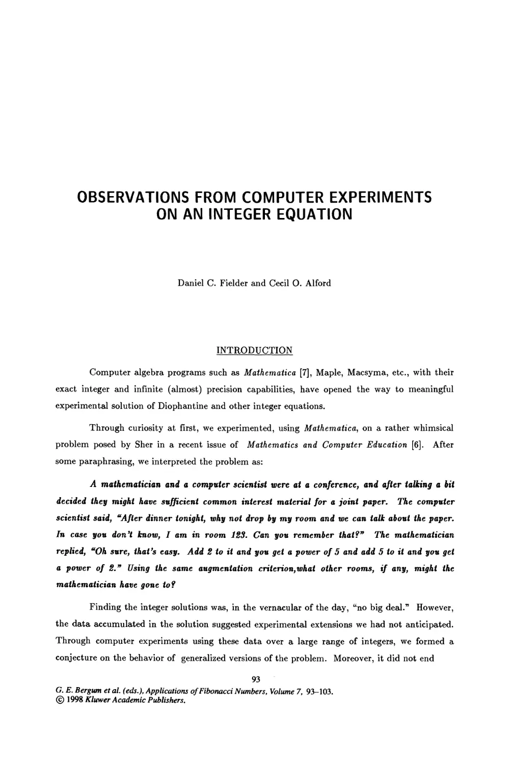
A NOTE ON DERIVED LINEAR RECURRING SEQUENCES
Michele Elia 83
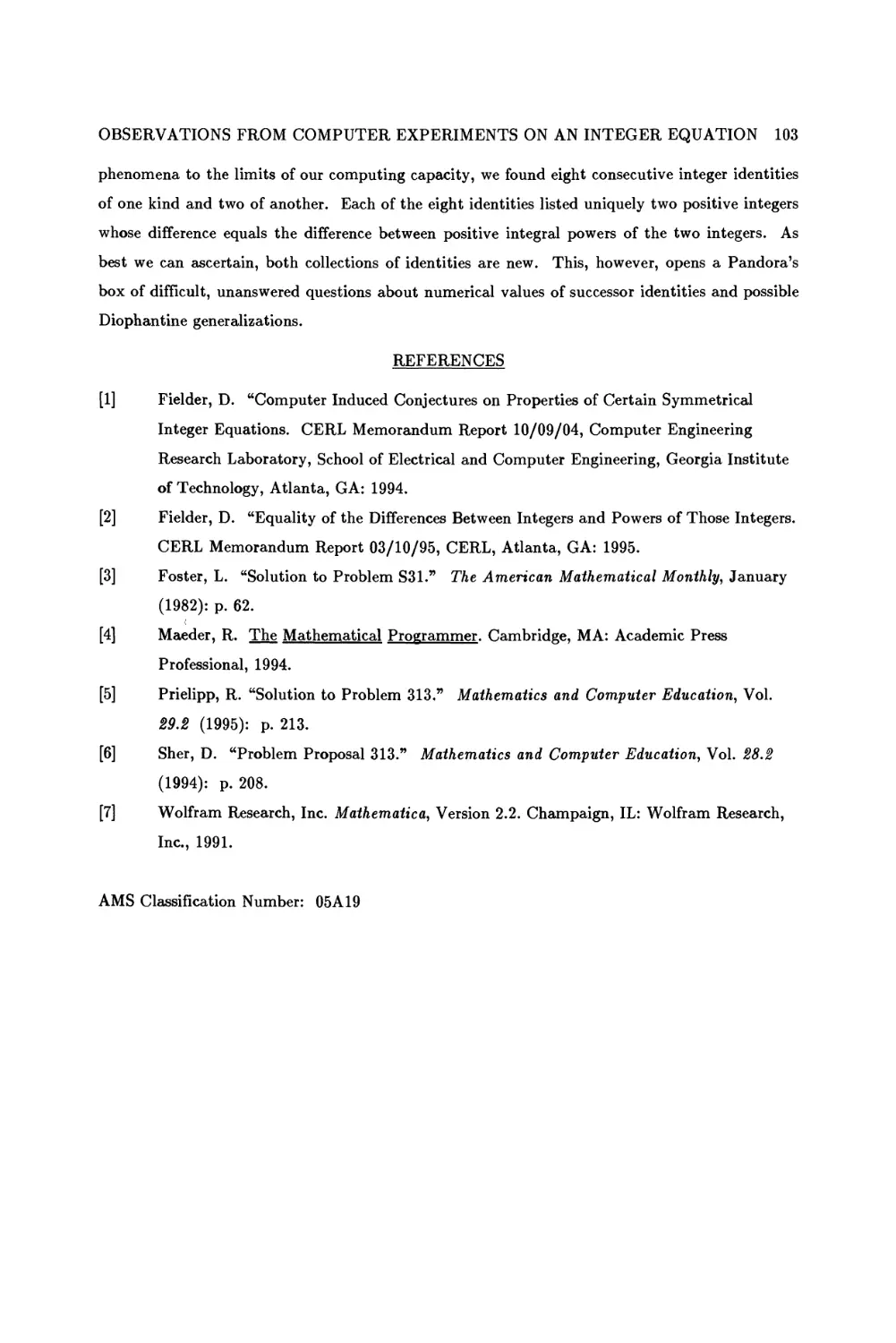
OBSERVATIONS FROM COMPUTER EXPERIMENTS ON AN INTEGER EQUATION
Daniel C. Fielder and Cecil O. Alford 93
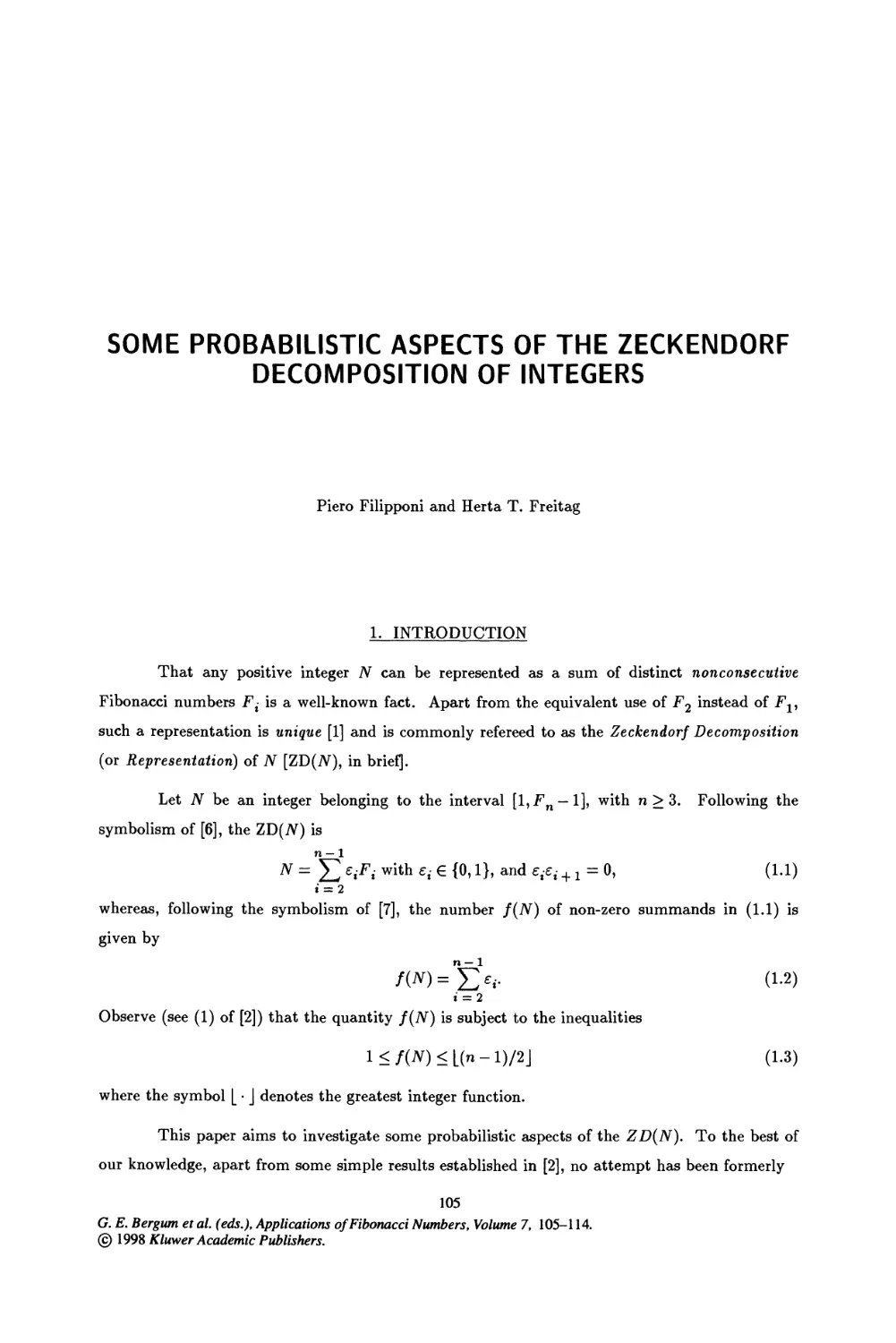
SOME PROBABILISTIC ASPECTS OF THE ZECKENDORF DECOMPOSITION OF
INTEGERS
Piero Filipponi and Heria T. Freitag 105
v

VI
TABLE OF CONTENTS
FIRST DERIVATIVE SEQUENCES OF EXTENDED FIBONACCI AND LUCAS
POLYNOMIALS
Piero Filipponi and Alwyn F. Horadam 115
ELEMENTS OF ZECKENDORF ARITHMETIC
Herta T. Freitag and George M. Phillips 129
BINOMIAL COEFFICIENTS GENERALIZED WITH RESPECT TO A DISCRETE
VALUATION
Sophie Frisch 133
THE DYING FIBONACCI TREE
Bernhard Gittenberger 145
SMALLEST INTEGRAL COMBINATORIAL BOX
Heiko Harborth and Meinhard Moller 153
NEW ASPECTS OF MORGAN-VOYCE POLYNOMIALS
A. F. Horadam 161
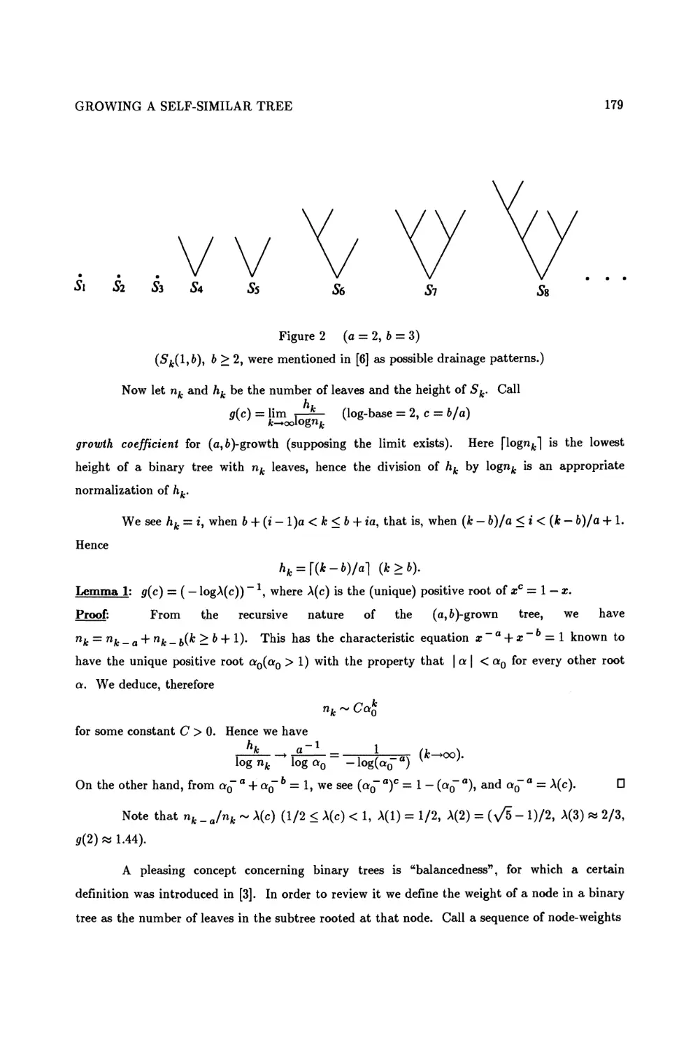
GROWING A SELF-SIMILAR TREE
Yasuichi Horibe 177
LACUNARY SUMS OF BINOMIAL COEFFICIENTS
F. T. Howard and Richard Witt 185
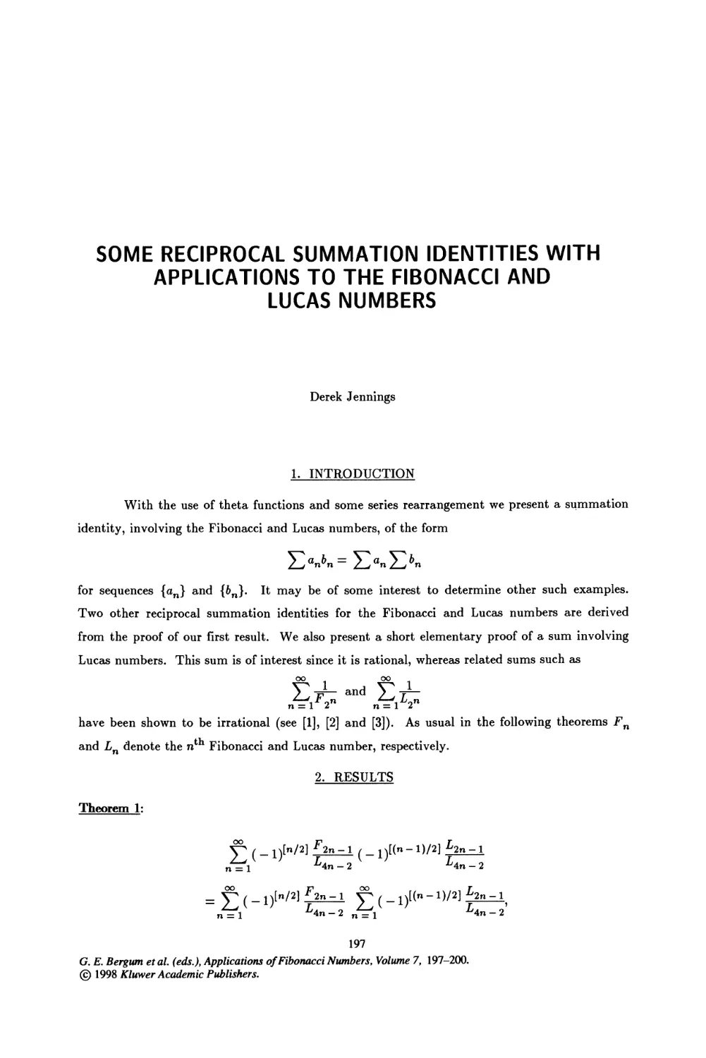
SOME RECIPROCAL SUMMATION IDENTITIES WITH APPLICATIONS TO THE
FIBONACCI AND LUCAS NUMBERS
Derek Jennings 197
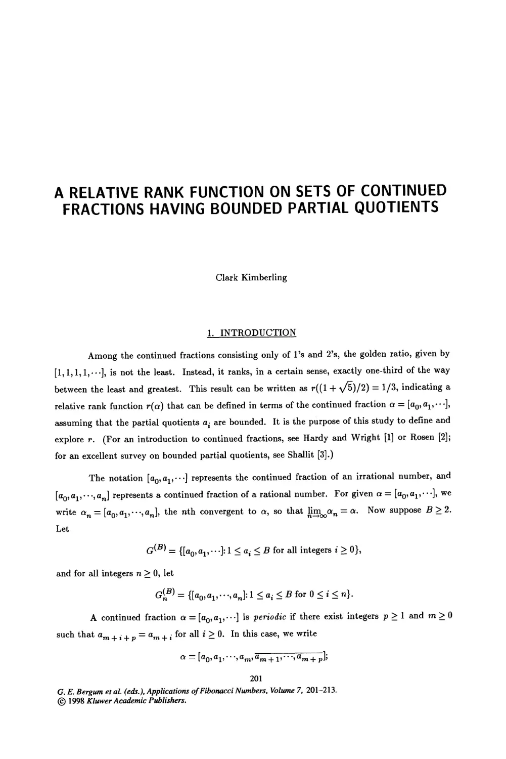
A RELATIVE RANK FUNCTION ON SETS OF CONTINUED FRACTIONS HAVING
BOUNDED PARTIAL QUOTIENTS
Clark Kimberling 201
ON SUMS OF THE RECIPROCALS OF PRIME DIVISORS OF TERMS OF A LINEAR
RECURRENCE
Peter Kiss 215
A FIBONACCI-FRACTAL: A BICOLORED SELF-SIMILAR MULTIFRACTAL
Wolf dieter Lang 221
A GENERALISATION OF RATIOS OF FIBONACCI NUMBERS WITH APPLICATION TO
NUMERICAL QUADRATURE
Timothy N. Langtry 239
THE FIBONACCI PYRAMID
T. G. Lavers 255
ON A THREE DIMENSIONAL APPROXIMATION PROBLEM
Kalman Liptai 265
ANALYSIS OF THE EUCLIDEAN AND RELATED ALGORITHMS
Calvin T. Long and William A. Webb 271
FUNDAMENTAL SOLUTIONS OF u2 - bv2 = - 4r2
Calvin T. Long and William A. Webb 279
PROBABLE PRIME TESTS USING LUCAS SEQUENCES
Willi More 283
ON A FUNCTIONAL EQUATION ASSOCIATED WITH THE FIBONACCI NUMBERS
Kiyota Ozeki 291
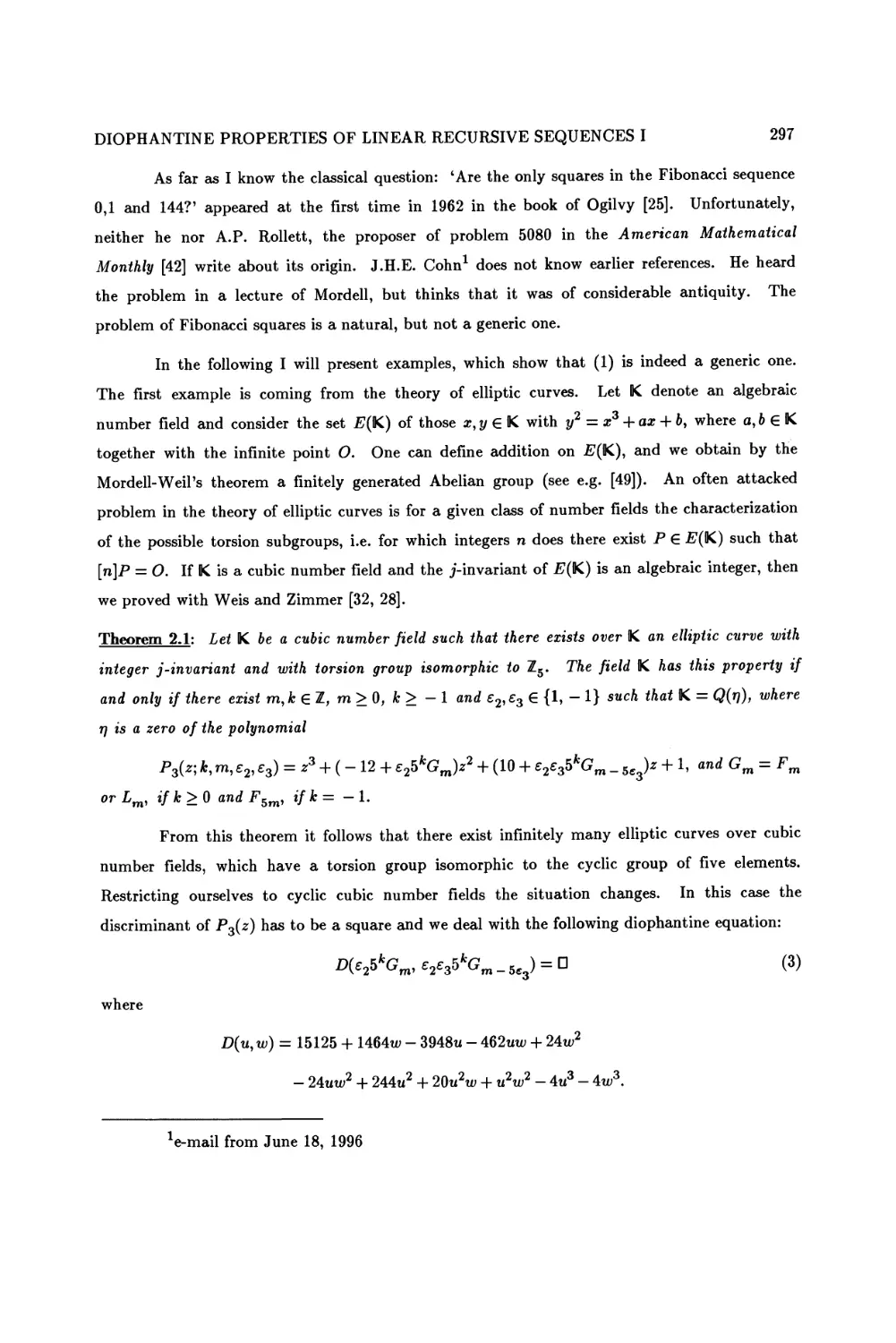
DIOPHANTINE PROPERTIES OF LINEAR RECURSIVE SEQUENCES I
Attila Petho 295
THE CANTOR-FIBONACCI DISTRIBUTION
Helmut Prodinger 311
ON THE PARITY OF CERTAIN PARTITION FUNCTIONS
Neville Robbins 319

TABLE OF CONTENTS
vn
THERE ARE INFINITELY MANY ARITHMETICAL PROGRESSIONS FORMED BY THREE
DIFFERENT FIBONACCI PSEUDOPRIMES
A Rotkiewicz 327
ON MIKOLAS' SUMMATION FORMULA INVOLVING FAREY FRACTIONS
Ken-ichi Sato 333
SECOND ORDER LINEAR RECURRING SEQUENCES IN HYPERCOMPLEX NUMBERS
Klaus Scheicher 337
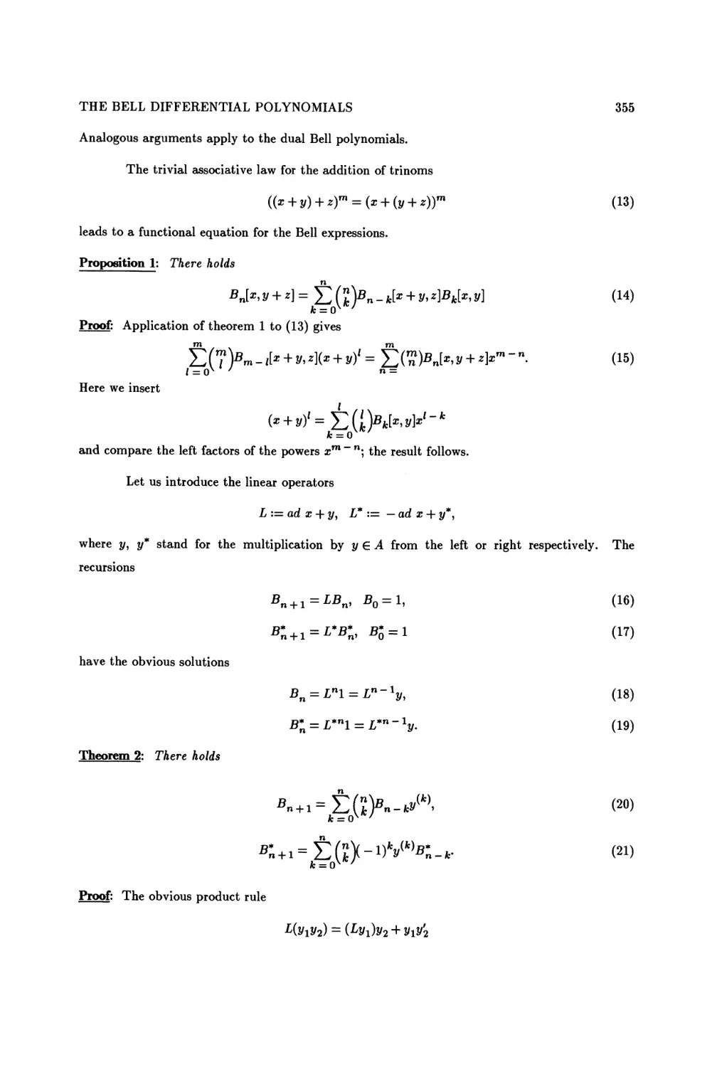
THE BELL DIFFERENTIAL POLYNOMIALS
R. Schimming and S. Z. Rida 353
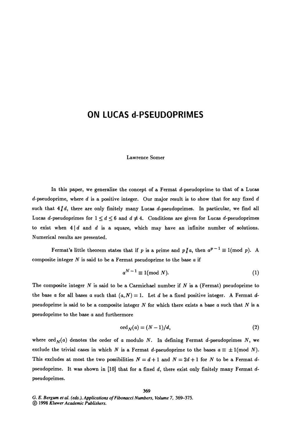
ON LUCAS d-PSEUDOPRIMES
Lawrence Somer 369
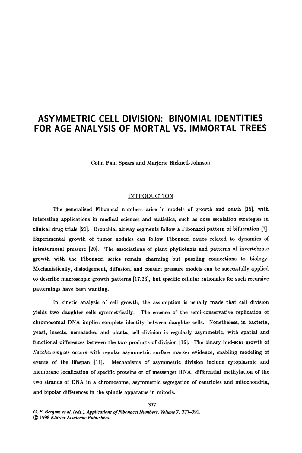
ASYMMETRIC CELL DIVISION: BINOMIAL IDENTITIES FOR AGE ANALYSIS OF
MORTAL VS IMMORTAL TREES
Colin Paul Spears and Marjorie Bicknell-Johnson 377
THE GOLDEN SECTION AND MODERN HARMONY MATHEMATICS
A. P. Stakhov 393
LUCAS FACTORS AND A FIBONOMIAL GENERATING FUNCTION
Indulis Strazdins 401
ELEMENTARY PROPERTIES OF CANONICAL NUMBER SYSTEMS IN QUADRATIC
FIELDS
J org M. Thuswaldner 405
THREE EXAMPLES OF TRIANGULAR ARRAYS WITH OPTIMAL DISCREPANCY AND
LINEAR RECURRENCES
Robert F. Tichy 415
A MULTIVARIATE INVERSE POLYA DISTRIBUTION OF ORDER K ARISING IN THE
CASE OF OVERLAPPING SUCCESS RUNS
Gregory A. Tripsiannis and Andreas N. Philippou 425
INTRODUCTION TO A FIBONACCI GEOMETRY
J. C. Turner and A. G. Shannon 435
TAYLOR FUNCTIONALS AND THE SOLUTION OF LINEAR DIFFERENCE EQUATIONS
Luis Verde-Star 449
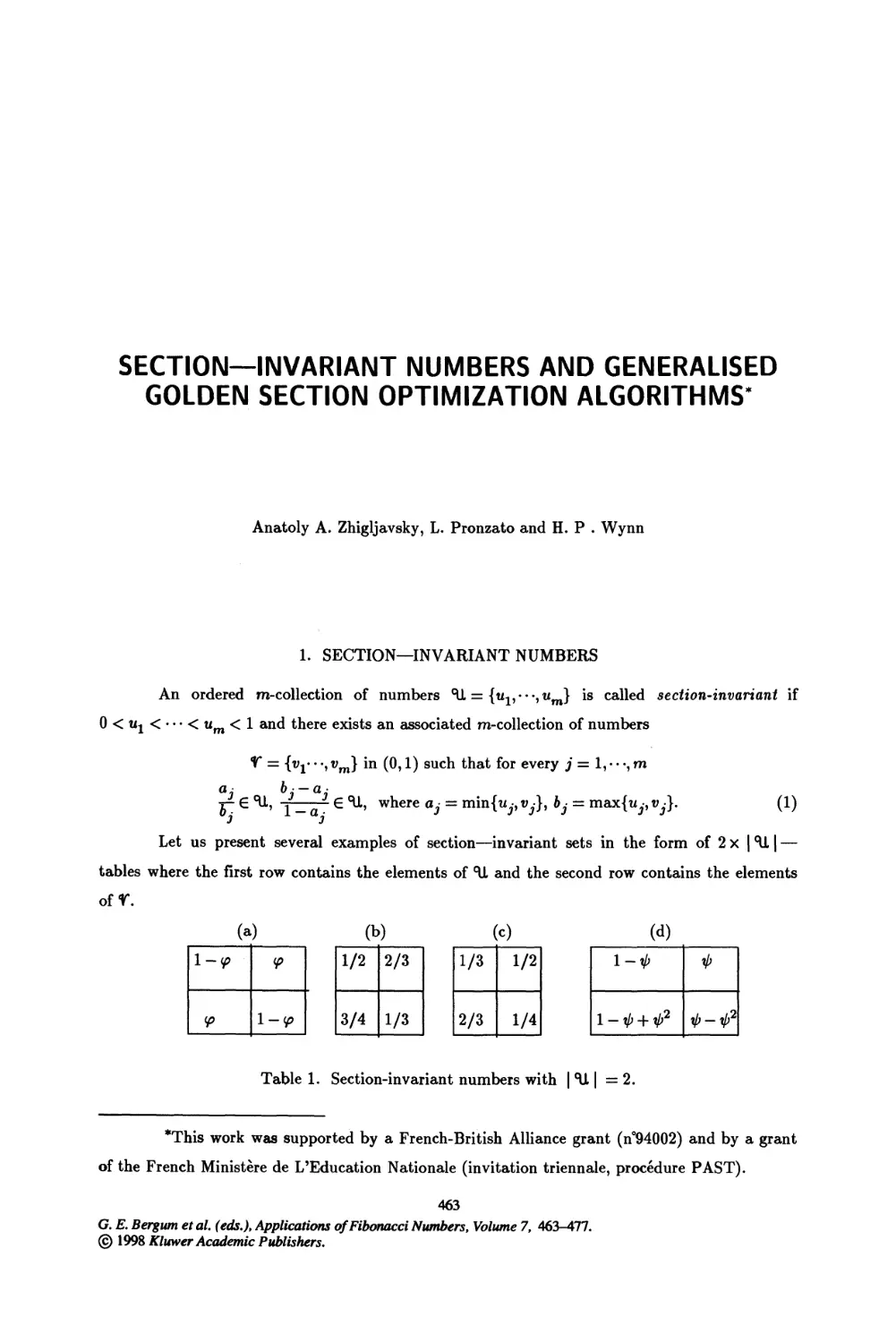
SECTION—INVARIANT NUMBERS AND GENERALISED GOLDEN SECTION
OPTIMIZATION ALGORITHMS
Antoly A. Zhigljavsky, L. Pronzato and H. P. Wynn 463
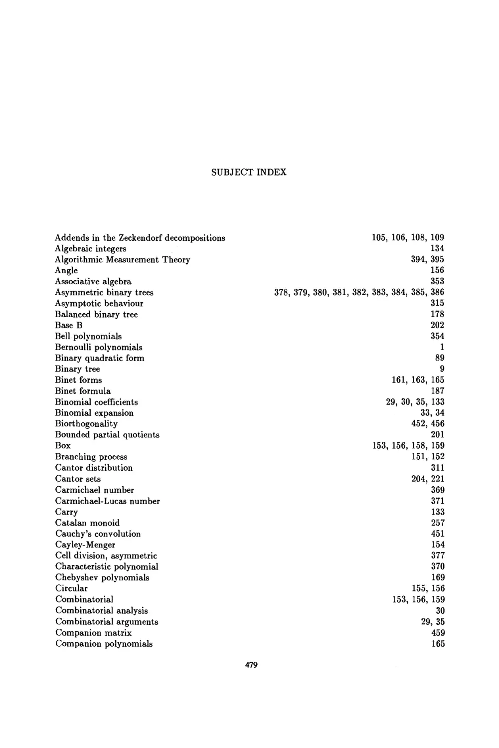
SUBJECT INDEX 479

A REPORT ON
THE SEVENTH INTERNATIONAL CONFERENCE
ON
FIBONACCI NUMBERS AND THEIR APPLICATIONS
The Seventh International Research Conference on Fibonacci Numbers and Their
Applications was held at the Technische Universitat in Graz, Austria, July 15-19, 1996. It was
sponsored by the Austrian Federal Ministry of Science, the Governor of Styria, the Mayor of
Graz, the Technische Universitat in Graz, the Austrian Academy of Sciences, the European
Mathematical Society, and the Fibonacci Association. We all wish to express our deep gratitude
to these sponsors.
How befitting that Graz was chosen as the site. This old university town (die alte
Universitat was founded in 1845) radiates the charm of old-worldliness combined with the spirit
of progressive modernism and technology. What an atmosphere for thought and reflection—
mathematical or otherwise! Enriched by new and happy experiences, all crammed into but a
few days, we once again felt what a unifying force our mathematics is. Being the international
language par excellence, it bridges nationalities, customs, ideas. Colorfully different accents but
enhance the fact that our discipline is understood by all its devotees. And loved by them.
A record number of 95 papers was presented: the U.S.A. provided 27 of them; Austria
11; Italy and Japan tied with nine each; France and Germany with eight. Three speakers came
from Canada, and also from Russia; one of two speakers hailed from each of the remaining
countries. Significantly justifying the fact that our Conference is truly an International one, a
count of the nationalities on the roster revealed the stunning number of 32—among them
Australia, the Republic of Belarus, Cyprus, New Zealand, and South Africa.
These large numbers bespeak the growing magnetism of our "Fibonacci-type
mathematics," and—maybe—Austria's popularity. (May I, a former Viennese, be accused of
bias?) Hence, it was with considerable reluctance that it became necessary to resort to double
sessions. We, indeed, wanted to hear it all.
We did work hard. The sessions started at 9:00 A.M. and extended to the early
evening, followed by enjoyable social events, planned by the Local Committee. Even just
listening to the titles of the presentations, no one could doubt that there is more imagination in
the mind of a mathematician than, possibly, in that of a poet.
The ties of old friendships were strengthened; new ones were kindled. Many of these
became fertile soil for joint authorship research. Predictably, the "Goddess Mathesis," as
Howard Eves calls her, smiles benevolently upon this phenomenon. I was saddened by the
absence of one of my co-authors, George M. Phillips, who, through illness, was unable to attend.
Our deep thanks go to Gerald E. Bergum, the very soul of the Fibonacci Association; to
our Robert Tichy, who ever-so-amiably coped with all the work; and, indeed, also to the other
Committee members, both local and international. Nor will we ever forget Verner E. Hoggatt,
Jr., who created The Fibonacci Association; or Andreas N. Philippou, who launched the idea of
a Fibonacci Conference. Our appreciation, however, also goes out to all the participants of the
Conference. The presentations mirrored their intense mathematical involvement and
enthusiasm.
IX

X
A REPORT ON- •
Finally, "Auf Wiederseheri" in Graz had to come to an end. Now, however, in another
two years—Rochester, here we come! And may our Conferences always be so very fruitful and
enjoyable.
Herta T. Freitag

LIST OF CONTRIBUTORS TO THIS PROCEEDINGS*
Professor Arnold Adelberg (pp. 1-8)
Department of Math. &; Comp. Sci.
PO Box 805
Grinnell, Iowa 50112-0806
Professor Cecil O. Alford (pp. 93-104)
School of Electrical Eng.
Georgia Institute of Technology
Atlanta, Georgia 30332-0250
Dr. Andre B. Ammann
Quartier Prairie 23
Ch-1400 Yverdon-les-Bains
Switzerland
Professor Peter G. Anderson (pp. 9-16)
School of Comp. Sci. and Tech.
Rochester Institute of Technology
102 Lomb Memorial Drive
Post Office Box 9887
Rochester, NY 14623-5608
Professor Shiro Ando (pp. 17-22; 23-28)
College of Engineering
Hosei University
3-7-2 Kajino-Cho
Koganei-Shi, Tokyo 184
Japan
Dr. Demetrios L. Antzoulakos (pp. 29-38)
Department of Mathematics
University of Patras
261.10 Patras, Greece
This list includes all authors and coauthors of papers presented at the conference even if their
paper was rejected, published elsewhere or not submitted to the proceedings. Those who
attended but did not present a paper are also in this list.
XI

xii CONTRIBUTORS TO THIS PROCEEDINGS
Dr. Guy Barat
CMI
39, Rue Joliot-Curie
13453 Marseille Cedex 13
France
Professor Bruno Barigelli
Universita Degli Studi Di Ancona
Instituto Di Matematicae. Stat.
"Giuseppe Avondo-Bodino"
Via Pizzecolli 37
60121 Ancona, Italy
Professor Gerald E. Bergum
Computer Science Dept.
South Dakota State University
Box 2201
Brookings, SD 57007-1596
Dr. Marjorie Bicknell-Johnson (pp. 39-42; 377-392)
665 Fairlane Avenue
Santa Clara, Ca 95051
Professor John R. Burke (pp. 43-48)
Department of Mathematics and Computer Science
Gonzaga University
Spokane, Wa 99258-0001
Professor Walter Carlip (pp. 49-60)
Department of Mathematics
321 Morton Hall
Ohio University
Athens, Ohio 45701-2979
Professor Vladimir M. Chernov
Image Processing Systems
Russian Academy of Sciences
151 Molodogvardeyskaja St.
Samara, 443001, Russia
Professor V. A. Chiricalov
Ul. Pechenegovskaya 1-7, AP. 112
254107, Kyiv, Ukraine
Professor Arnaldo D'amico
Dipt. Di Ingegneria Elettronica
Universita' Di Roma "Tor Vergata"
Via Delia Ricerca Scientifica
00133 Roma, Italia

CONTRIBUTORS TO THIS PROCEEDINGS
Professor Karl Dilcher
Department of Mathematics, Statistics and Computer Science
Dalhousie University
Halifax, Nova Scotia
Canada, B3H 3J5
Dr. Michael Drmota
Institute Fur Algebra Und
Discrete Mathematics
Technische Universitat Wien
Wiedner Hauptstrasse 8-10/118
A-1040 Wien Austria
Professor Andrej Dujella (pp. 61-68; 69-76)
Department of Mathematics
University of Zagreb
Bijenicka Cesta 30
10000 Zagreb, Croatia
Professor C. Dumitrescu
Univeristy of Craiova
Department of Mathematics
Craiova, 1100, Romania
Professor Jean-Marie Dumont (pp. 77-82)
Faculte Des Sciences De Luminy
Mathematique-Informatique
163, Avenue De Luminy-Case 901
13288 Marseille Cedex 9
France
Professor Ernest J. Eckert
Sondervangsvej 43
9000 Aalborg
Denmark
Professor Mohamed Samir Elbuni
Department of Computer Engineering
Al Fateh University
P.O. Box 13292
Tipoli, Libya
Professor Michele Elia (pp. 83-92)
Dipartimento Di Elettronica
Politecnico Di Torino
C.So Duca Degli Abruzzi 24
1-10129 Torino, Italy
Mr. Larry Ericksen
PO Box 172
Millville, New Jersey 08332

xiv CONTRIBUTORS TO THIS PROCEEDINGS
Professor Marco Faccio
Dipt. Di Ingegneria Elettrica
Universita' Di L'aquila
Localita' Monteluco Di Roio
67040 Poggio Di Roio
L'aquila, Italia
Dr. R. M. Femandes
Mathematics Department
Goa University, Taligao
Goa 403 202, India
Professor Giuseppe Ferri
Dipt. Di Ingegneria Elettrica
Universita' Di L'aquila
Localita' Monteluco Di Roio
67040 Poggio Di Roio
L'aquila, Italia
Professor Daniel C. Fielder (pp. 93-104)
School of Electrical and Computer Engineering
Georgia Institute of Technology
Atlanta, Georgia 30332-0250
Mr. Piero Filipponi (pp. 105-114; 115-128)
Fondazione Ugo Bordoni
Viale Baldassarre Castiglione,59
I-00142-Roma, Italy
Professor Philippe Flajolet
Algorithms Project
Inria Rocquencourt
F-78153 LeChesnay
(France)
Dr. Herta T. Freitag (pp. 105-114; 129-132)
B-40 Friendship Manor
320 Hershberger Road, N. W.
Roanoke, VA 24012-1927
Dr. Sophie Frisch (pp. 133-144)
Institut Fur Mathematik C
Technische Universitat Graz
Steyrergasse 30
A-8010 Graz, Austria
Mr. Johannes Gajdosik
Institute Fur Algebra Und
Discrete Mathematics
Technische Universitat Wien
Wiedner Hauptstrasse 8-10/118
A-1040 Wien Austria

CONTRIBUTORS TO THIS PROCEEDINGS
xv
Dr. Hosly Garcia
c/o Dr. Oscar Garcia
Instituto Forestal
Huerfanos 554
Santiago Chile
Professor Anne Gertsch
Universite De Neuchatel
Institut De Mathematiques
Rue Emile-Argand 11
CH-2007 Neuchatel, Switzerland
Dr. Bernhard Gittenberger (pp. 145-152)
Institut Fur Algebra Und Diskrete Mathematik
Technische Universitat Wien
Wiedner Hauptstrasse 8-10/118
A-1040 Wien
Austria
Professor Peter Grabner
Technische Universitat Graz
Institut Fur Mathematik
501 (A)
Steyrergasse 30
A-8010 Graz, Austria
Professor Jaroslav Hand
Department of Mathematics
University of Ostrava
Dvorakova 7
703 01 Ostrava 1
Czech Republic
Professor Dr. Heiko Harborth (pp. 153-160)
Diskrete Mathematik
Technische Universitat Braunschweig
Pockelsstrasse 14, D-38106 Braunschweig
Germany
Professor Debbie Harrell
507 Wachovia St.
Winston-Salem, NC 27101
Professor Alwyn F. Horadam (pp. 115-128; 161-176)
Department of Mathematics, Statistics
and Computer Science
The University of New England
Armidale, N.S.W. 2351
Australia

XVI
CONTRIBUTORS TO THIS PROCEEDINGS
Professor Yasuichi Horibe (pp. 177-184)
Dept. of Applied Mathematics
Science University of Tokyo
1-3 Kagurazaka, Shinjuku-Ku
Tokyo, 162 Japan
Professor Fred T. Howard (pp. 185-196)
Department of Mathematics and Computer Science
Box 7388, Reynolda Station
Wake Forest University
Winston-Salem, NC 27109
Professor Naotaka Imada
Department of Mathematics
Kanazawa Medical University
Uchinada, Ishikawa 920-02
Japan
Dr. Eliot Jacobson (pp. 49-60)
P.O. Box 3322
Santa Barbara, CA 93130-3322
Dr. Derek Jennings (pp. 197-200)
Faculty of Mathematics
University of Southampton
Southampton, S017 1BJ
England
Mr. Young-Soo Kim
Electronics and Telecommunications Research Institute
Taejon, Korea
Professor Clark Kimberling (pp. 201-214)
Department of Mathematics
University of Evansville
1800 Lincoln Avenue
Evansville, Indiana 47722
Dr. Sergey V. Kirpich
Nikiforov St. 7-160
220141 Minsk
The Republic of Belarus
Dr. Peter Kiss (pp. 215-220)
Eszterhazy Karoly Teachers' Training College
Department of Mathematics
3301 Eger PF. 43, Leanyka U. 4
H-Hungary

CONTRIBUTORS TO THIS PROCEEDINGS xvii
Dr. Arnold Knopfmacher
Dept. of Comp. and App. Math.
Univ. of the Witwatersrand
1 Jan Smuts Avenue
Johannesburg, Wits 2050
South Africa
Dr. Joseph Lahr
Rue De L'eglise, 56
1-7224 Walferdange
Grand-Duchy of Luxembourg
Dr. Wolfdieter Lang (pp. 221-238)
Institut Fur Theoretische Physik
Universitat Karlsruhe (th)
Kaiserstrasse 12
D-76128 Karlsruhe
Germany
Professor Timothy N. Langtry (pp. 239-254)
School of Mathematical Sciences
University of Technology, Sydney
PO Box 123
Broadway N.S.W. 2007
Australia
Professor T. G. Lavers (pp. 255-264)
School of Mathematical Sciences
University of Technology, Sydney
P.O. Box 123
Broadway, N. S. W. 2007
Australia
Dr. Jack Y. Lee
280 86 St., #D2
Brooklyn, NY 11209
Professor Pierre Liardet
Universite De Provence
Centre De Mathematiques Et Informatique
39, Rue Joliot-Curie
F-13453 Marseille Cedex 13
France
Dr. Kalman Liptai (pp. 265-270)
Eszterhazy Karoly Teachers' Training College
Department of Mathematics
3301 Eger PF.43, Leanyka U. 4
H-Hungary

XV111
CONTRIBUTORS TO THIS PROCEEDINGS
Professor Calvin T. Long (pp. 23-28; 271-278; 279-282)
Department of Mathematics
Northern Arizona University
Flagstaff, AZ 86011-5717
Professor Sri Gopal Mohanty
Department of Mathematics and Statistics
McMaster University
1280 Main Street West
Hamilton, Ontario, Canada
L8S 4K1
Professor Meinhard Moller (pp. 153-160)
Diskrete Mathematik
Technische Universitat Braunschweig
Pockelsstrasse 14, D-38106 Braunschweig
Germany
Dr. Willi More (pp. 283-290)
Department of Mathematics
University of Klagenfurt
Universitaetsstrasse 65-67
A-9020 Klagenfurt
Austria
Professor Kenji Nagasaka
Department of System k, Control Engineering
College of Engineering
Hosei University
3-7-2, Kajino-cho, Koganei-shi
184 Tokyo, Japan
Professor Shigeru Nakamura
Department of Mathematics
Tokyo Univ. of Mercantile Marine
2-1-6, Etchujima, Kotoku
Tokyo 135 Japan
Professor Tiziano Novelli
Universita Degli Studi Di Ancona
Instituto Di Matematica E. Stat.
Giuseppe Avondo-Bodino"
Via Pizzecolli 37
60121 Ancona, Italy
Professor Dr. Walter Oberschelp
Lehrstahl Fur Angewandte Mathematics
Insbesondere Informatik
Rwth Aachen, Ahornstrasse 55
52074 Aachen, Germany

CONTRIBUTORS TO THIS PROCEEDINGS
xix
Professor Agratini Octavian
University " Babes-Bolyai"
Faculty of Mathematics &; Informatics
Str. M. Kogalniceanu
3400 Cluj-Napoca
Romania
Professor Richard L. Ollerton
Department of Mathematics
University of Western Sydney
PO Box 10, Kingswood
Nepean 2747
Australia
Professor Kiyota Ozeki (pp. 291-294)
Faculty of Engineering
Department of Mathematics
Utsunomiya University
2753 Ishii-Machi
Utsunomiya-Shi, Japan
Professor Maria V. Pershina
Image Processing Systems Inst.
Russian Academy of Sciences
151 Molodogvardeyskaja St.
Samara, 443001, Russia
Dr. S. P. Pethe
Flat #1
Premsagar Co-op Housing Society
Plot #4, Mahatma Nagar
Off Trimbak Road
Nasik 422007 India
Professor Attila Petho (pp. 295-310)
Mathematical Institut
Lajos Kossuth University
H-4010 Debrecen, PO Box 12
Hungary
Professor Andreas N. Philippou (pp. 29-38; 425-434)
26 Atlantis Street
Aglangis
Nicosia, Cyprus
Dr. George M. Phillips (pp. 129-132)
The Mathematical Institute
University of St. Andrews
The North Haugh
St. Andrews KY16 9SS
Fife, Scotland

xx CONTRIBUTORS TO THIS PROCEEDINGS
Professor Stefan Porubsky
Department of Mathematics
Institute of Chemical Technology
Technicka 5
166 28 Prague 6
Czech Republic
Professor Helmut Prodinger (pp. 311-318)
Institut Fur Algebra
Und Diskrete Mathematik
Technische Universitat Wien
Wiedner Hauptstrasse 8-10/118
A-1040 Wien, Austria
Professor L. Pronzato (pp. 463-478)
Laboratoire I3S
Univ. De Nice-Sophia Antipolis
C.N.R.S.-U.R.A. 1376
250 Avenue Albert Einstein
F-06560 Valbonne, France
Professor Milan Randic
Dept. of Mathematics and Computer Science
Drake University
2507 University Avenue
Des Moines, IA 50311
Dr. Paolo E. Ricci
Universita' Di Roma "La Sapienza"
Dip. Di Math. "G. Castelnuovo"
Citta' Universitaria
P. Le A. Moro 2
1-00185, Roma, Italy
Mr. Saad Zagloul Rida (pp. 353-368)
Mathematisches Institut I
Freie Universitat
D-114195 Berlin Germany
Professor Neville Robbins (pp. 319-326)
Mathematics Department
1600 Hollo way Avenue
San Francisco State Univ.
San Francisco, CA 94132
Professor J. Adair Robertson
Peace College
15 East Peace St.
Raleigh, NC 27604

CONTRIBUTORS TO THIS PROCEEDINGS xxi
Professor C. Rocsoreanu
University of Craiova
Department of Mathematics
Craiova, 1100, Romania
Professor Andrzej Rotkiewicz (pp. 327-332)
Institute of Mathematics
Polish Academy of Sciences
UL. Sniadeckich 8
00-950 Warszawa, Poland
Professor Daihachiro Sato (pp. 23-28)
Department of Mathematics and Statistics
University of Regina
Regina, Saskatchewan
Canada S4S 0A2
Professor Ken-Ichi Sato (pp. 333-336)
Department of Mathematics
Nihon University
Koriyama, Fukushima-ken
983 Japan
Professor Klaus Scheicher (pp. 337-352)
Institut Fur Mathematik 501/A
Technische Universitat Graz
Steyrergasse 30/11
A-8010 Graz, Austria
Dr. Rainer Schimming (pp. 353-368)
Institut Fur Math. Und Informatik
Rrnst- Moritz- Srndt- Universitat
Friedrich Ludwig Jahn Strasse 15A
D-17487 Greifswald Germany
Professor A. G. Shannon (pp. 435-448)
School of Mathematical Sciences
University of Technology, Sydney
P.O. Box 123
Broadway, N. S. W. 2007
Australia
Dr. A. A. Sluchenkova
Computer Engineering
Firm "Fibonacci Systems"
P.O. Box 2878
Vinnitsa-286027, Ukraine

xxii
CONTRIBUTORS TO THIS PROCEEDINGS
Professor Yu Smetanin
Scientific Council "Cybernetics"
Russian Academy of Sciences
40 Vavilov Str
Moscow 117967 Russia
Professor Anthony Sofo
Dept. of Comp. and Math. Sciences
Victoria University of Technology
Melbourne 3000, Australia
Dr. Lawrence Somer (pp. 49-60; 369-376)
Department of Mathematics
The Catholic University of America
Washington, DC 20064
Dr. Colin Paul Spears (pp. 377-392)
University of Southern California
#206 Cancer Research Laboratory
1303 N. Mission Road
Los Angeles, CA 90033
Professor A. P. Stakhov (pp. 393-400)
P.O. Box 2878
Vinnitsa-27
Ukraine-286027
Professor Kenneth B. Stolarsky
Department of Mathematics
University of Illinois
1409 W. Green
Urbana, IL 61801
Professor Oto Strauch
Department of Mathematics
Mathematical Institute of the Slovak Academy of Sciences
V Stef anikova UL. 49
814 73 Bratislava, Slovakia
Professor Indulis Strazdins (pp. 401-404)
Department of Mathematics
Riga Technical University
Ausekla Iela 9, Rtu Astf
Riga LV-1010
Latvia
Professor M. V. Subbarao
Department of Mathematical Sciences
University of Alberta
632 Central Academic Building
Edmonton, Canada T6G 2G1

CONTRIBUTORS TO THIS PROCEEDINGS xxiii
Professor E. R. Suryanarayan
Department of Mathematics
University of Rhode Island
Kingston, RI 02881-0806
Professor T. Takahashi
Hosei University
Graduate School
3-7-2, Kajino-Cho, Koganei-Shi
Tokyo, 184, Japan
Professor R. Tamada
Hosei University
Graduate School
3-7-2, Kajino-Cho, Koganei-Shi
Tokyo, 184, Japan
Professor Christian Thurmann
Diskrete Mathematik
Technische Universitat Braunschweig
Pockelsstrasse 14, D-38106 Braunschweig
Germany
Professor Jorg M. Thuswaldner (pp. 405-414)
Institut Fur Mathematik
Technische Universitat Graz
Steyrergasse 30/11
A-8010 Graz, Austria
Professor Dr. Robert F. Tichy (pp. 415-424)
Institut Fur Math. 501 (A)
Technische Universitat, Graz
Steyrergasse 30
A-8010 Graz, Austria
Dr. Gregory A. Tripsiannis (pp. 425-434)
Faculty of Medicine
Department of Medical Statistics
Democritus University of Thrace
Alexandroupolis, Greece
Professor Zdzislaw W. Trzaska
Department of Electrical Engineering
Warsaw University of Technology
00-601 Warsaw Poland
Dr. John C. Turner (pp. 435-448)
Dept. of Math, and Stat.
University of Wikato
Private Bag 3105
Hamilton, New Zealand

XXIV
CONTRIBUTORS TO THIS PROCEEDINGS
Professor Gerhard Turnwald
Mathematisches Institut
Universitat Tubingen
Auf Der Morgenstelle 10
D-72076 Tubingen, Germany
Professor Brigitte Vallee
Departement D'informatique
Universite De Caen
14032 Caen Cedex France
Professor Theresa Vaughan
Dept. of Mathematics
The University of North Carolina
at Greensboro
Greensboro, NC 27412-5001
Professor Luis Verde-Star (pp. 449-462)
Departamento De Matematicas
Univ. Autonoma Metro., Iztapalapa
Apartado 55-534
Mexico D.F., C.P. 09340
Mexico
Professor Clara Viola
Facolta'di Economia
Instituto Di Math. E Statistica
Univ.'Degli Studi Di Ancona
Via Pizzecolli 37
60100 Ancona, Italia
Professor Marcellus E. Waddill
3385 Sledd Ct
Winston-Salem, NC 27106
Professor William A. Webb (pp. 271-278; 279-282)
Department of Pure and Applied Mathematics
Washington State University
Pullman, WA 99164-3113
Mr. Richard N. Whitaker
Bureau of Meteorology
Sydney, 2001, Australia
Professor Richard Witt (pp. 185-196)
Department of Mathematics and Computer Science
Box 7388 Reynolda Station
Winston-Salem, NC 27109

CONTRIBUTORS TO THIS PROCEEDINGS xxv
Professor H. P. Wynn (pp. 463-478)
Department of Mathematics
University of Warwick
Coventry CVA 7AL
United Kingdom
Professor Anatoly Zhigljavsky (pp. 463-478)
Laboratoire I3S
Univ. De Nice-Sophia Antipolis
C.N.R.S.-U.R.A. 1376
250 Avenue Albert Einstein
F-06560 Valbonne, France
Professor Maxime Zuber
Universite De Neuchatel
Institut De Mathematiques
Rue Emile-Argand 11
CH-2007 Neuchatel, Switzerland

FOREWORD
This book contains 50 papers from among the 95 papers presented at the Seventh
International Conference on Fibonacci Numbers and Their Applications which was held at the
Institut Fur Mathematik, Technische Universitat Graz, Steyrergasse 30, A-8010 Graz, Austria,
from July 15 to July 19, 1996. These papers have been selected after a careful review by well
known referees in the field, and they range from elementary number theory to probability and
statistics. The Fibonacci numbers and recurrence relations are their unifying bond.
It is anticipated that this book, like its six predecessors, will be useful to research
workers and graduate students interested in the Fibonacci numbers and their applications.
September 1, 1997 The Editors
Gerald E. Bergum
South Dakota State University
Brookings, South Dakota, U.S.A.
Alwyn F. Horadam
University of New England
Armidale, N.S.W., Australia
Andreas N. Philippou
House of Representatives
Nicosia, Cyprus
xxvn

THE ORGANIZING COMMITTEES
LOCAL COMMITTEE
Tichy, Robert, Chairman
Prodinger, Helmut, Co-Chairman
Grabner, Peter
Kirschenhofer, Peter
INTERNATIONAL COMMITTEE
Horadam, A.F. (Australia), Co-Chair
Philippou, A.N. (Cyprus), Co-Chair
Bergum, G.E. (U.S.A.)
Filipponi, P. (Italy)
Harborth, H. (Germany)
Horibe, Y. (Japan)
Johnson, M. (U.S.A.)
Kiss, P. (Hungary)
Phillips, G.M. (Scotland)
Turner, J. (New Zealand)
Waddill, M.E. (U.S.A.)
XXIX

LIST OF CONTRIBUTORS TO THE CONFERENCE
*ADELBERG, ARNOLD, "Higher Order Bernoulli Polynomials and Newton Polygons."
AMMANN, ANDRE, "Associated Fibonacci Sequences."
*ANDERSON, PETER G., "The Fibonacci Shuffle Tree."
*ANDO, SHIRO, "On the period of Sequences Modulo a Prime Satisfying a Second Order
Recurrence."
ANDO, SHIRO, (coauthor Daihachiro Sato), "On P-Adic Duality Between Pascal's Triangle
and the Harmonic Triangle I."
*ANDO, SHIRO, (coauthors Calvin Long and Daihachiro Sato), "Generalizations to large
hexagons of the Star of David Theorem with Respect to GCD."
*ANTZOULAKOS, DEMETRIOS L., (coauthor Andreas N. Philippou), "Longest success and
failure runs and new polynomials related to the Fibonacci-type polynomials of order k."
BARIGELLI, BRUNO, (coauthor Clara Viola and Tiziano Novelli), "On the Generation of
Pseudorandom Numbers using the Tribonacci Sequences."
*BICKNELL-JOHNSON, MARJORIE, "A note on a representation conjecture by Hoggatt."
*BURKE, JOHN R., "Some Remarks on the Distribution of Subsequences of Second Order
Linear Recurrences."
*CARLIP, WALTER, (coauthors Eliot Jacobson and Lawrence Somer), "A criterion for
stability of two-term recurrence sequences modulo odd primes."
CHIRICALOV, V. A., "Parallel numerical method for solution difference equations."
CHIRICALOV, V. A., "Recurrent relation for calculation of quadrature weight."
DILCHER, KARL, (coauthor Kenneth Stolarsky), "Recursions and Cubic Irrationals."
DRMOTA, MICHAEL, (coauthor Johannes Gajdosik), "The parity of the sum-of-digits-function
of generalized Zeckendorff representations."
*DUJELLA, ANDREJ, "A Problem of Diophantus and Pell Numbers."
*DUJELLA, ANDREJ, "On the Exceptional set in the Problem of Diophantus and Davenport."
DUMITRESCU, C, (coauthor C. Rocsoreanu), "Connections between the Smarandache
Function and the Fibonacci Sequence."
*DUMONT, JEAN-MARIE, "Substitutive numeration systems and a combinatorial problem."
ECKERT, ERNEST J., "Primitive Pythagorean triangles."
*ELIA, MICHELE, "A note on derived linear recurring sequences."
ERICKSEN, LARRY, "The Pascal-De Moivre Triangles."
FERRI, GIUSEPPE, (coauthors Marco Faccio and Arnaldo D'Amico), "Parametric Variations
and Sensitivity in Ladder Networks Recall Fibonacci Numbers."
*FIELDER, DANIEL C, (coauthor Cecil O. Alford), "Observations from computer experiments
on an integer equation."
*The asterisk indicates that the paper is included in this book.
xxxi

XXX11
CONTRIBUTORS TO THE CONFERENCE
*FILIPPONI, PIERO, (coauthor Herta T. Freitag), "Some probabilistic aspects of the
Zeckendorf decomposition of integers."
*FILIPPONI, PIERO, (coauthor Alwyn F. Horadam), "First derivative sequences of extended
Fibonacci and Lucas Polynomials."
FLAJOLET, PHILIPPE, (coauthor Brigitte Vallee), "Continued Fraction Algorithms,
Functional Operators and Structure Constants."
FREITAG, HERTA T., (coauthor George M. Phillips), "Fibonacci Reciprocal Form."
*FREITAG, HERTA T., (coauthor George M. Phillips), "Elements of Zeckendorf Arithmetic."
*FRISCH, SOPHIE, "Binomial coefficients generalized with respect to a discrete valuation."
GERTSCH, ANNE, (coauthor Maxime Zuber), "Fibonacci, Lucas and Pell Numbers: New
Congruences."
*GITTENBERGER, BERNHARD, "The Dying Fibonacci Tree."
GRABNER, PETER J., "Digital expansions with respect to linear recurrences."
GRABNER, PETER J., (coauthor Arnold Knopfmacher), "Metric properties of Engel and
Sylvester series expansions of Laurent series."
HANCL, JAROSLAV, "Irrationality and its application for linear recurrences."
*HARBORTH, HEIKO, (coauthor Meinhard Moller), "Smallest Integral Combinatorial Box."
HARBORTH, HEIKO, (coauthor Christian Thurmann), "Smallest Nonmeshy Trees in
Triangular and Hexagonal Lattices."
HE, MATTHEW, (coauthor Paolo E. Ricci), "Asymptotic distribution of the zeros of weighted
Fiboancci polynomials."
HENDEL, RUSSELL JAY, "Difference Triangles with Independent Displacements."
*HORADAM, A. F., "New Aspects of Morgan-Voyce Polynomials."
*HORIBE, YASUICHI, "Growing a self-similar tree."
*HOWARD, F.T., (coauthor Richard Witt), "Lacunary Sums of Binomial Coefficients."
IMADA, NAOTAKA, "A Sparsest Matrix and the Catalan Numbers."
*JENNINGS, DEREK, "Some reciprocal summation identities with applications to the
Fibonacci and Lucas numbers."
*KIMBERLING, CLARK, "A relative rank function on sets of continued fractions having
bounded partial quotients."
KIRPICH, SERGEY V., "Canonical criterion of structural and temporal organization of
systems."
♦KISS, PETER, "On Sums of the Reciprocals of prime divisors of terms of a linear recurrence."
*LANG, WOLFDIETER, "A Fibonacci-Fractal: a Bicolored Self-Similar Multifractal."
LANGE, LESTER H., "Some Golden mean appearances Verner Hoggatt would have liked."
*LANGTRY, TIMOTHY N., "A generalisation of ratios of Fibonacci numbers with application
to numerical quadrature."
*LAVERS, T. G., "The Fibonacci Pyramid."
LIARDET, PIERRE, "Ergodic properties involving the Fibonacci expansion."
*LIPTAI, KALMAN, "On a three Dimensional Approximation Problem."
*LONG, CALVIN T., (coauthor William A. Webb), "Analysis of the Euclidean and Related
Algorithms."
*LONG, CALVIN T., (coauthor William A. Webb), "Fundamental Solutions of
u — 5v2 = — 4r ."
MOHANTY, SRI GOPAL, "Fibonacci Sequences-a Lattice Path Perspective."
*MORE, WILLI, "Probable Prime Tests Using Lucas Sequences."
NAGASAKA, KENJI, (coauthor T. Takahashi and R. Tamada), "Fibonacci Applications to
Stock Prices Fluctuations with Neural Network System."
NAKAMURA, SHIGERU, "Some Fibonacci k Lucas identities via the Chebyshev Polynomials."
OBERSCHELP, WALTER, "Generating Functions for Linear Partial Recursions."
OCTAVIAN, AGRATINI, "Probabilistic and non-probabilistic properties of the sequences

CONTRIBUTORS TO THE CONFERENCE
XXXlll
OLLERTON, RICHARD L., (coauthor A. G. Shannon), "Some Properties of Generalized Pascal
Squares and Triangles."
OLLERTON, RICHARD L., (coauthor Richard N. Whitaker), "First-Order Recurrence
Relations for the Chebyshev Polynomials and Associated Functions."
*OZEKI, KIYOTA, "On a functional equation associated with the Fibonacci numbers."
PERSHINA, MARIA V., (coauthor Vladimir M. Chernov), "Fibonacci-Mersenne and Fibonacci-
Fermat discrete transforms."
PETHE, S. P., (coauthor R. M. Fernandes), "Two generalized trigonometric Fibonacci
sequences."
*PETHO, ATTILA, "Diophantine properties of linear recursive sequences I."
PORUBSKY, STEFAN, "Covering systems, generalized Kubert identities and difference
equations."
*PRODINGER, HELMUT, "The Cantor-Fibonacci Distribution."
RANDIC, MILAN, "Higher Order Catalan Numbers."
*ROBBINS, NEVILLE, "On the parity of certain partition functions."
*ROTKIEWCZ, A., "There are infinitely many arithmetical progression formed by three
different Fibonacci pseudoprimes."
*SATO, KEN-ICHI, "On Mikolas' summation formula involving Farey fractions."
*SCHEICHER, KLAUS, "Second order linear recurring sequences in hypercomplex numbers."
SCHIMMING, RAINER, "A Catalan triangle and enumeration of genealogical trees."
*SCHIMMING, RAINER, (coauthor Saad Zagloul Rida), "The Bell differential polynomials."
SMETANIN, YU, "The Fibonacci lower bound for the unique reconstruction of a binary word
given its fragments."
SOFO, ANTHONY, "A novel technique for summing series."
*SOMER, LAWRENCE, "On Lucas d-Pseudoprimes."
*SPEARS, COLIN PAUL, (coauthor Marjorie Bicknell-Johnson), "Asymmetric Cell Division:
Binomial Identities for Age Analysis of Mortal vs Immortal Trees."
*STAKHOV, A. P., "The Golden Section and Modern Harmony Mathematics."
STAKHOV, A. P., (coauthor A. A. Sluchenkova), "Ternary Golden Proportion Computers: New
Trend in the Computer Engineering."
STAKHOV, A. P., {coauthors A. A. Sluchenkova and Mohamed Samir Elbuni), "Number
system based on the Fibonacci Two-by-Two Matrix."
STRAUCH, OTO, "A Numerical Integration Method Based on the Fibonacci Numbers."
*STRAZDINS, INDULIS, "Lucas Factors and a Fibonomial Generating Function."
SURYANARAYAN, E. R., "Brahmagupta Polynomials in two complex variables."
*THUSWALDNER, JORG M., "Elementary properties of canonical number systems in
quadratic fields."
*TICHY, ROBERT F., "Three Examples of Triangular Arrays with Optimal Discrepancy k
Linear Recurrences."
*TRIPSIANNIS, GREGORY A., (coauthor Andreas N. Philippou), "A multivariate inverse
Polya distribution of order k arising in the case of overlapping success runs."
TRZASKA, ZDZISLAW W., "On properties and applications of the Fibonacci spiral and
complex Fibonacci numbers."
TURNER, J. C, "Notes on Fibonacci iteration principles."
*TURNER, J. C, (coauthor A. G. Shannon), "Introduction to a Fibonacci Geometry."
TURNWALD, GERHARD, "Distribution properties of linear recurring sequences."
* VERDE-STAR, LUIS, "Taylor functionals and the solution of linear difference equations."
*ZHIGLJAVSKY, ANATOLY A., (coauthor L. Pronzato and H. P. Wynn), "Section—invariant
numbers and generalised Golden Section optimization algorithms."

INTRODUCTION
The numbers
1, 1,2,3,5,8, 13,21,34,55,89,...,
known as the Fibonacci numbers, have been named by the nineteenth-century French
mathematician Edouard Lucas after Leonard Fibonacci of Pisa, one of the best mathematicians
of the Middle Ages, who referred to them in his book Liber Abaci (1202) in connection with his
rabbit problem.
The astronomer Johann Kepler rediscovered the Fibonacci numbers, independently, and
since then several renowned mathematicians have dealt with them. We only mention a few: J.
Binet, B. Lame, and E. Catalan. Edouard Lucas studied Fibonacci numbers extensively, and
the simple generalization
2, 1, 3, 4, 7, 11, 18, 29, 47, 76, 123, ...,
bears his name.
During the twentieth century, interest in Fibonacci numbers and their applications rose
rapidly. In 1961 the Soviet mathematician N. Vorobyov published Fibonacci Numbers, and
Verner E. Hoggatt, Jr., followed in 1969 with his Fibonacci and Lucas Numbers. Meanwhile, in
1963, Hoggatt and his associates founded The Fibonacci Association and began publishing The
Fibonacci Quarterly. They also organized a Fibonacci Conference in California, U.S.A., each
year for almost sixteen years until 1979. In 1984, the First International Conference on
Fibonacci Numbers and Their Applications was held in Patras, Greece, and the proceedings from
this conference have been published. It was anticipated at that time that this conference would
set the beginning of international conferences on the subject to be held every two or three years
in different countries. With this intention as a motivating force, The Second, Third, Fourth,
Fifth and Sixth International Conference on Fibonacci Numbers and Their Applications were
respectively held in alternate years at San Jose, California, Pisa, Italy, Winston-Salem, North
Carolina, St. Andrews, Scotland, and Pullman, Washington. The proceedings from these six
conferences have also been published. Because of the continuous success of the proceeding six
conferences, The Seventh International Conference on Fibonacci Numbers and Their
Applications was held at Graz, Austria July 15-19, 1996, and a Eighth Conference is scheduled
for July 1998 in Rochester, New York.
It is impossible to overemphasize the importance and relevance of the Fibonacci
numbers to the mathematical and physical sciences as well as other areas of study. The
Fibonacci numbers appear in almost every branch of mathematics, obviously in number theory,
but also in differential equations, probability, statistics, numerical analysis, and linear algebra.
They also occur in physics, biology, chemistry, and electrical engineering.
xxxv

XXXVI
INTRODUCTION
It is believed that the contents of this book, like its predecessors, will prove useful to
everyone interested in this important branch of mathematics and that this material may lead to
additional results on Fibonacci numbers both in mathematics and in their applications to science
and engineering.
The editors would like to acknowledge The Fibonacci Association, Austrian Federal
Ministry of Science, the Governor of Styria, the Mayor of Graz, the Technische Universitat in
Graz, the Austrian Academy of Sciences, and the European Mathematical Society for their
financial and other assistance in making the Conference a success.
The Editors

HIGHER ORDER BERNOULLI POLYNOMIALS
AND NEWTON POLYGONS
Arnold Adelberg
1. INTRODUCTION
The Bernoulli polynomials B^'fe) of degree n and order / can be defined by
OO n I
E/^HItti)- (i-D
They are monic of degree n in x. The constant coefficients B^' = -#J/(0) are called
(higher order) Bernoulli numbers. They are polynomial functions of / with rational coefficients
[5]. The Bernoulli numbers and polynomials, especially the case / = 1 which is called ordinary,
have been studied extensively, for reasons of intrinsic interest and because of connections with
Fermat's Last Theorem, the Riemann zeta function, the calculus of finite differences, etc.
In this paper, we are primarily concerned with factorization questions of the Bernoulli
polynomials, both over the rational number field Q and over the field of p-adic number Q . We
proved several results in [1] on the powers of p dividing the denominators of the Bernoulli
numbers. We assumed that the order / is an integer, in fact that /G{1,•••,«}, but all the
results remain true if / is a p-adic integer, with no essential change in the proof.
Subsequent to the publication of that paper, it was pointed out to us independently by
M. Filaseta and by B. Dwork that our results could be used to determine the Newton polygon of
1
G. E. Bergum et al. (eds.), Applications of Fibonacci Numbers, Volume 7, 1-8.
© 1998 Kluwer Academic Publishers.

2 A. ADELBERG
jE?J/(:e), or at least the down-sloping part. We carry this out in the current paper and get some
strong factorization results over Q . In certain cases where / € Z, we get factorization results
over Q as well. In particular, we have an irreducibility conjecture for B)?'(x) in §5, which is
proved in special cases. (The polynomial B\?'(x) is essentially Bernoulli of the second kind.)
2. BACKGROUND ON BERNOULLI POLYNOMIALS AND NUMBERS
Most of the following results are well know [12, chapter 6].
By(x) is symmetric about x = 1/2. (2.1)
^)(*)=E(7K)*""''- (2-2)
i = or '
Let (x)n = x(x — 1)- • -(x — n -+-1) be the usual falling factorial. The boundary conditions
are
B$\x) = 1 and B$\x) = xn. (2.3)
If Af(x) = f(x + 1) - /(a?), the basic recursions are
(B$(z)y = «£<,'>_ x(x), AJ?W(x) = nB^Zl\x), and
BV + %) = (l-t)BV\X)+1(x-l)BVl1(X). (2.4)
It follows that
B% + %) = (x - 1)„ , (£<,">(*))' = n(x - l)n _ x ,
3? + l 1
B<?\*) = J (t- l)„d<, and flW = / (* - l)nd*. (2.5)
a; 0
These explicit formulas indicate the significance of the polynomials B)?\x) for analysis.
The following examples illustrate the Bernoulli polynomials for small n.
Bj}\x) = l, B[l\x) = x-l/2,
B$\x) = x2-xl + /(3/ - 1)/12, and
B$\x) = x3- \x2l + xl(Zl - l)/4 + /2(1 - /)/8
= (2x - l)(4x2 - 4x1 + /(/ - l))/8. (2.6)
The irreducibility of B\ \x) and the factorization of B§ '(x) as polynomials in x and /
are typical, namely we have proved [2, Theorem 9.1] that considered as a polynomial in two
variables / and #, the polynomial B^^x) is irreducible over C if n is an even positive integer,

HIGHER ORDER BERNOULLI POLYNOMIALS AND NEWTON POLYGONS 3
while BV\x)/(x -1/2) is an irreducible polynomial over C if n is an odd integer > 1. The
arithmetic questions involving factorization over Q, when / is an integer, are much more subtle.
3. P-ADICS, POLES AND BERNOULLI POLYNOMIALS
The standard exponential valuation is defined by vp(u) = v(u) = r if u £ Q and pr || «,
with i/(0) = oo. Then \u\ = p ~ v^ is the p-adic norm on Q, and Q = completion of Q and
Z = completion of Z with respect to this norm. Clearly v extends to a valuation on Q_, which
is a complete non-archimedean field. It is well know that
oo
Q; = {c=£^Ke{o,---,P-i}, ak^o} (3.1)
i = k
i.e., jp-adic numbers have unique "Laurent series expansions" which generalize the base p
expansions of positive integers. It follows that given the expansion above, v(c) — k. If k > 0,
we say c has a zero, while if k < 0, we say that c has a pole of order | k | ; c is a unit iff k = 0;
zp = {ceQp\u(c)>0}.
In [1, Theorem 3.3 and Remark 2] we completely determined the pole pattern of B^(a?),
i.e., the precise way in which successively higher order poles occur in the coefficients, from the
top degree down. The main results can be summarized as follows:
r
If n = y, aiP% 1S the jp-adic expansion, first consider the digit sum
i = o
S(n) = S(nJp)=JTai. (3.2)
It is easy to see that n = S(n) (mod p — 1), so in particular, p — 1 | n iff p — 1 | S(n).
If S(n)> jp-1, consider Kimura's iV-Function [10] defined by N(n) = N(n, p) = the
smallest positive integer N such that
p-l|iVandp/(^). (3.3)
It is not difficult to show that S(N(n)) = p — 1, and that this condition determines
N(n) by truncating the jp-adic expansion of n from the bottom, i.e., start with the last digit of n
and continue upward until the digit sum is p — 1.
We showed in [1] that if / is any jp-adic integer, there are no poles in B^^x) if
S(n) < p — 1. On the other hand, if S(n) > p — 1, then there may be poles, and the first
occurrences of successively higher order poles are algorithmically determined using the TV-
function. Specifically, the first pole is simple and occurs in degree n — Nv where Nx is minimal
satisfying Nx = N(n-l1) for some bottom segment /x of n such that pU J"//* _i\ ]• Tne
other Ni are determined similarly, starting with n — lx — Nv Note that p — 1 | Ni for all i and

4 A. ADELBERG
that p | Ni for all i > 1. See [1] for details.
The next section gives a conceptually simpler way of understanding this algorithm in
terms of the geometry of Newton polygons.
4. NEWTON POLYGONS AND BERNOULLI POLYNOMIALS
n
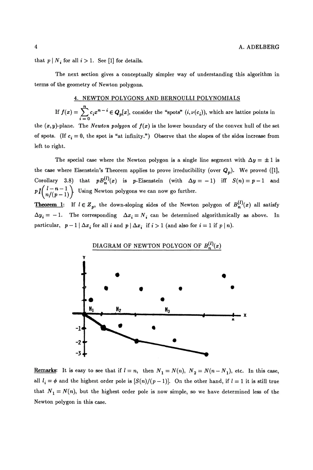
If f(x) = ^T cixn"i E Qp[x], consider the "spots" (t,^(c,)), which are lattice points in
i = o
the (z, y)-plane. The Newton polygon of f(x) is the lower boundary of the convex hull of the set
of spots. (If ci = 0, the spot is "at infinity.") Observe that the slopes of the sides increase from
left to right.
The special case where the Newton polygon is a single line segment with Ay = ± 1 is
the case where Eisenstein's Theorem applies to prove irreducibility (over Qp). We proved ([1],
Corollary 3.8) that pB^\x) is p-Eisenstein (with Ay = -1) iff S(n) = p-1 and
p/[ ~ n "" ■|. V Using Newton polygons we can now go further.
Theorem 1: If / 6 Z , the down-sloping sides of the Newton polygon of B]H\x) all satisfy
Ay, = — 1. The corresponding Axi = Ni can be determined algorithmically as above. In
particular, p — 1 | Ax± for all i and p \ Ax{ if t > 1 (and also for i = 1 if p | n).
DIAGRAM OF NEWTON POLYGON OF B^\x)
Remarks: It is easy to see that if / = n, then iV1 = N(n), N2 = N(n - A^), etc. In this case,
all /,- = <f> and the highest order pole is [S(n)/(p - 1)]. On the other hand, if / = 1 it is still true
that JVj = iV(n), but the highest order pole is now simple, so we have determined less of the
Newton polygon in this case.

HIGHER ORDER BERNOULLI POLYNOMIALS AND NEWTON POLYGONS 5
From [6, Theorem 6.1], we get the following theorem further describing the Newton
polygon of B^n\x) for / € Z . It is well known that v extends uniquely to a valuation of the
algebraic closure Q , which we continue to denote by v.
Theorem 2: For each down-sloping side of the Newton polygon of By(x), there is a unique
monic irreducible factor /,(#) in QJx] whose Newton polygon is that side translated to the
origin. The degree of f^x) is iVt- and the roots of f±(x) in the algebraic closure Qp are exactly
the roots a of By(x) such that i/(a) = — l/N^ All other monic irreducible factors of By(x)
are integral.
Recall the basic definitions of ramification theory. If K is an extension field of Q of
finite degree, the ramification index is the index of the subgroup of Q values in the group of all
K values. The extension is totally ramified if the ramification index equals the extension degree.
A totally ramified extension is wildly ramified if p divides the degree. The following corollary is
a direct consequence.
Corollary: All non-integer roots of B^'^x) in Q generate totally ramified extensions of Qp ,
which are wildly ramified except possibly for the roots of /1(a?), if jp/n.
We say that B^\x) is a maximal pole case if the entire Newton polygon is down-
sloping, i.e., if the highest order pole occurs only in the constant coefficient.
This case happens when B^n\x) has no integer roots in Q . It follows from [1] that the
maximal pole case occurs iff
In the maximal pole case, the highest order pole is S(n)/(p — 1), and Nx = N(n),
N2 = N(n-Nl), etc.
Example: B^\x) is a maximal pole case iff p — l\n. In particular B\^\x) is always a
maximal pole case for p = 2, and is a maximal pole case for p = 3 iff n is even. On the other
hand, Brn \x) = Bn(x) is a maximal pole case iff S(n) = p — 1.
Theorem 3: Suppose B^\x) is a maximal pole case. Then with the same notation as above,
B^n'(x) has a divisor of degree d in QJx] iff d is a sum of Nt-'s, in which case the divisor of that
degree is unique (up to units). In particular, the irreducible factors are distinct and have
different degrees.
Proof: Since all irreducible factors are now accounted for, existence is clear and uniqueness
follows from the fact that Ni > \J N • summed for all j < i. 0

6 A. ADELBERG
Thus in the maximal pole case, if b = S(n)/(p — 1) with the preceding notations, then
fi{x)y ••♦, fi{x) are all the (monic) irreducible factors over Q . There are precisely 2 monic
divisors, which are in one-to-one correspondence with the subsets of the degree set {Nv--, Nb}.
The next corollary is an immediate consequence, where irreducibility can refer to Q or
any subfield such as Q.
Corollary 1: In the maximal pole case, all divisors are symmetric about x = //2, all have degrees
divisible by p — 1, and at most one irreducible factor has degree not divisible by p (if pjn). If d
is the degree of any divisor, then Pn1] \
Example (p = 2): In the maximal pole case, B^n\x) has a divisor of degree d in Q2[x] iff
d = sum of powers of 2 in the 2-adic expansion of n, and for any such d, the monic divisor of
that degree is unique. There are precisely S(rc,2) irreducible factors and precisely 2 ^n' ' monic
divisors over Q2-
Example (n=l=2): In this case, we have B\ \x) = x2 — 2x + 5/6 and it is easy to see that the
maximal pole case occurs iff S(n) = p — 1 iff p = 2 or p = 3. In this case, the roots are
1 dr y/(l/6), which is consistent with the ramification discussion.
Corollary 2: If n is even then B)™\x) has no rational root, and in fact no root in Q2- ^ n IS
odd then n/2 is the only rational root of B)?\x), and is in fact the only root in Q2-
The preceding corollary is remarkable since it show how information about the single
prime 2 can give non-trivial results about Q, in this case completely determining the rational
roots of B)?\x). In the next section we consider the effect of using different primes.
5. GLOBAL RESULTS AND CONJECTURES
In this section, we concentrate on B\?\x), but some of the results are true more
generally for B^^x) if I £ Z. Any factorization of B)?\x) over Q must give consistent
factorizations over Q for all p — 1 | n, in particular for p = 2 and 3 if n is even.
Example: Consider n = 42 = 25 + 23 + 2 = 33 + 32 + 2 • 3. Thus the irreducible factors of
x) over Q2 have degrees 32, 8 and 2, whereas the irreducible factors over Q3 have degrees
36 and 6. It follows that B\2 \x) is irreducible over Q.
Theorem 4: If n is a positive even integer and 5(n, 2) < 2, then B)?\x) is irreducible; if n is an
odd integer > 1 and 5(n,2) < 2, then B^\x)/(x - n/2) is irreducible over Q.
Proof: The odd case is easy since the Newton polygon then consists of two sides with
corresponding irreducible factors, one of which is x — n/2.

HIGHER ORDER BERNOULLI POLYNOMIALS AND NEWTON POLYGONS 7
If n is even and S(n,2) = 1, then B^\x) is 2-Eisenstein, hence irreducible. The only
non-trivial case is where S(n,2) = 2, i.e., rc = 2* + 2J where i > j > 0. If B)?\x) is not
irreducible over Q, then it is the product of irreducible factors of degrees 2* and 2J. But this is
impossible since 3/2* and 3/2J, contradicting Corollary 1 to the preceding theorem.
Conjectures: B)?'(x) is irreducible over Q if n is an even positive integer, and B)™\x)l(x — n/2)
is irreducible over Q if n is an odd integer > 1.
Remarks: In [3] we have considered the complementary case, where S(n,p) < p — 1, by means
of zeros of the coefficients of the Bernoulli polynomials. In particular, we have proven the odd
part of the conjecture if n is an odd prime and the even part if n = rp, where 1 < r < p — 1 and
p( Br. See [3, Theorems 3 and 4(i)] for these proofs. Given the explicit formulas (2.5), it may
be possible to prove the conjectures without resorting to jp-adic analysis. In addition to the
special cases already noted, there is considerable empirical evidence for the conjectures.
REFERENCES
[1] Adelberg, A. "On the Degrees of Irreducible Factors of Higher Order Bernoulli
Polynomials." Acta Arith., Vol. 62 (1992): pp. 329-342.
[2] Adelberg, A. "A Finite Difference Approach to Degenerate Bernoulli and Stirling
Polynomials." Discrete Math, Vol. 140 (1995): pp. 1-21.
[3] Adelberg, A. "Congruences of p-adic Integer Order Bernoulli Numbers." Journal of
Number Theory, Vol. 59 (1996): pp. 374-388.
[4] Brillhart, J. "On the Euler and Bernoulli Polynomials." Journal fur Mathematik, Vol.
234 (1996): pp. 45-64.
[5] Carlitz, L. "Some Properties of the Norlund Polynomial B^\* Math. Nachr., Vol. S3
(1967): pp. 297-311.
[6] Dwork, B., Gerotto, G., and Sullivan, F. An Introduction to G-Functions. Princeton
Univ. Press, Princeton, 1994.
[7] Filaseta, M. "The Irreducibility of all but Finitely Many Bessel Polynomials." Acta
Math., Vol. 174 (1995): pp. 383-397.
[8] Howard, F. T. "Norlund's Number B^K" Applications of Fibonacci Numbers, Volume
5. Edited by G. E. Bergum, A. N. Philipponi and A. F. Horadam. Kluwer Academic
Publishers (1993): pp. 355-366.
[9] Howard, F. T. "Congruences and Recurrences for Bernoulli Numbers of Higher Order."
The Fibonacci Quarterly, Vol. 32 (1994): pp. 316-328.

8 A. ADELBERG
[10] Kimura, N. "On the Degree of an Irreducible Factor of the Bernoulli Polynomials."
Ada Arith., Vol. 50 (1988), pp. 243-249.
[11] McCarthy, P. J. "Irreducibility of Bernoulli Polynomials of Higher Order." Canadian
Journal of Mathematics, Vol. H (1962): pp. 565-567.
[12] Norlund, N. E. Vorlesungen iiber Differenzenrechnung. Chelsea Publ. Co., New York,
1954 (First ed. 1923).
[13] Zhang, Z. and Guo, L. "Recurrence Sequences and Bernoulli Polynomials of Higher
Order." The Fibonacci Quarterly, Vol. 33 (1995): pp. 359-362.
AMS Classification Numbers: 11B68, 11B83, 11S05

THE FIBONACCI SHUFFLE TREE
Peter G. Anderson
1. INTRODUCTION AND SUMMARY
We introduce the Fibonacci Shuffle Tree (FST) which is an infinite binary tree with
nodes 0,1,2,***. The FST is a binary search tree if we associate the key {ka} with node k for
each k = 0,1,2,•••, where a — (1 + v5)/2 and {x} denotes the fractional part of x. If F[k]
denotes a subtree of the FST induced by nodes 0,1,2, •••,£, then F[k] can be obtained from
F[k — 1] by standard binary tree insertion of the key {ka} into F[k — 1].
The sequence of numbers used to build the tree is the same as that in the Three Gap
Theorem [5,6]. The tree provides an intuitive, visual adjunct for that theorem for the irrational
a.
The finite subtrees F[k] of the FST exhibit a number of interesting properties. To study
these, we introduce the F-code, a Fibonacci radix code, similar to Zeckendorf s representation.
The immediate left and right neighbors of each point {ka} as it is visited in [0,1) are easily
identified as ancestors in the FST and substrings in the F-codes.
2. NOTATION k BASIC PROPERTIES
We need the following definitions and relations among: Fn, pn, a, and /?, valid for
n > 0 unless otherwise specified:
1. As usual, the Fibonacci numbers are: F0 = 0, F1 = 1, and Fn , 2 = Fn + ^n + v
2. The zeros of the polynomial x2 - x - 1 are a = (1 + \/5)/2 and (3 = (1 - V/5)/2.
9
G. E. Bergum et al. (eds.), Applications of Fibonacci Numbers, Volume 7, 9-16.
© 1998 Kluwer Academic Publishers.

10 P. G. ANDERSON
3. Let pn = - fin. We have: peven < 0 and podd > 0.
4. p1 = — P and p2 = a. — 2.
6. 1 - p2 = - fi.
7. E]J _ xFfc = Fn + 2 — 1 (by an easy induction).
8. E| = ^ =/?2—£^ = 02* + i_£ for5>0.
9. E£ = ^ - x = ±E£ = xfi2k = p2s - 1, for 5 > 0.
10. Fn = (*»-/?»)A/5.
11. aFn = Fn + x - /?" (using 2.2 and 2.10).
12. {Fna} = {pn} (by 2.3 and 2.11), which is | 0n | for n odd and 1 - fin for n even.
3. F-CODES, A GOLDEN RADIX
Definition 3.1: A vector D = (dmdm_1"-d1) of 0's and 1 's is called a Fibonacci radix code (or
F-code) of length m, for m > 1, ifd1 = dm — 1 and if dk ~ 0 implies dk , 1 = 1 for all k < m.
Definition 3.2: An F-code D represents the integer n(D) = EjJ^. \dkFk.
The F-codes representing Fibonacci numbers, for F2 and above, are given by:
^-"(((lO)-1!))
^2. + i = »«(10),"1"»
with 5 > 1; the code lengths are 2s — 1 and 2s, respectively. For example
(This coding of integers differes from the familiar Zeckendorf notation [3, section 6.6], which
does not use d1 and prohibits any adjacent l's. A regular expression for Zeckendorf codes is
1(01 + 0)*; a regular expression for F-codes is (10 + 1)*1.)
Definition 3.3: An F-code D = (dmdrn_1--d1) represents the real value v(D) = E™_ \dk"Pk'
A pattern for expressing numbers, in order, in their F-codes is established by the
following:

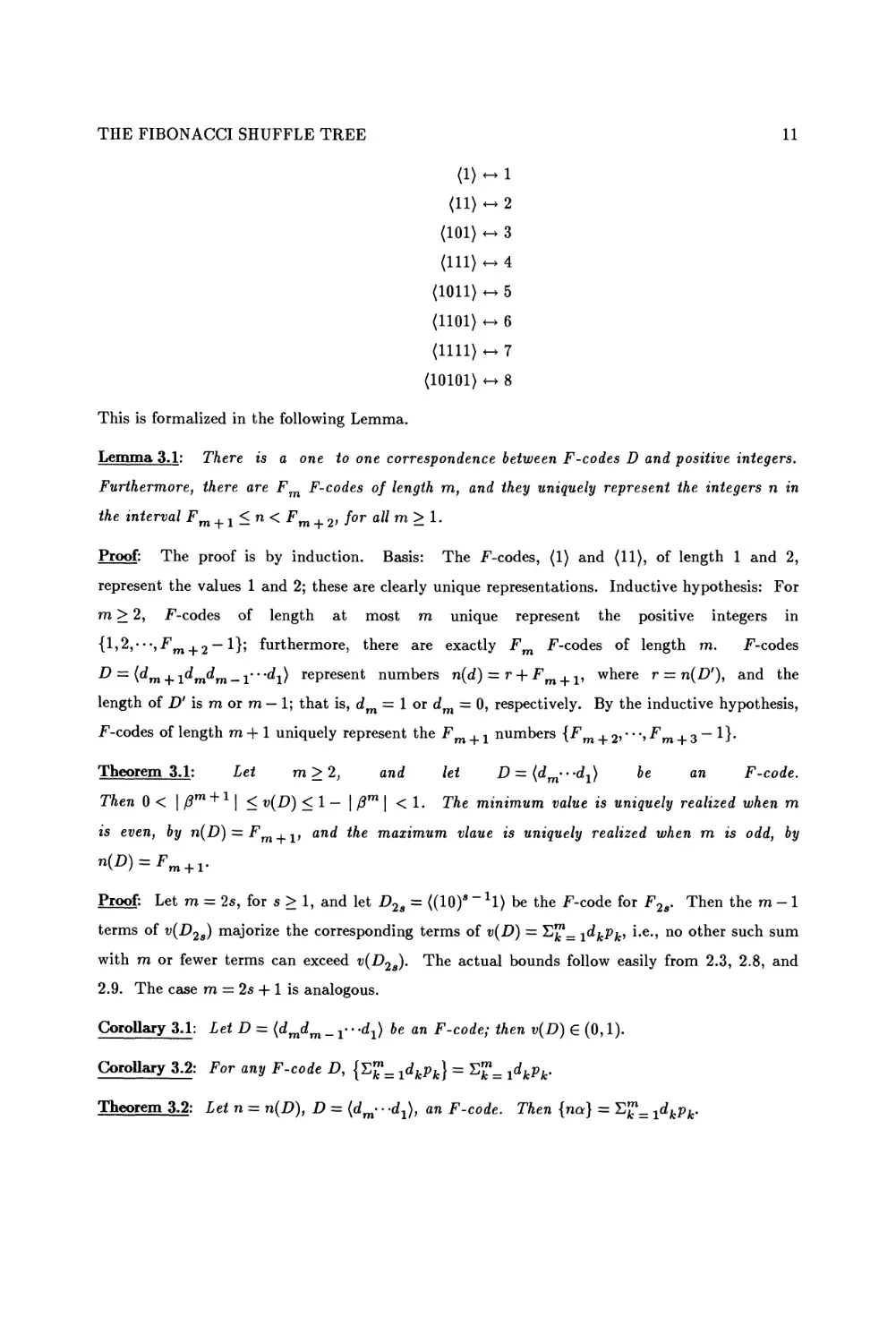
THE FIBONACCI SHUFFLE TREE 11
(1>~1
(11) ~ 2
(101) «-> 3
(111) «-> 4
(1011) ^ 5
(1101) «-> 6
(1111) ^ 7
(10101) <-♦ 8
This is formalized in the following Lemma.
Lemma 3.1: There is a one to one correspondence between F-codes D and positive integers.
Furthermore, there are Fm F-codes of length m, and they uniquely represent the integers n in
the interval Fm + 1<n< Fm + 2, for all m > 1.
Proof: The proof is by induction. Basis: The F-codes, (1) and (11), of length 1 and 2,
represent the values 1 and 2; these are clearly unique representations. Inductive hypothesis: For
m > 2, F-codes of length at most m unique represent the positive integers in
{l,2,---,Fm + 2 -1}; furthermore, there are exactly Fm F-codes of length m. F-codes
D = (drn^1dmdm_1'"d1) represent numbers n(d) = r + Fm + 1, where r = n(D'), and the
length of D' is m or m — 1; that is, dm = 1 or dm = 0, respectively. By the inductive hypothesis,
F-codes of length m -f 1 uniquely represent the Fm , x numbers {Fm + 2, • • •, Fm + 3 — 1}.
Theorem 3.1: Let m>2, and let D — (d^-d-^) be an F-code.
Then 0 < | p™^1 \ < v(D) < 1 — | (3m \ < 1. The minimum value is uniquely realized when m
is even, by n(D) = Fm_,1, and the maximum vlaue is uniquely realized when m is odd, by
n(D) = Fm + v
Proof: Let m = 2s, for s > 1, and let D2s = ((10)a ~ Xl) be the F-code for F2s. Then the m - 1
terms of v(D2s) majorize the corresponding terms of v(D) = HJJ1- idkpk, i.e., no other such sum
with m or fewer terms can exceed v(D2s). The actual bounds follow easily from 2.3, 2.8, and
2.9. The case m = 2s -+-1 is analogous.
Corollary 3.1: Let D - (dmdm _ r • -dj be an F-code; then v(D) € (0,1).
Corollary 3.2: For any F-code D, {E£*= ^p*.} = E£*= xdkpk.
Theorem 3.2: Let n = n(D), D = (dm- • -c^), an F-code. Then {na} = E^= ^p*..

12 P. G. ANDERSON
Proof:
by 2.12
= ^2 dkpk by Corollary 3.2.
k = i
Corollary 3.3: Let D = (dmdrn_1-"d1) be an F-code such that dr = l,l<r<m. Then
EjJ1- rdkPk *s Positive if and only ifr is odd.
Proof: Clear, by Theorem 3.2 and 2.3.
Corollary 3.4: The set {v(D) \ D is an F-code} is dense in (0,1).
Proof: a is irrational, so the numbers {na}, for n = 1,2,---, are dense in (0,1). The result
follows then from Theorem 3.2.
4. THE BINARY TREE
We construct a binary tree using the data values, in order:
{0a}, {la}, {2a}, ■■■
Construction follows the rules of searching for a value in the tree, and inserting that
value in the proper place—where it will be found by the search algorithm—in case it is not
already there. The tree begins with a single node, the root, which is associated with {Oct} = 0;
all searches start at this node. Each step of a search is located at a node; if the value we are
searching for is the same as the node's value, the search is done; if the value is less than the
node's, the search proceeds to the left child of the node, and, if there is no left child, a new tree
node is constructred as a left child of the current node, and the search terminates; the process in
similar if the value is greater than the node's.
As a consequence of the relationships we have established between F-codes and the
values of numbers of the form {na}, the tree-search path for a value with F-code
D = (dmdrn_1'"d2d1) depends explicitly upon this code. For the purpose of just the present
paragraph, let S • denote either '1' or '10', such that D = (S^S i**^2^i)* The tree search for
v(D) = {n(D)a} will start with the node 0, and then visit, in order, the nodes with F-codes:

THE FIBONACCI SHUFFLE TREE
The F-codes and the binary tree structure carry the same information.
21
1010101
Figure 1: The subtree F[54] of the Fibonacci Shuffle Tree. The nonroot nodes are labeled with
integers n and F-codes D. Geometrically, the node with label (n,D) is plotted at the point
(v(D),n(D)) € (0,1) x Z + , illustrating the use of F-codes for representing integers and real
numbers.

14 P. G. ANDERSON
4.1 The tree-building pattern
The tree grows in consecutive "stages." Let F[n] denote the finite binary tree with
n + 1 nodes containing the values {0a},{la},{2a}v, {not}. The tree's growth pattern is shown
by the following
stage number of children left or right
1 1 right
2 1 left
3 2 right
4 3 left
5 5 right
6 8 left
During stage m, we add Fm nodes to the tree, transforming it from F[Fm + 1 — 1] to
F[Fm _j_ 2 — 1]. All of them have code length m.
A simple pattern in tree-growing and node-placement is the following. A node with F-
code (D) will have children with F-codes (ID) and (10/}). If the length of D is odd, its node is
a right child of its parent, (ID) is a left child, and (10D) is a right child; and conversely for D
of even length. An F-code sub-pattern consisting of consecutive I's corresponds to a zig-zag
path through the tree. A sub-pattern of alternating I's and O's corresponds to a path in a
constant direction.
5. THREE GAPS
One of our motivations for studying the tree is to understand how the numbers {ka} for
0 < k < n subdivide the unit interval. This is answered for any irrational in the following
(quoted from [4, page 511]):
Theorem 5.1: Let 9 be any irrational number. When the points {0}, {20},---, {n0} are placed in
the line segment [0,1], the n + \ line segments formed have at most three different lengths.
Moreover, the next point {(n + 1)0} will fall in one of the largest existing segments.
Let n be a positive integer. We define integers, the left and right neighbors, L(n) and
R(n) of n as follows. L(n) satisfies: L(ri) < n, {L(n)a} < {na}, and {not} — {L(n)a} is minimal.
R(n) satisfies: R(n) < n, {R(n)a} > {na}, and {R(n)a} — (na} is minimal. The real points
under discussion lie in the unit interval, [0,1), consequently certain right neighbor values, R(n)
are undefined; that is, when n = Fm for even m (see Fig 1). For these cases, define the right
neighbor as R(n) — 0 and the right gap as 1 — {na}. It is particularly easy to determine L(n)
and R(n) in terms of the F-code for n. Assume that n(D) = n and that the length m of D is

THE FIBONACCI SHUFFLE TREE 15
even, so n is a left child in the tree. Then R(n) is the parent of n in the tree, and L(n) is the
parent of the nearest ancestor of n that is a right child. F-codes allow us to compute the left
gap {na} — {L(n)a} and the right gap {R(n)a} — {na} (letting the right gap be 1 — {na} for the
exceptional cases).
Theorem 5.2: Let D be an F-code of length m, and n(D) = n. If m is even, R(n) = n — Fm,
and the right gap is \ {3m \ . L{n) — n —Fm,1, and the left gap is |/?m + 1|. If m is odd,
L(n) = n - Fm, and the left gap is | (3m | . R(n) — n- Fm + v and the right gap is \ (3m + 1 \.
Proof: Suppose m is even. Clearly, D is the left child of some D', so n(D') = R(n), and 2.12
provides the specified right-gap value. For the left gap, write D in the form D = ((10)rlle.D"),
where c = X (empty string) or 6 = 0. D" is empty (corresponds to 0) or is an F-code. By the
comments of section 4, D is the end of the line of r -f 1 left children from the common ancestor
(leD"), which is itself the right child of D". Thus, L(n) = n(D"). Note further that the prefix
which extends D" to D is an F-code of F2r + 3, or equivalently, we obtain D" by "subtracting"
Fm + 1 from -D, so L(n) = n — Fm + V Consequently the left gap is
{na}-{L(n)a} = {Fm + 1a}= |/?m + 1|-
Suppose m is odd, and D is a right child. There are two cases to consider. If
D = ((lOyilcD"), the proof for odd m folllows identical reasoning to that of even m. If, on the
other hand, D = ((10)rl), then D is the F-code for ^n + 2 =-^m +1 whicn nas tne right gap
1-{Fm + l<*} = Pm + 1= I ^m + 1 |, as claimed.
6. COMMENTS
This work continues the study [1] of the "Fibonacci shuffle" —that is the permutaiton
of the integers {0, l,--«, Fn — 1} whose k-ih element is kFn_1 mod Fn —to relate how mixed
these numbers are. In the present work we relate this sequence to the standard binary tree for
sorting data as introduced in introductory data structures classes with the observation: "the
resulting tree will be bushy and shallow whenever the input data arrives in a sufficiently
jumbled order." Our FST provides a specific metric for that observation applied to the shuffled
data (or to the fractional parts of multiples of a, which is simply a rescaled set of data).
The study of this tree naturally evokes the F-code notation as an alternative to
Zeckendorfs. A remarkable property of the former, without an analog for Zeckendorfs
notation, is that F-codes located on any search path of the FST are consecutive extensions; i.e.,
the F-code of each tree node is a suffix of any descendant's F-code.

16 P. G. ANDERSON
Such trees and codes are not limited to the golden mean and Fiboancci numbers, but
generalize to other irrationals in the same way generalized Zeckendorf numbers can be built
using other linear recurrences. Irrationals whose simple continued fraction representations have
partial quotients greater than 1 have F-code analogs with coefficients greater than 1 (see [2]).
Irrational points in two- and higher-dimensional spaces have F-code analogs based on higher-
order recurrences, such as Tribonacci numbers, and tree-like structures for which the unit
interval I is replaced with I2. These will be covered in future expositions.
7. ACKNOWLEDGMENT
The author is very grateful to Waifong Chuan and Stanislaw Radziszowski, for many
helpful discussions and suggestions during the writing of this paper. Many thanks are also
hereby expressed to the anonymous referee whose suggestions greatly improved the paper.
REFERENCES
[1] Anderson, P.G. "A Fibonacci-based pseudo-random number generator." Applications
of Fibonacci Numbers. Volume 4. Edited by G.E. Bergum, A.N. Philippou and A.F.
Horadam. Kluwer Academic Publishers, Dordrecht, The Netherlands, 1991: pp. 1-8.
[2] Chuan, W. and Anderson, P.G. "a-radix codes and a-shuffle trees." (to appear).
[3] Graham, R.L., Knuth, D.E. and Patashnik, O. Concrete Mathematics. Addison-
Wesley, 1989.
[4] Knuth, D.E. The Art of Computer Programing. Vol. 3i sorting and Searching.
Addison-Wesley, 1973.
[5] van Ravenstein, T. "The three gap theorem (Steinhaus Conjecture)." J. Austral Math.
Soc. (Series A), Vol. 45 (1988): pp. 360-370.
[6] Sos, V.T. "On the theory of diophantine approximations, I." Acta. Math. Acad. Sci.
Hung., Vol. 8 (1957): pp. 461-471.
AMS Classification Number: 11Z05

ON THE PERIOD OF SEQUENCES MODULO A PRIME
SATISFYING A SECOND ORDER RECURRENCE
Shiro Ando
1. INTRODUCTION
Let {un} be an integer sequence satisfying un + 2 = un + j + un and y be a divisor of
x + x = 1 for an integer x. Juan Pla proved in [5] that the sequence {wn} defined by
wn = xun +1 — un satisfies one of the following two cases.
(a) y divides every wn, (b) y divides no wn.
He studied in [6] necessary conditions under which the case (a) occurs. He proved that a
necessary condition under which a prime divisor p of x2 + x — 1 for an x £ Z divides wn is that
{un} modulo p has a period p — 1. He showed also that this condition is not sufficient for
p | wn, giving an example.
The fact is, however, if a prime p divides x2 + x — 1 for an x £ Z, {un} modulo p has a
period p — 1 except when p = 5 without the condition p \ wn as can be seen easily using the
results of D.D. Wall [7].
The purpose of this short note is to remark this fact and extend it to the integer
sequences defined by un + 2 = «wn +1 + &wn' wnere a and b are integers, and to some of the
higher order recurrence sequences.
2. GENERALIZED LUCAS SEQUENCE
Put f(x) = x2 — ax — b and D — a2 + 46, where a and b are given integers, and let {un}
17
G. E. Bergum et al. (eds.), Applications of Fibonacci Numbers, Volume 7, 17-22.
(c) 1998 Kluwer Academic Publishers.

18 S. ANDO
be an integer sequence satisfying the recurrence relation un , 2 = aun +1 -f bun. Then, we have
the following theorem. For a discussion of the algebraic number theory used here, the reader is
referred to Hasse [3] and Ono [4].
Theorem 1: For a prime p which divides f(x) for an integer #, the sequence {un} has a period
p — 1 modulo p, provided p is not a divisor of D.
Proof: It is shown in M. Hall [1] that if an odd prime p does not divide D and the Legendre
symbol (D/p) = 1, then {un} has a period p — 1 modulo p. The theorem follows easily from
this fact. However, for the convenience of extending the result, we will review the outline.
If p — 2, then a is odd and b is even by the assumptions. Thus, we have un + 2 = un + i
(mod 2).
Now we assume that p is an odd prime. Let a and j3 be roots of f(x) = 0, where
a — P = y/D. Then, we have D / 0 and a ^ (3 by the assumption. Using a, (3 and initial
values, the general term un is expressed as
un = Aan + Bpn, where A = (ux - f3u0)/y/D and B = - (^ - auQ)/y/D.
Put D = c m, where c and m are rational integers and m is square free. If m = 1, then
a and (3 are rational integers and we have an + p~l = an(mod p), (3n + p ~ * = (3n(mod p) and
cun + © -1 = cun(mod p) for every n £ N. Since p is not a divisor of c by the assumption, we
have un+ x = wn(mod p) as is desired.
If m / 1, then the quadratic field F = Q(y/rn) has the discriminant d = m or d = 4m.
By the assumption that p \ f(x); we have
/(«)= (z-f)2-^ = 0 (mod p).
Hence, c2m = (2x — a)2 (mod p). Since (c, jp) = 1, there exists c~ £ TV such that
cc~l = 1 (mod p). Thus, we have m = {(2x — a)c~1}2 (mod p) so that m and d are quadratic
residues modulo p. Then, in the quadratic field F, p is decomposed into the product of two
ideals P and P', that is p = PP\ P ^ P' and iV(P) = p, where iV(P) denotes the norm of P.
Using the generalized Fermat's theorem in F (see [3]) which asserts
0N^ = 0 (mod P),
for any algebraic integer 9 in P, we have
an + p-l _ an (mod p)> ^n + p-l _ pn (mod p)?
V^ + p^EEv^ (mod P),

ON THE PERIOD OF SEQUENCES MODULO A PRIME SATISFYING ... 19
where yD is an integer in F which is not divisible by P. Hence, «n + p_1 = un (mod P). In a
similar manner, we have also un , _ 1 = un (mod P'), and consequently un _|_ 1 = un (mod
p), to complete the proof.
We denote the fundamental period of {un} modulo p with initial values w0, ux by
Tr^u^p).
Example 1: For f(x) = x2 - 7x + 1, D = 45. The recurrence relation for {«„} is
"n + 2-
■7u,
n + l
2//(z), Vx£Z. 7r(l,0;2) = 7r(0,l;2) = 3.
3 | /( — 1) = 9, Z\D. 7T(l,0;3) = 7r(0,l;3) = 6.
5 |/(1)= -5, 5|£>. 7r(l,0;5) = 7r(0,l;5) = 5.
7//(z), Vx£Z. 7r(l,0;7) = 7r(0,l;7) = 4.
11 | /(3) = - 11. tt(1, 0; 11) = tt(0, 1; 11) = 5.
19 | /( - 2) = 19. tt(1, 0; 19) = tt(0, 1; 19) = 9.
3. HIGHER ORDER RECURRENCE SEQUENCES
Let f(x) G Z[x] be a monic irreducible polynomial of degree m > 2, and let F = Q(a) be
a Galois extension of Q, where a is a root of f(x). Then, all roots ax = a, a2, •••, am are
distinct and contained in F. Let D(a) be the Vandermonde determinant of these roots and put
A(a) = D(a)2, D(a)
.m-l
(i)
Then, A (a) is a rational integer. For the integer sequences {un} satisfying the recurrence
relation
un + m = alun + m-l+a2un + m-2 + -' + am-lun + l+ amun
corresponding to
f(x) = xm-a1xm-l am_lX-am,
(2)
(3)
we have the following theorem similar to the quadratic case.

20
S. ANDO
Theorem 2: Assume the polynomial f(x) in (3) satisfies the conditions mentioned above. If a
prime p is a simple divisor of f(x) for an integer #, the sequence {un} satisfying (2) has a period
p — 1 modulo jp, provided p is not a divisor of A(a) defined by (1).
Proof: In the field F, f(x) is decomposed into linear factors;
f(x) = (x- aj (x-a2)>-(x- aj. (4)
Let P be a prime ideal factor of p in the ring of integers R in F. If we fix an x £ Z for which p
is a simple prime factor of f(x), each factor x = ak of (4), where & = 1, 2, ••♦, m, must have a
prime ideal factor Pk of p which is conjugate to P. Then, we have the expression
P = PiPi-Pm (5)
since p is a simple prime factor of f(x). Since the discriminant A of F over Q divides A (a), p
does not ramify in F by the assumption that A(a) is not divisible by p. Therefore, Pv P2, •••,
Pm in (5) are all distinct and we have N(Pk) = p for k = 1, 2, ••♦, m. The rest of the proof
can be done in a similar manner to that of Theorem 1, using the expression
"» = D{a){D^" + D*a* + -" + D",a-)'
where Dk is the determinant obtained by replacing the fc-th row of D(a) with the initial values
of {«„}, m0, uv m2, •••, um_v that is,
Du
ym-l
,m-l
and will be omitted.
The fields in the following three examples are shown in [2] as examples of non-quadratic
extensions of Q whose integer rings are Euclidean. In the examples we denote the fundamental
period of {«„} modulo p with initial values w0, tij, u2, w3 by tt(m0,uvu2,u3;p).
Example 2: For f(x) = xA - 10a?2 + 1, let
a = yfi + V^3.

ON THE PERIOD OF SEQUENCES MODULO A PRIME SATISFYING ... 21
Then, D(a) = 27 x 3 and the recurrence for {un} is un , 4 = 10wn + 2 — «n-
2 |/(1)= -8, 2|A(a).
tt(1, 0,0,0; 2) = tt(0, 1,0,0; 2) = tt(0, 0,1,0; 2) = tt(0, 0,0, l; 2) = 4.
23 |/(2)= -23, 23/A(a).
tt(1, 0,0,0; 23) = tt(0, 1,0,0; 23) = tt(0, 0,1,0; 23) = tt(0, 0,0,1; 23) = 22.
Example 3: For f(x) = a?4 - 2x2 + 9, let
a - i + a/2-
then Z}(a = — 27 x 3, and the recurrence for {un} is un + 4 = 2wn + 2 — 9wn.
2 |/(1) = 8, 2|A(a).
tt(1, 0,0,0; 2) = tt(0, 1,0,0; 2) = tt(0, 0,1,0; 2) = tt(0, 0,0, l; 2) = 4.
3 |/(0) = 9, 3|A(a).
tt(1, 0,0,0; 3) = tt(0, 1,0,0; 3) = tt(0, 0,1,0; 3) = tt(0, 0,0, l; 3) = 4.
5//(*), Va?€Z.
tt(1, 0,0,0; 5) = tt(0, 1,0,0; 5) = tt(0, 0,1,0; 5) = tt(0, 0,0, l; 5) = 24.
17 = /(2) | A(a).
tt(1, 0,0,0; 17) = tt(0, 1,0,0; 17) = tt(0, 0,1,0; 17) = tt(0, 0,0, l; 17) = 16.
Example 4: For f(x) = x4 + x3 + x2 + a? + 1 and a = exp(27n/5), A(a) = 53 and the recurrence
relation for {uj is un + 4 = ~un + 3-un + 2-un + 1-un.
In this case, we have
tt(1, 0,0,0; p) = ?r(0,1,0,0; p) = ?r(0,0,1,0; p) = tt(0, 0,0,1; p) = 5
for any prime p, since the original sequence {un} itself is purely periodic with period 5 for each
of these initial values. Therefore, if a prime p ^ 5 divides an f(x) for an integer a?, then we can
conclude that p = 1 (mod 5) by means of theorem 2.
However, this fact can also be shown directly by the following argument. Since p \ /(a?),
p | (x5 — 1), that is, x5 = 1 (mod p) so that the least positive integer r such that xr = 1 (mod p)
is 1 or 5. If x = 1 (mod p), then /(a?) = 5 (mod p) and p must be 5, contradicting the
hypothesis. Thus, r = 5 while xp~1 = 1 (mod p) as (p, #) = 1, and we have 5 | (p- 1) as is
expected.

22 S. ANDO
In this example, if we taken any prime q instead of 5, then, we have a similar result
concerning a prime p\ f(x) = xq~1 +xq~2 -\ \-x + 1 and the sequence {un} defined by the
recurrence un,1= —un,2 un + l~ un' Moreover, the last statement in example 4
can be extended to the rc-th cyclotomic polynomial $n(x) for any n € N. That is, if a prime p
is not a divisor of n and p \ $n(x) for an integer x, then n \ (p — 1).
REFERENCES
[1] Hall, M. "Divisors of Second-Order Sequences." Bulletin of the American Mathematical
Society, Vol. 43 (1937): pp. 78-80.
[2] Hardy, G.H. and Wright, E.M. An Introduction to the Theory of Numbers. Fifth
Edition. Oxford University Press, 1979.
[3] Hasse, H. Zahlentheorie. Volume 3. Berichtigte Auflage, Akademie-Verlag, Berlin,
1969.
[4] Ono, T. An Introduction to Algebraic Number Theory. Plenum Press, New York,
1990.
[5] Pla, J. "An 'All or None' divisibility Property for a Class of Fibonacci-Like Sequences
of Integers." The Fibonacci Quarterly, Vol. 32.3 (1994): pp. 226-27.
[6] Pla, J. "Some Conditions for 'All or None' Divisibility of a class of Fibonacci-Like
Sequences." The Fibonacci Quarterly, Vol. 33.5 (1995): pp. 464-65.
[7] Wall, D.D. "Fibonacci Series Modulo m." Amer. Math. Monthly, Vol. 07(1960): pp.
525-32.
AMS Classification Numbers: 11B37, 11B39

GENERALIZATIONS TO LARGE HEXAGONS OF THE STAR
OF DAVID THEOREM WITH RESPECT TO GCD
Shiro Ando, Calvin Long and Daihachiro Sato
1. INTRODUCTION
The Star of David theorem with respect to the greatest common divisor states that
GCD(A1, A3, A5) = GCD(A2,A4,A6) for the six coefficients Av A2, A3, A4, A5 and A6 in order
surrounding any element X in Pascal's triangle. This property was discovered by Gould [4] and
first proved by Hillman and Hoggatt [5]. Subsequently a number of alternative proofs and
various interesting generalizations have been presented.
One of the way to generalize this theorem is to extend the result to larger convex
hexagons of binomial coefficients with edges along the horizontal rows and main diagonals of
Pascal's triangle and which have an even number of elements on their perimeter S. The
problem is to compare the GCD's of two sets S1 and S2 of binomial coefficients taken
alternately in order around S.
Concerning this problem, Long and Hoggatt [8] conjectured that if a hexagon has an
even number of coefficients per side, then
GCD^) = GCD(52). (1)
A regular hexagon with an even number of coefficients per side is of this type. For regular
hexagons with an odd number of coefficients per side, Long and Ando conjectured that
GCD(51) = <-GCD(52)) (2)
will hold, where t is a rational number expressed by primes in a set M of small primes. M
depends only on the size of the hexagon and is independent of the location of the hexagon in
Pascal's triangle.
23
G. E. Berg urn et al. (eds.), Applications of Fibonacci Numbers, Volume 7, 23-28.
© 1998 Kluwer Academic Publishers.

24 S. ANDO, C. LONG AND D. SATO
These conjectures have been established for a couple of small hexagons. It was shown in
[6] that equality (1) holds for the regular hexagon with four coefficients per side, while equality
(2) holds with M = {2}, for the regular hexagon with three coefficients per side. In [7], equality
(1) was proved for a hexagon which was not regular and had 2, 4, 6, 2, 4, 6 coefficients in order
on the consecutive sides. Since then we have established equality (1) for the regular hexagon
with six coefficients per side. We do not want to show its proof here, since it is similar to that
in [6] and [7], but is much more complicated. Until now these results have all concerned small
hexagons of particular shape and size, and we had not obtained any results for hexagons of
arbitrary size.
In this paper, we generalize the earlier results to any convex hexagon of binomial
coefficients but in a weak form.
Other triangles, including the Fibonomial triangle, will also be discussed.
2. THE MAIN THEOREM
Let P denote an infinite graph whose vertices correspond to the coefficients in Pascal's
triangle and each vertex is adjacent to all the vertices immediately surrounding it. We denote
Pascal's triangle itself also by P. Define the distance between two vertices in P to be the
minimum length of all possible paths connecting them along rows and main diagonals of P.
The diameter d of a set S of vertices in P is the maximum of the distances between vertices of
S. Our principal result is the following.
Theorem 1: Consider any convex hexagon of binomial coefficients with sides along the rows and
main diagonals of Pascal's triangle and which has an even number of elements on its perimeter
S. Denote the two sets of coefficients taken alternately along the perimeter by Sx and S2>
Then,
v^GCDiSJ) = vp(GCD(S2))
for any prime p > d, where v denotes the jp-adic valuation and d is the diameter of S.
3. THE GCD COVERING PROPERTY IN P
Let X be any coefficient in Pascal's triangle. We say that a configuration C in P covers
X with respect to the GCD, if the equality GCD(C U {X}) = GCD(C) always holds independent
of the location of C and X in P, providing the relative positions of C and X is maintained. In
[3], Ando and Sato determined a necessary and sufficient condition that a star configuration in
P covered its center with respect to the GCD. Thus, here we study the GCD covering property
for configuration which are not stars.

As« ft •Ae
GENERALIZATIONS TO LARGE HEXAGONS OF THE STAR- • • 25
Let Av A2> A3, A4, A5, and A6 denote the hexagon of elements immediately surrounding
any given element X in Pascal's triangle.
In the following we use the same
notations as in [3]. Among the 15 pairs
taken from these six elements, three
pairs, {AVA2}, {A3,A4} and {A5,A6},
cover X with respect to the GCD. Omitting
three pairs, {A2,A3}j {A4,A5} and {AvA6}j Figure 1
from the remaining 12 pairs, we divide the other nine pairs into two groups:
<?i = [{A3,A6}{AVA4},{A2,A5}] and
G2 = [{AvA3},{A2,A4},{A3,As},{A4,Ae},{A5,A1},{Ae,A2}] as illustrated in Figures 2 and 3,
respectively.
Figure 2
•—° y •—q p—• c/ \)—•
Figure 3
First, for each pair in Gx and similarly for G2> we determine a necessary and sufficient
condition that a configuration C which includes that pair in the Pascal's triangle covers X with
respect to the GCD except for a finite number of prime factors depending only on C and not
depending of the location of X; that is, for any sufficiently large prime p, we have
vp(C) = vp(CU{X}), (3)
where v (C) — min{v (A) \ A € C}. By the symmetry and the 120° rotatable property of
covering with respect to the GCD in Pascal's triangle (see [9]), we only need consider (A3,A6)
and (AVA3) as the representatives of G1 and G2, respectively.
Let x = n\/h\kl, where n = h + k. Then, we have, A3 = hx/(k + 1), A6 = kX/(h + 1),
and A1 = kX/n. Fixing a prime p, we let v = v for brevity. Then we look for the conditions
which make v(C) < v(X) for every sufficiently large p, satisfying v(A3) > v(X) and

26
S. ANDO, C. LONG AND D. SATO
v(A6) > v(X), or viAJ > v(X) and v(A3) > v(X).
Thus, we assume that v(h) > 0
and v(k) > 0; that is p \ h and p \ k.
We denote X = nl/h\k\ by (h, k) and
put D = {(iJ)\i>h,j>k},
E = {(hj) \i>h, i + j< n}, and
F={(iJ)\j>k, i + j<n}.
Then, we have the next theorem.
Figure 4
Theorem 2: The equality (3) holds for every sufficiently large prime p such that p \ h and p \ k,
independent of the location of X, if and only if C n D ^ 0, or C H E ^ 0 and C C\ F ^ 0.
Proof: Consider the infinite graph P of section 2. Let r be the distance between X and any
vertex A in the configuration C, and assume that p is a prime and p > r. If p | Ai and p | fc,
then, v(n) = i>(/i + &) > min{i>(/i), t>(&)} so that v(n) > v(h) or v(rc) > v(k), and p | n. Therefore,
none of /i ± 1, • • •, /i ± r; fc ± 1, • • •, fc ± r; rc ± 1, • • •, rc ± r are divisible by p.
If A = (/i +1, A: + j) € Z), then i > 0, j > 0 and r = i + j, and we have that v(A) = v(X)
since A = (n + 1)- • -(n + r)X/(h + 1)- • -(/i + *)(^ +1 )•••(& + j), where we assume for convenience
that (n + 1)* • *(n + r) = 1 for r = 0, and so on.
Now, assume that C C\ E ^ 0 and C C\ F ^ 0. If i>(n) > v(/i), then v(A) < v(X) for
A = (/* - r, k + j) G C 0 F since r > j > 0 and
,4 = h(h - 1). • .(h - r + l)X/n(n - 1> ..(h-r + j + 1)(* + 1)- • •(* + j).
If v(n) > v(k), then a similar argument shows that v(A) < v(X) for AeC C\E.
Next, assume that equality (3)
holds for every prime p larger than the
distance r between X and any vertex A
in the configuration C satisfying p | h
and p | Ar. Set G = {(i, j) \i<h, i + j > n}
and # = {i,j)| j<fc}. UA = (h-i,k + r)eCriG,
then r > i > 0, and we have that v(A) > v(X) since
yt = h(h - 1). • <fc - i + l)(n + 1> -{n + r- i)X/(k + 1> • •(* + r).
If A = (h + i,k-j)£Cn H, then j > 0. Also, v(A) > v(X) when X = (p, p2) since,
i4 = *(*-!)..<!:-i+l)(n + l)..<n + i-i)X/(fc + l)...(fc + t) for t>i,
Figure 5

GENERALIZATIONS TO LARGE HEXAGONS OF THE STAR- • • 27
A = k(k- 1)- • •(* - j + l)X/n(n - 1> • .(n - j + i + l)(/i + 1> • •(/* + i) for 0 < i < i, and
4 = fc(fc-l)..^-i + l)/i(/i-l)...(/i- |t| +l)A'/n(n-l)..-(n-i + i+l) for i < 0,
contradicting the assumption. Thus, it follows that CC\D^0oiCC[F^0.
If we exchange h and fc, then we have CnD^0oiCC\E^:0 completing the proof.
This theorem gives the condition for a configuration C that includes (j43, >16), (ylj,^)
or (i42, A6) to cover X with respect to the GCD for any sufficiently large prime p since we only
need consider p such that p \ h and p \ k for such a configuration.
Corollary: In the case A3 and A6 € C, the condition under which equality (3) holds for every
prime p larger than the maximal distance r between X and all the vertices in the configuration
C is given by CnD^0, ot C C\ E ^ 0 and C fl F ^ 0. In the case ^ and A3 € C, it is given
by CnD -£0 or CflF^O, and in the case A2 and 46 € C, it is given by C H D ^ 0 or
C HE ^ 0. If C includes one of the other nine pairs in G1 and G^, we can characterize this case
in a similar manner, using the configurations obtained by rotating D, E and F 120° or 240°
around X.
4. PROOF OF THEOREM 1
From the above corollary, we can easily prove theorem 1. Applying the corollary to
X £ Sx and C = 52, we obtain v (X) > v (GCD(52)) since C and X meet the conditions in the
corollary no matter where X is located in Sv Thus, ^(GCD^)) > i>p(GCD(S2)).
Exchanging St and 52, we obtain v (GCD^j)) < v (GCD(52)) to complete the proof.
5. GENERALIZATIONS
Using similar arguments, we can prove the above results for the generalized Pascal
triangle, which has entries f? | = -,=?—f5—, where h + k = n, 0 <h <n, where FTan = a-.a2'• -an
and {aj is a strong divisibility sequence. This includes the Fibonomial array as the case where
<*« = *■»•
For the generalized Pascal triangle, the "if part of theorem 2 still holds by replacing
the condition p > r with p > ar as in [2]. Then, we can establish a theorem corresponding to
theorem 1, in which the condition p > d is replaced by p > ad.
For the modified Pascal triangle defined in [1], which has entries (n -+- \)\/h\k\, where
h + k = n, instead of binomial coefficients, we can prove corresponding theorems concerning the
least common multiple (LCM) instead of the GCD. Proofs using the facts shown in [1] are
similar to those above and will be omitted.

28 S. ANDO, C. LONG AND D. SATO
REFERENCES
[1] Ando, S. "A Triangular Array with Hexagon property, Dual to Pascal's Triangle."
Applications of Fibonacci Numbers, Volume 2. Edited by G.E. Bergum, A.N. Philippou
and A.F. Horadam, Kluwer Academic Publishers, Dordrecht, The Netherlands, (1988):
pp. 61-67.
[2] Ando, S. and Sato, D. "On the Proof of GCD and LCM Equalities Concerning the
Generalized Binomial and Multinomial Coefficients." Applications of Fibonacci
Numbers. Volume 4. Edited by G.E. Bergum, A.N. Philippou and A.F. Horadam.
Kluwer Academic Publishers, Dordrecht, The Netherlands, (1991): pp. 9-16.
[3] Ando, S. and Sato, D. "A Necessary and Sufficient condition that Rays of a Star
Configuration on Pascal's Triangle Cover Its Center with Respect to GCD and LCM."
Applications of Fibonacci Numbers. Volume 5. Edited by G.E. Bergum, A.N.
Philippou and A.F. Horadam. Kluwer Academic Publishers, Dordrecht, The
Netherlands, (1993): pp. 11-36.
[4] Gould, H.W. "A New Greatest Common Divisor Property of the Binomial
Coefficients." The Fibonacci Quarterly, Vol. 10.6 (1972): pp. 579-584, 628.
[5] Hillman, A.P. and Hoggatt, Jr., V.E. "A Proof of Gould's Pascal Hexagon Conjecture."
The Fibonacci Quarterly, Vol. 10.6 (1972): pp. 565-568, 598.
[6] Long, C.T. and Ando, S. "Two Generalizations of Gould's Star of David Theorem."
Applications of Fibonacci Numbers. Volume 4. Edited by G.E. Bergum, A.N. Philippou
and A.F. Horadam. Kluwer Academic Publishers, Dordrecht, The Netherlands, (1991):
pp. 219-230.
[7] Long, C.T. and Ando, S. "Another Generalization of Gould's Star of David Theorem."
The Fibonacci Quarterly, Vol. 30.3 (1992): pp. 251-255.
[8] Long, C.T. and Hoggatt, Jr., V.E. "Sets of Binomial Coefficients with Equal Products."
The Fibonacci Quarterly, Vol. 12.1 (1974): pp. 71-79.
[9] Sato, D. and Hitotumatu, S. "Simple Proof that a p-adic Pascal's Triangle is 120
Degree Rotatable." Proceedings of the American Mathematical Society. Vol. 59 (1976):
pp. 406-407.
AMS Classification Numbers: 11B65, 11A05, 05A10

LONGEST SUCCESS AND FAILURE RUNS AND NEW
POLYNOMIALS RELATED TO THE FIBONACCI-TYPE
POLYNOMIALS OF ORDER k
Demetrios L. Antzoulakos* and Andreas N. Philippou'
1. INTRODUCTION AN SUMMARY
Let L\ ' and Lr£' denote, respectively, the lengths of the longest success and longest
failure runs in n ( > 1) independent Bernoulli trials with constant success probability
p (0 < p < 1), and set q = 1 - p. Also, let {^„ (*)]^°=o ^e tne se(luence of Fibonacci-type
polynomials of order k of Philippou, Georghiou and Philippou [5]. Philippou and Makri [3]
modified a combinatorial argument of Philippou and Muwafi [4] to show that
P(L<Z)<k) = S^-F<£+2%/p), 0<k<n. (1.1)
In the present paper we introduce the sequence of Fibonacci-type polynomials of order
(fc, r), to be denoted by {F^ 'r'(#, y, z)}^_0, an<^ we derive two expansions of the nth term of
this sequence in terms of multinomial and binomial coefficients, respectively. A relation
between these polynomials and the Fibonacci-type polynomials of order k -f 1 is also established.
Next, we use new combinatorial arguments to derive the probability ^(X^ ' < fc, Isn ' < r) in the
case of Markov dependent trials and we relate this probability with the Fibonacci-type
polynomials of order (fc, r). The independent Bernoulli trials are covered as a special case.
*Now at Hellenic Naval Academy, Hatzikyriakou, 18539 Pireaus, Greece
**Now at the House of Representatives, Nicosia, Cyprus
29
G. E. Bergum et al. (eds.), Applications of Fibonacci Numbers, Volume 7, 29-38.
© 1998 Kluwer Academic Publishers.

30 D.L. ANTZOULAKOS AND A.N. PHILIPPOU
In this paper k and r are fixed positive integers, #, y and z are real numbers, and n ■ •
(1 < i < fc, 1 < j < r) are nonnegative integers as specified. Also, unless otherwise stated,
whenever sums and products are taken over i and j, ranging from 1 to k and from 1 to r,
respectively, we shall omit these limits for notational simplicity.
2. FIBONACCI-TYPE POLYNOMIALS OF ORDER (k , r)
In this section we introduce the sequence of Fibonacci-type polynomials of order (fc, r),
to be denoted by {F^ (#,2/, 2)}£°= o> an<^ we derive two expansions of F^ 'r'(tf,y, z) (n > 1) in
terms of multinomial and binomial coefficients, respectively. We also derive expansions in terms
of binomial coefficients for certain expressions in which this sequence is involved. Furthermore,
a relation between these polynomials and the Fibonacci-type polynomials of order k + 1 is
obtained. First, we state two lemmas from combinatorial analysis which will be used in the
sequel.
Lemma 2.1: Let M(n,m) be the number of ways in which n identical objects can be arranged to
form m groups with every group containing at least one object. Then
M(n,m) = (^_\)
Lemma 2.2: Let Q(n, m, s) be the number of ways in which n identical objects can be arranged
to form m groups with every group containing at least one object and no group containing more
than s objects. Then
Q(n,m,s)= £(-!)''(7) ("^V^-nd £<J(n,»n,«)«» = (*VE?)"
Lemma 2.1 is well-known and Lemma 2.2 is a special case of problem 17 on page 105 of
Riordan [6]. We note that Q(n, m, s) = 0 if n < m or n > ms.
Definition 2.1: The sequence of polynomials {F^'r^,2/,z)}^°_ 0 is said to be the sequence of
Fibonacci-type polynomials of order (fc, r), if
Ftf'r\x,y,z) = 0, F[k'r\x,y,z) = l,
and
£ £ zVzfV'JL >(*>». *). if 2 < n < fe + r,
F^'r\x,y,z) = l i + j<n
£ £ xVzF^r)_ fay,z), if n > k + r + 1.
I «' i
Definition 2.1 implies that

LONGEST SUCCESS AND FAILURE RUNS AND NEW POLYNOMIALS- • • 31
F^r\x,y,z) = F^k\y,x,z), n > 0.
The nth term of the sequence {F^ r\x, y, z)} (n > 1) may be expanded as follows:
Theorem 2.1: Let {F^,r\x,y,z)}™= 0 be the sequence of Fibonacci-type polynomials of order
(fc, r). Then, for n > 0,
(j) fi*+l(*'»'*) = E *'»""' E *mw m' *)(?(n - *•m'r)-
i; = 0 m = 0
We shall first establish the following lemma:
Lemma 2.3: ^t {F(^,r\x,y,z)}<^>:=0 be the sequence of Fibonacci-type polynomials of order
(fc,r), and denote its generating function by Gk r(t\x,y,z). Then, for \t\ <1 and
E-E; I ZXV I < 1,
Proof: Let EtE • | zx%yi | < 1. Then, it can be shown by induction on n that
| F\ ,r\x,y,z) | < 1, which shows the convergence of Gk r(t;x,y,z) for at least \t\ < 1. next,
by means of Definition 2.1, we have
oo
Gfc, ,(<;*,»,*)=£*<*•'>(*,»,*)*"
n =0
k + r oo
= ' + E ^n'%>V.Z)t"+ E Fn'r)(^»• Z)<"
n = 2 n = Jfc + r + 1
= '+*£ E E ^w^-,**,*,*)*"-'-''
n = 2 t i
t + j < n
oo
+ E E E ^)W^1. >(«,», *)*" - •' -''
n = Jfe + r + 1 » i
= <+ E E *(*ow *E ^i'.L/*,»,*)*»-'-■''
* i n = i + j
oo
+ 52 E *(*ow E ^fc-.}- >(*.».*)'" "*'"■''
* j n = A; + r + 1
oo
= *+ E E *(*ow E ^„fcir,L,■(*.».*)*"-'"''• (2-1)
« > n = i + j
Introducing the variable m = n — (* + i), (2.1) reduces to

32 D.L. ANTZOULAKOS AND A.N. PHILIPPOU
G*.r(<;*,»,*) = <+ £.£ z(xty(yty £ F<£'"\x,y,z)tm
> J
= <+£.£ **o wc*. r(Mx,», *),
* j
from which the lemma follows.
Proof of Theorem 2.1: First we shall show part (a). Using Lemma 2.3 and the multinomial
theorem, we get
oo oo _ _«
£*■&%.**)'"=£ *£ (**>T W
n = 0 n = 0 [ t J J
= £ £ ^n.nx-v<)^'+'>«
I J tj
Replacing n by n — St-E •(* + i — 1 )**,-.•, we get
£ fftrl<w>«" = £ £ iS^n .n .(«v«)""'«n.
which shows part (a).
We now proceed to part (b).
, by Lemma 2.3,
£Ff.Vl(*,»,*)<n = £ [*£ (*<)*'£ Wl
n = 0 m = 0[ »" i J
m
= £ ""{y^i-S} £ (*o,-Q('\ »».*), byLemma2-2.
m = 0 \ y ' i-m
oo t
: J] ^ *m(*0VJ(«,m,fc) X) (ytYQ(j,m,r), by Lemma 2.2,
i; = 0 m = 0 j — 0
oo t oo
» = 0 m = 0 n = i
oo n »
= £ £ * v* ~' £ 2m(?(j'. to' »•)<?(« -»'. m> *)*".
n = 0 • = 0 m = 0
which shows part (b).
Theorem 2.1(b) (or Theorem 2.1(a) by noting that Ji^ Axly3z) tJ can be expressed as
3nnini[(y/aOis]n,'i = ynn.ni[(a?/y),'z]n,'>) implies that

LONGEST SUCCESS AND FAILURE RUNS AND NEW POLYNOMIALS- • • 33
Fi%%,y,z) = xnF[%fl,lz) = y"F^(| 1,*} n > 0. (2.2)
In the following proposition we obtain binomial expansions for two expressions in which
the sequence {F^ ,r'(x,y,z)}<£'_0 is involved.
Proposition 2.1: Let {F)f 'r (^,2/,^)}^°=o be tne sequence of Fibonacci-type polynomials of
order (fc,r). Then, for n > 1,
min{r,n} n i
00 £ Vi*,£+)i-fav>z)= E^n"f'E 2rroQ(»\m,fc)Q(n-.\m + l,r);
jf = 1 t = 0 m = 0
min{Ar, n} n ,-
(») E *'Hfc+]-.-(*»»-z) = E*'»""*'E jrWo(,'»m+J>*)<?("-•'-m'r)-
i = 1 t = 0 m = 0
Proof: First we shall show part (a). Using Lemma 2.3 we get
oo min{r,n}
E E y^^l-M^r
n = 1 j = 1
oo
= E w'E^+ta^)'"
j n = 0
- £ <»•>'' £4^ (*W)
J m = 0 x ' v y/
m + 1
= £ *m(^^T~i?) £ W'0(»\w»»*)» *>y Lemma 2.2.
The proof may be easily completed along the lines of the proof of Theorem 2.1(b). We proceed
now to part (b). Following the proof of part (a) we have that for n > 1
min{A:,n}
E M\rl-i(w)
= E^xn_iE zmQ(i,rn,r)Q(n-i,m + l,k)
i =0 m = 0
n n-j
= ^T x3yn " 3 ^T zmQ(n - j, m, r)Q(j, m + 1, fc), by setting n - i = j,
j = 0 m = 0
= J2 x'y""' E zm(?(n - i."». r)QU>»» +1. *).
j = 0 m = 0
since Q(n — j, ra, r)Q(j, m + 1, fc) = 0 if m > min{n — j, i — 1}. The last relation establishes part
(b).
In the following proposition we relate the polynomials F^'

34 D.L. ANTZOULAKOS AND A.N. PHILIPPOU
Proposition 2.2: Let {F\f'r\x,y,z)}™= 0 and {F^\y)}^= 0 be the Fibonacci-type polynomials
of order (fc, r) and the Fibonacci-type polynomials of order fc, respectively. Then
min{r,n}
Iwoo £ yJFn\rl - /i. * i) = HVi'W* ^ °-
i = o
Proof: Using Lemma 2.3 we get
oo min{r,n} r oo
n = 0 j=0 j=0 n = 0
.i-(»<)'
r + ir
l-yt
_l-(yt)r + 1
~ l-yt
1 -1 * l-yt
(2.3)
Without loss of generality we can assume that | yt \ < 1, which implies that
lim (yt)r = 0. Therefore, for r—^oo, (2.3) reduces to
oo min{r,n}
n - 0 j = 0
(i-O
l-i(l + y) + t/<fc + 2
OO . .
by Lemma 2.1 of Philippou, Georghiou and Philippou [5], and this completes the proof.
In the following corollary we obtain a binomial expansion of F^l^y) (n > 1), which is
different from the one derived in Theorem 2.1(b) of Philippou, Georghiou and Philippou [5].
Corollary 2.1: Let {F^\y)}^=0 be the sequence of Fibonacci-type polynomials of order k.
Then
FL%i(y)=1£yn-i£,{nm%i,rn,k-l), n > 1.
i = 0 m = 0
Proof: Theorem 2.1(b) and Proposition 2.1(a), for n > 1, imply that
min{r,n}
3 = 0
= X>V""'E zmQ(^mMQ(n-i,m,r) + Q(n-i,m + l,r)].
i =0 m = 0

LONGEST SUCCESS AND FAILURE RUNS AND NEW POLYNOMIALS- • • 35
Using Proposition 2.2 and noting that Q(n, ra, r)^>M(n, m) as r—-kxj, we get
^n + i)(y)=i2vn~iil Q(hm,k)[M(n-i,m) + M(n-i,m + l)],
i = 0 m = 0
from which Corollary 2.1 follows.
3. PROBABILISTIC APPLICATIONS
Let {Xn, n = 1,2,3, —} be a sequence of Markov dependent trials defined by
P(X1 = l) = p0, P(X1=0) = qa,
and for n > 1
P(Xn + 1 = 1 | X„ = 1) = p!, P(Xn + 1 = 0 I Xn = 1) = 9l,
P(Xn + 1 = 1 I X„ = 0) = p2, P(Xn + 1 = 0 I -*„ = 0) = «2,
where 0 < pt- < 1 and ^ = 1 — pt, i = 0,1,2. Presently we use new combinatorial arguments to
express the probability P{Lrn ' < fc, L^' < r) (n > 1) in terms of the Fibonacci-type polynomials
of order (fc,r) and hence in terms of binomial coefficients. Also we derive a formula for
P(Ln ^ fy. Related but not overlapping results have appeared recently by Antzoulakos and
Philippou [1] and Mohanty [2].
Theorem 3.1: Let L^' and L^' denote, respectively, the lengths of the longest success and
longest failure runs in n ( > 1) Markov dependent trials. Then
min{r,n} min{A:,n}
m = l / = 1
where x = pv y = q2 and z = p2q1/p1q2-
Proof: The theorem is true for n — 1. For n > 2, modifying a combinatorial argument of
Philippou and Muwafi [2], we have that a typical element of the event (L^ ' < fc, L^n ' < r) is an
arrangement
AnyX = IW^W' '"E.E^.^±1 (3-1)
such that n{j of the a's are of the form 11---1 00- • -0 (1 < i < k, 1 < j < r), 0 < / < k,
« i
0 < ra < r, / + ra < rc, and EtE (i + j)nt- • = n -1 — ra. The probability of the above
arrangements depends on whether ra or / takes the zero value. Therefore, we shall derive
P(Lrn ' < fc, L^ ' < r) by employing the relation

36 D.L. ANTZOULAKOS AND A.N. PHILIPPOU
k r
p(lp < k, 4°) < r)=y: e KM A»yi)+ Kai1 4*$)
l = lm = l
l + m<n
min{r,n} min{A:,n}
+ y: KaDA-*oi)+ e HaUA«^) (3-2)
m = 1 / = 1
Consider the case 1 < / < k and 1 < m < r. Fix n-• (1 < i < k, 1 < j < r), / and m.
Then the number of the above arrangements (3.1) is (£t-E-nt- -^(IIJI^; •!) ~ *, and each one has
probability
*K>:y - so??* - * n. n ,(p2?r \<a - 1fijP2Plr x - rh^ymn. n .(*v *)"",
by introducing the variables x — pv y = q2 and 2 = P2Q1/P1Q2' Therefore,
/=lm=l
/ + m < n
t^EE-V" E ^#n.n.(xv^
= nri E E **V"4*+rl -1 - m(«.».*). byTheorem 2-!(a),
! = lm = l
/ + m < n
=r?ri ^Vlo^*)* byDefinition 2.1.
The cases m = 0 and / = 0, / = 0 and 1 < m < r, and m = 0 and 1 < / < fc, may be
treated analogously and then the proof of the theorem follows by (3.2).
Theorem 3.2: Let lSn ' and L^n ' denote, respectively, the lengths of the longest success and
longest failure runs in n ( > 1) Markov dependent trials. Then
p(lP<*,L(o)<r) = |>y*-*£ n(A+r^)W'm'*»(*-**.".
r)
+ yQ(i,m,fc)Q(n-i,m + l,r)+^(i,m + l,fc)(3(n-i,m,r)
where x = pv y = q2 and z = p2<l\IV\(l2'
Proof: The proof is an immediate consequence of Theorem 3.1, Theorem 2.1(b) and Proposition
2.1.
Proposition 3.1: Let L^n ' denote the length of the longest success run in n (> 1)

LONGEST SUCCESS AND FAILURE RUNS AND NEW POLYNOMIALS- • • 37
Markov dependent trials and let M(n,m) be as in Lemma 2.1. Then
i=0 m=0
(135+i=y )w. m' *)M(n" *>m)
+ jQ(i,w,^)M(n-i,m + l)+^0(i,m + l,fc)M(n-i,m)
where x = pv y ~ q2 and z = p2q1/p1q2'
Proof: The proof is an immediate consequence of Theorem 3.2 by noting that
P(L^ < k, L^ < r)->P(i£) < k) and Q(n,m,r)->M(n,m) as r-»oo.
The case of independent Bernoulli trials with constant success probability p is a special
case of the Markov dependent trials for pQ = p1 = p2 = p and q0 = q1 — q2 = <?• Therefore, the
results of this section reduce to respective ones regarding independent Bernoulli trials by setting
x = p, y = q and 2 = 1, which are all new results.
Next, we give a new derivation of relation (1.1) for 1 < k < n. In the case of
independent Bernoulli trials we observe that Theorem 3.1 may be written in the form
PiW < *, 4°» < r) = ± £ ^aii 4ft>m)
/ = 0 m = 0
I + m<n
/=0m = 0 E,.E,(.- + i)n.- = n-/-m l ' "
I + m<n l J %J
J'^3
= E E p'«m^+rl-/-m(P.9,l)- by Theorem 2.1(a),
/ =0 m = 0
l+m<n
k min{r,n-/} m
= PnH E (?) *iV!-<-m(l>£.l),by(2.2).
/=o m=o '
Letting r—>oo and using proposition 2.2 and Definition 2.1 of [5], the above relation
implies
p(41)<*) = p"t^V>,(fl=^i(f^1i«(fi=^^V)(f>
In ending this paper, we note that Definition 2.1 gives rise to the numbers
F\ 'r^ = F\ ,r'(l, 1,1), which we call Fibonacci numbers of order (k,r). These numbers have
interesting properties and we shall report on them elsewhere in a related paper.

38 D.L. ANTZOULAKOS AND A.N. PHILIPPOU
ACKNOWLEDGEMENTS
The authors should like to thank an anonymous referee for several comments which
were helpful in improving the clarity of exposition.
REFERENCES
[1] Antzoulakos, D.L. and Philippou, A.N. "Derivation of the probability distribution
functions for succession quota random variables." Ann. Inst. Statist. Math., Vol. 48.S
(1996): pp. 551-561.
[2] Mohanty, S.G. "Success runs of length k in Markov dependent trials." Ann. Inst.
Statist. Math., Vol. 46.4 (1994): pp. 777-796.
[3] Philippou, A.N. and Makri, F.S. "Longest success runs and Fibonacci-type
polynomials." The Fibonacci Quarterly, Vol. 23.4 (1985): pp. 338-346.
[4] Philippou, A.N. &; Muwafi, A.A. "Waiting for the fcth consecutive success and the
Fibonacci sequence of order fc." The Fibonacci Quarterly, Vol. 20.1 (1982): pp. 28-32.
[5] Philippou, A.N., Georghiou, C. and Philippou, G.N. "Fibonacci-type polynomials of
order k with probability applications." The Fibonacci Quarterly, Vol. 23.2 (1985): pp.
100-105.
[6] Riordan, J. An Introduction to Combinatorial Analysis. New York: Wiley, 1958.
AMS Classification Numbers: 62E15, 11B39, 60C05

A NOTE ON A REPRESENTATION CONJECTURE
BY HOGGATT
Marjorie Bicknell-Johnson
Let R(N) be the number of representations of the natural number TV as a sum of
distinct Fibonacci numbers. If no two consecutive Fibonacci numbers are used, then TV is
represented uniquely by Zeckendorf s theorem. For TV = Fn — 1, the Zeckendorf representation is
the only possible representation using distinct Fibonacci numbers; Carlitz [2] and Klarner [3]
both proved that R(Fn — 1) = 1, n = 2, 3, 4, ••• V. E. Hoggatt, Jr., conjectured that if {bn} is
a sequence of natural numbers such that bn , 2 = bn , x + 6n, then R(bn — 1) = R(bn ^_1 — 1) = K
for all sufficiently large n. Hoggatt's conjecture was proved by Klarner [3], who also wrote some
solutions of R(x) — K. Carlitz [2] computed many values for R(N) for specialized TV. This note
discusses when n is "sufficiently large" and computes some specialized sequences {6n} such that
R(bn - 1) = K. (Note: Carlitz uses the notation R(N) while Klarner uses T(TV) for the number
of representations of TV as sums of distinct Fibonacci numbers.)
When is n "sufficiently large"? Since limit (bn + 1/bn) = a = (1 + a/5)/2, we want the
minimum value for n such that bn,1 = [«6n], where [x] is the greatest integer in x. This is not
a trivial problem, since [abn] = bn + 1 or bn,1—l for n > k> where k depends upon how the
subscripts are defined. We compare {bn} with a standardized generalized Fibonacci sequence
{Hn(A*B)}. where Hx = A, H2 = B, Hn + 2 = Hn + 1 + Hn> n > 1, for natural numbers A and
By B > Ay and where also HQ = B — A> A. The Fibonacci sequence {Fn + j} (with initial value
Fj = 1 deleted) appears as Fn,1 = #n(l,2), while the Lucas sequence {Ln} is Ln = #n(l,3).
Given a pair of natural numbers 6^. and bk,v we can standardize the numbering of the
subscripts to write a corresponding sequence {Hn} as follows: If bk > bk + v then k = 0 and take
bk = H0 = Ay bk + 1 = H1= B] H _ t < 0. If bk — bk + v then k = 0 and take bk + 1 — H1 = Ay
39
G. E. Bergum et al. (eds.), Applications of Fibonacci Numbers, Volume 7, 39-42.
© 1998 Kluwer Academic Publishers.

40 M. BICKNELL-JOHNSON
HQ = bk = A = B-A = H2-H1. If bk<bk + v then subtract to find the previous term
bk _ j = bk +1 — bk and compare 6^ _ x and bk as before. Repeated subtraction of pairs of
successive terms will eventually yield zero or a negative value; take the first such term as H __ r
Given 9 and 16, the sequence is •••, -3, 5, 2, 7, 9, 16, 25, •••, where H1 =2, #3 = 9, and
H4 = 16. For 18 and 5, we have •••, - 13, 18, 5, 23, 28, 41, •••, where 18 = H0 and 5 = Hv
while 24 and 40 generate • • •, 0, 8, 8, 16, 24, 40, 64, • • •, with H1 = 8, H3 = 24, and H4 = 40.
For our purposes, however, we will not need to determine the value for the subscript n
to have n "sufficiently large", and Theorem 1, which was proved in [1], will be the easiest to
apply.
Theorem 1: In standardized generalized Fibonacci sequence {Hn(A, £)},
fl„ + 1 = K+l/2], n>k + 2,
where a = (1 + y/b)/2, and k is the smallest integer such that 1 < B — A < Fk, k>2.
Hoggatt's conjecture was proved by Klarner [3] for n "sufficiently large" and is repeated
here as Theorem 2, using {Hn(A,B)} as in Theorem 1.
Theorem 2: Let R(N) be the number of representations of N > 1 as a sum of distinct Fibonacci
numbers {Fn})n>l. If R(Hn - 1) = K and n > k + 2, then R(Hn + 1 - 1) = K, where
1 < H2 - H1 < Fk, k > 2.
As a convenience for the reader, we write R(N) for 1 < N < 60 in the table below.
N R(N) N R(N) N R(N) N R(N)
1
2
3
4
5
6
7
8
9
10
11
12
13
14
15
1
1
2
1
2
2
1
3
2
2
3
1
3
3
2
16
17
18
19
20
21
22
23
24
25
26
27
28
29
30
4
2
3
3
1
4
3
3
5
2
4
4
2
5
3
31
32
33
34
35
36
37
38
39
40
41
42
43
44
45
3
4
1
4
4
3
6
3
5
5
2
6
4
4
6
46
47
48
49
50
51
52
53
54
55
56
57
58
59
60
2
5
5
3
6
3
4
4
1
5
4
4
7
3
6

A NOTE ON A REPRESENTATION CONJECTURE BY HOGGATT 41
Suppose we wish to write {bn} such that R(bn - 1) = R(bn + 1 - 1) = 3. Select some N
such that R(N - 1) = 3; for example, take N = 37. Then [37a + 1/2] = 60 where #(60 - 1) = 3,
and {bn} = {37,60,97,---}. We can also generate many identities involving Fibonacci and Lucas
numbers using the table and Theorem 2. For example, #(29) = #(47) = 5 where 29 = 6F5 - 1
and 47 = 6F6 - 1, giving R(6Fk- 1) = 5, k > 5. One soon needs larger values for R(N) and
some way of organizing results, leading to patterns such as those following which generalize the
well-known R(Fn - 1) = 1, n > 3.
Theorem 3: R(FkFn ~1) = Fk> n>k, k>3.
Proof: Calculations from Theorems 1 and 2 provide
#(2Fn-l) = 2,
#(3Fn-l) = 3,
#(5Fn-l) = 5,
#(8Fn-l) = 8,
#(13Fn-l) = 13,
n>3
n>A
n>b
n>6
n>7.
Taking Hn = FhFn for n > *, we have: Hn = FkFn, Hn + 1 = FkFn + v Hn + 2 = i^n + 2,
satisfy [a#n +1/2] = #n + 1 since [otAFn +1/2] = AFn + 1 from [1]. Then
#(#n-l) = #(#n + 1-l). Carlitz [2] gives Aft**)2 - 1) = J1*, so
Ffc = a(2Tn-l) = Jl(2rn + 1-l).
Conjecture 1: #(FAZn - 1) = 2[(fc + l)/2], n > 2[(* + l)/2] + 1, fc > 2.
Calculations from Theorems 1 and 2 provide
R(Ln-l) = 2, n>3
#(2Ln-l) = 4, n>5
R(3Ln - 1) = 4, n > 5
#(5Ln-l) = 6, n>7
#(8Ln-l) = 6, n>7
#(13Ln-l) = 8, n>9
#(21Ln-l) = 8, n>9.
Conjecture 2: R(LkLn - 1) = 4(* - 1), n > * + 3, ife > 2.
Calculations from Theorems 1 and 2 provide

42 M. BICKNELL-JOHNSON
■R(3Ln-l) = 4, n>5
J2(4Ln-l) = 8, n>6
J2(7Ln-l) = 12, n>7
J2(llZn-l) = 16, n>8.
Conjecture 3: J2(LfcFn - 1) = 2[*/2] + 1, n > k + 2, it > 1.
Calculations from Theorems 1 and 2 provide
fl(Fn-l)=l,
fl(3F„-l) = 3,
fl(4Fn-l) = 3,
fl(7F„-l) = 5,
Ji(llFn-l) = 5,
fl(18F„-l) = 7,
n>3
ra>4
n>5
ra>6
n>7
n>8.
REFERENCES
[1] Bicknell-Johnson, Marjorie and Englund, David A. "Greatest Integer Identities for
Generalized Fibonacci Sequences {Hn}, where Hn = Hn _1 + Hn _ 2." The Fibonacci
Quarterly, Vol. 33.1 (1995): pp. 50-58.
[2] Carlitz, L. "Fibonacci Representations." The Fibonacci Quarterly, Vol. 6.4 (1968):
pp. 193-220.
[3] Klarner, David A. "Partitions of N into Distinct Fibonacci Numbers." The Fibonacci
Quarterly, Vol. 6.4 (1968): pp. 235-244.
AMS Classification Numbers: 11B39, 11B37, 11Y55

SOME REMARKS ON THE DISTRIBUTION OF SUBSEQUENCES
OF SECOND ORDER LINEAR RECURRENCES
John R. Burke
A common theme in mathematics is to examine a phenomenon in a local vs. global
sense. For example, a group may have a particular property if and only if every subgroup has
the same property. In number theory a given equation may be solvable in the integers if and
only if it is solvable mod n for each n. With sequences, it is often the case that a sequence has a
particular property (e.g. converges) if and only if each subsequence has a similar property. In
this article we wish to examine the relationship between the uniform distribution of a second
order linear recurrence and the behavior of certain types of subsequences. We begin with a few
well-known facts about uniformly-distributed second order recurrences [1,3,4,5,6,8].
Let {wn}^°= o ^e the second order linear recurrence defined by
un + l =aun + bun-V u0 = c> ul = d W
where a, 6, c, d are integers.
If we consider the terms of the sequence {ifn}£°_ 0 m°d m it is a periodic sequence. If
each residue mod m occurs the same number of times (i.e. has the same frequency) in any period
then we say the sequence is uniformly distributed mod m. In 1975, uniformly distributed second
order recurrences mod m were characterized in terms of the coefficients of the recurrence and the
initial terms of the sequence (a,b,c, and d above) independently by Bumby [1], Nathanson [5],
and Long and Webb [8]. A related (and equivalent when m = p , p a prime) form of u.d. mod
m was examined by Velez [7] in 1987. Let mf be the length of the minimum period of a u.d.
43
G. E. Bergum et al. (eds.), Applications of Fibonacci Numbers, Volume 7, 43-47.
© 1998 Kluwer Academic Publishers.

44 J. R. BURKE
mod m sequence {un}™= 0. If for any s each residue modm occurs exactly once in the set {us,
u8 + fi '"•> us + (m-1)/} tnen we sav ^e secluerice is f-u.d. modm
In the case m = p , p a prime, Velez was able to establish several interesting results.
One of the results we will use is the fact that / = ord Ji J where a is defined in (1). The second
result we will need is Lemma 8 in [7]. We state it here in a slightly restricted form and take
advantage of the fact that if m = p , u.d. mod p and f-u.d. mod p are equivalent.
Lemma 1: Suppose {un}£°_ 0 given by (1) is u.d. mod p , p a prime, then u8, u8 + kf, u8 + 2kfi
"-, u . are distinct mod p provided (fc, p) = 1.
We state and prove the main result.
Theorem 1: Let {UfJ^-o be a second order linear recurrence as in (1), let p be a prime, and let
Hea positive integer. The following are equivalent
0 KJ^oisu-d-mod/
ii) for nonnegative integers k and /,
{uj _j_ fcn}£°_ o is u.d. mod p if and only if (fc, p) — 1.
Proof: That ii) implies i) is immediate by choosing / = 0, h = 1.
To establish i) implies ii) let us assume {«n}^_ 0 is a second order linear recurrence as
in (1). Using the binet formula and solving in terms of a, 6, uQ, itj_ we find the nth term of the
sequence may be expressed as
z Jfc = Ox/ z fc = 0
It is well known (see e.g. [8]) that if {wn}^_0 satisfies (1) and is u.d. mod p, then p | a2+ 46.
Thus, reducing mod p, we have
r>n-l"
(n-l)an-\modp)
an-2(n{aux + 2buQ) \
un=^tr-^2—- v /mod p)
If we now choose arbitrary nonnegative integers k and /, we have
ul + kn= it + kn)-2{ 2 u°b) (mod p)
(2)
2'
or in a more convenient form,

SOME REMARKS ON THE DISTRIBUTION OF SUBSEQUENCES-•• 45
_ alfaku-2^(kn)(au1 + 2bu0) laUl + 2(1 - l)uQb\
ul + kn = ^k^2f^ 2 + 2 /mod P)'
If (k,p)£ 1 then
al{akn-2Vlau1 + 2(l-l)u0b\
Ul + kn= %^2 \— 5 — /m°d P)'
But then either ut + kn = 0(mod p) or ul + kn£ 0(mod p) for all n so that {«j + kn}£°= g is not
u.d. mod p and so cannot be u.d. mod p . Thus it is necessary that (k,p) = 1.
Finally we will show that if (k,p) = 1, then {«j + jfcn}£°= 0 is u-d- m°d Ph- To
accomplish this, consider the sets C/t- = {«j , ik , -•&/}?-"o1* We may now apply Lemma 1 with
5 = / + ik. Since we are assuming (p,k) = 1, it follows that U^ for each t, contains each residue
mod ph exactly once. Since U:f]U; = <j>, 0 < i, j < f — l,t ^ j, and since |J 171 contains p /
i = o ,
consecutive terms of the sequence {ut , fcn}JJ°_ o» ^ follows that {«j + fcn}£°= o 1S u,d- mod P •
As noted in the introductory remarks, it is a common occurrence that a sequence has a
particular property if and only if that property is shared by a particular family of subsequences.
That is the genre of Theorem 1. A quite unexpected result is that in our present situation, the
particular family of subsequences may constitute a single subsequence. We have the following:
Theorem 2: Let {«n}^_ 0 be a second order linear recurrence as in (1), let p be a prime, and let
h be a positive integer. If there exists nonnegative integers k and / such that {uj + kn}$J°_ 0 ls
u.d. mod p then {wn}^_ 0 is u.d. mod p .
Proof: Suppose {«n}£°_ 0 is not u.d. mod ph. If p/a2 + 4& then the minimum period of
{wn)n°= o 1S not divisible by p. If s is the minimum period of {«n}^_ q m°d P then TTTT 1S a
period of {ti, + A:n}^= 0. Thus if (s, p) = 1, f-^, p\ = 1 so {ut + Jb„>~= 0 is not u.d. mod p .
If p | aMx + 2buQ then {un}^_ 0 is either identically 0 mod p or never 0 mod p.
Consequently, {itj + jkn}^°= o w1^ nave the same behavior for any choice of / and k. In particular
it cannot be u.d. mod p .
In the special cases of p = 2 and p = 3, assuming {«n}$J°_ 0 is not u-d- m°d P (even
though p|a2 + 4& and p j[aux-\-2buQ) leads, by a straightforward case by case examination, to
the same conclusion about {uj , fcn}n°= 0 i-e- that regardless of the choices of / and fc,
iul + kn}™= o is not u-d- mod Ph-
The result of Theorem 1 can be extended to composite moduli with suitable
modifications to the hypothesis (which can become a bit cumbersome, see e.g. [7]). The essence
of the result, i.e. that any subsequence whose subscripts are in an arithmetic progression whose
common difference is relatively prime to the modulus is uniformly distributed provided the

46 J. R. BURKE
original sequence is uniformly distributed has some carry over to the concept of weakly
uniformly distributed sequences. A sequence {«n}^_ 0 ls weakly uniformly distributed mod m
(w.u.d. mod m) if it is uniformly distributed among the units of Zm i.e. it is uniformly
distributed in the residue classes of a complete reduced residue system mod m (see e.g. [2]).
If we examine (2) (so we are assuming p \ a2 + 46) it is clear that if p \ aux + 2bu0 then
the minimum period of {wn}5!°_ 0 mod p is given by ord Jtj\ In particular, {wn}$J°_ 0 wiU be
w.u.d. mod p if and only if p \ aux + 2buQ and ord J%- ) = p — 1. This leads to the following:
Theorem 3: Let {wn}$J°_ 0 satisfy (1) and let p be a prime satisfying p\a2 + 4b. {un}<^>_ 0 is
w.u.d. mod p if and only if for any nonnegative k and / with (k,p — 1) = 1, {«; + fcn}5^= o is
w.u.d. mod p.
Proof: Again, choosing / = 0 and k = 1 verifies the sufficiency of the condition.
Next proceed as in the proof of Theorem 1 until we reach (2). As {«n}£°_ 0 1S assumed
to be w.u.d. mod p we have p \ aux + 2bu0 so we have
un=(^y-2(-u0b) (mod p)
with (p,u0b) = 1. Since ordJ^j = p - 1, ordJW = p - 1 if and only if (k,p - 1) = 1.
Finally noting that
it is clear that the choice of / does not affect the distribution properties of {«j , ^n}^°= 0-
I would like to thank the referee for several valuable suggestions.
REFERENCES
[1] Bumby, R.T. "A distribution property for linear recurrences of the second order."
Proc. American Mathematical Society, Vol. 50 (1975): pp. 101-106.
[2] Burke, J.R. "Some Remarks on the Distribution of Second Order Recurrences and a
Related Group Structure." Applications of Fibonacci Numbers. Volume 6. Edited by
G.E. Bergum, A.N. Philippou and A.F. Horadam. Kluwer Academic Publishers,
Dordrecht, The Netherlands, 1996: pp. 47-52.
[3] Kuipers, L. and Shiue, J.S. "A distribution property of a linear recurrence of the
second order." Atti Accad. Naz. Lincei, Rend. CI. Set. Fis. Nat, Vol. 52 (1972): pp.
6-10.
[4] Narkiewicz, W. "Uniform Distribution of Sequences of Integers in Residue Classes."
Lecture Notes in Math., Vol. 1087 Springer-Verlag, Berlin (1984).

SOME REMARKS ON THE DISTRIBUTION OF SUBSEQUENCES- • • 47
[5] Nathanson, M. "Linear Recurrences and Uniform Distribution." Proc. American
Mathematical Society, Vol. 48 (1975): pp. 289-291.
[6] Turnwald, G. "Uniform distribution of second-order linear recurring sequences." Proc.
American Mathematical Society, Vol. 96 (1986): pp. 189-98.
[7] Velez, W. "Uniform distribution of two-term recurrence sequences." Trans. American
Mathematical Society, Vol. 301 (1987): pp. 37-45.
[8] Webb, W.A. and Long, C.T. "Distribution modulo p of the general order recurrence."
Atti Accad. Lincei, Vol. 58 (1975): pp. 92-100.
AMS Classification Numbers: 11B39, 11B50

A CRITERION FOR STABILITY OF TWO-TERM
RECURRENCE SEQUENCES MODULO ODD PRIMES
Walter Carlip, Eliot Jacobson and Lawrence Somer
1. INTRODUCTION
Consider the two-term recurrence sequence {un} defined by u0 = 0, u1 = I and
un — aun _ J + bun _ 2 for all n > 2, where a and b are fixed (rational) integers. Let p be a fixed
odd prime such that
pj(ab(a2 + 4b). (1.1)
Let £ be a root of f(x) = x2 — ax — b in its splitting field K over Q. Let <& = Oj^ be the ring of
algebraic integers in K and ty a prime ideal of <& lying over (p) in Z. By our assumption (1.1)
on p, p is unramified.
Let e be a positive integer, and let 8 = S(pe) denote the order of f + ^Pe in %/^Pe. Note
that f (f — a) = 6, which is a unit in <&/<Die, so this multiplicative order is defined. Let A = X(pe)
denote the length of the shortest period of {«„} modulo pe. The assumption that pfb
guarantees that {un} is purely periodic modulo pe, so u^ = 0 (mod pe) and u^ + 1 = 1 (mod pe).
For any integer r, let z/(r, jpe) denote the number of occurrences of the residue r
(mod pe) in one full period of {un} modulo jpe, and let
Q = Q(pe) = {V(r,pe)\reZ}.
That is, Q is the set of residue frequencies within any full period of {un} modulo pe. We say
that the sequence {un} is stable module p if there is a positive integer N such that
Q(pe) = Q(pN) whenever e > N.
49
G. E. Bergum et al. (eds.), Applications of Fibonacci Numbers, Volume 7, 49-60.
© 1998 Kluwer Academic Publishers.

50 W. CARLIP, E. JACOBSON AND L. SOMER
The study of stability can be viewed as an attempt to generalize the well-studied
concept of uniform distribution. In [6] it was shown that if 6 = 1 and X(p) = 4 (mod 8), then
{un} is stable modulo p, with Cl(pe) = Cl(p) = {0,2,4} for all e. More recently, Carlip and
Jacobson [4, 5, 3, 2], have exhaustively studied stability modulo 2, while in the forthcoming
paper [9], Somer has obtained comprehensive results on the stability modulo odd primes of the
general two-term recurrence {wn} that satisfies the same recurrence relation as {«„}, but with
arbitrary initial terms w0 and wv For example he shows that, if X(p) ^ X(p2) for the sequence
{un} and a2 + 46 is not a quadratic residue modulo p, then there exists a two-term recurrence
sequence {wn} which is not stable modulo p. Extensive results are also obtained giving upper
and lower bounds for the values of v(r,pe) for the two-term recurrence sequence {wn}. In this
work we complement Somer's work in [9], by describing a simple test for stability modulo an
odd prime.
We recall a theorem of Ward, [10]:
Theorem 1.1: (Ward). Let 0 be the largest integer such that X(p) = X(p ). Then
X(pe) = pX(pe-x) for all e > 9.
For the duration of this paper we will use the notation 9 = 0(p) to represent the largest
integer such that X(p) = X(p°). For any e > 0, let T(e) = [Tf-•] be the pxX(pe~1) matrix
determined by
Ttj = ui\ + j (modPe)>
0<i<p, 0<j<Hpe~1), and 0 < T{j < pe,
where A = A(jpe_1). Then, by Theorem 1.1, each row of T(e) is congruent to a full period of
{un} modulo jpe_1, and the rows laid end to end correspond to a full period of {un} modulo pe.
We can now state our main theorem.
Theorem 1.2: Let d = max(0 -f 1,3). // each column of T(d) has distinct entries, then {un} is
stable modulo p.
2. NECESSARY LEMMAS
We continue to use the notation of the previous section. In particular, p is an odd
prime such that pj[ab(a2 + 46).
Lemma 2.1: For all n > 0 and e > 1,
_e_(_H-ir

A CRITERION FOR STABILITY OF TWO-TERM RECURRENCE- • • 51
in both K and %/^e.
Proof: This is the standard Binet formula. Note that (f + 6f " *)2 = f2 + 26 + (6f " x)2 =
(af + 6) + 26 + (6-a6f _1) = a(f-6f -1)-f 46 = a2+ 46. By assumption, p/a2 + 46 so
f + 6f ~ * is a unit in <%/<$* for all e > 1. □
Lemma 2.2: For all positive integers e, 6(pe) | X(pe).
Proof: Let A = X(pe) and 6 = 6(pe). It suffices to show that fA = 1 (mod <3>e). Now from
ux = 0 (mod <iPe) and wA + x = 1 (mod <iPe) and Lemma 2.1 we obtain
£X = ( - b£ " *)A (mod <3>e), and
(A + 1-(-6(-1)A + 1 = ( + 6(-1 (mod<3>e).
Using these congruences, we have
tix-m+H-1) = zx+1+bzx-1-ii-br1
= eA + 1 + 6eA"1-(eA + 1-(-^"1)A + 1)(modgie)
= ^A"1 + (-^"1)A+1(modgie)
= ^A"1 + (-^"1)(-6e"1)A(modgie)
= bZX-1 + (-b£-1)Zx (mod <3>e)
= 6eA"1-6eA"1 (mod<3>e)
= 0 (mod <3>e).
But p/f+ 6£~1 (as in Lemma 2.1), so that fA-l = 0 (mod *f>e). It follows that S(pe) divides
A = A(pe), as desired. □
Lemma 2.3: Fix e > max(0 + 2,4), and write X = X(pe ~ *) and e = X(pe ~ 2). // for some i, j
and t such that 0 < t < t < p,
then uit + j = uu + • (mod pe " x).
Note: From Ward's theorem and the hypothesis that e > 9 + 2, we know that pe = A.
Proof: By our hypothesis, (f + 6f -1)(MtA + .,- «tA + ^ = 0 (mod ^Pe). Therefore, by
Lemma 2.1, £,A + ' - ftA + i = ( - 6£~1),'A + i - ( -b(~1)tX + j (mod <3>e). Thus
euix - *tA) = (- br y« -br lyx -(-br *)a) (mod g>e). (2.1)

52 W. CARLIP, E. JACOBSON AND L. SOMER
Let a = £ie and (3 = £te. By Lemma 2.2, a = p = 1 (mod «PC ~ 2). Now
p-i
aP-/?P = (a-/?)£aP-i-*/?*,
Ar = 1
and
p-i p-i
Y^^p-1~kpk= £l (mod^"2)
Ar = 0 fc = 0
= p (mod <3Pe~2).
Also, a - (3 = 0 (mod ^Pe ~2). The assumption that e > 4 implies that 2(e - 2) > e, and
therefore ap - (3P = (a - (3) • p (mod <3>e). That is,
£tA _ £t\ = ^ie _ £tej . p (mod cpe) (2.2)
Similarly, since ( — ^f"1) is the other root off(x) = x2 — ax — b, we have ( — 6f~ )c = 1
(mod <3Pe~2). (Just repeat the argument in Lemma 2.2 with 6 as the multiplicative order of
-ftf"1.) Hence
(-^-'^-(-^-'/^((-^-^-(-^-'^^(mod^). (2.3)
Substituting (2.2) and (2.3) into (2.1) yields:
Since ty is not ramified over (p), it follows that
WC -ec) = (-b(~ V(( -6£-x)ie - (-br *)*) (mod 3>e-!),
from which we immediately obtain
{»c + J-(-6(-1)»e + i = ^e + i-(-6(-1)*€ + i(modg>c"1)-
Therefore
uic + j = uu + j (modp6"1),
as desired. □
Lemma 2.4: Fix e > max(0 + 2,4). IfT(e-l) has distinct entries in each column, then T(e)
has distinct entries in each column.
Proof: Let A = \(pe " x) and € = \{pe " 2) and assume that T(e) has a column that does not
have distinct entries. By definition of T(e), there exist i, 2, and j such that 0 < i < t < p,
0 < j < A, and T-■ = Tt . That is, uiX , ■ = ut^ , • (mod pe). Apply the division algorithm to
write j = iQe + j0 with 0 < j0 < e. Since j < A we clearly have i0 < p. By Lemma 2.3,

A CRITERION FOR STABILITY OF TWO-TERM RECURRENCE- • • 53
uie + ,. = uu + ■ (mod pe ~ x) and hence ti(. + .^ + ^ = ti(t + -^ + ^(mod pe " X). Say « + i0 = ix
(mod p) and < + *0 = ^ (mod p) with 0 < ivtt < p. The fact that pe = A now implies that
iXj c+ = ut c+ (mod pe_1). Moreover, we cannot have ix = tx (or else * = t follows), so
Ti ■ = Tt • in T(e — 1). Thus T(e - 1) has a column without distinct entries, as desired. □
Lemma 2.5: Fix e > 0 + 1. // T(e) has distinct entries in each column, then for any r £ Z,
Kpe»p) = Kpe"1.p)'
Proof: Let A = A(pe-1), so that pX = A(pe). For fixed j, with 0 < j < A, by hypothesis T0jJ-,
Tj •, • • • , T j • are distinct modulo pe, while T • • = uiX + • = u ■ (mod pe ~1). It follows that
T0 •, Tx •, • • • ,T _ j ■ are (in some order) congruent modulo pe to u •, u • + jpe ~ , tx • + 2pe ~ ,
•■-, Uj + (P-1)PC-1.
Now fix rGZ and set j/ = ^(jpe-1,r). Then there exist integers nvn2,--,nu with
0 < nj < n2 < - • • < nu < A such that wn = r (mod pe ~ *) for all k = 1,2, • • •, v. Fix k such that
1 < k < v. Then utA + n =r (mod pe ~ *) for all i such that 0 < i < p. Thus, by the argument
above, there is a unique ik such that wt- ^ , n = r (mod jpe) with 0 < ik < p. Thus r occurs
exactly once in each of the columns of T(e) corresponding to un , un , • • ♦, wn and nowhere else
in T(e). It follows that v(pe, r) = v = i/(pe " \ r). D
3. MAIN THEOREMS
Theorem 3.1: Le* un be the two-term recurrence given by u0 = 0, Wj = 1, and
«n = aun _ j + 6wn _ 2 for n>2. Let p be an odd prime such that p/ab(a2 + 46). Assr/me Ma*
Mere z's an integer N > max(0-f 1,3) such that T(N) has distinct entries in each column. Then
{un} is stable modulo p. In fact, for any r £ Z and any e > N, we have ^(pe,r) = i/(p> ,r).
Proof: Fix N > max(0+ 1,3) with the property that T(N) has distinct entries in each column.
By induction and Lemma 2.4 it follows that, for all e > iV, T(e) has distinct entries in each
column. By repeated application of Lemma 2.5 it follows that for all r € Z and e > N that
i/(/,r) = i/(p ,r). It follows that wn is stable modulo p. □
Call a sequence pathological if X(p) = X(p2) and nonpathological if A(p) ^ A(p ). In
other words, {wj is pathological if 0(p) > 1 and nonpathological if 6(p) = 1. In practice, we
have noticed that almost all two-term recurrence sequences are not pathological. We have also
observed that for nonpathological sequences, if stability modulo an odd prime p occurs, then
stability most often begins at N = 1. Thus, it is reasonable to state this case separately.
Theorem 3.2: Let {wt-} be a nonpathological two-term recurrence sequence and assume the
notation of Theorem 3.1. If each column of T(3) has distinct entries, then {un} is stable
modulo p.

54 W. CARLIP, E. JACOBSON AND L. SOMER
We now refer the reader to Lemmas 6 and 7 of [6] to see an application of Theorem 3.1.
4. DISTRIBUTION DATA
In order to assess the usefulness of the test described in Theorem 3.2, we composed a
short computer program in the programming language C to seek stable recurrence sequences.
We used a second program, written in the language GAP [8], to confirm the results of the first.
We have included tables illustrating the results of our search for small a, 6, and p.
The computer programs contain two functions. The first takes as input a modulus n
and the two recursion parameters a and 6, and returns the period modulo n of the sequence and
a list containing one period modulo n of the recursive sequence.
The second function implements the algorithm described in Theorem 3.2. Before
examining the columns of T(3), the program performs the following tests.
(a) Make sure that (a,p) = (6, p) = 1. The requirement that (6, jp) = 1 is necessary for
the sequence to be purely periodic. If either equality is false the program returns
"X".
(b) Check whether p\(a2 + 46). If p\(a2 + 46) and p > 3, then, by theorems of Bumby
[1] and Nathanson [7], {un} is uniformly distributed. If p — 3, then Bumby's
theorem also requires 9/a -f 6 for stability. In this case the program returns "U".
(c) If \{p) = 4 (mod 8) and 6 = 1, then by a theorem of Carroll, Jacobson, and Somer,
[6], {un} is known to be stable. In this case the program returns "S".
(d) Finally, if X(p) = A(p2), then {un} is pathological and not subject to the test
described in Theorem 3.2. In this case the program returns "P". (While
Theorem 3.1 does apply, to do so would require computing 0(p).)
After performing these four tests, the program proceeds to check that the columns of T(3)
contain distinct elements. If so, the sequence is a newly discovered stable sequence and the
program returns "N". Otherwise it returns "-", indicating that the test is inconclusive.
In the following pages we reproduce the test data obtained by studying a and 6 in [1,30]
and p € {3,5,7,11,13}. Although for p = 3 our test discovered no new stable sequences, for
p € {5,7,11,13}, new stable sequences are quite plentiful. In particular, for p — 5,7,11, and 13
we discovered, respectively, 116, 144, 253, and 261 new stable sequences.

A CRITERION FOR STABILITY OF TWO-TERM RECURRENCE-
Table 1. Distribution data for p = 3
55
6
1
2
4
5
7
8
10
11
13
14
16
17
19
20
22
23
25
26
28
29
1 a
1
-
U
u
p
-
u
u
p
-
u
u
p
-
u
2
-
u
p
u
-
u
p
u
-
u
p
u
-
u
4
P
P
u
u
p
p
u
u
p
p
u
u
p
p
5
P
P
u
u
p
p
u
u
p
p
u
u
p
p
1 7
-
u
p
u
-
u
p
u
-
u
p
u
-
u
8
-
u
u
p
-
u
u
p
-
u
u
p
-
Jjj
1 io
-
u
u
p
-
u
u
p
-
u
u
p
-
u
11
-
u
p
u
-
u
p
u
-
u
p
u
-
Jjj
13
p
p
u
u
p
p
u
u
p
p
u
u
p
p
14
p
p
u
u
p
p
u
u
p
p
u
u
p
p
16
-
u
p
u
-
u
p
u
-
u
p
u
-
u
17
-
u
u
p
-
u
u
p
-
u
u
p
-
u
19
-
u
u
p
-
u
u
p
-
u
u
p
-
UJ
20
-
u
p
u
-
u
p
u
-
u
p
u
-
u
22
P
P
U
U
P
P
U
U
P
P
U
U
P
P
23
P
P
U
u
P
p
u
u
p
p
u
u
p
p
25
-
u
p
u
-
u
p
u
-
u
p
u
-
u
26
-
u
u
p
-
u
u
p
-
u
u
p
-
u
28
-
u
u
p
-
u
u
p
-
u
u
p
-
u
! 29
- 1
u
p
u
-
u
p
u
-
u
p
u
'
u 11
N - Newly discovered stable sequence.
P - Sequence is pathological.
S - Sequence previously known to be stable.
U - Sequence previously known to be uniformly distributed.
- - Test provides no new information.

56
W. CARLIP, E. JACOBSON AND L. SOMER
Table 2. Distribution data for p = 5
6
1
2
3
4
0
7
y
n
13
14
10
17
18
19
21
23
24
2G
27
28
29
a
1
U
N
N
U
N
U
N
U
N
N
U
P
u
N
N
2
S
N
U
P
U
N
N
U
U
u
N
N
U
3
S
N
U
u
u
u
N
N
U
N
N
U
4
U
N
N
U
U
u
u
N
u
N
0
u
u
u
u
N
U
N
U
7
S
U
N
U
N
U
N
U
N
N
U
P
U
8
S
U
N
U
u
p
u
u
N
U
9
U
U
N
U
N
U
N
U
N
U
11
u
u
u
N
N
U
P
u
N
U
12
S
u
N
U
N
U
N
U
U
N
U
13
S
u
N
U
N
U
N
U
U
N
U
14
U
U
U
N
N
U
P
u
N
U
16
U
u
N
U
N
U
N
U
N
U
17
S
u
N
U
u
p
u
u
N
U
IS
s
u
N
N
U
N
U
N
U
N
U
P
U
19
U
U
U
u
N
U
N
U
21
U
N
N
U
U
u
u
N
u
N
N
22
S
N
U
u
u
u
N
U
N
N
U
23
S
N
U
u
N
U
U
U
N
N
U
24
U
N
N
U
N
U
N
U
N
N
U
P
U
N
N
26
U
N
N
U
N
U
N
U
N
N
U
P
U
N
N
27
S
N
U
U
N
N
U
U
U
N
N
U
28
S
N
U
u
u
u
N
N
U
N
N
U
29
U 1
N
N
U
U
U
U
N
N
U
N
N - Newly discovered stable sequence.
P - Sequence is pathological.
S - Sequence previously known to be stable.
U - Sequence previously known to be uniformly distributed.
- - Test provides no new information.

A CRITERION FOR STABILITY OF TWO-TERM RECURRENCE-.
Table 3. Distribution data for p = 7
57
\b
1
2
3
4
5
G
8
9
10
11
12
13
15
16
17
18
19
20
22
23
24
25
26
27
29
30
a
1
N
-
-
U
N
N
U
N
N
U
N
-
U
N
-
2
N
-
N
U
-
N
U
N
-
U
-
N
U
N
3
U
N
N
N
U
-
N
U
N
-
U
N
N
4
U
N
N
N
U
-
N
U
N
-
U
N
N
5
N
N
U
-
-
u
-
-
u
-
N
U
6
-
U
N
-
U
-
-
u
N
-
U
-
8
N
U
-
N
U
N
-
U
-
-
u
N
9
-
N
U
N
N
U
-
-
U
N
-
U
10
u
-
-
u
N
-
u
N
-
U
-
-
11
u
N
.
U
N
.
U
N
N
U
.
N
12
P
-
N
U
N
N
U
N
-
U
.
.
u
13
N
U
-
-
u
N
N
N
U
N
N
U
.
15
N
U
N
-
U
-
N
N
U
-
N
U
N
16
-
-
U
N
-
U
N
P
U
N
.
U
17
U
-
N
U
N
-
U
N
N
U
.
.
18
U
N
N
U
N
N
U
P
N
U
N
N
19
N
-
U
N
N
U
N
-
U
N
N
U
N
20
P
N
U
N
N
U
N
N
U
N
N
U
-
22
-
U
-
N
U
-
-
u
-
N
U
N
23
N
-
U
-
-
u
-
.
u
N
N
U
24
P
U
-
-
u
.
N
U
N
N
U
N
N
-
25
P
U
-
-
u
-
N
U
N
N
U
N
N
-
26
-
N
-
U
-
-
u
-
-
u
N
-
N
U
27
-
-
U
-
N
U
-
-
u
.
N
-
U
N
29
P
N
U
N
N
U
N
N
U
N
N
-
U
-
P
30
- 1
N
-
U
N
N
U
N
-
U
N
"
N
U
N
- 1
N - Newly discovered stable sequence.
P - Sequence is pathological.
S - Sequence previously known to be stable.
U - Sequence previously known to be uniformly distributed.
- - Test provides no new information.

58
W. CARLIP, E. JACOBSON AND L. SOMER
Table 4. Distribution data for p = 11
\\b
1
2
3
4
5
6
7
8
9
10
12
13
14
IS
1G
17
18
19
20
21
23
24
25
2G
27
28
29
30 1
a
1
N
.
N
N
-
U
N
N
N
.
.
N
.
.
U
.
N
-
.
-
N
.
U
o
.
P
.
-
N
N
U
_
N
.
N
_
N
N
_
N
U
.
N
-
N
.
-
3
N
N
-
U
.
.
N
N
N
.
-
.
U
N
.
-
N
N
N
U
.
-
4
N
N
U
N
N
.
N
.
N
N
U
N
N
.
.
.
.
U
N
5
P
U
N
N
.
-
N
U
.
N
.
N
.
N
N
.
U
N
.
N
_nJ
6
U
N
.
N
N
N
N
U
N
N
.
.
_
_
.
.
u
N
.
N
N
7
N
.
N
U
N
N
N
N
.
N
U
_
.
N
-
.
U
N
8
N
.
U
.
.
N
N
_
_
U
_
_
.
N
N
u
N
-
9
N
N
.
.
N
.
U
.
.
.
.
N
.
U
N
.
N
N
10
N
N
N
.
U
N
N
.
N
.
N
U
-
N
.
N
U
12
_
N
N
N
U
.
N
.
N
N
N
U
N
.
N
.
U
13
N
.
N
N
.
U
N
N
N
_
N
_
_
N
U
N
N
N
N
14
N
.
U
N
N
.
N
_
N
_
U
N
N
.
.
U
N
1 15
-
-
N
U
.
-
-
N
-
N
-
U
N
N
N
N
u
.nJ^J
16
U
N
.
-
N
N
N
U
.
N
.
N
-
N
N
U
N
.
.
N
17
U
N
-
-
.
N
N
U
-
N
.
-
N
.
N
U
N
N 1
.
N
18
P
.
N
N
U
N
.
.
N
.
N
U
N
N
-
-
N 1
U
•
19
P
-
-
U
N
N
N
N
-
-
U
-
-
N
-
-
-
u
-
-
20
-
-
N
N
-
U
-
-
-
N
-
N
N
U
-
-
.
N
•
21
N
N
N
-
U
-
N
-
N
N
N
U
N
N
N
-
N
N
U
23
.
N
-
N
U
N
N
-
N
N
-
U
-
-
N
-
-
-
U
24
P
N
N
-
N
U
-
-
N
N
N
N
U
-
-
-
-
N
25
N
U
N
N
-
N
-
U
-
N
-
N
N
U
N
N
26
N
N
U
-
N
N
-
N
U
-
-
-
-
N
U
N
27
U
N
N
-
N
-
U
-
N
N
N
-
U
N
N
N
N
28
U
N
N
N
N
-
U
-
N
N
N
N
-
U
-
N
N 1
N |
29
-
P
-■
-
U
N
-
N
-
-
-
U
-
N
N
-
N j
U
N ]
30
N
"
"
U
N
N
"
N
"
"
"
U
N II
N
N
N
N
"
U
N
- 11
N - Newly discovered stable sequence.
P - Sequence is pathological.
S - Sequence previously known to be stable.
U - Sequence previously known to be uniformly distributed.
- - Test provides no new information.

A CRITERION FOR STABILITY OF TWO-TERM RECURRENCE- • •
59
b
1
2
3
4
5
G
7
8
9
10
11
12
14
10
1G
17
18
19
20
21
22
23
24
25
27
28
29
30 1
Table 5. Distribution data for
P
= 13
1 a
1
S
N
U
N
N
-
-
N
-
N
N
U
. |
-
N
N
.
N
N
-
U
N 1
•>
S
N
.
-
-
N
N
N
U
N
-
N
N
N
N
N
U
N
N
N
- 1
3
U
N
N
-
-
.
.
.
N
U
N
N
-
N
.
N
U
.
N J
4
S
-
.
-
-
U
N
.
N
.
N
N
-
U
N
-
-
.
- 1
5
S
N
.
N
N
N
U
N
N
.
-
.
N
-
-
U
N
N
-
n[
6
.
N
U
.
N
N
.
.
.
N
N
.
U
N
N
N
N
N
N
U
7
.
N
U
-
.
N
.
.
.
N
N
N
U
N
N
N
-
N
N
u|
8
S
-
N
N
N
N
U
.
-
N
-
-
N
-
.
U
.
-
.
- 1
9
S
.
N
N
U
N
_
N
_
.
N
N
U
N
N
N
-
10
u
N
N
-
N
.
N
N
U
.
.
.
N
P
.
U
.
N 1 N |
11
s
N
.
-
.
N
N
U
.
.
.
.
N
N
U
N
N
N |
12
S
U
N
N
N
.
N
.
U
N
.
N
N
.
N-
U
N |
14
S
U
N
N
_
.
.
N
N
U
N
.
N
N
N
N
U
-1J.
15
S
N
N
N
.
U
.
N
N
.
.
N
N
N
U
.
N
-1.1
1G
U
.
.
N
N
N
U
N
.
N
.
P
.
N
U
-
17
S
.
N
N
N
U
.
_
.
.
N
.
U
N
.
N
N
18
S
.
N
.
.
U
_
.
.
N
N
.
.
U
.
N
N
N| - 1 - 1
19
-
N
U
N
.
.
N
.
N
U
N
N
N
N
N
N
N
20
-
N
U
N
-
N
N
.
N
U
-
N
N
N
N
.
N
u 1 uj
21
S
N
N
.
U
N
-
.
.
N
-
P
U
.
N
N
- 1
22
S
-
.
U
N
N
-
N
.
-
N
U
P
N
.
-
N 1
23
U
N
N
-
N
U
N
N
N
-
-
N
-
N
N
U
-
24
S
-
-
N
.
U
-
-
-
N
-
-
N
N
N
U
-
-
N 1 N |
25
S
U
N
N
N
N
-
-
-
U
-
N
-
N
N
-
N
-
U
N 1
27
S
U
N
N
N
.
N
N
N
U
N
-
-
P
N
-
-
-
U
N 1
28
S
N
.
-
N
N
U
N
.
N
-
-
N
N
N
N
U
-
N
! 29
U
-
-
-
-
N
N
U
N
-
N
-
-
N
-
N
N
U
-
UiU
30
S 1
N
.
N||
.
N
U
N 1
N
"
-
N
N
n||
-
*
u
n||
*
N
-
N 1
- 11
N - Newly discovered stable sequence.
P - Sequence is pathological.
S - Sequence previously known to be stable.
U - Sequence previously known to be uniformly distributed.
- - Test provides no new information.
REFERENCES
[1] Bumby, R.T. "A distribution property for linear recurrence of the second order." Proc.
Amer. Math. Soc, Vol. 50 (1975): pp. 101-106.
[2] Carlip, Walter and Jacobson, Eliot "Unbounded stability of two-term recurrence
sequences modulo 2fc." Acta AritL, Vol. 74 (1996): pp. 329-346.
[3] Carlip, Walter and Jacobson, Eliot "A criterion for stability of two-term recurrence
sequences modulo 2fc." J. Finite Fields, Vol. 2 (1996): pp. 369-406.
[4] Carlip, Walter and Jacobson, Eliot "On the stability of certain Lucas sequences modulo
2fc." The Fibonacci Quarterly, Vol. 34 (1996): pp. 298-305.
[5] Carlip, Walter and Jacobson, Eliot "Stability of two-term recurrence sequences with
even parameter." J. Finite Fields, Vol. 3 (1997): pp. 70-83.

60 W. CARLIP, E. JACOBSON AND L. SOMER
[6] Carroll, D., Jacobson, E. and Somer, L. "Distribution of two-term recurrences mod pe."
The Fibonacci Quarterly, Vol. 32 (1994): pp. 260-265.
[7] Nathanson, M.B. "Linear recurrences and uniform distribution." Proc. Amer. Math.
Soc, Vol. 48 (1975): pp. 289-291.
[8] Schonert, Martin et. al. GAP: Groups, algorithms and programming, Lehrstuhl D fiir
Mathematik, RWTH, Aachen, 1992.
[9] Somer, Lawrence "Bounds for frequencies of residues in second-order recurrences
modulo pr." (Preprint), 1996.
[10] Ward, Morgan "The arithmetical theory of linear recurring series." Trans. Amer.
Math. Soc, Vol. 35 (1933): pp. 600-628.
AMS Classification Numbers: 11B39, 11B50, 11B37

A PROBLEM OF DIOPHANTUS AND PELL NUMBERS
Andrej Dujella
1. INTRODUCTION
{1 *x*x 17 1 n^o
Tfi' Tfi' ~4~' Tfi~ I
has the following property: the product of its any two distinct elements increased by 1 is a
square of a rational number (see [3]). Fermat first found a set of four positive integers with the
above property, and it was {1,3,8,120}. In 1969, Davenport and Baker [2] showed that if
positive integers 1,3,8 and d have this property then d must be 120.
Let n be an integer. A set of positive integers {^^'"^w} ls sa^ to nave ^e
property of Diophantus of order n, symbolically D(n), if a{a- + n is a perfect square for all
1 < « < i < m. The sets with the property D(l2) were particularly discussed in [4]. It was
proved that for any integer / and any set {a, 6} with the property D(l2), where ab is not a
perfect square, there exist an infinite number of sets of the form {a,6,c,d} with the property
D(l2). This result is the generalization of well known result for / = 1 (see [8]). The proof of this
result is based on the construction of the double sequences yn m and zn m which are defined in
[4] by second order recurrences in each indices. Solving these recurrences we obtain
»„,m = -£Tb {(^+ \fi) [fa + s/abjf(s + t^b)m
+ ( Vb - v^) [|(fc - v^)]^* - <v^)m},
Zn,m = J^{{^+Vb)[](k + Vrijf(s + t^br
61
G. E. Bergum et al. (eds.), Applications of Fibonacci Numbers, Volume 7, 61-68.
© 1998 Kluwer Academic Publishers.

62 A. DUJELLA
+(Sa - aA) [j(* - \A»)f («- <v/^)m},
where 5 and tf are positive integers satisfying the Pell equation s2 — abt = 1. The desired
quadruples have the form {a, 6, xn m, xn +1 m}, where
-n,m = (<m-'2)/«=«m-'>-
In [5], using the above construction, some Diophantine quadruples for the squares of
Fibonacci and Lucas numbers are obtained. In [6], similar results are obtained for some classes
of generalized Fibonacci numbers wn = wn(a, b; jp, #), defined as follows:
w0 = a,w1 = 6, wn = pwn _1-qwn_2 (n> 2).
The properties of that sequence were discussed in detail in [10], [11] and [12].
In present paper we will apply the results from [6] to Pell numbers Pn = wn(0,1;2, — 1)
and Pell-Lucas numbers Q'n = 2Qn = wn(2,2;2, - 1).
2. PROPERTIES OF THE SEQUENCE xn m
In this section we repeat the relevant material from [4] with some improvements.
Theorem 1: For all integers m and n the product of any two distinct elements of the set
{a, 6, xn m, xn,1 m} increased by I is a square of a rational number. If m is an integer and
n £ { — 1,0,1}, then xn m is the integer.
Proof: See [4]. □
Remark 1: From Theorem 1 it follows that if x ± x 0 and x ± 2 0 are positive integers then the
set {a, 6, x ± x 0, x ± 2 0} has the property D(l2)- Note that x ±1 0 = a + b±2k and
*±2,o= ±4fc(fc±a)(fc±6)//2.
Theorem 2: ffngf-1,0,1} and (n,m) £ {( - 1,0),( - 1,1),(0, - 1),(0,0),(1, - 2),(1, - 1)},
then xn is the positive integer greater than b.
Proof: We have
Xn, m + 3 ~~ Xn} m = aWn, m + 3 + Vn, m)(yn, m + 3 ~~ 2^n, m)
= 5(25-1)(2/n,m + 2 + 2/n,m + l)(25+1)(2/n,m + 2-2/n,m + l)
= {As2 - l)(xn> m + 2 " V m + l)« C1)
We conclude from y01 = /(s + at) > fc and y0 -1 = K5 ~~ a0 ^ ' t^iat ^o 1 > ^ an<^ ^0 -1 — ®'
We will prove by induction that for m > 1 it holds:

A PROBLEM OF DIOPHANTUS AND PELL NUMBERS 63
*0,m + l>(4*2-3K),m'
For m = 1 the assertion follows from (1). Assume the assertion holds for the positive integer m.
Then from (1) and s > 2 it follows that
X0, m + 2 = I45 — IX^O, m + 1 ~~ X0, m) + X0, m - 1
>(4,2-l^l-i-f-5y0m + 1>(4,2-3)x0,m + 1.
In the same manner we can see that for m< —1 it holds: x0 m-1 > (4s — 3)x0 m. Since
x0 _ 2 = x0 j + (4s2 — l)(x0 _i — XQo)>Xoi>b,we conclude that xQ m > b for m £ { — 1,0}.
It is easy to prove by induction that for every integer m it holds:
2>1, m = 7(^0, m + a*0,m)> 2/ - l,m = 7(^0, m " flZ0,m)' (2)
Therefore, if
kyo,m-a\zo,m\ >kl> (3)
then Xj m and # _ 1 m are integers greater than 6. The condition (3) is equivalent to x0 m > w,
where
w = i[a/2 + 2fc26 + 2fcV/2 + &2].
Since w = a + ( 2 + ^ }(6 + \//2 + &2) < a + 26 + 6(a + 2) + 2a6(26 + 1) < 4a6(6 + 2), it suffices
to hold
*0,m>4aK* + 2).
Note that xQ 2 > (4s2 - 3)x0 x and x0 _ 3 > (4s2 - 3)x0 _ 2 > (4s2 - 3)x0 r Furthermore,
(4s2 - 3)z0>! > 4(s2 - l)z0> x = 4a6t2 Z (5 + ^) ~l _ 4a6t2 . ^^ + a* + 6t)
> 4a6(6 + 2).
Hence, if m is an integer such that m > 2 or m < —3, then £0 m > if.
Thus, we proved that if n€{-l,l} and (n,m) £ {( - 1, - 2),( - 1, - 1),( - 1,0),
( — 1,1), (1, —2),(1, — 1), (1,0), (1,1)} then the integer xn m is greater than 6. But the integers
x1Q = a + b + 2k and x1 1 = (tk + s)[(at + bt + 2s)k + (as + 65 + 26*)] are obviously greater
than 6. Furthermore, from y _1 _1 = s(k — a) — a£(fc — 6) = fc(s — a£) + a(bt — s) > k + a > k we
obtain x_x _x>6. Since z _1 _j = k(s -bt) + b(at- s) < 0, the relation
Vn, m -1 = 52/„, m - atznt m implies y_1_2>2/_i>_i>^ and x _ 1? _ 2 > 6. This completes
the proof. D

64 A. DUJELLA
See [4, Example 3] for the illustration of situation where xn m = 0 for all
(n,m)€{(-l,0),(-l,l),(0,-l),(0,0),(l,-2),(l,-l)}.
Theorem 3: Let I be an integer and let {a, 6} be the Diophantine pair with the property D(l ).
7/ the integer ab is not a perfect square then there exist an infinite number of Diophantine
quadruples of the form {a, 6, c,d} with the property D(lf ).
Proof: We will show that the sets {a,6,xQ m,x_1 m}, m^ { — 1,0,1}, and {a,6,xQ m,%i m},
m £ { — 2, — 1,0}, are Diophantine quadruples with the property D(l ).
By Theorems 1 and 2, it suffices to prove that xQ m ^ x _ x m and xQ m ^ xt m
respectively. Let us first observe that y0 m > 0 and (2) implies yt m > 0 and y _ x m > 0. If
X0, m = X ± 1, m then 2/0, m = 2(fc _ /) ' Fr°m ^0, m > * We obtain (* ~ ')2(2* + 0 + ^ < °> which
is impossible. This proves that the above sets are Diophantine quadruples. There is an infinite
number of distinct quadruples between them, since xQ m + x > xQ m for m > 1. D
3. DIOPHANTINE QUADRUPLES AND PELL NUMBERS
In this section we construct several Diophantine quadruples represented in terms of Pell
numbers Pn and Pell-Lucas numbers Q'n = 2Qn. These numbers are defined by
J'o = 0,P1 = l,.PI, + 2 = 2Pn + 1 + Pn, n>0;
Q0 = l,Q1 = l,Qn + 2 = 2Qn + 1 + Qn, n>0.
We will start with the analogs of the fact that the sets
{n,n + 2,4(n + l),4(n + l)(2n + l)(2n + 3)},
iF2n' F2n + 2' F2n + 4'4"f12n + 1^2n + 2F2n + 3}
have the property D(l) (see [13], [9], [14]).
Theorem 4: For every positive integer n, the sets
iP2ni 'P2n + 2' 2^2n' /^2nP2n + \®2n + 1/'
V 2n' 'P2n + 2' 2'P2n + 2' ^^2n + l^n + l®2n + 2/
Aai;e the property D(l), the sets
\P2r%i P2n + 4> ^P2n + 2' 4i*2n + i^n + 2'P2n + 3J'
V 2n' P2n+4> ^-^2n + 2' 4<22n + l^n + 2®2n + 3}
Aaae the property D(4) and the set

A PROBLEM OF DIOPHANTUS AND PELL NUMBERS 65
V 2n' P2n+8' 36P2n + 4> P2n + 2P2n + 4P2n + 6J
&as Me property £)(144).
Since P2n = 2™n(0,1;6,1), we obtain from [6, (9)] the identity:
P2n - 4P2n - 2P2n + 2^2n + 4 + K" ± 2)P2n]2 = {P\n ± 24)2,
and the following theorem can be proved using the construction from Remark 1 (see [6, Theorem
5]).
Theorem 5: For every integer n>3, the set
{P2n - 4P2n - 2' P2n + 2P2n + 4' 196-P2n' ^P2n - 3P2n + 3(^21* + 24)j
has the property D(l§GP^n), and the set
{P*n - 4^2n - 2' ^2„ + 2^2n + 4- 200P£n, 4Q2n _ 3Q2n + 3(P*„ - 24)}
&as Me property D(100P2n).
If we have the pair of identities of the form: ab + I2 = k2 and s2 - abt2 = 1, then we can
construct the sequence xn m and obtain an infinite number of Diophantine quadruples with the
property D(l2). There are several pairs of identities for Pell and Pell-Lucas numbers which have
the above form. For example,
Pn-lPn + l + Pl = Ql W
{Pi + Pn-iPn + i)2- 4^„ -1 Pn + i^ = l (5)
and
<?„_!<?„ + ! + Ql = 4Pl (6)
4^-Q„_i<J„+ i<# = l. (7)
Applying the construction of section 2 to these pairs of identities we get
Theorem 6: For every positive integer n>2, the sets
{Pn-V Pn + V 4Qn-!l*Qn, WlQnQn + l)
{Pn -l,Pn + 1- 4I*nQnQ« + V 4<?n^„ + lQ« + l(^ + 1 " PnPn + 1 " K)) (9)
have the property D(P2%), and the sets
{Qn - 1. Qn + 1. *Pn - lPnQl ^nQ^u + 1>. (">)
{On -!,<?„ + 1. 4PB<^PB + !, 4PnP„ + 1Q„ + r{PnPn + 2~Pn_1Pn + 0} (11)

66 A. DUJELLA
have the property D(Q2%).
Theorem 7: For every positive integer n > 3, the sets
{*\,-2> -P„ + 2. *Pn-lPn + lQlPn + V *Qn-lPnQ2nQn + l}>
{^n-2- -P„ + 2- 4Qn-lPnQlQn + l, ™Qn - lPnQn + 1^ " P„ - 1^„ + l)K
Aaae Me property D(4Q2%).
Proof: The proof is based on the following identities:
Pn-2Pn + 2+4&n = 9Pl (12)
(3P2n - 2Pn _ 1Pn + 2)2 - Pn _ 2Pn + 2P2n = 4. (13)
Dividing both sides of the identity (13) by 4, we can set a = Pn_2, b = Pn + 2, I — 2Qn,
k = 3P„, s = i(3P* - 2Pn _ rPn + x) and t = \Pn.
We have
2/o,o = *o,o = 3Pn, </!,(, = 3Pn + Pn_2, 2rlf0 = 3Pn + Pn + 2,
2/-1,0 — 3-Pn--Pn_2' z-i,o = 3Pn-Pn + 2-
To simplify notation, we write Pn , x = A, Pn = B. This gives
(A2-2AB-B2)2 = h (14)
We now have
yOA = sy0i0 + atz00 = 2(A-B)(4B2 + AB-A2)
yM = 2(A3 - 7425 + 74#2 + 1153)
y_11 = 2(A- B)(ZAB -A2- B2),
and, by (14), we get
*o,i = [2/o,i - /2(^2 - 2AB ~ B2?Va = 4B(A - B)2(A + B)(3B - A)
= *PnQ2nQn + lQn-l
Xll = UB(A + B)(W - A)(2B2 + 2AB - A2)
= ™?nQn + iQn - 1^1 " Pn - i^„ + l)
x _ lf! = 445(4 - 2B)(4 - 5)2
- ^PnPn + l^n - l^n'

A PROBLEM OF DIOPHANTUS AND PELL NUMBERS 67
which proves the theorem. □
4. DIOPHANTINE QUINTUPLES
It was proved in [7] that for every Diophantine quadruple {xvx2,x3,x4} with the
property D(l2) such that x1x2x3x4 ^ /4, there exist a positive rational number x5 with the
property that z?tz?5 + /2 is a square of a rational number for t = 1,2,3,4. This construction
generalizes that of [1]. However, on the quadruples in this paper these two constructions
coincide. We proceed with an example.
Example 1: From (6) it follows that the set {l,Qn_i^Qn + i> has the property D(P2nQ2n).
For a = l, b = Qn_1P2nQn + v k = 2P2n and l = PnQn we get *lf0 = ^-iQ^n + i.
x2 o = 8P2 Q2. The constructions from [1] and [7] on the set {a, 6, xx 0, x2 0} giye the rational
6P2 (Q2 -4)
number 2"———2~. Hence, for every integer n > 2 the set
{(Q22n - 10)2, Qn _ ^Q,, + ^(ft, - 10)2, P„ _ XQ2 P„ + x((?2„ - 10)2,
2^nWL-10)2,6P22n(QL-4)} (15)
is the Diophantine quintuple with the property ^(P^QniQln ~ ^)4)- From (15) for n = 2 we
get the Diophantine quintuple {961,3040,26908,43245,276768} with the property £>(36 • 314).
One question still unanswered is whether exists a Diophantine quintuple with the
property D(l). Therefore one may ask which is the least positive integer nv and which is the
greatest negative integer rc2, f°r which there exists a Diophantine quintuple with the property
£>(nt.), i = 1,2. It holds: nx < 256 and n2 > -255, since the sets {1,33,105,320,18240} and
{5,21,64,285,6720} have the property £>(256), and the set {8,32,77,203,528} has the property
D( - 255).
REFERENCES
[1] Arkin, J., Hoggatt, V.E. and Strauss, E.G. "On Euler's solution of a problem of
Diophantus." The Fibonacci Quarterly, Vol. 17(1979): pp. 333-339.
[2] Baker, A. and Davenport, H. "The equations 3a?2 - 2 = y2 and 8a?2 - 7 = z2." Quart.
J. Math. Oxford Ser. (2), Vol. 20 (1969): pp. 129-137.
[3] Diofant, Aleksandriiskii Arifmetika i kniga o mnogougrnvh chislakh. Moscow: Nauka,
1974.
[4] Dujella, A. "Generalization of a problem of Diophantus." Acta Arithmetical Vol. 65
(1993): pp. 15-27.

68 A. DUJELLA
[5] Dujella, A. "Diophantine quadruples for squares of Fibonacci and Lucas numbers."
Portugaliae Mathematica, Vol. 52 (1995): pp. 305-318.
[6] Dujella, A. "Generalized Fibonacci numbers and the problem of Diophantus." The
Fibonacci Quarterly, Vol. 84 (1996): pp. 164-175.
[7] Dujella, A. "On Diophantine quintuples." Acta Arithmetica, Vol. 81 (1997): pp.
69-79.
[8] Heichelheim, P. "The study of positive integers (a, 6) such that ab+ 1 is a square." The
Fibonacci Quarterly, Vol. 17(1979): pp. 269-274.
[9] Hoggatt, V.E. and Bergum, G.E. "A problem of Fermat and the Fibonacci sequence."
The Fibonacci Quarterly, Vol. 15 (1977): p. 323-330.
[10] Horadam, A.F. "Generating functions for powers of a certain generalized sequence of
numbers." Duke Mathematical Journal, Vol. 32 (1965): pp. 437-446.
[11] Horadam, A.F. "Generalization of a result of Morgado." Portugaliae Mathematica,
Vol. 44 (1987): pp. 131-136.
[12] Horadam, A.F. and Shannon, A.G. "Generalization of identities of Catalan and
others." Portugaliae Mathematica, Vol. 44 (1987): pp. 137-148.
[13] Jones, B.W. "A variation on a problem of Davenport and Diophantus." Quart. J.
Math. Oxford Ser. (2), Vol. 27(1976): pp. 349-353.
[14] Long, C. and Bergum, G.E. "On a problem of Diophantus." Applications of Fibonacci
Numbers. Volume 2. Edited by G.E. Bergum, A.N. Philippou and A.F. Horadam.
Kluwer Academic Publishers, Dordrecht, The Netherlands, 1988: pp. 183-191.
AMS Classification Numbers: 11B37, 11D09, 11B39

ON THE EXCEPTIONAL SET IN THE PROBLEM OF
DIOPHANTUS AND DAVENPORT
Andrej Dujella
The Greek mathematician Diophantus of Alexandria noted that the numbers #, x -f 2,
4x + 4 and 9x + 6, where x = j~f have the following property: the product of any two of them
increased by 1 is a square of a rational number (see [4]). Fermat first found a set of four
positive integers with the above property, and it was {1,3,8,120}. Later, Davenport and Baker
[3] showed that if d is a positive integer such that the set {l,3,8,d} has the property of
Diophantus, then d has to be 120.
In [2] and [5], the more general problem was considered. Let n be an integer. A set of
positive integers {ava2,'-,am} is said to have the property D(n) if for all i,jG{l,2,---,m},
t ^ J, the following holds: ata • + n = b] •, where 6 • • is an integer. Such a set is called a
Diophantine m-tuple. If n is an integer of the form 4k + 2, k € Z, then there does not exist a
Diophantine quadruple with the property D(n) (see [2, Theorem 1], [5, Theorem 4] or [8, p.
802]). If an integer n is not of the form 4k + 2 and n £ S - { - 4, - 3, - 1,3,5,8,12,20}, then
there exists at least one Diophantine quadruple with the property D(n) , and if n £ S U T, where
T- {-15, -12, -7,7,13,15,21,24,28,32,48,60,84}, then there exist at least two distinct
Diophantine quadruples with the property D(n) (see [5, Theorems 5 and 6] and [6, p. 315]). For
n € S the question of the existence of Diophantine quadruples with the property D(n) is still
unanswered. This question is at present far from being solved. Remark 3 from [5] reduces the
problem to the elements of the set 5" = { — 3 — 1,3,5,8,20}. Let us mention that in [2] and [11],
it was proved that the Diophantine triples {1,2,5} and {1,5,10} with the property D( — 1)
cannot be extended to the Diophantine quadruples with the same property.
69
G. E. Bergwn et al. (eds.), Applications of Fibonacci Numbers, Volume 7, 69-76.
(c) 1998 Kluwer Academic Publishers.

70 A. DUJELLA
Our hypothesis is that for n £ S there does not exist a Diophantine quadruple with the
property D(n). In this paper we consider some consequences of this hypothesis to the problem
of Diophantus for linear polynomials.
Definition 1: Let k ^ 0 and / be integers. A set of linear polynomials with integral coefficients
{aaa? + b^.i = 1,2,- --,m} is called a linear Diophantine m-tuple with the property D(kx + /) if
is a square of a polynomial with integral coefficients for all t, j € {l,2,---,m}, t ^ j. We call a
linear Diophantine m-tuple canonical if gcd(ava2,'-,arn,k) = 1-
Remark 1: If the set {a^ + b^.i = l,---, m} is a linear Diophantine m-tuple with the property
D{kx -f /), then the numbers «ir#,»am are a^ °f the same sign. Therefore we may assume that
ai'*"'am are positive. If the above m-tuple is canonical, then the numbers aV"'tam are perfect
squares. If gcd(a1,---,am, k) = e > 1, then replacing ex by x we get a canonical linear
Diophantine quadruple with the property D\^x + /).
Some aspects of the problem of Diophantus for polynomials were considered in [1], [5],
[7], [9] and [10]. In [5], it was proved that if {aix + bi:i = 1,2,3,4} is a linear Diophantine
quadruple with the property D(kx + /), then k is even, and if the above quadruple is canonical
and if gcd(fc, /) = 1, then / is a quadratic residue modulo k. It is not known whether the
converse of this result is true. We will show that this question is connected with the our
hypothesis about the elements of the exceptional set 5.
The basic idea is to consider linear Diophantine quadruples which have two elements
with equal constant terms.
Lemma 1: Let {a2x — (3,b2x — (3} be a linear Diophantine pair with the property D(kx + l).
Then there exists an integer a such that I = a2 — j32 and k = j3(a2 + b2) + 2aab.
Proof: Since /?2 + / is a perfect square, we conclude that there exists an integer a such that
I = a2-P2. From
(a2x - P)(b2x -f3) + kx + l = (abx + a)2
it follows that k = (3(a2 + b2) + 2aab. U
Lemma 2: Let {a x — (3,b2x — /?, c(x)} be a linear Diophantine triple with the property
D(kx + /). In the notation of Lemma 1, we have:

ON THE EXCEPTIONAL SET IN THE PROBLEM OF DIOPHANTUS-
c(x) € {(a + bfx + 2a- 2/?, (a - bfx -2a- 20,
J2
P(a + b)
'_ , 2t(tt-/?)
+ f}(a + bf
/»(«-»)
}•
71
(1)
(2)
Proof: Write c(x) = c a? — 7. Then there exists an integer 6 such that
l3y + a2-l32 = S2.
We conclude from (a2x — (3)(c2x — 7) + kx +1 = (acx ± df and Lemma 1 that
7a2 - 13c2 + (3(a2 + h2) + 2aab = ± 2<fac.
Combining (2) with (1) we obtain
{aa + (3bf = (6a±(3cf
and finally
aa + (3b = ±6a± (3c.
In the same manner we can see that from (b2x — (3)(c2x — 7) + kx + I = (bcx ± 6)2 it follows that
ab + (3a = ±6b + (3c. (4)
Solving the systems of the equations (3) and (4) we get
(\c\,\6\)e{(\a + b\,\a-p\),(\a-b\,\a + 0\),
(3)
(3(a + b)
(<x-(3)(a-b)
a + b
(3(a-b)
(a + 0)(a + b)
a — b
From (1) we see that
c(x) € {(a + bfx + 2a - 2(3, (a - bfx -2a- 2(3,
(3(a + b)
x +
2k(a - (3) \ k ] ^ 2k(a + (3)
P(a + b)2'
[P(a-b)\ (3{a-bfh
Lemma 3: Let {a2x- (3,b2x- (3,c(x),d(x)} be a linear Diophantine quadruple with the property
D(kx -f /), where gcd(fc,/) = 1. In the notation of Lemma 1, we have:
H
±(3-2a (3 2a ± 3(3 3(3 ±(3-2a]
±(3 -2a' (3 '2a ±30' (3 '±(3 -2a' 3(3

72
A. DUJELLA
Proof: Set px(x) = (a + bfx + 2a- 2j3, p2(x) = (a- bfx -2a- 2/?, p3(x)
P(a + b)
0(a + by
f}(a-b)
x 1 1 According to Lemma 2, we have
(3(a-bf
{c(x),d(x)} C {p1(x),p2(x),p3(x),pA(x)}.
Thus we need to consider six cases. We can assume that gcd(a,6) = 1, since otherwise we put
x' = e2x, where e = gcd(a, 6).
Case 1: {c(x), d(x)} = {px(x), p2(x)}
If y is an integer such that (2a - 2(3)( - 2a - 20) + / = y2, then
J/2=-3/. (5)
From px(x) • p2(x) + kx + I = [(a2 - b2)x + yf it follows that
(2a - 2(3)(a - b)2 - (2a + 2(3)(a + bf + (3(a2 + b2) + 2aab = 2y(a2 - b2).
This gives
- 3* = 2y(a2 - b2). (6)
Therefore \y\ = 3, by (5), (6) and gcd(fc,/) = 1. We conclude that / = - 3 and that \a\ = 1,
| /? | =2. Combining k = ± 2(a2 + b2) ± 2ab with (6) we get | € { ± L ± 2}. It is easily seen
that in all of these four cases the intersection
{c(x), d(x)} n {a2x - /?, b2x - (3)
is nonempty, which contradicts our assumption that {a2x — /3,b2x — {3,c(x),d(x)} is a quadruple.
Therefore the first case is impossible.
Case 2:
We have:
Case 3:
We have:
{c(x),d(x)} = {Pl(x\p3(x)}
ar\ P P~2a P 2a-3/?l
6^/?-2a' j3 '2a -3/?' p ]'
{c(x),d(x)} = {P2(x),p4(x)}
b^\-(3-2a'
-(3-2a (3
(3 ' 2a + 3(3
2a + 3(3\
' P J'

ON THE EXCEPTIONAL SET IN THE PROBLEM OF DIOPHANTUS-
73
Case 4:
We have:
Case 5:
We have:
Case 6:
We have:
{c(x),d(x)} = {Pl(x),p4(x)}
6fc\-/?-2<*'
3/? -P -2a P-2a]
H
P-2a' P '3/?
{c(x),d(x)} = {p2(x),p3(x)}
P 3/? p-2a -p-2a
-2a' -P-2a' p ' 3/?
{c(x),d(x)} = {p3(x),pA(x)}
}
H
-p-2a p
P ' P-2
_ p-2* p \
a' p '-P-2ol\
We give the proof only for the case 6, which is the most involved; the proofs of the
other cases are similar in spirit.
Let y be an integer such that
4ib2(/?2-a2)
+ / =
'V-62)2 02(a2-b2f
(?)
From p3(x) • p4(x) + kx + / :
-x + -
y
32(a2-b2) rp(a2-b2[
P\a2-b2)2-4pk2 = 2ky.
it follow that
(8)
Combining (8) and (7) we have
[4k2 - p\a2 - b2)2] • [4k2a2 - p\a2 - b2)2] = 0 •
Let 4k2 = p2(a2 - b2)2. We can assume that 2k = P(a2 - b2). We conclude that
2P(a2 + b2) + 4aab = P(a2 - 62), and hence that
Pa2 + 4aab + Zpb2 = 0.
(9)

74
A. DUJELLA
From this we have g = ~2a±z, where z2 = 4a2 - Zp2. Write £ = "2^ + Z, £ = " 2% " *,
b 0 ' ^ bx 0 b2 0
where gcd(a1,61) = gcd(a2,62) = 1, and 2fc- = /?(a2 - 62),i = 1,2. We claim that gcd(fc-,/) > 1
for t = 1,2. Suppose, contrary to our claim, that gcd(fct-, /) = 1 for some i € {1,2}. We have
4*1*2 = /?2(a2-&2)(a2-62)
32-b-&-[(-2a + z)2-P2]-[(-2«-z)2-
J-&.[{2a + P)2-z2}.[(2a-P)2-z2]
= ^.16/?2(/?2"«2)= -16/6262.
We conclude from ( - 2a + z){ - 2a - z) - Z02 that fc^ | 0, and hence that kxk2 \ 402l. Set
ct- = a2 — b2. Since gcd(fct-,/) = 1 and the integer 2ki = /?ct- divides 8/?2, we have 8/? = 0 (mod
ct). From (9) it follows that Saaibi = - 8/?6t- - 2Pci = 0 (mod ct). We conclude from
gcd(at-,6t) = 1 that gcd(at-6t-, ct) = 1, and hence that 8a = 0 (mod c,-). Thus we have 2fc = 0
(mod c-), 8/ = 0 (mod ct) and gcd(fc,/) = 1, which implies c-1 8, i.e. cx G { ± 1, ± 2, ± 4, ± 8}.
Since at- ^ 0 and 6t- ^ 0, it follows that ct- = ± 8. Hence a- and P are odd and / is even, which
contradicts the fact that k is even and gcd(fc,/) = 1.
Let 4fcV = P\a2 - b2)2. We have
[2ka + p\a2 - b2)] • [2ka - 02(a2 - b2)}
= [pa + (2a + p)b] • [(2a - p)a + pb] • [pa + (2a - 0)6] • [(2a + /?) + pb] = 0.
Hence
a \ -0-2* p P-20L p \
6fc\ p ' /?-2a' P ' -0-2aj'
Theorem 1; Let I £ { - 3, - 1,3,5}. Write e( -3) = 21, e(-l) = 5, e(3) = 39 and e(5) = 55.
Suppose that there does not exist a Diophantine quadruple with the property D(l). Then there
does not exist a linear Diophantine quadruple with the property D(kx +1), provided
gcd(*,«(/)) = l.

ON THE EXCEPTIONAL SET IN THE PROBLEM OF DIOPHANTUS- • • 75
Proof: Let / E { - 3, - 1,3,5} and let k be an integer such that gcd(fc,/) = !• Suppose that
{a^ + b^i — 1,2,3,4} is a canonical linear Diophantine quadruple with the property D(kx + /).
Then the set {bvb2,b3,b4} has the property that the number bfij + l is a perfect square for all
i, y G {1,2,3,4}, £ 7^ .;. Since, by assumption of the theorem, this set is not a Diophantine
quadruple with the property D(l), we conclude that there exist indices t, j € {l,2,3,4},t ^ j,
such that 6t< = 6 •. Without loss of generality we can assume that b1 — b2 = /?.
The integers / have the unique representation as a difference of the squares of two
integers:
- 3 = l2 - 22, - 1 = 02 - l2, 3 = 22 - l2, 5 = 32 - 22.
From Lemma 3 by an easy computation we conclude that for / 6 { — 3, — 1,3,5} there is one and
only one canonical linear Diophantine quadruple with the property D(kx + /), such that
gcd(fc, /) = 1. These quadruples are
{4a? - 2,9a? - 2,25a? - 6,49* - 14}, (10)
{x - 1,9a? - 1,16a? - 2,25* - 5}, (11)
{9a? + 1,25a? + 1,64a? + 6,169a? + 13}, (12)
{9a? + 2,16a? + 2,49a? + 10,121a? + 22} (13)
with the properties £>(14a?-3), £>(10a?-l), £>(26a? + 3) and £>(22a? + 5) respectively. This
proves the theorem. D
Remark 2: The sets (10) - (13) are the special cases of the following more general formula from
[7]: the set
{9m + 4(3Ar - 1), (3fc - 2)2m + 2(ib - l)(6ib2 - 4k + 1),
(14)
(3* + l)2m + 2ib(6Jb2 + 2k - 1), (6* - l)2m + 4k(2k - l)(6fc - 1)}
has the property D(2m(Gk - 1) + (4k - l)2). The sets (10) - (13) can be obtained from (14) for
fc = — 1, m=-a? + 2; ib = 1, m = a?-l; fc=-2, m=-a? + 3 and k = 2, m — x — 2
respectively.
REFERENCES
[1] Arkin, J. and Bergum, G.E. "More on the problem of Diophantus." Applications of
Fibonacci Numbers. Vol. 2. Edited by A.N. Philippou, A.F. Horadam and G.E.
Bergum. Kluwer Academic Publishers (1988): pp. 177-181.

76 A. DUJELLA
[2] Brown, E. "Sets in which xy -f k is always a square." Mathematics of Computation,
Vol. 45 (1985): pp. 613-620.
[3] Davenport, H. k Baker, A. "The equations 3a?2 - 2 = y2 and 8a?2 - 7 = z2." Qr/aH. 7.
Math. Oxford Ser. (2), Vol. 20 (1969): pp. 129-137.
[4] Diofant, Aleksandriiskii Arifmetika i kniga o mnogougoPnvh chislakh. Moscow:
Nauka, 1974.
[5] Dujella, A. "Generalization of a problem of Diophantus." Acta Arithmetica, Vol. 65
(1993): pp. 15-27.
[6] Dujella, A. "Diophantine quadruples for squares of Fibonacci and Lucas numbers."
Portugaliae Mathematica, Vol. 52 (1995): pp. 305-318.
[7] Dujella, A. "Some polynomial formulas for Diophantine quadruples." Grazer
Mathematishe Berichte, Vol. 328 (1996): pp. 25-30.
[8] Gupta, H. k, Singh, K. "On fc-triad sequences." Internat. J. Math. Math. Sci., Vol. 8
(1985): pp. 799-804.
[9] Jones, B. W. "A variation on a problem of Davenport and Diophantus." Quart. J.
Math. Oxford Ser. (2), Vol 27(1976): pp. 349-353.
[10] Jones, B. W. "A second variation on a problem of Diophantus and Davenport." The
Fibonacci Quarterly, Vol. 16 (1978): pp. 155-165.
[11] Mohanty, S. P. k, Ramasamy, M. S. "The simultaneous Diophantine equations
by2 - 20 = x2 and 2y2 + 1 = z2." Journal of Number Theory, Vol. 18 (1984): pp. 356-
359.
AMS Classification Numbers: 11D09, 11C08

SUBSTITUTIVE NUMERATION SYSTEMS
AND A COMBINATORIAL PROBLEM
J. M. Dumont
1. INTRODUCTION
Let k and n be positive integers and Fk(n) denote the set of the binary sequences of
length n such that there are at least k — 1 zeros between any two ones, and for u € Fk{ri) let
s(u) be the number of ones in u. Recently P. Kiss and B. Zay, [4], computed the asymptotic
mean value of s(u). In this paper, we establish a connection between this problem and some
"substitutive numeration systems"; then we prove the result of Kiss and Zay by a different
method as well as we compute the asymptotic variance of s(u). Section 2 is devoted to recalling
some definitions and to proving an important property related to primitive substitutions. In
section 3, we study the problem mentioned above. Section 4 deals with extension of the problem
for the ternary sequences.
2. SUBSTITUTIVE NUMERATION SYSTEMS
Let dbea positive integer and let cr be a map from A = {l,2,-«-,d} to A~*~ = A*\lj, i.e.
the set of nonempty words over the alphabet A. We write, for u and v € A*, u < v iff u is a
prefix of v; and for a € A and n € N
we define an a-admissible sequence to be rnn,mn_V'--,m0(mi£ A*) such that there exist
ai € A with rnnan < cr(a) and for any t, 0 < i < n — 1, mfat- < cr(ai + 1). If u is a word, we denote
the length by | u \. We extend a to A* by concatenation and denote the n times iterated a by
<rn.
77
G. E. Bergum et al. (eds.), Applications of Fibonacci Numbers, Volume 7, 77-82.
© 1998 Kluwer Academic Publishers.

78 J.M. DUMONT
Then one can prove (see [2]) that it is possible to associate with any a £ A and
u < crn(a) a unique a-admissible sequence mn-ii'"imo such that
m = o-n_1(mn_1)o-n~2(mn_2)---o-°(m0) and mn_1^u> if u^uj. Now let / be a mapping
from A* to R with f(u>) — 0. In the case u < crn(a) and (mi)i _ n _ x ... 0 being the a-admissible
sequence associated to w, we define sa(u) = 2Z0 <i <n- i/(mt')'
Example: d = 2; <r(l) = 12, <r(2) = 1, f(u) = 0, /(l) = 1. We can easily check that if TV is an
integer and u a prefix of length N of crn(l) for some rc, then s-^u) is the sum of the digits of N
in its Zeckendorf representation (notice that for any integer n one has: | <rn(l) | = Fn + 2).
From now on, we assume a to be primitive (i.e. that there exists an integer k such that
for any a in A all the letters appear in crk(a)). We define, for any real number 2?, M(x) as the
square matrix of order d whose the element of the row a and column b (a and b in A) is:
M(x)a b = Y^mb < 0.(a\tf ' , the sum being extended over all the (m,6) Gi*xi such that mb
is a prefix of a(a). For instance, in the previous example, we have M(x) = I 1 n J. Note
that M(l)a fe counts the number of occurrences of the letter b in the work <r(a); this implies that
M(l) is a primitive matrix and thus by the Perron-Frobenius theorem its maximal eigenvalue is
positive and simple and we will assume it to be greater than 1. So it is the case for M(#), if x is
sufficiently close to 1. We will denote by X(x) the maximal eigenvalue of M(x). One can prove
that X(x) is a differentiable function of a? in a neighborhood of 1, the entries of M(x) being
polynomials in x.
Theorem 1: Let, for n > 1, Tn be the number of the 1-admissible sequences of length n. We
have:
(i) limn^ + oo XI w < <rn(l)5l(w)(nTn) ~ 1 exists and its value is a = ^C1)/^1)"
(ii) limn_> + ^ YJ n( x(s1(w) — an)2(nTn) ~ 1 exists and its value is
/3 = X"(l)/X(l)-a2 + a.
This theorem is a consequence of results in [1]; nethertheless we shall indicate briefly the
proof for sake of completeness.
Lemma
1: Let Vn(x) be the vector ( ^ < <rn(a)**a(tl) ) • Then V0(x) = 1 and Vn > 1
Vn(*) = M(x)Vn_1(x). °*A
rroof: We note that u < <rn(a)<$3(m,6,uf) £ A*xAx A* such that mb < o-(a),u = crn~ 1(m)M/
and m; < crn ~ 1(b). For the direct proof we first define m and b by crn~ 1(rn) <u < <rn~ 1(m6),
and then u'. the converse proof is trivial. This leads easily to the result.

SUBSTITUTIVE NUMERATION SYSTEMS AND A COMBINATORIAL PROBLEM 79
Proof of the Theorem 1: By the lemma and the Jordan form of (M(z))n, the first coordinate of
Vn(x) is
W4 = (^PW + ^W (!)
where Rn(x) is a sum of terms (Xj(x))nPjx(n)kj(x) corresponding to the eigenvalues
Xj(x) ^ \(x) of M(x). Now we have ^2u < <rn(\\s^u^ ~ (^l(l))l- Moreover, using induction
on n,Tn = |<r"(l)| = (Vn(l)\ ~ (A(l))»*(l).
Hence we obtain (i) by differentiation in (1) and majorization of R'n(x). Now we
obtain (ii) in the same way, noticing that TJ n/i/si(u)) = (^n(^))i + (^rn(^))l*
We shall now give without proof (one can find it in [3]) a general theorem about the
Gaussian behaviour of 51(m).
Theorem 2: Using the notations of the Theorem 1, if (3 > 0
lim (TJ-14^<^(1)/Jl(tf^M)<4 = -r-[' e~s2/2ds
for any real number t.
3. APPLICATION TO A COMBINATORIAL PROBLEM
Let k be a positive integer. We define the substitution crk on A = {1,2,---, k} by
<rk(l) = Ik, if 2 < j < k then <rk(j) = j — 1. For fc = 2, <r2 is the same as in the example of §2.
In the general case ak is primitive.
Lemma 2: (for the notations see §2)
(i) For any n > 1, "in,^n_1,***?mo 1S an 1-admissible sequence relative to <rk iff
Vi < n, mt- = l=^mt-_1 = mj_2 — '" — mt-fc + i = LJ-
(ii) The greatest eigenvalue Xk(x) of the matrix Mk(x) relative to <rk, satisfies the
equation (\k(x))k = (Xk(x))k~ x + x.
(iii) ak = , _ where Afc = Xk(l) is the greatest root of X = X ~ +1.
k + Xk
Proof: (i) is straightforward using the fact that m^ = 1=^ = k.

80 J.M. DUMONT
(ii) We obtain, for any real number A, det(Af (a?) - XI) = ( - X)k ~ x(l - A) + ( - 1)* ~ xx,
and then the result;
(iii) This is now clear by differentiating (ii).
(iv) We obtain: \%(1) = ^^[^~ *^* ~ 2 ~ *A*^ and the value of /?,, using the
relation
l-ak(k-l) = ak\kk.
Examples: For k = 1, we have A = 2, a = 1/2, /? = 1/4. For k = 2, we have A = —^—,
Corollary: (i) limn^ + 00( £u6 Ft(lt)«(ti)) (n#ffc(n)) " X = a,
(ii) lim„^ + ^ E« 6 WW«) - ««)2) ("#^("))" X = /»*.
a^ and 0k being same as in the Lemma 2.
This proposition is a direct consequence of the Theorem 1 and the Lemma 2, noticing
that there exists a one-to-one correspondence between the 1-admissible sequences of length n for
crk and Fk(n), in which 51(m) = s(u).
The part (i) is the result of [4]. We remark also that in any cases one has ftk> 0 and
hence theorem 2 can be applied.
4. THE PREVIOUS PROBLEM FOR THE TERNARY SEQUENCES
Now given any positive integers k and /i, we define Fk h(n) to be the set of the elements
of {0, l,2}n such that any 1 is followed by at least k — 1 zeros and any 2 is followed by at least
h — 1 zeros.
We consider the alphabet A = {1,2,---, fc,2',3', ••♦,/*'} and the substitution a = ah k on
A defined by: <r(l) = lkh'. If 2 < j < k then a(j) = j - 1. If 2 < j < /i then <r(f) = (j - 1)'
with the identity 1' = 1.
It is easy to prove that a is primitive and moreover that mn,rnn_ j,-- •,m0 in an 1-
admissible sequence for cr^ ^ iff for any integer t < n:
mi — l=>mi _1=mi_2 = >•- = mi_k + 1 = u> and
m■ = lfc=*m • _ ! = m • _ 2 = • • • = m • _ h + x = w.

SUBSTITUTIVE NUMERATION SYSTEMS AND A COMBINATORIAL PROBLEM 81
Indeed m^ = l=>at- = k and m^ = lfc=>at- = h'.
Now we set f(u) = 0, /(l) = /(12) = 1. Then we have:
Lemma 3: (i) X(x) satisfies the relation: (X(x))k = (X(x))k~x + x[(X(x))k~h + l].
(ii) Let P(X) = Xk-Xk-1-Xk-h-l&ndX = A(l) the greatest root of P(X). Then
a ■
l + Xk~h= l + Xk~h
xp'(x) k + xk-1 + hxk-h'
(m)A(l)=: ^t^t ; 0 = —j a + a.
,wn _, 2 . * a2[fc(fc-2-fcA) + l] ,
(lv) If fc = h then a = *-t—- and 0 = —i^-rr—iN , , - + a.
V ' 2fc + A*-1 Ar(A - 1) + 1
Proof: Computing the characteristic polynomial of the matrix M(x) we find that
det(M(a?) - A/) = ( - 1)* + h[Xh ~ \Xk ~ \\ -X) + x) + Xk~ 1x] and we deduce the result (i).
Differentiating in the variable x the relation (i) we obtain (ii); the second form of a
comes from: A* - A* ~ * = Xk~h + 1. The first relation in (iii) is obtained by differentiation in
(i). In the case k = h some simplifications appear.
Examples: If k = h = 1 then we have A = 3, a = 2/3 and 0 = 2/9. if k = h = 2 then A = 2,
a = 1/3 and 0 = 2/27.
Thus we have determined the asymptotic mean value a of the number of nonzero
symbols in the set Fk h(n) and the asymptotic variance of the same quantity.
Remark: We can solve the same problem but counting now for each u € Fk h(n) the sum of its
symbols instead of the number of nonzeros.
The substitution adaptated to this case is the same as in the previous one but now
f(lk) = 2. The new matrix is equal to the previous one, except for the element in the first row
1-4- 9A^ ~~ ^
and last column, which is now x instead of x. We find her that a = —% p//%\—» X and P(X)
\r [A)
being as in the Lemma 3. Concerning the computation of 0, we have to modify the numerator
of A"(l) whose value is now 4(* - h)Xk ~ha- X2P"(X)a2 + 2Xk ~ \
For instance, if k = h — 1 then a = 1 and 0 = 2/3. Of course, this last result could be
obtained more rapidly.

82 J.M. DUMONT
REFERENCES
[1] Dumont, J.M. "Summation formulae for substitutions on a finite alphabet." Springer
Proc. Phys., Vol. ^7(1990): pp. 185-194.
[2] Dumont, J.M. and Thomas, A. "Digital sum problems and substitutions on a finite
alphabet." J. Number Theory, Vol. 39.3 (1991): pp. 351-356.
[3] Dumont, J.M. and Thomas, A. "Gaussian asymptotic properties of the sum-of-digits
function." J. Number Theory, Vol. 62.1 (1997): pp. 19-38.
[4] Kiss, P. and Zay, B. "On sequences of zeros and ones." Stud. Sci. math. Hung., Vol. 29
(1994): pp. 437-442.
AMS Classification Number: 11A67

A NOTE ON DERIVED LINEAR RECURRING SEQUENCES
Michele Elia
1. INTRODUCTION
A linear recurring sequence {w0, uv w2> '"} °f ^tn order over Q, the field of rational
numbers, is defined by the recurrence
«„ + fc=E(-ir"Vn + fc-.- *.-€Q (i)
iI = 1
The sequence {un} can be nicely characterized, [2, Vol. I, p. 410], by determinants that define
derived sequences. For any sequence, the terms of the £th derived sequence are defined to be
„o:
un "n +1
un + 1 "n + 2
Un + «Un + « + l
•• un+e
(2)
A recurring sequence is linear of fcth order if and only
are identically zero [2], that is
u$ = 0 Vn > 0.
Let A(x) denote the characteristic polynomial of recurrence (1):
*• Un+2t
if, for any t > fc, the £th derived sequences
A(*) = **+E (-l)V
t = 1
• _ _A: — •
This research was partially supported by CNR
83
G. E. Bergum et al. (eds.), Applications of Fibonacci Numbers, Volume 7, 83-92.
© 1998 Kluwer Academic Publishers.

84 M. ELIA
and let F be the field of its complete reducibility. An expression for un as an explicit function of
«„ = E Pj(n)al
(3)
where ai £ F denotes a root of A(x) with multiplicity n- > 1 and pAn) is a polynomial in n of
degree n •— 1.
Let A^ '(a?) denote the characteristic polynomial of the £th derived sequence. It is
known [2] that irn ~ ' satisfies a first-order linear recurrence vSn ^1 ' — o~kvSn ~ K More
generally we will see that any derived sequence of a linear recurring sequence satisfies a linear
recurrence. Specifically, for every t < fc, we shall prove that A^ '(x) can be obtained from A(x)
on the basis of a fundamental theorem on symmetric functions, [1],
The paper is organized as follows. In Section 2, after showing the aforementioned
properties formally, we introduce the notion of transformed sequence by F-automorphism and
consider the problem of the coincidence of transformed and derived sequences. In Section 3 we
review special properties of second-order recurring sequences and their application to solve
quadratic diophantine equations. In Section 4 we discuss in full the problem of the coincidence
of transformed with derived sequences, for third-order recurring sequences. Lastly, in Section 5
we summarize our results and make some comments on open problems and possible
developments.
2. MAIN RESULTS
In this section we present some basic properties of derived linear recurring sequences. In
particular, we give formal proofs of the properties mentioned in the introduction. Moreover,
after observing that the right-hand side of (3) belongs to F, we define transformed sequences by
field automorphisms induced by the Galois group of A(x) and investigate some of their
properties.
Theorem 1: Any linear recurring sequence of kth order, has ith derived, sequences identically
zero for every i>k, that is
un + l
an + 1 "n + 2
Un + l Wn + £ + l
0 n>0
(4)

A NOTE ON DERIVED LINEAR RECURRING SEQUENCES 85
Proof: Given I > k, the definition of linear recurring sequence of kth. order implies that, for any
j such that l> j >k, the jth column in (4) is a linear combination of the previous k columns,
hence the determinant is zero. Conversely, if we assume that the determinant with I > k is zero
for every n > 0, then the (k + 1) the column is a linear combination of the first k columns, i.e.
the sequence is linear. Since (£—1) rows of a determinant are shifted up rows of a previous
determinant, the coefficients of this column's linear combination do not depend on n. □
Let us quote now the fundamental theorem on symmetric functions, (see [1], Vol. I, p.
167 for a proof).
Theorem 2: Every rational symmetric function of the roots of an algebraic equation can be
expressed rationally in terms of the coefficients.
The theorem holds over fields where the notion of rational expression is defined. With
"expressed rationally" in terms of a set {^i?*"^™} of m variables we mean a function that can
be written as a ratio of polynomials in such variables with coefficients in the given field. For
later use, let Sp denote the symmetric group of degree £, i.e. the group of permutations over the
set {1, 2, ..., I}.
Theorem 3: The Ith derived sequence of a linear recurring sequence of kth order, is a linear
recurring sequence. The vector space of tth derived sequences has dimension not greater than
L=(tU) (5)
The characteristic polynomial A^ '(x) has coefficients that can be rationally expressed in terms
of the coefficients of A(x).
Proof: To avoid cumbersome calculations, we shall consider explicitly only polynomials A(a?)
having simple roots. The result holds the same also for multiple roots. Substituting (3) into the
determinant (2) we get
£; = ic/*j
n + l
EW/*
n + l
£; = ic;a!
n + l
3~3
S5-
r-n
^n + l + l
3 3
ypk f.^n + 21
^ 3 = lC3a3
(6)
This determinant can be expanded into a sum of determinants whose entries are monomials
having a common factor of the form c -an in each column. Determinants where the same a ■
occurs in two different columns are zero. Otherwise, we factor out c an from each column,
3{ Jj*
thus obtaining the factor
ric
; = i J'
(7)

86
M. ELIA
which multiplies a determinant of the form
*v
'%):
1 a-
H >2
a) 1 a)
Jl J2
J-l
3J
Jl
H
(8)
where A(a ,,">aj ) denotes a Cauchy-Vandermonde determinant. For each product (7), the
sum of the coefficients 6(a- ,•••,<*.■ )
B>w2.--£=E/(%i)''"'aW
is clearly a symmetric function of the roots a. • . It is not hard to see that such a sum is simply
Ji
given by A (a- , •••, a • ) . In fact, regarding B- • . • as a function of a-s, it is evident that
it has A(a • ,•••,<*.• ) as a factor and the exponent 2 is implied by symmetry and homogeneity
Jl jg
degree conditions.
Since, the maximum number of distinct products Yli = \aj. 1S ^ see (*>)» we c^n write
^=^w^J^ i^ (9)
where the sum is extended over all possible combinations of groups of I distinct roots of A(x).
In conclusion, irn ' satisfies a linear recurrence of degree not greater than L. The coefficients of
x) can be rationally expressed in terms of the coefficients of A(z), because the elementary
symmetric functions of J| ^_ -.a • are symmetric functions of afs. □
j%
In some special cases, it is straightforward to obtain from A(x).
Theorem 4: Under the hypotheses of Theorem 3 we have:
(i) vSn ~ ' satisfies the first-order linear recurrence
un + l -
7kun
(Ar-1)
(10)
(ii) If A(x) has simple roots, then u^ ' satisfies a kth-order linear recurrence with
characteristic polynomial:
A^k-2\x) = xkA((Tkx-1)
Proof: To prove (i) let us consider the difference
(11)
7kun
(*-l)
and observe that a cyclic shift of columns leaves a determinant unchanged if k is odd and
changes the sign if k is even. Let the columns in u^ ~ ' be cyclically shifted one step left, and
let the last column of this shifted determinant be multiplied by o~k. Thus, the determinants

A NOTE ON DERIVED LINEAR RECURRING SEQUENCES 87
defining uj*""1' and uJ^-M ^ave ^e same first ^_1 columns and their difference yields a
determinant with the last column given by the difference of the last columns. By the recurrence
relation, the last column in the resulting determinant is a linear combination of the first I — 1
columns, hence the determinant is 0.
To prove (ii) let us observe that (9) can be rewritten as
h = \
because the product of k — 1 roots of A(x) is o~k divided by the missing root. Then, any simple
root of \x) is of the form o~kah *, and can be obtained from A(x) by the variable
substitution x^>o~k/x. □
Theorem 5: // A(x) has simple roots, then all roots of the characteristic polynomial A^ '(x) of
the ith derived sequence are simple too.
Proof: In the proof of Theorem 3 we have seen that the characteristic roots of the £th derived
sequence are the product of t distinct roots of A(x). If some of these products coincide
numerically, the degree of x) is accordingly decreased thus giving a recurrence of smaller
order. □
2.1 Transformed sequences by field automorphisms
Let us assume that A(x) is a polynomial over Q with simple roots that belong to a
larger field F. A closed-form expression for un as a function of n is
3 = 1
The Galois group (j of A(x) is the automorphism group of F that leaves the elements of Q
invariant. For a given 0 £ (j, we define the new sequence
The 0 transformation is linear in the vector space of linear sequences with characteristic
polynomial A(x). If § acts transitively on the set of roots of A(#), then a subset U C § exists
that allows us to write
3 = 1
where $• £ U and a is a.root of A(x). If (j does not act transitively on the set of the roots of
A(e), then it partitions this set into subsets of transitivity.
Theorem 6: //(j is the automorphism group of the splitting field of A(x), then:
1. Both un and Q(un) satisfy the same recurrence;

88 M. ELIA
2. 7/Q is an abelian group, then ifun£Q then B(un) £ Q.
Proof: Statement 1 follows from the definition of B(un) which implies that both Q(un) and un
have the same A(x).
To prove Statement 2, it is sufficient to assume that Q is transitive because, when Q is
not transitive, the same conclusions apply to any transitivity subset. We shall show first that
the A-s are generated by the automorphisms in U acting on a fixed element. Since rj(un) — un
for all T) £ Q by hypothesis, with the above notations we have
*>(«„) = E viA^icc)"] = un = £ Af,{<*)» (13)
3 = 1 3 = 1
The transitivity implies ifi • — 0i for some i, thus 7; = OfiJ1^ which replaced in (13), yields
i = 1 3' = 1
By comparing the coefficients in the above identity, we get the equations Ai = OfiJ1 {A •) or,
equivalently, 0~ 1(Ai) — 0~ 1(AA — A. Hence, the equations A • — 0 -{A) V0 • £ U allows us to
write
un = E *(>W(")n.
The assertion C(0(un)) = Q(un) for all C € Q is proved by writing Q(un) as follows
ew= E *(A)*[*(a)n] = E ^-1W^]W«)n
Then, for any £ £ Q, we have
C(e(0)= £ C^"1W(A)Ma)n= E c^-1C"1[*(>4)]*Wn= E ^-1*(>i)*(a)n = e(tin)
where £0 ~ *£ ~ * = 0~1 since (j is abelian. D
The following property is an immediate consequence of Theorem 4.
Proposition 1: All kth-order transformed sequences by automorphisms of F have the same
(k — l)th derived sequence.
In this context, an interesting problem is the study of coincidences between derived and
transformed sequences. This problem, which is trivial for recurring sequences of order 2, will be
fully discussed only for recurrences of order 3.
3. SECOND-ORDER RECURRENCES
The first derived sequence of a second order linear recurring sequence
un + 2 = bun _j_ j — cwn, is the quadratic form in un , 1 and un (the so-called Simson formula):
u™ =
an an + 1
un + 1 un + 2
nun + 2-un + l= ~ un + 1 + bunun + 1 ~ Cun (14)

A NOTE ON DERIVED LINEAR RECURRING SEQUENCES 89
whence we are let to consider a quadratic form x2 — bxy -f- cy2 associated to the above recurrence.
Gauss developed the theory of binary quadratic forms, [4], and initiated the theory of algebraic
numbers. In this stimulating context a remarkable, although elementary, result by Ramanujan,
[5], shows that the diophantine equation x3 + y3 = z3 + 1 has infinitely many solutions. To
prove Ramanujan's result, Hirschhorn, [5], used quadratic forms and recurring sequences. In
particular, he used infinitely many solutions x = u2n +1 and y = u2n of x — 9xy — y =1
obtained from the recurrence un , 2 = 9wn , j + un with initial conditions uQ = 0 and ux = 1. In
fact, it was already known to Gauss that a quadratic equation Q(x,y) = x — bxy — y = ra, with
positive discriminant A = 62 + 4, has infinitely many solutions m = Q(u2n + i>«2n) *°r an^ m
whose prime factors with odd exponent are quadratic residues modulo A, and with un taken
from the recurrence un , 2 = bun , j — wn, [9].
If a and /? denote the root of an irreducible A(#), then the extension field F = Q(a) is a
quadratic field with automorphism group of order 2. The non-identity automorphism 0 of F has
order two and /? = 0(a). Therefore, given un = Aan + Bftn, the transformed sequence results in
0(ti„) = A6(a)n + B0(0)n = Ban + A(3n.
If un € Q, then Theorem 6 implies that 0(A) = B, 0(B) = A and B(un) € Q.
Example 1: Consider the diophantine equation
x2 — Zxy + y2 = m
with discriminant A = 5. Representable prime numbers are congruent to 0, 1 or 4 modulo 5.
For instance, m = 31 is represented by x = 9 and y = 2. We get infinitely many solutions
x = un + v y — «n, by considering the recursion un + 2 = 3wn +1 — un with u0 = 2 and ux = 9.
Since A(x) is irreducible, 31 is represented by the transformed sequence, obeying the same
recursion with u0 = 2 and ux = — 3.
Example 2: Consider the equation
2 2
x — xy — y — m
with discriminant A = 5. Representable prime numbers are congruent to 0, 1 or 4 modulo 5.
For instance m = 1 is represented by x — 2, y — 1, then by considering the recursion
un + 2 = un +1 + un w^n uo = 1 an<^ wi = 2 we get the Fibonacci sequence and the infinitely
many solutions x = u2n + v y = u2n, [8, p. 34]. Considering the same recursion with uQ = 1 and
ux = 3 we have the Lucas sequence which gives infinitely many representations of 5, [8, p. 36].
Since 4 and 9 are perfect squares, they can be obtained from the representation of 1. The
smallest prime of the form 5fc + 4 (namely 19) is represented by infinitely many pairs

90 M. ELIA
x = u2n + i, y = u2n, °beying the recursion un + 2 = un + j + wn with w0 = — 1 and Wj = 4.
4. THIRD-ORDER RECURRENCES
Third-order recurring sequences have two non trivial derived sequences. Assuming that
A(x) has simple roots, a, /? and 7, the second derived sequence results in
„W:
"n + 1
*n + 2
"n + 1
^n + 2 "n+3
"n + 2 "n + 3
"n + 4
-^BC[(a-^)(^-7)(7-«)]2
(15)
and satisfies the first-order recurrence ivn ' = 0"3u„'_ v
The first derived sequence results in
uW = c$AB(a - /?)2(7) - » + BC(/? - 7)2(<*)" n + Ci4(7 - <*)2(/?)" n]
We know from Theorem 4 that if the condition A(x) = xkA(akx~1) is satisfied, that is if A(x)
is a reciprocal polynomial
x3 ± ax2 + ax ± 1 = (x ^ l)(z2 ± (a - 1)* + 1)
then un and w^ ' belong to the same vector space.
It is straightforward to check that only trivial sequences coincide with their derived
sequence. Let us assume that (x2 ± (a — l)x + 1) is irreducible over Q, and let a and a~
denote its roots. Let 0 be an automorphism of the extended field F = Q(a). Then, it is
interesting to investigate whether the first derived sequence coincides with 0(un).
We exclude the recurrence with characteristic polynomial x3 + ax2 + ax + 1 because its
roots — 1, a and a-1 are different from the roots 1, —ct and —a-1 of the derived sequence.
Let 1, a and a~1 denote the roots of x3 — ax2 + ax—l. From the set of equations
A1 = A2A3(l-a2)2a-2
A3 = A1A2(l-a)2
A2 = AxA3(l-a)2a-2
if we disregard the trivial solution Ax = A2 = A3 = 0, we obtain four solutions
Ax = sign(A2)sign(A3)—
A* = ±(l-a)2(l+a)
A - ± q2
3 (l-a)2(l+a)
a
a — 3
= ±
1
1
a-31+a
1
a
"a-3 1+a

A NOTE ON DERIVED LINEAR RECURRING SEQUENCES 91
where all sign combinations are to be considered. Correspondingly, we have four initial triples
w2-a-3
■1
1 -2a
a — 3 1 4- a
1 -2
a-31 + a
1 (q-l)a-(q + l)
a-3 1 + a
1 -2
a-31+ a
1 -2a
a-3 14-a
a-1
a-3
If we are looking for sequences of integers, the parameters a, w0, ux and «2 must be integers.
Thus T3 and T4 should be discarded because they are not in Q. As for T2, any integer a is
acceptable and every sequence is of the form
0, 0, -1, -a, -a2 + a, •••
As for Tv the only possible values of a are 1,2,4,5 and actually we have four sequence; namely,
a=l, A(x) = (x-l)(x2 + l) : - 1, -1,0, 0, -1, -1, 0, •••
a = 2, A(x) = (x-l)(x2-x+l) :-2, -2, - 1, 0, 0, -1, -2, -2, - 1, •••
a = 4, A(x) = (x-l)(x2-3x+l) :2, 2, 3, 6, 14, 35, 90, •••
a = 5, A(x) = (x-l)(x2-4x + l) :1, 1, 2, 6, 21, 77, 286, •••
It is interesting to observe that
1. the first two sequences are periodic with period 4 and 6, respectively;
2. derived sequences coincide with the original sequence shifted back by one position,
hence the operations giving a derived sequence, a transformed sequence and a shifted
back sequence are equivalent.
3. if the computation of derived sequence is iterated k times, the resulting sequence is the
original sequence shifted back by k positions.
4. the third sequence is the Fibonacci sequence where the odd-subscripted terms are
increased by 1.
5. CONCLUSIONS
The concept of derived sequence of recurring sequences permits a simple characterization
of linear sequences. This notion and related techniques can be used to test linearity and to

92 M. ELIA
find the shortest recurrence generating a given linear sequence. In this paper we have shown
many properties of derived sequences. Then we have introduced the notion of transformed
sequences by automorphisms of the splitting field of characteristic polynomials. We have also
considered the problem of the coincidence of derived with transformed sequences. In particular,
this problem has been completely solved for linear third-order sequences. However, this problem
certainly deserves further attention. Moreover, we believe that other problems of transformation
invariance are interesting. For instance, the observation that the Fibonacci sequence is
unchanged under a transformation induced by a non-identity automorphism of the quadratic
field Q(w), with w = (1 -+- \/5)/2, whereas the Lucas sequence is changed in sign, suggests a
further search for other invariant sequences with respect to higher order recurrences and more
complex Galois groups.
REFERENCES
[1] Burnside, W.S. and Panton, A.W. The Theory of Equations. Volume I and II. New
York: Dover, 1960.
[2] Dickson, L.E. History of the Theory of Numbers. New York: Dover, 1971.
[3] Dodd, F.W. Number Theory in the Quadratic Field with Golden Section Unit. Passaic:
Polygonal Publ. House, 1983.
[4] Gauss, C.F. Disquisitiones Arithmeticae. New York: Springer-Verlag, 1986.
[5] Hirschhorn, M.D. "An Amazing Identity of Ramanujan." Mathematics Magazine, Vol.
68.3 (1995): pp. 199-201.
[6] Lucas, E. Theorie de Nombres. Paris: Blanchard, 1961.
[7] Lucas, E. Recherches sur VAnalyse Indeterminee et l'Arithmetique de Diophante.
Paris:Blanchard, 1961.
[8] Vajda, S. Fibonacci &, Lucas Numbers, and the Golden Section. Chichester (UK): Ellis
Horwood, 1989.
[9] Venkov, B.A. Elementary Number Theory. Groningen: Wolters-Noordhoff, 1970.
AMS Classification Numbers: 39A99, 12F05, 11B39

OBSERVATIONS FROM COMPUTER EXPERIMENTS
ON AN INTEGER EQUATION
Daniel C. Fielder and Cecil O. Alford
INTRODUCTION
Computer algebra programs such as Mathematica [7], Maple, Macsyma, etc., with their
exact integer and infinite (almost) precision capabilities, have opened the way to meaningful
experimental solution of Diophantine and other integer equations.
Through curiosity at first, we experimented, using Mathematica, on a rather whimsical
problem posed by Sher in a recent issue of Mathematics and Computer Education [6]. After
some paraphrasing, we interpreted the problem as:
A mathematician and a computer scientist were at a conference, and after talking a bit
decided they might have sufficient common interest material for a joint paper. The computer
scientist said, "After dinner tonight, why not drop by my room and we can talk about the paper.
In case you donH know, I am in room 123. Can you remember that?" The mathematician
replied, uOh sure, that's easy. Add 2 to it and you get a power of 5 and add 5 to it and you get
a power of 2." Using the same augmentation criterion,what other rooms, if any, might the
mathematician have gone to?
Finding the integer solutions was, in the vernacular of the day, "no big deal." However,
the data accumulated in the solution suggested experimental extensions we had not anticipated.
Through computer experiments using these data over a large range of integers, we formed a
conjecture on the behavior of generalized versions of the problem. Moreover, it did not end
93
G. E. Bergum et al. (eds.), Applications of Fibonacci Numbers, Volume 7, 93-103.
© 1998 Kluwer Academic Publishers.

94 D.C. FIELDER AND CO. ALFORD
here, since data collected for the conjecture suggested further computer experimentation. The
experimentation led to discovery of the first eight members of an apparently new and previously
undocumented sequence of integer identities. We found sets of integers in which the differences
between the integers equals the differences between powers of those integers.
This note summarizes our efforts and displays our results. We include generating
functions and sequences of integers which are peripheral to our investigations.
A detailed account of our work can be found in two research reports [1], [2] from which
we selected the substance of this note.
STARTING EQUATIONS
A system of equations in positive integers and extensions for simultaneous solution of
the example problem is
d + q = px (la)
d + p = q" (16)
qy = p* + (p-q) (2)
y = Logq[p* + (p-q)] (3)
For identification, we call d a basic integer, p and q the argumenting integers, and x and
y the powers. In the example, one value of d is 123 for which p and q are 5 and 2, respectively.
To avoid the trivial case, we stipulate that p and q cannot be equal. For consistency, we
arbitrarily set p > q. Then x and y cannot be equal because an integer solution would require
p = q. We assume that neither power, x or y, be zero or negative. For consistency we set y > x.
But this limits y > 2. Since p > q, q cannot be 1 without violating (2). Thus, q must be > 2.
In our computer experiments we deliberately tried to force offending conditions, but to no avail.
COMMENTS ON AN ESTABLISHED SOLUTION
Using different symbols, Prielipp [5] essentially compared 2y —5X = 3 (from use of (1))
with 1 + 2y = 4 • 3* + 5X, for which Foster [3] had previously established all the integer solutions.
Foster had found (y,z,x) = {(2,0,0), (3,0,1), (4,1,1), (7,0,3), (12,5,5)}. When z = 0, the only
non-negative solutions are (y,x) — {(2,0), (3,1), (7,3)}. In terms of the problem, these
solutions, in order, lead to the d's, the room numbers, — 1, 3, 123. Our computer experiments
quickly verified the positive results, but the restrictions on the powers intentionally excluded
negative ePs. (A hotel with negative room numbers???)

OBSERVATIONS FROM COMPUTER EXPERIMENTS ON AN INTEGER EQUATION 95
EXPERIMENTAL VERIFICATION
We set p = 5 and q = 2 in our Mathematica program 08119_94.ma with x ranging from
1 to 10. If a decimal point appears in an output, the output is not an integer even if the space
to the right is blank or filled with zeros. The program anticipates this and prints only integral
values for rf, with blanks otherwise. The listing of 08119_94.ma is shown followed by Table 1
with values of p, q, ar, y, and d. Even when integral d does not exist, a judiciously selected
integer, smaller than the lesser of the failed px — q or qy — p values yields a conservative
estimate of the range of potential d's searched. Using this criterion, Table 1 indicates we have
inspected at least the first 223 — 5 = 8,388,603 possible positive d values and have turned up
only the 3 and the 23 we knew were there. This is a good argument for the validity of our
experimental testing.
Program 08119_94.ma
Module[{p,q,x,y,d},
p=5;
q=2;
Print [» "];
PrintppV VqV VxV VyV Vd"];
f[x_]:=px+(p-q);
For[x=l,x<=10,x++,
IfpntegerQELogfofM^Printfr," ",q," ",x," ",
Log[q,f[x]],» ",px-q],Print[p," ",
q,» »,x,» »,N[Log[q,f[x]]]]]
]]
Table 1. Sample output from 08119_94.ma, x = 1(1)10
p
5
5
5
5
5
5
5
5
5
5
q
2
2
2
2
2
2
2
2
2
2
x
1
2
3
4
5
6
7
8
9
10
y
3
4.80735
7
9.29462
11.611
13.9318
16.2536
18.5754
20.8974
23.2193
d
3
-
15
-
-
-
-
-
-
-

96 D.C. FIELDER AND CO. ALFORD
AN EXTENSION
The obvious next experiment is the search for other positive, basic integer-augmenting
pair-powers combinations. Now we let p range from 2 to 150 in steps of 1. Consistent with our
convention that p > q, a nested q ranges from 1 up through p—1 for each new p. For each p, q
combination, we let an inner, nested x range from 1 to 3. (To be sure of our results, we tried
various ranges of x from 1 to 100 on down. The table values remained the same until the upper
limit was less than 3.) The Mathematica program for this experiment is 09_01_94.ma and is
shown below followed by output values in a composite Table 2 and 2(a). For efficient printout,
we arranged for the program to print all those, but only those, integral p, g, x, y and d values
which satisfy (1).
Program 09_01_94.ma
Module[{p,q,x,y,d,rnge},
rnge=150;
Print ["pV VqV Vx"," Vy"," Vd"];
For[p=2,p<=rnge,p++,
For[q=l,q<p,q++,f[x_]:=p*x+(p-q);
For[x=l,x<=3,x++,If[IntegerQ[Log[q,f[x]]],
Printfe," ",q," ",x," ".LogMx]],"
PX-q]]]]]]
Table 2 and Table 2(a).
p
3
5
5
5
6
9
10
15
15
17
21
28
Q
2
2
2
3
3
2
4
3
5
2
6
7
Output from 09_01_
X
1
1
3
2
1
1
1
1
1
1
1
1
y
2
3
7
3
2
4
2
3
2
5
2
2
d
1
3
123
22
3
7
6
12
10
15
15
21
_94.ma, p = 2(1)150, q =
P
42
45
55
65
65
66
78
91
105
111
120
123
Q
3
9
10
2
5
11
12
13
14
6
15
3
: 1(1)|>-
X
-l,x=
y
4
2
2
7
3
2
2
2
2
3
2
5
=1(1)3
d
39
36
45
63
60
55
66
78
91
105
105
120

OBSERVATIONS FROM COMPUTER EXPERIMENTS ON AN INTEGER EQUATION 97
33
34
36
2
4
8
1
1
1
6
3
2
31
30
28
129
130
136
2
4
16
1
1
1
8
4
2
127
126
120
Lines 2 and 3 are the values of the original problem. While line 4 indicates that "room"
number 22 is the only basic integer with augmenting pair 5 and 3, it also couples (in bold face
type) with line 3 as the only two basic integers with both powers x and y greater than 1.
Moreover, all other lines in Table 2 have the lesser power, #, always equal to 1. If lines 3 and 4
are removed, the remaining entries are designated Table 2(a).
EXPERIMENTS INDUCED BY TABLE 2(a)
Since x always has the value 1 in Table 2(a), we can free system (1) of z for the
parameters of Table 2(a). The less restrictive conditions which result are
d + q = p (4a)
d + p = qy (4b)
System (4) leads to
«» = £fS (5)
P = ^ (6)
In computer experiments, (4) through (6) compute p and d directly. There are no
discarded computer calculations as there were previously for 09_01_94.ma. Program
09_17a94.ma uses (5) and (6) to produce a rearranged version of Table 2(a). The output of
Program 09_17a94.ma is shown in Table 3. In Program 09_17a94.ma we let q control the
tabulation by starting with q = 2 to exhaust all consistent calculations, and then repeating the
process for successive g's. We set the limit on p at 150, as we did for Table 2. In essence,
Program 09_17a94.ma sorts Table 2(a), first on q and next on y.
Program 09_17a94.ma
Module[{y,q,x,qlim},
Print["pV VqV ","x"," ","y"," ","d"];
qlim=150; x=l;
For[q=2,q<=qlim+l,q++,
y=2;
While[((q>q)/2)<=qlim,
Print[(qy+q)/2,
" ",q," ",x," ",y," ",(q>q)/2];y++]] ]

98 D.C. FIELDER AND CO. ALFORD
Table 3. Output from Program 09_17a94.ma
p
3
5
9
17
33
65
129
6
15
42
123
10
34
130
15
q x y
2 ]
2 ]
2 ]
2 ]
2 ]
2 ]
2 ]
3 ]
3 ]
3 ]
3 ]
4 ]
4
4
5
L 2
L 3
L 4
L 5
L 6
L 7
L 8
L 2
L 3
L 4
L 5
L 2
L 2
L 4
L 2
d
1
3
7
15
31
63
127
3
12
39
120
6
30
126
10
P
65
21
111
28
36
45
55
66
78
91
105
120
136
153
q x y
5 ]
6 ]
6 ]
7 ]
8 ]
9 ]
10 ]
11 ]
12 ]
13 ]
14 ]
15 ]
16
17 ]
L 3
L 2
L 3
L 2
L 2
L 2
L 2
L 2
L 2
L 2
L 2
L 2
L 2
L 2
d
60
15
105
21
28
36
45
55
66
78
91
105
120
136
According to (5) and (6), d and p are each functions of q and y. Thus, for all values of
dependent variable y > 2 and corresponding q > 2, (g, y) pairs exist uniquely. Although not
very obvious in Table 2(a), we clearly observe in Table 3 the unique (g,y) ordered pairs, (2,2),
(2,3), (2,4), . . . and (3,2), (3,3), . . . , etc. When the table was extended by raising the limit on
p more pairs became evident. The value of #, however,always remained at 1.
At this point, we state a conjecture.
Conjecture: Except for 123 and 22, there are no positive integer values of d which satisfy
d + q = px and d + p = qy with both x and y greater than 1. All the other positive integer
values of d have x = 1 and y > 1 where p> q.
COMMENTS ON THE REPRESENTATION OF d AND p
Reference [1] includes a very comprehensive development of open and closed generating
functions, difference equations, and general terms for parameters d and p from (5) and (6).
Because of space limitations, open generating functions only are displayed here. For all other
expressions and their derivations, we refer the reader to references [1] and [2], available from the
first author.

OBSERVATIONS FROM COMPUTER EXPERIMENTS ON AN INTEGER EQUATION 99
Open (or series) generating functions for d or p each assume two forms:
(1) Parameter y is the index variable with q fixed, or (2) parameter q is the index variable with
y fixed. For example, (1) designates D (q) as a series in w with gL(<?)'s as coefficients and y as
the power of w. In the second form, the roles of y and q are reversed.
GENERATING FUNCTIONS FOR Dy(q) AND Py(q)
From [3] the open generating functions for D Jq) and Py(q) are
Du(q) = i^+ow+l^^+lpw3+...+^wy+...= 1£^pwy (7)
y = 0
Py{q) = i^ + qw + lpw2 + l+lw^ + ... + £+lwy + ...= '£l+lwy (8)
y = 0
The constant terms and the coefficients of w1 are not physically part of the tabulations.
They are included only to provide correctly recursive initial conditions. An example for q = 2 is
Dy(2) = - i + 0w + w2 + 3w3 + 7w4 + 15w5- • • (9)
d series —► — i, 0, 1, 3, 7, 15- ••
Py(2) = | + 2w + Zw2 + 5w3 + 9w4 + 17w5- • • (10)
Py series -» |, 2, 3, 5, 9, 17-••
GENERATING FUNCTIONS FOR Dq(p) AND Pg(p)
From [3], the open (series) generating functions for Dip) and PQ(p) are
Dq(y) = 0 + 0w + ^w> + ^w3 + ... + ^w« + ...= f^q-^w<> (11)
gr = 0
p^) = o + w+21^+3!^+...+s!^+...= £s!^ (i2)
gr = 0
Again, the constant terms and the coefficients of w are not part of the tabulations. An
example for y = 2 is
Dg( 2) = 0 + 0w + w2 + 3w3 + 6w4 + 10 w5- • • (13)
dg series -» 0, 0, 1, 3, 6, 10-••
Pq(2) = 0 + w + 3w2 + 6w3 + 10w4 + 15w5- • • (14)
Pq series -► 0, 1, 3, 6, 10, 15- ••
NEW INTEGER EQUALITIES
If Table 2(a), Table 3 or the generating functions with numerical substitutions are

100 D.C. FIELDER AND CO. ALFORD
examined closely, it is observed that d and p occasionally repeat to form pairs. For example, we
observe repeat 3's, 15's, 105's, and 120's as repeat ePs and repeat 15's and 65's as repeat jp's.
Naturally we extended computer experiments to see if this phenomenon persisted. As d
increased, we found more repeat ePs, but at increasingly infrequent intervals. A few sets of
repeat jp's were found, but repeat jp's appear to be much scarcer than repeat d's.
What do the repeat d's tell us? They indicate that every so often we encounter a basic
integer with two sets of y's and g's. We show this from (5) as
«* = £p (15)
d-^M2 (16)
Elimination of the d's yields
922-<tf1 = «2-«l (17)
where q2 > q1 and y1 > y2- We note that (17) is a system of integers whose difference equals the
difference of the integral powers of those integers. In order to find consecutive solutions for (17),
we set up a computer experiment to ferret out as many consecutive d repeats as our facilities
permitted. We have discussed our numerical solutions for this equation with many
mathematicians (including the esteemed Dr. Paul Erdos and Dr. Paulo Ribenboim, winner of
the 1995 Polya award.). No one was aware of any sets of solutions to this system. On this basis
we cautiously use "new" to describe our finite, experimental set of solutions.
We composed program ll_04_94.ma to calculate repeat d's and corresponding q and y
values. It is interesting to note that the first six sets of d's were originally calculated by a
program using traditional procedural methods (as in Basic, Pascal, etc.). The program became
impracticably sluggish for large efs. Program ll_04_94.ma makes use of features from
Mathematical faster functional programming mode and list manipulations. Now, we were able
to extend d tests through 50,000,000 within a reasonably short time span. (Functional
programming rewards like this are illustrated in Maeder [4].) Program ll_04_94.ma is shown
below followed by its output

OBSERVATIONS FROM COMPUTER EXPERIMENTS ON AN INTEGER EQUATION 101
Program ll_04_94.ma
d=50000000;
join[n_]:=Join(join[n-l],lis[n]];
join[0]={ }; join[l]={ };
noflsts=Ceiling[N [Log[2,2d]]];
For[kk=2,kk<=noflsts,kk + + ,lis[kk]=Table[(q-kk-q)/2,{q,2,
Ceiling[N[(2d)-(l/kk)]]}]];
sloppy ds=join[noflsts];
allds=Sort [Cases [sloppy ds,x_/;x<=d]];
nodupds=Union[allds];
allpairs=Map[{Count[allds,#],#}&,Union[allds]];
t wopairs=:Cases [allpairs, { 2, _ }];
flat wopairs=Flatten [twopairs];
comptwopairs=Complement [flatwopairs,{ 2}];
dscount=Length [compt wopairs] ;
listA={{"d","q","y"}};
For[kj=2,kj<=noflsts,kj+ +,
For[kl=2,kl<=Ceiling[N[(2dni/kj)]],kl + +,
For[km=l,km<=dscount,km+ +,
If[(krkj-kl)/2=comptwopairs[[km]],
AppendTo[listA,{(krkj-kl)/2,kl,kj}]]]]];
MatrixForm[RotateRight[Sort[listA],l]]
Table 4. Output of Program ll_04_94.ma
d
3
3
15
15
105
105
120
120
092
092
9
2
3
2
6
6
15
3
16
3
13
y
3
2
5
2
3
2
5
2
7
3

102 D.C. FIELDER AND CO. ALFORD
4095
4095
39060
39060
12149985
12149985
2
91
5
280
30
4930
13
2
7
2
5
2
By substituting the appropriate g's and y's from each set of paired d's in (17), we
obtained the following eight equalities in integer differences. Note that the powers are always
prime and that the repeat c?'s are always divisible by 3.
32 - 23 = 3 - 2
g2 _ 25 = 6 _ 2
152 - 63 = 15 - 6
162-35 = 16-3
133-37=13-3
912-213 = 91-2
2802 - 57 = 280 - 5
49302 - 305 = 4930 - 30 (18)
Although we also investigated repeated p's to the limit of our computing capabilities [2],
we only found two integer difference equalities. We were relieved to note they did not duplicate
or otherwise adversely affect (18) since the differences were negative. Here, the powers are still
prime, but the repeat jp's are divisible by 5. For what it is worth, this set is
52-33=-(5-3) (19)
53 - 27 = - (5 - 2)
SUMMARY
Through a computer experiment using Mathematica to search for a specific solution to a
Diophantine type equation, we observed how the experiment might be modified and extended to
possibly yield general results. Through computer experimentation, we were able to present and
justify a conjecture applicable to all positive integer solutions of the equation. Further
experimentation and the presentation of open generating functions brought into evidence the
occasional appearance of repeating factors. By pursuing investigation of the repeating

OBSERVATIONS FROM COMPUTER EXPERIMENTS ON AN INTEGER EQUATION 103
phenomena to the limits of our computing capacity, we found eight consecutive integer identities
of one kind and two of another. Each of the eight identities listed uniquely two positive integers
whose difference equals the difference between positive integral powers of the two integers. As
best we can ascertain, both collections of identities are new. This, however, opens a Pandora's
box of difficult, unanswered questions about numerical values of successor identities and possible
Diophantine generalizations.
REFERENCES
[1] Fielder, D. "Computer Induced Conjectures on Properties of Certain Symmetrical
Integer Equations. CERL Memorandum Report 10/09/04, Computer Engineering
Research Laboratory, School of Electrical and Computer Engineering, Georgia Institute
of Technology, Atlanta, GA: 1994.
[2] Fielder, D. "Equality of the Differences Between Integers and Powers of Those Integers.
CERL Memorandum Report 03/10/95, CERL, Atlanta, GA: 1995.
[3] Foster, L. "Solution to Problem S31." The American Mathematical Monthly, January
(1982): p. 62.
[4] Maeder, R. The Mathematical Programmer. Cambridge, MA: Academic Press
Professional, 1994.
[5] Prielipp, R. "Solution to Problem 313," Mathematics and Computer Education, Vol.
29.2 (1995): p. 213.
[6] Sher, D. "Problem Proposal 313." Mathematics and Computer Education, Vol. 28.2
(1994): p. 208.
[7] Wolfram Research, Inc. Mathematica, Version 2.2. Champaign, IL: Wolfram Research,
Inc., 1991.
AMS Classification Number: 05A19

SOME PROBABILISTIC ASPECTS OF THE ZECKENDORF
DECOMPOSITION OF INTEGERS
Piero Filipponi and Herta T. Freitag
1. INTRODUCTION
That any positive integer N can be represented as a sum of distinct nonconstcutive
Fibonacci numbers Fi is a well-known fact. Apart from the equivalent use of F2 instead of Fv
such a representation is unique [1] and is commonly refereed to as the Zeckendorf Decomposition
(or Representation) of N [ZD(7V), in brief].
Let N be an integer belonging to the interval [l,.Fn —1], with n > 3. Following the
symbolism of [6], the ZD(iV) is
n-l
N = J2 £iFi with €i e f°» !>' and ei£i + l = °» (L1)
« = 2
whereas, following the symbolism of [7], the number f(N) of non-zero summands in (1.1) is
given by
/(JV) ="][>,.. (1.2)
« = 2
Observe (see (1) of [2]) that the quantity f(N) is subject to the inequalities
l</(*)<L(n-l)/2j (1-3)
where the symbol [ • J denotes the greatest integer function.
This paper aims to investigate some probabilistic aspects of the ZD(N). To the best of
our knowledge, apart from some simple results established in [2], no attempt has been formerly
105
G. E. Bergum et al. (eds.), Applications of Fibonacci Numbers, Volume 7, 105-114.
© 1998 Kluwer Academic Publishers.

106 P. FILIPPONI AND H.T. FREITAG
made to investigate these aspects, so we hope that the results established by us will be of some
interest to the readers.
2. A BASIC QUESTION
In our eyes, a basic question concerning the probabilistic aspects of ZD(iV) is as follows.
Question 1: If N is randomly chosen within the interval [l,Fn — 1] (with n > 3), what is the
probability P(k, n) that ek = 1? In other words, what is the probability that the Fibonacci
number Fk(2 <k<n-l) appears in the ZD(N)?
2.1. Answering Question 1
To answer Question 1, let us consider (see Fig. 1) the binary string having the symbol 1
in the position Jc, and the symbol 0 in the positions k — 1 and k -f 1.
fc-3 n-k-2
' A ' 0 1 0 ' A s
f—I 1 I I I I H
2 ••• k-2 k fc + 2 •■• n-1
Fig. 1 - ZD(7V) with N G [l,Fn - 1] and ek = 1.
The number of integers N having Fk in the ZD(7V) clearly equals the number of ways in which
the two sub-strings of length fc —3 and n — k-2 can be filled with 0, l,2,-«- nonadjacent ones.
After recalling (see Theorem 2 of [2]) that the number B^ m of distinct binary sequences of
length M > 1 containing m nonadjacent ones and M — m zeros is given by
BM,m={M~m+1) (0<m<L(M + l)/2J), (2.1)
we are in a position to answer Question 1. In fact, after replacing M by k — 3 and n — k — 2 in
(2.1), we can write
i C(kY2]B ) C
Fn-1 { J^0 D*-3<»>) {
/l(*-2)/2j \
^-1 \ J*0\ m >)
Fk_1Fn_k
(n-k-l)/2\
ZL Bn-k-
m = 0
/l(n-*-l)/2j
\ m = 0
-2,m J
- k — 1 — m
m
F„-l
(2.2)
(2.3)

SOME PROBABILISTIC ASPECTS OF THE ZECKENDORF DECOMPOSITION... 107
Remark 1.
The scheme of Fig. 1 has full meaning only for 4 < k < n - 3. The cases k = 2 or 3, and
k = n — 1 or n — 2 should be treated separately for only one sub-string has to be considered.
Fortunately, since the first (second) summation in the expression (2.2) equals 1 for k = 2 or
3(fc = n — 1 or n — 2), this expression encompasses these special cases.
2.2. Some properties of P(k,n)
It is readily seen that P(k,n) enjoys the symmetry property
P(k, n) = P(n + 1 - k, n). (2.4)
As a special case, observe that
P(2,3) = Fl/(F3-l) = l. (2.5)
Proposition 1: For a given n, P(k,n) attains its maximum value [namely, Fn_2/(Fn — l)] at
k = 2 [or n-1, by (2.4)].
Proof: From (2.4), it is suffices to prove that
P(2,n) > P(i,n) (3<i<L(n + l)/2j;n>5). (2.6)
From (2.3), rewrite (2.6) as
Fn_2>Fi_1Fn_i (3<i<L(n + l)/2j;n>5). (2.7)
For n = 5 and 6, the only admissible value of i is 3, so that one can immediately ascertain that
F3 > F\ and F4 > F2F3. For n > 7, by using the Binet forms for the Fibonacci and Lucas
numbers, we can replace the right-hand side of inequality (2.7) by the expression
[Ln__1 + ( — l)*Xn_ 2t- _j_ i]/5 whose maximum value is at t = 4. Consequently, it is suffices to
prove that
^„-2>(i„-! + £n-7)/5 (»>T). (2.8)
To do this, express the right-hand side of (2.8) in the form
(L(n-4)+3 + L(n-4)-3)fi
= 5F3Fn _ 4/5 = 2Fn _ 4 (by using identities I21-I24 of [8]), (2.9)
and use (2.8) and (2.9) to write the obvious inequality
Fn_2>2Fn_4 (n>7). Q.E.D.

108 P. FILIPPONI AND H.T. FREITAG
Proposition 2: For a given n, P(k,n) attains its minimum value [namely, Fn_3/(Fn — 1)] at
k = 3 [or n - 2, by (2.4)].
Proof (a sketch): The proof of. Proposition 2 is analogous to that of Proposition 1, so it is
simply sketched. By (2.3) and Proposition 1, it is suffices to prove that
P(3, n) < P(it n) (4 < i < [(n + l)/2J; n > 7)
or, equivalently, that
Fn-3<Fi_1Fn_i (4<i<L(n + l)/2j;n>7). (2.10)
For n = 7 and 8, the only admissible value of t is 4, so that one can immediately ascertain that
F4 < F\ and F5<F3F4. The right-hand side of (2.10) attains its minimum value [namely,
(Ln _ j — Ln _ 9)/5] at i = 5. Consequently, it is suffices to prove that
^n-3<(^n-i-^-9)/5( = 3Fn_5) (n > 9). (2.11)
The proof of (2.11) is trivial. Q.E.D.
3. RELATED QUESTIONS
Some questions related to Question 1 are answered in this section. From this point
onward, N is tacitly assumed to be as in Question 1, that is, it is assumed to be randomly
chosen within the interval [l,Fn — 1] with n > 3.
Question 2: What is the probability Q(k, n) that Fk is the largest addend in the ZD(N)?
Question 3: What is the probability R(k, n) that Fk is the smallest addend in the ZD(7V)?
The answer to Questions 2 can be given immediately, whereas the answer to Question 3
can be obtained by means of arguments analogous to those used to answer Question 1. In fact,
with the aid of the scheme of Fig. 1, we readily obtain
Q(k,n) = ^±lZlzI^l = lkr± (3.1)
r n £ n
l(n-k-l)/2j F
*(*■») = ;TTt; £ *n-*-2,™ = ;r^ (3-2)
and
Remark 2
(i) Remark 1 applies to (3.1) and (3.2) as well.
(ii) The probability that Fk is simultaneously the largest and the smallest addend in the
ZD(iV) is, obviously, Prob(iV = Fk) = l/(Fn - 1).

SOME PROBABILISTIC ASPECTS OF THE ZECKENDORF DECOMPOSITION... 109
(iii) From (2.3), (3.1) and (3.2), we get the relation
P(k,n) = Q(k,n)R(k,n)(Fn-l). (3.3)
Question 4: What is the probability p(h,n) that f(N) = h (l<h<[(n- 1)/2J)?
Answer to Question 4 is a direct consequence of Theorem 2 of [2]. In fact, we have
(3.4)
^»)=nWB"*_1>
that /(
Pe(") :
Proposition 3: The probability pe(n) that f(N) [cf. (1.2)] is even is given by
F„-d
2(Fn-l)'
(3.5)
where
( 1 if n = 1 or 2 (mod 6)
d = l 2 if n = 0 or 3 (mod 6) (3.6)
V 3 if n = 4 or 5 (mod 6)
Remark 3:
(i) Observe that, as expected, pe(3) = pe(4) = 0.
(ii) Obviously, the probability p0(n) that f(N) is odd is given by p0(n) = 1 — Pe(n).
(iii) By (3.5) and (3.6), it follows that, if n = l or 2 (mod 6), then pe(n) = 1/2, while
pe(n) < 1/2 if n £ 1 or 2 (mod 6).
A sketch of the proof of Proposition 3 is given in the Appendix where combinatorial
expressions for pe(n) and pQ(n) are also shown.
Question 5: What is the probability q(h, n) that 1 < f(N) < h?
From (3.4), we readily get
where the numbers Fn(h) are the incomplete Fibonacci numbers which have been defined and
investigated in [5].
We now use a property of these numbers to obtain an interesting closed-form expression
for the expected value fJ.[f(N)] of f(N).
Proposition* /i[/(iV)] = ^"^-"l)^"'
where L„ is the rc-th Lucas number.
(3.8)

110 P. FILIPPONI AND H.T. FREITAG
Proof: From (3.4), we can define (cf. (3) of [2])
M(N)]d^i£hp(h,n)=T±r[ E(n"*T1> <3-9)
where
ri =L(n-l)/2j. (3.10)
First, by (3.4), rewrite (3.7) as
*(M)=5>(»» (3-11)
« = i
whence
J2q(h,n) = p(l,n)n+p(2,n)(n-l) + ■■■ + p(n,n)-l
h = l
n
= ]C (" +1 - OK1'* n)
t = i
rt ri
2 = 1 2 = 1
= (n +1)-1-fi[f(N)] [by (3.9)]. (3.12)
Then, from (3.12) and (3.7) write
Mm=
2? i 1 1
n
./i = i
,(*)-«
Finally, use (3.13), (3.10), and the identity
h = 0
n the desired result after som
'l3-5(-l)"
5 -F„ + "£„
e simple algebra
ic steps.
{(2.13) of [5]}
(3.13)
(3.14)
Q.E.D.
Remark 4:
(i) It can readily be proved (cf. Theorem 4 of [2]) that
hm^/WJ/n - (5 - V5)/10 = l/(a2 + 1) = l/(« + 2) (3.15)
cx being the positive root of the equation x2 — x — 1 = 0.
(ii) An expression for p[f(N)] equivalent to that given by (3.8) can be obtained from (3.9) and
[3, (1.8) and (2.5)] after some simple manipulations. In fact, we get
df(N)] = F^_1/(Fn-l), (3.16)

SOME PROBABILISTIC ASPECTS OF THE ZECKENDORF DECOMPOSITION... Ill
where
F^ = {nLn-Fn)/h (3.17)
is the n-th element of the Fibonacci first derivative sequence whose properties have been
investigated in [3] or, equivalently, the (n — l)-th element of the first convolution Fibonacci
sequence (see [9]).
(iii) On the basis of a computer experiment carried out for 3 < n < 10000, we conjecture that
fJ>[f(N)] is an integer only for n = 3 and 4.
We conclude our study by finding a closed-form expression for the variance var[/(7V)] of
f(N).
Proposition 5: 2
,„i/W).ri-"+(,"-6'^'_-f-3"+;)r--(^). o.»)
where
42> = [(5n2-2)Fn-3nIJ/25 (3.19)
is the n-th term of the Fibonacci second derivative sequence whose properties have been
investigated in [4].
Proof: We have, by definition,
var[/(7V)] ^ X>(M) {h-»[f(N))}2, (3.20)
where n is given by (3.10). After some algebraic steps, (3.20) can be rewritten as
var[/(AT)] = £ p(h, n)h2 - {fi[f(N)]}2 (3.21)
A = l
_i_ Y/(n-h-iy_{li[f(N)]}2 ^y(3A)]
n h = l
d= f%t-M/W]}2. (3-22)
Taking (3.18), (3.16) and (3.22) into account, it is evident that a compact form for En needs yet
to be found. To do this, put x = 1 in [4, (1.10)], and use the right-hand sides of (3.9) and (3.16)
to obtain, after some simple manipulations,
E„ = & 12) - ("2 - 3n + 2)Fn + (4n - 6)fW ,}. Q.E.D.

112 P. FILIPPONI AND H.T. FREITAG
APPENDIX
Proof of Proposition 3 (a sketch): First, from (3.4) one readily gets
L(«-1)/4J/
p (n) - 1 V f^-2J-M4£f bn
(A.l)
and
After ascertaining that Sn = (Fn — d)/2 for 3 < n < 8, the proof that this identity holds
for n > 8 can be carried out by means of six inductive steps on n. Such a proof is very tedious
so, to save space, we confine ourselves to show only one of these steps. Suppose n = 0(mod 6).
According to (3.6), we shall prove that the equalities Sn = (Fn — 2)/2 and
Sn_1 = (Fn_1-3)/2 imply that Sn + 1 = (Fn + 1-l)/2. On using (A.l) and the basic
recurrence for binomial coefficients, write
After recalling that n is even by hypothesis, observe that
(a) if n = 2 (mod 4), then [n/A\ = [(n - 1)/4J,
(b) if n = 0 (mod 4), then the binomial coefficient in the first summation of (A.3) vanishes for
j = n/4.
Take (a) and (b) into account, and replace n — 1 by m in the second summation to
rewrite (A.3) as
L(»-1)/4J/ 0. 1N L(m + i)/4j
*.♦.-£ (-r)+ £ ft-)
F -2
= —^— + Tm [by hypothesis and (A.2)]

SOME PROBABILISTIC ASPECTS OF THE ZECKENDORF DECOMPOSITION... 113
: ^V^ + (Fm - 1 - SJ [by Remark 3 (ii)]
= £n_2+{Fn_i_1_Sn_i)
= £nZl+(Fn_1-l-Fn-21-*) (by hypothesis)
_Fn-2 + 2Fn_1-2-Fn_1 + Z_Fn + 1-l
2 2
ACKNOWLEDGEMENT
The contribution of the first author (P.F.) has been given in the framework of an
agreement between the Italian PT Administration (Istituto superiore PT) and the Fondazione
Ugo Bordoni.
REFERENCES
[1] Brown, J.L., Jr. "Zeckendorf s Theorem and Some Applications." The Fibonacci
Quarterly, Vol. 2.3 (1964): pp. 163-168.
[2] Filipponi, P. "A Note on te Representation of Integers as a Sum of Distinct Fibonacci
Numbers." The Fibonacci Quarterly, Vol. 244 (1986): pp. 336-343.
[3] Filipponi, P. and Horadam, A.F. "Derivative Sequences of Fibonacci and Lucas
Polynomials." Applications of Fibonacci Numbers. Volume 4. Edited by G.E. Bergum,
A.N. Philippou and A.F. Horadam. Kluwer Academic Publishers, Dordrecht, The
Netherlands, 1991: pp. 99-108.
[4] Filipponi, P. and Horadam, A.F. "Second Derivative Sequences of Fibonacci and Lucas
Polynomials." The Fibonacci Quarterly, Vol. 31.3 (1993): pp. 194-204.
[5] Filipponi, P. "Incomplete Fibonacci and Lucas Numbers." Rend. Circ. Mat. Palermo,
Series II, Vol. 45A (1996): pp. 37-56.
[6] Grabner, P.J., Tichy, R.F., Nemes, I. and Petho, A. "Generalized Zeckendorf
Expansions." Appl. Math. Lett., Vol. 7.2 (1994): pp. 25-28.
[7] Freitag, H.T. and Filipponi, P. "On the Representation of Integral Sequences {Fjd}
and {Ln/d} as Sums of Fibonacci Numbers and as Sums of Lucas Numbers."
Applications of Fibonacci Numbers, Volume 2. Edited by G.E. Bergum, A.N. Philippou
and A.F. Horadam. Kluwer Academic Publishers, Dordrecht, The Netherlands, 1988:
pp. 97-112.

114 P. FILIPPONI AND H.T. FREITAG
[8] Hoggatt, V.E., Jr. Fibonacci and Lucas Numbers. Boston: Houghton Mifflin, 1969.
[9] Hoggatt, V.E., Jr. "Convolution Triangles for Generalized Fibonacci Numbers." The
Fibonacci Quarterly, Vol. 8.2 (1970): pp. 158-171.
AMS Classification Numbers: 11A67, 11B39, 05A19

FIRST DERIVATIVE SEQUENCES OF EXTENDED
FIBONACCI AND LUCAS POLYNOMIALS
Piero Filipponi and Alwyn F. Horadam
1. INTRODUCTION AND PRELIMINARIES
In this article we conclude our investigation on the Fibonacci and Lucas derivative
sequences by generalizing the sequences {f1^} and {!#>}, and {G^} and {JJ^} studied in [1]
(see also [2]) and [3], respectively. To do this, we consider the polynomials Un(x;k,h,m) and
Vn(x; fc, h, m) (or simply Un(x) and Vn(x), if no misunderstanding can arise) defined by the
second-order recurrence relations
Un + 2(x) = xkUn + .(x) + xhUn(x), [U0(x) = 0; Ux(x) = xm], (1.1)
and
Vn + 2W = ^n + 1« + **"„(*), IW = ^ ^l(*) = '"I. (J-2)
where a? is a nonzero indeterminate, and Jc, h and m are integers. Observe that
Un(l\Jc,h,m) = Un(x;0,0,0) = Fn and Vn(l\k,h,m) = Vn(x;0,0,0) = Ln, the nt/l Fibonacci and
Lucas numbers, respectively. As an illustration, the polynomials Un(x) and Vn(x) are shown
below for the first few values of n.
115
G. E. Bergum et al. (eds.), Applications of Fibonacci Numbers, Volume 7, 115-128.
© 1998 Kluwer Academic Publishers.

116 P. FILIPPONI AND A.F. HORADAM
U0(x) = 0 V0(x) = 2
Ux{x) = xm V^x) = xm
U2(x) = xm + k V2(x) = xm + k + 2xh
U3(x) = xm + 2k + xm + h V3(x) = xm + 2k + 2xh + k + xm + h
U4(x) = xm + 3k + 2xm + h + k V4(x) = xm + 3k + 2xh + 2k + 2xm + h + k
+ 2x2h
U5(x) = xm + 4k + 3xm + h + 2k + xm + 2h V5(x) = xm + 4k + 2xh + 3k + 3xm + h + 2k
+ 4x2h + k + xm + 2h
Table 1. The polynomials Un(x) and Vn(x) for 0 < n < 5.
Strictly speaking, the archetype of the Lucas-type sequences requires that xm = x (i.e.
m = k). In our opinion, definition (1.2) really extends all previously considered generalizations
of these sequences. An account of the basic properties of Un(x) and Vn(x) will be given at the
end of this section.
The principal aim of our study is to establish (see Sections 2-4) some properties of the
sequences {V£\x)} and {V^\x)} defined by
jtf'OO = £"„(*) (1-3)
and
Kn)W = £^„W (1-4)
where the bracketed superscript symbolizes the first derivative with respect to x. As done in [1],
[2] and [3], we shall confine ourselves to considering the case x = 1. Since letting x = 1 in (1.1)
and (1.2) produces Fn and Ln, respectively, the sequences {{/„ (1)} and {V^(l)} will be
referred to as Fibonacci and Lucas generalized derivative sequences, and their elements will be
denoted by
U^(l) = U^(l;k,h,m) = U^ (1.5)
and
V^(l) = V^(l;k,h,m) = V^\ (1-6)
respectively. As we shall see in Section 2, the numbers F)f\ l£\ £„ and H^' (see [1], [2]
and [3]) emerge for special choices of k, h and m.

FIRST DERIVATIVE SEQUENCES OF EXTENDED FIBONACCI ... 117
Let us conclude this section by providing the reader with some basic properties of the
polynomials Un(x) and Vn(x). Their proofs are omitted for brevity.
Binet forms
From definitions (1.1) and (1.2), the Binet forms for Un(x) and Vn(x) can be readily
found to be (e.g., by (2.1)-(2.5) of [6])
Un(z) = zm(an-pn)/A (1.7)
and
Vn(x) = xm(an - (3n/A + 2xh(an-1-(3n~ X)/A (1.8)
= Un(x; *, h, m) + 2Un _ ^x; *, M), (1.9)
where a and (3 are th roots of the characteristic equation of (1.1) and (1.2), namely
\2-xk\-xh = Q. (1.10)
Thus
( a = (xk + A)/2
(3 = (xk-A)/2 and
I A = (x2k + 4xh)1'2
( ad = - xh
a + (3 = xk (1.11)
a-(3 = A.
Remark: By (1.1), we have U_ t(x; k,h,m) = xm~h whence, as expected, the relation (1.9) also
holds for n = 0. Clearly, the material in this article may readily be developed to include
negative values of n in (1.1) and (1.2).
Simson Formulas
For any given sequence of numbers {>!„}, let us define
We find that
<r[Un(x)) = ( - 1)" + Vm + h(n ~ 1>, (1.13)
a[Vn(x)] = ( - l)n + 1xh^n ~ * Vm " 4*h " 2^m + k) (1.14)
[ = ( - l)nxh<<n ~ ^A2, if k = m}. (1.14')
Expressions (1.13)-(1.14') can be obtained by letting r = 1 and s — — 1 in (2.12) of [6].

118 P. FILIPPONI AND A.F. HORADAM
2. EXPRESSIONS FOR l#> AND vffi IN TERMS OF Fn AND Ln
The first step we have to do to investigate properties of U^ ' and V^ ' is to find their
expression in terms of Fibonacci and Lucas numbers. First, let us define
A(1) = ^A = (kx2k ~1 + 2hxh ~ ^/A,
a(1) = ^ = (^~1 + A(1))/2,
^1>=^ = (tefc-1-A(1))/2,
(an)(1) = j^n = nan ~ V1* = nan ~ \kxk ~ 1 + A(1))/2,
(/?n)(1) = £(3n = n/3n " V(1) = n/3n ~ \kxk ~1 - A(1))/2,
then, by (1.3) and (1.7), let us write
u£\*)=jfM=^[*™k - m*\
= mxm ~ \an - (3n)/A + *m{[(an)(1) - (pn){1)]A - (an - /?n)A(1)}/A2
= mxm ~ V" - Pn)/A + zm{nAfcz* ~ V" -1-(3n~1}/2
+ nAA(1)(an " x + /?n ~ x)/2 - (an - /?n)A(1)}/A2. (2.1)
Finally, put x = 1 in (2.1) to obtain [see definition (1.5)]
!fl>(l) = IT W = mF„ + 5nfcF" - 1 + "(* + ^" - » ' 2(* + 2A)f ■
_ , "fc(5-F„ _ i + K -1) + 2nM„ -1 - 2(* + 2h)Fn
= mFn + 10
2nkLn + 2nhL„ ,-2(k + 2h)F„ „ ., . T
= mF„ + 2 2^1 i is. (by identity I9 of [4])
whence
„(i) _ <kLn + hLn -1) + (5m - fc - 2ft)F„
» ~ 5
(2.2)
(2.3)
= t^[(2* - h>Ln + (5*« + 10m - 2* - 4fc)Fn] [by I„ _ x = i(5F„ - !„)]. (2.3')
By (1.4), (1.9) and (2.2), we can write [see definition (1.6)]
"Iftl) = y^ =[iy»(*)). = i = ^1)(l5*,fc,m) + 2^1l1(l;*,fc,fc)
_ nt£n + nfc£B_1 -(fc + 2h)F„
-mFn + g
+ 2AFn t , >-l)fcIn_1 + (n-l)/,£n_2-(fc + 2/,)Fn_1

FIRST DERIVATIVE SEQUENCES OF EXTENDED FIBONACCI ... 119
whence, after several manipulations involving some usual Fibonacci identities,
vV = [m + (n-l)k]Fn + nhFn_1 (2.4)
= \{hnLn + [(2k - h)n + 2(m - k)]Fn} [by Fn _ t = %Ln - Fn)]. (2.4')
Some special cases of (2.3) and (2.4) are (cf. [1] and [3] for the symbols F%\ L%\ G^
and H&)
^(l; 0,0,1) = ^(ljO.0,1) - F„, (2.5)
irW(l; 1,2,1) = V<£\l; 1,0,1) = nFn = l£\ (2.6)
U%\hS,0,1) - V$\l; 1,2,1) = nLn, (2.7)
^(l; 1,0,0) = (nLn-Fn)/5 = Fnx>, (2.8)
U£\li0,1,0) = (nLn _ x - 2FJ/5 = <#>, (2.9)
1#>(1S 2, - 1,0) = nFn _ j = H$\ (2.10)
1#>(1; 1,1,0) = (nLn + x - 3FJ/5, (2.11)
1^(1; 1,1,1) = (nl„ + x + 2FJ/5, (2.12)
VJftl; l,l,l) = nrn + 1 = lW + ff(", (2.13)
v£>(l; 0,1,1) = Fn + nF„ _ x = F„ + 2#>. (2.14)
Observe that subtracting the right-hand side of (2.13) from the sum of those of (2.6) and (2.14)
gives Fn, whereas subtracting the right-hand sides of (2.8) and (2.9) from that of (2.11) gives
zero.
Remark;
Formulas (98) and (100) of [7] show clearly that the numbers (7^(1; 1,1,1) given by
(2.12) are the elements F(n) of the first convolution Fibonacci sequence (e.g., see [5, p. 163])
defined as
nn)=E^„ + i-i, (2.12')
i = i
whereas the numbers V^'(1; 1,1,1) given by (2.13) can be also expressed by the "mixed"
convolutional sum L(n) defined as
i(»)=E^n + l-^ (2.13')
i = i
Let us exemplify this section by displaying the numbers U™ and Vp for the first few
values of n.

120
P. FILIPPONI AND A.F. HORADAM
n
0
1
2
3
4
5
6
uP
0
m
m + k
2m + 2k + h
Sm + 5k + 2h
bm + Wk + bh
8m + 20k + lOh
r n
0
m
m + fc + 2/i
2m + 4fc + 3/i
3m + 9fc + 8/i
bm + 20k+l5h
8m + 40fc + 30/i
Table 2. The numbers U^ and V^ for 0 < n < 6.
3. BASIC PROPERTIES OF U^ AND V^
The following basic properties of UM and K^ can readily be established.
Generating functions
£ l/Wy» = (ft-m)y3 + (fc-m)y2 + m^
n = o (jr + y-1)
,(l) n _ (2* - h - m)t/3 + (k + 2/t - m)y2 + my
(y2 + y-i?
(3.2)
-ftecizrrences
By taking the first derivative with respect to x of both sides of (1.1) and (1.2) at x = 1,
we get
*#l 2 = UQ 1 + vP + kFn + 1 + hFn, [itf> = 0; itf) = m]
(3.3)
and
V{nl2 = V£{i + vP + kLn + 1 + hLn, [V$> = 0; vf > = m]. (3.4)
Since the characteristic polynomial of U^' and V^' is
(y2 — 2y — l)2 = y4 — 2y3 — y2 + 2y + 1, from (3.1) and (3.2), another recurrences can be obtained
which are
it(i) -2U{1) +uM -2/7^ -uM f3 3^
and

FIRST DERIVATIVE SEQUENCES OF EXTENDED FIBONACCI ... 121
1,(1) -ovW +V(1) -2VM -V^ (3.40
Negative subscripts
If required, we can extend U%' and V\f' through negative value of the subscript n by
using (2.3) and (2.4) along with the identities F_ n = (- l)n + 1Fn and L_n = (-l)nLn.
Thus,
tf(i)n = (-!)» + \VW - nhFn) = ( - 1)» + \UW - fcl'1"), (3.5)
vWn = (-!)» +*[VW - n(2k - h)Fn] = ( - l)n + ip™ - (2k - h)L^]. (3.6)
Expressions in terms of Fn,F^\G^\L^ and H^
By (2.3)-(2.4), and the right-hand sides of (2.8)-(2.9), and (2.6) and (2.14), it can be
readily observed that
U^ = mFn + kF^ + hG^ (3.7)
and
V^ = (m-k)Fn + kL^ + hH^. (3.8)
The relations (3.7) and (3.8), together with the relations
r Gw = F(i)
I ^n x n — 1
< {see (2.8) and (2.9) of [3]}, (3.9)
( nn — ^n-1^ r n-1
are useful tools for discovering properties of U^ ' and V\ ' on the basis of analogous properties
established in [1] and [3] for F^\l^\g^ and H%\
4. SOME IDENTITIES INVOLVING U^ AND V^
Some identities involving U^ ' and V^ ' are exhibited in subsection 4.1. For the sake of
brevity, only a few of them are proved in detail in Subsection 4.2. The missing proofs are
available upon request.
4.1. Results
Sums and differences
U{*1 p + ( - iM1! p = LpuW + L<£\hFn _ 1 + kF„), (4.1)
VftP" (- iM1!p = F„(UW + 2U%11 + 2tn_1) + ptnLp (4.2)
where tn = (kLn + hLn _ t)/S,

122 P. FILIPPONI AND A.F. HORADAM
V{*1 p + ( - 1)TW p - Vn> + ^\hLn _ , + kLn), (4.3)
y{nlP- (- iM1! P = f pO^ + ™{nli + 2s„-0 + P*nIp (4.4)
where sn = kFn -f fri^ _ v
V™ - UM = 2[(k - h)G^] + hF^] (independent of m). (4.5)
Duplication and triplication formulas
Since Ufr' = Vfr' = 0, letting p = n in (4.1) and (4.3), we obtain the duplication
formulas
U$ = L„U^ + Z$\hFn _ t + kFn), (4.6)
Vfn* = KVP + ^\hLn _ t + kFJ. (4.7)
Letting p = 2n in (4.1) and (4.3), and using (3.5) and (3.6) along with identity Id. 9 of
[I], we obtain the triplication formulas
V® = U(n\hn + (-!)"] + L^[2Ln(hFn _ x + kFn) - ( - l)"h], (4.8)
V® = y(n\hn + ("!)"] + L^[2Ln(hLn _ ! + kLn) - (- 1)»(2* - h)]. (4.9)
Sims on formulas
The following rather complicated expression for <r[uW] (see definition (1.12) for the
symbol a applied to the sequence {{/^ '}) has been found by us.
a[uU] = <r[Fn]m2 + ,[fW]i2 + a[G^]h2 - ( - 1)> - l)fcm
+ *fcl2^„^„ -1 - (- 1)V - ")]/5, (4-10)
where
^„] = (-!)" + 1, (4.H)
<^[^1)] = t4 + (- ^"(^n2 - 4)]/25 (identity Id. 14 of [1]), (4.12)
a[G^] = [L2n_1-(-l)"(5n2- lOn + l)]/25 {(3.6) of [3]}. (4.13)
Expression (4.10) simplifies beautifully in the special case k = h = m. In fact, we have
<r[ljV(l;k,k,k)] = fc^n + i-(-D> +1)2. (4.14)
The proof of (4.14) involves the use of the Fibonacci identities L2n + L2n_ x = 5ir2n_1 and
F2n - 1 + 2FnFn - 1 = Fn + 1*

FIRST DERIVATIVE SEQUENCES OF EXTENDED FIBONACCI... 123
The referee worked out the following expressions for <r[{/„ '] and ^[V^ '], and gave the
proofs which are reported in Subsection 4.2.
+ ( - l)n[(*2 - kh~ h>2 _ (5™ - k~ 2ft)ft" _ (2*^)2 _ TO2 + roh| (4.100
^^(^n + Wn-lf
+ (- l)n[(/»2 + fc/» - k2)n2 - (m - fc)(2k - h)n -m2-mh + 2mk - h2]. (4.10")
Finite series
J2uW = U$+2-m-k(FN + 3-l)-h(FN + 2-l) (4.15)
n = 0
= a^m -I- ^ATH-l^ -*" 6JV^ (4-16)
where aN = F^ + 2 - 1 and bN = [(JV + 2)1^ + x - 7FN + 2 + 5]/5.
E^1) = ^V2-^-K% + 3-3)-^iV + 2-l) (4-!7)
n = 0
= a^m + c^fc + d^/i (4.18)
where cN = (N + l)/1^ + 2 - Z^ + 3 + 3 and dN = (N+ 2)FN + 1- LN + 2 + l.
N
E
n = 0
where r^ = (NL2N _ 2 - 2F2N)/b.
N
E
n = 0
where s^ = ^F2N _ 2-
In the special case k = h = ra, expressions (4.15), (4.17), (4.19), and (4.20) reduce to
k[(N-l)LN + 3-FN_1 + 5]/5, (4.15')
k[NFN+3-FN + 4 + 3], (4.17')
fc[(iV+l)I2JV-F2AA_3]/5, (4.19')
E (£KX) = mF2iV + (rN + i - rw)fc + r^fc (4.19)
E(nK) = mF2W + (^ + i-^-2F2W)* + SjvA (4.20)

124 P. FILIPPONI AND A.F. HORADAM
kNF2N = kLNL$ [by (2.6)], (4.200
respectively.
While further progress could be made in our endeavours, this seems to be an appropriate
place at which to halt our advance.
4.2. Proofs
Proof of (4.1): Denoting the left-hand side of (4.1) by X(n,p), from (3.7) and (3.9), we can
write
X(n,p) = m[Fn + p + (- l)"Fn_p] + k[F^+ p + (- l)»F<£l p]
+ h[F^+p_1 + (-l)"F^_p_1]
whence, by identities I21 and I23 of [4], and identity Id. 1 of [1],
X(n, p) = mFnLp + k(LpF^ + FnL^) + h(LpF^_ 1 +Fn_ .L^)
= Lp(mFn + kF^ + hF^l 2) + lW(/»Fn _ x + fcFJ
= Lp(mFn + kF^ + haW) + L^hF,, _ t + kFJ [ by (3.9)]
= LpuW + LW(hFn _ x + kFn) [ by (3.7)].
Proofs of (4.2) and (4.4): Let Wn = anLn -f (bn + c)Fn where a, 6, c are independent of n. Then
wn + p-(-i)pwn_p
= a(n + p)Ln + p + (bn + bp + c)Fn + p-(-l)Pa(n-p)Ln_p-(-iy(bn-bp + c)Fn_p
= «"[*„ + P - (- l)pi„ - p] + ap[Ln + p + (- \)"Ln _ p] + (bn + c)[Fn + p-(- l)»Fn _ p]
+ HFn + p + (-l)pFn_p]
= 5anF„Fp + apLnLp + (bn + c)LnFp + bFnLp
= [5anFn + (bn + c)I jFp + pLp(aLn + bFJ
= [an(Ln + 2Ln _ x) + (bn + c)(Fn + 2Fn _ t)]Fp + PLp(aLn + bFJ
= {anLn + (bn + c)Fn + 2a(n - l)Ln _ x + 2[b(n - 1) + c]Fn _ t + 2aLn _ x + 2bFn _ JF,
+ PLp(aLn + bFJ
= {^n + 2^„ _ x + 2rn _ JF,, + pLprn. (4.21)

FIRST DERIVATIVE SEQUENCES OF EXTENDED FIBONACCI ... 125
When a = (2k - h)/10, b = h/2, c = (5m - fc - 2fc)/5, we have Wn = U^ by (2.3'), and
rn = JcLjb + h(SFn - LJ/10 = (kLn + hLn _ 2)/5 = tn. Then, from (4.21), we get (4.2).
When a = h/2, b = (2k-h)/2, c = m-k, we have Wn = V^ by (2.4'), and
rn = kFn + hFn _! = *„. Then, from (4.21), we get (4.4).
Proof of (4.5): From (2.3) and (2.4), after some simple manipulation we have
^(nX) - V^ = |{[5(n - 1)* + * + 2h]Fn + 5nhFn _ 2 - n(kLn + hL„ _ t)}
= |[n(5Fn - Ln) - AFn] + |[n(5Fn _ x - Ln _ a) + IF J
= §(2nln _ t - 4Fn) + |(2nln _ 2 + 2FJ (by identity I9 of [4])
= |(ni„ -1 - 2^„)fc + (n£„ _ 2 + F„)fc]
= §K»i» -1 - 2f „)* + (nLn - "i„ -1 + 2*-„ - FJh]
= 2(kG<P + M-W - AG*,1') [by (2.8) and (2.9)]
= 2[(k-h)G^ + hF^].
Proofe of (4.10') and (4.10"): Let Wn be as in the proofs of (4.2) and (4.4). Then, from (1.12)
we can write
c[Wn)=[anLn + (bn + c)Fnf
- [a(n + l)Ln + 1 + (bn + b + c)Fn + Jafa -1)L„_ t(bn - b + c)Fn _ J
= («"i„)2 + [(*» + c)Fn]2 + 2an(bn + c)LnFn - a2{n2 - 1)I„ + 1Ln_1
-[(bn + c)2-b2]Fn + 1Fn_1-a(n + l)(bn-b + c)Ln + 1Fn_1
-a(n-l)(bn + b + c)Fn + 1Ln_1
= «2"M£„] + (bn + c)2<r[Fn] + 2an(bn + c)LnFn + a2Ln + 1Ln_1 + b2Fn + 1Fn_1
-a(bn2 + cn-b)(Ln + 1Fn_l + Fn + 1Ln_1) + a(Fn + 1Ln_1-Ln + 1Fn_1).
(4.22)
Taking into account that cr[Ln] = 5( - 1)", a[Fn] = (- 1)" + x,
^n + i^n-^^-^J. *» + iin-i = Ll~ °\L J and usin8 the identity
FnLm - LnFm = 2( - l)mFn _ m (e.g., see (16b) of [7]), identity (4.22) can be rewritten as

126 P. FILIPPONI AND A.F. HORADAM
<r[Wn] = 5a V( - 1)" + (bn + c)2( - 1)" +1 + 2an(bn + c)F2n + a2[Z2 _ 5( _ i)»]
+ 62[F2n + ( - 1)"] - 2a(bn2 + en - b)F{n + 1) + {n_1) + 2ac( - 1)» ~ * f(n +1} _ (n _ 1}
= (aZJ2 + (6FJ2 + 2a6F2n + ( - l)n[5aV - (bn + c)2 - 5a2 + b2 - 2ac]
= (aLn + bFn)2 + ( - l)n[(5a2 - 62)n2 - 2bcn - (5a2 - b2) - c(2a + c)]. (4.23)
If we let a = (2k- h)/10, b = h/2 and c = (bm-k-2fc)/5 in (4.23), then, from (2.3'),
we get (4.10')- If we let a = h/2, b = (2k-h)/2 and c = m-k, then, from (2.4'), we get
(4.10").
Proof of (4.15): Let S(N) denote the left-hand side of (4.15). First, from (3.7), write
n=0 n=0 n = 0
then use (4.24) along with identity lt of [4], (3.6) of [1] and (3.8) of [3] to get
S(N) = m(FN + 2-l) + k(F$+2-FN + 3 + l) + h(G$+2-FN + 2 + l)
= [mFN + 2 + kF^+2 + hG%\2]-m-k(FN + 3-l)-h(FN + 2-l)
and observe that the expression within square brackets equals t/}y + 2 by (3.7).
Proof of (4.16): First, from(3.7) and (3.9), write
S(N) = mf2Fn + kf2^)^hJ2^lv (4.25)
n = 0 n = 0 n =0
and observe that, by virtue of [1, (2.7) and (1.12)],
N , , N-l , , N-l t ^ t s N = l , ,
E F(nli - E 41' = E 4X)+f ^- E FiP+°- (4-26)
n = o i=-i i = o i = o
Then, use (4.25) and (4.26), along with identity Ix of [4] and (3.6) of [1], to get
S(N) = m(FN + 2 - 1) + fc(FJJ>+ 2 - FN + 3 + 1) + fc(FJJ>+ x - FN + 2 + 1). (4.27)
Finally, it remains to render explicit the bracketed factor of the third summand on the right-
hand side of (4.27) to obtain the desired expression for bN. In fact, from (2.8), we have
F^)+1-FN + 2 + l = [(N + l)LN + 1-FN + 1-5FN + 2 + b}/5
= [(N + l)LN + 1-2FN + 2 + LN + 1-$FN + 2 + 5]/h
= [(N + 2)LN + 1-7FN + 2 + S]/5.
Proof of (4.19): Let T(N) denote the left-hand side of (4.19). From (3.7), (3.10) of [1] and
(3.10) of [3], we get
T(N) = m£(»[)Fn+fylj&_1 + rNh (4.28)
n = 0

FIRST DERIVATIVE SEQUENCES OF EXTENDED FIBONACCI ... 127
whence, on letting j = 0 in [4, Ex. 6, p. 51],
T(N) = mF2N + %kF$ _ ! + rNh (4.29)
Clearly, it remains to prove that the equality F^fi _ x/2 = rN ,-^ — r^ holds. To achieve this
goal, let us render explicit the right-hand side of this equality by writing
rN + i~rN =l[(N + 1)L2N-2F2N + 2- NL2N _2 + 2F2N]
= §(NL2N - 1 + L2N - 2F2N + l)
= TO^2^ ~~ ^)L2N -1 + L2N - 1 + %L2N - ^F2N + ll
= i[(2iV - 1)L2N _1-F2N_1) = 1^ _ ! [by (2.8)].
5. CONCLUDING REMARK
The referee pointed out that our study could be expanded by further generalizing the
recurrence relations of Un(x) and Vn(x). For example, xk and xh in (1.1) and (1.2) could be
replaced by polynomials a(x) and &(#), respectively, provided they satisfy the relation
a(l) = 6(l) = l. The investigation of the properties of the corresponding derivative sequences
could be subsequently undertaken. This might be the subject of a future work.
ACKNOWLEDGMENTS
The contribution of the first author (P.F.) has been given within the framework of an
agreement between the Italian PT Administration and the Fondazione Ugo Bordoni. The
authors wish to thank the anonymous referee whose many valuable suggestions led to a
substantial improvement of this article.
REFERENCES
[1] Filipponi, P. and Horadam, A.F. "Derivative Sequences of Fibonacci and Lucas
Polynomials." Applications of Fibonacci Numbers. Volume 4. Edited by G.E.
Bergum, A.N. Philippou and A.F. Horadam. Kluwer Academic Publishers, Dordrecht,
The Netherlands, 1991: pp. 99-108.
[2] Filipponi, P. and Horadam, A.F. "Second Derivative Sequences of Fibonacci and Lucas
Polynomials." The Fibonacci Quarterly, Vol. 31.3 (1993): pp. 194-204.
[3] Filipponi, P. and Horadam, A.F. "Partial Derivative Sequences of Second-Order
Recurrence Polynomials." Applications of Fibonacci Numbers. Volume 6. Edited by
G.E. Bergum, A.N. Phillipou and A.F. Horadam. Kluwer Academic Publishers,
Dordrecht, The Netherlands, 1995: pp. 105-122.
[4] Hoggatt, V.E., Jr. Fibonacci and Lucas Numbers. Boston: Houghton Mifflin, 1969.

128 P. FILIPPONI AND A.F. HORADAM
[5] Hoggatt, V.E., Jr. "Convolution Triangles for Generalized Fibonacci Numbers." The
Fibonacci Quarterly, Vol. 8.2 (1970): pp. 158-171.
[6] Horadam, A.F. "Generalization of a Result of Morgado." Portugaliae Maihemaiica,
Vol. 44.2 (1987): pp. 131-136.
[7] Vajda, S. Fibonacci & Lucas Number and the Golden Section. Theory and
Applications. Chichester (UK): Ellis Horwood Ltd., 1989.
AMS Classification Numbers: 11B39, 11B83, 26A06

ELEMENTS OF ZECKENDORF ARITHMETIC
H.T. Freitag and G.M. Phillips
1. INTRODUCTION
It is well known that any positive integer n can be written uniquely in the form
oo
»=X>r*V- (1)
r = 2
where er € {0,1}, er = 1 =^er + x = 0 and only a finite number of the coefficients er are non-zero.
This is called the Zeckendorf form. See for example, Vajda [4]. In this paper we will discuss
algorithms for deriving the Zeckendorf form of the sum and product of two positive integers,
given that each is expressed in Zeckendorf form. Filipponi [1] has given the Zeckendorf form for
the difference of two Fibonacci numbers, which is also discussed by Freitag and Phillips [2].
2. ADDITION
Given positive integers a and 6, each in Zeckendorf form, we can obtain the Zeckendorf
form of a + b by repeatedly adding, one at a time, the Fibonacci numbers occurring in one of the
number, say 6, to the other number a. At each stage, when we add a Fibonacci number, we
express the partial sum in Zeckendorf form. Thus the addition problem reduces to the following:
given the Zeckendorf form
oo
«=EerFr. (2)
r = 2
we write
oo
« + ^m=X>r*Fr. (3)
r = 2
129
G. E. Bergum et al. (eds.), Applications of Fibonacci Numbers, Volume 7, 129-132.
© 1998 Kluwer Academic Publishers.

130 H.T. FREITAG AND G.M. PHILLIPS
where
er, r ^ ra
er + l, r = m
and convert the right side of (3) into Zeckendorf form. We now give an informal description of
an algorithm for doing this. (See also Graham et al [3].)
First we note that (3) will already be in Zeckendorf form if and only if
(«m + l.«m.«m-l) = (0.1.0) W
where, if m = 2, we define e\ = 0. We now consider how to transform (3) into Zeckendorf form
in all other cases. Besides (4), we may have
(«m + l.«m.<.-l) = (0.M). (5)
(«m + l.C«m-l) = (LLC). (6)
«. + l.C<,-l) = (1.1.1). (7)
«,+ !.<,.<,-!) = (0.2,0). (8)
(Note that cases (5) and (7) do not occur when m = 2.) Cases (5) and (6) are equivalent: there
is a pair of consecutive l's with at least one zero immediately to the left and to the right of
them. Since two or more consecutive l's are inadmissible in a Zeckendorf form, we proceed as
follows. Consider (6), for example, where it is clear that ej^_j_2 = 0- ^ em + 3 = ® we carrv ou*
the change
(«m + 3.C + 2-C +1. C <n- l) = (0.0,1,1,0)-(0,1,0,0,0),
using the relation Fm +1 -f Fm = Fm , 2, and thus obtain the Zeckendorf form. Otherwise, with
4 + 3= !f we have
(4+3.i + 2.«i + i.Ci-i) = (M,M,oMM,o,o,o)
and, since ej^ , 4 = 0, we still have a pair of l's with a zero to the left. Since the sum in (2) has
a finite number of non-zero terms, we obtain the Zeckendorf form by this process of "chasing the
pair of l's to the left" and it is clear that this process must terminate.
In (7) we have three consecutive l's with at least one zero immediately to the left and
to the right. If e^ + 3 = 0 we carry out the change
(C + 3. em + 2- e*m + 1- C e*m - l) = (0,0,1,1, l)-»(0,1,0,0,1),
thus attaining the Zeckendorf form. Otherwise, with eJ^ + 3 = 1, we have

Fm + l+Fm-2>
F4 + F2,
F»
m — Fm + 1 "*" ^m -
m > 4
m = 3. (9)
m = 2
_2 holds for all integers m, we have
ELEMENTS OF ZECKENDORF ARITHMETIC 131
(«m+3.em+2.«m + l.em.em-l) = (1.0,l,l,lMl.l,0,0,l)
and, since eJ^ + 4 = 0, we have a pair of l's with a zero to the left. We convert this to
Zeckendorf form by "chasing the l's", as described above.
Finally, we need to consider (8), and use
2F
Note that, although the relation 2Fn
expressed 2Fm in the form (9) because it gives the Zeckendorf form for 2Fm for all m > 2. Thus
(8) leads to the two cases
(e™ + l.«m.«m-l.*m-2) = (0,2.0,0Ml,0,0,l) (10)
and
(«m + l.«m.«m-l.«m-2) = (0,2,0,lMl.0,0,2) (11)
both valid for m > 4. In (10), if there is a '1' to the right of (1,0,0,1), we replace (1,0,0,1) by
(1,0,1,0) and if there is a '1' to the left of (1,0,0,1) we will have to chase the pair of l's to the
left. In (11) we may also have to chase l's to the left. It remains to deal with the '2' in
(1,0,0,2). Note that there is a '0' to the right of (1,0,0,2), so the effect of (11) is to move the '2'
two places to the right. Thus we may "chase the 2's to the right" and so obtain the Zeckendorf
form.
3. MULTIPLICATION
Let a, 6 be positive integers whose Zeckendorf forms are
oo oo
r = 2 r = 2
Then
oo m
a6=E Ecm,«v»' (12)
m = 2 n = 2
where cm n £ {0,1,2}. Note that if cm n = 2 then m^n. We will show how to express FmFn
and 2FmFn in Zeckendorf form. Hence we can derive the Zeckendorf form of the product ab by
using (12) and repeatedly applying the addition algorithm described above, beginning with the
term involving k = 4 since the number of operations required in the addition algorithm tends to
grow with k. We have:

132 H.T. FREITAG AND G.M. PHILLIPS
Theorem 1: For m > n > 2, the Zeckendorf form for FmFn is
[»/2] J ^
r=l (rm-n+V
n even
n odd
where, for m = n odd, F1 is replaced by F2.
Theorem 2: For m > n > 2, the Zeckendorf form for 2FmFn is
[(n-l)/2] r
2FmFn = ^m + n-l+]£ ^m + n + 1 -4r + | F™ Z "'+ i, * odcT
where, for n = 2, the empty sum denotes zero and, for n = m — 1 even, Fx is replaced by F2.
Theorem 1 is easily proved by using induction on n, with m fixed, and Theorem 2 may
be deduced from Theorem 1 by using (9).
4. CONCLUDING REMARKS
Given a and b in Zeckendorf form we could, of course, easily compute the Zeckendorf
forms of a -f 6 and ab via binary or decimal arithmetic. However, this would be to cut the
Gordian knot: our self-imposed challenge is to compute these forms using only "Zeckendorf
arithmetic". Of course, because the above Zeckendorf addition algorithm is rather more
complicated than the addition algorithm for binary or decimal arithmetic, we do not claim that
it has any practical application. However, we hope that this paper will encourage others to seek
more efficient algorithms for Zeckendorf arithmetic. Finally, we gratefully acknowledge the
most careful work of the referee, whose guidance was particularly helpful to us in improving the
statements of Theorems 1 and 2.
REFERENCES
[1] Filipponi, P. "The Representation of Certain Integers as a Sum of Distinct Fibonacci
Numbers." Tech. Rept. 2B0985. Rome: Fondazione Ugo Bordoni, 1985.
[2] Freitag, H.T. and Phillips, G.M. "On the Zeckendorf form of Fkn/Fn." The Fibonacci
Quarterly, Vol. 34.5 (1996): pp. 444-446.
[3] Graham, R.L., Knuth, D.E. and Patashnik, O. Concrete Mathematics. Reading, MA:
Addison-Wesley, 1991.
[4] Vajda, S. Fibonacci & Lucas Numbers, and the Golden Section. New York: Wiley,
1989.
AMS Classification Number: 11B39

BINOMIAL COEFFICIENTS GENERALIZED
WITH RESPECT TO A DISCRETE VALUATION
Sophie Frisch
1. INTRODUCTION
There is a fine Theorem of Kummer on the power to which a prime appears in the
prime factorization of a binomial coefficient:
Theorem: (Kummer [10]) // p is a prime, then the exact power of p dividing the binomial
coefficient I *} ] is equal to the number of carries that occur in the addition of k and n — k in base
p arithmetic.
One objective of this paper is to show an analogue of this result for a certain
generalization of the binomial coefficients that arises naturally in the study of integer-valued
polynomials. Recall that a polynomial with coefficients in the quotient field K of an integral
domain D is called integer-valued if f(d) £ D for all d £ D. The starting point of this
generalization is the following well known fact.
Fact 1: (folklore) Let (x)n = x(x - 1)- • -(x — n + 1), (x)Q = 1. The binomial polynomials
(xn) = (-^r (-eNo)
form a basis of the free 2-module Int(Z) = {/ € Q[x] | /(Z) C Z}.
To be able to generalize the falling factorials (x)n — x(x— \)--(x — n + 1), we need a
sequence with nice distribution properties with respect to a discrete valuation to take the place
of the sequence of natural numbers.
133
G. E. Bergum et al. (eds.), Applications of Fibonacci Numbers, Volume 7, 133-144.
© 1998 Kluwer Academic Publishers.

134 S. FRISCH
Before we make this precise, we state the second objective of this paper, namely to show
that in certain cases, in particular when R is the ring of algebraic integers in a number field,
these sequences can be chosen to enumerate R bijectively. For this, we introduce Z-bases with
special properties with respect to a prime p G Z for the ring of algebraic integers in a number
field in section 5.
2. DEFINITIONS
Integer-valued polynomials are much studied objects; we mention only the seminal work
by Polya [16] and Ostrowski [15], and, as more recent examples, the papers by Cahen [1, 2],
Chabert [3], McQuillan [13, 14] and Gilmer, Heinzer and Lantz [6]. We use the common
notation of Int(jR, D) for {/ G K[x] \ f(R) C D}, where R is a subset of the quotient field K of
an integral domain D, and Int(.D) for Int(.D, D). The technique of constructing integer-valued
polynomials by replacing the natural numbers in the definition of the binomial polynomials by a
specially chosen sequence of ring elements goes back to Polya [16].
We first define sequences in arbitrary commutative rings. (We will specialize to discrete
valuation rings later.) All (finite or infinite) sequences are indexed by an initial segment K of
N={1,2,---} or Nq = {0,1,2, •••} and quantifiers over indices of such a sequence are always
assumed to range over precisely the index-set.
Definition: For a set 5 of ideals in a commutative ring R we define an ^-sequence in R to be a
sequence (an) of elements in R with the property
V/G 3 Vn,m (an = am mod J •<=> [R'l] \ n — m).
(Any infinite [R:I] we regard as dividing 0, but no other integer.) We define a homogeneous 3-
sequence to be one with the additional property
V/€3 Vn>l (an6l&[R:I]\n).
Note that every 3-sequence with a0 = 0 is homogeneous. Also note that a sequence in R is an
5-sequence if and only if every [R: I] consecutive elements form a complete system of residues
mod I for every J € 3 of finite index, and the elements of the sequence are pairwise incongruent
modulo every / G 3 of infinite index.
It is not hard to see [4, Proposition 2.1] that 3-sequences exist for every descending
chain of ideals 3 = {Jn | n G N}, In , ^ C 7n> in a commutative ring R. We can therefore count
on having an 3-sequence with respect to the set 3 of all ideals of i2, whenever it forms a
descending chain. This is our motivation for turning to discrete valuation rings.

BINOMIAL COEFFICIENTS GENERALIZED WITH RESPECT TO • • • 135
Recall that a discrete valuation on a field K is a function v from #\{0} onto Z
(supplemented by the convention v(0) = oo) satisfying v(ab) = v(a) + v(b) and
v(a + 6) > min(v(a), v(b)). A discrete valuation ring is a ring Rv — {a € K \ v(a) > 0}, where v
is a discrete valuation on K. It is a local ring with maximal ideal Mv — {a € K \ v(a) > 0} (see,
e.g. [12]).
For an important class of rings including all Dedekind rings and all unique factorization
domains, R is the intersection of a family of discrete valuation rings in its quotient field,
# = I) v G VRV. For Dedekind rings, the relevant discrete valuation rings are the localizations
at maximal ideals, for UFDs the localizations at principal prime ideals. One can then study
Int(ii) = P| v e I/Int(ii, Rv) by first considering each Int(72, Rv) individually, which we will do
here, and then combining the information to obtain results on Int(J£), which we will omit, since
the combinatorial properties we are interested in only appear in Int(i£, Rv).
If R is an infinite subring of a discrete valuation ring, there is a straightforward
generalization (defined below) of the binomial polynomials. They form a basis of the i^-module
Int(R,Rv) (cf. [4], Theorem 2.8).
Definition: // R is an infinite subring of a discrete valuation ring Rv, we define a v-sequence
for R to be an ^-sequence with 3 = {M" D R \ n £ N}. In other words, (an) j^ C R is a v-
sequence for R if and only if for all n € N and all i,j € N,
K«i-flj)>rc <^ [R:M^nR)\i-j.
If [R: M" PI R] is infinite, the elements of a v-sequence must be pairwise incongruent mod
M^HR.
Notation: From now on, Rv will be a discrete valuation ring (with value group Z and
v(Q) = oo), Mv its maximal ideal, K is quotient field and R (unless otherwise specified) an
infinite subring of Rv. For brevity, we write Pn for M"C\R, from this point on.
Note that since R is infinite and by the Krull Intersection Theorem (1^=0^" = W» ^ne mdices
[R: Pn] grow arbitrarily large or are infinite from some n on.
Definition: The falling factorials with respect to a v-sequence (an)n > 0 are
(x)n = (X~ ao)(X ~ al> ' <X -an-l)
and the binomial polynomials constructed from the v-sequence (an)n > q are
(x)
bQ = 1 and bn(x) = ^-y- for n > 0.
\an)n

136 S. FRISCH
These binomial polynomials were introduced in [4]. They generalize a construction of Polya [16]
that has also been employed by Cahen [2], Gunji and McQuillan [7, 13] and others.
If R = Z, p is a prime and v is jp-adic valuation, then the classical v -sequence for Z is
an = n. The corresponding binomial polynomials are bk(x) = (? \ and bk(an) = ( ? )• Therefore,
if (an) is a v-sequence and bk is the binomial polynomial of degree k constructed from it, we
may regard bk(an) as a generalization of (?).
3. A CARRY THEOREM
As before, R is an infinite subring of a discrete valuation ring Rv and Pn = M™ PI R.
For j, fc € N0, let r-(k) be the remainder of k under integral division by [R:PA if [R:P-] is
finite, and r Ak) = k if [R:P-] is infinite.
Lemma 1: Let (an)„ _ 0 be a v-sequence for R and (6n)„ = 0 the binomial polynomials
constructed from it. Then for all r G R and all k = 0, • • •, TV,
v(fyb(r)) = I ii ^ 1 I f°r some / < r •(&), r = ^ mod P •} |
and, in particular, bk 6 Int(i?,i?v).
Proof: v(bk(r)) = v((r)k) - v((ak)k). For any s € R, v((s)k) = £ ? ~ Jv(* - a •), so
«((«)*) = E I {* I 0 < t < It, K5-a-)> j}| = £ |{i|0<i'<*, s = a • mod P ■} | .
i > i i > i
Since every [i2:P •] consecutive terms of a v-sequence form a complete set of representatives
mod P-, | {z | 0 < i < k, s = a- mod Pfi | is either | *p A or | rRkp A + 1. The extra "1"
appears for each j such that s = ai mod P for some * with 0 < i < r •(&), and never appears at
all if s = ak. □
We now introduce the number system associated to the valuation v that will appear in
our generalization of Rummer's theorem. We call it v-ary number system but note that it
depends not only on v, but also on the subring R of Rv. It is the Cantor (or mixed-radix)
number system to the basis bn = [#:Pn], 0 < n < oo, cf. [8] 192 ff. Since the indices [R:Pn]
either grow arbitrarily large while remaining finite (the non-degenerate case of our number
system) or are finite at first, at least for PQ = R, and infinite from some n on (the degenerate
case), every n 6 N0 has a unique representation n = J2 ?°= oel(n)l^: -^/]» w^
0 < ez(n) < [Pf. Pj + x], (We use the convention that 0 • [R: P{[ = 0 even if [R: Pz] = oo.)

BINOMIAL COEFFICIENTS GENERALIZED WITH RESPECT TO • • • 137
Definition: If n = J2TLoel(n)iR:Pll where ° ^ €l(n) < lpl:Pl + i\> we caU £l(n) the l~th di9il
of n in the v-ary number system. Additions of numbers in v-ary arithmetic is performed by
addition with carry on the vectors of digits, where a carry from position I to position I -+-1
occurs when the l-th digit reaches or exceeds [Pj:Pj + 1],
If [RV:MV] is finite, then [P,:P, + i] divides [Mlv:Mlv+1] = [Rv:Mv]; if RJMV is
infinite, however, the digits need not be uniformly bounded or bounded at all. In the degernate
case, if N is maximal with [R: PN] finite, the N-th digit may be arbitrarily large, while for all
/ > iV, £j(n) = 0 for all n.
If n= T,r=o£l(n)iR:Pll we set rj(n) = E/=o£/(n)[i2:P/]- This is consistent with
our earlier use of r An) as the remainder of n under integral division by [R:P-\ if [R:Pj] is
finite, and n otherwise.
Theorem 1: Let (a,)"- 0 be a v-sequence for R and for 0 <k <n let bk be the binomial
polynomial of degree k constructed from it. Then
W v(bk(an))= |{/>l|r,(*)>r|(n)}|,
(b) v(bk(an)) *s the number of carries occurring in the addition of k and n — k in v-ary
arithmetic,
(c) v(bk(an)) = 0 <=> V7 e^k) < e^n) in the v-ary number system.
Proof: The condition an = a^ mod P^ with 0 < i < rt(k) is equivalent to rt(n) < rf(fc), such that
(a) follows from Lemma 1. For all /, either rj(fc) + rt(n — k) = rj(rc), in which case no carry
occurs at the /-th digit in the addition of k and n — fc, or rt(k) + rfa — k) — [R: Pi + a] + rj(rc), in
which case a carry does occur. In the first case, rj(fc) < rt(n)\ in the second case, rt(k) > r^n)
since r^n - k) < [R:Pl + 1]. Thus (b) follows from (a). Since V/ £/(*)<£/(*») is clearly the
criterion for no carry to occur, (c) follows from (b). D
Note that Theorem 1 (b) implies v(bk(an)) = v(bn _ k(an)) for all k < n.
In the case where R = Z, v = v and an = n, we retrieve Kummer's theorem that
vJ (? )) is equal to the number of / > 1 such that the remainder of k mod p is strictly greater
than the remainder of n mod p , which number is also equal to the number of carries in the
addition of k and n — k in base p arithmetic [10; pp. 115-119]. For an account of related facts
about the classical binomial coefficients, see [17], for a different generalization, [9]. There is
another version of Kummer's theorem that also carries over to generalized binomial coefficients
in some cases.

138 S. FRISCH
Variant of Rummer's Theorem: Let p be a prime, and 0 < k < n. Then
**>((*))=i^tX>(*)+(i(n ~k)- £'(n)'
where €t(j) means the l-th digit of j in base p.
We look at falling factorials: If (a,)fL 0 is a v-sequence and c*t- = aN — aN _ t-, i — 0, • • •, N, then
(ajfL 0 is a v-sequence with aQ — 0, and therefore homogeneous. Let (at)t- _ 0 be a
homogeneous v-sequence and n < Ny then a^ • -an is a v-analogue of n!, since, for
n = Sp=of,(n)[JR:P/]
i = i|
[R-Pj]
i
"(<v ••«*„)= Efre^rl= E Eei(")t^pi]= E^WE^d-
i = 1/ = i / = i i = l
If [P :P _j_ x] = q for all j (for instance, if Rv is the localization of R at a maximal ideal
of finite index) this further simplifies to
and we can generalize the above variant of Kummer's theorem:
Theorem 2: Let (a,)"— q be a v-sequence for R and for 0 < k <n let bk be the binomial
polynomial of degree k constructed from it. If [Pt: Pt , -J = q for all I > 0 then
* />o
wAere ej(j) denotes the l-th digit of j in base q.
Proof: This follows from the preceding calculations, since bk(an) —
n?=o1(«„-«,-) __ n?=i(«„-«„-.•)
n?=S(«fc-«,)n?=iK-«,) n?=i(«*-«*-.on?=i*(«„-«„-•)
and a,- = an — an _ , (0 < i < n), /?,- = afc — ak _ i (0 < i < &) and 7,- = an — an _ ,- (0 < i < n — k)
are v-sequences, and homogeneous ones, since a0 — (3Q — j0 = 0. D
4. ENUMERATING fl BIJECTIVELY AS AN Sf-SEQUENCE
It is often possible to arrange all of R bijectively as a v-sequence. This has applications
to interpolation by integer-valued polynomials.

BINOMIAL COEFFICIENTS GENERALIZED WITH RESPECT TO — 139
Theorem 3: // R is a countably infinite ring and 3 = {In \ n (E N} a descending chain of ideals
of finite index in R with f\ ^Jn = (0) then there exists an ^-sequence which enumerates R
bijectively.
Proof: Consider the elements of R labeled by natural numbers. (Such a label will be called the
"number" of an element, not to be confused with the index at which it occurs in the sequence.)
As the first step of constructing our sequence, we put a0 = 0 and assign the different residue
classes of Ix other than Jx itself to the indices i = l,---, [R: J-jJ — 1 in any order. We then define
ai to be the element with the smallest number in the residue class of I± assigned to i.
Assuming a0,• • •,dtR.j -,_ 1 already defined, we define a. n,• • •,arR.j i_1 as
follows. For 0 < i < [R: In_1] — 1, assign the residue classes of In contained in ai + In _ 1 but
different from a{ + In to the [In_1:In]-l indices i + j[R:In_1] with 0 < j <[In_1:In]- 1;
then for k = [R: Jn_1],"-,[i2: In] — 1, define ak to be the element with the smallest number in
the residue class of In assigned to index k.
This procedure inductively defines an Sf-sequence with the property that every sequence
element ai with i < [R: Jn] is the element of lowest number in this residue class mod Jn. Since
every [R: In] consecutive sequence elements form a complete set of representatives mod Jn, every
element of smallest number in its residue class mod In occurs among aor"5ar#.j i_r
P|. e*I = (0) together with R being infinite implies that every 3-sequence is injective.
Given r £ R, we show that it appears in the sequence: Since f) *iln = (0), there exists
N € N, such that r is not congruent mod IN to any element of smaller number, r is therefore
the element of smallest number in its residue class mod IN, and will appear among the first
[R: IN] sequence elements. D
Theorem 3 implies that every countably infinite subring R of a discrete valuation ring
Rv can be arranged as a v-sequence, on condition that all intersections of powers of Mv with R
are of finite index in R. For the application to interpolation, we use the fact that every function
from the set A = {at-1 i > 0} enumerated by a v-sequence (a,-)fl 0 *° ^v can De represented as an
infinite 72^-linear combination of the binomial polynomials bn constructed from the sequence.
(This infinite linear combination reduces to a finite sum upon evaluation at a,-, since &n(at-) for
all n > i.)
Fact 2: Let R be an infinite subring of a discrete valuation ring Rv, (flj)fL0 a v-sequence for
R, A = {a-11 > 0} and
60 = 1 and bn(x) =£* = &*-Gi) forn>0

140 S. FRISCH
the binomial polynomials constructed from the sequence. Then every function f:A—>Rv has a
unique representation f(x) = E?*L Qdfi^x) with di £ Rv.
Proof: From Lemma 1 we know that the bn are in Int(R,Rv). By the definition of the binomial
polynomials, bn(an) = 1 and &n(at) = 0 for n > i.
Every infinite i2v-linear combination of the &,-, / = S^_ 0^,^,? represents a function
f:A—>Rv, since it reduces to the finite sum f(an) = dn + E"Zo<ft-&t-(an) upon evaluation at an
and the bi are in Int(i2, Rv).
Conversely, given a function /: A—»i2v, we can define coefficients di £ Rv inductively by
d0 = f(a0) and dn = f(an) — ^Zo^fii(an)^ an(* ^in(^ ^at ^1°= O^A represents the function /. D
We can now give a short proof of the possibility of interpolation by integer-valued
polynomials on a discrete valuation ring. (A more involved proof, which, however, has the
advantage of determining, for each set of arguments in i2, the minimal d such that there exists
an interpolating polynomial of degree at most d for every choice of values in Rv, will appear in
[5]-)
Corollary to Theorem 3: Let R be a countably infinite subring of a discrete valuation ring Rv
with the property that for all n, Pn = M"C\R is of finite index in R. Then for all rV'"yrm
(distinct) in R and all sv---,sm £ Rv there exists f £ lnt(RyRv) with f(r •) = s • for 1 < j < m.
Proof: By the Krull Intersection Theorem, Q £°_ QPk = (0). Therefore there exists n £ N such
that rV";rm are pairwise incongruent mod Pn. We show that rv-"1rrn can be embedded in a
v-sequence as elements of index < [R: Pn]. In the proof of Theorem 3, choose the initial
numbering of the elements of R in such a way that r is element number j; each r • is then the
element of smallest number in its residue class mod Pn and will therefore occur among the first
N = [R: Pn] elements of the v-sequence (ct,)fL 0 so constructed. Now let bk be the binomial
polynomial of degree k constructed from (a,)fL 0- Let A = {at-1 i > 0}. If we consider any
function <p:A—>RV satisfying (p(r ■) = s ■ for 1 < j < m, it has a representation as EfL Qdibi w^^
di £ Rv by Fact 2. Since &j.(at) = 0 for k > i, the values vKat) f°r 2 < <W> and in particular <p(r •)
for 1 < ,; < m, are determined by d0, • • •, d^ _ j. Therefore we can set / = EfL"0lrfA» and sti11
have f(r •) = s • for 1 < j < m. As an i2v-linear combination of the bi £ Int(i2, i2v), / is in
Int(#, Rv). U

BINOMIAL COEFFICIENTS GENERALIZED WITH RESPECT TO • • • 141
5. EXPLICIT CONSTRUCTION FOR THE RING OF ALGEBRAIC INTEGERS IN A
NUMBER FIELD
In some cases there is an explicit and natural bijective arrangement of R as a v-
sequence, for instance, when R is the ring of algebraic integers in a number field If, p E 2 a
prime such that only one prime ideal P of R lies above p, and Rv is the localization Rp of R at
P. Since the intersections of the powers of the valuation ideal with R are just the powers of P,
we need to construct an 3-sequence for 3 = {Pn \ n E N} that enumerates R bijectively. We first
show the existence of an integral basis of R having special properties with respect to a prime p.
(For definitions of the notions related to the splitting of primes in number fields see [11]).
If pR = Pe with [R:P] = pf and wv---,wn is a 2-basis of i£, then
R = 2w1 H h 2wn and Pe = pR — p1w1 H V p2wn,
but whether an element of R belongs to P for 0 < k < n is note readily seen from the
coefficients in its representation as a 2-linear combination of the Wj. There are, however, 1-
bases of R with the property that
Pk = pZwt + • • • + P%wkf + 1wkf + x + ... + lwn.
More generally, we will show in Lemma 2 that if pR = P^ Prr, and fi denotes the inertial
degree of Pi | p, there is a 2-basis of R such that for 1 < i < r and 0 < k < et-,
P* = 2wM + ... + 2wtyi+...
+ p2w[t^^^plwktJ^lwkiJi + 1^'''^2w[t^-{-^'
+ lw{r) + --- + lw[r)f .
Lemma 2: Let K be an algebraic number field with [lf:Q] = n, R the ring of algebraic integers
e e /•
in K, and p E 2 a prime that splits in R as pR — P^ Prr with [ifcPj = p '. Then there
exists a ~L~basis of R consisting of blocks w\1', • • ♦, tir'\ , 1 < i < r, such that for all s E R, where
1 L e\H cl'l 1 1 erfr erJr
with my E 1, we have, for 1 < i < r and 1 < k < eif
SEP* & p\ mW for 1 < j < kf{.
Proof: For 1 < i < r, let V& = R/P^ and V = V(1) x • • • x V(r). Also let tt: R->R/pR be the
canonical projection, <p:R/pR-+V the isomorphism of rings <p(s + pR) = (s + P-^^-^s + Prr),
and pfV—>V^%* the projection of V onto the direct factor V*%K Then the composition p^px
equals the canonical projection 7rt-: R-^R/P]*, 7rt(s) = s + P**.

142 S. FRISCH
R _* R/pR <p R/P^x^-xR/P^ Pi R/P^
s i-h. 8 + pR i-h. (a + P^.-.jS + P^) i-h. s + P;«
In V^ the images irt-(P*) = VJ^\ for 0 < fc < e,-, form a chain of ideals with V$ = V^\
V^V = (0) and [Vjj' :^i'-|-i] = P '• If we consider them as a chain of subspaces of the 2/pi
vector space V*%\ then dim(V^) = (ei — &)/,-. By repeated basis completion, we get a Z/pZ-
basis for V^ with the property that for k = 0, ••♦, ei the last (ei — k)fi basis elements form a
basis of Vy\ so that v E V'*' is in Vy if and only if the first k- fi coefficients are zero in the
representation of v as a Z -linear combination of the basis elements.
Through the canonical embeddings of the direct factors we get a basis B of the Z/pZ
vector space V that consists of r blocks, the i-ih of which is a basis of V^', and such that v € V
is in Pi~1(Vy) if and only if the first k-fi coordinates in the i-ih block are zero in the
representation of v with respect to basis B.
For 0 < k < e^ an element s £ R is in P* if and only if <pn(s) E p[~ 1(Vy). Also, every
Z-basis Q of R maps to a Z/pZ-basis C of V under y>7r, and the coordinates of (pir(s) with
respect to C are just the coordinates of s with respect to Q reduced mod p.
Therefore, if we can find a Z-basis of R that maps to B under ^>7r, it will have the
desired property, let Q, be any Z-basis of R and C its image under (fir. We may assume that
the determinant of the basis transformation T of V that maps C to B is 1. (If not, multiply an
element of B by the appropriate unit in Z/pZ; this does not affect the subspaces spanned by the
blocks of J5.) Since reduction mod p is surjective SL(Z, n)—>SL(Z/pZ,n) (see remark below), we
can lift this basis transformation to T E SL(Z, n), apply T to Q and get a Z-basis for R that
maps to B under (pir, as desired. D
Remark: The easiest way to see that reduction of matrix entries mod p is surjective
SL(Z,n)—>SL(Z/pZ,n) (I thank Paul Gerardin for pointing this out), is to observe that every
matrix in SL(Z/pZ,n) is a product of elementary matrices (i.e., matrices with only Is in the
diagonal and only one non-zero off-diagonal entry) which can be lifted individually to
elementary matrices over Z whose product is the desired lifting to SL(Z, n).

BINOMIAL COEFFICIENTS GENERALIZED WITH RESPECT TO • • • 143
Theorem 4: Let [K:Q] = n, R the ring of integers in K, and p el a prime with pR = Pe,
[R:P] = pf, ef = n. Let v>Qr"iwn-i ^e a 1-basis of R with the property that
Pk = plwQ H h plwkf _ ! + Iwfcf "• *" ^-wn _ i for 0 < ^ < e.
For 0 < m < pny with m = E^ ~ om jPJ (0 < m- < p), define /?(m) = E^ ~ om/V and for ' G No
with / = E,- > q/^" (0 < /,. < p») let a(l) = V- > 0/?(y( - p)J. Then
(a) a: N0—+R is bijective,
(6) afOGP^P^ll/,
(c) <*(/) - a(/') E PN&[R: PN]\l- /'.
Proof: First note that for 0 < k < e we have (3(m) E Pfc if and only if m • = 0 for 0 < j < fc/,
that is if and only if pkf divides m. Also for 0 < k < e, /3(m) - /?(m') E Pfc if and only if
m = m' for 0 < j < fc/, that is if and only if m = m' mod pk*.
Ad (b). a(/) E PN, where iV = fce + r with 0 < r < e, if and only if /?(^) = 0 for j < k
and /?(/fc) E Pr, that is if and only if / • = 0 for j < k and prf divides /fc, or equivalently, p + r*
divides /. Since ef = n, and therefore pfcn + r/ = p^fce + r) = [R:Pke + r] = [R:PN], we are
done.
Ad (c). Similarly, a(l) -a(l') E Pke + r if and only if (3(1) = 0(1') for j<fc and
P(lk) = /?(/*.) m°d Pr- This is equivalent to / • = /'• for j < I and lk = l'k mod prf, which is the
case if and only if / = /' mod pkn + r/ = [i2: Pfce + r].
Ad (a). Being a P-sequence, a is injective. To show surjectivity, we use the fact that
every m el has a representation m = E >om7( ~ P)"7 w^h 0 < m < p, only finitely many
mj^O. Given a E #, a = aQu;0 + ^n-i^n-i' witn ak^^ ak = ^j>oaj (~P)Ji
0<4*)<p, let / = Ei>0(Ej-104*)p*)p»J, then /,-= EaWp* for j > 0, so
/?(/,-) = Ej^o^W and *(/) = E,- > 0/?(/,)( - p)3 = E,. > 0E^ I^* W " P)J
= SZ = 10(Ei>0aW(-p)>fc = a. D
REFERENCES
[1] Cahen, P.-J. "Integer-valued polynomials on a subset." Proc. Amer. Math. Soc, Vol.
117(1993): pp. 919-929.
[2] Cahen, P.-J. "Polynomes a valeurs entieres." Canad. J. Math., Vol. 24 (1972): pp.
747-754.
[3] Chabert, J.-L. "Le groupe de Picard de l'anneau des polynomes a valeurs entieres." /.
Algebra, Vol. 150 (1992): pp. 213-230.

144 S. FRISCH
[4] Frisch, S. "Integer-valued polynomials on Krull Rings." Proc. Amer. Math. Soc, Vol.
124.12 (1996): pp. 3595-3604.
[5] Frisch, S. "Interpolation by integer-valued polynomials." To appear in J. Algebra.
[6] Gilmer, R., Heinzer, W. and Lantz, D. "The Noetherian property in rings of integer-
valued polynomials." Trans. Amer. Math. Soc, Vol. 338 (1993): pp. 187-199.
[7] Gunji, H. and McQuillan, D.L. "On a class of ideals in an algebraic number field." /.
Number Theory, Vol. 2 (1970): pp. 207-222.
[8] Knuth, D.E. "The Art of Computer Programming." (Second edition), Vol. 2:
Seminumerical Algorithms. Addison-Wesley, Reading, MA, 1981.
[9] Knuth, D.E. and Wilf, H.S. "The power of a prime that divides a generalized binomial
coefficient." /. reine angew. Math., Vol. 396 (1989): pp. 212-219.
[10] Kummer, E.E. "Uber die Erganzungssatze zu den allgemeinen Reciprocitatsgesetzen."
/. reine angew. Math., Vol. 44 (1852): pp. 93-146.
[11] Marcus, D.A. Number Fields. Springer, New York, 1977.
[12] Matsumura, H. Commutative ring theory. Cambridge University Press, 1986.
[13] McQuillan, D.L. "On Priifer domains of polynomials." /. reine angew. Math., Vol. 358
(1985): pp. 162-178.
[14] McQuillan, D.L. "Split primes and integer-valued polynomials." /. Number Theory,
Vol. 43 (1993): pp. 216-219.
[15] Ostrowski, A. "Uber ganzwertige Polynome in algebraischen Zahlkorpern." J. reine
angew. Math., Vol. ^ (1919): pp. 117-124.
[16] Polya, G. "Uber ganzwertige Polynome in algebraischen Zahlkorpern." /. reine angew.
Math., Vol. 149 (1919): pp. 97-116.
[17] Singmaster, D. "Notes on binomial coefficients I-III." /. London Math. Soc. (2), Vol. 8
(1974): pp. 545-560.
AMS Classification Numbers: 11B65, 05A10, 13G05

THE DYING FIBONACCI TREE
Bernhard Gittenberger
1. INTRODUCTION
Consider a tree with two types of nodes, say A and J3, and the following properties:
1. Let the root be of type A.
2. Each node of type A produces exactly one descendent of each type with probability
p and no descendent with probability 1 — p.
3. Nodes of type B produce one descendent of type A with probability p and no
descendent with probability 1 — p.
If p = 1 then the resulting tree is the Fibonacci tree. It can easily be verified that the
number of j4's is the n-th layer equals the n-th Fibonacci number Fn and the number of J5's
equals Fn_v Let An and Bn denote the number of A's and J3's, respectively, in the first n
layers of the tree. Then we have
n S^r=lFf _1 Fn + i~Fl
i D — V—> ~ l 1 _ — -*- V—"N ~ I 1 _
Using the well known representation of the Fibonacci numbers Fn = (an-o~n)/y5 where
a = (l + \/o)/2 we immediately get
-a + l/a i _ \/5 — 1
K + Bn (a2(l - an) - a ~ x(l - a ~ n))/(l - a) a'
145
G. E. Bergum etal. (eds.), Applications of Fibonacci Numbers, Volume 7, 145-152.
(c) 1998 Kluwer Academic Publishers.

146 B. GITTENBERGER
We are interested in the distribution of the number of A's and B's conditioned on the
total number of nodes for the case p < 1. In this case there occur trees with a finite number of
nodes with positive probability and due to (1) we might conjecture that the ratio An/(An + Bn)
behaves similarly for trees conditioned on the tree size to be n if p is close to 1. This is the
topic of the next section. The last section is devoted to the connection between the dying
Fibonacci tree and branching processes.
2. THE NUMBER OF TYPE A NODES IN THE DYING FIBONACCI TREE
We will consider now the case p < 1. Let X denote a dying Fibonacci tree, TA and TB
the number of j4's and J3's, respectively, and | T | the total number of nodes. Set
anm = p{TA = ^TB^m} and q=l-p. Let A(u,v) = £„,„,> 0«„m«,v" ^ the
probability generating function associated to anm. Furthermore let B{u,v) be the analogous
generating function for trees that start with a root of type B. Due to the construction of the
dying Fibonacci tree we have the following relations between A(u, v) and J3(u, v):
A(u, v) = u(q + pA(u, v)B(u, v))
J3(u,v) = v(q + pA{u, v))
and thus
A(u, v) = u(q + vpqA(u, v) + vp A (u,«)).
From this we get
Theorem 2.1: The probability that a tree with exactly n A's and exactly m B's occurs is given
by
p{^ = „)rs = m} = i(»)(n_-_1)p"-V+1
Proof: The above probability is given by the coefficients anm which may be determined
explicitly by means of Lagrange's inversion formula. We have
[un)A(u, v) = i [zn ~l){q + vpqz + vp2z2)n.
This implies
[unvm]A(u, v) = i [zn ~ lvm](q + vpqz + vp2z2)n
= k(m)<tn-mPml*n-1-rn](<l + Pzr
_l(n\( m V»-y»» + l

THE DYING FIBONACCI TREE 147
and we are done. Q
The distribution of the number of j4's in trees of size n is given by
m, n — m
2^/i + j = naij
In order to get some information on the behavior of these quantities we modify the generating
function A(u,v) to A(xu,x) such that it keeps track on the number of j4's and the tree size and
use as a lemma the following result of Drmota [2]:
Lemma 2.1: Let A(x,u) = J^n k > 0ankxnuk = J^ n > 0<pn(u)xn be a generating function of
non-negative numbers an k such that there are n1,n2,n3,k1 <k2< k3 with an k an k an k > 0
and gcd(k3-k2,k2-k1) = 1. Set d = gcd{n- l:ipn(u) ^ 0} where I = min{m > Q:<pm(u) ^ 0}.
Furthermore let A(xyu) satisfy a functional equation A — F(A,x,u) where the expansion
F(A,x,u)= y]f-kA%x^uk has a non-negative coefficients and suppose that the system of
equations
A = F(A9x,u)
l = FA(A,z,u)
has positive solutions A = f^u), x = f2(u) for u £ [a, 6] such that (/1(w),/2(w),w) are regular
points of F(A,x,u). In addition suppose that Fx(f1(u)if2(v),v) and F^^(fi(u)^f2(u)yu) are
positive. Then we have
nk 27rn2 <r(h(k/n)) h(k/n)kf 2(h(k/n))n V J
uniformly for k/n £ [/*(<*),//(&)] and n = /mod d, where
s(u)=([S](/l(u)'/2(u)'u))1/2'
M«) = [^](/i(«),/a(«).«)»
and h(u) is the inverse function of fi(u).
If 1 € (a,6) then discrete random variables Xn with P{Xn = k} = ank/<pn(l) are
asymptotically normal with mean EXn = //(l)n + 0(1) and variance O(n). Furthermore we
have

148 B. GITTENBERGER
^(l)=-^!/(l)/2(l)-n""3/2(l+0(«~1)). «n-K». (2)
As a consequence we get
Theorem 2.2: Let T be a dying Fibonacci tree and p close to 1. Then the distribution of the
random variable TA/n conditioned on \T \ = n is asymptotically normal with mean value
hO+^m*"8))
and variance 0(l/n). Besides, we have
P{\T\ = n}=-2-.p-nn-3'2(l + 0(n-1))
where
4(,+i^",+o<'2'3)) -'-'■ m
and
-^(-iV*^)
L as q—>0.
Remark: This means that for p close to 1 large Fibonacci trees contain about twice as many
type A nodes as type B nodes and so the conjecture stated in the introduction, namely that the
ratio will be close to the golden ratio, is surprisingly false.
Proof: Obviously, A(xu, x) satisfies the functional equation
A = F(A, a?, u) = xuq + x2upqA + x2up2A2.
Thus we have to show that the system
A = xuq + x2upqA + x up2A2
1 = x upq + 2x2up A
has positive solution A = f^u) and x = f2(u>) for u £ (a, b) for some interval (a, b). As the first
equation is quadratic in A we can get an explicit expression for A:
. __ 1 — x2upq — y/x*p2q2u2 — Ax3p2qu2 — 2x2pqu + 1
~" 2x2up2

THE DYING FIBONACCI TREE 149
The second equation means that we have to set the discriminant equal to zero:
x4p2q2u2 - Ax3p2qu2 - 2x2pqu + 1 = 0. (4)
Note that the left hand side is positive if x = 0 and negative if u = 1 and x = 1/\fpq>
Thus there exists a positive root of the above equation if u lies near 1. Consequently there exists
an interval (a, b) containing 1 such that for u £ (a, b) the above system has positive solutions f1
and /2. Furthermore, it is easy to verify that the other assumptions of Lemma 2.1 are also
fulfilled. Thus the number of A's in trees of size n is asymptotically normally distributed with
mean jz(l) and variance 0(n-1). Now let us study the mean in detail, especially for p tending
to 1. We have already seen that x = 0(1/^/pq). If q tends to zero then p2q/(y/pq)3-+oo while
the other terms of (4) remain bounded. Thus x = o(l/+/pq). This implies that the third order
term is the dominant one and we get
3V4P^
where y = 1 + w with w = o(l). Using this and keeping in mind that yk = 1 + kw + 0(w2) and
that p = 1 + O(q) we get
=>\ ^ = 3^-^ + 0(^ = 0
— 4 VI
Set s = y~qj2. We will now use this information to get a better asymptotic result via
bootstrapping as demonstrated by de Bruijn [1]. We have
|(1 + \w + 0(w2))s2 -Zw- Zw2 + 0(w3) - (1 + 2w + 0(w2))s = 0
2
=> ^- - 3w - 3k;2 - s - 2sw + 0(w3) = 0
=>™2 + u{l+^) + f-^+O(s3) = 0

150
Solving the quadratic equation yields
B. GITTENBERGER
and consequently
Since
we get
= -f + M*2 + °(*3)
x = -±
"3^36
2x2p2
A=
(5)
_ 3
The mean value /i(l) we are searching for is given by
Ml)
— ^ u /
A(*(l),l),z(l),l) =
i? + 2xipqA + 2*^^
Using the asymptotic expansions for x and A we get
Mi) = j(i+^1/3 + o(g2/3))
The second statement is an immediate consequence of (2): Note that
1/2
(6)

THE DYING FIBONACCI TREE
151
= ^i±£A±^(1+0(g))
and thus inserting (5) and (6) we obtain (3). D
3. THE DYING FIBONACCI TREE AND BRANCHING PROCESSES
This section is devoted to the connection between the dying Fibonacci tree and
branching processes. We will first present a few basic facts of the theory of branching processes.
The reader who is interested in detail may e.g. consult [3].
Consider a particle that produces £ children after one time unit and assume that £ is a
random variable on the natural numbers. Denote by Zi the number of particles of the a-th
generation (thus ZQ = 1). The stochastic process (Zn;n > 0) is called branching process if the
following conditions are fulfilled:
1. The value of Zn + 1 only depends on Zn, i.e. (Zn\n > 0) is a Markov chain.
2. The numbers of children of the particles are independent and identically distributed
with the distribution of £.
Let (k = P{( = k} = P{ZX = k}. Then the probability generating function associated
to the branching process is
/(*) = £****
fc>0
and EZX = /'(l). Depending on the value of /'(l) three classes of branching processes can be
distinguished: If /'(l) < 1 then the process is called subcritical, for /'(l) > 1 it is called
supercritical and for /'(l) = 1 it is called critical. For subcritical processes we have EZn—+0, in
the supercritical case EZn—*oo holds and in the critical case we have EZn = 1. The total
number of particles that is produced is called the total progeny. It can be^h own that P{total
progeny = n} tends to zero polynomially if the process is critical and exponentially otherwise.
If a branching process consists of several types of particles then a similar situation
occurs. Let a • • be the expectation of the number of particles of type j produced by a particle of
type i. Then the indicator for criticality is the largest positive eigenvalue p of the matrix (at- •).
If p < 1 the process is subcritical and the expected generation sizes tend to zero. For p > 1 the
process is supercritical and for p = 1 it is critical. P{ total progeny = n} behaves in the same
way as for single type branching processes.

152 B. GITTENBERGER
The dying Fibonacci tree may obviously be regarded as a branching process with two
types of particles. Now let us examine for which p the dying Fibonacci tree is a critical
branching process. The matrix of the expectations ai • is given by
and the eigenvalues are the solutions of
A2-pA-p2 = 0.
Thus the largest positive eigenvalue is p(\ + y5)/2. This implies that the dying Fibonacci tree
yields a critical branching process if and only if p equals the golden ratio. This fits also with the
behaviour of the total progeny: We have by Lemma 2.1
Pjtotal progeny = n} = y? (1) = -£= *(1)" "n ~3/2
\/27r
and p = (y5 —1)/2 is the only value for which x(l) = 1 as can easily be seen by setting x = 1
and u = 1 in (4).
Let us investigate the expected number of type A particles if p is the golden ratio. It is
easy to see that A(x(l), 1) = 1 and xFx = 1 - p + 2p(l - p) + 2p2 = 1 + p and thus we get
Theorem 3.1: The dying Fibonacci tree yields a critical branching process if and only if p
equals the golden ratio and in this case the ratio of the number of type A nodes and the total
number of nodes conditioned on the total progeny tends to the golden ratio.
REFERENCES
[1] De Bruijn, N. G. Asymptotic Methods in Analysis. North Holland, 1958.
[2] Drmota, M. "Asymptotic distributions and a multivariate Darboux method in
enumeration problems." J. Comb. Theory, Ser. A., Vol. 67.2 (1994): pp. 169-184.
[3] Sevastyanov, B.A. Verzweigungsprozesse. Akademie-Verlag, Berline, 1974.
AMS Classification Number: 05C05

SMALLEST INTEGRAL COMBINATORIAL BOX
Heiko Harborth and Meinhard Moller
1. INTRODUCTION
To prove or disprove the existence of a perfect box is an old unsolved problem (see
[2,4]). Here a perfect box or cuboid means a rectangular parallelepiped with all edges, face
diagonals and space diagonals of integer lengths. More general, in [5] combinatorial boxes are
considered, that are, convex bodies with six quadrilaterals as faces. These bodies then also have
8 vertices and 12 edges. In [5] the existence of integral combinatorial boxes is proved by the
presentation of 20 examples where all edges, face diagonals and space diagonals are of integer
lengths. It is conjectured in [5] that one of these examples (see Figure 1) is the smallest integral
combinatorial box, that means, that the largest distance between any two vertices, 17 in this
case, is the minimum of any largest integer distance between vertices of all integral
combinatorial boxes. Here we will prove that up to this largest distance 17 other integral
combinatorial boxes do not exist.
Theorem. There exists only one integral combinatorial box with all edges, face diagonals, and
space diagonals or lengths at most 17.
153
G. E. Bergwn etal. (eds.), Applications of Fibonacci Numbers, Volume 7, 153-159.
(c) 1998 Kluwer Academic Publishers.

154
H. HARBORTH AND M. MOLLER
Figure 1.
2. INTEGRAL QUADRANGLES
For a proof we first construct all plane integral quadrilaterals where the diameter, that
is the largest distance between vertices, is at most 17. We used a computer to check for four
points Pv P2, P3, P4 with integral distances X- , 1 < i < j < 4, and with 1 < X- < 17
whether the following three items are fulfilled:
(1) The Cayley-Menger determinant vanishes (see [1]), that is,
0
X2
A12
X2
A13
X2
A14
1
X2
A12
0
X2
A23
X2
A24
1
X2
A13
X2
A23
0
X2
A34
1
X2
A14
X2
A24
X2
A34
0
1
This means, that the volume of the tetrahedron determined by the four points is zero.
(2) For every triple of points the Cayley-Menger determinants are negative, that means all
triangle inequalities are fulfilled.
(3) The sum of the areas of any three triangles is different from the area of the fourth triangle,
that means, the four points determine a convex quadrilateral.

SMALLEST INTEGRAL COMBINATORIAL BOX 155
As result we obtain the 92 integral quadrilaterals in Table 1 with the notation of Figure
2. There are 5 rectangles, 63 isosceles trapezoids, 8 further circular quadrilaterals, 10
Figure 2.
1 a
4
8
12
12
15
4
5
6
7
7
8
8
8
8
8
9
9
9
9
9
10
10
9
10
11
12
12
12
12
12
11
b
3
6
5
9
8
2
4
5
5
6
3
4
5
5
7
3
6
8
7
8
7
9
9
8
10
4
5
6
7
8
8
C_
4
8
12
12
15
3
4
4
7
4
5
6
3
7
4
8
5
4
8
9
10
4
9
8
4
7
8
9
6
3
11
d
3
6
5
9
8
2
4
5
3
6
3
4
5
5
7
3
6
8
7
5
3
9
7
8
10
4
5
6
7
8
6
e
5
10
13
15
17
4
6
7
8
8
7
8
7
9
9
9
9
10
11
11
11
11
12
12
12
10
11
12
11
10
13
f
5
10
13
15
17
4
6
7
8
8
7
8
7
9
9
9
9
10
11
11
11
11
12
12
12
10
11
12
11
10
13
| a
rrr
12
12
13
13
12
12
13
13
14
15
15
15
15
13
14
14
14
15
15
16
16
16
16
16
16
16
16
16
16
13
14
b
9
7
11
9
12
8
10
8
11
13
4
7
8
11
10
10
12
12
11
14
4
5
6
7
8
8
9
10
11
12
12
11
C
8
10
4
13
4
11
8
13
8
4
12
8
15
5
12
14
8
14
9
4
15
9
10
11
12
5
9
6
3
7
13
12
d
9
7
11
3
12
8
10
7
11
13
4
7
7
11
10
6
12
5
11
14
4
5
6
7
8
8
9
10
11
12
10
11
e
13
13
13
14
14
14
14
15
15
15
14
13
13
14
16
16
16
16
16
16
16
13
14
15
16
12
15
14
13
16
17
17
f
13
13
13
14
14
14
14
15
15
15
14
13
13
14
16
16
16
16
16
16
16
13
14
15
16
12
15
14
13
16
17
17
1 a
rrr
16
16
16
116
7
8
12
13
14
16
16
16
5
7
7
9
10
9
11
10
11
13
11
16
16
13
13
14
b
13
7
9
11
15
7
6
8
13
14
8
14
12
5
4
6
8
5
7
7
10
8
6
8
11
13
8
11
13
c
8
15
13
16
4
5
4
8
8
10
8
5
8
5
7
7
9
10
9
11
10
11
13
9
8
5
11
8
6
d
13
7
9
3
15
3
4
3
7
6
5
8
8
5
4
6
8
5
7
7
10
8
6
3
9
9
5
9
11
e f |
17 17
17 17
17 17
17 17
17 17
7 8
7 8
10 12
13 15
14 16
12 14
12 16
14 16
6 8
7 9
7 11
11 13
9 13
8 14
12 14
12 16
9 17
11 17
9 13
13 17
11 17
9 17
11 17
13 17 1
Table 1.

156 H. HARBORTH AND M. MOLLER
parallelograms, and 6 more general quadrilaterals which neither are circular ones nor
parallelograms. It can be remarked that all 6 quadrilaterals of the last set are trapezoids. For
the first four sets of quadrilaterals it may be simpler to determine all integral solutions ( < 17)
of a2 -f 62 = e2 for rectangles, of ac -f 62 = e2 for isosceles trapezoids, of ac + bd = ef for circular
quadrilaterals (Ptolemy), and of 2a2 -f 262 = e2 -f f2 for parallelograms, however, for the fifth set
we have to check (1) to (3) in any case.
3. COMPOSITION
At first we combine the quadrilaterals of Table 1 in all possibilities to form a net that
could be the net of a combinatorial box. One quadrilateral is surrounded by four neighbour
quadrilaterals such that the sides at each vertex are equal and such that the four remaining sides
are sides of a quadrilateral which occurs in Table 1. Next all nets can be deleted which do not
fulfill one of the three following criteria.
(I) At each vertex the sum of the angles of the three adjacent quadrilaterals has to be less than
2*.
(II) If two quadrilaterals with parallel sides have one of the parallel sides in common then the
two remaining parallel sides together with two face diagonals determine a plane quadrilateral
which has to be in Table 1.
(III) Two pairs of straight lines determined by corresponding pairs of opposite sides of two
opposite quadrilaterals of a box may have two points of intersection. On each of these four
straight lines one vertex of the box is closest to the corresponding point of intersection. Then
these four vertices have to be vertices of the same quadrilateral of the net.
Only the ten nets in Figure 3 to 12 remain as candidates for a combinatorial box.
9

SMALLEST INTEGRAL COMBINATORIAL BOX
157
Figure 10.

158
H. HARBORTH AND M. MOLLER
If one quadrilateral of a net is rotated on one of its sides s which is in common with
another fixed quadrilateral of the net then the straight line determined by the projections of the
two rotating vertices has to intersect that straight line determined by s outside s or it covers 5
completely. In Figures 3 to 8 the projections of the two vertices are constructed by rotation of
the two neighbour quadrilaterals of each vertex. Then in all Figures the corresponding rotation
side s is intersected inside s so that the nets of Figures 3 to 8 cannot be nets of boxes.
No box exists for Figure 9 since the two dotted line segments do not have a point in
common so that the projection of the corresponding vertex of a possible box does not exist.
Figure 10 does not allow a box since the straight line determined by the two indicated
projection points has to be parallel to the parallel sides of lengths 8 and 12 of the rotated
trapezoid.

SMALLEST INTEGRAL COMBINATORIAL BOX 159
Besides Figure 12 which is the net of the smallest integral combinatorial box of [5] the
net of Figure 11 looks most likely to be another candidate. Indeed, using paper one can glue the
net to obtain a form which looks as a desired box. However, by symmetry a cut plane through
the opposite sides of lengths 3 and 12 of this box would determine a trapezoid with parallels of
lengths 3 and 12, with both legs of length 8, and the middle parallel should be of the length 8
which is impossible since 8 / (3 -f 12)/2.
4. REMARKS
It remains open whether infinitely many integral combinatorial boxes do exist.
All 20 examples presented in [5] are of the same type, two congruent parallel rectangles,
rotated by ninety degree so that 4 congruent trapezoids with equal legs are formed. However,
there exist other types of integral combinatorial boxes as presented in [7].
Similar problems on integral distances and further literature can be found in [2,3,4,6].
REFERENCES
[1] Berger, M. Geometry I. Springer-Verlag, Berlin 1987.
[2] Guy, R.K. Unsolved Problems in Number Theory. Springer-Verlag, New York 1981.
[3] Harborth, H., Kemnitz, A. and Moller, M. "An upper bound for the minimum diameter
of integral point sets." Discrete Comput. Geom., Vol. 9 (1993): pp. 427-432.
[4] Klee, V. and Wagon, S. Old and New Unsolved Problems in Plane Geometry and
Number theory. Mathematical Association America (MAA) 1991.
[5] Peterson, B. E. and Jordan, J. H. "Integer hexaedra equivalent to perfect boxes."
American Mathematical Monthly, Vol. 102 (1995): pp. 41-45.
[6] Peterson, B.E and Jordan, J. H. "The rational heart of the integer Fibonacci
pentagons." Applications of Fibonacci Numbers, Volume 6, Kluwer Academic
Publishers. Edited by G.E. Bergum, A. N. Philippou and A. F. Horadam, 1996, pp.
381-388.
[7] Wagner, J. "Integer hexaedra." Preprint 1993.
AMS Classification Numbers: 11D09, 11H16, 52B10

NEW ASPECTS OF MORGAN-VOYCE POLYNOMIALS
A. F. Horadam
1. MOTIVATION
Preamble
What formal connection, if any, is there between the equation
/i2»-I^» + (-l)» = 0 (1.1)
(where Ln is the n Lucas number) and the Morgan-Voyce polynomials Bn(x) and &„(#), *° be
defined in (2.1) - (2.6)?
From the Binet forms [7] for Ln and Fn (the nth Fibonacci number), we readily have
where
* ~ 2
__I„-v/5F„
1 + V^ a_l-yfi
(1.2)
(1.3)
are the roots of the characteristic quadratic equation t2 — t — 1 = 0 for both Fn and Ln. Thus,
acn and j3n are the roots of (1.1) or, alternatively, of
161
G. E. Bergum etal. (eds.), Applications of Fibonacci Numbers, Volume 7, 161-176.
© 1998 Kluwer Academic Publishers.

162 A.F. HORADAM
u2n - y/lFnvn + ( - l)n + x = 0 (1.4)
since [7]
Main Purpose of this Paper
5Fl-L2n = 4(-ir + \ (1.5)
Our major effort, to which the introductory query incorporating (1.1) is relatively
incidental, is to investigate in some detail the most essential features of two polynomials Cn(x)
and cn(x) associated with the Morgan-Voyce polynomials Bn(x) and bn(x), which were
introduced [11] as recently as 1959 in the analysis of ladder networks. (See the Historical note in
Section 6.) Many elegant interrelationships amongst these four polynomials are revealed.
The term "Morgan-Voyce polynomials" was first used by Swamy [15] in 1968. In this
context, please observe the references in [14] to the publications by Basin in 1963 and 1964.
Much of the many-faceted material herein presented is thought to be new.
2. MORGAN-VOYCE POLYNOMIALS
We define the Morgan- Voyce polynomials Bn(x) and bn(x) by the recurrences
Bn(x) = (2 + x)Bn_l(x)-Bn_2(x) (2.1)
with initial conditions
B1(x) = l,B2(x) = 2 + x, (2.2)
and
bn(x) = (2 + x)bn_1(x)-bn_2(x) (2.3)
with initial conditions
b1(x) = l,b2(x) = l + x. (2.4)
Caveatl Please note that our initial values (2.2) and (2.4) differ from those used by
Morgan-Voyce [11], Swamy [14] and others e.g. [1], [6]. Ours follow those used in [9].
Allowing for the values
Bo(x) = 0 (2.5)
and
b0(x) = 1 (2.6)

NEW ASPECTS OF MORGAN-VOYCE POLYNOMIALS
163
when n = 0 in (2.1) and (2.3), we may easily display the first few polynomials of the sets
{Bn(x)} and {»„(*)}.
Polynomials Bn(x) obey the same recurrence relation as do the voltages and currents in
the ladder network described in [9, p. 147].
Characteristic equation for both Bn(x) and bn(x) is clearly
A2 - (2 + x)X + 1 = 0.
Roots a(x) = a,/3(x) = 0 of this equation are the functions
2 + x + \J\x + x2
a = 2
(2.7)
(2.8)
and
2 + x - \J\x + x2
(2.9)
whence
ap = l
a + /? = 2 + *
a-fi = y/\x + x2 = A
Properties of Bn(x), bn(x)
(2.10)
Applying standard techniques to (2.1) - (2.4), we establish without undue effort the
crucial Binet forms
Bn(*) = -^
(2.11)
and
w=»«
(2.12)
= bn(x)-Bn_1(z) by (2.10), (2.11). (2.13)
Equation (2.13) reveals a very basic relationship between the two species of polynomials.

164 A.F. HORADAM
Taken in conjunction with (2.1) it gives immediately
B„(«)-(1+«)B„ _,(«) = *„_!(«) (2.14)
from which
»„(*)-»„-i(*) = **„-i(*) (2-15)
follows. Properties (2.14) and (2.15) may be regarded as alternative definitions of the Morgan-
Voyce polynomials. Originally, they were discovered by Morgan-Voyce himself [11].
Generating functions are shown, by (2.1) - (2.4), to be
oo
£ B$W " X = [1 - (2 + x)y - y2]"1 (2.16)
i = 1
and
oo
£»,• _!(»y "l = [1 - (1 + *)y][l - (2 + x)y -y2]'1 (2.17)
i = 1
from which (2.14) ensues forthwith.
Simson formula analogues for Bn(x) and bn(x) are known [15] to be
BB + 1(«)i?fl_1(x)-^(x) = l by (2.11) (2.18)
and
»»+i(»)*„-i(*)-»»(*) = « by(2-12) (2-19)
which are both independent of n.
Worth recording [14] are the explicit summation expressions (n > 1)
and
»„w=S CVr1)*' (2-2i>
fc = 0
Geometric progressions taken in conjunction with (2.11) and (2.12) - or, repeated use of
(2.15) - lead to the known result [14]
x<TBi(x) = bn + 1(x)-l (2.22)
t = l
whence ([14] also)

NEW ASPECTS OF MORGAN-VOYCE POLYNOMIALS
165
J2bi(x) = Bn(x) by (2.13). (2.23)
t = i
Other routine properties of Bn(x) and bn(x), which are suppressed here, are listed in, for
example, [9], [14], and [15]. Binet forms (2.11), (2.12) are usually invaluable calculating devices
in revealing such properties.
3. THE COMPANION POLYNOMIALS Cn(x), cn(x)
Natural curiosity urges an investigation of companion polynomials Cn(x) and cn{x) of
Bn{x) and bn(x) respectively, defined recursively in the following manner:
Cn + 2(x) = (2 + x)Cn + 1(x)-Cn(x) (3.1)
with
C0{x) = 2,Cl(x) = 2 + x (3.2)
and
c„+2(x) = (2 + I)C„ + 1(i)-cn(I) (3.3)
with
c0(x) = - 1, Cl(x) = 1. (3.4)
It should be noted that, in essence, Cn(x) has already been defined in [16] where it has
been used in the analysis of ladder networks.
Expressions for the first few polynomials in the sets {Cn(x)} and {cn(x)} may be readily
generated.
Observe the archetypal initial value C0(x) = 2 of Lucas-type corresponding to the
Fibonacci-type initial value B0(x) = 0. No such nexus exists for b0(x) and c0(x). Nevertheless,
because of the special description of {cn(x)} in (3.3) and (3.4), a rich collection of
interrelationships among {Bn(x)}y {6n(a?)}, Cn(x), and cn(x) emerges.
Straightforward procedures reveal the Binet forms
C„(*) = <*" + /?" (3.5)
and
^) = ^« (3-6)
whence immediately

166 A.F. HORADAM
cn(x) = Bn(x) + Bn_ x(*) by (2.11). (3.7)
Appropriate exploitation of Binet forms (2.11), (2.12), (3.5), and (3.6) gives
Bn(x)Cn(x) = B2n{x) (3.8)
Bn +1(«) - Bn _ x(x) = Cn(x) (same as [16, (3)]) (3.9)
Cn + i(*)-Cn-1(x) = A?Bn(x) (3.10)
c„ + i(*)-cn(*) = C„(*) (3.11)
*„(*) + *„ + !« = <?„(*) (3-12)
Cn(x) + Cn_1(x) = cn + 1(x)-cn_1(x) (3.13)
6„ + 1(x)-*n_1W = xc„(ir) (3.14)
cn +1W - c„ _ x(«) = (4 + *)»„(*) = #U*)- (3.15)
Simson formula analogues are (cf. (2.18), 2.19))
Cn + l{*)Cn_1(x)-Cl{x) = tf (3.16)
and
cn + x(x)c„ _ x(«) - «£(«) = - (4 + «) = ^ (3.17)
so that, symbolically, for the formulas we have
(2.19)(3.17) + (2.18)(3.16) = 0.
Generating functions are, by (3.1) - (3.4),
£ Cf.(*y = [2 - (2 + x)y][l - (2 + *)y " 2/2]" ' (3-18)
t = 0
and
whence
£ c<(*y = [ - 1 + (3 + x)j/][l - (2 + x)j, - y2] -1 (3.19)
" Cn + x(x) + (3 + x)Cn(x) = 2c„ + x(x) - (2 + x)c„(x). (3.20)
Algebraic manipulation and subscript adjustment reduce this to
Cn(x)-Cn_1(x) = xcn(x). (3.21)
(Otherwise, use (3.5), (3.6)).
Explicit formulation, after arduous travail, is (n > l,n > k)

NEW ASPECTS OF MORGAN-VOYCE POLYNOMIALS 167
^*)=£ AGiJ:!)«t+«" <3-22)
n-l
= E
fc = 0
and
fc = 1
on appealing to (3.9), (3.14) respectively.
Differentiation in (3.5) yields
d-££l = nBn(x). (3.24)
No such simple calculus nexus exists for bn(x) and cn(x) because of the initial conditions of their
laws of formation already emphasized.
Other important properties of interest include, inter alia,
Bm(*)Cn(x) + Bn(x)Cm(x) = 2Bm + „(«) (3.25)
BJ*)Cn(*) - Bn{x)Cm(x) = 2Bm _ „(«) (3.26)
Cm(x)Cn(x) + A2Bm(x)Bn(x) = 2Cm + „(«) (3.27)
Cm(x)Cn(x) - A2BJx)Bn(x) = 2Cm _ „(«). (3.28)
Putting m = n in (3.25) returns us to (3.8). As we have learned to expect, there are no
corresponding addition and subtraction features for bn(x) and cn(x).
An interesting trilogy of properties which forms a pattern with Bn + 1(x) in (2.1) is:
(x + 1)B„(«) - Bn _ x(x) = bn + ,(x) (3.29)
(x + 3)B„(x) - Bn _ x(«) = cn + x(«) (3.30)
(x + 2)B„(x)-2B„_1(x) = Cn(x) (3.31)
Summations of importance are
£,Ci(x) = cn + 1(x) + l by (3.9) (3.32)
t = 0
and
x£Ci(z) = Cn(x) + x-2 by (3.21). (3.33)
t = 0
To this limited list of salient relationships amongst the four polynomials might be
added a great variety of others (omitted) of less significance.

168 A.F. HORADAM
Readers familiar with [8] will perceive that Bn(x) and Cn(x) may by (3.9), (3.10) be
incorporated into the synthesis of cognate polynomials therein portrayed. But bn(x) and cn(x)
(x ^ 1) are alien to that synthesis by (3.14), (3.15). All the theorems in [8] apply to Bn(x) and
Cn(x). Indeed, the material in [8] was used as a guide to derive many of the relationships given
above. Following the precedents in [8], we may extend our theory in the ensuing manner.
Allow the symbolism (k > 1)
J#>(«) = Blk^%) - B^ix) (3.34)
and
in which
Accordingly,
C[%) = cLVi1^) - <#-A*) (3-35)
i#>(x) = B„(x), C<£\x) = Cn(x). (3.36)
B{^(x) = Cn(x) by (3.9), (3.34), (3.36) (3.37)
and
C$\x) = A2Bn(x) by (3.10), (3.35), (3.36). (3.38)
Eventually, by repeated manipulation of the above formulas, we arrive at the compact
summary:
*?*>(*) = C(nk ~1](*) = A2**„(*) (3-39)
Bf + 1)W = C<2"(,) = A\(4 (3.40)
One cannot help being impressed by the simplicity and elegance of our theory and
appreciating the ease with which Cn(x) and cn(x) fit naturally into the broader scheme of the
four sets of polynomials.
4. SPECIAL PROPERTIES
Connection with Fibonacci and Lucas Polynomials Fn(x)y Ln(x)
Application of Binet forms reveals the following nice facts with their balanced neatness:
xBn(x2) = F2n(x) (4.1)
M^) = f2„-lW (4-2)
Cn(x2) = L2n(x) (4.3)

NEW ASPECTS OF MORGAN-VOYCE POLYNOMIALS 169
*c„(*2) = £2„-iM- (4-4)
Of these, the first two were established in [15]. The second pair is exhibited here. Relation (4.3)
also follows directly from [16,(3)].
Some Integration Properties
Among the differentiation and integration attributes of Morgan-Voyce polynomials in
[15], it is shown that, in our notation,
/ B2n + 1{x)dX = ^-l (4.5)
-4
and
/ B2n(x)dx = 0. (4.6)
-4
Immediately from (4.5), (4.6), and (3.9) we deduce
r°
/ C2n + l(x)dx = 0. (4.7)
-4
and
/0C2n(xMx = (2n + 1)«(2n_1). (4.8)
— 4
Likewise, by (4.5), (4.6), (2.13), and (3.7),
J t>2n + i(*)d* = 2^Tl= J c2„+ !«<** (4'9)
— 4 —4
and
r° r°
/ hn(*)d* = 2^T=- *2n(*)d*. (4.10)
J-A J -4
Connection with Chebyshev Polynomials Tn(x), Un(x)
Write
* + 2 = 2cos0 (-4<z<0). (4.11)

170
Then
sinf = ly/r=rx
„0_l
= \y/m
°2 -2
A.F. HORADAM
(4.12)
which we need later.
Information on the Chebyshev polynomials required in this sub-section may be sighted
in [10] and [12]. Slight notational deviations from these sources will be employed here, as
appropriate.
Comparison of recurrence relations and initial conditions requires
and
Likewise,
and
Observe that
Orthogonality
*»(*) = Un(^)-Un_J^p) by (2.13).
C„(x) = 2T„(£±l)
»„(*) + <=„(*) = 2BB(«), e„(*) - bn(x) = 2Bn _ ,(x).
(4.13)
(4.14)
(4.15)
(4.16)
(4.17)
Orthogonality features of Tn(x) and Un(x) are given in [10], [12]. Because of (4.13)-
(4.16), the orthogonality properties of Bn(x), bn(x)1 Cn(x), and cn(x) will be related to those of
Tn(x) and U„(x).
Theorem: Bn(x), Cn(z), bn(x), and cn(x) are orthogonal polynomials over [0, — 4] with weight
functions
(i) *„(*): ^4-(* + 2)2
= (-A2)5

NEW ASPECTS OF MORGAN-VOYCE POLYNOMIALS
171
(iii) 6„(x): y/-2£±
(iv) °n(*Y- yf^^U-
Proof:
(i) This is known [6], [14] and is easily established from (4.11)-(4.13). It is also
proved more generally for x + p = 2 cos0 in [1] (p = 2 in our case).
(ii) See [2] for the case x + p = 2 cos0.
(iii) No proof is offered in [6], [14] where (iii) is merely stated. (The proof is
straightforward by elementary trigonometry using properties of Tn(x), Un(x) [10],
[12], and (4.11), (4.12), (4.14).)
sin (2n-j\ e
cn(*) = . fJ by (4-16) (4-18)
(iv) Next,
whence by (4.11), (4.12), (4.18),
0 IT
J Cm(x)cn(x)vaZdx = 4| sin(^)0 sin (Z^pL)^
-4 0
= 0 (m ^ n). (4.19)
Orthogonality properties (i)-(iv) have thus been demonstrated.
Zeros
In [15] it is shown that, mutatis mutandis for our notation:
the n — 1 zeros of Bn(x) are
-4sin2 gf) r = l,.-., n-l(n>2) (4.20)
and the n — 1 zeros of bn(x) are
-4sin2(|^i|) r = l,..., n-l(n>2). (4.21)
Following the technique in [15] we may establish that the n zeros of Cn(x) (already
established in effect in [16]) are

172 A.F. HORADAM
-4 sin2 (2^=11) r=l,...,n-l(n>l) (4.22)
while the n — 1 zeros of cn(x) are
-4 sin2 (g^rrf) r = l,-,n-l(n>2). (4.23)
Cancellation where it is obvious is not recommended, as such simplification would
obscure the visual harmony of the bracketed terms.
Zeros (4.20)-(4.23) are all real and simple, and are located in the interval of
orthogonality of the polynomials, namely, [ — 4,0]. Consequently, the zeros are all negative.
For instance, the 3 zeros of C3(x) = (x + 2)(x2 + 4* +1) are, by (4.22),
-4sin2(£)-4sin2(f)=-2,-4sin2(ff).
Readers may wish to verify that 3 of the 5 zeros of B6(x) are —1,-2,-3 by (4.20), thus
verifying that B6(x) has linear factors a? + l,# + 2,a? + 3.
5. NUMERICAL SPECIALIZATIONS
Numerical Connections (x = 1)
All the relations in Sections 1-4 when evaluated at x = 1 give us additional results for
this special case x = 1. Denote Bn(l) = Bn,--.
Negative Subscripts
Admitting negative values of n to our definitions (2.1), (2.3), (3.1), and (3.3), we deduce
that
(5.1)
(5.2)
(5.3)
(5.4)
Special Sequences^ ^ 1)
Various pleasurable numerical discoveries involving {Bn(x)},{bn(x)}y{Cn(x)}y and
{cn(x)} may be made for certain restricted values x = —4, —3, —2, —1,0,2,4,5 (say). Inter
alia, one may note that
(0 (U2)},(cn(2)} occur in Euler [5,p.375];
{£n(2)},I{Cn(2)} occur in [4,p.l67];
B = -B ,
— n n'
C-n = Cn,
*>-n = 1>n + V
C -n — ~Cn + V
Bo = 0
C0 = 2
t0 = l
c0 = l.

NEW ASPECTS OF MORGAN-VOYCE POLYNOMIALS 173
(ii) x = 4 produces Pell and Pell-Lucas numbers;
(iii) x = 5 gives rise to Fibonacci and Lucas numbers;
(iv) historical appearances of {Bn(6)},±{C„(6)},({6„(6)}, {c„(6)}, {Bn(8)} and i{Cn(8)}
are recorded in [13];
(v) periodicity appears in the cases x = —1,-2,-3; and
(vi) divisibility properties are apparent, e.g. x + 1 | B3n(x),b3n _ -^ar);
x + 2\B2n(x)iC2n + 1(x); <mdx + Z\B3n(x),c3n_3(x), so (z + 1)(* + 2)(z + 3) is a
factor of B6n(a;), a feature already observed at the end of Section 4 above.
Morgan-Voyce Recurrences
Revert now to (1.1). Take n even.
Consider the following tabulation:
n
2
4
6
8
x = P-2
1
5
16
45
P = K
3
7
18
47
Morgan-Voyce Recurrence
A2-3A + 1 = 0
A2 - 7A + 1 = 0
A2 - 18A + 1 = 0
A2-47A+1 = 0
Roots
«\f
a4,/?4
«6,/?6
«8,/?8
(5.5)
2k
L2k ~2
u2k
A2_r A + 1 = 0 a2k,p2h.
Evidently these Morgan-Voyce recurrences are instances of (1.1) with A replaced
consecutively by //, //2, //3, //4, • • •, /A
Odd powers of a and /? pertain to this associated table:
3 2 4 A2-4A-1 = 0
5 9 11 A2-11A-1 = 0
7 27 29 A2 - 29A -1 = 0
9 74 76 A2-76A-1 = 0
3 *3
**,/*
*5,/?5
*7,/?7
*9,/?9
(5.6)
2k~l L2k "2 L2fc-1
2fc-l o2k-l
X2-L2k_1X-l = 0 azle-\l3'

174 A.F. HORADAM
Because of the presence in the equations of — 1 (instead of +1), the recurrences do not
relate to Morgan-Voyce polynomials.
An answer to the Preamble query for (1.1) has now been provided.
Reading off the rows in (5.5) in turn, we deduce:
2,— ;i8,--- J322,--- J5778, •••.••••
= C0(16) = ^(16) =C2(16) =C3(16).
Similarly for other powers of a,/? in relation to {Fn} and {Ln}. In particular Bn and bn
"bisect" the Fibonacci numbers into two discrete sets, one with even subscripts, the other with
odd subscripts. Likewise for Cn and cn with regard to Lucas numbers.
Lists of Fn and Ln(n = 1,2,---, 100) may be quickly sighted in [7].
6. CONCLUDING MISCELLANY
Historical
Morgan-Voyce [11] has this abstracted introduction to his short 1959 paper: "An
interesting mathematical relationship is demonstrated between the transfer characteristics of
ladder networks and the Fibonacci series of numbers. This relationship, apart from possible
academic interest, has been found to simplify network analysis by enabling the network transfer
functions to be stated in the form of simple arithmetic series."
He proceeds to establish the fundamental equations (2.14) and (2.15). Our x is replaced
by his K (ratio of two resistances). Developing his arguments mathematically, Morgan-Voyce
arrives specifically at our b2(x),b3(x),b4(x),- •. When x (his K) = 1, we have F3, F5, F7, • •-i.e.,
a subset of the Fibonacci numbers, not "the basic Fibonacci numbers" themselves, as he states.
Other Developments
(i) Negatively subscripted polynomials B_ n(a?),---,c_n(ar), and number sequences
arising from specific values of x;
(ii) Rising and falling diagonal polynomials derived from Bn{x), • • ♦, cn(x) (arranged in
descending powers of x);
(iii) Divisibility aspects;
(iv) Extensions of the definitions to more general polynomials, e.g. x + 2 replaced by
x + p with altered initial conditions ([1], [2], [3]).

NEW ASPECTS OF MORGAN-VOYCE POLYNOMIALS 175
Observe that the sum of the coefficients (of powers of x) in the upward-slanting (rising)
diagonals for {Bn(x)} and {bn(x)} is 2k(k = 0,1,2, •••) in both cases. Correspondingly, for
{Cn(x)} and {cn(x)} the sum is 3.2fc(fc = 0, l,2,--«) in each case. Starting points for k = 0 are
B1(x),b2(x),C2(x), andc2(ar).
Altogether it is clear that the four polynomials Bn(x),--,cn(x) offer fertile fields for
further exploration, in which some progress has already been achieved.
Acknowledgement
It gives me pleasure to thank the referee for several useful comments and, in particular,
for making reference [16] known to me.
REFERENCES
[1] Andre-Jeannin, R. "A Generalization of Morgan-Voyce Polynomials." The Fibonacci
Quarterly, Vol. 32.3, (1994): pp. 228-231.
[2] Andre-Jeannin, R. "A Note on a General Class of Polynomials." The Fibonacci
Quarterly, Vol. 32.5, (1994): pp. 445-454.
[3] Andre-Jeannin, R. "A Note on a General Class of Polynomials, Part II." The
Fibonacci Quarterly, Vol. 33.4, (1995): pp. 341-351.
[4] Brocard, M.H. "Notes Elementaires sur le Probleme de Peel." [*PELL (et non PEEL) -
editorial correction.] Nouvelle Correspondance Math'ematique, Vol. 4, (1878): pp. 166-
167.
[5] Euler, L. Opera Omnia. Teubner, Leipzig (1911).
[6] Faccio, M., Ferri, G., and D'Amico, A. "The DFF and DFFZ Triangles and Their
Mathematical Properties." Applications of Fibonacci Numbers, Volume 5. Edited by
G.E. Bergum, A.N. Philippou and A.F. Horadam, Dordrecht, The Netherlands, (1993):
pp. 199-206.
[7] Hoggatt, V.E. Jr. Fibonacci and Lucas Numbers. Houghton Mifflin, Boston (1969).
[8] Horadam, A.F. "A Synthesis of Certain Polynomial Sequences." Applications of
Fibonacci Numbers. Volume 6. Edited by G.E. Bergum, A.N. Philippou and A.F.
Horadam, Dordrecht, The Netherlands, (1996): pp. 215-229.
[9] Lahr, J. "Fibonacci and Lucas Numbers and the Morgan-Voyce Polynomials in Ladder
Networks and in Electric Line Theory." Fibonacci Numbers and Their Applications.
Volume 2. Edited by A.N. Philippou, G.E. Bergum and A.F. Horadam, Dordrecht, The
Netherlands, (1986): pp. 141-161.

176
A.F. HORADAM
[10] Magnus, W., Oberhettinger, F. and Soni, R.P. Formulas and Theorems for the Special
Functions of Mathematical Physics. Springer-Verlag (1966).
[11] Morgan-Voyce, A.M. "Ladder Networks Analysis Using Fibonacci Numbers." I.R.E.
Trans. Circuit Theory, Vol. 6.3, (1959): pp. 321-322.
[12] Rivlin, T. The Chebvshev Polynomials. Wiley (1974).
[13] Sloane, N.J.A. A Handbook of Integer Sequences. Academic Press (1973).
[14] Swamy, M.N.S. "Properties of the Polynomials Defined by Morgan-Voyce." The
Fibonacci Quarterly, Vol. 4.1, (1966): pp. 73-81.
[15] Swamy, M.N.S. "Further Properties of Morgan-Voyce Polynomials." The Fibonacci
Quarterly, Vol. 6.2, (1968): pp. 166-175.
[16] Swamy, M.N.S. and Bhattacharyya, B.B. "A Study of Recurrent Ladders Using the
Polynomials Defined by Morgan-Voyce." IEEE Transactions on Circuit Theory, Vol.
CT-14, (September, 1967): pp. 260-264.
AMS Classification Numbers: 11B83, 11B37

GROWING A SELF-SIMILAR TREE
Yasuichi Horibe
1. INTRODUCTION
In the Steinhaus's popular book [7], he writes "If a tree puts forth a new branch after
one year, and always rests for a year, producing a new branch only in the following year, and if
the same law applies to each branch, then in the first year we should have only the trunk, in the
second, two branches, in the third, three, then 5,8,13, etc., as in Fibonacci's sequence."
The Fibonacci tree, introduced in this way probably as a certain curiosity, has since
attracted attentions of a considerable number of people as a simple model for some growth
phenomena found in nature (see for example [1][5][8]). Because of its aesthetic appeal, it is
worthwhile to study the Fibonacci tree for its own sake as well as for offering mathematical
suggestions to the morphology of trees.
If we rewrite the condition in the sentence quoted above, using the graph-theoretical
terms (we always do so), then it becomes the following growth rule (with a = 1, b = 2, and with
"time 2" corresponding to "the first year").
(i) The one-leaf tree makes the initial split (i.e., the production of two children) at time
b + 1 to become the two-leaf tree.
(ii) For an arbitrary leaf, if it splits at time t, then the left child produced will split at
time t + a and the right at time t + b.
In this note we first (in §2) make a characterization of the Fibonacci tree in the class of
those trees that are grown by the rule (i) (ii) for various integers 1 < a < b. We are especially
interested in this class, because it represents the class of self-similar trees: any subtree of a self-
similar tree grows according to the same rule as the rule applied to the whole tree (see [9] for an
interesting observation on self-similarity). The characterization will be summarized in a
177
G. E. Bergwn et ah (eds.), Applications of Fibonacci Numbers, Volume 7, 177-184.
© 1998 Kluwer Academic Publishers.

178 Y. HORIBE
theorem (Theorem 1): "The Fibonacci tree is the only balanced self-similar tree with maximal
growth.", by using the concept of balancedness of a binary tree introduced earlier [3] and by
defining growth coefficient, which is a kind of asymptotic normalized height. Although this is a
simple observation, it may give us one answer to "Why a = 1 and b = 2?".
In [4] a complexity measure K(T) of a binary tree T was considered, which is roughly
the minimum worst number of questions required to identify a leaf in T. The questions here are
of the form "Is the leaf in subtree U of T?" for various U. It was shown in [4] that the
Fibonacci tree has the highest complexity in the class of all the binary trees. It is shown as the
second result of this note (§3) that, if T is a balanced self-similar tree, its complexity coincides
with its height, and, if T is an imbalanced self-similar tree, its complexity becomes strictly less
than its height at infinitely many stages of growth.
2. FIBONACCI TREE AS A BALANCED SELF-SIMILAR TREE
Consider a binary tree. A node having no children is called a leaf. Let a and b be
relatively prime integers such that 1 < a < b and put c = b/a. We grow a binary tree on discrete
times 1,2,3,—, starting with one-leaf tree and according to the recursive rule given in §1 (see
Fig. 1).
A tree grown in this way is called (a,6)-growing. An (a,6)-grown tree is self-similar,
because any subtree is also (a, 6)-growing by definition. Denote the (a,6)-grown tree at time k
by Sk = Sk(a,b). It is clear that the left subtree of Sk(k>b+l) is Sk_a and the right is
Sk-a Sk-b
• • • . V . . . V ...
S\ 52 Sb Sb+X Sk
(&>6+l)
Figure 1
Examples:
(1) 5^(1,1) is the completely balanced tree with 2k~1 leaves.
(2) 5fc(l,2) = Tk, the Fibonacci tree of order k ([2]).
(3) 5fc(2,3): Fig. 2.

GROWING A SELF-SIMILAR TREE
179
Sl & Sz 54 55 56 5? 5g
Figure 2 (a = 2, b = 3)
(5fc(l,6), 6 > 2, were mentioned in [6] as possible drainage patterns.)
Now let nk and hk be the number of leaves and the height of Sk. Call
*e) = 1hdek dog-base = 2, c = t/a)
growth coefficient for (a,6)-growth (supposing the limit exists). Here flognfc"| is the lowest
height of a binary tree with nk leaves, hence the division of hk by lognfc is an appropriate
normalization of hk.
We see hk = i, when b + (i - l)a < k < b + ia, that is, when (k - b)/a <i<(k- b)/a + 1.
Hence
hk = \(k-b)/a-} (k>b).
Lemma 1: g(c) = ( — logA(c)) ~*, where A(c) is the (unique) positive root of xc = 1 — x.
Proof: From the recursive nature of the (a,6)-grown tree, we have
nk = nk_a -f nk_h(k > b -f 1). This has the characteristic equation x~a + x~ =1 known to
have the unique positive root a0(ao > *) W1^ *he property that | a | < a0 for every other root
a. We deduce, therefore
nk ~ Cot*
for some constant C > 0. Hence we have
\ognk loga0 -log(a0 a) v
On the other hand, from a0~ a + <*0~ b = 1, we see (a0~ a)c = 1 - (a0~ a), and a0~ a = A(c). D
Note that nk_Jnk ~ A(c) (1/2 < A(c) < 1, A(l) = 1/2, A(2) = (y/b- l)/2, A(3) « 2/3,
<7(2) « 1.44).
A pleasing concept concerning binary trees is "balancedness", for which a certain
definition was introduced in [3]. In order to review it we define the weight of a node in a binary
tree as the number of leaves in the subtree rooted at that node. Call a sequence of node-weights

180 Y. HORIBE
wV'"*wm wei9hi sequence (of length m) if w- is the weight of the parent of the node with
weight wi + lii = l,---,m — 1.
Definition: A binary tree is defined to be balanced if the following is satisfied.
(C) For any weight sequence u, i>, iu, it holds that u > v + w.
Denoting by w the weight of the sibling of a node with weight ti>, we easily see that the
condition (C) is equivalent to the following condition (C).
(C')For any weight sequence v,w, where v is not the weight of the root, it holds that
v > w and v>w. That is, the weight of every non-root node is greater than or equal to
the weight of each of its "nephews" (if they exist).
Now a basic property is:
Lemma 2: Sk is balanced for every k > 1 if and only if c < 2.
Proof: Suppose Sk is balanced for every k > 1. For ib > 6 + a+ 1, the left-most grandchild of
the root has weight n,k _ a>._ a = nk _ 2a, which is a nephew of the right child (of weight nk _ h)
of the root. Hence, by (C), we have nk _ b > nk _ 2a for every k > b + a + 1. If b > 2a, there
would exist infinitely many k such that nk _ b < nk _ 2a since Sk is every (a, 6)-growing. Hence
we must have b < 2a, that is, c < 2. Conversely, suppose c < 2. We prove by induction on k
that Sk is balanced for every k > 1. For fc = l,---,6,5fc are all one-leaf trees, and for
k = 6 + l,---,6 + a,5fc are all two-leaf trees. They are all trivially balanced. So let
fc > 6 + a+ 1. By the induction hypothesis the left and the right subtrees of Sk are balanced.
We therefore need to check (C) only for the two children of the root. Their weights are nk _ Q
and f^k-b' ^v a — ^ we nave nk - a — nk - 6' so ^na^ ^ 1S enough to show
nk - 6 — n(k - a) - a ~ nk - 2a' wnere nfc _ 2a 1S tne weight °f the nephew (of greater weight) of the
node with weight nk _ b. But that surely holds by the assumption b < 2a. D
We may regard 1 and c(a:b = he) as "costs" (time-costs in our context) assigned to left
and right branches (edges), respectively, because right child needs c units of time to split if left
child is considered to need one unit of time to split (see also [2]). The functions A(c) and g(c) of
c are readily seen to be both strictly monotone increasing. Therefore, from Lemma 1 and
Lemma 2, we must take c = 2 (i.e., a — 1, b = 2) in order to grow a binary tree maximally but
preserving balancedness:
Theorem 1: The Fibonacci tree is the unique balanced self-similar tree with maximal growth
coefficient.
3. BALANCEDNESS AND COMPLEXITY
It may be appropriate to offer here another meaning to c = 2 by showing a property

GROWING A SELF-SIMILAR TREE 181
that relates the balancedness to the complexity treated in [4]. To do this, let us first write a
relevant part of [4] concerning the definition of the tree complexity.
Consider a binary tree T. In searching for a leaf x, we ask, choosing a node u (called
query node) in T, "Does x belong to the subtree U rooted at u?" If the answer to this question
is Yes, we then next ask, choosing a query node v in U, "Does x belong to the subtree V rooted
at v?" ---If the answer to the first question is No, then take the complementary tree U' of U
(with respect to T), that is, the tree obtained by deleting U from T and by contracting the edge
incident with the parent of u and with the u's sibling, and ask, choosing a query node v in U\
"Does x belong to the subtree V rooted at v?n • • •
Let K(T) denote the minimum worst number of questions required in this way to
identify a leaf. The formal definition of K(T) is as follows:
Definition: The complexity K(T) of tree T is recursively defined as:
K(T) = 0 for T with w{T) = 1
K{T) = 1 + min max{K(U\K(U')} for T with w(T) > 2,
where w(T) denotes the number of leaves in T, the first term 1 on the right hand side
corresponds to the first question, and the minimization is done by varying proper subtree U
(with its complementary tree U') of T.
Clearly K(T) < height (T).
Now going back to our self-similar trees 5fc, we show:
Theorem 2: (A) If c < 2, then K(Sk) = hk for every k > 1.
(B) If c > 2, then K(Sk) < hk for infinitely many k.
Proof of (A): It suffices to show K(Sk) > hk by induction on k. When 1 < k < 6, trivially
K(Sk) = 0 = hk. When b + 1 < k < b + a, Sk is the two-leaf tree so that K(Sk) = 1 = hk.
When b + a + 1 < k < b + 2a, Sk is either \/ orYYso that K(Sk) =2 = hk. Let now
k > b -f 2a -f 1. Then the left subtree of Sk has height > 2 and the right has height > 1, since
b < 2a implies Jb-6>2a + l>6+l. Hence Sk looks like Fig. 3.

182
Y. HORIBE
Figure 3
Suppose for some U and its complementary U' with respect to Sk that K(Sk) = 1-1- max
{K{U),K(U')} and let u be the first query node, i.e., the root of U.
In the following we use the notation T C T' by which we mean that T' is a grown
version of T, i.e., if some leaves of T are replaced with appropriate binary trees, we can obtain
T'. Obviously SkCSk + v
(1) If u = xv then, since U = Sk_a,we have K(Sk) > 1 + K(Sk _ J. But K(Sk _ J >
\((k — a) — b)/a~\ by the induction hypothesis. Hence K(Sk) > \(k — b)/a] = hk.
(2) If u is in the subtree rooted at a?2, then U' contains Sk_^ (rooted at x4) and Sk_a_b
(rooted at x3) disjointly as subtrees. By b < 2a, we have Sk _ b D Sk _ 2a = S,k _ a\ _ fl.
Let U" be the tree U' with its Sk_b (rooted at x4) replaced with Sk _ 2fl. Then U' D U".
Now U" contains S,k _ flx _ a and S,k _ flx_ b disjointly as subtrees, so that
K(U") > K(Sk _ fl). And therefore
K(Sk)>l + K(U')
> 1 + K{U")
>l + K(Sk_a)
>1+ [((*-a)-6)/al
>r(*-*)/«i
= **•

GROWING A SELF-SIMILAR TREE 183
(3) If u is in the subtree rooted at x3, then U' contains Sk _ 2a (rooted at x2) and Sk_b
(rooted at x4) disjointly as subtrees. Let U" be the tree U' with its Sk_b (rooted at x4)
replaced with S,k _a\_b- Then U' D U" since Sk _ b D S,k _ a\ b. U" contains
S(k - ) - an(* S(k _ a) _ 6 disjointly as subtrees so that K{U") > K(Sk _ a). Hence,
similarly as in (2), we have K(Sk) > hk.
(4) If U is in the subtree rooted at a?4, the U' contains Sk _ a (rooted at x-^). Hence
K(Sk) > hk.
Proof of (B): From Lemma 1, we have
So it suffices to show K(Sb + t-a + 1) < t, » = 2,3,«««. Let u be the left-most grandchild of the
root and let it be the first query node, in Sb , ia . v i > 2. If the answer to that question is Yes,
then we have to search through Sb±a-.2)a-\-v ®u* ^e height of this subtree is i — 1. If the
answer is No, then we have to search through the tree having 5/ _1\a,1 and 5ta + 1 as the left
and the right subtrees. But the height of this tree is l-\-\((ia + l) — b)/a\ which is
< l + ["((ia + l)-(2a + l))/al = i-l by the assumption 6>2a + l. Therefore
^(^ + .a + i)<l + («-l) = «- D
REFERENCES
[1] Gudder, S. A Mathematical Journey. 2nd Edition. N.Y.: McGraw-Hill, 1994.
[2] Horibe, Y. "An Entropy View of Fibonacci Trees." The Fibonacci Quarterly, Vol. 20
(1982): pp. 168-178.
[3] Horibe, Y. "A Fibonacci Theme on Balanced Binary Trees." The Fibonacci Quarterly,
Vol. 30 (1992): pp. 244-250.
[4] Horibe, Y. "On Dichotomous Complexity of the Fibonacci Tree." Applications of
Fibonacci Numbers, Volume 6. Edited by G.E. Bergum, A.N. Philippou and A.F.
Horadam. Kluwer Academic Publishers, Dordrecht, The Netherlands, 1996: pp. 251-
256.
[5] Jean, R.V. Phvllotaxis: a systemic study in plant morphogenesis. Cambridge
University Press, 1994.
[6] Sharp, W.E. "Fibonacci Drainage Patterns." The Fibonacci Quarterly, Vol. 10 (1972):
pp. 643-650, 655.
[7] Steinhaus, H. Mathematical Snapshots. Oxford University Press, 1969 (First Edition:
1938).
[8] Stevens, P.S. Patterns in Nature. Boston:Atlantic Monthly Press/Little, Brown and
Company, 1974.

184
Y. HORIBE
[9] Thompson, D'Arcy W. On Growth and Form, abridged edition. Cambridge University
Press, 1961.
AMS Classification Numbers: 05C05, 92C15

LACUNARY SUMS OF BINOMIAL COEFFICIENTS
F.T. Howard and Richard Witt
1. INTRODUCTION
Suppose r and n are positive integers and .; is a nonnegative integer, 0 < j < r. The
problem is to find simple formulas for the sums
^Q(rkn+i) = 0Hrh) + (2rn+iy ' <">
where [£] denotes the greatest integer < p. We call such sums "lacunary", meaning they have
lacunae, or gaps; the lower numbers in the binomial coefficients skip over the integers that are
not congruent to .; modulo r. For r = 1 and r = 2, we have the following well-known results.
For r > 2, formulas for sums of the type (1.1) are not well-known. Riordan [5, pp. 131,
161, 162] gives a general result, as well as formulas for the specific cases r = 3 and r = 4.
Comtet [1, p. 84] and Guichard [3] both give a general formula and they consider the specific
case r = 3. Guichard points out that these sums do not make an appearance in the typical
introductory combinatorics text.
In the present paper we give an original proof of a general formula, and we examine the
cases r = 3,4,5,6,8, and 10. The formulas for r = 5 and 10 involve Lucas numbers and
Fibonacci numbers, and the formula for r = 8 involves Pell numbers. To the authors'
knowledge, this connection between special number sequences (i.e., Lucas, Fibonacci, and Pell)
185
G. E. Bergwn et al. (eds.), Applications of Fibonacci Numbers, Volume 7, 185-195.
© 1998 Kluwer Academic Publishers.

186 F.T. HOWARD AND R. WITT
and sums of the type (1.1) has not appeared in the literature. We also examine the alternating
sums
|o(-i)fcU"+i)=(")-(4,>(2Ai)-(3Ai)+ • ^
for r = 2,3,4, and 5, and we prove that formulas for these sums also involve the Lucas numbers,
Fibonacci numbers, and Pell numbers.
2. A GENERAL FORMULA
We use the method "multisection of series", which is discussed in [5, pp. 131-141]. Once
the formulas are established, they can also be proved by induction; see section 7 for an example.
— h
Let 9 = e r , a primitive r'th root of unity, so that 0r = 1 and 0 ^ 1 for 0 < h < r.
If m = j + h(mod r), for h = 1,2, • • •, r - 1, then
1 j gm + (r-l)j j g2m + (r-2)j { { Q(r - l)m + j _ V^flfc/i _ 1 ~ (° Y _ Q
fc — o 1—0
OO K —U
Let -F(#) = /J afca? for complex numbers afc. For j = 0,1, • • ♦, r — 1, we have
fc = o
QO oo
rHark + j*rk + i= £ am(l + em + (r-1^ + e2m + <r-2)i + -.. + ^r-1)m + J')xm
fc = 0 m = 0
= F(ar) + 0(r " 1)jF(0x) + 0(r " 2)jF{02x) + • • • + 0'>(0r " 1a?)
fc = o
This gives us the formula
-r-l
fc=0 fc=0
which is presented without proof in [1, p. 84] and [5, p. 131]. If c is a complex number in the
circle of convergence of F(x), then we can replace x by c in (2.1).
In particular, for F(x) = (1 + x)n and ak = f™\ formula (2.1) gives us
£(rfen+7>rfc+M£V-fc>'(i+0Mn. (2.2)
fc = 0v J/ fc = 0

LACUNARY SUMS OF BINOMIAL COEFFICIENTS
Letting x = 1 in (2.2), we have
[n/r]
£(ri"+>HX>"-<«<'+<">".
187
(2.3)
Formula (2.3) can be found in [1, p.84] and [3], and in both of those references (2.3) is extended
to
[n/r]
1—
k
[('-l)/2]
Ur^j)^^ £ cos«^cos(^-^). (2.4)
Note that formulas for a specific value of r are not obvious from (2.2), (2.3) or (2.4). In this
paper we use only (2.2) and (2.3).
3. RESULTS FOR r = 5 AND r = 10
Theorem 3.1: Let Ln be the nth Lucas number. For j = 0,1,2,3,4,
i(2" + 2(-l)"Ln) ifn = 2j(mod5),
i(2" + (-l)n + 1£n + 1) ifn = 2j±l(mod5),
i(2" + ( - l)nLn _ x) if n = 2j ± 2 (mod 5).
Before proving Theorem 3.1 we introduce some notation.
._c¥=i+V5, 'V10-2^=i +ys | W^2-A . t. ._i±^.
[»/5]
E(5fcn+i)=
fc = ov
Let u;:
Let A.
1/2
1/2
w = A + Bi; w2 = C +£>*; w3 = - C + £>*; w4 = - A + £i; w5 = - 1;
u6=-A-Bi; u7=-C-Dv, u8 = C - Di; u9 = A-Bi;
Let
1 + y/E fl_l->/5
We will use the well-known Binet formulas
where Fn is the n'th Fibonacci number and Ln is the n'th Lucas number. We observe that
Ln _ t = ( - l)n{(u-4 + w6)n(u,2 + u,8) + (u,2 + u,8)"^4 + a-6)}. (3.2)

188 F.T. HOWARD AND R. WITT
2_7Tt
Proof of Theorem 3.1: Let 9 = J2 = e 5 . From (2.3) we have
[n/5]
k = CP '
= 1{2" + 04' " 2n(02 + 93)n + 03' + n(6 + 04)n + 02' + 4n(9 + 04)" + 0' + 2n(02 + 03)"}
= 1{2" + {B2 + 03)n(02(2 j " n> + 03<2j " n>) + (0 + 04)n(0(2i " n) + 04(2j " n))}.
We observe that
02(2j-n) + 03(2j-n) [02 + 03 if n = 2 j ± 1 (mod 5) ^
\ 9 + 04 if n = 2 j ± 2 (mod 5) '
(mod 5)
(mod 5)
0(2j-n) + 04(2j-n) (*2 + 03 if n = 2 j ± 2 .
\ 9 + 94 if n = 2 j ± 1
The theorem now follows from (3.1) and (3.2). □
To find the alternating sum for r = 5, it is convenient to use the following notation:
u(m)={L»>, if m is even\ v(m)=I bl/2TF- :;m :s ev;;' (3.3)
\-S1/2Fm if mis odd \-Lm if mis odd
Theorem 3.2: Let U(m) and V(m) be defined by (3.3). For j = 0, 1, 2, 3, 4, and t = 1 or - 1,
[n/5]
S-'V+j)-
(a) if n = 2 j (mod 5): 0 if n is odd,
2( - iy 5(n " 4)/4 U(fj if n is even;
(b) if n = 2j + t (mod 5): ( - ifj +' + W2 5<n " 3>/4 ^(^) if n is odd,
( _ !)i +1 5(» " 4)/4 v{^) if n is even;
(c) if n = 2j + 2t (mod 5): ( - 1)(2 j + * "1)/2 5(n " 3)/4 V^f^j if n is odd,
( _ !) j 5(» " 4)/4 v(2±^) if n is even.
2_7Tt
Proof: Let 0 = J2 = e 5 , and in (2.2) let x = - 1. Then
[n/5] [n/5]
x>.>V+;)=<-'>\?/->>"+V+,)=
( - iy\{9A\l - 9)n + 03j(l - 92)n + B2j(l - 93)n + 9\l - 94)n}
= (_ lyho4' - 2n(92 - 93)n + e8j - 4n(94 - 9)n + e2j - n(9 - 94)n + d6* - 3n(e3 - 92)n}
= ( _ iyU(92 - 93)n(92(2j - n> + ( - l)n03(2j " n)) + (0 - 04)n(0(2j ~ n) + ( - l)n04(2 j ~ n))}

LACUNARY SUMS OF BINOMIAL COEFFICIENTS 189
= ( - l)Wn - 4)/4{( - p)n/2(02(2j " n) + ( - l)n03(2j " n)) + a"/2(0(2j ~ n)
+ (-l)V(2i ""))}.
Theorem 3.2 now follows when we consider the different cases for n — 2j modulo 5. For
example, suppose n = 2 j + 2 (mod 5), and suppose n and -—^— are DO*h even. Then from the
above equations we have
[n/5]
£ ( _ 1)5* + j/n \ = (t.y.5(n - 4)/4{( _ ^n/2^ + ( _ ^4) + ^n/2^3 + ( _ 1}n^2)}
k = 0 ^ '
= ( - l)"/25(" " 4>/4{( - /?)<" + 2>/2 - oSn + 2>/2} = 5(n " 4)/4{a(n + 2>/2 - (3{n + 2)/2}
This completes the proof. D
Theorem 3.3: Let U(m) and V(m) be defined by (3.3). For j = 0, 1, •••, 9, and for t = 1 or
-1.
[n/10]
fc?0(io*V;) =
(a) l{2"-1 + Xn + (-l)j5"/4[7(^} if n = 2j (mod 10);
(b) ^ |2" + Ln + x + ( _ XfJ + * +1)/2 5(n +1)/4 tf(!l+I)} if n = 2 j + * (mod 10);
(c) i {2" + Ln _ x + ( - iy 5"/4 V(^)} if n = 2 j ± 2 (mod 10);
(d) ^ |2" - Ln _! + ( - l)(2i + t + 1)/25(n +1)/4 t^11^1)} if »» = 2j + 3* (mod 10);
W TO {2" " L" +1 + ( " 1)j + * 5"/4 K^f2)} if n = 2j ± 4 (mod 10);
(f) i{2n-1-Ln} if n = 2j + 5 (mod 10).
Proof: We can prove Theorem 3.3 by adding the equations of Theorems 3.1 and 3.2 and then
dividing by 2. For example, suppose n = 2j (mod 10). Then n is even, and n = 2j (mod 5).
From Theorems 3.1 and 3.2,
[n/10] , .
Eo(l„*n+ i) - I {ft** + 2in) + 2( " 1)V« -)/%(§)}
=i{2"-i+i„+(-iy5"/%(f)}.
All of the other cases are proved in the same straightforward way. D
We give two examples to illustrate these theorems.
Example 3.1: Evaluate (32°) -(37°) + (f !j) - (17) + (22)"(2?} We S6C that j = 2' and in Part

190 F.T. HOWARD AND R. WITT
(b) of Theorem 3.2 we have t = 1. Thus the answer is
( - l)3 513/2 V(U) = ( - l)3 513/2 51/2 F14 = - 57F14 = - 29453125.
Example 3.2: Evaluated (519) + (n) + (2?) + (3?) + (tl) + (5l) We see that i = 1, and in
part (d) of Theorem 3.3 we have t = — 1. Thus the answer is
i{259 - L58 - 515V(29)} = i{259 - L58 + 515L29} = 61155009787071066.
4. RESULTS FOR r = 4 AND r = 8
The Pell numbers pn and qn are defined by
Po = 0, Pi = 1, Pn = 2pn_1 + pn_2; g0 = 1. «i = 1. «„ = 2?n-i + «n-2- C4-1)
If
then
tf = 1 + y/2 and A = 1 - x/2, (4.2)
Pn = 272 ?" = _^~~ * ( }
It is easy to prove that the numbers -J^ are the convergents in the continued fraction expansion
of \/2. Also, the Pell numbers are special cases of the Pell and Pell-Lucas polynomials, for
which Horadam and Mahon [4] have worked out generating functions, explicit formulas, and
many other properties. The Pell numbers occur in formulas for sums of the type (1.1) and (1.2)
when r = 4 or 8, as we show below.
For convenience we will use the following notation.
PM=iq™ if m is even\ Qim)={2l/2p™ *m :s ev;; ^
{ } \*'%vm if mis odd ^ ^ W if mis odd ^
-Z 2 *
1/4 xA + V^ 1/4 \/\/2-l
Let E = 21/4 • V 2 , F = 21/4 • iJL . Then
* = E + Fi, $2=^ + ^, *3 = F + £i, $4 = i, <P5=-F + Ei,
2
$6=-^ + ^', $7=-E + Fi, $8=-l, <P9=-E-Fi,
$
10
= _^_\/^ *ii= -F-^i, <*12=-z, <*13 = F-£;;,

LACUNARY SUMS OF BINOMIAL COEFFICIENTS
«i4 = >/L:Sp,-, &* = E-Fi.
Our first theorem in this section does not involve the Pell numbers.
Theorem 4.1: For j = 0, 1, 2, 3, and t = 1 or 3,
191
[n/4]
£(4*+'")=
fc = 0
2» " 2 + ( - 1)(" " 2'')/4 2<n " 2)/2 if n = 2j (mod 4),
2n"2 if n = 2j + 2 (mod 4),
2"-2 + (_l)(*-1)/22^-3)/2 if n = 2 j ± * (mod 8),
2*r*
Proof: Let 0 = e 4 = i. From (2.3) we have
[n/4]
t = (A ^
= i {2n + 0^(1 + •)" + 6>{\ - •)"}
l|2" + (- l)>/22<" + 2)/2 cos(^)| if j = 0 or 2
l|2» + (- 1)0 " 1)/22<" + 2)/2 sin(2^)| if j = 1 or 3.
(4.5)
By considering the cases for n — 2j modulo 8, we can rewrite (4.5) to conform to the statement
of Theorem 4.1. This completes the proof. D
Theorem 4.2: Let P(m) and Q(m) be defined by (4.4). For j = 0, 1, 2, 3, and h = 0 or 1,
[n/4]
Eo<-.»V+>)=
(a) ( - l)h 2"/4 Pfe\ if n = 2j + Sh (mod 16);
(b) ( - l)h 2<n " 3)/4 p{IL^) if n = 2j 4- 8fc ± 1 (mod 16);
(c) ( - l)h 2(n " 2>/4 Q(|) if n = 2j + 8fc ± 2 (mod 16)
(d) ( - l)h 2(n ~3)/4 Q(^i) if n = 2j + Sh ± 3 (mod 16):
(e) 0 if n = 2j±4 (mod 16).
Proof: In (2.2) let 9 =e 4 = </>4 = i, and let x = e4 = <£2, with <f) = e8. We have, for
j = 0,1,2,3,

192
F.T. HOWARD AND R. WITT
[n/4] [n/4] [n/4]
S-"t«*+i)-*-'Sw1(«"«)=*"''£*"+V+i)-
3
£
fc = 0
= 1 J^(4-*W-W(i + ^4fc + a)«
= 2<" -8>/*{(^i— + (- 1)V(2i _ n))(l + \^)"/2 + (^3(2j "n) + (- l)"«^5(2i " n))(\/2 - l)n/2.}
The theorem now follows when we consider the cases for n — 2j modulo 16. This completes the
proof. □
Theorem 4.3: Let P(m) and Q(m) be defined by (4.4). For j = 0,1, • • •, 7, and h = 0 or 1,
[n/4]
Eo(8*+>)=
(a)2n-3 + 2(n-4)/2 + (-l)n2^-4)/4p(|) ifn = 2j + 8fc(modl6);
(b) 2n " 3 + 2(n " 5)/2 + ( - l)h 2(n " 7)/4 ^^4^) if n " 2j + 8/l =t * (mod 16)
(c) 2" ~ 3 + ( - l)h 2(n " 6)/4 Q(|) if n = 2j + 8fc ± 2 (mod 16):
(d) 2" " 3 - 2(n ~ 5)/2 + ( - l)h 2(n ~ 7)/4 0(ZL^1) if n = 2 j + M ± 3 (mod 16):
(e) 2" " 3 - 2<n ~ 4>/2 if n = 2j ± 4 (mod 16).
Proof: We can prove Theorem 4.3 by adding the equations in Theorems 4.1 and 4.2 and then
dividing by 2. For example, if n = 2j + Sh (mod 16), then n = 2j (mod 4) and (n — 2j)/4 is
even. Thus by Theorems 4.1 and 4.2,
[n/8]
k
»/8] , x
= 2n - 3 + 2(n - 4)/2 + ( _ 1)rt2(n - 4)/4p/n\
The other cases are easily proved in the same way. D
Example 4.1. Evaluate (4?X) + (15) + (23) + (ll) + (f^)' We S6C that n = 41; j = 7;
n = 9 = 2-7 + 8-l + 3 (mod 16). Thus we have from (d) in Theorem 4.3,

LACUNARY SUMS OF BINOMIAL COEFFICIENTS 193
S = 238- 218 - 217/2Q(20) = 238 - 218 = 217/221/2p20 = 266688497664.
5. RESULTS FOR r = 3 AND r = 6
We present in this section the formulas for sums of the type (1.1) and (1.2) for r = 3
2_7Tt
and r = 6. These theorems are proved by using (2.2) and (2.3), with either 9 = e 3 or
27Tt
9 = e 6 . The proofs are omitted; they are very similar to the preceding proofs. We note that
Guichard [3] proved theorem 5.1 by using (2.4).
l/o"
[n/3]
Theorem 5.1: For j = 0,1,2: £ ^k\ ^ =
1(2" + ( - 1)"2) if n = 2 j (mod 3)
i(2n + ( - l)n + X) if n = 2 j ± 1 (mod 3)
Theorem 5.2: For j = 0,1,2, and t = 1 or - 1,
[n/3]
k = o
2( - 1)(" " 2')/2 3(n " 2)/2 if n = 2 j (mod 6),
0 if n = 2 j + 3 (mod 6),
(_!)(»" 2i " 2)/2 3(n - 2)/2 if n = 2 j ± 2 (mod 6),
( _ 1}(n - 2> + 2 + «)/2 3(„ - l)/2 if n = y + t (mod 6)>
Theorem 5.3: For j = 0,1,2,3,4,5, and t = 1 or - 1,
[n/6]
Eo(6Ai)=
1(2" " l + ( - l)(" " 2^)/2 3"/2 + 1) if n = 2j (mod 6),
i(2n + ( - l)(n " 2j "t)/2 3(n +1)/2 + 1) if n = 2 j + * (mod 6),
1(2" + ( - l)(n " 2> + 2)/2 3"/2 - 1) if n = 2j ± 2 (mod 6),
i^""1-!)
if n = 2 j + 3 (mod 6).
6. MISCELLANEOUS RESULTS
In (2.2) let x = v^, r = 2, and 0 = - 1. Then for j = 0,1,
^(2fcB+j)(V5)tt+i=i(i+^"+(-i)''i(i-^".

194 F.T. HOWARD AND R. WITT
This gives us the following well-known formulas:
[n/2] [n/2]
We can derive similar formulas for the Pell numbers. In (2.2) let x = \/2, r = 2, 0 = — 1.
Then for j = 0,1,
and
[n/2] [n/2]
«.=£„(£)* *.= £oUB+0* <6-2>
Equations (6.2) are undoubtably known, but we do not have a reference for them.
We note that Piero Filipponi [2] used (2.2), with j = 0 and k replaced by 1/fc, to prove
(6.1) and many other identities.
Finally, in (2.2) we let 0 = — 1, and we let x = i. Then
[n/2]
Y
k:
For j = 0,1, this implies
^(2fcB+i)«-^i-J{(1+0"+(-i)'«-.->"}.
[»/2]
.?„<-"V+>)=
k = o
2n/2 cos(n7r/4) if j = 0,
2n/2 sin(n7r/4) if j = 1.
7. FINAL COMMENTS
We have used (2.2) and (2.3) to prove all of the results in this paper, and we believe
most of the formulas are new. The calculations involved in the proofs appear formidable, but
they are all quite simple; there are many cases to consider, but all of them are easy to handle.
Detailed proofs of all the theorems in this paper are available upon request.
The results can also be proved by induction, using properties of binomial coefficients,
Fibonacci numbers, Lucas numbers, and Pell numbers. In fact, the referee believes that

LACUNARY SUMS OF BINOMIAL COEFFICIENTS 195
induction is a more natural and revealing approach once the formulas are discovered. We give
here an induction proof of part of Theorem 3.3, as provided by the referee: "Suppose
n = 2j + 1, so that n — 1 = 2 j = 2(j — 1) + 2. By the induction hypothesis,
^(lOfc + j)= 22{^l0k + jJ+^yi0k + j-l)
= i(2" " 2 + Ln _ , + ( - 1)V" " ^%((n - l)/2))
+ i(2" " ! + Ln _ 2 + ( - lY ~ V" " *>'V((n + l)/2))
= ^(2" + Ln + x + ( - iy5<" " l)/4(2tf((n - l)/2) - V((n + l)/2)))
= ^(2" + Ln + , + ( - l)i + V" + 1}/%((n + l)/2)).
The last equality follows from 2U(m — 1) — V(m) = — y/§U(m), an interesting identity in its
own right, perhaps."
We and the referee agree that multisection is probably the best way to discover the
results.
REFERENCES
[1] Comtet, L. Advanced Combinatorics. Dordrecht: Reidel, 1974.
[2] Filipponi, P. "Some Binomial Fibonacci Identities." The Fibonacci Quarterly, Vol. 33
(1995): pp. 251-257.
[3] Guichard, D.R. "Sums of Selected Binomial Coefficients." The College Mathematics
Journal, Vol. 20(1995): pp. 209-213.
[4] Horadam, A.F. and Mahon, J.M. "Pell and Pell-Lucas Polynomials." The Fibonacci
Quarterly, Vol. 23 (1985): pp. 7-20.
[5] Riordan, J. Combinatorial Identities. New York: Wiley, 1968.
AMS Classification Numbers: 11B65, 11B39

SOME RECIPROCAL SUMMATION IDENTITIES WITH
APPLICATIONS TO THE FIBONACCI AND
LUCAS NUMBERS
Derek Jennings
1. INTRODUCTION
With the use of theta functions and some series rearrangement we present a summation
identity, involving the Fibonacci and Lucas numbers, of the form
XX6" = XX XX
for sequences {an} and {&„}. It may be of some interest to determine other such examples.
Two other reciprocal summation identities for the Fibonacci and Lucas numbers are derived
from the proof of our first result. We also present a short elementary proof of a sum involving
Lucas numbers. This sum is of interest since it is rational, whereas related sums such as
y 1 and y 1
have been shown to be irrational (see [1], [2] and [3]). As usual in the following theorems Fn
and Ln denote the n Fibonacci and Lucas number, respectively.
2. RESULTS
Theorem 1:
V* ( _ l)t"/2] F2n-1 / _ jx[(n - l)/2] L2n - 1
n = ! LAn - 2 L4n - 2
00 ip 00 r
„ = 1 L4n-2 ^l L4n-2
197
G. E. Bergum etal. (eds.), Applications of Fibonacci Numbers, Volume 7, 197-200.
© 1998 Kluwer Academic Publishers.

198 D. JENNINGS
where [ ] denotes the greatest integer function.
Theorem 2:
2
/ oo * \ oo „ oo
(E^l-E^^E^ w
(»)
Theorem 3:
mj=
2
4
5
3. PROOFS OF THEOREMS 1 AND 2
If q is an arbitrary complex number such that \q\ < 1, then we have
2n-l
The proof follows by expanding the summand on the LHS by the binomial theorem and
interchanging the order of summation. Replacing q by q in the above then splitting the
summation over the odd and even values of n we obtain
oo An - 2
A Sp / _ i \n - 1 M
^ H -U „4« - 2\2 "~ Z-f^ L> i An
An - 2 oo nAn
n=l 1_tf n=lX ?
Now a theorem originally due to Guass gives
oo „8n-4 n -\4
n=l 1_tf ^ J
(i)
where
«2(9)=e «(n+i/2)W/4n (i-«2n)(i+?2")2.
n= -00 n = 1
Therefore

SOME RECIPROCAL SUMMATION IDENTITIES WITH APPLICATIONS- • ♦ 199
2
oo An - 2 / oo 7n -1 \
E(2«-i)rv^=U:iT7^' (2)
using
oo 2n - 1
n = lL+<l
The last equality follows directly from equating the coefficient of x in (2) of [4].
Again, by expanding the summand on the RHS by the binomial theorem and
interchanging the order of summation, we have
^ nqn _f^ g2"-1
n-\ 1_tf n = l (1_tf )
which on replacing q by q4 gives
oo^ na4n ^^ a8"-4
„?1r^=„?1a-^-4f (3)
Replacing the RHS of (1) by the RHS's of (2) and (3) gives
2
oo^ a4n~2 / ^ a2"-1 \ v2^ a8"-4
„?1(i+94-2)2 =[Si TTT^J ~l?i (i-?8-4)2- (4)
Let /3 = — 11 a —(I — \/5)/2. Replacing q by /?e'^ (i the imaginary unit) in (4), equating the
imaginary parts, setting 9 = 7r/4, and using the Binet forms of the Fibonacci and Lucas numbers
gives theorem 1.
Equating the real parts yields an identity which gives Theorems 2 (a) and 2 (6) for
9 = 0 and 9 = 7r/2, respectively.
4. PROOF OF THEOREM 3
Our starting point is the identity
g ■ V _ ?
(l + g)2 + (l-g2)2 (1-g)2*
This telescopes to

200 D. JENNINGS
q . 4q2 16q4 q
(l + ,)2 + (l + g2)2 (l-^4)2 (l-^)2
and continuing the expansion process we arrive at
^ 22V" = q
Now we put q = (3 in the above identity and use the Binet form for the Lucas numbers to obtain
Theorem 3.
REFERENCES
[1] Badea, C. "The irrationality of certain infinite series." Glasgow Math. J., Vol. 29
(1987): pp. 221-228.
[2] Good, I.J. "A reciprocal series of Fibonacci numbers." The Fibonacci Quarterly, Vol.
12, (1974): p. 346.
[3] Hoggatt, V.E. Jr. and Bicknell, M. "A reciprocal series of Fibonacci numbers with
subscripts of 2nfc." The Fibonacci Quarterly, Vol. U (1976): pp. 453-455.
[4] Jennings, D. "An identity for the Fibonacci and Lucas Numbers." Glasgow Math. J.,
Vol. 55(1993): pp. 381-384.
AMS Classification Numbers: 11B39, 30B10, 33D10

A RELATIVE RANK FUNCTION ON SETS OF CONTINUED
FRACTIONS HAVING BOUNDED PARTIAL QUOTIENTS
Clark Kimberling
1. INTRODUCTION
Among the continued fractions consisting only of l's and 2's, the golden ratio, given by
[1,1,1,1,---], is not the least. Instead, it ranks, in a certain sense, exactly one-third of the way
between the least and greatest. This result can be written as r((l + y5)/2) = 1/3, indicating a
relative rank function r(a) that can be defined in terms of the continued fraction a = [ao>ai>"*]>
assuming that the partial quotients ai are bounded. It is the purpose of this study to define and
explore r. (For an introduction to continued fractions, see Hardy and Wright [1] or Rosen [2];
for an excellent survey on bounded partial quotients, see Shallit [3].)
The notation [a0'ai'***] represents the continued fraction of an irrational number, and
[a0,a1,---,an] represents a continued fraction of a rational number. For given a = [ao>ai>***]> we
write »n = [a0'ai'***'an]' *ne n*n convergent to a, so that lim an — a. Now suppose B > 2.
Let
G(S) = {[a0,av---]: 1 < a • < B for all integers i > 0},
and for all integers n > 0, let
G{n] = {[%>«v'~,an]:l < a, < B for 0 < i < n}.
A continued fraction a = [a0,aV"*] is periodic if there exist integers p > 1 and m > 0
such that am + %: + = am + i for all i > 0. In this case, we write
a = [a0, av • • ♦, am, am + 1,...,am + p];
201
G. E. Bergum etal. (eds.), Applications of Fibonacci Numbers, Volume 7, 201-213.
© 1998 Kluwer Academic Publishers.

202 C. KIMBERLING
the finite sequence am + ir**?am + p is called a period of a, of period length p. It is easy to
verify, for example, that the least number in
G(B)
is given by the periodic continued fraction
[175] = [1,£,1,£,♦••], and the greatest by [RJl Thus G^ is a subset of the interval
/W = [[l7B],[5J]].
2. RANK AND RELATIVE RANK
The foregoing example is a special case of a classical theorem that underlies much of
what follows:
Theorem 1: Suppose a, (3 E where a = [a0, av • • •], and /3 = [&0, bv • • •]. Then ft < a if and
only if there exists an integer k > 0 such that 6^ = ai for every £ satisfying 0 < i < k — 1, and
6fc < ak if fc is even, and bk > afc if k is odd.
Likewise, if an, /?nGG[, ' for n in NQy where
<*n = [a0> aV '' •> aJ and /?n = t60> 61>'' •> U>
then /3 < a if and only if 6t- = at- for 0 < » < ib — 1, for some k < n, and 6fc < afc if and only if k is
even.
Proof: First, suppose (i) or (ii) holds. If (i) holds then ft < bQ + 1 < % < a. Suppose, on the
other hand, that (ii) holds, and that k = 1. We have
[ai,a2,...] = l/(a-a0), [bvb2,—] = l/(0-bo),
and 6X > av so that l/(/? —60) > l/(c* — a0), which implies ft < a. If fc = 2, the argument is
similar, for if b2 < a2, then
P ~ bO _ru h \^\n „ I- Q~a0
l-61(/?-60)-^^3r"J<La2,a3,---J-1_ai(a_ao),
from which readily follows /? < a. For arbitrary & > 3, the same argument now applies
inductively to [afc, ak _|_ 1? • • •] and [6fc, 6fc , 1? • • •] to establish that ft < a.
For the converse, suppose (3 < a. If b0 ^ a0, *nen dearly 60 < ao- Assuming there is a
least k > 1 such that bk ^ afc, we find by reversing the arguments in the first half of this proof
that bk < ak if k is even and bk > ak otherwise.
The proof for rational numbers an, (3n is similar and omitted. D
Definition: For any finite set S of real numbers and s £ 5, the rank of s is the number #s of
elements r of S that satisfy r < s.

A RELATIVE RANK FUNCTION ON SETS OF CONTINUED FRACTIONS— 203
Theorem 2: Suppose an = [a0,a1,---,an] £ G^\ The rank of an in G\?' is given by
#«n=E^""N where
{ai = 1, if i is even
B — a^ if i is odd.
Proof: Let Gn0 = {(3 £ G^\ bQ < a0}. For all odd i < n, let
Gn,i = W e GiB):bj = aj for 0 < i < •' - 1, and 6- > a J,
and for all even i < n, let
G„f i = {/? G G(nS): *,. = fli for 0 < j < i - 1, and 6 • < a •}.
The set of /? satisfying /? < a is U Gn ,-, so that if ct is the number of elements in Gn t, then
t =0
#a = ^2 ct-. Moreover, ct = (at- = 1)J5" ' if i is even, and ct = (J5 - a,)!?" ' if i is odd, and
t = 0
the desired representation follows. D
Definition: Suppose an = [a0'ai'***'an] *= ^L • The relative rank, r(an), of an in G^ ' (and in
G^ ') is defined by r(an) = n "r If a = [a0,a1,--«] e Cr \ the relative rank, r(a), of a is
defined by r(a) = lim r(an). (Strictly speaking, the notation should be #orn ' and r(a[l ^), but
we shall often suppress the superscript.)
Theorem 3: If x £ [0, J5], then there exists a £ 1^ such that r(a) = x/B.
Proof: Let a base B representation of x be given by x = #0-^2^3* * *• ^or a^ z — ^» ^
_ f <*• + 1, if i i
ai~\B- 6., if i i
is even;
is odd.
Then 6t- = at- — 1 if i is even, and 6t = B — a{ otherwise. Let an = [a0, av • • ♦, an]. By Theorem 2,
r(a) = lim 4^T = Km —^rr f"* *,-*" "' = *Z#- D
The proof of Theorem 3 shows that if r(a) = x/B for given z, then a is a unique
solution of this equation if and only if the base B representation of x is unique. As this not the
case for some values of x we have the following theorem:

204 C. KIMBERLING
Theorem 4: Suppose x £ [0, B]. If the base B representation of x is unique, then the number a
given in Theorem 3 is unique; otherwise, x is given by
x = h/Bm (2)
for some h satisfying 1 < h < J5m + 1, and x has exactly two base B representations. These are
of the form
x = 6oA6r-6m6tn + l (3)
where
or
(*m.*m + l) = (<*.«)• (5)
for some d. In this case there are exactly two numbers j in such that r(j) = x/B. These
are of the form
Ti
and
T2
_ I tao> *' 'am -v B»5> !]» if m i
l[ao»,,,»am-i>1»VB]» if mi
is odd
is even,
_ f tau>'' 'am -1» !» !»Bl» if m is odd5
I ta0> •' •> am - 1 > B> 5TI> if m is eVen«
Proof: Suppose x is given by equation (3). As in the proof of Theorem 3, let ai be defined as in
(1). Let 7X and 72 be the resulting number [a0,av--'] obtained from cases (4) and (5),
respectively. It is easy to check that these cases yield the continued fractions stated for 7X and
T2- D
In view of Theorem 1, we have *y1 < 72 for all a? as in (2), and clearly no number in
lies in the interval (71,72). Therefore, the set can be obtained from the interval
/ = [[1,-B],[By 1]] through a sequence of removals. Starting with /, first remove the intervals
(71,72) f°r which r(7x) = r(j2) = h/B, for 1 < h < B2 — 1. From the remaining set, delete the
intervals (7^72) for which r{jx) = r(j2) = h/B2y l<h<B3— 1, and continue inductively.
The numbers in J not removed at any stage comprise and the method of construction
shows that
G(B)
is a Cantor set.

A RELATIVE RANK FUNCTION ON SETS OF CONTINUED FRACTIONS-♦♦ 205
Consider next the numbers
a = [1X2] = (2 + v/l0)/3, a' = [2^T| = (5 + y/tt)/G
in Observe that a' results from the continued fraction for a by swapping each partial
quotient at- with 2 — a,-. More generally, we define the swap function s in terms of a = [<*()> ai>***]
in G^B) by the rule
*(<*) = [Ml>H,
where bi = B -f 1 — a,- for all i > 0. For a in G^ ', we define 5(a) = [60,61? • • •, bn].
Theorem 5: If a = [a0>ai>**\l 1S m G , then r(a) + r(s(a)) = 1. (By Theorem 4, 5(a) is a
singleton unless a is of the form k/Bk, and then s(a) is a set of two numbers.)
Proof: Suppose a„ = [a0, ax, • • •, an] and /?„ = [60, bv • • •, bn] are in G^. Let an = [a0, ax, • • •, aj
and /?n = [b0,bv• • •,6n], where at- = B -f 1 — a, and 61 = J3 -f 1 — &,-• It follows from Theorem 1
that if j3n < an, then /3n > an. That is, there is a one-to-one correspondence between numbers
in Gjj ' that are less than an and numbers in G^ ' that are greater than s(an). Consequently,
#a„ = B" + 1-#S(a„)-l, so that
jgn + 1 ^ jgn + 1 — x jgn +1'
and as n—>oo, we obtain r(a) + r(s(a)) = 1.
Theorem 6: Suppose x £ [0, B] and r(a) = x/B. The £ is rational if and only if a has a periodic
continued fraction; that is, a = [aQ, av • • ♦, am, flmj.i,,,,)am + »] *°r some m > 0 and p > 1.
Proof: First, suppose x is rational. Then the base-J5 representation and the sequence of
numbers 6i therein are periodic. The connection between the 8i and ai shown in the proof of
Theorem 3 implies that the sequence of numbers ai is periodic.
For the converse, let n = m -f lp for any / > 1. Then #an = Sx + 52, where
t = 0 j = 0 t = 1
where 8i are as in equation (1).
Case_l: p even. In this case, the sequence {<$t} is periodic with period p. Consequently,
#on = J hBn ~' = S3B'P + S4^§£,
t =0

206 C. KIMBERLING
where
i — 0 » = m + 1
so that
1-J3Z*\
rw=teo s=n^ w*+*^).
■ lim
S3fffp(l-J9p) + S4(l-£**>)
J5m + 1(l-J5p) /-«> jg'p
J5m + 1(J5p-l)'
a rational number.
Case 2: p odd. Here, the sequence {8A is periodic with period 2p, and
where
Finally,
m + 2p
« = m + 1
r(tt) = Urn rV-rr (5'i-Blp + S'Al~B^)
I-*™ Bm + 'p +! v 3 4i - jg2Py
• lim
53Bfp(l - B2P) + 54(1 - BlP)
Bm + 1(l-B2p) t-*oo Blp
S'4 + (B2P-1)S'3 . ,
: JW + 1 2p_ , a rational number.

A RELATIVE RANK FUNCTION ON SETS OF CONTINUED FRACTIONS- ••
3. RELATIVE RANKS OF PURELY PERIODIC CONTINUED FRACTIONS
207
Suppose that a = [a0, av • • •, am, am + v • • •, am + ] is a periodic continued fraction. The
finite sequence, or block,
is a period of length p. If (a0, av • • •, am) = (am + v • • •, am + p), then a is purely periodic. Using
the formula for r(a) in the proof of Theorem 6, it is easy to obtain the entries in the following
table.
Table 1: Relative ranks r^([j,---]) for period lengths 1,2,3,4.
| a
[t]
o
1 [i>j>k]
[i,j,k,l]
relative rank, r(a)
i
B + l
iB-j
£2-l
iB2-jB + k
£3 + l
iB3 - jB2 + kB-l
B4-l
domain
1 <i <B
l<i,j<B
1 <i,j,k<B
1 <i,j>k,l<B
Table 1 leads one to expect an amenable result for arbitrary period length, as given in Theorem
7.
Theorem 7: Suppose a = [a0,a1,---,am] is a purely periodic continued fraction in G^ K Then
r(a)= <
anBm-a,B"
+ ---am_1B + a„
B
m + l
+ 1
L, if m is even;
aogw-a1Bw-1 + - + flm.1B-agl
5m+1-l
■, if m is odd.
Proof: If m is odd, then the period length, m + l, is even. Following the proof of Theorem 6,
we easily obtain S3 = S4 = aQBm — axBm _1H ham_1J5 — am, and the asserted value of r(a)
follows. The proof for even m will be written out more fully. First, let
S = a0Bm-a1Bm-1 + --am_1B + am
Following the notation in the proof of Theorem 4, we find
S'3 = 60Bm + 61Bm-1+62Bm-2 + - + 6m
= (a0-l)Bm + (B-a1)Bm-1 + (a2-l)Bm-2 + ~- + (am-l)
= 5-1

208 C. KIMBERLING
and
m + 2p
S4=J2 6iBm + 2P~i
i = m + l
= (B-am + 1)B2'» + 1 + (am + 2-l)B2'" + - + (B-a2m + 1)Bm + 1 + ...
+ (a2m-l)Bm + -. + (B-am + 2p_1)B + (am + 2p-l)
= (B-a0)B2m + 1 + (a1-l)B2m + --- + (B-am)Bm + 1+---
+ (a0-l)Bm + - + (B-am_1)B + (am-l)
= B2m + 2-l-Bm + 1S + S'=(Bm + 1-l)(Bm + 1 + l-,S'),
so that
rfa.x.g;+(*2p-i)*3
which easily simplifies to 5/(J5m + x + 1), □
Regarding the fractions obtained for r(a) in Theorem 7, as (ao>ai>'">am) ranges
through all Bm + 1 possible m + 1 tuples for the given base J5, the numerator
aoBm-a1Bm-l + ~--am_1B + am
for even m ranges one-to-one through the numbers l,2,---,J5m + 1, whereas the numerator
a0Bm-a1Bm-1+- + am_1B-am_1
for odd m ranges one-to-one through the numbers 0,1,2,—, JB"1 "*"1 — 1. Thus, for odd m all the
relative ranks
n 1 Bm+1-2 i
' Bm + x - 1''"' Bm + x - 1
in
G(B)
are taken by numbers a of period length m. For even m, however, it remains to be seen
what numbers occupy relative ranks 0 and 1; here, 2m + 1 is odd, and by Theorem 7, we obtain
numbers a' and a" such that r(a') = 0 and r^") = 1, so that the minimal period length in
these two cases is 2m -f 1 •
4. RELATIVE RANKS OF THE FORM h/p, WHERE p IS A PRIME
Two irrational numbers a and a' are equivalent (e.g., [1, §10.11]) if and only if
a = [a0, av • • •, am, c0, cv c2, • • •] and a' = [60, bv • • •, 6n, c0, c1? c2, • • •],
the sequence of partial quotients in a after the mth being equal to the sequence in a' after the

A RELATIVE RANK FUNCTION ON SETS OF CONTINUED FRACTIONS-•• 209
nth. In particular, if a and a' are both periodic and have the same period, then they are
equivalent. By a type we shall mean an equivalence class; thus a and a' are of the same type if,
in the sense made precise just above, their continued fractions have identical tail-sequences.
Consider now the following table.
Table 2. Numbers a in G^ ' having relative ranks h/7 for h = 1,2,- • -,6
[ a
11,2313] = (12 + 2v/210)/29
[l3,23T3] = (17 + 2v/210)/29
[12,23T3] = (6+V^i0)/12
[2213,2313] = (21 + 2V/210)/21
! [23T3"] = (17 + 2\/210)/19
[213,23l3] = (21+2i/210)/19
relative rank
1/7 j
2/7
3/7
4/7
5/7
6/7 |
The relative ranks h/7 are occupied by numbers of a single type, as all six are equivalent to
[2,2,2,1,1,1]. (In Table 2, we have abbreviated 2,2,2,1,1,1 in the customary manner as 2313;
similar abbreviations follow.) In contrast to the results in Table 2, we shall see in Table 3 that
relative ranks of the form h/11 are occupied by continued fractions of two types. We designate
as type 1 those a having period 2,1,1,1,1 and as type 2 those having period 2,2,2,2,1.
Table 3. Numbers a in having relative ranks h/11 for h = 1,2,---, 10
1 a
[l,2F] = (3+x/65)/8
[1,2*1] = (29 + x/2813)/58
[l3,2F]=(3+v/65)/7
[l4,2F]=(5+v/65)/8
[l2,2F]=(4+V^65)/7
[221, ¥l] = (37 + \/2813)/38
[2*1] = (29 + y2813)/34
[23l,24f] = (39 + y/7^U)/^
[21*] = (5+x/65)/5
[2,1,2*1] = (1131 + 29v/2813)/986
relative rank
1/11
2/11
3/11
4/11
5/11
6/11
7/11
8/11
9/11
10/11
type
1
2
1
1
1
2
2
2
1
2 1
Continuing with B = 2, the least prime for which there are more than two types is 31. As
shown in Table 4, the three types are determined by the periods 121231212,1212221221, and
12514, each of length 10.

210
C. KIMBERLING
Table 4. Numbers a in having relative ranks h/Zl for h = 1,2,---, 15.
[ a
[1212H212]
1 [1212,121231212]
[1212221221]
[1231212,121231212]
[12514]
[1221,1212221221]
[1221221,121231212]
[12,121231212]
[12,12514]
[l4,12514]
[13,12514]
[12221221,1212221221]
[l.TS5*!4]
[1,1212221221]
[221212,121231212]
relative rank
1/31
2/31
3/31
4/31
5/31
6/31
7/31
8/31
9/31
10/31
11/31
12/31
13/31
14/31
15/31
type
1
1
2
1
3
2
2
1
3
3
3
2
3
2
1 J
Tables 2-4 suggest that the odd primes p not dividing B are partitioned into classes according to
the number of associated types; for B = 2, these tables indicate that the primes 7,11,31 are of
types 1,2,3, respectively. Of course, for other choices of B, the odd primes are likewise
scattered according to type. Let T^B\p) denote the number of associated types - that is, the
number of distinct periods assumed by the quadratic irrational number a as r^B\a) ranges
through the numbers h/p for h = l,2,---,p - 1. Table 5 shows several values of T^B\p).
Table 5. Values of T{B\p)
\Bl r~
2
3
4
5
6
7
8
9
10
3
2
1
2
1
2
1
5
1
1
4
2
1
1
4
7
1
2
1
2
6
3
1
2
11
2
1
1
1
2
2
2
1
10
13
1
2
4
3
1
1
3
2
4
17
2
1
4
1
1
1
2
2
1
19
2
2
1
1
1
3
6
1
2
23
1
1
1
2
1
2
1
1
2
29
1
1
4
4
4
2
1
4
1
31
3
1
3
5
10
1
3
1
1
Theorem 8: Suppose B > 2 and p is a prime that does not divide B. Let a; = zfl be the least
positive integer such that Bx = l(modp). As h ranges from 1 to p- 1, the number of distinct
periods among the continued fractions of the numbers a for which AB\a) = h/p is given by

A RELATIVE RANK FUNCTION ON SETS OF CONTINUED FRACTIONS-••
211
T{B)(p) =
{p-l)/x, if z = 0(mod 4);
2(p - I)/x, \ix = 2(mod 4);
(p — l)/2z, if x is odd.
Proof: As already seen in the proof of Theorem 3, the partial quotients ai derive from the base-
B representation of B/p. By a well known minimal period theorem (e.g., [2, Chapter 10]), this
representation is periodic with minimal period length x:
~p = Ml*2" "6x-l 8x8x + 1* * '62x - 162x ' "•
> V * s, '
Now if i > 0, and if j = 0 or if j is a period length (not necessarily minimal), then
(^+• + 1 ifi + ii
a; + ;-j#_^+. ifi + ii
so that
Since
S.J'*-1
' \B-*i
we have from (7) for odd j,
and for even j',
is even
is odd,
{^ +1 if i + j is
B-6{ ifi + jis
even
odd.
if i is even
if i is odd.
Jb-K-i) ifi
> + ' \(B-a,) + l ifi
is even
is odd,
_f(at.-l) + l if i is
<lj^i~\B-(B-ai) if i is
even
odd.
In summary,
^* + i |j3+l-a. if i i
is even
is odd.
(6)
(7)
(8)
(9)

212 C. KIMBERLING
Equation (9) shows that if the period length x is even, then a? is a period length of the number
a — (p ')~1(B/p), whereas if x is odd, then 2x is a period length of a. Now suppose
x = 2(mod 4). It is known [2, Chapter 10] that
Sx , .-B-l-6i
2 + *
for all i> 0, so that equations (7) and (8) imply that a period length of a is x/2. We turn now
to the problem of showing that the three period lengths, a?, a?/2,2a?, are, for their respective cases,
minimal.
Case 1: x = 0(mod 4). Suppose a has a period length y that is less than x.
Case 1.1: y even. Here a , i = at-, or equivalently, 8 +1- + 1 = 8i + 1, which is to say
that y is a period length of the sequence {<5J, and by the minimal period theorem, that
By = l(modp), a contradiction, since x is the least positive integer satisfying this congruence.
Case 1.2: y odd. This time, a , i = a^ is equivalent to 8 +1■ = B — 8t■ — 1, so that
so that 2y is a period length of {6J. Now 2y cannot equal x since 2y = 2(mod 4), whereas
x = 0(mod 4). Let g = gcd(aj,2y). We have 2 < g < #, and as is easy to confirm, g is a period
length of {6J, contrary to the minimal period theorem.
Case 2: x = 2(mod 4). Suppose a has a period length y that is less than x/2.
Case 2.1: y even. This is identical to case 1.1.
Case 2.2: y odd. As in case 1.2, 2y is a period length of {6J. Here (unlike case 2.1)
2y < x, contrary to the minimal period theorem.
Case 3: x odd. Suppose a has a period length y that is less than 2x.
Case 3.1: y even. Here, y is a period length of {6J. Let q be the minimal period
length of {6t-}, so that q \ y and q \ x. Then q \ (y/2), since y is even and x is odd. But since
y < 2x, we have q < a?, contrary to the minimal period theorem.
Case 3.2: y odd. Here, 2y is a period length of {6t}. Let g = gcd(ar, 2y), and reach a
contradiction as in case 1.2.
Each number in the set
% = {(rW)-1(h/p):h = l,2,-,p-l}

A RELATIVE RANK FUNCTION ON SETS OF CONTINUED FRACTIONS • 213
is of the form (3 = [&o>^i>*"^y-i]> where y, the minimal period length, is x,x/2, or 2a?, as
determined above. For any such /?, the y numbers
[b0,bv~;by_1], [bvb2,-~,by_vb0], •••, [by_vb0,~',by_2] (10)
are distinct and lie in %. Therefore, T^B\p) = (p - l)/y. □
Further examination of Tables 2-4 leads to a question: which values of h correspond to
type 1 values of a? For example, in Table 3, these values are 1,3,4,5,9—which happen to be
the quadratic residues modulo 11. Similarly, in Table 4, the values of h for which a is of type 1
are cubic residues modulo 31.
Additional numerical evidence supports a conjecture. In order to state it, we specify
first what is meant in general by "type 1": write the number (r* ')~1(l/p) as [bQ1bv^;b _1];
the numbers of type 1 are the y numbers pA '(/?), where j3 runs through the numbers in list
(10).
Conjecture: Let k = T^ '(p). Then the numbers of type 1 are the k-ih power residues modulo
p; that is, the numbers h for which there exists x satisfying x = h(mod p).
REFERENCES
[1] Hardy, G. H. and Wright, E. M. An Introduction to the theory of Numbers, fifth
edition, Clarendon Press, Oxford, 1979.
[2] Rosen, K. H. Elementary Number Theory and its Applications, third edition. Addison-
Wesley, Reading, Massachusetts, 1993.
[3] Shallit, J. "Real numbers with bounded partial quotients: a survey." V'Enseignement
Mathematique, Vol. 38 (1992): pp. 151-187.
AMS Classification Numbers: 11J70, 11B05, 11B39

ON SUMS OF THE RECIPROCALS OF PRIME DIVISORS
OF TERMS OF A LINEAR RECURRENCE
Peter Kiss*
1. INTRODUCTION
Let R = {Rn}™= o be a linear recurrent sequence of rational integers defined by the
recursion
K = AK-l + BRn-2 (">*)
with coprime integers A, B and initial terms R0 = 0, R1 = l. We suppose that the sequence R
is non-degenerate, i.e. a//? is not a root of unity, where a and (3 are the roots of the
characteristic equation x — Ax — B = 0.
It is well known that for any integer m > 1 with (m, B) = 1, there exist terms Rn(n > 0)
of the sequence, which are divisible by m. The least positive index of such terms is called the
rank of apparition of m in the sequence Ry and is denoted by r(m). Thus m | Rr/m\ but m | Rn
for any integer n with 0 < n <r(rn).
Let D = A2 + 4J5( ^ 0) be the discriminant of the characteristic polynomial of Ry and
let m,n be integers. Further let p be an odd prime with (mn, B) = (p,BD) = 1. For the rank
of apparition of integers in R we have
Research (partially) supported by the Hungarian National Foundation for Scientific
Research, Grant No. T 16975 and 020295.
215
G. E. Bergum etal. (eds.), Applications of Fibonacci Numbers, Volume 7, 215-220.
© 1998 Kluwer Academic Publishers.

216 P. KISS
r(p) |(p-(£)), (1)
<P) | \ (p -(f)) if and only if (-=jjS) = 1, (2)
n | /2m if and only if r(n) | m (3)
and
r(mn) = [r(m),r(n)], (4)
where (^ j and (—j^) are Legendre symbols and [,] denotes the least common multiple (cf. e.g.
D. H. Lehmer [6] and H. J. A. Duparc [2]).
In the following, we shall denote by f(n) the reciprocal sum of the prime divisors of
Rn(n > 0), that is
/W=Ef
P\Rn
Several properties of this function have been described. We know e.g. that /(n) can be
arbitrarily large and arbitrarily small values. For example we know that
/(n)<Cl(l2ii^)!
for infinitely many n and there are infinitely many integers n, such that
f(n) > log log log n + c2,
but the average order of f(n) is a constant,
n < x
where cvc2,c3 are constants, depending only on the sequence R (see [5]).
In the case A = 3, B = — 2( that is for the sequence Rn = 2" — 1), in a joint paper with
P. Erdos and C. Pomerance [3] among others we proved that for any positive number C and
integer s there exist consecutive integers n, n+l,,,,?w + s sucn *na* f(n + i) > C for
i = 0,1, •••,$.
The purpose of the present paper is to show that several of the above properties hold
also for more general recurrences.
2. RESULTS
Theorem 1: Let R be a non-degenerate sequence with D > 0. Then for any positive number C
and integer s there exist integers n, n + 2, • • •, n + 2s such that

ON SUMS OF THE RECIPROCALS OF PRIME DIVISORS OF TERMS... 217
/(n + 2«)>C for i = 0,l,---,s.
In the case B<0we can prove a stronger result.
Theorem 2: Let R be a non-degenerate sequence with D > 0 and B < 0. Then for any positive
number C and integer s there exist consecutive integers n, n + 1, • • •, n + s such that
f(n + i)>C for » = 0,l,'"ys.
In the case s = 1 we can show, that for infinitely many m, the function f(m) can be
estimated from below even by an increasing function of m.
Theorem 3: Let R be a non-degenerate sequence with D > 0 and B < 0. Then there is a
positive constant c, depending only on the sequence, such that
/(m)>c-log7m and f(m + 1) > c -log4m
for infinitely many positive integers m, where logzm denotes the z-fold iterated natural
logarithm.
3. PROOFS
The proofs of the above theorems are based on some results of prime number theory (see
e.g. in [1] and [4]) and on the following auxiliary result.
Lemma: If D > 0 then for any positive real number C and any positive integer m, there is an
integer n, such that (n, m) = 1 or 2 and /(n) > C.
Proof: Let C > 0 be a real number and let m be an integer. We can choose primes Pi,P2'"*'Pt
of the form Sk^mD — 1, where k-(i = 1,2,« • •, t) are integers, such that
t = 1
Let D = 2 Q, where 6 > 0 and Q > 0 is an odd integer. By the quadratic reciprocity law and
some elementary properties of the Legendre symbol we have
q|Q q|Q
for i = l,'",t, where q runs over all (not necessarily distinct) prime divisors of Q. By (1) and
(5) we obtain
r(Pi) \(pt-(g)) where Pi-(g) = 2(4tlmD- 1).

218 P. KISS
Let
n = r(pr • -pt) = [r(px), • • •, r(pt)].
Then (n, m) = 1 or 2 and by (3) we get
pi\Rnioi i = 1,•••,*,
hence
/(")>££>c
t = l
which proves the Lemma.
Proof of Theorem 1: By our Lemma we can construct integers nQ, nv--y ns such that
(n^n-) = 1 or 2 for any i ^ j and /(nt) > C for i = 0,1,•••,«• Since {n^n-) £ {1,2}, hence the
system of congruences
x = — 2i(mod nt), i = 0,1, • • •, s
has a solution, say ar = n. For this n we have
nt- | n + 2i i = 0, l,---,s
and by (3) i2n. | i2n , 2t- also holds. Hence we obtain
/(n + 20>/(n,.)>C,
which proves the theorem.
Proof of Theorem 2: Applying our Lemma and the arguments of its proof, replacing m by m5,
it follows that we can choose primes pv---,pt of the form Sk^BD — 1 such that
±h>c
t = l
and
r(pi)\2(AkimBD-l).
Let B = - 26 • Q, where 6 > 0 and Q is an odd integer. As in (5), for the Legendre symbol
( — B/p) we have
(t?)-(*)-'-
Combining this with (2) we obtain

ON SUMS OF THE RECIPROCALS OF PRIME DIVISORS OF TERMS... 219
r(pi)\\kimBD-l,
hence if
n' = r(pr • -pt) = [r(px), • • •, r(pt)],
then (n\m) = 1. For this n', as in the proof of Lemma, we have
f{n') > C.
We concluded that there are integers n0, nV'*;ns such that (nt-,n) = l for any i ^ j, and
/(nj > C for i = 0,1, •••,*. By the Chinese remainder theorem, there is an integer n such that
n +1 = 0(mod nt) for i = 0,1, • • •,«
and so, as in the proof of Theorem 1 we obtain
f(n + i)>C
for 0 < i < s.
Proof of Theorem 3: In the proof cv c2, • • • will denote positive constants which are either
absolute or depend only upon the sequence. Let y and z be sufficiently large integers with
V < log4*. (6)
Further, let Pi < p2<"' be the sequence of all primes of the form p = SkBD — 1. By
Dirichlet's theorem for primes in an arithmetic progression we have
53^>c1«log22/.
i
Let M be the least common multiple of the numbers —%-r— over those pi in our sequence which
are < y. We have seen above that r(pt) | -——, hence
/(^p)>E^>Cl-log22/«
Pi<y
As above, let q1 < q2 < • • • be the sequence of all primes of the form q = SkBDM — 1. Then,
combining
>p{Mp) < Mp < J] V < e°2V
p<y
(where (p denotes the Euler function) with (6) we obtain
,§i > Wtf^* > (I^l0g>* > C<l0g3*

220 P. KISS
Let M be the least common multiple of the number -^— for which q^<z. As above we
obtain the inequality
f(Mq) > C4l0g32,
where
M q < e 8 .
Because of the form of the primes pi and qiy the integers Mp and Mq are relatively
prime and so by the Chinese remainder theorem there is an integer m for which
M | m, M | m + 1 and 0 < m < MM < e 6 . For this m we have
/(m)>/(Mp)>c1.log2y,
and
/(m+l)>/(M9)>c4log3z.
On the other hand, z > <r-logm and we can choose y such that y > c7 • log4z, with some
6
0 < c7 < 1, hence
/(m) > c8log7m and /(m + 1) > c9log4m,
which proves the assertion of the theorem with c = min(c8, cQ).
REFERENCES
[1] Apostol, T.M. Introduction to Analitic Number Theory. New York-Heidelberg-Berlin:
Springer Verlag, 1976.
[2] Duparc, H.J.A. Divisibility Properties of Recurring Sequences. Ph.D. dissertation,
Amsterdam, 1963.
[3] Erdos, P., Kiss, P. and Pomerance, C. "On Prime Divisors of Mersenne Numbers."
Ada Arithm., Vol. 87(1991): pp. 267-281.
[4] Halberstam, H. and Richert, H.E. Sive Methods. London: Academic Press, 1974.
[5] Kiss, P. "On Prime Divisors of the Terms of Second order Linear Recurrence
Sequences." Applications of Fibonacci Numbers. Volume 3. Edited by G.E. Bergum,
A.N. Philippou and A.F. Horadam, Kluwer Aced. Publ., Dordrecht, The Netherlands,
1990, pp. 203-207.
[6] Lehmer, D.H. "An Extended Theory of Lucas Function." Ann. Math., Vol. 31 (1930):
pp. 419-448.
AMS Classification Number: 11B37

A FIBONACCI-FRACTAL:
A BICOLORED SELF-SIMILAR MULTIFRACTAL
Wolfdieter Lang
1. INTRODUCTION AND SUMMARY
Since the concept of a multifractal (or multiscale fractal) has been introduced within the
theory of fully developed fluid turbulence [10,4,12,13] it has found widespread applications in the
description of fractal geometry in nature [9,2]. In physics multifractals emerged also in the
study of chaotic dynamics, disordered systems, critical phenomena and pattern growth [5,14,15].
Whereas in homogeneous fractals the scaling laws of quantities like density of points in boxes of
D dimensional space or phase space and probability distributions are characterized by a single
exponent, or dimension DQ < £), a continuous range for such exponents is necessary to describe
multifractals. Generalized dimensions Dq defined for real q enter the stage [6].
Typical examples for self-similar fractals are Cantor sets. The standard middle thirds
set in D = 1 with equal probability distribution, p = 1/2, is homogeneous (or uniform) with
fractal dimension D0 = In 2/In 3 « .631. If in the construction of this set the generating process
splits the probability unevenly, p ^ 1/2, a multifractal will result with
D = ln(pq + (1 — p)q)/((l — q)(ln 3)). In the literature, e.g. [5,12], a two scale Cantor set is
usually quoted as simple example of a multifractal. Such self-similar multifractals have the
property that a single generator is applied iteratively to produce a cascade of intervals.
In this paper a self-similar multifractal in dimension D = 1 is proposed which needs two
generating transformations for the intervals depending on their color, white and black. A simple
221
G. E. Bergum etal. (eds.), Applications of Fibonacci Numbers, Volume 7, 221-237.
© 1998 Kluwer Academic Publishers.

222 W. LANG
example of such a fractal is the D = 1 middle thirds Cantor set where odd numbered intervals
(say, white ones) on each level of the cascade are replaced by a white and a black one with
probability split pv 1 — pv and even numbered intervals (black ones) are replaced by a white
and black one with probability split p2> 1 ~~ V^ w^h V\ ^ Vi' ^n^s bicolored fractal is based on
the odd, even substitution rule 1—>1,0 and 0—>1,0. for p1 = p2 = '.p one recovers the middle
thirds Cantor set with probability p which we mentioned above. Our example uses the more
subtle Fibonacci substitution rule 1—>1,0, and 0—>1. The positioning of the intervals will be
very special. One may use other cascades. As long as the principal substitution rule is the
same, the recursion method used in this paper will work for all such fractals. Our interest in
such Fibonacci cascades stems from the spectra of Fibonacci chains [7] which are special periodic
linear chains of atoms of two types (AB—chains). They have nearest neighbor harmonic
interaction and the order of the atoms in the elementary unit consisting of N atoms follows the
first N entries of the binary Fibonacci sequence 1,0,1,1,0,1,0,-•• (in this paper called {h(n)}).
The frequency spectra of such chains with a Fibonacci number of atoms N = Fj + 2 in the unit
cell can be considered as a cascade (level number /) of white and black intervals. However this
cascade is not strictly self-similar. In this paper an approximation to these spectra is studied.
One salient feature of the chain spectra is the range increase when a white parent interval is split
into a white and a black one (in our model by a factor of 3/2). this is in contrast to Cantor
type constructions.
The paper is organized as follows. In section 2 we define the generators for the self-
similar Fibonacci-fractal. Interval lengths of the cascade will be computed based on recursion
relations. The starting points, as well as the end points, of the intervals at each level are
computed. The fractal A is defined in the limit of infinite level number. In section 3 the
recursion formula for the probabilities is given. A multifractal measure is thus defined on the
interval sets. Section 4 is devoted to the analysis of this multifractal. Here we follow the
method of ref. [5]. Multifractals have been discussed earlier in refs. [10,4]. Based on the
recursion relations for the interval lengths and probabilities, the partition function is computed
for given level number /. The requirement of finite, non-vanishing limit /—»oo leads to an
implicitly defined curve r(<j), where r and q are the moment exponents for the inverse interval
lengths and the probabilities. The generalized dimensions [6] are given by D = r(q)/(q— 1)
[5,12]. It turns out that for a certain input probability, related to the golden section
<p = s(l + \/o), one can compute the function q(r) explicitly. An explicit result can also be
found in the more trivial case when all intervals at a given level have the same probability.
These q(r) functions are the main results of this paper. Besides various special Cantor sets this

A FIBONACCI-FRACTAL: A BICOLORED SELF-SIMILAR MULTIFRACTAL 223
provides a new example of a multifractal where the q, t relationship can be found analytically.
Therefore one can test approximation methods, like box counting, used in real or computer
experiments to extract the r(q) or D curves, also with this Fibonacci model.
A convenient way to characterize a multifractal is to plot the spectrum curve /(a),
technically the Legendre transform of — r(g), which pictures the dimensions of the intermingled
fractal sets with a given infinitesimal interval [a, a + da] of scaling exponents. A parametric
form of this spectrum curve can also be computed from the inverse function q(r). Fig 6 shows
this spectrum for the Fibonacci-fractal with the two different probability assignments mentioned
above.
In Appendix A the entropy (in the sense of information theory) for each level of the
Fibonacci cascade is computed. For the non-trivial probability distribution for which an explicit
result for q(r) was found, the entropy divided by In <p is an integer in the quadratic number field
Q(\/5) for all level number /. The entropy diverges linearly in the limit /—»oo.
In Appendix B the partition function for the case of uniformly distributed probabilities
is discussed. The corresponding spectrum curve fu (a), shown in Fig. tf, is much narrower (i.e.
nearer to a homogeneous fractal) than the one for the non-trivial probability distribution.
2. CONSTRUCTION OF THE FRACTAL SET A
In this section a generation of a self-similar cascade of closed intervals of two colors,
white (W) and black (B), is given which is based on the Fibonacci substitution rule 1-*1,0 and
0—»1. The levels of the cascade will be numbered by / € jY0 and the union of all disjoint
intervals at each level defines a set In the limit /—»oo the self-similar set A is obtained.
The 1—*1,0 part of the substitution rule is represented by a generation of a white and a
black interval from a white one. Similarly, the rule 0-»l means to transforms a black to a white
interval. At the lowest level, / = 0, one starts with a white interval. In order to be specific we
use the following generators with the notation [a, c]w for white intervals, I, and [6, d]B for black
ones, J.
gw: [a,c]w-*[a,fya + c)]w U [±(a + 3c),i(3c - a)]B, (2.1a)
9* fc d]B-,[\{b + d)\{b + Sd)]w. (2.16)
The first interval, at level number / = 0, is taken as a white one Iy' := [0,4]. Then gw and gB
are applied to generate iteratively the higher level sets of bicolored intervals
Fig. 1 shows the first steps of this construction, and in Fig. 2 one sees the first five levels. (We

224 W. LANG
have used black and white bars to color the intervals, but the intervals have, of course, zero
thickness.) Note that the g^y application expands the range of the interval by a factor of 3/2.
However, for all / € NiA^ C [0,1].
1 = 2 <
<
1 = 3 '
j/<p
1/6 1/4
314 7/8
' " ~ us i/4 x» 7/i6 3m mtzrm wu
F1g.l: Fibon accl-Fractal Input 1 = 4 cd — □ □ — □ — a
1 = 5 C3 mm c awn a mm a om a g«
Fig. 2: Fibonacci-Fractal Construction
We now list some Lemmas which give the data for the sets
Lemma 1: Number and order of the intervals
a) At level / £ NQ there are Ft + x white intervals I) \i = 1,2,• • ♦,Ft + x, and Fj black ones
•A »J = 1,2,—>^/« Here {Fn} are the Fibonacci numbers.
b) The sequence of the white and black intervals at level / follows the binary Fibonacci
F
sequence {h(n)}1 l + 2 which is defined by
h(n) := A(n + 1) - A(n) - 1, A(n) := \n<p\, <p := i(l + V^), (2.2)
with 1 for white and 0 for black.
Proof: a) This is a simple consequence of the Fibonacci substitution rule 1—*1,0 and 0—*1.
Starting at level / = 0 with 1, this rule produces at level / a word over the 'alphabet' {0,1} with
Ft + 2 letters, namely ^/ + 1 l's and Ft 0's.
b) This follows from the substitution rule for / £ N
gw: /|')-*/<{(+1W|' + 1> , f=l,2,-,FI + 1 (2.3a)
9B- jip-^IBU)) ,j = l,2,--,Fl (2.36)

A FIBONACCI-FRACTAL: A BICOLORED SELF-SIMILAR MULTIFRACTAL 225
with B(n) := [n<p2\ = n + A(n) which is the Wythoff partner of A(n). An updated list of
references on the rabbit sequence {h(n)} and Wythoff pairs {A(n), J3(n)} can be found in refs
[1,8]. Here we use the basic fact h(A(n)) = 1, h(B(n)) = 0.
Lemma 2: Interval lengths
For l£N, i = l,2,--.,Fl + 1 and j=l,2,---,Fz let s[l) = \ l[l) |, resp. tf = | jf |, be the
length of the white, resp. black, intervals. Put s\> = ^. Then:
' g N: s%)=Hz~1)j k=i»2»-»fi (2-4a)
/€{2,3,-..}: «g)(^) = ^"1), *' = 1,2>...>F,_1 (2.46)
'G ^: *?= K"1)j j = 1«2«-«Ff (2*4c)
Proof: This follows from the rules (2.1) which produce the sequence of intervals given in Lemma
lb). From (2.46,c) one has *^Jfc/) = ^s^~ 2).
Definition 1: An edge labeled Fibonacci tree (WZ)/ +1
The length of each interval at a given level / can be found by using an edge labeled Fibonacci
tree ^/j.! with Ft , 2 final branches. There are three types of branches in this tree labeled
L, /?, and V for left, right, and vertical. An example of such a T5 (/ = 4) tree is depicted in
Fig. 3. It has root (*) at level / = 0 and F4 , 2 = 8 terminating branches at level / = 4. Because
these labeled trees T/ + 1 coincide with the Wythoff-Zeckendorff trees (WZ)l + 1 used in ref. [8],
after renaming the vertical edges labels from L • to V and the left edges labels from L • or L2
to Z, we shall call these trees {WZ\ + v
Fig. 3: (VVZ)5 tree
k
1
2
3
4
5
6
7
8
(W5(k))rev
L4
L3R
L2RL
LRL2
LR«R
RL3
RL«R
R«RL
W"0U
L4
L3R
L2RV
LRVL
LRVR
RVL
RVLR
(RV)2
length [aj
1/16
3/32
3/64
3/64
9/128
3/64
9/128
9/256
probabilil
.5
<P
.5
<P
(p-4
(p-5
r4
<p-2
Fig. 4: Interval lengths and probabilities from (WZ)
L = (l/2,Cp"2) ,R = (3/4,Cp*1) ,V = (1/4,1)
In the paper a = 2/3

226 W. LANG
Definition 2: Algorithm for interval lengths
At level number / £ N the interval lengths {s) '}j '+1 and {A '}j ' can be computed from the
(WZ)/ . J tree defined above as follows. One assigns a value v to each edge label, viz v(L) = i,
O 1
v(R) = ^, and v(V) = k. The Fl + 2 intervals at level / are symbolized by the endpoints of the
final branches of the tree (WZ)l + 1 which are numerated from left to right with 1,2,---, Fl + 2.
Each of these numbers k has a unique (reversed) Wythoff code obtained by collecting the labels
of the monotone path in the tree starting with the root (*) at the top and ending with the
branch at level / which is numbered k. See Fig. 4 for the example / = 4 and the (reversed)
Wythoff codes of 1,2,—,8 in the second row of the table. (The first row gives the original
reversed Wythoff code used in ref. [8].) We now associate to each of the Fi + 2 final nodes of the
tree (WZ)t + 1 a value v. If the node is numbered with k its value v(k) is the product of all the
values of the labels of the Wythoff code of k. For example:
,(5) = v(L)v(R)v(V)v(R) = 1 f 1 3 = _9_
Proposition 1: Interval lengths
At level / £ N the interval lengths are given by s) ' = 4v(^4t) and A' = 4v(BA, where v(k) is the
value of the Ar-th terminating node of the (WZ)t , j tree. v(k) has been given in Definition 2.
Examples: s^ = |t;(A(3) = 4) = jv(LRVL) =|j|j5 = ^
44) = JH*(3) = 7) = \viRVLR) = § H H = i
Proof: The recursion relations (2.4) up to level / are visualized with the help of the (WZ )i + i
tree. (2.4a), (2.46) and (2.4c) correspond to the L,V and R branches, respectively. The values
13 1
^, j, 4 for L,R,V are the shrinking factors for the intervals. The input value for the root (*) at
level / = 0 is | = | 40) |.
From the construction of the sets of intervals it is clear that they are for any / non-
overlapping, i.e. disjoint. Also, the cascade of sets ^4^, / = 0,1,---, is self-similar. This means
that at any level / a white interval together with its descendant intervals can be inflated (in the
horizontal direction only) such that it fits to any other white interval at lower level T < / with
all its descendants. The same is true for black intervals and their descendants. This self-
similarity reflects the invariance of the rabbit sequence {h(n)} under the 1—>1,0 and 0—>1
substitution. The generating elements of the self-similarity are gw and gB of (2.1).

A FIBONACCI-FRACTAL: A BICOLORED SELF-SIMILAR MULTIFRACTAL 227
Lemma 3: Interval boundaries
The left-hand side endpoints of the white intervals at level / £ JV, a\ \i = l,2,---,Fj + 1, and the
black ones, by,j = 1,2,-••, F^ obey the following recursion relation:
'€* <#(*) = 4'_1) (2.5a)
l€{2,3,-}: a^) = a('r2)+|^-2) (2.56)
UN: 6(/) = a(?-1)+|4'-1). (2.5c)
The input is a{0) = 0, and {s^} obey eqs. (2.4).
Example: I = 3, a& = aU = 0, a& = 0 + | § = |; a& = 0 + § \ § = §;
6(3)-0 + !H2-I. J3)_Q 92 , _3_32_27
°i -u + 4223~8' °2 ~u + 83+16 43~32*
Proof: This follows from the action of the generators gw and gB defined in (2.1) and the
structure of the binary {h(n)} sequence (2.2).
The right-hand side interval endpoints are, of course, c\ ' = a) ' + s\ ' and
Definition 3: The set A
The set A is the union of the black and white intervals generated in the limit of level number
J-*oo:
A := lim^0O{( U f^ * J?*) U ( U JL i^°» (™)
Note that A is not the section of all sets like in the usual Cantor set construction.
Therefore it not clear whether A is closed. It is not empty because 0 € A. Later it will be seen
that | A | =0, thus it is totally disconnected, i.e. contains no intervals, only isolated points.
Lemma 4: The set A is a fixed point under the combined generating transformations gw and
gB defined in eqs. (2.1).
Proof: This follows from .4^ + ' = gwgBA^ ' and the definition of A in the limit /—»oo.
Lemma 5: Upper boundaries at level /
c<2*) :=<£*) = «(»> + .g*> =|1 18y, (2.7a)
*2k + l *2k + l *2fc + l 4 i_JL
3
"16
d{2k +1) .= d(2k +1) = 6G* +1) + tg* +1) = 3 _1246L. (2.76)
*2Jfe + l *2fc + l *2fc + l 4 i_JL V '
1 16

228 W. LANG
Therefore: c := lim*.^2*) = j§ = limAr_>00d(2fc +1} = :d and A C [0,12/13].
Proof: We use the Wythoff representation of odd indexed Fibonacci numbers (cf. [8])
F2k + i = B (1), with k iterations of the Wythoff sequence {B(n)} defined after eqs. (2.3). The
a)p ' = aS 'jg_i recursion can then be applied, together with the s-recursions (2.46).
2fc + l B(B (1))
Iteration leads to a formula for cr fc' . Similarly one finds s$K> = I (j|r. Together this
produces (2.7a), and (2.76) follows in the same way.
3. CONSTRUCTION OF THE FRACTAL MEASURE /i
In this section first a probability measure /r ' is defined on the sets of of white and
black intervals at a given level /. In the limit /—>oo this will then define the measure \i on the
fractal set A.
We think of 'mass' distributed along the intervals of A^l\ for / € N0. At level / = 0 the
probability is normalized to 1: p[ ' = 1. At the first level we split the probabilities into
p^' = p, with 0 < p < 1 and gj. ' = 1 — p, and we shall use the notations p) \i = l,---,Ff + 1,
resp. gv',j = l,---, Fj, for the probabilities of white, resp. black intervals. These probabilities
will be distributed in a self-similar way on the cascade {AS '}. Therefore it is sufficient to define
the probability assignments for the generating elements gw and gB of (2.1). In the 0—*1 step
(2.36) the probability is carried over from the black interval, i.e. Vgu) = Tj- In tne 1-*1,0
step the probability for a white interval 7} ' is split into p p\ ', resp. (1 — p)p\ ' for the
generated intervals IAu\ \ resp. J\ + K Thus we have the recursion rules for J € JV:
PA(k) ~
Pp[/_1), *=l,-,Ff, (3.1a)
P{B)(k') = 4~1\ ^= l,-^i-i, (3.16)
qf = (l-p)p^!-1\ j=h-,Fl. (3.1c)
The input is p(°) = 1.
Probability conservation is evident: ]jT] ,• l* * Vi + 5Z ? L i ^ j * ^or a^ '* *n
Fig. 2 the probabilities for the first four levels are written above the intervals for the example
p = 1/tp =2 — <p, with the golden section <p, whence 1 — p = l/<p = <p — 1. It is clear that the
same algorithm, based on the labeled (WZ )i + i Fibonacci tree, which produces the interval
lengths can be used to compute the probabilities at a given level / as well. The values to be
used for the branch labels L,R,V are p, 1,1 —p, respectively. The probability measure fr' at
level l£N is defined by ^l\l[l)) = p[l) and ^l\j{p) = q^\ satisfying recursions (3.1).
fi^l\A^) = 1, for all /. Therefore, also fi(A) := lim^^^A^) = 1. Note that a uniform

A FIBONACCI-FRACTAL: A BICOLORED SELF-SIMILAR MULTIFRACTAL 229
probability distribution would have at level hpy = qy = l/ir/_|_2, independent of i and j. See
Appendix B for a discussion of this case.
4. MULTIFRACTAL ANALYSIS
In this section the cascade of sets AS ' together with their probability measure n(AS ')
are analyzed using the multifractal formalism proposed in [5]. This method starts with the
partition function at level / £ N0 which in our case is
r (*T)-5 Wr+&W
This function of the q—th moment of the probabilities and the r—th moment of the inverse
interval lengths provides a convenient quantity to study the probability distribution /r ' defined
in Sec. 3 on the sets constructed in Sect. 2. We shall also use P(/)(g):=r(/)(g,r = 0), the
moment function of the probabilities. Obviously, ijS'(aS') = P* '(1) = 1. The total length of
the intervals at level / is E(/) = T(/)(0, - 1).
T (<?>?") can be used to find the generalized (or Renyi) dimensions [6] D for the fractal
measure \i defined on the set A. To this end a functional relation q = g(r), or r = r(g), is found
from the requirement that in the /—»oo limit T^ '(g, r) stays finite and does not vanish. The
relation of this exponent r(q) to D is (q— l)D = r(g). For q = 0 one has D0 = — f(0), the
fractal dimension of the set A = lim^^ This coincides with its Hausdorff dimension DH.
Other D of special interest are the information dimension Dx = r'(q) \ Q -i (L'Hospital's rule
applies because r(l) = 0 due to r(/^(l,0) = P^l\l) = 1, for all /), and the correlation dimension
D2 = r(2).
We now compute T^ \q, t) and then find the functional dependence q = q(r). It will
turn out that this function can be given analytically for the probabilities (3.1) with p = 1/tp
(besides the simpler p = 1/2 case).
Proposition 2: Partition function at level /
For / € N, 0 < p < 1, r, q E R, - oo < g, r < + oo:
r(')(g,r) = 3v(i + (|)r(^)»)
tpr
U,(q, r) + * l_ U, _ ,(q, r)
(4.2a)
(f(i + |r(Y)'
Ufa r) i= (A<+ (,, r) - A'_ (,, r))/(A + («, r) - A _ (,, r)), (4.26)
A±(«Z,r):=2r-V(l±V/l + 4(|)T(l-p)«p-2«). (4.2c)

230 W. LANG
Note that the p dependence of the symbols is implicit.
Corollary 1: The polynomials {(7J (4.26) satisfy the generalized Fibonacci recursion relation
Ufa r) = x(q, rpt _ fa t) + y(g, r)Ut _ fa r) (4.3a)
16x
x(q,T):=p<*2T,y(q,T):=(l-pnfy,
(4.36)
with the inputs Ufa r) = 0, Ufa t) = 1. Thus y(q, t)U _ fa r) = 1.
Corollary 2: For p = l/<p2y <p = A(l + \/5) one has
r<'>(ft r) = 3\ ~ \ 1 + (§)V) \ufa r) + (3)r(1f(|)V)^ -i(* *>
A ± fo r) = 2^ " V " 29( 1 ± y/l + 4(§) V9)
(4.4a)
(4.46)
For the Proof oi Proposition 2 we define
F
F' (rfV
(4.5)
Thus r('\g, r) = r$(«, r) + T^(q, r). Because the Wythoff sequences {A(n)} and (B(n)} cover
the integers disjointly we can write
(4.6)
The recursion formula (2.4) for the interval lengths and the one for the probabilities (3.1) is now
employed to yield
T&+ %, r) = p«2T#(«, r) + 4Tg)(«, r). (4.7)
^+ ' V) = (§)r(l - p)" r\j)(q,r). (4.8)
Inserting (4.8) into (4.7) produces the Tyy recursion relation
r&+1W) = x(q,T)T$(q,T) + y(q,T)rtir%,T), (4.9)
with the coefficients given in (4.36). This is a generalized Fibonacci recursion with inputs
r$(?, r) - (J)', r$(«, r) = 3 V = *(«, r)rg)(«, r), (4.10)
which are found from data of the lowest levels.

A FIBONACCI-FRACTAL: A BICOLORED SELF-SIMILAR MULTIFRACTAL 231
For general input Tty of (4.9) can be written as linear combination of polynomials Uj
and yUi_x which satisfy the recursion (4.3) with standard input. The solution is
r#(g, r) = Fpfyfa r) + (i^£)*(§)Tr, _ x(g, r)] = (f)^, + x(g, r). (4.11)
The characteristic roots of the recursion (4.9) (or (4.30)) are for given q and r
A ± (q, t) = !(*(«, r) ± Jx2(g, t) + Ay(q, r)), (4.12)
which is just (4.2c). In the case A , ^ A_ (which is always satisfied for a?(g, r) / 0 or r / — oo,
q ^ + oo) the Binet form of the {/-polynomials (4.3) is (4.26), which proves Corollary 1. (4.8)
becomes with (4.11) for / € N
T®(q,T) = (l-p)l2TUl(q,T). (4.13)
The sum of (4.13) and (4.12) produces (4.2) which proves Proposition 2.
Lemma 6: For large / one has
r('W)~C(9,r)A'+(g,r). (4.14)
One could write down c(g, r) but it will not be of interest later on.
Proof: This follows from (4.2a) observing that | A _ /A + | < 1 and U^q, t) ~ A^ /(A + - A _)
for large /.
In order to find a non-vanishing and finite T(g, r) in the limit /—»oo one therefore has to
impose
A + («,r) = l, (4-15)
which yields the implicit q versus r relation j/(g, r) + a?(g, r) = 1 , or
for the general 0 < p < 1 case. This is only a necessary condition for (4.15), in addition one has
the constraint 0 < x(q,r) < 2, or q(r) > In 2(r- l)//n(l/p). (4.16) can be solved explicitly if
p = 1/v?2, with the golden mean <p = (1 -f \Z§)/2. One obtains
(^)2-(^)V~2r = 0. (4.17)
The positive solution of this quadratic eq. for <pq leads to
q(r) = (rlnf + /n[l(l + ^/5 + 4((3^/16)2'-l))])//n v. (4.18)

232
W. LANG
Fig. 5: Fibonacci - Fractal, p = 1/cp , q(x)
Inset: close-up of T - axis
A plot of this monotone q(r) curve is shown in Fig. 5. q(r) satisfies the above found constraint.
Note that q(0) = 1 for general p because A + (g,0) = 1 , viz. pq + (1 - p)q = 1, is satisfied for
q=l.
The fractal dimension of the set A := lim^^ (which is p independent) is obtained
from D0= — r(0) which obeys
(WW-*-
(4.19)
One can find a numerical value from a close up of Fig. 5 :D0& .62469, or solve numerically
either for r in (4.18) with q = 0, or for D0 in (4.19). The information dimension D1 is p
dependent and can be given explicitly because D± = r'(q) \Q-\ and r(l) = 0 (for all p). The
result is from (4.16)
n .^(i-p) ln(l-p) + p In p
1~(l-p)/rz3-(4-3p)/n2'
which for p = l/<p becomes
(4.20)
(2 + y)/ny, 5U81
ln2 + iplnif
(4.21)

A FIBONACCI-FRACTAL: A BICOLORED SELF-SIMILAR MULTIFRACTAL 233
Due to a general theorem [6] Dx < DQ. The fact that in our case Dx < D0 shows that we are
dealing with an inhomogeneous or multifractal.
Next we compute the total lengths of white, resp. black, resp. all intervals on a given
level /, denoted by E$, resp. E$, resp. E(/). These quantities follow from (4.12), (4.13) and
(4.2a) with q = 0 and r = — 1 in terms of numbers {uj} defined by
"/••=|(3'-(-l)'), leN0. (4.22a)
Lemma 7:
E[^ = W/ + 1/(3.22/-1), (4.226)
E$ = V22/_\ (4-22<0
E(/) = (W/ + 2-W/ + 1)/(3.22/-1). (4.22d)
Example: The sequence {u,}g° = {0,1,2,7,20,61,182,547,1640,4921,•••} leads to
E$ = 20/(3 • 25) = 5/24, E^ = 7/32, E(3) = 41/96.
Proof: It is convenient to define u{ := 22(/~1)t//(? = 0,r = - 1), / € N0, with the Ut
polynomials defined in (4.3a) with x = 1/2 and y = 3/16. Then the numbers Uj satisfy the
recursion relation
u/ = 2u,_1 + 3u/_2, uo = 0, u1 = l, (4.23)
and their Binet form is given by (4.22a). With these {uj} one finds from (4.11)
T$(0, -1) = (2ix/ + 3ii/_1)/(3-22,-:l) which becomes (4.226) after use of the recursion (4.23).
Similarly (4.22c) follows from (4.13) for q = 0, r = - 1. Adding both results together yields
(4.22a1), again using the recursion relation.
Corollary 3: Large / behavior of E$, E$, E(/)
*W := Hm^^E^ = 0, EB := lim^E^ = 0, E := UmMooE« = 0. (4.24)
This follows immediately from (4.22a-aI). Thus the fractal A has length or Lebesgue
measure zero.
On can also compute various ratios, e.g. lim/_KX,Ey/E£ ' = limj^^E^Z/E^y =
lim^E^/^'"1^! or Um/_KS04°/Si9 = l=^ lim^E^/E^. We omit the proofs
which are elementary.
Another quantity of interest is the 'entropy' at level / which is defined by
S<'>:= _ r^\\')lnp^+^lnA= -^%)\q = 1, (4.25)

234 W. LANG
where the last step follows with P^ (q) := P \q, 0) and the definition (4.1). In the Appendix we
give the computation of this entropy for the case p = l/<p2.
We conclude this section with a discussion of the multifractal spectrum f(a) [3,4,5], the
Legendre transform of — r(g), defined for the general case in implicit form by (4.16).
/(a) = - T(q) + otq with ot(q) = r\q). (4.26)
If r'(q) is invertible (which is the case for p = l/<p where we know q(r)) one finds from (4.26)
q(pt) = f'(ac). The Legendre transform can be considered as parametric equation for /(a) if one
writes
7(ff)=(«£-l)r(«), <*(?) = ''(?)• (4-27)
and f(a) = f (q(a)). We have to express the Legendre transform of — r(q) through the inverse
function q(r) which is known explicitly for the p = l/<p2 case. Therefore we use the following
parametric representation of /(a)
f(r) = 7 («(r)) = - r + q{r)/q'(r), 5(r) := a(q(r)) = l/q'(r), (4.28)
with /(a) = /(r(a)). q'(r) can be computed from (4.18) but we refrain from quoting the result.
Instead we show in Fig. 6 the spectrum curve f(a) computed from (4.28) with (4.18). Some
well-known features of spectrum curves /(a), originating from their definition as Legendre
transforms, are found in e.g. [11,12]).
0.7
* ...
0.5
0.4
0.3
0.2
0.1
0
0 0.2 0.4 0.6 0.8 1 1.2 1.4 ">
Fig. 6: Fibonacci-Fractal, f(a) spectra. Uniform probability (u.p.) and p = l/(p'
Finally, some open questions:
• Is the set A a Cantor set?
• Is it possible to find a code for points belonging to A?

A FIBONACCI-FRACTAL: A BICOLORED SELF-SIMILAR MULTIFRACTAL 235
APPENDIX A: COMPUTATION OF THE ENTROPY
The entropy at level / has been defined in eq. (4.25).
Lemma: For level number / £ N and p = l/<p2
S(l> = (/np)(C|-DjP), (A-la)
C,:=7Jl + a+4Fl + 1-ll-4/, r>,:=C( + 4 + ;-I(+3) (A.lb)
and the Fibonacci and Lucas numbers {Fj} and {.£/}.
Remark: The sequences are {C,}g° = {0,3,10,24,49,92,164,283,478,796,- ••} and
{£/K5° = {0,1,5,13,28,54,98,171,291,487, • • •}.
Proof: One has to compute — 4-T"\q,Q)\v using T"\q,0) which follows from (4.4) by
putting t = 0. For this computation one needs
Ul(l,0) = (l-(-l + p)'y(2-p) = (Fl + 2-l)-(Fl + 1-l)<p, (A.2)
where the first step follows form (4.26, c) with A + (1,0) = 1, A_(1,0) = p — 1, and in the second
step p = l/<p2 was used. One also needs the derivative 4-Ufa, 0) | _ x which follows from
(4.26) with -j-\ ± (q, 0) | _ v This latter expressions are (4 - ?><p)ln <p and (5<p - &)ln <p for the
-I- and — sign, it is also possible to find the desired derivative from differentiation of the
recursion relation (4.3). Both ways lead to -j-U^q, 0) | _ _ j = (In <p) Vj, where Vj satisfies the
inhomogeneous recursion relation
vt = (2 " <P)vl - i + (V>" !)*>/ - 2 + T/» U-3a)
T| = (F| + 3-3)v7-(4F| + 1+Fl_2-4), (A36)
with inputs v0 = v1 = 0. The solution could be given but for the computation only the
combination wt := vt — (1 — v?)v/-i *s °f interest. (A.Z) implies wt = wt _ 1 + 7/ w^h
tu0 = l(v _ ! = <p). The solution is for / € TV"
/
^=LTt = (f» + 5-5-3^-(^ + 4F/ + 3-9-4l). (A4)
fc = 2
The final result (A.l) then follows from S^ = In ^{(2-^/(1,0)4-1-^} with (A.2) and
(AA).
Corollary: For large /:
S(l)/in <p ~ (3v? - 4)/ « .411 /. (A5)
This follows from Fj ~ <p /y/b for large /.

236 W. LANG
Appendix B: Uniform probability case
If one uses instead of (3.1) at each level / uniform probabilities (u.p.)r
p\' = qy = 1/Fj,2 independent of i and j, one finds from (4.1)
r^.O = ^rJ^r^(olr). (B.i)
With the result of (4.2) for q = 0 one has for large l:T^}p (qyr) ~ c (fl,r)(A + (Q,r)/<pq)1. The
requirement of finite, non-vanishing T^' in the /—»oo limit now becomes A _|_ (0, r) = y?9, or
^ti.p.(r) = in ^ + (®iT)/in <Pi or witn (4.2c)
*„.p.to = ((*" ~ 1)'» 2 + Kl + ^/l+4(4/3)r))//n V?. (5.2)
The fUtPm{a) spectrum obtained from this expression ma (4.28) coincides with the result one
finds using the free energy F((3) approach of ref. [3] with the replacements /?<-* — r, — F{fi)<r+q.
See Fig. 6 for this spectrum /„«(<*)•
REFERENCES
[1] Brown, T.C. "Description of the characteristic sequence of an irrational." Canad. Math
Bull, Vol. 36 (1993): pp. 15-21.
[2] Falconer, K.J. Fractal Geometry, Mathematical Foundations and Applications. Wiley,
Chichester, 1990, Ch. 17.
[3] Feigenbaum, M.J. "Some characterizations of strange sets." J. Stat. Phys., Vol. 46
(1987): pp. 919-924.
[4] Frisch, U. and Parisi, G. "On the singularity structure of fully developed turbulence."
Appendix to the article by U. Frisch in Turbulence and Predictability in Geophysical
Fluid Dynamics and Climate Dynamics. Edts. M. Ghil, R. Benzi and G. Parisi, North
Holland, 1985, Proceedings of the "Enrico Fermi" School, course LXXXVIII, 1983.
[5] Halsey, Th. C, Jensen, M.H., Kadanoff, L.P., Procaccia, I. and Shraiman, B.I. "Fractal
measures and their singularities: The characterization of strange sets." Phys. Rev. A,
Vol. 55(1986): pp. 1141-1151.
[6] Hentschel, H.G.E. and Procaccia, I. "The infinite number of generalized dimensions of
fractals and strange attractors." Physica, Vol. 8D (1983): pp. 435-444.
[7] Lang, W. "On the characteristic polynomials of Fibonacci chains." J. Phys. A, Vol. 25
(1992): pp. 5395-5413, ibid. Vol. 26 (1993): p. 1261.

A FIBONACCI-FRACTAL: A BICOLORED SELF-SIMILAR MULTIFRACTAL 237
[8] Lang, W. "The Wythoff and the Zeckendorf Representations of numbers are
equivalent." Applications of Fibonacci Numbers. Volume 6. Edited by G.E. Bergum,
A.N. Philippou and A.F. Horadam. Kluwer Academic Publishers, Dordrecht, The
Netherlands, 1996: pp. 321-337.
[9] Mandelbrot, B.B. The Fractal Geometry of Nature. W.H. Freeman, New York, 1983.
[10] Mandelbrot, B.B. "Intermittent turbulence in self-similar cascades: divergence of higher
moments and dimension of the carrier." /. Fluid Mechanics, Vol. 62 (1974): pp. 331-
358.
[11] Mandelbrot, B.B. "An Introduction to multifractal distribution functions." Random
Fluctuations and Pattern Growth: Experiments and Models. Kluwer, Dordrecht, 1988.
Cargese proceedings 1988: pp. 279-291.
[12] McCauley, J.L. "Introduction to multifractals in dynamical systems theory and fully
developed fluid turbulence." Phys. Rep., Vol. 189 (1990): pp. 225-266.
[13] Paladin, G. and Vulpiani, A. "Anomalous scaling laws in multifractal objects." Phys.
Rep., Vol. 156 (1987): pp. 147-225.
[14] Schroeder, M. Fractals, Chaos. Power Laws. W.H. Freeman, New York, 1991.
[15] Stanley, H.E. and Ostrowsky, N. edts. Random Fluctuations and Pattern Growth:
Experiments and Models. Kluwer, Dordrecht, 1988. Cargese proceedings 1988.
AMS Classification Numbers: 28A80, 11B39

A GENERALISATION OF RATIOS OF FIBONACCI NUMBERS
WITH APPLICATION TO NUMERICAL QUADRATURE
T. N. Langtry
1. INTRODUCTION
The relationship between Fibonacci numbers and two-dimensional quadrature on the
unit square is well-known and was first investigated some 30 years ago by Bakhvalov [1] and
Zaremba [25]. In higher dimensions, Korobov [9] developed number-theoretic rules for
quadrature on the s-dimensional unit cube Us = [0,1 )* of the form
0(/)=JE1/({i*/^})f (i.i)
i = o
where z = (1, z, z2, • • •, zs ~ 1) for some fixed z £l and { • } denotes the fractional part of a vector.
The vector z/N is called the generator of the rule Q. Later authors allowed z = (z1? • • •, zs) to be
any integer vector such that gcd(z1,"«, zs, N) = 1. In the two-dimensional case Fibonacci ratios
of the form Fk_l/Fk can be used to construct number-theoretic rules that are optimal, in a
particular sense [25]. No such 'optimal' constructions are known in the higher-dimensional case,
although some results have been obtained by exhaustive computer search ([15], [8], [2], [12], [13],
[14]).
Acknowledgements. Part of this work was carried out as part of a doctoral program under the
supervision of Prof. I. H. Sloan and Dr. S. A. R. Disney of the University of New South Wales.
The author expresses his appreciation of their guidance and support.
239
G. E. Berg urn etal. (eds.), Applications of Fibonacci Numbers, Volume 7, 239-253.
© 1998 Kluwer Academic Publishers.

240 T.N. LANGTRY
The form (1.1) was generalised independently by Frolov [4] and Sloan and Kachoyan
[18], [20] by allowing more than a single generator and allowing the generators to be arbitrary
rational vectors. It is known that the generalised form, called a lattice rule, may be written in
the form
, "l"1 "m"1 I( m }\
where gi/n1,'",gm/nrn are fixed rational vectors, called the generators of the rule, the braces in
(1.2) indicate that addition is modulo I.8, each quadrature point occurs only once in the sum,
N = Y\?= lnt 1S ^ne number of quadrature points (called the order of the rule), 1 < m < s, and
ni +1 I nt» f°r * = 1,•''»m — 1» where nm > 1. The set G = {g1/nv• • •,9m/nm} is called a
generator set for the rule. The set of points generated under addition is Rs by the union of G
and the set of standard Cartesian basis vectors for I.8 forms a lattice L of rational vectors in Rs
called the integration lattice corresponding to the rule. Where necessary, we shall denote by Q^
the lattice rule associated with an integration lattice L. The values of m and n-^,'",nm in (1.2)
are uniquely determined for a given lattice rule and are called the rank and invariants,
respectively, of the rule. A rule of the form (1.1) is thus a lattice rule of rank 1. A rank 1 rule
with generator of form ( 1 , g)/N, where g £ Is ~ 1, is called simple. A rank s rule is said to be
of maximal rank. Recent surveys of lattice rules are given in [19] and [16].
Sloan and Lyness [21] also showed that any rule of rank s can be obtained by scaling the
lattice of some rule of lower rank and lower order by a factor of 1/n, for some n € 2, along each
of the s coordinate axes. The resulting maximal rank rule is called the ns copy of the original
rule. Certain types of ns copy rules appear to be competitive with the best known rules of lower
rank [3], [7], [14]. In recent work [11] the author presented a construction of rank 1 rules based
on vectors, produced by the Szekeres multidimensional continued fraction algorithm [23], that
possess properties analogous to those of the continued fractions for Fk_ 1/Fk(k = 2,3,---) and
(v/5 —l)/2. In this paper we refer to such vectors as generalised Fibonacci ratios, and we
extend the results of [11] to the case of maximal rank rules that are ns copies of rank 1 simple
rules constructed from these and similar vectors.
2. ERROR BOUNDS AND RELATED CRITERIA
Bakhvalov [1] and Zaremba [25], in studying the two-dimensional, rank 1 case, noted
that in this case the parameter choices z = Fk_1 and N = Fk in (1.1) produced particularly
good rules, using as criteria the figure of merit p, the discrepancy D and the value Pa (for

A GENERALISATION OF RATIOS OF FIBONACCI NUMBERS- • • 241
a > 1) defined by
p(L) = min{r(fc): h£LL - {0}}, (2.1a)
D(L)= sup _
ICU8
^r-rtiH (2-lb)
* <E I -1 - {0}
where r(h) = JJ*= 1max(l, | /it-1 ),L -1 = {h £ T\x-h € 1, Var € X} is called the dua/ /attice for
the rule QL, (7 s = [0,1]*,/ denotes an s-dimensional interval of the form JJ*= i[uf-,vf-)»/iC0 1S
the length of this interval and A(I) is the number of points of L contained in I. The use of the
values of p and Pa as measures of the merit of a rule derives from the fact that they may be
used to obtain bounds on the quadrature error | 1(f) — Q(f) |, where /(/) = JrjSf(x)dx, for
various classes of functions. In particular, if / is 1-periodic in each of its variables and has an
absolutely and uniformly convergent Fourier series /(^) = E^ <= 7*^Wc2 * wnere
f(h) = JySf(x)e-2nih'xdx, and QL is a rule of the form (1.2) with N points, then
QL{f)- 1(f) = V^ | ,/(J*). In studying the quality of individual rules for 1-periodic
*-^ h 6 L — {o}
integrands it is usual to classify functions having an absolutely and uniformly convergent
Fourier series according to their regularity, in the sense of the following definition. Let a > 1
and c> 0, and let Esa(c) = {/: f(h) < c/r(h)ay h£ls- {0}}. For a > 1, the value of Pa(L) is
precisely the absolute value of the error when the rule QL is applied to the 'worst' function in
the class Esa(l). An alternative measure that is less strongly associated with a specific class of
functions is given by the value of p(L). Comparing (2.1a) and (2.1c), the larger the value of
/?(£), the smaller we might expect Pa(L) to be, and hence the 'better' the rule. Bounds on Pa
in terms of p are known: for a > 1 there exists a constant c(s, a), depending only on s and a,
such that
2
^jjs < PaW < c(s, a)p(L) ~ «(1 + \ogp(L))s " \ (2.2)
the lower bound being noted by Niederreiter [16, p. 133] and the upper bound being established
by Sloan and Kachoyan [20].
In the case of a function / that is not necessarily 1-periodic, but is of bounded variation,
say V(f), in the sense of Hardy and Krause, Hlawka [5] derived the bound
\I(f)-Q(f)\<V(f)D*(L) for a rule «/) = (l/JV)££r01/({*fc}), where
{xk: k = 0, • • ♦, N — 1} is an arbitrary set of rational points in U8 and

242
T.N. LANGTRY
D*(L) = sup _
I*CUS
*P-«n
(2.3)
in which I* denotes an s-dimensional interval of the form TT f _ -JO,«,-) (cf (2.1b)) and A and \i
are as defined previously. The value of D* is called the star discrepancy. Rules QL for which
D*(L) (or, as discussed in [16], D(L)) is small yield small error bounds.
The two-dimensional constructions of Bakhvalov [1] and Zaremba [25] were based on
bounds on p, Pa and D arising from approximation results in the theory of simple continued
fractions, for which the reader is referred to [25] and, for later results, [16]. In particular, if in
(1.1) z/N has the continued fraction expansion [Oja-p •••,<*£] and we define M := max(a1, • • ♦, afc),
then [25, §2]
jfin <»<§■ <2-4)
These bounds imply that two-dimensional rules of the form (1.1) should be chosen so
that the continued fraction of z/N has as small a value of M as possible. With M = 1 we
obtain z/N = Fk_1/Fk. We note that such numbers are poorly approximated by rationals of
lower denominator and are the convergents of one of the 'worst' approximate irrationals,
namely (y/b-l)/2.
Later workers ([6], [26]) investigated the construction of rank 1 rules in s dimensions
from rational vectors used in the approximation of certain integral bases of number fields which
have similar properties to Q[(\/5—l)/2], including the real cyclotomic fields and the splitting
field of F(x) = xs — xs~ 1. However, as discussed in a separate paper [11], it is apparent
that the best of these rules are not competitive with the best rules of form (1.1) found in a
variety of computer searches. Also in that paper new bounds on p were obtained for rank 1
simple rules where z is allowed to assume the form z = (1,5), where g may be any fixed integer
vector (g2i'"'»9s)' These bounds were expressed in terms of the errors of the best simultaneous
rational approximations of g/N, relative to 1/./V, and led to new constructions via the Szekeres
multidimensional continued fraction algorithm [23]—in particular, of rank 1 simple rules where
g/N is, in the terminology of [23], a principal approximation of the vector [1, l,--«] € Rs~ . As
noted above, when 5 = 2, these principal approximations are the convergents
Fk_1/Fk(k = l,2,...) of (v/5-l)/2. For dimension s > 2 we shall refer to them as generalised
Fibonacci ratios.
In the remainder of this paper we describe related bounds on the figure of merit and the
discrepancy of maximal rank lattice rules formed by copying rank 1 simple rules. We then

A GENERALISATION OF RATIOS OF FIBONACCI NUMBERS- •♦
investigate the performance, relative to other lattice rules, of certain rules of this type
particular, rules constructed using generalised Fibonacci ratios and similar vectors.
3. BOUNDS ON THE FIGURE OF MERIT AND DISCREPANCY
Definition 3.1: Let v£Ul and for q (E N define
fiq(v) = mm{\\qv-p\\:P€Zth C3-1)
where || • || is a given norm on Rl. The best simultaneous approximation denominators
(BSADs) gfc, where k £ N, for t; with respect to || • || are defined by
«1 = !> «* = min(? € N: q > qk _ v 0q < (3Qk _ ^.
The best simultaneous approximations (BSAs) of t; are the vectors vk = Pk/qk ^ Q* ^or wnicn
pk = (p\ v«-,p[ ') achieves the minimum (3qk in (3.1).
Now let Pi/<?i>'**>Pfc-l/tffc-i>Pfc/?fc ^e tne BSAs of g/N with respect to the uniform
norm, and note that, by definition, pk/qk = g/N. The bounds on p established in [11] are given
by
(,_!)-(*-!) max (^-2min(iV/?9,g.))
t € {1,"',k — 1} Ht Ht
(3.2)
< p < . g rn^c k_ i}(max((S - 1)*" \,(s - lyNq}^" 1^q.)).
It is well known that the Fibonacci ratios Fk_x[Fk used to construct good two-
dimensional rank 1 rules are amongst the rationals that are worst approximated by rationals of
lower denominator. As noted in [11], the bounds in (3.2) indicate that good rank 1 higher-
dimensional rules with generators of the form (l,^2r**?^s)/^? where gcd(g2,---ygs,N) = 1, may
be constructed from rational vectors g/N that are poorly approximated by rational vectors of
lower denominator in the sense that min{g '^s~ 'P (g/N):q = l,--*, N — 1} is large. Further, it
was shown in that paper that such generators can be constructed from certain sets of (s — 1)-
fractions produced by the Szekeres algorithm. In particular, if t; € Us ~ x is poorly approximate
in this sense, we may choose g/N = (l,J)/iV, where g/N is a principal approximation (in the
sense of [23]) to v.
The numerical results in [11] indicated that the method produced sequences of rules that
were of similar quality (with respect to />, P2 and P4) to other constructions of rank 1 rules in
dimensions 3 to 8. Further, following [22], searches were conducted over samples of such
sequences in dimensions 3 to 8, for rules with orders in three 'windows': the 103, 104 and 105
windows containing rules of orders 948—1052, 9972—10764 and 99500—100500, respectively.
243
— in

244 T.N. LANGTRY
The best rules obtained by these searches appear to be competitive with the higher-rank
constructions of [24] and other sample searches of rank 1 rules, based on a comparison with
results reported in [22] and [3]. Nevertheless, the results were not competitive with those of
sample searches of higher rank rules reported in [3], [7], [14], [22]. Of these, the most promising
appear to be the maximal rank rules that are 2s copies of rank 1 rules, reported in [3]. The
results below extend the analysis presented in [11] to obtain loose bounds on the figures of merit
of na copies of rank 1 rules.
Theorem 3.2: Let QL be an s-dimensional rank 1 lattice rule with generator g/N, where
9— (1>S)« let Q (n\ De tne ns copy of QL, and let Pi/^ir-'iPk-i/^k-l ^e tne successive best
approximations of g/N, excluding g/N itself. Then,
p^^n^-l)-^-1) . max (/?«:2min(iV/?g.)?i)),
where p = \\ Qig/N - Pi \\ ^
Proof: Since Q , v is the ns copy of QL, we have //"' = (l/n)L and thus Lrn' = nL .
Consequently, hi £ L^n' if and only if there exists a vector h£ L such that h! = nh. In this
r(fc') = nJr(h), (3.3)
where j is the number of non-zero components in h. Now if h ^ 0 we must have at least one
non-zero component in h, and hence we obtain from (3.3) and Theorem 3.5 of [11] that
r(ft') > nr(ft) > n(«- 1)"<s"x> . ^ max ^_ (/JJ"2min(iV/?g.,9i))
for all ft' € £(n) . The result now follows. D
Theorem 3.3: In the notation of Theorem 3.2,
p(L{n))<n° . min (max((s -1)-1*,^-l)«iV,}/<-*>/? )).
t G {1,••♦,&- 1} *
Proof: As in the proof of Theorem 3.2, for each hi € Is* — {0}, we have h' = nh for some
h£ L . Consequently, letting .; denote the number of non-zero components in h,
r(h') = njr(h) < n'min- e{1...k_ 1}(max((s - l)s~ % (s - l)sNq}/{s" 1)pq.)) for at least one
hi G £(n) , by Theorem 3.6 of [11]. The result now follows. D
We observe that, for fixed n and s, choices of the generator g/N which, for each of the
best simultaneous approximations pjq^ to g/N, have an error P which is large relative to
1/g,-, that is, are vectors which are uniformly poorly approximated by rational vectors of lower
denominator, yield higher values for the bounds on p given by Theorems 3.2 and 3.3. Taking

A GENERALISATION OF RATIOS OF FIBONACCI NUMBERS- •• 245
into account Proposition 4 and Theorem 5 of [3], which together indicate that the choice n = 2
is likely to produce, on average, better ns copy rules than other values of n, Theorems 3.2 and
3.3 suggest that 2s copies of rank 1 rules formed from approximations to uniformly poorly
approximable vectors may be worthy of investigation—indeed, bounds on p in these theorems in
turn yield bounds on the values of Pa, the discrepancy and the quadrature errors for various
classes of integrands, all in terms of the Diophantine approximation errors. For convenience,
define
B^IJ^^-l)"^-1) . max (^-2min(iV/?g,«,)),
BU(L) = . min (max((S - 1)* " lqf,(s - lyNq1^'" X>/?g.)).
Theorem 3.2 suggests we should choose g/N so as to maximize BJL). Relation (2.2)
immediately yields the following observation, which lends further support to this suggestion, as
do the succeeding results describing related bounds on the discrepancy and quadrature error.
Corollary 3.4: For a > 1 there exists a constant c(s, a) depending only on s and a such that
2 <P(L)< c(s Jl + WBuW))-1
2 < P „(»)) < c(s a)(l+l°gKBu(I))r
Proposition 3.5: In the notation of Theorem 3.2,
D\L) < D(L)
D*(L(n)) < D(L^)
< ^N + UBjEi^j W-W + 3(log(n^))« " *).
(3.4)
(3.5)

246 T.N. LANGTRY
Proof: The first inequality in each of (3.4) and (3.5) is noted in [16, Proposition 2.4] and the
second follows from Theorems 5.27 and 5.35 of [16]. D
Corollary 3.6: Let / be of bounded variation V(f) on Us in the sense of Hardy and Krause.
Then
\i(f)-Qdf)\
< v^ (*+wg4^) 1(2( w+3(W"1})
\*(f)-QLln)(f)\
Also, let C C IIs be convex and define
Ql£)(f)=-k £ /(*).
xemc
xeL^'nc
Then
\Jcf(x)dx-QP(f)\
<(V(f)+\f((l,-l))\)
(3.6)
(3.7)

A GENERALISATION OF RATIOS OF FIBONACCI NUMBERS- • •
247
Jcf(*)<<*-Q%(f)\
<(n/)+l/((l.-l))l) (3-9)
\1/S
Proof: The inequalities (3.6) and (3.7) follow from Proposition 3.5 and [16, Theorem 2.11]. The
inequalities (3.8) and (3.9) follow from Proposition 3.5, [16, Theorem 2.14] and [17, Corollary 1].
□
4. LATTICE RULES CONSTRUCTED FROM GENERALISED FIBONACCI RATIOS
The continued fraction [0:1, l,-*% 1] = Fk_1/Fk is distinguished by the fact that its
elements are of the smallest possible magnitude, and that consequently (by virtue of the relation
2t +1 = ai + i?t + 2t -1 f°r 2 > 0 between the denominators qi of the convergents of a continued
fraction [a0',av- "]» which in this case reduces to the Fibonacci recurrence relation) the
denominators of convergents are in this sense not widely separated. With the possible exception
of the first, these are precisely the denominators of the best rational approximations to the
continued fraction. In the case of higher dimensions, it follow from Theorem 3.8 of [11] that an
analogous statement may be made: the denominators of the best simultaneous rational
approximations to rational vectors that are poorly approximated by rational vectors of lower
denominator are not widely separated.
As in [11] we may use the Szekeres multidimensional continued fraction algorithm [23]
to construct rational vectors whose principal approximations, which in practice appear to
include many of the best approximations, are not widely separated—in particular, the
generalised Fibonacci ratios [1,1,- • •, 1], in the notation of [23]. In the current work, however, we
will be concerned not with rank 1 rules derived form vectors constructed in this way, but rather
with their 2s copies.
In considering these rules, we shall wish to compute the corresponding values of p and
Pa. Disney and Sloan [3] observe that, rather than calculating it directly, Pa(Lrn') may be
evaluated more efficiently in practice by computing the related 'modified' figure of merit
Pa%n{L) defined by

248 T.N. LANGTRY
where /a?n(s) = $^& € 1s(l/r(nh)a)ei2*h'xi for the rule QL of which Q (n) is the ns copy. It
also follows from the work of [3] that the value of p(L^n') is given by
pn(L) := />U(n)) = mil/ jfl[ max(^ I »* j I): h € ^ ^ " {0}
Table 1 lists the />, P2 and ^4 values obtained for rules that are 2s copies of rank 1
simple three-dimensional rules with generators (l,5)/iV, where g/N is a generalised Fibonacci
ratio. Results for higher dimensions may be found in [10]. The values of N that occur are
determined by the Szekeres algorithm, making it difficult to compare the performance of one of
these rules directly with that of rules determined by other methods. However, such a
comparison may be made for rules in a slightly larger class, namely those constructed from
samples of Szekeres fractions generated by the same procedure as described in [11]. For each
fraction, an upper bound M G {2,3} was chosen using the system pseudo-random number
generator. Each integer in the set R = {1,---,M} was then assigned an integer weight, also in
R, again using the system pseudo-random number generator. Finally, the elements of the
(s — Infraction were chosen from R according to the probability distribution determined by the
set of weights.
For each dimension from 3 to 8, approximately 50 rules were considered with orders in
each of three 'windows' (the 103, 104 and 105 windows), corresponding to the three orders of
Korobov-type rules considered by Disney and Sloan [3]. The number of rules in each sample
was chosen for comparability with the sample size of 50 used by these authors. The first seven
rows of Table 2 summarise both the best P2 values and the mean (over the rules searched) P2
values found in the 10 window. In this table N is the order of the uncopied rank 1 rule, 2sN is
the order of the corresponding copy rule, N0 is the lower bound on the values of

A GENERALISATION OF RATIOS OF FIBONACCI NUMBERS— 249
TABLE 1. Best P2 2s copies of rank 1 rules derived
from approximations to v = [1,1,« • •] E Us ~ *: s = 3
N
1
2
3
4
5
7
9
12
16
21
37
65
86
114
! 151
200
265
351
465
616
816
2'N
8
16
24
32
40
56
72
96
128
168
296
520
688
912
1208
1600
2120
2808
3720
4928
6528
P
2
4
4
4
4
8
8
8
8
14
16
16
28
28
48
56
80
56
112
100
112
z*
5.20e-01
6.93e-01
5.30e-01
4.33e-01
3.69e-01
5.75e-01
4.75e-01
3.80e-01
3.03e-01
4.27e-01
3.08e-01
1.92e-01
2.66e-01
2.09e-01
2.82e-01
2.58e-01
2.89e-01
1.58e-01
2.48e-01
1.73e-01
1.51e-01
Pi
5.05e+00
2.13e+00
1.27e+00
9.08e-01
6.51e-01
3.87e-01
2.79e-01
1.98e-01
1.47e-01
8.55e-02
3.64e-02
2.02e-02
1.08e-02
8.41e-03
4.45e-03
3.24e-03
2.01e-03
1.69e-03
8.08e-04
6.60e-04
4.63e-04
Pi
4.63e-01
7.43e-02
3.24e-02
2.07e-02
1.15e-02
2.68e-03
1.80e-03
9.34e-04
7.14e-04
1.62e-04
4.36e-05
3.48e-05
5.57e-06
5.31e-06
8.32e-07
5.46e-07
1.44e-07
2.52e-07
2.64e-0S
3.58e-08
1.63e-08
g
111
111
12 1
132
142
153
174
195
1 12 7
1 16 9
1 28 16
1 49 28
1 65 37
1 86 49
1 114 65
1 151 86
1 200 114
1 265 151
1 351 200
1 465 265
1 616 351

250 T.N. LANGTRY
N to be considered in the sample, and Nx is the upper bound. The final four rows of the table
describe the results obtained by Disney and Sloan and are taken from Table 4 of [3]. Note that
the PQ values in these tables are rounded to two significant figures. The interested reader may
find the data for the other windows reported in [10].
TABLE 2. Best P2 2* copies of Szekeres-type
rank 1 rules in the 104 point window.
s
2'
No
Ni
Best N
2'N
Best P2 [A]
Mean P2 [B]
JV(DS)
2'N (DS)
Best P2 (DS) [C]
Mean P2 (DS) [D]
3
8
1293
1301
1301
10408
l.le-4
2.3e-4
1301
10408
l.le-4
2.0e-3
4
16
649
653
650
10400
1.8e-3
3.8e-3
653
10448
1.9e-3
1.0e-2
5
32
329
331
331
10592
1.8e-2
2.8e-2
331
10592
1.7e-2
2.5e-2
6
64
162
163
162
10368
1.2e-l
1.5e-l
163
10432
1.2e-l
1.9e-l
7
128
83
83
83
10624
6.0e-l
6.6e-l
83
10624
5.8e-l
7.3e-l
8
256
41
41
41
10496
2.6
2.7
41
10496
2.6
2.8
A comparison of the best P2 values for Szekeres-type 2J copy rules (row '[A]') with the
best values for Korobov-type 28 copy rules found by Disney and Sloan (row '[C]') indicates that
the two methods of determining generators produce comparable results, although it should be
noted that the Korobov-type generators have the advantage of requiring less computation to
produce. On the other hand, a comparison of the mean P2 errors listed in Table 2 of the sets of
Szekeres-type rules (row '[B]') considered in each dimension and in each window, with the
corresponding mean for the set W2 N of all 2a copies of rank 1 Korobov-type rules (row '[D]') of
order N indicates that these Szekeres-type rules are usually, but not always, better on average—
particularly in the lower dimensional and higher order cases. Analogous results were obtained in
the 103 and 105 point windows.

A GENERALISATION OF RATIOS OF FIBONACCI NUMBERS-
5. CONCLUDING REMARKS
251
For ease of interpretation, Figure 1 gives a comparison of the best P2 results reported in
the 104 point window, both in this paper and in [3], with the best P2 rank 1 (i.e. uncopied)
Szekeres-type rules reported in [11] and the best P2 rank 1 and rank 2 (with n = 2 in their
notation) rules reported by Sloan and Walsh [22]. The figure plots the ratios of the P2 values
of each of the other rules to the P2 value of the Szekeres-type rank 1 rule. A ratio exceeding
unity indicates that the latter rule has the better P2 value, and a ratio less than one indicates
the contrary case. The figure indicates that, in the 104 point window at least, the two types of
2s copy rules perform similarly across the dimensions considered, and that both appear to
possess an increasing advantage over the other types as the dimension increases. Similar
comments hold when comparing the results obtained in the other two windows.
In summary, this paper describes the performance of sequences of maximal rank lattice
rules whose construction is based on vectors that generalise the properties of Fibonacci ratios
F^_1/Ffc from which well-known two-dimensional rules are constructed.
J!
£
I
2
I
GO
0.4
0.2
0.0
Disney and Sloan 2As copies
Szekeres type 2As copies
Sloan and Walsh rank 1
Sloan and Walsh rank 2
5 6
Dimension
FIGURE 1. Ratios of best P2 values obtained in the 104 point window.

252 T.N. LANGTRY
REFERENCES
[I] Bakhvalov, N. S. "Approximate computation of multiple integrals." Vestnik Moskov.
Univ. Ser. Mat. Meh. Astr. Fiz Him. (Russian), Vol. 4 (1959): pp. 3-18.
[2] Bourdeau, M. and Pitre, A. "Tables of good lattices in four and five dimensions."
Numer. Math., Vol. ^7(1985): pp. 39-43.
[3] Disney, S. A. R. and Sloan, I. H. "Lattice integration rules of maximal rank formed by
copying rank 1 rules." SIAM J. Numer. Anal, Vol. 29 (1992): pp. 566-577.
[4] Frolov, K. K. "On the connection between quadrature formulas and sublattices of the
lattice of integral vectors." Dokl Akad. Nauk SSSR (Russian), Vol. 232 (1977): pp. 40-
43.
[5] Hlawka, E. "Funktionen von beshrankter Variation in der Theorie der
Gleichverteitlung." Ann. Mat. Pura Appl, Vol. 54 (1961): pp. 325-334.
[6] Hua, L. K. and Wang, Y. Applications of Number Theory to Numerical Analysis.
Springer Verlag and Science Press, Berlin and Beijing, 1981.
[7] Joe, S. and Disney, S. A. R. "Immediate rank lattice rules for multidimensional
integration." SIAM J. Numer. Anal, Vol. 30 (1993): pp. 569-582.
[8] Kedem, G. and Zaremba, S. K. "A table of good lattice points in three dimensions."
Numer. Math., Vol. 23 (1974): pp. 175-180.
[9] Korobov, N. M. "The approximate computation of multiple integrals." Dokl Akad.
Nauk SSSR (Russian), Vol. 124 (1959): pp. 1207-1210.
[10] Langtry, T. N. Algebraic and Diophantine methods in the investigation of lattice
quadrature rules. PhD thesis, University of New South Wales, Kensington NSW,
Australia, 1995.
[II] Langtry, T.N. "An application of Diophantine approximation to the construction of
rank 1 lattice quadrature rules." Math. Comp. Vol. 65 (1996): pp. 1635-1662.
[12] Lyness, J. N. and S0revik, T. O. "A search program for finding optimal integration
lattices." Computing, Vol. ^7(1991): pp. 103-120.
[13] Lyness, J.N. and S0revik, T.A. "An algorithm for finding optimal integration lattices of
composite order." BIT, Vol. 32 (1992): pp. 665-675.
[14] Lyness, J. N. and S0revik, T. O. "Lattice rules by component scaling." Math. Comp.,
Vol. 61 (1993): pp. 799-820.
[15] Maisonneuve, D. "Recherche et utilisation des 'Bon Treillis'. Programmation et
resultats numeriques", in Applications of Number Theory to Numerical Analysis (S.K.
Zaremba, ed.), Academic Press, New York, 1972, pp. 121-201.

A GENERALISATION OF RATIOS OF FIBONACCI NUMBERS • 253
[16] Niederreiter, H. Random Number Generation ad Quasi-Monte Carlo Methods. SIAM
(Society for Industrial and Applied Mathematics), Philadelphia, Pennsylvania, 1992.
[17] Niederreiter, H. and Wills, J. M. "Diskrepanz und Distanz von Mafien bezuglich
konvexer und Jordanscher Mengen." Math. Z., Vol. 144 (1975): pp. 125-134.
[18] Sloan, I. H. "Lattice methods for multiple integration." /. Comp. Appl. Math., Vol. 12
& 13 (1985): pp. 131-143.
[19] Sloan, I. H. and Joe, S. Lattice Methods for Multiple Integration. Oxford University
Press, Oxford, 1994.
[20] Sloan, I. H. and Kachoyan, P. J. "Lattice methods for multiple integration: theory,
error analysis and examples." SIAM J. Numer. Anal., Vol. 24 (1987): pp. 116-128.
[21] Sloan, I. H. and Lyness, J. N. "The representation of lattice quadrature rules as
multiple sums." Math. Comp., Vol. 52 (1989): pp. 81-94.
[22] Sloan, I. H. and Walsh, L. "Computer search of rank 2 lattice rules for
multidimensional quadrature." Math. Comp., Vol. 54 (1990): pp. 281-302.
[23] Szekeres, G. "Multidimensional continued fractions." Ann. Univ. Sci. Budapest Eotvos
Sect. Math., Vol. 13 (1970): pp. 113-140.
[25] Zaremba, S. K. "Good lattice points, discrepancy and numerical integration." Ann.
Mat. Pura Appl, Vol. 73 (1966): pp. 293-317.
[26] Zinterhof, P. "Gratis lattice points for numerical integration." Computing, Vol. 38
(1987): pp. 347-353.
AMS Classification Numbers: 65D32, 11B39, 11J71

THE FIBONACCI PYRAMID
T. G. Lavers
1. ORDER-PRESERVING FUNCTIONS
A transformation of [n] = {1,2,---, n} is a function from the set to itself. Such a
function, 0, is order-preserving if, for all i, j E [n], i < j=>iO < j9. The property of being order-
preserving is maintained under composition, and the identity function is order-preserving, so the
set of all order-preserving functions of [n] forms a monoid, which is denoted On. An element, 0,
of On is idempotent if 9 o 9 = 0, where o denotes composition of functions. This paper is an
examination of combinatorial properties of the set of idempotents of On.
The monoids Ov 02, ••• have many fascinating algebraic and combinatorial properties.
In [6], Howie proves the remarkable result that the number of idempotents in On is the In1
Fibonacci number, a result extended by this author in [7]. In [1], Gomes and Howie discuss
minimal generating sets for On. In a different vein, Higgins' paper [5] (see also Chapter 6 of [4])
explores probabilistic features of this family monoids.
It is useful to realize elements of On geometrically, as simple vines. A vine consists of:
(i) a set of initial nodes, {(l,0,l),---,(n,0,1)};
(ii) a set of terminal nodes, {(1,0, ()),•••, (n,0,0)}; and
(iii) a set of n arcs joining the initial nodes to the terminal nodes.
The monoid of vines is the subject of [9]
255
G. E. Bergwn et al. (eds.), Applications of Fibonacci Numbers, Volume 7, 255-263.
© 1998 Kluwer Academic Publishers.

256
T.G. LAYERS
A vine is simple if none of its arcs cross. In the representation of 0 € On as a simple vine, the
i arc begins at (i, 0,1), is strictly decreasing in the z-coordinate, joins any other arc that it
intersects, and meets the terminal node (iO, 0,0). Two vines are equivalent if one can be
obtained from the other by a level-preserving homotopy of the arcs that fixes the initial and
1^
Figure 1: This simple vine represents the transformation that
fixes 1, takes 2 and 3 to 4, and takes 4, 5 and 6 to 6.
terminal nodes. The product of two (equivalence classes of) vines, u and v, is obtained by:
(i) shrinking the vine u by a factor of | in the z-coordinate, keeping the initial nodes fixed;
(ii) shrinking the vine t; by a factor of ^ in the z-coordinate, keeping the terminal nodes fixed;
and
(iii) identifying the terminal nodes of u with the initial nodes of v, and concatenating the arcs
of u with those of v that they meet.
• • • • 4
hk.l
Figure 2: The composition process.
An element of On is idempotent if and only if its fixes its image set point-wise. That is,
0 G On is idempotent if and only if for all ,;' in the image of 0, j0 = 0. In terms of simple vines,
this means that (;,0,1) is connected to (j,0,0) by a vertical straight arc.

THE FIBONACCI PYRAMID 257
The Catalan monoid, Cn, is the submonoid of On consisting of non-increasing order-
preserving functions. That is,
Cn = {7 G On | iy < i for all i G [n]}.
In [3], it is shown that the number of elements in Cn is the nth Catalan number (see also [11]).
Figure 3 shows the elements of 03 as simple vines, and the first row of elements in this figure
represents C3. Note that, for a simple vine representing an idempotent in Cn, the first arc of
each 'bunch' of arcs is straight and vertical. (Except for the vine second from the right, each of
the elements in the top row of Figure 3 is an idempotent.)
Ill W. V.\ W. W.
IM kM MI W. >U
Figure 3: The simple three-arc vines. The vines in the upper row
represent elements of C3.
2. COUNTING IDEMPOTENTS
In this section, idempotents in On are classified according to their rank and their Catalan
degree. This leads to the formation of the pyramid of numbers referred to in the title.
Definition 1: The rank of a function is the size of its image set.
Definition 2: An idempotent 0 G @n is of Catalan degree i if there is a subset [r] of [n] that is
fixed by 0 and such that 0 restricted to [r] is an element of Cr of rank i.
For example, a transformation 0 is of Catalan degree 1 if 10 = 1. If a function is of Catalan
degree Ar, then for all i < Ar, it is also of Catalan degree i. All transformations are to be regarded
as having Catalan degree 0.
Figure 4: This simple vine represents a transformation that has
Catalan degrees 0, 1, 2 and 3.

258 T.G. LAVERS
Definition 3: For n > 1, 1 < fc < n, and 0 < / < fc, denote by En(k, I) the number of idempotents
in On that are of rank k or less and are of Catalan degree /.
Thus En(ny0) is just the number of idempotents in Gn, and En(n,l) is the number of
idempotents fixing 1.
The numbers En(k,l), where n > 1, k £ [n], and 0 < / < fc, form the Fibonacci pyramid.
The monoid Ox consists of the identity alone, and this element is of rank 1 and Catalan degree 1.
The monoid 02 has 3 elements, each of which is an idempotent. The identity has rank and
Catalan degree 2, while one of the rank 1 elements is of Catalan degree 1, and the other is of
Catalan degree 0 only. These observations, and the representation of 03 in Figure 3, provide the
data for the first 3 layers of the pyramid, which are given in Figure 5.
Definition 4: For n > 1, 1 < k < n, and 0 < / < Jb, let Dn(kJ) denote the number of idempotents
in On that are of rank k (exactly) and are of Catalan degree /.
(n = l)
/ = 0
/ = 1
(n = 2)
/ = 0
/ = 1
1 = 2
(n = 3)
/ = 0
/ = 1
1 = 2
/ = 3
k = l
1
1
k = 2
3
2
1
Ar = 3
8
5
3
1
k
k
= 1
2
1
= 2
7
4
2
k = l
3
1
Thus
Figure 5: The first three layers of the pyramid.
£n(*,o= XX(M)- a)
*• = /
Lemma 5: For n > 1, l<Ar<n and 0 < / < Ar,

THE FIBONACCI PYRAMID
259
D-c*.')=("+iii-i> (2)
Proof: Suppose that 6 £ On is an idempotent of rank k and Catalan degree /. Let ava2,~;(Xie
be the image points of 0.
The pre-image of {a1,a2r,,?a/} is a subset [r~\ of [n], and 6 restricted to [r~\ has rank /
and Catalan degree /; while 6 restricted to Lnl\Lrl can ke considered as an idempotent element of
0n _ r that is of rank k — I and Catalan degree 0. Therefore,
Dn(k,l)=nj2r>r(V)Dn-r(*-W)
r = l
-V"* (r+' -' - l\(n -r+* -' - ° - A
"r^\ r-l )\ n-r-k + 1 J
(by an inductive hypothesis)
_nr* (r-l\(n + k-r-l-l\
~ 1L, \r-ljy n-k-r + l J
_ (n + k-l-l\
- \ n-k /'
by a binomial identity (see [2, page 22]). 0
Theorem 6: For n > 1:
(0 £„(*,*)=(»:})
(ii) for 1 < J < n -1,
En(n,l) = En_1(n-l,l) + En_1(n-l,I -l);
(iii) £„(l,0) = n;
(iv) for 1 < Jfc < n - 1,
En(k, 0) = En_ #, 0) + En _ ,(k, 1) + £„_#-1,0);
(v) En(n, 0) = £„(n, 1) + En _ x{n - 1,0); and
(vi) for 1 < / < n - 1 and 1 < Jfc < n - 1,
En(k,I) = En_1(k,I) +En_l(k-1,1-1).
Proof: Part (i) follows from Lemma 5, since En(k, k) = Dn(ky k).

260 T.G. LA VERS
The number of simple vines of rank 1 is just the number of possible image points, so
(iii) holds.
To prove (iv), let Q denote the set of idempotents of rank k in On, and define:
R = {9 <E Q | 10 > 1}
S = {9 <E Q | 16 = 26 = 1}
T = {9£Q\26>ie = l}.
Elements of R do not fix 1, so cannot have 1 in their image set (else they would not be
order-preserving). So elements of R can be restricted to {2,3,---,n} to give idempotent, order-
preserving transformations of this set. Such a restricted transformation has the same rank as
the original transformation. Thus | R | = En_ 1(fc,0).
Elements of S do not fix 2, so cannot have 2 in their image sets (else they would not be
idempotent). So the restriction of an element of S to {l,3,*--,n} creates an idempotent, order-
preserving transformation of this set. Moreover, this restriction process does not affect the rank
of a transformation, so \S\ = En _ x(fc, 1).
Finally, the restriction of elements of T to {2,3,---,n} defines a bijection between T and
the idempotent, order-preserving transformations of {2,3,***, n) of rank k — 1, so
|T| =En_1(k -1,0).
Since Q = RU S UT and these sets are disjoint,
|0| = |fl| + |5| + |T|
= En_1(k,0) + En_1(k,l) + En_1(k-l,0),
as required. Parts (ii), (v) and (vi) can be proven by similar arguments. D
These recursive formulae allow more layers of the pyramid to be built, based on those
already given in Figure 5, and this is done in Figure 6.
An immediate result of parts (ii) and (v) of the theorem, and the initial conditions given
in Figure 5, is that the Fibonacci sequence can be obtained by intermixing two of the columns of
the pyramid.
Proposition 7: For n > 1,
(i) (see [6], [7])En(n,0) = F2n,

THE FIBONACCI PYRAMID
261
(» = 4)
/ = 0
/ = 1
1 = 2
/ = 3
/ = 4
(» = 5)
/ = 0
/ = 1
1 = 2
/ = 3
/ = 4
/ = 5
Jb
lb
= 4
21
13
8
4
1
= 5
55
34
21
12
5
1
fc
fc
= 3
20
12
7
3
= 4
54
33
20
11
4
k
k
= 2
14
7
3
= 3
46
26
14
6
*=1
4
1
Ar = 2
25
11
4
Jb=l
5
1
Figure 6: The fourth and fifth layers of the pyramid,
(ii) (see [7]) En(n,l) = F2n_v
From this result and Equations 1 and 2, the following formulae may be deduced.
Proposition 8: (See [2, page 10].) For n > 1,
k — 1
k = r
3. ORDERED PARTITIONS
An ordered partition2 of a natural number n is a sequence of positive integers summing
to n. For example, the ordered partitions of 3 are (1,1,1), (2,1), (1,2), and (3).
A simple vine with image {^^'"^k} defines an ordered partition as follows: the i*
term is the size of the inverse image of at% Conversely, a pair A, i2, where R is a subset of [n],
and X is an ordered partition of n into | R \ parts, determines a unique simple vine.
Sometimes called a composition.
3The submonoid of On consisting of transformations that have image set of the form
{1,2,---,r} forms the monoid of ordered partitions of n, which is the subject of [8].

262 T.G. LAVERS
The condition that an idempotent of On must fix its image points implies that there are
Aj x A2 x • • • x \k idempotent simple vines associated with an ordered partition A = (Ax, A2, • • •, Afc).
That an idempotent simple vine with associated ordered partition A = (A1,A2,---,Afc) is of
Catalan degree / means that its first / image points are determined by A: the first image point is
1, the second image point is 1 + AlT the third image point is 1 + A-j^ + A2, and so on. Therefore,
with the convention that an empty product is 1,
£>n(M)= $3 A*_z + 1xAfc_z + 2x...xAfc. (3)
Since (Afc,A^ _1,---,A1) is an ordered partition of n whenever (Aj, A2, —?-Afc) *s' Equation 3 may
be rearranged as follows.
Proposition 9: For n > 1, for 1 < k < n, and for 0 < / < k,
Dn(k,l) = (n + *z'k-l)= E ^xAjX-xAfc.,. (4)
Proposition 9 and Equation 1 together imply the following theorem.
Theorem 10: For n > 1, for k € [n\ and for 0 < / < fc,
JW)=E £ AlXA2x...xA-_„ (5)
i = l Ax + A2 + • • • + X{ = n
where an empty product is taken to be 1. D
This result and Proposition 8 together imply interesting formulae for the Fibonacci numbers:
(i) (see [10, page 46]) F2n = £ \ x A2 x • • • x Ar; and
Aj + A2 + • • • + Ar = n
(ii) (see [7]) F2n_1 = £ Ax x A2 x-.-x Ar_r
\1+\2 + '- + \r = n

THE FIBONACCI PYRAMID 263
REFERENCES
[I] Gomes, G.M.S. and Howie, J.M. "On the ranks of certain semigroups of order-
preserving transformations". Semigroup Forum, Vol. 41 (1991): pp. 1-15.
[2] Gould, H.W. Combinatorial Identities. Morgantown Printing and Binding Co. (1972).
[3] Higgins, P.M. "Combinatorial results for semigroups of order-preserving mappings."
Math. Proc. Camb. Phil. Soc, Vol. 113 (1993): pp. 281-296.
[4] Higgins, P.M. Techniques of Semigroup Theory. Oxford University Press, 1992.
[5] Higgins, P.M. "Random products in semigroups of mappings" In
Lattices, semigroups and universal algebra (ed. J. Almeida et al) Plenum Press, New
York, (1990): pp. 89-90.
[6] Howie, J.M. "Products of idempotents in certain semigroups of transformations."
Proc. Edinburgh Math. Soc, Vol. i7(1971): pp. 223-236.
[7] Lavers, T.G. "Fibonacci numbers, ordered partitions, and transformations of a finite
set." Australasian J. of Comb., Vol. 10 (1994): 147-151.
[8] Lavers, T.G. "The Monoid of Ordered Partitions of a Natural Number." Semigroup
Forum, Vol. 53 (1996): pp. 44-56.
[9] Lavers, T.G. "The Theory of Vines." Communications in Algebra (to appear).
[10] Stanley, R.P. Enumerative Combinatorics (Volume I). Wadsworth and Brooks
(1986).
[II] Solomon, A.I. "Catalan Monoids, Monoids of Local Endomorphisms, and their
Presentations." Semigroup Forum, Vol. 53 (1996): pp. 351-368.
AMS Classification Numbers: 11B39, 20M20

ON A THREE DIMENSIONAL APPROXIMATION PROBLEM
Kalman Liptai
Let {i2n}£°_0 and {Vrn}^°=.0 ^e second order linear recurring sequences of integer
defined by
Rn = ARn_1-BRn_2 (n>l),
yn = AVn_1-BVn_2 (n>l),
where A > 0 and B are fixed non-zero integers and the initial terms of the sequences are R0 = 0,
i2j = 1, V0 = 2 and Vj = A. Let a and /? be the roots of the characteristic polynomials
x2 = Ax + B of these sequences and denote its discriminant by D. Then, we have
V^ = VA2-AB = a-p, A = a + (3,B = al3. (1)
Throughout the paper we suppose that D > 0 and D is not a perfect square. In this case, a and
/? are two irrational real numbers and \a\ ^ | (3 \, so we can suppose that | a | > | /? |.
Furthermore, it is well known that the terms of the sequences R and V are given by
K = ^f and V„ = <*" + /?". (2)
Some results are known about points whose coordinate are terms of linear recurrences
from a geometric points of view. G.E. Bergum [1] and A.F. Horadam [2] showed that the points
Pn = (i2n, Rn + x) lie on the conic section Bx2 — Axy + y2 + eJ5n = 0 where
e = ARqRx = BRq = R\ and the initial terms R0 and Rx are not necessarily 0 and 1. For the
Fibonacci sequence, when A = \ and B = — 1, C. Kimberling [5] characterized conies satisfied
by infinitely many Fibonacci lattice points (x,y) = (Fro, Fn). J.P. Jones and P. Kiss [4]
considered the distance of points Pn = (Rn,Rn + 1) from the line y = ax. they proved that this
Research supported by the Hungarian National Scientific Research Foundation, Operating Grant Number
OTKA T 016 975, 020295 and the Universitas Foundation of Kereskedelmi Bank Rt.
265
G. E. Bergum etal. (eds.), Applications of Fibonacci Numbers, Volume 7, 265-270.
© 1998 Kluwer Academic Publishers.

266 K. LIPTAI
distance tends to zero if and only if | (3 | < 1. Moreover, they showed that in the case | B \ = 1
there is no nonzero lattice point (x,y) nearer to the mentioned line than Pn, if | x \ < \ Rn \.
They also proved similar results in the three-dimensional case.
In this paper we investigate the geometric properties of the lattice points
Pn = (Rn,Rn + v Vn). We shall use the following result of P. Kiss [6]: if \B\ =1 and p/q is a
rational number such that (p,g) = 1, then the inequality
implies that p/q = Rn + 1/Rn for some n > 1.
It is known, that
R^
n-^oo R
and
lim ^j£± = a (3)
lim Yp=y/D, (4)
which can be proved easily using (2) and the hypothesis A > 0, (see e.g. [3], [7]).
Let us consider the vectors (i?n, Rn + v Vn). Since
(RniRn + VVn) = Rni h ~^ ' ^ )'
by (3) and (4), we see that the direction of vectors (RnyRn,vVn) tends to the direction of the
vector (l,o, yD). However, the sequence of the lattice points Pn = (Rn,Rn + v Vn) does not
always tend to the line passing through the origin and parallel to the vector (l,a, \/D). We
give a necessary and sufficient condition for this to happen.
Theorem 1: Let L be the line parametrized by x = tf, y = at, z = y/Dt, t E R. Furthermore, let
dn be the distance from the point (Rn,Rn + v Vn) (n = 0, l,2,--«) to the line L. Then
lim dn = 0 if and only if I (3 I < 1.
Proof: By a known result, the distance from the point (a?0, y0, xQ) to the line L is
0'2/0^0~Y'
(y/Dx0 - zQ)2 + (ax0 - yQ)2 + {\fPy0 - azQ)2
By (1), (2) and (5), we have

ON A THREE DIMENSIONAL APPROXIMATION PROBLEM
267
d = kVDK - vn)2 + (gfln - K +1)2 + (y/DK +1 - *vj.
N
^+(-a/£y+1)+(-/y+1-«/na)
i + «-= + r>
(6)
2
4/?2n + /?:
1^V^_ poTT^ ,,,,nCT-
1 + a2 + £> y 1 + a2 + D V1 + <*2 + D*
From this the theorem follows.
It is easy to see that points Pn lie in the same plane. We investigate whether or not
there is a nonzero lattice point P = (x,y,z) such that \x\ < \ Rn\ where P is nearer to the line
L than Pn. Using the previous notation, we prove:
Theorem 2: The points Pn = (Rn,Rn + 1,Vn) are in the same plane. Furthermore, if n
is sufficiently large, than there is no nonzero lattice point (a;,y,z) such that dx z < dn.
Finally, \x\ < \Rn\ if and only if | B \ = 1.
Proof: First, suppose | B \ = 1. In this case, we obviously have | ft \ < 1 and a is irrational, as
it was assumed to be.
Using (2), we have
"n + l-* Q_p + ^ZTp -<*"n + P
and similarly
Adding these equations, we get
2Rn + 1 = (a + /3)Rn + Vn. (7)
Consequently, the points Pn are in the plan which is defined by the equation Ax — 2y + z = 0.
It is easy to prove that the line also lies in this plane.
First we show that there is no lattice point out of the plane which is near the line L. By
Theorem 1, for any e > 0, there is a lattice point (a?,y, z) such that c? z < e. However, by (5),
ax — y |, and | yfby — az | are sufficiently small. If | ax — y \ is small then,
since
| y/Dx -z\ = | (a - fi)x - z | = \(a-(A- a))x - z \ =
\2ax-Ax-z\ = \2(ax-y) + 2y-Ax-z\

268 K. LIPTAI
and 2y — Ax — z is an integer number, it is obvious that | y/Dx — z | can be small only if
2y — Ax — z = 0. That is, (x, t/, z) is on the plane mentioned above.
Assume that, for some n, there is lattice point (a?, y, z) in this plane such that
<*«,„.. <<*» W
and \x\ < | Rn |. Using the equation of the plane,
(a + /?)z-2t/ + z = 0, (9)
we get the following equalities
\\/Dx-z\ = \(a-(3)x-z\ =
\ax-(Bx + z)\ = | ocx - (2y - ax) \ =2\ax-y\ (10)
and
| y/Dy -az\ = \(a-(3)y- (2ay - a(a + fi)x) \ = \a +p\ \ax-y\. (11)
Thus, from (1), (5), (6), (8), (10) and (11), we obtain the inequality
*-- -i/i£*?5"-"s"'"i/fS*fe
Hence, by using |x| < |/in|,|B| =1 and (1), we get
L V\< I /? I" _ 1 _ 1-(W .!-(/?/")"
\° *\~ |*| - |a|"|x|- |B„|>/D|«| %/£|*|2'
From this, using the previously mentioned theorem of P. Kiss and its proof, it follows that
x = R{, V = -RjI +1 and, by (9), z = 2y — (a + /?)a? = Vn, for some i, if n is sufficiently large.
Thus dx y z = dt- < c?n. However, by (6), c?fc < c?n, only if fc > n, so i > n. It is obvious that
| Rt |, | Rt + j |, • • • is an increasing sequence, if t is sufficiently large. Therefore,
1*1 = I -R| I ^ I Rn I > whicn contradicts the assumption | x \ < | Rn \.
To complete the proof, we have to show that in the case | B \ > 1 there are lattice
points (a?, y, z) for which d z< dn and \x\ < \ Rn\ for some n.
Suppose | B | > 1. Then, by (6), dn—*oo as n—»oo, so there are such lattice points for
any n sufficiently large.
If | ft | = 1 then dn is a constant and there are infinitely many n and points (a?, y, z)
which fulfill the assumptions.
Suppose that | (3 \ < 1. Let y/x be a convergent of the simple continued fraction
expansion of the irrational a. Then, by the elementary properties of continued fraction
expansions of irrational numbers and by (10), (11), we have the inequalities

ON A THREE DIMENSIONAL APPROXIMATION PROBLEM 269
I ocx - y | < i,
\y/Dx-z\ =2\ax-y\ < §,
and
\y/Dy-az\ = \a + p\ \ax-y\ < \ a + 0 | J.
Using the comments above with (5), we obtain
'••»*< iWriSS (12)
Let the index n be defined by \Rn_1\ < \x\ < \Rn\. For this n, by using (1), (2), (6) and
(12), we have
A - Iff in /~^+5~_ \B\n r^YT _
1*1" 1 r^+5~_ (1-W<-') .j.n / A' + 5
\a\n-l \a\\l + Q2 + D \a\y/rD\Rn_1\l Vl + ^ + D
1 / ;42 + 5
|x|Vl + a2 + £
if n is sufficiently large, since | B \ > 1 and
ii vi±»'± n *.»•*
1-(/»/«)" = i
This shows that, for any lattice point (a?, y,z) defined as above, there is an n such that
dx yz < dn and \x\ < \ Rn \. This completes the proof.
Lastly, we give those equations that are satisfied by the lattice points (Rn,Rn + \)Vn).
Theorem 3: Let \B\ = 1. Then the coordinates of the lattice points (x,y,z) = (Rn,Rn + v Vn)
satisfy the system of equations
x = t
y = *t + c{t)\t\S
z-{pt-0)t±2c(t) \t\6
where 6 = log | j3 | /log | a | and c(x) is a function such that lim c(t) = (y/D) .
Proof: From the proof of theorem 2, it follows that
K + i = <*#„ + /?" (13)
and by (2)
I *„ I =-^(1-(W)-

270 K. LIPTAI
From this, we have n = — :—j where en = log(l — (/?/<*)") and en—>0 as n—>oo,
since | j3/a | < 1. This implies that
log I/?
(_ log | a |
logv^_f^ogml=± ,^
a I log I a I J i m v
(14)
log
where 8 = log | (3 | /log | a | and
logm_ e,log|/>| ,gas
" log | a | i0g ^/g log | a |
since en—>0 as n—k>o. From these, using (2), we have
VB = a» + /J» = ^|!(a-/?) + 2> = (a-/»)Jin±2|iiB|«V3SB,
which with (13) and (14) completes the proof of the theorem.
REFERENCES
[1] Bergum, G.E. "Addenda to Geometry of a generalized Simson's Formula." The
Fibonacci Quarterly, Vol. 22.1 (1984): pp. 22-28.
[2] Horadam, A.F. "Geometry of a Generalized Simson's Formula." The Fibonacci
Quarterly, Vol. 20.2 (1982): pp. 164-68.
[3] Jarden, D. Recurring Sequences. Riveon Lematematika, Jerusalem (Israel) (1958).
[4] Jones, J.P. and Kiss, P. "On points whose coordinates are terms of a linear recurrence."
The Fibonacci Quarterly, Vol. 31.3 (1993): pp. 239-245.
[5] Kimberling, C. "Fibonacci Hyperbolas." The Fibonacci Quarterly, Vol. 28.1 (1990):
pp. 22-27.
[6] Kiss, P. "A Diophantine approximative property of second order linear recurrences."
Period. Math. Hungar., Vol. 11 (1980): pp. 281-287.
[7] Lucas, E. "Theorie des fonctions numeriques simplement periodiques." American J.
Math., Vol. 1 (1878): pp. 184-240, 289-321.
AMS Classification Number: 11B39

ANALYSIS OF THE EUCLIDEAN AND RELATED ALGORITHMS
Calvin T. Long and William A. Webb
INTRODUCTION
The Euclidean algorithm has been analyzed in detail, particularly with regard to the
number of steps needed. In 1845 Lame proved that if the Euclidean algorithm for (a, b) with
a > b > 0 requires exactly n divisions and the number a is minimal, then a = Fn _|_ 2 and
6 = irn_|_1. [4] This result can claim to be the first practical application of the Fibonacci
numbers [3] and the first algorithm whose worst-case running time was precisely determined. [4]
In turn this implies that for any pair (a, b) where 0 < b < a < iV, the number of divisions is at
most [log^(y/bN)] — 2 where <j> = (1 + \/5)/2. [3] Much more difficult to show is that the
average number of divisions when b = N is approximately ((12 In 2)/7r2) In N. [1] [6] [7]
BACKGROUND
Recently, several combinatorial problems led naturally to some related questions about
the Euclidean algorithm or a close relative. Analyses again show connections to the Fibonacci
numbers and the Pell numbers.
Questions concerning efficient methods to accomplish fair division between two people in
the ratio a: b where a, b £ Z "*" have lead to the concept of a Ramsey partition. [5] Suppose
nl + n2 H h nfc = a + t, nt- G 2 +, has the following property:
Color each of the numbers nt- either red or blue. Then either there is a subset of red
numbers whose sum is a or a subset of blue numbers whose sum is b.
271
G. E. Bergum etal. (eds.), Applications of Fibonacci Numbers, Volume 7, 271-278.
© 1998 Kluwer Academic Publishers.

272 C.T. LONG AND W.A. WEBB
We say that {nt} is an (a,6)-Ramsey partition. For example {4,4,3,1,1,1,1} is an
(ll,4)-Ramsey partition but {4,3,3,2,1,1,1} is not (color the two 3's blue). The partitions are
quite interesting in their own right, as well as being applicable to fair division.
It can be shown that all (a, 6)-Ramsey partitions can be derived from a unique (a,6)-
Ramsey partition having a minimal number of parts. Moreover, the number of parts in this
minimal Ramsey partition is one more than the sum of the quotients in the Euclidean algorithm
for (a, b). [5]
Among all pairs (a, b) whose sum of quotients is s, how large or small can a be? Clearly
a can be as small as s if 6 = 1. We will see later how large a can be.
A second question concerns how to seat two groups of people (e.g. men and women)
around a large table as uniformly as possible, (i.e. so as to minimize concentrations of either
group in blocks of consecutive seats.) Several methods yield the same optimal seating
arrangement. [2] One of the methods uses a modified Euclidean algorithm, and the application
of this method uses the number of divisions in this algorithm. This algorithm will be described
in detail and analyzed in what follows:
NOTATIONS
Since all of the algorithms we analyze are similar in form we introduce some uniform
notation.
Given the pair of positive integers (a, b) let a^= a, b = b^ generate a sequence of pairs
{(at>^t)}?= i> according to a rule to be specified for each algorithm. Furthermore, let
al = Ml + rl
a2 = M2 + r2
; (i)
ak = M*-
For each of the specific algorithms we encounter it will be the case that
9cd(ai ,b1) = gcd{a{, b -) = bk.
Sum of Quotients: For the ordinary Euclidean algorithm the defining rule is a- , j = bi and
&,- + ! = ri where in each division 0 < r- < 6t-. As described earlier, the question of interest is:
Among all pairs (a, b) such that s = q-^-\ h qk is fixed, what is the maximum value of a?

ANALYSIS OF THE EUCLIDEAN AND RELATED ALGORITHMS 273
Since the quotients in the Euclidean algorithm for (a,b) and (ad,bd) are identical, there
is no maximum value for a unless we restrict gcd(a,b) = 1, which we do from here on.
Intuitively, we want to keep s small. This can be done by making both k and the qi
small. Unfortunately these goals are in direct conflict. We will show that making the qi small
is the more important.
It is well known that if a = Fk , 2 and b = Fk + 1 then q^ = q2 = • • • = qk _ i = 1, tffc = 2.
Theorem 1: Given a > b > 0, gcd(a,b) = 1, if the sum of the quotients in the Euclidean
algorithm for (a, b) is s then a < Fs , 1#
Proof: If we let r _ j = a, r0 = 6, and rfc = 0 then the j equation in (1) can be written
ri-2 = «iri-l+ri- (2)
Also, since gcd(a,b) = 1 we have rfc_ j = 1.
Conversely, given any sequence {<?£>'**><?i}> equation (2) defines the sequence
{r*>'">r-l} where rfc = 0, rk_1 = 1.
Now suppose (a,6) is a pair with a maximal, such that the quotients {<?i, •**><?&} in its
Euclidean algorithm have sum s. If (a, b) is not the pair (FS,VFS) let g- be the first term in
{<?&>* **><?i} which is greater than the corresponding term in {2,1,1, —, 1}, the sequence for
Define the sequence {g'fc + 1,—,?i} by q'i = qi_1 for i > j + 1, g^ + 1 = l, q'j = qj-h
q'l = q^ for 1 < i < j. Clearly the sum g'j -\ \- q'k , 1 = s. This sequence defines a
corresponding sequence {r'k^V'"<)r'_1} using equation (2) and the initial values r'fc + 1=0,
r'k = 1, and the q\ are the quotients in the Euclidean algorithm for the pair (a',6') where
a' = r'_ j and b' = r'0.
Comparing the values ri and rj we find:
r'i = rt- _ ! for i > ;,
rj-l = «i>lri + ri>l = rj-l + rj>ri-l>
r'i.2 = «'/i-1 + r'i = (gi-l)(ri.1 + ri) + ri.1
= 3/i-i + (gi-l)rj>ri_2.
It follows that rJ > rt- also for all ii < j — 3 since
r'i = q\ + 2rJ + x + rJ + 2 > gt- + 2r,- +1 + r; + 2 = rt- ^n particular a' = r'_1>_r _1 = a. Moreover,

274 C.T. LONG AND W.A. WEBB
equality holds only if r ■ = 0 which implies .; = fc, and q • = 2. But then qk = 2 does not exceed
the first term in {2,1,1,« • ♦, 1}. Thus a' > a and we contradict the maximality of a.
A common modification of the Euclidean algorithm uses the least absolute value
remainder in each division step. This corresponds to the defining rule in (1) of at + 1 = bi and
bi +1 = | ri | where in each division | ri | < bj2.
Thus, all quotients gt-, except possibly qv must be at least 2. The sequence having all
quotients of 2 is the Pell sequence {PJ where P0 = 0, Px = 1 and Pi + 2 = 2Pt +1 + Pt- for
i > 0. Specifically, the pairs (-Pj + ij-P,-) and (^, + i + Pt-,P,+ 1) correspond to sequences of
quotients {2,2, •••,2} and {1,2,2, ••♦,2} respectively.
As in Theorem 1 every pair (a, b) generates a sequence of quotients {<?i, •*•>#&} and
conversely every sequence {qk, ••♦,#!} generates a corresponding sequence {#£,♦*•> R_ j} by
% = 0, Rk _ ! = 1 and
^■-2 = «;*;-! ±*i- W
The 72^- are the absolute values of the ri in (1). For a given sequence {#*.,♦--^i) there
are many corresponding pairs (a, 6), depending on the sign of rt-. However, since we are
interested in the maximum a such that the pair (a, b) has a sum of quotients q1 -\ h qk = 5,
we should always choose the plus sign in (3).
Theorem 2: Given a > 6 > 0, gcd(a,b) = 1, if the sum of the quotients in the least absolute
value form of the Euclidean algorithm is s then:
(i) a < Pn if s = 2n - 2
(ii) a<Pn + Pn_! if5 = 2n-l.
Proof: Suppose (a,b) is a pair with a maximal and sum of quotients s. Note that a = R_1 and
b = RQ.
(i) If 5 = 2n — 2, assume a ^ Pn.
(ii) If s = 2n — 1, assume a± Pn + Pn_v
We consider two cases depending on whether q1 = 1 or qx > 1.
Case i: gx = 1
Let q ■ be the last term in {<?*., •*'><h} whicn exceeds 2. Such a term exists since:

ANALYSIS OF THE EUCLIDEAN AND RELATED ALGORITHMS 275
(i) If s = 2n — 2, some g • must be odd for j > 1. All such quotients are at least two,
so q- > 2.
(ii) If s = 2n - 1, and a ^ Pn + Pn _ x then {gj ^ {2,2, • • ♦, 2,1} so some qj > 2.
Define a new sequence {g'^-'Wi} by <l'j = <lj~ 1> <?i = 2, gj = g, for i^l,.;. Let
a = R'_ j and 6' = R'q.
Case 2: qx > 1
Again let g • be the last qi > 2. Such a term exists since:
(i) If 5 = 2n - 2 and a ^ Pn then {gj ^ {2,2, • • ♦, 2} so some q- > 2.
(ii) If s = 2n — 1 then either gj > 2 or some other qi is odd and hence qi > 2.
Define a new sequence {g'fc,-**>?o} bv tfj = tfj_1» tfo = *» ?i = Qi for « # 0»i- Let
a = i2'_ 2 and 6' = i2'_ ^.
In both cases the sum of the g^ and the sum of the q\ both equal 5. It suffices to show
a' > a to contradict the maximality of a.
With slight modifications we can handle the two cases simultaneously. If {R^} is the
sequence generated by the gj- then iEJ = R± for i > j — 1.
Now R-2 = qjRj _ i + i2--. Since gt = 2 for 1 < i < j we can write
Rj_3 = 2Rj_2 + Rj_1 = (2qj+l)Rj_1 + 2Rj,
Rj-t = (Pt-1qj + Pt-2)Rj-1 + Pt-1Rj for*>3.
Similarly, Rj-2 = *'jR'j -1 + R'j = («i " l)*i -1 + * ;
and ^-t = (^t-i(«i-l) + ^t-2)^i-l + /,*-l^ for<>3.
Since gg = 1 in Case 2, we have the one exceptional case where
a, = R _2 — R — \~\~ Rq
= (Pjtij -i) + Pj-i)Rj-i + PjRj + Pi _ i(«i -1) + Pj - 2)Rj -i + Pj- iRj
= (Pfli + P,- _ 1)Rj _ j + (Pi _!(«,-1) + /»,-_ a - P,-)*,- _ i + /y*> + ^ -1*,-
>H_1 + (2P,._1 + Pi_a-Pi)«i-i + ^-i«i
>o.

276 C.T. LONG AND W.A. WEBB
Note that if equality occurs we can repeat the argument with the sequence {gj} and are now in
Case 1.
Similarly, in Case 1, q1 = 1 so
a' = /?'_! = (P,<8i - 1) + Pj_JR;_ 1 + PjRj
while
a = R_1 = R0 + R1 = (Pj_1qi + Pj_jRj_1 + Pj_1Rj
+ (Pj-2qj + Pj_3)Rj-1 + Pj-2Rj.
Hence
a'-a = ((Pj-Pj_1-Pj_2)qj-Pj + Pj_1-Pj_2-Pj_3)Rj_1
+ (Pi-Pi_1-Pj_2)i2i
= (Pj.1qj-Pj.1-2Pj_2-Pj_3)Rj_1 + Pj_1Rj
>(2Pj_1-2Pj_2-Pj_3)Rj_1
= Pj-iRj-i
>0.
Thus, the maximality of a is contradicted.
A MODIFIED ALGORITHM
As mentioned in the Background section, one of methods used to produce a uniform
seating uses an algorithm similar to the Euclidean algorithm. The defining rule for this
modified algorithm is: ai + 1= max(6t- — rt-, rt) and bi + 1 = min(6t- — r,-, rt) for 1 < i < Ar, where
0 < rt- < 6t-. It is easy to see that as in the usual Euclidean algorithm
gcd(a, b) = gcd(ax, bx) = gcd(a2, b2) = • • • = gcd(ak, bk).
Since we wish to bound the number of divisions in the algorithm, it suffices to assume
gcd(a, b) = 1. Here we ask for the minimum value of a that produces a given number of
divisions k. Also, as before, we determine the minimal a by working backwards through the
algorithm from a given sequence of quotients {<?,-}.
Two cases must be considered in going backward from the pair («,-,&,-) to (ai_lybi_1).
If ai = bi_1 — ri_1 and bi = ri_x then

ANALYSIS OF THE EUCLIDEAN AND RELATED ALGORITHMS 277
*,•_! = a,- + rt._1 = a,. + 6. (4)
«i-l=ti-lbi-i + ri_1 = qi_1(ai + bi) + bi.
If ai = ri_1 and bi = bi_1 — ri_1 then
*>i-i = ri_1 + bi = ai + bi ^
at_l = ^_A_l + r._1 = g-_1(a. + 6|) + a..
Thus, the minimal a is generated by taking all qi = 1 and using the recurrence in (4)
since all bi < at-. Thus
bi-l = ai + bi (6)
ai_1 = ai + 2bi
for 2 < j < k.
Also, from (1) the minimal a is generated by taking ak = bk = 1. Thus, if we take
ak +1 = * an^ frfc _|_ i = 0, then (6) also holds for j = fc + 1.
Moreover, from (6) we obtain bi _ 2 = at- _ x + &,- _ i = a,- + 2&t + a,- + &, = 2(at- + &;) + &,-
= 26-_! + &,- for 2<i<fc+l where fcfc + 1 = 0, bk = 1. Thus, 6fc_t + 1 = P,-, the i"1 Pell
number as in the previous section. Also,
ak-i = (ak-i + i + bk-i + i) + bk-i + i = bk-i + bk-i + i = Pi + l + PH
so in particular a = a^ = Pfc + Pk _ v
We have therefore proved:
Theorem 3: The minimal value of a for which the above algorithm requires exactly k divisions
steps, is Pk + Pk _ v
REFERENCES
[1] Heilbronn, H. "On the average length of a class of finite continued fractions."
Abhandlungen aus Zahlentheorie und Analysis zur Erinnerung an Edmund Landau,
(Berlin and New York): pp. 87-96.
[2] Hudelson, M., Kerzel, D. and Webb, W. "Uniform seating arrangements." (In
preparation).
[3] Knuth, D. The Art of Computer Programming, Vol. 2: Seminumerical Algorithms,
2nd Edition, Addison-Wesley (Reading), 1981.
[4] Niven, I., Zuckerman, H. and Montgomery, H. An Introduction to the theory of
Numbers. 5th Edition, John Wiley & Sons (New York), 1991.

278 C.T. LONG AND W.A. WEBB
[5] McAvaney, K., Robertson, J. and Webb, W. "Ramsey partitions of integers and fair
divisions." Combinatorica, Vol. 12.2 (1992): pp. 193-201.
[6] Porter, J.W. "On a theorem of Heilbronn." Mathematika, Vol. 22 (1975): pp. 20-28.
[7] Tonkov, T. "On the average length of finite continued fractions." Acta Arithmetical
Vol. 26 (1974): pp. 47-57.
AMS Classification Numbers: 11Y16, 11A05

FUNDAMENTAL SOLUTIONS OF „»-5»2= -^
Calvin T. Long and William A. Webb
INTRODUCTION
In this paper we consider the number of fundamental solution possessed by the Pell
equation
u2-bv2 = -4r2 (1)
where r is a given positive integer. In [2], it is shown that (1) has only the fundamental
solutions ± r + ry/h and 4r + 2ry5 provided r has no prime factor p with p = ± 1 (mod 10).
Moreover, it is conjectured that, if m \ r where m = Yl* = \Pi% an^ Pj = ± 1 (mod 10) for each i,
then the number of fundamental solutions of (1) is given by
s(m) = 3r(m2) (2)
where r(m ) is the number of divisors of m2. Here we prove that the conjecture is correct.
PRELIMINARY CONSIDERATIONS
Let D be a natural number and consider the equation
u2-Dv2 = C (3)
where C is a non-zero integer. In brief summary, see [3, chapter 6], if (u0lv0) satisfies (3), we
speak of uQ + v0y/D as a solution. If xQ + y0y/D is any solution of
z2-iV = l. (4)
it is easy to see that
279
G. E. Bergum et ah (eds.), Applications of Fibonacci Numbers, Volume 7, 27^-282.
© 1998 Kluwer Academic Publishers.

280 C.T. LONG AND W.A. WEBB
(«o + vo\/~D){xo + Vo y/D) = u0x0 + v0y0D + (u0y0 + vQxQ)y/D
is also a solution of (3). This solution is said to be associated with uQ + vQy/D and the set of all
solutions associated with one another forms a class of solutions of (3). Among all the solutions
in a given solution class 5* we choose a solution u* + v*y/Dy the fundamental solution of the
class, as follows: Chose u* + v*y/D so that v* is the least non-negative value of v in 5*. This
may uniquely determine u*. If not, then — u* + v*\/D is also in 5* and we get a uniquely
determined u* by requiring that u* be non-negative. For (4), there is only one solution class
given by
*n + vny/D = (x1 + y1y/D)n, n£z> (5)
where xx + y^y/D is the fundamental solution of the class. Moreover, if (3) is solvable, there are
a finite number of solution classes, and the class S* containing u* + v¥\JD is given by
un + vn^ = (u* + v*y/D)(x1 + y1y/D)n, n£Z.
Given the above, it is of interest to know how many fundamental solutions a given Pell
equation possesses. A partial answer to this question appears in [3, pp. 206-207] in the form of
inequalities that the u and v of a fundamental solution of (3) must satisfy. Similar bounds for
the equations
u2-Dv2= ±4iV
appear in [4] and bounds depending on the canonical representation of N appear in [5]. As
noted above, it was shown in [2] that (1) has only three fundamental solutions if r is not
divisible by a prime p = ± 1 (mod 10). We now show that the number of fundamental solution
of (1) is 3r(m ) where m is as above.
PROOF OF THE MAIN RESULT
First, it is easy to see that
9 + V5 = (i±^) (6)
is the fundamental solution of
*2-5y2 = l. (7)
Thus, each solution class of (1) is given by
un + vnV$ = («* + ^*V^)(9 + 4 V5)n (8)
where u* + v*y5 is a fundamental solution of (1) and n is an integer.

FUNDAMENTAL SOLUTIONS OF u2 - 5v2 = - 4r2 281
Now consider the ring of integers
fl* = |fl + Mi|fl>6€Z> a = 6(mod2)|
in the quadratic field Q[\/f>\. We know [1, p. 222] that the units in R* are the numbers
0, where a = (1 + \/5)/2. Also, the primes in i2* are the numbers v^? aU rational
primes p = ± 2 (mod 5), and the factors a + ba of rational primes p = ± 1 (mod 5). If
u0 + v0v 5 is a solution of (1), then
(«o + »o\/5)K - »o>/5) = " 4r2 (9)
is a factoring of the form \l\l in R*. Let
r = 5c«?-#j£...p}« (10)
where qi = ±2 (mod 5) for all i and p • = ± 1 (mod 5) for all j. Then p- = ir -f • where the Wj
are primes in R*. Also, we must have that
-4r2 = ^p (11)
where
p = A2(V/5)C<Z?1- • ^«xji*f 1" *i. • **«»*«_ fc', (12)
A is a unit in #*, and 0 < fct- < 2bi for 1 < i < t. Note that every solution of (1) is a
factorization of — 4r2 as in (9) and every factorization satisfying (12) yields factors of — 4r2 of
the form a + &\/5 and not of the form {a + by/h)/2 with a and b odd. That is, every
factorization satisfying (12) yields a solution of (1) as in (9). Moreover, from (8), all the
solutions in a solution class of (1) yield effectively the same factorization since they differ only
by units in R*. Thus, the number of solution classes of (1) and hence the number of
fundamental solutions is the same as the number of distinct factorizations of — 4r in R*. But
this number is easily determined. There are
(2&x + 1)(262 + 1). • .(26t + 1) = r(m2)
choices for the k^ 1 < i < t since rr? = f| Pi '• Also since
i = l
- 1 = AA = ( ± a)n{±^)n = ( - l)n
it follows that n is odd. And since a6 = 9 + 4y5 is the fundamental solution of (1), values of n
that are congruent modulo six yield equivalent solutions. Thus, we need only consider the three
values n = 1,3, and 5, and it follow that the number of distinct factorizations and hence the
number of fundamental solutions of (1) is 3r(m2) as claimed. This completes the proof since if
p is a prime and p = ± 1 (mod 5) then, in fact, p = ± 1 (mod 10).

282 C.T. LONG AND W.A. WEBB
REFERENCES
[1] Hardy, G.H. and Wright, E.M. The Theory of Numbers. 3rd Edition. London, Oxford
University Press, 1954.
[2] Long, C.T., Cohen, G.L., Langtry, T. and Shannon, A.G. "Arithmetic Sequences and
Second Order Recurrences." Applications of Fibonacci Numbers. Volume 5. Edited by
G.E. Bergum, A.N. Philippou and A.F. Horadam, Dordrecht, The Netherlands, (1993):
pp. 449-457.
[3] Nagell, T. Introduction to the Theory of Numbers. New York, John Wiley and Sons,
(1951): pp. 188-215.
[4] Stolt, B. "On the Diophantine Equation u2 - Dv2 = - 4N, Part I." Arkiv for
Mathematik, Vol. 2.1 (1951): pp. 1-23.
[5] Stolt, B. "On the Diophantine Equation u2 - Dv2 = - 4AT, Part II." Arkiv for
Mathematik, Vol. 2.10 (1951): pp. 251-268
AMS Classification Numbers: 11D09, 11E16, 11R04

PROBABLE PRIME TESTS USING LUCAS SEQUENCES
Willi More
1. INTRODUCTION
In [1] Baillie &; Wagstaff proposed that a strong probable prime test combined with a
strong Lucas probable prime test would be a swift and powerful probable prime test. Even
today, 16 years after it was proposed, no number has been found for which the test fails. This
test for the primality of n includes a search for a quadratic non-residue D mod n, and in the
worst case this search may take many steps (0(n4 ) with e > 0). It will be shown how to
avoid this search in 7 out of 8 cases of n mod 24 by explicitly producing quadratic non-residues.
Let P, Q be integers. The polynomial z2 - Pz + Q with its discriminant D = P2 -4Q
has the two roots a = ^— and /3 = ;p—. It is obvious that a + /? = P, aft = Q and
a-P= y/D.
Let D ^ 0. Then the integer sequences
Un(P> Q) = ^ZJ- and Vn(p> Q) = <*" + P", for n > 0
are called Lucas sequences with parameters P, Q.
In particular, U0(P,Q) = 0, U\{P,Q) = 1 while V0(P,Q) = 2, VX{P,Q) = P. For n > 2
the linear recurrences of second order
Un{P, Q) = PU„ _ t(P, Q) - QUn _ 2(P, Q),
V„(P, Q) = PVn_1(P,Q)- QV„ _ 2(P, Q)
give us a glimpse at the structure of the Lucas sequences.
283
G. E. Bergum etal. (eds.), Applications of Fibonacci Numbers, Volume 7, 283-289.
© 1998 Kluwer Academic Publishers.

284 W. MORE
To simplify the notations we write Un = Un(P, Q) and Vn = Vn(P, Q). The systematic
study of these sequences was done firstly by E. Lucas [2]. An exhaustive listing of their
algebraic properties and a lot of recent and historic remarks are given by Ribenboim [6].
Several modern applications of mathematics need huge (e.g. 512-1024 bits) randomly
chosen prime numbers. However, no test is known which decides, in polynomial time, on the
number of bits of an arbitrary integer n, if n is prime or composite. Many probable prime tests
rely on theorems on congruences, especially
Fermat's Little Theorem If p is a prime number and if a is an integer, then ap = a mod p. In
particular, if p does not divide a, then ap_1 = 1 mod p.
An odd integer n with gcd(n, a) = 1 is called probable prime in base a (prp(a)) if
an ~1 = 1 mod n. A pseudoprime (psp(a)) is a composite prp(a). There are infinitely many
pseudoprimes for every base a. An odd integer n which is a pseudoprime for all non trivial bases
is called Carmichael number. There exist infinitely many Carmichael numbers. Thus a
probable prime test using prp(a) for different bases a simultaneously is not sufficient. Let n be
an odd integer, let n— 1 = 2sdy with d odd and s > 1. Let a be an integer with gcd(n,a) = 1 so
n is called strong probable prime in base a (sprp(a)) if ad = 1 mod n or a = — 1 mod n, for
some r, 0 < r < s. A strong pseudoprime (spsp(a)) is a composite sprp(a). There exist infinitely
many strong pseudoprimes for every base a ^ 0, ±1. An odd composite integer n cannot be a
strong pseudoprime to all non trivial (i.e. gcd(n,a) = l) bases. It is a strong pseudoprime
simultaneously to no more than 4(n— 1) non trivial bases. An algorithm testing n to be sprp(a)
for randomly chosen bases a is called Miller-Rabin probable prime test. This is a probabilistic
test with probability < 1/4 to indicate an composite integer as prime (cf. [6]).
Lucas sequences can be seen as power functions over a quadratic extension of the
integers. The following congruences are generalizations of Fermat's Little Theorem. Let n be
an odd prime, then
Un-(D/n) = ° mod n' if gcd(n,£>)= 1; (1)
Vn = P mod n. (2)
An odd integer n for which congruence (1) holds is called a Lucas probable prime with
parameters P,Q (i,prp(P,Q)). A Lucas pseudoprime (i,psp(P,Q)) is a composite Lucas
probable prime. There exist infinitely many Lucas pseudoprimes for every P, Q. Algebraic
properties of probable primes related to congruence (2) are given by Muller &; Oswald [4].

PROBABLE PRIME TESTS USING LUCAS SEQUENCES 285
Let n be an odd integer, with gcd(n,D) = 1, let n - (D/n) = 2s d, with d odd, s > 1. If
Ud = 0 mod n, or
V r , = 0 mod n, for some r, 0 < r < s
then n is called a strong Lucas probable prime with parameters PyQ (si,prp(P,Q)). A strong
Lucas pseudoprime (s£psp(P,Q)) is a composite si,prp(P,Q). An odd composite integer n
cannot be a strong Lucas pseudoprime to all non trivial parameters P, Q. However no bound on
the number of parameters is known in contrast to strong pseudoprimes.
Note that it can be easily tested whether a large odd number n is a probable prime of
one specific type, but it must be known somehow that n is composite to determine that n is a
pseudoprime of the same type.
2. LP Probable Prime Test
Baillie k Wagstaff [1] proposed testing n for primality by doing a little trial division (to
1000, say) and then checking whether n is a sprp(2) and si,prp(P,Q), where the parameters P,Q
are chosen by one of the following two algorithms:
A. Let D be the first element of the sequence 5, — 7,9, — 11,13, • • • for which
(D/n) = - 1. Let P = 1 and Q = (1 - D)/4.
B. Let D be the first element of the sequence 5,9,13,17,21,- • • for which (D/n) = — 1.
Let P the least odd number exceeding LP, and Q = (P2 — D)/A.
The LD (Lucas discriminant) probable prime test avoids to search for an integer D with
(D/n) = — 1 (except in the case n = 1 mod 24) as required by the Baillie & Wagstaff-probable
prime test. The parameters P,Q with Q = ±2 are given by
Theorem Let gcd(n, 6) = 1 and n ^ 1 mod 24. There exist parameters P and Q = ± 2
dependent only on n mod 24 such that (D/n) = — 1 with D = P2 — 4Q.
Proof Possible values for P, Q dependent only on a n mod 24 are

286
W. MORE
Tl = 2 mod 3
n = 3 mod 8 n = 1 mod 3
n = 2 mod 3
n = 5 mod 8 n = 1 mod 3
n = 2 mod 3
n = 7 mod 8 n = 1,2,4 mod 7
n = 3,5,6 mod 7
P
2
2
4
4
2
6
1
Q
-2
-2
-2
-2
-2
2
2
D
12
12
24
24
12
28
-7
(#)
»)=(*)-(*)—
(*W*)=<-i)-(S)=-i
(*)=(ij(ft)=(-i)-(-o-(f)=-i
(f)-ffl=(-«-(?)=-i
To calculate the Jacobi symbol (D/n) in the given table we use Gaufi's Law of Reciprocity, q.e.d.
We are not able to avoid the search for parameters P, Q in case n = 1 mod 24 because
then n might be a square. Algorithm A is preferable to algorithm B as the sequence
5, —7,9, —11,13,-•• for choosing D results in the sequence —1,2, —2,3, — 3,-" for calculating
Q — (1 — D)/A. An immediate consequence is (Q/n) = 1 as the Q-sequence "lies behind" the D-
sequence and (— 1/n) = (2/n) = 1.
Algorithm LD (probable prime test) Let n > 1 be an integer. The LD (Lucas discriminant)
probable prime test checks if n is a strong probable prime in base 2 and a strong Lucas probable
prime with respect to parameters Pn, Qn dependent only on n mod 24. If n £ 1 mod 24 then
the above theorem, otherwise the slightly modified method A result in a choice of parameters
Pn,0n. The LD probable prime test certainly makes no mistakes for n < 1013. If n > 1013 no
composite number passing the LD algorithm is known (even if pm = 5 and S = {2,3} in step
LD2.).
LD1. [Input.] n > 1.
LD2. [Initialize.] Let pm some convenient prime number (e.g., pm = 1009). Let S the set of all
primes p with 5 < p < pm. Set £«-{2,3,1093,3511} and N-+"[[ P-

PROBABLE PRIME TESTS USING LUCAS SEQUENCES 287
LD3. [Small prime?] If gcd(n, N) > 1 and n £ S U D, then n is prime. If gcd(n, N) > 1 and
n^5UD, then n is composite. If gcd(n, N) = 1 and n < p2m, then n is prime.
LD4. [spsp(2)?] If n is not a spsp(2), then n is composite.
LD5. [Choose P, <?.] If n ^ 1 mod 24 then choose parameters P and Q according to the above
theorem and go to step LD8.
LD6. [n a square?] If n is a square then n is composite.
LD7. [Search ^.] Let D € ^ the smallest element with (D/n) < 1. If there is not such D £%
then let D > pm the smallest odd number with (D/n) < 1. If (D/n) = 0, then n is
composite, else set P<— 1 and Q<— (1 - J9)/4 for D = 1 mod 4; Q<— (1 + £>)/4 otherwise.
LD8. [si,psp(P,Q)?] If n is not a strong Lucas probable prime with parameters P and Q, then
n is composite. Otherwise, n is almost certainly prime. D
If n is a square, then (D/n) = 1 for all D with gcd(n,D) = 1. So if n = 1 mod 24, it is
necessary to check if n is a square. The only known prime factors of non squarefree strong
pseudoprimes in base 2 with multiplicity greater than 1 are 1093 and 3511 (cf. [6]). Both
numbers are included in step LD2 for efficiency purposes only.
The maximum, over all odd composite integer n < 1013 with n = 1 mod 24, of the
smallest D with (D/n) = — 1 is D — 59, which occurs for
n = 4164368841361 = 1597 • 47563 • 54721. Detailed numerical data and a Maple V
implementation of the LD probable prime test can be found in [3].
The primality testing algorithms implemented in some popular computer algebra
systems had been evaluated by Pinch [5]. One part of the evaluation consisted in using three
lists1 of composite numbers (the Carmichael numbers up to 1016, the pseudoprimes in base 2 up
to 1013 and a "zoo" list of special cases) to exercise the primality testing routines of the various
systems. Feeding these lists to the LD probable prime test declare all containing numbers to be
composite, a fact which did not apply to three of the most common computer algebra systems at
the time of evaluation.
To estimate the time complexity of the LD probable prime test we count the bit
operations used (cf. [1], [6]).

288
W. MORE
Algorithm
Calculate gcd(ra, n) with m <n.
Calculate (m/n) with 1 < m < n.
Is n a square?
Calculate m mod n.
Calculate 2m mod n.
Calculate Um mod n; Vm mod n.
Let n = 1 mod 24.
Find the smallest m,l < m < n with (m/n) < 1.
Complexity
0((log n)3)
0((log n)3)
O((log n)2)
0((log n)2)
O((log m)(log n)2)
0((log m)(log n)2)
0(n3 + e) with e>0
Lemma If n£ 1 mod 24, Men Me LD probable prime test has a worst case running time
complexity of 0((log n)3). In the case of n = 1 mod 24 the worst case complexity is 0(n* )
with e > 0. If the extended form of Riemann's hypothesis is true, then the worst case complexity
of the special case is also 0((log n)3).
The running time can be reduced considerably if the implementation makes use of
various dependencies among probable primes, (cf. [3]).
3. Conclusion
We have shown that the probable prime test proposed by Baillie k, Wagstaff can be
improved by avoiding the search for parameters P, Q with (D/n) = — 1 for D — P2 — AQ if
n ^ 1 mod 24, that is in 7 out of 8 cases of n mod 24. Finding a composite number bypassing
the LD probable prime test seems to be a difficult task, but it may be possible. Whether the
proposed combination of a sprp(2)-test with a s£prp(P, Q)-test is sufficient is still an open
problem. If it is not sufficient, further research on a probabilistic estimate with respect to the
failure of the LD probable prime test will be necessary.
Acknowledgement I am grateful to the anonymous referee, whose comments and suggestions
helped to improve the quality of this paper.
I am grateful to Richard Pinch for providing these files.

PROBABLE PRIME TESTS USING LUCAS SEQUENCES 289
References
[1] Baillie, R. and Wagstaff, S.S. Jr. "Lucas Pseudoprimes." Math. Corny, Vol. 35 (1980):
pp. 1391-1417.
[2] Lucas, E. "Theorie des fonctions numeriques simplement periodiques." Amer. J.
Math., Vol. 1 (1878): pp. 184-240 and 289-321.
[3] More, W. Der QNR-Primzahltest2. Dissertation Universitat Klagenfurt, Austria 1994.
[4] Miiller, W.B. and Oswald, A. "Generalized Fibonacci pseudoprimes and probable
primes." Applications of Fibonacci Numbers, Vol. 5. Edited by G.E. Bergum, A.F.
Horadam and A.N. Philippou. Kluwer Academic Publishers (1993): pp. 459-464.
[5] Pinch, R.G.E. "Some primality testing algorithms." Notices Amer. Math. Soc, Vol.
40 (1993): pp. 1203-1210 - corr. version Nov. 24, 1993.
[6] Ribenboim, P. The New Book of Prime Number Records. 3rd Ed. Springer, New
York, 1996.
AMS Classification Numbers: 11Y11, 11A51, 11B39
QNR (quadratic non residue) probable prime test was the original name for the LD
probable prime test.

ON A FUNCTIONAL EQUATION ASSOCIATED WITH
THE FIBONACCI NUMBERS
K. Ozeki
1. INTRODUCTION
Recently Shannon, Loh and Horadam [1] proved the following interesting result.
Consider the sequence {An(x)}, where x ^ 2 is an integer:
An(x) = xAn_2(x)-An_4(x), (n>4)
with initial conditions,
A0(x) = Oy A^x) = A2(x) = 1, A3(x) = x-1
Theorem: If n > 2, then A2n_3(x) satisfies the functional equation
A2n - s(x)A2n - s( " *) = A2n - s(2 " *?)
The proof depends on some properties of the Fibonacci numbers. Shannon, Loh,
Melham and Horadam [2] have discussed relations between difference equations and functional
equations. In this paper we consider the functional equation, where P(x) is a given polynomial
of degree m.
f(x)f(-x) = f(P(x)) (1)
Lemma 1:
(i) If fi(x), /20*0 are solutions of (1), then a product f1(x)f2(x) is a solution of (1).
(ii) If f(x) is a solution of (1), which is not identically zero, then ^J^r is a solution of
Proof: Obvious.
291
G. E. Bergum et at. (eds.)f Applications of Fibonacci Numbers, Volume 7, 291-294.
© 1998 Kluwer Academic Publishers.

292 K. OZEKI
Remark:
We notice that the converse of Lemma 1 does not hold generally.
Example:
f(x)f(-x) = f(-x2 + l) (2)
It is easy to see that
gt(x) = x2-x, g2(x) = x2 + x-l = (x + a)(x + /?),
03C
x) = x2 + (l + y/E)x + ^^=(x + a)2,
(x) = x2 + (l-y/E)x + :^¥l=(x + (3)2
9^\x; — * ~r vx — v "j* "t 2~
are only quadratic solutions of the functional equation (2), where a = « , ft = s •
g±(x) and g2(x) are in Z[x], g^(x) and g4(x) are in R[x],
Each factor of ^(z), x or x — 1, does not satisfy (2), however x + a, x + ft are both
polynomial solutions of degree one over R.
Now we shall study non-zero polynomial solutions over real numbers (or complex
numbers). Comparing the leading coefficients of (1), we can see that the degree of P(x) is two.
f(x)f(-x) = f(ax2 + bx + c),a±0 (3)
2. POLYNOMIAL SOLUTIONS
Let f(x) = aQxn + axxn ~ 1 H h an, a0 ^ 0, be a solution of (3).
Lemma 2;
«o = (-«)"
Proof: Comparing the coefficients of the term of degree 2n in (3), we have
( — l)"a02 = aoa"> so we nave ao — ( — a)"*
Lemma 3:
If b ^ 0, then there is no polynomial solution.
Proof: Assume that f(x) is a solution of (3).
( - a2)nx2n + ( - l)n " x\a2 - 2( - a)na2}x2n " 2 + • • •
= ( - a2)nx2n + ( - l)nna2n ~ Hx2n " x + • • •.

ON A FUNCTIONAL EQUATION ASSOCIATED WITH THE FIBONACCI NUMBERS 293
Comparing the coefficients of the term of degree 2n— 1, we get
( — l)nna2n ~ H — 0, which is a contradiction.
f(x)f(-x) = f(ax2 + c) (4)
3. POLYNOMIAL SOLUTIONS OVER C FOR c = 0
Shannon et al. [2] have studied the case a = — l,c = 0 over Z.
Theorem 1;
For an odd natural number m, define the natural number d(j,m;2) or simply d
d = minjs; s > 1,2*j = j(mod .m)j, where j £ {jv j2, • • •, jsj,
ii = i. i2 # 2'ii, i3 # 2% 2'ii, • • •, j. * 2«i. -1, • • •. 2'ii,
0 < * < d —1.
Let aO be a primitive m root of unity, and let /(j; x) be
/(j5x) = (-«)<* df[{x-a^-^).
t = 0
Then f(j;x) is a solution over C of the functional equation
/(*)/(-*) =/(a*2) (5)
Proof:
/(*; *)/(*; - ^) = (- lA2" df((j - «2'+ ^' -2*2'+ x>)
= (- l)Vd(x2 - </> " *<?i) df[{x2 - a2'+ *i ~ H* + *i)
t = o
= ( - l)da2d{x2 - a> - 26J)df[{x2 - a2*'> ' 2B2^)
= fir, ax2)
4. GENERAL CASE
gn(x) is defined by the recurrence
g1(x) = ax2 + c, a^O
9n + l(x) = 9n(ax2 + c)'

294 K. OZEKI
Lemma 4:
deg gn{x) = 2", gn{x) = gn{ - x) for n > 1
Proof: Obvious.
Lemma 5:
3n + i(x)^a{gn(x)}2 + c, n>l (6)
Proof: We shall prove by induction on n. For n = 1,
g2(x) = gx{ax2 + c) = a(aa?2 + c)2 + c = a{g1(x)}2 + c,
(6) holds. Suppose that Lemma 5 holds for n < fc, we have
9k + l(x) = 9k(ax2 + c) = a\9k - l(ax2 + c)}2 + c = a{9k(x)j + c-
Theorem 2:
Let /n(z) be a<^n(a?) — zk then /n(z) is a solution of (4).
Proof:
fn(X)fn( ~x) = «{$„(*) ~ ^W ~ X) + X} = ^nM ~ X) (9n(X) + X)
= «2{(9n(*))2 ~ x2} = a{a{gn(x)f - ax2}.
On the other hand
fn(ax2 + c) = a{gn(ax2 + c) - (az2 + c)} = a|a(^n(a?))2 + c - ax2 - cj
= a|a(^z))2-a:E2}.
Therefore f n(x) is a solution of (4).
REFERENCES
[1] Shannon, A.G., Loh, R.P. and Horadam, A.F. "Generalized Fibonacci and Lucas
Factorizations." Applications of Fibonacci Numbers. Volume 4. Edited by G.E.
Bergum, A.N. Philippou and A.F. Horadam. Kluwer Academic Publishers, Dordrecht,
The Netherlands (1991): pp. 271-276.
[2] Shannon, A.G., Loh, R.P., Melham, R.S. and Horadam, A.F. "A Search for solutions
of a functional equation." Applications of Fibonacci Numbers. Volume 6. Edited by
G.E. Bergum, A.N. Philippou and A.F. Horadam. Kluwer Academic Publishers,
Dordrecht, The Netherlands (1996): pp. 431-441.
AMS Classification Numbers: 11B39, 11C08, 39B05

DIOPHANTINE PROPERTIES OF LINEAR
RECURSIVE SEQUENCES I
A. Petho*
1. INTRODUCTION AND NOTATIONS
Let Gn be a fc-th (k > 2) order linear recurrence sequence of integers defined by initial
terms G0, • • ♦, Gk _ x 6 2 and by the relation
Gn + k = AlGn + fc - 1 + * * * + AkGn
for n > 0, where A^'-^A^ £ Z, A^ ^ 0. We give in this note a survey on results concerning the
mixed exponential-polynomial diophantine equation
<?n = P(x), (1)
where P(x) (E l[x] denotes a polynomial of degree d > 2. The ultimate goal is to find all
integers n,x for which (1) holds. It is often the case that, with the currently available methods,
we are unable to completely solve the problems, though we are usually able to at least obtain an
upper bound for the number of solutions or to prove that the number of solutions is finite.
In the case P(x) — 0 there were proven recently very important, general finiteness
theorems about (1) by Evertse [12] and by Schlickewei and van der Poorten [44], moreover
This paper was written when the author was a visiting professor at the Mathematical
Institute of the Technical University of Graz, Austria. Research partially supported by
Hungarian National Foundation for Scientific Research Grant No 16741/95.
295
G. E. Bergum et al. (eds.), Applications of Fibonacci Numbers, Volume 7, 295-309.
© 1998 Kluwer Academic Publishers.

296 A. PETHO
Schlickewei [43] was able to give an upper bound for the number of solutions of (1). We
mention also that Laurent [18, 19] and Schlickewei and Schmidt [45] characterized completely in
which cases two linear recurrence sequences can have infinitely many common terms. As this
method, which is based on the subspace theorem of W.M. Schmidt [46] seems not applicable if
the degree of P is at least two, we do not go into details, but refer to the survey paper [13] and
the book [47].
After this remark we introduce more notations. Let us denote
CG(x) = x — Axx ~x Ak the characteristic polynomial of Gn and ax,• • ♦,ah the distinct
zeros of CG with multiplicities m1}"-, mh respectively. To exclude discussions of special cases
we assume in the sequel that Gn is non-degenerated, i.e. if no quotients of distinct zeros of its
characteristic polynomial are roots of unity.
We will distinguish some sequences which occur frequently in the paper with special
notation. So Fn and Ln will denote the Fibonacci and Lucas sequences respectively. They are
defined by the parameters: k = 2, Al = A2 = 1, F0 = 0, Fx = 1 and L0 = 2, Lx = 1.
In this part of the paper we first show mathematical problems, which lead to equations
of the form (1). Then the most frequently used elementary methods are discussed. In the
second part [29] we are dealing with methods based on lower bounds for linear forms in
logarithms of algebraic numbers.
2. IS (1) AN ORGANIC PROBLEM?
In 1984 I gave a lecture in Cologne about perfect powers in second order linear
recurrences after which C. Meyer asked me: 'Is this a generic problem? Are there mathematical
problems which lead to this question?' I was not able to give him a satisfactory answer.
There are of course diophantine equations which can be transformed more or less
directly to an equation of type (1). Consider for example
ax2q + bxqy + cy2 = d, (2)
with a, 6, c, d £ TL and such that b — \ac > 0 and not a square. Then we have to deal with a
generalized Pellian equation in unknowns xq and y. It is well-known that the solutions of a
Pellian equation can be given by terms of finitely many second order linear recurrence sequences
and we get equations of the form (1). I will come back to (2) in [29]. I do not consider this
example a generic one in the sense of C. Meyer.

DIOPHANTINE PROPERTIES OF LINEAR RECURSIVE SEQUENCES I 297
As far as I know the classical question: 'Are the only squares in the Fibonacci sequence
0,1 and 144?' appeared at the first time in 1962 in the book of Ogilvy [25]. Unfortunately,
neither he nor A.P. Rollett, the proposer of problem 5080 in the American Mathematical
Monthly [42] write about its origin. J.H.E. Cohn1 does not know earlier references. He heard
the problem in a lecture of Mordell, but thinks that it was of considerable antiquity. The
problem of Fibonacci squares is a natural, but not a generic one.
In the following I will present examples, which show that (1) is indeed a generic one.
The first example is coming from the theory of elliptic curves. Let K denote an algebraic
number field and consider the set E(K) of those a?, y £ K with y2 = x3 -f ax + &, where a, b £ OC
together with the infinite point O. One can define addition on E(K), and we obtain by the
Mordell-Weil's theorem a finitely generated Abelian group (see e.g. [49]). An often attacked
problem in the theory of elliptic curves is for a given class of number fields the characterization
of the possible torsion subgroups, i.e. for which integers n does there exist P £ E(K) such that
[n]P = 0. If OC is a cubic number field and the ./-invariant of E(K) is an algebraic integer, then
we proved with Weis and Zimmer [32, 28].
Theorem 2.1: Let K be a cubic number field such that there exists over K an elliptic curve with
integer j-invariant and with torsion group isomorphic to Zg. The field K has this property if
and only if there exist m,k £l, m > 0, k > — 1 and £2,e3 ^ {*■» ~~ *} suc^ ^at K = Q(rj), where
rj is a zero of the polynomial
P3(z; *, m, e2, e3) = z3 + (- 12 + e2hkGm)z2 + (10 + e2e3SkGm _ ^z + 1, and Gm = Fm
or Lm, ifk>0 and F5m, if k = - 1.
From this theorem it follows that there exist infinitely many elliptic curves over cubic
number fields, which have a torsion group isomorphic to the cyclic group of five elements.
Restricting ourselves to cyclic cubic number fields the situation changes. In this case the
discriminant of P3(z) has to be a square and we deal with the following diophantine equation:
D(e2bkGm,e2e35kGm_Se3) = D (3)
where
D(u, w) = 15125 + 1464w - 3948u - 462uw + 24w2
- 2Auw2 + 244u2 + 20u2w + u2w2 - 4u3 - Aw3.
e-mail from June 18, 1996

298 A. PETHO
Thus, for fixed k,£2>e3> *^e ^ nano1 s^e °f these equations are eighth order linear
recurrence sequences, which are of course related to the Fibonacci and Lucas sequences. Using
the methods of sections 3.1 and 3.2 we were able to solve these equations completely and proved.
Theorem 2.2: Let Gm be one of the sequences Fm, Lm, if k > 0 or F5m, if k = — 1. Then the
diophantine equation (3) has in the integers k> — l,ra,y > 0 nd €2,£3 € { — 1,1} only the
solutions
Fm: (1,0,65,1,1) (1,4,4075,1,-1) (0,3,163,-1,1)
Lm: (1,1,520,-1,1) (0,2,63,1,1) (1,2,65,1,1)
F5m/5: (-1,0,117,1-1) (-1,5,139,-1,1).
Remark that even the finiteness of the number of solutions of equations (3) does not
follow from general results about diophantine equations.
The second example is coming from algebraic number theory. Let OC be an algebraic
number field of degree d and let us denote by /«• its ring of integers. It is well known that 1^
admits always a TL basis u^ = l^r**^^ but usually the w's are not powers of a fixed element
of Zn/, i.e. Zi£ does not have a power integer basis. For quartic number fields with Galois group
D4 we proved with Gaal and Pohst [15, 16] that in order to establish all power integer bases it
is enough to find quadratic polynomial values in some second order linear recurrence sequences.
3. ELEMENTARY METHODS
From now on we shall concentrate on methods for the resolution of equation (1). To
solve a concrete equation, elementary methods are the most frequently used ones. Relations
between sequences, divisibility properties, etc. are often very useful, but we restrict ourselves
here to dealing with two sieving procedures, which we consider the most powerful and specific
elementary tools in this topic.
3.1. Wunderlich sieve
In order to prove that among the first one million Fibonacci numbers only 0,1 and 144
are squares, Wunderlich [58] used a sieving procedure. We describe his method in the more
general situation, for equation (1).
We start with a common trick of the theory of diophantine equation: if n, x £ Z is a
solution of (1) then

DIOPHANTINE PROPERTIES OF LINEAR RECURSIVE SEQUENCES I 299
Gn = P(x) (mod m)
holds for all m £l. For the integer m let us fix a complete residue system. This consists
usually of the absolute smallest or of the smallest positive residues. It is well known that the
sequence Gn mod m is periodic and if (m, ak) = 1 then it is purely periodic. Let rG{m) denote
the length of the minimal period of Gn mod m.
Choose integers mV";mt> 0 with (m^Ak) = 1, i = l,-",< and initialize an array
A[z, j] := 0, i = 1, • • ♦, t; j = 0, • • •, rG(mt) — 1. Compute now for any i = 1, • • •, tf the numbers Gn
mod mt- for n = l,"-,rG(mt) — 1 and P(x) mod mt- for a? = 0,'««,mj — 1 and put A[i,j] := 1 if
there exists a 0 < x < mi such that G = P(a?) (mod mt). The pair of integers n, x is a solution
of (1) only if
A[i, n mod mt] = 1
holds for all i = 1, •••,<. By this simple procedure we are able to localize the possible solutions in
n modulo the least common multiple R of rQ(m1),"-,rG(mt).
One can considerable increase the performance of the sieving procedure by computing
first the period lengths for the elements of a large set of integers and choosing only those as
sieving moduli for which the least common multiple of their period length is small compared to
the individual period length. This method was implemented by Nemes [24].
If equation (1) has no solution, then one can prove this quickly by using the Wunderlich
sieve. In [16] we reported about an extensive computation, where 13267 equations of type (1)
were considered with Gn second order linear recurrence sequence and P(x) quadratic
polynomials. We got these by transforming index form equations of quartic number fields with
Galois group DA and discriminants up to 106. The Wunderlich sieve found 6595 cases in which
the equations were not solvable.
A typical application of the Wunderlich sieve is to prove, with an appropriate choice of
the set 2ft = {m^-^mj, that all solutions of (1) in n belong to some residue classes mod R.
Enlarging the set 2ft we can prove the same result with respect to a larger range. But this
process never yields a complete solution of (1) in the case when it admits a solution n £l,
because the elements of the residue class of n mod R always solve (1). To completely solve (1)
in such cases one needs either an upper bound for the possible solutions or one has to combine
this method with Cohn's sieve. By combining the Wunderlich sieve with an upper bound for the
possible solution, which was proved by using a lower bound for linear forms in logarithms of
algebraic numbers I proved that only 0, 1 and 8 are cubes [26] and only 0 and 1 are fifth power

300 A. PETHO
Fibonacci numbers [27]. You may find examples for the combination of the sieves Wunderlich
and Cohn in [16] and [28, 33].
I finish this section with a problem:
Problem: The sequence of tribonacci numbers is defined by TQ = Tx = 0, T2 = 1 and
Tn + 3 = Tn + 2 + Tn + 1 + Tn for n > o. Are the only squares To = T1 = 0, T2 = T3 = 1,
T5 = 4, T10 = 81, T16 = 3136 = 562 and T18 = 10609 = 1032 in TJ
By using the sieving moduli 3, 7, 11, 13, 29, 41, 43, 53, 79, 101, 103, 131, 239, 397, 421,
911, 1021 and 1123 one can show that this is true for n < 2 • 106, but no known method seem to
be applicable for the solution of this problem.
3.2. Cohn sieve
In this section D will denote a square of an integer. The essential tools of J.E.H. Cohn
[3] in solving the equations Fn = 0, 2D and Ln = D, 2D were the following identities:
Fn+e=-Ft (mod/y-im)'
Ln + t--Ll (m0di2*-lm)>
provided that n = 2tm with t > 2 and m =£ 0 (mod 3). Several different generalizations were
presented by himself [6, 7], by Ribenboim and McDaniel [34, 35, 36], by Gaal, Petho and Pohst
[16] and by Petho and Zimmer [33]. We cite here a combination of Lemma 1 of [36] and
Theorem 3.2 of [16].
In the rest of this section, Un = Un(AvA2),Vn = Vn(AvA2) and Gn — Gn(AvA2)
denote second order linear recurrence sequences satisfying the same recurrence relation with
coefficients AVA2 and with initial terms U0 = 0,U1 = 1,F0 = 2,FX = Ax and G0,G1€Z
respectively. We assume further that (AVA2) = 1 and A\ +4^42 > 0. We will denote by (a \ m)
the Jacobi symbol. The core of Cohn's sieve is the following theorem
Theorem 3.1: Let Ax be odd, n = 2tm with t>l and m>\, odd. Then
G2n + £=-(^2)"G£ (modVJ (4)
for all t > 0.
This is a combination of Lemma 1 of [36] and theorem 3.2 of [16]. Extending Cohn's
idea Ribenboim and McDaniel used this theorem in the following way: If, for example, for given
parameters Ax and A2l Un = D, then the residue class {7nmodulo M is a square and therefore
(Un | M) = 1 for any odd M coprime to Un. They were able to find, for most n, appropriate

DIOPHANTINE PROPERTIES OF LINEAR RECURSIVE SEQUENCES I 301
moduli Mv>-,Mt such that the product (Un \ Mj)« -(Un \ Mt) = - 1, leading to contradiction.
The remaining values of n were treated by using divisibility properties of Un. They proved [36]
Theorem 3.2: Let A-± and A2 be odd integers, then
(a) If Vn = □, then n = 1,3 or 5,
(b) IfVn = 2D, then n = 0,3 or 6.
(c) IfUn = n, thenn = 0,1,2,3,6 or 12.
(d) IfUn = 2D, then n = 0,3 or 6.
Remark that in [36] the exceptional cases are completely described. Special cases of this
theorem were proved in [3,6,7,8,59]. By using A. Baker's method Mignotte and Petho [21]
proved that if Un(Av - 1) = dO, with d = 1,2,3,6 then n < 4, moreover U4(AV -l) = dU only
if Ax - 338, *74(338, - 1) = 2 • 13 • 239)2. In this case Ax is arbitrary. Another general result of
this sort was found by Chen and Voutier [2]. By using hypergeometric polynomials they proved:
Let d > 3 and (u, v) be the fundamental solution of the Pell equation X + 1 = dY . Then the
equation X2 + 1 = dY4 has got at most one solution in positive integers. If this solution (a?, y)
exists, we have v = y2. This result implies that if U2t + i(^i> 1) = E then t = 0, whenever
Ax>2.
You can find several applications of variations of Theorem 3.1 in the literature.
Williams [55] determined the Fibonacci numbers of the form D + l, Robbins [39] solved the
equations Fn,Ln = w2 — l,w3±l; Wall [52] determined the triangular Fibonacci numbers and
Ribenboim and McDaniel [37, 34] the square classes in the Fibonacci and Lucas sequences and in
their generalizations. I remark here that using linear forms in logarithms of algebraic numbers
Kiss [17] generalized the latest mentioned result.
Theorem 3.1 can be used successfully to find quadratic polynomial values in second
order linear recurrence sequences, and more generally in polynomials of second order linear
recurrence sequences as well. For this purpose the following theorem [33] is useful
Theorem 3.3: Let H(x) £ 1[x], Gn an linear recurrence sequence with \ A2\ = 1, rnQ G TL and
P = {Pi,-",pt} a set of primes with pi > 5,1 < i < t. Suppose that there exist positive integers
a, bv • • ♦, bt such that there exist for any a>a — l integers j3v • • •, /?t with 0 < j3i < bi (i = 1, • • ♦, t)
for which
(ff(-G"°>'V,f,.,»,)=-'
holds. Then equation

302 A. PETHO
H{Gn) = □ (5)
has at most one solution n satisfying
n = m0lmod 2a + 1p11 • ptlJ,
namely n = mQ.
This theorem implies the following process which we call Cohn's sieve. Put
M' = H(— Gm ) and let M be the square free part of M'. For simplicity we assume M to be
odd. Let hbe a, positive odd integer, then
{M\V2*h)=±{V2ah\M)
holds by the reciprocity law of the Jacobi symbol.
Let now a run through the set of positive integers, then the sequence {V2ah mod M} is
periodic, thus {(V2ah \ M)} is periodic, too. Let denote e(h,M) the length of its preperiod and
r(h,M) its period respectively. It is easy to see that e(h,M) < e(l,M) holds for all odd h.
The sieving process is now the following: Choose primes pv • • -,pt > 5 and set
A[iJ]:=fM\V^\i = l,—, *, 3 = h -. e(l,M) + r(p-,M).
If there exists for any j > e(l, M) an integer 1 < i < t such that A[i,j] = — 1 then Theorem 3.3
can be applied and we conclude that the only solution of (5) with n = m0 (mod
2el ' ) + p^.. .p^ is mQ< if? on the other hand, we are able to prove, for example by using the
Wunderlich sieve, that (5) holds only if n = mQ (mod 2e^1' ^ + p^ • -pt), then the equation is
completely solved.
We illustrate the method by a simple example. Consider the equation
Gn = y2 + 30,
where Gn denotes the sequence defined by G0 = 70, Gx = 55, Gn + 2 = 3Gn + x — Gn for n > 0. It
is clear that (n,y) = (1,5) is a solution, hence we have m0 = 1 and H(x) = x — 30. Thus taking
Af' = — Gx + 30 = — 85, which is square-free and odd M = M'.
It is easy to see that the Lucas sequence {Vn(3, — 1)} associated to Gn has the property:
Vt = — 1 (mod 4) for every <, which is not divisible by 3. Let t be such an integer. Then
(M | Vt) = ( - 5 • 17 | Vt) = - (Vt | 5)(V, 117) = (Vt 117),
because (Vt | 5) = —1 for all t. We also have

DIOPHANTINE PROPERTIES OF LINEAR RECURSIVE SEQUENCES I 303
j =01234
(V2, 117) = -1-11 -1 -1 .
(Ve.a,|17) =1-111-1
The period length of both sequences is three and by Theorem 3.3 we obtain n = 1
whenever n= 1 (mod 20). On the other hand, {Gn-30 mod 3} = (1,1,2,2)°° and {Gn-30
mod 7} = (5,4,2,4)°° thus both sequences have period length 4 and as (2 | 3) = (5 | 7) = — 1 we
obtain n = 1 (mod 4), hence our equation has got the only solution n = 1.
Cohn's sieve was implemented at the Lajos Kossuth University by J. Sajtos. By using it
we were able to solve 5919 of 7850 equations of type Gn = D + A coming from index form
equations over quartic number fields [16]. This was also the essential tool, using which we
proved Theorem 2.2, see [33, 28].
Remark that Cohn's sieve does not work always; an example is presented in section 4,
but the cases when it fails to work can be characterized. In [16] it is proved namely, that if
there exist integers e(l, M) < mvm2 < e(l, M) + r(l, M) such that
(V2m1 | M)(V2m2 | M) = - 1, then there exists an integer a < e(l, Af) + r(l, M) + 1 and primes
Pl>***>Pt>3 such that equation (5) has got at most one solution n — rriQ (mod 2ap1---pt),
namely n = mQ.
4. TOOLS FROM ALGEBRAIC NUMBER THEORY
Elementary methods often fail in solving equation of type (1). In such cases we have to
use much involved methods. Tools of the theory of algebraic numbers are often helpful to
transform equations to more simple or more treatable ones. We illustrate this by an example,
which is taken from de Weger [54].
Ray Steiner observed that the eleventh Fibonacci number 89 has the property
oo
Ft
He asked de Weger, whether a similar phenomenon occurs for expansions in the base y number
system of reciprocals of Fibonacci numbers for values of y other than 10. This is equivalent
with the question: for which positive integers n, y does the identity
hold? One can easily check, that it happens also for (n,y) = (1,2), (2,2), (5,3) and (10,8) and de
Weger [54] was able to prove that these are the only solutions.

304 A. PETHO
What does this problem have to do with diophantine equations? By observing that
00 F t
k = o y y —y — i-
we see that to solve Steiner's problem it is enough to solve the equation
F„ = y2-y-l. (6)
Before continuing de Weger's argument we shall point out that for this equation Cohn's
sieve fails to work because not only (1,2) but also (— 1,1) is a solution of (6), hence we can not
rule out (1,2) by the sieving procedure.
Using the well-known identity I?n — 5F2 = ±4 we transform (6) to the pair of equations
x2-$(y2-y-l)2 = ±4. (7)
Both of the equations (7) are quartic elliptic equations. It is well-known (see Mordell
[23]) that all integer solutions can be obtained from integer solutions of finitely many quartic
Thue equations. To find these Thue equations we have to work in algebraic number fields. De
Weger followed essentially Mordell's argument, but made use of the special nature of the
number fields appearing in the transformation.
After this remark consider first the case of minus sign in (7) and observe that
4-5(y2-j/-l)2 = (2-(y2-y-l)V/5)(2 + (y2-y-l)%/5)= -x2,
thus we have to work in the algebraic number field Q(\/5). It has got class number 1, a
fundamental unit is (1 -f y5)/2, and 2 remains prime. A common prime divisor of
(2 + (y2 - y- l)y/E) and (2-(y2-y- l)\/b) can only be 2. Thus we obtain
\c
2 + (y2-s,-iK/5 = (-i)a2{^^)<*2,
where a,b,c£ {0,1}, and a is an integer in Q(\/5)- Assuming y > 2 and since x has to be odd,
this implies a = b = 0. Finally, since the norm of 2 + (y2 — y — l)v5 is ( — l)cJV(a) = — x , we
have c = 1. Writing a = (A + J5y5)/2, where the integers A,B have the same parity we obtain
A2 + 10AB + 5B2 = 16 (8)
A2 + 2AB + 5J52 = 8(y2 - y - 1).
Now five times the first equation plus eight times the second equation yields
13A2 + MAB + 65B2 = 16(2?/ - l)2.

DIOPHANTINE PROPERTIES OF LINEAR RECURSIVE SEQUENCES I 305
Observe that the polynomial staying on the left hand side factors over Q(y 61)
(13A + 33B + 2BV/61)(13A + 33J5 - 2By/El) = 13 • 16(2y - l)2.
The field Q(\/6l) has got again class number 1, a fundamental unit is (39 + 5y61)/2, the
prime 2 remains prime, and 13 splits: 13 = - ((3 + \/(yL)/2)(3 - y/§i)/2)). As a common prime
divisor of the two factors of the left hand side of the last equation divides 2-13-61, we obtain
ISA+ 3W +21^81 = ± 2{^)\^)Wl^^)^,
where a,b,c,d, |e| E {0,1}, and a is an integer in Q(\/6l). Taking again norm we conclude
that the only possibilities are a = d = 0,(6,c) = (0,1) or (1,0) and e = ± 1. Thus, letting
a = (u + vv61) with integers u,v, we find
13,4 + 335 + 2J5V/61 - (47 ± 6y/(fi)(u + v^l). (9)
Comparing the coefficients of 1 and y61 we can express A and B as quadratic forms in
u, v. The negative sign in (9) which corresponds to the case (6,c, e) = (0,1,1) leads to
contradiction modulo 13. The positive sign can not be ruled out so easily. In that case we
insert the expressions for A and B into (8) and using the transformation E = v, F(u + 7v)/2 we
find the Thue equation
E4 + 2E3F - A1E2F2 - 102EF3 - 59F4 = 1.
Similarly, considering the plus sign in (7) and working first in the field Q(y — 5) and
then in the field Q(y/21) we obtain one more non trivial quartic Thue equation to solve, namely
9E4 + ISE3F + 31£2F2 + 2EF3 - 11F4 - 9.
De Weger finished the solution of Steiner's problem by solving these Thue equations.
Remark that for the solution of Thue equations there are very efficient methods
available. We will not present them here, but refer to the papers [30, 50, 1]. We also mention
that the method of [1] is implemented in the computational number theory package KANT,
which was developed at the TU Berlin by M. Pohst and by his collaborators.
REFERENCES
[1] Bilu, Yu. and Hanrot, G. "Solving Thue equations of high degree." /. Number Theory,
Vol. 60 (1996): pp. 373-392.
[2] Chen, Jian Hua and Voutier, P.M. "Complete solution of the Diophantine equation
x2 + 1 = dY4." J. Number Theory, Vol. 62 (1997): pp. 71-99.

306 A. PETHO
[3] Cohn, J.H.E. "On square Fibonacci numbers." J. London Math. Soc, Vol. 39 (1964):
pp. 537-540.
[4] Cohn, J.H.E. "Square Fibonacci numbers, etc." The Fibonacci Quarterly, Vol. 2
(1964): pp. 109-113.
[5] Cohn, J.H.E. "Lucas and Fibonacci numbers and some Diophantine equations." Proc
Glasgow Math. Assoc, Vol. 7(1965): pp. 24-28.
[6] Cohn, J.H.E. "Eight Diophantine equations." Proc. London Math. Soc, Vol. 16
(1966): pp. 153-166.
[7] Cohn, J.H.E. "Five Diophantine equations." Math. Scand., Vol. 21 (1967): pp. 61-70.
[8] Cohn, J.H.E. "Squares in some recurrent sequences." Pacific J. Math., Vol. 41 (1972):
pp. 631-646.
[9] Cohn, J.H.E. "The diophantine equation x2 + C = yn." Acta Arith., Vol. 65 (1993):
pp. 367-381.
[10] Cohn, J.H.E. "The Diophantine Equation x4 + 1 = Dy2." Math. Comp., to appear.
[11] Eswarathasan, A. "On square pseudo-Lucas numbers." Canad. Math. Bull, Vol. 21
(1978): pp. 297-303.
[12] Evertse, J.H. "On sums of S-units and linear recurrences." Comp. Math., Vol. 53
(1984): pp. 225-244.
[13] Evertse, J.H., Gyory, K., Stewart, C.L. and Tidjeman, R. "S-unit equations and their
application." New Advances in Transcedence Theory. Edited by A. Baker. Cambridge
University Press, Cambridge, 1988.
[14] Finkelstein, R. "On Fibonacci numbers which are one more than a square." /. reine
angew. Math., Vol. 262-263 (1973): pp. 171-178.
[15] Gaal, I., Petho, A. and Pohst, M. "On the resolution of index form equations in
biquadratic number fields." /. /. Number Theory, Vol. 38 (1991): pp. 18-34.
[16] Gaal, I., Petho, A. and Pohst, M. "On the Resolution of Index Form Equations in
Dihedral Quartic Number Fields." Experimental Math., Vol. 3 (1994): pp. 245-254.
[17] Kiss, P. "Pure powers and power classes in recurrence sequences." Math. Slovaca, Vol.
44 (1994): pp. 525-529.
[18] Laurent, M. "Equations exponentielles polynomes et suites recurrentes lineaires."
Asterisque, Vol. 147-148 (1987): pp. 121-139.
[19] Laurent, M. "Equations exponentielles polynomes et suites recurrentes lineaires II." /.
Number Theory, Vol. 31 (1989): pp. 24-53.

DIOPHANTINE PROPERTIES OF LINEAR RECURSIVE SEQUENCES I 307
[20] London, H. and Finkelstein, R. "On Fibonacci and Lucas numbers which are perfect
powers." The Fibonacci Quarterly, Vol. 7(1969): pp. 476-481. Errata bf, Vol. 8
(1970): p. 248.
[21] Mignotte, M. and Petho, A. "Sur les carres dans certaines suites de Lucas." Journal de
Theorie Nombres de Bordeaux, Vol. 5 (1993): pp. 333-341.
[22] Mignotte, M. and Tzanakis, N. "Arithmetical study of recurrence sequences." Acta
Arith., Vol. 57(1991): pp. 357-364.
[23] Mordell, L.J. Diophantine equations. Academic Press, 1969.
[24] Nemes, I. "On the solution of the diophantine equation Gn = P(x) with sieve method."
Computational Number Theory. Edited by Walter de Gruyter. Berlin-New York,
(1991): pp. 303-311.
[25] Ogilvy, C.S. Tomorrow's Math. Unsolved problems for the amateur. Oxford University
Press, 1962.
[26] Petho, A. "Full Cubes in the Fibonacci Sequences." Publ. Math. Debrecen, Vol. 30
(1983): pp. 117-127.
[27] Petho, A. "Perfect Powers in Second Order Recurrences." Topics in Classical Number
Theory. Budapest, (1981): pp. 1217-1227.
[28] Petho, A. "Systems of norm equations over cubic number fields." Grazer Math. Ber.,
Vol. 318 (m2): pp. 111-120.
[29] Petho, A. "Diophantine properties of linear recursive sequences II." in preparation.
[30] Petho, A. und Schulenberg, R. "Effektives Losen von Thue Gleichungen." Publ. Math.
Debrecen, Vol. 34 (1987): pp. 189-196.
[31] Petho, A. and de Weger, B.M.M. "Product of Prime Powers in Binary Recurrence
Sequences I." Math. Comp., Vol. ^7(1986): pp. 713-727.
[32] Petho, A., Weiss, Th. and Zimmer, H.G. "Torsion groups of elliptic curves with
integral ./-invariant over general cubic number fields." Intern. J. Alg. Comp., to
appear.
[33] Petho, A. and Zimmer, H.G. "On a system of norm-equations over cyclic cubic number
fields." In preparation.
[34] Ribenboim, P. and McDaniel, W.L. "Square classes of Lucas sequences." Port. Math.,
Vol. 48 (1991): pp. 469-473.
[35] Ribenboim, P. and McDaniel, W.L. "Squares and double-squares in Lucas sequences."
C.R. Math. Rep. Acad. Sci. Canada, Vol. 14 (1992): pp. 104-108.

308 A. PETHO
[36] Ribenboim, P. and McDaniel, W.L. "The square terms in Lucas sequences." J.
Number Theory, Vol. 58 (1996): pp. 104-123.
[37] Ribenboim, P. "Square classes of Fibonacci and Lucas numbers." Port. Math., Vol. 46
(1989): pp. 159-175.
[38] Robbins, N. "On Fibonacci numbers which are powers." The Fibonacci Quarterly, Vol.
16 (1978): pp. 515-517.
[39] Robbins, N. "Fibonacci and Lucas numbers of the form w2 — 1, w3 ± 1." The Fibonacci
Quarterly, Vol. 19 (1981): pp. 369-373.
[40] Robbins, N. "On Fibonacci numbers of the form px , where p is a prime." The
Fibonacci Quarterly, Vol. 21 (1983): pp. 251-254.
[41] Robbins, N. "On Pell numbers of the form PX2, where P is a prime." The Fibonacci
Quarterly, Vol. 22 (1984): pp. 340-348.
[42] Rollett, A.P. "Problem 5080." Amer. Math. Monthly, Vol. 70 (1963): p. 216.
[43] Schlickewei, H.P. "S-unit equations over number fields." Invent. Math., Vol. 102
(1990): pp. 95-107.
[44] Schlickewei, H.P. and van der Poorten, A.J. The growth conditions for recurrence
sequences. Macquarie University Math. Rep. 82-0041. North Ryde, Australia.
[45] Schlickewei, H.P. and Schmidt, W.M. "Linear Equations in members of Recurrence
Sequences." Ann. Scuola Norm. Sup. di Pisa, Vol. 20.4 (1993): pp. 219-246.
[46] Schmidt, W.M. "Norm form equations." Annals of Math., Vol. 96 (1972): pp. 526-
551.
[47] Schmidt, W.M. Diophantine Approximations and Diophantine Equations. Lecture
Notes in Mathematics Vol. 1467, Springer Verlag, 1991.
[48] Shorey, T.N. and Tijdeman, R. Exponential Diophantine Equations. Cambridge
University Press, 1986.
[49] Silverman, J, The Arithmetic of Elliptic Curves. Graduate Text in Math., Springer
Verlag, 1985.
[50] Tzanakis, N. and de Weger, B.M.M. "On the practical solution of the Thue equation."
-/. Number Theory, Vol. SI (1989): pp. 99-132.
[51] Vorobjev, N.N. Fibonacci Numbers (in Russian). Sixth edition, Nauka Moskau, 1978.
[52] Wall, C.R. "On the triangular Fibonacci numbers." The Fibonacci Quarterly, Vol. 23
(1985): pp. 77-79.
[53] de Weger, B.M.M. "Algorithms for diophantine equations." CWI Tract, Vol. 65
(1989).

DIOPHANTINE PROPERTIES OF LINEAR RECURSIVE SEQUENCES I 309
[54] de Weger, B.M.M. "A curious property of the eleventh Fibonacci number." Rocky
Mountain J. of Math., Vol. 25, (1995): pp. 977-994.
[55] Williams, H.C. "On the Fibonacci numbers of the form k2 + 1, is a prime." The
Fibonacci Quarterly, Vol. 13 (1975): pp. 213-214.
[56] Williams, H.C. and Zarnke, C.R. "Computer solution of the Diophantine equation
x — dy4 = — 1." Proceedings of the Second Manitoba Conference on Numerical
Mathematics. (Univ. Manitoba, Winnipeg, Man., 1972), pp. 405-416. Congressus
Numeratium, No. VII, Utilitas Math., Winnipeg, Man., 1973.
[57] Wolfskill, J. "Bounding squares in second order recurrence sequences." Acta Arith.,
Vol. 54 (1989): pp. 127-145.
[58] Wunderlich, M.C. "On the existence of Fibonacci squares." Math. Comp., Vol. 17
(1963): pp. 455-457.
[59] Wyler, O. "Solution of Problem 5080." Amer. Math. Monthly, Vol. 71 (1964): pp.
220-222.
[60] Zimmer, H. G. "Torsion Groups of Elliptic curves over Cubic and Certain Biquadratic
Number Fields." Contemp. Math., Vol. 174 (1994): pp. 203-220.
AMS Classification Numbers: 11B37, 11D61

THE CANTOR-FIBONACCI DISTRIBUTION
Helmut Prodinger
1. INTRODUCTION
The Cantor distribution with parameter tf, 0 < fl < A, was introduced in [5] by the
random series
where the Xi are independent with the distribution
P{X,. = 0} = P{X,. = l} = i (2)
and fl = 1 — d. The name stems from the instance d = A, since then exactly those numbers from
the interval [0,1] appear that have a ternary expansion solely consisting of the digits 0 and 2.
We might of course alternatively think of an infinite (random) word w1w2- • • over the
alphabet {0,1} and a mapping value, defined by
valueKu;2...)=| $>/• <3)
Observe the recursion formula
value(0ti>) = fl - value(tt;)
(4)
value(ltt;) = d + d • value(tf).
Whenever we are dealing with words over the alphabet {0,1}, we might also think
about restricted words, according to the Fibonacci restriction, that two adjacent letters '1' are
not allowed.
311
G. E. Berg urn et al. (eds.), Applications of Fibonacci Numbers, Volume 7, 311-318.
© 1998 Kluwer Academic Publishers.

312 H. PRODINGER
Compare some of the papers of the author for that [8,9,10].
The set of (finite) Fibonacci words 5 (no two adjacent letters '1') is given by
*F = {0,10}*{£ + 1}; (5)
here, V means arbitrary repetitions and 'e' the empty word. There is also the recurrence
? = e + 1 + {0,10)5. (6)
In the original setting probabilities are simply introduced by saying that each letter can
appear with probability A. Here, the situation is more complicated. We say that each Fibonacci
word of length m is equally likely. There are Fm>2 suc^ words, with Fm,2 denoting the
(m + 2) Fibonacci number, whence the name. We will work with finite words, and then let
the length m tend to infinity. In the independent original case this can be avoided, but here it is
necessary.
As an example, consider the classical Cantor case with t? = k and m = 3. Then the
values
<°i+0-i+1-i)=*
2(0.l + l.l + 0.i) = | (7)
2
3
V 3 + U 9 + 1 27J-27
appear, each with probability A.
It is also useful to have .F(2), the generating function of Fibonacci words, according to
their lengths. From (5) and general principles we get it as
m>0
note that
Fn = ~U"n'r) With a = i^ and P-iT^ (9)

THE CANTOR-FIBONACCI DISTRIBUTION 313
THE MOMENTS
Lad and Taylor obtained a recursion formula in [5] for the n1 moment of the Cantor
distribution; Grabner and the author analyzed this recursion formula in [2]. Other papers
dealing with the Cantor distribution are [3] and [4].
In this paper, we want to analyze the nth moments of the Cantor-Fibonacci distribution.
We do this by considering the generating functions
^nWJ-E(ValueWA|W;1' (10)
where | w \ denotes the length of the Fibonacci word it;. The quantity
inGn(z)
[zm]F(z) K >
is then the n moment, when considering words of length m; finally we consider the limit of
this for m-^oo and call it Mn.
We rewrite the recursion for value, when restricted to Fibonacci words;
value(0u;) = t? • value(it;)
(12)
value(l(hi;) = t? + t?2- value(w). v }
Note also that valued) = 0 and value(l) = tf. Using the recursion 5 = e + 1 + {0,10)5, we find
for n > 1
Gn(z) = -dnz + #nzGn(z) + ]T (d + 02value(u;))V + ' w '
'6* (13)
: tinz + #nzGn(z) + z2 J2 (*}\9n - {-d2iGi(z).
i=0v
This recursion can be made explicit by rewriting it as
-l
g„M =
l-0nz-02nz2
$nz+z2 x)(?yn"^2,'GiW
(14)
Note the special instance G0(z) = F(z) and
Gi(z) = n X .2 7 [** + zHF(z)] = J§- 5-. (15)
1W l-dz-d2z2V WJ {l-tiz-ti2z2){l-z-z2) v }

314
H. PRODINGER
From this we could get (by partial fraction decomposition) the coefficient of zm
explicitly.
However, since we only consider the limit for m—»oo, life is easier. Both, G^z) and
F(z) have the dominant singularity at z — 1/a, and it is a simple pole. Consequently,
and
Therefore
[zm]Gx(z) ~ Aam, with A = Km (l-z^G^z)
z—>l/a
[zm]F(z)~Bam, withB = lim (l-za)F(z).
z—►l/cr
mSJoo [zm]F{z) ~ B'
(16)
(17)
(18)
which we can compute as
l-fo-flV .
t?
lim .. , — 0 o
z_l/a 1 + 2 a2_at?_^2
(19)
The fact that z — 1/a is a simple pole remains true for all the functions Gn(z). We can
thus divide Gn(z) by F(z), cancel the pole, and insert z — \ja in the rest, to obtain the nth
moment Mn as
fi n£(kT~k*kMk\ (20)
M =
n l-0n/a-J*n/d'
fc = ov
Theorem 1: The moments of the Cantor-Fibonacci distribution fulfill the following recursion:
M0 = 1 and for n > 1
M=-0 1 ,- y*(i\9n-kiPkMk.
n a2_at?n_^2n fe^k) k
(21)
For instance
■d
a~(a2-o*2-tf4)(a2-a*-tf2)'
(22)
Variance = M 2 — M J = -
5V
(cf-aP-PXcr-ea-Pj
w

THE CANTOR-FIBONACCI DISTRIBUTION 315
3. THE ASYMPTOTIC BEHAVIOUR OF THE MOMENTS
The next problem is to investigate the asymptotic behaviour of the moments Mn, as
n—»oo. Remember that this investigation for the classical ( = non-Fibonacci) case was done in
[2].
A rough estimation shows us that the moments decrease exponentially. Indeed, if we set
Mn & An, we might infer that A = t? + At?2, or
> = ih>- (23)
This is not rigorous, but we can set
m„:=M„.(l + tf)n (24)
anyway and show that this sequence has nicer properties. It fulfills the modified recurrence
To study this sequence further, we rewrite it as
mn(a2 - a#n - t?2n) = £ ft\l - t?2)n ~ k-d2kmk - t?2nmn (26)
or
mn(a2 - atin) = £ ft Yl - t?2)n " kti2kmk (27)
and note that this holds for all n > 0. Then we introduce the exponential generating function
"(*)=EmȤ (28)
n > 0
and get
a2m(z) - am{-dz) = e(1 ~ *2)xm(02z). (29)
As in [2], we have to consider the Poisson transformed function m(z) = e~~zm(z), which fulfills
the functional equation
rh(z) = eZp-fh{tiz) + im(i?24 (30)
or
This functional equation can - at least in principle - be solved by iteration. Even though it is
hard to write down the explicit solution, we can consider it to be a known function.
The next step is to consider the behaviour of m(z) for 2—kx>. The reason is that
mn ~ ^(n)« The justification for this is a technique called de-Poissonization. A preliminary
reference for that is [11]. However, Jacquet and Szpankowski are currently working on a

316 H. PRODINGER
monograph about de-Poissonization, which will probably be the ultimate reference for at least
the next ten years. We follow [2], where the technique is explained in more detail.
It might be suggestive to use a new name R(z) for ^-g—rhi^dz) and consider it to be an
auxiliary (and known) function;
m(z) = \m{ti2z) + R(z). (31)
a
We compute the Mellin transform of (31) (see [1] for definitions and properties);
m'(s) = jp- V(8) + R*(s) = i _ ffi] _ w (32)
The function m(z) can be recovered from this by Mellin's inversion formula,
™M = WiJ !-*-%-*-'"' (33)
c — ioo
where 0 < c < — log^a. By shifting the integral to the right and taking the negative residues
into account, we get the desired asymptotic behaviour of rh(z). There are simple poles at
s = — log^a + r=£|, k 6 Z. The negative residue there is
loff a — ^^7r>
The value for k — 0 is of special interest; it is, to make it more explicit.
-2hbzl°gtfa re^**)*-***-1**. (35)
0
Traditionally, one collects all the terms into a periodic function.
Theorem 2: The nth moment Mn of the Cantor-Fibonacci distribution has for n^oo the
following asymptotic behaviour
M„ = (1 +1?) - "*( - logdn)n1°S''a(l + 0(k)), (36)
where $(x) is a periodic function with period 1 and known Fourier coefficients. The mean
(zeroth Fourier coefficient) is given by
-d^jf4^*"10*"'1*- w
This integral can be computed numerically by replacing rh{dz) by the first few values of
its Taylor expansion, which can be obtained by iterating the recurrence for the numbers mn.

THE CANTOR-FIBONACCI DISTRIBUTION 317
As an example, we treat the classical case t? = ^. Then (apart from small fluctuations),
Mn ~ .6160498 • n ' -4380178 ♦ 0.75n. (38)
This is consistent with the actual values; the reader is encouraged to check it. It is fun!!
The fact that in an asymptotic formula the generating function of the sequence in
question, evaluated at a certain point, appears, is not at all uncommon in combinatorial
analysis. We cite for instance the classical papers [7], [6].
Acknowledgement. This paper was worked out mainly while I was on holiday in Thailand. I
completed it and wrote it up while I was an invited researcher in the Centre de Recerca
Matematica, Institut d'Estudis Catalans, Barcelona. I am thankful for the hospitality
encountered there.
REFERENCES
[1] Flajolet, P., Gourdon, X., and Dumas, P. "Mellin transforms and asymptotics:
Harmonic sums." Theoretical Computer Science, Vol. 144 (1995): pp. 3-58.
[2] Grabner, P. and Prodinger, H. "Asymptotic analysis of the moments of the Cantor
distribution." Statistics and Probability Letters, Vol. 26 (1996): pp. 243-248.
[3] Hosking, J.R.M. "Moments of order statistics of the Cantor distribution." Statistics
and Probability Letters, Vol. 19 (1994): pp. 161-165.
[4] Knopfmacher, A. and Prodinger, H. "Exact and asymptotic formulae for average values
of order statistics of the Cantor distribution." Statistics and Probability Letters, Vol. 27
(1996): pp. 189-194.
[5] Lad, F.R. and Taylor, W.F.C. "The moments of the Cantor distribution." Statistics
and Probability Letters, Vol. 13 (1992): pp. 307-310.
[6] Otter, R. "The number of trees." Ann. Math., Vol. 49 (1948): pp. 583-599.
[7] Polya, G. "Kombinatorische Anzahlbestimmungen fur Gruppen, Graphen und
chemische Verbindungen." Acta Mathematica, Vol. 68, (1937): pp. 145-254.
[8] Prodinger, H. "On the number of Fibonacci partitions of a set." The Fibonacci
Quarterly, Vol. 19 (1981): pp. 463-466.
[9] Prodinger, H. "Ordered Fibonacci partitions." Canadian Mathematical Bulletin, Vol.
26 (1983): pp. 312-316.
[10] Prodinger, H. Uber langste 1-Teilfolgen in 0-1-Folgen. In E. Hlawka, editor,
Zahlentheoretische Analysis II, Volume 1262 of Lecture Notes in Mathematics, Pages
124-133, 1987.

318
H. PRODINGER
[11] Rais, B., Jaquet, P. and Szpankowski, W. "Limiting distribution for the depth in
Patricia tries." SIAM Journal on Discrete Mathematics, Vol. 6 (1993): pp. 197-213.
AMS Classification Numbers: 60C05, 11B39

ON THE PARITY OF CERTAIN PARTITION FUNCTIONS
Neville Robbins
INTRODUCTION
If n belongs to N and 5 is a non-empty subset of iV, let Ps(n)y qs(n) denote
respectively the number of partitions of n into parts, distinct parts from 5. Let
ps(0) = qs(0) = 1. If S = JV, then ps(n), qs(n) are usually denoted p(n), q(n) respectively. It
is known [4], p. 552, that q(n) is odd iff n is a pentagonal number. Thus q(n) changes parity
infinitely often. Kolberg [1] proved that p(n) changes parity infinitely often. In this note, we
generalize these results by giving sufficient conditions such that ps(n) and qs(n) change parity
infinitely often. We show that these conditions apply when S is the set of all distinct positive
values assumed by (i) the Fibonacci sequence; (ii) the Lucas sequence.
For fixed S, let cn = Ps(n)- Let {cn} have the generating function:
n = 0
Likewise, let
oo
1/F(«) =£«„*».
n=0
In Theorem 2 below, we give sufficient conditions on the {an} such that the {cn} change parity
infinitely often. The much simpler corresponding problem for qg(n) is addressed by Theorem 1
below.
319
G. E. Bergum etal. (eds.), Applications of Fibonacci Numbers, Volume 7, 319-325.
© 1998 Kluwer Academic Publishers.

320 N. ROBBINS
NOTATION AND DEFINITIONS
S = a non-empty subset of N
cn = Ps(n) = the number of partitions of n into parts from S
rn = qs(n) = the number of partitions of n into distinct parts from S
rE(n) = the number of partitions of n into evenly many distinct parts from S
r0(n) = the number of partitions of n into oddly many distinct parts from S
an = a(n) = rE(n) - r0(n)
Fn = nth Fibonacci number
Ln = n Lucas number
E(n)=J2\ak\
k = i
IDENTITIES
£akVk = 0fcrn>l (1)
k = o
rn = rE(n) + r0(n) (2)
an = 2rE(n) -rn = rn- 2ro(n) (3)
PARITY THEOREMS
Theorem 1: rn changes parity infinitely often iff an does.
Proof: (3) implies rn = an (mod 2), from which the conclusion follows.
Theorem 2: Suppose there exists iV0 > 2 such that for all n>NQ there exist m = m(n),
g = g(n) such that
(i) Min {g,m-g} >n
(») am = am-^ = 1(mod2)
(iii) am _ k = 0 (mod 2) for all k such that 1 < k < g — 1
(iv) E(m -g) = l (mod 2)
Then cn changes parity infinitely often as n tends to infinity.
Proof: Let i — 0 or 1. Suppose there exists Nx such that cn = t (mod 2) for all n> Nv Let
N2 — max {Nq.N-^}, m = m(N2), g = g(N2). Now (1) implies

ON THE PARITY OF CERTAIN PARTITION FUNCTIONS 321
m
£flm-fccfc = 0(mod2)
k = 0
so that
5-1 m
amC0 + Yl Qm - kck + £ flm - kCk = ° (mod 2)' (*)
fc = l fc = p
By hypothesis, amc0 = 1 (mod 2), am _ fc = 0 (mod 2) for 1 < k < g - 1, and ck = i (mod 2) for
k > g > N2. Thus (*) reduces to:
m
l+5>ro_fci = 0(mod2). (**)
k = g
If i = 0, we get 1 = 0 (mod 2), an impossibility. If i = 1, then letting j = m - fc, we get
m- g
1 + £ a- = 0 (mod 2).
i = 0
Noting that a0 = 1, this yields:
m — g
^2 aj; = 0 (mod 2).
i = l
But | a^ | = a- (mod 2), so we have ^ | c^ | =0 (mod 2), that is, E{m - g) = 0 (mod 2),
j = i
contrary to hypothesis.
Remark: If S = N, then Theorem 2 applies with m(n) = u( - n) = hi(Zn +1), g(n) = n,
m-g = uj(n) = An(3n - 1).
PARITY OF FIBONACCI PARTITIONS
In this section, we consider the case where S is the set of all distinct positive values
assumed by the Fibonacci sequence, that is, S = {1,2,3,5,- • •} = {Fn:n > 2}. We will need the
following additional definitions and identities.
[a, b] = the set of all integers x such that a < x < 6, where a <b.
Ik = [Fk + l-1'Fk + 2-1] wherefc>3
^,1 = ^ + 1-1.2^-2]
Iky3 = [Lk>Fk + 2~1]
Ln = Fn + l + Fn-l W
2Fn-2>n ifn>4 (5)
2 + Fn_3>n ifn>9 (6)

322
X>* = ^n + 2-2
k = 2
a(F x = /0 if n = 0,1 (mod 4)
K n) \ -1 ifn = 2,3(mod4)
Letn = Fk + Fk + ... + Ffc where r > 2,fc--fc- + 1 > 2
for all i such that 1 < i < r — 1. Let n2 = n — Fk , n2 = nx — Fk > 0. Then
- a^) - a(n2) if kt - k2 = 0 (mod 4)
— a(n2) if fc2 — fc2 = 1 (mod 4)
N. ROBBINS
(7)
(8)
(9)
a(n)-.
a(n2)
0
if kx - k2 = 2 (mod 4)
if kx — k2 = 3 (mod 4)
a(F»-1) = {-l ifn.O,
= 1,2 (mod 4)
3 (mod 4)
a(n + Lk) = a(n) if 0 < n < Ffc_2 - 1
If n is in Ik, then a(n) = (- l)ka(Fk + 3 - 2 - n).
IfO<j<Ffc_2-l, then |o(2Ffc-2-i)| = |a(Ifc + j)|.
(10)
(11)
(12)
(13)
Remarks: (4) through (7) are well-known and/or easily proven by induction. (8), (9), and (10)
are Theorems 3, 6, and 8 in [2]. (11) follows from (4) and (9). (12) follows from (7). (13)
follows from (12).
Theorem 3: rn changes parity infinitely often.
Proof: This follows from (8) and Theorem 1.
In Theorem 4 below, we show that cn changes parity infinitely often. First, we need to
establish Lemmas 1 through 6.
Lemma 1: Let n > 3. Then a(Fn - 2) = <
- 1 if n = 0 (mod 4)
0 if n = 1,2 (mod 4)
1 if n = 3 (mod 4).
Proof: (Induction on n) The conclusion holds by inspection if 3 < n < 6. If n > 7, then
^„-2 = Fn_1 + Fn_3 + (Fn_4-2). Now (9) implies a(Fn- 2) = a(Fn_4 -2), so we are
done.

ON THE PARITY OF CERTAIN PARTITION FUNCTIONS 323
Lemma 2: If n > 2, then a(2Fn - 2) = ( - l)n.
Proof: The conclusion holds by inspection if 2 < n < 6. If n > 7, then
2Fn-2 = Fn + 1 + (Fn_2-2) = Fn + 1 + Fn_3 + (Fn_4-2). Now (9) implies
a(2Fn -2) = - a(Fn _ 2 - 2) - a(Fn _ 4 - 2). The conclusion now follows from Lemma 1.
Lemma 3: If n > 3 and - 1 < k < Fn _3 - 1, then a(2Fn + k) = 0.
Proof: If 0 < k < Fn_3- 1, then since 2Fn + k = Fn + 1 + Fn_2 + k, the conclusion follows
from (9). Now let k = - 1. by inspection, a(2Fn - 1) = 0 for 3 < n < 5. If n > 6, then, as in
the proof of Lemma 2, we have a(2Fn - 1) = - a(Fn _ 2 - 1) - a(Fn _ 4 - 1). The conclusion
now follows from (10).
Lemma 4: If k > 3, then E(Fk + 2 - 1) = E(Fk + 2 - 1) + 2£(Ffc _ 2 - 1) + 1.
Proof: For 1 < i < 3, let xfc t- denote the number of indices, n, such that n is in Ik ,- and
| a(n) |=1. Since the Ik i form a set-theoretic partition of Jfc, and since | a>(Fk + 1 — 1) | =1
by (10), it follows that
«fcii + «fci2 + *M = £?(JPfc + 2-1)-£?(Ffc + i-1) + 1-
Since | a(Xfc) | = 1 by (11), we have xk3 = E(Fk + 2 - 1) - E(Lk) + 1 =
E(Lk + Fk_2-l)-E(Lk) + l. Now (11) implies xk3 = E(Fk_2 - 1) + 1. Since Lemma 3
implies xk 2 = 0 and (13) implies xk 1 = xk 3, we have
^(^fc + 2 ~ !) ~ ^(^fc + 1 —1) + 1 = 2(£'(Ffc _ 2 - 1) + 1). The conclusion now follows.
Lemma 5: If 0 < m < Fk_2 - 1 and | a(m) | = 1, then E(2Fk- 2) -E(2Fk-2-m) = E(m).
Proof: The conclusion is trivially true if m = 0. If 1 < m < Fk_2 — 1, then
m — 1 m — 1 m — 1
E(2Fk-2)-E(2Fk-2-m)=J2 \a(2Fk-2-j)\ =£ |a(I» + i)| = ^ | a(j) | =
i = o j = o j = o
1 + £(m - 1) by (13) and (11). If | a(m) \ = 1, then 1 + E(m - 1) = E{m), so we are done.
Lemma 6: If k > 4, then E(2Fk - 2) = 1 (mod 2).
Proof: Let m = Fk_2 — 1. Now (10) and Lemma 5 imply
£,(2Ffc-2) = £,(Ffc + 1-l) + JE,(Ffc_2-l). But Lemma 4 implies that
^(Ffc + j - 1) = #(Ffc — 1) + i (mod 2) for j > 0, from which the conclusion follows.
Theorem 4: {cn} changes parity infinitely often.
Proof: Let JV0 = 9, m = m(n) = Ln, g = g(n) = 2 + Fn _ 3. Now
m-^ = JLn-Fn_3-2 = 2Fn-2>n by (5); g > n by (6). Also am = am _ g = 1 (mod 2) by

324
N. ROBBINS
(11) and Lemma 2; am_k = 0 (mod 2) if 1 < k < g — 1 by Lemma 3. Finally, E(m — g) = 1
(mod 2) by Lemma 6. The conclusion now follows from Theorem 2.
PARITY OF LUCAS PARTITIONS
In this section, we consider the case where S is the set of all distinct positive values
assumed by the Lucas sequence. We will need to make use of the following known results:
5-F„ = £„ + ! + £„.
Xn_2>nifn>6
a(Ln)J Oifn.2,3
V n) \ - 1 ifn = 0,l
= 2,3 (mod 4)
(mod 4)
1 if n = 1 (mod 4)
a(Ln -!) = •{ 0 if n = 0,3 (mod 4), where n > 1
I - 1 if n = 2 (mod 4)
If n > 1, then a(2Ln - 1) = ( - l)n.
If 0 < n < Lk _3 - 1, then a(2Lk + n) = 0.
Let n = Lk + Lk H \- Lk , where r > 2, ki — ki + 1>2
(14)
(15)
(16)
(17)
(18)
(19)
(20)
for all i such that 1 < i < r — 1, and if kr = 1, then 2 | kr _ v Let ^=71 — Lk ,
n2 = n1 — Lk > 0. Then
a(n)={
-aK)-aK)
- a(ni)
a(n2)
0
if kr — k2 = 0 (mod 4)
if kx — k2 = 1 (mod 4)
if kr - k2 = 2 (mod 4)
if kx - k2 = 3 (mod 4)
Uk>Z,thenE(Lk + 2-l) = E(Lk + 1-l) + 2E(Lk_2-l) + 2
If k > 2 and Lk + 2 < n < Ifc + 2 - 1, then
r JE,(2Ifc)-£'(2Ifc-2-n)-l if Zfc_,_ 1 < n < 2Xfc -2
JS?(n) = j E(2Lk) if2Lk-l<n<$Fk-l
{ E{2Lk) + E{n-$Fk) + l if 5Fk < n < Lk + 2 - 1
(21)
(22)

ON THE PARITY OF CERTAIN PARTITION FUNCTIONS
325
Remarks: (14) is well-known; (15) is easily proven by induction. (16) through (22) are
Theorem 7, Lemma 6, Lemma 7, Lemma 8, Theorem 13, Theorem 15, Theorem 16 respectively
from [3].
Theorem 5: rn changes parity infinitely often.,
Proof: This follows from (16) and Theorem 1.
Lemma 7: E(2Lk) = 1 (mod 2) for all k > 3.
Proof: E(2L3) = E(S) = 5 = 1 (mod 2). If k > 4, then applying (22) with n = Lk + 1, we get
E(2Lk) = E(Lk + 1) + E(Lk_2-2) + l. Therefore it suffices to show that
E(Lk + 2) = E{Lk _ 2 - 2) (mod 2) if k > 4.
Let f = { VL^Vo^oTod4])- Now (16) implies £?(JW = t + £?<£*+i-1>- Also
(17) implies ' E(Lk_2 -1) = t + E(Lk_2 - 2). Therefore
E(Lk + 1) + E(Lk_2-2) = E(Lk + 1-l) + E(Lk_2-l). Now (21) implies
E(Lk + ! - 1) = E(Lk_2 - 1) (mod 2), which in turn implies E(Lk + 1) = E(Lk_2-2) mod 2),
so we are done.
Theorem 6: cn changes parity infinitely often.
Proof: Let N0 = 7, m = m(n) = 5Fn, g = g(n) = Ln _ 3 +1. Now
m-^ = 5Fn-In.3-l=In + 1 + In_1-In_3-l = (In + In_1) + ^n-2-l = 2In-l.
Now Min {9,m — g] = -^n_3 +1 > n if n>7 by (15). Also,
a(m) = a(5Fn) = a(£n + ! + Xn . 2) = a(0) = 1 by (14) and (20); a(m - g) = a(2£n - 1) = ( - l)n
by (18). If 1 < k < Ln _ 3, then a(m -k) = a(5Fn - k) = a(2In + In _ 3 + k) by (19). Finally,
£'(m-fli) = £,(2Xn-l) = £,(2In) by (19). But E(2Ln) = l (mod 2) by Lemma 7. The
conclusion now follows from Theorem 2.
REFERENCES
[1] Kolberg, O. "Note on the parity of the partition function." Math. Scand., Vol. 7
(1959): pp. 377-378.
[2] Robbins, N. "Fibonacci Partitions." The Fibonacci Quarterly, Vol. 34 (1996): pp.
306-313.
[3] Robbins, N. "Lucas Partitions." (to appear in Internal. J. Math. & Math. Sci.).
[4] Watson, G. N. "Two Tables of Partitions." Proc. London Math. Soc, Vol. 42.2
(1937): pp. 550-556.
AMS Classification Numbers: 11P81, 11P83, 11B35

THERE ARE INFINITELY MANY ARITHMETICAL PROGRESSIONS
FORMED BY THREE DIFFERENT FIBONACCI PSEUDOPRIMES
A. Rotkiewicz
A composite n is called a pseudoprime if n 12n — 2. The smallest pseudoprime is
341 = 11-31.
W. Sierpinski raised the question whether there exist infinitely many arithmetical
progressions consisting of three pseudoprimes. In 1964 [3] I proved that the answer to this
question is in the affirmative. One of such progressions is the progression:
237 + l 238-l o37 i
3 ' 3 '
Later [4] I proved that there exist infinitely many arithmetic progressions formed by four
pseudoprimes.
Let Fn = —_^ , where a = —^— and /? = ——— denote the nth Fibonacci number
and Ln = an + j3n the n Lucas number. A composite n is called a Fibonacci pseudoprime if
F ,5\ = 0(mod n), where (|M is the Jacobi symbol. The smallest Fibonacci pseudoprimes are
323 = 17-19 and 377 = 13-29; indeed (ofj) = (gfr)= _1 and {t may be calculated that
F324 = 0(mod 323) and F378 = 0(mod 377).
In the paper [5] I found the following three Fibonacci pseudoprimes which form an
arithmetical progression:
F -a ~P F _<* -P T _ „73 ,073
*73- 7J '^74- Jz ^73~a +P '
The difference of the above progression is the Fibonacci number F72.
327
G. E. Bergum et al. (eds.), Applications of Fibonacci Numbers, Volume 7, 327-332.
© 1998 Kluwer Academic Publishers.

328 A. ROTKIEWICZ
Here we shall prove the following
Theorem 1: // p and 2p-l are primes of the form 101+1, then the numbers
_ Q(2p -l)pm_ p{2P - l)pm a2pm + 1 _ 02pm + 1 _ a(2P - l)pm + p(2P - l)Pm
ap -pp a2p -/32p ap + (3P
for m =1,2,••• form an arithmetical progression consisting of three Fibonacci pseudoprimes
and each of the numbers a^ and a3 has at least m +1 distinct prime factors and a2 has at least
two distinct prime factors.
For p = 31 we get the following
Theorem 2: The numbers
a61-31m_ o61-31m a2-31m + 1_ o2-31m + 1 a61 • 31m , qG\ • 31m
Gl = a31m _ ^31m ' G2 = a2-31m_/?2-31m ' °3 = Q31m + ^31m
/or m = 1,2,* •• /orm an arithmetical progression consisting of three Fibonacci pseudoprimes and
each of the numbers a^ and a3 has at least m + 1 distinct prime factors and a2 has at least two
distinct prime factors.
Corollary: There exist infinitely many arithmetical progressions formed of three different
Fibonacci pseudoprimes.
A prime p is called a primitive prime factor of a number Fn if p \ Fn but pfFk for
0 < k < m.
Lemma 1: If n > 2, then the number Fn has at least one primitive prime factor with the only
exception F12.
First proof of the above lemma was given in 1912 by Carmichael [1] (Theorem XVIII).
2: If a = —« , fi = —<T~~> P and 2p — 1 are primes of the form 5fc + 1 then
apm(p - 1) = 1(mQd pm + 1^ ppm(p - 1) _ 1(mod pm + 1^ m > q
and
a2p~2 = l(mod 2p - 1), /32p~2 = l(mod 2p - 1).
Proof of Lemma 2: Since p and 2p — 1 are primes of the form bk + 1 we have ap ~1 = l(mod
p), j3p~ = l(mod p) in the field Q(\/5) (see for example the book of Hardy and Wright [2], p.

THERE ARE INFINITELY MANY ARITHMETICAL PROGRESSIONS- • • 329
222). Further a(p "1)p™ = l(mod pm + 1) and /?(p " 1)pTO = l(mod pm + 1) follows by induction.
Also by Fermat's theorem for the field Q(y/§),
a2p~2 = l(mod 2p - 1), (32p~2 = l(mod 2p - 1).
Proof of Theorem 1; We see that the numbers av a2, a3 form an arithmetical progression since
a1+a3 = 2a2.
Let q(i) denote a primitive prime factor of F±. We have:
9((2p-l)p,')|F(2p_1)pmfori = 0,l,2,---,m,
fl((2p-l)pl")/Fpmfort = 0lll2|...|ml
hence g(2p-l).g((2p-l)p1) «((2p- l)pm)| ax = -^±^,
F ..
9(pm + 1)-?(2pra + 1)|f,„m + 1, 5(pm + 1) IF,™, «(2p~ + 1)If2,»,
hence q(pm + *) • g(2pm + *) | a, = 2'm + \
2pra
Further
hence
«(2(2p -1))-«(2(2p- l)p)-«(2(2p - l)p2>..«/(2(2p- l)pm) | a3 = -2^C
Thus each of the numbers o2 and a3 has at least m +1 distinct prime factors and a2 has
at least two distinct prime factors. We must prove that
a
First we shall prove that f ^ J = 1.
«,• I ^ for ' = 1.2,3.
By induction it is easy to prove that Fn = n • 3n 1(mod 5) and Ln = 3n 1(mod 5).
If n = lOfc + 1, then Fn = (10k + l)310fc = (32)5* = ± l(mod 5) and Ln = 310fc = ± l(mod 5).
If p = l(mod 10) then pm = 1 ( mod 10), pro + 1 = l(mod 10), (2p-l) = l (mod 10),
(2p-l)pm = l(mod 10).
Thus
Fpm = ± l(mod 5), F m + 1= ± l(mod 5),
L m = ± l(mod 5), L m + 1= ± l(mod 5),
p p

330 A. ROTKIEWICZ
F(2p - l)m = ± 1(m°d 5)' L(2p - l)pm = ± 1(m°d 5)*
Hence
and
ai = F(2p-1)pm=±l(modS)
a2P _ 32P pm + 1 vm +1
a2= o m 9 m = —& T = ±l(mod5)
a2p _^2p t pm Lpm
: (2pr 1)pm = ± l(mod 5), hence
Lpm
{a1)-{a2)-{a3)-1'
Thus to complete the proof we must prove that
a--l a.-l
a-|- S fort = 1,2,3,.
We have
a , ^m^2pm(p"i:
_ a»m(a2"m('-1) - l)-^m(^»"'('-^-l)
3l _ 1 _ ^ __
_ _a^m(a2""'^-1)-l)-^m(/?2''m^-1)-l)
_aP"'(Q2P"-(P-l)_1) + ^(^P"'(P-l)_1)
CU — 1 — ss in
(1)
By Lemma 2: o^1'"1) = l(mod pm + 1), /9p",(p"1) = l(mod pm + 1), a2p"2 = l(mod
2p - 1), p2p - 2 = l(mod 2p - 1), hence
a2Pm(p -1) _ 1(mod yp _ 1)pm +1j
(2)
/?2pf"(p "1} = l(mod (2p - l)pm + 2).
Hence the numerators in the quotients (1) are divisible by (2p — l)pm "*~1. Since \/h is a
prime in the field Q{y/h), p > 5, V^/P* V^/(2p - 1) we have
(p(2p-l), >/5) = l. (3)

THERE ARE INFINITELY MANY ARITHMETICAL PROGRESSIONS- • • 331
Now we shall prove that
(P(2p-l),^m-/?2"m)=l. (4)
Indeed, p(2p - 1) | F2(p_ 1}, hence since (F2(p_1)t F2j>m) = F(2{p_1)2pm) = F2 = 1 we have
(p(2p - 1), F2pm) = 1 and from (3) we get
(p(2p-l), v/5-^2pm) = (p(2p-l),a2pm-/?2pm)=l
and (4) holds. Thus from (1), (2) and (4) it follows that
(2p-l)pm + 1|a,-l. (5)
On the other hand from p > 5, 3/p, 3/2p — 1 it follows that 2/a,-, hence
2 | a--1 for* = 1,2,3 (6)
and from (5) and (6) we get
2(2p - l)pm + x | at- - 1 for i = 1,2,3. (7)
Hence, from (7) we get
a(2p-l)pm_p(2p-l)p"
: — ~rn
ap -pp
m oZJn
a2rm-?P
a-/?
Qa2-l_^2-l
a(2p-l)Pm + ^(2p-l)p"
m „m
ap +pp
o2(2p-l)pm_f32(2p-l)p"
a^3
and av a2, a3 are Fibonacci pseudoprimes. This completes the proof of Theorem 1.
For p < 2851 there exist 14 primes of the form 10/ + 1 such that p and 2p — 1 are
primes: (p,2p - 1) = (31,61), (211,421), (331,661), (601,1201), (661,1321), (811,1621),
(1171,2341), (2011,4021), (2131,4261), (2221,4441), (2311,4621), (2551,5101), (2791,5581),
(2851,5701).

332 A. ROTKIEWICZ
REFERENCES
[1] Carmichael, R.D. "On the numerical factors of arithmetic forms an±/?n." Ann. of
Math, Vol. 15.2 (1913): pp. 30-70.
[2] Hardy, G.H. and Wright, E.M. An Introduction to the Theory of Numbers. Oxford
1960.
[3] Rotkiewicz, A. "Sur les progressions arithmetiques et geometriques formees de trois
nombres pseudopremiers distincts." Acta Arithmetical Vol. 10 (1964): pp. 325-328.
[4] Rotkiewicz, A. "The solution of W. Sierpinski's problem." Rend. Circ. Mat. Palermo,
Vol. 28 (1979): pp. 62-64.
[5] Rotkiewicz, A. "Arithmetical progressions formed by k different Lehmer pseudoprimes."
ibid. Vol. 43 (1994): pp. 392-402.
AMS Classification Numbers: 11A07, 11B39

ON MIKOLAS' SUMMATION FORMULA INVOLVING
FAREY FRACTIONS
Ken-Ichi Sato
1. INTRODUCTION
For N > 1, let FN be the Farey sequence of order N which consists of all the fractions
a/n with 1 < a < n < N, (a,n) = 1, arranged in increasing order of magnitude.
N
$(j\T) := ])P ^(n)> where <j>(ri) is the Euler's (^-function, is the total number of elements
n = l
ofFN.
7T
O JIT" 2
It is well-known that $(JV) = ^\- + 0(N • log N) and furthermore,
N- log N holds. See, example, [3, p. 124].
Let pv = Pi/ ' be the i/-th of FN and let
In 1924, J. Franel showed that Q(N) := ^ h\ = 0(N~1 + e) for every e > 0 holds is
equivalent to the Riemann hypothesis (abbreviated as the RH hereafter).
In the 1950's, M.Mikolas proved three interesting properties concerning Farey sequences:
(1) lim Q(N) = 0 is equivalent to the Prime Number Theorem.
333
G. E. Bergum et al. (eds.), Applications of Fibonacci Numbers, Volume 7, 333-336.
© 1998 Kluwer Academic Publishers.

334 K. SATO
(2) Y,pl= -y-^ + 0(N2 + C) for every e > 0 holds is equivalent to the RH.
u = 1
(3) (Mikolas' summation formula)
£■ . . ...
v = 1 n = 1
^ p2u = —Li.{. I -j. 1^2 ^ • Af( 7f J, where p(n) is the Mobius function and
M(x) = Y, M*).
n < x
Remark 1.1: For the proof of the formula (1), see, e.g., [6, p. 111]. For the proof of (3), see,
e.g., [4] and [5]. Formula (2) follows from (3) and the well-known theorem of Littlewood which
asserts that M(N) = 0(JV2 + C) for
every e > 0 holds is equivalen^to the RH.
In this paper, the modified form of Mikolas' formula
v = 1 n = 2 p\n
will be given.
The recurrence R(N +1) = R(N) + J n« JJ (l-p)» with R(N) denoting
b^+1^ p|(AT + l)
•(AT) $w,
y^ p£ ^-i, follows immediately.
V = 1
2. THE MODIFIED FORM OF MIKOLAS' FORMULA
Now let us consider a formula involving the sum of the squares of Farey fractions which
is useful to calculate R(N). For this purpose, we use the formula of H. Davenport (see [1])
n
which is given by the following Lemma 1. We put </>a(n) = V* ma. When a = 0, the 0o(n)
m = l
becomes the Euler's ^-function. ~
Lemma 1: For a ^ — 1, we have
*<M_<fi(n). 1 V^Vo + A R ^,/n\ i
-^"""-^TT + ^TT* 2-rl P + i i'"r + i2^t\d 'dr'
r = 1v ' d I n
Proof: See [1, p. 291].
Proposition 1: For N > 1, we have
v = 1 n = 2p|n

ON MIKOLAS SUMMATION FORMULA INVOLVING FAREY FRACTIONS 335
Proof: For each positive integer r, we have
d\n d\n p\n
where the notation indicates a product over all distinct primes which divide n.
Using Lemma 1, we put a = 2. We obtain
p\n p\n
Thus we have
£m.Ss¥*iUi£im.„
n = 2
p\n
" = 2 p\n
Adding 1 on both sides of (2.2), we obtain the summation formula involving the squares of
Farey fractions:
E^^HX^II(w)- (2-3)
v = 1 n = 2p|n
This completes the proof of Proposition 1.
$(JV)
Remark 2.1: The summation formulas involving Y^ /?*, for any integer k > 2, can be derived
by the analogous method given above.
3. ON MIKOLAS' FORMULA
In [4], Mikolas showed his summation formula by the analytic method. Here we
proceed to prove the Mikolas' summation formula by a simple arithmetic method.
Firstly, we require the following useful lemma 3.1 due to Mikolas.
Lemma 3.1: For a completely multiplicative function h(n) and each positive real x > 1,
f>(§)./,(n)=:£ £/{{fYA0O.
n = l n<x d\n X '
Proof: See [5, p. 10].
We will now derive the Mikolas' summation formula from the modified Mikolas'
formula.

336 K. SATO
i> = 1 n = 2 p\n
_*(JV) i A ,Bv ! o
n = 2 d\n v '
M
Here we put h(d) = A.
(3.1)
Using Lemma 3.1, we obtain the Mikolas' summation formula
$(N)
^-^WfMff)
Remark 3.1: We can derive also the summation formula of Mikolas' type by J^ pv for each
V = 1
integer fc > 2. As the method of proof is similar to the case of k = 2, we will omit their proofs.
ACKNOWLEDGEMENTS
This research was supported by the Research Fund of the College of Engineering. Nihon
University in 1995 and 1996.
The author would like to thank the anonymous referee for a number of helpful
suggestions which improved the presentation of this paper.
REFERENCES
[1] Davenport, H. "On a generalization of Euler's function 0(n)." /. London Math. 5oc,
Vol. 7(1932): pp. 290-296.
[2] Graham, R.L., Knuth, D.E. and Patashnik, O. Concrete Mathematics. Reading, MA:
Addison-Wesley, 1989.
[3] LeVeque, W.J. Topics in number theory. Volume 1. Reading, MA: Addison-Wesley,
1965.
[4] Mikolas, M. "Farey series and their connection with the prime number problem, 11."
Acta Sci. Math. Szeged, Vol. H (1951): pp. 5-21.
[5] Mikolas, M. "Uber summatorische Functionen von Mobiusschem Charakter." C.R.
Acad. Sci. Bulgare, Vol. 4.2 (1951): pp. 9-12.
[6] Mikolas, M. and Sato, K. "On the asymptotic behaviour of Franel's sum and the
Riemann hypothesis." Results in Mathematics, Vol. 21 (1992): pp. 368-378.
AMS Classification Numbers: 11B37, 11B39, 11B57

SECOND ORDER LINEAR RECURRING SEQUENCES IN
HYPERCOMPLEX NUMBERS
Klaus Scheicher
1. INTRODUCTION
Linear recurring sequences appeared in the thirteenth century in a book of Leonardo da
Pisa, called Fibonacci. He studied the growth of a population of rabbits when he found the
sequence 1,1,2,3,5,8,* • •, which was later called the Fibonacci sequence. It is the most
important example of a second order linear recurring sequence
cn = acn_l+bcn_2, a^c^^eC. (1)
M. Lewin [4] studied conditions for (1) to be periodic. We will generalize this ideas to
hypercomplex number systems.
A difference equation of type (1) can be solved in the following way: Let
then the recurring formula can be formulated as follows:
I "n^l^J LCn-lJ*
= :M
This yields
Cn^MCn_l^M2Cn_2 = - = MnC0.
The eigenvalues of M are the roots of the characteristic polynomial
337
G. E. Bergum et al. (eds.), Applications of Fibonacci Numbers, Volume 7, 337-351.
© 1998 Kluwer Academic Publishers.

338
hence
- A2 + a\ + b = 0,
K. SCHEICHER
(2)
Aa 2=la±l\A2 + 46.
We can write M as M = TJT "1. J denotes the Jordan matrix of M. Thus
Cn = T JnT~lC0.
At this point it is necessary to distinguish two possible cases:
1. The special case b = — a2/4. There exists only one eigenvalue A = i. We obtain
J =
and
T =
0 f
-M 1
Induction yields
Jn =
We define
Hence
0 (§)"
Gn = J"G0.
Cn is periodic if and only if Gn is periodic. Gn is periodic if and only if the
following two conditions are fulfilled:
• hi is a root of unity.
• G0 has the special form
for a given \i.

SECOND ORDER LINEAR RECURRING SEQUENCES ... 339
Because of C0 = TG0, the second condition can be reformulated as
c0 =
a (i
"T
1 ~
c0 = ±an
for a given $ .
2. The case 6 ^ — a2/4. In this case J is a diagonal matrix:
0
J =
±a + ±vV + 46
0
£a-±V7 + 4&
T = [f j,£2] denotes the matrix containing the eigenvectors of M. We define
Gn = T~1Cn. Hence
Gfn = A?[oJ+A2[^J'
for given \i and j/. Thus
We obtain: Cn is periodic if and only if X1 and A2 are roots of unity.
We conclude:
Proposition 1.1 The sequence cn is periodic if and only if the following conditions are fulfilled:
• The roots of (2) are roots of unity.
• Cq is a linear combination of eigenvectors of M.
IfXj = exp(27ri^), j = 1,2 then the period of cn is LCM(k^k^).
2. QUATERNIONS
2.1 Definition
There exists a well known generalization of the complex number field to four
dimensions. For detailed information about quaternions see [3]. We know that complex

340
K. SCHEICHER
numbers can be written in the form a = a-^ + a2i. In this formula ava2 denote real numbers and
i the "imaginary" unit, i = — 1. As usual multiplication of complex numbers is given by
(zl + VX^I = w2{) = (^1^1 _ ™2*2) + ("Vl + ^l)1'- (3)
We try to define addition and multiplication in jR4 in such a way, that most of the
properties of the usual multiplication will be conserved. We introduce two new "units" j and k
and define quaternions as terms
9 = 9\ = 92{ + 93J + Uk-
Multiplication is defined by the following table:
1
2
j
k
1
1
2
j
k
i
i
-1
-k
j
j
j
k
-1
— t
k
k
-j
i
-1
Commutativity does not hold for quaternions because of ij = — ji, but there exists a similar
property. Because of k = ij we can write
9 = 9\ + q2i + 93J + W = al + H3
with a^ = q1 + q2i, a2 = q3 + g4i. This notation is called the complex notation of a quaternion.
Because of j(q-^ + q2i) = q^j — q2ij we get jq = qj. Taking this in mind, the definition of
multiplication in quaternions becomes very simple:
(zl + *2i)(™l + W2J) = (*1™1 - ™2*2) + (W2Z\ + *2™l).?'
2.2 Matrix notation
(4)
Quaternions can be considered as vectors in R4. For this reason we shall use the
following notation: if q = qx -f q2i + q3j + q4k, we define
9i
92
9s
94
9 :=\
We shall identify q with "J, (q*->q). Furthermore we have

SECOND ORDER LINEAR RECURRING SEQUENCES ...
ac = (a1c1—a2c2 — a3c3 — a4c4)l
+ (a2ci + alc2-a4c3 + a3c4>'
+ (a3cl + a4c2 + alc3 - a2c4)i '
+ {aAcx - a3c2 + a2c3 + axcA)k
This multiplication rule leads to
341
= :A,
= :Cr
Matrices of type Aj are used for multiplications from the left side, matrices of type Cr are used
for multiplications from the right side. Using this notation we can write
ac<r+Aft<r+C~a.
2.3 Properties
If Q = Qi + ?22 + 03.? + 04^' we s^a^ ca^ 1 = 9i~ ?2Z ~~ W — 04* *^e conjugate of q.
Let C be a matrix. We shall denote by C the matrix which we get if we multiply all
columns of C, except the first column, with minus one. We shall call C* as usual the matrix
transpose of C. This leads to the following relations:
ac^Afc^C ~a (5)
ac++A ^c^-^C^a. (6)
Now we can show the associative law of multiplication:
a(6c)^AzCr?
{ab)c^CrAfi.
A simple calculation shows, that /-matrices commute with r-matrices. Multiplication of
quaternions does not commute because /-matrices do not commute with /-matrices, and r-
matrices do not commute with r-matrices.
We define the inner product of two quaternions a,b by (a,b) — ~a*b and we call
| a | = (a^a)1'2 the norm of a. Furthermore we have
(ab,c) = (A,6)*?
b*Afc
= (b,ac)

342
K. SCHEICHER
(a6,c) = (Br-a)*c = ~a*B^ = (a,c6)
(a,6c) = (6a, c> = (ac,6).
A simple computation tells us that AfAt = \a\ 2U, where U denotes the unit matrix. Hence we
have aa = | a \ 2. Thus we get | detAt | = | a | 4. In fact we have
2
det A,
{?,4
Since aa — \ a \2 it is possible to define a division. In consequence of the non-
commutativity of multiplication there exist two kinds of divisions: division from right and left.
If ax = b then aax = ab or x = -r^-t
\a\
ab. If xa = b then x = , , 6a.
\a\
Because of (AtBi)* = BfAf we get
a6 = 6a,
and hence
| a6 | 2 = (ab)(ab) = abba= \ a \ 2 | b \ 2.
Let a = a1 + a2i + a3j + a4k. We shall define the real and imaginary parts of a:
3*a := a.
%a:=
Let p,q be arbitrary quaternions. Let p^p^q^q- We know that multiplication is not
commutative for quaternions. On the other hand, multiplication is commutative for any real
and complex numbers which can be interpreted as special cases of quaternions. A simple
computation gives the following formula
Thus multiplication of two quaternions p and q is commutative if and only if their imaginary
parts are linear dependent.
2.4 Linear Recurrences
Let O be the zero, and U the unit matrix in RS x K We want to study linear
recurrences of the form

SECOND ORDER LINEAR RECURRING SEQUENCES ...
Cn = aCn-l+&Cn-2>
where a, b denote given quaternions. We can write this equation in matrix form
343
["Cfl-l
[ *»
V
O
B,
U
A>
,
^n-2\
yn-i\
The characteristic equation of this matrix is
det
= :M
-XU U
Bl - XU + Ax
= det
-XU
O -XU + At + ^Bi
Hence we get
We have
Let Gn = T"1Cn, then
= A4det[-Atf + ^ + j^,]
= l(-X2+a1X^b1)2+J2(aiX + bif
= 0.
(-A2 + a1A + 61)2+EKA + 6.)2=0-
1 = 2
C =
n-1* = MnC0 = TJnT-1C0.
Gn = JnG0.
(7)
(8)
Since all roots of (7) are double roots, there exist at most four different roots of (7). Let Ji be a
certain Jordan block of size k x k. Then we can write
J^Xp + N.
The matrix N will be such that N ■ ■ + x = 1 for j = 1, • • •, k — 1 and N ■ k = 0 otherwise. Thus
(A,.ir+;v)"=!>rj(;-)jv'.
The matrices NJ have a special structure, because multiplication with N just shifts the columns
one step to the right and cuts the last. In the same way as in the introduction we see, that the

344
K. SCHEICHER
following two conditions must be fulfilled for periodicity of Gn:
• \i must be a root of unity.
• G0 must be a multiple of the first canonical basis vector:
G0-
Hence
1 = 1
where £t- denote four distinct eigenvectors.
Theorem 2.1: The sequence cn is periodic if and only if the following conditions are fulfilled:
• The roots of (8) are roots of unity.
• Cq is a linear combination of eigenvectors of M.
L
If A • = exp(27rf|^-), .; = l,---,4, then the period of cn is LCM(kv-*;k4).
3. CAYLEY NUMBERS
3.1 Construction
Next we define a multiplication in R8 as a generalization of multiplication in R . For
this reason we introduce a new "imaginary" unit E, E2 = — 1, and double the dimension in the
following way: We define Cayley numbers as terms of the form
0 = 01 + Q2E>
where q-± and q2 denote quaternions. We define addition as the usual vector addition in R . We
define multiplication of Cayley numbers by
(*i + ^E)(wi + W2E) = (z\wi - ^2) + (^2*1 + z2WdE-
We will identify Cayley numbers with vectors:
(9)
q^q =
08
Using (5), (6) and (9) we can describe the multiplicative structure by matrices. Let

SECOND ORDER LINEAR RECURRING SEQUENCES ...
u = ux -f u2E and v = v-^ + v2E be two Cayley numbers. Then we obtain
Explicitly, we write
(vl)r -W?
= :V„
i^J"
K){ "(«2)r
(«2)f K)r
Pi
= :tf
:Ut
345
and
- vT - v«
v8 v7
~V5
V4
v3
~v2
Vi
u,=
u7
— U0 — Ito — UA -Mr
u.
Ua
-uA
Ui
"4 «!
-u3 u2
Ua
U7
-UA -U~
— u0 —u7
u8 ux
— u7 u2
u6 u3
-u~ - uK
- ufi -u7
-u6 u5
-u6
- Wo - UA
A computation using MAPLE proves that V*Vr = \ v \ 2U. Hence we obtain in the same way i
for quaternions

346 K. SCHEICHER
det^
-(£.«)•
and 4
The columns of Vr and J7j form a orthogonal basis of R8. Multiplication of Cayley numbers is
not associative because /-matrices do not commute in general with r-matrices.
3.2 Periodicity
The characteristic equation is
det
-xu u
Bt -XU + Ax
= A8det[-Atf-M, + ^z]
= ^(-A2 + a1A + 61)2 + JkA + 6,.)2)
= 0. (10)
Hence
( " A2 + axX + bxf + J2 (a,A + 6-)2 = 0. (11)
i = 2
Corollary 3.1: 77ie sequence cn is periodic if and only if the following conditions are fulfilled:
• The roots of (11) are roots of unity.
• Cq is a linear combination of eigenvectors of M.
/,
If X ■ = expf27n*7^-), j = l,--4 then the period of cn is LCM(kv--,k4).
Remark 3.1: A different generalization of linear recurrences in Cayley numbers is studied in [2].
4. CLIFFORD NUMBERS
4.1 Construction
Clifford numbers are defined for all dimensions 2n in a way, such that associativity of
multiplication is conserved. In contrast to quaternions or Cayley numbers, we admit an ordered
set of indices for each "imaginary" unit, for example e^, c12,c123. Multiplication of "imaginary"
units is defined by the following laws:

SECOND ORDER LINEAR RECURRING SEQUENCES ... 347
ei 'ei= — 1 if t > 1,
e • • e3■= + etJ if t < j,
ei 'ej= ~ ejiif * > h
C/il* * 'enm ~ C/il« • 'pm'
For example,
c12 ' c23 = cl ' c2 ' c3 = — cl * c3 = — C13*
We will use a standard notation with distinct indices in increasing order. For further
information about Clifford numbers see [1]. The set {c0,---,en} can generate by multiplication
in this way at most 2n — 1 different "imaginary" units. (Each subset of {l,---n} corresponds to
exactly one "imaginary" unit.) This algebra will be called the 2"-dimensional Clifford algebra
or shortly JL(n). There exists an isomorphism between jl(l) and the complex number field.
There also exists an isomorphism between *A(2) and the algebra of quanternions, but there exists
no isomorphism between ^1(3) and the algebra of Cayley numbers, because multiplication of
Cayley numbers is not associative.
It is possible to construct the multiplication matrices with a doubling technique similar
to that we used for Cayley numbers.
Let A be any combination of indices /z1,---,^m, with fi1<-"<fim. We define
eA = e v. . Let aA be the coefficient of eA. Thus we can write an element a 6 *A(n) as
a= YlaA'e*
A
where A runs over all subsets of {l,---,n}.
Let p be an element of jl(n-f-l). Then we can write p as p = px + p2 • cn + 1 with
pvp2 6 *A(n). For example
V0 + alcl + a2c2 + a12c12 = (a0c0 + alCl) + (a2C0 + a12Cl) * e2'
For this reason it is useful to consider the "imaginary" units in the following order:
c05 eV C2> C12' C3' C13> C23' c123' * * **
It is necessary at this point to consider multiplications of the type en + x • e^, where eA is an
"imaginary" unit of J.(n). For example let n = 2.
Then we have

348
K. SCHEICHER
e3'e0 ~ e3'l
c3>
eo • 6t
- 6-t • 6q
Thus we see
c3 ci — ci c3 — ~" ci3>
c3 ' c12 = c3 ' cl ' c2 = ~" Cl ' c3 ' C2 = Cl ' C2 ' c3 = C123*
en + 1-eA = (-l)caiaAeA.en + v
for e^ 6 .A(n). Let a € .A(n),
Let
a= J^a
>TC>1-
a=E(-1)CaXd%*^
then we have en,1*a = a -en . r We will identify Clifford numbers in the usual way by
vectors:
a = a0e0 + alcl + a2c2 + a12c12* * '<-*a =
"12
1 V 9
Let O be the zero-matrix. We define the following sequence of matrices Tn 6 R ,
n = 0,l,---. LetT0 = l6i?2 x2 and
T =
T„-i O
Let 6 6 ^4.(n), &+-»&. With this notation we can write
6~r„7.
Let Ai be the left-multiplication-matrix for a 6 A(n). Thus we can write
ab ^AflTJ.
With these formulae, we get the multiplication law of A(n + 1):
K + W2Cn + l) * K + v2Cn + l) = Kwl ~ ¥2) + Kv2 + ¥l) * Cn + V (12)

SECOND ORDER LINEAR RECURRING SEQUENCES ...
349
We obtain the structure of the multiplication matrices as
(»l)r
Mr
(«l)( - («2)/Tn
13
= :V.
= :IT,
Explicitly, we get for n = 3
17,
u0 -Uj -iij -t*12 -u3 -u13 -u23
u0 -u12 u2 -u13
-It,
u.
23 "123
"12
"23
"123
M123 ~u
23
"123
"13
"123
"23
"13
"23
" M123 u0
— It, — «9 — U
12
- u3 u123 u23
"12
"123
"23
"13
"12
u0
"13
"12
UQ
A computation with MAPLE shows that Ut splits into two 4 X 4-matrices if a special
transformation is performed. Let
B =
1
0
0
0
1
0
0
0
0
1
0
0
0
1
0
0
0
0
1
0
0
0
1
0
0
0
0
1
0
0
0
1
0
0
0
1
0
0
0
-1
0
0
-1
0
0
0
1
0
0
1
0
0
0
-1
0
0
-1
0
0
0
1
0
0
0
A simple calculation yields
B~
kB*.
The rows of B form a basis of Rs. In the following we will denote both the matrix and the basis
by B. Let "a be a coordinate vector with respect to the canonical basis. Then "a = Ba is the

350
K. SCHEICHER
coordinate vector with respect to B. We will denote coordinate vectors with respect to B by
Greek letters. Let
and
Then
c = a£, <->c = Aft
a = Ba,~p = Bb, 'y=Bc.
~y = B(B-1a)lB-1{3.
Thus B(B ~ 1'a)lB ~1 := at is the left multiplication matrix of c? = Ba with respect to B. A
computation with MAPLE gives
B(B~1a)lB~1 =
- a2 — C*3 — C*4 0 0
0 0
0
0 0
0
c*3 a4 ax — a2 0 0
0 0
0 0 0 0
0 0 0 0 a5 — a6 — a7 — a^
0 0 0 0 a6 a5 —oc8 a7
0 0 0 0 a7 a
<*k - "a
0 0
0 0 ao
Both non-zero 4x4 blocks are left-quaternion matrices. Thus
^«i=(.£^)(xx
2. .2
2'
From
we obtain
Let
4.2 Periodicity
Cn = aCn-l+bcn-
T„ = a/7„_i + ^/7„_2-
r =
7„-i
7„
and

SECOND ORDER LINEAR RECURRING SEQUENCES ...
351
o
Pi
MT»
U
<*l
-l
M=\
Thus
rn
As the left-multiplication matrix with respect to B splits into two submatrices, the linear
recurrence in *A(3) disconnects into two linear recurrences in ^4.(2). We will write the conditions
of periodicity with respect to B.
Corollary 4.1: The sequence ~yn is periodic if and only if the following conditions are fulfilled:
• The roots of
(- A2 + axA + fitf + J2 (fltX + ft)2 = 0
and
(- A2 + <*5A + /?5)2 + J2 K* + ft)2 = °
« = 6
are roots of unity.
• T0 is a linear combination of eigenvectors of M.
If A • = exp(27rf|^-), j = l,-«-,8, then the period of cn is LCM(kv-;k8).
Remark 4.1: In *A(4) it is also possible to factorize the determinant of U^
Remark 4.2: The matrix notation, which was derived in this paper, is used in [5] to study
Mobius-Transformations in hypercomplex number systems.
REFERENCES
[1] Brackx, F., DeLanghe, R. and Sommen, F. Clifford Analysis. Pitman Advanced
Publishing Program, Boston, London, Melbourne, (1982).
[2] Horadam, A.F. "Octave Recurrence Relations." Portugalie Mathematical Vol. 44
(1987): pp. 167-181.
[3] Kantor, I.L. and Solodovnikov, A.S. Hypercomplex Numbers - An Elementrv
Introduction to Algebras. Springer New York, Berlin, Heidelberg (1989).
[4] Lewin, M. "Periodic Fibonacci and Lucas Sequences." The Fibonacci Quarterly, Vol.
29.4 (1991): pp. 310-315.
[5] Scheicher, K., Tichy, R.F. and Tomantschger, K. Elementary Inequalities in
Hypercomplex Numbers. Preprint.
AMS Classification Numbers: 11B37, 15A66

THE BELL DIFFERENTIAL POLYNOMIALS
R. Schimming and S. Z. Rida
1. A NON-COMMUTATIVE BINOMIAL LAW
Let A be an associative algebra with a unit element 1. If A is commutative then there
holds the well-known binomial law
(z + y)"= £(£)*" "V, (1)
where formally x° = 1, y° = 1. Our aim is to generalize the binomial law to the case where A is
not necessarily commutative. This is possible if the successive commutators
are considered to be known. Namely, a factor x can be shifted from the left to the right by
means of identities like
xy = y' + yx, xy' = y" + y'x, • • •.
We obtain
(x + y)2 = x2 + 2yx + (y' + y2), (2)
(x + yf = x3 + Zyx2 + 3(2/' + y2)x + {y" + 2yy' + y'y + y3). (3)
and so on. Some notions have to be introduced in order to describe the general procedure.
353
G. E. Bergum et al. (eds.), Applications of Fibonacci Numbers, Volume 7, 353-367.
© 1998 Kluwer Academic Publishers.

354 R. SCHIMMING AND S.Z. RIDA
Definition 1: The adjoint map to x G A is the linear operator ad x: A—>A defined by
(ad x)y := [x, y] = xy- yx. (4)
The image of y € A under the fc-th power or iteration (ad x)k is called the fc-th derivative of y
with respect to x
j/fc> := (ad x)ky.
Supplementally, y* ' := y.
Definition 2: Let x,y denote variable elements of A. The Bell differential polynomials
Bn = Bn[x,y] in y with respect to x and their duals B^ = B^[x,y] for n = 0,1,2,--- are
recursively defined by
Bn + 1:=(adx)Bn + yBn, BQ := 1, (5)
B*n + 1:=(adx)B*n + B*ny, B*:=l. (6)
The choice of the notions derivative and differential polynomial is motivated by the obvious fact
that for each x 6 A the map ad x is a derivation of A.
Generally speaking, a differential polynomial in y with respect to x is, by definition, a
polynomial in y, y', • • •, y^ \ •••. Its degree deg is the polynomial degree in y,y',y",-- and its
order ord is the highest k such that y^ ' effectively occurs in it. A trivial mathematical
induction shows
deg Bn = deg B*n = n, (7)
ord Bn = ord B*n = n-1. (8)
The Bell sequences begin with
JB0 = 1, JB1 = y, JB2 = y' + y2, B3 = y" + y'y + 2y'y + 2/3, (9)
B*0 = 1, B{ = 2/, B* = - y' + y\ B*3 = y" - 2y'y = yy' + y3. (10)
Let us now present the wanted non-commutative binomial law.
Theorem 1: For every z, y 6 A and for n = 1,2, • • • there holds
(« + y)"= £(j)Bfc[«,v]*B-fc= £(£>"-*£*[*>*/]• (11)
The proof is by mathematical induction. In the induction step we insert xBk — (ad x)Bk -f- Bkx
into
(x + y)n + l = (x + y)(x + y)» = £ (»)(*Bj + yBfc)*» " fc. (12)

THE BELL DIFFERENTIAL POLYNOMIALS
Analogous arguments apply to the dual Bell polynomials.
The trivial associative law for the addition of trinoms
((* + y) + *)ra = (* + (y+ *))•"
leads to a functional equation for the Bell expressions.
Proposition 1: There holds
Bn[x, y + z)=Y, (J)fln _ k[x + y, z]Bk[x, y]
Proof: Application of theorem 1 to (13) gives
m m
E(?K-i[« + y.*](« + y),= E(n)«»[«.y + *m"n-
i = ov ' n =
Here we insert
I
(* + y),= ]E(j^k[*,y]*,-
i-k
and compare the left factors of the powers xm ~ n; the result follows.
Let us introduce the linear operators
L := ad x -f y, L* := — ad x + y*,
where y, y* stand for the multiplication by y € A from the left or right
recursions
Bn + l=LBm Bo = 1>
have the obvious solutions
Bn = Lnl = Ln-1y,
Theorem 2: There holds
B*n = L*nl = L*n~ly.
K+i=£Q(l}-i)hy{k)K-k-
Proof: The obvious product rule
£(2/l2/2) = (£2/i)2/2 + 2/l2/2

356 R. SCHIMMING AND S.Z. RIDA
is generalized by means of mathematical induction to
Ln(y1y2)=tl(nkyL"-ky1)yik\ (22)
Specializing here y-± = 1, y2 = y, we obtain
Lny=£,(nk)(Ln-kl)yW (23)
and the result for the sequence (Bn) follows. Analogous arguments apply to the dual sequence
Let us decompose the Bell expressions Bn into their homogeneous parts Bn d according
to
Bn=1LBn,* Bnid[x1Xy] = XdBn[x1y]
d = l
for every number A. The recursion formula (20) decomposes into
B« + M= k £ fiY^-J"-^ (24)
Specializing this to d = 1 and d — n -f 1, we get simple recursions which are solved by
B n =v(n~1), B =yn.
n,l * ' ^n^n *
Insertion of this partial result into (24) for d = 2 and d = n gives simple recursions for Bn 2 and
Bn n _ i, which are solved by
^2=E](^1>(fc"1Vn-fc-1), (25)
Bn^n_l=n^kyk-Wyn-k-1=n^yn-k-\yk)^ (26)
k=i k-i
Example 1: Assume
[*>y] = 2/,
that means, x,y span a copy of the non-commutative two-dimensional Lie algebra. Then we
have
B„id = S(n,d)yd (27)
where S(n, d) is the Stirling number of the second kind to the integers n and d.

THE BELL DIFFERENTIAL POLYNOMIALS 357
Proof: An ansatz (27) is justified; with that (24) reduces to
S(n+l,d)=£ (J)S(M-I).
This, together with the appropriate initial conditions, characterizes the Stirling numbers of the
second kind.
Example 2: Assume
that means l,z,2/ span a copy of the Heisenberg algebra #(3). Then we have
Bn = cnHn(ey) (28)
_l
where Hn = Hn(t) denotes the n-th Hermite polynomial in t, and c = ( — 2) 2 = (y 2i) ~ .
Proof: Since now y' = 1, y" = y'" = • • • = 0, the recursion (20) reduces to
Bn + l=Bny + nBn_v (29)
This is compared with the recursive definition of the Hermite polynomials:
*» + i = 2(IT„«-»»*„_!), H0 = l. (30)
Note that the Bell polynomials for commutative variables are well known in
combinatorics, cf. e.g. [7,8]. We have introduced the non-commutative Bell polynomials in [9].
The present paper is a continuation of [9].
2. A LAW FOR EXPONENTIAL SERIES
Let now A be a Banach algebra, that means a complete normed associative algebra.
Then the series
^-^ n!
converges for every x 6 A and defines the exponential ex 6 A. (If A is not a Banach algebra
then the results of this section can be interpreted in terms of formal power series.) If A is
commutative then
ex + y = exey = eyex.
If A is not commutative then ex + ye~x and e ~ xex + y deviate from ey; this can be described in
terms of the Bell expressions or their duals respectively.

358 R. SCHIMMING AND S.Z. RIDA
Theorem 3: There holds
c* + yc-*=g JjBJx.y], (31)
n = 0 '**
e-V + »=f; Afl^y]. (32)
n = 0
The proof is straight-forward:
oo oo n
The assertion (31) now follows from (ex)~x = e~x. An analogous calculation produces (32).
Conclusion: From (31), (32) there follow formulas related to the Campbell-Hausdorff formula:
^x=fl^Bn[-^+yl (33)
n = 0
exe»=f^±B*n[-x,x + y]. (34)
n = 0 *
For the classical Campbell-Hausdorff formula cf., e.g., [4,1]. Comparing the homogeneous
polynomial parts in x,y in the series on both sides of (33), (34), we obtain
g(2yxB-fc = Bn[-xfx + y]f (35)
,£(2)*n"V = B;[-xfx + y]. (36)
k = o
Note that the left-hand side of (36) equals the right-hand side of (1); thus this expression is
given a meaning now in the non-commutative case.
Theorem 2 can be reexpressed in terms of the exponential generating functions
*(<)«= £i*„<". **(o«= ££*;<"
n = 0 * n = 0
of the sequences Bn — Bn[x, y], B*n — B* [x, y]. Namely,

THE BELL DIFFERENTIAL POLYNOMIALS 359
etx + tye - tx .
= B{t), (37)
e-txetx + ty = B*(t). (38)
Evaluating the obvious relations
B( - t)B*(t) = B*(t)B( -t) = I,
we obtain
E (fc) - l)"BkK -k = 0, Eo(£) - l?B'kBn - fc = 0 /or » > 1.
Let us also introduce the exponential generating function of the sequence y^n' = y, y', y", • • •
oo
n = 0"
Formally, we have
Y(t) = el ad xy. (39)
Theorem 4: There holds
4jB{t) = B(t)-Y{t), (40)
dt
■ijB*(0 = y(-0-^*(0- (41)
Proof: We rewrite (20) in the form
^T)! /M(^^ J ATT* /
Summation over n gives the result (40) for B(t). Analogous arguments yield (41) for B*(t).
Let us introduce the transpose
LT :=ad x + y*
of L = ad x + y and, accordingly, the transposed bell polynomials B^ = B^x, y) by
BTn + i*=I?Bl B?:=l (42)
or, equivalently, by
Bi+i=£o(iyk)Bi-k> ^==i- w

360 R. SCHIMMING AND S.Z. RIDA
The exponential generating function
*T(0 *=££*£" (44)
n = 1
satisfies
p*(t) = Y(t)B'r(t). (45)
3. EXPLICIT FORMULAS FOR THE BELL POLYNOMIALS
An explicit expression for the Bn = Bn[x, y] can be given in terms of the variables
»«=(f>(*_l) + «f + 1. (46)
where, as before, y(k* := (ad x)ky for k > 0, and additionally y* ' := 0 for k < 0. The second
term in (46) is a Kronecker symbol.
Theorem 5: There holds for n > 1
B.
where the sum runs through all integers k1,k2,--,kn such that
0<fct<fc,_l + l for i = l,2,---,n,
ko = 0, kn = 0.
Proof: Let us apply (ad x)k to the recursion equation
Bn = (adx)Bn_1 + yBn_v (48)
The Leibniz rule for higher derivatives and the special definition of the quantities ykl yield
j = <r " 1 = 0
B^=Bt\i)^Uiyk'i)B^=^^B^
where an upper symbol (k) means the fc-th derivative with respect to x. This double recursion
equation has the solution
^'=tE fn;,.> (49)
were now kQ = k, kn = I. Setting here k — 0 and By = 6l0 we obtain the assertion.
Recall that the product symbol in a generally non-commutative algebra is defined by

THE BELL DIFFERENTIAL POLYNOMIALS
361
n
ria«:=ala2,,,an-
i = l
Let us introduce the infinite matrix
Y'-=(ykl)k,l>0
and the infinite row vector
Then the formula (47) can be rewritten as
Bn[x,y] = eYneT,
where Yn = YY- • Y is the n-th power of the matrix Y. Effectively, only the left upper block
with format nxn
contributes to Bn = Bn[x, y]:
where cn:=(«jb0)0< fc<n-1 ■
*3
We are also able to derive explicit expressions for the homogeneous parts of the Bell polynomials
Bn and their transposes B^.
Theorem 6: There holds forn>d>2
*-= t (n(r>(n,"ni-i_1)) <»>
n1,-",nd_1 = l\» = l VS-1/ /
where nQ = 0, nd = n and
Yn'— (ykl)o<k,l<n-l
d _ c YneT
nn — cnI neni
; (1,0,0, • • •, 0). For instance,
= (1,0,0)
1 y 1 0
y' y 1
y" 2y' y
\3
/
f')
0
V ° J

362 R. SCHIMMING AND S.Z. RIDA
where now n0 = n, nd = 0.
Proof: Let us rewrite (20) in the form
n-l
B.=^-i>+r(\-1)V""*i"1)-
Here we insert
b»,=,".->+ t£(v) v-
■*2-l)
Next we insert an analogous formula for Bk and so on. In the d-th step there are summation
indices kv k2, • • •, kd such that
n > kx > k2 > • • • > kd > 1.
The process steps at d = n — 1 where there
kx = n -1, k2 = n - 2, • • •, kn _ x = 1
and B0 = 1. The expression for Bn appears properly decomposed into its homogeneous parts
Bn d. In the final result, we rename the summation indices and let them formally run through
1,2, • • •, n. Actually, we have in (50)
1 < nx < n2 < • • • < nd _ x < n,
since for other values at least one binomial coefficient vanishes. An analogous proof holds for
the transposed Bell polynomials.
4. POWERS OF FIRST-ORDER DIFFERENTIAL OPERATORS
Let independent variables xi = xvx2^",xM be composed to a column vector
x = (xvx2,--xM)T ^ ^M and dependent variables y = y1,y2»,,,»yiv ^ composed to a columm
vector y = (yi,y2r**>2/jv)T ^ ^N- More precisely, let us consider a domain of definition G C RM
and smooth functions G—*R , x—»y = y(x). A first-order linear differential operator on this
function space C°°{G, RN) has the form
i=flM*)&:+v(*)> (52)
1 = 1 *
where the potential U = U(x) and the coefficients Ai = Afa) are matrix valued that means

THE BELL DIFFERENTIAL POLYNOMIALS
363
U(x) =
Vn(x)
U
lN(x)
UNl(x) ••• UNN(x)
with smooth functions Ukl = Ukl(x) (k,l = l,2,---,iV) and analogously for the
Ai(x) = Al(x)>'~,AM(x).
We are able to give an explicit expression for the powers Ln = LL- • -L of L. Let us, to
this aim, introduce the derivation operator
t = 1 *
Theorem 7: There holds
l~k (53)
(D + U)n=J2 (£)Bk(U, DU, • •., Dk ~ 1U)Dn'
for n = l,2,««« where U,DU,--,Dk~1U on the right-hand side result from the applications of
l1Dy"^Dk~1 to the matrix-valued function U — U{x), while on the left-hand side the symbol U
means multiplication from the left by the function U = U(x).
Proof: We apply the non-commutative binomial law to the following situation: A is chosen to
the algebra of linear operators C00(G,IRJV)^C00(G,IRAr), x is replaced by D G A and y is
replaced by the multiplication from the left (abbreviated: mult.) by U. We observe
(ad JD)(mult. by U) = mult, by DU,
(ad £>)2(mult. by U) = mult, by D2U,
and so on. Formula (11) gives the result.
Let us specialize theorem 7 to the simplest case M = N = 1: the potential is a function
u = u(x) of one variable x with derivatives it', u", • • • and
k = o
for a function y = y(x).
Example 1: Let u = ex. The operators -4- and multiplication by ex span a copy of the non-
commutative two-dimensional Lie algebra. A previous result implies
(i^^=£a)V"-*\
fc = Ox
where now the Bn are expressed by the Stirling numbers of the second kind S(n, k):

364 R. SCHIMMING AND S.Z. RIDA
Bn = Bn{x) = ^ S(n,k)ekx for n > 1.
k = i
It is well known, that S(n, k) equals the number of all partitions of a set with n elements into
exactly k classes. Hence, Bn(0) = Eg _ i5(n, k) = 6n, where the so-called n-th Bell number bn
equals the number of all partitions of a set with n elements.
Example 2: Let u = x. The operators l,-r-> and multiplication by x span the Heisenberg
algebra H(Z). A previous result implies
where now
_£ i.
Bk = Bk(x) = e *£>e* =c"Hn(cx),
c = (-2)? = (y/2i)-\
Theorem 8: Lei the matrices Ai = A^x^i) additionally depend from a real parameter t and set
fork = 1,2,- ••. There holds
(^^^tllhi^v---^.^. (54)
Proof: Now we have variable xi and a parameter t. The algebra A is chosen to be the algebra
of linear operators on the space of smooth parameter-dependent functions y = y(x, t); we have
^, Z), Dv D2l • • • € A. Again, we apply the binomial law (11).
Let us in the special case N = 1 change the notation from Ai = j4,(x, t) to vi — vfa, t)
and rewrite
D=^vi(x,t)£ = v(x,t)£
» = 0 «
Then theorem 8 admits a physical interpretation, as follows. Let y = y(x, t) denote a (generally
time-dependent) physical field and let
describe a (generally non-autonomous) dynamical system, where x is a position vector, t a time
parameter, and v = v(x, t) a vector field. The flow ip of (55) represents, by definition, the
solution x = x(t) = <p(xQ,t) with the initial value z(0) = <p(x0,Q) = xQ. Physically, the flow can
be interpreted as a stream of some matter. An observer with fixed position xQ feels the field
y(x0, t), while an observer floating with the matter feels y(<p(x0,t),t) = y(x,t). Moreover, the
first feels the rate of change jr: while the second feels the so-called material derivative

THE BELL DIFFERENTIAL POLYNOMIALS 365
Theorem 8 now presents how the higher rates of change are related for the two observers:
A. A. Kamel [6] and J. Henrard [5] dealt with that problem; they offered rather complicated
algorithms instead of the simple formula (57).
The method of the material derivative leads, moreover, to the Taylor coefficients of the
general solution of (55) and, for analytical v, to a series expansion of the general solution.
Theorem 9: Let the vector field v = v(x,t) be analytical in a neigbourhood of (zo,0), in
particular
v(x,t)=f^yn\x,0)tn (58)
n = 0
for small \ t \ . Then the general solution x — x(t) of the evolution equation (55) admits a series
expansion for small \t\:
oo
*(0 = *(0) + E 7$Bn(D' DV~,Dn- iW (59)
n = 1
= x(0)+f^J2(n-k1)Bk(D,Dv...,Dk_l)v^-1-k\X,0)t" (60)
n = 1 k = 0
where now
M
0*'=»(k)(M)£=I>ifc)(M)£. (61)
t = l '
Proof: From (55) there follows
dtn-{dt^vdi)x-\dt^vdi) v
Here we express the powers of -^ = j?- -f v(aj, t)^- by (67), then we set t = 0 and insert the result
into
«0=£iSK0)*«.
5. A COVARIANT FAA' DE BRUNO FORMULA
Let us recall the classical Faa' de Bruno formula for real variables t,x,y [2,3]. If
x = x(t) is inserted into y = y(z), then the higher derivatives of the composed function are given
by
A.f^fi (dxd2X d"x\ /fiox

366 R. SCHIMMING AND S.Z. RIDA
where Bn k denotes the ^-homogeneous part of the n-th Bell differential polynomial Bn. This
formula can be generalized to M variables xi = xvx2,-"'>xmi **e* *° *^e situation
y = y(x) = 2/(ajj), xi = x^t). If the partial derivatives of y with respect to the xi are used, then
the polynomials Bn k keep their commutative character. If, instead, covariant derivatives with
respect to a Riemannian metric are used then the non-commutative Bn k come into play.
Theorem 10: Let (M, g) be a Riemannina manifold, y — y{x) a scalar field on M, x = x(t) a
curve in M. Let then V y denote the covariant tensor formed by all Levi-Civita covariant
derivates of k-th order of y, -^f- the vector with components ~-, ^ff = ^rr^i ^e directional
convariant derivative, < , > the pairing between a covariant tensor and a contravariant tensor
of the same valence. The field along the curve y = y{x(t)) has the derivatives with respect to t
^#= >] < WBJ -$* ■*&, -, -&£)>, (63)
where the multiplication in the polynomials Bn k is the tensor product <8>.
Proof: In the first step one shows that an ansatz (63), with polynomials Bn k to be determined,
is justified. In the second step, the Bn k are recognized by means of the recursion formula.
to be the homogeneous parts of the Bell polynomials.
Formula (63) reads for n = 1,2,3
where we write, for simplicity, powers with respect to <g> like ordinary powers. Non-
commutativity becomes manifest only from n = 4 on, since V 2y is a symmetric tensor.
REFERENCES
[1] Czichowski, G. "Hausdorff und die Exponentialfunktion in der Lie-Theorie." Seminar
Sophus Lie Darmstadt, Vol. 2 (1992): pp. 85-93.
[2] di Bruno, F. "Sullo soiluppo delle fusioni." Annali di Scienze Mathematiche e Fisiche
di Tortolini, Vol. 6 (1855): pp. 479-480.

THE BELL DIFFERENTIAL POLYNOMIALS 367
[3] di Bruno, F. "Note sur une nouvelle formule de calcul differentiel." Quart J. of Pure
and Appl. Math., Vol. 1 (1857): pp. 359-360.
[4] Hausdorff, F. "Die symbolische Exponentialformel in der Gruppentheorie." Ber.
Verhandl. Konigl. Sachs. Ges. Wiss. Leipzig, Vol. 58 (1906): pp. 19-48.
[5] Henrard, J. "On a perturbation theory using Lie transforms." Celestial Mechanics,
Vol. 3 (1970): pp. 107-120.
[6] Kamel, A. A. "Perturbation method in the theory of nonlinear oscillations." Celestial
Mechanics, Vol. 3 (1970): pp. 90-106.
[7] Kaufmann, A. Introduction a la Combinatoriaue en vue des Applications. Dunod,
Paris (1968).
[8] Riordan, J. Combinatorial Identities Wiley, New York (1968).
[9] Schimming, R. and Rida, S. Z. "Non-commutative Bell polynomials." Intern. J. of
Algebra and Comput., Vol. 6 (1996): pp. 635-644.
AMS Classification Numbers: 05A10, 16W25, 34L40

ON LUCAS d-PSEUDOPRIMES
Lawrence Somer
In this paper, we generalize the concept of a Fermat d-pseudoprime to that of a Lucas
d-pseudoprime, where d is a positive integer. Our major result is to show that for any fixed d
such that 4/d, there are only finitely many Lucas d-pseudoprimes. In particular, we find all
Lucas d-pseudoprimes for 1 < d < 6 and d ^ 4. Conditions are given for Lucas d-pseudoprimes
to exist when 41 d and d is a square, which may have an infinite number of solutions.
Numerical results are presented.
Fermat's little theorem states that if p is a prime and p/a, then ap~x = l(mod p). A
composite integer N is said to be a Fermat pseudoprime to the base a if
aN-1 = l(modN). (1)
The composite integer N is said to be a Carmichael number if N is a (Fermat) pseudoprime to
the base a for all bases a such that (a,JV) = 1. Let d be a fixed positive integer. A Fermat d-
pseudoprime is said to be a composite integer N for which there exists a base a such that N is a
pseudoprime to the base a and furthermore
otdN(a) = (N-l)/d, (2)
where oidN(a) denotes the order of a modulo N. In defining Fermat d-pseudoprimes N, we
exclude the trivial cases in which N is a Fermat d-pseudoprime to the bases a = ± l(mod N).
This excludes at most the two possibilities N = d + 1 and N = 2d +1 for N to be a Fermat d-
pseudoprime. It was shown in [10] that for a fixed d, there exist only finitely many Fermat d-
pseudoprimes.
369
G. E. Bergum et al. (eds.), Applications of Fibonacci Numbers, Volume 7, 369-375.
© 1998 Kluwer Academic Publishers.

370 L. SOMER
We will now proceed to define Lucas pseudoprimes and Lucas d-pseudoprimes. From
here on, N will denote an odd composite integer whose factorization into prime powers is given
by
N=Y[nk^ (3)
i = l
where n^n- if i < j. Let J7(P,Q) be a Lucas sequence of the first kind (LSFK) with
parameters P and Q satisfying the second-order recursion relation
Un + 2 = PUn + 1-QU„ (4)
and having initial terms U0 = 0, U1 = l1 where P and Q are integers. Let D = P2 — 4Q be the
discriminant of U(P,Q). We note that the integer D can be the discriminant of a LSFK
U(PyQ) if and only if D = 0 or l(mod 4). Associated with U(P,Q) is the characteristic
polynomial
f(x) = x2-Px + Q (5)
with characteristic roots a and /?. By the Binet formula
Un = (<xn-()n)l(a-f}). (6)
Given the LSFK U(P,Q) and positive integer m, let p(m) be the least positive integer n, if it
exists, such that m | Un. Then p(m) is called the rank of apparition (or simply the rank) of m
in U(P,Q). It is known (see [4, pp. 344-345]) that if (m,Q) = 1, then U(P,Q) is purely periodic
modulo m. Since U0 = 0, it follows that if (m,Q) = 1, then p(m) exists. It was proved in [3, p.
38] that if (m,Q) = l, then
m | Un if and only if p(m) \ n. (7)
It thus follows that if U{P,Q) is a LSFK, (N,Q) = 1, and N has the factorization given in (3),
then
P(N)= lg£t [p(nf«)], (8)
where LCM denotes the least common multiple. If (m,2QD) = 1, let e(m) denote the Jacobi
symbol (D/m). It was proved in [8, pp. 295-97] and [3, pp. 44-45] that if p is a prime such that
pJ[2QD, then
Up__e{p) = 0(modp). (9)
It was further shown in [8, p. 210] and [3, p. 42] that if pf2QD and pc \\ U , *, then

ON LUCAS d-PSEUDOPRIMES
371
P(pk) = pmax{k'c)-Cp(p)- (10)
We say that N is a Lucas pseudoprime (lpsp) for the LSFK U(P, Q) if (N, QD) = 1 and
UN__£{N) = 0(modN). (11)
If N is an lpsp for the LSFK U(P,Q), we define the signature of N with respect to U(P,Q) to
be the t-tuple (£(n1),£(n2),'"'>£(nt)) consisting of —I's and -f I's, where the n^'s are the
distinct prime divisors of N given in the factorization (3). We note that
k k k
e(N) = (e(n1)) 1(e(n2)) 2"'(s(nt)) *. Although there are infinitely many lpsp's for a given
LSFK U(P,Q) if a//? is not a root of unity, such integers are scarce when compared to primes.
For example, let P\j(x) denote the number of lpsp's < x for the LSFK f7(P,Q), where a/0 is
not a root of unity. Then for large a:, there exists a constant C > 0 such that
exp{l„(sf} < Pu{x) < x exp { -J.H^)}, (12)
where lnfc denotes the fc-fold iteration of the natural logarithm. The lower bound in (12) is
proved by Erdos, Kiss, and Sarkozy in [5] and the upper bound in (12) is proved by Gordon and
Pomerance in [6]. The rarity of lpsp's leads to primality tests as shown in [1] and [2].
Let («i,«2»"*'st) ke a <-tuple consisting of — I's and + I's. If N has the factorization
given in (3), we say that N is a Carmichael-Lucas number for the signature (sv s2?' * *» st) ^ ^ 1S
an lpsp for any LSFK U(P,Q) for which (N,DQ) = 1 and e^) = s- for 1 < i < t. In [11, p.
137], H.C. Williams has shown that if p is an odd prime, D is an integer such that pjD and
D = 0 or 1 (mod 4), and m > 1 is a divisor of p - (D/p), then there exists a LSFK U(P, Q) with
discriminant D such that p\Q and
/KPfc) = P*-1m. (13)
We now show that a Carmichael-Lucas number is squarefree. Let N be a Carmichael-Lucas
number for the signature (svs2,-;st) and suppose that p2\N. By the law of quadratic
reciprocity and the Chinese remainder theorem, there exists a discriminant D = 0 or 1 (mod 4)
such that (D/n^ = s{ for 1 < i < t By (13), there exists a LSFK U(P,Q) with discriminant D
for which p(p2) = p(p - e(p)). By (8) and (10), we see that p(p2) | p(N). It follows by (7) and
(11) that p | N — e(iV), a contradiction.
Given the fixed positive integer d, we say that the integer N is a Lucas d-pseudoprime
with signature (^(nj),^^),---,^^)) if there exists a LSFK U(P,Q) such that (N,DQ) = 1, N

372 L. SOMER
is an lpsp for U(PyQ) with signature (^(^i),-**»^(nt))» and
p(N) = (N-e(N))/d. (14)
When we seek to find all Lucas d-pseudoprimes, we will consider all possible signatures for the
Lucas d-pseudoprimes.
We note that N is a Lucas d-pseudoprime with signature (1,1,—, 1) if and only if N is
a Fermat d-pseudoprime. First suppose N is a Fermat d-pseudoprime to the base a. Then
ordN(a) = (N — l)/d. Now consider the LSFK U{a -f l,a) with characteristic roots a and 1, and
discriminant D = (a — l)2. Then e(nt) = 1 for 1 < i < t and e(N) = 1. Moreover, one sees that
p(N) = (N — l)/d. Hence, N is also a Lucas d-pseudoprime with signature (1,1, •••,!.) for the
LSFK U(a+ l,a). Now suppose that N is a Lucas d-pseudoprime with signature (1,1, —, 1) for
the LSFK U(P,Q) with characteristic roots a and (3 such that a ^ (3. Then one can find
nonzero residues a and (3 modulo N such that a and (3 are distinct roots of the characteristic
polynomial modulo N. By the Binet formula (6), one sees that if a = a/?_1(mod iV), then
ordjy(a) = (N — l)/d, and N is a Fermat d-pseudoprime to the base a.
By similar arguments, one sees that N is a Lucas pseudoprime with signature (1,1, * ♦ ♦, 1)
if and only if N is a Fermat pseudoprime, and N is a Carmichael-Lucas pseudoprime for the
signature (1,1, —, 1) if and only if N is an ordinary Carmichael number.
Theorem 1; Let d be a fixed positive integer such that 4/d. Then there exist only finitely
many Lucas d-pseudoprimes.
The proof, while not particularly difficult, is long and will not be given here. This proof
is similar to the proof of the finitude of Fermat d-pseudoprimes given in [10]. Details of the
proof of the finitude of Lucas d-pseudoprimes when 4/d are given in [9, pp. 143-160].
The following table lists all (Lucas) d-pseudoprimes N with all possible signatures for
d = 1,2,3,5,6 as well as a LSFK U(P, Q) for which N is a d-pseudoprime. In addition, those d-
pseudoprimes which are also Carmichael-Lucas numbers (C-L numbers) are identified.

ON LUCAS d-PSEUDOPRIMES 373
TABLE 1
Listing of all d-pseudoprimes for d = 1,2,3,5,6.
d
1
2
3
5
5
5
6
6
6
6
N
none
9 = 32
2015 = 5-13-31
21=3-7
2849 = 7-11-37
6601 = 7-23-41
25 = 52
35 = 5 ♦ 7
49 = 72
2015 = 5-13-31
Signature
(-1)
(-1,-1,-1)
(-1,-1)
(1,1,-1)
(1, 1, 1)
(1)
(-1,1)
(-1)
(-1,-1,-1)
C-L
number
no
yes
no
yes
yes
no
yes
no
yes
LSFK for which N is
a d-pseudoprime
U(4,-l)
U(l,-9)
U(Z,1)
(7(1,-23)
tf(951,950)
tf(8,7)
17(13, -2)
tf(20, -1)
17(19,81)
Remark: When 4/d, the proof of Theorem 1 proceeds by finding an effectively computable
constant Cx such that if N is a composite integer greater than Cv then N is not a d-
pseudoprime. Thus, for any positive integer d such that 4/d, one can find all composite d-
pseudoprimes by a systematic procedure. Unfortunately, we do not at present have a uniform
procedure for finding the constant C1 given any arbitrary d such that 4/d, but must instead
find Cl by a separate procedure for each d.
Table 1 lists all Lucas d-pseudoprimes for d = 1,2,3,5,6. Complete details of these
cases can be found in [9, pp. 160-187]. The methods used in finding all Lucas d-pseudoprimes
when d = 1,2,3,5, or 6 are also illustrated in [10, pp. 854-859] where all Fermat 5-pseudoprimes
are found.

374 L. SOMER
COMPUTATIONAL RESULTS
Theorem 1 leaves unanswered the question of whether there are infinitely many Lucas d-
pseudoprimes when 4 | d. The following numerical results based on Algorithms 1 and 2 given
below will provide evidence that there are potentially infinitely many Lucas d-pseudoprimes
N = n1n2,n3 for the case in which 4 | d and d is a square, where nv n2, and n3 are distinct odd
primes. Algorithm 1 can be shown to find Lucas d-pseudoprimes which are also Carmichael-
Lucas numbers for the signature ( — 1,1, — 1) for the case in which 4 | d, d is a square, and 3/d.
Algorithm 2 can be shown to determine Carmichael-Lucas d-pseudoprimes for the signature
( — 1,1,1) for the case in which 36 | d and d is a square.
Algorithm 1: Find a value of k such that k is an odd positive integer and — 3 is a square
modulo k. Find an odd prime n1 = ( — l± y/ — 3)/2(mod k) and both n2 = nx + 1 — k and
n3 = ((nx -f l)n2 — n^/k are primes. Let L = LCM(n1 -f 1, n2 — 1, n3 + 1). Then L \ n^rig — 1.
Let d = (nj^ng - l)/L. Then 4 | d, d is a square, 3/d, and N = n^^ is a Carmichael-Lucas
d-pseudoprime for the signature ( — 1,1, — 1).
Algorithm 2: As in Algorithm 1, find a value of k such that — 3 is a square modulo k. Find an
odd prime nx such that n1 = ( — l± \J — 3)/2(mod k) and both n2 = nx -f1 + k and
n3 = ((nx -f l)n2 - n1)/fc are primes. Let V = LCM(n1 -f 1, n2 — 1, n3 — 1). Then V \ nxn2n^ + 1.
Let d = {nxn2n^-\-1)1 L'. Then 36 | d, d is a square, and N = n1n2n3 is a Carmichael-Lucas d-
pseudoprime for the signature ( — 1,1,1).
For example, N = 37 -31 • 163 = 186,961 was found by Algorithm 1 and is a
Carmichael-Lucas 4-pseudoprime with signature ( - 1,1 - 1); and N = 23 • 31 • 103 = 73,439 was
found by Algorithm 2 and is a Carmichael-Lucas 36-pseudoprime with signature (— 1,1,1).
Eliot Jacobson of Ohio University applied Algorithms 1 and 2 for values of k such that
7 < k < 133 and k = l(mod 6). For a given value of fc, he then tested the first 100,000 values of
nx such that nx = ( — 1 ± yj — 3)/2(mod k). Richard Stevens of the Naval Research Laboratory
applied Algorithms 1 and 2 for values of k such that 133 < k < 1000 and k = l(mod 6). For a
given value of k, he then tested all n such that n1 = ( — l± \J — 3)/2(mod k) and nx < 100,000.
Combining the results of Jacobson and Stevens, there were found 4526 4-pseudoprimes, 1719 16-
pseudoprimes, 334 64-pseudoprimes, 468 100-pseudoprimes, 2317 36-pseudoprimes, 622 144-
pseudoprimes, and 282 324-pseudoprimes.

ON LUCAS d-PSEUDOPRIMES 375
REFERENCES
[I] Baillie, R. and Wagstaff, Jr., S.S. "Lucas Pseudoprimes." Math. Comp., Vol. 35
(1980): pp. 1391-1417.
[2] Brillhart, J., Lehmer, D.H., and Selfridge, J.L. "Primality Criteria and Factorizations
of 2m ± 1." Math. Comp., Vol. 29 (1975): pp. 620-647.
[3] Carmichael, R.D. "On the Numerical Factors of the Arithmetic Forms an ± /?"." Ann.
Math. Second Series, Vol. 15 (1913): pp. 30-70.
[4] Carmichael, R.D. "On Sequences of Integers Defined by Recurrence Relations." Quart.
J. Pure Appl. Math., Vol. 48 (1920): pp. 343-372.
[5] Erdos, P., Kiss, P., and Sarkozy, A. "A Lower Bound for the Counting Function of
Lucas Pseudoprimes." Math. Comp., Vol. 51 (1988): pp. 315-323.
[6] Gordon, D.M. and Pomerance, C. "The Distribution of Lucas and Elliptic
Pseudoprimes." Math. Comp., Vol. 57(1991): pp. 825-838.
[7] Lucas, E. "Considerations Nouvelles sur la Theorie des Nombres Premiers et sur la
Division Geometrique de la circonference en Partie Egales." Assoc. Franc. Avancement
Sci. C.R., Vol. 6 (1877): p. 162.
[8] Lucas, E. "Theorie des Fonctions Numeriques Simplement Periodiques." Amer. J.
Math., Vol. 1 (1878): pp. 184-240, 289-321.
[9] Somer, L. "The Divisibility and Modular Properties of fcth-Order Linear Recurrences
Over the Ring of Integers of an Algebraic Number Field with Respect to Prime Ideals."
Ph.D. Thesis. The University of Illinois at Urbana-Champaign, 1985.
[10] Somer, L. "On Fermat d-Pseudoprimes." In Theorie des Nombres. Number Theory.
Edited by J.M. de Koninck and C. Levesque, Berlin: Walter de Gruyter (1989): pp.
841-860.
[II] Williams, H.C. "On Numbers Analogous to the Carmichael Numbers." Can. Math.
Bull., Vol. 20 (1977): pp. 133-143.
AMS Classification Numbers: 11A51, 11B39, 11Y11

ASYMMETRIC CELL DIVISION: BINOMIAL IDENTITIES
FOR AGE ANALYSIS OF MORTAL VS. IMMORTAL TREES
Colin Paul Spears and Marjorie Bicknell-Johnson
INTRODUCTION
The generalized Fibonacci numbers arise in models of growth and death [15], with
interesting applications in medical sciences and statistics, such as dose escalation strategies in
clinical drug trials [21]. Bronchial airway segments follow a Fibonacci pattern of bifurcation [7].
Experimental growth of tumor nodules can follow Fibonacci ratios related to dynamics of
intratumoral pressure [20]. The associations of plant phyllotaxis and patterns of invertebrate
growth with the Fibonacci series remain charming but puzzling connections to biology.
Mechanistically, dislodgement, diffusion, and contact pressure models can be successfully applied
to describe macroscopic growth patterns [17,23], but specific cellular rationales for such recursive
patternings have been wanting.
In kinetic analysis of cell growth, the assumption is usually made that cell division
yields two daughter cells symmetrically. The essence of the semi-conservative replication of
chromosomal DNA implies complete identity between daughter cells. Nonetheless, in bacteria,
yeast, insects, nematodes, and plants, cell division is regularly asymmetric, with spatial and
functional differences between the two products of division [16]. The binary bud-scar growth of
Saccharomyces occurs with regular asymmetric surface marker evidence, enabling modeling of
events of the lifespan [11]. Mechanisms of asymmetric division include cytoplasmic and
membrane localization of specific proteins or of messenger RNA, differential methylation of the
two strands of DNA in a chromosome, asymmetric segregation of centrioles and mitochondria,
and bipolar differences in the spindle apparatus in mitosis.
377
G. E. Bergum et al. (eds.), Applications of Fibonacci Numbers, Volume 7, 377-391.
© 1998 Kluwer Academic Publishers.

378 C.P. SPEARS AND M. BICKNELL-JOHNSON
Asymmetric binary cell division can be described by the generalized Fibonacci numbers
{Gn}, Gn = Gn _ 1 + Gn _ c with starting conditions G0 = 0, Gx - G2 - • • • = Gc _ x = 1, c > 2.
In the limiting case of c = 2, immortal and mortal identity asymmetric binary trees may be
represented as in Fig. 1, in which the filled symbols are replicating or stem cells (Sn) and open
symbols are immature, non-replicating cells.
rfCk
Figure 1. Immortal and mortal identity trees: above, the Fibonacci case. Below, the
interchange of vertices that creates the Gn identity.
The symbols denote different generations. One of the products of division is parent-like
and the other, daughter-like. An identity between immortal and mortal Gn sequences results
from the operation of decreasing the lag period for maturation by one cell cycle unit of time,
from c — 1 in immortal division to the mortal lag of c — 2, and setting the lifespan (with death
of parent in childbirth) as L — 2c — 2; L is equal to 2(c — 2) degree two vertices plus 2 degree
three vertices. In Fig. 1, at Gn — c = 2, the degree two vertex has been exchanged with the
degree three vertex, by rearrangement in the skeletonized subtrees as shown in Fig. 1. Mature
cells of mortal identity trees show continuous binary production of daughter cells for c
consecutive cell cycles, L = c + (c — 2). These rules preserve the distribution and sum of the
degrees of the vertices, so that a bijection exists between the immortal asymmetric binary tree
and the mortal asymmetric binary tree, c > 2, n > 1.

ASYMMETRIC CELL DIVISION: BINOMIAL IDENTITIES FOR AGE...
379
Thus, in the Fig. 1 example, both trees have 6 leaves, 2 degree two vertices, and 4
degree three vertices. Note that the Fig. 1 mortal Fibonacci tree is all stem cells: we define stem
or Sn cells as replicating cells, i.e., the progenitor or potential parent of another cell. For a
given tree of size Gn it is immediately apparent that the number of degree one vertices is
Gn + 1, the number of degree three vertices is Gn — 1, and since the sum of all vertices is equal
to Gn + c — 1, the number of degree two vertices is Gn + c — 2Gn — 1.
Gn values over time n are not only the population sums, but also represent the number
of paths from root vertex at n = 0 to leaves of these ordered trees. GQ begins with the (k — l)st
entry of 1 (represented by the dotted line, Fig. 1) for the mortal tree, vs. fcth for the immortal
tree, which normalizes n = 1 at Gn = 2. Among positive integers, the c = 2 Fibonacci mortal
series is unique among the mortal identity trees in having no maturation lag, and for which
Sn = Gn. Our convention in tree display is that sequential generations are alternated left and
right.
IMMORTAL TREES 1. GENERATION AND AGE ANALYSES OF IMMORTAL
ASYMMETRIC BINARY TREES BY Gn = Gn _ x + Gn _ c.
\
n
0
1
2
3
4 1
5
6
7
8
k
O A
J) 1_
1 1
1 2
1 3
1 4
1 5
1 6
1 7
L 8
a
2
1
3
6
10
G„ = Gn.1 + Gn.c,c = 4
1
1
1
1
2
3
4
5
7
10 /
14 /!
19 /hi
Figure 2. Immortal Gn = Gn = ± + Gn _ 4.

380 C.P. SPEARS AND M. BICKNELL-JOHNSON
Binomial coefficients are conveniently c-adjusted to give horizontal rows of entries to
describe Gn = Gn _ i + Gn _ c. For example, for c = 4, the number array and tree are shown in
fig. 2. For each k and (n, k) = (kc — c + 1, k) the entry is 1, that is there is a c-step displacement
downward. This gives horizontal inventory of all cells at time n, in population Gn by fcth
generation.
Traditionally, the Gn = Gn _ x -f Gn _ c recursion is associated with slants of Pascal's
triangle, for which there is an extensive number theoretic literature [3,5,6,9,12-14], but here the
rising diagonals are converted to horizontal rows. We set n = 1 at Gn = 2, which normalizes the
start of population growth to Gn = 2 for variable c; more thorough accounting of starting
condition values could set n = 0 at the top of the zeroth column (as in the Tm case, below), or
at k = — 1 (in which case, however, the rather unbiological Gn values l,0,0-«- occur).
It is readily shown that
«.-«.-.+«.-.3Jf("-(*-t,,('-,)) m
Spreadsheet labeling of all age groups of these immortal trees by maturation and
replicative status is obtained by c repetitions of k columns in double left-justified array, as in
d 5= 1,2,3 for c — 3 in Table 1, which presents a comparison between single-column, generation
sums and the stem-cell array for Gn = Gn _ i + Gn _ 3.
An expression for the stem cell array is:
Ik
_£_ /„ _ u* — -\\ _ A a. 1 \
(2)

ASYMMETRIC CELL DIVISION: BINOMIAL IDENTITIES FOR AGE...
381
Table 1
Immortal c-Adjusted Arrays
Generational Sums
\
n
0
1
2
3
4
5
6
7
8
(Single Columns)
k 0
1
1
1
1
1
1
1
1
1
1
1
1
1
2
3
4
5
6
7
8
2
1
3
6
10
15
3
1
4
4
1
1
1
2
3
4
6
9
13
19
28
Stem Cell Array
(c-Column Repeats)
k
d
1
0
1
1
1
1
1
1
1
1
1 j
1
1
0
2
0 1
3 1
1 1
1 2
1 3
1 4 j
1 5
1 6
1
1 2
1
2
3
4
5
1
3
1
2
3
4
2
1
1 j
3
6
2
2
1
3
2
3
1
Table 1. Age analysis of immortal asymmetric binary trees. Left, immortal Gn single column
array for c = 3 in which entries are the total for each fcth generation for a given cell cycle time,
n, by (1). Right, c-column-repeat horizontal distribution of cells by maturational age, by (2).
The right-most column entry within each (k + l)th generation is the number of stem or
replicating cells (5n), with the number of youngest, newborn cells in the left-most entry within a
given fcth generation. For example, for Gn = 19, the 7 first generation cells include 1 newborn,
1 adolescent, and 5 Sn cells, and the 10 second generation cells include 4 newborn, 3 adolescent,
and 3 Sn cells.
2. MATRIX AGE ANALYSIS OF IMMORTAL BINARY TREES
We recently described combinatoric identities of c x c matrices whose elements obey the
Gn = C?n_i + Gn_c generalized Fibonacci recursion equation [1]. Matrices of order c give a
facile approach to age analysis of the immortal asymmetric binary tree. For example, for c = 4,

382
C.P. SPEARS AND M. BICKNELL-JOHNSON
r\s 0 1 2 3 4...
1 ® 1 5 19 69...
2 12 7 26 95...
3 13 10 36 131...
4 1 14 14 50 181...
The Pascal-triangle-like construction is apparent with (r, s) = (r, s — 1) + (r — 1, s), r > 1;
(1,$) = (1,5—l) + (4,s —1). Many identities exist in these arrays [1]. Each entry Gn is the
sum of the horizontal row entries, beginning with 5 = 0, ending in the (r — l)th entry just above
Gn. The circled (s,r) = (0,1) entry is set to 1, for combinatorial convenience; thus the bottom
row contains sums from (r, o) to (r, s), with the sum of the elements in the bottom row equal to
the (1,5 + 1) entry at the top of the next column. There is also a "column sum" rule; each
entry Gn is the sum of c consecutive column entries beginning with Gn(2C_2) and ending with
^n(c-i)' Thus, Gn = 131 cells at time n of asymmetric immortal division by
Gn = Gn_1 + Gn_4 is comprised of 19 + 26 + 36 + 50 cells, in order, from oldest to youngest
non-replicating age, except for 50 (Gn _ c . x) which is the number of replicating cells since this
is the sum of all prior entries up to Gn _ 2c +1*
The organism C. elegans is a small nematode with more than a thousand somatic cells
in initial development to adulthood, of which exactly 131 cells are regularly programmed for
death [22]. Thus, one could conjecture that these 131 cells are comprised of 50 stem cells, 36
newborn, 26 youngster, and 19 juvenile cells, in the immortal Gn = Gn_ 1 + Gn _ 4 model. In
the mortal identity array for c = 4, below, these would be 58 stem, 42 newborn, and 31 juvenile
cells, which numbers are conceivably relevant for subpopulations [22]. The immortal model may
be most applicable to budding yeast populations [11] and plant cells. The asymmetrical division
of bacterial species is typically associated with non-reproductive sporulation [16].
3. GENERATION AND AGE ANALYSES OF MORTAL IDENTITY ASYMMETRIC
BINARY TREES BY Gn = Gn _ t + Gn _ c.
In most normal cells, a programmed, discrete lifespan exists in vitro. Several
intracellular proteins, such as p53, control both the lag before cell cycling and the lifespan [10].

ASYMMETRIC CELL DIVISION: BINOMIAL IDENTITIES FOR AGE... 383
Mutations in such genes can shorten lag and concurrently block programmed cell death (also
known as apoptosis, after the Greek word for dying leaves falling from trees), which helps
immortalize cells, such as malignant transformation of mammalian cells. Thus, those mortal
asymmetric trees with unperturbed growth curves (Gn vs. n) that are typically identical to the
immortal case enable statements about the relative contributions of lag vis-a-vis lifespan (c vs.
L) on growth. In plant cells, however, although apotosis can occur after toxic stress [4], an
immortal model of asymmetric binary division, or mortal models with very long lifespan,
combined with parastichy behaviour are more relevant for pursuing clues in Fibonacci/Lucas
phyllotaxis [17].
Figure 3 shows the Gn = Gn __ x + Gn _ c mortal identity asymmetric binary tree for
c = 4, L = 2c — 2 = 6, with maturation lag c — 2 = 2, and the associated stem cells Sn and dying
cells Dn.
n fin Sn Ea
.T
10 0
10 0
0 110
12 10
2 3 10
3 4 2 1
4 5 2 0
5 7 3 0
6 10 5 1
Figure 3. Gn = Gn _ x + Gn _ 4 mortal (L = 6) asymmetric tree
inwhichG^S^^.i + S^.
The number of stem cells is obtained from the starting conditions Sn = 0 at n = — 1,
Sn = 1 at n = 0, 1, and 2 and summation of c —1 consecutive Sn terms. Thus,
Gn = Gn-l+Gn-4 = 5n + 5n - 1 + Sn-2'
Si sequences also describe other age groupings (e.g., £>n = £„ _ 2c + 2) adjusted
according to starting points for that given age, similar to the assumptions of [15]. Since the
stem cells of the mortal identity trees include the terminal vertex degree-two dying cells,
Sn-Dn = Gn_c + v
A natural partitioning or sectioning of mortal trees into age units based on lifespan
(2c —2) units is a fundamental difference, of course, from immortal trees. Table 2 is the
spreadsheet array for mortal Gn = Gn _ x + Gn _ 3. L = 4, and four age grouping-columns

384 C.P. SPEARS AND M. BICKNELL-JOHNSON
repeat to describe all ages by cycle or n values.
Equation (3) describes the Table 2 array of X-partitioned mortal cells for c = 3, with k
representing the generation identifier. Ages d from 1 to 2c — 2 all apply to the same generation.
Since lag is c — 2 = 1, entries in the d = 1 columns are newborn, non-dividing offspring, and
d > 2 are all Sn cells of increasing age to the right.
2c-2
*>1 d = l j W N
-(fc-l)(c-l)-cj + fc-d-l\
(3)
Table 2
Lifespan-Partitioning of Mortal Identity Gn = Gn _ 1 + Gn _ 3
k
\
1
1
2
3
4
5
6
7
8
9
0
0
d 1 2 3 4
1
1
1
1
ll
12 3 4
1
1 1
111
111
1 1
1
[2
1 2
1
2 1
3 2
2 3
1 2
1
JL
1
2
3
2
1
4
1
2
3
2
1
3
12 3 4
1
3 1
6 3 1
7 6 3 1
6 7 6 3
3 6 7 6
4
12 3 4
1 j
4 1
10 4 1
16 10 4 1
5
1 2
Gn
1
1
2
3
4
6
9
13
19
28
1 41
5 1 60
Table 2. Partitioning of L = 2c — 2 = 4, of i7n = Gn _ x + C?n _ 3 mortal identity asymmetric
binary tree array. The number of column repeats is equal to L. The spreadsheet rule for
formation is that c vertical entries are entered L steps to the right and c — 1 steps down from
the top of the summed entries. From left to right within each k generation, there are c - 2
columns(s) of immature cells, plus c columns of Sn cells of increasing age. Entries in d — L
columns are Dn cells.
Table 3 presents a single column per generation array, and a stem cell (c — l)-column-
repeat array for spreadsheet display of asymmetric mortal identity Gn = Gn _ x + Gn _ c, c — 4.

ASYMMETRIC CELL DIVISION: BINOMIAL IDENTITIES FOR AGE...
385
As in the immortal case given in Eq.(2) and Table 1, d represents the column repeats, from 1 to
(c — 2), for newborn cells up to the oldest immature age then c ages for Sn cells. Sums for d = 1
to 2c — 2 in Eq. (3) at a given k give the single-column entries of the mortal array in Table 3.
Table 3.
Gn = Gn _ x + Gn _ 4 Mortal Identity Arrays
Generational Sums
Single Columns
n
0
1
2
3
4
5
6
7
8
9
0 1
1 1
1 2
1 3
4
4
4
3
2
1
2
1
3
6
10
13
15
3
1
4
10
GB
1
1
1
2
3
4
5
7
10
14
19
26
Stem Cell Array
c-1 Column Repeat
1 2
1
rr
2
i
i
i
i
i
i
11
i
i
i
i
2
1
1
1
1
z
1
2
3
4
3
2
1 1
1 1
1
2
3
4
3
2
2
1
2
3
4
3
z
1
3
6
10 j
1 2
1
3 1
6 3
I
1
Table 3. Age analysis of mortal identity asymmetric binary trees, by maturation age to
replicative status Sn. Left, single column array for mortal identity tree (c = 4): entries are
generation sums. The spreadsheet rule for formation is that c vertical entries of a fcth
generation are summed and entered c — 1 steps lower in the (k + l)st generation. The number of
vertical Is in the fcth generation is equal to L. Right, c — 1 column-repeat array for mortal
identity trees. Column entries form a left lower diagonal array. The spreadsheet rule of
formation is that c vertical entries are entered c — 1 steps down and c — 1 steps to the right.
The maturational age distribution of cells reads horizontally from left to right for newborn plus
maturing (from 1 to c — 2) and Sn cells. Sn cells are summed without regard to age, in the
rightmost column (£) within each generation.
The stem cell, lower diagonal array of the mortal identity asymmetric binary tree in
Table 3 is obtained from the lifespan-partitioned, upper diagonal array (such as the example in
Table 2, where c = 3) by summation of the rightward c columns within each k generation.

386 C.P. SPEARS AND M. BICKNELL-JOHNSON
A likely more familiar, combinatorial interpretation of (3), for the j value sums is that
entries are the number of compositions of n into k parts [8].
4. Tm OR TRIBONACCI-TYPE ARRAYS AND TIME-SYMMETRIC MORTAL TREES
Equations related to familiar Tm arrays [2,3,6,19] may be used to vary L and c
independently and keep the convention that columns of c-adjusted spreadsheet arrays represent
generations. In contrast to the identity trees and arrays, here the arrays present the initial
conditions for determination of the behaviour of the trees vs. the rules of tree formation
determining the number arrays, above. Time-symmetric, but spatially asymmetric, binary
division with no maturation lag (c = 1) of mortal trees may be described using Tm or
Tribonacci-type equations of the form £n = C?n_cH-Gn_c_1H I" ^n - (c + m -1) where m is
the order of the array of coefficients in the expansion of (l + z + z2 + --- + *m"1)nform, n > 0.
In our arrays such as Figure 4, label units of downward column displacement between successive
increasing k generations as c (with tree maturation lag as c — 1), and let the order m of the
array be equal to lifespan L to write
Figure 4 illustrates a Tm array and mortal binary tree for T6 with L = 6 and c = 3. To
preserve k as the generation identifier, c > 2, one solution is to have the offspring of a dying cell
show no maturation lag and produce self-generation for c — 1 divisions, here two consecutive
divisions (starred). This may be viewed as a mutational event, with temporary loss of
maturation to the next generation. Such a hyperproliferation parameter could represent "crisis"
periods in aged normal fibroblast populations, in which subpopulations fail to differentiate to
programmed cell death. When c = 1 (no maturation lag), Eq. (5) results, which then represents
time-symmetric, but spatially asymmetric binary division, with L > 2 as the only variable:
G-=%lZ(-1>i(hl1)(n~kLi) w
When L = 2, the Fig. 1 mortal Fibonacci tree results, and L = 3 gives the ersatz 'Treebonacci'
case [5].

ASYMMETRIC CELL DIVISION: BINOMIAL IDENTITIES FOR AGE... 387
Gn=Gn-c + Gn-c-l''' + Gn-(c + L-l) = Gn-3 + Gn-4>''' + Gn-8
<
n
0
1
2
3
4
5
6
7
8
9
10
11
O
0
1
11
1
1
1
1
12
13
A
1_
1
2
3
4
5
6
5
4
3
2
1
D
2^
1
3
6
10
15
21
25
27
Figure 4. Tribonacci-, or Tm-type, array and binary mortal tree for T6, or L = 6, and c = 3.
To preserve k = generation, c > 2, one solution is to have the offspring of a dying parent cell
show no maturation lag and produce self-generation for c — 1 divisions, here 2 consecutive
divisions (starred).
In Figure 5, taking c = 2 and L = 2, the resulting
Gk = Gk-c + Gk-(c + L-i) = Gk-2 + Gk-3 are commn sums of the classic Mann-Shanks
array [18], described by Eq. (6):
which of course is (4) with c = 2, L = 2. A Tm-type tree for this case, in which maturation lag
is c — 1 for the first daughter cell (and thus the second daughter, produced at 'death in
childbirth,' 'back-mutates' just once (c — 1) and has no maturation lag), is shown in Fig. 5, n
and k according to [18].
1
4
10
20
35
1
5
Gn
1
1
1
2
3
4
5
8
12
16
23
34
48
68

388
C.P. SPEARS AND M. BICKNELL-JOHNSON
12 3 4 5 6
k
1
2
3
4
5
6
7
8
9
10
11
12
13
1
2
1 1
3
3 1
1 4
6 1
4 5
1 10 1
10 6
Figure 5. Left, T2 array for the Mann-Shank series. The spreadsheet rule for formation of
entries n > 2 is that c = 2 vertical entries are summed to be entered one step to the right and
c = 2 steps down; n and k are labeled in conformity with [2], so that when k is prime, all entries
for that row are evenly divided by their n values. Right, a Mann-Shanks tree, L = 2, c = 2, lag
= c — 1, terminal (2nd) offspring maturation lag == 0 with c — 1 'back mutations' production of
self-generation. There are four different types of cells per generation, as exemplified by
generation A. Each type of cell is described by the same sequence, {• • -1,0,1,1,1,2,2,3,—},
i.e., Sk = Sk_2 + Sk_3.
The occurrence of unequal dichotomies in plants, such as in Fucus spiralis [17] could
result from asymmetric binary cell division with consequences on a macroscopic scale. Although
a physical representation of our tree structures is only implicit, the spatial relationships among a
given population may echo the temporal patterns, such as by secretion of products that provide
structural scaffolding. From Jean [17, p. 142], "The botanist Church (1904) frequently insists
on ••• the periodic sequence of ones and twos ••• for the explanation of rising phyllotaxis,
analogous to the phenomenon of cell division." Is regular asymmetric cell division, temporal or
spatial, the fundamental mechanism of plant phyllotaxis? Is it the unifying theme behind
mathematical patterning in animals, and if so, could it relate to combinatoric homeostatic
mechanisms that compensate apopotic losses with gain of form and function?

ASYMMETRIC CELL DIVISION: BINOMIAL IDENTITIES FOR AGE... 389
SUMMARY
Binary cell division is regularly asymmetric in most species. Growth by asymmetric
binary division may be represented by the generalized Fibonacci equation, Gn = Gn _ 1 + Gn _ c.
Mortal-immortal identities are of interest for study of influences of checkpoint genes with dual
functions for control of programmed cell death vs. lag period before cycling. The mortal and
immortal growth models presented give predictions of percentages of cells by age after birth and
by generation. Our models, for the first time at the single cell level, provide rational bases for
the occurrence of Fibonacci and other recursive mathematical phyllotaxis and patterning in
biology, founded on the occurrence of regular asymmetry of binary division.
ACKNOWLEDGMENTS
We are grateful to Rhonda Schruby for extensive and capable literature searching.
Supported in part by NCI CA39629 and the Gary Ford Duthie Fund for Cancer Research.
REFERENCES
[1] Bicknell-Johnson, M. and Spears, C.P. "Class of Identities for the Generalized
Fibonacci Numbers Gn = Gn _ x -f Gn _ c from Matrices with Constant Valued
Determinants." The Fibonacci Quarterly, Vol. ^.2(1996): pp. 121-128.
[2] Bollinger, R.C. "Extended Pascal Triangles." Math. Mag., Vol. 66.2 (1993): pp. 87-
94.
[3] Bondarenko, B.A. Generalized Pascal Triangles and Pyramids. Their Fractals, Graphs.
and Applications (translation by R.C. Bollinger). The Fibonacci Association, Santa
Clara University, Santa Clara, CA, 1993.
[4] Eady, C, Lindsey, K. and Twell, D. "The Significance of Microspore Division and
Division Symmetry for Vegatative Cell-Specific Transcription and Generative Cell-
Differentiation. " Plant Cell, Vol. 7.1 (1995): 65-74.
[5] Feinberg, M. "Fibonacci-Tribonacci." The Fibonacci Quarterly, Vol. 1.3 (1963): pp.
70-74.
[6] Fiedler, D.C. and Alford, CO. "Pascal's Triangle: Top Gun or Just One of the
Gang?" Applications of Fibonacci Numbers. Volume 4. Edited by G.E. Bergum, A.N.
Philippou and A.F. Horadam. Kluwer Academic publishers, Dordrecht, The
Netherlands, 1991: pp. 77-90.
[7] Goldenberger, A.L., West, B.J., Dresselhaus, T. and Bhargava, V. "Bronchial
Asymmetry and Fibonacci Scaling." Experientia, Vol. 41 (1985): pp. 1537-1538.

390 C.P. SPEARS AND M. BICKNELL-JOHNSON
[8] Goulden, LP. and Jackson, D.M. Combinatorial Enumeration. Exercise 2.3.2:59,351.
N.Y.: John Wiley k Sons, 1983.
[9] Green, T.M. "Recurrent Sequences and Pascal's Triangle." Math. Mag., Vol. 41.1
(1968): pp. 13-21.
[10] Greenblatt, M.S., Bennett, W.P., Hollstein, M. and Harris, C.C. "Mutations in the p53
tumor Suppressor Gene: Clues to Cancer Etiology and Molecular Pathogenesis."
Cancer Res., Vol. 54.18 (1994): pp. 4855-4878.
[11] Grover, N.B. and Woldringh, C.L. "Relationship between the Fraction of Cells of
Different Genealogical Ages and their Cycle Times in Saccharomyces cerevisiae: a
Theoretical Analysis." /. Theor. Biol, Vol. 77^.2(1995): pp. 223-225.
[12] Harris, V.C. and Styles, C.C. "A Generalization of Fibonacci Numbers." The
Fibonacci Quarterly, Vol. 2.4 (1964): pp. 277-289.
[13] Hoggatt, V.E. Jr. and Bicknell, M. "Diagonal sums of Generalized Pascal Triangles."
The Fibonacci Quarterly, Vol. 7.4 (1969): pp. 341-358, 393.
[14] Hoggatt, V.E. Jr. "A New Angle on Pascal's Triangle." The Fibonacci Quarterly, Vol.
6.4 (1968): pp. 221-234.
[15] Hoggatt, V.E. Jr. and Lind, D.A. "The Dying Rabbit Problem." The Fibonacci
Quarterly, Vol. 7.4 (1969): pp. 482.487.
[16] Horvitz, H.R. and Herskowitz, I. "Mechanisms of Asymmetric Cell Division: Two Bs
or Not Two Bs, That is the Question." Cell, Vol. 68.2 (1992): pp. 237-255.
[17] Jean, R.V. Mathematical Approach to Pattern and Form in Plant Growth. New York:
John Wiley k Sons, 1984.
[18] Mann, H.B. and Shanks, D. "A Necessary and Sufficient condition for Primality, and
its Source." /. Combinat. Theor. (A), Vol. 13.1 (1972): pp. 131-134.
[19] Philippou, G.N. and Georghiou, C. "Fibonacci-type Polynomials and Pascal Triangles
of Order &." Fibonacci Numbers and Their Applications. Volume 1. Edited by G.E.
Bergum, A.N. Philippou and A.F. Horadam. Kluwer Academic Publishers, Dordrecht,
The Netherlands, 1986: pp. 229-233.
[20] Prokopchuk, V.S. "Mathematical Model of the Morphogenesis of Tumor Nodules."
Arkhiv Patologii, Vol. 45.1 (1983): pp. 55-61.
[21] Safran, C. "The Fibonacci Numbers." M.D. Computing, Vol. 8.4 (1991): pp. 204-207.

ASYMMETRIC CELL DIVISION: BINOMIAL IDENTITIES FOR AGE... 391
[22] Strome, S. "Generation of Cell Diversity During Early Embryogenesis in the Nematode
Caenorhabdiiis elegans." Int. Rev. Cytol, Vol. 114.1 (1989): pp. 81-123.
[23] Van der Linden, F.M. "Creating Phyllotaxis: the Dislodgement Model." Math.
Biosci., Vol. 100 (1990): pp. 161-199.
AMS Classification Numbers: 11B65, 92C15, 11B39

THE GOLDEN SECTION
AND MODERN HARMONY MATHEMATICS
Alexey Stakhov
1. INTRODUCTION
In recent years, the scientific community has shown renewed interest in the Fibonacci
numbers and in the Golden Section. The American-based Fibonacci Association is largely
devoted to number theory [11,29] while the Slavonic group of the Fibonacci scientists is pursuing
applications in philosophy, architecture, biology, computer science, and physics as reported in
annual international seminars entitled "The Golden Section and Problems of the System
Harmony" since 1992. This article discusses contemporary investigations of the Slavonic
Fibonacci scientists with representative references [2-4,10,13-28,30,31].
2. THE DODECAHEDRON-ICOSAHEDRONICAL IDEA: SOURCES
AND MODERN ACHIEVEMENTS
The Russian architect I. P. Shmeljov [19] analyzed wood carved panels from the tomb
of the ancient Egyptian architect Khesi-Ra (2800 B.C.) which indicate that the harmony theory
based upon the Golden Section arose in Egyptian science. This hypothesis was supported by N.
A. Pomerantseva [15] who showed the mathematical essence of the ancient Egyptian aesthetic
canon in terms of eight geometric segments proportional to the Golden Section.
Substantial contributions to the dodecahedron-icosahedronical idea were made by the
Pythagoreans (the doctrine of numerical harmony of the universe), by Euclid (the geometric
theory of Platonic solids), by Luca Pacioli ("De Divina Proportine") and especially by Kepler.
In his works Keplez had formulated his geometric and harmonic principles of the universe
structure based on the Platonic solids [5].
393
G. E. Bergum et al. (eds.), Applications of Fibonacci Numbers, Volume 7, 393-399.
© 1998 Kluwer Academic Publishers.

394 A. STAKHOV
After Kepler the Golden Section was forgotten until the nineteenth century, when
investigations of French mathematicians Lucas and Binet generated a new wave of interest in
the Fibonacci numbers and the Golden Section. Recently, there have been a number of
astronomical, physical and biological discoveries concerning the Golden Section. The discovery
of the quasi-crystals [9] based on the icosahedron and the Golden Section appeared 100 years
after publication of Klein's "Lectures" [12] in which Klein predicted the part which the
icosahedron should play in future science and mathematics. The Russian astronomer K. P.
Butusov [4] analyzed planet movement periods and showed that the frequencies of planet
circulations form the spectrum with time period r — —~—> that is, the spectrum based upon
the Golden Section. Butusov described the resonance phenomenons between neighboring planets
with the help of the following algebraic equations:
x2-x-l=0; (1)
x3 - 3* + 1 = 0, (2)
T
where x — tj?- is the ratio of the neighboring planets periods Tt and T2. Equation (1) is the
algebraic equation of the Golden Section r. One root of the equation (2) equals r2 = —o^~~-
Butusov's resonance theory of the solar system explains solar system stability and leads
to a new explanation of the Pythagorean "Music of Spheres". Butusov concludes that numbers
of the kind r are the natural numbers of the solar system, appearing in such roundabout fields
of knowledge as astronomy, architecture, music theory, and botany. Possibly, the creation of a
special number system based not on the number 10 but on the Golden Section would permit
solution of some problems in the above mentioned fields of knowledge more clearly and logically.
3. NEW MATHEMATICAL DIRECTIONS BASED ON FIBONACCI NUMBERS AND
THE GOLDEN SECTION
Members of the Slavonic group have extended Fibonacci number theory in several
directions, such as the generalized Fibonacci numbers called the p-Fibonacci numbers [23], the
generalized Golden Section called the p-Golden Section [23], algorithmic measurement theory
[23,25], new coding theory including the positional number systems with irrational radices
[1,24,28], the hyperbolic Fibonacci and Lucas functions [27] and a new geometric theory of
phyllotaxis [2,3].
The p-Fibonacci numbers arose [23] from investigation of Pascal's triangle by summing
the binomial coefficients along the diagonals of Pascal's triangle. The p-Fibonacci numbers
satisfy the following recurrence:

THE GOLDEN SECTION AND MODERN HARMONY MATHEMATICS 395
Fp(n) = Fp(n - 1) + Fp(n -p-1) with n > p + 1:
Fp(n) = l withn = l,2,3,---,p + L (3)
where p = 0,1,2,3, • • •.
Note that p = 0 generates the binary sequence while p = 1 is the Fibonacci sequence.
The p-Fibonacci numbers [23] satisfy
F (n)
where r is the root of
t.p + * = **> -
(4)
Geometrically, we can obtain the same equation (4) if we divide the line segment AB by point
C in the ratio
CB _ (AB\P
AC~\CB)'
where p = 0,l,2,3,--«. Since, when p = 1, equation (4) becomes equation (1), the roots rp of
equation (4) are called the Golden p-Proportions [23]. E.M. Soroko [21] has formulated his
"Law of Structural Harmony" using the Golden p-Proportions.
The algorithmic measurement theory [23,25] is a modern generalization of the problem
of choosing the best system of standard weights [6,7,8] suggested by a thirteenth century
problem of Fibonacci's [7]. The principle of measurement asymmetry [23] has led to
relationships generating an infinite amount of number sequences including the p-Fibonacci
numbers, the binary numbers, the binomial coefficients and the number sequence of the positive
integers.
A new coding theory and computer arithmetic [24,28] arises from optimal measurement
algorithms, described by the p-Fibonacci numbers (4) and the p-Golden Proportions r , which
generate positional representation of the positive integer N and real number A:
N=1LaiFp({) (5)
t=i
+ oo
^=E VJ, (6)
t = — oo
where ai G {0,1}; F (i) is the p-Fibonacci number; r is the radix of the number system (6).
The mathematical expressions (5), (6) present theoretically an infinite number of new
methods for positional number representation because each p is supplied by its own method of
number representation. The special case of the p-Fibonacci codes (5) and the Golden

396 A. STAKHOV
p-Proportion codes (6) is the classical binary number system (p = 0). Thus, the codes (5), (6)
generalizes binary (using the digits 0 and 1) methods of number representation.
Except for the classical binary number system (p = 0), all the p-Fibonacci and Golden
p-Proportion codes (p > 0) are redundant binary methods of number representation, which is
the basis of the Fibonacci computers conception [23,24,28]. The golden 1-Proportion code leads
to the noise-tolerant Fibonacci arithmetic [28], which may lead in the new direction of fault-
tolerant computers.
Stakhov and Tkachenko [27] introduced the Fibonacci and Lucas hyperbolic functions:
r2x_ r-2x
(a) Fibonacci sine sFx = j= (7)
V5
2a;+ 1 , -(2x + l)
(b) Fibonacci cosine cFx = ^ XI (8)
V5
(c) Lucas cosine cLx = t2x + t~2x (9)
(d) Lucas sine six = t2x + 1-t~{2x + 1\ (10)
where x is a continuous parameter and r = —tt^-
O. Y. Bodnar [2,3] applied the hyperbolic Fibonacci and Lucas functions (7)-(10) for
simulation of natural processes, among which the Fibonacci numbers and the Golden Section
widely occur. It is well-known that the process of growing thick flosculas and collective fruits,
such as pine cones, sunflower heads, and pineapples is accompanied by a modification of the
spiral symmetry orders which are described by ratios of Fibonacci and Lucas numbers. In
Fibonacci phyllotaxis the progress of the spiral symmetry to presented through the numerical
sequence:
1:2=>2:3=>3:5=>5:8=>8:13=>13:21=>- • • (11)
Bodnar established that special hyperbolic geometry lies in the basis of biological objects
and modification of the spiral symmetry orders (11) is realized by a hyperbolic rotation as the
basic transformation. The hyperbolic Fibonacci and Lucas functions (7)-(10), based on the
Golden Section, provide the ideal mathematical apparatus for simulation of the phyllotaxis.
Bodnar sees the Golden Section as the fundamental numerical constant of animated nature.
ACKNOWLEDGMENT
The author is grateful to an anonymous referee for useful comments.

THE GOLDEN SECTION AND MODERN HARMONY MATHEMATICS 397
REFERENCES
[I] Bergman, G. "A Number System with an Irrational Base." Mathematics Magazine,
Vol. 31 (1957): pp. 98-119.
[2] Bodnar, O.Y. "Geometria filotaksisa." Doclady A cademij nauk Ukrainy, Vol. 9 (1992):
pp. 8-14. (The Geometry of Phyllotaxis).
[3] Bodnar, O.Y. Zolotoe sechenie i neevclidova geometria v prirode i iskusstve. Lvov, Svit,
1994. (The Golden Section and Non-Euclidean Geometry in Nature and Art).
[4] Butusov, K.P. "Zolotoe sechenie v colnechnoy sisteme." Astronomia i nebesnaya
mechanika. Series: Problemy issledovania vselennoy, Vol. 7 (1978): pp. 475-500. (The
Golden Section in the Solar System).
[5] Danilov, Y.A. and Smorodinskij, Y.A. "Iohann Kepler: ot "Misterii" do "Gamonii"."
Uspekhi fizicheskikh nauk, Vol. 109 (1973): pp. 175-209. (Iohann Kepler: from Mystery
to Harmony).
[6] Davydov, E. S. Naimenshie grupy chisel dlia abrazonvania naturalnvch rjadov. S-
Peterburg, 1903. (The Least Number Group for Representation of the Natural
Numbers.)
[7] Depman, I.J. Istoria arifmetiki. Moscow: Fizmatghiz, 1950. (The History of
Arithmetics.)
[8] Gartz, V. F. Luchshava sistema vesovvch gir' S-Peterburg, 1910. (The Best System of
the Standard Weights).
[9] Gratea, D. "Kvazikristally." Uspekhi fiziceskikh nauk, Vol. 2 (1988): pp. 347-363.
(Quasi-crystals).
[10] Gregzdelskij, J. Energetvczno-geometrvcznv kod przygodv. Warszava, 1986. (Energy-
geometric Code of Nature).
[II] Hoggatt, Jr. V. E. Fibonacci fc Lucas Numbers. Boston: Houghton Mifflin Company,
1972.
[12] Klein, F. Leksii ob ikosaedre i reshenii uravnenii pjatoi stepeni. Moscow: Nauka, 1989.
(Lectures on the Icosahedron and the Solution of the 5th Power Equations).
[13] Korobko, V. I. Zakonomernosti zolotoi proportsii v stroitelnoi mekhanike. Stavropol,
1991. (Regularities of the Golden Proportion in Building Mechanics).
[14] Petrunenko, V. V. "Volnovye kratnosti zolotogo sechenia vo vnutriyadernom
vzaimodeystvii nuklonov." Cicly prirody i obstchestva, Vol. 3.4 (1995): pp. 171-175.
(The Wave Multiplicity of the golden Section for Intranuclear Nucleon Interaction).

398 A. STAKHOV
[15] Pomerantseva, N. A. Esteticheskiie osnovv iskusstva Drevnego Eghipta. Moscow,
Iskusstvo, 1985. (Aesthetic Foundations of Ancient Egyptian Art).
[16] Petukhov, S. V. Biomekhanika, bionika i simmetriia. Moscow: Nauka, 1981.
(Biomechanics, Bionics and Symmetry).
[17] Radjuk, M. S. "Zolotaja proportsija v structure khloroplastov vysshikh rastenii."
Isvestia Academii Nauk SSSR, Seria: Biologiya, Vol. 5 (1987): pp. 774-777. (The
Golden Section in the Structure of the Higher Plant Chloroplats).
[18] Shevelev, M.S., Marutajev, M.A. nd Shmeljov, M.P. Zolotoie secheniie. Tri vzgliada na
prirodu garmonii. Moscow: Stroiizdat, 1990. (The Golden Section. Three Approaches
to Harmony in Nature).
[19] Shmelijov, LP. Fenomen Drevnego Eghipta. Minsk: University RITS, 1993.
(Pheonomenon of Ancient Egypt).
[20] Sokolov, A.A. and Sokolov, Y.A. "Kombinatornyje sootnoshenija v spektre EEG."
Bjulleten' experimentalnoi biologhii i meditsiny, Vol. 7(1975). (Combinatorial
Relations in the Spectrum of Encephalograms).
[21] Soroko, E.M. Structumaia garmonii a sistem. Minsk: Nauka i Tekhnika, 1984.
(Structural harmony of Systems).
[22] Stakhov, D.A. Problemo-orientirovannve fibonachievye sistemy schislenia dlia
specializirovannvch computerov (PhD dissertation). Vinnitsa: 1992. (Problem-
oriented Fibonacci Number Systems for Special Computers).
[23] Stakhov, A.P. Vvedeniie v algoritmiceskuiu teoriiu izmereniia. Moscow: Soviet Radio,
1977. (Introduction to Algorithmic Measurement Theory).
[24] Stakhov, A.P. Kodv zolotoi proportsii. Moscow: Radio i Svjaz, 1984. (Codes of the
golden Proportion).
[25] Stakhov, A.P. "The golden Section in Measurement Theory." Computers &
Mathematics with Applications, Vol. 4.5 (1989): pp. 613-638.
[26] Stakhov, A.P. "Zolotyi pereriz i nauka pro garmoniju system." Visnyk Akademii nauk
Ukrainy, Vol. 12 (1991): pp. 8-15. (The Golden Section and the Science of System
Harmony).
[27] Stakhov, A.P. and Tkacheno, I.S. "Ghiperboliceskaja trigonometrija Fibonacci."
Doklady Academii nauk Ukrainy, Vol. 7(1993): pp. 9-14. (Hyperbolic Fibonacci
Trigonometry).

THE GOLDEN SECTION AND MODERN HARMONY MATHEMATICS
399
[28] Stakhov, A.P. "Algoritmicheskaya teoria izmerenia: novyi vzgljad na teoriju
pozicionnych sistem schislenia i komputernuju arifmetiku." Upravljajuschie Systemy i
Mashiny, Vol. \.5 (1994): pp. 38-52. (Algorithmic Measurement Theory: New
Approach to Positional Number System Theory and Computer Arithmetic).
[29] Vajda, S. Fibonacci & Lucas Numbers, and the Golden Section. New York: Wiley,
1989.
[30] Vasjutinsky, N.A. Zolotaia proportsiia. Moscow: Molodaja Gvardija, 1990. (The
Golden Proportion).
[31] Vorobjov, N.N. Chisla Fibonacci. Moscow: 1978. (Fibonacci Numbers).
AMS Classification Number: 11B39

LUCAS FACTORS AND A FIBONOMIAL
GENERATING FUNCTION
Indulis Strazdins
In this short note we give a factorization of the basic polynomial in the Fibonomial
triangle and find the generating function of diagonal coefficients. The result is obtained from
well-known identities [1,2].
F F • • *F
1. Let [£] = npn'J w "JT + * be the Fibonomial coefficients and a, j3 = ±(1 ± y/b).
The basic (n th row) polynomial
pn = p„w="£( - !)fc(fc+1)/2[n t 'K=n (i - «b - w (^
fc = 0 j = 0
often occurs as denominator in various standard generating functions. Also used are the Lucas
factors
t„ = !„(*) = 1 - L„x + (-1)V = (1 - a"x)(l - pnx) (n = 1,2, • • •)• (2)
By means of the factors £n and the adjoint ones
l'n = £n(-x) = l + Lnx + (- l)nx2 = (1 + anx)(l + pnx) (3)
the following factorization is obtained.
Theorem 1: p0 = 1 - x, px = ^, p2 = (1 + aj)«2> p3 = ^3, (4)
P4k +1 = M3V * *^4fc - 1^4fc + 1'
P4fc + 2 = (l + *)M4V-^4* + 2.
P4fc + 3 = W5"-«4fc + l«4fc + 3- (5)
401
G. £. Bergum et al. (eds.), Applications of Fibonacci Numbers, Volume 7, 401-404.
© 1998 Kluwer Academic Publishers.

402 I. STRAZDINS
Proof: Multiplication of the powers of a, (3 in the factors 1 —an~J(3Jx of (1) "from the middle
(j = [n/2j) backwards", taking account of the identities a(3 = — 1,
and symmetrically - in the opposite direction - for /?, gives the following "inverse" roots of pn:
n = 4k
(«,/?), (-a3,-/?3),-, (-««-!,-/J4*-!), (a4fc + 1,^* + 1)
n = 4* + 1
n = 4& + 2
n = 4* + 3
l,(-a2, - A (a4,/H) ,-.., (-a4k~2, -/?4fc~2), (a4*,/?4*)
-l,(a2,/?2), (-a4, -/?4) ,-.., (-a4*, -/J4*), (a4* + 2,/94* + 2)
(-a,-/?), (a3,/?3),-, (-«« + !, _^fc + i)t (^ + 3^4^ + 3)
The bracketed pairs relate to factors (2) and (3), and hence (5) holds.
This factorization can be expressed in several equivalent forms.
Corollary 1:
P2r = (l + (-l)r-Mfl(l + (-l)r + J'-1i2^ + A
3 = 1
r + 1
P2r + l=II(1 + (-1)r + ii2i-l:C-a;2) C^1)-
i = i
Corollary 2: P„ = P„ _ A - 2«„ (n > 4).
(6)
(7)
Denote
p'n=p'n(*)=Pn(-*)=Z(-if-i)k/in+k1¥-
fc = 0
Corollary 3: Pn = p'n_2*n (» > 2).
Together with (4), the recurrences (7) and (8) present this result in the shortest form.
2. Next we describe the coefficients of the expansion l/^n. It is known that
(8)
«»(*)
and hence
There is also
^ F x A 2-L x
Z-f £ mnx — a (y\> Z-f ^mnT ~ '
n = 0 croW n = 0
1 _ffm(n + l)^
"» n = 0 m
m(n + l)_ ^^ „, nm/,r
"7 2-^ t-1' Lm(n-2hy
m h=0
(9)
(10)

LUCAS FACTORS AND A FIBONOMIAL GENERATING FUNCTION 403
where the last term is Lm or 1 (and * means taking this 1 instead of L0). Indeed, using the
second formula (9),
£ (Lmn + ( - l)m£ra(n - 2) + *m(„ - 4) + • • • >"
n = 0
^l + Lmx + L2mx2 + L3mx3 + ~.^( 1-Lmx \ j
1 + (_1)— V [l-Lmx + (-l)mx2 )l + (-l)mx2
It can be easily seen that the expansion l/£n has all positive coefficients, whereas the
series l/i'n (and l/p'n) is an alternating one (x > 0).
Some numbers F*n , i)/Fm are shown in the table.
m n
1
2
3
4
5
0
1
1
3
4
7
11
2
2
8
17
48
122
3
3
21
72
329
1353
4
5
55
305
2255
15005
5
8
144
1292
15456
166408
3. Let
/„(*)=£[Btmk
n = 0
be the generating function of the m th diagonal in the Fibonomial triangle (m = 0, 1, 2,
Theorem 2: fm(x) = l/pm(x).
Proof: We use induction from m — 2 to m. For m = 0, 1 obviously
Suppose that (12) holds for m — 2. The identity
[m + nj_ i ^. k rm + n_2]
m k = 0
(ii)
■)•
(12)

404 I. STRAZDINS
enters into the convolution that corresponds to (8) for fm(x), and therefore from (10), (9)
/j«)=^te:3]-te:5>+[m-2>a-"-]£/-(-+i^
1 Fm = 1 = 1
so that (12) is valid also for m. D
Example: m = 5
/5(*)=
1 _ 1 _
p5(z) l^^g (1 _ * _ z2)(l + \x - x2)(l - \\x - x2)
1
1 - Sx - 40z2 + 60z3 + 40a;4 - Sx5 - x6
"WWWWWWW
= 1 + Sx + 104z2 + 1092z3 + 12376a;4 + 136136a;5 + • • •
Corollary 4:
jj+.
OO IT IP IT
EF rp j? „n _ * 1* 2'' '* m
rn + lrn + 2'"rn + mx " v (x) '
This is a natural generalization of the known results for particular values of m.
(13)
Similarly to Pascal's triangle (where fn(x) = 1/(1 — x)n), the denominator of the
generating function is the basic polynomial of the nth row. Supposedly a wide class of
numerical (and polynomial) triangles has this property.
REFERENCES
[1] Hoggatt, V.E. Jr. "Fibonacci Numbers and Generalized Binomial Coefficients." The
Fibonacci Quarterly, Vol. 5.4 (1967): pp. 383-400.
[2] Hoggatt, V.E. Jr. and Lind, D.A. "A Primer for the Fibonacci Numbers: Part VI." The
Fibonacci Quarterly, Vol. 5.5 (1967): pp. 445-460.
AMS Classification Numbers: 05A15, 11B39, 12D05

ELEMENTARY PROPERTIES OF CANONICAL
NUMBER SYSTEMS IN QUADRATIC FIELDS
J org M. Thuswardner*
1. INTRODUCTION
In this paper we want to generalize some results on counting automata and the sum-of-
digits function. All the stated results were established by P. Grabner, P. Kirschenhofer and H.
Prodinger in [4] for Gaussian integers. In this paper we present them for the more general case
of algebraic integers in quadratic fields.
At the beginning we want to define the basic objects that are used in this paper. Let Q
be the field of rational numbers, Q(0) shall be its extension generated by 0. We will confine
ourselves to extensions of degree 2 (i.e. the minimal polynomial of 0 over Q has degree 2). If 0
is of degree 1, Q(0) = Q, if it has degree 2, Q(0) is called a quadratic field. Its numbers can be
written in the form
q = co + Cl0 (1.1)
with rational numbers c0 and cv It is plain that q is a solution of a quadratic equation since 9
is of degree 2. If the coefficient of x2 in this equation is equal to 1, q is called an algebraic
integer of the field Q(0). The algebraic integers of a quadratic field can be characterized as
follows (cf. [5], Theorem 238):
I = qU2)
Proposition 1.1: The integers of a real quadratic field Q(0) = Q>\N2) (N squarefree) are the
numbers
The author was supported by the Austrian National Bank project Nr. 4995.
405
G. E. Bergum etal. (eds.), Applications of Fibonacci Numbers, Volume 7, 405-414.
© 1998 Kluwer Academic Publishers.

406 J.M. THUSWARDNER
l
a + bN2
when N = 2 or N = 3 (mod 4), and the numbers
a + i&U^-l)
when N = 1 (mod 4), a and b being in either case rational integers.
The integers of an imaginary quadratic field Q(0) = QUW2) (N squarefree) are the
numbers
l
a + biN2
when N = — 2 or iV = — 3 (mod 4), and the numbers
when N = — 1 (mod 4), a and b being in either case rational integers.
We will denote the set of all integers of Q(0) by Q[0]. Let
m(x) = t0 + t-^x + *2£2
be the minimal polynomial of 6 over Q. Then
N(0):=to
is called the norm of the extension field Q(0).
After these preparations we are in a position to give the following definition.
Definition 1.1: Let X(0) = {0,1,---, | N(0) \ - 1} and 7 6 Q[0]. Then {-y,K} is called a
canonical number system if for every /3 E Q[#] there exists a unique representation of the form
f) = bo + bll + ... + bm7m (»,.6Jf,i = l,...,m). (1.2)
The question, for which integers 7 the pair {7, K} forms a canonical number system can
be answered for some cases. I. Katai and J. Szabo characterized the canonical number systems
in the field Q(t) (cf. [8]). In 1980 and 1981 I. Katai and B. Kovacs generalized this
characterization to canonical number systems in quadratic fields (cf. [6,7]). In particular they
proved for real quadratic fields:
Theorem 1.1: ([6]). Let N > 2 be squarefree. Then {a, N] is a canonical number system in
QViVViff
1
a = A±N2 and 0 < -2A < A2 -N > 2, for N £ l(mod 4)

ELEMENTARY PROPERTIES OF CANONICAL NUMBER SYSTEMS IN ... 407
a = ±U ± NV and 0 < - B < ±(B2 - N) > 2, for N = l(mod 4)
where A is an integer and B is an odd integer.
For imaginary quadratic fields one can prove
Theorem 1.2: ([7]). Let N > 2 be squarefree. Then {a,N} is a canonical number system in
Q\iN2 J iff
l
a = A ± iN2 and 0 < - 2A < A2 + N > 2, for - N t l(mod 4)
a = ^B±iN2) and 0 < - B < ±(B2 + W) > 2, for -iV = l(mod4)
where A is an integer and B is an odd integer.
Remark: The two different cases in the above theorems depend on the different integer bases of
the number systems for N = 1 andiV = 2,3 mod 4 in the real case respectively — N = 1 and
— N = 2,3 mod 4 in the imaginary case (cf. [1,5]).
With help of these results we are able to extend the so called polynomial method (cf.
[3,4]) to canonical number systems of quadratic fields. Also we can give the automaton for the
addition of 1 in these systems. The results on the sum-of-digits function stated and proved in
the second chapter of [4] can also be generalized easily.
2. THE POLYNOMIAL METHOD
The polynomial method was invented by W. J. Gilbert (cf. [2]). Recently Grabner,
Kirschenhofer and Prodinger presented a recurrence formula being equivalent to this method
(cf. [4]). They proved this recurrence formula for the canonical number systems of the Gaussian
field. We want to extend this result to arbitrary quadratic fields. We prove the following
theorems:
i\NV be
Theorem 2.1a: Let N > 2 be a squarefree integer and let be the real quadratic extension
generated by iV2. Then we have (according to Theorem 1.1 we have to distinguish two cases):
l
(1) If N ^ l(mod 4) then let b = A ± N2 be the basis for a canonical number system as
characterized in Theorem 1.1. For z = zx + N2z2 6 qU2] (zvz2 e Z) let sk(z) e 2 be defined
by the recurrence
« /^_9iSfcWl K-l(*)1 L^ft
(2.1)
s_x{z) = Tz2N(b), s0(z) = zr^Az2.

408 J.M. THUSWARDNER
(2) If JV = l(mod 4) then let 6 = i(b ± lA be the basis for a canonical number systen
±1
2
em
as characterized in Theorem 1.1. For z = z, (zv z2 G 2) let sk(z) G 2 be
defined by the recurrence
>+i<«H5$]-
l m i
L * > o,
(2.2)
s _ j(z) = T «2JV(ft). soW = *i T :&TIz2-
Then
k>o
with afc(<2r) = 5^.(2) (mod N(b)).
Theorem 2.1b: Let N > 2 be a squarefree integer and let be the imaginary quadratic
extension generated by N2. Then we have (according to Theorem 1.2 we have to distinguish
two cases):
1
(1) If —N£ l(mod 4) then let b = A ± iN2 be the basis for a canonical number system
as characterized in Theorem 1.2. For z = zx -f iN2z2 G QUiV^J (zvz2 G 2) let sk(z) G 2 be
defined by the recurrence
S _ i(^) = q: 22W(&), so(*) = *l T ^*2'
(2.3)
(2) If -iV = l(mod 4) then let b=±\B±iN2) be the basis for a canonical number
system as characterized in Theorem 1.2. For z = z-^+^i—z2 G QUiV^J (zvz2 G 2)
sk(z) G 2 be defined by the recurrence
let
sk + l(z) = A\
ffcW"
iV(6)
sk-i(z)
N(b) |
, fc > 0,
(2.4)
* _ i(*) = =F ^(ft), 5o W = *i =F ^V^-
Then
k>0
with afc(<2r) = sk(z) (mod N(b)).
Remark: Note that N(b) has different values for the real and the imaginary case. In particular
we have N(b) = A2 - N and N(b) — A2 -f N, respectively, in the first part of the theorems and

ELEMENTARY PROPERTIES OF CANONICAL NUMBER SYSTEMS IN ... 409
N(b) = Ub2 - N) and N(b) = Ub2 + N), respectively, in the second part of the theorems.
Proof: This proof is similar to that of the special case of Gaussian integers presented in [4].
Because all the cases stated in the theorem can be shown in the same way we only want to
l l
prove the real part of case (1). Here we only consider the case b = A + iV2, the case b = A — N2
being totally similar. We have
l(*)
N(b)
+ s0(z)-
z = zx + N2z2 — z2b + zx — Az2 = — W —T7T
Because the minimal polynomial of our basis b is given by
m(x) = x2- 2 Ax + (A2 - N)
we have N(b) = (A2 -N) = b\A- N2), so b \ N(b) and hence we get
ao(z) = zi~ Az2 = s0(z) (mod N(b)).
This will be used as the starting point for an induction argument. Assume that
(2.5)
■H$8]+w>-
bk+i
holds. That would imply
afc + l = *fc + l(mod N(b))-
l
Using the fact that the minimal polynomial of the basis b = A + N2 is given by (2.5) we get
*fc + l(*)
(2.6)
sk + l(z) = ak + l(z) +
N(b)
N(b)
= aib + i(z) + 6( -'
Qk + lJz)
N(b)
+ 2A\
N(b)\f
Hence the right hand side of (2.6) reads
WH<«^] -[^]-^])
= «»+.W+t('»t.-'[5$7])
This shows that (2.6) is valid for k + 1 instead of k and the induction proof is finished.
Remark: The proof of the other cases is done in the same way with the minimal polynomial
related to the basis in question.
As one can see the various cases of quadratic number fields cause lengthy statements of
theorems and make it hard to survey the results. Because the results can be achieved in the

410 J.M. THUSWARDNER
same way in all cases we will confine ourselves to the real case characterized in the first half of
Theorem 1.1.
The shape of the recurrences in Theorems 2.1a and b is intimately related to the
minimal polynomial in consideration. If we substitute the minimal polynomial by another
polynomial with the property m(6) = 0 we get other recurrence formulae. For
m^x) = (x — l)m(x) we get
l
Theorem 2.2: Let N > 2, N £ 1 and let b = A ± N2 be the basis of a canonical number system
in QLiV2 J. For z _ ^ + N2Z2 e q[#2 J let ak{z) be defined by the recurrence (2.7)
^ + 1(Z) = (^-^ + 2^]-(2A+l{^] + [^}fe>0,
<r _ 2(z) = ± z2N(h\ a -1 = °» *o(z) = zi^ Az2-
Then
z=Y,H(z)1>k
k>o
with ak(z) = sk(z) (mod N(b)).
Theorem 2.2 will be helpful to derive a representation for the sum-of-digits function.
3. SUM-OF-DIGITS FUNCTION AND COUNTING AUTOMATA
As in the special case discussed in [4] it is possible to give a representation of the sum-
of-digits function v(z) for the canonical number systems in quadratic fields. We can prove:
l
Theorem 3.1: Let N > 2, N ^ 1, and let b = A + N2 be the basis of a canonical number system
inQl/-1
Then the sequence (<rk(z)) is ultimately constant and the limit (^^(z)) is divisible by
N(b). Moreover the sum-of-digits function has the representation
v(z) = v(zx + A2) = zx + (- A + l)z2 -{A ~^b~ Na<x{z). (3.1)
Proof: In [6] and [7] Katai and Kovacs proved that the 6-representation of algebraic integers has
finite length. Therefore Theorem 2.2 yields
<rk(z) = 0(mod N(b))
for all k > kQ. Hence
tf(ft)k*(*). ^oi k>k0.
with that we can write the recurrence (2.7) in the form

ELEMENTARY PROPERTIES OF CANONICAL NUMBER SYSTEMS IN ...
**(*) = (M2 ~ff + 2A)<rt _,(*)- (2A + \)<rk _ 2(z) + crfc _ 3(^))^j)-
We consider the characteristic equation of this linear recurrence
(A2 - N)X3 - (A2 - N + 2A)\2 + (2A + 1)A - 1
and get with help of its solutions
A _i A _1 A _1
411
(3.2)
U = A-iV2J:
<r^) = x + yi + zi *>*0,
with some constants X, Y, Z. Because 6 and 6 are bases of a canonical number system we can
easily derive from Theorem 1.1 (or cf. [6, Lemma 3]) that | 6 | > 1 and | 6 | > 1, hence
With that we get
|i|<l and|i|<l.
iM \h\
*«>(*) = {.^/fcM = X*
(3.3)
Since <rk(z) 6 Z, (3.3) shows that the sequence (<rk(z)) is ultimately constant (so (T^z) = <rk for
kQ sufficiently large).
To derive the representation of v(z) we use again the recurrence formula (2.7). Let
M > 1, then we have:
M M
I>4M=^oW+{*•-«+«)4E [tjit]
~^4NrVM
'"k-3(z)
N(b)
=*i-^+w>;cj3$
-N(b)
From this we get for M—>oo
*m(*)
fc>(A
N(b)
<Tk(Z)
]+"N*
(*)'
^M-2(2)
AT(6)
aW
I JV(6)
LiV(t)
]«r(t)) = *! + (- a +1)*2 - (i-J^J^z).
Since the sum on the left hand side is the same as v(z) the proof is complete.
To achieve the representation of an algebraic integer in terms of a canonical number
system, we can also use an algorithmic approach. For this sake we construct an automaton
that is able to add certain quantities to a given number. This was done in [4] for canonical

412 J.M. THUSWARDNER
number systems in Q[»]. In the general case of quadratic number systems we find the following
recurrences (A bar over a term indicates that it is one digit of the representation):
P _f aiT+T for z6{0,---,A2-iV-2}
1 *~ foix = A2-N-l
» _ J ax -f 1
Uflo
<=ia-RA2-N-l
\ ax — 1
la_c?ic-(A2 + 2A-iV + ]
/oa.)-P = J a~HAz-N-l foix = 0
* ' for xe {!,-••, A2 -iV-1}
for ze{0,---,A2 + 2A-iV}
- (A2 + 2A - iV + 1) for z 6 {A2 + 2A - iV + 1, • • •, A2 - N - 1}
r o—;
(ax)~Q = <
aQx + A2 + 2A-N + l for z 6 {0,• • •, -2A-2}
a~Fx + 2A + l) fora;6{-2A-l,---A2-iV-l}
(3.4)
(3.5)
(ax)R-l a X + A +2A~N for a: 6 {0,.-, -2A-1}
~\a~px + 2A foixe{-2Ar->A2-N-l}
R_iaPx-2A forz€{0,---,A2 + 2A-JV-l}
\a-Qx-(A2 + 2A-N) for x 6 {A2 + 2A- W,.-, A2 -iV - 1}
In this notation a±,a±<^,a± have the meaning
(a±P) 1 = (a) 1±1,
,4 + JV2 ,4 + N2
(a*®) 1=(o) i±(iV2-A-l),
^ + JV2 ,4 + N2
(a±i?) 1=(o) ^{a-NH
A + N2 A + N2
The accompanying automaton is shown in Figure 1. The automaton reads the digits
from right to left. The notation j \ k means that the automaton reads j and outputs k. If the
procedure ends in one of the two accepting states (indicated by " • ") the remaining digits are
copied. The automaton is able to add ± 1 (if one starts at ± P), ± \N2 — A — l) (if one starts
at ± Q) and (if one starts at ±R). By combining all this possibilities we are able
to perform the addition of ± JV2, hence any algebraic integer can be represented by finite
applications of the automaton. Note that this proves that (A + iV2, K) forms a canonical
number system. So we proved that the conditions required in Theorem 1 for a pair (a, K) to be
a canonical number system are sufficient. The necessity of these conditions can be proved easily
(cf [6,7]).

ELEMENTARY PROPERTIES OF CANONICAL NUMBER SYSTEMS IN ...
The automaton has the following shape:
413
FIGURE 1
By observing the automaton we get the following result on the sum-of-digits function v:
l
Theorem 3.2: Let c = x -f yN2 be a fixed algebraic integer, then v(z + c) — v(z) attains only
finitely many values. For the action P (addition of 1) of the automaton we have
v(z + I) - v(z) £ {- A2 + 2A + N,l),
for the action R (addition of A-N2) we have
v[z + A - N2)- v(z) e {A2 -N,2A- 1}.
With that we get for arbitrary algebraic integers c the estimate
| v\z + z + yN2)- v(z) | < (A2 - 2A - N) \ y \ + max(A2 - N, - 2A + 1) | x - Ay \ (3.6)
l
Proof: For the cases c = 1 and c = A — N2 it suffices to add the change of v(z) at every path
from P (resp. R) to one of the accepting stages (if the procedure enters one of the accepting
stages, the sum-of-digits function remains constant). One easily computes that the two
possibilities are - A2 + 2A + iV, 1 if P is the starting node, and A2 - JV, 2A - 1 if R is the

414 J.M. THUSWARDNER
starting node. So the first part of the theorem is proved.
For general c we split the difference v(z -f c) — v(z) into differences of the types
v(z + 1) — v(z) and v\z + A-N2)- v(z). We consider the case where y < 0 and x > — Ay the
other cases being totally similar. In this case we write x -f yN2 = —y\A — N2) + (x — Ay) and
split the difference as follows
1 1
v(z + c) - v(z) = v(z + c)-v(z-A + N2 + c) + v(z-A + N2 + c)
-v{z + 2{-A + N2) + c) + --- + v{z-{y+l){-A + Nl) + c)
l l
-v{z-y{-A + N2) + c) + v{z-y{-A + N2) + c)
l l
-v(z-y(-A + N2) + c-l) + --' + v(z-y(-A + N2) + c-x + Ay-l)v(z).
Each of these differences can take only two values. By counting the difference terms on the
right side of the equation one gets immediately the estimate (3.6).
With the help of the automaton it is possible to derive certain periodicity-properties of
the digits tk{z) of z if z runs e.g. through the natural numbers. For details we refer to [4].
REFERENCES
[1] Borewicz, S.I. and Safarevic, I.R. Zahlentheorie. Birkhauser, Basel, Stuttgart, 1966.
[2] Gilbert, W.J. "Radix representations of quadratic fields." J. Math. Anal AppL, Vol.
83 (1981): pp. 264-274.
[3] Gilbert, W.J. Gaussian Integers as Basis for Exotic Number Systems. Manuscript.
[4] Grabner, P.J., Kirschenhofer, P. and Prodinger, H. "The sum-of-digits function for
complex bases." Journal of LMS (to appear).
[5] Hardy, G.H. and Wright, E.M. An Introduction to the Theory of Numbers. Clarendon
Press, Oxford, 1979.
[6] Katai, I and Kovacs, B. "Kanonische Zahlensysteme in der Theorie der quadratischen
algebraischen Zahlen." Acta Sci. Math. Szeged, Vol. 42 (1980): pp. 99-107.
[7] Katai, I. and Kovacs, B. "Canonical number systems in imaginary quadratic fields."
Acta Math. Acad. Sci. Hungar, Vol. 57(1981): pp. 159-164.
[8] Katai, I. and Szabo, J. "Canonical number systems for complex integers." Acta Sci.
Math. Szeged, Vol. 37 (1975): pp. 255-260.
AMS Classification Numbers: 11R11, 68Q68

THREE EXAMPLES OF TRIANGULAR ARRAYS WITH
OPTIMAL DISCREPANCY AND LINEAR RECURRENCES
Robert F. Tichy
1. ZEROES OF BESSEL FUNCTIONS
In the first part of this short note we give an answer to a question asked by Franz J.
Schnitzer (Leoben). Let ((*k)k>i denote the sequence of positive zeroes of the Bessel function
J0(x) in increasing order. We consider the triangular arrays (xkN) = [aih\ 1 < & < AT, iV E N
in [0,1). F.J. Schnitzer (personal communication) has conjectured that this triangular array is
uniformly distributed modulo 1, i.e.
lim jf*{k<N:xkNeI}=\I\ (1)
for any subinterval I C [0,1) of length 111.
We note here that these kinds of arrays were extensively studied by E. Hlawka, see [4]
and [5]. Furthermore we mention that Hlawka has called such arrays "double sequences",
somewhat different to the terminology in [8]. By WeyPs criterion uniform distribution is
equivalent to the fact that
j&.-k E/(***)=//(*>'« (2)
k - 1 0
holds for all continuous functions /:[0,1)—»C or for all characters f(x) = e2*thx, hETL; see [4]
and [8]. As a quantitative measure of the distribution behaviour of a triangular array (xkN) we
introduce as usual its discrepancy
415
G. E. Bergum et al. (eds.), Applications of Fibonacci Numbers, Volume 7, 415-423.
© 1998 Kluwer Academic Publishers.

416 R.F. TICHY
»N(*kN) = buP |A# {* < iV:^N € 1} -l/ll; (3)
7C[0,1) ,JV •
(xkN) is uniformly distributed if and only if lim DN(xkN) = 0.
The following proposition answers the above problem from a quantitative point of view.
In the following we denote by C0, Cv C2, C3, ••• unspecified positive constants and by O the
usual "big oh"-symbol.
Proposition 1: Let (aj.), k > 1 be the sequence of positive zeroes of J0 in increasing order and
set xkN = ^, l<k<N, N e N. Then
Proof: We use the asymptotic formula (see [1], p. 371)
«AT = **"! + »*. (4)
N'
where 16N | < -^?. Thus we obtain
* , a 1 1 , "k
+ e* _ k lZMl±_kI1_±»_k)f^ „v
ttN _
iN^ N
1—48 C
where uN = —.„ N. Since | 0N | <-^we have for N >N0
which yields because of 1 < k < N:
Q
From |^| <-j^<C0 we immediately get
2!
ArAT "
=*+<<*}
Now we set yfc^ = -A and apply [8], Corollary 1, p. 133 to the sequences xkN and ykN
(k = 1, • • ♦, N) with e = -rp Thus we obtain
\DN(xkN)-DN(ykN)\ <^.

THREE EXAMPLES OF TRIANGULAR ARRAYS WITH OPTIMAL- • • 417
Since DN(ykN) = Of -i J, the result follows immediately.
Remark 1: Obviously, the result of Proposition 1 remains true, if (ak) is an arbitrary sequence
of positive numbers satisfying the asymptotic formula
afc = afc + 6 + o(±) (*-><»), (5)
with constants a > 0, 6 € IR. Further examples of such sequences are the zeroes of the Bessel
functions Jv(x) (cf. [1], p. 371).
Remark 2: Since for any double sequence (zkN) we have DN(zkN) > ^ the bound of
Proposition 1 is best possible apart from the O-constant.
Corollary 1: The double sequence (xkN) =(^-\ 1 < fc < JV, JV € N is uniformly distributed in
[0,1).
Corollary 2: Let A be a given'positive integer. Then the double sequence ( a^P * — * — ^'
N G N is uniformly distributed in the interval [0,A).
Proof: The proof of Corollary 2 follows immediately by inserting Ak instead of k in the proof of
Proposition 1.
Corollary 3: The point set < ■^L: fc, N E N > is everywhere dense in the set of positive real
numbers.
2. SQUARE ROOTS
In the second part of this note we consider a triangular array related to the step by step
construction of square roots. We start with a triangle A0 with a right angle and cathetas
N € N and 1. The hypotenuse this is y/N^+1, and in the next step we use y/N2 + 1 and again
1 as cathetas of a triangle A v This triangle has hypotenuse y/N2 + 2 and we continue this
construction. Hence we obtain a sequence of triangles with a right angle, the smaller catheta
always is 1 and the value of the angle opposite to 1 is
a;"=atctg7FT? (6)
In the following we consider the triangle array
k-1
<tkN=JZ £ aJN with 1 < * < i2*Nl (7)
i = o
[t] denoting the integral part of t. E. Hlawka (see [4]) has proved that the sequence ( 9—9*1 )?°= 1

418 R.F. TICHY
is uniformly distributed modulo 1. For the array we obtain by Taylor expansion from (6)
(8)
and
J
From this we derive
9kN = ^ i?0(^Tl"vp)+^^+O(^)
(9)
q*N ~Ln- I £ Ny/N* + MN'* + j + N) + °{n3) " ^ £ + ^
(10)
*-l
'£„■
Applying again [8], Corollary 1, p. 133 yields
Proposition 2: The discrepancy of the triangular array (qkjy) given in (7) satisfies
DN(qkN) = o(Jl).
3. LINEAR RECURRENCES
In the third part of this note we consider linear recurring sequences (Rn) of order s with
dominating real characteristic root /? and Rn > 0, i.e. Rn + 8 = a8 _ 1Rn + 8 _ 2 + h a0#n (at-
real) and
Rn = A<T_1n'-1/3n + - + A0p" + O(pn), (11)
where 0< \p\ < j3:<r denotes the multiplicity of j3 > 0 and A{(i = 0,«««,<r— 1) are real
constants. R.L. Duncan [3] and L. Kuipers [7] showed that the sequence (logio-^n)n°= l 1S
uniformly distributed modulo 1, where (Fn) denotes the sequence of Fibonacci numbers. L.
Kuipers extended this result to sequences (log6Fn)^= v where b > 2 is an arbitrary integer base.
Later on Kuipers and Shiue [9] generalized it to recurrences of higher order. In the following we
will supply a discrepancy bound, and furthermore we prove an extension to double sequences.
Since Rn > 0, we have Aa _ x > 0, and
K = K-i"*" V"(l + 0(i)) (n-wo). (12)
Hence we have
log6i?n = „ log,,/? + log^,, _! + (»- l)logtn + 0(1). (13)
first we consider the easy case, where <r = 1. In this case we have
xn:=logfcii„ = na + o + 0(r") (14)

THREE EXAMPLES OF TRIANGULAR ARRAYS WITH OPTIMAL- • • 419
with a — y-^p a — -, ^, and 0 < r < 1. We recall here the definition of the discrepancy of xn
modulo 1:
DN(xn) = sup I 1 #{n < N: {xn} 6 1} - \ I | L (15)
JC[0,l),iV '
where {t} = t — [t] denotes the fractional part of t; cf. [8]. The sequence (xn^=1 is uniformly
distributed modulo 1, if and only if lim DN(xn) = 0. In the following we assume that a is
irrational which implies the uniform distribution of (na -f a)^= i modulo 1. Since the
discrepancy is invariant under translations, we can apply [8], p. 132, Theorem 4.1 with e = --y,
en = C3rn, to the sequences xn and yn = net + a. Thus we obtain
\DN{xn)-DN{na)\=c(^j. (16)
If a is an irrational with bounded continued fraction expansion it is known that
DN(na) = Of °. 1, which is the best possible discrepancy bound (apart from the choice of the
O-constant) for infinite sequences, cf. [8].
Proposition 3: Let (Rn) be a linear recurring sequence with positive elements and dominating
characteristic root /? of multiplicity 1. Let further 6 be an integer base and suppose that
a = t r- is an irrational with bounded continued fraction expansion. Then
^(l°g6*„) = 0(^).
Of course, the assumption that a has bounded continued fraction expansion is quite restrictive.
Much more natural is to suppose that (Rn) is a recurrence with integral coefficients. In that
case the following version of Baker's method (cf. [2]) can be applied (see also [6]):
Lemma 1: Let A = /^log yx H h h8\og y8, where the fy's are rational integers and the 2/,'s
denote algebraic numbers (yi ^ 0,1). We assume that not all of the hfs are 0 and that the
logarithms mean their principle values. Suppose that max,-1 hi \ < B ( > 4), yi has height (the
maximum of the absolute values of the coefficients in the defining minimal polynomial) at most
M±( > 4) and the field generated by the y^ over the rational numbers has degree at most d. If
A ^ 0, then
|A|>B-c0filogir
where Q = log Mjlog M2 • • • log Ma, Q! = ,—^tt-, and cQ is an effectively computable constant
depending only on s and d.
From this lemma we immediately obtain for all large h EN

420
R.F. TICHY
log b\
>^'
(17)
for some positive exponent n provided that , K is irrational. Here || • || denotes the distance
log Q
to the nearest integer.) The number n is called the approximation type of a = , , , and from
Dirichlet's approximation theorem it follows that n > 1. in order to show (17) it is sufficient to
prove
log/?
log b
+ k
\h\
; for all h E N, k E Z, assuming that
*r8L4+*
log b
< 1. Thus we have
k = 0(/i) and (17) follows from lemma 1 setting s = 2, ^ = h, h2 = fc, ^ = /?, 2/2 = &•
Applying [8], p. 123, Theorem 3.2 yields
Proposition 4: Let (Rn) be a linear recurring sequence with integral coefficients, Rn > 0 and let
/? be the dominating (positive) characteristic root of multiplicity 1. Furthermore let 6 > 2 be a
given integer and assume that ] ° ^ is irrational, then
DN(logbRJ = o(-±I^
where n > 1 is some constant depending on the recurrence.
In order to settle the general case, where /? has multiplicity <r > 1 we make use of the
following lemma:
Lemma 2: Let a be an irrational number and let yn = an + c log n + a, where c, a are arbitrary
real numbers. Then
N
n = 1
2irihy
h\ogN
-ClJV||MI
for every positive integer h; c1 > 0 is a suitable constant.
N
Proof:
2*ihyn
n = l
N / n \ N
y^ I V^ c2*-t7i(afc + d) \ (c27rt7ic logn _ e2nihc log(n + 1)) _ y^ e2irih(ak + d) ^Trtftc log(N + 1)
n = 1\ fc = 1 / At = 1
N
n = l
„27r«7iaJfc
fc = l
iV
(2tt/ic) I log n - log(n + 1) | + ]P e2*ihak
n = l
n = l
„2nihak
N
a2irihan
k=l
n = l

THREE EXAMPLES OF TRIANGULAR ARRAYS WITH OPTIMAL- • • 421
Next we sum up the involved geometric series and use the bound
N
V^ 2fcihna
n=l
<-±-
- |c2x«7ia_1| \smirha\ ~ 2\\ha\\
Thus the result of Lemma 2 follows immediately
Remark 3: In [10] a much more general version of Lemma 2 is proved.
Now we assume that (Rn) is a linear recurrence with integral coefficients. Let /? > 0 be
the dominating (real) characteristic root of multiplicity <r and set a = -, r-. An application of
the inequality of Erdos-Turan cf. [8] yields
for arbitrary H £ N. Proceeding as in [8], Lemma 3.3., p. 123, we obtain
J^r0^1^- (19)
Inserting this in (18) yields
DNiv^<e^+Hi]ogH1^: (20)
Choosing H = [N1 + *»J, we obtain
!>*(»„)< estf^Oogtf). (21)
Applying again [8], p. 132, Theorem 4.1, with e = -jh, and the sequences xn = log(,iJ„ and
yn-na + ^| log n + o, we derive from i„ = yn + O(i) (see (13))
\DN(Xn)-DN(yn)\=O^Jj. (22)
Combining (21) and (22) and observing that 77 > 1 immediately completes the proof of the
following proposition.
Propoeition 5: Let (Rn) be a linear recurring sequence with positive elements and integral
coefficients and a dominating characteristic root /? > 0. Let b > 2 be an integer basis and
assume that logfc/? is irrational. Then
l
DN(\ogbRn) = 0(N1 + "\ogN)i

422 R.F. TICHY
where rj > 1 is a constant depending on the recurrence (namely the approximation type of
log*/*)-
Finally, we consider triangular arrays of the type 1—^-^ , 1 < k < N. From (13) we
logbKN
immediately derive for /? ^ 1:
J^log k\
_\ogRk_k 1 + °V k )_k {J\o%N\
l™-\of>RN-N x i(J\ogN\-N + UV N /
Thus, applying again [8], Corollary 1, p. 133, we have shown
Proposition 6: Let (Rn) be a linear recurring sequence with positive elements and dominating
characteristic root j3 ^ 1 and suppose that logb/? is an irrational with bounded continued
fraction expansion, where b ^ 1 is an arbitrary positive real basis. Then the discrepancy of the
triangular array i—^^-, 1 < k < N satisfies the estimate
MSfeM^)
Remark 4: If j3 has multiplicity 1, then the bound of Proposition 6 can be improved to (the
optimal) bound
REFERENCES
[1] Abramovic, M. and Stegun, LA. Handbook of Mathematical Functions. Dover Pub.,
New York, 1965*
[2] Baker, A. Transcendence Theory: Advances and Applications (A. Baker and D.W.
Masser, Eds), Academic Press, London-New York, (1977): pp. 1-27.
[3] Duncan, R.L. "An Application of Uniform Distribution to the Fibonacci numbers."
The Fibonacci Quarterly, Vol. 5 (1967): pp. 137-140.
[4] Hlawka, E. Theorie der Gleichverteilung. Mannheim-Wien-Zurich, Bibl. inst., 1979.
[5] Hlawka, E. Eine Bemerkung zur Theorie der Gleichverteilung. Studies in Pure
Mathematics, Akademiai Kiado, Budapest, (1983): pp. 337-345.
[6] Kiss, P. and Tichy, R. "A Discrepancy Problem with Applications to Linear
Recurrences, I." Proc. Japan Acad., Vol. 65 (1989): pp. 135-138.

THREE EXAMPLES OF TRIANGULAR ARRAYS WITH OPTIMAL- • • 423
[7] Kuipers, L. "A Property of the Fibonacci Sequence (Fm),m = 0,1,- • ♦,." The Fibonacci
Quarterly, Vol. 20 (1982): pp. 112-113.
[8] Kuipers L. and Niederreiter, H. Uniform Distribution of Sequences. John Wiley, New
York, (1974).
[9] Kuipers L. and Shiue, J.S. "Remark on a paper by Duncan and Brown on the Sequence
of Logarithms of Certain Recursive Sequences." The Fibonacci Quarterly, Vol. 11
(1973): pp. 212-294.
[10] Tichy, R.F. and Turnwald, G. "Logarithmic Uniform Distribution of (an + (3 log n)."
Tsukuba J. Math., Vol. 10 (1986): pp. 351-366.
AMS Classification Numbers: 11K06, 11B37

A MULTIVARIATE INVERSE POLYA DISTRIBUTION OF
ORDER k ARISING IN THE CASE OF OVERLAPPING
SUCCESS RUNS
Gregory A. Tripsiannis and Andreas N. Philippou
1. INTRODUCTION
The study of multivariate distributions of order k was initiated by Philippou et al. [20],
[21], who introduced and studied the multivariate negative binomial, Poisson, fc-point, log-
arithmetic series and modified logarithmic series distributions of order k. These two papers
generalized several results of Sibuya [24], Patil and Bildikar [13], Johnson, Kotz and Kemp [7],
Philippou [15, [16], [17], Philippou et al. [22], Aki et al. [3], Aki [1] and Hirano and Aki [5] on
multivariate distributions and distributions of order k.
Since then, a number of papers have appeared dealing with new (or the above)
multivariate distributions of order fc. Ling and Tai [10] derived bivariate binomial distributions
of order fc, while Philippou and Antzoulakos [18], Philippou and Tripsiannis [19], Antzoulakos
and Philippou [4] and Tripsiannis and Philippou [25] generalized to the multivariate case the
respective work of Aki [1], Philippou et al. [23], Aki and Hirano [2] and Panaretos and Xekalaki
[12].
All those of the above-mentioned papers which discuss success runs consider them to be
non-overlapping.
Ling [9] allowed success runs to overlap.
Consider an urn containing cQ + 0^ = c) balls of which cx bear the letter F and c0 bear
the letter S. A ball is drawn at random and then it is replaced into the urn together with s
balls bearing the same letter. Let denote the minimum number of drawings until r ( > 1)
overlapping 5-runs of length k ( > 1) appear. Ling [9] assumed s > 0 and he derived the
425
G. E. Bergum et al. (eds.), Applications of Fibonacci Numbers, Volume 7, 425-434.
© 1998 Kluwer Academic Publishers.

426 G.A. TRIPSIANNIS AND A.N. PHILIPPOU
following exact formula for the probability distribution of for x > k + r — 1,
r _yk + r — l i ryk + r — 1 i
PfTw-xx*+f-yf«i+"-+»*+r-iY«b/«)[ iml ,JW j=1 Xjl
where crx* = a(a+ l)--«(a -f x — 1) and the inner summation is taken over all non-negative
integers *ir"ixk + r-i sucn tnat
^ + 2^ + h(fc + r-l)a;ifc + r_1 + ^ — x and
Ling [9] called the above negative binomial distribution of order fc, type II. However,
another distribution has been properly named so by Philippou [17] (see, also, Philippou [15]). In
addition, if this is properly shifted to the left and k = 1, it reduces to the inverse Polya
distribution (see, e.g. Johnson and Kotz [8], p. 192). We therefore introduce the following.
Definition 1.1: A random variable Y is said to have the inverse Polya distribution of order k
type III, with parameters r1s1c1c1 (s integer and r,c and cx positive integers), to be denoted by
/pjfc,m(r;s;c'ci)' iffors/ = o,l,---,
P(Y-y) - gk Y,i[ yll.-,yfc + rI1 ) (c/8)(y + fc + r-if.) >
where aS ' ' = a(a + d)---(a + (6 — l)d) and J^ i denotes summation over all non-negative
integers 2/,- (1 < i < fc + r — 1) such that
2/1 + 22/2 + --- + fc2/fc + fc2/fc + 1 + -- + ^ + r_1 = y and (1.1)
2/ik + i + 22/ik + 2 + .-- + (r-l)2/ifc + r_1 + (<-Ar+l) = 4, *<<<* + r-l.
Throughout the present paper success runs are allowed to overlap. First we establish a
sampling derivation of IPk ///(r^jc,^) (see Proposition 2.1), which we then generalize to the
multivariate case to obtain a multivariate inverse Polya distribution of order fc, type III, say
MIPk>///(.) (see Proposition 2.2 and Definition 2.1). We also derive MIPk IU(.) by
compounding the multivariate negative binomial distribution of order fc, type III, MNBk ///(•)>
of Tripsiannis and Philippou [26] with the Dirichlet distribution (see Proposition 2.3). We note
that MIPk ///(.) includes as special cases a new multivariate inverse hypergeometric
distribution of order fc, a new multivariate negative inverse one of the same order, and the
MNBkIjj(.). Moreover, we obtain the mean and variance-covariance of MIPk ///(.) (see
Proposition 2.4), and we relate it asymptotically to MNBk ///(•) (see Proposition 3.1).

A MULTIVARIATE INVERSE POLYA DISTRIBUTION OF ORDER K... 427
The present paper generalizes several results on multivariate distributions and
distributions of order k (see Janardan [6], Johnson and Kotz [8], Mosimann [11] and Ling [9]).
We note in ending this section that in this paper whenever sums and products are taken over i
and j, ranging from 1 torn and from 1 to k 4- r — 1, respectively, we shall omit these limits for
notational simplicity.
2. MULTIVARIATE INVERSE POLYA DISTRIBUTION OF ORDER fc, TYPE III
In the present section we derive a new multivariate inverse Polya distribution of order fc,
type III, by means of a generalized urn model and by compounding, and we derive its mean and
variance-covariance.
We first establish a sampling derivation of the inverse Polya distribution of order fc,
type III.
Proposition 2.1: An urn contains cQ + cx ( = c) balls of which cx bear the letter F and c0 bear
the letter 5. A ball is drawn at random from the urn, its letter is recorded, and it is replaced
into the urn together with s balls bearing the same letter. This procedure is repeated until r
( > 1) possibly overlapping 5-runs of length k ( > 1) appear. Consider random variables X and
Lj (1 < 3 < X) denoting, respectively, the number of outcomes F and the length of the 5-run
proceeding the jth appearance of F. Furthermore, if Z • = min{L-,fc —1}, let
L '= Lt -f L2 H h Lx and set Y = X + L. Then the random variable Y is distributed as
Proof: For any fixed non-negative integer y, a typical element of the even (Y = y) is an
arrangement
clx*2
of the letters F and 5, such that y • of the a's are c • = SS- • «5 F (l<j<k + r — 1) and they
satisfy (1.1). J"1
Fix y • (1 < j < k + r — 1) (r is fixed). Then the number of the above arrangements is
and each one of them has probability
(y + fc + r-l-Ej-y,*) (E-y-,«)
^0 °\
The proposition then follows, since the non-negative integers y • (1 < j <k + r — 1) may
vary subject to (1.1).

428 G.A. TRIPSIANNIS AND A.N. PHILIPPOU
For k = 1, Proposition 2.1 reduces to a sampling derivation of the inverse Polya
distribution (see, e.g. Patil et al. [14], p. 52).
We proceed now to derive the multivariate inverse Polya distribution of order fc, type
III, by generalizing Proposition 2.1 to the multivariate case.
Proposition 2.2: An urn contains c0 + cx-\ h cm ( = c) balls of which ci (1 < i < m) bear the
letter Fi and c0 bear the letter 5. A ball is drawn at random from the urn, its letter is
recorded, and it is replaced into the urn together with s balls bearing the same letter. This
procedure is repeated until r ( > 1) possible overlapping 5-runs of length k ( > 1) appear.
Consider random variables Xi (1 < i < m) and L- (1 < i < m and 1 < j < X,) denoting,
respectively, the number of outcomes Fi and the length of the S-run proceeding the jfth
appearance of F,. Furthermore, if £• =min{£- , k — 1}, let Li = Lix -f Li2-\ h LiXm
(1 < i < m) and set Yi = Xi -f £,. Then, for yi = 0,1, • • ♦. (1 < i < m), we have
(2.1)
and the summation J2 2 ^s *aken over all non-negative integers yt- (1 < z < m, l<,;<fcH-r — 1)
such that
E * = xiJ/ii + E J + r* +\*»ii = »<• 1 <«■<"», «»d (2-2)
EiEi±fc+\0'-*)!/.i + <-fc+1=r' *<*<* + r-l.
Proof: For any fixed non-negative integers yi,";ym, a typical element of the event
(yi = Vv' *'»ym = 2/m) is an arrangement
^*^Jy*J v1
of the letters Fv**;Fm and 5, such that yt-• of the a's are eaj = SS--S Fi (1 < i < m,
1 < i < * + r - 1) and they satisfy (2.2). j " *
Fix y • • (1 < i < m, 1 < j < k -f r — 1) (r is fixed). Then the number of the above
arrangements is (£ i £ jVij)*/ II i YI jViy an^ eacn one °f them has probability
/>(y1=v1,-,rm = vm) = E E2-
e(Ejy,- + fc + r-i..)
The proposition then follows, since the non-negative integers y • • (1 < t < m,
l<j<fc + r — 1) may vary subject to (2.2).

A MULTIVARIATE INVERSE POLYA DISTRIBUTION OF ORDER K... 429
For k = 1, Proposition 2.2 reduces to sampling derivation of the multivariate inverse
Polya distribution (see, e.g. Janardan [6] and Johnson and Kotz [8], p. 198), and for m = 1 it
reduces to Proposition 2.1. We therefore introduce the following.
Definition 2.1: A random vector Y — (Yv-;Ym) is said to nave tne multivariate inverse Polya
distribution of order fc, type III, with parameters r1s1cicli"-icrn (s integer and r,c and ci
(1 < i < m) positive integers such that Eici < c)> to be denoted by MIPk ///(**; sic,^,---,^),
if, for 2/- = 0,1,- • •. (1 < i < m) P(Y = y) is given by (2.1).
We proceed now to give another derivation of the multivariate inverse Polya
distribution of order fc, type III, by compounding.
Proposition 2.3: Let Y = (Yv • • •, Ym) and Q = (Qv • • •, Qm) be two random vectors such that
(Y | Q = q) is distributed as MNBk jjj(y*;?i»***»?m) and Q is distributed as Z)(of0,a1}---,am)
(the Dirichlet distribution with positive real parameters ao>al>'">am suc^ *hat a = ^T=oai)'
Then, for y{ — 0,1, • • •. (1 < t < m), we have
(2.3)
P(Y- ^_fc +^- V (E*EP*i} r(q)r(a0 + Eto + * + r-1- E,•E,-y.,-)„ r(a,- + £jVij)
1 y)~t^k ^2 n.rW r(a+E,-y,- = * + r-i)r(oo) ili rfo)
Proof: By assumption, for yi = 0,1, • • •. (1 < i < m), we have
fc + r-1 ( EiSjJ/ij)- Ev+fc + r-1-EEy.- E y. •
t = k 11111 j*ij'
and
Therefore, for yi = 0,1, • • •. (1 < i < m), we get
(EiEjy.-i)
< = * 11.11^0- J 0 J 0
E,«i<l
n/'+EiV,'i"1rf?irf«m
=fc + r-i (£ ,■ £,-y<j)r(a)r(a0 + £<y< + * + r-1 - £,■ Ejy,-,-)„ r(a,-+£,■»,-,•)
«-* ^2 nin,W r(a+£i2/i + fc + r-i)r(a0) u« ix«,-)
which establishes the proposition. We note that relation (2.3) reduces to (2.1) if ai = cjs
(1 < i < m) and a = c/s (s ^ 0), which indicates that (2.3) may be considered as another form
of MIPkIII{.). For k = 1, Proposition 2.3 reduces to the derivation of the multivariate inverse
Polya distribution by Mosimann [11], even though he calls the latter /^-compound negative
multinomial.

430
G.A. TRIPSIANNIS AND A.N. PHILIPPOU
Proposition 2.4: Let Y = (^ir**>^m) be a random vector following the multivariate inverse
Polya distribution of order fc, type III, with probability function as given by (2.3). Let
/!,- = E(Yi), o* = VariYf), ait = CoviY^Y^ and set
'1 r(a0)r(a - Ik + Ij)
Then
(a) ^ = rVjjApi - (r - 1)2^. + ,<*,• + k(r - 1)£, a0 > k (1 < » < m);
(b) *
?=ra|s,-i(i-
• (r - l)a,(Ep(i - 1)A,- +, + 2rE/A2> + fa + 1)]
AK + 1)
1)^. + (r + lXCZjjAjY + 2*(r - l^j-^-j^-
3 J
•2(r-l)a,.(a.+ l)
•^i + i
2^ < i2hi**h + J2 + 1 + k(r - 2)Sf,a_tJ+Ty+1J
+ (r-l)(r-2fl
\ y a — k + j + 1 ,v * '/ a(a+.
+ *(* - l)(r - 1&+ r(r + lJE^^a-K + 1) - A'-a?]
+ 2Kr + 1)^ < i2hi{Ah + >2a,.(a,. + 1) - A^a]]
+ 2(r - l)(r - 2)Six < ^^A^ + ^ + 2a,(a,. + 1) - A^ +,^ + lQ?]
+ (r - l)(r - 2)S/A2i + 2(a - 2* + 2j + l)(a - 2fc + 2i)«j(«1- + 1)
- (r - l)(r - 2)Ei(Mi(a - k + i)a,)2 + /i,- - /i?, a0 > 2fc (1 < i < m);
(c) ait = r(r + 1)[e/A2j + E^ < ^^ + ,-J
A;
- 2r(r - l)a,-oJ
+ (r-l)(r-2)a,aJ
E^' 4y +1 + 2Ejj < jjihAj^ + j2 +1 + *EiJ a-k + :
Sji2A2 ,• + 2 - 2fcsij a_k'+j + 1 + fc2a(a + 1)
+ [2Six < V'l^i, + i, + 2]- /»«/««. <*0 > 2* (1 < »' # ' < "»)•
Proof: It follows by means of Proposition 2.3 and simple expectation properties.
For k = 1, Proposition 2.3 provides the mean and variance-covariance of the
multivariate inverse Polya distribution (see, e.g. Patil et al. [14], p 121, even though he calls the
latter negative multinomial Dirichlet distribution).
For m = 1, a1 = c1/s and a = c/s (s = l,2,---), Proposition 2.4 gives the mean and
variance of IPk jjj(r;s;c5ci)«

A MULTIVARIATE INVERSE POLYA DISTRIBUTION OF ORDER K... 431
3. SPECIAL CASES - LIMITING CASE
In the present section we note that the multivariate inverse Polya distribution of order
fc, type III, includes as special cases three multivariate distributions of order fc, of which two are
new, and we relate this distribution asymptotically to the multivariate negative binomial
distribution of the same order and type.
The following special cases of the multivariate inverse Polya distribution of order fc,
type III, may be easily verified by some algebra. Each one arises when success runs are allowed
to overlap by means of Proposition 2.2. Their means and variance-covariances may be easily
obtained from Proposition 2.4.
Case 1: In MIPkjII(r\s)cicV'"icm)i let s=-l and r<c0-fc + l. Then, for
yt. = 0,l,...*ct. (l<t<m),
P(Y - y\ - y* Y \ x 3 tJJ fo lltci
ny-y)-thk ^2 n.iw c(e.*.-+*+'-i)
where a^x' = a(a — 1 )•••(<* — x -f 1), which reduces to the multivariate inverse hypergeometric
distribution with parameters ricicv-"icm (see, e.g. Patil et al. [14], p. 115) for k = 1. We say
that the random vector Y = (Yv---}Ym) has the multivariate inverse hypergeometric
distribution of order fc, type III, with parameters rtctcV";cmt and denote it by
MIHk ///(nc>ci>,,,»cm). For m = 1, this distribution reduces to a new univariate distribution,
which we call inverse hypergeometric distribution of order fc, type III, and denote by
7J3rMJ/(r;c>ci)-
Case 2: In MIPkjn(r\8\c,cv-"tcm)t let s = 1. Then, for y; = 0,1,••-,*<:,. (1 < i < m),
p(y _ t/\ _ y^ v^ V J JJ 10 ll»cl
K y)~ttk ^2 n,-n,-wyj jE,-»,-+*+r-i]
which reduces to the multivariate negative inverse hypergeometric distribution with parameters
r>C)Cli'"Cm (see, e.g. Janardan [6]) for k = 1. We say that the random vector Y = (^i>***>^m)
has the multivariate negative inverse hypergeometric distribution of order fc, type III, with
parameters r,c,c1,---,cm, and denote it by MNIHk ///(nc>ci>***>cm). For m = 1, this
distribution reduces to a new univariate distribution, which we call negative inverse
hypergeometric distribution of order fc, type III, and denote by NIHk ///(r;c,c1).
Case 3: We finally note that for s = 0, MIPk ijj(r\s\cicV'"icm)} reduces to
p(Y - V) - +f" X Y (£''£ J**) S.-V,. + * + r - 1 n /«i\Si»ii
P(Y-y)-Zk E2 UiUjyijl P U{j) ,
for yi = 0,1,- • •. (1 < i < m), which is the multivariate negative binomial distribution of order k,

432 G.A. TRIPSIANNIS AND A.N. PHILIPPOU
type III, MNBk ///(^tfir"^™)? of Tripsiannis and Philippou [26] with qi = cjc (1 < i < m).
Proposition 3.1: Let Y„ „ .., „ (a- > 0 for 0 < i < m) and Y be two m x 1 random vectors
*: a0'al' 'am v » ~ ~ '
distributed as in (3.2) and MNBk m(r;qv••*,?,„), respectively, and assume that <*,•/<*—►£,•
(0 < qi < 1 and Ttiqi < 1) as o^—>oo (1 < i < m) and c*0—xx>. Then
P(Yao<av-,am = y)^p(Y = v), Vi = 0,1,• • - (1 < < < m).
Proof: We observe that
r(g)r(g0 +'£iyi + k + r-l-ZiY; jVij) r(g,. + E flg)
r(«+£j»,-* + r-i)r(«o) [[i r(Qi)
-< 1 - E A)2*" + * + r " ' " ^ j I! A^", - a^oo (0 < ,• < m),
from which the proof follows.
For m = 1, Qtj = Cj/s and a = c/s (s = l,2,--«) Proposition 3.1 reduces to a corollary
regarding IPk,ni(r'isic>ci) f°r * = lt2,•••-
REFERENCES
[1] Aki, S. "Discrete distributions of order k on a binary sequence." Annals of the
Institute of Statistical Mathematics, Vol. 57(1985): pp. 205-224.
[2] Aki, S. and Hirano K. "Distributions of numbers of failures and successes until the first
consecutive k successes." Annals of the Institute of Statistical Mathematics, Vol. 46.1
(1994): pp. 193-202.
[3] Aki, S., Kuboki, H. and Hirano K. "On discrete distributions of order fc." Annals of
the Institute of Statistical Mathematics, Vol. 36.3 (1984): pp. 431-440.
[4] Antzoulakos, D.L. and Philippou, A.N. "On Multivariate distributions of various orders
obtained by waiting for the rth success run of length k in trials with multiple
outcomes." Advances in Combinatorial Methods and Applications to Probability and
Statistics. Edited by N. Balakrishnan. Birkhauser, Boston, 1997, pp. 411-426.
[5] Hirano K. and Aki, S. "Properties of the extended distributions of order &." Statistics
and Probability Letters, Vol. 6 (1987): pp. 67-69.
[6] Janardan, K.G. "Chance mechanisms for multivariate hypergeometric models."
Sankhya, Vol. 35A (1973): pp. 465-478.
[7] Johnson, N.L., Kotz, S. and Kemp, A.W. Univeriate Discrete Distributions. 2nd Edn.
Wiley, New York, 1992.
[8] Johnson, N.L. and Kotz, S. Urn Models and their Applications. Wiley, New York,
1977.

A MULTIVARIATE INVERSE POLYA DISTRIBUTION OF ORDER K... 433
[9] Ling, K.D. "On discrete distributions of order k defined on Polya-Eggenberger urn
model." Soochow Journal of Mathematics, Vol. H.2 (1988): pp. 199-210.
[10] Ling, K.D. and Tai, T.H. "On bivariate binomial distributions of order fc." Soochow
Journal of Mathematics, Vol. 16.2 (1990): pp. 211-220.
[11] Mosimann, J.E. "On compound negative multinomial distribution and correlations
among inversely sample pollen counts." Biometrika, Vol. 50 (1963): pp. 47-54.
[12] Panaretos, J. and Xekalaki, E. "On some distributions arising from certain generalized
sampling schemes." Communications in Statistics-Theory and Methods, Vol. 15 (1986):
pp. 873-891.
[13] Patil, G.P. and Bildikar, S. "Multivariate logarithmic series distribution as a
probability model in population and community ecology and some of its statistical
properties." Journal of the American Statistical Association, Vol. 62 (1967): pp. 655-
674.
[14] Patil, G.P., Boswell, M.T., Joshi, S.W. and Ratnaparkhi, M.V. Dictionary and
Classified Bibliography of Statistical Distributions in Scientific Work. Volume 1.
International Cooperative House, Fairland, 1984.
[15] Philippou, A.N. "Poisson and compound Poisson distributions of order k and some of
their properties" (in Russian, English summary). Zapiski Nauchnykh Seminarov
Leningradskogo Otdelinya Matematicheskogo Instituta im V.A. Steklova AN SSSR, Vol.
130 (1983): pp. 175-180.
[16] Philippour A.N. "The negative binomial distribution of order k and some of its
properties." Biometrical Journal, Vol. 20.7(1984): pp. 784-789.
[17] Philippou, A.N. "On multiparameter distributions of order fc." Annals of the Institute
of Statistical Mathematics, Vol. 40 J (1988): pp. 467-475.
[18] Philippou, A.N. and Antzoulakos, D.L. "Multivariate distributions of order k on a
generalized sequence." Statistics and Probability Letters, Vol. 9.5 (1990): pp. 453-463.
[19] Philippou, A.N. and Tripsiannis, G.A. "Multivariate Polya and inverse Polya
distributions of order fc." Biometrical Journal, Vol. 33.2 (1991): pp. 225-236.
[20] Philippou, A.N., Antzoulakos, D.L. and Tripsiannis, G.A. "Multivariate distributions
of order fc." Statistics and Probability Letters, Vol. 7.3 (1988): pp. 207-216.
[21] Philippou, A.N., Antzoulakos, D.L. and Tripsiannis, G.A. "Multivariate distributions
of order k, part II." Statistics and Probability Letters, Vol. 10.1 (1990): pp. 29-35.

434 G.A. TRIPSIANNIS AND A.N. PHILIPPOU
[22] Philippou, A.N., Georghiou, C. and Philippou, G.N. UA generalized geometric
distribution of order k" Statistics and Probability Letters, Vol. 1.4 (1983): pp. 171-
175.
[23] Philippou, A.N., Tripsiannis, G.A. and Antzoulakos, D.L. "New Polya and inverse
Polya distributions of order k.v Communications in Statistics-Theory and Methods,
Vol. 18.6 (1989): pp. 2125-2137.
[24] Sibuya, M., Yoshimura, I. and Shimizu, R. "Negative multinomial distribution."
Annals of the Institute of Statistical Mathematics, Vol. 16 (1964): pp. 409-426.
[25] Tripsiannis, G.A. and Philippou, A.N. "A new multivariate inverse Polya distribution
of order k." Communications in Statistics-Theory and Methods, Vol. 25.1 (1997): pp.
149-158.
[26] Tripsiannis, G.A. and Philippou, A.N. "A multivariate negative binomial distribution
of order k arising when success runs are allowed to overlap." Advances in
Combinatorial Methods and Applications to Probability and Statistics. Edited by N.
Balakrishnan. Birkhauser, Boston, 1997, pp. 427-438.
AMS Classification Number: 62E15, 62H10

INTRODUCTION TO A FIBONACCI GEOMETRY
J. C. Turner and A. G. Shannon
1. INTRODUCTION
If we take three consecutive points from the Fibonacci sequence, and regard them as an
integer triple thus, (Fn_vFn,Fn + 1), we can at once move from regarding the Fibonacci
sequence as a sequence of points on a number line to viewing it as a sequence of vectors in 3-
dimensional space. From this viewpoint, we can quickly develop geometric ideas and spacial
concepts directly related to Fibonacci numbers. New types of identities and recurrence equations
emerge, and new possibilities for generalizations arise.
Definition 1.1: The nth Fibonacci vector is Fn, defined to be the vector (Fn_vFn,Fn + 1).
Similarly, we define Ln the nth Lucas vector, to be (Ln_vLn,Ln + 1).
Definition 1.2: The general Fibonacci sequence is:
{G} = {•••, a, 6,a + 6,la + 26,2a + 36,---,Fn_2o + Fn_16,...}.
We shall sometimes denote this sequence by F(a, 6). The nth vector associated with this
sequence is Gn, defined to be (Gn _ v Gn, Gn,1).
It should be noted that the domain of the vector geometry we are about to develop is
strictly Z3; but it is convenient to extend it to Z23. Most of our theorems will apply in the real
number domain; some will refer particularly or exclusively, to the integer domain. It will be
obvious from the contexts when the restriction to integers has to be made.
435
G. E. Bergum et al. (eds.), Applications of Fibonacci Numbers, Volume 7, 435-448.
© 1998 Kluwer Academic Publishers.

436 J.C. TURNER AND A.G. SHANNON
The work represents an extension of ideas advanced by the first-named author, which
attempt to develop mathematical theories for sequences of integer pairs or triples, linked with
geometric diagrams or graphs. For example, in [13] he studied rational numbers (as integer
pairs) arranged in a special way on the nodes of a binary tree, producing what he called 'enteger
geometry'. This paper deals with integer triples, as defined above, and combines in a variety of
ways work on integer sequences (known as Fibonacci mathematics) with well-known ideas of
three-dimensional geometry: the new subject-matter would seem fully to deserve the title
Fibonacci Geometry. It is particularly helpful in suggesting ways to study classes of integer
sequences, relating them to geometric objects in planes, and enabling geometric theorems to shed
light on their individual and collective properties. Conversely, geometric objects can be
generated sequentially, using Fibonacci-type recurrences, and study of these objects sheds new
light on the integer sequences associated with their vertices. Further papers on results from this
kind of sequence geometry are in preparation.
Most previous work (e.g. [1],[2],[5],[7]) on Fibonacci tessellations of spaces has focussed
on tiling, as has some previous work linking Fibonacci numbers with geometry [4]. Regular
tiling, such as that investigated here, has concentrated on polyominoes [10],[12],[15].
Some similar geometric work has been done by others, but in two dimensions in the
XY-plane, with point coordinates being consecutive pairs of elements from Fibonacci sequences
[3],[9],[11],[6]. At first thought, taking the idea into three dimensions would seem somewhat
pointless; but we have found it to have many appealing advantages. For example, every linear
second-order recurrence equation determines (or corresponds to) a plane in R3; each integer
sequence generated by that equation determines a vector polygon which lies in that plane;
indeed, the set of such polygons partitions the integer points of the plane. Thus, as we shall
see, the polygons determined by Fibonacci vector sequences lie in a plane which has a
honeycomb of integer points; and much interesting geometry concerning them can be discovered.
Whereas, for example, the polygons and geometry of Pell vector sequences occur in a different
plane. Comparisons and links between these Fibonacci and Pell geometries make interesting and
fruitful studies.
2. SOME ELEMENTARY RESULTS
In this Section we describe two types of result that derive easily from the linking of
Fibonacci recurrences with geometric notions. The first is concerned with vector identities, and
the second with deriving solutions to Diophantine equations via a geometric study of a triangle.

INTRODUCTION TO A FIBONACCI GEOMETRY 437
Fibonacci Vector Identities
Identities in Fibonacci numbers abound. It is interesting to study how (or if) they
correspond with useful or attractive Fibonacci vector identities. Moreover, whereas the former
have no additional meaning—they exist as beautiful patterns in Fibonacci numbers—the latter
can sometimes be interpreted geometrically, and thereby acquire further meaning and interest.
A few Fibonacci vector identities now follow; they are easily derived from similar identities in
Fibonacci numbers.
*» = '»-l + '» + l (2)
Some partial sum identities:
Fl + F2 + F3 + ... + Fn = Fn + 2-F2 (3.1)
L1 + L2 + L3 + --- + Ln = Ln + 2-L2 (3.2)
'i-'a+-+'te-i-'*.={:}5::;:f:£^L (4-3>
Now some Fibonacci vectors with multiples of 2 as subscripts:
*2» = *„-!*■„+ *■„*■„+ r (5«!)
^n^n-l^n + ^n + l- (5'2)
F • = F F +F • F.i. (5.3)
2'n (2«-l)n-l n+ (2«-l)n n + 1 V '
A Result From a Fibonacci Triangle
The vector Fn projects into the points A(Fn_1,0,0), £(0,Fn,0) and C(0,0,Fn + 1) on
the coordinate axes. By considering the area of the triangle ABC, one is quickly led to a general
solution of the equation x2 + y2 + z2 — w2, in terms of the Fibonacci numbers, thus:
Solution:
y = Fn-iFn+i
^ = F2n-l + Fn.1Fn.

438 J.C. TURNER AND A.G. SHANNON
In [14] the details of the derivation of this solution are given: and it is shown how to
extend results to include general solutions, in terms of Fibonacci numbers, of the infinite class of
Diophantine equations x\ +x\-\ 1" ^m -1 = ^L ^or to = 3,4,5, • • ♦, oo.
We now begin a study of the geometry of Fibonacci vectors. First we shall find where
the vectors (regarded as points) are all situated, and how they are configured, in 3-space.
3. THE FIBONACCI HONEYCOMB PLANE
3.1 A Partition of the Integer Lattice
Let (a, 6, c) G Z3 be a point in the integer lattice JL We can partition the points of t
into three non-intersecting sets thus:
Sj = {(a,6,c):a + 6 > c}
52 = {(a, 6, c): a H- 6 = c}
53 = {(a,6,c):a + 6<c}
Note that, if (a, 6, c) is in the positive octant and represents lengths of three sides of a triangle,
then SVS2 and S3 represent, respectively, the sets of 'real', 'degenerate' and 'virtual' integer
triangles.
Theorem 3.1: Points in S2 lie in the plane x + y — z = 0; call this plane II0. S1 is the set of
points in L which lie below II0; whereas 53 is the set of points in L which lie above II0.
In this paper we study the geometry of points (vectors) and figures in the plane II0.
3.2 Fibonacci vectors in the plane IIq
We first examine how points in II0 determine Fibonacci vectors and Fibonacci vector
sequences.
Theorem 3.2: Any point (a,6,c) in II0 determines the general Fibonacci sequences F(a,6), since
c — a + b (see definition (1.2) above). Hence it is a Fibonacci vector Gn. We can call these
Fibonacci points.
Theorem 3.3: Three different vector sequences may be distinguished within F(a,6), each of
which contains amongst the vectors' coordinates all elements of F(a, 6) exactly once. These are:
{GJ = {••-, (a, 6, a + 6), (a + 26,2a + 36,3a + 56> • ♦};
{G2} = {•••, (6, a + 6, a + 26), (2a + 36,3a + 56,5a + 86), • • •};
{G3} = {••♦, (a + 6, a + 26,2a + 36), (3a + 56,5a + 86,8a + 136), • • •};

INTRODUCTION TO A FIBONACCI GEOMETRY 439
Note that if (a,b,c) is the point (J(0,0,0), these vector sequences are identically equal to the
constant vector sequence {.-«, (0,0,0), (0,0,0),.-.}, which is Q repeated indefinitely. We shall
denote the union of these three sets of vectors by {6?}, and call it The General Fibonacci vector
sequence.
Example:
The Basic Fibonacci vector sequence {F} is defined to be the union of the following
three vector sequences:
{FJ = {..., (0,1,1), (2,3,5), (8,13,21),-..};
{F2} = f..,(l,l,2),(3,5,8),(13,21,34),...};
{F3} = f..,(l,2,3), (5,8,13), (21,34,55),...};
Thus: {F} = {F1}U{F2}U{F3}. We shall usually omit the word 'Basic', when referring to
this Fibonacci vector sequence, if the context allows it.
Theorem 3.4: Every point in II0 belongs to one and only one General Fibonacci vector sequence.
Proof: Given a point (a, 6, c) in II0. Since c = a + b the point determines uniquely some General
Fibonacci vector sequence, which contains the vector (a, 6, a -f- b). Hence that point cannot occur
in any other General Fibonacci vector sequence.
Corollary: The set of integer points of the plane II0 is partitioned by the class of all General
Fibonacci vector sequences.
3.3 The Honeycomb of Points in IIq
We shall now show that the points in the plane II0 form a honeycomb arrangement,
which we shall call The Fibonacci Honeycomb.
First we show that every point P in II0 has six neighbouring points in II0 placed
symmetrically with respect to it. They determine a regular hexagon having P as centre. It will
follow from this that the set of points in II0 can be covered by three sets of parallel lines,
arranged at 60° to one another.
Theorem 3.5: Let P = (a, 6, c) be any integer point in II0. Then its nearest neighbours are the
six points Pi as defined below. They are arranged in a regular hexagon about P, of side length
\/2 and diameter 2^/2.
Nearest neighbours of Pi

440 J.C. TURNER AND A.G. SHANNON
P1 = (a,6 + l,a + 6 + l)
P2 = (a+l,6,a + 6+l)
P3 = (a + l,6-l,a + 6)
P4 = (a,6-l,a + 6-l)
P5 = (a-l,6,a + 6-l)
P6 = (a-l,6 + l,a + 6)
Proof: It may quickly be established that the Euclidean distances PPi with i — 1,«««,6, and also
the distances PtPt + i, with t = 1,"«,5 and P6Pi are all equal to \/2. In view of the relation
a + b = c for points in II0, all other points are further than \J2 from P, since all possible
arrangements whereby a 1 is added to or subtracted from the coordinates of P have been
included amongst the six points; adding or subtracting a 2 (or more) to any coordinate will
require a 2 (or more) to added or subtracted to one of the other coordinates: then the distance
from P to this new point will be greater than \/2.
The resulting hexagon is demonstrated by the left-hand diagram of Fig. 1. The right-
hand diagram shows the hexagon having Q(0,0,0) as centre-point.
9,(0,1,1) (1,0,1)^
The neighbours o/P(a,6,c) The neighbours o/Q(0,0,0)
Fig. 1. Hexagons in the Plane nQ.
Theorem 3.6: Let Q(0,0,0) be designated the centre (origin) of the plane II0. Let l,m,n be
symbols for three sets of parallel lines, which are defined as follows:
i0 is the line through Q and (^(0,1,1): it has direction cosines (0, l,l)/\/2. / is the set of all
lines parallel to /0, separated by perpendicular distances which are multiples of y6/2. Similarly
m0 is the line through Q and Q2(1»^» l)i xt ^^ direction cosines (1,0, l)/\/2.

INTRODUCTION TO A FIBONACCI GEOMETRY 441
m is the set of all lines parallel to m0, separated by perpendicular distances which are multiples
of y/fS/2.
n0 is the line through Q and Q3(l, — 1,0); it has direction cosines (1, — l,0)/v2-
n is the set of all lines parallel to /Q, separated by perpendicular distances which are multiples of
vG/2.
Any three lines, one of each of /,m, and n, intersect in a point. Each of the sets of
parallel lines (i.e. each of /, m, n) covers every integer point of the plane II0.
Proof: This is immediately evident, as a glance at Fig. 1.2 will confirm. The sets of lines l^m^n
triangulate the plane II0, into equilateral triangles of side \/2 and height y6/2. The set of
vertices of all the triangles constitutes the set of integer points in II0.
Definition 3.1: We shall call mQ the X-axis, /0 the Y-axis; and the Z-axis is taken to be the line
through Q (in II0) which is perpendicular to nQ.
We shall use the set of these three axes, with Q(0,0,0) as origin, as a reference frame, in
order to define points and figures in II0. Unit 'steps' along both the X- and Y-axes are to be of
length \/2, whereas unit 'steps' along the Z-axis are to be of length y/6/2. With these
conventions, taking X = a and Y = b (with a, b being integers) will serve to define the integer
point P(at 6, c). (Note that actually the Z-axis is redundant, since in II0 we have c — a -f b; it is
often convenient to use it, however.)
If we take the hexagon drawn on the nearest neighbours of Q, it is evident that we can
draw six hexagons around it, on its sides; then continue drawing hexagons on the outer sides,
and so on, until the whole plane is tessellated with hexagons.
It will follow that by this tessellation we partition the points of II0 into two sets,
namely:
B = the set of points at the hexagon centres;
H = the set of points on all the hexagons.
We may call the points in B the B-points (Bees!) of II0: and the points in H the H-
points (Honey points), (see Fig. 2)
Definition 3.2: The fT-points and the lines parallel to the three axes which join them constitute
the Fibonacci Honeycomb, with the B-point Q(0,0,0) being the Queen Bee.

442 J.C. TURNER AND A.G. SHANNON
Before embarking on a study of Fibonacci vector sequences and other geometric figures
on the Honeycomb, we shall state one or two useful theorems about B- and if-points. A great
deal more can be said about these sets of points, and lines joining them, than we have space for
here.
4. SOME PROPERTIES OF fl-POINTS
4.1 Location of the B-points
Let P(a, 6, c) be any point in II0. The following algorithm determines whether or not P
is a B-point. (Note that \d\3 designates the remainder from d after division by 3; i.e.
'remainder modulo 3'.)
Algorithm: Compute | a \ 3 and | 6 | 3. Then P is a B-point if and only if both these
remainders modulo 3 are equal.
Proof: We can arrive at P in two moves, traveling from Q to P as follows:
Move (i): Move a hexagon-side lengths (i.e. ay/2) in the direction QQ2 (along the X-axis);
move up if a is positive, and down if a is negative.
Move (ii): Move b hexagon-side lengths (i.e. by/2) in the direction QQX (parallel to the Y-axis);
move up if b is positive, and down if b is negative.
There are three possibilities to be considered, for move (i) followed by move (ii). They
are:
First: If | a | 3 = 0, then move (i) arrives at a B-point, after which move (ii) will lead to a B-
point if and only if | b \ 3 = 0, because of the honeycomb structure.
Second: If | a | 3 = 1, then move (i) arrives at an #-point, after which move (ii) will lead to a
B-point if and only if | b \ 3 = 1, because of the honeycomb structure.
Third: If | a | 3 = 2, then move (i) arrives at an fT-point, after which move (ii) will lead to a B-
point if and only if | b \ 3 = 2, because of the honeycomb structure.
Since these are the only possible ways in which a B-point can be arrived at, the
Theorem is proved.
Evidently, all other points in II0 are fT-points.
Corollary 1: It easily follows from the theorem that P is a B-point iff | a + c \ 3 = 0.

INTRODUCTION TO A FIBONACCI GEOMETRY
443
Corollary 2: The above algorithm shows that we can classify the B-points into three types, as
follows:
A B-point P(a, 6, c) is of type
£0, iff | a | 3 = 0;
Bv iff | a | 3 = 1;
[ B2, iff | a | 3 = 2.
Corollary 3: The set of B-points in II0 which are of type B0 form an Abelian group under
vector addition; the identity element is the Queen Bee (i.e. Q(0,0,0)).
Proof: Q is a point of type BQ. Take any two points of type B0 and add them. In the resulting
point, the value of | a 4- c | 3 is zero; so by Corollary 1, the new point is also of type B0. Hence
the set is closed under addition; and vector addition is commutative; so the set forms an Abelian
group under addition.
Corollary 4: Addition of B-point types can be defined in the obvious way, since the addition of
elements of two given types always leads to an element of the same type. Below we give the
addition table for l?-point types. It shows that the tree types form an Abelian group under
addition, with the identity element being the type B0. This group is the cyclic group of order 3.
+
Bo
*i
B2
B0
B0
Bi
B2
Bi
*l
B2
B0
B2
B2
BQ
*i
Much more can be said about points and lines in II0, and their geometry, but space does
not allow it.
We shall close the paper by defining Fibonacci and Lucas polygons, showing how they
occur on the Honeycomb, and then stating a few theorems relating to them.
5. FIBONACCI AND LUCAS POLYGONS
Recall that the Fibonacci vector sequence is: {,♦•♦,( —1,1,0), (1,0,1),(0,1, l),---}, with
the general element being Fn = (Fn _ v Fn, Fn + 2).
In similar fashion, we can write down the Lucas vector sequence.

444 J.C. TURNER AND A.G. SHANNON
Definition 5.1: If we join the 'points' of the Fibonacci vector sequence, plotted in the
Honeycomb plane, by straight lines, we obtain a geometric figure which we shall call the
Fibonacci Polygon. Similarly, we can join the points of the Lucas vector sequence, to obtain the
Lucas Polygon. Fig. 2 shows these two polygons drawn in the Honeycomb plane.
5.1 Some Properties of the Polygons
Property 1 (convergence): It may be observed that both polygons progress indefinitely upwards,
and appear to tend towards a line which passes through Q and has a direction which is to the
left of the Z-axis. Below, we find the equation of this line.
It may also be observed that there are two other limit directions for the polygons; the
vector Fn with negative and odd values of n tend to one of these, whilst those with negative
even values of n tend to the other.
We shall use the notations u,v,w for the direction cosines of these three limit lines,
respectively.
Theorem 5.1: The direction cosines u are (l/2a, 1/2, a/2), where a is the golden ratio.
Proof: Since Q is the point (0,0,0), and Fn is the point {Fn_t ,Fn,Fn + 1), the direction
cosines of the vector QPn are: (Fn_v Fn, Fn + 1)/yJ(F2n_1 + F2n + F2n + 1).
Dividing numerator and denominator by Fn_v and letting n tend to infinity, for each
coordinate, we obtain the required result.
In like manner, we can take the general Fibonacci vector sequence, derived from F(a,6),
and compute the limit of vector QPn. We find that the result is independent of the choice of a
and b (except that at least one must be nonzero). This means that all (except F(0,0)) Fibonacci
vector sequences tend to the same ray QP^ which has direction cosines u. The equations of this
line are: ax = y = z/a.
Theorem 5.2: The direction cosines v and w are, respectively,
(a/2, - 1/2, l/2a) and ( - a/2,1/2, - l/2a).
Proof: The proof follows similar lines to that for Theorem 5.1. It will be left to the reader.
The diagram of Fig. 3 summarizes these results, and shows the angles between the limit
lines. Note that v and w are collinear: v.w = — 1. The line x = — ay = a2z is a lower bound
to both polygons.

INTRODUCTION TO A FIBONACCI GEOMETRY 445
Fig. 2. The plane II0, and the Fibonacci and Lucas Polygons
21
Fig. 3. The limit lines in II0 for the Fibonacci polygons.
5.2 Some Theorems about triangles, lines, and quadrilaterals

446
J.C. TURNER AND A.G. SHANNON
Theorem 5.3: Let U*, V, and W be three consecutive points in a general Fibonacci polygon. Let
U = (a,b,a + b). Consider their relationship with Q; in particular, consider the quadrilateral
QUWV (see Fig. 4).
(i) The figure QUWV is a parallelogram.
(ii) A(QUV) = A(UVW)=^\b2-a2-ab\.
W(« + &,a + 26,2a + 3&)
V{b,a + b,a + 2b)
\J(a.b.a + b)
Q(0,0,0)
Fig. 4. The quadrilateral QUWV defined in Theorem 5.3
Proof:
(i) Since U-Q = W-V we have QU \\ VW. Similarly, QV\\UW. Hence QUWV is a
parallelogram; and A(QUV) = A(UVW).
(ii) The area of A(QUV) is given by J(A\ + A% + A|) where:
2A1 =
0 0 1
a b 1
6 a + & 1
= | 62 - a2 - a6 |.
Similarly we find that both 2A2 and 2A3 are equal to \b2 — a2 — ab\. Hence the
theorem's result for A.
Theorem 5.4: For any given Fibonacci vector sequence, the triangle formed by any three
consecutive Fibonacci vectors has an area which is constant throughout the sequence. The
formula for this area is ^L- \ b2 — a2 — ab \.
Proof: Take two consecutive general Fibonacci vectors, namely U(Fn __ 3a + Fn __ 26, Fn __ 2a +
Fn _ !&, Fn _ xa + Fnb) and V(Fn __2a + Fn^_1b,Fn__1a^ Fn6, Fna + Fn + fy and then

INTRODUCTION TO A FIBONACCI GEOMETRY 447
compute the area of triangle QUV. It is found that, after reduction using Fibonacci identities,
the area is the formula of the theorem. Then, applying Theorem 5.3 shows that it is constant
throughout the sequence.
Corollaries:
(i) The area of A(Fn __ 1FnFn + 2) is constant, and equals yfzjl*
(i) The area of A(Zn __ \LnLn . i) is constant, and equals 5y/Z/2.
The final three theorems give interesting geometric results about the Fibonacci and
Lucas polygons. They will be stated, and left to the reader to prove.
Theorem 5.5: The triangle A(Xn __ v Xn, Ln + 1) includes the point Fn + 2. In fact, we have that:
Fn + 2 = ^£„_! +§£„ + §£„ + 1, for all n.
1 2
Theorem 5.6: Side LnLn + 2 cuts side Fn + 2Fn + 3 in the ratio £ : # internally; and vice versa,
it also cuts side Fn^_1Fn , 2 in the ratio 2 : 1 externally.
Theorem 5.7: The quadrilateral LnFn + 1Ln + 1Fn + z is a parallelogram, for all n, of constant
area 2\/3-
6. SUMMARY
In this paper we have introduced the notation of Fibonacci vector, and begun a study of
properties of such vectors. We have shown that they lie in a plane of points arranged in a
honeycomb-like structure; and we have demonstrated a few properties of these points.
We showed how to form polygons from sequences of vectors obtained directly from the
Fibonacci and Lucas sequences, and similarly from the general sequence F(a,6). After showing
how all of these polygons tend towards certain limit lines (the same in each case), we gave five
general theorems about their points and sides, and about triangles on triples of consecutive
points in the polygons.
It should be clear to the reader that further study of points, lines and figures which are
constructed upon or related to Fibonacci vector polygons may yield attractive geometric
theorems which are related to Fibonacci numbers. For example, we are currently preparing a
paper on sequences of certain rhombuses which are constructed on sides of the polygons. More
generally, we are interested in problems about the limit lines of Fibonacci-like polygons derived
from families of other types of Fibonacci vector sequence, in various other planes, and
determining what characterises this paper's class of polygons.

448 J.C. TURNER AND A.G. SHANNON
REFERENCES
[I] Arkin, J., Arney, D.C., Bergum, G.E., Burr, S.A. and Porter, B.J. "Recurring Sequence
Tiling." The Fibonacci Quarterly, Vol. 27.4 (1989): pp. 323-332.
[2] Arkin, J., Arney, D.C., Bergum, G.E., Burr, S.A. and Porter, B.J. "Tiling the fcth
Power of a Power Series." The Fibonacci Quarterly, Vol. 28.3 (1990): pp. 266-272.
[3] Bergum, G.E. "Addenda to Geometry of a Generalized Simson's Formula." The
Fibonacci Quarterly, Vol. 22.1 (1984): pp. 22-28.
[4] Brousseau, A. "Fibonacci Numbers and Geometry." The Fibonacci Quarterly, Vol.
70.3(1972): pp. 303-318,323.
[5] Herda, H. "Tiling the Plane with Incongruent Regular Polygons." The Fibonacci
Quarterly, Vol. 19.5 (1981): pp. 437-439.
[6] Hilton, P. and Pedersen, J. "A Note on a Geometric Property of Fibonacci Numbers."
The Fibonacci Quarterly, Vol. 32.5(1994): pp. 386-388.
[7] Holden, H.L. "Fibonacci Tiles." The Fibonacci Quarterly, Vol. 13.1 (1975): pp. 45-49.
[8] Horadam, A.F. "A Generalized Fibonacci Sequence." American Mathematical Monthly,
Vol. 68 (1961): pp. 455-459.
[9] Horadam, A.F. "Geometry of a Generalized Simson's Formula." The Fibonacci
Quarterly, Vol. 20.2 (1982): pp. 164-68.
[10] Klarner, D.A. and Pollack, J. "Domino tilings of Rectangles with Fixed Width."
Discrete Mathematics, Vol. 32.1 (1980): pp. 53-57.
[II] Page, W. and Sastry, K.R.S. "Area-Bisecting Polygonal Paths." The Fibonacci
Quarterly, Vol. 30.3 (1992): pp. 263-273.
[12] Turner, J.C. "On Polyominoes and Feudominoes." The Fibonacci Quarterly, Vol. 26.3
(1988): pp. 205-218.
[13] Turner, J.C. and Schaake, A.G. "The Elements of Enteger Geometry." Applications of
Fibonacci Numbers. Volume 5. Edited by G.E. Bergum, A.N. Philippou and A.F.
Horadam. Kluwer Academic Publishers, Dordrecht, the Netherlands, 1993: pp. 569-
583.
[14] Turner, J.C, and Shannon, A.G. "On Fibonacci Sequences, Geometry, and the
4-Square Equation." (Submitted to The Fibonacci Quarterly, (1996)).
[15] Wu, T.C. "Counting the Profiles in Domino Tiling." The Fibonacci Quarterly, Vol.
21.4 (1983): pp. 302-304.
AMS Classification Numbers: 10A35, 10A40, 11B37, 11B39

TAYLOR FUNCTIONALS AND THE SOLUTION
OF LINEAR DIFFERENCE EQUATIONS
Luis Verde-Star
1. INTRODUCTION
We present a method for the construction of solutions of a class of linear difference
equations which includes the case of constant coefficients, some equations with variable
coefficients, and some matrix equations. Our method can be considered as a simplified
combination of the traditional method of generating functions and the operational methods. It
is a particular case of a general method for the solution of functional equations that we
introduced in [14] for differential equations and we generalized in [16]. The basic ideas are the
following. We consider a suitable generating function G(z,n) and apply to it difference
operators with respect to the discrete variable n and Taylor functionals with respect to the
continuous variable z. One of the key results is that the order in which we apply the operators
and the functionals can be interchanged.
Given a difference operator L, if we can find a G(z,n) such that LG(z,n) — zG(zyn)
then we can solve any equation of the form u(L)g(n) — /(n), where tt is a polynomial and / is
any sequence in a space generated by G(z,n) in a certain way. In fact, we construct a right
inverse for the operator u(L) using a convolution of sequences related to the multiplication of
rational functions. The relationship of L with multiplication by z is an example of the theory of
adjoint operators with respect to a generating function, which was developed by Freeman [4] and
used in [10] for the construction of umbral calculi.
Our development can also be described using ideas from the theory of Hopf algebras,
which have been used to study linearly recurrent sequences. See [2], [3], [8], [15], and [16]. The
main references for the theory of linear difference equations are [1], [5], and [6]. For rational
generating functions see [9].
449
G. E. Bergum etal. (eds.), Applications of Fibonacci Numbers, Volume 7, 449-462.
© 1998 Kluwer Academic Publishers.

450 L. VERDE-STAR
In sections 2 and 3 we present some results about Taylor functionals, rational functions,
and divided differences that we need in sections 4 and 5, which contain the main results of the
present paper.
2. TAYLOR FUNCTIONALS AND RATIONAL FUNCTIONS
We denote by ^ the complex vector space of all polynomials in the indeterminate 2, and
by <?* the dual vector space of *P. For n > 0 the subspace of ^ of all polynomials whose degree
is at most n is denoted by *$„, and its dual by *?*.
The duality pairing of <?* and <$ is described with the angular bracket notation, that is
(£, p) = Lp, for L in 9*, and p in *P. The basic Taylor functionals Ta k are the elements of <?*
defined by
<Ta,*.P> = ip*P(a). " G C' k E N' P G '• (2,1)
where D denotes the usual differentiation operator. The vector space generated by the basic
Taylor functionals is denoted by ^T, and its elements are called Taylor functionals. We define a
commutative multiplication on ^T by
Ta,k*Tb,m=\ k J^a + M + m* (2'2)
Note that T0 0 is the unit element for the multiplication *.
Leibniz's rule for differentiation, which reads
and the multiplicativity of the evaluation functionals give us
<Ta, „, pq) = ± <Ta, t, P)(Tai n _ fcl g), (2.4)
k=0
which we call Leibniz's rule for Taylor functionals.
Let a be an element of <JT. It is clear that we can write
. m • -1
(2.5)
,=0j=0 ,J *'J
where the ai are distinct complex numbers, the mi are positive integers, and the ci • are
complex coefficients. Define the polynomial
w(z)=fl(z-ai)m^ (2.6)
»=0
and let n + 1 be the degree of w. By Leibniz's rule (2.4) we have
(Ta.j,pw) = 0, 0 < i < 5, 0 < j < m,, p € %

TAYLOR FUNCTIONALS AND THE SOLUTION OF LINEAR • • • 451
and thus (A, pw) — 0 for any polynomial p. This means that the ideal wW is contained in the
kernel of A. The Hermite interpolation theorem [12] can be used to show that T is the set of
functional whose kernel contains an ideal of the form u/3*. In the context of Hopf algebra
theory this means that 9* is the finite, or continuous, dual of the polynomials. See [15] and [16].
Taylor functionals may be applied to functions more general than polynomials, like
entire or meromorphic functions, for example. Suppose that G(z,t) is a function of two
variables for which
9a, *(') = <Ta, k> G(*> ')>. a € C, k € N, (2.7)
is a well defined function of t, for t is some suitable domain and such that the g k are linearly
independent. Then the complex vector space Q generated by the ga k is isomorphic to T. We
say that Q is generated by G(z,t). Note that we can equip Q with the multiplication * by
means of the isomorphism between Cj and <JT. For example, for G(z,t) = (t — z)~ we define
'., *(0 = (Ta, fc. G(z, t)) = (<_a1)1+fc, a € C, k e N. (2.8)
These basic rational functions form a basis for the space *% of the proper rational functions.
The multiplication * gives
which is called Hurwitz convolution.
Now let G(z, n) — zn. In this case t is replaced by the discrete variable n that takes
values in the nonnegative integers. We have
(Tai k, G(z,»)) = (»)b» " * a g C, It g N. (2.10)
These sequences, which we denote by sa fc(n), generate the complex vector space S of linearly
recurrent sequences. They are the solutions of homogeneous linear difference equations with
constant coefficients. A simple computation using the binomial formula shows that the
multiplication * in S coincides with Cauchy's convolution of sequences, defined by
/*»<»)=.£j(5y(i)*(»-i)- (2-n)
The natural multiplication of sequences as complex valued functions of n is the termwise
multiplication, also known as the Hadamard product.
Observe that ^T, <&, and S are all isomorphic as complex vector spaces, and that a
multiplication in any one of them can be transferred to all the others. It is clear that we can
enlarge the list of isomorphic structures as we please, taking other suitable generating functions.

452 L. VERDE-STAR
One of the fundamental properties of rational functions is the partial fractions
decomposition formula, which we state next. Let r > 0, let a0,av-'-,ar be distinct complex
numbers, and m0, mv • • •, mr positive integers. Define n + 1 = £ mi an(^
„(2)=fl(2-a,.)m-. (2.12)
t=0
Let 3 = {(z, j): 0 < i < r, 0 < j < mi — 1} and define the polynomials
and the linear functional Li • by
?.» =—^~> (;.j)e3- (2-13)
(iiii)P) = {Ta.j,^), Pe% {i,j)ea. (2.14)
Using Leibniz's rule for Taylor functionals it is easy to see that
<L«.i'«*..>=*(.-,,•),(*,.). ft'")' (Mel (2-15)
This biorthogonality relation implies that {g, : (i, j) € 3} is a basis for <3>n and {£t •: (i, j) € 3} is
the corresponding dual basis. Therefore
PW=E (^,i.P>ff.-,iW. P^n. (2.16)
(.',i)€3
Dividing this equation by u(z) and using (2.13) we get the partial fractions decomposition
formula
Using Leibniz's rule it is easy to see that Li • is a finite linear combination of the Ta. •,
and thus it is in <JT.
From (2.17) it is clear that <% is the set of functions of the form p/w, where p and u are
polynomials, u is monic with positive degree, and the degree of p is strictly less than the degree
of it.
We define the linear functional <j> on % by <j>ra k — 60 k. The next proposition is an
important property of the residues of proper rational functions. For a proof see [13].
Proposition 2.1: Let u be a monic polynomial of degree n -f 1 and let p be an element of ^Pn.
Then
*g = £ Residues of £ = (T0f n, p). (2.18)
Consider now the multiplication of elements of <% considered as functions of t. The
partial fractions decomposition formula gives us

TAYLOR FUNCTIONALS AND THE SOLUTION OF LINEAR ••• 453
k m
•-..fcCKmW = E <raii,r6,m)r0ifc_i(«) + E CZM.VfcKm-iW, (2.19)
j = 0 i = 0
for a ^ &, and
'■,k(0r„imW = ra,fc + m + 1(0- (2-2°)
We construct next an inner product on the space *%. For a ^ 6 we have
<ra,*,rt,m(0> = (- Df +fc m) {a_b)hk+* (2-21)
The functional Ta fc is extended to an element of 3fe>* defining
Cro,fc,ro,m> = 0, «ec,t,meN. (2.22)
Therefore, as an element of *&*, Ta k is given by
Pa, *> /(*)) = Residue at a of /(*>., *(<)> (2-23)
and we define the inner product on *% as
(%, * r6, m) = Residue at a of r0> fc(t)r6i m(t). (2.24)
which gives zero if a = 6, and gives the right hand side of (2.21) if a ^ 6. It is easy to see that
(ra, fc> rb, m) = " (r6, m' ra, *)> and (ra, n> ra, fcr6, m) = (ra, n + fc + 1» r6, m)«
Using the inner product notation, for a ^ 6, (2.19) becomes
fc m
'a.fcM'b.mW = E (^^6,mK,fc-iW+ E (rbtj,ratk)rhtm_3{t). (2.25)
It is very easy to verify that (f+g)(z) = (/(*), 0(2 — *)), for / and g in *&.
3. DIVIDED DIFFERENCES
We introduce here some definitions and basic properties of divided difference
functionals. For the proofs and more details see [11] and [13]. We use the notation introduced
in Section 2.
Let u{z) be a monic polynomial of degree n + 1, as defined in (2.12), and let p be an
element of *Pn. From the partial fractions decomposition formula (2.17) we see that the element
of *3T that corresponds to p/u under the natural isomorphism between *% nd *$ is the functional
A= £ (^f*,P)Ta m i.fc. (3.1)
We say that a complex valued function / of a complex variable t is defined on the roots
of u if and only if (Ta fc, /) is well defined for (i, k) in 3. For any such / we have
{A,f)= E (Li,k>P){Ta,m-i-k>f)- (3-2)

454 L. VERDE-STAR
From now on we write (p/u, f) instead of (A, /). That is, we identify p/u with its image in f
under the natural isomorphism that sends ra k to Ta fc, as we did in the definition of the inner
product on <&.
The definition of the Li k and Leibniz's rule give us from (3.2)
(&/)=£ <£.-,m,.-i.P/). (3-3)
which can be written as
(& /) = E Residue at a • of Sf. (3.4)
x ' t = o
The linear functional associated with 1/w is called the divided difference functional with
respect to the roots of u. For any / defined on the roots of u we have
(k f) = E Residue at a{ of |. (3.5)
x ' i = 0
We list next some elementary properties of divided differences. Most of them are direct
consequences of (3.4). For the proofs see [11] or [13].
If u has simple roots aQ,aV";an and / is defined on the ai then
For any monic polynomial u of degree n+lwe have
Qz)'zk) = S».K> °^*^n' (3.7)
and (1/w, z ) is a polynomial in the roots of u for k > n. If / is any function defined on the
roots of u then
(l,u/) = 0. (3.8)
If u and v are monic polynomials of positive degree and / is defined on the roots of uv then
(&>"/) = (If)- (3-9)
If u and v have no common roots and / is defined on the roots of uv then
(m»/) = (U) + (U)- (3-10)
If u has degree n + 1 and / is defined on the roots of u then
(&/) = (n.P/). P£9, (3.11)
If p/w is in <&, g is a polynomial and / is defined on the roots of u then
(& If) = (W) = (4 »•/) = (fr />. (3-12)

TAYLOR FUNCTIONALS AND THE SOLUTION OF LINEAR • • • 455
where pq = uv + r, and the degree of r is strictly less than the degree of u. This is, r is the
residue of pq modulo u.
4. THE ALGEBRA OF c-RECURRENT SEQUENCES
Let c(n) be a sequence of complex numbers such that c(n) ^ 0 for n in N. Define the
sequence C(n) by
CM = c{0)c(iy..c{n-iy "^ (4J)
and C(0) = 1. Let G(z, n) = C(n)zn, for z in C and n in N. Define
Sa, t(n) = <r0l *(*), G(2, »)> = C(n)(^»( a € C, k € N. (4.2)
Let Sc be the complex vector space generated by the sequences ga k. Note that Sc coincides
with the algebra S of linearly recurrent sequences if c(n) — 1 for all n in N. We call Sc the
algebra of c-recurrent sequences. Note that the map that sends the rational function p/u in *%
to the sequence
is an isomorphism for *% to Sc. The multiplication *, defined by
makes Sc isomorphic to ^T and also to <% with the Hurwitz convolution. A simple computation
gives
This is a generalized Cauchy convolution of sequences.
The shift operator E is defined by Ef(n) = /(n +1), and the operator L by
Lf(n) = c(n)Ef(n) = c(n)f(n + 1), for any sequence /. Using the relation c(n)C(n + 1) = C(n)
it is easy to see that LG(z, n) = zG(z, n), Lga 0 = aga 0, and
L9a,k = a9a,k + 9a,k-V k > L (4«5)
This shows that Sc is invariant under L.
Proposition 4.1: Let u(z) be a monic polynomial of degree m + 1. Then the linear subspace of
Sc which consists of the solutions of the homogeneous equation u(L)g = 0 is the set
Sc(u) = {S(n) = (£g,G(Z,n)):P € 9>m}. (4.6)
Proof: Let g be in Sc(u). Then, since LG(zin) = zG(z,ri) implies u(L)G(z,n) = u(z)G(z,n), by

456 L. VERDE-STAR
(3.8) we have
u(L)g(n) = (^u(z)G(z,n)) = 0.
On the other hand, if g is an element of Sc such that u(L)g = 0 then
for some q/v in 3fe>, and q and v relatively prime. By (3.12) we have
0 = «(£),(») = (|| u(z)G(z,«)) = (^, G(*,n)),
where 0(2)11(2) = d(<2r)v(<2r) + r(z), and the degree of r is strictly less than the degree of v. Since
the map from <% to Sc described in (4.3) is an isomorphism, we must have r/v = 0. Therefore
r = 0 and v divides qu. But q and v are relatively prime, thus v divides it and u = vw for some
polynomial w. Consequently q/v = qw/vw = qw/u and therefore g is an element of Sc(u). □
Corollary 4.1: Let {Po»Pl»'"»Prn} ^e a *fl5t'5 °f^m an^ ^ u ^e a mon*c polynomial of degree
m+1. Define
9k(*) = (^M*>"))> 0<k<m.
Then {90j9V'",9m} is a basis ofSc(u).
We consider next the problem of finding the solution of u(L)g = 0 that takes some given
initial values.
Let
and define
u(z) = zTO + 1 + 61*TO + ... + 6m* + *m + 1, (4.7)
uk(z) = z +hz +••• + &*> 0<k<m. (4.8)
These polynomials clearly form a basis for *Pm. They are called the Horner polynomials of u
and satisfy
See [13, Prop. 2.1]. Using this biorthogonality relation we get immediately the following result.
Proposition 4.2: Let u be as in (4.7) and let d0,dV'-,dm be given complex numbers . Then the
solution of u(L)g = 0 thai satisfies g(j) — d ■ for 0 < j <m is given by
*»>=({■$*(*,»)),
where

TAYLOR FUNCTIONALS AND THE SOLUTION OF LINEAR • • • 457
p(2)=fc?ocWra-fc(2)'
Consider now the inhomogeneous equation
u(L)g(n) = f(n), (4.10)
where the forcing function / is a given element of Sc and hence it is of the form
/(n) = (q(z)/v(z),G(z,n)), where q/v is in <% and q and v are relative prime. Suppose that
g(p) = (s(z)/w(z),G(z,n)), where s/w is in <3fe, is a solution of (4.10). Then we have
(iglU(2)G(2,„)> = (^|lG(,,n)). (4.11)
Let sit = pw + r, with degree of r strictly smaller than the degree of w. Applying (3.12) we
obtain r/w = q/v and therefore any rational function of the form s/w = (pv + q)/uv, where p is
in *?, corresponds to a solution g of (4.10). Taking p = 0 we get s/w = q/uv. Therefore
is a particular solution of (4.10).
Let * denote the convolution product in Sc that corresponds to multiplication of
rational functions in <3fe. This means,
9a,k(n>Sb,m(n) = (ratk(z)rbm(z),G{*,n)), (4-13)
and thus
k m
9a,k*9b,m= £ (ra,J'r&,rn)0a,fc-j+ £ (r6, j>ra,fc)^6f m - j»
j = 0 j = 0
which follows from (2.25) using the isomorphism from *& to Sc. Note that this convolution is
not the same as the multiplication *, described in (4.5). For example, for a ^ b we have
(9ato*9bto)(n) = C(n)nt1akbn'1'k.
k = o
Using the convolution product we can write (4.12) as g(n) = f(n)*h(n), where
Mn) = (^j,G(*,n)). (4.14)
Therefore, we have proved the following result.
Proposition 4.3: For any f in Sc the function g = f*h, where h is defined in (4-14), is a
particular solution of the inhomogeneous equation (4.10).
Since
VoW = (^a'G(2'")) = (T*o,G{z,n)) = G(a,n), (4.15)
for any complex number a, we can consider G(z, n) = gz 0(n) and then

458 L. VERDE-STAR
<,(„) = /(»)♦*(») = /(n)*(^j, «,i0(n)> = (^y, /(«)*</,, „(")). (4.16)
The interchange of the operations is easily justified using linearity and the case where / and 1/it
are basic elements of Sc and 3fe>, respectively.
Note that we have proved that the linear map on Sc that sends / to f*h, where
h(n) = (l/u(z),G(z,n)), is a right inverse for u(L). This means that h(n) is a Green's function
for the problem (4.10). See [7] for some related results.
Proposition 4.4: For any f and g in Sc we have
L(f*g) = Lf*g + gf(0). (4.17)
Proof: Let /(n) = (p(z)/u(z),G(z,ri)) and g(n) = (q(z)/v(z),G(z,n)), where p/u and q/v are in
3fe>. Let the degree of it be m -f-1 and let zp(z) = du(z) -f- r(z) where d is a constant and the
degree of r is at most equal to m. Note that d is the coefficient of zm in p(z) and then, by (3.7)
'-«&»M>-^'>-^0W>>-«*
Since zp(z)q(z)/u(z)v(z) is in <%, by (3.12) we have
and Lf(n) = (r(z)/u(z),G(z,n)). Writing
*P(*)g(*) _ /(*) | r(z)q(z)
u(z)v(z) v(z) u(z)v(zy
we get L(f*g) = dg + X/*p and this completes the proof. □
5. MATRIX DIFFERENCE EQUATIONS
We consider next some matrix difference equations. Let c(n) and L be as in the
previous section. Let A be a constant square matrix of order m. It is easy to see that the
solution of the equation
LM(n) = AM(n), n > 0, (5.1)
is given by
M(n) = C(n)AnM(0% n > 0. (5.2)
We will use some ideas introduced in [12] and [14] to find explicit expressions for M(n).
For any polynomial it of degree HI we define the difference quotient
*'*]- z-i '
It is a symmetric polynomial in z and t of degree k in each variable. A simple computation

TAYLOR FUNCTIONALS AND THE SOLUTION OF LINEAR ••
yields
u[z,t] = £ uAz)t
i = o
k-j
459
(5.3)
Proposition 5.1: Let A be a constant square matrix of order m and let u be a monic polynomial
such that u(A) = 0. Define
M(n) = (^ryG(z,n)u[ziA]). (5.4)
Then LM{n) = AM(n) and M(0) = 7.
Proof: Let k -f 1 be the degree of u and let uAz) be the Horner polynomials of u. Then u[z, A]
is a polynomial in A with coefficients that are polynomials in z and
(z — A)u[z, A] = u(z) — u(A). Then we have
(L - A)M(n) = (L- A){-^, G(z, n)u[z, A])
= (^'(2->1)ut2,"l]G(2'n))
= (^)>M2)-"W)G(z'n)) = °-
Since the term with the largest power of z in u[z, A] is z A0 we have
M(0) = (^ryu[z,A]) = A° = I. 0
Substitution of
in (5.4) gives
where
1 = 0
M(n) = E 9}{n)A>
»;(") = (^pG(z,n)), 0<j<k.
(5.5)
(5.6)
(5.7)
Note that the sequences g- form a basis for the solution space of the scalar difference equation
u{L)g{n) = 0.
Using other expansions for w[z, A] we can obtain other explicit expressions for M(n).
Suppose now that A is a block companion matrix, that is,
A=\
J* + i
*•-!
-Bo
0
0
I
-B

460 L. VERDE-STAR
where the blocks are square matrices of order K and m = (s + l)K. Then, using the well-known
procedure to transform a higher order equation to a first order system, the homogeneous
equation
8ZBjL* + 1-JF(n) = 0, (5.8)
3=0
where B0 = I and F is a KxK matrix sequence, can be reduced to the equation
LM{n) = AM{n).
Let Mi An), for 0 < t < s and 0 < j < s, be the blocks in the decomposition of
M(n) = C(n)An into KxK blocks. Then Moj(n) is a solution of (5.8) for 0 < j < s, and
Mif j{n) = VMQ /n), 0 < i < s. (5.9)
Since M(0) = 7 we have
MiJ(0) = 6iJI = LiMOJ(0), 0<z<5, 0<j<s. (5.10)
By (5.4) it is clear that Af(n) commutes with A. Therefore LM(n) = M(n)A and this
implies
LM0Jn) = M0J_1(n)-M0i,(n)Bt + 1_j, 0 < j < s, (5.11)
where MQ _ j(n) = 0. This recurrence yields
M0,, - j(n) = I'M0,,(n) + £J " 1M0>,(n)B1 + V ~ 2M0<a(n)B2 + ■■■ + M^Bj. (5.12)
Define the difference operators with matrix coefficients H AL) by
HAL)F{n)=J:V-iF{n)Bi, 0<j<s. (5.13)
i = 0
Then (5.12) reads
*o,.-» = *j(JW>,». 0<-i<». (5.14)
From (5.10) and (5.14) we obtain the following
Corollary 5.1 Let Qq,Qi,-%;Q8 be KxK matrices. Then the solution F(n) of (5.8) that
satisfies
F{i) = Qj, o<j<s,
is given by
F(n) = ± QjM0J(n) = ± Q,_ ^^M^n). (5.15)
j = 0 3'<= 0
The matrix function M0 8(n) is called the dynamic solution of (5.8). From (5.6) we see
that

TAYLOR FUNCTIONALS AND THE SOLUTION OF LINEAR • • • 461
M0tM(n)=j:gj(n)[A\M,
3=0
where [AJ]0 8 is the block (0, s) in the decomposition of A3 into KxK blocks. Since A3 is the
solution of the matrix difference equation Fj.1 = AF • with initial condition F0 — I, and A is
a block companion matrix, there is a sequence P ■ of K x K matrices such that [Ar]^ 8 = Pr + •
for 0 < j < s and r > 0. The sequence P • satisfies the recurrence
Pj + , + 1 + B1Pj + , + B2Pj + t_1 + - + B, + 1Pj = 0, (5.16)
and its initial values are PQ = Px — • • • = Ps _ t = 0 and P8 = I. Therefore we have the
following explicit formula for the dynamic solution
^o»=E9i(")JY (5-17)
3=0
We can also extend the methods described above to the case of inhomogeneous matrix
difference equations. See [12].
REFERENCES
[I] Agarwal, R.P. Difference equations and inequalities, M. Dekker, New York, 1992.
[2] Cerlienco, L., Mignotte, M. and Piras, F. "Suites recurrentes lineaires."
L'Enseignement Math., Vol. 33, (1987): pp. 67-108.
[3] Chin, W. and Goldman, J. "Bialgebras of linearly recursive sequences." Comm.
Algebra, Vol. 21 (1993): pp. 3935-3952.
[4] Freeman, J.M. "Transforms of operation on #[aj]|[tf]|." Congr. Numerantium, Vol. 48
(1985): pp. 115-132.
[5] Mickens, R.E. Difference equations. Van Nostrand Reinhold, New York, 1987.
[6] Miller, K.S. Linear Difference Equations. Benjamin, New York, 1968.
[7] Peterson, A. and Schneider, J. "The Cauchy function for n-th order linear difference
equations." Rocky Mountain J. of Math., Vol. 25 (1995): pp. 441-457.
[8] Peterson, B. and Taft, E.J. "The Hopf algebra of linearly recursive sequences."
Aequationes Math., Vol. 20 (1980): pp. 1-17.
[9] Stanley, R.P. Enumerative Combinatorics. Vol I. Wadsworth h Brooks/Cole,
Monterey, CA, 1986.
[10] Verde-Star, L. "Dual operators and Lagrange inversion in several variables." Adv. in
Math., Vol. 58 (1985): pp. 89-108.
[II] Verde-Star, L. "Divided differences and combinatorial identities." Stud. Appl. Math.,
Vol. 85 (1991): pp. 215-242.

462 L. VERDE-STAR
[12] Verde-Star, L. "Operator identities and the solution of linear matrix difference and
differential equations." Stud. Appl. Math., Vol. 91 (1994): pp. 153-177.
[13] Verde-Star, L. "Divided differences and linearly recurrent sequences." Stud. Appl.
Math., Vol. 95 (1995): pp. 433-456.
[14] Verde-Star, L. "Solution of linear differential equations by the method of divided
differences." Adv. in Appl. Math, Vol. 16 (1995): pp. 484-508.
[15] Verde-Star, L. "A Hopf algebra structure on rational functions." Adv. in Math., Vol.
116 (1995): pp. 377-388.
[16] Verde-Star, L. "An algebraic approach to convolutions and transform methods." Adv.
in Appl. Math., Vol. 19 (1997): pp. 117-143.
AMS Classification Numbers: 39A10, 39A70

SECTION—INVARIANT NUMBERS AND GENERALISED
GOLDEN SECTION OPTIMIZATION ALGORITHMS*
Anatoly A. Zhigljavsky, L. Pronzato and H. P . Wynn
1. SECTION—INVARIANT NUMBERS
An ordered m-collection of numbers Hi = {uv •••,«„»} is called section-invariant if
0 < Wj < • • • < um < 1 and there exists an associated m-collection of numbers
T = {v^ • •, vm] in (0,1) such that for every ,; = 1, • • •, m
Y 6 Hi, l_a3 6 Hi, where Oj = min^,Vj}, bj = max{^,v-}. (1)
Let us present several examples of section—invariant sets in the form of 2 X | Hi | —
tables where the first row contains the elements of Hi and the second row contains the elements
off.
(a) (b) (c) (d)
!-¥>
9
<P 1
i-y 1
p/2~
3/4
2/3
1/3
11/3
2/3
1/2
1/4
1-*
i - i> + ^2
*
tl>-tl>2\
Table 1. Section-invariant numbers with | Hi | = 2.
*This work was supported by a French-British Alliance grant (n°94002) and by a grant
of the French Ministere de L'Education Nationale (invitation triennale, procedure PAST).
463
G. E. Bergum et al. (eds.), Applications of Fibonacci Numbers, Volume 7, 463-477.
© 1998 Kluwer Academic Publishers.

464 A.A. ZHIGLJAVSKY, L. PRONZATO AND H.P. WYNN
\/5 — 1
Table 1(a) corresponds to the Golden Section. Here <p = ^—^ ~ 0.61804 is the
smallest root of the polynomial t2 + t-l and is called the Golden Section ratio. In Table 1(d)
V> — 0.5698 is the minimal positive root of the polynomial tf? — ip2 + 2xj> — 1.
Table 1 gives all possible sets of section-invariant numbers with | SJL | =2. The authors
have enumerated all sets of section-invariant numbers with 1111 = 3, see [5]: there are exactly
47 different pairs (11, X) with u2 < v2. The number of collections of section-invariant numbers
with | It | > 3 is infinite. Some examples with | It | = 3 and | °U | = 4 are given in Tables 2
and 3.
(a)
0>)
v>-v>2
*
1-V
4,
l-V + V-2
4>
(c)
2/5
4/5
1/2
3/4
2/3
4/9
1-p
2(1-V)
1
2
|(i + y)
9
l-V
(d)
1/2
3/4
2/3
8/9
3/4 I
1/2
Table 2. Examples of section-invariant numbers with | Hi | =3.
«
G>)
(c)
a 6 c d \ w — tp \ l—tp
1-a'
tt-V>
iP-iPz
1 - ^ + V>2
l-$ + i>2 1/4 17/32 15/32 3/4
7/16
15/32
17/32
9/16
Table 3. Examples of section-invariant numbers with | li | =4.
In Table 3(b) \j) is as in Table 1(a), in Table 3(a), a can take any value in (0,1 — <p) and
b,c,d,a' are chosen according to 6 = 2a3 — 4a2 H-3a,c = 1 — 6,d = 1 — a,a' = 2a — a2. The
algorithm GS4 presented below corresponds to a~ 0.19412, the smallest positive root of the
polynomial 2t4 - 8*3 + ll*2 - 7* + 1. Table 3(c) is obtained by choosing a = 1/4.
We use section-invariant numbers as the basis for the construction of a family of
"second-order" line search algorithms. In a suitable sense, defined below, some of these

SECTION INVARIANT NUMBERS AND GENERALIZED GOLDEN SECTION... 465
algorithms have better convergence rates than the Fibonacci and Golden Section algorithms
which are optimal in the "worst-case" sense.
2. SECOND-ORDER LINE-SEARCH ALGORITHMS
Let us consider the problem of minimizing of a uninextremal function /(.) on a given
interval [A,B] using a "second-order" algorithm, as defined by Kiefer [4]. Let x* be the
unknown point at which /(.) is minimum, with /(.) monotonously increasing (resp. decreasing)
for x > x* (resp. x < x*).
Algorithm 1: (General second-order line-search algorithm.)
Step (0): Chose N > 2 and/or 8 > 0 to define the stopping rule of Step (iii).
Step (i): Define an interval [A-^B-J such that [A,B] C [ApBj, select a point Ex G{AVB-^)^
compute f{E^) and set n = 1.
Step (ii): At iteration n select a point E'n G (An, £n), define Un = minl-E^, E'n},
Vn = max{En, E'n}, compute /(£'„), compare the values of /(.) at Un and Vn. Then, if
f(Un) ^ fi^n) delete the segment [An,(7n), otherwise delete (Vn,Bn]. The remaining part of
the interval defines the uncertainty interval [An + 1,Bn + 1] for the next iteration. Either Un or
Vn belongs to [An + v Bn + -J, denote this point En + 1.
Step (iii): If n + 1 > N and/or #n + 1 — An + 1<8 stop; otherwise set n + 1—m and go to Step
(ii).
The deletion rule of n-th iteration of algorithm 1 is shown in Figure 1.
K un vn Bn
I I I I
(R)
An +1 En +1 Bn +1
An +1 En +1 Bn +1
(L) \ | |
Figure 1. One iteration in a second-order line-search algorithm.
On this figure, (R) and (L) stand respectively for Right and Left deletion. In each case,
one of the two points Un, Vn is carried forward to [An + v Bn + J. This point is denoted

466 A.A. ZHIGLJAVSKY, L. PRONZATO AND H.P. WYNN
En + v At iteration n+1 we thus only need to compare f(En + j) to the value of /(.) at a new
point E'n + v Any second-order line-search algorithm is therefore defined by the choice of the:
(i) initial uncertainty interval [A-pB-J D [A,£], (ii) initial test-point Ex € [ApB-J, (iii) selection
rule for E'n + V n > 0.
The reduction, or convergence, rate at iteration n is defined as rn = Ln/Ln +1 where
Lq = B — A, Lk = Bk — Ak is the length of the uncertainty interval at iteration fc, so that
n-l
Ln = LQ [] *Y For symmetric algorithms, E'n in Step (ii) of Algorithm 1 is selected according
t=0
to the rule E'n = An -f Bn — En. For symmetric algorithms the length Ln does not depend on
the sequences of (R) and (L) deletions and is thus independent of the objective function /(•).
The most famous second-order line-search algorithms are the Fibonacci and Golden Section (GS)
algorithms. Both are symmetric.
For a fixed N > 2, the total number of observations, the Fibonacci algorithm is defined
by Algorithm 1 with [AvBr] = [A,JB], Ex = (AFN_r + BFN)/FN + x and E'n = An + Bn-En
for any n > 1, where {F^^L-^ is the Fibonacci sequence. After N function evaluations the
length of the uncertainty interval is LN = LQ/FN + v This value is minimal for the worst
uniextremal function in the class of all line-search algorithms, see [4].
For the GS algorithm, one has
[Av Bx\ = [A, B], E1 = A1 + <pLv and E'n = An + Bn - En
for any n > 1. The key property of the GS algorithm is that En , j satisfies:
^ + 1-^n+l£{1_yy}
^n + 1
This algorithm is known to be asymptotically worst-case optimal in the class of all uniextremal
functions, see [4] and [3], theorem 9.2.2, p. 181. It satisfies r0 = 1 and rn = <p, for all n > 1, so
that LN = L0<pN~1.
3. THE ALGORITHMS BASED ON THE USE OF THE
SECTION-INVARIANT NUMBERS
Let us particularize Algorithm 1 to the case when the selection rule for E'n is based on
the use of section-invariant numbers.
Algorithm 2: (General algorithm based on the use of section-invariant numbers.)
Step (0): Let Hi = {^j,•••,«„,} and T = {v1,-",vm} be the sets defining the section-invariant
numbers it,-. Choose j £ {1,- • ♦, m} and c > 0 to define Step (i) as well as N > 2 and/or 8 > 0 to
define the stopping rule of Step (iii).

SECTION INVARIANT NUMBERS AND GENERALIZED GOLDEN SECTION... 467
Step (i): Compute A1 = A-e(B-A), B1 = B + e(B-A). Take Ex = Ax + uj(B1 -Ax),
compute f{Ex) and set n = L
Step (ii): Compute E'n = An + v{Ln if En = An + u{Ln. Compute f(E'n).
IfEn<E'nsetU = En, V = E'n, fu = f(En), fv = f(E'n),
otherwise set U = E'n, V = En, fu = f(E'n), fv = f(En).
Step (iii):
lffu<fv set[iln + llBn + 1] = [Anin
otherwise set [An + v Bn + J = [(7, Bn].
If n + 1 > iV and/or £n + 2 < 6 stop; otherwise set n + 1—>n and go to Step (ii). A key
point in the algorithm is the generalisation of the property (2) of the GS algorithm:
£W + 1-AW + 1^
for all n > 0.
The GS Algorithm is defined by the pair (^r) given in Table 1(a) and e = 0. This
algorithm is the fastest, according to all asymptotic criteria of Section 7, within the class of the
algorithms above with | *M \ =2. When | °U | < 3, the best algorithm with respect to some of
these asymptotic performance criteria is defined by Table 2(a). However, the improvement over
the GS algorithm is rather marginal. In the class of algorithms above the best algorithm with
| Hi | < 4, according to many finite-sample and asymptotic criteria of Section 6 and 7, is defined
by Table 3(a) with a ~ 0.19412 and c = i^ ~ 0.43008. In the sequel we shall mainly consider
this algorithm which we shall call the GS4 algorithm.
We want to emphasize that choosing c > 0, which corresponds to expanding the initial
uncertainty interval, affects the initialisation of the dynamic system presented below, but also
has a strong influence on some asymptotic performance characteristics.
4. RENORMALISATION AND DYNAMIC SYSTEM REPRESENTATION
The cornerstone of the study of the behaviour of the algorithm is renormalisation. After
(L) or (R) deletion, we renormalise each uncertainty interval [An,i?n] to [0,1]. Thus introduce
normalised variables in [0,1]:
x X*~A» e -E»-A" c' -E'»-A»

468 A.A. ZHIGLJAVSKY, L. PRONZATO AND H.P. WYNN
and un = min(en,e^), i>n = max(en,e'n). Straightforward calculations then show that right and
left deletions respectively give:
*n + l-
l-u„
(R)
(3)
Moreover, from the definition of En + 1, we obtain
Si +1 - '
l-i*-
(R)
(L)
Assume that the function /(.) is symmetric with respect to x*. Then the decision for
E +E'
left or right deletion only depends on the position of x* with respect to w ^—-. In the
renormalised form we thus obtain
e -fe'
(R) 'Ifxn<-±T^1
(L) ifzn>£lL±<
For the GS algorithm, the updating rule (3) simply becomes
Ln + 1
(1+ *>)*„ if*n<4,
which defines a dynamic system. Its ergodic behaviour was studied in [8], and it was shown in
[6] that this ergodic behaviour is the same when /(.) is only locally symmetric with respect to

SECTION INVARIANT NUMBERS AND GENERALIZED GOLDEN SECTION... 469
For the GS4 algorithm, the updating rule is
(*„ + i,*n + 1) = <
if e„ = a and x„ <
a + a'
if e„ = a and z„ >
a + a'
»- 2
if (en = 6 or en = c) and z„ < —j^-,
if (en = 6 or en = c) and xn > —^-,
(4)
(^,d) if en = d and *n < 1-^1,
fxn-(1-a') A .4. j j >.! a + a;
^-^—^ ,&J ifen = d andzn>l g—.
Due to the symmetry of the possible values of en in [0,1] and the symmetry of the possible
choices of e'n, the dynamic system can be simplified as follows. Define for n > 2
fcrnO ifen = aoren = 6,
(yn^n) = {
(l-zn,l-en) ifen = coren = d.
Since the rate of convergence of the algorithm is the same for the initial values xl and 1 — xv we
define
J (xvb) if a?! < 1,
(yv9l)=\
[ (1-^,6) if xx > i,
so that 2/j < i Then the new system (yn, gn) obeys the simplified updating rule:
(^n + l'^n + l) —
if #n = a and 2/n<—g—,
if gn = a and yn > ^±-^-,
if 9n = h and j/n < i
if yn = 6 and j/n > g-
(5)

470
A.A. ZHIGLJAVSKY, L. PRONZATO AND H.P. WYNN
The price for this simplification is that knowing (yn,9n) we do not know whether (xn,en) equals
(yn,0n), (l-y^9n\ (yn^-9n) or (l-yn,l-gn). However, this has no consequence on the
calculation of the performance characteristics presented below. In order to obtain a one-
dimensional dynamic system on [0,1], we now introduce
i + y„ ., ,
which gives
^n + l-TK)=<
if z„<
a + a'
2z„-a
2(1
1
2
2z
-a)
**n'
2c
-1-
1
b
2c
n^ 4
if q + q/<z <1
11 4 ^ zn^ 0'
if 5<2„<|
if |<V
(6)
Note that the convention used to define the mapping T(.) at 1/2 is arbitrary since 1/2 can be
reached only if the process is initialised at x* = A1 or Bv which is impossible if c > 0.
In order to be able to base our study of the performances of the GS4 algorithm on that
of the dynamic system (6), we need to know the convergence rate obtained at each iteration of
(6). This is given by:
1-a
.r a + a' . 1
lf -f-<*n<?
if i<*„.
(7)
Note that rn = . T,(—r-p, that is rn corresponds to the inverse of the modulus of the slopes of
I ■*■ \zn) I
the piecewise linear mapping T(.) (which appear in the Perron-Frobenius equation (15)).
5. MARKOV CHAIN REPRESENTATION
Consider the collection A of all points mentioned in the right-hand side of (6), that is
A = {0,^-,±1,1] and define S°° = U™= 0Tn(A), where Tn{A) = {Tn{z),z € A}.
Straightforward calculations, using computer algebra, show that S°° is finite and given by

SECTION INVARIANT NUMBERS AND GENERALIZED GOLDEN SECTION...
471
5oo = {a0,a1,..-a12}, with a0 = 0, ax = % a2 = %-- 2a2 + fa-±, «3=-^- + |a,
_3
-al_L,2 , 5,
l_j_a
„2_i_3„
a ,3
a11=^--a2+|a + |, a12 = 1. The set S°° defines a partition of [0,1] into 12 intervals
Ii = lai-vail « = 1,"-,12.
Let us take a Bayesian viewpoint, and assume that zx has a probability density 0Z(.) on
[0,1], such that <j>\{z) is constant on each interval 7l-,i = l,--, 12. In particular, if x* is
uniformly distributed on [A, B] then for the GS4 algorithm
*i(*) = <
:8-4a
if*€79U710
0 otherwise
The density of zn then remains constant on each interval 7,-. Let ir\n' denote the probability
Pr(*n 6/j). Each interval 7|,i = 1,—, 12, can be interpreted as the ith state 5^ of a finite
Markov chain, with ttj"^ the probability to be in state 5t- at iteration n. The transition
probability *■ • • from state 5j to state Sj is simply given by:
V 'fjl,f | *>*«*
0 otherwise,
where \Ik\ is the length of the interval Ik and Qi — {j \ Ij C T(7i)}. Let P denote the
transition matrix with elements 7r—-,ijj = 1,—, 12, it is given by
_i ^ _ lr.3,2,,2 ,2 ^ _2L3 22 , 3 ^ _i
^1,12- X> ^2,10- ~5° + 5° +5'7r2,ll=5a _5° +5»w3,9-1»
*4,2 = *» ^5,3 — fl3 ~~^a2 + 2fl> ^5 4= _ fl3 + 3a2 - 2a +1, 7r6 5 = 1,
tt7 6 = a, 7T77 = 1 — a, 7T8 7 = 1, tt9 5 = — 2a3 + 4a2 — 3a + 1,
7r9f6 = 2a3-4a2 + 3a, w10f2 = -a3 + 2a2-| + i tt10j 3 = a2 - 2a + ±
7T104 = a3-3a2+|a, 7T112= - 2a3 + 4a2 + a, 7r113 = 2a2 -5a + 1,
7T114 = 2a3- 8a2 + 8a- 1, ir115 — 2a2-4a + l, n126 — a, tt12j7 = 1 -a,
the other elements being equal to 0. The initial distribution, given by tt\ \i = 1, —, 12, is that
induced on the states by the prior distribution of x *, it is
tt(1) = (0,0,0,0,0,0,0,0, -2a3 + 6a2-4a + l,2a3-6a2 + 4a,0,0)T.
From (7), a reduction rate Ri is associated with each state St-. Now, Ri is the inverse of the
modulus of the slope of the transformation T(.) on the interval 7t«,

472 A.A. ZHIGLJAVSKY, L. PRONZATO AND H.P. WYNN
Ri-T |/Ji/r w
The vector jR of rates associated with the twelve states is thus
R = (a', a', a', 1 - a, 1 - a, 1 - a, 1 — a, c, c, c, c, c) . (10)
The above Markov-chain representation will be used in Section 7 to analyze the asymptotic
behaviour, and in Section 6 to obtain closed-form expressions for certain finite sample
performance characteristics of the algorithm.
6. FINITE SAMPLE BEHAVIOUR OF THE GS4 ALGORITHM
We shall consider the following performance criteria
ELN = £?,.{!„(*•)}, L]f a = inf{< | /*(!„(«•) > <) < «}.
P%s = Pr(Ln(x*) < L0<pN ~ *}, PFN = Pr(Ln(x') < **-},
x N + l
where x* is assumed uniformly distributed on [i4,JB]. The criteria P% and P^ respectively
correspond to the probability that the GS4 algorithm has a faster convergence (in terms of
LN(x*)) than the GS and the Fibonacci algorithms. We shall also consider the worst-case
performance criterion
MLN = max {LN(x*)}t
x* e[A,B]
and the criterion E\ogLN = E *{\ogLN(x*)}. Note that ELN and MLN are more natural
criteria than E\ogLN for characterizing the precision of the localisation of x*.
Theorem 1: For the GS4 algorithm with the initial distribution tp ' = (tt\ v--,7T}2) for the
states Sfri = 1, —, 12, we have, when /(.) is symmetric with respect to x*:
ELN = LoPTRN-\ (11)
with Pi = irj1) \Ii\,qi = Ri/\Ii\, Rij = *?,- and
EU>gLN = log£0 + ir^Q* _ 2/, (12)
with
N-2
QN-2=Y1 ^ '=0<>g«l.-.log«12f • (13)
fc = 0
The proof is omitted and can be found in [7].
The expression for MLN can be computed from the determination of the worst case.
Since for the GS4 algorithm the initial probabilities tt[ \ tt\ \ tt§ ' and tt[^ are equal to zero,
from the structure of the Markov chain one gets

SECTION INVARIANT NUMBERS AND GENERALIZED GOLDEN SECTION... 473
We can thus consider a reduced Markov chain with eight states,
and the associated eight intervals JJ. Its transition probability matrix P' is given by the
corresponding submatrix of P. We can then prove [7] the following theorem.
Theorem 2: For the GS4 algorithm we have, when /(•) is symmetric around x*:
WV>3, MIN = (l-a)2m + Vc)%
where k = (N - 3)[mod 4], m = N~j*~k and
1 iffc
1-a iffc
I (1-a)2 if*
a'(l-a)2 if Ar
Corollary 1: For the GS4 algorithm and for functions symmetric with respect to x*, we have:
VN > 38, Vx* E [A, B], LN(x*) < L0<pN ' x
ViV > 42, Vz* 6 [A, B], LN(x*) < J^-
r N + 1
that is the GS4 algorithm performs better than the GS (respectively Fibonacci) algorithm for any
N > 38 (respectively 42) and any x* in [A, B],
The criteria L\fa, P%S and P^ are difficult to compute analytically, but can be
evaluated with any arbitrary precision for any reasonable N. We simply need to compute the
value of Lnj and the probability it) V; ■ •••tt; ■ associated with any sequence of states
" J *1 '1*2 %N-2XN-1
Si >Si »''•»5» _ • Note that from Corollary 1, P%5 = 1, N > 38 and p£ = 1, N > 42.
Table 4 presents the numerical performances of the GS4 algorithm with e — ~q with
respect to all criteria above for 1 < N < 30. Note the expansion of the initial interval, that is
Lx > L0.
= 0,
= 1,
= 2,
= 3.

474
A.A. ZHIGLJAVSKY, L. PRONZATO AND H.P. WYNN
N <PN-X Fi— ELN MLN PNS PN *%
r JV + 1
1
2
3
4
5
6
7
8
9
10
15
20
25
30
1.0000
0.6180
0.3820
0.2361
0.1459
9.017 10"
5.573 10"
3.444 10"
2.129 10"
1.316 10"
1.186 10"
1.070 10"
9.645 10"
8.697 10"
-2
-2
-2
-2
-2
-3
-4
-6
-7
1.0000
0.5000
0.3333
0.2000
0.1250
7.692 10"
4.762 10"
2.941 10"
1.818 10"
1.124 10"
1.013 10"
9.136 10"
8.238 10"
7.428 10"
-2
-2
-2
-2
-2
-3
-5
-6
-7
1.8059
1.0000
0.6463
0.3862
0.2117
0.1064
6.076 10"
3.345 10"
1.764 10"
9.511 10"
4.515 10"
2.098 10"
9.817 10"
4.584 10"
-2
-2
-2
-3
-4
-5
-7
-8
1.8059
1.0000
0.8059
0.6494
0.5234
0.1835
0.1016
8.188 10"
6.598 10"
2.313 10"
1.615 10"
1.640 10"
1.667 10"
7.366 10"
-2
-2
-2
-3
-4
-5
-7
0.0000
0.0000
0.3506
0.3506
0.1361
0.3555
0.6100
0.6100
0.8421
0.6196
0.9267
0.9943
0.9999
1.0000
0.0000
0.0000
0.0000
0.3506
0.1361
0.3555
0.6100
0.6100
0.3823
0.6196
0.9267
0.9943
0.9999
1.0000
1.8059
1.0000
0.8059
0.6494
0.5234
0.1835
0.1016
8.188 10"
6.598 10"
2.313 10"
1.615 10"
7.136 10"
4.982 10"
2.202 10"
-2
-2
-2
-3
-5
-6
-7
Table 4. Performances of the GS4 algorithm (LQ = 1).
Table 5 presents the value of N required for the corresponding characteristic to reach
the precision indicated. For instance, the Fibonacci algorithm requires 30 function evaluations
to reduce the length of the initial interval by a factor 106, while the GS4 algorithm requires
respectively 25 and 28 evaluations to achieve the same precision, on the average and with
probability 0.99.

SECTION INVARIANT NUMBERS AND GENERALIZED GOLDEN SECTION... 475
precision 10"1 10"2 10~3 10"4 IP"5 10"
GS: (pN~1
Fibonacci: —-
FN + 1
GS4: ELN
GS4: MLN
GS4: L%"
11
11
10
13
13
16
16
14
18
17
21
20
18
22
20
25
25
22
26
24
30
30
25
30
28
Table 5. Number of function evaluations to achieve a given precision (LQ = 1).
Numerical simulation with x* uniformly distributed in [A,B] and non symmetric
functions /(•) indicate that the GS4 algorithm is fairly robust with respect to non symmetry
[7].
7. ASYMPTOTIC BEHAVIOUR OF THE GS4 ALGORITHM
7.1 Invariant measure
The mapping T(.) defined by (6) is expanding. This implies the existence of a T-
invariant measure /iz(.), absolutely continuous with respect to the Lebesgue measure, see [1], p.
210. Its density, denoted in what follows by 0Z(.)> can be normalised and considered as a
probability density, that is fo<l>z(z)dz = 1. It satisfies the Perron-Frobenius equation:
yj\T(yj) = z]1 Wj>]
Since T(.) is piecewise linear, and in view of the definition of 5°°, <t>z(-) is piecewise constant on
the intervals I-:<l>x(z) = 4>iyz 6 7t-,i = 1, —, 12. Equation (15) then reduces to a linear equation
0 = M0, with 0 = (0i,*"»0i2) » anc* M- = 7r -111 • | / | Ii |, which is the reduction rate from
state Sj to state S,-. The equation 0 = M4> thus gives
3 = 1
or equivalently tt = P tt, with wi = </>i \ I- \. This means that n is the invariant distribution for
the Markov chain with matrix P, given by the normalised eigenvector associated with the
eigenvalue 1 for the matrix P . Ergodicity of T(.) follows from the existence of a single

476 A.A. ZHIGLJAVSKY, L. PRONZATO AND H.P. WYNN
absorbing class for the Markov chain consisting of states {2,3,4,5,6,9,10,11}. The distribution
7f can be easily computed and expressed in an analytic form.
7.2 Lyapunov exponent and ergodic log-rate
The Lyapunov exponent of the dynamic system (6) is defined by
A=lf5Sx,wE logins i. (i«)
k=i
if this limit exists and is the same for almost all zv Birkhoffs ergodic theorem, see [2], p. 44,
implies that A exists and is given by
12
A = - ]T 7f • \ogR. ~ 0.63006, (17)
i = i
where lri and i?t- respectively correspond to the invariant probability and reduction rate for state
5,-. Since | T'(zk) \ = -p- for zk 6 /,-, the expression for A can also be written as
1 n 1
k = l
This last limit is called the ergodic log-rate in [8], as it is the same for almost all x* (and any
fixed e > 0). This is a consequence of the piecewise linearity of the mapping T(.). It is also easy
to show that if x* has a prior density p(x*) on [A,£] absolutely continuous with respect to the
Lebesgue measure then for the GS4 algorithm with /(•) symmetric around x*
7.3 Asymptotic behaviour of the expected length
Theorem 3: Assume that x* has a uniform prior distribution on [A,B] and /(•) is symmetric
around x*. Then the GS4 algorithm is such that
where Amax(Af) denotes the maximal eigenvalue of the matrix M and where (R')ij = {P\j)2,
with P' the submatrix of P associated with the eight states S'if see (14), which gives
Ixjtojfr \ogEx*{LN(x*)} = \ogfi - -0.61273,
where fi ~ 0.54187 is the largest positive root of the polynomial
At6 - 8a2t* + ( - 24a3 + 54a2 - 42a + 6)*3 + (- 12a3 + 18a2 - 14a + 2)*2
+ (52a3 - 102a2 + 90a - 14)* + 68a3 - 125a2 + 99a - 15.
The proof is omitted and can be found in [7].

SECTION INVARIANT NUMBERS AND GENERALIZED GOLDEN SECTION... 477
7.4 Asymptotic behaviour of worst-case performances
From Theorem 2, we obtain the asymptotic expression for the GS4 algorithm with
symmetric functions:
UmjL \o%MLN = |log(a(l - a)2) ~ - 0.51773.
A crucial point here is that this value is less than logA ~ —0.48121, which corresponds
to the performance of the GS algorithm.
The results of Section 7 imply that limAr_f00iJE,logXJV is not sensitive to the choice of e
in the GS4 algorithm, whereas \imN^^j\ogELN and limjy^^4rlogAf-Ljy are. This reinforces
our opinion that E\ogLN is not a suitable criterion for evaluating the performances of the
algorithm.
REFERENCES
[1] Barndorff-Nielsen, O.E., Jensen, J.L. and Kendal, W.S. Networks and Chaos -
Statistical and Probabilistic Aspects. Chapman k, Hall, London, 1993.
[2] Bedford, T., Keane, M. and Series, C. Ergodic theory. Symbolic dynamics and
Hyperbolic Spaces. Oxford University Press, New York, 1991.
[3] Du, D.Z. and Hwang, F.K. Combinatorial Group Testing and its Applications. World
Scientific, Singapore, 1993.
[4] Kiefer, J. "Optimum sequential search and approximation methods under minimum
regularity assumptions." /. Soc. Indusi. Appl. Math., Vol. 5.3 (1957): pp. 105-136.
[5] Pronzato, L., Wynn, H.P. and Zhigljavsky, A.A. Stochastic analysis of convergence via
dynamic representation for a class of line-search algorithms. Technical report 95-54,
Laboratorie I3S, CNRS-URA 1376, Sophia-Antipolis, 06590 Valbonne, France, 1995.
[6] Pronzato, L., Wynn, H.P. and Zhigljavsky, A.A. Improving on Golden-Section
optimisation for locally symmetric functions. Proceedings MODA 4-Advances in Model-
Oriented Data Analysis, Ch. P. Kitsos and W.G. Muller, Eds. Physica Verlag,
Heidelberg, 1996, pp. 285-297.
[7] Pronzato, L., Wynn, H.P. and Zhigljavsky, A.A. A generalised Golden Section
algorithm for line-search. Technical Report 95-55, Laboratoire I3S, CNRS-URA 1376,
Sophia-Antipolis, 06560 Valbonne, France, 1995.
[8] Wynn, H.P. and Zhigljavsky, A.A. "Chaotic behaviour of search algorithms." Acta
Applicandae Mathematicae, Vol. 32 (1993): pp. 123-156.
AMS Classification Numbers: 90B40, 93C50, 93D05

SUBJECT INDEX
Addends in the Zeckendorf decompositions 105, 106, 108, 109
Algebraic integers 134
Algorithmic Measurement Theory 394, 395
Angle 156
Associative algebra 353
Asymmetric binary trees 378, 379, 380, 381, 382, 383, 384, 385, 386
Asymptotic behaviour 315
Balanced binary tree 178
Base B 202
Bell polynomials 354
Bernoulli polynomials 1
Binary quadratic form 89
Binary tree 9
Binet forms 161, 163, 165
Binet formula 187
Binomial coefficients 29, 30, 35, 133
Binomial expansion 33, 34
Biorthogonality 452, 456
Bounded partial quotients 201
Box 153, 156, 158, 159
Branching process 151, 152
Cantor distribution 311
Cantor sets 204, 221
Carmichael number 369
Carmichael-Lucas number 371
Carry 133
Catalan monoid 257
Cauchy's convolution 451
Cayley-Menger 154
Cell division, asymmetric 377
Characteristic polynomial 370
Chebyshev polynomials 169
Circular 155, 156
Combinatorial 153, 156, 159
Combinatorial analysis 30
Combinatorial arguments 29, 35
Companion matrix 459
Companion polynomials 165
479

480
SUBJECT INDEX
Complexity
Composition
Computer
Computer algebra
Continued fractions
Convex
Convolution sequences
Counting automaton
c-recurrent sequences
Cuboid
De-Poissonization
Derivative sequences
Derived sequence
Determinant
Diagonal
Diameter
Differential operator
Diophantine approximation
Diophantine equations
Diophantine quadruple
Diophantine quintuple
Dirichlet distribution
Discrepancy
Discrete valuation
Discriminant
Distance
Distribution
Divided differences
Dodecahedron-Icosahedronical Idea
Dynamic solution
Dynamic systems
Entropy
Euclidean algorithm
Faa' de Bruno formula
Face
Factorization
Falling factorials
Farey fractions
Fermat d-Pseudoprime
Fermat Pseudoprime
Fibonacci and Lucas polygons
Fibonacci Arithmetic
Fibonacci Computers
Fibonacci convolution sequences
Fibonacci derivative sequences
Fibonacci fractal
Fibonacci Geometry
Fibonacci Honeycomb Plane
Fibonacci number Fn
Fibonacci numbers
Fibonacci numbers of order (fc, r)
178
261
154
93
201, 240
153
119
411
455
153
315
115, 116, 118, 119
83
154
153, 156
154
362
245
93, 295
62,69
67
429
418
134
18,20
153, 154, 159
50, 59, 60
453, 454
393
460, 461
468
235
271, 272, 273, 274, 276
365
153
281
133
333
369
369
443
396
396
111
111
221
435
438
185, 186, 187, 188, 189, 190, 194
161, 173, 174, 271, 273, 291, 320, 327, 393, 394
37

SUBJECT INDEX
Fibonacci phyllotaxis
Fibonacci polynomials
Fibonacci pseudoprime
Fibonacci pyramid
Fibonacci substitution rule
Fibonacci tree
Fibonacci vector
Fibonacci vector sequence
Fibonacci-like identities
Fibonacci-type polynomials of order (k, r)
Fibonacci-type polynomials of order k
Fibonomial triangle
Field's automorphism
Fourier coefficients
Fractal
Functional equation
.F-uniformly distributed mod m
Galois group
GCD Covering Property
Generalized dimensions
Generalized Fibonacci numbers
Generating functions
Golden p-Proportion codes
Golden p-Proportions
Golden ratio
Golden Section
Golden Section algorithm
Green's function
Growth coefficient
Hadamard product
Harmony Mathematics
Hermite interpolation
Hopf algebra
Horner polynomials
Hurwitz convolution
Hyperbolic Fibonacci and Lucas Functions
Hypercomplex numbers
Idempotent
Incomplete Fibonacci numbers
Independent Bernoulli trials
Information dimensions
Integer differences
Integer-valued polynomials
Integral
Integral equations
Intersection
Inverse hypergeometric distribution of order fc, type III
Inverse Polya distribution
Inverse Polya distribution of order k, type III
Isosceles trapezoid
Lacunary

482
SUBJECT INDEX
Lagrange's inversion formula
Large Hexagon
Lattice rule
Legendre transform
Linear Diophantine m-tuple
Linear recurrence sequence
Linear recurrences
Linear recurrent sequence
Linear recurring sequences
Line-search
Longest failure runs
Longest success runs
Lucas d-Pseudoprime
Lucas factors
Lucas number Ln
Lucas numbers
Lucas polynomials
Lucas Pseudoprime
Lucas Sequence of the First Kind
Lucas sequences
Lucas vector
Mann-Shanks tree
Markov dependent trials
Matrix age analysis
Matrix difference equation
Maximal pole case
Means
Mellin transform
Mikolas' summation formula
Mixed basis
Mixed radix
Morgan-Voyce numerical specializations
Morgan-Voyce polynomials
Morgan-Voyce recurrences
Multifractal
Multifractal spectum
Multinomial coefficients
Multinomial theorem
Multiplication matrices
Multisection
Multivariate distributions of order k
Multivariate inverse hypergeometric distribution
185, 186,
Multivariate inverse hypergeometric distribution of order k, type III
Multivariate inverse Polya distribution
Multivariate inverse Polya distribution of order fc, type
Multivariate negative binomial distribution of order fc,
III
type III
Multivariate negative inverse hypergeometric distribution
Multivariate negative inverse hypergeometric distribution of order fc,
Negative inverse hypergeometric distribution of order k
Net
Newton polygons
Number system
, type III
187, 188,
161,
426,
type III
146
23
240
234
70
295
337
215
83, 418
464
29, 35, 36
29, 35, 36
369, 370
401
189, 190, 194, 195
173, 174, 320, 327
168
370
370
283
435
387, 388
29, 35, 36, 37
381, 382
458, 460
5
427, 430, 431
316
334, 336
136
136
172
162
162, 165, 173
221
234
29, 30
32
341
186, 195
425
431
431
429, 430
, 428, 429, 430, 431
426, 431
431
431
431
156, 158
1
136

SUBJECT INDEX
483
Numerical quadrature
Ordered partition
Orthogonality
Overlapping success runs
p-adic analysis
Parallelogram
Partial fractions decomposition
Partition
Partition function
Pascal triangle, slants
Pell equation
Pell number pn, qn
Pell numbers
Pell-Lucas numbers
Period modulo p
p- Fibonacci codes
p-Fibonacci Numbers
Platonic Solids
Poisson transformed function
Primality test
Prime
Prime divisor
Primitive prime factor
Primitive root of unity
Probability
Probable prime test
Projection
Property D(n)
Property of Diophantus
Pseudoprimes
Ptolemy
Quadrangle
Quadrilateral
Ramsey partitions
Rank of Apparition
Reciprocal sum
Rectangle
Recurrence
Relative rank
Renyi dimensions
Representations
Representations of integers
Residues
Rings of algebraic numbers
Rising diagonals
Rotation
Second-order recurrences
Section-invariant numbers
Self-similar multifractal
Self-similar tree
Sequence
239
261
170
425, 427, 428
7
156
452, 453
320
229
380
62, 279
185, 186, 190, 191, 193, 194
64, 173, 274, 275, 276, 277
64, 173
17
395, 396
394, 395
393
315
283
208
216
328
186
29, 35, 36, 37
283
158
69
61
284
156
154
153, 154, 155, 156, 158
271, 272
370
216
155, 156, 159
49, 50, 53, 54, 59, 60
201
229
39
77
452, 454
281
175
158
115, 120, 121
463
221
177
49, 50, 53, 54, 55, 56, 57, 58, 59

484
SUBJECT INDEX
Series rearrangement
Shift operator
Sieve method
Signature
Simson formulas
Space
Special sequences
Stability
Stable
Star of David Theorem
Straight line
Sum-of-digits function
Swap function
Taylor functional
Tetrahedron
Theta functions
Three-gap theorem
Tm arrays
Transformation
Trapezoid
Triangle
Triangle inequality
Uniform distribution
Uniformly distributed mod m
Variance-covariances
Vine
Weakly uniformly distributed mod m
Zeckendorf
Zeckendorf decompositions
Zeckendorf Representations
197
455
298
371
164, 166
153
77
49, 50, 53, 54, 59
49, 50, 53, 54, 55, 56, 57, 58, 59
23
156, 158
407
205
450, 451
154
197
9
386, 387, 388
255
155, 156, 158, 159
154
154
415
43, 44, 45
427, 430, 431
255
46
129
105, 106, 108
9,39