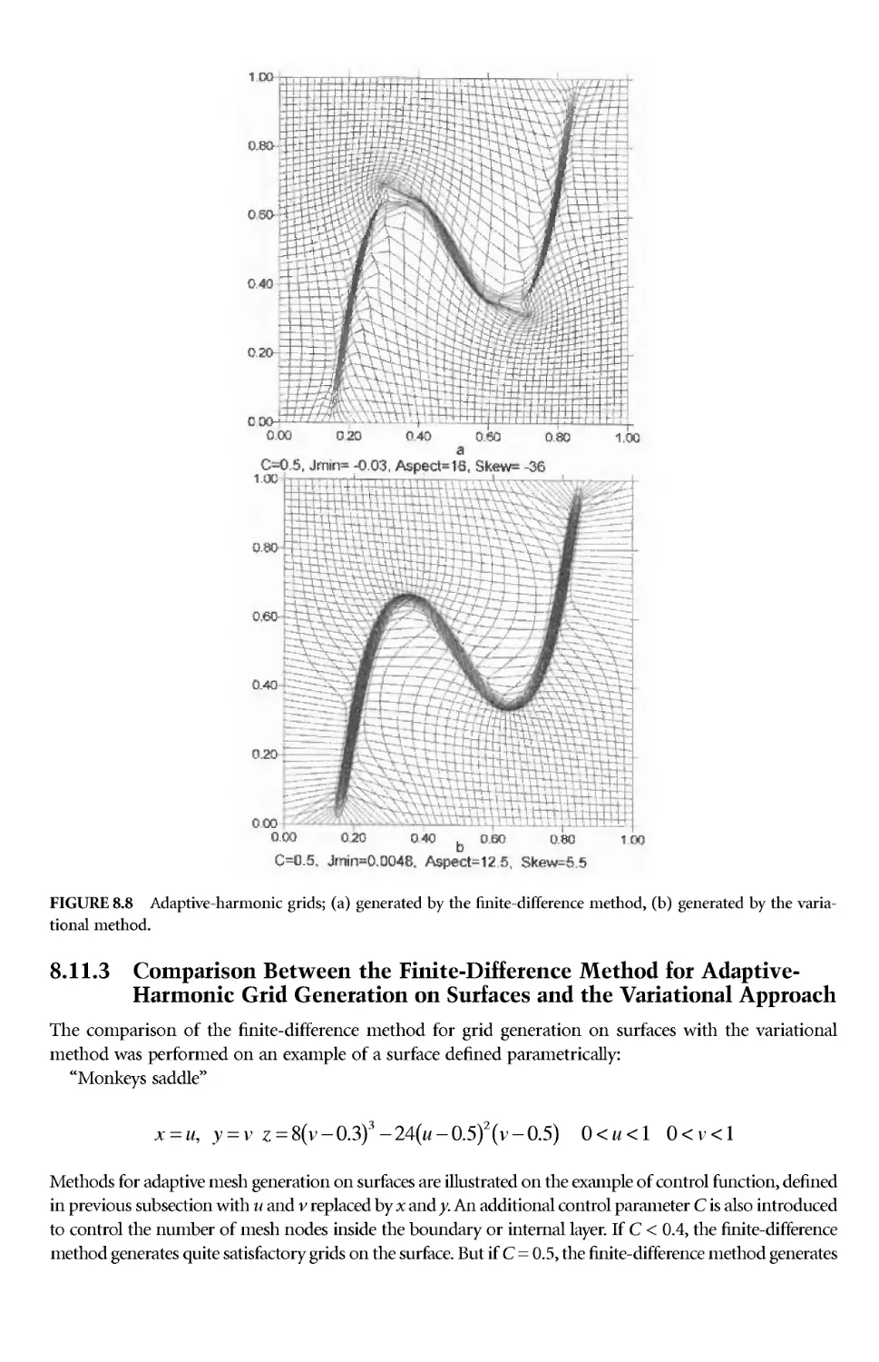
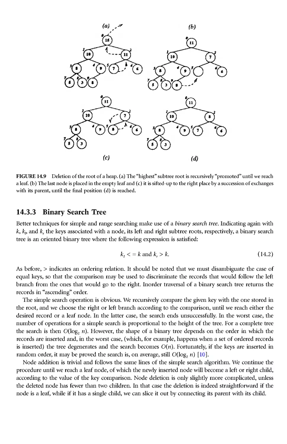
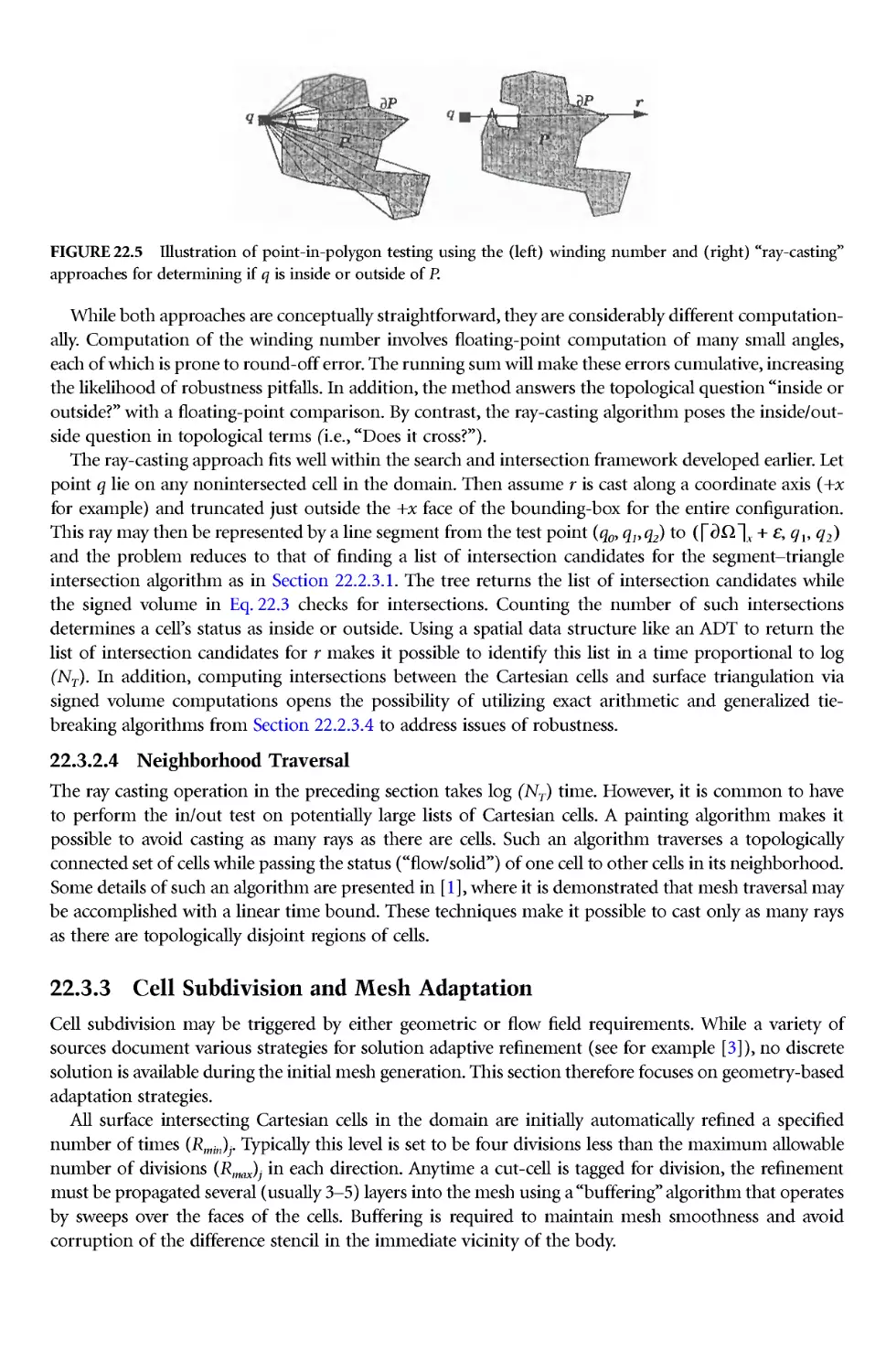
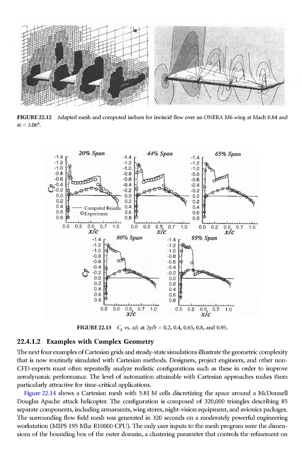
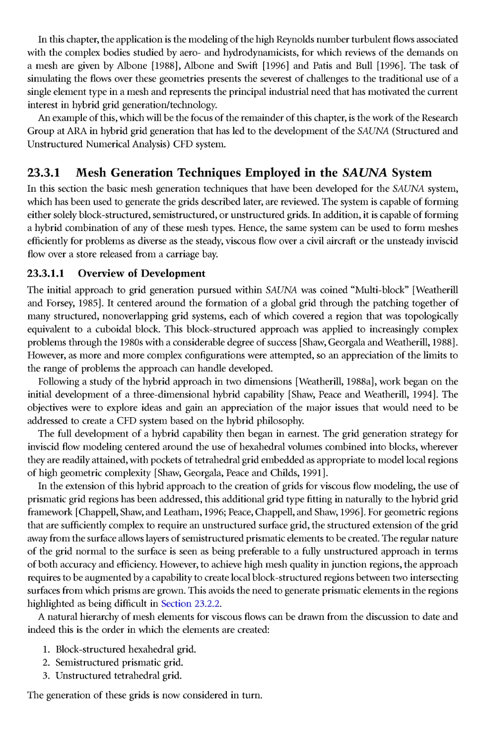
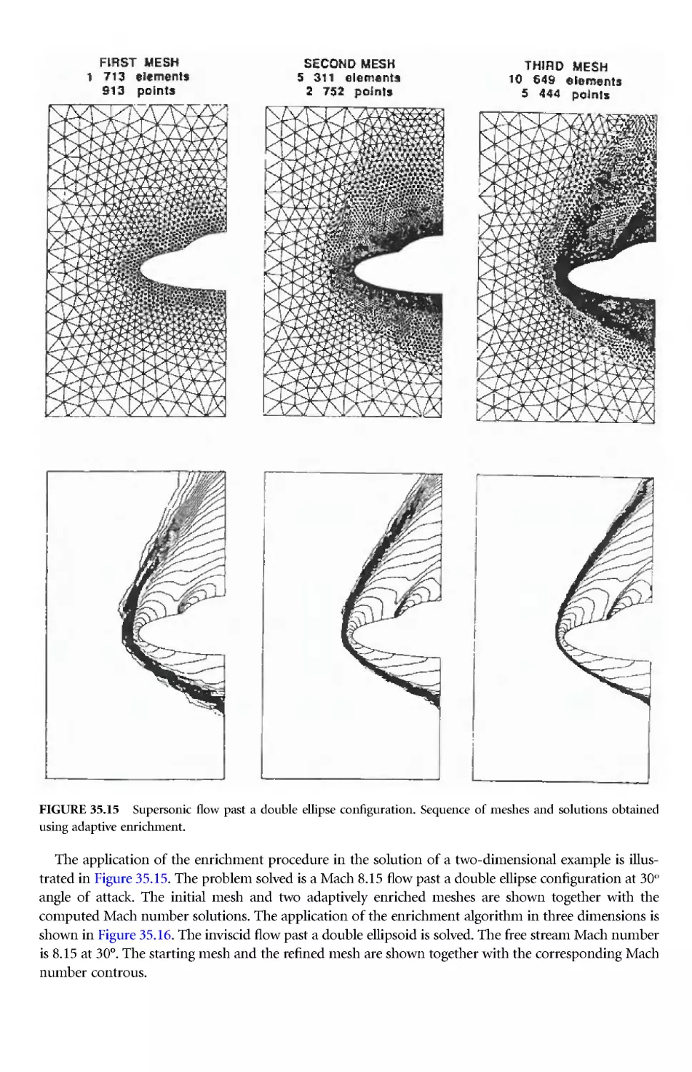
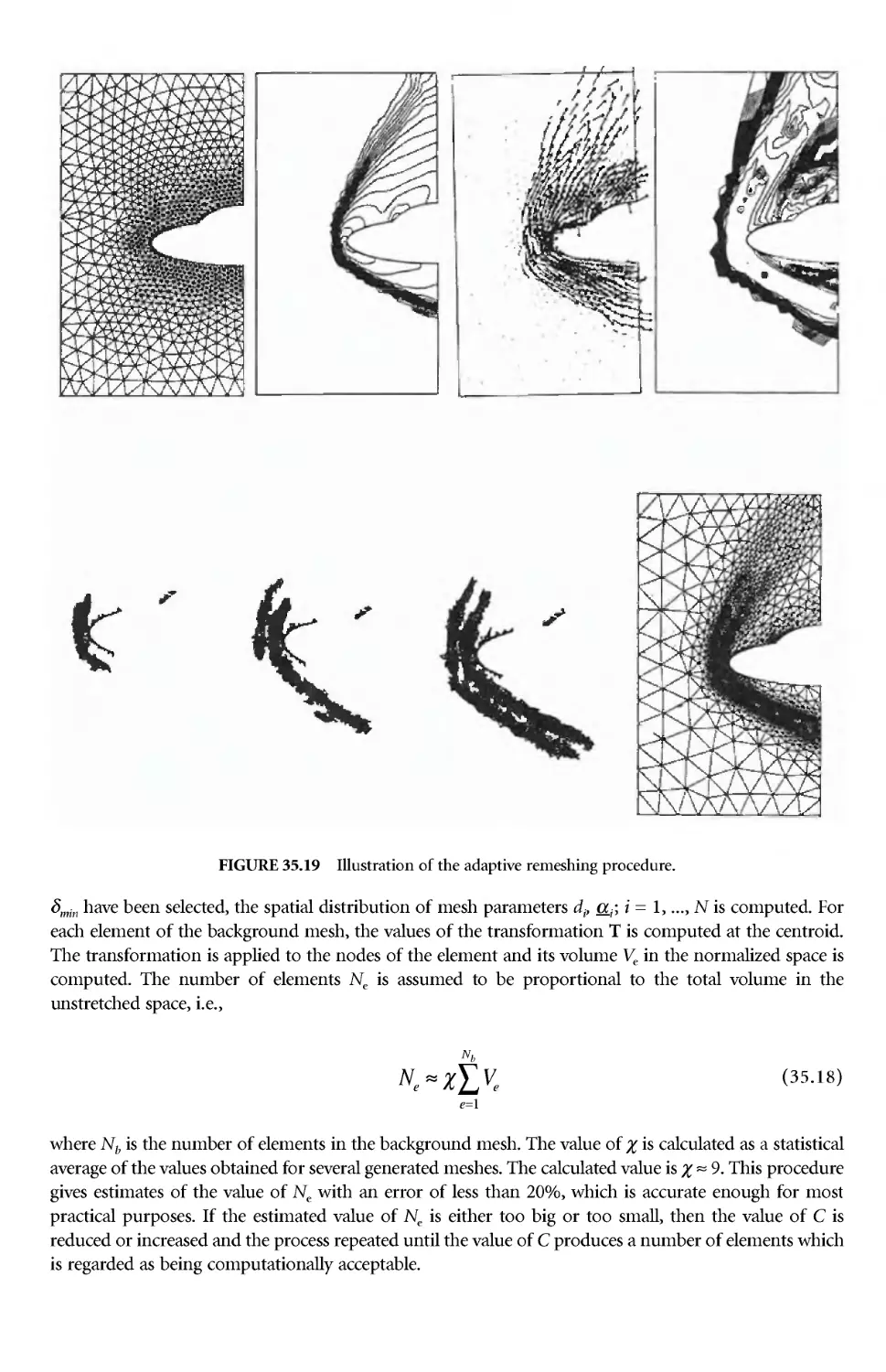
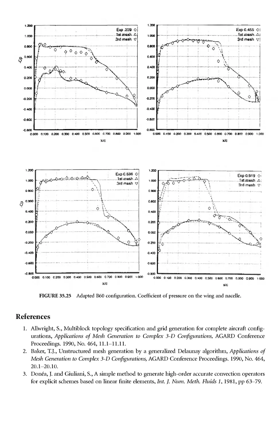
/


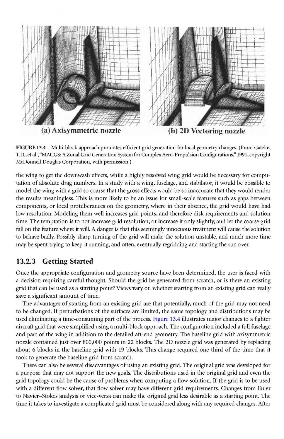


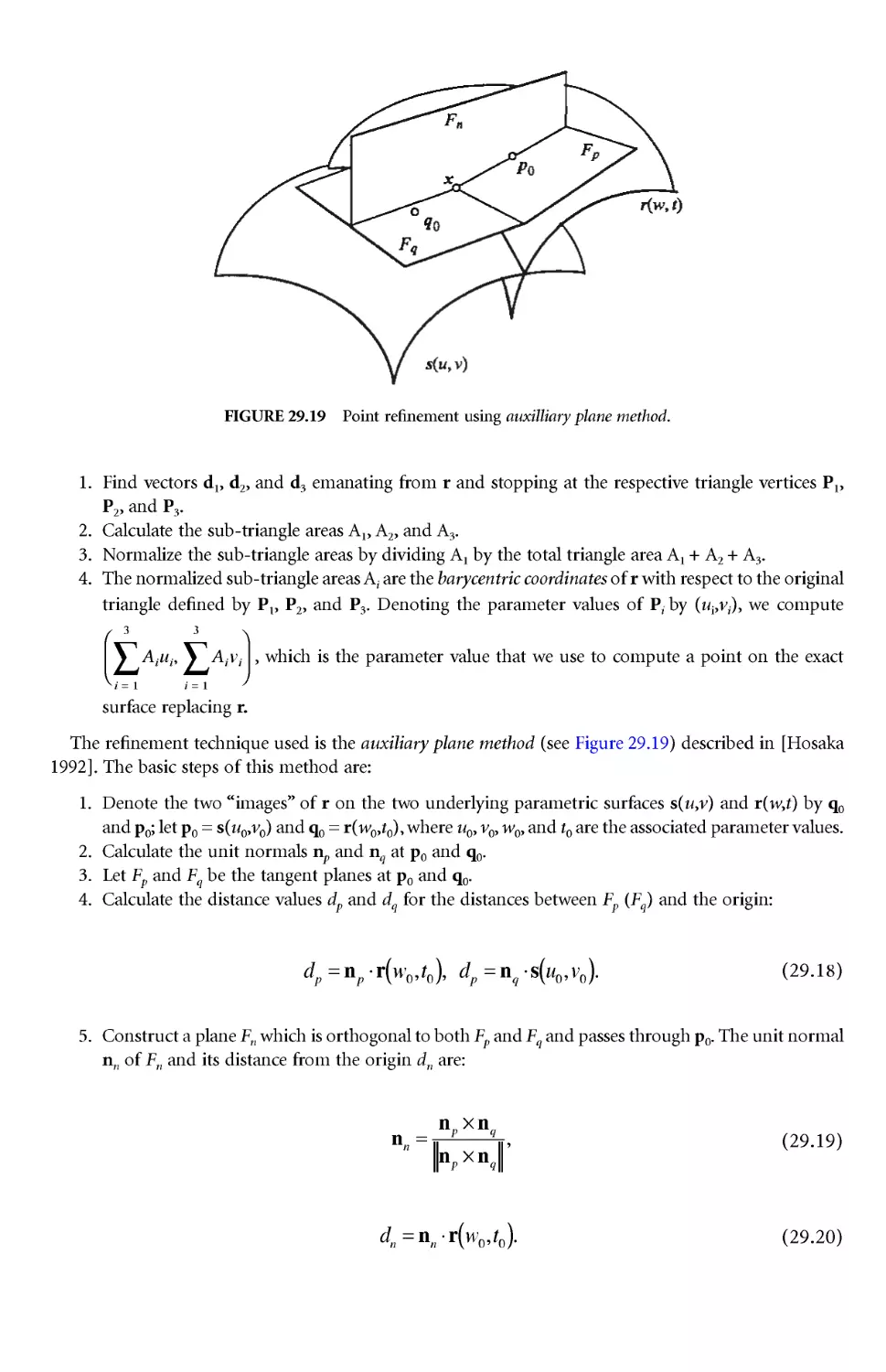


Author: Thompson J.E. Soni B.K. Weatherill N.P.
Tags: mathematics computer science
ISBN: 0-8493-2687-7
Year: 1999
Similar


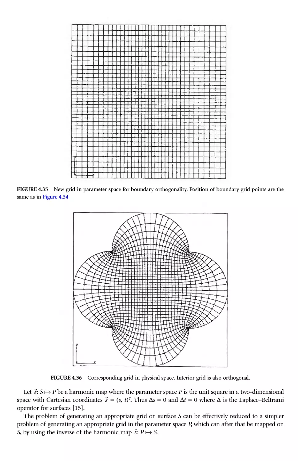
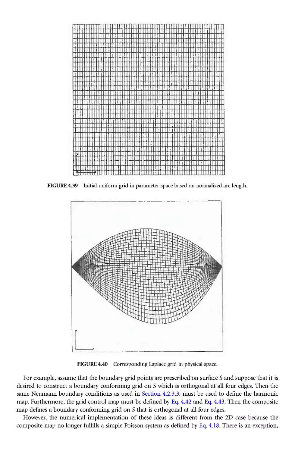
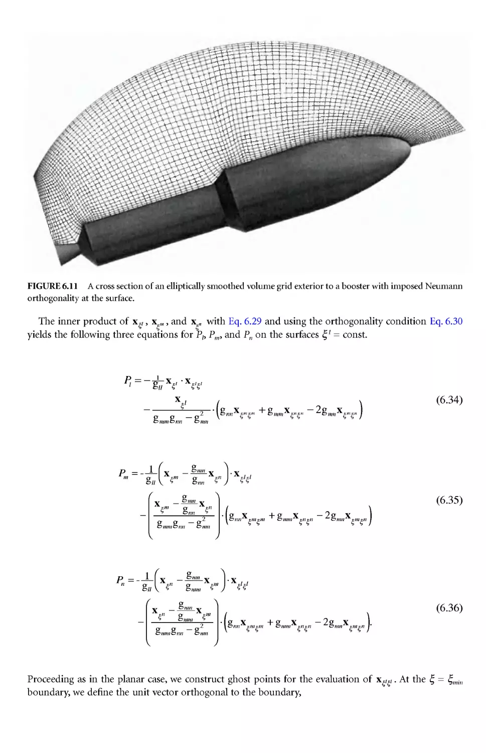
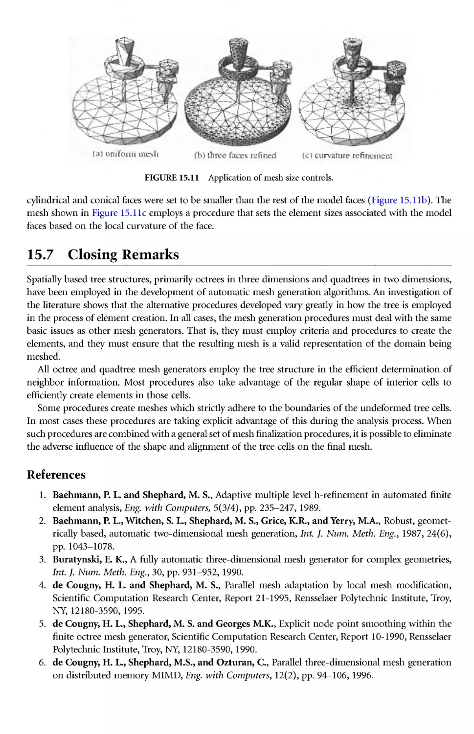
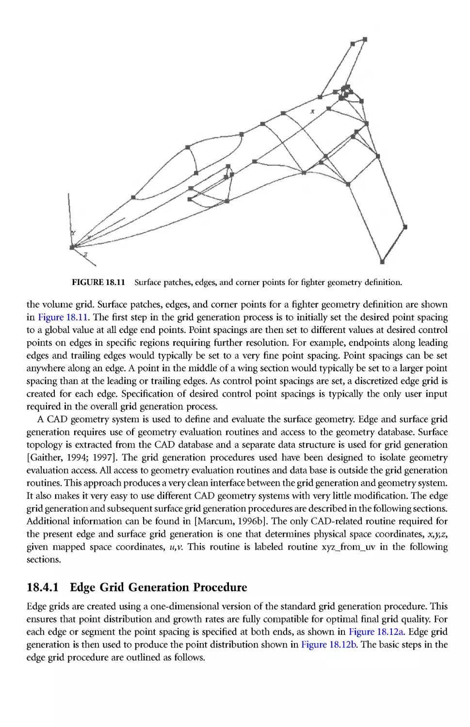
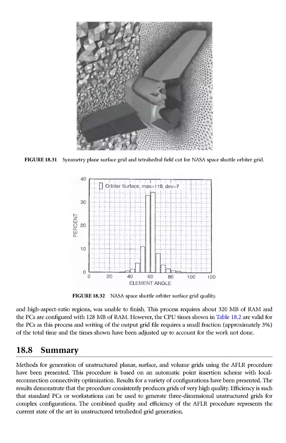
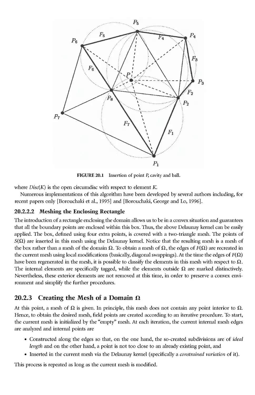
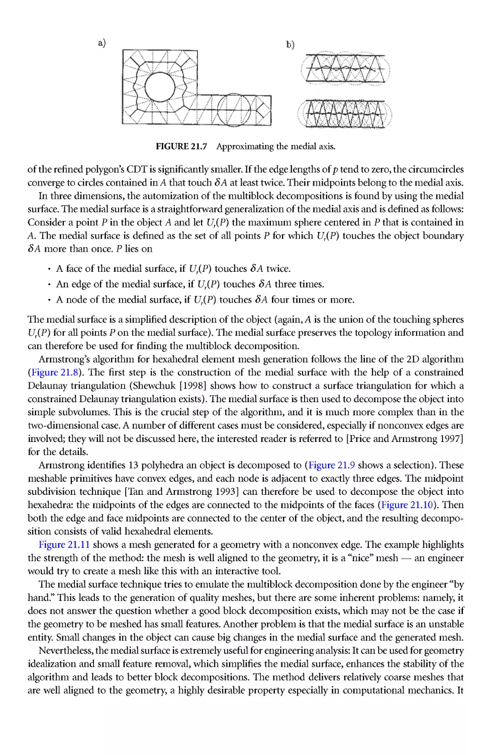
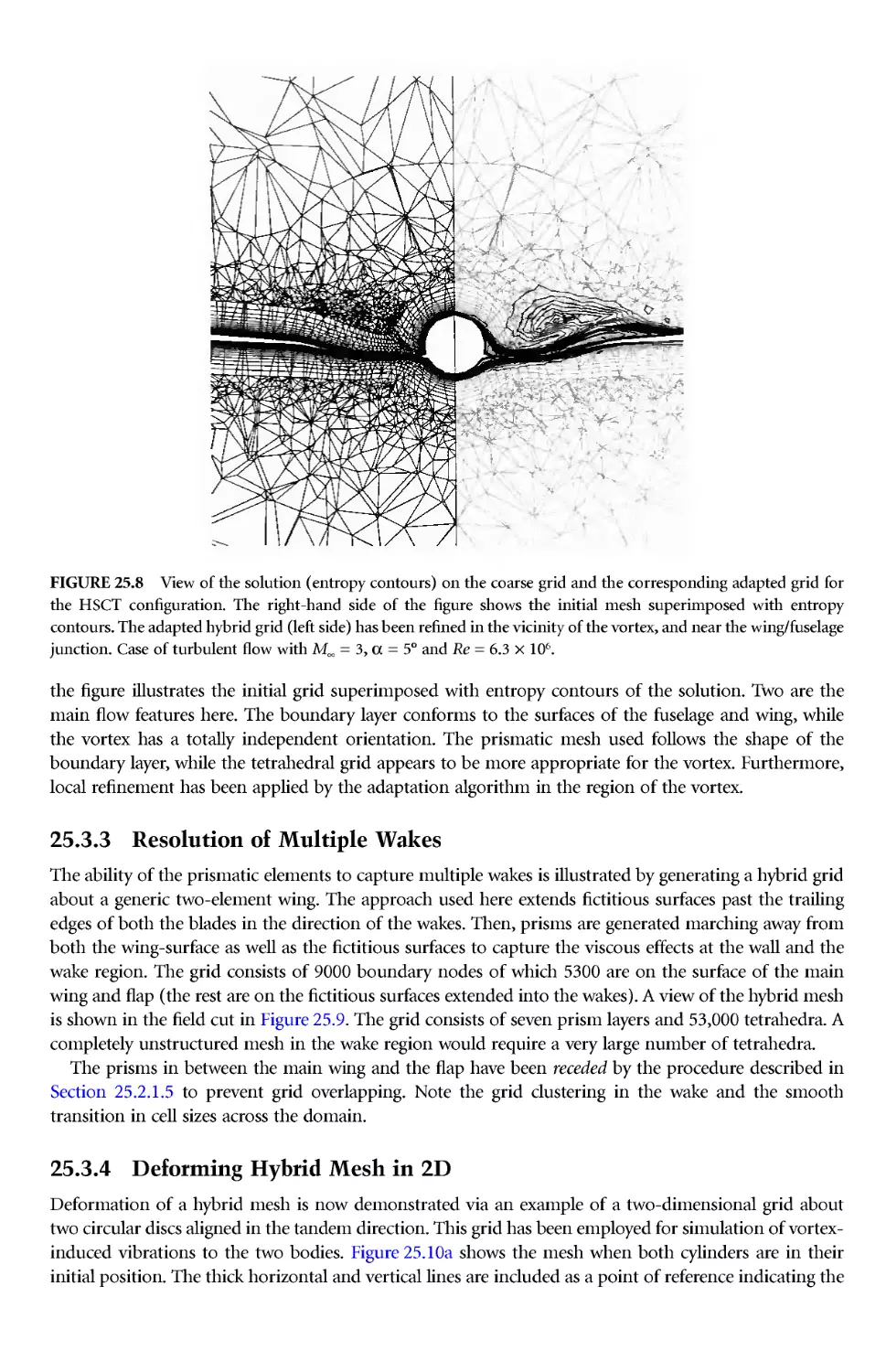
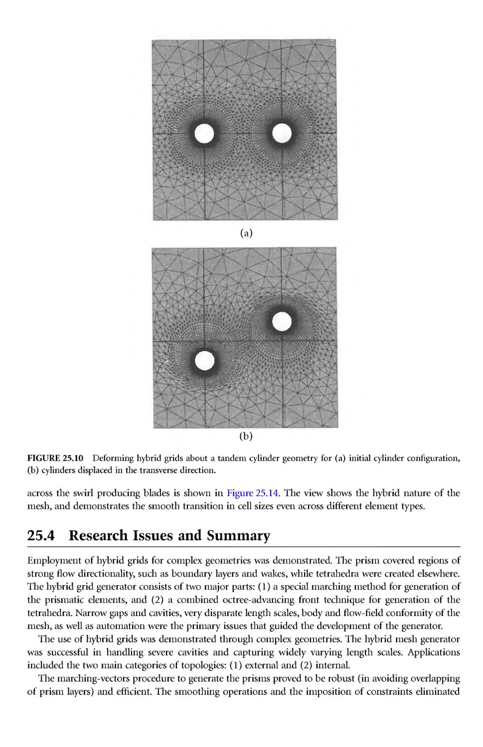
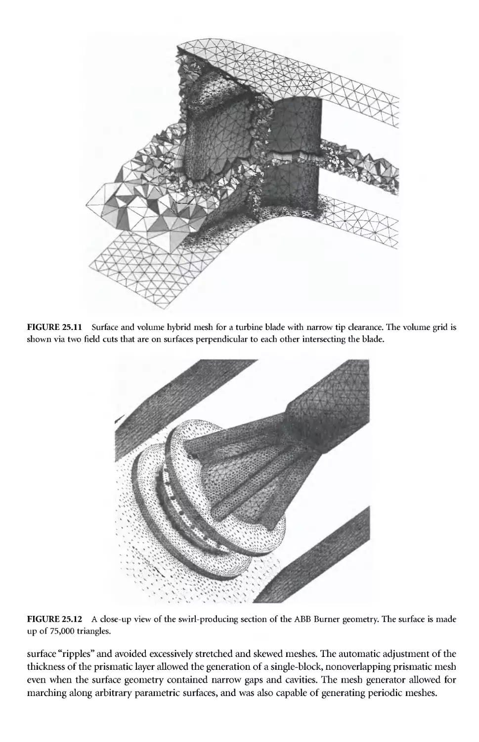
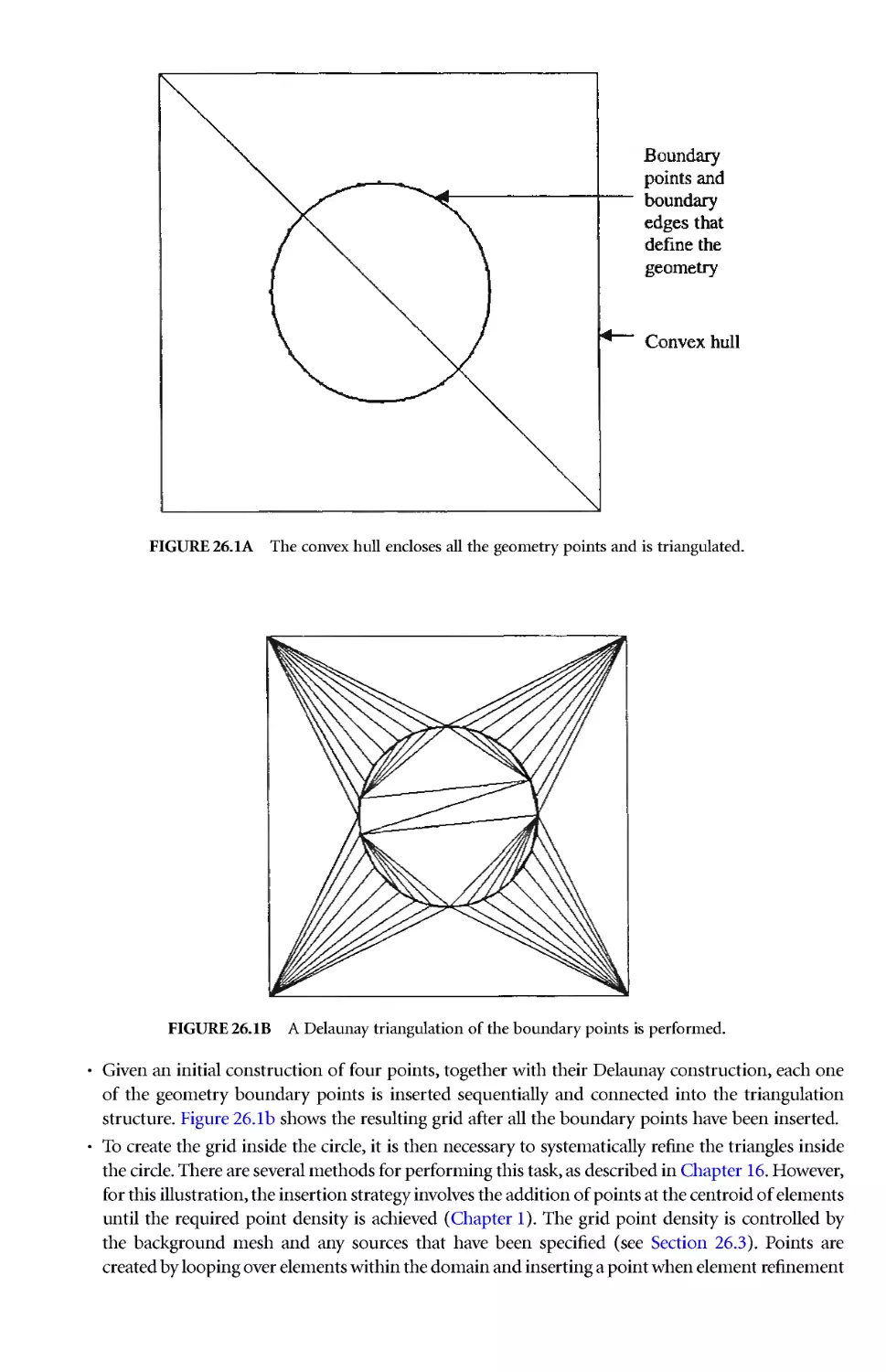
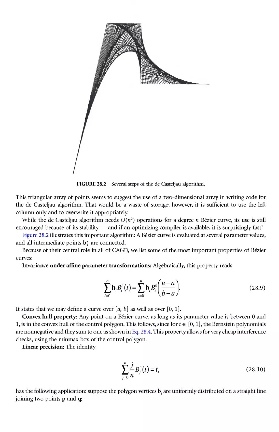
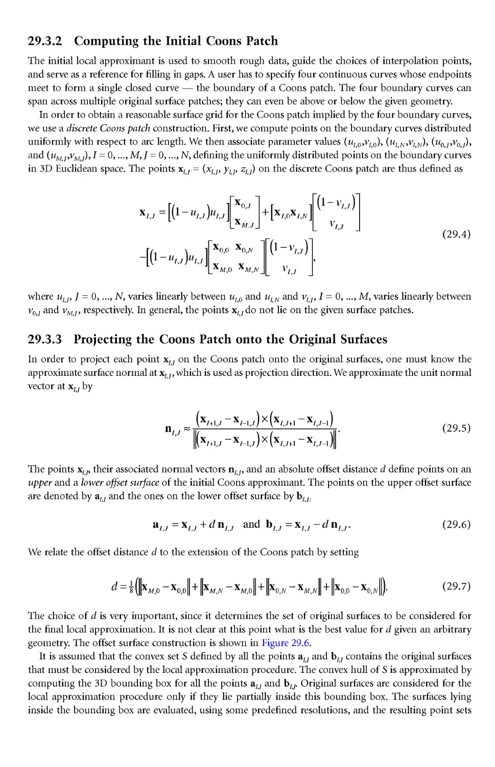
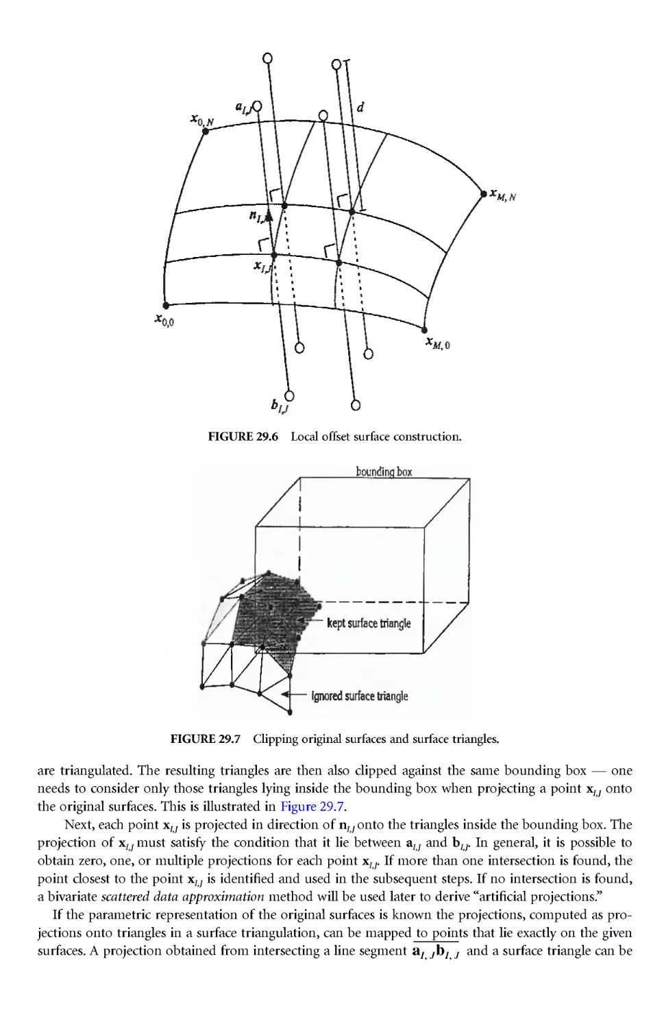
Text
©1999 CRC PressLLC
Acquiring Editor:
B. Stern
Project Editor:
Sylvia Wood
Marketing Manager:
J. Stark
Cover design:
Dawn Boyd
Manufacturing Manager:
Carol Slatter
Library of Congress Cataloging-in-Publication Data
Thompson, Joe F.
Handbook of Grid Generation / Joe F.Thompson, Bharat Soni, Nigel
Weatheril, editors.
p. cm.
Includes bibliographical references and index.
ISBN 0-8493-2687-7 (ak. paper)
1. Numerical grid generation(Numerical analysis) I. Thompson,
Joe F. II. Soni, B.K. III. Weatherill, NP.
QA377.H3183 1998
519.4--dc21
98-34260
CP
This book contains information obtained from authentic and highly regarded sources.Reprintedmaterialis quoted w ith
permission, and sources areindicated.A wide variety of referencesare listed. Reasonable efforts ha
ve beenmade to pubish
reliable data andinformation, but the authorand the publisher cannot assume responsibility for the validityof al materials
or for the consequences of their use.
Neitherthis booknor anypart may be reproduced ortransmitted in anyform or byany means, electronic ormechanical,
including photocopying, microfilming, and recording, or by any information storage or retrieval system, without prior
permission in writing from the pubisher.
Al rights reserved. Authorization to photocopy items for internal or personal use, or the personal or internal use of
specific clients, may be granted by CRC Press LLC, provided that $.50 per page photocopied is paid directly to Copyright
Clearance Center
, 27 Congr
ess Street,Salem, MA 01970 USA. The fee codefor users of the T
ransactionalReporting Service
isISBN 0-8493-2687-7/99/$0.00+$.50. Thefee is subject to change without notice. For organizations that have been granted
a photocopy license by the CCC,a separate system of payment has been arranged.
The consent of CRC Press LLC does not extend to copy ing for general distribution, for promotion, for creating new
works, or for resale. Specific permission must be obtainedin writing from CRC Press LLC for such copying .
Direct all inquiries to CRC Press LLC, 2000 Corporate Blvd., NW., Boca Raton, Florida 33431.
Trademark Notice: Product or corporate names may be trademarks or reg istered trademarks, and are used only for
identification and explanation, without intent to infringe.
© 1999 by CRC Press LLC
No claim to original U.S. Government works
International Standard Book Number 0-8493-2687-7
Library of Congress Card Number 98-34260
PrintedintheUnitedStates ofAmerica12 3 4 5 6 7 8 9 0
Printed on acid-free paper
Foreword
Grid (mesh) generation is, of course, only a means to an end: a necessary tool in the computational
simulationof physical fieldphenomena and processes. (Theterms grid and mesh are used interchangeably,
with identical meaning, throughout this handbook.)
And grid generation is,unfortunately from a technology standpoint, still something of an art, as well
as a science. Mathematics provides the essential foundation for moving the grid generation process from
a user-intensive craft to an automated system. But there is both art and science in the design of the
mathematics for --- not of --- grid generation systems, since there are no inherent laws (equations) of
grid generation to be discovered. The grid generation process is not unique; rather it must be designed.
There are, however, criteria of optimization that can serve to guide this design.
The grid gener ationprocess has matured nowtothe pointwhere theuse of developed codes--- freeware
and commercial --- is generally to be recommended over the construction of grid generation codes by
end users doing computational field simulation. Some understanding of the process of grid generation
--- and its underlying principles, mathematics, and technology --- is important, however, for informed
and effective use of these developed systems. And there are always extensions and enhancements to be
made to meet new occasions, especially in coupling the grid with the solution process thereon.
This handbook is designed to provide essential grid generation technology for practice, with sufficient
detail and development for general understanding by the informed practitioner.Complete details for the
grid generation specialist are left to the sources cited. A basic introduction to the fundamental concepts
and approaches is provided by Chapter l, which covers the state of practice in the entire field in a ver y
broad sweep. An even more basic introduction for those with little familiarit y with the subject is given
by the Preface that precedes this first chapter. Appendixes provide information on a number of available
grid generation codes, both commercial and freeware, and give some representative and illustrative grid
configurations.
The grid generation process in general proceeds fromfirstdefining the boundary geometry as discussed
in Part III. Points are distributed on the curves that form the edges of boundary sections. A surface grid
is then generated on the boundarysurface,and finally,a volume grid is generated in the field. Chapter 13,
although directed at structured gr ids, gives a general overview of the entire gr id gener ation process and
the fundamental choices and considerations involved from the standpoint of the user. Chapter 2, though
also largely directed at structured grids, covers essential mathematical elements from tensor analysis and
differential geometry relevant to the entire subject, particularly the aspects of curve and surfaces.
The other chapters of this handbook cover the various aspects of grid generation in some detail, but
still from the standpoint of practice, with citations of relevant sources for more complete discussion of
the underlyingtechnology.The chapters are grouped into four parts:structuredgrids, unstructuredgrids,
surface definition, and adaptation/quality. An introduction to each part provides a road map through
the material of the chapters.
A source of fundamentals on structured grid generation is the 1985 textbook of Thompson, Warsi,
and Mastin, now out of print but accessible on the Web at www.erc.msstate.edu. A recent comprehensive
text of both structured and unstructured gr ids is that of Care y 1997 from Taylor and Francis publishers.
The first step in generating a grid is, of course,toacquire and input the boundary data. This boundary
data may be in the form of output from aCAD system, or maysimply be sets of boundary points acquired
from drawings. CAD boundary dataare generally in the form of someparametricdescription of boundary
curves and surfaces, typically consisting of multiple segments for which assembly and some adjustments
may be required. Point boundary data may be in the form of 1D arrays of points describing boundary
curves and 2D arrays for boundary surfaces, or could be an unorganized cloud of points on a surface.
In the latter case, conversion to some surface tessellation or parametr ic description is required. These
initial steps of boundary definition are common in general to both structured and unstructured grid
generation. And, unfortunately, considerable human intervention may be necessary in this setup phase
of the process.
The setup of the boundary definition from the CAD approach is discussed in general in Chapter 13,
while details of application, together with procedures for boundar y curve and surface paramet ric repre-
sentations, are covered in Part III. There is then the fundamental choice of whether to use a structured
or unstructuredgrid. Structured grids are covered in Part I,and unstructured gridsare covered in Par t II.
The next step with either type of grid is the generation of the corresponding type of grid on the
boundary surfaces --- preceded, of course, by a distribution on points on the curves that form the edges
of these surfaces. This surface grid generation is covered in Chapters 9 and 19 for structured and
unstructured grids, respectively.
Finally, the quality of the grid, with relation to the accur acy of the numerical solution being done on
the grid, and the adaptation of the grid to improve that accuracy are covered in Part IV.
Grid generation is still under active research and development, particularly in regard to automation,
adaptation, and hybrid combinations. This handbook is therefore necessarily a snapshot in time, espe-
cially in theseareas, but much of the material has matured now, and thiscollection should be of endur ing
value as a source and reference.
Bharat K. Soni
Joe F. Thompson
Nigel P. Weatherill
Star kville, MS, and Swansea, Wales, UK
Contributors
Michael J. Aftosmis
NASA Ames Research Center
Moffett Field, CA
Timothy J. Baker
Princeton University
Princeton, NJ
Mark W. Beall
Rensselaer Polytechnic Institute
Tr oy, NY
Marsha J. Berger
Courant Institute
New York University
William M. Chan
MCAT, Inc. at NASA Ames
Research Center
Moffett Field
Zheming Cheng
Program Development
Corporation
White Plains,NY
Hugues L. de Cougny
Rensselaer Polytechnic Institute
Tr oy, NY
Luís Eça
Technical University of Lisbon
Lisbon, Portugal
Peter R. Eiseman
Program Development Corporation
White Plains,NY
Austin L. Evans
NASA Lewis Research Center
Cleveland, OH
Gerald Farin
Arizona State University
Tempe,AZ
David R. Ferguson
The Boeing Company
Seattle, WA
Luca Formaggia
Ecole Polytechnique Federale de
Lausanne
Lausanne, Switzerland
Timothy Gatzke
The Boeing Company
St. Louis, MO
Paul-Louis George
INRIA
Le Chesnay Cedex, France
Bernd Hammann
University of Calfornia at Davis
Davis, CA
O. Hassan
University of Wales Swansea
Swansea, UK
Jochem Häuser
CLE Salzgitter Bad
Salzgitter, Germany
Frédéric Hecht
INRIA
Le Chesnay Cedex, France
Sergey A. Ivanenko
Computer Center of the Russian
Academy of Sciences
Moscow, Russia
Olivier-Pier re Jacquotte
Research Directorate (DRET)
Paris, France
Brian A. Jean
U.S.Army Corps of Engineers
Waterways Experiment Station
Vicksburg, MS
Yannis Kallinderis
University of Texas
Austin, TX
O.B. Khair ullina
Urals Branch of the Russian
Academy of Sciences
Ekaterinburg , Russia
Ahmed Khamayseh
Los Alamos National Laboratory
Los Alamos, NM
Andrew Kuprat
Los Alamos National Laboratory
Los Alamos, NM
Kelly R. Laflin
Nor th Caroina State University
Raleigh, NC
Kunwoo Lee
Seoul National University
Seoul, Korea
David L. Marcum
Mississippi State University
Starkville, MS
C. Wayne Mastin
Nichols Research Corporation
Vicksburg, MS
D. Scott McRae
North Carolina State University
Raleigh, NC
Robert L. Meakin
ArmyAeroflightdynamics
Directorate (AMCOM)
Moffett Field, CA
John E. Melton
NASA Ames Research Center
Moffett Field, CA
David P. Miller
NASA Lewis Research Center
Cleveland, OH
K. Morgan
University of Wales Swansea
Swansea, UK
Robert M. O'Bara
Rensselaer Polytechnic Institute
Tr oy, NY
Sangkun Park
Information Technology R&D
Center
Seoul, Korea
J. Peraire
Massachusetts Institute
of Technology
Cambridge, MA
J. Peiró
Imperial College
London, UK
E. J. Probert
University of Wales Swansea
Swansea, UK
Anshuman Razdan
Arizona State University
Tempe,AZ
Robert Schneiders
MAGMA Giessereitechnologie
GmbH
Aachen,Germany
Jonathon A. Shaw
Aircraft Research Association
Bedford, U.K.
A.F. Sidorov
Urals Branch of the Russian
Academy of Sciences
Ekaterinburg, Russia
Mark S. Shephard
Rensselaer Polytechnic Institute
Troy, N Y
Robert E. Smith
NASA Langley Research Center
Hampton, VA
Bharat K. Soni
Mississippi State University
Starkville, MS
Stefan P. Spekreijse
National Aerospace Laboratory
(NLR)
Emmeloord, The Netherlands
Joe F. Thompson
Mississippi State University
Starkville, MS
O.V. Ushakova
Urals Branch of the Russian
Academy of Sciences
Ekaterinburg , Russia
Zahir U.A. Warsi
Mississippi State University
Starkville, MS
Nigel P. Weatherill
University of Wales Swansea
Swansea, UK
Yang Xia
CLE Salzgitter Bad
Germany
Tzu-Yi Yu
Chaoyang University of Technology
Wufeng, Taiwan
Paul A. Zegeling
University of Utrecht
Utrecht, The Netherlands
Acknowledgments
Grid (mesh) generation is truly a worldwide active research area of computation science, and this
handbook is the work of individual authors from around the world. It has been a distinct pleasure, and
an opportunity for professional enhancement, to work with these dedicated researchers in the course of
the preparation of this book over the past two years. The material comes from universities, industry,and
government laboratories in 10 countries in North America, Europe, and Asia. And we three are from
three different countries of origin, though we have collaborated for years.
The attention to qualit y that has been the norm in the authoring of these many chapters has made
our editing responsibility a straightforward process. These chapters should serve well to present the
current state of the art in gr id generation to practitioners, researchers, and students.
The assembly and editing of the material for this handbook from all over the world via the Internet
has been a rewarding experience in its ow n right, and speaks well for the potential for worldwide
collaborative efforts in research.
Our thanks go to Mississippi State University and the University of Wales Swansea for the encourage-
ment and support of our efforts to produce this handbook. Specifically at Mississippi State, the work of
Roger Smith in administering the electronic communication is to be noted, as are the efforts of Alisha
Davis, who handled the word processing.
Bob Stern of CRC Press has been great to work with and appreciation is due to him for recognizing
the need for this handbook and for his editorial guidance and assistance throughout its preparation. His
efforts, and those of Sylvia Wood, Suzanne Lassandro and Dawn Mesa, also at CRC, have made this a
pleasant process.
We naturally are especially grateful for the support of our wives, Purnima, Emilie, Barbara, and our
families in thisand all ourefforts.And finally, Mississippi andWales--- two great places to live and work.
Bharat K. Soni
Joe F. Thompson
Nigel P. Weatherill
Author/Editors
Preface:
An Elementary Introduction
Joe F. Thompson, Bharat K. Soni, and Nigel P. Weatherill
This firstsection is an elementar y introduction providedfor those with little familiarity with grid (mesh)
generation in order to establish a base from which the technical development of the chapters in this
handbook can proceed. (The terms grid and mesh are used interchangeably throughout with identical
meaning.) The intent is not to introduce numerical solution procedures, but rather to introduce the idea
of using numerically generated grid (mesh) systems as a foundation of such solutions.
P-1 Discretizations
The numerical solution of partial differential equations (PDEs) requires first the discretization of the
equations to replace the continuous differential equations with a system of simultaneous algebraic
difference equations. There are sever al bifurcations on the way to theconstruction of the solution process,
the first of which concerns whether to represent the differential equations at discrete points or over
discrete cells. The discretization is accomplished by covering the solution field with discrete points that
can, of course, be connected in various manners to form a network of discrete cells. The choice lies in
whether to represent the differential equations at the discrete points or over the discrete cells.
P-1.1 Point Discretization
In the former case (called finite difference), the derivatives in the PDEs are represented at the points by
algebraicdifference expressions obtained by performing Taylor ser iesexpansions of the solution variables
at several neighbors of the point of evaluation. This amounts to taking the solution to be represented by
polynomials between the points. This can be unrealistic if the solution varies too strongly between the
points. One remedy is, of course,to use more points so that the spacing between points is reduced.This,
however,can be expensive, since there will then be more points at which the equations must be evaluated.
This is exacerbated if the points are equally spaced and strong variations in the solution occur over
scattered regions of the field, since numerous points will be wasted in regions of small variation. An
alternative, of course, is to make the points unequally spaced.
P-1.2 Cell Discretization
The other possibility of this first bifurcation is to return the PDEs to their more fundamental integral
form and then to represent the integrals over discrete cells. Here there is yet another bifurcation ---
whether to representthe solution variablesover the cell in termsof selectedfunctions and then tointegrate
these functions analytically over the volume (finite element), or to balance the fluxes through the cell
sides (finite volume).
The finite element approach itself comes in two basic forms: the var iational, where the PDEs are
replacedby a more fundamental integral var iationalprinciple(fromwhich they arisethrough the calculus
of variations), or the weighted residual (Galerkin)approach, in which the PDEs are multiplied by certain
functions and then integrated over the cell.
In the finite volume approach, the solution variables are considered to be constant within a cell, and
the fluxes through the cell sides (which separate discontinuous solution values) are best calculated with
a procedure that represents the dissolution of sucha discontinuity during the time step (Riemann solver).
P-2 Curvilinear (Structured) Grids
The finite difference approach, using the discrete points, is associated historically with rectangular
Cartesian g rids, since such a regular lattice structure provides easy identification of neighboring points
to be used in the representation of derivatives, while the finite element approach has always been, by the
nature of its construction on discrete cells of general shape, considered well suited for irregular regions,
since a network of such cells can be made to fill any arbitrarily shaped region and each cell is an entity
unto itself, the representation being on a cell, not across cells.
P-2.1 Boundary-Fitted Grids
The finite difference method is not, however, limited to rectangular gr ids and has long been applied on
other readily available analytical coordinate systems (cylindrical, spherical, elliptical, etc.) that still form
a regular lattice. albeit curvilinear, that allows easy identification of neighboring points. These special
curvilinear coordinate systems are all orthogonal, as are the rectangular Cartesian systems,and they also
can exactly cover special regions (e.g., cylindrical coordinates covering the annular region between two
concentric circles) in the same way that a Cartesian grid fills a rectangular region. The cardinal feature
in each case is that some coordinate line is coincident with each portion of the boundary.
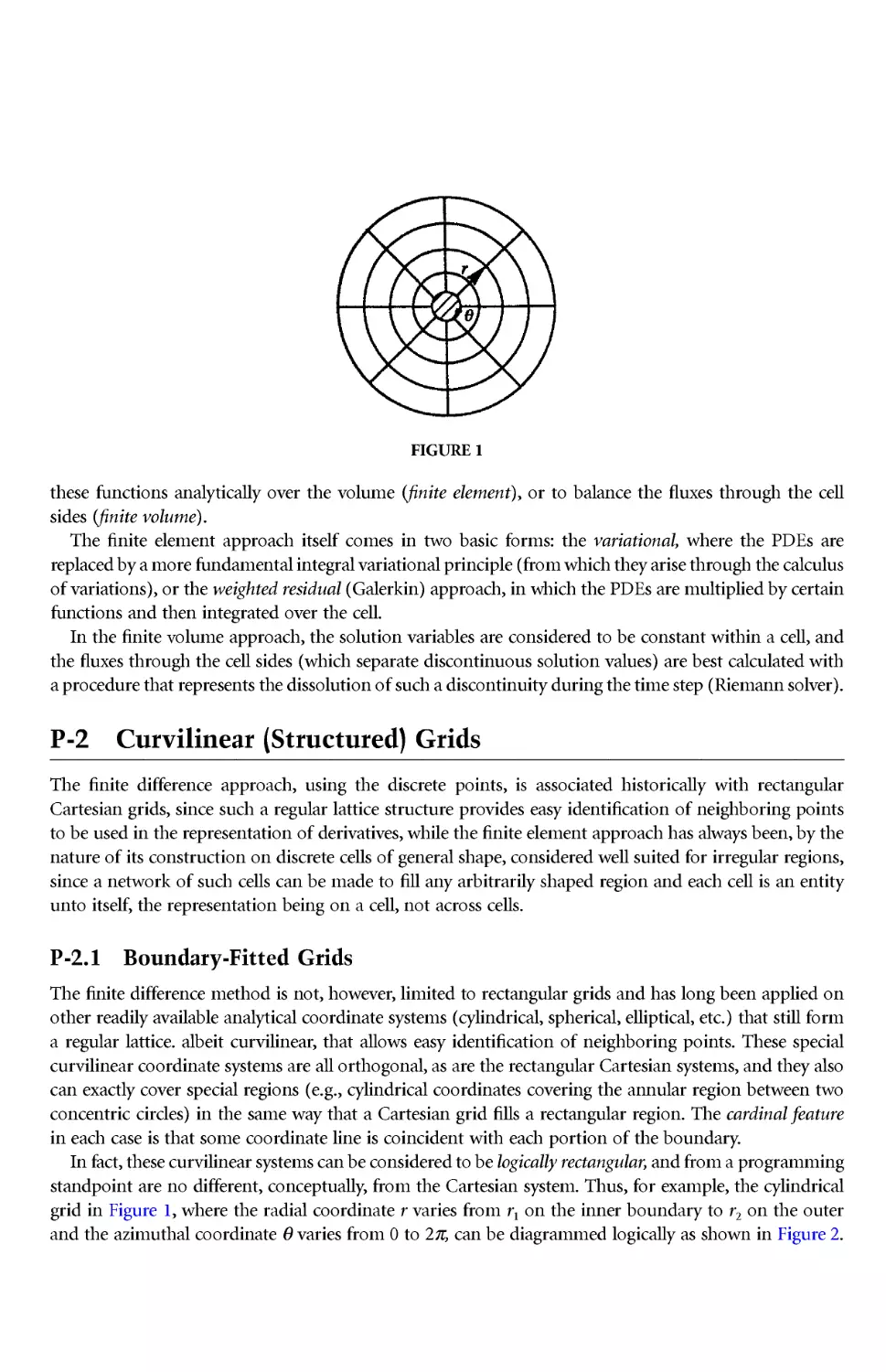
In fact,these curvilinear systems canbe considered to belogically rectangular,and from aprogramming
standpoint are no different, conceptually, from the Car tesian system. Thus, for example, the cylindrical
grid in Figure 1, where the radial coordinate r varies from r1 on the inner boundary to r2 on the outer
and the azimuthal coordinate θ varies from 0 to 2π, can be diagrammed logically as shown in Figure 2.
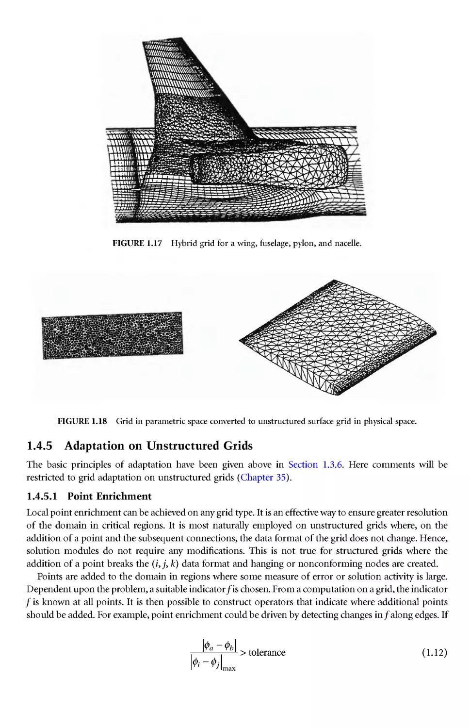
FIGURE 1
The continuity of the azimuthal coordinate can be represented by defining extra"phantom" columns
to the left of 0 and to the right of 2π and setting values on each phantom column equal to those on the
corresponding "real" columns inside of 2π and 0, respectively. This latter, log ically rectangular, v iew of
the cylindrical grid is the one used in programming anyway, and without being told of the cylindrical
configuration, a programmer would not realize any difference here from programming in Cartesian
coordinates --- there would simply be a different set of equations to be programmed on what is still a
logically rectangular grid, e.g., the Laplacian on a Cartesian grid (with ξ = x and η = y),
becomes(withξ=θandη =r)
on a cylindrical grid. The ke y point here is that in the logical (i.e., programming) sense there is really
no essential difference between Cartesian grids and the cylindrical systems: both can be programmed as
nested loops; the equations simply are different.
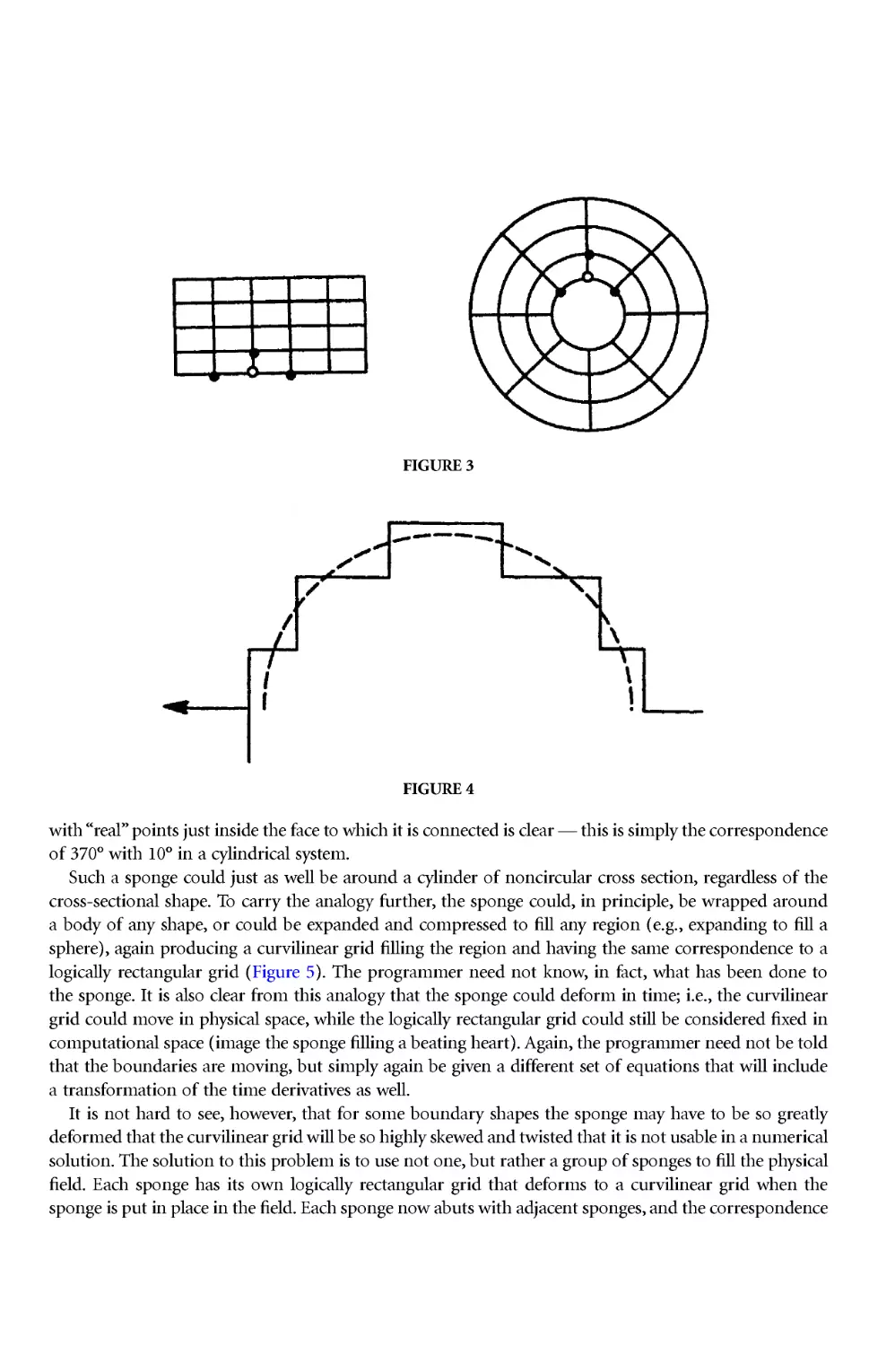
Another key point is that the cylindrical grid fits the boundary of a cylindrical region just as the
Cartesian grid fits the boundary of a rectangular region. This allows boundary conditions to be repre-
sented in the same manner in each case also (see Figure 3). By contrast, the use of a Cartesian grid on
a cylindrical region requires a stair-stepped boundary and necessitates interpolation in the application
of boundary conditions (Figure 4) --- the proverbial square peg in a round hole.
P-2.2 Block Structure (The Sponge Analogy)
The best way to visualize the correspondence of a curvilinear grid in the physical field with a logically
rectangular grid in the computational field is through the sponge analogy. Consider a rectangular sponge
within which an equally spaced Cartesian grid has been drawn. Now wrap the sponge around a circular
cylinder and connect the two ends of the sponge together. Clearly the original Cartesian grid in the
sponge now has become a cur vilinear grid fitted to the cylinder. But the rectangular logical form of the
grid lattice is still preserved, and a programmer could still operate in the logically underformed sponge
in constructing the loop and the difference expressions, simply having been given different equations to
program. The correspondence of "phantom" pointsjust outside oneof the connected faces of the sponge
FIGURE 2
∇=+
2ff f
ξξ ηη
∇=++
22
ffff
ξξ
ηηηη
η
with"real" points justinside the face to which it is connected is clear --- this is simply thecor respondence
of 370° with 10° in a cylindrical system.
Such a sponge could just as well be around a cylinder of noncircular cross section, regardless of the
cross-sectional shape. To carry the analogy further, the sponge could, in principle, be wrapped around
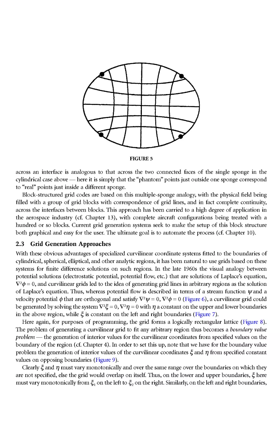
a body of any shape, or could be expanded and compressed to fill any region (e.g., expanding to fill a
sphere), again producing a curvilinear grid filling the region and having the same correspondence to a
logically rectangular grid (Figure 5). The programmer need not know, in fact, what has been done to
the sponge. It is also clear from this analogy that the sponge could deform in time; i.e., the curvilinear
grid could move in physical space, while the logically rectangular g rid could still be considered fixed in
computational space (image the sponge filling a beating heart). Again, the programmer need not be told
that the boundaries are moving, but simply again be given a different set of equations that w ill include
a transformation of the time derivatives as well.
It is not hard to see, however, that for some boundary shapes the sponge may have to be so greatly
deformed that the curvilinear grid will be sohighly skewed and twisted thatitis not usable in anumerical
solution. Thesolution to this problem is to use not one, but rather a group of sponges to fill the physical
field. Each sponge has its own log ically rectangular grid that deforms to a curvilinear grid when the
sponge is put in place in the field. Each sponge now abutswithadjacent sponges, and the correspondence
FIGURE 3
FIGURE 4
across an interface is analogous to that across the two connected faces of the single sponge in the
cylindrical case above --- here it is simply that the "phantom" points just outside one sponge correspond
to "real" points just inside a different sponge.
Block-structured grid codes are based on this multiple-sponge analog y, with the physical field being
filled w ith a group of grid blocks with correspondence of grid lines, and in fact complete continuity,
across the interfaces between blocks. This approach has been carried to a high degree of application in
the aerospace industry (cf. Chapter 13), with complete aircraft configurations being treated w ith a
hundred or so blocks. Current grid generation systems seek to make the setup of this block structure
both graphical and easy for the user. The ultimate goal is to automate the process (cf. Chapter 10).
2.3 Grid Generation Approaches
With these obvious advantages of specialized curvilinear coordinate systems fitted to the boundaries of
cylindrical, spherical, elliptical, and other analytic regions, it has been natural to usegrids based on these
systems for finite difference solutions on such regions. In the late 1960s the visual analogy between
potential solutions (electrostatic potential, potential flow, etc.) that are solutions of Laplace's equation,
∇2 φ = 0, and curvilinear grids led to the idea of generating grid lines in arbitrary regions as the solution
of Laplace's equation. Thus, whereas potential flow is described in terms of a stream function ψ and a
velocity potential φ that are orthogonal and satisfy ∇2ψ = 0, ∇2φ = 0 (Figure 6), a curvilinear grid could
be generated by solving the system ∇2ξ =0, ∇2η =0 with η a constant on the upper and lower boundaries
in the above region, while ξ is constant on the left and right boundaries (Figure 7).
Here again, for purposes of programming, the grid forms a logically rectangular lattice (Figure 8).
The problem of generating a curvilinear grid to fit any arbitrar y region thus becomes a boundar y value
problem --- the generation of interior values for the curvilinear coordinates from specified values on the
boundary of the region (cf. Chapter 4). In order to set this up, note that we have for the boundary value
problem the generation of interior values of the cur vilinear coordinates ξ and η from specified constant
values on opposing boundaries (Figure 9).
Clearly ξ and η must vary monotonically and over the same range over the boundaries on which they
are not specified, else the grid would overlap on itself. Thus, on the lower and upper boundaries, ξ here
mustvary monotonically from ξ1 on the left to ξ2 on the right. Similarly, on the leftand right boundaries,
FIGURE 5
η mustvar y monotonically from η1 at thebottom to η2at the top. The nextquestion is what this variation
should be. This is, in fact, up to the user. Ultimately, the discrete grid will be constructed by plotting
inesofconstant ξand lines of constant η at equal intervalsof each, with thesize of theintervaldetermined
by the number of grid lines desired. Thus, if there are to be 10 grid lines running from side to side
between the top and bottom of the region, 10 points would be selected on the left and right sides ---
with their locations being up to the user. Once these points are located, η can be said to assume, at the
10 points on each side, 10 values at equal intervals between its top and bottom values, η1 and η2. With
this specification on the sides, the cur vilinear coordinate η is thus specified on the entire boundary of
FIGURE 6
FIGURE 7
FIGURE 8
the region, and its interior values can be determined as a boundar y value problem.A similar specification
of ξ on the bottom and top boundaries by placing points on these boundaries sets up the determination
of ξ in the interior from its boundary values. Now the problem can be considered a boundary value
problem in the physical field for the curvilinear coordinates ξ and η (Figure 10) or can be considered a
boundary value problem in the logical field for the Cartesian coordinates, x and y (Figure 11).
Note that the boundary points are by nature equally spaced on the boundary of the log ical field
regardless of the distribution on the boundaries of the physical field. Continuing the potential analogy,
the curvilinear grid can be generated by solving the system ∇2ξ = 0, ∇2η = 0, in the first case, or by
solving the transformation of these equations (transformation relations are covered inChapter 2),inthe
FIGURE 9
FIGURE 10
FIGURE 11
second case. Although the equation set is longer in the second case, the solution reg ion is rectangular,
and the differencing can be done ona uniformly spaced rectangular grid. This is, therefore, the preferred
approach. Note that the placing of points in any desired distribution on the boundary of the physical
regio n, w here x and y are the independent variables, amounts to setting (x,y) values at equally spaced
points on the rectangular boundary of the logical field, where ξ and η are the independent variables.
This is the case regardless of the shape of the physical boundary.
This boundary value problem for the curvilinear grid can be gener alized beyond the analogy with
potential solutions, and in fact is in no way tied to the Laplace equation. The simplest approach is to
generate the interior values by interpolation from the boundary values --- a process called algebraic grid
generation (cf. Chapter 3). There are several variants of this process. Thus for the region considered
above, a grid could be generated by interpolating linearly between corresponding points on the top and
bottom boundaries (Figure 12). Note that the point distr ibutions on the side boundaries h ave no effect
here. Alternatively, theinterpolation could be betweenpairs of points on the side boundaries (Figure 13).
The second case is, howe ver, obviously unusable since the grid overlaps the boundary. Here the lack of
influence from the points on the bottom boundar y is disastrous.
Another alternative is transfinite interpolation in which the interpolation is done in one (either)
direction as above, but then the resulting error on the two sides not involved is interpolated in the other
direction and subtracted from the first result. This procedure includes effects from all of the boundary
and consequently matches the point distribution that is set on the entire boundary.This is the preferred
approach, and it provides a framework for placing any one-dimensional interpolation into a multiple-
dimensional form. It is possible to include any type of interpolation, such as cubic, which gives orthog-
onality at the boundar ies, in the transfinite interpolation format.
FIGURE 12
αβγ
αβγ
α
γβ
ξξξηηη
ξξξηηη
ηη
ξξ
ξη ξη
xx
x
yy
y
xy
xy
xx yy
-+
=
-+
=
=+
=+
=+
20
20
22
22
It is still possible in some cases for the grid to overlap the boundaries with transfinite interpolation, and
thereis no control over the skewness of the grid. This givesincentive to nowreturntothe grids generated
from solving the Laplace equation.
The Laplace equation is, by its ver y nature,a smoother, tending to average values at points with those
at neighboring points. It can be shown from the calculus of variations, in fact, that grids generated from
the Laplace equation are the smoothest possible.Therearises, however,the needtoconcentratecoordinate
ines in certain areas of anticipated strong solution variation, such as near solid walls in viscous flow.
This can be accomplished by departing from the Laplace equation and designing a partial differential
equation system for grid generation: designing because, unlike physics, there are no laws governing grid
generation waiting to be discovered.
The first approach to this, historically, was the obvious: simply replace the Laplace equation with
Poisson equations ∇2ξ = P, ∇2η = Q and leave the cont rol functionson theright-hand sides to be specified
by the user (with appeal to Urania, the muse of science, for guidance). This does in fact wor k but the
approach has evolved over the years, guided both by logical intuition and the calculus of variations, to
use a similar set of equations but with a somewhat different right-hand side. Also, the user has been
relieved of the responsibility for specifying the control functions, which are now generally evaluated
automatically by the code from the boundary point distributions that are set by the user (cf. Chapter 4).
These functions may also be adjusted by the code to achieve orthogonality at the boundary and/or to
reduce the grid skewness or otherwise improve the grid quality (cf. Chapter 6).
Algebraic grid generation, based on transfinite interpolation, is typically used to provide an initial
solution to start an iterative solution of the partial differential equation for this elliptic grid generation
system that provides a smoother grid, but with selective concentration of lines, and is less likely to result
in overlapping of the boundary.
This elliptic grid generation has an analogy to stretching a membrane attached to the boundaries
(cf. Chapter 33) Grid lines inscribed on the underformed membrane move in space as the membrane is
selectively stretched, but the region between the boundaries is always covered by the grid. Another form
of grid gener ation from partial differential equations has an analogy with the waves emanating from a
stone tossed into a pool This hyperbolic gr id generation uses a set of hyperbolic equations, rather than
the Poisson equation, to grow an orthogonal gridoutwardfrom aboundary (cf.Chapter 5). This approach
is, in fact, faster than the elliptic grid generation, since no iterative solution is involved, but it is not
possible to fit a specified outer boundary. Hyperbolic grid generation is thus limited in its use to open
regions. As with the elliptic system, it is possible to control the spacing of the grid lines, and the
orthogonality helps prevent skewness.
FIGURE 13
The control of grid line spacing can be extended to dynamically couple the grid generation system
with the physical solution to be performed on the grid in order to resolve developing gradients in the
solution wherever such variations appear in the field (cf. Chapter 34 and 35). With such adaptive g rids,
certain solution variables, such as pressure or temper ature,are made to feed back to the controlfunctions
in the grid generations system to adjust the grid before the next cycle of the physical solution algorithm
on the grid.
P-2.4 Variations
Structured grids to day are typically generated and applied in the block-structured form described above
with the multiple-sponge analogy. A variation is the chimera (from the monster of Greek mythology,
composed of disparate par ts) approach in which separate grids are gener ated about various boundar y
components, e.g , bodies in the field, and these separate grids are simply overlaid on a background grid
and perhaps on eachother in a hierarchy (cf. Chapter 11). The physical solutionprocess on this composite
grid proceeds with values being transferred between grids by interpolation. This approach has a number
of advantages: (1)simplicity in grid generation since thevarious grids are generatedseparately, (2) bodies
can be added to, or taken out of, the field easily, (3) bodies can carry their grids when moving relative
to the background (think of simulating the kicking of a field goal with the ball and its grid tumbling end
over end), (4) the separate grids can be used selectively to concentrate points in regions of developing
gradients that may be in motion.Thedisadvantages are thecomplexity of setup (but this is beingattacked
in new code development) and the necessity for the interpolation between g rids.
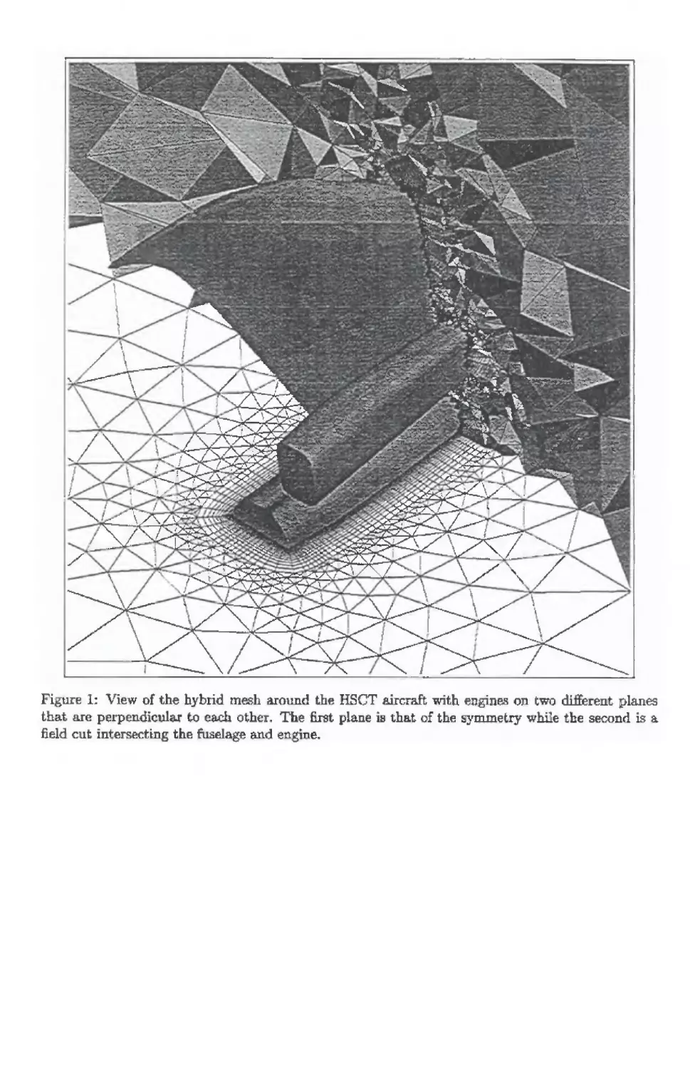
Another approach of interest is thehybrid combinationwithseparate structuredgrids over the various
boundaries, connected by unstructured grids (cf. Chapter 23). There is great incentive to use structured
grids over boundaries in viscous flowsimulation because the boundary layer requires very small spacing
out fromthe wall,resulting either in very longskewed triangular cells or aprohibitively and unnecessarily
large number of small cellswhen unstructuredgrids are used. This hybrid approach is less well deve loped
but can be expected to receive more attention.
P-2.5 Transformation
The use of numerically generated nonorthogonal curvilinear grids in the numerical solution of PDEs is
not, in principle, any more difficult than using Cartesian grids: the differencing and solution techniques
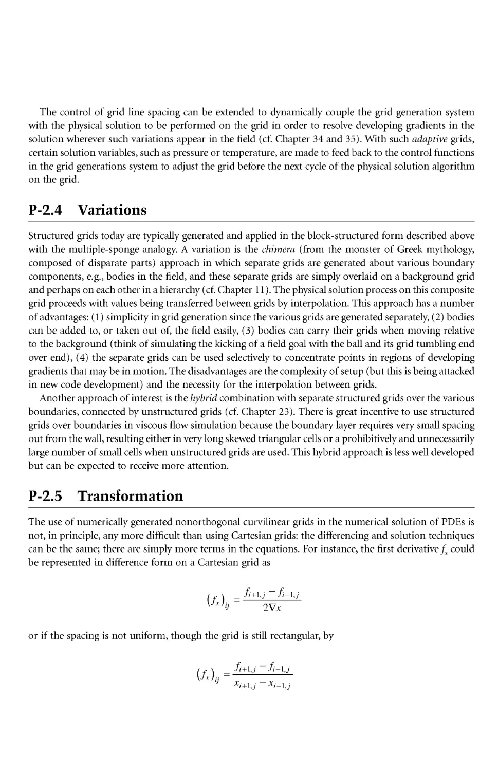
can be the same; there are simply more terms in the equations. For instance, the first derivative fx could
be represented in difference form on a Cartesian grid as
or if the spacing is not uniform, though the grid is still rectangular, by
fff
x
x ij ijij
()=
-
∇
+-
11
2
,,
fff
xx
xij ijij
ij ij
()=
-
-
+-
+-
11
11
,,
,,
To use a cur vilinear grid, this derivative is transformed so that the curvilinear coordinate (ξ,η) rather
than the Cartesian coordinate x,y, are the independent coordinates. Thus
where J = xξ yη -- xη yξ is the Jacobian of the transformation and represents the cell volume. This then
could be written in a difference form, taking Δξ and Δη to be unity without loss of generality, using
with analogous expressions for xξ, xη, yξ, yη.
Movement of the grid, either to follow moving boundaries or to dynamically adapt to developing
solution g radients, is not really a complication, since the time derivative can also be transformed as
where the time derivative on the left is taken at a fixed position in space, i.e., is the time derivative
appearing in the PDEs while the one on the right is that seen by a particular grid point moving with a
speed . The spatial der ivatives (fx ,fy) are transformed as was discussed above.There is no need to
interpolate solution values from the gr id at one time step to the displaced grid at the next time step,
since that transfer is accomplished by the g rid speed terms
in the above transformation relation.
The straightforwardness of the use of curvilinear grids is further illustrated by the appearance of the
generic convection--diffusion equations;
where u is the velocity, v is a diffusion coefficient, and S is a source term, after transformation:
where now the time derivative is understood to be that seen by a certain (moving) grid point. Here the
elements of the contravariant metric tensor g j are given by
fxfxf
J
x=
-
()
ξηη
ξ
f
ff
f
ij
ij ij
ij iji
j
ξ
η
()=-
()
()=-
()
+-
+-
12
12
11
11
,,
,,
fff
x
f
y
tr
tx
y
()= ()-+
()
ξ
˙
(˙,˙)
xy
(˙,˙)
xy
ffv
f
S
O
t +∇⋅()+∇⋅ ∇
()
+=
u
AU
vAg
v
AA
a
u
S
ti
ii
i ijij ji
i
ii
++
∇
()
+ ()+⋅
+
=
==
=
=
ΣΣ
Σ
Σ
1
3
2
1
3
1
3
1
3
0
ξξξ
ξ
ξ
ga
a
ijij
=⋅
where the ai are the contravariant base vectors (which are simply normals to the cell sides):
with the ai the covariant base vectors (tangents to the coordinate lines):
where r is the Cartesian coordinate of a grid point, and is the Jacobian of the transformation (the
cell volume):
Also, the contravariant velocity (normal to the cell sides) is
where u is the fluid velocity and r is the velocity of the moving grid. For comparison, the Cartesian grid
formulation is
The formulation has thusbeen complicated bythe cur vilinear grid onlyinthe sense thatthe coefficient
ui has been replaced by the coefficient U i + v(∇2ξ i), and the Kronecker delta in the double summation
has been replaced by g j (thus expanding that summation from three terms to nine terms),and through
the insertion of variable coefficients in the last summation. When it is considered that the transfor med
equationistobe solved on a fixedrectangular field w ith a uniform square grid,while theoriginalequation
would have to be solved on a fieldwithmoving cur ved boundaries,the advantages of usingthe curvilinear
systems are clear.
These advantages arefurtherevidenced by consideration of boundaryconditions. In general, boundary
conditions for the example being treated would be of the form
where n is the unit normal to the boundary and α, β, and γ are specified. These conditions transform to
aaa g
ijk
=×
()
/(ijkcyclic)
ar
i
i
=ξ
g
gaa a
=⋅×
()
123
Ua
u
r
i=⋅-
()
Au
A
v
AA
uS
tiixijijx
x
iix
ij
i
i
++()+ () +=
==
=
=
ΣΣ
ΣΣ
1
3
1
3
1
3
1
3
0
δ
αβγ
Au
A
+⋅∇
()
=
n
αβ
γ
ξ
Av
ggA
iijijj
+=
=Σ1
3
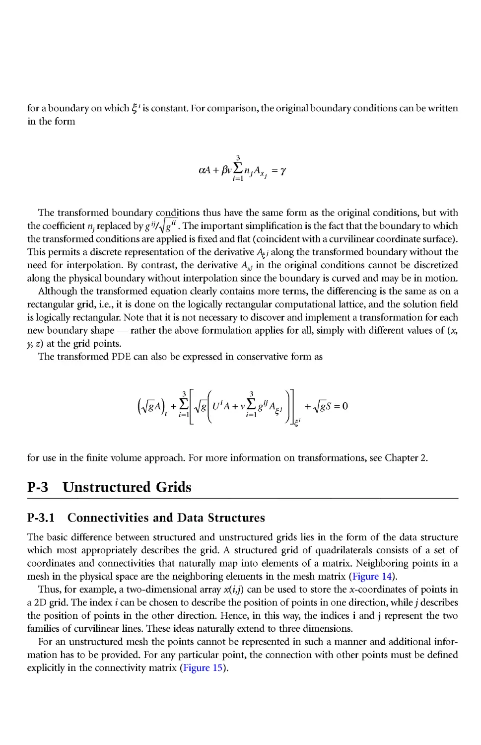
for a boundary on whichξ i is constant. Forcomparison, the original boundaryconditions canbe written
in the form
The transformed boundary conditions thus have the same form as the original conditions, but with
the coefficient nj replaced by g ij/ . The important simplification is the factthat theboundary to which
the transformed conditionsare appliedis fixed and flat (coincident with a curvilinear coordinate surface).
This permits a discrete representation of the derivative Aξj along the transformed boundary without the
need for interpolation. By contrast, the derivative Axj in the orig inal conditions cannot be discretized
along the physical boundary without interpolation since the boundary is curved and may be in motion.
Although the transformed equation clearly contains more terms, the differencing is the same as on a
rectangular grid, i.e., it is done on the logically rectangular computational lattice, and the solution field
is logically rectangular. Note that it is not necessary to discover and implement a transformation for each
new boundary shape --- rather the above formulation applies for all, simply with different values of (x,
y, z) at the grid points.
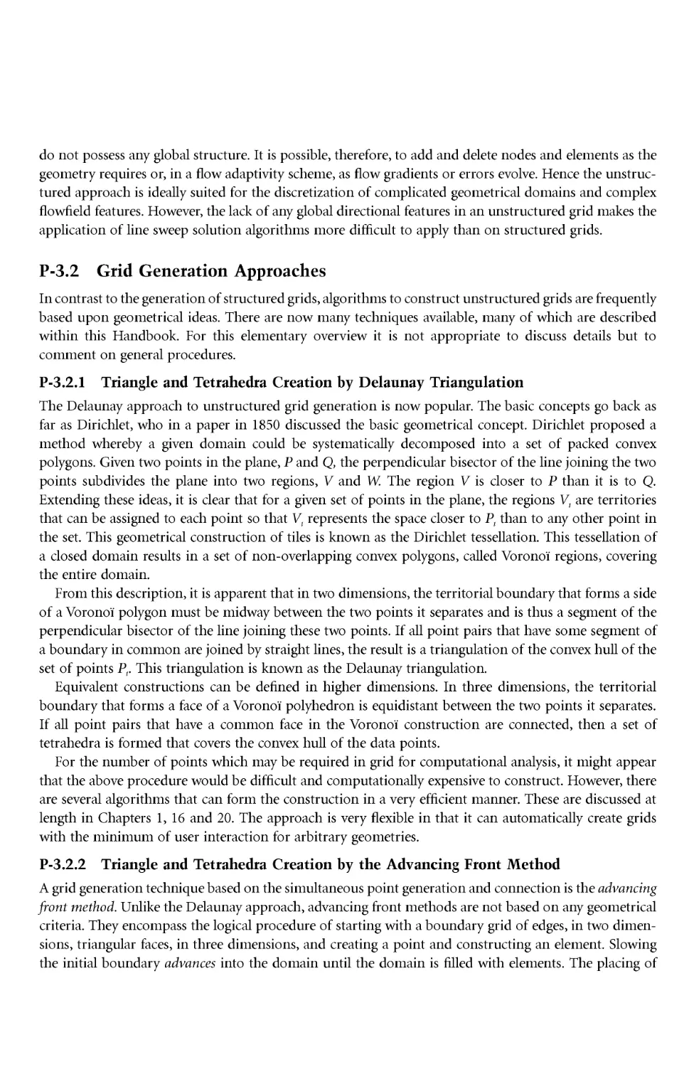
The transformed PDE can also be expressed in conservative form as
for use in the finite volume approach. For more information on transformations, see Chapter 2.
P-3 Unstr uctured Grids
P-3.1 Connectivities and Data Structures
The basic difference between structured and unstructured grids lies in the form of the data structure
which most appropriately describes the grid. A structured grid of quadrilaterals consists of a set of
coordinates and connectivities that naturally map into elements of a matrix. Neighboring points in a
mesh in the physical space are the neighboring elements in the mesh matrix (Figure 14).
Thus, for example, a two-dimensional array x(i,j) can be used to store the x-coordinates of points in
a 2D grid. The index i can be chosen to describe the position of pointsin one direction, while j describes
the position of points in the other direction. Hence, in this way, the indices i and j represent the two
families of curv ilinear lines. These ideas naturally extend to three dimensions.
For an unstructured mesh the points cannot be represented in such a manner and additional infor-
mation has to be provided. For any particular point, the connection with other points must be defined
explicitly in the connectivity matrix (Figure 15).
αβγ
Avn
A
ijx
j
+=
=Σ1
3
gii
gA
gUAvgA
gS
ti
i
i
ijj
i
()
++
+=
==
ΣΣ
1
3
1
3
0
ξξ
A typical form of data format for an unstructured grid in two dimensions is
Number of Points,
Number of Elements
x1, y1
x2, y2
x3, y3
...
n1, n2, n3
n4, n5, n6
n7, n8, n9
...
where (x1, y1) are the coordinates of point i, and ni, 1=1,N are the point numbers with, for example, the
triad (n1, n2, n3) forming a triangle.
Other forms of connectivity matrices are equally valid, for example, connections can be based upon
edges. The real advantage of the unstructured mesh is, howe ver, because the points and connectivities
FIGURE 14
FIGURE 15
do not possess any global structure. It is possible, therefore, to add and delete nodes and elements as the
geometry requires or, in a flow adaptivity scheme, as flow gradients or errors evolve. Hence the unstruc-
tured approach is ideally suited for the discretization of complicated geometrical domains and complex
flowfield features.However, the lack of any global directional features inan unstructured gridmakes the
application of line sweep solution algorithms more difficult to apply than on structured grids.
P-3.2 Grid Generation Approaches
In contrastto the generation of structured grids,algorithms to construct unstructured grids are frequently
based upon geometrical ideas. There are now many techniques available, many of which are descr ibed
within this Handbook. For this elementary overview it is not appropriate to discuss details but to
comment on general procedures.
P-3.2.1 Triangle and Tetrahedra Creation by Delaunay Triangulation
The Delaunay approach to unstructured grid generation is now popular. The basic concepts go back as
far as Dirichlet, who in a paper in 1850 discussed the basic geometrical concept. Dirichlet proposed a
method whereby a given domain could be systematically decomposed into a set of packed convex
polygons. Given two points in the plane, P and Q, the perpendicular bisector of the line joining the two
points subdivides the plane into two regions, V and W. The region V is closer to P than it is to Q.
Extending these ideas, it is clear that for a given set of points in the plane, the regions Vi are territories
that can be assigned to each point so that Vi represents the space closer to Pi than to any other point in
the set. This geometrical construction of tiles is known as the Dirichlet tessellation. This tessellation of
a closed domain results in a set of non-overlapping convex polygons, called Voronoï regions, covering
the entire domain.
From this description, it is apparent thatin two dimensions,the territorial boundary that forms a side
of a Voronoï polygon must be midway between the two points it separates and is thus a segment of the
perpendicular bisector of the line joining these two points. If all point pairs that have some segment of
a boundary in common are joined by straight lines, the result is a triangulation of the convex hull of the
set of points Pi. This triangulation is known as the Delaunay triangulation.
Equivalent constructions can be defined in higher dimensions. In three dimensions, the territorial
boundary that forms a face of a Voronoï polyhedron is equidistant between the two points it separ ates.
If all point pairs that have a common face in the Voronoï construction are connected, then a set of
tetrahedra is formed that covers the convex hull of the data points.
For the number of points which may be required in grid for computational analysis, it might appear
that the above procedure would be difficult and computationally expensive to construct. However, there
are se veral algorithms that can form the construction in a very efficient manner. These are discussed at
length in Chapters 1, 16 and 20. The approach is very flexible in that it can automatically create grids
with the minimum of user interaction for arbitrary geometries.
P-3.2.2 Triangle and Tetrahedra Creation by the Advancing Front Method
A grid generation techniquebased on the simultaneous point generationand connection is the advancing
front method . Unlike the Delaunay approach, advancing front methods are not based on any geomet rical
criteria. They encompass the logical procedure of starting with a boundar y grid of edges, in two dimen-
sions, triangular faces, in three dimensions, and creating a point and constructing an element. Slowing
the initial boundary advances into the domain until the domain is filled with elements. The placing of
points within the domain is, like the Delaunay approach, controlled by a combination of a backg round
mesh and sources that provides the required data to ensure adequate resolution of the domain. The
algor ithms that generate grids in this way are based on fast geometrical search routines. Details are to
be found in Chapter 17.
It is possible to combine techniques from both the Delaunay and the Advancing Front methods to
produce effective grid generation procedures -- a sort of combination that tries to utilize the advantages
of both approaches. Chapter 18 discusses one such approach.
The Delaunay triangulation produces elements that are isotropic in nature. Although the Advancing
Front methodcan produce elements with stretching, it cannot produce high quality meshes with stretch-
ing factors applicable to some problems, such as high Reynolds number v iscous flows. Hence, it is
necessary to augment the standard procedures outlined above. In general, this is done by introducing a
mapping that ensures that regular isotropic g ridscan be generated but once mappedback to the physical
space are distorted in a well defined manner to give appropriate element stretching. Such a method is
described in detail in Chapter 20.
P-3.2.3 Unstructured Grids of Quadrilaterals and Hexahedra
The preference of some developers for quadrilateral or hexahedral element based unstructured meshes
has resulted in effor t devoted to the generation of such meshes. In two dimensions, it is possible to
modify the Advancing Front algorithm to construct quadrilaterals, although the additional complexity
in extending this approach to three dimensions has not yet been overcome for practical geometries. An
alternative approach that has seen some success is that of "paving."This approach relies upon iteratively
layering or paving rows of elements in the interior of a region. As rows overlap or coincide they are
carefully connected together. It is fair to conclude that almost without exception the methods for the
construction of unstructured hexahedralbased grids are heuristic in nature,requiring considerable effort
to include the many possible geometrical occurrences. Chapter 21 discusses in detail aspects of this kind
of grid generation.
P-3.2.4 Surface Mesh Generation
The generation of unstructured grids on surfaces is, in itself, one of the most difficult and yet important
aspects of mesh generation in three dimensions. The surface mesh influences the field mesh close to the
boundary. Surface meshes have the same requirement for smoothness and continuity as the field meshes
for which they act as boundary conditions, but in addition, they arerequired to conform to the geometry
surfaces, including lines of intersection and must accurately resolve regions of high curvature.
The approach usually taken to generate gr ids on surfaces is to represent the geometry in parametric
coordinates. A parametric representation of a surface is straightforward to construct and provides a
description of a surface in terms of two paramet ric coordinates. This is of particular importance, since
the generation of a mesh on a surface then involves using grid generation techniques developed for two
space dimensions. A full description of these procedures is given in Chapter 19.
P-3.3 Grid Adaptation Techniques
To resolve features of a solution field accurately it is, in general, necessary to introduce grid adaptivity
techniques. Adaptivity is based on the equidistribution of errors principle, namely,
widsi = constant
where wi is the error or activity indicator at node i and dsi is the local gr id point spacing at node i.
Central to adaptivity techniques and the satisfaction of this equidistribution principle is to define an
appropriate indicator wi. Adaptivity criteria are based on an assessment of the error in the solution of
the governing equations or are constructed todetect features of the field. These estimators are intimately
connected to the analysis equations to be solved. For example, some of the main features of a solution
of the Euler equations can be shock waves, stagnation points and vortices, and any indicator should
accurately identify these flow characteristics. However, for the Navier-Stokes equations, it is important
not only to refine the mesh in order to capture these features but, in addition, to adequately resolve
viscous dominated phenomena such as the boundary layers. Hence, it seems likely that, certainly in the
near future, adaptivity criteria will be a combination of measures, each dependent on some aspects of
the flow and, in turn, on the flow equations.
There is alsoan extensive choice of criteria based on error analysis. Such measures include, a compar-
ison of computational stencils of different orders of magnitude, comparison of the same derivatives on
different meshes, e.g., Richardson extrapolation, and resort to classical error estimation theor y. No
generally applicable theor y exists for errors associated with hyperbolic equations, hence, to date combi-
nations of rather ad hoc methods have been used.
Once an adaptivity criterion has been established, the equidistribution principle is achieved through
a variety of methods, including point enrichment, point derefinement, node movement and remeshing,
or combinations of these. For more information on grid adaption techniques, see Chapter 35.
P-3.3.1 Grid Refinement
Grid refinement, or h-refinement, involves the addition of points into regions where adaptation is
required. Such a procedure clearly provides additional resolution at the expense of increasing the number
of points in the computation.
Grid refinement on unstructured grids is readily implemented. The addition of a point or points
involves a local reconnection of the elements, and the resultinggrid has the same form as the initial grid.
Hence, the same solver can be used on the enriched grid as was used on the initial grid.
It is important that the adaptivity criteria resolve both the discontinuous features of the solution (i.e.
shock waves, contacts) and the smooth features as the number of grid points are increased. A desirable
feature of any adaptive method to ensure convergence is that the local cell size goes to zero in the limit
of an infinite number of mesh points.
Grid refinement on a structured or multiblock grids is not so straightforward.The addition of points
will, in general, break the regular array of points.The resulting distributed grid pointsnolongernaturally
fit into the elements of an array. Furthermore, some points will not "conform" to the grid in that they
have a different number of connections to other points. Hence g rid refinement on structured grids
requires a modification to the basic data structure and also the existence of so-called non-conforming
nodes requires modifications to the solver. Clearly, point enrichment on structured gridsis not as natural
a process as the method applied on unstructured grids and hence is not so widely employed. Work has
been undertaken to implement point enrichment on structured grids and the results demonstrate the
benefits to be gained from the additional effort in modifications to the data structure and the solve.
P-3.3.2 Grid Movement
Grid movement satisfies the equidistribution principle through the mig ration of points from regions of
low activity into regions of high activity. The number of nodes in this case remains fixed. Traditionally,
algorithms to move points involve some optimization principle. Ty pically, expressions for smoothness,
orthogonality and weighting according to the analysis field or errors are constructed and then an opti-
mization is performed such that movement can be driven by a weight function, but not at the expense
of loss of smoothness and orthogonality. Suchmethods are in general,applicableto both structured and
unstructured grids.
An alternative approach is to use a weighted Laplacian function. Such a formulation is often used to
smooth grids, and of course the formal version of the formulation is used as the elliptic grid generator
presented earlier.
P-3.3.3 Combinations of Node Movement, Point Enrichment and Derefinement
An optimum approach to adaptation is to combine node movement and point enr ichment with dere-
finement. These procedures should be implemented in a dynamic way, i.e., applied at regular intervals
within thesimulation. Such anapproach also provides the possibility of using movementand enrichment
to independently capture different features of the analysis.
P-3.3.4 Grid Remeshing
One method of adaptation which, to date, has been primarily used on unstructured grids, is adaptive
remeshing. As already indicated,unstructured meshes canbe generated using the concept of abackground
mesh. For an initial mesh, this is usually some very coarse triangulation that covers the domain and on
which the spatial distribution is consistent with the given geometry. For adaptive remeshing, thesolution
achieved on an initial mesh is used to define the local point spacing on the background mesh which was
itself the initial mesh used for the simulation. The mesh is regenerated using the new point spacing on
the background mesh. Such an approach can result in a second adapted mesh that contains fewer points
than that contained in the initial mesh.However, there is the overhead of regeneration of the mesh which
in three dimensions can be considerable. Nevertheless, impressive demonstrations of its use have been
published.
Contents
Foreword
Contributors
Acknowledgments
Preface: An Elementary Introduction Joe F. Thompson, Bharat K. Soni,
and Nigel P. Weatherill
1 Fundamental Concepts and Approaches Joe F. Thompson and
Nigel P. Weatherill
PART I Block-Structured Grids
Introduction to Structured Grids Joe F. Thompson
2 Mathematics of Space and Surface Grid Generation Zahir U.A. Warsi
3 Transfinit e Interpolation (TFI) Generation Systems Robert E. Smith
4 Elliptic Generation Systems Stefan P. Spekreijse
5 Hyperbolic Methods for Surface and Field Grid Generation
William M. Chan
6 Boundary Orthogonality in Elliptic Grid Generation
Ahmed Khamayseh, Andrew Kuprat, and C. Wayne Mastin
7 Orthogonal Generation Systems Luís Eça
8 Harmonic Mappings Sergey A. Ivanenko
9 Surface Grid Generation Systems A hmed Khamayseh and Andrew Kuprat
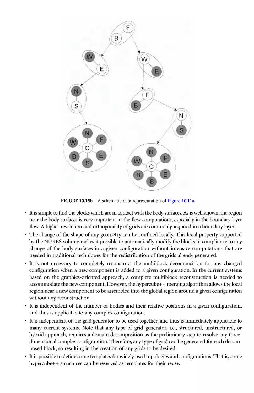
10 A New Approach to Automated Multiblock Decomposition for Grid
Generation: A Hypercube++ Approach Sangkun Park and Kunwoo Lee
11 Composite Overset Structu red Grids Robert L. Meakin
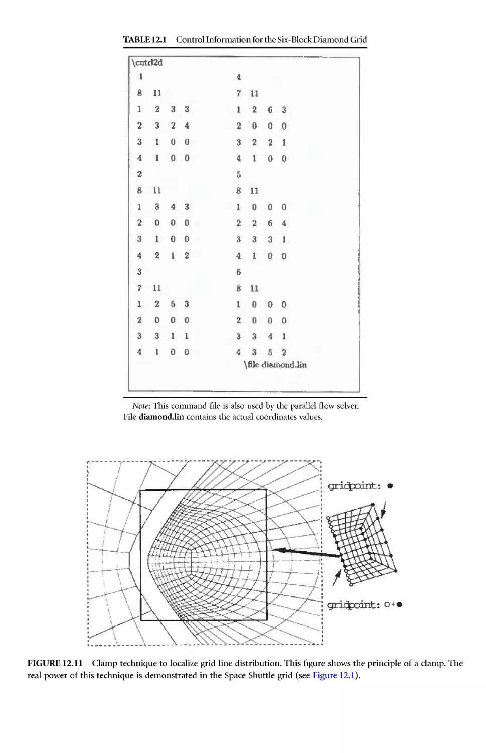
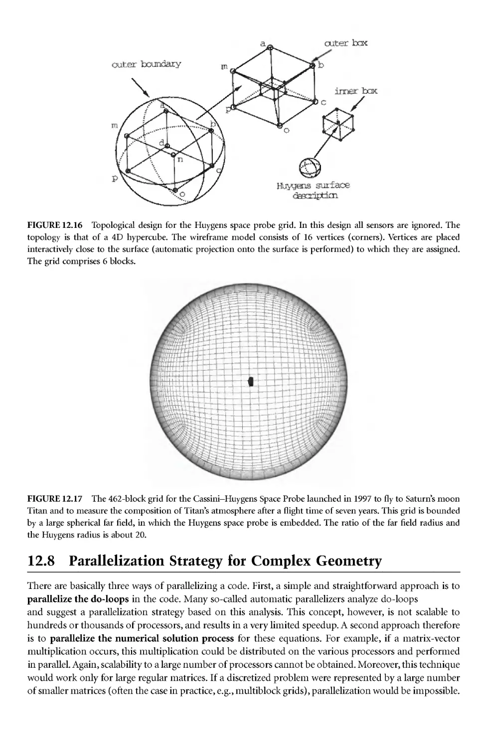
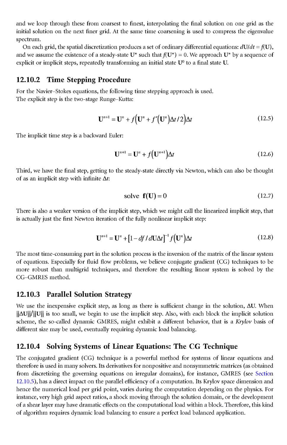
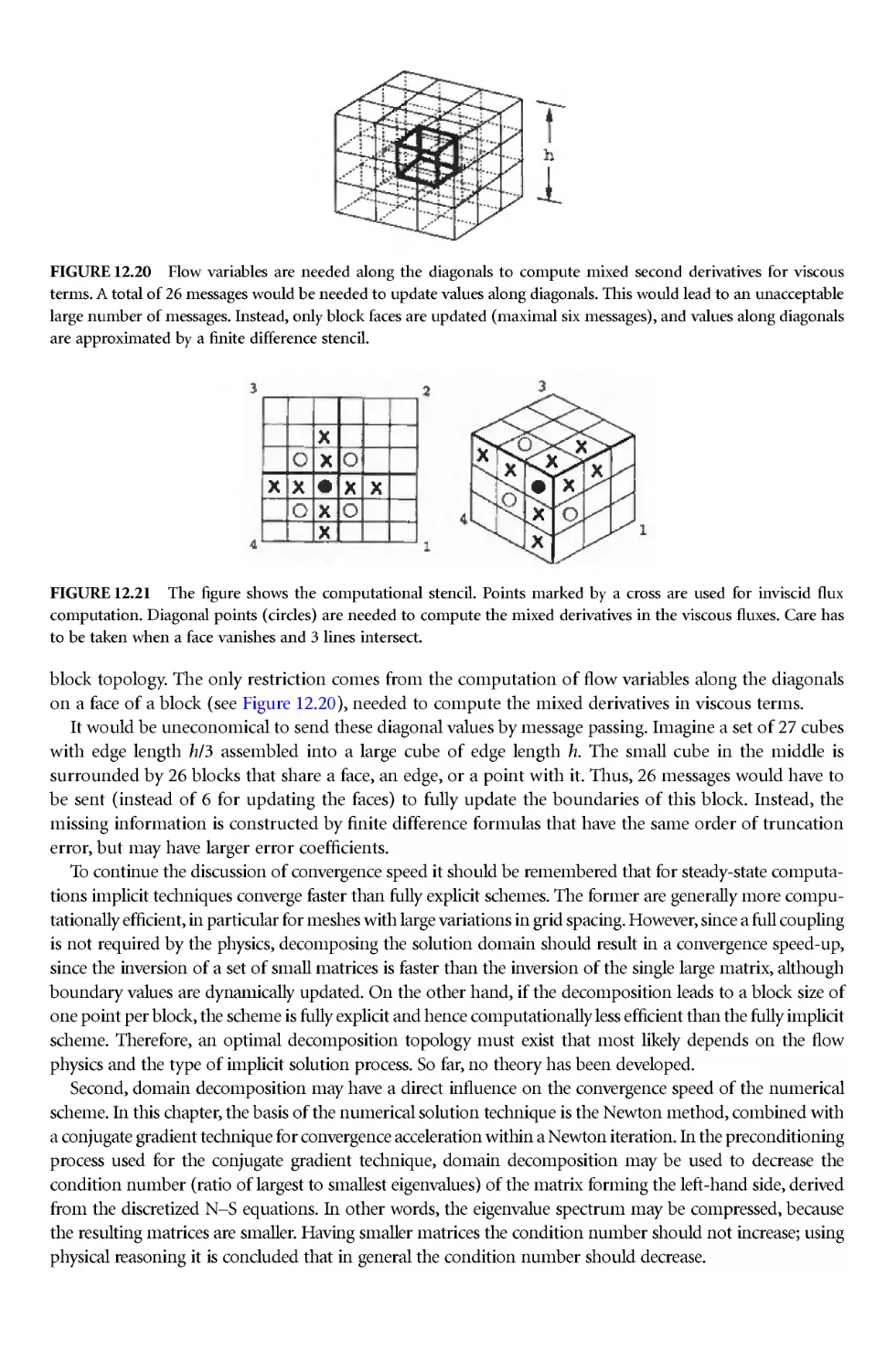
12 Parallel Multiblock Structured Grids Jochem Häuser, Peter R. Eiseman,
Yang Xia, and Zheming Cheng
13 Block-Structured Applications Timothy Gatzke
PART II Unstructured Grids
Introduction to Unstructured Grids Nigel P. Weatherill
14 Data Structures for Unstructured Mesh Generation L uca Formaggia
15 Automatic Grid Generation Using Spatially Based Trees
Mark S. Shephard, Hugues L. de Cougny, Robert M. O'Bara, and Mark W. Beall
16 Delaunay--Voronoï Methods Timothy J. Baker
17 Advancing Front Grid Generation J. Peraire, J. Peiró, and K. Morgan
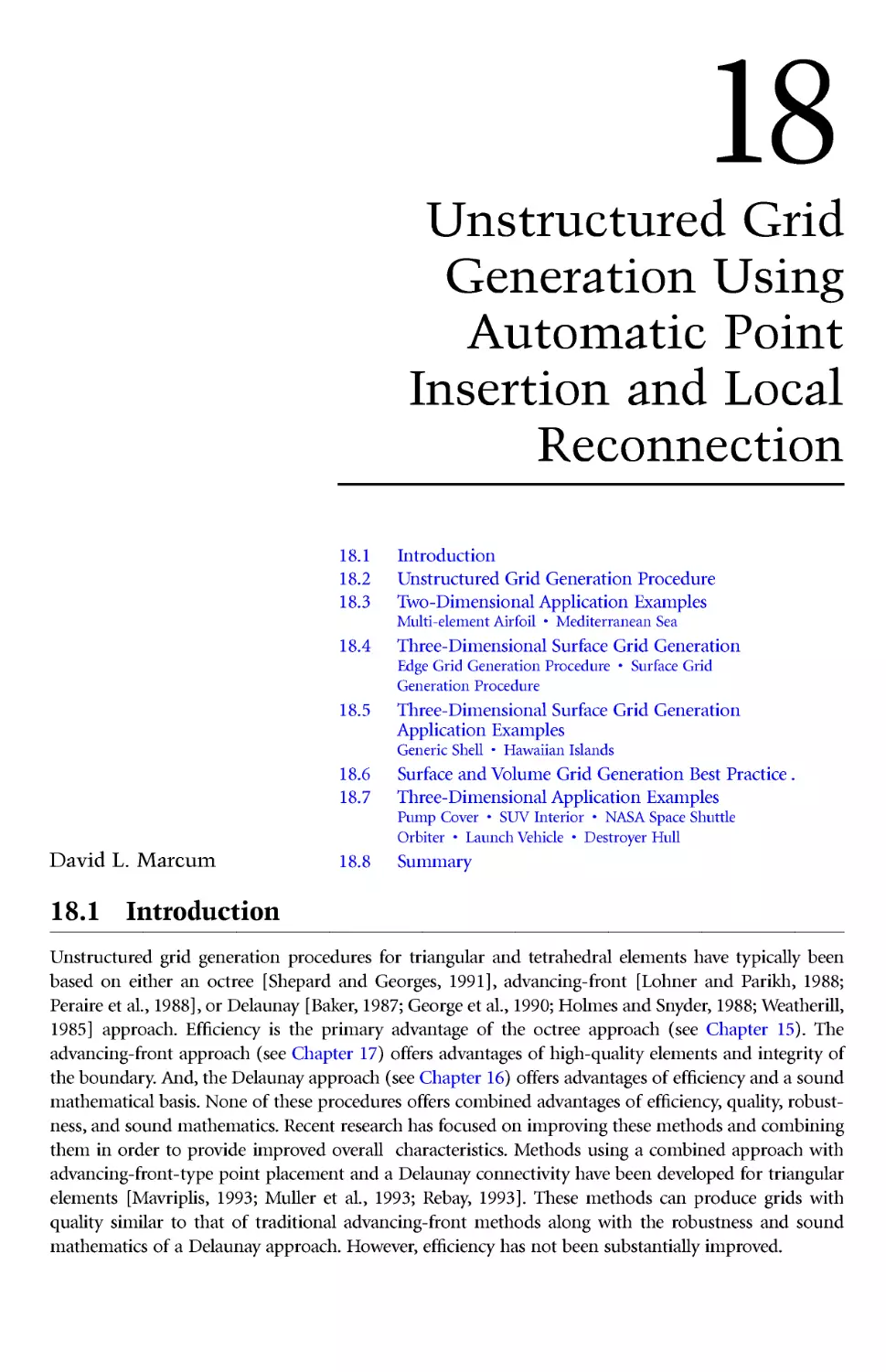
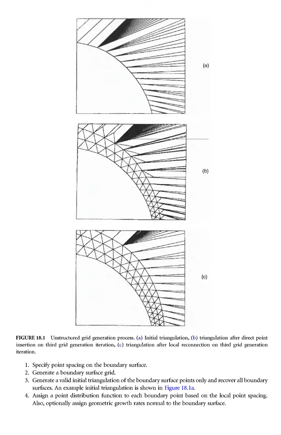
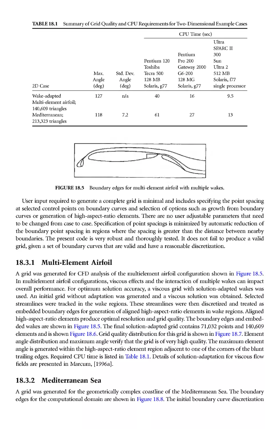
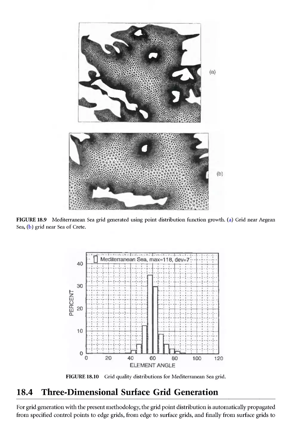
18 Unstructured Grid Generation Using Automatic
Point Insertion and Local Reconnection David L. Marcum
19 Surface Grid Generation J. Peiró
20 Nonisotropic Grids Paul Louis George and Frédéric Hecht
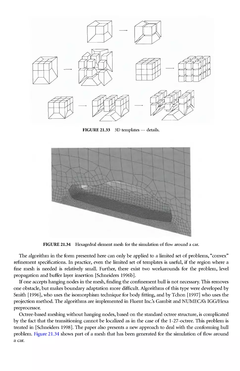
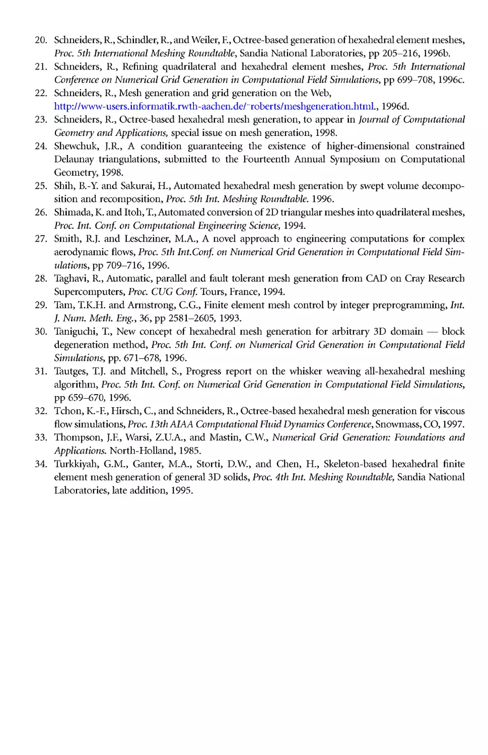
21 Quadrilateral and Hexahedral Element Meshes Robert Schn eiders
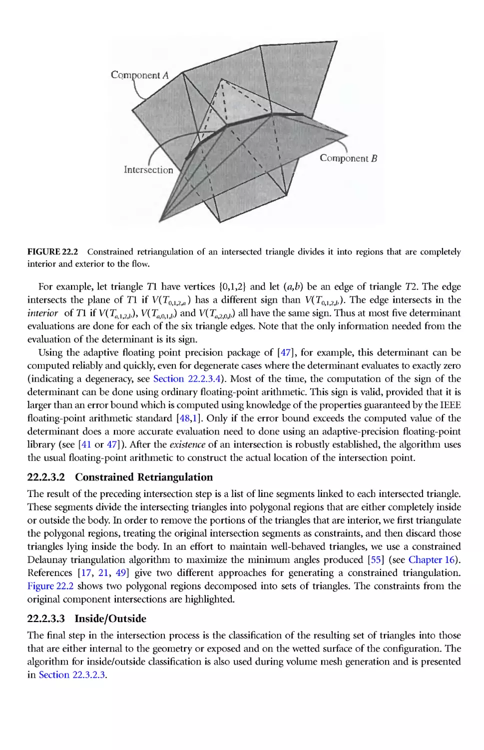
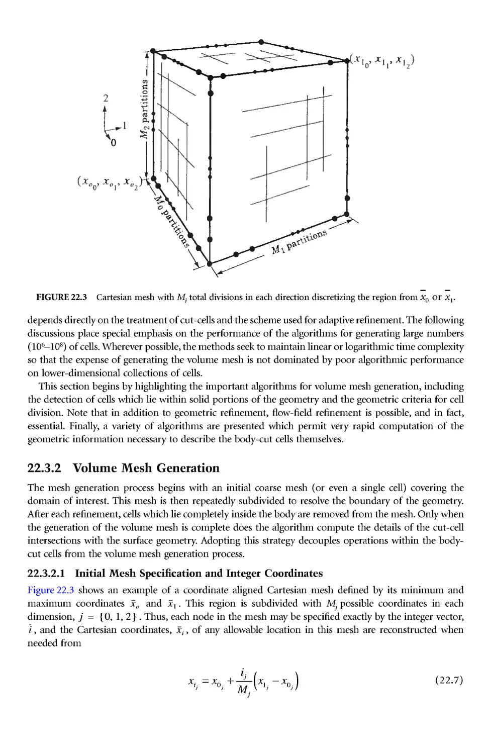
22 Adapt ive Cartesian Mesh Generation Michael J. Aftosmis, Marsha J. Berger,
and John E. Melton
23 Hybrid Grids Jonathon A. Shaw
24 Parallel Unstructured Grid Generation Hugues L. de Cougny and
Mark S. Shephard
25 Hybrid Grids and Their Applications Yannis Kallinderis
26 Unstructured Grids: Procedures and Applications Nigel P. Weatherill
PART III Surface Definition
Introduction to Surface Definition Bharat K. Soni
27 Spline Geometry: A Numerical Analysis View David R. Ferguson
28 Computer-Aided Geometric Design Gerald Farin
29 Computer-Aided Geometric Design Techniques for Surface
Grid Generation Bernd Hamann, Brian Jean, and Anshuman Razdan
30 NURBS in Structured Grid Generation Tzu-Yi Yu and Bharat K. Soni
31 NASA IGES And NASA-IGES NURBS Only Standard Austin L. Evans
and David P. Miller
PART IV Adaptation and Quality
Introduction to Adaptation and Quality Bharat K. Soni
32 Truncation Error on Structured Grids C. Wayne Mastin
33 Grid Optimization Methods for Quality Improvement and
Adaptation Olivier-Pierre Jacquotte
34 Dynamic Grid Adaptation and Grid Quality D. Scott McRae and
Kelly R. Laflin
35 Grid Control and Adaptation O. Hassan and E. J. Probert
36 Variational Methods of Construction of Optimal Grids O. B. Khai rullina,
A. F. Sidorov, and O. V. Ushakova
37 Moving Grid Techniques Paul A. Zegeling
Appendix A: Grid Software and Configurations Bharat K. Soni
Appendix B: Grid Configurations Bharat K. Soni
I
Block-Structured
Grids
Joe F. Thompson
Introduction to Str uctured Grids
The grid generation process, in general, proceedsfrom first defining the boundary geometry as discussed
in Part III. Then points are distributed on the curves thatform the edges of boundary sections. A surface
grid is then generated on the boundary surface, and finally a volume grid is generated in the field.
Chapter 13 gives a general overview of the entire grid generation process and the fundamental choices
and considerations involved from the standpoint of the user.
The underlying essential mathematics of structured grid generation, including essential concepts from
differential geometry and tensor analysis, is collected in Chapter 2. The mathematical constructs
explained in this chapter are utilized throughout the chapters of this handbook.
The distribution of points on boundar y curves (edges of boundary surfaces) is commonly done
through several distribution functions as described in Section 3.6 of Chapter 3. (The mathematics of
curves is covered in Section 2.3 of Chapter 2.) These functions have been adopted over time as providing
point distributions that comply with certain constraints that must be applied in order to control error
that can be introduced into the solution by the grid if the spacing changes too rapidly, as discussed in
Chapter 32 of Part IV.
Structured grids can be generated algebraically or as the solution of PDEs. Algebraic grid generation
is simply some form of interpolation from boundary points --- the variants just use different kinds of
interpolation. The most fundamental and versatile form --- and now commonly incorporated in grid
generation codes --- is TFI (transfinite interpolation), which is introduced in Section 1.35 of Chapter 1
and described in Chapter3. The basic equations of TFI are given in Section 3.4 of Chapter 3, and the
specific equations for application with and without orthogonality at the boundaries are given in
Section 3.5.
Algebraic grid generation based on TFI is the fastestprocedure for structured grids, and is also commonly
used to generate an initial grid in generation systems based on PDEs. Grids generated algebraically can,
however, have some problems with smoothness and may overlap strongly convex portions of boundaries.
Generation systems based onPDEs can produce smoother g rids with fewer problems with boundary overlap.
Such generation systems are therefore often used to smooth algebraic grids.
Since grid generation is essentially a boundary-value problem, grids can be generated from point
distributions on boundaries by solving elliptic PDEs in the field. The smoothness proper ties and extre-
mum principlesinherentinsome such PDE systemscan servetoproduce smooth grids without boundary
overlap. The PDE solution is generally one by iteration, and therefore elliptic grid generation is not as
fast as algebraic grid generation.
The elliptic PDEs for grid generation are not unique, of course, but must be designed. This design
has converged over the years to the elliptic system given in Section 1.3.3 of Chapter 1, which forms the
basis for most gr id generation codes today. This formulation incorporates control functions that are
determined from the boundary point distribution to control the grid line spacing and orientation in the
field to be compatible with that on the boundary. Procedures for the deter mination of these control
functions in grid codes have evolved in time to the forms noted in this section of Chapter 1, which can
accomplish boundary orthogonalitythrough iterative adjustment dur ingthe generation process. A more
recent and general formulation, with a sounder basis for evaluation of the control functions, is given
here in Chapter 4: for 2D in Section 4.2 and for 3D in Section 4.4. This iterative solution of the elliptic
system isoften done by SOR, but a Picard iteration is given in Section 4.2.2 of Chapter 4, and a conjugate
gradient solution is given in Section 12.10.4 of Chapter 13, in connection with parallel implementation.
The generation of a grid on a boundary surface is a necessary prelude to the generation of a volume
grid, andthis is generally done by representing theboundary surfaceparametrically by NURBS or another
spline formulation, and then generating the grid in parameter space either algebraically or using PDEs.
This is perfectly analogous to 2D grid generation except that surface cur vature terms appear in the PDEs.
With the generation system operating in parameter space, the resulting g rid is guaranteed to lie on the
boundary surface. The parametric representation of the boundary surface is covered in Chapter 29,
utilizing the underlying curve and surface constructs given in Chapter 28. Other aspects of surface
generation are covered in the other chapters in Part III, and the mathematical foundations are g iven in
Section 2.4 and in Section 2.5.2 of Chapter 2.
Algebraic surface grid generation is simply the application of TFI to generate values of the surface
parameters on the surface from the values set on the edges of the boundary surface by the grid point
distribution on those edges, as covered in Section 9.2 of Chapter 9. Elliptic surface grid generation
operates with the PDEs formulated in terms of the surface parameters, and surface curvature terms
appearing in the PDEs (see Section 2.5.2 of Chapter 2). A commonly applied procedure is given in
Section 9.3 of Chapter 9, and a more recent and general procedure is given in Section 4.3 of Chapter 4.
Hyper bolic surface grid generation is covered in Section 5.3 of Chapter 5.
It is generally advantageous, in view of such things as boundar y layer phenomena and turbulence
models, to have the grid orthogonal to boundarieseven though orthogonality is not imposed in the field.
This is commonly done through iterative adjustment of the control functions as described in Chapter6:
in Section 6.2 for 2D grids, Section 6.3 for surfa ce grids, and Section 6.4 for volume grids. Another
procedure in 2D, also using the control functions, is given in Section 4.2 of Chapter4.
An alternative approach to grid generation via PDEs is to use a hyperbolic generation system rather
than an elliptic. Elliptic equations admit boundary conditions, i.e., grid point distributions, on all
boundaries of a region. Hyperbolic systems, however, can take boundary conditions only on a portion
of the boundary.Therefore, while elliptic grid generation systems can produce agrid in the entire volume
from point distributions of the entire boundary, hy perbolic systems generate the grid by marching
outward from a portion of the boundary. Hyperbolic grid generation systems therefore cannot be used
togenerate a gridin the entirety of avolume defined by a complete boundar y. Chapter 5 covers hyperbolic
grid generation in volumes in Section 6.2 and on surfaces in Section 6.3.
Structured grids are not generally made orthogonal, although orthogonality at boundaries is often
incorporated, as has been noted above. In fact, 3D orthogonality is not, in general, possible without
imposing certain conditions on the grids on the boundary surfaces. And even in 2D, orthogonality
imposes severe restrictions on the grid distribution. Transformed PDEs, however, take a much simpler
form on orthogonal grids, providing some incentive for their use when feasible --- w ith relatively simple
boundary configurations and physical problems without strong localized gradients. Chapter 7 covers
orthogonal grid generation systems.
As has been noted, PDEs for grid generation are designed, not discovered. Considerable research has
gone into this topic, leading to generally standard elliptic (Chapter 4) and hyperbolic (Chapter 5) grid
generation systems. The underlying theory of harmonic mappings provides a framework for the devel-
opment of elliptic grid generation systems, and this topic is treated in some depth in Chapter 9. This
theoretical base also leads to the formulation of adaptive grid systems, also covered in this chapter.
Adaptive grids are most fundamentally formulated from variational principles, and this is covered in
Chapter 36 of Part IV. Adaptive grids and grid quality are covered in the chapters of Part IV.
A strong and versatile alternative to block-structured grids is the overset grid approach (originally
called chimera,after the composite monster of Greek mythology).With this approach, individual struc-
tured grids are generated around separate boundar y components, e.g., bodies, and these separate grids
simply overlap each other in some hierarchy. Data is transferred between overlapping grids by interpo-
lation.The overset grid approach is coveredhere inChapter 11. The grid generation involved is typically
done by hyperbolic generation systems, described in Chapter 5.
The mathematics and technolog y of structured grid generation have matured now so that the tech-
niques covered in Part I can be expected to be of enduring utility. The block structure is versatile, and
serves as the foundation for efficient solutions because of its inherently simple data structure. Construc-
tion of the block configuration by hand, even with graphically inter active tools, is very labor intensive,
however, as noted in Chapter 13. Automation of the block structure, rather than graphical interaction,
is the goal, and this is an area of active research and development (Section 21.2 of Chapter 21 is relevant
here). A very promising recent approach is included in Chapter 11. Finally, oper ation on parallel pro-
cessors is essential now, and the block structure provides a natural means of domain decomposition, as
covered in Sections 12.8--12.10 of Chapter 12.
The operation of the block structureis discussed in Sections 12.2--12.6 of Chapter 12. Chapter 12 also
covers a script-based meta-language approach to structured grid generation in Section 12.7. Although
most available grid generation systemshavedeparted from thescript-basedapproach in favor of graphical
interaction, the scr ipt-based approach has definite advantages in design cycles.
1
Fundamental Concepts
and Approaches
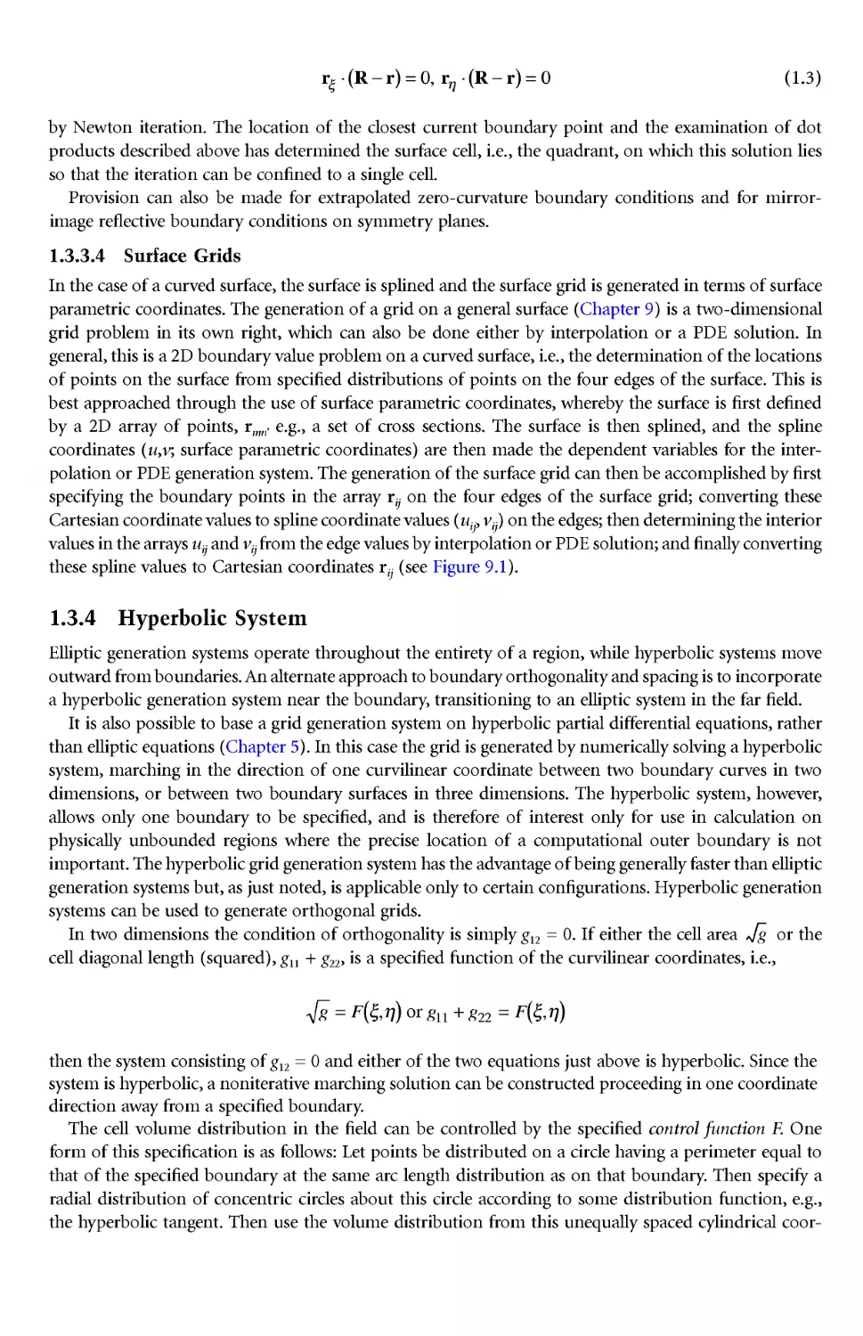
1.1 Introduction
1.2 Mesh Generation Considerations
1.3 Structured Grids
Composite Grids • Block-Structured Grids • Elliptic
Systems • Hyperbolic System • Algebraic System • Adaptive
Grid Schemes
1.4 Unstructured Grids
The Delaunay Triangulation • Point Creation • Other
Unstructured Grid Techniques • Unstructured Grid
Generationon Surfaces • Adaptation on Unstructured
1.1 Introduction
This introductorychapter uses fluidmechanics as an example field problem forreference;the applicability
of the concepts discussed is, however, not in any way limited to this area.
Fluid mechanics is described by nonlinear equations, which cannot generally be solved analytically,
but which have been solved using various approximate methods including expansion and perturbation
methods, sundry particle and vortex tr acing methods, collocation and integral methods, and finite
difference, finite volume, and finite element methods. Generally the finite difference, finite volume, and
finite element discretization methods have been the most successful, but to use them it is necessary to
discretize the field using a gr id (mesh). (The terms grid and mesh are used interchangeably throughout
with identical meaning .) The mesh can be structured or unstructured, but it must be generated under
some of the various constraints described below, which can often be difficult to satisfy completely. In
fact, at present it can take orders of magnitude more person-hours to construct the grid than it does to
construct and analyze the physical solution on the grid. This is especially true now that solution codes
of wide applicability are becoming available. Computational fluid dynamics (CFD) is a prime example,
and grid generation has been cited repeatedly as a major pacing item (cf. Thompson [1996]). The same
is true for other areas of computational field simulation.
The proceedings of the severalinternational conferences on grid generation(Thompson [1982],Hauser
and Taylor [1986], Sengupta, et al. [1988], Arcilla, et al.[1991], Eiseman, et al.[1994], Soni et al. [1996])
as well as those of the NASA conferences (Smith [1980],Smith [1992], Choo [1995]) provide numerous
illustrations of application to CFD and some other fields.
A recent comprehensive text is Carey [1997].
Joe F. Thompson
Nigel P. Weatherill
Grids • Summary
1.2 Mesh Generation Considerations
The generated mesh must be sufficiently dense that the numerical approximation is an accurate one, but
it cannot be so dense that the solution is impractical to obtain. Generally, the grid spacing should be
smoothly and sufficiently refined to resolve changes in the gradients of the solution. If the grid is also
boundary-conforming and curvilinear, the application of boundary conditions is simplified. Boundary-
conforming curvilinear grids mayalsoallow the use of various approximate equationssuch as boundary-
layer equations. The grid should also be constructed with computational efficiencyin mind. The accuracy
of a numerical approximation can also be impaired, if a grid changes discontinuously or is too skewed.
Variouscomputers often requirewell-organized data, and memory requirements can growto impractical
imits unless the data is organized well. Finally, the choice of a grid should not lead to overly complex
computer codes.
A mesh is a set of points distributed over a calculation field for a numerical solution of a set of partial
differential equations (PDEs). This set may be structured, e.g.,formed by the intersections of curvilinear
coordinate surfaces, or unstructured, i.e., with no relation to coordinate directions. In the first case the
points form quadrilateralcells in 2D, or hexahedral cells in 3D (with nonplanar sides). The unstructured
mesh generally consists of triangles and tetrahedra in 2D and 3D, respectively, in its most basic form,
but may be made of hexahedra or elements of any shape in general.
The structured grid can be generated algebraically by interpolation from boundaries, eg., transfinite
interpolation, orby solving a set of partial differential equations in the region. An entire subject, complete
with textbook (Thompson, Warsi, and Mastin [1985], now on the Web at www.erc.msstate.edu ), has
developed around the generation of structured grids having the fundamental characteristic that some
curvilinear coordinate surface is coincident with each boundary segment, i.e., boundary conforming. A
latertext is Knupp and Steinberg [1993]. Castillo [1991] provides a compilationof mathematical aspects
aswell.Structured grid generation is also covered in the recent text of Carey [1997]. Several earlier surveys
of the field are still useful for basic understanding (Thompson, Warsi, and Mastin [1982], Thompson
[1984], Thompson [1985], Eiseman [1985]).
Structured boundary-conforming meshes have been widely applied in computational fluid dynamics.
Basically, the algebraic generation systems (Chapter 3) are faster, but the grids generated from partial
differential equations are generally smoother. The hyperbolic generation systems (Chapter 5) are faster
than the elliptic systems,but are more limited in the geometries that can be treated. The elliptic systems
(Chapter 4) are the most generally applicable with complicated boundary configurations, but transfinite
interpolation is also effective in a composite grid framework.
The generation of unstructured meshes can be done by tessellation of a point distribution that could
be random but is more likely to have been produced by some ordered procedure. This tessellation is not
unique,and involves some type of nearest-neighborsearch, suchas the Delaunaytriangulation (Chapter
16). Other approaches are the advancing front procedure (Chapter 17) and the finite octree method
(Chapter 15). The recent text of Carey [1997] covers unstructured grid generation as well as structured
grid generation. An earlier text on unstructured grids is George [1991].
General configurations can conceivably be treated with either type of mesh, and hybrid combinations
(Chapter 23) are also possible, using individual structured meshesnear boundaries, with thesesubregions
being connected by an unstructured mesh. Still another approach is overlaid grids (chimera) (Chapter
11), in which separate boundary-conforming structured grids are generated for each component of a
complex configuration, and data is communicated betweenthe various component grids by interpolation.
Of particular importance is the development of dynamically adaptive meshes (Chapters 33--36) coupled
with the physical solution. In this mode the mesh is locally refined by the selective addition of points,
and/or is moved to concentrate points, in order to resolve developing gradients in the physical solution
on the mesh. Both of these approaches have seen considerable development and show much promise in
particular areas.
Implementation of solution algorithms on structured,unstructured, andoverlaid grids places differing
requirements on the algorithms. Various conflicts arise between the grid and solution procedures in
regard to requirements and ease of operation. In particular, unstructured grids require a much more
complex solution data structure, but are more easily generated and adapted. Structured grids provide a
more natural representation of normal derivative boundary conditions and allow more straightforward
approximations based on prevailing directions, e.g., parallel or normal to a boundary or flow direction.
The structure also leads to a much simpler data set construction, and allows the use of directional time
splitting and flux representations. On the other hand, unstructured grids can be much more readily
imagined for complicated boundary configurations.
1.3 Structured Grids
1.3.1 Composite Grids
Structured g rid generation had its roots in the U.S. in the work of Winslow and Crowley at Lawrence
Livermore National Lab in thelate 1960s (Winslow [1967]), and in Russia from Godunov and Prokopov
[1967] at about the same time. (There is also that enigmatic Biblical reference to the "four corners of
the earth," once thought to proclaim a flat earth but now seen to be a prophesy of structured grid
generation.) Another very fundamental component was the work of Bill Gordon at Drexel on transfinite
interpolation for the automotive industry, introduced to the emerging grid generation community at the
grid conference in Nashville in 1982 (Gordon and Thiel [1982]).
1.3.1.1 Terminology
Theuseofcomposite grids has been thekeytothe treatmentof general 3Dconfigurations with structured
grids. Here in general, composite refers to the fact that the physical region is divided into subregions,
within each of which a structured grid is generated. These subgrids may be patched together at common
interfaces, may be overlaid, or may be connected by an unstructured grid. Considerable confusion has
arisen in regard to terminolog y for composite grids, making it difficult to immediately classify papers
on the subject.
Composite gridsinwhichthe subgridsshare common interfaces arereferred to as block, patched, embedded,
or zonal grids in the literature. The use of the first two of these terms is fairly consistent with this type of
grid (patchedcomes from the common interfaces,block from the logicallyrectangular structure),but the last
two are sometimes also applied to overlaid grids. Overlaid (overset) grids are often called chimera grids after
the composite monster of Greek mytholog y. Unfortunately, the common interface grids can also be said to
overlap, since they typically use surrounding layers of points to achieve continuity. Embedded grids can be
almost anything, and the term is probably best avoided.The use of zonalcomes mostly from CFD applications
where the suggestion of applying different solution equations sets in different flow regions is made. Perhaps
block or patched would be best for the common interface grids, chimera for the overlaid (avoiding overlaid)
grids, and hybrid for the structured--unstructured combinations.
1.3.1.2 For ms
With this terminology adopted, the block (or patched) g rids may be completely continuous at the
interfaces, have slope or line continuity, or be discontinuous (sharing a common interface but not
common points thereon). (Block seems to cover all of these possibilities, but patched is being stretched
a bit in the latter case.) Complete continuityis achieved through a surrounding layer of (image, phantom)
points at which values are kept equal to those at corresponding object points inside an adjacent block.
This requires adata indexing procedure to link theblocks across theinterfaces. With complete continuity,
the interface is not fixed (not even in shape), but is determined in the course of the solution. This type
of interface necessitates an elliptic generation system. Slope continuity requires that the grid generation
procedureincorporate some control overthe intersectionangle at boundaries (usually, but not necessarily,
orthogonality),ascan be done through Hermite interpolation in algebraic generationsystemsor through
iterative adjustment of the control functions in elliptic systems. In this case the points on the interface
are fixed, and the subgrids are generated independently, except for the use of the common interface
points and a common (presumably orthogonal) angle of intersection with the interface. The PDE coding
construction is greatly simplified with either complete or slope continuity, since then no algorithm
modifications are necessary at the interfaces.
The chimera (overlaid) grids are composed of completely independent component grids that overlap
a background grid, other component grids and/or other component boundary elements, creating holes
in the component grids. This requires flagging procedures to locate grid points that lie out of the field
of computation, but such holes can be handled even in tridiagonal solvers by placing ones at the
corresponding positions on the matrix diagonal and all zeros off the diagonal. These overlaid grids also
require interpolation to transfer data between grids, and that subject is the principal focus of effort in
regard to the use of this type of composite grid.
The hybrid structured--unstructured grids avoid this interpolation by replacing the overlaid region
with an unstructured grid connecting logically rectangular structured component grids. This can require
modification of solution codes, however.
1.3.2 Block-Structured Grids
Block-structured grids opened the door to real-world CFD in the late 1980s, and many real applications
are still based on these grids (see Chapters 12 and 13). The idea appears in the proceedings of the grid
conference in Nashville in 1982 (Rubbert and Lee [1982]), but it was Weatherill and Forsey [1984], and
Miki and Takagi [1984] that attracted attention to the block-structured approach. Today's structured
grid codes are based on this approach. Although the grid is log ically rectangular within each block, the
blocks fit together in an unstructured manner. Block-structured generation systems that maintain com-
plete continuit y across block interfaces allow difference representations to be applied on the block
interfacesas in the rest of the field.Complete continuity across blockinterfacesin the field is accomplished
by treating the interface in the manner of a branch cut, with correspondence between "phantom"points
outside one block with "real" points inside the adjacent block.
The curvilinear grid system can be constructed simply by setting values in a rectangular array of
position vectors,
and identifying the indices i, j, k w ith the three curvilinear coordinates. The position vector r is a three-
vector giving the values of the x, y, and z Cartesian coordinates of a grid point. Since all increments in
the curvilinear coordinates cancel out of the transformation relations for derivative operators, there is
no loss of generality in defining the discretization to be on integer values of these coordinates.
Fundamental to this curvilinear coordinate system is the coincidence of some coordinate surface with
eachsegment of the boundary of the physical region,in thesame manner that surfaces of constant radius
coincide with theinner and outer boundary segments of the region between twoconcentric spheres filled
with a polar co ordinate system.This is accomplished by placing a two-dimensional arr ay of points on a
physical boundarysegmentand entering these values into the array rijkof position vectors, with one index
constant, e.g., in , r jk with i from 1 to I and j from 1 to J. The curvilinear coordinate k is thus constant
on this physical boundary segment. With values set on the sides of the rectangular array of position
vectorsinthis manner, the generationofthe gridis accomplished by determining the values in its interior,
e.g., by interpolation or a PDE solution. The set of values rjk then for ms the nodes of a curvilinear
coordinate system filling the physical region. A physical region bounded by six generally curved sides
can thus be considered to have been transformed to a logically rectangular computational region on
which the curv ilinear coordinates are the independent variables.
Although in principle it is possible to establish a correspondence between any physical region and a
single empty logically rectangular block for general three-dimensional configurations, the resulting grid
is likely to be much too skewed and irregular to be usable when the boundary geometry is complicated.
A better approachwith complicatedphysical boundariesis to segment thephysical region into contiguous
rijk iI
jJ
kK
===
()
12
12
12
, ,...,
, ,...,
, ,...,
subregions, each bounded by six curved sides (four in 2D) --- each of which transforms to a logically
rectangular block in the computational region. Each subregion has its own curvilinear coordinate system
irrespective of that in the adjacent subregions (see Figure 13.5).
This then allows both the grid generation and numerical solutions on the grid to be constructed to
operate in a logically rectangular computational region, regardless of the shape or complexity of the full
physical region. The full region is treated by performing the solution operations in all of the logically
rectangular computational blocks. With the block-structured framework, partial differential equation
solution procedures written to operate on logically rectangular regions can be incorporated into a code
for general configurations in a straightforward manner, since the code only needs to treat a rectangular
block. The entire physical field then can be treated in a loop overall the blocks. Transformation relations
for partial differential equations are covered in Chapter 2 and in Thompson, Warsi, and Mastin [1985],
on the Web.Discretization error related to the grid is covered in Chapter 32. The evaluation and control
of grid quality (Chapter 33) is an ongoing area of active research.
The generally curved surfaces bounding the subregions in the physical region form internal interfaces
across which information must be transferred, i.e., from the sides of one logically rectangular computa-
tional block being paired with another on the same, or different, block, since both correspond to the
same physical surface. Grid lines at the interfaces may meet with complete continuity, with or without
slope continuity, or may not meet at all.
Complete continuity of grid lines across the interfacerequires that the interface be treatedas a branch
cut on which the generation system is solved just as it is in the interior of blocks.The interface locations
are then not fixed, but are determined by the grid generation system. This is most easily handled in
coding by providing an extra layer of points surrounding each block.Here the grid points on an interface
of one block are coincident in physical space with those on another interface of the same or another
block, and also the gr id points on the surrounding layer outside the first interface are coincident with
those justinside theother interface, and vice versa. Thiscoincidence can be maintained duringthe course
of an iterative solution of an elliptic generation system by setting the values on the surrounding layers
equal to those at the corresponding interior points after each iteration. All the blocks are thus iterated
to convergence together, so that the entire composite grid is generated at once. The same procedure is
followed by PDE solution codes on the block-structured grid.
The construction of codes for complicated regions is greatly simplified by the block structure since,
with the use of the surrounding layer of points on each block, a PDE co de is only required basically to
operate on a logically rectangular computational region. The necessary correspondence of points on the
surrounding layers (image points) with interior points (object points) is set up by the grid code and
made available to the PDE code.
1.3.3 Elliptic Systems
Elliptic grid generation is treated in detail in Chapter 4. This section provides an overview of the
technology as applied inthe EAGLE system (Thompson [1987]), as anexampleof thetechnology applied
in several current grid generation codes.
1.3.3.1 Generation System
An elliptic grid generation system used in many codes is
(1.1)
where the gmn are the elements of the contravariant metric tensor,
ΣΣ
Σ
mn
mn
mn
n
nn
n
n
gg
P
==
=
+=
1
3
1
3
1
3
0
rr
ξξ
ξ
gmn
m
n
=∇ ⋅∇
ξξ
Theseelements are more conveniently expressedfor computation in terms of theelements of the covariant
metric tensor, gmn,
which can be calculated directly. Thus
where g, the square of the Jacobian, is given by
In these relations, r is the Cartesian position vector of a grid point (r = ix + jy + kz) and the ξi (i = 1,2,3)
are the three curvilinear coordinates. The Pn (n = 1,2,3) are the control functions that serve to control
the spacing and orientation of the grid lines in the field.
The first and second coordinate derivatives are normally calculated using second-order central differ-
ences. One-sided differences dependent on the sign of the control function Pn (backward for Pn < 0 and
forward for Pn > 0) are useful to enhance convergence with very strong control functions. The control
functions are evaluated either directly from the initial algebraic grid and then smoothed, or by interpo-
lation from the boundary-point distributions.
1.3.3.2 Control Functions
The now-standard procedure in block-structured systems is to first generate surface grids on block faces ---
both boundary and in-field block interfaces --- from point distributions placed on the face edges by distri-
bution functions. Then volume grids are generated within the blocks. In both this surface and volume grid
generation, the first step is normally TFI, to be followed by elliptic generation with control functions inter-
polated into the field in accordance with boundary point distribution and surface curvature.
The three components of the elliptic grid generation system, Eq. 1.1, provide a set of three equationsthat
can be so lved simultaneously at each point forthe three control functions, Pn (n = 1,2,3), with thederivatives
here representedby central differences. This producescontrol functions thatwill reproduce the algebraic grid
from the elliptic system in a single iteration, of course. Thus, evaluation of the control functions in this
manner would be of trivial interest except that these control functions can be smoothed before being used
inthe elliptic generationsystem.This smoothingis done by replacing the control function at eachpoint with
the average of the four neighbors in thetwo curvilinear directions (one in 2D) other thanthat of the function.
Thus Pi is smoothed in theξ j and ξk directions, where i, j, k are cyclic.No smoothingis done in the direction
of the function because to do so would smooth the spacing distribution.
An algebraic grid is generated by transfinite interpolation (Chapter 3) from the boundary point
distribution, to serve as the starting solution for the iterative solution of the elliptic system. With the
boundary point distribution set from the hyperbolic sine or tangent functions, which have been shown
to give reduced truncation error (Chapters 3 and 32), this algebraic gr id has a good spacing distribution
but may have slopebreakspropagated from cornersinto the field. The use of smoothed controlfunctions
evaluated from the algebraic grid produces a smooth grid that retains essentially the spacing of the
algebraic grid.
The elliptic generation system can be solved by point SOR iteration using a field of locally optimum
acceleration parameters.Theseoptimum parametersmakethe solution robust andcapable of convergence
with strong control functions.
gmn =⋅
rr
ξξ
mn
gg
g
g
g
g
mij nk
mn
ikjjk
=-
()
ll
l/
(,
,)
,)
cyclic, ( , cyclic
gg
mn
==
⋅
×
()
det
rrr
ξξξ
122
Control functions can also be evaluated on the boundaries using the specified boundary point distri-
bution in the generation system, with certain necessary assumptions (orthogonality at the boundary) to
eliminate some terms, and then can be interpolated from the boundaries in this manner. More general
regions can, however, be trea ted by interpolating elements of the control functions separately. Thus
control functions on a line on which ξ n varies can be expressed as
(1.2)
where An is the logarithmic derivative of the arc length, Sn is the arc length spacing, and Ρn the radius of
curvature of the surface on which ξn is constant.
The arc length spacing, Sn, and the arc length contribution, An, to the control function can be
interpolated into the interior of the block from the four sides on which they are known by two-
dimensional interpolation. The radius of curvature, ρn, however is interpolated one-dimensionally
between the two surfaces on which it is evaluated. The control function is finally formed by adding the
arc length spacing divided by the radiusof curvature to the arc length contribution according to Eq. 1.2.
This procedure allows verygeneral regions with widely varying boundarycurvature to be treated. A more
general construction of the control functions is given in Chapter 4.
1.3.3.3 Boundary Orthogonality
The standard approach used to achieve orthogonality and specified off-boundary spacingon boundaries
has been the iterative adjustment of control functions in eliptic generation systems, first introduced by
Sorenson in the GRAPE codeinthe 1980s (Sorenson [1989]). Various modifications of thisbasic concept
have been introduced in several codes, and the general approach is now common (see Chapter 6).
A second-order elliptic generation system allows either the point locations on the boundar y or the
coordinate line slope at the boundary to be specified, but not both. It is possible, however, to iteratively
adjust the control functions in the generation system until not only a specified line slope but also the
spacing of the first coordinate surface off the boundary is achieved, with the point locations on the
boundary specified. These relationscan be applied oneachsuccessive coordinatesurfaceoffthe boundary,
with the off-surface spacing determined by a hyperbolic sine distribution from the spacing specified at
the boundary. The control functionincrements are attenuated away from theboundary,and contributions
are accumulated from all orthogonal boundary sections. Since the iterative adjustment of the control
functions is a feedback loop, it is necessary to limit the acceleration parameters for stability. This allows
the basic control function structure evaluated from the algebraic grid, or from the boundar y-point
distributions, to be retained, and thus relieves the iterative process from the need to establish this basic
form of the control functions. The extent of the orthogonality into the field can also be controlled. This
orthogonality feature is also applicable on specified grid surfaces within the field, allowing grid surfaces
in the field to be kept fixed while re taining continuity of slope of the grid lines crossing the surface. This
is quite useful in controlling the skewness of grid lines in some troublesome areas.
Alternatively,boundary orthogonality can be achieved through Neumann boundaryconditions, which
allow the boundary points to move over a surface spline. The boundary point locations by Newton
iteration on the spline to be at the foot of normals to the adjacent field points. This is done as follows:
The Neumann point on the section currently closest to the field point R is first located. This is done by
sweeping the section in ever expanding squares centered on the Neumann point. (These squares are
actually limited by the section edges, of course, and hence, may become rectangles.) Next the quadrant
about this closest point above which the field point lies is deter mined by comparing the dot products of
the distance vector (from the closest point to the field point) with the tangent vectors (rξ , rη ) to the two
grid lines on the section. The quadrant is identified by the signs of these two dot products. The Neumann
boundary point in question, r, is then moved to the foot of the normal from the adjacent field point to
the surface. This position is found as the solution of the nonlinear system
PAS
nn
n
n
==
+
ρ
(1.3)
by Newton iteration. The location of the closest current boundary point and the examination of dot
products described above has determined the surface cell, i.e, the quadrant, on which this solution lies
so that the iteration can be confined to a single cell.
Provision can also be made for extrapolated ze ro-curvature boundary conditions and for mirror-
image reflective boundary conditions on symmetry planes.
1.3.3.4 Surface Grids
In the case of a curved surface, the surface is splined and the surface grid is generated in terms of surface
parametric coordinates. The generation of a grid on a general surface (Chapter 9) is a two-dimensional
grid problem in its own right, which can also be done either by interpolation or a PDE solution. In
general, this is a 2D boundary value problemon a curved surface, i.e.,the determination of the locations
of points on the surface from specified distributions of points on the four edges of the surface. This is
best approached through the use of surface parametric coordinates, whereby the surface is first defined
by a 2D array of points, rmn' e.g., a set of cross sections. The surface is then splined, and the spline
coordinates (u,v; surface parametric coordinates) are then made the dependent variables for the inter-
polation or PDE generation system. The generation of the surface grid can then be accomplished by first
specifying the boundary points in the array rij on the four edges of the surface grid; converting these
Cartesiancoordinate valuestospline coordinatevalues (uij, vij)onthe edges;thendetermining theinterior
values in the arrays uij and vjfrom the edge values by interpolationor PDE solution;and finally converting
these spline values to Cartesian coordinates rj (see Figure 91).
1.3.4 Hyperbolic System
Elliptic generation systems operate throughout the entirety of a region, while hyperbolic systems move
outward from boundaries.An alternateapproach to boundary orthogonality and spacing is to incorporate
a hyperbolic generation system near the boundary, transitioning to an elliptic system in the far field.
It is also possible to base a grid generation system on hyperbolic partial differential equations, rather
than elliptic equations (Chapter 5). In this case the grid is generated by numerically solving a hyperbolic
system, marching in the direction of one curvilinear coordinate between two boundary curves in two
dimensions, or between two boundary surfaces in three dimensions. The hyperbolic system, however,
allows only one boundary to be specified, and is therefore of interest only for use in calculation on
physically unbounded regions where the precise location of a computational outer boundar y is not
important.Thehyperbolic grid generationsystem has the advantage of being generallyfaster than eliptic
generation systems but, as just noted, is applicable only to certain configurations. Hyperbolic generation
systems can be used to generate orthogonal grids.
In two dimensions the condition of orthogonality is simply g12 = 0. If either the cell area
or the
cell diagonal length (squared), g11 + g22, is a specified function of the curv ilinear coordinates, i.e.,
then the system consisting of g12 = 0 and either of the two equations just above is hyperbolic. Since the
system is hyperbolic, a noniterative marching solution can be constructed proceeding in one coordinate
direction away from a specified boundary.
The cell volume distribution in the field can be controlled by the specified control function F. One
form of this specification is as follows: Let points be distributed on a circle having a perimeter equal to
that of the specified boundary at the same arc length distr ibution as on that boundary. Then specify a
radial distribution of concentric circles about this circle according to some distribution function, e.g ,
the hyperbolic tangent. Then use the volume distribution from this unequally spaced cylindrical coor-
rRr rRr
ξ
η
⋅-
()
=⋅
-
()
=
00
,
g
gF ggF
=()+=
()
ξη
ξη
,,
or1122
dinate system as F. The specification of the cell volume prevents the coordinate system from overlapping
even off a concave boundary. In this case the line spacing will expand rapidly away from the boundary
in order to keep the cell volume from vanishing. Although this prevents overlap, the rapid expansion
that occurs can lead to problems with truncation error in some cases. This approach is extendable to 3D
with the coordinate lines emanating from the boundary being orthogonal to the other two coordinates,
but the latter two lines not being orthogonal. There apparently is no system, hyperbolic or elliptic, that
will give complete orthogonality in 3D in general.
This hyperbolic grid generation system is faster than the elliptic generation systems by one or two
orders of magnitude, the computational time required being equivalent to about that for one iteration
in a solution of the elliptic system. The specification of the cell volume distribution avoids the grid line
o verlapping that otherwise can occur with concave boundaries in a method involving projection away
from a boundary. The grid may, however, be somewhat distorted when concave boundaries are involved.
The cell volume specification also allows control of the grid line spacing, but again concave boundaries
may cause the intended spacing to occur in the wrong coordinate direction, since it is only the vol ume,
and not the spacing in the two separate coordinate directions, that is controlled. As has been noted, the
grid is constructed to be orthogonal.
The hyperbolic generation system is not as general as the elliptic systems, however, since the entire
boundary of the region cannot be specified. Boundary slope discontinuities are propagated into the field,
so that the metric elements will be discontinuous along coordinate linesemanating from boundary slope
discontinuities. Finally, since hyperbolic partial differential equations can have shock-like solutions in
some circumstances, it is possible for very unsuitable grids to result withsome specifications of boundary
point and cell volume distributions. This is in contrast with the elliptic generation system, which tends
to emphasize smoothness because of the nature of elliptic partial differential equations.
1.3.5 Algebraic System
Transfinite interpolation (TFI) has become the standard for algebraic grid generation systems, and is
now incorporated in most large codes. TFI can accomplish interpolation from any combination of faces,
edges, and corners --- with boundary orthogonality and with blending functions interpolated from
boundary point distributions.
Algebraic grid generation is treated in detail in Chapter 3. This section provides an overview of the
technology as applied in the EAGLE system, for example (Thompson [1988]).
1.3.5.1 Transfinite Interpolation
An algebraic three-dimensional generation system based on tr ansfinite interpolation (using either
Lagrange or Hermite interpolation) generates an initial solution to start the iterative solution of the
elliptic generation system. The interpolation, in general complete transfinite interpolation from all
boundaries, can be restricted to any combination of directions or lesser degreesof interpolation,and the
form (Lagrange, Hermite,or incomplete Hermite) can be different in different directions or in different
blocks. The blending functions can be linear or, more appropriately, based on interpolated arc length
from the boundar y point distributions. (This arc length is interpolated by 2D transfinite interpolation
from four sides of the block.)
Hermite interpolation, based on cubic blending functions, allows orthogonality at the boundary.
Incomplete Hermite uses quadratic functions and hence can give orthogonality atone of two opposing
boundaries, while Lagrange, with its linear functions, does not give orthogonality.
The tr ansfinite interpolation is done by the appropriate combination of 1D projectors, Fi, for the type
of interpolation specified. (Each projector is simply the 1D interpolation in the direction indicated.) For
interpolation from all sides of the section, if all three directions are indicated and the section is a volume,
this interpolation is from all six sides, and the combination of projectors is the Boolean sum of the three
projectors:
With interpolation in only the two directions j and k, or if the section is a surface on which ξi is
constant, the combination is the Boolean sum of Fj and Fk:
With interpolation in only a single direction i, or if the section is a line on which ξ i varies, the
interpolation is between the two sides on which ξ i is constant using only the single projector Fi.
With interpolation from the edges of the section, with all three directions indicated and the section a
volume, the interpolation is from all 12 edges using the Boolean combination
Interpolation from the eight corners of the section is done using F1 F2 F3.There are also other possible
combinations.
Blocks can be divided intosubblocks for the purpose of generation of thealgebraicgrid andthe control
functions. Point distributions on the sides of the subblocks can either be specified or automatically
generated by transfinite interpolation from the edge of the side. This allows additional control over the
grid in general configurations, and is particularly useful in cases where point distributions need to be
specified in the interior of a block or to prevent grid overlap in highly curved regions. This also allows
points in the interior of the field to be excluded if desired, e.g, to represent holes in the field.
1.3.6 Adaptive Grid Schemes
Adaptive grid systems are treated in detail in Chapters 33 and 34. This section provides an overview of
the technology as applied in the EAGLE system as an example, ( Tu and Thompson [1991], Kim and
Thompson [1990]).
Dynamically adaptive grids continually adapt to follow developing gradients in the physical solution.
This adaptation can reduce the oscillations associated with inadequate resolution of large gradients,
allowing sharper shocks and better representation of boundary layers. Another advantageous feature is
the fact that in the viscous regions where real diffusion effects must not be swamped, the numerical
dissipation from upwind biasing is reduced by the adaptation. Dynamic adaptation is at the frontier of
numerical grid generation and may well prove to be one of its most important aspects, along with the
treatment of real three-dimensional configurations through the composite grid structure.
There are three basic strategies that may be employed in dynamically adaptive grids coupled with the
partial differential equations of the physical problems. (Combinations are also possible, of course.)
1.3.6.1 Redistribution of a Fixed Number of Points
In this approach, points are moved from re gions of relatively small error or solution gradient to
regions of large error or gradient.As long as the redistribution of points does not seriously deplete
the number of points in other reg ions of possible significant gr adients, this is a viable approach.
The increase in spacing that must occur somewhere is not of practical consequence if it occurs in
regions of small error or gradient, even though in a formal mathematical sense the global approx-
imation is not improved. The redistribution approach has the advantage of not increasing the
computer time and storage during the solution, and of being straightforward in coding and data
structure. The disadvantages are the possible deleterious depletion of points in certain regions and
the possibility of the grid's becoming too skewed.
FFFF
FF
FF
FF
F
F
1231
22
33
11
2
3
++- -
-+
FFF
Fi
j
k
jkjk
+-
cyclic
(,,)
FFFFFFFFF
122331123
2
++-
1.3.6.2 Local Refinement of a Fixed Set of Points
In this approach,points are added (or removed) locally in a fixed point structure in regions of relatively
large error or solution gradient. Here there is, of course, no depletion of points in other regions, and
therefore no formal increase of error occurs. Since the error is localy reduced in the area of refinement,
the global error does formally decrease. The practical advantage of this approachis that the original point
structure is preserved. The disadvantages are that the computer time and storage increase with the
refinement, and that the coding and data structure are difficult, especially for implicit flow solvers.
1.3.6.3 Local Increases in Algorithm Order
In this approach, the solution method is changed locally to a higher-order approximation in reg ions of
relatively large error or solution gradient without changing the point distribution. This again increases
the formal global accuracy elsewhere. The advantage is that the point distr ibution is not changed at all.
The disadvantage is the great complexity of implementation in implicit flow solvers.
1.3.6.4 For mulations
Adaptive redistribution of points traces its roots to the principle of equidistribution of error, by which
a point distribution is set so as to make the product of the spacing and a weight function constant over
all the points:
With the point distribution defined by a function x(ξ), where ξ varies by a unit increment between
points, the equidistribution principle can also be expressed as
(1.4)
This one-dimensional equation can be applied in eachdirection in an alternating fashion, but a direct
extension to multiple dimensions can also be made in either of two ways as follows.
From the calculus of variations, the above equation can be shown to be the Euler variational equation
for the function x(ξ ), which minimizes the integral
Generalizing this, a competitive enhancement of grid smoothness, orthogonality, and concentration
can be accomplished by representing each of these features by integral measures over the grid and
minimizing a weighted average of the three.
The second approach is to note the correspondence between Eq. 1.4 and the one-dimensional form
of the following commonly used elliptic grid generation system, Eq. 1.1. Here the control functions, Pn,
serve to control the grid line spacing and o rientation. The 1D form of Eq. 1.1 is
(1.5)
Differentiation of Eq. 1.4 yields
(1.6)
Then, from Eq. 1.5 and 1.6,
wx
∇=constant
wxξ = constant
Iw
x
x
d
x
=()
∫ξ2
xP
x
ξξξ
+=
0
wx
wx
ξξ ξξ
+=
0
x
xPw
w
ξξ
ξ
ξ
=- =-
from which the control function can be taken as
(1.7)
It is logical th en to represent the control functions in 3D as
(1.8)
This can be generalized to 3D as
(1.9)
which, in fact, does arise from a variational form (Warsi and Thompson [1990]). An example of the use
of adaptive grids is shown in Figure 34.9.
1.4 Unstructured Grids
Unstructured grid generation has its roots in the finite element world of structures modeling. The real
introduction to the CFD community came in the 1980s primarily from Baker, Weatherill, and Lohner.
Unstructured grids have inherent simplicityof constructioninthat,by definition, no structure is required.
Also it is not inherently necessary to communicate the actual topology of the configuration to the grid
generator. Although largely synonymous with tetrahedral grids, unstructured grids may alternatively be
composed of hexahedral cells (without directional structure). The term might strictly encompass any
combination of cell shapes, but in the grid generation literature combinations of regions with structure
(e.g., structured or prismaticgrids near body surfaces) with regions withoutstructure are generally called
hybrid grids. For that matter, block-structured grids are unstructured in the large.
Traditionally, unstructured grids have been used with the finite element method. There is, therefore,
an extensive literature that covers techniques to generate unstructured grids (cf. Carey [1997], George
[1991], Thacker [1980]).
In this introductory chapter,it is not possible to present, in detail, all the different techniques. Instead,
emphasis here will be given to one particular approach, based upon the Delaunay triangulation, which
provides a powerful unstructured grid generation method. This will be used to illustrate the flexibility
and characteristics of unstructured grid methods when applied to complicated geometries in two and
three dimensions and in grid adaptation. Brief details of other methods will be given.
1.4.1 The Delaunay Triangulation
Structured gr idgeneration methods place anemphasis on creating the position of points. The subsequent
connections between points are defined automatically given the (i, j, k) ordering. Such ordering does not
exist in unstructured grids and hence connections between points, in addition to the position of points,
have to be defined by an unstructured grid method.
Grid generation based on the Delaunay triangulation (Chapter 16) uses a particularly simple criterion
for connectingpoints to formconforming, nonintersecting elements. Thisgeometrical constructionhas been
known for many years, but only relatively recently has it been used for grid generation for computational
Pw
w
=ξ
Pw
wn
n==
ξη
,,
,
123
Pg
g
w
w
ijiji
ii
i
=()
Σξ
fluid dynamics. The geometrical criterion provides a mechanism forconnecting points.The task of point
generation must be considered independently. Hence, g rid generation byDelaunay triangulation involves
the two distinct problems of point connection and point creation.
1.4.1.1 Delaunay--Voronoï Geometrical Construction
Dirichlet [1850] first proposed a method whereby a given domain, in arbitrary space, could be system-
atically decomposed into a set of packed convex regions. For a given set of points (Pi), the space is
subdivided into regions (Vi), in such a way that the region (Vi) is the space closer to Pi than to any other
point. This geometrical construction of tiles is known as the Dirichlet tessellation. This tessellation of a
closed domain results in a set of non-overlappingconvex regionscalledVoronoï regions (Voronoï [1908])
that cover the entire domain. More formally, if a set of points isdenoted by (Pi),thenthe Voronoï regions
(Vi) can be defined as
(1.10)
i.e., the Voronoï reg ions (Vi) are the set of points P that are closer to Pi than to any other point. The sum
of all points p forms a Voronoï region.
From this definition, it is clear that, in two dimensions, the territorial boundary that forms a side of
a Voronoï polygon must be midway between the two points that it separates and is thus a segment of
the perpendicular bisector of the line joining these two points. If all point pairs that have some segment
of boundary in common are joined by straight lines, the result is a triangulation within the convex hull
of the set of points (Pi). This triangulation is known as the Delaunay triangulation (Delaunay [1934]).
An example of this geome trical construction is given in Figure 1.1.
The construction is also valid in three dimensions. Territorial boundaries are faces that form Voronoï
polyhedra and are equidistant between point pairs. If points with a common face are connected, then a
set of tetrahedra is formed that covers the convex hull of points.
The Delaunay triangulation possesses some interesting properties. One such property is the in-circle
criterion, which states that the circumcircles of the triangles T(Pi) contain no points of the set (Pi). This
applies in arbitrary dimensions and is the property used to constr uct an algorithm for the triangulation.
As a consequence of the in-circle criterion, in two dimensions, the triangulation T(Pi) also satisfied the
maximum--minimum criterion, which states that if the diagonal of any strictly convex quadrilateral is
replaced by the opposite one, the minimum of the six internal angles will not decrease. This is a
particularly attractive proper ty, since it ensures that the triangulation maximizes the angle regularity of
the triangles, and inthis way is analogous to the smoothness property of grids gener ated by elliptic partial
differential equations.
FIGURE 1.1 The Delaunay triangulation (soid line), and Voronoï regions (hashed line).
VPpPpPji
ii
j
()=-
<
-
∀
≠
{}
:,
The structure of the Voronoï diagram and Delaunay triangulation can be described by constructing
two lists for each Voronoï vertex: a list of the points that define a triangle fora given vertex of the Voronoï
construction (so-called forming points), and a free data structure containing the neighboring Voronoï
vertices to a given Voronoï vertex. As an example, Figure 1.2 contains the vertex structure for the
construction shown in Figure 1.1.
This data structure naturally extends to applications in three dimensions, where each Voronoï vertex
hasfour forming points(tetrahedra of theDelaunay triangulation) and four neighboringVoronoï vertices.
1.4.1.2 Algorithm to Construct the Delaunay Triangulation
There are several algorithms used to construct the Delaunay triangulation. One approach, which is
flexible in that it readily applies to two and three dimensions, is due to Bowyer [1981]. Each point is
introduced into an existing Delaunay satisfying structure, which is locally broken and then reconstructed
to form a new Delaunay-satisfying construction. In the presentation here the terms in italics indicate the
interpretation for three dimensions.
Algorithm I
Step 1
Define the convex hull within which all points will lie. It is appropriate to specify four points (eight
points) together with the associated Voronoï diagram structure.
Step 2
Introduce a new point anywhere within the convex hull.
Step 3
Determine all vertices of the Voronoï diagram to be deleted. A point that lies within a circle (sphere)
centered at a ver tex of theVoronoï diagram and passes through its three (four) forming points results in
the deletion of that vertex. This follows from the"in-circle" criterion.
Step 4
Find the forming points of al the deleted Voronoï vertices. These are the contiguous points to the new
point.
Step 5
Determine the neighbor ingVoronoï vertices to the deleted verticesthat have not themselves been deleted.
These data provide the necessary information to enable valid combinations of the contiguous points to
be constructed.
Step 6
Determine the forming points of the new Voronoï vertices. The for ming points of the new vertices must
include the new point together with the two (three) points that are contiguous to the new point and
form an edge (face) of a neighbor triangle (tetrahedron). These are the possible combinations obtained
from Step 5.
Voronoï Vertex DelaunayTriangle Neighbor Voronoï Vertex
11
2
32
φφ
2
234
13φ
3
349
24φ
4
479
356
5
789
47φ
6
467
48φ
7
587
58φ
8
576
67φ
FIGURE 1.2 The data structure for the Voronoï diag ram and Delaunay triangulation shown in Figure 1.1.
Step 7
Determine the neighboring Voronoï vertices to the new Voronoï vertices. Following Step 6, the forming
points of all new vertices have been computed. For each new vertex, perform asearch through the forming
points of the neighboring vertices, as found in Step 5, to identify common pairs (triads) of forming
points. When a common combination occurs, then the two (three) associated vertices are neighbors of
the Voronoï diagram.
Step 8
Reorder the Voronoï diagram structure, overwriting the entries of the deleted vertices.
Step 9
Repeat Steps 2--8 for the next point.
Figure 1.3 indicates that for a given point, the local region of influence is detected, i.e., the triangles
associated with circles which contain thepoint. These trianglesare deleted, and the new point connected
to the nodes which form the enclosing polygon. This new construction is Delaunay satisfying.
The algorithm described here can be used toconnect an arbitrary set of points that lie within a convex
hull.The efficiency with which this can be achieved depends upon theuse of appropriate data structures.
The tree structure of neighbor vertices, indicated in Figure 1.2, is central to the implementation. To
illustrate performances, Figure 1.4 shows a plot of CPU time against a number of elements generated in
3D on a workstation.
The algorithm described provides an important basis for an unstructured gr id method. To illustrate
its use and to demonstrate an additional problem, consider the problem of generating a boundary
FIGURE 1.3 The addition of a new point results in deletion of some triangles and the constr uction of new ones.
FIGURE 1.4 CPU time v. number of connec ted points.
conforming grid within a multiply connected domain defined between twoconcentric circles. The circles
are defined by a set of discrete points. Folowing the algorithm outlined, these points can be contained
within an appropriate hull and then connected together. The result is shown in Figure 1.5a. It is clear
that a setof valid triangles has been derived that covers the reg ion of the hull. Two issues are immediately
raised. First,toderive atriangulation in the specified region,triangles outside this region must be deleted.
Second, if the triangles are to provide a boundary conforming grid it is necessary that edges in the
Delaunay triangulation form the given geometrical boundaries of the domain. Unfortunately, given a set
of points which define prespecified boundaries there is no guarantee that the resulting Delaunay trian-
gulation will contain the edges which define the domain boundaries. Such a case is also true in three
dimensions, where boundary faces must be included in the tetrahedra of the Delaunay triangulation for
the resulting grid to be boundary conforming. It is necessary, therefore,to check the integrity of bound-
aries, and if found not to be complete, appropriate steps must be taken.
Prespecified boundary connectivities can be reconstructed by combinations of edge swapping to
recover boundaries in two dimensions is given in Figure 1.6. The given boundary edges are recovered
through edge swapping. In 3D, this problem is more severe and requires careful attention.
Once the boundary is complete, it is a simple task to delete triang les exterior to the region of interest.
Deletion of unwanted triangles in Figure 1.5a leads to the triangulation shown in Figure 1.5b.
Figure1.5b represents a validtriangulation of the pointsthatdefine thetwo concentriccircles. However,
the triangles span the entire region and are clearly inappropriate for any form of analysis. Hence, it is
necessary to address the problem of point creation.
1.4.2 Point Creation
1.4.2.1 Points Created by an Independent Generation Technique
Points for connection by the Delaunay algorithm could be derived by a method external to the triangu-
lation routine. For example, in the case of the two circles, a polar grid could be generated and the set of
points then connected together to form the grid. Such a triangulation with polar grid points is overly
FIGURE 1.5 Delaunay triangulation of points on two circles. (a) Delaunay construction including the convex hul
points. (b) Delaunay constructionafter the removalof theconvex hullpoints. (c) Delaunay construction w ith points
from a polar grid.
FIGURE 16 The boundary is completed by swapping edges in the Delaunay triangulation.
complicated. However, for more realistic domains, which may be more geometrically complex, the
approach can prove to be effective. Taking an example from aerospace engineering, Figure 1.7 shows a
grid in which two structured grids have been independently generated around the two components and
the total set of points connected together to form the unstructured mesh. For more general geometries,
alternative, more flexible point creation routines are required.
1.4.2.2 Points Created by Grid Superposition and Successive Subdivision
It is possible to extend the use of an independent gridgeneration technique to includegrid super position
and successive subdivision. The basic idea is to superimpose a regular grid over the domain. The regular
grid can be generated using a quadtree or octree data str ucture that allows point density in the regular
grid to be consistent with point spacing at the boundary. An example of this approach is shown in
Figure1.8. In general, this approach results in good spatial discretization in the interior of the domain,
although in the vicinity of boundaries the grid quality can be poor.
1.4.2.3 Point Creation Driven by the Boundary Point Distribution
For grid generation purposes, the domain is defined by points on the geometrical boundaries. It w ill be
assumed that this point distribution reflects appropriate geometrical features, such as variation in bound-
ary curvature and gradient. Ideally, any method for automatic point generation should ensure that the
boundary point distribution is extended into the domain in a smooth manner. A procedure that has
proved successful in creating a smooth point distribution consistent with boundary point spacing and
that naturally extends to three dimensions is as follows.
FIGURE 1.7 Unstructured grid with points generated from a structured method.
FIGURE 1.8 Delaunay triangulation of a regular set of points superimposed over the domain.
Algorithm II
Step 1
Compute the point distribution function dpi for each boundary point ri = (x, y), where it is assumed
that points i+1 and i are contiguous:
Step 2
Generate the Delaunay triangulation of the boundary points.
Step 3
Initialize j = 0.
Step 4
For each triangle Tm within the domain, perform the following:
a. Define a point at the centroid of the triangle Tm, w ith nodes n1, n2, n3:
b. Derive the point distribution function dpc by interpolating the point distribution function from
the nodes n1, n2, n3:
c. If
then reject point Pc; next triangle. If
then, if
acceptpointPc andaddtolistPj,j=1,N.If
then reject point Pc; next triangle
Step 5
Ifj=0,gotoStep7.
dpii
i
i
i
=-
()
+-
()
+-
051
2
12
.
rrr
r
Pr
r
r
cn
n
n
=+
+
()
1
3 123
dpdpdpdp
cn
n
n
=+
+
()
1
3 123
Pr
c
nk
c
dpk
-<
=
α
123
,,
Pr
c
nk
c
dpk
->
=
α
123
,,
PP
jc
c
dpj N
->
=
β 1,...,
PP
jc
c
dpj N
-<
=
β 1,...,
Step 6
Perform Delaunay triangulation of the derived points Pj, j = 1, N. Go to Step 3.
Step 7
Smooth the grid.
It proves beneficial to smooth the position of the grid points using a Laplacian filter. The coefficient
α controls the grid point density, while β has an influence on the regularity of the triangulation. Figure
1.9 shows two triangulations produced using this point creation algorithm. In Figure 1.9a, α = 1, β =
10, while in Figure 1.9b α = 1, β = 0.02. The effect of β is clearly evident. A more realistic example is
given in Figure 110, where a grid is shown for a fini te element stress analysis of a tooth.
The algorithm outlined is equally applicable in three dimensions. Figure 1.11 shows an unstructured
tetrahedral grid around an airplane. Appropriate point clustering has been achieved close to the plane.
A flow solution has been computed on this mesh as a further demonstration of the applicability of the
approach.
The procedure outlined creates points consistent with the point distribution on the boundaries.
However, in many problems information is known about features within the domain that require a
suitable spatial discretization. It proves possible to modify the above algorithm to take such effects into
account. Two techniques can be readily implemented. The first utilizes the idea of point and line sources,
while the second uses the concept of a background mesh.
FIGURE 1.9 Grid point creation and distribution controlled by the boundar y point distribution.
1.4.2.4 Point Creation Controlled by Point and Line Sources
In somewhat of an analogous way to point sources used as control functions with elliptic PDEs, it is
possible to define line and point sources to provide grid control for unstructured meshes. Local grid
point spacing can be defined as
(1.11)
where Aj, Bj, and Rj (j = 1, number of sources) are user-controlled amplification and decay parameters
and the position of sources, respectively. Grid point creation is then performed as outlined, but in Step
4b, the appropriate point distribution function at the centroid is determined by Eq. 1.10. In practice,the
substitution of Eq. 1.10 for Step 4b is trivial.
FIGURE 1.10 Unstruc tured grid used for finite element stress analysis.
FIGURE 1.11 Automatic point creation in three dimensions driven by boundary point distribution. (a) Surface
grid. (b) Cuts through the field. (c) Solution of inviscid flow.
dp
Ae
j
ij
Bjji
==
-
min
,
,...
{}
Rr 1 number of sources
Examples of the use of point sources are given in Figure 1.12a.Figure 1.12a shows the mesh controlled
through the boundary point distribution, while in Figure 1.12b a point source has been specified. It is
clear that grid spacing is controlled by the source position and associated parameters. Line sources can
also be introduced.For simp icity, line sources are treated as a series of pointsources. In this way Eq. 1.10
is also applicable. An example of grid control by a line source is given in Figure 1.12c.
Combinations of line and point sources can also be used,such as the example shown in Figure 1.12d.
It should be noted that the user-specified information to implement the sources is minimal.
It is clear that the sources provide a mechanism for clustering points. To ensure an adequate point
spacing in regions not influenced by the sources, it is appropriate to use a combination of point spacing
derived from the sources and the boundary point distribution. In practice, this can be implemented by
defining the local length parameter to be
where dpbou dary is the point spacing parameter defined from the boundary point distribution and derived
using Algorithm II. An example of the use of this approach is shown in Figure 1.13, for ocean modeling
of the North Atlantic. An unstructured g rid generated from the boundary point spacing is shown in
Figure 1.13a, while in Figure 1.13b, a single line source has been appropriately positioned to ensure a
hig her point resolution to capture the Gulf Stream.
FIGURE1.12 Point density controlled through point and line sources.
dp
Ae
dpj
ij
Bjji
==
-
min{
,
},
, ...
Rr
boundary
number of sources
1
1.4.2.5 Point Creation Controlled by a Background Mesh
An alternative way to control grid point spacing is by defining a background mesh on which the local
point spacing is defined. To implement this approach in the proposed algorithm the point spacing in
Step 4b is derived from the background mesh.
As an example, consider the rectangular domain in Figure 1.14a. A background mesh is defined of 10
elements at whose nodes a point spacing is specified. If small spacing is defined at interior nodes and
larger spacing on the boundary, then the use of the automatic point creation algorithm results in the
mesh shown in Figure 1.14b. Modification to the topology of the background mesh or the point spacing
function at nodes allows complete control of the unstructured grid density. In practice, the backg round
mesh is a previous mesh used for analysis in which a measure of the analysis is converted, by an
appropriate transformation, to spacings in the physicaldomain.An example of this is given inthe section
on adaptation techniques.
The above ideas provide some examples of the way unstructured grids can be generated. There is
considerable flexibility to introduce points where required. Algorithms to construct such grids are not
over complicated to progr amand are fastand efficient provided, as already emphasized, appropriate care
is taken with respect to data structures.
FIGURE 1.13 Unstructured grid for the North Atlantic.(a) Points created from boundary point spacing.(b) Points
created from boundary point spacing and line source.
FIGURE1.14 Grid control using a background mesh.
1.4.3 Other Unstructured Grid Techniques
1.4.3.1 Advancing Front Methods
Another class of unstructuredgrid generators is basedupon the idea of an advancing front (Chapter 17).
Such methods construct a mesh of a domain from its boundary information. The method is applicable
in both two and three dimensions, where triangles and tetrahedra are generated, respectively.
The basic ideas of the method are best illustrated in two dimensions. Consider a region bounded by
points (Pi) and edges (PmPn). The edges are called the front. A test case example is shown in Figure 1.15.
To construct a grid in the domain, perform the following:
1. Choose an edge on the front, say P1 P2.
2. Construct the perpendicular bisector of P1 P2 and create a point s a distance dinto the domain.
3. Create a circle, center s, of radius r.
4. Determine any pointswhich liewithin this circle(ai) and order them indistance from the center s.
5. Form triangles (P1P2 ai) and accept the first triang le that satisfies the following conditions:
a. Edges (P1ai) and (P2ai) do not intersect any other edges.
b. Triangle (P1P2 ai) satisfies an appropriate quality indicator. (Such indicators are based upon
regularity of interior angles, etc.)
6. If ai is a new point, add to the list of points. Add any new edges to the front and delete the old
edge (P1P2).
This procedure is repeated until the front is empty, i.e., there are not edges left in the front.
In the above algor ithm, the grid point density can be controlled by the length d1, i.e., the distance
away from the mid-point of the current edge on the front. This length parameter can be obtained using
a background mesh, or a distribution of line or point sources. The effects are the same as those indicated
for the Delaunay algorithm.
FIGURE 1.15 Test case example indicating the steps in the advancing front technique.
In principle, this basic procedure holds for applications in three dimensions, where the front consists
of a set of triangular faces which bound the domain. In practice, the implementation of this basic
procedure requires an efficient data structure to ensure realistic computational times.
It is worth commenting that the advancing front technique can be used to also generate grids with
elementsaligned in given directions. This is achieved by introducing a directional parameter, in addition
to a length parameter d. In this way, instead of constructing aline perpendicular to theedge on the front,
a line inclined in the specified direction can be generated. Again the directional parameters can be
specified in the background mesh.
1.4.3.2 Quadtree and Octree
Grid generation based upon quadtree (2D) and octree (3D) have recently been introduced (Chapter 15).
Such methods begin with a point definition of the boundaries. Superimposed over the domain is a sparse
regular grid that is subdividedsothat at boundaries the cell size is consistent with theboundary point spacing.
The data points and cells are contained in the quadtree or octree data structure. The gr id is made to be
boundary conforming by appropriate cutting and reconnecting to form triangles and tetrahedra.
1.4.3.3 Hybrid Grids
To achieve an optimum compromise between regularity and flexibility, it is possible to combine grid
types in the form of hybrid or structured--unstructured grids (Chapter 23). Figure 1.16 shows three
airfoils where each is locally discretized using a structured grid that is connected using an unstructured
grid. The idea can be also applied in three dimensions. Figure 1.17 shows a surface grid for a fuselage,
wing, pylon, and nacelle, where the pylon and nacelle components have been incorporated into a
structured grid usinglocallyunstructured grid. Such grid generation techniques require analysis modules
that can utilize mixed element types.
1.4.4 Unstructured Grid Generation on Surfaces
In most engineering applications it is not possible to define a surface in a closed form mathematical
expression. In general, a given surface is defined as a discrete set of points, that map to a regular array.
In such cases, it is possible to define the surface in terms of two parametric coordinates(u, v) where each
pair maps to a point on the surface. With this description of a surface it is possible to construct grids
on surfaces by utilizing 2D techniques applied in the parametric coordinates (Chapter 19). The final grid
on the surface is then obtained by mapping to the physical space. The point connections remain fixed
through the transformation.
Complicated surfaces can be defined by using more than one set of rectangular point sets. Figure 1.18
shows a grid in parametric coordinates, which when mapped to physical space becomes an unstructured
grid on the surface of a wing. The grid at the tip of the wing is treated separately from the grid on upper
and lower surfaces of the wing .
FIGURE1.16 Hybrid grid for multiple airfoils.
1.4.5 Adaptation on Unstructured Grids
The basic principles of adaptation have been given above in Section 1.3.6. Here comments will be
restricted to grid adaptation on unstructured grids (Chapter 35).
1.4.5.1 Point Enrichment
Local point enrichmentcan be achieved on any grid type. It is an effective way to ensure greaterresolution
of the domain in critical regions. It is most naturally employed on unstructured grids where, on the
addition of a point and the subsequent connections, the data format of the grid does not change.Hence,
solution modules do not require any modifications. This is not true for structured grids where the
addition of a point breaks the (i, j, k) data format and hanging or nonconforming nodes are created.
Points are added to the domain in regions where some measure of error or solution activity is large.
Dependent upon the problem, a suitable indicatorf ischosen. Froma computation on agrid,the indicator
f is known at all points. It is then possible to construct operators that indicate where additional points
should be added. Forexample,point enrichment could be driven by detecting changes in f along edges. If
(1.12)
FIGURE 1.17 Hybr id grid for a w ing, fuselage, pylon, and nacelle.
FIGURE 118 Grid in parametric space converted to unstructured surface grid in physical space.
tolerance
max
φφ
φφ
ab
ij
-
-
>
thenadd a point alongthe edge a to b. Connections to thenew nodecan then be made.Similarexpressions
can be constructed for triangles, tetrahedra, etc. For some class of problems, more sophisticated er ror
indicators can be used. These can be applied to give a solution which can have a prespecified bound on
the errors. In some regions of the domain it may be possible to delete nodes. This process can be driven
by cr iteria similar to the one for enrichment.
Examples of point enrichment and derefinement are given in Figure 1.19 and Figure 1.20a. The first
example illustrates the use of point enrichment, driven by gradients of density, on an unstructured grid,
for a simulation of Mach 3 flow around a cylinder. Contours of densit y for the flowfield are shown in
Figure 1.19c. It is clear that points have been added where gradients in density are high. Figure 1.20a
shows an enriched structured multiblock grid. As indicated earlier, once points are added to such a grid,
the data format has to be modified. To provide flexibility for grid point enrichment on such grids, the
data format has been converted to quadtree. In the example shown the point addition was driven by
gradients in density. Contours of density are shown in Figure 1.20d, again confirming that the point
enrichment has occurred in the relevant regions.
1.4.5.2 Node Movement
Node enrichment successfully enhances the resolution of an analysis. However, it can become computa-
tionally expensiveand provides a diminishing return on successive enrichments. After ensuringthat there
is sufficient mesh point resolution, node movement can provide the required mechanism to achieve high
resolution at a negligible cost. Many techniques have been explored to move points. One that is partic-
ularlysimple, is applicable to all grid types, andis effective,is basedona weighted Laplacian formulation.
A typical form is the following:
(1.13)
where r= (x, y), ro
n+1 is the positionof node o at relaxation level n + 1, Cio is the adaptiveweight function
between nodes i and o, and ω is the relaxation parameter. The summation is taken over all edges
connecting points o and i, where it is taken that there are M surrounding nodes. The weight Cio can be
taken as a measure of activity, and a ty pical form is
(1.14)
FIGURE 1.19 Mach 3 flow around a cylindershowing point enrichment. Flowfield contours of density also shown.
rr
rr
010
1
0
1
nn
i
M
io inn
i
M
io
c
c
+
=
=
=+
-
()
ωΣ
Σ
Ci
M
io
io
io
==-
+
=
ααφφ
φφ
12
1, ..,
where φ is the adaptive parameter, α1 and α2 are constants.
Figure 1.20b shows a multiblock structured grid that has been adapted using node movement driven
by density gradients. As was the case for point enrichment, comparison with the contours of density
confirms the point movement has been into regions with high gradients.
For extensive numerical studies it appears that the use of point enrichment, derefinement,and move-
ment should be closely coupled. Sequences of these adaptive procedures give the optimum results, as
judged by solution accuracy and computational efficiency. Examples of computations where these adap-
tive mechanisms have been cycled are given in Figure 1.20c and Figure 1.21. In Figure 1.21, thecontours
of density on a refined and derefined grid can be compared with those obtained after the grid points
have been moved. A clear improvement in shock capturing is evident.
FIGURE 1.20 Adaption on a multblock grid; (a) point enrichment, (b) node movement, (c) point enrichment,
derefinement and no de movement, (d) contours of densit y.
FIGURE 1.21 Mach 2 flow in a channel showing refined/derefined grid with flow contours of density.
1.4.5.3 Remeshing
The concept of grid point generation driven by the spacing specified on a background mesh can be
utilized for adaptation. In this case, the result of an analysis can be used to construct spacings,
which are then assigned to the mesh, which in turn are used in the background mesh. There are
several ways of performing the transformation between results and local length scales, but typically
they take the form of
(1.15)
where dpinew and dpi d are the new and old point distributions, φi is the adaptive indicator, φaverage is the
indicator averaged throughout the domain. An example of remeshing, where the initial mesh is used as
a background mesh and pressure was used as the adaptive indicator, is given in Figure 1.22. It is seen
that local point clustering has occurred in the vicinity of the bow shock wave, but not in the region rear
of the cylinder, which might be expected from the contours shown in Figure 1.19c. This illustrates a key
area in grid adaption, in that, although there are steep gradients in density rear of the cylinder, there are
no such gradients in pressure. Hence, the adaption process for remeshing, driven in this example by
pressure, does not detect the features in density rear of the cylinder. As yet, for flow problems, there is
no universal indicator and hence the selection of the parameter has to be made on a case-by-case basis.
1.4.6 Summary
Unstructured grids provide considerable flexibility for the discretization of complex geometries and grid
adaptation. In these sections a brief outline has been given on such techniques. Particular details have
been given on the use of the Delaunay triangulation. It should beemphasized that, although the majority
of applications have been drawn from aerospace engineering, the ideas and principles discussed are
equally applicable to other fields.
References
1. Arcilla, A. S., Hauser, J., Eiseman, P. R., and Thompson, J. F., (Eds.), Numerical Grid Generation
in Computational Fluid Dynamics and Related Fields, Proceedings of the 3 dInternational Conference ,
North Holland, 1991.
2. Bowyer,A., Computing Dirichlet Tessellations, The Computer Journal, Vol. 24, pp. 162--166, 1981.
FIGURE 1.22 Mach 3 flow over a cylinder showing remeshing.
dp dp
iii
new
old average
=⋅
φφ
3. Carey,G. F., Computational Grids:Generation, Adaptation, and Solution Strategies, Taylor & Francis,
1997.
4. Castillo, J. E., (Ed.), Mathematical Aspects of Numerical Grid Generation, SIAM Press, 1991.
5. Choo, Y., (Ed.), Proceedings of the Surface Modeling, Grid Generation and Related Issues in Compu-
tational Fluid Dy namics Workshop, NASA Conference Publication 3291, NASA Lewis Research
Center, Cleveland, OH, May 1995, p. 359.
6. Delaunay,B., Sur lasphere v ide, Bulletinof Academic ScienceURSS, Class. Science National, 1934,
pp. 793--800.
7. Dirichlet, G.L., Uber dieReduction der positiven Quadratischen for menmit drei Underestimmten
Ganzen Zahlen, Z. Reine Angew. Mathematics, Vol. 40, No. 3, pp. 209--227, 1850.
8. Eiseman, P.R.,Grid generationfor fluid mechanics computations,AnnualReview of Fluid Mechan-
ics, Vol. 17, 1985.
9. Soni, B. K., Thompson, J.F., Eiseman, P.R., and Hauser, J., (Eds.), Numerical Gr id Generation in
Computational Field Simulation. Proceedings of the 5h International Conference, MSU Publisher,
Mississippi State, MS, U.S.,April 1996.
10. Eiseman, P.R.,Hauser, J.,Thompson, J. F., and Weather ill,N. P., (Eds.),NumericalGrid Generat ion
in Computational Field Simulation and Related Fields, Proceedings of the 4h International Grid
Conference, Pineridge Press, Swansea Wales, U.K., 1994.
11. George, P. L., Automatic Mesh Generation, Wiley Publications, 1991.
12. Godunov, S. K. and Propokov, G.P., On the computation of confor mal transformations and the
construction of difference meshes, Zh. Vychisl. Mat. Mat. Fiz., Vol. 7, p. 209, 1967.
13. Gordon, W. J. and Thiel, L. C., Transfinite mappings and their application to grid generation,
Numerical Grid Generation, Thompson, J. F., (Ed.), North Holland, 1982.
14. Hauser, J. and Taylor, C., (Ed.), Numerical Grid Generation in Computational Fluid Dynamics,
Proceedings of the 1stInternational Conference, Pineridge Press, 1986.
15. Kim, J. K. and Thompson,J. F., Three-dimensional solution-adaptive grid generation on a com-
posite block configuration, AIAA Journal, Vol. 28, p. 420, 1990.
16. Knupp, P. and Steinberg, S., Fundamentals of Grid Generation, CRC Press, Boca Raton, FL, 1993.
17. Miki, K. and Takag i, T., A domain decomposition and overlapping method for the generation of
three-dimensional boundary-fitted coordinate systems, Journal of Computational Physics,Vol. 53,
p. 319, 1984.
18. Rubbert, P.E. and Lee, K. D.,Patched coordinate systems, Numerical Grid Generation, Thompson,
J.F., (Ed.), North-Holland, 1982.
19. Sengupta, S., Hauser, J., Eiseman, P. R., and Thompson, J. F., (Eds.), Numerical Grid Generation
in Computational Fluid Dynamics 1988, Proceedings of the 2nd International Conference, Pineridge
Press, 1988.
20. Smith, R. E., (Ed.), Numerical Grid Generation Techniques, NASA Conference Publication 2166,
NASA Langley Research Center, 1980.
21. Smith, R. E., (Ed.), Proceedings of the Software Systems for Surface Modeling and Grid Generation
Workshop, NASA Conference Publication 3143, NASA Langley Research Center, Hampton, VA,
1992, p. 161.
22. Sorenson, R. L., The 3DGRAPE book: theory, users' manual, examples, NASA TM-10224, 1989.
23. Thacker, Int. J. Numer. Meth. Eng., 15, p. 1335, 1980.
24. Thompson, J.F., (Ed.), Numerical Grid Generation, North Holland, 1982. (Also published as Vol.
10 and 11 of Applied Mathematics and Computat ion, 1982.)
25. Thompson, J. F., Grid generation techniques in computational fluid dynamics, AIAA Journal, Vol.
22, p. 1505, 1984.
26. Thompson, J.F., Warsi, Z.U. A., and Mastin, C. W., Numerical Grid Generation: Foundations and
Applications. North Holland, 1985.
27. Thompson, J. F., A survey of dynamically adaptive grids in the numerical solution of partial
differential equations, Applied Numerical Mathematics,Vol. 1, p. 3, 1985.
28. Thompson, J. F.,A general three-dimensional elliptic grid generation system on a composite block
structure, Computer Methods in Applied Mechanics and Engineering, Vol. 64, p 377, 1987.
29. Thompson, J. F., A composite grid generation code for 3D regions ---the EAGLE code, AIAA
Journal, Vol. 26, p. 915, 1988,.
30. Thompson, J. F, Areflection on gridgeneration in the '90s: trends,needs and influences,Numerical
Grid Generation in Computational Field Simulation . Soni, B. K, Thompson, J. F., Hauser, J.,
Eiseman, P. R., (Eds.), Proceedings of the 5th Inter national Conference , MSU Publisher, Mississippi
State, MS, U.S., April 1996, p. 1029.
31. Thompson, J. F., Warsi, Z. U.A.,Mastin, C. W., Boundary-fitted coordinate systems for numerical
solutionof partial differential equations --- a review, J. ofComputational Phy sics,Vol. 47, p.1, 1982.
32. Tu, Y. and Thompson, J. F., Three-dimensional solution-adaptive grid generation on composite
configurations, AIAA Journal, Vol. 29, p. 2025, 1991.
33. Voronoï, G., Nouvelles applications des parametres continus a la theorie des formes quadratiques.
recherches sur les parallelloedres primitifs, Journal Reine Angew. Mathematics, Vol. 134, 1908.
34. Warsi, Z. U.A. and Thompson, J. F., Application of variational methods in the fixed and adaptive
grid generation, Computers in Mathematics with Applications, Vol. 19, p. 31--41, 1990.
35. Weatherill, N. P. and Forsey, C. R., Grid generation and flow calculations for complex aircraft
geometries using a multi-block scheme, AIAA-84-1665, AIAA 17th Fluid Dynamics, Plasma
Dynamics, and Laser Conference, Snowmass, CO, 1984.
36. Winslow, A. M., Equipotential zoning of two-dimensional meshes, J. of Computational Physics,
Vol. 1, p. 149, 1966.
37. Winslow,A. M., Numerical solution of the quasilinear Poisson equation in a nonuniform triangle
mesh, Journal of Computational Physics, Vol. 135, pp. 128--138, 1997; reprinted from November
1966, Vol. 1, Number 2, pp. 149--172.
2
Mathematics of Space
and Surface Grid
Generation
2.1 Introduction
2.2 A Résumé of Differential Operations in
Curvilinear Coordinates
Representations in Terms of i and i • Differential
Operations • Metric Tensor and the Line
Element • Differentiation of the Base Vectors • Covariant
andIntrinsic Derivatives • Laplacian of a Scalar
2.3 Theory of Curves
A Colection of Usable Formulae for Curves
2.4 Geometrical Elements of the Surface Theory
TheSurface Christoffel Symbols • Normal Curvature and the
Second Fundamental Form • Principal Normal
Curvatures • Mean andGaussian Curvatures • Deriv ativesof
the Surface Normal;Formulae of Weingarten • Formulaeof
Gauss • Gauss--Codazzi Equations • Second-Order
Differential Operator of Beltrami • Geodesic Curves in a
Surface • Geodesic Torsion
2.5 Elliptic Equations for Grid Generation
Elliptic GridEquationsinFlat Spaces • EllipticGrid Equations
in Curved Surfaces
2.6 Concluding Remarks
2.1 Introduction
The purpose of this chapter is to provide a comprehensive mathematical background for the develop-
ment of a set of differential equations that are geometry-oriented and are generally applicable for
obtaining curvilinear coordinates or gr ids in intrinsically curved surfaces. To achieve this aim it is
imperative to consider some geometrical results on curvilinear coordinates in the embedding space.
The geometrical results are usually a consequence of some differential operations in the embedding
space which also lead toward the theory of curves.The embedding space for non-relativistic problems
is Euclidean or flat. Sections 2.2, 2.3, and 2.4 contain some basic results that are more fully explained
in the books by Struik [1], Kreyszig [2], Willmore [3], Eisenhart [4], Aris [5], and McConnell [6]
among others, and in a monograph by Warsi [7]. In the course of development of the subject in this
chapter, some elementary tools and results of tensor analysis have helped to provide concise results
a
a
Zahir U. A. Warsi
with full generality.* This chapter mainly focusesonone aspect of grid generation, which is themethod
of elliptic partial differential equations. It has been shown that the developed equations automatically
satisfy some important results of the theory of surfaces. From this we conclude that the developed
equations should be preferred to any other arbitrarily chosen set of equations to generate coordinates
or grids in a surface. Another important outcome of these model equations is that the "fundamental
theorem of surface theory"can be re-stated in a computationally realizable form. In other words, the
proposed model equations can also be used to generate a surface if appropriate metric data** hasbeen
specified. Thus the proposed model equations have dual use, viz., generating the coordinate lines in
a given surface, or generating a surface based on the metric data. Further, because of the ellipticnature
of the equations, the generated grid lines will be smooth.
The idea of coordinate generation by using the elliptic partial differential equations in a plane is
essentiallydue to Winslow [8]. However, if onestretches backward fromWinslow to tracethe foundations
of the theor y of coordinate generation by el iptic partial differential equations, then it is not possible to
escape from the conclusion that the seed work was done byAllen [9], though in a different context.Later
Chu [10] and Thompson, et al. [11] have used Winslow's model for applications. In [11] extensive work
was done to choose the coordinate control functions for application to a variety of problems. The
application of the methods developed in [11] to extremely difficult problems involving geometries
encountered in aeronautical engineering made the method of grid generation an important tool in CFD.
Many years of work by a number of researchers and workers was published in a book [12]. Other books
have followed in recent times ([13, 14]).
In an attempt to generalize the Winslow model of numerical coordinate generation, and further, to
provide a mathematical foundation to the model equations, Warsi [15--18] has used the formulae of
Gauss to arrive at themodelequations as discussed inthe cited references and in this article.Thesemodel
equations are applicable for coordinate generation on generally curved surfaces with the coordinate
generators (the control functions)appearing in them in anatural way. As noted earlierthe same equations
can also be used to generate a surface. For a plane these model equationsreduce to thosegiven in [8--11].
Some authors have also developed the surface coordinate generation model by using variational methods
[19--21].
2.2 A Résumé of Differential Operations
in Curvilinear Coordinates
For a presentation of aconnectedaccount of the theory of numerical coordinate mapping,itis imperative
to review some basic concepts and formulae pertaining to the differential operations in curvilinear
coordinates. As noted in the introduction, the formulae obtained by using simple tensor operations
expose themselves effectively and in their full generality. Thus we use the symbol xi, i = 1, 2, ..., n to
represent a curvilinear coordinate system in either a Euclidean or non-Euclidean n-space. In a Euclidean
3-space, denoted by E3, one can introduce a rectangular Cartesian coordinate system xk, k = 1, 2, 3, or
x1 =x,x2=y, x3= z,andthe correspondingunit vectorsik,k=1,2,3,or
. The
position vector is
(2.1a)
(2.1b)
*For those readers who have not used tensor calculus in their works,the material presented here is, nevertheless,
useful if the tensor quantities are viewed as abbre viations. For example, a Christoffel symbol is nothing but an
abbreviated name of an algebraic sum of the first partial derivatives of the metric coefficients.
**Metric data means the first and second fundamental coefficients. Refer to Section 2.4
i˜1 i˜ i˜2
, j˜i˜3
,k˜
===
r
˜
rixixixxi
kk
~
~~~
~
=++=
112233
=++
ixjykz
~
~
~
(In generalthe repeatedindices, when one is asubscr ipt andthe other a superscript, willimplysummation
over the range of index values. Exceptions tothis rule will sometimes occur when the background system
is rectangular Cartesian, as in Eq. 2.1a where both repeated indices are subscripts.) By introducing a
general coordinate system xi, i = 1, 2, 3, in E3 and assuming the functions
(2.2a)
to be continuously differentiable and which are also invertible, i.e.,
(2.2b)
we form the covariant base vectors
(2.3a)
where is tangent to the coordinate curve xj. A system of reciprocal base vectors are formed that
satisfy the equations
(2.3b)
where
is the Kronecker symbol. (In a purely rectangular Cartesian setting it is a common practice to use δij as
the Kronecker symbol.) Since the coordinates xj are independent among themselves, the simple result
leads one to the formula
(2.3c)
where
(2.4)
is the gradient operator.
xf
x
x
xi
ii
=()
=
123 123
,,,
,
,
xx
x
x
i
ii
=()
Φ 123 123
,,,
,
,
=
a
r
xj
jj
~
~,,
,
==
∂
∂
123
a
˜j
a˜
i
aa
ijji
~~
⋅=
δ
δji ifi j
ifi j
=≠
==
0
1
α
αδ
x
x
i
jji
=
ax
i
i
~=grad
grad
xi
m
m
=∇= ()
~
~
∂
∂
2.2.1 Representations in Terms of i and i
All quantities that followcertain transformation of coordinate rules are called tensors. Tensors of various
orders (ranks) can either be formed or appear naturally. In particular, scalars and vectors are tensors of
order zero and one, respectively. A vector can be represented in either of the following forms:
(2.5a)
(2.5b)
(2.5c)
In Eqs. 2.5a, 2.5b ui and ui are the contravariant and covariant components of , respectively. In the
same fashion a tensor of second order can be represented in any one of the following forms:
(2.6a)
(2.6b)
(2.6c)
(2.6d)
Her e Tij are the contravariant components and Tj are the covariant components of . In Eqs.2.6c, 26d
the components are of the mixed type. Further is the dyadic product of the vectors and . A
unit tensor has units on the main diagonal and zeros elsewhere. Thus using either Eq. 2.6c or Eq. 2.6d
we have
In short,
(2.7)
The tr anspose of the tensor is denoted as , and has the representation
(2.8)
and similarly with the other representations. A tensor is symmet ric if
(2.9a)
a
a
u
˜
uu
a
i
i
~~
=
=ua
ii
~
UiVjWk
~
~
~
++
u
˜
˜T
TTa
a
ij ij
=~~
= Taa
ij ij
~~
=Ta
a
ijij
~~
=Ta
a
i jij
~~
T˜
a
˜ia
˜j
a˜i
a
˜j
I˜
Ia
aa
a
ji
ij ijij
~
~~
~
~
==
δδ
Ia
aa
a
i
ii
i
~
~~
~~
==
T˜
T˜T
TT
a
aT
a
a
Tji
ijijji
~
~~
~~
==
TT
T
~
~
=
and skew-symmetric if
(2.9b)
Vectors and tensors in the rectangular Car tesian system canbe writtenin a straightforward manner using
summation on repeated subscripts, e.g., [22].
2.2.2 Differential Operations
Let the position vector be expressed in terms of the curvilinear coordinates xi. The first differential
is then
Using Eq. 2.3a,
(2.10)
On comparison with Eq.2.5a we note that dxi are the contravariant components of the differential
displacement vector . It must, however, be noted that xi are not the contravariant components of any
vector.
Let φ (x1, x2, x3) be a scalar point function. Then its first differential is
(2.11a)
From Eq. 2.10, using Eq. 2.3b we have
(2.11b)
which when used in Eq. 2.11a yields
(2.11c)
where
(2.11d)
is the gradient of φ, and is a vector.
Let be a vector function of position; then its first differential is
TT
T
~~
=-
r
˜
dr˜
dr
r
xdx
i
i
~
~
=∂
∂
dr adx
i
i
~
~
=
dr
˜
d xdx
i
i
φ∂φ
∂
=
dx adr
ii
=⋅
~
~
dd
r
φφ
=∇
()
⋅
~
∇=
φ∂φ
∂xa
ii
~
u˜
du
u
xdx
ii
~
~
=∂
∂
Using Eq. 2.11b, we have
We shall use the definition of the gradient of a vector as
(2.12)
so that
(2.13)
The divergence of a vector field is obtained by adding the diagonal terms of the tensor grad , which
in vector operational form is
(2.14)
Taking a lead from Eq. 2.14, the divergence of a tensor is
(2.15)
To complete this discussion, the curl of a vector field is defined as
2.2.3 Metric Tensor and the Line Element
In E3 we introduce a system of curvilinear coordinates xi. The differential displacement vector is then
given by Eq. 2.10 and the length element ds is given by
Writing
(2.16)
we obtain
(2.17)
du
u
xad
r
ii
~
~
~
~
=
⋅
∂
∂
grad u
u
xa
ii
~
~
~
=∂
∂
du gradu dr
~~
~
= ⋅
u
˜
u˜
div u
u
xa
ii
~
~
~
=⋅
∂
∂
divT T
x
a
ii
~
~
~
=⋅
∂
∂
u
˜
curlu a
u
x
i
i
~~
~
=×
∂
∂
dsdrdr aadxdx
ij ij
2 =⋅=⋅
~~ ~~
ga
a
ij ij
=⋅
~~
ds gdxdx
ij ij
2=
The coefficient gj are the covariant components of the metric tensor. Though Eq. 2.17 has been obtained for
a Euclidean space, it is appicable to both the Euclidean and non-Euclidean spaces. In fact, Eq. 2.17 forms
the one and the only postulate of Riemannian geometry. Obviously, gj are symmetric components, i.e.,
and the determinant of the matrix formed by gij is
(2.18)
which is strictly positive for E3. The contravariant components of the met ric tensor are
(2.19)
which are easily obtained in terms of gj as
(2.20)
where the groups (i, r, l) and (j, p, t) separately assume values in the cyclic permutations of 1, 2, 3, in
this order. Introducing the following subdeterminants,
(2.21)
we have on using Eq. 2.20:
(2.22)
As is shown in the cited references, e.g. [2, 7],
(2.23)
(2.24a)
(2.24b)
gg
ij ji
=
gg
ij
=()
det
ga
a
ij ij
=⋅
~~
gg
gg
gg
j rplt rtlp
=-
()
/
Ggg g
Gg
gg
Gg
gg
Gg
gg
g
Gg
gg
g
Gg
gg
g
12
2
3
32
3
2
21
1
3
31
3
2
31
1
2
21
2
2
41
3
2
31
2
3
3
5 1223 1322
61
21
31
12
3
=-
()
=-
()
=-
()
=-
=-
=-
gG
ggG
ggG
g
gG
g
gG
g
gG
g
111
22
2
33
3
124
135
236
===
===
/,
/,
/
/,
/,
/
gg
jlkl jk
=δ
aga
ikk
~~
=
aga
jjk
k
~~
=
(2.25a)
Writing x1 = ξ, x2 = η, x3 = ζ, anddenotinga partial derivative by avariable subscript, oneofthe expanded
forms of is
(2.25b)
Using Eq. 2.21, we also have
(2.25c)
Other representations of the base vectors are
(2.26a)
(2.26b)
where ejk and ejk are the per mutation symbols. In terms of the metric tensor, the unit tensor defined in
Eq.2.7 is
(2.27a)
(2.27b)
(2.27c)
Using Eq. 2.24 in Eq. 2.5, we have
(2.28a)
and
(2.28b)
2.2.4 Differentiation of the Base Vectors
The main aim is to express the partial derivatives of the base vectors in terms of the base vectors. First,
from the definition of the covariant base vectors, Eq. 2.3a, it is readily obvious that
(2.29)
aaa aaa a
aag
~~~ ~
~~~
~~
123 231 3
12
⋅×
=×
=×
=
g
yzyzx xzxzyxyxyzg
ξηη
ξζηξξ
ηζξηη
ξζ
-
()
+-
()
+-
()
=
gG
gG
gG
g
GgGgGg
GgGgGg
=++
=++
=++
11
141
2 513
22
241
262
3
33
3 513 623
ag
g aae
i
jkjk
~~
~
2
×
agaae
ij
k
ijk
~~
~
2×
Iga
a
ij ij
~
~~
=
= gaa
ij ij
~~
=δji
i
j
aa
~~
ug
u
ii
k
k
=
ug
u
i ikk
=
∂
∂
∂
∂
a
x
a
x
ij ji
~
~
=
Using this result and the simple derivations given in [7] we have the following results:
(2.30a)
(2.30b)
where the abbreviations
(2.31a)
and
(2.31b)
are called the Christoffel symbols of the first and second kind, respectively. Note that [ ij, k] = [ji, k]
and =
. Eq. 2.30b can also be stated as
(2.32)
To obtain the partial derivatives of the contravariant base vectors , we differentiate Eq. 2.3b withrespect
to any coordinate, say xk, and use the previous results to obtain
(2.33)
Taking the dot product of Eq. 2.33 with and using the definition in Eq. 2.3c, we readily get
(2.34)
where
is the Laplacian operator and xm are the Cartesian coordinates.
2.2.5 Covariant and Intrinsic Derivatives
When one takes the partial derivative of a vector in its entity form, i.e ,
∂a
˜i
∂xj
----- ij k
,
[]
a
˜
k
=
Γijka
˜k
=
ijk
gx
g
x
g
x
ikj jk
i
ijk
,
[]
=+
-
12 ∂∂
∂
∂
∂
∂
Γijks
k
gi
js
=[]
,
Γijk Γ ji
k
∂
∂∂
2r
xx
a
ij ijk
k
~
~
=Γ
a
˜
i
∂
∂
a
x
a
i
kjk
ij
~
~
=-Γ
ak
∇=
-
2xg
ij
k
jk
i
Γ
∇=
2
2
∂
∂∂
xx
mm
∂
∂
∂
∂
u
xx
ua
kk
i
i
~
~
=
and uses Eq.2.30b, the result is
(2.35a)
where
(2.35b)
is called the covariant derivative of a contravariant component. A semicolon before an index implies
covariant differentiation. Similarly,
and then on using Eq. 2.33, one gets
(2.36a)
where
(2.36b)
is called the covariant derivative of a covariant component. The idea of covariant differentiation can be
extended to tensors of any order. Refer to [5] and [22] for some explicit formulae for a second-order
tensor. In particular it can be shown that the covariant derivatives of the metric tensor components are
zero. That is
These two equations yield explicit formulae for the partial derivatives of the covariant and contr avariant
metric components, which are
(2.37a)
and
(2.37b)
Let Grm be the cofactor of grm in the determinant g. T hen
∂
∂
u
xua
k
k
i
i
~
;
~
=
u
u
x
u
k
i
i
kjk
ij
;=+
∂∂Γ
∂
∂∂
∂
u
xx
ua
kk
ii
~
~
=
∂
∂
u
xua
k iki
~
;
~
=
u
u
u
u
ik
ik ikjj
;=-
∂
∂Γ
gjk
k
ij
;
;
,
==
00
g
∂
∂
g
x
gg
j
k
ik
r
rj jk
r
ri
=+
ΓΓ
∂
∂
g
x
gg
ij
k
rk
ir
jrkjri
=-
-
ΓΓ
gg
G
pr
pm
rm
δ=
and
Thus
(2.38)
Using Eq. 2.37a in Eq. 2.38, one readily obtains
(2.39a)
(2.39b)
Using Eqs. 2.3b, 2.30b, and 2.39a in Eq. 2.14, the formula for the divergence of a vector becomes
(2.40)
Similarly, the formulae for the divergence of a tensor can be developed.
Let the curvilinear coordinates xi be functions of a single parameter t, i.e.,
Then becomes a function of t, i.e.,
and the total derivative of with t is
Using the chain rule of par tial differentiation and the definition of the covariant derivative, one obtains
The intrinsic derivative of ui is defined as
(2.41)
Gg
g
rm
rm
=
∂
∂
∂
∂
g
xggg
x
jrm
mj
=
Γrjr
j
g
g
x
=1
2
∂
∂
=()
∂
∂xg
jln
u˜
divu gx gu
i
i
~= ()
1∂
∂
xx
ttt
t
ii
=()≤≤
,01
u˜
ux uxt
ii
~~
()= ()
()
u˜
du
dt ddt ua
du
dt au
da
dt
i
i
i
i
ii
~
~
~
~
=
=+
=
du
dt
u
tudxdta
ijij
i
=+
∂∂;
~
δ
δ
∂
∂
u
t
u
tudx
dt
ii
jij
=+
;
and then
(2.42)
2.2.6 Laplacian of a Scalar
Let φ (x1, x2, x3) be a scalar. The Laplacian of φ is defined as
(2.43)
From Eq.2.11d, the components
are the covariant components of the vector grad φ. According to
Eq.2.28a, the contravariant components are
Thus using Eq.2.40,
(2.44)
which is one of the form for the Laplacian. Another form canbe obtained by opening the differentiation
on right-hand side and using Eqs.2.37b and 2.39a , or else using Eq. 2.11d in Eq. 2.14 and using the
preceding developed formulae. In either case, we get
(2.45a)
or, by using Eq. 2.34,
(2.45b
)
Note that if φ = xr, a curvilinear coordinate, then from Eq. 2.45a,
which is Eq. 2.34.
2.3 Theory of Curves
Practically all standard texts on differential geometry describe thetheoryof curvesinformal details [1--6].
This section is intended to supplement the textual material in later sections for reference.
In E3 using the rectangular Cartesian coordinates xm, m = 1, 2, 3, the position vector at a point on the
curve is stated as a function of an arbitrary parameter t as
du
dt
u
ta
i
i
~
~
=δ
δ
∇= ()
2φφ
div grad
∂f
∂xi
----
gx
iji
∂φ
∂
∇=
21
φ∂
∂
∂φ
∂
gxggx
j iji
∇=
-
2
2
φ∂φ
∂∂
∂φ
∂
gxx
x
ij ijijk k
Γ
∇=
+
∇
()
2
2
2
φ∂φ
∂∂
∂φ
∂
gxx
x
x
ijijk
k
∇=
-
2xg
ri
j
ijr
Γ
rtxtittt
m
m
~
~
,
()= () ≤≤
01
The main assumption here is that at least one derivative,
is different from zero. A simple example of the paramet ric equation of a curve is that of a straight line,
which is
where and are constant vectors with the components of being proportional to the direction
cosines of the line.
On a curve the arc length from a point P0 of parameter t0 to a point P of parameter t can be obtained
by using Eq. 2.17 in Cartesian coordinates. Thus,
(2.46)
so that
If instead of t one takes the arc length as a parameter, then from Eq. 2.46
(2.47a)
where
(2.47b)
From Eq. 2.47a it is obvious that is a unit vector tangent to the curve. Further,
(2.47c)
is also a tangent vector. Differentiating Eq. 2.47a, we get
Writing
(2.48)
˙
,,
,
xdx
dtm
m
m
==
123
rt abt
~
~~
()=+
a
˜b˜
b~
ds drdr
rrdt
2
2
=⋅
=⋅()
~~
~~
˙˙
st rrdt
t
t
()⋅
∫˙˙
~~
0
tt
~~
⋅=1
tdr
ds
~
~
=
t
˜ s()
˙
~
~
rt
ds
dt
=
tdt
ds
~
~
⋅=
0
ˆ
~
~
kdt
ds
=
we note that the vectors and are orthogonal. The vector is the curvature vector because it
expresses the rate of change of the unit tangent vector as one follows the curve. Now forming the unit
vec tor
(2.49a)
where
(2.49b)
is the curvature of the curve at a point. The unit vector is called the principal normal vector. The
plane containing and is called the osculating plane.
Another vector is now for med as
(2.50)
The triad of vectors ,
,
, in this order, form a right-hand system of unit vectors at a point of the
curve. Besides the osculating plane the two other planes, termed the normal plane and the rectifying
plane, are shown in Figure 2.1.
The vector is called the binormal vector and is associated with the torsion of the space curve. Based
onsimple arguments, e.g. [7],wecan obtain thefamous formulae of Frenet,or of Serret-- Frenet,which are
(2.51a)
(2.51b)
(2.51c)
FIGURE2.1 Right-handed triad , ,of unitvectors atP ona space curveC. OP= osculatingplane;NP = normal
plane; RP = rectifying plane.
t˜p˜b˜
t˜ kˆ
˜
kˆ
˜
pkk
~
~
ˆ/
=
kk
=ˆ
~
p˜
t˜ p˜
b˜
btp
~~
~
=×
t˜p˜b˜
b˜
dt
ds kp
~
~
dp
dsktb
~
~~
=- +τ
db
dsp
~
~
=-
τ
The scalar τ is called the torsion of a curve at a point and it is zero for plane curves.
Eqs. 2.51 are fundamental to the theory of curves. In fact, the fundamental theo rem for space curves
is stated as follows. "If s > 0 is the arc length along a cur ve and the functions k(s) and τ(s) are single-
valued and prescribed functions of s, then the solution of Eqs.2.51 yields a space curve which is unique
except for its position in space." For prescr ibed k(s) and τ (s) Eqs.2.51 can be solved in analytical forms
for some very small number of cases. Eqs. 2.51 form a set of nine scalar equations, and if the initial
conditions at some s = s 0 are prescribed for and (initial condition for can then be obtained from
Eq.2.50),then acco rding to the theory of existence of the ordinary differential equations, the set of nine
equations can be solved by any standard numerical method, such as the Runge--Kutta method. If k and
τ are prescribed in terms of some other parameter t, then the same program can be slightly altered by
prescribing ds/dt and replacing k(s) by k(t), etc., in the progr am.
2.3.1 A Collection of Usable Formulae for Curves
The formulae of curvature and torsion in terms of the arc length s for a curve
are as follows:
(2.52a)
(2.52b)
where
is the radius of curvature. If the curve is expressed in terms of a parameter t as
, then denoting
differentiation with t by a dot, we have
(2.53a)
(2.53b)
Let a space curve be defined as the intersection of the two surfaces f(x, y, z) = 0 and g( x, y, z) = 0. Then
the unit tangent vector of the curve is given by [1]
(2.54)
where
and a variable subscript denotes a partial derivative.
t˜ p˜
b˜
r
˜ s()
ks dr
ds
dr
ds
()=⋅
2
2
3
2
12
~~
τρ
sdr
ds
dr
ds
dr
ds
()=⋅×
2
2
2
3
3
~~~
ρs ks
()= ()
1
r
˜ t()
kt
rrrr rr
rr
()=⋅
⋅
-⋅
⋅()
˙˙
˙˙˙
˙˙˙
˙
~
˙˙
~~ ~~
~~
~
/
2
32
12
τρ
tr
r
r
r
r
()=⋅
×
×
2
3
˙
˙˙
˙˙/˙˙
~~~ ~~
ti
Jj
Jk
J JJJ
~~~
~/
=+
+
++
()
1231
2 22 3212
Jf
gf
gJf
gf
gJf
gf
g
yz zy
zx
xz
xy yx
123
=-
=- =-
,,
2.4 Geometrical Elements of the Surface Theory
The theory of surfaces embedded in E3 was developed with all its essential aspects in the 19th century.
Almost all of the useful concepts and formulae presently used in engineering and applied sciences were
developed by Gauss, Monge, Darboux, Beltrami, and Christoffel, just to name a few. For a detailed
discussion of the topics discussed in this section, the reader is referred to Refs. [1--3].
In the theory of surfaces embedded in E3 we can either use the rectangular Cartesian coordinates xm
or some general coordinates xi. For the sake of generality, let us first use a general system of coordinates
xi. A surface is then defined parametrically by the use of two parameters uα = (u1, u2) as
(2.55a)
The functions xi defined in Eq. 2.55a are continuously differentiable with respect to the parameters u1
and u2, and the matrix
is of rank two, i.e., at least one square subdeterminant is not zero. From Eq. 2.55a,
(2.55b)
where the Greek indices assume values 1 and 2. Also, the displacement vector , which belongs both
to the surface and the embedding space E3, can be represented either as
(2.55c)
or as
(2.55d)
The element of length
from Eq.2.17, or alternatively from Eq. 2.55c by using Eq. 2.55b, can be stated as
(2.56)
where
(2.57)
xx
u
ui
ii
= ()=
12 123
,,
,
,
∂
∂α
x
u
i
dx
x
udu
i
i
=∂
∂α
α
dr
˜
dr
r
xdx adx
i
i
i
i
~
~
~
==
∂
∂
dr
r
udu
~
~
=∂
∂α
α
ds drdr
2=⋅
~~
ds a dudu
2=αβαβ
ag
x
u
x
u
j
ij
αβ
αβ
∂
∂
∂
∂
=
O bviously aαβ are symmetric. Since the embedding space is Euclidian, one can also use the rectangular
Cartesiancoordinatesxm in placeofthe curvilinear coordinates xi.Insucha case g j = δij, andfrom Eq. 2.57,
From here onward we shall return to the previous symbolism and use gαβ in place of aαβ so that
(2.58)
and Eq. 2.56 is written as
(2.59)
which gives an elemental arc on a surface of parameters/coordinates u1, u2. The metric, Eq. 2.59, for an
element of length in thesurface iscalledthe "firstfundamentalform."Forthe purpose of having expanded
formulaewe writex1= x,x2=y,x3 =z;u1=ξ,u2=ηandthenfromEq.2.58:
(2.60a)
(2.60b)
(2.60c)
(2.60d)
where a variable subscript implies a partial deri vative. Further, similar to Eq. 2.23 we have
(2.61a)
so that
(2.61b)
The vectors
(2.62)
are the covariant surface base vectors and they form a tangent vector field. The angle θ between the
coordinate lines ξ = u1 and η = u2 at a point in the surface is obv iously given by
(2.63a)
a
x
u
x
u
r
u
r
u
mm
αβαβαβ
∂
∂
∂
∂
∂
∂
∂
∂
==
⋅
~~
g
r
u
r
u
αβαβ
∂
∂
∂
∂
=⋅
~~
ds g dudu
2=αβαβ
gxyz
11 222
=++
ξξξ
gx
xy
yz
z
12 =++
ξηξηξη
gxyz
22 222
=++
ηηη
Gg
gg
31
1
2
21
2
2
=-
()
gg
αβαγ βγ
δ
=
ggG
ggg
G
gg
G
112231221
12322113
==
=
-=
/,
/,
/
a
r
u
~
~
,,
α
α
∂
∂α
==
12
cos~~~
~
/
/
θ=⋅
=
aa aa
gg
g
12 12
12
11 22
and
Thus, using Eq. 2.63a, we have
(2.63b)
Coordinates in the surface at a point are orthogonal if g12 = 0 at that point.
The surface base vectors in Eq. 2.62 define the unit normal vector at each point of the surface
through the equation
Thus
(2.64)
The rectangular Cartesian components of denoted by X, Y, Z are
(2.65)
where
2.4.1 The Surface Christoffel Symbols
ThesurfaceChristoffel symbols can beformed by the same technique as noted in Section 2.2, independent
of any other consideration. For clarity in the analysis to follow, we shall denote the surface Christoffel
symbols of the second kind by . The formula is
(2.66)
where
(2.67)
and [αβ, δ ] are the surface Christoffel sy mbols of the first kind. The technique mentioned above can
concisely be stated as follows:
aag
g
gg
~~
sin
cos
12
2
1122 2
11 22
2
1
×=
=-
()
θ
θ
aag
gg
G
~~
12
2
11 22
122
3
×=-
()
=
n˜
naa aa
~~
~/ ~~
=×
×
12 12
nGaa
~~
~
=×
1
312
n
˜
XJGYJGZJG
===
132333
///
,,
Jy
zy
zJx
zx
zJx
yx
y
123
=-=-=-
ξηη
ξ
ηξξ
η
ξηη
ξ
,,
Υab
s
Υαβ
σσ
δ
αβδ
=[]
g,
αβδ
∂
∂
∂
∂
∂
∂
αβ
α
αββ αβδ
,
[]
=+
-
1
2
g
u
g
u
g
u
Obviously (similar to Eq. 2.29),
(2.68a)
Next
(2.68b)
(2.68c)
(2.68d)
Adding Eq. 2.68c and Eq. 2.68d and subt racting Eq. 2.68b while using Eq. 2.68a, one obtains
(2.69)
where are the contravariant surface base vectors satisfying
(2.70a)
and
(2.70b)
As a caution, one must not hurriedly conclude an equation similar to Eq. 2.30b from Eq. 2.69. It mus
t
also be mentioned here that according to Eq. 2.70a, is orthogonal to and is orthogonal to ,
but still and lie in the tangent plane to the surface.
2.4.2 Normal Curvature and the Second Fundamental Form
A plane containing the unit tangent vector and the unit surface normal vector at a point P of the
surface cuts the surface in differentcurveswhen rotated about as an axis. We refer to Figure 2.2, where
the vectors , , the curvature vector , and another unit vector in the tangent plane are shown.
Each curve obtained by rotating the -- plane is called a normal section of the surface at P. Since
thesecurvesbelong both tothe surface and also the embedding space, a study of the curvature properties
of these curves also reveals the curvature and torsion properties of the surface itself.
We decompose the vector at P of C, defined by Eq. 2.48, as
(2.71)
∂
∂
∂
∂
αβ
βα
a
u
a
u
~
~
=
∂
∂
∂
∂
γαβ
αβγ
uaag
u
~~
⋅
=
∂
∂
∂
∂
βαγαγβ
u
aag
u
~~
⋅
=
∂
∂
∂
∂
αβγ
βγα
uaag
u
~~
⋅
=
∂
∂αβθαβ
θ
a
ua
~
~
⋅=
Υ
a
˜
q
aa
~~
αββα
δ
⋅=
aga
~~
θθα
α
=
etc.
a
˜
1
a
˜2
a
˜
2
a
˜1
a˜
1
a˜
2
t˜
n
˜
n
˜
t
˜n˜
kˆ
˜
e˜
t
˜n˜
kˆ
˜
ˆ
~~~
kkk
ng
=+
where the vector , is normal to the surface, and the vector is tangent to the surface as shown in
Figure2.2. The vector is called the normal cur vaturevector at thepoint, anditis directedeither toward
or against the direction of the surface normal . Thus
(2.72)
where kn is the normal curvature of the normal section of the surface, and is an algebraic number. To
find a formula for kn we consider the equation
and differentiate it with respect to s, which yields
(2.73)
Next we differentiate
with respect to uα and have
Further
FIGURE 2.2 Right-handed triad of unit vectors at P on a surface. The vectors and are per pendicular to
and lie in the -- plane.
t˜e˜n
˜
p˜ b˜
t˜
e
˜n
˜
k˜
n
k˜g
k˜
n
˜
kn
k
n
~~
=
nt
~~
⋅=0
k dndr
ds
n=
-⋅
()
~
~
2
na
~~
⋅=
β0
∂
∂
∂
∂∂
αβ
αβ
n
uan
r
uu
~
~~
~
⋅=
-
⋅
2
dn
n
ududr adu
~
~
~
~
,
==
∂
∂α
α
ββ
Eq.2.73 yields
(2.74)
A set of new coefficients bαβ are now defined as
(2.75a)
(2.75b)
(2.75c)
Thus Eq. 274, beside having the form given in Eq. 2.73, can also be stated as
(2.76a)
(2.76b)
It is easy to see from Eq. 2.76a that
But is arbitrary, so that
(2.77)
which is due to Rodrigues [1].
The form
is called the "second fundamental form," and bαβ the coefficients of the second fundamental form. In
expanded form, writing ξ = u1, η = u2, we have
kn
r
uu
du du
ds
n=⋅
()
~
~
∂
∂∂
αβ
αβ
2
2
bn
r
uu
αβ
αβ
∂
∂∂
=⋅
~
~
2
=-
⋅
∂
∂αβ
n
ua
~
~
=⋅
×
1
312
2
Gaa
r
uu
~~
~
∂
∂∂
αβ
kbd
ud
u
ds
n= ()
αβαβ
2
=bd
ud
u
gd
ud
u
αβαβ
μνμν
kdr dn dr
n
~
~
~
+
⋅=
0
dr
˜
kdr dn
n~
~
+=
0
bd
ud
u
αβαβ
(2.78a)
(2.78b)
(2.78c)
(2.78d)
Returning to the consideration of kn we note that from Eqs. 2.71 and 2.72
which on using Eq. 2.51a gives
(2.79)
where
and k is the cur vature of the cur ve C. Introducing the radius of curvatures
we get from Eq. 2.79
(2.80)
which is due to Meusnier [1].
2.4.3 Principal Normal Curvatures
Let us introduce the directions
then Eq. 2.76a takes the form
(2.81)
If only the direction
bX
xY
yZ
z
11 =++
ξξξξξξ
bX
xY
yZ
zb
12
21
=++=
ξηξηξη
bX
xY
yZ
z
22 =++
ηη
ηη
ηη
bbb b
=-
()
1122 122
nk kn
~~
ˆ
⋅=
kk
k=cosφ
pn=
~~
⋅ cosφ
ρρ
==
11
/,/
kk
nn
ρρφ
= ncos
lddsmdds
==
ξη
,
kb
lb
l
m
b
m
n=++
112
12
222
2
ληξ
=dd
is introduced, then
(2.82)
With the coefficients gαβ and bαβ as constants at a point, the quantity kn is a function of λ. The extremum
values of kn are obtained by
and the roots of this equation determine those directions for which the normal curvatures kn assumes
extreme values.These extreme values are called the principal normal curvatures at P of the surface, which
we shall denoteby kIand kII.The corresponding directions λ arecalled the principal directions. Following
the details given in [2], we obtain the following impor tant equations for the sum and product of the
principal curvatures:
(2.83)
(2.84)
where G3and b have been defined in Eqs. 2.60d and2.78d, respectively.Here afew definitions are in order.
(i) Lines of cur vature:
The line of curvature is a curve in a surface whose curvature at any point is either kI or kI. The
tangent to the lineof curvature falls in theprincipaldirection.Theequations for the determination
of the lines of curvature are obtained by differentiating Eq. 2.82 with respect to λ and setting the
result equal to zero. Thus
(2.85)
wher
e
Note that Eq.2.85 is equivalent to two first-order ordinary differential equations, and their solutions
define two families of curves in a surface which are the lines of curvature. Further, these curves are
orthogonal.Itis obviousfrom Eq. 2.85thatifA=0,thendξ=0,andifC =0 thendη =0.Thus th
e
curvesξ=const.andη=const.arethelinesofcurvatureifA=0and C=0.
In an actual computation if the coefficients of the first and second fundamental forms are known
throughout the surface as functions of ξ and η, and further the initial point ξ0, η0 is prescribed, then
k bbb
ggg
n=
++
++
11
12 222
11
12 222
22λλ
λλ
dk
dnλ=0
kk bg
II
I
+=
αβ αβ
kkb
G
II
I=
3
Add Bdd C
ηξ ηξ
++
=
2
0
Abg bg
Bbg bg
Cbg bg
=-
=-
=-
2212 1222
2211 1122
1211 1112
the curves of curvature can be obtained by a numerical method, e.g., the Runge--Kutta method. If the
curves ξ and η are themselves the curves of cur vature, then as discussed above in these coordinates g12
=0andb12 =0,andfromEq.2.82,
(2.86)
a formula due to Euler. The normal curvatures are then
(ii) Asymptotic directions:
Points on a surface where kn = 0 give two directions, which from Eq. 2.82 are
(iii) Results for a surface of the form z = f(x, y):
When the equation of a surface is given in the form z = f (x, y), then it is convenient to take
Then
(2.87)
As an example, for a monkey saddle
for which all the geometrical elements can be computed from Eq.2.87.
kbd
dsbd
ds
n= +
11
2
22
2
ξη
kb
g for
const
curve
k bg for const
curve
l
ll
==
-
()
==
-
()
11
11
22
22
ηξ
ξη
.
.
d
d
bbb
b
b
ηξ = -±()-
12
12
2
11 22
22
xyz
f
===
()
ξηξ
η
,,,
rijkf
ai
k
f
aj
k
f
gf
g
f
f
gf
Gf
f
ni
fj
fk
G
dA G dxdy
f
x
y
xx
yy
xy
xy
~
~
~
~
~~
~
~
~~
~~
~
~
,
,,
,
=++()
=+
=+
=+
=
=+
=++
=-
-+
=
=
ξηξ
η
1
2
11
212
22
2
3
22
3
3
11
1
element of area
b11 xx
xy
yy
G
bfG fG
///
,,
31
2
3
3
b22
==
zyy
x
=-
32
3
(iv) Results for a body of revolution:
Let a curve z = f(x) in the plane y = 0 be rotated about the z-axis. The surface of revolution so
generated has the parametric representation
whereξ>0and
is bounded. For this case,
Also referr ing to Eq. 2.93,
and all other Christoffel symbols are zero.
As a particular case, for a cone
where r is the radial distance from the origin (apex of the cone) to a point on the cone's surface, and α
is the angle made by r with the z-axis. Then
which yields the equation of a cone:
2.4.4 Mean and Gaussian Curvatures
The mean curvature Km of a surface at a point is defined as
(2.88a)
while the Gaussian or total curvature at a point is defined as
(2.88b)
xyz
f
===
()
ξηξη ξ
cos ,
sin ,
df
dx
---- f′
=
aijk
f
aij
gf
ggG f
nfifjfk
bf
i
~~
~
~~
~
~~
~
cos
sin
sin
cos
,,,
,
cos
sin
=++
′
=-+
=+′
===
+
()
=
+′
′
+′
-
=
′
′
ηη
ξηη
ξξ
ηη
2
11
212
222322
2
11
101
1
1ff bbff
1
0
1
212
22
2
+′
==
′
+′
,,ξ
ΥΥΥ
11
1
222
1
212
2
111
=′′
+
=+
=
fff
,,
ξ
ξ
ξα
ξα
=()
rr
sin ,
cos
f
xr
r
zr
=sincos,
sin cos ,
cos
αη∂ηα
y=
=
xyz
22 22
+=tan α
kk
k
mI
I
I
=+
()
12
Kk
k
II
I
=
Surfaces for which Km = 0 are called "minimal" surfaces, while surfaces for which K = 0 are called
developable surfaces. The manner in which kI and kII have been obtained and the Gaussian curvature K
has been formed suggests that K is an extrinsic property. In fact, K is an intrinsic property of a surface,
that is, it depends only on the first fundamental form and on the derivatives of its coefficients [1, 2, 7].
2.4.5 Derivatives of the Sur face Normal; Formulae of Weingar ten
From the simple identit y
one obtains by differentiation the following two equations:
These two equations suggest that
, α = 1, 2, lie in the tangent plane to the surface. Thus
To find the coefficients P, Q, R, S, we differentiate
= 0 with respect to the u2 and
=0with
respect to u1. The solution of the four scalar equations yields [7],
(2.89)
Eq.2.89 were obtained by Weingarten [2, 7], and provide the formulae for the partial derivatives of the
surface normal vector with respect to the surface coordinates.
2.4.6 Formulae of Gauss
In E3 the vectors ,
, form a system of independent vectors. It should therefore be possible to
express the first partial derivatives of a base vector in terms of the base vectors themselves. Based on the
preceding developments, the logical outcome is to have
(2.90)
As a check we note that thedot productsof Eq. 2.90 with and yield Eqs. 2.69 and2.75a,respectively.
Eq.2.90 provides the formulae of Gauss for the second derivatives
.
The coefficients of the secondfundamentalform bαβfora surface have already been definedinEq. 2.75a.
One can obtain a new formula for them by considering the Gauss' formulae, Eq. 2.90, and the space
Christoffel symbols as stated in Eq. 2.32. In E3 consider a surface defined by x3 = const., and let x1 = u1
and x2 = u2. Then from Eq. 2.32,
nn
~~
⋅=
1
n
n
u
~
~
,,
⋅==
∂
∂
α
α01
2
∂n
˜
∂ua
------
∂
∂
∂
∂
n
uPaQa
n
uRaSa
~
~~
~
~~
1
12
2
12
=+
=+
n
˜a
˜1
⋅
n˜ a˜2
⋅
∂
∂
α
α
αββγγ
n
u bga
~
~
,,
=-
=12
a˜1 a˜2 n˜
∂
∂
∂
∂∂
αβ αβ
γαβγαβ
a
u
r
uu
an
b
~
~
~~
=
=+
2
Υ
a˜
q
n
˜ ∂2r
˜∂ua∂ub
G
Since both and have been evaluated at x3 = const., taking the dot product with the unit surface
normal vector , one gets
Writing
(2.91a)
and comparing with Eq. 2.90, one obtains
(2.91b)
which canalso be used tofind the coefficients bαβ , [16]. Thus the formulae of Gauss can alsobe stated as
(2.92)
From Eq. 2.66, the expanded form of the surface Christoffel symbols for the surface x3 = const. and with
u1=ξ,u2=ηareasfollows:
(2.93)
∂
∂∂
αβ αβ
αβ αβ
2
1
1
2
2
3
3
3
r
uu
a
a
a x const
~
~~
~
;
=+
=
ΓΓΓ
a
˜1
a˜2
n
˜
n
r
uu
na
~
~
~~
⋅=
⋅
∂
∂∂
αβαβ
2
3
3
Γ
na
~~
⋅=
3λ
b
x
const
αβ αβ
λ
=()
=
Γ33
∂
∂∂
λ
αβαβ
νγ αβ
2
3
3
r
uu
anx
const
~
~~
.
=+
()
=
ΥΓ
Υ
Υ
Υ
11
1
22111211
12
3
22
2
11221222
12
3
22
1
22
12
22
2
22
22
2
=+-
=+-
=-
-
gggggG
gggggG
g ggg
∂
∂ξ∂
∂η
∂
∂ξ
∂
∂η
∂
∂ξ∂
∂η
∂
∂η
∂
∂ξ∂
/
/
gG
gggggG
ggggG
gggg
22
3
11
2
11
12
11
12 11
3
12
1
21
2
22111222
3
12
2
21
2
11221211
2
22
2
∂η
∂∂ξ ∂∂η
∂∂ξ
∂
∂η
∂
∂ξ
∂∂ξ ∂∂
=-
-
==
-
==
-
/
/
/
Υ
ΥΥ
ΥΥ
η
∂∂ξ
∂∂η
+=
+=
=-
()
/2
1
2
1
2
3
11
1
12
2
3
3
12
1
22
2
3
3
31
2
21
2
2
G
GG
GG
Gg
gg
ΥΥ
ΥΥ
2.4.7 Gauss--Codazzi Equations
Consider the identity
for any choice of α, β, and γ. Using Eq. 2.90 and then Eq. 2.89, one obtains
(2.94)
and
(2.95)
where Rμαγβ is the two-dimensional Riemann curvature tensor, given as
(2.96)
Eq.2.94 is called the equation of Gauss and is exhibited here in tensor form. In two dimensions, only
four components are non-zero. That is
and
where
The Gaussian curvature K is given by
(2.97)
Ontheotherhand,Eq.295yieldstwoequations:oneforα=1,β=1,γ=2andtheotherforα=2,β=2,
γ = 1. The resulting two equations are called the Codazzi or Codazzi--Mainardi equations.
2.4.8 Second-Order Differential Operator of Beltrami
First of all, it is of interest to note that Eqs. 235b and 2.36b for the covariant derivative and Eqs. 2.37a,
2.37b and 2.39 are all valid in any space including E3, and are equally applicable to a surface that is
∂
∂
∂
∂∂
∂
∂
∂
∂∂
γαββ
αβ
u
r
uuu
r
uu
22
~~
=
Rb
b
b
b
μαγβ αβλμ αγβμ
--
()
=0
∂
∂
∂
∂
αβ
γαγβαβ
λδγ αγλβλ
b
u
b
u
bb
-+-=
ΥΥ0
R
gu
u
μαγβ μδ αβ
δ
γ αγδ
βαβ
σ
ασ
δ
αγ
λβλ
δ
∂
α
∂
α
=-
+
-
ΥΥΥΥΥΥ
RRb
1212 2121
==
RRb
2112 1221
==
-
bbb b
=-
()
1122 122
KRG
=12123
/
nothing but a two-dimensional non-Euclidean space. Thus the above-noted formulae for a surface are
as follows:
(2.98)
The second-order differential operator of Beltrami when applied to a function φ yields [2]
(2.99)
Suppose φ = uδ, a surface coordinate, then
(2.100)
Using the formulae given in Eq. 2.98, we get
(2.101a)
Note the exact similarity between Eqs. 2.44 and 2100, and between Eqs. 2.34 and 2.101a. Using the
formulae given in Eqs.2.98, Eq. 2.99 becomes
(2.101b)
or, by using Eq. 2.101a,
(2.101c)
u
u
u
u
u
u
u
g
g
u
gg
g
u
gg
G
G
u
uG
βα
α
β γβαγ
αβαβαβ
γγ
αβγ
δγα
βγδδ
α
αβγ
δγα
δγβ δα
δβδ
β
β
∂
∂
∂
∂
∂
∂
∂
∂
∂
∂
∂
∂
δβ
δβ
=+
=+
=-
-
=-
-
=
=()
Υ
Υ
ΥΥ
ΥΥ
Υ
,
1
2
1
3
3
3
n
Δ2
3
3
1
φ
∂
∂
∂φ
∂
α
αββ
=
GuGgu
Δ2
3
3
1
uGuGg
δ
α
αδ
∂
∂
=()
ΔΥ
2ug
δ
αβδ αβ
=-
ΔΥ
2
2
φ
∂φ
∂∂
∂φ
∂
αβαβαβ
γγ
=-
guu
u
ΔΔ
2
2
2
φ∂φ
∂∂
∂φ
∂
αβ
αβ
δδ
=+
()
guu
uu
2.4.9 Geodesic Curves in a Surface
The geodesic curves in a surface are defined in two ways [1]:
(i) Geodesics are curves in a surface that have zero geodesic curvature.
(ii) Geodesic curves are lines of shortest distance between points on a surface.
In the first definition, we must first obtain the formula for the geodesic curvature. Referring to Eq. 2.71
and Figure 2.2, we w rite the curvature vector of a curve C as
(2.102)
where the unit vector lies in the tangent plane to the surface. Refer to Figure 2.2. Note that
and
(2.103a)
Further
(2.103b)
Using the formulae of Gauss, Eq. 2.90, in Eq. 2.103b, putting the result in Eq. 2.103a, and writing u1 =
ξ , u2 = η, we get after some simplification
(2.104)
Eq.2.104 is the formulafor the geodesic curvature of a curve C in thesurfacewith referencetothe surface
coordinates ξ, η. Here s is the arc length along the curve C. From Eq. 2.104, the geodesic curvature of
the coordinate curve η or ξ = const. is
(2.105a)
ˆ
~~
~
kn
ke
k
ng
=+
e
ent
~~
~
=×
ke
k
edt
ds
nt dt
ds
tdt
dsn
g=⋅
=⋅
=×
⋅
=×
⋅
~~
~
~
~~
~
~
~
~
ˆ
dt
ds
a
u
du
ds
du
ds
adu
ds
~
~
~
=+
∂
∂αβ
αβ
α
α
2
2
kG dds
dds
dds dds
dds dds dds dds dds dds
g/ 31
1
2
3
22
1
3
12
2
11
1
2
12
1
22
2
2
2
2
2
2
2
2
ΥΥΥ
Υ
ΥΥ
ξηξ
η
ηξξηηξ
- +-
()
--
()
+-
kG
g
g const
() =-
=
ξ.
/
32
2
122
32
Υ
and the geodesic cur vature of the coordinate curve ξ or η = const. is
(2.105b)
Obviously if the η-curve is a geodesic then
= 0,while if the ξ-curve is a geodesic then
=0.The
differential equation for the geodesic curve is obtained from Eq. 2.104 by putting kg = 0. For brevity,
writing
and using
we get
(2.106)
By solving Eq. 2.106 under the initial conditions
a unique geodesic can be obtained. According to [3], a geodesic can be found to pass through any given
point and have any given direction at that point. If the Christoffel symbols are known for all points of
a surface in terms of thesurface coordinatesξ, η, then a numerical method, e.g., the Runge--Kutta method,
can be used to solve Eq. 2.106.
In E3 a straight line is the shortest distance between two points. A generalization of this concept to
Riemannian or non-Euclidean spaces can beaccomplished by using the integral of Eq.2.46 and applying
the Euler--Langrange equations. The end result (refer to [2]) is that the intrinsic derivative (Eq.2.41)
applied to the contravariant components of the unit tangent vector with the parameter t replaced by
the arc length s is zero. That is,
which yields
(2.107)
kG
g
g const
()=
=
η
.
/
31
1
211
32
Υ
Υ22
1
Υ11
2
′=
′=
ξξηη
dds
dds
,
′′
′
-′′
′
=′
′
′
= ′
ξηηξξηξξηξ
22
d
ds
dds dd
d
d
d
d
d
d
d
d
2
222
1
3
12
1
22
2
2
12
2
11
1
11
2
220
η
ξ
ηξ
ηξ
ηξ
- --
()
+-
()
+=
ΥΥ
ΥΥ
Υ
Υ
ηξ
ηξ ξξ
0
0
()() ()
=
, int;
,
po
and dd
direction
t˜
δ
δ
γ
s
du
ds
=0
d
ds
du
ds
du
ds
u
2
2
01
2
α
βλ
αβγα
+=
=
Υ
,,
The two second-order ordinary differential equations from Eq. 2.107 can be solved simultaneously to
yield the geodesic curves u1 = u1(s), u2 = u2(s) by specifying the initial conditions. Alternatively, writing
u1=ξ,u2=ηand
and using the two equations from Eq. 2.107, one obtains Eq. 2.106.
2.4.10 Geodesic Torsion
The torsion of the geodesic of a surface is called the geodesic torsion and is denoted by τg. Before we
proceed further, it is important to note that the basic triads of vectors for space cur ves is ( ) and
for the surface curves is ( ). It can be proved (refer to [2]) that for a surface geodesic the unit
normal to a surface at a point is equal to the principal normal of the surface geodesic at the same
point, i.e., = . Thus from Eq. 2.50,
and from Eq. 2.51c,
Thus
The first term is zero, since is parallel to , and we obtain
(2.108)
To establish a relationbetween the torsion τ of acurve C lying on a surfaceand the torsion of the geodesic
τg which touches C at the point P, we consider Eq. 2.102 and write it as
where k is the curvature of the curve C and kg is the geodesic (tangential) curvature of the surface at P.
Further, using the relation
d
d
d
ds
ds
d
d
d
ηξηξηξ
η
ξηξξη
ξ
=⋅=
′
′
=′′
′
-
′′′
′
2
223
t˜p˜b˜
,,
t˜e˜n˜
,,
n
˜
p˜
p˜
n˜
btn
~~
~
=×
db
ds
n
g
~
~
=-
τ
dt
ds ntdn
ds
n
g
~
~~
~
~
×+× =-
τ
kˆ
˜
n
˜
τgndn
dst
=×
~
~
~
kpnkek
ng
~
~~
=+
kk
g= sinφ
from Figure 2.2 and Eq.2.79, we get
(2.109)
On differentiating Eq. 2.109 with respect to s, using Eq. 2.51b, and taking the dot product with , we
obtain
Differentiating
using = sinφ ≠ 0, and Eq. 2.108, we get
(2.110)
2.5 Elliptic Equations for Grid Generation
In this section we shall develop the elliptic equations for grid generation, or numerical coordinate
mapping, in both the Euclidean and non-Euclidean spaces. The mathematical apparatus to achieve this
aim has already been developed in Sections 2.2 through 24. In this regard the following two important
points should be noted.
(i) Depending on the number of space dimensions, one has to choose a set of "grid or coordinate
generators,
" which form a sort of constraints on the var iables of computational or logical space.
(ii) The resulting gr id generationequations should be obtained in a form in which the computational
space variables appear as the independent variables rather than the dependent var iables.
2.5.1 Elliptic Grid Equations in Flat Spaces
First by setting φ = in Eq.2.45a and noting that
so that its Laplacian is zero, we have
Using Eq. 2.34, we get
(2.111)
If we now take the grid generators as a set of Poisson equations, i.e.,
(2.112)
pn
e
~
~~
cos
sin
=+
φφ
n
˜
τφ
φφ
bn nde
ds
d
ds
~~
~
~ sin
sin
⋅
=⋅
-
ent
~~
~
=×
b˜n
˜
⋅
ττφ
g dds
=+
r˜
r˜ i˜
mxm
=
gr
xx
r
x
ij ijjk
k
∂
∂∂
∂
∂
2
0
~~
-
=
Γ
gr
xx
x
r
x
jijkk
∂
∂∂
∂
∂
2
2
0
~~
+∇
()=
∇=
2xP
kk
where Pk are arbitrary functions of the coordinates xi, then from the identity shown as Eq. 2111 a
deterministic set of equations is obtained, which is
(2.113)
where D is a second-order differential operator defined as
Writing
, where xm(x1, x2, x3) with m = 1, 2, 3, one can readily w rite three coupled quasilinear
partial differential equations for x1, x2, x3 from Eq. 2.113. Writing x1 = ξ , x2 = η, x3 = ζ, denoting a
partial derivative by a variable subscript, and using Eq. 2.22, the operator D is written as
(2.114a)
In two dimensions there is no dependence on z and g33 = 1, so that
(2.114b)
and the two equations for x1 = x, x2 = y, from Eq. 2.113 are
(2.115a)
(2.115b)
A more general choice for Pk is to take it as [15--17]
(2.116)
where Pkij = Pkji are arbitrary functions. As an example, with this choice the P1 and P2 appearing in
Eqs. 2.115 become
(2.117)
Note that the g appearing in Eqs. 2.115 and 2.117 is
With the choice of Eq.2.116, Eq. 2.113 becomes
DrgPr
x
kk
~
~
+=
∂
∂0
Dg
gxx
ij ij
=∂
∂∂
2
r˜ i˜
mxm
=
DGGGGGG
=+++++
12345
6
222
∂∂∂∂∂∂
ξξηηζζ
ξη
ξζ
ηζ
Dggg
=-+
22
12
11
2
∂∂∂
ξξ
ξη
ηη
gxgxgygPxPx
22
12
11
12
20
ξξ
ξη
ηη
ξη
-+
++
()
=
gygygygPyPy
22
12
11
12
20
ξξ
ξη
ηη
ξη
-+
++
()
=
Pg
P
ki
j
ijk
=
Pg
Pg
Pg
Pg
k
kkk
k
=-+
()
=
22 11
1212 1122
21
2
/,,
ggg g
=-
()
11 12
122
(2.118)
Either Eq. 2.113 or Eq. 2.118 forms the basic coordinate generation equations of the elliptic type in
Euclidean spaces. For engineering and applied sciences, usually the Euclidean spaces of two (E2 ) or three
(E3) dimensions are needed. In all cases these equations arequasilinear and are solved numerically under
the Dirichlet or mixed Dirichlet and Neumann boundary conditions. Note that bothEqs. 2.113 and 2.118
are elliptic partial differential equations in which the independent variables are xi or ξ, η, ζ, and the
dependent variables are the rectangular Cartesian coordinates
.
2.5.1.1 Coordinate Transformation
Let be another coordinate system such that
A transformation from one coordinate system to another is said to be admissible if the transformation
Jacobian J ≠ 0, where
(2.119a)
Under the condition J ≠ 0, the inverse transformation
exists and
(2.119b)
where ≠ 0.
The theory of coordinate transformation playstwo key roles in grid generation.First,if the coordinates
are considered, then Eq. 2.118 takes the form
(2.120)
How are the control system function Pkj and related? An answer to this question may prov ide a
significant advancement towards the problem of adaptivity. For details on the relationships between Pkij
and refer to [15] and [23]. Second, the consideration of coordinate transformation leads one to the
generating equationsin which the dependent variables are not the rectangular Cartesian coordinates. For
example, in some problems the dependent variables may be cylindrical coordinates.
Before proceeding on the second topic it will be helpful to summarize some basic transformation
formulae. Refer to [2, 7], etc.,
DrggPr
x
j ijk
k
~
~
+=
∂
∂0
r˜
xm
() xyz
,,
()
==
xi
xfx
x
xi
ii
=()
=
123 123
,,, ,
,
J
x
x
i
j
=
det ∂
∂
xx
x
x
ii
=()
φ 123
,,
J
x
x
i
j
=
det ∂
∂
J
xi
DrggPr
x
ijjk k
~
~
+=
∂
∂0
Pijk
P ijk
(2.121a)
(2.121b)
(2.121c)
(2.121d)
Using Eq. 2.121c in Eq.2.121d, we get
(2.121e)
Inner multiplication yields
(2.121f)
Eq.2.121e, 2.121f provide the formulae for the second derivatives. The first partial derivatives of xi with
respect to are given by
(2.121g)
(2.121h)
where (i, s, n) and (j, r, k) are cyclic permutations of (1, 2, 3), and J is defined by Eq. 2.119a.
According to Eq.2.34 the Laplacian of the coordinates is
(2.122)
and
(2.123)
Thus writing φ = in Eq. 2.45b and using Eqs. 2.122 and 2.123, we get
(2.124)
gg
x
x
x
x
pn ijp
i
nj
=∂
∂
∂
∂
gg
x
x
x
x
pniji
pjn
=∂
∂
∂
∂
ΓΓ
kn
p
ijs p
s
i
k
j
n
j
kn
p
j
x
x
x
x
x
x
x
xx
x
x
=+
∂
∂
∂
∂
∂
∂
∂
∂∂
∂
∂
2
∂
∂∂
∂∂
∂∂ ∂∂
2x
xx
x
x
x
x
x
x
p
kn kn
sp
s
rtp r
k
t
n
=-
ΓΓ
∂
∂∂∂
∂∂∂∂ ∂∂ ∂∂
22
x
xx
x
xx
x
x
x
x
x
x
p
kn
j
rt
p
j
r
k
t
n
=-
∂
∂∂∂
∂∂
∂∂∂
∂∂
∂
22
x
xx
x
xx
x
x
x
x
x
x
s
mn
p
kr
s
p
k
m
r
n
=-
xj
∂
∂x
x
C
J
i
jji
=
Cx
x
x
x
x
x
x
x
ji
r
s
k
n
r
n
k
s
=-
∂∂∂∂∂∂∂∂
xs
∇=
-
2xg
si
j
ijs
Γ
∇=
-
==
2xg
gPP
ki
j
ijs
j ijkk
Γ
xs
g
x
xxPx
xg
ij
s
ijk s
k
ij ijs
=+=
∂
∂∂
∂
∂
2
Γ
Writing
in Eq. 2.124 and using Eq. 2.121g, we get
(2.125)
For prescribed functions Pk,the set of Eq. 2.125generates the coordinates asfunctions of xi coordinates.
Here can be either rectangular Cartesian or any other coordinate system, e.g., cylindrical. Note that
if are rectangular Cartesian coordinates, then
and
so that Eq.2.125 becomes Eq. 2.113.
2.5.1.2 Non-Steady Coordinates
There are many situations in which the curv ilinear coordinates are changing with time. This occurs
mostly in problems where the coordinates move in an attempt to produce an adaptive solution. For a
review of the time-dependent coordinates the reader is referred to [22]. For our present purposes we
consider one possible grid generator to obtain time-dependent coordinates.
Basically a time-dependent coordinate system xi is stated as
(2.126a)
(2.126b)
and its inverse as
(2.127a)
(2.127b)
From [22], we have the result
(2.128)
ggx
x
x
x
ijmni
mjn
=∂
∂
∂
∂
CCg x
xxJPx
xJg
m
i njm
n
s
ijks
k
ij js
∂
∂∂
∂
∂
2
22
+=
-
Γ
xs
xs
xs
CCg
CC
m
i njm
n
m
imj
m
=
=∑1
3
Γijs=0
xx
r
ti
ii
= =
~
,,
,
,
123
τ=t
rr
x
i
~~
,
=()
τ
t=τ
∂
∂τ
∂
∂
∂
∂
rr
x
x
t
k
k
~~
=-
Suppose for time-dependent coordinates we change the grid generator, Eq. 2.113, to the form
(2.129)
where φ = φ(xk). One may choose φ = c/g, or, φ = c, where c is a constant. Substitution of Eq. 2.129 in
Eq.2.111 with φ = c and using Eq. 2.128 yields
(2.130)
where σ = τ/c and the operator D is same as used in Eq. 2.113. Eq.2.130 is parabolic in σ and may be
used to proceed in stepwise fashion from some initial time. It must, however, be noted that the success
of the grid generator, Eq. 2.129, depends upon a proper choice of the control functions Pk or Pkj if the
form of Eq. 2.116 is used. The proper choice of the control functions depends on the physical problem.
Much work in this area remains to be done.
2.5.1.3 Nonelliptic Grid Generation
Besides the elliptic grid generation methodology as discussed in the preceding subsections, which gives
the smoothest grid lines, many authors have used theparabolic and hyperbolic equation methodologies.
In the hyperbolic grid generation as developed in [24] the grid generators are formed of the following
three equations:
(2.131)
where ΔV is a prescribed cell volume. One may take a certain distribution of x1 and x2 at the surface x3 =
const.and march alongthe x3 direction. Efficient numericalschemescanbe used if Eq. 2.131 are combined
as a set of simultaneous first-order equations. It must, however, be noted thatEqs. 2.131 are not invariant
to a coordinate tr ansformation.
2.5.2 Elliptic Grid Equations in Curved Sur faces
The basic formulation of the elliptic grid generation equations for a curved surface, forming a two-
dimensional Riemannian space, is available in [15--18], and [25]. Here wesummarize the salient features
of the equations with the intent of establishing the fact that the proposed equations are not the result o
f
any sort of simplifyingassumptions. (Inthis regard,readers are referredto [26].) Further,every coordinate
system in a surface must satisfy the proposed equations irrespective of the method used to obtain them.
We consider a curved surface embedded in E3 and use the formulae of Gauss as given in Equatio
n
2.90. Inner multiplication of Equation 2.90 by gαβwhile using Eqs. 2.83 and 2.101a results in havin
g
(2.132
)
From Eq. 2.101c we note that by setting φ = , the left-handsideof Eq. 2.132 can be written as Δ2 .Thus
(2.133)
where in both Eqs.2.132 and 2.133 is the surface unit normal vector. Also by using Eq. 2.99 we have
∇=+
∂
∂
2xP x
t
kkk
φ
grDrgPr
x
k
k
∂
∂=+∂
∂
~
~
~
σ
ggg
V
13
23
00
===
,,Δ
g
r
uu
u
r
u
nkk
II
I
αβαβ
δδ
∂
∂∂ +()
∂
∂=+
()
2
2
~~
~
Δ
r˜
r
˜
Δ2 rn
kk
II
I
~
~
=+
()
n˜
(2.134)
We will return to Eqs. 2.133 and 2.134 subsequently. First, in Eq. 2.132 writing x1 = ξ, x2 = η, and
(2.135a)
(2.135b)
while using the operator D defined as
(2.136)
we get
(2.137)
where
(2.138)
Eq.2.137 is a deterministic equation for grid gener ation if the control functions P and Q, which are the
Beltramians of ξ and η, respectively, given in Eq.2.135, are prescribed. The three scalar equations from
Eq.2.137 are
(2.139a)
(2.139b)
(2.139c)
where = (X, Y, Z).
For prescribed P and Q, which may be chosen as zero, the set of elliptic equations stated in Eq. 2.139
form a model for surface coordinate generation. Looking back we note that the basis of these equations
are the formulae of Gauss. To check whether the same equations can be obtained by using the formulae
of Weingarten stated in Eq. 2.89 we proceed from Eq. 2.134. First we use the easily verifiable identity
∇=
2
3
3
1
rGuGgr
u
~
~
∂
∂
∂
∂
α
αββ
ΔΥ
2
1
ξ αβαβ
=-
=
gP
ΔΥ
2
2
η αβαβ
=-
=
gQ
DGg uu
ggg
=
∂
∂∂
=∂- ∂+∂
3
2
22
12
11
2
αβαβ
ξξ
ξη
ηη
DrGPrQr
nR
~~
~
~
++
=
3ξη
RGkk gb gbgb
II
I
=+
()
=-+
3
2
21
1 121
2 112
2
2
DxGPxQxXR
++
()
=
3ξη
DyGPyQyYR
++
()
=
3ξη
DzGPzQzZR
++
()
=
3ξη
n
˜
ga
an
αββαδ
δ
ε
~~
~
=×
in Eq. 2.134. Here
and as before
Thus
Opening the differentiation and using Eq. 2.89 along with the definition of given in Eq.2. 64, we obtain
which is precisely Eq. 2.133 or Eq. 2.132. From this analysis we conclude that the proposed set of
equations, i.e., Eq. 2.132,satisfies both the formulae of Gauss andWeingarten.In summary,we may state
the follow ing:
(i) The solution of the proposed equations automatically satisfies the formulae of Gauss and Wein-
garten.
(ii) When the curved surface degenerates to a plane z = const., then the proposed equations reduce
to the elliptic coordinate generation equation given as Eq. 2.115. In this situation the Beltrami
operator reduces to the Laplace operator, i.e.,
The key term in the solution of Eq. 2.139 is the term kI + kII appearing on the right-hand side. For a
given surface if this term can be expressed as a function of x, y, z, then there is no difficulty in solv ing
the system of equations. Suppose the equation of the surface is given as F(x, y, z) = 0, then from [17],
(2.140)
where
εεε
ε
11
12
321
322
0110
===
-=
,,,
GG
a
r
u etc
~
~
.
ββ
=∂
∂
Δ2
3
3
1
rGuGa
n
~
~~
=
∂
∂
×
α
εδ
δ
ε
Δ2 rn
bg
nkk
II
I
~
~
~
=
=+
()
αβ αβ
ΔΔ
2
2
2
2
ξξηη
=∇
=∇
,,
kkFFF
F
FF
FF
F
FF FF FFF FFF FFF
FFF
F
FF
FF
FP
F
F
II
Iyzx
z
x
zz
x
xx
z
z
xyzx
y xyz
z yzxz xzy
z
xzyzyzzyyyzz
zz
++
() --
()
++
-
-
()
++
() --
()
≠
[
]/,
22
22
2
22
223
2
2
2
20
PFFF
xyz
2 222
=++
If Fz = 0, then a cyclic interchange of the subscripts will yield a formula in which Fz does not appear in
the denominator. Thus we see that the whole problem of coordinate generation in a surface through
Eq.2.139 depends on the availability of the surface equation F(x, y, z) = 0. Numerical solutions of
Eq.2.139 have been carried out for various body shapes, including the fuselage of an airplane [25]. Here
the function F(x, y, z) = 0was obtained bya least square fit on the available data. As an example, Figure 2.3
shows the distribution of coordinate curves on a hyperbolic paraboloidal shell.
To alleviatethe problem of fitting the function F(x, y, z) = 0, another set of equations can be obtained
from Eq.2.139. The basic philosophy here is to introduce an intermediate transformation (u,v) between
E3 and (ξ,η), as shown in Figure 2.4.
Let u and v be the paramet ric curves in a surface in which the curvilinear coordinates ξ and η are to
be generated. Introducing
then from the expressions such as
and simple algebraic manipulations, Eq.2.137 yields the following two equations.
(2.141a)
FIGURE 2.3 A demonstrative example of the solution of Eq. 2137 for a hyperbolic paraboloidal shell.
FIGURE2.4 Transformation from the physical space (a) to the parametric space (b) to the logical space (c).
gr
r
gr
r
gr
r
Gg
ggJu
vu
v
uu
uv
vv
11
12
22
31
1
2
21
2
2
3
=⋅=⋅=⋅
=-
() =-
~~
~~
~~
,,
, ξηη
ξ
rr
ur
vrr
ur
v
uv
uv
~~~~~
~
,
ξξξ
η
ηη
=+ =+
au bu
cuJPuQuJu
ξξ ξη
ηη
ξη
-+
++
()
=
2
32
3
22
Δ
(2.141b)
where
and
Eqs. 2.141 were also obtained independently in[27] and recentlyin [28] by using the Beltrami equations
of quasiconformal mapping. Nevertheless, the simple conclusion remains that Eqs. 2.141 are a direct
outcome of Eq. 2.137.
2.5.2.1 Transformation of the Surface Coordinates
Let
= fα (u1, u2) be an admissible coordinate transformation in a surface. It is a matter of direct
verification that
and
Using these and other derivative transformations, it can be shown that Eq. 2132 transforms to
(2.142)
where
Similarly
The above analysis shows that Eq. 2.132 is form-invariant to coordinate transformation. The same result
was obtained previously with regard to Eq. 2.118. How are the control functions
and related?
An answer to this question is similar to the one addressed in [23] and is given in [17, Appendix A]. If
av bv
cvJPvQvJv
ξξ ξη
ηη
ξη
-+
++
()
=
2
3
2
322
Δ
agGbgGcgG
===
223
123
113
///
,,
Δ
Δ
2
3
22
3
2
3
2
3
11
3
12
3
1
1
uGug
Gvg
G
vGvg
Gug
G
=
∂
∂
- ∂
∂
=
∂
∂
-∂
∂
ua
nuu
nuuiniant
~~
,
,
, var
12
12
()
=()
kkkkiniant
II
III
I
+=+, var
g
r
uu
u
r
u nkk
II
I
αβαβ
δδ
∂
∂∂ +()
∂
∂=+
()
2
2
~~
~
Δ
ΔΥ
2ug g
P
δ
αβ αβ
δ
αβ αβδ
==
ΔΔ
22
rr
~~
=
Pab
d Pab
d
initially a harmonic coordinate system is chosen [29], then a recursive relation gives the subsequent
surface coordinate control functions.
2.5.2.2 The Fundamental Theorem of Surface Theory
The fundamental theorem of surface theory proves the existence of a surface if the coefficients of the
first and the second fundamental forms satisfy certain conditions. Referring to [1] the statement of the
theorem is as follows:"If gαβand bαβare given functions of uδ, sufficiently differentiable, which satisfy the
Gauss and Codazzi equations as given in Eqs.2.94 and 2.95, respectively and G3 ≠ 0, then there exists a
surface that is uniquely determined except for its position in space." The demonstration of this theorem
consists in showing that the formulae of Gauss andWeingarten as given in Eqs.2.90 and 2.89 respectively
have to be solved under proper conditions. It may be noted that Eqs. 2.89 and 2.90 are 5vector equations
that yield 15 scalar equations, and the proper conditions are
The above statement poses an elabor ate scheme and is quite involved for practical computations if one
wants to generate a surface based on a knowledge of gαβ and bαβ . A restatement of the fundamental
theorem of surface theory is now possible because Eq. 2.132 already satisfies Eqs.2.89 and 2.90. Thus, a
restatement of the theorem is as follows: "If the coefficient gαβand bαβ of the first andsecond fundamental
forms have been given that satisfy the Gauss and Codazzi equations (Eqs. 2.94, 2.95), then a surface can
be generated by solving only one vector equation ( Eq.2.132) to within an arbitrary position in space."
This theorem has been checked numerically for a number of cases [30].
2.5.2.3 Time-Dependent Surface Coordinates
If in a given surface the coordinates are time-dependent, then we take the "grid generator" similar to
Eq.2.129 with φ = c as
(2.143)
Realizing that the surface is defined by x3 =const.,the resulting surface grid generation equation becomes
(2.144)
where σ = τ /c and all other quantities are similar to those given in Eq. 2.137. The choice φ = c/G3 has
been used to generate the surface coordinates in a fixed surface by parametric stepping and using a
spectral technique [31].
2.5.2.4 Coordinate Generation Equations in a Hypersurface
In the course of an effort to extend the fundamental basis of Eq.2.132 we have considered an extension of
the embedding space E3 to a Riemannian-4 (M4) space. In M4 let the local coordinates be xi, i = 1, ... , 4
and let S be an immersed hypersurface of local coordinates ξα
,α=1, ... ,3.Intheensuinganalysis,
a comma preceding an index denotes a partial derivative. From
nn an
aag
n
r
uub
~~
~~
~~
~
~
,,
,
,,
,
,,
,
⋅=⋅==
⋅=
=
⋅∂
∂∂ ==
10
1
2
12
12
2
α
αβ αβ
αβαβ
α
αβ
αβ
Δ2
12
ug
Pc
u
t
δ αβαβ
δ
δδ
=+
∂
∂=
,,
,
GrDrPrQr
nR
3
∂
∂=++
-
~
~~ ~~
σ
ξη
we note that xiα are the tangent vectors. Here, and in what follows, a comma preceding an index will
denote a partial derivative while a semicolon will denote a covariant derivative. Further gij and aαβ are
the covariant metric tenors and Γijk and Υαβγ are the Christoffel symbols in M4 and S, respectively. The
metric coefficients are related as
(2.145a)
(2.145b)
Let aiα be a contravariant vector in M4 and a covariant vector in S, then from [2],the covariant derivative
ofaiαinSisgivenby
(2.145c)
Replacing aiα by xiα in Eq. 2.145c, we get
(2.146)
From [2], the formulae of Gauss in a Riemannian manifold are
(2.147)
and the formula of Weingarten is
where n i are the components of the normal to S in M4 and bαβ is the covariant tensor of the second
fundamental form. Using Eq. 2.147 in Eq. 2.146 and taking the inner multiplication of every term with
aαβ, weget
(2.148)
where
and
Eq.2.148 is a generalization of Eq. 2.132 for a Riemannian hypersurface [32, 33]. The main difference
is the appearance of the space Christoffel symbols, which vanish when M4 becomes E3.
dx xd
ii
a
=,ξα
ag
x
x
iji j
αβ
αβ
=,
,
ag
mn
mn
αβ
αβ
ξξ
=
,,
axa
x
a
iir
rk
iki
αβαβαβγαβ
γ
;,
,
=+-
ΓΥ
xxx
xx
ii
rk
irk
i
,;
,
,
,
,
αβ αβ
αβαβ
γγ
=+
-
ΓΥ
xb
n
ii
,;
αβ αβ
=
nb
a
xx
n
kk
rp
krp
,
,
,
βα
β
αγγ
β
=-
-Γ
axx
g
P
n
ii
r
k
rk
i
αβ αβ
γγ
ξ
,
,
+ ()=-
+
ΔΓ
2
ΔΥ
2
2
=
∂
∂∂- ∂
∂
aαβαβαβ
γγ
ξξξ
Pab
= αβαβ
2.6 Concluding Remarks
1. If Dirichlet data is prescribed on the bounding curves of a given surface, then the three scalar
equations from Eq. 2.132 can be used to generate coordinates in the surface. The distribution of
these coordinates can be controlled by assigning suitable functions P and Q.
2. If the coefficients of the first and the second fundamental for ms have been given as functions of
somesurfacecoordinates,thenthe surface suitable to these coefficients can begenerated by solv ing
the three scalar equations from Eq. 2.132. In this case, Δ2uδ is expressed in terms of the given gαβ,
andkI+kIIisexpressedintermsofgαβbαβ.
3. For a recent account of the use of elliptic equations in grid generation with algebraic parametric
transformations, refer to [34].
References
1. Struik, D.J., Lectures on Classical Differential Geometry. Addison-Wesley Press, 1950.
2. Kreyszig,E.,Introductionto Differential Geometryand Riemannian Geometry. University of Toronto
Press, Mathematical Exposition No. 16, 1968.
3. Willmore, TJ., An Introduction to Differential Geometry. Oxford University Press, 1959.
4. Eisenhart, L.P., Riemannian Geometry. Princeton University Press, 1926.
5. Ar is, R., Vectors, Tensors, and the Basic Equations of Fluid Mechanics. Prentice-Hall, Englewood
Cliffs, NJ, 1962.
6. McConnell, A.J., Application of the Absolute Differential Calculus. Blackie, London, 1931.
7. Warsi, Z.U.A., Tensors and differential geometry applied to analytic and numerical coordinate
generation, MSSU-EIRS-81-1, Engineering and Industrial Research Station, Mississippi State
University, 1981.
8. Winslow, A.M., Numerical solution of the quasi-linear poisson equation in a non-uniform trian-
gular mesh, J. Computational Phys. 1967, 1, pp 149--172.
9. Allen, D.N. de. G., Relaxation methods appliedto conformal transformations, Quart. J. Mech.Appl.
Math. 1962, 15, pp 35--42.
10. Chu, W-H., Development of a general finite difference approximation for a general domain, part
i: machine transformation, J. Computational Phys. 1971, 8, pp 392--408.
11. Thompson, J.F., Thames, F.C., and Mastin, C.W., Automatic numerical generation of body-fitted
curvilinearcoordinate system for field containing anynumber of arbitrary two-dimensionalbodies,
J. Computational Phys. 1974, 15, pp 299--319.
12. Thompson, JF., Warsi, Z.U.A., and Mastin, C.W., Numerical Grid Generation: Foundations and
Applications. North-Holland, Elsevier, New York, 1985.
13. Knupp, P. and Steinberg, S., Fundamentals of Grid Generation. CRC Press, Boca Raton, FL, 1993.
14. George, P.L.,Automatic Mesh Generation: Application to Finite Element Methods. Wiley, NY, 1991.
15. Warsi, Z.U.A., Basic differential models for coordinate generation, Numerical Grid Generation .
Thompson J.F. (Ed.), Elsevier Science, 1982, pp 41--77.
16. Warsi, Z.U.A., A note on the mathematical formulation of the problem of numerical coordinate
generation, Quart. Applied Math. 1983, 41, pp 221--236.
17. Warsi, Z.U.A.,Numerical grid generation in arbitrar y surfaces through a second-order differential-
geometric model, J. Computational Phys. 1986, 64, pp 82--96.
18. Warsi, Z.UA., Theoretical foundation of the equations for the generation of surface coordinates,
AIAA J. 1990, 28, pp 1140--1142.
19. Castillo, JE., The discrete grid generation method on curves and surfaces, Numerical Grid Gener-
ation in Computation Fluid Dynamics and Related Fields. Arcilla, A.S. et al. (Eds.), Elsevier Science,
1991, pp 915--924.
20. Saltzman, J. and Brackbill, J.U., Application and generalization of variational methods for gener-
ating adaptive grids, Numerical Grid Generation. Thompson, J.F. (Ed.), North-Holland, 1982,
pp 865--878.
21. Warsi, Z.U.A. and Thompson, J.F., Application of variational methods in the fixed and adaptive
grid generation, Computer and Mathematics with Applicat ions. 1990, 19, pp 31--41.
22. Warsi, Z.U.A.,FluidDynamics: Theoretical and Computational Approaches. CRC Press,Boca Raton,
FL, 1993.
23. Warsi, Z.U.A., A Synopsis of elliptic PDE models for grid generation, Appl. Math. and Computation.
1987, 21, pp 295--311.
24. Steger, J.L. and Rizk, Y.M., Generation of Three-Dimensional Body-Fitted Coordinates Using Hyper-
bolic Partial Differential Equations. NASA TM 86753, 1985.
25. Warsi, Z.U.A. and Tiarn, W.N., Numerical grid generation through second-order differential-
geometric models, IMACS, Numerical Mathematics and Applications. Vichnevetsky, R. and Vign-
ers, J. (Eds.), Elsev ier Science, 1986, pp 199--203.
26. Thomas, P.D., Construction of composite three-dimensional grids from subregion grid generated
by elliptic systems, AIAA Paper No. 83-1905, 1983.
27. Garon, A. and Camerero, R., Generation of surface-fitted coordinate grids, Advances in Grid
Generation. Ghia, K.N. and Ghia, U. (Eds.), ASME, FED-5, 1983, pp 117--122.
28. Khamayesh, A., Ph.D. Dissertation, Mississippi State University, May 1994.
29. Dvinsky, A.S.,Adaptive grid generation from harmonic maps on Riemannian manifolds, J. Com-
putational Phys. 1991, 95, pp 450--476.
30. Beddhu, M., private communication, 1994.
31. Koomullil, G.P. andWarsi, Z.U.A., Numerical mapping of arbit rary domains using spectral meth-
ods, J. Computational Phys. 1993, 104, pp 251--260.
32. Sritharan, S.S. and Smith, P.W., Theory of harmonic grid generation, Complex Variables. 1988, 10,
pp 359--369.
33. Warsi, Z.U.A., Fundamental Theorem Of The Surface Theory And Its Extension To Riemannian
manifolds of general relativity, GANITA. 1995, 46, pp 119--129.
34. Spekreijse, S.P., Elliptic grid generation based on Laplace equations and algebraic transformations, J.
Computational Phys. 1995, 118, pp 38--61.
3
Transfinite
Interpolation (TFI)
Generation Systems
3.1 Introduction
3.2 Grid Requirements
3.3 Transformations and Grids
3.4 Transfinite Interpolation (TFI)
Boolean Sum Formulation • Recursion Formulation •
Blending Function Conditions
3.5 Practical Application of TFI
Linear TFI • Langrangian TFI • Hermite Cubic TFI
3.6 Grid Spacing Control
Single-Exponential Function • Double-Exponential
Function • Hyperbolic Tangent and Sine Control
Functions • Arclength Control Functions •
Boundary-Blended Control Functions
3.7 Conforming an Existing Grid to New Boundaries
3.8 Summary
3.1 Introduction
This chapter describes an algebraic grid generation produced called transfinite interpolation (TFI). It is
the most widely usedalgebraicgrid generation procedure andhas many possible variations. Itis the most
often-used procedure to start a structured grid generation project.
The advantage of using TFI isthat it is an interpolation procedure that can generate grids conforming
to specified boundaries. Grid spacing is under direct control. TFI is easily programmed and is very
computationally efficient.
Before discussing TFI, a background on grid requirements and the concepts of computational and
physical domains is presented. The general formulation of TFI is described as a Boolean sum and as a
recursion formula. Practical TFI for linear, Lagrangian, and Hermite cubic interpolation is described.
Methods for controlling grid point clustering in the application of TFI are discussed. Finally, a practical
TFI recipe to conform an existing grid to new specified boundaries is described.
3.2 Grid Requirements
Grids provide mathematical support for the numerical solution of governing field equations in a contin-
uum domain. The physics is expressed as a system of differential or integral equations subject to initial
and boundary conditions. A numerical solutionis obtained by superimposing a grid onto the continuum
Robert E. Smith
domain, discretizing the governing equations relative to the grid, and applying a numerical solution
algor ithm to the discrete approximation of the governing equations. The result is an evaluation of the
solutionat the gr id points. Two key ingredients necessaryfor obtaining an accurate and efficient solution
are (1) the numerical solution algorithm, and (2) the grid.
A grid generation technique should be as efficient as possible to achieve the desired characteristics.
However, the importance of a particular characteristic or combination of characteristics can outweigh
alone in determining which grid generation technique is applied to a particular problem.
The most efficient grid generation techniques are algebraic and are based on the application of
interpolation formulas. Algebraic grid generation techniques relate a computational domain, which is a
rectangular parallelepiped (a square in two dimensions and a box in three dimensions), to an arbitrarily
shapedphysical domain with corresponding sides. The computational domainis a mathematical abstrac-
tion. The physical domain is the bounded continuum domain where a numerical solution to a system
of governing equations of motion is desired.
A side in the computational domain can map into a line or a point in the physical domain, in which
case asingularity occursin themapping.Singularities can pose problems for the computation of numer-
ical solutions whenthe governing equations are expressed in differential form. However, gridsingularities
usually do not cause problems when the governing equations are expressed in integral form.
A single block (square or boxin the computational domain anddeformedblock in thephysical domain)
is not usually sufficient to fit to boundaries of a complex solution domain. Therefore, the complex
domains must be divided into subdomains and multiple blocks used to cover the subdomains. Depending
on the solution technique used to solve the governing equations, the grid points at the boundaries of
adjoining blocks must be contiguous.
TFI is a multivariate interpolation procedure. When TFI is applied for algebraic grid generation, a
physical grid is constrained to lie on or within specified boundaries. TFI is a Boolean sum of univariate
interpolations in each of the computational coordinates. Virtually any univariate interpolation (linear,
quadratic, spline, etc.) can be applied in a coordinate direction. Therefore, there are a limitless number
of possible variations of TFI that can be created by using different combinations and forms of the
univariate interpolations. Often for a particular application, a high order and more sophisticated inter-
polation is used in one coordinate direction, which we will call the primary coordinate direction, and a
low-order interpolation, such as linear interpolation, is used in the remaining coordinate directions.
3.3 Transformations and Grids
Algebraic grid generation techniques are transformations from a rectangular computational domain to
an arbitrarily shaped physicaldomain.This isshownschematicallyinFigure3.1 and as a generalequation
(3.1)
A discrete subset of the vector-valued function X, (ξΙ , ηJ, ζK) is a structured grid for
where
X
x
y
z
ξηζ ξηζ
ξηζ
ξηζ
ξηζ
,,
,,
,,
,,
()
=()
()
()
≤≤ ≤≤
≤≤
01
01 01
and
0
1
110
1
110
1
11
≤=
-
- ≤≤=
-
-≤≤
=
-
-≤
ξηζ
IJI
I
I
J
J
K
K
ˆˆ
ˆ
II
JJ
KK
===
123
123
123
,,,...,ˆ
,,,...,ˆ
,,,..,ˆ
The relationships between the indicesI,J, and Kand the computational coordinates (ξ,η ,ζ)uniformly
discretize the computational domain and imply a relationship between discrete neighboring points. The
transformation to the physical domain produces the actual grid points, and the relationship of neigh-
boring grid points is invariant under the transformation (Figure3.2). A grid created in this manner is
called a structured grid. TFI provides a single framework creating the function X(ξ,η ,ζ).
3.4 Transfinite Interpolation (TFI)
Transfinite interpolation (TFI) was first described by William Gordon in 1973 [1]. TFIhas the advantage
of providing completeconformity to boundaries in the physical domain. Inthe early 1980s,Lars Eriksson
describedTFI forapplication to grid generation forcomputationalfluid dynamics(CFD) [2,3,4]. Variants
of TFI have since been described many times [5,6,7].
3.4.1 Boolean Sum Formulation
Theessence of TFI isthe specification of univariate interpolations in each of the computational coordinate
directions, forming the tensor products of the interpolations, and finallythe Boolean sum. The univariate
FIGURE 3.2 Grids in computational and physical domains.
FIGURE 3.1 Transformation between computational and physical domains.
interpolation functions are a linear combination of know n (user-specified) information in the physical
domain (positionsand derivatives)for given values of the computational coordinate and coefficients that
are blending functions whose independent variable is the computational coordinate. The general expres-
sions of the univariate interpolations for three dimensions are
(3.2)
Conditions on the blending functions are
(3.3)
The tensor products are
(3.4)
The commutability in the above tensor products isassumed in mostpractical situations, but in general,
it is not guaranteed. It is dependent upon the commutability of the mixed partial derivatives.
The Boolean sum of the three interpolations is
(3.5)
3.4.2 Recursion Formulation
The application of TFI as a Boolean sum of univariate interpolations in the computational coordinate
directions implies that each of the terms in the sum be evaluated and then the sum is evaluated.
U
V
W
ξηζ αξ ξηζ
ξ
ξηζ
βη ξηζ
η
ξηζ αξ ξηζ
ζ
,,
,,
,,
,,
,,
,,
()
= ()∂()
∂
()
=
()∂ ()
∂
()
= ()∂()
∂
=
=
=
=
=
=
∑
∑
∑
∑
∑
∑
in
n
P
i
L
nin
jm
m
Q
j
M
mj
m
in
l
R
k
N
k
X
X
X
0
1
0
1
0
1
l
l
∂∂()
∂=
∂()
∂
=
∂()
∂=
n
i
ni
n
inn
mjmj
m
jj mm
kk
kk
ξ
ξδδβη
η
δδ γζ
ζδδ
ll
l
ll
iL
jM
kN
nP
mQR
===
===
12
12
12
01
01
01
, ,...,
, ,...,
, ,...,
,,...,
,,...,
, ,...,
l
UW WU
UV VU
VW WV
in
n
P
R
k
N
i
L
k
nik
n
i
n
n
R
m
Q
j
M
i
L
jm
nmj
mn
jm
== ()()∂ ()
∂∂
==
() ()∂ ()
∂∂
==
=
=
=
=
=
=
=
=
=
∑
∑
∑
∑
∑
∑
∑
∑
αξγζ ξηζ
ζξ
αξβη ξηζ
ηξ
β
0
0
1
1
0
0
1
1
0
l
l
l
l
X
X
,,
,,
R
m
Q
k
N
j
M
k
mjk
m
in
n
P
m
Q
R
k
N
j
M
i
L
jm
k
mn ijk
m
UVW
∑
∑
∑
∑
∑
∑
∑
∑
∑
∑=
=
=
=
=
=
=
=
=
() ()∂ ()
∂∂
=
() ()()∂ ()
∂∂∂
0
1
1
0
0
0
1
1
1
ξγζ ξηζ
ζη
αξβη
γζ ξηζ
ζη
l
l
l
l
l
l
l
X
X
,,
,,
ξn
X
UVWUVWUVUWVWUVW
ξηζ
,,
()
=
⊕
⊕=
+
+
-
--+
Alternately, TFI can be expressed as a three-step recursion formula. The first step is to express the
univariate interpolation in one coordinate direction
(3.6)
The second and third steps use the preceding step. That is
(3.7)
(3.8)
3.4.3 Blending Function Conditions
In the above equations,
are blending functions subject to δ function con-
ditions. The defining parameters
in the equations are positions and partial derivatives
inthe physical domain andare user-specified.Inthis definition,the implicit assumption isthatcoordinate
curves are to be interpolated along w ith their derivatives. This occurs through a network of intersecting
surfaces and derivatives that must be specified.
3.5 Practical Application of TFI
In the practical process of generating grids, it is necessary to minimize, or at least keep to a manageable
level,the amount of inputgeometry data (positionand derivatives along curves or surfaces). At the same
time, it is necessary to maintain a high degree of control, particularly near boundary surfaces for which
there may be high gradients in the solution of the governing equations.
3.5.1 Linear TFI
The simplest application of TFI is to use linear interpolation functions for all coordinate directions and
specify the positional data on the six bounding surfaces (Figure 3.3). P = Q = R = 0 and L = M = N =
2 in Eq. 3.2.
The linear blending functions that satisfy the δ function conditions in Eq. 3.3 are
X
X
in
n
P
i
L
ni
n
1
0
ξηζ αξ ξηζ
ξ
,,
,,
()
= ()∂()
∂
=
=∑
∑
XX
XX
jm
m
Q
j
M
mj
m
m
j
m
210
1
1
ξηζ ξηζ βη ξηζ
η
ξηζ
η
,,
,,
,,
,,
()
=()
+
()∂ ()
∂
-∂ ()
∂
=
=∑
∑
XX
XX
k
R
k
N
k
m
k
ξηζ ξηζ γζ ξηζ
ζ
ξηζ
ζ
,,
,,
,,
,,
()
=()
+ ()∂()
∂
-∂ ()
∂
=
=∑
∑
2
0
1
2
l
l
ll
l
ain x()bjm h
()andgklz
()
,
,∂lmnXxihjzk
,,
()
∂zl∂hm∂xn
--------------------------
αξξ
αξξ
βηη
βηη
γζζ
γζζ
10
2
0
10
20
10
20
1
1
1
()=-
()=
()=-
()=
()=-
()=
The univariate interpolations and tensor products are
The expression for a TFI grid (
) with linear
interpolation functions (Eq. 3.5) is
(3.9)
3.5.2 Lagrangian TFI
When additional surfaces corresponding to the inter ior of the computational box can be provided (see
Figure3.4 for the case of two interior surfaces thatwould correspond to cubic Lagrangian interpolation),
FIGURE 3.3 Boundary surfaces for linear TFI.
UX
,
X
VX
,
X
WX
,
X
ξηζ ξηζξηζ
ξηζ ηξζηξζ
ξηζζξηζξη
IJK
I
Jk
IJ
K
IJK
I
k
IIK
IJK
KIJII
,,
,
,,
,,
,
,
,
,,
,
,
()
=-
()
()
+()
()
=-
()
()
+()
()
=-
()
()
+
101
101
10
J
IJK
IKJ
IKJ
IKJ
I
JK
IJK
,
,,
,
,
,,\
,,
,
,
,
,,
1
11 00
10
1
11
0
1
01
1
1
()
()
=-
()
()
()
+-
()
()
+-
()
()
()
+()
()
=
UW
-X,
X
X+
X
,X
UV
K
ξηζξζηξζη
ξζη ζξ
ηζ
ξηζ -
()
()
()
+()
+-
()
()
()
+()
()
=-
()
()
()
+-
()
ξη ζξ
ζη
ξηηζξ
ηζ
ξηζ ηζξ
ηζ
IJ
I
KJ
IJJ
I
JK
IJK
JKI
J
10
01
1
111
01
1
110
0
1
-X,
X
X-X,
X
VW
-X
K
K
,,
,
,,
,
,,
,
,
KI
JK
IJ
K
I
IJK
IJK
IJK
I
X
XX
UVW
X
X
ξ
ηζξ η
ζξ
ξηζξηζ
ξηζ
ξη
,,
,,
,
,
,,
,,
,,
10
10
11
1
111
00011
001
1
()
+-
()
()
+()
()
=-
()
-
()
-
()
()
+-
()
-
()()
+-
()
JK
I
J
K
IJK
IJK
10
1
0
11
0
1
1
110
111
-
()
()
+-
() ()
+-
()
()
+
()
ζξ
η
ζ
ξηζ
ξηζ
XX
XX
,,
,,
,,
,,
I1...IˆJ
,,
,1...JˆK
,,
, 1...Kˆ
,,
===
XUVWU
W
UV
VW
UVW
ξηζ ξηζ ξηζ ξηζ ξηζ
ξηζ ξηζ
ξηζ
IJK
IJK
IJK
IJK
IJK
IJK
IJK
IJK
,,
,,
,,
,,
,,
,,
,,
,,
()
=()
+()
+()
-()
-()
-()
+()
a general formula for the blending functions can be used. The for mula for a computational coordinate,
for instance, the ξ coordinate is
(3.10)
The univariate interpolation function in the ξ computational coordinate direction is
(3.11)
The Lagrange blending function allows a polynomial interpolation of degree L -- 1 through L points and
satisfiesthe cardinal condition
. Itis not recommended that high-degreeLagrangian blend-
ing functions be used for grid generation because of the large quantit y of geometric data that must be
supplied and the potential excessive movement in the interpolation. Using L = 2 results in the linear
interpolation above being a special case of Lagrangian interpolation.
3.5.3 Hermite Cubic TFI
Often in grid generation, the outward derivative at one or more sides of the physical domain cor re-
sponding to sites of the computational domain can be specified. It is then feasible to use Hermite
blending functions in the coordinate direction in which derivative information can be specified. For
example, if ξ is the coordinate direction, the univariate Hermite interpolation (L = 2, P = 1) corre-
sponding to Eq.3.2 is
(3.12)
FIGURE 3.4 Tr ansfinite interpolation with Lagrangian blending functions.
αξ
ξξ
ξξ
i
ii
i
i
L
ii
i
ii
0
1
1
()=
-
()
-
()
≠
=
≠
=
∏
∏
U
X
X
ξηζ αξ ξηζ
ξ
αξ ξηζ
,,
,,
,,
()
=()∂()
∂
=()()
==
∑∑
i
i
L
i
i
L
0
1
0
0
0
1
ai0xi
()di
=
U
X
X
X
X
X
ξηζ αξ ξηζ
ξ
αξ ξηζ αξ∂ξηζ
ξ αξξηζαξξηζ
ξ
,,
,,
,,
,,
,,
,,
()
= ()∂()
∂
=
() ()
+()()
∂ +()()
+()∂()
∂
=
=∑
∑in
n
i
nin
0
1
1
2
10
11
1
1
20
22
1
2
where
The outward derivatives in the ξ coordinate direction can be specified by the cross-product of the
tangential surface derivatives in the η and ζ coordinate directions at ξ = 0 and ξ = 1. This effectively
creates the trajectories of grid curves that areorthogonal to thesurfaces X(ξ1, η,ζ ) and X(ξ2,η,ζ ). That is,
(3.13)
FIGURE 3.5 Transfinite interpolation w ith Hermite cubic blending functions.
FIGURE 3.6 Outward derivatives obtained from cross-product of surface derivatives.
αξξξ
αξξξξ
αξξξ
αξξξ
103
2
113
2
203
2
213
2
231
2
23
()=-+
()=- +
()=- +
()=-
∂()
∂ =∂()
∂ ×∂()
∂
()
XXX
ξηζ
ξ
ξηζ
η
ξηζ
ζ ψηζ
11
1
1
,,
,,
,,
,
and
(3.14)
The scalar functions ψ1( , ) and ψ2( , ) are magnitudes of the outward derivatives in the ξ
direction at X
and X
. The derivative magnitude parameters can be constants or surface
functions. Increasing the magnitudes of the derivatives extends the orthogonality effect further into the
physical domain between the two opposing surfaces. However, the magnitudes can be excessively large,
resulting in the interpolations equation being multivalued. This is manifested by grid crossover and is
remedied by lowering the mag nitudes. Note that when the interpolations in the η and ζ directions are
applied, the orthogonality effect achieved with the above application of Her mite interpolation in the ξ
direction can be altered.
3.6 Grid Spacing Control
TFI transforms a rectangular computational domain to a physical domain with irregular boundaries. A
uniform grid in the computational domain is obtained by partitioning each computational coordinate
into equal increments. With the transformation, the discrete points in the computational domain map
into ir regular spaced points in the physical domain creating a physical grid. The spacing between points
in the physical domain is controlled by the blending functions
and
Blending
functions that produce the desired shape of a grid (i.e., relative orientation between points) may not
produce the desired spacing between points. In order to create grids with desired grid concentrations,
additional information must be provided. One approach is to design or modify the blending functions
to exactly produce the desired concentrations. Another approach, which is effective and practical, is to
define an intermediate control domain between the computational domain and the physical domain.
An intermediate control domain is defined to be a rectangular domain where each intermediate
coordinate is related to the computational coordinates by
(3.15)
Under the application of these functions, uniformly spaced grid points in the computational domain
map to nonuniformly spaced grid points in the control domain enclosed by the unit cube (Figure 3.7).
The intermediate coordinates u, v, and w must be single-valued functions of f(ξ,η,ζ ), g(ξ,η,ζ ), and
h (ξ,η,ζ ), respectively.
The blending functions are redefined with the intermediate coordinates as the independent variables.
That is
and
.
There are many practical considerations to be exercised at this point. The overall TFI formulation will
shape a grid to fit the six boundary surfaces. Control functions that manipulate the grid point spacing
are applied. These functions can be simple and be applied universally, or they can be complex and blend
from one form to another, transversing from one boundar y to an opposite boundary. It may be desirable
for a control function to cause concentration of grid points at the extremes of the computational
coordinate or somewhere in between. A low slope in a control function leads to grid concentration and
hig h slope leads to grid dispersion. Several control functions are described.
3.6.1 Single-Exponential Function
A useful function that maps an independent variable,
to a monotonically increasing
dependent variable,
is
∂()
∂ =∂()
∂ ×∂()
∂
()
XXX
ξηζ
ξ
ξηζ
η
ξηζ
ζ ψηζ
22
2
2
,,
,,
,,
,
hz
hz
x1hz
,
() x2hz
,
()
ain x()b jm h
() gklζ
().
ufvgwh
=()=()=()
ξηζ ξηζ ξηζ
,,
,,
,,
ain u
()bjm v() gkl w
()
r0r1
≤≤
,
r0r1
≤≤
,
(3.16)
where ρ is assumed to be a computational coordinate and r is assumed to be an intermediate variable.
The sign and magnitude of the parameter A specifies whether the lowest slope is near (0, 0) or (1, 1)
and the magnitude of the slope (Figure 3.8). For A = 0 the single exponential function is singular and is
not useful for producing an exact straight line between (0, 0) and (1, 1). This would correspond to a
uniform clustering of the dependent variable. However, a magnitude of = .0001 will produce a very
near straight line. A uniform discrete spacing of the independent variable evaluation of the control
FIGURE3.7 Intermediate control domain.
FIGURE 3.8 Single-exponential control function example.
re
e
A
A
=
-
-
ρ1
1
A
function produces concentration or dispersion in the discrete values of the dependent variable. Often
the r2 value(r1=0)at
or the
value
at
is specified, and the value of A that
causes the function to pass through the point
or
is determined with a
Newton--Raphson iteration. This creates a control function that specifies the spacing between the first
and second grid point or the next to last and last grid point in a coordinate direction. is the index
for the last grid point.
3.6.2 Double-Exponential Function
Anotherfunction that maps an independentvariable,
toa monotonically increasingdepen-
dent variable
and provides more flexibility than the single exponential is
(3.17)
The user-specified parameters in Eq.3.17 are A1, A2, and A3. The parameter A4 is computed. A3 and
A1 are the abscissa and ordinate of a point inside the unit square through which the function will pass.
A2 and A4 are exponential parameters for the two segments. The derivative condition at the joining of
the two exponential functions is satisfied by applying a Newton--Raphson iteration that adjusts the value
of theparameter A4.The double exponential controlfunctionprovides added spacing control as compared
to the single exponential function for concentrations near (0, 0) or (1, 1).Also, the double-exponential
function allowsa grid concentration in theinteriororthe domain (Figure 39).Theconceptofthe double-
exponential function can be extended to an arbitrary number of segments, but it is recommended to
keep the number of segments small.
3.6.3 Hyperbolic Tangent and Sine Control Functions
Two other single-segment control functions that are used for grid clustering are the hyperbolic tangent
(tanh) control function and the hyperbolic sine (sinh) control function. They are
(3.18)
(3.19)
where the parameters B andC govern the control functions and their derivatives. The hy perbolictangent
function in many references is a preferred controlfunction for clustering grid points in a boundary-layer
for computational fluid dynamics applications.
Δr
rNˆ 1
--
rN
ˆ1
=
()1 Δr
--
Δrr2
()1ΔrrNˆ1
--
--
()
Nˆ
r0r1
≤≤
,
r0r1
≤≤
,
rA
e
eAr
A
rA Ae
e
AA
r
A
DrA
D
C
A
A
A
AA
A
A
=
-
-
≤≤ ≤≤
=+-
()-
-
≤≤ ≤≤
∋ ()⊂
-
-
1
31
11
1
31
4
3
1
2
3
2
4
3
3
4
1
1
00
1
1
1
11
ρ
ρ
ρ
ρ
ρ
chosen
r
B
B
=+
-
()
()
1
1
tanh
tanh
ρ
r
C
C
r
=+
-
()
()
≤≤ ≤≤
1
1
01
01
sinh
sinh
ρ
ρ
3.6.4 Arclength Control Functions
Very often an existing sequence of grid points along a coordinate curve, for instance, along a boundary
curve, is known (Figure 3.10). It is desirable to use the sequence of points to create a control function.
This can be done by normalizing the indices of the points to create the independent variable and
computing the nor malized accumulated chord lengths along the sequence of points to create the depen-
dent variable. This process approximates the normalized arclength along the curve.A sequence of points
is {xIJ,K, yI,J,K, zI,JK, I = 1, 2, } and J and K are fixed, the formulae for the independent variable
and the dependent variable
are
...Nˆ
r0r1
≤≤
,
r0r1
≤≤
,
FIGURE 3.9 Double-exponential control function example.
FIGURE 3.10 Arclength control function example.
(3.20)
Note that if the number of grid points to be used in the grid generation formula (i.e., TFI) is , there
is no need to computethe independent variable ρI.If,however, the number of gridpoints in the coordinate
direction is different from , then the dependent variable rI must be interpolated from the normalized
approximate arclength evaluation, and the independent variable values ρI are necessary.
3.6.5 Boundary-Blended Control Functions
One of the practical problems that occurs in grid generation is the need to have differentcontrolfunctions
specified along each edge of the intermediate domain and compute blended values of the intermediate
var iables interior to the domain. Soni [8] has proposed a blending formulafor arclengthcontrol functions
along the boundary edges that is ver y useful. This formula also is applicable for other control functions
defined along the edges (Figure3.11). A two-dimensional description of this type of blending is shown.
Let s1(ξ),
and s2(ξ),
be control functions along the edges spanningbetween
t1(η = 0), t2(η = 0) and t1(η = 1), t2(η = 1). Let t1(η),
and
, be control functions along the edges spanning between s1(ξ = 0), s2(ξ = 0)
and s1(ξ = 1), s2(ξ = 1). The blended values of intermediate control variables are
(3.21)
FIGURE 3.11 Boundary-blended control function example.
ρI
I
IJKIJK
IJK JK
IJKIJK
I
I
I
N
I
N
sxxyyzzs
rs
s
=-
-
=-
()
+-
()
+-
()
+
=
--
-
1
1
1
2
1
2
1
2
1
ˆ
,,
,,
,,
,,
,,
,,
ˆ
Nˆ
Nˆ
0 s1x()1
≤
≤
0 s2x
()1
≤
≤
0 h 10t1h
()1
≤
≤
,
≤≤
t2h
()0 h 10t2h
()1
≤
≤
,
≤≤
,
u
ts ts
ss
tt
v
st st
tt
ss
=
-()
()
()+ () ()
-()-()
()
()- ()
()
=
-()
()
()+ () ()
-()-()
()
()- ()
()
1
1
1
1
11 12
21
21
11 12
212 1
ηξ ηξ
ξξηη
ξη ξη
ηηξ ξ
3.7 Conforming an Existing Grid to New Boundaries
TFI is normally used to generate a g rid given three pairs of defined opposing boundaries. A variation of TFI
can also be used to adjust an existing grid to three new pairs of opposing boundaries. This TFIvariation can
be stated in the following way. Note that ,
, and are replaced with the indicesI, J, and K.
Given a grid (I, J, K),
and boundary surface grids
X(1,J,K),X( ,J, K),X(I,1,K),X(I,
, K), X(I, J, 1), and X(I, J, ), an adjusted grid X(I, J, K), can
be produced by
where the constants C1, C2, ...C6 specify how far into the original grid the effect of the six boundary
surfaces is carried.
xIhJ zK
Xˆ
I 12...Iˆ J
,
,
12...Jˆ K
,
,,
12...Kˆ
,,
===
Iˆ
Jˆ
Kˆ
X IJK XIJK
XJKXJK
XIJK XIJK
XIJK XIJK
XIKXIK
1
10
20
21
10
1
11
11
,,
ˆ,,
,,
ˆ,,
ˆ,,
ˆˆ
,,
,,
,,
,,
,,
()
=()
+ ()()
-()
[]
+ ()()
-()
[]
()
=()
+ ()()
-
αξ
αξ
βη
()
[]
+ ()()
-()
[]
()
=()
+()()
-()
[]
+ ()()
-()
[]
()=-
βη
γζ
γζ
αξ
2
0
1
2
10
22
0
2
10
11
1
XIJK X IJK
XIJK X IJK
XIJ XIJ
XIJK X IJK
, ˆ,,
ˆ,
,,
,,
,,
,,
,,
ˆ
,,
ˆ
u
u
v
v
w
w
u
e
e
u
e
e
v
e
e
C
C
C
C
C
1
20
2
10
1
20
2
10
1
2
0
2
1
2
1
1
1
1
1
1
1
1
1
1
2
2
3
ξ
αξξ
βηη
βηη
γζζ
γζζ
ξ
ξ
η
ξ
ξ
η
()
()= ()
()=- ()
()= ()
()=- ()
()= ()
()=
-
-
()=
-
-
()=
-
C
C
C
C
C
C
C
v
e
e
w
e
e
w
e
e
3
4
4
5
5
6
6
1
1
1
1
1
1
1
2
1
2
-
()=
-
-
()=
-
-
()=
-
-
η
ζ
ζ
η
ζ
ζ
3.8 Summary
TFI generates grids that conform to specified boundaries. The recipe is a Boolean sum of univariate
interpolations, and it is also expressed as a recursion formula.Since any univariate interpolation subject
to δ conditions can be applied in a coordinate direction, there are an infinite number of variations of
TFI. However, low-order univariate interpolation functions are the most practical. Lagrangian and
Hermite cubic formulae have been presented.
Grid spacing control can be best achieved by creating intermediate variables to be used in the inter-
polation functions. The intermediate variables are computed with control functions whose independent
var iables are computational coordinates and have adjustable parameters affecting spacing.Several exam-
ples of practical control functions have been presented.
A variation of TFI to conform an existing grid to new specified boundaries has also been represented.
This minor variation is highly useful in a practical gr id generation env ironment.
References
1. Gordon, W.N. and Hall, C.A., Construction of curvilinear coordinate systems and application to
mesh generation, International J. Num. Methods in Eng., Vol. 7, pp. 461--477, 1973.
2. Eriksson, L.-E., Three-dimensional spline-generated coordinate transformations for grids around
wing-body configurations, Numerical Grid Generation Techniques, NASA CP 2166, 1980.
3. Eriksson,L.-E., Generationof boundary conforminggrids aroundwing-body configurations using
transfinite interpolation, AIAA J., Vol. 20, pp. 1313--1320, 1982.
4. Eriksson, L.-E., Transfinite Mesh Generation and Computer-Aided Analysis of Mesh Effects, Ph.D.
Dissertation, University of Uppsala, Sweden, 1984.
5. Smith, R.E. and Wiese,M.R., Interactive Algebraic Grid Generation, NASA TP 2533, 1986.
6. Eiseman, P.R. and Smith, RE.,Applications of algebraic grid generation, AGARD Specialist Mee ting
Applications of Mesh Generation to Complex 3-D Configurations, 1989.
7. Samareh-Abolhassani, J., Sadrehaghighi, I., Smith, R.E., and Tiwari, S.N., Applications of
Lagrangian blending functions for grid generation around airplanegeometries, J. Aircraft, 27(10),
pp. 873--877, 1990.
8. Soni, B.K.,Two- and three-dimensional gridgeneration for internal flow applications, AIAA Paper
85-1526, 1985.
4
Elliptic Generation
Systems
4.1 Introduction
4.2 Two-Dimensional Grid Generation
Harmonic Maps, Grid Control Maps, and
Poisson Systems • Discretization and Solution
Method • Construction of GridControlMaps • BestPractices
4.3 Surface Grid Generation
4.4 Volume Grid Generation
4.5 Research Issues and Summary
4.6 Further Information
4.1 Introduction
Since the pioneering work of Thompson on elliptic grid generation, it is known that systems of elliptic
second-order partial differential equations produce the best possible grids in the sense of smoothness
and grid point distribution. The grid generation systems of elliptic quasi-linear second-order partial
differential equations are so-called Poisson systems with control functions to be specified. The secret of
each "good" elliptic grid is the method to compute the control functions [3].
Originally Thompson and Warsi introduced the Poisson systems by considering a curvilinear coordi-
nate system that satisfies a system of Laplace equations and is transformed to another co ordinate system
[30,35]. Then this new coordinate system satisfies a system of Poisson equations with control functions
completely specified by the transformation between the two coordinate systems. However, Thompson
did not advocate to use this approach for grid generation.Instead he proposed to use the Poisson system
withcontrolfunctions specified directly rather thanthrough atransformation[30]. Since then,the general
approach is to compute the control functions at the boundary and to interpolate them from the bound-
aries into the field [5,29]. The standard approach used to achieve grid orthogonality and specified cell
height on boundaries has been the iterative adjustment of the control functions in the Poisson systems
(Chapter 6), first introduced by Sorenson of NASA Ames in the GRAPE code in the 1980s [24].Various
modifications of this basic concept have been introduced in several codes, and the general approach is
now common [23,5,29]. Although successful, it appears that the method is not easy to apply in practice
[14]. Eventoday, new modifications areproposed to improve the gridquality and to overcomenumerical
difficulties in solving the Poisson grid generation equations [23,16,12].
In this chapter we describe a useful alternative approach to specify the control functions. It is based
on Thompson's and Warsi's original idea to define the control functions by a transformation. The
transformation, which we call a grid control map, is a differentiable one-to-one mapping from compu-
tational space to parameter space. The independent variables of the parameter space are harmonic
functions in physical space. The map from physical space to parameter space is called the harmonic map
Stefan P. Spekreijse
(Chapter 8). The composition of the grid control map and the inverse of the harmonic map obeys the
familiar Poisson systems with control functions completely defined by the grid c ontrol map. The con-
struction of appropriategrid control mapssuch that the corresponding grid in physical space has desired
properties is the main issue of this chapter.
One of the main advantages of this approach is that the method is noniterative. If an appropriate grid
control map has been constructed, then the corresponding grid control functions of the Poisson system are
computed and their values remain unchanged dur ing the solution of the Poisson system. Picard iteration
appears to be a simple and robust method to solve the Poisson system with fixed control functions.
Another advantage is that the construction of an appropriate grid control map can be considered as
a numerical implementation of the constructi ve proof for the existence of the desired grid in physical
space. If the grid controlmap is one-to-one, then the composition of thegrid control map and theinverse
of the harmonic maps exist so that the solution of the Poisson system is well-defined.
This chapter is organized as follows. Section 4.2 concerns the two-dimensional case. Although pub-
ished earlier [25], the 2D Poisson system together with the expressions to compute the control functions
from the grid control map are given for completeness. The solution of the Poisson system by Picar
d
iteration is shortly described. Section 4.2.3 describes methodstoconstruct appropriategrid control maps.
Boundary orthogonality is obtained by applying Dirichlet--Neumann boundary conditions for the har-
monic map and by applying cubic Hermite interpolation in parameter space. In that case, the harmonic
mapis quasi-conformal. This observation leads to the construction of appropriate grid control maps such
that the solution of the Poisson system generates an orthogonal gridin physical space with boundary grid
points fix ed on two adjacent edges but moved along the other two opposite edges (see Chapter 7). This
result is similar to that reported byKangand Leal[13],althoughthey used the Ryskin--Lealgrid generatio
n
equations [19] instead of the Poisson grid generation equations. Section 4.2.4 shows generated grids i
n
physical space for well-defined geometries so that the reader is able to recompute the grids (by the
methods presentedin this chapter or by his/her own favorite methods for c omparison). The correspond-
ing constructed grid control maps are shown as grids in parameter space.
Section 4.3 briefly describes how the same methods to construct appropriate grid control maps for
2D grids can also be used for grid generation on surfaces in 3D physicalspace (see Chapter9).It is shown
that surface grid generation on minimal surfaces (soap films) is in fact the same as 2D grid generation
.
Conceptually, the same methods can also be used for parametrically defined surfaces, although th
e
numerical implementation is completely different
.
The extension to volume grid generation is described in Section 4.4. The construction of appropriate
grid control maps for 3D domains is less well developed than for 2D domains. However, a method to
construct a grid control map has been proposed which works surprisingly well for many applications.
The now-standardprocedure in multi-block structured grid generation codes istofirstgeneratesurface
grids on block faces, both boundary and interior block interfaces, from grid point distributions placed
on the face edges by distribution functions. Then volume grids are generated within the blocks. For this
reason, the elliptic grid generation methods described in this chapter assume fixed position of the
prescribed boundary grid points.
4.2 Two-Dimensional Grid Generation
4.2.1 Harmonic Maps, Grid Control Maps and Poisson Systems
Consider a simply connected bounded domain D in two-dimensional space with Cartesian coordinates
(x, y)T. Suppose that D is bounded by four edges E1, E2, E3, E4. Let (E1, E2) and let (E3, E4) be the two
pairs of opposite edges as shown in Figure 4.1.
A harmonic map is defined as a differentiable one-to-one map from D onto a unit square such that
1. The boundary of D is mapped onto the boundary of the unit square,
2. The ver tices of D are mapped, in the proper sequence, onto the corners of the unit square,
3. The two components of the map are harmonic functions in the interior of D.
r
x
Let : D a P be aharmonic map where the parameter space P is the unit square in a two-dimensional
space with Cartesian coordinates = (s, t)T. Assume that
•
at edge E1 and at edge E2,
•
at edge E3 and at edge E4.
The problem of generating an appropriate grid in the physical domain D can be effectively reduced
to a simpler problem of generating an appropriate grid in the parameter space P, which can after that be
mapped into D, by using the inverse of the harmonic map : P a D.
Define the computational space C as the unit square in a two-dimensional space with Cartesian
coordinates
. A grid control map : C a P isdefined as a differentiable one-to-one map from
C onto P and maps a uniform grid in C to a nonuniform (in general) grid in P. Assume that
•
and
,
•
and
.
Then the computational coordinates also fulfill
•
at edge E1 and
at edge E2,
•
at edge E3 and
at edge E4.
The composition of a grid control map : C a P and the inverse of the harmonic map : P a D
define a map : C a D which transforms a uniform grid in C to a nonuniform (in general) grid in D.
The composite map obeys a quasi-linear system of elliptic partial differential equations, known as the
Poisson grid generation equations, with control functionscompletely defined by the grid control map. The
secret of each "good" elliptic grid generation method is the method of computing appropriate control
functions, which is thus equivalent to constructing appropriate grid control maps.
Wewill now derive the quasi-linearsystem of elliptic partial differential equations whichthe composite
mapping = ( (ξ)) has to fulfill. Suppose that the harmonic map and the grid control map are defined
so that the composite map exists. Introduce the two covariant base vectors (see Chapter 2)
(4.1)
and define the covariant metric tensor componentsas the inner product of the covariant base vectors
(4.2)
The two contravariant base vectors 1 = ∇ξ = (ξx, ξy)T and 2 = ∇η= (ηx, ηy)T obey
(4.3)
FIGURE 4.1 Composite map from computational (ξ,η) space to a domain D in Cartesian (x,y) space.
r
s
rs
s0
≡
s1
≡
t0
≡
t1
≡
r
x
rξ xh
,
()
T
=
r
s
s0h
,
()0
≡
s1h
,
()1
≡
tx0
,
()0
≡
tx1
,
()1
≡
x0
≡
x1
≡
h0
≡
h1
≡
r
s
r
x
r
x
r
xr
xr
s
r
r
rr
r
r
a
xxaxx
12
=∂
∂==
∂
∂=
ξη
ξ
η
,
rr
r
aa
aij
ij ij
,
,{
,
}
{
,
}
= ()==
12
12
r
a
r
a
rr
aaij
ijj
i
,
()
δ ={,} ={,}
12 12
with δji the Kronecker symbol. Define the contravariant metric tensor components
(4.4)
so that
(4.5)
and
(4.6)
Introduce the determinant J2 of the covariant metric tensor: J2 = a11a22 -- a212 .
Now consider an arbitrary function φ =φ (ξ, η). Thenφ is also defined in domainD, andthe Laplacian
of φ is expressed as
(4.7)
which may be found in Chapter 2 and in every textbook on tensor ana lysis and differential geometry
(for example, see [15]). Take as special cases respectively
and . Then Eq.4.7 yields
(4.8)
Thus the Laplacian of φ can also be expressed as
(4.9)
Substitution of respectively
and in this equation yields
(4.10)
(4.11)
Using these equations and the property that s and t are harmonic in domain D, thus Δs = 0 and
Δt = 0, we find the following expressions for the Laplacian of ξ and η:
(4.12)
where
(4.13)
aa
aij
ijij
= ()==
rr
,{
,
}
{
,
}
12
12
aa
aa
aa
aa
11 12
12 22
11 12
12221
0
0
1
=
rrr
rrr
rrr
rrr
aa
aa
aaa
aa
a
aa
aa
aaa
aa
a
11
1
1 122
121222
11
1
1122
21
2
1 222
=+
=+
=+
=+
2
Δφφ φ
φφφφ
ξ
ηξ
ξ
ηη
=+-
+
()
++
()
xx yyJJa Ja
Ja Ja
111
12
12
22
{}
fx
≡fh
≡
ΔΔ
ξη
ξη
ξη
=()+()=()
+()
11
11
12
12
22
JJa
Ja
JJa
Ja
{}
{}
ΔΔ
Δ
φφφφξ
φη
φ
ξξ
ξη
ηηξ
η
=+ ++
+
aaa
11
12
22
2
fs
≡ft
≡
ΔΔ
Δ
sas as as
ss
=+++
+
11
12
22
2
ξξ
ξη
ηηξη
ξη
ΔΔ
Δ
ta
tatat
tt
=+ ++
+
11
12
22
2
ξξ
ξη
ηηξη
ξη
Δ
Δξη
=+ +
aPaPaP
11 11
1212 2222
2
rr
r
rrr
PT
s
tPT
s
tPT
s
t
11
1
12
1
22
1
=- =- =-
---
ξξ
ξξ
ξη
ξη
ηη
ηη
and the matrix T is defined as
(4.14)
The six coefficients of the vectors 11 = (P111 , P211)T, 12 = (P112 , P2
12)Tand 22 = (P122 , P222 )T are the so-
called control functions. The six control functions are completely defined and easily computed for a given
grid control map = ( ). Different and less useful expressions of these control functions can also be
found in [30,35].
Finally, substitution of φ ≡ in Eq. 4.9 yields
(4.15)
Substituting Eq. 4.12 into this equation and using the fact that Δ ≡ 0, we arrive at the familiar Poisson
grid generation system:
(4.16)
Using Eqs. 4.2, and 4.5 we find the following well-known expressions for the contravariant metric
tensor components:
(4.17)
Thus the Poisson g rid generation system defined by Eq.4.16 can be simplified by multiplication withJ2.
Then we obtain:
(4.18)
This equation,together withthe expressions for the control functions Pkij given byEq.4.13, is the two-
dimensional grid generation system. For a given grid control map, so that the six control functions in
Eq.4.18 are given functions of ξ and η, boundary confor ming gr ids in the interior of domain D are
computed by solv ing this quasi-linear system of elliptic partial differential equations with prescr ibed
boundary grid points as Dirichlet boundary conditions. The discretization and solution method of this
Poisson system is discussed in the next section. The construction of appropriate grid control maps such
that thecorresponding gridinphysical space has desired properties isdiscussed in the remaining sections.
4.2.2 Discretization and Solution Method
Consider a uniform rectangular grid of (N + 1) × (M + 1) points in computational space C defined as
(4.19)
Assume that i,j is prescribed on the boundary of this grid and consider the computation of i,j in the
interior of the computational grid based on the solution of the Poisson system defined by Eq.4.18.
Tss
tt
=
ξη
ξη
rP
rP
rP
rs rsrξr
x
ΔΔ
Δ
rr
rrrr
xa
xaxax
xx
=+ ++
+
11
12
22
2
ξξ
ξη
ηηξη
ξη
r
x
ax axax aPaPaPx
aP aPaPx
11
12
22
11 11
11
2
12
12
2
22
1
11 11
21
2
12
22
2
22
2
22
20
rr
r
r
r
ξξ
ξη
ηη
ξ
η
+++
++
()
+++
()
=
JaaxxJa
a
xxJaaxx
21
122
21
212
22
211
==
() =- =-() ==
()
rr
rr
rr
ηη
ξη
ξξ
,,
,
axaxaxaPaPaPx
aP aP aPx
22
12
11
22 11
1
12 12
1 1122
1
22 11
2
12 12
2 1122
2
22
20
rr
r
r
r
ξξ
ξη
ηη
ξ
η
-+
+
-+
()
+-+
()
=
ξξ ηη
iji
ijj
iN
jMiNjM
==
==
=
=
//
,
...
...
00
rx
r
x
Assume that a grid control map : C a P has been constructed. Thus the values sj and tij are known
at each grid point. At each interior grid point (i, j) ∈ (1... N -- 1, 1... M -- 1), the six control functions
P1l, P2l1, P112, P212, P122, P222 defined by Eq. 4.13 are now easily computed using central differences for the
discretization of sξξ, sξη , sηη, sξ, sη and tξξ, tξη, tηη, tξ , tη.
The iterative solution process of the nonlinear elliptic Poisson grid generation system defined by
Eq.4.18 can be simply obtained by Picard iteration. Rewrite the Poisson system as
(4.20)
with
(4.21)
The iterative solution by Picard iteration can be written as
(4.22)
where k is the Picard index and
(4.23)
Thus, a current approximate solution
(4.24)
FIGURE 4.2 Boundary conditions for both control of orthogonality and first grid cell height.
r
s
PxQxRxSxTx
rr
r
r
r
ξξ ξη
ηηξη
-+
+
+
=
20
Px
xQx
xRx
x
SP
PQ
PR
P
TP
PQ
PR
P
=()=()=()
=-+
=-+
rr
rr
rr
ηη
ξη
ξξ
...
11
1
12
1
22
1
11
2
122
22
2
2
2
Px QxRx SxTx
kkkkkkkkkk
--
-
-
-
-+
+
+
=
11
1
1
1
20
rr
r
r
r
ξξ
ξη
ηη
ξ
η
Px
xQx
xRx
x
SP
PQ
P
R
P
TP
PQ
P
R
kk
kkk
kkk
k
kkkk
kkkk
--
---
---
-
--
-
-
--
-
-
=()=()≈()
=-+
=-+
11
111
111
1
11
11
11
12
11
22
1
11
1121
12
2
2
2
rr
rr
rr
ηη
ξη
ξξ
,,
,
122
2
P
rr
xx
iN
jM
k
ijk
--
===
11
00
{}
,
... ,
...
is improved by the following steps:
• Compute at interior grid points the coefficients Pk-1,Qk--1,Rk-1,Sk1,Tk-1 by applying central differ-
ences for the discretization of and . Note that the six control functions remain unchanged
during the iterative procedure.
• Discretize at interior grid points ,
,
,
, using central differences.
• After the discretization of ,
,
,
, we arrive at a linear system of equations for the
unknowns i = 1... N -- 1, j = ... M -- 1. At each interior grid point we have a nine-point stencil.
Boundary grid points are prescribed and remain unchanged. This linear system can be solved by
a black-box multigrid solver.Such amultigrid solver is called twice to compute thetwo components
xkj and ykij of . The solution of the linear system provides a better approximate solution .
The following algorithm describes the computation of an interior grid in domain D with prescribed
boundary grid points and a given grid control map.
Algorithm 1. Grid Generation.
1. Compute the six control functions from the grid control map.
2. Compute an initial grid in the interior of domain D by a simple algebraic grid generation method
(see Chapter 3). The quality of the initial grid is unimportant, and severe grid folding is allowed.
The initial grid is used as starting solution for the Picard iteration process. The final grid w ill be
independent of the initial grid.
3. Solve the quasi-linear Poisson grid generation equations iteratively by Picard iteration. The fixed
position of the boundar y grid points defineDirichlet boundaryconditions. In general, a sufficiently
converged grid is obtained in about 10 Picard iterations. The residual is then typically decreased
by a factor 1000.
4.2.3 Construction of Grid Control Maps
4.2.3.1 Laplace Grids
The simplest grid control map is the identity map = . The six control functions are identical zero and
the Poisson grid generation system defined by Eq. 4.18 simplifies to a22 ξξ -- 2a12 ξη + a11 ηη = 0, which
is equivalent with Δξ = 0 and Δη = 0, according to Eq.4.12.
Grids based on thisequation are theso-called Laplace (or Harmonic) grids, which were first introduced
by Winslow [34]. The inherent smoothness of the Laplace operator makes the grid evenly spaced in the
interior. Therefore, the quality of a Laplace grid will be acceptable only as long as the boundary grid
points are evenly spaced along the edges.
This is illustrated in Figure 4.5 and Figure 4.6 where a region about a NACA0012 airfoil is subdivided
into four domains. The domains have common edges, and more or less evenly spaced boundary grid
FIGURE 4.3 Composite map from computational ( ξ, η) space to a surface S in Cartesian (x, y, z) space.
r
xkξ -1
r
xkη -1
r
xkξξ rx kξη
r
xkηη
r
xkξ r
xk
η
r
xkξξ r
xkξη
rxk
ηη
r
xkξ r
xkη
r
xijk
r
xijk
r
xk
r
s
rξ
r
x
r
x
r
x
points are prescribed. Figure 4.6 shows Laplace grids in each domain. The result is not bad for this O-
type Euler mesh. (Only smooth grids are required for the solution of the Euler equations for nonviscous
flow, where strong gradients near boundaries do not occur.) Laplace gr ids provide no control about the
angle distribution between internal grid lines and the boundary. This causes slope discontinuity of the
grid lines across internal domain boundaries, as shown in Figure 4.6.
The situation is completely different for Navier--Stokes type of meshes where the gr id must contain a
boundary layer grid. Highly stretched grids are required for solutions of the Navier--Stokes equations for
viscous flow, where large gradients occur near boundaries. Figure 4.9 shows a region about a RAE2822
airfoil also subdivided into four domains. The boundary grid point distribution is highly dense near the
leading and trailing edge of the airfoil. Figure 4.10 shows the Laplace grids in the four domains. These
grids are unacceptable because the inherent smoothness of the Laplace operator causes evenly spaced
grids so that the interior grid contains no boundary layer at all. Therefore, Laplace grids are in general
unusable in most practice.
FIGURE4.4 Composite mapping from computational (ξ, η, ζ) space to a domain D in Car tesian (x, y, z) space.
FIGURE 4.5 Domain boundaries near NACA0012 airfoil. The location of grid points on the domain boundaries
is prescribed and fixed.
4.2.3.2 Arc Length Based Grids
Consider domain D as shown in Figure 4.1. Assume that the boundar y grid points are prescribed at the
four edges of D. A boundary-conforming grid in the interior of domain D with an interior grid point
distribution which is agood reflection of the prescribed boundary grid point distribution can beobtained
by constructing a grid control map based on normalized arc length. In order to construct such a grid
control, we define
•
at edge E1 and at edge E2,
• s is the normalized arc length along edges E3 and E4,
•
at edge E3 and at edge E4,
• t is the normalized arc length along edges E1 and E2.
For example, this means that along edge E3 we define s(u) =
where
a
is a parametrization of edge E3 in the rig ht direction. Thus : ∂D a∂P is defined by these
requirements. The two Laplace equations Δs = 0 and Δt = 0, together with the above-specified Dirichlet
boundary conditions, define the harmonicmap : D a P. Note that thismapdepends only on theshape
of domain D and is independent of the prescribed boundary grid point distribution.
The boundary grid points are prescribed at the four edges of D. Thus : ∂C a ∂D is prescribed.
Because : ∂C a ∂D is prescribed and : ∂D a∂P is defined as described above, it follows that : ∂C a∂P
is also defined.
From the preceding requirements it follows that
(4.25)
where the functions saE3,s aE4 are monotonically increasing, and
(4.26)
FIGURE 46 Laplace grid. Grid control map is the identity map.
s0
≡
s1
≡
t0
≡
t1
≡
rr
xd
uxd
u
u
o
u
u
∫∫
0
1
r
x:u 01
,
[]
Œ
xy
,
()R2
Œ
r
s
r
s
r
x
r
x
r
s
rs
ss
s
s
s
s
E
a
E
a
0011 0
1
34
,,,
,
ηηξξ
ξ
ξ
()
=()
=()
=()()=()
ttt
t
t
t
E
a
E
a
ξξη
η
η
η
,,
,
,
00 110
1
12
()
=()
=()
=()()=()
where the functions taEl, t aE2 are also monotonically increasing. The superscript a is used to indicate that
these functions measure the normalized arc length at the boundary grid points.
The grid control map : C a P is now defined by the following two algebraic equations:
(4.27)
(4.28)
Eq. 4.27 implies that a coordinate line ξ = const. is mapped to the parameter space P as a straight line:
s is a linear function of t, and Eq. 4.28 implies that a grid line η = const. is also mapped to P as a str aight
line: t is a linear function of s. For given values of ξ and η, the corresponding s and t values are found
as the intersection point of the two straight lines. It can be easily verified that the grid control map is a
differentiable and one-to-one because of the positiveness of the Jacobian: sξ tη -- sηtξ > 0.
The discrete computation of the grid control map is straightforward. For a grid of (N + 1) × (M + 1)
points, the distance between succeeding grid points at the boundary are computed as
(4.29)
(4.30)
Define the length of edges E1, E2E3, E4 by
(4.31)
and the normalized distances as
(4.32)
(4.33)
The discrete components si,j and tij of the gridcontrol map are computed at the boundar y by
(4.34)
(4.35)
and
(4.36)
(4.37)
The interior values are defined according to Eq. 4.27 and Eq. 4.28 and are thus found by solving
simultaneously the two linear algebraic equations,
r
s
ss
tst
Ea
E
a
= ()-
()
+()
34
1
ξξ
tt
sts
E
a
E
a
= ()-
()
+()
12
1
ηη
dx
xdxxjM
jjj N
jN
j
N
j
,
,,
,
,
000
1
11
=-
=-
--
rr
rr
= ...
dx
xdxxiN
ii
ii
M
i
M
i
M
,,
,
,
,
,
,
001
0
11
=-
=-
--
rr
rr
= ...
Ld
Ld
Ld
Ld
Ej
j
M
EN
j
j
M
Ei
i
N
Ei
M
i
N
12 34
0
110
11
====
====
∑∑ ∑∑
,,
,
,
ddLd dLjM
ojojE NjNjE
,,
,,
//
...
==
=
12
1
ddLddLiN
iiEi
M
i
M
E
,,
,,
//
...
0034
1
==
=
ssj
M
oj
Nj
,, ...
==
=
01
0
tti
N
ii
M
,,
...
001
0
==
=
ssdss diN
ii ii
M
i
M
i
M
,,
,,
,
01
00
1
1
=+
=+
--
= ...
ttdtt djM
o
jjN
j
i
M
N
jN
j
,,
,
,,
,
=+
=+
--
01
1
1
= ...
(4.38)
(4.39)
for each pair(i, j)∈(1...N-- 1,1...M--1).
The next algorithm summarizes the computation of arc length-based grid in the interior of D.
Algorithm 2. Arc length-based grids
1. Compute the four edge functions taEl, taE2
, saE3 and s aE4 from the boundary grid point distribution.
2. Compute the grid control map according to Eq. 4.27 and Eq. 4.28
.
3. Compute the corresponding interior grid in D as described in Algorithm 1.
Illustrations of boundary conforminggrids obtained withthis grid controlmap are shown in Figure 4.7
and Figure 4.11. As opposed to Laplace grids, the interior grid point distribution is always a good
reflection of the prescribed boundary grid point distribution. Grid folding hardly ever occurs, because
both the grid control map and the harmonic map are one-to-one. When grid folding occurs, then it
must be caused by discretization errors [18]. Hence, grid folding will always disappear when the grid is
sufficiently refined.
A shortcoming of this grid controlmapis that there is no controlaboutthe angledistribution between
interior grid lines and the boundary edges of the domain. It is often desired that the interior grid lines
are orthogonal at the boundary edges.For example, viscous flow simulations often require orthogonality
of the grid in a boundary layer. This can be achieved with a grid control map as constructed below.
4.2.3.3 Grid Orthogonality at the Boundary
Consider domain D with prescr ibed boundary grid points. Suppose that it is desired to generate a
boundary-conforming grid in the interior of D which is or thogonal at all four edges of domain D. This
can be achieved by imposing Dirichlet--Neumann boundar y conditions for the harmonic map:
FIGURE 4.7 Arc length-based g rid.
ssts
t
iji
ij iMij
,, ,,
,
=-
()
+
01
tt st
s
ijjijNjij
,,,,
,
=-
()
+
01
•
at edge E1 and at edge E2,
•
along edges E3 and E4, where n is the outward normal direction,
•
at edge E3 and at edge E4,
•
along edges E1 and E2, w here n is the outward normal direction.
The two Laplace equations Δs = 0 and Δt = 0, together with the above specified boundary conditions,
define the harmonic map : D a P. Again this map depends only on the shape of domain D and is
independent of the prescribed boundary grid point distribution.
The Neumann boundary conditions ∂s/∂n = 0 along edges E3 and E4 imply that a parameter line s =
const. in P will be mapped into domain D by the inverse of the harmonic map as a curve which is
orthogonal at those edges. Similarly, a parameter line t = const. in P w ill be mapped as a curve in D
which is orthogonal at edge E1 and edge E2.These properties can be used to construct agrid control map
such that the interior g rid in D will be orthogonal at the boundary.
The boundary grid points are prescribed at the four edges of D. Thus : ∂C a ∂D is prescribed.
Because : ∂C a∂D is prescribedand : ∂Da ∂P is also defined,it follows that : ∂Ca ∂P is also defined.
From the preceding requirements it follows that
(4.40)
wherethe functions s0E3, s0E4 are monotonically increasing, and
(4.41)
where the functions t0E1, t0E2 are also monotonically increasing. The superscript 0 is used to indicate that
these functions are constructed in a way to obtain grid orthogonality at the boundary.
The grid control map : C a P is now defined by
(4.42)
(4.43)
whereH0 and H1 are cubic Hermite interpolation functions defined as
(4.44)
Note thatH0(0)=1,H0′(0)= 0,H0(1)= 0,H0′(1)= 0 andH1(0)= 0,H′1(0)= 0,H1(1)=1,H′1(1)=
0. It follows from Eq. 4.42 that a coordinate line ξ = const. in C is mapped to parameter space P as a
cubic curve (with t as dependent variable) which is orthogonal at both edge E3 and edge E4 in P. Suc h a
curve in parameter space P will thus be mapped by the inverse of the harmonic map P a D as a curve
which is orthogonal at both edge E3 and edge E4 in D. Similar observations can be made for coordinate
ines η = const. Thus the g rid will be orthogonal at all four edges in domain D.
Grid orthogonality at boundaries may introduce grid folding. Fortunately, grid folding will not easily
arise. From Eq. 4.42 it follows that two different coordinate lines ξ = ξ1, ξ = ξ2, ξ1 ≠ ξ2 are mapped to
parameter space P as two disjunct cubic curves which are or thogonal at both edge E3 and edge E4 in P.
This is due to the fact that s0E3(ξ) and s0E(ξ) are monotonically increasing functions. The same holds for
different coordinate lines η = η1, η = η2, η1≠ η2. For given values of ξ and η, the corresponding s and
t values are found as intersection point of two cubic curves. However, such two cubic curves may have
s0
≡
s1
≡
∂s∂n
G
t0
≡
t1
≡
∂t ∂n
G
r
s
r
x
r
x
r
s
rs
sss
s
s
s
EE
0011 0
1
34
00
,,,
,
ηηξξ
ξξ
()
=()
=()
=()()=()
ttt
t
t
EE
ξξη
η
η
η
,,
,
,
00 110
1
12
00
()
=()
=()
=()()=()
t
r
s
ss Hts Ht
EE
= ()()+ ()()
34
0
0
0
1
ξξ
tt Hst Hs
EE
= ()()+ ()()
12
0
0
0
1
ηη
Hs
ssHs
s
s
0
2
1
2
121
32
()=+
()
-
()(
)
=-
()≤≤
0s1
r
x
more than one intersection point. In that case, grid folding will occur. However, in practice we hardly
ever encounter grid folding due to orthogonalization of the grid at the boundary.
We have described a method to obtain an orthogonal grid at all four edges of domain D. In practice,
orthogonality of the grid is often only desired at less than four edges. Suppose for example that it is only
desired to have an orthogonal grid at edge E3. Then take tE1(η)= t0E1(η), tE2(η) = t0E2(η), sE4(ξ) = s0E4(ξ)
and sE3(ξ)=s0E3(ξ). Furthermore, the grid control map : C a P is such that a coordinate line η = const.
is mapped to P as a straight line and a coordinate line ξ = const. is mapped to P as a parabolic curve
(with t as dependent variable) which is only orthogonal at edge E3 in P. For given values of ξ and η, the
corresponding s and t values are then found as intersection point of a straight line anda parabolic curve.
The discrete computation of the grid control map is more complicated when grid orthogonality is
required. We have seen that for a grid control map based on normalized arc length, the
functions t0E l, t0E2, s0E3 and s0E4 can be directly computed from the prescribed boundary grid points only.
However, when grid orthogonality is required, the functions t0E1, t0E2,s0E3 and s0E4 can only be found by
solving the Laplace equations Δs = 0 and Δt = 0 supplied with the above mentioned Dirichlet--Neumann
boundary conditions.The solution of the Laplaceequations Δs =0 and Δt =0 suppliedwith the boundary
conditions requires an initial folding-free grid in the interior of domain D.Therefore, an orthogonal grid
at the boundary is in general obtained in three steps:
Algorithm 3. Grid orthogonality at boundary
1. Compute an initial boundary conforming grid in the interior of D without grid folding. Such a
grid can be computed using the grid control map based on normalized arc length as described in
Algorithm 2
.
2. Solve on this mesh Δs = 0 and Δt = 0 supplied with the above specified Dirichlet--Neumann
boundary conditions. Asolution method is describedin[19]. The solution atthe boundarydefines
the edge functions t0E1, t 0E2, s 0E3and s 0E4.
3. Compute the grid control map according to Eq. 4.42 and Eq. 4.43
.
4. Compute the corresponding interior grid in D as described in Algorithm 1
.
Illustrations of boundary conforminggrids obtained withthis grid controlmap are shown in Figure 4.8
and Figure 4.19. The common interior boundary edges of the four domains can hardly be recognized
any more because of the excellent grid orthogonality at these edges. The grid spacing of the interior grid
is also good in both cases. For more information on grid orthogonality at the boundary, see Chapter 6.
In the next section we will prove that the harmonic map : D a P supplied with Dirichlet--Neumann
boundary conditions is quasi-conformal. This observation leads to the construction of appropriate grid
control maps such that the corresponding grid is orthogonal, not only at the boundary but also in the
interior of D.
4.2.3.4 Orthogonal Grids
There is a famous theorem in conformal mapping theory which states that each simply connected domain
D can be mapped conformally to a rectangle R in such a way that the vertices of domain D are mapped,
in the proper sequence, onto the cor ners of the rectangle [8,11]. The ratio of the length of two adjacent
sides of the rectangle is called the conformal module M, which is a characteristic and fundamental
property of each domain.
Let : D a R be the conformal map where R is the rectangle [0, 1] × [0, M] in a two-dimensional
space with Cartesian coordinates = ( u, v)T. The components of the conformal map obey the
Cauchy--Riemann relations:
(4.45)
r
s
r
s
r
u
r
u
u
u
v
v
x
y
y
x
= -
Hence Δu = 0 and Δv = 0 in the interior of domain D. Furthermore, we may assume that the map :
DaRobeys
•
at edge E1 and
at edge E2,
•
at edge E3 and
at edge E4.
From these boundary conditions and using the Cauchy--Riemann relations we can also conclude that
• ∂u/∂n = 0 along edges E3 and E4, w here n is the outward normal direction,
• ∂v/∂n = 0 along edges E1 and E2, where n is the outward normal direction.
Thusthe conformal map : D a R is harmonic and obeys the same set of Dir ichlet--Neumann boundary
conditions as the harmonic map : D a P.Therefore the two maps are related toeachother according to
(4.46)
This means that the harmonic map is quasi-conformal and obeys
(4.47)
Thus the two contravariant vectors are orthogonal but have different lengths. It is not difficult to show,
using the relations between covariantand contravariant vectors givenby Eq. 4.6, that the covariantvectors
fulfill
(4.48)
FIGURE 4.8 Grid with boundary orthogonality. Boundary orthogonality makes the grid smooth across internal
domain boundaries.
r
u
u0
≡
u1
≡
v0
≡
vM
≡
r
u
r
s
sut vM
==
s
sMt
t
x
y
y
x
= -
x
yM
y
x
s
s
t
t
=
-
1
so that the inverse mapping obeys
(4.49)
which is the well-known partial differential equation for quasi-conformal maps [14, page 96]. It can also
be easily verified that the conformal module can be computed from
(4.50)
where n is the outward normal direction and σ a line element along edge E2 in D [11].
Conformal maps are angle preserv ing.The inverse of the conformal map : D a R is also conformal
and maps an orthogonal grid in the rectangle R to an orthogonal grid in D. Therefore, an algorithm to
compute an orthogonal grid in the interior of D with a prescribed boundary grid point distribution at
all four edges may consist of the following steps:
1. Compute an initial boundary conforming grid in the interior of D without grid folding. This can
be achieved using the grid control map based on normalized arc length.
2. Solve on this mesh Δs = 0 and Δt = 0 supplied with Dirichlet--Neumann boundary conditions.
Compute the edge functions t0E1, t 0E2,s0E3, and s0E4 and the conformal module M according to
Eq. 4.50.
3. Map the edge functions in P to the rectangle R, using Eq. 4.46, and compute an orthogonal
boundary conforming grid in R.
4. Map the orthogonal grid in R to P, again using Eq. 4.46. This grid in P defines a grid control map
that will create an orthogonal grid in the inter ior of D.
Thus, a difficult problem of generating an orthogonal grid in a domain D can be effectively reduced
to a simpler problem of generating an orthogonal grid in the rectangle R. Unfortunately, there is no
simple algorithm available to generate an orthogonal grid in the interior of a rectangle
FIGURE 49 Region about RAE2822 airfoil subdivided into four domains.
Mxx
ss tt
2
0
rr
+=
M
s
nd
E
=∂
∂
∫2
σ
r
u
withprescribed boundary gridpoints at allfour sides. The question of anexistenceproof for this problem
still remains unanswered [17]. Numerical experiments indicate that even for a rectangle it is probably
not possible to generate an orthogonal grid for all kinds of boundary grid point distributions [9].
However,if the boundary grid points have fixed positions on two adjacent edges of domain D but are
allowedtomove alongthe boundaryofthe othertwo edges,then a simple algorithmdoesexist to generate
an orthogonal grid inD. This resultis similar to that reported by Kangand Leal [13], although they used
the Ryskin--Leal grid generation equations [19] instead of the Poisson grid generation equations. For
example, suppose that the boundar y g rid points are fixed at edges E1 and E3 and are allowed to move
along edges E2 and E4. Then the algorithm becomes the following.
Algorithm 4. Grid orthogonality
1. Compute an initial boundary conforming grid in the interior of D without grid folding. Such a
grid can be computed using the grid control map based on normalized arc length as described in
Algorithm 2.
2. Solve on this mesh Δs = 0 and Δt = 0 supplied with Dirichlet--Neumann boundar y conditions
and compute the edge functions t 0E1, t 0E2, s 0E3, and s 0E4
.
3. The initial position of the boundary grid points at edge E2 corresponds with the edge function
t0E2. Move the boundar y gridpoints along edge E2 in such a way that the new position corresponds
with t0E1. This is simply a matter of interpolation. The points along edge E4 should be moved such
that their new position corresponds with s0E3.
4. Define the grid control map as s(ξ,η) = s 0E3 (ξ) and t(ξ,η) = t0E1(η).
5. Compute the corresponding orthogonal grid in D as described in Algorithm 1.
The g rid in parameter space Pis a simple nonuniform rectangular mesh. Such a mesh also corresponds
to a nonuniform rectangular grid in the rectangle R so that the corresponding grid in D will indeed be
orthogonal.
An illustration of this algorithm is shown in Figure 4.13, which consists of two grids in a channel with
a circular arc. The lower part shows a grid obtained with Algorithm 3. The grid points are prescribed
and their position is fixed while grid orthogonality is obtained at all four edges. The upper part shows
FIGURE 4.10 Laplace grid near airfoil. Grid control map is the identity map.
an orthogonal grid obtained by Algorithm 4. The figure clearly demonstrates how the boundary grid
points have to move in order to obtain an orthogonal grid. For more information on orthogonal grids,
see Chapter 7.
4.2.3.5 Complete Grid Control at the Boundary
In Section 4.2.3.3 we described the construction of a grid control map such that grid orthogonality is
obtained at the boundary of D. However, the method provides no precise control of the height of the
FIGURE 411 Arc length-based grid.
FIGURE 4.12 Grid with boundary orthogonality.
first grid cells along the boundary. In general, the cell height distributions of the first grid cell along the
boundary in D is fairly good, as illustrated in Figure 4.8 and Figure 412. However, there are applications,
especially in grid boundary layers for viscous flows, where not only gr id orthogonality but also grid
spacing should be precisely controlled. For example, it may be required that the first grid cell height is
constant in the completegrid boundary layer,in spite of convex orconcave parts of the boundary shape.
In orderto have precisecontrol about both grid orthogonality and grid cell height, we have to consider
more general grid control maps. Both the grid control map based on normalized arc length, defined by
Eq.4.27 and Eq. 4.28, andthe one basedonDirichlet--Neumann boundaryconditions, definedby Eq. 4.42
and Eq. 4.43, have the form
(4.51)
Grid control maps of this type have the advantage that the two families of grid lines are independent: a
grid line ξ = const. in C is mapped to parameter space P as a curve defined by s = (ξ,t), which will be
mapped by the inverse of a harmonic map to a curve in domain D. For given values of ξ and η, the
corresponding grid point in P is found as the intersection point of the two curves s = (ξ,t), t = (s,η).
When the boundary grid point distribution is changed in one set of opposite edges and remains
unchanged in the other set, then one family of grid lines remains unchanged in both P and D.
Suppose that grid orthogonality and first-cell height specification are required at all four edges. Then
the boundary conditions for the grid control map defined by Eq. 4.51 are shown in Figure 4.11. The
boundary condition ∂ /∂t = 0 at E3 and E4 in (ξ, t)-space is needed for grid orthogonality at E3 and E4
in D. The values of ∂ /∂ξ at E1 and E2 in (ξ, t)-space control the cell height of the first grid cells at E1
and E2 in D. Similarly, the boundary condition ∂ /∂s = 0 at E1 and E2 in (s, η)-space is needed for grid
orthogonality at E1 and E2 in D. The values of ∂ /∂η at E3 and E4 in (s, η)-space control the cell height
of the first grid cells at E3 and E4 in D.
The algorithm for complete control of both grid orthogonality and cell height along the four edges
becomes the following.
Algorithm 5. Complete grid cont rol at boundary
1. Use Algorithm 3 to compute an initial boundary conforming grid in the interior of D which is
orthogonal atthe boundary. The corresponding grid control map is based on Eq. 4.42 and Eq. 4.43.
2. Compute ∂ /∂ξ at E1 and E2 in (ξ, t)-space from Eq.4.42. Compute ∂ /∂η at E3 and E4 in (s, η)-
space from Eq. 4.43. Adapt ∂ /∂ξ and ∂ /∂η so that the grid in domain D gets the desired grid
cellheight distr ibution along thecor responding edges. Note that the harmonic map and itsinverse
depend only on the shape of domain D. Therefore it is possible to compute how a change, in for
example ∂ /∂ξ at E1 in (ξ, t)-space w ill change the cell height along edge E1 in D.
3. Compute s = (ξ, t) in (ξ, t)-space so that all boundary conditions are satisfied. Also compute
t = (s, η) in (s, η)-space such that all boundary conditions are satisfied. Compute the corre-
sponding grid control map : C a P for given values of ξ and η. The corresponding grid point
in P is found as the intersection point of the two curves s = (ξ, t), t = (s, η).
4. Compute the corresponding interior grid in D as described in Algorithm 1.
The question remains how to compute s = (ξ, t) and t = (s, η) such that all boundary conditions are
fulfilled. The boundary data (0, t), (1,t), (ξ,0), (ξ,1) and ∂ /∂ξ (0,t), ∂ /∂ξ (1,t), ∂ /∂t (ξ,0),
∂ /∂t (ξ,1), can be interpolated by using a bicubically blended Coon's patch [10,36]. However, the use
of such an algebraic interpolation method has a severe shortcoming because twist vectors have to be
specified at the four corners.In general, the tangent boundary conditions ∂ /∂ξ, ∂ /∂t, are conflicting
at a corner when the two edges of domain D are not orthogonal at the corresponding vertex. In that
case, the twist vector is not well-defined at the corner. Because of the conflicting tangent boundar y
conditions at the corners, we prefer to apply an elliptic partial differential equation to interpolate the
boundary data. A fourth-order elliptic operator is needed to satisfy all boundary conditions. Therefore,
the biharmonic equations
sst tt
s
h
=() ()
ξ,
=,
s
s
t
s
s
t
t
s
t
s
t
s
s
t
s
s
t
s
t
s
s
s
s
s
s
s
s
s
s
(4.52)
where Δ = ∂2/∂ξ2 + ∂2/∂t2, and
(4.53)
where Δ = ∂2/∂s2 + ∂2/∂η2 is a proper choice. The advantage of the use of the biharmonic equation to
interpolate the boundary data is that the solution is always a smooth function even when the tangent
boundary conditions are conflicting at the corners. A disadvantage is that the biharmonic operator does
not fulfill a maximum principle. When there is a grid boundary layer along for example edge E1 in D
then the monotonic boundary functions s0E3 (ξ) and s0E4 (ξ) have very small values in a large part of the
interval 0 << ξ << 1. In that case, the solution of the biharmonic equation may have small negative
values in the interior, which is of course unacceptable. This problem is solved by applying a change in
var iables. In fact, we solve ΔΔf = 0 where f: : ∈ [0,1] a [0, 1] is a monotonic function which maps a
unit interval onto a unit interval. The boundary conditions for are transferred to corresponding
boundary conditions for f. After solving ΔΔf = 0, we find f values at inter ior grid points and the
corresponding values are found using f--1. In practice, we define f : ∈ [0, 1] a [0, 1] so
that f((s
0E3(ξ) + s 0E4 (ξ)) .A similarchange in variableisused for the grid control functiont= (s, η).
The biharmonic equations are solve dby the black-box biharmonicsolverBIHAR [3],which is available
on the electronic mathematical NETLIB librar y.
Algorithm 5 describes complete boundary control for both grid orthogonality and grid spacing. It is
also possible to have only grid spacing control w ithout boundary grid orthogonality. In that case,
FIGURE 4.13 Orthogonal gridgeneration by boundary grid point movement along an edge. The grid in thelower
part is orthogonal only at the boundary. The grid in the upper part is also orthogonal in the interior.
ΔΔs =0
ΔΔt=0
s
s
s
s
12
-
x
≡
t
Algorithm 2 must be used instead of Algorithm 3 in the first step of Algorithm 5. An illustration of the
result of grid spacing control is shown in Figure4.14 through Figure4.17. The same test case was also
used by Eiseman [28]. The upper side of the domain is convex; the lower side is concave. The boundary
grid points are prescribed and evenly distributed. Figure 4.14 shows a Laplace grid with the typical
behavior near the convex and concave parts of the boundary. Figure 4.15 shows the grid with mesh
spacing control at the upper and lower side. Clearly, the cell height becomes constant at both the convex
and concave sides. Figure 4.16 shows the grid with grid orthogonality only at the convex and concave
sides and Figure 4.17 shows the grid with combined control of bothmesh spacing andgrid orthogonality
at the convex and concave sides.
4.2.4 Best Practices
In this section we show how the previously discussed algorithms work in practice. The chosen examples
mainly concern simple well-defined geometries so that the reader is able to recompute the generated
grids. In all cases, the boundary grid points are predefined and their location is fixed.
Example 1. Triangular domain
This example illustrates Algorithm 3 to obtain grid orthogonality at the boundary. Figure 4.19 show
s
the grid obtained with Algorithm 2. The correspondinggrid control map, based on Eq. 4.27 and Eq. 4.28,
is shown in Figure 4.18 as agridinparameterspaceP. Notice that thegrid lines are straight in P. Figure 4.21
shows the grid in parameter space obtained by solving Δs = 0 and Δt = 0 on the grid shown in Figure 4.19
supplied with Neumann boundary conditions on the two bottom edges of the triang le. It should be
noticed that although this grid control map is completely different from the grid control map shown in
Figure 4.18, the corresponding grid in the interior of the triangle will still be thesame. Figure 4.22 shows
the new grid control map based on Eq. 4.42, 4.43. Thus the position of the boundary grid points is the
same in both Figure 4.22 and Figure 4.21. Notice that the grid is orthogonal at the left and bottom edge
of P. These two edges in P correspond with the two bottom edges of the triang le. The corresponding grid
is shown in Figure 4.23.Thegrid is clearly orthogonal atthe two bottom edges of the triangle. Figure 4.23
shows the nice behavior of the grid near the 0-type singularity.
FIGURE 4.14 Laplace grid.
Example 2. Circular domain
This example illustrates Algorithm 5 for complete grid control at the boundary. The prescribed
boundary grid points are evenly spaced as shown in Figure 4.26. The grid in parameter space P, based
on Eq. 4.27 and Eq. 4.28, is shown in Figure 4.25 and is thus uniform so that the corresponding grid in
Figure 4.26 is a Laplace grid. Figure 4.27 shows the grid in parameter space obtained by solving Δs = 0
and Δt = 0 supplied with Neumann boundary conditions at all four sides. Figure 4.28 shows the new
FIGURE4.15 Grid with cell height control at upper and lower side.
FIGURE 4.16 Grid with boundary orthogonality at upp er and lower side.
grid control map based on Eq. 4.42 and Eq. 443. This grid in parameter space is no longer uniform but
remains rectangular because of the symmetry in both geometry and boundary g rid. The corresponding
grid in physical space, shown in Figure 4.29, is thus orthogonal as explained in Section 4.2.3.4. Notice
the bad mesh spacing along the boundar y of this orthogonal grid. The adapted grid in parameter space
to obtain also a good mesh spacing is shown in Figure 4.30. This adapted grid isobtained by the method
describedinSection 4.2.35. Figure 4.31shows the correspondinggrid in physical spaceand demonstrates
the successful combination of boundary grid orthogonality and good mesh spacing.
FIGURE 4.17 Grid with both cell height control and boundar y orthogonality at upper and lower side.
FIGURE4.18 Initial grid in parameter space based on normalized arc length.
Example 3. Domain bounded by semicircles on the four sides of the unit square
This geometry is also used by Duraiswami and Prosperetti [8] and Eça [9]. The prescribed boundar y
grid points areno longer evenlyspaced but dense near the four corners of thedo main.Figure4.32 shows
the grid in parameter space based on Eq. 4.27 and Eq. 4.28. Figure4.33 shows the corresponding grid in
physical space. Figure 4.34 shows the grid in parameter space obtained by solving Δs = 0 and Δt = 0
supplied with Neumann boundary conditions at all four sides. Figure 4.35 shows the new grid control
mapbased on Eq.4.42 and Eq. 4.43. This grid inparameter space is rectangular because of thesymmetry
FIGURE 4.19 Corresponding grid in physical space.
FIGURE 4.20 Blow up near O-type singularity.
in both geometry and boundary grid. The corresponding grid in physical space, shown in Figure 4.36,
is thus orthogonal as explained in Section 4.2.3.4. The adapted grid in parameter space to obtain also a
good mesh spacing is shown in Figure 4.37 and Figure 4.38 shows the result in physical space.
FIGURE 4.21 Grid inparameter space obtained by solving Laplaceequations withNeumannboundary conditions
at the two bottom edges of the triangle.
FIGURE 4.22 New grid in parameter space for boundary orthogonality. Position of boundary grid points are the
same as in Figure4.21.
Example 4. Degenerated domains
Two degenerated domains are considered: a lune bounded by the curves y = x(1 -- x) and y= --x(1 -- x2)
and a trilateral. The lune has two degenerated edges, the trilateral only one. Both geometries are also
used by Duraiswami and Prosperetti [8] and Eça [9].
FIGURE 4.23 Corresponding grid in physical space.
FIGURE 4.24 Blow up near O-type singularity.
In case of the lune, an evenly spaced boundary grid point distribution is used so that the gr id in
parameter space based on Eq.4.27 and Eq. 4.28 is uniform and the corresponding grid in physical space
is harmonic. See Figure 4.39 and Figure 4.40. Figure 4.41 shows the grid in parameter space obtained by
solving Δs =0 and Δt = 0 supplied with Neumannboundary conditions at the two nondegenerated edges.
Notice the large change in the position of the boundary grid points in parameter space compared to the
initial uniform grid. Figure 4.42 shows the new grid control map based on Eq. 442 and Eq. 4.43. This
FIGURE 4.25 Initial uniform grid in par ameter space based on normalized arc length.
FIGURE 4.26 Corresponding Laplace grid in physical space.
grid in parameter space is almost rectangular. The corresponding grid in physical space, shown in
Figure4.43, is therefore almost orthogonal.
For the trilateral, we show only the final grid in parameter space, obtained by Algorithm 5, and the
corresponding grid in physical space. See Figure 4.44 and Figure 4.45.
FIGURE 4.27 Grid in parameter space obtained by solving the Laplace equations with Neumann boundary con-
ditions at al four sides.
FIGURE 4.28 New grid in parameter space for boundary orthogonality at all four sides. Position of boundary
points is the same as in Figure 4.27.
Example 5. Navier--Stokes grid around a complex artificial boundary
This example is used to demonstrate the robustness of the proposed algorithms. Figure 4.46 shows
the grid in parameter space based on Eq. 4.27 and Eq. 4.28, and Figure 4.47 shows the corresponding C-
type Navier--Stokes grid in physical space. Figure 4.49 sho ws the grid in parameter space obtained by
solving Δs = 0 and Δt = 0 with Neumann boundary conditions at the lower boundary of the domain
(three edges). Figure 450 shows the new grid in parameter space based on Eq. 4.42 and Eq. 4.43. The
grid is orthogonal at the left, right, and lower side of the parameter space. The corresponding grid in
physical space is shown in Figure4.51 and Figure 4.52.
FIGURE 4.29 Corresp onding grid in physical space. Interior grid is also orthogonal.
FIGURE 4.30 Adapted grid in parameter space for complete boundary control.
4.3 Surface Grid Generation
The concepts of harmonic maps and grid control maps as used for grid generation in 2D domains can
also be used for grid generation on surfaces in 3D.
Consider a surface S bounded by four edges E1, E2, E3, E4. Let (E1, E2) and (E3, E4) be the two pairs of
opposite edges as shown in Figure 4.3.
FIGURE 4.31 Corresponding grid in physical space.
FIGURE4.32 Initial grid in parameter space based on normalized arc length.
A harmonic map is defined as a differentiable one-to-one map from S onto a unit square such that
1. The boundary of S is mapped onto the boundary of the unit square,
2. The vertices of S are mapped, in the proper sequence, onto the corners of the unit square,
3. The two components of the map are harmonic functions on S.This means that thetwo components
obey the Laplace--Beltrami equations for surfaces (see Part II of Section 2.5 in Chapter 2).
FIGURE 4.33 Corresponding grid in physical space.
FIGURE 4.34 Grid in parameter space obtained by solving the Laplace equations with Neumann boundary con-
ditions at al four sides.
Let : S a P be a harmonic map where the parameter space P is the unit square in a two-dimensional
space with Car tesian coordinates = (s, t)T. Thus Δs = 0 and Δt = 0 where Δ is the Laplace--Beltrami
operator for surfaces [15].
The problem of generating an appropriate grid on surface S can be effectively reduced to a simpler
problem of generating an appropriate g rid in the parameter space P, which can after that be mapped on
S, by using the inverse of the harmonic map : P a S.
FIGURE 4.35 New grid in parameter space for boundary orthogonality. Position of boundary grid points are the
same as in Figure4.34
FIGURE 4.36 Corresp onding grid in physical space. Interior grid is also orthogonal.
r
s
r
s
r
x
Define the computational space C as the unit square in a two-dimensional space with Cartesian
coordinates = (ξ, η)T A grid control map : C a P is defined as a differentiable one-to-one map from
C onto P and maps a uniform grid in C to a, in general, nonuniform grid in P.
The composition of a grid control map : C a P and the inverse of the harmonic map P a S
defines a map : C a S which transforms a uniform grid in C to a, in general, nonuniform grid on
sur face S. The same ideas as used for 2D domains can be applied to construct appropriate grid control
maps such that the corresponding surface grid has desired properties.
FIGURE 4.37 Adapted grid in parameter space for complete boundary control.
FIGURE 4.38 Corresponding grid in physical space.
rξ
r
s
r
s
rx
r
x
For example, assume that the boundary grid points are prescribed on surface S and suppose that it is
desired to construct a boundary conforming grid on S which is orthogonal at all four edges. Then the
same Neumann boundary conditions as used in Section 4.2.3.3. must be used to define the harmonic
map. Furthermore, the grid control map must be defined by Eq. 4.42 and Eq. 4.43. Then the composite
map defines a boundar y conforming grid on S that is orthogonal at all four edges.
However, the numerical implementation of these ideas is different from the 2D case because the
composite map no longer fulfills a simple Poisson system as defined by Eq. 418. There is an exception,
FIGURE 4.39 Initial uniform grid in par ameter space based on normalized arc length.
FIGURE 440 Corresponding Laplace grid in physical space.
namely when S is a minimal surface. A minimal surface has zero mean curvature, and its shape is a soap
film bounded by its four edges. There is a famous theorem in differential geometry which states that the
Laplace--Beltrami oper ator applied on the position vector of an arbitrary surface S obeys
(4.54)
FIGURE 4.41 Grid inparameter space obtained by solving Laplaceequations withNeumannboundary conditions
at the two nondegenerated edges.
FIGURE 4.42 New grid in parameter space for boundary orthogonality at the two nondegenerated edges. Position
of boundary grid points are the same as in Figure 441.
Δrr
xH
n
=2
where is the unit vector normal to the surface and H is the mean curvature. (See Part II of Section 2.5
in Chapter 2, or Theorem 1 in Dierkes, et al. [7]). The requirement of zero mean curvature implies
(4.55)
Thus for minimal surfaces we also have Δs = 0, Δt = 0 and Δ = 0. Following the same derivation as
in Section 4.2.1 for 2D domains, we find that the composite map obeys the same Poisson system given
FIGURE 4.43 Corresponding grid in physical space.
FIGURE 4.44 Constructed grid in parameter spa ce for both grid orthogonality and mesh spacing control at the
boundary of a trilateral.
r
n
Δr
x=0
r
x
by Eq.4.18 (for more details see [25]). Thus an interior grid point distribution on a minimal surface is
found by solving Eq. 4.18 with the prescribed boundary grid points as Di richlet boundary conditions.
The only difference compared with the two-dimensional case is that now = (x, y, z)T instead of = (x, y)T.
The same ideas to construct appropriate grid control maps and their corresponding grids in 2D
domains can also be directly applied to minimal surfaces. In fact, all previously discussed 2D examples
are generated as minimal surface grids where the four boundar y edges are lying in a plane in three-
dimensional space.
FIGURE 4.45 Corresponding grid in trilateral.
FIGURE 446 Initial grid in parameter space map based on normaized arc length.
r
x
r
x
Examples of characteristicminimalsurface grids are shown in Figures 4.53--4.57.Figure 4.53 isa so-called
square Scherk surface [7]. Figure 4.54 shows what happens when the boundary edges of the Scherk surface
are replaced by semicircular arcs. Figure 4.55 and Figure 4.56 show the change in the shape of the minimal
surface when these semicircular arcs are bent together. Boundary orthogonality is imposed at all four sides
for all these three cases. Because of the symmetry in both geometr y and boundary grid point distribution,
the generated surface gridsare notonly orthogonal at the boundarybutalso in theinterior. Finally, Figure 4.57
is Schwarz's P-surface [7], which is in fact constructed as a collection of connected minimal surfaces.
FIGURE 4.47 Corresponding grid in physical space.
FIGURE4.48 Blow up.
In general, surface S is not a minimal surface but a parametrically defined surface with a prescr ibed
geometrical shape given by a map : Q a S where Q is some par ameter space defined as a unit square
in 2D. In order to construct, for example, a boundary conforming grid on S which is orthogonal at all
four edges,we solve on an initial surface grid on S theLaplace--Beltramiequations withthe same Neumann
boundary conditions as used in Section 4.2.3.3. The solution can be written as a map : Q a P. The
appropriate grid control map, defined by Eq. 4.42 and Eq. 4.43, defines a nonuniform grid in P. The
corresponding grid in Qcan then be found by using theinverse map --1:Pa Q. This is done numerically
FIGURE 4.49 Solution of Laplace equationswith Neumann boundary conditions at the three bottom edges of the
domain.
FIGURE 4.50 New grid in parameter space for boundary orthogonality at the three bottom edges of the domain.
Position of the boundary grid points is the same as in Figure 4.49.
r
x
r
s
r
s
in a way described in [25]. Once the corresponding grid in Q is found, then the corresponding surface
grid on S is computed using the parametrization : Q a S. This new surface grid on S differs from the
initial surface grid S. The complete process should be repeated until the surface gr id on S (and the
corresponding gr ids in parameter space P and Q) do not change anymore. In practice, only a few
(Eq. 4.2--45) iterations appear to be sufficient. After convergence, the final surface grid not only isor-
thogonal atthe boundary but is also independent of the parametrization and depends only on theshape
of the surface and the position of the boundary grid points.
FIGURE 4.51 Corresponding grid in physical space.
FIGURE4.52 Blow up.
r
x
4.4 Volume Grid Generation
Consider a simply connected bounded domain D in three-dimensional space with Cartesian coordinates
= (x, y, z)T. Suppose that D is bounded by six faces Fl, F2, F3, F4, F5, F6. Let (F1, F2), (F3, F4), and (F5,
F6) be the three pairs of opposite faces.Furthermore, consider the 12 edges {Ei, i = 1 ... 12} and assume
that these edges are related to the six fa ces as shown in Figu re4.4.
FIGURE 4.53 Minimal surface grid (Scherk surface). Surface grid is orthogonal.
FIGURE4.54 Minimal surface grid bounded by four orthogonal circular arcs. Surface grid is orthogonal.
r
x
In 3D, a harmonic map is defined as a differentiable one-to-one mapfrom D onto a unit cube such that
1. The boundary of D is mapped onto the boundary of the unit cube,
2. The vertices, edges, and faces of D are mapped onto the corresponding vertices, edges, and faces
of the unit cube,
3. The three components of the map are harmonic functions in the interior of D.
FIGURE 455 Change in shape by bending opposite circular arcs together.
FIGURE 4.56 Proj ec tion on xy-plane.
Let : D a P be a harmonic map where theparameter space P is the unit cube in a three-dimensional
space with Cartesian coordinates = (s, t, u)T. Inside D the components obey
(4.56)
Define the computational space C as the unit cube in a three-dimensional space with Cartesian coordi-
nates = (ξ, η, ζ)T. A grid control map : C a P is defined as a differentiable one-to-one map from C
onto P and maps a uniform grid in C to a, in general, nonuniform grid in P.
The composition of a gr id control map : C a P and the inverse of the harmonic map : P a D
defines a map : C a D that transforms a uniform grid in C to a, in general, nonuniform gr id in D. As
in 2D, the composite map obe ys a quasi-linear system of elliptic partial differential equations, known as
the Poisson grid generation equations,with control functions completely defined by the grid controlmap.
The derivation of the Poisson grid generation equations can be done along the same lines as for the
2D case. Suppose that the harmonic map and grid control map are defined so that the composite map
exists. Introduce the three covariant base vectors
(4.57)
and the covariant metric tensor components
(4.58)
The three contravariant base vectors 1
,2
, and
3
obey
FIGURE 4.57 Schwarz's P-minimal surface.
r
s
rs
ΔΔ
Δ
ssss
tttt
uuuu
xxyyzz
xxyyzz
xxyyzz
=++= =++= =++=
000
rξ
r
s
r
s
r
x
r
x
rrrr
r
xaxax
1
23
===
ξ
η
ζ
aa
a
ijij
=()
rr
, i = {1,2,3} j = {1,2,3}
r
a ∇xx
xxyxz
,,
()
T
==
r
a ∇hh
xhyhz
,,
()
T
==
r
a ∇zz
xzyzz
,,
()
T
==
(4.59)
Define the contravariant metric tensor components
(4.60)
so that
(4.61)
Define J2 as the determinant of the covariant metric tensor.
Consider anarbitrary function
. Then is also definedindomainD and theLaplacian
of can be expressed as
(4.62)
As in the two-dimensional case, substitution of
and φ≡ ζ into this equation yields
expressions for Δξ, Δη, and Δζ. Combining these expressions with Eq. 4.62 gives
(4.63)
Substitute = (s, t, u)T in Eq. 463 and use the property that s, t, and u are harmonic in domain D, i.e.,
Δs = 0, Δt = 0, and Δu = 0. Then the following expressions for the Laplacian of ξ, η, and ζ are found:
(4.64)
where
(4.65)
rr
aa
i
j
ijj
i
,
{,,} {,,}
()
===
δ
123 123
aaa i
j
iji j
rr
, {,,} {,,}
()==
123
123
aaa
aaa
aaa
aaa
aaa
aaa
111213
122223
132333
111213
122223
132333
1
0
0
00
10
01
=
f fxhz
,,
()
=
f
f
Δφφ
φ
φφ
φ
φ
φφφ
ξ
η
ζξ
ξ
η
ζη
ξ
η
ζζ
=+
+
()
+++
()
+++
()
111
12
13
12
22
23
13
23
33
JJa Ja
Ja
Ja
Ja
Ja
JaJaJa
{}
}
fxfh
≡
,
≡
ΔΔ
Δ
Δ
φφφφφφφξ
φη
φζ
φ
ξξ
ξη
ξζ
ηη
ηζ
ζζξηζ
=++++++
++
aaa
aaa
11
12
13
22
23
33
22
2
f
Δ
Δ
Δ
ξηζ
=+++++
aPaPaPaPaPaP
11 11
12 12
1313 2222
2323 3333
22
2
rrr
rr
r
rrr
rr
PT
s
t
u
PT
s
t
u
PT
s
t
u
PT
s
t
u
P
11
1
12
1
13
1
22
1
23
=-
=-
=-
=-
=-
---
-
ξξ
ξξ
ξξ
ξη
ξη
ξη
ξζ
ξζ
ξζ
ηη
ηη
ηη
T
s
t
u
PT
s
t
u
--
=-
1
33
1
ηζ
ηζ
ηζ
ζζ
ζζ
ζζ
r
and the matrix T is defined as
(4.66)
The 18 coefficients of the six vectors 11, 12, 13, 22, 23, 33, are so-called control functions. Thus the
18 control functions are completely defined and easily computed for a given grid control map = ( ).
Finally, substitutingφ≡ in Eq. 4.63 andusing the fact that Δ ≡ 0, we arrive at the following equation:
(4.67)
The final formof the Poisson grid generation system can now be derived from this equation by substitu-
tion of Eq. 4.64, by multiplication with J2,and by expressing the contravariant tensor components in the
covariant tensor components according to Eq. 4.61. The result can be written as
(4.68)
with
(4.69)
and
(4.70)
This equation,together with the expressions for the control functions Pkj given by Eq. 4.65, forms the
3D grid generation system. For a given grid control map, so that the 18 control functions in Eq. 4.68 are
given functions of (ξ, η, ζ ), boundary conforming grids in the interior of domain D are computed by
solving this quasi-linear system of elliptic partial differential equations w ith prescribed boundary grid
points as Dirichlet boundary conditions.
The construction of appropriate grid control maps for 3D domains is less well developed than for 2D
domains. In [25], a grid control map has been proposed which works surprisingly well for many
applications. The grid control map is the 3D extension of the 2D grid control map defined by Eq. 4.27
andEq.4.28.The map :CaPisdefinedby
(4.71)
T
sss
ttt
uuu
ξηζ
ξηζ
ξηζ
r
PrPr
PrPrPr
P
r
sr
s
rξ
r
x
r
x
axaxaxaxaxax
x
xx
11
12
13
22
23
33
22
2
0
rrr
rr
r
r
r
r
ξξ
ξη
ξζ
ηη
ηζζζξηζ
ξηζ
+++
++
+
+
+
=
ΔΔΔ
axaxaxaxaxax
aPaPaPaPaPaPx
aPaPaPa
11
12
13
22
23
33
11 11
11
2
12
11
3
13
12
2
22
12
3
23
13
3
33
1
11 1121
2
12
21
3
13
22
2
22
2
22
2
22
rrr
rr
r
r
ξξ
ξη
ξζ
ηη
ηζ
ζζ
ξ
+++
++
++
+
+
+
=+
+
=
()
++
+
+
+
=
PaPa
P
x
aPaPaPaPaPaPx
22
22
3
23
23
3
33
2
11 1131
2
12
31
3
13
32
2
22
32
3
23
33
3
33
3
2
22
2
0
++
=
()
++
+
+
+
=+
+
=
()
=
r
r
η
ζ
aa
aaaa
aa
aaa
aa
a
aa
aa
aa
aa
aaa
aa
11 2233 23
21
21323 1233 13 1223 1322
22 1133 13
22
31312 1123 33 1122 12
2
=- =-
=-
=- =-
=-
ax
xax
xax
x
ax
xax
xax
x
11
12
13
22
23
33
=() =() =()
=() =() =()
rr
rr
rr
rr
rr
rr
ξξ
ξη
ξζ
ηη
ηζζ
ζ
,,,
,,
,
r
s
ss
tustus
t
ust
u
EE
E
E
= ()-
()-
()
+()-
()
+ ()-
()
+()
12
3
4
11
1
1
ξξ
ξ
ξ
(4.72)
(4.73)
where the twelve edge functions sE1, ..., uE12 measure the normalized arc length along the corresponding
twelve edges of domain D (see Figure4.4).
Equation 4.71 implies that a g rid plane ξ = const. is mapped to the parameter space P as a bilinear
surface: s is a bilinear function of t and u. Similarly, Eq. 4.72 and Eq. 4.73 imply that grid planes η =
const. and ζ = const. are also mapped to the parameter space P as bilinear surfaces. For a given
computational coordinate (ξ, η, ζ) the corresponding (s, t, u) value is found as the intersection point
of three bilinear surfaces. Newton iteration is used to compute the intersection points. It can be easily
verified that two bilinear surfaces corresponding totwo differentξ-values will never intersectin parameter
space P. The same is true for two different η or ζ values.This observation indicates that the grid control
map is a differentiable one-to-one mapping.
An illustration of a volume grid computed by solving Eq.4.68, with the grid control map defined by
Eq.4.71--4.73, is shown in Figures 4.58--4.61. The domain is a semi-torus. The prescribed boundary grid
points on the surface of the semi-torus are shown in Figure 4.58. Figure 4.59 shows the surface grid on
the two exterior circular grid planes. Figure4.60 shows the computed interior grid depicted on some
internal circularplanes. Figure 4.61shows thecomputed interior grid on the circularplane exactlyhalfway
inside the torus. The mesh spacing of the interior g rid is excellent despite the concave boundar y. The
angles between the interior grid lines and the boundary surface are reasonablebut no longer orthogonal.
This is not surprising, because the grid control map provides no control about the angle distribution
between interior grid lines and the boundary of the domain.
FIGURE 4.58 Boundary surface grid of a semi-torus.
tt
sutsut
s
uts
u
EE
E
E
= ()-
()-
()
+ ()-
()
+ ()-
()
+()
5
6
78
11
1
1
ηη
η
η
uu
stustu
s
tus
t
EE
E
E
= ()-
()
-
()
+ ()-
()
+ ()-
()
+()
90
1
1
1
2
11
1
1
ζζ
ζ
η
4.5 Research Issues and Summary
The grid generation systems of elliptic quasi-linear second-order partial differential equations are the
familiar so-called Poisson systems with control functions to bespecified. In this chapter, a Poisson system
is considered as a system of partial differential equations that the composition of a grid controlmapand
the inverse of a harmonic map has to obey. The control functions in the Poisson system are then
completely defined by the grid control map. Boundary conforming grids in physical space are computed
by solving the Poisson system with control functions specified by a grid control map.
FIGURE4.59 Surface grid on the two exterior circular planes.
FIGURE 4.60 Interior grid planes inside the torus.
One of the main advantages of this approach is that themethod is noniterative. If an appropriate grid
control map has been constructed, then the corresponding grid control functions of the Poisson system
are computed and their values remain unchanged during the solution of the Poisson system. Another
advantage is that the construction of an appropriate grid control map can be considered as a numerical
implementation of the constructive proof for the existence of the desired grid in physical space. If the
grid control map is one-to-one, then the composition of the grid control map and the inverse of the
harmonic maps exist so that the solution of the Poisson system is well-defined.
In two dimensions, boundary orthogonality is obtained by applying Dirichlet--Neumann boundary
conditions for the harmonic map. In that case, the harmonic map is quasi-conformal. This property
shows the relation with orthogonal grid generation.
The use of harmonicmaps and grid control maps forsurface grid generation is also shortly descr ibed.
The two-dimensional Poisson systems can be directly extended to surface grid generation on minimal
surfaces (soap films). The extension to volume gr id generation is also given.
The construction of appropriate grid control maps such that the corresponding grid in physical space
has desired properties is the main issue of thischapter. The chosen examples concern mainlysimple well-
defined geometriesso that the reader is ableto recompute thegrids. However, the elliptic gr id generation
methods described in thischapter have been implemented in ENGRID, NLR's multi-blockgrid generation
code [26,27,2], and are nowadays used on a routine basis to construct Euler or Navier--Stokes grids in
blocks and block-faces with complex geometrical shapes. The construction of appropriate grid control
maps for 3D domains is less well developed than for 2D domains and surfaces. Further investigation is
expected in this direction.
4.6 Further Information
The book of Thompson, Warsi, and Mastin [30] is still the best introduction to el iptic grid generation
systems.A more recent bookis Carey [4].Also the book of Knupp and Steinberg [14] is a valuable source
about the fundamentals of structured grid generation and related topics, like tensor analysis and differ-
ential geometry.Thebook of Kreyszig[15] and Dierkes,et.al.[7] are excellent textbooks about differential
geometry and tensor analysis.
FIGURE 4.61 Interior grid inside the torus on a circular plane halfway be tween the two exterior circular planes.
The proceedings of the grid generation conferences [1,22,33], the VKI lecture series about grid gen-
eration [31,32], and the NASA conference publications [5,6] contain a lot of useful information about
the application of ellipticgrid generationsystems, often embeddedinmultiblock grid generation systems.
The Journal of Computational Physics provides many good more or less fundamental articles about
elliptic grid generation systems.
References
1. Arcilla, A.S., (Ed.) et al., Numerical grid generation in computational fluid dynamics and related
fields, Proceedings of the 3rd International Conference, Barcelona, Spain, North-Holland, 1991.
2. Boerstoel, J. W., Kassies, A., Kok, J. C., and Spekreijse, S. P., ENFLOW --- a full-functionality
system of CFD codes for industr ial Euler/Navier--Stokes flow computations, Proceedings of 2nd
International Symposium on Aeronautical Science and Technology, IASTTI'96, Jakarta, Indonesia,
1996.
3. Bjorstad,P. E., Numerical solution of the biharmonic equation, Ph.D. thesis, Stanford University,
1980.
4. Carey, G. F., Computational Gr ids, Taylor & Francis, 1997.
5. Chawner, J. R. and Steinbrenner, J. P., Automatic Structured Grid Generation using GRIDGEN,
Surface Modeling, Grid Generation, and Related Issues in Computational Fluid Dynamic (CFD)
Solutions, Choo, Y. K., (Ed.), NASA-CP-3291, 1995, pp. 463--476.
6. Choo, Y. K., (Ed.), Surface Modeling, Grid Generation, and Related Issues in Computational Fluid
Dynamic (CFD) Solutions , NASA-CP-329 1, Proceedings of a workshop held at NASA Lewis,
Cleveland, Ohio, 1995.
7. Dierkes, U., Hildebrandt, S., Kuster, A., and Wohlrab, O., Minimal surfaces I, Grundlehren der
Mathematischen Wissenschaffen 295, Springer Verlag, Berlin, 1991.
8. Duraiswami, R. and Prosperetti, A., Orthogonal mapping in two dimensions, J.Comput. Phys.,
98, pp. 254--268, 1992.
9. Eça, L., 2D orthogonal grid generation with boundary point distribution control, J. Comput. Phys.,
125, pp. 440--453, 1996.
10. Farin, G.,Curves andSurfaces for Computer Aided GeometricDesign ---A Practical Guide. Academic
Press, San Diego, 1990.
11. Henrici, P., Applied and Computational Complex Analysis, Vol. 3, Wiley, New York, 1986.
12. Hsu, K. and Lee, S.L.,A numerical technique fortwo-dimensional gridgeneration with grid control
at all of the boundaries, J.Comput. Phys., 96, pp. 451--469, 1991.
13. Kang, I.S. and Leal, L.G., Orthogonal grid generation in a 2D domain via the boundary integral
technique, J. Comput. Phys., 102, pp. 78--87, 1992.
14. Knupp, P. and Steinberg, S., Fundamentals of Grid Generation, CRC Press, Boca Raton, FL, 1993.
15. Kreyszig,E., Differential Geometry, Dover, New York, 1991.
16. Mastin, C. W., Multilevel elliptic smoothing of large three-dimensional grids, Surface Modeling,
Grid Generation, and Related Issues in Computational Fluid Dynamic (CFD) Solutions, Choo, Y. K,
(Ed.), NASA-CP-3291, pp. 689--696, 1995.
17. Oh, H. J. and Kang, I. S., A non-iterative scheme for orthogonal grid generation with control
function and specified boundary correspondence on three sides, J. Comput. Phys, 112,
pp. 138--148, 1994.
18. Roache, P.J.andSteinberg, S.,A new approach to gridgeneration using avariational formulation,
AIAA 7th Computational Fluid Dynamic s Conference, AIAA paper 85-1527, pp. 360--370, 1985.
19. Ryskin, G. and Leal, L. G., Orthogonal mapping, J. Comput. Phys., 50, pp. 71--100, 1983.
20. Smith, R. E., (Ed.), Software systems for surface modeling and grid generation, NASA-CP-3143,
Proceedings of a workshop held at NASA Langley, Hampton, VA, 1992.
21. Sonar, T., Gr id generation using elliptic partial differential equations, DFVLR Forschungsbericht
89--15, 1989.
22. Soni, B. K., (Ed.), et al., Numerical grid generation incomputational field simulations, Proceedings
of the 5th International Conference ,Mississippi State University, NSF Engineering Research Center
for Computational Field Simulation, 1996.
23. Sorenson, R. L. and Alter, S. J., 3D GRAPE/AL: The Ames/Langley technology update, Surface
Modeling, Grid Generation, and Related Issues in Computational Fluid Dynamic (CFD) Solutions,
Choo, Y. K, (Ed.), NASA-CP-3291, pp 447--462, 1995.
24. Sorenson, R. L. and Steger, J. L., Numerical Generation of Two-Dimensional Grids by Use of
Poisson Equations with Grid Control, Numerical Grid Generation Techniques, Smith, R. E., (Ed.),
NASA-CP-2166, pp. 449--461, 1980.
25. Spekreijse, S.P., Elliptic g rid generation basedonLaplace equationsand algebraic transformations,
J. Comput. Phys., 118, pp. 38--61, 1995.
26. Spekreijse, S. P. and Boerstoel, J.W., Multiblock grid generation, Part 1: Elliptic grid generation
methods for structured grids, Computational Fluid Dynamics, VKI-Lecture-Series 1996-06, Decon-
inck, H., (Ed.), Von Karman Institute for Fluid Dynamics, pp. 1--39, 1996.
27. Spekreijse, S. P. and Boerstoel, J. W., Multiblock Grid Generation, Part 2: Multiblock Aspects,
Computational Fluid Dynamics, VKI-Lecture-Series 1996-06, Deconinck, H., (Ed.), Von Karman
Institute for Fluid Dynamics, pp. 1--48, 1996.
28. Takahashi, S. and Eiseman P. R., Adaptive grid movement with respect to boundary curvature,
Numerical Grid Generation in Computational Fluid Dynamics and Related Fields , 4th International
Grid Conference,Weatherill N. P.,et al. (Eds.), Pineridge Press Limited, Swansea, Wales (UK),1994,
p. 563.
29. Thompson, J. E., A composite grid generation code for general 3D regions --- the EAGLE code,
AIAA Journal, 1988, 26, Vol.3, p 271.
30. Thompson, J. F., Warsi, Z.U.A., and Mastin, C.W., Numerical Grid Generation: Foundations and
Applications, Elsevier, New York, 1985.
31. Weatherill, N. P., (Ed.), Grid generation, VKI-Lecture-Series 1994-02, Von Karman Institute for
Fluid Dynamics, 1994.
32. Weatherill, N. P., (Ed.), Numer ical grid generation, VKI-Lecture-Series 1990-06, Von Karman
Institute for Fluid Dynamics, 1990.
33. Weatherill,N. P., (Ed.), et al., Numerical Grid Generation in Computational Fluid Dynamics and
Related Fields, Proceedings of the 4th International Conference , Swansea, Wales, Pineridge Press,
1994.
34. Winslow, A., Numerical solution of the quasilinear poisson equations in a nonuniform triangle
mesh, J. Comput. Phys., 2, pp. 149--172, 1967.
35. Warsi, Z. U. A., Basic differential models for coordinate generation, Proceedings Numerical Grid
Generation. Thompson, J. F. (Ed.), North-Holland, Amsterdam, pp. 41--77, 1982.
36. Yamaguchi, F., Curves and Surfaces in Computer Aided Geometric Design, Springer Verlag, Berlin,
1988.
5
Hyperbolic Methods
for Surface and Field
Grid Generation
5.1 Introduction
5.2 Hyper bolic Field Grid Generation
Governing Equations for Hyperbolic Field Grid
Generation • Numer ical Solution of Hyperbolic Field Grid
Generation Equations • Specification of Cell Sizes •
Boundary Conditions • Grid Smoothing Mechanisms
5.3 Hyperbolic Surface Grid Generation
Governing Equations for Hyperbolic Surface Grid
Generation • Numerical Solution of HyperbolicSurface Grid
Generation Equations • Communications with theReference
Surface
5.4 General Guidelines for High-Quality Grid Generation
Grid Str etching • Point Distrbution Near Corners
5.5 Applications
Applications Using 2DHyperbolic FieldGrids • Applications
Using 3D Hyperbolic Field Grids • Applications Using
Hyperbolic Surface Grids
5.6 Summary and Resear ch Issues
5.1 Introduction
Two of the most widely used classes of methods for structured grid generation are algebraic methods
and partial differential equation (PDE) methods. The PDE methods can be classified into three types:
elliptic, parabolic, and hyperbolic. This chapter will focus on the use of hyperbolic partial differential
equation methods for structured surface gr id generation and field grid generation.
In hyperbolic grid generation, a mesh is generated by propagating in the normal direction from a
known level of points to a new level of points, starting from a given initial state. For two-dimensional
(2D) field grid generationand forsurfacegridgeneration, the initial stateis a curve.Forthree-dimensional
(3D) field grid generation, the initial state is a surface. The governing equations are typically derived
from grid angle and grid cell size constraints. Local linearization of these equations allows a mesh to be
generated by marching from a known state to the next. The total marching distance from the initial state
and the marching step sizes at each level can be prescribed based on requirements of the specific
application.
When generating 2D field grids or surface grids using algebraic interpolation or elliptic methods, grid
points on all four boundaries of a nonperiodic mesh have to be specified prior to the generation of the
interior points. Thus,exact control of the mesh boundaries is inherent with such methods. When using
William M. Chan
hyperbolic methods, only the initial state can be exactly prescribed as one of the boundaries of the mesh.
Exact specification of the side and outer boundaries is not possible with a one sweep marching scheme
but limited controlis achievable. When exact control of all the mesh boundaries is not needed, less work
is required using hyperbolic methods since only one boundary has to be prescribed instead of four. The
reduction in effort becomes more sig nificant in 3D field grid generation where only the initial surface
needs to be prescribed instead of the six boundary surfacesrequired for a nonperiodic grid usingalgebraic
interpolation orelliptic methods. Excellent orthogonality and gr idclustering characteristics areinherently
provided by hy perbolic methods. Since a marching scheme is used, the grid generation time can be one
to two orders of magnitude faster than typical elliptic methods.
In a structured grid approach for solving field simulation problems for complex configurations, the
complex domain is typically decomposed into a number of simpler subdomains. A grid is generated for
each subdomain, and communications between subdomains are managed by a domain connectivity
program. The two main methods for domain decomposition are the patched grid approach [Rai, 1986];
[Thompson, 1988] and the Chimera overset grid approach [Steger, Doug herty,and Benek, 1983]. In the
patched grid approach, neighboring grids are required to abut each other. Since exact specification of all
the grid boundaries is needed,algebraic and elliptic methods are best suited for generating grids for this
scheme. In the overset grid approach, neighboring grids are allowed to overlap with each other. This
freedom is particularly well suited to hy perbolicgrid generation methods. Thus, hyperbolically generated
grids are heavily used in most overset grid computations on complex geometries (see Section 5.5 for a
sample list of applications; also see Chapter 11).
Field g rid generation in 2D using hyperbolic equations was introduced by Starius [1977] and Steger
and Chaussee [1980].A 2D field grid in the Cartesian x-y plane is generated by marching from an initial
curve in the plane (see Figure 5.1a). Related work in two dimensions includes that by Kinsey and Barth
[1984] for implicitness enhancements, Cordova and Barth [1988] for non-orthogonal grid control,
Klopfer [1988] for adaptive grid applications, and Jeng, Shu and Lin [1995] for internal flow problems.
Exact prescription of the side boundaries can be achieved by performing elliptic iterations at the end of
each step [Cordova, 1991]. Extension of the hyperbolic grid generation scheme to 3D was presented in
[Steger and Rizk, 1985]. A 3D volume grid is generated by marching from an initial surface (see
Figure5.1b). Enhancements to the robustness of the basic field grid generation scheme were developed
by Chan and Steger [1992]. Hybrid schemes formed by mixing hyper bolic with elliptic and parabolic
equations have been used by Nakamura [1987], Steger [1989a], Takanashi and Takemoto [1993].
Surface grid generation using hyperbolic equations was introduced by Steger [1989b]. A surface grid
is generated by marching from an initial curve that lies on a reference surface (see Figure 5.2).The basic
FIGURE 5.1 (a) Example of hyperbolic field grid in two dimensions (airfoil O-grid). The marching direction is
given by η.(b) Example ofhyperbolicfield grid inthreedimensions(simplfied SpaceShuttle Orbiter).The marching
direction is given by ζ.
scheme allowed only a single rectangular array of quadrilateral cells (sing le panel network) to be the
reference surface. In practical situations, a complex surface geometry is typically described by numerous
surfacepatches whereeachpatch maybe a nonuniform r ational B-spline (NURBS)surfaceor some other
geometric entity (cf. Part III). For hyperbolic surface grid generation to be applicable in such cases, the
scheme has to be able to grow surface g rids that can span over multiple patches. A first step toward this
goal was madeby extending the basic scheme to generate surface grids that can span over multiple panel
networks [Chan and Buning, 1995]. Each panel network is used tomodela surface patch where the point
distribution on the panel network can be made as fine as necessary from the original patch definition.
5.2 Hyperbolic Field Grid Generation
In hyperbolic field grid generation, a field grid is generated in two or three dimensions by marching
from a specified initial state. A new grid level is produced by linearizing about the current known level
and solving the governing equations.In two dimensions (2D),the initial state is a curve onthe Cartesian
x-y plane. In three dimensions (3D), the initial state is a surface in three-dimensional space.For practical
applications,the initial state is typicallychosen to coincide with the configuration body surfacetoproduce
body-fitted grids.
5.2.1 Governing Equations for Hyperbolic Field Grid Generation
The governing equations presented below are der ived from gr id orthogonality and cell size constraints.
By demanding that the marching direction be orthogonal to the current known state, an orthogonality
relation can be derived for 2D, and two orthogonality relations can be derived for 3D. The system of
equations can be closed by a cell area/volume constraint where the local cell areas/volumes are user-
specified. A convenient method for specifying cell areas/volumes is described in Section 5.2.3. Other
formulations of the governing equations have been used. For example, locally nonorthogonal grids in
2D can be generated by the introduction of an angle source term [Cordova and Barth, 1988]; an arc
length constraint can be used instead of the cell area constraint in 2D [Steger and Chaussee, 1980].
In 2D, consider generalized coordinates (x,y) and (x,y). The 2D field grid generation equations
can be written as
(5.1a)
(5.1b)
FIGURE 5.2 Example of hyperbolic surface grid (cap grid over w ing tip region). The local initial curve direction,
local marching direction and local surface normal are indicated by ξ and η, and n, respectively.
x
h
xx yy
ξη ξη
+=
0
xyyxA
ξη ξη
-=
Δ
where A is the user-specified local cell area.The initial stateis chosento be at the first = const. curve.
In 3D, consider generalized coordinates (x, y, z), (x, y, z), and (x, y, z) corresponding to grid
indices j, k, and l, respectively. The 3D field grid generation equations can be written as
(5.2a)
(5.2b)
(5.2c)
where
and V is the user-specified local cell volume. The initial state is chosen to be at
the first = const. surface.
5.2.2 Numerical Solution of Hyperbolic Field Grid Generation Equations
Local linearlization of Eq. 5.1a,b and Eq. 5.2a,b,c results in systems of grid generation equations in 2
D
and 3D, respectively. Such systems have been show n to be hyperbolic for marching in in 2D and for
marching in in 3D (see [Steger, 1991]). The system of grid generation equations is solved with a
noniterative implicit finite difference scheme.
Second-order central differencing is used in the direction in 2D and in the and directions in
3D. In these directions, appropriate boundary conditions have to be employed (see Section 5.2.4), and
smoothingterms have to be added to provide numerical stability (see Section 5.2.5). A first-order implicit
scheme is used in the marching direction. An unconditionally stable implicit scheme has the advantage
thatthe marching step sizecan be selected based onlyonconsiderations of gridaccuracy.At eachmarching
step, linearizationis performed about the previous marching step. More details of the numerical scheme
are now presented
.
Local linearization of Eq. 5.1 about a known state results in the system of grid generation equations
(5.3)
where the subscript 0 denotes evaluation at the know n state 0, and
(5.4)
The matrix
exists if
. Moreover,
is a symmetric matrix. Hence, the system in
Eq.5.3 is hyperbolic for marching in . The numerical solution of the 2D equations follows closely that
of the 3D equations. Only the details for the 3D equations are given below.
Local linearization of Eq.5.2 about a known state 0 results in the system of grid generation equations
(5.5)
where
(5.6a
)
Δ
h
xh
z
rr
rrx
xyyzz
ξζξζξζξζ
⋅=++=
0
rr
rrx
xyyzz
ηζηζηζηζ
⋅=++=
0
rrr
rrr xyzxyzxyzxyzxyzxyzV
ζξηξηζζ
ξηη
ζξξ
ζηη
ξζζ
ηξ
⋅×
()
=++--- =
Δ
r
r xyz
,,
()
T
=
Δ
z
h
z
x
xh
ArBrf
00
rr
r
ξη
+=
Axy
yxB xy
yxf
=
=-
=
ηη
ηη
ξξ
ξξ
-
-
A+A
r
0
0
ΔΔ
B01
--
xξ2 yξ2 0
≠
+
B01
--A0
h
ArBrCre
000
rrr
r
ξηζ
++=
A
xy
z
zz
x
z
x
zx
y
x
y
=
-
()
-
()
-
()
0
0
0
yy
ζζ
ζ
ηζζ
η ζηη
ζ ηζζ
η
(5.6b)
(5.6c)
and
The matrix
exists unless ( V0) → 0. Moreover, A0 and B0
are symmetric matrices and hence the system of equations is hyperbolic for marching in .
Eq. 5.5 is solved numerically by a noniterative implicit marching scheme in .Additional smoothing
and implicitness are attained by differencing ∇ζ = as l+1 -- l = (1 + θ) l+1 -- θ l, where values of
the implicitness factor range between0 and 4[Kinsey and Barth,1984]. After approximatefactorization
and addition of numerical smoothing terms, the equations to be solved can be written as
(5.7)
with
(5.8a)
(5.8b)
where l +1
I is the identity matrix;
are the implicitness factors in ξ and η,
respectively; εeξ, εeη are second-order explicit smoothing coefficients in ξ and η, respectively;
in
ξ and η;and the subscript lindicates the gr id level in the marching direction. The smoothing coefficients
can be chosen to be constants or made to vary spatially depending on local geometric demands. Proper
choice of spatially varying smoothing coefficients can significantly enhance the robustness of the scheme
in cases involving complex geometry (see Section 5.2.5 for more details). Only the indices that change
are shown in Eq. 5.8, i.e., j ≡ j,k,l .
The coefficient matrices Al, Bl and Cl contain derivatives in ξ, η, and ζ. The ξ- and η-derivatives ar
e
computed by central differencing, while the ζ-derivatives are obtained from Eq.5.2 as a linear combi-
nation of ξ- and η-derivatives as follows:
(5.9)
with Det(C) =
. In regions with sudden grid spacing
jumps in the ξ or η direction, a more robust method for computing the ζ derivatives in described in
[Chan and Steger, 1992].
Bx
yz
zzxzxzxyxy
=
-
()
-
()
-
()
0
0
0
yy
ζζ
ζ
ζξξ
ζ ξζζ
ξ ζξξ
ζ
C
xy
z
xy
z
zz
x
z
x
z
x
y
x
y
=
-
()
-
()
-
()
yy
ξξ
ξ
ηη
η
ξηη
ξ ηξξ
η ξηη
ξ
r
e 00ΔV 2ΔV0
+
,,
()
T
˙
.
=
C01
--
Δ
C01
--
C01
--
z
z
r
r
rFr
r
r
r
r
Fr
F
q
IC
BIC
Ar
r
Cg
r
lli
lli
ll
lle
e
l
++
() -∇
()
[]
++
() -∇
()
[]
-
()
=-
∇
()+∇
()
[]
--
+
-+
11
11
1
11
θδ
ε
θδ
ε
εε
ηη
η
η
ξξ
ξ
ξ
ξξη
η
ΔΔ
ΔΔ
rr
rr
δδ
ξ
η
r
rr
r
rr
rrrrrr
jjjkkk
=
-
=
-
+-
+-
11
11
22
ΔΔ
∇
()=-
+∇
() =-+
+-
+-
ξη
rr
rr
rr
rr
rr rr
rr rr
jj jj
kk kk
11
11
22
rg 00ΔVl 1
+
,,
()
T
˙
.
=
qxqh
,
ei 2ee
≈
r
rr
r
x
y
z
V
Det C
yz yz
xz xz
xy xy
Cg
ζ
ζ
ζ
ξηη
ξ
ηξξ
η
ξηη
ξ
= ()
-
-
-
= -
Δ
1r
yxz h yhzx
--
()
2 xhzx xxzh
--
()
2 xxyh xhyx
--
()
2
++
Extra robustness at sharp convex corners can be achieved by demanding that the mar ching increment
Δ l = l +1 -- l at the corner point be the average of the marching increments of its neighbors. This can
be achieved by solving the following averaging equation at the corner point:
(5.10)
where
(5.11)
Approximate factorization of Eq. 5.10 gives
(5.12)
which has the same form as the block tridiagonal matrix factors of the hyperbolic equations. A switch
is made to solve Eq. 5.12 if a sharp convex corner exists in either the or direction. For example,
the switch can be made if the external angle of the corner is greater than 240°. The averaging equation
works particularly well if the surface grid spacings on the two sides of the corner are equal.
5.2.3 Specification of Cell Sizes
The local cell sizes ( A in 2D and V in 3D) have to be specified at each point on each grid level as the
mesh is marched from the initial state. There is no unique method for prescribing the cell size but a
convenient method is described below. Other schemes for cell size specification are described in [Steger
and Chaussee, 1980] and [Steger and Rizk, 1985].
For both 2D and 3D, aone-dimensional (1D) stretching functioninthe marching directionis specified
by the user. The stretching function provides the step sizes to be used at each grid level in the marching
direction. In 2D, A is computed by the product of the local arc length and the marching step size at
the current level. In 3D, V is computed by the product of the local cell area and the marching step size
at the current level. The step size specification via the stretching function provides good grid clustering
control near the initial state which is usually chosen to be at a solid surface for fluid flow computations.
Such clustering control is particularly important in viscous calculations.
The stretching function used is typically geometric or hyperbolic tangent, although any arbitrary
stretching function can be employed (cf. Chapter 32). For both geometric and hyperbolic tangent
stretching, the total marching distance and the number of points to be used in the marching direction
have to be specified. The geometric stretching allows the prescription of grid spacing at one end of the
domain only (usually at the initial state). The hyperbolic tangent stretching allows grid spacing at one
or both ends of the domain to be specified. This is convenient when it is necessary to control the outer
boundary grid spacing. Sucha situation frequently arises in overlapping grid systems where it isdesirable
to have comparable grid spacings at the boundaries of neighboring grids.
For typical applications,the same initial/final spacings and marching distance are applied at every grid
point on the initial state. However, certain applications re quire the use of different initial/final spacings
and marching distances at different points on the initial state (see three-element airfoil example in Section
5.5).A convenient method for specifying the variablegrid spacings and marching distances is to prescribe
these parameters at key control points on the initial state, and then use interpolation to provide their
values at the remaining points.
Grid smoothnesscan be enhanced to a certain degreeby performing smoothing steps on the prescribed
cell sizes. This has the effect of making the cell sizes more uniform which is typically a desirable
r
rr
r
r
r
Δ=+
()
Δ
rr
rr
jk
jk
,,
1
2μμ
ξη
μμ
ξ
η
Δ=Δ +
Δ
()
Δ=Δ +
Δ
()
+-
+-
rr
r
rr
r
rr
r rrr
jk
jk jk
jk
jk jk
,,
,
,
,
,
1
2
1
2
11
11
IIr
-
-
Δ=
1
2
1
2
0
μμ
ξ
η
r
xh
Δ
Δ
Δ
Δ
characteristic in the far field regions of a grid. For example, a smoothed cell volume
in 3D can
be computed as
(5.13)
where this is applied one or more times under each marching step. A typical value of va that has been
employed is 0.16.
5.2.4 Boundary Conditions
Numerical boundary conditions have to be supplied in for 2D cases, and in and for 3D cases.
The boundary conditions used are dictated by the topology of the specified initial state or by the desired
boundary behavior of the grid being generated. For example, a periodic initial curve in 2D demands the
use of a periodic boundar y condition in . For a nonperiodic initial curve in 2D, the user has several
choices in influencing the behavior of the grid sideboundaries emanating from the twoendpoints of the
initial curve. The boundaries can be allowed to float freely, splay outward, or made to be at a constant
Cartesian plane station (see Figure 5.3).
An implicit boundary scheme is used to implement the above boundary conditions.A periodic solver
is used to invert the left-hand-side factor in Eq. 5.7 that corresponds to a periodic direction. A mixed
zeroth- and first-order extrapolation scheme is used for the free-floating and splay conditions. For
example,the dependent var iable Δ = (Δx,Δy, Δz)T = l+1 -- lat the j = 1boundary can bemade to satisfy
(5.14)
where
is the extrapolation factor. The appropriate elements at the end points of the block
tridiagonal matrix on the left-hand side of Eq. 5.7 are modified by Eq. 5.14. A free-floating condition is
achieved by setting x = 0. Increasing x from zero has the effect of splaying the boundary of the field
grid away from the grid interior. Aconstant planecondition in x,y, or z can be imposed bysimply setting
the appropriate component of to zero. For example, a constant plane condition at the j = 1
boundary is set by imposing ( x, y, z)Tj=1 = (0, y, z)Tj=2.
In 3D, more complicated topologies are possible with a surface as the initial state. The surface may be
1. Nonperiodic in both and directions,
2. Per iodic in one direction and nonperiodic in the other direction (cylinder topology),
3. Per iodic in both directions (torus topology).
FIGURE 5.3 A field grid slice with (a) a free floating boundary, (b) a free floating boundary w ith splay, and (c) a
constant plane boundary ( initial curve).
ΔV jkl
Δ=
-
()
Δ
+
Δ+
Δ+
Δ+
Δ
()
+- +-
Vv
V
v VVVV
jkl
ajklaj
k
lj
k
lj
k
lj
k
l
,,
,,
,,
,,
,,
,,
1
4 1111
x
xh
x
r
r
r
r
r
r
Δ
() =Δ
() +Δ
() -Δ
()
[]
== ==
rr
rr
rr rr
jj
xjj
12 23
ε
0ex1
≤≤
e
e
Δr
r
x
ΔΔΔ
ΔΔ
xh
At a nonperiodic boundary, the same nonperiodic boundary schemes may be applied as in the 2D
case (see Figure 5.3). Furthermore, singularities may be present at a surface grid boundary such as a
singular axis point or a collapsed edge. Special numerical boundary treatment is needed at these bound-
aries. A singular axis point is a surface grid boundary where all the points are coincident. The volume
grid contains a polar axis emanating from the axis point on the surface grid (see Figure5.4).A collapsed
edge condition is sometimes applied at a w ing tip under a C-mesh or O-mesh topology. The C-type or
O-type grid lines on the wing surface grid collapse to zero thickness at the wing tip to form a collapsed
edge. Figure 5.5 shows a collapsed edge case for a C-mesh of a wing. The slice of the volume grid
emanating from the collapsed edge forms a singular sheet (k = kmax slice in Figure 5.5). Further illus-
tration of different boundary conditions in 3D are shown in [Chan, Chiu, and Buning, 1993].
5.2.5 Grid Smoothing Mechanisms
There are three mechanisms throug h which smoothing is supplied to a grid generated with the scheme
described above.All three mechanisms can be controlledby the user. The first is throughthe implicitness
factors and in Eq. 5.7.Values of these parametersinthe range 1--4are mildly effective in preventing
crossing of grid lines in concave corner regions in the and directions, respectively. The second
smoothing mechanism is introduced by the number of times the specified cell areas/volumes are
smoothed as described in Section 5.2.3. This has the effect of spreading clustered grid lines apart so that
the cells sizes tend towards a uniform distribution as the number of smoothing steps is increased. The
strongest and the most important is the third smoothing mechanism governed by the second-order
smoothing coefficients in Eq. 5.7. These are discussed in more detail below.
The second-order smoothing applied in Eq.5.7 serves toprovide numerical dissipation needed for the
central differencing scheme. A direct effect of this smoothingterm is the enhancement of grid smoothness,
but at the same time, a reduction in grid orthogonality also occurs. For a complex geometry, it is clear
that different regions of the field grid require different amounts of added numerical smoothing. A low
amount of smoothing is desired in regions where grid orthogonality should dominate. This is typically
needed in regions near the body surface and in low curvature regions of the geometry. In concave regions
of the surface, a high amount of smoothing is needed to prevent grid lines from crossing. A spatially
var iable dissipation coefficient based on the above attributes was designed and shown to work well for
FIGURE 5.4 Surface grid with a singularaxis point and slices of volume grid with apolar axis emanating from the
singular axis point.
qx qh
xh
a widevariety of cases [Chan andSteger,1992]. Essential highlights of the dissipation model are discussed
below. The or iginal reference can be consulted for further details.
Let De be the explicit second-order dissipation added to the right-hand side of Eq.5.7 given by
(5.15)
The coefficients
and are designed to depend on five quantities as follows:
(5.16)
The only user-adjustable parameter is All other quantities in Eq. 5.16 are automatically computed by
the scheme.
1. is a user-supplied constant of O(1). A default of 0.5 can be used but the level of smoothing in
difficult cases can be raised by changing .
2. Scaling with the local mesh spacing is provided through and , which are approximations
to the matr ix norms
and
, respectively, given by
(5.17)
3. The scaling function Sl is used to control the level of smoothing as a function of normal distance
from the body surface. It is designed to have a value close to zero near the body surface where
grid or thogonality is desired, and to gr adually increase to a value of one at the outer boundar y.
4. The grid convergence sensor functions
and are used to locally increase the smoothing
where grid line convergence is detected in the and directions, respectively. The function
is made to depend on the ratio of the average distances between grid points in the direction at
FIGURE 5.5 Surface gridwand slices of volumegrid near a collapsed edge for a C-mesh topology. The surfacegrid
has jmax by kmax points in the j and k directions with the collapsed edge at k=kmax.
Dr
e
e
e
l
=- Δ∇
()+Δ
∇
()
[]
εε
ξξη
η
r
eex eeh
εε
εε
ξξ
ξ
ξηη
η
η
e
cl
ecl
NSda
NSda
==
ec
ec
ec
Nx Nh
C1
--A
C1
--B
N xyz
xyz N xyz
xyz
ξ ζζζ
ξξξ η ζζζ
ηηη
=
++
++
=
++
++
222
222
222
222
dx dh
xh
dx
x
level (l -- 1) to that at level l. This ratio is high in concave regions where grid lines are converging
and hence more dissipation is provided here. It is of order one or smaller in flat or convex regions
where less dissipation is needed. A limiter is used to prevent the value of the function from
becoming too low in convex regions. The function behaves similarly in the direction.
5. The grid angle functions and are used to locally increase the smoothing at severe concave
corner points in the and directions, respectively. Both and are designed to have the
value of one exceptat a severe concave corner point.Extra smoothing is added onlyat the concave
corner point as opposed to the entire concave region as supplied by or .Grids for concave
angles down to 5° have been obtained with this scheme.
5.3 Hyperbolic Surface Grid Generation
In hyperbolic surface grid generation, a surface grid is generated by marching from a specified initial
curve on a given surface geometry (reference surface). As in hyper bolic field grid generation, a new grid
levelis produced by linearizing about the current known level and solving the governing equations.After
each marching step, the new set of points are projected on to the reference surface pr ior to the next
marching step. The scheme described below is independent of the form of the reference surface (see
Section 5.3.3).
5.3.1 Governing Equations for Hyperbolic Sur face Grid Generation
Consider generalized coordinates (x, y, z) and (x, y, z) and let
be the local unit
surface normal. An orthogonality relation is derived by demanding that the local marching direction
be orthogonal to the local curve direction of the current known state. A cell area constraint and the
surface tangency of the marching direction are used to close the system by providing the remaining two
equations. The governing equations can be written as
(5.18a)
(5.18b)
(5.18c)
where = (x, y, z)T and S is a user-specified surface mesh cell area. This can be prescribed using a
similar method as that for A described in Section 5.2.3.
5.3.2 Numerical Solution of Hyperbolic Surface Grid Generation Equations
Local linearization of Eq. 518 about a known state 0 results in a system of grid generation equations
(5.19)
with
(5.20a)
dx
dh
h
ax ah
xh
ax ah
dx dh
x
h
nˆ
nˆ1 n
ˆ2n
ˆ3
()
T
=
h
x
rr
rrx
xyyzz
ξηξηξηξη
⋅=++=
0
ˆˆ
ˆ
ˆ
,
nrrnyzzynzxxznxyyxS
⋅×
()
=-
()
+-
()
+-
()
=Δ
rr
ξη
ξη ξη
ξη ξη
ξη ξη
123
ˆˆ
ˆˆ,
nrnxnynz
⋅=++=
r
ηηηη
1230
r
r
Δ
Δ
ArBrf
00
rr
ξη
+=
,
A
xy
z
nynz nznx nxny
=-
-
-
ηη
η
ηηηηηη
ˆˆ
ˆˆ ˆˆ
32 1321
00
0
(5.20b)
(5.20c)
The matrix
exists unless the arc length in is zero. Moreover, A0 is symmetric and the system
of equations is hyperbolic for marching in (see [Steger 1989b, 1991] for more details). A local unit
vector in the marching direction canbe obtained by the cross product of the local unit surface normal
with a local unit vector in the direction.
Eq. 519 issolved numerically by a non-iterative implicit marching schemein , similar to the scheme
employed for solving the field grid generation equations described in Section 5.2.2. The nearby known
state 0 is taken from the previous marching step. Central differencing w ith explicit and implicit second-
order smoothing is employed in while a two-point backward implicit differencing is employed in .
The numerical scheme can be written as
(5.21)
where
(5.22)
and k+1
. I is the identity matrix, j, k are the grid indices in and , respectively,
is the implicitness fac tor as introduced for Eq. 5.7, and are the explicit and implicit smoothing
coefficients, respectively, w ith
; These can be chosen to vary spatially as described in Section
5.2.5. Only the indices that change are shown in Eq. 5.21 and Eq. 5.22, i.e., j + 1 ≡ j+ 1, k, etc.
The elements of Acontain derivatives in . These derivatives can be expressed in terms of derivatives
in using Eq. 5.18 and are computed as
(5.23)
where
(5.24a)
(5.24b)
(5.24c)
B
xyz
nynznznx nxny
nn
n
=-
-
-
-
-
-
12
3
ξξξ
ξξξξξξ
ˆˆˆˆˆˆ
ˆˆ
ˆ
321321
rfS
S
=Δ+
Δ
0
00
B01
--
x
B01
--
h
h
n
ˆ
x
h
x
h
IB
Ar
r
B
gr
kki
kkk
ke
k
++
() -Δ
∇
()
[]
-
()
=-
Δ
∇
()
[]
-
+
-+
1
1
1
11
θδ
ε
ε
ξ
ξξ
rr
r
r
δξ
ξ
r
rr
rr
r
r
rrr
rr rr
jjj
jj jj
=
-
∇
() =-+
+-
+-
11
11
2
2
Δ
rg
0ΔSk1
+0
,
,
()
T
=
xh
q
ee
ei
ei 2ee
≈
r
r
r
r
h
x
x
y
z
Bg
xnwnznynsxw
ynwnxnznsyw
znwnynx nszw
η
η
η
ξξ
ξ
ξ
ξ
ξξ
ξ
ξ
ξ
ξξ
ξ
ξ
ξ
β
==
-1
123 1
2
231 2
2
312 3
2
1
r
ˆˆˆ ˆ
ˆˆˆˆ
ˆˆˆ ˆ
-
-
-
-
-
-
rg
wn
rn
xn
yn
z
=⋅=++
ˆˆˆˆ
rξξξξ
123
sr
rxyz
ξξξξ ξξ
22
2
2
=⋅=++
rr
β
ξ
==
-
DetBsw
() 22
5.3.3 Communications with the Reference Surface
At the beginning of each marching step, the local unit surface normal at each point on the currentknown
state have to be computed. These normals are needed in the matrices for marching the grid generation
equations. After each marching step, the new points have to be projected back onto the reference surface.
For a high-quality grid, the local step size should be small relative to the local curvature of the surface.
This ensures that the distances moved by the grid points due to projection are small, which would in
turn guarantee that the final grid spacings in the marching direction are close to the step sizes originally
specified.
Each hyperbolic marching step is performed independently from the surface normal evaluationbefore
the step and the point projection after the step.This implies that different representations of the reference
surface can be easily substituted if routines are provided to
1. Compute the surface normal at a given point on the reference surface,
2. Project a given point onto the reference surface.
A scheme is outlined below for the above two steps for a reference surface consisting of a collection
of multiple panel networks. Each panel network contains a rectangular array of points. The surface patch
represented by these points is typically approximated by a set of bilinear quadrilaterals with vertices
located at the points.
Surface normals on a panel network can be computed as follows. The surface normalof a quadrilateral
is given by the cross-product of its diagonals. The surface normal at a vertex point on the panel network
is then computed as the average of the surface normals of the quadrilaterals that share the vertex. For a
given point on the panel network,bilinear interpolation of the normals at the vertices of the quadrilateral
on which the point lies is used to obtain the normal at the point.
A stencil walk method can be used to project a given point onto the multiple panel networks. First,
Cartesian bounding boxes of each panel network are employed to determine the set of panel networks that
may contain the point. Next, a quadrilateral from the set of candidate panel networks that is closest to the
given point is taken to be the starting location of the stencil walk. On seeking bilinear interpolation
coefficients of the given point on the chosen quadrilateral, the results either indicate the point is inside the
quadrilateral, or the next quadrilateral in the appropriate direction should be tried. When the stencil walk
hits a boundary of the panel network, the walk continues on to the neighboring network if there is one. In
practical situations, small gaps may exist between neig hboring panel networks. A tolerance parameter may
be used to extrapolate the boundaries of each panel network to cover the gaps for projection purposes.
The stencil walk continues until the point converges inside a quadrilateral. For points close to the
reference surface, the stencil walk typically converges very quickly. However,if the point is far away from
the reference surface (e.g., as a result of taking too large a marching step relative to the cu rvature of the
surface), convergence may not occur or the point may converge to an erroneous location. For further
information, see Chapter 29.
5.4 General Guidelines for High-Quality Grid Generation
Hyper bolic grid generation requires the specification of an initial state from which a field or surface grid
is generated. The grid point distribution on the initial state directly affects the quality of the hyperbolic
grid that can be produced. Two important areas of concern are described below.
5.4.1 Grid Stretching
In a given direction, let the grid spacings on each side of an interior point be s1 and s2. The grid
stretching ratio R at an interior point in the given direction is defined to be
(5.25)
Δ
Δ
Rs
ss
s
=()
()
max ,
min ,
/
ΔΔ
ΔΔ
12
12
In order to limit truncation error, a stretching ratio of about 1.3 should not be exceeded in any direction
on the initial state and in the marching direction, i.e., large and sudden jumps in the grid spacings in
any direction should be avoided.
5.4.2 Point Distribution Near Corners
Proper gridpoint placement nearconvex and concave corners on theinitialstatecan significantlyenhance
the quality of the resulting hyperbolic grid.Thegrid spacings on each sideof a convex or concave corner
should be equal. Moreover,grid points should be clustered toward a convex corner with shar per corners
requiring more cluster ing. These grid proper ties are desirable for producing smooth grids and are also
essential for satisfactorily resolving the flow around the corner. On the other hand, grid points should
not be clustered into a concave corner on the initial state. A uniform or declustered g rid spacing at the
concave corner can significantly reduce the tendency for grid lines to converge as the grid is marched
out from the corner.
5.5 Applications
In field grid generation, hyperbolic methods are usually usedto produce body-fitted gr ids, i.e., the initial
states are chosen to lie on the body surface of the configuration. Such methods have been frequently
employed in single grid computations where the outer boundary of the grid lies in the far field. These
methods have been equally successful in producing multiple body-fitted grids in complex configurations
using the overset grid approach. In such applications, individual grids are typically generated indepen-
dently of each other and the outer boundaries are not too far from the body surface. The freedom of
allowing neighboring grids to overlap makes hyperbolic grids particularly well suited for this gridding
approach.
Ty pical speeds of a hy perbolic field grid generator for a 3D problem on a number of computing
platforms are given in Table 5.1. The speed is given by the number of grid points generated per CPU
second, e.g., a 3D field with 220,000 points requires about 1 CPU second to generate on the Cray C-90.
Typical speed of a hyperbolic surface g rid generator is about 20,000 points per CPU second on a SGI
R10000 machine.
Sample grids from several overset grid configurations are presented in the subsections below. Other
interesting applications not shown here include the F-18 Aircraft [Rizk and Gee, 1992], a joined-wing
configuration [Wai, Herling, and Muilenburg, 1994], the RAH-66 Comanche helicopter [Duque and
Dimanlig, 1994, 1995], and various marine applications [Dinavahi and Korpus, 1996].
5.5.1 Applications Using 2D Hyperbolic Field Grids
5.5.1.1 Three-Element Airfoil
Thefirstexampleonthe use of 2D hyperbolicfield gridgeneration isa three-element airfoil configuration
consisting of five grids shown in Figures 5.6a--5.6d ([Rogers, 1994]). Hyperbolic grids are generated
TABLE 5.1 Approximate Speeds of Hyper bolic Field
Generator on a Variety of Platforms
Platform
Approximate Speed
(numberof points generated
per CPU second)
CRAY C-90
220,000
SGI R10000 175 MHz
28,000
SGI R4400 250 MHz
20,000
HP 9000/755 99 MHz
16,000
Pentium PC 90 MHz
1,400
independently around the slat, main element, and flap. In order to properly resolve the shear layers in
the wake regions for this configuration, two specially tailored algebraic gr ids are needed. One is used
downstream of the finite thickness trailing edge region of the flap and the other is used in the cove and
wake regions of the main element.
A nonuniformstretching function in the normal direction (see Section 5.2.3) is usedtospecify va riable
marching step sizes to accomplish two effects in this configuration:
1. The fanned wake in the slat. In standard C-mesh topologies,a uniform viscous wall spacing is used
along the wake cut and along the body surface. If such a g rid spacing is used for the slat grid,the
downstream boundary in the wake would contain viscous spacing. However, the grid spacing is
much coarser in theregionof themain element field grid which overlaps the slat grid downstream
boundary.Such drastic differences in grid resolution between neighboring grids at the grid bound-
aries can be highly undesirable for interg rid communication. Flow features from the finegrid may
not be resolvable by the coarse grid. Moreover,interpolation of information from the coarse grid
onto the fine grid may contaminate the fine grid solution. In the slat grid shown (Figure 5.6b),
the wallspacing is kept constant along the body surface but is increased with distance dow nstream
from the trailing edge along the wake cut. The declustered spacing at the downstream wake
boundary now provides better quality communication with the main element grid.
2. The clustered regions in the field grid of the main element. In multi-element airfoil configurations,
the flow in the wake of an element has to be sufficiently resolved by the field grid associated with
FIGURE 5.6 Field grids for three-element airfoil. Only every two points are shown in the normal direction. Field
points that lie in the interior of a neighboring element have b een blanked by a domain connectivity program. (a)
Over view. (b) Close-up view of the slat region. (c) Field grid of main element in the flap re gion. (d) Field grid of
flap, flap wake, and cove/wake grid of main element in the flap region.
the element downstream. For example, the slat grid wake passes into the main element field grid.
A special stretching function is used in the normal direction for the main element to achieve a
tight normal spacing in the vicinity of the wake of the slat (see Figure 5.6a, 5.6b). A similar grid
clustering is installed in theflap field grid in thevicinity of the mainelement wake(seeFigure 5.6d).
5.5.1.2 Greater Antilles Islands and Gulf of Mexico
Thesecond example of the use of 2D hyperbolicfield grids is takenfrom grids around the GreaterAntilles
Islands and the Gulf of Mexico in geophysical simulations [Barnette and O ber, 1995]. Body-fitted grids
are generated using hyperbolic methods around the coastlines of the islands and the guf (see Figure 5.7).
Each grid is grown to a distance not too far from the initial state. The set of curvilinear grids is embedded
in a uniform background Cartesian mesh. This approach makes generation of the body-fitted grids much
easier than when one of the body-fitted grids is also made to serve as a background grid by g rowing to a
large distance from the body surface. Moreover, the use of a uniform Cartesian mesh in the background has
the desirableadvantageofproviding auniform resolutionin the space between the differentbody-fitted grids.
5.5.2 Applications Using 3D Hyperbolic Field Grids
5.5.2.1 SOFIA Telescope
SOFIA stands for Stratospheric Observatory for Infrared Astronomy. A telescope is placed in an open
cavity in a Boeing 747 aircraft for airborne astronomical observations. Part of the structure that houses
the SOFIA telescope is shown in Figure 5.8. The lower structure is the truss base, which contains the
primary and tertiary mirrors. A ring-like structure called the truss yoke is situated above the truss base.
Only half of the truss yoke grid isshownso that theentire truss base gridisvisible. Flowfieldcomputations
on the SOFIA configuration have been performed by Atwood and Van Dalsem [1993], and Srinivasan
FIGURE 5.7 Hyper bolic field grids around the Greater Antiles Islands and the Gulf of Mexico. The body-fitted
grids are embedded in a uniform Cartesian background grid.
and Klotz [1997]. Surface grids for most of the SOFIA configuration were generated using GRIDGEN
[Chawner and Steinbrenner, 1995], while most of the body-fitted volume grids were generated using
hyperbolic methods with HYPGEN [Chan, Chiu, and Buning, 1993].
5.5.2.2 Apache Helicopter
Thetail section of the Apache helicopter isshown in Figure 59. Surfacegrids were generatedusing elliptic
methods with ICEMCFD [Wulf and Akdag, 1995] and GRIDGEN. Body-fitted volume g rids were gen-
erated using hyperbolic methods with HYPGEN. The overlapping volume g rids in the tail section are
embedded in a background Cartesian grid for the tail alone to provide a uniform grid resolution in the
off-body region of the tail. Then, the entire vehicle (fuselage and tail) is embedded in a largerbackground
Cartesian mesh.
5.5.2.3 Space Shuttle Launch Vehicle
The SpaceShuttle Launch Vehicle configuration consists of the Orbiter,External Tank (ET), Solid Rocket
Boosters (SRB), and the various attach hardware between the main components. A high-fidelity grid
system consisting of 111 grids and approximately 16 million points was constructed using overset grids
and a number of flow computations were performed [Pearce, et al., 1993]; [Gomez and Ma, 1994];
[Slotnick, Kandula, and Buning, 1994]. Surface grids were primarily generated directly on the CAD data
using algebraic inter polation and elliptic methods with ICEMCFD. All the body-fitted volume grids were
generated using hyperbolic methods with HYPGEN except for thevolume grids in the elevon gaps where
algebraic interpolation was used to provide control of multiple grid boundaries. A sample of the volume
grids for some of the components are shown in Figures 5.10a, 5.10b, and 5.10c.
5.5.3 Applications Using Hyperbolic Surface Grids
In practical applications, the initial states of hyperbolic surface grids are typically chosen to be control
curves of the surface geometry. These control curves can be one of the follow ing types:
FIGURE5.8 Surface grids and slices of volume grids for SOFIA truss base and truss yoke.
1. Intersection curve between surface components, e.g., an intersection curve between
a wing and a fuselage.
2. Cur ve along a surface discontinuity.
3. Cur ve along a high curvature contour, e.g., along the leading edge and tip of a wing.
4. Cur ve along a surface domain boundary.
5. Special curve at which clustering is needed for nongeometrical reasons.
The possibility of covering a complex surface geometry with overlapping surface grids was suggested
by Steger [1991]. Such surface grids may be conveniently generated using hyperbolic methods and
algebraicmethods. For agridthatis boundedby justone control curve,a hy perbolicoralgebraicmarching
scheme is the most convenient method for generating the grid. Variable marching distances and step
sizes for different points on the initial cur ve are frequently used to ensure sufficient overlap between
neighboring grids. For a grid bounded by two or more control curves, algebraic interpolation methods
are more appropriate.
There is currently only one software package that the author is aware of for performing hy perbolic
surface grid generation --- a code called SURGRD developed at NASA Ames Research Center [Chan and
Buning, 1995]. The code has hyperbolic and algebraic marching options for surface grid generation on
a reference surface consisting of multiple panel networks. Surface descriptions derived from CAD data
(e.g., NURBS surfaces) are usually converted to a high fidelity multiple panel network description prior
to using SURGRD. This data translation is typically performed via some other grid generation package
such as GRIDGEN [Chawner and Steinbrenner, 1995], ICEMCFD [Wulf and Akdag, 1995], or NGP
[Gaither, et al, 1995]. The initial curves needed for hyperbolic surface grid generation can also be
generated from these packages or selected directly from curve subsets of the multiple panel networ k
description.
FIGURE 5.9 Body-fitted volume grids and ba ckground Cartesian grids for the tail region of the Apachehelicopter.
FIGURE 5.10 A sample of surface grids and slices of volume grids from the Space Shuttle Launch Vehicle config-
uration. (a) For wardtop region of External Tank. (b) Back half of Solid Rocket Booster.(c) Liquidhydrogenfeedline.
5.5.3.1 Collar Grid
When applying overset grid methods on twointersecting geomet ric components, the surface and volume
grids for the two components are usually generated independently of each other. A third grid called a
collar grid is typically used in the intersection region to resolve the local geometry of both components
[Parks, et al., 1991]. One of the first practical applications of hyperbolic surface grid generation was on
producing collar surface grids. The intersection curve between the two components is used as the initial
curve for the hyperbolic marching scheme. Surface grids are then generated onto the two components
by marching out from both sides of the initial curve. The two resulting surface grids are concatenated
to form the collar surface grid. Figure 5.11 shows a collar surface grid for the junction between a pipe
and a curved wall.
5.5.3.2 Pylon
Figure5.12 shows a set of overlapping surface grids generatedusing hyperbolic methods for a pylon.The
surface definition consists of multiple patches converted from IGES format to panel network format.
Initial curves are selected from intersection curves and surface discontinuit y curves of the geometry.
Highly skewed grids are avoided by using more grids and allowing them to overlap.
5.5.3.3 V-22 Tiltrotor
Flow computations on the V-22 Tiltrotor configuration were performed by Meakin [1993]. The surface
geometry was described by 22 panel networks. Since a hyperbolic surface grid generator was not available
at the time, all the surface grids for the simulation were generated using algebraic methods with the
GRIDGEN package. Figure 5.13 showssurfacegrids that were more recently generatedusing theSURGRD
code as a demonstration of hyperbolic surface grid gener ation capability. All the grids were produced
using hyperbolic methods except for the following two grids where algebraic marching was used: the
wing portion of the wing/fuselage collar grid and the wing portion of the wing/nacelle collar grid.
5.5.3.4 X-CRV Crew Return Vehicle
TheX-CRV Crew ReturnVehicle is presented as a further example that featuresone of the first production
computations on complex configurations that uses hy perbolic surface grids extensively (see
Figures 5.14a--d). Surface and volume grid generation and flow computations were performedby Gomez
FIGURE 5.11 Collar surface grid for pipe/curved wall intersection region. The intersection curve is used as the
intial curve for hyperbolic marching.
FIGURE 5.12 Surface grids for pylon region of subsonic transport. Initial curves are indicated by thick lines.
FIGURE 5.13 Surface grids generated using hyperbolic me thods for the V-22 Tiltrotor fuselage, wing,and nacelle.
Initial curves are indicated by thick lines.
and Greathouse [1996]. The surface geometry consists of 62 trimmed NURBS surfaces. These were
converted to a multiple panel network format using NGP. Selection of initial curves and distribution of
grid points were accomplished using GRIDGEN. Most of the surface grids were generated using hyper-
bolic methods with SURGRD except for several grids in the flap and rudder area where GRIDGEN was
employed to produce surface grids via algebraic inter polation. The symmet ric configuration contains 20
surface grids while the full configuration contains 33 surface grids. Body-fitted volume grids were
generated using hyperbolic methods with HYPGEN.
The approximate time spent by the user on each grid generation step is given below. About half a day
was spent on cleaning up the surface geometry. Selection of the initial curves required about one hour
while generation of the hyperbolic surface grids took about half an hour. Most of the time was spent on
adjusting the variable marching distances of each grid to ensure sufficient overlap between neighbor ing
grids. The hyperbolic volume grids were produced in about half an hour. Surface grids were generated
on an SGI Power Onyx and volume grids were generated on a Cray J-90.
5.6 Summary and Research Issues
Hyperbolic grid generation methods and a sample of working applications have been presented. The
scheme requires the solution of a set of nonlinear hyperbolic partial differential equations and can be
formulated for 2D and 3D field g rid generation as well as surface gr id gener ation. Orthogonal or nearly
orthogonal grids can be generatedby afast marchingmethod.Gridclustering neara boundary isnaturally
accomplished by specifying the cell sizes via a 1D stretching function. A variety of grid topologies can
be produced with different boundary conditions. Robustness is achieved by the use of spatially var ying
smoothing coefficients and proper treatment of convex corners.
The exactspecification of side and outer boundariesis not allowed in a one-sweep hyperbolic marching
scheme. This restriction makes hyperbolic grid generation methods unsuitable for the patched grid
approach for computations on complex configurations. However, hyperbolic g rid generation methods
are particularly well suitedfor theoversetgrid approach whereneighboringgrids are permitted to overlap.
Numerous overset grid applications have successfully used hyperbolic methods for field grid generation.
Structured grid generation on complex configurations has typically been a highly time-consuming
step for the user. As the geometric configurations of interest become more and more complex, there is
a growing demand to automate the grid generation process. It is unclear whether a totally "black box"
grid generation method can be de vised using overset grids where absolutely no input is required from
the user.However, the grid generation procedure can be dividedinto substeps where someof thesubsteps
can be automated. For the substeps that are difficult to automate, schemes can be developed to reduce
the human effort needed. The resulting process will require some user interaction but may still be
acceptable and quite fast for many applications.
For reasons already discussed in this chapter, hyperbolic grid generation methods will most likely play
a keyrole in the future of automating the overset grid generation process. Some potential research issues
are highlighted below. Althoug h hyperbolic field grid generation is currently fairly robust, some adjust-
ments of the smoothing parameters (see Section 5.2.5) are still needed for very complex cases. Since the
scheme is fast, these iterations typically do not take much time. However, the smoothing mechanisms
may still be improved to a point where no adjustments are necessary. Further research in mixed hyper-
bolic--elliptic methods in 3D would allow specifications of the side and outer boundaries as needed in
certain special situations.
In order for hy perbolic surface grid generation to be more pr actical and convenient, the software has
to be developed to grow surface grids directly onto different types of surface definitions, e.g., NURBS
surfaces and triangulated surfaces. More convenient methods for specifying the initial curves will have
to be dev ised. As the emphasis shifts toward automation, less user input w ill be expected. This implies
the follow ing:
FIGURE 5.14 X-CRV Crew Return Vehicle. (a) Surface definition. (b) Initial curves for hyperbolic surface grid
generation.Points on curves are indicated by black dots.
FIGURE 5.14 (continued) X-CRV Crew Return Vehicle. (c) Partially completed surface grids generated by hyper-
bolic methods. (d) Final hyperbolic surface grids.
1. Complicated surface topologies requiring significant user interaction will be avoided. Simple
surface gridtopologies will be favored, which typicallyresultsin an increaseinthe numberof grids.
2. User-specified spatially varying marching distances and step sizes to provide proper overlap
between neighboring grids will be employed less often. Surface grids may be marched hy perbol-
ically to a constant distance from their initial curves and the gaps between the surface g rids may
be filled by algebraic grids via an automatic scheme [Chan and Meakin, 1997].
3. The resulting set of relatively simple overlapping surface grids may be radiated out into the field
using hyperbolic methods. These body-fitted field grids may be grown to some constant distance
away from thebody surface and embedded in layers of background Cartesianmeshes of decreasing
resolutions with distance from the body [Meakin, 1995].
Acknowledgments
The author would like to thank the following for providing the image files for some of the examples
shown in this chapter: Dr. Daniel Barnette for the Greater Antilles Islands and the Gulf of Mexico, Mr.
Jim Greathouse for the X-CRV, and Dr. Earl Duque for the Apache helicopter.
References
1. Atwood, C. A. and Van Dalsem, W.R., Flowfield simulation about the stratospheric observatory
for infrared astronomy, J. of Aircraft, 30, 5, pp. 719--727, 1993.
2. Barnette, D. W. and Ober, C. C., Progress report on a method for parallelizing the overset grid
approach,"Proceedings of the 6th International Sy mposium on Computational Fluid Dynamics,
Lake Tahoe, NV, 1995.
3. Chan, W. M.andBuning, P. G.,Surface grid generation methods for overset grids, Computers and
Fluids, 24, 5, pp. 509--522, 1995.
4. Chan, W. M. and Meakin, R. L., Advances towards automatic surface domain decomposition and
grid generation for overset grids, Proceedings of the 13th AIAA Computational Fluid Dynamics
Conference, 1997, AIAA Paper 97-1979, Snowmass Village, CO.
5. Chan, W. M. and Steger, J. L., Enhancements of a three-dimensional hyperbolic grid generation
scheme, Appl. Math. and Comput., 51, pp. 181--205, 1992.
6. Chan, W. M., Chiu, I. T., and Buning, P. G., User's Manual for the HYPGEN Hyperbolic Grid
Generator and the HGUI Graphical User Inter face , NASA TM 108791, 1993.
7. Chawner, J. R. and Steinbrenner, J. P., Automatic structured grid generation using GRIDGEN
(Some Restrictions Apply), Proceedings of NASA Workshop on Surface Modeling, Grid Ge nerat ion,
and Related Issues in Computational Fluid Dynamics (CFD) Solutions, NASA CP 3291, 1995.
8. Cordova,J. Q., Advances in hyperbolic grid generation, Proceedings of the 4th International Sym-
posium on Computational Fluid Dynamics, Davis, CA, U.S.A., Volume 1, pp. 246--251, 1991.
9. Cordova,J. Q. and Barth, T.J., Grid generation for general 2Dre gions using hyper bolic equations,
AIAA Paper 88-0520, 1988.
10. Dinavahi,S. P. G.and Korpus,R. A., Overset Grid Methods in Ship Flow Problems, Unpublished
results, Science Applications International Corp., 1996.
11. Duque, E. P. N. and Dimanlig, A. C. B., Nav ier-Stokes simulation of the RH-66 comanche heli-
copter, Proceedings of the 1994 American Helicopter Soc iety Aeromechanics Specialist Meeting, San
Francisco, CA, 1994.
12. Duque, E. P. N., Berry, J. D., Budge, A. M., and Dimanlig, A. C. B., A comparison of computed
and experimental flowfields of the RAH-66 helicopter, Proceedings of the 1995 American Helicopter
Society Aeromechanics Specialist Meeting, Fairfield County, CT, 1995.
13. Gaither, A., Gaither, K., Jean, B., Remotigue, M., Whit mire, J., Soni, B., Thompson, J., Dannen-
hoffer, J, andWeatherill,N., The National Grid Project: a system overview, Proceedings of NASA
Workshop on SurfaceModeling, Grid Generation, and Related Issues in Computational Fluid Dynam-
ics (CFD) Solutions, NASA CP 3291, 1995.
14. Gomez, R. J. and Greathouse, J. S., Manned spacecraft overset grid applications, Unpublished
results, NASA Johnson Space Center, 1996.
15. Gomez, R. J. and Ma, E. C., Validation of a large scale chimera grid system for the space shuttle
launch vehicle, Proceedings of the 12th AIAA Applied Aerodynamics Conference, AIAA Paper 94-
1859, Colorado Springs, CO, 1994.
16. Jeng,Y. N.,Shu,Y. L. and Lin, W. W., Grid generation for internal flow problems by methods using
hyperbolic equations. Numer. Heat Transf. Part B 27, pp. 43--61, 1995.
17. Kinsey, D. W. and Barth, T. J., Description of a hyperbolic grid generation procedure for arbitrary
two-dimensional bodies, AFWAL TM 84-191-FIMM, 1984.
18. Klopfer,G. H.,Solution adaptive meshes with ahyperbolic gridgenerator, Proceedings of the Second
International Conference on Numerical Grid Generation in Computational Fluid Dynamics, Miami,
FL, pp. 443--453, 1988.
19. Meakin, R. L., Moving body overset grid methods for complete aircraft tiltrotor simulations,
Proceedings of the 11th AIAA Computational Fluid Dynamics Conference, AIAA Paper 93-3350,
Orlando, FL, 1993.
20. Meakin,R.L., Anefficient means of adaptive refinement within systemsofoversetgrids, Proceedings
of the 12th AIAA Computational Fluid Dynamics Conference, AIAA Paper 95-1722, San Diego, CA,
1995.
21. Nakamura, S., Noninterative three dimensional grid generation using a parabolic-hyp erbolic
hybrid scheme, AIAA Paper 87-0277, 1987.
22. Parks, S. J., Buning, P. G., Steger, J. L., and Chan, W. M., Collar grids for intersecting geometric
components within the chimera overlapped grid scheme, Proceedings of the 10th AIAA Computa-
tional Fluid Dynamics Conference, AIAA Paper 91-1587, Honolulu, HI, 1991.
23. Pearce, D. G., Stanley, S. A., Martin, F. W., Gomez, R. J., Le Beau, G. J., Buning, P. G., Chan, W.
M., Chiu, I. T., Wulf,A., and Akdag, V., Development of a large scale chimera grid system for the
space shuttle launch vehicle, AIAA Paper 93-0533, 1993.
24. Rai, M. M., A conservative treatment of zonal boundaries for Euler equation calculations, J.
Comput. Phys. 62, pp. 472--503, 1986.
25. Rizk, Y.M. and Gee, K., Unsteady simulation of viscous flowfield around F-18 aircraft at large
incidence, J. of Aircraft, 29, 6, pp. 986--992, 1992.
26. Rogers, S.E., Progress in high-lift aerodynamic calculations, J. of Aircraft, 31, 6, pp. 1244--1251,
1994.
27. Slotnick, J.P., Kandula,M.,and Buning, P.G., Navier-Stokes simulation of the space shuttle launch
vehicle flight transonic flowfield using a large scale chimera grid system, Proceedings of the 12th
AIAA Applied Aerodynamics Conference, AIAA Paper 94-1860, Colorado Springs, CO, 1994.
28. Srinivasan, G. R. and Klotz, S. P., Features of cavity flow and acoustics of the stratospheric
observatory for infrared astronomy, Proceedings of the ASME Fluids Engineering Conference, Van-
couver, British Columbia, Canada, June 1997.
29. Starius, G., Constructing Orthogonal Curv ilinear Meshes by Solving Initial Value Problems,
Numerische Mathematik 28, pp. 25--48, 1977.
30. Steger, J. L., Generation of three-dimensional body-fitted grids by solving hyperbolic partial dif-
ferential equations, NASA TM 101069, 1989a.
31. Steger, J. L., Notes on surface grid generation using hyperbolic partial differential equations,
Internal Report TM CFD/UCD 89-101, Department of Mechanical, Aeronautical and Materials
Engineering, University of California, Davis, 1989b.
32. Steger, J. L., Grid generation with hyperbolic partial differential equations for application to
complex configurations, Numerical Grid Generation in Computational Fluid Dynamics and Related
Fields, Ascilla, A. S, Hauser, J., Eiseman P. R., Thompson, J. F, (Ed.), Elsevier Science, B.V, North-
Holland, 1991.
33. Steger, J. L. and Chaussee, D. S., Generation of body-fitted coordinates using hyperbolic partial
differential equations, SIAM J., Sci. Stat. Comput., 1, pp. 431--437, 1980.
34. Steger, J. L.,Dougherty, F. C., and Benek,J.A.,A chimera gridscheme, Advances inGridGeneration,
Ghia K.N. and Ghia, U., (Ed.), ASME FED, Vol. 5, 1983.
35. Steger, J. L. and Rizk, Y.M., Generationof three-dimensional body-fitted coordinates using hyper-
bolic partial differential equations, NASA TM 86753, 1985.
36. Takanashi, S. and Takemoto, M., Block-structured grid for parallel computing, Proceedings of the
5thInternational Symposiumon Computational Fluid Dynamics, Sendai, Japan, Vol. 3,pp. 181--186,
1993.
37. Thompson, J. F.,A composite grid generation code for general3D regions --- the Eagle code, AIAA
J., 26, 3, pp. 271--272, 1988.
38. Wai, J., Herling, W. W., and Muilenburg, D. A., Analysis of a joined-wing configuration, 32nd
Aerospace Sciences Meeting & Exhibit, AIAA Paper 94-0657, Reno, NV, 1994.
39. Wulf, A. and Akdag, V., Tuned grid generation with ICEM CFD, Proceedings of NASA Workshop
on Surface Modeling, Grid Generation, and Related Issues in Computational Fluid Dynamics (CFD)
Solutions, NASA CP 3291, 1995.
Further Information
In addition to the references given above, further information on applications of hyperbolic grid gener-
ation methods can be found in Chapter 11.
6
Boundary Orthogonality
in Elliptic Grid
Generation
6.1 Introduction
6.2 Boundary Orthogonality for Planar Grids
Neumann Orthogonality • Dirichlet Orthogonality
6.3 Boundary Orthogonality for Surface Grids
Neumann Orthogonality • Dirichlet Orthogonality
6.4 Boundary Orthogonality for Volume Grids
Neumann Orthogonality • Dirichlet Orthogonality
6.5 Summary
6.1 Introduction
Experience in the field of computational simulation has shown that grid quality in terms of smoothness
and orthogonality affects the accuracy of numerical solutions. It has been pointed out by Thompson et
al. [8] that skewness increases the truncation error in numerical differentiation. Especially critical in
many applications is orthogonality or near-orthogonality of a computational grid near the boundaries
of the grid. If the boundary does not correspond to a physical boundary in the simulation, orthogonality
can still be important to ensure a smooth transition of grid lines between the grid and the adjacent grid
presumed to be across the nonphysical boundary.If the grid boundary corresponds to a physicalbound-
ary, then or thogonality may be necessary near the boundary to reduce truncation errors occurring in
the simulation of boundary layer phenomena, such as will be present in a Navier--Stokes simulation. In
this case, fine spacing near the boundary may also be necessary to accurately resolve the boundar y
phenomena.
In elliptic grid generation, an initial grid (assumed to be algebraically computed using transfinite
interpolation of specified boundary data) is relaxed iteratively to satisfy a quasi-linear elliptic system of
partial differential equations (PDEs).The most popular method, the Thompson, Thames, Mastin ( TTM)
method, incorporates user-specifiable cont rol functions in the system of PDEs. If the control functions
are not used (i.e., set to zero), then the grid produced will be smoother than the initial grid, and grid
folding (possibly present in the initial grid) may be alleviated. However, nonuse of control functions in
general leads to nonorthogonality and loss of grid point spacing near the boundar ies.
Imposition of boundaryorthogonality canbe effected in twodifferent ways. In Neumannor thogonality,
no control functions are used, but boundary grid points are allowed to slide along the boundaries until
boundary orthogonality is achieved and the elliptic system has iterated to convergence. This method,
which is taken up in this chapter, is appropriate for nonphysical (internal) grid boundaries, since grid
spacing present in the initial boundary distribution is usually not maintained. Pre vious methods for
Ahmed Khamayseh
Andrew Kuprat
C. Wayne Mastin
implementing Neumann orthogonality have relied on aNewton iteration methodto locate the orthogonal
projection of an adjacent interior grid point onto the boundary. The Neumann orthogonality method
presented hereuses a Taylor series to move boundary points to achieve approximateorthogonality. Thus,
there is no need for inner iterations to compute boundary grid point positions.
In Dirichlet orthogonality, also taken up in this chapter, control functions (called orthogonal control
functions) are used to enforce orthogonality near the boundary while the initial boundary grid point
distribution is not disturbed. Early papers using this approach were wr itten by Sorenson [3] and Thomas
and Middlecoff [6]. In Sorenson's approach, the control functions are assumed to be of a particular
exponential form.Orthogonality anda specified spacing of the firstgrid line offthe boundaryare achieved
by updating the control functions during iterations of the ellipticsystem. Thompson [7]presents a similar
technique for updating the orthogonal control functions. This technique evaluates the control functions
onthe boundaryand interpolatesfor interiorvalues. A user-specifiedgridspacing normaltothe boundary
is required.
The technique of Spekreijse [5] automatically constructs control functions solely from the specified
boundary data without explicit user-specification of grid spacing normal to the boundary. Through
construction of an intermediate parametric domain by arclength interpolation of the specified boundary
point distribution, the technique ensures accurate transmission of the boundary point distribution
throughout the final orthogonal grid. Applications to planar and surface grids are given in [5].
In this chapter, we present a technique similar to [7] for updating of orthogonal control functions
during elliptic iteration. However, our technique does not require explicit specification of grid spacing
normal to the boundary but, as in [5], employs an interpolation of boundary values to supply the
necessary information. However, unlike [5], this interpolation is not constructed in an auxiliary para-
metric domain, but is simply the initial algebraic grid constructed using transfinite interpolation.
Although this grid is very likely skewed at the boundary, the first interior coordinate surface is assumed
to be correctly positioned in relation to the boundary, which is enough to g ive us the required normal
spacing information for iterative calculation of the control functions. Ghost points, exterior to the
boundary, are constructed from the interior coordinate surface, leading to potentially smoother grids,
since central differencing can now beemployed atthe boundary in the direction normal to the boundary.
Since our technique does not employthe auxiliary parametric domain of [5], theory and implementation
are simpler. The implementation of this technique for the case of volume grids is straightfor ward, and
indeed we present an example.
Wemention herethatSoni[2] presents another method of constructing an orthogonal grid byderiv ing
spacing information from the initial algebraic grid. However, unlike our method which uses ghostpoints
at the boundary, this method does not emphasize capture of grid spacing information at the boundary.
Instead, the algebraic grid influences the grid spacing of the elliptic grid in a uniform way throughout
the domain. With no special treatment of spacing at the boundary, considerable changes in normal grid
spacing can occur during the course of ellipticiteration. This may be unacceptable in applications where
the most numerically challenging physics occurs at the boundaries.
In Section 6.2, we present Neumann and Dirichlet orthogonality as applied to planar grid generation.
We also present a control function blending technique that allows for preservation of interior grid point
spacing inaddition to preservation of boundarygrid point spacing. In Section 6.3, we present analogous
techniques for co nstruction of orthogonal surface grids, and in Section 6.4, we present the analogous
techniques for volume grids. To demonstrate these techniques, examples are presented in these sections.
We present our conclusions in Section 6.5.
6.2 Boundary Orthogonality for Planar Grids
We assume an initial mapping x(ξ,η) = (x(ξ,η), y(ξ,η)) from computational space [0, m] × [0, n] to
the bounded physical domain Ω ⊂ IR2. Here m, n are positive integers and grid lines are the lines ξ = i
or η = j, with 0 ≤ i ≤ m or 0 ≤ j ≤ n being integers. The initial mapping x(ξ,η ) is usually obtained using
algebraic grid generation methods such as linear transfinite interpolation.
Given the initial mapping, a general method for constructing curvilinear structured grids is based on
partial differential equations (see Thompson et al. [8]). The coordinate functions x(ξ,η ) and y(ξ,η) are
iteratively relaxed until they become solutions of the following quasi-linear elliptic system:
(6.1)
where
The control functions P and Q control the distribution of grid points. Using P = Q = 0 tends to
generate a grid with a uniform spacing. Often, there is a need to concentrate points in a certain area of
the grid such as along par ticular boundar y segments --- in this case, it is necessary to derive appropriate
values for the control functions.
To complete the mathematical specification of system Eq. 61, boundaryconditions at the four bound-
ariesmustbegiven.(Thesearetheξ=0,ξ=m,η=0,andη =nor"left,""right,
" "bottom," and "top"
boundaries.) We assume the orthogonality condition
(6.2)
We assume that the initial algebr aic grid neither satisfies Eq. 6.1 nor Eq. 6.2. Nevertheless, the initial
grid may possess grid point density information that should be present in the final grid. If the algebraic
grid possesses important grid density information, such as concentration of grid points in the vicinity
of certainboundaries, then it is necessary to invoke "Dirichlet orthogonality" wherein weusethe freedom
of specifying the controlfunctions P,Q in such a fashion as to allowsatisfaction of Eq. 6.1,Eq.6.2 without
changing the initial boundary point distribution at all, and without greatly changing the interior grid
point distribution. If, however, the algebraic grid does not possess relevant gr id density information
(such as may be the case when thegrid is an"interior block" that does not border any physical boundary),
we attempt to solve Eq.6.1, Eq. 6.2 using the simplest assumption P = Q = 0. Since we are not using the
degrees of freedom afforded by specifying the control functions, we are forced to allow the boundar y
points to "slide to allow satisfaction of Eq. 6.1, Eq. 6.2. This is "Neumann orthogonality.
" The composite
case of having some boundaries treated using Dirichlet orthogonality, some treated using Neumann
orthogonality, and some boundar ies leftuntreated will be clear after our treatment of the pure Neumann
and Dirichlet cases.
6.2.1 Neumann Orthogonality
As is typical, let us assume that the boundary segments are given to be parametric curves (e.g., B-
splines). If we set the control functions P, Q to zero, then it will be necessary to slide the boundar y
nodes along the parametric cur ves in order to satisfy Eq.6.1, Eq.6.2. A standard discretization of our
system is central differencing in the ξ and η directions. The system is then applied to the interior
nodes to solve for xij = (xij, yij) using an iterative method.
With regard to the implementation of boundary conditions, suppose along the boundary segments ξ
=0andξ=mthevariablesxandycanbeexpressedintermsof aparameteruasx=x(u)andy=y(u).
For the ξ = 0 and ξ = m boundaries, let (xη )ij denote the central difference (1/2(xi,j+1 -- xi,j--1)) along the
boundaries (i = 0 or i = m). Using one-sided differencing for xξ, Eq. 6.2 is discretized as
(6.3)
gg
g
22
12
11
20
xxxxx
ξξξ
ξη
ηη
η
+
()
-++
=
PQ
()
g
g
g
11
22
12
22
22
=⋅= +
=⋅= +
=⋅=+
xx
xx
xx
ξξξξ
ξηξηξη
ηηηη
xy
xx yy
xy
,
,
.
xx
ξη
ξη
⋅=
=
=
000
,,
,,
.
on
and
mn
xx
x
ijij j
i
+
-
()
⋅()==
=
1
000
,
η
ξ
along
(6.4)
Solution of Eq. 6.3 or Eq.6.4 for xij = (xij, yi,j) in effect causes the sliding of xij along the boundary so
that the gr id segment between xi,j and its neighbor on the first interior coordinate curve (ξ = 1 or ξ =
m -- 1) is orthogonal to the boundary curve. (See Figure 6.1.)
To solve for xij the old parameter value u0 is used to solve for the new u to compute the new xi,j.Using
the Taylor expansion of x(u) about u0 to give
(6.5)
substituting Eq.6.5 in Eq. 6.3 implies that
(6.6)
to give xij = x(u) along the boundary ξ = 0. Whereas, substituting Eq.6.5 in Eq. 6.4 implies that
(6.7)
to give xij = x(u) along the boundary ξ = m.
Consider next the case where the boundaries are η = 0 and η = n. Orthogonality Eq. 6.2 with central
differencing in the ξ direction and one-sided differencing in the η direction implies
(6.8)
FIGURE 6.1 Change in xξ when boundary point is repositioned in Neumann orthogonality.
xxx
ijijmj
im
,.
-
()
⋅()==
=
-1
0
η
ξ
along
xxxx
ij
u
uuu
u
, ()()()
(
=≈+ -
00
uu
u
u
jj
ju
=+()⋅-
()
()⋅ ()
0
0
10
0
0
xx
x
xx
η
η
()
uu
u
u
mj mj
mju
=+() ⋅-
()
()⋅ ()
-
0
10
0
xxx
xx
η
η
()
uu
u
u
i
i
iu
=+()⋅-
()
()⋅ ()
0
0
10
0
0
xx
x
xx
ξ
ξ
(),
which gives xij = x(u) along the boundary η = 0, and
(6.9)
to give xij = x(u) along the boundary η = n.
These boundary condition equations are to be evaluated for each cycle in the course of the iterative
procedure. Note that a periodic boundary condition is used in the case of doubly connected regions.
Also note that during the relaxation process, "guards" must be used to prevent a given boundary point
from overtaking its neighbors when sliding along the boundaries. Indeed, near obtuse corners, there is
a tendency for grid points to try to slide along the boundary curves past the corners in order to satisfy
the orthogonality condition. An appropriate guard would be to limit movement of each grid point so
that its distance from its two boundary-curve neighbors is reduced by at most 50% on a given iteration,
down to a user-specified minimum length δ in physical space.
As an application of Neumann orthogonality, consider Figure 6.2, which is an initial algebraic planar
grid on a bicubic geometr y. The mesh is highly nonorthogonal at certain points along the boundaries,
and it possesses an undesirable concentration of points inthe interior of the grid. In fact, there is folding
of the algebraic grid in this central region.
Figure 6.3 shows an elliptically smoothed grid using Neumann orthogonality. The grid is clearly seen to
be smooth,boundary-orthogonal, and nolonger folds in the interior.For certain applications,this grid may
be entirely acceptable. However, if the bottom boundary of the grid corresponded to a physical boundary,
then the results of Figure 6.3 might be deemed unacceptable. This is because, although orthogonality has
been established, grid point distribution (both along the boundary and normal to the boundary) has been
significantly altered. In this case, the Dirichlet orthogonality technique wil have to be employed.
6.2.2 Dirichlet Orthogonality
The above discussion shows how orthogonality can be imposed without use of control functions, by
sliding grid points along the boundary. Orthogonality can also be imposed by adjusting the control
FIGURE 6.2 An algebraic planar grid on a bicubic geometry.
uu
u
u
in in
inu
=+()⋅-
()
()⋅ ()
-
0
10
0
xxx
xx
ξ
ξ
()
functions near the boundary and keeping the boundary points fixed. This approach was originally
developed by Sorenson [3] for imposing boundary or thogonality in two dimensions. Sorenson [4] and
Thompson [7] have extended this approach to three dimensions. However, as mentioned in the intro-
duction,our approachdoes notrequireuser specificationofgrid spacing normal tothe boundary. Instead,
our technique automatically derives normal grid spacing data from the initial algebraic grid.
Assuming boundary orthogonality Eq. 6.2, substitution of the inner product of xξ and xη in to Eq. 6.1
yields the following two equations for the control functions on the boundaries:
(6.10)
These control functions are called the orthogonal control funct ions because they were derived using
orthogonality considerations. They are evaluatedat the boundaries and interpolated to the interior using
linear transfinite interpolation. These functions need to be updated at every iteration during solution of
the elliptic system.
We now go into detail on how we evaluate the quantities necessary in order to compute P and Q on
the boundary using Eq. 6.10. Suppose we are at the "left" boundary ξ = 0, but not at the corners (η ≠ 0
and η ≠ n). The derivatives xη , xηη and the spacing g22 = ||xη ||2 are determined using centered difference
formulas from the boundary point distribution and do not change. However, the g11, xξ , and xξξ terms
are not determined by the boundary distribution. Additional infor mation amounting to the desired grid
spacing normal to the boundar y must be supplied.
A convenient way to infer the normal boundar y spacing from the initial algebraic grid is to assume
that the position of the first interior grid line off the boundary is correct. Indeed, near the boundary, it
is usually the case that all that is desired of the elliptic iteration is for it to swing the intersecting grid
lines so that they intersect the boundar ies orthogonally, without changing the positions of the grid lines
parallel to the boundary. This is shown graphically in Figure 6.4, where we see a grid point, from the
first interior grid line, swung along the grid line to the position where orthogonality is established. The
FIGURE 6.3 An elliptic planar grid on a bicubic geometry with Neumann orthogonaity.
P
Q
=-
⋅
-
⋅
=-
⋅
-
xx xx
xx xx
ξξ
ξ ξηη
ηη
ηηξξ
gg
gg
11
22
22
11
.
effect of forcing all the grid points to swing over in this fashion would thus be to establish boundary
orthogonality, but still leave the algebraic interior grid line unchanged. The similarity of Figure 6.1 and
Figure 6.4 seems to indicate that this process is analogous to, and hence just as "natural" as, the process
of sliding the boundar y points in the Neumann or thogonality approach w ith zero control functions.
Unfortunately,this preceding approach entails thedirectspecification of the positions of thefirstinterior
layer of grid points off the boundary. This is not permissible for a couple of reasons. First, since they are
adjacenttotwo different boundaries, thepoints x1,1, xm--1,1, x1,n--1,and xm--1,n--1 have contradictorydefinitions
for their placement. Second, and more importantly, the direct specification of the first layer of interior
boundary points together with the elliptic solution for the positions of the deeper interior grid points
can lead to an undesirable "kinky"transition between thedirectly placed points andthe elliptically solved-
for points. (This "kinkiness" is due to the fact that a perfectly smooth boundar y-orthogonal grid will
probably exhibit some small degree of nonor thogonality as soon as one leaves the boundary --- even as
close to the boundary as the first interior line. Hence, forcing the grid points on the first interior line to
be exactlyorthogonal to the boundary cannot leadto thesmoothest possible boundary-orthogonal grid.)
Nevertheless, our "natural" approach for deriving grid spacing information from the algebraic grid
can be modified in a simple way, as depicted in Figure 6.5. Here, the orthogonally-placed interior point
is reflected an equal distance across the boundary curve to form a "ghost point.
" Repeatedly done, this
procedure in effect forms an "exterior curve" of ghost points that is the reflection of the first (algebraic)
grid line across the boundar y curve. The ghost points are computed at the beginning of the iteration
and do not change. They are employed in the calculation of the normal second derivative xξξ at the
boundary and the normal spacing off the boundary; the fixedness of the ghost points assures that
the normal spacing is not lost during the course of iteration, as it sometimes is in the Neumann
orthogonality approach. Conversely, all of the interior grid points are free to change throughout the
course of the iteration, and so smoothness of the grid is not compromised.
More precisely,again at the "left" ξ = 0 boundary, let (xη)0j denote the centrally differenced derivative
1/2(x0,j+1 -- x0,j--1). Let (xoξ )0, j denote the one-sided derivative x1,j -- x0,j evaluated on the initial algebraic
grid. Then condition Eq. 6.2 implies that if a is the unit vector normal to the boundary, then
FIGURE 6.4 Projection of interior algebraic grid point to orthogonal position.
g11
a
x
x
≡=
-
+
=
-
()
ξ
ξ
ηη
ηη
ηη
yx
xy
yx
,
,
,
22 22
g
Now the condition from Figure 6.4 is
(6.11)
where Pa = aaT is the orthogonal projection onto the one-dimensional subspace spanned by the unit
vector a. Thus we obtain
(6.12)
Finally, thereflection operationof Figure 6.5 implies that the fixedghost point location should be given by
This can also be viewed as a first-order Taylor expansion involving the orthogonal derivative (xξ )0,j:
withΔξ = --1.The orthogonal derivative (xξ )0,j is computed in Eq. 6.12 usingonly data from the boundary
and the algebraic grid. Now in Eq.6.10, the control function evaluation at the boundary, the second
derivat ive xξξ is computed using a centered difference approximation involving a ghost point,a boundary
point, and an iteratively updated interior point. The metric coefficient g11 describing spacing normal to
the boundary is computed using Eq. 6.12 and is given by
FIGURE 6.5 Reflection of orthogonalized interior grid p oint to form external ghost point.
xx
ξξ
=()
Ρa
0,
xa
a
x
ξξ
ηη
ηξ ηξ
=⋅
()
=
-
()-
()
0
22
00
yxyx xy
,
.
g
xxx
-=-
()
10 0.
jjj
ξ
xxx
- =+()
10
0,
jjj
Δξξ
g11 0
00
()= ()⋅ ().
j
jj
xx
ξξ
Finally, note that the value for (xξ )0, j used in Eq. 6.10 is not the fixed value given by Eq. 6.12, but is the
iteratively updated one-sided difference formula given by
Evaluation of quantities at the ξ = m boundary is similar. Note, however, that the ghost point locations
are given by
where (xξ)m, j is evaluated in Eq.6.12, which is also valid for this boundary .
On the "bottom" and "top" boundaries η = 0 and η = n, it is now the derivatives xη , x ηη, and the
spacing g11 that are evaluated using the fixed boundary data using central differences. Using similar
reasoning to the "left" and "right" boundary case, we obtain that for the "bottom" boundar y the ghost
point location is fixed to be
where we use
(6.13)
Here, ( --yη , xη),g11 is evaluated using centraldifferencing of the boundary data,and (xoη, yoη) represents
a one-sided derivative xi,1 -- xi,0 evaluated on the initial algebraic grid. The metric coefficient
(g22)i,0 =(xη )i,0 . (xη)i,0 is now computed using Eq. 6.13, and xηη is computed using a g host point, a
boundary point,and an iteratively updated interior point. The value of (xη )i,0 used in Eq. 6.10 is not the
fixed value given in Eq. 6.13, but is the iteratively updated one-sided difference formula given by
Finally, the "upper" η = n boundar y is similar, and we note that the ghost-point locations are given by
with (xη)i,n, evaluated using Eq. 6.13.
Quantities for the four corner points, x0,0, xm,0, x0,n and xm n, are computed somewhat differently in
that no orthogonality considerations or ghost points are used. Indeed, the values xξ, xξξ , xη, xηη , g11, g22
are all evaluated once using one-sided difference formulas that usethe specified boundary values and do
not change during the course of iter ation.We forego imposition of orthogonality at the corners, because
at the corners conformality is more important than orthogonality. In other words, orthogonality at the
corners should be sacrificed in order to ensure that the resulting grid does not spill over the physical
boundaries in the neighborhood of the corners. For the case of highly obtuse or highly acute corners, it
may in fact be necessary to relax orthogonality in the regions that are within se veral grid lines of the
xx
x
ξ
() =-
0
0.
jijj
xx
x
mjmjmj
+=+
()
1
,
ξ
xxx
iii,
-=-
()
100
η
xη ξξξηξη
=
-()
-+
()
yxyxxy
,
.
g11
00
xx
x
η
()=-
i
ii
,
,,
0
10
xx
x
in
in
in
,
+=+
()
1
η
corners. One way to do this is to construct ghost points near the corners with the orthogonal projection
operation Eq. 6.11 omitted (i.e., constructed by simple extrapolation), and to use a blend of these ghost
points and the ghost points derived using the orthogonality assumption.
To further ensure that the elliptic system iterations do not cause grid folding near the boundaries,
"guards" may be employe d, similar to those mentioned in the previous section on Neumann orthogo-
nality. In practice, however, we have found these to be unnecessar y for Dirichlet orthogonality.
6.2.2.1 Blending of Orthogonal and Initial Control Functions
The orthogonal control functions in the interior of the grid are interpolated from the boundaries using
linear transfinite interpolation and updated dur ing the iterative solution of the elliptic system. If the
initial algebraic grid is to be used only to infer correct spacing at the boundaries, then it is sufficient to
use theseorthogonal control functions in the elliptic iteration. However, notethat theorthogonal control
functions do not incorporate information from the algebraic grid beyond the first interior grid line. Thus
if itis desired to maintain theentire initial interior point distribution, thenat each iteration the orthogonal
control functions must be smoothly blended with control functions that represent the grid density
information in the whole algebraic grid. These latter control functions we refer to as "initial control
function," and their computation is now described.
The ellipticsystem Eq. 6.1 can be solved simultaneously at each point of the algebraic grid for the two
functions P and Q by solving the following linear system:
(6.14)
where
The derivatives here are represented by central differences, except at the boundaries where one-sided
difference formulas must be used. This produces control functions that will reproduce the algebraic grid
from the elliptic system solution in a single iteration. Thus, evaluation of the control functions in this
manner would be of trivial interest except when these control functions are smoothed before being used
in the elliptic generation system. This smoothing is done by replacing the control function at each point
with the average of the nearest neighbors along one or more coordinate lines. However, we note that the
P control function controls spacing in the ξ-direction and the Q control function controls spacing in the
η-direction. Since it is desired that grid spacing normal to the boundaries be preserved between the
initial algebraic grid and the elliptically smoothed grid, we cannot allow smoothing of the P control
function along ξ-coordinate lines or smoothing of the Q control function along η-coordinate lines. This
leaves us with the following smoothing iteration where smoothing takes place only along allowed coor-
dinate ines:
(6.15)
Smoothing of control functions is done for a small number of iterations.
gg
gg
22
11
22
11
1
2
xx
yy
P
QR
R
ξη
ξ
η
=
Rxxx
Ryyy
11
22
21
1
21
22
21
1
2
2
=-
-
=-
-
g
g
g and
ggg
ξη
ξξ ηη
ξη ξξ ηη.
PPP
QQQ
ijijij
ijijij
()
()
.
=+
=+
+-
+-
1
2
12
11
11
Finally, byblending the smoothed initial control functions together w ith orthogonal control functions,
we willproduce control functions that will result in preservation of grid density information throughout
the grid, along with boundary orthogonality. An appropriate blending function for this purpose is
where δ is some positive number chosen such that the exponential decays smoothly from unity on the
boundary to nearly zero in the interior. δ can be considered to be the characteristic length of the decay
of theblending function in the(ξ,η ) domain. So,for example, if δ= .05, the orthogonal controlfunctions
heavily influence a region consisting of 5% of grid lines which are nearest to each boundary. Now the
new blended values of the control functions are computed as follows:
(6.16)
where PO and QO are the orthogonal control functions from Eq. 6.10. PI and Q1 are the smoothed initial
control functions computed using Eqs.6.14 and 6.15.
As an application of Dirichlet orthogonality, in Figure 6.6 we show the results of smoothing the
algebraic grid of Figure 6.2 using orthogonal control functions only. Like the grid produced using
Neumann orthogonality, the grid is smooth, boundary-orthogonal, and no longer folds in the interior.
However, unlike the grid of Figure 6.3, we see that the grid of Figure 6.6 preserves the grid point density
information of the algebraic grid at the boundaries. The effect of smoothing near the boundaries has
been essentially to slide nodes along the coordinate lines parallel to the boundar ies, w ithout affecting
the spacing between the coordinate lines normal to the boundary.
We note that if the user for some reason wished to preserve the interior clustering of grid points in
the algebraic gr id, then the above scheme given for blending initial control functions with orthogonal
control functions would have to be slightly modified. This is because the fact that the algebraic grid is
actually folded in the interior makes the evaluation of the initial control functions using Eq. 6.14 ill-
defined. This is easilyremedied by evaluating theinitialcontrol functionsusing Eq. 6.14 at the boundaries
FIGURE 6.6 An eliptic planar g rid on a bicubic geometry with Dirichlet orthogonality.
be
ij
im jn
mi
m
nj
n
,
,
=
-
--
1δ
Pij bPij b Pij
Qij bQij b Qij
ijo
ijI
ijo
ijI
(,) (,)( )(,)
(,) (,)( )(,)
=+
-
=+
-
1
1
only using one-sided derivatives, and then defining them over the whole mesh using transfinite interpo-
lation. Since there is no folding of the algebraic grid at the boundaries, this is well-defined. (The
interpolated initial control functions will reflect the grid densityinformation in the interior of the initial
grid, because the interior grid point distribution of the initial grid wascomputedusing the same process
--- transfinite interpolation of boundary data.) Then we proceed as above, smoothing the initial control
functions and blending them with the orthogonal control functions.
Finally we note that if the algebraic initial grid possesses folding at the boundary,thenusing data from
the algebraic grid to evaluate either the initial control functions or the orthogonal control functions at
the boundary will not work. In this case, one couldreject the algebraic grid entirely and manually specify
grid density information at the boundary. Thiswould however defeatthe purpose of our approach, which
is to simplify the grid generation process by reading grid density information off of the algebraic grid.
Instead, we suggest that in this case the geometry be subdivided into patches sufficiently small so that
the algebraic initial grids on these patches do not possess grid folding at the boundaries.
6.3 Boundary Orthogonality for Surface Grids
Now we turn our attention to applying the same principles of the previous section to the case of surface
grids. Our surface is assumed to be defined as amapping x(u,v): IR 2 → R 3. The (u,v) space is the parametric
space, which we conveniently take to be [0,1] × [01]. The parametric variables are themselves taken to be
functions of the computational variables ξ, η, which ive in the usual [0, m] × [0, n] domain. Thus
(6.17)
Themappingx(u,v) and its derivatives xu, xv, etc, are assumed to be known andevaluatable at reasonable
cost. It is the aim of surface grid generation to provide a "good" mapping (u(ξη ), v(ξ,η)) so that the
composite mapping x(u(ξ,η ), v(ξ,η )) has desirable features, such as boundary orthogonality and an
acceptable distribution of grid points.
A general method for constructing curvilinear structured surface grids is based on partial differential
equations (see Khamayseh and Mastin [1], Warsi [9], and Chapter 9). The parametric variables u and v
are solutions of the follow ing quasi-linear elliptic system:
(6.18)
(6.19)
where
(6.20)
x==
=
(,,)(, ,
,, ,)(,)(,,
,)
()()()
()()
xyz xuv yuv zuv
uvuv
and
ξη ξη
g
gg
and
22
12
11
2
2
2
() ()
uP
uuuQ
uJu
ξξξ
ξη
ηη
η
+-++=
Δ
gg
g
22
12
11
22
2
() (),
vP
vvvQ
vJv
ξξξ
ξη
ηη
η
+-++=
Δ
gggg
ggg
g
gggg
gg
11 112
12
222
12 11
12
22
22 112
12
222
2
22
12
2
2
2
=++
=++
+
=++
= -
=
uu
v
v
uu
uv uv
vv
uu
v
v
uJuJ vJ
vJ
ξξ
ξ
ξ
ξη
ξηη
ξξ
η
ηη
η
η
∂∂
∂∂
∂
,
(),
,
,
Δ
Δ∂
∂∂
ξηη
ξ
vJ uJ
JJ
u
v
u
v
uv
uv
uu
uv
vv
gg
ggg
ggg
and
0
11
12
11
12
22
1122 12
2
1
-
=⋅=⋅=⋅
=-
=
-
=≤
≤
,
,,,
,,
(, ),
,
.
xx
xx
xx
xx
Notethatifx≡u,y≡v,z≡0,then
=1,
=0,
=1, =1,andΔ2u=Δ2v= 0, making
Eqs. 6.18--6.20 identical to the homogeneous elliptic system for two-dimensional grid generation Eq. 6.1
presented in the previous section.
Asin the previoussection, the control functions P and Q can besettozero,and Neumann orthogonality
can be imposed by sliding points along the "left," right,
" "bottom," and "top" boundar ies. These four
boundaries are respectively (0, v(0,η )), (1,v(m,η )), (u(ξ,0),0), (u(ξ ,n), 1) in parametric space, which
are mapped to the boundar ies x(0,v), x(1,v), x(u,0),and x(u,1) in physical space. Of course orthogonality
must be established in physical space. As before, if there is a need to respect the grid point concentration in
the initial algebraic grid, we implement Dirichlet orthogonality, deriving appropriate values for P and Q.
6.3.1 Neumann Orthogonality
We require the condition of orthogonality in physical space:
(6.21)
Symbolically this is identical to Eq. 6.2, but here we understand that x is a composite function Eq. 6.17
which takes on values in IR3. Expanding Eq. 6.21 using the chain rule yields the equation
This orthogonality condition is used to formulate derivative boundary conditions for the elliptic system.
If the "left" and "right" boundary curves u = 0 and u = 1 are considered, we have uη = 0 and the
orthogonality condition reduces to
(6.22)
Similarly,along the "bottom" and "top"curves v = 0 and v = 1, vξ = 0 and orthogonality is imposed by
(6.23)
When solving the elliptic system, Eq. 6.22 determines the values of v on the boundary segments u = 0
and u = 1, and Eq.6.23 determines the values of u on the boundary seg ments v = 0 and v = 1.
To implement this numerically, we use forward differencing on the boundaries u = 0 and v = 0 and
backward differencing on the boundaries u = 1 and v = 1 to compute the new values for ui,j and vi,j:
g11 g12 g22
J
xx
ξηξη
⋅=
=
=
000
,,
,
,
.
on
and
mn
ggg
11
22
12
0
uu vv
uv uv
ξη ξη
ξηη
ξ
+++
=
()
.
gg
22
120
vu
ξξ
+=
.
gg
11
120
uv
ηη
+=
.
vu
u
v
jn
vu
u
v
uv
v
u
im
uv
v
jj
j
j
mj
mjmjmj
ii
i
i
in
in in
0
12
22
101
12
22
11
0
12
11
101
12
11
0
0
,,
,
,
,,
,
,
,,
,
,
,,
,
()
()
()
(
=-
+
<<
=-
-
+
=-
+
<<
=-
-
--
g
g
g
g
g
g
g
g
--
+
11
),.
uin
Since the boundar y points are permitted tofloat with thesolution as a means to achieve orthogonality
(Figure 6.3), the values of must, of course, be reevaluated after each cycle using the definition of the
geometry x(u,v). Also, as in the last section, "guards" must be used to prevent a given boundary point
from overtaking its neighbors when sliding along the boundaries.
Figure 6.7 shows an initial algebraic grid on a bicubic surface geometry. The grid was obtained using
linear transfinite interpolation and is the starting iterate for our elliptic smoothing. Clearly, the initial
grid is not orthogonal atthe boundaries where orthogonality is often desired, especially for Navier--Stokes
computation.
Figure 6.8 shows the elliptically smoothed surfacegrid on the same geometry. Neumann orthogonali ty
was applied to allow the boundary points to float so that the grid is orthogonal on the boundary.
Significant changes in boundary grid spacing occur near some of the corners.
6.3.2 Dirichlet Orthogonality
For the case of Dirichlet orthogonality for surface grids, we essentially follow the same technique as that
used in Section 6.2.2. Expressions for the control function P and Q are derived at the boundary using
the assumption of orthogonality, and then to facilitate evaluation of these expressions, ghost points are
placed orthogonally off the boundary with normal spacing derived from the initial grid (Figure 6.5).
We rewrite the elliptic system Eqs.6.18--6.19 in vector form:
(6.24)
FIGURE 6.7 An algebraic surface grid on a bicubic geome try.
gij
gg
22
12
11
22
2
() (),
uuuuuu
ξξξ
ξη
ηη
η
+-++=
Pg
Q
J
Δ
where u = (u,v). For u1 = (u1, v1) and u2 = (u2, v2), define
Note that u1°u2=
_ uT1 u2, which is theinner product inparametric space induced by the metric tensor
. Orthogonality in this inner product is equivalent to orthogonality in physical space.
Suppose that the grid lines are orthogonal, i.e.,xξ . xη = uξ ° uη vanishes. Applying °uξ to Eq. 6.24yields
In the samemanner, applying °uξtoEq.6.24 yieldsthe following equation for the second control function
on the boundaries:
The values of P and Q can be determined from the complete expansion of the above equations as follows:
FIGURE 68 An elliptic surface gr id on a bicubic geometry with Neumann orthogonality.
uu
121112121221
2212
o =++
()
+
ggg
uu uvuv
vv.
G
G g11 g12
g12 g22
=
gg
22
11
2
2
().
uuuuuu
u
u
ξξξξξ
ηη ξξ
oo
o
o
++=
PJ
Δ
gg
22
11
2
2
uu uuuu
u
u
ξξη
η
ηη ηη
η
oo
oo
++
=
()
.
QJ
Δ
(6.25)
As in the previous section, these control functions derived using orthogonality considerations are
called orthogonal control functions, are interpolated to the interior using linear transfinite interpolation,
and are updated at every iteration during solution of the elliptic system.
We now go into somedetail about the exact way these control functions are evaluatedat the boundary.
The terms ,
,
, Δ2u, Δ2v are evaluated at the boundary from the geometry definition x(u) and
do not change during the course of iteration.
At non-corner points on the "left" u = 0 and "right" u = 1 boundaries, as in Section 6.2.2 we have
that thederivatives uη, uηη andthe spacing g22 = ||xη ||2 are determinedusing centered differenceformulas
from the boundary point distribution and do not change. The normal derivative uξ off the boundary is
computedusing one-sided difference formulas that involve one boundary point and theadjacentinterior
point. Dependence on the interior point implies that this value must be updated during the course of
iteration. Alsoupdated during thecourseofiteration is uξξ, which is computed usinga centered difference
formula involving an interior point, a boundary point,and a ghost point u--1,j or um+1,j off the boundary.
The ghost point value is derived once at the beginning of iteration by doing an analysis of the correc
t
grid spacing off the boundary and by imposing physical orthogonality.
We now derive the location of the ghost points at the "left" u = 0 boundary. Similar to Section 6.2.2
,
let (uη)0,j denote the centrally differenced derivative 1/2(u0,j+1 -- u0,j--1) and let (uoξ)0,j denote the initial
one-sided derivative uo1, j -- u0, j, whe re uo1,j ≡ u1,j on the initial algebraic grid, and u0,j is the unchanging
boundary value.
Now to define uξ, used in the definition of ghost points and grid spacing off the boundary, we again
make the assumption of Figure 6.4 that in physical space xξ is the projection of xoξ (= xuuoξ + xvvoξ) onto
the direction a ≡ physically orthogonal to the boundary. This is equivalent to Eq. 6.11 or, in terms
of the grid spacing off the boundary, this is equivalent to
(6.26)
Combining Eq. 6.26 with the parametric space orthogonality condition Eq.6.22, we obtain
PJ uu
vv
uv
vu
uuvv uvvu
uuvv uvvu
QJ uu
=
+++
-
+++
-
+++
=
2112
222
122
2
11 22
11
22
12
22
11
22
12
11
2112
ggg
gg
ggg
g
ggg
g
g
ΔΔΔ
Δ
Δ
ξξξ
ξ
ηηξ
ηηξ
ηηξηηξ
ξξξ
ξξξ
ξξξ ξξξ
η
()
()
()
+++
-
+++
-
+++
gg
gg
ggg
g
ggg
g
222
122
2
11 22
11
22
12
22
11
22
12
11
ΔΔ
Δ
vv
uv
vu
uuvv uvvu
uuvv uvvu
ηη
η
ηηη
ηηη
ηηη ηηη
ξξη
ξξη
ξξη ξξη
()
()
()
g11 g12 g22
xx
xx
---
xx
x
x
ξξξ
ξ
=⋅
0
.
(6.27)
Thegrid point locations are then definedby the reflection operation in physical space shown in Figure 6.5
or equivalently, the first order Taylor expansion in parametric space involving the orthogonal boundary
derivat ive:
This leads to ghost point locations at the left boundary given by
and
The last quantity requiredfor computation of the control functions at the u = 0 boundary using Eq. 6.25
is the grid spacing orthogonal to the boundary g11 = ||xξ||2 orthogonal to the boundar y. We have that
Substituting Eq. 6.27 into this formula, we easily obtain
(6.28)
where
. Since the boundary points are fixed, this quantity is constant at each boundary
point throughout the iteration.
uξξ ξ
=-
uu
012
22
0
,.
gg
uu
u
-=+
=-
10
00
()
()
jjo
j
jj
u
u
Δξξ
ξ
uuu
uu
uu
u
u
jjj
j
j
jjj
j
-=-
()
=-
()
=--
()
=-
100
0
0
0
01
0
0
1
0
ξ
ξ
vvv
vu
vu
u
vu
jjj
j
j
jj
j
jj
-=-
()
=+()
=+-
()
=+
100
0
12
22
0
0
0
12
22 10
0
0
12
22
10
,,
,
,
,
,,
,
,,
.
ξ
ξ
g
g
g
g
g
g
gggg
11 112
12
222
2
=++
uu
v
v
ξξ
ξ
ξ
.
gg
g
11 22
02
=()
uξ,
gg
11g22 g12
2
--
≡
Computation of the control functions at the u = 1 boundary is done in the same way as that for the
u = 0 boundary.We note that Eq. 6.27 is still valid, and using the first-order Taylor expansion
the ghost point locations are given by
and
Also note that the expression for grid spacing off the "left" boundary Eq. 6.28 is still valid for the "right"
boundary.
For the non-corner "bottom" and "top" boundaries, we have that uξ, uξξ, g11 = ||xξ||2 are computed
once using centereddifference formulas, uη is computed repeatedly using a one-sided difference formula,
and uηη is computed repeatedly using a centered difference formula involving a ghost point value ui,--1
or ui,n+1 that is computed once using grid spacing and physical orthogonality considerations. In fact,
analogous to the orthogonal boundary derivative Eq. 6.27 which is valid for the "left" and "right"
boundary, we can derive with similar reasoning that for the "bottom" and "top" boundaries we should
have
where voη is a one-sided difference computed using the initial algebraic grid. This corresponds to the
orthogonal projection in physical space shown in Figure 6.5. By similar reasoning as that used for the
"left" and "right" boundaries, this leads to fictitious boundary point locations
uu
u
mj mj
mj
mj mj
u
u
+=+
=+
1
()
(),
Δξξ
ξ
uu
u
uu
uuu
u
mjmj mj
mj mj
mjmjmj
mj
+
-
-
=+
()
=+
()
=+-
()
=-
1
0
1
0
1
0
2
ξ
ξ
vv
v
vu
vu
u
vu
mjmjmj
mj
mj
mj
mj mj
mj
mj
+
-
-
=+
()
=-()
=-
-
()
=--
()
1
12
22
0
12
22
1
0
12
22
1
0
1
.
ξ
ξ
g
g
g
g
g
g
uηη
η
=-
g
g12
11
00
vv
,,
uuv
vv
iii
ii
-
-
=+
=-
1012
111
0
11
0
g
g
on the "bottom" boundary, and
for the "top" boundary. Similar to Eq. 6.28, the grid spacing off the "bottom" and "top" boundaries is
given by
Using the same rationale as used in Section 6.2.2, quantities for the four corner points,
are computed without orthogonality considerations or ghost points. The values uξ , uξξ , uη , uηη, g11, g22
are all evaluated once using one-sided difference formulas using the specified boundary values and do
not change during the course of iter ation.
If blending of orthogonal and initial control functions is desired to maintain the initial interior poin
t
distribution, we follow the sameprogram followedinSection 6.2.2, whichis to compute the initial control
functions that would reproduce the algebraic grid, smooth them, and then blend them with orthogonal
control functions using Eq. 6.16. However, now the blending is done in the parametric domain, so that
the blending function is given by
and δ can be considered to be the characteristic length of the decay of the blending function in the
(u,v)-parametric domain.
Figure 6.9 exhibits an elliptically smoothed orthogonal grid on the surface geometry depicted in
Figure 6.7. The elliptic grid was generated using control functions computed from an initial algebraic
grid that hadbeenblended with orthogonal control functions computed on theboundaries using Eq. 6.25.
We see that initial spacing is preserved throughout the grid, and the grid near the boundaries is almost
perfectly orthogonal.
6.4 Boundary Orthogonality for Volume Grids
The elliptic system of partial differential equations for generating curvilinear coordinates in volumes is
given by (see Chapter 4 and Thompson [7])
(6.29)
where ξi, i = 1, 2, 3 are the curvilinear coordinates and x = (x1, x2, x3) is the vector of physical coordinates.
The construction of a three-dimensional grid on agivengeometry in physical space (x1, x2, x3) maybe viewed
as construction of a mapping x(ξ ) to physical space from a convenient computational space (ξ 1, ξ2, ξ3),
which we take to be the brick [ξ 1min, ξ 1max] × [ξ 2min, ξ2max] × [ξ 3min, ξ3max].
uu
v
vv
in
in
in
in
in
+-
+-
=-
-
()
=-
1
2
11
1
0
11
0
1
2
g
g
gg
g
22
11
02
=()
vη
00 00
,, ,,,, ,,
()
()
()
()
mn
m
n
be
u
v
ijuvuv
ij ij
ijij ij ij
,,
,
,,
=≤
≤
--
()
-
()
1
11 01
δ
gP
mn
nn
n
n
m
mn
n
xx
ξξ
ξ
+=
∑∑
∑=
= n=1
3
g0
1
3
1
3
The Pn are the three control functions that serve to control the spacing and the orientation of the grid
ines in the field. The elements of the contravariant metric tensor gmn and the elements of the covariant
metric tensor gmn are expressed by
Moreover, the contravariant and covariant metrics are matrix inverses of each other and are related as
where g, the square of the Jacobian of the mapping x(ξ ), is given by
The elliptic generation system in Eq. 6.29 is the one used in smoothing volume grids. The first step
in solving the systemin Eq. 6.29 is to generate grids on the six surfaces bounding the physical subregion.
Then the initial algebraic volume gr id is generated between six faces using transfinite interpolation. The
initial grid is considered to be the initial solution to the elliptic system Eq. 6.29 and the faces of the grid
provide boundar y conditions for (x1, x2, x3).
The concept of volume orthogonality proceeds in the same spirit as the surface case.
FIGURE 6.9 An elliptic surface grid on a bicubic geometry with Dirichlet or thogonality.
g
g
mn
m
n
mn
mn
=∇ ⋅∇
=⋅
ξξ
ξξ
xx
.
g gggg g(,,),(,,)cyclic
mn
kjl ljk
mij nkl
=-
()
,
gg
=[]
=⋅×)
(
det
.
mn
xxx
ξξξ
123
2
6.4.1 Neumann Orthogonality
The first technique of achieving boundary orthogonalit y requires moving the physical coordinates on
the surface (face) (or ) so that the orthogonality conditions
(6.30)
are satisfied with (l, m, n) cyclic. Assume for the moment that our objective is to move the node xi,jk on
the surface
represented parametrically by x(u0, v0) to a new location x(u,v) on the surface. To
determine the position of the new node x we need to solve for u and v. Denoting the node off the surface
by x⊥ using one-sided differencing, we can write
Thus, the orthogonality conditions in Eq. 6.30 are expressed as
(6.31)
Taylor expansion of x(u,v) about (u0, v0) gives
(6.32)
where xo = x(u0, v0), xo
u = xu(u0, v0), and xo
v = xv(u0, v0). Substituting Eq. 6.32in thesystem Eq. 6.31yields
(6.33)
Using the chain rule of differentiation on xξ and xη
and substituting in Eq. 6.33, we obtain the linear system
Sx min
l Sxmax
l
xx
xx
ξξ
ξξ
lm
ln
⋅=
⋅=
0
0
Sx min
l
xxx
ξξ
ll
S
≈-
⊥
on min
.
xx
x
xx
x
⊥
⊥
-
()
⋅=
-
()
⋅=
ξ
ξ
m
n
0
0.
xx
xx
uv
uu
vv
uv
,,
()
≈+-
()
+-
()
oo
o
00
xx
xx
xxx
xx
xx
xxx
uv
uv
mm
m
nn
n
uu
vv
uu
vv
oo
o
oo
o
⋅
()
-
()
+⋅
()
-
()
=-
()
⋅
⋅
()
-
()
+⋅
()
-
()
=-
()
⋅
⊥
⊥
ξξξ
ξξξ
00
00.
xxx
xxx
ξξξ
ξξξ
mmm
nnn
uv
uv
uu
uu
=+
=+
oo
oo
Awb
=
where
Solving the above system for w1 andw2, we then compute u = u0 +w1 and v= v0+ w2. Finally,we compute
new coordinates x(u,v) to get the location of the grid point on the surface
.
Figure 6.10 shows the cross section of an algebraic volume grid on a booster geometry. Clearly the
grid is highly nonorthogonal at various points on the booster surface.
Figure 6.11 shows the same grid after elliptic smoothing with imposed Neumann orthogonaity. The
grid points successfully moved along the booster surface to achieve orthogonality, but with the unfortu-
nate side effect of some degradation of the initial boundary node distr ibution.
6.4.2 Dirichlet Orthogonality
As in the case of planar or surface grids, an alternativewayofconstructing orthogonalvolume coordinates
is to keep the surface nodes fixed and to allow the interior values in the array xi,jk to move. This type of
orthogonality can be enforced using the control functions P1, P2, and P3 computed on the surfaces.
An iterative solution procedure for the determination of the three control functions for the general
three-dimensional case was initially developed by Sorenson [4]. Expressions for the control functions on
a coordinate surface on which ξ l is constant can be obtained from the two coordinate lines lying on the
surface, i.e., the lines on which ξ m and ξ n vary, (l,m,n) being cyclic. The development presented here
follows that of Thompson [7].
FIGURE6.10 A cross section of an algebraic volume grid exterior to a booster.
A
xx
xx xx
xx
xx
xx xx
xx
w
=
=
uu
uv uv
vv
uu
uv uu
uv
uv
uv
uv
uv
w
mm
mm
nn
nn
oo
oo
oo
oo
oo
oo
oo
oo
⋅
()+⋅
()⋅
()+⋅
()
⋅
()
+⋅
()⋅
()+⋅
()
ξξξξ
ξξξξ
1
w
uu
vv
uv
uv
uv
uv
mm
nn
2
0
0
=
-
-
-
()
⋅-
()
⋅
-
()
⋅-
()
⋅
⊥⊥
⊥⊥
bxx
xxx
xx
xxx
=
x
x
oo
oo
oo
oo
ξξ
ξξ
.
Sx mn
1
The inner product of ,
, and with Eq. 6.29 and using the orthogonality condition Eq. 6.30
yields the following three equations for Pl, Pm, and Pn on the surfaces ξ l = const.
(6.34)
(6.35)
(6.36)
Proceeding as in the planar case, we construct ghost points for the evaluation of . At the ξ = ξmin
boundary, we define the unit vector orthogonal to the boundary,
FIGURE 6.11 Across section of an eliptically smoothed volume grid exteriorto a booster with imposed Neumann
orthogonality at the surface.
xxl xxm
xxn
Pl
ll
l
mm nn
mn
nn
mm
mn
ll
l
mm
nn
mn
=-
⋅
-
-
⋅+-
()
1
2
2
g
gggggg
xx
x
xxx
ξξ
ξ
ξ
ξξ
ξξ
ξξ
Pm
lm
mn
nn
n
ll
m
mn
nn
n
mm nn
mn
nnmm
mm
nn
mn
mn
=-
⋅
-
-
-
⋅+-
()
-g
gg
gg
ggg ggg
1
2
2
xx
x
xx
xxx
ξξ
ξξ
ξξ
ξξ
ξξ
ξξ
Pn
lln
mn
mm
m
ll
n
mn
mm
m
mm nn
mn
nn
mm
mm
nn
mn
mn
=-
⋅
-
-
-
⋅+
-
()
-g
g
g
g
g
gggggg
1
2
2
xx
x
xx
xxx
ξξ
ξξ
ξξ
ξξ
ξξ
ξξ.
xxlxl
The fixed derivative orthogonal to the boundary is then defined by
where is the one-sided derivative obtained from the initial algebraic gr id, and Pa = aaT is the
orthogonal projection onto the one-dimensional subspace by the unit vector a. Thus we obtain
(6.37)
So, for the ξ lmin surface (i.e., i = 0), our ghost point locations would be given by
where ( )0,j,k was computed using Eq. 6.37 and is fixed, since it depends only on fixed boundary data
and data fromthe initial grid. For the ξlmax surface (i.e., i=m), our ghostpoint locations would be given by
again using the fixed orthogonal derivative Eq. 637. The ghost points for the ξ 2min ,ξ 2max, ξ 3min , and ξ 3max
surfaces are similarly computed.
Note that for computed by Eq. 6.37, we have that
This means that the ghost points will form cells with the same volume as the first layer of cells in the
algebraic grid. This is expected because, as in Figure 6.5 for the planar case, the ghost points have been
constructed to form a surface that is the reflection of the first interior coordinate surface, and so cell
volume must be conserved. Of course, the ghost points w ill form cells which are orthogonal to the
boundary, while the first layer of cells from the algebraic grid are probably not.
Now, similar to the planar case, the
terms in Eqs. 6.34--6.36 are computed using a ghost point,
a boundary point, and an iteratively updated interior point, while gl = || ||2 computed using Eq. 6.37
and is fixed for the whole iteration. The terms appearing in Eq. 6.34 are evaluated using one-sided
differencing involving a boundary point and an iteratively updated interior point. The remaining terms
in Eqs. 6.34--6.36 are computed using central differencing on the fixed boundary data. At the 8 corners
and the 12 edges, theterms in Eqs. 6.34--6.36 are evaluated using all one-sided differences (for thecorners)
or a combination of one-sided and central differences (for the edges). As in the planar case, no orthog-
onality information is incorporated into the calculation of the orthogonal control functions at these
a
x
x
xx
xx
≡=×
×
ξ
ξ
ξξ
ξξ
l
l
mn
mn
.
xP
x
a
ξ
ξ
l
l
=
o
,
xxl
o
xa
a
x
xx
xx
xx
x
ξξ
ξξ
ξξ ξξξ
ll
mn
mn
mn
l
=⋅
()
=
×
×
×⋅
()
o
o
2
.
xxx
-=-
()
100,
jk jk
jk
lξ
xxl
xx
x
mj
km
j
k
mjk
l
+=+
()
1,,
,,
,,
ξ
xxl
xx
xxx
x
ξξ
ξ
ξξ
ξ
mn
l
mn
l
×⋅=×⋅
o
.
xx xl
xxl
xxl
points that are at the boundaries of the boundary surfaces. Finally, the orthogonal control functions
computed using Eqs. 6.34--6.36 are interpolated to the interior by linear transfinite interpolation.
If blending of orthogonal and initial control functions is desired to maintain the initial interior point
distribution, we follow the sameprogram followedinSection 6.2.2, whichis to compute the initial control
functions that would reproduce the algebraic grid, smooth them, and then blend them with orthogonal
control functions using Eq. 6.16. However, now the blending is done on abrick rather than on a rectangle,
and so the blending function is given by
where
As in the planar case, δ is some positive number that can be considered to be the characteristic length
of the decay of the blending function in the computational domain.
In Figure 6.12 we show the cross section of the grid of Figure 6.10 after elliptic smoothing using
Dirichlet or thogonality. Clearly the grid is orthogonal at the surface, and the effect of smoothing has
been to slide nodes along the coordinate surfaces parallel to the boundary, without affecting the spacing
of the coordinate surfaces normal to the boundary.
FIGURE 6.12 A cross sectionof an elliptically smoothe d volume gridexter iorto a booster with imposed Dir ichlet
orthogonality at the surface.
be
ijk
uvwuvw
ijk ijk ijk
ijk
ijk
ijk
,,=--
()
-
()
-
()
1
111
δ
u
i
v
j
w
k
ijk
ijk
ijk
min
max
min
mn
max
min
mn
max
mn
.
=-
-
=-
-
=-
-
ξ
ξξ
ξ
ξξ
ξ
ξξ
1
11
2
22
3
33
6.5 Summary
A comprehensive development has been presented for the implementation of boundary orthogonality
in elliptic grid generation for planar domains, surfaces, and volumes. For each of these three cases, two
techniques have been presented. One technique, Neumann orthogonality, involves sliding points along
the boundaries to establish orthogonality. Our implementation of the other technique, Dirichlet orthog-
onality, involves sliding points along the first interior coordinate surface of the initial grid and then
reflecting them across the boundary to form the ghost points which will be used in the computation of
the orthogonal control functions in the elliptic system. The former technique is appropriate for interior
boundaries between different grid patches, while the latter technique is appropriate for physical bound-
aries where gridpoint density must be preserved under elliptic iteration. These techniques can be applied
at all or selected boundaries.
In the case of Dirichlet orthogonality, orthogonal controlfunctions can be blended with initial control
functions if preservation of interior grid point distribution is desired. These orthogonality techniques
have proven to be reliable and efficient in the construction of planar, surface, and volume grids.
References
1. Khamayseh, A. and Mastin, C W.,Computational conformal mapping for surface grid generation,
J. Comput. Phys. 1996, 123, pp 394--401.
2. Soni,B.K., Elliptic grid generation system: control functions revisited-I, Appl. Math. Comput. 1993,
59, pp 151--163.
3. Sorenson, R.L., A computer program to generate two-dimensional grids about airfoils and other
shapes by the use of Poisson's equations, NASA TM 81198. NASA Ames Research Center, 1980.
4. Sorenson, R.L., Three-dimensional elliptic grid generation about fighter aircraft for zonal finite
difference computations, AIAA-86-0429. AIAA 24th Aerospace Science Conference, Reno, NV,
1986.
5. Spekreijse, S.P., Elliptic grid generation based on laplace equations and algebraic transformations, J.
Comput. Phys. 1995,118, pp 38--61.
6. Thomas, P.D. and Middlecoff, J.F.,Direct control of the gr idpoint distribution in meshes generated
by elliptic equations, AIAA J. 1980, 18, pp 652--656.
7. Thompson, J.F.,A general three-dimensional elliptic grid generation system on a composite block
structure, Comp. Meth. Appl. Mech. and Eng. 1987, 64, pp 377--411.
8. Thompson, J.F., Warsi, Z.U.A., and Mastin, C.W., Numer ical Grid Generation: Foundations and
Applications. North-Holland, New York, 1985.
9. Warsi, Z.U.A., Numerical grid generation in arbitrary surfaces through a second-order differential
geometric model, J. Comput. Phys. 1986, 64, pp 82--96.
7
Orthogonal
Generating Systems
7.1 Introduction
7.2 Generating Systems
Two-DimensionalRegions • Curved Surfaces
7.3 Numerical Solutions
Discretized Equations • Boundary Conditions •
Convergence Criteria • Two-Dimensional Regions •
Curved Surfaces
7.4 Summary
7.1 Introduction
The generation of orthogonal grids is still one of the great challenges of grid generation. An orthogonal
grid offers significant advantages in the solution of systems of partial differential equations:
• The transformation of partial differential equations producesthe smallest number of additional terms.
• In general, theaccuracy of the numerical differencingtechniques isthe highestinorthogonal grids.
• The boundary conditions on rigid boundaries can be enforced in the simplest possible way.
• The implementation of turbulence models, which often require information along per pendicular
directions, is simplified.
However, for a three-dimensional complex geometry, a fully orthogonal grid may not exist. In fact, as
noted in [1], the coordinate lines on the bounding surfaces of an orthogonal three-dimensional grid
mustfollow linesin the direction of the maximum or minimum curvature of thesurface.Therefore, this
chapter will be limited to orthogonal generating systems for planes and curved surfaces.
In an orthogonal grid, all the off-diagonal components of the metric tensor are equal to zero. This
strong restriction on the grid construction is often in conflict with the possibility to have direct control
of the grid line spacing. Conformal mapping is a well-known technique (see for example [2]) for
orthogonal grid generation in two dimensions, which enforces all the grid cells to have the same aspect
ratio.* Therefore, conformal mapping has no control of the grid line spacing. Although some successful
applications of confo rmal mapping are still reported, for example [3], this chapter is mainly dedicated
to orthogonal generating systems that allow control of the grid line spacing.
As reported in [4] and [5], there are basically two types of orthogonal generating systems:
• Trajectory methods, which generate an orthogonal grid from an existing nonorthogonal grid.
• Field methods, which are based on the solution of a system of partial differential equations.
*Conformal mapping preserves the grid cell aspect ratio. In grid generation, the standard procedure is to adopt
a uniform computational domain, which implies that in physical space all the grid cells have the same aspect ratio.
Luís Eça
In the first approach, the grid is constructed from a known nonorthogonal grid, where one set of
coordinate lines is retained. In general, these methods use a marching process to recalculate the grid
node distribution along the retained set of grid lines in such a way that the intersection between the new
grid lines and the retained set of grid lines is orthogonal. The grid line spacing is determined by the
retained set of coordinate lines of the nonorthogonal grid and by the grid node distribution on the
boundary where the new set of grid lines starts.This type of methods allows the specification of the grid
node distribution on three of the four boundaries of the domains. Several of these types of methods are
discussed in references [1] and [4]. The main difficulties reported are the dependency of the orthogonal
system on the nonorthogonal original grid and the requirement that in singly connected regions, the
components of the boundary must be orthogonal; otherwise, the orthogonal trajectories may leave the
physical domain.
In the field approach,the grid is generated by the solution of a systemof partial differential equations.
Two types of generating systems have been used to generate orthogonal grids: elliptic systems and
hyperbolic systems. Hyperbolic systems, which have some resemblances with the orthogonal trajectories
methods, require that one of the boundaries must be left completely free. The solution is obtained by a
marching procedure that starts from a known boundary and proceeds toward the free boundary. Hyper-
bolic generating systems are discussed in Chapter 5 of this book.
Thischapter willfocus on orthogonal generatingsystems based on ellipticsystems of partial differential
equations, which require the knowledge of the boundary shape of allthe domain.Thecontrol of the grid
ine spacing may beexercisedby the specification of the boundar y node distributionorby the specification
of the grid cells aspect ratio. Elliptic systems of equations offer a wide range of possibilities for the
generation of orthogonal grids. Unfortunately, there are only proofs of the existence and uniqueness of
such orthogonal mappingsfor a restricted number of conditions [6].Nevertheless, the numericalsolution
of ellipticsystems of partial differential equations shows that it is possible to obtain orthogonal grids for
a wide r ange of practical domains, with some control of the grid line spacing.
7.2 Generating Systems
In an orthogonal grid, all the off-diagonal components of the metric tensor are identical to zero, which
means that
(7.1)
where gij are the components of the covariant metric tensor, are the covariant base vectors, (x, y, z)
are the coordinates in the physical domain, and (ξ 1, ξ 2, ξ 3) ≡ (ξ,
, ) are the coordinates of the
transformed plane.
It is also known, [4] and [5], that any orthogonal grid has to satisfy the following system of partial
differential equations:
(7.2)
where (x1, x2, x3) ≡ (x, y, z) and are the scale factors defined by:
(7.3)
gijaiajxixjyiyjzizj
ij
=⋅=
+
+
=
≠
with
rr∂
∂ξ∂
∂ξ∂
∂ξ∂
∂ξ∂
∂ξ∂
∂ξ0
r
ai hz
∂
∂ξ∂∂ξ∂∂η∂∂η∂
∂ζ ∂∂ζ
ζ
ξ
ξζ
ξ
ζ
()()()
hh
hxh
h
hxh
h
hx
iii
++=
0
hxi
hg xyz
i
ii
iii
ξ
∂∂ξ ∂∂ξ ∂∂ξ
==
+ +
222
7.2.1 Two-Dimensional Regions
In an orthogonal two-dimensional grid, Eq.7.1 reduces to
(7.4)
The ratio between the grid cell area in the physical and transformed domains is given by the Jacobian,
, of the transformation:
(7.5)
From the orthogonality condition, Eq. 7.4, and the definition of the Jacobian in a 2D orthogonal grid,
Eq.7.5, it is easy to see that a 2D orthogonal grid must also satisfy the Beltrami equations
(7.6)
where f is the so-called distortion function, which defines the grid cell aspect ratio
(7.7)
The equality of the second-order cross-derivatives of x and y and the Beltrami equations imply that
(7.8)
Eq.7.8 are no more than the two-dimensional form of Eq. 7.2. If f is known, Eq.7.8 are a set of linear
elliptic partial differential equations. Otherwise, Eq. 7.8becomes nonlinear,which implies that itssolution
must be iterative. The two equations are coupled through the specification of the boundary conditions
or through the distor tion function determination, if f is assumed to be unknown.
It is interesting to note that Eq.7.8 multiplied by the Jacobian of the transformation,
,maybe
rewritten as
(7.9)
g xxyy
12
0
=+=
∂∂ξ ∂
∂η∂
∂ξ∂
∂η
g
gxyxygghh
=
-==
∂∂ξ ∂∂η ∂∂η ∂∂ξ
ξη
11 22
fxy
fyx
∂
∂ξ∂
∂η
∂
∂ξ∂
∂η
=
=-
fh
h
xy
xy
==
+
+
η
ξ
∂∂η ∂∂η
∂∂ξ ∂∂ξ
22
22
∂∂ξ ∂∂ξ ∂∂η ∂∂η
∂∂ξ ∂∂ξ ∂∂η ∂∂η
fx fx
fy fy
+ =
+ =
1
0
1
0
g
hxPxhxQx
hyPyhyQy
ηξ
ηξ
∂∂ξ ∂∂ξ ∂∂η ∂∂η
∂∂ξ ∂∂ξ ∂∂η ∂∂η
2
2
2
2
2
2
2
2
2
2
2
0
0
2
+
++
=
+
++
=
with
(7.10)
Equations 7.9 are the well-known elliptic generating system proposed by Thompson et al., [5], and
the control functions P and Q, given by Eq. 7.10, are the control functions calculated iteratively at the
boundaries with the GRAPE approach, [7], to obtain orthogonality at the boundaries (cf. Chapter 6).
Although this result shows that Eq. 7.9 may also be used as an orthogonal generation system, for
orthogonal grid generation it is better* to adopt Eq. 7.8 as the generating system.
7.2.1.1 Distortion Function and Boundary Conditions
The specification of the distortion function and of the boundary conditions in Eq. 7.8 areclosely related.
In a closed domain, two types of boundary conditions may occur:
• The coordinates of the boundary grid nodes are prescribed, which corresponds to Dirichlet
boundary conditions.
• The shape of the boundary line is prescribed and the orthogonality condition Eq.7.4 is satisfied,
which leads to a Neumann--Dirichlet boundary condition.
The distortion function maybe seen as aknown function or as an unknown that hasto be determined
by the simultaneous solution of Eq. 7.8 and Eq. 7.7. If f is a known function, then Neumann--Dirichlet
boundary conditions must be applied to ensure that the grid is orthogonal. The specification of x, y, and
f at a boundary makes the problem overdetermined and will not guarantee that the orthogonality
condition is satisfied. On the other hand, if f is assumed to be an unknown quantity to be determined
in the solutionprocedureby Eq. 7.6 or Eq. 7.7, then the boundary gridcoordinates should be prescribed.
Unfortunately, it is only possible to prove that Eq. 7.8 has a unique solution [6] when f is given by an
equation of the t ype
(7.11)
where M is the conformal module of the physical domain, which guar antees that the four corners of the
physical domain are mapped into the four corners of the transformed domain.The conformal module,
M, is an intrinsic property of any quadrilateral domain which depends only on the boundary lines that
define the domain. M may be calculated a priori, as in [6], orit may be calculated iteratively as suggested
by Arina in [8] using
(7.12)
*See Section 7.31
Pff xxyy
h
xx yy
h
Qff
xx yy
h
xx yy
==
-
+
-
+
=
+
-
+
=-
1
1
2
2
2
2
2
2
2
2
2
2
2
2
2
2
2
2
2
2
2
∂∂ξ
∂∂ξ ∂∂ξ ∂∂ξ ∂∂ξ ∂∂ξ ∂∂η ∂∂ξ ∂∂η
∂∂η
∂∂η ∂∂ξ ∂∂η ∂∂ξ ∂∂η ∂∂η ∂∂η ∂∂η
ξ
η
ξ
()
hη2
f(,) ()()
ξη ξη
=ΜΠ Θ
M
h
h
h
h
2 =∫∫∫∫
η
ξξ
η
ξη
ξη
dd
dd
If f is constant, and therefore equal to M,the grid is quasi-conformal,* which means that all the grid
cells have the same aspect ratio.
The functions
and
represent one-dimensional stretching functions. Eq. 7.11 may be
rewritten in an alternative way,where theone-dimensional stretching functionsare determined iteratively
from a prescribed boundary point distribution on two adjacent boundaries, and :
(7.13)
There is no analytical proof that the system of partial differential Eq.7.8 has a unique solution, or
even a solution, if f is not prescribed by a function of type Eq.7.11, which is equivalent to specifying the
boundary point distribution in two boundaries. However, it is possible to solve numerically the system
of Eq. 7.8 with different approaches. Other forms of distortion functions may be used when Neu-
mann--Dirichlet boundary conditions are applied on all the boundaries. It is also possible to generate
orthogonal grids with theboundary point distribution prescribed on all theboundaries, if f is determined
iteratively as a part of the solution.
For complete boundary point correspondence, two different techniques have been attempted:
• The distortion function is calculated at the boundaries from its definition equation, and the field
values are obtained from the boundar y values by algebraic interpolation or by the solution of a
partial differential equation.
• The distortion function is calculated from its definition equation in the whole field.
The first approach, which was introduced by Ryskin and Leal [9], allows control of the gr id line spacing
from the boundary point distribution and from the definition of the field values of f. However, this
method is strongly dependent on the geometry of the physical domain and, in general, it is only able to
producenearly orthogonal grids [10]. More promising results can be obtained with the second approach,
as reported in [11, 12, 13].
7.2.1.2 Orthogonality Parameters
The off-diagonal metric terms of an orthogonal grid are equal to zero. In general, these terms are not
calculated analytically. Therefore, in numerical solutions, it is important to quantify the orthogonality
of a given grid. Usually, the deviation from orthogonality
, where is given by
(7.14)
is used to quantify the grid orthogonality. Another parameter which may also be used to quantify the
grid orthogonality is the mean quadratic error of the Beltrami Eq.7.6, which can be defined as
(7.15)
7.2.2 Curved Sur faces
On a curved surface, the orthogonality condition Eq. 7.1 reduces to
*M = 1 corresponds to a conformal mapping,where Eq.7.6 become the Cauchy--Riemann equations.
Πx() Θh
()
x0 h0
fff
f
ξη ξηξη
ξη
,
,
()
=()
()
()
00
00
p
2-q
--
q
cosθ ξη
()= g
hh
12
φ
∂
∂ξ∂
∂η
∂
∂η
∂
∂ξ ξη
b
gffxyff xydd
=-
++
∫∫ 11
1
2
2
(7.16)
In a curved surface there are only two independent variables, which means that any curved surface
may be described by a parametric representation with independent coordinates (u, v):
(7.17)
As described in [14], an orthogonal grid must satisfy the following relations:
(7.18)
where aij are the components of the metric tensor of the transformation between the physical domain,
(x, y, z), and the parametric space (u, v):
(7.19)
(7.20)
As in the two-dimensional regions, f defines the grid cell aspect ratio, which in this case is defined by
(7.21)
Adding Eq. 7.18 differentiated with respect to and [14] it is possible to obtain the following
elliptic system of partial differential equations:
(7.22)
g xxyyzz
12
0
=++=
∂
∂ξ∂
∂η
∂
∂ξ∂
∂η
∂
∂ξ∂
∂η
xX
u
v
yY
u
v
zZ
u
v
=
=
=
(,)
(,)
(,)
fua
a
ua
a
v fua
a
ua
a
v
fva
a
ua
a
v fva
a
ua
a
v
∂∂ξ ∂∂η
∂
∂η
∂∂η
∂∂ξ ∂∂ξ
∂∂ξ ∂∂η
∂
∂η
∂∂η
∂∂ξ ∂
∂ξ
=+
=
-
-
=-
-
=
+
12
22
12
22
11
12
11
12
1
1
a
x
u
y
u
z
u
a
x
v
yv
z
v
a
x
u
x
v yuyv
z
u
z
v
11
222
22
222
12
= + +
= + +
=++
∂∂∂∂∂∂
∂∂∂∂∂∂
∂∂∂∂∂∂∂∂∂∂∂∂
aa
aa
=-
1122 12
2
fh
h
xyz
xyz
==
+ +
+ +
η
ξ
∂
∂η
∂
∂η
∂
∂η
∂
∂ξ∂
∂ξ∂
∂ξ
222
2
2
2
xh
∂∂ξ ∂∂ξ ∂∂η ∂∂η ∂∂η ∂∂ξ
∂∂η ∂∂ξ
∂∂ξ ∂∂η ∂∂ξ ∂∂η
∂∂ξ ∂∂ξ ∂∂η
fu fuua
a
va
a
ua
a
va
a
fv
+ =
+
-
-
+
1
1
12
22
12
22
f vua
a
va
a
ua
a
va
a
∂∂η ∂∂ξ ∂∂η ∂∂ξ ∂
∂η
∂∂η ∂∂ξ ∂∂η ∂∂ξ
=
+
-
-
11
12
11
12
Eq. 7.22 is a coupled system of partial differentialequations which, in general, arenon-linear. Eq. 7.22
will become linear if f is assumed to be known and if the derivatives of the components of the aj metric
tensor are independent of u and v.
In the generating system defined by Eq. 7.22, the coefficients of the left-hand-side terms are functions
of the transformation between physical domain, (x, y, z), and computational domain, ( , ), and the
coefficients on the right-hand-side terms arefunctions of the transformationbetween the physical domain
and the parametric space, (u, v). In [15] it is shown that it is possible to derive a generating system,
which does not include explicitly the transformation between physical domain and computational
domain, which is based on the orthogonality condition Eq. 7.16 written for the parametric coordinates:
(7.23)
where
(7.24)
Eq.7.23 is written in a form similar to the off-diagonal component of the covariant metric tensor of a
2D coordinate transformation. Therefore, with an algebraic manipulation equivalent to the one which
enables the derivation of the Beltrami equations in a 2D orthogonal transformation [4] it is possible to
obtain the following equations:
(7.25)
where bij stands for the component of the covariant metric tensor of the 2D coordinate transformation
between parametric space and computational domain:
(7.26)
From the equality of the cross-derivatives of the parametric coordinates, u and v with respect to and
and Eq.7.25, it is possible to construct the following generating system:
(7.27)
xh
∂∂ξ ∂∂η ∂∂ξ ∂∂η
uu vvH
++
=
0
Haaauvuvavvauu
=+
+
--
1
112212
11
22
∂∂ξ ∂∂η ∂∂η ∂∂ξ ∂∂ξ ∂∂η ∂∂ξ ∂∂η
∂
∂ξ∂
∂ξ∂
∂η
∂
∂η
∂
∂ξ∂
∂η
∂
∂ξ
∂∂ξ ∂∂η ∂∂η
∂
∂ξ∂
∂η
uH
b
vb
b
vu
b
b
vH
b
v
vH
bub
buv
b
buH
bu
=+
=
-
-
=-
-
=
+
11
22
11
22
buv
b
uv
buvuv
11
22
22
22
= +
= +
=-
∂∂ξ ∂∂ξ
∂∂η ∂∂η
∂∂ξ ∂∂η ∂∂η ∂∂ξ
x
h
∂∂ξ ∂∂ξ ∂
∂η ∂∂η ∂∂ξ ∂∂η ∂∂η ∂∂ξ
∂∂ξ ∂∂ξ ∂
∂η ∂∂η ∂∂ξ ∂∂η
b
b
ub
b
uH
b
uH
b
u
b
b
vb
b
vH
b
v
22
11
22
11
0
+ + + =
+ + +∂∂η ∂∂ξ
H
b
v
=0
Eq. 7.27 is a nonlinear set of partial differential equations that relate the parametric coordinates (u,
v) to the computational domain coordinates ( , ). This system of Eq. 7.27 was suggested by Nieder-
drenk [16] as an alternative to the syst em proposed in [15], which is based on an equivalent form of
Eq.7.25 that led to a coupled system of equations.
The generating system Eq. 7.27 does not include the distortion function f explicitly. Therefore, when
the distortion function f is assumed to be known, it is better to adopt the generating system defined by
Eq.7.22. On the other hand, if f is assumed to be an unknown, then the numerical solution of Eq. 7.27
is the simplest.
7.2.2.1 Distortion Function and Boundary Conditions
With the introduction of the parametric space (u, v), grid generation on a curved surface reduces to a
two-dimensional transformation between the parametric space and the computational domain, ( , ).
Therefore, in general, the specification of the distortion function f and of the boundary conditions is
similar to what occurs in a two-dimensional region, which is described in Section 7.2.1.1.
Asinthe two-dimensional regions, the boundary nodesmust be allowed to move along the boundaries
when the distortion function is specified, and f should be calculated iteratively when the coordinates of
the boundary nodes are fixed.
As shown by Arina [14], Eq. 7.22 reduces to a two-dimensional plane mapping when (u, v) are
isothermic or conformal coordinates, [17], for which the right-hand side of Eq. 7.22 is zero. Therefore,
the analytical proofs of existence and uniqueness of orthogonal mappings on curved surfaces are equiv-
alent to the ones existing for two-dimensional plane regions [14]. The definition of f on a curved surface
should also follow Eq. 7.11, Eq. 7.12, and Eq. 7.13, where the conformal nodule of the curved surface,
M, also guarantees that the four corners of the physical domain are transformed into the four corners
of the computational domain. As in the two-dimensional case, although there is no proof of existence
and uniqueness of thesolution, it is possibletosolve numericallyEq.7.22 withdifferent types of distortion
functions or with Dirichlet boundary conditions in more than two boundaries.
For complete boundary point correspondence, it is better to solve Eq. 7.27 where the distortion
function is not calculated explicitly. In this case, the metric coefficients of the transformation between
parametric space and computational domain are calculated iteratively.
Both generating systems Eq. 7.22 and Eq. 7.27, require the calculation of the covariant metric tensor
components of the transformation between the physical and parametric domains, aj. In general, the best
results are obtained when all the derivatives are discretized with the computational domain variables,
and , as the independent var iables. Therefore, the derivatives of x, y, and z with respect to u and v are
obtained from
(7.28)
with
(7.29)
7.2.2.2 Orthogonality Parameters
On a curved surface, the deviation from orthogonality can be calculated in the same way as in a two-
dimensional region,
, with give by Eq. 7.14.
On a curved surface, the relations between the first der ivatives of the parametric coordinates, u and
v, with respect to and may be written in several ways, Eq. 7.18 or Eq. 7.25. These equations may
xh
xh
x
h
∂∂ ∂∂ξ ∂ξ
∂ ∂∂η∂η
∂
∂∂ ∂∂ξ ∂ξ
∂ ∂∂η∂η
∂
x
u
x
u
x
u
x
v
x
v
x
v
iii
iii
=+
=+
∂ξ
∂
∂
∂η
∂ξ
∂
∂
∂η
∂η
∂
∂
∂ξ ∂η
∂
∂
∂ξ
ub
v
vb
u
ub
v
vb
u
==
-=
-
=
111
1
p2-- q
--
q
xh
be seen as generalized forms of the Beltrami equations in a two-dimensional mapping. The definition
of amean quadratic error for these equations is not unique. However, the closest form to Eq. 7.6 is given
by Eq.7.18, which lead to a mean quadratic error,
, given by
(7.30)
where
(7.31)
7.3 Numerical Solutions
The generation of orthogonal grids on planes and curved surfaces with systems of partial differential
equations is a nonlinear problem. In general, the nonlinearity is introduced by an unknown value of the
distortion function f, which can be simply the conformal module of the domain, M. Even in the case
where the distortion function is know n, the orthogonality condition and the specified boundary shape
will lead to a nonlinear equation at the boundar y. Although there are methods to estimate a priori the
unknown quantities, when f is defined by a product of two one-dimensional stretching functions [6,18],
the following iterative algorithm may be applied to the generation of an orthogonal grid with a system
of elliptic partial differential equations:
1. Construct an initial approximation forthe gr id.Ingeneral, lineartransfiniteinterpolation provides
an acceptable initial guess.
2. Calculate the metric coefficients that appear as coefficients of the generating system.
3. Solvethe elliptic systemof partial differential equations with fixed coefficientsand the appropriate
boundary conditions.
4. Go back to Step 2 if the convergence criteria are not satisfied.
7.3.1 Discretized Equations
There are several discretization techniques that can be applied to elliptic systems of partial differential
equations. The advantages and drawbacks of the different discretization techniques are not discussed in
this chapter. Although some of the basic ideas may be extended to other discretization techniques, the
present discussion will be restricted to finite-difference discretizations. For the sake of simplicit y, the
discretization of thegenerating systemof equationsis exemplified for the xequation of a two-dimensional
orthogonal mapping, Eq. 7.8. The integration of the x equation in a typical control volume with the
unknowns collocated at the center of the control volume, as shown in Figure 71, leads to
(7.32)
The discretization of the first-order derivatives of x w ith central differencing schemes produces the
following pentadiagonal system of algebraic equations:
fc
φξ
η
ξ
η
ξ
η
c
bgg
=
()
+()
()
∫∫1 12
,,
d
d
gf
ua
a
ua
a
vfva
a
ua
a
v
gf
va
a
ua
a
vfua
a
ua
a
v
1
12
22
11
12
2
11
12
12
22
1
1
(,)
(,)
ξη ∂∂ξ ∂∂η ∂∂η ∂∂η ∂∂ξ ∂∂ξ
ξη ∂∂ξ ∂∂η ∂∂η ∂∂η ∂∂ξ ∂∂ξ
=-
-
--
=++
++
fxfxfxfx
ij ijij ijij
ij ij
ij
+
+
-
-
+
+
-
-
- + - =
1
2
12
1
2
12
12
1
2
12
1
2
11
0
∂∂ξ
∂∂ξ
∂∂η
∂∂η
(7.33)
where
(7.34)
In each iteration of the solution procedure, Eq. 7.33 represent a linear algebraic system of equations,
which, for example, can be easily solved with a successive line over-relaxation method.
If the distortion function is an unknown quantity, its value at the boundaries of the control volume
can becalculated using central differencing schemes in Eq. 7.7, where the (x, y) coordinates at the corners
of the control volume are interpolated from the four surrounding nodes.
(7.35)
The accuracy of the calculation may be strongly affected by the determination of f at the faces of the
control volume, or if Eq. 7.9 is adopted as the generating system of a two-dimensional orthogonal grid.
The numerical errors that can be introduced by the discretization of the generating system areillustrated
with a simple example. Consider a two-dimensional orthogonal mapping between two square domains.
The computational domain has square grid cells defined by
. In the physical domain, a
FIGURE7.1 Typical control volume used in the discretization.
fxfxfxfxF
x
ijij ijij ij ij ij ij ijij
+
+
-
-
+
+
-
-
+++-
=
1
2
11
2
1
1
2
1
1
2
1
11
0
Fffff
ij ijijij ij
=++ +
+-
+-
1
2
1
2
1
2
1
2
11
fxx
xx yyyy
xx yy
fx
ij
iji
jiji
jijijiji
j
ijij iji
j
ij
i
+
++++-
-
++
++-
-
++
-
≅
+--
()
++
-
-
()
-
()
+-
()
≅
1
2
111111
2
111111
2
1
2
1
2
1
2
2
-++--
-
-+
+--
-
-
+
+
+--
()
++
-
-
()
-
()
+-
()
≅
-
111111
2
111111
2
1
2
1
2
1
2
1
2
2
ji
ji
ji
ji
ji
ji
ji
j
ijij ijij
ij
iji
xxxyyyy
xx yy
f
xx
ji
ji
j
ij jijij
jijijij
ij
ij ij
ij
yy
xxxx yyyy
f
xxy
()
+-
()
+-
-
()
++-
-
()
≅
-
()
+
+
+++-
-+
+++-
-+
-
-
2
1
2
11
1
11
1
2
11
1
11
1
2
1
2
1
2
2
-
()
+-
-
()
++-
-
()
-
+
-
-
--
+-
-
--
y
xxxx yyyy
ij
ijijijij ijijijij
1
2
11
1
11
1
2
11
1
11
1
2
ΔxΔh1
==
one-dimensional stretching function is appied in such a way that y is constant and
,
where
. The two regions are illustrated in Figure 7.2. In this mapping, the distortion
function f and the x coordinate are independent of , and so Eq. 7.33 reduces to
(7.36)
Eq. 7.36 is numerically satisfied if
and are calculated by Eq.7.35. However, if the distortion
function at the boundaries of the control volume is calculated from the mean of f at the two surrounding
grid nodes, Eq. 7.36 is not satisfied numerically,which means that the discretized equations indicate that
the grid is not orthogonal!
In the present example, it is easy to see that the application of central differencing schemes to Eq. 7.7
at a grid node produces
(7.37)
The mean values of f at the faces of the control volume are
(7.38)
The substitution of Eq. 7.38 in Eq. 7.36 shows that with this approach, the discretized equations are not
satisfied in an orthogonal grid!*
A similar problem occurs with the generating system defined by Eq.7.9, where the second-orde
r
derivatives have been expanded into two terms. Therefore, for the numer ical generation of or thogonal
grids, Eq.7.8 is written in a more suitable form than Eq. 7.9.
FIGURE 7.2 Two-dimensional orthogonal mapping with one-dimensional stretching applied in the x direction.
*This result is in agreement with one of the first remarks made by Joe Thompson in the first Lecture Series on
Grid Generation held at the von Kármám Institute in 1990: "Do not average metric coefficients! It is better to
interpolate grid coordinates and to calculate the metric coefficients from the interpolated coordinates.
"
Δ
Δxi
Δxi 1
--
=
Δxixixi1
--
--
=
h
fxfx
i
i
iji
+
+
-
-=
1
2
11
2
0
ΔΔ
,
fi1
2
--
+ fi1
2
--
--
fy
xx
y
x
x
x
y
x
x
x
i
iii
i
ii
i
i
≅
+
=
+
=
+
++
+
+
21
1
2
1
2
1
11
1
1
Δ
ΔΔ
Δ
Δ
Δ
Δ
Δ
Δ
Δ
Δ.
fy
xx
x
x
fy
xx
x
x
i
ii
i
i
i
ii
i
i
+
++
+
+
-
+
+
+
-
+
++
-
+
+
+
1
2
11
1
1
1
2
1
2
1
1
1
11
1
11
˜
˜
Δ
ΔΔ
Δ
Δ
Δ
ΔΔ
Δ
Δ
7.3.2 Boundary Conditions
The generation of orthogonal grids on plane and curved surfaces may include two types of boundary
conditions:
• Dirichlet boundary conditions. The coordinates of the grid nodes are specified.
• Neumann--Dirichlet boundary conditions. The orthogonality condition is directly satisfied at the
boundary, and the grid nodes lie on a specified boundar y shape.
The numerical application of Dirichlet boundary conditions is straightforward. However, in general,
the Neumann--Dirichlet boundary conditions lead to a nonlinear equation at the boundary. In general,
it is easier to uncouple the solution of the system of algebraic equations that determines the coordinates
of the inter ior grid nodes from the application of the Neumann--Dirichlet boundary conditions. There-
fore, the linear algebraic system of equations obtained from the discretization of the generating system
of partial differential equations is usually solved with Dirichlet boundary conditions.The orthogonality
condition at the boundary is enforced a posteriori. Howe ver, if an iterative solver is adopted for the
solutionof the algebraic systemof equations,the or thogonalitycondition atthe boundary canbe enforced
after each iteration of the solver.
The easiest way to implement theorthogonality condition ata boundary is to represent the boundary
ine in a parametric form. For example, in a boundary, the derivatives of the grid coordinates with
respect to are obtained from the parametric representation of the boundary line. Using backward or
forward differencing schemes for the derivatives in the direction, the orthogonality condition becomes
a nonlinear equation with as the independent variable. This nonlinear equation may be solved by
Newton iteration.
7.3.3 Convergence Criteria
Any iterative solution procedure requires a convergence cr iterion to determine when to stop the iterative
process. The maximum difference between grid coordinates of consecutive iterations,
, can be used
to define the convergence cr iterion.
(7.39)
where the superscript n refers to the iteration number. In surface gr id generation (x, y) are substituted
by the parametric coordinates (u, v).
When f is calculated iter atively as part of the solution, it is also necessary to specify a convergence
criterion for the determination of the distortion function. The examples presented in [13] show that it
is difficult to specify a convergence criterion based on the maximum relative difference between the
distortion function of consecutive sweeps,
(7.40)
However, the same results suggest that the difference between φf of consecutive iterations,
(7.41)
may be used as theconvergence criterionof thedetermination of the distortion function. The application
of this convergence criterion based on , allows the use of Neumann--Dirichlet boundar y conditions
when f is obtained from its definition equation,which, as shown in [13], leads to an unstable calculation
if no convergence criteria is applied in the iterative determination of f.
x
x
h
x
fx
φx
nn
n
n
n
xx yy
=--
()
--
max
,
,
11
φfn
nn
n
ff
f
=
-
-
max
.
1
ψφφ
nfnfn
=-
-1
,
ψn
7.3.4 Two-Dimensional Regions
The generation of two-dimensional orthogonal gr ids with systems of elliptic partial different equations
is exemplified for three types of domains: nonsymmetric, symmetric, and domains which do not have
orthogonal boundary lines.
In all these examples, the maximum and mean deviations from orthogonality, MDO and ADO, are
calculated with the coordinateder ivatives discretizedby central differencing schemes. The meanquadratic
error of the Beltrami equations, defined by Eq. 7.15, is calculated assuming that the integrand is
constant in each control volume.
The convergence criterion applied in these examples is
. The convergence criterion of
the iterative calculation of the distortion function is assumed to be ≤
in more than two
iterations. The boundary lines are represented by cubic splines, based on the initial boundar y point
distribution. The initial grids are generated with linear transfinite inter-polation.
7.3.4.1 Nonsymmetric Domains
The different possibilities of orthogonal g rid generation in a nonsymmetric region,with and without control
of the gridline spacing, are illustrated in a very popular test case of orthogonal grid generation.The physical
domain is defined by
and
. The following options are considered:
1. Quasi-conformal mapping. Neumann--Dirichlet boundary conditions on all the boundaries and
f=M.
2. Grid notedistribution fixed on twoboundaries and f given by theproduct of two one-dimensional
stretching functions, Eq. 7.13.
3. Neumann--Dirichlet boundary conditions on all the boundaries and f given by the sum of linear
and sine functions.
4. f obtained from Eq. 7.7 and grid note distribution fixed on three or four boundaries.
The first two options correspond to situations for which there is an analytical proof of the existence
and uniqueness of the solution.Although there is no proof that thesolutions are unique for theremaining
two options, the numerical solutions illustrate the versatility of the elliptic system of partial differential
Eq.7.8 in the generation of two-dimensional orthogonal mappings.
Figure 7.3 presents thequasi-conformalgrid and two gridswhere the one-dimensionalstretching functions
are iteratively determined from a fixed boundary node distribution on two boundaries. In both cases,
Figures7.3b and 7.3c, the boundary point distribution is prescribed on the boundary
.
In grid 7.3b, Dirichlet boundary conditions are also applied at the boundary y = 1,whereas,in grid 7.3c, an
equidistant grid nodedistribution is prescribed on boundary y = 0. The quasi-conformal grid illustrates the
lack of control of the grid ine spacing of this technique, which, in this case, is caused by the boundary
curvature. In grids 7.3b and 73c, the control of the grid spacing is determined by the two boundaries with
fixed boundary nodes.
The control of the grid line spacing can be achieved through the definition of the distortion function.
As an example of such control, Figure 7.4 includes two grids where f is given by the sum of linear and
sine functions of ξ and η. The definition of f in these examples is not included in the general class of
distortion functions defined by Eq.7.11. Therefore, there is no analytical proof of the existence of such
mapping. Nevertheless, the numerical results show that, in practice, it is possible to adopt more general
distortion functions to obtain a different grid line spacing. In the previous examples, the control of the
grid line spacing is determined by the specification of the distortion function. In some cases, it may be
useful to control the grid line spacing fr om the boundary point distribution. Figure 7.5 presents three
grids where f is calculated iteratively from its definition equation. In grid 7.5a, the boundary nodes are
prescribed on all the boundaries. In general, it is difficult to guess a boundary point distribution that
produces a smooth orthogonal grid. In this example, there is a region where the grid line spacing tends
to zero, which, in most cases, is unacceptable for numerical purposes. However, if the grid nodes are
allowedtomove in one of the boundaries,the grid becomessmooth,as illustrated in Figures 7.5band 7.5c.
fb
fx 1.0 106
--
×
≤ ψf1.0105
--
≤
0x12-1
3
--
py
()
cos
+
≤≤
0y1
≤≤
x 12- 13-
py
()
cos
+
=
Table 7.1 includes the orthogonality par ameters, maximum deviation from orthogonality (MDO),
mean deviation from orthogonality (ADO), and the mean quadratic error of the Beltrami Eq. 7.15, of
the 25 × 25 grids plotted in Figures 7.3, 7.4, and 7.5. The large values of MDO of the grids 7.3a and 7.4b
are related to the lack of resolution at thelower right corner, whereas the large value of MDO of the grid
7.5a is originated by the distortionimposed by theorthogonality condition and the fixed boundary point
distribution at the upper boundary.All the grids exhibit small values of ADO and .
Figure 7.6 presents the variation of the orthogona ity parameters with the number of gr id nodes per
direction, i.e., the effect of the discretization truncation error in the grid orthogonality. There are two
different patterns in thevar iation of the orthogonalit y parameters,MDO,ADO, and , with the number
of grid nodes per direction. As expected, in the mappings calculated with the distortion function equal
to constant or given by the product of two one-dimensional stretching functions, grids 7.3, 7.3a, and
7.3b, the orthogonality parameters tend to zero with the increase in the numberof grid nodes. Thesame
FIGURE7.3 25 × 25 orthogonal grids in a nonsymmetric region. Distortion function equal to constant, f = M, quasi-
conformal mapping, and f given as the product of two one-dimensional stretchingfunctions.
FIGURE7.4 25 × 25 orthogonalgrids in a nonsymmetrical region. Distortion function equal to the sum of inear and
sine functions, f1(ξ,η)= ξ -- η and f2(ξ, η) = sin (πξ ) -- sin (πη).
fb
fb
behavior is obtained when f is calculatedby the definition equation and thecoordinates of the boundary
nodes are fixed in three boundaries, 7.5a and 7.5b. However, in the mappings calculated with f defined
by a sum of linear and sine functions, grids 74a and 7.4b, and in the mapping with complete boundary
point correspondence and f determined by the definition equation, grid 7.5a, the orthogonality param-
eters become almost independent of the number of grid nodes per direction. This result suggests that
the conditions of grids 7.4a, 7.4b and 7.5a correspond only to a nearly orthogonal mapping.
7.3.4.2 Symmetric Domains
In many cases of practical importance, the geometry exhibits one or more axes of symmetry. If the
boundary point distribution is also symmetric, it is possible that there is more than one orthogonal
mapping that satisfies the prescribed boundary point distribution. In fact, the grid orthogonality is
completely independent of the grid node distribution along the symmetry line. Therefore, if different
orthogonal mappings are generated in half-domain with fixed boundary point distributions, which only
differ in the grid coordinates along the symmetry line, there is more than one orthogonal mapping for
the full domain. This means that in these types of mappings, the distortion function should be specified
to determine the mapping and, therefore, the boundary conditions should allow the grid notes to move
FIGURE 7.5 25 × 25 orthogonal grids in a nonsymmetric region. Distortion function obtained from the definition
equation.
TABLE 7.1 Orthogonality Parameters of Two-D imensional Orthogonal Mappings in a Nonsymmetric Region
(25 × 25 grids)
Distortion Function
Boundary Conditions
MDO
(degrees) ADO
(degrees) φb × 103 Figure
Constant = M
Neumman--Dirichlet on the four boundaries 14.16
0.63
0.61 7.3a
T
wo one-dimensional
stretching functions
Dirichlet on two boundaries
4.25 1.40 1.11 7.3b
T
wo one-dimensional
stretching functions
Dirichlet on two boundaries
1.72
0.66
0.22
7.3c
Linear and sine functions Neumann--Dirichlet on the four boundaries
4.38
0.46
0.17
7.4a
Linear and sine functions Neumann--Dirichlet on the four boundaries
22.76 1.43
2.49
7.4b
Definition Equation 7.7
Dirichlet on thefour boundaries
6.79
0.82
0.56
7.5a
Definition Equation 7.7
Dirichlet on three boundaries
1.19
0.21 0.03
7.5b
Definition Equation 7.7
Dirichlet on three boundaries
0.41 0.07
0.002 7.5c
along the boundary. However, as shown in [13],itis possible to specifythe gridnodes in all the boundaries
and to determine f from the definition Eq. 7.7.Although the solution of the problem may not be unique,
it is possible to generate numerically a grid which may be useful for practical purposes.
A widely used geometry has been selectedtoillustrate the results of orthogonal mappings in symmetric
regions with f determined by its definition Eq. 7.7. It is a concave region limited by the lines x = 0, x = 1,
y=0,andy=
.
Figure 7.7 presents three 25 × 25 grids generated with fixed boundary point distributions on all the
boundaries. The corresponding orthogonality parameters ar e givenin Table 7.2.The three grids have the
same boundary point distribution on the top boundary, but ver y different grid node distributions along
the remaining three boundaries. The orthogonality parameters of the three grids confir m the ability to
generate or thogonal grids w ith a complete boundary point correspondence.
The variation of MDO, ADO and with the number of grid nodes per direction is illustrated in
Figure7.8. The orthogonality parameters tend to zero with the increase in the number of grid nodes per
FIGURE7.6 Variation of the orthogonality parameters with the number of grid nodes per direction. Orthogonal
mappings in a symmetric region.
3
4-1
4
-- p1
2- 2x
--
()
()
sin
+
fb
direction in the three cases, which are orthogonal mappings with complete boundary point cor respondence.
This result is not obtained in a nonsymmetric region, as illustrated in Figure 7.6. However, in a symmetric
region, the symmetr y line corresponds to a boundary with moving grid nodes, which means that this result
is in agreement with the one obtained in the grids of the previous example, where the same behavior of the
orthogonalit y parameters is obtained for a grid with fixed grid nodes on three boundaries.
7.3.4.3 Domains with Nonorthogonal Boundaries
The g rid topology and/or the geometry of the domain may imply boundary lines which are not orthog-
onal. At the corners of the domain where the boundary lines are not perpendicular, the orthogonal
TABLE 7.2 Or thogonality Parameters ofTwo-Dimensional OrthogonalMappings in a Symmet ric Region (25× 25grids)
Distortion Function
Boundary Conditions
MDO
(degrees)
ADO
(degrees) φb × 103 Figure
Definition Equation7.7 Dirichlet on the four boundaries
167
030
0.06
7.7a
Definition Equation7.7 Dirichlet on the four boundaries
220
036
0.09
7.7b
Definition Equation7.7 Dirichlet on the four boundaries
403
049
0.17
7.7c
FIGURE7.7 25 × 25 orthogonal g ridsin asymmetric region. Boundary nodes fixed onthe four boundaries. Distortion
function obtained from the definition equation.
FIGURE 7.8 Variation of the orthogonality parameters with the number of grid nodes per direction. Orthogonal
mappings in a symmetr ic region.
mapping becomes singular, which means that the Beltrami equations are not satisfied and so the elliptic
generating system 7.8 cannot be applied. When Dirichlet boundary conditions are applied, it is not
necessary to solve any differential equation at the boundary.Therefore, grid singularities can be handled
very easily when f is determined iteratively from its definition equation. Gr id singularities can also be
dealt with when the distortion function is prescribed, as in quasi- conformal mapping. Examples of
distortion functions appropriate to domains with grid singularities are given in [6].
To illustrate the possibilities of the elliptic generating system in geometries with nonorthogonal
boundaries, three geometries with different types of singularities are considered:
• A typical cross-section of aship stern, where the intersectionof theship surface with the waterline
is not orthogonal.
• An O-grid for a NACA 2412 airfoil, where the grid lines angle at the trailing edge is close to π.
•Atrilateralregion,limitedbythelinesy=x,y=--x,andthelinedefinedbyx=rcos ,y=rsinθ,
with r(θ) = 1.0 -- 0.15(1.0 -- sinθ ). In this case, one of the sides of the computational domain is
transformed into a single point in the physical domain.
In these examples, Dirichlet boundary conditions are applied on all the boundaries, which means that f
is determined iteratively from the definition equation.
Figure 7.9 presents 25×25 orthogonalgrids in the threedomains, andthe correspondent orthogonality
parameters are given in Table 7.3. With the chosen boundary point distribution, the grid 7.9c is not
symmetric. The orthogonality parameters of these grids are very similar to the ones obtained without
grid singularities.Theinfluence of thenumber of grid nodes per direction in theorthogonality parameters
is illustrated in Figure 710. The three parameters tend to a constant value,which is the behaviorobtained
in a domain without grid singularities and fixed grid nodes in all the boundaries. It is also possible to
consider mappings with moving grid nodes along the boundaries. However, the implementation of
Neumann--Dirichlet boundary conditions in the v icinity of grid singularities may be troublesome.
FIGURE7.9 25 × 25 orthogonalgrids in domains with nonorthogonalboundaries. Boundary nodes fixed on the four
boundaries. Distortion function obtained from the definition equation.
TABLE 7.3 Orthogonality Parameters of Two-Dimensional Orthogonal Mappings in a Domains
with Nonorthogonal Boundaries (25 × 25 grids)
Distortion Function
Boundary Conditions
MDO
(degr
ees) ADO
(degrees) φ b × 103
Figure
Definition Equation 7.7
Dirichlet on the four boundaries
4.47
0.51
0.18
7.9a
Definition Equation 7.7
Dirichlet on the four boundaries
6.95
0.39
0.14
7.9b
Definition Equation 7.7
Dirichlet on the four boundaries
1.42
0.24
0.04
7.9c
q
7.3.5 Curved Surfaces
The generation of orthogonal grids on curved surfaces has the same possibilities as two-dimensional
orthogonal mappings in plane regions, which have been described in the previous section. On curved
surfaces, the grid coordinates are determined in a parametric space (u, v), where u and v are obtained
from a mapping between parametric space and computational domain, which ensures that the mapping
between physical space, (x, y, z), and computational domain, (ξ, η), is orthogonal. As in the two-
dimensional case, three types of domains are considered: nonsymmetr ic, symmetric and domains with
non-orthogonal boundaries. In the present examples, Eq. 7.22 are solved when the distortion function
is prescribed, whereas Eq.7.28 are adopted when the distortion function is assumed to be unknown.
The orthogonality parameters, MDO, ADO, and are calculated with the coordinate derivatives
discretized by central differencing schemes.
, defined by Eq. 7.32, is calculated assuming that the
integrand is constant in each control volume. The initial grid is obtained w ith linear transfinite interpo-
lation in the parametric space. In many practical problems, the surfaces do not have an analytical
representation and some type of interpolation is required. In these examples, the surface geometry is
represented by a cubic spline interpolation based on a fixed number of nodes. All the coordinate deriv-
atives are discretized in the computational domain, which means that the derivatives of x, y, and z with
respect to u and v are obtained from Eq.7.30.
The convergence criterion applied in these examples is
. The convergence criterion
of the iterative calculation of the coefficients of Eq.7.27 is assumed to be
in more than
two iterations.
7.3.5.1 Nonsymmetric Domains
On a curved surface it is possible to generate or thogonal grids with a prescribed distortion function, f,
without control of the boundary point distribution,or with a specified boundary pointdistribution and
an unknown f. The first case is equivalent to a specified boundary point distribution on two adjacent
sides of the domain, when f is given by the product of two one-dimensional stretching functions. The
following options are considered:
1. Quasi-conformal mapping. Neumann--Dirichlet boundary conditions on all the boundaries and
f=M.
2. Boundary point distribution fixed on two boundaries and f given by the product of two one-
dimensional stretching functions, Eq. 7.13.
3. f obtained from Eq. 7.21 and boundary point distribution fixed on three or four boundaries.
FIGURE 7.10 Variation of the orthogonality parameters with the number of grid nodes per direction. Orthogonal
mappings in regions with nonorthogonal boundar ies.
fc
fc
fx 1.0 10
×5
--
≤
yf 1.0 104
--
×
≤
In these options, only the first two have analytical proofs of the existence and uniqueness of the solution.
However, asin the two-dimensional case,itispossibletoobtain numericalsolutions for the remainingoption
and, therefore, to increase the possibilities of control of the grid ine spacing. The results of these mappings
are illustrated for a surface defined by
and
. In this case, the parametric coordinates (u, v) are defined in the (x, z) plane.
Figure 7.11 presents 25 × 25 grids correspondent to the first two options, which are calculated from
the solution of Eq. (7.22). In the grids 7.11b and 7.11c, the boundary point distribution is prescribed on
the boundary x = 1. In grid 7.11b, Dirichlet boundary conditions are also applied at the boundary z =
1, whereas, in grid 7.11c, an equidistant grid node distribution is prescribed on boundary z = 0. The 25
×25 grids plotted in Figure 7.12wereobtained with the generating system (7.27).Grid7.12a is amapping
with complete boundary point correspondence and grids 7.12b and 7.12c include moving grid nodes on
one of the boundaries. Table 7.4 presents the orthogonalityparameters of the gridsplottedin Figures 7.11
and 7.12. The values of MDO, ADO, and of these grids confirm the ability to generate orthogonal
grids on curved surfaces with different ty pes of control of the grid line spacing.
FIGURE 7.11 25 × 25 orthogonal grids ina nonsymmetric curved surface.
FIGURE 7.12 25 × 25 orthogonal grids ina nonsymmetric curved surface.
TABLE 7.4 Orthogonality Parameters of Mappings in a Nonsymmet ric Curved Surface (25 × 25 grids)
Distortion Function
Boundary Conditions
MDO
(degrees) ADO
(deg rees) φc ×104 Figure
Constant = M
Neumann--Dirichlet on the four
boundaries
2.06
009
0.14 7.11a
Two one-dimensional stretching functions Dirichlet on two boundaries
090
0.22
0.30 7.11b
Two one-dimensional stretching functions Dirichlet on two boundaries
082
0.15
0.23 7.11c
Definition equation 7.21
Dirichlet on the four boundaries 142
0.63 1.68 712a
Definition equation 7.21
Dirichlet on three boundaries
036
0.11 0.07 712b
Definition equation 7.21
Dirichlet on three boundaries
038
0.10
0.06 712c
0x1y
,
≤≤ 1.0 0.5x232
x
--
()
(
--
=
1.0 p1
2
--z
--
()
sin
--
(
)
0z1
≤≤
fc
Figure 7.13 illustrates the influence of the number of grid nodes per direction on the orthogonality
parameters of the mappings plotted in Figures 7.11 and 7.12.Although different values are obtained for
each mapping, all the curves exhibit the tendency to converge to a constant value. This result may be
unexpected for the mappings of Figure 7.11. However,it is important to note that the proof of existence
and uniqueness of an orthogonal mapping on a curved surface, given in [14], is based on the use of
isothermic parametric coordinates, for which the problem reduces to a two-dimensional orthogonal
mapping between (u, v) and
. In the present example, u and v are not isothermic coordinates,
which means that the right-hand side of Eq. 7.22 does notvanishand sothe mapping between parametric
space and computational domain is not orthogonal. Therefore, the proof presented in [14] is not
applicable to the present example.
7.3.5.2 Symmetric Domains
If the surface exhibits an axis of symmetry and the boundary node distribution is also symmetric, the
grid orthogonality becomes independent of the boundary point distribution along the symmetry line.
Therefore, the grid cell aspect ratio should be specified. However, as in the two-dimensional case, it is
possible to generate or thogonal grids on a symmetric domain assuming that the grid cell aspect ratio is
unknown, as shown in [15].
The generation of orthogonal grids on symmetric curved surfaces is ilustrated on a surface defined by
and
(1,0 -- sin(π ( -- z)),
with the u and v parametric coordinates defined in the (x, z) plane.
Figure 7.14 presents three 25 × 25 grids calculated with complete boundary point correspondence,
which are obtained from the solution of the system of Eq. 7.27. The orthogonality parameters of thes
e
grids are given in Table 7.5 andthe influence of the number of gridnodes in theorthogonality parameters
FIGURE 7.13 Variation of the orthogonality parameters with the number of grid nodes per direction. Orthogonal
mappings in a nonsymmetric curved surface.
xh
,
()
0x10z3
4
-- 14-
p12-2x
--
()
()
sin
+
≤≤
,
≤≤
y1.01
4
-- 1.0
(
p12-2x
--
()
()
sin
--
--
=
1
2
--
is illustrated in Figure 715. The results confirm the possibility to control the boundary point distribution of
an orthogonal mapping on a curved surface, even in a symmetric domain. As in the nonsymmetric reg ion,
the values of MDO, ADO, and tend to a constant value with the increase in the number of grid nodes
per direction. These constant values are almost independent of the specified boundary point distribution.
7.3.5.3 Domains with Nonorthogonal Boundaries
In many practical problems, a surface may exhibit boundary lines that are not orthogonal. At these
locations, an orthogonal mapping becomes singular. However, when Dirichlet boundary conditions are
applied, it is not necessary to solve any equation at the boundary. Therefore,non-orthogonal boundaries
can be handled easily when Dirichlet boundary conditions are applied.
The ability to generate orthogonal grids on curved surfaces with non-orthogonal boundaries is illus-
tratedon two different geometries: the nose andcockpitof a fighter aircraft anda wing of elliptical planform
FIGURE 7.14 25 × 25 orthogonal grids in a symmetric curved surface. Distortion function obtained from the
definition equation. Complete boundary point correspondence.
TABLE7.5 Orthogonality Parameters of Mappings in a Symmetric Curved Surface (25 × 25 grids)
Distortion Function
Boundary Conditions
MDO
(degrees) ADO
(degrees) φc × 104
Figure
Definition Equation 7.21 Dirichlet on the four boundar ies 1.56
0.29
065
7.14a
Definition Equation 7.21 Dirichlet on the four boundar ies 1.34
0.31
068
7.14b
Definition Equation 7.21 Dirichlet on the four boundar ies
3.56
0.56
322
7.14c
FIGURE 7.15 Variation of the orthogonality parameters with the number of grid nodes per direction. Orthogonal
mappings in a symmetr ic curved surface.
fc
with a NACA 4412 airfoil section. In both cases, one side of the parametric domain is transformed into a
single point of the physical space. The present examples are restricted to mappings with Dirichlet
boundary conditions on all the boundaries and, therefore, the generating system defined by Eq. 7.27.
Three 25 × 25 grids are plotted in Figure 7.16 and the respective orthogonality parameters are given
in Table 7.6.Figure 7.17 presents theinfluence of the numberof grid nodes per directionon MDO,ADO,
and . The results are equivalent to the ones obtained for curved surfaces without grid singularities.
As in the two-dimensional mappings, the application of Neumann--Dirichlet boundar y conditions with
finite-difference discretizations in the vicinity of g rid singularities may be troublesome.
FIGURE 7.16 25 × 25 orthogonal g rids in curved surfaces with grid singularities. Distortion function obtained from
the definition equation. Complete boundary point correspondence.
TABLE7.6 Orthogonality Parametersof OrthogonalMappings inCurved Surfaces with NonorthogonalBoundaries
(25 × 25 grids)
DistortionFunction
Boundary Conditions
MDO
(degrees) ADO
(degrees) φc × 104 Figure
Definition Equation 7.21 Dirichlet on the four boundaries
4.22
1.26
8.19
7.16a
Definition Equation 7.21 Dirichlet on the four boundaries
2.14
0.97
4.12
7.16b
Definition Equation 7.21 Dirichlet on the four boundaries
1.79
0.13
0.24
7.16c
FIGURE 7.17 Variation of the orthogonality parameters with the number of grid nodes per direction. Orthogonal
mappings in curved surfaces with nonorthogonal boundaries.
fc
7.4 Summary
This chapter presents an overview of orthogonal generating systems based on the solution of elliptic
partial differential equations. In three-dimensional geometries,it is impossible to generate fully orthog-
onal grids in most of the cases, which implies that the main research effortin orthogonal grid generation
is concentrated in two-dimensional regions and curved surfaces.
The use of generating systems based on elliptic systems of partial differential equations allows the
control of the grid linespacing from the definition of the grid cell aspect ratio or through the specification
of the boundary point distribution. However, the number of situations for which there is a theoretical
proof of the existence and uniqueness of an orthogonal mapping is rather small. In two-dimensional
regions, it is possible to obtain such a proof when the grid cell aspect ratio is defined as the product of
two one-dimensional stretching functions,which is equivalent to the specification of theboundary point
distribution ontwo adjacent boundaries. This proof can be extended to curved surfaces when isothermic
parametric coordinates are adopted to describe the surface.
For practical purposes, it is possible to generate numerically orthogonal grids on two-dimensional
regions with more general distributions of the grid cell aspect ratio or with the boundary point distri-
bution fixed in more than two boundaries. In the latter case, the grid cell aspect ratio is determined
iteratively as part of the solution. Although there is no theoretical proof that these mappings yield well-
posed problems, the numerical solutions obtained in nonsymmetric and symmetric domains show that
there are several possibilities to control the grid line spacing in orthogonal mappings. However, in
mappings with complete boundary point correspondence, the orthogonality restriction may produce an
interior grid line spacing which is unacceptable for numerical purposes. In general, in these cases, the
use of moving grid nodes along one of the boundaries is sufficient to obtain a smooth interior grid line
spacing.
The numerical results also show that it is possible to generate orthogonal grids on curved surfaces
adopting nonisothermic parametric coordinates. Overall, the properties of such mappings are similar to
the ones of two-dimensional mappings. However, the numerical results suggest that complete orthogo-
nality will only be achieved with isothermic parametric coordinates.
Elliptic generating systems are alsoable to handle orthogonal mappings that include grid singularities
at the boundar y. The ability to specify Dirichlet boundary conditions at the boundaries allows the
generation of orthogonal grids in domainswithnonorthogonal boundaries with the same approach used
in domains without grid singularities.
References
1. Eiseman, P. R., Orthogonal grid generation,Numerical Grid Generation, Thompson, Joe F., (Ed.),
Elsevier Science, pp. 193--233, 1982.
2. Henrici, P., Applied and Computational Complex Analysis, Vol. III, John Wiley & Sons, NY, 1986.
3. Moretti, G., Orthogonal grids around difficult bodies, AIAA J., 30(4) pp. 933--938,1992.
4. Thompson, J.R., Warsi, Z.U.A.,and Mastin, C. W., Boundary-fitted coordinate systems for numerical
solution of par tial differential equations --- a review, J. Comput. Phys., 47(1), pp. 1--108, 1982.
5. Thompson, J. F, Warsi, Z. U. A., and Mastin, C. W., Numerical Grid Generation --- Foundations
and Applications, Elsevier Science, 1985.
6. Duraiswami, R. and Prosperetti, A. , Orthogonal mapping in two dimensions, J. Comput. Phys.,
98, pp. 254--268, 1992.
7. Sorensen, R. L., Grid generation by ellipticpartial differential equations for tri-element augmentor-
wing airfoil, Numerical Grid Generation, Thompson, Jo e F., (Ed.), Elsevier Science, pp. 193--233,
1982.
8. Arina, R., Orthogonal grids with adaptive control, Proceedings of the 1st Internat ional Conference
on Numerical Grid Generation in CFD, Hauser, J. and Taylor, C., (Ed.), Pineridge Press, pp.113--124,
1986.
9. Ryskin, G. and Leal, L. G., Orthogonal Mapping, J. Comput. Phy s., 50, pp. 71--100, 1983.
10. Chikhliwala, E. D. and Yortsos,Y. C., Application of orthogonal mapping to some two-dimensional
domains, J. Comput. Phys., 57, pp. 391--402, 1985,.
11. Albert, M. R., Orthogonal Curvilinear Coordinate Generation for Internal Flows, Proceedings of
the 2nd International Conference on Numerical Grid Generation in CFD, Hauser, J. and Taylor, C.,
(Ed.), Pineridge Press, pp. 113--124, 1988.
12. Allievi, A. and Calisal, S.M., Application of Bubnov-Galerkin formulation to orthogonal grid
generation, J. Comput. Phys., 98, pp. 163--173, 1992.
13. Eça, L., 2D orthogonal gr id generation with boundary point distribution control, J. Comput.Phys.
125, pp. 440--453, 1996.
14. Arina, R., Adaptive orthogonal surface coordinates, Proceedings of the 2nd International Conference
on Numerical Grid Ge nerat ion in CFD,Hauser, J. and Taylor,C., (Ed.),Pineridge Press,pp. 351--359,
1988.
15. Eça, L., Orthogonal grid generation with systems of partial differential equations, Proceedings of
the 5th International Conference on Numerical Grid Generation in Computational Field Simulations,
Soni, B. K, Thompson, J. F., Hauser, J. and Eiseman, P., (Ed.), Mississippi State University, 1996,
pp. 25--36.
16. Niederdrenk, P., private communication, 1996.
17. Doubrovine, B.,Novikov, S., and Fomenko, A., Géométrie contemporaine --- méthodes et appli-
cations --- géométrie des surfaces, des groupes de transformations et des champs, (French trans-
lation), Édit ions MIR, Moscow, 1982.
18. Kang, I. S.andLeal, L. G., Orthogonal Grid Gener ation in a 2D Domain via the Boundar y Inte gral
Technique, J. Comput. Phys., 102, pp. 77--87, 1992.
Further Information
The proceedings of the Conferences in Numerical Grid Generation in Computational Field Simulations
include several papers dedicated to orthogonal grid generation. The conferences have been held since
1986.
The monthly Journal of Computational Phy sics has reported most of the advances in orthogonal grid
generation in the last few years.
8
Harmonic Mappings
8.1 Introduction
8.2 Nondegenerate Planar Grids
Two-DimensionalRegular Grids • Discrete Analog of the
Jacobian Positiveness • Irregular Two-Dimensional Meshes
8.3 Planar Harmonic Grid Generation
Problem Formulation • Variational Method for Irregular
Planar Mesh Smoothing
8.4 Harmonic Maps Between Surfaces. Derivation
of Governing Equations
Introductory Remarks • Theory of Harmonic
Maps • Derivationof Governing Equations
8.5 Two-Dimensional Adaptive-Harmonic
Structured Grids
Derivation of Equations • Numerical Implementation
8.6 Two-Dimensional Adaptive-Harmonic
Irregular Meshes
Problem F ormulation • Approximation of the Functional •
Minimization of the Functional • Derivation of
Computational For mulas
8.7 Adaptive-Harmonic Structured Surface
Grid Generation
Derivation of Equations • Numerical Implementation
8.8 Irregular Surface Meshes
Problem Formulation • Approximation of the
Functional • Minimization of the Functional • Derivation
of Computational Formulas
8.9 Three-Dimensional Regular Grids
Derivation of Equations • Numerical Implementation
8.10 Three-Dimensional Irregular Meshes
Discrete Analog of the Jacobian Positiveness • Problem
Formulation • Approximation of the
Functional • Minimization of the Functional • Derivation
of Computational Formulas
8.11 Results of Test Computations
Comparison Between the Winslow Method and theVariational
Approach • Comparison Between the Finite-Difference
Method for Two-Dimensional
Adaptive-Harmonic Meshes and the Variational
Approach • Comparison Between the Finite-Difference
Method for Adaptive-Harmonic
Grid Generation on Surfaces and the Variational
Approach • Comparison Between the Finite-Difference
Method for Adaptive-Harmonic
Three-Dimensional Meshes and theVariational Approach
812 Conclusions
Sergey A. Ivanenko
8.1 Introduction
Methods of grid generation based on the theor y of harmonic maps are presented in this chapter.
Algorithms for structured and unstructured adaptive grids in two-dimensional and three-dimensional
cases as well as for grids on surfaces aredescribedin detail.All methods are basedon gr idnodesmovement
(r-refinement).
Two fundamental problems in grid generation are considered in the present chapter.
The first problem is to find conditions for discrete mappings to the nondegenerate. The condition of
convexityof all thegridcells in twodimensions isassumed asa discrete analog of theJacobian positiveness.
It guarantees the grid to be nondegenerate. Indeed,if all grid cells are convex, then all grid nodes do not
leave a domain, and such a grid does not contain self-intersecting cells. In the three-dimensional case, a
more complicated analog of Jacobian positiveness is presented.
The second problem is to develop a suitable theoretical framework for grid generation. The theor y of
harmonic maps has been chosen as a basis for this purpose. The problem of constructing harmonic
coordinates on the surface of the graph of control functions is formulated. Harmonic coordinates are
constructed from harmonic mapping of the surface onto a parametric square (or cube in the three-
dimensionalcase).The projectionof these coordinates onto aphysical region producesan adaptive--harmonic
grid [Liseikin, 1991, 1993; Ivanenko, 1993, 1995]. The application of such monitor ing surfaces was also
considered by Dwyer, et al. [1982], Eiseman [1987], and Spekreijse, et al. [1996].
Two methods are used for numerical solution. The first one is based on the finite-difference approx-
imation of Euler equations. The second method is based on a direct minimization of the discrete analog
of the harmonic functional.
The variational approach has been extended to the case of irregular meshes [Ivanenko, 1995b]. The
main principle can beformulated as follows. Recall that harmoniccoordinates are generatedby the global
harmonic mapping of the physical domain or the surface of control function onto a parametric square.
The result will be a regular grid. Irregular (unstructured) grids can be considered as a set of local
coordinates, different for each cell or element. Hence, each cell, for example a quadrilateral, can be
harmonically mapped onto the same auxiliary unit square. The total irregular grid w ith fixed connections
can be computed by minimizing the sum of harmonic functionals, written for each grid cell. This will
be a smoothing and adaption stage in the method of irregular grid generation.For triangular grids, each
triangle should be mapped harmonically onto an equilateral triangle and so on.
A very important property of variational approaches is that the functionals are approximated in such
a way that all their discrete analogues have infinite barrier on the boundary of the set of nondegenerate
grids. The resulting algorithms assure generationof nondegenerate grids according todeveloped discrete
conditions of the Jacobian positiveness. Consequently, the theory of harmonic maps, applied to grid
generation, can be assumed as a general framework for the development of fully automated algorithms.
Moreover, as on the continuous level, the theory of harmonic maps provides construction of nondegen-
erate curvilinear coordinates; on the discrete level, the developed application of this theory guarantees
generation of nondegenerate g rids in arbitrary domains.
8.2 Nondegenerate Planar Grids
Two t ypes of grids/meshes are used in computations: regular (structured) and irre gular (unstructured).
Regular grids contain only regular nodes, or nodeswhose neighbors areknown only from the indexation.
A typical example is a curvilinear grid constructed by a mapping of a parametric square onto a physical
domain. Grid nodes are enumerated with double indices in the two-dimensional and by triple indices
in the three-dimensional case. This is not the case of irregular meshes. For such a mesh, neighbors of
nodes must be specified. In spite of the fact that the set of regular grids is a reduction of the set of
irregular meshes, we will start with the consideration of regular gr ids. The condition of the Jacobian
positiveness is considered as the condition for a regular grid to be nondegenerate. An irregular mesh can
be assumed as a set of local coordinates, so the condition of the Jacobian positiveness can be used also
to define discrete conditions for an irregular mesh to be nondegenerate.
8.2.1 Two-Dimensional Regular Grids
The problem of grid gener ation in two dimensions will be considered in the following for mulation. In
a simply connected domain Ω on the plane x, y a grid
(8.1)
must be constructed with given coordinates of boundary nodes
(8.2)
The problem can be treated asa discrete analog of the problemoffinding functions x(ξ, η) and y(ξ, η),
ensuring one-to-one mapping of the parametric square
(8.3)
onto adomain Ω (see Figure 8.1)witha given transformation of the squareboundary onto the boundary
of Ω , associated with the boundary conditions Eq. 8.2, i.e., on each side of the parametric square the
following eight functions are specified:
Instead of the parametric square Eq. 8.3 on the plane ξ, η the parametric rectangle is often introduced
to simplify the computational formulas
FIGURE 8.1 Correspondence of nodes numbers for a mapping of the square cell 2+1/2, 2+1/2 in the plane ξ, η
onto a corresponding quadrilateral cell in the plane x, y.
(,)
,....,
,...,
,
xyi
ijj
ij ==
∗∗
11
(.) (,) (,) (,)
,
xyxyxyxy
i
ij
j
ij
11
∗∗
01
01
<<
<<
ξη
xx xxxx xx
yyyyyyyy
down
up
left
right
down
up
left
right
ξξ
ξ
ξ
η
η
η
η
ξξ
ξ
ξ
η
η
η
η
,,
,
,
,,
,
,
01
01
01
01
()
= ()()=()()
=()()=()
()
=()()()()
=()()=()
=
(8.4)
associated with the square grid ( ξi, ηj) on the plane ξ, η such that
In the paper by Bobilev, Ivanenko, and Ismailov [1996], the following theorem has been proven:
THEOREM 1. If a smooth mapping of one domain ontoanother w ith aone-to-one mapping between
boundaries possesses a positive Jacobian not only inside a domain but also on its boundary, then such
a mapping will be one-to-one.
Hence, the curvilinear coordinate system constructed in a domain Ω will be nondegenerate if the
Jacobian of the mapping x(ξ, η), y(ξ, η) is positive:
(8.5)
Thus, the problem of constructing curvilinear coordinates in a domain Ω can be formulated as the
problem of finding of smooth mappingofa parametric square onto adomainΩ that satisfiesthe condition
of the Jacobian positiveness Eq. 8.5. The mapping between boundaries must be one-to-one, which can
be easily provided from the condition of monotonic variations of ξ and η along the appropriate parts
of the boundary of a domain Ω .
Consequently, in the discrete case for the grid (Eq.8.1) a discrete analog of the Jacobian positiveness
must be also applied.
8.2.2 Discrete Analog of the Jacobian Positiveness
The condition of grid cell convexity was introduced by Ivanenko and Charakhch'yan [1988] as a discrete
analog of the Jacobian positiveness. The mapping x(ξ, η), y(ξ, η) was approximated by quadrilateral
finite elements.
Let the coordinates (x, y)ij of grid nodes be given. To construct the mapping xh(ξ, η), y h(ξ, η) of the
parametric rectangle Eq. 8.4onto thedomain Ω suchthatxh(i, j) = xij and yh(i, j) = yij we use quadrilateral
isoparametric finite elements [Strang and Fix, 1973]. The square cell numbered i + 1/2, j + 1/2 on the
plane ξ, η is mapped onto the quadrilateral cell on the plane x, y, formed by nodes with coordinates
The cell vertices are numbered from 1 to 4 in the clockwise direction as is shown in Figure 8.1.The node
(i, j) corresponds to the vertex 1, node (i, j + 1) to vertex 2 and so on. Each vertex is associated with a
triangle: vertex 1 with Δ412, vertex 2 with Δ123 and so on. The doubled area Jk, k = 1, 2, 3, 4, of these
triangles is introduced as follows:
In the first expression the vertex indices are used and in the second the cor responding node indices are
used.Functionsxh,yhfor i≤ξ≤i+1,j≤ η≤j+1arerepresentedintheform
(8.6)
11
<< <<∗
ξη
ij
ξη
ij
ij
ii
jj
==
=∗∗
= 1,...,
1,...,
Jx
yx
y
=-> ≤
≤≤
≤
ηξ ηξ
ξη
00101
xyxyxy
xy
ij
ij
ij
ij
,,,
,
,
,,,
()() () ()
++
++
11
11
Jxx
yy yy
x
x
xx
yy yy
xx
ijijijijijijijij
141
2
14
1
2
1
1111
=-
()
-
()
--
()
-
()
=
-
()
-
()
--
()
-
()
++
++
xx
x
x
i
x
x
j
x
x
x
x
i
j
yy
y
y
i
y
y
j
y
y
y
y
i
h
hξη
ξ
η
ξη
ξη
ξ
η
ξη
,
,
()
=+-
()
-
()
+-
()
-
()
+-
-+
()
-
()-
()
()
=+-
()
-
()
+-
()
-
()
+-
-+
()
-
()-
141
21
34
21
14
1
21
3421 j
()
Each side of the square is linearly transformed onto the appropriate side of the quadrilateral. Conse-
quently, the global transformation xh, yh is continuous on the cell boundaries. To check the one-to-one
property of the transformation Eq. 8.6, we write out the expression for the Jacobian
where A = x3 -- x4 -- x2 + x1, B = y3 -- y4 -- y2 + y1. Jacobian is linear, not bilinear, since the coefficient
before ξη in this determinant is equal to zero. Consequently, if Jh > 0 in all corners of the square, it does
not vanish inside this square. In the corner 1 (ξ = i, η = j) of the cell i + 1/2, j + 1/2 the Jacobian
i.e., Jh(i, j) = J1 is the doubled area of triangle Δ412, introduced above.
From this it follows that the condition of the Jacobian positiveness for the mapping xh(ξ, η), yh(ξ, η)
is equivalent to the system of inequalities
(8.7)
where Jk = (xk--1 -- xk)(yk+1 -- yk) -- (yk--1 -- yk)(xk+1 -- xk), and in expressions for Jk one should put k -- 1 = 4
ifk=1,andk+1=1ifk= 4.
If conditions Eq.8.7 are satisfied, then all grid cells are convex quadrilaterals. Hence, if the mapping
x(ξ, η), y(ξ, η) is approximated by piecewise-bilinear functions, then the one-to-one condition is equiv-
alent to the condition of convexity of all grid cells Eq. 8.7. Such grids werecalled convex grids [Ivanenko
and Charakhch'yan, 1988], and only convex grids can be used in the finite element method w ith con-
forming quadrilateral elements.
The set of grids satisfying inequalities Eq. 8.7 is called a convex grid set and denoted by D. This set
belongs to the Euclidean space RN, w here N = 2(i* -- 2)(j* -- 2) is the total number of degrees of freedom
of the grid equal to double the number of its internal nodes. In this space D is an open bounded set. Its
boundary ∂D is the set if g rids for which at least one of the inequalities Eq. 8.7 becomes an equality.
8.2.3 Irregular Two-Dimensional Meshes
In the employment of irregular meshes we must define the correspondence between local (for each
element)and global nodes numeration.In Figure 8.2the simplest example of an irregular mesh is shown.
Element numbers are show n in circles. The local numerationis shown only for the element 1. The global
numeration is shown with a bold font.
The function of COR(N, k) is introduced to define a correspondence between local and global node
numbers:
where n is a global node number, Nn is a total number of mesh nodes, N is an element number, Ne is a
number of elements, k is a local node number in the element. This function is implemented in the
computer program as a function for a regular grid and as an array for an irregular mesh. For example,
Jx
yx
y xxAjxxAi
yyB j yyB
hh
hh
h
=-=-+-
()-+ -
-
()
ξηη
ξ
ηξ
ηξ
det
()
41
21
2
41
1
-+
-+(-
i
)
Jijxxyyyyxx
h,
()
=-
()
-
()
--
()
-
()
41
21 4121
xy xy
i
j
hh hh
ξηη
ξ
ξη
->≤
≤≤
≤
∗∗
01
1
Jk
i
i
j
j
kij
[] >=
=-=-
++
∗∗
121201
2
3
41111
,
,,,
,...,
,...,
CORNk n n
NN
Nk
ne
,
, ...,
,...
,,,
()
==
=
=
11
1
2
3
4
for the irregular mesh shown in Figure 8.2 the correspondence between local and global numerations is
defined as follows:
For irregular meshes the array COR is filled up during the mesh construction, for example, by a front
method. It is often necessary to use other correspondence functions, for example, when we must define
numbers of two elements from the number of their common edge or to define the neighbor numbers
for a given node. The choice of these functions depends on the type of elements used and on the solver
peculiarities. We will consider below only the simplest data structure, defined by COR(N, k), which is
enough for our purposes.
For regular grids we can use the function with the same nameinsteadofthe array COR. It is convenient
to use one-dimensional numeration instead of double indices. For node numbers of a regular grid,
introduced above in Eq. 8.1, we have
where n(i, j) corresponds to the node i, j, and N(i, j) corresponds to the cell number i + 1/2, j + 1/2.
Then the correspondence function is defined as follows:
Now we consider conditions for the mesh node coordinates to assure a mesh to be nondegenerate.
Note, that in the case of a regular grid instead of the mapping x(ξ, η), y(ξ, η) of the parametric rectangle
Eq.8.4 onto a domain Ω, a bilinear mapping of the same unit square onto each quadrilateral cell can be
FIGURE 8.2 Correspondence of nodes numbers for a mapping of the unit square in the plane ξ, η onto the
quadrilateral cell 1 of irregular mesh in the plane x, y.
COR
COR
COR
COR
111
123
134
142
,,,,
()
=
()
=
()
=
()
=
Nijiji
iijj
nijijiijj
,
,...,
,...,
,
,...,
()
=+-
()-
()=-
=-
()
=+-
()=
∗∗
∗
∗∗∗
111111
11 =1, ...,
CORNij nij CORNij nij
CORNij ni j CORNij ni j
,,
,
,,
,
,,
,
,,
,
()
()
=() ()
()
=+
()
()
()
=++
()(
)
()
=+
()
12
1
31
1
41
conside red.All argumentation in Section 8.2.1will be true in this case, since the Jacobian of the mapping
xh(ξ, η), yh(ξ, η) is not changed if the square cell is shifted in the plane ξ, η. Hence, for each cell of
irregular mesh a bilinear mapping of the unit square on the plane ξ, η onto this cell can be introduced
(see Figure 8.2). The condition of the Jacobian positiveness can be written as follows:
(8.8)
where Jk = (xk--1 -- xk)(yk+1 -- yk) -- (yk--1 -- yk)(xk+1 -- xk) is the areaof the triangle, writteninlocal numeration.
Consequently, all the mesh cells satisfying inequalities Eq. 8.8 will be convex quadrilaterals.
As in the case of regulargrids, irregular meshes,satisfyinginequalities Eq.8.8 will becalled convexmeshes.
As in the previous subsection the set of meshes, satisfying inequalities Eq. 88 is called a convex mesh
set and denoted by D. This set belongs to the Euclidean space RNin, whe re Nin is the total number of
degrees of freedom of the mesh equal to double the number of its internal nodes. In this space D is an
open bounded set. Its boundar y ∂D is the set of meshes for which at least one of the inequalities Eq. 8.8
becomes an equality.
8.3 Planar Har monic Grid Generation
Experience has shown the efficiency and the reliability of the method based on harmonic mapping ,
proposed by Winslow [1966]. This is consistent with the theoretical foundation of the method, since the
theory guarantees that the generated curvilinear coordinate system is nondegenerate. This proper ty
follows from the general result on existence and uniqueness of the one-to-one harmonic mapping of an
arbitr ary domain onto a parametric square.
Development of the method suggested by Godunov and Prokopov [1972] is based on the use of such
additional parameters that there was no loss of the one-to-one property. This approach was introduced
to control the grid spacing (adaption).Further developments of this approachwere presented by Thomp-
son, et al. [1985].
The system of two Laplace equations is used for constructing harmonic mapping. The natural way to
extend this method is to use more common elliptic equations w ith right-hand sides. However, in the
general case it is not clear how to obtain conditions on control parameters under which the generation
of a nondegenerate curvilinear coordinate system (regular grid) is guaranteed.
8.3.1 Problem Formulation
The simplest and the most investigated elliptic equation is Laplace equation. That is why the system
or its direct extensions may be considered for grid generation.
However,these equations cannot guarantee the generation of a nondegenerate grid.A simple example
was constructed by Prokopov [1993]. Let us consider the transformation
definedontheunit square0<ξ<1,0<η<1.
Obv iously, this transformation satisfies Laplace equations and the Jacobian
JkN
N
kN
e
[]>=
=
01
2
3
41
,,,
, ...,
xx yy
ξξ ηη
ξξ ηη
+=
+=
00
xy
ξηξηξξηξηξη
,,
,
()
=-
()
-()
=+-
1
2
2
3
1
2
1
3
22
Jx
y
x
y
ξη
ξξηη
ξηη
ξ
,
()
=-=
-
-
++
2
3
1
3
1
2
Since J(ξ, 0) = (ξ -- 2/3)(ξ -- 1/3) < 0 on the interval η = 0, 1 /3 < ξ < 2/3, the transformation is folded near
the image of the lower part of the square boundary. The example is interesting because the image of the
square has a very simple form so the transfor m degeneration and the grid folding seems absolutely
unexpected.
The method of g rid generation guaranteeing the one-to-one mapping on the continuous level was
proposed by Winslow [1966]. Two families of grid lines are constructed as contours of functions ξ(x, y),
η(x, y) satisfying two Laplace equations
(8.9)
with Dirichlet boundary conditions associated with the one-to-one mapping of the boundary of para-
metric square Eq.8.4 onto the boundary of domain.
After transforming to independent variables ξ, η, these equations take the form
(8.10)
whereα=x2η+y2η
,β=xξxη +yξyη,γ=x2ξ+y2ξ.
The standard approximation of Eq. 810 with centered differences for the first-order derivatives was
used byWinslow [1966] and Godunov and Prokopov [1972].Computational formulas for the extension
of the method to the case of adaptive planar grids w ill be described in detail in the next section.
8.3.2 Variational Method for Irregular Planar Mesh Smoothing
The process of irregular mesh generation usually contains two stages. The meshes produced at the first
stage by automated techniques often exhibit large variations of mesh cells. The smoothing techniques
are used thento form bettershapedcells and yield more accurate analyses. Various approaches have been
developed, but the most promising is, in our opinion, an approach based on harmonic mappings. For
regular grids such algorithms were proposed by Yanenko, et al. [1977], Brackbill and Saltzman [1982],
and Ivanenko and Charakhch'yan [1988]. In this section we will consider extension of the method
presented in papers by Ivanenko and Char akch'yan [1988] and Ivanenko [1988], guaranteeing the con-
vexity of all the grid cells to the case of irregular meshes.
The Dirichlet (harmonic) functional was considered by Brackbill and Saltzman [1982]:
(8.11)
The minimum of this functional is attained on the harmonic mapping of a domain Ω onto a parametric
square. This functionaland its gener alizationshavebeen used in many papers for regular grid generation.
The problem of ir regular mesh smoothing or relaxation is formulated as follows. Let the coordinates
of ir regular mesh be given:
(8.12)
The mesh is formed by quadrilateral elements, i.e., the array COR(N, k) is also defined. The problem is
to find new coordinates of the mesh nodes, minimizing the sum of the functional Eq.8.11 values,
computed for a mapping of the unit square onto an each cell of a mesh.
It is clear that for a regular g rid, this for mulation reduces to a discrete analog of the problem to
construct harmonic coordinates ξ and η in a domain Ω . Now we will consider the approximation of the
functional Eq. 8.11.
ξξ ηη
xx yy
xx yy
+= +=
00
αβγ αβγ
ξξ
ξη
ηη
ξξ ξη
ηη
xx
xyy
y
-+
=-+
=
20
20
I xyxy
J
dd
=
+++
∫ ξξηη
ξη
2222
xyn
N
n
n
,
,...,
() =1
The present algorithm is based on a particular approximation of the functional Eq.8.11 whereby the
minimum ensures all mesh cells to be convex quadr ilaterals and guarantees no folding for the mesh. In
its implementation the peculiarity of vanishing the Jacobian when the one-to-one property is lost can
be used explicitly.
The mapping x(ξ, η), y(ξ, η) is approximated by functions xh(ξ, η), yh(ξ, η) introduced above.
Substituting these expressions into Eq. 8.11 andreplacing integrals over the square cell by the quadrature
formulas with nodes coinciding with the square corners on the plane ξ, η, the following discrete analog
can be obtained:
(8.13)
where Fk is the integrand evaluated in the kth grid node
and Jk is the doubled area of triangle introduced above.
Note thatthe approximation Eq. 8. 13 of the functional Eq. 8.11can beobtained as follows. The square
cell on the plane ξ, η is divided into two triangles first by the diagonal 13,and then by 24. The mapping
of the square onto a quadrilateral cell in the plane x, y is approximated by a function which is linear in
each triangle. Denote this function asbeforexh(ξ, η), yh(ξ, η). All derivatives in the in tegrand of Eq. 8.11
are easy to compute, for example, for one of two triangles obtained by splitting the quadrilateral cell
with the diagonal 13 we have
The integral Eq. 8.11 over the quadrilateral cell in the plane ξ, η is approximated by half of the sum of
values of this integral,computed for piecewise-linear approximations on triangles,obtained for the first
and the second splittings. The result is the approximation Eq. 8.13.
The function Ih has the following property, which can be formulated as a theorem:
THEOREM 2. The function Ih has an infinite barrier at the boundary of the set of convex meshes, i.e.,
if at least one of the quantities Jk tends to zero for some cell while remaining positive, then
.
Proof. In fact, suppose that
in Eq.8.13 for some cell, but Ih does not tend to +∞. Then the
numerator inEq. 8.13must alsotend to zero,i.e.,the lengthsof two sides ofthe cell tend to zero. Consequently,
the areas of all triangles that contain these sides must also tend to zero. Repeating the argument as many
times as necessary, we conclude that the lengths of the sides of all grid cells, including those at the boundary
of the domain, must tend to zero, i.e., the mesh compresses into a point, which is impossible.
Thus, if the set D is not empty, the system of algebraic equations
has at least one solution that is a convex mesh. To find it, one must first find a certain initial convex
mesh, and then use a method of unconstr ained minimization. Since the function Eq. 8.13 has a infinite
barrier on the boundary of the set of convex meshes, each step of the method can be chosen so that the
mesh always remains convex.
IF
h
k
N
N
kN
e
=[]
=
=∑
∑1
4
1
4
1
Fxxx
x yyyyJ
kkk k
k kkk
kk
=-
()
+-
()
+-
()
+-
()
[]
+-
+
-
-
1
2
1
2
1
2
1
21
xxxyyyxxxyyy
Jx
x
y
yyy
x
x
hhhh
h
ξξηη
=-
=-
=-
=-
+-
()
-
()
--
()
-
()
32
32
21
21
1232 1232
Ih +∞
→
Jk0
→
RIx
RIy
x
h
n
y
h
n
== ==
∂∂
∂∂
00
We first consider a method of minimizingthe function assuming that the initial convex mesh has been
found. Suppose the mesh at the lth step of the iterations is deter mined. We use the quasi-Newtonian
procedurewhen the (l + 1)-th step isaccomplished bysolving two linear equationsfor each interior node:
(8.14)
From this follows
(8.15)
where τ is the iteration parameter, that is chosen so that the mesh remains convex. For this purpose,
after each step the conditions Eq. 8.8 arechecked and if they are not satisfied, this parameter is multiplied
by 0.5. Note that Eq. 8.15 is not the Newton--Raphson iteration process, because not all the second
derivatives are taken into account. The rate of convergence is low by comparison. At the same time, the
Newton--Raphson method gives a much more complex system of linear equations.
Each of the derivatives in Eq. 8.15 is the sum of a proper number of terms, in accordance with the
number of triang les containing the given node as a vertex. For example, for the irregular mesh shown
in Figure 8.2, the number of such triangles for the node 3 is equal to 9. Rather than write out such
cumbersome expressions, we consider the first and second derivatives of the terms in Eq. 8.15. Arrays
storing the derivatives are first cleared, and then all mesh triang les are scanned and the appropriate
derivatives are added to the relevantelements of the arrays.The use of formulasEq.8.15 for the boundary
node (if its position on the boundary is not fixed) should be completed by the projection of this node
onto the boundary.
If the initial mesh is not convex, the computational formulas should be modified so that the initial
grid need not belong to the set of convex meshes [Ivanenko, 1988]. To achieve this, the quantities Jk
appearing in the expressions for Rx, Ry and in their derivatives are replaced with new quantities ~Jk:
where ε > 0 is some sufficiently small quantity.
It is important to choose an optimal value of ε sothat the convex mesh isconstructed as fast as possible.
The method used for specifying the value of ε is based on the computation of the absolute value of the
average area of triangles with negative areas:
where Sneg is double the absolute value of the total area of triangles with negative areas, and Nneg is the
number of these triangles. The quantity ε1 > 0 sets a lower bound onε to avoidvery large values appearing
in computations. The coefficient α is chosen exper imentally and is in the range 0.3 ≤ α ≤ 07.
τ∂∂
∂∂
τ∂∂
∂∂
RR
x
xxR
yyy
RR
x xxR
yyy
x
x
n
nl
nl
x
n
nl
nl
y
y
nnl
nl
y
nnl
nl
+-
()
+-
()
=
+-
()
+-
()
=
++
++
11
11
0
0
xxR
R
yRR
y
R
x
R
y
R
x
R
y
yyR
R
xRR
x
R
x
R
y
R
nl
nl
x
y
n
yx
n
x
n
y
n
y
n
x
n
nl
nl
yx
n
xy
n
x
n
y
n
y
+
-
+
=-
-
-
=-
-
-
1
1
1
τ∂∂ ∂∂∂∂∂∂∂∂∂∂
τ∂∂ ∂∂∂∂∂∂∂∂∂∂
x
R
y
n
x
n
-1
˜J Ji
fJ
ifJ
k
kk
k
=
>
≤
ε
εε
εα
ε
=+
()
[]
max
.
,
SN
neg neg 001 1
Computational formulas for the direct extension of the method to the case of adaptive planar grids
will be descr ibed in detail below.
8.4 Harmonic Maps Between Surfaces. Derivation
of Governing Equations
8.4.1 Introductory Remarks
Recall that forgrid generation in adomain Ω the auxiliary problem of constructing a harmonic mapping
of this domain onto the parametric square is involved. A mapping of the domain boundary onto the
square boundary is given. Laplace equations for unknown functions ξ and η are "inverted" into the
equations for the functions x and y, Eq. 8.10, which are then solved numerically, as described in Section
8.3.1. On the other hand, the problem can be stated as a variational minimization of the functional
Eq.8.12 dependent on theunknownfunctions x(ξ, η) andy(ξ, η).Thevariational approach is convenient
for the method extension to the case of surfaces. To achieve this, the problem of finding the harmonic
mapping of the surface onto the parametric square is for mulated. The one-to-one mapping between
boundaries should be specified.
In the following subsection a more common problem of constructing harmonic maps between man-
ifolds is considered. The emphasis is placed on the formulation of the conditions, providing the one-to-
one mapping.
8.4.2 Theory of Harmonic Maps
First we present some common definitions from the survey by Eells and Lemaire [1988]. Let M and N
be two n-dimensional manifolds (surfaces) with metrics g and h, defined in local coordinates ui and ξα,
i,α = 1, ..., n. The energy density of a map ξ(u): (M, g) → (N, h) is called the function e(ξ): M → R(≥ 0),
defined in local coordinates as follows:
(8.16)
where the standard summation convention is assumed, gij and hij are the elements of metric tensors G
and H manifolds M and N, and gij is the inverse metric:
This means if gij are the elements of matrix G, then gj are the elements of the inverse matrix G--1.
The generalization of Dirichlet functional for the mapping ξ(u) is called the energy of the mapping
and is defined as follows:
(8.17)
A smooth map ξ(u): (M, g) → (N, h) is called harmonic if it is an external of the energy functional E.
The Euler equations, whose solution minimizes the energy [Eells and Lemaire, 1988] contain Christ-
offel symbols. The simplified solution form of these equations will be presented below.
The fundamental result on the sufficient conditions of existence and uniqueness of harmonic maps,
proved by Hamilton [1975] and Shoen and Yau [1978], can be formulated as the theorem.
eug
uu
u
u
uhu
ij
ij
ξ
∂ξ∂
∂ξ∂ ξ
α
β
αβ
()()= () () () ()
()
gg
ifik
ifi k
jjk ki
==
≠
δ1
0
=
Ee
u
d
u
d
u
dM
dM
G
n
M
ξξ
()= ()()
()
=
∫,
det
...
where
1
THEOREM 3. Let the smooth one-to-one map φ : M → N exist that is also one-to-one between
boundaries ∂M and ∂N. The curvature of the manifold N is nonpositive, and its boundar y ∂N is convex.
Then there exists a unique harmonic map φ : M → N, such that φ is homotopy equivalent to φ and
φ(∂M) = φ(∂M).
Here we consider the case when N has a simple shape, for example, it is a unit cube in the Euclidean
space. Theconditions of the theorem (nonpositivecurvatureand convex boundary)are obviously satisfied
in this case.Consequently,the theoryof harmonic maps includes the theoretic foundation ofthe method,
proposed by Winslow [1966].
So,considerwhenMisan-dimensional manifold,Nisaunitcubein Rn:0<ξi<1,i=1, ...,n.The
Euclidean metric in Rn is hαβ = δαβ. If the local coordinates ui and ξα are the same, then Eq.8.16 can be
simplified to give
Hence, the energy functional Eq. 8.17 will be
(8.18)
The Euler equations for the functional Eq. 8.18 can be also simplified, and we can avoid the appearance
of Christoffel symbols in these equations.Now we will der ive these equations follow ing Liseikin [1991].
8.4.3 Derivation of Governing Equations
We denote by Srn a n-dimensional in Rn+k with a local coordinate system
The surface is defined by a nondegenerate transform
(8.19)
The new parameterization of the surface Srn is defined by a mapping of a unit cube Qn : {0 < ξi < 1,
i=1, ..., n}inRnontoasurfaceSrn:
(8.20)
which is the composition of r(u) and some nondegenerate transform
(8.21)
The problem of finding a new par ameterization of the surface is stated as the problem of construction
at this transfor mation u(ξ). The mapping of r(u(ξ )) defines on a surface Srn a new coordinate system
(ξ1 ... ξ n) = ξ, which generates a local metric tensor
eg
ggTrG
ijijjjii
ξ ∂ξ∂ξ ∂ξ
∂ξ δδ
αβαβ
()==
=
=
()
-1
E
gdM
TrG
Gdd
ii
M
n
ξξ
ξ
ξ
()= () = ()()
-
∫
∫
∫ ...
det
...
1
0
1
0
1
1
uuu
SR
inn
n
, ...,
()
=∈⊂
ruSSrrr
nr
n
n
k
() →=
()
+
:
,...,
1
ruQS
Q
nr
n
nn
ξξ
ξ
ξ
()
() →=
()
∈
:
,...,
1
uQS
nn
ξ
()→
:
Ggi
jn
r
ijr
ξξ
={} =
,
, ...,
12
whose elements are scalar products of the vectors ri = ∂r/∂ξi and rj = ∂r/∂ξ j:
The elements of the metric tensor defined by the transformation r(u) are given by
These elements are the scalar products of the vectors ∂r/∂ui and ∂r/∂uj:
Consider the contravariant metric tensors whose elements form the symmetric matrices Gξr and Gur,
inverse to the matrices Grξ and Gru:
where diξrand djiur are the determinants of cofactors of the elements grξij andgruj in the matrices Grξ and Gru
corresponding ly.
Let us prove the following relation:
(8.22)
Indeed, substituting in the following identity the right-hand side of Eq. 8.22 instead of glpξr we obtain
The summationisperformedon repeatedindices,hereα=1, 2, ...,n+k;i,j,l,p,t,h,m= 1, ...,n.Now
taking Eq. 8.22 into account, the functional Eq. 8.17 takes the form
(8.23)
In the der ivation of the Euler equations the integration domain in Eq. 8.23 will be replaced by Srn, and
the surface element is transformed as follows:
gr
rrr
ijr
ij
m
i
m
nk
m
j
ξ
∂∂ξ ∂∂ξ
==
=
+∑1
Ggi
jn
ru
ijru
={} =
,
, ...,
12
g
r
u
r
u
ijru
m
i
m
nk
m
j
=
=
+∑∂∂ ∂∂
1
gd
G
gd
G
rj
ij rji
r
ur
ij
ij urji
ru
ξξ
ξ
=-
() ()=-
() ()
++
11
det
det
gg
uu
r
ij
ur
mli
m
j
l
ml
n
ξ
∂ξ
∂∂ξ
∂
=∑,
δ
∂
∂ξ∂
∂ξ∂
∂
∂
∂
∂
∂ξ∂
∂ξ
∂
∂ξ∂
∂ξ ∂ξ
∂
∂ξ
∂
δ∂
∂ξ ∂ξ
∂
ξξ ααξ αα
ξ
ip lr
r
lp
il
r
lp
th
t
i
h
lr
lp
th
ru
ur
mjt
i
h
l
l
m
p
j
thru
ur
mjmh t
i
p
j
h
ru
ggrrgr
u
r
u
uugg
guu
uu
ggu
ug
==
=
=
=
=gu
u
u
u
ur
hjt
i
p
jtjt
i
p
jip
∂
∂ξ ∂ξ
∂δ∂
∂ξ ∂ξ
∂δ
==
I gdS
g uudS
r
ii
S
rn
ur
mli
m
iml
n
S
i
l
rn
n
rn
==
∫∑
∫
ξ
∂ξ
∂∂ξ
∂
,,
dS
GdS
Gdudu
rn
run
ru
n
=()=()
det
det
...
1
Consequently, the functional Eq. 8.23 can be written as
(8.24)
The quantities
and gmlur in the functional Eq. 8.24are independent on the functions ξi(u) and
their der ivatives, and hence remain unchanged when ξ(u) is varied. Therefore the Euler equations for
the functions ξi(u), minimizing Eq. 8.24 are of the form
(8.25)
The equations whicheachcomponent u(ξ) of the function u(ξ) satisfies can be derived from Eq. 8.25.
To achieve this, ith equation of the system Eq.8.25 is multiplied by ∂uj/∂ξi and summed over i. As a
result, we have
Herej=1, ...,n.
Now, multiply ing each equation on 1/
and taking into account Eq. 8.22 and the r elation
we finally obtain
(8.26)
This is a quasilinear system of elliptic equations that is a direct extension of the system Eq.8.10. It will
be the basisof thealgor ithmsfor structured two-dimensional adaptive grids, gridson surfaces and three-
dimensional grids. For derivation of governing equations in all these cases, we need only to express the
contravariant components gijξr and gjur as functions on the covar iant components gξr
ij and gurj and substitute
the associate expressions into Eq.8.26 for n = 2 and n = 3.
8.5 Two-Dimensional Adaptive-Harmonic Structured Grids
8.5.1 Derivation of Equations
Let Ω be a two-dimensional domain in R2, and let in a Euclidean space R3, the surface Sr2 is given as z =
f(x, y). We introduce new notations
IG
g
uudu du
ru
ur
mli
m
i
l
iml
n
S
n
n
=
∑
∫det( )
...
,,
∂ξ
∂∂ξ
∂1
det Gru
()
L
u
Gg
u
in
i
m
ru
ur
mli
l
l
n
m
n
ξ∂
∂
∂ξ
∂
()=
==
=
=
∑
∑det()
,...,
1
1
01
Lu
u
Ggu
u
u
Ggu
u
Gg
ij
im
im
n
i
n
ru ur
mpi
p
p
n
j
i
m
m
n
ru ur
mpi
p
j
i
ip
n
ru urmp i
()
det
det
det
,
,
ξ∂∂ξ ∂
∂
∂ξ
∂ ∂∂ξ
∂
∂
∂ξ
∂ ∂∂ξ
∂ξ
=
()
=
()
- ()
=
==
==
∑
∑∑
∑∑1
11
11
∂∂ξ
∂∂
∂ξ ∂ξ
uu
u
p
t
m
impt
n
j
it
,,,=
∑
=
1
20
det Gru
()
∂ξ
∂∂∂ξδ
i
p
j
i
pj
i
n
u
u=
=∑1
gu
G
u
Gj
n
r
itj
it
ru
m
ru ur
mj
m
n
ξ∂
∂ξ ∂ξ
∂
∂
2
1
1
1
=()()
()
=
=∑
det
det
,...,
g
The problem formulation is the following. Suppose we are given a simply connected domain Ω with
a smooth boundary in the x, y plane. Consider the surface z = f(x, y) of the gr aph of the function f ∈
C2(Ω). It is required to find a mapping of the parametric square Q2 onto the domain Ω under a given
mapping between boundaries such that the mapping of the surface onto the parametric square be
harmonic (see Figure 8.3). Thus,the problem is to minimizethe Dirichlet functional, writtenfor asurface
(8.27)
where g11ξr g12ξr g22ξr are the elements of the contravariant metric tensor Gξr dependent on the elements of
the covariant metric tensor Grξ as follows:
where
(8.28)
FIGURE8.3 Harmonic coordinates on the surface of the graph of the graph of a function z = f(x, y).
rrrrxyzxyfxySRuuu
xy
R
QRr x
y
zr xy
z
r
=()
=()
=()
() =()
=()
=()
=()
=()
=()
∈⊂
∈
⊂
∈⊂
123
23
12
2
12
22
,,
,,
,,
,
,
,
,,
,
,
,,
,
Ω
ξξξ ξ
η
ξξ
ξ
ξ
ηη
η
η
Igg
d
S
rr
r
=+
()
∫ξξ
11222
g
gGg
gGg
ggG
rrr
r
rr
rr rr
ξξξ
ξξξ
ξξ ξξ
11 22
22 11
12 21
12
=
=
det
det
det
() ()==
-()
grxyz gg r
rx
xy
yz
zgrxyz
Gg
gg zf
xf
yz
rr
r
r
rr
r
r
xy
11 2222 12 21
22 2222
11 22
12
2
ξξξξξξξξηξηξηξηξηη
η
η
ξξ
ξξ ξξξη
==++
==⋅
()
=++
=
=
+
+
()
=-
() =+
det
,
=+
fx fy
xy
ηη
Inverting dependent and independent variables in Eq. 8.27 and taking in account
we obtain
(8.29)
Euler equation for the functional Eq.8.29 follow from Eq. 8.26 for n = 2, k = 1. We need only to
compute the elements of the covariant metric tensor Grξ and contr avariant metric tensor Gξr of the
transform r(u) = r(x, y) : Ω → Sr2:
Substituting these expressions into Eq. 8.26, we obtain equations, written in a form convenient for
practical use:
(8.30)
where
8.5.2 Numerical Implementation
Eq.8.30 areapproximated on the square grid with the unit sizeEq.8.4, introduced above with thesimplest
difference relations
dSgggdd
r
rr
r
2
11 22
12
2
=-
()
ξξ ξξη
I
gg
gggdd
rr
rr
r
=
+
-()
∫11 22
11 22
12
2
ξξ
ξξξξη
rx
y
f
x
yrfrf
gr fggr
rf
fgr f
Gg
gg ff
xx
yy
ru xx
ru ruxyx
yruyy
ru
ru ru
ru
xy
=()
()
=()=()
==
+
= =⋅=
==
+
()
=-
()=+ +
,,
,
,,
,
,
det
10
01
11
1
11 22
12 21
22 22
11 22
12
2
22
2
11 22
22
2
12
21
22
22
2
2
11
1
1
det
det
det
det
GG
x
y
x
y
ggGfff
gg Gf
fff
ggffg
r
ru
ur ru
ru
yx
y
ur
ru
ru
xy
xy
ury
ru
xy
ξ
ξηη
ξ
()
=()-
()
=()
=+
()++
()
=- ()
=-
++
()
=+
+
()
ur
rT
g
22=
Lx
x
x
xJDxf
Dy
ff
D
LyyyyJDxff
Dyf
D
yx
y
xy
x
()=- +-
+-
=
()=- +-
-
+
+
=
αβγ ∂
∂
∂
∂
αβγ ∂
∂
∂
∂
ξξ
ξη
ηη
ξξ
ξη
ηη
2
1
0
2
1
0
2
2
2
2
Df
f
J
x
yx
y
fx
x
y
y
f
fx
y
f
xy
=++ =
=++=++
=++
122
222
222
,,
,
,
.
ηξ
ηηηξηξηξη
ξξξ
αβγ
(8.31)
Substitute these expressions into Eq.8.30 and denote the difference approximations of L(x) and L(y) as
[L(x)]ij and [L(y)]ij correspondingly. Suppose that the coordinates of g rid nodes (x, y)ij at the lth step of
iterations are determined. Then the (l + 1)-th step is accomplished as follows:
(8.32)
The expressions in square brackets denote the corresponding approximations of expressions in the grid
node (i, j) at the lth iteration step. The value of iter ation parameter τ is chosen in limits 0< τ < 1,usually
τ=0.5.
Derivatives [fx]j and [fy]ij in the ijth grid node are evaluated with the centered differences
These formulas must be modified for the boundar y nodes. Indices,"leaving" the computational domain
must be replaced by the nearest boundary indices. For example, if j = 1, then (i, j -- 1) must be replaced
by (i, j).
Note that if [fξ]ij = 0 and [fη]j = 0, then [fx]ij = 0 and [fy]ij = 0 and the method Eq.8.32 reduces to the
Winslow method, described briefly in Section 83.1.
The adaptive-harmonic grid generation algorithm is formulated as follows:
1. Compute the values of the control function at each grid node. The result is fij.
2. Evaluate derivatives (fx)j and (fy)ij and other expressions in Eq. 8.32 using the above formulas.
3. Make one iteration step and compute new values of xij and yj.
4. Repeat, starting with Step 1 to convergency.
x
x xxx
xxx
y
y yyy
yyy
ij
ij ij
ij
ij ij
ij
ij ij
ij
ij ij
ξξ
ηη
ξξ
ηη
≈[]=-
()
≈ []=-
()
≈ []=-
()
≈ []=-
()
+-
+-
+-
+-
05
05
05
05
11
11
11
11
..
..
,,
,,
,,
,,
ff ffff ff
xxxx
x
xx
x
ij
ij ij
ij
ij ij
ijiji
jij
ij
ij
ξξ
ηη
ξξ ξξ
ξη ξη
≈ []=-
()
≈ []=-
()
≈ []=-
+
≈ []=
+-
+-
+-
+
05
05
2
025
11
11
11
1
..
.
,,
,,
,,
,
,++
--
+-
-
+-
+
-
++
--+
()
≈[]=-+
≈
[]=-
+
≈ []=
11
11
11
1
11
1
1
1
22
025
xxx
xxxx
xyyyy
y
yyy
ijijij
ijij ijij
ijiji
jij
ij
ij
,,,
,,
,
,
,
,
.
ηη
ηη
ξξ ξξ
ξη ξη
11
11
11
1
11
222
2
--+
()
≈ []=-
+
≈[]+ []+ [] ≈ [][]+ [][]+ []
+-
-+ --
+-
yyy
yyy y
y
xyf x
xy
yff
ijijij
ijij jij
ijijij
ijijijijj
,,,
,,
ηη
ηη
ηηηξηξηξη
αβ [] ≈[]+[]+[]
ij
ijijj
xyf
γ ξξξ
222
xx Lx
yy Ly
ijl
ijl
j
ij
ij ijl
ijl
ij
ij
j
++
=+ ()
[]
[]+ []
()
[]
[]+ []
11
22
22
ταγ
ταγ
=+
f ffyy ffyy
xxyy xxy
xij
ij
ij
ij
ij
ij
ij
ij
ij
ijijij
ij
j
iji
[]=
-
()
-
()
--
()
-
()
-
()
-
()
--
()
+-+- +-
+-
+-+- +-
+
1111 11
11
111
111
1
,,
,, ,,,,
,,
,, ,,,
,
,,
,,
,,
,,
,,,
ji
j
yij
ijijij
ij
ij
ij ij
j
ijijij
ij
ij
y
f
ffxx ffxx
xxyy x
-
()
[]=-
-
()
-
()
--
()
-
()
-
()
-
()
-
-
+-+-+-
+-
+-+- +
1
1111 11
11
1111 1
-
()
-
()
-
-
xyy
ij
ijij
,,
,
111
The resulting algorithm can be used in the numerical solution of the partial differential equations. In
this case, at the first step of the algorithm the values fij in each grid node are taken from the finite-
difference or finite element solution of the host equations.
Note that for control of the number of grid nodes in the layers of high gradients, it is convenient to
use Cf instead of f(x, y). The larger the coefficient C, the greaterthe number of nodes in the layer of high
gradients of the function f.
8.6 Two-Dimensional Adaptive-Harmonic Irregular Meshes
8.6.1 Problem For mulation
In notations of Section 8.5.1 the problem is formulated as follows. Suppose we are given a simply
connected domain Ω with a smooth boundary in the x, y plane. Consider the surface z = f(x, y) of the
graph of the function f ∈ C1(Ω). It is required to find a mapping of the parametric square Q2 onto a
domain Ω under a given mapping between boundaries such that the mapping of the surface onto the
parametric square be harmonic (see Figure 8.3). Thus, the problem is to minimize the harmonic func-
tional Eq. 8.27.
Substituting expressions Eq. 8.28 for zξ and zη into Eq.8.29, we obtain the functional from the pape
r
by Ivanenko [1993] to define adaptive-harmonic grid, clustered in regions of high gradients of the
function f(x, y):
(8.33)
The problem of irregular mesh smoothing and adaption is formulated as follows. Let the coordinates of
irregular mesh be g iven. The mesh is formed by quadrilateral elements, i.e., the array COR(N, k) is also
defined. The problem is to find new coordinatesof themesh nodes, minimizing the sumof the functional
Eq.8.33 values, computed for a mapping of the unit square onto each cell of a mesh (see Figure 8.3)
.
8.6.2 Approximation of the Functiona
l
The functional Eq. 8.33 possesses the same properties as the functional Eq. 8.11, and it can be also
approximated in such a way that its minimum is attained on a grid/mesh of convex quadrilaterals:
(8.34)
where
I xxfyyff
fx
yx
y
xyxyff
dd
xy
x
y
xy
=
+
()
+
()
++
()
+
()
++
()
-
()
++
∫ξη
ξη
ξξ ηη
ξηη
ξ
ξη
222222
22
11
2
1
IF
h
kN
k
N
Ne
=[]
=
=∑
∑1
4
1
4
1
F DfDfD
ff
Jff
DxxxxDyyyy
Dx
k
xk
yk
xk yk
k
xk
yk
kk kk
kk kk
=
+()
[]
++
()
[]
+ ()()
+ ()+()
[]
=-
()
+-
()
=-
()
+-
()
=
-+
-
+
1
2
2
2
3
2
212
1
1
2
1
2
2
1
2
1
2
3
11
2
1
kk
kk kk
kk
kkkkkkkkk
xyyxxyy
Jxxyyxxyy
--
++
-+
+-
-
()
-
()
+-
()
-
()
=-
()
-
()
--
()
-
()
11 11
11 11
Her e (fx)k and (fy)k are the values of derivatives, computed in the node number k of the cell number N.
If the set of convex meshes D is not empty, the system of algebraic equations
has at least one solution which is a convex mesh. To find it, one must first find a certain initial convex
mesh, and then use some method of unconstrained minimization of the function Ih. Since this function
has an infinite barrier on the boundary of the set D, each step of the method can be chosen so that the
mesh always remains convex.
8.6.3 Minimization of the Functional
Suppose the mesh at the lth step of the iterations is determined. We use the quasi-Newtonian procedure
when the (l + 1)-th step is accomplished as follows:
(8.35)
where τ is the iteration parameter, which is chosen so that the mesh remains convex. For this purpose
after each step conditions Eq. 8.8 are checked and if they are not satisfied, this parameter is multiplied
by 0.5. Then conditions Eq. 8.8 are checked for the grid, computed with a new value of τ and if they are
not satisfied, this parameter is multiplied by 0.25 and so on.
The adaptive-harmonic algorithm for r--refinement is formulated as follows:
1. Generate an initial mesh by the use of a marching method.
2. Compute the values of the control function fn at each mesh node.
3. Evaluate derivatives (fx)n and (fy)n and other expressions in Eq. 8.35.
4. Make one iteration step and compute new values of xn and yn.
5. Repeat starting with Step 2 to convergency.
Computational formulas for [fx]n and [fy]n will be presented below.
8.6.4 Derivation of Computational Formulas
Note that the approximation Eq. 8.34 of the functional Eq. 8.33 can be obtained as it was done for the
functional Eq. 8.11 in Section 8.3.2. The square cell on the plane ξ , η is divided into two triangles first
by the diagonal 13, and then by 24. The mapping of the square onto a quadrilateral cell in the plane x,
y is approximated by two functions which are linear in each triangle. Denote this functions as before
xh(ξ, η), yh(ξ,η). All derivatives in the integrand of Eq. 8.33 is easy to compute, as it was done in Section
8.3.2. Then the integral Eq.8.33 over the square cell in the plane ξ, η is approximated by a half of the
sum of values of this integral, computed for piecewise linear approximations on triangles, obtained for
the first and the second splittings. The result is the approximation Eq.8.34.
Four triangles, introduced above are considered for the quadr ilateral cell number N. Each of these
triangles corresponds to a corner w ith the number k and gives a proper contribution to the functional
and also to the values of its derivatives. Since the integrand in Eq. 8.33 does not depend on the rotation
of the coordinate system ξ, η, then all the computational formulas will be the same for all triangles. We
enumerate nodes of triang le corresponding to the corner with the local number k from 1 to 3 as follows:
RI
x
RI
y
x
h
n
y
h
n
== ==
∂
∂
∂
∂
00
xxR
R
yRR
y
R
x
R
y
R
x
R
y
yyR
R
xRR
x
R
x
R
y
R
nl
nl
xy
n
yx
n
x
n
y
n
y
n
x
n
nl
nl
yx
n
xy
n
x
n
y
n
y
+
-
+
=-
-
-
=-
-
-
1
1
1
τ∂∂ ∂∂∂∂∂∂∂∂∂∂
τ∂∂ ∂∂∂∂∂∂∂∂∂∂
x
R
y
n
x
n
-1
node 1 corresponds to the local node number k -- 1 of the cell N,
node 2 corresponds to the local node number k of the cell N,
node 3 corresponds to the local node number k + 1 of the cell N.
Then in the new numeration the expression for Fk will be
(8.36)
where
We introduce notations
We use formulas for the derivatives of the relation of two functions. Differentiating, we obtain
(8.37)
For the triangle vertex with the number 1, we shouldsubstitute appropriate expressions insteadof U and
V,UxandVx andsoonintoEq.8.37andreplacexandybyx1andy1.
For the vertex 1 we have
F DfDfD
ff
Jff
xk
yk
xkyk
xk
yk
=+
[]
++
[]
+
++
[]
1
2
2
2
3
2
22
12
11
2
1
() () ()()
() ()
Dxx xx Dyy yy
Dxxyy xxyy
Jxxyyxxyy
11
2
2
32
2
21
2
2
32
2
31
2
1
23
2
3
2
212
323
2
1
2
=-
()
+-
()=-
()
+-
()
=-
()
-
()
+-
()
-
()
=-
()
-
()
--
()
-
()
U DfDfD
ff
ff
Vxxyy xxyy
xk
yk
xkyk
xk
yk
=
+()
[]
++
()
[]
+ ()()
+()+ ()
[]
=-
()
-
()
--
()
-
()
1
2
2
2
3
2
212
1232 3212
11
2
1
FU
V
FUF
V
VFUF
V
VFUF
V
F
V
V
FUF
V
F
V
V
FFUF
VF
VF
V
V
x
xx
y
yy
xx
xx
xx
xx
yy
yy
yy
yyxyyx
xyxyyx
xy
=
=-
=-
=
--
=
-- == ---
2
2
VyyVxx
VVV
U
fx
x ffy
y
ff
U
fy
xy
xx
xy
yy
x
xk
xkyk
xk
yk
y
yk
=-
=-
===
=
+()
[]
-
()
+()() -
()
+ ()+()
[]=
+()
[]
32
23
2
12
12
2
212
2
1
000
21
1
21
,
,,
-
()
+()() -
()
+ ()+()
[]
=
+()
+()+()
[]
= ()()
+()+ ()
[]
=
+
yffx
x
ff
U
f
ffU
ff
ffU
f
xkyk
xk
yk
xx
xk
xk
yk
xy
xkyk
xk
yk
yy
y
21
2
2
212
2
2
212
2
212
1
21
1
21
2 1()
+()+ ()
[]
k
xk
yk
ff
2
2
212
1
For the vertex 2 we have
For the vertex 3 we have
Computations are performed as follows.Let F and its derivatives on x1 and y1 be computed with the use
of formulas Eq. 8.37 for the cell number N and triangle number k. Then the computed values are added
to the appropriate array elements
wheren=COR(N,k--1).
Similarly for the vertex 2, the correspondence between local and global number is n = COR(N, k).
Similarly for the vertex 3, the cor respondence between local and global number is n = COR(N, k + 1).
Derivatives [fx]n and [fy]n are computed as follows. All triangles of the mesh are scanned and for the
triangle number k of the cell number N the following values are computed:
VyyVxx
VVV
U
fx
x
xffy
y
y
ff
U
f
xy
xx
xy
yy
x
xk
xk yk
xk
yk
y
=-
=-
===
=
+()
[]
--
()
+ ()() --
()
+()+()
[]
=
+
13
31
2
213
213
2
212
000
212
2
1
21 yk
xkyk
xk
yk
xx
xk
xk
yk
xy
xk yk
xk
y
yyyffxxx
ff
U
f
ffU
ff
ff
()
[]--
()
+ ()() --
()
+ ()+()
[]
=
+()
+()+ ()
[]
= ()()
+()+
2
213
213
2
212
2
2
212
2
22
1
41
1
4
1()
[]
=
+()
+()+ ()
[]
k
yy
yk
xk
yk
U
f
ff
212
2
2
212
21
1
VyyVxx
VVV
U
fx
x ffy
y
ff
U
fy
xy
xx
xy
yy
x
xk
xk yk
xk
yk
y
yk
=-
=-
==
=
=
+()
[]
-
()
+()() -
()
+()+()
[]
=
+()
[]
21
12
2
32
32
2
212
2
000
21
1
21
32
32
2
212
2
2
212
2
212
1
21
1
21
21
-
()
+()() -
()
+()+()
[]
=
+()
+()+()
[]
= ()()
+()+()
[]
=
+
yffx
x
ff
U
f
ffU
ff
ffU
f
xkyk
xk
yk
xx
xk
xk
yk
xy
xkyk
xk
yk
yy
yk
xk
yk
ff
()
+()+()
[]
2
2
212
1
IF
RFRF
RF
RF
RF
h
xn
xy
n
y
xxn
xx
xyn
xy
yyn
yy
+= []+= []+=
[]
+= []+= []+=
where f1, f2, and f3 are values of the function f at vertices of the triangle, numbered 1, 2, and 3, corre-
sponding to local numbers of corners of a quadrilateral cell k -- 1, k and k + 1. Computed values are
added to corresponding array elements (which were first cleared):
New values of der ivatives are computed as follows:
Here, according to C-language notations, a+ = b means that the new value of a becomes equal to a + b,
and a/ = b means that the new value of a becomes equal to a/b.
So, the iteration method for irregular mesh relaxation and adaption is described in detail.
8.7 Adaptive-Harmonic Structured Surface Grid Generation
8.7.1 Derivation of Equations
Introduce the following notations:
Thus, consider a two-dimensional surface in a four-dimensional space, defined as x = x(u,v),y = y(u,v),
z = z(u,v), f = f(u,v). Let functions ξ = ξ(u,v), η = η(u,v) are used to define a new parameterization of
a surface.
The problem of construction the adaptive-harmonic grid on a surface is stated as the problem of
finding the new parameterization u = u(ξ,η), v = v(ξ,η), minimizing the functional Eq. 8.24, specified
for this surface.
The result of minimization will be a new parameter ization u = u(ξ,η), v(ξ,η), defining the adaptive-
harmonic grid on a surface. Difficulties encountered in this problem are concerned with nonunique
solutions of its discrete analog,in spite of the result from the harmonic map theory that the continuous
problem has a unique solution [Steinberg and Roache, 1990].
Metr ic tensor elements g ruj are defined
We write out the Euler equations in the case of adaption. These equations follow fromEq. 8.26ifn= 2, k = 2:
fffyy ffyy
fxxffxxff
Jxxyy xxyy
x
y
=-
()
-
()
--
()
-
()
=-
()
-
()
--
()
-
()
=-
()
-
()
--
()
-
()
123 2 3212
12
32 3212
21
2
3
23
2
1
2
ffffJ
J n CORNk
xn
xy
n
y
n
[]+= []+= []+=
=()
2
,
fJfJ
xn
n
yn
n
[]=[] []=[]
rr
r
r
rx
y
z
fSR
uu
uu
vQR
QR
rx
y
zf rx
y
zfr
r
u
=()
=()
=()
=()
=()
=()
=()
=()
=
∈⊂
∈⊂
∈⊂
1234
24
1
2
22
1
2
22
,,,
,
,
,
,,
,,
,,,
,,,
ξξξ ξ
η
ξξ
ξ
ξ
ξηη
η
η
η xyzf r xyzf
uuuu v
vv
vv
,,
,
,,,
()
=()
g xyzfgx
xy
yz
zf
fg xyzf
ru
uuuuru uvuvuvuvru vv
vv
11
2222
12
22 2222
=+++
=+++
=+++
(8.38)
where
8.7.2 Numerical Implementation
The method Eq. 8.32 is used for the numerical solution of Eq. 8.38, where x and y are replaced by u and
v and [L(u)]ij and [L(v)]ij are the approximations of Eq. 8.38 at the grid node ij. All derivatives on u and
v are computed with the use of formulas similar to formulas from Section 8.5.2:
The adaptive-harmonic surface grid generation algorithm is formulated as follows:
1. Generate a quasi-uniform harmonic surface grid using the same algorithm asfor adaption, but f = 0.
2. Compute the values of the control function at each grid node. The result is fij.
3. Evaluate derivatives (fu)ij and (fv)j and other expressions in Eq. 8.38 using the above formulas.
4. Make one iteration step and compute new values of uj and vij.
5. Repeat starting with Step 2 to convergency.
The resulting algorithm is simple in implementation but can demand a special procedure for the choice
of the parameter τ to achieve the numerical stability.
8.8 Irregular Surface Meshes
8.8.1 Problem For mulation
In notations of the previous section, consider a two-dimensional surface in a four-dimensional space,
definedasx=x(u,v),y =y(u,v),z=z(u,v),f=f(u,v).Letfunctionsξ= ξ(u,v),η =η(u,v)areused
to define a new parameter ization of a surface.
The problem of construction of the adaptive-harmonic grid on a surface is stated as the problem of
finding the new parameterization u = u(ξ, η), v = v(ξ, η) minimizing the functional
(8.39)
Luu
uuJDu
g
Dv
g
D
Lvv
v
v JDu
g
Dv
g
D
ru
ru
ru
ru
()
()
=- +-
-
=
=- +-
-+
=
αβγ ∂∂ ∂∂
αβγ ∂∂
∂∂
ξξ ξη
ηη
ξξ ξη
ηη
20
20
2
22
12
2
12
11
Dg
ggJ
u
v
u
vg
D
Jxyzf
gDJxxyyzzff gDJxyzf
ru ru
ru
r
rr
=-
() =-
==
+
+
+
==
+
+
+==
+
+
+
1122 12
2
22222222
12 22
11222222
ξηη
ξ
ξ
ηηηη
ξ
ξηξηξηξη
ξ
ξξξξ
α
βγ
f ffvv ffvv
uuvv uuv
uij ijijijij ij ijijij
ijijijij ijiji
[]=
-
()
-
()
--
()
-
()
-
()
-
()
--
()
+-+- +-
+-
+-+- +-
+
111111
11
111111
1
,,
,,,,,,
,,
,,,,,
,
,,
,,,,,,
,,
,,,
jij
vj ijijijij ijijijij
ijijij ij ij
v
f ffuu ffuu
uu
vvu
-
()
[]=-
-
()
-
()
--
()
-
()
-
()
-
()
-
-
+-+-+-
+-
+-+-+
1
1111 11
11
1111 1
-
()
-
()
-+-
uvv
ijijij
,,
,
111
Iguugu
vu
vgvv
ggguvuv
dd
ru
ru
ru
ru ru
ru
=
+
()
++
()
++
()
-() -
()
∫11 22 12
22 22
1122 12
2
2
ξη
ξξ ηη
ξη
ξηη
ξ
ξη
where
(8.40)
The result of minimization will be a new parameter ization u = u(ξ, η), v = v(ξ, η).
Now we canformulate the problem of irregular surface mesh smoothing and adaption.Let coordinates
of an ir regular mesh in the plane u, v be given:
The mesh is formed by quadrilateral elements, i.e., the array COR(N, k) is also defined. Functions x =
x(u, v), y = y(u, v), z = z(u, v) and f = f(u, v) are assumed to be specified, for example, can be computed
by analytic formulas.
The problem is to find new coordinates of the mesh nodes, minimizing the sum of the functional
Eq.8.39 values, computed for a mapping of the unit square in the plane ξ, η onto each cell of a mesh
in the plane x, y.
8.8.2 Approximation of the Functional
Note that if in the functional Eq.8.33 we replace expressions for 1 + ( fx)2 by gru11, fx fy by gru12, and 1 +
( fy)2 by gru22, we obtain the functional Eq. 8.39. Hence, the last one possesses all the properties of the
functional Eq. 8.33 and also can be approximated in such a way that the minimum of its discrete analog
is attained on a nondegenerate grid of convex quadrilaterals on the plane u, v. The algorithm from the
Section 8.5 can be used for its approximation and minimization:
(8.41)
where
Here the values gru
ij are computed at the node number k of the cell number N.
If the set D of convex meshes on the plane u, v is not empty, the system of algebraic equations
has at least one solution that is a convex mesh. To find it, one must first find a certain initial convex
mesh, and then use some method of unconstrained minimization of the function Ih. Since this function
has an infinite barrier on the boundary of the set of convex meshes, each step of the method can be
chosen so that the mesh always remains convex.
g xyzfgx
xy
yz
zf
fgxyzf
ruuuuuruuvuvuvuvuvvvv
11 222 212
22 2222
=+++
=+++
=+++
uv
nN
n
n
,
,...,
() =1
IF
h
kN
k
N
Ne
=[]
=
=∑
∑1
4
1
4
1
FDgDgDg
Jg
gg
Duu uuDvv vv
Duu
vvu
k
ru
ru
ru
kruru
ru
kk kk
kk kk
kk
kkk
=
++
-()
=-
()
+-
()
=-
()
+-
()
=-
()
-
()
+-
-+
-
+
--
+
11
122
2
31
2
11 22
12
2
1
1
2
1
2
2
1
2
1
2
3
111
2
uvv
Juuvvuuvv
kkk
kkkkkkkkk
()
-
()
=-
()
-
()
--
()
-
()
+
-+
+-
1
11 11
RI
u
RI
v
u
h
n
v
h
n
== ==
∂∂
∂∂
00
8.8.3 Minimization of the Functional
Suppose the mesh at the lth step of the iterations is determined. We use the quasi-Newtonian procedure
when the (l+1)-th step is accomplished by solving two linear equations for each interior node:
(8.42)
where τ is the iteration parameter, which is chosen so that the mesh remains convex. For this purpose
after each step the conditions of grid convexity on the plane u, vare checked and if they are not satisfied,
this parameter is multiplied by 0.5.
The adaptive-harmonic algor ithm for the mesh smoothing and adaption on a surface is formulated
as follows:
1. Generate an initial mesh with the use of a marching method.
2. Compute new values xn, yn, zn and fn at each mesh node.
3. Evaluate derivatives [xu]n and [xv]n, [ yu]n and [yv]n, [zu]n and [zv]n, [fu]n and [fv]n used in Eq. 8.42.
4. Make an iteration step and compute new values of un and vn.
5. Repeat starting with Step 2 to convergency.
Computational formulas for [fu]n and [fv]n can be obtained as described in Section 8.6.4.
8.8.4 Derivation of Computational Formulas
Recall that if in the functional Eq. 8.33 we replace expressions for 1 + (fx)2 by gru11
, fxfybygru
12, and1+
(fy)2 by gru22, we obtain the functional Eq. 8.39. From this follows that for derivation of computational
formulas for surface meshes we need only to perform these replacements in computational formulas for
adaptive planar meshes, described in Section 8.6.4.
8.9 Three-Dimensional Regular Grids
8.9.1 Derivation of Equations
We will derive equations at once for the case of adaptation. Introduce notations
The functional Eq. 8.24 in the three-dimensional case has the form
(8.43)
where dSr3 is the element of the surface Sr3.
τ∂∂
∂∂
τ∂∂
∂∂
RR
u uuR
vvv
RR
u
uuR
v
vv
u
u
n
nl
nl
u
n
nl
nl
v
v
n
nl
nl
v
n
nl
nl
+-
()
+-
()
=
+-
()
+-
()
=
++
++
11
11
0
0
rr
r
r
rx
y
z
fSR
uu
u
ux
y
zR
QR
rx
y
zf rx
y
z
r
=()
=()
=()
=() =()
=()
=()
=
∈⊂
∈⊂
∈⊂
1234
34
123
3
123
33
,,,
,
,
,
,,
,
,
,,
,
,
,,,
,,
Ω ξξξξξ
η
μ
ξξ
ξ
ξ
ξηη
η
η
frx
y
zf
rf
rf
rf
xx
yy
zz
ημμ
μ
μ
μ
()
=()
=()
=()
=()
,,
,,
,,,
,,,
,,,
.
100
010
001
Iggg
d
S
rr rr
=+
+
()
∫ξξξ
112233
3
The functional Eq. 8.43 can be usedfor constructing harmonic coordinates onthe surface of the graph
of control function dependent on three variables. Projection of thesecoordinates onto a physical domain
gives an adaptive-harmonic grid, clustered in regions of high gradients of adapted function f(x, y, z).
The Euler equations of the functional Eq. 8.43 follow from Eq.8.26 for n = 3, k = 1.We need only to
compute the elements of the covariant metric tensor Gru and contravariant tensor Gur of the transform
r(u)= r(x,y,z):Ω→Sr3:
Substituting these expressions into Eq. 8.26, we obtain equations co nvenient for practical use:
(8.44)
where
grfgrfgrf
ggr
rf
fggr
rf
fggr
rf
f
Gg
g
g
ru xx
ru yy
ru zz
ru ruxyx
yru
ruxzxzru ru yzy
z
ru
rururu
11 22
22 22
33 22
12
21
13 31
23 32
112233
111
==
+
==
+
==
+
==
⋅
=
==
⋅
=
==
⋅
=
()
=
,
det
-()
[]
--
()
+-
()
=
+
()
++
()
-
-=
+++
()
=
g gggggggggg
f fff
ff
f fff
Gg
g
g
ru
ru ruru ruru
rururu ruru
xy
z
x
y
x
zx
y
z
rr
r
r
23
2
121233 1323
131223 2213
2 222
22
2 222
112233
11
1
det ξξ
ξ
ξ
-()
[]
--
()
+-
()
=
()-
()
--
()
+-
()
[]
=
g gggggggggg
Gx
y
zy
zyx
zx
zzx
yx
y
gg
r
rrrrr rrrrr
ru
r
23
2
121233 1323
131223 2213
2
11
ξξξξξξξξξξξ
ξημμηξημμηξξηη
ξ
ξ
det
22 33
23
2
12
1233 1323
13
1223 1322
22
11 33
12
2
rrr
r
r
rr rr
r
r
rr rr
r
r
rrr
r
gg
GgggggG
gg
gg
g Ggg
ggG
ξξξ
ξξ
ξξ ξξ
ξ
ξ ξξξξ
ξξξξξ
ξ
-()
[]
() =-
-
()
(
)
=-
[]
() =-
()
[]
(
det
det
det
det )
=-
-
[]
() =-
()
[]
()
gg
g
g
gGg
g
g
gG
r
rr rr
r
r
rrr
r
ξ
ξξ ξξ
ξξξξξ
ξ
23
1123 1312
33
1122 12
2
det
det
gfffffgf
f fff
gf
f fffg ff fff
gf
u
ryz xyzu
rx
y xyz
ur
xz
x
y
z
ur
xz
x
yz
ur
1
1 22 2221
2
222
1
3
222 2
222222
23
11
1
11
1
=++
()
+++
()
=
-
+++
()
=
-
+++
()
=++
()
+++
()
=- yz
xyzu
r
xy
xyz
f fffg ff fff
11
1
222 3
322
222
+++
()
=++
()
+++
()
Lxgxgxgxgxgxgx
Dx ff
Dy
ff
Dz
ff
D
Lygyg
rrr
rr
r
yz
x
y
xz
r
()=+++++-
+++ -
+-
=
=+
ξξ
ξξξ
ηξξ
μξηη ξημξμμ
ξξ
ξξ
∂
∂
∂
∂
∂
∂
11
12
13
22
23
33
22
11
22
2
11
0
2
()
rr
rr
r
xy
xz
yz
rrr
yg
y
g
yg
yg
y
Dxff
Dyff
Dz
ff
D
Lzgzgzgz
12
13
22
23
33
22
11
12
13
22
11
0
22
ξη ξξμξηη ξημξμμ
ξξ
ξξξ
ηξξ
μ
∂
∂
∂
∂
∂
∂
++
++
-
-
+
+++ -
=
=+++
()
gzgzgz
Dxff
Dy
ff
Dzff
D
rr
r
xz
yz
xy
ξηη ξημξμμ
∂
∂
∂
∂
∂
∂
22
23
33
22
2
1
1
0
++
-
-
+-
+
++
=
D fff
xyz
=+++
1 222
8.9.2 Numerical Implementation
The problem of grid generation in three dimensions will be considered in the following formulation. In
a simply connected domain Ω in the space x, y, z a grid
must be constructed with given coordinates of boundary nodes
Instead of the parametric cube the following parametric domain can be introduced to simplify the
computational formulas:
associated with the cube grid (ξi, ηj, μm) such that
Eq.8.44 are approximated on this grid with the use of simplest finite-difference relations for derivatives
on ξ, η, μ. For example, derivatives of f(ξ, η, μ) are approximated as
The method similar to Eq. 8.32 is used for the numerical solution of the resulting finite-difference
equations:
(8.45)
xyziijjm
m
jm
,,
,...,
,...,
, ...,
()== =
∗∗
∗
111
xyz xyz xyz xyz xyz xyz
ij
ijm
im
ijm
jm
ijm
,,
,,
,,
,,
,,
,,
***
()
()()()()()
1
11
111
<<
<<
<<
ξημ
ijm
***
ξημ
ijm
ijm
ii
jj
m
m
====
=
=
,
,..., *
,...,
,..., *
*
111
f
f fff
fff
ffffffff
ijm
ijm ijm
ijm
ijm ijm
ijm
ijm
ijm
ijm ijm
ijm
ξξ
ηη
μμ
ξξ ξξ
≈[]=-
()
≈[]=-
()
≈[]=-
()
≈ []=-
+-
+-
+-
+
1
2
1
2
1
2
2
11
11
11
1+
≈ []=-
-
+
()
≈ []=-
-
+
-
++
-+
+-
-
+++--+
f
ffffff
fffff
ijm
ijm
ijm ijm ijm ijm
ijm
ij
mij
mij
m
1
11
11 11
11
111111
1
4
1
4
ξη ξη
ξμ ξμ
f
fffff
ffffff
ff
ijm
ijm ijm ij
m ijm
ijm
ijm
ijm ijm
ijm
--
+-
++
+-
-+
--
()
≈ []=-
+
≈ []=-
-
+
()
≈
11
11
11111111
2
1
4
ηη ηη
ημ
ημ
μμ
μμ
[]=-
+
+-
ijm ijm
ijm ijm
ff
f
11
2
xx
Lx
ggg
yy
Ly
ggg
zz
Lz
g
ijm
l
ijm
l
ijm
r ijm
r ijm
r ijm
ijm
l
ijm
l
ijm
rjm
r ijm
r ijm
ijm
l
ijm
l
ijm
r ijm
+
+
+
=+ ()
[]
[]+ []+ []
=+ ()
[]
[]+ []+ []
=+ ()
[]
[]+
1
11
22
33
1
11
22
33
1
11
222
222
2
τ
τ
τ
ξξξ
ξξξ
ξ22
22
33
gg
r ijm
r ijm
ξξ
[]+ []
Consider formulas for the transformation of derivatives in the three-dimensional case:
From this follows
where J = xξ(yηzμ -- yμzη) -- xη(yξzμ -- yμz ξ) + xμ(yξzη -- yηzξ).
Approximating all derivatives in these expressions with the use of the above formulas, we obtain the
approximation of derivatives [fx]jm, [fy]ijm, and [fz]ijm, used in Eq.8.45.
The adaptive-harmonic grid generation algorithm is formulated as follows:
1. Generate a quasi-uniform grid using the same algorithm as for adaption, but f = 0.
2. Compute the values of the control function fijm at each grid node.
3. Evaluate derivatives [fx]jm, [fy]ijm, and [fz]ijm and substitute them into Eq. 8.45.
4. Make on iteration step and compute new values of xjm, yjm, and zijm.
5. Repeat starting with Step 2 to convergency.
The resulting algorithm is simple in implementation and can be used for meshingthe three-dimensional
domains until the increased complexity of domain or boundar y layers produce the appearance of self-
intersecting cells. Then the special algorithm should be employed, based on a variational formulation
and guaranteeing nondegenerate grid generation.
8.10 Three-Dimensional Irregular Meshes
8.10.1 Discrete Analog of the Jacobian Positiveness
The three-dimensional case is much more complicated than the two-dimensional case, because simple
conditions of the Jacobian positiveness cannot be obtained for the trilinear mapping of the unit cube
onto a hexahedral cell. The notation of convexity also cannot be used, since faces of a hexahedron are
not plane. This is why the approach developed for two-dimensional meshes in Section 8.2 cannot be
directly extended to the three-dimensional case.
Nevertheless, the discrete analog of the Jacobian positiveness for the mapping of the unit cube onto
a hexahedral cell can be obtained.We use the decomposition of the parametr ic cube to tetrahedra, which
are mapped onto the corresponding tetrahedraof the decomposedhexahedral cell. The mapping of each
tetrahedra is one-to-one. This approachis analogous to the approach used in 2D case for approximation
of the functional Eq. 811 in such a way that it has an infinite barrier at the boundary of the set of
nondengenerate meshes.Recall that in Section 8.3.2 the quadrilateral cell is decomposed to two triangles
first by the one diagonal and then by the other. In the first and second decompositions the mapping is
approximated by the functions which are linear in each triangle. All the conditions of the Jacobian
positiveness for each of such mappings coincide with the condition for all the mesh cells to be convex
quadrilaterals.
Consider a unit cube in the three-dimensional space ξ, η, μ, shown in Figure 8.4. We divide it into
two prisms by the plane 1584. Then we devide the prism shown in Figure 8.4 into three tetrahedra
drawing the diagonals 14, 25, 58, 45, and 46. Obtained tetrahedra denote as Tξ5124, T ξ5684 and Tξ5624
. Note
xfyfzffxfyfzffxfyfzff
xyz xyz
xyz
ξξξξ
ηη
ηη
μμ
μμ
++= ++=
++=
ffyzyzJfyzyzJfyzyzJ
ffxzxzJfxzxzJfxzxzJ
ffxyxyJfx
x
y
z
=-
()
--
()
+-
()
=-
-
()
+-
()
--
()
=-
()
-
ξημμηηξμμ
ξ
μ ξηη
ξ
ξημμη
ηξμμ
ξ
μ ξηη
ξ
ξημμη
ηξyx
yJfx
yx
yJ
μμ
ξ
μ ξηη
ξ
-
()
+-
()
that all these tetrahedra are equal to each other (with rotation and reflection taken into account) and
one of the edges of the cube corresponds to each of them. For example, tetr ahedron Tξ5124 can be referred
to the edge 12. Only one extra tetrahedrons is referred to this edge, namely Tξ3126. What is the difference
between tetrahedra Tξ5124 and Tξ3126? The answer is that each of them corresponds to a proper type of
coordinate system, right-hand or left-hand. It is easy to compute the total number of such tetrahedra. It
is equal to double the number of the cube edges,i.e., 24. For theunit cube the volume of one tetrahedron
is equal to 1/6, and the total volume of all such tetrahedra is equal to 4.
FIGURE8.4 Vertex numeration and decomposition of the cube to tetrahedrons.
FIGURE 8.5 Vertex numeration for the base tetr ahedron.
Consider the base tetrahedron shown in Figure 8.5. Vertices are enumerated from 1 to 4 as shown in
Figure8.5. Each vertex corresponds to a radius-vector r1, r2, r3, or r4 in the space x, y, z. All these vectors
define tetrahedron in the space x, y, z. We introduce the base vectors
Note that the coordinate system e1, e2, e3 is a right-hand system,which is easy to see from the orientation
of the base tetrahedron in Figure 8.5. Hence, the volume of the"r ight" tetrahedron is equal to
At the same time, the volume of the "left" tetrahedron is equal to
Now, in analogy w ith the two-dimensional case, the condition for the mesh to be nondegenerate for
the three-dimensional hexahedral mesh can be expressed as follows:
(8.46)
where ( JT lft)m is a volume of the tetrahedron corresponding to the edge number m and defining the left-
hand coordinate system, (JT righ)m is a volume of the tetrahedron corresponding to the edge number m
and defining the right-hand coordinate system (each cube has 12 edges), N is the cell number, Ne is the
total number of cells. Conditions Eq. 8.46 define the discrete analog of the Jacobian positiveness in the
three-dimensional case. Meshes satisfying inequalities Eq. 8.46 we will call nondegenerate hexahedral
meshes.
As in the two-dimensional case, we should introduce the function COR(N,k) to define a correspon-
dence between local and global node numbers:
where n is a global node number, Nn is a total number of mesh nodes, N is an element number, Ne is a
number of elements, k is a local node number in the element. This function is implemented in the
computer program as a function for a regular grid and as an array for an irregular mesh.
8.10.2 Problem Formulation
Let adapted function f(x, y, z) define a three-dimensional surface in the four-dimensional space. In
notations of the previous section, the functional Eq. 8.24 can be written as follows:
(8.47)
where
err err err
121 232 343
=-
=-
=-
,,
.
Je
e
e
Tright =×
()
⋅
123
Je
e
e
Tleft =- ×
()
⋅
123
JJm
N
N
Tleft m N
Tright m N
e
()
[]
>()
[]
>=
=
00
1
1
2
1
,..., ;
, ...,
n CORNk n
NN
NK
ne
=()
==
,
, ...,
, ...,
, ...,
=11 1
8
I
ggggggggg
ggg g ggggg gggg
rrrrrrrrr
rr
rr rrrrrrrrr
=
-()+-
()+-
()
-()
[]
--
()
+-
11 22
12
2
11 33
13
2
22 33
23
2
112233
23
2
121233 1323
131223 22
ξξξξξξξξξ
ξξξξ ξξξξξξξξξ
g
ddd
r13ξ ξημ
()
∫
gr
gr
grgg r
rgg r
rgg r
r
rrrrr
rr
rr
11
222
233
212
21
13 31
23
32
ξξξηξμξξξηξξξμξξημ
=== =
=
⋅
() ==
⋅
() ==⋅
()
here
The functional Eq. 8.47 can be usedfor constructing harmonic coordinates on the surface of the graph
of control function dependent on three variables. Projection of thesecoordinates onto a physical domain
gives an adaptive-harmonic grid, clustered in regions of high gradients of adapted function f(x, y, z).
The problem of irregular three-dimensional mesh smoothing and adaption is formulated as follows.
Let the coordinates of irregular mesh be given:
(8.48)
The mesh is formed by hexahedral elements, i.e., the array COR(N, k) is also defined. The problem is to
find new coordinates of the mesh nodes, minimizing the sumof thefunctional Eq. 8.47 values,computed
for a mapping of the unit cube onto each cell of a mesh.
8.10.3 Approximation of the Functional
First consider the case, where f(x, y, z) = 0. The functional Eq. 8.47 in this case can be written in a more
simple form:
(8.49)
where × is a vector product, and ⋅ is a scalar product,
Let the linear transform xh(ξ, η, μ), yh(ξ, η, μ), zh(ξ, η, μ) map the base tetrahedron Tξ1234 in the space
ξ, η, μ onto a tetrahedron T1234 in the space x, y, z. The value of the functional with the linear functions
xh(ξ, η, μ), yh(ξ, η, μ) and zh(ξ, η, μ) can be computed precisely. Consequently, the approximation of
this functional can be written as
(8.50)
where
Consider one term inEq.8.50, for example,(Fm)left, and suppose that the Jacobian (Jm)left tends to zero,
remaining positive. For Ih not to tend to infinity in this situation it is necessary that the numerator in
(Fm)left must also tend to zero. From the form of the numer ator it follows that vectors e1 = r2 -- r1, e2 = r3
ff
xf
yf
zff
xf
yf
zff
xf
yf
z
xyz xyz
xyz
ξξξξ
ηη
η
η
μμ
μμ
=++ =++ =++
xyznN
n
n
,,
,...,
()=1
Irrrrrr
rrr ddd
=×
()
+×
()
+×
()
×
()
⋅
∫ξηξμη
μ
ξημξημ
222
rx
y
zrx
y
zrx
y
z
ξξ
ξ
ξηη
η
ημμ
μ
μ
=()
=()
=()
,,
,,
,,
IF
F
h
m left
m right
m
N
N
N
e
= ()+()
[]
=
=∑
∑1
24
1
12
1
F
rrrrrr
J
F
rrrrrr
J
Jr
r
r
J
m left
hhhhhh
m left
m right
hhhhhh
m right
m left
hhh m right
()=
×
()
+×
()
+×
()
()
()=
×
()
+×
()
+×
()
()
()=- ×
()
⋅()
ξηξμη
μ
ξηξμη
μ
ξημ
222
222
=×
()
⋅
rrr
hhh
ξημ
-- r2 and e3 = r4 -- r3 are parallel, hence all points r1, r2, r3, and r4 lie on a straight line. Consequently, the
volumes of all tetrahedra that contain corresponding faces must also tend to zero, including the tetra-
hedron defined by the edge 34 and containing the edge 23. Repeating the argument as many times as
necessary, we conclude that all mesh nodes, including those at the boundary of the domain,must lie on
a straight line, which is impossible.
From this follows that the function Ih has an infinite barrier at the boundary of nondegenerate three-
dimensional hexahedral meshes,satisfying inequalities Eq. 8.46.Hence, if this set is not empty, the system
of algebraic equations
has at least one solution which is a nondegenerate mesh. To find it, one must first find a certain initial
nondegenerate mesh, and then use some method of unconstr ained minimization of the function Ih. Since
this function has an infinite barrier on the boundary of the set of nondegenerate meshes, each step of
the method can be chosen so that the mesh always satisfies inequalities (Eq. 8.46).
For adaptive mesh generation with the employment of the functional Eq. 847, we use the same
approach: consider T tetrahedra, described above. Then the mapping of the base tetrahedron onto each
of these tetrahedra is approximated by linear functions, with assumption that f is also approximated by
a linear function defined by its values in tetrahedron vertices. Then the integrand in Eq. 8.47 will be
equal to constant. Note that the integrand in Eq. 8.47 differs from Eq. 8.49: the first is an invariant for
the orthogonal transformations of the base tetrahedron. This means that we do not need to use two
terms in the approximation of Eq. 8.47 corresponding to right-hand and left-hand coordinate systems.
The value of this functional depends only on the numeration of nodes of the base tetrahedron, not on
its type.
8.10.4 Minimization of the Functional
Suppose the mesh at the lth step of the iterations is determined. We use the quasi-Newtonian procedure
when the (l+1)-th step is accomplished by solving two linear equations for each interior node:
(8.51)
where τ is the iteration parameter, which is chosen so that the mesh remains nondegenerate. For this
purpose after each step the conditions Eq. 8.46 are checked and if they are not satisfied, this parameter
is multiplied by 05.
The adaptive-harmonic algorithm for the three-dimensional mesh is formulated as follows:
1. Generate initial mesh with the use of a marching method.
2. Compute new values fn at each mesh node.
3. Make one iteration step Eq.8.51 and compute new values of xn, yn, and zn.
4. Repeat starting with Step 2 to convergency.
Note, that the algorithm contains computational formulas for [fx]n, [fy]n and [fz]n which will be
presented below.
RI
x
RI
y
RI
z
x
h
n
y
h
n
z
h
n
======
∂∂
∂∂
∂∂
000
τ∂∂
∂∂
∂∂
τ∂∂
∂∂
∂∂
RR
x xxR
y yyR
zzz
RR
x
xxR
y yyR
zzz
x
x
nnl
nl
x
nnl
nl
x
nnl
nl
y
y
n
nl
nl
y
n
nl
nl
y
n
nl
nl
+-
()
+-
()
+-
()
=
+-
()
+-
()
+-
()
=
++
+
++
+
111
111
0
0
0
111
τ∂∂
∂∂
∂∂
R Rx xxRy yyRz zz
z
z
n
nl
nl
z
n
nl
nl
z
n
nl
nl
+-
()
+-
()
+-
()
=
+++
8.10.5 Derivation of Computational Formulas
We will obtain computational formulas in the case of adaption, i.e., we will approximate the functional
Eq.8.47. The used approach is similar to the method of approximation to the functional described in
Section 8.3.
Consider the linear transform xh(ξ, η, μ), y h(ξ, η, μ), zh(ξ, η, μ) of the base tetrahedron shown in
Figure8.5 onto one of tetrahedraof thecelldecomposition. Function f will be approximated by thelinear
function fh(ξ, η, μ). Derivatives of these functions can be easily computed taking into account the
numeration of the vertices of the base tetrahedron:
From this follows
i.e.,
(8.52)
Substituting these expressions into the integrand of Eq. 8.47 we obtain
where
(8.53)
(8.54)
We use formulas for differentiating the relation of two functions. After differentiating we obtain
(8.55)
rx
y
z
fr
rx
x
y
y
zz
ff
rx
y
z
fr
rx
x
yy
zz
ff
rx
y
hh
h
h
h
hh
h
h
h
hh
h
ξξ
ξ
ξ
ξ
ηη
η
η
η
μμ
μ
=()
=-= -
-
-
-
()
=()
=-= -
-
-
-
()
=
,,
,
,
,
,
,,
,
,
,
,
,
212121
21
21
32 32
32
32
32
,
,
,
,
,
zfrr xxyyzzff
hh
μμ
()
=-= -
-
-
-
()
43 4343
43
43
grr
rr
iji
ijj
=-
()
⋅-
()
++
11
gr
rgr
rgr
r
ggr
rr
r
ggr
rr
r
ggr
rr
r
11
21
2
22
32
2
33
43
2
12
21
3221
13 31
4321
23
32
4332
=-
() =-
() =-
()
==-
()
⋅-
()
()
==-
()
⋅-
()
()
==-
()
⋅-
()
()
FU
V
=
Ugggg
ggggg
=-
()+-
()+-
()
11 22
12
2
1133 13
2
22 33
23
2
Vg
g
ggg
g
gg
gg
g
gg
g
=-
()
[]
--
()
+-
()
112233
23
2
121233 1323
131223 2213
FUF
V
VFUF
V
V FUF
V
V
FUF
V
F
V
V
FUF
V
F
V
V
FUF
V
F
V
V
FFUF
VF
VF
V
V
FFUF
V
x
xx
y
yy
zzz
xx
xx
xx
xx yy
yy
yy
yy
zz zz
zz
zz
yyx
yxyyx
yxzzx
xz
x
=-
=
-
=-
=--=
--=
--
==---
==-
2
2
2
zz
xx
z
yz zy
yzzyyz
yz
FV FV
V
FFUF
VF
VF
V
V
--
== ---
For the vertex 1 of the tetrahedron we shouldsubstitute the expressions Eq.8.52, Eq. 8.53, and Eq. 8.54
into Eq. 8.55, and also replace x, y and z by x1, y1 and z1 in the resulting formulas.
For the vertex 2 x, y, and z in Eq. 8.55 are replaced by x2, y2, and z2.
For the vertex 3 x, y, and z in Eq. 8.55 are replaced by x3, y3, and z3.
For the vertex 4 x, y, and z in Eq. 8.55 are replaced by x4, y4, and z4.
In computing the derivatives of fi on xj, yj, and zj, i = 1, ..., 4, j = 1, ..., 4, we use the formulas for the
transformation of derivatives in the three-dimensional space:
From this follows
(8.56)
where
Note that the derivatives on x, y, and z are independent on which system of coordinates, right-hand or
left-hand is used in Eq. 8.56. Substituting the expressions for the derivatives of xh, yh and zh on ξ, η, μ
into Eq.8.56, we obtain formulas for the derivatives f hx, f hy, and f hz. We use the following formulas in
computations:
Computations are performed as follows. Let F and its derivatives on x1, y1 and z1 in the numeration
of the base tetrahedron be computed with the use of formulas Eq. 8.55 for the cell number N and the
local node number k. Then the computed values are added to the appropr iate array elements (which
were first cleared):
(8.57)
where n = COR(N, k1). Here, a+ = b means that the new value of a becomes equal to a + b.
Similarly for the vertex 2, the correspondence between local and g lobal number is n = COR
(N, k2).
Similarly for the vertex 3, the correspondence between local and g lobal number is n = COR
(N, k3).
xfyfzffxfyfzffxfyfzff
xyz xyz
xyz
ξξξξ
ηηηη
μ μμμ
++= ++=
++=
ffyzyzJfyzyzJfyzyzJ
ffxzxzJfxzxzJfxzxzJ
ffx
yx
yJfx
x
y
z
=-
()
--
()
+-
()
=-
-
()
+-
()
--
()
=-
()
-
ξημμη
ηξμμ
ξ
μ ξηη
ξ
ξημμη
ηξμμ
ξ
μ ξηη
ξ
ξημμη
ηξyx
yJfx
yx
yJ
μμ
ξ
μ ξηη
ξ
-
()
+-
()
Jxyzyzxyzyzxyzyz
=-
()
--
()
+-
()
ξημμη ηξμμ
ξμξηη
ξ
∂∂
∂∂
∂∂
fx fi
f
ij
ifijfy fi
fij
ifijfz
fi
f
ij
ifi j
i
j
xh
i
j
yh
i
j
zh
=
=
≠
=
=
≠
=
=
≠
0
0
0
IF
RF
RF
RF
RF
RF
RF
RF
RF
RF
h
xn
xy
n
yz
n
z
xxn
xx
yyn
yy zzn
zz
xyn
xy
xzn
xz
yzn
yz
+= []+= []+= []+=
[]+= []+= []
+=
[]+= []
+= []+=
Similarly for the vertex 4, the correspondence between local and g lobal number is n = COR
(N, k4).
So, the iteration method for irregular three-dimensional mesh relaxation and adaption is described
in detail.
8.11 Results of Test Computations
8.11.1 Comparison Between the Winslow Method
and the Variational Approach
Comparison between the variational algorithm described in Section 8.3 and the Winslow method was
presented in the paper by Ivanenko and Charakhch'yan [1988]. We will describe here results of compu-
tations shown in Figure 8.6. In Figure 8.6 the regular grids 10 × 10, 19 × 19 and 37 × 37, generated for
backward facing step by the Winslow method (Figures8.6a, 8.6c, 8.6e) and by the variational barrier
methods (Figs. 8.6b, 8.6d,8.6f) are shown. The choice of this example is concerned with the discussion
about the applicability of the Winslow method. There is an opinion that this method can generate quite
satisfactory grids if the number of grid nodes is sufficiently large, despite the fact that in many cases this
method generates grids with self-intersecting cells. Indeed, if the number of grid nodes tends to infinity,
the limit will be a continuous mapping which is one-to-one. Such a mapping can be used then for the
replacement of independent variables (Jacobian is positive inside a domain). This is not the case of a
discrete mapping (a grid). If the Jacobian is negative on the boundary, then the Winslow method might
generate grids with degenerate cells near the boundar y for any number of grid nodes. As shown in the
presented example, the form of degenerate cell near the internal corner is worse with increasing the
number of nodes (theWinslow method, Figures 8.6a,8.6c,8.6e). At the same time, thevariational method
generates satisfactory (convex) grids for any number of grid nodes (Figures 8.6b, 8.6d, 86f).
The geometric sense of the smoothing procedure defined by harmonic functional is that the shape of
each cell tends to be a square. From this followsconstraints on the application of the variational method
for irregular meshes. In fact, satisfactory mesh with square cells might not exist for the given mesh
structure. It is clear that if the square cell is used as initial, the variational method will not change it (the
Winslow finite-difference method will not change it, too). If the initial mesh has the form show n in
Figure 8.7a we obtain the irregular smoothed mesh shown in Figure 8.7b after 700 iterations.
The grid quality was estimated with the following parameters: Jmin is the minimum of the areas of all
triangles, scaled by the maximum area, Aspect is the maximum ratio of edge lengths inquadrilateral,and
Skew is the minimum cells angle in degrees. For meshes in Figure 8.7 the minimum area decreases from
0.13 to 0.0002, the maximum ratio increases from 10 to 10.3 and minimum angle decreases from 139
to 11.7. But the mesh in Figure8.7b looks more smooth than the mesh in Figure 8.7a. This means that
all these qualityparameters do not estimate themesh qualityproperly. Note that themeshaftersmoothing
looks like several cobwebs and is extremely nonuniform. This example shows that in some cases the
var iational method can be unsatisfactory for smoothing of irregular meshes, for example, if refinement
is used for several blocks with regular grid structure in each as shown in Figure 8.7a.
8.11.2 Comparison Between the Finite-Difference Method
for Two-Dimensional Adaptive-Harmonic Meshes
and the Variational Approach
Methods for adaptive mesh generation are illustrated by the following example of control function
[Ivanenko, 1993]. The square domain 0 < x < 1, 0 < y < 1 is considered. The cubic curve
yx
x
x
x
0 250507502505
()=-
()
-
()
-
()
+
...
.
determines the form of a layer of high gradients. For a given point x, y the function f(x, y) is calculated
as follows:
Her e
FIGURE 8.6 Regular grid 10 × 10, 19 × 19, and 37 × 37 generated by the Winslow method (a,c,e), and by the
variational barrier method (b,d, f).
f
ifyy
yy
ify
yy
ifyy
=
≥+
-+
()+≥≥-
≤-
1
05
0
0
00
0
0
δ
δδ
δ
δ
δ
.
δδ ∂∂
=+
0
0
212
1y
x
The value of δ is chosen so that the width of the layer will be about 2δ0 everywhere along the curve. In
all test computation this value was chosen to be δ0 = 0.02.
An additional control parameter C is introduced to control the number of mesh nodes inside the
boundary or internal layers. The function Cf(x, y) is used in computational formulas instead of f(x, y).
Increasing the value C, more mesh nodes will be in the layer of high gradients. This value is chosen in
the range from 0.1 to 0.5. A number of points in a layer is approximately C/(C + 1), ie., if C = 0.5 one
third part of points will be in a layer of high gradients.
The grid, generated by the finite-difference method with C = 0.2 slightly differs from the grid
generated by variational method with the same value of parameter C. But with the value of parameter
C = 0.5, the satisfactory grid cannot be generated by the finite-difference method ( Figure 8.8a). The
grid generated for this value of parameter by the variational method is shown in Figure 8.8b. All grid
cells are convex.
FIGURE8.7 Smoothing of irregular mesh; (a) initial mesh, (b) smoothed mesh.
8.11.3 Comparison Between the Finite-Difference Method for Adaptive-
Harmonic Grid Generation on Surfaces and the Variational Approach
The comparison of the finite-difference method for grid generation on surfaces with the variational
method was performed on an example of a surface defined par ametrically:
"Monkeys saddle"
Methods for adaptive mesh generation on surfaces are illustrated on the exampleofcontrol function, defined
inprevioussubsectionwith u and v replaced by x andy.An additional control parameterC is also introduced
to control the number of mesh nodes inside the boundary or internal layer. If C < 0.4, the finite-difference
methodgeneratesquite satisfactory grids on the surface. But if C = 05, thefinite-difference methodgenerates
FIGURE 8.8 Adaptive-harmonic grids; (a) generated by the finite-difference method, (b) generated by the var ia-
tional method.
xuyvz v
u
v
u
v
==
=
-
()
--
()
-
()
<< <<
,.
.
.
80
32
40
50
501
01
3
2
degenerate grid shown in Figure 8.9 , i.e.,triang les with negative areas appear in the parametric space u, v,as
show n in Figure 8.9a. There is also a problem with convergency of iterative process. Such meshes are often
unsuitable for computations. At the same time, variational method gives us a satisfactory mesh, shown in
Figure 8.10. The grid generated in the parametric space u, v is shown in Figure 810a.
8.11.4 Comparison Between the Finite-Difference Method for Adaptive-
Harmonic Three-Dimensional Meshes and the Variational Approach
The comparison between variational and finite-difference methods was performed with the grid quality
estimated by the following parameters: Jmin is the minimum of the tetrahedra volumes, scaled by the
maximum volume, Aspect is the maximum ratio of lengths of adjacent edges, and Skew is the minimal
angle between edges in degrees.
FIGURE 8.9 Adaptive-harmonic grid on the surface generated by the finite-difference method; (a) the grid in the
parametric space u, v, (b) the grid on the surface.
Methods for adaptive mesh generation are illustrated using the same example of the control function
dependent only on two variables x and y. An additional control parameter C is introduced to control the
number of mesh nodes inside the boundary or internal layer.
The domain is a cube with a pedestal in the middle of the down face.
An adaptive grid generated in the domain by the finite-difference method with C = 0.2 is shown in
Figure8.11. Values of quality parameters are shown in the figure. The projection of the mesh surface μ
= 3 onto the plane z = 0 is shown in Figure 8.11a. The section of the mesh in Figure 8.11c shows the
presence of degenerate cells (Jmin = -- 0.3). At the same time, the mesh shown in Figure 8.12 generated
for the same domain with the same parameter C by the variational method does not contain degenerate
cells (Jmin = 0.02).
Note that the control function is two-dimensional, but the generated adaptive grids are substantially
three-dimensional. Moreover, variational method generates are more fitted to control function mesh.
The same results can be obtained for irregular mesh smoothing and adaption.
FIGURE 8.10 Adaptive-harmonic grid on the surface generatedby the variational barrier method. (a) The grid in
the parametric space u, v, (b) the grid on the surface.
8.12 Conclusions
Algorithms for adaptive regular and irregular mesh generation in two and three dimensions as well as
for surfaces are considered in the present chapter. The approach is based on the theory of harmonic
maps. Formulated algorithms canbe used for grid/mesh generationwithstrong clustering of mesh nodes
and assure generation of nondegenerate meshes. The main conclusion is the following. The meshes
produced by irregular mesh smoothing and adaption are better for more regular meshes.
The variational algorithm for three-dimensional meshes appear to be cumbersome. At the same time
it is approximately 10 times more expensive than the finite-difference method for regular grids.
These investigations have been stimulated by the need in fully automatic numerical solvers for the
complex problems of mathematical physics. This means that the human intervention into the solution
process, especially into adaptive grid generation, should be minimized. Modern methods do not always
satisfy these conditions, so the development of new fully automatic grid generation algorithms is of great
importance today.
FIGURE 8.11 Adaptive-harmonic three-dimensional grid 19 × 19 × 7 generated by the finite-difference method;
(a) projection of the coordinate surface μ = 3 onto the x, y plane, (b) coordinate surfaces μ = 1 and η = 19, (c)
coordinate surfaces μ = 2 and η = 11, (d) coordinate surfaces μ = 4 and η = 11.
References
1. Belinsky, P. P., Godunov, S. K., Ivanov, Yu B., and Yanenko, I. K., The use of a class of quasicon-
formal mappings to construct difference nets in domains with curvilinear boundaries, USSR
Comput. Maths. Math. Phys., 15(6), pp. 133--139, 1975.
2. Bobilev, N. A., Ivanenko, S. A., and Ismailov, I. G., Some remarks on homeomorphysms, Russian
Mathematical Notes,Vol. 60(4), pp. 593--596, 1996.
3. Brackbill,J.U., An adaptive grid with directional control, J. Comp. Phys., 108(1), pp. 38--50, 1993.
4. Brackbill,J. U. and Saltzman, J. S., Adaptive zoning for singular problems in two dimensions, J.
Comput. Phys., Vol. 46(3), pp. 342--368, 1982.
5. Dvinsky, A. S., Adaptive grid generation from harmonic maps on Riemanian manifolds, J. Comp.
Phys., 95(3), pp. 450--476, 1991.
6. Dwyer, H.A., Smooke, M.D.,andKee, R.J., Adaptive gridding for finite difference solution to heat
and mass transfer problems, Appl. Math. and Comput., 10/11, pp. 339--356, 1982.
FIGURE 8.12 Adaptive-harmonic three-dimensional grid 19 × 19 × 7 generated by the variational barriermethod;
(a) projection of the coordinate surface μ = 3 onto the x, y plane, (b) coordinate surfaces μ = 1 and η = 19, (c)
coordinate surfaces μ = 2 and η = 11, (d) coordinate surfaces μ = 4 and η = 11.
7. Eells, J. E.andLemaire,L., Another report on harmonic maps, Bulletin of theLondon Mathematical
Society, 20(86), pp. 387--524, 1988.
8. Eells, J. E. and Sampson, J. H., Harmonic mappings of Riemannian manifolds, Amer. J. Math.,
86(1), pp. 109--160, 1964.
9. Eiseman, P. R., Adaptive grid generation, Comput. Methods in Appl. Mech. and Engineering, 64,
pp. 321--376, 1987.
10. Godunov,S. K. and Prokopov,G.P.,Theuseof movingmeshes in gas-dynamics calculations,USSR
Comput. Maths. Math. Phys., 12(2), pp. 182--191, 1972.
11. Godunov, S. K., Zabrodin, A.V., Ivanov, M. Ya, Prokopov, G P., and Kraiko, A.N., Numerical
Solution of Multidimensional Problems of Gas Dynamics, Nauka, Moscow (in Russian), 1976.
12. Hamilton,R., Harmonic maps of manifolds w ith boundary, Lecture Notes in Math., 471, pp. 165--172,
1975.
13. Ivanenko,S. A., Generation of non-degenerate meshes, USSR Comput. Maths. Math. Phys., 28(5),
pp. 141--146, 1988.
14. Ivanenko, S. A., Adaptive grids and grids on surfaces, Comput. Maths. Math. Phys., 33(9), pp.
1179--1193, 1993.
15. Ivanenko, S. A., Adaptive curvilinear grids in the finite element method, Comput. Maths. Math.
Phys., 35(9), pp. 1071--1087, 1995a.
16. Ivanenko,S. A., Adaptive-harmonic grid generation and its application for numerical solution of
the problems with boundary and interior layers, Comput. Maths. Math. Phys., 35(10), pp.
1203--1220, 1995b.
17. Ivanenko,S. A. and Charakhch'yan, A.A., Cur vilinear grids of convex quadrilaterals, USSR Com-
put. Maths. Math. Phys. 1988, 28(2), pp. 126--133
18. Liseikin,V. D.,Constructionof structured grids on n-dimensional surfaces, USSRComput. Maths.
Math. Phys. 1991, 31(11), pp. 1670--1683.
19. Liseikin,V. D., On some interpretations of a smoothness functional used in constructing regular
and adaptive grids, Russ. J. Numer. Anal. Modelling, 8(6), pp. 507--518, 1993.
20. Prokopov, G. P., About the comparative analysis of algorithms and programs for regular two-
dimensional grid generation, (in Russian)Topics of Nuclear Science and Technology. Ser. Mathemat-
ical Modelling of Physical Processes, Issue 1, pp. 7--12, 1993.
21. Spekreijse, S. P., Hagmeijer, R., Boerstoel, J. M., Adaptive grid generation by using Laplace-
Beltrami operator on a monitoring surface, In Proceedings of the 5th International Conference on
Numerical Grid Generation in Computational Field Simulations, April 1--5, 1996, Mississippi State
University, pp. 137--146.
22. Steinberg,S.and Roache, P, Anomalies in gridgeneration in curves, J. Comput. Phys., 91, pp. 255-277, 1990.
23. Strang, G.andFix,G. J., An Analysis of the Finite Element Method, Prentice-Hall, Englewood Cliffs,
NJ, 1973.
24. Thompson, J.F.,Warsi, Z.U.A, andMastin,C.W, Numerical Grid Generation, North-Holland, NY, 1985.
25. Winslow,A.M., Numerical solution of quasilinear Poisson equation in nonuniform triangle mesh,
J. Comput. Phys., 1(2), pp. 149--172, 1966.
26. Yanenko, N. N., Danaev, N.T., and Liseikin,V. D., On a Var iational Me thod for Generating Grids,
(in Russian) pp. 157--163, 1977.
9
Surface Grid
Generation Systems
9.1 Introduction
9.2 Algebraic Surface Grid Generation
Distribution of Grid Points on the Boundary
Curves • Interpolation of Grid Points Between Boundary
Curves • NURBs Surface Grid Generation Examples
9.3 Elliptic Surface Grid Generation
Conformal Mapping on Surfaces • Formulationof the Eliptic
Generator • Numerical Implementation • Control Function
9.4 Summary and Resear ch Issues
9.1 Introduction
Structured surface grid generation entails the generation of a curvilinear coordinate grid on a surface.
It may be necessary to generate such a grid in order to perform a two-dimensional numerical simulation
of a physical process involving the surface. Alternately, surface grid generation may represent a stage in
the generation of a volume grid, which itself would be used in athree-dimensionalnumericalsimulation
involving the volume or volumes bounded by the surface. We mention here that unstructured surface
mesh generation (wherein the surface is usually decomposed into a collection of triangles but no obvious
curvilinear coordinate system exists) is covered in Chapter 19. Unstructuredsurface meshes are arguably
easier to construct and have found wide application in numerical simulation as well.
Grid quality is a critical area for many numerical simulation problems. The distribution of the grid
points and the geometric properties of the grid such as skewness, smoothness, and cell aspect ratios have
a major impact on the accuracy of the simulation.Thesolution of a system of partial differential equations
can be greatly simplified by a well-constructed grid. It is also true that a grid which is not well suited to
the problem can lead to an unsatisfactory result. In some applications, improper choice of gr id point
locations can lead to an apparent instability or lack of convergence. This chapter will cover techniques
for the generation of structured surface meshes of sufficient quaity for use in physical simulations.
Before a grid can be generated, the surface geometry itself must be created, usually by one of two
methods. In the first method, the object to be simulated has a shape that can be calculated from a
mathematical formula,such as a sphere. There are a wide variety of shapes in this class, including airfoils,
missile geometries, and sometimes even complete wings. These types of shapes are very easy to define,
and lead to an efficient grid generation process, with high-quality resulting grids.
The second manner in which surface geometries are specified involves representation of the initial
geometry asa computer-aided design (CAD) surface, where CAD systems t ypically represent the surfaces
of a certain geometry with a set of structured points or patches. The CAD surface is then typically
converted to a nonuniform rational B-splines (NURBS) surface representation (cf. Part III).
Ahmed Khamayseh
Andrew Kuprat
In any event, we presume that the surface geometry is available as a parametrically defined surface such
as a quadric surface, Bezier surface, B-spline surface, or NURBS surface.We thus presume the existence of
a surface geometry definition in the form of a mapping (x(u,v), y(u,v), z(u,v)) from a parametric (u,v)
domain to a physical (x,y,z) domain. This mapping is assumed differentiable, and we assume that the
mapping and its derivatives can be quickly evaluated. We compactly denote this mapping as x(u), where
x = (x,y,z), and u = (u,v).
In structured surface gr idgeneration, the actual grid generation process is the generation of amapping
from the discrete rectangular computational (ξ,η) domain to the paramet ric (u,v) domain, which results
in the composite map x(ξ,η) = (x(ξ,η ), y(ξ,η ), z(ξ,η ) (see Figure 9.1).
Asseen in the figure, the physical space isa subset of IR3; the parametric space is a subset of IR2, which
is taken to be the [0,1] × [0,1] unit square. Technically speaking, the computational space is a discrete
rectangular set of points (ξ,η),
. However, in order for us to be able to
apply the powerful machinery of differentiable mappings between spaces, we extend the computational
space to be a continuum, so that it is the rectangle [0,m] × [0,n]. This is what is depicted in Figure 9.1.
(Note: In thischapter the coordinates of a point in computational space are sometimes denoted by (ξ,η),
and other times (i,j). The (i,j) notationis usually used in algorithms where i,j take on only integer values,
while the (ξ,η) notation is usually used in mathematical derivations where ξ,η can take on continuum
values.)
With regard to the composite map x(ξ,η ) or the mapping u(ξ,η ), we define grid lines to be lines of
constant ξ or η, grid points to be points where ξ,η are integers, and grid cells to be the quadrilaterals
formed between grid lines. It will always be clear if by grid lines, grid points, o r grid cells we are referr ing
to objects on the gridded surface or to objects in the parametric domain.
The surface geometry x(u) may contain some singularities (e.g , the mapping of a line to a point in a
certain parameterization of a cone). We require that the composite map x(ξ,η) = x(u) o u(ξ,η) not
contain any additional degeneracies. This leads to the requirement that u(ξ,η) be one-to-one and onto.
If a u(ξ,η) mapping is generated which is not one-to-one and onto, quite often the problem will be
detected as a visible "folding" of grid lines when the gridded surface is viewed using computer graphics.
That u(ξ,η ) should be an isomorphism is a "bare bones"requirement. It is usually also required that
the u(ξ,η ) map be constructed such that the composite map x(ξ,η ) have the following properties in the
interest of reducing errors occurring in numerical simulations that use the grid:
1. Grid lines should be smooth to provide continuous transformation derivatives.
2. Grid points should be closely spaced in the physical domain where large numerical errors areexpected.
3. Grid cells should have areas that vary smoothly across the surface.
4. Excessive grid skewness (nonor thogonal intersection of grid lines) should be avoided, since it
sometimes increases truncation errors.
FIGURE9.1 Mapping from computational ("ξ,η") space to physical ("x,y,z") space via parametric ("u,v") space.
x01...m
,,,
{}
Œ
h 01...n
,,,
{}
Œ
In order to generate surface grids with the above requirements, two approaches, algebraic and elliptic,
have been most popularly embraced in the mesh generation community. This chapter covers these two
techniques in some detail, presenting practical algorithms as well as theoretical development. Both these
methods complement each other and both are typically used in a complete grid generation system.
Algebraic mesh generation proceeds in stages. The grid is first constructed on the boundary curves,
and a surface grid is then constructed by algebraic interpolation between the boundary curves. In fact,
one could then continue further by constructing an interpolated volume grid between bounding surface
grids. This process can itself be a complete method for the generation of meshes. Indeed, a certain
interpolation method that we describe --- cubic Hermite interpolation --- can be used to generate surface
meshes that possess boundary orthogonality requiredin certain numerical simulations.Usually,however,
the simplest form of algebraic mesh generation --- linear transfinite interpolation --- is used to produce
a valid "initial" mesh that can then be smoothed by another method to satisfy possible requirements on
grid line orthogonality or grid point distribution.
Elliptic mesh generation is the natural complement to the above process. An initial grid, usually
producedby algebraic methods, is smoothed by iterativelysolving a system of partial differential equations
that relate the physical (x,yz) and computational (ξ,η) variables. Desired orthogonality properties and
desired grid point distributions in the physical domain are effected by imposing appropriate boundary
conditions and/or source terms in the ellipticsystem of equations. Analternative technique forsmoothing
initial grids to produce desired properties are the variational methods in Brackbill and Saltzman [5],
Castillo [6], and Saltzman [18]. They will not be covered in this chapter.
Related surveys on algebraic methods and the use of transfinite interpolation in grid generation can
be found in Abo hassani and Stewart [1], Chawner and Anderson [7], Smith [19], and Soni [20]. For
surveys on elliptic methods in grid generation, we refer the reader to Khamayseh and Mastin [12],
Sorenson [21], Spekreijse [22], Thomas and Middlecoff [26], Thompson et al. [27], Thompson [29],
Warsi [30], andWinslow [33].For further study on the foundations and fundamentals of grid generation,
we refer to Knupp and Steinberg [ 13] and Thompson et al. [28].
Finally, we refer the reader to other related chapters in thisbook; these are Chapter 3 on TFI generation
systems, Chapter 4 on elliptic generation systems, Chapter 6 on boundary orthogonality, Chapter 7 on
orthogonal generation systems, and Part III on surface generation. Although we cite individual papers
throughout this chapter, in most cases referral to these chapters will suffice.
9.2 Algebraic Surface Grid Generation
Algebraic surface grid generation involves (1) distribution of grid points along the boundary curves and
(2) bidirectional interpolation usually called transfinite interpolation (TFI), which defines the remaining
points, while simultaneously matching all four boundary curves (cf. Chapter 3). Step (2) can be done
by unidirectional interpolation between boundaries, but this is not as reliable or popular an approach.
The transfinite interpolation will incorporate the specified spacing at the boundaries, and possibly
orthogonality conditions as well. Grid orthogonality at the boundaries, wherein the grid intersects the
boundaries as close as possible to a 90° angle, can be crucial in certain numerical applications.
Since interpolation is fundamentally projection from boundaries, problems can ariseinconfigurations
in which the line of sight to boundaries in the parametric plane is not present.In this case, the user must
break the surface into a sufficient number of subsurface patches to alleviate theproblem.In the following ,
we assume that we are to generate a grid on a reasonably well-behaved subsurface patch.
9.2.1 Distribution of Grid Points on the Boundary Curves
The methodology of constructing an (m + 1) × (n + 1) algebraic grid on a physical surface starts with
the specification of the boundary distribution along the physical boundaries of the surface. This is
equivalent to specifying the distribution of the four boundary curves in the parametric domain:
Without loss of generality, let us generate the points on the " lower" boundar y curve {u(ξ,0)|0 ≤ ξ ≤ m}.
This curve in parametric space corresponds to the curve { x(u,0)|0 ≤ u ≤ 1} in physical space. The treatment
of the other three ("upper,
" "left,
" and "right") boundary curves will be similar. For convenience, we
suppress the constant second arguments of x and u, so that we have
and our task is to find
so that
is a "good" par ameterization
of the boundary curve x(u).
The task of finding u(ξ) is of course equivalent to finding ξ(u). Now let us define
. Then
We see that finding ρ is equivalent to obtaining ξ. However, ρ is readily seen to be the desired grid point
density, which can be dictated in a straightforward manner from physical considerations.
Indeed, physical considerations may guide the user to desire
1. Equal arc length spacing wherein points are spaced at equal distances in physical space. In this
case,grid point densityshould be proportional to the rateof changeof arc length. That is,
.
2. Cur vature-weighted arc length spacing, wherein points are connected in areas of large cur vature.
In this case, we have
where κ(u) is the curvature of the boundary curve x(u) at u.
3. Grid attraction to an attractor point u* in parametric space corresponding to a point x* = x(u*)
inphysical space.A typical case is u* = 0 or u* = 1, when one has interesting physical phenomena
(such as a Navier--Stokes boundary layer) at one end of the boundarycurve. Or perhaps we might
have 0 < u* < 1, w ith a point in the inter ior of the curve being of interest.In either case, a good
choice for ρ is
where κ is a strength factor that determines the degree of attraction to u*.
9.2.1.1 Hybrid Grid Density Functions
In practice, the userwill likely desirea hybrid grid density functionthat is a linearcombination of several
other grid density functions. Assume we have grid density functions ρi, each normalized so that
. Then if we have positive constants λi such than Σλi = 1, we have that ρ = Σ λi ρi
is a grid density function with suitable normalization.This hybrid density function will attempt to move
grid points into regions where any one of the functions ρi desires grid points. Thus one could distribute
uu
n
vv
mmn
ξξ ηη
ξη
,
,
,,
,
000
0
()()()( )≤≤ ≤≤
{}
uu
xu xu
ξξ
()≡ ()
()≡ ()
,
,
0
0
ux
()0xm
≤≤
{}
xux
()
()
0xm
≤≤
{}
ru
() dx
du
----
≡
ξρ
uw
d
w
u
()= ()
∫0
rx′
∝
ρκ
∝()′
ux
ρ
κ
uu
uu
∗
∗
()∝
-
()
()
+
1
1
2
riu
d
0
1∫ x1()x0()
--
m
==
grid points based on the hybrid criteria of arc length, curvature,and attraction to a set
of distinct
points.
This hybrid approach is the most useful, since it can accommodate many different situations that arise
in practice. In thissection,wewill presentan algorithm for gridpoint distributionalong boundarycurves
based on a hybrid gr id density function. The general principle of the algorithm is that (1) we construct
ρ(u) on a relatively fine gridof points
where M is 5--10 times m, (2) the grid function
ξ(u) = dw is evaluated by integrating ρ on the fine grid, and (3) the curve points u(ξ ) are
generated in the parametric space of the curve by inverting the grid function ξ(u). Note: Without
computing ξ(u) on a finer grid than that desired for u(ξ ), step (3) wouldbe prone to inaccuracy, possibly
leading to an unacceptable grid distribution.
Before we present the algorithm, we touch on a few technical points.
1. The grid density function for arc length is given by
Here
is the normalization required so that
.Ifu=
and
, we use the approximation.
2. The grid density function for curvature-weighted arc length is
By definition κ(u) =
where dθ is the angular change in the direction of the tangent of the
curve during a small traversal of arc length ds along the curve. Thus
If u = we use the approximation
where
is the unit tangent vector to the physical curve at If the total integrated
curvature
is less than some minimal angular tolerance (say ε κ =
.01 radian), then we remove curvature weighted arc lengthas a criterionfor grid point distribution
and replace it with a simple arc length criterion. We do this to avoid distributing points based on
a quantity which is essentially absent, which can lead to a nonsmooth distribution.
ui∗
{}
ui
˜
i
m
---0 iM
≤≤
,
=
rw
()
0
u∫
ρsu
mu
wd
w
()=
′()
()
∫x
x
0
1
m
xw
()w
d
0
1∫--------------------
rsu
()u
d
0
1∫m
=
u
˜i
duu
˜iu˜i1
--
--
=
′()≈()-()
-
xx
x
˜˜
˜
ud
uuu
ii
i
1
ρ
κ
κ
κu muu
ww
d
w
()= () ′()
()′()
∫x
x
0
1
dq
ds
----
κ
θθ
uud
ds
ds
du
d
du
() ′()==
x
u˜i
κθ
θ
˜˜
uu
d
u
t
t
iii
ii
i
()′() ≈- =-
--
x
11
ti
x'u
˜i
()
x' ui
()
---------
≡
u
˜i
k u()x' u() u
tit
--i1
--
i1
=
M∑
≈
d
0
1∫
3. The grid density function for attraction (with strength k) to a point u* is given by
(9.1)
Ifu*=0,wehave
This leads to a grid distribution of the form
It has been noted that the smoothness of this distribution in the vicinity of u* = 0 results in smaller
truncation errors in finite difference discretizations than "exponential" distributions that approach the
point of attraction in a more severe fashion, see Chapter 32 and Thompson et al. [28].
Algorithm 2.1 Hybrid Curve Point Distribution Algorithm
Assume physical curve x(u),
. Given weig hts λs,λκ, points {u *
i|
}, weights
{λi | } and strengths {
} with λs + λκ + Σpi=1λ i = 1, we create a distribution of
m + 1 points u0,u1,K,um that are simultaneously attracted to each of the points in { ui*}, placed in regions
of high curvature, and placed to avoid large gaps in arc length. User also specifies a parametric grid size
and minimum integrated curvature tolerance εκ . (We suggest M = 5m and εκ =.01)
1. Initialize grid function ξ to zero.
2. Compute arc lengths. Rescale so that maximum scaled arc length is m. Add to ξ, weighted by λs.
ρ
ρ
u
u
u
umku u
kwu dw
wdw m
kuu
ku
k1u
ku
∗
∗
()=
-
()
()
+
-
()
()
+
()=
-
()
()
+()
-
()
()
+()
∗
∗∗
∗∗
∫
∫
1
1
1
1
2
2
0
1
0
*
arcsinh
arcsinh
arcsinh
arcsinh
ρ0
0wdwm
ku
k
u()=
()
()
∫ arcsinh
arcsinh
u
m
ξ
αξ
α
()=
sinh
sinh
0u1
≤≤
0ui∗11ip
≤≤
,
≤≤
1ip
≤≤
kiki 01ip
≤≤
,
≥
Mm
≤
Do
i
iM
=
←
1
0
,...,
ξ
Do
+
Do
s
iM
ss
i
M
i
M
iM
sm
s
s
s
ii
i
i
M
ii
s
i
0
1
0
1
1
1
←
=
←
-
-
=
←
←+
-
,...,
,...,
xx
ξξλ
3. Compute curvature weighted arc lengths on fine grid. Check if curve has nontrivial amount of
curvature.If so, normalize to m, andadd into ξ, weighted by λκ . Otherwise, use arclength instead.
4. Add in contributions to grid function due to attractor points.
5. Obtain point distribution by inverting grid function.
9.2.1.2 Determination of Weights s, , 1 and Strengths ki
When using the boundar y point distribution algorithm, one must choose weights λsλκ,λi and strengths
ki. As a rough guide, we find it is sufficient to set the weights for each desired criterion to be equal (and
to add to 1). So for example, if we desire distribution on arc length and two attractor points, we would
setλs=λ1=λ2= .(In thiscase,wewouldsetλκ=0.)
Do
Do
If
then
Do
Else
Do
iM
i
i
M
i
M
iM
ii
iM
m
iM
ii
M
i
i
M
iii
ii
=
()← ′ ′
←
=
←+
()--
()
≥
()
=
←
←+
=
←+
-
0
0
1
1
1
1
0
1
, ...
,...
,...
,...
txx
tt
θ
θθ
θε
θ
θ
θ
ξξλ
θ
ξξλ
κ
κ
κsi
Do
arcsinh
arcsinh(
arcsinh k
arcsinh
jp
Doi
M
m
ki
Muk
u
uk
u
iij
jjj
j
jj
j
j
=
=
←+
-
+
-
()
()
+
∗∗
∗∗
1
1
1
,...,
,...,
)
()
ξξλ
ξ
ξξξξ
M
i
j
i
ii
j
mm
u
jiM
j
u
i
M
i
Mj
Mui
M
jj
←()
←
←=
≤
←-
-
-
<≤
←+
-
Force final grid function value to be exactly ,
Do
Do while
Obtain i-1
using linear interpolation.
0
1
0
11
1
,..., ()
1
3
--
As far as setting the strengths ki on the attractor points ui*, one needs to consider the degree of
concentration required by the particular application. We consider the case of a single attractor point u*
= u1*. From Eq. 9.1 we have that
So
(9.2)
Thus, for example, setting k = 100 would give us ρ(
, which means that the grid lines are
packed in the neighborhood of u* at a density in excess of 10 times of the average grid density ρave = m.
Now suppose that the user is required to construct a grid with a specified value of
-- that is,
a specified excess grid density at the attractor u*. As a rough guide, we recommend tr ying the heuristic
(9.3)
and adjusting it as needed. Although one could solve the nonlinear Eq.9.2 for k exactly,the presence of
other criteria (such as arc length, cur vature, or other attractor points) muddles the analysis, so that one
in practice tries Eq.9.3 and adjusts k as necessary.
If one desires a certain grid spacing Δx in the region near x* = x(u*), we note that
Using Eq. 9.3, we conclude that
is a rough estimate for the strength k required to obtain a grid with the desired spacing Δx near the
attractor x* = x(u*) on the physical curve x(u(ξ)).
9.2.2 Interpolation of Grid Points Between Boundar y Curves
Thesecond step in algebraic gridgeneration involvesinterpolation from theboundary curve distributions
onto the interior of the surface. This is equivalent to finding the interior points in parametric space:
given that we know the boundary distributions in parametric space:
pumkk
u
u
ku
k
u
()=
-
()
()
+
-
()
()
+()
∗
∗∗
21
1
arcsinh
arcsinh
ρum
k
ku
k
umkk
∗
∗∗
()=
-
()
()
+()
≥
arcsinh
arcsinh
arcsinh
1
2
2
u∗) 10m
≥
ru∗
()m
G
k
u
m
=()
∗
15ρ
Δxu
u
u
uu
uu
==
′⋅=
′()
()
=
=
∗
∗
∗
∗
xx
x
ξξ
ρ
k
u
mx
=
′()
∗
15x
Δ
uv
mn
ξηξηξ η
,,
()()<< <<
{}
,
00
The technique for accomplishing this is called transfinite interpolation (Chapter 3), which generates
an interpolated grid while matching all four boundaries at all points. When performing interpolation
calculations, it is mathematically convenient to rescale the domain (ξ,η) space to be the unit square.We
thus define
and our task is made equivalent to finding
given that we know the boundary curves
(9.4)
As always, "i,j" will denote coordinates in computational space. So, for example (us)i,j means
evaluated at ξ = i, η = j, or equivalently at
.
Transfinite interpolation involves the sum of unidirectional interpolation in both the "s" and "t"
directions, minus a tensor product interpolation that ensures the simultaneous matching of all four
boundaries. Symbolically, this is written as
(9.5)
Hereus
i,j is obtained by interpolation in s between the uo,j and um,j and ut
i,jis obtained by interpolation in
t between ui,0 and ui,n. ust
i,j is obtained by the composite operation of (1) interpolation in t between the
four corners u0,0,u0,n,um,0,umn to produce interpolated u0j,umj values, and (2) interpolation in s between
the interpolated u0,j,um,j values. (No te: It will be seen in the expressions that follow that the order of s-
and t-interpolation in the evaluation of usti,j could be interchanged with no change in the result.) In this
section,we give explicit formula for two kinds of transfinite interpolation schemes cor responding to two
different choices for the underlying unidirectional interpolation scheme.
Our first set of transfinite interpolation formulas assume that the underlying unidirectional interpo-
lation scheme is simply linear interpolation. The formulas for this kind of interpolation are given by
(9.6)
The (u,v) values computed by the above formula may produce a surface gr id suitable for many
applications.However, it is possible that the grid might be unsuitabledue tononorthogonality of the grid
uu
n
vv
m
mn
ξξηηξη
,,
,,
,,
,
000
0
()()()( )≤≤ ≤≤
{}
sm
tn
ξηξξηη
,,
()
≡()
≡
ust vst s
t
,,,
()()<< <<
{
}
01
01
ususvtvts
t
,,
,
,
,
01
01
011
() ()()()≤≤ ≤≤
{
,
,
0
du ds
G
ss
ii
m
--t
,
≡
tj jn
--
≡
==
uuuu
ij ij
s
ij
t
ij
st
,,,,
=+-
u
u
u
u
u
u
u
uu
uu
ij
s
i
i
T
mj
ij
t
i
in
Tj
j
ij
st
i
i
T
n
mm
n
j
j
s
s
t
t
s
s
t
t
=-
= -
=-
-
1
1
1
1
0
0
0j
0
00
ines. In this case, the grid is still suitable as a starting grid for elliptic smoothing iterations which can
impose orthogonality of the grid lines at the boundar ies.
Alternately, if the surface grid generated using Eq. 9.6 is unacceptable due to nonorthogonality at the
boundaries, one may rectify the problem by using Hermite cubic transfinite interpolation. The formulas
for this kind of interpolation allow the direct specification of derivatives at the boundaries, which means
that orthogonality can be imposed.
Cubic Hermite transfinite interpolation is given by Eq. 9.5, where now
(9.7)
Her e
which obey the conditions
Note: The above expressions forusij, utij, usti,j can be also used in the context of surface generation, rather
than grid generation. In other words, by viewing u(s,t) as a mapping from paramet ric space to physical
space, one could use these expressions to generate a surface patch that matches the specified physical
boundary curves. This type of surface patch is known as a Coons patch, see Part III and Farin [9] and
Yamaguchi [34].
u
u
u
u
u
u
u
u
u
u
ij
s
i
i
i
i
j
sj
smj
mj
ij
t
i
ti
tin
in
Hs
Hs
Hs
Hs
=()
()
()
()
()
()
=()
()
00
0
1
11
1
0
0
0
0
0
()
()
()
()
=()
()
()
()
() ()
Ht
Ht
Ht
Ht
Hs
Hs
Hs
Hs
j
j
j
j
ij
t
i
i
i
i
T
tt
n
00
01
1
1
1
0
00
0
1
11
1
0
00
00
0
u
uuuu
0
00
00
0
0
00
0
0
0
0
0
1
1
1
n
ss
ts
t
n
s
n
sm
stm
st mn
smn
mt
m
tmn
mn
j
j
j
Ht
Ht
Ht
uuuu
uuuu
uuuu
()()()()
()()()()
() ()
()
()
()
Ht
j
10 ()
Htt
t
Htt
t
Httt
Httt
00
2
012
11
2
1
02
121
32
1
1
()=-
()+
()
()=-
()
()=-
()
=-
()
()
dH
dt
t
αβα
α
ββ
αα
βδα
α
β
β
′
′
′
′
()=
′′
{}
∈
,
,
,,
,
,
01
The above formulas are not complete until we can supply the normal derivatives us at the left and
right boundaries and ut at the bottom and top boundaries. We also need the "twists" ust at the four
corners. It turns out that the assumption of orthogonality of grid lines at the boundaries in the physical
domain w ill allow us to supply the normal derivatives in the parametric domain.The tw ists will then be
chosen to be consistent with these normal derivatives.
We now consider computation of the normal derivative us at the left and right boundaries, and ut at
the top and bottom boundaries. The computation of these derivatives is equivalent to the computation
of uξ and uη, since us = muξ and ut = nuη. To compute uξ , at the left andright boundaries in parametric
space, we first assume boundary orthogonality in physical space. That is, we assume
Thus,
Now on these boundaries we know that uη = 0. We also know that vη ≠ 0 because the density of grid
points on the boundaries is finite ever ywhere. Using this, we easily derive
Denoting the metric tensor components by =
,2=
22=
, this is equivalently
written as
(9.8)
This determines the normal derivatives uξ to within a constant. To determine the mag nitudes of the
derivatives, we need to add one more piece of data, which is the spacing off of the boundary:
We have found that a good spacing is obtained from linear transfinite interpolation as follows. We
compute Eq. 9.5 using Eq. 9.6, denoting the normal derivatives computed at the boundary by
Here, for the left boundar y, (uoξ)0j= u1,j -- u0,j, where u1j was computed by Eq. 9.5 and Eq.9.6. For the right
boundary (uoξ)m,j = um,j -- um--1j where again um--1j was computed by Eq. 9.5 and Eq. 9.6. Now we specify that
the new grid spacing ||xξ || should be equal to xoξprojected onto the orthogonal direction xξ/ ||xξ || off the
boundary.The idea is that thecorrectpositionsof theinterior gridpoints in ourfinal gr idwill beobtained
by having the interior grid points of the linear TFI grid slide along the first interior grid line until they
are in orthogonal position (see Figure 9.2). This condition is
(9.9)
xx
ξη
⋅=
0
xxxx
uv uv
uv uv
ξξ ηη
+
()
⋅+
()
=0
xx
xx
uv
vv
uv
⋅
()
+⋅
()
=
ξξ
0
g11 xu xu
⋅gxuxv
⋅gxvxv
⋅
gu gv
12
220
ξξ
+=
xξξξ
ξ
ξ
=++
vgu guv gv
112
12
222
2
xxx
ξξξ
000
=+
uv
uv
xx
x
x
ξξξ
ξ
=⋅
0
Solving both Eq. 9.8 and Eq. 9.9, we obtain
Using similar reasoning at the "bottom" and "top" boundaries, we obtain
Here, for the bottom boundary, (u oη)i,0= ui,1-- ui,0, where ui,1 was computed by Eq. 9.5 and Eq. 9.6. For
the top boundary, (uoξ)i,n = ui,n -- ui,n--1 where again uin--1 was computed by Eq. 9.5 and Eq. 9.6. Thus, the
desired normal derivatives are given by
(9.10)
Thus it appears that we can use substitution of Eq. 9.10 into Eq.9.7 to obtain algebraic surface grids
withperfectly orthogonalgrid lines atthe boundary. Unfortunately, ournormal derivativeswill in general
not satisfy the following compatibility conditions:
(9.11)
FIGURE 9.2 Derivation of g rid spacing off boundary from linear TFI.
uξξ ξ
=
ug
gu
00
,-12
22
uηη
η
=-
g
gvv
12
11
00
,
u
u
s
t
mug
gu
ng
gvv
=-
=-
ξξ
ηη
012
22
0
12
11
00
,
,
lim
lim
t
ss
s
tt
t
s
→
→
()
=(){}
()
=()∈
β
α
αα
β
αβ
βα
β
uu
uu
,,
,
,,
.
,
01
This is because the right-hand side values are determined by the boundary data Eq.9.4, while the left-
hand side values are determined by the orthogonality conditions Eq. 9.10, and these can be very easily
inconsistent.
Since Eq. 9.11 is violated, it is necessary to relax the orthogonality conditions in some vicinity of the
corners. Although elliptic methods in the next section allow this vicinity to be quite small, algebraic
methods are quite fragile, and so it is in practice best to impose exact orthogonality Eq. 9.10 only at the
midpoint positions
Normal derivatives between the midpoints and the corners are then computed using cubic Hermite
interpolation. Thus for the derivatives along the "left"and the"r ight" boundaries,
(9.12a)
Similarly, for the "top"and "bottom" boundaries, we have
(9.12b)
Note: In case one or more of the four boundaries does not require orthogonality (e.g., the boundary is
an inter nal boundary dividing two subsurface patches), we can use a Hermite interpolation scheme
similar to Eq. 9.12 to interpolate all the derivatives on the curve. So for example, for the bottom curve,
a purely interpolated (nonorthogonal) derivative would be
Violation of consistency conditions also causes problems for the twists ust, see Farin [9]. In general,
neither the orthogonal derivatives Eq. 9.10 nor the interpolated derivatives Eq. 9.12 will satisfy
(9.13)
This means that the twists ut(α,β ) are not necessarily well-defined. (Indeed, if Eq. 9.11 is also false, the
one or both sides of Eq. 9.13 may be infinite!)
A practical resolution of this is to compute the twists us(α,β ) using a finite difference formula with
a sufficiently large finite difference increment to "blur" the inconsistencies. For the twist ust(0,0), such a
formula is suggested by Figure 9.3. Here
st
,
,,,, ,, ,
()
=
01
211
2
1
201
21
u
uu
uu
s
ss
ss
t
Ht
Ht
Ht Ht
t
α
αα
α
αα
,
(),
,
,,
()
=
+ ()()
{}
-
()
+-
()
(
)<<
∈
10
00
10
00
2
1
2
20
221
2
22 11
21
0<t<1
2
0,1
u
uu
uu
t
tt
tt
s
Hs
Hs
s
Hs Hs
s
,
(),
,
,,
β
ββ
β
ββ
()
=
+ ()()
{}
-
()
+-
()
() <<
∈
10
00
10
00
212
20
22 12
2211
21
0< <12
0,1
uuu
ttt
sH
sH
s
s
,,,
01
00
0
0
1
10
00
()
=()()+()()<<
lim
lim
s
tt
t
ss
s
s
t
t
→→
()
-()
-
=()
-()
-
{}
∈
αβ
βα
β
α
αα
β
βαβ
uu
uu
,,
,
,
,,
01
where u*00 is the intersection point between (1) the line with direction ut(1/2,0) passing through u(1/2,0)
and (2) the line with direction u(0,1/2) passing through u(0,1/2).
For the general twist us(α,β), we thus use
where u*αβ is the intersectionpoint between (1) theline with direction u(1/2β) passing through u(1/2,β )
and (2) the line with direction, us(α,1/2) passing through u(α,1/2).
9.2.3 NURBS Surface Grid Generation Examples
After generation of a grid {uij |
} in parametric space,the actual grid in physical space
is simply {x(uij) |
}. The examples in this chapter all utilize a NURBS surface repre-
sentation (cf. Chapter 30):
FIGURE 9.3 Heuristic scheme for computing a reasonable twist us(0,0).
u
uu
u
u
uu
u
u
st 00
0
1
2
00
1
2
1
2
4
1
200
0
,
,,
,,
()
≈
- - -()
=-
- +()
∗
∗
0,0
0,0
1
2
0,1
2
0,1
2
uu
u
u
u
st αβ
βα
αβ
αβ
,,
,
,
()
=-
- +()
∗
4
12
12
0im
0jn
≤≤
,
≤≤
0im
0jn
≤≤
,
≤≤
x
d
uv
NuNv
NuNv
ijiji
kjl
i
m
j
n
iji
kjl
i
m
j
n
,
,,
,
()
=
() ()
() ()
=
=
=
=
∑
∑
∑
∑
ω
ω
0
0
0
0
defined by
• Two orders k and l,
• Control points dij = (xij,yi,j,zij), i = 0, K, m,j = 0K,n,
• Real weights ωij,i = 0,K,m,j = 0,K,n,
• A set of real u -- knots, {u0,Kum+k |,
K(m+k--1)},
• A set of real v -- knots, {v0,K,vn+l |,
K,(n +l--1)},
• B-spline basis functions Nk(u),
,i = 0,K,m,
• B-spline basis functions Nl
j(v),
,j = 0,K,n, and
• Surface segments xi,j(u,v),
,i=(k--1),K,,
j=(l--1),K,n.
The advantage of using a NURBS-based geometry definition is the ability to represent both standard
analytic shapes (e.g., conics, quadrics, surfaces of revolution, etc.) and free-form curves and surfaces.
Therefore, both analytic and free-form shapes are represented precisely, and a unified database can store
both. Another potential advantage of using NURBS is the fact that positional as well as derivative
information of surfaces can be evaluated analytically. For the use of NURBS in grid generation we refer
to Khamayseh and Hamann [11]. For a detailed discussion of B-spline and NURBS cu rves and surfaces
we refer the reader to Bartels et al. [3], de Boor [8], Farin [9], and Piegl [16]. We also refer the reader
to Part III on CAGD techniques for surface grids.
In our first example (Figure 9.4), we use linear TFI to generate a surface grid on a portion of a surface
of revolution. The boundary point distribution on these curves was generated by using Algorithm 2.1
with λs = λκ = 1/2. That is, the points are distributed equally according to both arc length and curvature
considerations.The effect of curvature distribution is clearly seen: boundary grid points are clustered in
areas of high curvature. The fact that arc length is still considered to some degree is seen in the fact that
a nonzero density of grid points is still distributed where curvature is small or absent. The linear TFI
uniformly propagates these boundary distributions into the interior of the grid.
In the next example (Figure 9.5), we again use linear TFI to generate a grid on a similar surface of
revolution. However, in addition to distribution on arc length and curvature, we instruct Algorithm 2.1
FIGURE 9.4 Linear TFI surface grid w ith boundary point distribution based on arc length and curvature.
uiui1
+i
,
≤
0
=
vjvj1
+j,
≤
0
=
uu
i uik
+
,
[]
Œ
vv
jvj1
+
,
[]
Œ
uu
iui1
+
,
[]
∈
mv vjvj1
+
,
[]
Œ
toheed the influence of four attractor points on the"top"and "bottom"boundary curves.Theseattractors
can be seen to be at both endpoints and at two interior points. (The concentration of the grid at the
center, however, is not due to any attractor, but is due to the physical curvature of the surface.) The
parametersusedfor the topandbottom curves wereλs=λκ= λ1=λ2=λ3=λ4=1/6,k1=k2=k3=k4=
120, and u*1 = 0,u*2 = .1,u*3 = .9, and u*4 = 1. By Eq. 93, ki = 120 implies that the grid should be packed
in the neighborhood of the attractors u*i at a density approximately 8 times higher than the average grid
line density. This is consistent with the appearance of Figure 9.5.
The final example of algebraic surface grid generation in this section (Figure 9.6) uses cubic Hermite
TFI in conjunction with uniform arc length boundary pointdistribution. Orthogonalityat the boundaries
is clearly visible on this surface. However, boundary orthogonality can easily cause cubic Hermite grids
to"fold" in theinterioronmore challenging geometries. In practice, a more robust approachtoenforcing
boundary orthogonality is to gener ate an initial linear TFI grid and then use it as a starting grid for the
elliptic grid generation system described in the next section.
9.3 Elliptic Surface Grid Generation
Elliptic grid generation is a technique of smoothing an initial (usually algebraic) mesh to improve grid
quality. Grid improvement may involve forcing grid line orthogonality, forcing smooth gr ading of cell
sizes,etc. What makes elliptic grid generation challenging is that grid smoothing must always ensure that
the resulting grid points stay on the surface. With this constraint in mind, the efficiency approach of
constructing a smooth grid is to work in the parametric space rather than on the physical surface.
However, there are some disadvantages associated with this approach.The differential equations become
more complicated and contain two setsof derivatives, the derivativesofthe physical variableswithrespect
to the parametric variables (xu,xv,yu,yv,zu,zv,xuu,xuv ,xvv ,K) and the derivatives of the parametric var iables
with respect to the computational variables (uξ,uη,vξ,vη,uξξ,uξη,uηη,K).
The elliptic system may preserve the original distribution of grid points or redistribute points based
upon the choice of the control functions that are commonly used in adaptive grid generation. The control
functions are evaluated either directly from the initial algebraic grid, or by interpolation from the
boundary point distributions and then smoothed. Orthogonality of the grid may be imposed along
certain boundary components of the physical region. Boundar y orthogonality can be achieved through
Neumann boundar y conditions, which allow the boundar y points to float along the boundary of the
FIGURE 95 Linear TFI surface grid with boundar y point distribution based on arc length, curvature, and four
attractor points.
surface. Alternatively, the control functions can be determined to provide orthogonality at boundaries
with specified normal spacing.
The use of elliptic models to generate curvilinear coordinates is quite popular, see Chapter 4 and
Thompson et al. [28]. Since elliptic partial differential equations determine a function in terms of its
values on the entire closed boundary of a region, such a system can be used to generate the interior
values of a surface g rid from the values on the sides. An important property is the inherent smoothness
in thesolutions of elliptic systems. As a consequent of smoothing, slope discontinuities on the boundaries
are not propagated into the field.
Early progress on the generation of surface grids using elliptic methodswas made by Takagi et al. [25],
Warsi [31], and Whitney and Thomas [32]. The elliptic grid generation system and the surface equations
obtained by Warsi [30, 31] were based on the fundamental theory of surfaces from differential geometry,
which says that for anysurface, the surface coordinates mustsatisfy the formulasofGauss andWeingarten,
see Struik [24]. On the other hand, the same generation system was derived by Takagi et al. [25] and
Whitney and Thomas [32] based on Poisson's differential equation in three dimensions.
Distinct from theprevious twoapproaches to deriving a systemofelliptic equations forgrid generation,
there is the approach based on conformal mappings. Mastin [15], Thompson et al. [27], and Winslow
[33] developed elliptic generationsystemsbased on conformal transformations between the physical and
computational regions. Planar two-dimensionalsmooth orthogonal boundary-fitted gridswereproduced
using these techniques. These methods have been extended by Kham ayseh and Mastin [12] to develop
the analogous elliptic grid generation system for surfaces.
In this section we present the derivation of the standard elliptic surface grid generation system using
the theoryofconformal mappings. First, conformal mapping of smooth surfaces onto rectangular regions
is utilized to derive a first-order system of partial differential equations analogous to Beltrami's system
for quasi-conformal mapping of planar regions. Second, the usual elliptic generation system for three-
dimensional surfaces, including source terms, is formulated based on Beltrami's system and quasi-
conformal mapping. We conclude this section with a detailed description of how the elliptic grid gener-
ation system is implemented numerically.
9.3.1 Conformal Mapping on Surfaces
A surface grid generated by the conformal mapping of a rectangle onto the surface is orthogonal and has a
constant aspect ratio. These two conditions can be expressed mathematically as the system of equations
FIGURE 9.6 Cubic Hermite TFI surface grid with uniform arc length boundary p oint distribution.
(9.14)
where F is the grid aspect ratio. These two equations can be rewritten as
Using the chain rule for differentiation, the physical derivatives are expanded as
Thus, the above system is equivalent to
and
The above equations are combined to give the complex equation
xx
xx
ξη
ξη
⋅=
=
0
F
xxyyzz
Fxyzxyz
ξηξηξη
ξξξ ηηη
++=
++
()
=++
0
2222222
xxx
xxx
xxxxxx
xxx
xxx
xxx
ξξξ
ηηη
ξξ
ξ
ξξ
ξξξξξ
ξη
ξη
ξηη
ξξ
η
ξη ξη
ηη
η
=+
=+
=+ +++
=++
()
++
+
=+
uv
uv
uu
uv
vv
u
v
uu
uv
vv
u
v
uu
uv
uv
uv
uu
v
v
u
v
uu
uv uv
vv
u
v
u
22
2
2
2
and
uv
v
u
v
vv
u
v
ηη
η
η
η
η
η
+++
xxx
2
xuu xxuv uv xvv
yuu yyuv uv yvv
zuu zzuv uv zvv
uu
v
v
uu
v
v
uu
v
v
22
22
22
0
ξη
ξηη
ξξ
η
ξη
ξηη
ξξ
η
ξη
ξηη
ξξ
η
++
()
+
+++
()
+
+++
()
+=
Fx
ux
x
u
vx
v
yu yyuv yv
zu zzuv zv
xu xxuv xv
yu yyuv
uu
vv
uu
vv
uu
vv
uu
vv
uu
v
22
2
2
2
22
22
22
22
22
22
22
2
2
2
2
2
ξξ
ξ
ξ
ξξ
ξ
ξ
ξξ
ξ
ξ
ηη
η
η
ηη
η
+
(
+
++
+
++
+)
=+
+
++
+
yv
zu zzuv zv
v
uu
vv
22
22
22
2
η
ηη
η
η
++
+.
xyzF
ui
u
xxyyzzFuiuFviv
xyzF
vi
v
uuu
uvuvuv
vvv
222
2
222
2
2
0
++
()
+
()
++
+
()
+
()
+
()
+++
()
+
()
=
ξη
ξηξη
ξη
This equation can be put into a compact form:
(9.15)
where
(9.16)
Solving the quadratic Eq. 9.15 either for Z or W, say Z, we have
orinterms ofuandv,
where
and
is the Jacobian of the mapping from the parametric space to the
surface. We equate the real and the imaginary parts of the above equation to obtain
The above system of equations can be expressed in the form of a first-order elliptic system:
(9.17)
where
Note that ac -- b2 = 1 which issufficient forellipticity. The sign ± needs to be chosen such that the Jacobian
gg
W
g
W
112
12
222
20
ΖΖ
++
=
gx
y
z
gx
x
y
y
z
z
gx
y
z
ZFuiu
WFviv
uuuuu
uvu
vu
vu
v
vvvvv
11
222
12
22
222
=⋅=++
=⋅=++
=⋅=++
=+
=+
xx
xx
xx
ξη
ξη
and
Zgg
g
g
g
W
=-±-
12
12
2 1122
11
Fuiugi
J
gFviv
ξη
ξη
+=
-±+
()
12
11
Jg
=
gg
11g22 g 212
--
=
Fug
gFv J
gv
uJ
gFvg
gv
ξξ
η
η
ξ
η
=-
±
=±
-
12
11
11
11
12
11
Fuavbu
Fvbvcu
ξηη
ξηη
=-
=-
ag
J
bg
J
cg
J
=-±
=±
=-±
22
12
11
and
Ju
vu
v
=->
ξηη
ξ0
We have that by definition
and
, so choosing the negative sign will make
and .
From the system Eq. 9.17, we see that FJ = F(uξvη -- uηvξ) = av2η -- 2buηvη + cu2η. Noting b2 = ac -- 1 implies
thatb=
,wehavethatFJ>av2η--2
and hence J
>0.
9.3.2 Formulation of the Elliptic Generator
In this subsection, we will see that conformal mappings on surfaces produce an ellipticsystem equivalent
to that produced by quasi-conformal mappings of planar regions. The inhomogeneous form of this
system will be our elliptic g rid generator for surfaces.
A quasi-conformal mapping is a homeomorphism:
that maps the ( u,v) space onto (ξ,η) space so that thereal and the imaginary parts of ψ satisfy Beltrami's
system of equations:
(9.18)
where p,q, and r are functions of u and v with p,r > 0 and satisfy the equation pr -- q2 = 1. The quasi-
conformal quantity M is invariant and often referred to as the module or the aspect r atio of the region
of consideration. For further study of the theor y and application of quasi-conformal mappings, we refer
to Ahlfors [2] and Renelt [17].
It is the system Eq. 9.18 that forms the basis of general elliptic grid generation for the planar two-
dimensional case, see Mastin and Thompson [14]. An earlier approach was proposed by Belinskii et al.
[4] and Godunov and Prokopov [10] to handle the problem of quasi-conformal mappings to construct
curvilinear grids.
In fact, Eq. 9.18 forms the basis of a general elliptic grid generator for surfaces as well. We first invert
the system Eq. 9.17 so that the computational variables (ξ,η) are the dependent variables and the
parametric variables ( u,v) become the independent variables.
Assume that ξ and η are twice continuously differentiable and the Ja cobian of the inverse transfor-
mation J = uξvη -- uηvξ is nonvanishing in the region under consideration. Then the metrics (uξuη,vξ,vη)
and (ξu,ξv,ηu,ηv) are uniquely related by the following:
(9.19)
Using these quantities the system Eq. 9.17 so that the parametric variables become the independent
var iables, the system can be expressed either in the form
(9.20)
or
(9.21)
g11 0
≥
g22 0
≥
a0
≥
c0
≥
ac1
--
ac
<
acuhvh cu2h
+
avh cuh
--
()
20
≥
=
ψξη
uv uv iuv
,,,
()
=()
+()
Mpq
Mqr
vuv
uuv
ηξξ
ηξξ
=+
-=
+
ξξ
ηη
ηη
ξξ
uv
uv
v
J
u
J
v
J
u
J
==
-
=-
=
and
Fab
Fbc
uv
uuv
ηξξ
ηξξ
=+
-=+
ξη
η
ξη
η
uv
u
vu
v
Fcb
Fab
=+
()
-=
+
()
These first-order elliptic systems (which represent conformal mapping of a parametric surface onto a
square) are thus in the form of Beltrami's system of equations for quasi-conformal mapping of planar
regions.
The elliptic system of equations actually used for surface gr id generation is a straight-forward gener-
alization of the above systems. Indeed these systems are equivalent to the following uncoupled second-
order elliptic system:
This implies ξ and η are solutions of the following second-order linear elliptic system with Φ = Ψ = 0:
(9.22)
where Δ2u and Δ2v are defined by
It is this system which forms the basis of the elliptic methods for generating surface gr ids. The source
terms (or control functions), Φ and Ψ, are added to allow control over the distribution of grid points
on the surface. In the computation of a surface grid, the points in the computational space are givenand
the points in the parametric space must be computed. Therefore, in an implementation of a numerical
grid generation scheme, it is convenient to interchangevar iables again so that the computational variable
ξ and η are the independent variables. Introducing Eq.9.19 in Eq. 9.22, the transformation is reduced
to the following system of equations:
(9.23)
where
abca
bb
c
abca
bb
c
uu
uv
vv
uvuuvu
uu
v
v
uvu
uvv
ξξξξξ
ηηηηη
++
+
+
()
++
()
=
++
+
+
()
++
()
=
20
20
gg
guv
ggguv
uu
uv
vv
u
v
uu
uv
vv
u
v
22
12
11
2
2
22
12
11
2
2
2
2
ξξξξξ
ηηηηη
ψ
-+
+
()+()=
-+
+
()+ ()=
ΔΔ
ΔΔ
Φ
Δ
Δ
2
22
12
2
11
12
uJ
abJu
g
Jv
g
J
vJ
bc Jv
g
Ju
g
J
uv
uv
=+
()
= -
=+
()
= -
∂∂
∂∂
∂∂
∂∂
-+=
-=
Au Bv
Au Bv
ξξ
ηη
ψ
Φ
Agvgvgv
JJ
v
JJ
Bgugugu
JJ
u
JJ
gg
u
g
u
v
g
v
gg
u
u
g
u
v
u
v
=
-+
-
=
-+
-
=⋅= +
+
=⋅=
+
+
()
+
22
12
11
3
2
22
12
11
3
2
11
112
12
222
12
11
12
2
2
2
ξξ
ξη
ηη
ξξ
ξη
ηη
ξξξξ
ξξ
ξη
ξη
ξηη
ξ
Δ
Δ
xx
xx
gvv
gg
u
g
u
v
g
v
22
22
112
12
222
2
ξη
ηηη
η
ηη
xx
and
=⋅= +
+
Solving the system Eq. 9.23 for A and B, we have
From the above equations, we see that u and v are solutions of the following quasi-linear elliptic system:
(9.24a)
(9.24b)
where
We thus have completed our derivation of the standard elliptic generation system Eq. 9.24 from the
confo rmal mapping conditions for surfaces Eq. 9.14. This system is solved for the parametric functions
u(ξ,η) and v(ξ,η) at the grid points using the techniques of the next section.
Note thatif
,then
, and Δ2u =Δ2v = 0, making
the generation systemidentical to the well-known homogeneous elliptic system for planargrid generation
presented in Thompson et al. [28].
9.3.3 Numerical Implementation
In this subsection, we deal w ith thenumerical discretizationand implementationof the elliptic generation
system derived in this chapter. We first examine the basic concept of finite difference approximation, and
the derivation of the difference schemes for the elliptic equations. Later we present the effect and the
methodology of computing control functions in elliptic surface grid generation.
We begin our discussion of finite difference schemes for the elliptic generation system Eq. 9.24. Th
e
basic idea of finite difference schemes is to replace derivatives by finite differences. As before,ui,j denotes
u(ξ,η) evaluated at the ξ = i, η = j grid point, and similarly for vi,j. The first derivatives are computed
using difference approximations of the form
AJvv
uu
n
=-
+
[]
=-
+
[]
1
1
Φ
Φ
ξ
ξη
ψ
ψ
and
BJ
guPuguguQuJu
22
12
11
22
2
ξξξ
ξη
ηη
η
+
()
-++
()
=Δ
gvPvgvgvQvJv
22
12
11
22
2
ξξξ
ξη
ηη
η
+
()
-++
()
=Δ
PJJ
g
QJJ
g
=
=
2
22
2
11
Φ and
ψ
xuyvz0
≡
,
≡
,
≡
g11 1 g12
,
0 g22
,
1J
,1
===
=
∂∂ξξη ξ
∂∂ξξη ξ
∂∂ξ ξη
ξ
u
uu
u
uu
u
uu
iji
j
ijij
ij ij
,
,
,
()
≈
-
()
≈-
()
≈
-
()
+
-
+-
1
1
11
2
Δ
Δ
Δ
where Δξ is the computational grid spacing in the ξ-direction. The above discretizations are known as
forward, backward, and central differences, respectively. The second derivatives are approximated with
central difference expressions of the form
and expressions of the form
for the mixed partial derivatives. Now we apply centr al difference discretization to approximate the
solutionof the elliptic system Eq. 9.24for uij and vi,j. Knowing that Δξ =Δη = 1, weobtain the following
finite difference schemes:
(9.25a)
(9.25b)
The quantities gij,J,Δ2u, and Δ2v in the difference equations involve two types of approximations. The
derivative of the parametric variables with respect to the computational variables are approximated using
finite difference approximation, whereas the derivative terms of the physical variables with respect to the
parametric variables are computed analytically from the surface definition x(u). For ease of notation, quan-
tities w ith subscr ipts omitted are assumed evaluated at (i,j), so that for example g11 = (g11)ij = g11(ui,j,vij).
As a convenience, we present the expanded forms of Δ2u and Δ2v, which must be evaluated in the
numerical scheme
with
∂∂ξ ξη
ξ
2
2
11
2
2
u
uu
u
iji
jij
,
()
≈
-+
()
+-
Δ
∂∂ξ∂η ξη
ξη
2
11111111
4
u
uuuu
ijijijij
,
()
≈
--+
()
()
++
-+
+-
--
ΔΔ
gu uu gPuu
gu
uugQuu
g uuu
iji
jij
ij ij
ij ijij
ij ij
ijijij
221
1
22
11
11
1
1
11
11
12111111
2
2
2
2
2
+-+
-
+-+
-
++
-+
+-
-+
()
+-
()
+
-+
()
+-
()
=
--+
()
+
--
uJ
u
ij
1122
Δ
gv
vvgPvv
gv
vvgQvv
g vvv
iji
jij
ij ij
ij ijij
ij ij
ijijij
221
1
22
11
11
1
111
11
12111111
2
2
2
2
2
+-+
-
+-+
-
++
-+
+-
-+
()
+-
()
+
-+
()
+-
()
=
--+
()
+
--
vJ
v
ij
1122
Δ
Δ
Δ
22
2
1
2
2
2
1
2
21
1
1
2
1
1
2
1
1
uJJgg gJgJ
vJJgggJgJ
uv uv
vu vu
= ()-()
[]
-()-()
[]
{}
= ()-()
[]
-()-()
[]
{}
JJgggggg
JJgggggg
u
uuu
v
vvv
()= ()+ ()- ()
[]
()= ()+ ()- ()
[]
1
2
2
1
2
2
11 22
22 11
12 12
11 22
22 11
12 12
Now we consider the iterative method known as successive overrelaxation (SOR) to solve the elliptic
generation system 9.24. This method is relatively easy to implement and requires ittle extra computer
storage when we use the Gauss--Seidel methodology of immediate replacement of the "old" values by the
"new" values at each iteration. For these reasons, this technique is very widely used in the numerical
solution of elliptic equations.
Solving for ui,j from Eq.9.25a, and for vi,j from Eq.9.25b, we have
(9.26a)
(9.26b)
To update the solution throug h an iterative method, SOR is used so that the values of the parametric
coordinates given by Eq. 9.26 are taken as intermediate values, and the acceleration process yields the
new values at the current iteration as
where ωij is the acceleration parame ter. It is well known, see Strikwerda [23], that for linear systems a
necessary condition for convergence is that the acceleration parameter ωi,j should satisfy
(9.27)
However, Eq. 9.27 does not in general imply convergence for linear systems, or our system Eq. 9.26
which is usually nonlinear. In practice, we have found that for most geometries, the choice of ωi,j = 1
leads to convergence. This is the usual Gauss--Seidel relaxation scheme. For certain hig hly curved geom-
etries, the system is highly nonlinear, and underrelaxation (choosing 0 < ωi,j < 1) may be required to
ensure convergence. In practice, we have never used overrelaxation (1 < ωij < 2) for the solution of
Eq.9.26.
g
g
g
g
g
g
u
uu
u
v
uu
v
u
vu
v
u
vv
v
uuu
vvu
u
vuv
vvu
v
11
11
22
22
12
12
2
2
2
2
()=⋅
()=⋅
()=⋅
()=⋅
()=⋅ +⋅
()=⋅ +⋅
xx
xx
xx
xx
xxxx
xx xx
,
,
,
,
,
.
and
uggguugPuu
guugQuu
gu
u
i
j
ij ij
ij ij
ij ij
ij ij
ij ij
=
+
()+
()
{
+-
()
+
+
()
+-
()
-
-
+-
+-
+-
+-
++
-+
1
4
2
2
2
11 22
221
1
22
1
1
11
1
111
11 11
11
12
-+
()
-}
+-
--
uuJ
u
ij ij
11112
2Δ2
vgggvvgPvv
gvvgQvv
gv
v
i
j
ij ij
ij ij
ij ij
ij ij
ij ij
=
+
()+
()
{
+-
()
+
+
()
+-
()
-
-
+-
+-
+-
+-
++
-+
1
4
2
2
2
11 22
221
1
22
1
1
111
1
11
1
1
1
211 11
-+
()
-}
+-
--
vvJ
v
ij ij
11112
2Δ2
uu
u
ij
k
ij ij
k
ij ij
k
++
=+
-
()
11
1
ωω
02
<<
ωij
,
9.3.4 Control Function Computation
For the elliptic generation system, the source terms or control functions P and Q are used to control the
specified distribution of grid points on the surface. In the computation of the elliptic surface grid, the
control functions are evaluated once and then used in the iterative technique to update the grid. The
control functions must be selected so that the grid has the required distribution of grid points on the
sur face.
In the absence of control function, i.e.,P =Q = 0, thegeneration system tends to producethe smoothest
possible uniform grid, with a tendency of grid lines to concentrate over convex boundar y reg ions and
to spread out over concave reg ions.
The elliptic system Eq. 9.24 can be solved simultaneously at each point of the algebraic grid for the
two functions P and Q by solving the following linear system:
(9.28)
where
The derivatives here are represented by central differences, except at the boundaries where one-sided
difference formulas must be used. This produces control functions that will reproduce the algebraic grid
from the elliptic system solution in a single iteration. Thus, evaluation of the control functions in this
manner would be of trivial interest except when these control functions are smoothed before being used
in the elliptic generation system. This smoothing is done by replacing the control function at each point
with the average of the nearest neighbors along one or more coordinate lines. However, we note that the
P control function controls spacing in the ξ-direction and the Q control function controls spacing in the
η-direction. Since it is usually desired that grid spacing normal to the boundaries be preserved between
the initial algebraic grid and the elliptically smoothed grid, it is advisable to not allow smoothing of the
P control function along ξ-coordinate lines or smoothing of the Q control function along η-coordinate
ines. This leaves us with the following smoothing iteration where smoothing takes place only along
allowed coordinate lines:
Smoothing of control functions is done for a small number of iterations.
The effect of using smoothed initial control functions is that the final elliptic grid is smoother as well
as more orthogonal than the initial grid, while essentially maintaining the overall distribution of grid
points.
As presented up to this point, the elliptic smoothing scheme with nonzero control functions is well-
defined only if the Jacobian of the transformation from computational to parametric variables for the
initial grid is non-vanishing. If, for example, the initial grid was produced by linear TFI and contains
"folded" grid lines, the system Eq. 9.28 for gener ating control functions Pi,j, Qi,j will in fact be singular.
If the "folding" of initial grid lines occurs at the boundary, this is a fatal flaw and the surface patch must
gu gu
gv gv
P
Q
R
R
22
11
22
11
1
2
ξη
ξη
=
RJug
ug
ug
u
RJvg
vg
vg
v
1 221
22
21
1
2221
22
21
1
2
2
=+-
-
=+-
-
Δ
Δ
ξηξξηη
ξηξξηη
and
PP
P
QQQ
ijijij
ij
ijij
,,
,
,,
,
=+
()
=+
()
+-
+-
1
21
2
11
11
be divided into sufficiently small subsurface patches for which we can generate nonfolded initial meshes
inthe vicinities of the patchboundaries. If, however,the initial meshhas valid Jacobiansat the boundaries,
with folding restricted to the interior, then the surface patch need not besubdivided. In this case, control
functions can be computed at the boundaries from Eq. 9.28 using one-sided derivatives, and then linear
transfinite interpolation (discussed in Section 9.2.2) can be used to define the control functions in the
interior of the grid.
Figure 9.7 shows the effect of elliptic smoothing (with zero control functions) applied to an aircraft
geometry. The initial algebraic mesh computed using linear TFI with uniform arc length distribution
clearly exhibits kinked grid lines in front of the aircraft engine inlet, as well as a nonuniform distribution
of grid points in this region. These grid defects could conceivably lead to unacceptable artifacts in a
Navier--Stokes flow computation involving the grid. The elliptically smoothed grid has created orthog-
onalityof grid lines and uniformity of grid point distribution. Of course theshape of the gridded surface
has not been affected whatsoever, since all smoothing is done in the parametric domain.
We close this section by noting that our derivation of the elliptic grid generation equations from the
confo rmal mapping conditions for surface Eq.9.14 did not take boundary conditions into account. A
consequence of this is that even with zero control functions (P = Q = 0) the elliptic generator Eq. 9.24
may produce nonorthogonal grids in the vicinity of the surface boundaries, especially if a highly non-
uniform grid point distribution is specified on the boundary curves. Grid orthogonality at the boundaries
is often necessary for accuracy of numerical simulations.
In this book, Chapter 6 covers in detail two techniques for achieving grid orthogonality at the bound-
aries. The first technique allows the g rid points to move along the boundary. This technique involves
derivative boundary conditions for the elliptic grid generation equations and is referred to as Neumann
orthogonality. The second technique leaves the boundarypoints fixed, but modifies theelliptic equations
through the control functions to achieve orthogonalit y and a specified grid spacing off the boundary.
This technique is referred to as Dirichlet or thogonality, since the boundary conditions for the elliptic
system are of Dirichlet type.
FIGURE 97 Aircraft geometry --- algebraic grid (top) and elliptic grid (bottom).
9.4 Summary and Research Issues
Algebraic and elliptic techniques for the efficient construction of high-quality structured surface grids
have been presented in this chapter. We have seen that surface grids are first generated using algebraic
methods, and usually improved by applying elliptic smoothing iterations.
Algebraic techniques start with the distribution of points along the boundary curves of the surface.
For this,we have presented a sophisticated algorithm which takes into account arc length, curvature, and
attraction to an arbitrary set of "attractor" points.
Linear and cubic Hermite transfinite interpolation methods are presented for algebraic surface grid
generation. We have described the simplest and most widely used algebraic grid generator --- linear
transfinite interpolation. This method is usually sufficient for producing the initial grids required by
elliptic methods. We have also presented a detailed algorithmic description of cubic Hermite transfinite
interpolation, which is an algebraic method capable of imposing boundary orthogonality --- a common
requirement for thesuccess of numerical simulations. However,in practice cubicHermite TFI is not very
robust and might force the user to subdivide the surface into an excessive number of subsurface patches
in order to achieve the desired result.
A complete development of elliptic surface grid generation with control functions has been presented.
Our development follows from the properties of conformal mappings of surfaces. Elliptic smoothing is
a robust method of enforcing desired grid propertiessuch as orthogonality and smoothness of grid lines.
Elliptic smoothing is especially useful when the surface is "poorly parameterized" and the algebraic
interpolation of parametric values does not give a satisfactory grid. Since this situation arises frequently
when surfaces are defined by CAD packages, the capability to smooth and improve surface grids is
essential in any state-of-the-art grid generation code.
The techniques covered in this chapter have been incorporated into several grid generation packages
that have the capability of producing high-quality surface grids on complex design geometries. Never-
theless, research issues still exist.
The iterativesolution of the nonlinear elliptic system Eq. 9.24 is considerably more expensivethan the
analogous system for planar two-dimensional grids. This is because of the presence of the geometry-
dependent terms Δ2u,Δ2v,g11,g12,g22 which must be reevaluated every iteration. These terms require
evaluation of the geometry definition x(u), which can be relatively expensive. Thus very large surface
meshes may require a nontrivial amount of computer time to smooth elliptically. Multigrid or ad hoc
grid sequencing methods are a promising avenue of research addressing this problem.
Much more daunting than any amount of computer time required to generate a mesh is the much
larger amount of "people time" required to "block" complex surface geometries. "Blocking" of a complex
surfaceis thetaskof decomposinga surface into an adequate set of subsurfacepatches. Subsurface patches
must for the most partbe four-sided,although some degeneracies are allowed. Moreover, it is better (for
good performance of the algebraic and elliptic techniques covered in this chapter) if the subpatch
boundaries are aligned in a natural way with the distinctive geometrical features of the overall surface.
This process thus represents an area of expensive human intervention and is usually the most time-
consuming component of the grid generationprocess. "Autoblocking" ---the automation of the blocking
task --- is thus a hot area of research. For a description of progress in this area, see Chapter 10.
Finally, we mention that adaptive surface grid generation is ver y much an open problem. Given a
computational field (such as temperature, pressure, etc.) defined over a surface grid, it may be desired
to concentrate grid lines in areas where the field has a large gradient or second derivative. This problem
has been addressed in planar two-dimensional g rid generation by modifying the control functions inthe
elliptic grid generation system to force adaptation of grid lines to the field being simulated. Analogous
modification of controlfunctions for surface grid generation has notbeen undertaken to our knowledge.
We note that the rewards of adaptive grid generation are potentially large, especially in time-dependent
simulations where it is desirable to have a dense region of grid lines track moving solution features.
References
1. Abolhassani,J.S. and Stewart, J.E., Surface grid generation in parameter space, J. Comput. Phys.,
113, pp. 112--121, 1994.
2. Ahlfors, L.V., Lectures on Quasiconformal Mappings, Van Nostrand, New York, 1996.
3. Bartels, R.H., Beatty,J.C.,and Barsky, B.A., AnIntroductionto Splines for Use in Computer Graphics
and Geometric Modeling, Morgan Kaufmann, Los Altos, CA, 1987.
4. Belinskii, P.P., Godunov
, S.K., and Yanenko, I.K., The use of a class of quasiconformal mappings
to construct difference nets in domains with curvilinear boundaries, USSR Comp. Math. Math.
Phys., 15, pp 133--144, 1975.
5. Brackbill, J.U. and Saltzman, J.S., Adaptive zoning for singular problems in two dimensions,
J. Comput. Phys., 46, pp 342--368, 1982.
6. Castillo, J.E., Discrete variations grid generation, In Mathematical Aspects of Numerical Gr id Gen-
eration, (Ed.), Castillo, JE., SIAM, Philadelphia, pp 35--58, 1991.
7. Chawner, J.R. and Anderson, D.A., Development of an algebraic grid generation method with
orthogonality and clustering control, in Numerical Grid Generation inComputationalFluidDynam-
ics, (Ed.), Arcilla, A.S., Häuser, J., Eiseman, P.R., Thompson, J.F., North-Holland, NY, pp 107--117,
1991.
8. de Boor, C., A Practical Guide to Splines. Springer-Verlag, NY, 1978.
9. Farin, G., Curves for Sur faces for Computer Aided Geometric Design, 3rd Edition, Academic Press,
Boston, 1993.
10. Godunov,S.K. and Prokopov, G.P., On the computational of conformal transformations and the
construction of difference meshes, USSR Comp. Math. Math. Phys., 7, pp. 89--124, 1967.
11. Khamayseh, A. and Hamann, B., Elliptic grid generation using NURBS surfaces, Comput. Aid.
Geom. Des., 13, pp. 369--386, 1996.
12. Khamayseh,A.andMastin,C.W., Computational conformal mapping for surface grid generation,
J. Comput. Phys., 123, pp. 394--401, 1996.
13. Knupp, P. and Steinberg, S., Fundamentals of Grid Generation, CRC Press, Boca Raton, FL, 1993.
14. Mastin, C.W. and Thompson, J.F., Quasiconformal mappings and grid generation, SIAM J. Sci.
Stat. Comput., 5, pp. 305--310, 1984.
15. Mastin, C.W.,Elliptic grid generation and conformal mapping, in Mathematical Aspectsof Numer-
ical Grid Generation, Castillo, J.E., (Ed.), SIAM, Philadelphia, pp. 9--17, 1991.
16. Piegl, L.and Tiller, W., The NURBS Book, Springer-Verlag, Berlin, Germany, 1995.
17. Renelt, H., Elliptic Systems and Quasi-Conformal Mappings. Wiley, NY, 1988.
18. Saltzman, J.S., Variations methods for generating meshes on surfaces in three dimensions, J.
Comput. Phys., 63, pp. 1--19, 1986.
19. Smith, R.E., Algebraic Grid Generation, in Numerical Grid Generation, Thompson, J.F., (Ed.),
North-Holland, NY, pp. 137--170, 1982.
20. Soni, B.K., Two and three dimensional grid generation for internal flow applications of computa-
tional fluid dynamics, AIAA-85-1526, AIAA 7th Computational Fluid Dynamics Conference, Cin-
cinnati, OH, 1985.
21. Sorenson, R.L, Three dimensional elliptic grid generation about fighter aircraft for zonal finite
difference computations, AIAA-86-0429. AIAA 24th Aerospace Science Conference, Reno, NV, 1986.
22. Spekreijse, S.P.,Elliptic grid generation based on laplace equations and algebraic transformations,
J. Comput. Phys., 118, pp. 38--61, 1995.
23. Strikwerda, J.C., Finite Difference Schemes and Partial Differential Equations, Wadsworth &
Brooks/Cole, Pacific Grove, CA, 1989.
24. Struik, D.J., Lectures on Classical Differential Geometry, Dover, NY, 1988.
25. Takagi, T., Miki, K., Chen, B.C., and Sha, W.T., Numerical generation of boundary-fitted curvi-
inear coordinate systems for arbitrarily curved surfaces, J. Comput. Phys., 58, pp. 67--79, 1985.
26. Thomas,P.D.andMiddlecoff, J.F.,Direct control of the grid point distribution in meshes generated
by elliptic equations, AIAA J., 18, pp. 652--656, 1980.
27. Thompson, J.F., Thames, F.C., and Mastin, C.W., automatic numerical generation of body-fitted
curvilinear coordinate system for field containing any numberofarbitrary two dimensional bodies,
J. Comput. Phys., 15, pp. 299--319, 1974.
28. Thompson, J.F., Warsi, Z.U.A., and Mastin, C.W., Numerical Grid Generation: Foundations and
Applications. North-Holland, NY, 1985.
29. Thompson, J.F., A general three-dimensional elliptic grid generation system on a composite block
structure, Comp. Meth. Appl. Mech. and Eng, 64, pp. 377--411, 1987.
30. Warsi, Z.U.A., Numerical grid generation in arbitrar y surfaces through a second-order differential
geometric model, J. Comput. Phys, 64, pp. 82--96, 1986.
31. Warsi, Z.U.A., Theoretical foundation of the equations for the generation of surface coordinates,
AIAA J., 28, pp. 1140--1142, 1990.
32. Whitney, A.K. and Thomas, P.D., Construction of grids on curved surfaces described by general-
ized coordinates through the use of an elliptic system, in Advances in Grid Generation, Ghia, K.N.
and Ghia, U., (Ed.), ASME Conference, Houston, TX, pp. 173--179, 1983.
33. Winslow,A.M., Numer ical solution of the quasilinear poisson equations in a nonuniform triangle
mesh, J. Comput. Phys., 2, pp. 149--172, 1967.
34. Yamaguchi, F.,Curvesand Surfacesin ComputerAided Geometric Design, Springer--Verlag, NY, 1988.
10
A New Approach to
Automated
Multiblock
Decomposition for
Grid Generation:
A Hypercube++
Approach
10.1 Introduction
10.2 Underlying Principles
NURBS Volume • Hypercube++ Structure
10.3 Best Practices
Hypercube++ Generation • Hypercube++Merging •
Main Features of Hypercube++ Approach • Applications
10.4 Research Issues and Summary
10.1 Introduction
A wide variety of grids may be desired in various applications depending on the solution technique
employed. The typical types of grids used in the field of computational fluid dynamics (CFD) are block
structured [1--8], unstructured [9--12], overset [13--15],hybrid [16--18], and Cartesian grids [19]. Among
them, the block-structured grid method is the most established (see Chapter 13). These grids tend to be
computationally efficient, and high aspect ratio cells that are necessary for efficiently resolving viscous
layers can be easily generated. But, in general, it takes too much time to generate the associated grids
due to the lack of the automated techniques for block decomposition.
All the methods including the block-structured approachfor grid generationhavetheir own advantages
and have been used with satisfactory results. However, a critical obstacle to be overcome for the effective
use of such approaches is the automatic decomposition of the spatial domain. The multiblock decom-
position of a flow domain is the first and the most important step in the generation of the grids for
computationalflow simulations, and is considered asthe most labor intensivetaskinany CFD application.
Soni et al. [20] pointed out that it can take a si gnificantly longer labor time to generate a computational
grid than to execute the flow field simulation co de on the grid or to analyze the results. Similarly, Vatsa
Sangkun Park
Kunwoo Lee
et al. [21] also noted the biggest bottlene ck in the grid generation process is the domain decomposition
and asserted that efforts should be focused on automating or simplifying the domain decomposition
process.
Allwright [4] has devised various rules and strategies from the experience gained in graphical block
decomposition. These rules are being progressively implemented in his automated method, which gen-
erates a wire-frame schematic to represent the grid topology when a simple block representation of the
configuration to be modeled is given. Shaw and Weatherill [5] also proposed a similar approach. They
used a Cartesian H-type blockstructureglobally and C- orO-typeto pology was locally embedded around
certain components. Stewart [6] has developed the search rules for d riving directional probing from the
boundary for an appropriate block decomposition, in analogy with balloons inflating to obtain a coarse
approximation to the outer boundary of a region. Dannenhoffer [7] suggested an abst raction concept
of the geometry to capture the basic topology. In his scheme, the grid topology is specified by placing
blocking objects on the background grid, and then a set of transformations [8] is used to generate a
suitable assembly of grid blocks. This approach is now being developed for three-dimensional cases.
In general, the multiblock structure is, to a large extent, capable of filling up topologically complex
flow domains in an efficient way. This multiblock approach also allows different flow models in different
blocks and different grid refinement strategies for different blocks. Furthermore, it may be expected that
this multiblock approach naturally leads to parallel executions of calculations per block on different
computing resources if blocks are constrained to satisfy a supplementary constraint; the block's dimen-
sionality has to be consistent with a suitable load balancing.
This chapter presents a new algorithm for an automatic multiblock decomposition. The main idea
proposed in this chapter isinspired by thehypercube intro duced byAllwright and the abstraction concept
by Dannenhoffer. All procedures related to this algorithm are automaticallyperformed with some defaults
or can becustomizedusing any user-specifiedparametervalues fora special purpose. Thus,this algorithm
would enable any grid generation system to simply and efficiently construct both a block topology and
its geometry for general geometries in a systematic fashion.
10.2 Underlying Principles
The basic idea behind an automatic domain decomposition into multiblocks suggested in this chapter
is to carry out thedecomposition not in a complex space in which the curved or complicated geometries
exist, but in a simple space in which the transformed simple shapes appear. This transformation is
accomplished by introducing a nonuniform rational B-spline volume that maps a physical domain onto
a parameter domain. Then, all the geometric operations related to the multiblock domain decomposition
are carried out in the parametric space. These procedures include the hypercube++ generation and hyper-
cube++merging algorithms to be described later. Grid generation or grid refinementcanalso beimplemented
in the parameter space in an effective way. Once the grids are generated in the parameter space, the grids in
the physical space are derived by remapping, which is basically evaluating the NURBS volume.
The basic idea described abovecan be illustrated as shown in Figure 10.1.Thehypercube++ generation
algorithm allowsa real curved body andits surroundings to transform into simple br ick-shapedelements,
and the hypercube++ merging algorithm allows the production of a sum of the brick-shaped elements
when a space surrounding multiple bodies is considered, and is similar to the Boolean sum used in solid
modeling systems. Each brick-shaped element in the hypercube++ structure is mapped onto the corre-
sponding physical space by the NURBS volume such that the face of a brick element adjacent to the
internal body is transformed into the curved surface of the corresponding physical body.
10.2.1 NURBS Volume
Nonuniform rational B-splines,commonly called NURBS (see Chapter 30),have becomevery popular
in curve and surface description, and in the representation, design, and data exchange of geometric
information in many applications, especially in numerical gr id generation. [22]
While in the past, the computer-aided geometric design (CAGD) has been mostly concerned with
curves and surfaces, more recently there has been an increasing interest in higher-dimensional multi-
var iate objects such as volumes and hypersurfaces in Rn, n > 3. Almost all of the methods de veloped for
surfaces in the CAGD literature can be generalized to higher-dimensional objects. A typical example is
a tensor product Bezier volume, B-spline volume, or their gener alized for m, NURBS volume. As noted
earlier [23, 24], the NURBS volume is an extension of the well-known NURBS surface, in the same
manner that the NURBS surface is an extension of the NURBS curve.
A NURBS volume of order ku in the u direction, kv in the v direction, and kw in the w direction is a
trivariate vector-valued piecewise rational function of the form
(10.1)
The {Bijk} form a tridirectional control net, the {hijk} are the weights, and the {Niku(u)},{Njkv (v)}, and
{Nkkw (w)} are the nonrational B-spline basis functions defined on the knot vectors
FIGURE10.1 Global steps of the suggested multiblock decomposition and its related algorithms.
Buvw uvw
huvw
hN
u
N
v
N
w
hNuNvNw
,,
,,
,,
()
=()
()
=
()()()
()()()
=
=
=
=
∑
∑
∑
∑
∑
∑
Ω
ijk ijk iku jkv
kkw
k
nw
j
nv
i
nu
ijk i
ku jkv
k
kw
k0
nw
j0
nv
i0
nu
B
0
0
0
U
V
={} = ⋅⋅⋅
⋅⋅⋅⋅⋅⋅
⋅⋅⋅
{}
=⋅⋅⋅ =
=⋅⋅⋅=
={} = ⋅⋅⋅
⋅⋅⋅⋅⋅
⋅
=
+
-+
+
-++
=
+
-
uu
u
u
u
u
u
uuuu
vv
v
v
v
ii0
nu ku
ku1ku
nu
nu1
nu ku
ku1
nu1
nu ku
jj0
nv kv
kv1kv
nv
where
and
0
0
0
,,
,,
,,
,,
,
,,
,,
,,
,
,
,
,,
,
,
,,
,,
vv
vvvv
ww
w
w
w
w
w
www
nv1
nv kv
0k
v
1
n
v
1
n
v
k
v
kk0
nw kw
kw1 kw
nw
nw1
nw kw
kw1
nw1
where
and
where
and
++
-++
=
+
-+
+
-+
⋅⋅⋅
{}
=⋅⋅⋅=
=⋅⋅⋅=
={} =
⋅⋅⋅
⋅⋅⋅⋅⋅⋅
⋅⋅⋅
{= ⋅⋅⋅=
W
0
0
=⋅⋅⋅= +
wnw kw.
Notice that this parametric representation maps a cube in the parameter space onto a three-dimen-
sional space. The domain of the mapping, which is sometimes referred to as parametric space, has axes
u, v, and w, and the range, which is called model space, has the usual x, y, and z axes.
10.2.2 Hypercube++ Structure
10.2.2.1 Hypercube and Its Limitations
As shown in Figure 10.2, the hypercube structure introduced by Allwright and his colleagues [15] is
useful for a multiblock decomposition of a region around a simple convex body by wrapping around
the body. In this wrap-around strate gy, a convex-shaped body is located in the central region and the
other six regions are placed around the body.
Thus, a hy percube is composed of seven blocks, called east, west, south, north, front, back, and center
block, as shown in Figure 10.2. This naming convention naturally defines the relative position of the
seven blocks. In addition to this elementary structure, degenerate structures can also be considered.They
are referred to as sevenbasic hypercubes [18], which are shown in Figure 10.3. The co mbination of these
basic hypercubes can lead to better geometric flexibility.
However,a basic hy percube has a limitationin representing more general configurations.It is basically
impossible to represent a region surrounding body surfaces by any one of the basic hypercubes in such
cases that the body shape is not convex or there are multiple bodies. Therefore, we need an enhanced
hypercube structure to solve two such problems. For this purpose, a hierarchical hypercube++ structure
is proposed in this chapter.
10.2.2.2 Hypercube++ Structure
The hypercube++ structure, which is a hierarchical extension of the hypercube, represents the par-
ent/child relations between the related hypercubes with the relative positions (e.g., east, west, etc.) of the
blocksineachhypercube, andthus prov ides all the topological information between decomposedblocks.
The hypercube++ structure allows such topologicalstructures, as shown in Figure 104. These examples
demonstrate the capabilities of the hypercube++ structure.
In the hypercube++ str ucture, a hypercube structure can be located in one of the blocks of the parent
hypercube, as is shown in Figure 10.4a,where the west and the east block of the parent hypercube located
in the center has a pointer to its child hypercube located to the left and the right, respectively. And also
the center block can be degenerated into one face so that only two blocks exist in the hypercube as shown
in Figure 104b, where only the back and the front block can be found. These enhanced structures make
it possible to have any number of hypercubes stand in a line as shown in Figure 10.4c, or in a combined
way as in Figure 10.4d. In Figure 10.4, the hypercube++ data representation of each example is shown
at the right-hand side. The circles in the figure mean the blocks, and their terminal nodes represent the
true blocks having the geometric definition, i.e, a NURBS volume. The blocks corresponding to the
nonterminal nodes have no geometric meaning, but are introduced to represent the hierarchy between
the hypercubes. In the figure, the hierarchical parent/child relation is displayed with an arrow.
FIGURE 10.2 Hy percube structure.
10.2.2.3 Data Structure
As noted earlier, the hypercube++ structure has a hierarchical form. In this chapter, the hierarchy is
implemented by the combination of the Hycu and Blk data structure written in the C language shown
in Figure 10.5. The Hycu data structure is composed of seven blocks, bk [7], and also has a pointer to
its parent block. The Blk data structure has pointers to its parent and child hypercube for a hierarchical
structure, and bspvol to point the corresponding NURBS volume. Also, it has grid or mesh pointer for
creating or modifying grid points or mesh elements.
By using some operators or procedures for adding a child or parent hypercube to the hierarchical
structure of a given hypercube++, the hypercube++ structurecan be grown up to represent a multiblock
decomposition of any complex configuration.
FIGURE 10.3 Seven basic hy percube shapes.
FIGURE 10.4 Examples of hypercube++ structure.
10.3 Best Practices
10.3.1 Hypercube++ Generation
For a givencomponent,the region around the component is representedby one of seven basic hy percubes
once a user or a system specifies all feature surfaces of the component in the given configuration. The
hypercube++ generation algorithm can be summarized by the following:
Step 1: For a given component, input the boundary surfaces, as shown in Figure 10.6a.
Step 2: Generate an inner box that minimally encloses the input surfaces and an outer box that wraps
around the inner box. The size of the outer box is calculated from a characteristic length in the
flow condition, e.g., the thickness of a boundary layer, or determined by a user's input. See
Figure 10.6b.
Step 3: Generate a NURBS volume of which the size is the same as the outer box. In this chapter, the
volume is called the local mapping volume.
Step 4: Increase the number of control points of the mapping volume by knot insertion. The knots
inserted into the volume are the parametric values of maximal, minimal, and center point of
the inner box: three knots are inserted along each parametric direction. In general, the knots
are inserted to increase the geometric flexibilit y in shape control. See Figure 10.6c.
Step 5: Move the control points of the mapping volume, which are located on the boundary faces of
the inner box, onto the input boundary surfaces. The new position of each control point is
obtained suchthat thedistance between the controlpoint and the new position isthe minimum
distance from the initial control point to the boundary surfaces. See Figures 10.6d and 10.6h.
Now we can notice that splitting the volume at the inserted knots results into the approximate
shape of the input surfaces as shown in Figure 10.6e.
FIGURE 10.5 Hypercube++ data structure.
Step 6: Add more control points by inserting knots at appropriate points such that they are uniformly
distributed on the inner box as shown in Figure 10.6f. Then translate the new control points
onto the input boundary surfaces as in Step 5. See Figure 10.6g. These steps are necessary to
approximate the inner shape of the mapping volume more closely. After moving the control
points onto the input boundary surfaces, we can see that the curved boundary surfaces are
FIGURE 10.6 Hypercube++ generation.
transformed into the planes in the parametric domain. That is, the curved object in real space
(x,y,z) is transformed intothe box-like shape in parameter space (u,v,w), and the region around
the curved object shown in Figure 10.6i is simplified into the parametric re gion bounded by the
inner box and the outer box as shown in Figure 10.6j.
Step 7: Generate a hypercube structure in the parametric domain of the mapping volume. That is, the
inner box is located in the center block of the hypercube and the other blocks are created by
connecting the vertices of the inner box to the corresponding vertices of the outer box in the
paramet ric domain. The surrounding blocks except the center have their different NURBS
volumesas their geometric objects,which are called as block volumes inthis chapter. The center
block does not need to have a NURBS volume because the grid will not be generated in the
center block, i.e. inside the object.
10.3.2 Hypercube++ Merging
Thehypercube++mergingalgorithm permits that two basic hy percubesbe mergedintoone hypercube++
structure in a hierarchical form, or the merged hypercube++'s are also combined into a single hyper-
cube++. In this way, an arbitrary number of the hypercube++'s are merged into one complex hyper-
cube++, regardless of whether two hypercube++'s are overlapping or not. The relative position between
two hypercube++'scan be classified intothree cases: a separate, a contained,and an overlapped condition.
The necessary steps in the hy percube++ merging algorithm for the three cases mentioned above are
outlined as follows:
Step 1: Check the relative position between two given hypercube++'s. The possible situations are:
"separ ate" as shown in Figure 10.7, "contained" as in Figure10.8, and "overlapped" as in
Figure 10.9. We will briefly describe how these situations are handled as below. Note that the
center blocks are colored dark in the figures.
Step 2: For a separate case, the outer-merge algorithm allows a new merged hypercube++ to include
two given ones as a child in its new hierarchical structure as shown in Figure 10.7.
Step 3: For a contained case, the inner-merge algorithm allows a larger hy percube++ to includea smaller
hypercube++ in its new hierarchical structure as shown in Figure 10.8.
FIGURE10.7 Hypercube++ merging for a separate case.
Step 4: For an overlapped case, the hypercut algorithm allows one of two hypercube++'s to be cut by
all the infinite cutting planes which are obtained fromthe outerboundary faces of the box which
minimally encloses the other, resulting in maximal six pieces which also have a hypercube++
structure. Next, the hypercube++ that originated the cutting planes, called a cutting hyper-
cube++, is merged w ith one of the cut pieces located inside by using the inner-merge algorithm.
Finally, the result is also merged with the cut pieces located outside the cutting hypercube++
by using the outer-merge algorithm. The above merging processes are executed by calling the
overlap-merge algorithm. Two initial hypercube++'s and their merged hypercube++ are shown
in Figure 10.9.
To implement the three algorithms described above,two op erators, i.e., hycucut and hypercut (A,B,m)
algorithm, need to be developed. The hycucut operator cuts a single hypercube++ by a given cutting
plane, and creates two cut hypercube++'s as shown in Figure 10.10.
FIGURE 10.8 Hypercube++ merging for a contained case.
FIGURE 10.9 Hypercube++ merging for an overlapped case.
Thehypercut (A,B,m) operator is anelementarymechanism for the cutting process between A andBwhere
A and B, respectively, are a hypercube++ or a single block. The algorithm is briefly described as follows:
FIGURE 10.10 Hycucut operator.
• hycucut operator
Input: a hypercube++, a cutting plane
Output: two hypercube++'s
Procedure: Step 1 ~ 2
Step 1: Generate two hypercube++'s copied from the given hypercube++.
Step 2: For each hypercube++,geometrically, cut all theblock volumes that can be cut by the cutting
plane. Topologically, remove the unnecessary blocks that do not exist in the half-space
selected, where the half-space is one of the two regions separated by the cutting plane. See
Figure 10.10.
• hypercut (A,B,m) operator
Input: A, B, and m, {A,B} can have the following forms: {H,H}, {H,b}, {b,H}, and {b,b} where H =
hypercube++ and b = block, and the m indicates a merging option, no action if m is equal to
0, and perform a merging process if m is 1.
Output: separated hypercube++'s or their combined hypercube++
Procedure: Step 1 ~ 5
(Cutting process) Step 1 ~ Step 3
Step 1: With the hycucut algorithm, B is cut by the cutting planes which are generated by infinitely
extending the boundary planes of the box which minimally encloses A. Here, the cutting
planes are orthogonal to the maximal length direction of B. If not cut, continue to cut with
the boundary planes orthogonal to the nextmaximal-lengthdirectionof B.SeeFigures 1011a
and 10.11b.
Step 2: Among the hypercube++'s or the blocks that are cut from B, find one which overlaps A. If
not found, then the cutting process is terminated. Otherwise, the selected one becomes B to
be used in Step 1. See Figure 10.11b.
Withan appropriate choiceof A, B, and min thehypercut(A,Bm) operatorexplained above,the outer-
merge, the inner-merge, and the overlap-merge algorithms can be easily implemented as shown below.
Step 3: Repeat Step 1 until B does not overlap A. See Figure 10.11c .
(Note that this cutting process has the purpose of minimizing the total area of the boundary
faces of each cut volume, which is desirable for the parallel computing in that the load on
the processors is balanced and communications among processors are minimized.)
(Merging process) Step 4 ~ Step 5
Step 4: Check the merging option, m. If m is 0, then this merging process is skipped, and return the
cut hypercube++'s as outputs. See Figure10.11c.
Step 5: Otherwise, the cut hypercube++'s are merged into a single combined hypercube++ of which
a hierarchical structure is built in a reverse sequence of the cutting process, and return the
combined hypercube++ as an output. See Figure 10.11d.
• outer-merge algorithm
Input:two hypercube++'s, H1 and H2
Output: a single merged hypercube++
Procedure: Step 1 ~ 4
Step 1: Generate a block which encloses two given hypercube++'s minimally. See Figures 10.12a and
10.12b.
Step 2: Generate a new hypercube++ by cutting the block in Step 1 into three blocks, b 1,b2, and the
middle block such that H1 and H2 are located in b 1and b2, respectively. See Figure 10.12c.
Step 3: Execute the hypercut (A,B,m) algorithm where A = H1,B =b1, and m = 1. See Figure 10.12d.
Step 4: Execute the hypercut (A,B,m) algorithm where A = H2, B = b2, and m = 1. See Figure 10.12d.
(Note that the new hypercube++ includes two given hypercube++'s in its hierarchical structure.)
• inner-merge algorithm
Input: two hypercube++'s, H1 (contains H2) and H2 (inside H1)
Output: a single merged hypercube++
Procedure: Step 1 ~ 4
Step 1: For each center block of H1 where a real body is located, perform the following Step 2 and 3.
Step 2: Execute the hypercut (A,B,m) algorithm where A = bc (= center block), B = H2, and m = 0.
See Figure 10.13a.
Step 3: Kill the cut hypercube++ inside bc and combine the remainders into a single hypercube++
(= H2 again) of which a hierarchical structure is built in a reverse sequence of the cutting
process in Step 2. See Figure 10.13b.
Step 4: Finally, execute the hypercut (A,B,m) algorithm where A = H2, B = H1, and m = 1. See
Figure 10.13c. (Note that H2 is absorbed into H1 while H 1and H2are cut by each other.)
• overlap-merge algorithm
Input: two hypercube++'s, H1 (supplies the cutting planes) and H2 (is cut)
Output: a single merged hypercube++
Procedure: Step 1 ~ 3
Step 1: Execute the hypercut (A,B,m) algorithm where A = H1, B = H2, and m = 0. See Figures 10.14a,
10.14b and 10.14c.
Step 2: Execute the inner-merge algorithm with H1 and the cut piece located inside H1. See
Figure 10.14c.
Step 3: Execute the outer-merge algorithm with the mergedresult in Step 2 and thecut pieces located
outside H1 in a reverse sequence of the cutting process in Step 1. See Figure 10.14d.
Figure 10.15 illustrates a hierarchical structure of the merged hypercube++ shown in Figure 10.7b.
This exampleaids understanding of amerged hier archical structure causedby the hypercube++ merging
algorithm. Figure 10.15a shows the physical shape of the hypercube++ at each hierarchical level while
Figure10.5b shows its corresponding schematic data representation of the topological information. Note
that the final blocks decomposed by the suggested hypercube++ approach are colored dark in
Figure10.15b.
10.3.3 Main Features of Hypercube++ Approach
The hypercube++ approach has many features or advantages over current graphics-based approaches
that rely on high-speed graphics to allow expert users to inter actively design the block topology and
generate the block geometr y with the trial-and-error process. The main features of this new approach
are summarized as follows:
FIGURE 10.11 Hypercut (A,B,m) operator.
FIGURE 10.12 Outer-merge algorithm.
FIGURE 10.13 Inner-merge algorithm.
FIGURE 10.14 Overlap-merge algorithm.
• A multiblock decomposition is derived in about an order-of-magnitude less timethan is typically
required by traditional techniques and in an automatic manner.
• It is easy to search the neighboring blocks of a specific block by a simple evaluation of the
hypercube++str ucture.The neighboringinformationisnecessary forthe generation of contiguous
grids, especially forthe communication of the flowdata between the blocks whensolving the flow
problems.
FIGURE 10.15a A hierarchical structure of the merged hypercube++ shown in Figure 10.7b. An example for
llustrating the hierarchical st ructure of the hypercube++ merged by the hypercube++ merging algorithm.
• It is simple to find theblocks which areincontactwith the body surfaces. As is well known, the region
near the body surfaces is very important in the flow computations, especially in the boundary layer
flow. A higher resolution and orthogonality of grids are commonly required in a boundary layer.
• The change of the shape of any geometry can be confined locally. This local property suppor ted
by the NURBS volume makes it possible to automatically modify the blocks in compliance to any
change of the body surfaces in a given configuration without intensive computations that are
needed in traditional techniques for the redistribution of the grids already generated.
• It is not necessary to completely reconstruct the multiblock decomposition for any changed
configuration when a new component is added to a given configuration. In the current systems
based on the graphics-oriente d approach, a complete multiblock reconstruction is needed to
accommodatethe new component.However, the hypercube++ merging algorithm allows the local
regionnear a new component to be assembled into the global reg ion around a given configuration
without any reconstruction.
• It is independent of the number of bodies and their relative positions in a given configuration,
and thus is applicable to any complex configuration.
• It is independent of the grid generator to be used together, and thus is immediately applicable to
many current systems. Note that any type of grid generator, i.e, structured, unstructured, or
hybrid approach, requires a domain decomposition as the preliminary step to resolve any three-
dimensional complex configuration. Therefore, any type of grid can be generated for each decom-
posed block, so resulting in the creation of any grids to be desired.
• It is possibleto define sometemplates for widely used topologies and configurations. That is, some
hypercube++ structures can be reserved as templates for their reuse.
FIGURE10.15b A schematic data representation of Figure 10.11a.
10.3.4 Applications
Three different examples have been selected to demonstrate the applicability of the present approach.
These examples illustrate decomposed multiblocks and structured initial gr ids. The initial grids have
been generated in a simple way that all g rid points of each block are generated in the parameter space
and then transformed into the real space by the mapping function of each block. Even though the initial
grids generated in these examples have a structured type, it is possible to generate any type of grids with
an appropr iate grid generator, since all topological information can be derived from the hypercube++
structure generated, and all the geometr ic information can be calculated from the NURBS volume
corresponding to each block.
Figure 10.16 shows an example of an impeller configuration. The hypercube++ generation algorithm
is applied to the blade surfaces of each impeller, resulting into the creation of 12 basic hypercubes, and
then the hypercube++'s for all the blades are merged into a single hypercube++ by the hypercube++
merging algorithm. Figure 10.16a shows the multiblock architecture of the impeller, which is made of
140 blocks, and Figure 10.16b shows the block-structured grids, which globally have the grid dimensions
of 50 × 16 × 240 in the respective (i,j,k) directions.
The second example shown in Figure 10.17 is a complex airplane configuration consisting of the
fuselage, the main wing, the nacelle, the pylon, the tail, and the tail wing as the shape components. The
hypercube++ generation algorithm is applied to each shape component resulting in the six basic hyper-
cubes, and then, as in the impeller case, all generated hypercubes are merged into a single one by the
hypercube++ merging algorithm. It takes about 3 minutes to generate the hypercube++ structure for
the airplane on a 10 MIPS eng ineer ing workstation. Figure 10.17a shows the multiblock architecture of
the airplane, which has 157 blocks, and Figure 10.17b shows the block-structured grids, which globally
have the grid dimensions of 80 × 30 × 50 in the three coordinate directions, i, j, k, respectively.
Figure10.17c gives another view of the wing-nacelle configuration in detail.
The final example shown in Figure 10.18 is a building complex that consists of 43 buildings. To each
building, the hypercube++ generation algorithm is applied into the creation of 43 basic hypercubes,and
then all generated hypercubes are merged into a single one by the hypercube++ merging algorithm as
inthe two casesabove. Figure 10.18a showsthe multiblock architectureof thebuildingcomplexcomposed
of 304 blocks, and Figure 10.18b shows the block-structured grids, which globally have the grid dimen-
sions of 70 × 50 × 10 in the three coordinate directions, i, j, k, respectively.
10.4 Research Issues and Summary
A new method for an automatic multiblock decomposition of a field around any number of complex
geometries has been proposed. This method is based on hypercube++ data structure to represent the
hierarchical relationship between various types of hypercubes, while the geometry of the hypercube is
represented by nonuniform rational B-splines (NURBS) volume, which maps the physical space of a
hypercube onto the parameter space.
The generation of grid topology based on the hy percube++ structure consists of two main steps: (1)
the hypercube++ generation step, which is applied to the region around a single shape element, e.g., a
wing in an airplane, to generate an appropriate hypercube, and (2) the hypercube++ merging step, which
merges simple hypercubes or the ones merged already into a single but more complex hy percube++ to
represent the regions around the shape composed of several shape elements.
This approach has been demonstrated with some examples to show that it allows a user to construct
a multiblock decomposition in a matter of minutes for any three-dimensional configur ations in an
automatic manner.
The multiblock approach proposed in this chapter currently has two problems. First, the number of
the resulting blocks may be too big in certain cases. A scheme to reduce the number of the blocks needs
to be developed and inserted into the hypercube++ merg ing algorithm. One way to solve this problem
would be to impose the size constraint to the hypercube in the hypercube++ generation algorithm. The
appropriate size limit on the hypercube++ w ill not allow the blocks to be cut unnecessarily in the
hypercube++ merging algorithm. Second, the current approach cannot generate the hypercube for
strongly nonconvex shape elements withoutdividing theminto a setof convex shape elements. A method
to generate a well-structured hypercube is desired to deal with a strongly nonconvex shape element. In
some cases, the given configuration may have strong nonconvex shape elements as its component. This
problem may be resolved by introducing the technique of FFD [25, 26].
FIGURE10.16 Application of the hypercube++ appro ach to an impeller configuration.
Further Information
A number of Internet sites have World Wide Web home pages displaying grid- or mesh-related topics.
The following is just a sample. Other sites containing the electronic information related to the compu-
tational fluid dynamics can be found from the following lists.
• http://www-users.informatik.rwth-aachen.de/~roberts/meshgeneration.html (Information on
people, research groups, literature, conferences, software, open positions, and related topics)
• http://www.cecmuedu/NetworkZ/sowen/www/mesh.html (A good overview of the current liter-
ature available on the subject of mesh gener ation; conferences, symposiums, selected topics,
authors, and other resources)
• http://www.erc.msstate.edu/thrusts/grid/ (Grid technology overview: Historical perspective and
state-of-the-art, and accomplishments and significant events in research)
• http://www.erc.msstate.edu/thrusts/grid/cagi/content.html (Introductiontoa CAGI system, which
can either read the standard IGES format or generate grids from NURBS definition)
• http://www.erc.msstate.edu/education/gumb/html/index.html (Tutorial on a modular multiblock
structured grid generation system derived from the structured grid system embedded within the
NGP system)
• http://www.tfd.chalmers.se/CFD_Online/ (An overview of the vast resources available on the
Internet for people working in CFD)
FIGURE 10.17 Application of the hy percube++ approach to an airplane configuration.
FIGURE10.17 (continued)
FIGURE 10.18 Application of the hypercube++ approach to a building complex configuration.
References
1. Weatherill, N.P. and Forsey, C.R., Grid generation and flow calculations for complex aircraft
geometries using a multi-block scheme, AIAA Paper 84-1665. 1984.
2. Arabshahi, A. and Whitfield, D.L., A multi-block approach to solv ing the three-dimensional
unsteady Euler equations about a wing-pylon-store configuration, AIAA Paper 89-3401.1989.
3. Sorenson, R.L. and McCann, K.M.,A method for interactive specification of multiple-block topol-
ogies, AIAA Paper 91-0147. 1991.
4. Allwright, S.E., Techniques in multiblock domain decomposition and surface grid generation,
Numerical Grid Generation in Computational Fluid Mechanics '88. Sengupta, S., Thompson, J.F.,
Eiseman, P.R., and Hauser, J., (Eds.), Pineridge Press, Miami, FL, 1988, pp 559--568.
5. Shaw, J.A. and Weatherill, N.P., Automatic topology generation for multiblock grids, Applied
Mathematics and Computation. 1992, 53, pp 355--388.
6. Stewart, M.E.M., Domain-decomposition algorithm applied to multielement airfoil grids, AIAA
J., 1992, 30.
7. Dannenhoffer,J.F., A new method for creating grid abstractions for complex configurations,AIAA
Paper 93-0428. 1993.
8. Dannenhoffer, J.F., A Block-structuring technique for general geometr ies, AIAA Paper 91-0145.
1991.
9. Blake, K.R. and Spragle, G.S., Unstructured 3D Delaunay mesh generation applied to planes,trains
and automobiles, AIAA Paper 93-0673. 1993.
10. Baker, T.J., Prospects and expectations for unstructured methods, Proceedings of the Surface Mod-
eling, Grid Generation and Related Issues in Computat ional Fluid D ynamics Workshop, NASA
Conference Publication 3291, NASA Lewis Research Center, Cleveland, OH, May 1995.
11. Marcum, D.L. and Weatherill, N.P., Unstructured grid generation using iterative point insertion
and local reconnection, AIAA J. 1995, 33, pp 1619--1625.
12. Lohner, R. and Parikh, P., Generation of three-dimensional unstructured grids by the advancing-
front method, AIAA Paper 88-0515. 1988.
13. Meakin, R.L, Grid related issuesfor static and dynamic geometry problemsusing systemsofoverset
structured grids, Proceedings of the Surface Modeling, Grid Generation and Related Issues in Com-
putational Fluid Dynamics Workshop, NASA Conference Publication 3291, NASA Lewis Research
Center, Cleveland, OH, May 1995.
14. Wang,Z.J. andYang, H.Q.,A unified conservative zonal interface treatment for arbitrarily patched
and overlapped grids, AIAA Paper 94-0320. 1994.
15. Kao, K.H., Liou, M.S., and Chow, C.Y., Grid Adaptation using chimera composite overlapping
meshes, AIAA J. 1994, 32, pp 942--949.
16. Kallinderis, Y., Khawaja, A., and McMorris, H., Hybrid pr ismatic/tetrahedral grid generation for
viscous flows around complex geometries, AIAA J. 1996, 34, pp 291--298.
17. Parthasarathy, V. and Kallinderis, Y., Adaptive prismatic-tetrahedral gr id refinement and redistri-
bution for viscous flows, AIAA J. 1996, 34, pp 707--716.
18. Steinbrenner, J.P. and Noack, R.W, Three-dimensional hybrid grid generation using advancing
front techniques, Proceedings of the Surface Modeling Grid Generation and Related Issues in
Computational Fluid Dynamics Workshop, NASA Conference Publication 3291, NASA Lewis
Research Center, Cleveland, OH, May 1995.
19. Aftosmis, M.J., Melton, J.E., and Berger, M.J., Adaptation andsurface modeling for Cartesian mesh
methods, AIAA-95-1725-CP. 12th AIAA Computational Fluid Dynamics Conference, San Diego,
CA, June 1995.
20. Soni, B.K., Huddleston, D.H., Arabshahi, A., and Vu, B., A study of CFD algorithms applied to
complete aircraft configurations, AIAA Paper 93-0784. 1993.
21. Vatsa, V.N., Sanetrick, M.D., Parlette, E.B., Block-structured grids for complex aerodynamic con-
figurations,Proceedings ofthe Surface Modeling Grid Generation and Related Issues in Computational
Fluid Dynamics Workshop, NASA Conference Publication 3291, NASA Lewis Research Center,
Cleveland, OH, May 1995.
22. Yu,T.-Y.,Soni, B.K.,and Shih, M.H., CAGI : Computer Aided GridInterface,"AIAA Paper 95-0243.
1995.
23. Casale, M.S. and Stanton, E.L., An overview of analytic solid modeling, IEEE Computer Graphics
and Applications. 1985, 5, pp 45--56.
24. Lasser, D, Bernstein-Bezier representation of volumes, Computer Aided Geometric Design. 1985, 2,
pp 145--149.
25. Barr, A.H., Global and local deformations of solid pr imitives, Computer Graphics. 1984, 18,
pp 21--30.
26. Coquillart, S., Extended free-form deformation: a sculpturing tool for 3D geometric modeling,
Computer Graphics. 1990, 24, pp 187--196.
11
Composite Overset
Structured Grids
11.1 Introduction
11.2 Domain Decomposition
Surface Geometry Decomposition • Volume Geometry
Decomposition • Chimera Hole-Cutting • Identificationof
Intergrid Boundary Points
11.3 Domain Connectivity
DonorGrid Identification • Donor Element Identification
11.4 Research Issues
Surface Geometry Decomposition • Surfaceand Volume
Grid Generation • Adaptive Refinement • Domain
Connectivity
11.1 Introduction
The use of composite overset structured gridsis an effectivemeans of dealing with a widevariety of flow
problems that spans virtually all engineering disciplines. Numerous examples involving steady and
unsteady three-dimensional viscous flow for aerospace applications exist in the literature. The literature
also chronicles a host of applications of the approach in areas as diverse as biomedical fluid mechanics
and meteorology. Many factors provide incentive for adopting the approach. A geometrically complex
problem can be reduced to a set of simple components. Arbitrary relative motion between components
of multiple-body configurations is accomplished by allowing grid components to move with six degrees
of freedom in response to applied and dynamic loads.Limited memor y resources can be accommodated
by problem decomposition into appropriately sized components. Scalability on parallel compute plat-
forms can be realized throug h problem decomposition into components (or groups of components) of
approximately equal size.
In manyways,a composite overset grid approachis similarto the so-called patched, or block-structured
approach (see Chapter 13). However, even though differences between the approaches may appear slight
(i.e., one requires neighboring grid components to overlap and the other does not), they are in fact
substantial. In an overset approach, grid components are not required to align with neighboring com-
ponents in any special way. Accordingly, theapproach offers an additional degree of flexibility that is not
available with patched grids. Steger [1992] observed that an overset grid approach assumes " ... charac-
teristics of an unstructured grid finite element scheme that uses large powerful elements in which each
element is itself discretized.
" Indeed, the approach should enjoy many of the grid generation freedoms
commonly associated with unstructured grids, while retaining , on a component-wise basis, all of the
computational advantages that are inherent to structured data.
The maturation process for overset grid generation tools is ongoing. Historically, application scientists
and engineers have used grid genera tion software designed for patched grids to generate requiredoverset
Robert L. Meakin
grid components. Since available software has not been designed with overlappinggrids in mind, problem
components are typically gridded independently in a sequential fashion. Given the level of geometric
and physical complexity that is often required for flow simulation, this practice places a heavy burden
on the analyst in terms of time and expertise required to generate needed grids. Fortunately, grid
generation schemes that exploit the flexibility inherent toan overset approach are active areas of research
[Petersson, 1995; Chan and Meakin, 1997]. Efficient and highly automated methods of overset grid
generation and domain decomposition should be available in the near future.
The present chapter is div ided into three main sectionscovering the topics of domain decomposition,
domain connectivity, and research issues. These sections are followed by brief sections that define terms,
references, and sourcesfor more detailed information on subjects related to oversetgrids. Terms peculiar
to overset grid nomenclature appear in italic at their first occurrence, and are defined in Section 11.5
.
For the purposes of this chapter, the starting point for grid generation is assumed to be a trimmed
"water-tight" definition of problem surface geometry in a suitable format (e.g., NURBS, or panel net-
works). Note that the subjects of surface and volume grid generation are covered in other chapters of
the handbook (Chapter 9 and 4,respectively) and will be referred to only indirectly in thepresent chapter.
Chapter 5 on hyperbolic grid generation should be of particular interest to anyone seeking more infor-
mation about the overset grid approach.
11.2 Domain Decomposition
This section covers domain decomposition issues for composite overset structured grids. Included in the
discussion are surface geometry decomposition, volume decomposition, and issues peculiar tomultiple-
body applications.
11.2.1 Surface Geometr y Decomposition
All real objects can be viewed as composites of discontinuities (point and line) and simple surfaces. A
finite cone, forexample,has both pointand line discontinuities. Surface geometry entities not associated
with point or line discontinuities are simple surfaces. The task of surface geometry decomposition is to
partitiongivenproblem definitionsintosets of surface areasthatcan readily beconverted into overlapping
surface g rid components. It is worth noting that surface geometry decomposition problems do not have
unique solutions. A number of trivial shapes can be represented very well with a single surface (e.g., a
sphere, a rectangular flat plate, etc.). However, even simple shapes can be decomposed into component
parts and represented with an infinite variety of sets of component surface areas. The present objective
is simply to define a convenient set of surface areas to form the basis for surface grid generation. In this
chapter, the term seam is used to denote surface areas that are associated with either point or line
discontinuities in a geometry definition. The term block is used to denote simple surface areas. Hence,
the task of surface geometry decomposition can be restated as one of partitioning a given problem
geometry into a quilt* of overlapping seams and blocks (see Figure 11.1).
Once a surface definition has been decomposed into seams and blocks, generation of acorresponding
number of overlapping surface grids is a conceptually simple task. Most of the basic algorithms needed
to develop fully automated surface grid generation software currently exist. Algebraic and elliptic surface
grid generation techniques, appropriate for simple surfaces, have long been available (see Chapter 9 of
this handbook). The idea for hyperbolic surface grid generation (Chapter 5) was put forward more
recently [Steger, 1989], and has since been generalized [Chan and Buning, 1995].
*Quilt nomenclature has been adopted here to describe surface geometr y decomposition issues unique to com-
posite overset structured gr ids. The patches of material stitched together in"patchwork quilts" are commonly know
as "blocks."Hence, in this analogy, seam andblock surface components correspond to quilt stitches andsquare quilt
patches, respectively.
11.2.1.1 Seam Topologies
Point discontinuities can exist as a natural feature of an object, such as the tip of a cone. Such situations
may dictate the use of a tip topology for the surface area in the immediate vicinity of the discontinuity.
A tip topology is defined by placing a grid point coincident with the discontinuity and marching away
from the point an acceptable distance on the surface. A tip decomposition preserves the point disconti-
nuity in the corresponding surface grid. In addition, a volume gr id generated from the surface will have
a polar axis that extends from the discontinuity. The existence of an axis generally implies that the flow
solver will be required to implement special boundary conditions along the axis. Typically, this means
that the flow solution along the axis will be derived from an averaging process involving the nearby off-
axis solution. If the point discontinuity is mild, as in a wide-angle cone, it may be acceptable to ignore
the discontinuity and use a block topology in the vicinity of the point.
Figure 11.2 indicates two surfaces that could be decomposed with a tip topology. The tip of a generic
finned-store is shown in Figure 11.2a, and an aircraft fuselage nose tip is shown in Figure11.2b. The
figure contrasts narrow and wide-angle tips, and illustrates how a wide-angle tip can be appropriately
represented as a block (i.e., a simple surface) rather than as a seam.
Surface intersections on an object result in line discontinuities, such as at the junction between an
aircraft fuselage and wing. An object can also have line discontinuities as a result of "forced contouring,"
such as exterior mold lines on an automobile, or crease lines that result from plastic deformation of an
object due to stress, or fold lines as on the edges of a box. All line discontinuities that are germane to
the flow analysis problem at hand must be faithfully represented in the surface grid system. A seam
topologycan be defined in the vicinity of aline discontinuity by marching in both line-normal directions
away from the line an acceptable distance on the surface, resulting in a quadrilateral patch. In this way,
a seam topology can be used as the basis for surface g rids that are aligned with the discontinuity and
accurately represent the surface shape. Figure 11.3 indicates three example seams aligned w ith surface
ine discontinuities. Seam components are indicated in the figure for a fuselage crease-line, rotor-blade
trailing edge line, and fin-store intersection line. In some of the Chimera literature*, seam topologies
ike that shown in Figure11.3c are referred to as collars [Parks et al., 1991].
FIGURE 11.1 Surface geometr y decomposition into a quilt of seams and blocks. (a) X-38 surface geometry defi-
nition, (b) seams over control lines and line discontinuities, (c) blocks over simple surfaces.
In addition to actual line discontinuities in an object surface, it is sometimes desirable to align grid
lines on a surface for other reasons. For example, even though the leading edge of a wing generally has
a smooth radius of cur vature, and is not a surface discontinuity, accurate flow simulations require a high
degree of geometric fidelity of this aspect of a wing surface definition. This is easily done by identifying
the wing leading edge as a surface control line, and decomposing the wing surface with a seam topolog y
in the vicinity of the leading edge (see Figure 11.4a). Other examples of seam topologies are shown in
Figures 11.1 and 11.4b. Figure 11.1 shows a possible surface geometr y decomposition of the X-38 (crew
returnvehicle).Specifically, Figure11.1b showsseamcomponents at the vehicle nose, around thecanopy,
and over the rims of the twin vertical tails. Additional seam topologies are also indicated in the figure
(less visible) for various components of the aft portion of the vehicle. Figure 11.4b shows a seam
component over the tip of a rotor blade, which avoids the special boundary conditions required by"slit"
topologies commonly used as wing and blade tip endings. Seams like this can provide a higher degree
of geometric fidelit y to the grid system employed than is realizable by collapsing a wing, or blade-tip,
into a slit.
*A "Chimera" is a mythologicalcreature made up ofincongruent parts of other beasts. Steger appropriately coined
the term"Chimera overset grids" to indicate a powerful wayto apply structuredgrid solution techniques to geomet-
rically complex multibody configurations.
FIGURE 11.2 Seam topologies. (a) Sharp nose of a store decomposed into a surface tip. The radial boundar y of
the seam is indicated by a thin black line, (b) blunt nose of a fuselage decomposed into a quadrilateral surface area.
Seam boundaries are indicated by thin black line segments.Dots indicate seam boundary corners.
FIGURE 11.3 Surface geometr y decomposition into seams over line discontinuities. Discontinuities are indicated
by thick black lines.Seam boundaries are indicated by thin black ines. Dotsindicate seam boundary corners. (a) V-
22 fuselage/sponson crease,(b) rotor-blade tr ailing edge, (c) fin-store intersections.
A final topology that deserves mention here is one for point discontinuities that result from the
intersection of three surfaces, such as exist at the corners of a box. This type of discontinuit y defines the
point of intersection of three line discontinuities. In most cases of this type, the appropriate decompo-
sition is a seam topology likethat which isused for simpleline discontinuities. The situation isi lustrated
in Figure 11.5 for acomponent of the X-38.For thisty pe of decomposition, two of the three intersecting
lines are concatenated into one coordinate line. The seam is then defined by marching in both line-
normal directions away from the concatenated line an acceptable distance on the surface, while con-
straining one of the line-normal seam lines to be co-linear w ith the third line discontinuity. If the three
angles of intersection of a corner point are all narrow, then the corner will approximate a cone and a tip
topology can be used instead.
11.2.1.2 Block Topologies
Blocks are simple surface areas, or areas that contain mild discontinuities that can effectively be ignored
(as in the case shown in Figure 11.2b). Typically the surface area of a given geometry definition can be
decomposed primarily into such blocks. For example, Figure 111c shows the blocks corresponding to
one possible decomposition of the X-38. Block boundaries are always quadrilateral and represent the
simplest basis from which structured surface grid components can be generated.
11.2.2 Volume Geometry Decomposition
A convenient way to think of volume decomposition is to categorize the physical domain of a problem
into near-body and off-body regions. The near-body portion of a domain is defined to include all seams
and blocks required to describe problem surface geometry and the volume of space extending a short
distance away from therespective surfaces. The off-body portion of adomain is defined to be the domain
FIGURE 11.4 Surface geometry decomposition into seams over control lines. (a) Rotor-bladeleading edge control
ine, (b) outboard blade-tip ending control line. Control lines are indicated by thick black lines. Seam topology
boundaries are indicated by thin black lines. Dots indicate seam boundar y corners.
FIGURE 11.5 Surfacegeometry decomposition in the vicinity of a point discontinuity. (a) Intersectionof three line
discontinuities, (b) seam topology over the point of intersection. Line discontinuities are indicated by thick black
ines. Seam topology boundaries are indicated by thin black lines.Dots indicate seam boundary corners.
volume not covered (except that required for minimum overlap) by the near-body volumes. The aspect
of a Chimera overset grid approach that trivializes off-body grid generation is the fact that off-body
volume components can overlap the near-body domain by an arbitrary amount. Hence, the off-body
domain can be filled using any convenient set of topologies.Typically, Cartesian systems are used for this
purpose (e.g., see Figures 11.6b and 11.7a). Hyperbolic grid generation schemes can efficiently generate
hig h quality near-body grids radiating from appropriate quilts of overlapping surface grid components.
Generation of off-body Cartesian volume grids (Chapter 22) is trivial for this application.
Althoughthe ideaof solving differential equations on overlappingdomains is very old [Schwarz, 1869],
the idea did not blossom into a pr actical analysis tool until relatively recent times. Steger et al. [1983]
introduced the Chimera methodof domain decomposition to treat geometricallycomplex multiple-body
configurations using composite over-set structured grids. In the approach, curvilinear body-fitted struc-
tured grids are generated about body components and overset onto systems of topologically simple
background grid components. Solutions to the governing flow equations are then obtained by solving
the requisite systems of difference equations according to some prescribed sequence on all grid compo-
nents. Physical boundary conditions are enforced as usual (e.g., no-slip conditions at solid surfaces),
while interg rid boundary conditions are supplied from solutions in the overlap regions of neighboring
grid components. The solution procedure is repeated iteratively to facilitate free transfer of information
between all grids, and to drive the overall solution to convergence. Intergrid boundary conditions are
typically updated explicitly.
FIGURE116 Overset grid components for unsteady simulation of basin-scale oceanic flows. (a) Body-fitted g rid
components for the Gulf of Mexico and the Greater Antlles Islands, (b) background Cartesian grid component boundaries.
FIGURE 11. 7 Grid components for a flapped-wing configuration. (a) Background Cartesian grid with Chimera
hole caused by the w ing, (b) body-fitted grid components about the wing and double-slotted flap.
Examples of the Chimera method of domain decomposition are illustrated in Figures 11.6 through
11.9 (see Chapter 5 of this handbook for more examples).Figure11.6 indicates a set of overlapping grids
for unsteady simulation of basin-scale oceanic flows in the Gulf of Mexico [Barnette and Ober, 1994].
Body-fitted grids are used to discretize the Gulf coastline and the Greater Antilles Islands. The body-
fitted grids are overset onto a system of Cartesiangrids that cover the rest of the oceanic region enclosed
within the Gulf Coast solution domain. In the figure, the outlines of nine Cartesian grid components
are indicated. However, the number of off-body Cartesian grids used is ar bitrary. The body-fitted island
grids of Figure 11.6 are topologically similar to the body-fitted grids used to discretize the flapped-wing
illustrated in Figures 11.7 and 11.8. Figure 11.8 is illustrative of the capacity of an overset grid approach
to accommodate relative motion between problem components. The grid components shown in
Figure11.8 are for a tiltrotor and flapped-wing configuration [Meakin, 1995]. Grids associated with the
rotor-blades move relative to stationary wing and background grid components. Figure 11.9 shows a
detail of some of the overlapping surface grid components of the integrated spaceshuttle vehicle [Gomez
and Ma, 1994]. The figure indicates the degree of geometric complexity and fidelity that has been realized
with the approach.
The novel contribution of Chimer a to the overall approach of structured grid based domain decom-
position is the allowance for holes within grid components. For example, the rotor-blade grids shown in
Figure11.8 cut through several other grid components during the course of a simulation. Likewise, the
flapped-w inggrids cut holesinbackg round Cartesian grid systems.A detail of this is shown in Figure 11.7,
where a hole is cut in a background Cartesian grid by the flapped-wing. As indicated in the figure, a
Chimera domain decomposition gives rise to two types of intergrid boundary points: hole fringe points
and grid component outer boundary points.
It is a relatively simple matter to adapt any viable structured grid flow solver to function w ithin the
framework of Chimera overset grids. For example, the implicit approximately factored algorithm of
Warming and Beam [1978] for the thin-layer Navier--Stokes equations
(11.1)
FIGURE 11.8 Selected surface g rid components for a tiltrotor and flapped-wing configuration. Rotor blade grids
move relative to stationary wing,nacelle, and backg round grid components.
∂∂∂∂ ∂
τξηζζ
ˆ
ˆˆˆˆ
QEFGReS
++ +=
-1
is easily expressed in Chimera form as
(11.2)
The single and overset grid versions of the algorithm are identical except for the variable ib, which
accommodates the possibility of having arbitrary holes in the grid. The array ib has values of either 0
(for hole points), or 1 (for conventional field points). Accordingly, points inside a hole are not updated
(i.e., ΔQ = 0) and the solution values on intergrid boundary points are supplied via interpolation from
corresponding solutions in the overlap region of neighboring grid systems. By using theib array, it is not
necessary to provide special branching logic to avoid hole points, and all vector and parallel properties
of the basic algorithm remain unchanged [Steger et al., 1983].
11.2.3 Chimera Hole-Cutting
Definition of the Chimera ib array is an important step in the realization of the several advantages of a
general composite overset structured grid approach. The ib array accommodates the possibility of arbi-
trary holes in grid components, and thereby, allows efficient execution of the structured grid flow solver
being used. The only nontrivial task associated with the definition of ib is to determine whether points
in a givengrid component lieinside specified hole-cutting surfaces. A number of procedures are available
to make this determination. Consider point P and a surface S defined by a group of surface grid
components taken from an existing set of volume grids (see Figure 11.10).
11.2.3.1 Surface Normal Vector Test
Let rP be the position vector of point P, rij, the position vectors*of discrete points on S, and nijthe surface
normal vectors at points rj. Point P is outside of surface S if any of the dot products (rP -- rij) · nj > 0.
FIGURE 11.9 Selectedsurface grid components from a compositeoverset grid discretization of the integrated space
shuttle vehicle.
*Note that the use of "ij"here is to denote grid indices, rather than tensor rank.
IitA IitBIitC it
R
eJM
JQ
itEFGR
eS
b
n
b
n
b
nb
nn
b
nnn
n
+
[]
+
[]
+-
[]
=
-+
+
-
()
--
-
ΔΔΔ
ΔΔ
Δ
δδδ δ
δδδ δ
ξ
η
ζζ
ξ
ηζζ
ˆ
ˆ
ˆ
ˆ
ˆ
ˆˆˆˆ
11
1
The cost of this operation is proportional to the number of points in the grid component being tested
and the number of points used to definethe hole-cutting surfaces. Typically,the cost of the test is reduced
by trading dot product computations for computations to determine the Euclidean distance between
point couples. Hence, the hole-cutter surface point nearest to point P is first identified. Then, only the
dot product between P and the nearest hole-cutter surface point needs to be computed.
The surface normal vector test has one significant failure mode. Hole-cutting surfaces, viewed from
the outside, must be convex. Even if hole-cutting surfaces are constructed from multiple surface grid
components, the composite surface must be closed and convex. Hole-cutting surfaces that have concav-
ities must be broken into multiple closed convex surfaces.
11.2.3.2 Vector Intersection Test
The number of intersections between an arbitrary ray extended from a point P and any closed hole-
cutting surface can beusedasthe basis of a robust and unambiguous inside/outside test. If a ray intersects
the closed surface an odd number of times, then the point is inside. If the ray intersects the surface zero
or an even number of times, the point is outside. The test is illustrated in Figure 11.10a with an arbitrary
ray drawn from a test point in the proximity of S. Results of the test are independent of the direction in
which rays are extended from the test points, and do not require that the hole-cutting surfaces be convex.
If a ray extendedfrom atest point intersects thehole-cutting surface at an edge of a facethat is coplanar
with the ray, the test will fail. However, the failure is easily overcome by redefining the ray in a random
direction away from the offending face. Implementation of this test is more complicated than for the
surface normal vector test. Still, the test is practical and may provide a more robust mechanism for hole
determination.
FIGURE11. 10 Chimera hole cutting.Given cuttingsurface S, deter minethehole/field statusof point P. (a)Hole cutting
surface defined by collection ofsurfaces from existing grid components. (b) Approximatehole cuttingsurface represented
with a uniform Cartesian"hole-map.
"
11.2.3.3 Uniform Cartesian Test
An idea suggested by Steger [1992] offers an efficient means of hole point determination that may prove
to be the basis of future fully automatic domain connectivity algorithms. A closed surface S can be
enclosed within a uniform Cartesian grid, as indicated in Figure 11.10b. Points in the grid can be marked
as being inside or outside of S veryeasily [Chiu and Meakin, 1995]. A uniform Cartesian grid so marked
becomes an approximate representation of S and is referred to as a hole-map.The proximit y of any point
P w ith respect to surface S can be determined by consulting the hole-map of S.
Given the coordinates of P, the correspondingbounding hole-map element canbe computed directlyas
(11.3)
where x0, y0, z0 are the coordinates of the hole-map origin, and Δx, Δy, Δz are the hole-map spacings. If
the eight vertices of hole-map element j, k, l are all marked as a hole, then P is inside the hole-cutting
surface. If the eight vertices are all unmarked, P is outside the surface. However, if the eight ver tices are
of mixed type (marked and unmarked), P is near a hole-cutting plane and a simple radius test, or the
vector intersection test can be used to determine the actual status of P.
11.2.4 Identification of Intergrid Boundary Points
The solution of field equations on overlapping systems of grids re quires numerical boundary conditions
to be supplied at all interg rid boundarypoints. Givena definition of the ib array, it is very easy to identify
the intergrid boundary points that exist in all components of an overset system of grids. Points on grid
component outer boundaries that are not physical boundaries (e.g., no-slip surfaces), conventional
numerical boundaries (e.g., planes of symmetry, inflow/outflow, etc.), or Chimera hole-points, are
intergrid boundarypoints. In addition,field points bordered by one or more hole-points are also intergrid
boundary points (i.e., fringe-points).
Accordingly, a list of all intergrid boundary points can be made by inspecting the ib array on a grid-
by-grid basis. The list must include the grid component identity, and the j, k, l and x, y, z coordinates of
each intergrid boundary point in the system of grids. Such a list completely defines the domain connec-
tivity needs associated with a given overset system of grids and specified hole-cutter definitions.
11.3 Domain Connectivity
The costs of the advantages inherent to an overset grid approach are reflected in the need to establish
domain connectivity. Domain connectivity is the communication of dependent variable information
between gr id components. Transmission of this information occurs through the intergrid boundary
points of a problem. Specifically, values of the dependent variables are defined on intergrid boundary
points by interpolation from the interior of overlapping neighboring grid systems. Accordingly, the
domain connectivity solution for a given system of overlapping grids is the identity of a suitable donor
element for each intergrid boundary point in the system. The present section describes basic algorithms
for establishing domain connectivity among general systems of overlapping structured grids.
Gener al implementations of the method must allow for g rid components posed in curvilinear coor-
dinate systems. This fact makes the task of establishing domain connectivity nontrivial. The position of
points within all grid components is defined relative to a fixed reference fr ame. Data structure is realized
on a component-wise basis due to the fact that grid points are distributed along curvilinear coordinate
ines. However, the coordinate systems of the respective grid components are mutually independent.
Hence, there is no direct correspondence between the computational space of one grid component and
that of any other component in the system. The task of establishing domain connectivity can be stated
for a single intergrid boundary point as follows. Given an intergrid boundary point P, identify a grid
jxx
x
kyy
y
lzz
z
PPP
=-
()
+=
-
()
+=
-
()
00
0
11
ΔΔΔ
,,
component that can satisfy the domain connectivity needs of P, and the position of P within the
computational space of the donating component. The following sections of this chapter describe alter-
native methods of establishing domain connectivity for a single intergrid boundary point. Of course, to
establish domain connectivity for an entire overset system of grids, any such method would need to be
applied to all of the intergrid boundary points in the system.
11.3.1 Donor Grid Identification
Typically, only one donor element will exist for a given intergrid boundary point.Indeed, an individual
intergrid boundarypoint can beboundedby onlyone elementfrom any one overlappinggridcomponent.
However, it is not uncommon for some intergrid boundary points to be overlapped by more than one
neighboring grid component, leading to the possibility of multiple donor elements for such points. The
situation is illustrated in Figure 11.11, where interg rid boundary point P is overlapped by an element
from two different grid components.Identification of the grid which provides interpolation information
for point P depends on which donor element provides the best match. A discussion of "best" donor is
given shortly. However, first consider a method for identifying all grid components that might contain
a donor element for point P.
The extreme values, (xmin, ymin, zmin) and (xmax, ymax, zmax), of the reference frame coordinates of any
grid component define the diagonal end-points of a rectilinear box that encompasses the entire compo-
nent (e.g., see Figure 11 11a). Even for an overset system of grids that contains numerous grid compo-
nents, the information re quired to define all diagonal end-points is minimal (viz., 6 × N, where N is the
number of grids). A necessary condition fordonor grid identification isthatPbe bounded by the diagonal
end-points of the grid component in question, ie.,
(11.4)
If the grid component is Cartesian,then Eq. 11.4 issufficient proof that the component contains a donor
element for P. However, in general, overset grid discretizations are comprised of (at least some) non-
Cartesian grid components. Therefore, in general, Eq. 11.4 is only an indicator of donor potential. For
example, Figure 11.11a illustrates three overlapping grid components overset onto a background Cartesian
FIGURE 11.11 Donor grid identification using simple min/max bounding boxes. (a) Three overlapping grid com-
ponents overset onto a background Cartesian grid. Bounding-boxes are indicated by light dashed lines. Black dots
are used to indicate bounding box diagonal end points. (b) Detail of intergrid boundaries. Point P is bounded by
an element from component 3 and from component 4.
xx
xyy
yzz
z
PPP
min
max
min
max
min
max
,,
<<
<<
<<
grid component. The bounding-box diagonals readily indicate donor potential between the four com-
ponents shown. The present discussion considersidentificationof thedonor grid and element for a single
intergrid boundary point. Inpractice, this information is sought for groups of intergrid boundarypoints
at a time. In this sense,the information available through Eq. 11.4 also provides a simple mechanism for
identifying all intergrid boundar y points that may have a donor in a given grid component.
For intergrid boundary points that are bounded by an element from more than one neighboring grid
component, a choice must be made as to which element will be allowed to provide the needed donor
information. Current domain connectivity algorithms employ only a rudimentary set of rules for deter-
mining the acceptability of available donor elements. The most fundamental rule is that none of the
vertices which define a donor element can be hole points. Values of the dependent variables are not
defined at hole points. Hence, acceptance of donor elements with any number of hole-point vertices
would corrupt the transfer of dependent variable information tothe re ceiving intergrid boundary point.
Typically, the first donor element identified that satisfies the rudimentary set of donor acceptability rules
is used when more than one bounding element exists for a given intergrid boundary point.
The accuracy of dependent variable information transfer is maximum when the geometric properties
of donor and recipient elements are comparable. The relative volume size, orientation, and aspect ratios
betweendonor and recipient elementsgovern sources of numerical error in theintergrid communication
process. Of course, the magnitude of numerical error is proportional to the gradients of the dependent
var iables being communicated between the gr ids. Hence, if the dependent variables are represented
smoothly in donor and recipient grids, then the error will be small. Indeed, formal solution accuracy
can be maintained on overlapped systems of grids using simple interpolation [Meakin, 1994]. Hence,
given a robust method of adaption to guarantee smooth variation of dependent flow variables in com-
putational space, the existing rudimental rules of donor element acceptability should be sufficient.
There are two reasons why this is not the case in practice, and that donor acceptability rule definition
constitutesa validarea of research.First, very few flowsolvers that accommodate an overset grid approach
also have an adaptive capability. Therefore, resolution of gradients of the dependent variables cannot be
ensured in most overset grid solvers currently available.In addition, the magnitude of interpolation error
for resulting applications can only be estimated after the fact. Second, donor acceptability rules based
on geometric measures of goodness will accept only the best available donor element in instances where
multiple donors exist. Probably much more significantly, rules based on geometric measures of goodness
can form the basis of an iter ative procedure to obtain the best realizable domain connectivity solution
from a given system of grids. Maximization of domain connectivity solution quality will even contribute
to error reduction when coupled with solution adaption.
11.3.2 Donor Element Identification
Once it has been determined that a given grid component may contain a suitable donor for an intergrid
boundary point P, the task remains to identify the actual element that bounds P and evaluate its
acceptabilit y. Some of the acceptability issues have been discussed in the previous section.In the present
section,methods of donor element identification aregiven. By far the simplest method of donor element
identification is an exhaustive search. Such a scheme would involve testing all possible elements within
a grid component to determine if point P is inside, or not. Although simple inside/outside tests can be
devised, the cost of an exhaustive search is prohibitive for all but highly idealized problems.Fortunately,
a variety of alternatives to an exhaustive search exist.Since all search procedures requirean inside/outside
test, a particularly useful test is described below. Then, some of the search algorithms in common use
within available domain connectiv ity codes are discussed.
11.3.2.1 Inside/Outside Test
Let x(sP) define the reference frame coordinates of intergrid boundary point P as a function of the
computational space coordinates s of a candidate interpolation donor element. Values of x and s are
known for the eight vertices of the candidate donor element. The value of x is also known for point P.
We seek values of s for point P, sP . If P is inside the element, values of sP will be bounded between 0 and
1. A quadratically convergent iterative scheme for sP can be constructed from Eq. 11.5 and is outlined in
Figure11.12.
(11.5)
If the solution to Eq. 11.5 produces values of sP < 0, or sP > 1, P is outsidethe candidatedonor element.
The expressions used to define x(sP) and [A] depend on the specific interpolation scheme used to define
the variation s of within the donor element. A definition of x(sP) is given by Eq.11.6 below, assuming
the use of trilinear interpolation and the element notation indicated in Figure 11.13.
(11.6)
FIGURE 11.12 Iteration to solve Eq. 11.5 for the computational space position of a point relative to the origin of
a candidate interpolation donor element.
FIGURE 11.13 The computational space of a candidate interpolation donor element for point P.
xx
sA
s
pp
= ()+ []δ
xsx
xx
xx
xx
xxxx
xxxx
xxxx
xxxxxxx
p
()=+
-+
()
+-+
()
+-+
()
+-+-
()
+-
-+
()
+--+
()
+
-+-++-+-
11
21
41
5
1234
125 6
145 8
1234 5 67
ξηζ
ξη
ξζ
ηζ
x8
()
ξηζ
The gradient matrix [A] is simply
(11.7)
where the elements of [A] are the corresponding derivatives of Eq. 11.6.
Although other methods exist to determine whether, or not, a point is inside a given element, the
iteration definedby Eq. 115 iscertainly adequate.Equation 11.5 isan expressionofthe method of steepest
descents, and can be used to drive a gradient search procedure* for the bounding element of P .
11.3.2.2 Gradient Search
The use of a gradient search procedure to find an element within a structured grid component that
bounds a given intergrid boundary point can be very effective [Benek et al., 1986]. A search for the
element that bounds pointP can be initiated froman arbitrar y element in the donating grid component.
However, typicalimplementations of the method often begin byevaluatingthe euclidean distancebetween
P andpoints onthe grid component outer boundary. The grid component outer boundary point nearest
to P defines a convenient element from which to initiate the search. If this elementfails, at least the actual
donor is nearby and, hopefully, only a few steps of the search procedure will be required to find it.
In any case, the element identified as the search starting point is considered as a candidate donor
element for point P, and Eq. 11.5 is solved for the local coordinate increments sP from the candidate
donor element origin. If the vector components of sP are bounded between 0 and 1, then P is inside the
element and the search is complete. If any of the components of sP are outside these bounds, the search
must be continued. However, the direction (i.e, gradient), in computational space, to the element that
bounds P is indicated by sP. For example, consider the situation indicated in Figure 11.14. If Eq. 11.5 is
solved for the element "a" and point P indicated, the vector components (2D example) of sP would be
[ξ > 1),(η < 0)]T. Accordingly, the gradient to the actual bounding element points in the +j,--k direction
in computational space. Further, the correct donor to the example indicated in Figure 1114 would be
identified on the second application of Eq. 11.5 from element "a."
FIGURE 11.14 Gradient search of a given grid component for theelement that bounds point P. Search initiated in
element "a" and terminated in bounding element "c."
*A gradient search method is commonly referred to as "stencil-walking" in the Chimera overset grid iterature.
A
[]=()()()
()()()
()()()
∂
∂ξ∂
∂η
∂
∂ζ
∂
∂ξ∂
∂η
∂
∂ζ
∂
∂ξ∂
∂η
∂
∂ζ
xs
xs
xs
ys
ys
ys
zs
zs
zs
ppp
ppp
ppp
General implementations of the method must take into account cer tain grid topological situations
that can obscure the path (in computational space) to needed donor elements. A periodic plane, for
example, poses a minor difficulty. The same is true for "slit" topologies (e.g., wake cuts). The search
procedurewill step in computational space toward the element that boundsPfrom the side of theperiodic
(or slit) plane where the search is initiated. The search will terminate on either the actual bounding
element, or on the element nearest P on the "wrong" side of the periodic (or slit) plane. A grid about a
thin body may also pose a similar type of problem. If a search is initiated for the element that bounds
P near the actualbounding element in physical space, but far from it in computational space (i.e.,because
it's on the opposite side of the body), the search may fail. In this case, the search procedure would step
in computational space toward the actual bounding element, but terminate on the thin body surface
nearest the actual bounding element, but on the"wrong" side of the body. Pathological search situations
that arise because of topological issues can easily be remedied by allowing for restart locations within
the grid component.
General search algorithms must also allow for degenerate elements. For example, the donor element
for a given intergrid boundary point may reside in the volume grid generated from a surface seam
component that has a"tip" topology. Accordingly, the volume grid will have a polar axis that emanates
from the point discontinuity at the body surface, and all grid elements associated with the axis will have
a collapsed edge. Axis elements are prismatic, rather than hexahedral. This type of element can be
acceptable. Therefore, a robust domain connectivity algorithm must detect candidate donor element
degeneracies and allow the gradient search procedure to continue when encountered.
11.3.2.3 Spatial Partitioning
A viable alternative to anexhaustive search approach to donor identification isspatialpartitioning.There
are numerous methods of this type. Applied to the domain connectivit y problem, the methods involve
partitioning the physical space of a grid component into rectilinear volumes of space, and establishing
a correspondence between par titions and the grid points they contain. Then, the task of domain con-
nectivity is to identify the partition that boundsa given intergrid boundary point, and applyan exhaustive
search w ithin the partition to find the actual bounding element. The methods differ primarily in the
allowable levels and mechanisms of partitioning .
The simplest spatial partitioning approach is known as the"bucke t" method, and allows only one level
of partitioning. Applied to the domain connectivity problem, the approach partitions the domain of a
grid component into a three-dimensional array of rectilinear buckets. Then, the grid points are sorted
into the resulting buckets. In order to find the grid component element that bounds intergrid boundary
point P, the bucket that contains P is first identified. If the data structure used to define the buckets is
Cartesian, identification of the bucket that bounds P is trivial, otherwise this step could become com-
putationally significant for large problems. Given the identity of the bucket that bounds P, an exhaustive
search of the grid points contained in the bucket is conducted to find the actual bounding element.
It is possible that none of the points inside the bucket that bounds P define the origin of the grid
element that bounds P. In fact, since the possibility of empty buckets exists, it is possible that the bucket
that boundsPis empty.Accordingly, if the search of the bounding bucket fails,neighboring buckets must
be searched until the actual bounding element is identified. The bucket method is an improvement over
an exhaustive search, but is limited by costs associated with nonuniform distribution of grid points
among existing buckets. Large numbers of empty buckets may exist, requiring cost to identify the bucket
which contains the donor element.Otherbuckets mayhavea large numberofpoints, requiringsubstantial
computational effort to do an exhaustive search of individual buckets.
Multilevel partitioning methods exist that remedy many of the shortcomings of the simple bucket
method. A "split tree" (binar y alter nating direction tree) is one example. In this approach, the physical
space of a grid component is split into two partitions at each level. The partitioning occurs alternately
along planes of constant x, y, and z. Ideally, positioning of the planes is done such that the grid points
are divided equally between the two partitions that exist at any level. In this approach, the empty bucket
problem does not exist, and grid points are more evenly distributed among partitions. However, the
hig hest level partition (tree branch) that bounds a given intergrid boundary point must be identified.
This requires a recursive search of the tree-structure of the partitioning. Once the high-level bounding
partitionhas been identified, an exhaustive search of the points inside the partition is required to identify
the actual element that bounds P.
As with the bucket method, it is possible that the or igin of the bounding element of P does not lie
inside the partitionthat bounds P. For such cases,neighboring partitions on the same branch that bounds
P must be searched until the bounding element is found.
11.3.2.4 Combined Spatial Partitioning and Gradient Search
Many overset g rid applications involve very large geometrically complex three-dimensional domains.
Discretization of such problems can involve numerous grid components and millions of g rid points.
Problems of this magnitude demand an efficient and robust domain connectivity algorithm. A way to
enhance the computational efficiency of the search aspects of domain connectivit y is to combine the
strengths of spatial partitioning with a g radient search procedure.Such an approachhas been introduced
to provide domain connectivit y for problems involving relative motion between component parts
[Meakin, 1991].
In the implementation just noted, a set of rectilinear partitions, or "buckets," are used to completely
enclose the physical space of a curvilinear grid component,the partitions forming a stair-step enclosure
around the grid component boundaries.An example of such a partitioning is illustrated in Figures 11.15a
and 11.15b. Each partition encloses a unique portion of the grid component. The computational space
of the g rid component bounded by a given partition is mapped to a uniform Cartesian grid defined
within the partition. Discretization of the several partitions into separate uniform Cartesian grids is a
second level of par titioning of the domain, but one that retains data structure to facilitate search by
truncation, rather than by exhaustion.
Partitioning and mapping the computational space of a grid component is a one-time expense, even
for moving body problems (assuming rigid-body motion). The object of the mapping is to define values
of the grid component curv ilinear coordinates (j, k, l) at each uniform Cartesian grid point within the
partitions. This can be done with a single sweep through a grid component. For example, consider the
curvilinear grid indicated in Figure 11.15c. All uniform Cartesian points in a partition will be bounded
at least once by the bounding box of a curvilinear element from the g rid component. Figure 11.15c
indicates three curvilinear element bounding boxes associated with points j,k, j,k + 1, and j,k + 2,
respectively. The values of j, k, l assigned to a bounding-box are the coordinates of the curvilinear element
origin bounded by the box. Then, all partition uniform Cartesian points that are also enclosed within
the bounding box are defined to have the same j, k, l values as the box. Accordingly, in Figure 11.15c,
curvilinear grid indices j, k (2D) are mapped to the uniform Cartesian points marked with solid squares
during the k-sweep indicated. The curvilinear grid indices mapped to the two upper solid squares are
then overwritten by j,k + 1. Also, j,k + 1 is mapped to the uniform Cartesian points marked with solid
diamonds. This procedure is continued through the k-sweep indicated, and on through the curvilinear
grid. A single pass through the curvilinear grid is sufficient to define j, k, l (3D) at all uniform Cartesian
points in all partitions associated with the grid component. This is true even thoug h spacing of the
uniform Cartesian grids may be small or large relative to the curvilinear grid. In Figure 11.15c, the
uniform Cartesian elements are slightly smaller than the curvilinear grid. In contrast, the uniform
Cartesian elements are large relative to the curvilinear grid shown in Figure 1115d. Figure 11.15e indi-
cates the mapping of the "k" coordinate direction to the partitions of the curvilinear grid indicated in
Figure 11.15a (shades of gray are proportional to values of k).
Given this type of spatial partitioning, a very good approximation to the grid component element
that bounds a given intergrid boundar y point P can beidentifieddirectly. First,the partition that contains
P is identified by evaluating Eq.11.4 for each partition. Then, the uniform Cartesian element (of the
bounding par tition) that bounds P is computed directly using Eq. 11.3. In many cases, these two steps
correctly identify the element that bounds P. If the element identified does not bound P, Eq.11.5 can be
used to drive a gradient search for the correct bounding element. Since the actual bounding element is
guaranteed to be near the element identified by the spatial partitioning, only a few steps (at most) of the
gradient search routine should be required.
11.4 Research Issues
Thepreceding sections have described basic conceptsindomain decomposition and domain connectivity
required for implementation of a composite oversetstructured grid approach. It has been noted thatthe
approach has been used advantageously on a wide variety of applications of practical importance. The
approach is indeed very powerful. However, it is still a maturing technology. The following paragraphs
provide a brief statement of areas that require furtherdevelopment to realize the full advantages inherent
to the approach.
11.4.1 Surface Geometry Decomposition
Software tools are needed to simplify the task of surface geometry decomposition. Automation of many
aspects of this task are possible (see Chapter 29).This aspect of grid generation is the most fundamental
part of grid generation and affects all subsequent processes of analysis from grid generation to solution
FIGURE 11.15 Simplespatialpartitioning of cur vilinear gridcomponent.(a) Cur vilinear grid,(b)partition bound-
aries, or "buckets," (c) j, k space of curvilinear grid mapped to uniform Cartesian points within a partition,
(d) partition uniform Cartesian grid that is coarse relative to the curvilinear grid component being mapped,
(e) k-coordinate of curvilinear grid component mapped onto uniform Cartesian grids of several partitions,
(f) definition of symbols used in (c) and (d).
of PDEs on the final systemof grids. Moreover, this aspect of grid generationcurrently relies mostheavily
on user expertise, but has the least amount of software available to assist in the task. Some research is
being carried out in this area by Petersson [1995], and Chan and Meakin [1997]. Continued effort in
the area is needed.
11.4.2 Surface and Volume Grid Generation
Research in the areas of surface and volume grid generation for overset grid applications is much less
pressing than for surface geometry decomposition. This is so because a number of excellent software
tools already exist for performing these tasks automatically (see Chapter 5 of this handbook). The main
problem here is that grid generation software designed for overset gr ids exist as stand-alone entities. A user
must be familiar withmany codes and inputrequirements to use the software. A software engineering effort
to combine existing overset grid generation tools into a stand-alone and easy-to-use package is needed.
11.4.3 Adaptive Refinement
A criticism sometimes leveled against str uctured grid approaches is that adaptive refinement cannot be
done, or is very difficult to do within a structured gr id framework. This is simply not true. Adaptive
refinement schemes have been developed and applied within structured grid codes for many years. The
first adaptive mesh refinement (AMR) schemes began to appear in the international literature in the
early 1980s [Berger and Oliger, 1984]. Many advances have been realized since then. Perhaps a more
accurate criticism would beto note that structured-grid adaptive refinement applications involving geomet-
rically complex configurations have been very limited. Adaptive refinement needs to be demonstrated for
applications of practical importance using overset structured grids. In general, all methods of adaptive
refinement require further research to improve generality and robustness. The area of error estimation and
feature detection is independent of discretization methodology, and requires further investigation.
11.4.4 Domain Connectivity
Software exists to establish domain connectivity among systems of overset structured grids [Benek et al.,
1986; Brown et al., 1989;Meakin, 1991; Suhs and Tramel, 1991; Maple and Belk,1994]. Existing domain
connectivity software is ver y close to providing the degree of automation required for this task. Software
advancesinthe areas of surface geometry decomposition and volume grid generation will eliminate many
of the overset grid related problems that currently do not become apparent until domain connectivity
is attempted. Still, existing domain connectivity software is deficient in some respects. Requirements for
user specified hole-cutting surfaces need to be eliminated. For problems of pr actical importance, hole-
cutter shape specification is a tedious task that is prone to human er ror. Given a set of volume grids and
corresponding topological and boundary condition information, fully automatic, high-quality domain
connectivity solutions should be realizable. Advances in methods to create Chimera holes and the
establishment of robust definitions of geometric measures of donor element goodness are basic to the
realization of fully automatic domain connectivity software.
Even w ith fully automatic domain connectivity, improved computational efficiency in the areas of
Chimera hole-cutting and donor element identification will probably always be desirable. This is espe-
cially true for unsteady moving body applications that require domain connectiv ity to be established at
every time-step.
Defining Ter ms
Block: simple surface area in a geometry definition that can be covered with a quadrilateral patch (see
Figure11.1c).
Chimera: a type of domain decomposition that allows arbitrary holes in overlapping gr id components
(see Figure 11.7).
Collar: grid component generated from a seam about the junction of two surfaces, such as the junction
between an aircraft wing and fuselage (see Figure 11.3c).
Donor element: the element of a gr id component used to supply values of the dependent variables
(typically by interpolation) to an intergrid boundary point (see Figure 11.14).
Field points: points in a grid component where values of the dependent variables are determined by
numerical solution to the governing set of equations to be solved on the grid system.
Fringe points: points in a grid component that define the border between conventional field points and
Chimera hole points (see Figure 11.7).
Hole-map: an approximate representation of a Chimera hole-cutting surface (see Figure 11.15e).
Hole points:points in a gridcomponent for which values of the dependent variables will not be updated
or defined (see Figure11.7).
Outer boundary points: points on the exterior surfaces of a grid component that are not flow boundaries
or hole points (see Figure 11.7).
Quilt: surface geometry decomposition that results in a set of overlapping seams and blocks (see
Figure11.1).
Seam: surface areas that are associated with point or line discontinuities, or control lines, in a geometr y
definition (see Figure 11.1b).
Tip: surface topology for an area associated with a point discontinuity in the geometry definition (see
Figure11.2a).
Acknowledgment
A chapteron compositeoverset structured grids, such aspresentedhere, mustinclude anacknowledgment
of theseminalrole of the lateProfessor Joseph L. Stegertothis area of computational mechanics.Recently,
the Third Symposium on Overset Composite Grid and Solution Technolog y was held at the LosAlamos
National Laboratory. The impact of Steger's "Chimer a" method of domain decomposition was clearly
apparent.Applications ranging from biological issues regarding the mechanisms of food particle entrap-
ment inside the oral cavities of vertebrate suspension feeding fish, to the aerodynamic performance of
atmospheric reentry vehicles were also presented. Simulations of blast wave propagation to consider
safety regulations for launch facilities located near populated regions, studies of the acoustic noise levels
of high-speed trains passing through tunnels, and simulations of the aeroacoustic performance of rotar y
wing aircraft were also presented. Demonstrations of analysis capability that relate to many other aspects
of our society were also given. Truly, Professor Steger's influence has been great.
Further Information
Many domain connectivity issues are actually problems in computational geometry, which has a large
iterature of itsown. The text by O'Rourke[1994] is very good.Melton'sPh.D. thesis [1996] also describes
a number of algorithms that are par ticularly relevant to domain connectivity. A complete discussion of
spatial partitioningmethods isgiven in the book by Samet [1990]. Computational Fluid DynamicsReview
1995 includes a review article on "The Chimera Method of Simulation for Unsteady Three-Dimensional
Viscous Flow" [Meakin, 1995a] and has a substantial set of references that point to basic research being
carried out in a number of areas related to composite overset structured grids. Henshaw [1996] recently
publisheda review paperon automatic grid generation that de votes a section to overlapping grid generation.
References
1. Barnette, D. and Ober, C., Progress report on high-performance high resolution simulations of
coastal and basin-scale ocean circulation Proceedings of the 2nd Overset Composite Grid Sol. Tec h .
Symp., Fort Walton Beach, FL, 1994.
2. Benek, J., Steger, J., Dougherty, F, and Buning, P., Chimera: A grid-embedding technique AED C-
TR-85-64, 1986.
3. Berger, M. and Oliger, J.,Adaptive mesh refinement for hyperbolic partial differential equations J.
Comput. Phys. 1984, 53: 484--512.
4. Brown, D., Chesshire, G., Henshaw, W., and Kreiss, O., On composite overlapping grids 7th Int.
Conf. Finite Element Methods in Flow Probs., Huntsville, AL, 1989.
5. Chan, W. and Buning,P., Surface grid generation methods for overset grids Computers and Fluids.
24, (5): 509--522.
6. Chan, W. and Meakin, R., Advances towards automatic surface domain decomposition and grid
generation for overset grids(submitted for publication) InProceedings of the13th AIAA CFD Conf.,
Snowmass, CO, 1997.
7. Chiu, I.T. and Meakin, R., On automating domain connectivity for overset grids AIAA Paper 95-
054, 33rd Aero. Sci. Mtg. Reno, NV, 1995.
8. Gomez, R. and Ma, E.,Validationof a large-scale chimeragrid systemfor the Space Shuttle Launch
Vehicle In Proceedings of the 12th AIAA Applied Aero. Conf. 1994, Paper 94-1859-CP., pp 445--455.
9. Henshaw, W., Automatic grid generation Acta Numerica. 1996, pp 121--148.
10. Maple, R. and Belk, D., Automated set up of blocked, patched, and embedded grids in the beggar
flow solver Numerical Grid Generation in ComputationalFluid Dynamics and RelatedFields, Weath-
erill, N.P., et al., (Ed.), Pine Ridge Press, 1994, pp 305--314.
11. Meakin, R., A new method for establishing intergrid communication among systems of overset
grids Proceedings of the 10th AIAA CFD Conf., Paper 91-1586-CP, 1991, pp 662--671.
12. Meakin, R., On the spatial and temporal accuracy of overset grid methods for moving body
problems Proceedings of the 12th AIAA Appl. Aero. Conf., 1994, Paper 94-1925-CP, pp 857--871.
13. Meakin, R., The chimera method of simulation for unsteady three-dimensional viscous flow
Computational Fluid Dynamics Review. Hafez, M. and Oshima, K., (Eds.), John Wiley & Sons,
Chichester, England, 1995, pp 70--86.
14. Meakin, R., Unsteady simulation of the viscous flow about a V-22 rotor and wing in hover
Proceedings of the AIAA Atmos. Flght. Mech. Conf., 1995, Paper 95-3463-CP, pp 332--344.
15. Melton, J., Automated three-dimensional Cartesian grid generation and Euler flow solutions for
arbitr ary geometries Ph.D. thesis, University of California, Davis, 1996.
16. O'Rourke, J., Computational Geometry in C. Cambridge University Press, 1994.
17. Parks, S., Buning, P., Steger, J., and Chan, W, Collar grids for intersecting geometric components
within the chimera Overlapped Gr id Scheme Proceedings of the 10th AIAA CFD Conf. Paper
91-1587-CP, 1991, pp 672--682.
18. Petersson, N.A., A new algorithm for generating overlapping grids CAM-report 95-31, (submitted
to SIAM J. Sci. Comp.)UCLA, 1995.
19. Samet, H., The Design and Analysis of Spatial Data Structures.Addison-Wesley,Reading, MA, 1990.
20. Schwarz, H.A., Ueber einige Abbildungsaufgaben J. Reine Angew. Math. 1869, 70, pp 105--120.
21. Steger, J., Notes on surface grid generation using hyperbolic partial differential equations. (unpub-
ished report), Dept. Mech., Aero. & Mat. Eng., University of California, Davis, 1989.
22. Steger, J.,Notes oncomposite oversetgrid schemes --- chimera. (unpublished report),Dept. Mech.,
Aero. and Mat. Eng., University of California, Davis, 1992.
23. Steger, J.,Dougherty, F.C., and Benek,J., 1983.A chimera grid schemeAdvancesinGridGeneration,
Ghia K.N. and Ghia, U., (Eds.), ASME FED, 1983, Vol 5., pp 59--69.
24. Suhs, N. and Tramel, R., PEGSUS 4.0 User's Manual. AEDC-TR-91-8, 1991.
25. Warming, R. and Beam, R., On the construction and application of implicit factored schemes for
conservation laws SIAM-AMS Proc. 1978, 11: 85--129.
12
Parallel Multiblock
Structured Grids
12.1 Overview
12.2 Multiblock Grid Generation and Parallelization
12.3 Computational Aspects of Multiblock Grids
12.4 Description of the Standard Cube
12.5 Topology File Format for Multiblock Grids
12.6 Local Grid Clustering Using Clamp Technique
12.7 A Grid Generation Meta Language
Topology Input Language
12.8 Parallelization Strategy for Complex Geometry
Message Passing for Multiblock Grids • Parallel Machines
and Computational Fluid Dynamics
12.9 Parallel Efficiency for Multiblock Codes
12.10 Parallel Solution Strategy: A Tangled Web
Parallel NumericalStrategy • Time Stepping
Procedure • Parallel Solution Strategy • Solv ing Systems
of LinearEquations: The CG Technique • BasicDescription
of GMRES
12.11 Future W ork in Parallel Grid Generation and CFD
12.1 Overview
In this overview the lesson learned from constructing 3D multiblock grids for complex geometries are
presented, along with a description of their interaction with fluid dynamics codes used in parallel
computing. A brief discussion of the remaining challenging problems is given, followed by an outlook
of what can beachieved within the next two or three years in the field of parallel computing in aerospace
combined with advanced grid generation.
The overall objective of this chapter is to provide parallelization concepts independent of the under-
lying hardware --- regardless whether parallel or sequential --- that are applicable to the most complex
topologies andflow physics. Atthe same time, thesolvermust remain efficient andeffective. Anadditional
requirement is that once a grid is generated, the flow solver should run immediately without any further
human inter action.
The field of CFD (computational fluid dynamics) is rapidly changing and is becoming increasingly
sophisticated: grids define highly complex geometries, and flows aresolved involving very different length
and time scales. The solution of the Navier--Stokes equations must be performed on parallel systems,
both for reasons of overall computing power and cost effectiveness.
Complex geometriescan either by gridded by completely unstructured grids or by structured multiblock
grids. In the past, unstructured grid methods almost exclusively used tetrahedral elements. As has been
Jochem Häuser
Peter Eiseman
Yang Xia
Zheming Cheng
shown re centlythis approach has severe disadvantageswith regard to program complexity, computing time,
and solution accuracyas compared to hexahedral finite volumegrids [Venkatakrishnan, 1994].Multiblock
grids that are unstructured on the block level but structured within a block provide the geomet rical
flexibility and retain the computational efficiency of finite difference methods. Consequently, this tech-
nique has been implemented in the majority of the flow solvers.
In order to have the flow solution independent of the blocktopology, grids must be slope continuous.
This causes a certain memory overhead: if nis the number of internal points in each direction for a given
block, this overhead is the factor (n + 2)3/n3, where an overlap of two rows or columnshas been assumed.
The overhead is mainly caused by geometrical complexity, i.e., generating a block topology that aligns
the flow with the grid as much as possible requires a much more sophisticated topology.
Since grid topology is determined by both the geometry and the flow physics, blocks are disparate in
size, and henceload balancing isachieved bymapping a g roup of blocks to asingle processor. The message
passing algorithm --- we will specify our parallelization strategy in more detail in Section 12.8 --- must
be able to efficiently handle the communication between blocks that reside on the same processor,
meaning that only a copy operation is needed. For message passing, only standard librar y packages are
used, namely Parallel Virtual Machine (PVM) and Message Passing Interface (MPI). Communication is
restricted to a handful of functions that are encapsulated, thus providing full portability.A serial machine
is treated as a one-processor parallel machine without message passing.Available parallelism (the max-
imum number of processors that canbe used for a givenproblem) isdetermined by the number of points
in the grid: a tool is available to split large blocks, if necessary. Grids generated employ NASA's standard
Plot3D format.
In particular, a novel numerical solution strategy has been developed to solve the 3D N--S equations
for arbitrary complex multiblock grids in conjunction with complex physics on parallel or sequential
computer systems.
In general, numerical methods are of second order in space. A set of two ghost cells in each direction
exists for each block, and parallelization is simply introduced as a new type of boundary condition.
Message passing is used for updating ghost cells, so that each block is completely independent of its
neighbors. Since blocks are of different size,several blocks are mapped onto a single processor to achieve
almost always a perfect static load balancing. This implementation enables the code to run on any kind
of distributed memory system, workstation cluster, massively parallelsystem as well as on shared memory
systems and in sequential mode.
A comprehensive discussion of the prevailing concepts and experiences with respect to load balancing,
scaling, and communication is presented in this article. Extensive computations employing multiblock
grids have been performed to investigate the convergence behavior of the Newton-CG (conjugate gradi-
ent) scheme on parallel systems, and to measure the communication bandwidth on workstation clusters
and on large parallel systems.
There can be no doubt that the future of scientific andtechnicalcomputing is parallel.The challenging
tasks to be tackled in the near future are those of numerical scaling and of dynamic load balancing.
Numerical scaling means that the computational work increases with O(N) or at most O(NlogN) where
N denotes problem size. This is normally not the case. A simple example, the inversion of a matrix with
N elements, needs an order of O(N3) floating point operations. For instance, increasing the problem size
from 100,000 points to 10 million points would increase the corresponding computing time a million
times. Obviously, no parallel architecture could keep pace with this computational demand.
Therefore, one of the most challenging tasks is the development of algorithms that scale numerically.
The so-called tangled web approach (see Section 12.10), basedon the idea of adaptive coupling between
grid points during the course of a computation, is an impor tant technique that might have the potential
to achieve this objective. It should be clear that in order to obtain numerical scaling, this tangled web
approach will not resultinan algorithmthatis scalableand parallel.This isdue to the high load imbalance
that may be caused during the computation, based on the dynamic behavior of the algorithm. Thus, this
approach is inherently dynamic and therefore needs dynamic load balancing. Only if these two require-
ments are satisfied can very large scale applications (VLSA) be computed in CFD.
From the lessons learned so far it can be confidently predicted that the techniques are available both
for numerical scaling and dynamic load balancing for these VLSA. It remains to implement the basic
ideas in such a way that routine computations for the complex physics and the complex geometries that
characterize today's aerospace design can be performed at the increased level of accuracy demanded by
the CFD applications of the future.
12.2 Multiblock Grid Generation and Parallelization
Structured grids use curvilinear coordinates to produce a body-fitted mesh. This has the advantage that
boundaries can be exactly descr ibed and hence boundary conditions can be accurately modeled. In early
grid generation it was attempted to always map the physical solution domain to a single rectangle or a
single box in the computational domain. For multiply connected solution domains, branch cuts had to
be introduced, a procedurewell knownincomplex function theory and analytic mapping of 2D domains,
e.g., for the Joukowski airfoil. However, it became soon obvious that cer tain grid line configurations
could not be obtained. If one considers, for example, the 2D flow past an infinitely long cylinder with a
small enough Reynold number, it would be advantageous if the grid line distribution would be similar
to the streamline pattern. A 2D grid around a circle which is mapped on a single rectangle necessarily
has O-t ype topolog y, unless additional slits (double-valued line or surface) or slabs (blocks that are cut
out of the solution domain) are introduced. However in this case, the main advantage of the structured
approach, namely that one has to deal logically only with a rectangle or a box, that is, the code needs
only two or three "for" loops (C language), no longer holds. The conclusion is that this structuredness
is too rigid, and some degree of unstructuredness has to be introduced. From differential geometry the
concept of an atlas consisting of a number of charts is known. A set of charts covers the atlas where
charts may be overlapping. Eachchartismapped ontoa single rectangle.In addition, now the connectivit y
of the char ts has to be determined. This directly leads to the multiblock concept, which provides the
necessary geometr ical flexibility andthe computational efficiency of thefinite volume or finite difference
techniques used in most CFD codes.
For a vehicle like the Space Shuttle a variety of grids can be constr ucted. One can star t with a simple
monoblock topology that wraps around the vehicle in an O-t ype fashion. This always leads to a singular
line, which normally occurs in the nose region.This line needs special treatment in the flow solution. It
has been observed that the convergence rate is reduced; howe ver, special numerical schemes have been
devised to alleviate this problem. Furthermore, a singularity invariably leads to a clustering of grid points
in an area where they arenot needed. Hence,computing time may be increasedsubstantially. In addition,
with a monoblock mesh, gridline topology is fixed and additional requirements with regard to grid
uniformity and orthogonalit y cannot be matched. However, with a multiblock mesh, a grid has to be
smooth across block boundaries.
Since multiblock grids are unstructured at the block level, information about block connectivity is
needed along with six faces of each block. For reasons of topological flexibility it is mandatory that each
block has its own local coordinate system. Hence blocks are rotated with respect to each other. Slope
continuity of grid lines across neighboring block boundaries, for instance as shown in Figures 12.1 and
12.2, is achieved by overlapping edges (2D) or faces (3D). For grid generation an overlap of exactly one
row or one column is necessary (see Figure 12.8). A flow solver that retains second-order accuracy,
however, needs an overlap of two rows or columns.
The solution domain is subdivided into a set of blocks or segments (in the following the words block
and segment are used interchangeably). The multiblock concept, used as a domain decomposition
approach, allows the direct parallelization of both the grid generation and the flow codes on massively
parallel systems. Employment of the overlap feature directly leads to the message passing concept, i.e,
the exchange of faces between neighboring blocks.
Each (curvilinear) block in the physical plane is mapped onto a Cartesian block in the computational
plane (see Figure 12.3). The actual solution domain on which thegoverning physical equations are solved
is therefore a set of connected, regular blocks in the computational plane. However, this does not mean
that the solution domain in the computational plane has a regular structure, rather it may look frag-
mented. Therefore, an important point is that the parallelization approach must not rely on a nearest
neighbor relation of the blocks. Hence, communication among blocks follows a random pattern. A
parallel architecture based on nearest neighbor communication, eg., for lattice gauge problems, will not
perform well for complex aerodynamic applications, simply because of communication overhead, caused
by randomcommunication.However, as we willsee in Section 12.9,communicationtimeisnot a problem
for implicit VFD codes, but load balancing is a crucial issue.
The grid point distribution within each block is generated by the solution of a set of three Poisson
equations, one for each coordinate direction, in combination with transfinite inter polation and grid
quality optimization (cf. Chapter 4). In this context, a grid point is denoted as a boundary point if it lies
on one of the six faces of a block in the computational plane. However, one has to discern between
physical boundary points on fixed surfaces and matching boundary points on overlap surfaces of neigh-
boring blocks. The positions of the latter ones are not known a priori but are determined in thesolution
process. Parallelization, therefore, in a multiblock environment simply means the introduction of a new
boundary condition for block interfaces. Even on a serial machine, block updating has to be performed.
The only difference is that a copy from and to memory can be used, while on a parallel system block
updating is performed via message passing (PVM or MPI). The logic is entirely the same, except for the
additional packing and sending of messages.
FIGURE 12.1 HalisSpace Shuttle grid with local three dimensional clusteringaroundthe body flap.Thisclustering
leads to high resolution at the body flap, but prevents the extension of this resolution into the farfield, thus
substantially reducing the number of grid points. The grid isgenerated fully automatically, once the basic wireframe
topology has been given. This procedure leads to a more complex topology and to blocks that are of different size.
Vector computers that need long vector lengths will perform p oorly on this topology. On the other hand, parallel
machines incombination with the parallelization strategy described in this article, will give a high parallel efficiency.
12.3 Computational Aspects of Multiblock Grids
As has been discussed previously, boundary-fitted grids have to have coordinate lines, i.e., they cannot
be completely unstructured. In CFD in general, and in high speed flows in particular, many situations
are encountered for which the flow in the vicinity of the body is aligned with the surface, i.e., there is a
prevailing flow direction. This is especially true in the case of hypersonicflow because of the hig h kinetic
energy. The use of a structured grid, allows the alignment of the grid, resulting in locally 1D flow.Hence,
FIGURE 12.2 Cassini--Huygens Space Probe grid. The probe will enter Titan's atmosphere in 2004 to measure its
composition. On the windward side several instruments are shown, leading to microaerodynamics phenomena
[Bruce, 1995]. The grid comprises a complex topology, consisting of 462 blocks that are of different size.
FIGURE 12.3 Mapping of a block from solutiondomain to computational domain.Arrows indicate orientation of
faces, which are numbered in the following way : 1 bottom, 2 left, 3 back, 4 front, 5 right, 6 top. The rule is that
planeζ=1correspondsto1,plane η=1to 2,andplaneξ=1to3.
numerical diffusion can be reduced, i.e., better accuracy can be achieved. In the present approach, a
solution domain may be covered by hundreds or thousands of blocks. Second, structured grids can be
made orthogonal at boundaries and almost orthogonal within the solution domain, facilitating the
implementation of boundar y conditions andalso increasing numerical accuracy. This will beof advantage
when turbulence models are employed using an almost orthogonal mesh. In the solution of the
Navier--Stokes equations, the boundary layer must be resolved. This demands that the grid is closely
wrapped around the body to describe the physics of the boundary layer (some 32 layers are used in
general for structured gr ids). Here some type of structured grid is indispensable. For instance, the
resolution of the boundary layer leads to large anisotropies in the length scales of the directions along
and off the body. Since the time-step size in an explicit scheme is governed by the smallest length scale
or, in the case of reacting flow, by the magnitude of the chemical production terms,extremely small time
steps w ill be necessar y. This behavior is not demanded by accuracy considerations but to retain the
stability of the scheme. Thus, implicit schemes will be of advantage. In order to invert the implicit
operator, a structured grid produces a regular matrix, and thus makes it easier to use a sophisticated
implicit scheme.
12.4 Description of the Standard Cube
A formal description of blockconnectivity is needed to perform theblock updating, i.e., to do the message
passing. To this end, grid information is subdivided into topology and geometry data. The following
format is used for both the grid generator and the flow solver, using the same topology description. All
computations are done for a standard cube in the computational plane as shown in Figure12.5. The
coordinate directions in the computational plane are denoted by ξ, η, and ζ, and block dimensions are
given by I, J, and K, respectively.
In the computational plane, each cube has its own right-handed coordinate system (ξ, η, ζ), where
the ξ direction goes from back to front, the η direction from left to right, and the ζ direction from
bottom to top, see Figure 12.5. The coordinate values are given by proper grid point indices i, j, k in the
ξ, η, ζ directions, respectively. That means that values range from 1 to I in the ξ direction, from 1 to J
in the η direction, and from 1 to K in the ζ direction. Each grid point represents an integer coordinate
value in the computational plane.
A simple notation of planes within a block can be defined by specifying the normal vector along with
the proper coordinate value in the specified direction. For example, face 2 can be uniquely defined by
FIGURE 12.4 Multiblock g rids are construc ted using an overlap of one row or column. The information from an
internal cel of the neighboring block is transferred via message passing (or memory copying) in the overlap cel of
the current block.
describing it as a J(η) plane with a j value 1, i.e., by the pair (J, 1) where the first value is the direction
of the normal vector and the second value is the plane index. Thus, face 4 is defined by the pair (I, J).
This notation is also required in the visualization module.
Grid points are stored in such a way that the I direction is treated first, followed by the J and K
directions, respectively. This implies that K planes are stored in sequence. In the following the matching
of blocks is outlined. First, it is shown how the or ientation of the face of a block is determined. Second,
rules are given how to describe the matching of faces between neighboring blocks. This means the
determination of the proper orientation values between the two neighboring faces.
To determine the orientation of a face, arrows are drawn in the direction of increasing coordinate
values. The rule is that the lower-valued coordinate varies first, and thereby the orientation is uniquely
determined.The orientation of faces between neig hboring blocks is determined as follows,see Figure 12.7.
Suppose blocks 1and 2 are oriented as shown.Each blockhas its own coordinate system (right-handed).
For example, orientation of block 2 isobtained by a rotation of π of block 1 about the ζ-axis --- rotations
FIGURE 12.5
FIGURE 12.6 Orientation offaces. Coordinates ξ, η, ζ are numbered 1, 2,3 where coordinates withlower numbers
are stored first.
are positive in a counterclockwise sense. Thus face 4 of block 1 (used as the reference block) and face 4
of block 2 are matching with the orientations as shown, determined from the rules show n in Figure 12.9.
All cases in group 1 can be obtained by rotating a face about an angle of 0, 1/2π, π, or 3/2π. This is also
valid for elements in group 2. The code automatically recognizes when the orientation between two faces
needs to be mirrored. Thus cases 1 and 7 in Figure 12.9 are obtained by rotating case 1 by π/2. Here,the
rotations are denoted by integers 0, 1, 2, and 3, respectively.
12.5 Topology File Format for Multiblock Grids
To illustrate the topology description for the multiblock concept, a simple six-block grid for a diamond
shape is shown in Figure 12.10. Only control file information for this grid is presented. The meaning of
the control information is explained below. Since the example is 2D, the first line of this file star ts with
\cntrl2d. In 3D, this line has the form \cntrl3d. The corresponding coordinate valueshave been omitted,
since they only describe the outer boundaries in pointwise form.
After the control line, object specific information is expected. The object specification is valid until
the next control line is encountered or if the end of the current input file is reached. Control lines that
cannot be identified are converted to the internal object type error.
FIGURE 12.7 Determination of orientation of faces between neighboring blocks as seen from block 1 (reference
block). The face of the reference block is always oriented as shown and then the cor responding orientation of the
neig hboring fa ce is determined (see Figure 12.9).
FIGURE 12.8 The figure shows the overlap of two neighboring blocks.For the flow solver, an overlap of two rows
or columns is needed. The algorithm is not straightforward, because of the handling of diagonal points.
The control information in 2D has the form
where nos is the block number, and I, J are the number of grid points in the respective directions. The
next four lines describe the four edges (or sides) of a block. s1 to s4 denote the side number where 1 is
east, 2 north, 3 west, and 4 south. st is the side-type.0 meansfixed side, 1 is a fixed side used to compute
the initial algebraic grid. A side of type 2 is a matching side (overlap). In this case, the corresponding
values for nb and nshavetobe given where nbis the number of the neighboringblock and ns the number
of the matching side of this block. If st is 0 or 1, these values should be set to zero. The edge control
FIGURE 12.9 The 8 possible orientations of neighboring faces are shown. Cases 1 to 4 are obtained by successive
rotations e.g., 0,
π,and The same situation holds for cases 5 to 8 upon being mirrored.
FIGURE 12.10 A six-block grid for a diamond-shaped body.Thistype of gridline configuration cannot b e obtained
by a monoblock grid. Grid lines can be clustered to match the flow physics, e.g., resolving a boundar y layer. The
topology information of this grid is shown in Table 12.1.
\cntrl12d
nos
IJ
s1stnbns
s2stnbns
s3stnbns
s4stnbns
12- p
3
2
--p.
information can be in any order.The only restriction is that the same order must beused when boundary
data are read. A similar format is used for the control information in 3D:
Again, nos denotes the block number, and I, J, and K are the dimensions in x, y, and z-direction,
respectively. Each block has six faces, so for each face there is one line with face-specific information. s1
to s6 are the face numbers as used for the standard block, see Figure 12.5, st is the face type, where a 1
denotes a face used for initialization (interpolated initial grid). In addition, to specify the neighboring
block nb and the neighboring face ns, the rotation value nr is necessary.
• s1..s6: [1,6] → face number
• st: [0,3] → face type
• nb: [1,N] (N is total number of blocks) → neighboring block number
• ns: [1,6] → neighboring face of block nb
• nr: [0,3] → rotation needed to orient current face to neig hboring face
Once the coordinates of a g rid have beencomputed, the topology fileasdescribedaboveis constructed
automatically from the grid points. While in the six-block example the command file could be set up by
the user, the grid for the Cassini--Huygens Space Probe (see Figure 12.2), with its detailed microaerody-
namics description, required a fully automatic algorithm. It would be too cumbersome for the user to
find out theorientation of the blocks.Moreover, the gener ic aircraft (see Figure 12.15 later in thischapter),
comprises 2200 blocks. All these tools are provided to the engineer in the context of the PAW (Parallel
Aerodynamics Workbench) environment that serves as a basis from the conversion of CAD data to the
realtime visualization of computed flow data by automating as much as possible the intermediate stages
or grid gener ation and parallel flow computation.
12.6 Local Grid Clustering Using Clamp Technique
In the following we briefly describe a technology to obtain a high local resolution without extending this
resolution into the far field where it is not needed. We thus substantially reduce the total number
of grid points. This local clustering, however, changes block topology and leads to blocks of widely
different size [Häuser et al., 1996]. Thus, it has a direct impact on the parallelization strategy, because
size and number of blocks cannot be controlled. Therefore the parallelization strategy has to be adjusted
to cope with this kind of sophisticated topology.
It is well known that along fixed walls a large number of grid lines is required in order to capture the
boundary layer. In the remaining solution domain this requirement would cause a waste of grid points
and reduce the convergence speed of flow solver. It is therefore mandatory to localize the grid line
distribution. To this end, the so-called clamp clip technique was developed. Its principle is to build a
closed block system connected to the physical boundary. The number of grid lines can be controlled
within the block. Using clamp clips, grid lines are closed in clamp blocks. The local grid refinement can
be achieved without influencing the far fieldgrid. This is demonstrated in the lower partof Figure 12.11
and in Figure 12.1.
\cntrl13d
nos
IJK
s1stnbns nr
s2 stnbns nr
s3 stnbns nr
s4 stnbns nr
s5 stnbns nr
s6 stnbns nr
TABLE12.1 ControlInformation fortheSix-Block Diamond Grid
Note: This command file is also used by the parallel flow solver.
Fle diamond.lin contains the actual coordinatesvalues.
FIGURE 12.11 Clamp technique to localize grid line distr bution. This figure shows the principle of a clamp. The
real power of this technique is demonstrated in the Space Shuttle grid (see Figure 12.1).
12.7 A Grid Generation Meta Language
12.7.1 Topology Input Language
With the parallel computers of today substantially more complex fluid flow problems can be tackled.
The simulation of complete aircraft configurations, complex turbine geometries, or flows including
combustion is now being computed in industry. Consequently, geometries of high complexity are now
of interest as well as very large meshes, for instance, computations of up to 30 million grid points have
FIGURE 12.12 Navier--Stokes grid for a four-element airfoil, comprising 79 blocks. The first layer of grid points
off the airfoil contour is spaced on the order of 10--6 based on chord length. Only the Euler grid is generated by the
grid generator,the enrichment in the boundary layer is generated within a few seconds by the clustering module.
FIGURE 12.13 The figure shows the block str ucture of the four-element air foil.
been performed. Clearly,both grid generation codes and flow solvers have to be capable of handling this
new class of application.
Conventional grid generation te chniques derived from CAD systems that interactively work on the
CADdata to generate the surface grid and then the volume gr idare not useful for these large and complex
meshes. The userhas to perform tens of thousands of mouse clicks with no or little reusability of his/her
input. Moreover, a separation of topology and geometry is not possible. An aircraft, for example, has a
certain topology, but different geometry data may be used to describe different aircraft. Topology definition
FIGURE 12.14 This picture shows the grid of the gener ic aircraft including flaps in a wind tunnel; however, the
topology is exactly the same as for a real aircraft.
FIGURE 12.15 By modifying only a few lines of the TIL code, a four-engine generic aircraft is generated. The
original two-engine grid was used as a starting grid.
consumes a certain amount of work, since it strongly influences the resulting grid line configuration.
Once the topology has been described, it can be reused for a whole class of applications.One step further
would be the definition of objects that can be translated, rotated, and multiplied. These features could
be used tobuild an application-specific data base that can be employed by the design engineer to quickly
generate the grid needed.
In the following a methodology that comesclose to this ideal situation is briefly described.A complete
description can be found in [Eiseman, et al., 1996]. To this end, a completely different grid generation
approach will bepresented.A compiler-t ype grid generation language has been built, based on theANSI-
C syntax that allows the construction of objects. The user provides a (small) input file that describes the
so-called TIL (Topology Input Language) code to build the wirefr ame model, see below, and specifies
filenames used for geometry description of the configuration to be gridded. There is also the possibility
tointeractively construct this topologyfile, using the so-calledAZ-Manager [Eiseman et al, 1996] package
that works as a"topology generation engine.
"
For the description of the surface of a vehicle, a variety of surface definitions can be used. The surface
can be described as a set of patches (quadrilaterals) or can be given in triangular form. These surface
definitions are the interface to the grid generator. In general, a preprocessor is used that accepts surface
definitionsfollowing the NASA IGES CFD [NASA, 1994] standard and converts all surfacesinto triangular
surfaces. That is, internally only triangular surfaces are used. In addition, the code allows the definition
of analytic surfaces that are built in or can be described by the user
in a C function type syntax. The user does not have to input any surface grids,that is, surface and volume
grids are generated fully automatically.This approach has the major advantagethatitis reusable,portable,
modular, and based on the object-oriented approach. Highly complex grids can be built in a step-by-
step fashion from the bottom up, generating a hierarchy of increasingly complex grid objects.
For example, the grid around an engine could be an object (also referred to as component). Since an
aircraft or spacecraft generally has more than one engine located at different positions beneath its wing,
the basic engineobject would have to beduplicated and positionedaccordingly. Inaddition, thelanguage
is hierarchical, allowing the construction of objects composed of other objects where, in turn, these
objects may be composed of more basic objects, etc. In this way, a library can be built for different
technical areas, e.g., a turbomachinery libr ary, an aircraft library, or a library for automotive vehicles.
The TIL has been devised with these features in mind. It denotes a major deviation from the current
interactive blocking approach and offers substantial advantages in handling both the complexity of the
grids that can be generated and the human effort needed to obtain a high quality grid. No claims are
made that TIL is the only (or the best) implementation of the concepts discussed, but it is believed that
it is a major step toward a new level of performance in grid generation, in particular when used for
parallel computing.
The versatility and relative ease of use --- the effort is comparable with mastering LaTex, but the user
need not write TIL code, because a TIL prog ram can be generated by the interactive tool AZ-Manager,
a procedure similar to the generation of applets using a Java applet builder --- will be demonstrated by
presenting TIL code for the six-block Cassini--Huygens probe. All examples presented in this chapter
demonstrate both the versatility of the approach and the high quality of the grids generated.
In the following we present the TIL code to generate a 3D g rid for the Cassini-Huygens space probe.
Cassini-Huygens is a joint NASA-ESA project launched in 1997. After a flight time of seven years, the
planet Saturn will be reached, and the Huygens probe will separate from
the Cassini orbiter and fly on to Titan,Saturn's largest moon. Titan is the only moon in the solar system
possessing an atmosphere (mainly nitrogen). During the two-hour descent, measurements of the com-
positionof theatmosphere will be performed byse veral sensors located at the windward side of the space
probe. In order to ensure that laser sensors will function properly, no dust particles must be convected
to any of the lens surfaces. Therefore, extensive numerical simulations have been performed investigating
this problem.
In ordertocompute the microaerodynamics caused by the sensors, the propergrid has to be generated.
A sequence of grids of increasing geometrical complexity has been generated. The simplest version,
comprising six blocks, does not contain the small sensors that are on the windward side of the probe.
With increasing complexity the number of blocks increases as well. The final grid, modeling the sensors,
comprises 462 blocks.However, it isimportant to notethat eachof themore complex grids was generated
by modifying the TIL code of its predecessor.
The general approach for constructing the Cassini-Huygens grids of increasing complexity is to first
produce an initial mesh for the plain space probe without any instruments. Thus the first topolog y is a grid
that cor responds to a box in a box, shown in Figure 12.16. The refinement of the grid is achieved by adding
other elements designed as different objects.This topologydescribes the sphericalfarfield and thebody.The
final grid is depicted in Figure 12.2 and Figure 12.17. This grid has a box-in-box structure: the outer box
llustrates the far field and the interior one is the Huygens body. It should be noted that AZ-Manager was
employed to automatically produce the TIL code from graphical user input [Ref.: "AZ-Manager"].
TABLE 12.2 TIL Code for Six-Block Huygens Space Probe
Note: The topolog y of this grid is explained in Figure 12.16.
12.8 Parallelization Strategy for Complex Geometry
There are basically three ways of parallelizing a code. First, a simple and straightforward approach is to
parallelize the do-loops in the code. Many so-called automatic parallelizers analyze do-loops
and suggest a parallelization strategy based on this analysis. This concept, however, is not scalable to
hundredsor thousands of processors, and results in avery limited speedup. A second approach therefore
is to parallelize the numerical solution process for these equations. For example, if a matrix-vector
multiplication occurs, this multiplication could be distributed on the various processors and performed
inparalel. Again, scalability to alarge numberofprocessors cannotbe obtained. Moreover,this technique
would work only for large regular matrices. If a discretized problem were represented by a large number
of smaller matrices (often thecase in practice, e.g., multiblock grids), parallelization would beimpossible.
FIGURE 12.16 Topological design for the Huygens space probe grid. In this design all sensors are ignored. The
topology is that of a 4D hypercube. The wireframe model consists of 16 vertices (corners). Vertices are placed
interactively close to the surface (automatic projection onto the surface is performed) to which they are assigned.
The grid comprises 6 blocks.
FIGURE 12.17 The462-blockgrid for the Cassini--Huygens Space Probe launched in 1997to fly to Saturn's moon
Titan and to measure the comp osition of Titan's atmosphere after a flighttime of seven years.This grid isbounded
by a large spherical far field, in which the Huygens space probe is embedded. The ratio of the far field radius and
the Huygens radius is about 20.
The third approach adopts a simple idea and is denoted as domain decomposition, sometimes also
refereed to as gr id partitioning.
The solution domain is subdividedinto a setof subdomains that exchange information to updateeach
other during the solution process. The numerical solution takes place within each domain and
is thus independent of the other domains. The solution space can be the actual space--time continuum
or it can be an abstract space. For the computer simulation, this space is discretized and thus is described
by a set of points.Domain decomposition is the most general and versatile approach. It also leads to the
best parallel efficiency, since the number of points per subdomain (or block) can be freely varied as well
as the number of subdomains per processor. A large number of codes in science and engineering use
finiteelements, finite differences, or finite volumes on either unstructured orstructured grids. The process
of parallelizing this kind of problem is to domain decompose the physical solution domain. Software
[Williams et al., 1996] is available to efficiently perform this process both for unstructured and structured
grids. Applying this strategy results in a fully portable code, and allows the user to switch over to new
parallel hardware as soon as it becomes available.
There is, however, an important aspect in parallelization, namely the geometrical complexity of the
solution domain. In the following, a brief discussion on geomet rical complexity and how it affects
parallelization is given.If the solutiondomain comprisesa largerectangle or box, domain decomposition
is relatively straightforward. For instance, the rectangle can be decomposed into a set of par allel stripes,
and a box can bepartitioned into a set of planes. This leads toa one-dimensional communication scheme
where messages are sent to left and right neighbors only.
However,more realistic simulations in science and engineering demand a completely different behav-
ior.For example,the calculationpast an entire aircraft configuration leads to a partitioning of thesolution
domain that results in a large number of subdomains of widely different size, i.e., the number of grid
points of the variousblocks differconsiderably. Asa consequence,itis unrealistic to assume that a solution
domain can be partitioned into a number of equally sized subdomains. In addition, it is also unrealistic
to assume a nearest-neighbor communication. On the contrary, the set of subdomains is unordered
(unstructured) on the subdomain level,leading to random communication among subdomains. In other
words, the communication distance cannot be limited to nearest neighbors, but any distance on the
processor topology is possible (processor topology describes how the processors are connected, for
instance in a 2D mesh, in a torus or in a hypercube etc.). Hence, the efficiency of the parallel algorithm
must notdepend on nearest-neighbor communication. Therefore, the parallelization of solution domains
of complex geometr y requires a more complex communication pattern to ensure a load-balanced appli-
cation. Italsodemands more sophisticated message passingamong neighboring blocks,which may reside
on the same, on a neig hboring, or on a distant processor.The basic parallelization concept for this kind
of problem is the introduction of a new type of boundary condition, namely the interdomain boundary
condition that is updated in the solution process by neighboring subdomains via message passing.
Parallelization then is simply achieved by the introduction of a new ty pe of boundary condition. Thus,
parallelization of a large class of complex problems has beenlogically reduced to the well-known problem
of specifying boundary conditions.
12.8.1 Message Passing for Multiblock Grids
The following message-passing strategy has been found useful in the implementation of a parallel
multiblock code. The parallelization of I/O can bevery different with respect to the programming models
(SPMD, Single Program Multiple Data, host-node --- not recommended) and I/O modes (host-only I/O,
node local I/O, fast parallel I/O hardware, etc.) suppor ted by the parallel machines. The differences can
also be hidden in the interface library.
Por tability: Encapsulation of message passing routines helps to reduce the effort of porting a parallel
application to different message passing environments.
Sourcecode: Encapsulation allowsthe use of onesourcecodebothfor sequential andparallel machines.
Maintenance and further development: Encapsulation keeps message-passing routines local. Thus,
software maintenance and further development will be facilitated.
Common message-passing subset: Portability can be highly increased by restricting oneself to use
only operations included in the common subset for implementing the interface routines.
• Since each processor of the parallel machine takes one or more blocks, there may not be enough
blocks to run the problem on parallel machines. There are tools to automatically split the blocks
to allow the utilization of more processors.
• In general, blocks are of very different sizes, so that the blocks must be distributed tothe processors
to produce a good load balance. There are tools to solve this bin-packing problem by a simple
algorithm that takes virtually no time.
An extremely simple message passing model is implemented, consisting of only send and receive. The
simplicity of this model implies easy portability.
For an elementary Laplace solver on a square grid, each grid point takes the average of its four
neighbors, requir ing 5 flops, and communicates 1 floating-point number for each gridpoint on the
boundary. For a more sophisticated elliptic solver, needing 75 flops per internal grid point, grid coordi-
nateshavetobe exchangedacross boundaries.Our flow solver, ParNSS [Williams et al., 1996], in contrast,
does a great deal of calculation per grid point, while the amount of communication is still rather small.
Thus we may expect any implicit flow solver to be highly efficient in terms of communication. When
the complexity of the physics increases, with turbulence models and chemistry, we expect the efficiency
to get e ven better. This is why a flow solver is a viable parallel program even when running on a
workstation cluster with slow communication (Ethernet).
12.8.2 Parallel Machines and Computational Fluid Dynamics
For the kinds of applications that we are considering, we have identified four major issues concerning
parallelism, whether on workstation clusters or parallel machines.
Load balancing. As discussed above,the number of blocks in the grid must be equal to or larger than
the number of processors. We wish to distribute the blocks to processors to produce an almost equal
number of grid points per processor; this is equivalent to minimizing the maximum number of grid
points per processor. We have used the following simple algorithm to achieve this.
The largest unassignedblock is assigned to the processor with the smallest total number of gridpoints
already assigned to it, then the next largest block, and so on until all blocks have been assigned.
Given the distribution of blocks to processors, there is a maximum achievable parallel efficiency, since
the calculation proceeds at the pace of the slowest processor,ie., the one with the maximum number of
grid points to process. This peak efficiency is the ratio of the average to the maximum of the number of
grid points per processor, which directly proceeds from the standard definition of parallel efficiency.
Convergence. For convergence acceleration a block-implicit solution scheme is used, so that with a
monoblock grid, the solution process is completely implicit, and when blocks are small, distant points
become decoupled. Increasing the numberof processors means that the number of blocks must increase,
which in turn may affect the convergence properties of the solver. It should be noted that any physical
fluid has a finite information propagation speed, so that a fully implicit scheme is neither necessary nor
desirable.
Performance. It is important to estabish the maximum achievable performance of the code on the
current generation of supercomputers.Resultsfrom the Intel Paragon machine andSGI Power Challenge
are presented.
Scalability. Parallel processing isonly usefulfor largeproblems. For a flowsolver, we wishtodeter mine
how many processors may be effectively utilized for a given problem size, since we may not always run
extremely large problems.
12.9 Parallel Efficiency for Multiblock Codes
It is often stated the scientific programs have some percentage of serial computational work, s, that limit
the speedup, S, of parallel machines to an asymptotic value of 1/s, according to Amdahl's law where s +
p = 1 (normalized) and n is the number of processors:
(12.1)
This law is based on the question, given the computation time on the serialcomputer, how long does it take
on the parallel system? However, the question can also be posed in another way: Let s', p' be the serial and
parallel timespent on the parallelsystem,then s' + p'n is the time spent on a uniprocessor system. This gives
an alternative to Amdahl's law and results in the speedup which is more relevant in practice:
(12.2)
It should be noted that domain decomposition does not demand the parallelization of the solution
algor ithm but is based on the partitioning of the solution domain; i.e., the same algorithm on different
data is executed. In that respect, the serial s or s′ can be set to 0 for domain decomposition and both
formulas give the same result. The important factor is the ratio rCT (see below), which is a measure for
the communication overhead. In general, if the solution algorithm is parallelized, Amdahl's law gives a
severe limitation of the speedup, since for
, S equals 1/s. If, for example, s is 2% and n is 1000,
the highest possible speedup from Amdahl's law is 50. However, this law does not account for the fact
that s and p are functions of n. As described below, the number of processors, the processor speed, and
the memory are notindependent variables which simplymeans,ifwe connect more and faster processors,
a larger memory is needed, leading to a larger problem size and thus reducing the serial part. Therefore
speedup increases. If s' equals 2% and n = 1024, the scaled sized law will give a speedup of 980, which
actually has been achieved in practice. However, one has to keep in mind that s and s' are different
var iables. If s' denoted the serial part on a parallel processor in floating point operations, it is not correct
tosets= s' n,since the solutionalgorithms on the uniprocessor and parallel systemare different in general.
For practical applications the type of paralel systems should be selected by the problem that has to
be solved. For example, for routine applications to compute the flow around a spacecraft on 107 grid
points, needing around 1014 floating point operations, computation time should be some 15 minutes.
Systems of 1000 processors can be handled, so each processor has to perform about 1011 computations,
and therefore a power (sustained!) of 100 MFlops per processor is needed. Assuming that 200 words, 8
bytes/word, areneeded per grid point,the totalmemory amounts to 16 GB:that means 16MB of private
memory for each processor, resulting in 22 grid points in each coordinate direction. The total amount
of processing time per block consists of computation and communication time:
TABLE 123 Intel Paragon Computations for a 192-Block Halis Grid
Node Wall Time
CorrectedTime
(per step) Iterations Speedup Maximum Efficiency
128
606
14.46
35
3.647
0.835
64
631
27.59
21
1.932
0.918
32
648
53.28
12
1.000
0.986
Note: Distributing 192 blocks of different size onto 128 processors leads to a certain load
imbalance, hence speedup is somewhatreduced.
Ssp
spn sp
n
=+
+
=+
//
1
Ssp
n
spnns
=′+′
′+′
=--
()
′
1
n∞
→
(12.3)
where we assumed that 10,000 floating point operations per grid point are needed, and 10 variables of
8 byte length per boundary point have to be communicated. Variables tc, tT are the time per floating
point operation and the transfer time per by te, respectively. For a crude estimate, we omit the set-up
time for a message. Using a bus speed of 100 MB/s, we find for the ratio of computation time and
communication time.
(12.4)
That is, for N = 22, communication time per block is less than 0.25% of the computation time. In that
respect, implicit schemes should be favored, because the amount of computation per time step is much
larger than for an explicit one.
In order to achieve the high computational power per node a MIMD (multiple instruction multiple
data) architecture should be chosen; that means that the system has a parallel architecture. It should be
noted that the condition rCT > > 1 is not sufficient. If the computation speed of the single proc essor
is small, e.g., 0.1 MFlops, this will lead to a large speedup, which would be misleading because the high
value for rCT only results from low processor performance.
12.10 Parallel Solution Strategy: A Tangled Web
12.10.1 Parallel Numerical Strategy
In thissectiona brief overviewof the parallel strategy for the solutionof large systems of linear equations
as may be obtained from the discretization of the Navier-Stokes equations or elliptic grid generation
equations is presented. The "tangled web" of geometry, grid and flow solver is discussed. The solution
strategy is multifaceted, with
• space strategy: halving the grid spacing, termed grid sequencing,
• linear solver st rategy: domain decomposition conjugate gradient--GMRES,
• time-stepping strateg y: explicit/implicit Newton schemes for the N--S equations.
First we distinguish space discretization from time discretization. In case of the elliptic equations, we
only have to solve the linear system once. The Navier--Stokes equations require the solution of a system
of linear equations at each time step. If we are interested in a steady-state solution, a Newton--Raphson
scheme is used. In addition, there is a sequence of grids, each with 8 times as many points as the last,
TABLE 12.4 Convergence Behavior for 2D NACA 0012 Airfoil Speedup
as Function of Number of Blocks
Block Grid Points Per Block Iteration Computing Time Speedup
2
2400
253
52519
1.00
32
1560
305
33930
1.55
120
435
317
22577
2.326
256
213
333
19274
2.725
480
119
349
17752
2.958
1024
61
380
18012
2.916
Note: This table clearly demonstrates that a fully coupledimplicit solutionscheme
is not optimal.
tN
tN
t
pcT
=∗
+
32
10000 6 108
**
*
*
rN
N
N
CT:
**
**
*
=≈
3
2 10000 100
6 10810020
and we loop through these from coarsest to finest, interpolating the final solution on one grid as the
initial solution on the next finer grid. At the same time coarsening is used to compress the eigenvalue
spectrum.
On each grid, the spatial discretization produces a set of ordinary differential equations: dU/dt = f(U),
and we assume the existence of a steady-state U* such that f(U*) = 0. We approach U* by a sequence of
explicit or implicit steps, repeatedly transforming an initial state U0 to a final state U.
12.10.2 Time Stepping Procedure
For the Nav ier--Stokes equations, the following time stepping approach is used.
The explicit step is the two-stage Runge--Kutta:
(12.5)
The implicit time step is a backward Euler:
(12.6)
Third, we have the final step, getting to the steady-state directly via Newton, which can also be thought
of as an implicit step with infinite Δt:
(12.7)
There is also a weaker version of the implicit step, which we might call the linearized implicit step, that
is actually just the first Newton iteration of the fully nonlinear implicit step:
(12.8)
The most time-consuming part in the solution process is the inversion of the matrix of the linear system
of equations. Especially for fluid flow problems, we believe conjugate gradient (CG) techniques to be
more robust than multigrid techniques, and therefore the resulting linear system is solved by the
CG--GMRES method.
12.10.3 Parallel Solution Strategy
We use the inexpensive explicit step, as long as there is sufficient change in the solution, ΔU. When
||ΔU||/||U|| is too small, we begin to use the implicit step. Also, with each block the implicit solution
scheme, the so-called dynamic GMRES, might exhibit a different behavior, that is a Krylov basis of
different size may be used, eventually requiring dynamic load balancing.
12.10.4 Solving Systems of Linear Equations: The CG Technique
The conjugated gradient (CG) technique is a powerful method for systems of linear equations and
therefore is used in many solvers.Its derivatives for nonpositive and nonsymmetric matrices (asobtained
from discretizing the governing equations on irregular domains), for instance, GMRES (see Sectio
n
12.10.5), has a direct impact on the parallel efficiency of a computation. Its Kr ylov space dimension and
hence the numerical load per grid point, varies during the computation depending on the physics. For
instance, very high gr id aspect ratios, a shock moving through the solution domain, or the de velopment
of a shear layer may have dramatic effects on the computational load within a block. Therefore, this kind
of algorithm requires dynamic load balancing to ensure a perfect load balanced application.
UUU U
nnnn
fft
t
+=++
′()
()
1
2
ΔΔ
/
UUU
nnn
ft
++
=+()
11
Δ
solve f U
()= 0
UU
UU
nn
n
dfdtft
+
-
=+
-
[]
()
1
1
1/ΔΔ
In the followingwe give a brief descriptionofthe conjugategradientmethod,explaining the geometric
ideas on which the method is based. We assume that there is a system of linear equations derived from
the grid generation equations or an implicit step of the N--S equations, together with an initial solution
vector. This initial vector may be obtained by an explicit scheme, or simply may be the flow field from
the previous step. It should be noted that the solution of this linear system is mathematically equivalent
to minimizing a quadratic function. The linear system is written as
(12.9)
using the initial solution vector x0. The corresponding quadratic function is
(12.10)
where gradient ∇f = Ax -- b. For the solution of the Navier--Stokes equations, x0 is obtained from the
most recent time steps, that is x0:= Un -- Un--1 where index n denotes the number of explicit steps that
have been performed. In the conjugate gradient method, a succession of one-dimensional search direc-
tions pm is employed, i.e., the search is done along a straight line in the solution space --- how these
directions are constructedis of no concern at the moment --- and a parameter αm is computed such that
function f(xm -- αmpm) along the pm direction is minimized. Setting xm+1 equal to xm -- αmpm, the new
search direction is then to be found. In two dimensions, the contours f = const.form a set of concentric
ellipses, see Figure 12.19, whose common center is the minimum of f. The conjugate gradient method
has the major advantage that only short recurrences are needed, that is, the new solution vector depends
only on the previous one and the search direction. In other words, storage requirements are low. The
number of iterations needed to achieve a prescribed accuracy is proportional to the square root of the
condition number of the matrix, which is defined as the ratio of the largest to the smallest eigenvalue.
Note that for second-order elliptic problems, the condition number increases by a factor of four when
the grid-spacing is halved.
It is clear from Figure 12.18 that the norm of the error vector xm+1 is smallest being orthogonal to the
search direction pm.
(12.11)
FIGURE 12.18 Geometrical interpretation of CG method. Le t x* denote the exact (unknow n) solution, xm an
approximate solution, and Δxm the distance from the exact solution. Given any search direction pm, except f or pm
orthogonal to Δxm, it is straightforward to see that the minimal distance from pm to x* is found by constructingΔxm+1
perpendicular to pm.
MURAx=b
Δ=⇔
fx
TT
()=-
1
2xAx xb
xxp
=
mnm
-
()
⋅0
From this first orthogonality condition,αm can be directly computed.Figure 12.18 shows a right-angled
triangle,and it directly follows (Euclidean norm) that the sequence of error vectors is str ictlymonotonic
decreasing. In other words, if the linear system derived from the Navier--Stokes equations, A x = b, has a
unique solution, convergence is guaranteed, ifN linear independent search vectors pm areused. This,however,
is not of practical relevance, because in the solution of the Navier--Stokes equations theremay bemillions
of variables, and only a few hundred or thousand iterations are acceptable to reach the steady state.
Since the exact change in the solution is not known, in practical computations the residual is used
that is defined as
(12.12)
Minimizing the quadratic function f(xm -- αmpm) along search direction pm and using the expression for
the residual directly gives
(12.13)
In addition, it is required that f(xm -- αmpm) also be the minimum over the vector space spanned by
all previous search directions p0, p1, K, pm--1, because we must not destroy the minimal property when
a new search direction is added. Hence the search directions are chosen to be A orthogonal, denoted as
the second orthogonality condition defining the scalar product (pk, pm)A:= (pk, Apm) = 0 for k ≠ m.
In determining the direction vectors, pm, a natural condition is that if a minimum in direction pm is
computed, the minimization already performed in the previous search directions, p0, p1, K, pm--1 must
not be affected. This is clearly the case if pm is orthogonal to all previous basis vectors, because then pm
has no components in these directions and thus the minimum of f with respect over the subspace of p0,
p1, K, pm--1 is not changed by adding pm.
The original conjugate gradient method, however, has a requirement that matrix A by symmetric and
positive definite (i.e., thequadratic form xT A x > 0). Clearly,matrix A of Eq. 12.9does not possess these
features. Therefore, anextension of the conjugategradientmethod,termedDynamicGMRES is employed
that is described next.
FIGURE 12.19 Geometrical interpretation of conjugate gradient method: since rm is perpendicular to pm, a plane
is spanned by these two vectors. The residual rm is the g radient of the quadratic form f(x) and thus perpendicular
to the tangent of f(x) = const. = f(xm) at xm, because xm is a minimal point. The next search direction pm+1 must
therefore go through the midpoint of the ellipse,which is the projection of f(x) onto this plane. The midpoint is the
optimal point, i.e. gives the lowest residual in this plane. It is straightforward to show that pm+1 must satisfy (pm+1,
Apm) = 0, simply becausewe are dealing with an ellipse. Moreover, pm+1 must be a linear combination of rm and pm,
and thus can be expressed as pm+1 = rm + βkpm.
rbx
mm
:=-
Α
αm
mm
A
mm
A
=()
()
rp
p,p
,
12.10.5 Basic Description of GMRES
We have seen that the Navier--Stokes equations can be reduced to a system of linear equations, Eq. 12.9.
Since a problem may comprise several million variables, an efficient method is needed to invert the
matrix on the LHS. The system resulting from the Navier--Stokes equations is linear but neither positive
definite nor symmetric, the term (pm, Ap m) is not guaranteed to be positive, and the search vectors are
not mutually orthogonal. Therefore the conjugate gradient technique cannot be used directly. The
extension of the conjugate gradient technique is termed the generalized minimum residual (GMRES)
method [Saad, 1996]. It should be remembered that pm+1 = rm + αmpm and that the αm are determined
such that the second orthogonality condition holds, but this is no longer possible for the nonsymmetric
case. However, this feature is mandator y to generate a basis of the solution space. Hence, this basis must
be explicitly constructed. GMRES minimizes the norm of the residual in a subspace spanned by the set
of vectors r0, Ar0, A2r0, K, Am--1r0, where vector r0 is the initial residual, and the mth approximation to
the solution is chosen from this space.The above-mentioned subspace,a Krylov space,ismade orthogonal
by the well-known Gram--Schmidt procedure, known as an Arnoldi process when applied to a Krylov
subspace.When a new vector is added to the space (multiplying by A), it is projected onto all other basis
vectors and made orthogonal with the others. Nor malizing it and storing its norm in entry hmm--1, a
matrix Hm is formed with nonzero entries on and above the main diagonal as well as in the subdiagonal.
Inser ting the equation for xm into the residual equation, and after performing some modifications, a
linearsystem of equations for the unknown coefficients γ lm involving matrix Hm isobtained. Hm is called
an upper Hessenberg matrix. To annihilate the subdiagonal elements, a 2D rotation (Givens rotation) is
performed for each column of Hm until hmm--1 = 0. A Givens rotation is a simple
rotation matrix.
An upper triangular matrix Rm remains, which can be solved by back substitution.
It is importanttonotethatthe successful solutionof theparallel flow equations can only be performed
by aTriadnumericalsolution procedure. Numerical Triad isthe concept of usinggrid generation, domain
decomposition, and the numerical solution scheme itself. Each of the three Triad elements has its own
uniquecontribution in thenumericalsolution process. However, in the past, these topics wereconsidered
mainly separately and their close interrelationship has not been fully recognized. In fact, it is not clear
which of the three topics will have the major contribution to the accurate and efficient solution of the
flow equations. While it is generally accepted that grid quality has an influence on the overall accuracy
of the solution, the solution dynamic adaptation process leads to an intimate coupling of numerical
scheme and adaptation process, i.e.,the solution scheme is modified by this coupling as well as the grid
generation process. When domain decomposition is used, it may produce alarge numberof independent
blocks (or subdomains). Within each subdomain a block-implicit solution technique is used, leading to
a decoupling of grid points. Each domain can be considered to be completely independent of its neigh-
boring domains, parallelism simply being achieved by introducing a new boundary condition, denoted
as inter-block orinter-domain boundary condition. Updating these boundary points is done by message
passing. It should be noted that exactly the same approach is used when the code is run in serial mode,
except that no messages have to be sent to other processors. Instead, the updating is performed by simply
linking the receive buffer of a block to its corresponding neighboring send buffer. Hence, par allelizing
a multiblock code demands neither rewriting the code nor changing its structure.
A major question arisesinhow the decomposition process affects the convergence r ate of the implicit
scheme. First, it should be noted that the N--S equations are not elliptic, unless the time derivative is
omitted and inertia terms are neglected (Stokes equations). This only occurs in the boundary layer when
a steady state has been reached or has almost been reached. However, in this case the Newton method
will converge quadratically, since the initial solution is close to the
final solution. The update process via boundaries therefore should be sufficient. In all other cases, the
N--S equations can be considered hyperbolic. Hence, a full coupling of all points in the solution domain
would be unphysical,becauseof the finite propagation speed, and is therefore not desired and not needed.
To retain second-order accuracy across block (domain) boundaries, an overlap of two points in each
coordinate direction has to be implemented. This guarantees the numerical solution is independent of
22
×
block topolog y. The only restriction comes from the computation of flow variables along the diagonals
on a face of a block (see Figure12.20), needed to compute the mixed derivatives in viscous terms.
It would be uneconomical to sendthesediagonal values by message passing. Imagine a set of 27 cubes
with edge length h/3 assembled into a large cube of edge length h. The small cube in the middle is
sur rounded by 26 blocks that share a face, an edge, or a point with it. Thus, 26 messages would have to
be sent (instead of 6 for updating the faces) to fully update the boundaries of this block. Instead, the
missing information is constructed by finite difference formulas that have the same order of truncation
error, but may have larger error coefficients.
Tocontinue the discussionof convergence speed it should be remembered that for steady-state computa-
tions implicit techniques converge faster than fully explicit schemes. The former are generally more compu-
tationally efficient,in particular for meshes withlargevariations in grid spacing. However, since aful coupling
is not required by the physics, decomposing the solution domain should result in a convergence speed-up,
since the inversion of a set of small matrices is faster than the inversion of the single large matrix, although
boundary values are dynamically updated. On the other hand, if the decomposition leads to a block size of
one point per block, the schemeisfully explicit andhence computationaly less efficient than the fully implicit
scheme. Therefore, an optimal decomposition topology must exist that most likely depends on the flow
physics and the type of implicit solution process. So far,no theory has been developed.
Second, domain decomposition may have a direct influence on the convergence speed of the numerical
scheme. In this chapter, the basis of the numerical solution technique is theNew ton method,combined with
a conjugategr adient technique for convergence acce leration within a Newton iteration. In the preconditioning
process used for the conjugate gradient technique, domain decomposition may be used to decrease the
condition number (ratio of largest to smallest eigenvalues) of the matrix forming the left-hand side, derived
from the discretized N--S equations. In other words, the eigenvalue spectrum may be compressed, because
the resulting matrices are smaller. Having smaller matrices the condition number should not increase; using
physical reasoning it is concluded that in general the condition number should decrease.
FIGURE 12.20 Flow variables are needed along the diagonals to compute mixed second derivatives for viscous
terms. A total of 26 messageswould be needed to update values along diagonals. This would lead toan unacceptable
large number of messages. Instead, only block faces are updated (maximal sixmessag es), and values along diagonals
are approximated by a finite difference stencil.
FIGURE 12.21 The figure shows the computational stencil. Points marked by a cross are used for inviscid flux
computation. Diagonal points (circles) are needed to compute the mixed derivatives in the viscous fluxes. Care has
to be taken when a face vanishes and 3 lines intersect.
From these remarks,itshould beevident that only a combination of grid generation scheme, numerical
solution procedure, and domain decomposition approach w ill result in an effective, general numerical
solution strategy for the parallel N--S equations on complex geometries. Because of their mutual inter-
action these approaches must not be separ ated. Thus, the concept of numerical
solution procedure is much more general than devising a single numer ical scheme for discretizing the
N-S equations. Only the implementation of this interconnectedness in a parallel solver will lead to the
optimal design tool.
12.11 Future Work in Parallel Grid Generation and CFD
Since neither vector nor parallel computing is of interest to the scientist or engineer who has tocompute
an application, a simple but general rule is that scalar architectures requiring the smallest number of
processors to provide a certain computing power should be favored. As experience shows, it is the input
and output that becomes cumbersome when a large massively parallel system is used. The paradigm of
having each processor read its own file and write its own file starts to tax the file system greatly. This is
because thereis a single disk controller converting file names into disktrack locations, and thisconstitutes
a sequential bottleneck. It is better to have all the processors opening a single large file,and eachreading
and writing large records from that file whose size is a power of two number of bytes. For instance, this
I/O approach has been implemented for the Intel version of ParNSS running on several hundred pro-
cessors.
One of the most challenging tasks is the development of algorithms that scale numerically. The so-
called TangledWebapproach, see Section 12.10, basedon the idea of a varying coupling strength among
grid points during the solution process, will be one of the most important novel techniques that might
have the potential to achieve this objective.
Acknowledgment
We are grateful to our colleagues Jean Muylaert and Martin Spel from ESTEC, Noordwijk, The Nether-
lands for many stimulating discussions. This work was partly funded under EFRE Contract 95.016 of
the European Union and the Ministry of Science and Culture of the State of Lower Saxony, Germany.
References
1. Br uce, A., et al., JPL setsacoustic checksof cassini test model,AviationWeek and Space Technology,
143(9), pp. 60--62, 1995.
2. Eiseman, P., et al., GridPro/AZ3000, User's guide and reference manual, PDC, 300 Hamilton Ave,
Suite 409, White Plains, N, 10601, pp. 112, 1996.
3. Häuser, J., etal., Euler and N--S grid generation for halis configuration with body flap,
" Proceedings
of the5thInternationalConference onNumericalGrid Generation in Computat ional FieldSimulation,
Mississippi State University, pp. 887--900, 1996.
4. NASA Reference Publication 1338, NASA geometry data exchange specification for CFD, (NASA
IGES), Ames Research Center, 1994.
5. Saad, Y., Iterative Methods For Sparse Linear Systems, PWS Publishing, 1996.
6. Venkatakrishnan, V., Parallel implicit unstructured grid Euler solvers, AIAA Journal, Vol. 32, 10,
1994.
7. Williams, R., Strategies for approaching parallel and numerical scalability in CFD codes, Paralle l
CFD, Elsevier, North-Holland 1996.
13
Block-Structured
Applications
13.1 Introduction
13.2 Guidelines for Generating Gr ids
Basic Decisions • Preparation for Grid
Generation • Getting Started • Generating the
Grid • Checking Quality • Grid Generation
Example • Summary
13.3 CFD Application Study Guidelines
Managing Large CFD Studies • Modular "Master Grid"
Approach • Communication
13.4 Grid Code Development Guidelines
Development Approach • Geometry Issues • Attention
to Detal
13.5 Research Issues and Summary
13.6 Defining Terms
13.1 Introduction
The goal of computational fluid dynamics (CFD), and computational field simulation in general, is to
provide answers to engineering problems using computational methods to simulate fluid physics. CFD
has demonstrated the capability to predict trends for configuration modifications and parametr ic design
studies. Its most valuable contribution today may be in allow ing detailed understanding of the flow field
to determine causes of specific phenomena. Surface pressure data is routinely accepted subject to the
imitations of the solution algorithms used. Careful application of CFD can provide reasonably accurate
increments between configurations. A great deal of care (and validation) is required to get absolute
quantities, such as drag, skin friction, or surface heat transfer, on full vehicles.
Grid generation is a necessary step in the process, and includes the bulk of the setup time for the
problem. The grid generated will impact many aspects of the study. The rate of stretching in the grid,
and the grid resolution in regions of curvature and/or high flow field gradients will affect the quality of
the results. The number of grid points will dictate the CPU requirements and the computational and
calendar time for the study. A rough rule of thumb is that the CPU time for a flow solution is proportional
tothe number of grid pointsraised to the 3/2 power. The complexity of the grid willdrive thepersonnelcosts.
Engineers would look forward to grid generation if it were a low-stress and straightforward task that
could be performed in a morning and success were guaranteed. Someday that may be the case, but for
now, grid generation is often challenging, and usually very time-consuming. However, as can be seen in
other chapters of this handbook, grid gener ation methods have come a long way. The simple geometries
of a few years ago have been replaced by very complex configurations,such as fighter aircraft withstores,
the underhood of an automobile, and human respiratory and circulatory systems.
Timothy Gatzke
The goal of this chapter will be to focus on the implementation of the technology rather than the
development of the technology. This chapter will take a broad view of "applications" and discuss three
categories of applications: (1) application of grid generation tools to generate grids for engineering
studies, (2) general application of CFD to engineering problems, and (3) application of grid generation
technology in the development of grid generation codes. For each of these categories, a key element is
managing three types of risk: cost, schedule, and technical. Can the project be completed at a cost that
is competitive with other approaches? Can the product or results be obtained in time to meet the end
user's needs? And when complete, will the results satisfy expectations? An understanding of the process
and key issues should help control technical, budget, and schedule risk.
13.2 Guidelines for Generating Grids
This section looks at issues that arise inthe gridgeneration environmentfor production CFDapplications.
Creating a g rid for a specific application is highly dependent on several factors. These includedetails and
features of the configuration to be analyzed, the grid generation and flow solver codes to be used, and
the type of grids being generated, i.e., structured, overset, orunstructured. Grid generation is also subject
to management issues, such as schedule, budget, and resource allocation.
An important requirement for confidence in any CFD study is a validation of the approach. This
validation should include use of the same grid approach on a configuration of similar complexity, with
similar run conditions on the same solver (since different solvers can have very different grid require-
ments), and comparison with tr usted experimental results. Similar smaller-scale validations should also
be performed for novel grid generation techniques used to control grid resolution, and to compare the
effectiveness of different gridding approaches.
One important consideration for production CFD usage is the availability of sufficient resources to
meet the study goals.Setting aside for now schedule issues, the issues affecting gridgeneration boil down
to disk space to store the grid (and eventually the related flow solution) and memor y to compute the
solution (or to smooth the grid). Disk space limitations can cause skimping on the number of points in
the grid. Splitting into more blocks does not always reduce the total number of points, although it may
allow portions of the grid to be generatedseparately andcombined on another systemwithmorememory.
Memory limitations can often be addressed by splitting the problem into more blocks, presuming a
multiblock approach. This may mean a little more overhead in the solution process and a little more
work generating the g rids, but tools can be deve loped to automate the splitting or combining of blocks
(Dannenhoffer, 1995) which set up the block-to-block connectivity information for the user as well. It
is suggested that skimping on grid points beavoidedasmuch as possible,as it endangers both the accuracy
and convergence of the solution. Often a better approach is to simplify the geometry being used in the
study to produce a smaller grid.
Similarly, schedule constraints often lead to trying to do more with fewer points, to reduce the time
required for both gr id generation and flow solution. Schedules rare ly include enough time to perfor m a
study as it ought to be done. In this case, it is better to eliminate unnecessary detail rather than crudely
model more complex detail. It is important to examine the goals of the study closely, and rescope the
problem as necessary to fit within the required schedule.Then a suitable grid may be generated to meet
these new goals. If it is clear that the schedule requirements and study goals cannot be met in a manner
that benefits theend customer, it maybe best to abandon thestudy early, rather than expending significant
resources and ultimately failing to obtain results in time to be useful.
The block-structured grid generation process can be divided into several discrete steps, as shown in
Figure13.1, although some of these steps may be interchanged or overlap. The boundary condition and
connectivity step mayor may not be considered part of the grid generation process depending on whether
the boundary conditions are viewed as associated with the geometry and grid, or with the solution
algor ithm. We will take the view inthis chapter that the boundary conditions andblock connectivity are
associated withthe grid as part of the process of providing a complete model of the flowfield around the
vehicle.
13.2.1 Basic Decisions
Before actually starting the grid generation process, several decisions need to be made. The selection of
a grid method such as structured or overset, a grid code, and a solution code will ultimately define much
of the process. The grid code may determine the specific order in which steps are performed, or leave
the order to the discretion of the user. The process around which the tools are built, along with the
expertise of the user, will determine how long the process will take. The flow- solver selection will affect
the choice of the gr id code, and can have a large impact on how the grid is generated. Rarely is the flow
solver chosen based on the fact that it might make the grid generation task easier. The most common
reasons for choosing a particular flow solver are availability and familiarity with it, and confidence in its
accuracy for the type of application.
Figure 13.2 illustrates several basic decisions that quickly narrow the list of candidate flow solvers,
based on the fundamental needs of the application. The first is often made unconsciously: should a
structured or unstructured approach be used? At times this decision is made based on the prevailing
approach used by the user's organization rather than the strengths and weaknesses of these approaches
for a specific application. Similarly, the decision to use an overlapping or non-overlapping method is
also not always made based on technical merit, but rather the availability and familiarity with a given
code. If a nonoverlapping approach is chosen,a third decision that falls into the same category is whether
to use a code with point-match interfaces or arbitrary non-point-match interfaces. As indicated previ-
ously, many of these decisions may be predetermined by factors beyond the user's control. But for the
user without a large commitment to any one code, or with the flexibility to choose from a variety of
codes, the benefits and limitationsof different approaches and their impacton the gridgeneration process
will be presented.
The primary use for unstr uctured grid methods currently is Euler analyses, although many efforts at
unstructured viscous analysis may someday gain their share of production applications. The primary
benefit is a reduction in grid generation time. Unstructured methods also offer hope to exploit adaptive
solution strategies. Structured grid methods predominate in Navier--Stokes analyses and applications
FIGURE 13.1 Steps in the gird generation process.
FIGURE13.2 Method selection decision tree.
using existing grids that need little or no modification. Overset grids offer simplified generation of grid
points at the expenseof more complex generation of holes andconnectivity between overlappingblocks.
Overset grid quality issues related toappropriate resolution in the overlapping regions are more complex
due to the 3D nature of the gr id-to-grid interface. The use of point-match block interfaces for nonover-
lapping grids simplifies the passing of information between blocks in the flow solver, at the expense of
a much more restrictive grid generation problem. These restrictions generally result in more grid points
or require innovative strategies to control g rid resolution. These innovativestrategies require more effort
to keep an appropriate resolution in critical areas, without large numbers of points propagating where
the y are not needed. Some of these techniques will be illustrated later in this chapter. One alternate
decision that can avoid the block interface issue is to use a single block grid. For some applications this
may be optimum, but most complex configurations quickly eliminate this option from consideration,
due to difficulties obtaining suitable resolution on the block boundaries and still being able to generate
an acceptable grid on the interior.
13.2.2 Preparation for Grid Generation
A fundamental requirement for grid generation is a geometric definition of the configuration, be it a
simple 2D airfoil, a complex fighter aircraft, the underhood area of an automobile, or the passages of a
human heart. Thisgeometry often is contained in a CAD (computer-aideddesign) model. Other possible
sources of the information are drawings (only useful for very simple shapes), a series of cross sections,
arrays of discrete points defining"patches" of the geometry, clouds of points triangulated to form a stereo
lithography (STL) model of the geometry, or sometimes even select sections of an existing grid of the
model. More detail on geometry modeling is discussed in Part III.
One factor that can affect generation of grids on a geometry definition is the inherent skewness of the
geometry definition. This can occur in a point definition geometry if the cross-section cuts or defining
curves have kinks or discontinuities in spacing distributions. For analytic surfaces, this skewness can be
embedded in the geometryparametrization.For both analytic and point definitionsurfaces, this skewness
can affectthe ability to obtain a smooth grid. The user generally has morecontrol over a point definition
geometry, and canbreak the surface or redistribute to get a more uniform distribution. Analytic surfaces
with unusual parameterizations require careful selection of operations that are not sensitive to the
parametrization of the surface.
Another issue related to geometry that is often overlooked is verification that the geometry definition
actuallycorresponds to thedesiredconfiguration of interest. For simplestudies this may not be a problem,
especially if only one geometrydefinition is available.However, in the design environment, configurations
can be changing rapidly. As a matter of fact, it may not be possible to complete the grid for a given
configuration before it is obsolete. In this environment, documentation of the specific details of the
geometry definition that went into a particular grid is critical.(Record-keeping is often the first casualty
of the hectic environment where it is most critical.)
Once the user has the right geometry, how faithful must the grid be to the geometry definition? Some
grid generation codes ensure that the grids generated lie precisely on the geometry definition,
while others leave it tothe user to verify theintegrity of the grid. For example,when redistributingpoints
on surfaces that have been manipulated, is the new grid on the original geometry definition, or on an
approximation resulting from subsequent manipulation? Will the grid automatically be projected back
onto the original surfaces, or is that up to the user? Many times the user needs to modify the geometr y
to correct deficiencies, and may not want the grid to lay on the original geometry. An important point
to remember is that by its nature, CFD is a discretization of the problem to be solved. A geometry
definition is suitable if it provides the appropr iate level of detail, and sufficient fidelity to the "real"
geometry to make solution effects due to geometry inaccuracy small compared to the overall accuracy
of the analysis. Obviously, the higher the accuracy required, the more important geometry fidelity
becomes.
It is highly recommendedthatthe usersketch out the blocklayout prior to generating the grid. Draw ing
the topology in this manner provides sever al benefits. First it verifies that the topology is possible. Many
times verbal discussions of topology, especially w ith less exper ienced users, lead to misunderstandings.
When the user is asked to draw a picture, it is easy to point out good features and problem areas, and
when trying to put their ideas on paper, users wi l often realize on their own the flaw in the mental
visualization. The information on the layout, such as number of points and preliminary distributions,
can aid the user when sitting at the tube generating the grid or preparing an input file for the solution
code. Another benefit is as a visual aid for communicating about the study with others. This is especially
important if more than one individual wil be working to generate the grid, or run the flowsolver. Finally,
this picture will containinformationthatwill beused for postprocessing the solution andcommunicating
the results to the customer. An example of a block layout for selected blocks of a 17-block grid about a
fig hter aircraft configuration is shown in Figure 13.3. Notice the inclusion of the number of points and
the direction of the indices. As the grid is generated, the user may wish to include additional data such
as the spacings used.
13.2.2.1 Level of Detail
Another key decision that often arises is how much detail should be included for a particular study. For
example, when looking for forces on the radome of a fighter aircraft, the aft part of the vehicle is not
needed, and the actual break will depend on the accur acy that is needed. On the other hand, afterbody
drageffects will be highly dependent on at least grosseffects of the forwardelements of the configuration.
Does an antenna sticking out on the lower side of the fuselage need to be modeled when predicting
cruise drag on a commercial transport? In modeling a high-lift system, do the struts that support
the wing slats and flaps need to be modeled or is modeling the gaps enough?When optimizing a wing ,
do the gaps between the flaps need to be modeled or can they be blended together?
In the past, many of these decisions were made for us by the limitations of our solution algorithms
and grid generation tools. Now the reasons stem from time and schedule constraints, limited computing
resources, and a practical decision as to what is realy needed to get an answer to the design question
being asked. A few guidelines are presented below.
If it is worth modeling a particular feature, use sufficient resolution. Conversely, if you cannot model
a feature in enough detail, why include it at all? This is not to say that features cannot be modeled at
one level of detail for gross effects, and at a finer level of detail for more accurate analysis. For example,
the study of the control effectiveness of a horizontal stabilator might require only a coarse modeling of
FIGURE13.3 Sketch of a block layout for a point-match grid about a fighter aircraft with wing tip missle.
the wing to get the downwash effects, while a highly resolved wing g rid would be necessary for compu-
tation of absolute drag numbers. In a study with a wing , fuselage, and stabilator, it would be possible to
modelthe wing with a grid socoarse thatthe gross effects would be so inaccurate thatthey would render
the results meaningless. This is more likely to be an issue for small-scale features such as gaps between
components, or local protuberances on the geometry, where in their absence, the grid would have had
low resolution. Modeling them well increases grid points, and therefore disk requirements and solution
time.The temptation is to not increase grid resolution, or increase it only slightly,and let the coarse grid
fall on the feature where it will.A danger is that this seemingly innocuous treatment will cause the solution
to behave badly. Possibly sharp turning of the grid w il make the solution unstable, and much more time
may be spent trying to keep it running, and often, eventually regr idding and starting the run over.
13.2.3 Getting Started
Once the appropriate configuration and geometry source have been determined, the user is faced with
a decision requir ing careful thought. Should the grid be generated from scratch, or is there an existing
grid that can be used as a starting point? Views vary on whether starting from an existing grid can really
save a significant amount of time.
The advantages of starting from an existing grid are that potentialy, much of the grid may not need
to be changed. If perturbations of the surfaces are limited, the same topology and distributions may be
used eliminating a time-consuming part of the process. Figure 13.4 illustrates major changes to a fighter
aircraft grid that weresimplified usinga multi-block approach. The configuration included a full fuselage
and part of the wing in addition to the detailed aft-end geometry. The baseline grid with axisymmetric
nozzle contained just over 800,000 points in 22 blocks. The 2D nozzle grid was generated by replacing
about 6 blocks in the baseline grid with 19 blocks. This change required one third of the time that it
took to generate the baseline grid from scratch.
There can also be several disadvantages of using an existing grid. The original grid was developed for
a purpose that may not support the new goals. The distributions used in the original grid and even the
grid topology could be the cause of problems when computing a flow solution. If the grid is to be used
with a different flow solver, that flow solver may have different grid requirements. Changes from Euler
to Navier--Stokes analysis or vice-versa can make the original grid less desirable as a starting point. The
time it takes to investigate a complicated grid must be considered along with any required changes.After
FIGURE 13.4 Multi-block approach promotes efficient grid generation for localgeometry changes. (From Gatzke,
T.D., et al., "MACGS:AZonalGrid GenerationSystem for ComplexAero-Propulsion Configurations," 1991, copyright
McDonnell Douglas Corporation, with permission.)
investigating the grid, it may require such extensive rework that the user will generate a new grid from
scratch anyway.
There are many times when an existing grid can be used as a starting point. An organized approach
to using existing grids will be presented later. However, careful consideration up front, and a willingness
to start from scratch when necessary, can avoid spending a lot of time heading down the wrong path.
13.2.4 Generating the Grid
The goal of any application is to get a reasonable answer to a particular problem. The difficulty of a study
depends on how accurate the answer must be to be"reasonable.
" Besides using capable tools,the quality
of a solution is based on getting suitable resolution where it is required by the physics of the problem.
The efficiency of the solution will be driven by minimizing unnecessar y grid points.
How does one determine resolution requirements? Knowing ahead of time what flow featurestoexpect
would be veryuseful here.While we don't know the solution before we start, we can make some educated
guesses. These may be based on the user's understanding of fluid flow. This can be very difficult for even
the expert fluid dynamicist when it comes to complex configurations, and this experience takes a long
time to acquire. Therefore, it is impor tant to rely on other experts as the user travels up the learning
curve. Another place to look for understanding is other studies that have been run for similar cases.This
can also include analyses using lower-order methods, such as panel codes, to get rough estimates of the
flowfield. While the features may not occur in the same place, there is a distinct probabilit y that some
of them will occur. Another place to look is experimental data. While this does not often precede the
computational analysis, CFD studies are sometimes run to give a better understanding of a feature
observed in test, and if the data is available, use it.
13.2.4.1 Controlling Grid Resolution
There are several ways to control grid resolution. Some of these are inherent in a particular grid
generation approach. Some are"tricks" that improve control of gr id resolution over brute force methods
that require more grid points.
Structuredgrids that require one-to-one point-match atblock interfaces areone of the most restrictive
approaches from the grid generation standpoint. Points added to resolve a feature in one block propagate
to adjacent blocks that may not require the additional points. The primary means to control this is
through the grid topology.
In the 2D multiblock example shown in Figure 13.5, a technique is used to get a C- topology grid
around an airfoil while satisfying a restriction that the upstream and downstream boundaries have the
same number of points and spacing distribution. The C-topolog y close to the airfoil provides better
resolutionof theleading edge, and allows conversion to a viscous grid by increasing the numberof points
only in the normal direction of this block.
When gridding a surface which is conceptually triangular, i.e., one edge is singular, a common tech-
niqueinvolves introducing an"artificial" corner. In the leading edge extension (LEX) surface grid shown
in Figure 13.6a, the downstream section of the outer edge of the LEX belongs to the streamwise family
of grid lines while the upstream section of the edge belongs to the spanwise family of gr id lines. This
introduces the artificial corner along the outer edge of the LEX and avoids a singularity at the upstream
corner. However, this technique does introduce some skewness at the corner.
In another common approach, the streamwise family of grid lines on the LEX coalesce to form a
singular line on the fuselage. Variations of this approach have the grid lines fan back out forward of t he
leading edge of the LEX, or instead of coming to a true singular point, they may come to a near
singular point before fanning out, as shown in Figures 13.6b and 13.6c, respectively.These two methods
also eliminate the singular line, but at the expense of the stretching rate (in the transitions from normal
to the singular or near singular point) instead of the increased skewness that is often inherent in the
artificial corner method. Suitability of any of these methods depends on the ability of the solution
algorithm to accurately compute on such grids with embedded singularities.
There are many ways to generate any grid. For a grid in a duct, the most obvious approach is a polar
grid, as shown in Figure 13.7a. This type of grid makes it easy to cluster grid points to the wall surface,
but it may be difficult to use this topology if the block is to connect to a block without a singularity.
Another approach is to use a rectangular grid topology as shown in Figure 13.7b. Note the use of four
artificial corners that continue down the length of the duct. A disadvantage of this approach is that
clustering points toward the wall involves adding points normal to four faces of the gridblock, as shown
in Figure 13.7c.
Other topologies can be implemented to replace singularities where desired. An example of a multi-
block approach that avoids the singular axis down the middle of a duct is shown in Figure 13.7d. Note
that this approach does not involve artificial corners, but it does increase the number of blocks. This
topologydoes notlend itself to connecting the end of the duct with other blocks if a point-match scenario
is being used.
One of the main benefits of block-structured g rids that do not require point-to-point matching at
boundaries is the ability to provide more resolution in the block adjacent to the vehicle and lesser
resolution in adjacent blocks. Without the point-match restriction, finer resolutions do not need to
propagate to adjacentblocks. The user must make sure that resolution in eachblock issufficient for flow
features that may occur. Proximity to a vehicle surface alone is not enough to determine the level of
resolution. For example, a wake behind a wing will have a shear layer downstream from the wing that
requires adequate resolution in this downstream region.
A word of caution: it is best to limit the variation in grid spacing across a block interface, especially
in thevicinity of strong flowfield gradients.In simple flows, grids with poororthogonality and stretching
can produce acceptable results. However,if large flow gradients are present at the block interface, severe
spacing mismatch can introduce convergence problems.
13.2.4.2 Overset Grid Methods
As with non-point-match grids, overset grids also offer more flexibility in distributing points.Increased
resolution can be added where desired by simply overlapping the region with a finer resolution block.
To a large degree, the key concept for overset grids is really boundary condition and block-to-block
interface specification. Instead of all boundaries being faces of the block, now some of the boundaries
are defined by the edge of a hole within a grid block, as show n in Figure 13.8. At any overset boundary,
the solution values must be interpolated from some other block of the grid.
FIGURE 13.5 Multi-block approach allows good resolution of the airfoil while satisfying constraints on the edges
of the grid.
From a production g rid generation standpoint,controlling the resolution of the background and overlap-
ping gr id blocks, particularlyin the region of overlap, is of primary importance.Generating an independent
grid soundseasy, but in reality the overlapping grid layout is often dependent on flow features present in the
background grid. For example, with an airfoil and flap, the flap is so close to the airfoil that the flap grid
must be able to resolve features such as shocks or wakes from the airfoil. The resolution in the region of
overlap should be comparable to avoid smearing of gradients. In 3D, the resolution of the background gr id
and the overlapping grids may var y drastically throughout the region of overlap.
FIGURE 13.6 Gridding techniques for singularities.
FIGURE13.7 Techniques for avoiding a singularity in a duct grid.
The nature of overset gridsoftencauses overlapping regions to occur in criticalregions of the flowfield,
such as in thejunction between thewing and the fuselage. Collargrids, whichare used to provide suitable
surfaceresolution whereindependent overlapping component grids cometogether, can help this problem.
But the overlap region between the collar grid and the wing or fuselage grid still goes all the way to the
surface of the vehicle where large gradients may be found. It takes care to make sure that the blocks
which will contain features such as shocks, vortices, and wakes have appropriate resolution, especially if
these features cross overlapping boundaries.
Because the overlapping issues are more complex due to their 3D nature, it is important to use grid
quality assessment tools for overset grids. These tools should check for smooth hole region boundaries,
a sufficient amount of overlap for adjacent regions, andcomparable resolution in the overlappingregion.
13.2.4.3 Spacing Normal to a Wall
When determining the grid spacing normal to a wall for a viscous analysis, there are several factors
that influence the decision. The normal spacing is a function of the flow condition at which the analysis
will be run and also a function of the length scale of the geometry. For a wing, the reference length is
usually taken to be the root chord. For a blended body, or a duct, the length would be the total length
of the geometry. It is also a factor of the flow solver parameters such as turbulence model, and the
sensitivity of the algorithms to wall spacing. The goal is to get enough resolution in the boundary layer
to adequately define the boundary layer profile, and get reasonably accurate turbulence effects(depending
on study goals), without slowing down convergence excessively due to tight grid spacing. One method
of assessing this spacing is through calculation of a quantity called "y+"
. For practical applications, the
reference length is used in the y+ calculation and a fixed spacing is usually applied at the wall, even though
the thickness of theboundary layer grows as flowmovesdownstream.This means that a gooddistribution
needs plenty of points at the reference location, so that the distribution still has some points in the
boundary layer upstream where the boundary layer is thinner.
The quantity y+ is the first grid spacing increment normal to the wall, measured in units of the Law
of the Wall. It is based on flat plate boundary layers. An appropriate equation is
(13.1)
FIGURE 13.8 Boundary defined by the edge of a hole in an overset grid.
Δy
Ly
R
v
vC
physical
eL
wall
wall f
=
+
∞∞
ρρ2
where L is the length scale used inReL(L could be chord, diameter, bodylength, orany other dimension);
Re is the Reynold's number, ρ is the density, ν is the kinematic viscosity, and Cf is the skin friction
coefficient. The subscript "wall" denotes values at the wall, and the subscript "∞" denotes freestream
values. If a better estimate is not available, a suitable value of Cf is 0.002. The flat plate relationship for
Cf also is useful:
(13.2)
Except for hypersonic applications, the engineer can generally assume (νwal /ν∞) and (ρwall /ρ∞) are 1.0.
However, these are functions of pressure and temperature: if the pressure and temperature (especially
temperature) differ strongly (say 50%) from the freestream in critical regions, then those differences
must be recognized.
The following guidelines for y+ are based on the flow solver NASTD (Bush, 1988) used at McDonnell
Douglas Corp. For NASTD, the recommended y+ is 1--3 for the Spalart-Allmaras turbulence model, 3--5
for the Baldwin--Barth turbulence model, and less than 1 for two-equation turbulence models. For
hypersonic analyses where wall heat transfer rates or adiabatic wall temperature is to be predicted, y+
should be in the range of 0.1 to 0.5 (based on experience with hypersonic aerothermal predictions). The
preferred y+ for other flow solution algorithms and turbulence models would be determined from
appropriate benchmarking and validation studies.
13.2.4.4 Typical Distributions
How does the user determine what is a good distribution? There are really two parts embedded in
that question; "How many points are required?"and "How should the pointsbe spaced?"Thesequestions
are interdependent, since a poor spacing scheme will require more points than an "optimum" scheme.
First, consider point spacing. For the distribution normal to the surface of the configuration, the most
common distribution is some form of a hyperbolic tangent or hyperbolic sine distribution (cf. Chapter
3, Section 3.6, and Chapter 32.) Thompson, et al., (1985) discuss advantages and disadvantages of these
and other distribution functions. For distributions along the surface of the geometry, the choice of
distributions is more open; however, most cases can be handled using primarily hyperbolic tangent and
equal arc distributions, as well as the ability to match an existing distribution from some other part of
the grid. The driving issues for surface grids are resolution of geometric features, such as curvature and
smooth spacing transitions.
Once the grid spacing normal to the wall for viscous analyses is set as discussed above, the required
number of points can be found by setting a maximum stretching rate. Of course, this is a starting value
thatmay need to beadjustedtoresolve additional features of theflowfield. Along the surfaceofa geometry,
the number of points is based upon resolving geometric features such as curvature, discontinuities, etc,
combined with limits on stretchingrate. Typicaldistributions for certain geometricfeatures are presented
in Table 131. These guidelines were compiled from a survey of several"expert" users. Additional variation
can be expected for different solution algorithms that may require finer resolution or tolerate coarser
resolution to achieve comparable results.
While these distribution guidelines were developed from aerodynamic studies using a particular
solution algorithm, some of the information may be extended to the general case. When extrapolating
theseguidelines to other applications, thenormal spacings are generally applicable.If the spacingis being
generated from the surface to the far field, the larger number of points is preferable. If the distribution
is for a block that has a much shorter normal distance, the smaller number of points may be adequate.
For inviscid analyses, the normal distribution may generally be on the order of magnitude of the
streamwise spacing, but usually the normal spacing is smaller than the streamwise spacing. But other
features such as curvature or the presence of other components may increase the needed number of
points in any location. Add points to resolve expected gradient regions. If possible, limit the ratio of
adjacent cell sizes to about 1.2 (preferably smaller for most distributions).
CR
f
eL
=[]
()
0 025
1
7
.
,
13.2.5 Checking Quality
Once the surface grids are complete, it is useful to generate a shaded view of the surface grids. This often
hig hlig hts cusps or dimples in the grid surface, as well as highly skewed gr id areas. The shading of the
grid can be compared with the shading of the geometryto quickly look for variances. Thiscannot replace
numerical g rid quality checks, but it does often pick up discrepancies that may otherwise remain unde-
tected until much further into the analysis. The last place you want this kind of problem to show up is
when you are showing surface contours of the final solution to your customer or boss.
Grid quality is discussed in more detail in Chapters 33 and 34, but it cannot be overemphasized how
important quality is. Just about everyone uses negative volume checks or Jacobian checks. Most codes
also have other quality assessment available. USE THEM! Yes, it takes more time, and rarely do you have
a lot of extra time in the typical CFD engineering environment. But checking quality will save time in
the long run. Some of the checks most useful for finding grid flaws are checks for stretching (from one
cell to the nextcell), discontinuity or turning angle(to look for kinks or corners in the grid), and spacing
(to verify appropriate spacing at wall boundaries). Other checks that can often guide refinement of the
grid include or thogonality and aspect ratio. Just as important as grid quality checks are automated
checking of boundary conditions and connectivity between blocks. Checks of this sort are especially
important for emerging technologies such as overset grids where 3D visualization is more difficult.
Tools that compare the surface grid to the analytical geometry definition can increase confidence that
the grid generation process has remained faithful to the original geometry. They are very valuable when
a grid is obtained from another source, and it is not known which specific configuration was used to
generate the grid. The grid can be compared with a var iet y of components to determine which most
closely matchesthe grid.There isa limit to the usefulness however,since de viationis oftendue to decisions
to exclude geomet ric details, or differences between the geomet ry as designed, and the geometry as
gridded with features such as deflected flaps, specific nozzle settings, etc.
TABLE13.1 Ty pical Grid Point Dist ributions
Wing:
Chordwise
41--100 Points
Low end for gross effects
High end for detailed pressure/lift/drag
Hyperboic tangent distribution
Leading edge spacing
Enough to define radius of curvature
Not more than defining geometry
0.1% of chord
20 points in first 5% of chord
Trailing edge spacing
1 to 10 times leading edge spacing
10 points in last 5% of chord
Spanwise
21--33 Points (Euler)
41--57 Points (viscous cluster at root)
Root spacing 20% of largest(Euler)
y+ = 1 to 5 (viscous)
Tip spacing 10% of largest
Normal
33--41 Points (Euler)
41--65 Points (viscous)
Spacing at wall
Match leading edge cell size (Euler)
02% of chord (Euler)
y+ = 1 to 5 (viscous)
0002% of chord (viscous)
13.2.6 Grid Generation Example
As an example, we will look briefly at two grid approaches for a fictitious fighter called "NEWPLANE."
NEWPLANE is a geometr y developed to evaluate geometry and gridding tools. Generated within a CAD
system, it uses variety of surface types, and includes intentional gaps, overlap, and mismatch to fully
evaluate the capabilities of the grid generation system. The first grid generated uses non-point-match
interfaces,and consists of 18 blocks and over 1.3 million points. The block layout for this grid is shown
in Figure 13.9. Figure 13.10 shows the surface grids and select grid planes through the wing and vertical
tail. Note the "C" topology around each of these components. This grid required about one and a half
weeks to generate.
A second grid was generated using point-match interfaces. It contains 167 blocks and about 960,000
points. Because of the point-match feature, many of these blocks could be combined to end up with far
fewer blocks. In comparing this grid to the non-point-match g rid, the point-match grid has much less
resolution in several areas, including chordwise on the wing and normal to wall surfaces. Figures 13.11
and 13.12 illustrate the overall block topology and symmetry plane, r espectively. Note in the symmetry
plane view, the block downstream of the tail, which is "D" shaped. Wrapping the block in this manner
allows two opposite faces of this block to connect with the upstream blocks.Another face of the block
that does not contain as many points will connect with the downstream zones. This technique keeps the
fine resolution near the body from propagating to the outer blocks wherehighresolutionis not required.
13.2.7 Summary
Because of the variety of grid codes available, it is impossible to assess the effectiveness of each of these
codes. However, we w ill lay out a generic process and try to estimate a level of effort assuming a "state
of the art" code. The times quoted here are meant to be engineering estimates for production use, which
take into account real-world issues. These issues include the fact that (1) not every user has the same
level of experience and ability, (2) the user may find it difficult to sit at a tube doing grid generation at
peak efficiency for 8 hours aday forstudy after study, and (3) tasks almost always take longer than people
estimate.
Let's define a few configurations to give a rough estimate of times. The first configuration that we will
define is a simple wing-body, where the wing is clean, and the fuselage is not overly complex, and each
component is defined by no more than two surfaces. For an Euler study, grid generation for this case
FIGURE 13.9 Block layout for a non-point-match grid of the NEWPLANE configuration.
should not take more than about 3 days with current to ols, and tools tailored to this narrow class of
problem may operate in a matter of hours.
For a second case, let's consider a fighter configuration with wing including deployed flaps and slats,
fuselage, inlets, nozzles,pylons, and stores. The CAD model for this configur ation will contain hundreds
to thousands of individual surfaces. It may also contain many additional details besides the external aero
surfaces that will need to be sorted out. For a Navier--Stokes analysis using a nonoverlapping structured
grid, it would likely take about 6 weeks to generate the grid. This time would include several days just
to figure out and verify what is in the CAD model, a few days to determine a suitable topology for the
grid, 2 to 3 weeks generating the grids on the vehicle surface, with attention to number of grid points
and spacing distributions to get suitable grid resolution in key areas. This would be followed by the
generation of the remaining faces of the blocks and then generation of the interior grid. As mentioned
earlier, quality checks must be performed and problems corrected. Andfinally, specification of boundar y
conditions and block-to-block connectivity associated with the grid is performed. These estimates are
hig hly dependent on the code, the application, and the skill level of the user.
FIGURE 13.10 Surface grids and select grid planes f or the non-point-match NEWPLANE grid.
FIGURE 1311 Symmetry plane block layout for a point-match grid of the NEWPLANE configuration.
13.2.7.1 When Is It Time To Change Codes?
When is it worth switching to a new code? How important is experience and familiarity? The developer
of the new code (or the salesman) will be very optimistic about the ease of switching. The user who will
have to learn the new code may have a different view. First, is there a compelling reason to replace the
current code, i.e., things that it cannot do, far too slow, too hard for new users to learn, etc.? Second,
does the new code have all of the capabilities required, or is the problem just going to shift to some other
aspect of the grid generation process? If the user gets to a point and then is stuck, the code is worthless
no matter how quickly the impasse was reached. Third,what isthe cost to purchase/license the new code
and provide training? These first three reasons are just common sense. A fourth consideration that is
underestimated is how does the new code fit into the organization's process? Typically, there are a lot of
related tools that are developed over a period of time, as a par ticular code is used. It may be format
conversion tools, tailoring for the flow solver or post processors, or ways to get geometry ready for the
gridding process. The cost to replace the function of these tools needs to be taken into account. If the
new code alreadyincludesmost of thesecapabilities, this impactwill be small. Otherwise, building a new
process to go around a new code can be more expensive than the code itself.
13.3 CFD Application Study Guidelines
A primary motivation for grid gener ation is to facilitate CFD application studies. These studies can be
managed in several ways. One individual may be tasked with the full process of generating the grid,
running the flow solver, postprocessing the data, and extracting the engineering information to satisfy
the study goals. Or, one individual may generate the grid, another run the solver, and yet another
postprocess the data. For a large study, there may be multiple persons performing each step. The more
complex the study, the more involved management usually is, but there are a few common points that
apply to all.
For any study, it is impor tant to agree on the goals up front. Putting this in writing minimizes
misunderstandings later. The most common format is a memo that should includethe goals of the study,
a description of the configuration to be modeled, the approach being taken, a schedule and estimate, as
well as assumptions, technical, schedule, and budget risks, and resource requirements. The required
accuracy should also be stated, and should be the basis for determining the appropriate level of detail to
be included in the analysis configuration. The scheduleshould berealistic,and all parties should be aware
of firm deadlines, possible delays, and the resulting risk.
13.3.1 Managing Large CFD Studies
Large CFD studies can pose special challenges. By large, we mean studies that have large and/or complex
grids, studies that require a large number of solutions with different flow conditions and/or grid varia-
tions, and/or studies that utilize more than two persons. A hardware issue that arises is finding enough
disk space and CPU availability to perform the study. These studies either involve large files (~30 to 500
megabytes each), or a large number of files, or both. This necessitates documentation and a clear file
naming convention, so that data can be easily located at a future date.It also often means regular backing
up of files, and archiving data or moving it to some other location as soon as a run is finished. Similarly,
input parameters and history files need to be correlated with the grids and solutions to be able to extract
the real meaning of the results.
The large CFD study will have schedules measured in weeks and months rather than days. It is
impractical to plan for an individual tospend 100%ofhis time ona task of thisduration and continuously
maintain peak productivity. Depending on the user's expertise, it may be difficult at the beginning of a
study to sit at a terminal doing grid generation for eighthours straight each day. Also, there is a tendency
when estimating a task to look at how long it would take the most efficient person to perform the task.
However, the actual user may not match this productivity, so estimates should take into account a
"nominal" efficiency.
Large CFD studies also lend themselves more readily to parallel computing. If this is done on a block-
by-block basis, this information may influence the grid generation effort with respect to the number and
relative size of blocks. Attention must be paid to the sizes and number of blocks to aid in load balancing
among the available processors. It must also be remembered that the speed of all processors may not be
equal. If solutions are computed in a distributed (workstation) parallel environment, there is the addi-
tional need to track multiple machines, and the increased vulnerability to network or individual work-
station problems.
There can be an infinite number of possibilities for file naming conventions. An important consider-
ation is embedding as much information into the name as possible to distinguish one solution from
another. Written notes can be separated from the files themselves, and self documentation w ithin the
files may be the only way to answer questions that arise. This is especially important in light of the fact
that large studies are more likely to be performed by more than one individual, through team efforts or
as a result of personnel turnover/reassignment. Self-documenting files avoid many of these issues.
As a body of studies is performed, it is essential to develop a method of cataloging the configurations
analyzed, gridsgenerated,and solutionsobtained, alongwith the miscellaneous input and post-processing
files that accompany the solution. Then as the need arises to find old data or extract additional infor-
mation, or to reuse or modify a grid, the data is easily available to avoid starting from scratch.
13.3.2 Modular "Master Grid" Approach
Another method that has been used to reduce cycle time is a "master grid"approach. The object of this
approach is to generate one grid that can be used for any study. This means that it must have sufficient
resolution for any study. This approach leads to a very dense grid.This is a modular approach, with new
blocks being generated for each variation in the configuration, retaining the blocks in regions where the
configuration does not change. This approach has been used at McDonnell Douglas Corp. for analyses
of the F-15 Eagle fighter. The grid produced has in excess of 6.2 million gr id points in approximately
104 blocks for a half model utilizing symmetry. Upto 12.4 million points have been used for asymmetric
cases.
In order to create this master grid that can be used for a wide range of studies, additional resolution
is built in when the grid is first created, rather than modeling less important features coarsely. This adds
a little more time up front, with the expectation of saving time on grid generation for future studies. For
actual analyses, the blocks in regions of high interest are run as is,while blocks away from the region of
interest can be coarsened by solving on a subset (such as every other point) in one or more directions
to reduce run times. As additional studies are performed, a library of grid blocks is accumulated that
can be plugged in for various studies.
FIGURE13.12 "D" shaped block behind tail illustrates a method for reducing grid points in the far field.
13.3.3 Communication
Due to the length of time that a study can take, it is important to have good communication with the
customer. This starts with the w ritten statement of goals, and should continue with regular progress
reporting, either verbal or written. There are also several points at which specific concurrence should be
obtained. The first is when geometry is available prior to gridding. Presumably, the customer is familiar
with the configuration, and can pass judgment on its suitability for the study goals, and give guidance
on problem areas in the geometry model. The customer should view the final grid to verify its fidelity
to the configuration and the impact of simplifications. The customer should review the first solutions as
data becomes available, to guide postprocessing requirements and to guide changes in direction of the
study as necessary. The goal is not to perform CFD studies, but to solve engineering problems. Many
times this will lead to replanning during the course of the study, based on initial data.
Communication is also very important among those working on a large study. There are several ways
in which the labor can be divided. Several people may each work on a different variation of the config-
uration while collaborating on common areas. Or, thegrid task may be divided into regions, such as fore
and aft, inboard and outboard. This requires careful selection of breakpoints and coordination at these
interfaces. In this latter case, best results are obtained if the individuals are co-located so that commu-
nication can be continuous (this is really a benefit for any study).
In small CFD application studies, one person may generate the grid and also run the flow solver and
process the data. In a larger study, these tasks are often split among several individuals. If several
individuals aregenerating grids,itisbeneficialifthe person who will runthe flow solver is also responsible
for "assembling" the grid. This refers to the process of combining blocks generated separately into a
complete grid file, and setting boundary conditions and block connectivity. This gives the person who
will perform the solution, more intimate knowledge of the grid that is useful for looking for problems
in the solution process, and setting up an efficient postprocessing method.
13.4 Grid Code Development Guidelines
Several decisions must be made before embarking on writing a grid generation code. A ke y issue is
whether to write a new code, purchase a commercially available code, or utilize public domain/free
software.Thereare anumber of grid generation codes that are products of significant development efforts
and incorporate a wide range of technology.Another decision is whether to develop a code for a specific
application, or write a general code encompassing a variety of gr id generation approaches (LaBozzetta,
et al., 1994). Other decisions include interactive or batch, type of graphical user interface, platforms to
be supported, grid methodolog y, etc. Many of these decisions will fall out naturally from need that the
code is to address.
While many decisions are a matter of preference, the following discussion highlights some features
that should be included in any modern system.
13.4.1 Development Approach
One of the most important features for efficient development is modularity. By this we mean isolating
I/O, graphical display, and machine-dependent features from the computational "guts" of the computa-
tional method. This offers several benefits including ease of maintenance. If care is taken in the devel-
opment, a librar y of grid algorithms can be developed and then the developer need only remember the
interface to the routine. Since the "program" includes calls to the library rather than these algorithms
themselves, the code is much cleaner and easier to understand.
Another benefit is reusability. The same modular functions, or library, can be called from a general
purpose interactive graphical system, a specialized batch program for a common class of problem, or an
optimization routine whichmight be automaticallyperturbing the geometry.This can speed development
of new applications and specialized analysis tools.
Isolating machine-dependent operations, which may include platform-dependent I/O formats and
graphics drivers, enhances portability across platforms. The librar y of machine-dependent operations
can be created for each platform of interest, and the rest of the code may be the same for all systems.
The selection of input, output, and intermediate file formats affectscompatibilitywith other grid tools,
flow solvers, and postprocessors, and thus the efficiency of the whole process. An approach such as the
McDonnell Douglas "common file format," or the CGNS (computational grid Navier--Stokes) effort
supported by NASA and Boeing, defines a flexiblefile format. This approach consists of two fundamental
parts, the software routines to read and write data "variables" into the file, and a standard naming
convention that allows programs to access data byname rather than requiring knowledge of the structure
of the file. Using a binary direct access format allows rapid reading and writing of files in a compact
format. A powerful feature of the software is its ability to read from and write to binary files that have
been created on other ty pes of machines. All translation is handled by library routines transparent to
the user and the application calling the routine. This provides maximum portability of both code and
data files.
Even though grid generation has come a long way, keeping up with all of the literature on grid
generation would be a full-time job. Without time to read everything that is written, it is ludicrous to
expecttoinclude every gridtechnology. Yet,itis tempting to make a list of all theproven and or promising
technologies and try tocombine them into the ultimate system.But such a system would (1)be confusing
to learn, and (2) probably never get done. So common sense dictates the following guidelines.
The real goal of a system should be a seamless integration of tools to go start-to-finish, without being a
strainonthe user's endurance, patience, or blood pressure. This doesnot mean the processwill beflawless
for every case, but should always have a reasonable approach to work around problems. The process
should be natural so that the user will easily understand the organization and quickly move up the
learning curve. When features are added, they should enhance the process, not just the raw technology
of the program. Candidates are those features that a user would say "If only the program could ..." as
the y are using it.
The "state of the art" in CFD requires that grid generation algorithms operate using double precision
and that the resultinggrids also bestored that way.Figure 13.13comparesa grid storedindouble precision
with the same grid stored in single precision. The initial grid was generated in double precision, and all
storage was in a binary file. This grid could represent a polar grid around a body where the body grid
becomes singular. The spacing normal to the wall is 0.0005, and the singular axis is not located at the
origin. (Shifting to the origin might be precluded by the existence of multiple singular axes.) It should
be apparent that calculationof such agrid in single precision would be troublesome and have little value.
13.4.2 Geometry Issues
Geometric data can come from a variety of sources, including computer aided design (CAD) systems,
IGES (initial graphicsexchange specification) files from various sources, point definition surfaces (which
may come from existing grids), and stereo lithography (STL) models. From an applications perspective,
the user has limited control over the source of geometry. The user may be able to request the data in a
particular format if it isan option of the software being used to create the geometry, but may still require
additional processing to get it into the format acceptable to the grid generation system. From a code
development standpoint, the code must first meet the most common requirements of the targeted end
user, and from there the more flexible the better.
Linking the grid generation tools directly to a particular CAD system could eliminate the need to
convert CAD data to some format outside the CAD system,such as IGES. This is an aggressive approach
which faces several technical challenges. Most CAD system internaldata structures are proprietar y, which
means the developer is limited to "hooks" to the data provided by the CAD system. Often, using these
hooks means being limited to a machine that is running the CAD software, and requires a license. CAD
systems can contain a large number of surface types, which can significantly increase development costs
unless tools exist to make these different types transparent to the application. CAD system software is
FIGURE 13.13 Limitations of single precision grid generation.
upgraded frequently, making it a moving target, which requires more maintenance time. Also the CAD
modelmay contain large numbers of surfaces or patches, and lots of unneededdetail that makes gridding
more difficult. Maintenance is difficult, as the CAD vendor may change internal data formats on future
releases, and be reluctant to provide timely and detailed discussion of these formats. In spite of these
issues, this approach has been used successfully for several systems (Gatzke and Melson, 1995).
IGES is a standard for the exchange of geometry data.As with CAD systems, IGES has a large number
of entity types. However, not all CAD systems and design tools support all of the standard IGES types.
In addition to the standard entity types, IGES permits creation of user-defined entity types. These will
not be portable among systems unless both systems know how to interpret the user-defined entity type.
To simplify working with IGES files for computational analysis, two standards have been proposed for
subsets of the IGES entity types: these are the NASA IGES standard and the NASA IGES NURBS Only
(NINO) standard. These standards are discussed in detail in Chapter 31. These standards simplify
development of the grid generation system, because only a small subset of the IGES entities need be
supported. Unfortunately, designers often do not restrict themselves to these limited subsets, so tools are
required to convert orapproximate the actualgeometry with entity types availableinthe subset, primarily
NURBS (non-uniform rational B-spline) surfaces. Currently, this seems to be themost popular approach
(Steinbrenner and Chawner, 1995)(Gaither et al., 1995).
If one can expect the majority of geometry data to subscribe to the NASA IGES orNINO specifications,
or be readily translatable into these formats, then the reduced subset of IGES will simplify development
of the grid generation tools. Additional details on geometry modeling are given in Part III.
Some geometries may not be available in an analytical form (CAD or IGES). If the geometry exists
only on paper, in which case it is generally simpler, CAD tools can be built into the grid generation
system. These tools are also important for modifying and repairing geometry models, unless the user
will rely on a designer to change the model whenever required (not very realistic in most organizations).
But unless the grid generation system is actually built within a CAD system (Akdag and Wulf, 1992),
these tools will not be expected to be a full-blown CAD system. Again, the minimum reasonable set of
CAD tools that enhance the process as it is envisioned in its ideal state is a good guideline. The CAD
tools can be aug mented as needs arise.
Many designs and CAD systems utilize trimmed surfaces. These surfaces combine an analytic shape
of the surface with information about how to limit the surface to a subset of the "shape." These bounds
for the surface are referred to as trimming curves. The developer must decide whether trimmed surfaces
will be supported and if so, how to implement this support. It support for trimmed surfaces is not
required, the development effort will be much simpler.
13.4.3 Attention to Detail
A final thought on grid generation code development. The code developer needs to pay attention to
details ---The Little Things. This might seem a bit odd, and puts us on the edge of a fine line between
practicality and extravagance. Are we going to make things work, or fine tune the details? Yes, there are
certain things that the program needs or it is worthless, and these have to get done. There are codes that
have the necessar y ingredients, but that are not used because they are considered tedious. The easiest
way for the developer to know about these needs is to also be a user of the code, as well as getting as
much feedback from other user's as possible. Soon there will be a mile-long"scroll" of desired features,
and it is some of the seemingly minor features from this list that may have the greatest effect in making
the code a success. Attention to detail can make or break a code.
An example for a graphical program is the quality of the zoom capability. The program may generate
superb grids, but users need to be able to visually inspect their gr ids. If the grid is for viscous analyses,
the user willwant to zoom in to see the spacing at thewall.All graphical programs have zoom capabilities,
but not all give the user the control to easily zoom in on the wall spacing at a particular spot. In some
codes, you can get just so close (usually not enough for a tig htly packed g rid) and then your "eye" passes
through the grid. Others make it awkward to keep the feature of interest centered in the view when
zooming extremely close. If you're going to do it, do it right! Users often decide in the first 15 minutes
that they don't like a code because of the interface or other problems right off the bat, and they rarely
come back if they have other alternatives.
There are many forms that documentation can take: user manuals, on-line help, HTML documents
on the Internet. These are all important, but should not be counted on to overcome shortcomings in the
interface or intuitiveness of the process. More important than the type of documentation is the quality
and commitment to keep it up to date. The type of documentation should promote easy updates as new
features are added.
A geometry issue that comes down to the philosophy of the grid generation approach, rather than the
detailsof thegeometry model, is the handling of intersections. If two surfaces intersecttoform the corner
of a block, how will the intersection be defined and to what tolerance will it be computed? If the grids
on the two adjoining faces have large spacing at the corner, as shown in Figure 13.14a, the tolerance can
be very loose. However, if the clustering toward the corner is tight for one or both surfaces, as shown in
Figure13.14b, the tolerance can be very impor tant. The zoomed in view of Figure 13.14c shows the
problem that can be buried in the boundary layer. Moving the edge of either surface will cause a major
kink in that surface grid. Even if points on the adjacent grid faces stay on their respective surfaces, if the
tolerance for the intersection is larger than the spacing normal to the cor ner,a discontinuity or jump in
the spacing can occur. So care must be taken if the exact intersection curve cannot be found.
A related issue is edge preservation. It is not always enough to make sure that the grid lies on the
original surfaces. It may also be critical that the edge grid lies on a specific defining curve.As is the case
withintersections,this defining curveshould be anexact curve. This avoidsproblems that can arise when
an approximate curve is used to generate surface grids which, when projected onto other surfaces, may
not be compatible with their common edge definition.
Many of the modern codes, such as GRIDGEN (Steinbrenner and Chawner, 1995), MACGS
(LaBozzetta et al., 1994), and NGP (Gaither, et al., 1995) have built-in boundary condition specification
as part of the grid generation process. This was rare several years ago. However, it makes quite a bit of
sense if looked at from a generic boundary condition perspective. By that, wemean boundary conditions
that are not defined in a particular format for a specific code, but represent a fundamental property of
the grid being generated. Examples of such boundary conditions are physical solid wall surface of a
vehicle, interface between two blocks, area through which mass is entering the flowfield (jet/nozzle),
freestream (far field) boundary, etc.This information can be associated with surfaces of the grid without
knowing the code that the flow solver expects to see, or indeed, even without knowing what flow solver
will be used with this grid.
13.5 Research Issues and Summary
Mainstream grid generation methods are fairly mature in their technical capabilities, but still do not
meet the speed requirements that industry would like to see. Research areas that would be of great value
are automation of the process for real-world problems, and more validation of grid and CFD techniques.
As more and more new methods are developed, a great deal of management and technical suppor t is
needed to take these methods to the production environment.
In spite of the limitations, grid generation and CFD methods are being used successfully for a wide
var iet y of applications. Many users move up the learning curve rapidly. The r ate at which workstations
capabilities aregrowing is phenomenal. However, whentaking these factors into account,it isalsoessential
to include the fact that the "typical" problem size is also growing very rapidly.
Increased problem size, computer resources,and user experience base lead to the bottom line for CFD
applications. There are more new customers for CFD applications everyday, and for most of those
applications, grid generation turn-around time is a limiting factor. Whoever can solve that problem will
provide a great service to the CFD engineer.
FIGURE 1314 Accuracy of intersections and edge definitions is cr itical for viscous grids.
13.6 Defining Terms
Grid: the set of all the blocks that model a configuration for analysis
Block (or zone): a three-dimensional array of g rid points modeling a region or subregion that will be
used in computation of a solution.
Topology: the layout, orientation, and/or organization of one or more blocks that form a grid.
Point-match: a grid in which each point on a block face that interfaces with an adjacent block face will
have an identical point on the adjacent block face.
Non-point-match: a gr id in which the points on a block face that interfaces with an adjacent block face
will not in general have an identical point on the adjacent block face, but will rather be arbitrarily
located within some cell on the block face.
Inviscid (Euler) analysis: analysis in which viscous terms are neglected. The resulting non-zero velocity
at the surface, and lack of a boundary layer velocity profile, reduces the required grid resolution
at the wall in the normal direction.
Viscous (Navier--Stokes) analysis: analysis that includes viscous terms. The zero velocity condition at
the wall and the resulting boundary layer velocity profile require fine resolution normal to the wall
for proper modeling.
y+: a measure of the spacing from the wall to the first grid point off the wall measured in units of the
Law of the Wall.
Further Information
For more information, readers are encouraged to check papers describing CFD studies of the type in
which they are interested, and perform their own systematic demonstration and validation for their
specific grid methods, g rid code, and solution code, or contact others using these same codes.
References
1. Akdag, V. and Wulf, A., Integrated geometry and grid generation system for complex configura-
tions, NASA CP 3143, pp. 161--171, April 1992.
2. Bush, R. H., A three dimensional zonal Navier--Stokes code for subsonic through transonic pro-
pulsion flowfields, AIAA Paper No. 88-2830, July 1988.
3. Dannenhoffer, J. F., A technique for optimizing grid blocks, NASA CP 3291, pp. 751--762, May
1995.
4. Gaither, A., Gaither, K., Jean, B., Remotigue, M., Whitmire, J., Soni, B., and Thompson, J., The
National Grid Project: a system overv iew, NASA CP 3291, pp. 423--446, May 1995.
5. Gatzke, T. D. and Melson, T. G., Generating grids directly on cad database surfaces using a
parametric evaluator approach, NASA CP 3291, pp. 505--515, May 1995.
6. LaBozzetta,W. F.,Gatzke, T. G., Ellison, S., Finfrock, G. P., and Fisher, M. S., MACGS - toward
the complete grid generation system, AIAA Paper No. 94--1923, June 1994.
7. Panton, R. L., Incompressible Flow. 1st ed.,Wiley Interscience, NY, 1984.
8. Steinbrenner, J. P. and Chawner, J. R., The GRIDGEN user manual: version 10, available from
Pointwise, Inc., Jan 1995.
9. Thompson, J. F., Warsi, Z. U. A., Mastin, C. W., Numerical Grid Generation Foundations and
Applications, 1st ed., North--Holland, NY, 1985.
II
Unstructured
Grids
Nigel P. Weatherill
Introduction to Unstructured Grids
The fundamental difference between a structured and an unstructured grid is the ordering of the nodes to
form the elements or cells within the grid. If the nodes can be ordered into a regular array (i,j,k), with the
assumption that the nodes (i,j,k),(i,j,k+1), etc., are neighbors, then the grid is described as structured. If the
nodescannot bearranged in such a form the grid is unstructured. Hence, an unstructured grid must include,
aspartof its definition,the connection between nodes that form the mesh. Clearly, any method thatgenerates
an unstructured mesh must include a procedure for providing the explicit definition of the connections
between nodes to form elements, in addition to the coordinates of the nodes themselves.
In common with theprocedure of generating structured grids, the process of constructing unstructured
grids begins with a geometrical definition of the domain to be meshed (see Part III). Such a definition
will be in the form of NURBs curves and surfaces, or an equivalent, such as splines and bicubic splines.
Most unstructured grid methods then build a grid based on a hierarchical approach that involves
generating grids on boundary curves, boundary surfaces, and finally a volume grid. The shape of the
elements generated in unstructured grids can vary; traditionally, triangles on surfaces and tetrahedra in
the volume have been used; however, quadrilaterals and hexahedra are favored in some applications
(Chapter 21). Therequirement to definea connectivity matrix betweennodes may appearan unnecessary
burden whencompared with structured grids, but such a requirement provides the flexibility to generate
a mesh of any element type andmore recently gridsof mixed (hybrid)element type(Chapters 23 and 25).
By their very nature, the irregular ordering of the connections between nodes within an unstructured
mesh places great emphasis on techniques that enable searches tobe made through the grid in a fast and
efficient manner. Hence, data structures play a major role both in the generation of unstructured meshes
and in the subsequent use of such grids with solution algorithms. Techniques to generate unstructured
grids are, in most cases, based on relatively straightforward concepts. However, the practical implemen-
tation of some of these methods within a computer code is a major challenge. Hence, it is appropriate,
prior to any discussion, to introduce an in-depth discussion on data structures (Chapter 14). Basic data
structures are described, including linear lists and tree structures. These techniques are then applied to
multidimensionalsearch algorithms, with some detailsgiven on thealternating digital treethathasproven
to be so effective in many unstructured grid generation algorithms, in particular, the advancing front
method.
With all the research activity devoted to automatic grid generation, there are now many techniques
for the construction of unstructured grids. However, three approaches are very widely used. They can
be broadly described as tree-based methods,such as octree (Chapter 15), point insertion methods based
on Delaunay triangulation (Chapters 16, 18, 20, and 26), and advancing front methods (Chapter 17).
Chapter 15 describes the method whereby a domain is broken down into elements using a recursive
subdivision based on a spatial tree structure. Such approaches can be thought of as starting with a cube
that encloses the geometry of the domain on which a grid has already been generated. The initial cube
is subdivided into eight cubes. Hence, from one cube there are eight branches, which is the beginning
of a tree data structure. After subdivision, a check is performed to determine if the length scale of one
of the cubes is consistent, i.e., is of the same order, as the local length scale of the grid on the boundary
that is enclosed by the cube. If there is no consistency, then the cube is further subdivided; if there is
consistency then no further subdivision is required. When no further cubes need to be subdivided, then
the final step requires the subdivided grid to be connected to the boundary surfacemesh. This approach,
which can clearlyadmit directionalrefinement, makes fulluseof treedata structures andis often referred
to as quad-tree in two dimensions, and octree in three dimensions.
Many unstructured grid generation methods are based on Delaunay--Voronoï methods (Chapters 16,
18, and 20). These geometrical constructions have been known for many years, with a paper by Dirichlet
appearing in 1850. The basic concept of the Delaunay triangulation is simple and elegant. Given a set of
nodes, the Voronoï diagram subdivides the space into tessellations, in which each tile is the space closer
to a particular node that any other node. Clearly, the boundaries of the Voronoï diagram represent the
perpendicular bisectors between adjacent nodes. If nodes are connected that have a common boundary
of theVoronoï diagram, then a triangulationof the nodes is formed. In two dimensions the triangulation
is a set of triangles, in three dimensions the triangulation consists of tetrahedra. The Delaunay triangu-
lation has some interestingproperties, and the so-called in-circle criterion, in which no nodeis contained
within a circle (in two dimensions) or sphere (in three dimensions) passing through the nodes thatform
the element, can be used to construct the triangulation in an efficient manner. Delaunay--Voronoï
methods provide a mechanism for connecting nodes; they do not provide a method for creating nodes.
Hence, it is necessary to consider methods for the automatic creation of nodes. Such methods are based
on the iterative refinement of the initial triangulation formed when the boundary nodes are connected
using a Delaunay triangulation. A variety of methods have been investigated, including simply adding
nodes at centroids of elements, along element edges, or, more generally, using Steiner points. Following
the generation of interior nodes, a major issue with Delaunay--Voronoï methods is to ensure that the
elements of the mesh conform to the boundary of the domain. In general, this will not be the case
everywhere within the grid, and hence, steps must be taken to ensure boundary integrity. This issue can
be addressed by introducingwhat is termed a constrained Delaunay triangulationor using postprocessing
methods which, through element face and edge swapping, recover the boundary mesh within the global
unstructured mesh.
The advancing frontmethod (Chapter 17) takesa boundary descretization and creates elements within
the domain, advancing in from the boundary until the entire domain is filled with elements. Given an
initial front, which in two dimensions is the set of edges forming the boundary discretization, and in
three dimensions is the set of triangular faces of the surface mesh, a node is created from which a valid
element is made. Clearly, in forming a new element, it is essential that the edges of the element do not
intersect any existing elements and that the elementquality is satisfactory. Such checks highlight the need
for effective data structures.
Common to all unstructured grid methods is the requirement to control the grid point spacing
(Chapters 16, 17, 18, 20, 35). The construction of grids usually involves a subdivision of the boundary
geometry into a surface grid followed by the volume grid generation.Hence, if a grid is to have consistent
point spacing both on boundaries and within the domain, it is essential the gr id point density is specified
before the boundary g rid generation. The grid point density is commonly controlled by a background
mesh. This can be a very coarse grid that covers the domain and at each node of the background mesh
the gridpoint density is specified.Hence, in the grid generation, therequiredpoint spacingat anyposition
in the domain is interpolated from the background mesh spacing. In practice, for relatively simple
geometries, it is possible to define the background grid automatically and then allow the user to set the
spacing at each node of the mesh. However, this becomes more problematic for more complicated
geometrical shapes and the method has been supplemented with the use of grid sources. A grid source
is defined in terms of a position in a mesh where the required grid point spacing is specified, together
with the region over which the source should influence the grid (Chapter 35). Such an approach does
not require the user to construct a coarse background mesh and hence is more time-efficient. A source
can be defined to be effective as a point, line, surface, or even a volume.
The basicmechanics of grid pointcont rol can be readily extended to enable grid adaptationtosolution
data. Chapter 35 presents an in-depth discussion on adaptation techniques based around the use of a
background mesh and sources, together with themore conventional techniques of point enrichment (h-
refinement) and point mo vement (r-refinement).
Most grid generation techniques require the surface of a domain to be meshed prior to the generation
of the volume grid. Hence,surface grid generation is an essential and important step in the unstructured
grid procedure. In Chapter 19, details are presented of how high-quality surface meshes of triangles can
be generated on geometrical support surfaces. This step in the grid generation procedure links grid
generation techniques with geometrical representation, and it is essential that a good understanding of
surfacemodelingis acquired (see PartIII).In mostmethods, surface gridsare generated in the parametric
space, which can be interpreted as two dimensional with additional information that represents surface
curvature. Hence, standard grid generation techniques can be used to construct surface grids.
The Voronoï--Delaunay method does naturally allow for the construction of highly stretched or non-
isotropic elements. The advancing front method does allow elements to be created that are stretched and
aligned in prespecified directions, although the degree of stretching of elements that can be formed is
imited. Hence, there is a major interest in unstructured grid methods that can form elements that are
aligned in specified directions and have arbitrary aspect ratios. A typical application for such meshes is
in the simulation of high Reynolds number flow fields where the efficient resolution of boundary layers
is required. In Chapter 20, the generation of nonisotropic grids is discussed within the framework of
the Voronoï--Delaunay approach. In the approach described, the unstructured grid is generated in a
mapped space using the notion of a metric to distort regular elements into nonisotropic elements within
the computational domain.
As computational methods advance and mature, there is both a requirement to attempt simulations
with largermeshes and to use new parallel processing computer hardware. Both theserequirementsplace
an additionalburden on grid generation technology. To meet these challenges, it is necessary to consider
the generation of grids in parallel. Chapter 24 introduces some of the issues involv ed in generating
unstructured grids in parallel.
It is clear from the contents of this handbook and a rev iew of the literature that there are now many
different approaches to the generation of grids. An obvious question is "Which is the best approach?"In
this handbook we have not addressed this issue; we are content to present descriptions of key techniques
and leave the reader to decide which is the most appropriate approach for any given application or
problem. In fact, in the grid generation communit y, there is a realization that there is no such thing as
the best grid generation approach --- it is problem-dependent. However, there are now emerging grid
generation packages that provide a userwiththe capability to generate structured gr ids and unstructured
grids, and provide an abilitytogenerate gridsthat are combinations of structured and unstructured grids
or so-called hybrid grids. Chapter 23 presents an in-depth discussion for the motivation of hybrid grids
and furthermore describes a system that provides a capability to generategrids thatare totally structured
(multiblock) to hybrid to totally unstructured (see also Chapter 25).
Theapplication of unstructured grids to realistic problems requires techniques described in sever al chapters
in the handbook to be used and integrated. To provide an overview of the complete procedure, Chapter 26
providesillustratedexamplesof the use of unstructured grids.Inparticular, a realexample is taken and details
provided on how an unstructured grid was generated starting from the initial geometry specified as point
strings through to the final unstructured tetrahedral grid and solution using a finite element algorithm.
In the Foreword, it was emphasized that grid generation is only a means to an end. Once the spatial
discretization, that is the grid, has been generated, attention can focus on developing the solution
algorithm forthe particularequation orset of equations. Chapter 26 provides someintroductorymaterial
that describes how mathematical operations can be performed on unstructured grids. Some elementary
concepts relating to the finite element method are described.
14
Data Structures for
Unstructured Mesh
Generation
14.1 Introduction
14.2 Some Basic Data Structures
Linear Lists • A Simple Hash Table
14.3 Tree Structures
Binary Trees • Heaps • Binary Search Tree • Digital Trees
14.4 Multidimensional Search
Searching Point Data • Quadtrees • Binary Trees for
Multidimensional Search • Intersection Problems
14.5 Final Remarks
14.1 Introduction
The term data structures, or information structures, signifies the structural relationships between the
data items used by a computer program. An algorithm needs to perfor m a variety of operations on the
data stored in computer memory and disk; consequently, the way the data is organized may greatly
influence the overall code efficiency.
For example, in mesh generation there is often the necessity of answering queries of the follow ing
kind: give the list of mesh sides connected to a given node, or find all the mesh nodes laying inside a
certain portion of physical space, for instance, a sphere in 3D. The latter is an example of a range search
operation, and an inefficient organization of the node coordinate data will cause the looping over all
mesh nodes to arrive at the answer. The time for this search operation would then be proportional to
the number of nodes n, and this situation is usually referred to by saying that the algorithm is of order
n, or more simply O(n). We will see later in this chapter that a better data organization may reduce the
number of operations for that type of query to O(log2 n), with considerable CPU time savings when n
is large.
The final decision to use a certain organization of data structure may depend on many factors; the
most relevant are the type of operations we wish to perform on the data and the amount of computer
memory available. Moreover, the best data organization for a certain t ype of operation, for instance
searching if an item is present in a table, is not necessarily the most efficient one for other operations,
such as deleting that item from the table. As a consequence, the final choice is often a compromise. The
fact that an efficient data organization strongly depends on the kind of problem at hand is probably the
major reason that a large number of information structuresare described in the literature. Inthis chapter,
we will descr ibe only a few of them: the ones that, in the author's opinion, are most relevant to
unstructured mesh generation. The reader interested in a more ample surveys may consult specialized
Luca Formaggia
texts, among which we mention [10, 2] for a general introduction to data structures and related algo-
rithms, and [11, 20, 17] for a more specific illustration of range searching and data st ructures relevant
to computational geometry.
It is a commonly held opinion that writing sophisticated data structures is made simpler by adopting
programminglanguages that allow for recursion, dynamic memory allocation,pointer and structure data
types. This is probably true, and languages such as C/C++ are surely among the best candidates for the
purpose. However, all the data structures presented in this work may be (and indeed they have been)
implemented in Fortran, and a Fortran implementation is often more cumbersome but normally not
less efficient than the best C implementation. I am not advocating the use of Fortran for this type of
problem --- quite the contrary --- but I wish to make the point that also Fortran programs may well
benefit from the use of appropriate information structures.
Thischapter is addressed to people with amathematical or engineeringbackground, and only a limited
knowledge of computer science,who would like to understand how a more effective use of data structures
may help them in developing or improvinga mesh generation/adaption algorithms. Readers with astrong
background in computer science will find this chapter rather trivial, apart from possibly the last section
on multidimensional searching.
14.2 Some Basic Data Structures
In this section we review some basic data structures. It is outside the scope of this work to give detailed
algor ithmic descriptions and analysis. We have prefer red to provide the reader with an overview of some
of the information structures that may be profitably used in mesh generation/adaption procedures,
together w ith some practical examples, rather than to delve into theoretical results.
First,some nomenclaturewill begiven.A record R is a set of one or more consecutive memorylocations
where the basic pieces of information are kept, in separate fields.Many authors use theterm node instead
of record. We have chosen the latter to avoid possible confusion with mesh nodes. The location &R of
record R is the pointer to the position where the record is stored, while *p indicates the record whose
location is p. In the algorithm descriptions, I will use a C-like syntax, for example i++ is equivalent to i =
i+1. Moreover, with the expression A.b we will indicate the attribute b, which can be either a variable or
a function, associated to item A. For instance R.f may indicate the field f of the record R.
14.2.1 Linear Lists
Quoting from Knuth [10] "A linear list is a set of records whose structural proper ties essentially involve
only the linear (one-dimensional) relative position of the records." In a list with n records, the record
positions can be put in a one-to-one correspondence with the set of the first n integer numbers, so that
we may speak of the ith element in the list (with 1 < i < n), which we will indicate with L.i. The type of
operations we normally want to perform on linear lists are listed in the following.
Record Access RA(k). This operation allows the ret rieval of the content of a record at position k.
Re cord Ins er t RI(r,k).After this operation thelist has grown by one record and the insertedrecord will
be at position k. The record previously at position k will be at k + 1 and the relative position of
the other records remains unchanged.
Re cord Delete RD(k). The kth record is eliminated, all the other records remain in the same relative
position.
14.2.1.1 Stacks and Queues
Linear lists where insertion and deletion are made only "at the end of the list" are quite common, so
the y have been given the special name of deques, or double-ended queues. Two special types of deques
are of particular impor tance: stacks and queues.
With stack, or LIFO list, it is indicated a linear list where insertion, deletion, and accesses are made
only at one end. For example, a list where the operations allowed are RA(n), RI(n+1), and RD(n), i.e.,
all the operations made on the last list position, is a stack. The insert operation is often called a "push,"
while the combination of RA(n) and RD(n) is referred to as a "pop" operation.
In a queue, also called FIFO list, the elements are inserted at one end, and accessed and deleted at the
other end. For instance, a linear list where only RD(1), RA(1), and RI(n+1) operations are allowed is a
queue.
The stack is a very common data str ucture. It occurs every time we wish to "accumulate items" one
by one and then retrieve them in the inverted order. For instance, when in a triangulation process we
are searching the nodes that lie inside a sphere, every time a new node is found it may be pushed onto
a stack. At the end of the search, we may "pop" the nodes from the stack one by one. We have so far
identified a linear list by its properties and the set of operations that may be performed on it. Now, we
will investigate how a linear list could be actually implemented, looking in some detail at the implemen-
tations based on sequential and linked allocation.
14.2.1.2 Sequential Allocation
The method of sequential allocation is probably the most natural way of keeping a linear list. It consists
in storing the records one after the other incomputer memor y, so that there is a linear mapping between
the position of the record in the list and the memory location where that record is actually stored.With
sequentialallocation, direct addressing is, therefore, straightforward.A sequentially allocated list broadly
corresponds to the ARRAY data structure, present in all high-level computer languages. In thefollowing,
we use the C convention that the first element in array A is A[0].
As an example, let us consider how to implement a stack using sequential allocation. One possibility
is to store the stack S in a structure formed by two integers. S.max and S.n indicating the maximum and
the actual number of records on the stack, respectively, and an array S.A[max] containing the records.
Unless we know beforehand that the prog ram will never try to store more than S.max records on the
stack, we need to consider the possibility of stack overflowing . When such condition occurs, we could
simply set an error indicator and exit the push function. A more sophisticated approach would consider
the possibility of increasing the stack size. In that case, we will probably store an additional variable sgrow
indicating how much the stack should increase if overflow occurs. In that situation, we could then allocate
memory for an array sized S.max + sgrow, adjourn Smax to the new value, and move the old array on the
new memory location. We must remember to verify that there are enough computer resources available for
the new array. If not, we have a "hard" overflow and we can only exit the function with an error condition.
We have just considered the possibility of letting the stack grow dynamically. What about shrinking it
when there is a lot of unused space in S? We should first decide on a strategy, in order to avoid growing
and shrinking the stack too often, since these may be costly operations. For instance, we could shrink
only when Smax -- S.n> 1.5sgrow. The value of sgrow may itselfbe aresult of a compromise between memory
requirement and efficiency. A too small value could mean performing too many memory allocation/deallo-
cations and array copying operations. Too large a value will imply awaste of memory resources. We will not
continue this discussion further. We wanted only to show how, even when dealing with a very simple
information structure such as stack, there are subtle details that could be important for certain applications.
The sequential implementation just described may be readily modified to be used also for a general
double-ended queue Q. Figure 14.1 shows how this may be done. We use an array Q.A[max], plus the
integer quantities Q.n, Q.max, Q.start, and Q.end, respectively, indicating the actual and maximum
number of records in the deque and the position of the initialand final recordin the array. In Table 14.1,
we illustratethe algorithms for the fourbasic operations, RI(1),RI(n+1),RD(1),and RD(n). As a matter
of fact, Q.n is not strictly necessary, yet it makes the algorithms simpler. When an overflow occurs we
may decide to grow the structure by a given amount, and the same considerations previously made for
stacks apply here.
14.2.1.3 Linked Allocation
What happens if we have to add a record at a randomlocation inside a sequentiallystored list? Figure 14.2
graphically shows that we should move "in place"a slice of the arr ay.This procedure requires, in general,
O(n) operations and therefore it should be avoided. In order to increase the flexibility of a linear list by
allowing an efficient implementation of random record insertion and deletion, we need to change the
way the structure is implemented. This may be done by adding to each record the link to the next record
in the list. For instance, we could add to R a field R.next, containing the location of the successive record.
A list which uses this type of layout is called a linked list, or, more precisely a singly linked list. There are,
in fact, many types of linked lists. If we have also the link to theprev ious record R.prev, we have a doubly
linked list that permits enhanced flexibility, as it allows one to sequentially traverse the list in both
directions and to perform record insertions in O(1) operations. Figure 14.3 illustrates an example of a
singly and of a doubly linked list.
A disadvantage of linked allocation is that direct addressing operations are costly, since they require
traversing the list until the correct position is reached. Moreover, a linked list uses more memory space
perrecordthanthe corresponding sequential lists.However, in many practicalapplicationsdirect address-
ing is not really needed. Furthermore, with a linked list it is normally easier to manage the memory
requirements dynamically and to organize some sharing of resources among different lists.
FIGURE 14.1 How to implement a double-ended queue (deque) using sequential allocation.
TABLE 14.1 An Example of Algorithms for Inserting and Removing
Records from the Se quentially Allocated Deque Illustrated in Figure 14.1.
Deque::RI (R,1)
Deque::RI (R,n+1)
1. (n> max) a OVERFLOW;
2. start = (start + max --1) mod max
3. A [start] = R;
4. n++.
1. (n > max) a OVERFLOW;
2. end=(end+1)modmax;
3. A[end]=R;
4. n++.
Deque::RD (1)
Deque::RD(n)
1. n = 0 a UNDERFLOW;
2. start = (start + 1) mod max;
3.n----.
1. n = 0 a UNDERFLOW;
2. end=(end+max --1)modmax;
3.n----.
FIGURE 14.2 Adding a record in a sequentially stored list.
It is often convenient to use a variant of the linked list, called a circular linked list. In a circular (singly
or doubly) linked list every record has a successor and a predecessor and the basic addition/deletion
operation has a simplerimplementation. There is also usually a specialrecord called header that contains
the link to the first record in the list, and it is pointed to by the last one. Table (14.2) shows a possible
algorithm for the implementation of the basic addition/deletion operations on a circular doubly linked
list L. The memory location for a new record could be dynamically allocated from the operating system,
where we would also free the ones deleted from the list. However, this type of memory management
could be not efficientifwe expecttohavefrequent insertions and deletions, as theoperations of allocating
and deallocatingdynamic memory have a computationaloverhead. Moreover, it cannot be implemented
with programming languages that do not support dynamic memory management. It is then often
preferable to keep an auxiliary list, called list of available space (LAS), or free list, which acts as a pool
where records could be dumped and retrie ved. At start-up the LAS will contain all the initial memory
resources available for the linked list(s). The LAS is used as a stack and is often singly linked. Here, for
sake of simplicity,we assume that also the LAS is stored as a doubly linked circular list.Figure 14.4 shows
graphically an example of a doubly linked circular list and the corresponding LAS, plus the operation
required for the addition of a record. In the implementation shown in the table we have two attributes
associated with a list L, namely L.head, and L.n, which gives the location of the header and the number
of records currently stored in the list, respectively. Consequently, LAS.n indicates the number of free
records currently available for the linked list(s). In Table (14.3) we illustrate the use of the LAS for the
insertand delete operation. We have indicated with R.cont the field wherethe actual dataassociated with
R is kept.
It remains to decide what to do when an overflow occurs. Letting the ist grow dynamically is easy:
we need to allocate memory for a cer tain number of records and join them to the LAS. The details are
left to the reader. If we want to shrink a linked list we can always eliminate some records from the LAS
by releasing them to the operating system. Again, we should take into account that many fine grain
allocations/deallocations could cause a considerable computational overhead, and a compromise should
be foundbetween memoryusage andefficiency. Wehave mentioned the possibility that the list of available
storage could be shared among many lists. The only limitation is that the records in all those lists should
be of equal size. Linked lists may be implemented in languages, such as Fortran, that do not provide
pointer data type. Pointers would be substituted by array indices, and both the linked list and the LAS
could be stored on the same array.The interestedreader may consult [2] for some implementationdetails.
FIGURE 14.3 An illust ration of a singly and of a doubly linked ist.
TABLE14.2 Algorithmic Implementation of the Addition and Deletion
of a Record from a Doubly Linked Circular List
Dcllist:RI (R, Q).
Insert record R in list, after record Q Dclist::RD (R).
Delete record R from list
1. p = Q.next;
2. R.next = p;
3. (*p).prev = &R;
4. Q.next = &R;
5. R.prev = &Q.
1. r = R.prev;
2. p = P.next;
3. (*r).next = p;
4. (*p).prev = r.
14.2.2 A Simple Hash Table
It may be noted that searching was not present among the set of operations to be performed on a linear
ist. This is because linear lists are not well suited for this type of application. We will now introduce a
data structure used in unstructured grid generation and grid adaption procedures and that is better
designed for simple search queries.
Let's first state in a general form the problem we wish to address. Let us assume that we need to keep
in a table H some records thatare uniquely identified by a setof keys K = {k1, k2,K, kl} and let us indicate
with R.ki the ith key associated to R, respectively. The ty pe of operations we want to perform on H are
as follows:
FIGURE 14.4 An example of a doubly linked circular list and of the associate list of availablestorage. Theoperations
involved in the addition of record D after position Q are graphically ilustrated.
TABLE143 RecordAddition and Deletion froma Doubly LinkedCircular
List, Using a List of Available Space for Record Memory Management
Insert data x in list Lin a recordplaced
after record Q
Delete R from list L
1. LAS.n = 0 → OVERFLOW;
2. p = (LAShead).next ;
3.R=*p;
4. LAS.RD(R);
5. LAS.n -- --;
6. R.cont = x;
7. RI(R,Q)
8.n++.
1. n = 0 → UNDERFLOW;
2. RD(R);
3.n----;
4. Q = *LAS.head ;
5. LAS.RI(R,Q);
6. LAS.n++ .
1. Search if a record with given keys is present in the table;
2. Add a new entry to the table;
3. Delete an entry from the table.
A possible implementation that may allow efficiently solving the problem is to consider one of the keys
as the principal key. Without loss of generality, we assume that the first key k1 is the principal key, and
in the following it will be simply referred to as k. Let U be a set of keys and
a generic key of the
set. We now build a function h(k), called hashing function,* h(k):
, that assigns to
each key of U an integer number between 0 and m -- 1. We have various ways of building the hashing
table H, depending whether h is a one-to-one mapping or not. However, before proceeding further, let
us consider a practical example.
Assume that we want to keep track of the triangular faces of a 3D tetr ahedral mesh, when the mesh
layout is constantly changing, for example during a mesh generation or adaption process. A face F could
be identified by its node numbering{i1, i2, i3}, and to make the identification unique we could impose that
= min(i1, i2, i3),k3=max(i1,i2,i3),k2={i1,i2,i3}--{k1,k2}
Since k is an integer number, and we expect that the k's will be almost uniformly distributed, a simple
and effective choice for h(k) is the identity function h(k) = k. A hash table H may then be formed by an
arrayH.A[m],where mis themaximum node numbering allowed inthe mesh.The array willbe addressed
directly using the key k. Each table entry H.A[k] will either contain a null pointer, indicating that the
corresponding key is not present in the table, or a pointer to the beginning of a linked list whose records
contain the remaining keys for each face with principal key k, plus possible ancillary information. If we
use doubly linked lists, each entry in the table may store two pointers, pointing to the head and the tail
of the corresponding list, respectively. In practice, each array element acts as a header for the list.
Figure14.5 illustrates this information structure, where, for simplicity a 2D mesh has been considered.
If we use doubly linked list, add and delete operations are O(1) while simple search is a O(1 + n/m)
operation, where n indicates the number of records actually stored in the table. Since in many practical
situations, such as the one in the example, the average value of n/m is relatively small ( ≈ 6 for a 2D
mesh), the searching is quite efficient. Asfor memoryusage, if we assume that no ancillary data is stored,
we need approximately 2mP + nmax[2P + (l -- 1)I] memory locations, where P and I are the storage
required for a pointer and an integer value, respectively, while l is the number of keys (3 in our case),
and nmax is the maximum number of records that could be stored at the same time in the linked lists. In
this case, nmax is at most the maximum number of faces in the mesh.All chained lists have records of the
samesize, therefore a common LAS is normally used to storethe available records. Some memory savings
may be obtained by storing the first record of each chained list directly on the corresponding ar ray
element, at the expense of a more complicated bookkeeping.
The structure just presented is an example of a hash table with collision resolved by chaining. The
term collision means the event caused by two or more records that hash to the same slot in the table.
Here, the event is resolved by storing all records with the same hash function in a linked list. This is not
the only possibility, however, and many other hashing techniques are present in the literature, whose
description is here omitted. In the previous example we have assumed that we know the maximum
number of different keys. What can be done if we do not know this beforehand, or if we would like to
save some memory by hav ing a smaller table? We need to use a different hash function. There are many
choices for hash functions that may be found in the literature. However, for the type of problems just
described, the division method, i.e,
h(k)=kmodm
*In general, h may be a function of all keys,i.e., h = h(K). For sake of simplicity, we neglect the general case.
kU
Œ
U0...m1
--
,,
{}
→
kk
1
≡
is simple and effective. Going back to our example, if we choose m = 103, then faces {104, 505, 670} and
{342, 207, 849} have the same hash value h = 1, even if their principal key is different (104 and 207,
respectively). In order to distinguish them, we need to store also the principal key in the chained linked
list records, changing the memory requirement to approximately 2mmax P + nmax [2P + lI]. Comparing
with the previous expression, it is clear that this method is convenient when nmax < < mmax. In which
particular situations would a hash table like the one presented in the example be useful? Let us assume
that somebody has g iven you a tetrahedral grid, without any indication of the boundary faces. How do
you find the boundary faces? You may exploit the fact that each mesh face, apart from the ones at the
boundary, belongs to two tetrahedra, set up a hash table H of the type just described, and run the
following algorithm.
1. Loop over the elements e of the mesh
1.1. Loop over element faces
1.1.1. Compute the keys K for the face and the principal key k
1.1.2. Search K in H
• If K is present then delete the corresponding record
• Otherwise add to H the record containing the face keys
2. Traverse all items in the hash table and push them onto stack F
The stackF will now obtain all boundary faces.A similar structure maybe used also todynamically store
the list of nodes surrounding each mesh node, or the list of all mesh sides and many other grid data.We
have found this hash table structure very useful and rather easy to program.
The implementation just described is useful in a dynamic setting, when add and delete operations are
required. In astaticproblem, when the grid is notchanging, we may devise more compact representations
based on sequential storage and direct addressing. Again, let'sconsider a practicalproblem,such asstor ing
a table with the nodes surrounding each given mesh node, when the mesh, formed by n nodes and ne
elements, is not changing. We use a structure K with the following attributes:
K.n = n, number of entries in the table;
K.IA[n + 1], the array containing the pointer to array JA;
K.JA[3ne], the array containing the list of nodes.
FIGURE 145 A simple hash table to keep track of triangular faces.
Figure14.6 gr aphically shows how the structure works. The indices {IA[i],K, IA[i + 1] -- 1} are used to
directly address the entries in array JA that contain the numbering of the nodes surrounding node i
(here, we have assumed that the smallest node number is 0). The use of the structure is straig htfor ward.
The problem remains of how to build it in the first place. A possible technique consists of a two-sweep
algorithm. We assume that we have the list of mesh sides.* In the first sweep we loop over the sides and
we count the number of nodes surrounding each node, preparing the layout for the second pass:
1. For(
)IA[i]= 0
2. Begin sweep 1: loop over the mesh sides i1, i2
2.1. For
) IA[i] ++
3.For(i=1,i≤n,i++)IA[i]+=IA[i--1]
4.For(i=n--1,i≥1,i-- --)IA[i]=IA[i--1]
5. IA[0]=0
6. Begin sweep 2: loop over the mesh side i1, i2
6.1. For( )
6.1.1. JA[IA[i]] = i1 + i2 -- i
6.1.2. IA[i] ++
7.For(i=n,i≥1,i-- --)IA[i]=IA[i--1]
8. IA[0]=0
It is worth mentioning that this structure is also the basis of the compressed sparse row format, used to
efficiently store sparse matr ices.
FIGURE 14.6 The structure used for searching the point surrounding each mesh node in the static case.
*The algorithm that works using the element connectivity list, i.e., the list of the nodes on each element, is only
a bit more complicated, and it is left to the reader.
i 0ini+
+
;
≤
,
=
ii
1i2
,
{}
Œ
ii
1i2
,
{}
Œ
14.3 Tree Structures
The data structures seenso far are not optimal when thefollowing operations are to be made on the data:
1. Simple search: search if a record is present in the structure;
2. Range search: find all data which are within a certain range of values;
3. Tracking the maximum (or minimum) value: return the record which has the maximum value of
a given field.
Those queries are normally better answered with the adoptionof a tree-type structure. Before explaining
why this is so, let us give some nomenclature. Formally, a tree T is a finite set whose elements are called
nodes (here we cannot avoid the ambiguity with mesh nodes), such that
1. The re is a special node called root, which will be normally indicated by T.root;
2. The other nodes may be partitioned into n disjoint sets, {T1,K, Tn}, each of which is itself a tree,
called subtrees of the root.
If the order of the subtrees is important, then the tree is called an ordered tree. The one just given is
a recursive definition, and the simplest tree has only one node.In that case the nodeis called a leaf node.
A tree takes its name by the way it is usually represented. Actually, the most used representation, such
as the one shown in Figure 14.7, is an upside-down tree, with the root at the top. The tree root is linked
to the root of its subtrees, and the branching continues until we reach a leaf node. Sometimes null links
are also indicated, as in Figure14.7. In all graphical representations of a tree contained in the remaining
part of this work, we have omitted the null links.
The number of subtrees of a node is called the degree of the node. A leaf has degree 0. A tree whose
nodes have at most degree n is termed an N-ary tree.The root of a tree T is said to be at level l = 0 with
respect to T and to be the parent of the roots of its subtree, which are called its children and are at level
l = 1, and so on. If a node is at level k it takes at least k steps to reach it starting from the tree root, and
the highest levelreached by the nodes of given treeis called theheight of that tree. A tree is called complete
if it has the minimum height possible for the given number of nodes.
An important case is that of binary trees. In a binary tree each node is linked to at most two children,
normally called theleft and rightchild, respectively.Binary trees areimportantbecausemany information
structures are based on them and also because all trees may in fact be represented by means of a binary
tree [10]. Tree structure is applied to grid generation in Chapter 15.
FIGURE 14.7 An example of the representation of a generic tree.
14.3.1 Binary Trees
In a binary tree each node may be considered as a record N whose two fields N.left and N.right contain
a pointer to the left and right subtree root, respectively. Therefore, a binary tree may be thought of as a
different layout of the same record used in a doubly linked list. Indeed, all considerations about using a
LAS for records management apply straight away to binary trees. While there isan unequivocal meaning
to the term "traversing a linear list," i.e., examine the records in their list ordering, this is no longer true
for a tree structure. So, if we want to list all the nodes in a binary tree, we must first decide which path
to follow. There are basically three ways of traversing a binary tree,depending whether the root is visited
before traversing the subtrees (preorder traversal), between the traversing of the left andthe right subtree
(inorder, or symmetric, traversal), or after both subtrees have been traversed (postorder traversal).
Table 14.4 shows two possible recursive algorithms for inorder and preorder traversal, respectively, the
extension to postorder beingobvious. We have used recursion,since it allows to write concise algorithms.
We should warn, however, that recursion causes some computational overhead. Therefore, nonrecursive
algorithms should be preferred when speed is an issue.
14.3.1.1 How to Implement Binary Trees
We have already seen that a binary tree implementation is similar to that of a doubly linked list. Each
node is represented by a record which has two special fields containing pointers that may be either null
or pointing to the node subtrees. If both pointers are null, the node is a leaf node.
However,if thetree is a complete binary tree, a morecompact representation couldbe adopted, which
uses an array and no pointers, but rather integer operations on the array addresses. We will use a data
organizationof this type in the next section dedicated to a special complete binary tree: theheap. A more
general discussion may be found in [10].
14.3.2 Heaps
Often, there is the necessity to keep track of the record in a certain set that contains the maximum (or
minimum) value of a key. For example, in a 2D mesh generation procedure based on the advancing front
method [14] we need to keep trackofthe front side with the minimum length, whilethe front is changing.
An information structure that answers this type of query is a priority queue, and a particular data
organization which could be used for this purpose is the heap. A heap is normally used for sorting
purposes and indeed the heap-sort algorithm exploits the prop erties of a heap to sort a set of N keys in
O(Nlog2N) time, with no need of additional storage. We will illustrate how a heap may also be useful as
a prior ity queue.
We will indicate in the following with > the ordering relation. A heap is formally defined as a binary
tree with the following characteristics: If k is the key associated with a heap node, and kl and kr are the
keys associated to the not-empty left and right subtree root, respectively, the following relation holds:
TABLE 14.4 Inorder and Preorder Traversal of a Binary Tree
inorder_walk (T)
preorder_wak (T )
1. T.root = NIL a RETURN;
2. inorder_walk (T.left);
3. VISIT (Tro ot);
4. inorder_walk (T.right);
1. T.root = NIL a RETURN;
2. VISIT (Tro ot);
3. preorder_wak (T.left);
4. preorder_wak (T,right);
Note: VISIT indicated whatever operation we w ish to do on the tree node,
for exampleprinting its content.
kk kk
r
>=
>=
1 and
As a consequence, thekeyassociated to each node is not"smaller" than the key of any node of its subtrees,
and the heap root is associated tothe "largest"key in theset.We have placed inquotes the words "largest"
and "smaller" because the ordering relation > may in fact be arbitrary(as long as it satisfies the definition
of an ordering relation), and it does not necessarily correspond to the usual meaning of "greater than."
An interesting feature of the heap is that, by employing the correct insertion and addition algorithms,
the heap can be kept complete, and the addition, deletion, and simple query operations are, e ven in the
worst case, of O(log2 n), while accessing the "largest" node is clearly O(1).
A heap T may be stored using sequential allocation. We will indicate by T. n and T.max the current
and maximum number of records stored in T, respectively, while T.H[max] is the array that will hold
the records. The left and right subtrees of the heap node stored at H[i] are rooted at H[2i + 1] and H[2i
+ 2], respectively, as illustrated in Figure 14.8. Therefore, by using the integer division operation, the
parent of the node stored in H[j] is H[(j -- 1)/2]. The heap definition may then be rewritten as
(14.1)
When inserting a new node, we provisionally place it in the next available position in the array and
we then climb up the heap until the appropriate location is found. Deletion could be done employing a
top-down procedure, as shown in Figure 14.9. We consider the heap rooted at the node to be deleted,
and we recursively move the "greatest" subtree root to the parent location, until we reach a leaf where
we move the node stored on the last array location. Finally, a bottom-up procedure analogous to that
used for node insertion is performed.*
Since the number of operations is clearly proportional to the heig ht of the tree, we can deduce that,
even in the worst case, insertion and deletion are O(log2 n). Simple and range searches could be easily
implemented with a heap as well. However, a heap is not optimal for operations of this type.
FIGURE 14.8 Tree representation of a heap and an example of its sequential alocation.
*The terms top-down and bottom-up refer to the way a tree is normally drawn. So, by climbing up a tree we
reach the root!
Hj
[].key =H j 1
--
()
2
G
[]
.key 0 jn
<<
()
<
14.3.3 Binary Search Tree
Better techniques for simple and range searching make use of a binary search tree. Indicating again with
k, kl, and kr the keys associated with a node, its left and right subtree roots, respectively, a binar y search
tree is an oriented binary tree where the following expression is satisfied:
k1<=kandkr>k.
(14.2)
As before, > indicates an ordering relation. It should be noted that we must disambiguate the case of
equal keys, so that the comparison may be used to discriminate the records that would follow the left
branch from the ones that would go to the right. Inorder traversal of a binary search tree returns the
records in "ascending" order.
The simple search operation is obvious. We recursively compare the given key with the one stored in
the root, and we choose the right or left branch according to the comparison, until we reach either the
desired record or a leaf node. In the latter case, the search ends unsuccessfully. In the worst case, the
number of operations for a simple search is proportional to the height of the tree. For a complete tree
the search is then O(log2 n). However, the shape of a binary tree depends on the order in which the
records are inserted and, in the worst case, (which, for example, happens when a set of ordered records
is inserted) the tree degenerates and the search becomes O(n). Fortunately, if the keys are inserted in
random order, it may be proved the search is, on average, still O(log2 n) [10].
Node addition is triv ial and follows the same lines of the simple search algorithm. We continue the
procedure until we reach a leaf node, of which the newly inserted node will become a left or right child,
according to the value of the key comparison. Node deletion is only slightly more complicated, unless
the deleted node has fewer than two children. In that case the deletion is indeed straightforward if the
node is a leaf, while if it has a single child, we can slice it out by connecting its parent with its child.
FIGURE 14.9 Deletion of theroot of a heap.(a)The "highest"subt ree rootisrecursively "promoted" untilwe reach
a leaf.(b)The last node is placed inthe emptyleaf and (c) it is sifted-up to the right place by a successionof exchanges
with its parent, until the final position (d) is reached.
In the case that the deleted node has two children, we have to find its successor S in the inorder
traversal of the tree, which has necessarily at most one child. We then slice S out of the tree and put it
at the deleted node location. The resulting structure is still a binary search tree, Figure14.10 illustr ates
the procedure.It can be proved that both insert and delete operations are O(log2 n) for complete binary
search trees. Other algorithmic details may be found, for example, in [2].
A binary search tree may be kept almost complete by various techniques, for example, by adopting
the red-black tree data structure [7] or the AVL tree, whose description may be found in [22].
14.3.4 Digital Trees
In a binary search tree the discrimination between left and right branching is made by a comparison
between keys. What happens if we make the comparison with fixed values instead? Let us suppose that
the keys are floating point numbers within the range [A, B). We will say that a tree node N is associated
to the interval [a, b) if all keys stored on the tree rooted at N fall within that range. Then, we can put
[a, b) = [A, B) for theroot of tree T, and we may recursively build the intervalsassociated to the subtrees
as follows: given a tree associated to the interval [a, b), the left and right root subtrees will be associated
to the intervals [a,r) and [r, b), respectively, where
is a discriminating value, which is usually
taken as r = (a + b)/2. This data structure is called dig ital search tree. Adding a node to a digital binary
tree is simple, and resembles the algorithms used for binary search trees. We start from the root and
follow the left or right path according to the result of the test k > r? The difference with binary search
trees is that the discriminant r now has a value that does not depend on the record currently stored at
the node, but on the node position in the tree structure. We want again to point out that the result of
the discriminating test must be unique: that is why the intervals are open at one end. In this way, the
case k = r will not be ambiguous, by leading to follow the path on the right.
Deleting a node is even more triv ial, since every node of a digital search tree can be placed at the root
position! Therefore, when deleting a node N, we just have to substitute it with a convenient leaf node of
the subtree rooted at N (of course, we do not move the nodes, we just reset the links). For example, if
N is not a leaf node (in which case we could just release it), we would traverse in postorder the subtree
rooted at N, as the first "visited" node will certainly be a leaf, and substitute N with it. In order to keep
a better balanced tree in a highly dynamic setting, when many insertion and deletion operations are
expected, we could keep at each node N a link to a leaf node of the tree rooted at N with the highest
levell. That node will be used to substituteN whenit has to be deleted. With this technique thealgorithms
for insertion/deletion are just a little more involved, and it could be useful to store at each node N also
the link N.parent to the parent node. With a digital tree we cannot slice out of the tree a single-child
node as we have seen in binary trees,since this operation will cause a change of node level in the subtree
rooted at the sliced-out location, and the discriminant value r, which is function of the node level, will
FIGURE 14.10 An example of binary search tree and a graphical llustration of the operations necessar y to delete
a "single parent" node (025) and a node with two children (0.70). The tree has been created inserting the keys in
the following order: 0.37, 0.25,0.50, 0.10, 070, 0.15, 0.20, 0.55, 0.75, 0.52, 0.74.
ra
b
)
,
[
Œ
change. As a consequence the structure resulting from this operation will, in gener al, not be a digital
search tree anymore.
The name of this data structure derives from the fact that it is in principle possible to transform a key
into an ordered set of binary digits d0, d1, K, dm so that, at tree level l, the decision to follow the right
or left path could be made by examining the lth digit. In particular, for the example just shown, the
decisioncould be made by considering the lth significant digit of the binary representation of the number
(k -- a)/(b -- a), and following the left path if dl = 0.
Directly related to the digital search tree is the trie structure [11],which differs from the digital search
tree mainly because the actual data is only stored at the leaf nodes. The trie shape is completely inde-
pendentfrom the order in whichthe nodes areinserted. The shape of a digital tree, instead, still depends
on the insertion order. On the other hand, a tr ie uses up more memory, and the algorithms for adding
and deleting nodes are a little more complex. Contrary to a binary search tree, both structures require
the knowledge of the maximum and minimum value alowed for the key.
Figure 14.11 shows an example of thesearch structuresseen so far fora given set of keys
For
the digital and binary trie we have put beside each node the indication of the associated interval.
14.4 Multidimensional Search
In mesh generation procedures there is often the necessity of finding the set of nodes or elements lying
within a specified range, for instance, finding the points that are inside a given sphere. There also arises
the need to solve geometric intersectionproblems, such asfinding the triangular faces that may intersect
a tetrahedron.
Needless to say, these are fundamental problems in computational geometry (cf. Part III of this
handbook) and there has been a great deal of research work in the last years aimed at devising optimal
data structures for this purpose. There is not, however, a definite answer. Therefore, we will again
concentrate only on those structures suited for mesh generation procedures, where we usually have
dynamic data and where memory occupancy is a critical issue.
FIGURE 14.11 An example of a binary search tree (a), a digital search tree (b), and binar y trie structure (c), for a
given set of data.
k 01).
,
[
Œ
14.4.1 Searching Point Data
Given a set of points P in Rd, where d is either 2 or 3, we will consider the following queries:
• Point search: is the point P present in the P?
• Range search: that are the points of P that lie inside a given interval
?
In addition to those operations, we may want to be able to efficiently add and delete nodes to the set.
Fo r the case d = 1,it was shown in the previous section that a binary search tree could efficiently answer
these queries. It would be natural to ask whether it can be used also for multidimensional searches.
Unfortunately, binary search is based on the existence of an ordering relation between the stored data,
and there is normally no way of determining an ordering relation between multidimensional points. In
fact, we will see that in principle an order ingrelation may be found, for instance using a technique called
bit interleaving, but in practice this procedure is not feasible, as it would require costly operations, both
in terms of computation and memory.
The most popular proceduresfor handling multidimensional searches are either based on hierarchical
data structure or on grid methods [20]. We will illustra te some of the former, and in particular data
structures based either on binary trees quadtrees, or octrees. For sake of simplicity, we will consider only
a Cartesian coordinate system and the two-dimensional case, the extension to 3D being obvious.
14.4.2 Quadtrees
The quadtree is "4-ary" treewhose construction is based on the recursive decomposition of the Cartesian
plane. Its three-dimensional counterpart is the octree. There are basically two types of quadtrees,depend-
ing whether the space decomposition is driven by the stored point data (point-based quadtrees) or it is
determined a priori (region-based quadtrees). Broadly speaking, this subdivision is analogous to the one
existing between a binary and a digital search tree. We will in the following indicate with B the domain
bounding box defined as the smallest interval in R2 enclosing the portion of space where all points in P
will lie. Normally, it can be determined becausewe usually know beforehand the extension of the domain
that has to meshed. For sake of simplicity, we will often assume in the following that B is unitary, that
is
. There is no loss of generality when using this assumption, as an affine transfor-
mation can alwaysbe found that maps our point data set into a domain enclosed by the unitary interval.
14.4.2.1 Region-Based Quadtrees
A region-based quadtree is based on the recursive partitioning of B into four equally sized parts, along
lines parallel to the coordinate axis. We can associate to each quadtree node N an interval N. I = [a, b)
× [a, b) where all the points stored in the tree rooted at N will lie. Each node N has four links, often
denoted by SW, SE, NW, NE, that point to the root of its subtrees, which have associated the intervals
obtained by the partitioning. Point data are usually stored only at leaf nodes, though it is also possible
to create variants where point data can be stored on a ny node. Figure (14.12) illustrates an example of
a region quadtree. The particular implementation shown is usually called PR-quadtree [20,19].
Point searching is done by starting from the root and recursively following the path to the subtree
root whose associated interval encloses the point, until we reach a leaf. Then the comparison is made
betweenthe given nodeand the one storedin theleaf. Range searching could beperformed by examining
only the points stored in the subtrees whose associated interval has a non-empty intersection with the
given range. Details for point addition/deletion procedures may be found in the cited reference. The
shape of the quadtree here presented, and consequently both search algorithm efficiency and memory
requirement, is independent of the point data insertion order, but itdependson the current set of points
stored. If the points are clustered, as often happens in mesh generation, this quadtree can use a great
deal of memory because of manyempty nodes. Compression techniqueshavebeen developedto overcome
this problem: details may be found in [15]. In unstructured mesh generation the region quadtree, and
the octree in 3D, is often used not just for search purposes [12], but also as a region decomposition tool
(seealsoChapter 22). To illustratethe ideabehind this, letus consider the example shown in Figure 14.13,
IR
d
⊂
B 01) 01)
,
[
×
,
[
≡
where the line at the border with the shaded area represents a portion of the domain boundary. A region
quadtree of the boundary nodes has beenbuilt, andwe are showingthe hierarchy of partitions associated
to the tree nodes. It is evident that the size of the partitions is related to the distance between boundary
points, and that the partitioning is finer near the boundary. Therefore, structures of this type may be
used as the basis for algorithms for the generation of a mesh inside the domain, in various ways. For
instance, a grid may be generated by appropriately splitting the quad/octree partitions into triangle/tet-
rahedra [23]. Alternatively, the structure may be used to create points to be triangulated by a Delaunay
type procedure [21] (cf. Chapter 16).Finally,it can be adopted for defining the mesh spacing distribution
function in an advancing front type mesh generation algorithm [9] (cf. Chapter 17).
14.4.2.2 Point-Based Quadtrees
A point quadtree is a type of multidimensional extension of the binary search tree. Here the branching
is determined by the stored point, as shown in Figure 14.14. It has a more compact representation than
the region quadtree, since point data is stored also at non-leaf nodes. However, the point quadtree shape
strongly depends on the order in which the data is inserted, and node deletion is rather complex.
Therefore, it is not well suited for a dynamic setting. However, for a static situation, where the points
FIGURE 14.12 An example of a region-based quadtree.
FIGURE 14.13 Domain partitioning by a region quadtree. The quadtree contains the boundary points. The parti-
tions associated with the quadtree nodes are shown with dotted lines.
are known a priori, a simple technique has been devised [4] to generate optimized point quadtree, and
this fact makes this structure veryinteresting for static situations, since simple search operations become
O(log4 n) n being the total number of points stored.It should be mentioned that a procedure that allows
for dynamic quadtree optimization has also been devised [16]. Its description is beyond the scopeof this
chapter.
14.4.3 Binary Trees for Multidimensional Search
A shortcoming of quad/octrees is that they are rather costly in terms of the memory required. It is
possible, however, to use a binary tree also for a multidimensional search. Indeed many of the ideas
illustrated for the one-dimensional case may be extended to more dimensions if we allow the discrimi-
nating function r at each tree level to alternate between the coordinates. We may use the same technique
adopted for the binary search tree, but we now discriminate according to the x coordinate at even-level
nodes, while nodes at odd level are used to discriminate according to the y coordinate. We have now a
two-dimensional search tree denoted k-d tree,which may bealsoconsideredas the binary tree counterpart
of a point-based quadtree. Figure (14.15) shows an example of a k-d tree. As the node where point D is
stored by a y-discriminator, its left subtree contains only points P that satisfy P.y < D.y. K-d trees are a
valid alternative to point-based quad/octrees. According to Samet [20]: "we can characterize the k-d tree
as a superior serial data structure and the point quadtree as a superior parallel data structure."However,
the y also sharethe same defects. Their shape strongly depends on the node insertion order, unless special
techniques are adopted [3], and node deletion is a quite complex operation also for k-d trees.
An alternative that has encountered great success in unstructured mesh generation is the alternating
digital tree (ADT) [1], which is a digital tree where, as in a k-d tree, the discrimination is alternated
between the coordinates. It differs from a k-d tree because here the discrimination is made against fixed
space locations. To each node N we associate an interval in [x1, x2) × [y1, y2), and all point data in the
subtree rooted at N will lie in that interval. The tree root is associated to the bounding interval B. If a
node is an x-discriminator, its left and right child will be associated to the intervals [x1, r) × [y1, y2) and
[r, x2) × [y1, y2), respectively, with r = (x1 + x2)/2. A y-discr iminating node will act in a similar fashion
by subdividing the interval along the y axis. Figure(14.15) illustrates an example of an ADT tree.
The algorithms for node addition and deletion are analogous to the ones shown for the one-dimen-
sional digital tree. Simple searching is O(log2n) if the tree is complete. Unfor tunately, the tree shape is
not independent of the order of node insertion, even if, in general, ADT trees are better balanced than
their k-d counterpart. For static data, while a special insertion order has been devised to get a balanced
k-d tree, no similar techniques are currently available for an ADT. Therefore, we may claim that ADTs
are better than k-d trees for dynamic data, while for a static situation, a k-d tree with optimal point
FIGURE 14.14 An example of a point-based quadtree. Nodes have been inserted in lexicographic order.
insertion order ismore efficient. Range searchesinan ADT aremade by traversing the subtrees associated
with intervals which intersect the given range.
A region decomposition based structure similar to ADT, where the data points are stored only at leaf
nodes is the bintree [20]: it has not been considered here because of its higher memory requirement
compared with ADT.
14.4.3.1 Bit Interleaving
For sake of completeness, we mention how, at least theoretically, a binary search tree may be used also
for multi-dimensional searching using a technique called bit interleaving. Let us assume that B is unitary.
Then, given a point P = (x, y) we may consider the binary representation of its coordinates, which we
will indicate as x0, x1, x2, K, xd and y0, y1, y2, K, yd. We may now build a code by interleaving the binary
digits, obtaining x0, y0, K, xd, yd and define an ordering relation by treating the code as the binary
representation of a number. The code is unique for each point in B, and we can use it as a key for the
construction of a binary search tree. This technique, however, is not practical because it would require
storing at each node a code that has a number of significant digits twice as large as the one required for
the normal representation of a float (three times as large for 3D cases!). It may be noted, however, that
the ADT may indeed be interpreted as a digital tree where the discrimination between left and right
branching at level l is made on the base of the lth digit of the code built by a bit interleaving procedure
(without actually constructing the code!).
14.4.4 Intersection Problems
Geometryintersection problems frequently arise in meshgeneration procedures (see also Chapter 29).
In a front advancing algorithm,for instance, we have to test whether or not a new triangle intersects the
current front faces. General geometrical intersection problems may be simplified by adopting a two-step
FIGURE 14.15 An example of a two-dimensional k-d tree (top) and an ADT (bottom), on the same set of data.
Nodes at even levels discriminate the x coordinate, while odd nodes discriminate the y coordinate. In the k-d tree
the discrimination is made against the data stored at the node, w hile in the ADT structure we use fixed spatial
locations. Nodes have been inserted in lexicographic order in both cases.
procedure. In the first step we associate with each geometrical entity of interest G its smallest enclosing
interval
, and we then build specialized data structure which enables one to
efficiently solve the following problem.
Given a set I of intervals (rectangles in 2D or hexahedra in 3D), find the subset
ofal
elements of I which intersect a given arbitrary interval.
In the second phase, the actual geometrical intersection test will be made, restricted only to those
geometrical entities associated to the elements of H.
Data structures that enable solving efficiently this type of problem may be subdivided into two
categories: the ones that represent an inter val in Rn as a point in Rn2, and those that directly store the
intervals. An example of the latter technique is the R-tree [20], which has been recently exploited in a
visualization procedure for three-dimensional unstructured grid for storing sub-volumes so that they
can be quickly retrieved from disk [13]. We will here concentrate on the first technique: i.e., how to
represent an interval as a point living in a greater dimensional space.
14.4.4.1 Representing an Interval as a Point
Let us consider the 2D case, where intervals are rectangles with edges parallel to the coordinate axis. A
rectangle
may be represented by a point
. There are different representa-
tions possible, two of which are listed in the following:
1.
2.
wherexc=(x1 +x2)/2,dx=(x2--xc), K
In the following we will consider the first representation. Once the rectangle has been converted into a
point, we can adopt either a k-d or an ADTdata structure bothfor searching andgeometrical intersection
problems. If we use an ADT tree, the problem of finding the possible intersections can be solved by
traversing the tree in preorder, excluding those subtrees whose associated interval in R4 cannot intersect
the given rectangle. Figure14.16 shows a simple example of this technique.
14.5 Final Remarks
We have given an overview ofsome of the information structures thatmay besuccessfully adopted within
mesh generation schemes. This survey is, of course, not exhaustive.Many ingenious data structures have
been devisedby people working on gridgeneration and related fieldsinorder to solveparticular problems
in the most effective way. We w ill in this final section, just mention a few of the efforts in this direction
that we have not had the possibility to describe in detail.
FIGURE 14.16 Intersection problem solved by means of an ADT structure. The subtree rooted at node B (shaded
nodes) does not need tobe examined, since all subtree nodescorrespondto rectangles that lie inthe half-hyperspace
x1 ≥ 1/2, which cannot intersect R, since R.x2 ≤ 1/2.
IG x1G x2G
,
[]
y1G y2G
,
[]
×
≡
HI
⊂
Rx
1x2
,
[]
y1y2
,
[]
×
≡
PR4
Œ
P x1y1x2y2
,,,
[]
≡
P xcycdxdy
,,,
[]
≡
The List [10] structure (with uppercase L!) has been adopted [18] to control a hi erarchy of grids for
multigrid computations. An edge-based structure [8] has been devised for storing mesh topology data,
which should be more efficient for Delaunay mesh generation algor ithms. Doubly linked circular lists
are used for the implementation of a grid topology model that allows an efficient automatic block
detection for multiblock structured mesh generation procedures [5, 6].
Many other examples could be made. We hope that the reader now has and idea of how appropriate
data str uctures may help in devising efficient grid generation procedures.
References
1. Bonet, J. and Peraire, J., An alternating dig ital tree (ADT) algorithm for 3D geometric searching
and intersection problems, Int. J. Num. Meths. Eng., 31, pp. 1--17, 1991.
2. Cormen, T. H., Leiserson, C. E., and Rivest, R. L., Introduction to Algorithms, The MIT Electrical
Engineering and Computer Science Series, McGraw-Hill, 1990.
3. Fiedman, J. H., Bentley, J. L., and Finkel, R. A., An algorithm for finding best matches in loga-
rithmic expected time, ACM Transactions on Mathematical Software, 3(3), pp.209--226, September
1977.
4. Finkel, R. A.and Bentley, J. L., Quad trees: a data structure for retrieval on composite keys, Acta
Inform. 1974, 4: pp 1--9.
5. Gaither,A.,A topology modelfor numerical grid generation, Weatherill, N., Eiseman, P.R., Hauser,
J., Thompson, J. F., (Eds.), Proceedings of the 4th International Conference on Numerical Grid
Generation and Related Fields, Swansea, Pineridge Press, 1994.
6. Gaither, A., An efficient block detection algorithm for structured grid generation, Soni, B. K.,
Thompson, J. F., Hauser, J., Eiseman, P. R., (Eds.), Numerical Grid Generation in Computational
Field Simulations, Vol. 1, 1996.
7. Guibas, L. J. and Sedgewick, R., A diochromatatic framework for balanced trees, Proceedings of
the 19th Annual Symposium on Foundations of Computer Science, IEEE Computer Society, 1978,
pp. 8--21.
8. Guibas, L. J. and Stolfi, J., Primitives for the manipulation of general subdivisions and the com-
putation of Voronoï diagrams, ACM Transaction on Graphics, April 1985, 4(2).
9. Kallinderis,Y., Prismatic/tetrahedral grid generationfor complex geometries, ComputationalFluid
Dynamics, Lecture Series 1996-06. von Karman Institute forFluidDynamics, Belgium, March 1996.
10. Knuth, D. E., The Art of Computer Programming. Vol. 1, Fundamental Algorithmsof Addison-Wesley
Series in Computer Science and Information Processing. Addison--Wesley, 2nd ed., 1973.
11. Knuth, D. E., The Art of Computer Programming, Vol. 3, Sorting and Searching of Addison--Wesley
Series in Computer Science and Information Processing. Addison-Wesley, 1973.
12. Lohner, R., Generation of three dimensional unstructured grids by advancing frontmethod, AIAA
Paper 88-0515, 1988.
13. Ma, K. L., Leutenegger, S., and Mavriplis, D., Interactive exploration of large 3D unstructured-
grid data, Technical Repor t 96-63, ICASE, 1996.
14. Morgan, K., Peraire, J., and Peirò, J., Unstructured grid methods for compressible flows, Special
Cours e on Unstructured Grid Methods for Advection Dominated Flow s, 1992,AGARD-R-787.
15. Ohsawa, Y. and Sakauchi, M., The BD-tree, a new n-dimensional data structure with highly
efficient dynamic characteristics, Mason, R.E.A., (Ed.), Information Processing 83, North-Holland,
Amsterdam, 1983, pp. 539--544.
16. Overmars,M. H.and van Leeuwev,J. , Dynamic multi-dimensional data structures based on quad-
and k-d trees, Acta Informatica, 17(3), pp. 267--285, 1982.
17. Preparata F.P. and Shamos, M. I., Computational Geometry: An Introduction, Springer--Verlag, 1985.
18. Rivara, M. C., Design and data structures of fully adaptive, multigrid, finite-element software,
ACM Trans. Math. Soft., 10, 1984.
19. Samet,H., The quadtree and related hierarchical data structures, Computing Surveys,1984, 16,pp.
188--260.
20. Samet,H., The Design and Analysis of Spatial Data Structures, Addison--Wesley, 1990.
21. Schroeder, W. J. and Shephard, M. S., A combined octree/Delaunay method for fully automatic
3D mesh generation, Int. Journal on Numerical Methods in Eng., 29, pp. 37--55, 1990.
22. Wirth, N., Algorithm + Data Structures = Programs, Prentice-Hall, Englewood Cliffs, NJ, 1976.
23. Yerr y, M. A. and Shephard, M. S.,A modified quadtreeapproach to finite elementmesh generation,
IEEE Computer Graphics and Applications, 3, pp. 39--46, Januar y/February 1983.
15
Automatic Grid
Generation Using
Spatially Based Trees
15.1 1ntroduction
15.2 Recursive Domain Subdivisions to Define
Spatially Based Trees
15.3 Quadtrees and Octrees for Automatic Mesh
Generation
15.4 Tree Construction for Automatic Mesh Generation
Preliminaries • Mesh Control and Octant
Sizes • Definitions of Octree • Information Stored in the
Tree
15.5 Mesh Generation within the Tree Cells
Meshing Interior Cells • Meshing Boundary Cells
15.6 Mesh Finalization Processes
NodePointRepositioning • Elimination of Poorly Sizedand
Shaped ElementsCaused by Interactions of the Object
Boundary and the Tree • Three-Dimensional Mesh
Modifications to Improve Mesh Quality • A Couple of
Examples
15.7 Closing Remarks
15.1 Introduction
This chapter examines the use of spatially based trees defined by recursive subdivision methods in the
automatic generation of numer ical analysis grids. The application of recursive subdivision over a spatial
domain beginswitha regular shape that is subdivided, in some regular manner, into a number of similarly
shaped pieces, to be referred to as tree cells. The subdivision process is recursively applied until the
smallest individual cells satisfy a given criteria. This subdivision process leads naturally to the definition
of a spatially based tree structure where the root node of the tree corresponds to the starting regular
shape, and the nodes of the tree defined by its recursive subdivision correspond to a specific portion of
the spatialdomain.The terminal nodes represent the smallestcell defined for that portion of the domain.
Recursivesubdivisionprovides a naturalmeans to decompose a geometric domaininto a set of terminal
cells that canbe relatedto the grids or elements used in a numerical analysis. The associated tree structure
provides an effectivemeansfor supporting various operationscommon to grid generation and numerical
analysis,including determiningthe cell coveringa particular location in space anddetermining neighbors.
If the shape of the geometric domain of the analysis corresponded directly to the regular shape of the
root node, the process of automatic gr id generation using recursive subdivision would be trivial. Since
Mark S. Shephard
Hugues L. de Cougny
Robert M. O'Bara
Mark W. Beall
the geometric domainof the analysis typically has a complex shape, specific consideration must be given
to the interaction of the cells of the tree and the geometric domain of the analysis. Alternative methods
for determining and representing those interactions have been devised for use in automatic grid gener-
ation. The method selected strongly influences all aspects of the grid generation process.
Deter mining the interactionsof the cells of the tree with the analysis geometry and the decomposition
of the cells intoelements represents the most complex aspect of automatic grid generation using spatially
based trees. In those cases where the tree cells are directly allowed to represent whate ver portion of the
analysisgeometry included within them, thegridgeneration processis straightforward. The onlytechnical
issuesrelate to indicating the appropriate information to the analysis procedure for those cells containing
some portion of the boundar y of the domainon their interior.In those cases, where the elements defined
in the tree cells have to conform to the geometry, the creation of elements in cells containing por tions
of the boundary of the domain is far more complex. In the worst case, the element creation procedures
used in those cells represent complete automatic mesh generation procedures.
Section 15.2 outlines spatial subdivision techniques and associated trees that have been used in
automatic mesh generation. Section 15.3 describes the basic issues that must be addressed in the use of
spatialsubdivision inautomatic gridgeneration. Section 15.4 presents thetechniques usedinconjunction
with automaticgrid generation to construct the spatially based tree. Section 15.5 discusses the issues and
approaches used to create elements within the cells of the tree. Finally, Section 15.6 indicates procedures
that can be applied to improve the mesh after the basic mesh has been constructed.
15.2 Recursive Domain Subdivision to Define Spatially
Based Trees
Theapplication of recursive subdivision of a domain into subdomains, and thedefinition of an associated
tree str ucture,has a long histor y (see Samet for a reviewof the area [3]) in a number of application areas
including computer graphics, image processing, and computational geometry [9,10] (grid generation
can be considered a computational geometry application). There are a variety of means in which the
domains can be subdivided and the associated trees defined. For purposes of this discussion, emphasis
will be placed on the quadtree structures for two-dimensional domains, and oct ree structures for three-
dimensional domains, which have been most commonly used in grid generation (see also Section 3 o
f
Chapter 14)
.
Considering the two-dimensional case, the first step in the generation of a quadtree for a given object
is the definition of a rectangular-piped, typically a square, which covers the domain of the object. The
rectangle is then subdivided into the fourquadrants defined bybisecting each of the sides of the rectangle.
Each quadrantis then examined to determine if it is to be subdivided based on given subdivision criteria.
If they areto be subdivided,the process of creating the four quadrants for that rectangle is repeated. The
process continues until the subdivision criteria are satisfied throughout the domain.
The process naturally defines a tree structure where the nodes in the tree correspond to rectangles at
a particular point in the process. The tree is referred to as a quadtree, since four children are defined
each time a node is subdivided an additional level in the tree. The original rectangle that encloses the
object defines the root of the tree. The four quadrants defined by the subdivision of the root define the
next level.These quadrants are each tested against the subdivision criteria. If they pass the criteria, they
are marked as terminal quadrants. Any quadrant that does not pass the criteria is subdiv ided into its
four quadrants, which formlevel two of the tree.This process is continued until all quadrants satisfy the
given criter ia, or the maximum tree level is reached. An octree for a three-dimensional object is defined
in the same way, with the only difference being that the rectangular hexahedron, typically a cube, is
subdivided into its eight octants such that each parent node in the domain has eight children.
A common cell (quadrant or octant) subdivision criteria used by many applications of spatial quadtrees
and octrees is to refine the cell if it contains any of the boundary of the object, that is if the cell is neither
fully within a single material region or exterior to the model. Figure 15.1 demonstrates the generation
of a four-level quadtree for a simple two-dimensional domain bounded by three line segments and a
circular arc. The object and tree quadrants resulting from three levels of subdivision of quadrants
containing portions of the boundary are shownin theupper portion of Figure 15.1. The bottom portion
of the figure shows the resulting tree structure. By the subdivision criteria used in this example, each
parent quadrant contains a portion of the boundary and is neither fully inside or outside the object. The
terminal quadrants are marked are either interior, exterior, or boundary depending on their relationship
to the geometric domain.
There are alternative spatial decompositions and associated storage structures. One possibility is to
consider the recursive subdivision of cells with alternative shapes. For example, in two dimensions, the
root cell could be a single equilateral triangle and its four children defined by the bisection of the three
sides forming four similar triangles, as shown in Figure15.2. The extension of this procedure to three-
dimensional simplices is not straightforward since the subdiv ision of a tetrahedron does not yield a set
of similar tetrahedra (a regular tetrahedron does not close pack).
An alternative possibility to construct a spatially based structure is to consider anisotropic refinement
of cells in which cells are only bisected in selected directions. Such subdivision processes do require the
introduction of alternative structures for their definition. One example is a switching function represen-
tation [27,28] in which subdivision of cells can be limited to whichever coordinate direction is desired.
Figure15.3 shows the application of a switching function representation to the simple two-dimensional
domain used earlier.
15.3 Quadtrees and Octrees for Automatic Mesh Generation
Octree andquadtree structureshavebeen used tosupport thedevelopment of two- andthree-dimensional
mesh generators for a number of years [1,2,3,11,12,16--18,20,22,24,26,31,32]. Although each of the
FIGURE 15.1 Quadtree example.
FIGURE 15.2 Quadtree defined by the subdivision of a triangle.
quadtree- and octree-based mesh generators are different, there are specific basic aspects common to all
the procedures: the mesh generation process is implemented as a two-step discretization process. The
quadtree or octree is generated in the first step. The tree is then used to localize many of the element-
generation processes,whichconstitute the second step.Thosecells (quadrants or octants)containingportions
of the object's boundary receive specific consideration to deal with the boundary of the object. The corners
of the cells are used as nodes in the mesh. In specific procedures, additional nodes are defined by the
interaction of the boundary of the object being meshed with the cells' boundaries. The mesh gradation is
controlled by varying the level of the cells within the tree through the domain occupied by the object.
The specific algorithmic steps used within a quadtree- or octree-based mesh generator depend strongly
on the assumptions made with respect to the representation of the boundary of the model, and on the
form of interaction between the boundary of the model and a tree cell that is represented. Before
discussing the alternative tree construction and element creation algor ithms,these basic options for the
representation of the model boundary and its interaction with the tree are discussed.
In general, the geometric domains to be meshed are curvilinear models defined within a geometric
modeling system. The tree-based mesh generation procedures can attempt to interact directly with this
curvilineargeometry, or require a polygonal approximation. The use of apolygonal approximation greatly
simplifiesthe determination of the interactions of the geometric model with the tree cells. The polygonal
approximation may be constructed through a process which is independent of the mesh generation
process, or it may be the boundary triangulation that defines the surface mesh. These two polygonal
forms are typically handled differently.
Factors that enter into the selection of the approach to account for the interactions of the model
boundary with the boundary of the tree cells include (1) level of geometric approximation desired, (2)
sensitivity of the element creation procedures to small features created by the model and cell boundary
interactions, (3) importance of maintaining spatial associativity of the resulting tree cells. Figure 15.4
demonstrates three basic options (columns) for representing the interactions of the tree and model
boundary (top row) and the potential influence on the resulting mesh (bottom row). The first option
(left column) employs exact interactions of the model and tree as defined by the intersections of the
modeland cell boundaries. This option maintains the spatial associativity of the tree cells*, and does not
introduce any geometric approximations. However, under the normal assumption in mesh generation
that the trees cellsare on the order of the sizeof the desired elements, this approach has the disadvantage
of producing disproportionally small and distorted elements (seemesh inlower-leftcornerofFigure 15.4)
when the model and cell interactions leave small portions of a cell in the model.
FIGURE 15.3 Sw itching function representation of a two-dimensional example.
*Spatial associativ it y of the tree cells is maintained when the cells remain undistorted. When spatial associativity is
maintained, the appropriate tree cell can be obtained by traversing down from the root using thecoordinates of a point.
The other two options eliminate the influenceonthe mesh of these small portions of the cells by either
distorting the necessary cells (center column, Figure 15.4), or distorting the geometry of the appropriate
model entities (right column, Figure 15.4). Both approaches require the development of specific logic to
determine when and how to perform the needed distortion. If tree cells are deformed (center column,
Figure15.4)they no longer can employ operationsthatrely on spatial associativity, while the deformation
of the model can introduce undesirable geometric approximations into the process.
There are a variety of options available to create elements once the tree has been defined and the cells
qualified with respect to the model.Thetree cells that are interior to the domain of the objectare typically
meshed quickly employing procedures that take specific advantage of the simplicity of the cell's topology
and shape, and use knowledge of the tree structure to determine the influence of neighboring cells on
the mesh within the cell of interest.
Meshing of the cells that contain por tions of the boundary of the object is a more complex process
with thedetails being strongly influencedby the representation of the boundary of the model being used
and the method used to represent the tree's boundary cells (see Section 15.5).
The input information required to generate the tree structure for use in mesh generation is the
geometric model and information on the size of elements desired throughout the domain. For purposes
of this discussion, no specific representation of the geometric domain is assumed. Instead, it is assumed
that it exists and there is support for the interrogations of that representation needed to obtain the
information required for the various operations performed during the tree construction and meshing
processes. This approach allows a more uniform presentation of the tree building and element creation
procedures, and provides a generalized method to link the meshing procedures to the domain geometry
in a consistent manner [21,23].
In this discussion it is explicitly assumed that the size of the terminal cells throughout the domain of
the geometric model is on the order of the element sizes required. Therefore, the information on desired
element sizes will define the sizes of the terminal cells in the tree. Any spatially based mesh control
functions can be easily represented using such an approach.
FIGURE 15.4 Options for the interactions of the model boundary with the boundary of the tree cells.
15.4 Tree Construction for Automatic Mesh Generation
15.4.1 Preliminaries
It is convenient to view the process of octree- and quadtree-based mesh generation as one of discretizing
the geometric model into a model defined by the cells of the tree, and then discretizing the cells of the
tree into the mesh model. Both of these steps require interactions withthe geometr ic model. Irrespective
of the algorithmic details used to carry out these steps, the key issue in ensuring the resulting mesh is
valid is understanding the relationship of the mesh to the geometric model [19,23]. At the most basic
level,the relationships between the modelscan bedescribedinterms of theassociation of the topological
entities definingthe boundaries of thevarious model entities. In threedimensionsthe primary topological
entities are regions, faces, edges and vertices which will be denoted for the geometric, octree, and mesh
models, as indicated in Table 15.1.
To support the mesh generation requirements for the entire range of engineering analyses, the models
must be non-manifold models [ 8,29], in which the entities and their adjacencies, in terms of which
entities bound each other, are defined for general combinations of regions, faces, edges, and vertices.
The association of topological entities of the mesh with respect to the geometric model is referred to
as classification, in which the mesh topological entities are classified with respect tothe geometric model
topological entities upon which they lie.
Definition: Classification --- The unique association of mesh topological entities of dimension ,
to
the topological entity of the geometric model of dimension ,
where
, on which it lies is termed
classification and is denoted
where the classification symbol,
, indicates that the left-hand
entity, or set, is classified on the right-hand entity.
In specific implementations it is possible to employ the classification of the mesh entities against
octree entities. Octree entities can cover portions of more than one model entity; therefore the use of
classification of octant entities against model is not possible for all octant entities. However, under-
standing the relationship of the octant to the model is important to track during the tree and mesh
construction processes. One device used to aid in the process of understanding the relationship of the
closure* of the octant,
with respect to the geometric model is to assign each octant a type. The
four octant types indicate if is inside the geometric model region,
where is
the model region the octant and all its bounding entities are classified within, outside the domain,
contains a portion of the model boundary,
or its status is not yet
determined
TABLE15.1 Topological Entities for the Three Models
Model
Geometric
Octree
Mesh
Regions
Gi3
Oi3
Mi3
Faces
Gi2
Oi2
Mi2
Edges
Gi1
Oi1
Mi1
Vertices
Gi0
Oi0
Mi0
*The closure of an octant includes the octant, its 6 faces, 12 edges, and 8 vertices. Althoug h it possbly can define
an octant's relationship either with respect to the entity or its closure, thespecfic choice made influences the details
of the various algorithms that carry out algorithmic steps based on the octant status.
di Midi
djGjdj
di dj
≤
Midi Gjdj
Oj3
Oj3
TOj3
() in Gi3
()
=
Gi3
T Oj3
() out
=
TOj3
() bdry
=
TOj3
() unk.
=
15.4.2 Mesh Control and Octant Sizes
Since the edges of the terminal octants will become the edges of the elements in the grid, the size of the
octants is dictated by the meshcontrol information applied. For a givenroot octant, the size of a terminal
octantiscontrolledby its level in the octree; therefore, thesizes of the elements are controlled byspecifying
octant root size and levels throughout the object being meshed. Since the octree is, at least initially,
spatially addressable, any mesh control function that can indicate theelement sizein a particular location
in space can be used.
Although general functions to define element sizes as a function of position have application, alter-
native methods to specifymesh control tend to be easier to use. For a pr iori mesh size specification,users
of automatic mesh gener ators findit advantageous to associate mesh sizeparameters with the topological
entities of the model. For example, to indicate the maximumelement size associated with an edge, vertex,
face, or region. Users also like to be able to control the mesh size based on the local curvature of the
model faces. A posteriori mesh size specification as defined by an adaptive procedure, which typically
associates a desired element size with elements in the mesh of the prev ious steps. In an octree mesh
generator, there is some advantage to associating this information directly with the octree octants to
define the level variation.
In most octreemesh generators, the final octant sizeat a location is equal to or lessthan that indicated
by the mesh control parameters. The octant size at a location can be forced to be less than requested by
the mesh control parameters when the octant is subdivided to satisfy the commonly applied one-level
difference rule. The one-level difference rule [31] (also known as the 2:1 rule [10]) is commonly used
in octree-based meshing procedures to control mesh gr adations and element aspect ratios. This rule
forces octants that share an edge to have no more than a one-level difference. (This forces the maximum
difference for octants that share only a cor ner to two levels.)
15.4.3 Definition of Octree
The first step in the construction of the octree is to define the size and position of the root octant,
typically referred to as the universe. The object must be contained within the closure of the universe. If
the domainhas a polygonal representation, the minimum limits of the rootcan beeasily defined in terms
of theextreme coordinate components of the model vertices.Howe ver, if the modelis curved, the extreme
coordinate values have to be determined using more complex algorithms, which typically have some
known degree of approximation error. In these cases, the conservative approach is to expand the coor-
dinates defining the universe by some amount greater than the possible approximation error to ensure
, where is the closure of the model. Note that
A number of alternative approaches have been proposed to decompose the root octant into the final
octants that will be meshed [10,12,18,22].Most of these rely on a recursive subdivision of a given parent
octant into its children until the children are of the desired size as defined by the local mesh control
information. Given a function that indicates the smallest element size desired within an octant, it is a
simple processto examine the size of the current octant,and tosubdivide it if it has not yet been refined
to a sufficient level. The more critical issues of octant refinement are associated with determining, and
representing, the interactions of octants with the portion of the geometric domain that are fully or par tly
contained within it, particularly in the case when these operations are performed directly with respect
to the solid model representation.
The minimum information requirement during octant refinement is the octant type for each child.
Since this understanding is gained by qualifying the interactions of the children octants with the model
entities that inter acted with the child'sparent,the process of octree creation focuses on the mosteffective
means to determine these interactions.In the case when the mesh control parameters are associated with
the model's topological entities, determining which model entities interact w ith the octant is central to
determining if a given octant is to be subdivided further.Octants can also be forced to subdivide simply
due to the complexity of the portion of the geometric model within them because of limitations of
specific octant triangulation procedures used to handle that level of complexity.
O13
O13 G
»G
=
G
T O13
() bdry.
=
If an octant to be subdivided is inside,
or outside,
each of the eight
children receives the same octant type. The octants that contain portions of the model boundary,
or possibly contain portions of the model boundary,
require execution
of geometric operations to determine which of those entities are associated with each child octant, so
that the octant's t ype can be properly set and the proper model entities associated with the children
octants. In general the determination of the interactions of the model entities w ith an octant requires
performance of intersections of octant boundary entities with model boundar y entities, as well as
operations to determine when model entities are entirely contained within an octant. Since these inter-
section operations can dominate the cost of an octree meshing process, their effective execution to
determine the octant type and the specific intersection information needed for further tree refinement
and later creation of elements is cr itical. The reader is referred to Kela [10] for details of a complete and
effective procedure for this process.
Asa demonstration of the type of operations that would be performed whenthe fullset of interactions
between the octant and model entities are desired, consider Figure 15.5a, which shows an octant with a
rectangular prism in the upper rear portion of the octant. The model vertices, edges, and faces of this
simple model are entirely inside the root octant.Key to determining the relationship of the model with
the eight children created by subdivision of the root octant is determining the interactions of the three
bisection planes shown in Figure 15.5b. The basic intersection operations performed to determine these
interactions are the intersection of themodel edges fully or partly within theparent octant with thethree
planes, and the intersections of the edges of the planes and the edges defined by the intersections of the
three planes, with the model faces contained fully or partly in the original octant. In the particular
example shown in Figure15.5a, the result of these operations determines four intersections of the edges
of the model with one bisection of the planes. The resulting intersection vertices, shown as darkened
vertices in Figure 15.5b, are used in an edge and loop building algorithm to create the darkened edges
that complete the qualification of the model information in the children octants and are used as edges
and vertices in the finite element mesh.The result of subdividing the original boundary octant yields six
children octants that are outside, and two that are boundary octants. Note that only performing inter-
sections with the bisection planes is not sufficient to properly qualify the children octants in all cases.
Information on portions of model entities associated with the original octant that do not interact with
the bisection planes has to be transferred to the appropriate children. Information on the interactions
of the model entities with octant entities, and model entity bounding boxes, allows this information to
be determined quickly in most cases. When the results of these operations are inconclusive, more costly
geometric operations are required [10].
In some octree-based mesh generators, the interaction that can be represented between theoctant and
modelis more limited. For example,a procedure may allow interaction which can be adequately approx-
imated by the diagonals between octant corners with only one model face cut per octant. If the model
complexity atthe requested octant levelis too great to beproperly approximatedinthe prescribedmanner,
FIGURE 15.5 Octant subdivision and determination of model/octant interactions.
S Oj3
() in G3i
()
=
SOj3
() out
=
SOj3
() bdry
=
SOj3
() unk
=
the octant must be subdivided further until the number and complexity of model entities within the
octant can be represented. This process does introduce refinement past what was requested. In addition,
it is always possible to devise situations, particularly on nonmanifold models, where the topological
complexity at the boundary of a particular model entit y is such that no level of refinement will allow a
topologically correct approximation of the situation when there arepreset limitson the model topological
complexity allowed within an octant.
15.4.4 Information Stored in the Tree
As the octree representation for a geometric domain is constructed, information about the interactions
of the geometric model and the octants is associated with the octant in preparation for the creation of
the elements in the next step. The amount of information stored is a strong function of the type of
model/octree interaction information used to create the elements inside the octants.
Once an octant has been given the type outside, no additional information need be stored with it. In
the case of octants inside a model region, the basic information stored with the octant is a pointer to
the model region it is inside of, and information on the local element sizes, or at least the means to
obtain that information through the region pointer.
Boundary octants carry additional information which aids in qualifying the interactions of the octant
with the boundary of the domain. The specific model information stored isa function of what is needed
to control octant subdivision and by the element creation procedures. In the simplest of cases where the
analysis procedure will use the entire octant geometry and only account fora volume fraction correction,
the informationcan be limited toa knowledge of themodelboundary entities interacting with theoctant,
as is sufficient to calculate the volume fraction and control further octant subdivision.
Since there are no a priori limits on the number of model entities interacting w ith an octant, general
octree mesh generation algorithms employ a more complete representation of the interactions of the
model and the octant. The approach used to do this employs a localized boundary representation
consisting of the entities defined by the intersection of the model and octant entities. As octants are
subdivided, the octant level topological information is updated to indicate the information that is
associated with the children octants and thenew entities created by the intersection of the model entities
with the new octant entities.
As a m ore explicit example of the information that may be stored in an octant [22], consider the
boundary octant shown in Figure 15.6, where most of the octant is interior to a model region and one
corner is exterior to the domain due to a reentrant corner in the geometric model. Since the octant level
information stored will be used to drive the octant meshing process, the specific entities defined at the
octant level w ill consist of mesh vertices, mesh edges, and octant level loops which are classified against
the original model. Figure 15.6 shows the visible mesh vertices and mesh edges for our example.
Visible meshvertices M0i through are classified on octant vertices, M0i O 0j and interior to amodel
region,M0i G3k.
,
and are classified on octant edges, M0i O 1k , and model faces,
M0i G2k.
,
and are classified on octant faces,M0i O 2k , andmodel edges, M0i G 1k . is
classified in the octantinterior, M013 O3k , and a modelvertex M 013 G 0k . The one inv isible mesh vertex
is classified on an octant vertex, M0i O 0j , and interior to a model region, M0i G3k .
Visible mesh edges
through are classified on octant edges, which they span, and interior to
a model region M1i G3k.
through are classified on the octant edges, which they partly span,
and interior to a model region M1i G3k .
through are classified on octant faces, and on model
faceM1i G2k.
through are classified in an octant region, and on model edge M1i G1k . There
are three invisible mesh edges which are classified on octant edges, which they span, and interior to a
model region M 1i G3k .
There are six visible loops of mesh edges in the example octant. The mesh edge loops
,
and
are classified on octant faces, M0i O 2k , with four of the edges inter ior to a model region M1i G3k ,
and two on model faces. The mesh edge loops
and
M60
M80 M10
0 M12
0
M70 M90 M11
0
M13
0
M11
M61
M71
M91
M10
1
M15
1
M16
1
M18
1
M41 M5
1
-- M91
-- M14
1
-- M15
1
-- M51
-- M11 M71
-- M10
1
-- M11
1
-- M81
-- M21
--
M31 M81
-- M12
1
-- M13
--M9
--M6
--
M14
1 M13
1
--
M18
1
-- M16
1
-- M11
1 M17
1
-- M18
1
--
M12
1
--
are classified in the octant interior, M013 O3k , and on model faces, M1i G2k .
The three invisible loops each have four mesh edges that correspond to the four octant edges that bound
the octant face. They are classified interior to a model region M1i G3k.
As a last step before generating the mesh within the octants, most octree-based mesh generators will
enforce a one-level difference between octants sharing edges and neighbors. This process helps control
element gradations and shapes, and makes the meshing of interior octants easier. Figure 15.7 demon-
strates this for a two-dimensional quadtree case. The left image shows a tree before the application of a
one-level difference operation, while the right image shows the tree with the additional quadrant refine-
ments (dashed lines) required for one-level difference between edge neighbors. The determination of the
tree cells needing refinement is easily determined using tree traversal [31]. It should be noted that when
this process forces boundary cells to be refined, the process of determining the appropriate boundar y
interaction must be carried out w ith respect to the refined cells.
15.5 Mesh Generation Within the Tree Cells
15.5.1 Meshing Interior Cells
It is common to take specific advantage of the simple geometric shape of theinterior cells when creating
the elements within those cells. In some cases, the interior octants are treated as individual hexahedral
FIGURE15.6 Information stored at the octant level.
FIGURE 157 Quadtree example before (left) and after (right) one-level difference enforcement.
M10
1 M15
1
--
M16
1
-- M17
1
--
elements. If the tree level through the domain is uniform, the use of one hexahedron per interior octant
is possible withoutfurtherconsideration.In thecasewhere thereare level differencesbetween neighboring
octants, it becomes necessary to account for the fact that the faces of neig hboring hexahedra across level
differences will not be conforming. For example, in the case of a one-level difference, the one face of the
hexahedron will be covered by four quadrilateral faces of the lower level neighbors. These situations can
be addressed by the imposition of appropr iate multipoint constraint equations. The tree structure can
be effectively used to determine the neighboring information needed to construct these constraints.
It is possibletoconstruct conformingmeshes that will accountfor thelevel differences when tetrahedral
elements are used. Again, the tree structure is used to determine the required neighboring information.
In some implementations, template structures have been devised to mesh most or all of the inter nal
octants. The simple six-pyramid procedure [31] is easy to implement, but yields more than the desired
number of elements in the cases of level differences. More elaborate schemes thatmaintain theminimum
number of elements are possible [18].
Template procedures for interior octants which produce conforming Delaunay meshes have also been
developed [18]. By using a slightly reduced circumsphere concept the Delaunay triangulation for an
octant, which has all eight vertices on the same circumsphere, becomes uniquely defined by the order in
which points are inserted during octant Delaunay point insertion. Combining the abilit y to control the
triangulation, by the order of point inser tion, coupled with the knowledge of the octants neighbors
available from the tree structure, allows the automatic construction of octant template codes for the
interior octants. These procedures can account for neighbors with a level difference. Note that interior
octants neighboring boundary octants with non-corner mesh verticesnear the interioroctants will require
the overriding of the template defining the interior octant triangulations to regain a globally Delaunay
triangulation. The tr iangulationprocess in this casemust consider informationfrom neighboring octants.
15.5.2 Meshing Boundary Cells
The process of meshing the boundary cells is a strong function of the level of geometric complexity
supported by the mesh generator.In cases where there is only a limited amount of geometric complexity
allowed per octant, simple templates are possible. When there is no specific limitation on the level of
geometric complexity allowed within the octant, the process of meshing the boundary octant requires
all the functionality of an automatic mesh generator applied to the local region [12,19,22].
To demonstrate the issues and options associated with meshing boundary octants, the basics of four
different approaches will be considered for the creation of elements in the boundary octants. The first
two create tetrahedral elements assuming that the surface has not been pre-triangulated. The first of
these approaches applies an element removal procedure starting from a basic octant level boundar y
representation as outlined in the previous section. The second approach develops a Delaunay triangula-
tion based on the mesh vertices of the octant level boundary representation, which is then followed by
an assurance algorithm that insures the resulting surface triangulation is topologically compatible and
geometrically similar. Since the first two procedures operate strictly accounting for the intersections of
the model and octant boundary entities, theyare susceptible tothe small,poorly shaped elements caused
by boundary octants nicking the model boundar y.
The third procedure creates te trahedral elements from a given surface triangulation using an element
removal procedure. The last boundar y octant meshing procedure considers the creation of hexahedral
elements to fill the re gion between the interior octants and the model boundary. These two procedures
create the elements in the regions between the model boundary and interior octants without strict
adherencetothe boundaryoctant's boundary. Therefore,they arenot susceptible to thecreation of poorly
shaped elements caused by the boundary octants nicking the model boundary.
15.5.2.1 Element Removal to Mesh Boundary Octants
One approach to gener ate meshes in the boundary octants is to apply a general set of element removal
operations to the local octant boundary representation developed during the octree creation process. In
this approach the only interaction with neighbor ingoctants which must be taken into account is to copy
the surface triangulations of any common neighboring interior or boundar y octant's faces that already
have been triangulated.
The most general procedure forthe creation of elements inthe boundary octants isto apply the three-
element removal operators of vertex removal, edge removal,and face removal [22,30], working from the
boundary representation defined in terms of octant face loops. These removal operators are capable of
creating the surface triangulation on octant face loopsthathavenot yet been triangulated, whilematching
existing triangulation for those that have been previously triangulated. Preference is given to the appli-
cation of the vertex removaland edge removal operations since they do notcreate any newmesh vertices.
However, situations can arise where face removal must be applied.
To demonstrate the application of element removal on the boundary octant, the process of meshing
the boundary octant of Figure 15.6 with the octant faces already triangulated (Figure 158, upper-left
image) is considered. The first three tetrahedral elements are created by the removal of mesh vertices
,
,and .The upper-rightimageof Figure 15.8 shows the octant after thethree vertexremovals.
The next three elements are created by edge removal of edges
,
, and
. The
lower-left image of Figure15.8 shows the octant after the application of the three edge removals. The
next six elements are created by the application of three edge removals and three vertex removals. For
example,the three edge removals could be
,
,and
. This process creates edges
,
, and
, thusallowing the application of vertex removal atvertices
,
,
and . The lower-right image of Figure 15.8 shows the octant after the removal of these sixelements.
The last six elements are created by one edge removal and five vertex removals. For example, if edge
is removed, edge
is created, thus allowing vertex removal at vertex . The last
four vertex removals are then applied to vertices ,
,
, and in order.
15.5.2.2 Delaunay Point Insertion to Mesh Boundary Octants
An alternative approach to meshing boundary octants has been used in an octree-Delaunay mesh
generation procedure [18]. In this procedure each complete boundary octant is first meshed without
consideration of the model boundary, using thesame procedure thatproduces compatible triangulations
for the interior octants. Assuming that the surface has not already been pre-triangulated, the remaining
steps in meshing the boundary octant in this procedure include the follow ing:
1. Insert the mesh vertices necessary to account for the interaction of the model boundary with the
octant.
2. Perform topological compatibility and geometrically similarities of the octant level mesh edges
and faces classifiedin themodel'sboundary to ensure a valid geometric tr iangulationof theoctant
[19,23].
3. Eliminate all tetrahedra exterior to the model.
The vertices inser ted in the first step are defined by (1) model vertices within the octant, (2) the
intersection of model edges with the octant faces, and (3) the intersection of the octant edges with the
model faces. The creation of a globally Delaunay triangulation as these points are inserted requires
consideration of the triangulationof, at aminimum, those octantsthe meshvertex being inserted bounds.
In addition, when the mesh vertices are close to other octants, their triangulation may also need to be
considered during the vertex insertion process. Specific methods to know which octants must be con-
sidered have been developed [18].
A generalized topological compatibility and geometric similari ty algorithm [19,23] must be applied
after the points have been inserted. In some cases it is not possible with the given set of points to recover
a valid geometric triangulation which satisfies the Delaunay empty circumsphere requirement. In these
cases, additional points can be generated using octree subdivision or specific point insertion processes
[14,18]. After a valid boundary triangulation has been constructed, it is a simple task to complete the
boundary octant triangulation process by deleting those elements outside the domain of the object.
M10
0 M80 M12
0
M70 M11
0
-- M11
0 M90
--
M90 M70
--
M70 M30
-- M50 M90
--
M20 M11
0
--
M40 M13
0
-- M60 M13
0
--
M10 M13
0
--
M70 M90
M11
0
M40 M50
--
M00 M13
0
--
M50
M60 M20 M10 M30
15.5.2.3 Element Removal from a Pre-Triangulated Surface to Interior Octants
In this octree mesh generator the tetrahedral mesh is created from a pre-triangulated surface mesh [6].
The octree for this procedure is created such that the octants containing the surface triangles are sized
to haveedgelengths equivalent to that of the edges of the surface triangulation that is partly orcompletely
interior to them. The interior octants are created such that they satisfy the one-level difference rule. To
avoid the poorly shaped elements caused by close interaction of surface triangles and interior octants,
the additional cellty pe of boundary-like interior cells is introduced.Theseare interior cellsthat are closer
than some fraction of the surface triangle edge length to the surface triangulation. Using one half an
edge length of the near-by surface triang le as the distance criterion works well for this purpose.
Figure 15.9 demonstr ates the application of this process to a simple two-dimensional domain.Theleft
image shows the set of domain boundary segments and the quadrants generated based on them. The
image shows the boundary quadrants that contain portions of the boundary segments, the interior
quadrants that are more than half an edge length from the boundary segments, and the boundary-like
interior quadrants that are interior octants within one half an edge length of the boundary segments.
The interior cells are meshed using templates and are indicated by the shaded triangles inthe right image
of Figure 15.9.
FIGURE 158 Mesh generation in a boundary octant by element removal.
Afterthe interior octants are meshed, the remaining portion of the domain to be meshed is that region
lying between the outer faces of the meshed interior octants and the surface triangulation. This region
is meshed employing element removal operations in a manner similar to that used in the current
advancing front mesh generators.
The description of the procedure to mesh the remaining portion of the domain focuses on the mesh
faces defining the surface triangulation and those on the exterior of the interior octants. Since the
completion of the meshing process requires connecting tetrahedra to one or, in multiregion problems,
up to two sides of these faces, these faces are referred to as partly connected faces. The mesh generation
process is complete when all mesh faces are fully connected.
The element creation process to connect partly-connected faces is not constrained to following cell
boundaries. It is guided solely by the creation of elements to fill the reg ion between partly connected
faces. This is depicted in the right image of Figure 159 by the unshaded triangles created during this
step. The tree structure is used during this process toefficiently locate neighbor information. Each partly
connected face is associated with one or more octants,thus allowing thetree neighbor-finding procedure
to be used to locate neighboring partly connected faces that a current face can be connected to.
Given a partly connected mesh face, the face removal consists of connecting it to a mesh vertex of a
near by partly connected face. Since the volume to be meshed consists of the region between the given
surface triangulation and the interior octree, the vertex used is usually an existing one.In some situations
it is desirable to create a new vertex. The choice of this vertex must be such that the created element is
of good quality and its creation does not lead to poor (in terms of shape) subsequent face removals in
that neighborhood.
Early element removal procedures had some difficulty in the process of determining the vertex to
connect to, in that the criteria used emphasized the element being created with little consideration for
the situation remaining for subsequent face removals. Consideration of the influence on subsequentface
removals is a difficult processsince one does not know about them until they arise. One possiblesolution
is to make surethatany element creation does not make newmesh entities too close(relatively) to existing
mesh entities. This process requires an exhaustive set of geometric checks against mesh entities in the
neighborhood. Althoughitis possible to develop the appropriate set of checks,itisingeneral anexpensive
process since the number and complexity of checks requiredis quite high even whenefficient procedures
are used to provide a proper set of candidate mesh entities to consider. An alternative method is to use
a more efficient cr iterion that indirectly accounts for the various situations that can arise. The Delaunay
circumsphere criteria does provide a quality mesh when given a well-distributed set of points that avoids
the creation of flat elements. The use of Delaunay criteria in general element removal mesh generation
procedures has been shown to be an effective means to control this process.
FIGURE 15.9 Mesh generation given a discretized boundary
One procedure [6] combines the use of the octree, Delaunay meshing criteria, and more exhaustive
checks when a local Delaunaysolution is not available. Starting with the mesh vertices closest to the face
to be removed, the Delaunay circumsphere test is perfor med. Since the Delaunay mesh for a given set
of points is unique to within the degeneracy of more than four points on the circumsphere, the first
vertex which satisfies this criteria is used to create the element. If there are degeneracies, consideration
must be given to the other points on the circumsphere to ensure a proper selection is made. If none of
the candidate vertices satisfy the Delaunay criteria for that face, a more exhaustive checking procedure
is undertaken which explicitly considers the shapes of the element created as well as shapes of future
elements dictated by other nearby connections.
Face removals are performed in waves. A new partly connected mesh face resulting from some face
removal is not processed until all other partly connected mesh faces existing at the beginning of that
wave are processed. Also, partly connected mesh faces resulting from the meshing of interior terminal
octants are never processed for face removals so long as other partly connected faces exist. This gives
priority to partly connected mesh faces coming from the model boundary. The process of removing
partly connected mesh faces ends when there are no more partly connected mesh faces.
15.5.2.4 Hexahedral Element Creation from the Interior Octants to the Model Boundary
A technique for the generation of hexahedral elements for the boundar y octants has also been proposed
[17]. The implementationdiscussed here requires theuse of a uniformtree level throughoutthe domain.
Octants more than one-half elementlength away from the model boundar y are defined as interior octants
and meshed with a single hexahedra. The region from those interior octants to the model surface is then
meshed using a projection method.
The basic idea is to define one or more projection lines from each of the vertices on the outer surface
of the interior octree to the outer surface of the model. The square faces on the outer surface of the
interior octants and the projection lines are used to define hexahedra. The number and direction of
projectors defined from a ver tex on the surface of the interior octree depends on which of the eight
octants the vertex bounds are interior octants.
In the case when the exterior of the object isa single smooth closed face, it is reasonably straig htforward
to use the default projectors anddirections to define a set of hexahedrainthe volume between theinterior
octants and boundary. The existence of model edges and vertices will force decisions to be made to alter
the direction used for the projectors so that those edges and vertices are properly represented. In cases
where they can be represented using the default numbers of projectors, it is possible to define elements
that are topologically hexahedral in the volume from the interior octree to model surface. The problem
that arises is that often somenumber of those hexahedra have unacceptable shapes in that some element
angles are in the invalid range. Specific subdivision techniques can be used to produce a valid element
at the cost of local increases in the number of elements. In addition to the geometric complexities
introduced by the model edges and vertices, there can be configurations of edge and vertex interaction
that will not always produce topological hexahedral polyhedra using the default projection edges.
15.6 Mesh Finalization Processes
Some analysis procedures take specific advantage of the regular shape, square in two dimensions and
cube in three dimensions, of the tree cells. In other cases, particularly when confirming meshes of
triangular and tetrahedral are generated, the analysis calculation does not require that the elements stay
strictly aligned with the cell boundaries. In these cases, it is possible to apply procedures to improve the
shapes and gradation of elements.
The most commonly, and easily, applied operation for such element shape improvements is to repo-
sition node point locations. Although node point repositioning can lead to substantial improvements in
element shape measures, there are many cases where the constraints of the neighboring elements are
such that the element shape remains poor. The inclusion of various local mesh modifications can yield
more dramatic improvements in the mesh. In addition,the application of a full set of mesh modification
operators can be used to eliminate the adverse effects of the small elements caused when the model
boundary and octant boundaries are close.
15.6.1 Node Point Repositioning
The application of node point repositioning within a quadtree or octree mesh generator can follow the
normal process of iteratively repositioning one node at a time based on a specific repositioning criteria
using the mesh connectivity information.It is also possibletouse information basedonthe tree structure
to define alternative connectivities.
Although any of the standard criteria for node point positioning can be applied, itis advisable to only
apply criteria which ensures that the elements w illremain valid. The application of Laplacian smoothing
often yields good element shape improvements, but should only be applied in a constrained manner
such that a node is allowed to move onlyif theshape of the worst shapeelement connected to it improves.
One approach that has worked well in an octree mesh generator is to employ a combination of two
smoothing operators. The first operator applied is a constrained Laplacian operator where the standard
average of all connected nodes is used as the target for the node point. If this location is found to yield
improvement in the shape of the worst-shaped element connected to the node, the node is moved to
that position. If that location do es not yield improvement in the worst-shaped element, locations on the
ine from thecurrent position to the centroidare checkedand the first that yields improvement is selected.
The overall result of the Laplacian smoothing step is general improvement in the overall quality of
the elements and reasonable improvements in the mesh gradation. However, asmall number of themost
poorly shaped elements are not improved, since the direction of motion defined by the centroid only
degrades the shape of this element.
The second smoothing operator focuses its attention on the small number of poorly shaped elements.
Several approaches thatspecificallyfocus on improving the shape of the worst shaped element connected
to a node are possible. One reasonably efficient means to this is to employ a line search approach where
the direction of motion is selected to ensure improvement in the shape of the worst element connected
to the vertex. Given a node and the worst shaped element connected to it,it is possible to determine the
position of the node which will optimize the shape of that element [5].
Moving the node all the way to the optimum position of the initially worst-shaped element can
degenerate the shapes of other elements connected to the node being moved. Therefore, care must be
taken to move the node to a location which does improve the shape of the current worst shape element,
but limits the degradation of any other connected element such that its current shape and the shape of
the starting connected worst-shaped-element are equivalent. Using the vector from the original model
position to the optimum location for the worst shape element, it can be shown that the worst-shaped of
any of the connected elements defines a precise function with a unique minimum that can be effectively
determined using an efficient golden section searc h procedure [5].
A important aspect of node point smoothing in quadtree and octree mesh generators is to apply
smoothingto all nodes classified on the boundary of the domain,aswell as interior nodes near themodel
boundary.The procedurestosmooth nodesclassified on nodal edges and faces must consider the resulting
shapes of all connected elements, while being constrained to stay on the model edge or face the node is
classified on.
15.6.2 Elimination of Poorly Sized and Shaped Elements Caused
by Interactions of the Object Boundary and the Tree
One undesirable feature of octree based mesh generators is the disproportionately small and poorly
shaped elements that can arise when the boundary of the model comes close to the boundar y of an
octant. As indicated in Figure 15.4, for the two-dimensional case, it is possible to deform the octree cells
so the model and octree boundaries yield elements of the desired size. In the two-dimensional case it is
a reasonably straightforward process to performthe quadrant distortion as the model boundary quadrant
interactions are determined.
The complexity of the possible model boundary/octant boundaries in the three-dimensional case
makes the immediate distortion of the octants as the interactions are determined much more difficult.
An alter native approach to meet the same goal is to carry out the octree creation and mesh generator
process without octant distortion and to then apply an appropriate set of mesh modification operators
to eliminate the appropriate entities.
Tosuccessfully meet the goal of eliminatingthe adverse effectsofthe smallfeatures,the setofoperators
must include deletion and splitting operators in addition to the swapping operator commonly used to
improve the element shapes. As a specific example of the usefulness of a deletion operator, consider the
two-dimensional mesh shown in the lower part of Figure 15.4a. A collapse operator that eliminates the
short edge on the boundary of the model yields the mesh shown in Figure 15.4b.
15.6.3 Three-Dimensional Mesh Modifications to Improve Mesh Quality
The set of generalized three-dimensional mesh modification operators includes
1. Edge and face swaps [4,7].
2. Edge, face, and region split operators [4].
3. Edge collapse operators [4,25].
The edge collapse operator is a key tool in the elimination of dispropor tionally small and poorly shaped
elements caused by close model/octant boundary interactions. The majority of these situations are
characterizedby the existence of one or more mesh edges that are substantially shorter than that dictated
by the local mesh control information. Once detected, edge collapse operations can beapplied to eliminate
these and their influence on the mesh. Although the majority of these edges can be collapsed, there are
situations for curved geometr ic domains where the direct application of an edge collapse would yield an
invalid mesh in that vicinit y. In these cases the application of various swapping and splitting operations
will produce a mesh configuration where an edge collapse can be applied, or the local mesh quality
measures are improved.
The application of mesh modification operators with the goal of locally improving the quality of the
elements must first decide the mesh quality measure to be concerned with. Since the application of the
general mesh modification operators is reasonably expensive, these are often applied in an attempt to
improve the quality of only elements that have shapes worse than some specific limit. In the case when
mesh modifications are applied after disproportionately small mesh edges have been applied, reducing
the maximum dihedral angles below some upper limit works well.
15.6.4 A Couple of Examples
The first example (Figure 15.10) demonstrates the influence of the mesh finalization procedures and the
alignment of the octree with respect to the model. One concern often expressed in the literature about
the use of octree mesh generation techniques is the influence of the alignment of the octree has with
respect to the mesh generated for a model. In general, the alignment of the octree does affect the final
mesh generated. However, the degree and importance of the influence depends strongly on details of
how the mesh is generated within the octree and the level of mesh finalization used. In this example,the
mesh wasgeneratedwiththe octreealigned with thevertical axisof themodel (Figures 15.10a and 15.10c)
and tilted at 30° to the vertical axis (Figures 15.10b and 15.10d) of the model. In the top images
(Figures 15.10a and 15.10b) the mesh was generated strictly following the interactions of the model and
octree cells. Although the meshes generated look ver y different, and one may feel the aigned mesh
(Figure 15.10a) is superior to the one tilted at 30° (Figure 1510b): both meshes lack acceptable control
of mesh quality in that the maximum dihedral angle of the worst element in the mesh in both cases is
greater than 179.9°. In contrast, the application of a full set of mesh finalization oper ations which
reposition nodes, and modify the mesh to eliminate small segments caused by nicks and elements with
large dihedral angles (Figures 15.10c and 15.10d), yields meshes that do not show any clear indication
of the influence of the alignment of the octree with respect to the model. The quality of the element
shapes produced is also similar, with the maximum dihedral angles of any elements in the meshes for
the two cases being the same to three significant figures (145°) in this particular example.
The ability of the mesh finalization procedures to produce the control mesh entity shape quality is a
strongfunction of thesetofmesh finalizationtools employed. If only thesmoothing proceduresdescribed
in Section 15.6.1 are applied to the meshes in Figures 15.10a and 15.10b, the resulting meshes would
look much the same as those in Figures 15.10c and 15.10d. However, the quality of the worst-shaped
elements would not be the same as when the full set of mesh finalization procedures are applied. In this
example, smoothing would reduce the largest dihedral angle down to 169° and increase the smallest
dihedral angle to only 1.23°. Including the mesh modifications to eliminate the small nicks does not
eliminate the largest dihedral angle, but does increase the minimum angle to 6.7°. Finally, inclusion of
the mesh modification operations to decrease the dihedral angle of elements with too large of a dihedral
angle reduces the maximum dihedral angle to 145° and increases the smallest dihedralangle in the mesh
to 11°.
Oct ree-based mesh generators easily support the application of any spatially basedisotropic mesh size
control functions.Figure15.11 demonstrates the applicationof mesh controlsassociated with the entities
of the geometric model. Figure 1511a shows a uniform mesh in which the element sizes requested were
the same throughout the model. In the mesh shown in Figure 15.11b,the element size requested for two
FIGURE 15.10 An example problem with different octree alignments, with andwithout mesh finalization applied.
cylindrical and conical faces were set to be smaller than the rest of the model faces (Figure 15.11b). The
mesh shown in Figure 1511c employs a procedure that sets the element sizes associated with the model
faces based on the local cur vature of the face.
15.7 Closing Remarks
Spatially based tree structures, primarily octrees in three dimensions and quadtrees in two dimensions,
have been employed in the development of automatic mesh generation algorithms. An investigation of
the literature shows that the alternative procedures developed vary greatly in how the tree is employed
in the process of element creation. In all cases, the mesh generation procedures must deal with the same
basic issues as other mesh generators. That is, they must employ criteria and procedures to create the
elements, and they must ensure that the resulting mesh is a valid representation of the domain being
meshed.
All octree and quadtree mesh generators employ the tree structure in the efficient determination of
neighbor information. Most procedures also take advantage of the regular shape of interior cells to
efficiently create elements in those cells.
Some procedures create meshes which strictly adhere to the boundaries of the undeformed tree cells.
In most cases these procedures are taking explicit advantage of this during the analysis process. When
suchprocedures arecombined with a generalsetofmesh finalizationprocedures,itispossible to eliminate
the adverse influence of the shape and alignment of the tree cells on the final mesh.
References
1. Baehmann, P. L. and Shephard, M. S., Adaptive multiple level h-refinement in automated finite
element analysis, Eng. with Computers, 5(3/4), pp. 235--247, 1989.
2. Baehmann, P. L., Witchen, S. L., Shephard, M. S., Grice, K.R., and Yerr y, M.A., Robust, geomet-
rically based, automatic two-dimensional mesh generation, Int. J. Num. Meth. Eng., 1987, 24(6),
pp. 1043--1078.
3. Buratynski, E. K., A fully automatic three-dimensional mesh generator for complex geometries,
Int. J. Num. Meth. Eng., 30, pp. 931--952, 1990.
4. de Cougny, H. L. and Shephard, M. S., Parallel mesh adaptation by local mesh modification,
Scientific Computation Research Center, Report 21-1995, Rensselaer Polytechnic Institute, Troy,
NY, 12180-3590, 1995.
5. de Cougny, H. L., Shephard,M. S. and Georges M.K., Explicit node point smoothing within the
finite octree mesh generator, Scientific Computation Research Center, Report 10-1990, Rensselaer
Polytechnic Institute, Troy, NY, 12180-3590, 1990.
6. de Cougny, H. L., Shephard, M.S., and Ozturan, C., Parallel three-dimensional mesh generation
on distributed memory MIMD, Eng. with Computers, 12(2), pp. 94--106, 1996.
FIGURE 15.11 Application of mesh size controls.
7. de l'Isle,E. B. and George,P.L.,Optimizationof tetrahedral meshes, INRIA, Domaine de Voluceau,
Rocquencourt, 1993, BP 105, 78153, Le Chesnay Cedex, France.
8. Gursoz, E. L., Choi, Y., and Prinz, F. B., Vertex-based representation of non-manifold boundaries,
Geometric Modeling Product Engineering, (Eds.) Wozny, M. J., Turner, J. U., Pr iess, K., North
Holand, pp. 107--130, 1990.
9. Jackins, C. L. and Tanimoto,S. L., Octreesand their use in the representation of three-dimensional
objects, Comput. Graphics and Image Processing, 14, pp. 249--270, 1980.
10. Kela,A.,Hierarchical octree approximations for boundaryrepresentation-basedgeometric models,
Computer Aided Design , 21, pp. 355--362, 1989.
11. Kela, A., Perucchio, R., and Voelcker, H. B., Toward automatic finite element analysis, Comput.
Mech. Eng., pp. 57--71, July, 1986.
12. Perucchio, R., Saxena, M., Kela, A., Automatic mesh gener ation from solid models based on
recursive spatial decompositions. Int. J. Num. Meth. Eng., 28, pp. 2469--2501, 1989.
13. Samet,H., Applications of Spatial Data Structures, Addison-Wesley, Reading, MA, 1990.
14. Sapidis, N. and Perucchio, R., Combining recursive spatial decompositions and domain delaunay
triangulation for meshing arbitrary shaped curved solid models, Comp. Meth. Appl. Mech. and
Eng., 108, pp. 281--302, 1993.
15. Saxena, M. and Perucchio, R., Parallel FEM algorithms based on recursive spatial decompositions
- {i}.automatic mesh generation, Computers and St ructures, 45, pp. 817--831, 1992.
16. Saxena, M., Finnig an, P.M., Graichen, C.M., Hathaway, A.F., and Parthasarathy, V.N., Octree-
Based Automatic Mesh Generation for Non-Manifold Domains, Engineering w ith Computers, 11,
pp. 1--14, 1995.
17. Schneiders, R. and Bunten, R., Automatic mesh generation of hexahedral finite element meshes,
Computer Aided Geometric Design, 12, pp. 693--707, 1995.
18. Schroeder, W.J. and Shephard, M. S., A combined octree/Delaunay method for fully automatic
3-D mesh generation, Int. J. Num. Meth. Eng., 29, pp. 37--55, 1990.
19. Schroeder, W. J. and Shephard, M. S., On rigorous conditions for automatically generated finite
element meshes, Product Modeling for Computer-Aided Design and Manufacturing, Turner, J. U.,
Pegna, J., Wozny, M. J., (Ed.), Nor th-Holland, Amsterdam, 1991, pp. 267--281.
20. Shephard, M.S., Update to: Approaches to the automatic generation and control of finite element
meshes, Applied Mechanics Reviews, 49(10-2), S5--S14, 1996.
21. Shephard, M. S.andFinnigan, P.M.,Toward automatic model generation,State-of-the-Art Surveys
on Computational Mechanics, 3, A.K. Noor, AK., Oden, J.T., (Eds.), ASME, pp. 335--366, 1989.
22. Shephard, M.S. and Georges, M. K., Automatic three-dimensional mesh generation by the finite
octree technique, Int. J. Num. Meth. Eng., 32, pp. 709--739, 1991.
23. Shephard, M.S. and Georges, M. K., Reliability of automatic 3-D mesh generation, Comp. Meth.
Appl. Mech. and Eng., 101, pp. 443--462, 1992.
24. Shephard, M.S., Baehmann, P. L., and Grice, K. R., The versatility of automatic mesh generators
based on tree structures and advanced geometric constructs, Comm. Appl. Num. Meths., 4, pp.
145--155, 1988.
25. Shephard, M. S, Flaherty, J. E., de Cougny, H. L., Bottasso, C. L., and Ozturan, C., Pa rallel
automatic mesh generation and adaptive mesh control, Solving Large Scale Problems in Mechanics:
Parallel and Distributed Computer Applications, Papadrakakis, M., (Ed.), John Wiley &Sons, Chich-
ester, U.K., 1997, pp. 459--493.
26. Shephard, M. S., Yerry, M. A. , and Baehmann, P. L., Automatic mesh generation allowing for
efficient a priori and a posteriori mesh refinements, Comp. Meth. Appl. Mech. and Eng., 55, pp.
161--180, 1986.
27. Shpitalni,M., Switching function based representation --- an alternative to quadtree encoding for
manufacturing systems, Annals of the CIRP, 34, pp. 163--167, 1985.
28. Shpitalni, M., Bar-Yoseph, P., and Krimberg, Y., Finite element mesh gener ation via sw itching
function representation, Finite Elements in Analysis and Design, 5(2), pp. 119--130, 1989.
29. Weiler, K. J., The radial-edge structure: A topological representation for non-manifold geometric
boundary representations, Geometric Modeling for CAD Applications, Wozny, M.J., McLaughlin,H.
W., Encarnacao, J. L., (Eds.), North Holland, pp. 3--36, 1988.
30. Wordenweber, B., Automatic mesh generation, Computer-Aided Design, 16(5), pp. 285-291, 1984.
31. Yerr y, M. A. and Shephard,M. S.,Automatic three-dimensional mesh generation by the modified-
octree technique, Int. J. Num. Meth. Eng., pp. 1965--1990, 1984.
32. Yerr y, M. A. and Shephard,M. S., Finite element mesh generation based on a modified-quadtree
approach, IEEE Computer Graphics and Applications, 3(1), pp 36--46, 1983.
16
Delaunay--Voronoï
Methods
16.1 Introduction
16.2 Underlying Principles
Voronoï Diagram and Delaunay Triangulation •
Bowyer--Watson Algorithm • Tanemura--Ogawa--Ogita
Algorithm • Edge/Face Swapping • Grid Optimization •
Constrained Delaunay Triangulation
16.3 Research Issues
16.1 Introduction
It is a remarkable fact that seemingly simple concepts can often lead to whole new fields of research and
find extensive applications in many diverse areas. This phenomenon is well illustrated by the Voronoï
diagram [Voronoï, 1908] and its dual the Delaunay triangulation [Delaunay, 1934]. Though formulated
early in the twentieth century long before the rise of scientific computing, these fundamental geometric
ideas have recently found a wealth of applications ranging from interpolation of data [Farin, 1990], to
medical imaging [Boissonnat, 1988], computer animation and grid generation [Cavendish, et al., 1985;
Shenton and Cendes, 1985; Baker, 1987; George, et al., 1988; Perronnet, 1988; Schroeder and Shephard,
1988; Weatherill and Hassen, 1992; Sharov and Nekahashi, 1996].
Each application has its own specific requirementsthatlead to interestingand often difficultquestions.
For example, medical imaging usually requires the detection and representationof biological tissues and
features (i.e., complicated surfaces embedded in 3D space). The input data provided by the imaging
device is often in the form ofa cloud of points.A precise representation of thesurface geometr y isusually
not required, but a faithful rendering of the topology certainly is. The requirements for computer
animation are somewhat similar, although there is often a greater need for correct rendering of surface
geometry, especially sharp corners and cusp-like features. In addition, the constr aints of computer
memory and processing speed put a premium on efficient data management. Thus it is preferable to
choose a set of points and surface triangles with small cardinality to represent a given object. Conse-
quently, one would like to know what is the best surface representation for agiven number of points and
triangles.
Grid generation places a great emphasis on achieving a good representation of the surface geometry.
This in turn requires a close link between the CAD definition and grid generator and a stringent need
to ensure that not only the surface points but also the edges and faces of the surface grid lie on the true
surface.At the same time, it would be highly desirable to automate the grid gener ation process and allow
the user to proceed directly from CAD definition to surface and volume grid, and then finite element
solution, without any user intervention.
Timothy J. Baker
Despite thelarge number of grid generation paperswhose titles contain the adjective "automatic" (the
author is himself guilty of this hyperbole), truly automatic grid generation still remains an elusive goal.
Althoughfullyautomated grid generators have been created for very specific problems (e.g.,a structured
grid around a fuselage and two lifting surfaces [Baker, 1991a], grid generation for arbitrary domains is
still insufficiently robust to qualify as completely automatic.Despite this cautionary note, it is fair to say
that tetrahedral grid generation, and in particular Delaunay-based methods, are at a highly advanced
stage and tantalizingly close to achiev ing the ultimate goal of black box grid generation.
The most difficult issue is the preservation of surface integrity. Since the Delaunay triangulation of a
set of points does not necessarily have edges and faces that coincide with the desired boundary surface,
some extra algorithm or procedures must be imposed to ensure this property. One early method [Baker,
1987; Baker, 1989] allowed the boundary surface to be defined by a cloud of points arranged as a series
of cuts or space curves (see also [Boissonnat, 1988]).An algorithmtogenerate a layerof additional points
just offset from the boundary surface [Baker, 1991b] provided the means to create a Delaunay triangu-
lation whose edges and faces almost always lay on the boundary surface. In the few instances that this
technique failed to preserve boundary integrity, the defining cloud of points could be modified until the
desired end was achieved. The disadvantage of this approach is the lack of any direct control over
boundary surface integrity; varying degrees of user interactionare required depending on the complexity
of the domain being triangulated.
An alternativeapproach that does,inprinciple,leadtofullautomationis basedon the idea of modifying
the Delaunay triangulation by a series of edge/face swaps until boundary surface integrity is achieved.
First proposed by George et al. [1988] (see [George,1988] for a more detailed description), this idea has
been pursued by several others[Weatherill and Hassan, 1992; Sharov andNakahashi, 1996]and a number
of grid generators that exploit this technique are now available. One advantage of this approach is the
opportunity to treat surface grid generation and volume gr idgeneration as independent operations. Thus
surface grid generation can be closely coupled to the CAD systems, allowing the user to create a good
quality surface grid that conforms to thetrue boundary. The volume grid generator, as a separatemodule,
then creates a grid of tetrahedra that conform to the prescribed surface grid.
For planar domains the situation is very satisfactor y. In this case, the boundary surface is given by a
prescribed set of points and edges, and a grid of t riangles is required that conforms to the boundary
edges. Given a pair of triangles with a common edge that form a convex quadrilateral, one can replace
the common edge by connecting the other pair of points instead. Using this technique of diagonal
swapping, it is known [Guibas and Stolfi, 1985] that any planar triangulation of a fixed point set can be
converted into the Delaunay triangulation. Moreover, it is possible to convert the Delaunay triangulation
of the set of boundary points into a triangulation whose edges match the prescribed boundar y edges
(the so-called constrained Delaunay triangulation [Lee and Lin, 1986]). Selective insertion of points
inside the domain will then leadto a planar triangulation whose triangles meet certain guaranteedquality
measures [Ruppert, 1992; Chew, 1993; Baker 1994].
In three dimensions the theory is far less developed.The main difficulties are the following: (1) there
exist configur ations of boundary points and faces for which no conforming grid of tetrahedra exists
unless extra points are inserted, (2) although 3D analogs of diagonal swapping exist, it does not appear
possible to convert an arbitrary 3D triangulation into the corresponding Delaunay triangulation, (3) the
presence of slivers, formed by four coplanar points, can arise and indeed will often arise when efforts
are made to create a constrained Delaunay triangulation that conforms with a prescribed boundary.
In practice, it is possible to generate a constrained Delaunay triangulation in 3D provided the pre-
scribed surface tr iangulationis sufficiently nice, and what distinguishes a good tetrahedral grid generator
from one that is not so good lies in how nice the surface triangulation has to be for the grid generator
tocreatea validgridofboundary conforming tetrahedra. For example, if the boundary surface is extracted
from the Delaunay triangulationof theboundary surface points,then there should clearly be no difficulty
in creating a conforming grid of tetrahedra, since this is precisely the Delaunay triangulation to which
the boundary surface corresponds. If, as is usually the case, the surface triangulation is close to but not
completely Delaunay, then a combination of edge/face swaps and point insertions will establish a con-
strained Delaunay triangulation that does conform to the boundary. For boundary triangulations which
deviate greatly from the Delaunay state, it will be difficult and perhaps impossible to construct a con-
forming set of tetrahedra. Surface triangulation is addressed in Chapter 19.
Once the initial boundary-conforming set of tetrahedrahasbeen established, a final gridcan be created
by selectively adding points into the domain in order to produce a set of good quality tetrahedra whose
size varies gradually, leading to a grid suitable for accurate computation by a finite element method.
Because of the appearance of slivers,itis also necessary to apply a grid optimization procedure to remove
these singular tetrahedra. The following sections provide more detail about the current procedures and
outline those areas that are actively being researched.
16.2 Underlying Principles
16.2.1 Voronoï Diagram and Delaunay Triangulation
The Delaunay triangulation [Delaunay, 1934] of a set of points and the dual geometric construct, the
Voronoï diagram [Voronoï, 1908], are extremelyfertileconcepts that have been the subject of considerable
theoretical investigation and have found numerous practical applications. The Voronoï diagram marks
off the region of space thatliescloser to each point than the other points. This is illustrated forthe planar
case in Figure 16.1. The solid lines make up the Voronoï diagram, forming a tessellation of the space
sur rounding the points. Each Voronoï tile (e.g., the hatched area around point P) consists of the region
of the plane that is closer to that point than any other. The edges of the Voronoï diagram are formed
from the perpendicular bisectors of the lines connecting neig hboring points (e.g., points P, Q3, Q4 in
Figure16.1) and, hence, each vertex is the circumcenter of the triangle formed by three points. This
determines a unique triangulation known as the Delaunay triangulation and is such that the circumcircle
through each triangle contains no points other than its forming points.
These concepts generalize to higher dimensions. In particular, the Delaunay triangulation of three-
space is the unique triangulation suchthatthe circumspherethrough each tetrahedroncontainsnopoints
other than its forming points. In two dimensions, this circle criterion can be shown [Sibson, 1978] to
be equivalent to the equiangular property that selects the triangulation that maximizes the minimum of
the six angles in any pair of two triangles that make up a convex quadrilateral. No equivalent character-
ization appears tobe known in three dimensions, but the circle criterion can still be regarded as selecting
a good triangulation for the given set of points.
FIGURE 16.1 Voronoï diagram of a planar set of points.
16.2.2 Bowyer--Watson Algorithm
A particularly straightforward method for generating the Delaunay triangulation is the Bowyer--Watson
algor ithm [Bowyer, 1981; Watson, 1981], which can readily be applied to any number of dimensions. It
is an incremental algorithm that directly exploits the circle criterion of the Delaunay triangulation as
follows.
Let Tn be the Delaunay triangulation of the set of n points, Vn = {Pi | i = 1, ..., n}. For any simplex
S ∈ Tn, let Rs be the circumradius and Qs the circumcenter. Now introduce a new point Pn+1 inside the
convex hull of Vn, and define B = {S | S ∈ Tn, d (Pn+1, Qs) < R} where d(P, Q) is the Euclidean distance
between points P and Q. Now B is non-empty, since Pn+1 is inside the convex hull of Vn and hence inside
some simplex S′ ∈ Tn, from which it follows that S′ ∈ B. The region C formed when B is removed from
T is simply connected, contains Pn+1 (since Pn+1 is inside S′ ∈ B), and Pn+1 is v isible from all points on
the boundary of C. It is therefore possible to generate a tr iangulation of the set of points Vn+1 = Vn ∪
{Pn+1} by connecting Pn+1 to all points on the boundary of C.Furthermore, this triangulation is precisely
the Delaunay triangulation Tn+1.
Proofs that the cavit y C is simply connected, that Pn+1 is visible from the cavity boundar y and that the
new triangulation is also Delaunay can be found in [Baker, 1987; Baker, 1989].
The implementation of the Bowyer--Watson algorithm in three dimensions starts with a supertetra-
hedron, or supercube partitioned into five tetrahedra, which contains all the other points. The remaining
points, which comprise the grid to be triangulated, are introduced one at a time and the Bowyer--Watson
algor ithm is applied to create the Delaunay triangulation after each point insertion.
It is necessary to maintain two lists, each of length four,for each tetrahedron in the existing structure.
One listholds the forming points of the tetrahedron, the other holdsthe addresses of the four neighboring
tetrahedra that have a common face. The second list, which provides information about the contiguities
betweenthe tetrahedra,is not strictly needed for the implementation of the algorithm. However, it allows
all tetrahedra belonging to a cavity to be found by means of a tree search, once one such tetrahedron
has been found. Without the contiguity information the algor ithm would be hopelessly inefficient. It is
also convenient to store the radius of the circumsphere and the coordinates of the circumcenter for each
tetrahedron.
The remaining step in the Bowyer--Watson algorithm is the requirement to update the data structure.
Tetrahedra belonging to the set B are deleted from the lists, and new tetrahedr a, obtained by connecting
the new point to all triangularfaces of the cavity boundary, areadded. Finally, it isnecessar y to determine
the contiguities that exist among the new tetrahedra, and also between the new tetrahedra and the old
tetrahedra that have faces on the cavity boundary.
The only floating point operations required in this algorithm occur in the Delaunay test for each
tetrahedron that is examined when searching for those tetrahedra that make up the cavity.Owing to the
finite precision arithmetic that is used, the Delaunay test will make an ambiguous decision if the new
point falls on the circumsphere of a tetrahedron [Baker, 1992]. High-precision arithmetic must therefore
be used. Moreover, it is particularly important when forming the set of B of cavity tetrahedra to exclude
from B any tetrahedron whose circumsphere does notstrictly contain the new point. This can be achieved
by introducing a tolerance μ > 0 and including in B only those tetrahedra S for which d(P, Q) < Rs -- μ,
where μ is chosen sufficiently large to ensure strict inclusion.
When anew point is inserted,a searchis made through thelist of tetrahedr a to find the first tetrahedron
that fails the Delaunay test. The remaining tetrahedra that make up the cavity can be found by a tree
search. After these tetrahedr a have been removed, the points on the boundary of the cav ity are connected
to the new point P and the new tetrahedra thus formed are added to the data structure.
The time required to triangulate N points will be given by
TT
k T′k
+
()
k
N∑
=
Here, Tk is the time taken to search for the first cavity tetrahedron that arises from the introduction of the
kth point into the triangulation of k -- 1 points. T′k is the time taken to find all remaining tetrahedra in the
cav ity and construct the new triangulation. The time T′k will be proportional to the number of tetrahedra
in the cav ity. If the points are inserted in a widely distributed manner corresponding to a coarse sprinkling
followed by a finer distribution [Baker, 1987], the cavity size, and hence time T′k , should be roug hly inde-
pendent of k. The majority of points are field points that are introduced selectively(e.g., at the circumcenter
of the tetrahedron having maximum volume). Under fairly mild conditions on the current state of the
triangulation, the time T′k can therefore be regarded as O(1).
Thus, the time complexity of the algorithm is dominated by the search time Tk . In general, the list of
tetrahedra will be randomly ordered and, in the worst case, Tk will be O(k), leading to an overall time
complexity for the triangulation that is O(N2).
It is therefore necessary to introduce a data structure that allows an efficient search for the first
tetrahedron that fails theDelaunay test irrespective of the point ordering. Toachieve this,one can exploit
an octree structure to store the points that have previously been inserted [Baker, 1989]. The octree data
structure is used to find the point nearest to a newly introduced point.With each prev iously introduced
point, one associates a tetrahedron that has this point as a vertex. The search for the first tet rahedron in
the Delaunay cavity thus starts with the tetrahedron associated with the point nearest to the new point,
and proceeds to examine all neighbor ing te trahedra that have this nearest point as a vertex. In this way,
it is possible to find the first cavity tet rahedron in a time Tk, that is O(log k). It follows that the overall
time complexity of the algorithm is O(N log N). Other data structures have been proposed that also
achieve a fast search time [Bonet and Peraire, 1991].
16.2.3 Tanemura--Ogawa--Ogita Algorithm
An alternative algorithm [Tanemura, et al., 1983] for generating the Delaunay triangulation can be
described for the planar case as follows.
Given a set of points Vn and a Delaunay edge e, we can construct a circle Ci through the endpoints of
e and any one of the remaining points Pi. One of these circles,say C1, will be empty and thus defines the
Delaunay triang le T containing point P1 and e as the edge opposite P1. For a constrained Delaunay
triangulation with respect to a fixed edge e, we require only the segment of the circle on the same side
of e as the candidate point Pi to be empty. The triangle T contains two edges other than e. If either of
these edges is not among the list of edges already generated, it is added to the list. Any internal edge(i.e.,
nonboundary edge) that is associated withonly one triangle is considered an activeedge on which a new
Delaunay triangle should be constructed by the above procedure. The algorithm stops, and the triangu-
lation is complete, when every boundary edge corresponds to the side of one triangle and every internal
edge forms the common side of precisely two triangles. This approach is the basis of an algorithm first
proposed by Tanemura et al. [1983] and subsequently exploited by Merriam [1991]and Mavriplis [1993].
In the planar case, the Tanemura--Ogawa--Ogita algorithm is well suited to the task of generating the
constrained Delaunay triangulation with respect to a prescribed set of boundary edges. After establishing
a triangulation consisting of the boundary points and conforming to the boundary edges, it is then
possible to use the Bowyer--Watson algor ithm to selectively add points until an acceptable grid has been
created. Various point placement strategies including circumcenter point insertion [Weatherill and Has-
san, 1992] and the Voronoï segment method [Rebay, 1993] have been proposed and analyzed [Chew,
1993; Baker 1994].
In 3D the possible nonexistence of a constrained Delaunay triangulation that w ill conform to a
prescribed surface triangulation severely limits the usefulness of the Tanemura--Ogawa--Ogita algorithm.
In this case, the preferred approach appears to be based on the Bowyer--Watson algorithm followed by
a series of edge/face swaps to establish any edges and faces of the prescribed boundar y surface [George,
et al., 1988; Weatherill and Hassan, 1992; Sharov and Nakahashi, 1996].
16.2.4 Edge/Face Swapping
The simplest swappable combination in 3D occurs when three tet rahedra share a common edge. In
Figure16.2, the three tetrahedr a ABP1P2, ABP2P3, and ABP3P1 together with the common edge AB can
be replaced by the two tetrahedra AP1P2P3 and BP1P2P3 together with the common face P1P2P3. Prov ided
that the ensemble of tetrahedra is convex (i.e., edge AB intersects face P1P2P3), then either combination
can exist without affecting the remaining tetrahedr a. In the general case, when n tetrahedra share a
common edge (see Figure 16.3), a transformation that replaces the n tetrahedra by 2(n -- 2) tetrahedra
can be found provided the ensemble of tetrahedra is convex. In order to determine the new set of
tetrahedra it is necessary to cover the interior of the polygon {P1, ..., Pn} by tr iangular facets. For n ≥ 4
the set of new tetrahedra is not uniquely defined [Briére de L'isle and George, 1993].
The utility of these swapping operations lies in the opportunity to establish any prescribed boundary
edges and faces that do not exist in the volume g rid. Suppose, for example, that a given edge AB lies on
the prescribed boundary but do es not exist in the volume mesh. After identifying the face P1P2P3 in the
volume mesh that intersects the line segment AB, one can apply the reverse of the edge/face swap
illustrated in Figure 16.2. It is possible, however, for the line segment AB to lie in or very close to one of
the faces AP1P2, AP2P3, AP3P1. For example, suppose that AB lies in face AP3P1 and thus intersects edge
P1P3. In this singular case it is necessary to identify the ring of tetrahedra incident to edge P1P3 and use
an edge/face swap that removes edge P1P3 and inserts edge AB assuming, of course, that points A and B
are both vertices associated with the tetrahedral ring. If this is not the case, or if the ring of tetr ahedra
is not convex, then the line segment AB cannot be established as an edge of the volume grid. In practice,
an edge that was not established initiallycan often appear in the volume gridor be established byswapping
procedures after further missing boundary edges have been inserted. If some missing boundary edges
stubbornly remain, then one can resort to the insertion of extra grid points, either inside the domain
[George, et al., 1988] or perhaps on the boundary surface [Weather ill and Hassan, 1992; Sharov and
Nakahashi, 1996] at the midpoint of the missing edge.
FIGURE 16.2 Three tetrahedra with common edge AB,or two tetrahedra with common face P1P2P3.
FIGURE 16.3 Several tetrahedr a surrounding edge AB.
After all boundary edges and possible additions of new boundary points and edges have been estab-
lished, it is necessary to ensure that all boundary faces are contained in the volume grid. In practice, a
volume grid that contains all boundary edges will at worst be missing only a handful of boundary faces.
Suppose, for example, that a missing face has vertices P1P2P3. Then (see Figure 16.2) it is necessary to
identify the edge AB that intersects the missing face and carry out the edge/face swap that removes edge
AB and establishes face P1P2P3.
It is,however, possible for more than one edge of the volume grid to intersect the missing face. In this
case, it is again necessary to add an extra grid point either in the domain or on the boundary surface at
say, the bar ycenter of the missing face. The reader is referred to the literature [George, et al.,1988;
Weatherill and Hassan, 1992; Sharov and Nakahashi, 1996] for a more detailed discussion of the various
ways in which edge/face swaps and grid point insertion can be applied to establish the prescribed
boundary surface.
16.2.5 Grid Optimization
The objectiveof grid optimization is to achieve a volumegrid with a smooth grading in size of tetrahedra
and good tetrahedral quality as measured by some criter ion such as dihedral angle or ratio of circum-
radius to in-radius. Perhaps the most pressing requirement is the identification and removal of slivers.
These tetrahedra are formed by four co-planar or nearly co-planar points and hence will have a volume
that is extremely small [Cavendish,et al., 1985].Although it is possible to monitor the formation of such
tetrahedra during the gr id generation process, any attempt to prevent their formation at this stage w ill
usually sabotage efforts to establish the boundary surface or lead to a final volume grid whose overall
quality is in fact worse. It appears best to apply grid optimization as a post processing operation on the
final grid [Briére de L'isle and George, 1993]. Sliver-like tetrahedra can be found by searching for edges
which have adjacent incident faces with a dihedral angle close to 180°.It follows that at least one of the
incident tetrahedra is a sliver, and an edge/face swap that removes this edge will also remove the sliver.
If the ring of tetradedra incident to the edge is nonconvex,then this approach fails. In practice,it is usual
to apply the edge/swap procedure to remove as many slivers as possible and then smooth the grid (i.e.,
adjust the positions of the nonboundary grid points). This two-step process can be iterated until a grid
of acceptable qualityhas beenobtained. A popularsmoothing techniqueis Laplacian smoothing,although
care must be taken to ensure that no grid points cross any faces, thus leading to an invalid grid. Another
technique is based on moving eachgrid point until allincident edges have nearly equal length. Still other
techniques have been based on linear programming. Smoothing changes the positions of the nonbound-
ary grid points but leaves the topology intact. Edge/face swaps leave the grid positions fixed but change
the topology. It is therefore reasonable to expect that an iterative process alternating between these two
procedures should lead to an improved grid.
16.2.6 Constrained Delaunay Triangulation
The key procedure that lies at the heart of the Bowyer--Watson algorithm is the determination of the
cavity tetrahedra whose circumspheres contain the new point P.For a Delaunay triangulation, the cavity
is simply connected and the point P is visible from all faces of the cavity. When the triangulation is no
longer Delaunaybut constrained by the presence of fixed faces that arise, forexample,when one or more
of the interior cavity faces is a boundary surface face, then the v isibility issue needs to be reexamined.
Since some of the faces of the restr icted cavity need not be visible from P, it is necessary to find the
tetrahedron that contains P and then examine neighboring tetrahedra by means of a tree search. Clearly
P lies within the circumsphere of the tetrahedron that contains P and every face of this tetrahedron is
visiblefrom P.Each face of this tetrahedron is examined to determine whether it is a fixed (i.e., protected)
face that must not be removed. If it is not a protected face, then the tree search proceeds to the adjacent
tetrahedron on the other side of this face. If P lies within the circumsphere of the new tetrahedron and
P is visible from its other three faces, then this tetrahedron is added to the list of cavity tetrahedra.After
each of the neighboring faces and tetraheda have been examined in this way, the process is repeated for
each of the tetradehra that has been newly admitted to the cavity list.
Starting from the original set B of tetrahedra whose circumspheres contain the point P we arrive at a
reduced set B1 ⊂ B whose faces found by the tree search were judged visible from the point P. Since the
tree search examines the tetrahedra in a particular sequence, it is possible that there exist one or more
tetrahedra in the subset B1 whose faces are not visible from P when the visibility test is reapplied to the
reduced set B1. The tree search and visibility test must therefore be repeated for set B1 to create a new
subset B2 ⊂ B1. If the sets B2 and B1 are identical, then all faces of B1 are visible from P. The points on
the boundary of the restricted cavity C1, formed when B1 is removed from the triangulation T, can then
be connected to point P to form a valid retriangulation. A detailed discussion of these issues has been
given by Wright and Jack [1994].
Let ri = (xi, yi, zi) be the coordinate vector of the ith vertex of a tetrahedron where i = 1, ..., 4 and let
rp = (xp, yp, zp) be the coordinate vector of the point P. The face opposite vertex 4 is visible with respect
to point P if point P lies on the same side of this face as vertex 4. An alternative statement is that point
P and vertex 4 must lie in the same half space formed by the plane containing vertices 1, 2, and 3. The
visibility test thus amounts to checking whether the volume of the tetrahedron formed by the points r1,
r2, r3, and r4, has the same sign as the volume of the tetrahedron formed by the points r1 , r2, r3, and rp.
In other words, the sign of the determinant
must be compared with the sign of the determinant formed by replacing x4, y4, and z4 with xp, yp, and
zp. The validity of the retriangulation therefore rests on the accuracy of the determinant evaluation and
hence on the precision of the computer arithmetic that is used. Difficulties arise when one or both
determinants are extremely close to zero leading to uncertainty as to whether the correct sign has been
computed.Various schemes using variable precision arithmetic [Shewchuk,1996] and also integer arith-
metic have been proposed to handle this situation. An interesting development by Edelsbrunner and
Mücke [1990] could lead to a systematic handling of these situations.
16.3 Research Issues
At the present stage of knowledge,it is fairto say that planar tr iangulations are well understood and that
the y enjoy a number of properties that do not apparently extend to three dimensions. The existence in
the planar case of a constrained Delaunay triangulation that conforms to any set of prescr ibed edges
makes it possible to construct a grid of triangles for any two-dimensional region whether simply con-
nected or multiply connected. The refinement of the planar grid by insertion of points inside the region
can be shown to generate isotropic grids of high quality. The issue of generating anisotropic grids that
are designed to contain high aspect ratio triang les, aligned with particular features in a finite element
solution, is less well developed but is currently an area of active research.
The most obvious difference between three-dimensional triangulations and the planar counterpart is the
existence in 3D of valid boundary surface triangulations for which no space filling, conforming set of
tetrahedra exists. This precludes the possibility of generating a constrained Delaunay triangulation (in fact,
any triangulation) containing only theboundary points and conforming with the boundary surface forevery
possible boundary surface configuration. It should always be possible, although the author is not aware of a
proof, to achieve a conforming triangulation if extra points (so-called Steiner points) are inserted inside the
domain. To ensure that thefinal grid has good quaity tetrahedra, theinserted points shouldnot be too close
to the boundary surface. In order to guarantee a grid for any boundar y surface configuration one therefore
needs to know when and where any extra points should be inserted inside the domain.
1 111
x1
x2
x3
x4
y1
y2
y3
y4
z1
z2
z3
z4
One potential research area of great importance is the classification of those boundary surface trian-
gulations for which no conforming volume triangulation exists. Given a boundar y surface triangulation
one can either (1) create a space-filling,boundary-conforming grid of tetrahedra, (2) be unable to create
any conforming tetrahedr a, or (3) build a number of tetrahedra inside the domain until no further
tetrahedra can be introduced because of the boundar y constraint. Case (3) can be viewed as a situation
in which tetrahedra are created as one would w ith an advancing frontmethod until the front, interpreted
as a boundary surface triangulation, falls into category (2). It seems likely that the number of triangles
in any boundary surface in category (2) should be relatively small, and that the number of distinct cases
that fall into category (2) may therefore be a finite and perhaps not too large number. If this is the case,
then it maybe possible to classify the different cases in category (2)and providean algorithm for adding
a point, or points, inside the domain to create a conforming grid. A satisfactor y answer to this question
would solve completely the problem of automatic gr id generation for tetrahedral gr ids.
A less ambitious question that may prove easier to tackle is to ask how far one can proceed with
swapping techniques to change a non-boundary conforming grid of tetrahedra into a grid that does
match a givenboundarysurface triangulation. Is it possible to quantify theextent to which a given boundary
surface triangulation fails to be Delaunay and is it possible to relate this characteristic to whether a Delaunay
volume grid can be converte dby agiven set of swapping techniques into aboundary conforming gr id? These
are all rather difficult questions and although some important work has been done in this area [Joe, 1991],
it may be a long time before they are answered in any reasonably satisfactory way.
Another important area of research relates to the quality of the final tetrahedral grid that is obtained
after the initial grid has been refined by successive insertion of points inside the domain. As pointed out
earlier, slivers will almost invariably appear and these extremely small volume tetrahedra wreak havoc
on most finite element methods. Edge/face swaps can be applied as described earlier to remove slivers
and generally improve grid quality. This approach works well most of the time but there are situations
where slivers persist in the optimized grid (the edge/face swap may fail because the tetrahedral ensemble
is non-convex for example). The application of smoothing may move the grid into a configuration in
which a further application of edge/face swaps will remove all slivers, but there is no guarantee that this
will always be the case. Any insight into this problem would be very useful, and a recipe for optimizing
the grid, with a guarantee of removing all slivers, would have a profound impact on grid generation.
A related question concerns the different optimization criteria and whether these will lead to a global
optimum or whether they might generate optimization schemes that get stuck in local optima. There
are numerous ways of defining the quality of a tetrahedron including minimum and maximum dihedral
angle, ratio of circum-radius to in-radius and several other criteria that have been reported in the
iterature. Some interesting work has already been carried out to establish which criteria are associated with
op timization problems that have global optima and continuing research in this area will undoubtedly lead
to better methods for grid optimization. A similar though somewhat different questionis how should a grid
be optimized to achieve the most accurate finite element solution for a given problem? This will obv iously
depend on the partial differentialequation being solved as well as thefinite element discretizationbeing used.
Even partial answersto these questions willgo along way to makingexistingtetrahedralgrid generation
more efficient and more reliable. With the much deeper knowledge that will eventually be gained, we
can look forward one day to achieving truly automatic three-dimensional grid generation.
References
1. Baker, T.J., Three-dimensional mesh generation by triangulation of arbitrary point sets, AIAA 8h
Computational Fluid Dynamics Conference, AIAA Paper 87-1124-CP, Hawaii, June 1987.
2. Baker, T.J. Automatic mesh generation for complex three-dimensional regions using a constrained
Delaunay triangulation," Engineering with Computers. 1989, 5, p 161.
3. Baker, T.J., Single block mesh generation for a fuselage plus two lifting surfaces, Proc. 3rd Interna-
tional Conference on Numerical Grid Generation in Computational Fluid Dy namics . Arcilla, A.S.,
(Ed.), Elsevier Science Publishers B.V., North-Holland, 1991a, p 261.
4. Baker, T.J., Shape reconstruction and volume meshing for complex solids, Int. J. Num. Meth. Eng.,
1991b, 32, p 665.
5. Baker, T.J., Tetrahedral mesh generation by a constrained Delaunay triangulation, Artificial Intel-
ligence, Expert Systems and Symbolic Computing . Houstis, E.N. and Rice, J.R., (Eds.), Elsevier
Science, Publishers B.V., North-Holland, 1992.
6. Baker, T.J., Triangulations, mesh generation and point placement strategies, Frontiers of Computa-
tional Fluid Dynamics, Caughey, D.A. and Hafez, M.M., (Eds.), John Wiley and Sons, 1994, p 101.
7. Boissonnat, J.D., Shape reconstruction from planar cross sections, Computer Vision, Graphics and
Image Processing, 1988, 4, p 1.
8. Bonet, J. and Peraire, J.,An Alternating Digital Tree (ADT) algorithm for geometric searching and
intersection problems, Int. J. Num. Meth. Eng., 1991, 31, p 1.
9. Bowyer, A, Computing Dirichlet tessellations, Comput. J., 1981, 24, p 162.
10. Brière de L'isle, E. and George, PL., Optimisation de maillages tridimensionnels, INRIA Report.
(2046), 1993.
11. Cavendish, J.C., Field, D.A., and Frey, W.H., An approach to automatic three-dimensional finite
element mesh generation, Meth. Eng., 1985, 21, p 329.
11. Chew, P.,Guaranteed qualitymesh generationfor curved surfaces, Proc. 9th Symp. On Comp.Geom.
ACM Press, 1993, p 274.
12. Delaunay, B., Sur la sphère vide, Bull. Acad. Science USSR VII: Class Sci. Mat. Nat., 1934, 6, p 793.
13. Edelsbrunner, H. and Mücke, E.P. Simulation of simplicity: a technique to cope with degenerate
cases in geometric algorithms, ACM Trans. Graphics, 1990, 9, p 66.
14. Farin, G., Surfaces over Dirichlet tessellations. Computer Aided Geometric Design, 1990, 7, p 281.
15. George, P.L., Hecht.F., and Saltel, E., Tétraedrisation automatique et respect de lafrontière, INRIA
Repor t. 835, 1988.
16. George, P.L., Hecht, F., and Saltel, E, Constraint of the boundary and automatic mesh generation,
Proc. 2ndInternationalConference on Numerical GridGenerationinComputationalFluidMechanics,
Sengupta, S., (Ed.), Pineridge Press, 1988, p 589.
17. Guibas, L. and Stolfi, J., Primitives for the manipulation of general subdivisions and the compu-
tation of Voronoï diagrams, ACM Trans. Graphics . 1985, 4, p 74.
18. Joe, B., Construction of three-dimensional Delaunay triangulations using local transformations,
Computer Aided Geometric Design, 1991, 8, p 123.
19. Lee, D. and Lin, A., Generalized Delaunay Triangulation for planar gr aphs, Discrete Comp. Geom.
1986, 1, p 201.
20. Mavriplis,D.,An advancing front Delaunay triangulation algorithm designed for robustness,AIAA
Paper 93-0671, 1993.
21. Merr iam, M., An efficient advancing front algorithm for Delaunay triangulation, AIAA Paper 91-
0792, 1991.
22. Perronnet, A.,Un algorithme de tètraèdrisation d'un objet multi-matériaux ou de l'extérieur d'un
objet, Numerical Analysis Laboratory Report. (R88005). University Pierre et Marie Curie, 1988.
23. Rebay, S., Efficient unstructured mesh generation by means of delaunay triangulation and Bow-
yer--Watson algorithm, J. Comp. Physics, 1993, 106, p 125.
24. Ruppert, J., Results on Triangulation and high quality mesh generation, Ph.D. thesis. University
of California at Berkeley, 1932.
25. Schroeder, W.J. and Shephard, M.S, Geometry-based fully automatic mesh generation and the
Delaunay triangulation, Int. J. Num. Meth. Eng., 1988, 26, p 2503.
26. Sharov,D. andNakahashi, K, Aboundary recovery algorithm forDelaunay tetrahedral meshing, Proc.
5th International Conference on Numerical Grid Generation in Computational Field Simulations, Soni,
B.K. and Thompson, J.F., (Eds.), NSF Engineering Research Center for Computational Field Sim-
ulation, 1996, p 229.
27. Shenton,D.N. andCendes, Z.J., Three-dimensional finite element meshgeneration using Delaunay
tessellation, IEEE Trans. Magnetics, 1985, MAG-21, p 2535.
28. Shewchuk,J.R., Adaptive precision floating-point arithmetic and fast robust geometric predicates,
Computer Science Report. Carnegie Mellon University, 1996, CMU-CS-96-140.
29. Sibson, R., Locally equiangular tr iangulations, Comput. J., 1978, 21, p 243.
30. Tanemura, M., Ogawa, T., and Ogita, N., A new algorithm for three-dimensional Voronoï tessel-
lation, J. Comp. Physics, 1983, 51, p 191.
31. Voronoï, G., Nouvelles applications des paramètrescontinues à la théorie des formes quadratiques,
dieuxieme memoire: researches sur les para lelloedres primitif, J. Reine Angew. Math., 1908, 134,
p 198.
32. Watson, D., Computing the n-dimensional Delaunay tessellation with application to Voronoï
polytopes, Comput. J., 1981, 24, p 167.
33. Weatherill, N.P. and Hassan, O., Efficient three-dimensional grid generation using the Delaunay
triangulation, Proc. First European Computational Fluid Dynamics Conference, Brussels, 1992.
34. Weatherill, N.P., Hassan, O.,and Marcum, DL., Calculation of steady compressible flowfields with
a finite element method, 1993, AIAA Paper, 93-0341.
35. Wright, J.P. and Jack, A.G., Aspects of three-dimensional constrained Delaunay meshing, Int. J.
Num. Meth. Eng., 1994, 37, p 1841.
17
Advancing Front Grid
Generation
17.1 Introduction
17.2 Mesh Generation Requirements
17.3 Geometry Modelling
Description of the Computational Domain • Curve and
Surface Representation • The Advancing Front
Technique • Front Updating • Characterization of the
Mesh: Mesh Parameters • Mesh Control • Background
Mesh • Distribution of Sources • Calculation of the
Transformation T • Curve Discretization • Triangle
Generationin Two-Dimensional Domains • Mesh Quality
Enhancement • Surface Discretization • Generation of
Tetrahed ra • Mesh Quality Assessment
17.4 Data Structures
The Alternating Digital Tree • Geometric Searching •
Geometric Intersection • The Use of the ADT for Mesh
Generation
17.5 Conclusions
17.1 Introduction
The advancing front technique (AFT) for the generation of unstructured triangular meshes was first
formulated by George [14], but this original publication did not receive significant immediate attention.
It seems that the first reference to this work appeared in an appendix of the book by Thomasset [32].
The first journal publication of the method was that of Lo [19], where the AFT was used to produce
a triangulation by linking a set of points, which had been generated beforehand in a Cartesian fashion.
The algorithm was modified by Peraire et al. [25], using a new formulation in which elements and
points were simultaneously generated. The method also allowed for the generation of high aspect ratio
triangles and, more importantly, grid control was introduced through the specification of a spatial
var iation of the desired element size and shape. This facility was later used for adaptive computations in
computational fluid dynamics.
The methodolo gy was subsequently extended to three dimensions (3D) in [21,26,20,15,16]. The use
of the AFT for 3D adaption in compressible flows is described in [28]. Recent implementations of the
AFT that improve the generationtimes and/or the point placement/selectionstrategies have been reported
[13,17,23,22,12]. In addition, the method has also been modified to produce a procedure for the gener-
ation of unstructured meshes of quadrilaterals in [34, 4] and of hexahedrals in [5].
J. Peraire, J. Peiró
K. Morgan
17.2 Mesh Generation Requirements
A computational domain of complex geometrical shape may be discretized in terms of an unstructured
mesh of tetrahedra. This is analternative to the approach based upon the use of the multi-block method
of grid generationinwhichthe domain isinitially subdivided intoan unstructuredassembly of hexahedral
blocks and a structured hexahedral mesh is employed within each block (see, for example, Chapter 13
and [1,31,33]). The unstructured mesh approach is attractive, as it offers the possibility of automating
this procedure so that mesh generation times can be significantly reduced. In an unstructured mesh, the
number of points and elements that are neighbors to an interior point will vary through the domain.
This lack of regularity in the mesh means that the use of an unstructured mesh solution algorithm
generally involves an additional cost, in terms of computer time and memory, when compared with its
structured mesh counterparts. On the other hand, the unstructured mesh approach offers, as a c ounter-
balance, a greater versatility and geometrical flexibility to the mesh generating process.
To take full advantage of these characteristics, the mesh generation procedure will be required to
comply with the following requirements:
• The algorithm should be able to handle arbitrary geometries in a fully automatic manner and
with minimum user intervention.
• The input data should be reduced to a computerized geometric representation of the domain to
be discretized.
• Theapproach followed should provide controlover the spatial variation of element size andshape
through the domain.
• Adaptive methods should be inco rporated into the process, with the objective of producing the
most accurate approximation of the solution for a given number of points.
The algorithmic procedure for the generation of elements and nodes to be described in the following
is a three-dimensional extension of the AFT method originally proposed in [25]. This method has been
implemented in the FELISA system [24].
17.3 Geometry Modeling
The boundary of the computational domain has to be represented in a convenient mathematical form
before the solution procedure can begin.As the objectiveis that the discretization of a domainofarbitrary
geometrical complexity should be accomplished in an automatic manner; the method adopted to achieve
this mathematical descriptionought to possess the greatest possible generality. In addition, the computer
implementation of this description must provide the means for automaticallycomputing any geometrical
quantity relevant tothe generation procedure. The area of solid modeling provides [29] the most general
up-to-date set of methods for the computational representation and analysis of general shapes matching
the above requirements.
In this section we give a brief description of the geometry modeling strategy that is employed. More
sophisticated representations that ease the task of performing quick geometry modifications, could also
be used [11].
17.3.1 Description of the Computational Domain
In the case of a planar two-dimensional analysis, the boundary of the computational domain is repre-
sented by closed loops of orientated composite cubic spline curves (cf. Chapter 27) [11]. For simply
connected domains these boundar y curves are oriented in a counter-clockwise sense while for multiply
connected regions the exterior boundary curves are given a counterclockwise orientation and all the
interior boundary curves are oriented in a clockwise sense (Figure 17.1).
In three dimensions, following solid modeling ideas, the domain to be discretizedis viewed as a region
in R3, which is bounded by a general polyhedron whose vertices are points on curved surfaces which
intersect along curves. The edges of the polyhedron are segments on these intersection curves. In our
notation, the portions of these curves and surfaces needed to define the boundary of the three-dimen-
sional domain of interest are called curve segments and surface regions, respectively. A surface region is
represented as a region --- a patch --- on a surface delimited by curve segments. Each curve segment is
common to two surface regions and is a segment of the intersection curve between their respective
support surfaces. Figure 17.2 shows the decomposition of the boundary of a three-dimensional domain
into itssurface andcurv e components. The approximaterepresentation of thecurves andsurfaces where
curve segments andsurfaceregions is accomplished by meansof composite curves and surfaces (Chapter
29 and [11]). These are called the curve and surface components.
In addition, boundary curves and surfaces are oriented (see Figure 17.3). This is impor tant dur ingthe
generation process as it defines the location of the region that is to be discretized. The orientation of a
boundary surface is defined by the direction of the inward normal. The orientation of the boundary
curves is defined with respect to the boundar y surfaces that contain them. Each boundary curve will be
common to two boundary surfaces and w ill have opposite orientations with respect to each of them.
17.3.2 Curve and Sur face Representation
The problem of cur ve and surface representation is not considered here, as it has been described in detail
in Part III of this Handbook.
FIGURE17.1 Boundary orientation for a two-dimensional domain.
FIGURE17.2 Decomposition of the boundary of a three-dimensionaldomain into its surface and curve components.
17.3.3 The Advancing Front Technique
The algorithmic procedure adopted for mesh generation is based upon the method originally proposed
in [25] for two dimensions and then extended to three dimensions in [26, 27]. The approach is regarded
as a gener alization of the advancing front technique [14, 19] with the distinctive feature that elements,
i.e., triangles or tetrahedra, and points are generated simultaneously. This enables the generation of
elementsof variable size and stretching and differs from the approach followed in tetrahedral generators
based upon Delaun ay concepts [2, 10], which generally connect mesh points that h ave already been
distributed in space (Chapter 16).
The generation problem consists of subdividing an arbitrarily complex domain into a consistent
assembly of elements. The consistency of the generated mesh is guaranteed if the generated elements
cover the entire domain and the intersection between elements occurs only on common points, sides or
triangular faces in the three dimensional case. The final mesh is constructed in what may be defined as
a bottom-up manner. This means that the process starts by discretizing each boundary curve in turn.
Nodesare placed on the boundary curve componentsand then contiguous nodes are joinedwithstr aight
ine segments. In the later stages of the generation process, these segments will become sides of tr iangular
faces. The length of these seg ments must therefore, be consistent with the desired local distribution of
mesh size. This operation is repeated for each boundary curve in turn.
The next stage consists of generating planar faces. For each two-dimensional region or surface to be
discretized, all the sides produced when discretizing its boundary curves are assembled into the so-called
initial front. The relative orientation of the curve components with respect to the surface must be taken
into account in order to g ive the correct orientation to the sides in the initial front. This front is used to
generated a triangular mesh on the surface. The size and shape of the generated tr iangles must be
consistent with the local desired size and shape. These triangles will become faces of the tetrahedra to
be generated later.
For the generation of tetrahedra the advancing front procedure is taken one step further. The front is
now made up of the triangular faces that are available to form a tetrahedron. The initial front is obtained
by assembling the triangulation of the boundar y surfaces. Nodes and elements will be simultaneously
created. When forming a new tetrahedron, the three nodes belonging to a triangular face from the front
are connected either to an existing node or to a new node. After generating a tetrahedron, the front is
updated. The gener ation procedure is completed when the number of triangles in the front is zero.
FIGURE 17.3 Orientation of the boundary comp onents in three dimensions.
17.3.4 Front Updating
The triangle generation algorithm utilizes the concept of a generation front. The front is a dynamic data
structure that changes continuously during the generation process. At the start of the process the front
consists of the sequence of straight line segments that connect consecutive boundary nodes. At any given
time, the front contains the set of all the sides which are currently available to form a triangular face.
Any straight line segment that is available to form an element side is termed active, whereas any
segment no longer active is removed from the front. During the generation process an active side is
selected from the front and a triangular element is generated. This may involve creating a new node or
simply connecting to an existing one. After the triangle has been generated, the front is updated. This
updating process is illustrated in Figure 17.4.
Thus while the domain boundar y will remain unchanged, the generation front changes continuously
and needs to be updated whenever a new element is formed. The generation proceeds until the front is
empty. Figure 17.5 illustrates the idea of the advancing front technique for a circular planar domain by
showing the initial front and the form of the mesh at various stages during the generation process.
17.3.5 Characterization of the Mesh: Mesh Parameters
The geometrical characteristics of a general mesh are locally defined in terms of certain mesh parameters.
If N is the number of dimensions (two or three) then the parameters used are a set of N mutually
orthogonal directions αi; i = 1, ..., N, and N associated element sizes δi; i = 1, ..., N (see Figure17.6).
Thus, at a certain point, if all N elementsizes are equal, the mesh in the vicinity of that point will consist
FIGURE 17.4 The front updating procedure in two dimensions. (a) The initial generation front. (b) Creation of a
new element: (1) no new point is created; (2) thenew point 19 is created. (c) The updating of the front for thecase
(b) (2).
of approximately equilateral elements. To aid the mesh generation procedure, a transformation T which
is a function of αi and δi is defined. This transformation is represented by a symmetric N × N matrix
and maps the physical space onto a space in which elements, in the neighborhood of the point being
considered, will be approximately equilateral with unit average size. This new space will be referred to
as the normalized space. For a general mesh this transformation will be a function of position. The
transformation T is the result of superimposing N scaling operations with factors in each αi direction.
Thus
(17.1)
where ⊗ denotes the tensor product of two vectors. The effect of this transformation in two dimensions
is illustrated in Figure 17.7 for the case of constant mesh parameters throughout the domain.
17.3.6 Mesh Control
The inclusion of adequate mesh control is a key ingredient in ensuring the generation of a mesh of the
desired form. Control over the characteristics is obtained by the specification of a spatial distribution of
mesh parameters. This isaccomplished by means of the background mesh supplemented by a distribution
of sources.
17.3.7 Background Mesh
The background mesh is used for interpolation purposes only and is made up of triangles in two
dimensions and tetrahedr a in three dimensions. Values of αi and δi are defined at the nodes of the
background mesh. The background mesh employed must cover the region to be discretized (see
Figure17.8).In the generation of an initialmesh for the analysis of a particularproblem, the background
mesh will usually consist of a small number of elements. The generation of the background mesh can
FIGURE 17.5 The advancing front technique showing different stages during the triangulation process.
1di
--
Tαδ δαα
ii
i
i
N
ii
,
()
=⊗
=∑1
1
in this case be accomplished without resorting to sophisticated procedures, e.g., a background mesh
consisting of a single element can be used to impose the requirement of a linearly vary ing or a constant
spacing and stretching through the computational domain.
The effect of prescribing a variable mesh spacing and stretching is illustrated in Figure 17.9 for a
problem involv inga rectangular domain,using abackground meshconsisting of two triangularelements.
17.3.8 Distribution of Sources
For complex geometries, the manual definition of a background mesh can become a ver y tiresome task.
The use of a distribution of sources eases the problem of ensuring the desired specification of the mesh
parameters in specific regions in the computational domain, such as the leading and trailing edges of
wings. In this approach, an isotropic* spatial distribution of element sizes is specified as a function of
FIGURE 17.6 Characterization of the mesh: (a) the meshparameters in two dimensions, (b) the meshparameters
in three dimensions.
FIGURE 17.7 The effect of the transformation T for a constant distribution of the mesh parameters.
the distance x from the point of interest to a "source." The source may take the form of a point, a line
segment or a triangle. The form adopted for the function is
(17.2)
This function is local in character and allows for a rapid increase in element size, thus ensuring that the
number of generated elements around the source can be kept within reasonable bounds. The quantities
*The spacing at a p oint is the same in all directions.
FIGURE17.8 The background mesh for the specification of a spatial distribution of mesh parameters.
FIGURE 17.9 Mesh generated for a rectangular domain using a background mesh consisting of two elements to
llust rate the effect of variable mesh spacing and stretching.
δ
δ
δ
x
ifx x
ei
f
x
x
c
c
xx
c
Dx
c
()=
≤
≥
-
-
1
1
2
log
δ1, D, and xc denote user-specified values that can be altered to control the form of δ(x). An example of
a mesh produced by such a function is shown in Figure 17.10.
For line and triangle sources the spacing δ at a point P is defined in a similar manner.We choose the
closest point S in the line or triangleto the point P --- see Figure 17.11 --- as a pointsource.The distance
x is now the distance between the points P and S and the quantities δ1, D, and xc at point S are linearly
interpolated from the nodal values at the points defining the line or triangle sources.
The spacing at a point is computed for the background mesh and for each of the user-defined point,
line and triangle sources. The final spacing is computed as the minimum of all of them.
17.3.9 Calculation of the Transformation T
The generation process is always performed in a normalized space. The transformation T, given by
Eq.17.1, is repeatedly used to transform regions in the physical space into regions in the normalized
space. In this way the process is greatly simplified, as the desired size for a side, triangle, or tetrahedron
in this space is always unity. After the element has been generated, the coordinates of the newly created
point, if any, are transformed back to the physical space, using the inverse transformation.
FIGURE 17.10 Mesh generated for a rectangular domain using a point source.
FIGURE 17.11 Point, ine, and triangle sources.
At any point of the computational domain the transformation T is computed as follows. First, the
element of the background mesh that contains the point isfound and the transformation Tb iscomputed
by linearly interpolating its components from the element nodal values. The stretching directions α bi
and corresponding spacings δbi; i = 1, 2, 3 are obtained from the eigenvalues and eigenvectors of the
matrix Tb. The spacings δ bi are then modified to accountfor the distributionof sources. The new spacings
δ *i at the point are computed as the smallest of the spacings defined by all the sources and the current
spacing δbi. Finally, the transformation T is obtained by substituting the values of αbi and δ *i in the
formula Eq.17.1.
17.3.10 Curve Discretization
The discretization of the boundary curve compounds is achieved by positioning nodes along the curve
according to a spacing dictated by the local value of the mesh parameters. Consecutive points are joined
by straight lines to form sides. The manner by which this can be accomplished has been described in
detail in Chapter 16.
17.3.11 Triangle Generation in Two-Dimensional Domains
The triangle generation algorithm utilizes the concept of a gener ation front. At the start of the process
the front of thesequence of straight-line segments that connect consecutiveboundary nodes. During the
generation process, any straight-line segment that is available to form an element side is termed active,
whereas any segment thatis no longeractive isremoved from thefront. Thus, while the domain boundar y
will remain unchanged, the generation front changes continuously and needs to be updated whenever a
new element is formed along the steps described in Section 17.3.4.
In the process of generating a new triangle the following steps are involved (Figure 17.12):
FIGURE 17.12 The generation of a new triangle.
1. Select a side AB of the fronttobe used as a basefor the triangle to begenerated. Here, the criterion
is to choose the shortest side. This is especially advantageous when generating irregular meshes.
2. Interpolate from the background mesh the transformation T at the center of theside M and apply
it to the nodes in the front that are relevant to the triangulation. Inour implementationwe define
the relevant points to be all those that lie inside the circle of center M and radius three times the
length of the side being considered. Let , and denote the positions in the normalized
space of the points A, B, and M, respectively.
3. Determine, in the normalized space, the idealposition for the vertex of the triangular element.
The point is located on the line perpendicular to the side that passes through the point
and at a distance δ1 from the points and . The direction in which is generated is determined
by the orientation of the side. The value δ1 is chosen according to the criterion
(17.3)
where L is the distance between points and . Only in situations where the side AB happens
to have characteristics very different from those specified by the backg round mesh will the value
ofδ 1 be different fromunity. Howe ver, the above inequalities mustbe takeninto account to ensure
geometrical compatibility. Expression (3) is pure empirical, and different inequalities could be
devised to serve the same purpose.
4. Select other possible candidates for the vertex and order them in a list. Two t ypes of points are
considered viz. (a) all the nodes ,
, ... in the current generation front that are, in the
normalized space, interior to a circle with center and radius r = δ1, and (b) the set of points
, ..., generated along the height
. For each point , construct the circle, with center
on the line defined by points and , and that passes throug h the points , and .
The position of the centers,
, of these circles, on the line
, defines an ordering of the
points. A list is created that contains all the points in which the point with the furthest center
from in the direction
appears at the head of list. The points , ...,
are added at
the end of this list.
5. Select the best connecting point. This is the first point in the order list which gives a consistent
triangle. Consistency is guaranteed by ensuring that none of the newly created sides intersects
with any of the existing sides in the front.
6. Finally, if a new node is created, its coordinates in the physical space are obtained by using the
inverse transformation T--1.
7. Store the new triangle and update the front by adding/removing the relevant sides.
This mesh generation procedure is schematically presented in the diagram shown in Figure 17.13.
17.3.12 Mesh Quality Enhancement
In order toenhance the quality of the generatedmesh, two post-processing procedures are applied.These
procedures, which are local in nature, do not alter the total number of points or elements in the mesh.
• Diagonal swapping: This changes the connectivities among nodes in the mesh without altering their
position.This process requires aloop overall the element sides, excluding thosesidesonthe boundary.
Foreach side AB(Figure17.14), common to the triangles ABC and ADB, one considersthe possibility
of swapping AB by CD,thus replacing the two triangles ABC and ADB by thetriangles ADC andBCD.
The swapping is performed if a prescribed regularity criterion is better satisfied by the new configu-
ration than by the existing one. In our implementation, the swapping operation is performed if the
minimum angle occurring in the new configuration is larger than that in the original configuration.
AˆBˆ M
ˆ
Pˆ1
Pˆ1
M
ˆ
Aˆ Bˆ
Pˆ1
δ1
100
055 100 200
055
055 100
200
100 200
=
×<<×
××
<
×>
×
..
.
.
..
.
..
.
ifL
L
Li
fL
Li
fL
Aˆ Bˆ
Qˆ1Qˆ2
Pˆ1
Pˆ1 Pˆ5
Pˆ 1Mˆ
Qˆi
Cˆ Qi
Pˆ1 Mˆ
QˆiAˆ Bˆ1
CˆQi
Pˆ1Mˆ
Qˆi
Qˆi
Pˆ1
Pˆ1 Mˆ
Pˆ1 Pˆ5
• Mesh smoothing: This alters the positions of the interior nodes without changing the topology of
the mesh. The element sides are considered as springs and the stiffness of a spring is assumed to
be proportional to its length. The nodes are moved until the spring system is in equilibrium. The
equilibrium positions are found by iteration. Each iteration amounts to performing a loop over
the interior points and moving their coordinates to coincide with those of the centroid of the
neighboring points. Usually three to five iterations are performed.
FIGURE 17.13 Flow chart for mesh generation using the advancing front technique. Double lined boxes are only
required f the effect of variable mesh size and stretching are to be included.
FIGURE 1714 The diagonal swapping procedure: (a) nonadmissible,(b) admissible.
The combined application of these two post-processing algorithms is found to be very effective in
improving the smoothness and regularity of the generated mesh.
17.3.13 Surface Discretization
The method followed for the triangulation of the surface components is an extension of the mesh
generation procedure for planar domains described above. The discretisation of each surface component
is accomplished by generating a two-dimensional mesh of triangles in the parametric plane (u1, u2) and
then using the mapping r(u1, u2) defined in Section 17.3. This mapping establishes a one-to-one corre-
spondence between the surface component and a region on the parametric plane (u1, u2). Thus, a
consistent triangular mesh in the parametric plane will be transformed, by the mapping r(u1, u2), into
a valid triangulation of the surfacecomponent.The construction of thetriangular mesh inthe parameter
plane (u1, u2) using the two dimensional mesh generator, requires the determination of an appropriate
spatial distribution of the two dimensional mesh parameters. This problem has been addressed in detail
in Chapter 19.
17.3.14 Generation of Tetrahedra
Thestartingpoint for the discretization of the three-dimensional domain into tetrahedra is theformation
of the initial generation front. The initial front is the set of oriented triangles that constitutes the
discretized boundary of the domain and is formed by assembling the discretized boundary surface
components. The order in which the nodes of these triangles are given defines the orientation, which is
the same as that of the corresponding boundary surface component. The algorithm for generating
tetrahedra is analogoustothatdescribedabove forthe generation of triangles(see Figure 17.13). However,
in the three-dimensional case the range of possible options at each stage is much wider and the number
of geometrical operations involved increases considerably. Thus, the ability of the method to produce a
mesh, and the efficiency of its implementation, relies heavily upon the type of strategy selected. The
generation of a generic tetrahedral element involves the following steps (Figure 17.15):
FIGURE 17.15 The generation of a tetrahedral element.
1. Select a triangular face ABC from the front to be a base for the tetrahedron to be generated. In
principle,any face could be chosen,butwe have found it to be advantageous in practice to consider
the smallest faces first. For this purpose, the size of the face is defined in terms of the size of its
shortest height.
2. Interpolate from the background mesh the transformation T at the centroid of the face M and
apply it to the nodes in the front that are relevant to the triangulation. In our implementation,
we define the relevant points to be those which lie inside the sphere of center M w ith radius
equal to three times the value of the maximum dimension of the face being considered. Let ,
, and denote the positions in the normalized space of the points A, B, C, and M,
respectively.
3. Determine, in the transformed space, the ideal position for the vertex of the tetrahedral
element. The point lies on the line that passes through the point and is perpendicular to
the face. The direction in which is generated is determined by the orientation of the face. The
location of is computed so that the average length of the three newly created sides, which join
point with points ,
, and ,is unity. For faces whose size in the parametric plane is ver y
different from unity, this step may have to be modified, as in Eq. 17.3, to ensure geometrical
compatibility. However,suchcases rarely occur in practice. Let δ1 be the maximum of the distances
between point and points ,
,and .
4. Select other possible candidates for the vertex and order them in a list. Two types of points are
considered viz. (a) all the nodes ,
, ... in the current generation front which are, in the
normalized space, interior to a sphere with center
andradius r =δ1, and(b)a new set of
points , ..., generated along the height
. Consider the set of points ,
, and
and denote by the member of this set that is furthest away from . For each point ,
construct the sphere with center
on the line defined by points and and which passes
though points and . The position of the centers
of these spheres on the line
defines an ordering of the points in which the point with the furthest center from in
the direction
appears at the head of list. The points , ...,
are added at the end of
this list.
5. Select the best connecting point. This is the first point in the ordered list that g ives a consistent
tetrahedron. Consistency is guaranteed by ensuring that none of the newly created sides intersects
with any of the existing faces in the front, and that none of the existing sides in the front intersect
with any of the newly created faces.
6. If a new node is created, its coordinates in the physical space are obtained by using the inverse
transformation T--1.
7. Store the new tet rahedron and update the front by adding/removing the necessary
triangles.
17.3.15 Mesh Quality Assessment
Any discussion of mesh quality should be intimately related to the for m of the solution we are trying to
represent on that mesh. Two factors need to be considered here:
1. Determination of the characteristics of the optimal mesh for the problem at hand. This intro duces
the concept of adaptivity and this aspect is considered elsewhere.
2. Assessment on how well the generated mesh meets therequirementsspecified by themesh param-
eters. This assessment can be made by examining the generated mesh and determining the statis-
tical distribution of certain indicators. For example, in Figure 17.16 we have chosen as indicators
the number of elements around a side, the magnitude of the element dihedral angles, and the
length of the side. These indicators are compared with optimal values, i.e., those of a regular
tetrahedron that has the exact dimensions specified by the mesh parameters.
Aˆ
BˆCˆ M
ˆ
Pˆ1
Pˆ1
Mˆ
Pˆ1
Pˆ1
Pˆ1
AˆBˆ Cˆ
Pˆ1
AˆBˆ Cˆ
Qˆ1Qˆ2
M
ˆ
Pˆ1 Pˆ5
Pˆ 1Mˆ
Aˆ Bˆ
Cˆ
Dˆ
Mˆ
Qˆi
Cˆ Qi
Pˆ1 M
ˆ
Qˆi Dˆ
Cˆ Qi
Pˆ 1Mˆ
Qˆ1
Pˆ1
Pˆ1Mˆ
Pˆ1 Pˆ5
17.4 Data Structures
From Section 17.2 it is apparent that a successful implementation of the mesh generation algorithm will
require the use of data structures that enable certain sorting and searching operations to be performed
efficiently. For instance, the generation front will require a data structure that allows for the efficient
insertion/deletion of sides/faces and that also allows for the efficient identification of the sides/faces that
intersect with a prescribed region in space.
The problem of determining the members of a set of n points that lie inside a prescribed subregion
of an N-dimensional space is known as geometric searching. Several algorithms have been proposed [3,
30, 9] that solve this problem, or equivalent problems, with a computational expense proportional to
log(n). The problem complexity increases considerably when, instead of considering points, one deals
with finite size objects such line segments, triangles, or tetrahedra. A common problem encountered
here, namely geometric intersection, consists of finding the objects that overlap a certain subregion of
the space being considered. The algorithm adopted here for solving these problems in three dimensions
is based on the use of the alternating digital tree [7].
The alternating dig italtree (ADT) algorithm allows for the efficientsolution of the geometric searching
and intersection problem. It naturally offersthe possibility of inserting andremoving points andoptimally
searching for the points contained inside a given reg ion. The ADT algorithm is an extension of the so-
called digital binary tree search techni que, which is exhaustively used in [18] for one-dimensional
problems. It is applicable to any number of dimensions, and allows any geometrical object in an N-
dimensional space to be treated as a point in a 2N-dimensional space.
The following sections describe the ADT algorithm, and the associated data structures employed, for
the efficient solution of the geometric searching problem.
FIGURE 17.16 Mesh quality statistics.
17.4.1 The Alternating Digital Tree
Binary trees provide the basis for several searching algorithms, including the one to be presented here.
A detailed exposition of binary tree structures can be found in Chapter 14 and references therein.
Consider a set of n points in a N-dimensional space (RN) and assume for simplicity that the coordinate
values of their position vectors x1, x2, ..., xn, after adequate scaling, vary within the interval [0, 1). The
aim of geometric searching algorithms is to select from this set those points that lie inside a give
n
subregion of the space. To facilitate their representation, only rectangular --- or " hyper-rectangular" ---
regions will be considered, thereby allowing their definition in terms of the scaled coordinates of the
lower and upper vertices as (a,b).
Comparing the co ordinates of each point k with the vertex coordinates of a given subregion, to check
whether the condition ai ≤ xik ≤ bi is satisfied for i = 1, 2, ..., N, would render the cost of the searching
operation proportional to the number of points n. This computational expense, however, can be sub-
stantially reduced by storing the points ina binary tree, in such away thatthe structureof thetree reflects
the positions of the points in space. There exist several well-know n algorithms that will accomplish this
effect forone dimensionalproblems; the most popular arethe binarysearch tree and digitaltree methods
[18]. Binary search trees have been extended to N-dimensional problems in [6], but the resulting tree
structure, known as N-d trees, do not allow for the efficient deletion of nodes. The algorithm presented
here is a natural extension of the one- dimensional digital tree algorithm and overcomes the difficulties
encountered in N-d trees.
Broadly speaking, an alternating digital tree can be defined as a binary tree in which a set of n points
are stored according to certain geometrical criteria. These criteria are based on the similarities arising
between the hierarchical and parental structure of a binary tree and a recursive bisection process: each
node in the tree has two sons, likewise a bisection process divides a given region into two smaller
subregions. Consequently, it is possible to establish an association between tree nodes and subregions of
the unit hypercube as follows: the root represents the unit hypercube itself; this region is now bisected
across the x1 axis and the region for which 0 ≤ x1 < 0.5 is assigned to the left son and the region for
which 0.5 ≤ x1 < 1 is assigned to the right son; at each of these nodes the process is repeated across the
x2 directionasshown in Figure 17.17. In atwo-dimensional spacethis processcan be repeatedindefinitely
by choosing x1 and x2 directions in alternating order; similarly, in a gener al N-dimensional space, the
process can be continued by choosing directions x1, x2, ..., xN in cyclic order.
Generally, if a node k at the hierarchy level m --- the root being level 0 --- represents a region (ck, dk), the
subregions associated to its left and right sons, (clk, dlk) and (crk, drk) result from the bisection of (ck, dk) by a
plane normal to the jth coordinate axis, where j is shown cyclically from the N space directions as:
(17.4)
and mod(m, N) denotes the remainder of the quotient of m over N. Hence (clk, dlk) and (cr k, drk) are
obtained as
(17.5)
FIGURE 17.17 The relation between a binary tree and a bisection process.
jm
N
=+ ()
1mod,
cc
ddijccdcd
kl
i
ki kli
ki
klj kj klj
kj kj
==/
==
=
+
()
,,
for
and
1
2
(17.6)
This correlation between nodes and subdivisions of the unit hypercube allows an ADT to be further
defined by imposing that each point in the tree should lie inside the region corresponding to the node
where it is stored.Consequently, if node k of an ADT structure contains a point with coordinates xk, the
following condition must be satisfied:
(17.7)
17.4.2 Geometric Searching
Consider now a set of points stored in an ADT structure. The fact that Eq. 17.7 is satisfied byevery point
provides the key to the efficient solution of a geometric searching problem. To illustrate this, note first
that the recursive structure of the bisection process described above implies that the region related to a
given node k contains all the subregions related to notes descending from k; consequently, all points
stored in these nodes must also lie inside the region represented by node k. For instance, all points in
the ADT structure are stored in nodes descended from the root and, clearly, all of them lie inside the
unit hypercube --- the region associated with the root. Analogously, the complete set of points stored in
any subtree is inside the region represented by the root of the subtree.
This feature can be effectively used to reduce the cost of a geometric searching process by checking,
at any node k, the intersection between the searching range (a, b) and the region represented by node k,
namely (ck dk). If these two regions fail to overlap, then the complete set of points stored in the subtree
rooted at k can be disregarded from the search, thus avoiding the need to examine the coordinates of
every sing le point.
Consequently, a systematic procedure to select the points that lie inside a given searching range (a, b)
can be derived from the traversal algorithm previously presented. Now the generic operation "visit the
root" can be reinterpreted as checking whether the point stored in the root falls inside the searching
range. Additionally, the left and right subtrees need to be traversed only if the regions associated with
their respective root nodes intersect with the range.
17.4.3 Geometric Intersection
Geometrical intersection problems canbe foundinmany applications;for instance, a commonproblem
that mayemerge in contact algorithms[8], hid den-line removal applications,or in the advancing front
mesh generation algorithm presented in Section 17.2, is to determine from a set of three-noded
triangular elements those which intersect with a given line segment. Similar problems, involving other
geometrical objects, are encountered in a w ide range of geometrical applications. In general, a geo-
metric intersection problem consists of finding from a set of geometrical objects thosewhich intersect
with a given object. If every one-to-one intersection is investigated,the solution of these problems can
become very expensive, especially when complex objects such as curves or surfaces are involved.
Fortunately, many of these one-to-one intersections can be quickly discarded by means of a simple
comparison between the coordinate limits of e ver y given pair of objects. For instance,a triangle with
x-coordinate varying from 0.5 and 0.7cannotintersect with a segment with x-coordinate rangingfrom
0.1 to 0.3. Generally, the intersection between two objects in the N-dimensional Euclidean space,
requires each of the N pairs of coordinate ranges to overlap. Consider for instance the intersection
problem between triangular facets and a target straight line segment in R3; then, if (xk,min, xk,max) are
thecoordinatelimitsof elementk and (x0,min, x0,max) are the lowerandupper limits of the target segment
(see Figure17.18), an important step toward the solution of a geometric intersection problem is to
select those that satisfy the inequality
cc
ddijc cddd
kr
i
ki kr
i
ki
klj
kjkjkljkj
==/
==
+
()
=
,,
for
and
1
2
cxdiN
ki
ki
ki
≤<
=
for
...
12
,,,
(17.8)
The cost of checking Eq. 17.8 for every element grows proportionally to n, andfor very numerous sets
may become prohibitive. This cost, however, can be substantially reduced by using a simple device
whereby the process of selecting those elements that satisfy Eq.17.8 can be interpreted as a geometric
searching problem.Additionally,since the number of elements that satisfy Eq. 17.8 will normally bemuch
smaller than n, the cost of determining which of these intersects with the target segment becomes
affordable.
In order to interpret Eq. 17.8 as a geometric searching problem, it is first convenient to assume that
all the elements to be considered lie inside a unit hypercube --- a requirement that can be easily satisfied
through adequate scaling of the coordinate values. Consequently, Eq. 17.8 can be rewritten as
(17.9)
Consider now a given object k in RN with coordinate limits xk,min, and xkmax; combining this two sets
of coordinate values, it is possible to view an object k in RN as a point in R2N with coordinates xik for i
= 1, 2, ..., 2N defined as (see Figure 17.19):
(17.10)
Using this representation of a given object k, Eq. 17.9 becomes simply:
FIGURE17.18 The definition of coordinate limits for triangular elements and straight line segments.
xx
iN
xx
kmin
i
max
i
k max
i
min
i
,
,
,
, ,...,
≤
=
≤
0
0
12
for
0
0
1
1
1
01
0
011
0
≤≤
≤≤
≤≤
≤≤
xx
xx
xx
xx
k min
max
k min
N
max
N
min
k max
min
N
k max
N
,
,
,
,
,
,
,
,
xk
k min
k min
N
k max
k max
NT
xx
xx
=[]
,,
,,
...,
,
,...,
11
(17.11)
where a and b can be interpreted as the lower and upper vertices of a "hyper-rectangular"region in R 2N
and, recalling Eq. 17.9, their components can be obtained in terms of the coordinate limits of the target
object (see Figure 17.20) as
(17.12)
Consequently, the problem of finding which objects in RN satisfy Eq. 17.8 becomes equivalent to a
geometric searching problem in R2N, i.e., obtaining the points xk that lie inside the region limited by a
and b. Once this subgroup of elements has been selected, the intersection of each one of them with the
target object must be checked to complete the solution of the geometric intersection problem.
17.4.4 The Use of the ADT for Mesh Generation
The advancing front algorithm described in Section 17.2 requires frequent use of operations such as
searching, for the points inside a certain region of the space, and determining intersections between
geometrical objects --- in this case sides and faces. The complexity of the problem is increased by the
fact that the set of faces forming the generation front changes continuously as new faces need to be
inserted and deleted during the process.Clearly, for meshes consisting of a large number of elements the
cost of performing this operations can be very important.
A successful implementation of the above algorithms has been accomplished by making extensive use
of the ADT data structure. For instance, the algor ithm for tetrahedra generation employs two tree
structures; one for the faces in the front and the other for the sides defined by the intersection between
each pair of faces in the front. This combination allows a high degree of flexibility so that the operations
FIGURE 17.19 The representation of a region in R1 as a point in R2.
FIGURE 17.20 The intersection problem in R1 as a searching problem in R2.
axbf
o
ri
N
iki
≤≤
=
1
122
, ,...,
a
b
=[]
=[]
00
11
01
01
0
,..., ,
,...,
,...,
, ...,
xx
xx
max
omax
NT
min
min
N
T
of insertion, deletion, geometric searching, and geometric intersection can be performed optimally. The
overall computational performance of the algor ithm is demonstrated by gener ating tetrahedral meshes,
using the above method, for a unit cube (see Figure 17.21). Different numbers of elements have been
obtained by varying the mesh size. In Figure 17.21 the computer time required on a VAX 8700 machine
has been plotted against the number NE of elements generated. It can be observed that a typical NE ×
log (NE) behavior is attained. Using this approach, meshes containing up to one million elements have
been generated and no degradation in the performance has been detected.
17.5 Conclusions
A detailed description of thebasicsofa mesh generation procedure,based upon advancing front concepts,
has been presented. Although no meshes for three-dimensional computational domains have been
included, there are numerous examples in the literature of the power of the approach when it is applied
to the problem of discretizing three dimensional domains of general complex shape [26, 17]. Recent
implementations [22] have beenshown to beextremely robust and achieve a high level of computational
efficiency.
References
1. Allwright, S., Multiblock topology specification and grid generation for complete aircraft config-
urations, Applications of Mesh Generation to Complex 3D Configurations, AGARD Conference
Proceedings, No. 464, pp. 11.1--11.11, 1990.
2. Baker, T. J., Unstructured mesh generation by a generalized Delaunay algor ithm, Applications of
Mesh Generation to Complex 3D Configurations, AGARD Conference Proceedings 1990, No. 464,
pp. 20.1--20.10.
3. Bentley J. L. and Friedman, J.H., Data structures for range searching, Computing Sur veys, 11, No
4, 1979.
4. Blacker T. D. and Sthepenson, M.B., Paving: a new approach to automated quadrilateral mesh
generation, Int. J. Num. Meth. Eng., 32, pp. 811--847, 1991.
5. Blacker T. D. and Meyers, R.J., Seams and wedges in plastering: a 3d hexahedral mesh generation
algor ithm, Eng. Computers, 9, pp. 83--93, 1993.
6. Bentley, J. L., Multidimensional binary search trees used for associative searching, Comm. ACM.
18, No 1, 1975.
FIGURE 17.21 Mesh generation CPU times.
7. Bonet J. and Peraire, J., An alternating digital tree (adt) algorithm for geometric searching and
intersection problems, Int. J. Num. Meth. Eng., 31, pp. 1--17, 1990.
8. Bonet, J., Finite element analysis of thin sheet superplastic forming process, Ph.D.Thesis, Univer-
sity of Wales, C/PhD/128/89, 1989.
9. Boris, J., A vectorised algorithm for determining the nearest neighbours, J. Comp. P hys., 66, pp.
1--20, 1986.
10. Cavendish,J.C., Field, D.A., and Frey,W. H., An approach to automatic three dimensional finite
element mesh generation, Int. J. Num. Meth. Eng., 21, pp 329--348, 1985.
11. Faux, I. D. and Pratt,M. J., Computational Geometry for Design and Manufacture, Ellis Horwood,
Chichester, 1981.
12. Formaggia, L., An unstructured mesh generation algorithm for three-dimensional aircraft config-
urations, Numerical Gr id Generation in CFD and Related Fields. (Ed.) Sanchez-Arcilla, A., et al,
13. Frykestig, J., Advancing front mesh generation techniques with application to the finite element
method, Dept. of Structural Mechanics Publication 94, 10, Chalmers Universit y of Technology,
Göteborg , Sweden, 1994.
14. George, A. J., Computer implementation of the finite element method, Ph.D. Thesis, Stanford
University, STAN--CS--71--208, 1971.
15. Golgolab, A., Mailleur 3D automatique pour des géométr ies complexes, INRIA Research Report
No 1004, March 1989.
16. Hu et , F., Generation de maillage automatique dans des configurations tridimensionnelles com-
plexes. Utilisation d'une Methode de Front, Applications of Mesh Generation to Complex 3D Con-
figurations, AGARD Conference Proceedings, No. 464, pp 17.1--17.12, 1990.
17. Jin H. and Tanner, R.I., Generation of unstructured tetrahedr al meshes by advancing front tech-
nique," Int. J. Num. Meth. Eng., 36, pp 1805--1823, 1993.
18. Knuth, D., The Art Of Computer Programming --- Sorting And Searching, Vol. 3, Addison-Wesley,
1973.
19. Lo, S. H, A new mesh gener ation scheme for arbitrary planar domains, Int. J. Num. Meth. Eng.,
21, pp. 1403--1426, 1985,.
20. Lo, S. H., Volume discretization into tetrahedra --- II. 3D triangulation by advancing front
approach, Comp. St ruct., 39, No 5, pp. 501--511, 1991.
21. Löhner R. and Parikh, P., Generation of three-dimensional unstr uctured grids by the advancing-
front method, AIAA Paper AIAA-88-0515, 1988.
22. Löhner, R., Extensions andimprovements of the advancingfront gridgeneration technique,Comm.
Num. Meth. Eng., 12, pp 683--702, 1996.
23. Möller P. and Hansbo, P., On advancing front mesh generation in three dimensions, Int. J. Num.
Meth. Eng., 38, pp. 3551--3569, 1995.
24. Peiró, J., Peraire J., and Morgan, K., FELISA system reference manual. Part I: basic theory, Civil
Eng.Dept. Report, CR/821/94, University of Wales, Swansea, UK., 1994. (More information about
the FELISA system is available at http://ab00.larc.nasa.gov/~kbibb/felisa.html.)
25. Peraire, J., Vahdati,M., Morgan, K., and Zienkiewicz,O.C., Adaptive remeshing for compressible
flow computations, J. Comp. Phys., 72, pp. 449--466, 1987.
26. Peraire, J. Peiró, J., Formaggia, L., Morgan, K., and Zienkiew icz, O.C., Finite element Euler
computations in three dimensions, Int. J. Num. Meth. Eng., 26, pp. 2135--2159, 1988.
27. Peraire, J., Morgan, K., and Peiró, J., Unstructured finite element mesh generation and adaptive
procedures for CFD, Applications of Mesh Generation to Complex 3D Configurations, AGARD
Conference Proceedings, No. 464, pp 18.1--18.12, 1990.
28. Peraire, J., Peiró, J., and Morgan, K., Adaptive remeshing for three-dimensional compressible flow
computations, J. Comp. Phys., 103, pp. 269--285, 1992.
29. Requicha, A. A. G. and Voelcher, H. B., Solid modeling: a historical summary and contemporary
assessment, IEEE Computer Graphics and Applications, 3, 2, pp. 9--24, 1982.
30. Shamos M. I. and Hoey, D., Geometric intersection problems, 17th Annual Symposium on Foun-
dations of Computer Science, IEEE, 1976.
31. Thompson, J. F, Warsi, Z. U. A., and Mastin, C. W., Numerical Grid Generation --- Foundations
and Application, Nor th-Holland, 1985.
32. Thomasset, F., Implementation of Finite Element Me thods for Navier--Stokes Equations, Springer
Ser ies in Comp. Physics, 1981.
33. Weatherill, N. P., Mesh generation in computational fluid dynamics, von Karman Institute for
Fluid Dynamics Lecture Series 1989-04, Brussels, 1989.
34. Zhu, J. Z., Zienkiewicz, O. C., Hinton, E, and Wu, J., A new approach to the development of
automatic quadrilateral mesh generation, Int. J. Num. Meth. Eng., 32, pp. 894--866, 1991.
18
Unstructured Grid
Generation Using
Automatic Point
Insertion and Local
Reconnection
18.1 Introduction
18.2 Unstructured Grid Generation Procedure
18.3 Two-Dimensional Application Examples
Multi-element Airfoil • Mediterranean Sea
18.4 Three-Dimensional Surface Grid Generation
Edge Grid Generation Procedure • Surface Grid
Generation Procedure
18.5 Three-Dimensional Surface Grid Generation
Application Examples
Generic Shell • Hawaiian Islands
18.6 Surface and Volume Grid Generation Best Practice .
18.7 Three-Dimensional Application Examples
Pump Cover • SUV Interior • NASA Space Shuttle
Orbiter • Launch Vehicle • Destroyer Hull
18.8 Summary
18.1 Introduction
Unstructured grid generation procedures for triangular and tetrahedral elements have typically been
based on either an octree [Shepard and Georges, 1991], advancing-front [Lohner and Parikh, 1988;
Peraire et al., 1988], or Delaunay [Baker, 1987; George et al., 1990; Holmes and Snyder, 1988; Weatherill,
1985] approach. Efficiency is the primary advantage of the octree approach (see Chapter 15). The
advancing-front approach (see Chapter 17 ) offers advantages of high-quality elements and integrity of
the boundary. And, the Delaunay approach (see Chapter 16) offers advantages of efficiency and a sound
mathematical basis. None of these procedures offers combined advantages of efficiency, quality, robust-
ness, and sound mathematics. Recent research has focused on improving these methods and combining
them in order to provide improved overall characteristics. Methods using a combined approach with
advancing-front-type point placement and a Delaunay connectivity have been developed for triangular
elements [Mav riplis, 1993; Muller et al., 1993; Rebay, 1993]. These methods can produce grids with
quality similar to that of traditional advancing-front methods along with the robustness and sound
mathematics of a Delaunay approach. However, efficiency has not been substantially improved.
David L. Marcum
Alter native approaches have been de veloped using automatic point insertion and connectivity opti-
mization. In this type of approach, point placement and connectivity schemes can be devised that are
independent processes. For connectivity optimization, variations of the edge-swapping or local-recon-
nection algorithm of Lawson [1986] can be used. In this scheme, the grid is repetitively reconnected to
locally satisfy a desired criterion. A Delaunay triangulation can be obtained using an in-circle criterion.
Barth [1995] has implemented this approach with a Delaunay criterion and circumcenter point place-
ment. However, alternative local reconnection criteria are desired for optimal grid quality. This is espe-
cially true in three dimensions,where a Delaunay satisfied grid typically containsmany "sliver" elements
(which have four, nearly coplanar points). Lawson's method can be used with alternative criteria which
should not produce slivers. Unfortunately, in three dimensions, most criteria quickly converge to opti-
mum local states which are far from the desired global optimum.
Marcum and Weatherill [1995] developed a very efficient local reconnection procedure using
advancing-frontpoint placement and a combined Delaunay/min--max (minimize the maximum angle)
type local-reconnection criterion for generation of triangular or tetrahedral element grids. It is often
referred to as the advancing-front/local--reconnection or AFLR method. This procedure differs sub-
stantially from the previously cited methods in that the combined Delaunay/min--max reconnection
criterionis the only criter ia developedto date that allowseffective optimizationof a three-dimensional
tetrahedral element connectivit y; it makes effective use of the existing grid as a search data structure,
and point insertion is performed using direct subdivision. This methodolog y has also been extended
for generation of high-aspect-ratio elements, right-angle elements, and solution-adapted grids [Mar-
cum, 1995a; 1995b; 1996a; Marcum and Gaither, 1997]. High-quality grids have been generated about
geometrically complex configurations in two and three dimensions for a variety of applications using
this method. The combined Delaunay criterion can beused effectively with optimization criteria other
than min--max. Various point placement strategies and connectivity optimization criteria have been
implemented and compared within this procedure. Results verify that, for isotropic grid generation,
advancing-front point placement with a combined Delaunay/min--max connectivity criterion consis-
tently produces the highest element quality in an efficient manner [Marcum, 1995c]. Fully compatible
edge and surface grid generationcomponents using this procedure have also been developed [Marcum,
1996b].
In this chapter, an overview of the AFLR method for planar, surface, and volume grid generation is
presented. Several application examples are presented demonstrating the capabilities, consistency, effi-
ciency, and quality of this approach. In addition, a discussion on best practices using this methodology
is presented.
18.2 Unstructured Grid Generation Procedure
The AFLR triangular/tetrahedral grid generation procedure used in the present work is a combination
of automatic point creation, advancing type ideal point placement, and connectiv ity optimization
schemes.A valid grid is maintained throughout the grid generation process. This provides a framework
for implementing efficient localsearch operations using a simple data structure. It also provides a means
for smoothly distributing the desired point spacing in the field using a point distribution function.This
function is propagated throughthe field byinterpolation from theboundary point spacing or by specified
growth normal to the boundaries. Pointsare generated usingeitheradvancing-front-t ype point placement
for isotropic elements, advancing-point-type point placement for isotropic right angle elements, or
advancing-normal typepoint placement for high-aspect-ratio elements. The connectivity for new points
is initially obtained by direct subdivision of the elements that contain them. Connectivity is then opti-
mized by local reconnection with a min--max type (minimize the maximum angle) t ype criterion. The
overall procedure is applied repetitively until a complete field grid is obtained.
The basic steps in the procedure are briefly outlined below. More complete details and results are
presented in Marcum and Weatherhill [1995] and Marcum [1995c].
1. Specify point spacing on the boundary surface.
2. Generate a boundary surface grid.
3. Generatea valid initial triangulation of the boundary surface pointsonly and recoverall boundary
surfaces. An example initial triangulation is shown in Figure 18.1a.
4. Assign a point distribution function to each boundary point based on the local point spacing.
Also, optionally assign geometric growth rates normal to the boundary surface.
FIGURE 18.1 Unstructured grid generation process. (a) Initial triangulation, (b) triangulation after direct point
insertion on third grid generation iteration, (c) triangula tion after local reconnection on third grid generation
iteration.
4. Assign a point distribution function to each boundary point based on the local point spacing.
Also, optionally assign geometric growth rates normal to the boundary surface.
5. For isotropic elements, generate points using advancing-front-type point placement. Points are
generated by advancing fromthe edge/face that satisfiesthe pointdistribution functionof elements
that only satisfy the point distribution function on one edge/face. An example triangulation
generated using advancing-front point placement is shown in Figure 18.2a.
6. For right angle elements, generate points using advancing-point-type point placement. Points are
generated by advancing as in step 5, except two points are created by advancing along edge/face
normals from the two/three points of the satisfied edge/face. An example triangulation generated
using advancing-point point placement is shown in Figure 18.2b.
7. For high-aspect-ratio elements, generate points using advancing-normal-type point placement.
Points are generated one layer at a time from the boundaries by advancing along normals depen-
dent upon the boundary surface geometry. An example triangulation generated using advancing-
normal point placement is shown in Figure 18.2c. A key aspect of the present implementation is
the use of multiple normals. At points where the boundary surface is discontinuous, multiple
normals are assigned to produce optimal grid quality. An example high-aspect-ratio element grid
with multiple normals is shown in Figure 18.3.
FIGURE 18.2 Different point placement strategies. (a) Advancing-front point placement for isotropic equiangular
elements, (b) advancing-point point placement for isotropic right-angle elements, (c) advancing-normal point
placement for high-aspect-ratio right-angle elements.
8. Interpolate the point distribution function for new points from the containing elements. If geo-
metric growth is specified, then the distribution function is determined from an approximate
distance to the nearest boundary and the specified geometric growth from that boundar y.
9. Reject new points that are too close to other new points.
10. Insert the accepted new points by directly subdividing the elements which contain them. A
triangulation after direct inser tion is shown in Figure 18 1b.
11. Optimize the connectivit y using local reconnection. For each element pair, compare the recon-
nection criterion for all possible connectivities and reconnect usingthe most optimal one. Possible
triangulations in two and three dimensions are shown in Figures18.4a and 18.4b, respectively.
Repeat this local reconnection process until no elements are reconnected. In three dimensions a
combined Delaunay/min--max type criterion is used [Marcum and Weatherill, 1995; Marcum,
1995a]. In this process, a Delaunay criterion is used initially and then the min--max criterion is
applied. This improves the overall grid quality substantially and overcomes most of the problems
associated with optimum local states that prohibit a global optimum from being obtained.Trian-
gulations before and after local reconnection are shown in Figures 18.1b and 18.1c.
FIGURE 18.3 Tetrahedral field cut for high-aspect-ratio elemnt gr id with multiple surface normals.
9
FIGURE 18.4 Possiblet riangulations for reconnectable element pairs. (a) Four re connectable points in two dimen-
sions,(b) five reconnectable p oints in three dimensions.
12. Repeat the point generation and local reconnection process, steps 5 through 11, until no new
points are generated.
13. Optionally combine elements to form quadr ilaterals in two dimensions or hexahedral, prism, or
pyramid elements in three dimensions. Elements are combined by advancing from boundary
surfaces and selecting combinations based on alignment and quality.
14. Smooth the coordinates of the field grid.
15. Optimize the connectivity using the local reconnection process (step 11).
The procedure described in the above steps allows complete control over the type and quality of grid
to be generated with minimal user interaction. In generating the boundary surface grid, user input is
required to specify point spacings at selected control points. Further control over the spacing of the field
points can be obtained using specified geometric growth, fixed field points, embeddedboundary surfaces
or adaptation sources [Marcum, 1995b; 1996a]. Once a boundary surface grid is generated no further
user input or adjustment of par ameters is required other than selecting desired options such as type of
point placement or geometric growth.
Withadvancing-normal-type point placementfor high-aspect-ratio elements, theprocedure described
above does produce sliver elements in three dimensions. These elements are generated only in regions
of high-aspect-ratio elements with a very structured alignment. Elimination of these elements with local
reconnection is not feasible. There may be no nearby optimization path which produces a better con-
nectivity. The problem is inherently due to the very structured nature of the grid in these regions. Only
a limited set of possible triangulations, that do not contain sliver elements, exists for a set of tetrahedra
aligned in prismatic groups. A modified process is used for three- dimensional cases. In the present
approach, the element connectivityis gener ated along withnew points in high-aspect-ratio regions. Local
reconnection is not used to determine the connectivity in these regions. Instead, the connectivity is
directly determined as each new point is generated. This produces a very structured connectivity and
allows the tetrahedral elements to be easily combined into structured type elements. Typically, the
majority of the tetrahedral elements within the high-aspect-ratio region can be combined into six-node
pentahedrons (prisms).The outer layer of this region may have somefive-node pentahedrons (pyramids)
to match the outer tetrahedral elements. In all cases, the pentahedral elements have strict node, edge,
and face matching to each other and to neighboring tetrahedral elements.
18.3 Two-Dimensional Application Examples
Selected application examples are presented here to demonstrate thecapabilities of the presentprocedure
for generation of two-dimensional unstructured grids. A summary of grid quality and required CPU
time for the primary examples is presented in Table 18.1.
Grid quality distributions and statistics are presented for each example. Element angle is used as the
grid quality measure. The complete set of grid quality data consists of the three corner angles for all
triangles. Maximum and standard deviation values are presented along with distribution plots in 5°
increments. The results for the examples presented are representative of those obtained for a variety of
configurations. Typically, for an isotropic grid, the maximum element angle is 120° or less, the standard
deviation is7°or less, and 99.5%or more of the elements haveangles between 30° and 90°.Theminimum
angle is usually dictated bythe geometr y. Standard deviation is notapplicable for grids with high-aspect-
ratio elements, as there should be peak distributions at a small angle, 60°, and 90°. Also, the minimum
angle typically depends upon the maximum aspect r atio with high-aspect-ratio elements.
CPU time required on a laptop PC, desktop PC, and workstation is presented for each example.
Computer routines for the two-dimensional grid generator are written in Fortran. All floating-point
calculations are performed using 64 bit precision with 8 byte data. The CPU times reported include all
I/O and generation of gr id quality data. A discretized boundary edge grid file is the input. The output
includes a grid coordinate and connectivity file and a quality data file. The efficiency of the overall
procedureissuchthatgeneration of a typical grid requires onlysecondsonany current PC or workstation.
All of the cases presented can be generated on a PC with at least 16 MB of RAM.
User input required to generate a complete gr id is minimal and includes specifying the point spacing
at selected control points on boundary curves and selection of options such as growth from boundar y
curves or generation of hig h-aspect-ratio elements. There are no user adjustable parameters that need
to be changed from case to case. Specification of point spacings is minimized by automatic reduction of
the boundar y point spacing in regions where the spacing is g reater than the distance between nearby
boundaries. The present code is very robust and thoroughly tested. It does not fail to produce a valid
grid, given a set of boundary curves that are valid and have a reasonable discretization.
18.3.1 Multi-Element Air foil
A grid was generated for CFD analysis of the multielement airfoil configuration shown in Figure 18.5.
In multielement airfoil configurations, viscous effects and the interaction of multiple wakes can impact
overall performance. For optimum solution accuracy, a viscous grid with solution-adapted wakes was
used. An initial grid without adaptation was generated and a viscous solution was obtained. Selected
streamlines were tracked in the wake regions. These streamlines were then discretized and treated as
embedded boundary edges forgeneration of aligned high-aspect-ratio elements in wake regions. Aligned
hig h-aspect-ratio elementsproduce optimalresolutionand gridquality. The boundary edgesand embed-
ded wakes are shown in Figure 18.5. The final solution-adapted grid contains 71032 points and 140,609
elementsand isshow n Figure18.6. Grid quality distributionfor thisgrid is shown in Figure 18.7.Element
angle distribution andmaximum angle verify that the grid is ofvery high quality.Themaximum element
angle is generatedwithin the high-aspect-ratio element region adjacent toone of the corners of the blunt
trailing edges. Required CPU time is listed in Table 18.1. Details of solution-adaptation for viscous flow
fields are presented in Marcum, [1996a].
18.3.2 Mediterranean Sea
A grid was generated for the geometrically complex coastline of the Mediterranean Sea. The boundary
edges for the computational domain are shown in Figure 18.8.The initial boundary curve discretization
TABLE18.1 Summary of GridQuait y and CPURequirements forTwo-Dimensional Example Cases
CPU Time (sec)
2D Case
Max.
Angle
(deg)
Std. Dev.
Angle
(deg)
Pentium 120
T
oshiba
T
ecra 500
128 MB
Solaris,g77
Pentium
Pro 200
Gateway 2000
G6-200
128 MG
Solaris, g77
Ultra
SPARC II
300
Sun
Ultra 2
512 MB
Solaris, f77
single processor
Wake-adapted
Multi-element airfoil;
140,609 triangles
127
n/a
40
16
9.5
Mediterranean;
213,323 triangles
118
7.2
61
27
13
FIGURE 18.5 Boundary edges for multi-element airfoil with multiple wakes.
was nearly uniform. Automatic point spacing reduction was used to reducethe point spacing near points
of high cur vature and in regions where boundaries are close to one another. Views of the g rid near the
Aegean Sea and Sea of Crete are shown in Figures 18.9a and 18.9b, respectively. The grid generated
contains 111,612 points and 213,323 elements. Point distribution function growth was used to increase
the element size away from the coastline. Element size varies smoothly within the grid. Grid quality
distribution for the grid is shown in Figure 1810. Element angle distribution, maximum value, and
standard deviation verify that the grid is of very high quality. Required CPU time is listed in Table 18.1.
FIGURE 18.6 Final solution-adapted grid for multi-element airfoil with multiple wakes.
FIGURE 187 Grid quality distribution for multi-element airfoil grid.
FIGURE 18.8 Boundary edges of Mediterranean Sea grid.
18.4 Three-Dimensional Surface Grid Generation
For grid generation with thepresent methodology,the grid point distribution isautomatically propagated
from specified control points to edge grids, from edge to surface gr ids, and finally from surface grids to
FIGURE 18.9 Mediterranean Sea grid generated using point distribution function growth. (a) Grid near Aegean
Sea, (b) grid near Sea of Crete.
FIGURE 18.10 Grid quality distr butions for Mediterranean Sea grid.
the volume grid. Surface patches, edges, and corner points for a fighter geometry definition are shown
in Figure 18.11. The first step in the grid generation process is to initially set the desired point spacing
to a g lobal value at all edge end points. Point spacings are then set to different values at desired control
points on edges in specific regions requiring further resolution. For example, endpoints along leading
edges and tr ailing edges would typically be set to a very fine point spacing. Point spacings can be set
anywhere along an edge. A point in the middle of a wing section would typically be set to a larger point
spacing than at the leading or trailing edges. As control point spacings are set, a discretized edge gr id is
created for each edge. Specification of desired control point spacings is typically the only user input
required in the overall grid generation process.
A CAD geometry system is used to define and evaluate the surface geometry. Edge and surface grid
generation requires use of geometry evaluation routines and access to the geometry database. Surface
topology is extracted from the CAD database and a separate data structure is used for g rid generation
[Gaither, 1994; 1997]. The grid generation procedures used have been designed to isolate geometry
evaluation access. All access to geometry evaluation routines and data base is outside the gridgeneration
routines.This approachproduces a very cleaninterface between thegrid generationand geometry system.
It also makes it ver y easy to use different CAD geometry systems with ver y little modification. The edge
grid generationand subsequent surfacegrid generationproceduresare described in thefollowing sections.
Additional information can be found in [Marcum, 1996b]. The only CAD-related routine required for
the present edge and surface g rid generation is one that determines physical space coordinates, x,y,z,
given mapped space coordinates, uv. This routine is labeled routine xyz_from_uv in the following
sections.
18.4.1 Edge Grid Generation Procedure
Edge grids are created using a one-dimensional version of the standard grid generation procedure. This
ensures that point distribution and growth rates are fully compatible for optimal final grid quality. For
each edge or segment the point spacing is specified at both ends, as shown in Figure 18.12a. Edge grid
generation is then used to produce the point distribution shown in Figure 18.12b.The basic steps in the
edge grid procedure are outlined as follows.
FIGURE18.11 Surface patches, edges, and corner points for fighter geometry definition.
1. Create an interpolation table for the mapped space coordinates versus arc length using the geom-
etry evaluation routine xyz_from_uv.
2. Advance from each end of the edge segment in arc-length space and create two new points. The
point spacings for these points are interpolated from the exposed inter ior endpoints of the edge.
3. Reject a new point if it is too close to the other new point.
4. Repeat the edge g rid point generation process steps 2 and 3 until no new points are created.
5. Smooth the arc-length coordinates of the edge grid.
6. Interpolate for mapped space coordinates, u,v, at the generated arc-length coordinates.
7. Obtain the physical space coordinates, x,y,z, at the interpolated mapped space coordinates, u,v,
using the geometry evaluation routine, xyz_from_uv.
The edge grid generation routine consists of steps 2 through 6 above. All generation parameters for
detailssuch asinterpolation, limiting,rejection, and smoothingare identicaltothose used in the standard
planar and volume grid generation procedures.
18.4.2 Surface Grid Generation Procedure
Given a geometry definition that uses a surface mapping, one can generate a surface grid in either
mapped or physical space.With a mapped space approximation(MSA), a standard two-dimensional grid
generator can be used as is. The advantage of this approach is efficiency. However, for realistic configu-
rations,the mappingsare often distorted in physical space and anMSA approach produces a poor-quality
surface grid. The two-dimensional grid generation procedure can be modified to generate near optimal
grids on a surface using a physical space approximation (PSA). In this approach,an approximate surface
definition is used within the surface grid generation procedure to determine point placement, such that
ideal surface triangles are created in physical space. The approximate surface definition provides an
efficient means of iterating on the surface and allows the CAD geometry system to be decoupled from
the grid generation procedure.A validgrid in both mapped and physicalspace is maintained throughout
the procedure and all searching is done in mapped space. Local reconnection is performed in both
mapped and physical space. The physical space reconnection cannot be used for elements that are
considerably larger than the desired element size. These elements exist early in the process and can be
composed of highly curved edges. The physical space reconnection does not account for edge cur vature.
However, in mapped space these edges are not curved and mapped space reconnection can be used. The
PSA procedure produces an output gridinmapped spacewhich corresponds to an approximately optimal
surface g rid when mapped back to the actual surface definition. The basic steps in the overall procedure
are listed below.
FIGURE 18.12 Specified point spacings and final point distr bution for a surface edge.
1. Generate a surface g rid entirely in mapped space using the standard two-dimensional procedure.
This grid will be used to define the physicalspace approximation. Any triangulation of the surface
that adequately resolves the geometry can be used for the physical space approximation.
2. For the grid from step 1 above, obtain the physical space coordinates, x,y,z, at the mapped space
coordinates, u,v, using the geometry evaluation routine xyz_from_uv.
3. Generate a valid initial triangulation of the edge points only and recover all discrete edges.
4. Assign a point distribution function to each edge point based on the local physical point spacing .
5. Generate points using advancing-front point placement by advancing from satisfied edges. These
points are generated to obtain approximately optimal elements in physical space. Iteration and
interpolation of physical space coordinates frommapped space coordinates are required. The grid
from steps 1 and 2 is used as a locally linear approximation to the surface definition.
6. Interpolate the point distribution function for new points from the containing elements.
7. Reject new points that are too close to other new points in physical space.
8. For each accepted newpoint, search in mappedspace for the containing elementand directly inset
the point.
9. Optimize the connectivity using local reconnection in mapped space.
10. Optimize the connectivity using local reconnection in physical space. Only elements that are close
to satisfying the distribution function are allowed to be reconnected.
11. Repeat the point generation and local-reconnection process, steps 5 through 10, until no new
points are generated.
12. Smooth the mapped space coordinates of the surface grid using physical space edge lengthweight-
ing. This is equivalent to smoothing directly in physical space.
13. Interpolate for the smoothed physical space coordinates using the grid from steps 1 and 2.
14. Optimize the connectivity using physical space local reconnection.
15. Obtain the"true" physical space coordinates, x,y,z, on the surface at the generated mapped space
coordinates, u,v, using the geometry evaluation routine, xyz_from_uv.
The PSA surface grid generation routine consists of steps 3 through 14above. All generation parameters
for details such as interpolation, limiting, rejection, and smoothing are identical to those used in the
standard planar and volume grid generation procedures. For both the edge and surface grid generation
procedures, the final physical space grid is located on the actual surface defined by the geometry data
base. The approximate physical space surface grid is used only within the grid generation procedures.
18.5 Three-Dimensional Surface Grid Generation
Application Examples
Two selected application examples are presented here to demonstrate the capabilities of the present
procedure for generation of unstructured surface grids. Grid quality distributions and statistics are
presented for each example. Element angle is used as the grid quality measure. The complete set of grid
quality data consists of the three corner angles for all surface triangles.Maximum and standard deviation
values arepresentedalong with distributionplots in 5° increments. The results for the examples presented
are representative of those obtained for a variety of surfaces. Typically, the resulting grid quality is
the same as that expected for the two-dimensional grid generator. Required CPU times are about
three times that required of the the two-dimensional grid generator.
18.5.1 Generic Shell
The first case is a generic shell that was derived from a circular surface patch with a circular hole that is
distorted in physical space. Surface grids were generated for this case with two different procedures. One
was generated with the mapped space approximation (MSA) approach. With MSA the standard two-
dimensional grid generator is used in mapped space. The other grid was generated using the physical
space approximation (PSA) approach. Both grids are shown in Figures 18.13a and 18.13b in mapped
space. The MSA grid is optimal in mapped space while the PSA grid is not. The grids in physical are
shown in Figures 18.14a and 18.14b. The MSA grid contains distorted elements in physical space while
the PSA grid is of very high quality. Grid quality distributions in physicalspace for thesegrids are shown
in Figure 1815. Element angle distribution,maximum value, and standard deviation verify that the PSA
surface grid is of very high quality and the MSA surface gr id is not.
18.5.2 Hawaiian Islands
A surface grid was gener ated on the geometrically complex ocean bottom around the Hawaiian Islands.
For this case, a usable grid can only be obtained using some form of physical space grid generation. The
surface grid generatedusing the PSA approach is shown in Figure 18.16. A nearly uniform point spacing
was specified and, as shown in Figure 18.16, a nearly uniform grid is generated. Grid quaity distribution
FIGURE 1813 Surface grids in mapped space for generic shell. (a) MSA grid, (b) PSA grid.
in physical space for this case are shown in Figure 18.17. Element angle distribution, maximum value,
and standard deviation verify that the PSA surface grid is of very high quality.
18.6 Surface and Volume Grid Generation Best Practice
The AFLR procedures previously described are very automated and require minimal user interaction.
User input can affect the usefulness and quality of the grid. Optimum qualitycan usually be approached
by reducing the element size. Unfortunately, a grid of optimal quality may often require an excessive
number of elements. Obtaining a solution with such a grid may require a prohibitive level of CPU effort.
The task for the user is to obtain a grid that offers the best compromise. An ideal grid is often not the
most optimal one from just a quality perspective. Instead, an ideal grid is one w ithin the size limits
dictated by CPU resources or time for the solution process, resolves the primary geometric features or
FIGURE 18.14 Surface grids in physical space for generic shell. (a) MSA grid, (b) PSA grid.
those of interest forthe givenanalysis, and has qualityat alevel that will not impactthe solver performance
or accuracy.
Problem size limits are usually well defined for a given problem. For grid resolution requirements,
there is typically at least a consensus on acceptable levels of resolution for a given method of analysis
and class of configurations. Requirements for grid quality are not often as well established. Significant
differencesin how quality affects solver performance and accuracy can existbetweensolution algorithms
of asimilar class. Ver y low quality elements, however,are always detrimental to the solution process. The
impact of low-quality elements on solver accuracy can be very localized and is not usually the critical
issue. Solver performance, eg., convergence rate, can be significantly reduced due to presence of even
just a few low-quality elements. Other aspects of the solution process can also be impacted by a low-
quality grid. For example, a low-quality element can create difficulties in cases where there may be grid
deformation during the solution process.
FIGURE 18.15 Grid quality distributions for generic shell surface grids.
FIGURE 18.16 PSA surface grid for ocean bottom near Hawaiian Islands.
The quality of a tetrahedral element may be defined in many ways. At the extremes, grid quality is
well defined. A very flat or sliver element with four nearly coplanar points is always considered a very
low-qualityelement. An ideal element, in isotropic cases, is one that approaches a tetrahedron with equal
length sides and equal dihedral angles. However, this definition is not appropriate for high-aspect-ratio
elements. In this case, an ideal high-aspect-ratio element contains one perfectly structured and aligned
corner with rig ht angles. Element quality can be quantified by a variet y of measures. Among those,
dihedral angle offers distinct advantages. Element dihedral angle is advocated in this chapter as it is
directly related to the solutionalgorithm performance and accuracy and it isfairly universal.Barth [1991]
demonstrateshow the dihedralangle contributesto the diagonal termin the solution matrix of aLaplacian
or Hessian. This applies to the solution of many equations, especially in CFD analysis. Large dihedral
element angles produce a significant negative contribution to the diagonal terms. Angles approaching
180° w ill degrade the performance of the solver. Another aspect of using the dihedr al element angle is
that it applies to both isotropic and high-aspect-ratio elements. A large angle in either case is a low-
quality element. Quality for a given surface or volume grid can be evaluated by inspecting worst-case
and overall measures. Worst-case qualit y can be quantified by the maximum angle for all of the grid
elements. Overall quality, for isotropic cases, can be quantified by the standard deviation in the angle.
In the case of high-aspect-ratio elements, there are multiple peak values and a single dev iation is not
appropriate. Inspection of the distribution near expected peak values of 0°, 70°, and 90° can verify the
overall quality. The minimum angle peak in this case is dictated by the maximum aspect ratio.
Several other measures of grid quality have been proposed (see Chapter 33). Many of these can be
obtained as ratios of element properties. The following element quality measures are of this type.
(18.1)
(18.2)
(18.3)
Ql is a length ratio based measure, Qr is a radius ratio based measure, Qv is a volume ratio based
measure, Lmax is the maximum edge length, Re is the circumsphere radius, Ri is the inscribed sphere
radius, and V is the volume. The constants in these equations are chosen such that a quality measure
value of one is an ideal isotropic element and a value of zero is a perfectly flat element with four co-
planar points. These measures are only appropriate for isotropic type elements. Perfectly aligned and
FIGURE18.17 Grid quality dist ributions for Hawaiian Island surface grid.
QR
L
l
i
=24 max
QR
R
ri
c
=3
QV
R
vc
=()
98
3
3
structured like high-aspect-ratio elements are identified as being of low quality (qualit y measure value
near zero). Even a grid generated to be isotropic may contain some high-aspect-ratio elements, if the
surface grid contains any high-aspect-r atio triangles. In most cases, these elements pose no problem for
the solver if they are not skewed. The measures defined above do not distinguish between skewed and
hig h-aspect-ratio elements. Skewed elements with large dihedr al angles are identified as low-quality
elements. However, a high-aspect-ratio element with a maximum dihedral angle of 90° is also identified
as being of low quality. Another characteristic of quality ratio measures is that they all are very sensitive
to deviations from ideal. For example, a perfect isotropic right-angle element has values of Ql = Qr =
0.732 and Qv = 0.5 which are relatively far from the equiangular ideal of Ql= Qr= Qv = 1. True "ideal"
elements cannot be generated for most geometries of interest. Ideal elements are arranged in groups of
five surrounding an edge and cannot match up to a flat surface or even a typical curved surface. Also,
ideal elements cannot exist if the element size varies.
Typical distributions in 0.05 increments of the quality ratios given by Eq. 18.1, Eq. 18.2, and Eq. 18.3
are shown in Figure 18.18. These distributions are for an isotropic type grid about a geometrically
complex NASA Space Shuttle Or biter geometry (presented in the next section on three-dimensional
application examples). Thehighquality of the volume gridisreflected in theclusteringofthe distributions
at high values of the quality ratios. The peaks at an ideal value less than one represent real limitations
on quality, which are independent of methodology. For each quality ratio, the maximum ideal value is
always one and the minimum value is usually dictated by the geometry. Typical average values are >
0.75,
> 0.85, and > 075. Typical limits on quality ratio distributions are 99.99% of elements
have Ql > 0.3, Qr > 0.4, and Qv> 0.1. Also, 99.5% of elements have Ql> 0.5, Qr > 0 6, and Qv > 0.35. For
comparison, 99.99% of element dihedral angles are less than 135° and 99.5% are less than 120°.
As pre viously mentioned, the user of a grid generation procedure can impact the final grid quaity. With
the proceduredescribedinthisar ticle,volumeelementsizeand distribution is deter mined fromthe boundary.
A low-quality surface grid will produce low-quality volume elementsnear the surface.In most cases, a high-
quality surface grid will produce a high-quality volume grid. Low-quality surface elements are usually the
result of inappropriate edge spacing. With fast surface grid regeneration and simple point spacing specifica-
tion, optimizing the surface quality is a quick process. An example of a surface mesh with a low quaity
triangle, which can be corrected by point spacing specification, is shown in Figure 18.19a. In this case, the
surface patch has close edges that cannot be eliminated. In Figure18.19a, the initial choice of a uniform
spacing at the edge end-points produces a single low-quality triangle. Specifying a single point spacing at the
middle of the edge near the close edges eliminates the low-quality element, as shown in Figure18.19b.
Alternatively,the spacing near theclose edges can bereduced toproduce amore "perfect"grid, at theexpense
of an increased number of elements, as shown in Figure 1819c.
FIGURE 18.18 NASA space shuttle orbiter volume grid quality ratios.
Ql
Qr
Qv
Surface definition can also impact surface grid quality. This type of problem is usually dueto a surface
patch with a width that is smaller than the desired element size. An example is shown in Figure 18.20a.
The original surface definition contains four patches, each w ith a minimum width less than the element
spacing, as shown in Figure 18.20a. The resulting surface grid contains elements with edges that are
shorter than the desired element size, as shown in Figure 18.20b. Combining the four patches into one
surface patch improves the quality, as shown in Figure 18.20c. Spacings between the nearby edges could
be reduced for further improvement.
Other conditions can affect volume quality even if the surface grid is of high-quality. An example is
shown in Figure 18.21. In this case, there are two nearby surfaces with large differences in element size.
FIGURE 18.19 Surface grid problem due to close edges. (a) Surface grid patch with distorted surface element, (b)
surface grid patch improved by applying a point spacing near problem edge, (c) surface grid patch improved by
applying a reduced point spacing near problem edge.
This resultsin distorted volumeelements between the surfaces, as shown in Figure 18.21.Theseelements
can beeliminated byincreasingthe spacing on thesurfacethathasthe smaller elementsand/or decreasing
the spacing on the surfaces which have the larger elements. From a solution algorithm, perspective, the
spacings should probably be reduced. The region between the two objects cannot be resolved by the
solver without additional grid points.
Usability of the volume g rid must also be considered along with quality. A high-quality surface grid with
desired geometric resolution may produce too many volume elements for efficient analysis. Often, high
resolution is only required near the surfaces. Geometric growth can beusedinthis case to producea volume
grid with substantialy fewer elements. With growth, element size is constant very close to the surface and
grows geometrically away from the surface. An example with growth is presented in the next section.
FIGURE 18.20 Surface grid problemdueto multiple surfacedefinitions. (a) Fouror iginal surface definitionpatches,
(b) surface grid with four surface definition patches, (c) surface grid with one combined surface definition patch.
FIGURE 18.21 Distorted tetrahedral elements between surface grids that are close and have large differences in
surface element size.
18.7 Three-Dimensional Application Examples
Selected application examples are presented here to demonstrate thecapabilities of the presentprocedure
for generation of three-dimensional unstructured grids. All surface grids were generated using the
prev iously described PSA surface grid generation procedure. A summary of grid quality and required
CPU time for the primary examples is presented in Table 18.2.
Grid quality distributions and statistics are presented for each example. Element angle is used as the
grid quality measure. The complete set of grid quality data consists of the six dihedral angles for all
tetrahedra. Maximum and standard dev iation values along with distribution plots in 5° increments are
presented for boththe surface and volume grids. The results for theexamples presented arerepresentative
of those obtained for a variety of configurations. Typically, for an isotropic grid, the maximum element
angle is 160° or less, the standard deviation is 17° or less, and 99.5% or more of the elements have angles
between 30° and 120°. The minimum angle is usually dictated by the geometry. Standard deviation
typically increases when geometric growth is used to increase the field point spacing.
CPU time required on alaptopPC, desktop PC,and workstationis presented for each primaryexample.
Computer routines for the three-dimensional gr id generator are wr itten in C with dynamic memory that
is automatically reallocated basedupon actual requirements.All floating-point calculations are performed
using 64 bit precision with 8 byte data. The CPU times reported include all I/O and generation of grid
quality data. A boundary surface grid file is the input. The output includes a grid coordinate and
connectivity file and a quality data file. The efficiency of the overall procedure is such that generation of
a typical grid requiresonly minutes on many current PCs orworkstations.Generation of a typicalsurface
grid requires only seconds. Memory required is about 100 bytes per isotropic element generated. For
grids with high-aspect-ratio elements, the memory requirements are considerably less.
User input required to generate a complete gr id is minimal and includes specifying the point spacing
at selected control points on the boundary curves for surface g rid generation. Selection of options such
as grow th from boundaries is the only required user input for volume grid generation. There are no user
adjustable parameters that need to be changed from case to case. The present code is very robust and
thoroughly tested. It does not fail to produce a valid volume grid, given a set of boundary surface
triangulations that are valid and have a reasonable discretization. Currently, the PSA surface and AFLR
volume generation routines areused in theSolidMesh grid generation system[Gaither,1997] for research
and education at the MSU ERC. All of the example cases presented in this section were generated using
TABLE18.2 Summary of Grid Quality and CPURequirements for Three-dimensionalExampleCases
CPU Time (sec)
3DCase
Max.
Angle
(deg)
Std.
Dev.
Angle
(deg)
Pentium 120
Toshiba
Tecra 500
128 MB
Solaris, gcc
Pe ntium
Pr
o 200
Gateway 2000
G6-200
128 MG
Solaris, gcc
Ultra
SPARCII 300
Sun
Ultra 2
512 MB
Solaris, cc
single processor
Pump;
123,439 tetrahedra
154
19
4.3
2.1
0.9
SUV interior;
527,563 tetrahedra
156
17
21
9.5
4.4
Space shuttle orbiter;
3,026,562 tetrahedra 155
17
n/a
n/a
44
Launch vehicle;
2,107,774 tetrahedra 160
n/a
34
16
5.2
Destroyer hull;
4,268,192 tetrahedra 163
n/a
69
34
15
SolidMesh. Also, the AFLR volume generation routines are used in the HyperMesh® finite element pre-
and post-processing commercial code from Altair Computing, Inc.
18.7.1 Pump Cover
A grid suitable for structural analysis was generated for a pump cover. The surface grid contains 40,534
boundary faces and is shown in Figure 18.22.Distr ibution of g rid points within the volume grid can be
visualized using a tetrahedral field cut, which displays the exposed surfaces of tetrahedron that intersect
a given plane, as shown in Figure 18.23. Element size is uniform within the volume grid. The complete
volume grid contains 30,897 points and 123,439 elements. High-order tetrahedrons can be obtained by
adding midpoints on the element edges. Midpoints on the surfacemust be evaluated using the geometry
definition. Grid quality distributions for the surface and volume grids are shown in Figures 18.24 and
18.25, respectively. Element angle distributions, maximum values, and standard deviations verify that
the surface and volume gr ids are of very high quality. The standard deviation is higher than typical, as
there are several areas where there are only one or two rows of elements between surfaces. This limits
the overall quality that can be obtained. Required CPU time is listed in Table 18.2.
18.7.2 SUV Interior
A grid was generated for interior airflow and thermal management analysis of a sport utility vehicle
(SUV). Exterior and interior surfaces are shown in Figures 18.26a and 18.26b, respectively. The surface
grid contains 69,744 boundary faces. A tetrahedral field cut near the drivers seatis shown in Figure 18.27.
FIGURE 18.22 Pump cover surface grid.
FIGURE 18.23 Tetrahedral field cut for pump cover gr id.
Point distribution function growth was used to automatically increase element size within the interior.
Element size grows smoothly away from the surfaces, as shown in Figure 18.27. The complete volume
grid contains 106,095 points and 527,563 elements. Without growth, the volume grid contains approx-
imately twice as many points and elements. For this case, a growth rate of 1.2 was used. The growth rate
can be increased to further decrease the number of elements. However, the quality begins to degrade
with high growth rates. Quality degr adation is typically not a significant factor for growth rates of 15
or less. Grid quality distributions for the surface and volume grids are shown in Figures 18.28 and 18.29,
respectively. Element angle distributions, maximumvalues, andstandard dev iations verify that thesurface
and volume grids are of very high quality. Required CPU time is listed in Ta bl e 18.2.
18.7.3 NASA Space Shuttle Orbiter
A grid suitable for inv iscid CFD analysis was generated for the NASA Space Shuttle Orbiter. This case
demonstrates the level of geometric complexity that can be handled routinely using the present meth-
odolog y. Geometry clean-up and preparation required approximately 3 days to complete. However,
geometry work is highly dependent on the state of the starting geometry definition. Total time for
geometry preparation can range from none to a couple of weeks. Surface and volume grid generation
FIGURE 18.24 Pump cover surface grid quality.
FIGURE 18.25 Pump cover volume g rid quality
related work required approximately 4 hours. This time included modifications for grid quality optimi-
zation and resolution changes based upon preliminary CFD solutions. The surface grid on the orbiter
surface is shown in Figure 18.30. The total surface grid contains 150,206 boundary faces. A tetrahedral
field cut is shown in Figure 18.31. Element size varies smoothly in the field. The complete volume grid
contains 547,741 points and 3,026,562 elements. Grid quality distributions for the surface and volume
grids are shown in Figures 1832 and 18.33, respectively. Element angle distributions, maximum values,
and standard deviations ver ify that the surface and volume grids are of very high quality. Required CPU
time is listed in Table 18.2. CPU times are not available for the PCs tested as they each are configured
with 128 MB of RAM and this case requires about 300 MB of RAM.
18.7.4 Launch Vehicle
A grid suitable forhighReynolds number viscous CFD analysiswas generated for a genericlaunch vehicle.
The surface grid on the launch vehicle surface is shown in Figure 18.34. The total surface grid contains
47,392 boundary faces. A tetrahedral field cut is shown in Figure 18.35. Element size varies smoothly in
the field, and there isa smooth transition between high-aspect-ratio and isotropic element regions.Also,
inareas wherethere are small distances between surfaces, the merginghigh-aspect-ratioregions transition
FIGURE 18.26 SUV surface grid. (a) Exterior su rfaces, (b) windows removed to show interior surfaces.
(locally)toisotropic generation. If these regions advance too close, without transition,the elementquality
can be substantially degraded. The complete volume grid contains 363,664 points and 2,107,774 elements.
Most of the tetrahedral elements in the high-aspect-ratio regions can be combined into pentahedral
elements for improved solver efficiency. With element combination, the complete volume grid contains
461,241 tetrahedrons, 4,757 five-node pentahedrons (pyramids), and 545,673 six-node pentahedrons
(pr isms). Grid quality distributions for the surface and volume grids are shown in Figures 18.36 and
18.37, respectively. Element angle distributions and maximum values verify that the surface and volume
grids are of very high quality. The distribution peaks are at the expected values of near 0°, 70°, and 90°.
Required CPU time islistedinT able 18.2.TheCPU times listedfor this casereflect the fact that generation
of high-aspect-ratio elements re quires considerably less time than generation of isotropic elements. For
the PCstested, the very last process, which mergesthe isotropic and high-aspect-ratio regions, was unable
to finish. This process requires about160 MB of RAM and thePCs are configured with 128 MB of RAM.
However, the CPU times shown in Table 18.2 are valid for the PCs, as this process and writing of the
output grid file requires a small fraction (approximately 6%) of the total time and the times shown have
been adjusted up to account for the work not done.
FIGURE 18.27 Tetrahedral field cut for SUV grid.
FIGURE 18.28 SUV surface grid quality.
18.7.5 Destroyer Hull
A grid suitable for hig h Reynolds Number viscous CFD analysis was generated for the Navy model 5415
destroyer hull. Multiple views of the surface grid onthe water-line, hull, and propeller surfaces are shown
in Figures 18.38a, 18.38band 18.38c. The total surface grid contains 86,026 boundaryfaces. A tetrahedral
field cut is shown in Figure 18.39.Element sizevariessmoothly in thefield and there is a smooth transition
between high-aspect-ratio and isotropic element regions. The complete volume grid contains 734,330
points and 4,268,192 elements. Most of the tetrahedral elements in the high-aspect-ratio regions can be
combined into pentahedral elements for improved solver efficiency. With element combination, the
complete volume grid contains 822,604 tetrahedrons, 9,398 five-node pentahedrons (pyramids), and
1,142,264 six-node pentahedrons (prisms). Grid quality distr ibutions for the surface and volume grids
are shown in Figures 18.40 and 18.41, respectively. Element angle distributions and maximum values
verify that the surface and volume gr ids areofvery high quality.The distribution peaksare at theexpected
values of near 0°, 70°, and 90°. Required CPU time is listed in Table 18.2. The CPU times listed for this
case r eflect the fact that generation of high-aspect-ratio elements requires considerably less time than
generation of isotropic elements. For the PCs tested, the very last process, which merges the isotropic
FIGURE 18.29 SUV volume grid quality.
FIGURE 1830 NASA space shuttle orbiter surface grid.
and high-aspect-ratio regions, was unable to finish. This process requires about 320 MB of RAM and
the PCs are configured with 128 MB of RAM. However,the CPU times shown in Table 18.2 are valid for
the PCs as this process and writing of the output grid file requires a small fraction (approximately 3%)
of the total time and the times shown have been adjusted up to account for the work not done.
18.8 Summary
Methods for generation of unstructured planar, surface, and volume grids using the AFLR procedure
have been presented. This procedure is based on an automatic point insertion scheme with local-
reconnection connectivity optimization. Results for a var iet y of configurationshave been presented. The
results demonstrate that the procedureconsistently produces grids of very high quality. Efficiency is such
that standard PCs or workstations can be used to generate three-dimensional unstructured grids for
complex configurations. The combined quality and efficiency of the AFLR procedure represents the
current state of the art in unstructured tetrahedral grid generation.
FIGURE 18.31 Symmetry plane surface grid and tetrahedral field cut for NASA space shuttle orbiter grid.
FIGURE 18.32 NASA space shuttle orbiter surface grid quality.
Acknowledgments
The author would like to acknowledge the efforts of Adam Gaither at the MSU ERC for preparing the
CAD geometry definitions,generating the surface grids, and integrating, within SolidMesh, the software
used to produce the results presented in this article. The author would also like to acknowledge support
for this work from the Air Force Office of Scientific Research, Dr. Leonidas Sakell, Program Manager,
Ford Motor Company, University Research Progr am, Dr. Thomas P. Gielda, Technical Monitor, Boeing
Space Systems Division,Dan L. Pavish, Technical Monitor, National Science Foundation, ERC Program,
Dr. George K. Lea, Prog ram Director. In addition, the author would like to acknowledge Dr. Thomas
Gielda of Ford Motor Company for providing the SUV interior geometry, Reynaldo Gomez of NASA
Johnson Space Center for providing the Space Shuttle Orbiter geometry, Dr. Jim Johnson of General
Motors Corporation forproviding the pump cover geometry, and Dr. Edwin Rood of the Office of Naval
Research for providing the destroyer model 5415 hull geometry.
FIGURE 18.33 NASA space shuttle orbiter volume grid quality.
FIGURE 18.34 Surface grid for launch vehicle.
FIGURE 18.35 Tetrahedral field cuts for launch vehicle grid.
FIGURE 18.36 Launch vehicle surface grid quality.
FIGURE18.37 Launch vehicle volume grid quality.
FIGURE 18.38 Destroyer hull surface grid. (a) Complete hull and water-line surfaces, (b) hull and propellers, (c)
propellers.
FIGURE 18.39 Tetrahedral field cut for destroyer hull grid.
FIGURE 18.40 Destroyer hull surface grid quality.
FIGURE 18.41 Dest royer hull volume grid quality.
References
1. Baker, T. J., Three-dimensional mesh generation by triangulation of arbit rary point sets, AIAA
Paper 87-1124, 1987.
2. Barth, T.J., Steiner triangulation for isotropic and stretched elements, AIAA Paper 95-0213, 1995.
3. Barth, T.J., Numer ical aspects of computing viscous high Reynolds number flows on unstructured
meshes, AIAA Paper 91-0721, 1991.
4. Gaither, J. A., A solid modelling topology data structure for general grid gener ation, MS Thesis,
Mississippi State University, 1997.
5. Gaither, J. A., A topology model for numerical grid generation, Proceedings of the Fourth Interna-
tional Conference on Numerical Grid Generation in Computational Fluid Dynamics, Weather ill, N.
P., Eiseman, P. R., Hauser, J., Thompson, J. F., (Ed.), Pineridge Press Ltd, 1994.
6. George, P. L., Hecht, F., and Saltel, E., Fully automatic mesh generator for 3D domains of any
shape, Impact of Computing in Science and Engineering , 2, p. 187, 1990.
7. Holmes, D.G. and Snyder, D.D., The generation of unstructured meshes using Delaunay triangu-
lation, Proceedings of the Second International Conference on Numerical Grid Generation in Com-
putationalFluid Dynamics,Sengupta, S.,Hauser, J., Eiseman, P.R.,Thompson, J.F., (Ed.),Pineridge
Press Ltd., 1988.
8. Lawson, C. L., Properties of n-dimensional triangulations, Computer Aided Geometric Design, 3 ,
p. 231, 1986.
9. Lohner, R. and Parikh, P., Three-dimensional grid gener ation by the advancing-front method,
International Journal of Numerical Methods in Fluids, 8, p. 1135, 1988.
10. Marcum, D. L., Generation of unstructured grids for viscous flow applications, AIAA Paper 95-
0212, 1995.
11. Marcum, D. L., Generation of high-quality unstructured grids for computational field simulation,
6th International Symposium on Computational Fluid Dy namics, Lake Tahoe, NV, 1995.
12. Marcum, D. L., Adaptive Unstructured Grid Generation for Viscous Flow Applications, AIAA
Journal, 1996, 34, p. 2440.
13. Marcum, D. L., Control of Point Placement and Connectivity in Unstructured Grid Generation
Procedures, IX International Conference on Finite Elements in Fluids, Venice, Italy, 1995.
14. Marcum, D. L., Unstructured Grid Gener ation Components for Complete Systems, 5th Interna-
tional Conference on Grid Generation in Computational Fluid Simulations , Starkville, MS, 1996.
15. Marcum, D. L. and Gaither, K.P., Solution adaptive unstructured grid generation using pseudo-
pattern recognition techniques, AIAA Paper 97-1869, 1997.
16. Marcum, D. L. and Weatherill, N.P., Unstructured grid gener ation using iterative point insertion
and local reconnection, AIAA Journal, 33, p. 1619, 1995.
17. Mavriplis, D. J., An advancing front delaunay triangulation algorithm designed for robustness,
AIAA Paper 93-0671, 1993.
18. Muller, J. D., Roe, P. L., and Deconinck, H., A frontal approach for internal node generation in
delaunay tr iangulations, International Journal of Numerical Methods in Fluids, 17, p. 256, 1993.
19. Peraire, J., Peiro, J., Formaggia, L, Morgan, K., and Zienkiewicz, O. C. , Finite element Euler
computations in three-dimensions, International Journal of Numerical Methods in Engineering, 26,
p. 2135, 1988.
20. Rebay, S., Efficient unstructured mesh generation by means of Delaunay triangulation and Bow-
yer--Watson algorithm, Journal of Computational Physics, 106, p. 125, 1993.
21. Shepard, M. S. and Georges, M. K., Automatic three-dimensional mesh generation by the finite
octree technique, International Journal of Numerical Methods in Engineering, 32, p. 709, 1991.
22. Weatherill,N. P.,A method for generationof unstructured grids using dirichlet tessellations,MAE
Repor t No. 1715, Princeton University, 1985.
19
Surface Grid Generation
19.1 Introduction
19.2 Surface Modeling
Geometrical Definition • Topological Description
19.3 Surface Discretization
Grid Control Function • Grid Quaity
19.4 Triangulation of Surfaces
Grid Generation Procedure • Computation of the
Local Coordinates of the Edge End Points • Curve
Discretization • Computation of Coordinates in the
Parameter Plane • Orientation of Initial Front • Grid
Generation in the Parameter Plane • Finding the Location
of the Ideal Point • Surface Grid Enhancement Techniques
19.5 Orientation of the Assembled Surface
19.1 Introduction
The triangular surface grid generation procedureto be descr ibed in this chapter has been developed with
the primary intention of employing it as the first step of 3D tetrahedral grid generation methods such
as the Delaunay or the advancing front (AFT) techniques described in Chapter 16--18. However, the
approach here discussed will be of more general interest, and applications to others areas such as, for
instance, finite element analysis of shells, graphical display of surfaces, and the calculation of surface
intersections in CAD systems, to name but a few, can also be envisaged.
The construction of a surface g rid consists of approximating the surface by a set of planar triangular
facets. In the rest of this chapter we will consider boundary-fitted grids only, i.e, the vertices of the
triangulation lie on the surface. The discretization of a surface (or a part of it) into a general body
conforming gridconsists of positioning points on thesurface,which will constitute the nodes of the grid,
and defining the links to be established between a node and its neighbors. Therefore, any surface
generation method requires an analytical definition of the surface that permits locating grid nodes on
it,and a criterion for positioning thegrid nodes on the surface anddefining theirconnectivities according
to a spatial distribution of the size and shape of the grid elements.
In current engineering practice, most of the geometrical data required in design is generated, stored
and manipulated using CAD systems [5]. Applications such as weather forecast modeling or medical
imaging, on the other hand, require the generation and handling of discrete data This type of data can
either be suitably transformed into a format compatible with that of a CAD system or be dealt directly
with in discrete form. The later approach is outside the scope of this chapter and the interested reader
is referred to [8] for a discussion of appropriate grid generation techniques. In what follows we will
assume that the required geometrical data is available in the form of CAD parametr ic curves and surfaces
represented byspline composite curves and tensor-product surfaces, such as Ferguson,Bezier, or NURBS
[10] (see Part III of this Handbook).
J. Peiró
Although a surface is topologically a two-dimensional region, the location of the grid nodes will be
three-dimensional.This allows for two possible strategies to be employed in the generation of triangular
surface grids. One can either generate grid nodes and connectivities directly in 3D or take advantage of
the 2D character of the surface and reduce the surface grid generation to a 2D problem. Both strategies
have their advantages and disadvantages.
The generation of t riangulations directly on the surface presents several difficulties. The advancing
front technique can be easily extended to deal with surfaces. However,determining the validity of a new
triangle in 3D by verifying whether it intersects with the sidesin the generationfront is not a trivial task.
A triangle and a side might not intersect in space, but they can cross and still produce an invalid triangle.
The main problem associated with Delaunay-based methods is the absence, for surfaces of variable
curvature, of circumcircle, and circumsphere criteria equivalent to those available for 2D and 3D grid
generation, respectively.
On the other hand, if a definition of the surface as a mapping from a 2D region and IR3 exists, this
can be used to generate a grid in the 2D region which, at a later stage, will be transformed onto the
surface. Nevertheless, existing 2D mesh generation methods will require considerable enhancements to
deal with the added difficulty of controling the size and shape of the elements to be generated in the
2D region since these grid characteristics will depend on the surface mapping employed.
In the approachadopted here,the use of geometrical definitions of surfaces in the form tensor-product
spline surfaces leads to a parametrization that defines the region of the surface to be discretized as a
mapping between a 2D region in a parameter plane and IR 3. The grid on the surface is obtained as the
image of a triangulation of the region in the 2D region. The spatial distribution of grid size and shape
in the parameter plane is defined in such a way that, after applying the mapping, the image grid on the
surface presents the geometrical characteristics required by the user. These are specified by means of a
3D grid control function. The triangular grid is generated using a modified 2D AFT that accounts for
the rapid variation of the grid characteristics in the parameter plane that the surface parametrization
might induce.
19.2 Surface modeling
In the following, the domain to be discretized, termed here computational domain, will be viewed as a
three-dimensional object that will be described by means of the surfaces that enclose it. This is known
as a boundary representation (B-Rep) of the domain [5, 10]. This is theinternal solid representation used
by the majority of commercial and research solid modelers.
In a boundar y representation, the computational domain is the region interior to a boundary surface.
This surface can be considered as a generalized polyhedron that is the union of a set of faces, bound by
edges, which in turn are bound by vertices. The faces lie on surfaces, the edges lie on curves, and the
vertices are endpoints of the edges. An illustration of the notation utilized here isdepicted in Figure 19.1.
Therefore, a B-Rep model requires the storage of two types of data: geometrical and topological.
The geometrical data consist of the basic parameters defining the shape of the surfaces and curves,
and the point coordinates of the vertices. The topological data are concerned with the adjacency relations
betweenthe differentcomponents of the boundary surface: vertices, edges,and faces.Finally,a convention
of orientations designates on which side of a face to find the computational domain. It will be seen later
that,by restricting thedomainand the faces forming its boundarytobe connected† regions, an orientation
compatible with the geometric definition can be obtained automatically.
†A region is said to be connected if any two points in the interior of the region can be joined by a continuous
curve whose points are all interior to the reg ion.
19.2.1 Geometrical Definition
TheB-Rep of the domain provides a description of the computational domain in terms of a set of oriented
faces. The generation of a boundary-fitted grid for this domain will require an analytical definition of
the surfacesonwhich thefaces are defined andtheir intersection curves. Thismathematical representation
should permit us to perform operations such as, for example, locating a point in space and calculating
lengths and tangent vectors of curves as well as normal vectors and areas of surfaces.
19.2.1.1 Curves
Although curves are represented in the B-Rep model of the computational domain as the intersection of two
surfaces, the use of such approach for grid generation is not recommended, since it results in an implicit
representation of the intersection curve. This curve is given as the solution of a system of two nonlinear
equations representing each of the intersecting surfaces (usually high-order polynomials). This means that
some of the most common operations required in grid generation such as positioning a point on the curve,
calculating the length of the curve, etc., will involve an iterative procedure for the solution of such system.
A more straightforward approach that eases the process of discretization is to adopt a parametric
representation of the curve that accurately approximates the true intersection. This curve is computed
once during a preprocessing stage. A method commonly employed is to locate a set of ordered points
along the surface intersection through which a spline curve is later interpolated. The distribution of
points should be such that the distance between the interpolated curve and the true surface intersection,
using an appropriate norm, is within the accepted bounds of accuracy. This is a procedure which is
readily available in most of the state-of-the-art systems for CAD.
Adopting the CAD representation of spline curves, e.g., Ferguson, Bezier, or NURBS, as described in
Part III, curves are given by a parametric representation such as
(19.1)
FIGURE 19.1 B-Rep of the boundary of the computational domain showing the orientation of the faces and the
notation employed.
ru
xu
xu
xu
uU
()= ()
()
()
≤≤
1
2
3
0
Here, and in the following, r will be denote the position vector of a point with respect to a Cartesian
frame of reference (x1, x2, x3). The tangent vector t to the curve, at a point with parametric coordinate
u, is given by
(19.2)
19.2.1.2 Surfaces
Tensor products of splines are the most common form of CAD surface representation. Suchsurfaces can
be described by a parametric representation such as
(19.3)
The normal vector n to the surface, at a point of parametric coordinates (u1, u2), is given by
(19.4)
where × denotes vector product.
Eq. 19.3 defines the surface as a mapping between a 2D rectangular reg ion on a parameter plane (u1, u2)
and IR3. Such a parametric representation is provided by the majority of surface representation systems
used in CAD.
For grid generation purposes, we will require that the mapping defining the surface is bijective almost
everywhere and thata normal to the surface can be defined,and is continuous,for all theinteriorpoints.
Singular points, i.e., those where the normal is not defined such as, for instance, the apex of a cone or
the pole of a sphere, are allowed to appear only on the boundary.
19.2.2 Topological Description
TheB-Rep model provides ahierarchical definition of the computational domain asthe 3D region interior
to a boundary partitioned into a set of faces. A face is a region on a surface delimited by an oriented set
of edges. † Finally, an edge is the segment on a curve bound by two vertices.
The topological data required by the model is the definition of the boundary of a region at a certain
level of the hierarchical model: domain, face, and edge, in terms of a list of regions in the next lower
level: faces, edges, and vertices, respectively.
Vertices are points common to three or more faces and are represented by their 3D Car tesian coordi-
nates. An edge is defined by the parametric curve on which it lies and the two end vertices. This
representation admits the definition of several nonoverlapping edges on the same curve. If the compu-
tation domain is assumed to be connected, then an edge will be common to two faces only. A face is
defined by the surface on which it lies and a set of edges forming its boundary. Again, several non-
overlapping faces can be defined on the same surface.
†A face is sometimes referred to as a"trimmed" surface.
t
r
ud
du
()=
ruu
xuu
xuu
xuu
uU uU
12
112
212
312
11 22
00
,
,
,
,
;
()
=()
()
()
≤≤≤≤
n
rr
uu uu
12 12
,
()
=×
∂
∂
∂
∂
19.3 Surface Discretization
The representationof asurface S given by Eq. 19.3 allows us to define a face as a region Ω on the surface
with boundary Γ, which is the image, by the mapping (Eq. 19.3), of a region Ω* in the parameter plane
(u1, u2). This region is delimited by a boundary Γ* which is the preimage in the parameter plane of the
boundary of the face Γ. The notation used here is illustrated in Figure 19.2.
If the mapping representing the surface is bijective, i.e., the normal tothe surface does not vanish and
is continuous, for all the points interior to the face, then such a mapping will transform a valid trian-
gulation T* in the parameter plane into a valid surface triangulation T (Figure 19.3).† This suggests the
idea of gener ating a grid in the parameter plane that will later be mapped onto the surface to produce
an appropriate surface discretization. This is accomplished by ensuring that the size and shape of the
triangles generated in the parameter plane are such that when mapped onto the surface the size and
shape of the resulting triangles comply with those specified by a suitably defined grid control function.
19.3.1 Grid Control Function
The inclusion of adequate grid control is a key ingredient in ensuring the generation of a grid of suitable
characteristics for the performance of a numer ical simulation. In this approach, the shape and size of
the elements in the grid are assumed to be a function of the position, and they are locally defined in
terms of a set of mesh parameters. Here the mesh parameters used are a set of three mutually orthogonal
directions αi; i = 1, 2, 3, and three associated element sizes, or spacings, δι ; i = 1, 2, 3 (see Figure19.4).
Thus, at a certain point, if all three element sizes are equal, the grid in the vicinity of that point will
consist of approximately equilateral elements.
FIGURE 19.2 Definition of a face on a surface as a mapping.
FIGURE19.3 Mapping of a t riangular grid T* in the parameter plane onto the surface.
†Strictly speaking, it suffices that the mapping be bjective at the nodes of the triangulation only.
The grid control is accomplished by defining a function which represents the characteristics of an
element in the neighborhoodof a point.This function is represented by means of alineartransformation
that locally maps the 3D space onto a space where elements, in the neighborhood of the point being
considered, will be approximately equilateral with unit average size. This new space will be referred to
as the normalized space. For a general grid, this transformation will be a function of position. The
mapping,denoted byT, isrepresented by a symmetric 3 × 3matrix; it is afunction of the mesh parameters
αi and δ i at that position, and can be expressed as r = (x1, x2, x3).
(19.5)
where ⊗ denotes the tensor product of two vectors. The effect of this transformation in two dimensions
is illustrated in Figure 19.5.
The spatial variation of the mesh parameters (or equivalently T) is obtained through the definition
of their values at aset of discrete positions and a procedure for interpolationat intermediatepoints. The
most commonly used methods for the definition of the grid control function are the background grid
and the distribution of sources [12]. In the first method, the mesh parameters are obtained via linear
interpolation from a grid of tetrahedra in which each node is assigned a set of grid parameters. In the
second method, themesh parameters at a point are given as a user-defined function of the distance from
the point to the reference sources.
FIGURE 194 Mesh parameters.
FIGURE19.5 The effect of the local mapping T (2D).
Tr
r
rr
()= () ()⊗ ()
=∑1
1
3
δαα
j
j
jj
19.3.2 Grid Quality
It is possible to impose restrictions on the grid spacing to ensure that some measure of grid quality is
satisfied. The method proposed heretries to avoidrapid spatial changes in gridspacing, since they usually
cause problems to the grid generation procedure and might lead to the creation of badly distorted g rids.
A simple argument in one dimension provides us with a criterion for ensuring a smooth spatial
var iation of elements sizes. Consider two adjacent element of sizes (or spacings) δ1 and δ2, for which we
would like to impose that the size should not change more than a certain fraction, K, of their average
size. This condition can be written as
(19.6)
A continuous analogue of Eq. 19.6 is given by
(19.7)
This can be easily extended to the multi-dimensional case by simply imposing that
(19.8)
where S denotes a 3D unit vector.
19.4 Triangulation of Surfaces
The surface grid generation method proposed here is based on the idea that, using a tensor-product
representation of a surface, a face can be obtained as a mapping between a region on a 2D parameter
plane and 3D. If the mapping is not singular, i.e., the normal to the surface is non-zero and finite, at
interior pointson theface,then a valid triangulationin the parameter plane will subsequently transform
onto avalid triangulation on the surface.Thecharacteristics of the triangulargrid in the parameter plane
should be calculated so as to guarantee that the distribution of element size and shape in the transformed
surface grid approximately complies with the user-specified 3D grid control function. The following
sections descr ibe how this is achieved in pr actice.
19.4.1 Grid Generation Procedure
The grid generation proceeds in a bottom-up fashion. Edges on the curves are discretized first into
straight sides. Triangular grids are independently generated in each of the faces on the surfaces forming
the boundary of the computational domain. A set of previously generated sides forms the initial gener-
ation front on the surface.
The procedural steps are the following:
1. Read the geometrical definition and a suitable distribution of mesh parameters.
2. Discretize the edges.
a. Calculate the local coordinate u of the points defining the end of the edges.
b. Position points along the edge according to the grid control function.
3. Discretize the faces.
a. Calculate the local coordinates (u1, u2) in the parameter plane of the points generated in
the previous step that belong to the edges in the boundar y of the face.
b. Form the initial front in the parameter plane and orientate the surface in a form compatible
with its normal, as defined by its parametrization (Eq. 19.3) and according to Eq. 19.4.
δδ δδ
21 21
2
-≤+
K
dx
dxK
δ ()≤
∇⋅≤
δSK
c. Generate an appropriate triangulation in the parameter plane using a suitably modified 2D
advancing front technique.
d. Perform grid enhancement techniques in the parameter plane to achieve a better represen-
tation of the surface curvature and to improve the quality of the surface grid.
e. Map the resulting grid onto the surface definition.
4. Orientate the discretized boundary.
19.4.2 Computation of the Local Coordinates of the Edge Endpoints
An edge is a region on a curve delimited by two endpoints. These endpoints are vertices of the boundary
of the computational domain. However, since the curve is onlyan approximation to the true intersection,
the vertices will not, in general, lie exactly on the curve. For this reason, the delimiting points of the edge
are taken to be the points on the curve which are the closest to the vertices. The distance between the
vertex and the closest point on the curve has to be smaller than a cer tain threshold distance D. Its value
is utilized to determine whether two points are coincident and it should be either known from the
geometrical tolerance used in the creation of the CAD data or, if this is not available, calculated from
the machine roundoff error.
The problem of finding the parametric coordinate of a vertex can be formulated as a point projection
problem, i.e., given a vertex r*, find the parametric coordinate u of the point r(u) on the curve such that
(19.9)
The solution to the above equation is obtained by means of a standard iterative procedure for function
minimization [4]. An initial bracketing of the minimum in Eq. 19.9 is given by a triplet of parametric
coordinates u(1) ≤ u(2) ≤ u(3). The interval end values are taken to be those corresponding to the endpoints
of the curve, u(1) = 0 and u(3) = U, and the third value, u(2), is obtained as follows. The curve is first
divided into a few straight segments, then the segment closest to the point is found and, finally, u(2) is
taken to be the average valueof the parametric coordinates of the endpoints of the closest segment. Once
the initial bracketing is done, the bracket is contracted, using a combination of sectioning by golden
section search and parabolic interpolation, until the position corresponding to a minimum of the
distance, D = Dmin, is found. If the geometrical data is correctly defined, the value of this distance
should not be larger than the threshold distance (Dmin ≤ D).
19.4.3 Curve Discretization
This procedure consistsof dividing the edge into straight sides. The sides should be such that their length
is approximatelycompliant with thespacing specified by thegrid control function. Here we will consider
two approaches which are equivalent in the hypothetical case that we could define a continuous grid
control function and that the length integrations involved could be carried out exactly. The first method
is based in the placement of points along the curve according to a distribution function which is remi-
niscent of those employed in PDE based gridgeneration methods f In thesecond approach, the linear
mapping T is used to transform the curve to a new space where the grid spacing is uniform.
19.4.3.1 Discretization Using a Distribution Function
The discretization of the edges in the surface definition is achieved by positioning nodes along the curve
according to a certain functionδ (s),the gr idspacing, whichrepresents the sizeofthe sides to be generated
along the curve. The parameter s denotes the arc length of the curve which, for a curve represented in
parametric form as r(u), 0 ≤ u ≤ U, is given by
(19.10)
Du
= ()-=
∗
rr
min
su
ds dt
dt dt
u
su
()==()
∫
∫()
r
0
0
where denotes the Euclidean norm of the vector a. In what follows,the edge is taken to be the region
on the curve given by the parametric interval 0 ≤ U1 ≤ u ≤ U2 ≤ U, where U1 and U2 are the parametric
coordinates of the points on the curve which are the closest to the vertices representing the endpoints
as computed by the procedure described in Section 19.4.2. The distribution of spacing along the edge,
δ (s), is calculated using the information about the spatial distribution of mesh parameters provided by
the grid control function described in Section 19.3.1. Consecutive points generated in the discretization
procedure will then by joined by means of straight lines to form sides. The procedure employed here to
determine the position and number of nodes to be created on the edges is based on the definition of an
appropriate node distr ibution function.
Consider an intervalof lengthdsat a point r(u)corresponding to an associated arc length s and assume
that the interval is small enoug h so that the spacing δ (s) can be taken to be approximately constant.
Under these assumptions, the number of subdivisions dAe of the inter val will be
(19.11)
The distribution function will be obtained through the integration of Eq. 19.11. To achieve this, the
definition of the spacing function δ(s) along the curve is required first. Here, this is accomplished by
generating a set of uniformly spaced sampling points r(ui); i = 1, ..., m along the curve. A safe choice for
the distance between samplingpoints is theminimumuser specifiedelement size but, often, considerably
larger values can be used. The position of the sampling points, i.e., the value of ui, is computed by
numerically solving the equation
(19.12)
where L1 = s(U1) and L2 = s(U2) denote the arc length values corresponding to the endpoints of the edge.
For all the sampling points r(uj); j = 1, ..., m, the mesh parameters are obtained by interpolation from
the grid control function and the spacing δj associated to a sampling point is computed as
(19.13)
where Tj is the value of the auxiliary transformation at the sampling point given by formula 19.5 and
tj represents the tangent to the curve at that point, ( uj). Then, a piecewise linear distribution of
spacings δ(s)along the edge is obtained from the values δcj computedinEq.19.13 and may be written as
(19.14)
where Ni(s) represents the linear finite element shape function
(19.15)
The positions sk, k = 1, ..., Ne -- 1 of the internal nodes to be created are the solutions of the equation
(19.16)
a
dA ds
s
e=()
δ
ss
uLi
mLLd
dudu i
m
ii
ui
= ()=+-
-
-
()
==
∫
12
1
0
1
1
1
r;
,...,
δjc jj
=
-
Tt1
dr
du
----
δδ
sN
s
i
c
m
i
()= ()
=∑1
Ns
ij
ij
ij
()=
≠
=
0
1
if
if
φ
δ
sN
As
dskk
N
k
e
e
L
s
e
k
()= ()== -
∫1
11
1
;
,...,
φ(s) is commonly referred to as the distribution function and Ne denotes the number of sides genera ted
on the curve. Its value is chosen to be the nearest integer value to Ae, which is computed by integrating
expression 19.10 as
(19.17)
The positioning of the points along the curve using the discretization procedure described above is
illustrated in Figure 19.6.
The integrals in Eqs. 19.16 and 19.17 can be computed explicitly sin ce the δ(s) is taken to be the
piecewise linear function Eq. 19.14. The solution of Eq. 19.16 is obtained via the Newton's iteration
(19.18)
where s(i)
k denotes the value of the arch length sk at iteration i and the initial value for the iteration is
taken to be s(0)
k = sk--1.
19.4.3.2 Discretization Using the Mapping T
Here the placement of points along the edge is based on a transformation of the curve to a normalized
space where the spacing along the curve is unifor m. In order to determine the position and number of
nodes to be created on each edge, the follow ing steps are followed:
1. Subdivide recursively each edge into smaller curves until their length is smaller than a certain
prescribed value, i.e., define a set of sampling points rj = r(uj); j = 1,..., n as described previously.
When subdividing an edge, the position and tangent vectors corresponding to these new points,
tj can be readily found directly from the original definition of the curve.
2. For each data point rj; j = 1, ..., n obtain from the grid control function the coefficients of the
transformation Tj and transform the position and tangent vectors according to = Tjrj and =
Tj tj. The new position and tangent vectors, and ; j = 1, ..., n, define a spline curve that can
FIGURE 19.6 Curve discretization by means o f a distribution function.
A
sds
eL
L
=()
∫1
1
2
δ
ss
s
Ask
ki
ki
k
i
e
ki
+
()(
)
()
()
=-()()
-
{}
1
δφ
rˆj
tˆj
r
ˆj tˆj
be interpreted as the image of the original edge in the normalized space. It must be noted that,
because of the approximate nature of this procedure, the new curve will in general have discon-
tinuities of curvature, even if the curvature of the original curve varies continuously.
3. Compute the length of the edge in the normalized space, subdivide it into seg ments of approxi-
mately unit length, and calculate the parametric coordinate of each newly created point. This
information is then used to determine the coordinates of the new nodes in the physical space,
using the parametric representation of the cur ve.
19.4.4 Computation of Coordinates in the Parameter Plane
A face is defined as a region on a surface delimited by a set of edges. These have been discretized in the
prev ious step of the gener ation process, and the assembly of the discretized edges forms the boundary
of the triangular grid to be generated. However, in the approach adopted here, the AFT generation of
the triangular grid will take place on the parameter plane. Consequently, to form the initial generation
front in the parameter plane, the (u1, u2) parametric coordinates of the nodes generated on the edges
need to be computed. Since the mapping r(u1, u2) cannot, in general, be inver ted analytically, the
coordinates (u1, u2) of such points are found numerically by means of an iterative procedure.
The curve where the edge is defined is only an approximation to the intersection curve of the surfaces
to which the two adjacent faces belong to. As a result of this, the nodes generated on the edges are not
exactly on the surface. The distance between these nodes and the surface depends on the accuracy used
to approximate the true intersection between the surfaces by a spline curve.
In this formulation, the parametric coordinates (u1, u2) of a node, denoted by r*, are taken to be those
of the point r(u1, u2) = (x1,x2, x3) in the surface closest to r*. This can be formulated as the minimization
problem of finding the parametric coordinates (u1, u2) for which
(19.19)
It should be pointed out that the discretization of the edges if performed directly in the 3D space and not
in the parameter plane in order to ensure compatibility of nodal coordinates between contiguous faces.
The non-linearEq.19.19 is solved by means of an iterative procedure that involves the following steps:
1. The distance
is calculated for all the singular points on the surface boundar y. If for one
of them, this valueis smaller than the threshold distance Dtused to determine whether two points
coincide, then its parametric coordinates are the sought solution.
2. If the answer is not found among the singular points, the search for the minimum continues on
the boundary. The minimization is performed using the 1D procedure described in the Section
19.4.2. The iteration stops if a point r is found that verifies
.
3. Finally, we look for the minimum in the interior of the region. The closest point found on the
boundary is used as the initial guess for a conjugate gradient method with line minimization [4].
This method is very efficient but might fail in certain circumstances, e.g , for interior points in
the vicinity of a singular point. In such cases, a more robust, but also more expensive, "brute
force" approach is used. This method starts with an initial uniform subdivision of the parameter
plane into rectangular regions along coordinate lines. Amongst these rectangles, the closest to the
target point is selected for further subdivision into four. The distance between the centroid of the
rectangle and the target point is used for this purpose. This procedure is repeated until a point r
is found which verifies the convergence criteria, i.e.,
.
19.4.5 Orientation of Initial Front
A simple procedure for automatically orientating the initial front can be devised if we assume that the
region in the parameter plane representing a face on the surface is a connected region. For this type of
rr
∗
-()
=
uu
12
,
min
rr
*
--
rr
*
--Dt
<
rr
*
--Dt
<
regions, the boundary of the face is formed by one or more closed non-self-intersecting loops of edges.
The edges in a loop join other edges at their end vertices and a vertex is always shared by two edges in
the face. Under these assumptions, the loops of edges can be identified and their points ordered so as to
assign a unique orientation to the closed curve. There are two possible orientations for a curve that can
be determined as follows.Thearea of a region in the parameter plane (u1, u2) delimited by a closed curve
C can be expressed, using Green's theorem, as the absolute value of the line integral
(19.20)
The sign of A is used to characterize the orientation of the curve.
The initial front representing the discretized boundary of the region in theparameter plane is formed
by one or more loops of discretized edges.This provides a piecewise linear representation of the loop as
a set of straight segments that permits a simple numerical evaluation of the integral Eq. 19.20. For a
connected region, the loop representing the outer boundary will have the largest area in absolute value.
Thefinal orientation of the loops defining the boundary of the region is selected sothe areaofthe exterior
loopis positive andthe area of theinteriorloops, if any, is negative according to Eq. 19.20. This is depicted
in Figure 19.7 .
19.4.6 Grid Generation in the Parameter Plane
The definition of the surface where a face lies as a mapping permits the surface grid generation to be
performed in the parameter planeby asuitably modified 2D grid generation method.The grid generation
method employed here is a modification on the 2D AFT, which is briefly summarized in Section 19.4.6.1
.
This procedure requires the definition of a suitable distribution of mesh parameters in the parameter
plane such that, when the triangular grid generated there is transformed onto the surface, the resulting
surface triangulation approximately complies with the grid characteristics specified by 3D grid control
function. The utilization of a bijective mapping permits to establish a correspondence between the 3D
mesh parameters on the surface and the 2D mesh parameters in the parameter plane. This is describe
d
in Section 19.4.6.2
.
19.4.6.1 The Modified 2D AF
T
The modified AFT follows these algo rithmic steps:
1. Select a side from the current generation front. The sides of the front are ordered, using a heap
structure, according to their length in 3D. The side selected is the shortest side, which is located
at the root of the binary tree representing the heap.
2. Determine the position of the "ideal" point to form a triangle. The position of the ideal point
should besuchthatthe sizeand shape of the resulting surface triangle complies withthose specified
FIGURE 19 7 Automatic boundary orientation in the parameter plane.
Au
d
u
u
d
u
c
=-+
∫1
2 2112
by the 3D grid control function. A detailed descr iption of the nonlinear iterative procedure
employed to achieve this is given in Section 19.4.7.
3. Generate a list of alternative locations and select a list of possible candidates among the nodes in
the generation front.
4. Go through the list of candidate nodes (which are organized in a heap structure according to a
measure of quality in 3D) and select the best among those producing a compatible triangle, i.e.,
one that does not intersect with the current generation front. This compatibility condition is
verified in the 2D parameter plane, thus avoiding the problem of crossing if checked directly on
the surface.
5. Update the generation front and repeat the process if there are sides left in the front.
19.4.6.2 Grid Characteristics in the Parameter Plane
The discretization of each face is accomplished by generating a two-dimensional grid of triangles in the
parametric plane (u1, u2) and then transforming it onto the surface using the mapping r(u1, u2) defined
in Eq. 193. This mapping establishes a one-to-one correspondence between the faceand a region on the
parametric plane (u1, u2) (Figure 19.2). Thus, a consistent triangular grid in the parametric plane will
be transformed, by the mapping r(u1, u2), into a valid triangulation of the surface component. The
construction of the triangular grid in the parameter plane (u1, u2) using the two-dimensional grid
generator, requires the determination of an appropriatespatial distributionof thetwo-dimensional mesh
parameters. These consist of a set of two mutuallyorthogonal directions α *i ; i = 1, 2, and two associated
element sizes δ *i; = 1, 2.
The two-dimensional mesh parameters in the (u1, u2) plane can be evaluated from the spatial distri-
bution of the three-dimensional mesh parameters and the metric tensor that locally represents the
deformation characteristics of the mapping. To illustrate this process, consider a point P*, in the para-
metric plane of coordinates (u*1, u*2), where the values of the mesh parameters α*i, δ *
i;i=1,2aretobe
computed. Its image on the surface will be the point P g iven by the position vector r(u*1, u*2). The
transformation between the physical space and the normalized space at this point T can be obtained
from the grid control function. A newmappingcan nowbe definedat the pointPbetween the parametric
plane (u1, u2) and the normalized space as
(19.21)
A curve in the parametric plane passing through point P* and with unit tangent vector β = (β1, β2)
at this point, is transformed by the above mapping into a curve inthe normalized space passingthrough
the point of coordinates R(u1, u2). The arc length parameters ds* and ds, along the original and trans-
formed curves, respectively, are related by the expression 19.14.
(19.22)
Assuming that this relation betweenthe arc lengthparameters also holds forthe spacings, we cancompute
the spacing δβ at the point P* and along the direction β in the parameter plane as
(19.23)
The two-dimensional mesh parameters α *i, δ *i; i= 1, 2 are determinedfrom thedirection in which δβ attains
an extremum. This reduces to finding the eigenvalues and eigenvectors of a symmetric 2 × 2 matrix.
RT
r
uu
uu
12
12
,,
()
=()
ds
uu ds
ij
ij
ij
2
1
2
2
=
=∑∂∂ ∂∂ ββ
RR
.*
,
1
1
2
δ
∂∂∂∂ββ
β=⋅
=∑ RR
uu
ij
ij
ij
,
19.4.6.3 Influence of the Surface Parametrization
It is clearly apparent from the discussion in the previous section that there is a direct relation between
the mesh parameters in the parameter plane required to produce a surface grid compliant with the 3D
grid control function and the parametrization of the surface. The main problem associated with this is
that the parametrization of a surface is not unique.A region in the parameter plane can be transformed
into a surface using an unlimited number of parametrizations. However, the choice of parametrization
will influence the performance and accuracy of the grid gener ation method, since different parametri-
zations will induce different degrees of distortion between the parameter plane and the surface. An
example of this is illustrated in Figure 19.8 in which a uniform tr iangulargrid for a square region, defined
on a planar surface, is obtained by using three different parametrizations. Figures 19.8(a), 19.8(c) and
19.8(e)show the triangulation anda set of5 × 5 coordinatelines u1 = 0,1, 2, 3, 4 andu2 = 0,1, 2, 3, 4
in the parameter plane. Figures 19.8(b), 19.8(d) and 19.8(f) show their respective images on the 3D
sur face.
The first parametrization, shown in Figures 19.8(a) and 19.8(b), preserves the length and area ratios;
the mapping does not introduce any distortion and the grids on the surface and the parameter plane are
alike. The second parametrization of the surface mapping, Figures19.8(c) and 19.8(d), maintains the
length ratio along u1but introduces distor tion in the u2-direction.The pre-imageof the 3D square region
is no longer a square since its sides are not straight lines due to the deformation
induced by the mapping. To account for this deformation, stretched triangles must be generated in the
parameter plane in order to produce a uniform triangulation in 3D. This certainly makes the task of
generating a suitable grid in the parameter plane more difficult. The third mapping, Figures 19.8(c) and
19.8(d), introduces distortion in both directions. Stretched elements are required for this case too, but
now the variation of the mesh parametersthrough the parameter plane is more rapid than before, which
further increases the difficulties associated with generating the grid in the parameter plane. A slight
deterioration of the grid quality is readily noticeable in Figure 19.8(d) .
As a consequence of the additional deformation introduced by the surface parametr ization, large
var iations of the mesh parameters in a relatively small neighborhood of a point in the parameter plane
might occur.† The best parametrization, from the point of view of grid generation, is the one that uses
parametric coordinates based on arc length. This results in a surface mapping that produces a small
distortion between the parameter plane and the surface. However, such a parametrization is not easy to
obtain in practice. Therefore, provisions should always be made to account for mapping-induced distor-
tion in the grid generation procedure.
The method originally proposed in [11] assumed that the values of the mesh parameters at the
midpoint of the side selected for the generation of a triangle were approximately constant in the neigh-
borhood of the side. In the presence of rapid local changes in the mesh parameters, the quality of the
surface grids deteriorates; therefore, it had to be modified to account for the rapid variation of mesh
parameters. An improved nonlinear iteration procedure is used here to deter mine the position of the
grid nodes on the surface. This is described in detail in the following section.
19.4.7 Finding the Location of the Ideal Point
Following the notation displayed in Figure 19.9, let us consider a si de AB in the generation front to be
used to generate a new triangle in the surface grid. A candidate location, the so-called "ideal point" P, is
sought as the vertex of a tr iangle with base AB that complies with the size and shape characteristics
prescribed by the 3D grid control function. The location of the ideal point is obtained as follows.
The matrix T iscalculated at themidpoint Mof theside AB using the valuesof the 3D mesh parameters
given by the user-specified grid control function. It is assumed that the local mapping, represented by
T, can be taken to be constant in the (3D) neighborhood of the side. This assumption is reasonably
correct if criteria of grid quality such those described in Section 193.2 are enforced on the grid control
†See [15] for a more detailed exposition of this problem.
function. It must be stressed that this is not necessarily true for the triangle in the parameter plane since,
as discussed in Section 19.4.6.3, the surface mapping might introduce rapid variations of the 2D mesh
parameters.
FIGURE 19.8 Influence of the surface parametrization. The network of lines on the surface represents the set of
coordinatecurvesu1=0,1,2,3,4andu2=0,1,2,3,4.
The location of the ideal point P is calculated by first transforming, using T, the coordinates of the
relevant points in the triangle to a 3D normalized space. Then its parametric coordinates (u1, u2) are
determined by requesting that its position r(u1, u2) in the normalized space satisfies
(19.24)
(19.25)
where rA, rB and rM denote the positions in the normalized space of the points A, B, and M,respectively.
The system of Eqs. 19.24 and 19.25 is nonlinear. Its solution is achieved by iteration using Newton's
method. The iterative procedure can be written in abbreviated matrix form as
(19.26)
with
(19.27)
and
(19.28)
where the index (k) denotes the value of the corresponding variable at the kth iteration of the Newton
procedure.
The convergence of this iterative method depends on the choice of initial guess u(0). If the surface
mappingdoesnot introduce severe distortions, aninitial guess of the location of the idealpoint calculated
using the values of the 2D mesh parameters from expression 19.23 usually leads to convergence of the
Newton method. However,ingeneral, it is not always possibletoavoid or reducethe deformation induced
by the mapping and, therefore, an alternative method for handling such situations is required.
FIGURE 199 Location of the ideal point.
rr
r
r
uu MB
A
12
0
,
()
-
{}
⋅-
{}
=
ruu r
A
12
21
,
()
-=
ΔuuuJu
f
u
kkk
kk
()+
()()-()()
=-
=
-[][]
1
1
Δuf
u
rrr
r
rr
k
k
k
k
k
k
k
MB
A
k
A
u
u
u
u
()
+
()
+
()
()
()
()
()
()
=
-
[]
=
-
{}
⋅-
{}
--
11
21
1
2
21
;
Ju
rrr
r
rr
r
rrr
rr
k
k
BA
k
BA
k
kA
k
kA
uu
uu
()
()
()
() ()
() ()
[]
=
-
{} ⋅-
{}
⋅-
{} ⋅-
{}
∂∂
∂∂
∂∂
∂∂
12
12
22
.
The approach adopted here is to improve upon this initial guess, if the nonlinear iteration fails to
converge, by means of a "brute force" approach based on selective recursive subdivision. In the event of
convergence failure of the Newton method, a conser vative estimate of the maximum ratio between the
length of a side in the parameter plane and their image on the surface is calculated first. This r atio is
used to determine the size of a rectangular region in the parameter plane that is to be attached to the
front side and will contain the location of the ideal point. The selection of the new initial guess for the
Newton iteration is based on a quadtree recursive subdivision. The rectangular region is first divided
into fourrectangles that and the new guessfor the position of the ideal pointis the center of the rectangle
that best approximates the requirements Eqs. 19.24 and 19.25. If the Newton iteration fails to converge,
the previously chosen rectangle is furthersubdivided into four to produce a new initial guess for another
iteration. The procedure is repeated until convergence of the Newton iteration is achieved.
19.4.8 Surface Grid Enhancement Techniques
Thetriangular gridgenerated on thefacein theprevious step maycontain somebadly distorted triangles,
especially if the mapping-induced distortions are large. In order to enhance the quality of the generated
grid, two post-processing are applied: diagonal swapping and grid smoothing. These procedures are local
in nature and do not alter the total number of nodes and elements in the grid. A description of the
implementation of these two methods follows.
19.4.8.1 Diagonal Swapping
This procedure modifies the grid connectivity without altering the positions of the nodes. This process
requires a loop over all the element sides, excluding those sides on the boundary. Following the notation
of Figure 19.10, for each internal side AB common to two triangles ACB and ABD, one considers the
possibility of swapping AB by CD, thus replacing the triangles ACB and ABD by the triang les AC D and
BDC, as shown in Figure 19.10(a).This operation is admissible only if the region bound by the rectangle
ACBD is convex. If it is not, the swapping procedure will result in an incompatible grid connectivity as
depicted in Figure19.10(b).
When the alternative configurationisadmissible, theswapping operationis performed if a user-defined
quality criterion is better satisfied by the new configurations than by the existing one. In the present
implementation, three grid quality criteria for swapping are used: optimal node connectivity, maximizing
the minimum angle, and accurate representation of surface curvature.
The optimal node connectivity is represented by the ideal number of sides joining at an internalnode.
This number is taken to be six for an internal node, which is the number of sides at a node for a grid of
equilateral triangles. For a boundary node, the ideal number of connectivities depends
on the boundary geometry. The difference between the actual and the ideal number of connectivities,
the defect value, is computed for each of the four nodes in the current configuration. The swapping is
performed if the new configuration reduces the sum of nodal defect values.
The criteria of maximizing the minimum angle requires to perform an admissible swapping if the
minimum of the angles between adjacent sides of the surface triang les in the new configuration is larger
than that in the original configuration.
'
FIGURE 19.10 The diagonal swapping procedure; (a) admissible, (b) inadmissible.
The final criterionis based on improv ingthe representation of the curvature of the surface. Following
the notation of Figure 19.11, A, B, C, and D are nodes of the triangular grid and are located on the
surfaces S. O is the midpoint of side AB and P is the image of the midpoint of the side in the parameter
plane. The length OPprovides ameasureof theaccuracy of the approximationof thesurfaceby triang les.
In this case the surface will be better represented by using the triangles ACD and BDC. The swapping
procedure aims at reducing the distance OP; here the swapping is performed only if the distance in the
current configuration is three to four times larger than that of the new configuration.
In practice, the strategy employed consists of performing two of three loops of side swapping according
to the first two criteria and then it concludes with an optimal loop over the internal sides to improve on
the representation of the surface curvature.
19.4.8.2 Grid Smoothing
This method modifies the positions of the interior nodes without changing the connectivity of the grid.
The element sides are considered as springs. The stiffness of a spring is assumed to be proportional to
its length in 3D. The nodes are removed until the spring system is in equilibrium. The equilibrium
positions are found by relaxation. Each step of this iterative procedure amounts to performing a loop
over the interior nodes in which each node is move independently. In order to move a node I, only the
sides that connect with the node are considered to be active springs, and the rest of the nodes J = 1, ...,
NI connected with Iby active sidesare taken to be fixed. Denoting thecoordinates in the parameter plane
by the vector u = (u1, u2),the node Iis then moved to an equilibriumpositionuIwhich is the solution of
(19.29)
ω J represents the spring stiffness, which is taken to be proportional to the difference between the 3D
length of the side and the length δIJ along the side IJ as specified by the 3D grid control function, i.e.,
(19.30)
The new position of the node I is approximately calculated by using one step of a Newton method for
the solution of Eq. 19.29 starting from an initial guess u0. He re u0 is taken to be the centroid of the
sur rounding nodes
(19.31)
and the new position uJ is given by
(19.32)
FIGURE 19.11 Accounting for surface curvature in the diag onal swapping procedure.
fu
uu
uu
II
J
J
N
JI
JI
()=
-
-
=
=∑ω
1
1
0
ωδ
IJI
J
I
IJ
ur
r
u
() -()-
=
uu
0
1
1
=
=∑
NI
J
J
NI
uuf
uuf
u
J
I
=- ()
()
-
0
1
∂∂ 00
The procedure is repeated for all the interior nodes. Usually two to four loops over the nodes are
performed to enhance the grid.
This procedure works well if the region formed by the triangles surrounding the node is convex.If it
is not, following the method suggested in [6], the motion of the point is restricted to the interior of a
convex region, representedby the shaded area in Figure 19.12. This area is defined by a new setof vertices
PJ, on the sides IJ surrounding point I, which are obtained as follows.
The coordinates of a point along the side IJ can be expressed as
(19.33)
The intersection between the straight lines along the sides IJ and KL will correspond to a value λ = λK
in Eq. 19.33 with
(19.34)
where nKdenotes thenormal to side KL. Finally, the position of the vertex PIJ is represented by λP given by
(1935)
When the region defined by the triangular elements surrounding node I is nonconvex, the vertices PIJ
determined in thisfashion are used instead of the original nodes J= 1,..., NI in thesmoothingprocedure
prev iously described.
The combined application of these two post-processing techniques is found to be very effective in
improving the smoothness and regularity of the triangular grid generated on the surface.
19.5 Orientation of the Assembled Surface
Following arguments similartothose presented in Section19.4.5,by assuming that the 3D computational
domain is connected, the faces forming its boundary can be automatically oriented.
Here the discretized faces generated in the prev ious step of the generation procedure can be joined
together to form closed surfaces by using the available information on the common edges. Since these
surfaces are assumed to be connected, an edge is always commonto twofaces. This also permits to assign
a consistent orientation to the set of faces forming the closed surface. This orientation is given by the
direction of its normal. Using the Gauss' Theorem,the volume of the region interior to a closed surface
S can be expressed as the absolute value of the surface integral
(19.36)
FIGURE 19.12 Mesh smoothing: The node I is moved to the equilibrium position I′ within the shaded area.
uu uu
=
with 0
IJ
I
+-
() ≤≤
λλ
1
λλ
K
IK
JIK
K
=-
⋅
-
()
⋅
≤≤
uu
uun with 0
1
λλ
λ
PN
I
=()
min ,...,
1
Vd
S
s
=⋅
∫1
3rn
where r is the position of a point on the surface and n denotes the unit normal to the surface. The sign of
V characterizes the orientation of the surface,i.e., a positive value of V indicates that the adopted nor mal n
is the outer normal. The integral 1936 can be computed numericaly given a triangulation of the face.
The closedsurfacethat gives the maximum volume in absolute value is taken to be the outer boundary
and is assigned an orientation compatible with a positive value of V according to Eq. 19.36. The other
surfaces, if any, are assigned an orientation such that the value of V is negative.
The imposition of the (not ver y severe) restriction that the computational domain and the boundary
faces formingits boundary shouldbe connected provides asimple method for their automatic orientation.
This g reatly reduces the amount of information about the topolog y of the computational domain that
the user has to provide to the grid generation code.
Further Information
A presentation of the discretization of surfaces using the advancing front directly on the surface and a
discussion of the problems associated with verifying the validit y of a new element directly in 3D space by
means of an auxiliary projection for triangular and quadrilateral grids are given in [8] and [3], respectively.
An alternative method for the discretization of curves in which the grid control function defines a
variable metric tensor M along the curve is presented in [7].Usingthe notation employed in this chapter,
the metric tensor can be written as M = TtT, where T is given by Eq.19.5.
A discussion of the generation of grids on surfaces that are piecewise continuous approximations of
discrete data and hence are not defined via a single mapping from a parame ter plane is given in [8].
Surface gridgeneration inthe parameter plane using the Delaunay approach requires the introduction
of a modified circumcircle criterion or the use of an auxiliary transformation to account for grid
stretching. Examples of such approaches have been proposed in [9, 1].
References
1. Borouchaki, H.and George, P.L., Maillage de surfaces paramétriques. partieI: AspectsThéoriques,
INRIA Research Report No. 2928, July 1996.
2. Casey, G.F.and Dinh,H.T. Grading functions and mesh redistribution, SIAM J. Num. Anal., 1985,
22, No. 3, pp. 1028--1040.
3. Cass, R.J, Benzley, S.E., Meyers, R.J., and Blacker, T.D., Generalized 3-D paving: an automated
quadrilateral surface mesh generation algorithm, Int. J. Num. Meth. Eng., 1996, 39, pp 1475--1489.
4. Fletcher, R., Practical Methods of Optimization, John Wiley, New York, 1987.
5. Hoffmann, C.M., Geometric and Solid Modeling, Morgan Kaufmann, San Mateo, CA, 1989.
6. Formaggia, L. and Rapetti,F., MeSh2D (Unstructured mesh generator in 2D) Algor ithm overview
and description, CRS4 Technical Report COMPMECH-96/1, February, 1996.
7. Laug, P., Borouchaki, H., and George, P.L., Maillage de courbes gouverné par une carte de
métriques, INRIA Research Report No. 2818, March, 1996.
8. Löhner, R., Regridding surface triangulations, J. Comp. Phys. 1996, 126, pp 1--10.
9. Mavriplis, D.J., Unstructured mesh generation and adaptivity, ICASE report No. 95-26, April, 1995.
10. Mortenson, M.E., Geometric Modeling, John Wiley, New York, 1985.
11. Peiró, J., Peraire, J., and Morgan, K., The generation of triangular meshes on surfaces, Creasy, C.
and Craggs, C., (Eds.), Applied Surface Modelling, Ellis Horwood, 1989, Chapter 3, pp 25--33.
12. Peiró, J., Peraire, J., and Morgan, K., FELISA system reference manual, part I: basic theory, Civil
Eng. Dept. report, CR/821/94, University of Wales, Swansea, U.K., 1994.
13. Peiró, J., Peraire, J., and Morgan, K.,Adaptive remeshing for three-dimensional compressible flow
computations, J. Comp. Phys. 1992, 103, pp 269--285.
14. Stoker, JJ., Differential Geometry, Wiley Interscience, New York, 1969.
15. Samareh-Abolhassani, J. and Stewart, J.E., Surface grid generation in parameter space, J. Comp.
Phys., 1994, 113, pp 112--121.
20
Nonisotropic Grids
20.1 Introduction
20.2 The Classical Delaunay Mesh Generation Method
Scheme of a Classical Mesh Generator • Boundary Mesh
Creation • Creating the Mesh of a Domain Ω
20.3 Scheme of an Anisotropic Mesh Generator
The Mesh of the Domain
20.4 Fundamental Definitions
Metric at a Point • Length of a Segment
20.5 The Anisotropic Delaunay Kernel
The Delaunay Measure • Approach Using Only One
Metric • Approach Using Two Metrics • Approach Using
Four Metrics
20.6 The Field Points Definition
The Control Space • Computation of the Edge
Length • Field Point Creation • Fltration of the Field
Points • Insertion of the Field Points
20.7 Optimization
Element Quality • Diagonal Swapping • Point Relocation
20.8 Metric Construction
Computation of the Hessian • Remark on Metric
Computation • Metric Associated with Classical
Norms • Metric with Relative Error • Metric Intersection
20.9 Loop of Adaptation
20.10 Application Examples
Navier--Stokes Solver • FlowOver a Backward
Step • Transonic Turbulent Flow Over aRAE2822
20.11 Application to Surface Meshing
20.12 Concluding Remarks
20.1 Introduction
Nonisotropic or anisotropic grids or meshes have a wide range of applications in engineering. An
important domain in which such grids can be beneficial is the numerical simulation of certain PDE
systems by the finite element method.
Local mesh adaptation, and specifically anisotropic adaptation, is a useful technique to improve the
accuracy of the numerical solution, see for example [Peraire et al., 1987], [Lohner, 1989], [Lo, 1991],
[Mavriplis, 1994], and [Weatherill et al., 1994]. It is a way of capture rapid variations of the solution
with a reasonable number of degrees of freedom. Isotropic adaptation allows a mesh to be obtained that
has a variable density in some reg ions, while anisotropic adaptation leads to an ability to capture
directional features requested by the physical problem.
Paul Louis George
Frédéric Hecht
Coupling regularization methods and local mesh refinement together is a possible solution to create
adapted meshes. Atfirst,an initial meshof thedomain is constructed using any mesh generation method,
then the solution is computed. Owing to a pertinent choice of a criterion (gradient, a posteriori error
estimate, etc.), the regions of the domain requiring some level of adaptation are emphasized. Then, a
new mesh is created, that is better suited, and the process is repeated until the convergence is achieved.
Irrespective of the space dimension (practically, in dimension three), the refinement procedures are
well known (see for example, [Berger and Jameson, 1985], [Bristeau and Periaux, 1986] and [Lee and
Lo, 1992]);however, the derefinementprocedures are rather difficult to implement. Thus,a global method
is proposed in place of amethod based on local modifications. Thisglobal method relies onthe adequate
use of a fully automatic mesh gener ation algorithm governed by a criterion (or a set of criteria) in an
iterative process. A mesh is reconstructed at each iteration step according to a function of the solution
resulting of the previous iteration.
In general, the adaptation criterion indicates the element sizes that are required. It can also specify
the desired sizes in a general metric rather than in the classical metric, see for instance [Peraire et al.,
1987] or [Vallet, 1992], thus making the treatment of anisotropic cases possible.
This chapter aims at discussing such an approach. We are pr imarily interested in a Delaunay-type
method; hence only unstructured meshes will be considered. This chapter will show how to extend this
well-known method to the case where anisotropic meshes are expected. To clarify the discussion, the
different stepsinvolved in a classical Delaunaymesh generationalgorithm arefirstrecalled(Section20.2).
In Section 20.3, the classical scheme is extended to the adapted or anisotropic mesh generation context.
The main features of such a scheme are given and further details are given in the following sections. The
notionsof a metricand length are both introduced inSection 20.4,ina Riemannian space.TheDelaunay
method is extended to this context (Section 20.5) revealing, in particular, that the proposed extension
results from the flexibility of the classical method. Field point construction is discussed in Section 20.6,
while optimization procedures are developed in Section 20.7. In Section 20.8, a solution is proposed for
the constr uction of the metric
used to govern the mesh generation algorithm and in Section 20.9 the use of previous materials to define a
loop of adaptationis discussed.Application examples areprovided in Section 2010, including computational
fluid dynamics computations and an application of anisotropic mesh generation for parametric surface
meshing. To conclude this chapter, sever al extensions to three dimensions will be briefly mentioned.
20.2 The Classical Delaunay Mesh Generation Method
This section recalls a seriesofwell-known issues regardingthe classicalDelaunay meshgeneration method
(see also Chapter 16). For sake of simplicity, the bidimensional case is assumed. Usually, the Delaunay
mesh generation procedure enables the mesh construction of adomain fromthe sole data of a boundary
discretization of this domain. Thus, the mesh of a (closed) domain in R2 is governed by geometrical
considerations only (the boundary discretization), irrespective of the physics of the given problem.
Resulting mesh sizes, as well as element densities or anisotropic features, are solely related to the given
discretization, this data being the only available information. Our objective is to recall this classical
scheme, as the method has alreadybeen described in numerous references,using the set of edges forming
the boundary discretization as data.
20.2.1 Scheme of a Classical Mesh Generator
Let Ω be a domain and let F(Ω) be the set of edges discretizing its boundary. These edges, the so-called
constrained edges, have a set of points, denoted as S(Ω) as endpoints.
In order to obtain a mesh of Ω , an empty mesh is first constructed, which is (according to [George,
1991]) an "empty" mesh in the sense that its ver tices are (at least in two dimensions) the sole members
of S(Ω). Then, a new mesh is constructed by adding the field points inside the empty mesh, this new
mesh being then optimized so as to complete the final mesh of Ω . The field points are defined so that
all internal mesh edges have an acceptable length. This classical mesh generation algorithm includes two
main steps.
1. Creation of the empty mesh of Ω.
• Creation of a rectangle enclosing Ω and construction of a mesh of this box,
• Inser tion of the points of S(Ω) into the previous mesh,
• Regeneration of F(Ω), the constrainededges, in the current meshinorder to define a meshof Ω.
2. Creation of the mesh of Ω.
• Initialization by means of the previous mesh.
• Field points creation (loop)
-- Generation of points along the internal edges of the current mesh using a length criterion,
-- Inser tion of these points,
-- Iteration if the current mesh has been modified.
• Optimization of the resulting mesh.
Someof these steps will be validwithout significant changes in classical situations (say, isotropiccase)
aswell asin anisotropic situations, thus theywill be only briefly mentioned.However, a few steps involved
in the mesh generation algorithm will be widely affected in the case of anisotropic requirements. These
changes mainly concern the way the field points are computed and the way a mesh point is inserted (the
so-called Watson algorithm). These two aspects will be detailed in the classical approach to clarify the
proposed extension in the anisotropic context.
20.2.2 Boundary Mesh Creation
At first the construction of the "empty" mesh by means of the Watson algorithm is explained. To this
end, this basic tool, later referred to as the Delaunay kernel, is recalled. This kernel is an incremental
process allowing the insertion of a point in a given (Delaunay) triangulation. The generation of the
constrained edgesof F(Ω) in order to obtainthe empty mesh is then recalled. Afterwards, the fieldpoints
creation and insertion procedures are described.
20.2.2.1 The Delaunay Kernel
The Delaunay kernel is a procedure resulting in the insertion of an inter nal point in a (Delaunay)
triangulation. This procedure is primarily based on a proximity criterion. The latter, based on length
evaluation, appears to be well suited in respect of the envisaged extension.
The Delaunay kernel in any dimension, using the classical Euclidean metric, has been proposed by
several authors, including Bowyer [1981], Watson [1981] and Hermeline [1982]. In two dimensions this
algorithm leads, cf. Figure 201, to replace the set of triangles whose open circumdiscs include the point
under consideration (i.e., the cavity) by the ball composed of the triangles formed by joining this point
to theedges that constitute theboundary of the currentcavity. The fundamental idea is, on the onehand,
that the cavity is a star-shaped polygon with respect to the point considered, and on the other hand, that
the mesh of the complement of this polygon is not affected. Formally speaking, the Delaunay kernel can
be written as
(20.1)
where C(P) is the cavity associated with point P, B(P) is the corresponding ball and Tn denotes the mesh
resulting of the insertion of the first n points. The cavity is constructed using the proximity criterion,
which can be written as
(20.2)
TTC
PB
P
nn
+ =-()+ ()
1
KKT
P DiscK
,,
∈∈
()
{}
such that
where Disc(K) is the open circumdisc with respect to element K.
Numerous implementations of this algorithm have been developed by several authors including, for
recent papers only [Borouchaki et al., 1995] and [Borouchaki, George and Lo, 1996].
20.2.2.2 Meshing the Enclosing Rectangle
Theintroduction of a rectangleenclosing the domain allows us to be in a convex situation andguarantees
that all the boundary points are enclosed within this box.Thus, the above Delaunay kernel can be easily
applied. The box, defined using four extra points, is covered with a two-triangle mesh. The points of
S(Ω) are inserted in this mesh using the Delaunay kernel. Notice that the resulting mesh is a mesh of
the box rather than a mesh of the domain Ω . To obtain a mesh of Ω, the edges of F(Ω) are recreated in
the current mesh using local modifications (basically, diagonal swappings). At the time the edges of F(Ω)
have been regenerated in the mesh, it is possible to classify the elements in this mesh with respect to Ω .
The internal elements are specifically tagged, while the elements outside Ω are marked distinctively.
Nevertheless, these exterior elements are not removed at this time, in order to preserve a convex envi-
ronment and simplify the further procedures.
20.2.3 Creating the Mesh of a Domain
At this point, a mesh of Ω is given. In principle, this mesh does not contain any point interior to Ω.
Hence, to obtain the desired mesh, field points are created according to an iterative procedure. To start,
the current mesh is initialized by the "empty" mesh. At each iteration, the current internal mesh edges
are analyzed and internal points are
• Constructed along the edges so that, on the one hand, the so-created subdivisions are of ideal
length and on the other hand, a point is not too close to an already existing point, and
• Inserted in the current mesh via the Delaunay kernel (specifically a constrained variation of it).
This process is repeated as long as the current mesh is modified.
FIGURE 20.1 Insertion of point P, cavity and ball.
To complete this algorithm we w ill have to define the concept of a constrained Delaunay kernel and
we have to discuss the notion of an ideal distance between two points in case the desired element sizes
are specified.
The constrained Delaunay kernel is a variation of the classical kernel that maintains the boundary
integrity during the point insertion process.
Let (P, Q) be a pair of points, let hP (resp. hQ) be the desired size at point P (resp. Q) and let h(t) be
a monotonous continuous function that indicates the size variations along the segment [P, Q ], such that
h (0) = hP and h(1) = hQ. The length l(P, Q) of the segment [P, Q] is ideal with respect to h(t) if and only
if (cf. [Laug et al., 1996]).
(20.3)
The function h(t) is a size interpolant inside the domain. The desired size at a boundary point is
considered as the average of the lengths of the edges sharing this point. The internal point size is defined
via the function h(t) associated with the supporting edge of this point.
A variation of this procedure regarding the creation of the internal points consists in processing the
edges according to their lengths. In this way, the most significant edges are first processed.
To close the description of the classical mesh generation process, we still have to mention that the
mesh resulting from the internal points insertion is optimized. The optimization is based on diagonal
swapping and point relocation procedures. These tools are driven by the element qualities and will be
described in a general context, in Section 20.7.
20.3 Scheme of an Anisotropic Mesh Generator
We assume nowthat thedesired mesh must have anisotropic featuresand weconsider that the anisotropy
is defined by means of a specified metric. More precisely, a metric is specified for which the desired size
is 1 (cf. [Vallet, 1992]). In this context, the mesh generator shall provide an acceptable mesh with respect
to this metric. To summarize, this leads to
• Generalizing the notion of a desired size, which can var y in two different directions, and
• Normalizing the classical ideal length to unity, with respect to the considered metric.
From a practical point of view, the metric is known as a discrete function and by interpolating the
metric everywhere it is not specified, a Riemannian structure is obtained on the domain. Associated with
the so-defined metric, the domain is called a control space. A mesh is satisfactory if all its elements are
equilateral with respect to this control space. Therefore, the problem is to extend the classical method
(as introduced in the prev ious section) to permit theconstruction of an (almost) satisfactory mesh, with
respect to the control space. Consequently, meshing the domain includes two main stages:
1. The mesh of the boundary of Ω and
2. The mesh of Ω using the boundary mesh as a support.
These two steps are governed by the control space.
Before discussing the extension of the previously described classical tools to the anisotropic case, it
may be noticed that, at this time, the mesh of the boundary of the domain is supposed to conform to
the control space. Thus, the anisotropic mesh of the domain can be obtained using an extension of the
classical Delaunay kernel and a generalization of the previous internal point creation procedure. To
summarize, both aspects lead us to define properly the lengths with respect to the control space.
lPQ ht dt
,
.
()
=()
∫-
1
0
1
1
20.3.1 The Mesh of the Domain
As mentioned before, the mesh of the domain according to the control space, can be obtained by
• Generalizing the Delaunay kernel to a Riemannian space (Section 20.5),
• Replacing the ideal length by theunitymeasure in the control space duringthe field point creation
(Section 20.6),
• Extending the triangle quality notion to a Riemannian space (Section 20.7).
Consequently, the scheme of an anisotropic mesh generation method governed by a control space, the
mesh of the boundary being supplied, can be summarized as
• Creation of the empty mesh resulting from the insertion of the boundary points and then regen-
eration of the boundary edges.
• Generation and insertion (loop) of the field points.
-- Computation of the edge lengths of the current mesh,
-- Subdivision of the edges whose lengths exceed the"unity" in the control space,
-- Insertion of these points in the current mesh,
-- Iteration if any modification arises.
• Optimization.
20.4 Fundamental Definitions
Several fundamental definitions are provided in this section, before returning to our purpose.
20.4.1 Metric at a Point
The metric or metric tensor at a point X of the domain Ω is the specification at X of a definite positive
matrix
(20.4)
suchthataX>0,cX>0andaXcX--b2X >0.
The metric field (M(X))X∈Ωinducesa Riemannian structureonΩ .Thelatter, along with this structure,
is denoted by (Ω , (M(X)) X∈Ω). If, for all points X in the domain, the metrics are identical, then the
Riemannian structure is nothing other than a Euclidean structure; Ω applied with this structure is then
denoted by (Ω, M(X)) or simply by (Ω , M), X being an arbitrary point of Ω.
20.4.2 Length of a Segment
In the Riemannian space defined by (Ω, (M(X))X∈Ω), the length L of a curve Γ of IRn
, parametrized by
γ (t)t=0.1, is
(20.5)
consequently, the length of a segment [P, Q] = (P + t )o ≤ t≤1 in Ω is given by
(20.6)
MX ab
bc
XX
XX
()=
Lt
M
t
t
d
t
t
=∇
() ()
()
∇()
∫γγ
γ
0
1
PQ
lPQ PQMPtPQPQdt
t
,
()
=+
→→
→
∫0
1
where is a vector of origin P and extremity Q.With = ( )and M(P + t )=
,then
(20.7)
Notice that in the case of an Euclidean space defined by (Ω, M), with M(X) = ( ), one has
(20.8)
20.5 The Anisotropic Delaunay Kernel
The key idea of the Delaunay kernel is the adequate definition of the cav ity associated with the point
considered (cf. relations 20.1 and 20.2). The sole component requisite, the evaluation of the cavity, is
based on length computations, thus, this sole operation shall be extended to the Riemannian space
context.
In the classical situation,the cavity can be evaluated from a base, i.e.,the set of triang les enclosing the
point to be inser ted, enr iched by adjacency with the triangles whose open circumdiscs enclose this point.
According to this algorithm, the cavity is necessarily connected. The circumdiscs are evaluated in the
usual Euclidean metric. This proximity criterion shall now be extended to the Riemannian context.
Let K = [P1, P2, P3] be a triangle in the current mesh and P be the point to be inserted. The problem
we face is to decide if a triangle K belongs to the cavity associated with P. It could be observed that in
this case, the edges ([P, P i])1≤ i ≤ 3 will be part of the ball associated with P, and therefore will be
automatically formed.
The problem is then to find a suitable proximity criterion that enables us to constr uct the cavity.
Finding a general solution of this problem is very difficult, as will be seen, because the met ric can vary
widely from one point to another.The easiest solution consists in replacing the Riemannian space by an
Euclidean space whose metric is that at point P. This is a quite natural choice (cf. Section 20.5.2). A
second solution results from the aboveremarks and leads to take into account two Euclidean spaces, one
of them associated with the point P and the other one associated with the vertex of element K not yet
in the cavity (cf. Section 20.5.3). A third solution consists in using the four points of the configuration,
the points P, P 1, P2, and P3, (cf. Section 20.5.4). Before debating the different options, we define locally,
Section 20.5.1,the proximity criterion by means of a measure related to ametric, the so-called Delaunay
measure.
20.5.1 The Delaunay Measure
Let Z be a point of Ω. Considering the Euclidean space (Ω, M(Z)), we denote by lZ the distance between
two points of Ω in this space. The circumdisc associated with a triangle K, whose center is denoted OZ,
is defined in this space by
(20.9)
where X ∈ R2 and k is a real value such that the disc is circumscribed to triangle K. Hence, the center
OZ is the solution of the linear system
(20.10)
PQ
PQ u1
u2
PQ at
()bt
()
bt
()ct
()
lPQ atu btuu ctudt
,
()
=()+()+()
∫1
2
12
2
2
0
1
2
ab
bc
lPQaubuuc
u
,.
()
=++
1
2
122
2
2
lOX O
X
MZO
Xk
ZZ
t
,
()
()
= ()=
2
2
→→
lOP lOP
lOP lOP
ZZ ZZ
ZZ ZZ
,,
,,
12
13
()
=()
()
=()
and k is precisely lZ(OZ, P1). The circumdisc of triangle K encloses the point P, if and only if
(20.11)
and, in this case, the Delaunay criterion associated with the pair ( P, K) is said to be violated according
to themetric atpoint Z. By normalizing to onethe above inequality, a dimensionless measure is obtained,
defined by
(20.12)
The violation of the Delaunay criter ion associated with the pair (P, K ) in the metric at Z means that
αZ(P, K ) < 1. The coefficient αZ(P, K ) is named the Delaunay measure of the triple (P, K, Z) [George
and Borouchaki, 1997].
20.5.2 Approach Using Only One Metric
According to this notion of measure, we consider the case where the Delaunay criterion depends only
upon the metric at one point P, the point to be inserted. This approach is the easiest one. The triangle
K belongs to the cavity if
(20.13)
It is obvious to check that the so-defined cav ity remains star-shaped with respect to P. This is a
consequence of the fact that the given circumdiscs are convex and that the cavity is constructed by
adjacency using an edge that separates the discs into two disconnected parts. Consequently, a valid
solution results from this choice, although this solution is a coarse approximation, as pointed out by
numerical experiences. Actually, a Riemannian space is locally approached by only one Euclidean space.
20.5.3 Approach Using Two Metrics
A more precise analysis of the process used to construct the cav ity shows that at least one triangle exists
in the cavity, that is adjacent to K. Let f be the common edge and let Pj be the vertex of K such that K =
[f, Pj]. Then, following the way the edges of the ball associated with P are constructed, it could be seen
that, if K belongs to the cavity, then the edge [P, P j] will be formed. So,it is quite natural to consider the
metric at the point P along with that at the point Pj, during the evaluations of the proximity criterion.
Hence, the triangle K belongs to the cav ity if
(20.14)
Similarly, it is easy to check that the cavity constructed in this way is star-shaped with respect to P.
Thus, a valid solution is obtained, which is a better approximation, as the violation of the Delaunay
criterion is evaluated using two metrics, that at the pointP andthat atthe vertex of Kpreviously defined.
20.5.4 Approach Using Four Metrics
This approach leads to the best approximation. Four metrics are considered, that at the point P and those
at the three vertices of the triangle K considered. In this case, the triangle K is valid for the Delaunay
criterion if
(20.15)
lOP lOP
ZZ ZZ
,,
,
()
<()
1
αZ
ZZ
ZZ
PK lOP
lOP
,
,
,
.
()
=()
()
1
αP PK
,.
()
<1
αα
PP
PK PK
j
,,
.
()
+()
<2
αααα
PP PP
PKPKPKPK
,,,,
.
()
+()
+()
+()
<
123
4
Similarly to the case of two metrics, this solution is valid. Never theless, numerical experiments indicate
that there is no significant difference with the previous approximation, except a bigger cost in terms of
CPU.
Remark: From the pure mathematical point of view, this problem is not well posed, as in Riemannian
geometry the side of a triangle is a geodesic curve and the triangles are generally not straight-sided.
20.6 The Field Points Definition
The field point creation is a crucial step in the mesh generation process. The aim is to create the
appropriate number of points and to locate them properly. The field points must be defined so that the
resulting mesh edges are of a unit length in the control space.
As for the classical method, an iterative procedure is proposed. At each iteration, field points are
constructed along the current mesh edges, the current mesh being initializedby the empty mesh.Hence,
at the iteration i, the mesh edges of the iteration i -- 1 are considered as supporting edges along which
the internal points will be created. The points are created so as to divide the edges into unit segments.
Each point constructed is stored and will be inserted if it is not too close to an already existing point.
The generation,filt ration as well as the insertion of theinternal points aregoverned by the control space.
The latter is a Riemannian space allowing the computation of edge lengths and distances between two
points. The control space is discussed in Section 20.6.1 and the different procedures involved in the field
points definition are described in Sections 20.6.2 and 20.63.
20.6.1 The Control Space
The control space is constructed from a background mesh and a metric map defined at each mesh vertex.
To obtainthe first governed mesh, the background mesh is set tothe classical mesh. Within anadaptation
loop (Section 20.9 ), the background mesh at stage j is the mesh at stage j -- 1. The Riemannian structure
of the control space is explicitly defined at each mesh vertex and implicitly known at any other location
in the domain. Indeed, if X is an interior point
• Either X is a vertex of the background mesh and the matrix at X exists in the metric map,
• Or X is enclosed in a triangle and the metric at X is defined using an interpolation based on the
triangle ver tices.
The metr ic map is a finite set of positive definite 2 × 2 matrices. These matrices define locally the size
as well as the desired element shapes. To define the above interpolation, let us recall first the geometrical
meaning of the metrics.
20.6.1.1 Geometrical Interpretation of the Metrics
In the isot ropic case, the metric is defined by λI2, where I2 is the 2 × 2 identity matrix and λ is a strictly
positive number. Let h be the desired element size in any direction, then the metric can be interpreted
in terms of h. In the Euclidean space supplied with this metric, the unit circle centered at the origin is a
circle of radius h in the space supplied with the usual metric; this circle is defined by
(20.16)
where X corresponds to the point (x1, x2). Consequently, h and λ are such that
(20.17)
φ Xxhxh
()=+=
122 2221
λ= 12
h.
In the anisotropic case, the metric is defined by a symmetric positive definite 2 × 2 matrix
(20.18)
and the unit circle, centered at the origin, is the ellipse of equation
(20.19)
in the usual Euclidean space. Obviously, in the base associated with the principal axis of this ellipse, φ
can be replaced by
(20.20)
where h1 and h2 are the desired sizes along the principal axis of the ellipse. Figure 20.2 illustrates the unit
circle associated with a metric where h1 = 2.5, h2 = 1, and θ = π/6, θ being the ang le of anisotropy.
20.6.1.2 Interpolation on a Segment
The question that arises is how to interpolate a metric on a segment from the metrics of its endpoints
or how to perform the interpolation(in termsof size),by means of a monotonous andcontinuous function,
from one ellipse, say M1, to another ellipse, say M2.
In the isotropic case, the solution is obvious. Actually, if the first metric is defined by λI2 and the
second by μ I2, the desired size specification with respect tothe firstmetric is h1 =
andh2=
for the second.Hence, the interpolationfunction for an arithmeticprogression(in terms of size),is defined
by
(20.21)
with M(0) = M1 and M(1) = M2. In the anisotropic situation, several solutions are possible. They will
be discussed hereafter.
20.6.1.2.1 Interpolation According to a Matrix Exponentiation
According to theisotropic case,where a metricis written as M = h--2 I2, one can observe that the variations
of h are "equivalent" to the variations of M--1/2. Thus,
(20.22)
FIGURE 20.2 Unit circle, anisotropic case.
Mab
bc
= ,
φXa
xb
x
xc
x
()=+ +
12
122
2
2,
′()=+=
φ Yyhyh
121222221;
1λ
G
1μ
G
Mt ht
hh It
()=
+-
()
()
≤≤
1
01
12
1
22
,
Mt
tM tM
t
()=-
()+
()
≤≤
--
-
1 112
21220 1.
The computation of M--1/2 requires the evaluation of the eigenvalues of M. To avoid this evaluation, it
is possible to consider an interpolation such that
(20.23)
and observe that this formulation promotes the smallest sizes.
Both interpolation schemes are well defined because, if M is a metric then tMα is a metr ic, where t >
0 and α are two reals, and if M1 and M2 are two metrics then M1 + M2 is a metric.
These schemes are not fully satisfactory as variations in terms of hs are not explicitly controlled. The
following solution allows us to control h according to two directions.
20.6.1.2.2 Simultaneous Matrix Reduction
We now consider a "better" interpolation scheme, the simultaneous reduction of two metrics, the latter
being two quadratic forms. The simultaneous reduction of two forms results in a base where the two
forms are defined by two diagonal matrices. Let M1 and M2 by the two metrics. Let us introduce the
matrix N = M--1
1 M2. This matrix is M1-symmetric, so it can be diagonalized in R2. Let (v1, v2 ) be the
eigenvectors of N, they define a base in R2, and
(20.24)
Let X = x1v1 + x2v2 be a real vector in the base (v1v2); if (λi = tvM1vi)1≤i ≤ 2 and (μi = tviM2vi)1 ≤ i≤2 then,
bydefinition,foralli,1≤i≤2,λi>0,μi>0,and
(20.25)
Let us define (h1,i = )1≤i ≤ 2 and (h2,i = )1≤i ≤ 2. The value h1,i (resp. h2,i) is precisely the
unit length in the met ric M1 (resp. M2), with respect to the axis vi. The metric interpolation between M1
and M2 is defined by
(20.26)
where P isthe matrix whose columns are (v1, v2) and (h1(t), h2(t)) are monotonous continuousfunctions
such that hi(0) = h1,i and hi(1)= h2,i for 1 ≤ i ≤ 2. In practice, one can consider two kinds of interpolation
functions:
• hi(t) = h1,i + t(h2,i -- h1,i) (arithmetic progression),
• hi(t) = h1,(h2,i/h1,i)t (geometric progression).
It could be observed that this interpolation is controlled for the axes (v1, v2) solely. To illustrate this
process, Figure 20.3 depicts the examples of two initial metrics and the related interpolated metrics in
the case of an arithmetic progression.
20.6.1.3 Interpolation over a Triangle
To interpolate over a triangle, we simply have to extend the interpolation scheme suitable for a segment.
Let X be a point in the triangle K = [P1, P2, P3] and (αi)1≤i ≤ 3 be the barycentric coordinates of X in K.
Then, for the M--12 interpolation scheme, we have
(20.27)
Mt
tM tM
t
()=-
()+
()
-≤
≤
--
11
11
2101,
tt
vMv vMv
11
2 1220
==
.
tt
XMX x
x
XMX x
x
11
1
222
2
21
1
222
2
=+
=+
λλ
μμ
and
.
1λi
G
1 μiG
MtP ht
ht Pt
t
()=
()
()
≤≤
--
1
12
22
1
1
1
0
0
01,
MX
MP
ii
()= ()
-
=
-
∑α
1
2
1
3
2
The interpolationscheme using the simultaneous reduction of matrices is not associative.To overcome
this drawback, we consider a global ordering of the point numbers. The vertices of K are ordered and
the scheme is applied accordingly. Assuming that the vertices of K are such that P1 < P2 < P3, where <
stands for the above order ing, then two reals α and β and a point
exist, such that
(20.28)
the scheme is applied at first on the segment [P1, P2] to interpolate the metric at and afterwards on
the seg ment [ , P3] to interpolate the metric at X.
20.6.2 Computation of the Edge Length
Each edge of the current mesh is embedded in the background mesh (inpractice, this meshis the current
mesh and its complement in the given bounding box). The visited edge is then subdivided into several
segments defined by the intersections of this edge with the edges of the background mesh elements
(Figure 20.4). This process is valid, as the rectangle enclosing the background mesh is also a bounding
box of the current mesh, such that every seg ment is included in a triangle of this backg round mesh.
The set of intersection points, the Ai's on the figure, forms the discrete specification of the metrics
needed to analyze the current edge. Using this specification,the edge length can be evaluated. Let [P, Q]
be an edge of the current mesh, let (Aj)1 ≤ j ≤ p be the intersections of this edge with the background
trianglesandlet(tj)1≤j≤pbe suchthatAj =P+tj ,withA0=PandAp+1=Q.Thentheedge length
of[P,Q]is
(20.29)
FIGURE 20.3 Arithmetic interpolation.
FIGURE 20.4 Edge length.
P3*
P
PPandX
PP
31
2
3
3
11
∗
∗
=-
()
+=
-
+
αα
ββ
();
P3*
P3*
PQ
lPQ lAA
jj
j
p
,,
,
()
=()
+
=∑1
0
and the length of each segment [Aj, Aj+1] is evaluated by considering a metric interpolation on [Aj, Aj+1]
(cf. Section 20.6.1.2)
.
The metrics at the points P and Q are known. Actually, the set points includes the boundary points
(for which the metric is well defined) and some previously created points whose metric was fixed at the
time they were created.
It is now possible to propose a numerical method for computing the length of each segment in the
abovesubdivision.In theisotropic case, the length of a segment canbe computed exactlyfrom the metrics
at its endpoints, using the interpolation scheme on the segment [Laug et al., 1996]. In the anisotropic
case, the length of the segment [Aj, Aj+1] is given by Eq.20.6. To compute this integral form, an approx-
imate scheme is used. Let la be the approximation solution. Then
•LetL=
• If L < L0 (L0 < 1) then la(Aj, Aj+1) = L; or, if M is the midpoint of segment [Aj, Aj+1],
then la(Aj, Aj+1) = la(Aj, M) + la(M, Aj+1).
This process is recursive. The resulting value is satisfactor y if the approximate values, i.e., the la's, are
smaller than a given value L0 (inpractice, L0 = 0.5 seems adequate). This process subdivides the segment
into subsegments whose length is smaller than L0. As a consequence, the proposed method provides a
series of points (Sji)1≤ i ≤rj on the segment [Aj, A j+1], such that
(20.30)
20.6.3 Field Point Creation
The edge lengths are computed and points are created along these edges so as to subdivide them into
subsegments of unit length. The latter represents the goal to achieve in order to create a (almost)
satisfactory mesh in the control space.
The subsegments whose length is smaller than L0 resulting from theedge length analysis are now used
to define a subdivision into unit length segments. According to Figure20.4, we have
(20.31)
and for each seg ment [Aj, Aj +1], the subdivision (S ji)0≤i ≤ rj +1 is known such that Sj0 = Aj, Sjrj +1= Aj+1 and
l(Sji,Sji+1)<L0for0≤i≤rj.Then
(20.32)
The method relies upon the definition of m such that m ≤ l(P, Q ) < m + 1. The edge [P, Q] will be
splitted in m or m + 1 segments if
(20.33)
AjAj 1
+ MAj
()
AjAj 1
+
t
AjAj 1
+MAj1
+
()
AjAj 1
+
t
+
2
-----------------------------------------------------------------------------------;
lAS L
lSS L
lSA L
ir
jj
ij ij
rj
j
j
,
,
(,) .
10
10
10
1
()
<
()
<
<
<<
+
+
PQ AA
jj
j
p
,,
;
[]
=[]
+
=
1
0U
lPQ lSS
ij ij
i
r
j
p
j
,,
()
=()
+
=
=∑
∑1
0
0
m
lPQ lPQ
m
m
lPQ lPQ
m
,
,
,
,
()
>()
+()
<()
+
11
or
holds. To clarify this choice, let us assume that m is selected. The edge must be divided into m segments
whose lengthisδ =l(P,Q)/m.Let(Ck =P +kδ)1 ≤ k < mbe the subdivisionpoints.For agivenk,jα and
iβ exists, such that
(20.34)
thus, on Ck ∈ [Sjα
iβ,Sjα
iβ +1], and
(20.35)
As the point Ck belongs to the segment [Ajα
, Ajα +1], the metric at Ck is well-defined using an inter-
polation on this segment. It can be observed that the value δ is bounded by the values δmin =
and
δmax = , which are two tolerance thresholds relative to the desired unit value.
20.6.4 Filtration of the Field Points
At the times the field points have been created along all edges, a filtration process is employed to discard
those points that are too close to the others. The threshold value used is the above value δmin. This step
is strictly required because the point generation process is local to every edge. To this end, a control grid
is introduced consisting of regular cells. The points already retained are stored within a cell, and a point
P wi l be retained or discarded if the enclosing cell (or the neighboring cells, at an appropriate distance)
already contains a point Q, such that lP (P, Q) < δmin and lQ (P, Q ) < δmin is satisfied or not.
20.6.5 Insertion of the Field Points
The set of points retained after filtration is inserted in the current mesh using the extended Delaunay
kernel in its constrained version.
20.7 Optimization
To improve the resulting mesh, two procedures can be used, the diagonal swapping and the internal
points relocation operators. The target is to achieve equilateral (or close to equilateral) triangles with
respect to the control space. The optimization procedure consists in successively applying the diagonal
swapping operator, then moving the points, these two steps being then repeated.
20.7.1 Element Quality
Let K = [P1, P2, P3] be a triangle. In the usual Euclidean space, a possible definition of its quality is,
according to [Lo, 1991],
(20.36)
where Det
is the determinant of the matrix whose columns are
and . Det
represents twice the surface of the triangle K, while
isthe lengthof edge[Pj, Pk]ofKandα=
is a normalization factor such that the quality of an equilateral triangle is 1.Accordingly, 0 ≤ Q(K)
lPS k lPS
ij
ij
,,
;
β
α
β
α
δ
()
≤<()
+1
CS kl
P
S
lSS SS
kij
ij
ijij ij ij
=+- ()
()-
()
+
+
β
α
β
α
β
α
β
α
β
α
β
α
δ,
,
.
1
1
12
G
2
QK
Det PP PP
PP
jk
jk
()=
→→
→
≤<≤
∑
α
12 13
2
13
,
,
P1P2 P1P3
,
()
P1P2 P1P3
PjPk
23
≤ 1 and a nice-shaped triangle quality is close to 1, while an ill-shaped triangle qua ity is close to 0. In
a Riemannian space, the quality of a triangle K can be defined as
(20.37)
where Qi(K) is the triangle quality in the Euclidean space associated with vertex Pi of K, and a simple
calculus gives
(20.38)
with Mi = M(Pi).
20.7.2 Diagonal Swapping
Diagonal swapping is a way to improve the mesh quality using a topological modification. This tool
allows edges to be removed, if possible. Let f be a mesh edge. We term the shell of f, the set of triangles
sharing f. The quality of a shell is that of its worst element. The diagonal swapping operator is then
applied if the resulting mesh qua ity improves, as compared to that of the initial shell. Each edge f is
associated with a ratio g f representing the qualit y improvement factor after the diagonal swapping is
applied to f.
In view of optimizing the mesh quality, diagonal swapping is applied iteratively depending on the
var iation of gf. Initially, the ratio of improvement is set to a value ω > 1 (in pr actice, a value ω = 2 is
advised), then the coefficient ω is decreased to 1. According to this procedure, the most significant
diagonal swapping are done first.
20.7.3 Point Relocation
Let P be an internal mesh point and (Ki) be the ball of P (the set of elements having P as vertex). The
point relocation process consists in moving P to improve the quality of the ball (i.e., that of its worst
element).Two procedures have been developed, the first one leading to unit edge lengths, the other one
leading to optimal elements (in terms of shape).
20.7.3.1 Relocation with Unit Length
Let (Pi) be thevertices of (Ki)other than P. Each point Pi isassociated with an optimal point such that
(20.39)
for which l(Pi, ) = 1holds. The processconsists in moving the point P stepby step toward the centroid
Q of the points , if the quality of the set (Ki) is improved. This process [Br iere de l'Isle and George,
1995] leads to establishing unit length for the edges sharing P.
20.7.3.2 Relocation with Optimal Shape
Let (fi) be the edges opposite to vertex P in the triangles (Ki)'s (Ki = [P, fi]). The optimal point is
associated with each edge fi, such that the triang le = [ , fi] enjoys the best possible quality Γ()
.
Let Q be the centroid of the points , then the point P is moved step by step towards the point Q,
as the quality variation is controlled.
ΓKQ
K
ik
i
()= ()
≤<≤
min
13,
QK
DetMDetPPPP
PPMPP
i
i
t
jk
ijk
jk
()= ()
→→
→→
≤<≤
∑
α
12 13
13
,
.
Pi
*
PP PPlPP
ii
i
i
∗
→→
=()
,,
Pi*
Pi*
Pi*
Ki
* Pi*
Ki*
Pi*
This process leads to optimally shaped triangles. To obtain the point , one can possibly consider
the centroid of the optimal points associated with fi, each of them being evaluated in the metric specified
at the ver tices of the triangle Ki. To clarify this approach, let us consider the edge fi = [Pi, Pi+1], (Ki = [P,
fi]) and letus compute the optimal point related to fi, with respect to an Euclidean structureassociated
with a given metric M = (bbc ). The point lies in the same half-plane as P, with respect to fi and is
defined so that = [ , fi] is an equilateral triangle in the Euclidean structure related to M. If P is the
matrix mapping the canonical base into the base of the eigenvectors of M, and Λ is the diagonal matrix
formed by the eigenvectors of M, the optimal point is defined by
(20.40)
as M = PΛP--1, and as R(θ) is a rotation matrix of angle θ , one has
(20.41)
or
(20.42)
where d =
20.8 Metric Construction
We now discuss theconstruction of the metric tensor M in order to satisfy an adaptation criterion.Suppose
that we have only one unknown, denoted by η . We are tr ying to determine the metric tensor in order
to equilibrate the interpolation error for the piecewise linear continuous finite element. The error
equilibration idea is natural if we want to minimize the number of unknow ns for solving the given
problem with a given error (don't put too many gr id points to get a too- small error in some place).
We assume that an initial solution has been computed for a given mesh and we denote by Πhη the
piecewise linear interpolation of η supposed to be regular enough.
In one dimension, the interpolation error can be defined by ∞ = η -- Πhη ∞.* On a segment [a, b]
of the 1D mesh (see Figure 20.5), we have (Πhη)(a) = η(a) and (Πhη )(b) = η (b), so by using Taylor
expansion, for all x ∈]a, b[, we have
(20.43)
FIGURE 20.5 Piecewise linear interpolation in 1D.
*|.|∞is the L∞ norm.
Pi*
Pi*
Pi*
Ki
* Pi*
Pi*
PPPR P
P
P
ii
i
i
∗
-
-
+
=+()→
ΛΛ
1
2
1
2
1
1
3
π
;
PPM
RM
P
P
ii
i
i
*
,
=+ ()
-
+
→
1
2
1
2
1
3
π
PPd
dbc
ad
b
PP
ii
i
i
*
,
=+ --
+
+
→
1
2
1
ac b2
--
()
3.
G
ηη
η
η
η
-
()
()=-
()
′()+ -
()′′()--
()
()
′()+-
()
()
ΠΠ
h
h
xx
aaxa ax
aaO
x
a
2
3
2
,
By construction of Πh,
(20.44)
and with again the Taylor expansion to evaluate η(b), we get
(20.45)
From Eq. 20.43 and Eq. 20.45 we obtain
(20.46)
therefore,
(20.47)
But, we have also
(20.48)
so the interpolation error ∞ on a segment [ab] is
(20.49)
In atwo-dimensional space, the interpolationerror is related to the Hessianmatrix of η (see [d'Azevedo
and Simpson, 1989] and [d'Azevedo and Simpson, 1991] for the proof )
(20.50)
where |.| is the H1(Ω) norm, or the L∞(Ω) norm and where the Hessian matrix is defined by
(20.51)
Let us define the absolute value of a sy mmetric matrix by
(20.52)
Π
ΠΠ
h
hh
a
ba
ba
ba
ba
η
ηη
ηη
()
′()= ()
()-()
()
-
=()-()
-
,
Πh aa
ba aO
ba
ηηη
()
′()= ′()+ -
()
′′()+-
()
2
2.
ηηη
η
xx
xaaxabaaO
ba
h
()-()
()= -
()
′′()-
-
()
-
()
′′()+-
()
Π
2
3
22,
ηη
η
xx
xaxb aO
ba
h
()-()
()= -
()
-
()
′′()+-
()
Π
2
3.
max
;
xa
bxaxb ab
∈[] -
()
-
()
=-
()
24
εη
∞=-
()′()+-
()
ba ab
a
2
3
8
0.
εηη η
=-≤()
Πh chH
02
,
H
xx
x
xxx
η
∂η
∂∂η
∂∂
∂η
∂∂ ∂η
∂
()=
2
1
2
2
12
2
12
2
22
.
HRR
df
e
-λ
λ
1
2
1
0
0
-
where R is the unit matr ix (i.e., tR = R--1), which diagonalizes the symmetric matrix H, and let λ1, λ2 be
the eigenvalues of H such that
(20.53)
The error on a mesh edge ai can be computed as
(20.54)
where c0 is the constant of the relation 20.50 or c0 = 1/8 if we consider Eq. 20.49. In order to minimize
the number of vertices, we have to equilibrate this error. So the error i must be close to a given constant
ε 0, a given threshold.
In the previous section, we have introduced se veral tools to construct a unit mesh with respect to a
metric M. Consequently, the length of the segment ai in the metric |H| is
. To achieve
a unit mesh size, we simply use the metric tensor M as defined
(20.55)
Remark: M is a dimensionless matrix.
For other interpolation, such as a quadratic triangle, we can compute an interpolation error (x, d)
in all the direction d, and the problem is now find, for all X, the biggest M(x) such that
(20.56)
20.8.1 Computation of the Hessian
The second derivatives are the fundamental key point in the metric definition, in case of a piecewise
inear finite element (i.e, the second derivatives are equal to zero in each triang le). Therefore, a weak
formulation (by means of the Green's formula) has to be used to compute the Hessians as
(20.57)
where vh is the classical P1 test function and H = (Hj)i=1,2j=1,2 and ηh is the numerical approximate of η
(remark ηh ≠ Πhη , but we assume ηh and Πhη are close enough).
To solve the liner problem Eq.20.57, we use a mass lumping technique so as to obtain a diagonal
problem, and the discrete Hessian Hkij at a vertex k is thus computed by
(20.58)
where vkh is the piecewise linear finite element hat function associated with the ver tex k.
HRR
= -
λ
λ
1
2
1
0
0
.
εi
tii
ca
H
a
≈0
,
a
t iHai
e0 c0
G
≈
McH
def- 0
0
ε
tdMxd xd d
()≤ ()
∀∈
ε,.
IR2
Hv
x
v
xx
v
ijh
i
h
j
h
i
h
.
ΩΩΩ
∫∫∫
=-
+
⋅
∂η
∂∂∂ ∂η
∂
∂
H
x
v
xx
v
v
ijk
h
i
h
k
j
h
i
hk
hk
=
-+
⋅
∫
∫∫
∂η
∂∂∂ ∂η
∂
∂Ω
Ω
Ω
20.8.2 Remark on Metric Computation
In the metric definition, we have to introduce the maximum and minimum mesh edge lengths in order
to avoid unrealistic metrics. This is not really a restriction as we have usually a pretty good idea of what
thesequantities should be. More precisely, the eigenvalues of the metric defined in Eq. 20.53 are founded
as follows:
h min and hmax being the minimal and maximal allowable edge lengths in the mesh.
20.8.3 Metric Associated with Classical Norms
All the results given in this section are obtainable by a compilation of the results in [Castro and Diaz,
1996] and [d'Azevedo and Simpson, 1991]
It is then possible to change the norm in Eq. 20.50 so as to compute the error = |η -- Πhη|. To this
end, we introduce a new class of metrics defined by
(20.59)
where the exponent p of a matrix is defined by, according to the notation of Eq. 20.52,
(20.60)
The given numberp and the given symmetric definitepositivematrix A can be defined for the different
classical norms as follows:
•FortheL∞norm,p=1,A=Id2,andtheerroris
(20.61)
•FortheH1norm,p=1,A=Id2,andtheerroris
(20.62)
• For the energy norm, p = 2 and the error is
(20.63)
•FortheL2norm,p=1/2,A=Id2,andtheerroris
(20.64)
˜
,,,
λλ
12
12 22
11
=
min max hh
max
min
McAHA
p
p
p
=0
0
1
2
12
ε
HR
R
pdef p
p
- -
λ
λ
1
2
1
0
0
.
∈=-()∞
ff
h
Π
,
∈=∇-()
()
ff
h
L
Π2,
∈=∇-()
()
∇- ()
()
∞
ff
A
ff
hh
ΠΠ
,
ε= -()
ff
hL
Π2.
20.8.4 Metric with Relative Error
In the previous computation we have used a global error.But the cutoff definition of the error becomes
a problem when the magnitude of the variation solution is greater than 103. The global error is not
sufficient, and we have to use a local relative error. The relative error r is defined by
(20.65)
where cutoff is a positive number that allows to avoid a division by zero.
The metric tensor M related to the relative error r is
(20.66)
Remark: This is a dimensionless error.
20.8.5 Metric Intersection
In the case where several metric maps are specified (for instance for multicriteria problems),we propose
a method that enables us to merge these maps so as to retrieve the one metric case and therefore to
define the control space. The problem is to define a metric at a point that is consistent with two or more
initially specified metrics.
Let us consider the unit circles (ellipses) associated with two initial metrics. The sought solution is
the metric associated with the intersection of these two circles. In general, this intersection is not an
ellipse, so we retain the largest ellipse included in it as the solution. The latter defines a metric, namely
the intersection metric.
To obtain this intersection metric, we use the simultaneous reduction applied to the initial metrics. If
M1 and M2 denote these two metrics, the two corresponding circles can be written in the base associated
with the simultaneous reduction of the matrices M1 and M2 as
(20.67)
The intersection metric M1∩M2 is then defined by
(20.68)
where P is the matrix that allows to transform the canonical basetothe base associatedwiththe reduction.
On Figure 206 the intersection metric of two given metrics can be seen.
If more than two metrics are involved, the above scheme is applied recursively,
(20.69)
∈= -()
()
r
hX
max
ηη
η
Π
,cutoff
M cAHA
max
r
p
p
p
p
=()
0
12
1
2
0
cutoff
εη
,
tt
XMX x
x
XMX x
x
11
1
222
2
21
1
2
22
2
11
=+=
=+=
λλ
μμ
and
.
MMP
P
t
121
11
22
1
0
0
∩= ()()
--
max ,
max ,
,
λμ
λμ
MMM
M
MM
qq
11
2
3
∩∩= ∩
()
∩
()
∩
()
∩
...
...
...
.
20.9 Loop of Adaptation
The aforementioned framework can be easily extended to construct a loop of adaptation. To this end,
the control space at iteration j is defined by the mesh at iteration j -- 1 and a metric map is specified at
every mesh vertex. In this general situation, it is also necessary to create the mesh of the boundary at
each step w ith respect to the control space.To this end, thegeometry of theboundary is strictly required.
We assume that this geometr y is known by Tgeom a mesh constructed so as to permit the creation of a
suitable mathematical support, denoted as Suppgeom, which can be easily handled. In so doing, we avoid
being too closely coupled with a CAD system.With this background, the scheme of a loop of adaptation
is given as
• Input of Tgeom, the mesh serving as definition for the geometr y and construction of the support
Suppgeom.
• Construction of the initial boundarydiscretization F0 according to asize map H0 g iven on Suppgeom.
• Initial mesh T0 using F0 and H0 as data.
• Adaptation loop (starting at j = 1).
--Input ofametricmapHjonTj--1.
-- Discretization Fj of the support Suppgeom governed by the control space (Tj--1, Hj).
-- Mesh adaptation Tj using Fj and the control space (Tj--1, Hj).
--Iterationj = j + 1, if required.
The diagram associated with an adaptation loop is summarized in Figure 20.7.
The above procedure is repeated until an almost satisfactory mesh Tj is obtained, with respect to
(Tj, Hj+1). In other words, the edgesinTj tend to have a length close toone, in the control space associated
with the current metric.
20.10 Application Examples
The CFD examples depicted in this section are the result of the NSC2KE solver. We describe two
configurations of compressible inviscid and viscous flows. In all cases, the initial meshes have been
generated using the EMC2 software [Hecht and Saltel, 1990], and the adaption loop can be done using
the Bamg software [Hecht, 1997].
We compare the normalized residualevolution of theadapted computation with a direct computation
for which we started on the last adapted mesh froman uniformsolution using the same time integration
procedure. The residual is based on the norm of the right-hand side of the equations and not on the
time derivative terms. In this way, the time step size does not influence the convergence history. This
gives an idea of the cost of similar computations on a large uniform grid. In fact, forthe same resolution
we would need many more grid points in an uniform mesh, but this just enforces our conclusions. For
both cases, the convergence is accelerated by the adaptation technique. In terms of CPU, as in the
FIGURE 20.6 Ellipse of the intersection of two metrics.
adaptation loop, most of the work is done at the coarser levels, the computation cost is reduced by at
least a factor of 20.
The stop criter ion for the adaptation loop has been the independence of the results, with respect of
the mesh (especially regarding the wall coefficients).
These techniques have been validated on several other configurations, such as multielement airfoils.
These computations can be found in [Castro, Diaz, et al., 1995].
20.10.1 Navier--Stokes Solver
We use the NSC2KE fluid solver for the computations; details can be found in [Mohammadi, 1994]. A
finite-volume-Galerkin formulation of Navier--Stokes equations in conservation form has been consid-
ered. Afour stage Runge--Kuttascheme isused for time integration. The Roe Riemann solver [Roe,1981]
has been used for the Euler part together with a MUSCL type reconstruction and Van Albada limiters
for second-order accuracy. P1 finite element has been used for the viscous part of the operation. A
Steger--Warming [Steger and Warming, 1982] flux splitting has been used at the inflow and outflow
boundaries, while nonpenetration or slipboundary conditions have beenapplied to solid walls depending
on the flow nature. Turbulent modeling is done using the classical k --ε [Launder and Spalding, 1972]
FIGURE 20.7 Adaptation diagram.
modelwith special wall-laws,enabling the computations for separated and unsteady flows [Mohammadi
and Pironneau, 1994]; [Hecht and Mohammadi, 1997].
20.10.2 Flow Over a Backward Step
This is the classical backward-step (ratio 2 between the step and the channel heights) at Re∞/ H = 44,000
and inflow Mach number of 0.1. The parameter δ is set to 0.005 H which corresponds to y+ ~ 20. For
mesh adaptation the parameters hmin, hmax, and hn are respectively 0.002 H, H, and 0.002H. We can see
that these parameters are quite easy to choose for a given configuration.
We compare the meshobtained using the global and relativeestimations presented above forthe same
interpolation error (c = 10--2).
20.10.3 Transonic Turbulent Flow Over a RAE2822
This is a transonic flow at inflow Mach number of 0.734 and 2.79 deg rees of incidence. The chord-based
Reynolds number is ReC = 6.5 × 10⁶. Experimental data are available for the pressure and friction
coefficients distribution. One difficulty here is to correctly predict the shock position. The aim here is
toshowthe impact of theingredients describedaboveregarding meshgeneration algorithms for boundary
layers. The parameters hmin, hmax, and hn are respectively 0.01C, 3 . C, and 0.0002C. The interpolationerror
is =5×10--3.
20.11 Application to Surface Meshing
We like to give a differentapplication of the anisotropicmesh generation method.To this end, we consider
the problem of parametric surface meshing.
Let Ω be a domain of R2 and σ be a smooth function, then the surface Σ defined by the following
parametrization σ
can be meshed in Ω by means of an anisotropictwo-dimensional mesh generationmethod, the resulting
mesh being then mapped in R3 by means of σ.
As the purpose is to obtain an accurate approximation of Σ, the mesh generation process must be
governed so as to provide this issue. The question is then to constr uct an adequate metric map in Ω ,
the domain where the construction is made, to obtain, after mapping the resulting mesh onto Σ, an
accurate surface mesh.
The key-idea is to use the intrinsic properties of the surface Σ to define a metric map in R3, referred
to as M3,enabling us to construct the needed metric map, M2 in R2. In this way, the scheme of the mesh
generation process is what follows
whereX∈ΩandP∈ΣarerelatedbyP=σ(X).
Assuming that M3 is given, M2(X) is the metric induced by M3(P) on the tangent plane of the surface
Σ at P. I f Π(P) denotes the matrix transforming the canonical base of R3 inthe local base at P, the metric
M2(X) is then defined by the two first rows and the two first lines of the matrix
(20.70)
σσ
:,
,,
Ω→()()
Ru
vu
v
3a
governed mesh
governed mesh ,
Σ
Ω
Σ
Ω
,
,
MP
MX
p
X
3
2
()
()
()
()
∈
∈
c
tPMPP
ΠΠ
() ()()
3
.
FIGURE 20.8 Partialview of the mesh obtained with the relative criterion. The mainand secondary recirculations
are correctly identfied.
FIGURE 20.9 Partial view of the mesh ob taine d withthe global criterion. The main recirculation is weaklydetected
and the secondary one has not been captured.
FIGURE 20.10 Partial view of the mesh obtained, main and se condar y recirculation are correctly identified with
the relative criteria and the secondary one has not been captured with the global error.
FIGURE 20.11 Backward facing step: particle tracking for the computation using the relative error estimation.
FIGURE 2012 RAE 2822: Adapted mesh with about 7000 nodes and Iso-Mach contours.
FIGURE 20.13 RAE 2822: Adapted mesh and Iso-Mach contours (partial view).
FIGURE20.14 RAE 2822: Zoom over the region of shock-boundary layer interaction.
FIGURE 20.15 RAE 2822: Zoom around the trailing edge.
Then, different types of approximate meshes can be obtained as a function of the metric M3(P). In
this respect, we can specify isotropic meshes with constant or var iable size as well as pure anisotropic
meshes. For instance, a met ric of the ty pe
(20.71)
leads to specify an isotropic mesh where h is the expected size at P (if h is independent of P, a uniform
mesh will be obtained), while
(20.72)
leads to specify an anisotropic mesh of sizes h1, h2 and h3 in the base vector directions of B(P) at P.
Two specific metric can be constructed in this way, referred to as M3(P, ρ) and M3(P, ρ1, ρ2) where ρ1
and ρ2 are the principal radii of curvature of the surface at point P while ρ is the minimal radius of
curvature of Σ at point P.
More precisely, if ρ, in fact ρ(P), is the smaller of the principal radii of curvature ρ1 and ρ2 then the
metric map
(20.73)
FIGURE 2016 RAE 2822: Pressure and friction coefficients dist ribution.
MPh h
h
h
3
2
2
2
100
010
001
,
()
=
tBP
hP
hP
hP
BP
() ()
()
()
()
100
010
001
12
22
32
MP
3
2
2
2
100
010
001
,ρ
ρ
ρ
ρ
()
=
is called the isotropic map related to the minimal radius of cur vature and, according to [Borouchaki and
George, 1996], this map enables us to obtain an isotropic mesh with a second-order approximation of
the surface Σ. Similarly, assuming ρ1 < ρ2 (where ρ1 and ρ2 are functions of P), the metric map
(20.74)
where λ is an arbitrary scalar value is called the anisotropic map related to the principal radii of curvature,
and this map allows to obtain an anisotropic mesh with a second order approximate of the surface.
To illustrate the surface meshing application, we given Figure 20.17 where the surface Σ is the head
sectiondepicted on top while the parametric domain Ω is aring. Theanisotropic mesh generation process
is governed by a metric map of the form M3(P, ρ1, ρ2) so as to obtain a second order approximate of the
surface. The resulting mesh includes 20,374 triangles and 10,190 ver tices.
20.12 Concluding Remarks
In this paper, the main lines of a classical Delaunay-typ e mesh generation algorithm have been recalled.
Special attention has been paid to the incremental insertion point procedure, the so-called Delaunay
kernel, and to the field point construction using the supporting edges.
We have proposed a scheme for a Delaunay generator in the anisotropic case, or more generally an
adaptationproblem, based onthe classical scheme as the usual metrichas been replaced by a Riemannian
FIGURE20.17 An isotropic geometric mesh of a cylinder using as domain Ω a r ing.
MP BP
BP
t
p
31
2
12
22
100
010
00
,,
ρρ
ρ
ρλ
ρ
()
=()′
()
structure. The Delaunay kernel as well as the field point creation procedure have been rewritten. To this
end, the notionof a controlspace has been introduced,leading to a new definition of the lengths involved
in the different steps of the method.
Application examples for two-dimensional CFD computations and parametric surfaces have been
presented to illustrate the features of the governed mesh generation algorithm.
The extension of the proposed method to three dimensions shall not induce any major difficulty. The
process used to define the field points along the edges is still valid. The Delaunay kernel can be formally
extended, while verifying that the star-shaped property of the cavity still holds. The delicate aspects
expected concern the proper definition of the set Suppgeom, geometric support of the domain and also
the ability to remesh the surface of the domain according to a specified map.
Acknowledgment
We are greatly indebted to Houman Borouchaki (currently at Université Technologique de Troyes) as
well as to Bijan Mohammadi (from INRIA) for helping us in this work.
References
1. Berger,M.J. and Jameson, A.,1985. Automatic adaptive g rid refinement for Euler equations, AIAA
J. 1985, 23,4, pp 561--568.
2. Borouchaki, H. and George, P.L., Maillage de Surfaces parametriques. partie i; aspects théoriques,
Rapport de Recherche. 1996, INRIA, 2928.
3. Borouchaki, H., George, P.L., and Lo, S.H., Optimal Delaunay point insertion, Int. Jour. Num.
Meth. Eng. 1996, 39, 20, pp 3407--3438.
4. Borouchaki, H.,George,P. L., and Mohammadi, B., Delaunay mesh generation governedby metric
specifications. part 2: application examples, Finite Elements in Analysis and Design, 1996, 25(1--2),
pp 85--109.
5. Borouchaki, H, George, P. L.,Hecht,F., Laug , P.,and Saltel,E, Delaunay mesh generation governed
by metric specifications. part 1: algorithms, Finite Elements in Analysis and Design 1996, 25(1--2),
pp 61--83.
6. Borouchaki, H., George, P. L., Hecht, F., and Saltel, E. Reasonably efficient Delaunay based mesh
generatorin3 dimensions, 4th International MeshingRoundtable,Albuquerque, NM, 1995, pp 3--14.
7. Bowyer, A, Computing dir ichlet tessellations, Comput. J. 1981, 24, pp 162--166.
8. Briere de l'Isle, E. and George, P.L., 1995. Optimization of tetrahedral meshes, IMA Volumes in
Mathematics and its Applications. Babuska, I., Henshaw, W.D, Oliger, J.E., Flaherty, J.E., Hopcroft,
J.E., and Tezduyar, T., (Eds.), Springer-Verlag, 1995, Vol. 75, p. 97--128.
9. Bristeau, M.O. and Periaux, J., Finite element methods for the calculation of compressible viscous
flows using self-adaptive refinement, in VKI Lecture Notes on CFD, 1986.
10. Castro Díaz, M.J., Mesh refinement over surfaces, INRIA, Rocquencourt, 1994, RR-2462.
11. Castro Díaz, M.J., Generación y adaptatión anisotrópa de mallados de elementos finitos para la
resolutión numérica de edp. aplicaciones, (Tesis doctoral), Universidad de Málaga,1996.
12. Castro Díaz, M.J. and Hecht, F. Anisotropic surface mesh generation, INRIA Research Report,
Rocque ncourt. 1995, RR-2672.
13. Castro Díaz, M. J, Hecht, F., and Mohammadi, B., New progress in anisotropic mesh adaption for
inviscid and viscous flow simulations, INRIA Research Report, Rocquencourt. 1995, RR-2671.
14. Cherfils, C. and Hermeline, F., Diagonal Swap procedures and characterizations of 2D-Delaunay
triangulations, M2 AN. 1990, 24,5, pp 613--625.
15. d'Azevedo, E.F. and Simpson, R.B, On optimal interpolation triangle incidences, SIAM's Journal
of Scientific and Statistical Computing, 1989, 6, pp1063--1075.
16. d'Azevedo,E.F. and Simpson, R.B.,OnOptimal triangular-meshs for minimizing the gradient error,
Numerische Mathematik, 1991, 59, 4, pp 321--348.
17. George, P.L.,Automatic Mesh Generation. Applications to Finite Element Methods. Wiley, 1991.
18. George, P.L. and Borouchaki, H., Triangulation de Delaunay et Maillage. Applications aux Éléments
Finis, Hermès, Paris, 1997.
19. George, P.L., Hecht, F., and Saltel, E., Automatic mesh generator with specified boundary, Comp.
Meth. in Appl. Mech. and Eng. 1991, 92, pp 269--288.
20. Hecht, F, Bidimensional anisotropic mesh generator, Technical report, INRIA, Rocquencourt. 1997
Source code: ftp://ftp.inria.fr/INRIA/Projects/Gamma/bamg.tar.gz
21. Hecht, F. and Mohammadi, B., Mesh adaption by metric control for multi-scale phenomena and
turbulence, AIAA Paper 97-0859, 1997.
22. Hecht, F. and Saltel, E., EMC2 un logiciel d'édition de maillages et de contours bidimensionnels,
Technical report INRIA, Rocquencourt, 1990, RT-0118.
Source code: ftp://ftp.inria.fr/INRIA/Projects/Gamma./emc2.targz
23. Hermeline, F.,Triangulation automatique d'un polyèdre en dimension N. R.A.I.R.O. Analyse Num.
1982, 16, 3, pp 211--242.
24. Laug, P.and Borouchaki,H., The BL2D mesh generator: beginner's guide, user's and programmer's
manual, R.T. INRIA. 0194, 1996.
Source code: ftp://ftp.inria.ft/INRIA/Projects/Gamma/bl2d.tar.Z
25. Laug, P., Borouchaki, H., and George, P. L., Maillage de courbes gouverné par une carte de
métriques, R. R. INRIA. 2818, 1996.
26. Launder, B.E. and Spalding, D.B., Mathematical models of turbulence, Academic Press. 1972, 40,
pp 263--293.
27. Lawson, C.L., Properties of n-dimensional triangulations, Comput. Aided Geom. Design. 1986, 3,
pp 231--246.
28. Lee, C.K. and Lo, S.H.,An automatic adaptive refinement finite element procedure for 2D Elasto-
static analysis, Int. Jour. Num. Meth. Eng. 1992, 35, pp 1967--1989.
29. Lo, S.H., Automatic mesh gener ation and adaptation by using contours, Int. Jour. Num. Meth. Eng.
1991, 31, pp 689--707.
30. Lohner, R., Adaptive remeshing for transient problems, Comp. Meth. in Appl. Mech.and Eng. 1989,
75, pp 195--214.
31. Mavriplis, D.J., Adaptive mesh generation for viscous flows using Delaunay triangulation, Jour. of
Comput. Phys.1990, 90, 2, pp 271--291.
32. Mohammadi, B., CFD with NSC2KE: A user guide, Technical report, INRIA, Rocquencourt.
RT-0164, 1994. Source code: ftp://frp.inria.fr/INRIA/Projects/Gamma/NSC2KE.tar.gz
33. Mohammadi, B. andPironneau,O., Analysis of the K-Epsilon Turbulence Model. J. Wiley andMasson
Pub, 1994.
34. Peraire, J., Vahdati, M., Morgan, K., and Zienkiewicz, O.C., Adaptive remeshing for compressible
flow computations, J. Comput. Phys. 1987, 72, pp 449--466.
35. Preparata, F.P. and Shamos, M.I., Computational geometry, an introduction. Springer-Verlag, 1985.
36. Roe,P. L. 1981. Approximate Riemann solvers,parameters vectors and difference schemes,JCP. 43.
37. Steger, J. and Warming, R.F., Flux vector splitting for the inviscid gas dynamic w ith applications
to finite-difference methods, Jour nal Comp. Phys. 1982, 40, pp 263--293.
38. Vallet, M.G., Génération de maillages éléments finis anisotropes et adaptatifs, Thèse d'Université.
Paris 6, 1992.
39. Watson, D.F., Computing the n-dimensional Delaunay tessellation with application to Voronoï
polytopes, Comput. J. 1981, 24, pp 167--172.
40. Weatherill, N.P., Marchant, M.J., Hassan, O., and Marcum, D.L., Grid adaptation using a distri-
bution of sources applied to inviscid compressible flow simulations, Int. J. Num. Meth. Eng. 1994,
19, pp 739--764.
21
Quadrilateral and
Hexahedral Element
Meshes
21.1 Introduction
21.2 Block-Decomposition Methods
21.3 Superposition Methods
21.4 The Spatial Twist Continuum
21.5 Other Approaches
21.6 Software and Online Information
21.1 Introduction
This chapter explains techniques for the generation of quadrilateral and hexahedral element meshes.
Since structured meshes are discussed in detail in other parts of this volume, we focus on the generation
of unstructured meshes, with special attention paid to the 3D case.
Quadrilateral or hexahedral element meshes are the meshes of choice for many applications, a fact
that can be explained empirically more easily than mathematically. An example of a numericalexperiment
is presented by Benzley [1995], who uses tetrahedral and hexahedral element meshes for bending and
torsionalanalysisof a simplebar, fixed atone end. If elastic material is assumed,second-order tetrahedral
elements and first-order hexahedral elements both give good results (first-order tetrahedral elements
perform worse). In the case of elastic--plastic material, a hexahedral element mesh is significantly better.
A mathematicalargumentinfavor of the hexahedral element is that the volume defined byone element
must be represented by at least five tetrahedra. The construction of the system matrix is thus computa-
tionally more expensive, in particular if higher order elements are used. Unstructured hex meshes are
often used in computational fluid dynamics, where one tries to fill most of the computational domain
with a structured gr id, allowing irregular nodes but in regions of complicated shape, and for the simu-
lation of processes with plastic deformation, e.g., metal forming processes.
In contrast to the favorable numerical quality of quadrilateral and hexahedral element meshes, mesh
generation is a very difficult task. A hexahedralelement mesh isa very"stiff" structure froma geometrical
point of view, a fact that is illustrated by the following observation: Consider a structured grid and a
new node that must be inserted by using local modifications only (Figure 21.1). While this can be done
in 2D, in the three-dimensional case it is no longer possible! Thus, it is not possible to gener ate a
hexahedral element mesh by point insertion methods, a technique that has proven very powerful for the
generation of tetrahedral element meshes (Delaunay--type algorithms, Chapter 16).
Many algorithms for the generation of tetrahedral element meshes are advancing front methods
(Chapter 17), where a volume is meshed starting from a discretization of its surface and building the
volume mesh layer by layer. It is very difficult to use this idea for hex meshing, even for very simple
Robert Schneiders
structures! Figure 21.2 shows a pyramid whose basic square has been split into four and whose triangles
have been split into three quadr ilateral faces each. It has been shown that a hexahedral element mesh
whose surface matches the given surface mesh exactly exists [Mitchell 1996], but all known solutions
have degenerated or zero-volume elements.
The failure of point-insertion and advancing-front type algorithms severely limits the number of
approaches to deal with the hex meshing problem. Most proposed algorithms can be classified either as
block-decomposition orsuperposition methods.Thesituation isbetterfor thegeneration of quadrilateral
element meshes.
In the remainder of the chapter,we will explain the basic techniques for quadrilateral and hexahedral
element mesh generation, with special attention paidtothe three-dimensional case.Muchof the research
work has been presented in the Numerical Gr id Generation in Computational Fluid Dynamics and in the
Mesh Generation Roundtable and Conference conference series, and detailed information can be found in
the proceedings. The proceedings of the latter are available online atthe Meshing ResearchCorner [Owen
1996],a large database with literature on mesh generation maintained at Carnegie Mellon University by
S. Owen.
21.2 Block-Decomposition Methods
In the early years of the finite element method, hexahedral element meshes were the meshes of choice.
The geometries considered at that time were not ver y complex (beams, plates), and a hexahedral element
mesh couldbe generated with less effortthana tetrahedral mesh (graphics workstations were not available
at that time). Meshes were generated by using mapped meshing methods: A mesh defined on the unit
cube is transformed onto the desired geometry Ω with the help of a mapping F : [0, 1]3 → Ω. This
method can generate structured g rids for cube-like geometries (Figure 21.3).
The mappingF canbe specifiedexplicitly(isoparametricorconformal mapping) or implicitly (solution
of an elliptic or hyperbolic partial differential equation). The problem of finding a suitable mapping F
has been the object of major research efforts in recent years, and an overview is given elsewhere in this
handbook.A summary of the results can be found in the books of Thompson [1985] and Knupp [1995].
FIGURE 21.1 Inserting a point into a str uctured quadrilateral element mesh.
FIGURE21.2 Surface mesh for a pyramid.
If the geometry to be meshed is too complicated or has reentrant edges, meshes generated by mapped
meshing methods usually have poorly shaped elements and cannot be used for numerical simulations.
In this case, a preprocessing step is required: The geometry is interactively partitioned into blocks that
are meshed separ ately (the meshes at joint interfaces must match, a problem considered in [Tam and
Armstrong 1993] and [Hannemann 1995]). These multiblock-type methods are state of the art in
university and industrial codes (see Chapter 13). Figure 21.4 shows an example mesh that was generated
with Fluent Inc.'s GEOMESH* preprocessor.
In principle, most geometries can be meshed in this way. However, there is a limitation in practice:
The construction of the multiblock decomposition, which must be done interactively by the engineer.
For complex geometries, e.g., a flow field around an airplane or a complicated casting geometry, this
task can take weeks or even months to complete. This severely prolongs the simulation tur naround time
and limits the acceptance of numerical simulations (a recent study suggests that in order to obtain a 24-
hour simulation turnaroundtime,the time spent for meshgeneration hastobe cut to at most onehour).
One way to deal with that problem is to develop solvers based on unstructured tetrahedral element
meshes. In the 1980s, powerful automatic te trahedral element meshers were developed for that purpose
(they are described elsewhere in this volume).
The first attempt to develop a truly automated hex mesher was undertaken by the finite element
modeling group at Queens University in Belfast (C. Armstrong). Their strategy is to automate the block
FIGURE 21.3 Mapped meshing.
FIGURE 21.4 Multiblock-str uctured mesh.
*GEOMESH is a trademark of Fluent Inc.
decomposition process. The starting point is the derivation of a simplified geometrical representation of
the geometry, the medial axis in 2D and the medial surface in 3D. In the following we will explain the
idea (see [Price, Armstrong, Sabin 1995] and [Price and Armstrong 1997] for the details).
We start with a discussion of the 2D algorithm. Consider a domain A for which we want to find a
partitioninto subdomains Ai.We define the medial axis or skeleton of A as follows: for each point
,
the touching circle Ur(P) is the largest circle around P that is fully contained in A. The medial axis M(A)
is the set of all points P whose touching circles touch the boundary δA of A more than once.
The medial axis consists of nodes and edges and can be viewed as a graph. An example is shown in
Figure21.5: two circles touch the boundary of A exactly twice; the respective midpoints fall on edges of
the medial axis. A third circle has three points common with δA, the midpoint is a branch point (node)
of the medial axis. The medial axis is a unique description of A: A is the union of all touching circles
Ur(P),
.
The medial axis is a representation of the topology of the domain and can thus serve as a starting
point for a block decomposition (Figures 21.5 and 21.6). For each node of M(A) a subdomain is defined,
its boundary consisting of the bisectors of the adjacent edges and parts of δA (a modified procedure is
used if nonconvex parts of δA come into play [Price, Armstrong, Sabin 1995]). The resulting decompo-
sition of A consists of n--polygons, n ≥ 3, whose interior angle are smaller than 180°. A polygon is then
split up by using themidpoint subdivision technique [Tamand Armstrong 1993],[Blacker and Stephen-
son 1991]: Its centroid is connected to the midpoints of its edges; the resulting tesselation consists of
convex quadrilaterals. Figure 21.6 shows the multiblock decomposition and the resulting mesh, which
can be generated by applying mapped meshing to the faces.
It remains to explain how to construct the medial axis. This is done by using a Delaunay technique
(Figure 21.7a): The boundary δA of the domain A is approximated by a polygon p, and the constrained
Delaunay triangulation (CDT) of p is computed. One gets an approximation to the medial axis by
connection of the circumcircles of the Delaunay triangulation (the approximation is a subset of the
Voronoï diagram of p).
By refining the discretization p of δ A and applying thisprocedure, one gets a series of approximations
that converges to the medial axis (Figure 21.7b). Consider a triangle of the CDT to p: part of its
circumcircle overlaps the complement of A. The overlap for the circumcircle of the respective triangle
FIGURE 21.5 Medical axis and domain decomposition.
FIGURE 216 Multiblock-decomposition and resulting mesh.
PA
∈
PM
A
()
∈
of therefinedpolygon's CDT is significantly smaller. If the edge lengths of p tend to zero, the circumcircles
convergetocircles contained in A that touch δ A at least twice. Their midpointsbelong to the medial axis.
In three dimensions, the automization of the multiblock decompositions is found by using the medial
surface.The medial surface is a straightforward generalization of the medial axis andis defined as follows:
Consider a point P in the object A and let Ur(P) the maximum sphere centered in P that is contained in
A. The medial surface is defined as the set of all points P for which U(P) touches the object boundary
δ A more than once. P lies on
• A face of the medial surface, if Ur(P) touches δA twice.
• An edge of the medial surface, if Ur(P) touches δA three times.
• A node of the medial surface, if Ur(P) touches δ A four times or more.
The medial surface is a simplified description of the object (again, A is the union of the touching spheres
Ur(P) for allpoints P on the medial surface). The medial surface preserves the topology information and
can therefore be used for finding the multiblock decomposition.
Armstrong's algorithm for hexahedral element mesh generation follows the line of the 2D algorithm
(Figure 21.8). The first step is the construction of the medial surface with the help of a constrained
Delaunay triangulation (Shewchuk [1998] shows how to construct a surface triangulation for which a
constrained Delaunay triangulation exists). The medial surface is thenused to decomposethe object into
simple subvolumes. This is the crucial step of the algorithm, and it is much more complex than in the
two-dimensional case.A number of different cases must be considered, especially if nonconvex edges are
involved; they will not be discussed here, the interested reader is referred to [Price and Armstrong 1997]
for the details.
Armstrong identifies 13 polyhedra an object is decomposed to (Figure 219 shows a selection). These
meshable primitives have convex edges, and each node is adjacent to exactly three edges. The midpoint
subdivision technique [Tan and Armstrong 1993] can therefore be used to decompose the object into
hexahedra: the midpoints of the edges are connected to the midpoints of the faces (Figure 21.10). Then
both the edge and face midpoints are connected to the center of the object, and the resulting decompo-
sition consists of valid hexahedral elements.
Figure 21.11 shows a mesh generated for a geometry with a nonconvex edge. The example highlights
the strength of the method: the mesh is well aligned to the geometry, it is a"nice" mesh --- an engineer
would try to create a mesh like this with an interactive tool.
The medialsurfacetechnique tries to emulate the multiblockdecomposition done by the engineer "by
hand.
" This leads to the generation of quality meshes, but there are some inherent problems: namely, it
does not answer the question whether a good block decomposition exists, which may not be the case if
the geometry to be meshed has small features.Another problem is that the medial surface is an unstable
entity. Small changes in the object can cause big changes in the medial surface and the generated mesh.
Nevertheless, the medialsurface isextremelyuseful for engineeringanalysis:It can be used for geometry
idealization and small feature removal, which simplifies the medial surface, enhances the stability of the
algorithm and leads to better block decompositions. The method delivers relatively coarse meshes that
are well aligned to the geometry, a highly desirable property especially in computational mechanics. It
FIGURE 21.7 Approximating the medial axis.
FIGURE 21.8 Medial-surface algorithm for the generation of hexahedral element meshes. (a) medial surface, (b)
edge primitives, (c) vertex primitives, (d) face primitives, and (e) final mesh.
FIGURE 21.9 Meshable primitives (selection).
FIGURE 21.10 Volume decomposition by midpoint subdivision.
is natural that an approach to high-quality mesh generation leads to a very complex algorithm, but the
problems are likely to be solved.
Two other hex meshing algorithms based on the medial surface are known in the literature. Holmes
[1995] uses the medial surface concept to develop meshing templates for simple subvolumes. Chen
[Turkkiyah 1995] generates a quadr ilateral element mesh on the medial surface which is then extended
to the volume.
21.3 Superposition Methods
Theacronym superposit ion methods refersto a class of meshing algorithms that usethe same basicstrategy.
All these algorithms start with a mesh that can be more or less easily generated and covers a sufficiently
large domain around the object, which is then adapted to the object boundary. The approach is very
pragmatic, but the resulting algorithms are very robust, and there are several promising variants.
Since we have actively participated in this research, we will concentrate on a description of our own
work, the grid-based algorithm [Schneiders 1996a]. Figure 21.12 shows the 2D variant: A sufficiently
large region around the object is covered by a structured grid. The cell size h of the grid can be chosen
arbitr arily, but should be smaller than the smallest feature of the object. It remains to adapt the grid to
the object boundary --- the most difficult part of the algorithm.
FIGURE 21.11 Medial surface and mesh for a mechanical par t.
FIGURE 21.12 2D grid-based algorithm.
According to [Schneiders 1996a], all elements outside the object or to o close to the object boundary
are removed from the mesh, with the remaining cells defining the initial mesh (Figure 21.12a, note that
the distance between the initial mesh and the boundary is approximately h). The region between the
object boundary and the initial mesh is then meshed with the isomorphism technique. The boundar y
of the initial mesh is a polygon, and for each polygon node, a node on the object boundary is defined
(Figure 21.12b). Care must be taken that characte ristic points of the object boundary are matched in this
step, a problem that is not too difficult to solve in 2D. By connecting polygon nodes to their respective
nodes on the objective boundary, one gets a quadrilateral element mesh in the boundary region
(Figure 21.12c).
The "principal axis" of the mesh depends on the structure of the initial mesh, and in the grid- based
algorithm the element layers are parallel to one of the coordinate axis. Consequently, the resulting mesh
(Figure 21.12) has a regular structure in the object interior and near boundaries that are parallel to the
coordinate axis; irregular nodes can be found in regions close to other parts of the boundary. This is
typical for a grid-based algorithm, but can be avoided by choosing a different type of initial mesh.
The only input parameter for thegrid-based algorithm is the cell size h. In case of failure, it is therefore
possible to restar t the algorithm w ith a different choice of h, a fact that greatly enhances the robustness
of the algorithm.
Another way to adapt the initial mesh to the boundary, the projection method, was proposed in
[Tag havi 1994] and [Ives 1995]. The starting point is the construction of a structured grid that covers
the object (Figure 21.13a), but in contrast to the grid-based algorithm, all cells remain in place. Mesh
nodes are moved onto the characteristic points of the object and then onto the object edges, so that the
object boundary is fully covered by meshedges (Figure21.13b). Degener ate elements may be constructed
in this step, but disappear after buffer layers have been inserted at the object boundary (Figure 21.13c,
the mesh is then optimized by Laplacian smoothing).
The projection method allows the meshing objects with internal faces; the resulting meshes aresimilar
to those gener ated with the isomorphism techniques,although there tend to be high aspect ratioelements
at smaller features of the object. In contrast to the isomorphism technique, the mesh is adapted to the
object boundary before inserting the buffer layer.
Superposition methods can be used for the 3D case. The idea of the grid-based algorithm is shown
for a simple geometry, a pyramid (1 quadrilateral, 4 triangular faces, Figure 21.14). The whole domain
is covered with a structured unifor m grid with cell size h.In order to adapt the grid to the boundary, all
cells outside the object that intersect the object boundary or are closer than 0.5 •h to the boundary are
removed from the grid. The remaining set of cells is called the initial mesh (Figure 21.14a).
The isomorphism technique [Schneiders 1996a] is used to adapt the initial mesh to the boundary, a
step that poses many more problems in 3D than in 2D. The technique is based on the observation that
the boundary of the initial mesh is an unstructured mesh M of quadrilateral elements in 3D. An
FIGURE 21.13 Grid-based algorithm --- boundary adaption by projection technique.
isomorphic mesh M' is generated on the boundary. For each node of
a node
is defined
on the object boundary, and for each edge
an edge
is defined. It follows that
for each quadrilateral
of the initial mesh's surface there is exactly one face
on the object
boundary. Figure 2114b shows the isomorphic mesh for the initial mesh of Figure21.14b.
Figure 21.15 shows the situation in detail: The quadrilateral face
corresponds to
the face
. The nodes A, B, C, D, a, b, c, d define a hexahedral element in the boundary
region! This step can be carried out for all pairs of faces, and the boundary region can be meshed with
hexahedral elements in this way.
The crucial step in the algorithm is the generation of a good quality mesh M' on the object boundary.
All objectedges must bematched by a sequence of mesh edges,and the shapes of the faces
must
be nondegenerate. If the surface mesh does not meet these requirements, the resulting volume mesh does
not representthe volume wellor has degenerate elements. Fulfilling this requirement is a nontriv ial task;
also, the implementation becomes a problem (codes based on super position techniques usually have
more than 100,000 lines of code). We will not describe the process in detail, but some important steps
will be discussed for the example shown in Figu res 21.16--21.21.
Figure 21.16a shows the initial mesh for another geometry that does not look very complicated but
nevertheless is difficult to mesh.The first step of the algorithm is to define the coordinates of the nodes
of the isomorphic mesh.Therefore, normals are defined for the nodes on the surface of the initial mesh
by averag ing the normals Nf of the n adjacent faces f (cf. Figure 21.16b):
FIGURE 21.14 Initial mesh (a) and isomorphic mesh (b) on the boundary.
FIGURE 21.15 Construction of hexahedral elements in the boundary region.
vM
∈
v′ M′
∈
vw
,
()M
∈
v′w′
,
()
M′
∈
fM
∈
f¢ M′
∈
ABC D
,,,
()
M
∈
abcd
,,,
()
M′
∈
f¢ M′
∈
NnN
v
f
fv
=∑
1
adj.
For each point
, the position of the corresponding point
is calculated as the intersection
of the normal Nv with the object boundary. The point v' is then projected onto
• A characteristic vertex P of the object, if dist(v', P) ≤ 01 • h.
• A characteristic edge E of the object, if dist(v', E) ≤ 0.1 • h.
In case of projection, a flag is set for the respective node to indicate the entity it has been fixed to.
Figure21.17a shows that the quality of the generated surface mesh is unsatisfactory but thatat least some
of the characteristic vertices and edges of the object are covered by mesh nodes and edges.
For the generation of hexahedral elements in the boundary region, the topology of the surface mash
M' must not be changed, but we are free to modify the location of the nodes in spaces. This allows the
optimization of the surface mesh by moving the nodes v' to appropriate positions (Figure 21.17b shows
that the quality of the surface mesh can be improved significantly). A Laplacian smoothing is applied to
the nodes of the surface mesh. The new position xnew
i of a node v' is calculated as the average of the
midpoints Sk of the N adjacent faces.
The following rules are applied in the optimization phase:
• After a correction step, the nodes are reprojected onto the object boundary.
• Nodes that are fixed to a characteristic vertex of the object are not considered.
• Nodes that are fixed to a characteristic edge are reprojected onto that edge.
• Nodes that are fixed to a characteristic edge but whose neighbors are not fixed are released from
that edge.
FIGURE 2116 Initial mesh (a) and normals (b).
FIGURE21.17 Isomorphic surface mesh.
vM
∈
v′ M′
∈
xNS
i
new
k
k
N
=
=∑
1
1
In the next step, the object vertices and edges are covered by mesh nodes and edges:
• Each object vertex is assigned the closest mesh node.
• Edge capturing: Starting from a vertex, mesh nodes are projected onto an object edge
(Figure 21.18).
• The smoothing procedure is reapplied.
Figure 21.17b shows that the surface mesh accurately represents the object geometry and that the
overall mesh quality has been improved. Never theless, degeneratefaces can result fromthe edge capturing
process if three nodes of a face are fixed to the same characteristic edge. This cannot be avoided if the
object edges are not aligned to the "principal axes" of the mesh (cf. Figure 21.18). There are two ways to
deal with the problem.
First, the boundary region is filled with a hexahedral element mesh. Due to the meshing procedure,
there are two rows of elements adjacent to a convex edge (Figure 21.19a). If the solid angle alongside the
edge is sufficiently smaller than 180°, the mesh quality can be improved by inserting an additional row
of elements, followed by a local resmoothing. At object vertices where three convex edges meet, one
additional element is inserted.
Figure 21.21a shows the resulting mesh after the application of the optimization step (note that many
degeneracies have been removed). The remaining degenerate elements are removed by a splitting procedure.
Figure 21.20 shows the situation: Three points of a face have been fixed to a character istic edge; the
node P is "free.
" This face is split up into three quadrilaterals in a way that the flat angle is removed
(Figure 21.20b). The adjacent element can be split in a similar way into four hexahedral elements. In
order to maintain the conformity of the mesh, the neighbor elements must be split up also; itis, however,
important that only neighbor elements adjacent to P must be refined --- the initial mesh remains
unchanged.
FIGURE21.18 Edge repair.
FIGURE 21.19 Inserting additional elements at sharp convex edges.
FIGURE 21.20 Spitting degenerated elements.
Figure 21.21b shows the resulting mesh. Note that the surface mesh is no longer isomorphic to the
initial mesh (Figure 21.16a) since removing the degenerated elements has had an effect on the topology
(the mesh in Figure 21.17b is isomorphic to the initial mesh). The mesh has a regular structure at faces
and edges that are parallel to one of the coordinate axes. The mesh is unstructured at edges whoseadjacent
edges include a "flat"angle and where degenerate elements had to be removedby the splitting operation.
Figure 21.22 shows another mesh for a mechanical part.
The grid-basedalgorithm is only one out of many possible mesh generators that use the superposition
principle. Figure 21.23 shows an examples where a nonuniform initial mesh has been generated. One
can then apply the isomorphism (or projection) technique to adapt the mesh to the object boundary.
A weak point of the grid-based method is the fact that the elements are nearly equal sized. This can
cause problems, since the element size h must be chosen according to the smallest feature of the object
--- a mesh with an unacceptable number of elements may result. The natural way to overcome this
drawback is to choose an octree-based structure as an initial mesh, which would allow the adaption of
the element size to the geometry. In the following we will explain the basic ideas and the problems that
must be solved in this approach (see [Schneiders 1996b] for the details).
For reasons that will become clear later, we choose a special kind of octree structure (cf. Chapter 14).
The root octant (a box that contains the object to be meshed) is subdivided into 27 octants (children).
FIGURE21.21 Removing degenerated elements.
FIGURE 21.22 Mesh for a mechanical par t.
These octants can be split up recursively until the mesh has the desired level of resolution. Figure 21.24
shows an example where one suboctant has been split. The example also shows that each octant can be
assigned a level in a natural way:
• The root octant is assigned level 0.
• If an octant of level l is split, its children get level l + 1.
The octree structure has hanging nodes thathave to be removed --- one has to find the "conforming hull."
This is the difficult problem to be solved in octree-based meshing , and it is equivalent to the refinement
problem for hexahedral element meshes. For ease of understanding, we will treat the 2D case first.
Figure 21.25 shows the object to be meshed. The mesh density is represented by tupels ( p, h), which
means that theelement sizeat the point p shouldnot exceed h (although there are better ways to represent
mesh density, this method has been chosen for ease of explanation). These points can be set according
to the object geometry or deliberately, for example to get a dense mesh in an area where a point load is
applied.
FIGURE 21.23 Octree-based initial mesh and isomorphic surface mesh.
FIGURE 21.24 Octree decomposition.
FIGURE 21.25 Mesh density information and initial quadtree.
Starting from a box that contains the object to be meshed, the following procedure generates the
quadtree:
procedure refine_quadrant (quadrant)
begin
if the quadrant contains a point p whose associated edge length
is smaller than the quadrant size then
split up the quadrant into 9 (3D: 27) quadrants;
for all new quadrants q_i
refine_quadrant (q_i);
end;
refine_quadrant (root_quadrant);
Figure 21.26a shows a part of the quadtree and the quadrant levels. There are quadrants withhanging
nodes at one or more edges if the level of a neighboring quadrant is different. These quadrants must be
split up in order to get a conforming mesh.
First, the level infor mation is transferred to the nodes of the quadtree: A node v is assigned the
maximum level of its adjacent quadrants (Figure 21.26b):
l(v) = max{l(q)| v is a node of q}
The hanging nodes are removed by inserting appropriate templates from the list shown in Figure 21.27.
The insertion is done successively for the quadrants with level 0, 1, 2, ... . The nodal subdivision levels
help in finding the correct template. Consideran ar bitrar y quadrant with level l(q): the nodes v of q with
l(v) > l(q) are marked (Figure 21.28a, l = 2).The configuration of the marked nodes uniquely determines
the template that must be inserted into q. Figure 21.28a shows the result after all quadrants with level 2
have been processed (the templates 1 and 2a were used).
The newly generated nodes and faces are assigned the level l(q) + 1. The procedure is then repeated
until no hanging nodes are left (Figure 21.28b):
FIGURE 21.26 Quadrant and node levels.
FIGURE 21.27 2D templates.
procedure conforming_closure
for 1 = 0 to maximum_level
for all quadrants q with level l
mark nodes v with level (v) > 1;
insert appropriate template;
set new levels;
The choice of templates guarantees that the process results in a conforming mesh. An edge is
• Split into three, if both nodes are marked.
• Split into two, if one of its nodes is marked.
• Not split, if no node is marked.
Only those elements with a perfect shape may be split up recursively, and it can be shown that the
minimum ang le in the mesh does not depend on the refinement level [Schneiders 1996c]. Figure 21.29
shows the situation after apply ing the conforming closure to level 3 and level 4 quadrants.
Boundary fitting of the mesh can be done by using either the projection or the isomorphism technique;
a shor t review of the latter one will be given here (see [Schneiders 1996b] for the details). A subset of
the conforming quadrilateral element mesh is selected as the initial mesh (Figure 21.30a). This is not as
straightforward as for the grid-based algor ithm: care must be taken that the distance of each boundary
edge e to the object boundary roughly equals the edge length (if this condition is not respecte d,elements
with unacceptable aspect ratios may be generated).
One can then construct normals for the boundary nodes of the initial mesh, generate mesh nodes on
the object boundary and construct elements in the boundary region (Figure 2130b). The mesh is then
optimized, in a manner similar to g rid-based mesh generation.
The 3D algorithm follows the same line. For ease of explanation, we choose as an example a block
where we want a very fine mesh at one locationonthe boundary (Figure 21.31). First, a three-level octree
is constructed. Octant and node levels are then computed as in the 2D algorithm.
FIGURE 21.28 Construction of the conforming closure.
FIGURE 21.29 Generation of the conforming closure.
Asin2D, the problem to be solved is theconstructionof theconforming hull. This is done byinserting
appropriate templates into the octree structure. In 3D, a total of 22 templates are needed; Figure 21.32
shows a selection. The templates are constructed by applying the 2D templates (Figure 21.27) to the
octant faces --- this guarantees that the process results in a conforming mesh. In this way, the problem
of how to find the conforming hull is reduced to finding volume meshes for these templates.
In the example in Figure 2131, the templates 1, 2, 3, and 4 from the list ar e needed (this set forms an
important subset, templates for"convex"refinement specifications). The solution for template 2is similar
to the splitting operation in Figure 21.20; template 3 is more complex. Template 4 may look confusing
at first glance, but is easier to understand if its construction is done in two steps. A sweep with face
template 2a is used in one direction, the three newly generated hexahedra at the face to be refined are
split in the same way but in the opposite direction. Note that the new elements at the marked nodes
have perfect shape, so that they can be refined further without reducing the smallest angle in the mesh.
Both the isomorphism and projection techniques can be used to fit the mesh to the object boundar y
[Schneiders 1996b].
Unfortunately, the proposed method does not work in every case. Template 6 in Figure 21.32 is the
weak point: it has a total of 55 quadrilateral faces on the surface. According to [Mitchell 1996], a
hexahedral element mesh has an even number of boundary faces, so a mesh that "fits into" template 6
cannot exist.
FIGURE 21.30 Adapting the mesh to the boundary.
FIGURE21.31 Three-dimensional refinement requirement.
FIGURE 21.32 Selected 3D-templates.
The algorithm in the form presented here can only be applied to a limited set of problems,"convex"
refinement specifications. In practice, even the limited set of templates is useful, if the region where a
fine mesh is needed is relatively small. Further, there exist two workarounds for the problem, level
propagation and buffer layer insertion [Schneiders 1996b].
If one accepts hanging nodes in the mesh, finding the confinement hull is not necessary.This removes
one obstacle, but makes boundary adaptation more difficult. Algorithms of this type were developed by
Smith [1996],who uses the isomorphism technique for body fitting, and by Tchon [1997] who uses the
projection method. The algorithms are implemented in Fluent Inc.
's Gambit and NUMECA's IGG/Hexa
preprocessor.
Oct ree-based meshing without hanging nodes, based on the standard octree structure,is complicated
by the fact that the transitioning cannot be localized as in the case of the 1-27-octree. This problem is
treated in [Schneiders 1998]. The paper also presents a new approach to deal with the conforming hull
problem. Figure 21.34 shows part of a mesh that has been generated for the simulation of flow around
a car.
FIGURE 21.33 3D templates --- details.
FIGURE 21.34 Hexagedral element mesh for the simulation of flow around a car.
The grid- and octree-based algorithms presented here prove that the superposition pr inciple is an
algorithmic tool to successfully deal with the hex meshing problem. They are, however, not the only
methods of choice; combinations with the other methods outlined in this chapter seem promising .
Further research may reveal the full potential of superposition methods.
21.4 The Spatial Twist Continuum
The techniques presented so far can also be used for the generation of tetrahedral element meshes. In
contrast to that, the spatial twist continuum isa unique concept for quadrilateral and hexahedral element
mesh generation.
The results presented here were mainly achieved by the CUBIT team, a joint research group at Sandia
National Laboratories and Brigham Young University that has been working on quadrilateral and hexa-
hedral element meshing since the beginning of the 1990s. The group is working on algor ithms that
generate a mesh starting from discretization of the object surface into quadrilaterals. As par t of their
research, the paving [Blacker and Stephenson 1991] and plaster ing [Blacker 1993] advancing-front type
mesh generators have been developed. These algorithms are described in section 21.5; here we will
describe other results.
Given an unstructured quadrilateral element mesh M = (V, E, F), the spatial twist continuum (STC)
[Murdock et al. 1997] M' = (V', E', F') is defined as follows:
• For each face
, the midpoint v' is a node of V'.
• For each edge
,we define an edge
where v'1 and v'2 are the midpoints
of the two quadrilaterals that share e.
For each node
,a face
is defined by the midpoints of the adjacent quadrilaterals.The STC
is the combinatorial dual [Preparata and Shamos 1985] of the quadrilateral mesh.
Figure 21.35 shows a quadrilateral mesh and the corresponding STC (gray lines). The edges of the
STC are displayed not as straight lines but as curves. This allows the recognition of chords, a ver y
important structure: one can start at a node, follow an edge e1 to the next node, then choose the edge
e2 "straight ahead" that is not adjacent to e1, continue to the next edge e3 and so on. The sequence e1, e2,
.... forms a chord (displayed as a smooth curve in Figure 21.35). Chords can be closed or open curves
and can have self-intersections, and a chord corresponds to a row of quadr ilaterals in the mesh.
By definition, an STC corresponds to a quadrilateral element mesh. Thus, in order to generate a
quadrilateral mesh, one can just construct an STC by arranging a set of chords, and then generate the
mesh by constructing the dual. The problem with this strategy is that elements with unacceptable shape
can be constructed. Figure 21.36 g ives an example: two chords intersect twice, and the quadrilaterals
corresponding to the intersection points have two edges in common. One can overcome this problem
by adding a chord to the STC. This corresponds to the insertion of an additional row of elements into
the mesh, and the degeneracy is resolved.
A quadr ilateral meshthat respects agiven boundary discretization can be constructed by first inserting
chords that connect the boundary segments, then adding chords to resolve the degeneracies.
FIGURE 2135 Quadrilateral mesh and spatial twist continuum.
fF
∈
eE
∈
e′ v′1v′2
,
()
=
E′
∈
vV
∈ f′F′
∈
The STC is a ver y good construct to analyze and improve mesh generation algorithms, and the idea
can also be used in 3D. This was noticed by the CUBIT team and led to important theoretical results
[Mitchell 1996] and to the whisker weaving algorithm [Tautges 1996], which will be described in the
following.
As in 2D, the STC is the combinatorial dual of a hexahedral element mesh. Figure 21.37 shows an
example: The midpoints of the hexahedra are the nodes of the STC, each pair of adjacent hexahedra
gives an edge, and the set of hexahedra that have an edge in common defines a face of the STC. As in
2D, onecan identify chords that correspond to rows of elements; in the example of Figure 21.37all chords
start and end at the mesh boundary, but there may also be cyclic chords in an STC. The faces of the STC
can be combined toa sheet that corresponds to a layer of elements. A chord is defined by the intersection
of two sheets or by a self-intersecting sheet.Vertices of the STC that correspondto hexahedra are defined
by the intersection of three chords or three sheets (or less in case of self-intersections).
Basically, the STC is a set of intersecting sheets, and "dualizing" the STC gives a hexahedral mesh.
From this,it is clear that itis difficult to applya local change to a hexahedral mesh, since that is equivalent
to a modification of the STC. The only operations allowed for an STC are the insertion or deletion of a
sheet, and both will likely have a global effect.
These ideas can be applied to the construction of a hexahedral mesh from a surface discretization.
Given a hexahedral element mesh, the STC of itssurfacemesh matches theintersection of the hexahedral
mesh's STC with the surface: An intersection of a sheet with the surface is a chord of the surface STC.
These intersections are called loops.Figure21.38 shows an example surface mesh and the corresponding
four loops. The generation of ahexahedral mesh isthus an inverse problem and can be solved as follows:
• Generate the surface STC.
• For each loop, construct a sheet whose intersection with the surface matches that loop.
• Add sheets in the interior to remove degeneracies.
• Dualize to get the hexahedral mesh.
FIGURE21.36 Removing a degeneracy from a quadrilateral mesh.
FIGURE 21.37 STC for a mesh of four hexahedra and corresponding surface STC.
In [Mitchell 1996], it is proved that, given a surface discretization with an even number of elements,
a hexahedral element exists. Mitchell shows that an STC that respects all constraints can be generated
by inserting sheets into the original STC. His proof is, however, nonconstructive, since he does not give
an algorithm for the construction of the first STC.This is done by the whiskerweaving algorithm [Tautges
1996], which is described in the following.
The firststepofthe algorithm is theinitialization of whiskersheet diagrams.Awhiskersheet corresponds
to a sheet of the STC to be constructed, so there is one whisker sheet for each loop. Figure 21.39 shows
the whisker sheets forthe loops of Figure 21.38.Thevertices of a sheet correspond the faces thatthe loop
intersects, and are labeled outside by the face numbers.Since thefaces also correspond to the intersection
of two loops, the ver tices are labeled inside with the number of the intersecting loop (whisker sheet).
The next step in whisker weaving is the formation of a hex by crossing three chords on three sheets.
Two sheets correspond to two chordsonthe third sheet, and it is required that the chords startat adjacent
faces. The chordsare pairwise crossed and define three vertices which cor respond to the same STC vertex
(hexahedron).
In the example of Figure 21.39 the sheets 1,2, and 3 have been selected, Figure 21.40ashows the result.
By duality, this step is equivalent to the construction of a hexahedron at the faces 1, 4, and 8
(Figure 21.41a).
Next the sheets 2,3, and 4 that cor respond to the chords starting at the faces 2, 9,and 11 are selected.
The result is shown in Figure 21.40b and is equi valent to the construction of another hexahedron
(Figure 21.41b). Obviously, glueing the hexahedra is the next step (Figure 21.40c), which is equivalent
to joining the chords 2 and 3 in the sheets 2 and 3 (Figure 21.40c).
In the following the chords corresponding to the faces 3, 5, 7 and 6, 10, 12 are joined. The gluing
operation completes the construction of the whisker sheet (Figure 21.42). Having dualized the STC, one
gets the mesh shown in Figure 21.38d.
The dualizing process does not alwaysresult in a valid hex mesh.Hexahedrawith more than two faces
in common may be present in the mesh or invalid elements may be constructed if their base faces are
nearly coplanar. Mitchell [1996] identifies 7 constraints an STC must fulfil in order to guarantee that
dualizing results in avalid hex mesh. This is done by inserting additional sheets intothe STC,see [Mitchell
1996] for the details.
It proved to be very difficult to derive a stable version of the whisker weaving algorithm. If the surface
STC has self-intersections, it may be nearly impossible (the STC corresponding to the surface in
FIGURE21.38 STC of a surface mesh.
FIGURE 2139 Initial set of whisker sheets.
Figure21.2 consists of two loops, one of them with 8 self-interactions --- whisker weaving done "by
hand" is very difficult). This is probably due to the fact that the algorithm is quite indeterministic and
relies more on topological than on geometrical information.
Compared to whisker weaving, block-decomposition and superposition methods are easier to realize,
since they are not constrained by a given surface discretization. Algorithmic complexity is the price one
FIGURE 21.40 Whisker weaving: example.
FIGURE 21.41 Dualized view of whisker weaving.
FIGURE 2142 Resulting whisker sheets.
has to pay for the potential benefit of the whisker weaving algorithm, and it is still a subject of research.
Nevertheless, the conceptspresented in this chapter give much insight into the nature of hexahedral mesh
generation, and the techniques are useful in enhancing block-decomposition of superposition type
algor ithms (the templates in Figure 21.32 were constructed by using the STC concept).
21.5 Other Approaches
Advancing-front type methods are very popular for the generation of tetrahedr al element meshes. First,
a mesh of triangles is generated for the surface, then a volume mesh is generated layer by layer. This
allows the control of mesh qualit y near the boundary; internal faces can be represented in the mesh,and
the method can be parallelized.
An advancing-front type algorithm for the generation of quadrilateral element meshes was proposed
in [Blacker and Stephenson 1991]. Figure 21.43 gives an idea of how it works: starting from a boundary
discretization, the interior is "paved" w ith quadrilater als layer by layer. If the layers overlap, a "seaming"
procedure is invoked, and the procedure is repeated until the remaining cavities have been filled.
The paving algorithmisprobablythe best mesh generator forquadrilateralelement meshes. It generates
meshes of high-quality elements with an acceptable number of elements.Irregular nodes (interior nodes
withotherthanfour elements adjacent) aremorelikelytobe found in the interiorthanclose theboundary.
The algorithm is very complex and not easy to implement.
An attempt to develop a three-dimensional version, the plastering algorithm, has been made in the
CUBIT project. Starting from a quadrilateral discretization of the object boundary, layers of hexahedral
elements are generated in the volume (Figure 21.44). The number of different cases to be considered is
far greaterthaninthe 2D case. Degeneratedelements (wedges) are removed by propagating them through
the mesh [Blacker 1993].
Unfortunately, it turned out to be impossible to develop a robust algorithm. The problems arise when
two fronts intersect. In the 2D case, one can glue ("seam") the fronts if the change in element size is not
too large. This is not sufficient in 3D, since these surface meshes must be isomorphic in order to seam
them. This condition is unlikely to hold for practical problems. Another problem is that the cavities
cannot be meshed in every case. Figure 21.2 shows an example (the cavity can be reduced to an octahe-
dron, a nonmeshable object in the sense that a valid hex mesh that matches the octahedron surface has
not yet been found).
FIGURE 21.43 Paving algorithm.
It turns out that generating a hex mesh from a surface discretization is hard to realize if the decisions
are made purely on local information. So the original idea was rejected, and global information was
incorporated using the concept of the dual described in section 20.4.
An algorithm for the generation of hexahedral element meshes for ver y complicated domains (geo-
logical structures with internal boundaries) was proposed by Taniguchi [1996]. His approach is similar
to Armstrong's algorithm in that he decomposes the domain into simple subvolumes (tetrahedra, pen-
trahedra, etc.) that are then meshed separately. The method is based on Delaunay triangulation, and
therefore can be applied for arbitrary convex domains that consist of a set of convex subdomains that
are surroundedby fracture planes.Figure 21.45 shows ameshgeneratedfor thesimulation of groundwater
flow; for simulations like this it is very importantthat theboundaries between different layers of material
are present in the mesh.
A similar method for hexahedral element meshing of mechanical parts was proposed by Sakurai [Shih
and Sakurai 1996] (volume decomposition method). Also notable is the work of Shang-Sheng Liu [Liu
1996]; he tries to integrate the mesh generation into a solid modeling environment, an approach that is
attractive particularly for mechanical engineering CAD systems.
So far we have concentrated on meshing strategies that can be applied both in two and three dimen-
sions. There are, however, strategies for quadrilateral element mesh generation that cannot be extended
to the 3D case. Two of these shall be discussed br iefly.
The block decomposition approach used by Armstrong poses far fewer problems in 2D. Whereas in
3D one must take care to generate subvolumes that can be split up into hexahedra, this is not really a
problem in 2D, since every polygon with an even number of edges can be meshed w ith quadrilateral
elements. So, there is much more room for finding a good partitioning strategy. An algorithm of this
type is describe by Nowottny [1997] (Figure 21.46). First the holes of the polygon to be meshed are
removed by connecting them to the outer boundary. Then appropriate cuts are inserted until sufficiently
small subregions have been generated. These are then meshed directly.
FIGURE 21.44 Plastering algorithm.
FIGURE 21.45 Mesh for a geological structure with internal boundaries.
This strategy works in 2D since a sufficiently large polygon can always be split into two meshable
subpolygons. This does not hold in 3D (Figure 21.2), and thus an extension of this strategy seems unlikely
to be realized.
Another approach forthe generation of quadrilater al elementmeshes was proposed in [Shimada 1994]:
first one generates a triangular mesh with an even number of elements; pairs of triangles are then
combined to quadrilaterals until no triangles remain.
This approach is very elegant, especially since it allows the use of the work done on triangulation
algorithms. Obtaining graded meshes or meshes for geometries with internal boundaries is especially
straightforward using this approach. Unfortunately, it cannot be usedfor 3D,since combining tetrahedra
into hexahedra is not possible except for tet meshes with a very regular structure.
21.6 Software and Online Information
In the followings a selection of quadr ilateral or hexahedral element mesh generators is given. We restrict
ourselves to unstructured mesh generation. Information on multiblock-based systems can be found
elsewhere in this handbook or on the web page "Mesh Generation and Grid Generation on the Web"
[Schneiders 1996d], which has links to all programs described here.
HEXAR (Cray Research, http://www.cray.com/products/applications/directory/codes
/HEXAR.html)
A gr id-based mesh generator, available for Cray's parallel machines.
FAM4 (FEGS Ltd, http://www.fegs.co.uk/FAM_products.html)
Medial-surface based mesh generator, an implementation of C. Armstrongs ideas.
KUBRIX (Simulation Works, Inc. http://www.siw.com, http://kubrix.com)
This mesh generator uses a fuzzy logic-based block decomposition method.
Houdini (Algor Inc., http://www.algor.com/houdini/homepage.htm)
This mesh generator uses an advancingfront technique for the generation of tetrahedr al and hexahedral
element meshes.
FAME (AVL-LIST GmbH, http://www.avl.co.at/html/11.htm)
Preprocessor for the FIRE cfd code, comes with a grid-based mesh generator.
PEP (http://www.rwth-aachen.de/ibf/)
A preprocessor for the simulationof metal forming processes, with 2Dand 3Dgrid-based mesh generators
[Schneiders 1996a] and an implementation of the paving algorithm [Blacker and Stephenson 1991].
CUBIT (http://sass577.endo.sandia.gov/SEACAS/CUBIT_sw/Cubit.html)
A tool for the generator of hexahedral element meshes: whisker weaving and mapped meshing.
FIGURE21.46 Quadrilateral mesh generation by geometrically optimized domain decomposition.
ICEM CFD Hexa (http://www.icemcfd.com/hexa.html)
A automatic hex mesher, part of a powerful preprocessor for cfd applications.
IGG/Hexa (http://stro5.vub.ac.be/pub/ numeca/numeca.html)
Numeca's octree-based hex mesher: Body-fitted meshes with hanging nodes.
Cooper Tool/Gambit (http://www.fluent.com)
Fluent's semiautomatic hex mesher and the octree-based automatic unstructured hex mesher (hanging
nodes are allowed).
Many groups who are active in the field have online information (cf. [Schneiders 1996d]):
http://web.cs.ualberta.ca/~barry/
Barr y Joe, University of Alberta: Author of the GEOMPACK tet mesher, is now working on algorithms
for the generation of hex meshes.
http://caor.ensmp.fr/Francais/Personnel/Mounoury/Francais/Introduction.html
Valéry Mounoury, CAOR (Paris), uses semantical analysis of volumes as a starting point for mesh
generation.
http://www-users.informatik.rwth-aachen.de/~roberts/index.html
Grid-based and octree-based hex meshing at the Techical University of Aachen.
http://www.rwth-aachen.de/ibf/
Automatic remeshing for the simulation of metal forming processes.
http://www.unibw-hamburg.de/MWEB/ikf/fft/home_e.html
The Institute for Production Technolog y at the University of Hamburg develops a grid-based mesh
generator for the preprocessing of the simulation of metal-forming processes.
http://daimler.me.metu.edu.tr/users/tekkaya/
A. Tekkaya, Middle East Technical University (Ankara), uses a grid-based mesh generator for the simu-
lation of metal-forming processes.
http://wwwinria.fr/Equipes/GAMMA-enghtml
The GAMMA project at INRIA (France, director: Paul-Louis George) has an outstanding record in
algor ithms for tet meshing and is also considering the hex meshing problem.
http://sog1.me.qub.ac.uk/femgroup.html
Web server for the finite element group at Queens Universit y in Belfast (C. Armstrong, medial-surface
tools).
http://www.et.byu.edu/~cubit/
CUBIT is a joint project of SANDIA National Laboratories and Brigham Young Universit y, sponsored
by the Depar tment of Energy and an industrial consortium, working on advancing-front and whisker-
weaving methods.
http://smartcad.me.wisc.edu/~shang-sh/homepage.html
Shang-Sheng Liu, University of Wisconsin, works on hex meshing in a solid modeling environment.
http://swhite.me.washington.edu/~cdam/PEOPLE/HAO/hao.html
Information on HaoChen's thesiswork at the University of Washington,medial-surface-based algorithm.
http://www.lance.colostate.edu/~hiroshi/mesh.html
A description of the advancing-layer mesh generator developed at Colorado State Universit y.
Acknowledgment
This work benefitted from the support of the follow ing people: C. Armstrong, T. Taniguchi, and D.
Nowottny contributed some of the figures. M.Schneider helped intranslating the text. The author wishes
to thank them for their help.
References
1. Benzley, S. E., Perry, E., Merkley, K, Clark, B, and Sjaardema, G. A comparison of all hexagonal
and all tetrahedral finite element meshes for elastic and elastic-plastic analysis, Proc. 4th Interna-
tional Meshing Roundtable, Sandia National Laboratories, Albuquerque, NM, pp 179--192, 1995.
2. Blacker, T.D. and Stephenson, M.B., Pav ing: a new approach to automated quadrilateral mesh
generation, Int. J. Num. Meth. Eng. 32, pp 811--847, 1991.
3. Blacker, T.D. and Meyers, R.J., Seams and wedges in plastering: a 3D hexahedral mesh generation
algor ithm, Engineering with Computers, 9, pp 83--93, 1993.
4. Brodersen, O., Hepperle, M., Ronzheimer, A., Rossow, C.-C., and Schöning, B., The parametric
grid generation system megacads,Proc. 5th Int. Conf. on Numerical Grid Generation Computational
Field Simulations. Soni, B.K., Thompson, J.F., Häuser, J., Eiseman, P., (Eds.), NSF, Mississippi, pp
353--362, 1996.
5. George, P.L., Automatic Mesh Generation: Applications to Finite Element Methods, John Wile y &
Sons, 1991.
6. Holmes, D., Generaized method of decomposing solid geometry into hexahedron finiteelements,
Proc. 4th International Meshing Roundtable, Sandia National Laboratories, pp 141--152, 1995.
7. Ives, D., geometric grid generation. surface modeling, grid generation, and related issues in com-
putational fluid dynamic(CFD)Solutions,Proc. NASA-Conference,Cleveland, OH,NASA CP-3291,
1995.
8. Knupp, P. and Steinberg, S., Fundamentals of Grid Generation. CRC Press, Boca Raton, FL.
9. Liu, S.-S. and Gadh, R., Basic logical bulk shapes (blobs) for finite element hexahedral mesh
generation, Proceedings 5th International Meshing Roundtable, 1996.
10. Mitchell,S.A.,Acharacterization of the quadrilateral meshes of a surface which admit a compatible
hexahedral mesh of the enclosed volume, Proceedings STACS '96. Grenoble, 1996.
11. Möhring, R., Müller-Hannemann, M., and Weihe, K. Using network flows for surface modeling,
Proceedings of the Sixth Annual ACM-SIAM Symposium on Discrete Algorithms , pp 350--359, 1995.
12. Murdock, P., Benzley, S.E., Blacker, T.D., and Mitchel, S.A., The spatial twist continuum: a con-
nectivity based bethod for representing and constructing all-hexahedral finite element meshes,
Finite Elements in Analysis and Design, 28, pp 137--149, 1997.
13. Nowottny, D., Quadrilateral mesh generation via geometricallyoptimizeddomain decomposition,
Proc. 6th International Meshing Roundtable, Park City, UT, pp 309--320, 1997.
14. Owen, S., Meshing research corner, Literaturdatenbank, URL, 1996.
http://www.ce.cmu.edu/~sowen/mesh.html
15. Preparata and Shamos, Computational Geomet ry: An Introduction. Springer Verlag, NY, pp 24--26,
1985.
16. Price, M.A, Armstrong, C.G., and Sabin, M.A., Hexahedral mesh generation by medial axis sub-
division: I. Solids with convex edges, Int. J. Num. Meth. Eng., 38, pp 3335--3359, 1995.
17. Price, M.A. and Armstrong, C.G.,Hexahedral mesh generation by medial axis subdivision: ii.solids
with flat and concave edges, Int. J. Num. Meth. Eng, 40, pp 111--136, 1997.
18. Sabin, M., Criteria for comparison of automatic mesh generation methods, Adv. Eng. Softw, 13,
pp 220--225., 1991.
19. Schneiders, R., A Grid-based algorithm for the gener ation of hexahedral element meshes, Engi-
neering with Computers,12, pp 168--177, 1996a.
20. Schneiders,R.,Schindler, R., andWeiler, F, Octree-based gener ationof hexahedral element meshes,
Proc. 5th International Meshing Roundtable, Sandia National Laboratories, pp 205--216, 1996b.
21. Schneiders, R., Refining quadrilateral and hexahedral element meshes, Proc. 5th International
Conference on Numerical Grid Generation in Computational Field Simulations, pp 699--708, 1996c.
22. Schneiders, R., Mesh generation and grid generation on the Web,
http://www-users.informatik.rwth-aachen.de/~roberts/meshgeneration.html., 1996d.
23. Schneiders, R., Octree-based hexahedral mesh generation, to appear in Journal of Computational
Geometry and Applications, special issue on mesh generation, 1998.
24. Shewchuk, J.R., A condition guaranteeing the existence of higher-dimensional constrained
Delaunay triangulations, submitted to the Fourteenth Annual Symposium on Computational
Geometry, 1998.
25. Shih, B.-Y. and Sakurai, H., Automated hexahedral mesh generation by swept volume decompo-
sition and recomposition, Proc. 5th Int. Meshing Roundtable. 1996.
26. Shimada, K.and Itoh,T., Automated conversion of 2D triangularmeshes into quadrilater al meshes,
Proc. Int. Conf. on Computational Engineering Science, 1994.
27. Smith, R.J. and Leschziner, M.A., A novel approach to engineering computations for complex
aerodynamic flows, Proc. 5th IntConf. on Numerical Grid Generation in Computat ional Field Sim-
ulations, pp 709--716, 1996.
28. Taghavi, R., Automatic, parallel and fault tolerant mesh generation from CAD on Cray Research
Supercomputers, Proc. CUG Conf. Tours, France, 1994.
29. Tam, T.K.H. and Armstrong, C.G., Finite element mesh control by integer preprogramming, Int.
J. Num. Meth. Eng., 36, pp 2581--2605, 1993.
30. Taniguchi, T., New concept of hexahedral mesh generation for arbitrary 3D domain --- block
degeneration method, Proc. 5th Int. Conf. on Numerical Grid Generation in Computational Field
Simulations, pp. 671--678, 1996.
31. Tautges, T.J. and Mitchell, S., Progress report on the whisker weaving all-hexahedral meshing
algorithm, Proc. 5th Int. Conf. on Numerical Grid Generation in Computational Field Simulations,
pp 659--670, 1996.
32. Tchon, K.-F., Hirsch,C., and Schneiders, R., Octree-based hexahedral mesh generation for viscous
flow simulations,Proc. 13thAIAA Computational Fluid Dynamics Conference, Snow mass, CO, 1997.
33. Thompson, JF., Warsi, Z.U.A., and Mastin, C.W., Numerical Grid Generation: Foundations and
Applications. North-Holland, 1985.
34. Turkkiyah, G.M, Ganter, M.A., Storti, D.W., and Chen, H., Skeleton-based hexahedral finite
element mesh generation of general 3D solids, Proc. 4th Int. Meshing Roundtable, Sandia National
Laboratories, late addition, 1995.
22
Adaptive Cartesian
Mesh Generation
22.1 Introduction
22.2 Overview of Cartesian Grids
Geometr ic Requirements of Cartesian Finite Volume
Flow Solvers • Data Structures • Surface Geometry
22.3 Cartesian Volume Mesh Generation
Overview • Volume Mesh Generation • Cell Subdivision
and Mesh Adaptation • Body Intersecting Cells
22.4 Examples
Steady State Simulations
22.5 Research Issues
Moving Geometry • NURBS Surface Definitions •
Viscous Applications
22.6 Summary
Appendix 1: Integer Numbering of Adaptive Cartesian Meshes
22.1 Introduction
The last decade has w itnessed a resurgence of interest in Cartesian mesh methods for CFD. In contrast
to body-fitted structured or unstructured methods, Cartesian grids are inherently non-body-fitted; i.e.,
the volume mesh structure is independent of the surface discretization and topology. This characteristic
promotes extensive automation, dramatically eases the burden of surface preparation, and greatly sim-
plifies the reanalysis processes when the topology of a configuration changes. By taking advantage of
these important characteristics, well-desig ned Cartesian approaches virtually eliminate the difficulty of
grid generation for complex configurations. Typically, meshes with millions of cells can be generated in
minutes on moderately powerful workstations [1, 2].
As the name suggests, Cartesian non-body-fitted grids use a regular, underlying, Cartesian grid. Solid
objects are carved out from the interior of the mesh, leaving a set of irregularly shaped cells along the
surface boundary. Since most of the volume mesh is completely regular, highly efficient and accurate
finite volumeflow solvers can be used. All the overhead for the geometric complexity is at the boundary,
where the Car tesian cells are cut by the body. This boundary overhead is only two-dimensional, with
typically 10--15% of the cells intersecting the body. Fundamentally, Cartesian approaches exchange the
case-specific problem of generating a body-fitted mesh for the more general problem of intersecting
hexahedral cells with a solid geometry. Fortunately,the geometry and mathematics of this problem have
been thoroughlystudied, and robust algorithms are available in the literature of computational geometry
and computer graphics [25,53,38,41].
Although Cartesian grid methods date backto the 1970s, itwas only with the advent of adaptive mesh
refinement (AMR) that their use became practical [11]. Without some provision for grid refinement,
Michael J. Aftosmis
Marsha J. Berger
John E. Melton
Cartesian grids would lack the ability to efficiently resolve fluid and geometry features of various sizes
and scales. This resolution is readily incorporatedinto structured meshes via grid point cluster ing.Many
algor ithms for automatic Cartesian grid refinement have, however, been developed in the last decade,
largely alleviating this shortcoming. Figure 22.1 illustrates a typical grid with refinement for discretizing
the flow around the General Dynamics F16XL.
Early work with Cartesian grids used astaircased representation of the boundary. In contrast, modern
Cartesian grids allow planar surface approximations at walls, and some even retain subcell descriptions
of the boundar y within the body-intersected cells. Obviously, this additional complexity places a greater
burden on the flow solver, and recent research has focussed on developing numerical methods to accu-
rately integrate along the surface boundaries of a Cartesian grid [3, 8, 9, 19, 26, 27]. The most serious
current drawback of Cartesian grids is that their use is restricted to inviscid or low Reynolds number
flows [28, 20]. An area of active research is their coupling to prismatic grids (see [11, 30, 36, 54, 50]) or
other methods for incorporating boundary layer zoning into the Cartesian grid framework [20, 13].
A fairly extensive literature on the flow solvers developed for Cartesian grids with embedded adaptation
is now available. This chapter therefore focuseson efficient approaches forCartesian meshgeneration.Section
22.2 contains an overview of Cartesian grids, including the geometric information needed by our finite
volume flow solver, and a brief discussion of data structures. Most impor tant are the surface geometry
requirements for thevolume meshgenerator.Section22.3presents thedetails of the volumemeshgeneration,
FIGURE 22.1 Cartesian grid for an F16Xl.
including the geometric adaptation criter ia and the treatmentof the cut cells. Section 22.4 contains a variety
of examples of both Cartesian meshes and flow solutions. Section 22.5 includes a discussion of remaining
research issues including approaches for viscous flow. For more thorough discussions of Cartesian mesh
topics, see references [1, 33] or the alternative approaches documented in [15,22, 43].
22.2 Overview of Cartesian Grids
22.2.1 Geometric Requirements of Cartesian Finite Volume Flow Solvers
Cartesian grids pose some unique challenges to the design of efficient finite volume schemes, accurate
surface boundary conditions, and associated data structures. While most of the cells in the volume mesh
may be regular, cells at the boundary between refinement levels and cells that intersect the surface may
have irregular neighbor connections and computational stencils. Nevertheless, a cell-centered finite-
volume scheme is easily implemented as a summation of flux contributions from each of a cell's faces:
(22.1)
where the flux,
, is computed using the normal vector and surface area dS associated with each face.
Fo r a simple first-order scheme, the contributions from the flow faces require the face area vector. More
accurate approaches require the positions of the face and volume centroids. This level of geometric
information is sufficient to support a linear reconstruction of the solution to the face centroid and a
second-order midpoint rule for the flux quadrature.
Since the cells of a Cartesian grid can intersect the surface geometry in a completely arbitrary way,
general strategies for imposing the surface boundary conditions and computing the flux contributions
from the surface faces must be devised. For inviscid flow simulations about solid objects, the surface
pressure, normal direction, and area must be available to form the flux contribution from the solid face.
Decisions about the surface representation within each mesh cell must therefore be made. Frequently,
schemes utilize the average surface normal and surface area within each cut cell. Applying the divergence
theorem to cell C and its closed boundary yields:
Substituting the vector function F = (1, 0, 0) yields an expression for nx, the x-component of the
surface vector within cell C:
A--x and A+x are the exposed areas of the cell's x-normal faces. This approach for determining the
components of the average surface normal is consistent with the use of a zeroth-order (constant) extrap-
olation of the pressure to the surface. Improved accuracy requires at least a linear extrapolation of the
pressure to the surface. Thus, volume centroids of the cut-cells and area centroids and normals of the
individual surface facets within each cut-cell are required. Borrowing the terminology from Harten, we
refer to this additional geometric data as subcell information [29]. Although the accuracy improvement
that this provides is still being quantified, [9] the mesh generation algorithm described in this chapter
is designed to extract this maximal level of geometric detail. The surface flux contributions are incorpo-
rated into the summation of Eq.22.1 in a straightforward manner.
(22.2)
∂∂t qdV f ndS
faces
∫∑
+⋅=
ˆ0
f
n
ˆ
C
∂
∇•
()
=⋅
()
∫∫
FF
CC
dV
ndS
ˆ
∂
ndSAAnA
x
bodySurface
xx
x
Surface
()=-=
⋅
∫-+
ˆ
The final piece of geometric information required for an accurate flow solution is provided by an
algorithm for recognition and treatment of "split-cells," i.e., those Cartesian cells that are divided into
two or more disjoint regions by thin pieces of surface geometry. Without an accurate treatment of split
cells, the effective chord of a thin wing may be reduced up to 15% due to an inadequate resolution of
thin leading and trailing edges [33, 30]. Successive grid refinements could be used to resolve thin pieces
of geometry.This approach, however, quickly becomes prohibitively expensive in three dimensions [34].
Although it complicates the mesh generation, it is far more economical to recognize split-cells during
the grid generation process and subdivide a cell into its distinct and separate flow regions.
22.2.2 Data Structures
Successful algorithms forCartesian gridgeneration can be implemented using a variety of data structures.
There are three predominant types usually encountered in the literature. The obvious first choice,
suggested by the nested hierarchical nature of the grid itself, is to use an octree in 3D or quadtree in 2D
[22, 19, 44, 40, 14] (See also Chapter14). The connectivity of the tree also provides the information
needed in a multigrid method.Although local refinement is easy to implement with this data structure,
drawbacks to tree approaches include the difficulties of vectorizing (on vector architectures) and mini-
mizing bandwidth to preserve locality (on cache-based machines). To avoid the tree traversal overhead,
a mapping of leaf nodes to some other data structure is often used [45].
A second alternative is the use of block structured Cartesian meshes, typically associated with the
adaptive mesh refinement (AMR) approach [10, 7, 11, 39, 43]. In this approach, cells at a given level of
refinement are organized into rectangular grid patches, usually containing on the order of hundreds to
thousands of cells per patch. This blocking process necessarily flags for inclusion some cells that do not
need refinement. However, this overhead is typically less than 30% of the flagged cells in time dependent
simulations. When the refinement stems from geometry alone, this number approaches 50% [6]. Nev-
ertheless, the use of a structured array with prescribed connectivity permits an entire grid patch to be
stored very compactly in approximately 20 words of memory. Offsetting this advantage is the fact that
efficient schemes for patch-to-patch communication are relatively complex to program.
Thethird alternative,and theone adopted throughoutthis chapter,istouse an unstructureddata structure
where the connectivity is explicitly stored with the mesh. The simplifications of using Cartesian grids lead
to an extremely compact data structure. We use a face-based data structure, where the mesh is described by
a list of cel faces that pointto the Cartesian cells oneither side. Adjacent cells at different levels of refinement
(which candiffer by at most one level) are incorporated into this structure by having the refined faces point
to their respective finercells on one side, and the same coarse cell on the other side.Despite the unstructured
framework for this approach, the Cartesian nature of the hexahedra permit cell and face st ructures in the
volume mesh to be stored with approximately 9 words per cell. This number increases to an average of 15
words per cell when including storage for the geometry and cut-cell information [2].
22.2.3 Surface Geometry
Three-dimensional geometries can be specified in a variety of formats. Examples include proprietary
CAD formats, trimmed NURBS, stereolithography formats, networks of grid patches, and others (see
Part III). The mesh generation process begins by assemblingthe surface descriptions of each component
into a configuration. Separate watertight triangulations of wings, fuselages, ailerons, and other compo-
nents are then created and positioned relative to each other. The individual component triangulations
need not be constrained to the intersection curves between components, and neighboring components
are not required to have commensurate length scales. Once created, the components can be easily
translated and/or rotated as necessary to quickly create new configurations. Adopting this component-
based approach greatly alleviates the CAD burden for studies of multiple component configurations.
Overlapped components can create internal (unexposed) geometry,which greatly complicates surface
operations in the volume mesh generator. In comparison to field cells, cells that intersect the surface
geometry are much more expensive to generate, and when the geometry is in fact internal to another
component, this expense is wasted. This inefficiency can be eliminated by preprocessing the component
geometry to extract the wetted (exposed) surface of the entire configuration as follows. Taking as input
the union of component descriptions, the triangulations are intersected against each other to produce a
triangulation containing only the wetted surface of the configuration. The original component triangu-
lations are therefore free to overlapin an arbitrary way, while the mesh generator ultimatelyreceives only
a triangulation of the wetted surface.
While conceptually straightforward, the efficient implementation of such an intersection algorithm is
delicate. The algorithm must be designed to perform a series of computational geometry operations:
1. Intersect the triangles from different components.
2. Retriangulatethe intersectedtriangles, keeping the intersection line segments as constraints inthe
new triangulation.
3. Discard those triangles that are inside of other components.
These steps will be discussed in detail in the following sections.
A major criterion for the designof the preprocessor is the robust treatment of geometric degeneracies. In
three dimensions, the vast majority of coding effort can be consumed by the special case handling required
for perhaps less than 1% of the intersections [2416]. The following presentation initialy assumes that no
degeneracies arise. This restriction is lifted in later sections, where a consistent algorithmic approach for
treating degeneracies is discussed. The approach is automatic, and does not require special case coding.
22.2.3.1 Triangle Intersections
The intersection of possibly hundreds of thousands of surface triangles requires an efficient algorithm
for finding lists of candidate intersecting triangles. While a variety of spatial data structures return this
ist in log N time, where N is the number of surface triangles, a particularly attractive structure is the
alternating digital tree (ADT)[12] (see also section 14.4.3 of Chapter 14). Although the ADT requires
O(N log N) time to initially insert the triangles into the tree, the approach compares very favorably to
brute force algorithms which can take O(N) time to find all the intersecting triangles for each cell. The
size of the tree can be minimized by using simple bounding box checks on each component inthe region
of possible intersection to screen the triangles as they are inserted. If there is no possibility of a triangle
in one component intersecting any other component, it is not inserted into the tree.
For robustness, the intersection of two triangles is computed in two steps. First, the topological
connectivity is determined using geometric primitives and robust arithmetic. This step treats the input
triangles as "exact." Once the logical connectivity has been established, the actual location of the inter-
section pointsof thetwo triangles is computed using (unreliable) floating-point arithmetic. For example,
due to the limited precision of floating-point math, a constructed intersection point may actually lie
slightly outside a triangle's interior. To avoid robustness problems arising from such circumstances,these
situations are resolved using the robustly computed logical connectivity.
Triangle--triangle intersection is easily reduced to computing the intersection of line segments and
triangles. One characterization is as follows:
1. Two edges of one triangle must cross the plane of the other.
2. There must be a total of two edges (of the available six) that pierce within the boundaries of the
triangles.
Both of these tests can be recast as the evaluation of the signed volume of a tetrahedron, where thepoints
p, q, r,s are vertices of t riangles in R3. The volume of a tetrahedron is
(22.3)
6
1
1
1
1
012
012
012
012
VT
ppp
qqq
rrr
sss
pqrs
,,,
()
=
For example, let triangle T1 have vertices {0,1,2} and let (a,b) be an edge of triangle T2. The edge
intersects the plane of T1 if V(T0,1,2,a) has a different sign than V(T0,1,2,b). The edge intersects in the
interior of T1 if V(Ta,1,2,b),V( Ta0,1,b) and V(Ta,2,0,b) all have the same sign. Thus at most five determinant
evaluations are done for each of the six triangle edges. Note that the only information needed from the
evaluation of the determinant is its sign.
Using the adaptive floating point precision package of [47], for example, this determinant can be
computed reliably and quickly, even for degenerate cases where the determinant evaluates to exactly zero
(indicating a degeneracy, see Section 22.2.3.4). Most of the time, the computation of the sign of the
determinant can be done using ordinary floating-point arithmetic. This sign is valid, provided that it is
largerthan an error bound which is computed using knowledge of the properties guaranteed by the IEEE
floating-point arithmetic standard [48,1]. Only if the error bound exceeds the computed value of the
determinant does a more accurate evaluation need to done using an adaptive-precision floating-point
ibrary (see [41 or 47]). After the existence of an intersection is robustly established, the algorithm uses
the usual floating-point arithmetic to construct the actual location of the intersection point.
22.2.3.2 Constrained Retriangulation
The result of the preceding intersection step is a list of line segments linked to each intersected triangle.
These segments divide the intersecting triangles into polygonal regions that are either completely inside
or outside the body. In order to remove the portions of the triangles that are interior, we first triangulate
the polygonal regions, treating the original intersection segments as constraints, and then discard those
triangles lying inside the body. In an effort to maintain well-behaved triangles, we use a constrained
Delaunay triangulation algorithm to maximize the minimum angles produced [55] (see Chapter 16).
References [17, 21, 49] give two different approaches for generating a constrained triangulation.
Figure22.2 shows two polygonal regions decomposed into sets of triangles. The constraints from the
original component intersections are highlighted.
22.2.3.3 Inside/Outside
The final step in the intersection process is the classification of the resulting set of triangles into those
that are either internal to the geometry or exposed and on the wetted surface of the configuration. The
algor ithm for inside/outside classification is also used during volume mesh generation and is presented
in Section 22.3.2.3.
FIGURE 22.2 Constrained retriangulation of an intersected tr iangle divides it into regions that are completely
interior and exterior to the flow.
22.2.3.4 Automatic Treatment of Degeneracies
Thepreceding discussion assumedthatthe input geometrywas free fromdegenerate data. In other words,
the determinants in Section 22.2.3.1 always evaluate to a non-zero number. However, degeneracies are
common in input geomet ry,and most of the complication in the grid generation arises from such cases
[16]. For example, if four input points are exactly co-planar, the determinant in Eq. 22.3 will return
exactly zero.For an algorithm to be robust, such degeneracies must be resolved in aconsistent manner[58,
57].One approach toward uniform treatment of degenerate geometr y isofferedby simulation of simplicity
which is a method of virtual displacements [24]. The idea is that all data points pk can be thoug ht of as
being perturbed by εk, where ε is large enoug h to break all degeneracies but small enough to not perturb
the general data. As long as all determinant evaluations use this same perturbation, this tie-breaking
algorithm consistentlyresolves degeneracies byreporting the sign of the perturbed determinantaspositive
or negative. By basing it on the global index of a node, the perturbation is consistent across all points
in the geometry.
The tie-breaking is implemented as follows. When evaluating determinants, if det (T)= 0, the more
complicated determinant det(T + E) is evaluated, where E is a perturbation matr ix given by
(22.4)
and i denotes the index of the point,
and d is the spatial dimension (d = 3 for
triangles in R3).
Eq. 22.3 is an asymptotic expansion of the deter minant in powers of an infinitesimal parameter ε.
Note that the perturbations εi, j are virtual; the geometric data itself is never altered. The first non-zero
term in the asymptotic expansion of the deter minant gives the sign of the determinant. As a simple two
dimensional example, let T and E be the 2 x 2 matrices
(22.5)
Then
(22.6)
The fifth term in the expansion has a coefficient of 1. Thus, if each of the first four ter ms evaluate to
0, the sign of the result would be taken to be positive. In three dimensions there are 15 possible terms
inthe expansion that generalizes Eq. 22.6before a constant term isreached(the sign of whichconclusively
establishes the sign of the original determinant). In practice, rarely are more than two or three terms
evaluated before a non-zero coefficient is found. The virtual perturbation computations can be easily
incorporated into the low-level subroutine which evaluates the determinant in Eq. 22.3.
22.3 Cartesian Volume Mesh Generation
22.3.1 Overview
Cartesian mesh generation is ostensibly a simple task, where the only complications stem from the
presence of body-cut cells and refinement boundaries. Since these occur as lower-dimensional features,
the vast majority of the cells in the final mesh are regular, non-body-intersecting, Cartesian hexahedra.
Since generation of uniform Cartesian cells is extremely fast, the performance of the overall algorithm
Ej
d
d
ijijj
() ==
<≥
-
,
,
,,
εε
δ
δ
21<
i0...V1
--
()
,
,
{}
∈
Taa
bbE
= =
01
01
12 14
21
,
εε
εε
detT E detT b
b
a
a
+
()
= ()+-
()+ () +()++
-
()+-
()
0141120
32
129
4
1
εεε
εεε
dependsdirectly on the treatment of cut-cells and the scheme used for adaptive refinement. The following
discussions place special emphasis on the performance of the algorithms for generating large numbers
(106--108) of cells. Wherever possible, the methods seek to maintainlinear or logarithmic time complexity
so that the expense of generating the volume mesh is not dominated by poor algorithmic performance
on lower-dimensional collections of cells.
This section begins by highlighting the important algorithms for volume mesh generation, including
the detection of cells which lie within solid portions of the geometry and the geometric criteria for cell
division. Note that in addition to geometric refinement, flow-field refinement is possible, and in fact,
essential. Finally, a variety of algorithms are presented which permit very rapid computation of the
geometric information necessary to describe the body-cut cells themselves.
22.3.2 Volume Mesh Generation
The mesh generation process begins with an initial coarse mesh (or even a single cell) covering the
domain of interest. This mesh is then repeatedly subdivided to resolve the boundary of the geometry.
After eachrefinement, cells which lie completelyinside the body are removed from the mesh. Only when
the generation of the volume mesh is complete does the algorithm compute the details of the cut-cell
intersections with the surface geometry. Adopting this strategy decouples operations within the body-
cut cells from the volume mesh generation process.
22.3.2.1 Initial Mesh Specification and Integer Coordinates
Figure22.3 shows an example of a coordinate aligned Cartesian mesh defined by its minimum and
maximum coordinates
and . This region is subdivided with Mj possible coordinates in each
dimension,
. Thus, each node in the mesh may be specified exactly by the integer vector,
, and the Cartesian coordinates,
, of any allowable location in this mesh are reconstructed when
needed from
(22.7)
FIGURE 22.3 Cartesian mesh with Mj total divisions in each direction discretizing the region from x0 or x1 .
xo
x1
j 012
,,
{}
=
i
xi
xxi
Mxx
i
j
j
jj jj
=+-
()
01
0
The use of integer coordinates makes it possible to unambiguously compare vertex locations and leads
to compact storage schemes. These properties make integer numbering schemes particularly attractive
for the construction of Cartesian meshes. Appendix 1 of this chapter provides details of one such integer
numbering scheme which is amenable to adaptively refined Cartesian meshes. This scheme is extremely
compact and provides all geomet ric information and cell-to-vertex pointers with only 96 bits per cell.
22.3.2.2 Efficient Spatial Searches
Assume that the intersection algorithm of Section 22.3 returns a set of triangles {T} that describe the
wetted surface of the configuration. If the NT surface triangles in {T} are inserted into a efficient spatial
data structure such as an ADT, then locating the subset { Ti} of triangles actually intersected by the i h
Cartesiancellwill have complexity proportionaltolog ( NT). When a cell is subdivided, a child cellinherits
the triangle list of its parent. As the mesh subdiv ision continues, the triangle lists connected to a surface
intersecting ("cut") Cartesian cell will get shorter by approximately a factor of 4 w ith each successive
subdivision. Figure 224 illustrates the passing of a parent cell's triangle list to its children.
This observation implies that there is a machine dependent crossover beyond which it becomes faster
to simply perform an exhaustive search over a parent cell's triangle list rather than perform an ADT
lookup to get a list of intersection candidates for cell i. This is easy to envision, since all of the triangles
that are linked to a child cut-cell must have originally been members of the parent cell's triangle list. If
a parent cell intersects only a very small number of triangles, then there is no reason to perform a full
intersection check using the ADT. The crossover point is primarily determined by the numberofelements
in NT and the processor's data cache size.
22.3.2.3 Inside/Outside Determination
A body-intersecting parent cell may find that some of its children cells lie completely inside the body.
These cells must be identified and removed from the mesh. Determination of a cell's status as "flow" or
"solid" is a specific application of the point-in-polyhedron problem that is frequently encountered in
computational geometry.
Figure 22.5 illustrates two common containment tests for a cell q and a simply connected polygon P.
On the left side of the sketch, the winding number [25] is computed by completely traversing the closed
boundary P from the perspective of an observer located on cell q, and keeping a running total of the
signed angles between successive polygonal edges. As show n in the left of the sketch, if
then the
positive ang les are erased by the negative contributions, and the total angular turn is identically zero. If,
however,
, then the winding number is 2π.
The alternative to computingthe winding number is to use a ray-casting approach based on the Jordan
Curve Theorem. As indicated in the right sketch of Figure 22.5, one casts a ray, r, from q and simply
counts the number of intersections of r with ∂P.If the point lies outside,
, this number is even; if
the point is contained,
, the intersection count is odd.
FIGURE 22.4 List of triangles associated withchildren of a cut-cell maybe obtained usingADT, or by exhaustively
searching over the parent cell's triangle list.
qP
∉
qP
∈
qP
∉
qP
∈
While both approaches are conceptually straightforward, they are considerably different computation-
ally. Computation of the winding number involves floating-point computation of many small angles,
eachof which isprone to round-off error. The runningsum will make these errors cumulative,increasing
the likelihood of robustness pitfalls. In addition, the method answers the topological question "inside or
outside?" with a floating-point comparison. By contrast, the ray-casting algorithm poses the inside/out-
side question in topological terms (i.e., "Does it cross?").
The ray-casting approach fits well within the search and intersection framework developed earlier.Let
point q lie on any nonintersected cell in the domain. Then assume r is cast along a coordinate axis (+x
for example) and truncated just outside the +x face of the bounding-box for the entire configuration.
This ray may then be represented by a line segment from the test point (q0,q1, q2) to
and the problem reduces to that of finding a list of intersection candidates for the segment--triangle
intersection algorithm as in Section 22.2.3.1. The tree returns the list of intersection candidates while
the sig ned volume in Eq. 22.3 checks for intersections. Counting the number of such intersections
determines a cell's status as inside or outside. Using a spatial data structure like an ADT to return the
ist of intersection candidates for r makes it possible to identify this list in a time propor tional to log
(NT). In addition, computing intersections between the Cartesian cells and surface triangulation v ia
signed volume computations opens the possibility of utilizing exact arithmetic and generalized tie-
breaking algorithms from Section 22.2.3.4 to address issues of robustness.
22.3.2.4 Neighborhood Traversal
The ray casting operation in the preceding section takes log (NT) time. However, it is common to have
to perform the in/out test on potentially large lists of Cartesian cells. A painting algor ithm makes it
possible to avoid casting as many rays as there are cells. Such an algorithm traverses a topologically
connected set of cellswhile passing the status ("flow/solid") of one cell to othercells in its neighborhood.
Some details of such an algorithm are presented in [1], whereit is demonstrated that mesh traversal may
be accomplished with a linear time bound. These techniques make it possible to cast only as many rays
as there are topologically disjoint regions of cells.
22.3.3 Cell Subdivision and Mesh Adaptation
Cell subdivision may be triggered by either geometric or flow field requirements. While a variety of
sources document various strategies for solution adaptive refinement (see for example [3]), no discrete
solutionis available during the initial mesh generation. This section therefore focuses on geometry-based
adaptation strategies.
All surface intersecting Cartesian cells in the domain are initially automatically refined a specified
number of times (Rmin)j. Typically this level is set to be four divisions less than the maximum allowable
number of divisions (Rmax)j in each direction. Anytime a cut-cell is tagged for division, the refinement
must be propagated several (usually 3--5) layers into the mesh usinga "buffering" algorithm that operates
by sweeps over the faces of the cells. Buffering is required to maintain mesh smoothness and avoid
corruption of the difference stencil in the immediate vicinity of the body.
FIGURE 22.5 Illustration of point-in-polygon testing using the (left) winding number and (rig ht) "ray-casting"
approaches for determining if q is inside or outside of P.
∂Ωx eq1q2
,,
+
()
Further refinement is based upon a curvature detection strategy similar to that originally presented
in f This is a two-pass strategy which first detects angular variation of the surface normal,
,whin
each cut cell and then examines the average surface normal behavior between adjacent cut cells.
Taking k as a running index to sweep over the set of triangles {T}, let represent the jth component
of the vector subtraction between the maximum and minimum components of the normal vectors in
each Cartesian direction:
(22.8)
The direction cosines of then provide a measure of the angular variation of the surface normal
within cell i.
(22.9)
Similarly, (φj),smeasures the jth component of the angular variation of the surface normals between
any two adjacent cut cells r and s. With denoting the average unit normal vector within any cut cell
i, the components of are
(22.10)
If θj or φ j in any cell exceeds a preset angle threshold, the offending cell is tagged for subdivision in
direction j. Figures 22.6a and 22.6b illustrate the construction of φ and θ in two dimensions.
Obv iously, by varying these thresholds, one may control the number of cut-cells that are tagged for
geometric refinement. When both thresholds are identically 0˚, all the cut cells will be tagged for refine-
ment, and when they are 180˚ only those at sharp cusps will be tagged. Reference [1] presents an
exploration of thesensitivity to variation of these parameters for angles ranging from 0˚ to 179˚ on several
example configurations. In practice, both of these thresholds are generally set at 20˚.
22.3.4 Body Intersecting Cells
In three dimensions, the surface triangulation will cut arbitrarily through the body intersecting Car-
tesian cells. The resulting intersections can therefore be quite complex. We can beg in to understand the
detailsofsuchan intersectionby considering the generic cut-cell illustrated in Figure 227. The abstraction
shown in the sketch presents a single cut-cell, c, which is linked to a set {Tc } of four triangles (T0-- T3)
that compose the small swatch of the configuration's surface triangulation intersected by the cell. Since
both theCartesian cell and the triangles are convex, the intersectionofeachtriangle with the cell produces
FIGURE 22.6 (a) Measurementof the maximum angular variationwithincut-cell i, (b)measurementof the angular
variation between adjacent cut-cels.
nˆ
Vj
Vnn
k
T
j
kj
kji
=()-()∀{}
∈
max
min
.
V
cosθj j
iV
V
()=
nˆi
frs
,
cos
ˆˆ
.
φjrs jj
rs
nn
nn
rs
()= -
-
a convex polygon referred to as a triangle-polygon, tp. Edges of the tr iangle-polygons are formed by the
clipped edges of the triangles themselves, and the face-segments, fs, that result from the intersection of
the triangles with the faces of the Cartesian cell. On the Cartesian cells themselves, these segments lead
toface-polygons, fp, whichconsist of edgesfrom the Cartesian cell andthe face segmentsfrom the triangle-
face intersection. Note that triangle-polygons are always convex, while face-polygons may not be (e.g . ,
face-polygons fp01, fp5,0, and fp5,1 in Figure 22.7).
Clearly,these intersections may become very complex.It is easytoenvision thepathological case where
an entire configuration intersects only one or two Cartesian cells, creating tens of thousands of t riangle
polygons. Thus, an efficient implementation is of paramount importance. Many of the algorithms for
efficiently constructing this geometry rely on techniques from the literature on computer graphics and
are highly specialized for use with coordinate aligned regions [18, 51]. In principle, similar methods
could be adopted for non-Cartesian hexahedra, or even other cell types; however, speed and simplicity
would be compromised. Since rapid cut-cell intersection is an important part of Cartesian mesh gener-
ation, we present a few central operations in detail.
22.3.4.1 Rapid Intersection with Coordinate Aligned Regions
Figure 22.8 shows a two-dimensional Cartesian cell c that covers the region
. The points (p,
q,...,v) are assumed to be vertices of c's candidate triangle list Tc. Each vertex is assigned an "outcode"
associated with its location with respect to cell c. This code is really an array of flags which has a "low"
and a "high" bit for each coordinate direction,
. Since the region is coordinate
aligned, a single inequality must be evaluated to set each bit in the outcode of the vertices. Points inside
the region, [c,d], have no bits set in their outcode.
Using the operators &and | to denote bitwise applications of the "and" and "or"Boolean primitives,
candidate edges (like rs) can be trivially rejected as not intersecting cell c if:
(22.11)
This reflects the fact that the outcodes of both r and s will have their low x bit set, thus neither point
can be inside the region. Similarly, since (outcodet| outcodev) = 0, the segment tv must be completely
contained by the region [c, d] in Figure 22.8.
If all the edges of a triangle, like Δtuv, cannot be trivially rejected, then there is a possibility that it
intersects the 0000 region. Such a polygon can be tested against the face-planes of the region by
FIGURE 22.7 Anatomy of an abstract cut-cell.
cd
,
[]
lo0hi0...lod 1
--hid1
--
,
,,
,
[]
outcode outcode
rs
&
≠0
constructing a logical bounding box (using a bitwise "or") and testing against each facecode of the region.
In Figure 22.8, testing
(22.12)
produces a non-zero result only for the 0100 face. In Eq. 22.12, the logical bounding box of Δtuv is
constructed by taking the bitwise "or" of the outcodes of its vertices.
Once a constructed intersection point, such as p´ or t´, is computed, it can be classified and tested for
containment on the boundary of [c, d] by an examination of its outcode. However, since these points lie
degenerately on the 01XX boundary, the contents of this bit may not be trustworthy. For this reason, we
mask out the questionable bit before examining the contents of these outcodes. Applying "not" in a
bitw ise manner yields
(22.13)
which indicates that t´ is on the face, while p´ is not.
There are clearly many alternative approaches for implementing the types of simple queries that this
section describes. However, an efficient implementation of these operations is central to the success of
a Cartesian mesh code. The bitwise operations and comparisons detailed in the proceeding paragraphs
generally execute in a single machine instruction making this a particularly attractive approach. Further
discussion of the use of outcodes may be found in [18].
22.3.4.2 Polygon Clipping
With the fast spatial comparison operators in the previous section outlined, we are ready to construct
the triangle-polygons and face-segments that describethe surface within the Cartesian cell. The triangle-
polygons (tp0 -- tp4) in Figure22.7 are the re gions of the triangles that lie within the cut-cells. Thus,
extraction of the triangle-polygons is properly thought of as a clipping operation performed on each
triangle.
The term "clipping" refers to a process where one object acts as a "window"and we compute theparts
of a second object visible through this window [25]. Numerous algorithms have been proposed for the
clipping of an object against a rectangular or cubical window[32,37].In this section we applyan algorithm
FIGURE22.8 outcode and facecode setup of coordinate aligned region [c, d] in two dimensions.
facecode
outcode outcode outcode
jt
u
v
jd
&
, , ,...,
()
∀-
{}
∈01221
outcode
facecode
outcode
facecode
′
′
¬
()
()
=
¬
()
()
≠
p
t
&
while
&
1
1
0
0
due to Sutherland and Hodgman for clipping against any convex window [51]. While slightly more
general than is absolutely necessary, this algorithm has the attractive proper ty that the output polygon
is kept as an ordered list of vertices.
The asymptotic complexity of this clippingalgorithm is O(pq),where pis thedegreeofthe clip w indow
and q is the degree of the clipped object. While this time bound is formallyquadratic, p fora 3D Cartesian
cell is only 6, and the fast intersection checks of the previous section permit very effective filtering of
trivial cases.
The Sutherland--Hodgman algorithm adopts a divide-and-conquer strategy that views the entire clip-
ping operation as a sequence of identical, simpler problems. In this case the process of clipping one
polygon against another is transformed into a sequence of clips against an infinite edge. Figure 22.9
illustrates the process for an arbitrary polygon clipped against a rectangular window. The input polygon
is clipped against infinite edges constructed by extending the boundar ies of the clip window.
The algorithm is conveniently implemented as two nested loops. The outer loop sweeps over the clip-
border (cell faces in 3D), while the inner is over the edges of the polygon. In our application to the
intersected triangles, the initial input polygon is the triangle T, and the clip-window is the cut Cartesian
cell.Implementation of the algorithm requires testing of the input triangle'sedges against the clip region,
so it is useful to combine this algorithm with the outcode flags discussed in the previous section.
Figure 22.10 illustrates the clipping problem (in 2D) for generating the triangle-polygons shown in
the view of an abstract cut-cell in Figure22.7. In Figure 22.10, the triangle T is for med by the set of
directed edges,
,
, and , and the clipped polygon, tp, is a quadrilateral.
As the edges of the input polygon are processed by each clip-boundary the output polygon is formed
according to a set of four rules. For each directed edge in the input polygon we denote the vertex at the
origin of the edge as"orig" and the vertex of the destinationas"dest.
" "IN" implies that thetest vertex
is on the same side of the clip-boundary as the clip-window. We may test for this by examining the
outcode of each vertex, and comparing to the facecode of the current-clip boundary. A test vertex is
"IN" if its outcode does not have the bit associated with the facecode of the clip-boundary set, while
"OUT" implies that this bit is set. Using the bitwise operators from the previous section,
(22.14)
FIGURE 22.9 Illustration of divide-and-conquer strategy of Sutherland--Hodgman polygon clipping.The problem
is recast as a series of simpler problems in which a polygon is clipped against a succession of infinite edges.
v1v0 v2v1
v0 v2
if
clip - boundary
vertex
then IN
if
clip - boundary
vertex
then OUT
facecode
outcode
facecode
outcode
()()
=
()
()()
≠
()
&
&
0
0
With these definitions, the output polygon is constructed by traversing around the perimeter of the
input polygon and applying the following rules to each edge. Table 22.1 summarizes the actions of the
Sutherland--Hodgman algorithm.
Notice that both SH.2 and SH.4 describe cases where the edge of the input polygon crosses the clip-
boundary.In both of these cases, we must add thepoint of intersection of the edge with the clip-boundary
to the output polygon. This point may be almost tr ivially constructed since the clip-boundary is coor-
dinate aligned. For the example in Figure 22.10, the constr uctor for point p, which is the intersection of
edge
with the rig ht side of the clip-boundary, reduces to
(22.15)
where α is simply the distancefraction in the horizontal coordinate of the clip boundary between vertices
v1 and v2.
Returning to the cut-cell shown in Figure 22.7, we note that the face-segments are the edges of the
triangle-polygons (just created) thatresult from a clip. The face-polygons are formed by simply connect-
ing loops of cut-cell edges with these face-segments. Thus, all the necessary elements of the cut-cell have
been constructed.
Since the Sutherland--Hodgman algorithm was originally developed for window clipping in computer
graphics, both hardware and software versions of it are available on many platforms. Thus, on platforms
with advanced graphics hardware, it is frequently possible to make direct calls to the hardware clipping
routines to perform the polygon clipping discussed in the preceding paragraphs. Such hardware imple-
mentations typically execute tens to hundreds of times faster than software implementations. Similarly,
many of the fast bitwise comparisons in the previous section are often available as hardware routines.
Figure 22.11 showsan example of the intersection betweenthe body-cutCartesian cells andthe surface
triangulation of a high wing transport configuration. In this case approximately 500,000 cells in the
Cartesian mesh intersected the surface triangulation. The figure shows a view of the port side of the
FIGURE 22.10 Setup for clipping a candidate triangle T, against a coordinate aligned region and extracting the
clipped triangle, tp.
TABLE22.1 Rules for Sutherland--Hodgmen Polygon Clipping
Case Origin Destination Action
SH.1 IN
IN Add dest to the output polygon.
SH.2
IN
OUT Add intersection of edge and clip-boundar y to the output polygon.
SH.3 OUT
OUT
Do nothing.
SH.4 OUT
IN Add both intersection and dest to output polygon.
v2v1
r
rr
r
pv vv
=+-
()
12
1
α
aircraft and two zoom-boxes with successive enlargements of the triang le-polygons resulting from the
intersection. In this example, the triangle-polygons themselves have been triangulated before plotting.
This example contained about 2.9M cells in the full Cartesian mesh.
22.4 Examples
22.4.1 Steady State Simulations
Cartesian grids generate d automatically about complex geometries are, of course, only useful if those
same grids are suitable for eng ineer ing analysis. In this section, numerous examples of complex grids
and their associated steady and unsteady flow field solutions are discussed in order to demonstrate that
non-body-fitted Cartesian methods are indeed suitable for a variety of demanding applications.
22.4.1.1 ONERA M6
The flow field about the ONERA M6 wing was computed at the standard test conditions of Mach 0.84
and α = 3.06˚[4,46].The cells in the original mesh were subdivided up to nine times, resulting in a total
of 1.2 million cells. The left frame in Figure 22.12 shows an isometric view of this final mesh, including
the symmetry plane and portions of the mesh at three outboard stations, while the frame at the right
contains the corresponding surface and flow field isobars. Figure 22.13 compares computed pressure
distributions for this wing at five locations along the span with experimental data [46].
As is typical of other high-resolution Euler computations for this case, these solutions overpredict the
strength of the main shock, but in general, the pressure distributions compare well with those presented
by other researchers. Additional information about these computations is presented in [33]. The lift and
drag coefficients for this case were 0.275 and 0.0128, respectively.
FIGURE 22.11 Triangle-polygons on surface of high wing transport configuration resulting from intersection of
body-cut Cartesian cells with surface triangulation.
22.4.1.2 Examples with Complex Geometry
Thenext fourexamples of Cartesian grids and steady-state simulations illustrate thegeometric complexity
that is now routinely simulated with Cartesian methods. Designers, project engineers, and other non-
CFD-experts must often repeatedly analyze realistic configurations such as these in order to improve
aerodynamic performance. The level of automation attainable with Cartesian approaches makes them
particularly attractive for time-critical applications.
Figure 22.14 shows a Cartesian mesh with 5.81 M cells discretizing the space around a McDonnell
Douglas Apache attack helicopter. The configuration is composed of 320,000 triangles describing 85
separate components, including armaments, wing stores, night-vision equipment, and avionics packages.
The surrounding flow field mesh was generated in 320 seconds on a moderately powerful engineering
workstation (MIPS 195 Mhz R10000 CPU). The only user inputs to the mesh program were the dimen-
sions of the bounding box of the outer domain, a clustering parameter that controls the refinement on
FIGURE 22.12 Adapted mesh and computed isobars for inviscid flow over an ONERA M6 wing at Mach 0.84 and
α = 306°.
FIGURE 2213 Cp vs. x/c at 2y/b = 0.2, 04, 065, 0.8, and 0.95.
the surface, and a target number of cells in the final mesh. Figure 22.15 displays the computed isobars
on this same configuration on a coarser mesh of approximately 1.2 M cells.
Figure 22.16 shows two views of a mesh generated after positioning three F-15 aircraft in formation
with the Apache helicopter. The helicopter is offset from the axis of the lead fighter to emphasize the
asymmetry of the mesh. Each fighterhasflow-through inletsand isdescribedby 13indiv idualcomponent
triangulations and 201,000 triangles. After surface preprocessing, the entire four-aircraft configuration
contained 121 components described w ith 683,000 triangles. The lower frame in Figure 22.16 shows
portions of three cutting planesthrough the mesh and geometry, whilethe upper frame shows one cutting
plane at the tail of the rear two aircraft, and another just under the helicopter geometry. The final mesh
includes 5.61 M cells, and required a maximum of 365 Mb to compute. Mesh generation time was
approximately 6 minutes and 30 seconds on a workstation with a MIPS 195 Mhz R10000 CPU.
22.4.1.3 Transport Aircraft with High-Lift System Deployed
Figure22.17 shows the mesh and flow field about a high-wing transport (HWT) aircraft with its high-
lift devices deployed ina landing configuration. The aircraft was composed of 18 components and a total
of 700,000 triangles. This solution contained approximately 1.7 million cells and had ten levels of cell
refinement. Flowfield adaptation was triggered by a simple criterion formed from the undivided first
difference of density. At a low subsonic Mach number and a moderate ang le of attack, this indicator
FIGURE 22.14 Left: Cartesian mesh for attackhelicopter configuration with 5.81 M cells. Right: Close-up of mesh
through left wing and stores.
FIGURE 22.15 Isobars resulting from inviscid flow analysis of attack helicopter configuration computed on mesh
with 12 M cells.
targets refinement of the suction peaks on the leading edge slat and main element, as well as the inviscid
jet through the flap system. Despite the fact that this simulation is inv iscid, the sharp outboard corner
of the flap has correctly spawned a flap vortex, which is evidenced by the twisting stream ribbon in the
figure. Additional information about the solution can be found in [3].
22.5 Research Issues
22.5.1 Moving Geometry
Developments in several directionswould greatly extend the applicability of Cartesiangrid methods. The
most obvious extensionis to applications involving moving and/or deforming geometry.A ver y successful
first step in thisdirection was demonstrated in two space dimensions in [5]. The sequence in Figure 22.18
shows ajet-powered projectile in a quiescent stream thatpenetratesa deformable shell structure. A simple
fracture model was used in calculating the deformation of the shell.
22.5.2 NURBS Surface Definitions
The mesh generation method presented in this chapter requires component surface triangulations as
input geometr y. Basing the method on simplicial geometry such as this has many advantages, since the
FIGURE 22.16 Cutting planes through mesh of multiple aircraft configuration w ith 561 M cells and 683,000
triangles in the tr iangulation of the wetted surface.
input geome try is known explicitlyto a specified level of precision. Extending themethodologyto accept
alternative descriptions of the input geometry would further simplify and improve the analysis process.
Fo r example, it would be convenient and expedient to work with a geometry format native to current
CAD/CAM systems, such as the NURBS description of the geometry [23] (see Part III). This approach
was investigated in [35]; however, the need to compute non-linear intersections of splines and Cartesian
hexahedra at each step made the procedure extremely expensive. The NURBS representation of a geom-
etry can be extremely flexible, and an ability to work directly from it would eliminate any errors due to
the surface faceting inherent in triangulations.
22.5.3 Viscous Applications
Finally, the ability to capture boundary layers with a nonisotropic refinement strategy will be necessary
for this method to be applicable to high Reynolds number viscous flows. A very interesting but not
entirely successful first attempt at combining Cartesian data structures with variable boundary layer
zoning is presented in [20]; however,the mesh was too irregular to accurately compute the viscous terms
using simple stencils. Other approaches currently under investigation use either integral boundary layer
models or hybrid grids (see Chapter 23) that combinea near-body fitted gridand a backgroundCartesian
grid [56, 54]. Although this latter approach only needs a small region around the body to have a viscous
grid, this severely compromises the automation of the Cartesian approach since it effectively couples the
surface discretization with part of the volume mesh. Developments in these directions will have a great
impact in extending the usefulness of Cartesian grids.
FIGURE 22.17 HWT example w ith high-lft system deployed. The mesh contains 1.65 M cells at 10 levels of
refinement. The mesh is presentedby cutting planes at 3 spanwise locations, and the cutting planeon the starboard
wing is flooded by isobars of the discrete solution.
22.6 Summary
The adaptive Cartesian mesh approach demonstrates great potential for dramatically accelerating the
routine inviscid analyses of complex configurations. Many of the advantages of Cartesian grids arise from
the independence of the surface description from the flow field discretization and the resultant ease and
speed with which grids can be generated. Incorporating a component-based Cartesian approach also
streamlines the surface definition process. New configurations can be quickly assembled from libraries
of existing components, and individual components can be easily repositionedusing simple transforma-
tions. Additionally, conventional inviscid finite volume flow solver schemes can be straightforwardly
modified and implemented on Cartesian grids.
Although many of the geometric algorithms descr ibed in this chapter have their roots in the fields of
computer graphics andcomputationalgeometry, they are well-suitedfor robust Cartesiangrid generation.
With appropriate attention to algorithmic complexity and careful programming, the resulting codes can
be designed to run extremely efficiently on current workstations. By taking full advantage of the natural
simplicity of Cartesian grids, a fast, automated, robust, and low-memory grid generation scheme can be
developed.
Appendix 1: Integer Numbering of Adaptive Cartesian Meshes
Figure22.A.1 shows a model of the jh direction of a Cartesian mesh covering the region
.As
shown in the sketch, specifying the domain with x0 and x1 and the initial partitioning by Nj uniquely
identifies a set of possible Cartesian cell locations in this region. Each additional refinement increases
the maximum integer coordinate by a factor of 2 (Nj -- 1). This relationship suggests a natural mapping
to a system of integer coordinates. If one definesa maximum number of permissible cell divisions in this
FIGURE 22.18 Density contours and adapted quadtree g rids showing a time history of a projectile p enet ration
problem. (Powell, K., von Karman Institute for Fluid Dynamics, Lecture Series 1994-05, Rhode-Saint-Genèse, Bel-
gium, March 1996.With p ermission.)
x0x1
,
[]
direction, Rmaxj, then any point in such a mesh can be uniquely located by its integer coordinates (i0,
i1, i2). Allocating m bits of memory to store each integer ij, the upper bound on the permissible total
number of vertices in each coordinate direction becomes 2m.
Figure 22.A.1 demonstrates that on a mesh with Nj prescribed nodes, performing Rj cell refinements
in each direction will produce a mesh w ith a maximum integer coordinate of
which
must be resolvable in m bits.
(22.A.1)
Thus, the maximum number of cell subdivisions that can be addressed by a set of m-bit integer coordi-
nates is
(22.A.2)
where the floor " " indicatesrounding down to thenext lower integer. Substituting back intoEq. 22.A.1
gives the total number of vertices we can address in each coordinate direction using m-bit integers and
with Nj prescribed nodes in the direction.
(22.A.3)
Thus, the floor in Eq. 22.A.2 ensures that Mj can never exceed 2m. The mesh in Figure 22.A.3 is an
illustration of this numbering scheme in three dimensions.
The examples in this chapter use up to m = 21 bits per direction, which provides over 2.1 × 10⁶
addressible locations in each coordinate direction. This choice has the advantage that all three indices
may then be packed into a sing le 64-bit integer for storage*.
FIGURE22A.1 Specification of integer coordinate locations for a coordinatedirection with Njprescribed boundaries.
*This is a choice of convenience. All three integer coordinates may, of course, be sorted separately, permitting 264 -- 1
= 1.84 × 10¹⁹ addressiblelocations using 64-bit integers.
2RjNj 1
--
()
1
+
21
1
2
Rj
m
jN-
()
+≤
Rmax
N
j
m
j
()
=-
()
--
()
log
log
22
21
1
MN
jRmaxj
j
=-
()
+
21
1
Cell-to-Node Pointers
Figure22.A.2 g ives an example of the vertex numbering within an individual Cartesian cell. This system
has been adopted by analogy to the study of crystalline structures specialized for cubic lattices [52].
Within this framewor k, the cell vertices are numbered with a boolean index of 0 (low) or 1 (high) in
each direction. Following this ordering,Figure 22.A.2shows the crystal direction of each vertex in square
brackets (with no commas). Reinterpreting this 3-bit pattern as an integer yields a unique numbering
scheme (from 0 to 7) for each vertex on the cell.
For any cell i, is the integer position vector ( ,
, ) of its vertex nearest to the x0 corner
of the domain. Knowing the number of times that cell i has been divided in each direction, Rj, one may
express its other 7 vertices directly.
(22.A.4)
Since the powers of two in this expression are simply a left shift of the bitwise representation of the
integer subtraction
, vertices
through can be computed from
and Rj at very low
cost. In addition, the total number of refinements in each direction will be a (relatively) small integer,
thus it is possible to pack all three components of into a single 32-bit word.
Acknowledgment
This work was supported in part by NASA Ames Research center, by DOE Grants DE-FG02-88ER25053
and DE-FG02-92ER25139, and byAFOSR grant F49620-97-0322. Thanks also to RIACS, whose support
of Dr. M. Berger is gratefully acknowledged.
FIGURE 22.A.2 Vertex numbering within a cell. Square brackets [-] indicate crystal directions.
V0
V00 V01 V02
VV
VV
VV
VV
VV
VV
RR
RR
RRRR
RR
RR
RR
R
10
20
30
40
5
0
60
00
2
02
0
02
2
20
0
20
2
2
22
1
12
0
0
2
=+
=+
=+
=+
=+
=+
-
-
--
-
-
-
(,
,)
(,
,)
(,
,)
(, ,)
(, ,)
(
max
max
max
max
ma
max
max
1
12
0
0
2
max
max
max
max
max
0
1
0
12
-
-
-
--
=+
R
RR
RRRRRR
VV
0
1
0
12
20
222
70
,,)
(, ,)
Rmaxj Rj
--
V1
V7
V0
R
References
1. Aftosmis, M.J., Solution adaptive cartesian grid methods for aerodynamic flows with complex
geometries, von Karman Institute for Fluid Dynamics, Lecture Series 1997-02, Rhode-Saint-
Genèse, Belgium, Mar. 3-7, 1997.
2. Aftosmis, M.J., Berger, M.J., and Melton, J.E., Robust and efficient Cartesian mesh gener ation for
component-based geometry, AIAA Paper 97-0196, Jan. 1997.
3. Aftosmis, M.J., Melton, J.E., and Berger, M.J., Adaptation andsurface modeling for Cartesian mesh
methods, AIAA Paper 95-1725-CP, June 1995.
4. AGARD Fluid dynamics panel, test cases for inviscid flow field methods, AGARD Advisory Report
AR-211. May 1985.
5. Bayyuk, S., Euler Flows with Arbitrary Geometries and Moving Boundaries. Ph.D thesis, Dept. of
Aero. and Mech. Eng., University of Michigan, 1996.
6. Berger M.J.,Aftosmis, M.J., and Melton, J.E., Accuracy, adaptive methods and complex geometry,
Proc. 1st AFOSR Conf. on Dy nam. Mot. in CFD. Rutgers, NJ, 1996.
7. Berger M.J. and Colella, P., Local adaptive mesh refinement for shock hydrodynamics. J. Comp.
Physics. 1989, 82, pp 64--84.
8. Berger, M. and LeVeque, R., Stable boundary conditions for Car tesian gr id calculations, ICASE
Repor t No. 90-37, 1990.
9. Berger,M. and Melton, J.E., An accuracy test of a cartesian grid method for steady flow in complex
geometries, Proc. 8th Int. Conf. Hyp. Problems, (also RIACS Report 95-02) Uppsala, Stonybrook,
NY, June 1995.
10. Berger,M.J.and LeVeque,R.,Cartesian meshes and adaptive mesh refinement for hyperbolic partial
differential equations, Proc. 3rd Int. Conf. Hyp. Problems, Uppsala, Sweden, 1990.
11. Berger, M.J. and Oliger, J., Adaptive mesh refinement for hyper bolic partial differential equations,
J. Comp. Physics, 1984, 53, pp 482--512.
12. Bonet, J. and Peraire, J., An alternating digital tree (ADT) algorithm for geometric searching and
intersection problems, Int. J. Num. Meth. Eng., 1991, 31, pp 1--17.
13. Chan, WM. and Meakin, R.L., Advances towards automatic surface domain decomposition and
grid generation for overset grids, Proc. of the AIAA 13th Comp. Fluid Dyn. Conf. , AIAA Paper 97-
1979, Snowmass, Colorado, June 1997.
14. Charlton. E.F. and Powell, K.G., An octree solution to conservation-laws over ar bitrar y regions
(OSCAR), AIAA Paper 97-0198, Jan. 1997.
15. Charlton. EF., An octree solution to conser vation-laws over arbitrary regions (OSCAR) with
applications to aircraft aerodynamics, Ph.D. thesis, Dept. of Aero. and Astro. Eng., Univ. of Mich-
igan, 1997.
16. Chazelle, B., et al., Application Challenges to Computational Geometry: CG Impact Task Force
Repor t. TR-521-96. Princeton Univ., April 1996.
17. Chew, L.P., Constrained Delaunay triangulations, Algorithmica, 1989, 4, pp 97--108.
18. Cohen, E., Some mathematical tools for a modeler's workbench, IEEE Comp. Graph. and App.
Oct. 1983, 3, p 7.
19. Coirier,W.J. andPowell, K.G., An accuracy assessment of Cartesian-mesh approaches for the euler
equations, AIAA Paper 93-3335-CP, July 1993.
20. Coirier, W.J., An adaptively refined, Cartesian, cell-based scheme for the Euler equations, NASA
TM-106754, Oct., 1994. also Ph.D. thesis, Dept. of Aero. and Astro. Eng., Univ. of Mich., 1994.
21. De Floriani, L. and Puppo, E., An on-line algorithm for constrained Delaunay triangulation,
CVGIP: Graphical Models and Image Proc. 1992, 54, 3, pp 290--300.
22. De Zeeuw, D. and Powell, K, An adaptively refined Cartesian mesh solver for the Euler equations,
AIAA Paper 91-1542, 1991.
23. DT_NURBS Spline Geometry Subprogram Librar y Theory Document , version 3.3. USN Surface
Warfare Center/Carderock Div. David Taylor Model Basin, Bethesda MD. CARDEROCKDIV-
94/000, Dec. 1996.
24. Edelsbrunner, H. and Mücke, E.P., Simulation of simplicit y: a technique to cope with degenerate
cases in geometric algorithms. ACM Transactions on Graphics, Jan. 1990, 9, 1, pp 66-104.
25. Foley, J., van Dam, A., Feiner, S., and Hughes, J., Computer Graphics: Principles and Practice ,
ISBN 0-201-84840-6, Addison-Wesley, Reading, MA, 1995.
26. Forrer, H., Boundary Treatment for a Cartesian Grid Method, Seminar für Angewandte Math-
matic, ETH Zürich, ETH Research Report No. 96-04, 1996.
27. Forrer, H., Second Order Accurate Boundary Treatment for Cartesian Grid Me thods, Seminar für
Angewandte Mathmatic, ETH Zürich, ETH Research Report No. 96-13, 1996.
28. Gooch, C.F., Solution of the Navier--Stokes equations on locally refined Car tesian meshes, Ph.D.
dissertation, Dept. of Aero. Astro. Stanford Univ., Dec. 1993.
29. Harten, A., ENO schemes with subcell resolution, ICASE Report 87-56,Aug. 1987.
30. Karman, S.L., Jr., SPLITFLOW: A 3D Unstructured Cartesian/prismatic grid CFD codefor complex
geometries, AIAA 95-0343, Jan. 1995.
31. Keener, E.R., Pressure-distribution measurements on a transonic low-aspect ratio wing, NASA
TM-86683, 1985.
32. Liang, Y. and Barsky, B.A., An analysis and algorithm for polygon clipping, Comm. ACM, 1983,
26, 3, pp 868--877.
33. Melton, JE., Automated Three-Dimensional Cartesian Grid Generation and Euler Flow Solutions
for Arbitrary Geometries, Ph.D. thesis, Univ. California Davis, 1996.
34. Melton, J.E., Berger, M.J., Aftosmis, M.J., and Wong, M.D., 3D applications of a Cartesian grid
Euler method, AIAA Paper 95-0853, Jan. 1995.
35. Melton, J.E., Enomoto, F.Y., and Berger, M.J., 3D Automatic Cartesian grid generation for Euler
flows, AIAA Paper -93-3386-CP, July 1993.
36. Melton, J.E., Pandya, S., and Steger, J, 3-D Euler solutions using unstructured Cartesian and
prismatic grids, AIAA Paper 93-0331, July 1993.
37. Newman, W.M. and Sproull, R.F., Principles of Interactive Computer Graphics, 2nd Ed. McGraw-
Hill, NY, 1979.
38. O'Rourke, J., Computational Geometry in C., Cambr idge Univ. Press, NY, 1993.
39. Pember, R.B., Bell, J.B., Colella, P., Crutchfield, W.Y., and Welcome, M.L., An adaptive Cartesian
grid method for unsteady compresible flow in irregular regions, J. Comp. Phy. 1995, 120,
pp 278--304.
40. Powell, K., Solution of the Euler and Magnetohydrodynamic Equations on Solution-Adaptive
Cartesian Grids, von Karman Institute for Fluid Dynamics, Lecture Series 1994-05, Rhode-Saint-
Genèse, Belgium, Mar. 1996.
41. Preparata, F.P. and Shamos, M.I., Computational Geometry: An Introduction, Springer--Verlag,
1985.
42. Priest, D.M., Algorithms for arbitrary precision floating point arithmetic, 10th Symp. on Computer
Arithmetic, IEEE Comp. Soc. Press, 1991, pp 132-143.
43. Quirk, J., An Alternative to unstructured grids for computing gas dynamic flows aroundarbitrarily
complex two dimensional bodies, ICASE Report 92-7, 1992.
44. Finkel, R.A. and Bentley, J.L., Quad trees: a data structure for retrieval on composite keys. Ac ta
Informatica, 1974, 4,1, pp 1--9.
45. Samet, H., The Design and Analysis of Spat ial Data Structures . Addison-Wesley Series on Com-
puter Science and Information Processing. Addison--Wesley, 1990.
46. Schmitt, V. and Charpin, F., Pressure distributions on the ONERA-M6-Wing at transonic mach
numbers, Experimental Data Base for Computer Program Assessme nt, AGARD Advisory Report
AR-138, 1979.
47. Shewchuk, J.R., Robust Adaptive Floating-point Geometric Predicates, Proceedings of the Twelfth
Annual Symposium on Computational Geometry, ACM, May 1996, pp 141--150.
48. Shewchuk,J.R., Adaptive precision floating-point arithmetic and fast robust geometric predicates.
CMU-CS-96-140, School of Computer Science, Carnegie Mellon Univ., 1996.
49. Sloan S.W., A fast algorithm for generating constrained Delaunay triangulations, Computers and
Structures, Pergammon Press Ltd., 1993, 47, 3, pp 441--450.
50. Stern, L.G., An Explicitly Conservative Method for Time-Accurate Solution of Hyperbolic Partial
Differential Equations on Embedded Chimera Grids, Ph.D. thesis, Univ. of Wash, 1996.
51. Sutherland, IE. and Hodgman, G.W., Reentrant polygon clipping, Comm ACM, 1974, 17,1, pp
32--42.
52. Van Vlack, L.H., Elements of Material Science and Engineer ing, Addison-Wesley, 1980.
53. Voorhies, D., Graphics Gems II: Triangle-Cube Intersections. Academic Press, 1992.
54. Wang, Z.J., Przekwas, A., and Hufford, G., Adaptive Cartesian/adaptive prism grid generation for
complex geometry, AIAA Paper 97-0860, Jan. 1997.
55. Watson, D.F., Computing the n-dimensional Delaunay Tessellation with application to Voronoï
polytopes, Computer J. 1981, 24, 2, pp 167--171.
56. Welterlen,T.J. and Karman, SL., Jr.,Rapid assessment of F-16 store trajectories using unstructured
CFD, AIAA 95-0354, Jan. 1995.
57. Yap, C. and Dubé, T., The exact computation paradigm, Computing in Euclidean Geometry, 2nd
Ed. Du, D.-Z. and Hwang, F.K., (Eds.), World Scientific Press, 1995, pp. 452-492.
58. Yap, C-.K, Geometric consistency theorem for a symbolic per turbation scheme, J. Comp. Sys. Sc i.,
1990, 40, 1, pp 2--18.
23
Hybrid Grids
23.1 Introduction
23.2 Underlying Principles
HistoricalReview • The Trendfrom Unstructur
edto Hybrid
Grids • TheTrend from Structured to Hybrid Grids •
Potential Computational Benefits of Using Hybrid Meshes
23.3 Best Practices
Mesh Generation Techniques Employed in the SAUNA
System • InterfacingDifferent Grid Types • Data Structures
forDescribing Hybrid Grids • Examples of Hybrid Meshes
23.4 Research Issues and Summary
23.1 Introduction
Recent years have witnessed much conjecture over the relative merits of the various methodologies that
have emerged as candidates for providing a robust, effective, high-quality mesh generation capability for
gridding complex three-dimensional domains. These methods are generally classified into one of two
categories, namely structured or unstructured approaches, with strong advocates of each still existing
amongst both the method development and user communities. Promoters of structured schemes high-
ightthe efficiency andaccuracy that is attained through the employment of regularlyarranged hexahedral
volumes. Supporters of unstructured schemes emphasize the geometric flexibility and suitability for
adaptation inherent to the use of irregularly connected tetrahedral volumes.
This Handbook will serve to further thedebate on the absolute superiority of one of these approaches
over the other without, one suspects, enabling a definitive conclusion to be reached.
However,a review of this handbook in conjunction with the proceedings of the now firmly established
series of conferences devoted to numerical grid generation indicates that there is an underlying trend
within the field of grid generation. This trend is toward an increasing cross-fertilization of ideas and
techniques between the two camps. Practitioners of the unstructured approach are having to use direc-
tional information to achieve elements of suitable quality near boundaries, while structured grid gener-
ators are devising increasingly irregular schemes to attain appropriate geometric flexibility.
The limit of this trend is to replace the sole use of one mesh type by the use of combined meshes
composed of both structured and unstructured grids --- hybrid grids. This combination of grid types
not only allows the benefits of structured and unstructured grids to be attained simultaneously, but
also allows high grid quality to be achieved throughout the domain due to the appropriate use of each
element type.
In this chapter, the pr ime interest is the generation of grids containing more than one element type.
This will be termed hybrid grid generation. However, reference will also be made to the generation of
single element type meshes where it is felt that the work particularly demonstrates the movement of
ideas between the two main fields of mesh generation. This will be termed hybrid grid technology.
Jonathon A. Shaw
Thischapter has three main sections anda summary. Section 23.2 is devoted to "Under lying Principles"
and contains a general description of both work in the field of hybrid grid generation and the use of
hybrid grid technology. It begins bytracingthe roots of hybrid grid generation back to two quitedistinct
sources. The move to hybrid grid generation/technology from the purely unstructured approach is then
reviewed,followed by observations on the progression of the structured community to hybrid grids. The
section ends with a discussion on the potential savings in execution times and memory requirements
that can be made through using hybrid grids instead of solely unstructured grids.
In Section 23.3, entitled "Best Practices,
" the discussion becomes more focused around the author's
own experience in generating hybrid grids. This is because, in spite of the very real potential benefits
that are to be gained through the use of hybrid grids, there is at present a dearth of evidence that other
capabilities exist that are able to form general three-dimensional hybrid meshes. The section begins with
a brief overview of the evolution of a mesh generation system that can be used to form either solely
structured (hexahedral cells), semistructured(prismatic cells),unstructured (tetrahedral cells) ora hybrid
combination of any of these grid ty pes. Attention is then focused briefly on the key elements of the
capabilities that are used to for m the different ty pes of elements, with the details left either to references
or study of other chapters in the book. The very important area of interfacing the different grid types is
then covered, and this is followed by a discussion on data structures for describing a hybrid g rid. Finally,
three examples of hybr id grids for aero- and hydrodynamic applications are presented along with a
description of the main considerations that have been borne in mind while forming these grids.
Section 23.4 covers some of the open research issues that will need to be addressed within the field of
hybrid grid generation for the approach to realize its potential. The discussion also focuses on some of
the practical implications that lie behind the adoption of a hybrid grid strategy, which possibly indicate
why there are currently so few general, three-dimensional hybrid capabilities.
23.2 Underlying Principles
23.2.1 Historical Review
As withmany other ideas,the origins of the concept of hybrid grid generation can be traced back to two
unrelated workers, namely Nakahashi from Japan and Weatherill from the U.K.
Nakahashi advocated the use of hybrid grids in conjunction with a zonal finite difference (FD) and finite
element (FE) flow solution methodology [Nakahashi and Obayashi, 1987a, b]. An implicit finite difference
method was applied on structured grids to viscous flow modeling near geometric surfaces. The remaining
regions were modeled by an explicit, node-based finite element solution of the Euler equations formulated
on unstructuredgrids. Communication between the FD and FE zones was achievedby allowing the grids to
overlap by one cell, with the grids sharing common nodes in these regions. Hence, information required at
the zonal boundary of one region could be taken from the interior of the adjacent grid.
The obser vation that the approach combined both the computational efficiency of the FD method and the
geometric flexibility of the FE method was central to Nakahashi's promotion of the use of hybrid grids.
In his early work, Nakahashi does not present sufficient detail about the techniques used to generate
the grids for it to be possible to judge the generality of the mesh generation tools he used. Nevertheless,
the fact that he was able to demonstrate that three-dimensional zonal flow solutions could be achieved
on hybrid grids composed of tetrahedra and hexahedra is indeed worthy of note.
Weatherill proposed the useof hybrid grids byconsidering the apparent advantages and disadvantages
of both the structured and unstructured approaches [Weatherill,1988a] (at this time, he was well placed
to give a prag matic view on both approaches, having been involved in pioneering work in both block-
structured [Weatherill and Forsey, 1985] and unstructured [Jameson, Baker, and Weatherill, 1986] mesh
generation for complete aircraft.) He observed that the structured grid approach provides high-quality
meshes at a relatively low cost and, because of inherent directional qualities, also provides an ideal environ-
ment for accurate and efficient flow algorithm techniques. However, structured meshes can be somewhat
restrictive when applied to complex geometriesand donotreadilyadmit mesh point enrichment.In contrast,
the unstructured mesh generation techniques have almost total flexibility for complex shapes and readily
accept mesh enrichment. These advantages are counterbalanced, however, by their relatively high com-
putational costs and lack of directional properties.
The observation that lies at the heart ofWeatherill's proposition of hybrid grids is that the real advantages
of one approach are the disadvantages of the other. The combination of the approaches is an attempt to
capitalize on the merits of both approaches. This was demonstrated in two dimensionals by embedding
unstructured regions of triangular grid in a background structured quadrilateral grid to
1. Form grids for multielement aerofoils.
2. Perform mesh adaptation to the flow over an aerofoil.
3. Improve mesh quality locally.
In thiswork,the structured regions were formed using theblock-structured approach and the unstruc-
tured regions were created using the Delaunay connectivity algorithm [Weatherill, 1988b].
In contrast to Nakahashi, Weatherill [1988a] developed a single finite-volume flow algorithm for use
with hybrid grids, as an extension of the scheme of Jameson, Baker and Weatherill [1986]. In this cell-
vertex scheme, the control volume for a node was viewed as being the sum of elements containing the
node, thereby creating overlapping control volumes. Hence, the flux balancing for nodes at the interface
of the two mesh types was achieved by operating over both triangular and quadrilateral elements.
23.2.2 The Trend from Unstructured to Hybrid Grids
The unstructured grid approach, based primarily around the Delaunay [Weatherill, 1988b] (see
Chapter 16) and moving-front (advancing front) [Morgan, Peraire and Peiro, 1992] (see Chapter 17)
algorithms,has been sho wn to provide a highly effective basis for simulating inviscid flows over complex
configurations, particularly when coupled with solution adaptive point enrichment and removal algo-
rithms. However,considerable obstacles have been encounteredin attempting to extendthesealgorithms
to the generation of the highly compressed tetrahedra that are necessary for the efficient computation
of viscous flows. These difficultiesarise principallybecause both techniques use the propertiesof a sphere
to determine the suitability of point connectivities, which works very well for the generation of isotropic
grids, but not for the highly anisotropic grids required to allow shear layers to be resolved.
These problems have motivated workers [Pirzadeh, 1992; Kallinderis, 1996; Marchant and Weatherill,
1994] to investigate employing structured grid generation techniques locally to march triangulations of
the geometric surfaces a distancesufficient to cover theexpected extent of theshearlayer (see Chapter 25).
The conventional unstructured mesh generation techniques are then employed to yield a triangulation
of theremainder of thedomain.This approach allows most of the flexibilityofthe unstructured approach
to be maintained through the use of triangles to cover the surface of the geometry, while also enabling
the required point densit y close to solid surfaces to be achieved.
In some cases, the semistructured layers of prismatic elements that are formed by this surface inflation
approach are retained for the flow simulation for reasons of efficiency [Kallinderis, 1996].In others,each
prism is subdivided into three tetrahedra [Marchant and Weatherill, 1994] to avoid the need to have a
flow algorithm that operates over more than one element type.Whichever the case, it is possible to make
use of the structured nature of the gr id normal to the surface to enhance the sophistication of the
subsequent modeling, as demonstrated by Weatherill, et al, [1987] in their use of locally structured
triangular grids for multielement aerofoil flows.
This approach has met with a considerable degree of success. However, it is prone either to lack
geometric flexibilit y, require excessive user inter vention,or produce grids whose quality is not sufficient
to support an accurate flow simulation. These limitations are observed in junction regions at disconti-
nuities in surface slope and where a geometry has a high degree of surface curvature in one direction
only. Combinations of these features exacerbate matters. Furthermore, the polar-like topology of the
semistructured region of grid is such that the point distribution normal to the wake center-line is not
of sufficient density for the wake to be adequately resolved.
An alternative approach to the generation of unstructured grids for viscous flows, which uses hybrid
grid technology, centers on the use of directional refinement, as proposed in two dimensions by Barth
[1994] and extended to three dimensions by Peraire and Morgan [1996]. Initially, an isotropic grid is
formed, which is subsequently enriched until each point in the grid satisfies user specified stretching
distributions that have been defined for curves and surfaces within the domain.
The scheme appears to offer significant potential savings in that, in addition to the stretching of the
grid normalto geometric and wak e surfaces,it allows anisotropic surface triangulations to be established
in regions where the surface curvature is only high in one direction. However, it is not clear how well
point density and element quality can be controlled in junction regions and at the edge of the refined
regions. Furthermore, there remains the question of how well viscous flows can be simulated on highly
stretched tetrahedral elements. The analysis of Baker [1996] adds significantly to this particular debate.
23.2.3 The Trend from Structured to Hybrid Grids
Within the class of mesh generation schemes that have been proposed to extend the application of
structured grids to geometrically complex domains, the block-structured [Weatherill and Forsey, 1985]
(see Chapter 13) and overlying [Benek, Steger , and Dougherty, 1983] (see Chapter 11) approaches have
met with most success. However, neither approach has yet matured sufficiently for novel configurations
to be treated accurately in a routine manner.
The block-structured approach has the potential to be the ultimate demonstration of hybrid grid
technology. Within each block the grid is formed of regularly arranged hexahedra that can be generated
by either of the established structured methods, namely the solution of elliptic partial differential equa-
tions or transfinite interpolation. The blocks have an irregular connectivity, however, which for all but
the simplest of domains is not amenable to efficient manual specification, as discussed in Shaw and
Weatherill [1992]. This motivates a requirement to be able to decompose a domain automatically into
a suitable block structure, which can be cast as the need to generate a coarse unstructured grid of
hexahedra.
Schonfeld and Weinerfelt [1991] proposed a scheme for this in two dimensions based on the use of
the moving f ront technique to form quadrilateral cells. However, while the scheme was demonstrated
for multielement aerofoil configurations, the block structures created did not form the most natural
topology for each component, which is a key feature in the successful application of block-structured
grids. The objective of forming effective block structures, which can be readily controlled, remains an
open problem which if ever realized may be so irregular as to negate most of the advantages of structured
grids. The semiautomatic approaches of Shaw and Weatherill [1992], Eiseman, Cheng and Hauser [1994],
and Dannenhoffer[1996] represent the most advanced solutionstothe problem to date (see Chapter 10).
The proposition that there is a limited range of problems that can be efficiently resolved using the
block-structured approach has led Shaw, et al., [1991] to discuss situations where the use of hybrid grids
would be favored. This is discussed further in Section 23.3.
Overlying grids do not have some of the restr ictions of block-structured grids. However, the time
taken to establish the meshes can be significant because of the need to ensure that sudden changes in
mesh size are not encountered in overlapping regions. The FAME (feature associated mesh embedding)
scheme of Albone [1988; 1992], which adopts a unified treatment to both geometric and flow features,
appears to overcome this particular problem. For each feature (whose topology is either a corner, line,
or surface), the approach forms individual meshes that are ordered hierarchically for the flow modeling
based on the deg rees of constraint possessed by the feature. An octree grid, formed by the repetitive
subdivision of Cartesian hexahedral cells into eight, is then used to cover the remainder of the domain,
with the refinement driven by the mesh spacing of the feature associated grids. This use of ver y many
overlapping regular grids, coupled to the employment in the background of multiple levels of unstruc-
tured, embedded hexahedra, appears very flexible. However, it suffersalong with other overlying methods
with conservation and nonuniqueness problems when transferring solutions between meshes.
Increasingly, overlying mesh generators are migrating toward the use of hybrid grids. Liou and Kao
[1994] demonstrate an approach in two dimensions whereby an initial set of regular, overlying grids is
formed. The quadrilateral cells in the regions of overlap are then identified and removed from the grids,
leaving a void which is subsequently filled with triangles. The approach adopted allows much of the tech-
nology developed for overlapping grids to be retained while overcoming the problems of conser vation.
Noack, Steinbrenner, and Bishop [1996] have pursued a similar approach in three dimensions. In their
work,the background mesh is an octree grid. Structured body-conforming meshes are formed adjacent
to solid surfaces, and tetrahedra are used to fill the void between the background and local sets of
hexahedra.In contrasttothe methodology described in Section23.3, thetriangular faces of the tetrahedra
are allowed to abut the quadrilateral faces of the hexahedra directly. The flow algorithm that operates
on these meshes is descr ibed in Bishop and Noack [1995].
23.2.4 Potential Computational Benefits of Using Hybrid Meshes
In this section, observations are made on the computational benefits that structured grids offer in
comparison with unstructured grids. If the majority of a hybr id mesh is composed of structured grid,
then it is apparent that these benefits will also extend to the hybrid environment.
Shaw, et al., [1993] undertook a study to model inviscid flow over a wing-foreplane-fuselage config-
uration with both a solely block-structured grid and with a hybrid grid, with the unstructured region
containing the foreplane. While this study cannot be viewed as totally rigorous, their findings were that
to achieve a similar accuracy in the flow simulation, the surface mesh density of the unstructured grid
had to be nearly an order of magnitude more dense than the structured grid. This was due primarily to
the isotropic nature of the surface mesh, which meant that to resolve the streamwise curvature of the
surface, the spanwise density of the mesh needed to be very high.
Also, it is apparent that independent of the strategy that is pursued to create a mesh for modeling
shear layer flow, the required point density normal to the surface will be the same. These factors lead
to the conclusion that in the viscous region of the flow domain the point density in an unstructured
grid will be approximately ten times greater than in a structured grid. Fur thermore, the rate at which
time marching can be performed on the unstructured grid will be about one half (for a cell-vertex
scheme) of that on a structured grid of the same point density. In addition to this, the amount of
work doneper time step will be greater dueto the larger numberof faces and edges in the unstructured
grid, and there will also be increased processing time due to the amount of indirect addressing that
needs to be done.
Thisshortdiscussionsuggests conservatively that to achieve the same levelof convergenceand accuracy,
computations of viscous flow on an unstructured grid will be more than 20 times as expensive as on a
structured grid.
Turning to memory requirements, the findings reported in Shaw, Peace and Weather ill[1994] indicate
that the storage requirements per point for a flow solution on an unstructured grid are about four times
those of a structured grid. Even if the unstructured grid is coarser in the farfield, the storage of the
unstructured grid, with its greater total number of points, would typically be 40 times greater than for
a structured grid.
There are thus very clear incentives to use structured grids whenever possible. For hybrid grids the
implication is that the extent of unstructured grid employed should be as minimal as possible.
23.3 Best Practices
There is general agreement on what is needed in a mesh.It must conform to boundaries, contain points
that are distributed effectively, be defined in a manner amenable to efficient computations, and have
connections between points that form elements whose geometric proper ties satisfy certain criteria. The
relative importance attached to these requirements will depend upon the problem being addressed.
In this chapter, the application isthe modeling of the high Reynolds number tur bulent flows associated
with the complex bodies studied by aero- and hydrodynamicists, for which reviews of the demands on
a mesh are given by Albone [1988], Albone and Swift [1996] and Patis and Bull [1996]. The task of
simulating the flows over these geometries presents the severest of challenges to the traditional use of a
single element type in a mesh and represents the principal industrial need that has motivated the current
interest in hybrid grid generation/technology.
An example of this, which will be the focusofthe remainder of this chapter, is the work of the Research
Group at ARA in hybrid grid generation that has led to the development of the SAUNA (Structured and
Unstructured Numerical Analysis) CFD system.
23.3.1 Mesh Generation Techniques Employed in the SAUNA System
In this section the basic mesh generation techniques that have been developed for the SAUNA system,
which has been used to generate the grids described later, arereviewed. The system iscapable of forming
either solely block-structured,semistructured, or unstructured grids.In addition, it iscapable of forming
a hybrid combination of any of these mesh types. Hence, the same system can be used to form meshes
efficiently for problems as diverse as the steady, viscous flow over a civil aircraft or the unsteady inviscid
flow over a store released from a carriage bay.
23.3.1.1 Overview of Development
The initial approach to grid generation pursued within SAUNA was coined "Multi-block" [Weatherill
and Forsey, 1985]. It centered around the formation of a global grid through the patching together of
many structured, nonoverlapping grid systems, each of which covered a region that was topologically
equivalent to a cuboidal block. This block-structured approach was applied to increasingly complex
problems through the 1980s with a considerable degree of success[Shaw, Georgala and Weatherill, 1988].
However, as more and more complex configurations were attempted, so an appreciation of the limits to
the range of problems the approach can handle developed.
Following a study of the hybrid approach in two dimensions [Weatherill, 1988a], work began on the
initial development of a three-dimensional hybrid capability [Shaw, Peace and Weatherill, 1994]. The
objectives were to explore ideas and gain an appreciation of the major issues that would need to be
addressed to create a CFD system based on the hybrid philosophy.
The full development of a hybrid capability then began in earnest. The grid generation strategy for
inviscid flow modeling centered around the use of hexahedral volumes combined into blocks, wherever
the y are readily attained, with pocketsof tetrahedral grid embeddedasappropriate to model local regions
of high geometric complexity [Shaw, Georgala, Peace and Childs, 1991].
In the extension of this hybrid approach to the creation of grids for viscous flow modeling, the use of
prismatic grid regions has been addressed,this additional gr id type fitting in naturally to thehybrid grid
framework [Chappell, Shaw, and Leatham, 1996;Peace, Chappell, andShaw, 1996]. For geometric regions
that aresufficiently complex to require an unstructured surface grid,the structured extension of the grid
away from thesurfaceallows layers of semistructured prismatic elements to be created.The regular nature
of the grid normal to the surface is seen as being preferable to a fully unstructured approach in terms
of both accuracy and efficiency. However, to achieve hig h mesh quality in junction regions, the approach
requires to be augmented by a capabilitytocreatelocal block-structured regionsbetween two intersecting
surfaces from which prisms are grown. This avoids the need to generateprismatic elements in the regions
hig hlig hted as being difficult in Section 23.2.2.
A natural hierarchy of mesh elements for viscous flows can be drawn from the discussion to date and
indeed this is the order in which the elements are created:
1. Block-structured hexahedral grid.
2. Semistructured prismatic grid.
3. Unstructured tetrahedral grid.
The generation of these grids is now considered in turn.
23.3.1.2 Structured Grid Generation
The multi-block approach [Weatherill and Forsey, 1985] is employed for the generation of structured
grids. The domain is decomposed into an assemblage of topologically cuboidal blocks, each of which
possesses its own curvilinear coordinate system. Grid lines are constrained to pass between
block interfaces with continuity of position, slope and curvature. The technique allows the embedding
of appropriate mesh structures local to components. The connectivity arrangement of blocks, known as
the block topology, is determined via a semiautomatic approach, based on an input schematic represen-
tation of the configuration [Shaw and Weatheri l, 1992].
23.3.1.2.1 Surface Grid Generation.
Thegeneration of the surface grids is accomplishedvia the solutionofelliptic PDEs[Thompson, Thames,
and Mastin, 1974], with the initial boundary point distribution established automatically using an
algorithm that is sensitive to local grid topology and geometry [Shaw and Weatherill, 1992] (see
Chapter 9).Ifthe default gridsare found to beofinsufficient quality,a graphics-based module is employed
to modify boundary point distributions and add constraints to the mesh. The meshes are subsequently
regenerated until satisfactory quality is achieved.
23.3.1.2.2 Field Grid Generation
The field mesh for inviscid flows is also generated by solution of elliptic PDEs with the source terms
calculated using the method proposed by Thomas and Middlecoff [1980] (see Chapter 4). Algebraic
techniques are employed to enrich the mesh for viscous flow modeling to allow exact control of the first
cell height away from the surface (see Chapter 3). A capability to regenerate the mesh automatically in
response to aperturbationofthe geometry allows the system to beembedded within a design optimization
strategy [Lovell and Doherty, 1994].
Mesh adaptation to either v iscous or inviscid flow phenomena is performed using the LPE method of
Catherall [1996]. This involves the numerical solution of equations for node positions that are formed
as a linear combination of an inverted Laplace equation, an inverted Poisson equation, and an equidis-
tribution equation. The Laplace term promotes smoothness and or thogonality, the Poisson term enables
the retention of favorable features of the initial mesh, and the equidistribution term controls the redis-
tribution of nodes according to a measure of solution activity. Mesh adaptation is covered in Part IV of
this Handbook.
Prior to performing a flow simulation, the grid is decomposed into microblocks containing four cells
in each coordinate direction. This micro-block structure is then recombined into macro-blocks based
on either the requirement to distribute the grid effectively over a number of processors or to allow long
loops to be achieved on vector machines. This recombination capability is also used in the generation
of hybrid grids to redefine the grid into blocks when part of the initial block-structured grid has been
removed to be replaced by tetrahedra and/or prisms.
23.3.1.3 Semistructured Grid Generation
The technique employed [Chappell, 1996] for generating prismatic elements is a marching method,
and as such starts from a defined surface and propagates outwards to an outerboundary, the exact shape
or location of which cannot be predetermined.The prismaticgrid is built up one layer at a time. At each
stage, the positions of points in the next layer are determined as a function of the current outer grid
surface, which will initially be the input unstructured surface gr id.
The generation of a prismatic layer can be separated into two distinct processes: the evaluation of
normal vectors and the determination of marching distances along these vectors.
23.3.1.3.1 Evaluation of Normal Vectors
The first stage of the prismatic grid generation process is the determination of marching direction
vectors atall points on the unstructured surface. Thisis achievedby evaluating the normals to all surface
triangles and sending contributions to the forming nodes weighted according to the angle subtended at
the node.All nodal vectors are then normalized to unit magnitude.
This yields an approximately normal marching vector for every point on the current grid surface. If
these vectors are used in this form, however, the normal grid lines will converge from concave surface
regions, leading to grid crossover. This undesirable feature can be overcome by an iterative smoothing
of the vectors using a Laplacian filter, with the amount required being surface-topology- dependent. The
trade-off is a reduction in grid orthogonality.
23.3.1.3.2 Marching Distances along Normal Vectors
In the development of prismatic grid generation methods, workers have given much attention to the
determination of appropriate marching distances along each grid line. If the initial surface features any
concave regions, then the maximum distance away from the body to which the grid can extend will be
limited, unless some form of marching distance variation is employed.
The goal of marching distance variation within a layer is to compensate for regions of high concave
and convex curvature, increasing marching distances in the former case and reducing them in the latter.
The overall effect is that the grid tends toward a spherical effect as it moves away from the geometric
surface.Severalapproaches to this problem havebeen investigatedwitha spring analogy approach found
to be the most successful [Chappell, 1996].
Bytreatingthe normal vectors connecting apoint to its neighbors as springs andsumming theireffects,
an overall "sp ring force" vector for the point can be calculated. The scalar product of this vector with
the nodal normal vector gives a measure of the local surface curvature. In convex regions, where the net
effect of the adjoining points will act in opposition to the marching direction, a negative measure will
be returned, and vice-versa in concave regions. This measure can form the basis of a marching distance
modification function which,with appropriate use of unit vectors, is independent of the distancebetween
a node and its neighbors. The modification function is subject to two constraints. The first checks that
the value lies within an appropriate range, the second ensures stability as the grid propagates radially.
An average distancefor the layer is calculated based on user-defined parameters, which is then multiplied
by the modification function to give the nodal marching distance.
23.3.1.4 Unstructured Grid Generation
The optimal properties of the Delaunay connection algorithm, and efficient algorithms that exist for its
implementation, led to its adoption within the SAUNA system for forming the regions of tetrahedral grid
[Childs, et al., 1992; Childs and Shaw, 1993]. The mesh generation is performed in two stages: surface grids,
followed by volume grids. For the former, the generation of grids that are independent of the geometry
definition has been a particular focus of effort. For the latter, the problem of boundary integrity requires
careful attention. See Chapters 19 and 16 for a discussion ofunstructured surface and volumegridgeneration.
23.3.1.4.1 Unstructured Surface Grid Generation
Separate meshes are formed for each surface of the configuration and for the boundary of the domain.
For each, boundary point distributions are defined in a graphics-based working environment, with
boundary lines delimited into segments to facilitate precise control over distributions. These point
distributions can be augmented by fixed internal lines either to exercise precise control of the local grid
or ensure that a feature (i.e., a slope discontinuity) is resolved accurately.
To be consistent with the creation of a high quality Delaunay field mesh, it is required that the surface
meshesconsist oftriangles that areapproximately equilateral inphysicalspace. To this enda pseudo-Delaunay
surface triangulation procedure has been developed [Childs and Shaw, 1993], which is coupled to a grid
point location algorithm. Control of grid density in regions of high surface curvature is assured through the
solution of an optimization problem based on determining a desired edge length distribution. Each surface
grid is generated independently, and they are then unified to form the bounding grid for the field grid.
23.3.1.4.2 Boundary Integrity
The Delaunay approach is beset by its inability to ensure that the resulting triangulation conforms to the
boundaries of the flow domain--boundary integr ity. Therefore, if the scheme is to be applied routinely,
the basic methodology must be supplemented by a procedure that overcomes this limitation.
To this end, an automatic boundary integrity algorithm has been developed that consists of local
modifications to the datum bounding surface grids so that they more closely match the Delaunay
triangulation of the boundary points. Such modifications are limited only by topological considerations
and the need to keep a faithful geometric description of curved surfaces. The procedure is an iterative
one that isdeemedtohave converged whenall edges and faces of the boundary triangulationare contained
in the tetrahedrization. The full implications of this approach to boundary integrity are discussed later,
in the section covering the interfacing of different grid types.
23.3.1.4.3 Unstructured Field Grid Generation
Thethree-dimensionalgrid is determined automatically from thebounding surface gridswith gridpoints
positioned according to boundary grid density, curvature and desired rate of change of grid density. The
procedure commences with the creation of an initial octree model of the flow domain (see Chapters 14
and 15).Each octant is subdivided as necessary until the density of the terminal octants cutting boundary
surfaces is compar able with that of the boundary g rid. Fur ther levels of refinement of the octree are then
performed based on surface curvature. Finally, the octree is graded so that adjacent octants do not differ
by more than one level. Gr id points are then located within the empty octants that lie interior to the
unstructured domain and connectedtogether to form a coarse tetrahedrization of the domain. This grid
is used as the basis for solving a coupled set of PDEs which yield a desired edge length in the field.
A denser set of points is then formed by selective addition of suitable points to the Delaunay grid, via
an automatic edge refinement procedure, until the optimal edge lengths for the tetrahedra are attained.
Throughout, it is found essential to employ the generalized Delaunay algorithm wherein the grid is
allowed to become non-Delaunay, due to boundary influences, but only if grid quality is enhanced.
Mesh smoothing techniques, coupled with point addition and removal algorithms are used to regen-
erate the grid in response to a change to the shape of the boundary of the domain. This technology can
be used toachieve meshes rapidlyeither as a result of a design modification or in response to the motion
of a body, as in a store release [Leatham, 1996].
23.3.2 Interfacing Different Grid Types
The interfacing of the different elements of a hybrid grid represents a major component in the
development of a hybrid grid generation system, which must be performed in an automatic manner. In
this section, the interfacing of block-structured, unstructured, and semistructured grids is discussed.
23.3.2.1 Interfacing Structured and Semistructured Grids
At the interface of block-structured and prismatic grid regions, the quadrilateral faces of the
elementsmust abut. This means that allpoints on the interface will be fixed points to which theprismatic
grid generator must conform as the layers are formed.
Tomakethe transition from block-structured to prismatic grid as smoothas possible, the vectors resulting
from the fixed boundary points are used in the smoothing process for the normals in the prismatic region
[Chappell, 1996]. This has the effect of preventing any sharp changes of direction near the interface.
To obtain a representative marching distance for the prismatic gr id,a Laplacian equation is solved for
each layer, with the multi-block mesh spacing providing the necessary boundary data.
23.3.2.2 Interfacing Structured and Unstructured Grids
Clearly, some form of special treatment is required at the interface between regions of structured hexa-
hedral grid and unstructured tetrahedral grid. One strategy could be to allow a number of tetrahedral
faces to abut the face of a hexahedra. However, while this would simplify the grid generation process, a
significant burden would be placed on the flow solver, which would not only have to perform well on
different types of elements but would also have to be insensitive to hanging nodes, edges, and faces.
Alternatively, an additional element, the pyramid can be used. For if the quadrilateral base of this
element adjoins a hexahedron, the remaining triangular faces can abut to this tetrahedra, thereby main-
taininga one-to-oneconnectivity of all faceswithin themesh.This is the approach that has been followed.
However, due to the point addition and edge swapping techniques adopted to ensure that the Delaunay
algor ithm conforms to the boundary of the domain, the interface of the pyramid elements is augmented
locally by a buffer "layer"of tetrahedra, prior to the generationof theunstructured grid. These tetrahedra
are formed in two stages, the first of which protects the faces, and the second the edges of the pyramids
from the unstructured grid generator. The pyramids and initial layer of tetrahedra are both formed in
an automatic manner [Shaw, et al., 1991].
Following the generation of the unstructured region of grid, the initial layer of tetr ahedra at the
interface needs to be adjusted as a result of the steps taken to ensure boundary integrity. An automatic
module has been developed to accomplish this task in response to knowledge of the edges that have been
swapped on, and nodes that have been added to, the boundary of the unstructured domain.
23.3.2.3 Interfacing Semistructured and Unstructured Grids
There are three principal factors governing the ideal extent of the pr ismatic region, the first two of which
place a lower limit and the third an upper limit on the extent of the prismatic reg ion:
1. The grid should extend to a distance where viscous effects become negligible.
2. The cell aspect ratio (height/average side length) should be as close to unity as
possible to promote a smooth transition to the tetrahedral region.
3. The quality of the triangulation on the outer layer should be as good as possible
in order to achieve a good quality tetrahedral mesh.
The concept of a buffer layer is also used to interface prisms and tetrahedra [Chappell, Shaw, and
Leatham, 1996]. In this case the buffer is not needed to ensure compatibility of element faces but rather
to eliminate the need to modify the prismatic grid after the generation of the unstructured grid. The
prismatic region canbe insulated from the effects of the procedure followedtoachieve boundary integrity
by breaking dow n the outer layer of prismatic cells, with each prism becoming three tetrahedr a. This
operation must be performed in such away that the diagonal introduced by splitting a quadrilateral face
matches forboth prisms abutting that face. An iterativealgorithm for achieving thist ype of decomposition
of the outer-most layer of semistructured grid was originally proposed by Lohner [1993]. The set of face
splits derived from this are used to determine the initial make-up of the tetrahedral buffer layer.
Following the generation of the unstructured grid, the same procedures that are used to modify the
definition of the tetrahedra in the structured/unstructured interface region are used to modify the
tetrahedra in the semistructured/unstructured interface.
On completion of the generation of the unstructured grid, all grid ty pes are passed to a separate
module that forms the complete data structure describing the grid.
23.3.3 Data Structures for Describing Hybrid Grids
The data structure that describes the hybrid grid to the flow solver is central to the success of the
approach. The description that has been adopted for a cell-vertex scheme is detailed in Peace and Shaw
[1992].
The nodes are all uniquely numbered, with all nodes at which a given boundary condition is applied
stored contiguously. Nodes that either lie inside each block or solely within the unstructured or semis-
tructured field grids are also stored contiguously.
Connectivity matrices are used to describe the joining of faces of tetrahedr a to the triangular faces of
either other tetrahedra, or prisms, or pyramids. Similarly, for the prisms, the unstructured surface grids
are stored in edge-based connectiv itymatrices, with surfacenode-based pointersused to define the nodes
lying along the lines of structure in the grid. The block-structured region is stored in a block-based
structured manner for points that do not lie on block faces. A pointer system, based on the faces of each
block, is used to access nodes that lie on block faces; these nodes might be either part of more than one
block or be part of other elements. All edges in the unstructured grid and on the boundaries of both
blocks and regions of semistructured grid are stored also.
In Section 23.3.1, the main emphasis of the discussion is on the techniques that have been developed
to position nodes for each of the grid types. It is worth nothing that a significant part of the total work
undertaken to develop the individual mesh generation modules has focused on creating and communi-
cating data that allows the data structure described above for the complete hybrid grid to be defined
automatically.
23.3.4 Examples of Hybrid Meshes
The creation of grids for three different aerodynamic and hydrodynamic configurations is discussed in
order to highlight what are considered to be "best practices" in the generation of hybrid grids. The
configurations are chosen because they demonstrate the three possible ty pes of mesh that can be formed
with the SAUNA grid generation system. The examples begin with the combination of block-structured
and unstructured grids, followed by the use of semistructured and unstructured grids and end with an
example which utilizes all mesh types.
Due to the commercial sensitivity of some of the configurations shown, there are no results presented
in this section from flow calculations performed on these meshes. However, details of the flow algorithm
that operates on these meshes can be found in Peace and Shaw [1992], w ith results from both inviscid
and viscous flow calculations g iven in Shaw, et al., [1993], Shaw, et al., [1994b], Peace, et al., [1994], and
Peace, et al., [1996]. Further discussions on the generation of hybrid meshes can be found in these
references and in Shaw, et al., [1994b].
23.3.4.1 Creation of a Block-Structured/Unstructured Grid for a Civil Aircraft*
To illustrate the creation of a block-structured/unstructured grid, a civil wing-fuselage-pylon-nacelle
configuration has been chosen. While block-structured grids have been formed for this type of layout,
significant time wastaken to establish these meshes, which are of a questionable qualityaround the pylon.
Furthermore, apparently minor changes to the pylon geometry can lead to a major requirement to modify
the local block topology.
However,if the configuration is considered without the pylon, then the remaining components, both
individually and collectively, are well-suited to the generation of a block-structured grid. The highly
three-dimensional pylon, with its complex shaping and intersection with both the wing and nacelle
surface, is readily modeled by an unstructured grid. The complete configuration can therefore be
addressed efficiently by the hybrid approach without having to incur the overhead associated with the
completely unstructured approach.
The creation of the hybrid grid commenced with the decomposition of the domain around the wing-
fuselage and nacelle into blocks. A polar topology was embedded around the fuselage, with a spherical
polar topology chosen to model the nose re gion. A "C" topolog y conformed to the wing leading-edge
geometry. Finally, a polar topology internal and exter nal to the nacelle, w ith a "C" topology around the
intake lip, yielded a total of 642 blocks.
The next stage in the creation of themesh was to identify the extentof the structured grid that should
be removed and replaced by unstructured grid. In this case, the pylon geometry was introduced into the
structured grid and allmicro-blocks that either contained thepylon or lay w ithin auser specifieddistance
of the pylon were removed. The remainder of the structured grid was combined into 34 macro-blocks
and the initial structured/unstructured interface formed as depicted in Figure 23.1.
An unstructuredgrid was formedonthe pylon andpart of thewing andnacelle surfaces. In conjunction
with the inner triangulation of the structured/unstructured interface this formed the boundary data for
the generation of the unstructured field mesh. The meshes were then fused together as shown in
Figure 23.2.
*Grid generated by A. Shires, DERA, Bedford, UK and C.M. Newbold, DERA, Farnborough, UK.
FIGURE 23.1 Boundary for unstructured part of hybrid grid.
FIGURE 23.2 Hybrid structured/unst ructured grid configuration 1.
23.3.4.2 Creation of a Semistructured/Unstructured Grid for a Submarine*
To demonstrate the use of semistructured/unstructured grids,a fully appendedsubmarine is chosen.The
configuration features several regions of high geometric difficulty for the generation of prismatic grids,
i.e., where the trailing-edges of the control surfaces intersect the hull, and a large range of length scales.
Unstructured grids were generated on all surfaces, as shown in Figure 23.3, and the surface inflation
technique employed to generate the semistructured grid away from the submarine. In practice, several
attempts had to be made to achieve a valid extent of prismatic grid, with user input parameters that
control the amount of smoothing and stretching of the grid adjusted to achieve the desired result.
Unstructured surface grids were then formed for the farfield boundary and the remaining extent of
the symmetry plane that had not yet been covered. These were used in conjunction with the outer
triangulation of the semistructured/unstructured buffer to provide boundary data for the generation of
the unstructured field grid.
Part of the unified hybrid mesh is shown in Figure 23.4. Note in particular how the marching distance
of the g rid adjusts to the size of the local surface triangulation to achieve a smooth transition of cell sizes
at the prismatic/tetrahedral interface.
While the example is an impressive demonstration of prismatic mesh generation, it does illustrate
some of the weaknesses of a strategy based on the sole use of prisms and tetrahedra that were alluded
to in Section 23.2.2.
23.3.4.3 Creation of a General Hybrid Grid for a Store Below a Research Aircraft**
The final configuration examined is a wing/fuselage/foreplane research model below the wing of which
is a finned store. To model the full trajectory of the store as it is released from the aircraft, possibly
pitching, yawing, and rolling, is beyond the efficient application of block-structured g rids.
FIGURE 23.3 Surface triangulat ion for fully appended submarine.
* Grid generated by J.A. Chappell, ARA, Bedford, UK.
**Gr id generated by JA. Shaw and J.A. Chappell, ARA, Bedford, UK.
However,the parent aircraft isamenabletothe generation of a block-structured grid, which was readily
attained. A region of this grid below the wing was then removed and the block-structured/unstructured
interface constructed.
Layers of prismatic grid were grown from a surface triangulation of the store and fins. The field mesh
was completed by forming tetrahedral grid in the region between the block-structured/unstructured and
semistructured/unstructured buffers.
Figures 23.5 and 23.6 illustrate the full hybrid surface grid and a section through the field grid,
respectively. The case amply demonstrates the building block route to forming efficient, high-quality
grids for configurations of great complexity that is possible with hybrid grids.
23.4 Research Issues and Summary
It is generally accepted that the techniques for generating meshes are well established and that the main
challenge lies in developing highly usable systems around these techniques. This is particularly the case
for hybrid grids.
For hybrid grids to become acceptable in theuser environment, clear indication of where a given mesh
type should be used for the problem of interest needs to be available. A user's own knowledge base,
coupled with good training, on-line support, and documentation will go some way toward meeting this
objective. However, what is and is not a difficult region of geometry to mesh with a structured grid is
FIGURE 23.4 Hybrid semistructured/unstr uctured grid for configuration 2.
FIGURE 23.5 Hybrid block-structured/semistructured/unstructured grid for configuration 3.
not always readily appreciated, even for experienced practitioners. Some form of artificial intelligence
that interrogates the local geometric properties of the boundaries of a domain would appear to be
required, but the level of sophistication that would be needed should not be underestimated.
It isapparent thatthe simulation of aerodynamics and hydrodynamic flows will be performed increas-
ingly on parallel processors. Foreffective computations to be achievedon these platforms, the algorithms
used to decomposethe domain need to be capable of providing a goodload balance acrossall processors.
This becomes an increasing ly significant issue in a hybrid g rid where the topology of the structured
regions imposes significant constraints on the decomposition and thedifferent elements require different
processing times per time step.
It was expected initially that significant problems may be encountered in the flow simulations at the
interface between the different elementty pes.To date this has notbeen observed, which maybe testament
to the care taken to join the grids together. However, it would be naive to suggest that this region of
mesh, which inevitably contains significant changesin element size, could not lead to difficulties.Further
validation of the flow solution in these regions is needed.
Furthermore, each of the tools within the hybr id system must be of a similarly high quality and easy
to use since the number of modules that need to be executed to produce the complete grid is inevitably
significant compared to single element systems.
The inevitable impact of this is the expense and long term commitment to the philosophy that is
required to develop a usable capability. When many groups have already invested heavily in either
structured or unstructured grid technology, the decision to move to hybr id grids is not taken easily.
While numerous papers are now appearing on the approach in two dimensions, the evidence of work
in threedimensions is sparse.Theformationof strategic alignments between major industrialcompanies
and/or government bodies, which allow specialists in thetwo main fields of gridgeneration to collaborate,
could arguably have the g reatest impact on changing this situation.
Hybrid grid generation offers the potential of combiningthe advantages of structuredand unstructured
grids, enabling high quality, efficient meshes to be formed for a wide range of problems. The meshes
will inevitably take longer to form and require greater expertise then totallyunstructured grids. However,
the potential efficiency and modeling gains that hybrid grids offer are such that the total elapsed time
and cost to achieve the end result the engineer needs justifies this required investment.
FIGURE 23.6 Slice through hybrid field grid for configuration 3.
Acknowledgments
This work has been undertaken with the support of the Procurement Executive, United Kingdom
Ministry of Defence. I am grateful to my past and present colleagues at ARA who have contributed their
ideas and effor t to the work described here and am indebted to those who have so willingly provided
the figures for the examples discussed.
Finally, I would like to dedicate this article to Dr. David Catherall, who has acted as technical monitor
for the work described here throughout its development and who is shortly to retire fromfull-time work
at DERA Farnborough, U.K. Dave's consistent support over many years for the work described has been,
and still is, greatly appreciated.
References
1. Albone, C.M., An approach to geometric and flow complexity using Feature-Associated Mesh
Embedding (FAME):Strateg y and First Results, Numerical Methods for Fluid DynamicsIII. Morton
K.W. and Baines, M.J., (Eds.), Clarendon Press, Oxford, U.K., 1988, p 215--235.
2. Albone, C.M., Embedded meshes of controllable quality synthesized from elementary geometric
features, AIAA Paper 92-0663. 30th AIAA Aerospace Sciences Meeting, Reno, NV, 1992.
3. Albone, C.M. and Swift, V.J., Resolution of high Reynolds number flow features using dynamically-
overlying meshes, Numerical Grid Generation in Computational Field Simulations. 1996, Soni, B.K.,
Thompson, J.F., Hauser, J., Eiseman, PR., (Eds.) Mississippi State University,MS, pp855--864.
4. Baker, T.J., Discretization of the Navier--Stokes equationsand mesh induced errors,Numerical Grid
Generation in Computational Field Simulations.Soni,B.K., Thompson, J.F., Hauser,J.and Eiseman,
P.R., (Eds.), Mississippi State University, MS, 1996, pp 209--218.
5. Barth, T., Aspects of unstructured grids and finite volume solvers for the Euler and Navier--Stokes
equations, VKI Lecture Series on Computational Fluid Dynamics, 1994, 05.
6. Bishop, D.G.and Noack, R.W., An implicit flow solver with upwind differencing for three-dimen-
sional hybrid grids, AIAA Paper 95-1707, 12th AIAA Computational Fluid Dynamics Conference,
1995.
7. Benek, J.A., Steger, J.L., Dougherty, F.C., A flexible grid embedding technique w ith applications to
the Euler equations, AIAA Paper 83-1944, Danvers, MA, 1983.
8. Catherall, D., 1996.Adaptivity v ia meshmovement with three-dimensional block-structured grids,
Numerical Grid Generation in Computational Field Simulat ions.Soni,B.K., Thompson, J.F.,Hauser,
J. and Eiseman, P.R., (Eds.), Mississippi State University, MS, 1996, pp 57--66.
9. Chappell, J.A., Private communication, 1996.
10. Chappell, J.A., Shaw, J.A., Leatham, M., 1996. The generation of hybr id grids incorporating pris-
matic regions for viscous flow calculations, Numerical Grid Generation in Computational Field
Simulations. Soni, B.K., Thompson, J.F., Hauser, J. and Eiseman, P.R., (Eds.), Mississippi State
University, MS, 1996, pp 537--546.
11. Childs, P.N. and Shaw, J.A., Generation and analysis of hybrid structured /unstructured grids,
Numerical Methods for Fluid Dynamics IV,Baines, M.J. and Morton, K.W.,(Eds.), ClarendonPress,
Oxford, U.K., 1992, pp 499--507.
12. Childs, P.N., Shaw, J.A.,Peace, AJ.,Georgala,J.M., SAUNA: A system for gr id generation and flow
simulationusing hybrid structured/unstructured grids, Computational Fluid Dynamics '92. Hirsch ,
Ch., Periaux, J., Kordulla, W., (Eds.), Elsevier, Amsterdam, Holland, 1992, pp 875--882.
13. Dannenhoffer III, J.F.,Automatic generationofblock structures--- progress and challenges,Numer-
ical Grid Generation in ComputationalField Simulations. Soni, B.K., Thompson, J.F., Hauser, J. and
Eiseman, P.R., (Eds.), Mississippi State University, MS, 1996, pp 403--412.
14. Eiseman, P.R., Cheng, Z., Hauser, J., 1994. Applications of multi-block grid generators with auto-
matic zoning, Numerical Grid Generation in Computational Fluid Dynamics and Related Fields .
Weatherill, N.P., Eiseman, P.R., Hauser, J., Thompson, J.F., (Eds.), Pineridge Press, Swansea, U.K.,
1994, pp 123--134.
15. Jameson, A., Baker, T.J., and Weatherill, N.P., Calculation of Inviscid transonic flow overa complete
aircraft, AIAA Paper 86-0103. 24th AIAA Aerospace Sciences Meeting, Reno, NV, 1986.
16. Kallinderis,Y., Discretisation of complex 3D flow domains with adaptive hybrid grids, Numerical
Grid Generation in Computational Field Simulat ions. Soni, B.K., Thompson, J.F., Hauser, J. and
Eiseman, P.R., (Eds.), Mississippi State University, MS, 1996, pp 505--515.
17. Leatham, M., Private communication, 1996.
18. Liou, M.S. and Kao, K.-H.,Progress in grid generation: from chimera to DRAGON grids, Frontiers
of CFD. Caughey,D.A. and Hafez,M.M., (Eds.),JohnWiley, Chichester, England, 1994, pp 385-412.
19. Lohner, R., Matching Semi-Structured and Unstructured Grids for Navier--Stokes Calculations,
AIAA Paper 93-3348. 1993.
20. Lovell, D.A. and Doherty, J.J., Aerodynamic design of aerofoils and wings using a constrained
optimisation method, Proc. of 19th ICAS Congress, Paper-94-2.1.2, 1994.
21. Marchant, M.J. and Weatherill, NP., Unstructured grid generation for viscous flow simulations,
Numerical Grid Generation in Computational Fluid D ynamics and Related Fields. Weatherill, N.P,
Eiseman, P.R.,Hauser,J., Thompson,J.F., (Eds.), Pineridge Press, Swansea, U.K., 1994, pp 151--162.
22. Morgan, K., Peraire, J, Peiro, J., Unstructured mesh methods for compressible flows, AGARD Report
787. Sp ecial Course on Unstructured Grid Methods for Advection Dominated Flows, 1992., 5.1--5.39.
23. Nakahashi, K. and Obayashi, S., FDM - FEM Zonal method for viscous flow computations over
multiple bodies, AIAA Paper 87-0604. 25th AIAA Aerospace Sciences Meeting, Reno, NV, 1987a.
24. Nakahashi, K. and Obayashi, S., Viscous flow computations using a composite grid, AIAA Paper
87-1128, 1987b.
25. Noack,R.W., Steinbrenner,J.P., Bishop,D.G.,A threedimensional hybrid grid generation technique
with application to bodies in relative motion, Numerical Grid Generation in Computational Field
Simulations. Soni, B.K., Thompson, J.F., Hauser, J. and Eiseman, P.R., (Eds.), Mississippi State
University, MS, 1996, pp 547--556.
26. Patis, C.C. and Bull, P.W., 1996. Generation of gr ids for viscous flows around hydrodynamic
vehicles, Numerical Grid Generation in Computational Field Simulations. Soni, B.K., Thompson,
J.F., Hauser, J. and Eiseman, P.R., (Eds.), Mississippi State University, MS, 1996, pp 825--834.
27. Peace, A.J. and Shaw, J.A., The modeling of aerodynamic flows by solution of the Euler equations
on mixed polyhedral grids, Int. J. Num. Meth. Eng. 1992, 35, pp 2003--2029.
28. Peace, A.J., May, N.E., Pocock, M.F., Shaw, J.A., Inviscid and viscous flow modeling of complex
aircraft configurations using the CFD simulation system SAUNA, Proc. of 19th ICAS Congress,
Paper-94-2.6.3, 1994.
29. Peace, A.J.,Chappell,J.A., Shaw, J.A, Turbulent flow calculations for complex aircraft geopmetries
using prismatic grid regions in the SAUNA CFD code. Proc. of 20th ICASCongress, Paper 96-1.4.2,
1996.
30. Peraire, J. and Morgan, K., Viscous Unstructured mesh generation using directional refinement,
Numerical Grid Generation in Computational Field Simulat ions.Soni,B.K., Thompson, J.F.,Hauser,
J. and Eiseman, P.R., (Eds.), Mississippi State University, MS, 1996, pp 1151--1164.
31. Pirzadeh, S., Viscous unstructured three-dimensional grids by the advancing layers method, AIAA
Paper 94-0417. 32nd AIAA Aerospace Sciences Meeting, Reno, NV, 1994.
32. Schonfeld, T. and Weinerfelt, P., The automatic generation of quadrilateral multi-block grids by
the advancing front technique, Numerical Grid Generation in Computational Fluid Dy namics and
Related Fields . Arcilla, A.S., Hauser, J., Eiseman, P.R, Thompson, J.F., (Eds.), Elsevier Science
Publishers B.V. (North-Holland), Amsterdam, Holland, 1991, pp 743--754.
33. Shaw, J.A. and Weather ill, N.P., Automatic topology generation for multi-block grids, App. Maths
Computation, 1992, 52, pp 355--388.
34. Shaw, J.A., Georgala, J.M., Weatherill, N.P., The construction of component adaptive grids for
aerodynamic geometries, Numerical Grid Generation in CFD '88. Sengupta, S.,Hauser, J., Eiseman,
P.R., J.F.Thompson, J.F., (Eds.), Pineridge Press, Swansea, U.K, 1988, pp 383--394.
35. Shaw, J.A., Peace, A.J., Weatherill, N.P., A three-dimensional hybrid structured--unstructured
method : motivation, basic approach and initialresults,Computational Aeronautical Fluid Dynam-
ics. Fezoui, L., Hunt, J.C.R., Periaux, J., (Eds.), Clarendon Press, Oxford, U.K., 1994, pp 157--201.
36. Shaw, J.A., Georgala, J.M., May, N.E., Pocock, M.F., Application of three dimensional hybrid
structured/unstructured grids to land, sea and air vehicles, Numer ical Grid Generation in Compu-
tational Fluid Dy namics and Related Fields. Weatherill, N.P., Eiseman, PR., Hauser, J., Thompson,
J.F., (Eds.), Pineridge Press, Swansea, U.K., 1994a, p151--162.
37. Shaw,J.A., Georgala,JM., Peace, A.J., Childs, P.N., The construction, application andinterpretation
of three-dimensional hybrid meshes,NumericalGrid Generation in Computational Fluid Dynamics
and Related Fields. Arcilla, A.S., Hauser, J., Eiseman, P.R, Thompson, J.F., (Eds.), Elsevier Science
Publishers B.V. (North-Holland), Amsterdam, Holland, 1991, pp 887--898.
37. Shaw, J.A., Peace, A.J., Georgala, J.M, Childs, P.N., Validation and evaluation of the advanced
aeronautical CFD system SAUNA -- A method developer's view, Recent De velopments and Applica-
tions in Aeronautical CFD. Paper 3. Royal Aeronautical Society, London, U.K., 1993.
38. Shaw,J.A., Peace,A.J., May, N.E., Pocock, M.F., Verification of theCFD Simulation system SAUNA
for complex aircraft configurations, AIAAPaper 94-0393. 32nd AIAAAerospace Sciences Meeting,
Reno, NV, 1994.
39. Thomas, P.D. and Middlecoff, J.F., Direct control of grid point distributions in meshes generated
by elliptic equations, AIAA J. 18:652-656, 1980.
40. Thompson, J.F., Thames, F.C, Mastin, W., Automatic Numerical generation of body fitted curvi-
inear co-ordinate systems for field containing arbitrary two-dimensional bodies, J. Comp. Phys.
1994, 15, pp 299--319.
41. Weatherill, NP., On the Combination of structured--unstructured meshes, Numerical Grid Gener-
ationinCFD '88. Sengupta, S, Hauser, J., Eiseman, P.R., J.F.Thompson, J.F., (Eds.), Pineridge Press,
Swansea, U.K., 1988a, pp 729--739.
42. Weatherill, N.P., A method for generating irregular computational grids in multiply connected
planar domains, Int. J. Num. Methods Fluids, 1988b, 8, pp 181--197.
43. Weatherill, N.P. and Forsey, C.R., Grid generation and flow calculations for aircraft geometries, J.
of Aircraft. 1985, 2210, pp 855--860.
44. Weatherill, N.P., Johnston, L.J, Peace, A.J.,Shaw, J.A., A method for the solution of the Reynolds-
averaged Navier--Stokesequationsontriangular grids,In Proc. of the 7th GAMM Conf. on Numerical
Methods in Fluid Dynamics. Louvain-La-Neuve, Belgium, 1987.
24
Parallel Unstructured
Grid Generation
24.1 Introduction
24.2 Requirements for Parallel Mesh Generation
24.3 Classification of Parallel Mesh Generators
24.4 Meshing Interfaces Along with Subdomains
24.5 Premeshing Interfaces
Initial Coarse Mesh Partitioning • Tree Partitioning •
Prepartitioning
24.6 Postmeshing Interfaces
24.7 Conclusion
24.1 Introduction
Scalable parallel computers have enabled researchers to apply finite element and finite volume analysis
techniques to larger and larger problems. As problem sizes have grown into millions of grid points, the
task of meshing models on a serial machine has become a bottleneck for two reasons: (1) it will take too
much time to generate meshes, and (2) meshes will not fit in the memory of a single machine.
Parallel mesh generation is difficult, because it requires the ability to decompose the domain to be
meshed into subdomains that can be handed out to processors. This is referred to as partitioning.
Partitioning in the context of parallel mesh generation is hard because it has to be done with an input
that is either a geometric model or a surface mesh. This means one is trying to partition a 3D domain
having only the knowledge of its boundary, at least initially. In contrast, it is much easier to partition a
3D mesh, which is what finite element or finite volume parallel solvers typically do. Proper evaluation
of the work load is also a challenge in parallel mesh generation. It is problematic to accurately predict
the number of elements to be generated in a given subdomain, or how much computation per element
will be required. This leads to difficulties in maintaining good load balance at all times.
There are two types of commercially viable parallel architectures: (1) distributed memory, and (2)
shared memory [11]. Distributed memory machines are such that each node has its own local memory.
They are often associated with message passing libraries, such as MPI [1].With a message passing library,
the programmer is explicitly responsible for communicating data across processors if needed. With a
shared memory machine, there is a global address space that each node can read and/or write to. To gain
full efficiency, and reduce communication (at the machine level) to a minimum, on today's shared
memory computers, the programmer may have to arrange the data in a specific form depending on how
the problem is partitioned. Also, high-level programming languages, such as FORTRAN 90 [12], may
not be well-suited for parallel mesh generation because of the lack of a static structure to the problem.
In the following, focus is given to the distributed memory parallel architecture. It is assumed parallelism
is driven by a message passing library, and in particular, MPI [1].
Hugues L. de Cougny
Mark S. Shepherd
The next two sections discuss the requirements that any parallel mesh generator should fulfill and
how parallel mesh generators can be classified into three separate classes. The following three sections
describe parallel mesh generation techniques presented in the literature using this classification. The last
section will conclude this chapter with remark and comments.
24.2 Requirements for Parallel Mesh Generation
The ideal parallel mesh generator should be
1. Scalable with respect to time and memory
2. Efficient in a parallel sense
3. Stable
A process isconsidered"time"scalable if the running timeincreasesslowly with the number of processors,
assuming the ratio of problem size to number of processors stays constant. As an example,a processwith
a complexity of O((n/np)log(np)), where n related to the problem size and np is the number of processors,
is scalable since the log(np) term increases slowly with np. The same concept applies to "memory"
scalability. The memory requirements on a single processor should increase slowly as the problem size
increases with the number of processors at the same rate. Scalability is an absolute requirement. If the
parallel procedure is not scalable, there will be a limit, sooner or later, on how big a problem can be.
Parallel efficiency refers to how well the parallel procedure makes use of the computing resources that
are available [11]. Idling processors should be avoided as much as possible. Parallel efficiency is u sually
related to how well the work load is balanced across the available processors (load balancing). Parallel
efficiency should not be confused with "sequential" efficiency, which relates to "sequential" algorithms
and has nothing to dowith parallelism. In the following, efficiency will refer to parallel deficiency unless
noted otherwise. Parallel efficiency is not an absolute requirement but is very desirable. Note that a
parallel procedure can be scalable but inefficient, and vice-versa. Stability is with respect to the quality
of the produced triangulations. If the quality degrades as the number of processors increases, the parallel
mesh generator is not stable.
24.3 Classification of Parallel Mesh Generators
Parallel unstructured mesh generators presented to date all employ the concept of domain partitioning.
Figure24.1 shows a partitioned domain in 2D as well as the associated partition graph obtained by
connecting neighboring subdomains with a graph edge. Typically, a processor will be given the task to
mesh a subdomain. What differentiates the various approaches is how they treat the interfaces between
subdomains. In this paper, three classes of parallel unstructured mesh generators are considered:
1. Those that mesh interfaces as they mesh the subdomains
2. Those that premesh the interfaces
3. Those that postmesh the interfaces
The first class of parallel mesh generators refers to those that neitherpremesh norpostmeshinterfaces.
Interfaces are meshed at the same time as subdomains. In the second class, objects are partitioned in
such a way that subdomain meshing requires no communication. This is possible by meshing interfaces
before the subdomains. In the third class subdomains are meshed, and interfaces are left out for later
processing.
24.4 Meshing Interfaces Along with subdomains
Theparallel implementations of the Bowyer--Watson algorithm [2, 21] (see Chapter 16)by Chrisochoides
and Sukup [4] and Okusanya and Peraire [13] are examples of meshing interfaces at the same time as
subdomains. The input is a distributed initial mesh that is boundary conforming. It should be noted
that this initial mesh could potentially be obtained using the same algorithm, assuming a parallel
boundary recovery procedure is available [9].
Assuming element sizes have been prescribed across the domain, any mesh edge in the triangulation
that is too long is refined by inserting one or more vertices along the edge using the Bowyer--Watson
algorithm [10]. In practice, imposed sizes are stored in a secondary structure such as a background grid
or a tree (see Chapter 14 and 15). It should be noted that if the number of grid cells or octants is
proportional to the size of theinput, the grid ortree hasto be distributed to ensure "memory"scalability.
Given a point to insert, the Bowyer--Watson algorithm proceeds as follows (in two dimensions):
1. Find one mesh face that contains the new point.
2. From that mesh face, find all mesh faces whose circumcircles contain the new point using mesh
adjacency.
3. Delete the mesh faces (this creates a cavity).
4. Connect the boundary edges of the cavit y to the new point.
A graphical description is given in Figure 24.2. If the mesh is distributed, the insertion of a new point
on a given processor may not be possible if the cavity extends to neighboring processors due to the mesh
being distributed.
The parallel Bowyer--Watson algorithm as described by Chrisochoides and Sukup [4] operates by
looping over the following inner loop:
FIGURE 24.1 Example of partition in 2D.
FIGURE 24.2 Delaunay insertion in 2D.
for each point to insert do
get triangle that contains it
perform task:
expand cavity
if cavity cannot be obtained then
add uncompleted task to blocking-queue
send a request to neighboring processor(s)
for needed triangles
else then
delete cavity
connect cavity's boundary to point
endif
poll for pending requests
put received requests (if any) in ready-queue
move any task from the blocking-queue
which has been serviced (by a neighboring processor) to
the ready-queue
while ready-queue not empty do
perform task
if task can be serviced on processor then
notify requesting processor that
task has been serviced
endif
endwhile
endfor
The blocking-queue contains tasks that are suspended due to missing information residing on other
processors. The ready-queue contains tasks that can be performed on a processor. Tasks can switch from
the ready-queue to the blocking-queue, and vice-versa. The complete procedure is actually an outer loop
that adds to the inner loop the processing of the ready-queue and a check for termination. The outer
loop is needed since some processors may still have points to insert while others are done.
This procedure has been implemented using Active Messages [3] on the IBM-SP2. From Chang et al.
[3], "Active Messages is a low-latency communication mechanism that minimizes overheads and allows
communication andcomputation tobe overlapped in multiprocessors." WithActive Messages, aprocessor
must poll for pending messages. If the poll is a hit, the message is received. Polling induces negligible
overhead (at least on the IBM-SP2).
This procedure is scalable since a processor usually needs to communicate with its neighbors when
inserting a point close to the par tition boundary. This is usually true if the partitions are initially, and
remain,"bulky.
" A "bulky" partition is such that the ratio of surface to volume is high.
For this procedure to work well, and therefore have a chance to be efficient, communication must
overlap computation well. Beside this communication/computation overlapping issue, the efficiency of
the above procedure depends upon how well the computationload isdistributed. It is difficult to evaluate
how much work is needed to "refine" a subdomain,or more exactly, how many vertices a processor will
have to insert. It is assumed that the work required to insert a point is, on average, constant. Note that
the number of vertices to be inserted on a subdomain is proportional to the number of elements that
will be generated. A rough estimate of the number of elements that need to be generated on a given
subdomain can be obtained after building asecondary structuresuchasa quadtree (in 2D) from imposed
sizesthat,for example, satisfies the maximum 2:1 level of differencerule.This tree construction issimilar
to the one described in [5]. The number of interior and boundary terminal quadrants (in 2D) provides
a roughestimate of the number of elements that will be generated on the subdomain. Here load balancing
is more difficult, since work on a given processor may be induced by a neighboring processor. This
typically happens when points are inserted near partition interfaces. It is assumed that, for a given
processor, the wor k induced by neighboring processors should average out the work the processor itself
has relayed to neighboring processors. This means that points to be inserted near interfaces should be
evenlydistributed amongprocessors.Although very different from interface postmeshing, discussed later,
this raises the same basic issue of how to partition the interface for proper load balance. Another issue
related to efficiency is how much time is spent updating the various mesh data structures as neighboring
processors answer to sent requests. The updating procedures must be very fast, typically as fast as the
deletion and creation procedures used in the course of the Bowyer--Watson algorithm.
This parallel Bowyer--Watson algor ithm is stable with respect to triangulation quality as the number
of processors increases since (1) the Delaunay triangulation is unique for a random input, and (2) no
interior artificial boundaries are introduced (see Section 24.5 for when this happens).
24.5 Premeshing Interfaces
This class has been further subdivided into three subclasses depending on how the partitioning into
subdomains is performed:
1. Partitioning of an initial coarse mesh
2. Partitioning of a background tree
3. Direct partitioning (prepartitioning) of the input surface mesh
24.4.1 Initial Coarse Mesh Partitioning
A commonly used approach [7, 22] consists of the following:
1. Generate a coarse initial mesh.
2. Partition that coarse mesh into np subdomains.
3. Refine interface edges of coarse mesh to proper sizes.
4. Distribute the subdomains to the np processors.
5. Mesh subdomains.
6. Optimize locally the submeshes.
7. Optimize globally the assembled mesh.
Figure24.3 gives a graphical description of the procedure.
Initial mesh generation, par titioning, and global optimization are performed on one processor (host),
and are therefore not scalable. Subdomain mesh generation and local mesh optimization phases are
performed in parallel. These steps are scalable.
The partitioning of the coarse mesh should be such that the subsequent parallel subdomain mesh
generation phase is load-balanced. This is a difficult task. The best one can do is to define heuristics to
estimate the number of elements the mesher will generate on a given subdomain.If partitioning is done
well, then it is expected that the speed-up will be nearly perfect for the subdomain meshing generation.
It is important to keep in mind that the quality of the meshes gener ated should not degrade as the
number of processors increases. This is a concern since this form of partitioning produces "artificial"
boundaries. A constrained Delaunay mesher is usually likelyto be minimally influenced by these artificial
boundaries as long as they are not too close to "natural" boundaries. On the other hand, an advancing
front method is likely to create triangulations that deg rade is artificial boundaries multiply. This is due
to the nature of the advancing front method which has, in general, a tendency to create poor elements
as fronts collide [7]. To alleviate this problem, it is necessary in this case to optimize the mesh.
24.4.2 Tree Par titioning
Saxena and Perucchio [14] suggest a tree decomposition of the geometric model to drive the parallel
meshing process. Here the input is ageometric model, nota boundary mesh. In 3D, theterminal octants
are such that their sizes correspond to the sizes imposed by the meshing attributes. Interior terminal
octants are meshed using meshing templates. Terminal octants that interact with the domain's boundary
(boundary octants) are intersected with the model and then meshed using either a meshing template or
an element extraction technique. The interaction between a boundary terminal octant and the model
results in the creation of model face loops and interior (to the model) octant face loops [16]. Figure 24.4
shows model face loops and octant face loops for an octant that interacts with three model faces joining
at a model ver tex.
The set of interior and boundary octants is partitioned among the available processors. The process
of intersecting boundary terminal octants with the model andmeshing the terminal octants isperformed
in parallel and without communication. Since an octant face can be shared by se veral processors (two if
the tree is uniform) and meshes on interfaces have to match, care must be taken when meshing octant
face loops. The Delaunay triangulation is very attractive here since it is unique,assuming vertices are not
in a degenerate situation (four vertices forming a rectangle). Because octant faces are rectangles, it is
ikely a loop on an octant face has degeneracies. Byinserting loop vertices in a given order, the uniqueness
of the Delaunay triangulation can again be guaranteed [15]. Note that the meshing of model face loops
does not require any such consideration since model face loops cannot be on interfaces. Once octant
FIGURE24.3 Meshing of subdomains coming from the partitioning of an initial coarse mesh.
FIGURE 244 Example of model face and octant face loops.
face loops and model face loops have been meshed, interiors of octants are meshed with meshing
templates or element extraction techniques.
Octree generation and partitioningare performed sequentially, and are thereforenot scalable.It should
be noted that a parallel scalable procedure to perform both at the same time is described later in the
present chapter. The subdomain meshing procedure is performed in parallel and is scalable.
The performance of the parallel steps of the meshing procedure depends upon howwell thepartitioner
can anticipate how much work will be spent meshing an octant. It iseasy to figure this out for an interior
octant. It is, however, difficult to estimate how much work will be spent on meshing a boundary octant
since one does not know a priori how complex the interaction with the model will be.
Stability of the meshing procedure (with respect to triangulation quality) is not an issue here, since
identical meshes are created irrespective of the number of processors.
24.4.3 Prepartitioning
Galtier and George [8] prepartition a surface mesh by triangulating appropriately placed separators. A
separator cuts a domain into two parts. Given a surface mesh and a separator (say, a plane), the
triangulation of the separator is such that
1. It separates, without modification, the initial surface mesh into two subsurface meshes.
2. Sizes of mesh entities on the separator are consistent with imposed sizes.
The separator is not triangulated in the usual sense. The geometry of the separator is used to guide the
meshing of the domain,defined by the input surface mesh, in the vicinity of the separator. The triangu-
lation associated with the separator is made of triangles. In other words, a separator and its associated
triangulation have the same dimension. Figure 24.5 shows a line separator andits associated triangulation
(dashed line segments ) when the input is a 2D polygonal mesh (solid line segments). How separators
are actually meshed is explained next after a short discussion of the properties of the"projective"Delaunay
concept. (Delauna y mesh generation is covered in Chapter 16.)
The technique used to mesh the separator is based on a rather new concept, refer red to as "projective"
Delaunay. In classic Delaunay, given a set of vertices in 3D, the Voronoï domain at a vertex is defined as
the locus of points that are closer to that vertex than to any other vertex in the set. Any two vertices
whose Voronoï domains share a side are connected by an edge in the associated Delaunay triangulation.
With projective Delaunay onto a surface, given a set of vertices in 3D space, the Voronoï domain at a
vertex is defined as the locus of points on the surface that are closer to that vertex than to any other
vertex in the set. This defines a Voronoï diagram on the surface. This Voronoï diagram on the surface
defines a projective Delaunay tr iangulation in 3D space. The Voronoï diagram is constructed on the
surface and the resulting projective Delaunay triangulation is built in 3D space by connecting vertices
whose Voronoï domains on the surface are adjacent.The term "projective" is misleading in this context,
since there is actually no projection involved here. Figure 24.6 shows a simple example of "projective"
FIGURE 24.5 A separator and its associated triangulation in 2D.
Delaunay triangulation when the surface is a plane. Given a set of vertices in 3D space and a separator,
only a subset of these vertices are involved in the projective Delaunay triangulation of the separator.This
means the meshing of the separator is local to the separator.
Given an input surface mesh and a separator, the projective Delaunay triangulation of the separator
is obtained as follows:
1. Define the poly-line boundary of what will be the triangulation associated with the separator by
intersecting edges of the input surface mesh with the separator.
2. Build the "projective" Delaunay triangulation of the separator using only vertices from the input
surface mesh.
3. Recognize the poly-line boundary.
4. Delete any mesh face that is outside the poly-line boundary.
5. Insert additional vertices on edges that are too long according to meshing attributes.
Figure 24.7 shows the meshing of a planar separator on a cube. The bottom left picture corresponds
to step 2. The bottom right picture corresponds to step 5. Note that only one additional vertex has been
inserted. This process is similar to the building of constrained Delaunay triangulations using insertion
[9]. If the poly-boundary is not part of the projective Delaunay triangulation, there is no attempt in
trying to recover the boundary. If boundary edges are missing, the meshing of the separator is aborted,
and an alternate separator is considered. Mesh entities resulting from the meshing of two different
separators cannot intersect each other because (1) the two projective Delaunay triangulations are part
of the Delaunay triangulation of the set of ver tices appear ing on these two triangulations, and (2) the
Delaunay triangulation is unique. It is assumed there are not Delaunay degenerate situations, that is,
more than four vertices on a sphere. However, a meshentityon a separator can possibly intersect another
mesh entity on the surface mesh. If this happens, the meshing of the separate is again abor ted. In the
context of prepartitioning, if a separator cannot be meshed, a nearby separator can be considered in its
place.This means that, even if a specificseparator cannot bemeshed,the prepar titioner may still succeed.
Nevertheless, due to the possible failure of meshing a given separator, there is no real guarantee the
prepartitioner will always succeed at placing the separators where they were meant to be. The cost of
meshing a separator depends upon the number of generated mesh faces.
Two different techniques for prepartitioning are considered [8]:
1. Cuts along a single direction.
2. Recursive cuts.
In both methods, the separator surfaces are planes.It should be noted that separators do not have to be
planes. A separator plane is always perpendicular to the cutting direction. It can be chosen so that it
separates any domain into two subdomains with nearly equal number of surface mesh faces. Given the
FIGURE 24.6 Example of projective Delaunay tr iangulation with respect to a plane.
surface mesh of a model, the principal axis of minimum inertia that gener ates the lowest rotation
momentum is a good choice for a cutting direction. In the first method, all cuts are made along that
axis. Inthe second method, thefirstcut is along that axis.This defines twosubdomainsthatcanthemselves
be cut independently along their respective principal axes of inertia, thus, forming four subdomains.
Recursive cutting continues until the desired number of subdomains has been obtained. A priori, the
desired number of subdomains is equal to the number of processors.
Efficient parallelization of the first method requires separators to be sufficiently distant from each
other so that there is no interference when meshing them. Each processor, except one, is responsible for
the meshing of a separator. Note that this requirement may conflict with proper load balance during the
volume mesh generationphase. The costof meshing the separators in parallel depends on the maximum
number (among all processors) of generated mesh faces. This does not scale since, as the number of
surface mesh faces increases, the number of mesh faces to generate on a separator increases (at the same
rate in the case of uniform sizing) irrespective of how many processors are used.
The second method can be easily parallelized with the divide and conquer paradigm [11]. At each
recursive cut, one half of the problem goes to one half of the processors. The cost of meshing the first
separator (corresponding to the first cut) depends upon the number of mesh faces generated. This again
does not scale if onlyone processor is involved in meshingthe separator. Scalability can be achievedonly
if the meshing of an individual separator can be performed in parallel. This was not discussed [8].
Once prepartitioning is complete, subdomain meshing is performed in parallel and without any
communication using constrained Delaunay triangulation in 3D [9]. Note that prepartitioningimplicitly
distributes the input meshed needed by the volume mesher on each processor. Subdomain meshing is
clearly scalable.
The quality of generated triangulations may degrade as the number of processors increases. This is
due to the fact that artificial boundaries are created that can potentially be close to original boundaries.
Because a Delaunay method is used here, the creation of ar tificial boundaries far enough away from
original boundaries will not cause degradation. It is possible to check for closeness of mesh entities as
the separators are being meshed and take appropriate decisions. Checking for closeness is, however,
expensive and will lower the performance of prepartitioning in terms of speed.
FIGURE 24.7 Meshing of a separator plane on a cube.
24.6 Postmeshing Interfaces
This technique has been used first by Shostko and Löhner [18]. Given an input surface mesh, a ba ck-
ground grid is built serially on processor 0 (host). The role of the background grid is twofold:
1. To keep track of desired element size information in space.
2. To control the parallel execution.
The task parallel paradigm drives the parallel mesh generator. Tasks are handed out by a dedicated host
processor. Other processors are referred to as nodes. The host processor is responsible for:
1. Building a background grid.
2. Partitioning the background grid in at least np subdomains.
3. Handing out a background grid subdomain along with the front faces it contains to the next
available node.
The individual np nodes do the following:
1. Mesh background gr id subdomains given by the host.
2. Send back to the host the front faces that could not be processed.
On a given node, the advancing front method is used to mesh the subdomain defined by the back-
ground grid elements. To prevent overlapping of submeshes coming from different nodes,a mesh region
will not be created if it crosses the subdomain's boundar y. More precisely, it will not even be created if
it is too close. Assuming the distance between interfaces is always large enough, stability of the parallel
mesh generation procedure with respect to triangulation quality degradation will be maintained.
Subdomains should be such that the rate of success of theadvancingfront method isas high as possible.
This rate of success can be defined as the ratio of front faces for which mesh reg ions could be created to
the total number of mesh faces processed. If this ratio gets too low, nodes spend most of their effort
determining that they cannot create mesh regions. Partitioning should define "bulky" partitions, that is,
partitions with a low surface-to-volume ratio. Note that, when computing this ratio, only the surface
shared by two processors should be considered. A"greedy" algorithm [6] that looks at element adjacency
to build subdomains is used here. It should be stressed that this par titioning is performed on one
processor. This is fine with respect to scalability as long as the size of the background grid is constant,
that is, is not a function of the size of the input mesh. If the size of the background gr id depends upon
the input surface mesh, partitioning mustbe performedinparallel for thatsteptobe scalable. Concerning
"memory" scalability,if the size of the background grid (number of elements) is of the order of the size
of the input surface mesh, the background grid should be distributed.
The host-nodes paradigm also poses a problem for scalability. This can be easily seen when the host
is handing out subdomains to available nodes for meshing. Assume that the host initially holds n input
mesh faces and that itis handing out n/npmesh faces to each processor in turn. The cost of this operation
is O(n), which is not scalable. The host-nodes paradigm poses a problem any time the host has to
communicate with a nonconstant number of processors at the same time.
Afterthe nodeshavecreatedthe meshregions w ithin their respectivesubdomains,the spaceinbetween
the meshed subdomains remains to be meshed. The "skeleton" of this empty space is made up of the
interfaces between the subdomains. In 3D problems, there are three types of interfaces:
1. Faces.
2. Edges.
3. Vertices.
Figure24.8 shows the interfaces after subdomain meshing on a simple 2D example with four processors.
In this particular example, there are four edge interfaces and one vertex interface.
The "base" methodology for interface meshing is as follows:
for each corner interface do
if no adjacent subdomain is marked as being used then
mark adjacent subdomains as being used
hand out data to next available node (for meshing)
endif
endfor
Implementation-wise,the node is given (by the host node) the background grid elements and the active
faces of the subdomains adjacent to the corner interface being considered. This means the node will
mesh all interfaces coming to that corner. The "base" methodology is repeated until there are no more
interface vertices remaining. Figure 24.9 explains the "base" methodology on a 2D example. What is
shown are 16 subdomains belonging to 16 processors. The thicker lines represent interfaces handed out,
for meshing, to nodes. To be more precise, each + sign is given to a node for meshing.
The cost of one iteration of the "base" methodology is equal (in 3D) to the maximum number of face
interfacescoming to a ver tex interfacetimes the maximum sizeof a face interface.Themaximum number
of iterations is equal to the maximum number of face interfaces coming to a vertex interface. As the
FIGURE 24.8 Inter faces in 2D.
FIGURE 24.9 Interface meshing in 2D using "base" methodology.
problem size increases proportionally with the number of processors, one can assume these quantities
remain nearly constant. This means that the procedure used for meshing the interfaces is scalable. It is,
however, not efficient with respect to parallelism. Consider ing Figure 24.9, only four processors out of
the 16 available can work at meshing the interfaces at the same time. Better efficiency can be obtained
by further subdividing the subdomains once subdomain meshing is complete. Figure 24.10 shows the
effect of subdomain refinement on interface meshing. Note that the initial subdomains were the same
as in Figure 24.9, meaning the vertex interfaces are at the same locations. Comparing with Figure 24.9
where only four processors could be work at the same time, here, all processors can work at the same
time. This "improved" methodology leads to better load balance and, therefore, better parallel efficiency.
The parallel mesh generator presented by de Cougny, et al. [5] also uses an advancing front method
to mesh the volumeinbetween a surface mesh and template-meshed interior octants.Givena distributed
surface mesh, the latest version of this procedure builds a distributed octree in parallel [20]. The octree
is such that
1. The root octant fully encloses the input mesh.
2. The size of any terminal octant is comparable to the size of the input mesh entities it contains or
will contain.
3. There is no more than one level of difference between octant edge neighbors.
The pur pose of the tree is to
1. Enable data localization during volume meshing
2. Have a quickly defined spatial structure that can be partitioned
3. Use fast octant meshing techniques on interior terminal octants that are more than one element
deep from the surface mesh
The input for tree building is a distributed array of points in 3D space associated with a tree le vel. It
is referred to as the (point, level) array. This array is built by considering, for each mesh vertex on the
input surface mesh, the average length of the connected mesh edges transformed into a tree level. Any
length d can be transformed into a tree level by applying the formula, level = log2(D/d) where D is the
dimension of the root octant. Tree building is decomposed into two steps:
1. Local root building
2. Subtree subdivision
The process for local root building is as follows:
1 Initialize processor set to all processors
2 Create global root octant on each processor in processor set
FIGURE 24.10 Subdomain refinement to improve interface meshing in "improved" methodology.
3 Initialize control of global root octant to processor set
while all processor sets not of cardinality 1 do
only consider terminal octants under processor set's control
4 subdivide (once) any terminal octant
that needs to be subdivided
5 assign terminal octants to processors
according to "load ratio rule"
6 split processor set into subsets
endwhile
7 Delete trees on all processors but 0
8 Migrate terminal octants according to their owning processors
The concept of processor sets is an attractive feature of MPI [1]. It enables subdivision of a set of
processors into subsets that can run in parallel independently of each other. A processor set can be
subdivided into subsets, and each subset can be fur ther subdivided as many times as desired.
In step 1, the processor set is initialized tothe complete set of processors. Its cardinality is np. The goal
of the procedure is to recursively split the processor sets until all processor sets contain a single processor.
When a processor set has control of a terminal octant, it means that (1) the ter minal octant exists on all
processors in the set, and (2) only that set can make decisions regarding whether or not to refine it. In
steps 2 and 3, the initial processor set is given control of the root octant. Critical to the effectiveness of
the tree-building procedure is whathappenswithinthe while loop (steps 4, 5, and 6). Consider aprocessor
set controlling a set of terminal octants. As a reminder, the set of terminal octants exist on all processors
in the set at this time. The (point, level) array known to the processor set contains only entries relevant
to the set of terminal octants the processor set is responsible for. If necessar y, this array can be evenly
distributed among the processors in the set for load balance using a simple data migration scheme. In
step 4, the decision to refine, or not refine, at terminal octant is made after (1) having each processor in
the set examinedits (point, level) array keeping trackofthe maximumlevel, and (2)having communicated
its maximum level with all processors in the set. If the global maximum level is more than the octant's
level, the terminal octant is refined once at this point. The reason why a terminal octant is refined only
once is because the tree must beasshallow as possible for subtree building, described next.Theshallower
the tree at that point, the more efficient the complete tree building procedure will be, since subtree
building requires no communication. Once the terminal octants under the processor set's control have
been processed for refinement (new ones areignored), they are assigned to processors within theprocessor
set according to a"load ratio rule" (step 5) and the current processor set is split into subsets (step 6).
The "load ratio rule" attempts to make sure that processor subsets will carry a load, measured by the
number of points within the volumes of the ter minal octants they will be in charge of, that is close to
the load average times the number of processors in the subset. Considering Figure 24.11, if the number
of processors in the set is three, then, octants 0 and 1 are assigned to processor 0, octants 2 and 3 are
assigned to processor 1 and 2. The processor set is split into two subsets: one containingprocessor 0 and
the other one containing processors 1 and 2. The (point, level) array is redistributed so that (1) each
entry ends up on a processor in the subsetthat is in charge of theterminal octant that contains the point,
and (2) processors in subsets hold the same number of entries. This guarantees locality of data and an
even distr ibution of the (point, level) array. Each subset resulting from the split is now considered a
processor set in the next iteration of the while loop. This process continues until all current processor
sets contain a single processor. The rest of the procedure can then be run without using the concept of
processor sets, since they have all been reduced to single processors. In Steps 7 and 8, the current tree is
actually distributed bydeleting it everywhere except on processor 0 andmig rating terminal octantsbased
upon which processors have control of them. This procedure builds a distributed "partial" tree where
eachterminal octant can be seen asa localroot of a constructed subtree. Figure 24.12 showsa distributed
"partial" treein2D. Each terminaloctant existsonly on a single processor. Details about the data structure
used for this distributed tree can be found in [20]. Subtree building, described below, is implicitly load
balanced with respect to the (point, level) array, that is, each processor will have approximately the same
number of points to insert into its subtree(s). This is due to the "load ratio rule" used in the above
procedure for local ro ot building.
The process of subtree subdivision is as follows:
Each processor is responsible for 1 or more local roots
for each (point, level) do
get octant(s) the point is in
if octant_level < level then
refine octant recursively to level
endif
enddo
Each processor builds subtrees rooted at the local roots. These subtrees only exist on the processors they
have been built in. Here terminal octants can be recursively subdivided until the desired level is reached.
This procedure requires no communication. Figure 24.13 shows the complete tree structure after subtree
building in 2D.
The cost for local root building is O((n/np)log(np)). The n/np term represents how many (point, level)
each processor is holding. The log(np) factor reflects the number of iterations in the while loop. The cost
for subtree subdivision is O((n/np)log(n/np)). The n/np term indicates how many (point, level) each
processor has to insert into its subtree(s). The log(n/np) ter m is for tree traversals of the subtree(s). The
FIGURE 24.11 Example for the "load ratio rule."
FIGURE 24.12 "Partial" distributed tree.
FIGURE 24.13 Complete distributed tree.
total cost for tree building is dominated by the subtree subdivision cost. Tree building is therefore a
scalable process.
Terminal octants are classifiedaccording to their interactions with theinput surface mesh. If a terminal
octant has mesh entities from the input mesh within its volume, it is classified boundar y. Once all
boundary terminal octants have been recognized, any unclassified terminal octant is classified either
interior to a model region or outside. Inter ior terminal octants at least one element length away from
the input surface mesh are meshed using meshing templates. Interior terminal octants are partitioned
using a parallel recursive inertial bisection procedure, described below, to ensure load balance while
meshing templates. The way templates have been designed is such that triangulations on octant faces
shared by two processors are guaranteed to implicitly conform.
Once interior terminal octants have been meshed, the domain between the input surface mesh and
the meshed octants is meshed in para lel by applying face removals.A face removal is the basic operation
in the advancing front method which, given a front face, creates a mesh origin. Figure24.14 graphically
shows the two meshing steps of the procedure on a 2D example.
It is important to explain how face removals are performed in parallel in order to understand the full
parallel face removal procedure. A front face is not removed if the tree neighborhood from which target
vertices are drawn is not fully present on processor. This implicitlyguarantees this parallel mesh generator
is stable with respect to triangulation quality degradation. Face removals can be applied until there is no
front face that can be removed. At that point, the tree is repartitioned. The process of applying face
removals and repartitioning the tree continues until the front is empty. The parallel face removal pro-
cedure is as follows:
where there are boundary terminal octants then
repartition the boundary terminal octants
apply face removals
reclassify boundary terminal octants which have no more
front faces in their volumes as complete
endwhile
Tree repartitioning is performed by a parallel recursive inertial bisection procedure [17] based upon
the divide and conquer paradigm [11]. The input to the parallel recursive inertial bisection procedure is
a set of distributed boundary terminal octants. All processors participate in the first bisection along the
axisof minimummomentum. Half the processors are g iven the task to further bisect the terminal octants
before the median. The other half is responsible for the terminal octants after the median. The median
is such that it separates the set of boundary terminal octants into two nearly equal parts. Bisection
continues until the number of partitions is equal to the number of processors. Terminal octants are
migrated according to their destinations. Whena terminal octant is migrated, the front faces in its volume
FIGURE 2414 Template meshing and face removals.
are migrated to the same destination.If a front face is connected on one side to a mesh region, the mesh
region is migrated. The cost of repartitioning n entities is O((n/np)log(n/np)log(np)). This is a scalable
process. The (n/np)log(n/np) ter m comes from sorting theentities along the axis of minimum momentum.
The log(np) factor represents how many times recursive bisection needs to be applied. Details about the
implementation of this parallel repartitioning scheme can be found in [17]. This repartitioning method
has been chosen because (1) it is relatively easy to parallelize, (2) it generates relatively good partitions
[19], and (3) it is multipurpose in the sense that it can be used for other applications than parallel mesh
generation. Note that other parallel repartitioners could be used. After a face removal step, boundary
terminal octants that have been "filled up" w ith mesh regions are reclassified as complete and do not
participate in the next tree repartitioning.
The number of available processors for meshing is reduced when the rate of success of the face removal
step drops considerably. This rate of success is defined as the ratio of successfully removed faces to tried
faces. To study the scalability of the face removal meshing loop, assume that, at each step, the number
of processors is reduced by half. Without loss of generality, the initial number of processors is assumed
to be a power of two. The proposed face removal meshing loop can only be scalable if the number of
octants to repar tition is reduced by half at each iteration. Reducing the problem by half at each iteration
cannot be guaranteed in theory. Although test case results have shown promising speed-ups for up to
32 processors with removal rates g reater than one half for most steps, scalability of the described face
removal meshing loop is questionable in a theoretical sense.
Scalability can, however, be ensured by explicitly meshing the interface resulting from subdomain
meshing. subdomain meshing is the combination of the first partitioning and face removal step. The
following procedure to mesh interfaces is similar to the one described by Shostko and Löhner [18]. The
main difference resides in the fact that here the host-nodes paradigm is not used. Decision making
concerning the repartitioning of interfaces and the actual migration of data is performed in parallel.
Interface meshing is hier archical, that is, face, edge, and vertex interfaces are considered in turn. Also,
here, "very" fine-grain parallelism coming from the tree is used to improve parallel efficiency. Since this
procedure can be used by other parallel mesh gener ators, it is discussed without considering the use of
template meshing for interior terminal octants. Template meshing on interior terminal octants reduces
the sizes of face and edge interfaces, which makes the procedure, described next, more efficient.
A face interface can be meshed by migrating to one processor boundary terminal octants that are
closer to that face interface than any other face interface. After the face removal step, each processor
assigns its remaining boundary terminal octants, that is, those that have not been "filled up," to its
bounding interfaces based on distance consideration. Within a subdomain, any remaining boundary
terminal octant is assigned to the closest bounding interface. Figure 24.15 shows the assignment (to
interfaces) of boundaryterminal octants resulting from subdomainmeshing. In this case, the subdomain
of interest is bounded by three edge interfaces denoted as 0, 1, and 2. Assignment of boundary terminal
octants to face interfaces is performed in parallelby all processors. Figure 24.15only shows what happens
on one processor. The idea is to have each face interface meshed by a single processor by migrating to
that processor (unless already there) all boundary terminal octants associated w ith the face interface. In
practice, to avoid unnecessary migration, aprocessor adjacent tothe face interface willbe chosen to mesh
it. Since the initial partitioning is "bulky" and terminal octants are similar in sizes to thefront mesh faces
the y contain, a pr iori all face interfaces can be meshed within the same step without interference except
at edge and vertex interfaces, which is expected.Thework needed to mesh a faceinterface can beaccurately
estimated by counting the boundar y terminal octants that have been associated with it. This means that
good load balance during face interface meshing is possible. The cost for face interface meshing is equal
to the maximum number of face interfaces a subdomain has, times the maximum number of elements
to be generated on a face interface. As remarked previously, this leads to a scalable procedure. Edge
interface meshing uses the exact same methodology and is not described here. Vertex interfaces can
efficiently be meshed independently of each other since they have become small and bounded subdo-
mains. Note that the tree is not needed anymore when meshing the vertex interfaces.
24.7 Conclusion
This chapter has reviewed parallel unstructured mesh generation procedures with respect to: (1) scal-
ability, (2) parallel efficiency, and (3) stability relative to triangulation quality. Scalability appears to be
a requirement since it guarantees that, as more processors are used, bigger problems can be solved in
reasonable clock time. Parallel mesh generation is difficult because there is no real structure than can
"perfectly"drive a parallel algorithm.The final structure appears only upon completion with the gener-
ated 3D mesh. Parallel mesh generation is also tedious because it usually involves several processes and
data str uctures that all need to be "time" and "memory" scalable, respectively. The parallel mesh gener-
ation field is still very young, which means that the algorithms presented in this chapter are probably
evolving very fast and completely new algorithms are being written. Because the development of efficient
scalable parallel techniques takes much more timethan their sequential counterparts, it may take a while
before parallel mesh generation comes to a state of maturity.
References
1. Message passing interface forum MPI: a message-passing interface standard, International Journal
of Supercomputer Applications and High-Performance Computing. 8(3/4), 1994. Special issue on
MPI.
2. Bowyer, A, Computing Dirichlet tessellations, The Computer Journal. 1981, 24, 2, pp 162--166.
3. Chang, C.-C., Czajkowski, G., von Eicken, T., design and performance of active messages on the
IBM SP-2, Technical report, Cornell University, 1996.
4. Chrisochoides, N. and Sukup, F., Task parallel implementation of the Bowyer--Watson algorithm,
5h Int. Conf. on Numerical Grid Generation in Computational Field Simulations. Mississippi State
University, 1996, pp 773--782.
5. de Cougny, H.L, Shephard, M.S., Özturan, C., Parallel three-dimensional mesh generation on
distributed memory MIMD computers, Engineering with Computers. 1996, 12, pp 94--106.
6. Farhat, C. and Lesoinne, M., Automatic partitioning of unstructured meshes for the parallel
solution of problems in computational mechanics. Int. J. for Numer ical Methods in Engineering.
1993, 36, pp 745--764.
7. Gaither, A., Marcum, D., Reese, D., A paradigm for parallel unstructured grid generation, 5th Int.
Conf. on Numerical Grid Generat ion in Computational Field Simulations. Mississippi State Univer-
sity, 1996, pp 731--740.
8. Galtier, J. and George, P.-L, Prepartitioning as a way to mesh subdomains in parallel, 5th Int.
Meshing Roundtable. 1996, Pittsburgh, PA, pp 107--121.
FIGURE24.15 Assignment of boundar y terminal octants to interfaces.
9. George, P. L., Hecht, F., Saltel, E., Automatic mesh generator with specified boundary, Computer
Methods in Applied Mechanics and Engineer ing. 92, pp 269--288.
10. George, P. L. and Hermeline, F., Delaunay's mesh of a convex polyhedron in dimension d. Appli-
cation to arbitrary polyhedra, Inte. J. for Numerical Methods in Engineering. 1992, 33, pp 975--995.
11. Jájá, J., An Introduction to Parallel Algorithms. Addison-Wesley, 1992.
12. Metcalf, M. and Reid, J., Fort ran 90/95 Explained. Oxford University Press, 1995.
13. Okusanya, T. and Peraire, J., Parallel unstructured mesh generation, 5th Int. Conf. on Numerical
GridGenerationin ComputationalField Simulations. Mississippi StateUniversity, 1996,pp 719--729.
14. Saxena, M. and Perucchio, R., Parallel FEM algorithms based on recursive spatial decomposition.
I. automatic mesh generation, Computers & Structures. 1992, 45(5--6), pp 817--831.
15. Schroeder, W.J. and Shephard, M.S., A combined octree/Delaunay method for fully automatic 3-D
Mesh Generation, Int. J. for Numerical Methods in Engineering. 1990, 29, pp 37--55.
16. Shephard, M.S. and Georges, M.K., Automatic three-dimensional mesh generation by the finite
octree technique, Int. J. for Numerical Methods in Engineering. 1991, 32(4), pp 709--749.
17. Shephard, M.S., Flaherty, J.E., de Cougny, H.L., Özturan, C., Bottasso, C.L., Beall, M.W., Parallel
automated adaptive procedures for unstructured meshes, Spec ial Course on Parallel Computing in
CFD. AGARD, 1995, number R-807, pp 61--76.49.
18 Shostko, A. and Löhner, R., Three-dimensional parallel unstructured grid generation, Int. J. for
Numerical Methods in Engineering. 1995, 38, pp 905--925.
19. Simon, H.D. and Teng, S.-H., How good is recursive bisection, technical report, NASA Ames
Research Center, 1993.
20. Simone, M., de Cougny, H.L., Shephard, M., Tools and Techniques for parallel grid generation,
5th Int. Conf. on Numerical Grid Generation in Computational Field Simulations. Mississippi State
University, 1996, Vol. II, pp 1165--1174.
21. Watson, D., Computing the n-dimensional Delaunay tessellation with applications to Voronoï
polytopes, The Computer Journal. 1981, 24(2), pp 167--172.
22. Wu, P. and Houstis, E.N., Parallel adaptive mesh generation and decomposition, Engineering with
Computers. 1996, 12, pp 155--167.
25
Hybrid Grids and
Their Applications
25.1 Introduction
25.2 Underlying Principles
The Structured Marching Method for Prisms • The
Octree-Advancing Front Methods for Tetrahedra
25.3 Best Practices
High Speed Civil Transport (HSCT) Aircraft • Adapted
Hybrid Mesh • Resolution of MultipleWakes • Deforming
Hybrid Mesh in 2D • Turbomachinery Blade with Tip
Clearance • ABB Burner Case
25.4 Research Issues and Summary
25.1 Introduction
There is an ever-increasing demand to perform flow simulations that incorporate the complete details
of geometry as well as sophisticated field physics. The success of numerical flow simulators depends to
a great extent on the computational g rid that is employed. As a consequence, grid generation has become
a task of primary importance. Books and surveys on grid generation include [1--6]. Structured meshes
consisting of blocks of hexahedra andunstructured gridsconsisting of tetrahedra have been the traditional
means of discretizing 3D flow domains [2, 3].
Hybrid gr ids usually consist of prisms and tetrahedra in 3D, and correspondingly quadrilaterals and
triangles in 2D. Layers of prisms are employed to resolve boundary layers and wakes, while tetrahedra
cover the rest of the domain. Hybrid meshes are intended to provide flexibility by combining essential
features of the two broad types of meshes, namely the structured and the unstructured grids [7--15].
Hybrid meshes consisting of triangles and quadrilaterals have been employed in two dimensions in
[16--26]. Other hybrid mesh tec hniques involve generating a mesh made up of tetrahedral and prismatic
elements and then destructuring the prisms to form te trahedra [27, 28]. Adaptation and load balancing
for parallel computation of hybrid grids have been presented in [29, 30].
There are a number of issues to be addressed when dealing with turbulent flow simulations involving
complex geometries. These considerations include: (1) the different orientation of the viscous flow
features, (2) the disparate length scales that need to be resolved within the same domain, (3) the
requirements of the Nav ier--Stokes solvers, (4) the grid generation time, (5) the required user expertise,
as well as (6) the university of application of the grid generator.
The main features that are encountered in flow fields include boundary layers, wakes, shock waves,
and vortices. These features have different orientations that makegeneration of asinglegridthatconforms
to them very difficult. In addition, the mesh has to follow the boundaries of the computational domain.
A hybrid grid that combines elements of different orientation appears to be much more flexible in
Yannis Kallinderis
conforming to the flow features. The prisms are assigned the task of capturing the features that are
following the body surface, while the tetrahedra are used for the features that are away (e.g., shocks and
vortices).
The different spatial scales encountered in viscous flows vary by orders of magnitude from each other.
These scales are imposed by the flow features and the geometry. The laminar sublayerrequires placement
of grid points at distances away from the wall of the order of 10--6 times the scale of the geometry, while
the points at the farfield may be at a distance of order 1 from one another. Shock waves and vortices
have very different scales as well. Furthermore, the details of the geometry frequently impose scales on
the grid generator. The gaps between themainwing and theflap and the tip clearances in turbomachinery
geometries are typical examples of small scales.
The issue beco mes even more complex when taking into account the directionality of the different
scales. The small scale required in the boundary layers is in the direction normal to the surface, while
much larger sizes of the mesh are sufficient in the lateral directions. Similar directionality also exists in
wakes and shock waves. This directionality leads to the issue of generating high aspect ratio grid cells.
Generation of thin prismatic gridsfor the boundary layers and wakes has the advantages of being feasible
and fast, and also results in a smaller number of elements compared to tetrahedra. On the other hand,
the isotropic nature of tetrahedra appears to be appropr iate for the vortices and other regions of the
domain where the flow is changing equally in all directions.
Navier--Stokes solvers place strict requirements on the mesh. Accuracy and stability of the numerical
methods depend crucially on the local resolution and the uniformity of the grid. Smooth transition of
element sizes at the prism/tetrahedra interface is important for accuracy and robustness of Navier--Stokes
numericalmethods [8, 9]. Furthermore,computing resources in terms of CPU time and memory storage
are dictated by the number of grid elements. These facts place several requirements on mesh generation.
Employment of the thin semistructured prismatic elements in the regions of shear layers results in
sufficient accuracy with significantly reduced computing resources compared to all-tetrahedral meshes.
The flow field on the body surface usually contains regions of strong flow directionality such as the
leading and trailing edges of awing. Generation of anisotropic surface grid elements results in significant
savings in the number of elements without sacrificing accuracy.
Minimum user expertise and universal application are also primary considerations placed on grid
generators. A generation method mustuse a relatively small number of control parameters whose effects
are obviouseven to aninexperienceduser.It is highly desired that a grid generation method be applicable
to a great variety of geometries without modification.Furthermore, thesetup time to apply thegenerator
should be kept to a minimum.
25.2 Underlying Principles
The hybrid grid generator consists of two major parts: (1) the prisms generator, which is an algebraic,
marching-type technique, and (2) the tetrahedra generator which is an advancing front type of method
(see Chapter 19). Details of the two techniques can be found in [6, 8, 9].
25.2.1 The Structured Marching Method for Prisms
An unstructured triangular grid is employed as the starting surface to generate a prismatic mesh. This
grid, covering the body surface, is marched away from the body in distinct steps, resulting in generation
of semistructured prismatic layers in the marching direction (Figure 25.1).
The process can be visualized as a gradual inflation of the body's volume. Amajor issue with marching
methods is the avoidance of crossing of the grid lines. There are three main aspects of the algebraic grid
generation process: (1) determination of the directions along which the nodes will march (marching
vectors), (2) determination of the distance by which the nodes will march along the marching vectors,
and (3) smoothing operations on positioning of the nodes on the new layer.
25.2.1.1 Determination of the Marching Vectors
Each node on the marching surface is advanced along a marching vector. The marching direction isbased
on the node-manifold, which consists of the groupof faces sharing the node to be marched. The primar y
criterion to be satisfied when marching is that the new node should be visible from all the faces on the
manifold (v isibility condition) [7]. An example of a manifold and its corresponding visibilit y region is
shown in Figure 25.2.The dark-shaded region is the manifold of node Pi, and the polyhedral cone above
the node is the visibility region. The vector, Vi, is one possible node-normal satisfying the visibility
constraint.
The node-normal vector lies on the bisection plane of the two faces on the manifold that form the
wedge with the smallest angle. This process has yielded consistently valid normal ve ctors at the nodes
by constructing the vector most normal to the most acute face planes. Essentially, it does this by
FIGURE 25.1 Generation of a prismatic grid from a triangular boundary surface.
FIGURE 25.2 Example of the manifold of point Pi and its cor responding visibility region.
maximizing the minimum angle between the node-normal and all the surrounding face normals. This
vector is then used as the marching direction for the nodes on the surface to form the newlayer.A more
detailed description of the marching procedure can be found in [7].
25.2.1.2 Marching Step Size
Determination of marching distances is based on the characteristic angle βave of the manifold of each
node to be marched. This angle is computed using the average dot product between the pairs of faces
forming the manifold. The marching distance is a linearfunction of βave. It yields relatively largemarching
steps in the concave regions, and small steps in the convex areas of the marching surface. Specifically,
the distance Δn is:
(25.1)
where Δnave is the averaging marching step for the layer, and α is a linear function of the manifold angle
βave. The sign of α is positive for concave regions and negative for convex regions.
The average marching step for each layer (j), Δnave is computed based on a user-specified initial
marching step Δno on the body surface and a stretching factor st, as follows:
(25.2)
25.2.1.3 Smoothing Steps
The initial marching vectors are the normal vectors. However, this may not provide a valid grid, since
overlapping may occur, especially in concave regions of the grid surface with closely spaced nodes. To
prevent overlapping, the directions of the marching vectors must be altered. Alter ing of the directions
should not end abruptly in the local neighborhood of the nodes involved, sincethis maycause overlapping
in nearby regions. A gradual reduction of the magnitude of the change in the vector direction is accom-
plished via a number of weighted Laplacian type smoothing operations over the marching vectors of all
nodes. Typically, ten smoothing passes are performed. These smoothing steps rotate each original march-
ing vector based on the normal vectors of its surrounding manifold nodes as follows:
(25.3)
where and are the initial and final marching vectors of node i, while are the marching vectors
of the surrounding nodes j that belong to the manifold of node i. The weighting factor ω is a function
of the manifold characteristic angle βave. It has small values in concave reg ions, and relatively large ones
in convex areas. The averaging of the marching vectors of the neighboring nodes is distance-weighted
with dj denoting the distance between nodes i and j.
A similar procedure is employed for the smoothing of the marching steps Δn to eliminate abrupt
changes in cell sizes.
25.2.1.4 Constraints Imposed to Enhance Quality
Typical Nav ier--Stokes integration methods impose restrictions on the spacing of the points along the
marching lines and on the smoothness of these lines. In other words, the prismatic grid should not be
excessively stretched or skewed. Constraints are imposed on the lateral and normal distribution of
marching step sizes and the deviation of thedirection of the marching vectors from one layer to the next.
The lateral distribution of cell sizes are constrained so that any node on the current marching surface
cannot have a step size (Δni) that is very different from the size (Δnj) corresponding to any of its
sur rounding nodes. Specifically,
(25.4)
ΔΔ
nn
ave
=+
()
1α
,
ΔΔ
nn
s
t
ave
jo
j
=×
-
()
1.
rr
r
VV
d
dV
ii
ij
j
ijj
j
= ′+-
() ()
∑∑
ωω
1
1
1
1,
r
′
Vi
r
Vi
r
Vj
05
20
..
,
×<<×
ΔΔΔ
nn
n
jij
The constraints on the step size variation along each marching line are applied in a similar manner.
A node on the prismatic layer j cannot have a step size that is smaller than that on the previous layer
(j -- 1). Also, it cannot exceed the size of the previous step by more than a factor of stmax (usually set to
1.3). Specifically,
(25.5)
Another constraint limits the deviation between two consecutive marching vectors
and to
be less than a specified angle (typically 30°).
The above-mentioned constraints reduce "kinks" in the marching vector directions as well as abrupt
changes in step sizes, thus providing a smooth mesh suitable for viscous flow computations. Since the
visibility criterion is the ultimate test for the validity of the mesh, this criterion is the final constraint
imposed on the grid.
25.2.1.5 Automatic Adjustment of the Prism Layer Thickness
Treatment of narrow gaps and cavities in regions such as wing--engine configurations and in between
different bodies in multiply connected domains has been a major concern for structured and semistruc-
tured mesh generators. The structured nature of prisms prohibits filling such complex geometries without
overlapping layers if special measures are not taken. A method has been developed that adjusts the
marching step of the prism layers for the treatment of such gaps [8]. The technique allows entirely
automatic generation of single-block, nonoverlapping prismatic meshes. Two key features of the method
are no userinteraction anduniversalityof its application to different geometries. The nodes in the vicinity
of a cavityare detected by aspecial algorithm.The marchingdistances of these flagged nodes are reduced
so that the mesh does not overlap. This may result in prismatic meshes of significantly varying local
thickness. Smooth variation of the thickness is attained via lateral smoothing of the size of the marching
steps.
The local thicknessof the prism layer in the cavity or gap region isreduced to avoid overlapping prism
layers. This is done by recomputing the initial marching distance Δno for all the flagged nodes according
to the following equation:
(25.6)
where dG denotes the gap distance computed by a special gap-detection algorithm, C1 is a user- specified
constant controlling the extent of reduction (usually chosen to be 0.25), st is the stretching factor, and j
is the prism layer index. Thus, the total thickness of the prism layers in the vicinity of the gap is
approximately C1 × dG, with slight variations depending on the local curvature of the marching surface.
The exact step size for every node on each layer is then determined by Eqs. 25.1 and 25.2.
In order to avoid abrupt changes in the thickness of the prism layers due to the local receding, the
unflagged nodes in the neighborhood of the cavity are also receded to a certain extent. This extent
gradually reduces to zero as the nodes get farther away from the cav ity or gap.
25.2.2 The Octree-Advancing Front Methods for Tetrahedra
A combined octree-advancing front method is used to generate the unstructured grid [9]. Advancing
front type methods require specification by the user of the distribution of three parameters over the
entire domain to be gr idded. These field functions are (1) are node spacing, (2) the grid stretching, and
(3) the direction of the stretching. Using the octree-advancing front method, these parameters do not
need to be specified. Instead, they are determined via an automatically generated octree.
The octree is constructed via a divide-and-conquer process, which starts with a master hexahedron that
contains the body. This hexahedron is recursively subdivided into eig ht smaller hexahedra called octants.
ΔΔΔ
n
nst
n
j
jmaxj
--
<<×
11
.
r
Vj-1
rVj
Δn Cd
st
o
G
j
j
=×
-
()
∑1 1,
Any octant that intersects the body is a boundary octant and is subdivided further (inward refinement).
The subdivision of a boundary octant ceases when its size matches the local length scale of the geometry.
The choice of the local length scale depends on the particular application of the octree. The length scale
can be chosen to be local prism thickness, edge length, or curvature. This flexibility allows the same
octree creation technique to be used for many different unstr uctured applications.
Then, the hexahedral grid is further refined in a balancing process (outward refinement) to prevent
neighboring octants whose depth differs by more than one. Outward refinement is performed to ensure
that the finaloctree varies smoothly in size away from the original surface. The sole criterion for outward
refinement is a depth difference greater than one between the octant itself and any of its neighbors. The
outward refinement continues until no octants meet the refinement criterion. Typically, five sweeps are
performed to produce a balanced octree. The octree data structure is similar to earlier data structures
used for search operations during the grid generation process [31] (see Section 14.4.2.1 of Chapter 14)
.
Two important features of the octree-advancing front method are its capability to match disparate
length scales and its geometry independence. The octree is able to insure a smooth size transition over
the large range of length scales which are present in a "viscous"mesh. The octree is also able to be used
for many different types of geometries with minimal user interaction.
25.2.2.1 Length Scales
Octree refinement is terminated when the size of a boundary octant is the same size as the local length
scale of the geometry. Thislocal length scale depends on the application. Three differentapplications are
considered, namely, surface mesh generation, tetrahedr al mesh generation for hybrid grids, and all
tetrahedral mesh generation.
For surface mesh generation,the locallength scaleis determined by the local curvature of the geometry.
This length scale is small in areas where the curvature is large, i.e., the trailing edge of a wing, and large
where the geometr y is flat. The distance between surfaces is another length scale used for surface mesh
generation. The local length scale is proportional to this distance. This allows for automatic clustering
in regions where surfaces are in close proximity.
For hybrid prismatic/tetr ahedral mesh generation, the local length scale is simply the local thickness of
the last prismatic layer. This wil ensure that the size of the tetrahedra in the direction normal to the outer
prismatic surface is the same as the height of the neighboring prisms. This smooth transition in size from
the prismsto the tetrahedra is impor tantfor accuracy of the numerical method. Finally,for anall tetrahedral
mesh,the local length scale is the local edgelength of the originaltriangulated surface. The octree-advancing
front method can also be used to create meshes forinviscid simulations. Given aninitial surface triangulation,
the octree is refined until the boundar y octants match the size of the local surface triangulation.
Figure 25.3 shows plane cuts of the octree for two different geometries. The first case corresponds to
the High Speed Civil Transport (HSCT) aircraft, while the second to a two-element wing. A plane cut
of the prismaticpart of the hybridmesh is also show n.The size of the octants intersecting the outermost
prismatic surfacematches the thickness of the last prismatic layer, even in the region of theengine where
the thickness of the prisms is several orders of magnitude smaller than their thickness away from the
engine. The same observations apply to the second case of the two-element wing.
25.2.2.2 Octree Guides Advancing Front Mesh Generation
Theadvancing front volumegridgeneration startsfrom the surfaceofthe body or theoutermost prismatic
surface for the case of a hybrid grid. The triangular faces of this surface form the initial front list. A face
from this list is chosen to start the tetrahedra generation. Then, a list of points is created that consists
of a new node,aswell as of "nearby"existingpoints of the front. One of these points is chosen to connect
to the vertices of the face. Following the choice of the point,a new tetrahedron is for med. The list of th
e
faces, edges, and points of the front is updated by adding and/or removing elements [32]. The metho
d
requires a data structure that allows for efficient addition/removal of faces, edges, and points, as well as
for fast identification of faces and edges that intersect a certain region. The alternating digital tree (ADT)
algorithm is employed for these tasks [33] (see Section 14.25.4.3 of Chapter 14).
The tetrahedra that are generated using this octree method grow in size as the front advances away
from the original surface. Their size, the rate of increase of their size, as well as the direction of the
increase, are all given from the octree. The octants ar e progressively larger with distance away from the
body. Their sizes determine the characteristic size of the tetrahedra that are generated in their vicinity.
This method is flexible and can be used to generate tetrahedra around different types of geometry.
The surface mesh generation proceeds in the same manner as the tetrahedr al mesh generation, except
that surface triangles are generated from an initial front made up of edges [32]. The surface geometry is
treated as a patchwork of CAD panels (see Chapter 19 and Part III).An interface is required between the
CAD representation and the surface grid generator. The interior of each panel is filled with triangles
using the same octree for each panel to insure smooth size transitions across panel boundaries. New
triangles are generated using either already existing points, or new points generated on the surface using
information from the octree. The octree allows for a smooth transition in size on the surface from areas
where the triangles are small (i.e, trailing edge) to areas where the triangles are larger.
The advancing front method creates a new element by connecting each face or edge of the current
front to either a new or an existing node. This new point is found by using a characteristic distance δ
calculated from the size of the local octant to which the face of the front belongs. Specifically,
FIGURE 25.3 Plane cuts of octreemeshes. Thetop figure shows aplane cut of an octree meshforthe HSCT aircraft.
The bottomfigure shows aplane cut of an octree mesh for the partial-flap high-lift wing at mid span of the flapped
region. Both figures showhowthe octant sizes match the localthickness of thefinal prismatic layer. Every third layer
of the prismatic mesh is shown for clarity of the figure.
(25.7)
where α is a scaling factor, st is the stretching parameter, lt is the total number of octant levels, and l is
the level of the local octant. The value of st controls the rate of growth of the mesh. The lower the value
of st, the less the mesh increases in size away from the body. A typical value of the stretching parameter
st is 1.8. The level l of the local octant is the number of subdivisions of the master octant required to get
to the size of the local octant.
For hybrid mesh generation, smooth transition in size from the prisms to the tetrahedra is important
for accuracy of the numerical methods. The value of the scaling factor α is calculated so that the initial
marching size (δ ) of the tetrahedr a equals the local thickness of the outermost prismatic layer.
For surface mesh generation, α can be varied to generate different meshes using the same octree.
Higher values of α result in coarser meshes, while lower values of α yield finer meshes. Both the coarse
and fine meshes will have similar local variation of the sizes of the surface triangles.
25.2.2.3 Anisotropic Surface Meshes
The octree-advancing front method can also create anisotropic surface meshes. Anisotropic meshes are
useful in reducing the number of triangular faces needed to capture all the flow features in a simulation.
Allowing highaspect ratiotriangles aligned with geometry andflow features in regions that exhibitstrong
directionality enables a substantial savings in number of both surface and volume grid elements. A user
only needs to specify the following: (1) a line segment that defines the direction of the stretching of the
mesh, (2) the aspect ratio (AR) of the triangles desired along that line segment, and (3) the area of
influence (dmax) of the line segment. Examples of such line segments include the leading edges, trailing
edges and engine inlets. The method for generating anisotropic meshes starts with the size, δot, given by
the octree and augments it with the per pendicular distance, d from the user-specified line segment. The
local mesh size is now characterized by three sizes, δ 1, δ2 and δ3 given by
(25.8)
with
(25.9)
and δ1 is the size of the mesh in the direction of the line segment, while δ2 and δ3 are the sizes of the
mesh in directions perpendicular to the line segment and perpendicular to each other. The method is
flexible and robust using multiple line segments at different locations and directions to define direction-
alit y on different parts of the surface. Furthermore, it provides a smooth transition between regions of
different directionality.
Figure 25.4 shows both an isotropic surface mesh for the M6 wing and an anisotropic mesh created
with line segments extending over the entire leading and trailing edges w ith the same aspect ratios as
the previous mesh. The isotropic mesh has 39,290 faces while the anisotropic mesh has 6333 faces while
maintaining the same chord-wise point density obtained from the same octree. These meshes show the
6.2:1 reduction in the number of generated faces when an anisotropic method is used. This reduction
in faces leads to a substantial reduction in the number of elements of the corresponding volume mesh.
25.2.2.4 Automatic Partial Remeshing
Grids generated using an advancing front type scheme can contain regions of low quality within the
mesh domain. These low-quality regions must be altered before the mesh can be used with a flow solver.
A method for improving low quality regions has been developed [9]. This method removes low quality
regions from the mesh and fills the resulting cavities using the same advancing front generator on the
new front defined by the surface of these holes.
δα
=
-
()
st ll
t
,
δδ
δ
δ
δ
δ
12
3
=×
=
=
c
oct
oct
oct,
cAR
ddA
R
max
=-+
1
,
In order to properly define the low quality regions of the mesh, the quality of a given region must be
quantified. There are several measures of mesh quality. One such indicator that has been used is the
volume ratio of the two tetrahedra sharing each face, R = Volmax/Volmin. Large values of R indicate a very
stretched mesh. If R = 1, the mesh is locally uniform.
Once the lowquality regions of the mesh havebeen located using the qualitymeasure R, these regions
must be removed from the mesh. For each face with a value of R greater than a user-specified value, Rp,
a cavity is opened around the low quality region by removing tetrahedra. The radius of the opened cavity
is dependent on the local length scale of the mesh.
After cavities have been formed around each of the low quality regions of the mesh, the exposed
triangular faces inside the cavities are put together to form a new initialfront. Then,the advancingfront
generator refills the cavities with better quality tetrahedra. This process of cavity definition and cavity
remeshing is repeated until a specific level of quality is reached.
The entire process of cavity definition and remeshing is performed automatically with no user inter-
vention. The remeshing process is efficient and typically takes a quarter of the time that the initial
tetrahedral generation requires.
25.3 Best Practices
This sectionpresents applications of hybrid grids that include both external and internal geometries.The
cases are chosen in order to demonstrates the suitabilit y of the hybrid g rids for complex geometries, as
FIGURE 25.4 Significant savings in number of triangles are reaized due to the use of leading- and trailing-edge
ine segments for the ONERA M6 wing. The top mesh is an isotropic mesh with 39,290 faces. The bottom mesh is
an anisotropic mesh with only 6,333 faces. Note that even though the isotropic mesh has six times the number of
faces, the anisotropic mesh has the same chordwise point distribution.
well as the robustness and generality of the generator to yield meshes for very different topologies. The
specific cases are: (1) an aircraft configuration, (2) an adapted hybrid mesh, (3) resolution of multiple
wakes past a wing, (4) a deformable hybrid grid in two dimensions, (5) a turbomachinery blade with
tip clearance, and (6) a burner.
25.3.1 High Speed Civil Transport (HSCT) Aircraft
The High Speed Civil Transport (HSCT) aircr aft is a next-generation aircraft being designed to travel at
supersonic speeds. It has a double-delta wing configuration emerging from the nose. The cavity between
the engine and the wing presents a challenge in grid generation.
An example of a locally directional surface mesh for the aircraft is illustrated in Figure 25.5. It is
observed that the method generates a reduced number of points on the wing in the spanwise direction
while maintaining a large number of nodes in the chordwise direction. A strongly directional mesh has
been generated primarily in the leading and trailing edge regions of the wing.
A view of the hybrid mesh is shown in Figure 25.6. The third is shown on two surfaces that are
perpendicular to each other. The first is the symmetry plane with the quadrilateral faces cor responding
to the pr isms and the triangular faces corresponding to the tetrahedra. The second surface is a field cut
intersecting the fuselage and engine. A field cut is a cut through the discretized grid showing all the cells
that intersect the plane cut,thus emphasizing the 3D nature of the gr id.The prisms are assigned the task
of capturing the features that are following the aircraft surface, while the tetrahedra are used for the
features that are away (e.g., shocks and vortices). Figure 25.7 illustrates the widely var ying length scales
of the hybrid grid. The field cut shows portion of the fuselage, the wing, as well as the engine. Note the
var ying thickness of the prismatic layer which is dictatednot only by the thickness of the boundary layer,
but also by the size of the cavity between the engine and the wing. The tetrahedral part of the mesh is
very dense in the cavity area in order to match the sizes of the local prisms and becomes isotropic away
from the cavity.
25.3.2 Adapted Hybrid Mesh
The case of an adaptively embedded hybrid mesh is presented next for the same HSCT aircraft geometry.
Turbulent flow is simulated with Mach number (M∞) equal to 3, angle of attack (α) equal to 5° and
Reynolds number (Re) equal to 6.3 × 10⁶. The grid is locally embedded according to the magnitude of
flow gradients [29]. Figure 25.8 shows a plane cut of the adapted hybrid grid employed for simulation
of turbulent supersonic flow around the aircraft. A view of the solution via entropy contours on the
initial coarse grid and the corresponding locally refined hybrid mesh is shown. The right hand side of
FIGURE 25.5 Anisotropic surface mesh forthe HSCT with engines. The figure shows the anisotropic regions near
the leading andtrailing edge of the wing . The mesh has 30,189 faces, while a similar ly spaced isotropic mesh would
have 60,583 faces.
FIGURE 25.6 View of the hybrid mesh around the HSCT aircraft with engines on two dfferent planes that are
perpendicular to each other. The first plane is that of the symmetr y whle the second is a field cut intersecting the
fuselage and engine.
FIGURE 25.7 Close up of the hybridgrid for the HSCT aircraft around the eng ine cavit y. The tetrahedral mesh is
very dense here compared with other regions so as to match the thin local prism cell sizes.
the figure illustrates the initial grid super imposed with entropy contours of the solution. Two are the
main flow features here. The boundary layer conforms to the surfaces of the fuselage and wing, while
the vortex has a totally independent or ientation. The prismatic mesh used follows the shape of the
boundary layer, while the tetrahedral grid appears to be more appropriate for the vortex. Furthermore,
local refinement has been applied by the adaptation algorithm in the region of the vortex.
25.3.3 Resolution of Multiple Wakes
The ability of the pr ismatic elements to capture multiple wakes is illustrated by generating a hybrid grid
about a generic two-element wing. The approach used here extends fictitious surfaces past the trailing
edges of both the blades in the direction of the wakes. Then, prisms are generated marching away from
both the wing-surface as well as the fictitious surfaces to capture the viscous effects at the wall and the
wake region. The grid consists of 9000 boundary nodes of which 5300 are on the surface of the main
wing and flap (the rest are on the fictitious surfaces extended into the wakes). A view of the hybrid mesh
is shown in the field cut in Figure 25.9. The grid consists of seven prism layers and 53,000 tetrahedra. A
completely unstructured mesh in the wake region would require a very large number of tetrahedra.
The prisms in between the main wing and the flap have been receded by the procedure described in
Section 25.21.5 to prevent grid overlapping. Note the grid clustering in the wake and the smooth
transition in cell sizes across the domain.
25.3.4 Defor ming Hybrid Mesh in 2D
Deformation of a hybr id mesh is now demonstrated via an example of a two-dimensional grid about
two circular discs aligned in the tandem direction. This gridhas been employed for simulation of vortex-
induced v ibrations to the two bodies. Figure 25.10a shows the mesh when both cylinders are in their
initial position. The thick horizontal and vertical lines are included as a point of referenceindicating the
FIGURE 25.8 View of the solution (entropy contours) on the coarse g rid and the corresponding adapted grid for
the HSCT configuration. The right-hand side of the figure shows the initial mesh superimposed with entropy
contours. The adapted hybrid grid (left side) hasbeen refined inthe vicinity of the vortex, and near the wing/fuselage
junction.CaseofturbulentflowwithM∞=3,α=5°andRe=63×106.
equilibrium position of each cylinder. Figure25.10b shows the resulting deformed mesh when the two
cylinders move away from each other in the transverse direction. Note that the significant displacement
of the two cylinders is nicely accommodated by the triangular elements, and connectivity of the mesh is
preserved.
25.3.5 Turbomachinery Blade with Tip Clearance
The next case considered is an internal geometr y. It is a turbine blade with narrow tip clearance.
Figure25.11 shows two perp endicular field cuts of the hybrid mesh around the blade. The surface was
composed of 13,663 tr iangular faces. The hybrid grid consists of 14 layers of prisms (191,282 prismatic
cells), and 415,086 tetrahedral cells. The tet rahedra were able to easily match the prismatic thickness
everywhere, including the small gap between the tip of the blade and the shroud. Also, the surface mesh
is much finer in the tip region adapting to the features of the geometr y. It is important to note that the
grid generation scheme was able to mesh an internal geometry as easily as the external geometries
presented in the previous sections.
25.3.6 ABB Burner Case
The final case corresponds to flow through a burner, which consists of an annulus diffuser, a swirl
producer, and a combustion chamber. This case has been provided by ABB. The geometry has various
complexities such as the fuel injection holes, severe cavities, twisted blades that produce the swirl, and
vastly different length scales. The geometr y has periodic boundaries, and only one burner is being
modeled.
Figure 25.12 shows a close-up of the surface triangulation for the swirl producing section. The surface
consists of approximately 75,000 triangles. A hybrid mesh of the burner is seen in Figure 25.13, which
is a two-dimensional cut along the axis. The view shows that the hybrid grid generator was capable of
capturing all the fine features of the geometry, and also clustered points downstream of the swirl
producing section. The mesh consists of 415,000 nodes, 521,000 prisms, and 748,000 tetrahedra. A cut
FIGURE 259 Field cut of the hybrid grid for the two-element wing. The grid comprises 9K boundary nodes
(including those o n the fictitious surface), seven prism layers and 53K tetrahedra. The prisms provide adequate gr id
clustering in the wake region w ith fewer cells compared with an all-tetrahedral mesh.
across the swirl producing blades is shown in Figure 25.14. The view shows the hybrid nature of the
mesh, and demonstrates the smooth transition in cell sizes even across different element types.
25.4 Research Issues and Summary
Employment of hybrid g rids for complex geometries was demonstrated. The prism covered regions of
strong flow directionality, such as boundary layers and wakes, while tetrahedra were created elsewhere.
The hybrid grid generator consists of two major parts: (1) a special marching method for generation of
the prismatic elements, and (2) a combined octree-advancing front technique for generation of the
tetrahedra. Narrow gaps and cavities, very disparate length scales, body and flow-field conformity of the
mesh, as well as automation were the primary issues that guided the development of the generator.
The use of hybrid grids was demonstrated through complex geometries. The hybrid mesh generator
was successful in handling severe cavities and capturing widely varying length scales. Applications
included the two main categories of topologies: (1) external and (2) internal.
The marching-vectors procedure to generate the prisms proved to be robust (in avoiding overlapping
of prism layers) and efficient. The smoothing operations and the imposition of constraints eliminated
FIGURE 25.10 Deforming hybrid grids about a tandem cylinder geometry for (a) initial cyinder configuration,
(b) cylinders displaced in the transverse direction.
(a)
(b)
surface"r ipples" and avoidedexcessively stretchedand skewed meshes. The automatic adjustment of the
thickness of the prismatic layer allowed the generation of a single-block, nonoverlapping prismatic mesh
even when the surface geometry contained narrow gaps and cavities. The mesh generator allowed for
marching along arbitrary parametric surfaces, and was also capable of generating periodic meshes.
FIGURE 25.11 Surface and volume hybrid mesh for a turbine blade with narrow tip clearance. The volume grid is
shown v ia two field cuts that are on surfaces perpendicular to each other intersecting the blade.
FIGURE 25.12 A close-up view of the swirl-producing section of the ABB Burner geometry. The surface is made
up of 75,000 triangles.
The octree-advancing front approach provided an automatic method for generating unstructured
meshes. The method was effective in generating surface triangulations for different complex geometries
including a burner surface. The octree allowed surface triangulations to be generated that captured all
of the geometry features. The octree also provided for a smooth variation of grid size over the entire
surface mesh.
FIGURE 25.13 A close-up v iew of the hybrid cut along the axis of the burner geometry. The grid generator was
capable of automatically handling the small length scales and the se vere cavities.
FIGURE 25.14 A cut across the swirl-producing blades of the burner geomet ry. The hybrid nature of the mesh and
the smooth t ransition in cell sizes are visible.
Anisotropic surface mesheswere generated using the octree andminimal user input. These anisotropic
meshes resulted in a significant reduction in the number of faces generated. Smooth transition between
the different regions of directionality was also accomplished.
Generation of tetr ahedra via the advancing front method was also made simpler and more automatic
by eliminating the traditional user-defined background mesh for determination of mesh spacing. An
automatically generated octree guided the growth of the tetrahedra and enabled a smooth transition of
the mesh from the prisms to the tetrahedra in a hybrid mesh. The universality of the octree-advancing
front method was demonstrated through its application to different complex geometries. The HSCT
aircraft configuration demonstrated that the method is flexible enough to adapt to 200:1 size variations
in the local length scale. Localremeshing of the tetrahedral mesh proved ver y effective in removing areas
of abrupt changes in size of the tetrahedra.
Further Information
Additional sources of information on hybrid grids and grid generation, in general, can be found in the
proceedings and papers of the following conferences:
• International Conference on Numerical Grid Generation, held every two years
• AIAA Computational Fluid Dynamics Conference, held every two years
• AIAA Aerospace Sciences Meeting, held in Reno, NV every year
• AIAA Applied Aerodynamics Conference, held every year
• International Conference on Finite Elements in Fluids, held e very two years
• International Meshing Roundtable, sponsored by Sandia National Labs
• NASA Conference Proceedings on "Unstructured Grid Generation Techniques" (NASA LaRC, CP
10119, Sept. 1993) and "Surface Modeling, Grid Generation, and Related Issues in Computational
Fluid Dynamics Solutions" (NASA LeRC, CP 3291, May 1995)
References
1. Thompson, J.F., Warsi, Z.U.A., Mastin, C.W., Numerical Grid Generation, North-Holland, New
York, 1985.
2. Thompson, J.F. and Weatherill, N.P., Aspects of numerical grid generation: Current Science and
Ar t, AIAA Paper 93-3539, 1993.
3. Baker, T.J., Developments and trends in three dimensional mesh generation, Applied Numerical
Mathematics. 1989, Vol. 5, pp 275--304.
4. Baker, T.J., Mesh generation for the computation of flowfields over complex aerodynamic shapes,
Computers Math. Applic. 1992, Vol. 24, No. 5/6, pp 103--127.
5. Eiseman, P. R. and Erlebacher,G., Grid Generation for the solution of partial differential equations,
NASA CR 178365 and ICASE Report No. 87--57, August 1987.
6. Von Karman Institute (VKI) Lecture series in computational fluid dynamics, LS 1996-06, March
25--29, 1996.
7. Kallinderis, Y. and Ward, S., Prismatic grid generation for 3D complex geometries, Journal of the
American Institute of Aeronautics and Astronautics. October 1993, Vol. 31, No. 10, pp. 1850--1856.
8. Kallinderis,Y., Khawaja, A., McMorris,H., Hybrid prismatic/tetrahedral grid generation for viscous
flows around complex geometries, AIAA Journal. February 1996, Vol. 34, No. 2, pp 291--298.
9. McMor ris, H. and Kallinderis, Y., Octree-advancing front method for generation of unstructured
surface and volume meshes, AIAA Journal. June 1997, Vol. 35, No. 6, pp 976--984.
10. Nakahashi, K. and Obayashi, S, FDM-FEM approach for viscous flow computations over multiple
bodies, AIAA-87-0605, 1987.
11. Karman, S. L., SPLITFLOW: A 3D unstructured Cartesian/prismatic grid CFD code for complex
geometries, AIAA-95-0343. Reno, NV, January 1995.
12. Sharov, D.and Nakahashi, K., Hybrid prismatic/tetrahedral grid generation for viscous flow appli-
cations, AIAA-96-2000, Proc. of the 27th AIAA Fluid Dynamics Conf. New Orleans, LA, June 1996.
13. Van der Burg, J., Maseland, J., Oskam, B., Development of a fully automated CFD system for three-
dimensional flow simulations based on hybrid prismatic-tetrahedral grids, Proc. of the 5th Int.
Conf. on Numerical Grid Generat ion in Computational Field Simulations. Mississippi State Univer-
sity, April 1--5, 1996, pp 557--566.
14. Chappell,J.,Shaw, J., Leatham, M., The generation of hybridgrids incorporating prismatic regions
for viscous flow calculations, Proc. of the 5th Int. Conf. on Numerical Grid Generation in Compu-
tational Field Simulat ions, pp 537--546, Mississippi State University, April 1--5, 1996.
15. Noack,R., Steinbrenner, J., Bishop, D., A three-dimensional hybrid grid generation technique with
application to bodies in relative motion, Proc. of the 5th Int. Conf. on Numerical Grid Generation
in Computational Field Simulations. Mississippi State University, April 1--5, 1996, pp 547--556.
16. Kallinderis, Y. and Nakajima, K., Finite element method for incompressible viscous flows with
adaptive hybrid grids, AIAA Journal. August 1994, Vol. 32, No. 8, pp 1617--1625.
17. Hufford, G.S. and Mitchell, C.R., The generation of hybrid and unstructured grids using curve
and area sources, AIAA-95-0215. Reno, NV, January 1995.
18. Sprag le, G.S., Smith, W.A., Weiss, J. M., Hanging node solution adaption on unstructured grids,
AIAA-95-0216, Reno, NV, January 1995.
19. Kao,K.H. and Liou, M.S., Direct replacement of arbitrary grid-overlapping by nonstructured grid,
AIAA-95-0346. Reno, NV, January 1995.
20. Nakahashi, K., FDM-FEMZonal approach for computations of compressible viscousflows,Lecture
Notes in Physics. 1986, Springer, Vol. 264, pp 494--498.
21. Weatherill, N.P, Mixed structured--unstructured meshes for aerodynamics flow simulation, The
Aeronautical Journal. Vol. 94, 134, pp 111--123.
22. Soetrisno, M., Imlay, S.T., Roberts, D.W.,A zonal implicit procedure for hybrid structured-unstruc-
tured grids, AIAA-94-0645, Reno, NV, January 1994.
23. Koomullil, R.P., Soni, B.K., Huang, C.-T., Navier--Stokes Simulation on hybrid grids, AIAA Pa p er
96-0768, Reno, NV, January 1996.
24. Hwang, C.J. and Wu, S.J., Adaptive finite volume approach on mixed quadrilateral-triangular
meshes, AIAA Journal. January 1993, Vol. 31, No. 1, pp 61--67.
25. Banks, D., Mueller, J.-D., VankeirsBilck, P., An Object oriented approach to hybrid struc-
tured/unstructured grid generation, AIAA Paper 96-0032. Reno, NV, January 1996.
26. Coirier, W. and Jorgenson, P., A Mixed volume grid approach for the Euler and Navier--Stokes
equations, AIAA Paper 96-0762. Reno, NV, January 1996.
27. Connell, S.D. and Braaten, M.E., Semistructured mesh generation for 3D Navier--Stokes
calculations, AIAA-95-1679-CP. San Diego, CA, June 1995.
28. Pirzadeh, S., Viscous unstructuredthree-dimensional grids by the advancing-layers method, AIAA
Paper 94-0417. Reno, NV, Januar y 1994.
29. Parthasarathy, V. and Kallinderis, Y., Adaptive prismatic-tetrahedral gr id refinement and redistri-
bution for viscous flows, AIAA Journal. April 1996, Vol. 34, No. 4, pp 707--716.
30. Minyard, T. and Kallinder is, Y., Octree partitioning of hybrid grids for parallel adaptive viscous
flow simulations, Int. J. for Num. Meth. in Fluids. January, 1998, Vol. 26, pp 1--22.
31. Lohner, R., Some useful data structures for the generation of unstructured grids, Communications
in Applied Numer ical Methods. 1988, Vol. 4, pp 123--135.
32. Peraire, J., Morgan, K., Peiro, J., Unstructured Finite element mesh generation and adaptive pro-
cedures for CFD, in Application of Mesh Generation to Complex 3D Configurations, AGARD Con-
ference Proceedings No. 464, 1990, pp 18.1--18.12.
33. Bonet, J. and Peraire, J., An Alternating Digital Tree (ADT) algorithm for 3D geometric searching
and intersection problems, Int. J. for Numer ical Methods in Engineering. 1991, Vol. 31, pp 1--17.
26
Unstructured Grids:
Procedures and
Applications
26.1 Introduction
26.2 Grids Constructed by Delaunay Triangulation ---
The General Procedure
26.3 Unstructured Grid Control Using a Background
Grid and Sources
26.4 Unstructured Grids of Triangles
26.5 Hybrid Grids of Quadrilaterals and Triangles
26.6 Unstructured Tetrahedral Grids
Dassault Falcon • THRUST Supersonic Car
26.7 Non-Isotropic Grid GenerationforViscous Flow
Simulation
26.8 Parallel Unstructured Grid Generation
26.9 Summary
Appendix: Graphics User Interfa ces
26.1 Introduction
The aims of this chapter are to provide some examples of unstructured grids and, moreover,to illustrate
the major steps involved in the generation and use of unstructured grids of triangles and tetrahedra. No
theory will be presented, since all the basic theory has been introduced in previous chapters.
26.2 Grids Constructed by Delaunay Triangulation ---
The General Procedure
The Delaunayapproach for theconstructionof unstructured grids is a popular method.It is appropriate,
therefore, before discussing real examples, to illustrate the general procedure. Chapters1 and 16 have
discussed the technical aspects of the approach and outlined relevant algorithmic details, sothey will not
be reproduced here.However, the illustrationspresentedare based upon the constr uction of theDelaunay
triangulation using the Bowyer [1--6] algorithm.
Consider a circle as shown in Figure 26.1a. It is described as a set of discrete points.
• Thefirst step istodefine a convex hull enclosingall theboundary pointsthatdescribe the geometry.
This can be automatically performed given the coordinates of the circle. In this case, four points
are used to define the convex hull. A Delaunay triangulation of these four points is performed,
and the resulting grid with thegeometry is shown in Figure 26.1a The convex hull encloses all the
geometr y points and is triangulated.
Nigel P. Weatherill
• Given an initial construction of four points, together with their Delaunay construction, each one
of the geometry boundary points is inserted sequentially and connected into the triangulation
structure. Figure 26.1b shows the resulting grid after all the boundary points have been inserted.
• To create the grid inside the circle, it is then necessary to systematically refine the triangles inside
the circle. There are several methods for performing this task, as describedinChapter 16. However,
for thisillustration,the insertion strategy involvesthe additionofpoints at the centroidofelements
until the required point density is achieved (Chapter 1). The grid point density is controlled by
the background mesh and any sources that have been specified (see Section 26.3). Points are
createdby looping overelements within the domain andinserting apoint when elementrefinement
FIGURE26.1A The convex hull encloses all the geometry points and is triangulated.
FIGURE 26.1B A Delaunay triangulation of the boundary points is per formed.
is required. Points are connected into the triangulation using the Delaunay based algorithm.
Figure 26.1c shows the grid after the insertion of some points, although the grid point density
criterion throughout the grid has not yet been satisfied. point density criterion throughout the
grid has not yet been satisfied.
• Once the grid point density has been achieved,a post-processing step deletes all triangles that are
not within the domain, and if appropriate, thegrid can thenbe smoothed using a Laplacian filter.
The final grid for this case is shown in Figure 26.1d.
As a further illustration, each stage of the process is illustrated, for a simple geometry, in Figure 26.1e.
The process illustrated here for very simple geometries and small grids highlights thesequence of steps
that are applied for the generation of Delaunay grids in both two and three dimensions. These simple
geometries do not illustrate a very important requirement in the generation of grids by Delaunay
triangulation. It is impor tant that in the final grid the edges of the initial boundary are preserved. This
is the so-called boundary integrity requirement. Hence, to augment the steps given above, it is necessary
to add a final step,
• Ensure that the initial boundary edges a re included within the final grid [7].
FIGURE 26.1C Points within the domain are inserted in an iterative process until the required point density is
obtained. Shown is the grid during the point insertion phase.
FIGURE 26.1D The final grid after point insertion and the deletion of elements outside the domain of interest.
26.3 Unstructured Grid Control Using a Background Grid
and Sources
Figure 26.1a of Section 26.2 shows the points that define the geometry of the circle. However, any mesh
generation procedure must provide a suitable mechanism for a user to change the number of points on
the boundary of any given geometry --- perhaps a coarse discretizationis required, or afine discretization.
One of the popular approaches to this problem in the generation of unstructured grids is to use a
background grid and sources [Chapters 1 and 17].
Figure 26.2a shows a schematic of a particularly simple background grid. The idea is straightforward.
• Define a mesh that covers the domain Ω to be gridded. The mesh should consist of nodes and
have a topologically valid connectivity that defines the elements. In Figure 26.2a the background
grid consists of four nodes and two triangles.
• At each node of the grid, a parameter is defined whichspecifiesthe point spacing at that position.
FIGURE 261E Each stage of the grid generation phase is shown for a simple geometr y.
• During the grid generation procedure, and included in this is the point discretization of the
geometry, the required spacing at any place in the domain is interpolated from the background
grid. Delaunay and advancing front methods require such information. Hence, given a position
P in the domain,
1. Determine the element, E, of the background grid that contains P.
2. Find the nodes {n1,n2,n3} of E.
3. Find the point spacing {d1,d2,d3} specified at each of the nodes {n1,n2,n3}.
4. Using {d1,d2,d3}, interpola te the spacing at P.
This procedure can also be used to generate grids with stretching (Chapter 19 and 20).
This is a very effective way of controlling the element and point density w ithin an unstructured grid.
However, it involves theuser in generating a suitable g rid and specify ingthe gridpoint density parameters
at each node of the grid. In two dimensions, using graphics user interfaces,this is not too time-consuming
and is readily achieved for most geometries. However, in three dimensions it is a nontrivial task. Hence
control of a grid by a background grid is usually augmented with the use of sources.
Figure 26.2b shows three basic types of sources. Although there are many variants of the definition of
a source now in the literature, the fundamental features of a point source are defined by
• A position, Q, within the domain.
•AtQ, the required g rid point spacing is defined, d.
• A circle is specified of radius r1, w ithin which the user specified grid point density, d, is defined.
• A second circle is specified of radius r2, where, r2 > r1. Within the region defined between the
circle radius r1 and the circle radius r2, the point spacing will decay from d to that specified by
the background grid.
Hence, for a point source with the structure just defined, the user must specify four parameters.
However, this does not involvethe intricacies of a mesh connectivity as required with a background grid.
In fact, the background grid which accompanies sources is effectively redundant, since uniform spacing
everywhere can be the default condition. Hence, no inter polation is required.
The extension to a line source, a triangle source, or even a volume source is straightforward.
Figure26.2b shows, in schematic form, a line and triangle source. These two allow the user to easily
specify the required grid point density over regions of the domain.
The concept of a source naturally extends to three dimensions.
26.4 Unstructured Grids of Triangles
The example chosen to illustratethe useof unstructured grids of triangles is the outline of San Francisco
Bay. The geometry is defined as aset of discrete points. The boundary can be modeled as aset of NURBS
FIGURE 26.2A The background mesh used to control grid point spacing.
or splines. This then enables an arbitrar y point distribution to be generated on the boundary for any
given grid density.
• Figure 26.3a shows the geometry as defined by a discrete set of points.
• A background grid is superimposed over the geometry and spacing is defined at the nodes. In
Figure 26.3b, the background grid consists of two elements and the specified spacing is shown by
the circles around the nodes.
• From the geometr ical data, and the background grid, the points which will define the boundary
within the grid can be generated. Figure26.3c shows the point distribution on the boundary.
• Figure 26.3d shows the resulting grid within the domain.
• To illustrate the use of sources, Figure 26.3e shows two line sources that have been designed to
construct a grid that will resolve an imaginary deep water channel. The sources that form the line
source have different regions of influence, as shown by the circles.
FIGURE 26.2B Point, line, and triangular sources.
FIGURE 26.3A The geometry of San Francisco Bay.
• Figure 26.3f shows the resulting boundary point distribution. The effect of the line sources is
apparent. (Compare with the boundary point distribution from the background grid only as
shown in Figure 26.3c).
• The resulting grid, controlled by both the background grid and the line sources, is shown in
Figure 26.3g.
• Following the generation of a mesh, it is good practice to make an assessment of grid quality [8]
.
In many cases, such an assessment can be included within a grid generator and only if there is a
problem would the user be informed.However, it can also be beneficial to have astand-alone grid
analysis package. The assessment of grid quality in relation to an analysis algorithm is still a topic
for much research. However, it is possible to identify geometr ical measures of the "goodness" of
a grid. Some appropriate measuresare shown inTable 26.1. After computation of quality measures
they can be presented in the form of histograms, as shown in Figure 26.3h.
FIGURE 26.3B The geometry ofSan FranciscoBay, together with the background grid. Note that the circlesattached
to the nodes of the background grid indicate to the user the spacing specified.
FIGURE 26.3C The boundary grid generated from the point spacing specified on the background grid.
• It is important to know thelocation of elements with particulargrid quality measures. Figure 26.3i
shows the generated grid and the elements that have been highlighted. In practice, such a presen-
tation will involve the user of color.
26.5 Hybrid Grids of Quadrilaterals and Triangles
As a second example of the use of unstructured grids, an approach is presented whereby a hybrid grid
is constructed from quadrilaterals and triangles. Shaw (Chapter 23) discusses at length the philosophy
behind the use of hybrid grids and presents results for three-dimensional aerospace configurations. The
FIGURE 26.3D A grid for the Bay generated with grid control from the background grid.
FIGURE 26.3E The geometry of San Francisco Bay with the background grid augmented by two line sources to
resolve a deep-water channel.
example shown here is based upon early work [9,10] and is presented to further elaborate and possibly
clarify some of the comments made in Chapter 23. Hybrid grids are also covered in Chapter 25.
Figure 26.4a shows an outline of a four component airfoil system composed of a main airfoil, one
leading edge slat and two trailing edge flaps. In the process of generating a hybrid grid,
• The first step is to generate a structured grid around the main component airfoil. Any structured
grid technique canbe used, but here a conformal mapping grid based upon a Von-Karman--Trefftz
transformation is used. Figure 26.4b shows such a grid. The outer boundary, which is not shown,
extends about 15 chord lengths away from the airfoil.
FIGURE 26.3F The boundary grid generated fromthe point spacing specified on the background gridand the two
ine sources.
FIGURE 263G The grid generated with control from the background grid and the line sources.
• The next step is to choose one of the flaps or slat components and construct a grid that does not
extend too far away from the geometry. In the case illustrated, the second flap is chosen and a
structured grid, again generated by a conformal mapping, is produced. Figure 26.4c shows the
grid in relation to the main component airfoil.
TABLE 26.1 Grid Element Quality Parameters
βequlaeral = 3.0
σequilatral = 4.8989
ωequilateral = 0.6125
ζequlaeral = 1.0
αequilateal = 8.479
γqulaeral = 8.479
Κequilater l = 4.5 × 10--4
FIGURE26.3H Typical histogram display of grid quality statistics.
b Radius of circumscribingsphere
Radius of inscribed sphere
---------------------------------- ---------
=
s
Maximum edgelength
Radius of inscribed sphere
------------------------------------
=
w Radius of circumscribedsphere
Maximum edge lengh
------------------------------------------
=
z Maximum edge lengh
Minimumedge length
------------------------------
=
a (averageelement edge lengh)3
Volume
------------------------------------------
=
g (R.M.Sedge length)3
Volume
----------------------------
=
K
(Volume)3
(Summation of all surfacearea oftrianglefaces) 2
------------------------------------------------------------------
=
• The grid around the flap is then superimposed over the main component grid, as shown in
Figure 26.4d.
• The next step is governed by user input, which specifies how much of the grid around the flap
should be preserved. A region of the main componentgrid is then deleted so that the two overlaid
grids do not intersect, as shown in Figure 264e.
• In order to connect the two grids it is then necessary to fill the void region by constructing an
unstructured grid. This is readily achieved since the boundary points, together with the boundar y
edge connectivities, can be easily extracted and sent to the Delaunay grid generator [1--6]. An
unstructured grid is then generated, as shown in Figure 26.4f.
• A hybrid grid can then be created by connectingtogether the three generated grids. This is shown
in Figure 26.4g.
• To introducethe remainingflap and slat, the processalready described is repeated. First, introduce
a component grid for the leading edge slat and overlay this over the existing grids, Figure 26.4h.
FIGURE26.3I Elements with par ticular grid quality measures can be visualized.
FIGURE 26.4A Geometry of the three component airfoil.
• Preserve a portion of the component grid, determine the empty void region, fill with an unstruc-
tured grid and connect all the grids. Figure 26.4i shows the final grid.
• To complete the grid, repeat the process again for the second flap component. The final hybrid
grid for the complete four component airfoil is shown in Figure 26.4j.
The quadrilaterals in the final grid could be directly triangulated if a grid of triang les is required.
However, this would defeat the objective of generating a hybrid grid. For high Reynolds number viscous
flow simulation, it is very easy to modify the structured grid generation so that appropriate point
FIGURE 26.4B A structured grid generated from a conformal mapping is constructed around the main
component airfol.
FIGURE 264C A structured grid is generated around the flap.
clustering in the vicinity of solid boundaries is suitable for capturing boundar y layer phenomena. In this
way, hybrid grids of the form shown have an important role to play. The major disadvantage of the
approach, as illustrated, is that the method is not automatic for general geometries (as defined in the
spir it of automatic unstructured grid generators), since a structured grid is required and, since this
involves a mapping procedure, the method is geometry-specific. However, the approach is potentially
powerfulinthe sense presentedby Shaw (Chapter 23). Hybrid grids aresuitablefor use with finite volume
solvers --- in particular, an edge-based scheme --- since then the fact that different element types are
present is not relevant to the solver [9].
FIGURE26.4D The structured grid for the fl ap is superimposed on the gr id for the main component.
FIGURE 26.4E Overlapping regions of the two grids are deleted leaving two disconnect grids.
26.6 Unstructured Tetrahedral Grids
This section attempts to describe the typical process by which three-dimensional grids of tetrahedra are
generated using a Delaunay based approach. Two examples are presented. The first is an aerospace
geometry, the Dassault Falcon, consisting of a wing, fuselage, rear-mounted engine, tail and fin, and the
second is the geometry of the THRUST Supersonic Car, which broke the world land speed record in
October 1997.
FIGURE 26.4F An unstructured grid is generated within the void domain, thus connecting the two
component g rids.
FIGURE 26.4G The two grids are connected by a ribbon of unstructured grid.
26.6.1 Dassault Falcon
• Figure 26.5a shows the geometry of the Falcon aircraft. For clarity, only half the aircraft will be
considered. The aircraft consists of 12 individual support surfaces.
• It will be assumed that a grid is required around the exterior of the geometry, typical for a flow
computation. Hence, the domain must be closed by the addition of bounding surfaces, in this
case, an outer hemispherical boundary and a plane of symmetry, as shown in Figure26.5b.
FIGURE 26.4H The third component with a local structured grid is laid over the main component grid.
FIGURE 264I The component grid is connected to the main grid by a ribbon of unstructured grid.
• Giventhe closed domain, the generationprocess involvesthe construction of a grid on the surfaces
which definethe domain,followed by a tetrahedralgrid generated to fill the domain. Beforeeither
of these tasks can be performed it is necessar y to define the required spacing of elements within
the domain. As in the case of the generation of grids in two dimensions, this is performed using
a background grid with added sources. For three dimensions it is not particularly beneficial to
present a figure which outlines the background grid. Hence, in Figure 26.5c the geometry of the
aircraft is shown together withthe representation of a line source. This linesource,ascan be seen,
is shown as a thick line along the leading edge of the wing.The two spheres at the end of the line
provide the user with an indication of the region of influence of the line source. The definition
of a line source by a user is easily performed within a graphics user environment, since points of
FIGURE26.4J The second component flap grid is introduced and connec ted to the main component grid.
FIGURE26.5A Shown is the geometry patches. Twelve support surfaces define the shap e of the aircraft.
the geometr y can be selected and then point sources/line sources created by the push of a button.
The line source shown in Figure 26.5c illustrates the concept. However, for a realistic mesh for
the Falcon aircraft it is necessary to define many line and point sources, and in such a case it is
not effective to show all these in a figure.
FIGURE 26.5B The region around the aircraft is enclosed by a hemispherical boundary and a plane of symmetry.
FIGURE 26.5C Sources areused to provide the requiredgrid control. Shownare two line sources along the leading
edge of the wind. The outline of the spheres at the ends of the line sources provide the user with an indication of
the regions of influence of the sources.
• The surface grid on the aircraft, generated using six point sources and ten line sources, is shown
in Figures 26.5d and 26.5e. Surface grid generation is described in detail in Chapters 17 and 19
and in reference [11]. The mesh shown is, for clarity, acoarse mesh,butit does exhibit the r equired
spacing in that the gr id has been clustered in regions around leading edges and trailing edges.
• Once the surface grid has been generated on all the boundary surfaces, a volume mesh can be
created. It is difficult to view tetrahedra, but Figure 26.5f shows the elements that fal inside a
cutting arc. This leads to effective pictures, but arguably these are of little value in assessing grid
qualit y.
• It is necessary to resort to analysis of the grid quality measures to assess the quality of the grid
and histograms are a suitable way to project this data, Figure 265g.
• If required, elements or nodes within the grid whose associated quality measures are of concern
can be viewed, Figure 26.5h.
FIGURE 26.5D A coarse surface grid on the aircraft. (Note: Thesources used to generate this gridare notthe ones
shown in Figure 26.5c.)
FIGURE26.5E A close-up view of the surface mesh.
• To complete the sequence of figures, the grid generated is suitable for an inviscid flow simulation.
Figure 26.5i shows the geometry of the aircraft, streamlines, contours, and sections through the
unstructured grid.
26.6.2 THRUST Supersonic Car
• Figure 26.6a shows the geometry of the Thrust car. The car is enclosed within a bounding box, as
shown in Figure 26.6b.
FIGURE 26.5F Sectional cut through the g rid of tetrahedra.
FIGURE 26.5G Histogram of grid quality measures.
• Figure 26.6c shows the geometry of the car together with sources to control the grid point density.
• Figure 26.6d shows a grid on the car, plane of symmetry and the ground.
• Figure 26.6e shows a cut through the grid of tetrahedra.
• A typical flow simulation is shown in Figure 26.6f.
FIGURE26.5H Elements with specific grid quality measures can be v iewed in the mesh.
FIGURE 26.5I Flow simulation for the Dassault Falcon.
FIGURE 26.6A Geometrical definition of the car.
FIGURE 26.6B The car inside a bounding box.
FIGURE 266C The geometry of the car showing sources to control grid density.
26.7 Non-Isotropic Grid Generation for Viscous Flow Simulation
For some applications, theuseofregularisotropic elements can leadtovery large meshes.A goodexample
of such a case is the simulation of high Reynolds number v iscous flows where, to capture boundary layer
effects, very small elements are required. It is appropriate, therefore, knowing the physics of boundary
layers, to consider a form of a priori adaptation to reflect the difference in gradients in flowfield variables
across a boundar y layer as compared w ith along a boundary layer in the direction of the flow. If such an
approach is followed, then elements with high aspect ratios will be required.
FIGURE 26.6D Surface grid on the car, plane of symmetry and the ground.
FIGURE 26.6E Cut through the domain of tetrahedra.
The generation of grids that incorporate elements with arbitrary stretching has been the focus of
interest for some time. Chapter 20 discusses this issue in some length and presents in detail one approach.
An alternative approach is highlighted in Figure 26.7.
• Figure 26.7a shows a grid of quadrilaterals which has been generated using an algebraic approach
[14,15]. The approach amounts to growing layers of elements by advancing along lines that are
approximately normal to the boundary. These layers of elements are grown until either they self-
intersect or reach an aspect ratio of unity.
• After this the domain is filled with regular isotropic elements using the standard Delaunay
approach, Figure 26.7c.
• Figures 267e show some of the details of this appr oach within a concave corner.
• The quadrilaterals can be triangulated to provide a grid consisting of triangles, Figures 26.7b,
26.7d, and 26.7f.
This approach is equally applicable in three dimensions where grids of tetrahedra or tetrahedra/prisms
can be created.
This method of advancing layers (or advancing normals) is a pragmatic approach and is clearly
applicable for solid boundaries. However, it does not take into account other features of viscous flow
phenomena, such as wakes. However, it is relatively easy to modify the approach to include a suitable
treatment for wakes. The approach adopted is as follows:
• Use an initial mesh to obtain a flow solution.
• From the flow solution, determine the wake lines. Figure 26.8a shows a four-component high lift
airfoil system with the computed wake lines.
• Attach the wake lines to the existing geometry and then use the advancing layer approach to
construct stretched elements along the geometry boundaries and along the computed wake lines,
Figures 268b and 26.8c.
• Determine the outer points and edges of the grid generated from the advancing layer stage. These
define a boundary which is input data for the Delaunay triangulation phase, Figures 26.8d and 26.8e.
FIGURE 26.6F Flow solution over the car.
• The advancing layers grid and the Delaunay grid are then combined to form the final grid,
Figure 26.8f.
• The final grid is suitable for a high Reynolds number viscous flow simulation, Figure 26.8g.
FIGURE 26.7 The advancing layer approach to the generation of stretched elements close to solid boundaries.
FIGURE26.8A Geometry of the high-lft airfoils, together with wake ines.
FIGURE 26.8B Highly stretched elements close to the geometrical boundary and the wake lines.
FIGURE 26.8C Close-up view of the stretched elements.
26.8 Parallel Unstructured Grid Generation
The introduction of scalable parallel computers is enabling larger problems to be solved in many areas
of computational engineering. In computational electromagnetics (CEM), typical simulations employ
meshes of five million triangles in two dimensions and many tens of millions of elements in three
dimensions. In computational fluid dynamics (CFD), a mesh of at least ten million elements can be
required for a high Reynolds number viscous flow simulation over a complete aircraft. As mesh sizes
become as large as this, the process of mesh generation on a serial computer can become problematic
both in terms of time for generation and memory requirements of computers. Parallel computers afford
the potential to relieve this problem.
Chapter 24 discussed in detail many aspects of parallel meshgeneration; therefore, here only examples
will be given. The approach that w ill be demonstrated, is based upon geometrical partitioning of the
domain [16]. To generate a grid in parallel, the complete domain is divided into a set of smaller
FIGURE26.8D The isotropic grid generated by Delaunay triangulation.
FIGURE 268E Close-up view of the unstructured isotropic elements.
subdomains, and a grid generated in every subdomain independently.A combination of the subdomain
grids forms the final grid of the total domain.A manager/worker model is employed, in which the initial
work is performed by the manager who then distributes the grid generation tasks to the workers. The
manager can recombine all the subdomain grids or, if the grid is particularly large, leave the partitioned
grid on disc.
Figure 26.9 shows the general procedure.
FIGURE 26.8F The final grid.
FIGURE 26.8G Flow solution for a high-lift airfoil system.
FIGURE 269A The inner geometry and the outer boundary is point discretized.
• The geometry is point discretized, Figure 26.9a.
• Theboundarypoints are connected using aDelaunay algorithmtoproduce an initial triangulation,
as shown in Figure26.9b.
• A greedy algorithm, with an area criterion, is employed to give a number of equally sized subdo-
mains, Figure 26.9c.
• Theinterdomain boundaries are discretize d leading to a set of independent grid generation tasks,
Figure 26.9d.
• The data for each subdomain grid is distributed to the processors and the grids generated. The
distribution of data is performed using the message passing library MPI.
If the number of domains is N, and the number of processors is M, then static load balances results
if N = M, and dynamic load balancing if N > M.The parallel procedure is more efficient if dynamic load
balancing is employed.
FIGURE 269B The initial triangulation formed by triangulating the boundary points.
FIGURE 269C Domain decomposition.
The approach outlined also applies to the generation of grids in three dimensions. The generation of
grids on the interdomain boundaries is significantly more difficult [16].
As an illustration of the procedure, Figure 2610 shows some of the stages in the generation of a grid
for a realistic geometry.
• Figure 26.10a shows the initial geometry.
• Figure 26.10b shows the surface grid of t riangles.
• Figure 26.10c shows each of the four partitions, first in the form following the initial decompo-
sition, and then after the surface grid has been suitably modified to provide input data for the
volume generation.
• Figure 26.10d shows sections cut through the four volume grids.
The procedure outlined is capable of generating very large meshes. As anexample,Figure26.11 shows
the profile data of a mesh with almost 50 million tetrahedra. The manipulation of such large meshes
becomes very difficult, and the user interaction with a graphics user interface described in the different
sections of this chapter is not practical. Therefore, itis necessary to use graphics frameworks based upon
parallel computer platfo rms[17]. Figure 26.12 shows anillustration of the parallel visualization of a large
mesh generated by the parallel mesh generator.
FIGURE 26.9D In this example, six independent grid generation problems are created.
FIGURE 26.10A The initial geometry.
26.9 Summary
In this chapter, an attempt has been made to provide examples of unstructured grids and to indicate the
procedures followed in the process of grid generation. Inthis way,itshould augment much of thematerial
presented in the other chapters of this par t of the handbook. All the grids have been generated using
software developed at Swansea and aresnapshots taken of results presented with graphics user interfaces
[18,19] (see also the Appendix to this chapter). The literature now provides many impressive examples
of grids generated for real-world problems, and the interested reader is directed to proceedings of recent
grid generation conferences [20--24] and survey papers [25].
Appendix: Graphics User Interfaces
With the wide-scale availabilit y of high-resolution computer graphics, theprocess of user-grid interaction
has been revolutionized. It is now common practice for grid generation algorithms to be embedded
within easy-to-use graphics user interfaces where users can be show n relevant data in a visually mean-
ingful way [1819]. This technology has reduced both the time taken to generate grids and the training
time required for new users to become proficient at generating grids. Images from some typicalwindows
of two graphics user environments for grid generation [18,19] are presented in Figure 26.A1.
Acknowledgment
The author would like to acknowledge Dr. O Hassan, Dr. M. J. Marchant, Mr. R. Said, Mr. E. Turner-
Smith, Mr. J. Jones for helping to produce the figures used in the chapter.
FIGURE 26.10B The surface mesh.
FIGURE 26.10C An example of a domain decomposed into four partitions. Shown is the surface grid, the inter-
domainsurface triangles (faces of the initial tetr ahedra thatfill thedomain),followedby the final surface grids prior
to volume meshing.
FIGURE26.10D Sections through the volume grids of the individual partitions.
FIGURE 26.11 Details of a mesh of almost 50 million elements generated in parallel.
FIGURE26.12 Sections through a grid computed using parallel visualization.
FIGURE 26.A1 Typical Windows environments for more effective interactive grid generation.
References
1. Weatherill, N.P., The generation of unstructured grids using Dirichlet tessellations, Department
of Mechanical and Aerospace Engineering, Report No. 1715, Princeton University, 1985.
2. Jameson, A., Baker, T.J., and Weatherill, N.P., Calculation of inviscid transonic flow overa complete
aircraft, 24th Aerospace Sciences Me eting, AIAA Paper 86-0103. Reno, NV, 1986.
3. Weatherill, N.P., A method for generating irregular computational grids in multiply connected
planar domains, Int. J. for Numer ical Methods in Fluids. 1988, Vol. 8, pp. 181--197.
4. Weatherill, N.P., Delaunay triangulation in computational fluid dynamics, Computers and Math-
ematics with Applications. 1992, Vol. 24, No. 5/6, pp. 129--150.
5. Weatherill, N.P. and Hassan, O., Efficient three-dimensional grid generation using the Delaunay
triangulation, Proc. of the 1st European Computational Fluid Dynamics Conf. Brussels, Belgium,
Hirsch, C., Periaux, J., Kodulla, W., (Eds.), Elsevier, Amsterdam, 1992.
6. Weatherill,N.P. andHassan,O., Efficient three-dimensional delaunay triangulationwithautomatic
point creation and imposed boundary constraints, Int. J. for Numerical Methods in Engineering.
1994, Vol. 37, pp. 2005--2039.
7. Weatherill, NP., The reconstruction of boundary contours and surfaces in arbitrary unstructured
triangular and tetrahedral grids, Engineering Computations. 1996,Vol. 3, No. 8, pp. 66--81.
8. Parmley, K.L., Dannenhoffer J.F. III, and Weather ill, NP., Techniques for the visual evaluation of
computational grids, AIAA Paper 93-3353. AIAA CFD Meeting Orlando, FL, July 6-9, 1993.
9. Weatherill, N.P., Mixed structured and unstructured meshes for aerodynamic flow simulation,
Aeronautical Journal. 1990, 94, pp. 111--123.
10. Weatherill, N.P. and Natakusumah, D., The simulation of potential flow around multiple bodies
using overlapping connected meshes, Appl. Math. Comput., 1991, 46, pp. 1--21.
11. Peraire, J., Peiro, J., Formaggia, L., Morgan,K, and Zienkiewicz, O.C., Finite element Euler com-
putations in three dimensions, 1988, Vol. 26, pp. 2135--2159.
12. Weatherill, N.P., Mixed structured and unstructured meshes for aerodynamic flow simulation,
Aeronautical Journal. 1990, 94, pp. 111--123.
13. Weatherill, N.P. and Natakusumah, D., The simulation of potential flow around multiple bodies
using overlapping connected meshes, Appl. Math. Comput., 1991, 46, pp. 1--21.
14. Marchant, M.J, Weatherill, N.P., and Hassan, O., FEA.
15. Hassan, O., AIAA.
16. Said, R., Weatherill, N.P., Morgan, K., and Verhoeven, N.A., Distributed Delaunay meshgeneration
for very large meshes, submitted for publication, January 1998.
17. Jones, J. and Weatherill, N.P., Parallel visualisation, submitted for publication.
18. Marchant, M.J. and Weatherill, N.P, The design of a software tutorial for computational aerody-
namics, Proc. of the Eng. Education Conf., Professional Standards and Quality. Sheffield, UK, Bram-
hall, M.D. and Robinson, I.M., (Eds.), SHU Press, 1997.
19. Marchant, M.J, Weatherill, NP., Turner--Smith, E., Zheng, Y., and Sotirakos, M., A parallel simu-
lation user environment for computational engineering, Proceedings of the 5th International Con-
ference on Numerical Grid Generation in Computational Field Simulat ion . April 1996, Soni, B.,
Hauser, J., Eiseman, P., Thompson, J.F., (Eds.), MSU Press, 1996.
20. Proc. of the 1st Int.Conf. on Grid Ge nerat ion . Landshut, West Germany, Pineridge Press, UK, 1986.
21. Proc. of the 2nd Int. Conf. on Grid Generation. Miami, FL, Pineridge Press, UK, 1988.
22. Proc. of the 5th Int. Conf. on Grid Generation in Computational Fluid Dynamics and Related Fields.
Starkville, MS, North-Holland, 1991.
23. Proc. of the 4th Int. Conf. on Grid Generation in Computational Fluid Dynamics and Related Fields .
Swansea, UK., North-Holland, 1994.
24. Proc. of the 3rd Int. Conf. on Grid Ge nerat ion in Computational Fluid Dynamics and Related Fields
Barcelona, Spain. North-Holland, 1991.
25. Thompson J.R. and Weatherill, N.P., Aspects of numerical grid generation, AIAA Applied Aero-
dynamics Meeting, Monterey, CA, August 1993.
III
Surface
Definition
Bharat K. Soni
Introduction to Surface Definition
The geometrypreparation is the most time-critical and labor-intensivepart of the overall grid generation
process. Mostofthe geometricalconfigurations of interest to practical scientific andengineering problems
are designed in the CAD/CAM system as a composition of explicit or implicit analytical entities, semi-
analytic parametric-based entities and/or sculptu red sets of discrete points. The standard common
interface for geometry exchange isIGES (International Graphics Exchange Specification), which is based
on the points,curves,and surface definition of geometric entities. There are numerous geometry output
formats that require a grid developer to spend a great deal of time manipulating geometrical entities to
achieve a useful sculptured geometrical description with appropriate distribution of points. Hence,
surface definition associated with all solid geometrical components pertinent to the field region under
consideration for grid generation plays a very crucial role in the efficiency and accuracy of the overall
grid generation. This part of the handbook is devoted to providing an in-depth description of the
mathematics, numerics, technology, and state of the practice of surface definition. In particular, the
concentration is placed on the computer-aided geometric design (CAGD) techniques based on the
interpolations and approximations involving parametric splines, B-splines and nonuniform rational B-
splines (NURBS).
The chapters included in Part III present the mathematical foundations of spline-based geometry
definition with pertinent numerics, basic computational and geometry manipulation tools of CAGD and
their respective applicationsin grid generation, and industrial standards for geometry treatments involv-
ing practical complex configurations. Basic theory of splines and tools for using splines in engineering
work are laid out by Ferguson in Chapter 27. This chapter provides the basic mathematical foundation
using a functional approach and discusses the properties and numerical evaluations of general splines.
Application of these methodologies in the development of engineering tools is described. The CAGD
techniques for curves andsurfaces involving widelyuseddeBoor and de Cateljau algorithms aredescribed
by Farin inChapter 28.Thediscussions also includeBezier and NURBS-basedsurfaces and their practical
applications: surface refinement and reparametrization, approximation of discontinuous surface geom-
etries containing gaps, holes and overlaps, surface--surface intersections are the widely utiliz ed CAGD
tools for complex grid generation. The detailed description and development of these tools is provided
by Hammann, Razdan, and Jean in Chapter 29.In Chapter 30, the development of grid generation tools
based on the NURBS-based surface and volume definition is described. In particular, a step-by-step
process to developNURBS description of widely utilized surface and volume geometrical entities in grid
generation is developed.
The development of IGES and NASA--IGES NINO (NURBS-Only) standards with pertinent applica-
tions is described by Evans and Miller in Chapter 31. This description also includes the presentation of
associated software and documentation for efficiently utilizing these standards.
Recently, the NURBS representation of geometric entities has become the de facto standard for geom-
etry description in most of the grid generation systems. Various grid systems presented in Chapter 2
utilize NURBS data structure for geometry and gridgeneration. The geometr y exchange standard, IGES,
based on curves and surfaces definition is not suitable for the treatment of trimmed curves that widely
appear in industrial CAD geometry design. Therefore, a research concentration has shifted toward using
solid modeling-based geometric entities and their utilizationin grid generation.Also, a new international
standard STEP (Standard for Exchange of Product Data) has been gaining popularity. The standard
provides users with the ability to exchange and express useful product information in digital form
throughout a product's life cycle. This includes the information needed from conceptual design stage to
analysis, manufacturing, and product support and maintenance. However, the utilization of STEP in
routine industrial application is still at the research level.
27
Spline Geometry:
A Numerical
Analysis View
27.1 Background and Introduction
27.2 A Functional Approach to Splines
27.3 Basics of Spline Theory
27.4 B-Splines
Description and Examples of B-Splines • Evaluation •
Robustness of the B-Spline Representation • A
Representation Format for Univariate Spines
27.5 Approximation with Splines
27.6 Constructing Spline Functions
Least Squares Approximation • Interpolation Methods
27.7 Parame tric Curves and Rational Splines
Parametric Curves • Rational Splines • Representation of
Rational Splines and an Example
27.8 Surfaces
TensorProduct Splines • InterpolationandApproximation
on aRectangular Grid • Interpolation and Approximation
of Scattered Data • Construction of Parametric Spline
Surfacesfrom Rectangular Data • Other Methods of
Construction of Surfaces
27.9 Functional Composition
27.1 Background and Introduction
In this Chapter the basic theory of splines and tools for using splines in engineering work are laid out.
Mathematical splines, introduced by Schoenberg [18], have become one of the workhorse tools of
mathematical modeling and geometry systems. Managing and controlling the wide variety of computer-
aided design, manufacturing and engineering (CAD/CAM/CAE) packages and geometry systems in use
in a modern engineering company is not only a challenge, but it is also a key to making the enterprise
successful. Here we address one aspect of that challenge: the construction, analysis,and management of
"geometric"data. By geometric data we include not only basic geometry but also analysis (e.g.,pressure,
thermal), grids, meshes, kinematic and other data associated with geometry.
To work well, geometry systems, analysis of geometry, conversion from one representation to another,
and graphical display of geometry must be based on sound mathematical theories and numerical meth-
ods. If the underlying mathematics and numerics are sound, the geometry system will, by and large,
performwell,be maintainable, and be adaptable to new needs as they arise. For geometric design, methods
David R. Ferguson
based on polynomialsplines usingthe B-spline representation provide some of thebest tools for meeting
thesegoals. Therefore,inthis chapter,we concentrate on the basic theory of multivariate, tensor product,
polynomial splines and their B-spline representation. The goal is to provide working engineers with the
insight and tools needed to use splines effectively in geometric design and related work.
To use splines effectively requires specific knowledge of what constitutes a spline, and familiarity with
common methods for working with splines. While most of this Chapter deals with the details of spline
theory and application, the remainder of this section discusses the attributes that make a mathematical
tool a valuable engineering tool and shows that splines have those attributes.
A mathematical tool or technique is understood and valued if it is simple and familiar, is usable in a
number of situations, leads to well-posed problems (i.e., problems in which the solutions are well
understood anduniquely defined), produces robust algorithms forcomputation, and provides techniques
for error analysis that practitioners can use to understand how we ll a problem is being solved and to
help manage error.That is, it must be simple, familiar, versatile, and useful. Splines satisfy these criteria.
As a natural extension of polynomials,and as a common engineering tool that has been in use for years,
the y are simple and familiar. Theirversatility is shown in their manyuses: describing curves and surfaces,
data fitting and smoothing, modeling analysis results, and paneling geometry in preparation for analysis
are some of the many uses of splines. There is a rich, comprehensive, unifying mathematical theory
complete with error analysis to guide practitioners in selecting alternatives and to aid in knowing how
well a problem is being solved.
The Chapter is organized into eight sections. Section 27.2 describes the functional or object-oriented
approach to splines, the separation of construction from evaluation, and includes extensions to higher
dimensions and a discussionof differences with thetraditional CAD and C AGDapproa ch. Sections 27.3,
27.4, and 27.5 are the spline theory parts of the chapter. Section 27.3 begins the development of splines
as linear vector spaces of mathematical functions. In this section the basic concepts --- break-points,
knots, degree, order, and continuity --- are described. Section 27.4 continues with a discussion of B-
splines. Section 27.5 lays out some of the theoretical results on approximation andshows howthis theory
can be used by the practitioner to manage error and control results.
The remaining sections are devoted to the practical construction and use of splines for representing
data and constructing curves, rational curves, and surfaces. In the final section, functional composition
is used to address classes of engineering problems where an analysis or geometry depends on another
more fundamental geometry as, for example, a mesh depends on the geometry being meshed. Since this
is a handbook and not a comprehensive treatment of spline theory, the emphasis in these sections is on
matters of interest to the pr actitioner. Those interested in more exhaustive treatments are advised to
consult the books A Practical Guide to Splines [3] or Spline Functions: Basic Theory [16].
27.2 A Functional Approach to Splines
The premise of this Chapter is that splines are mathematical objects that have a knowable structure, and
that structure is useful to understanding and applying splines. Specifically, splines form a finite-dimen-
sional vector space of mathematical functions f mapping an m-dimensional hypercube D into an n-
dimensional space. Two crucial ideas follow from this perspective. First, since the spline spaces being
considered are finite dimensional, it is possible to determine a priori the dimensionality and, hence, the
number of conditions needed to specify a spline. Further, it is possible to determine a set of basic splines
that can be used to represent other splines.These twoaspects provide theframework for the formulation
of well-posed problems and robust algorithms for construction and evaluation.
Second, it means that any particular spline can be understood as separate from both its method of
construction and its method of evaluation. This has powerful implications. One example might be in
hig hwayengineering, where a quadraticspline withone interior knot (see next section) with fixedstarting
and ending positions and tangents is used to connect two straight sections of hig hway while avoiding
the use of sharp corners. The resulting spline could be used immediately to help design forms by
evaluating the spline at a series of way points and also to determine the amount of concrete needed by
calculatingthe arc length of thespline.Moreover,since the spline exists independently of itsconstruction,
it may be stored and retrieved later to help determine how well the finished highway met the design goals.
Even more potential benefits come from developing a single evaluator for all tensor product splines.
To illustrate the power of a single,standard evaluator,suppose a simulation is built using piecewiselinear
splines but that later,perhaps years later,the simulation needs to be upgraded by replacing the piecewise
inear spline with a smooth, higher-order spline. Such an upgrade might be prohibitively costly if the
downstream uses of the original spline --- evaluation, calculation of mass properties, etc. --- had been
based on the assumption that the underlying model was piecewise linear. However, if the evaluating
functions are general and only assume a tensor product spline structure, then the cost of the upg rade
would be greatly reduced or nonexistent.
The functional approach to splines differs sharply from traditional CAD and CAGD. Traditionally in
CAD, the dependence of geometry on the underlying function f is suppressed; the image of f is the sole
object of interest, geometry is always planar or spatial, and the preferreddevelopment is as generalization
of polynomial arcs or patches with an emphasis on parameters (e.g., Bezier points, control points) that
can be manipulated interactively to y ield various curves and surfaces. By contrast, in the approach
undertaken here the underlying function f plays a critical role; properties of f itself become important,
geometry is no longerrestricted to be planar or spatial, andthe emphasis is on defining datarequirements
that lead to well-posed engineering problems. Having said this, however, it should be pointed out that
the end products are often the same. Any Bezier curve or rectangular patched surface can be represented
exactly as a spline. Conversely, any spline, as long as it is planar or spatial, can be represented in any of
the common CAGD forms. Where the two approaches are incompatible are w ith higher dimensional
objects that have no equivalent representation in CAD and, from the CAGD side, the use of other forms
(e.g., triangular patches, radial bases), which are not tensor product based.
27.3 Basics of Spline Theory
In thissectionthe basicsofspline theory --- degree, order, break-points, knots, continuity, and dimension
--- are covered. The objective is to describe splines and to determine the conditions required to specify
a spline, e.g., the dimension of the spline space. The basic spline is the tensor product spline
where D = [a1, b1] × [a2, b2] × ... ×[am, bm] is a rectangular parallelapiped. Tensor products are straig ht-
forward generalizations of univariate splines, so we begin with simple, univariate splines
What is aspline?A simple andintuitively pleasing definition is that a spine is a finitesequence of polynomial
arcs satisfying certain smoothness conditions at their break-points. The following are four examples.
Example 27.3.1:
FDE E
mn
:⊂→
fa
bE
:,
.
[]
→1
stttt
tt
1
10
01
()==--
≤
≤
≤≤
if
if
;.
Example 27.3.2:
Example 27.3.3:
Example 27.3.4:
s
tt
tt
2
2
2
10
01
=
--
≤
<
≤≤
if
if
;
st
tt
tt
3
2
10
01
()=
-≤<
≤≤
if
if
;
st tt
tt
4
3
2
10
01
()=
-≤<
≤≤
+t if
if
2
;
Each example satisfies the working definition, as each is composed of polynomial arcs. In the examples,
the degrees are 1, 2, 2, 3 with corresponding orders 2, 3, 3, and 4. Example 27.3 has degree 2 (order 3)
and Example 27.4 has degree 3 (order 4) even though, in both cases, there are segments of lower degree.
The following is a formal definition.
Definition 27.3.1: Let break-points a = ξ0 < ξ1 < ... < ξ q = b and polynomials p1, ..., pq,each of order
(degree + 1)* less than or equal to k be given. The function s defined as
is a spline function of order k having the indicated break-points.
The spline s is defined for all values of t by using the zero function to extend the definition. This
convention provides certainmathematical conveniences in setting up computations. In the examples, --1,
0, and 1 are all break-points.
The nextconcept is order of continuity. Observehow the examplesbehave at zero.Direct computation
shows that the first is continuous, but there is a continuity break at zero in its derivative. The same holds
for the third example. In the second, both the spline and its derivative are continuous, while a break in
continuity occurs in the second derivative. In the fourth there is a continuity breakin thethird derivative.
It is important to control the order of continuity or smoothness in order to correctly model phenomena
and toassure that the resulting computational models are appropriate for other mathematical operations
(e.g., optimization). Knots and multiplicities are used to manage smoothness.
Definition 27.3.2: Let k be the order of the spline s. The break-point ξ is called a knot of order λ if the
first break in continuity occurs in the k -- λ derivative. That is, it is a knot of order λ if
while
By this definition, thebreak-point 0 is a knot of multiplicity 1 inthe first,second, and fourth examples
and of multiplicity 2 in the third. Because of the convention of extending splines by the zero function,
the first and last break-points are knots of multiplicity equal to the order k of the spline.** Thus, the
break-points --1 and 1 are knots of multiplicity 2 for the first example, 3 for the next two examples, and
4 for the last example. Note that the number of spans or polynomial pieces of a spline is one less than
*Degree, the greatest exponent, is a classic polynomial exponent. However, order, which is always the degree plus
1, is a more natural parameter when dealing with dimensions of spline spaces and with multiplicities of knots. It
would be nice to pick one term and st ick with it, but spline theorists use both and the practitioner might aswell get
used to it. Therefore, in this Chapter we make no effort to exclude one or the other.
**Actually, the multiplicity would be less if the spline or some of its derivatives were zero at the end points but,
since that is not the usual case, we assume the knot to be of multiplicit y k.
st
t
pt
t
pt
t
t
qq
q
q
()=
<
()
≤<
()
≤≤
>
0
0
0
1
1
if
if
.
.
.
.
.
.
if
if
01
-
ξ
ξξ
ξξ
ξ
;
;
;
ss jk
jj
()- ()+
()= () =-
-
ξξ
λ
for
01
,...,
ss
kk
-
()-
-
()+
()≠ ()
λλ
ξξ
.
the number of break-points and is not derivable solely from the total number of knots. This fact is
sometimes a source of confusion.
There are two commonly accepted ways of representing knots and their multiplicities: either list the
knot and its multiplicity explicitly or replicate the knot a number of times corresponding to its multi-
plicity. Thus, theknots for Example 27.3.3 couldbe listed as --1, 0, 1 with multiplicities 3, 2,3 respectively
or as --1, --1, --1, 0, 0, 1, 1, 1. Except occasionally, the second representation is preferred.* In either form,
the total number of knots of Example 27.3.3 is 8. That is, knots are to be countered with their multi-
plicities.
Up to this point we have concentrated on individual splines and described the key concepts of order,
knots, multiplicities, and smoothness. Now we turn attention to the totality of splines having a specific
order and knot set. Understanding properties of a collection of splines is important because these
propertiesare used to representand construct specific splines that solve par ticular problems. In particular,
it is important to be able to calculate the dimension of the space and to produce a set of basis elements
to be used to represent arbitrary splines. Calculating the dimension is the topic of the remainder of the
section. Basis elements are covered in the next section.
Let k be the order and m the total number of knots. The dimension of the spline space is m-k. Since
the techniques of thisChapter rely on understandingand accepting this formula,itisworthwhile spending
time establishing itsvalidity. Thiscan be done bya simple counting argumentaccounting for the required
smoothness of the spline.
Let the break-points be ξ0 < ξ1 < ... < ξq with multiplicities λ0, ..., λ q. (This is one place where it is
convenient to use the distinct knots with multiplicities representation.) Thus,
and the
number of polynomial pieces is q. Since each polynomial piece can have order at most k, each can be
defined by k polynomial coefficients.Thus, there is a total of kq coefficients to be determined, nominally
requiring kq equations. However, satisfying the smoothness conditions implied by the multiplicities will
reduce the number of required equations as follows. At the knot ξ i there are k-- λ i continuity equations
oftheform s(j)(ξi--)= s(j) (ξi+)forj= 0, ...,k--1-- λi.Summingover alltheknotsgives a totalof
continuity conditions. Subtracting this from the total number of equations required gives
as the dimension of the spline space.
The following table shows order and knots for the Examples 27.3.1 -- 27.3.4, and the dimensions of
their associated spline spaces.
The following are three additional properties of splines considered as elements of a function space.
First, the derivative of a spline of order k is a spline of order k -- 1 with the same break-points. Any knot
of multiplicity k becomes a knot of multiplicity k -- 1, but all others retain their original multiplicity.
Second, an antiderivative of a spline of order k is a spline of order k + 1 with the same break-points.
Interior knots have the same multiplicities as before and the endpoints become knots of order k + 1.
*Preference is a matter of choice. The STEP [17]data exchange standards prefer the first form at this time. The
DT _NURBS Library [5] uses the second form. In general, when developing software, simplicity is to be preferred.
Because the s econd form lends itsef directly to computation (see Section 27.4) it is our preference.
m
lj
j0
=
q∑
=
kli
--
()
i0
=
q∑ kq1
+
()
m
--
=
kqkq1
+
()
m
--
()
--
mk
--
=
Third,any spline of order k can be expressed as a spline of order k + 1 with the multiplicity of each knot
increased by one.
We close with an observation: not all splines in any particular space necessarily have discontinuities
at any particular knot nor do they necessarily have the specified degree. The definition of a spline space
as having a particular order (degree) and knot set merely limits the location and multiplicities of knots
and the order of the splines in the space; it does not require that the actual order of each spline be equal
to the order of the spline space and does not require each of the knots to be active. For example,
polynomials of degree k -- 1 belong to every spline space of order greater than or equal to k even though
the polynomials have no discontinuities themselves.
It would be possible to restrict attention only to active knots and full degree, but there are two good
reasons for not doing so. First, by allowing inactive knots and less than full degree the spline spaces
become closed with respect to taking limits of splines. Second, collections of seemingly disparate splines
(e.g., splines of varying degrees, knots, and multiplicities, their derivatives and integrals) can be put
together under a common spline framework if inactive knots and less than full degree are accepted. For
example, each of the splines of Section 273 can be put in the framewor k of splines of order 4 with the
knots --1, --1, --1, --1, 0, 0, 0, 1, 1, 1, 1. That spline space has dimension 7. The triple knot at zero is
necessary if s1 to be included. But for s4, two of the potential discontinuities are inactive.
27.4 B-Splines
In the last section, examples of splines were given, basic parameters were described, and a formula for
the dimension of spline spaces was provided. In this section we look at how splines are represented.We
know that there is a certain number of data that are required to define a spline but the actual definition
can take many forms. For example, we could simply represent splines, as in the four examples, by
sequences of polynomial arcs using the standard power series representation. Inthis fashion a splinewith
q segmentswould berepresented by kqcoefficients and a corresponding number of constraints as required
by the knots and their multiplicities. But this is inherently inefficient and unstable. Inefficient because
in most cases it requires the storage of more coefficients than is str ictly necessar y. Unstable because the
power series is inherently unstable [7, 15].An alternate, more efficient, and more robust scheme uses B-
splines as the basic elements of the representation. In this section, B-splines will be examined, again at
the practitioner's level. We will use a shortcut definition for B-splines, give examples, provide a formula
for evaluation,and list a number of useful properties. We will finish the section by describing a standard
representation format for univariate splines. Readers wanting a deeper, more detailed discussion of B-
splines are again referred to [3] or [16].
27.4.1 Description and Examples of B-Splines
Start with a set of knots T = (τ1 ≤ ... ≤ τm) andassumenoknot isrepeated more than ktimes.The dimension
of thespace of splines of order k with these knots is m -- k. Now consider the subsets Tj=(τj, ..., τj+k). There
are m -- k of these subsets, and each one may be used to specify a subspace of splines of order k, the
dimension of which is exactly k + 1 -- k = 1. Thus, for each Tj there is, up to a scaling factor, only one
spline in the associated spline subspace. We assert, without proof, thatwe can choose one spline Bj,k from
Example Order
Knots
Dimension
273.1 2
--1, --1,0,1,1
3
273.2
3
--1,--1, --1, 0, 1, 1, 1
4
273.3
3
--1, --1, --1,0,0,1,1,1
5
273.4
4
--1, --1, --1, --1,0,1,1,1,1
5
each of the subspaces in such a way that
We will call these functions the B-splines for the
knot set T. * The following are four examples of collections of B-splines.**
Example 27.4.1: T = {--1, --1, 0, 1, 1} and order = 2. The three B-splines are
Example 27.4.2: T = {--1, --1, --1, 0, 1, 1, 1} and order = 3. Then the four B-splines are
*The notation Bj,k will be simplified to Bj when there is no danger of confusion about the order. In other cases, if
the knots are to be emphasized, we will use B(t ;τj,..., τj+k).
**These B-splines are presented inpiecewise polynomial form in order to provide specific examples. It is a useful
exercise to verify some propertiesof B-splines (e.g., positivity,partition of unity, see below). It is alsouseful to derive
the same collectionsusing the normaized divideddifference definition [3].However,neitherof these are the standard
formulas for B-spline evaluation. The preferred formulas are those of Section 27.42.
Bjk 1.
≡
j1
=
mk
--∑
Bt tt
t
Bt tt
tt
Bt
t
tt
12
22
32
0
1
0
1
0
1
;
.
;
.
;
.
()= -≤
≤
<≤
()=
≤<
≤≤
()=
≤<
≤≤
if -1
0 if0
+1 if-1
1- if0
0 if-1
if0
Bt tt
t
Bt
tt
t
tt
Bt
tt
tt
t
13
2
23
2
33
2
2
0
5
10
1
510
11
;
.
.
;
.
.
;
.
()=
≤≤
<
()=
-+
<
<
()
≤≤
()=
+
()
≤<
-+≤
≤
if -1
0 if0
3-2
if -1
1-
if0
if -1
3+2
if0
2
()=
≤<
≤≤
Bt
t
tt
43
200
1
;
.
if-1
if0
Example 27.4.3: T = {--1, --1, --1, 0, 0, 1, 1, 1} and order = 3. Then the five B-splines are
Mt tt
t
Mt tt
t
t
Mt
tt
t
tt
t
Mt
t
13
2
23
2
33
43
0
20
0
10
11
00
;
.
;
.
;
.
;
()=
≤≤
<
()=
-≤
<
≤
()=
≤<
≤≤
()=
≤<
if -1
0 if0
-2
if-1
if0
+2+ if-1
-2+ if0
if-1
2
2
-≤
≤
()=
≤<
≤≤
2+2
if0
if-1
if0
tt
t
Mt
t
tt
2
53
2
1
00
1
.
;
.
Example 27.4.4: T = {--1, --1, --1,--1, 0, 1, 1, 1, 1} and order = 4. Then the five B-splines are
Example 27.4.5: The Bernstein polynomials φi,k of order k defined by
are the B-splines for the knot set consisting of 0 and 1 each with multiplicity k. They are the basis for
Bezier curves.
The importance of B-splines lies in the fact that they may be used to represent arbitrary splines. For
a spline s there are unique constants a1, ..., am--k so that
For instance, the splines of Examples 27.3.1 -- 27.3.4 may be represented by the B-splines of Examples
27.4.1--27.4.4 as
Bt tt
t
Bt
ttt
t
tt
Bt
tt
t
tt
14
3
24
1
4
3
34
1
2
0
70
1
0
1
;
.
;
.
;
()= -≤
≤
<
()=()
<<
()
≤≤
()= ()-≤
<
if -1
0 if0
+3 -3+1 if-1
1-
if0
2-3+1 if-1
2-
3+
2
2
32
32 if0
1+
if -1
7+3+3+1if0
if -1
if0
3
32
≤≤
()=()()
<-
-≤
≤
()=
≤<
≤≤
t
Bt
tt
ttt
t
Bt
t
tt
1
0
1
00
1
44
1
4
54
3
.
;
.
;
.
φik
iki
tk
i
k
it
t
!!!
()=-
()
()
-
()-
1
st aBt
jjk
j
mk
()= ()
=
-∑.
1
sBB
sBB
sM MM
sBBB
B
11
23
2
21
3
4
3
31
3
12 23
53
413241334134454
=+
=-+
=-
-() +
=() -() +() +
Let SC(s) be the number of sign changes of the spline s and SV(c) be the number of sign in the sequence
c of B-spline coefficients. The following are some useful prop erties of B-splines.
where
and Cik--1 = (k -- 1)!/ (k -- 1 --i)!i! are the binomial coefficients.
These properties have numerical and geometrical significance. The partition of unity idea was used
in the shortcut definition of B-splines. The local support property leads to sparse linear equations for
solving for B- spline coefficients (see Section 27.6.1) and to methods for local modification of geometry.
Positivity leads to robust evaluation algorithms for B-splines.
The variation diminishing propert y providesa powerful tool for controllingsplinecurves. Forexample,
if all the coefficientsare nonnegative then so isthe spline.* The derivative representation andthe variation
diminishing property are also used to control shape. Control of the sequence of derivative coefficients,
(aj -- aj--1) / (τj--1+k -- τj--1) is a key to controlling shape. For instance, if there are no sign changes in the
sequence then s is monotonic.
27.4.2 Evaluation
The study of splines and B-splines began during World War II with Schoenberg's initial investigation of
piecewise polynomials and B-splines [18]. But early methods of evaluating B-splines were so inefficient
and inaccurate as to cause one commentator to ask "Will anyone ever use splines for anything useful?"
The answer,of course, is yes, but that answer could not be given until the publication of de Boor's 197
2
paper"On Calculating with B-spline" [2] in which formulas for the accurate and stable evaluation of B-
splines first appeared.
The crucial item for robust evaluation is a formula relating values of a kth-order B-spline to values of
a pair of (k -- 1)st -- order B-splines. Le t T be a set of m knots and k the order. The formula relating B-
splines of one order to those of a lower order is
(27.1)
Partition of Unity:
Local Support:
Positivity:
Variation Diminishing:
Marsden's Identity:
*Warning: The converse is not true. Splines can be nonnegative and still have negative coefficients. For example,
the parabola s(t) = t2 is a spline of order2 w ith knots --1, --1,--1, 1, 1, 1 and coefficients 1,--1,1. Yet s is nonnegative.
Bjk 1fortk t tmk
--1
+
≤≤
≡
j1
=
mk
--∑
Bjkt() 0ift tjort tjk
+
>
<
≡
Bjkt() 0iftj t tjk
+
<<
>
SCs()SVc
()
≤
ti
aijB jk t()
j1
=
mk
--∑
=
aC
iji
k
p
ppp
p
i
i
=()
--
<<
<
∑
11
1
12 ττ
....
Btt
Bt
tBt
jk
j
jkjjk
jk
jkjjk
,,
,
.
()=
-
- ()+
-
-()
+-
-
+
+
+
+-
τ
ττ
τ
ττ
1
1
111
Notice that this formula means that particular B-splines are evaluated by forming positive combinations
of positive quantities thus reducing the danger of errors growing through cancellation effects.
The example B2,3 has the knot sequence (τ2, τ3, τ 4, τ5) = (--1, --1, 0, 1). According to the formula it
can be evaluated as
Formula 27.1 is used also to obtain a formula for the value of a spline in terms of lower-order B-
splines. The formula is
where the coefficients a′j are given by
Using these formulas, algorithms for evaluating both B-splines and splines represented as B-spline
series can be developed. The formulas do not require the knots to be simple. Any multiplicity (≤ k) is
allowed. Thus, splines with multiple knots are as easily evaluated as those with simple knots. Most
geometry subroutine libraries and geometry modeling systems in use today use these or equivalent
formulas for B-spline evaluations. This formula also shows why representing multiplicities as repetitions
of knots is often the preferred representation. Simply put, it's the form used in evaluation so it is the
form of choice for representation.
27.4.3 Robustness of the B-Spline Representation
B-splines provide awell-conditioned, robust representation forsplines. This is an important concept that
we illustrate in this section. Again, readers wishing more details or a rigorous development are referred
to [3]. We illustrate robustness by examining the effects of error in the coefficients of a spline under
var ious representations. Let knots τ1 ≤ τ2 ≤ ... ≤ τm, order k, and the spline
be given. If each coefficient αj is modified by an amount ε j the result is a second spline
If each perturbation εj is at most ε in size (i.e., |εj| ≤ ε), then, using the partition of unity property of
B-splines, the difference between s and s* may be bounded by
Bt
t
Bt
tBt
232345
2
4222234
5
5332345
;,,,
;,,
;,, .
ττττ
τ
ττ
τττ
τ
ττ
τττ
()
=
-
()
-
()
()
+
-
()
-
()
()
staBtaBt
jjk
j
mk
jjk
j
mk
()= ()=
′()
=
-
-
=
-
∑∑
,,
1
1
2
′=-
()+-
()
-
-
-
+-
ata
t
a
j
jjjk j
jkj
ττ
ττ
1
1
1
.
sB
jjk
j
mk
=
=
-∑α ,
1
sB
jjjk
j
mk
∗
=
-
=+
()
∑αε .
1
s
tst Bt Bt
jjk
j
mk
jk
j
mk
()- ()= ()≤ ()=
∗
=
-
=
-
∑∑
εεε
.
11
Thus, the difference between the two splines is no bigger than the difference between coefficients.
This is important as it implies that errors in evaluating a B-spline series are no worse than errors in
individual coefficients. Thus, the practitioner can, by controlling errors in the coefficients, be assured
that errors throughout the spline model are under control. This is not the case for all representations.
For example, if a piecewise polynomial representation such as used for the Examples 27.3.1--27.3.4 is
used, there is no such guarantee. It is quite possible for the spline error to greatly exceed the errors in
the coefficients. The first portionof Example27.3.4 provides a simple illustration of this. Suppose errors
of ε and --ε are made in the coefficients of t 3 and t 2 respectively. Then, at t = --1 the total absolute error
is 2|ε|, i.e., the error in the function is g reater than the errors in any coefficient.
There is another difficultywither rors andthe piecewise polynomial representation. Using theB-spline
representation guarantees a priori that the continuity of the spline is maintained even if coefficients are
perturbed. This is not true with the piecewise polynomial representation. Errors in coefficients lead
immediately to loss of continuity unless additional care is exercised to assure that the constraints hold.
27.4.4 A Representation Format for Univariate Splines
A compact representation for splines, based on B-splines, is implemented in the Spline Geometr y
Subprogram Library (DT_NURBS) available from the United States Navy [5]. That representation con-
sists of: the dimension of the parameter space (for univariate splines this is 1), the dimension of the
model space (for functions this is 1), the order k of the spline, the number m -- k of B-spline coefficients,
a parameter jspan, the list of knots τ1,...,τm and the list of B-spline coefficients a1,...,am--k. The parameter
jspan is not part of the mathematical definition of the spline. It is an efficiency enhancement parameter.
In the DT_NURBS implementation, it helps the B-spline evaluator rapidly locate knot intervals needed
for evaluation thus, enhancing the speed of the basic evaluators. Its value is automatically controlled by
software.
A general univariate spline s(t) =
is represented as
The planarcurve C(t) = (x(t),y(t)) wherethe coordinatesx(t) =
xjBjk(t) and y(t) =
yjBjk(t)
are splines of order k with knots T is represented as
Similarly, the space curve C(t) = (x(t), y(t), z(t)) is represented as
Example 27.4.6: Consider the curve C(t) = (t 2, t3) on the interval [--1,1]. The order of this spline curve
is 4 and the knots are {--1,--1,--1,--1,1,1,1,1}. Using the Marsden Identity, we calculate the B-spline
coefficients of t2 to be {1,
,
, 1} and thosefor t 3 to be {--1,1,--1,1}. The DT_NURBS representation
of this curve is
27.5 Approximation with Splines
We have developed the rudiments of splinetheory ---splines, spline spaces, and a basis for representation.
The mathematical theory actually gives more. It is able to determine how well splines can approximate
aBt
jjk
jmk ()
=
-
∑1
11
11
,,,
,
,
,...,
,
,...
.
km k jspan
aa
m
mk
-
-
ττ
xBt
jjk
jmk ()
=
-
∑1
yBt
jjk
jmk ()
=
-
∑1
12
111
,,,
,
,
,...,
,
,...,
,
,...,
.
km kjspan
xxyy
m
mk
mk
-
--
ττ
13
1111
,,,
,
,
,...,
,
,...,
,
,...,
, ,...,
.
km kjspan
xxyyzz
m
mk
mk
mk
-
---
ττ
-1
3
-1
3
1244
1111111111
31
311
11
1
,
,
,
,
,,,,,,,,,,
,,,,,,
jspan ----
--
--
given functions and data and practitioners can make use of this information in their modeling . How
well a spline can approximate a given function or data set is given by the following. Suppose g is given
on an interval [a, b] and that g has k continuous derivatives. Let s be a spline of order k that interpolates
g at m equidistant points. Then the difference between s and g is bounded by
where h = (b -- a)/(m-- 1) and the constant D depends only on k and the maximum of |g(k)| but not on
the knots. Formulas of this type also apply to best approximation methods such as least squares and
minimax approximation. The practitioner can make use of this estimate in two important ways.
The first use of this formula is to estimate the number of knots required to achieve a desired fitting
tolerance ε.Suppose splines of order k are being used to approximate a smooth function or to fit a dense
set of data that come from a smooth process. Then the error is estimated as approximately Dhk if the
interval between knots is h. This can be solved for the required h if an estimate for D is known. D can
be estimated by placing , for some n, n -- 1 equally spaced knots inside the interval giving a maximum
knot step of h = l/n (l is the length of the interval) and then executing the interpolation process and
calculating the resulting error. Suppose that error is ε1. T hen , D ≈ ε1nk. Thus, to reduce the error to ε,
we estimate the number of knots needed to be m ≈ n(ε1/ε)1/k. Of course, this would have to be tested
and possibly refined.
Another,possibly more important application, is to use these estimates to gaina deeperunderstanding
of the data. Suppose that the convergence of the smoothing process is less than expected given our
understanding of the smoothness of the data. This means that something is wrong. Probably the process
that generated the data isnot as smoothasbelieved. Thus, understandingwhat the approximating process
should produce can lead the user to a more detailed examination and better understanding of the data.
The user can use that understanding to improve the fitting process by judiciously inserting knots at
specific points.
For example, suppose a curve (f (t), g (t)) is given and, for whatever reason, the curve needs to be
approximatedby a spline. If the curvehasa continuouslychanging tangent thena reasonable practitioner
might choose to approximate each coordinate function by a quadratic spline with simple knots, i.e.,
quadratics that are themselves continuously differentiable. The user would then expect O(h3) conver-
gence.* However, this mig ht not happen. It is possible for the curve to have a continuous tangent and
at the same time for the coordinates to have derivative discontinuities in which case the decrease in er ror
will bemuchslower than expected. It is possible that convergence couldbe greatly acceleratedby judicious
placement of some of the knots including placing double knots.**
This ends the discussion of spline basics --- properties, bases, robustness, and approximation power.
We now turn attention to algorithms for constr ucting splices.
27.6 Constr ucting Spline Functions
In this section we will look at numerical and mathematicaloperations for defining spline functions. The
context is always that the user has selected both an order and a knot set, i.e., has selected a spline space,
and now wishes to construct a specific spline function for some purpose. We do not delve, except
superficially, into questions of selecting order or knots as these are subjects beyond the scope of this
*The notation O(h3) is mathematical shorthand meaning the error is proportional to h3.
**An example is the ine segment
Geometrically, this is a ine.Butthe discontinuityin parametric velocity at t = 1 makes it difficult to fit with smooth
quadratics. Putting a double knot at t = 1 willinstantly cure this problem.
gt st Dhk
()- ()≤
st tt
t
tt
t
1
1
21
21
2
()= ()
≤<
--
()
≤≤
,;
,
if0
if1
chapter. We treat both the problem of approximation and of interpolation by splines and begin with the
general problem of least-squares approximation.
27.6.1 Least Squares Approximation
Let knots τ1 ≤ τ2... ≤τm be given with no multiplicity greater than k.Let a sequence of data pairs{(xi, yi )}ni=0
be given where the abscissae are strictly increasing: xi < xi+1 for each i. (Note: There is no assumption of
a relationship between the abscissae and the knots.) The least-squares problem is to choose s so that the
objective
is minimized over all choices of splines s of order k having the given knots. Assume that the number of
data points is at least equal to the dimension of the spline space, i.e., n ≥ m -- k. Using the B-spline
representation, rewrite the minimization problem as
Let
The problem then becomes find a so that
where a is the vector of B-spline coefficients a =(a1,...,am--k) and yis thevector of data values y = (y1,...yn).
Aisan ×(m--k)matrixwithn ≥m --k.If A is offullrank*then thereisaunique solutionto the
problem. The matrix A has full rank if, and only if, there is a subsequence of abscissae {xij }m--k
j=1 which
satisfies the interlacing conditions [19]
with τj = xij only if τj = τj+k--1 and xij = τj+k only if τj+1 = τj+k.
To illustr ate, consider least squares approximation using splines of order 3 and knots --1, --1, --1, 0,1, 1, 1.
The interlacing conditions are
*A matrix is a full rank if the number of linearly independent rows (or columns) is equal to the minimum
dimension, in this case, m -- k.
sxy
ii
i
n ()-
()
=∑2
1
aBx y
jji i
j
mk
i
n ()-
()
=
=
-
=∑
∑
2
1
1
minimum.
A
Bx Bx
x
xxB
x
Bx
x
x
mk
mk
nn
mkn
=
()() ()
()() ()
••
•
••
•
••
•
()() ()
-
-
-
11 21
1
12 22
2
12
... B
BB...
...
...
...
B ...B
Aay
-=
minimum
ττ
ji jk
xj
≤≤+
-≤<-<<-<<<≤
10
11
11
01
123
4
xxx
x
,,,
.
If the interpolation nodes are --1, --1/2, --1/4, 0, the interlacing conditions are violated and the resulting
matrix
is not of full rank. On the other hand, if the last node is 1 then the interlacing conditions are satisfied
and the matrix
is of full rank.
27.6.2 Interpolation Methods
We look at two methods of interpolation. The first is a general method where the knots and the
interpolation nodes are subject only to the interlacing conditions. The second method is actually a class
of methods where the interpolation nodes and knots are closely related, even equal. These methods are
(almost) always underdetermined and require a strategy for regularization.
27.6.2.1 General Interpolation
If the numbernof data points is equal to the number m -- k of coefficients and the interlacing conditions
are satisfied, then the solution of the least-squares problems is the solution to the interpolation problem
s(xi) = yi, i = 1,..., n. Hence, it is not necessary for interpolation nodes and spline knots to coincide.
Often it is preferable if they don't. Even though interpolation can, and often should, take place at points
other than the knots, spline interpolation has traditionally begun with interpolation at the knots. We
cover that topic next.
27.6.2.2 Underdetermined Problems --- Knots at the Data Abscissae
Let an order k and data {(xi, yi)}ni=1be given with x1 < x2 < ... < xn. The classic spline interpolation
problem is to construct a kh order spline s w ith break-points x2,..., xn--1 which has k -- 2 continuous
derivatives such that s(xi) = yi, i = 1,..., n. To construct such a function, set x1 and xn to be kh order
knots and x2,...,xn--1 to be simple (i.e., multiplicity one) knots. Then the spline space has dimension n +
2(k--1)-- k= n +k-- 2.If the orderis 2, then thedimensionis equalto the number ofequations and
the constr uction of the B-spline coefficients is easily done.
Problemsoccur if k > 2.Forexample,the cubic splineinterpolation problem with k= 4gives dimension
n + 2 which is 2 more than the number of interpolation conditions. Thus, additional conditions are
required. We discuss three (among many) methods for cubic interpolation and one for quadratic inter-
polation. Each of these methods is easily generalized to higher order splines.
Method 1: Natural Spline Interpolation
In this scheme, equations s′′(x1) = 0, s′′(xn) = 0 are added giving the linear system Aa = w to solve for
the coefficients a = (a1,..., an+2) where w = (0,y1,..., yn, 0) and the matrix is
1000
1458180
1162132 9320
01
21
2
0
1000
1458180
1162132 9320
01
21
2
1
The term "natural spline" was coined by I. J. Schoenberg. He called these splines natural because they
are equations of (infinitely) thin beams constrained to pass through the points (xi, yi). Even thoughthese
splines are called "natural" they may not be so natural. That is, there is no a prior i reason to believe that
the data would suggest that the best fittingfunction shouldhavezero second derivatives at the end points.
In fact, the user will seea problem very quickly if natural cubicspline interpolation is used to approximate
a function whose second derivatives are not zeroat the ends. The rate of convergence willbe O(h2) rather
than O(h4) that mig ht be expected otherwise.* The next method uses a different approach.
Method 2: Complete Spline Interpolation
When derivative information y′1, y′n, is available at the end-points, the complete spline interpolation
problem where the conditions s (x1) = y′1, s′ (xn) = y′1 are added may be solved. The right-hand side is w
= (y′1,y1,..., yn, y ′
n )and the matrix is
For this interpolation scheme, the convergence problem obser ved with the natural spline goes away.
Convergence is O(h4). Both methods discussed so far convert the interpolation at knots into a solvable
problem by adding data. The next method removes knots.
Method 3: Not-a-knot Interpolation
In this method, rather than adding equations, variables are removed by deleting x2 and xn--1 from the
knot sequence while keeping them as interpolation abscissae. Now, the number of coefficients is exactly
n, the right-hand side is w = (y1,...,yn), and the matrix is
*The natural cubic spline does solve an interesting and perhaps important variational problem. Among all the
possible twice continuously differentiable solutions to the interpolation problem, the natur al spine interpolant
minimizes thequality
. Thus, itwould appear that natural splines are an attractive starting point for practical
interpolation.But in practice, the difficultymentionedaboveplus the fact that in applicationswe are usually concerned
with problems about which a lot more is known than simply that thedesired modelis twice differentiable, make the
natural spline less attractive as an all inclusive interpolation tool.
′′() ′′() ′ ()
()() ()
()() ()
••
•
••
•
••
•
()() (
BxBxBx
BxBxBx
BxBx Bx
BxBx Bx
n
n
nn
n
n
11 21
1
11 21
21
12 22
22
12
2
...
...
...
...
...
...
...
n+2
)
′′() ′′() ′′ ()
BxBxBx
nn
n
12
...
n+2
′′
()
∫s
a
b
2
′() ′() ()
()() ()
()() ()
••
•
••
•
••
•
()() ()
′
BxBxBx
BxBxBx
BxBx Bx
BxBx Bx
B
n
n
n
nn
n
n
12
+
2
...
...
...
...
...
...
...
111
11 21
21
12 22
22
12
2
12
2
...
xB
xBx
nn
n
n
()′() ′()
The method is not restricted to removing the second and second-to-last knots. Any two knots may be
removed as long as the interlacing conditions hold.
Method 4: Even Degree Interpolation
The methods described above canbe easilyand naturally modifiedto handle any odd degree (even order)
spline interpolation with knots at the data points. Constructing even degree (odd order) splines presents
a slightly different problem. Consider interpolation by quadratic splines. Following the idea that the
knots and abscissae must coincide would give knots
for a total of n + 4 knots and n + 1 coefficients but only n equations. We need to select one additional
equation. This can be done in a var iety of ways, for example, by selecting a condition on the derivative
at one of the end points.
There is an elegant alternative. Rather than choosing the points x2,...,xn--1 to be the interior knots,
select the mid-points (xi + xi+1)/2, i = 1,..., n -- 1 to be the interior knots. Then, add the equations s′′ (x1)
= 0, s′′(xn) = 0 as in the natural cubic spline. As in the case of natural splines, the resulting linear system
Aa = w can be solved for the vector of coefficients. This is an example where interpolation by splines is
more conveniently done at nodes other than knots.
27.7 Parametric Curves and Rational Splines
Parametric curves and surfaces are interestingbecause they provide a convenient method of representing
closed curves, e.g., airfoil shapes,without the need to decompose thegeometry into a number of domains
where it can be represented directly as a function. Rational splines are interesting in that they provide a
spline representation for the conic sections so useful in the aerospace and automotive industries. The
actual construction of parametric and rational curves usually rely uponrepeated applicationofunivariate
methods as covered in the previous section or direct construction methods, especially those for conics
[6]. In this section we concentrate on what's different when dealing either with parametric curves or
rational curves.
27.7.1 Parametric Curves
Given a set of data points {(xi , y i)}n
i=1 in the plane, a typical geometric design problem is to construct a
curve C(t) = (x(t)y(t)) passing through or near the given points. That is, so that C(ti) ≈ (xi, yi). Before
the problem can be solved, parameter values {ti }ni=1 must be known. But these are usually not part of the
problem statement and must be constructed from the data.
The constr uction of parametric valuesmust be donewith care.If not, thecurvesmay display unwanted
behavior such as wild excesses or self-intersections.* It is generally recognized that a uniform parame-
trization ti = (i -- 1)/(n -- 1) is prone to giving ill-behaved curves. A more acceptable parametrization is
*Even w ith a good parametrization the curve may have unwanted characteristics.
Bx
x
x
xxx
xxx
n
n
nn
n
n
11 21
1
12 22
2
12
()()()
()() ()
••
•
••
•
••
•
()() ()
B ...B
BB...B
...
...
...
BB...B
xxxx xxxx
n nnn
1112 1
,
,
,
, ...,
,
,
,
-
that of normalized chord lengths. In this parametrization, the spacing between the parametric values is
made proportional to the physical distance between the points themselves. Other alternatives [14] are
available.
After the parametrization has been selected, any of the methods based on univariate splines may be used
to define a curve byfitting eachcoordinate in sequence.Thus, to construct a planar curve, construct the two
functions x(t) =
xjB(t) andy(t) =
yjBi(t) independentlyusing the parameter values and the x
and y data as appropriate. Since the coordinate functions are constructed independently, these methods do
not necessarily produce curves that are free from unwanted effects such as self-intersections or wavy shapes.
Methods which guarantee that the resulting curves will not have these problems exist. They are, however,
highly non-linear and require the simultaneous construction of the components of the curve. As such they
are beyond the scope of this chapter ([10, 11]). The B-splinerepresentation of a curve has geometric interest.
If the curve is C(t) =(x(t), y(t)) where x(t) =
xjBi(t) and y(t) =
yjBi(t), letPj = (xj,yj) and
rewrite the curve as
.
The quantities Pj are calledthe control points of the curve C and the polygon formed bythe control points
is called the control polygon.
The curve matches the control polygon at its first and lastpoints. The tangents to the curve at the first
and last points are parallel to the first and last legs of the control polygon. Since, at each t the B-splines
are positive and sum to 1, the curve is a convex combination of its control points and is contained in
the convex hull of its control polygon (the convex hull proper ty). The control polygon provides the basis
for much of the interactive curveand surface construction technology such as the classical Bezier methods
[8].Two other interesting properties are: (1) affine transformations (rotation plus translation) of para-
metric spline curves are accomplished by applying the transformation to each of the control points and
(2) if the control polygon is convex, then the curve itself will be convex. (However, convexity of the
polygon is not necessary for convexity.)
27.7.2 Rational Splines
A rational spline R(t) is defined as the ratio of two splines:
A planar rational spline curve is given by
The B-spline coefficients {wj}m--kj=1 of the denominator are called weights. The points Pi = wi--1(xi, yi) are
called control points. They, and the corresponding control polygons, have the same properties as the
control points and polygons have for planar spline curves.
xBt
ji
jmk ()
=
-
∑1
yBt
ji
jmk ()
=
-
∑1
xBt
ji
j
mk ()
=
-
∑1
yBt
ji
j
mk ()
=
-
∑1
Ct
t
i
jmk
() ()
=
-
∑ PjB
1
.
Rt xt
wt
xBt
wBt
ii
j
mk
ii
jmk
()= ()
()= ()
()
=
-
=
-
∑∑1
1
.
Ct xt
wt
yt
wt
()= ()
() ()
()
,.
The interestin rational splines lies in the fact thatthey prov ide a representation for conic sections that
is compatible with the spline representation. In fact, a conic section starting at Q0 and ending at Q2 with
initial and final tangents intersecting at a third point Q1 has the parametrization ([8])
which is clearly a quadradic, rational spline and further, the weights (coefficients of the denominator)
are non-zero.
27.7.3 Representation of Rational Splines and an Example
The Spline Geometry Subprogram Library (DT_NURBS) [5]represents rational spline functions,curves,
and surfaces in homogeneous coordinates which means thatthe numeratorsand denominators are stored
separately. For example, the function x(t)/w(t) is stored as the parametric curve ( x(t), w(t)). The fact
that it is to be rational is indicated by setting the second element of the spline array set to the negative
of the number of dependent variables.* Thus, the rational spline curve
is stored as the space curve (x(t), y(t)) except with the second element of the array set to --3. The spline
evaluator returns the values x(t)/w(t) and y(t)/w(t).
Example 27.7.1: One rational spline parametrization of a circular arc is
It is represented as
1, --3,3,3,jspan,0,0,0,1,1,1,1,1,0,0,1,2,1,1,2.
Storing rational splines this way is a decided departure from standard CAGD practice. In CAGD the
convention is to store control points, that is, the B-spline coefficients divided by the weights, in order to
make the control polygon the primar y data object. This is done to facilitate an interactive approach to
curve design. For our purposes, we prefer to store rational splines, curves,and surfaces in B-spline format
for two reasons. First, this scheme avoids the continual reconstruction of the actual B-spline coefficients
from the weights and control points and, hence, improves computational efficiency.
Second,and more importantly, the B-spline format allows for zero or negative coefficients in the denom-
inator. Example 27.71 cannot be stored using the CAGD convention but is easily represented in our con-
vention. Mathematically, using the CAGD representation means thatthe spine spaceswill not be closed with
respect to limits which is something we have gone to some pains to require by allowing degenerate degrees
and inactive knots. (It is a straightforward matter to construct sequences of rational splines with positive
weights which converge to Example 27.7.1. Thus, it is easy to construct rational splines having the CAGD
representation which converge to a rational spline that cannot be represented that way.) Using B-spline
coefficients directly assures that the resulting spline space is closed with respect to limits.
*This is a temporary state. In the future, it is planned to store the rational information as a specific property of
the curve.
ruwQu
wQu u wQu
wuw
uu
w
u
()=
-
()
+-
()
+
-
()
+-
()
+
00
2
11
222
0
2
12
2
121
12
1
Ct xt
wt
yt
wt
()= ()
() ()
()
,
Ct
t
t
t
t
()= -
++
1
1
2
1
2
22
,.
27.8 Surfaces
In this section definitions of (tensor product) spline surfaces will be given and methods for constructing
spline surfaces will be discussed.
27.8.1 Tensor Product Splines
A full generalization of univariate splineswould betoconsider collections of individual polynomial pieces
defined over arbitrary n-dimensionaldomains. Such a generalization wouldundoubtedly find application
within the engineering disciplines. However, at this time, such spaces are a subject of fundamental
mathematical research withmany open questions,one of which isthe basic question of the dimensionality
of the resulting spline spaces. Tensor product splines form an intermediate stage highly useful in their
own right but without the theoretical complications. They are direct generalizations of univariate splines
curvesand, as such, they inherit many of the properties of simple splines.Themost general tensor product
spline is defined as follows. Let D = [a1, b1] × [a2, b2] × ... × [am, bm] be a rectangular parallelapiped and,
for each [ai, bi] choose knots T = {τp, }Pi
p=1and order ki. Then define
where Ti,ij = {τi,ij, ..., τi,ij+ki--1}.
Rather than work in such gener ality however, we will concentrate on the most important case of the
bivariate tensor product spline. Let knots T = {τp}Pp=1 and X = {ξq}Qq=1 and orders ku , kv be g iven. The
tensor product splines with these knots and orders is the collection of functions
where Bp, Cq are the B-splines in u and v, respectively. Thus, f is a function defined on the rectangle
[τ1, τP] × [ξ 1, ξQ]. As in the univariate case, f is taken to be zero outside the rectangle.
There are two types of interpolation and approximation problems that arise with spline surfaces
depending on whether the data is given on a rectangular grid or is scattered. Tensor product spline
surfaces can be used effectively on both types of problems.
27.8.2 Interpolation and Approximation on a Rectangular Grid
Let a rectangular grid { ui, vj} and data {zij}(n,m)
(ij)=(1,1) be given where a = u1 <... < un= band c= v1 <... <
vm = d. Choose knots T, X and orders ku,, kv with τ1 = a, τPn= b, ξ1= c, ξQ = d. The approximation problem
is to find coefficients for the spline s so that
The same considerations hold here as in the univariate case. Namely, the problem is well posed and
a unique solution exists if, and only if, there are subsequences of the u and v points that interface (see
Section 27.6) with the knots T and X.
If the knots and the grid points coincide,underdetermined systems similar to those in Section 27.6 arise.
The methodsofSection27.6 can be generalized to construct analogousmethods for fitting multivariate data.
Fuu
f BuT BuT
mi
i
i
i
P
i
P
mm
i
m
m
m
m
11
1
11
1
1
,...,
...
,
...
,
,..,
,
,
()
=
()
()
=
=∑
∑
fuv fBuCv
jp
q
q
Qk
p
Pkv
u
,
()
=
() ()
=
-
=
-∑
∑1
1
zs
u
v
ij ij
j
m
i
n
-()
()
=
=
=∑
∑,.
2
1
1
minimum
For these types of problems there are very efficient computational methods that take direct advantage of
the rectangular nature of the data and the regular, sparse nature of the resulting matrices.
27.8.3 Interpolation and Approximation of Scattered Data
There is a variety of methods for dealing with scattered data using other mathematical forms such as,
for example, radial basis methods. Here we restrict our remarks to the use of tensor product splines for
the same problem. The least squares approach is the same as for the rectangularly gridded data. The
difference is that the efficient computational methods are no longer available. The resulting matrix will
tend to be large and sparse but beyond that will have no easily recognized structure.
There is yet another difference in that there is no equivalent for the interlacing conditions for deter-
mining when the matrices are of full rank. This means that the linear algebra needs to be done with
some care. It is possible for the systems of equations to be both overdetermined and rank deficient.
27.8.4 Construction of Parametric Spline Surfaces from Rectangular Data
Tensor productparametric spline surfaces are surfaces S(u,v)=X(u,v),Y(uv), Z(u,v).The coordinate functions
X, Y and Z are tensor product polynomial spline surfaces. If data {sij =(xij , yj , zij)}(n,m)
(ij)=(1,1)are given, the con-
struction of a surface approximating or interpolating proceeds as in the case of curves, by applying an
approximating or interpolating function to each of the coordinates. The problem, as before, is the constr uc-
tion of the parametrization points (ui, vj).
27.8.5 Other Methods of Construction of Surfaces
Othermethods for the construction of spline surfaces thatinterpolate a given family or mesh of spline curves
include transfinite interpolation [13]. These methods can be generalized to more general situationsto include
isolated points and disconnected curves [12].For transfinite interpolation to work, each of the curves in the
family needs to have the same order and knots. Thus, transfinite interpolation or blending of curves into
surfaces provides another example of where common spline frameworks are needed.
The common spline form for a spline surface is as expected: The first element is the number of
independent variables, for surfaces it will be 2.
This ends the discussion of curve and surface construction.We now turn to the final topic, the use of
composition of functions to construct piecewise polynomial surfaces.
27.9 Functional Composition
In this last section we discuss functional composition as a valuable tool for building engineering models
and handling engineering data. The space of tensor product splines are a valuable engineering tool.
However, they have a severe restr iction in that they are only applicable to rectangular domains. CAD
gets around this restriction by the use of trimmed and joined surfaces. However, this approach appears
to be limited to geometric curves and surfaces.
Functional composition has proven to be a useful tool in many application areas. It is useful for
building intricate engineering models where the ultimate behavior or performance depends on a number
of intermediate phenomena each of which needs to be modeled again as a function of numerous
parameters. Aerodynamic performance models are good examples of this use [11]. It is also useful for
managing analysis and gridding data that is dependent on a specific geometr y or subset of geometry.
Letf:D
and
be two tensor product splines. The composition
spline h defined by h(t) = f(g (t)) is then a mapping
. If f and g are both univariate
splines of respective degrees l1l2, then h is a univariate spline of degree l1l2. In the general case, similar
formulas for degree hold. However, it is not true that composition functions for other than univariate
splines have the same type of rectangular knot structure as the general tensor product spline. They
have a more general structure.
DR
nRP
→
⊂
g:ERmD
→
⊂
h:E Rm Rn
→
⊂
Piecewise polynomial functions in several variables with nonrectangular knotstructures are a valuable
engineering tool. However, they are also, at this time, a subject of fundamental mathematical research
withmany open questions, one of which is the basic question of the dimensionality of the resulting spline
spaces. Functional composition, however, gives the practitioner the ability to get some of the benefits of
a more general structure while not having to resolve the thorny research issues.
We illustrate some of these ideas with a simple example. Let a surface is given by f : D → R3 and
suppose par t of the surface is submergedin a liquidasillustrated in the Figure below. Nowsuppose some
interaction of the liquid with the surface is to be modeled. This requires restricting attention to the
submerged piece of the surface. One way of modeling the piece might be to break-off the piece as a
separate surface for the simulation. Functional composition provides another method.
Define a secondmappingg : E → D where theimage of gis simply the pre-image of the wettedsurface.
The composition map h of g with f provides a convenient model that can be analyzed and simulated.
Thus, functional composition provides a convenient method of modeling effects on pieces of geometry.
There are other benefits to this approach. First, suppose the simulation, because of some additional
information, is to be altered by changing the placement of the surface in the liquid. This is easily
accommodated in the functional composition model by redefining the function g.
Second, suppose that, instead of the placement of the surface changing,the surface itself has changed.
The change is transparent in the model because, as the base function f changes,the function g automat-
ically accommodates the change in the wetted surface. This idea is also useful in gridding. By mapping
surface grid points to a common parametric domain, the analyst can easily accept minor changes in
surfacedefinition w ithout having to regrid because regriddingis done directly byfunctionalcomposition.
Thus the methods of functional composition provide easily updatable models for simulating compli-
cated environments. The parametric domain E could be expanded to include other effects. For example,
a time dimension could be added which would allowthe wetted surface, or the grid points, orthe surface
to vary as a function of time. This gives the modeler a convenient method of managing these changes
and the data associated with them. For an expansion of these ideas, see [1].
References
1. Ames, R.A. and Ferguson, D.R., Applications to engineering design of the General Geometry, Grid
and Analysis (GGA) objectin DT_NURBS, Gridding Conference, Mississippi State University, May
2--3, 1996.
2. De Boor, C., On calculating w ith B-splines, J. Approximation Theory, 1972, 6(1), pp 50--62.
3. De Boor, C., A Pr actical guide to splines, Springer--Verlag, 1978.
4. Curry, H.B. and Schoenberg , I.J., On polya frequency functions. IV: The fundamental spline
functions and their limits, J. d'Analyse Math. 1966, 17, pp 71--107.
5. DT_NURBS Spline Geometry Library: dtnet33-199dt.navy.mil/dtnurbs/doc.htm
6. Farin, G., Curvesand Surfaces for Computer Aided Geome tric Design, A Practical Guide,2nd Edit ion.
Academic Press, 1990.
7. Farouki, R. and Rajan,V.T., On the numerical conditionof polynomials in Bernstein form, CADG.
1987, 4, pp 191--216.
8. Faux, I. and Pratt, M., Computational Geometry for Design and Manufacture. Ellis Horwood, 1979.
9. Ferguson, D.R., Construction of curves and surfaces using numerical optimization techniques,
CAD. 1986, Vol. 18, no. 1, pp 15--21.
10. Ferguson, D.R., Frank, P.D., and Jones, AK., Surface shape control using constrained optimization
on the B-spline representation, CAGD. 1988, 5, pp 87--103.
11. Ferguson, D.R., Mastro, R.A., and Blakely, R., Modeling and analysis of aerodynamic data, AIAA
89-0476, 27th Aerospace Sciences Meeting, Reno, NV, January 9-12, 1989.
12. Ferguson, D.R. and Grandine, T.A., On the Construction of surfaces interpolating curves: I. A
method for handling nonconstant parameter curves, ACM Transactions on Graphics. 1990, Vol. 9,
No. 2, pp 212--225.
13. Gordon, W., Distributive lattices and the approximation of multivariate functions, Schoenberg,
I.E., (Ed.), Approximation with Spec ial Emphasis on Splines. 1969, Academic Press, Orlando, FL,
pp 223--277.
14. Lee, E.Y., Choosing nodes in parametric curve interpolation, ComputerAided Design, 1989, 21(6).
15. Rice, J., On the condition of polynomial and rational forms, Numer. Math. 7, pp 426--435.
16. Schumaker, L., Spline Functions: Basic Theory. John Wiley & Sons, 1981.
17. STEP (STandard for the Exchange of Product model data) ISO 10303 (Industr ial automation
systems and integration---Product data representation and exchange), International Organization
for Standardization (ISO), Geneva.
18. Schoenberg, I.J, Contributions to the problem of approximation of equidistant data by analytic
functions, Quarterly Applied Math. 1946, 4, pp 45--99.
19. Schoenberg, I.J. and Whitney, A., On polya frequency functions, III: The positivity of translation
determinants with application to the interpolation problem by spline curves, TAMS, 1953, 74,
pp 246--259.
28
Computer-Aided
Geometric Design
28.1 History
28.2 Basic Principles
28.3 Bézier Curves
28.4 Cubic Hermi te Curves
28.5 B-Splines
28.6 Cubic Interpolation and Approximation
28.7 Bézier Patches
28.8 Composite Surfaces
28.9 Rational Curves and Surfaces --- NURBS
28.1 History
CAGD (computer-aided geometric design) dates backto Paris in 1959, when Citroën hiredPaul de Faget
de Casteljau to develop some mathematical tools. Citroën already had numerically controlled milling
machines; but in order to fully utilize them, a link had to be created between the standard blueprints
and the milling machines. This link would have to tr anslate the blueprints into formulas that could be
evaluated by aprogram, thus creating the coordinates to drive the milling machine. De Casteljau invented
what he called "Courbes à Poles," and what we now know, ironically, as Bézier curves. We will use them
throughout this chapter.
Pierre Bézier worked at Rénault, also in Paris, and learned about Citroën's (very secretive) efforts. He
was able to create a system with the same functionality himself, and Rénault allowed him to publicize it
widely. Thus Bézier curves started to dominate CAGD.
Another development was the introduction of splines --- this one being an American contr ibution. In
the late 1950s, J. Ferguson at Boeing developed a package based on interpolating piecewise cubic curves,
on C2 cubic splines, as we would say today. Splines werealready know n amongmathematicians following
the discovery of B-splines by I. Schoenberg in 1946. It was most notably C. de Boor who advanced the
theory of these curves, based upon practical experience at General Motors.
Based on de Boor's work,Gordon and Risenfeld realized in1972 that B-splines could be used in much
the same way as could Bézier curves.They showed how Bézier curves were just a special case of B-spline
curves, thus making possible a unification of systems based on splines (typically American) and those
based on Bézier curves (typically French).
One of the most influential American researchers in the field of CAGD was S. Coons, who developed
surfaces named after him in the late 1950s.Thesesurfaces have given way toB-spline-based systems now,
but another development, also initiated by Coons, has further unified all of CAGD. This is the concept
ofNURBS,ageneralizationofpiecewise polynomial curves topiecewise rational polynomial curves.Coons'
student K. Vesprille laid down the basic theory of rational B-splines in 1975.
Gerald Farin
It was quickly realized that they allowed a unified representation of splines and conics. This was
important when data were to be transferred between different design systems --- spline and Bézier curves
were widely used, but conic prevailed in several aircraft design systems, owing to Liming's work.
There have been several instances where CAGD interacted with finite element research,the most notable
one being S. Coons' work. Coons patches (including several generalizations) were in use for many years in
automotive design.But they also found their way into grid generation for finite elements,where they became
known as "transfinite interpolation.
" Another example is the finiteelementdeveloped by Clough and Tocher;
it was not known in the CAGD community until it was translated into Bernstein-Bézier for m.
Today, the main use of CAGD in the context of finite element methods is in grid generation. The
geometry of any object is nowadays expressed in the forms of surfaces from some CAD/CAM system,
typically using the B-spline or NURBS representation. Grids will have to be created on and around the
object. How canweincorporate the CAGD description of theobject into the desired grid?In what follows,
we will outline the centr al CAGD techniques to the extent that they will be of use for this problem.
Several books exist on the topic of CAGD, and they should be consulted for more details: Farin [6],
Faux and Pratt [8], Hoschek and Lasser [13],Yamaguchi [19]. When we describe results without explicit
references, then these texts should be consulted.Another source for up-to-date information is the home
page of the journal CAGD: http://www.elsevier.nl/locate/comaid.
28.2 Basic Principles
Geometric computation takes place in two- or three-dimensional Euclidean (or affine) space.Theobjects
of the computation are points, denoted by boldface letters: a, x, etc. We may obtain points from other
points by mapping such as affine maps. These are of the form
where A is a square matrix and v is a translation vector. All affine maps may be thought of as a
concatenation of rotations, scalings, shears, and translations.
Affine maps leave barycentric combinations unchanged: these are linear combinations where the
coefficients sum to one. Thus if
and Φ is an affine map, then also
Thus, for example, the midpoint of two points is mapped to the midpoint of the two image points.
Any time we have a relationship between points such as
it is mandatory that the αi sum to one:* other wise a simple translation would destroy this relationship.
If all αi are between 0 and 1, then we speak of a convex combination. These are known for their inherent
numerical stability.
It is possible that the αi sum to zero; then we have defined a vector.
Another basic operation on points is that of linear interpolation:
*This is also phrased as "they form a partition of unity."
Φxx
v
=+
,
A
xx
=αα
ii
i
i
i;,
=
∑
∑
1
ΦΦ
x= αii
i
x.
∑
xx
= αii
i
,
∑
(28.1)
Almost all geomet ric computations may be traced to this simple building block! The above is a compu-
tational definition; a geometric one would say that x(t) is obtained by the affine map Φ that maps [0,
1] to . Note that it is not necessary that t ∈ [0, 1]; in those cases, we speak of extrapolation.
The bivariate analog of linear interpolation is given as follows: given three points a, b, cin E 3, compute
points on the plane through them. We think of a, b, c as the image of three 2D points p,q, IR 2. Any point
uin2Dmaybewrittenasu=up+vq+wIR2whereu+v+w=1.Thenumbersu,v,warecalled
barycentr ic coordinates of u with respect to p, q, IR2. Now the image x of u will be a point on the plane
through a, b, c given by
The barycentric coordinates of u are defined as follows:
(28.2)
More information on this basic geometry can be found in many texts.*
28.3 Bézier Cur ves
Any polynomial cur ve in 2- or 3-space may be expressed as
where the Fi are a set of basis functions for all polynomials of degree n, and the ci are the coefficients
defining x(t). The most common choice is to set Fi(t ) = t i, i.e., to select the monomial basis. "Most
common" strictly refers to calculus classes; in numerical and geometric applications, this basis is very
unsuitable: the ci are almost completely devoid of geometr ic meaning , and worse, they are extremely
sensitive to the slightest round off. The latter observ ation is due to Farouki and Rajan [7], who demon
-
strated that a different basis is close to optimal in the sense of numerical stability: this is the Bernstein
basis. Using it, any curve may be written as
(28.3)
where the Bni (t), the Bernstein polynomials, are given by
(28.4)
They are set tozero for i ∉{0, ..., n }. Using Bernstein polynomials, one considers curves overthe interval
[0, 1], although any other interval could be used equally well. Polynomial curves that are expressed in
the Bernstein basis are called Bézier curves. Figure 28.1 gives two examples.
*For a website, see http://www.eros.cagd.eas.asu.edu/~farin/gbook/gbook_home.html.
xtt
t
()=-
()
1ab
+.
ab
xc
=++
uvw
ab.
uvw
=()
()= ()
()= ()
()
area,,
area,,
area,,
area,,
area,,
area,,
uqr
pqr
pur
pqr
pqu
pqr
,,.
xt
yt
zt
tF
t
ii
i
n
()
()
()
= ()= ()
=∑
xc
0
,
xtB
t
ii
n
i
n
()= ()
=∑b
0
,
Btn
itt
ini
ni
()= -
()
-
1.
In order for Eq.28.3 to be independent of a particular coordinate system, the basis functions must
sum to one, i.e., they must form a partition of unity. We thus have
(28.5)
Bernstein polynomials also satisfy the recursion
(28.6)
It leads directly to the de Casteljau algorithm for the evaluation of Bézier curves:
de Casteljau algorithm:
Given:b0,b1, ...,bn∈IE3 andt∈IR,
set
(28.7)
and b0i (t) = bi. Then bn0(t) is the point with parameter value t on the Bézier curve bn.
The polygon P formed by b0, ..., bn is called the Bézier polygon or control polygon of the curve bn.
Similarly, the polygon vertices bi are called control points or Bézier points.
The intermediate coefficients bri (t) are conveniently written into a triangular array of points, the de
Casteljau scheme. We give the example of the cubic case:
(28.8)
FIGURE 28.1 Bézier curves: top, n = 3, bottom, n = 5.
Bt
jn
j
n ()≡
=∑0
1.
Bt
tBtt
Bt
in
in
i
n
()=-
()(
)
+()
-
-
-
1
1
11.
bb
b
ir
ir
i
r
tt
t
t
t
rn
in
r
()=-
()(
)
+()=
=-
-
+
-
1
1
0
1
11
,...,
,...,
b
bb
bbb
0
10
1
21
102
32
1120
3
bbbb
.
This triangular array of points seems to suggest the use of a two-dimensional array in writing code for
the de Casteljau algorithm. That would be a waste of storage; however, it is sufficient to use the left
column only and to overwr ite it appropriately.
While the de Casteljau algorithm needs O(n2) operations for a degree n Bézier curve, its use is still
encouraged because of its stability --- and if an optimizing compiler is available, it is surprisingly fast!
Figure 28.2 illustrates this important algorithm: ABézier curve is evaluated atseveral parameter values,
and all intermediate points bri are connected.
Because of their central role in all of CAGD, we list some of the most impor tant properties of Bézier
curves:
Invar iance under affine parameter transformations: Algebraically, this property reads
(28.9)
It states that we may define a curve over [a, b ] as well as over [0, 1].
Convex hull property: Any point on a Bézier curve, as long as its parameter value is between 0 and
1, isinthe convex hull of the control polygon. This follows, since for t ∈ [0, 1], the Ber nstein polynomials
are nonnegative and theysum to oneas shownin Eq. 28.4.This propertyallows forvery cheap interference
checks, using the minmax box of the control polygon.
Linear precision: The identity
(28.10)
has the following application: suppose the polygonvertices bj are uniformly distributed on a straight line
joining two points p and q:
FIGURE 28.2 Several steps of the de Casteljau algorithm.
bb
ii
n
i
n
ii
n
i
n
Bt
Bua
ba
()=
-
-
==
∑∑
00
.
jnBt t
jn
j
n ()=
=∑0
,
The curve that is gener ated by this polygon is the straight line between p and q, i.e., the initial straight
line is reproduced.
The derivative of a Bézier curve is given by
here, Δ denotes the forward difference operator Δbj = bj+1 -- bj. Higher derivatives are given by
Bézier curves may be pieced together, thus forming composite curves. Let b0, ..., bn define one curve
and co, ..., cn a second one. Both curves form one continuous curve if bn = c0. They form one smooth
curve (no tangent discontinuities) if in addition bn--1, co , c1 are collinear. In order to say when they form
one C1 curve, we must define over which intervals they are defined. So let the curve b0, ..., bn be defined
over [a, b] and let c0, ..., cn be defined over [b, c]. They are C1 if
If at each level r of the de Casteljau algorithm, we use a different argument ti instead of t, we obtain
a function of n arguments: b[t1, ..., tn]. This is called the blossom of a Bézier curve after L. Ramshaw
[17]. It is clear from the definition of a blossom that
where t <n> denotes n--fold repetition of the argument t. One of the most useful properties of blossoms
is the following: suppose we wish to redefine our Bézier curve, so that now it is defined over an interval
[a, b] instead over [0, 1]. It will thenbe defined bya different control polygon c0, ..., cn. The ci are simply
calculated as
(28.11)
If [a, b ] = [0, 1/2], then the above is called subdivision. It is important for many numerical techniques
that need successive control net refinement.
An example is root finding, or, more generally, finding the intersection(s) of a straight line with a
curve. A very simple and robustalgorithm is the following: find the minmax box that contains the curve.
Using the convex hull proper ty, this is done by finding the maximal and minimal coordinate values of
the control polygon. Then test if the straight line intersects that box. If not, then there is no intersection.
If it does, subdivide the curve at t = 1/2 and repeatthe above for both halves. The algorithm will terminate
if the size of a minmax box is below a given tolerance. While extremely robust, the method is also slow.
We close this section with a collection of formulas.
bp
q
jjnjnjn
=-
+=
10
;
,..., .
d
dttnBtI
R
n
jj
n
j
j
n
bbb
()=
()
-
=
-
∈
∑ΔΔ
13
0
1
;
.
d
d
r
r
nr
jj
nr
rj
j
nr
tt
n
nr
Bt
I
R
bb
b
()=
-
() ()
-
=
-
∈
∑
!
!
;.
ΔΔ
3
0
c
bc
0
1
=-
()+-
()
-
cb ba
ca
n
1
-
.
bb
n
nn
tt
()= []
<>
,
cb
i
nii
abin
=[]
=
<-> <
>
,;
,...,.
0
Power basis {ti} and the Bernstein basis {Bni } conversion:
and
Recursion:
Subdivision:
Der ivative:
Integral:
Three degree elevation formulas:
Product:
tB
t
i
ji
n
ijn
j
=()
() ()
=∑1
Bt
njjit
i
n
ji
j
j
n
()=-
()
-
=∑1
1
.
Bt
tBtt
Bt
in
in
i
n
()=-
()(
)
+()
-
-
-
1
1
11.
Bc
t BcBt
i
n
ij jn
j
n
()= () ()
=∑0
.
d
dtBtnBtBt
in
in
in
()= ()- ()
[]
-
--
111
.
Bxd
xn
Bt
Bxx
n
in
jn
ji
n
t
in
()=+ ()
()= +
+
=+
+∑
∫∫
1
1
1
1
1
1
1
0
0
1
,
.
d
1
1
1
1
1
1
1
1
1
1
11
1
11
-
()(
)
=+-
+()
()= +
+()
()= +-
+ ()++
+()
+
+
+
+
+
tBt ni
nBt
tBti
nBt
Bt ni
n Bti
nBt
in
in
in
in
in
in
in
,
,
.
BuBu
Bu
im jn
m
i
nj
mn
ij ij
mn
() ()= ()()
() ()
+
+
+
+
.
28.4 Cubic Hermite Curves
Suppose one isgiven two p0, p1 and two tangentvectorsm0,m1.Theobjective istofind a cubicpolynomial
curve p that interpolates to these data:
where the dot denotes differentiation.
The inter polant can be written as
(28.12)
where
(28.13)
The H3i are called cubic Hermite polynomials.
28.5 B-Splines
If continuity higher than C1 is desired, joining Bézier curves becomes cumbersome, and the B-spline
approach is far easier. A B-spline curve consists of several polynomial pieces, or seg ments, that are
connected with aprescribed smoothness.Typically, degree n B-splines havesmoothness Cn--1.Our devel-
opment here is similar to that of [6], but is "leaner" because of a change in notation.
We are given a nondecreasing knot sequence u0, ..., uK and the degree n of a (to be defined) B-spline
curve. The curve will be defined by a control polygon
withp = K -- n. Thus there are as many control points as there are successive n--tuples of knots.Successive
knots do not have to be distinct; but no more than n successive knots may coincide. If r successive knots
coincide, we speak of a knot of multiplicity r.
Take all spans of n subsequent intervals and map them to the control polygon leg s by affine maps:
This way, each control polygon leg is "engraved" with a span of the knot sequence. Note that, since no
knot is allowed to have multiplicity higher than n, none of these spans w ill be empty.
pp
pm
pm
pp
0
0
1
1
0
0
1
()=
()=
()=
()=
,
˙
,
˙
,
,
1
ppmmp
tH
tH
tH
tH
t
()= ()+ ()+ ()+ ()
00
3
01
3
12
3
13
3,
HtBtBt
Ht Bt
Ht Bt
HtBtBt
03
03
13
13
13
23
23
33
23
33
1
31
3
()= ()+ ()
()= ()
()=- ()
()= ()+ ()
,
,
,
.
Pd
dd
=01
... p
uu
ii
nii
,.
++
[]
→dd1
Now let L be one of the intervals defined by two successive and different knots. It is part of n spans,
and will thus be engraved on n polygon legs. Wecall thecorresponding controlpolygon PL and its control
points dLi :
There is arestr iction on L: if it is "too close" to u0 or to uK, then thereare fewerthann spans L ni containing
it --- such intervals will not be considered. The admissible intervals will be called domain intervals. They
are un--1, ..., uK--n+1.
Note that we can now write the whole control polygon P as
with suitably defined left and right subpolygons Pl and Pr.
There are n spans containing L. We denote them by Lni, i = 1, ..., n. Each of these spans is mapped
to a control polygon leg by an affine map Φni .
Let u ∈ L. Then each of the affine maps Φni takes u to a point on a control polygon leg, and we define
(28.14)
We have augmented the knot sequence by one knot u, and we have augmented the control polygon PL
to a new polygon
We call this process knot insertion, after W. Boehm [1].
We utilize affine maps to describe knot insertion. Needless to say that we might have used linear
interpolation as well: then we would write
where t 1i is the local parameter in the span L ni.
Her e, l1i denotes the left endpoint of Lni, and |L ni| denotes the length of Ln
i.
The process of knot insertion may be repeated. However,aftern steps, the process ter minates, resulting
in a point on the curve. This process is known as the de Boor algorithm, first described in [2]. If u is
not already one of the knots, the intermediate de Boor points are found by
(28.15)
Here, we have set defined the affine maps Φn--+1
i(u) by
Pdd
L 0LL
= ,...,
.
n
PP
PP
=lr
L,
Φin in
ii
Lin
:
,
,..., .
L
LL
→=
-
dd
1
1
dii
n
uu
in
1
1
()=()=
Φ;,...,.
Pd
d
dd
d
Luu
u
u
nn
[]= ()() ()
01
1
2
11
...
.
dd
d
ii
i
i
i
utt
11
1
1
1
()=-
()+
-
,
tul
i
i
i
n
1
1
=-
L.
di
r
i
nr
uu
r
n
i
r
n
()()==
-+
Φ1
1
; ,...,; ,...,.
Φinr
inr
ir ir
u
-+
-+
-
()→
11
1
:L
dd
and dn
n is the desired result, i.e., the point on the curve.
Writing the involved affine maps as linear interpolants, we obtain
(28.16)
where t ri is the local parameter in the span L n--r+1
i:
Her e, lri denotes the left endpoint of Ln--r+1
i , and |L ri| denotes the length of Lri.
If at each level r of the de Boor algorithm, we use a different argument vr instead of u, we obtain a
function of n arguments: dL[v 1, ..., vn]. This is called the blossom of a B-spline curve after L. Ramshaw
[17]. It is clear from the definition of a blossom that
We have already encountered the spans Lri . Let us denote the set of r + 1 knots in Lri by {Lri }. The
blossom dL is well-defined for arguments outside of L. Thus expressions of the form dL[{Ln--1i }] formally
make sense. In fact, they allow us to write the control points of a B-spline curve as blossom values:
(28.17)
The blossom dL may also be used to find the Bézier points bi of the curve segment corresponding to
the seg ment L. Setting L = [u--, u+], we get
(28.18)
The simplicity of this formula is striking; in former days, involved papers were written on this
conversion problem! That is not to say, however, that Eq. 28.18 is the most efficient way to solve the
problem. But itdoes producevery readable code,which is equallyimportant.A B-spline blossom routine
can be obtained via anonymous ftp from enws102.cagd.eas.asu.edu in the directory pub/farin/floppy.
Figure 28.3 gives an example of a cubic B-spline curve.
While our definition of a B-spline curve was recursive, an explicit one also exists. It uses the B-spline
basis functions N ni (u), which are themselves defined recursively:
(28.19)
Her e, u ∈ Lni and t i is the local parameter in Lni . The recursion starts with
FIGURE 28.3 A cubic B-spline curve,its B-spline polygon (square marks), and the corresponding piecewise cubic
Bézier polygon (circular marks).
dd
d
ir
ir ir
ir ir
utt
()=-
()+
-
--
1
111
,
tul
ir
i
r
ir
=-
L.
dd
n
nn
uu
()= []
<>
L
.
dd
ii
nin
LL
L
={}
[]=
-1
0
; ,..., .
bd
i
nii
uui n
=[]
=
-
<->
+
<>
L
,;
,..., .
0
Nu
tNutNu
in
ii
n
ii
n
()=-
()()+ ()
++
--
111
11
.
Using these basis functions, a B-spline curve may be wr itten as
(28.20)
The derivative of a B-spline curve is given by
Using blossom notation, this becomes
where denotes the unit vector on the real line.Written in terms of the B-spline basis, this is
where the Nn--1
i (u) are numbered relative to the interval L. Higher der ivatives are expressed (and com-
puted!) more easily using just the blossom form:
An implementation remark: the above development only uses knots up to multiplicity n. The most
common data format, IGES (initial graphics exchange specification), uses knots of multiplicity n + 1 at
the domain endpoints. This is not necessary, but it may be important to be aware of. Also, IGES enters
multiple knots into the knot sequence as often as their multiplicity implies. It is cleaner programming
styleto list all knotsonly once andto keep track of their multiplicities in a separate ar ray. For a particular
operation, the knot sequence can then be "expanded."
28.6 Cubic Interpolation and Approximation
An important application of B-spline curves is for interpolation of data points; the cubic case is most
often encountered. Here, we are given L data points xi and corresponding parameter values u i. We wish
to find a cubic control polygon d0, ...
, dL+2 such that the corresponding B-spline curve passes through
the data:
Nu
uu
u
i
ii
0
1
1
0
()=
≤<
-
if
else
.
dd
n
ii
n
i
p
uN
u
()= ()
=∑.
0
˙
.
xdd
un
uu
n
n
n
n
()= ()- ()
()
-
-
-
L1
11
˙
,
,
xd
unu
n
()= []
<->
Lr1 1
r1
˙
,
x
d
un Nu
i
in in
i
()=
()
-
-
=∑Δ1 1
1L
xd
r
rn
r
u
n
nr
u
()
<-
()= -
()[]
!
!,.
Lr1
xd
ij
j
i
j
LNuiL
= ()=
=
+∑3
0
1
0
; ,..., .
Theseare L + 1 equations for the L + 3 unknowns dj.The common approach is to addtwo more equations,
corresponding to derivativeinformationat the endpoints.Thecoefficientmatrix is obtained by evaluating
the B-spline basis functions atthe given knots. Since each N 3i is nonzero foronly three subsequent knots,
the matrix is tridiagonal.
If we prescribe the two end derivatives, this amounts to selecting the Bézier points b1 and b3L--1. We
then obtain a linear system of the form
(28.21)
Here we set
The first and last polygon vertices do not cause much of a problem:
This linear system can be made symmetric: we can multiply each equation by a common factor. In
particular, we can divide the ih equation through by Δ2i--1 Δ2i. Also, we would have to delete the first and
last rows and columns from the system, and update the right-hand side accordingly. The resulting new
matrix will now be symmetric; its entries will satisfy αi+1 = γ i.
If more data pointsare given than the expected number of spline segments,thenspline approximation
is called for. The most common form is least squares approximation, and it is described now. We are
given data points pi with i = 0, ..., P. We wish to find an approximating B-spline curve p(u) of deg ree n
with L domain knots, i.e., with a knot sequence u0, ..., uL+2n--2. We want the curve to be close to the data
points in the following sense. Suppose the data point pi is associated with a data parameter value wi*.
Then we would like the distance ||pi -- p(wi)|| to be small. Attempting to minimize all such distances then
amounts to
(28.22)
The squared distances are introduced to simplify our subsequent computations. We shall minimize Eq.
28.22 by finding suitable B-spline control vertices dj:
(28.23)
*Note that wi does not have to be one of the knots.
1
1
11
111
1
2
1
0
1
1
αβγ
αβγ
1
--
O
LLL L
L
L
L
-
+
-
=
d
d
d
d
r
r
r
r
rb
rx
rb
01
1
31
=
=+
()
=
-
-
,
,
.
iii
i
LL
ΔΔ
dd
002
==
+
x
x
,.
LL
minimize pp
ii
i
P
w
-()
=∑2
0
minimize fN
w
Ln
i
jj
ni
j
Ln
i
P
dd
pd
01
0
1
2
0
,.., +-
=
+-
=
()
=- ()
∑
∑
Thusf is a quadratic formwithL +n independent variables dj .Such functionsonly have oneminimum,
and at its location, the partials with respect to the dj must vanish: ∂ƒ/∂dk = 0*. Thus:
or
(28.24)
This is a linear system of L + n equations for the unknowns dk, with a coefficient matr ix M whose
elements mjk are given by
These equations are usually called normal equations. The symmetric matrix M, although containing
many zero entries, isoften ill-conditioned --- specialequation solvers, such as aCholesky decomposition,
should be employed. For more details on the numerical treatment of least squares problems,see [11] or
[14].
The matrix M is nonsingular in all "standard" cases. It is obviously singular if the number of data
points P + 1 is less than the number of domain knots L + n + 1. It is also singular if there is a span [u j--1,
uj+n] that contains no wi. In that case, the basis function N nj would evaluate to zero for all wi , resulting
in a row of zeroes for M.
We have so far assumed much more than would be available in a practical situation. First, what should
the degree n be? In most cases, n = 3 is a reasonable choice. The knot sequence poses a more serious
problem.
Recall that thedata points are typically givenwithout assigned data parameter valueswi. The centripetal
parametrization [15] will give reasonable estimates, provided that there is not too much noise in the
data. But how many knots uj shall we use, and what values should they receive? A universal answer to
this question does not exist --- it will invariably depend on the application at hand. For example, if the
data points come from a lesser digitizer, there will be vastly more data points pi than knots ui.
After the cur ve p(u) has been computed, we will find that many distance vectors pi -- p(wi) are not
perpendicular to (wi). This means that the point p(wi ) on the curve is not the closest point to pi , and
thus ||pi -- p(wi)|| does not measure the distance of pi to the cur ve. This indicates that we could have
chosen a better data parameter value wi corresponding to pi. We may improve our estimate for wi by
finding the closest point to pi on the computed curve and assigning its parameter value i to pi. We do
this for all i and then recompute the least squares curve with the new i. This process typically converges
after three or four iterations. It was named parameter correction by J. Hoschek [12].
The new parameter value i is found using a Newton iteration. We project pi onto the tangent at
p(wi), yielding a point qi. Then the ratioofthe lengths |qi-- pi||/|| (wi)||is a measure for the adjustment
of wi. The actual Newton iteration step looks like this:
(28.25)
*This is shorthand for taking the partials for each of dk's components.
0=- ()
() =+
-
=
+
=∑
∑pd
ij
j
ni
j
Ln
i
P
kn
i
NwNw k Ln
0
1
0
01
;
,...,
dp
jj
niknii
kni
i
P
P
j
Ln NwNw
Nwk Ln
()()= () =+
-
=
=
=
+-
∑
∑
∑
;
,...,
0
1
0
0
0
1
mN
w
N
wj
k
L
n
jk
jnikni
i
P
;,.
= ()() ≤≤
+
=∑
0
0
p˙
w
ˆ
w
ˆ
wˆ
p˙
ˆ
˙
˙
.
ww
ww
w
u
s
iiiii
i
k
k
=+-()
[]
()
()
ppp
p
Δ
In this equation, sk denotes the arc length of the segment that wi is in, i.e., uk < w i < uk +1. This length
can safely (and cheaply) be overestimated by the length of the Bézier polygon of the kth segment.*
We finally note that Eq. 28.25 should not be used to compute the point on a curve closest to an
arbitr ary point pi. It only works if pi is already close to the curve, and if a good estimate wi is known for
the closest point on the curve.
28.7 Bézier Patches
There are two kinds of Bézier patches: rectangular and triangular.
A rectangular Bézier patch is defined by a rectangular array of control points bij; 0 ≤ i ≤ m, 0 ≤ j ≤
n.Forthecasem=3,n=3,itwouldlooklike
Figure 284 gives an example.
A point bm,n(u, v) on such a surface is given by
(28.26)
This surface is a map of the domain 0 ≤ u, v ≤ 1. Its actual degree is m + n, since the highest powers in
u and v appear in the term umvn
.
FIGURE 28.4 A rectangular Bézier patch with m = n -- 3.
*Hoschek's original development uses uL+n--1 -- un--1 instead of Δuk and the length of the total curve instead of sk.
Our formula is cheaper.
bbbb
bbbb
bbbb
bbbb
00010203
10
111213
20212223
303132
33
,,
,,
,,
,,
,,
,,
,,
,,
bb
mn
iji
m
jn
j
n
i
m
uv
BuBv
,
()
=
() ()
=
=∑
∑0
0
The control points of a triangularpatchare usually given threesubscripts, in the example of a quartic
patch, this would look like
Figure 285 gives an example.
A point bn(u) on the patch is defined by
(28.27)
where
Her e, u = (u, v, w) are barycentric co ordinates in a domain triangle, implying that u + v + w = 1. The
actual shape of this domain tr iangle is immaterial as barycentric coordinates are preserved under affine
maps. See Section 28.2 for details.
A de Casteljau algorithm is also defined for this patch type; it is given by
(28.28)
where*
FIGURE 28.5 A triangular Bézier patch with n = 3.
*Weusetheabbreviationse1=(1,0,0),e2=(0,1,0),e3=(0,0,1),and|i|=i+j+k.Whenwesay|i|=n,we
meani+j+k=n,alwaysassumingi,j,k≥0.
b
bb
bbb
bbbb
bbbbb
040
031 130
022 121 220
013 112 211 310
004 103 202 301 400
bububu
nn
n
nB
()= ()= ()
=∑
0
jj
j
B
n
ijkuvw
ni
j
k
ju
()= !
!!! .
bubububu
i
ie1
ie2
i3
rrr
r
uvw
()= ()+ ()+ ()
+-
+-
+-
111
,
r
nandnr
==
-
1,...,
i
And b0i(u) = bi. Th en bn0 (u) is the point on the triangular patch with parameter value u.
For a rectangular patch, the u--partial is given by
where Δ1,0bi,j = bi+1,j -- bi,j. Higher derivatives are found by repeated application of this formula:
For derivatives of triangular patches the notion of partials is not useful; instead, one uses directional
derivatives. These are taken along a direction d defined by the difference of two points in barycentric
coordinates: d = u1 -- u2. We obtain
where the b1i(d) are computed according to Eq. 28.28. Higher derivatives are then given by
28.8 Composite Surfaces
As for curves, a single patch is not flexible enough to describe complex shapes. For curves, the B-spline
approach works best; it is not very different in the surface case. Just as a rectangular Bézier patch is the
tensor product of univariate schemes, a B-spline surface can be w ritten as a tensor product:
(28.29)
where the subscripts run according to the cur ve case.
An important application is that of bicub ic sp line int erpolat ion . Here, m = n = 3, and the problem is as
follows: Suppose we have (K + 1) × (L + 1) data points xIJ and two knot sequences u0, ..., uK and v0, ..., vL.
For each row of data points, we prescribe two end conditions (e.g., by specifying tangent vectors or Bézier
points)and solvethe univariate B-spline interpolation problem as described above. As all these interpolation
problems use the same tridiagonal coefficient matrix, an L -- U decomposition should be performed before
the row-by-row loop is entered. We thus produce the elements of an intermediate matrix D.
We now take every column of D and perform univariate B-spline interpolation on it, again by
prescribing end conditions such as clamped end tangentsor Bessel tangents.The resulting controlpoints
constitute the desired B-spline control net.
The final B-spline control net has two more rows and columns than X.* This is due to the end
conditions; to resolve the apparent discrepancy, we can think of X as having two additional rows and
columns that constitute the end condition data.
*This is inherited from the curve case: there one gets L + 2 control points for L data points.
∂∂u
uvm
B uBv
mn
iji
m
jn
i
m
j
n
bb
,
,,
,,
()
=
() ()
-
=
-
=∑
∑ Δ10
1
0
1
0
∂∂
r
r
mn
r
iji
mr
j
n
i
mr
j
n
u
uv
m
mr
Bu
B
v
bb
,
!
,
()
=-
()
() ()
-
=
-
=∑
∑ Δ10
0
0
DnB
n
n
d
ii
i
bu
bdu
()= () ()
-
=-
∑11
1
,
D
n
nr
B
rr
n
r
nr
dbu
bdu
()= -
()()()
-
=-
∑
!
!
,
ii
i
xd
uv
NuNv
ijim jn
j
i
,,
()
=
() ()
∑
∑
If the data points are not organized in this way, the above approach is not applicable. In case of many
points p0, ..., pL without any structure, one can resort to tensor product least squares approximation.
We assume that we are given knot sequences u0, ..., uP and v0, ..., vQ.* We also assume that each data
point pi is assigned a parameter value (si, ti). Then every data point pi is associated with a surface point
x(si, ti). Our objective is to minimize all distance squares
or
We use the same approach as we did for curves: interpret the above as a multivariate function of the
unknowns dc,d, take partials w ith respect to each of them, and equate to zero.
This leads to
We have R = (P -- m)(Q -- n) equations in the same number of unknowns. Yet the structure of a linear
system is not clearly discernible.We achievethis bylinearizing: instead of using two subscripts forcounting
in our rectangular arrays, we will just use one. Thus c (ρ ) and d (ρ ) will give the row and column values
(c, d) for array element with number ρ and e(σ ) and f(σ) will give the row and column values (e, f )
for ar ray element with number σ. We now obtain
This has the form of a linear system; the coefficient matrix has elements
Figure 286 gives an example.
28.9 Rational Curves and Surfaces --- NURBS
Some of the most basic curves in this context are the conic sections. Comprising the familiar ellipses,
parabolas, and hyperbolas, they are all defined by five points in the plane. If the points have coordinates
(x1, y1), ..., (x5, y5) the implicit for m of the conic through them is given by
*In practice, some heuristic is typically necessary to find these.
px
ii
i
i
L
st
-()
=∑,
2
0
pd
i
cdc
midni
d
c
i
L
NsNt
- ()()
∑
∑
∑=
2
0
.
pd
ic
m
idni
d
c
i
L
cd
c
midnie
mifni
f
e
d
c
L
NsNt
NsNtNsNtc Pm
() ()=
()() ()()=-
∑
∑
∑∑
∑
∑
∑
∑
==
00
0
; ,...,
,
pd
ic
m
id
n
i
c
m
i
i
L
R
i
L
d
n
ie
m
ifn
i
Ns
Nt
Ns
Nt
Ns
NtR
ρρρ
ρ
ρ
ρ
σσ
σ
() ()
()
=
=
=
()()()
() ()=
()()()()=
∑
∑
∑
0
0
0
;...,.
αρσ
ρρσσ
.
= ()()()()
() ()
=
() ()
∑Ns
Nt
Ns
Nt
c
m
id
n
i
L
ie
m
ifn
i
0
The implicit form is important when dealing with the IGES data specification. In that data format, a
conic is given by its implicit form f(x, y) = 0 and two points on it, implying a star t and end point b0 and
b2 of a conic arc. Many applications, however, need the rational quadratic for m. Now a conic looks like
this:
(28.30)
We call the wi weights and the b i the control polygon. Without loss of generality, we can assume w0 = w2
= 1; this is called standard form of a conic.
To convert the implicit IGES format to this form, we have to determine b1 and its weight w1. First, we
find tangents at b0 and b2: we know that the gradient of f is a vector that is perpendicular to the conic.
The gradient at b0 is given by f 's partials: ∇f(b0) = [fx(b0), fy(b0)]T. The tangent is perpendicular to the
gradient and thus has direction f(b0) = [--fy(b0), fx(b0)]T. Thus our tangents are given by
FIGURE 28.6 B-spline approximation: the given data points are marked by square boxes; the control net is
superimposed in light gray.
fxy
xx
yyxy
xx
yyxy
xx
yyxy
xx
yyxy
xx
yyxy
xx
yyxy
,
()
=
22
1
2
11
1
2
11
2
2
222
2
22
3
2
333
2
33
4
2
444
2
44
52 555
255
1
1
1
1
1
1
=0.
x
bbbxb
twB
twBtwBt
wBt wBt wBt
tI
E
i
()= ()+ ()+ ()
()+ ()+ () ()∈
000
2
111
2
222
2
00
2
11
2
22
2
3
;,.
∇⊥
t
t
000
222
tt
f
ss
f
() =+
∇()
() =+∇()
⊥
⊥
and
bb
bb
.
Their intersection determines b1. Next, we compute the midpoint m of b0 and b2. Then the line
will intersect our conic in the shoulder point s.This requires the solution of a quadratic equation,* and
we find out desired weight w1 from the relationship
If the inputis not well defined --- imagine b0 and b2 being on two different branches of a hy perbola! ---
then theabove quadratic equation may have complex solutions. An error flag would be appropriate here.
If the arc between b0 and b2 subtends an angle larger than, say, 120°, it should be subdivided. For more
details, see [18].
If the control polygon of a conic forms an isosceles triangle, and the weights are g iven by w0, w1, w2 =
1, cosα, 1, where the angle alpha is given by α = ∠ b2b0b1, then that conic is a circular arc. Note that
cosα≤1.
In general, if the weights of a conic are 1, w, 1, with w > 0, then for w < 1 the conic is an ellipse, for
w=1itisaparabola,andforw>1itisahyperbola.
References for this topic: [3], [4], [5], [9], [16].
A rational Bézier curve is defined by
(28.31)
The wi arecalledweights; thebi form the control polygon.It is the projection of the 4Dcontrol polygon
[wi bi wi]T of a nonrational 4D curve.
If all weights equal one, we obtain the standard nonrational Bézier curve, since the denominator is
identically equal to one.** If some wi are negative, singularities may occur; we will therefore deal only
with nonnegative wi.
For the first derivative of a rational Bézier curve, we obtain
(28.32)
where we have set
At the endpoint t = 0, we find
For higher derivatives, some computation yields
(28.33)
* The quadratic equation will in general have two solutions.We take the one insider the triangle b0, b1, b2.
**This is also true f the weights are not unity, but are equal to each other --- a common factor does not matter.
mb1
w1= ()
ratio
1
msb
,,.
x
bb
xb
t wBt
wBt
wBt
wBt
tI
E
n
nnn
n
n
nn
n
i
()= ()++ ()
()++() ()∈
000
00
3
L
L
;,
.
˙
˙
˙
,
xp
x
twttw
tt
()= ()()- ()()
[]
1
ptw
tt ttI
E
()= ()() ()()∈
xp
x
;,
.
3
˙
.
xb
01
00
()= nw
wΔ
xpx
rr
jr
j
j
r
twt
rjwt t
()
()
()-
()
=
()=()-
() ()
∑
1
1
.
This isa recursive formula forthe r hderivative of a rational Bézier curve. It only involves taking derivatives
of polynomial cur ves.
The first derivative can also be obtained as a byproduct of the de Casteljau algorithm, as described by
Floater [10]:
(28.34)
If B-spline curves are made rational, they are called NURBS for nonuniform rational B-splines.* A
NURB cur ve s is defined by
(28.35)
A rational B-spline cur ve is given by itsknot sequence, its 3D control polygon, andits weight sequence.
The control vert ices di are the projections of the 4D control vertices [w i di w]T.
To evaluate a rational B-spline curve at a parameter value u, we may apply the de Boor algorithm to
both numerator and denominator of Eq. 28.35 and finally divide through. This corresponds to the
evaluation of the 4D nonrational curve with control vertices [wi di wi]T and to projecting the result into
E 3.Rational surfaces aredefined in the same way. The most widely used ty pe, a NURB surface, is defined
by
(28.36)
It is one of the most general data formats available. NURB surfaces encompass Bézier patches, both
rational and nonrational; quadrics, including spheres; surfaces of revolutions, including tori; and more.
As an example, we show how to produce a surface of revolution. These are given by
For fixed v, an isoparametric line v = const. traces out a circle of radius r(v), called a meridian. Since a
circle maybe exactly represented by rational quadratic arcs, we may find an exact rational representation
of a surface of revolution provided we can represent r(v), z(v) in rational form. Figure 28.7 gives an
example.
The mostconvenient wayto define a surface of revolution is toprescribe the(planar) generating curve,
or generatrix, given by
and by the axis of revolution, in the same plane as g. Suppose g is given by its control polygon, knot
sequence,and weig ht sequence. Wecan construct a surface of revolution such that each meridian consists
*A misnomer, since B-splines are defined over a nonuniform knot sequence to begin with.
˙
.
xb
b
0 0111
0
21101
()=[]-
[]
--
--
nww
w
nn
n
nn
s
d
u
wNu
wNu
iii
n
j
p
ii
n
j
p
()=
()
()
=
∑∑0
0
.
s
d
uv
wN
u
N
v
wNuNv
ijiji
m
jn
j
i
iji
m
jn
j
i
,.
()
=
() ()
() ()
∑
∑∑
∑
xuv
rvu
rvu
zv
,
cos
sin .
()
=()
()()
gvr
vz
v
()= () ()
[]
,,
0T
of four rational quadratic arcs. The resulting four control nets then for m three concentric squares in the
projection into the z = 0 plane. The control points at the squares' midpoints are copies of the generatrix
control points; their weights are those of the generatrix. The remaining weights, corresponding to the
squares' corners, are multip ied by cos (45°) =
.
Note that although the generatrix can be defined over a knot sequence {vj } with only simple knots,
this is not possible for the knots of the meridian circles; we have to use double knots, thereby essentially
reducing it to the piecewise Bézier form.
References
1. Boehm, W., Inserting new knots into B-Spline curves, Computer Aided Design. 1980, 12, 4,
pp. 199--201.
2. de Boor, C., On calculating with B-splines, J. Approx. Theory. 1972, 6, 1, pp. 50--62.
3. Farin, G., (Ed.), NURBS for Curve and Surface Design. SIAM, Philadelphia, 1991.
4. Farin,G., From conics to NURBS: atutorial and survey,IEEE Computer Graphicsand Applications.
1992, 12, 5, pp. 78--86.
5. Farin, G., NURB Curves and Surfaces. Peters, A.K., Boston, 1995.
6. Farin, G., Curves and Surfaces for Computer Aided Geometric Design, Fourth Edition. Academic
Press, 1996.
7. Farouki,R. and Rajan, V., On thenumerical conditionof polynomials in Bernstein form.Computer
Aided Geometric Design. 1987, 4, 3, pp. 191--216.
8. Faux, I. andPratt, M., Computational Geometry for Design andManufacture. Ellis Hor wood, 1979.
9. Fiorot, J. and Jeannin, P., Rational Curves and Surfaces. Wiley, Chicester, 1992.Translated from the
French by Harrison, M.
10. Floater, M., Derivatives of rational Bézier curves. Computer Aided Geometric Design. 1993, 10.
11. Hayes, J. and Holladay, J, The least-squares fitting of cubic splines to general data sets. J. Inst.
Maths. Applics. 1974, 14, pp. 89--103.
12. Hoschek, J., Intrinsic parametrization forapproximation, Computer Aided Geometric Design. 1988,
5, pp. 27--31.
13. Hoschek, J. and Lasser, D, Grundlagen der GeometrischenDatenverarbeitung.
Teubner, B.G., Stut-
tgart, 1989. English translation: Fundamentals of Computer Aided Geometric Design .Peters, A.K.,
1993.
FIGURE 28.7 A NURBS representation of a surface of revolution.
2
()2
G
14. Lawson, C. and Hanson, G., Solving Least Squares Problems. SIAM, 1995.
15. Lee, E., Choosing nodes in parametric curve interpolation, Computer Aided Design. 21, 6, 1989.
Presented at the SIAM Applied Geometry meeting, Albany, NY, 1987.
16. Piegl, L. and Tiller, W., The Book of NURBS. Springer Verlag, 1995.
17. Ramshaw,L., Blossoming: a connect-the-dots approach tosplines, technical report,Digital Systems
Research Center, Palo Alto, CA, 1987.
18. Worsey, A. and Farin, G, Contouring a bivariate quadratic polynomial over a triang le, Computer
Aided Geometric Design. 1990, 7(1--4), pp. 337--352.
19. Yamaguchi, F., Curves and Surfaces in Computer Aided Geometric Design. Springer, 1988.
29
Computer-Aided
Geometric Design
Techniques for Surface
Grid Generation
29.1 Introduction
Surface Refinement and Reparametrization •
Approximation of Discontinuous Geometries •
Surface--Surface Intersection
29.2 Surface Refinement and Reparametrization
Approaches toSolving theProblem • Modifying theExisting
Surface • The SurfaceApproximation S cheme • Boundary
Cu rve Approximation • Finding an Interpolating
Surface • Finding Interior Interpolation Points
29.3 Approximation of Discontinuous Geometries
The Algorithm and References • Computing the Initial
Coons Patch • Projecting the Coons Patch onto the Original
Surfaces • Computing Additional Approximation
Conditions • Constructinga Local Surface
Approximant • Error Estimation • Connecting the Local
B-Spline Approximants • Examples
29.4 Surface--Surface Intersection --- Underlying Principles
and Best Practices
The Intersection Algorithm • Triangulation • Triangle
Intersection • Intersection Preprocessing Using a Tree
Structure • Data Structure, Loop Detection, and Curve
Tracing • Refinement
29.5 Research Issues and Summary
Surface Refinement and
Reparametrization • Approximation of Discontinuous
Geometries • Surface--SurfaceIntersection
29.1 Introduction
This chapter focuses on three computer-aided geometric design(CAGD) techniques that are often needed
to "prepare" a complex geometry for grid generation. Standard grid generation methods, as discussed in
[George 1991], [Knupp and Steinberg 1993], and [Thompson et al., 1985], assume that parametric
surfaces are well parametrized and free of undesired discontinuities.We describe CAGD techniques that
are extremely helpful for the preparation of complex geometries for the grid generation process.
Bernd Hamann
Brian A. Jean
Anshuman Razdan
29.1.1 Surface Refinement and Reparametrization
One problem that has plagued most gr id generation systems is that poorly parametrized surfaces create
a poorly distributedgrid.This is due to the fact that the grid distributions are performedinthe parametric
domain and then mapped back to physical space. It is desirable that the parametrization reflect the
geometry of the surface in physical space, i.e., the parametrization should mimic the surface in physical
space. The more a distribution of points in parametric space resembles the corresponding distribution
of points in physical space, the better the parametrization is. Imagine using a uniform parametrization
on a sample of points that arenot distributed evenly; if one distributes points evenly in parameter space,
the y are not uniform in physical space. There are ways to achieve a uniform distribution in physical
space, but most approaches are based on iterative procedures. To eliminate the need for such iteration
procedures, a chord length parametrization can be used --- it best represents the surface in physical space.
29.1.2 Approximation of Discontinuous Geometries
Grid generation is concerned with discretizing surfaces and surrounding volumes in three-dimensional
(3D) space--- in this context, it isimportant that a givengeometry is continuous. Before one can generate
grids for geometries containing discontinuities, one must approximate the geometry by a set of surface
patches which arecontinuous. The most commonproblems are gaps between neighbor patches, surfaces
with undesired intersections, and overlapping surfaces. We have developed an interactive technique that
can be used to approximate a faulty, i.e., discontinuous, geometr y by a continuous one. One obtains
approximating surface patches by projecting local approximants, Coons patches, onto the discontinuous
geometry, see [Coons 1974].Each approximating surfacepatch is constructedby specifyingfour boundar y
curves, computing a Coons patch interpolating the four curves, and projecting the Coons patch onto
the given geometry. In the end, one has replaced the entire geometry by a new set of continuous surface
patches.
29.1.3 Surface--Sur face Intersection
Accurate computation of surface--surface intersection (SSI) curves is essential in many engineering
applications including numerical grid generation. SSI cur ves represent important features that must be
captured by the grid. These curves are typically used to trim surfaces; for example, the location where
an airplane wing meets the fuselage would be g iven in terms of the intersection of the wing and the
fuselage. Often, geometries defined in terms of standard dataexchange formats either do not contain the
needed intersection curves, or the curves given in the file may not be in a form that is suitable for the
grid generator. A good SSI algorithm must be capable of treating analytic surfaces (e.g., cylinders, cones,
etc.), parametric surfaces (e.g.,NURBS --- nonuniform rationalB-splines), surfaces described by discrete
data points (e.g., resulting from stereo lithography, Plot3D surfacegrids, etc.), and combinations of these
types. Accuracy must be good enough for packing of grid points allowing high-aspect-ratio cells near
the intersection cur ves, which typically requires that the curves be accurate to at least 10--6 units. A good
method should be robust and should require a minimum of user input. A user should have to specify
only the surfacestobe intersected and the requested tolerance. Use in an interactiveenvironment requires
that the method be reasonably fast, i.e., the solution of all but the most demanding problems should
take only a few seconds on a state-of-the-art workstation.
29.2 Surface Refinement and Reparametrization --- Underlying
Principles and Best Practices
The relationship between the parametrization and the control point net of a NURBS surface reflects the
relationship between parameter space and range. Each Bézier segment of a curve, forexample, may have
a normalized local parametrization (t, 0 ≤ t ≤ 1.0). However, there exists a global parametrization that
determines the relationship between each segment and the whole curve. The requirements for C2 con-
tinuity between two segments are that the second derivatives at the common break point should match
--- "from the left and right."The notion of Cr, r ≥ 1 depends on the interplay between the domain and
range configurations. In other words, the first- and the second-order derivatives are dependent on the
global parametrization of a NURBS curve. As a rule of thumb, a better curve is obtained if the geometry
(range) of the NURBS curve is incorporated into the parametrization. Several parametrization schemes
exist, such as uniform, chord length, centripetal, and one due to Nielson and Foley [1989]. Each scheme
has some favorable aspects; see [Foley 1986, 1987] for a detailed discussion.
In the context of grid generation, the grid can be smoothed to correct problems resulting from bad
underlying parametrization, but this procedure is rather time-consuming. The other alternative is to
reparametrize the surface. The process does not change the geometry in physical space. Without going
into the detail, we state that reparametrization is independent of the degree of the rational-polynomial
basis functions of NURBS,see [Farin 1995] (see also Chapter 28). The reparametrization will then create
a "smooth'' parametric domain that will promote high quality grids without jeopardizing accuracy.
The goal then is to refine a given, poorly parametrized surface, i.e., to construct a surface that is
chord length parametrized. A surface s(u,v) with knot sequence {u0, ..., uL+2n-2} and {v0, ..., vM+2m--2} is
said to be chord length parametrized if it has the following prop erties:
(29.1)
and
(29.2)
where
and || || denotes the Euclidean norm, see [Farin 1997].
For interrogation and analysis of a surface, it is desirable that the parametrization and control points
reflect the above situation. This is to enable the surface evaluation parameter values to be used as input
for subsequent analysis. The question then is, Can the surface be redefined, within a given tolerance, such
that the parametrization is in tune with the geometry of the surface? In other words, given a poorly
parametrizedNURBS surface, can one construct a redefined NURBSsurface that approximates the given
surface w ithin a given tolerance such that it has the properties of a chord length parametrization.
Some of the related research in the areas of reparametrization and curve and surface approximation
is reviewed in the following. Previous work related to this research can be categorized in two areas, the
firstbeing reparametrization and the second beingcurve and surface approximation/interpolation methods.
Some work has been done in the area of repar ametrization of curves. In [Fuhr and Kallay 1982], a
method is described for interpolating a monotone data sequence with a C1 monotone rational B-spline
curve of degree 1. If the original curveC and the reparametrization function f are rational B-splines,then
the reparametrized curve
is also a rational B-spline. The degree of is the product of the
degrees of Cand f. This results in a C1-continuous spline. We need to achieve C2 continuity. The algorithm
mentioned above ensures that the degree is not raised. This is useful in coming up with a common
parametrization for opposite boundary cur ves on a surface.
ss
ss
uvu
v
uvu
v
u
u
iji
j
iji
j
i
i
+
-
-
()
-()
()
-()
≈
1
1
1
,,
,,
Δ
Δ
ss
ss
uv
uv
uv
uv
v
v
ij ij
ij ij
i
i
,,
,,
+
-
-
()
-()
()
-()
≈
1
1
1
Δ
Δ
ΔΔ
uuuvvv
iiiiii
=-
=-
++
11
,,
C˜ CCf
=
C˜
In [Crampin et al. 1985] an algorithm is described to transmit a curve by sending discrete points off
the original curve, such thatthe curve canbe regeneratedat the other end. In order to interpolate a curve
effectively, few points should beplaced where the radius of curvature is large, but many where it is small.
Yu and Soni [1995] use reparametrization to create g rids with different parameter distributions. The
reparametrization in the curvecase is achieved asfollows:Let us consider a NURBS curvewithresolution
n (number of points), and let
1. s1(i), i = 1, ..., n, be the parametric values associated with the desired distribution of the curve
in physical space, and
2. s2(i), i = 1, ..., n,be the normalized chord length of the curve evaluated at parametric values s1(i),
i=1,...,n.
The s2(i) values are known, and the s1(i) values areto be determined such that ||s2(i) -- s1(i)|| is minimized
for all i = 1, ..., n. This is accomplished by an iterative process. The initial values of s1(i) are set to be the
same as those at which s2(i) and s3(i) are evaluated. If the absolute difference s2(i) -- s3(i) is smaller than
a certain tolerance, s1(i) is set as the desired parametric value. If the difference of s2(i) -- s3(i) is negative
and the absolute value of this difference is greater than the tolerance, s1(i) should be shifted to a value
between s1(i -- 1) and s1(i). The same str ategy is applied to the case where s2(i) -- s3(i) is positive. In this
case, the value of s1(i) should be shifted to a value between s1(i) and s1(i + 1). The algorithm is further
extended to deal with reparametrization of surfaces. Nevertheless, this approach cannot be used directly
for the reparametrization of surfaces, it leaves many questions open.
Kim [1993] has attempted to come up with knot placement for NURBS interpolation. He plots the
distance between the interpolation points as a monotonically increasing function f(s) over its parame-
trization. The parametrization is obtained from one of the several methods commonly used. The function
can be piecewise linear, piecewise rational--quadratic, or piecewise linear--rationalB-spline interpolation.
Knot placement is done by dividing the function space into equal number of segments and projecting
the division onto the parametric space. This is then used for determining the parametrization.
29.2.1 Approaches to Solving the Problem
Althoughmany different approaches may be applied to solve the problem at hand, the following two are
considered:
1. Modify the control parameters of the given surface, with only minimalchanges to the surface, i.e.,
change weights, control points, etc., with the result that the surface exhibits the property of chord
length parametr ization.
2. Construct a new NURBS surface that approximates the given surface, within a given tolerance,
such that the surface is chord length parametrized.
29.2.2 Modifying the Existing Surface
There are four design parameters available in the NURBS case that control its behavior (it is assumed
that the knot sequence does not have any multiplicities except at the ends); these are degree, control
points, weights associated with the control points (we will only deal with the case wi > 0), and parame-
trization.
Raising (or lower ing) the degree does not affect the parametrization and therefore is a non-issue in
our case. However, if one were to represent a NURBS curve with its approximation, the approximating
polynomial should be at least a cubic. This is due to the fact that cubics are the lowest degree which can
represent true space curves.
Modifying the control points modifies the surface itself. It is ver y difficult to predict the behavior of
the surface when its control points are modified. Let us consider the curve case. Moving a control point
means affecting (deg ree -- 1) segments on each side. In order to not change the curve itself, the affected
neighboring segments would also have to be changed (by moving their control points). This can start a
"chain reaction" and convergence might be a problem.
Changing the weights is similar to changing the control points. However, in conjunction with the
parametrization, it is possible to keep the curve or surface the same. Thus,it would be amatter of finding
the new parametrization (the desired one),and we could possibly change the poorly parametrized curve
to a chord length parametrized one without changing the curve itself. Here, the problem is to find the
desired knot sequences themselves. This approach, although theoretically appealing, requires as input
something that is not known. This first approach, though ideal, does not always result in a convergent
solution.
29.2.3 The Surface Approximation Scheme
The second approach is to find another surface as close as possible to the original surface. Let max be
the value which indicates the maximum Euclidean distance the two surfaces are apart from each other.
If s(u, v) is the given surface with knot sequence {u0, ..., uM}, {v0, ..., vN}, and r(u,v) with knot sequence
{u0, ..., uK}, {v0, ..., vL} is the approximation to the surface, then we want
(29.3)
where r(uk, vl) is the closest point on r(u, v) for a given point s(ui, vj) on s(u, v) and ε is the max bound
placed on the healing process.
This approach is used in Razdan [1995] to solve the problem at hand. The approximation is based on
the assumption that adequate points can befound on the surface, such that when an interpolatingsurface
is passed through them, the resulting surface will be very close to the original surface. The problem then
reduces to finding these interpolation points. If, however, the number of points is insufficient, then the
error estimation process identifies the point s(ui, vj) on s(u, v) where the maximum deviation, max,
occurs between s and r. This information can be used to insert a knot in surface r such that r is now
forced to inter polate to s(ui, vj).
The construction of the new surface is a two-step process. First, the four boundary curves are
determined, then the interior is filled. The reason for tackling the boundary curves first is twofold. The
boundary curves provide the spatial bounds to the filling process. Second, it works out well to fill using
the outside-in approach. Allcomputations are based on how wellthe surface isdiscretized. We have found
that surface evaluation at a density of 10 × 10 points per knot segment is sufficient.
29.2.4 Boundary Curve Approximation
Approximation of theboundary curves is the first step towards approximating the surface. Each boundary
curve is treated individually. The steps for approximating a NURBS curve are:
1. Estimate the number of interpolation points needed.
2. Find interpolation points on the given curve(while keeping such points to a reasonable number).
3. Pass a C2-continuous interpolating NURBS curve through these points.
The technique for choosing interpolation points uses arc length and curvature distribution charac-
teristics of the given curve. It also uses the adaptive knot selection scheme to properly place the knots on
the interpolating curve. Details on how this is done can be found in [Razdan 1995]. The underlying
principle is to capture as much of the geometric properties of the original curve as possible while tr ying
to keep the number of interpolation points to a minimum. Figure 29.1 is an example of a NURBS curve
and its approximation using this technique.
max min
,
,
,
uvuv
ij kl
iikl
uv
uv
sr
()
-()
{}
{}
<ε
29.2.5 Finding an Interpolating Surface
The next step in the process is to combine information (paramet rization) of opposite boundary cur ves
into one. Although the interpolation points required to describe each of the two boundary curves
independently are available, the distribution of these points will not, in general, be satisfactorily repre-
sented by a common knot sequence (parametrization). This is due to the fact that the distributions of
points in each set depends on the individual curves' curvature and arc length distributions. Choosing a
knot sequence of either one of the boundary curves will result in the same initial problem. However, if
somehow both curves and the interior surface did have the same distribution of interpolation points, a
singleparametrization could be used without a problem. But atthis time the interior interpolation points
are not fixed. This is dealt with as follows. First, a reconciliation process of the opposite boundar y curves
is performed to resolve the inequitable interpolation points distribution on the two boundary curves.
This ensures that the knot sequences computed after the reconciliation step of the opposite boundary
curveswill bethe same. Twoknotsequences result,one foreachparametricdirection of theapproximated
surface. Second, the inter ior interpolation points on the surface are located such that they satisfy the
parametrizations in both directions that resulted from the reconciliation process.
We describe briefly the reconciliation process between boundary curves. The distance (arc length)
between neighboring interpolation points of one boundary curve is computed and tabulated. The same
is done for its counterpart, the opposite boundary curve. Next, distances in each set are represented as
the fraction of the total arc length of the respective curves. Once the two sets are compiled, they are
reconciled. For every point in one set,a corresponding point is sought in the second set (and vice-versa)
that is the same fraction of distance away from the starting end of the curve it belongs to. If there is no
such point within a tolerance, then an auxiliary point is inserted intothe setthat does not have the point.
At the end of this process, both sets have points that are similarly distributed along the length of the
original boundar y curves. Similarity in distribution means that the ratio of distances between the neigh-
boring points is similar in the two sets. In other words, we have inserted auxiliary knots into the cur ves
so that both curves have the rightdistribution of knots or points for interpolation. This in turn is nothing
but chord length parametrization. This process is applied to the other set of opposite boundary curves.
FIGURE 29. 1 NURBS curve interpolation using arc length and curvature.
The set of interpolation points is now fixed for all four boundary curves. Figures 29.2 and 29.3 show two
sets of interpolation points before and after the reconci iation process. This process of adaptively gener-
ating knot sequences based on curvature information and arc length (chord length) is called the RCA
parametrizat ion (reconciled curvature arc length parametrization).
29.2.6 Finding Interior Interpolation Points
Once the outer framework of the boundary curves is accomplished, the interior of the surface is con-
structed. This is an iterative process. The parameter values at which the points on the boundary cur ves
will be interpolated are marked on the domain rectang le of the original surface. The correspondingpoints
on the opposite edges are joined with straight lines in the domain rectangle. The intersections of these
ines provide (u,v) values in the parameter space of the original surface. This leads to an initial guess for
the internal points of the new surface. In Figure 29.4, these points are marked as (1,1), (1,2), (2,1), and
(2,2). As is evident from the figure, these points do not reflect the parametrization of the surface. For
example,let u0 = 0.0, u1 = 033, and u2 = 0.66. In general, point (1,1) will not be half the distancebetween
points (1,0) and (1,2). In an ideal situation the process would stop here. However, for a poorly param-
etrized surface, this is the starting point for the iterative process.
FIGURE 29.2 Boundary interpolation points b efore reconciliation.
FIGURE29.3 Boundary interpolation points after reconciliation.
We describe an algorithm to find the interior points. As stated above, the first guess of internal
interpolation points willprobablynot satisfy the chosen parametrization. The algorithm iter ativelymoves
each interior point xij a finite distance in the domain and evaluates its relationship (distance) with its
immediate four neighbors, xi--1j, xi+1,j, xij--1, and xij+1, with respect to the new parametr ization. It attempts
to find the local minimum for placing this point. The points are always moved in the domain. This is
important asit is guaranteed that the corresponding point in the rangewill always lieonthe givensurface.
The evaluation, whether a particular choice (point location on the surface) is good or bad, is done based
on a penalty factor. A high penalty factor means "not good.
" The penalty factors of all the interior points
are computed and sorted in descending order. The point with highest penalty factor is tackled first, since
it is most likely to be moved. The algorithm keeps track of points moved in an iteration in a two-
dimensional array. In the iterative process, a point is acandidate for relocation if anyof its four neig hbors
have moved since the last iteration. In the case when none of the four neighbors have moved, then local
conditions have not changed and repeating the process will not improve the situation. On the other
hand, if the local conditions have changed, i.e., one or more of the neighbors has moved since the last
iteration, then it is likely that the current point is not the optimum point any more. Thus, it makes sense
to apply the algorithm again. The iter ative process is terminated when all the points occupy optimum
positions. Figure 29.5 shows an example before and after this procedure is applied.
29.3 Approximation of Discontinuous Geometries --- Underlying
Principles and Practices
29.3.1 The Algorithm and References
Theessentialprocedureusedtoapproximate a geometryis theconstructionofa single local approximant.
This procedure consists of these steps:
1. Creating four (or selecting four existing) curves as boundary curves for an initial local approximant
(Coons patch).
2. Constructing a bilinear Coons patch from the four boundary curves.
FIGURE 29.4 Surface and its domain rectangle.
3. Projecting a curvilinear grid on the Coons patch onto the original geometr y.
4. Determining "artificial projections" for those points in the curvilinear mesh that cannot be pro-
jected --- due to possible gaps in the original surface.
5. Interpolating the points resulting from steps 3 and 4.
One has to perform step 1 interactively, while all othersteps canbe performedwithout user interaction.
Thelocal surface approximant obtained as the result of this procedure is a bicubic B-spline surface, which
is guaranteed to lie within a certain distance of the original surfaces. The distance measure is based on
shortest (perpendicular) distances between points on an approximant and the original surfaces. We
compute this distance measure only in regions where there is a "clear" correspondence between an
approximant and the original surfaces and do not compute it for those parts of an approximant covering
a discontinuity.
Once all local approximants are determined and their topolog y (connectivity) is known, a final step
ensures that the overall resulting approximation is continuous by enforcing continuity along shared
boundary curves of the local approximants.
The methods that we rely on to approximate a discontinuous geometry are covered in great detail in
the literature dealing with CAGDmethods for curvesand surfaces.References include [Farin 1995,1997],
[Faux and Pratt 1979], [Piegl 1991a, 1991b], and [Piegl and Tiller 1996].
FIGURE 29.5 Surface before and after healing.
29.3.2 Computing the Initial Coons Patch
The initial local approximant is used to smooth rough data, guide the choices of interpolation points,
and serve as a reference for filling in gaps.A user has to specify four continuous curves whose endpoints
meet to form a single closed curve --- the boundary of a Coons patch. The four boundary curves can
span across multiple original surface patches; they can even be above or below the given geometry.
In order to obtain a reasonablesurface grid for the Coons patch implied by the four boundary curves,
we use a disc rete Coons patch construction. First, we compute points on the boundary curves distributed
uniformly with respect to arc length. We then associate parameter values (uI,0,vI,0), (uI, N,vI,N), (u0,J,v0,J),
and (uM,J,vM,J), I = 0, ...,M, J = 0, ...,N, defining the uniformly distributed points on the boundarycurves
in 3D Euclidean space. The points xI,J = (xI,J, yI,J, zI,J) on the discrete Coons patch are thus defined as
(29.4)
where uI,J, J = 0, ..., N, varies linearly between uI,0 and uI,N and vI,J , I = 0, ..., M, varies linearly between
v0,J and vM,J, respectively. In general, the points xI,Jdo not lie on the given surface patches.
29.3.3 Projecting the Coons Patch onto the Original Surfaces
In order to project each point xIJ on the Coons patch onto the original surfaces, one must know the
approximate surface normal atxI,J, which is usedas projection direction.We approximate theunit normal
vector at xI,J by
(29.5)
The points xI,J, their associated normal vectors nI,J, and an absolute offset distance d define points on an
upper and a lower offset surface of the initial Coons approximant. The points on the upper offset surface
are denoted by aI,J and the ones on the lower offset surface by bI,J:
(29.6)
We relate the offset distance d to the extension of the Coons patch by setting
(29.7)
The choice of d is very important, since it determines the set of original surfaces to be considered for
the final local approximation. It is not clear at this point what is the best value for d given an arbitrary
geometry. The offset surface construction is shown in Figure29.6.
It is assumed that the convex set S defined by all the points aIJ and bI,J contains the original surfaces
that must be considered by the local approximation procedure. The convex hull of S is approximated by
computing the 3D bounding box for all the points aI,J and bIJ. Original surfaces are considered for the
local approximation procedure only if they lie partially inside this bounding box. The surfaces lying
inside the bounding box are evaluated, using some predefined resolutions, and the resulting point sets
x
x
x
xx
xx
xx
IJ
IJ IJ
J
MJ
II
N
IJ
IJ
IJ IJ
N
MM
N
IJ
IJ
uu
v
v
uu
v
v
=-
()
[]
+[]
-
()
--
()
[]
-
()
1
1
1
1
0
0
000
0 ,
n
xx xx
xx xx
IJ
IJIJ
IJ
IJ
IJIJ
IJ
IJ
.
≈
-
()
×-
()
-
()
×-
()
+-
+-
+-
+-
11 11
11 11
axnbxn
IJ IJ
IJ
IJ IJ
IJ
dd
.
=+
=-
and
dM
M
NM NM
N
N
=-
+
-
+
-
+
-
()
1
8
00
0
00
0
00
xxxxxx xx
.
are triangulated. The resulting triangles are then also clipped against the same bounding box --- one
needs to consider only those triangles ly ing inside the bounding box when projecting a point xI,J onto
the original surfaces. This is illustrated in Figure 29.7.
Next, each point xI,J is projected in direction of nI,J onto the triangles inside the bounding box. The
projection of xIJ must satisfy the condition that it lie between aI,J and bIJ. In general, it is possible to
obtain zero, one, or multiple projections for each point xI,J. If more than one intersection is found, the
point closest to the point xIJ is identified and used in the subsequent steps. If no intersection is found,
a bivariate scattered data approximation method will be used later to derive "artificial projections.
"
If the parametric representation of the original surfaces is known the projections, computed as pro-
jections onto triangles in a surface triangulation, can be mapped to points that lie exactly on the given
surfaces. A projection obtained from intersecting a line segment
and a surface triangle can be
FIGURE 296 Local offset surface construction.
FIGURE 29.7 Clipping original surfaces and surface triangles.
aIJ
,bIJ
,
expressed as a barycentric combination of the vertices of this triangle. Let pI,J, be a projection, and let
p1, p2, and p3 be the vertices of the triangle containing the projection. We can express the projection in
barycentric form as
(29.8)
and can use the barycentric coordinates in this expression to compute the parameter tuple
(29.9)
where (ui,vi) is the parameter tuple of vertex pi We can now evaluate the associated original parametric
sur face s(u,v) using the parameter tuple ( ) and replace pIJ by s( ). We will denote the points
obtained by this "map-onto-real-surface step'" by yI,J. (If the parametric representation of the original
surfaces is not known, we simply use the intersections with the surface triangulations as final approxi-
mation conditions yIJ.)
29.3.4 Computing Additional Approximation Conditions
Due to existing discontinuities, gaps, in the original surfaces the projection strategy might not yield any
intersection points for certain line segments
. We must estimate"artificial projections" to obtain
a complete (M + 1) × (N + 1) array of points required later in the construction of a local B-spline
approximant. We use a bivariate scattered data approximation technique, called Hardy's reciprocal mul-
tiquadric method, see [Franke 1982].
Each intersection point pIJ, obtained by intersecting line segment
with the surface triangles,
can be written as a linear combination of aIJ and bI,J, i.e.,
(29.10)
The values tIJ are computed (and stored) when projecting points on the surface triangulation. These
values remain unchanged, even if intersection points are mapped onto the real parametr ic surfaces.
Hardy's reciprocal multiquadric method is used to compute a bivariate function t(u,v) that interpolates
all parameter values tI,J corresponding to intersection points that have been found. We must consider
these conditions:
(29.11)
where R and γ are fixed parameters and only those values tI,J, uIJ, ui,j, vI,J , and vi,j are considered for which
an intersection point hasbeenfound.Denotingthe "meanparameter spacing"in the two parameterdirections
by
and
,
we have found that the values R = 0.5(δu + δv) and γ = 0.001 yield good results. Further investigation is
necessary regarding appropriate choices for these parameters.
This global approach, considering all projections that have been found, is generally too inefficient.
Therefore, we localize Hardy's reciprocal method by considering only a relatively small number of found
projections to determine an "artificial projection.
" If there is no intersection between a line segment
pppp
IJ uuu
=++
112233
uvuuv uuv uuv
,,,,
()
=()
+()
+()
111 222 333
uv
,
uv
,
aIJ
, bIJ
,
aIJ
, bIJ
,
pp
ab
IJ
IJ
IJIJ IJIJ IJ
tttt
,,
.
= ()=-
()+
[]
∈
10
1
tt
u
v
c
R
uu vv
IM
JN
IJ
IJ IJ
ijIJijIJij
iM
jN
,,
,...,
,
,...
,
=()
=+
-
()
+-
()
()
{}{}
-
{}
{}
∈
∈∑
∑
∈∈
22
0
0
00
γ
du 12
--M
uI 10
+
uI0
--
()
uI1N
+
uIN
--
()
+
I0
=
M∑
=
δv
J
N
J
J
MJ
MJ
Nvvvv
= -+-
=
++
∑
1
20
010
1
()
()
,,,,
and the surface triangulations, we use the K closest found projections. For this purpose, we
identify the K found projections whose associated index tuples are closest to the index tuple (I,J). We
have found that values for K between five and ten yield good projection estimates. Thus,one has to solve
the linear system
(29.12)
where (uk,vk) and (ui,vi ) are parameter values for which projections are known. One must solve such a
linear system for each missing projection.
Having determined parameter values tI,J for all line segments
for which no projections are
nowhere obtain each needed "artificial projection" as the linear combination
(29.13)
The union of all points yIJ and zIJ defines an (M + 1) × (N + 1) curvilinear mesh which we use for the
construction of a local B-spline surface approximant.
29.3.5 Constructing a Local Surface Approximant
We use the (M + 1) × (N + 1) points yIJ and zI,J to define a cubic B-spline surface interpolating these
points and locally approximating the given surfaces. We denote this B-spline surface as
(29.14)
where di,j is a B-spline control point, Ni4(u) and Nj4 (v) are the normalized B-spline basis functions of
order four, and m = 3M and n = 3N. The (normalized) knot vectors are defined by values ξi (ξi < ξ i+1)
and ηj (ηj < ηj+1) and have quadruple knots at both ends and triple knots in the interior, i.e.,
(29.15)
For more details regarding B-splines, see, e.g., [Bartels et al. 1987], [Farin 1997], and [Piegl and Tiller
1996]. Here, we are using the indexing scheme used in [Bartels et al. 1987]. We are currently using a
uniform knot spacing, i.e., ξi = i/M and ηj = j/N.
Our construction yields local B-spline approximants degenerating to C1-continuous, piecewise bicubic
Bézier surfaces. The control points di,j are derived by first using a C1 cubic inter polation scheme for all
rows and columns of points to be interpolated and, second, applying C1 continuity conditions to obtain
the four interior Bézier control points of each bicubic patch constituting a single B-spline approximant.
The interior Bézier control points of all bicubic patches are defined by the equations
(29.16)
aIJ
, bIJ
,
tc
R
u
uv
vkK
k
i
ki
ki
i
K
=+
-
()
+-
()
()
=
-
=∑ 22
1
1
γ
,
,..., ,
aIJ
, bIJ
,
za
b
IJ
IJIJ IJIJ
tt
.
=-
()+
1
sd
uv
NuNv
iji j
i
m
j
n
,,
,
()
=
() ()
=
=∑
∑44
0
0
u
v
=()
=()
=()
=(
+
---
+
---
uuu
vvv
m
MMM
n
NNN
01
4
111
111
014
111
111
0000
1111
0000
1111
,
,...,
,
,
,
,,,,
...,
,
,
,,,,
, ,...,
,
,
,
,,,,
.
.
.
,
,
,
,,,,
ξξξξξξ
ηηηηηη
and
).
ddd
d
ddd
d
31
31 31
333133
31
31 31
333133
ijijijij
ijijij ij
++
+
+
+-
+
-
=+-
()
=+-
()
.
and
29.3.6 Error Estimation
Roughly speaking, the error between a locally approximating B-spline surface s(u,v) and the given
geometry isthe maximumof theminimum distances between points on theapproximant andthe orig inal
geometry. The existence of discontinuities and overlappingsurfaces in thegiven geometrymakes a precise
definition of error impossible. We estimate the maximum distance by a discrete error measure. We use
the points
(29.17)
to compute this discrete error measure. An approximating B-spline surface most likely has its greatest
deviation from the given geometry in the interior of its constituting bicubic Bézier patches due to the
oscillation characteristics of bicubic spline surfaces.
We compute shortest (perpendicular) distancesbetween points on the B-spline approximants and the
original surfaces by solving the implied bivariate minimization problem to identify closest points.We do
not compute shortest distances for all points eIJ, fI,J, and gI,J; whenever one of these points is associated
with a gap in the given geometry we do not compute a closest point for it. If the resulting error estimate
is too large for a particular B-spline approximant, the resolution parameters M and N are increased and
a new B-spline approximantiscomputed. In principle, there is no guarantee that this process willconverge
for arbitrar y geometr ies. Therefore, this iteration is terminated when a maximum resolution is reached.
In practice, however, one does not have to wor ry about this problem as long as the user specifies a
"reasonable"set of boundary curves for the initial Coons patch that is projected onto the geometr y.
29.3.7 Connecting the Local B-Spline Approximants
Topologically, all B-spline approximants are four-sided entities that can have at most four neighbors.
Two B-spline surfaces are neighbors when they share a common boundary curve. Bifurcations (more
than two surfaces sharing the same boundary curve) in the set of all B-spline approximants are not
allowed. In summary, the B-spline approximants must satisfy these topological conditions:
• Each boundary curve is shared by at most two B-spline approximants.
• A corner point of a B-spline approximant can be common to any number of
approximants.
• If a corner point of B-spline approximant is shared by a second approximant then this point is
also a corner point of the second approximant (full-face interface property).
All B-spline approximants used in the final approximation must be compatible, i.e., they must be
bicubic B-spline surfaces, must have the same number of control points, and must have the same knots
along common boundarycurves.Foran arbitrary configuration,this implies that one must use one global
number of control points in both parameter directions, one global knot vector used in both parameter
directions, and one global order.
However,it is sufficient for practical grid generation purposes to know the connectivity among all B-
spline approximants and to knowthat the distance between twoneighborB-splineapproximants is smaller
than some predefined toler ance. In this context, a distance is implied for two neighbor B-spline approx-
imants by the physically existing gap between the twodistinct boundary curves that, topologically, define
the common boundary. As long as the gaps between all neighbor B-spline approximants are negligible,
then one can use them directly for the generation of a mesh. In the context of mesh generation, we must
emphasize that an initial mesh is generated for the set of approximating B-spline surfaces and that this
e
f
g
IJ
IIJ
IJ
I
JJ
IJ
II
J
sI
M
J
N
sI
M
J
N
s
.
,
,
, ...,
,
,...,
,
,.
,
, ...,
,
, ...,
,
.,
.
=+
()
()
()
=-
()
=
=+
()
()
()
==
-
()
=+
()+
+
+
+
05
0
10
05
0
0
1
05
05
1
1
1
ξξη
ξηη
ξξη
and
ηJ
IM
JN
+
()
()
()
=-
()
=-
()
1
01
01
,
, ...,
,
,...,
mesh is finally projected onto the original surfaces --- unless an initial mesh point is in a gap region of
the given geometry.
The conditions that must besatisfied by the B-spline approximantsinorder to obtain an overall tangent
plane continuous approximation, also called it gradient-continuous approximation, are descr ibed in [Faux
and Pratt 1979]. Essentially, the conditions are coplanar ity conditions for certain B-spline control points
along shared boundary curves and around shared corner points of B-spline approximants.
This approximation scheme for the "repair" of discontinuous geometries is explained in much more
detail in [Hamann 1994] and [Hamann and Jean 1994, 1996].
29.3.8 Examples
Figures 29.8through 29.11 show single B-spline surfaces approximating various geometries with discon-
tinuities. One can see that the approximating surfaces are lying partially above and partially below the
original surfaces. The approximating B-spline surfaces were obtained by specifying combinations of
points and curves on the original geome tries. Figures29.8 and 29.9 show the line segments used to obtain
sample points. Figures 29.12 and 2913 show real-world geometries and their approximations (car body
and aircraft configuration). Both figures show the original surfaces (top) and their approximations
(bottom) consisting of multiple B-spline surfaces.
29.4 Surface--Surface Intersection --- Underlying Principles and
Best Practices
A good surface--surface intersection (SSI) algorithm should have the following characteristics:
• Accuracy. Grid generation for problems with hig h-gradient reg ions (such as viscous fluid flow)
require a high deg ree of precision; a good algorithm must yield precise results.
• Efficiency. In an interactive environment, all but the most demanding cases should require only
a few seconds to solve.
FIGURE 298 Approximation of part of single patch.
• Robustness. The algorithm should correctly determine multiple intersections among multiple
surfaces.
• Simplicity. The only action required by the user should be the specification of the surfaces to be
intersected and a requested tolerance.
At present, no single algorithmpossesses all of these properties. This is due to the fact thatan optimal
algorithm for a particular intersection problem depends on the type of surfaces involved. For example,
the intersection of two planes is a line, while the intersection of two quadrics can be a curve of degree
four. The representationof thesurfaces must also be considered (i.e., implicit, polyhedral,or parametric).
Thereader canfinda goodsurveyof several types of intersection algorithms in [Hoschekand Lasser1993].
FIGURE 29.9 Approximation of surfaces with gap.
FIGURE 29.10 Approximation of intersecting surfaces.
29.4.1 The Intersection Algorithm.
TheSSIalgorithm we aredescribingcan operate on surface triangulations, on analyticallydefined surfaces
such as NURBS, or combinations thereof, see [Jean and Hamann 1998]. If the intersection is performed
on surface triangulations, then the refinement step described below is skipped, and the piecewise linear
curve produced from the intersection of triangles is the end result. If an analytical surface description is
known for one orboth of thesurfaces involved then therefinementstepis included. Surfacetriangulations
are frequently encountered in the form of unstructured sur face grids and are rapidlybecoming a standard
for data exchange using the StereoLithography format (see [3D Systems, Inc. 1989]). These are the basic
steps of the algorithm:
FIGURE 29.11 Approximation of highly oscillating surfaces.
FIGURE 2912 Approximation of carbody.
1. Triangulate the surfaces to be intersected.
2. Store each triangulation in a space partitioning tree structure.
3. Intersect the trees to obtain a list of intersecting regions.
4. Intersect the indiv idual triangles within each set of intersecting regions to obtain a collection of
line segments.
5. Sort the line segments.
6. Find a star ting point for an "intersection loop.
"
7. Trace the loop storing sample points which are the endpoints of the line segments.
8. If an analytic surface representation is known, refine the sample points.
9. Interpolate the sample points with a spline curve in 3D physical space, 2D parameter space, or
both spaces.
The actual intersection algorithm can only operate on two surfaces at a time. When more than two
surfaces are to be intersected, the driver calls the intersection operator with successive pairs of surfaces
until all possible surface pairs are processed. If the desired result is the intersection of several surfaces,
then additional curve-cur ve intersections may be necessary.
29.4.2 Triangulation
Parametric surfaces are discretized using an adaptive tr iangulation technique based on recursive subdi-
vision (see [Anderson et al. 1997] and [Samet 1990]). This method triangulates the surface within a
specified tolerance w ithout using an excessive number triangles. An example of this method is shown in
Figure29.14. This "adaptive" feature allows the SSI algorithm to more accurately capture important
intersection features such as singular points,i.e., pointswhere thenormals of the two surfaces are colinear
or nearly colinear.
Triangles are stored as a list of vertices and a connectivity table. Each vertex in the triangulation is
stored only once in order to reduce memory requirements and to eliminate the possibility of slight edge
mismatches due to numerical error. A separate list of associated uv parameter values and uv connectivity
(connectivity in parameterspace) is maintained to allow refinement of the calculated intersection curves.
FIGURE 29.13 Approximat ion of aircraft.
29.4.3 Triangle Intersection
The first step in the intersection process is to intersect the triangulations of the two surfaces being
considered. The result of this process will be a set of line segments which, when arranged properly, will
provide a piecewise linear approximation to the intersection curves. The endpoints of the line segments
will be used laterasan initial guessfor the samplepoints on the trueintersection curves. The line segment
information is used to determine the topology of the intersection curves and to order the sample points
on the curves.
The method intersects two triangles by first performing a bounding box test to see if there is the
possibility of the triangles intersecting. If this test is passed, then the edges of the first tr iangle are
intersected with the plane defined by the second triangle and vice versa. The points resulting from the
edge-plane intersectionsare then tested to determine if they lie inside therespective triangles. Figure 29.15
illustrates the test that determines whether a point lies inside a triangle. If the area of each of the
subtriangles shown is positive, then the point is inside the triangle.
FIGURE 29.14 Adaptive surface triangulation.
FIGURE 29.15 Test used to determine whether or not a point is inside a triangle.
The triangle intersection can yield one of three possible results:
1. No points are found that lie within either of the triangles, i.e., the triangles do not intersect.
2. Only one unique point is found, i.e., the triangles intersect only along the edges or at a vertex.
3. Two unique points are found, i.e., the intersection is a line segment.
The SSI method only considers intersections that result in line segments. The first case is ignored for
obvious reasons. Case two is ignored because it yields only a point and therefore no information about
the topology of the intersection loop.
29.4.4 Intersection Preprocessing Using a Tree Structure
Thenumber of triangles needed to represent a surface maybe quite large. The bounding boxtest discussed
above is very fast. However, each triangle of the first surface must be compared with each tr iangle of the
second surface. If steps were not taken to reduce the number of comparisons, this step would dominate
the running time of the algorithm. There is a need to efficiently cull triangles that will not be involved
in the intersection process.This is achieved by storing the tr iangles in a tree structure. The tree partitions
the space occupied by the triangles and provides quick access to the set of triangles which inhabit a
particular region. The tree type we use is a k-d tree (see [Samet 1990] and [Bentley 1975]). Given N
triangles, the k-d tree will have at most 2N nodeswithN leaf nodes, each containing exactly one triangle.
A node is composed of a bounding box and an integer tag. The bounding box is specified by two points
in space and is just large enough to contain the bounding boxes of all its children; the bounding box of
a leaf node is just large enough to contain its associated triangle. We use a tag for leaf nodes to identify
the triangle that is contained in the leaf.
A separate tree is constr ucted for each surface. One tree is chosen --- it does not matter which one ---
as thebase tree, and the remaining tree is referred to as the target.Thetwo treesare intersected as follows:
1. Pick a leaf node in the base tree.
2. Intersect base leaf with target tree using recursive bounding box tests.
3. Associate each base leaf with each target leaf that intersects it. If the base leaf does not intersect
any target leaf, then the base leaf is not considered.
4. Repeat this procedure for each leaf in the base tree.
The result of the intersectionisa set of associationswhich encompass all possibletriangleintersections
for the given surfaces. Note that target leaves may be associated with multiple base leaves.However, each
base leaf appears only once. This relationship is depicted in Figure 29.16. Note that a two-dimensional
quadtree is used to simplify the figure. The k-d tree is a binary tree and can be searched in logarithmic
time. Hence, for two surfaces represented by M and N triangles, the tree intersection can be performed
in Mlog2(N) time.
FIGURE 29.16 Intersection of quadtrees and resulting node association list.
29.4.5 Data Structure, Loop Detection, and Curve Tracing
The pointsand line segments resulting from the triangle intersection step are stored in a special topology
data structure. This data structure provides explicit connectiv ity between the line segments and allows
intersection curves to be easily identified and traced.
The Point structure stores the coordinates in physical space, xyz space, for the point as well as its
associated parameter values for each of the two surfaces. A Point also has an associated circular linked
ist of PointUses. PointUse structures contain connectivity and other topological information about the
Point. Each Point in the system is unique.If a new Point is computed having the same coordinates as an
existing point, then a Point Use w ith the appropriate information is added to the list of uses for the
existing Point. This list of unique points and uses builds the topology of the intersection curves as the
triangles are intersected and does not depend on the order in which the intersections occur.
The PointUse structure contains topological information associated with a Point and a Segment. The
Segment data structure providesPoint connectivity informationusing PointUses. A Point shared by both
Segments has two PointUses. Since both of these PointUses belong to the same Point, they are linked
and hence the line segments are linked as well.
The PointUse structure contains a location field, which indicates where the PointUse is located on its
associated Segment structure. This location is either zero or one indicating the start point or end point
of the line segment. The P field and SSISeg_PTR field are links to the associated Point and Segment
structures. So-called prev and next fields link the PointUse to others (if any) in the circular linked list
of PointUses. The InUse field is a boolean flag used in the process of tracing the intersection curves.
Detection of individual intersection curves, loops, is based on PointUses.In this method, an endpoint
of a curve is defined as a point with a number of PointUses not equal to two (closed cur ves are a special
case where all points have two PointUses). If more than two PointUses are present, then the endpoint is
a singular point (where three or more curves meet). Intersection curves are automatically broken at a
bifurcation point.
Figure 29.17 illustrates this concept. We depict the intersection of four triangles, belonging to two
different surfaces, resulting in four intersection points, p1, p2, p3, and p4. This example yields one loop
whose two endpoints are p1 and p4. This is a basic outline of the overall curve tracing algorithm:
FIGURE29.17 Data structure used to represent SSI curve topology.
1. Find a Point with a number of PointUses ≠ 2 and at least one PointUse with its InUse flag set to
FALSE. If none can be found, stop.
2. Go to the PointUse with InUse set to FALSE.
3. Set PointUse → InUse = TRUE and addthe Point to theordered list of sample points on the curve.
(Remark: The two triangles used to generate the segment are also stored for use in refinement
steps.)
4. Go to the Segment associated with the PointUse and set Segment → InUse = TRUE.
5. Go to the opposite PointUse on the Segment.
6. Set PointUse → InUse = TRUE and add its associated Point to the ordered list of sample points
on the curve.
7. If the number of PointUses associated with the present Point is two, step to the other PointUse
associated with the Point (PointUse → next) and go to step 4; otherwise, continue below.
8. Store the ordered list of sample points for refinement.
9. Repeat.
Should this algorithm terminate and leave certain Segments unused, then one or more of the
intersection curves are closed. Closed curves are a special case and are treated separately. Closed curves
are foundby picking a random starting PointUse from the remaining "unused'' PointUses and proceeding
with the same basic algorithm. The difference is that the algorithm terminates when the curve is traced
back to its starting point.
29.4.6 Refinement
Once all possiblecurveshave beentraced, the result isan ordered set of sample points for each intersection
curve. In general, these points lie on the triangulation, or, to be more specific, on the piecewise linear
surface approximations, but not on the exact analy tical surface. The refinement procedure described
below maps the points to the surfaces and matches them, within a given tolerance, to the "true" inter-
section.
The first step in the refinement process is the mapping of the intersection points onto each surface.
Each intersection point on the triangulation has references to the triangles containing it. Figure 29.18
shows the stencil of data required to map a point r (inside a triangle) to the exact underlying surface.
The procedure to do this follows these steps:
FIGURE29.18 Stencil of data required to obtain intersection point on exact surface.
1. Find vectors d1, d2, and d3 emanating from r and stopping at the respective triangle vertices P1,
P2, and P3.
2. Calculate the sub-triangle areas A1, A2, and A3.
3. Normalize the sub-triangle areas by dividing A1 by the total triangle area A1 + A2 + A3.
4. The normalized sub-triangle areas Ai are the barycentric coordinates of r withrespecttothe original
triangle defined by P1, P2, and P3. Denoting the parameter values of Pi by (ui,vi), we compute
, which is the parameter value that we use to compute a point on the exact
surface replacing r.
The refinement technique used is the auxiliary plane method (see Figure 29.19) described in [Hosaka
1992]. The basic steps of this method are:
1. Denote the two "images" of r on the two underlying parametric surfaces s(u,v) and r(w,t) by q0
and p0; let p0 = s(u0,v0)and q0= r(w0,t0), where u0, v0,w0, and t0 arethe associated parameter values.
2. Calculate the unit normals np and nq at p0 and q0.
3. Let Fp and Fq be the tangent planes at p0 and q0.
4. Calculate the distance values dp and dq for the distances between Fp (Fq) and the origin:
(29.18)
5. Construct a plane Fn which is orthogonaltoboth Fp andFq and passes throughp0.Theunit nor mal
nn of Fn and its distance from the origin dn are:
(29.19)
(29.20)
FIGURE 29.19 Point refinement using auxilliary plane method.
Aiui Aivi
i1
=
3∑
,
i1
=
3∑
dw
t
du
v
pp
pq
=⋅
()=⋅
()
nr
ns
00
00
,,
,.
nnn
nn
n
pq
pq
=×
×,
dw
t
nn
=⋅
()
nr 00
,.
6. Calculate the intersection point x of the planes Fp, Fq, and Fn as
(29.21)
where [v1,v2,v3] is the scalar triple product (v1 × v2) ⋅v3 of three 3D vectors, see [Hosaka 1992].
(Remark: The point x is an approximate intersection point and, in general, will lie neither on
s(u,v) nor on r(w,t).)
7. The point x must be mapped back to the exact surfaces and new points p0 and q0 calculated.We
compute the difference vectors δp0 = x -- p0 and δq0 = x -- q0 and compute the values
(29.22)
and
(29.23)
where rw, rt, su,and sv are the partial derivative vectors (not normalized) at p0 and q0. Considering
that for infinitesimally small increments the two equations rwδw + rtδ t =
δ p0 and suδu + svδv = δ q0 hold, we can compute the increments for the parameter values as
(29.24)
(29.25)
The updated values of p0 and q0 are thus given by
(29.26)
8. Steps 2 through 7 are repeated until ||p0 -- q0|| is within a specified tolerance.
Convergence of this method is very good, even for"poor" initial values of p0 and q0. The curve defined
by the triangle intersections may or may not meet the requested tolerance. Intersection points can be
added ordeleted as necessary. Additional intersection points are obtainedusing the refinement algorithm
withstarting points based onthe known intersectionpoints. The final representation of the curvedepends
on the requirements of a particular application. Common representations are piecewise linear or cubic
curve representations in physical and/or parameter space.
29.5 Research Issues and Summary
In conclusion, we summarize the presented techniques, descr ibe possible improvements, and point out
remaining research issues.
29.5.1 Surface Refinement and Reparametrization
We have giventechniques forrefining the parametrization of aNURBSsurface. The surface approximation
method performs best when the interior surface geometr y more or less follows the geometry of the
boundary curves. Future work could be directed at the analysis of geodesic curvature distribution of
x
nnnnnn
nnn
=
×
()
+×
()
+×
()
[]
ddd
pqpqnpnpq
pqn
,,
,
′=× ′=×
rrnrrn
wwpttp
,
′=× ′=×
ssnssn
uuqvvq
,,
δ
δδ
δ
wt
t
tw
w
wt
=′⋅
′⋅
=′⋅
′⋅
rp
rr
rp
rr
00
,,
δ
δδ
δ
uv
s
v
vu
u
uv
=′⋅
′⋅
=′⋅
′⋅
sq
ss
sq
s
00
.
pr
qs
000 000
=++
()
=++
()
ww
tt uu
vv
δδ
δδ
,,
,.
isoparametric curves on the surface and using it as an interrogation tool. Data reduction is another
research issue. In some cases, this is achieved as a side effect. Torsion characteristics of the boundary
curves are not exploited. Torsion could be incorporated into the scheme in the same way as cur vature
and arc length to find "key interpolation points" where torsion may be a factor.
29.5.2 Approximation of Discontinuous Geometries
The interactive method for the approximation of discontinuous geometries allows the "replacement" of
entire 3D geometries while preserving original boundary curves of given surfaces, if so desired. The
method can be used to approximate geometries with gaps, transverse surface overlaps, and undesired
surface intersections.The finalapproximation is a set of bicubic B-spline surfaces determining an overall
continuous surface approximation --- with negligible gaps between neig hbor B-spline surfaces. One
should explore whether it is possible to reduce the required user input further, i.e., whether one can
construct local approximants automatically without having a user specify the boundary curves of the
initial Coons approximants. Currently, the resulting B-spline surfaces approximating the given discon-
tinuous geometry are stored as NURBS surfaces --- with all control point weights being one. Choosing
control point weights in a more"clever" way might allow the generation of equally good approximants
with fewer control points.
29.5.3 Surface--Sur face Intersection
The SSI algorithm discussed above is only one of many possible approaches to solving this difficult
problem. The advantages of this algorithm are its speed and accuracy and the ability to operate auto-
matically.The methodreliesontriangles that are locally planar approximations tothe underlying surface;
therefore, the algorithm can have difficulties when resolving intersection curve topologies near critical
points, where critical points occur when the normals of both intersecting surfaces are exactly or nearly
collinear. In the region around critical points, the intersection of the surface triangulations may not
accurately reflect the intersection of the underlying surfaces, hence causing the algorithm to fail.
Acknowledgments
This workwas suppor ted by the National Grid Project consortium and the National Science Foundation
under contract EEC-8907070 to Mississippi State University. Special thanks go to all members of the
research and development team of the National Grid Project, which was performed at the NSF Engi-
neering Research Center for Computational Field Simulation, Mississippi State University. Part of the
work was car ried out by the CAGD research group at Arizona State University.
Further Information
The followingjournals,magazines,and conference proceedings frequentlycovertopics related to the problems
discussed in this chapter: Computer-Aided Design (Elsevier), Computer Aided Geometric Design (Elsevier),
Journal of Computational Physics (Academic Press), Transactions on Graphics (ACM)Transactions on Visual-
ization and Computer Graphics (IEEE), The Visual Computer (Springer-Verlag), Computer Graphics and
Applications (IEEE), SIGGRAPH proceedings (ACM), and Supercomputing proceedings (ACM/IEEE). In
addition, the SIAMConferenceon Geometric Design, which is organized everyotheryear, is an excellent source
of information.
References
1. Anderson, J., Khamayseh, A., and Jean, B.A., Adaptive resolution refinement, Technical Report,
Los Alamos National Laboratory, Los Alamos, NM, 1997.
2. Bartels, R.H., Beatt y, J.C.and Barsky, B.A., An Introduction to Splines for Use in Computer Graphics
and Geometric Modeling, Morgan Kaufmann, Los Altos, CA, 1987.
3. Bentley, J., Multidimensional binary search trees used for associative searching, Communications
of the ACM. 1975, 18, 9.
4. Coons, SA., Surface patches and B-spline curves, Barnhill, R.E. and Riesenfeld, R.F., (Eds.), Com-
puter Aided Geometric Design, Academic Press, San Diego, CA, 1974, pp 1--16.
5. Crampin, M., Guifo R., and Read, GA., Linear approximation of curves with bounded cur vature
and a data reduction algorithm, Computer Aided Design, 1985, 17,6, pp 257--261.
6. Farin, G., NURB Curves and Surfaces, AK Peters, Wellesley, MA, 1995.
7. Farin, G., Cur ves And Surfaces For Computer Aided Geome tric Design, 4th Edition, Academic Press,
San Diego, CA, 1997.
8. Faux, I.D. and Pratt, M.J., Computational Geometr y for Design and Manufacture, Ellis Horwood,
New York, NY, 1979.
9. Foley,T., Local control of interval tensionusing weighted splines, Computer Aided Geometric Design .
1986, 3, 4, pp 225--230.
10. Foley, T., Interpolation with interval and point tension controls using cubic weighted v-splines,
ACM Trans. on Math. Software, 1987, 13,1, pp 68--96.
11. Foley T. and Nielson G.M., A Survey of applications of an affine invariant norm, Lyche, T. and
Schumaker, L.L., (Eds.), Mathematical Methods in Computer Aided Geometric Design, Academic
Press, San Diego, CA, 1989, pp 445--467.
12. Franke, R, Scattereddata interpolation: testsof some methods,Math. Comp.1982, 38, pp 181--200.
13. Fuhr, R.D. and Kallay, M., Monotone Linear Rational Spline Interpolation, Computer Aided Geo-
met ric Design, 1982, 9, pp 313--319.
14. George, P.L.,Automatic Mesh Generation, Wiley & Sons, New York, 1991.
15. Hamann, B., Construction of B-spline approximations for use in numerical grid generation,
Applied Mathematics and Computation, 1994, 65, 1--3, pp 295--314.
16. Hamann, B. and Jean, B.A., Interactive techniques for correctingCAD/CAM data, Weatherill, N.P.,
Eiseman, P.R., Häuser, J.,and Thompson, J.F., (Eds.), Numerical Grid Generation in Computational
Fluid Dynamics and Related Fields, Pineridge Press, Swansea, U.K., 1994, pp 317--328.
17. Hamann, B.and Jean, B.A., Interactive surface correction based on a local approximation scheme,
Computer Aided Geometric Design, 1996, 13, 4, pp 351--368.
18. Hosaka, M., Modeling of Curves and Surfaces in CAD/CAM . Springer--Verlag, New York, 1992.
19. Hoschek, J. and Lasser, D., Fundamentals of Computer Aided Geometric Design, AK Peters,Wellesley,
MA, 1993.
20. Jean, B.A. and Hamann, B, An efficient surface-surface intersection algorithm based on surface tri-
angulations and space partitioning trees, to appear in Mathematical Engineering in Industry, 1998.
21. Kim, T.W., Knot placement for NURB interpolation, M.S. thesis, Departmentof Computer Science
and Engineering, Arizona State University, Tempe, AZ, 1993.
22. Knupp, P.M. and Steinberg, S, Fundamentals of Grid Generation. CRC Press, Boca Raton, FL, 1993.
23. Piegl, L.A., On NURBS: A survey, IEEE Computer Graphics and Applications. 1991a, 11, 1,
pp 55--71.
24. Piegl, L.A, Rational B-spline curves and surfaces for CAD and graphics,Rogers, D.F. andEarnshaw,
R.A., (Eds.) State of the Art in Computer Graphics, 1991b, Springer-Verlag, New York,
pp 225--269.
25. Piegl, L.A. and Tiller, W., The NURBS Book, 2nd Edition, Springer-Verlag, New York, 1996.
26. Samet, H., The Design and Analysis of Spatial Data Structures. Addison Wesley, New York, 1990.
27. Thompson, J.F., Warsi, Z.U.A., and Mastin, C.W., NumericalGr idGeneration,North-Holland,New
York, 1985.
28. 3D Systems, Inc., Stereo Lithography Interface Specification. 1989.
29. Yu,T. and Soni, B.K.,Application of NURBS in numerical gr id generation, ComputerAided Design,
1995, 27, pp 147--157.
30
NURBS in Structured
Grid Generation
30.1 Introduction
30.2 NURBS Formulation
30.3 Transforming and Generating Procedures
General Circular Arc to NURBS Curve • Conic Arc to
NURBS Curve • Cubic Parametric Curve to NURBS
Curve • CompositeCurveto NURBSCurve • Superellipse
to NURBS Curve • Bicubic Parametric Spline Surface to
NURBS Surface • Surface of Revolution to NURBS
Surface • Transfinite Interpolation for NURBS
Surface • Cascading Technique for NURBS Surface
30.4 Grid Redistribution
ReparametrizationAlgorithm • Singularity Control
30.5 Volume Grid Generation by NURBS Control Volume
Ruled Volume • An Extruded Volume • Volume of
Revolution • Composite Volume • Transfinite
Interpolation Volume
30.6 Conclusion and Summary
30.1 Introduction
The parametric-based nonuniform rational B-spline (NURBS) is a widely utilized representation for
geometrical entities inCAD/CAM/CAE systems. The convex hull, local support, shape-preserving forms,
affine invariance,and variation diminishingpropertiesof NURBS are extremely attractive in engineering
design applications. These properties with associated mathematical and numerical development of
NURBS, including evaluation algorithms and knot insertion and degreeelevation schemes, are described
in detail in Chapters 27 and 28 of this handbook. The first commercial product that used the NURBS to
represent geometry came from the Structural Dynamics Research Cooperation (SDRC) in 1983. The
Boeing company proposed the NURBS as an IGES (initial graphics exchange specification) standard in
1981, and now the NURBS curve and NURBS surface have been adopted as the IGES geometric entities
126 and 128. The IGES format has become the de facto standard IO (input/output) for exchanging data
between various CAD/CAM and CAE systems. Recently, the IGES entities 126 and 128 have become
increasingly popular in grid (mesh) generation, computational field simulations (CFS) and in general
computer aided engineering analysis and simulation systems. In view of this popularity, theNASA Surface
Modeling and Grid Generation Steering Committee established a NASA-IGES (a subset of the standard
IGES) format in 1992, and has further proposed the NINO (NASA-IGES NURBS ONLY) standard.
Detailed description of IGES entities and the NASA-IGES and NINO standards are presented in
Chapter 31 of thishandbook. Most of the geometrical configurations of interest to practicalCFS problems
are designed in the CAD/CAM systems and are available to an analyst in an IGES format. The geometr y
Tzu-Yi Yu
Bharat K. Soni
preparation which is considered as the most critical and labor intensive part of CFS involves the dis-
crete--sculptured definitions of allboundaries/surfaces, with adesired point distribution and smoothness
and orthogonality criteria, associated with the domain of interest. The algorithms associated with geom-
etry preparation and structured grid generation based on the NURBS are presented in this chapter.
The NURBS-based geometry preparationfor addressing complex CFS problems encountered in indus-
trial environments involves
1. Transformation of widely utilized explicitly/implicitly/discretely defined IGES
geometric entities into a common data structure involving NURBS
2. Surface reparametrization for poorly defined surfaces and repairing of faulty
surfaces (most common faults involve gaps, overlaps, and undesired
discontinuity between neighboring surface patches) and pertinent geometric entities
3. Geometrical operations allowing projections, intersections (surface--surface
intersections), composition, union, and other related transformations essential for
surface grid generation with desired topological criteria
4. Grid point distribution with desired stretching and quality cri teria on domain
boundaries/surfaces
The algorithms for transforming widely utilized geometric entities into NURBS,composition of curves and
surfaces and their respective NURBS definitions, grid point distribution, and surface/volume reparametri-
zation are presented in this chapter. However, the algorithms for surface reparametrization, approximation
of faulty surfaces, and surface--surface intersections are described in Chapter 29 of this handbook.
The transfinite interpolation ( TFI) technique is a w idely used algebraic method for structured grid
generation (see Chapter 3). The NURBS formulation of TFI method [Yu, 1995] for surface and volume
grids is describedin this chapter w ith appropriate illustrations. The NURBS control-volume-based three-
dimensional grid generation algorithms for ruled, extruded, and composite volume and volumes of
revolution are also presented in this chapter. The applications of these algorithms facilitate the NURBS
common data structure for geometry preparation and grid gener ation.
30.2 NURBS Formulation
Theparametric representation of a NURBS curve/surface/volume involvescontrol polygons with weights,
knot vectors (vectors in higher dimension), and orders (representative of degree of polynomial in each
direction).
A NURBS curve of order k is defined [Farin, 1993] as
(30.1)
where the di, i = 0, ..., n denote the deBoor control polygon and the Wi are the weights associated with
each control point. The Nki (t) is the normalized B-spline basis function of order k and is defined over a
knot vector T = Ti, i = 0, ..., n + k by the recurrence relations
(30.2)
Ct
WdN t
WNt
iii
k
i
n
ii
k
i
n
()= ()
()
=
=
∑∑0
0
Nt tTNt
TT
Tt
Nt
TT
Nt
TtT
iki
i
k
iki
ik
ik
iki
i
ii
()= -
()()
-
+
-
()()
-
() =≤
<
=
-
+-
+
+
-
+
+
+
1
1
11
1
1
1
1
0
if
otherwise
Throughout this chapter, it is assumed that the knot vector has the form T = {0, ..., 0, Tk, ..., Tn, 1, ..., 1}
with the multiplicity k for the knot value 0 and 1 on both ends of the knot vector. If the knot vectors do
not match this format, the knot insert ion [Yu, 1995] techniques must be used to achieve the multiplicity
of k on the ends of the knot vector, and if the end knot values are not 0 and 1, the knot vector must be
normalized by the last knot value to match this format. Because shifting and scaling (normalizing) of
the knot values does not alter the underlying geometry, the basis function defined in Eq. 30.2 can be
normalized appropriately.
The NURBS surface is defined as a tensor product extension of the curve representation in two
directions and is formulated as
(30.3)
where dij denotes the 3D control net, and Wij are the weights associated with each control point. The
Nik1(s) and Njk2 (t) denote the normalized B-spline basis functions of order k1 and k2 over the two knot
vectorsT1=Ti,i=0, ...,m+k1andT2=Tj,j=0, ...,n+k2intheIandJdirections,respectively.The
definition of the B-spline basis functions of the NURBS surface is exactly the same as in Eq. 30.2.
The formulafor the 3D NURBS volume is defined analogous to the NURBS surface and is a 3D tensor
product form written as
(30.4)
The dijl form the 3D control volume, and the Wijl are weights associated with each control point. The
Nik1(s), Njk2(t), and Nlk3(u) are the normalized B-spline basis functions of order k1, k2, and k3 over the
threeknotvectorsT1 =Ti,i=0, ...,m +k1,T2 =Tj,j=0, ...,n +k2andT3=Tl,l= 0, ...,p+k3in
the I, J, and L directions (i.e., the s, t, u directions), respectively.
30.3 Transfor ming and Generating Procedures
Transforming proceduresfor the widely encounterednon-NURBSgeometric curves and surfaces, includ-
ing the TFI method of surface generation, to NURBS representation are described in this section. To
model a NURBS entity, according to Eqs. 30.1--304, one should define the control polygons (or control
net/volume), weights, knot vectors, and the respective order for the polynomial in each direction.
It iswell known that most commonly used geometricentities in engineering design can be analytically
transformed to a NURBS representation [Piegl, 1987, 1989, 1991]. However, there are many practical
issues not addressed in the transforming procedures published in the open literature. For example, the
IGES representation of the implicit conic arc,and important entity,is not contained in those references.
The tr ansforming algorithm for a general circular arc (a circular arc with arbitrary starting and ending
points) is also missing. The procedure for transforminga surface of revolution into a NURBS is prov ided
only for a 360° revolution, but many grid generation applicationsrequire a specified range of angle,such
as 60°. Also, several transforming algorithms are never discussed in any of the literature. These include
the transfinite interpolation (also known as the TFI) for a NURBS surface/volume and the modeling of
Sst
WdNsNt
WNsNt
jji
kjk
j
n
m
jik jk
j
n
m
,
()
=
() ()
() ()
=
=
=
=
∑
∑
∑
∑
12
0
0
12
0
0
Vstu
WdNsNtNu
WNsNtNu
ijljli
kjk
l
k
l
p
j
n
i
m
ijl ik jk
lk
l
p
j
n
i
m
,,
()
=
()()()
()()()
=
=
=
=
=
=
∑
∑
∑
∑
∑
∑
123
0
0
0
123
0
0
0
the superellipseasa NURBS curve.The enhancements and generalizations of thetransforming procedures
were accomplished [Yu, 1995] to meet needs arising from the grid generation process for complex
geometries defined in a CAD/CAM system.
These algorithms for transforming various non-NURBS definitions to NURBS representations are
described in the following section. (Only the generalized (or enhanced) algorithms are described. The
other transforming procedures that can be found in open literature are not repeated here.)
30.3.1 General Circular Arc to NURBS Curve
A circular arc as definedin theIGES standard is represented by a center point, starting point, andending
point within a given constant Z plane. The two endpoints and the center point form an arbitrary sector
angle that does notnecessar ily start from zero.It has been shown that any circular arc with a sector angle
less than or equal to 90° can be represented by NURBS [Piegl, 1989, 1991]. The basic control polygon
for this NURBS representation is shown in Figure 30.1.
In Figure 30.1 C is the center point, S is the starting point, and E is the ending point. The sector angle
SCE (θ) is less than or equal to 90°. The two tangent lines SD and ED intersect at D. The order of this
control polygon is 3, with the control points S, D, E (hence, the n in Eq. 30.1 will be set to 2) and the
weights are 1, cos (θ /2), and 1, respectively. The associated knot vector is (0, 0, 0, 1, 1, 1). A circular arc
with a sector angle greater than 90° and less than or equal to 180° can be represented by two arcs with
one half of the original sector angle. For each of these two sections the previous procedure can be used
to evaluate the corresponding control polygon. A 180° circular arc represented by two control polygons
is illustrated in Figure 30.2.
From Figure 30.2 the two control polygons can be combined and the common point M can be
eliminated. The resulting NURBS information is setting the control polygon to SIMJE (hence, the n is
4), the knot vector to (0, 0, 0,1/2, 1/2, 1, 1, 1) and the weights to (1., cos(θ /n),1., cos(θ/n), 1.). A similar
procedure can be used for circular arcs between 180° and 270° (with n equal to 6) resulting in a final
knot vector of (0, 0, 0, 1/3, 1/3, 2/3, 2/3, 1, 1, 1) and weights (1., cos( θ/n), 1., cos(θ /n), 1., cos(θ /n), 1.,
cos(θ /n)1.), and a knot vector of (0, 0, 0, .25, .25, .5, .5, .75, .75, 1, 1, 1) and weig hts (1., cos(θ /n), 1.,
cos(θ /n), 1., cos(θ/n), 1., cos(θ /n), 1.) for arcs between 270° and 360° for n equal to 8. These four cases
are shown in Figure 30.3.
This approach handles all possible circular arcs with no extra computation (such as knot insertion)
involved. Furthermore, this algorithm results in good distribution for all cases.
FIGURE30.1 The basic control triang le for a circular arc.
FIGURE 30.2 The NURBS control polygon for a semicircle.
30.3.2 Conic Arc to NURBS Curve
The transforming procedure for a conic arc was discussed in [Piegl, 1989, 1991], where the authors
described the case of three given control points and changing the weight (conic shape factor) to produce
a different family of conic arcs (elliptic, hy perbolic, or parabolic arcs). However, that case is completely
different from the one discussed in this section. The conic arc defined in IGES is represented by an
implicit form Ax2 + Bxy + Cy2 + Dx + Ey + F = 0, with starting point S and ending point T supplied
(counterclockwise). The transforming procedure for a basic conic arc is illustrated in Figure 30.4. In this
figure,m is the middle point of line TS. Since the two endpoints are known, the two slopesof the tangent
lines at the end points can be obtained. The equations describing these two tangent lines can be formed
and the intersection point N can bedetermined.This is accomplished as follows: Differentiatethe imp icit
form of the conic equation to obtain 2Ax + By + Bxy′ + 2Cy y′ + D+ Ey′ = 0. Solv ing theequation yields
(30.5)
Substitution of the coordinates of the two endpoints S and T into Eq. 30.5 yields the two desired
straight lines. The shoulder point h can then be obtained by solving for the intersection of the line Nm
and the given implicit equation. The control triangle is then defined by the polygon SNT (hence, the n
is 2 for this case) with weights of (1, mh/hN, 1). The order can be set to 3 and the knot vector is defined
ina manner analogous to thecircular arc.As long as this basic control triangle can befound, theprocedure
used for the circular arc with the sector angle greater than 90° can be applied to the conic arc by simply
combining the different control triangles together to form the final control polygon and by setting the
proper knot vector. The definition of the sector angle θ for the conic arc is only applied to the elliptic
arc; for the parabolic or hyper bolic arcs, three control points are sufficient to form the control polygon.
Hence, for a parabolic or hy perbolic arc, the knot vector is always (0., 0., 0., 1.0., 1.0., 1.0) with n equal
to 2 Figure 305 shows different conic arcs represented by the NURBS using this algorithm. From left to
right, (I) elliptic arc with equation 2x2 + 4xy + 5y2 -- 4x -- 22y + 7 = 0, formed by two NURBS control
polygons, (II) parabolic arc with equation 4x2 -- 4xy + y2 -- 2x -- 14y + 7 = 0, (III) hyperbolic arc with
equation2x2+ 4/3xy--2y2 --16=0.
30.3.3 Cubic Parametric Curve to NURBS Curve
The cubic parametric cur ve defined in IGES format is a sequence of parametric polynomial segments.
More precisely, it is composed of N (N ≥ 1) pieces of cubic parametric segments. For each parametric
curve, it is defined as
FIGURE 30.3 Arbitrary circular arc w ith the NURBS control polygons.
FIGURE 30.4 Basic NURBS control polygon for a conic arc.
′=+
+
()
--
-
()
y AxByD CyBxE
22
(30.6)
T(i), i = 1, ..., N + 1 are the breakpoints. It has been proven [Farin, 1993] that the cubic Bézier curve
is a special case of a B-spline curve with knots vector of (0, 0, 0, 0, 1, 1, 1, 1) (no interior knot value).
Also, the B-spline curve is a special case of a NURBS curve with all weights equal to 1. The mathematical
transformation from a parametric cubic spline curve in IGES definition to NURBS is accomplished as
follows.
The matrix form of each simple cubic parametric curve, according to Eq. 30.6, can be expressed as
C(t) = [1 t t2 t3] I4×4 [a b c d]T where I4×4 is the identity matrix and [a b c d]T is the transposed matrix
containing the coefficients of the cubic curve. The matrix form of the cubic Bézier curve is expressed as
C(t) = [1 t t2 t3] B4×4 [b0 b1 b2 b3]T. The B4×4 is the cubic Bézier matrix, and [b0 b1 b2 b3]T is the transposed
matrix containing the Bézier control polygon. The strategy is to first transform the cubic parametric
curve to Bézier form,since aBézier curve can betreated as a special caseofa NURBScurve. Each segment
of the parametric spline curve is transformed to a Bézier curve by finding the associated Bézier control
polygon. This is done by setting the two matr ix equations to be equal, as shown in Eq. 30.7:
(30.7)
and solvingthe Eq.30.7 for the Bézier control polygon. Since the cubic parametric spline defined in IGES
is composed of N pieces of cubic curves, the range of parametric value t for each piece is not the same
as that of the Bézier curve. Hence, a reparameterization of the cubic parametric curve is necessary. For
each piece of cubic curve, the coefficients [ai bi ci di]T can be obtained from the given data; therefore, the
final equation to solve (for each segment) is
(30.8)
where h = T(i + 1) -- T(i) and T(i) is the break value. After all the Bézier control polygons have been
obtained, one can join them together and set the multiplicity of joint knot value equal to 3 to form the
finalB-spline curve. For example, if two cubic Béziercontrol polygons are obtained,the final knot vector
will be set as (0, 0, 0, 0, 0.5, 0.5, 0.5, 1, 1, 1, 1), and the final curve would be C0 continuous with order
equal to 4 and all weightsequal to 1. Figure 30.6 (not apply ingthe knot removal algorithm) demonstr ates
this approach.
FIGURE 30.5 NURBS control polygon represent different conic arcs.
Cuabtc
tdtTiuTi
tuTi
()=+++ ()≤≤+
() =-()
23
1 and
Bezier
Cubic curve =
=[]
-
-
--
=[]
1
1000
33 00
3630
13 31
1
1000
0100
0010
0001
23
0
1
2
3
23
ttt
b
b
b
b
ttt
a
b
c
d
i
i
i
i
b
b
b
b
a
bh
ch
dh
i
i
i
i
0
1
2
3
2
3
1
3
3000
3100
3210
3333
=
30.3.4 Composite Curve to NURBS Curve
A composite curve in the IGES formatis definedasa curve entity consisting of listsof constituent curves.
The constituent cur ve can be any parameterization curve exceptanother composite curve. And this entity
is a directed curve, which means the direction of the composite curve is induced by the direction of the
constituent curves in the following manner. The start point for the composite curve is the start point of
the first cur ve entity appearing in the defining list, and the terminate point for the composite curve is
the terminate point of the last constituent curve appearing in the defining list. Within the defining list
itself, the terminate point of each constituent curve entity has the same coordinates as the start point of
the succeeding cur ve entity. It is quite difficult to represent the composite curve precisely without
transforming all the constituent cur ves to the NURBS form. After transforming all curve entities (like
straight lines, circular arcs, conic arc, parametric curves and rational B-spline curves), the "NURBS
Joining"algorithm for all the constituentNURBS curves is performed to formthe NURBS representation
for the composite curve. The procedure is illustrated as follows.
Suppose two constituent curves C1 and C2 (already transformed to NURBS definition) form a com-
posite curve. Then the first step is to perform the degree of elevation [Piegl, 1991] of the lower-degree
curve so that the curves can have the same order. The second step is to adjust the knot vector of the
second curve C2 so that the first knot value of the second curve can have the same value as the last knot
value of the first curve. Shifting the knot vector will not change the original NURBS curve because the
basis function is a "nor malized" basis function. The third step is to build up the final knot vector by
joining the two knot vectors into one knot vector, and to set that knot value at the joint point to have the
multiplicity equal to (order --1). For example, if the first knot vector is [0, 0, 0, 1, 1, 1] and the second knot
vector is [2, 2, 2, 3, 3, 3], the second knot vector is adjusted by shifting --1 to each value. Thus, the second
knot vector becomes [1, 1, 1, 2, 2, 2]. Suppose the order of these two curves is 3, then the final knot vector
should be [0, 0, 0, 1, 1, 2, 2, 2] (one may notice the interior knot 1 has multiplicity of (order --1) = 2). The
fourth step is to match the weights by timing the ratio of (the last weight of the first cur ve / the first
weight of the second curve) to all the weights of the second curve so that the we ights at the joint point
for the two curves are the same. The last step is to build up the final control polygon and weights by
throwing the first control pointand weight of the second curveaway and joining the othersas one control
polygon and one weights vector. After these procedures have been applied to all the constituent curves,
a composite NURBS curve should be formed. One more procedure that may apply to this final curve is
to perfor m the knot removal to remove the redundant knot vector [Tiller, 1983,1992]. Figure 30.7 shows
this algorithm for transforming the composite cur ve consisting of, from right to left, one straight line,
one circular arc, one str aight line, one ellipse arc, and another straight line.
30.3.5 Superellipse to NURBS Curve
A superelliptic arc can be described as Eq. 30.9:
(30.9)
FIGURE30.6 B-spline control polygon for parametric curve with two segments.
x
a
y
b
+ =
ηη
1
where a is the semimajor and b is the semiminor axis of the superellipse.Special cases of Eq. 30.9 include
acircle(witha=b,andη=2),anellipse(witha≠b,andy=2)andarectangle(witha≠b,andη=∞).
The superellipse is a commonly used geometr ic description in aerospace design. An example of this
is the modeling of a transition duct used for the testof a single-enginenozzle [Reichert et al.,1994]. The
transition duct was designed by using a sequence of constant area, superelliptic cross sections according
to Eq. 30.9. In this chapterthe transforming of this superellipse toa NURBS curve is presented as follows.
Thistransforming approach is a combination of the circulararc and the conic arcalgorithms. Consider
a superellipse w ith semimajor a and semiminor b in the first quadrant, as shown in Figure 30.8. This arc
starts at the point (a, 0) and ends at the point (0, b). Two tangent lines intersect at the point (a, b).
Similar to the algorithm for thecircular arc, these threepoints can be used as the NURBS control polygon
while setting the order tobe 3 with knot vector (0., 0., 0., 1., 1.,1.).The weights at the starting and ending
control polygon can be set to 1.0. The only problem remaining is determining the weight at the middle
point D of the control polygon. This is done similarly to the algorithm of the conic arc.The straight line
OD is constructed to intersect with the line SE and the superelliptic arc at the points of m and h. The
weight at point D is then set as the ratio of (hm/hD).
Thisapproach is self-explanator y. When the exponent of the superellipse η increases, thearc is changing
from a circular arc to a rectangular arc, this means that point h is approaching the control point D. Also,
the distance of hD isdecreasing, and as aresult, the weight at point D is increased. This situation matches
the NURBS theory --- a NURBS curve is pulled toward the control point when the weight of this control
point increases. The mathematical verification can also be done by comparing the h point w ith the
shoulder point evaluation from the NURBS representation. Since the variables (a, b, and η) of the
superellipse are all given, the h can be solved from the intersection of the line OD and the arc. On the
other hand, after the entire NURBS representation is set up for this superellipse, the shoulder point h
can also be evaluated with the parametric value t = 0.5. Comparing the locations of these h's, one can
find out that the relative deviation is as small as 1.0e -- 9. Table 301 shows the selected values of the
exponent η of the superellipse and the corresponding values of weights.
From Table 30.1 one can also notice that in the case of a circular arc or an elliptic arc (when η = 2),
the corresponding weight (for the sector angle equal to 90°) is the same as cos(90°/2.0), which has been
discussed in circular/elliptic arc section.
30.3.6 Bicubic Parametric Spline Surface to NURBS Surface
The cubic parametric spline surface defined by IGES is composed of M by N cubic patches,as illustrated
in Figure 30.9. For each cubic patch, it can be represented as Eq.30.10:
FIGURE 30.7 NURBS control polygon for a composite cur ve.
FIGURE 30.8 A superellipse arc w ith the NURBS control polygon.
TABLE 30.1 The Relationship
between Exponent η and Weights
η
Weight
2.000000
0.7071067807
2.076143
0.7615055209
2.184741
0.8391550277
2.310944
0.9294727665
2.446475
1.0265482055
2.736506
1.2345144266
2.894152
1.3476587943
3.064489
1.4699782629
3.250206
1.6034070829
3.676614
1.9099667660
3.924127
2.0880154404
4.201364
2.2875017047
4.515468
2.5136151423
4.875638
2.7729511992
5.293192
3.0736854139
5.786112
3.4287875496
6.375087
3.8531827169
7.047038
4.3374610450
7.759080
4.8507150955
8.451551
5.3499221183
9.061041
5.7893464878
9.533431
6.1299460466
9.999865
6.4662654998
10.00000
6.4663630857
FIGURE30.9 A 4 × 4 Bicubic parametric patch.
FIGURE30.10 B-spline surface converted from the bicubic parametric surface.
(30.10)
Two sets of breakpoint vectors are TU(i), ..., TU(M + 1) and TV(i), ..., TV(N + 1), where TU(i) ≤_ u
≤
_TU(i+1)i=1, ...,M,ands=u--TU(i),andTV(i)≤_ u≤_TV(i+1)i=1, ...,Nandt=v--TV(i).
The strategy for transforming this entity to a B-spline tensor product surface is similar to the one for
the cubic parametric spline. The matrix form for the parametric cubic spline surface, according to
Eq.30.10, can be expressed in a matrix form, as shown in Eq. 3011.
(30.11)
The matrix form of the Bézier surface with Bézier control points Bj can be expressed as Eq. 30.12.
(30.12)
The coefficients of this cubic parametric surface are contained in the given data set; therefore, the
var iables of Eq.30.11 are all known, and the only unknown for Eq.30.12 is matrix term of Bézier control
points Bj. Hence, the Bézier control points for each bicubic patch are obtained by setting Eq.30.11 equal
to Eq. 30.12 and solving the matrix Eq. 30.13 with reparameterization:
(30.13)
After all Bézier control patches Bi,j are obtained, one can join each subpatch to form the final B-spline
surface by setting the multiplicity of the knot value at the junction to 3 in both directions (I and J).
Figure30.10 shows a nacelle of an engine converted from the bicubic parametric surface.
30.3.7 Surface of Revolution to NURBS Surface
The surface of revolution has been discussed in many places [Piegl 1987, 1991] [Piegl and Tiller, 1989]
[Tiller, 1992]. However, the more general algorithm is presented here. IGES defines the surface of
revolution as thesurface formed by rotatinga boundary curve (called generatrix) with respect to astraight
ine (axis of revolution) from a starting angle (not necessarily zero) to an ending angle. This general
algor ithm for creating the surface grid by NURBS revolution can be stated as follows.
Asa first step, theaxis of revolutionistransformed (translated or rotated or both) so that it is coincident
with the Z axis. It is assumed that the generatrix is defined as a NURBS curve with the control polygon
d0 to dm, order equal to k, and weights are w0 to wm. Next, for each control point di (on generatrix i = 0,
..., m),the surface control net dij j = 0, ...,nat the ith cross section is constructedaccording to the starting
and ending angle by utilizing the circular arc algorithm. Based on the procedure described in Section
30.3.1, n is determined by the sector angle (equal to the difference between ending and starting angles).
For example, if the angle is less than 90°, n is equal to 2, if the angle is in the range of 90°--180°, n is equal
Suvabscsdstefsgshs tklsmsns topsqsrs
,
()
=+++++++
()
++
++
()
++
++
()
23
232
233
23
Suv
sss
ae ko
bflp
cgmq
dhnr
t
t
t
,
()
=[]
1
1
23
2
3
Suv
uuu
B
v
v
v
ij
,
,
()
=[]
-
-
--
--
-
-
1
1000
33 00
36
3
0
13 31
133 1
03 63
0033
1001
1
23
2
3
B
ae
hk
ho
h
bh fhh lhh phh
ch ghh mhh qhh
dh hhh nhh rhh
j
[]
=
1
3
3000
3100
3210
3333
1
9
99
22
2
2
3
11
21
2
2
12
3
1
2
1
2
21
2
2
2
1
2
2
3
1
3
1
3
21
3
2
2
1
3
2
3
99
0369
0039
0009
1
1
1
2
=+
()
-()
=+
()
-()
h TUi
TUi
h TVj TVj
to 4, etc. For the section angle θ, the weights are set as Wij = wi, wi cos(θ/n), wi, wi cos(θ /n), ..., (repeat
wi, wi cos(θ /n) with total n + 1 terms). The knot vector in direction I(s) is the same as the one of the
generatrix while the other one in direction J(t) is determined according to the procedure described in
Section 30.3.1. The control net and the weights are then transferred back to the original coordinates by
reversingthe translating/rotating operations. Figure 30.11 showsthe construction of the associated control
polygon at each cross section for the case of n equal to 2 (section angle equal to 90°).
The final NURBS definition for the constructed surface in Figure 30.11 contains dij i = 0, ..., m, j =
0, ..., 2 as the control net. The order and knot vector in the direction I are simply those of thegeneratrix,
while the order in the J direction will be set as 3 and the knot vector is set as (0, 0, 0, 1, 1, 1). Weights
are Wj = (wi, wicos(90/2), wi) i = 0, ..., m for all j.Figure30.12 illustrates an example for this algorithm.
This figure displays the "candle stand" NURBS control nets as well as the revolved surfaces for different
starting and ending angles. The left figure also shows the generatrix.
30.3.8 Transfinite Interpolation for NURBS Surface
In many of the numerical grid generation applications, the H-type grid can be generated easily by the
transfinite interpolation algorithm (TFI) [Shih, 1994] [Thompson, 1985] (see Chapter 3). As a matter
of fact, the TFI algorithm isthe most frequently used function for the numerical grid generation package.
TFI, also referred to as Coons--Gordon patch, is a bivariate interpolation constructed from the super-
position of a set of univariate interpolation schemes by the formation of the Boolean sum projector
[Thompson, 1985]. In other words, given a set of boundaries (or isoparametric cur ves), the TFI is a
FIGURE30.11 Illustration of the generaized algorithm for surface of revolution by NURBS.
FIGURE30.12 NURBS surface of revolution. (a) 90° ~ 180°, (b) 90° ~ 270°, (c) full revolution.
function that constructs the interior surface grid bounded by the given boundaries. The Boolean sum
operator for a surface is defined in Eq. 30.14.
(30.14)
where Pξ (S) interpolates the ξ direction of boundaries (the given isoparametric curves) and Pη (S)
interpolates the η direction of boundaries, while Pξ Pη (S) captures the failures of Pξ(S) and Pη(S). The
finalsurface PS bidirectionally interpolates the given curves. There aremany functions that can be applied
to TFI. For example, one can use the linear, quadratic, or even cubic interpolation for function P in
Eq.30.14. Taking the linear interpolation for a surface with the resolution N by M as an example, the
Eq.30.13 can be rewritten as Eq. 30.15:
(30.15)
Variables Rij in Eq. 30.15 are the control vertices, which need to be determined. For the NURBS case, the
Rij could be dx, dy, dz (control points) and wij (the weights).
This TFI function is a fundamental tool for generating grids in many grid applications. However,
Eqs. 30.14 and 30.15 cannot be applied to NURBS TFI directly, because when four NURBS cur ves are
given to generate a NURBS TFI surface, the interior control points can be created according to Eq. 30.15
(for the bilinear interpolation) by supplying the control vertices of the boundaries without a problem.
The problem comes when determining the interior weights. The addition and subtraction operations in
Eq.30.15 maylead to the interior weights being negative or zero values. Any negative weights will destroy
the convex hull property of a NURBS entity, while any zero weights will make the control vertices lose
their influence.This obstacle can be overcome by the modified NURBS TFI [Lin and Hewitt,1994]. The
formula for this is shown in Eq. 30.16:
(30.16)
Each termof Eq. 30.16 (for the case of linear interpolation of P) is defined as follows: thePξ(S)represents
a NURBS "ruled surface" with weights of Wξ formed in ξ direction (hence, the order is 2, knot vector is
[0, 0, 1, 1] in ξ direction). Pη(S) represents another NURBS "ruled surface" with weig hts of Wη formed
in η direction (order is 2, knot vector is [0, 0, 1, 1] in η direction) and the Pξ Pη(S) is a NURBS surface
constructed by using the four corner points as the control net w ith orders 2 by 2 in ξ and η directions.
This is demonstrated in Figure 30.13.
After creating the intermediate surfaces of Pξ(S), Pη(S), and Pξ Pη(S), one has to perform the "knot
insertion" [Piegl, 1991] and "degree ele vation" [Piegl, 1991] [Tiller, 1992] algorithms to these three
surfaces to ensure all of them have the same orders and same knot ve ctors in both the ξ andη directions.
If the NURBS surfaces have the same orders and same knot vectors, then the dimension of the control
net is the same also. Therefore, the control net of the final NURB TFI surface can be obtained by adding
the control nets of Pξ(S), Pη(S) and subtracting those of Pξ Pη(S), while the weights are determined by
multiplying Wξ and Wη.
Comparing the NURBS TFI with the traditional TFI shows that the NURBS TFI needs more compu-
tation because the weights need to be handled properly. In addition, the knot insertion and degree
elevation algorithms need extra computation. However, this function is fundamental and useful when
there is a need to create H-type grids. Also, when generating the volume grids for a nozzle, this function
is particularly useful to create the inlet and outlet surfaces. Figure 30.14 demonstrates this example.
PSPPPSPSPPS
=⊕ =()+ ()- ()
ξηξ
η
ξη
Rs
R
s
Rt
R
t
R
stR stRstRstR
j
ijijijNj
iji ijiM
ijj
ijjM ij jN ijijNM
=-
()++
-
()+-
-
()
-
()+-
() +-
()+
()
11
111
1
1
11
1
1
WPS
W
WWPS PSPPS
WW
ij
ij
()= ()+ ()- ()
()
ξηξ
ηξη
ξη
30.3.9 Cascading Technique for NURBS Surface
As discussed in the previous transforming procedures, the surface of revolution algorithm can be used to
model symmetric surfaces. In CFD applications, some of the geometries for analysis are symmetric objects,
such as the simulation of the flow passing around a missile. Generally speaking, the surface of revolution
algorithm can be used to model a "simple" symmetric surface, but for many CFD applications, the real
geometric objects interact with other objects and cannot be modeled by rotating a boundary curve to form
a surface of revolution, as shown in Figure 30.15,where a surface blade withthe boundary is intersected with
a fin. Even though this surface is symmetric, the surface of revolution (SOR) algorithm fails to model it.
This situation also occurs with the "cascade" surface. A cascade surface is usually referred to as the
"blade-to-blade" surface in turbomachiner y [Shih, 1994]. Even though most of the cascade surfaces are
axisymmetric, they cannot be modeled by the NURBS surface revolution algorithm. Also, in the grid
generation area, creating the surface grid for the cascade is a challenge. The difficult y of modeling the
surface g rids for a 3D cascade surface is that when the blade leading edge (or trailing edge) circle radius
is too big, such as in a turbine, or if the blade setting angle (the blade angle) is ver y low, it is hard to
generate a well behaved H-ty pe grid. Particularly, there is often a grid crossing near the leading edge (or
trailing edge) for such a geometry. Traditionally, this kind of surface grid is generated by transforming
the 3D surface of the (x, y, z) coordinates to 2D parametric (m′, σ ) space, gr iding in the parametric
space and then transforming the coordinates back to 3D physical space according to the relation of the
(m′, σ ). Detailed information can be found in [Shih, 1994]. In this section NURBS modeling approach
is presented for modeling this ty pe of geometry.
FIGURE30.13 An illustration of NURBS TFI surface.
FIGURE 30.14 NURBS TFI creates the inlet/outlet surface for a circular--rectangle nozzle.
The NURBS algorithm for modeling the cascade surface is described as follows: given a boundar y
curve of a cascade surface, transform it to a B-spline curve (as curve A shown in Figure 30.16) by the
interpolation technique. A plane that bisects the surface sector angle (the θ, angle of ao1b shown in
Figure30.16) is created and then the "mir ror" function [Yu, 1995] is used to reflect curve A with this
plane to create curve C. Curve C will have the same order, knot vector,and number of control points as
curve A. The next step is to create a straight line on the plane that contains the points o1, a, and c. This
is done by projecting the control polygons of cur ve A to the plane and setting the order and knot vector
of the line tobe the same as those of curve A. After this line iscreated,the surface ofrevolution algorithm
is performed to rotate this line with respect to the center of o1o2 for a total sector angle of θ. A NURBS
tabulated cylinder [Yu and Soni, 1995] with sector angle θ will be generated after this step. However,
since this surface is not the desired cascade surface, the first and last iso-control polygons (in the axis
direction) of this surfacemust be replaced withthe existing B-spline curves A and C. Because the tabulated
cylinder is created by rotating a line that has the same order and knot vector as those of curve A, it is
secure to replace the two control polygons of the surface with A and C without altering the entire shape
of the surface. The control net, with curves A and C replacing the first and last iso-control polygons, is
the finaldesired NURBS control net.A missile configuration, composed of the surface of revolution and
cascade surface, is shown in Figure 30.17 to demonstrate this algorithm.
FIGURE30.15 A symmetric surface blade.
FIGURE30.16 Illustration of modeling casca de surface by the NURBS control net.
30.4 Grid Redistribution
The NURBS entity (curve, surface, or volume) is presented as a parametric format, and a grid point on
a NURBSentity is generated by evaluatingthe parametricvalue t (or s, t for surface,s,t , u for the volume).
The placement of gr id points on the physical geometry of interest with the desired stretching/concen-
tration criteria is of key importance for CFS analysis. This in turn requires the reparametrization of
parametric values t ( s,tfor surface ands,t, u forthe volume) such that when NURBS formulais evaluated,
the desired distribution criteria are met on the physical geometry. For example, evenly distributed
parametric values t may not result in a sequence of evenly distributed grid points of C(t) on the physical
NURBS cur ve. The location of the control polygon, the value of weig hts, and even the knot vector are
all possible factors in evaluation of the NURBS entity. Changing any of these factors could result in an
unexpected (or undesired) packing of the grid points (lines or surface) in the physical geometry. This
situation is referred to as "bad parametrization" and is remedied by performing reparametrization. The
problem in this case is calculating the proper parametric values to obtain the desired distribution on the
physical NURBS entity without altering the NURBS definition (control polygon, weights, and knot
vector). The reparametrization algorithm is presented for the three-dimensional NURBS volume entity.
The respective algorithms for the one-dimensional (curve) and the two-dimensional (surface) NURBS
entities can be easily deduced from the three-dimensional scheme.
30.4.1 Reparametrization Algorithm
Beforediscussingthe algorithms, it is necessary to define several notations. Forthe NURBStensor product
volume with resolution ni, nj, and nl, the 3D arrays are defined as follows:
1. (vs1(ij,l), vt1(i,j,l), vu1(i,j,l)), i = 1, ..., ni, j = 1, ..., nj, and l = 1, ..., nl are the parametric
distribution volume associated with the desired distribution of the volume in physical space.
2. (vs2(ij,l), vt2(i,j,l), vu2(i,j,l)), i = 1, ..., ni, j = 1, ..., nj, and l = 1, ..., nl are the normalized chord
length of the volume with desired distribution in direction I, J, and L, respectively.
3. (vs3(ij,l), vt3(i,j,l), vu3(i,j,l)), i = 1, ..., ni, j = 1, ..., nj, and l = 1, ..., nl are the normalized chord
length of the volume evaluated at parametric values ( vs1(i,j,l), vt1(i,j,l), vu1(i,j,l)), i = 1, ..., ni, j =
1, ...,nj,andl=1, ...,nl.
These variables are explained as follows: If the designer would like to have the final volume grid, say, evenly
distributed, then (vs2(i,j,l), vt2(i,j,l)) would be a 3D array that contains the even distr ibution, and (vs1(ij,l),
vt1(i,j,l)) wouldbethe parametricvaluesthat areto bedetermined suchthat (vs3(i,j,l),vt3(i,jl)), the normalized
FIGURE 30.17 A missile surface grid modeled by the NURBS control net.
chord length of final volume, would be the same as (vs2(i,j,l), vt2(i,j,l)) or within certain tolerance. The
algorithm for finding the desired parametric values is illustrated by the pseudo-code Algorithm I:
Algorithm I
For each parametric value, search the index of I, J, and L such that
After the (I, J, L) is found, for each parametric value, solve the α, β , and γ for Eq. 30.17:
(30.17)
After α, β, and γ are obtained, the new parametr ic values are determined as shown in Eq. 30.18:
(30.18)
Finally, replace the vs1(i,j,l), vt1(i,j,l), vu1(i,j,l) with vs(i,j,l), vt(i,j,l), vu(i,j,l).
vsijlvtijlvuijl
vsIJLvtIJLvuIJL
vsI JLvtI JLvuI JL
vsIJ LvtI
222
333
333
33
111
1
,,,
,,,
,,
,,,
,,,
,,
,,,
,,,
,,
,,
,
()()()
()
()
()
()
()
+
()
+
()
+
()
()
+
()
is located within the cells of
,
,
,
,
,
,,
,
,,
,
,,
,,
,
,,
,
,,
,,
,
J LvuIJ L
vsIJL vtIJL vuIJL
vsIJLvtIJLvuIJL
vsIJL
+
()+
()
()
+
()+
()+
()
()
++
()
++
()
++
()
()
++
()
11
111
11 11
11
11
3
333
333
3
vtI JL vuI JL
vsIJLvtIJLvuIJL
vsIJLvtIJLvuIJL
33
333
333
11 11
111111
111 111 11
++
()
++
()
()
++
()
++
()
++
()
()
+++
()
+++
()
+++
,,
,
,,
,,,,,,,,
,,,
,,,
,,1
()
()
vsijlvtijlvuijl
vsIJLvtIJLvuIJL
vsI JLvtI JLvuI
222
333
333
111
11
1
1
,,,
,,,
,,
,,,
,,,
,,
,,,
,,,
()()()
()
=-
()
-
()
-
()()
()()
()
+-
()
-
()+
()
+
()
αβγ
αβγ
+
()
()
+-
()-
()+
()+
()+
()
()
+-
()
-
()+
()+
()+
()
()
+-
()
1
11
111
11
1
1
1
1
333
333
,,
,,
,,,
,,,
,,
,
,,
,
,,
JL
vsIJ LvtIJ LvuIJ L
vsIJL vtIJL vuIJL
αβγ
αβ
γ
αβγvsIJLvtIJLvuIJL
vsIJLvtIJLvuIJL
vsIJ L
333
333
3
11 11
11
11
1
1
1
1
1
11
1
++
()
++
()
++
()
()
+-
() ++
()
++
()
++
()
()
+-
() ++
()
,,
,
,,
,
,,
,,
,
,,
,
,,
,,,
αβ
γ
αβγ
vtIJLvuIJL
vsIJLvtIJLvuIJL
33
333
11
11
111 111 111
,,,,,
,,,
,,,
,,
++
()
++
()
()
++
+
+
()
+++
()
+++
()
()
αβγ
vsijlvtijlvuijl
vsIJLvtIJLvuIJL
vsI JLvtI JLvuI
,,,
,,,
,,
,,,
,,,
,,
,,,
,,,
,
()()()
()
=-
()
-
()
-
()()
()
()
()
+-
()
-
()+
()
+
()
+
111
11
1
1
1
111
111
αβγ
αβγ
JL
vsIJ LvtIJ LvuIJ L
vsIJL vtIJL vuIJL
vsI
,
,,
,,,
,,,
,,
,
,,
,
,,
()
()
+-
()-
()+
()+
()+
()
()
+-
()
-
()+
()+
()+
()
()
+-
()
11
111
11
1
1
1
1
111
111
1
αβγ
αβ
γ
αβγ
++
()
++
()
++
()
()
+-
() ++
()
++
()
++
()
()
+-
() ++
()
11 11
11
11
1
1
1
1
1
11
1
11
111
11
,,
,
,,
,
,,
,,
,
,,
,
,,
,,,
JL
v
t
IJL
v
u
IJL
vsIJLvtIJLvuIJL
vsIJ L vtI
αβ
γ
αβγ
,
,
,
,
,
,,,
,,,
,,
JLv
u
I
JL
vsIJLvtIJLvuIJL
++
()
++
()
()
++
+
+
()
+++
()
+++
()
()
11 11
111 111 111
1
111
αβγ
30.4.2 Singularity Control
It can easily be shown that the reparametrization algorithm presented here will fail if the underlying
NURBS curve/surface/volume contains any singularities. Using a NURBS curve as an example, if all the
points on this curvecollapse to one point, then thisNURBS curve is a singular curve. The same definition
can be applied to NURBS surface and volume. If any one of the iso-parametric lines on a NURBS surface
collapses to one point, then this line is defined as a singular line. For a volume, if any one of the iso-
planeson a NURBS volume collapses to a line, then thisplane isa singular plane. When these singularity
problems occur, the total arc length from calculating it according to the reparameterization algorithms
will bezero. Since thenormalized arc lengths are obtained bydividingthe total arclength by theindividual
ones,this will lead to the operation of 0/0, which is mathematically undefined. These singularity problems
are often encountered in CFS applications requiring str uctured grids. For example, the surface grid that
represents the canopy of an aircraft has a singular line at the nose position: a surface grid that represents
the missile has a singular line in the nose position; and the volume grid of a cylinder (or any cylindrical
pipe) has a singular plane at the axial direction. In each of these cases, the singularity problems occurred
because the control points collapse to one point (for the surface case) or one line (for the volume case).
While evaluating the NURBS entities with certain parametric values by utilizing these collapsed control
points, the singularity problem arises. Hence, it is necessary to enhance the algorithm to handle this
problem.
The strategy for the enhancement of the algorithm is related to the machine accuracy (also called
machine precision). The machine accuracy,commonly represented as symbol ε, is defined as the smallest
positive real number such that 1 + ε > 1. On the Silicon Graphics Personal Ir is, this number is equal to
10.0--16 (double precision). In many numerical simulations, this number is needed to represent the finite
precision arithmetic of the computer architecture. For example, the convergence criteria of an iteration
scheme isdependent upon themachine accuracy. A var iable expected to be ze ro in numerical representa-
tion may not be reached due to the finite precision of the computer memor y representation. Therefore,
in many numerical applications, the exact zero is replaced by a valuerelated to ε; forexample,ifa variable
is less than √ε ; then that variable is assumed to be equal to zero. This concept is also utilized to avoid
the singularity problems. Using the NURBS surface with a singular line (say, occurring at grid line index
i = 0) as an example, the grid line evaluated with the parametric values of (ss1(0,j), st1(0,j), j = 0, ..., nj
will shrink to one singular point due to the control vertices d0j collapsing to one point. However, if one
perturbs these parametric values by a small value, perhaps √ε and then reevaluates the surface, the
returned grid line will not be the same as the singular one since these parametric values are no longer
exactly zero. Instead, it will return a grid line with a small but recognizable total arc length. Even though
the total arc length is small, the normalization process will make the values of (ss3(0,j), st3(0,j) J = 0, ...,
nj to 0.0 ~ 1.0 and will avoid the uncertain situation of 0/0.
The associatedalgorithm applied to a3D NURBS volume is presented as Algorithm II,and Figure 30.18
shows a 3D NURBS cylindric pipe evaluated with even parametric values. Notice that in its L direction,
the surface degenerates to a singular line. The result of reparameterization for this volume is shown in
Figure30.19.
Algorithm II
fork k nkk
forjjnjj vsjk
vsnijk
fork k nkk
fori i nii
vtik
ctinjk
for j
=<+
+
()
=<+
+
()
(
)
+=
-
()
-=
=<+
+
()
=<+
+
()
()
+=
-
()
-=
0
001
0
001
11
11
;;
;;
,
,;,
,;
;;
;;,
,;,,;
εε
εε
=<+
+
()
=<+
+
()
()
+=
-
()
-=
0
00
1
11
;;
;;
,
,;,
,;
jn
jj
fori i nii
vuij
vuijnj
εε
30.5 Volume Grid Generation by NURBS Control Volume
Volume grid generation algorithms have been utilized in many CFD analysis procedures. A w idely used
technique to algebraically generate a three-dimensional volume grid is to utilize the transfinite interpo-
lation algorithm based on the bounding surface grids. However, the volume generation techniques are
seldom applied to CAD/CAM applications. Even though NURBS representation has been widely used
in many industry applications, the geometry modeled by the NURBS volume approaches are seldom
discussed in the computer-aided geometry design (CAGD) literature. In this chapter, using the NURBS
volume to model the geometry for the volume grid is presented. Instead of storing the surface/volume
grid points, one can store the associated control polygon (or control net for the surface/volume) with
the associated weights to reduce the memor y requirement. This is especially useful for volume grid
generation. Even though computer memory availability has been dramatically improved, a complicated
geometry usually consumes a great deal of computer memory for the volume grid. Storing the NURBS
control net to reduce the size of an entire volume grid is demonstrated in the examples of this section.
The ultimate objective is to explore var ious NURBS control volume options applicable to three-
dimensional grid generation. In this section, the development of NURBSruled volume, NURBSextruded
volume, NURBS volume of revolution, NURBS composite volume, and transfinite interpolation (TFI)
NURBS volume are discussed.
FIGURE 30.18 A NURBS volume grid with a singular plane in flow direction.
FIGURE30.19 The reparameterizat ion algorithm for a NURBS volume g rid with singular ity.
30.5.1 Ruled Volume
The easiest 3D NURBS volume to generate is the ruled NURBS volume. The algorithm is described as
follows: Given two NURBS surfaces, the first step to form a ruled volume is to make the knot vectors of
the surfaces be in the same range of [(0~l]. Next, considering the I direction of both surfaces, the degree
raising technique is used to raise the low degree (order -- 1) of the surface. This procedure w ill yield a
new knot vector and new control net. If the new knot vector differs from the other knot vector, then the
knot insertion algorithm is performed to merge them into one final knot vector. Then these steps are
applied to the knot vectors in the J direction of both surfaces. After this step, the two NURBS surfaces
will have the same orders and the same knot vectors in both I and J directions. This means that the
resolutions of the control nets of both surfaces will be the same. Finally, connect the corresponding
control points together to form the 3D NURBS volume. The orders and knot vectors of the final volume
in theI andJ directions will be the same as those of the surfaces after degree elevation and knot insertion,
and the order in L direction will be set as 2 with the knot vector set as (0,0,11). Figure 30.20 shows a 3D
"apple-like" NURBS volume and its volume grid, while Figure 30.2l shows a missile configuration with
the control volume formed by this algorithm.
30.5.2 An Extruded Volume
The generation of a NURBS extruded volume is an extension of the extruded surface definition. The
extruded surface is defined as a surface formed by moving a line segment parallel to itself along a curve.
In other words, g iven a NURBS curve, onecan generate another curve by extruding the given curve with
a distance α along a vector V. Similarly, the NURBS extruded volume is defined as follows: Given a
NURBS surface with control net dij and the associate weights, knot vectors and orders, the new surface
can be generated by"extruding" the given surface with a distance α along a vector V. Mathematically,
this new NURBS extruded surface can be described as = dij + αV with the same orders, same weights
and same knot vectors as those of the given surface. After this step the algorithm of "ruled volume" can
be applied to these surfaces to for m a final NURBS volume. Figure30.22 shows a 3D NURBS extr uded
volume.
FIGURE 30.20 A volume grid created by NURBS control volume (r uled volume option).
dij
dij
30.5.3 Volume of Revolution
Another commonly used approach for generating volume grids is the "revolution"method.A revolution
resulting in a surface is known as a "surface of revolution,
" while a revolution resulting in a volume is
then known as a "volume of revolution." The fact that this modeling technique can be used only for
symmetric geometries is not limiting, since many objects in real-world applications, such as turboma-
chinery configurations, are symmetric. The extension of a volume revolution modeled by NURBS is
presented as follows: the definition of surface of revolution is a surface formed by rotating a given curve
with respect to an arbitrar y straight line from a starting angle to an ending angle. Likewise, the volume
of revolution is definedasa volumeformed by rotatinga given NURBSsurface with respect to anar bitrar y
axis of revolution from any starting angle to an ending angle.
The general algorithm is outlined as follows: the first step is translating/rotating the axis of revolution
by a proper transformation matr ix so that it is coincident with the Z axis. This transformation matr ix
FIGURE 30.21 A missile volume grid modeled by NURBS ruled volume.
FIGURE30.22 A volume grid created by the NURBS extruded volume option.
is also applied to the given NURBS surface so that the entire surface can be kept in the same position as
the axis of rotation. It is assumedthat the surface is defined (or transformed) as NURBS with the control
netdij order k1 and k2, weights Wj and two knot vectors. The second step isto construct, for each control
netdj(onthe generatrixi=0, ...,m,j=0, ...,n),thecontrolvolumedijll= 0...pat eachjth cross
section through the starting and ending angle by utilizing the circular arc algorithm.In other words, this
approach constructs the NURBS control net at each J-constant plane by revolving the control polygon
diJ with respecttoL direction and then "stacks" them together toform a finalNURBS volume. Figure 30.23
demonstrates this approach. The general procedure of generating the NURBS circular arc is described
in a previous section. The p for the last dimension of control volume is determined by the sector angle
θ (equal to the difference between ending and starting angle). For example, if the angle is less than 90°,
pisequalto2.Iftheangleisintherangeof90° ~180°,pisequalto4;ifintherangeof180°~270°,
p is 6; if it is greater than 270°, p should be 8. For the sector angle θ , the weights are set as (in each J
constant plane,J = 0, ..n) WiJp = wiJ, wJ cos(θ/p), wiJ, wiJ, cos(θ /p),... i = 0, ...,m (repeat wiJ,wiJcos(θ /p)
with total p + 1 terms). The knot vectors in directions of I(s) and J(t) are the same as the ones of the
given surface,whilethe knotvector in direction L(u)is determinedaccording to thecircular arcprocedure.
For example, when p is 2, the associated knot vector is set as (0, 0, 0, 1, 1, 1); for the case of p equal to
4, the knot vector is set as (0, 0, 0, 1/2, 1/2, 1, 1, 1); for the case of p equal to 6, the knot vector is set as
(0, 0, 0, 1/3, 1/3, 2/3, 2/3, 1,1,1); and for the case of p equal to 8, the knot vector is (0,0,0, .25, .25, .5,
5, .75, .751,1,1). Also, the orders in I and J are set to be k1 and k2 (as the orders of the original surface),
while 3 is set as the order of L direction.
Because the NURBS has the translate and rotate invariant properties,the inverse transformation matrix
can beapplied to the control volume(w ithout altering the weights and knot vectors) returning the volume
to the original coordinates. Figure 30.21 shows a 3D volume grid and its control volume, according to
this algorithm. This example was developed by revolving the TFI surface from 0° to 180°. Because the
NURBS surface TFI technique needs four boundary curves to define a surface, this results in an"H" ty pe
surface grid. Revolving this "H" t y p e TFI surface creates "H" type NURBS control volume and yields the
"H" volume grid. This topology can be changed by revolving another "0" type NURBS surface to form
an "0"type volume grid, as shown in Figure 30.24 . Notice that the sizes of this control volume are only
3 × 3 × 5 (for "H" type grids) and 9 × 9 × 5 (for"0" type grids), yet the resolution of the entire volume
grid can be any number (for this case, 31 × 31 × 61).
30.5.4 Composite Volume
A composite NURBS volume is defined as a volume consisting of lists of constituent volumes. The
composing procedure is stated as follows: Suppose two constituent NURBS volumes V1 and V2 form
a composite volume. Assume that V1 has control volume d1[0:m1, 0 n1, 0:l1], weight W1 [0:m1, 0:n1,
FIGURE 30.23 Illustration of constructing the NURBS volume of revolution.
0:l1], three knot vectors knot_ i)1, knot_j)1, knot_ l )1 and orders k_i)1, k_j)1, k_l) 1 while V2 has control
volume d2[0:m2, 0:n2, 0:l2], weight W2[0:m2, 0:n2, 0:l2], three knot vectors knot knot_i)2, knot_j)2,
knot _ l)2 and orders k_i)2, k_j)2, k_l)2.There are manypossible combinations of the two volumes joined
together. For example,one can join the volumes in the Idirection with theinterfaceof the J, L surface,
or join in the L direction with the interface of the I , J surface, etc. Even thoug h there are many cases,
the procedure is similar. When joining in the I direction, for example, the first step is to perform the
degree elevation to V1 and V2 so that these two volumes can have compatible degrees in the I, J, and
L directions. If the twoknot vectorsin the J direction for V 1 and V2 are not the same, they are merged
together by setting the final knot vector as {knot_ j)1 / knot_ j)2 }; then the knot insertion is applied
to V1 and V2 in the J dimension. The same procedure should be applied to the L direction if knot_l)1
and knot_l)2 are not the same.After this step, V1 and V2 will have the same degree in three directions,
and the number of control points and knot vectors in the J and L directions will be the same. The
second step is to adjust the knot vector knot_i)2 so that its first knot value can be the same as the last
knot value knot_i)1. Shifting the knot vector will not change the original NURBS because the basis
function is a"normalized" basis function. The third step is to build up the final knot vector by joining
the two knot vectors into one knot vector and setting that knot value at the joint point to have the
multiplicity equal to (order --1). For example, if the knot vector knot_i)1 is [0., 0., 0., 1., 1., 1.] and
the knot vector knot_i)2 is [2., 2., 2., 3., 3., 3.], the second knot vector is adjusted by shifting --1 to
each value. Thus, the knot_i)2 becomes [1,1,1,2,2,2]. Suppose the final order of these two volumes in
the I direction is 3; then, the final knot vector should be [0., 0., 0., 1., 1., 2., 2., 2.] (notice the interior
knot 1 has multiplicity of ( order --1) = 2). The four th step is to match the weights at the interface
surfacebymultiplyingtheratioofW1[m1,j,l]/W2[0,j,l]toW2[i,j,l]fori=0, ..., m2,j=0, ... ,
n1, and l = 0, ..., l1]. The last step is to construct the final control volume and weights by removing
the d2[0:0, 0:n2, 0 :l 2] and W2[0:0, 0:n2, 0:l2] and joining the others as one control volume and weights.
Figure 30.25 demonstrates this algorithm.
Generally speaking,itis difficult to model a complicated geometry bya single NURBS control volume.
However, one can construct the individual control volume and then utilize this composite algorithm to
merge for a final volume. Figure 30.26 demonstrates the flexibility and the advantage of this approach.
The NURBS control volume is used to model the internal pipes. The griding of the turning portions of
the pipe can be constructed by "volume of revolution" without any difficulties. Assembling all the sub-
NURBS volumes makes the final single block NURBS control volume.
FIGURE 30.24 H and O type volume grids created by NURBS volume of revolution.
30.5.5 Transfinite Interpolation Volume
Similar to the NURBS TFI surface algorithm [Thompson et al., 1985], this approach is frequently used
to generate an H-type volume grid (see Chapter 3) Instead of providing four NURBS curves for a TFI
surface, this algorithm requires six NURBS surfaces to generate a NURBS TFI volume. This algorithm
is the extension from the surface to volume. The Boolean sum equation is defined as Eq. 30.19
(30.19)
The P could be any interpolation function, such as the linear, quadratic hermit orthe cubic interpolation.
The traditional definitions of each term in Eq. 30.19 can be found in [Thompson 1985, 1992]. However,
FIGURE 30.25 A volume grid for the turning pipe created by NURBS composite volume.
FIGURE 30.26 Volume grid created by NURBS composite volume.
PVPPP
PV PV PV PPV PPV PPV PPPV
=⊕⊕=
++-
--+
ξηζ
ξηζξηη
ζξζξηζ
as one can find the formulas from the reference, the traditional TFI approach [Thompson, 1985], [Soni,
1993] cannotbe applied to the process of generating a NURBS TFI control volume because the addition
and subtraction operations in Eq. 30.19 may lead to zero or negative weights in the interior control
volume. Any zero weight will make the corresponding control point lose its influence and the negative
weights will create undesirablegrids, such as theunbounded gridsor crossinggrids. Hence,when applying
Eq.30.19 to a NURBS TFI volume, it is necessary to redefine the individual terms listed in Eq. 30.19.
The procedure is as follows: Suppose the six NURBS surfaces are all predefined, and the surfaces of S1
and S2 are used for the ξ direction. S1 and S2 have the same orders of k2, k3, and same number of control
points of n × L (refer to Eq.30.3). If the orders of these two surfaces do not match, one should perform
the degree-raising algorithm to the low degree surface. If the resolutions of the control points of S1 and
S2 are different, then the knot insertion algorithm should be used to make them the same. The same
procedures should be applied to the surface of S3, S4 (w ith the orders of k1, k3 and the resolutions of
control net of m × L) and S5, S6 (with the orders of k1, k2 and the resolutions of control net of m × n).
After this step, each term for a linear NURBS TFI volume can be defined as follows: the PξV is a NURBS
volume that is created by using the surfaces of S1 and S2 with the algorithm of "ruled NURBS volume"
(described in the previous section of this chapter). Hence, the three orders of PξV are 2, k2, and k3, while
the resolution of the control volume is 2 × n × L. The same procedures should be applied to Pη V and
PζV. Therefore, the orders of Pη V are k1, 2, k3 with the resolution of the control volume of m × 2 × L,
while the orders of PζV are kl, k2, 2 with the resolution of the control volume of m × n × 2.PξPη (V) is a
NURBS volume that is created by utilizing the boundaries (in ζ direction) of S1, S2 and the corner points
of S3, S4, S5, S6. In other words, it has orders of 2, 2, k3 and the dimension of control volume of 2, 2, L.
The PηPζ(V) and PξPζ(V) are defined analogously --- the orders of the PηPζ (V) are k1, 2, 2 and the
resolution of the control volume is m, 2 , 2, while the orders of the PξPζ(V)are 2, k2, 2 and the resolution
of thecontrol volume is2, n, 2.The lastterm of PξPηPζ(V) is simply a NURBS control volume constructed
by all the corner points of the six surfaces. Hence, the orders of this volume are 2, 2, 2 and the size of
control volume is 2 × 2 × 2. These seven control volumes are illustrated in Figure 30.27.
After these seven intermediate control volumes are created, Eq. 30.20 below should be used for the
final linear NURBS TFL This equation will avoid the creation of any undesired interior we ights.
(30.20)
In additionto the algorithm of NURBS TFI surface,one hasto perform the knot insertion and degree
elevation algorithms on all seven intermediate control volumes to ensure all of them have the sameorders
and same knot vectors in all the ξ, η, and ζ directions, respectively.After this step is completed, the sizes
of all the control volumes will be the same. Hence, the final control volume for NURBS TFI can be
obtained by adding the corresponding control points of Pξ (V), Pη(V),Pζ(V), PξPηPζ(V) and subtracting
those of PξPη(V), PηPζ (V) and PξPζ(V), while the weights are determined by multiplication of Wξ , Wη ,
and Wζ. Figure 30.28 shows an H-type nozzle generated according to this approach.
30.6 Conclusion and Summary
The geometry modeling techniques used in computer-aided geometric design have been extended and
applied to numerical grid generation for CFS simulation. The generalized algorithms that convert the
non-NURBS entities to NURBS (orB-spline) representations have been presented. These algorithms can
be utilized to bridge the gap between the grid generation and the CAD/CAM systems. The formulation
of NURBS has been extended from curves, surfaces to full 3D NURBS control volumes to model the
CFS configurations. The development of the redistribution schemes on volume grids with singularity is
WP
W
WWWPPPPPPPPPP
WWW
ijk
jk
=
++-
-+
()
ξηζξηζξηη
ζ ξηζ
ξηζ
demonstrated by computational examples. The applications of these reparametrization techniques to
precise grid distribution control with accurate geometr y fidelity have been demonstr ated. In addition,
the applications of NURBS to grid generation presented in this chapter have proven the versatility of
NURBS in the CFS simulation processes.
FIGURE 30.27 Illustr ation of NURBS TFI volume.
FIGURE 30.28 A volume grid for a nozzle created by NURBS volume TFI option.
31
NASA IGES and
NASA-IGES
NURBS-Only Standard
31.1 Introduction
Purpose • Scope • Background • NASA Support
32.2 Underlying Principles (the CFD Process)
The CFD Analysis Process • The CFD Design
Process • Problems with Pre-NASA-IGES Methods • CFD
Design Utilizing NASA-IGES • CFD Design Utilizing the
Supplied Database Information Format • General
Information on Data Description
31.3 Best Practices
Multidisciplinary Data Exchange Standards • Summary of
Entity Types and Recommended Usage • Case
Studies • Other NASA-IGES Compatble Software
31.4 Research Issues and Summary
31.1 Introduction
31.1.1 Purpose
This chapter is intended to provide background on the NASA Geometry Data Exchange Specification
for Computational Fluid Dynamics (NASA-IGES) [RP1338, 1994] andthe NURBS-Only subsetof NASA-
IGES. This will elucidate the logic behind the standard. Documentation in this area will be referenced
to provide additional sources of information for future reference. Sample NASA-IGES compatible soft-
ware will also be discussed. This should facilitate the usage of the NASA-IGES protocol for rapid and
accurate data transfer, and should serve to promote the use of an accurate and unified geometry repre-
sentation method for CFD research.
31.1.2 Scope
This chapter contains an updated synopsis of the NASA-IGES specification along with information on
the follow-on activities to the standard. This material has been divided into six sections.The first is this
introductory section, which provides some background in this area. Section 31.2 relates the underlying
principles and the logicbehind thestandard and its application. Section 31.3 includes the recommended
best practices for use while implementing the NASA-IGES standard. Section 31.4 notes future research
issues in this area. The fifth and sixth sections contain the references and bibliogr aphy for further
information.
Austin L. Evans
David P. Miller
31.1.3 Background
The geometr y data received by NASA scientists for analysis and modification has been supplied in
numerous formats that often require hundreds of hours of manipulation to achieve a format capable of
being utilized by analysis software. It has been estimated that this accounts for from 70% to 80% of the
analysis cycle time. This modified data set usually has lost a level of accuracy from the original data and
often may not maintain the design intent of the original data as developed on the original designer's
system. If multidisciplinary analysis is added into the analysis cycle, the problem can increase by one
order of magnitude for each discipline. In some cases so much fidelity has been lost between design
geometry and the hardware that test data is nearly impossible to relate directly to the analysis.
In the spring of 1991, the NASA Surface Modeling and Grid Generation Steering Committee deter-
mined that one of the leadingdetrimentstothe gridgeneration process was the lack of a standard method
of transferring complex vehicle geometries between various software systems.A subcommittee forGeom-
etryExchangeSpecificationcomposedoftechnicalpersonnel fromthe Ames,Langley, and Lewis Research
Centers was formed to develop a data exchange format.
Following an analysis of existing and proposed standards,the Subcommittee for Geometr y Exchange
Specification selected the existing Initial Graphics Exchange Specification (IGES) format [IGES, 1995]
as the basis for a NASA standard. In the U.S., IGES is by far the most widely used product data exchange
specification. The latest version of the IGES specification (Version 5.3) provides an adequate set of
geometric entities to cover the current data transfer needs for computational fluid dynamics (CFD)
research. Plans were made to take advantage of the developing STEP standard when moving beyond a
CFD-only standard.
A subset of the IGES capability was selected, and a draft NASA Te chnical Specification was released
in September of 1991 entitled "NASA Geometry Data Exchange Specification Utilizing IGES.
"Inthe
specification, the rational B-spline was chosenas the most stable format to represent all t ypesofgeometry
and was selected asthe primar y geometry representation method. InApr il of 1992, this subset of entities
was proposed to the IGES/PDES Organization (IPO) for acceptance as an official IGES application
protocol (AP). The IPO did not feel comfortable with restricting geometry entities to a limited subset
inan AP. As therestrictiononentities was the key to the usability of this specification, the NASAgeometry
subcommittee chose to proceed with the completion of this document and the development of software
to utilize data based on this standard without pursuing official IPO acceptance. Since files conforming
to this specification are valid IGES files, there should be minimal impact on industry conversion to
utilizing NASA-IGES.
The standard IGES file format isvery complex. The IGESdocumentation is also ver y largeand complex.
Utilizing IGES data files requires expert knowledge of the associated format. Even though the NASA-
IGES specification contains significantly fewer entities, it still inherits a major portion of the complexity
of theIGES file format. It isunreasonable toexpect most scientists and CFD softwaredevelopers to spend
the timenecessar y to understand the file for mat andto handle the files directly.This IGES file complexity
problem has led to the development of the main body of the specification.
It should be noted that the IGES entities allowed under this specification and other related information
are contained in summary form in this chapter. Reference in this chapter to "NASA-IGES specification"
or "NASA-IGES files"refers to the subset of IGES entities specifiedin the tables in this chapter and IGES
files conforming to that specification.
31.1.4 NASA Support
TheNASA-IGES specification hasthe direct supportof theNASA SurfaceModeling and Gr id Generation
Steering Committee representing the NASA Headquarters Office of Aerospace Science and Technology
(OAST), three NASA Research Centers --- Ames, Langley, and Lewis --- and two operational NASA
facilities --- Johnson Space Center and Marshall Space Flight Center.
These NASA facilities are committed to utilizing this specification for geometry representation for
design andanalysisof aerospace vehicles utilizing CFD techniques. Several pilot software implementation
programs were undertaken at these centers. NASA-IGES compatiblesoftware is presented in Section 31.4
of this chapter. In addition, most CAD systems have moved toward being NURBS-based or compatible.
This means that they are more or less NASA-IGES compatible.
31.2 Underlying Principles (the CFD Process)
NASA research centers support studies in a variety of scientific areas. Utilizing computer simulation,
NASA supports extensive research on analysis of the behavior of complex physical fields. Examples of
physical field analysis include computational fluid dynamics (CFD), computational electromagnetics
(CEM), heat transfer, and finite element modeling (FEM). Virtually any field that utilizes partial differ-
ential equations (PDE) performs some form of field solution calculation. Most of these fields study the
effects of a phenomenon around a particular object. The numerical data that provide a mathematical
description of that object are called the geometry data or model data. For these computer simulations
to be useful in the design process, the geometry data must be passed among many groups rapidly and
accurately. Even in the case of pure research, the geometr y data must be shared with other groups. For
example, in a typical fluid dynamics study, the computational solutions are compared w ith wind tunnel
data. The manufacturer of the wind tunnel model must have an accurate geometry definition from the
computational scientist.
The NASA-IGES specification addresses the geometry data transfer and geometry data usage require-
ments for these complex field simulations. The specific research area most applicable at this time is CFD.
The remainder of this section focuses mainly on the CFD process but is generally applicable to other
field simulation processes.
31.2.1 The CFD Analysis Process
Research in CFD is accomplished by modeling the fluid as a discrete set of points and computing the
velocity and other properties of the fluid at each of these points. The set of points is referred to as a
"grid" or "mesh."A general representation of the CFD analysis process and the data transferred is shown
in Figure 31.1 .
Two forms of geometry definition are utilized by grid generation tools: surface definition and solid
definition. In surface definition, the surfaces of the object to be analyzed are required by the grid
generation tool. Currently, amajority of thegrid generationtools require thissurfacegeometr y definition.
Most of the grid generation tools utilizing surface definition are used interactively in the grid generation
process.
Solid definition is usually required by tools that perform automatic grid generation. Currently, only
a few grid generation tools utilize solid geometry definition. The NASA-IGES specification is intended
for surface geometry only; future enhancements may include solid definition.
31.2.2 The CFD Design Process
When CFD is used for design, the analysis process must be donea great many times in order to determine
an optimal design. If a computer-aided design (CAD) system is available to the analysis group, the
geometry is modified on the CAD system, the new data are transferred to the grid generator, and the
grid generation process is repeated. This "pipeline" is repeated for each different design modification.
Even though most current CAD systems can provide geometry in IGES format today, transferring new
geometry for each analysis has to bedone via data conversion, since not all grid generation tools currently
read IGES data. This conversion is tedious and usually introduces additional errors.
CAD systems are often not available to the analysis group. In these cases, the grid is modified and the
rest of the grid generation process is repeated. Currenttools perform this geometrymodification through
changes to the gr id representing the surface of the model. Such tools are limited in their capabilities and
introduce additional data errors. Once a particular configuration is selected, the grid representing the
surface of the model is transferred to the CAD system for reintegration with the original model. The
methods for this data transfer are not standardized, andthe data must be converted into the particular CAD
system's format. This entire process is tedious and usually introduces additional data conversion errors.
31.2.3 Problems with Pre-NASA-IGES Methods
The pre-NASA-IGES methods for data transfer and grid generation are very time- and manpower-
intensive and often require data approximation during conversion and use.
When the NASA-IGES specification was published, most grid generation software could not utilize
the geometry definition generated by CAD systems directly. The geometr y had to be massaged into the
different ad hoc formats required by the different types of grid generationsoftware,and there are as many
formats as there are grid generation packages. These formats frequently utilize only discrete point
information for representing the geometry and do not retain complete information about the geomet ry.
Intensive human interaction and extensive manipulation may be required to convert the geometry
into the particular format required by a piece of grid generation software. These operations are laborious
and er ror-prone. The geometric information, e.g., surface curvatures, lost during this conversion iseither
extremely difficult or impossible to recover. Sometimes, the incompleteness of geometric information
imposes severe limitations on the capability of the grid generation software.
Consistent utilization of NASA-IGES would dramatically improve these areas. This will be discussed
in Section 31.3.
31.2.4 CFD Design Utilizing NASA-IGES
If both the geometry definition system and the grid generator can utilize the NASA-IGES specification
data format without any conversion errors, geometr y data can be passed back and forth quickly and
accurately. A series of design modifications could be generated on a CAD system and transferred to the
grid generation software in minutes. The first configuration may require a fair amount of timetoperform
FIGURE 31.1 CFD analysis process. Source: RP1338, NASA Geometr y Data Exchange Specification forComputa-
tional Fluid Dynamics (NASA-IGES), National Aeronautics and Space Administration, Washington, DC, 1994.
surface gridding, volume gridding, and solution computation. Successive iterations should be available
in very little time if the g ridding programs could rapidly regenerate new grids from new geometry data
that has similar topology to the previous data. The errors identified in Section 31.23 could be eliminated
entirely if both the CAD system and the grid generation software operate on the same geometry data.
The NASA-IGES specification is designed to be bidirectional. Software systems should be capable of
both reading and writing data in this NASA-IGES format. This will require grid generation programs to
read in NASA-IGES data, perform any modifications directly on the NASA-IGES geometry rather than
the computational grid, and to write out modified surfaces in NASA-IGES format.
31.2.5 CFD Design Utilizing the Supplied Database Information For mat
To facilitate the use of this data transfer method, NASA is developing software forseveral functions such
as reading, writing, and translating NASA-IGES data. (See Section 31.3) Utilizing these programs and
their implementation of the abstract database, Standard Data Access Interface, (SDAI) [Evans, 1997],
grid generation software can utilize NASA-IGES geometry through their existing in-memor y databases
without handling NASA-IGES files directly. One possible scheme for such in-memory data access is
through a shared memory architecture utilizing the reader--writer software. Alternatively, the user may
choose to utilize NASA-IGES data files for transfer, using this do cument for an understanding of the
mathematics behind thegeometric entitieswhile using the IGES document to understand the file format.
Since different grid generators may require different internal database formats to satisfy individual
needs, a grid generator may need to convert the in-memor y database obtained from the reader--writer
to its internal in-memory database format. The process for a grid generator to use the reader--writer is
expressed in Figure 31.2. All the stages in the process can be done internally and automatically by the
grid generator, and the reader-writer will do most of the work of incorporating NASA-IGES files.
31.2.6 General Information on Data Description
The geometr y and nongeometry information is described and defined in the NASA-IGES standard
[RP1338, 1994]. Tables summar izing this information are included in this chapter. The information is
separated into logical units, each of which is called an object or an entity. The word entity is used in this
chapter. An entity represents either a complete geometric concept or a complete bit of information.
However, in some instances an entity becomes meaningful in the database only after it is attached to
another entity.
31.2.6.1 Entity Description Overview
This chapter does not provide all the details necessary to utilize IGES files. The developer of software for
reading or writing any IGES files will need to review the IGES document and the RP1338 for a complete
description of the file format. This chapter does provide a listing of the entities and restrictions placed
onNASA-IGES andNASA-IGESNURBS-Only files. NASA-IGES is a subset of standard IGES, andNASA-
IGES NURBS-Only is a subset of NASA-IGES. All NASA-IGES NURBS-Only and NASA-IGES files are
valid IGES files.
Throughout this chapter reference is made to NASA-IGES. These comments also pertain to NASA-
IGES NURBS-Only files. All comments and restrictions are the same for both types of files except as
noted. NASA-IGES files can include seven additional entities not allowed in NASA-IGES NURBS-Only
files. These are identified in Sections 31.3.2.
This specification is a subset of the Initial Graphics Exchange Specification (IGES) Version 3 [IGES,
1995],National Institute of Standards and Technology (NIST) number NISTIR 4412. There are no items
in this specification that do not adhere to the standard IGES format.There are no IGES entities requiring
or utilizing any implement defined types.
There are five classes of IGES entities: (1) curve and surface geometry entities, (2) constructive solid
geometry (CSG) entities, (3) B-Rep solid entities, (4) annotation entities, and (5) structure entities.
31.2.6.2 Coordinate System
All of the entities are defined in a local coordinate system that forms the definition space of the entity.
The local coordinate system is usually the most convenient and stable coordinate system to define the
entity. However, the designed model usually resides in a different coordinate system, called the model
space. The local coordinate system may coincide with the model space coordinate system. If not, one or
more coordinate transformation matrices must be used to bring the entity from its definition space
position to its final model space position.
A model may be designed at an enlarged or reduced size.To obtain its real-world size, the dimensions
of a model as specified in the database must be divided by the factor Model Space Scale (RP 1338,
Section 6.2).
A transformation matrix pointer is associated with every entity. This pointer is either 0, for the identity
rotation matrix and zero translation vector, or a transformation matrix entity that w ill be applied to the
entity in the process of bringing the entity to the model space. In fact, a transformation matrix entity
contains a transformation matrix pointer. Hence,it is possible to store successive transformations under
one transformation matrix pointer. (See RP 1338, Section 5.1 for more information.)
Since the database is hierarchical, i.e., an entity may be a part of another entity, recursively, multiple
transformation matrices, following the hierarchy, may be necessary to bring an entit y from its definition
space to the model space. For example, if entit y A is a part of the definition of entity B, entity A will be
transformed by the transformation matrix associated with A first and then by that associated with B.
All coordinate systems are right-handed.
FIGURE31.2 Gr id generation with NASA-IGES file reader--writer. Source: RP 1338,NASA Geometry Data Exchange
Specification for Computational Fluid Dynamics (NASA-IGES), National Aeronautics and Space Administration,
Washington, DC, 1994.
31.2.6.3 Common Information
Information common to all entities is not describedfor each individual entity. This informationincludes,
but is not limited to, color, level, form, and transformation matrix pointer.
Some infor mation common to the entire model and data files is also contained in the database. This
includes,butis not limited to,text identifying the model,measuring systemunits, and data of file creation.
This informationcorrespondstothe global sectionof theIGES files. The common and global information
and other database related issues are discussed in Section 6 of the NASA-IGES standa rd (RP1338,1994).
31.3 Best Practices
This section is divided intofour subsections. The first, Multidisciplinary Data Exchange Standards,relates
follow-on activities that have occurred since the NASA-IGES standard was published. The second,
Summary of Entity Types and Recommended Usage, describes the contents of the standard and how to
use its elements. In the third section, three case studies are presented. The last section, Other NASA-
IGES compatible software, lists some additional NASA-IGES-compatible software not mentioned in the
case studies.
31.3.1 Multidisciplinary Data Exchange Standards
The charter of the NASA Geometry Exchange Standard Subcommittee was to develop a standard that
was focused on CFD. It was intended that the standard work that was done would be expanded to cover
other disciplines. The section gives information on that effort.
Turbomachiner y characteristics are strongly influenced by a combination of aerodynamic, ther mal,
and structural effects. The predictions of turbomachinery perfor mance for off-design conditions usually
require the inclusion of the ther mal and structural displacements to determine blade operating shape.
Also, blade, rotor, andcasing deflections andtip clearance changes have significanteffects on aerodynamic
stability and impact to the overall operability of turbomachinery.
The ability to address these multidisciplinary aerodynamic, thermal, and structural effects related to
turbomachiner y do es not require a tightly coupled and fully integrated aeroelastic analysis. The analysis
of steady state operating points can be achieved by exchanging boundary condition data between multiple
disciplines required for turbomachinery analysis. Stand alone computational fluid dynamics (CFD) and
thermal/structural finite element analysis (FEA) codes can be loosely coupled in this manner to obtain
turbomachiner y analysis results for the steady state coupled effects in a small number of loosely coupled
iterations.
An enhanced method for exchanging this boundary condition data between aerodynamics CFD grids
and thermal/str uctural FEA analysis grids has been developed by NASA, DOD Navy, and Boeing. This
enhanced method associates the boundary condition data from each analysis discipline's grid with the
geometric representation. This method also moves toward a standardized method for the exchange of
loosely coupled engineering analysis information. This methodology relies heavily on the use of nonuni-
form rational B-spline (NURBS) as the technique to represent both the geometry and the boundary
conditions information. NURBS mathematics (see Chapter 30) has become the de facto standard in the
CAD/CAM industry for definition of geometric information (see Chapter 31). Therefore, the multidis-
ciplinary method focuses on associating the engineering data in the NURBS mathematical form. The
method also relies on the NASA-IGES subset with the inclusion of IGES user defined-extensions (IGES
5000 entities) for the exchange of both the geometric and boundary data definitions.
The NASA-IGES subset was initially established and adopted by the NASA Centers for the exchange
of geometric definitions between CAD/CAM systems and aerodynamic CFD analysis. NASA Lewis and
DOD Navy are exploring prototype methods to extend the NASA-IGES geometric subset to multidisci-
plinary analysis for turbomachinery and for future ISO STEP engineering analysis standardization. The
NASA-IGES subset of the overall IGES specification is the basis for the data exchange method and the
protot ype development. This subset was adopted and supported by the DT_NURBS Spline Subroutine
Library [US. Navy, 1993]. The development of and extension to the multidisciplinary capabilities were
built upon the initial capabilities in the DT_NURBS library.
31.3.2 Summary of Entity Types and Recommended Usage
This sectioncontains summaries and recommended usage of the entity types utilizedby the NASA-IGES
specification as listed in the several tables included in this chapter. Since NASA-IGES is a limited subset
of IGES entities, recommend conversion from non-NASA-IGES entities to NASA-IGES entities has been
included in Tables31.1 and 31.2. The entities in the tables are grouped by function. Table 31.3 contains
a summary list, ordered by IGES entity type number, of all the entities allowed in NASA-IGES and
TABLE 31.1 NASA-IGES Conversion Map
>From Entity Type (,Form)
>To Entity Type (,Form)
Copious Data, Type 106, Form 11
Rational B-Spline Curve Type 126, Form 0, Degree 1, PROP1 1, PROP3 1,
PROP4 0
Copious Data, Type 106, Form 12
Rational B-Spline Curve Type 126, Form 0, Degree 1, PROP3 1, PROP4 0
Copious Data, Type 106, Form 13
Rational B-Spline Curve Type 126, Form 0, Degree 1, PROP3 1, PROP4 0,
the informationabout the vectors associated with the points wil be lost
Copious Data, Type 106, Form 63
Rational B-Spline Curve Type 126, Form 0, Degree 1, PROP1 1, PROP2 1,
PROP3 1, PROP4 0
Parametric Spline Curve, Type 112
RationalB-Spline Curve, Type 126
Parametric Spline Surface, Type 114
RationalB-Spline Surface, Ty pe 128
Ruled Surface, Type 118
Rational B-Spline Surface, Type 128
Surface of Revolution, Type 120
Rational B-Spline Surface, Type 128
T
abulated Cylinder, Type 122
Rational B-Spline Surface,Type 128
Offset Curve, Ty pe 130
Rational B-Spline Curve, Type 126, CircularArc Type100 or Line Type 110
on exact conversion.
OffsetSurface, Type 140
RationalB-Spline Surface, Type 128
T
rimmed ParametricSurface, Type 144 Bounded Surface, Type 143
Definition Levels, Type 406, Form 1 The entitywith thispropertyis placedinthefirst levelidentified bythis Definition
Levels entity
Source: RP1338,NASAGeometryDataExchange Specificationfor Computational Fluid Dynamics (NASA-IGES), National
Aeronautics and Spac
e Administration, Washington, DC, 1994.
TABLE31.2 NASA-IGES-NURBS-Only Conversion Map
>From Entity Type (,Form)
>To Entity Type (,Form)
Cir
cular Arc,Type 100
Rational B-Spline Curve, Type 126, Form 2, Degree 1,PROP1 1, PROP3 0,
PROP4 0
Composite Curv
e, Type 102
Rational B-Spline Curve, Type 126, Forms 1, 2, 3, 4, or 5 as appropriate,
Degree 1, PROP1 1, PROP3 1, PROP4 0
Conic Arc,Type 104
Rational B-Spline Curve, Type 126, Forms 3, 4, or 5 as appropriate, Degree 1,
PROP1 1, PROP4 0
Copious Data,Type 106, Form 1
Rational B-Spline Curve, Type 126, Form 0, Degree 1, PROP1 1, PROP3 1,
PROP4 0
Copious Data,Type 106, Forms 2 or 3 Rational B-Spline Curve, Type 126,Form 0, Degree 1 PROP3 1, PROP4 0
Line, Type 110
Rational B-Spline Curve, Type 126, Form 1,Degree 1, PROP1 1, PROP3 1,
PROP4 0
Singular Subfigure, Instanc
e Type 408 A copyof the geometryusingoriginal entities. Theseentities are thenconverted
as specified in these Conversion Maps
Source: RP1338,NASA GeometryDataExchange Specificationfor Computational Fluid Dynamics (NASA-IGES), National
Aeronautics and Space Administration, Washington, DC, 1994.
NASA-IGES NURBS-Only data files. Tables 31.4--31.6 contain summary groupings of the entities by
recommended usage. It is desirable to represent all geometric objects utilizing the following entities that
are available in NASA-IGES andNASA-IGES NURBS-Only files. Eachentitysectionhasthree subsections
covering the following: (1) Usage: Explaining the general usage and how to use any options. (2) Recom-
mendations: Listing recommended practices, such as explaining any specific usage that is desired but not
required, listing any alternate entities that may be preferred over this one, and what application each
entity is good for and itemizing exactly for what this entity should be used. (3) Restrictions: Listing
specific restrictions such as forms and options that are not allowed. These are additional restrictions to
those in IGES Version 5.1. If no restriction are mentioned in this section, then only the restrictions in
IGES apply.
Entity 0 : Null Entity
This entity is used to remove an entity from the current file without renumbering the entire file. This
entity is a good method for manually removing entities from a specific IGES file without utilizing much
of the user's time by not having to reorder and repack an IGES file.
TABLE 31.3 Summary of NASA-IGES Entities
IGES Entity No.
Entity Name
NASA-IGES NURBS-Only
Entity 0
Null entit y
yes
yes
Entity 100
Circular arc
yes
no
Entity 102
Composite cur ve
yes
no
Entity 104
Conicarc
yes
no
Entity 106
Copious data
yes
no
Entity 110
Line
yes
no
Entity 116
Point
yes
no
Entity 124
T
ransformationmatrix
yes
yes
Entity 126
Rational B-spline curve
yes
yes
Entity 128
Rational B-spline surface
yes
yes
Entity 141
Boundary
yes
yes
Entity 142
Curve on a parametric surface
yes
yes
Entity 143
Bounded surface
yes
yes
Entity 212
General note
yes
yes
Entity 308
Subfigure definition
yes
no
Entity 314
Color definition
yes
yes
Entity 402
Associativity instance
yes
yes
Entity 406
Property, Form 15: name
yes
yes
Entity 408
Singular subfigure instanc
e
yes
no
Source: RP1338, NASA Geometry Data Exchange Specification for Computational
Fluid Dynamics (NASA-IGES), National Aeronautics and Space Administration, Wash-
ington, DC,1994.
TABLE 31.4 Geometric Entities Allowed in NASA-IGES NURB-Onl y Files
IGES Entity No. Entity Name
Entity Class (see [IGES, 1995])
Entity 124
T
ransformation matrix
Geometry
Entity 126
Rational B-spline curve
Geometry
Entity 128
Rational B-spline surface
Geometry
Entity 141
Boundary
Geometry
Entity 142
Curv
e on a parametric surface
Geometry
Entity 143
Bounded surface
Geometry
Source: RP1338, NASA Geometry Data Exchange Specification for Computational
Fluid Dynamics (NASA-IGES), National Aeronautics and Space Administration,Wash-
ington, DC, 1994.
Entity 100: Circular Arc
This entity is used to transfer circular arcs, including full circles. A circular arc should be transferred
through this entity, although Entity Type 126 could be used. The receiving system may convert the data
to a B-spline format as necessary. This entity is not allowed in NASA-IGES NURBS-Only files.
Entity 102: Composite Curve
This entity is used to transfer a curve composed of several parametrized curves. Note that a composite
curve entity is not allowed as a component of a composite curve entity. A connect point entity (not a
NASA-IGES entity) or a point entity in a composite curve should be ignored. This does not invalidate
the geometry of a composite curve. However, if a parametric spline curve (not a NASA-IGES entity) is
in a composite curve, the composite curve should be ignored by a nonrestrictive reader. This entity is
not allowed in NASA-IGES NURBS-Only files.
Entity 104: Conic Arc
This entity can be used to represent many types of conic sections. It is recommended that this entity not
be used. Conics can be accurately represented by B-splines (Entity Type 126). In order to maintain
compatibility with many older systems, this entity is included in this specification. If the sending system
knows the conic type, the for m of this entity should be set to indicate the type. The entity should be put
into its canonical position by the sending system as indicated in Appendix C of IGES V5.3. This entity
is not allowed in NASA-IGES NURBS-Only files.
Entity 106: Copious Data
This entity is used to transfer an ordered list of points. This entity with Forms 1 to 3 is recommended
for transferring a list of points from a cross-section curve. However, the cross-section curve itself should
be transferred, instead of points on the curve, since the curve retains more information that may be
TABLE 31.5 NASA-IGES EntitiesNot Allowed in NASA-IGES NURBS-Only Files
IGES Entity No.
Entity Name
Entit y Class (see [IGES, 1995])
Entity 100
Circular arc
Geometry
Entity 102
Composite curv
e
Geometry
Entity 104
Conic arc
Geometry
Entity 106
Copious data
Geometry
Entity 110
Line
Geometry
Entity 116
Point
Geometry
Entity 308
Subfigure definition
Structure
Entity 408
Singular subfigure instance
Structure
Source: RP1338, NASA Geometry Data Exchange Specification for Computational
Fluid Dynamics (NASA-IGES), National Aeronautics and Space Administration, Wash-
ington, DC, 1994.
TABLE 316 Nongeometric Entities Allowed in NASA-IGES and NASA-IGES
NURBS-Only Files
IGES Entity No.
Entity Name
Entity Class (see [IGES, 1995])
Entit y 0
Null entity
Structure
Entit y 212
General note
Annotation
Entit y 314
Color definition
Structure
Entit y 402
Associativity instance
St ructure
Entit y 406
Property, Form 15: name
Structure
Sour
ce: RP1338, NASA Geometry Data Exchange Specification for Computational
Fluid Dynamics (NASA-IGES), National Aeronautics and Space Administration,Wash-
ington, DC, 1994.
useful in the receiv ing system. In addition to the point coordinate data, a vector is associated w ith every
point in the parameter data section of this entity with Form 3.It is recommended that, if Form 3 is used,
this vector be set as the direction vector of the cross-section cur ve. For other recommended usages of
this entity, see Entity 402. Only Forms 1 to 3 are included in this specification. This entity is not allowed
in NASA-IGES NURBS-Only files.
Entity 110: Line
The line entity is used to transfer line segments. It is preferred to transfer line segments by this entity
rather than by Entity Type 126, since this is a commonly used and more compact representation. This
entity is not allowed in NASA-IGES NURBS-Only files.
Entity 116: Point
This entity is used to transfer a point in space. The list of points on a curve or the mesh of points on a
surface should be transfer red through the appropriate entities, see Entity Type 106 and Entity Type 402.
The pointer (PD Index 4) in the parameter data section, which points to the subfigure definition entity
specifying the display symbol, will be ignored. The display symbol will be determined by the receiving
system. This entity is not allowed in NASA-IGES NURBS-Only files.
Entity 124: Transformation Matrix
The transformation matrix is used to transform an entity from its local coordinate system to its true
model space position. A number of entities are required by IGES to be transferred in their canonical
definition space. For these entities, a transformation matrix is required to relocate them to their true
position.Only Form 0and Form 1 areincluded in this chapter. The other forms, for viewtransformation
and finite element modeling, are not included.
Entity 126: Rational B-Spline Curve
This format is used as the primary entity for curve transfer. All the other curve types, excluding lines
(Entity Type 110), conics (Entity Type 104), and circular arcs (Entity Type 100), must be converted
(maybe with approximation) to this entityfor transfer. Thisis themost flexible format to representcurves
and is recommended for transferring all cur ves. All lines, circular arcs, and conics can be represented by
this entit y. This entity contains forms that identify each curve type.If the sending system knows theform
of the curve, the form of this entity should be set appropriately. All parametric splines can also be
represented by this entity. Software for the required conversion to thisentit y can be obtained from National
Institute of Standards and Technology (NIST), U.S. Department of Commerce, Gaithersburg, MD.
Entity 128: Rational B-Spline Surface
This entity is used as the primaryentityfor surface transfer. All the other surface t ypesmust be converted
(maybe with approximation) to this entity for transfer. This is the most flexible format to represent
surfaces andis recommendedfor transferring all surfaces. Thisentityhasformsfor some analytic surfaces.
If the sending system can determine the Form of the surface, the Form of this entity should be set
appropriately.
Entity 141: Boundary
This entity should be used with Entity Type 143.It describes one boundary of a bounded surface. There
are two types in this entity. Type 0 transfers only model space curves, and the surface may not be
parametric.Type 1transfers both parameter and modelspace curves,and the surface has to be parametric.
Only Type 1 is used in the NASA-IGES specification.
Entity 142: Curve on a Parametric Surface
This entity isusedtotransfera curve on a parametric surface when itsparameterspacecurve is important.
A curve on a parametric surface may be a curve from the projection of another curve onto the surface,
a curve from the intersection of two surfaces, or an isoparametric curve. IGES provides the curve on
parametric surface entity for use in either of two ways. It can be used with the trimmed surface entity
(Type 144) to form a trimmed surface. Entity 144 is not allowed under this specification, so this use is
not allowed. The boundary entity (Type 141) should be used for this purpose. The other use for this
entity is to simply represent a curve on a surface. This is the only use allowed for this entity under this
specification.
Entity 143: Bounded Surface
The bounded surface entity is used to transfer a bounded surface, a surface whose domain space is
relimited (trimmed back) from its original domain. It should be used with Entity Type 141, boundar y
entity. This entity should be used instead of Entity Type 144, the trimmed parametric surface, for a
surface with relimited domain, since Entit y Type 144 disallows surfaces with poles or seams, which limits
its usage. There are two types in this entity. Type 0 transfers only model space curves, and the surface
may not be parametric. Type 1 transfers both parameter and model space curves,and the surface has to
be parametric. Only Ty pe 1 is used.
Entity 212: General Note
This entity is used to pass textual infor mation about the geometry. This can include such information
as the history of the object, relevant airfoil section numbers, and reference documents. A general note
entitycan exist separately or can beassociated with another entity or entities. Thisentityis recommended
as the entit y for transferring relevant nongeometric design information. Form 0, which states that the
text strings in the note are not related to each other positionally, is the only form included in this
specification. This is also the default form. Font 1, the default font style for the ASCII char acter set, is
the only font included in this specification. This allows the receiving system to use its default font for
display.
Entity 308: Subfigure Definition
The subfigure definition and subfigure instance entities allow one copy of the geometry to be placed in
many locations in a design without duplicating the geometry. For example, in a turbine engine design,
all the turbine blades on the same stage are identical in shape. Only the geometry for one generic blade
must be definedby using a subfigure definitionentity. All the bladescan then be created with the subfigure
instance entity. The user should be discriminatory and exercise sound judgment in using this entity. For
example, it is a good practice to represent turbine blades with instances, since this reduces file sizes
tremendously and makes processing of the files much easier. However, to represent the two wings of an
aircraft with an instance may not be wise, since the geometry for the w ings is not stored explicitly in an
instance; if the user decides to build a CFD grid on the w ings, the grid generation software must create
the geometry first. The grid generation software will probably not have the capability to create the
geometry for an instance. This entity is not allowed in NASA-IGES NURBS-Only files.
Entity 314: Color Definition
Entity 314 is used to define additional colors (there are nine predefined colors in IGES). There are no
recommendations on this entity, as its usage is self-evident.
Entity 402: Associativity Instance
This entity is used to group geometry entities into classes. It contains pointers to the grouped entities,
called the members of the class. There are 18 predefined forms (classes), of which four (Forms 1, 7, 14,
15) are for grouping. For ms 1 and 7 are for unordered groups, i.e., the entities pointed to by this entity
are an unordered set. Forms 14 and 15 are for ordered groups, i.e., there is an order specified for the
entities pointed to by this entity; the order is defined by the sequence of the pointers specified within
this entity. Unordered groups are frequently used to group surfaces from the same object, hence creating
one group per object.Currently,very few CAD systems utilize the ordered group forms. Ordered groups
are recommended for grouping a sequence of cross sections and associating them as a surface. In the
recommended usage of the ordered forms, it is not required that the curves be from one surface; this
information is irrelevant to this entity. The curves could be sliced from numerous surfaces. In this usage,
the members of the class will be the cross-section curves. Ordered groupsare also recommended to define
a mesh of points (either topologically rectangular or nonrectangular) from a surface. In this usage, the
members of the class will be the copious data entity (Entity Type 106, Forms 1--3). The same format is
recommended to transfer points on a surface sampled along a list of cross-section curves on the surface.
Only Forms 1, 7, 14, and 15 are included in this specification.
Entity 406: Property, Form15: Name
This entity is used to associate a name (or brief description) to an entity or a group of entities. All it
contains is a text string that is the name. This entity would be appropriate for grouping a portion of the
object together, such as a wing, and assigning it a name "wing.
" Longer comments should be handled
through the general note entity.
Entity 408: Singular Subfigure Instance
The singular subfigure instance entity creates one instance of a subfigure, which is defined by a subfigure
definition entity. See Section 3.4.15 of RP1338 for more information. See Entity 308 for recommended
usage. This entity is not allowed in NASA-IGES NURBS-Only files.
31.3.3 Case Studies:
31.3.3.1 Blade Surface Geometry Modeling
Solid geometr y modeing has become increasingly important in designing turbomachiner y blading. The
blade desig ns include turbines, pumps, compressors, fans, propellers, etc. In all these applications,the blade
design is critical for achieving optimal over all performance. Since the underlying function is to smoothly
change the fluid velocity around the blade, it generally consists of pararnetric sculptured surface models. In
order to manufacture the blade using contemporary computer-aided manufacturing technology, the blade
must be in a standardized portable format. The blade is represented as a nonuniform rational B-spline
(NURBS) [Piegl, 1991] surface and is written to a standard NASA IGES (Initial Graphics Exchange Specifi-
cation) file [NIST, 1990] which is portable to most design, analysis, and manufacturing applications.
A new methodology forinteractive designofturbomachiner y blades has been de velopedusing methods
that provide users with an interface that is intuitive to designers while operating with standardized
geometric forms. BladeCAD [Miller, et al., 1996] introduces a new design technique that was motivated
by the need to modify blade geometry on general surfaces of revolution, while providing intuitive
interaction techniques. The blade is constructed as a three-dimensional space curve that characterizes
both the shape of the blade and the stream surfaces. These surfaces and curves are represented as NURBS
surfaces and curves with control point specification. Entity 128 is the recommendation for this purpose,
see Section 31.3.2. This surface representation is a departure from point specification of blades that
designers have used in the past. The point data specification would eventually be incorporated into a
CAD system. To accomplish this, the blade point data would be resplined and interpreted by CAD
operators who would essentially remodel the blade.
In the development of the surface model, a subset to the IGES file specification was proposed and
adopted by the NASA Centers for Geometry Definitions [RP1338, 1994]. The subset was considerably
smaller than the full IGES standard [NIST, 1990], which reduces the total number of entities required
for an IGES file. The subset was adopted and included in the DT_NURBS library [U.S. Navy, 1997],
which is used to generate the surface description of the airfoil. The last Fortran version of this library
was released in 1997. Future versions of the library will be in the C++ language. Geometry for typical
axial flow fans, propeller, centrifugal compressors, and turbines generated from BladeCAD are shown in
Figures 31.3--31.7. The geometry is saved in an IGES standard file for different applications including
grid generation or stress analysis.
FIGURE 313 AST quiet fan blade.
FIGURE 31.4 General aviation propeller.
FIGURE 31.5 Centr fugal compressor.
FIGURE 31.6 Axial flow turbine rotor.
31.3.3.2 Computational Fluid Dynamics
Once the blade geometry has been specified,the aerodynamic flow fieldmust be computed to determine
the aerodynamic performance associated w ith the blade design. In order to perform a computational
fluid dynamics simulation on the geometry, the fluid domain must first be gridded in order to perform
the computation. Since the geometry was written in IGES format, grid generation packages must be able
to reconstruct the geometry as specified in the IGES file. Many grid packages can be used to read an
IGESformatted geometry.A sampling of some of these code are GRIDGEN [Steinbrenner, 1990], GridPro
[Program Development Corporation, 1995], APTGRID [Beach, 1995], TIGER [Shih, 1994], NTIGG
[Mokhtar, 1994] and CFD-GEOM [CFDRC 1995]. Since other grid packages have or are adding this
capability,a thoroug hsearch should be made beforechoosing a gridpackage. These types of codesusually
take the geomet ry and subdivide the domain to obtain a gridfor the computational codes. Once the grid
has been generated, there are a number of flow solvers that can be used to obtain the aerodynamic
performance associated with the geometry just constructed. Figure 31.5 shows the grid domain created
from a high-speed fan design. In Figure 316, the flow solution obtained using RVC3D [Chima 1991], a
3-dimensional Navier--Stokes flow solver, is shown.
After the 3D flow solution has been obtained, the flow field proper ties are then mapped back to the
surface using the DT_NURBS utility library, which uses the original NURBS description of the surface
geometry, the discrete grid specification and the flow quantities obtained from the flow solver. This
produces anIGESfile that has pressures and temperatures mappedtothe surface geometry for computing
structural analysis of the blade with the blade aero dynamic loads and surface temperatures.
FIGURE31.7 3D C-grid generated for a t ransonic fan blade.
31.3.3.3 Multidisciplinary Geometry, Grid, and Analysis Association
The loosely coupled multidisciplinary methodology relies on the construction of a concept called a
"subrange surface.
" The subrange surface concept is an entity developed in the DT_NURBS libr ary for
loose multidisciplinary coupling. It allows scalar or vector component values such as surface pressure or
displacement components in an engineer analysis context to be associated with an existing underlying
geometric definition in a general way. Subsequent evaluations of the underlying geometric entity w ill
yield interpolated values of the scalar or vector components such as pressure and displacement as an
example. The actual interpolation of the boundary condition information is done with NURBS. The
B-spline definition for the boundary information may have different order and knot spacing from the
underlying geometric definition.
As an example, consider a geometric NURBS surface definition for the blade airfoil. The Cartesian
coordinates (x,y,z) on the airfoil surface are defined with a B-spline function f. The function f is defined
over the parametric domain u and v.
Geometric B-spline-Surface { x ,y,z} = f(u,v)
(31.1)
Furthermore, consider that the analysis results from some aerodynamic CFD grid that produces the
surface pressure P and temperature T at discrete points on surface f (u v).
AnalysisGridxij,yij, zj,Pij, Tijwherei =l, nxandj=l, ny
FIGURE 31.8 3D flow solution through a transonic fan blade.
The corresponding surface parameters uij and vj are either known from the original aerodynamic CFD
grid discretization or can be calculated. A second B-spline function g w ith parameters s and t can be
constructed from the value of u, v, P, T so that:
Boundar y Condition B-spline Function {u ,v, P, T} = g(s,t)
(31.2)
Subsequently the function g in Eq. 31.2 can be evaluated using the parameters s and t. The evaluation
of the boundar y condition B-spline function g produces values of u, v, P, T. The parametric values u and
v obtained from the evaluation of the function g can then be used to evaluate the function f in Eq. 31.1
to produce geometric values of x, y, z. The evaluation of the f and g functions can be composed together
to produce the following:
x,y,z,P,T=f{g{s,t}}
(31.3)
Therefore, the evaluation of the composition of functions using parametric values s and t in Eq. 31.3
would produce x, y, z, P, T. In this example, the geometric and boundary condition data needed for a
structural FEA (finite element analysis) grid is generated. The DT_NURBS library has been developed
by NASA, DOD Navy, and Boeing to provide this encapsulated functionality for the subrange methods
and association of each analysis discipline's geometry, grid, and analysis (GGA) data.
To demonstrate this fundamental discipline couple methodology and technique, NASA Lewis has
developed several prototype multidisciplinar y coupling tools. The prototype software was used to dem-
onstrate methodology for steady state aeroelastic analysis problems for turbomachinery blading. NASA
has developed mapping and interpolation prototypes for pre and post processors aerodynamic CFD
analysis APTGRID [Beach 1995] and FEA structural analysis SABER [Thorp, 1995] based on the
DT_NURBS library's GGA concept. For this prototype development and the testing of these methods
the mapping and interpolation software was incorporated directly into both the CFD and FEA grid
generators. This proved to be the most convenient approach, but is not a necessity.
The process was applied to the prediction of the hot running blade shape of the NASA Transonic
Rotor 37 stage. The Rotor 37 rotor stage was used because experimental and analy tical CFD and FEA
data was plentiful forthis turbomachinery test case. Experimental data also includedmeasuretip location
and displacement at operating speed from NASA Lewis rig testing. Both the pre- and postprocessing
tools APTGRID and SABER along with the VSTAGE CFD and NASTRAN FEA analysis codes were used
to solve the steady-state aeroelastic problem. In this specific application, two aero/structural iterations
were sufficient to achieve a converged solution basedonboth pressure anddisplacement criteria to within
acceptable accuracy.
The loosely coupled geometry, grid and analysis method has proven to be an accurate and practical
approach for loosely coupling aerodynamic CFD to thermal/structural FEA. Fur ther, work is ongoing to
enhance and expand this method to larger dimensional problems in terms of geometric complexity and
data exchangepropor tions. Plansare to incorporatethis loosely coupled methodology into the ISO 10303
Standard for the Exchange of Product Data (STEP), Part 42, for engineering analysis data exchange.
31.3.4 Other NASA-IGES Compatible Software
Although much NASA-IGES compatible software has been referenced in the above section, some was
not covered. This section will deal with three additional codes. This is not meant to be a comprehensive
ist. The reader is encouraged to search other sources for additional codes. Searching the Web is a good
starting point.
It shouldbe noted that while the codes included hereare generally freeofcharge,many have restrictions
on their release. The reader will need to check with the point of contact to determine the pertinent
restrictions. Since these are free codes,the reader should be cautioned that their quality will varywidely.
The following list of NASA-IGES compatible software contains the name of the code followed by a
brief description and a point of contact (POC) for additional information.
• NASA-IGES Translator (NigesT) --- POC: Jin Chou (415) 424-1202. NigesT is a noninteractive
program that reads NASA-IGES CAD data files, which is a subset of the IGES standard, and
converts those entities it understands into NURBS. The resulting file is a NASA-IGES NURBS-
Only file (NINO). (This is highly recommended by the author. Since most CAD systems output
extraneous IGES information that is of no use to a g rid generator, NigesT can be used to filter
out this information. If you are having trouble generating a grid from a IGES file generated by a
NASA-IGES compatible CAD system and the grid generator is NASA-IGES compatible, run the
file through the NigesT software.)
• Portable Extensible Viewer (PEV) --- POC: npss-pev-request@lerc.nasa.gov. PEV is a program
designed to read, write, evaluate, display, graphically manipulate, and analyze NURBS data. The
NURBS data may be stored in several predefined file formats (including NASA-IGES) or in a file
format that canbe read in by a user-defined function.Thedata maybe multidisciplinary,including
not only geometry information, but pressure and temperature defined over multiple time steps,
and various conditions.
• Standard Data Access Interface(SDAI) for STEP Repositories --- POCs: Jeff Meister (216) 433-6731.
Austin L. Evans (216) 433-8313. The C++ SDAI implements classes and methods specified in the
standard data access interface for the C++ programming language, ISO/CD 10303-23. The SDAI
is a function level interface that provides a standard model and syntax for creating and accessing
STEP-based entities contained within a database. Thus, the SDAI enables developers to build
applications free of storage method specific function calls.
31.4 Research Issues and Summary
There are many open issues in the area of geometry and data exchange standards due to the fact that
not all the standards have been defined nor fully implemented. This is especially true as one moves away
from simple surface representation and toward solid models and subrange surface data representation.
The state of the art in the solid modeling area is currently at the same level surface modeling was at in
1991 when our team began working on NASA-IGES. There is great difficulty in sharing solid models
between various CAD systems. What is a solid model in one system is not read as a solid model when
transferred to another system. The use of subrange surfaces to map andexchange databetween discipline
codes is not yet an accepted practice.
It is currently planned that these issues will be addressed by the STEP standard. The PDES Inc., a
business/government consor tium, is currently coordinating the U.S. input to the STEP standards. A
NASA PDES Working Group has been formed to work with PDES. This group is forging ahead with the
work started by the team that wrote the NASA-IGES standard. One of the projects this group is working
on is to push for the incorporation of the GGA, subrange,data exchange method into ISO 10303 Part 42.
Once this has been accomplished and a consistent solid modeling standard has been implemented, the
goal of being able to widely use acommon,or master, model across heterogeneous hardwareand software
systems will be achieved.
Further Information
A good introduction to curves, surfaces and NURBS representation of geometry and data can be
found in the following reading list. The first two books are highly recommended.
Farin, G., Curves and Surfaces for Computer Aided Geometric Design, A Practical Guide, Third Edition.
Academic Press, 1993.
Piegl, L. and Tiller, W., The NURBS Book, Monographs in Visual Communications. Springer, 1995.
Bartels, R.H., Beatty, J.C., Barsky, B.A., An Introduction to Splines for Use in Computer Graphics and
Geometric Modeling, Morgan--Kaufmann, Palo Alto, CA, 1987.
Boehm, W., Farin, G., Kahmann, J., A Survey of Curve and Surface Methods in CAGD, Computer Aided
Geometry Design. July 1984, Vol. 1, No. 1, pp. 1--60.
de Boor, C., A Practical Guide to Splines. Springer Verlag, New York, 1978.
Lee, E.T.Y., Rational quadratic Bézier representationfor conics, Geometric Modeling: Algorithms and New
Trends. Farin, G., (Ed.), SIAM Philadelphia, 1987, pp. 3--19.
Tiller, W. Rational B-splines for curve and surface representation, CG&A. Sept. 1983, Vol. 3, No. 10, pp.
61--69.
Piegland, L. and Tiller, W., curve and surface constructions using rational B-splines, Computer-Aided
Design, Nov. 1987, Vol. 19, No. 9, pp. 485--498.
Piegland, L. and Tiller,W., A menagerie of rational B-spline circles, IEEE Computer Graphics and Appli-
cations. Sept. 1989,Vol. 9, No. 5, pp. 48--56.
References
American National Standard Institute. Dimensioning and tolerancing, (Y14.5M-1982), 1982.
Beach, T. APTGRID, User's Guide and Reference Manual, 1995.
Chima, R.V., Viscous three-dimensional calculations of transonic fan performance, NASA TM103800.
Presented at the 77th Symposium of the Propulsion and Energetics Panel CFD Techniques for
Propulsion Applications, San Antonio, TX, May 1991.
CFDRC. CFD-GEOM, CFD Research Corporation, 1995.
Evans, A.L., et al. NPSS Software Catalog, Version 1.0, NASA Lewis Research, Cleveland, Ohio, 1997.
Farin, G. Curves and Surfaces for Computer Aided Geome tric Design. Academic Press, 1988.
Initial Graphics Exchange Specification (IGES),Version 5.3, distributed by National Computer Graphics
Association, Administrator, IGES/PDES Organization, 2722 Merrilee Drive, Suite 200, Fairfax, VA,
1995.
Miller, P.L., Oliver, J.H., Miller, D.P, and Tweedt, D.L. BladeCAD: An interactive geometric design tool
for turbomachinery blades, NASA Technical Memorandum 107262, presented at the 41st Gas
Turbine and Aeroengine Congress, Birmingham, UK, June 1996.
Mokhtar, J. and Oliver, J.H. Parametric volume models for interactive three-dimensional grid generation,
advances in design automation, 1994, Vol. 1, pp. 435--442.
NIST (National Institute of Standards and Technology), Initial Graphics Exchange Specification, Version
5.3. 1990.
Piegl, L. On NURBS: A survey, IEEE Computer Graphics and Applications, 1991, Vol. 11, No.1, pp. 55--71.
Piegl, L. and Tiller, W. The NURBS Book, Springer Verlag, Berlin, 1995.
Program Development Corporation, GridProTM/az3000, User's Guide and Reference Manual, 1995.
RP1338,NASA GeometryData ExchangeSpecificationfor Computational Fluid Dynamics(NASA-IGES),
National Aeronautics and Space Administration, Washington, D.C., 1994.
Shih,A.M. Toward a comprehensive computational simulation system for turbomachiner y, Ph.D. thesis,
Mississipi State University, 1994.
Steinbrenner, J., et. al. The Gridgen 3D multiple block grid generation system, Final report WRDC-TR-
90-3022, 1990.
Thomas, G. Calculus and Analytic Geometry. Addison-Wesley, 1960.
U.S. Navy, DT_NURBS Spline Geometry Subprogram Library Users' Manual, Version 3.5, Naval Surface
Warfare Center, David Taylor Model Basin, Bethesda, MD, 1997.
IV
Adaptation
and Quality
Bharat K. Soni
Introduction to Adaptation and Quality
The accuracy of numerical simulation of a physical field problem depends not only on the formal order
of approximation but also on the distribution of grid points in the computational domain. The quality
of thegridbased on thegeometric characteristics influencedby the numericalscheme under consideration
and solution characteristics influenced by the field properties being simulated is extremely important in
view of improving the accuracy and convergence rate of the simulation process. The usual practice is to
evaluate and improve grid quality based on the geometric characteristics and known general physical
solution characteristics (for example, number of points needed in the boundary layer in case of viscous
fluid simulation), and then perform grid adaptation by coupling the grid generation with the field
simulation procedure.
The chapters included in Part IV provide detailed descriptions of grid quality evaluations and grid
adaptation procedures. First, the grid quality requirements based on the truncation error analysis asso-
ciated with the finite difference and finite volume discretization are discussed by Mastin in Chapter 32.
The importance of grid stretching with well-behaved aspect ratio, and grid smoothness and near-
orthogonality requirements are mathematically developed in this chapter. A systematic mathematical
treatment of grid optimization and grid quality improvement is presented by Jacquotte in Chapter 33.
The grid quality and optimization is carried out by developing meaningful measures of cell deformation
utilizing functional analysis in this chapter. This analysis is further extended to develop error indicators
and their utilization in grid adaptation.
There are three basic strategies that may be employed in dynamically adaptive grids coupled with the
PDEs of the physical problem. The first approach is to redistribute a fixed number of points. In this
approach, points move from regions of relatively small error to regions of large error. While the global
order of approximation cannot be increased by such movement of points, it is possible to improve
approximation locally. As long as the redistribution of points does not seriously deplete the number of
points in other regions, this is a viable approach. The second approach involves local refinement. In this
approach, points are added (or removed) locally in a fixed point structure in regions of relatively large
error. Here there is, or course, no depletion of points in other regions and therefore no formal increase
of error order occurs. However, the computer time and storage increase with refinement and data
structures can be difficult. This approach is well suited to unstructured grids. In the last approach, the
solution method is changed loca ly to higher order approximation in regions of relatively large error.
This again increases formal global accuracy but involves great complexity of implementation in field
simulation software. This approach has not had any significant application in field solvers involving
multiple dimensions.
In Chapter 34, the grid quality measures discussed in Chapters 32 and 33 are utilized in the develop-
ment of the dynamic grid adaptation technique by McRae and Laflin. The grid adaptation procedure is
based on the grid redistribution str ategy (r--refinement) by improving grid quali ty on the local solution
and is developed for the structured grids. The technique ensures the preservation of the field character-
istics.
The grid control and grid adaptation algorithms applicabletounstructured gridsusing grid refinement
and grid movement are discussed by Hassan and Probert in Chapter 35. A detailed description starting
from the generation of unstructured grids using the Delaunay triangulation method to the development
of error indicators,grid move ment, and grid refinement is given in detail with practical demonstrations.
The mathematical analysis of the grid generation naturally leads to variational methods. Khairullina,
Sidorov, and Ushakova in Chapter 36 exploit the variational method for optimal grid generation. The
basic mathematicalfoundation of the variational approach ispresentedand extended to generate adaptive
grids using the combination of variational integrals representative of geometric and physical field char-
acteristics.
The mathematical foundation and numerical treatmentassociated with the dynamically movinggrids
are described by Zegeling in Chapter 37. The moving grid techniques are critical, especially in the
treatment of time-accurate PDEs allowing temporally moving/changing/deforming and adapting geom-
etry/grids. Here a discrete approach of variational methods for mesh optimization and adaptation is
employed and discussed for grid adaptation.
32
Truncation Error on
Structured Grids
32.1 Introduction
32.2 Order on Nonuniform Spacing
Order with Fixed Distribution Function • Order
with Fixed Number Points
32.3 Effect of Numerical Metric Coefficients
32.4 Evaluation of Distribution Functions
32.5 Two-Dimensional Forms
32.1 Introduction
A structured grid determines a natural curvilinear coordinate system in the region spanned by the grid.
With a curvilinear coordinate system defined, a partial differential equation can be transformed from
Cartesian coordinates to curvilinear coordinates using the classical change of variables techniques of
applied mathematics.A difference approximation of the differential equation can be obtained from the
equationin curvilinear coordinates by forming difference approximations of the derivatives with respect
to the curvilinear coordinates (see Chapter2). An error analysis reveals that the accuracy of the approx-
imation is related to the quality of the grid.
One-dimensional distribution (or stretching) functions are used for distributing grid points along
boundary curves of planar regions and surfaces and along edges of three-dimensional regions. Hoffman
[1] and Vinokur [5] have analyzed the effect of the grid on truncation error for one-dimensional
problems. These results were further developed andextendedtotwo-dimensional problems by Thompson
and Mastin [4] and Mastin [3]. Extensions to higher dimensions is straightforward, but lengthy. The
problem of accurately and efficiently estimating the truncation error in any dimension remains open.
Some progress in that area was made by Lee and Tsuei [2].
The "order"of a difference representation refers to the exponential rate of decrease of the truncation
error with the point spacing. On a uniform grid this concerns simply the behavior of the error as the
point spacing decreases.With a nonuniform point distribution, there is some ambiguity in the interpre-
tation of order, in that the spacing may be decreased locally either by increasing the number of points
in the field or by changing the distribution of a fixed number of points. Both of these could, of course,
be done simultaneously, or the points could even be moved randomly, but to be meaningful the order
of a difference representation must relate to theerror behavior as the point spacing is decreased according
to some pattern. This is a moot point with uniform spacing, but two senses of order on a nonuniform
grid emerge: the behavior of the error (1) as the number of points in the field is increased while
maintaining the same relative point distr ibution over the field, and (2) as the relative point distribution
is changed so as to reduce the spacing locally with a fixed number of points in the field.
C.Wayne Mastin
On curvilinear coordinate systems the definition of order of a difference representation is integrally
tied to point distribution functions. The order is determined by the error behav ior as the spacing varies
with the points fixed in a certain distribution, either by increasing the number of points or by changing
a parameter in the distribution, notsimply by considerationofthe points used in the difference expression
as being unrelated to each other. Actually, global order is meaningful only in the first sense, since as the
spacing is reduced locally with a fixed number of points in the field, the spacing somewhere else must
certainly increase.This second sense of orderona nonuniformgrid then is relevantonly locally in regions
where the spacing does in fact decrease as the point distribution is changed.
In the following section an illustrative error analysis is given. The general development from which
this is taken appears in Thompson and Mastin [4], together with references to related work.
32.2 Order on Nonuniform Spacing
A general one-dimensional point distribution function can be written in the form
(32.1)
In thefollowing analysis, x will be considered to vary from 0to1. (Any other rangeofx canbe constructed
simply by multiplying the distribution functions given here by an appropriate constant.) With this form
for the distribution function,the effect of increasing the number of points in a discretization of the field
can be seen explicitly by defining the values of ξ at the points to be successive integers from 0 to N. In
this form, N+1 is then the number of points in the discretization, so that the dependence of the error
expressions on the number of points in the field will be displayed explicitly by N. This form removes the
confusion that can arise in interpretation of analyses based on a fixed interval (0 ≤ ξ ≤ 1), where variation
of the number of points is represented by variation of the interval Δξ. The form of the distribution
function, i.e, the relative concentr ation of points in certain areas while the total number of points in the
field is fixed, is varied by changing parameters in the function.
Considering the first derivative in one dimension,
(32.2)
with a central difference for fξ we have the following difference expression (with Δξ = 1 as noted above):
(32.3)
where T1 is the truncation error. A Taylor series expansion then yields
(32.4)
Here the metric coefficient, xξ, is considered to be evaluated analytically, and hence has no error. (The
case of numerical evaluation of the metric coefficients is considered in section 32.3.)
The series in Eq.32.4 cannot be truncated without further consideration since the ξ-derivatives of f
are dependent on the point distribution. Thus if the point distribution is changed, either through the
addition of more points or through a change in the form of the distribution function, these derivatives
will change. Since the terms of the series do not contain a power of some quantity less than unity, there
is no indication that the successive terms become progressively smaller.
xx
()qxN
---
0x N
≤
=
fx fx
xx
---
=
fx1
2xx
------fi 1
+fi1
--
--
()
T1
+
=
T1 16- fxxx
xx
------
--
1
120
-----fxxxx
xx
------- ....
--
=
It is thus not meaningful to give the truncation error in termsof ξ-derivative of f. Rather, it is necessary
to transform these ξ-derivatives to x-derivatives which, of course, are not dependent on the point
distribution. The first ξ-derivative follows from Eq.32.2:
(32.5)
Then
(32.6)
and
(32.7)
Each term in fξξξ contains three ξ-differentiations. This holds true for all higher derivatives also, so that
each term in fξξξξξ will contain five ξ-differentiations, etc.
32.2.1 Order with Fixed Distribution Function
From Eq. 32.1 we have
(32.8)
Therefore, if the number of points in the grid is increased while keeping the same relative point distri-
bution, it is clear that each term in fξξξ will be proportional to 1/N3, and each term in fξξξξξ will be
proportional to 1/ N5, etc.
It then follows that the series in Eq. 32.4 can be truncated in this case, so that the truncation error is
given by the first term, which is, using Eq. 327,
(32.9)
The first two terms arise from the nonuniform spacing, while the last term is the familiar term that
occurs with uniform spacing as well.
From Eq. 32.9 it is clear that the difference representation Eq. 32.3 is second order regardless of the
form of the point distribution function, in the sense that the truncation error goes to zero as 1/N2 as the
number of points increases. This means that the error w ill be quartered when the number of points is
doubled in the same distribution function. Thus all difference representations maintain their order on a
nonuniform grid with any distribution of points in the formal sense of the truncation error decreasing as the
number of points is increased while maintaining the same relative points distribution over the field.
The critical point here is that the same relative point distribution,i.e., the same distribution function,
is used as the number of points in the fieldis increased.If this is the case, then the error will be decreased
by a factor that is a power of the inverse of the numberof points in the field as this number is increased.
Random addition of points will, however, not maintain order. In a practical vein this means that with
twice as many points, the solution will exhibit one fourth of the error (for second-order representations
in the transformed plane) when the same point distribution function is used. However, if the number
of points is doubled without maintaining the same relative distribution, the error reduction may not be
as great as one fourth.
fx xxfx
=
fxx xxxfx xxfx
()
x
+
xxxfx xx2fxx
+
==
fxxx xxxxf x 3 xx
+ xxxfxx xx3fxxx
+
=
xx q′
N′
---- xxx q′′
N2
---- xxxx q′′′
N3
-----
===
Tx
xfx
fx
f
i
xx
xxx
=-
-
-
1
6
1
2
1
6
2
ξξξ
ξξξ
ξξ
From the standpoint of formal order in this sense, there is no need for concern over the form of the
point distribution. However, for mal order in this sense re lates only to the behavior of the truncation
error as the number of points is increased, and the coefficients in the series may become large as the
parameters in the distribution are altered to reduce the local spacing with a given number of points in
the field. Thus, although the error will be reduced by the same order for all point distributions as the
number of points is increased, certain distributions will have smaller error than others with a given
number of points in the field, since the coefficients in the series, while independent of the number of
points, are dependent on the distribution function.
32.2.2 Order with Fixed Number of Points
An alternate sense of order for point distributions is based on expansion of the truncation error in a
series in ascending powers of the spacing, xξ, with the number of points in the grid kept fixed and the
point distribution changed to decrease the local spacing. From Eq. 329, second order requires that
(32.10)
This is a severe restriction that is unlikely to be satisfied. This is understandable, however, since with a
fixed number of points the spacing must necessarily increase somewhere when the local spacing is
decreased.
The difference between these twoapproaches to ordershould bekept clear. The first approachconcerns
the behavior of the truncation error as the number of points in the field increases with a fixed relative
distribution of points. The series there is power series in the inverse of the number of points in the field,
and formal order is maintained for all point distributions. The coefficients in the ser ies may, however,
become large for some distribution functions as the local spacing decreases for any given number of
points. The other approach concerns the behavior of the error as the local spacing decreases with a fixed
number of points inthe field. This second sense of order isthus more stringent, but the conditions seem
to be unattainable.
32.3 Effect of Numerical Metric Coefficients
Theaboveanalysis has assumedthe use of exact valuesofxξ ,the metric coefficient. Ifthe metric coefficient
is evaluated numerically, we have, in place of Eq.32.3, the difference expression
(32.11)
The Taylor expansion yields
or
(32.12)
xxxx~xx3 and xxx~xx2
fxfi1
+fi1
--
--
xi1
+xi1
--
--
----------------- T2
+
=
Tff
xxfxxxx
fxx xx xx
xx
iix
x
ii ii
x
x
x
iiiiii
2
11
1
2
1
2
1
3
1
3
11
1
2
1
6
=-
-
()
+-
()
--
()
[]
=-
()
--
()
[]
-
()
+-
+
-
+-+
-
{
}/
T2 12-fxx x i1
+ 2xi
--
xi1
--
+
()
--
=
-
-
()
--
()
-
()
+-
+-
1
6
1
3
1
3
11
fxxxx
xx
xxx ii ii
ii
The coefficient of fxx here is the difference representation of xξξ, while that of fxxx reduces to a difference
expression of xξ2.We thus have T2 given by the first two terms of the T1,and the first term of T1 has been
eliminated from the truncation error by evaluating the metric coefficient numerically rather than ana-
lytically.
Thus the use of numerical evaluation of the coordinate derivative, rather than exact analytical evalu-
ation, eliminates the fx term from the truncation error. Since this term is the most troublesome part of
the error, being dependent on the derivative being represented, it is clear that numerical evaluation of the
metric coefficients by the same difference representation used for the function whose derivative is being
represented is preferable over exact analyticalevaluation.It shouldbe understood that there is no incentive,
per se, for accuracy in the metr ic coefficients, since the object is simply to represent a discrete solution
accurately, not torepresent the solution on some particular coordinate system. The only reasonfor using
any function at all to define the point distribution is to ensure a smooth distribution. There is no reason
that the representations of the coordinate derivativeshave to be accurate representationsof the analytical
derivatives of that particular distribution function.
We are thus left with truncation error of the form
(32.13)
when the metric coefficient is evaluated numerically. As noted above, the last term occurs even with
uniform spacing. The first term is proportional to the second derivative of the solution and hence
represents a numerical diffusion, which is dependent on the rate-of-change of the grid point spacing.
This numerical diffusion may even be negative and hence destabilizing. Attention must therefore bepaid
to the variation of the spacing, and large changes in spacing from point to point cannot be tolerated,
else significant truncation error will be introduced.
32.4 Evaluation of Distribution Functions
The above error analysis can be of value in judging the suitability of distribution functions for one-
dimensional grid generation. Table 32.1 contains a listing of popular distribution functions along with
the ratios
(32.14)
All distribution functions are defined in terms of the normalized computational variable
Each of these distributionfunctions can be used to construct agrid on the unit interval 0 ≤ x ≤ 1 with
the grid points clustered at the endpoint x = 0. The spacing at x = 0 decreases with increasing values of
the parameter α . Other distribution functions that force clustering at both endpoints and at interior
points have been considered by Vinokur [5].
From the values of L2 and L3 in Table 32.1, it can be seen that for each distribution function at least
one of these values becomes infinite as the grid spacing at x = 0 approaches zero. A careful analysis, as
in Thompson and Mastin [4], will reveal that some of the distribution functions are better at preserving
formal order than others. Figure 32.1 contains plots of the distribution functions x = 0 approaches zero.
A careful analysis, as in Thompson and Mastin [4], will reveal that some of the distribution functions
Tx
fx
f
xx
xxx
=-
-
1
2
1
62
ξξ
ξ
Lx
x
Lx
x
2
2
3
3
0
0
0
0
=()
()=()
()
ξξ
ξ
ξξξ
ξ
,
ξξ
=N
are better at preserving for mal order than others. Figure 32.1 contains plots of the distribution functions
x=x withavalueof
TABLE 32.1 Distr ibution Functions and Error Coefficients at x = 0
Function
x()
L2
L3
Exponential
Hyperbolic tangent
2 sinh2 α
Hyperbolic sine
0
sinh2 α
Error Function
Tangent(0≤ α≤ )
0
2tan2α
Arctangent
2α tan--1α
2(3α2--1)(tan--1α)2
Sine(0≤α≤ )
tan2 α
--tan2α
Log arithm
ln(1+ α) 2[ln(1+ α)]2
Inverse hyperbolic tangent
(0≤α≤)
0
2(tanh--1 α)2
Quadratic (0 ≤ α ≤ 1)
0
x
lax 1
--
la1
--
--------- -
la1
--
la1
--
()
2
1
a1x
--
()
tanh
a
tanh
-----------------------
--
12-3tanh2α 1
--
()
sinh2 2α
sinh ax
sinh a
-------------
1 erfa1x
--
()
erfa
-------------------
--
paea2erf a
p2-2a2 1
--
()
ea2erf a
()
2
p2--
tan αξ
tan α
----------
1 tan1
--a1x
--
()
tan 1
--a
---------------------
--
p2-
1 sina1x
--
()
sina
-------------------
--
1ln1a1x
--
()
+
[]
ln1 a
+
()
--------------------------
--
p
2
--
tanh 1
--ax
tanh 1
--a
--------------
1a
--
()
xa
x
2
+
2a
1a
--
()
2
-------------
x
()
dx
dξ=01
.
This would then give a spacing at x = 0 of 0.1/N. The symbols are uniformly spaced in the direction.
Thus, the distribution of grid points imposed by each function is determined by the x coordinate of each
symbol.
The curves plotted in Figure 32.1 reveal properties of some of the distribution functions which would
make them unsuitable for use ingrid generation. The tangent,logarithm, and inverse hyperbolic tangent
functions concentrate nearly all points near x = 0 and few points near x = 1. The sine and quadratic
functions give a more uniform distributionofpoints on the interval [0,1] at theexpenseof large variations
in grid spacings at x = 0.While this may not be important for some problems, itwould be a poor choice
for solving boundary layer problems. The changes in grid spacings are more apparent in the magnified
view of the distribution functions in Figure 32.2.
The change in slope of the sine and quadratic curves are much greater than the other curves which
have a more linear behavior near x = 0. This behavior is further verified by the expression for L2 in
Table 32.1. Note the asymptotic behavior of L2 for the sine and quadratic functions as α approaches π/2
and 1, respectively. This indicates very large changes in grid spacings correspond to small grid spacings
at x = 0. For thisparticular grid spacing, thefollowing distribution functions doa good job of distributing
the points on the unit interval without excessive variations in grid spacings anywhere on the interval:
exponential, hyperbolic tangent, hyperbolic sine, error function, and arctangent. For smaller grid spac-
ings, it was noted by Thompson and Mastin [4] that the arctangent concentrated too many points near
x = 0. Therefore, based on the observations presented here and the more detailed analysis of error
coefficients in Thompson and Mastin [4], the following conclusions can be reached concerning the
suitability of the various distribution functions in generating computational grids for solving boundary
value problems.
FIGURE 31-01 Distribution functions in the unit interval [0,1].
x
1. The exponential is not as good as the hyperbolic tangent or the hyperbolic sine. (See Chapter 3
for implementation procedures.)
2. The hyperbolic sine is the best function in the lower part of the boundary layer. Otherwise this
function is not as good as the hyperbolic tangent.
3. The error function and the hyperbolic tangent are the best functions outside the boundary layer.
Between thesetwo, the hyperbolictangent is thebetterinside, while the error function isthe better
outside. The error function is, however, more difficult to use.
4. The logarithm, sine, tangent, arctangent, inverse hyperbolic tangent, quadratic, and the inverse
hyperbolic sine are not suitable.
Although, as has been shown, all distribution functions maintain order in the formal sense with non-
uniform spacing as the number of points in the field is increased, these comparisons of particular
distribution functions show that considerable error can arise with nonuniform spacing in actual appli-
cations. If the spacing doubles from one point to the next we have, approximately, xξξ = 2xξ -- xξ = xξ so
that the ratio of the first term in Eq. 32.13 to the second is inversely proportional to the spacing xξ .Thus
for small spacing, such a rate-of-change of spacing would clearly be much too large. Obviously, all of
the error terms are of less c oncern where the solution does not vary greatly. The important point is that
the spacing not be allowed to change too rapidly in high gradient regions such as boundary layers or shocks.
32.5 Two-Dimensional Forms
The two-dimensional transformation (see Chapter 2) of the first derivative is given by
(32.15)
FIGURE31-02 Distributions functions near x=0.
fy
fy
fg
x=-
()
ηξξ
η
where the Jacobian of the transformation is
(32.16)
With two-point central difference representations for all derivatives, the leading term of the truncation
error is
(32.17)
where thecoordinate derivatives are to beunderstoodhere to represent central difference expressions, e.g.,
These contributions to the truncation error arise from the nonuniform spacing. The familiar terms
proportional to a power of the spacing occur in addition to these terms, as has been noted.
Sufficient conditions can now be stated for maintaining the order of the difference representations,
with a fixed number of points in each distribution. First, as in the one-dimensional case, the ratios
must be bounded as xξ, xη, yξ, yη approach zero. A second condition must be imposed which limits the
rate at which the Jacobian approaches zero. This condition can be met by simply requiring the cotθ
remain bounded, where φ is the angle between the ξ and η coordinate lines. The fact that this bound
on the nonorthogonality imposes the correct lower bound on the Jacobian follows from the fact that
|cotφ | ≤ M implies
(32.18)
With these conditions on the ratios of second to first derivatives,and the limit on the nonorthogonality
satisfied, the order of the firstderivative approximations is maintained in the sense that the contributions
to thetruncation error arisingfor the nonuniform spacing will be second-order termsinthe grid spacing.
The truncation error terms for second derivatives that are introduced when using a curvilinear coor-
dinate system are very lengthy and involve both second and third derivatives of the function f. However,
it can be shown that the same sufficient conditions, together with the condition that
remain bounded, will insure that the order of the difference representations is maintained.
gx
yx
y
=-
ξηη
ξ
T
gyxx xyxf gyyyyf
gyyx x xyyxyyf
x
xx
yy
xy
=-
()
+ ()-
()
+-
()
+-
()
+
1
2
1
2
1
2
ξηη
ηξηξξξ
ξηη
ηξξ
ξηη
ηξξ
ηξηη ξηξξ
second - order terms in the spacing
xx
x xxx
xxxxxxxx
ijij
ij ij
ijijij
ijijij
ξ
η
ξξ
ηη
=-
()=-
()
=-+
=-
+
+-
+-
+- +-
1
2
1
2
22
11
11
11 11
,
xyxy
ξξ
ξ
ξξ
ξ
ηη
η
ηη
η
rrrr
2222
,,,
gM
≥+
⋅
1
1
2
22
rr
ξη
xy
ξη
ξη
ξη
ξη
rr
rr
..
and
It was noted above that a limit on the nonorthogonality, imposed by Eq. 32.18, is required for
maintaining the order of difference representations. The degree to which nonorthogonality affects trun-
cation error can be stated more precisely, as follows. The truncation error for a first der ivative fx can be
written
(32.19)
where Tξ and Tη are the truncation errors for the difference expressions of fξ and fη. Now all coordinate
derivatives can be expressed using directions cosines of the angles of inclination, φξ and φη of the ξ and
η coordinate lines. After some simplification, the truncation error has the form
(32.20)
Therefore, the truncation error, in general, var ies inversely with the sine of the angle between the
coordinate lines. Note that there is also a dependence on the direction of the coordinate lines.
Reasonable departure from orthogonality (φ ≤ 45°) is therefore of little concern when the rate-of-change
of grid spacingis reasonable.Large departure from orthogonality may be more of a problem at boundar ies
where one-sided difference expressions are needed. Therefore, grids should probably be made as nearly
orthogonal at the boundaries as is practical.
This analysis has been primarily concerned with the effect of the grid on the truncation error. Clearly
the higher-order solution derivatives are just as impor tant in analyzing error. The numerical dissipation
that arises in the solution of boundary layer problems is a result of variations in both grid spacing and
solution gradients. No prescription has been given for measuringtruncation error, but the resultsof this
analysis will hopefully give the computational scientist or engineer some insight into how a grid can
effect solution error and howthe grid might be improved to increase accuracy inthe numerical solution.
References
1. Hoffman, J.D., Relationship between the truncation errors of centered finite-difference approxi-
mation on uniform andnonuniform meshes, J. ofComputationalPhysics. 1982,Vol. 46,pp 469--474.
2. Lee, D. and Tsuei, Y.M., A formula for estimation of tr uncation errors of convection terms in a
curvilinear coordinate system, J. of Computational Physics. 1992, Vol. 98, pp 90--100.
3. Mastin, C.W., Error analysis and difference equations on curvilinear coordinate systems, Large
Scale Scientific Computation. Parter, S.V. (Ed.), Academic Press, Orlando, FL, 1984.
4. Thompson, J.F., and Mastin, C.W., Order of difference expressions in curvilinear coordinate sys-
tems, ASME J. of Fluids Engineering. 1985, Vol. 107, pp 241--250.
5. Vinokur, M., On one-dimensional stretching functions for finite difference calculations, J. of
Computational Physics. 1983, Vol. 50, pp 215--234.
Ty
Ty
Tg
x=-
()
ηξξ
η
T
T
x
T
x
x=
-
()-
1
sin
sin cos
sin cos
φφφφφφ
ηξ
ηξξ
ξ
ξηη
η
33
Grid Optimization
Methods for Quality
Improvement and
Adaptation
33.1 Introduction
Notation and General Framework of the Chapter
33.2 Regularity--Orthogonality Formulation .
Measure of the Orthogonaity • Measure of the
Regularity • Global Functional • Origin of the
Regularity--Orthogonality Functional • Discussion of the
Regularity--Orthogonality Functional
33.3 Deformation Formulation
Measure of the Cell Deformation • Characterization of
Functional σ • Mechanical Interpretation of the
Method • Cell Deformation and Measure of the Mesh
Quality • Choice of the Functionals in Two and Three
Dimensions
33.4 Handling of an Initial Grid
General Principle • Regularity--Orthogonaity
Formulation • Deformation Formulation • Summary of
the Optimization
33.5 Handling of Adaptation
Introduction • General Principle • Use of Error
Indicators • Use of Error Estimators • Formulation Using
Volume Integral
33.6 Optimization Algo rithm
General Algorithm • Handling of Conditionson the
Boundary • Handling of Multidomain Topologies
33.7 Extension to Unstructured Meshes
Regularity Criterion • Deformation
Formulation • Adaption
33.8 Summary and Research Issues
Appendix A
Appendix B
Olivier-Pierre Jacquotte
33.1 Introduction
All the mesh generation methods, in particular those presented in this handbook, have been developed
over 30 years to construct, as efficiently as possible, grids with good quality. By quality, one often means
purely geometric quality: the grid should be as regular and orthogonal as possible in order to limit the
truncation errors introduced in nonuniform grids or in boundary condition computations on grids that
are excessively deformed and skewed (see Chapter32). One also wants to include the feature for the grid
to fit to a physical field in the domain, which means that the points are located in accordance to the
characteristics of the solution for the computation of which the grid is used. Unfortunately, grid gener-
ators do not necessarily produce the grids that satisfy all users' requirements,and one is often interested
inways to aposter iori improve a gr idfor better quality or to better adaptit to a solution: grid optimization
precisely consists in the improvement of an existing gridtoward the best one with respect to given criteria
resulting from the geometry or the physics of the problem it is constructed for.
To come up with an optimization method, one needs to build a criterion σ, function of a mesh, that
will drive the optimization process; besides obvious data concerning the overall domain shape, it is
important to introduce in the criterion information on the refinements desired in the mesh. This
information is twofold, either related to purely geometric refinements, or to adaptive ones. First, any
code user is always able to foresee what type of grid refinement should be obtained, and where to place
grid points in the domain before solving the associated gover ning equations. This can be a finer mesh
in areas where the user wants to capture details on the domain geometry, close to some part of the body
for instance in external fluid mechanics, or close to discontinuities in the boundary conditions (point
forces, mixed free/fixed boundary) in strength of materials. This can also be a coarser mesh in the far
field or in parts of the domain wherethe user a priori knowns that the solution will not vary significantly
or, conversely, stretched cells (very refined in one direction in comparison to the other ones) where it
var ies rapidly in areas, such as a boundary layer, for which one has a reasonable idea about the location.
However,when one has solved theproblem equations and has gottena physical solution, the adaptation
of the grid will require that σ takes this solution into account; this requires that relevant information is
first extracted from it, then transformed into adaptive refinement data and introduced into σ.
In this chapter optimizationcriteria are introducedina constructive way: basic functionals σ searching
for uniformity and orthogonality of the grids are first described --- two classes of functionals will be
presented (Sections 33.2 and 33.3); then we show how this basic formulation can be enhanced in order
to take desired refinements (Section 33.4) or adaptation (Section 33.5) into account and ways to modify
these functionals are presented. Practical reference values that fix for each mesh cell its desired size are
used to prescribe refinements: they can be defined either from an initial mesh only for quality improve-
ment, or with the introduction of infor mation from a solution for adaptation.
There are two approaches to constr uct mesh optimization criteria: a first approach, only applicable to
structured grids, is to consider the mesh as a transformation from the unit square or cube (depending
on the space dimension) onto the computational domain, rather than a set of cells or points, and to
define optimization criteria on this transformation; the book by Knupp and Steinberg [12] thoroughl
y
describes this continuous approach. Here we have chosen the discrete approach: elementary quality
measures are first constructed locally by study of the geometry of the cells (basically its shape); for that,
we will use of so-called least square formulation (LSF),* enforcing desired geometric properties in such
a weak sense. Then theselocal contributions areadded to obtain a global criterion; continuous description
can finally be recovered going back to the transformation from the unit square or cube. This latter more
heuristic approach, though less formal, enables the discovery of a class of functionals impossible to put
forward otherw ise.
Conversely to the discrete approach, which is meaningful only for structured grids, the discrete
approach enablesthe extension of the variational method to unstructured grids: themesh quality measure
* A least-squares formulation replaces the problem "find x such that f(x)=0" by the formulation "find x that
minimizes f(x)2."
and optimization criteria presented next have a meaning for unstructured meshes where the notion of
grid line does not exist; this is shown in Section 33.7.
33.1.1 Notation and General Framework of the Chapter
In this chapter we mainly consider the optimization of a single str uctured domain Ω; the way to handle
multidomain configurations is described in Section 33.6.3. We consider a three-dimensional structured
grid formed by imax × jmax × kmax nodes xjk of coordinates (xijk, yijk, zijk); we use
(33.1)
The unit square or cube will be denoted by . We also consider the mesh, i.e., a discrete set of points,
in a continuous manner: each index (i,j,k) corresponds to a point
(33.2)
in , and the mesh can be considered the transformation of a uniform mesh of (with cell
size Δ u × Δv × Δw) by a piecewise continuous trilinear transformation x(u) defined by
(33.3)
Thetransformationx(u) iscalledthe meshfunction. In the following,one will often refer to "orthogonal"
grids; of course,exact orthogonality of the cells cannot be achieved, so rather than looking forgrids with
orthogonal cells, one will be looking for a mesh function x(u) such that the two families of curves
obtained by having u and v var y separately are orthogonal.
33.2 Regularity--Orthogonality Formulation
33.2.1 Measure of the Orthogonality
As noted in Chapter 32 and above in this chapter, orthogonality between gridlines is often sought; this
quality can be used to build a first optimization criterion where the orthogonality is enforced in a weak
sense, in a least-squares formulation. In order to implement the LSF for the orthogonality, we consider
the angles between the edges around a node in the mesh; among these angles, orthogonality is desired
for four of them in 2D and twelve of them in 3D. Instead of directly considering the values of the angle
in a LSF thatcould be written "minimize (angle -- 90°),2"* the scalar products between the edges forming
these angles are considered to define a node function; in 2D this function can be written for node (i, j),
(33.4)
When all the angles around the node are 90˚, σ j is 0.
In order to be consistant withfinite element for mulations usedin thischapter,we rewritethis orthogonality
measure function considering edges r ei,i =1.4 in celle (numbered in such a way that rei and rei+1 areadjacent),
so the expression of the or thogonality measure in a cell becomes
(33.5)
*This approach is turned down because of practical difficulties in the optimization due to the nonpolynomial
nature of this criterion.
ΔΔΔ
ui
vj wk
=-
()
=-
()
=-
()
111111
max ;
max ;
max
Ωˆ
uijk
ijk
uvwiujvkw
=()
=-
()-
()-
()
()
,,
,
,
111
ΔΔΔ
Ωˆ
Ωˆ
xux
ijk
ijk
()
=
σjjijjj
ijijjj
ijijijij
ijijijij
=-
()
⋅-
()
[]
+-
()
⋅-
()
[]
+-
()
⋅-
()
[]
+-
()
⋅-
()
[]
++
-+
+-
--
xx xx
xx xx
xx xx
xx xx
11
2
11
2
11
2
11
2
σorho
ee
ee
ee
ee
e
=⋅
[]
+⋅
[]
+⋅
[]
+⋅
[]
rrrrrrrr
12
2
23
2
34
2
41
2
33.2.2 Measure Of The Regularity
A second quality that is often required of a mesh is the so-called regularity property by which uniformity
of the nodepartition inthe the domain is looked for; of course, a strictuniformity is not alwaysdesirable
and refinements areoftena pr iori necessaryinorder to handle geometrical details or physical phenomena
(such as boundary layers) for which the location is known before any computation. In Section 33.4 we
will present the ways to obtain nonuniform grids, where refinements can be carefully controlled, but
here, as a first step, uniformity is looked for.
As mentioned earlier,the mesh quality measure must exhibit terms in a square form in order to come
up w ith a LSF. One must first note that, contrar y to the orthogonality that could be defined at the node
or cell le vel, theregularityproperty is global: it concerns all the cellswith respect to one another. However,
one will try here to exhibit cell contributions to the global measure.
The construction of the regularity function can more easily be explained and understood by consid-
ering a uniform mesh between 0 and 1: xi = (i -- 1) / (imax -- 1). This mesh realizes the minimum of the
functional
(33.6)
The minimization of each of the term in the summation leads to the meaningless collapse of the cells,
but the global minimization has a sense because of the constraints prescribed on the boundaries 0 and
1, imposing that these points stay fixed.
In two and three dimensions, a functional can be defined using similar expressions at the element
level; in 2D the elementary regularity functional is
(33.7)
In 3D, this functional includes twelve terms.
33.2.3 Global Functional
For each cell it is then possible to define a measure of its quality by combining both criteria and obtain
(33.8)
where λ is a parameter chosen between 0 and 1 to weigh the contributions. These elementary contribu-
tions are summed over the elements and we obtain a global quantity measure σ :
(33.9)
For λ =1, the pure regularity is enforced; the minimization of this functional leads to an uncollapsed
mesh because of boundary conditions that force the nodes to remain on the domain boundary.
The discrete functionals can be rewritten in a continuous form. Noting that the cell edges rei are
derivatives of the mesh function x(u) with respect u, v, or w depending oftheir orientation,the regularity
and orthogonality functionals, respectively, become
(33.10)
σreg D
i
i
ii
11
11
2
=-
+
=-
∑xx
ma
x
σreg
eeeee
=+++
rrrr
1
2
2
2
3
2
4
2
σλ
σλ
σ
e
reg
e
ortho
e
=+
-
()
1
σσ
=
∈∑e
e Mesh
σ reg
u
v
w
uuuvvvwww
dd
xyzxyzxyzd
xx
u
x
x
x
u
u
u
()=∇= ++
()
++++++++
()
∫∫
∫
2
222
222222 222
ΩΩ
Ω
=
and
(33.11)
and the mesh obtained with the method corresponds to the mesh function minimizing λσreg(x) + (1 -- λ)
σortho (x). In fact, these compact expressions for σreg and σortho are not exactly the transcription of the
functionals introducedabovesince derivations w ith respect to u, v, and w, introduce division of the edges
by Δu, Δv, and Δw; rigorous expressions will be given in Section 33.4, after introducing nonuniform
reference cells.
33.2.4 Origin of the Regularity--Orthogonality Functional
The approach using these regularity and orthogonality functionals was put forward by Brackbill and
Saltzman [3]; they used a smoothness integral measuring the roughness of the grid:
(33.12)
and the orthogonality measure
(33.13)
where J, the cell volume, was introduced to emphasize orthogonality more strongly in smaller (s < 1) or
larger (s > 1) cells. The grid was obtained from the Euler equations associated to the minimization of
the combination
(33.14)
The refinements in the grids can be obtained by the minimization of another integral that will be
introduced in the section devoted to the adaptation.
33.2.5 Discussion of the Regularity--Orthogonality Functional
The regularity--orthogonality functionals introduced by Kennon and Dulikravitch [11], and Carcaillet
[6] are the discrete equivalent of the continuous approach put forward by Brackbill and Saltzman [3]:
their construction is quite easy to explain and to understand, and mechanical interpretation can be
provided for both functionals σreg and σortho. If we first consider a spring between two points x1 and
x2 at rest (equilibrium position) when the points are in the same position, the potential energy of this
system is
(for a unit spring stiffness). If all the grid nodes joined two-by-two by an edge
are linked by such a spring, the potential energy of the system is precisely the regularity functional*:
the mesh optimized with respect to the regularity criterion is therefore the equilibrium position of
the system, which minimizes its potential energy. Similarly, one now considers that the same points
are linked by rods, rigid but free to extend, and that rods corresponding to edges where orthogonality
is desired (adjacent edges) are linked by torsion springs, at rest when the angle is 90˚, with potential
*Up to within a multiplicative factor.
σortho
uvvwwu
uvuvuv
vwvwvwwuwuwu
d
xxyyzzxxyyzzxxyyzzd
xx
x
x
xx
x
u
u
()=⋅
+
⋅+
⋅
++++++++
()
∫∫ 222
222
Ω
Ω
=
Id
reg=∇+∇+∇
()
∫ ξηζ
2
2
2
Ω
x
IJ
d
orho
s
=∇⋅∇+∇⋅∇+∇⋅∇
()
∫ξηηζζξ
2
2
2x
Ω
II
I
reg
orho
=+
-
()
λλ
1
1
2
-x2x1
--2
energy*
: the potential energy of the system is here the orthogonality functional**
and the mesh optimized with respect to the orthogonality criterion is the equilibrium position of this
second mechanical system.
A rapid look at the elementary contr ibution shows that polynomials of degree 2 and 4 of the node
coordinates are obtained for σreg and σortho: this indicates that computation of the functional and its
gradients are quick to implement and that gr id optimization using these criteria can be easily coded.
Even though the method provides satisfying results and considerably improves grids in numerous cases
[6, 11], results can also be disa ppointing, even difficult or impossible to obtain in mildly severe cases.
This can happen in particular in the neighborhood of nonconvex boundaries where points can move
outside of a boundary; problems with convergence of the optimization algorithm may also occur, in
which case the solution is either not found, or oscillates in the iterative optimization process between
several values that minimize the functional.
These difficulties canbe imputed to the lack of mathematicalsupport of the method and to theabsence
of theproperties that ensure the uniquenessofthe solution and/or***the convergenceof the optimization
algor ithms;in particular, akeycondition for the well-posedness of the problem is missing --- theconvexity
of the functional to be minimized. The functional presented next overcomes this difficulty. It also tries
to avoid the mesh overlapping by embodying a volume control term, that tends to prevent algebraic cell
volumes from becoming negative.
33.3 Defor mation Formulation
In this section we construct another optimization criterion that overcomes the difficulties evoked above.
Here the construction of the criterion is based on principles of contiuum mechanics --- the nonlinear
elasticit y theory--- and ischaracterizedamong several choices by the appropriate mathematical property
--- the convexity. We first define a measure of deformations in space, and next we apply this concept to
the definition of the deformation of a cell with respect to an"optimum" desired mesh cell. This mesh cell,
used as reference to define the deformation measure, is first taken as the unit cube [0, 1] × [0, 1] × [0, 1].
33.3.1 Measure of the Cell Deformation
We consider the transformation x(χ ) which transforms points χ = (ξ, η, ζ ) of the reference unit cube
into points x = (x, y, z) of the mesh cell considered, and we denote as F the matrix which is the gr adient
of this transformation (F = ∇x). In order to identify a correct measure of the mesh cell deformation,
four axioms and properties can be stated:
1. First-order dependence: the measure of the deformation in x depends only on the gradient of the
transformation in this point, σ = σ(x, F).
2. Material indifference principle: the measure depends only on the form of the mesh cell and is
independent of the orthonormal basis in which it is evaluated, σ(F) = σ (QF) for any orthogonal
matrix Q.
3. Isotropy property: the measure is independent of the axis system in the reference space, σ (F) =
σ(FQ) for any orthogonal matrix Q.
4. Homogeneity property: the measure is independent of the cell position, σ = σ(F).
The material indifference axiom and the isotropy property result in the so-called objectivity of the
measure: the measure is independent of the orthonormal basis chosen to represent F, σ(F) = σ (QFQT)
for any orthogonal matrix Q. Thisproperty is also consistent with thegeneral physical principle according
* The classical linear definition of the torsion stiffnessisKθ2 whereθ is thedeviation from 90˚ ((ri, ri+1 ) -- 90°)
and does not include the length fa ctors.
** Once again, up to w ithin a multipicat ive factor.
***Both are related.
ri2ri 1
+
2cos2riri1
+
()
to which any observable quantity of an intrinsic nature must be independent of the orthonormal basis
in which it is computed.
From these four properties, it is possible to demonstrate that measure σ of the deformation of the
reference unit cube in a cur rent mesh cell depends only on invariants I1, I2, and I3 of the deformation
matrix C, also called right Cauchy--Green matrix of transformation x(χ ):
(33.15)
where
(33.16)
and
(33.17)
In Appendix A, we recall thedefinition of thecofactor matrix,as well as certainproperties of the invariants.
We also introducethe determinantofF(I3 = J 2), which measuresthe cell volume. In addition, σ is required
to depend on the orientation of the cell in physical space: indeed the dependence of σ on I3 makes it
impossible to see if the cell is volume positive or not, in which case overlapping may occur. In order for
the celldeformation to effectivelysee the cell orientation,the dependence of σ on I3 must then be replaced
by a dependence on J, giving
(33.18)
This is also achieved by restricting the material indifference principle and the isotropy property to the
direct orthogonal matrices Q.
33.3.2 Characterization of Functional
The second step consists of insuring that the minimization of functional σ is correctly stated and that it
gives the least deformed mesh possible in the sense specified above. This leads to setting hypotheses on
σ and on its first two derivatives for so-called rigid transformations, which preserve the form of the cell
and its orientation. These transformations verify the following equivalent properties:
1. x(χ ) is a rigid transformation
2. F is a direct orthogonal matrix
3.C=IdanddetF=+1
4. (I1,I2,J)=(3, 3,1)
The rigid transformations will next be characterized by index 0. In order to ensure the mathematical
propertiesallowing theminimization problem to bewell-posed (uniquesolution) andgiving the certainty
that the usualminimization algorithms will converge efficiently toward a unique solution, threeproperties
are assumed:
1. A normalization: σ is zero for a rigid transfor mation σ 0 = 0.
2. An equilibrium condition in the mechanical sense: the reference configuration is an unstressed
(also called natural) state and therefore σ is stationary for rig id transformations DF σ 0 = 0 where
DF denotes the derivative of σ with respect to gradient F of the transformation.
3. A convexity condition: σ is convex in the neighborhood of the rigid transformations,
D2Fσ 0 = 0.
σσ
=()
III
123
,,
I trace I trace
I
12
3
==
=
of and
CC
C
,
det
C
CF
F
=∇⋅∇= ⋅
xx
TT
σσ
=()
IIJ
12
,,
These three properties restrict the possible choices for the functional. It can in effect be shown that they
require thefunction of theinvariants σ (I1,I2,I3) and its derivatives to verify the following inpoint (3, 3, 1):
(33.19a)
(33.19b)
(33.19c)
(33.19d)
where index i denotes the derivative of σ with respect to invariant Ii.
33.3.3 Mechanical Interpretation of the Method
The type of functional exhibited has been known for some 20 years to solid mechanics specialists, in
particular to those familiar with nonlinear elasticity. Indeed, these functions of the invariants are used
for the modelization of the behavior of nonlinear elastic materials such as rubbers; more precisely, they
represent the deformation of the material. The mesh gener ation method proposed can therefore be
mechanically inter pretedas follows: givena domain (for instanceintwo dimensions) in which it is desired
to constr ucta mesh, considering a rectangular rubber membrane at rest on which a regulargrid has been
drawn,the mesh obtainedby the method described is the grid obtained when themembrane is stretched
so that its boundary coincides with the boundary of the domain. The approach described herein is
inspired from continuum mechanics by contrast with that presented in Section 33.2 which tends to
assimilate the mesh to a discrete network of springs and torsion bars. This approach also yields a
variational formulation that has satisfactor y mathematical properties for solving the minimisation
problem, contrary to those described in [14] for the continuum case and above for the discrete case.
33.3.4 Cell Deformation and Measure of the Mesh Quality
Before introducing explicit expressions for the function σ of the invariants, we note that up to here we
have only defined the measure of a transformation x( χ) and obtained σ which is still a continuous
function defined pointwise in the unit cube. Indeed, for a hexahedral cell e with nodes xelmn, with l, m,
n equalto 0 or1, accordingto the value ofχ =(ξ,η,ζ)x(χ)canbe written as:
(33.20)
Similarly, F, C and its invariants are functions of χ, which leads to σe (χ ) as soon as the function σ of
the invariants is known.
For each point χinthe reference unit cube, the functionσe (χ ) givesan expression of the deformation
in the neighborhood of the point xe (χ) in the deformed cell. A measure of the cell deformation σ def is
obtained by integration (exactly or using an integration rule) this function over the unit cube. The
measure of the mesh deformation is finally obtained in a way similar to the regularity--orthogonality
formulation by summation of the elementary contributions; this leads to a function of the node coor-
dinates whose form (polynomial or else) depends, of course, on the form of the function σ of the
invariants. In the next section we introduce several expressions for this function, for which geometrical
interpretation are g iven.
σ=0
σσ
σ
12
3
20
++
=
-->
σσ
230
23
46
20
23
11
22 33
12
23 13
σσσσσσσσ
+
()
+++
()
+++
()
>
x
xxx
x
xxx
x
e
eee
e
eee
e
χξ
η
ζξ
η
ζξ
η
ζξ
η
ζ
ξη
ζξη
ζξ
η
ζξ
η
ζ
()-
()
-
()
-
()+-
()
-
()+-
()-
()+-
()
+-
()
-
() +-
()+-
()+
11 1
11 11
1
11
1
1
000
100
010
110
001
101
011
111
33.3.5 Choice of the Functionals in Two and Three Dimensions
Several simple functions (polynomials) of the invariants were exhibitedin thenonlinear elasticity theory.
In particular, several authors proposed the function
(33.21)
where the convexit y condition requires that constants C1, C2, and C3 must satisfy
(33.22)
As far as the optimization of meshes is concerned, it is interesting to select a few special cases from
this family of functions, leading to geometric interpretations.
33.3.5.1 Two-Dimensional Functional
A useful functional in two dimensions can be obtained from the above results by considering plane
transformations:
(33.23)
Inthiscase,3× 3matricesFandCconsistof2×2blocks, and ,madecompleteby0,0,and1on
the last rows and columns. The invariants of C are then related by the equation:
(33.24)
and the first two terms in Eq. 33.21 are the same. The invariants of C verify
(33.25)
They are used to define the 2D equivalent of the functional
(33.26)
whereK>C>0.Thiscanbewrittenagainintheform
(33.27)
Below, symbols are dropped. This expression includes two terms preceeded by positive constants; the
first term, (I1 -- 2J), can be interpreted by considering matrix F:
(33.28)
and we have
(33.29)
σIIJCII CII CJ
12
113
223
3
2
22
11
,
()
=-
-
()
+-
-
()
+-
()
340
31
2
CC
C
>+
()
>
xx yy
=()=()
ξη ξη
,,
,
F˜ C˜
III
213
1
=+-
˜˜
II
II
11
33
1
=-
=
and
σ21
3
2
11
DCII KJ
=-
-
()
+-
()
˜˜
˜
σ21
2
21
DCIJKCJ
=-
()
+-
()
-
()
˜˜
˜
.
˜
F=
xx
yy
ξη
ξη
Ixyxy Jx
yx
y
1 2222
=+++
=-
ξξηη
ξηη
ξ
and
and therefore
(33.30)
This term, when minimized, represents a LSF of the Cauchy--Riemann relations:
(33.31)
which ensures that the cell is a square. These relations can also be w ritten
(33.32)
where k is the unit vector positively orthogonal to the 2D plane. These relations also mean that the 2D
transformation x(ξ, η) is conformal.
In the minimization of the second term (J--1)2, one recognizes a LSF of constraint J = 1; this contri-
bution to the functional forces the cell to have an area Jto remain as close as possible to 1,thus it prevents
the cell overlapping, occuring when J becomes negative.
When summation of the elementary contributions is made, the mesh obtained by minimization of
the resulting functional corresponds to a mesh function minimizing
(33.33)
For the same reasons as in Section 33.2.3, this expression is not exactly the expression corresponding to
the functional described up to here; Section 33.4 will come back to this issue.
33.3.5.2 Surface Functional
Functional σ2D can also be used and interpreted in geometric terms in two dimensions but on a surface.
In effect, in this case matrix F (where symbols are dropped) is now a 3 × 2 matrix defined by
(33.34)
Matrix C is a 2 × 2 matrix whose first invariant is equal to
(33.35)
Previously given definition of J (as the determinant of F) no longer applies but, considering the area
elements on the surface, can be replaced by
(33.36)
IJ
x
yx
y
1
22
2
-=-
()
++
()
ξ
ηη
ξ
xy
yx
ξη
ξη
-=
+=
0
0
xxk
ξη
=×
Cxy xyd K
Cx
yx
yd
uv vu
u
vv
u
-
()
++
()
[]
+-
() --
()
∫
∫22
2
1
uu
Ω
Ω
.
˜
F=
xx
yy
zz
ξη
ξη
ξη
Ixyz xyz
1 222222
=+++++
ξξξηηη
J
det
xxn
yyn
zzn
=×
()
⋅= ()
=
xxn x
x
n
ξη
ξη
ξη
ξη
ξη
,,
1
2
3
where n designates the vector normal to the surface. Functional σ 2D then represents a LSF of the
Cauchy--Riemann equations on a surface, translating the conformity of transformation x(ξ, η) and which
can be written
(33.37)
33.3.5.3 Three--Dimensional Functional
In 3D, the following choice
(33.38)
allows certain interesting geometric interpretations. In this case, the general expression given for σ in
Section 33.3.3 becomes
(33.39)
and the first term(I1 +I2 --6 J ) can be interpreted by recalling that the aim is to minimize the deformation
of each mesh cell and therefore to obtain F as close as possible to a rigid transformation. In addition to
the four properties mentioned above, such a transformation is also characterized by
(33.40)
A least-squares formulation of this is obtained by minimizing
(33.41)
It is verified that this expression is effectively equal to σ3D, by choosing
(33.42)
as matrix norm, then remarking that
(33.43)
In addition to the interpretation given above for (J -- 1)2, we note here that this term completes the first
one by requiring F to be a direct orthogonal matrix (det F = +1).
In addition, the nine equations contained in F = Cof F and detailed in Appendix A are equivalent to
the vector equations:
(33.44)
These equations can also be interpreted as 3D extensions of the Cauchy--Riemann equations and can be
considered for generalizing the conformity concept in three dimensions: they mean that the basis {xξ ,
xη, xζ} is orthonormal and that the deformed cell is the unit cube. As before,summation of the elementary
xxn
ξη
=×
CCCCCK
12
3
3
=≡
≡+
;
σ31
2
2
61
DCIIJKJ
=+
-
()
+-
()
FFF
1
==
+
Cof and det
CCofK
FFF
-+
-
2det12
AA
A
2=⋅
()
Trace T
FF
-=
+
-
CofIIJ
2 126
xxx
xxx
xxx
ξηζ
ηζξ
ζξη
=×
=×
=×
contributions leads to a global functional; its continuous correspondant can be written (with the reser-
vations already made in Sections 33.2.3 and 333.5.1)
(33.45)
Remark: In 2D, the equation I1 -- 2J = 0 leads to a set of transformations for which J can take any value
and the term (J -- 1)2 must be added for the minimization in order to fix J. However, in 3D, I1 + I2 -- 6J
= 0leads to transfor mations forwhich J can only take the values 0 and±1,which meansthatthe functional
I1 + I2 -- 6J contains some information about the volume. For this reason, the term (J -- 1)2 need not be
added in 3D, and the minimization of I1 + I2 -- 6J is sufficient to avoid cell overlapping.
33.4 Handling of an Initial Grid
33.4.1 General Principle
As mentioned in the introduction, it is important to have the possibility to include data in the optimi-
zation functionals that will lead to mesh refinements. Besides this reason, a scaling of the functionals
appears necessary. Indeed, one can notice that the terms in σ e
reg,σe
orho, and σ edef are not homogeneous
in orders: if h is the order of the cell size in an isotropic grid, i.e., a grid where the cell edges have the
same order of magnitude in all directions, we have the following orders for the functionals encountered
up to here:
(33.46)
and the scaling is necessary in order to be able to meaningfully add these contributions in either of the
functionals. These expressions also show that the functionals are not homogeneous in unit: if h is
measured in a given unit (in inches, millimeters, or in any unit system), various powers of this unit are
added, which is not acceptable. Also, if the desired grid is anisotropic, i.e., differences in length between
adjacent cell edges are large, contributions forming each of these elementary measures have different
orders of magnitude, so scaling also appears impor tant for the functionals to take all directions into
account.
Moreover, even though one can remark that σregand σotho, taken separately, are consistant and have
a meaning (terms of the same scale --- lengths to the second or to the fourth --- are added), this is not
the case for the functionals defined with expressions carelessly adding invariants (as in I1 -- 2J, I1 + I2 --
6J, (J -- 1)2 ...), and scaling appears more crucial for the deformation criterion.
This scaling will be done by the introduction of reference lengths chosen to be the length of cell edges;
though the optimization method tendstorealizethe following compromise:firstto obtain ratios between
edge lengths as close as possible (in a LSF sense) to the ratios between reference lengths, and second, to
ensure the orthogonalitybetweengrid lines. Moreover, if reference data are properly scaled, values of the
edge lengths themselves will be looked for by the optimization, rather than ratios between them. As a
consequence, the regularity and smoothness of these reference data will appear in the mesh optimized
with the functionals where they have been introduced; for example, if large discontinuities between
reference lengths occur, they will also appear in the optimized grid. Conversely, if one wants a smooth
partition of the nodes in the mesh, smooth reference data will have to be given.
These reference edges can be the edges in the mesh initial; if the interior of the initial mesh is not
satisfactory, interpolations of edge lengths between the boundaries can be used and smooth values
can be obtained after a careful construction limited to the boundaries. However, other contraints may
prevent the data from being smooth on the boundaries, leading to irregular reference data propagated
by the interpolation from the boundaries to the interior of the domain. In any case (definition directly
Cd
K
d
uvw vwu wuv
u
v
w
xxx xxx xxx u
x
x
x
u
-× +-×+-×
{}
+[]
-
()
∫
∫ 222
2
1
det ,
,
ˆ
ˆ
Ω
Ω
σσ
reg
e
ortho
ee
e
e
h
h
Ih
Ih
Jh
=() =()=()=()=()
ΟΟ
Ο
Ο
Ο
24
1
22
43
,,
,
,
from the initial mesh, or by interpolation from the boundaries), a Laplace filter can be applied to the
unsatisfactory data in order to obtain smoothness of the reference values.
33.4.2 Regularity--Orthogonality For mulation
In 2D the following expressions for the regular ity and orthogonality functionals take the reference data
aei (length of a reference edge ae
i) into account:
(33.47)
(33.48)
Analogously, continuous functionals can also be considered: introducing piecewise constant reference
functions a(u), b(u), and c(u) that are the actual lengths that one wants to obtain in the i-, j- and k-
directions for the cell of index u = (u,v,w) in the unit cube, respectively divided by Δu, Δv, and Δw (in
order to properly consider derivations with respect to u, v, and w), one obtains
(33.49)
and
(33.50)
If theinitialmesh defined by its mesh functionx0isusedtoconstruct the reference lengths, theexpressions
become
(33.51)
and
(33.52)
Der ivative norms x0u , x0v , and x0w are averaged in each element in order to have piecewise constant
reference functions,and thus polynomial expressions under the integrals. If theinitial grid is not smooth,
these derivatives are irregular: the Laplace filter can be applied to them and the criteria σreg and σotho
are then computed using these smoothed reference data. Before carrying out the optimization, a visual-
ization of these reference lengths can be useful in order to verify their regularity. As an example,
Figure33.1 shows a plot obtained before the optimization of an O-grid about an airfoil with iso-value
ines of the longitudinal reference length drawn; their smoothness ensures that the optimized grid will
be regular, whatever the initialization is.
σ reg
e
e
e
e
e
e
e
e
e
aaaa
=+++
rrrr
1
2
1
2
2
2
3
2
3
4
2
4
2222
σ ortho
e
ee
ee
ee
ee
ee
ee
ee
ee
aa
aa
aa
aa
=⋅
[]
+⋅
[]
+⋅
[]
+⋅
[]
rrrrrrrr
12
2
12
23
2
23
34
2
34
41
2
41
22
22
22
22
σ reg
uvw
abc
d
x
xxxu
()=+
+
∫2
2
2
2
2
2
ˆ
Ω
σortho
uvvwwu
ab bc
cad
x
xxxxxxu
()=
⋅+⋅
+⋅
∫2
22
2
22
2
22
ˆΩ
σ reg
u
uo
v
vo
w
wod
x
x
x
x
x
x
x
u
()=+
+
∫2
2
2
2
2
2
ˆ
Ω
σ ortho
uv
uo vo
vw
vow
o
wu
w
o uod
x
xx
xx
xx
xx
xx
xx
u
()=
⋅
+⋅
+⋅
∫2
22
2
22
2
22
Ω
33.4.3 Deformation Formulation
33.4.3.1 Reference Configurations
Until now, the cell deformation measure has been defined w ith respect to the unit cube. It is, however,
possible to generalize this definition and to specify for each mesh cell the dimensions ae, be, and ce of a
reference rectangular parallelepiped with respect to which one desires to compute the cell deformation.
In this case the transformation xe(χ) is defined for each cell: it goes from the reference cell [0, ae] × [0,be]
× [0,c] to the current cell and is given by
(33.53)
As before σe is then obtained and the local contribution σe is computed by integr ation over [0,a] ×
[0,be] × [0,ce].
As previously mentioned, the minimization of the 2D deformation functional can be interpreted as a
LSF of Cauchy--Riemann relations. Introducing a(u,v) and b(u,v) the desired edge lengths (respectively
divided by (Δu, Δv), minimization of I1--2J and ( J -- 1)2 respectively corresponds to a LSF of
(33.54)
Thefirst set of equations, extention of Cauchy--Riemann relations, means that the cell isonly homothetic,
but not equal, to the rectangle of sides a and b, and the second equation adjusts the size of the cell so
FIGURE33.1 Visualization of the functional reference parameters before optimization --- iso-a contours.
x
xx
xx
e
eee
e
eee
e
ee
e
e
ee
e
e
abc abc
abc
abc
χ
ξηζ ξηζ
ξηζξηζ
()=
-
-
-
+-
-
+-
-
+-
111
11
11
1
000
100
010
110 +-
-
+-
+-
+
11
11
001
101
011
111
ξη
ζ
ξη
ζξ
η
ζξ
η
ζ
ab
c
ab
c
a
b
ca
b
c
ee
e
e
ee
e
e
ee
e
e
eee
e
x
xx
x
x
a
y
b
ya
xb
ab
xyyxab
uv
uv
uv
uv
uv
-=
+=
=×
-=
0
0or
and
xxk
that its volume is ab; combination of both represents an LSF of "the current cell is the rectangle of sides
aandb.
"As another consequence of the linearity of Cauchy--Riemann relationsina and b, it isnotewor thy
that the relevant value for the reference configuration is the ratio b/a rather than both values a and b,
which is equivalent to saying that the current cell, which is looked for when solving the LSF of
Cauchy--Rieman relations, is homothetic to a rectangle of side lengths 1 and b/a. The ratio f = b/a that
plays an impor tant role here is called the distortion function.
Finally, one can note that the extended Cauchy--Riemann relations enable the definition of a distortion
function that will have the effect to force the optimized grid to present the refinements found in its initial
grid x0; indeed one can use
(33.55)
or use values smoothed by a Laplace filter as before.
33.4.3.2 Toward Conformity and "Exact" Orthogonality in 2D
The minimization of thefunctionals being an LSF of the relations written just above does not mean that
the minimum 0 is necessarily reached and that these relations are necessarily satisfied by the solution;
in particular, the mesh may not be orthogonal. For example, if in a rectangular domain of side lengths
α and β , one looks for a mesh where all the cells are homothetic to the rectang le of side lengths, a and
b constant and independent of ξ and η, Cauchy--Riemann relations can be reached if and only if the
following relation is satisfied:
(33.56)
More gener ally,the existence of such aconstraint canbe extended foran arbitrary domain: for an arbitrary
ratio b/a, Cauchy--Riemann relations cannot be satisfied in general,but there exists a constant μ such that
(33.57)
The existence of this so-called conformal module μ is a consequence of the Riemann Mapping Theorem;
this parameter depends only on the domain shape and on the distortion function. Going back to the
example of the rectangular domain, if the ratio b/a does not satisfy the constraint above, it should be
modified and replaced by μb/a, with μ defined by
(33.58)
(If the constraints are satisfied, μ = 1). Another interesting interpretation of the parameter μ can be
obtained when looking at the particular case where all cells are first looked for as squares (b/a = 1) in a
domain with arbitraryshape. In this case μ represents the rectangular aspect of the domain orthe domain
results from the deformation of the rectangle of side lengths 1 and μ by a conformal transformation.
Going back to the mesh obtained, when the number of cells is equal in both directions (imax = jmax),
all cells are homothetic to the rectangle 1 × μ.
In the general case (arbitrary Ω , a, and b), there is no easy way to obtain μ; however, this parameter
satisfies
fvo
uo
=x
x
αβ
ai
bj
max
max
-
()
=
-
()
11
μ
μ
μ
x
ayb
y
a
x
b
ab
uv
uv
uv
-=
+=
=×
0
0
or xxk
μβα
=
-
-
ab ijmax
max 11
(33.59)
The combination of this relation with the minimization of the conformality functional (σCR, only based
on the Cauchy--Riemann relations σCR(I1, J) = I1 -- 2J ), provides a way to construct orthogonal grids in
2D. If we note σCR(f, .) the functional using the distortion function f, a fixed point algorithm enables the
adjustment of μ and the computation of the corresponding transformation satisfying the Cauchy--Rie-
mann relations:
1.Chooseε;setμ0=1andn←0
2. xn=ArgMinσCR(μnf, x)
3. μn+1= (xn)
4.If|μn+1--μn|≥ε,setn←n+1andgotoStep2;otherwiseμ=μn+1,stop.
Remark 1: This procedure can be possible only if the boundar y nodes are allowed to move from their
initial position, still remaining along the boundary curve.
Remark 2: Even though orthogonal coordinate system do not seem to exist in three dimensions, one
may use an approach similar to the conformal technique just presented to get closer to orthogonality by
adjustment of the reference functions; this is presented in Appendix B.
We show in Figures 33.2 to 335 how this procedure can be used to construct orthogonal grids that
respect cer tain conditions on the boundaries. The grids are C-grids around an airfoil. Starting from an
arbitrary initial grid (Figure 33.2) that is used only to give the overall shape of the domain (here the
nodes are uniformly partitioned in arc length on the boundary and the inside grid is constructed by
transfinite interpolation from this data on the boundary), the variational method (with a = b = 1)
combined with the iterative adjustment of μ, constructs an orthogonal grid (thus a mesh function x0(u ))
where allthe cellsare homothetic to the same rectangle 1 × μ (Figure 33.3); here μ is closeto2.6. However,
the method determines the position of the nodes on the boundaries and it might be interesting (or it is
prescribed) to construct the grid with another partition on these boundaries in order to respect special
points or desired refinement. The family x0(u ) found can nevertheless be used.
We suppose that the four boundary sides are paratrametrized by xi(simaxt) (i = 1,4), where simax is the
length of the boundary arc and t is a parameter varying from 0 to 1, such that simaxt is the cur vilinear
arc length. In a first step, we suppose that the respect of the boundary is desired on two adjacent sides
(sharing a boundary corner), e.g., sides 4 and 1, respectively, corresponding to u = 0 and v = 0. The
prescription of node partition on these sides means that two distribution functions R4(t) and R1(t) are
given and that the desired mesh function x(u) must verify:
(33.60)
which is not necessarily the case for x0(u); indeed, this mesh function may verify (or at least what it
verifies can be wr itten)
(33.61)
μμ
μ
= () ()=∫∫
˜˜
ˆ
xx
x
xu
x
xu
with 2
a
bd
b
ad
v
u
u
v
Ω
Ω
m
xx
xx
0
0
444
111
,
,
max
max
vs
R
v
us
R
u
()
=
()
()
()
=
()
()
xx
xx
0
0
0
0
444
0
111
0
,
,
max
max
vs
R
v
us
R
u
()
=
()
()
()
=
()
()
A property of the distribution functions is that they are strictly monotonous from [0, 1] onto [0, 1], so
their inverse exists; then one can easily show that the mesh function x(u),
(33.62)
satisfiesthe desired refinements onthe two boundaries labeled 1 and 4 and is or thogonal.Geometr ically,
one can say that, starting from the two networks of "parallel" cur ves obtained by having u and v vary
separately in x0(u), one constructs two new networks, each of them parallel to the first ones, leading to
x(u); the modification of the spacing between each of the networks is dr iven on the boundaries by R10--1
oR1and R40--1 oR4.Practically,the construction of x(u) fromx0(u)amounts to an algebraictransformation
FIGURE 33.2 Initialgrid around an airfoil--- uniformrepartitionon the boundaries and transfinite interpolation.
FIGURE 33.3 Conformal g rid obtained with a = b = 1; μ ≈ 2.6.
xux
()= ()
() ()
()
()
-
01014
04
11
RR
uRR
v
,
--- it easy to implement and cost-efficient. Figure 33.4 shows the mesh obtained from the previous one
(Figure 33.3) prescribing the respect of a node distribution given on the airfoil and the wake so that two
nodes (one on each side of the profile) coincide with the leading edge and so that the mesh refines close
to this point. Finally, a refinement closed to the profile has been achieved by a last modification using
an appropriate node distribution on one of the downstream boundaries (Figure33.5).
If one wants to respect node distribution on opposite sides of the domain, exact orthogonality cannot
be achieved anymore; however, one can use x0(u) and the networks of parallel curves it underlies to
improve orthogonality, while respecting boundary conditions. In that case, one constructs a grid in the
unit square by the interpolation
(33.63)
between the four sides (U1(u),0), (1, V2(v)), (U3 (u),1), and (0, V4(v)), where the node distributions on
the sides, U1(u), V2(v), U3(u), and V4(u), are given by
(33.64)
Then
(33.65)
satisfies the boundary conditions; however the orthogonality of x(u) depends on the orthogonality of
U(u). This orthogonality is improved when the conformal g rid x0(u) is determined using non-constant
reference functionsa and b,and more astutely functions where the desired distribution on the boundaries
have been introduced. The following choice satisfies this prerequisite:
(33.66)
FIGURE 33.4 Orthogonal grid respecting the distribution and the profile and wake.
U= =
-
()
(
)
+()
-
()
(
)
+()
U
V
vUu vUu
uVv uVv
1
1
13
42
URR
VRR
URR
VRR
11
0
122
0
233
0
44
0
1111
== ==
----
oo oo
34
,,,
xu xU
()= ()
0
a
b
vR us
vR us
uRvs uRvs
= -
()
(
)+ ()
-
()(
)+ ()
1
1
11 33
44 22
max
max
max
max
33.4.4 Summary of the Optimization
So far, we have presented two optimization methods based on the definition of mesh quality measures.
These criteria rely on reference data constructed to obtain desired refinements, the method handling
then the compromise between respecting these refinements and the overall orthogonality of the grid. It
is possible to construct these data using an initial mesh; the corresponding mesh optimisation algorithm
writes
1. Construct an initial mesh M0.
2. Choose an optimization criter ion σ (M0, . ).
3. Find Mopt = ArgMin σ (M0 , M).
FIGURE 33.5 Orthonalgrid respecting the distribution and the profile and wake and refined closed to the profile.
(a) View around the profile, (b) close-up on the leading edge.
Smoothness of the node partition in the domain requires the regularity of the reference data. Refer to
[10] for details on the implementation of the deformation method and to [10, 9] for an evaluation of
the benefits of the optimization in 3D.
33.5 Handling of Adaptation
33.5.1 Introduction
In times where continuous efforts toward efficiency, cost reduction, and budget optimization are made,
mesh adaptation has become a major subject of interest and investigation, since the location of grid
nodes largely dictates thelevel of accuracy achievable for a givenproblem,and since their number directly
determines the computational cost. In order to properly master adaptation, three questions need to be
answered: where, how, and when to adapt? By "where to adapt," we mean that it is important to know
what is the best possible location for the nodes to obtain the optimal accuracy of the result. Once this
location is known, one answers the second question by use of an appropriate mesh generation technique
capable of taking this location into account and places the nodes accordingly. Finally, the last question
concerns the coupling between the flow solver and the adaptation process and asks how coupled the
codes should be. For example, what is the optimal level of convergence of the flow solution before any
mesh adaptation: full convergence,one order of magnitude before convergence, or a few iterations. How
does one have to couple the codes and include the node displacements into the flow equations?
Here we concentrate on the second of these questions (how?) and we indicate how optimization
presented above can be modified and used to constr uct adapted grids. Of course, once a grid has been
adapted, it is used for a new computation, so its purely geometric quality must be ensured. Therefore,
the process that leads to an adapted grid must improve grid quality,or at least preserve it, if optimization
has already been performed.
As described above, the optimization methods tend to construct orthogonal grids with edge lengths
as close as possible to given referencelengths; they rely on the construction of criteria defined using these
given reference lengths. A first way to obtain adapted grids is to introduce appropriate reference lengths
in the criteria. In order to preser ve the geometric quality of the grids, smoothness of these adaptation
data will of course be required. Another way consists in defining appropriate adaptation criteria. Both
ways are described in the next paragraphs.
33.5.2 General Principle
Adaptation is most oftendrivenby an adaptation parameter that represents the ratio between the desired
adapted size of the cell and the original one; if this parameter is smaller than 1, the cell size tends to
decrease and themesh is locally refined. By size, lengths, areas, or volumes can be considered, but lengths
are the most interesting to use, because this enables anisotropic adaptation where a cell can be refined or
unrefined in function of the direction.
Both methods presented in the previous sections relyonreference lengths: this implies that anisotropic
adaptation can be handled by them. To do so, one introduces for each cell e three adaptation weights
ωe
a
,ωeb,andωe
c associated to each index direction; the adaptated mesh is obtained by optimization of
the functional constructed with reference data (aeωe
a, beωb, cω e) for the cell e. Of course the smoothness
of the node partition is ensured by the regularity of these new reference data. Once again, avisualization
of the modified reference lengths can be useful before carrying out the adaptation. For the example
described in Section 33.4.3.1 (an O-grid about an airfoil), a plot similar to that of Figure 331 is shown
in Figure 33.6 for the field aωa, where a is the reference length in the longitudinal direction. Here an
initial mesh (Figure 33.7) is used to compute a solution represented by iso-value lines in Figure 33.8, the
field used for this representation is the one used for the evaluation of the weight ωa described below
(Section 33.5.3). Figure 339 shows the resulting adapted grid.
The adaptation algorithm is as follows:
1. Construct an initial mesh M0 and compute a solution Φ0.
2. Choose an adaptive optimization cr iterion σ(M0 , Φ0, ·).
3. Find Madapt = ArgMin σ (M0 , Φ0, M).
It might be interesting to loop on the adaption process; in this case the adaptation loop writes
1. Choose an adaptive optimization cr iterion σ(M , Φ, ·); set n ← 0.
2. Construct the mesh Mn and compute a solution Φn.
3. Find Mn+1= ArgMin σ(Mn
,Φn
, M).
4. If adaption is not satisfactor y, set n ← n + 1 and go to Step 2; otherwise, Madapt = Mn+1, stop.
FIGURE 33.6 Visualization of the functional reference parameters before adaptation --- iso-ωaa contours.
FIGURE 33.7 Initial grid before adaptation.
The dependenceof σ on M0 corresponds to the determination of the reference data set (ae
,be
, ce) from
the initial mesh as described in Section 33.4; similarly, the dependence of σ on Φ0 corresponds to the
determination of the adaptation data set (ωe
a,ωb,ωe
c)from the initial solution. Thus, in order to fully
use the possibility to perform anisotropic adaptation, ways to extract this three-dimensional field from
a solution must be put forward; we indicate here two ways.
33.5.3 Use of Er ror Indicators
The most commonly used strategy in structured grid adaptation is based on the use of error indicators,
rough information about the possible location of the error; they are generally determined as gradients
of a variable characteristic of the physical solution and, in that case,the adaptation refines the grid where
large variations of this var iable occur. This variable can be, for instance, the displacement, the strain or
the stress in solid mechanics, the pressure, the Mach number, or the density in fluids; usually, it is up to
FIGURE 338 Solution used to determine the adaptation weights.
FIGURE 339 Adapted grid.
the user to choose the variable, but programs should be written in such a way that, knowing which
var iable will drive the adaptation, the user is able to select it easily in the grid generation code, which
then performs the adaptation w ithout any new user input.
Within our general framework, the adaptation data are computed according to the following steps.
1. The variable gradient components are computed and normalized between 0 and 1:
(33.67)
The gradient considered can be
a. Either the real physical gradient in the cell edge directions
b. or logical gradient in the mesh line direc-
tions, where only differences are considered
; the latter one corresponds
to a variation per cell in each index direction and turns out to be more suitable.
2. These normalized gradients are then modified to sharpen the adaptation area: a threshold θth is
chosen between 0 and 1; above (respectively below) this value, the gradient is set to 1 (resp. to 0):
(33.68)
Alternatively, one can fix a number N(or percentage N/Ntot) of cells; the gr adient of the N cells
with highest values will be set to 1. This procedure also allows emphasis of weak phenomena.
3. For each component, adaptation parameters are calculated as a linear function of : this linear
function is determined by the refinement (ω0 < 1) or enlargement (ω1 > 1) parameters:
(33.69)
Of course ω0 and ω1 cannot be chosen independently. The volume of the domain remaining the
same before and after adaptation, one has
(33.70)
A practical way to satisfy this volume constraint consists in choosing the ratio ρ between the
enlargement and refinement parameters
(33.71)
and calculate by the following equality deduced from the volume equation and the definition of
the adaptation parameters
(33.72)
4. The adaptation reference data (aeω e
a, beω eb, ceωe
c)are smoothed to ensure the smoothness of the
adaptated mesh.
θ= ∇-
∇
∇-
∇
ΦΦ
ΦΦ
min
max
min
∇iΦΦ
i1
+Φi
--
=
()
˜
;˜
θθ
θ
θ
=≥=
10
if
otherwise
th
q
ωωθω
θα
αα
α
=-
()
+=
10
1˜˜
,,
for
abc
abc
abc
ee
e
a
ee
b
ee
c
ee
e
e
=∑
∑ ωωω
ρωω
=>
101
ω
θρ
θθρ
θθρ
θ
0
3
111
=
-+
[]
-+
[]
-+
[]
∑
∑
abc
abc
ee
e
e
ee
e
e
aabbcc
˜˜˜˜˜
˜
∇=
-
()
()
→
+
a
a
ii
a
ΦΦ
Φ
Δ
Δ
lim 0
1/,
This methodology requires four choices: the adaptation variable, the type of gradient, the number or
percentage of cell in Step 2, and ρ. Here also, these choices should be easy to make in an adaptation
module, and any interactive way to select or pick parameter values is of most interest.
33.5.4 Use Of Error Estimators
The estimation of errors started in the 1950s by so-called a priori estimates that were derived as soon as
algor ithms to solve PDEs numerically were developed; they were aimed at proving that these algorithms
were robust, in the sense that they led to approximate solutions converging indeed towards the exact
solution when one refines the mesh.An a priori estimation can be written (with obvious notations)
(33.73)
This estimate is a function of the unknown u and cannot be explicitly evaluated. For example, for the
classical Laplace operator (--Δu = f with Dirichlet boundary conditions), solved with a finite element
method (FEM), this estimate is
(33.74)
where u belongs to Hs+1 (Ω) (0 ≤ s ≤ k) and k is the degree of the approximation in the elements (k ≥ 1).
Conversely, an a posteriori estimate involves the numerical solution of the problem, which is known
after a computation, and can be w ritten
(33.75)
They can only be evaluated oncethe computation is made and measure the qualityof the solution.These
kinds of estimates appeared more recently, in the late 1970s, with Babuska's works [1], later extended by
Oden [13], Bank [2] and others in the late 1980s [5]. All these researchers are FEM specialists, and
therefore these a posteriori estimates are always derived for this type of discretization. Because of the
generality of this type of discretization, these theories have been applied when the power of the FEM can
be most taken advantage of, that is, with unstrutured meshes; of course, it has been so for "classical"
unstructured conformal triangular (or tetraedrical) meshes, but also for more peculiar types of mesh,
such as the ones introduced by Oden [13].
In order to be useful for mesh adaptation, a posteriori error estimates should also be able to give
information on the localization of the error; expressions such as the previous one are global and do not
give this information. However,η,the second member in thea posterior iinequality, can often be writtenas
(33.76)
with
which provides necessar y and sufficient information to perform adaptation. Indeed, both inequalities
are important: the upper bound ensures that the numerical solution is obtained everywhere within a
prescribed tolerance, making sure that refinements (or coarsenings) are sufficient; the lower bound
enables the optimization of the adaptation, making sure that refinements are necessary, but not too
excessive.
uu Fhu
h
-≤()
,
uuC
hu
h
H
s
Hs
-≤
()
()
+
1
1
Ω
Ω
uu Gh
u
hh
-≤()
,
ηη
=
∑e
e
12
Cu
u
eh
e
e
ηη
≤-≤
Ω
These local estimations can be used to elaborate an adaptation strategy based on the principle of
equidistribution of the error [7, 15]: in one dimension a point distribution is set so as to make the
product of the spacing in the adapted mesh and the error constant over the points:
(33.77)
This basic equation is modified in the following way to obtain expressions applicableinthree dimensions:
1. The initial mesh on which the error is computed is taken into account:
(33.78)
which becomes
(33.79)
in three dimensions.
2. Since the error can be 0 in cer tain elements, it is modified, and a strictly positive quantity is
considered:
(33.80)
and the equidistribution is considered for instead of η; this leads to
(33.81)
At this point the strategies based on the use of error indicators (Section 335.3) and error estimators
merge, since we can write
(33.82)
with
(33.83)
in the first approach, and
(33.84)
for the second. Equivalently, the use of the directional weights ωα introduced in Section 33.5.3 as a
function of a gradient,leading to a volume term ω (∇Φ) by multiplication of the three contributions, is
equivalent to the equirepartition of the error η estimated by
(33.85)
ηΔx Constant
adapt =
ηΔ
Δ
x
x Constant
adapt
init
=
ηV
VC
adapt
int
=1
˜˜
ηηη η
=+
=+′
()
11
1
22
CC
or
h
V
V
C
C
V
VCC
adapt
init
adapt
int
=
+
() =+
′
()
1
2
12
1
1
η
η
or
V
Vadapt
int
=ω
ωω
ω
ω
= abc
ω
η
ωη
=+
() =+
′
()
C
C
CC
1
2
12
1
1
or
ω
η
ωη
∇
()
=+
()∇
()
=+
′
()
ΦΦ
C
C
CC
1
2
12
1
1
or
However, using errorindicators ( Section 33.5.3), it was possible to identify in the weight threedirectional
contributions. A source of directional information needs to be chosen: a variable is selected (once again,
displacement, strain or stress in solid mechanics, pressure, Mach number or density in fluids, but this
can be the error η itself) and its normalized gr adient (na, nb, nc) written in a basis linked to the initial
cell is used to split the global weight in three by
(33.86)
The weights satisfy
(33.87)
and when large variations occur in one direction,this choice of splitting performs the adaptation on the
corresponding edge.
The constantsC1 and C2 (orC′2) are then adjusted in a similarway to what is done using error indicators
(Step 3): C1 and C1/(1 + C2ηmax) (or C1(1 + C2 ηmax) represent volume enlargement and refinement
parameters; one of them (or their ratio) can be chosen and the other one is computed by volume
consideration. It turns out that the use of C′2 instead of C2 leads to explicit expressions and in more
convenient to select because of this last step.
33.5.5 Formulation Using Volume Integral
Following the introduction of the functionals put forward by Brackbill and Saltzman [3] in Section 33.2.4
,
we mention that concentration of grid points can be obtained by minimizing the integral Iw defined as
(33.88)
where η is a weight function that can be a measure of the error; the minimization of this functional
causes the cells to be small where this weight is large and is equivalent to finding a g rid realizing the
equi-repartition of ηJ, which is the principle used to introduce the error estimations as a driver for the
adaptation in the previous paragraph. Once again the integral Iw cannot introduce anisotropy in the
adaptation and turns out not to be ver y useful.
33.6 Optimization Algorithm
33.6.1 General Algorithm
Practically, the different functionals defined above can be written as polynomials of the mesh node
coordinates. The degree of the polynomial is different depending on the contribution:
but 4 is the maximun degree for any complete functional.
A conjugate gradient algorithm is used for the minimization of the polynomial. It can be written as:
ωω
α
αα
=∗
∗
=
na
b
c
2 for
,,
ωωω ω
abc
=
IJ
d
w=∫η2 x
Ω
-
-=
-
=
-
()
-=
+
-
degree for
and
degree for in
and
degree for in
24
222
41
43
6
1
2
12
I forI
I
Dwith I J
with
J
I
DwithIIJ
reg
ortho
defdef
,
,
,
σσ
σ
This algorithm essentially requiresthe computation of the functional derivatives with respectto thenode
coordinates at the current configuration Dσ(Xn). The gradient represents a set of vectors, each of them
associated to a node and are obtained by summation of contributions coming from the differents to
which the node belongs:
(33.89)
At each iteration the minimization of the polynomial
(33.90)
must be performed; however,the solution of this one-dimensionalminimization problem is also solution
of
(33.91)
Since σ is a polynomial of degree 4 of the mesh node coordinates, P(ρ) has the same degree and P′(ρ)
is of degree 3, leading to 3 roots for the equation P′(ρ) = 0.
In the general case, these three roots must be checked to determine which one leads to the minimum
of σ(Xn + ρHn).However, an important and major difference between the variational methods presented
in this chapter appears in this optimization algorithm, and shows the benefit of the mathematical
background, and moreprecisely the convexity condition introduced in the definition of the deformation
formulation: the polynomial P′(ρ) has three roots, but when the convexity condition is prescribed, out
of these three roots, only one is real --- the other two are complex conjuguate. The descent step simply is
Descent Step: Find ρn solution of Dσ(Xn + ρHn) · Hn = 0
This remark shows that the calculation of the functional is in fact never required, which makes the
deformation method very efficient and easy to implement.
33.6.2 Handling of Conditions on the Boundary
The conjugate gradient algorithm that is used to minimize the functionals can be interpreted as an
iterative calculation of displacements that pull the nodes from their initial positions at one step to their
position at the next step. Nodes that are interior to the domain are free to move and are driven by the
value of the functional gradient. On part of the boundar y whose shape does not matter, one may want
to let the nodes entirely free: in that case, the algorithm optimizes the boundary shape and the domain
deforms as iterations go (the volume control term prevents from any catastrophic blow up or collapse).
One canalso fix asetofboundary nodes: this isdone by simply fixing to 0 the corresponding displacement
vector in the algorithm.
Initialization Choose the initial mesh
Iteration loop
Find
:,
,
:.
.
.
.:
.
XH
GDX
GG GG
HGH
ArgMin X H
XX
nn
nn
nn
n
nn
n
n
nn
n
nnn
00
11
2
1
1
0
1
2
3
4
5
()
=
=()
=-
()
⋅
=+
=+
()
=+
--
-
-
ε
σ
λ
λ
ρσ
ρ
ρ
Descent Step
H
ifH
n
n goto
61
..
>ε
DD
n
e
n
eln e
σσ
=
∈∑
PX
H
ρσρ
()=+
()
′()=+
()
⋅=
PD
X
H
H
ρσρ 0
Between these two ty pes of conditions, one can consider an intermediate condition where the nodes
are able to move on a given cur ve of surface (Σ): taking the boundary geometry into account is possible
but makes the functional lose its polynomial nature, complicating the exact calculation of the gradient
and the descent step. This difficulty is overcome by a projected conjugate gradient algorithm that locally
linearizes the problem or, equivalently, supposes that the boundary is plane. The descent direction is
projected on the curve or surface tangent to the boundary ( T(Σ)) and the node position is projected on
the prescribed curve or surface. The descent (3) and updating (5) steps are:
At equilibrium (convergenceofthe algorithm), the g radient is not zero but is orthogonaltothe boundary;
therefore, the node does not move anymore.
This type of boundary condition turns out to be indispensable, both for mesh quality enhancement
and for adaptation: first it improves the orthogonality across a boundary (indeed it has been shown that
exact orthogonality can be reached in a continuous approach [8]); second, it allows the capture o
f
phenomena attached to a boundary --- shocks in particular. Once again, we refer to [9] for a thorough
study of the benefits of this kind of boundary condition in the case of the adaptation to the shocks
developing in the flow around the ONERA M6 wing.
33.6.3 Handling of Multidomain Topologies
Themultidomain approach consists in decomposingthe global computational domain into sub-domains,
each meshed with a structured grid. Several decomposition topologies can be adopted: with or w ithout
subdomain overlapping, with or without node coincidence at subdomain interfaces. The variationals
methods presented here with the discrete approach are able to handle decompositions with node coin-
cidence, presenting the stiffest constaints, and respect this coincidence as iteration go, that is to say, keep
the nodes belonging to different subdomains (and thus topologically different) at the same relative
position (geometrical identity).
As mentioned in Sections 33.2.3 and 33.3.4, the global functional associated to one subdomain is
obtained by summation of elementary contributions. In the multidomain case, summation over each
subdomain is then performed:
(33.92)
For each node, the assembly process consists in adding the gradients associated to this node in each
element. In the multidomain approach, the assembly process can be extended to the case where a node
belongsto sever al subdomains. The gradient component associated to an interfacenode will beevaluated
by summation of the gradients computed in all subdomains to which it belongs:
(33.93)
3
3
5
5
12
1
1
1
2
1
2
1
2
.
..
..
..
a
b
a
b
HGH
HH
XXH
XX
nn
n
n
n
n
T
n
nn
n
n
n
--
-
∑()
-
-
-
∑
=+
=
=+
=
∏
∏
λ
ρ
σσ
σ
==
∈∈
∑∑
∑
e
e
e
e ubDomain
SubDomain
Mesh
S
Mesh
DD
n
e
n
e SubDomain
suchhatn e
SubDomain
σσ
=
∈
∈
∈∑
∑ Mesh
The minimum information needed for a general multidomain topology consists, for each node located
on an interface, in the number of subdomains to which it belongs, and for each of them, the indices of
the node in this subdomain.
Remark: This general assembly process enables the handling of so-called multiple nodes in a unique
domain, that are, for example, the nodes on the wake in a C-mesh around a profile. The multidomain
algor ithm is necessary to treat this kind of topology if one wants to optimize theposition of such nodes.
Here also, this type of treatment turns out to be indispensable, both for mesh quality enhancement
and for adaptation: it enables the optimization of the mesh inside a multidomain topolog y; in that case
the interface shape is optimized. It also enables a proper adaptation to phenomena that occur close to
or across a domain interface.
33.7 Extension to Unstructured Meshes
As mentioned in the introduction, the discrete approach chosen in this chapter enables the extension of
the variational methods to unstructured meshes: first, most of the cr iteria can be defined for any type
of element (quads or triangles, hexahedra or tetrahedra), the only criterion being meaningless is the
orthogonality; second, the principle of summation of elementary contributions can be used, whatever
the mesh topology is, structured or unstructured. Sothe methodology developed in the previous sections
can be applied to any kind of mesh, knowing that it requires that the topology remains fixed, which
means that the connexions between the nodes remains the same; however, we recall that one of themost
important advantages of unstructured meshes with respect to structured grids is the flexibility provided
by theirarbitrar y topology.Therefore, this optimizationand variational strategy based on a fixedtopology
can be useful when one judges too high the cost implied by modification of the topolog y, and/or when
sufficient improvement can be achieved just by displacement of the nodes.
33.7.1 Regularity Criterion
In a way similar to the construction done in Section 33.2.2, one defines the local regularity measure by
summation of the squared edge lengths:
(33.94)
By summation of these elementar y contributions, one obtains a global measure where each edge is
counted as many times as the number of elements to which it belongs ( η(i)):
(33.95)
with
(33.96)
This functional tends to make uniform the node partition inside the domain. In order to obtain refine-
ments, reference lengths aei are introduced:
(33.97)
σ reg
e
ie
iedge ofe
=∑r2
ση
reg
i
e
i edgeof e
i
edges i
e
i
=
()
∑∑
∑=
""
rr
2
2
ηie
edge of e
()= ∑1
/i
σreg
e
e
e
edge ofea
=∑ri
i
i
2
2
These reference lengths could be the length of the edges in the initial mesh; however, the corresponding
global functional would then be minimum for the initial mesh. It is preferable to use an elementary
reference length ae:
(33.98)
then
(33.99)
with
(33.100)
This approach has the advantage of automatically averaging the contributions from the elements sur-
rounding each edge through the term
. Note that one parameter is sufficient to scale the local
function. This parameter can be a length, as presented, or an area/volume, from which the length is
deduced by a root.
The mechanical interpretation of the method in terms of springs linking the nodes is still valid.
33.7.2 Deformation Formulation
In the unstructured case, the deformation is evaluated withrespecttoa reference elementthatis a triangle
or a tetrahedron: an equilateral element is chosen and, once again, one parameter --- its edge length or
a reference volume --- is sufficient to scale the local contribution. The same procedure is usedto compute
the measure of a current cell w ith respect the equilateral reference element, here xe(χ ) is linear. Once
again the rubber membrane anology can be given to interpret the method in mechanical ter ms. This
approach has been successfully implemented by Cabello [4].
33.7.3 Adaption
The ingredients put forward for the adaptation of structured grids can be used in the unstructured case
through the reference area/volume introduced above: an adaptive optimization is performed using ωeVe
as reference cell for the element e where Ve is the volume of the cell in the initial mesh mesh, and ω e the
volumetric adaptation weight as introduced in Section 33.5 . Due to the uniqueness of the parameter
scaling the elementary contribution, one cannot achieve anisotropy of the adaptation.
33.8 Summary and Research Issues
We have presented a discrete approach of variational methods for mesh optimization and adaptation;
this kind of approach enables the geometrical construction of local, then global grid quality measures
on which the optimization relies. It also leads to mechanical interpretation of the method. The "finite
element"nature of the method shown in the use of summation over elementarycontributions, combined
with the conjugate gradient algorithm used to obtain the optimal grids, make these methods easy to
computationally implement in str uctured, multidomain, unstructured, or hybrid topologies; this repre-
sents a major advantage of these methods in times where it appears that compromises taking advantage
of the different kinds of mesh topology must be made.
σ reg
e
e
ie
i edgeof e
a
=∑
12
2
r
ση
reg
e
e
ie
i edgeofe
i
edges i
a
i
==
()
∑∑∑
12
2
2
rr
˜
""
˜ηi
ae
eliedge of e
()=∑12
h i()
More specifically, one of the methods presented merges in other continuous formulations and the
other one, deduced from pr inciples of mechanics, gives well-known geometrical results back. The first
one hasbeen introduced in commercial codes,while the second one has drawn theattention of research-
ers, attracted by its sound mathematical basis, to improve its computational performance.
These variational methods have all the same limits due to the rigidity of the topology that needs to
remain fixed; however, they are one of the bricks necessary in any mesh generation code to improve
geometrical property and overall quality of the gr ids or meshes. Concerning their adaptation capability,
the y enable the movement of nodes toward regions of interest, once one knowns where these regions
are; for this reason, their presence as a necessary brick in any code is once again justified. We have
presented ways to locate these interesting areas that are well suited to the node displacement procedure,
but research is being done to improve this determination; its results will have direct repercussions on
the use of these variational methods.
As mentioned before, another challenge arising as soon as one faces adaptation is the optimization of
the adaptation process and the search of the best way to couple the grid generator and the solver: in the
iterative or unsteady solution of steady problems, or in the solution of unsteady problems, a new
parameter --- a (pseudo-)time --- must be dealt with, not only for the physical problem of interest, but
also for the mesh. Current research tackles this issue.
Finally, note that in both of these subjects of research,answers to the questions labeled above as where
and when to adapt are not specific to the variational methods, but are general and concer n all the grid
and mesh generation community.
Appendix A
We have the following corresponding expressions for a 3 × 3 matrix A and its cofactor matrix Cof A:
We have the following properties:
and therefore for an invertible matrix A,
The second invariant I2 of A satisfies
The matrix can also be written considering its three column vectors (A=[u, v, w]). We then have
AA
==
--
-
---
---
adg
beh
cfi
Cof eifhhcibbfce
fgdiiagccdaf
dheggbhaaebd
;
AAA
AA
I
d
⋅=⋅
=
()
Cof Cof
TT
det
AA
A
-=
1 CofTdet
I trace Cof trace
trace
2
2
22
=
()- ()
()
=
AAA
Cof ,,
Auv
v
w
wu
=×××
[]
Thus for the gradient of a transformation x(χ), we have
and therefore,
Appendix B
As in two dimensions, it is possible to introduce functions a, b, and c defining the dimensions of the
reference parallelepiped (up to within a division by Δu, Δv, and Δw); the minimization of I1 + I2 -- 6J is
then equivalent to a LSF of the generalized and extended Cauchy--Riemann relations:
In a way similar to the 2D conformal approach, we relax this system and introduce three parameters λ,
μ, and ν constant in the domain, such that
From these equations it is possible to obtain symetrical expressions for λ, μ, and ν with the form
Fx
x
x
x
=∇ =
=[]
xxx
yyy
zzz
ξηζ
ξηζ
ξηζ
ξηζ
,,
Cofyzzyyzzyyzzy
zxxzzxxzzxxz
xyyxxyyxxyyx
Fx
x
x
x
x
x
=
---
---
---
=× × ×
[]
ηζ ηζζ
ξ ζξξ
ηξη
ηζ ηζζ
ξ ζξξ
ηξη
ηζ ηζζ
ξ ζξξ
ηξη
η ζζξξη
,,
FF
xxx
xxx
xxx
=⇔
=×
=×
=×
Cof ξ
ηζ
ηζ
ξ
ζ
ξ
η
xxx
xxx
xxx
uvw
vwu
wuv
abc
bca
cab
=×
=×
=×
xxx
xxx
xxx
uvw
vw
u
wuv
ab
v
c
bv
ca
vc
a
b
λμ
μλ
λμ
=×
=×
=×
λ4x
xx
x
u
x
xxu
xx
x
u
xxu
()=
×
×
×
×
∫∫
∫∫
b
ac
d
ac
b
d
c
ab
d
ab
c
d
uw
v
v
uw
uv
w
w
uv
ˆ
ˆ
ˆ
ˆ
.
Ω
Ω
Ω
Ω
x
For constant reference functions (a = b = c = 1), these three parameters measure the parallelepiped
appearance of the domain. A fixed point algorithm on x, λ, μ, and ν enablesthe adjustment of thethree
parameters.
The Cauchy--Riemann relations above prov ide formulaefor acomputation of reference functions from
a initial mesh function x0:
References
1. Babuska, I. and Rheinboldt, W.C., Error estimates for adaptative finite element computations,
SIAM J. Numer, Anal. 1978, 15, pp 736--754.
2. Bank, R.E., Analysis of a local a posteriori error estimate for elliptic equations, Accuracy Est imates
and Adaptivity for Finite Elements. John Wiley and Sons, NewYork, 1996, pp 119--128.
3. Brackbill,J.U. and Saltman, J.S., Adaptive zoning for singular problems in two dimensions, J.Comp.
Phys. 1982, 46, pp 342--368.
4. Cabello, J., Löhner, R., and Jacquotte, O.-P., A variational method for the optimization of two-
and three-dimensional unstructuredmeshes, AIAA Paper No 92-0450 andONERA T.P.N˚ 1992--24,
30th Aerospace Sciences Meeting and Exhibit, Reno, NV, Jan. 6--9, 1992.
5. Calcul d'Erreur a posteriori et Adaptation de Maillage, Ecole CEA-EDF-INRI, Org. by le Tallec, P.
and Perthan, B., Rocquencourt, Sept. 18--21, 1995.
6. Carcaillet, R., Optimization of three-dimensional computational grids and generation of flow
adaptive computational grids, AIAA Paper. 86-0156, 1986.
7. Eiseman, P.R., Orthogonal Grid Generation, Numerical Gr id Generation. Thompson, J.F., (Ed.),
North Holland, 1982, pp 193--226.
8. Jacquotte, O.-P., A mechanical model for a new mesh generation method in computational fluid
dynamics, Comp. Meth. Appl. Mech. Eng. 1988, 66, pp 323--338.
9. Jacquotte, O.-P., Coussement, G., and Catherall, D., Evaluation of mesh and solution quality
obtained by optimization and adaptation, to appear in Experimentation, Modeling and Combustion
in Flow, Turbulence and Combustion. Wiley-Interscience, 1997.
10. Jacquotte, O.-P., Desbois, F., Coussement, G., and Gaillet, C., Contribution to the development of
a multiblock grid optimisation and adaption code, Multiblock Grid Generation, Noteson Numerical
Fluid Mechanics, Weatherhill, N.P., Marchant, M.J, King, D.A., (Eds.),Vieweg, 1993, 44.
11. Kennon, S.R. and Dulikrav itch, G.S.,A Posteriori optimization on computational grids, AIAA Paper
85-0483 and 85-0486, 1985.
12. Knupp, P. and Steinberg, S., Fundamentals of Grid Generation, CRC Press, Boca Raton, FL, 1994.
13. Oden, J.T., Stroboulis, T., and Devloo, D., Adaptative finite element methods for the analysis of
inviscid compressible flows: part 1. fast refinement/unrefinement and moving mesh methods for
unstructured meshes, Comp. Meths. Appl. Mech. Eng. 1986, 59, pp 327--362.
14. Saltzman, J.S. and Brackbill, J.U., Application and generalizations of variational methods for
generating adaptive meshes, Numerical Grid Generation. Thompson, J.F., (Ed.), North Holland,
1982, pp 865--884.
15. Thompson, J.F. and Kim, HJ., Three-dimensional adaptive grid generation on a composite-block
grid, AIAA Journal. 1989, 28, p 3.
abc
u
o
v
o
v
o
uo
w
o
wo
v
ou
o
uo
v
o
w
o
w
o
w
o
v
o
v
o
w
o
uo
uo
222
=
××=
××=
××
xx
x
xx
x
xx
x
xx
x
xx
x
xx
x
.;.;.
34
Dynamic Grid Adaption
and Grid Quality
34.1 Introduction
34.2 Problem Statement
34.3 Theory and Principles
Fundamentals • Adaptive Algorithm Implementations
(DSAGA, SIERRA) • DSAGA
34.4 Grid Quality
34.5 SIERRA
Weight Function • Transformation to PhysicalSpace • Grid
AdaptationCut-Off Criteria • Interim Steps
34.6 Results
Experimental Comparisons
34.7 Summary and Conclusions
34.8 Research Issues, Current and Future
34.1 Introduction
Many natural physical processes can be described by conservation laws that can be expressed as integral
equations. Conservation, in this instance, implies that these equations must account for local changes of
dependent quantities, for the effect of fluxes of these quantities across the chosen domain surface, and
for any resulting forces, changes in energy levels, etc. An exact evaluation of these integral equations
would require complete functional knowledge of the temporal and spatial distribution of the conserved
quantities on domain interiorsand boundaries. Since such apriori physicalknowledge of a given problem
is unlikely, available information must be used to obtain as complete an approximation to the exact
solutionas ispractical.This statement identifiesthe two central opposing issuesin the process of obtaining
a description of an unknown physical process: accuracy versus practicality. To illustrate these issues,
consider that the integral statements of those conser vation laws are formulated based on consideration
of the fluid as a continuum. Since we do not usually know thecontinuous distribution a priori,we could,
instead, assign a location and appropriate kinematic and state variables to each molecule in the fluid.
The integrals could then be evaluated, including appropriate interactions between the molecules. The
problem is that a vanishingly small domain in even low density fluids would immediately overtax the
largest available computers (given that we had sufficient knowledge of interactions). The most accurate
approach to our problem is immediately tempered by practical considerations.
Thisleads to a"tool-driven" approach to evaluationofconservation laws that involveschoosingdiscrete
domains of the fluid andusing statistical averages of the properties and locations of these discrete domains
in order that our "tool" (the digital computer) will be able to produce results in a reasonable temporal
period. Our task then is to balance the need for the averages to be representational of the fluid in the
discrete domains versus the need to limit the number of domains that can be stored and processed in
D. Scott McRae
Kelly R. Laflin
the computer. Note that the requirements will be similar whether we consider the fluid as a continuum
that we divide into discrete domains or as collections of particles existing in discrete domains (such as
the direct simulation Monte Carlo method).
The task is then to distribute the discrete domains in which we define our fluid properties such that
those associated with each domain are accurately resolved, both spatially and temporally, to the extent
permitted by the available resources.The remainder of this chapter will present a process for evaluating
how adequately we distribute the domains and will present dynamic solution adaptive mesh procedures
that will automaticallyredistributecellvolume based on solution interpolation and grid quality measures.
The discussion will be restricted to body-fitted structured meshes, although the ideas apply locally to
unstructured meshes and to Cartesian mesh interfaces with general geometries.
34.2 Problem Statement
Mathematical statements of the above issues can be obtained from considering an integral statement for
the conservation of linear momentumina fluid system defined in a domain with surface S and volumeV:
(34.1)
where thequantitytobe conservedis
and the tensor F=
contains termsthatdescribe
surface stresses on V and the flux of across S. A differential statement of the conservation law can be
obtained by invoking Gauss' theorem and requiring Eq. 34.1 to be valid for arbitrarily small volumes:
(34.2)
A discrete statement of either Eq.34.1 or Eq.34.2 can be obtained by subdividing V and defining values
of U either as averages over the smaller subdivided volumes or at nodes. In either case, thediscrete form
of the equations leads to similar issues of accuracy. Divided differences of the dependent variables occur
in either case.
The fundamental issue that results can be illustrated by examining an exact expression for a derivative
obtained by a Taylor series expansion between two spatial points located at xi and xi+1:
(34.3)
where Δx = xi+1 -- xi.
We obtain an approximate form of the first derivative by truncating the higher der ivative terms on
the RHS of the expression. If u(x, t) is continuous and the approximation is consistent, then this
approximate value will approach the exact value of the derivative as Δx → 0. Since we cannot in general
afford small Δx everywhere, then a reasonable compromise would be to make Δx small only where the
derivative ter ms in the truncation error are large. This example illustrates the most basic fundamental
issue, which affects the accuracy of our solution and points to a possible beneficial approach.
However, other issues must be addressed, especially when two-dimensional and three-dimensional
solutions areconsidered.Brackbill and Saltzman[1] developed a fundamental means of optimizing mesh
smoothness and orthogonality with the basic property of cellvolume distribution to themaximum extent
possible through the use of variational calculus. Within the precepts of a structured mesh, this excellent
workillustrates the interrelational issues and demonstrates that they are not independent. This approach
has been further developed by others as noted in the references cited by Luong, Thompson, and Gatlin
∂∂t UdV FndA
s
v∫∫
+⋅=
ˆ0
UU
x
it
,
()
=
FU
()
U
∂∂U
tF
+∇⋅ =0
uu
x
t
u
uu
x
xu
xu
xi iixxi
xxx i
=()
=-
---
+
,
!!...
1
2
23
Δ
ΔΔ
[16]. As an alternative to solving the Euler--Lagrange equations in order to obtain the mesh as done in
[1], Luong et al. add cell aspect ratios to the issues considered and develop weight functions based on a
generalization of the equidistribution principle by Eiseman [5].
34.3 Theory and Principles
The adaptive grid techniques set forth below require the following conditions for full implementation.
Exceptions, qualifications, and current research will be noted as appropriate.
1. Dependent variables are defined at discrete structured grid nodes in the physical domain. If the
grid is divided into contiguous blocks, no hanging blocks or "singular" locations must be present.
(This may be relaxed in 2D, [9].)
2. The boundaries of the physical domain must be stationary. (Moving boundary research is in
progress.)
3. The basic techniques require the existence of a one-to-one transformation to a parametric/com-
putational space. This requirement can be made local rather than global by a more advanced
implementation.
4. The solution is always considered to be known relative to an inertial coordinate system. Any
changes to the mesh should preserve the solution in the inertial system.
5. Mesh changes will be accomplished by grid node relocation only (i.e., r-refinement).
As noted above, our approach to achieving the goal of reducing mesh spacing dynamically, where
needed, relies on the concept of the solution being defined relative toa known inertial coordinate system.
If we then superimpose an additional coordinate system in motion relative to the inert ial system, the
vector and scalardependent variablesasreferencedtothe moving systemremainunchangedinthe iner tial
system. This implies that, at any given time, we can transform the solution from one system to the other
by a simple interpolation. Since we are considering vector quantities, further explanation is required.
34.3.1 Fundamentals
Consider the 1D conservation law
(34.4)
subject to a transformation to a "computational" coordinate system
for which, according to the usual requirements, the inverse exists:
Performing the transformation and returning to conservation law form,
(34.5)
The quantity xτ can be interpreted asa "mesh velocity.
" This interpretation requires that theindependent
var iable x also beallowed to indicate the present location of agrid node position vectorin inertial space.
The "mesh speed" is a temporal der ivative of this position vector.
ufu
u
x
tff
u
tx
+= =()= ()
0
,
τ
ξξ
=
=()
t
xt
,
t
xx
=
=()
τξτ
,
xUfxU
ξ
τ
τ
ξ
()
+-
()
=0
If we let f = cu, where c is a wave speed, then the second term of Eq. 34.5 is
We observe that the quantity xτ is in reality a correction of the wave speed (or the characteristic slope)
for the movement of the mesh. Clearly, if the translating mesh is moving exactly at c, then the solution
is stationary relative to this mesh.In case f is a more general flux, xτ can be considered to be a correction
of the flux convective velocity for the relative motion of the translating mesh.
Another perspective isrevealed when theequation is discretized. Using backwardsEuler as an example,
(34.6)
If we know the local meshmovement
and , then numerical approximations can be substituted
into the last term:
(34.7)
The time step Δτ cancels and the remaining terms can be considered to be an interpolation (or redistri-
bution)of thesolution tothe n+1mesh locations (for thelinearwave equation, theΔτ(cu)ξ term behaves
similarly when cΔτ is interpreted properly). This redistribution is easier to relate to a physical process by
considering a discrete finite volume integral.
We have chosen to use the fact that "there is only a single solution in inertial space" in an algorithm
that seeks to: (1) provide an appropriately resolved mesh at each time step, and (2) preser ve the inertial
solution (i.e., temporal accuracy). We have included mesh adaptation and solution redistribution in the
integration of Eq. 34.5 in two different ways. In the first, Eq. 34.5 is integrated exactly as shown, with
the time marching scheme determining the number of algorithm steps. The grid speed, xτ is found
through use of information at the nth time level. When solved as a single, unsplit vector equation, the
grid speed serves to modifythe convective flux in the locally moving coordinate system (seeFigure34.1).
If an explicit solver is used to integrate the equation in this form, mesh movement may have to be
restricted in order to maintain stability.
In PDE form, the second split-equation technique proceeds [2] as follows for the transformed con-
servation law:
(34.8)
FIGURE 34.1 Moving boundary velocity interface.
ucx
-
[]
()
τξ
xUxUffxUxU
i
n
i
n
in in
i
n
i
n
ξξ
ττ
τξ
τξ
()= ()--
[]
+()
-()
[]
+
-
-
1
1
1
Δ
Δ
Δ
Δ
xti
n
xti1
--
n
Δ
ΔΔ
Δ
τξτ
τ
xx
Uxx
U
in
in
i
in
in
i
+
-+
-
-
-
-
-
1
11
1
1
xUfxU
ξ
τ
ξ
τ
ξ
()
+-
()
=0
First integrate
(34.9)
Then, adapt the mesh to improve resolution of the U′ solution (note that the grid upon which U′ is
obtained is fixed in time). Then to obtain the final solution distribution, integrate
(34.10)
Note that the use of U′ in the last term introduces, for explicit solvers, a nonlinearity that is still an issue
for debate and examination. The integral statement for conservation of a dependent variable U over a
domain V can be obtained through application of Leibnitz' rule [2] or through physical arguments.
When generalized for changing V, with the exception of any nonlinear effects caused by use of U′ rather
than U inEq.34.10 and the difference in xτ computation level, both approaches should produce thesame
mathematical result. However, as will be illustrated below, implementation of the two approaches may
be dissimilar.
The secondtwo-step procedureserves to couple themesh more closely to the solution,thereby ensur ing
that the mesh upon which the first step (i.e., the flow solver) of the procedure occurs resolves the nth
level solution well. It then adapts the mesh to the results of this step and interpolates this solution to the
new mesh such that temporal accuracy is preserved. The word "preserved" is appropriate, since the
adaptive process only concerns spatial resolution; the task is to conduct this process (specifically, the
interpolation to the new grid) such that the temporal accuracyinherent in the first step of the algorithm
is carried forward to the new grid.
As noted above, the issues are somewhat more complex for an integral conservation law but the task
is exactly the same, i.e., to resolve spatially the solution while preserving time accuracy. The integral
statement for conservation of a dependent variable U over a domain V when generalized for chang ing
V becomes
(34.11)
where
and
Note that Eq.34.6 and Eq. 34.7 in Benson and McRae [2] are oversimplifications of the discretized form
of this integral.
The first and last integrals inEq.34.11 arethe standard forms thatwe normally encounter. The second
integral is the correction to the conserved quantity for the gain/loss due to movement of the cell sides
independently of the fluid velocity. An illustration of this movement in both 1D and 3D is given in
Figures 34.1and 34.2.The value of the secondintegral in Eq. 34.11for eachcellis thesum of the conserved
quantity U contained in the volume swept by the cell faces as the grid translates.
The split form of the algorithm can be expressed as follows, using a multistage Runge--Kutta time-
stepping algorithm for solution Step (1) where i indicates the ith stage of the multistage Runge--Kutta
algorithm:
xUf
ξτ
ξ
′
()
=-
xU
xU
xU
ξτ
ξτ
τξ
()
=
′
()
+
′
()
∂∂
-⋅
+
⋅
=
∫∫∫
t UdV UxdS AdS
Vs
rr
r
s
˙
0
UV
E
t
=
⊥
ρρ
,,
AE
iF
jG
kEE
Uxx
iy
jz
k
⊥ =++
=
() =++
ˆˆˆ
,
˙
˙ˆ
˙ˆ
˙ˆ
etc.
Step (1)
(34.12)
The mesh is then adapted to the results of this step. The final step is (where (2) indicates the results
of Step (1)):
Step (2)
(34.13)
In this equation, the term ΔnV represents the change in volume between the n and n+1 time level
(Figure 34.2). Asa cautionary note,care must be taken to insure that ΔnVincludesall of the swept volume
as indicated in Figure 34.2. If this final step is carried out with sufficient accuracy, the result will be the
solution obtained at Step (1) expressed on a grid that will give very high spatial resolution for the next
application of Step (1).This is thefundamental and only goal of grid adaptation when applied to an explicit
solution technique.
34.3.2 Adaptive Algorithm Implementations (DSAGA, SIERRA)
Within theframework notedprev iously,the next task is to setforth the versions of the adaptive algorithm
and to examine their strengths and weaknesses. The original version of the adaptive algorithm was
reported at theThird International Grid ConferenceinBarcelona [6]. This version wasdesignated DSAGA
(dynamicsolution adaptivegrid algorithm) andwas developed for both2D and 3D. The original adaptive
algorithm (DSAGA) can be used with either the split or unsplit form of the conservation law. The only
difference occurs in the choice of data upon which to base the adaption decision. Since the manner in
which these data are processed such that a criteria for adaption results has been both controversial and
widely differing among researchers, we will offer a brief rationale herein for the original approach. Also,
DSAGA can be coded and implemented with relative ease. For this reason we will use it as a basis for
introducing the new developments that followed.
Although many successful time-varying solutions were obtained, DSAGA has limitations due to the need
for weight function tailoring when both strong and weak flow features mustbe resolved simultaneously and
due to problems with stability when large grid movement is necessarytoresolve moving solution features.
FIGURE 34.2 Cell at time le vels n and n+1.
UU
t
V EFG
iii
n
iii
()
-
()(
)
-
()
-
()
-
()
=-
++
{}
11
1
1
α
ξ
η
ζ
Δ ΔΔΔ
ˆˆˆ
U
VV
UUVUVUV
n
nn
n
n
()=+
()
+()
+()
{}
+
()
()
()
()
1
2222
ΔΔΔ ΔΔΔ
ξ
η
ζ
The two limitations noted above plus others are addressed in the new code SIERRA [13,14,15]. This
new code replaces the solution redistribution step of DSAGA but retains the basic structure. Ease of use,
stability,and feature resolution aremuch improved with SIERRA. The detailsof SIERRA will be presented
in a later section.
34.3.2.1 DSAGA
The steps of DSAGA are as follows:
1. Use an available grid generator (preferably elliptical partial differential equation based) to obtain
an initial structured, body-fitted grid.
2. Obtain the numerical approximations to the metric derivatives that define numerically a one-to-
one transformation to a parametric space. These initial transformation metrics and their approx-
imations remain temporally fixed.
3. A discrete source-term distribution is obtained based on selected parameters and criteria. This
step is crucial to successful adaptation.
4. The discrete source term distribution is input to the Poisson solver (in our case Eiseman's "mass
weighted algorithm") to find new solution-dependent node locations.
5. The new gr id node locations are then used to find a "grid velocity" (finite difference) or input to
a finite volume redistribution algorithm (split or unsplit conservation law). In either case, the
final step results in a solution at the n+1 time step on a grid that has been adapted to the chosen
criteria at the n or n+1 time level.
Step 1 on the preceding list is standard. We must always define an initial mesh which, in most
applications, is body conforming. The cartesian cut-cell meshes are not appropriate as initial meshes for
this adaptation method. Step 2 is not always standard, as many modern finite-volume codes compute
cell volume and surface areas in physical space, thereby negating the need for a computational or
parametric space. However, the use of a coordinate transformation avoids expensive searches which may
otherwise be needed to maintain structured connectivity after grid adaptation. The transformation is
used in Step 5and will also be important to the goal of developing "stand alone" versions of the adaptive
algorithm.
Step 3 involves first selecting the solution parameters and/or featuresthat require increasedresolution.
Two obviouscandidates areviscous layersand shock waves (note thatany solution featurecan be chosen).
Once these features are chosen, then parameters must be selected that vary appropriately at the feature
location. For instance, static pressure would not be an appropriate choice on which to base a viscous
layer weight function.Itis usuallynecessary to selectmore than one parameter in ordertoresolve multiple
flow features. Oncethe parameters are chosen, first or second differences of each parameter are calculated
to produce a set of raw weight functions. To respond to the obvious question as to why not divided
differences, the problemis that adivided differencemay become very large as the mesh spacing decreases.
The usual stated goal for an adaptive mesh algorithm is to promote equal distribution of the approx-
imation error such that the solution is uniformly accurate. This equidistribution concept must,however,
remaina goalin most algorithms.Manysuchalgorithms (includingthe presenttechnique) use an iterative
"solution"toa Poisson's type differential equation in orderto determine new mesh mode locations. Since
the goal is equidistribution of er ror, it would seem reasonable to base the source term for Poisson's
equation on the truncated approximation error terms. Unfortunately, as revealed by a Fourier analysis,
these terms are in general oscillatory and change sign depending on local solution behav ior. A solution
to Poisson's equation depends on both the magnitude and sign of the source term on the RHS. Sign
change alone will change locally the mesh obtained through Poisson's type solvers from clustered to
declustered in character. This effect w ill be dominant if the leading approximation error ter m is second
order (i.e., third derivative for convective flux terms).Therefore, the grid solver imposes the requirement
that the raw truncation error distribution be processed to create a source term distribution that will give
an acceptable solution of Poisson's equation. The first step involves the calculation of a solution (and
grid quality, for SIERRA) dependent raw weight function at each mesh node. This, in its simplest form,
may be composed of a linear combination of individual first or second differences of the dependent
var iables. This proceeds by first taking either a first difference, a second difference, or both at each mesh
node in the domain. Next, the absolute value operator is applied to all values obtained.A normalization
coefficient is then defined by
If the final weight function is to include dependence on more than one dependent variable, a biasing
coefficient γ k can then be chosen to determine specific influence of each term in the linear combination.
The partially processed weight function at each node is then described by
(34.14)
This semi-raw weight function may contain values differing by many orders of magnitude. It also may
contain very large spatial gradients which can result in unacceptable skewness or volume shear in the
mesh. A procedure to limit the variation of the weight function which adjusts (somewhat) to the current
distribution results from obtaining an average value of ω . The minimum value of ω is increased to a
percentage of this average.All maxima greater than a chosen multiple of the average are truncated. The
resulting distribution is then smoothed to reduce mesh skewness and shear.
After theseprocessing steps,there may remain regions of interest inwhich the weight function is small
compared to the coordinate maximum.If this occurs, themultiple of the average weight used to truncate
maximum can be reduced, thereby reducing the maxima relative to the small values. An expansion
function is then used to retur n the weight function to a maximum level appropriate for the degree of
adaptation desired. This step results in increasing the magnitude of the small value regions relative to
the maximum.
In Step 4 the weight function obtained above is input to a modified Eiseman's mean-value relaxation
algor ithm. This algorithm begins with a designated stencil of mesh nodes (9 for 2D, or 27 for 3D) and
associated weights from Step 3. The algorithm is then applied to locate the center of mass, which is the
geometric location at which a body can be replaced by a point with the same total mass. This can be
determined for the computational cell in three dimensions by applying the following equation for each
coordinate in turn:
(34.15)
This determines the movement of the mesh node at i, j, k to the center of mass for each stencil. This
calculation is repeated for every point in the parametric domain except that a reduced stencil is used at
boundaries. the mesh nodes are locally redistributed until a movement criteria is satisfied.
The problem of grid-point crossover needs to be addressed.Crossover occurs when the center of mass
of the local cell is outside the cell boundaries. There are two cases in which this situation is likely to
occur: in the vicinity of concave curved boundaries (which are not present in the parametric space for
single block grids and for restricted arrangements of multiple-block grids) or in the interior of the mesh.
Adapting the mesh in parametric space reduces greatly the possibility of crossover. At the beginning of
each global adaption step, all stencils in parametric space describe rectangular figures, which implies that
the center of mass will always be inside the stencil. The mesh in parametric spacemay become sufficiently
distorted for crossover to occur in this case in 3D but this is seldom observed.
αφ
k
kmk
MAX
≡()
=
11
/.
ωγ
α
φ
=∑ kk
k
k
ξ
ωξ
ω
cm
ijk ijk
i
i
j
j
k
k
ijk
i
i
j
j
k
k
ijk
,, ,,
,,
=
-
+
-
+
-
+
-
+
-
+
-
+∑
∑
∑∑
∑
∑1
1
1
1
1
1
1
1
1
1
1
1
Prior to application of the mass-weighted algorithm, therelationship between the forward and inverse
space metrics is obtained by excluding the time terms in the unsteady mapping. Since the mapping
defines a parallelepiped in the parametric space and Δξ = Δη = Δζ = 1 by definition, the original nodes
or grid points have integer values which correspond directly to the i, j, k that are used to reference the
arrays, i.e.,
(34.16)
After application of the center-of-mass algorithm, the mesh node positions have been changed in para-
metric space and are no longer located at integer values of ξ, η, and ζ. This requires that a mapping to
determine thenew x, y,and z locations in physicalspace fromthe new ξ, η,and ζ positions in parametric
space must be obtained. Beginning with the differential dx,
(34.17)
This differential can be approximated by finite differences:
(34.18)
The differences are chosen to be just the new location of the mesh node, referenced with i, j, k, minus a
nearest original position, denoted with the superscript (˚). The metric derivatives are also identified with
the superscript (˚), since the transformation is only determined initially:
(34.19)
If the mesh node at i, j, k is moved to a new position in the parametric space (Figure 34.3), the
corresponding new position in physical space must be determined. Truncating the new coordinate
locations to integer values identifies the vertex nearest the orig in of the reference parallelepiped cell that
now contains the mesh nodes:
(34.20)
The vertex of the cube of the original parallelepiped that is closest to the new ξ, η, ζ position, shown in
Figure34.3, is given by the nearest integer function:
FIGURE 34.3 Sample cell in parametric space after grid relocation.
int
ijk
ξηζ
ooo
,,
,
,
()
=
dxxdxdxd
=∂∂ +∂∂ +∂∂
ξξηηζζ
ΔΔΔ Δ
xxxx
=++
ξ
ηζ
ξηζ
xx
x
x
x
ijk
ijk
ijk
ijk
-=
-
()
+-
()
+-
()
o
o
oo
oo
o
ξ
η
ζ
ξξηηζζ
l int
m int
n int
ijk
ijk
ijk
=()
=()
=()
ξη
ζ
(34.21)
Recall that the original ξ, η, and ζ were defined tobe integers that corresponded directly to the reference
coordinates i, j, k, and therefore,the values defined in Eq. 34.20 and Eq. 34.21 correspond directly to the
array positions for x, y, z of the original grid point at those respective vertices.
In order to completely define Eq.34.19 the metrics xξ, xη, and xζ, are approximated such that they
represent the distance between adjacent nodes in the ξ-, η-, and ζ-directions. The metrics are stored in
arrays as forwarddifferences and therefore, for the example cell in Figure 34.3, they arebased at the point
l, mn, nn for the ξ-direction, ln, m, nn for the η-direction, and ln, mn, n for the ζ-direction. By using
the integer valueof ln in place of ξ˚ inEq.34.19, this will subtract the distance
if ξijk is closer
to theξ-axis than the nearest original point and add the distance if ξi,jk isgreater than the nearest original
point. The result is similar for η˚ and ζ ˚. Therefore, a final expression for the new value of x in the
physical space is
(34.22)
which is simply a Taylor series expansion in three dimensions utilizing the initial grid as a reference grid.
Similar equations can be derived for y and z by substituting for x.
The above can be shown to preserve the original boundary shape. Choosing the boundary where η =
const. = 1, note that a term drops out of Eq. 34.22 leaving
(34.23)
Since the new position ξij,k, ηij,k, ζi,jk is restricted to the plane in parametric space where ηi,jk = const.,
the new position of xij,k, yi,jk, zijk in the physical space must also be restricted to the boundary surface
defined by the mapping.
34.4 Grid Quality
Obtaining a grid that will allow a well-resolved, accurate computational solution is the goal of all mesh
generation efforts. However, determining whether you have generated such a grid remains an area for
research. In the context of dynamic grid adaptation, we are effectively regenerating the grid as often as
eachtime step as the solution evolves,which means that an initially "good"grid willhaveto be constantly
reevaluated.
Grid quality has been a topic of many previous investigations and discussions. Rather than survey
prior work, some observations will be offered based on our own exper ience. This discussion is intended
to focus on the primary issues that must be addressed in order to achieve our stated goal.
The first observation, and most important, is that mesh "quality" cannot be determined with-out
considering the function/solutionto be resolved bythe mesh.This statement underlies all of our adaptive
mesh research. An example is prov ided by considering a shock wave crossing a 2D Cartesian mesh
diagonally (i.e., 45˚ to cell face). If the shock wave is planar, both exact and approximate 1D Riemann
solvers can be applied normal to the shockwave with accurate results. However, the Riemann solvers in
most formulations are applied to fluxes projected on normals to cell faces, resulting in maximum
misalignment with a shock wave at 45˚ to all cell faces.
ln nint
l
m nint
m
nn nint
n
ijk
ijk
ijk
=()
=+
=()
=+
=()
=
ξη
ζ
1
1
x°xxx
°
--
()
xxx
l
n
x
m
n
xm
n
ijk
n
lnmnnn
ijk
ijk
ijk
lm
n
nn
ln mnn
lnmnn
,,
,,
,,
,,
,,
=+-
()
+-
()
-
()
oo
o
o
ξ
η
ζ
ξη
ζ
+
xxx l
n
x
n
n
ijk
n
lnmnn
ijk
ijk
lnmnnn
lnnn
=+
-
()
+-
()
oo
o
ξ
ζ
ξζ
Recognition of this inaccuracy has led to research in so called "rotated" or "2D" upwind schemes,
which either align a local axis with the largest g radient or seek to solve a 2D Riemann problem. This
recognition,along with the discussion at the beginningof thechapter, points to thetwo main gr idquality
requirements of a structured adaptive mesh: (1) to reduce grid spacing where derivatives are large in the
solver error structure, and (2) to align, to the maximum extent possible, the cell surfaces with large
gradients in the flow.
Note that we have made no mention, until now, of the grid attribute usually considered to be a
fundamental problem of structured adapted grids: grid cell skewness. In our method, skewness inev-
itably results if the cell surfaces align with shock waves, for instance. As will be noted in the results
section, the benefits of alignment far exceed any possible problems due to cell skewness. In fact, we
have found that the resolution of a continuously defined shock wave solution becomes much poorer
as the mesh changes from aligned with the shock wave but skewed in one region to near Cartesian
but at 45˚ to the shockwave in another region along the same shockwave. The cell volumes were of
similar order in both regions.
The question of cell skewness was addressed by Thompson et al. [22] by evaluating analytically the
leading truncation error for centr al difference representation of a first derivative on a skewed cell with
parallel surfaces. Eq. 34.13 in Chapter V of [22] illustrates several points:
(34.24)
The first term on theRHS is present in all cases in which xξ varies. The second and third terms represent
contribution to the truncation error due to skewness for this restricted ce l geometry. The ratio (yξ/xξ)
represents thecotangent of the included angle between the x and ycoordinates. Analysisof this equation
reveals that
1. Skewness has no effect on the solution when the metric derivatives of the transformation are
constant or when the solution varies linearly. Note that constant metric derivatives correspond to
even mesh spacing.
2. As noted in [10], yξ/xξ > 1 is required for the contributions from skewness to have a larger
coefficient than the first term in Tx.
This again supports the conclusion that mesh "quality" should be examined only together with the
solution and agrees with the conclusion reached in [22].
The doctoral research [15] of the second authoraddressed mathematically the question of grid quality,
stability, and accuracy of r-refinement adaptation (movement of grid locationsrather than subdivision).
The results of this research have been included in asolver-independent efficient r-refinement algorithm
(SIERRA). Although this algorithm is evolved from DSAGA and uses thebasic mass-weighted algorithm
for node relocation, important advances have been made in the remainder of the steps.
34.5 SIERRA
34.5.1 Weight Function
A weight function [9] that inherently includes grid geometry as part of an assessment of the solution
resolution is given by
(34.25)
Tx
fy
xyfy
xxf
xx
xn
n
y
y
x
y
=-
+ -
1
2
1
2
1
2
ξξ
ξ
ξ
ξ
ξξξ
ωφφ
ii
rd
V
i
= ()-
()
∫Ω
where φi is the computed piecewise constant representation of the solution scaler function in the ith grid
cell, as computed by the flow solver on the prev ious grid. It is assumed that φ(ri) = φi, where
and is the position vector of the cell center and Ωi is the domain of the ith cell. Using the mean-value
theorem, this weight function can be expressed as
(34.26)
where
(34.27)
is the volume-averaged value of φ(r) over the ith grid cell which has volume Vi. Eq. 34.26 shows that the
weight function is a measure of how well conservation of the variable is predicted by the piecewise
constant representation of the solution φ(r).
In order to determine how the magnitude of this weight function is influenced by the behavior of the
solution and the grid geometr y, the solution scalar function φ(r) is expanded in a Taylor series about ri.
The resulting expression is substituted into Eq.34.25, and the volume integration is performed. This
procedure results in
(34.28)
where
(34.29)
are various moments of inertia of region Ωi about ri, and
(34.30)
where xi, yi,and zi are the position coordinates of ri. The terms Iy, Iz, Iyy, Izz, Iyz, Ixz,... are defined similarly
to Ix, Ixx, and Ixy.
Eq. 34.28 shows that each term of the weight function is comprised of the product of a derivative of
the solution function φ(r) and a moment of inertia of the gr id cell. The derivatives of φ(r) are evaluated
at the ri and the various moments of inertia, Ix, Iy, Iz, Ixx, Iyy, Izz, Ixy, ..., are defined relative to point ri.
The first moments of inertia multiply the solution gradient, and the second momentsof inertia multiply
the solution curvature.
If it is assumed that the r-refinement adaptation process iteratively adjusts the grid so that the mag-
nitude of the weight function is reduced to a minimum uniform value, then characteristics of the
converged adapted grid can be determined by examining Eq. 34.28.
ri Wi
Œ
ωφ
φ
ii
ii
V
=-
()
φi
iW
V frdV
ii
≡()
∫1
ωφφφφφφ
ix
x
y
yz
zx
x
x
xy
y
y
yz
z
z
z
IIIIII
=+++++
1
2
1
2
1
2
+φφφ
xyxy yzyz xzxz
i
III
O
r
V
+++
Δ
()
3
Ix
d
V
Ix
d
V
Ix
y
d
V
xi
xx
i
xy
ii
i
i
i
≡
≡
≡
∫∫∫
Δ
Δ
ΔΔ
Ω
Ω
Ω
2
Δ=-
()
Δ=-
()
Δ=-
()
xx
xyy
yzz
z
ii
ii
ii
The terms Ix, Iy, andIz are the first moments of inertia of region Ωi.They givethe relative displacement
coordinates of the center of mass of region Ωi to the support point ri. These terms can be made zero by
repositioning thesupport point sothat it is coincident with the center of mass of Ωi. Therefore, the terms
Ix, Iy, and Iz promote even grid-node spacing but will not discourage grid-cell skewing.
The second moment of inertia term Ixy will vanish when the support point riis coincident with the
center of mass of Ωiand when Ωi exhibits x-y symmetry. Similarly, Iyz and Ixz will vanish when the support
point ri is coincident with the center of massofΩiand whenΩi exhibits y--z andx--zsymmetry,respectively.
Note that Eq. 34.28 will result for any orientation of the orthogonal coordinate system with respect to
an inertial frame of reference. Therefore, if region Ωi exhibits symmetry about three or thogonal axes,
then Ixy, Iyz, and Ixz will vanish regardless of how the axes are rotated. The terms Ixy , Iyz , and Ixz influence
the shape of the grid-cells and promote grid-cell orthogonality.
The terms Ixx, Iyy, and Izz are second moments of inertia, that only vanish in the limit of zero spacing
in the x, y, and z directions, respectively. The magnitude of the terms vary quadratically with grid-cell
spacing. These terms effect grid-node clustering.
From the above analysis, the minimum obtainable weight function for a fixed grid-node density is
given by
(34.31)
which is obtained when the grid is orthogonal and evenly spaced. Further reduction of the magnitude
of the weight function can only be achieved through decreases in the Ixx, Iyy, and Izz terms, i.e., through
grid-node clustering.
The relation expressing the minimum weight function for a fixed grid-node density given by Eq. 34.31
was found by considering evenly spaced or thogonal grids. This expression can also be obtained through
proper orientation of the grid-cell with respect to the solution field. The dependency of ωi on the
orientation of Ωiin the solution field is better examined by rewriting Eq. 34.28 in the equivalent form:
(34.32)
where
(34.33)
and
(34.34)
where (Δri)T is the transpose of (Δri).
The matrix [Φ] is symmetric and is composed of the second derivativesof the solution field evaluated
at ri. It is analogous to the point stress tensor of fluid [6] and solid mechanics [18]. Because [Φ] is
symmetric, it satisfies certain properties [11 ], which include the fact that it can be diagonalized to
(34.35)
ωφφφ
ix
x
x
xy
y
y
yz
z
z
zi
III
O
r
V
=+++
()
1
2
1
2
1
2
4
Δ
ωφφφ
ix
xy
yz
zi
T
ii
IIIrr
d
V
O
r
V
i
=+++()[]()
()
+()
∫ΔΦ
ΔΔ
Ω
4
Φ
[]=
φφφ
φφφ
φφφ
xx
xy xz
xyyyyz
xzyzzz
Δ
Δ
Δ
Δ
r
x
y
z
xx
yy
zz
i
i
i
i
i
i
i
()
=
=
-
-
-
′
[]=
′
′
′
φφφφ
xx
yy
zz
00
00
00
by rotating the (x, y, z) reference coordinate system of Figure 34.4a to coincide with the principal
directions of the solution curvature, which coincide with the directions of the (x′, y′, z′ ) coordinate
system of Figure 34.4b.
Assuming that the principal directions of the solution curvature are nearly equal throughout region
Ωi, the weig ht function will be reduced to
(34.36)
when the sides of region Ωi are oriented so that they are normal to and parallel with the (x′, y′, z′ )
coordinate directions.
If the support points are evenly distributed, then Ix′ = Iy′ = Ιz′ = and the resulting weight function is
given by
(34.37)
FIGURE 344 (a) Reference axes arbitrarily oriented in solution field, (b) Reference axes aligned with principal
directions of solution curvature.
ωφφφφφφ
i
xx
yyzzxxxx
yy yy zzzz
i
IIIIII
O
r
V
=+
+++++
Δ
()
′′
′′
′′
′′ ′′
′′ ′′
′′ ′′
1
2
1
2
1
2
4
ωφφφ
i
xx xx
yy yy
zz zz
i
III
O
r
V
=++
+
Δ
()
′′ ′′
′′ ′′
′′ ′′
1
2
1
2
1
2
4
where Ix′, Iy′, Iz′, Ix′x′ , Iy′y′, Izz′, Ix′y′ , ... are moments of inertia of region calculated in the (x′, y′, z′ )
coordinate system. Because
(34.38)
is invariant for a symmetric matrix, Eq. 34.31 and Eq.34.37 are equivalent.
It isconcluded from this analysis that the adapted grid is expected to exhibit both gr id-node clustering
and grid-node alignment adaptation processes. When cell edges are not aligned normal to the principal
directions of solution curvature, the grid cells are expected to exhibit orthogonality.
An efficient discrete approximation of the weight function given by Eq. 34.31 is obtained by trans-
forming the analytic expression of the weight function in physical space (x, y, z) to an equivalent
expression in computational space (ξ, η, ζ). This is accomplished by transforming Δxi, Δy i, Δzi,and each
of thederivatives of φ(r)appearing in Eq. 34.31into equivalent expressions in computational space, using
the transformation
(34.39)
Upon performing the transformation and algebraic manipulations, the weight function expressed in
computational space reduces to
(34.40)
where
(34.41)
is the Laplacian operator defined in computational space (ξ, η, ζ) and HOT denotes higher-order terms.
Eq. 34.40 is efficiently approximated by
(34.42)
where Δ2 is a discrete approximation of the Laplacian The quantity
reduces to an undivided-
difference expression, because of the unit spacing of the computational grid.
The discretized weight function given by Eq. 34.42 is expressed in terms of the discrete computed
solution variables by the formula
(34.43)
where
(34.44)
Ixx
yyzzxx
yy zz
1=++=++
′′
′′
′′
φφφφφφ
ξξ
ηη
ζζ
=()
=()
=()
xyz
xyz
xyz
,,
,,
,,
ωφ
i
i
i
V
=∇
()+
22
ˆ
HOT
ˆ∇≡∂∂ +∂∂ +∂
∂
2
2
2
2
2
2
2
ξηζ
ωφ
i
i
i
V
=()
22
Δ
∇ˆ2.
Δ2f
()
i
ωα
φ
α
φ
ii
kk ii
k
N
Vk
=()
-
=∑
21
αα
i
k
k
Nk
=()
=∑1
Here, the number of distinct discrete values of the ith solution vector
is used in the discrete
approximation
, and αk are constant coefficients of the values φk that define the discrete approx-
imation. The coefficient of the value φi is αi and is dependent on the values αk Eq. 34.43. Figures 34.5a
and 34.5b show the stencils of two discrete approximations of
in two dimensions. The boxes
represent the discrete values φk and the numbers in the box give the value of the coefficient αk associated
with φk. The center box represents the discrete value φi and contains the value of --αi.
If each of the discrete values φk = φ(rk) of Eq. 34.43 are expanded in Taylor series about the ri, in
physical space, then
(34.45)
results, where
(34.46)
The relations givenby Eq. 34.46show that the approximate discrete weight function will behave similarly
to the analytic weight function, if the terms Rx,Ry, R z , Rxx, Ryy, Rzz, Rxy, Ryz , Rxz, are close approximations
of Ix, Iy, Iz, Ixx, Iyy , Izz, Ixy , Iyz, Ixz, respectively.
Note that for the stencil given in Figure34.5.a, the term will go to zero for an evenly spaced skewed
cell. However, the term Ixy will not be zero unless the grid cell is orthogonal. Therefore, using the stencil
of Figure 34.5.b to approximate the Laplacian may result in highly skewed cells. Orthogonality can be
enforced by considering the stencil shown in Figure 34.5.b. For this stencil, Rxy will go tozero only if the
cell is orthogonal.
If the weight function is to be formed from a set of Ni dependent variables,φ(l)i , then it is defined as
(34.47)
FIGURE 34.5 (a) Five-point discreteapproximationstencl of the Laplacian,(b) Nine-point discrete approximation
stencil of the Laplacian.
fk fi
≠
()
Δ2f
()
i
∇ˆ 2f
()
i
ωφφφφφφ
φφφ
ix
x
y
yz
zx
x
x
xy
y
y
yz
z
z
z
xy xy
yzyz zxzz
i
RRRRRR
RRR
O
r
V
=+
++++
+++
Δ
()
1
2
1
2
1
2
3
+
RV
xxVx x
d
VI
RV
xxVxx
xdV I
RV
xxyy
x
i
kki
k
N
ii
ix
xx
i
kki
k
N
ii
i
ix
x
xy
i
kkiki
k
i
k
i
= -
()
≈() ≡=
= -
()
≈() ≡=
= -
()
-
(
=
=
∑
∫
∑
∫
2
2
2
1
2
1
2
α
α
α
ΔΔ
ΔΔ
Ω
Ω
)≈() ≡=
=∑
∫
k
N
ii
i
i
ix
y
k
i
Vxy xy
d
VI
1
ΔΔ ΔΔ
Ω
ωω
ii
l
l
N
il
l
w
= ()=
()
=
()
∑2
1
2
where
(34.48)
A large range in the magnitude of the variables may occur in the computational domain. Therefore,
it may be desirable to scale the weight function by the solution. The weight function can be scaled by
using the relation
(34.49)
where the constant Ε > 0 is a small number that prevents a division by zero if φ(l)i = 0.
Control over the grid-node density distribution is gained by using the weight function given by
Eq.34.48 or Eq. 34.49 with ωi(l) defined as
(34.50)
where ωmin, w1, and w2 are user specified parameters.
The parameter w1 controls whether emphasis is placed on small or large volume grid cells. If w1 > 0,
then larger cells will be weighted more heavily than smaller cells, relative to the non-modified weight
function given by Eq. 34.48 or Eq. 34.49. Similarly, if w1 < 0, then small cells w ill be weighted more
heavily than larger cells, relative to the nonmodified weight function. A consequence of choosing w1 >
0 is that weak solution features, e.g , shock waves, w ill be less resolved, than when w1 = 0 is specified. A
consequence of choosing w1 < 0 is that smooth flow regions may be underresolved.
The parameter w2 ≥ 0 allows control over the rate of change of the cell volumes in the grid. Setting
w2 > 0 will tend to prevent the evacuation of grid nodes from regions of uniform flow and will promote
grid cell orthogonality. Note that if the value of w2is such that
(34.51)
then adaptation to the solution will be lost.
The parameter ωmin is the minimum allowable weight function value and is typically set to
The upper range of values are specified if it is desired to adapt the grid only to regions associated with
prominent errors, as indicated by the weight function.
Because of machine round-off errors, the weight function will contain noise that must be eliminated
so that smooth grids can be produced. The noise is eliminated by applying an elliptic smoother to the
weight function [ 14]. Typically, two to five passes of the weight function through the elliptic smoother
are sufficient to produce a smooth grid.
ωφ
il
i
l
i
V
()
()
=)
22
Δ
ω
ω
φ
i
il
l
N
il
l
N
l
l
=()
()+
()
=
()
=
∑
∑
2
1
2
1
E
ωφω
i
l
i
w
l
i
w
i
min
V
V
V
()
+
()
=
+
1
2
1
2
Δ
V
Vi
w
l
>()
2φ
10
1 102
X machine zero ≤≤
×
-
ωmin
The weight function in uniform regions of the flow has a zero value. If an explicit method is used to
reposition the grid nodes, then the movement of the grid nodes in these regions will be slight. In order
to increase the movement of the grid nodes from nonactive regions of the computational domain to
regions of interest, the following procedure is used [15]. The initial weight function values are smoothed
excessively using the elliptic smoother.The excessively smoothed weight function values are then super-
imposed with the initial weig ht function values and again smoothed to eliminate any noise that might
be present. This procedure is depicted in Figure 34.6.
34.5.2 Transformation to Physical Space
The transformation from parametric space to physical space (Eq.34.18) can also be written as
(34.52)
where
represents the change in the x, y, and z position coordinates of g rid-node i in physical space, and
(34.53)
are the grid-node position changes in parametric space. The transformation given by Eq. 34.53 can lead
to grid-linecrossover if the grid cell is distorted, i.e., if the grid-cell geometry significantly deviates from
a parallelogram.
The higher-order transformation
(34.54)
which includes cross-derivative terms, can be used to reduce the occurrence of grid-line crossover.
34.5.3 Grid Adaptation Cut-Off Criteria
The adaptation process is stopped when any one of a number of user specified tolerances is exceeded.
For example, the adaptation process will stop if the maximum number of allowed adaptive iterations is
exceeded; the maximum grid-node translation distance is below a specified value, e.g., the g rid is con-
verged; the standard deviation of the weight function is below a specified value, e.g., the weig ht function
FIGURE 346 Weight function excessive smo othing procedure.
ΔΔΔ Δ
rrrr
i=++
ξ
ηζ
ξηζ
Δrr r
iii
=-
() ()
new
old
ΔΔΔ
ξξξηηηζζζ
=-
=- =-
() ()
() ()
() ()
ii
ii ii
new
old
new
old
new
old
ΔΔΔΔΔΔΔΔΔΔΔΔΔ
r
r
r
r
rr rr
i=++++++
ξ
ηζξη
ηζ
ξζ
ξηζ
ξηζξ
ηη
ζξ
ζξ
η
ζ
is equally distributed; the maximum value of the weight function is below a specified value, e.g., the
solutionerror measure is small; or the percent change in the global value of any of the solution variables
exceeds a specified value, e.g., global conservation is violated.
34.5.4 Interim Steps
An interim step procedure can been added to the solution-variable correction procedure to increase the
accuracy of the variable corrections. The interim-step procedure is performed by dividing the time step
into M smaller interim steps, δtg, i.e., Δtg = Mδtg. If the change in position of a grid-
node ν over the time step Δtgis given by
, then the change in position of grid-node ν
over the time step δtg is δrν = (Δrv)/M. Because the grid-node movement over each interim step is a
fraction of the total grid-node movement, the magnitude of the cell side-sweep volumes (CSSV) associ-
ated with each interim step δtg issmaller than the magnitudes of the CSSVs associated with the time step
Δtg.The solution-variable correction
is obtained by iteratively applying the approximate CIE,
(34.55)
M number of times. The interim step counter is denoted by m, whe re m = 1, 2, ..., M. Here, βm = m/M
andβ0=0sothat
and
.
FIGURE 34.7 SIERRA flow chart.
Δtg tg
ng1
+ tgng
--
=
Δrv rv
ng1
+rv
ng
--
=
Ung1
+
U
V
VU
VUn
n
n
n
n
pgm
gm
p
N
gm
gm
gmp
+
+
+
-
=
= ()+()+
+
-∑
β
β
β
ββ
1
1
1
1
Ung b0
+
Ung
=
UngbM
+
Ung 1
+
+
In Eq.34.55, the cell volume at time
is
, the cell volume at time
is
,
and
is the volumeswept outby cell side p fromtime
to time
.The cell volumes
and the CSSVs associated with the inter im-step procedure are computed according to formulas pre-
sented in [9], using the grid-node locations defined at the appropriate interim step. The position
coordinates of grid-node ν at time
are given by
(34.56)
FIGURE 348 Spike-tipped body geomet ry.
tg
ng bm
+Vg
ng bm
+
tg
ngbm1
--
+
Vg
ngbm1
--
+
Vngbm1
--
+
ng bm
+
Vg
ngbm1
--
+
tg
ng bm
+
tg
ng bm
+
xxx
x
M
yyy
y
M
zzz
z
M
vn
vn
vn
vn
v
n
v
n
v
n
v
n
vn
vn
vn
vn
gm gm
gg
gm gm
g
g
gm gm
gg
+++
+++
+++
=+
-
()
=+
-
()
=+
-
()
-
-
-
ββ
ββ
ββ
1
1
1
1
1
1
/
/
/
which assumes that the grid-node moves with a constant velocity over the time step, Δtg. In general,
choosing the value of M so that
, where ΔL is the local dimension of the cell in the direction
of the grid-node movement, will produce accurate solution-variable corrections.
34.6 Results
In order to illustrate the operation and effectiveness of DSAGA and SIERRA, we have included selected
results. These are chosen in order to illustrate the adaptive techniques rather than to highlight the
particular application.
To begin, some observations based on our experience are offered:
1. Alignment of the mesh with physical features in the flow is more impor tant than achiev ing
minimum spacing .
2. If the mesh is aligned with the feature as in 1 (above), skewness does not noticeably degrade the
solution.
3. Worst-case resolution of strong features, such as shock waves, occurs when they are diagonal to
a low aspect ratio Cartesian-like g rid. Note that upwind solvers may contribute to this behavior.
We will indicate locations in these results that support these observations.
The initial goal for DSAGA was to improve accuracy for unsteady flow calculations, w ith steady-state
accuracy improvement as a converged result. Unfortunately, the body of detailed experimental data for
unsteady flows is not large. One data set that is frequently used was obtained for supersonic flow over a
spike-nosed bluff conical body at supersonic flow conditions for which a self-excited oscillatory flow
occurs. Some high-frequency data [4,21] were obtained that we have used for comparison [10].
Figure34.9 illustrates the shape of the spiked-nosed body. Figure34.9 contains results at four time steps
during the oscillatory cycle. In this case the 100 × 100 grid was mapped such that 100 points lie on the
spike and 100 points on the cone [10]. This mapping also resolves the spike-cone junction well, which
proved to be crucial forobtainingthe correct oscillation frequency. Figure 3410a gives the Fourieranalysis
of the pressure signal compared with experiment at a point on the bluff cone face, and the waveform is
shown in Figure 34.10b.
The ability of SIERRA to enhance solution quality is demonstrated first by numerical simulations of
a laminar viscous supersonic channel flow [15], using both a static evenly spaced fine grid and an r-
refined adapted grid. The static grid (121 streamwise by 91 crossflow, evenly spaced nodes) is used as
the initialgrid for the r-refinedgrid simulation.A 15 degree compression rampand a 15 degreeexpansion
corner are used as a shock and expansion wave generator. Volume weight parameters were w1 = 1, w2 =
0, and ωmin = 1 × 10--6. One interim step, a single RK procedure, third-order accurate cell side average
flux values, and a conservative limiter were employed by SIERRA.
Figure 34.11 illustr ates the channel geometry and shows the SIERRA weight function distribution for
a solution obtained on the initial 121 × 91 static grid. This plot is useful for determining where higher
resolutionwould reduce interpolation error. The results of repeating this solution with the mesh adapted
by SIERRA are shown in Figure 3412. Figure 34.13 shows the weight function distribution for this case.
It is apparent that use of SIERRA has resolved the solution to the extent that the density contours
approach the detail present in a schlieren photograph. Of particular note is the manner in which the
compression waves at viscous layer separations and reattachment coalesce to form shock waves. Also,the
flow structure can be analyzed by examining the adapted grid alone.
Figure 34.14 showsdetailsofthe vortical structure wherethe rampshockwave interacts with the upper
viscous layer. The resolution of the impinging shock wave and the alignment with the flow direction
reveals three vortex structures with a full saddle point between two of them.
The mesh independence of the adapted result was assessed by repeating the solution on a 533 ×
721 evenly spaced static grid. This would place approximately 95 mesh lines in the vortical structure
resolved by 17 to 18 lines in the adapted case. Figure 34.15 illustrates the streamlines for the same region
δrn ΔL
8
----
<
shown in Figure 34.14. Note that little change has occurred, indicating that the adapted solution may
be approaching grid independence for this case with a re latively small total number of nodes.
The adapted grid for this case provides excellent support for statements made in the grid quality
section. The following observations are appropriate:
1. The grid lines have been aligned to a great extent with the strong features of the flow.
2. Because of this alignment grid, skewness has been increased in the shock transitions rather than
decreased. In spite of this, it is obvious that an excellent solution has been obtained, hence our
earlier statement that skewness does not degrade the solution appreciably if the mesh is aligned
locally with the solution features.
FIGURE34.9 Adapted grid and Mach contours seriesduringoscillation cycleover spike-tippedbody, 100 × 100 grid.
3. Also due to the alignment, this well resolved solution was obtained with relatively large minimum
cell volumes. For example, the large vortical structure on the upper surface was resolved by only
17--18 mesh lines in the direction normal to the surface.
4. For steady solutions,mesh cells can be evacuated from constant property reg ions withoutsolution
degradation. (Note that this may not be appropriate for unsteady flows with rapidly translating
features.)
FIGURE 34.10a Comparison of computed spectral data [17,18] with experiment [16], 100 × 100 grid.
FIGURE 34.10b Computed pressure waveform on bluff face of cone, 100 × 100 grid.
The next demonstrationofSIERRA will illustrate dynamic adaptationtoan impulsively star ted inviscid
flow inthe above 2D geometr y. The conditions are M = 1.8 and 97 × 31 g rid nodes. The developing flow
was adapted each time step with w1 = 0.50, w2 = 0, and ωmin = 1 × 10--6. As this solution begins
(Figure 34.16), SIERRAmoves nearly all of the nodes to the vicinity of the ramp. The initial development
of the shock and expansion waves is highly resolved. As these features move into the outer flow, points
are redistributed to maintain resolution in the disturbed portion of the domain. The constant property
region remains nearly evacuated of nodes.
FIGURE 34.11 Static g rid weight function distribution for 2D v iscous laminar supersonic channel flow.
FIGURE 34.12 r-Refined grid and density contours for 2D viscous laminar supersonic channel flow. Inflow Mach
number is 2.0.
It is interesting to note that none of these meshes appear to meet conventional standards of quality.
Skewness, high aspect ratio cells, rapid cell volume change, and large line curvature are present in each
of the grids shown. Yet examination of the Mach contours for smoothness and resolution reveals that
the grids are, in fact, allowing the solver to produce a continuously well- resolved dynamic solution.
34.6.1 Experimental Comparisons
Numerical simulations of two experimental investigations were conducted using SIERRA with CFL3D
[12] SIERRA was modified to read in the CFL3D grid and restart files, perform the r-refinement adap-
tation, and rewrite the new grid and redistributed primitive flow variables tothe CFL3D grid and restart
files. Grid adaptation was performed every tenth time-iteration step of the flow solver, as only steady
state simulations were considered. This method of couplingSIERRA with CFL3D is notcomputationally
efficient, but it illustrates how SIERRA canbe used completely independentlywitha flowsolvertoprovide
r-refinement adaptation capability. No modifications of any kind were made to the CFL3D source code
or input file.
For both test problems, SIERRA employs one interim step with the one RK procedure, third-order
accurate cell side average value (CSAV) approximations, and the conservative limiter. Grid-node move-
ments were restricted such that the CSSV restrictions given in Section 34.5.4 were satisfied for the 2
D
and 3D simulation, respectively. The volume weig ht parameters of the first simulation were w1 = 1, w2
= 0, and ωmin = 1 × 10--12. The volume weight parameters of the second simulation were w1 = 0, w2 = 1
× 10--8, and ωmin = 1 × 10--15.
34.6.1.1 Hypersonic 2D Compression Corner
The first experimental test problem is a Mach 14.1 2D flow over a compression corner that is formed by
a wedge intersecting a flat plate at 18°. This test case was exper imentally investigated by Holden and
Moselle [7] in the Calspan 48-inc h Shock Tunnel. The freestream conditions are M∞ = 14.1, T∞ = 160˚R,
and Reynolds number of Re = 7.2 × 10⁴ per foot, so the flow is considered to be laminar. The wall
temperature is Tw = 535˚ R. The wedge begins xL = 1.0 foot from the leading edge of the plate. The results
of a previous numerical investigation of this experiment that used CFL3D [19,20] led to the correction
of the originally released experimental data. The present numerical results are compared with the cor-
rected experimental data.
As a test of how well a laminar viscous flow could be resolved with very few points, the simulation
was first performed with a49 × 33 evenlyspaced initial grid. Results were adequate in all but heat transfer.
The case was thenrepeated with aninitialgrid of 101×51. Relatively small changesoccurred in surface
pressure and skin friction but heat transfer is improved. Figures 34.17 and 3418 show results of the 101 ×
51 SIERRA-adapted grid and solution. Previous simulations of this flow used larger numbers of grid cells.
FIGURE 34.13 r- Refined grid weight function distribution for 2D viscouslaminarsupersonic channel flow. Inflow
Mach number is 2.0.
FIGURE 34.14 Upper-surface shockinduced boundary layer separation region predicted by adapted grid compu-
tation.
FIGURE 34.15 Streamlinesin upper surface separated boundary layer obtained from fine static grid computation.
34.6.1.2 Supersonic 3D Symmetric Corner Flow
The final example is the supersonic flow in a 3D symmetric corner formed by the intersection of two
9.48˚ wedges. The freestream conditions are M∞ = 3.0, T∞ = 105˚ K, and the Reynolds number is Re =
0.39 × 10⁶ per meter, with a wall temperature of Tw = 294˚ K. Experimental data were obtained for this
FIGURE 3416 Developing grid and solution of 2D inviscid supersonic channel flow.
FIGURE 34.17 Comparison of CFL3D r-refined 101 × 51 grid computationsand exper iment, Mach14.1 flow over
an 18-degree compression cor ner.
FIGURE 34.18 r-refined grid for Mach 14.1 flow over an 18-degree compression corner.
flow by West and Korkegi[24] The computations were started from freestream conditions and a uniform
57 × 57 × 57 initial grid.
Experimental pitot tube pressure surveys and surface pressure distributions in the crossflow plane
were obtained at Re x = 3.07 × 10⁶ so that the flow was considered to be laminar. Computed crossflow
plane Mach contours at this Reynolds number are shown in Figure 34.19 and are compared to the
experimentally observed flow structure. Embedded internal shocks extend from the oblique corner and
wedge shock intersections toward the wedge surface, where the boundary layer is separ ated. Weak
separation induced compression waves from which intersect the embedded internal shocks.Also, curva-
ture of the slip lines that extend from the intersection of the oblique corner shocks and wedge shocks
toward the wedge intersection is induced by crossflow expansion. The computed flow structures are
hig hly resolved and are in excellent agreement with the experimental pitot tube pressure survey obser-
vations. The agreement with wedge surface data is less adequate, but is better than previous fixed grid
results and a fixed grid 57 × 113 ×113 solution with CFL3D. The reduced level of agreementis attributed
to the fact that transition is evident just past the location at which data were collected, indicating that
the data may have been transitional.
The converged r-refined grid for this simulation is shown in Figure 34.20. Adaptation to the shocks
and boundarylayer are evident in thecrossflow plane grid.Adaptation to theregions of weakcompression
waves can also be seen. Note that large nonorthogonal grid cells remain in the uniform flow regions
where the spatial resolution of the flow is not required. The wedge surface grids indicate extensive grid-
node clustering near theboundary layer reattachment point,just inside of the embedded internal shocks,
and at the intersection of the wedges. Note that gridcells along the wedge surfaces where properties vary
inearly exhibit orthogonalit y and have smoothly varying volumes.
34.7 Summary and Conclusions
Two algorithms, DSAGA and SIERRA, for dynamic r-refinement adaption of str uctured grids have been
described and demonstrated. The goal for these algorithms is to improve spatial resolution of numerical
solutions to conservation laws while preserving temporal accuracy. This is accomplished by defining a
FIGURE 34.19 Computed Mach contours at Re = 0.39 × 10⁶, Mach 30 symmetric corner flow.
grid which moves relative to the original inertially defined mesh. The transformed conservation law is
then split into two steps in which a new solution is obtained on the last available initial or adapted grid.
A weight function is calculated based on this new solution that is large where additional resolution is
needed. This weig ht function isused in a mass-weighted algorithm to relocate points such thatresolution
is improved. The solution is then redistr ibuted to these new node locations which becomes the input to
the next marching step of the flow solver. Therefore, for each marching step that uses initial data from
a previously adapted solution,the solution is well resolved and truncation error will be reduced.Temporal
accuracy remains that provided by the solver.
The original algorithm, DSAGA, was used to introduce the details of the parametric space upon which
adaption occurs and the simple algorithm that allows transform of the new mesh locations to physical
space without searches. The mass-weighted algorithm is also described. Results are show n for dynamic
adaption of a self-excited excillatory flow with excellent agreement with exper imental data from spectral
frequencies of 2.8 KHz to 25 KHz.
The new algorithm, SIERRA, contains important advances over DSAGA. Rather than using specific
algor ithm truncation error as a weight function criteria, SIERRA is based on a measure of how well the
local cell volume and orientation resolves the solution. This solver-independent error criteria uses a
determinant of local grid quality to form the weight function used to adapt the mesh. This means that
mesh quality is based on the local solution, not a set of preconceived standards.
SIERRA also contains an interim step algorithm for improving the accuracy and robustness of the
redistribution of the solution to the new adapted grid. Improved techniques are included for ensuring
that conservation is preser ved when the conserved quantities contained in the swept volumes are calcu-
lated.
Results obtained through useof SIERRA were shown for2D viscousand inviscidflows and 3D viscous
flows. A steady viscous laminar solution on a 101 × 51 grid adapted by use of SIERRA was shown to be
extremely well resolved when compared with a 533 × 755 fixed grid solution. Density contour plots for
this case approach Schlieren photograph resolution. A developing inviscid flow in the same geometry is
shown to be extremely well resolved and clean, even though the grid appears to be of poor quality by
conventional standards. As a further example, SIERRA was used for uncoupled adaption with the NASA
code CFL3D. This interaction involved periodic output of the meshand solution from CFL3D. The mesh
was adaptedand the solution redistributed by SIERRAafterwhich the CFL3D restart filewas overwritten.
Excellent results were obtained as compared with experiment and fixed grid solutions.
FIGURE 34.20 r-Refined grid for Mach 3.0 symmetric corner flow.
The r-refinement algorithms, DSAGA and SIERRA, were shown to greatly improve results on grids
with few mesh nodes. Based on this and prior work,we offer the following observations and conclusions
for the reader:
1. Grid quality can only be assessed in terms of the local solution variation.
2. Alignment of the grid w ith strong solution features isat least as important as the reduction of cell
volumes at those features.
3. Skewness of the mesh cells causes problems only when inappropriate for the local solution or
when some part of the solver is not transformed or projected accurately.
4. Dynamic adaption of both steady and unsteady flows with temporal accuracy preserved was
demonstrated.
5. SIERRA, in stand-alone form, can be used to provide sing le-grid block mesh adaption for any
code using a structured body-fitted mesh. Some work remains in the area of complex surface
definition for moving surface nodes.
34.8 Research Issues, Current and Future
Presently,various versions of these algorithms are being applied to simulate unstart of hypersonic aircraft
inlets and to improve accuracy of environmental air quality models. Dynamic r-refinement for 2D
unstructured meshes has been implemented and shown to improve mesh characteristics.
A future task is the extension of SIERRA to allow adaption of 3D multiblock grids. We anticipate that
this extension may reduce portabilit y, since block numbering and structure, etc. tends to vary between
codes and grid generators. This work will be based on a current 2D multiblock version of DSAGA. We
also plantodevelop further the weight function and redistribution routines presentlyinSIERRA. Finally,
much work remains in the area of geometry definition and in the interaction between solvers, models,
and moving grids.
References
1. Brackbill, J. U. and Saltzman, J., An adaptive computation mesh for the solution of singular
perturbation problems, Numerical Grid Generation Techniques, NASA Conference Publication
2166, pp. 193-196, 1980.
2. Benson, R. A. and McRae, D. S., Time accurate simulation of unsteady flows with a dynamic
solution adaptive mesh, Proceedings of the 4th International Conference on Numerical Grid
Generation in Computational Fluid Dynamics and Related Fields, Swansea, U.K., April 1994.
3. Benson, R. and McRae, D. S., A solution adaptive mesh algorithm for dynamic/static refinement
of two and three dimensional grids,3rd International Conference on Numerical Grid Generation
in Computational Fluid Dynamics and Related Fields, Barcelona, Spain, June 1991.
4. Calarese, W. and Hankey, W. L., Modes of shock-wave oscillations on spike tipped bodies, AIAA
Journal, Vol. 23, No. 2, pp. 185--192, February 1985.
5. Eiseman, P. R., Adaptive grid generation, Computer Methods in Applied Mechanics and Engineering,
Vol. 64, No. 1--3, pp. 321--376, October 1987.
6. Hentschel, R. and Hirschel, E. H.,Self adaptive flow computations on structured grids,Proceedings
of theSecondEuropean ComputationalFluid Dynamics Conference, pp.242--249,September 1994.
7. Holden, M.S. and Moselle, J. R., Theoreticaland experimental studies of the shock wave-boundary
layer interaction on compression surfaces in hypersonic flow, ARL 70-0002, Aerospace Research
Laboratories, Wright-Patterson AFB, OH, January 1970.
8. Ilinca, A.,Camareo, R., Trepanier,J.Y., and Reggio,M., Error estimator and adaptive moving grids
for finite volume schemes, AIAA J., Vol. 33, No. 11, pp. 2058--2065, November 1995.
9. Ingram, C. L., Laflin, K. R., and McRae, D. S., A structured multi-block solution-adaptive mesh
algor ithm with mesh quality assessment, Proceedings of the ICASE LaRC Workshop on Adaptive
Grid Methods, Hampton, VA, Nov. 7--9, 1994.
10. Ingram, C. L. and McRae, D. S., Extension of a dynamic solution - adaptive grid algor ithm and
sober to general structured multi-block configurations, AIAA 96-0294, AIAA 34th Aerospace
Sciences Meeting, Reno, NV, Jan. 1996.
11. Kim, Y.-M.and Gatlin, B., Incompressible viscous flows on adaptive multi-block grids, AIAAPaper
93-0770, January 1993.
12. Kr ist, S. L, Biedron, R. T., and Rumsey, C. L., CFL3D user's manual (version 5.0), Aerodynamic
and Acoustic Methods Branch, NASA Langley Research Center, 1996.
13. Laflin, K. R. and McRae, D. S., Solution-dependent grid-quality assessment and enhancement, 5th
International Conference on Numerical Grid Generation in Computational Field Simulations,
April 1-5, 1996.
14. Laflin, K. and McRae, D. S, Three-dimensional dynamic viscous flow computations using near-
optimal grid redistribution algorithm, Proceedings, First AFOSR Conference on Dynamic Motion
CFD, Rutgers Univ., New Brunswick, NJ, June 2--5, 1996, pp. 245--268.
15. Laflin, K.R., Solver-independent r-refinement adaptation for dynamic numerical simulations,
Ph.D. Dissertation, Depar tment of Mechanical and Aerospace Engineering, N.C. State University,
Raleigh, NC, 1997.
16. Luong, P. V., Thompson, J. F., and Gatlin, B., Solution-adaptive and quality-enhancing grid gen-
eration, J. Aircraft, Vol. 30, No. 2, pp. 227-234, 1993.
17. Marchant, M. J. and Weather ill, N. P, Adaptiv ity techniques for compressible inviscid flows,
Computer Methods in Applied Mechanics and Engineering, North Holland, 106, pp. 83--106, 1993.
18. Marchant, M. J. and Weatherill, N. P, Adaptiv ity techniques for compressible inviscid flows,
Computer Methods in Applied Mechanics and Engineering. 1993, North Holland, 106, pp 83--106.
19. Rudy,D. H.,Thomas, J. L., Gnoffo,P. A., and Chakravarthy, S.R.,A validation study of four Navier-
Stokes codes for high-speed flows, AIAA Paper 89-1838, 1989.
20. Rudy, D. H., Thomas, J. L., Kumar, A., Gnoffo, P. A., and Chakravarthy, S. R., Computation of
laminar hypersonic compression-corner flows, J. Aircraft, Vol. 29, No. 7, pp. 1108--1113, 1991.
21. Shang, J. S., Hankey, W. L., and Smith, R. E., Flow oscillations of spike-tipped bodies, AIAA Paper
80-0062, AIAA 18th Aerospace Sciences Meeting, Pasadena, CA, January 1980.
22. Thompson, J. F., Warsi, Z. U. A., and Mastin, C. W., Numerical Grid Generation, North Holland,
NY, 1985.
23. Warren, G. P., Anderson, W. K., Thomas, J. L., and Krist, S. L., Grid convergence for adaptive
methods, AIAA Paper 91-1592, April 1992.
24. West, J. E. and Korkegi, R. H., Supersonic interaction in the corner of intersecting wedges at high
reynolds numbers, AIAA J., Vol. 10, No. 5, pp 652--656, May 1972.
NCSU Adaptive Grid Bibliography
Benson, R. and McRae, D.S., A three-dimensional dynamic solution adaptive mesh algorithm, AIAA 90-
1566, AIAA 21st Fluid, Plasma Dynamics, and Lasers Conference, Seattle,WA, June 1990.
Benson, R. A. and McRae, D. S., Numerical-simulations using a dynamic solution-adaptive grid algo-
rithm, with applications to unsteady internal flows, AIAA 92-2719, 10th Applied Aerodynamics
Conference, Palo Alto, CA, June 1992.
Benson, R. A. and McRae, D. S., Numerical simulations of the unstart phenomena in a supersonic
inlet/diffuser,AIAA 93-2239,29th AIAA/SAE/ASME/ASEE Joint Propulsion Conference,Monterey,
CA, June 1993.
Benson, R. A. and McRae, D. S., Unsteady transients in a supersonic inlet subject to freestream pertur-
bations and dynamic attitude changes, AIAA 94-0581, 32nd Aerospace Sciences Meeting, Reno,
NV, Jan. 1994a.
Carpenter, J. G. and McRae, D. S., Adaption of unstructured meshes using node movement, 5th Inter-
national Conference on Numerical Grid Generation in Computational Field Simulations, Missis-
sippi State University, April 1--5, 1996.
Ingram, C. L., McRae, D. S., and Benson, R. S., Time accur ate simulation of a self-excited oscillatory
supersonicexternal flow witha multi-block solutionadaptive mesh algorithm, AIAA 93-3387,11th
Computational Fluid Dynamics Conference, Orlando, FL, July 1993.
Ingram, C. L. and McRae, D. S., Extension of a dynamic solution--adaptive grid algor ithm and sober to
general structured multi-blockconfigurations, AIAA 96-0294, AIAA 34thAerospace Sciences Meet-
ing, Reno, NV, Jan. 1996.
Laflin, Kelly R. and McRae, D. S., Stable, Temporally-accurate computations on highly dynamic moving
grids, 5th International Conference on Numerical Grid Generation in Computational Field Sim-
ulations, Mississippi State University,April 1-5, 1996a.
Neaves, M.D. and McRae,D. S.,Numerical investigation of theunstart phenomenon in an axisymmetric
supersonic inlet, Proceedings, International Symposium on Computational Fluid Dynamics in Aero-
propulsion, AD-Vol. 49, ASME, San Francisco, CA, Nov. 12-17, 1995, pp. 149-156.
Neaves, M. D. and McRae, D. S, Numerical investigation of axisymmetric and three-dimensional super-
sonic inlet flow dynamics using a solution adaptive mesh, 5th International Conference on Numer-
ical Grid Generation in Computational Field Simulations, Mississippi State Universit y, April 1-5,
1996.
Odman, M. T., Mathur, R., Alapaty, K., Srivastava, R. K., McRae, D. S., and Yamar tino, R. J., Nested and
adaptive grids for multiscale air quality modeling, Proceedings of the 1995 Joint Summer Research
Conference on Analysis of Multi-Fluid Flows and Interfacial Instabilities, Bay City, MI, SIAM.
Srivastava, R. K., Odman, M.T., and McRae,D., Governing equations of atmospheric pollutant transport,
International Specialty Conference on Acid Rain and Electric Utilities, Air & Waste Management
Association, Pittsburgh, PA, 1995.
Srivastava, R. K., McRae, D. S., and Odman, M. T., Application of solution adaptive grid techniques to
air quality modeling, 5th International Conference on Numerical Grid Generation in Computa-
tional Field Simulations, Mississippi State Universit y, April 1--5, 1996.
35
Grid Control and
Adaptation
35.1 Introduction
35.2 Unstructured Mesh Control
Characte
rization of an Unstructu red Mesh • Advancing
Front Grid Control • Delaunay Grid Control
35.3 Mesh Quality Enhancement
Mesh Cosmetics • Grid Quality Statistics
35.4 Mesh Adaption
Introduction • Error Indicator in 1D • Extension to
Multidimensions • Mesh Enrichment • Mesh
Movement • Adaptive Remeshing • Grid Adaptation using
the Delaun ay Triangulationwith Sources
35.1 Introduction
The recent rapid development of solution algorithms in the field of computational mechanics means
that presently it is possible to attempt the numerical solution of a wide range of practical problems. The
essential prerequisite to a solution process of this ty pe is the construction of an appropriate mesh to
represent the computational domain of interest. A widely used approach [17,20] has been to divide the
computational domain into a structured assembly of quadrilateral or hexahedral cells, with the structure
in the mesh being apparent from the fact that each interior nodal point is surrounded by exactly the
samenumber of mesh cells(or elements).Generally, such meshes are constructed bymappingthe domain
of interest into a square or cube and then constructing a regular mesh over the mapped domain. The
mapping can be accomplished by the use of conformal techniques or differential equations or algebraic
methods. To the analyst, a major advantage arising from the use of a structured mesh is that an appropriate
solution method can be selected from among the large number of algorithms that are generally available for
implementation on meshes of this type. The major disadvantage of the approach is the fact that it is not
always possible to guarantee that an acceptable mesh will be produced following theapplicationof a mapping
method to regions of gener al shape. This difficulty can be alleviated by initially constructing an appropriate
subdivision of the computational domain into blocks and then producing a mesh by applying the mapping
method to each block separately. This results in a powerful multiblock method of mesh generation [1] that
hasproved extremelysuccessful in awide variety of applications. However, for domains of extremely complex
shape, theelapsedtime required bythe general analysttoproduce a mesh by this approach canbe significant,
and the approach can stil result in the generation of elements of poor quality.
The alternative approach is to divide the computational domain into an unstructured assembly of
computational cells. The notable featureof an unstructured mesh isthat thenumber of cells surrounding
a typical interior node of the mesh is not necessarily constant. We will be concentrating our attention
upon the use of triangular meshes. The methods normally adopted to generate unstructured triangular
O. Hassan
E. J. Probert
meshes are based upon either the Delaunay [2] or the advancing front [15] approaches. Discretization
methods for theequations of fluid flow that are basedupon integral procedures, such as the finite volume
or the finite element method, are natural candidates for use with unstructured meshes. The principal
advantage of the unstructured approach is that it provides a very powerful tool for discretizing domains
of complex shape [5,14], especially if trian gles are used in two dim ensions and tetrahedra are used in
threedimensions.Inaddition,unstructured mesh methods naturally offer the possibilityof incorporating
adaptivity [6]. Disadvantages following from adopting the unstructured grid approa ch are that the
number of alternative solution algorithms is currently rather limited and that their computational
implementation places large demands on both computer memoryand CPU [4]. Further, thesealgorithms
are rather sensitive to the quality of the grid being employed, and so great care has to be taken in the
generation process. The improvement of grid quality is a problem of major importance, particularly as
grid generation techniques mature, and it is an issue that will be addressed in this chapter.
35.2 Unstructured Mesh Control
35.2.1 Characterization of an Unstructured Mesh
The provision of an adequate mechanism of mesh control is a key ingredient in ensur ing the generation
of a mesh of the desired form. To achievethis, the user needsto be able to specify, to the mesh generator,
the geometrical characteristics of the required mesh. In the approach described here, the geometrical
characteristics of a general unstructured mesh of triangular (2D) or tetrahedral (3D) elements are
considered to be defined locally in terms of certain mesh parameters. For a Delaunay approach (see
Chapter 16) the parameter used is element size, δ. In the case of an advancing front approach (see
Chapter 17) a set of N mutually orthogonal directions α i ; i = 1, ... N,and N associated element sizes δ i ;
i = 1, ... N (see Figu re35.1) where N (= 2 or 3), is the number of dimensions. Thus, at a certain point,
if all N element sizes are equal, the mesh in the vicinity of that point will consist of approximately
equilateral elements. To aid the advancing front mesh generation procedure, a transformation T that is
a function of αi and δi is defined. This transformation is represented by a symmetric N × N matr ix and
maps the physical space onto a space in which elements, in the neighborhood of the point being
considered, will be approximately equilateral with unit average size. This new space is referred to as the
normalized space. For a general mesh this transformation will be a function of position. The transfor-
mation T is the resultof superimposing N scaling operations w ith factors1/δi in each α i direction.Thus
(35.1)
FIGURE 351 Characterization of the mesh. (a) In two dimensions (b) in three dimensions.
Tαδ δαα
ii
i
i
N
ii
,
()
=⊗
=∑1
1
where ⊗ denotes the tensor product of two vectors. The effect of this transformation in two dimensions
is illustrated in Figure 35.2 for the case of constant mesh parameters throughout the domain.
35.2.2 Advancing Front Grid Control
Thealgor ithmic procedurefor mesh generation bythe advancing front method isbased uponthe method
originally proposed in [5] for two dimensions and then extended to three dimensions in [12,13]. Th
e
approach has the distinctive feature that elements, i.e., triangles or tetrahedra, and points are generated
simultaneously. This enables the generation of elements of variable size and stretching. The mechanism
that can be employed to achieve the necessary degree of control over the characteristics of the generated
mesh in this context is to define the required spatial distribution of the mesh parameters by means of a
background mesh and /or by the use of sources.
35.2.2.1 The Background Mesh
The background mesh is used for interpolation purposes only and is made up of triangles in two
dimensions andtetrahedra in three dimensions. Values of α i and δi, andhenceT, are defined at the nodes
of the background mesh.At any point within an element of the background grid, the tr ansformation T
is computed by linearly interpolating its components from the element nodal values. The background
mesh employed must cover the region to be discretize d (see Figure 35.3). In the generation of an initial
mesh for the analysis of a particular problem, the background mesh w illusuallyconsist of a small number
of elements. The generation of the background mesh can in this case be accomplished without resorting
to sophisticated procedures,e.g.,a background mesh consisting of asingleelement can be used to impose
the requirement of linear or constant spacing and stretching through the computational domain. The
generation process is always carr ied outin thenormalized space. The transformation T is repeatedly used
to transform regions in the physical space into regions in the normalized space. In this way the process
is greatly simplified, as the desired size for a side, triangle, or tetrahedra in this space is always unity.
After the element has been gener ated, the coordinates of the newly created point, if any, are tr ansformed
back to the physical space using the inverse transformation. The effect of prescribing a variable mesh
spacing and stretching is illustrated in Figure 35.3 for a rectangular domain and using a background grid
consisting of two triangular elements.
FIGURE 35.2 The effect of transformation T for a constant distribution of mesh parameter.
35.2.2.2 Sources
The requirement of constructing an adequate background grid for complex geometries has proved to be
a significant barrier to the successful use of the approach by the inexperienced user. To allev iate this
problem, the concept of the use of point,line, and plane sources can be added to the process of defining
the variation of the grid parameters over thecomputational domain. For example [11], with the location
of a point source specified, the nodal spacing δ defined by the source at location x is determined as
(35.2)
where | x1 | denotes the distance from x to the point source and δs, r1 and r2 are user-specified constants.
Line and plane sources can be constructed in a similar fashion. Point, line, and plane sources defined in
this way provide an isotropic distr ibution in which the element size is specified to be the same in all
directions. When combined with the background mesh, the mesh generatorwill, at alocation x, consider
the required mesh size to be the minimum of the spacing defined at x by the background mesh and by
all the active sources. To illustrate the simplicity of using sources to aid the mesh generation process,
consider the problem of producing an adequate mesh for the simulation of inviscid aerodynamic flow
over a wing. It is well known that the mesh employed should be clustered in the vicinity of the leading
and trailing edges of the wing, while larger elements can be employed elsewhere. A mesh of this type is
readily generated by using a background mesh consisting of one tetrahedral element supplemented by
ine sources lying along the leading and trailing edges of the wing. Figure 35.4 shows a mesh that has
been generated on a wing surface when this approach is followed.
35.2.3 Delaunay Grid Control
The Delaunay grid generation approach is based on a simple geometrical construction. Given a set of
points, a tiling is constructed with the property that each point has an associated region closer to that
point than to any other point. The boundary of the tile is formed by the perpendicular bisectors of the
ines joining each point and its immediate neighbors. If points having a common tile boundary are
connected,then a triangulation of the points is obtained.Points forconnection bythe Delaunay algorithm
can be derived in many ways. Two ways that have been used include superposition methods and points
generated from an independent technique (e.g., structured grid methods [18]). The former approach
gives rise to good-quality grids in the interior of regions, but grid quality can de teriorate where the
FIGURE 35.3 Variable mesh spacing and st retching for a rectangular domain using a background mesh consisting
of two elements.
δδ
δδ
xx
r
xe
x
r
s
s
x
rr
()=<
()=≥
-
ln2
2
11
11
1
1
tetrahedra and the connections are constrained by the boundaries. The latter approach is restrictive for
general geometries. Newmethods have been developed whichare flexible, easy and efficient to implement,
require minimal manual user input, and prov ide good grid quality.
35.2.3.1 Automatic Point Creation Driven by the Boundary Point Distribution
For grid generation purposes, the boundary of the domain is defined by points and associated connec-
tivities. It will be assumed that the grid points on the surface reflect appropriate variations in surface
slope and curvature. Ideally any method which automatically creates points should ensure that the
boundary point distribution is extended into the domain in a spatially smooth manner. The method
used employs a similar idea to interpolating from a background grid as described in the advancing front
method, but here the Delaunay triangulation is used to provide automatically an equivalent background
grid whose node spacing is derived from the given boundary point spacing.
Consider, in two dimensions, boundary line segments on which points have been distr ibuted that
enclose a domain. It is required to distribute points within the region so as to construct a smooth
distribution of points. For each point on the boundary, a typical length scale for the point can be
computed as the average of the two lengths of the connected edges. No points should be placed within
a distance comparable to the defined length scale, since this would inevitably define a badly formed
triangle. Hence, for each point, i, it is appropriate to define a region Γi within which no interior point
should be placed. In the Delaunay tr iangulationalgor ithm, the surface or boundary pointsare connected
together to forman initial triangulation. Points can be placed anywhere within the interior but not inside
any of the regions Γi already identified. Hence, points are placed at the centroid of each of the formed
triangles and then a test is performed to determine if any of the points lie within any Γi. If a point lies
within Γi, it must be rejected; if it does not, then it can be included and connected using the Delaunay
triangulation algorithm. Once a point has been inserted, it toomust have associated with ita length scale
which defines an effective region Γi for point exclusion. A newly inserted point takes a length scale from
interpolation of the length scales from the nodes that formed the triangle from which it was created. In
this way a smooth transition between boundaries of interior points canbe ensured.This process of point
insertion continues until no point can be added because the union of all Γi covers the entire interior
domain.
The interpolation of the boundary point distribution function is linear throughout the field. If
required, this can be modified to provide a weighting towards the boundaries so as to ensure greater
point density in such regions. The implementation of such a procedure involves a scaling of the point
distribution of the nodes that form an element on the surface.
FIGURE 35.4 Discretization of the surface of a wing.
35.2.3.2 Automatic Point Creation Controlled by a Background Mesh
Another way to control the point spacing in the domain is to use a background mesh [6,15]. A mesh is
overlaid over the domain, and at each node a point spacing is specified. The point distribution function, δ,
for a prospective point is obtained from the interpolated spacing from the background mesh. Figure 35.5
shows a grid within arectangular domain that has used the background grid shown to ensure grid clustering.
35.2.3.3 Automatic Point Creation by the Use of Sources
In some cases the boundary point distribution is notthe best distribution to use to construct an efficient
grid, while the construction of an adequate background grid mesh for a three-dimensional geometry is
a tedious process. However, the use of point and line sources has proved to be a successful technique for
the advancing front method, and it also proves effective when implemented with the Delaunay triangu-
lation procedure. The spacing δ at a point is taken to be the minimum of the spacing interpolated from
the boundary point distribution and the spacing obtained from all the sources using Eq. 35.2. Examples
of the use of the sources approach are shown in Figure 35.6.
35.3 Mesh Quality Enhancement
35.3.1 Mesh Cosmetics
In the case of simple geometries, and for regularly spaced elements, the mesh generation procedure will
often prove satisfactory. However, for more complex configurations, or in situations where variation in
FIGURE 35.5 The effec t of the background grid on the control of gr id point clustering. (a) The background gr id
with specified point spacing, (b) the generated grid.
FIGURE 35.6 Effects of point and line sources
element size is rapid and considerable, deformed elements (i.e., elements with a minimum dihedral angle
less than some specified tolerance) may appear. In these situations there are several operations that can be
performed to enhance the qualityof the mesh that has been generated.Four possible operations arediagonal
swapping, element reconnection, element removal,and mesh smoothing.Thesedevices are described below
and should be car ried out in the following order.
35.3.1.1 Edge Swapping
For a mesh of triangular elements, local diagonal swapping is a straightforward procedure performed on
a pair of adjacent elements to improve the regularity of the triangles. This situation is illustrated in
Figure35.7. The connectivity of the existing pair of elements is changedif the minimum angle occurring
in the new pair of triangles is greater than the minimum angle in the existing pair. In three dimensions,
it is possible, although more difficult, to enhance grid quality through the implementation of an edge
swapping procedure. The method can be described algorithmically as follows:
Loop over sides
If (side i1-i2 is not a boundary side) then
1- list all elements which have i1-i2 as an edge
2- determine the minimum dihedral angle(dh) for the elements in list
3- if (dh) is less than α, then
3.1 form the skew polygon from the nodes of the elements excluding i1 and i2, i.e., j1-j2-j3-j4-j5
(Figure35.8)
3.2 from the sides of the skew polygon determine the two adjacent sides containing the smallest
angle n1-n2-n3
FIGURE 35.7 Diagonal swapping in two dimensions.
FIGURE 35.8 Skew polygon.
3.3 form two tetrahedral elements n1-n2-n3-i1, n1-n2-n3-i2
3.4 check that neither of the two new elements contains a dihedral angle smaller than (dh)
3.5 update the skew polygon
3.6 go to step 3.2
End if
End if
End loop
35.3.1.2 Nodal Reconnection
A search is made over all distorted elements (containing dihedral angle less than α), andtheir neig hbors,
and the possibility of creating a new element by reconnecting the connectivities of a distorted element
and one of its neighbors is investigated. This procedure results in the creation of three elements out of
the or iginal pair of adjacent elements, as illustrated in Figure 35.9. The creation and reconnection is
performed if the minimum dihedral angle in the new configuration is greater than that in the existing
one. The reconnection procedure will not apply for meshes generated using the Delaunay method, as
this situation should not arise. For meshes generated by the advancing front method, a significant
improvement in mesh quality results from implementing this technique.
35.3.1.3 Edge Deletion
If badly deformed elements (containing dihedral angle less than β) are still present after the previous
two operations have been performed, then an attempt is made to remove these elements from the mesh.
This is achieve d by collapsing one of the sides of the deformed element so that its nodes coincide. When
investigating an element, the decision of which side to collapse is made by considering each side in turn
and examining the adjacent elements that would exist if that particular side were to be removed. The
chosen configuration is the one with the largest minimum dihedral angle.
35.3.1.4 Spatial Smoothing
The sides of the element in the mesh are replaced by springs of unit stiffness. The force Fij exerted by
the spring connecting nodes i and j is taken to be:
(35.3)
where xi and xj are the position vectors of nodes i and j, respectively. For badly deformed elements the
resulting nodal forces w illnotbe in equilibrium,whereas for regions of well-formedelements the resulting
nodal forces will nearly vanish. A relaxation procedure is adopted that moves the nodes until nodal
equilibrium of forces is achieved. The new nodal position is accepted provided an improvement in the
dihedral angle of the surrounding elements results from the smoothing procedure. A few passes are
usually enough to ensure local smoothing of the mesh.
FIGURE 35.9 Nodal reconnect ion.
Fxx
ij ij
=-
35.3.2 Grid Quality Statistics
It is difficult to display unstructured three-dimensional gr ids in a way that provides effective information
of the gr id quality. Planar cuts taken through the unstructured grid prov ide some information on grid
point density, but do not provide any useful information on the quality of the grid connectivity.
For further information on grid quality, statistics of the grid should be computed. Statistics that can
be computed include the ratio of the dihedral anglewithin a tetrahedron to the optimum angle, the ratio
of volumes of two adjacent tetrahedra, the ratio of the maximum to minimum side length per element
and per point, and the number of elements surrounding a point. For comparison, Figure 35.10 shows
grid statistics for two distinct grids that have been generated using the same surface grid: one using the
Delaunay approach and the other using the advancing front. The advancing front gr id contained 231,507
elements and 42,410 points and the Delaunay gr id contained 233,182 elements and 40,442 points. The
plots of the number of elementssur rounding a point show two distinct maxima; one is centered around
the optimum value of 24 elements per point, and a second at approximately 12, which is the op timum
number of element connections to a boundary point. The plot of dihedral angle shows that the distri-
bution is centered about an angle just less than the optimum of about 72°. The ratios of volumes of two
adjacent elements are also well distributed, indicating smoothly varying element sizes. The smoothness
of the grid is also confirmed by the plots of maximum side length to minimum side length both per
element and per point. The two grids are comparable in the measures chosen. The improvements in
mesh quality that can be obtainedby the implementation of the four mesh cosmetic operationsdescribed
in Section 35.3.1 and applied to the previous mesh are displayed in Table 35.1.
Figure 3.11 shows a further illustration of the mesh quality enhancement that can be achieved by
var ying the control parameters α and β. Practical exper ience shows no significant improvement can be
gained from adopting a value of α greater than 50°. In addition, the value of β should be restricted to
approximately 10° to avoid theremoval of an inordinately large number of points, whichwould adversely
affect the mesh resolution.
This mesh cosmetic procedure can prove vital in the case of time-dependent problems, where the solution
is advanced at the minimum time step, which is related to the minimum element height. Traditionally this
problem is circumvented by using a local time step for the badly distorted elements, hence avoiding the
requirementof an excessive number of time steps to perform the simulation. However, the use of local time
stepping cancause a deterioration in solution quality. The following computational electromagnetic example
demonstrates a reduction in the number of time steps required to perform a calculation and in the number
ofelements running atlocal time step.Inthisexample all nodal points connected to elements below aspecified
minimum heightare advanced atlocal time step.The improvements that can be obtainedthroughapplication
of the mesh cosmetics are clearly shown in Figure 35.12 and Table 35.2.
35.4 Mesh Adaption
35.4.1 Introduction
The procedures described above allow for the computation of an initial approximation to the steady state
solution of a given problem. This approximation can generally be improved by adapting the mesh in some
manner. Here, we follow the approach of using the computed solution to predict the desired characteristics
(i.e., element size and shape) for a new, adapted mesh. The ultimate aim of the adaptation procedure is to
predict the characteristics of the optimal mesh. This can be defined as the mesh in which the number of
degrees of freedom required to achieve a specified level of accuracy is a minimum. Alternatively, it can be
interpreted as the mesh in which a given number of degrees of freedom are distributed in such a manner
that the highest possible solution accuracy is achieved. We have made an attempt to de velop a heuristic
adaptive strategy that uses error estimates based upon concepts from interpolation theory. The possible
presence of discontinuities in the solution is taken into account and, in addition, the procedure provides
FIGURE 35.10 Grid statistics for grids around an Onera M6 wing.
TABLE 35.1 Improvements in Mesh Quality Around an Onera M6 Wing
Mesh
Number of Elements Number of Points Min. Volume Min. Dihedral Ratio of Adjacent Volumes
Initial
202,091
35,482
2.2e-05
0.032
2891
α=70,β=10
187,463
35,478
1.1e-05
6.270
17
α=50,β=10
188,270
35,481
1.5e-05
62
17
information about any directionality that maybe present in thesolution. Theadvantages of using directional
er ror indicators become apparent when we consider the nature of the solutions to be computed involving
flows with shocks, contact discontinuities,etc.Such features canbe most economically represented onmeshes
thatare stre tched in appropriate directions.Although these error estimates have no associated mathematical
rigor, considerable success has been achieved with their use in practical situations.
The computed error, estimated from the current solution, is transformed into a spatial distribution
of "optimal" mesh spacings that are interpolated using the current mesh. The current mesh is then
modified with the objective of meeting these optimal distribution of mesh characteristics as closely as
possible. Three alternative procedures will be discussed here for performing the mesh adaption. The
resulting mesh is employed to produce a new solution and this procedure can repeated several times
until the user is satisfied with the quality of the computed solution.
35.4.2 Error Indicator in 1D
The development of a method for error indication is considerably simplified if we restrict consideration
to problems involving a sing le scalar variable. For this reason, when solv ing the Euler equations, a key
var iable is identified and then the mesh adaptation is based on an error analysis for that variable alone.
The choice of the best variable to use as a key variable remains an open question,but the Mach number
has been adopted for the computations reported in the chapter.
FIGURE 3511 Mesh quality enhancement by varying the control parameters α and β.
FIGURE 35.12 Improvement in the number of nodes v iolating the minimum time step.
Consider first the one-dimensional situation in which the exact values of the key variable σ are
approximated by a piecewise linear function . The error E is then defined as
(35.4)
We note here that if the exact solution is a linear function of x1, then the error will vanish. This is
because our approximation has been obtained using piecewise linear finite element shape functions.
Moreover, if the exact solution is not linear, but is smooth, then it can be represented, to any order of
precision, using polynomial shape functions.
To a first order of approximation, the error E can be evaluated as the difference between a quadratic
finite element solution and the linear computed solution. To obtain a piecewise quadratic approxi-
mation, one could obviously solve a new problem using quadratic shape functions. This procedure,
however,although possible,isnot advisable as it would be even more costlythanthe or iginal computation.
An alternative approach for estimating a quadratic approximation from the linear finite element solution
is therefore employed. Assuming that the nodal values of the quadratic and linear approximations
coincide, i.e, the nodal values of E are zero, a quadratic solution can be constructed on each element,
once the value of the second derivative is known. Thus the variation of the error E within an element e
can be expressed as
(35.5)
where ζ denotes a localelement coordinate and hedenotesthe element length.A procedure for estimating
the second derivative of a piecewise linear function is described below.
The root-mean-square value EeRMS of this error over the element can be computed as
(35.6)
where | . | stands for absolute value.
We define the "optimal" mesh, for a given degree of accuracy, as the mesh in which this root- mean-
square error is equal over each element. In the present context, this requirement may be regarded as
being somewhat arbitrary. However, it has been shown [9] that the requirement of equidistribution of
the error leads to optimal results when applied to certain elliptic problems.This requirement is therefore
written as
(35.7)
TABLE 35.2 Computational Electromag netic Example: Computational Improvements
Achieved Throug h the Implementation of Mesh Cosmetics
Number of Points at Local Time Step
Number of Time Steps per Cycle
Min. Height
Initial Mesh Mesh 1 Mesh 2 Mesh 3
Initial Mesh Mesh 1 Mesh 2 Mesh 3
3e-6
0
0
0
0
15135
204
204 1000
00001
8
0
0
0
5001
204
204 1000
00005
12
0
0
0
5001
204
204 1000
0001
52
0
0
4
1000
204
204
500
0005
3670
41
42
44
101
101 101 101
001
7624
125 101 84
79
79
79
79
s
Exx
=()-()
σσ
11
ˆ
s
Eh
d
dx
ee
e
=-
()
1
2
2
12
ζζσ
˜
E
E
hdh
d
dx
e
RMS
e
e
h
e
e
e
= =
∫2
0
12
22
1
1
120
2
ζ
σ˜
hd
dxC
e22
12
˜
σ=
where C denotes a positive constant.
Finally, the requirement of Eq. 35.7 suggests that the "optimal" spacing δ on the new adapted mesh
should be computed according to
(35.8)
The first derivative of the computed solution on a mesh of linear elements will be piecewise constant
and discontinuous across elements. Therefore, straightforward differentiation of leads to a second
derivative which is zero insideeachelement and is notdefined at the nodes. However,by using a recovery
process, based upon a variational or weighted residual statement [21], it is possible to compute nodal
values of the second derivatives from element values of the first derivatives of . The use of Eq. 35.8
then yields directly a nodal value of the "optimal" spacing for the new mesh.
35.4.3 Extension to Multidimensions
Equation 35.8 can be directly extended to the N-dimensional case by writing the quadratic form
(35.9)
where β isan arbitrar y unit vector, δβ is the spacingalong the direction of β, and mj are the components
of a N × N symmetric matrix of second derivatives:
(35.10)
These derivatives are computed, at each node of the current mesh, by using the N-dimensional
equivalent of the procedure presented in the previous section. The meaning of Eq. 35.9 is graphically
illustrated in Figure 3513, which shows how the value of the spacing in the β direction can be obtained
asthe distance from the origin to the point of intersection of the vector β with the surface of an ellipsoid.
The directions and lengths of the axes of the ellipsoid are the principal directions and eigenvalues of the
matrix m, respectively.
Several alternative procedures exist for modifying an existingmesh in such a way that the requirement
expressed by Eq. 35.9 is more closely satisfied. Three such methods will be described here. In the first
procedure,called mesh enrichment , the nodes of thecurrent mesh are kept fixed but some new nodes/ele-
ments are created. In the second procedure, referred to as mesh movement, the total number of elements
and nodes remains fixed but their position is altered. Finally, in the adaptive remeshing algorithm, the
mesh adaption is accomplished by completely regenerating a new mesh.
35.4.4 Mesh Enrichment
In order to adapt a mesh using mesh enrichment, a sweep over all the sides in the mesh is made and the
"optimal" spacing in the direction of each side is computed according to expression 35.9. For each side,
the matrix m is takentobe the averageofits value at the twonodes of the side.Theenrichment procedure
consists of introducing an additional node for each side for which the calculated spacing is less than the
length of the side. For interior sides, this additional node is placed at the mid-point of the side, whereas
for boundary sides, it is necessary to refer to the boundary definition and to ensure that the new node
is placed on the true boundar y. When any side is subdivided in this manner, the elements associated
with that side will also need to be subdivided in order to preserve the consistency of the final mesh.
δσ
22
12
d
dxC
˜
=
s
s
δβ
β
β2
1
mC
jij
ij
n
;=∑
=
m
xx
ij ij
=∂σ
∂∂
2ˆ
Figure35.14 illustrates the three possible ways in which this element subdivision might have to be
performed in two dimensions. The number of sides to be refined depends on the choice of the constant
C in Eq. 35.9.To avoid excessiverefinement in the vicinityof discontinuities, a minimum threshold value
for the computed spacing can be used. When the mesh enrichment procedure has been completed, the
values of the unknowns at the new nodes are linearly interpolatedfrom the original mesh and thesolution
algorithm is restarted. This procedure has been successfully implemented in two and three dimensions,
and several impressive demonstrations of the power of this technique have been made [6,10,13].
FIGURE 35.13 Determination of the value of the spacing along the β direction.
FIGURE 35.14 Mesh enrichment: three possible cases of refinement.
The application of the enrichment procedure in the solution of a two-dimensional example is illus-
trated in Figure 35.15. The problem solved is a Mach 8.15 flow past a double ellipse configuration at 30o
angle of attack. The initial mesh and two adaptively enriched meshes are shown together with the
computed Mach number solutions. The application of the enrichment algorithm in three dimensions is
shown in Figure 35.16.The inviscid flow past a double ellipsoid is solved. The free stream Mach number
is 8.15 at 30°. The starting mesh and the refined mesh are shown together with the cor responding Mach
number controus.
FIGURE 35.15 Supersonic flow past a double ellipse configuration. Sequence of meshes and solutions obtained
using adaptive enrichment.
It can be observed, from the examples presented, how the quality of the solution is significantly
improved by the application of the enrichment procedure. The main drawback of the approach is that
the number of elements increases considerably following each application of the procedure. This means
that,in thesimulation of practical three-dimensional problems,only a small number of such adaptations
can be contemplated.
FIGURE 35.16 Supersonic flow past a double ellipsoid configuration. Sequence of meshes and solutions obtained
using adaptive enrichment.
35.4.5 Mesh Movement
For the mesh movement alogrithm, the element sides are considered as springs of prescribed stiffness
and the nodes are moved until the spring system is in equilibrium. Consider two adjacent nodes J and
K as show n in Figure 35.17. The force fJK exerted by the spring connecting these two nodes can be taken
to be
(35.11)
where CJK is the stiffness of the springand rJand rK are the position vectors of nodes J and K,respectively.
Assuming that
(35.12)
the adaptation requirement of Eq. 35.11 will be satisfied if the spring stiffnesses are defined as
(35.13)
Here n JK is the unit vector in the direction of the side joining nodes J and K. For equilibr ium, the sum
of spr ing forces at each node should be equal to zero. The assembled system can be brought into
equilibrium by simple iteration. In each iteration, a loop is perfor med over all the interior nodes and
new nodal coordinates are calculated according to the expression
(35.14)
where the summation extends over the number of nodes, SJ, which surround node J. Sufficient conver-
gence is normally achieved after three to five passes through this procedure.
FIGURE 3517 Mesh movement: element sides are replaced by springs.
fC
r
r
JK
JK JK
=-
()
hrr
JK
=-
Chm
n
n
JK
ijJKiJKi
ij
N
=
=∑;1
r
Cr
r
JNEW
JKK
K
S
K
K
S
J
J
==
=
∑∑1
1
This technique will not necessarily produce meshes of better quality, as badly formed elements can
appear in regions (such as shocks) in which the spring coefficients CK vary rapidly over a short distance.
To avoid this problem, the definition of the value of CK given in Eq. 3513 canbe replaced by an expression
of the form
(35.15)
This can be regarded as a blending function definition for the spring stiffnesses, and it has been
constructed so as to ensure that, with a suitable choice for the constants A and B, excessively small or
excessively large element sizes are avoided.This, in turn, means that meshes of acceptable quality will be
produced. More sophisticated procedures for controlling the quality of the mesh during movement can
also be devised [11], and mesh movement algorithms have been successfully used in two- and three-
dimensional flow simulations on both structured and unstructured meshes [7,11].
The mesh movement algorithm described has been applied to the problem of viscous flow past an
aerofoil. Figure 35.18 shows the initial mesh and the final mesh obtained after applying the mesh
movement routine every 500 time steps for 9 times. It can be seen that the final mesh inherited all the
solution features solutions produced following a series of mesh movement adaption.
In some cases the improvement obtained using this method is minor. This is because the algorithm
does not allow for the creation of new nodes, and so the quality of the final solution is very much
dependent on the topology of the initialmesh. This is a major drawback of the mesh movement strategy.
A possible remedy to this problem is to combine mesh enrichment and mesh movement procedures.
35.4.6 Adaptive Remeshing
Thebasic idea of the adaptive remeshing techniqueistousethe computed solutiontoprovideinformation
on the spatial distribution of the mesh parameters. This information will be used by the mesh generator
described in Sections 35.1 and 35.2 to generate a completely new adapted mesh for the problem under
investigation.
FIGURE 35.18 Example of node movement on an unstructured grid.
C
AC
BC
JKMOD
JK
JK
=++
1
The "optimal" values for the mesh parameters are calculated at each node of the current mesh. The
directions αi; i = 1, ..., N, are taken to be the principal directions of the matrix m. The corresponding
mesh spacings are computed from the eigenvalues ei; i = 1, ..., N, as
(35.16)
The spatial distribution of the mesh parameters is defined when a value is specified for the constant
C. The total number of elements in the adapted mesh will depend upon the choice of this constant. For
smooth regions of the flow, this constant will determine the value of the root-mean-square error in the
key variable that we are willing to accept. Therefore this constant should be decreased each time a new
mesh adaption is performed. On the other hand, solutions of the Euler equations are known to exhibit
discontinuities. At such discontinuities, the root-mean-square error will always remain large, and there-
fore a different strategy is needed in the vicinit y of such features.
In the practical implementation of the present method, two threshold values for the computed spatial
distribution of spacing are used: a minimum spacing δmin and a maximum spacing δmax, so that
(35.17)
The reason for defining the maximum value δmax is to account for the possibility of a vanishing
eigenvalue in Eq. 35.16 which would render that expression meaningless. The value of δmax is chosen as
the spacing that will be used in the regions where the flow is uniform (the far field, for instance). On
the other hand, maximum values of the second derivatives occur near the discontinuities (if any) of the
flow where the error indicator will demand that smaller elements are required. By imposing a minimum
value δmin for the mesh size, we attempt to avoid an excessive concentration of elements near disconti-
nuities. As the flow algorithm is known to spread discontinuities over a fixed number of elements (i.e.,
two or three), δmin is therefore set to a value that is considered appropriate to ensure that discontinuities
are represented to a required accuracy. This treatment also accounts for the presenceof shocks of different
strength in which, since the numerical values of the second derivative are different,Eq.35.16 will assign
them different mesh spacings (e.g., larger spacings in the vicinity of weaker shocks).
The total number of elements generated in the new mesh will now depend on the values selected for
C, δmax, and δmin. However, it turns out that this number is mainly determined by the choice of the
constant C, which is somewhat arbitrary. The criterion employed here is to select a value that produces
a computationally affordable number of elements.
The adaptive remeshing strategy presented in this section is illustrated in Figure 35.19 by showing the
various stages during the adaptation process. Figure 35.19a shows the initial mesh employed for the
computation of the supersonic flow past a double ellipse configuration. The Mach number contours of
the solution obtained on the inital mesh are shown in Figure 3519b. The flowconditions are a free stream
Mach number of 8.15 and an angle of attack of 30°. The application of expression 35.16 to the solution
obtained produces the distribution of spacing and stretching displayed in Figures 35.19c and 35.19d
respectively. In Figure 35.19d, the contours corresponding to thevalue of the minimum spacing occuring
in any direction is shown, whereas in Figure 35.19c the valueand the direction of stretching are displayed
in the form of a vector field. The magnitude of the vector represents the amount of stretching, i.e., ratio
between maximum and minimum spacings, and the direction of the vector indicates the direction along
which the spacing is maximum. In this example, expression 35.17 has been applied to the computed
spacings with values of δmax = 15 and δmin = 0.9. Figures 3519e and 35.19h show various stages during
the regeneration process. The completed mesh is shown in Figure35.19h.
The regeneration process uses the current mesh as the background mesh. Such a background mesh
clearly represents accurately the geometry of the computational domain. In this case, the number of
elements to be generated, denoted by Ne, can be estimated as follows. Once the values of C, δmax, and
δi
i
C
e
iN
==
for 1,...,
δδ
δ
min i
max
iN
≤≤ for = 1,...,
δmin have been selected, the spatial distr ibution of mesh parameters di, α i ; i = 1, .., N is computed. For
each element of the background mesh, the values of the transformation T is computed at the centroid.
The transformation is applied to the nodes of the element and its volume Ve in the normalized space is
computed. The number of elements Ne is assumed to be proportional to the total volume in the
unstretched space, i.e.,
(35.18)
where Nb is the number of elements in the background mesh. The value of χ is calculated as a statistical
average of the values obtained for several generated meshes.The calculated valueis χ ≈ 9. Thisprocedure
gives estimates of the value of Ne with an error of less than 20%, which is accurate enough for most
practical purposes. If the estimated value of Ne is either too big or too small, then the value of C is
reduced orincreased and the processrepeated until the valueof C produces a number of elements which
is regarded as being computationally acceptable.
FIGURE 35.19 Illustration of the adaptive remeshing procedure.
NV
ee
e
Nb
≈
=∑
χ1
The adaptive remeshing procedure is applied twice to the problem of flow past a double ellipse. The
flow conditions arethose previously considered for this configuration. The inital and two adapted meshes
and the solutions forMach numberare shown in Figure 35.20. The characteristics of the meshes employed
are displayed in Table 35.3.
It is obser ved how the application of the adaptive procedure, when compared to the enrichment
strategy,allows for a larger increase in the resolution at the expense of a smaller increase on total number
of elements. On the other hand the remeshing procedure does not suffer from the limitations inherent
in the mesh movement algorithm.
FIGURE 35.20 Adaptive remeshing applied to the supersonic flow past a double elipse.
TABLE 35.3 Double Ellipse
(M∞ = 8.15, α = 300):
Mesh Characteristics
Mesh Elements Points δmin
1 2027 1110 40
2
3557 1864 09
3
6403
3294 025
The application of this method in three dimensions is demonstrated on the solution of shock inter-
action on a swept cylinder. The numerical simulation has been carried out for a sweep angle of 15° on
a cylinder of diameter D equal to 3 in. and length L equal to 9 in. The undisturbed free stream Mach
number is 8.03.Thefluid which has beenturned bythe shock generator entersthe computational domain
with a Mach number of 5.26. The initial mesh and those obtained after two adaptive remeshings and
the density contours distribution are shown in Figure 35.21 The characteristics of the meshes are shown
in Table 35.4.
FIGURE 35.21 3D adaptive remeshing. Shock interaction on a swept cylinder.
TABLE 35.4 3D Shock Interaction on
a Swept Cylinder Mesh Characteristics
Mesh Elements Points δmin δmax
1 51190 10041 1.0 1.0
2 100071 18660 0.5 3.0
3 171 800 31 083 0.18 3.0
The potential advantages of the adaptive remeshing procedure are clearly illustrated in this three-
dimensional example. The final adapted mesh has a resolution of more than five times that of the
inital mesh, whereas the total number of degrees of freedom increases by only a factor of 3.4.
35.4.7 Grid Adaptation Using the Delaunay Triangulation with Sources
Here we outline a method that uses the automatic point creation and the ideas outlined for point
clustering using sources [19]. The new approach is a combination of h-refinement and remeshing and
recovers both these procedures for given input parameters. The technique is equally applicable for steady
and transient adaptation. The main steps are as follows.
Algorithm I
1. Generate an initial mesh capable of prov iding an initial solution.
2. Obtain a flow solution.
3. Derive sources.
a. On the line segments between surfaces.
b. On surface triangles on the surfaces.
c. In the field.
4. Generate the adapted surface grid.
5. Generate the adapted field grid.
6. Return to step 2.
Once a flow solution has been obtained the sources are derived by detecting regions in the domain
where solution or error activity is high. Several approaches have been implemented, including taking
measures of gradients within an element and introducing directional measures of the gradient in the
direction of the velocity vector. Typically, density is used as the basis of the error indicator. Once an
element has been identified as requiring enrichment, a source is defined with a position inside the element
and a strength that is obtained by performing a statistical analysis of the error measure as computed for
all elements. A minimum and maximum source strength is set, which controls the degree of enrichment
to be provided by the sources.
35.4.7.1 Surface Adaptation
Grid adaptation on the configuration surface is performed as outlined in Algorithm II.
Algorithm II
1. Input the prev ious surface mesh.
2. Derive the surface sources.
a. On line segments between surfaces.
b. On triangles on the surface.
3. Perform adaptation on line segments between surfaces.
a. Insert points on line segment and connect to surrounding points.
b. Modify the values of the point distribution function at the surrounding points.
4. Perform adaptation on surface triangles.
a. Insert a point at the position of the source and connect to form triangles using a "local
Delaunay edge swapping"algorithm.
b. Modify the values of the point distribution function at the nodes that form the element.
5. Perform the automatic point creation witha specified value of concentration factor αa to generate
additional points, connecting the points with a "local Delaunay edge swapping" algorithm.
In the surface triangulation grid adaptation the point connection is performed by a direct connection
between the new point and the three points that form the triangle that contains it, followed by several
implementations of a "local Delaunay incircle criterion" diagonal swapping routine. Thislatter approach
is used, since a two-dimensional Delaunay algorithm is not applicable on a three-dimensional surface.
It is noted that if αa is large, ty pically the order of 103, then the automatic point creation algorithm will
not create any additional points and the surface grid is refined in the standard h-refinement manner.
In the generation of adapted surface grids it is necessary to ensure that the added points are placed on the
geometrical surface of the configuration. The traditional method is to use the given geometrical definition
of the configuration. However, for complex configurations this data can be very extensive, involving very
large data sets. For grid adaptation, where it is the aim to couple the grid generation fully within a flow or
solution module, the use of such potentially large data files can be problematic. An alternative method for
adding points onto surface geometries is explored here. The method adopted is to reconstruct the surface
geometry using a transfinite, visually continuous, triangular interpolant [8]. It is viewed that this approach
is more efficient and applicablethan returningto the original geometrical definition of the surfaces.However,
it is relatively easy to provide the necessary calls to the geometry data base if this is desired. The inter polant
utilizes outward surface normals, unlike such methods as the Ferguson patch, which uses partial derivatives
on boundaries. The resulting reconstructed surface is G1 in that the surface has a continuously varying
outward normal vector. When compared with results obtained using linear interpolation, it is apparent that
the use of the G1 patch to calculate the position of points being inserted reduces the displacement error by
a factor in excess of 4, for both the average and maximum displacement values.
35.4.7.2 Field Adaptation
Grid adaptation in the field is performed as follows.
Algorithm III
1. Generatea mesh from the nonadapted surface meshwitha concentration factor α 1. If appropriate,
a different concentration factor αcan beusedfrom the previousgrid or inputthe previous volume
mesh.
2. Input the additional surface points that are included in the adapted surface grid and connect with
the Delaunay algorithm.
3. Input the field sources.
a. Determine the elements that contain the sources.
b. Insert a point at the position of the source and connect with the Delaunay algorithm.
c. Modify the values of the point distribution function at the nodes in the element.
4. Perform automatic point creation to generate the adapted field with a concentration factor α 2.
Steps 1 and 2 are straightforward to apply. Step 3 requires a searching process to find the elements
that contain the sources. This type of search is similar to the one used in the Delaunay algorithm to find
all spheres that contain a point. Hence, in the implementation of Step 3a. the Delaunay algorithm search
routine is used with the addition of a routine to determine the element rather than the sphere which
contains the source. The important issue in the search is that a tree data structure, which is essential for
an efficient implementation of the Delaunay algorithm, is used.
If the parameter α2 is small, typically in the range 0.8 to 1.4, then points will, in general, be added
by the automatic point creation procedure until the point distribution satisfies that which was specified
with the sources. If, however, α2 is large, say the order of 103, then after the insertion of a point
corresponding to the position of the source, the automatic point creation procedure will not add points.
In this way, with the appropriatevalues of α, the proposed adaptation procedure degenerates to standard
h -refinement. This was also the case for the surface grid as considered in Section 35.47.1. It is clear,
therefore, that the method proposed generalizes h-refinement so that an arbitrary number of points can
be added. Furthermore, since α1 can be varied it is possible to regenerate a mesh prior to the inclusion
of sources so that once features in the flowfield have been detected and sources defined, the initial mesh
can be coarsened. Hence, the proposed method has a remeshing capability to ensure that with successive
adaptation the number of grid points does not always increase. As with remeshing, the proposed proce-
dure can result in a final adapted mesh having fewer points than the initial mesh.
Two examples arenow presented of theapplication of the gr id adaptationmethod described here.The
first example is the hypersonic flow over a double ellipsoid. The flow conditions are Mach number of
8.15 and 30° of incidence. Figure 35.22 shows cuts through the initial and the adapted meshes together
withthe distribution of thesourcestrength. Several viewsof the flow solutions obtainedusing this method
on the initial and second adapted grids is shown in Figure 35.23.
FIGURE 35.22 Hypersonic flow over a double ellipsoid. Meshes and source strength.
FIGURE 35.23 Hypersonic flow over a double ellipsoid. Mach number contours.
The next example is that of a transport wing-body-pylon-nacelle configuration. Figures35.24 and
35.25 show the results of grid adaptation of the B60 configuration. The freestream Mach number was
0.801 and theangle of attack 2.738° . Forthe simulation the engine conditions imposed were a jetpressure
ratio of 2477, an engine mass flow ratio of 2.733 lb/s, and a jet total temperature of 370.04 K.
It is clear from these results the distinct effects of the grid adaptation. The shock wave resolution is
greatly improved both on the wing and in the field, and the comparison of the pressure coefficient on
the wing with exper iment shows an incremental improvement.
FIGURE 35.24 Adapted B60 configuration. Surface meshes and contours of pressure.
References
1. Allwright, S., Multiblock topology specification and grid generation for complete aircraft config-
urations, Applications of Mesh Generation to Complex 3-D Configurations, AGARD Conference
Proceedings. 1990, No. 464, 11.1--11.11.
2. Baker, T.J., Unstructured mesh generation by a generalized Delaunay algorithm, Applications of
Mesh Generation to Complex 3-D Configurations, AGARD Conference Proceedings. 1990, No. 464,
20.1--20.10.
3. Donéa, J. and Giuliani, S.,A simple method to generate high-order accurate convection operators
for explicit schemes based on linear finite elements, Int. J. Num. Meth. Fluids 1, 1981, pp 63--79.
FIGURE35.25 Adapted B60 configuration. Coefficient of pressure on the wing and nacelle.
4. Formaggia, L, Peraire, J., Morgan, K., and Peiro, J., Implementation of a 3D explicit Euler solver
ona CRAY computer, Proc.4th Int. Symposium on Sc ience andEngineeringon CRAY Supercomputers ,
Minneapolis, 1988, pp 45--65.
5. Jameson, A., Baker, T.J., and Weatherill, N.P., Calculation of inviscid transonic flow overa complete
aircraft, AIAA Paper 86-0102, 1986.
6. Löhner, R., Morgan, K., and Zienkiewicz, O.C., Adaptive grid refinement for the compressible
Euler equations, Babuska, I., et al., (Ed.), Accuracy Estimates and Adaptive Refinements in Finite
Element Computations, Wiley, 1986, pp 281--297.
7. Nakahashi, K. andDeiwert, G.S., A practicaladaptive-gridmethodfor complex fluid flow problems,
Lecture Notes in Physics. Springer Verlag, 1985,Vol. 218, pp 422--426,
8. Nielson, G.M., The side vertex method for interpolation in triang les, Journal of Approximation
Theory, 1979, 25, pp 318--336.
9. Oden, J.T., Grid optimisation and adaptive meshes for finite element methods,University of Texas
at Austin, Notes, 1983.
10. Palmerio, B., Billey, V., Dervieux, A., and Periaux, J., Self-adaptive Mesh Refinements And Finite
Element Methods For Solving the Euler equations, Numerical Methods for Fluid Dynamics II,
Morton, K.W. and Baines, M.J., (Eds.), 1985, Clarendon Press, Oxford, pp 369--388.
11. Palmerio,B.and Dervieux,B, 2D and3D Unstructured meshadaption relying on physicalanalogy,
Proc. of the Second International Conference on Numerical Grid Ge neration in Computational Fluid
Mechanics, Miami Beach, FL, 1988.
12. Peraire, J., Morgan, K., and Peiro, J., Unstructured finite element mesh generation and adaptive
procedures for CFD, Applications of Mesh Generation to Complex 3-D Configurations, AGARD
Conference Proceedings, 1990, No. 464, 18.1--18.12.
13. Peraire, J., Morgan, K. Peiro, J., and Zienkiewicz, O.C., An adaptive finite element method for high
speed flows, AIAA Paper 87-0558, 1987.
14. Peraire, J. Peiro, J., Formaggia, L, Morgan, K., and Zienkiewicz, O.C., Finite element Euler com-
putations in three dimensions, Int. J. Num. Meth. Eng. 26, 1988.
15. Peraire, J., Vahdati, M., Morgan, K., and Zienkiewicz, O.C., Adaptive remeshing for compressible
flow computations, J. Comp. Phys. 1987, 72, pp 449--466.
16. Peiro, J., Peraire, J., and Morgan, K., FELISA System Reference Manual. Part I: Basic Theory,
Technical Report CR/821/94, University of Wales, Swansea, 1994.
17. Thompson, J.F., Warsi, Z.U.A., and Mastin, C.W., Numerical Grid Generation --- Foundations and
Applications. North-Holland, 1985.
18. Watson, D.F., Computing the n-dimensional Delaunay Tessellation with application to Voronoï
polytopes, The Computer Journal. 1981, 24, pp 167--172.
19. Weatherill, N.P., Hassan, O, Marchant, MJ., and Marcum, D.L., Adaptive inviscid flow solutions
for aerospace geometries on efficiently generated unstructured tetrahedral meshes, AIAA CFD
Conference, July, 1992.
20. Weatherill, N.P., Mesh generation in computational fluid dynamics, von Karman Institute for Fluid
Dynamics, Lecture Series 1989-04, Brussels, 1989.
21. Zienkiewicz, O.C., and Morgan, K., Finite Elements and Approximation, Wiley, 1983.
36
Variational Methods of
Construction of
Optimal Grids
36.1 Introduction
36.2 Constructions of the Functionals Formalizing the
Optimality Criteria
Analysisof the Functionals (U) and(A) in One-Dimensional
Case • Construction of Two-Dimensional and Three-
Dimensional Functionals (U), (O), (A) • Boundary
Conditions. The Analysis of Boundary Value Problemsin the
Two-Dimensional Case
36.3 Effective Algorithms of Optimal Grid Generation
Organization of the Iterative Process • Multiply-Connected
Optimal Grids inTwo-Dimensional Domains. The Program
MOPS-2a • Algorithm of Two-Dimensional Optimal
Adaptive Grid Generation. TheProgram LADA
36.4 Simulation of Rotational Flows of Gas in Channels of
Complex Geometries by Means of Optimal Grids
36.5 Conclusion
36.1 Introduction
Although the variational methods of construction of curvilinear grids in complex domains require
realization of the solution of rather laborious problems (minimization of functionals for functions of
many variables or solution of the appropriate Euler--Ostrogradsky equations (E-O)), nevertheless they
give an opportunity to generate grids with good computational properties. As a rule, with the help of
the variational approaches structured or block-structured grids in simply connected and multiply con-
nected domains can be generated with distinct gr id topology.
The following criteria of gridoptimality are mostlyusedinthe solution of theboundary value problems
associated with the pertinent partial differential equations.
1. Closeness to uniformity (U). The volumes of the neighboring elementary cells of a grid should
be of the same size. Otherwise, it is difficult to build difference approximations of sufficient
accuracy for the differential equations. Besides, the conditionality of the systems of difference
equations approximator on the constructed grid a system of differential equations is sharply
worsened.
O.B. Khairullina
A.F. Sidorov
O.V. Ushakova
2. Closeness to or thogonality (O).The coordinate lines or surfaces of various families in each block
should not cross at angles close to 0 or π. Otherwise, again the conditionality of systems of
difference equations is worsened.
3. Adaptation (A). The curvilinear grid should follow the properties of a given function (family of
functions) or shouldchange in iterative or nonstationary processesinaccordance with the solution
of boundar y value problems.
The concentration of grid lines should take place, in par ticular, in zones of large gradients, for which
adaptive grid is generated.
These criteria, especially (U)and (A), are contradictory. As a rule, they are applied by meansof weight
parameters determining the values of optimality criteria.
The most widely used is theapproach where smooth nondegenerate mapping of some simple domain
in the space of parameters (rectangle, parallelepiped, their combinations) onto the given domain in the
space of initial variables is searched.A set of functions that define therequired mapping shouldminimize
some variational functional with a given boundary or natural conditions. The set of such functionals is
rather wide (some examples can be found in Chapter 35.)
In the overwhelming majority of cases, integral variational functionals, formalizing the optimality
criteria, contain first partial derivatives of functions realizing the mapping. The E-O equations for them
is the system of partial differential equations of the second order, as a rule, of elliptic type. These
approaches inthe literature have gotten enough attention, and they will be described in this chapter very
briefly, by way of review.
The main contents of the chapter are concerned w ith the presentation of another concept of
constructing grids, developingmainly in works of Russian scientists during the past 30 years[25]. The
main feature of the approach is associated with the special way of formalization of criterion(U) which
gives a nonlinear variational functional containing both first and second partial derivatives of the
functions realizing the mapping. This continuous functional arises naturally after the consideration
of a discrete functional minimization of the measure of a relative error of a nonuniform grid in
comparison with uniform grid. Such formalization leads to a system of E-O equations of the fourth
order, hyperbolic in a wide sense. It has enabled consideration of new wider types of boundary
conditions, as well as development of effective algorithms and programs of grid generation for the
complex domains.
The economic and effective procedures of calculation of grids are connected with the use of iterative
processes based on the special nonstationar y modification of E-O equations, as well as on the direct
geometrical ways of minimization of discrete functionals formalizing all three optimality criteria.
In Section 36.2 of this chapter, a brief review of variational functionals for constructing structured
grids is presented. The deduction of discretefunctionals formalizing criteria (U), (O), (A) is carried out,
and the analysis of their properties in one-dimensional cases is given.
Section 36.3 is devoted to the description of effective algorithms that allow the construction of two-
dimensional optimal smooth grids with simple and complex topology in simply connected and multiply
connected domains. The description of capabilities of two programs MOPS-2a and LADA for generation
of optimal and adaptive grids is given. A new way of automatic generation of an initial approximation
of a grid is considered. Examples of grids and results of their testing are shown.
In Section 36.4 a number of applications of geometrically optimal grids to the numerical solution of
problems of hydrodynamic and gasdynamic flows in axially symmetric channels involving complex
geometries is described. In the construction of fast iterative processes of the solution of these stationary
problems, the requirements on grids are very high, since the parameters of flows change in a wide range.
Examples of such calculations are given.
In the conclusion of this chapter the capabilities of the approach under development for generation
of three-dimensional gr ids and problems arising here as well as for parallelizing the algorithms for
computing optimal grids are briefly described.
36.2 Constr uctions of the Functionals Formalizing
the Optimality Criteria
36.2.1 Analysis of the Functionals (U) and (A) in One-Dimensional Case
We shall consider first the possibilities of representations of the functional (U). Let on the seg ment L =
[0, M] it be required to construct gr id nodes xi (i = 0, 1, ..., N) with given lengths of boundary inter vals
A and B at the ends. The grid should be closest in the some metric to the uniform grid. For evaluation
of a measure of deviation of grids from uniform grids we shall use two functionals,
(36.1)
(36.2)
(hi=xi--xi--1,i=1,2, ...,N,h1 =A,hN=B,x0=0,xN =M,M>A+B),whichneedtobeminimized.
Usually it is more convenient to use the continuous formulation of these problems.
Let x = x(ξ ) transform the parametric segment ξ ∈ [0, N] into the segment L so that xi = x(i), i = 0,
..., N. We shall consider
where y(ξ ) = xξ (ξ ), ξ ∈ [0, N]. Obviously, the relation
must be satisfied. Then instead of
the discrete functionals 36 1 and 36.2 it is possible to consider the continuous functionals
(36.3)
(36.4)
The minimization of the functionals I (1)
U and I(2)
U should be considered under the conditions
(36.5)
Thus, isoperimetric variational problems arise with analytical solution.
The extremal functions for Eq. 36.3 have one of three possible forms:
(36.6)
J
h
h
U
i
i
i
N
1
1
2
1
1
1
()
+
=
-
=-
∑,
Jh
h
Ui
i
i
N
2
1
2
1
1
()
+
=
-
=-
()
∑,
hy
ih hy
ihh
h
yi
yi iN
ii
iii
i
≈() -≈
′()-≈′()
() =-
+
+
,
,
,
,...,
1
1
01
hi
i1
=
N∑M
=
Ix
xd
U
N
1
2
2
0
()=∫ξξ
ξξ,
Ix
d
u
N
2
2
0
()=∫ ξξ ξ.
xdMx AxNB
N
ξξξ
ξ= ()= ()=
∫ ,,.
0
0
ya aa
ξξ
()=+
()
-
1
2
23
cos
,
(36.7)
(36.8)
where ch is a designation of a hyperbolic cosine. The constants ak, bk, ck are defined from the conditions
Eq.36.5. If in this case the value
is less than 1, the representation Eq. 36.6 applies, if q > 1 -- Eq. 36.7, and, finally, if q = 1 -- Eq. 36.8
applies. The positive solution exists at any N, A > 0, B > 0, A + B < M. The problem can be solved
analytically also for the functional Eq. 36.4, but the condition of the positiveness of the solution (hk >
0) is not always satisfied here. For example, at A = B it is satisfied only under the condition
For this reason, hereinafter in constructing the multidimensional functional during the generalization,
preference is given to the functional Eq.36.1 and is analog Eq. 36.3, though in the literature the gener-
alization of the functionals Eqs. 36.2, 36.4, which leads to linear E-0 equations in the parametric spaces,
is very frequently used.
It turns out that the grids constructed on the basis of Eqs. 36.6--36.8 [29] have a number of useful
properties.Thus in [28]ithasbeen shown that hi+1 --hi ≈ 0(N--2) at large N and it is possible to approximat
e
more precisely the derivatives of high orders.
In [40, 41] it has been show n that at the expense of choice only of the boundar y values A(ε, N),
B(ε, N) constructed on the basis of such grids, usual difference schemes for the solution of boundary
value problems for ordinary equations containing the small parameter ε have the property of uniform
convergence on parameter ε at N → ∞. Thus, this construction of the functional in a number of cases
allows adaptation of grids to the properties of the boundary value problem solution at the expense only
of choice of boundary intervals.
Let us consider now someways of formalization of criterion (A), when thegrids should automatically
concentrate in the zones of large gradients of a given function Φ(x) or system of functions {Φi (x)}.
Let us use as a discrete measure of adaptation
(36.9)
The functional JA presents a sum of squares of the areas of rectangles (Figure 36.1), the vertices of
which belong to the curve f = Φ (x). The minimization of JA with the choice of the nodes xi results in
concentrations of a grid in zones of large gradients of the function Φ.
If x = x(ξ ), the continuous counterpart of the functional JA will be of the form
Let λU ≥ 0 and λA ≥ 0 --- some constant weight coefficients. The general functional for construction
of a grid satisfying criteria (U) and (A) will have the form
yb bb
ξξ
()=+
()
-
1223
ch
,
ycc
ξξ
()=+
()
-
12
2,
qM
ABN
=
M
NA
->
13 0.
Jx
x
h
Ai
i
i
i
N
= ()-()
[]
-
=∑ ΦΦ
1
22
1
.
Ix
d
Ax
N
=∫Φ2
0
4ξ ξ.
(36.10)
Note that if λA ≠ 0, we do not manage to get rid of second derivatives in Eq. 36.10 in the first integral
by means of function xξ.
Two boundary conditions for the function x(ξ ) are obvious:
(36.11)
At λ U = 0 and Φ′ ≡/ 0 from Eqs. 36.10, 36.11 we get the solution in the implicit form:
The analogs of this solution are used frequently (see [33]) for construction of adaptive grids. Instead
of Eq. 36.10) it is possible to use functionals of a more general for m (k = 1, 2);
(36.12)
where bk, cj -- nonnegative weight constants. At bk = 0, k = 1, ..., s the minimization of Eq. 36.12 gives
the uniform grid x(ξ ) = Mξ /N.
Besides the conditions Eq.36.11 for I Eq. 36.10, it is necessary to set two more boundary conditions.
These can be,for example, conditions xξ(0) = A, xξ (N) =B (see Eq. 36.5) or natural bounda ry conditions
xξξ(0) = xξξ(N) = 0.
FIGURE 36.1
I
x
xdx
d
UA
x
N
N
=+
∫
∫
λξ
λξ
ξξ
ξ
ξ
2
2
2
0
0
4
Φ.
xx
N
M
00
()= ()=
,.
ξ
ζζ
ζζ
x
Nd
d
x
x
x
M
()= ()
()
∫∫
Φ
Φ
2
4
0
2
4
0
.
for a system of functions
I
x
xdw
x
x
d
wxb bdx
dx
wxc
cd
dx
kU
N
k
N
k
k
s
k
k
jj
j
l
=+
()
()
()=+ ()
()=+ ()
∫∫
∑
∑=
=
λξ ξξ
ξξ
ξ
ξ
2
2
00
4
10
1
2
20
1
2
,
,
Φ
Φ
The E-O equation for the functional Eq. 36.12 has the form
Without an analytical solution here we need to use numerical methods, in particular, the method of
reaching the steady-state condition during the solution of appropriate boundary value problems [34].
In [35]the theoremof existence and uniqueness of the solution of the boundary value problemsfor wide
classes of functions wk(x) has been proven.
36.2.2 Construction of Two-Dimensional and Three-Dimensional
Functionals (U), (O), (A)
We shall consider, at first, an elementary situation in the two-dimensional case. Let G be a simply
connected domain in the plane x, y that is considered as a curvilinear quadrangle ABCD w ith the given
vertices. We shall seek the functions
(36.13)
mapping at integers N, M a parametric rectangle P = {[0, N] × [0, M]} onto a given domain G. Eq. 36
13 determine at ξ = i, η = j (i = 0,..., N, j = 0, ..., M) the equations of coordinate lines in the parametric
form, if the Jacobian D of the mapping is nondegenerate.
The variational approach by Brackbill and Saltzman [3], generalizing the Winslow approach [42] for
generation of grids, consists of minimization of the functional
(36.14)
As a rule, it is assumed that the functions x, y on ∂P are given, i.e., the arrangement of nodes on the
boundary ∂Gis given. The E-O equationsfor Eq. 36.14 giverise to elliptic generators of grids. Algorithms
for construction of such grids are described in Chapter 4.
In [3] to the functional Eq. 36.14 the functionals
responsible for criteria (O) and(A) were also added. Here W = W (x, y) --- somepositive weight function,
dependent on the solution, under which the adaptation of a grid is carried out.
Note that earlier in [39] the variational principles for construction of a moving grid, adapted to the
solution of gas dynamics problems were formulated.
In [6] one can find the algorithm for the solution of the variational problem of minimizing the
functional
λμμ μμ
μμ
μμμμξ
U
kk
ww
x
′′
-
′′+′
()
-
′
-
′==
23
8
6
43
3
2
60
,
.
xx yy
=()=()
ξη ξη
,,
,
1 2222
D xyxy
d
d
P ξξηηξη
+++
()
∫∫
.
Ix
y
x
y
d
d
ID
W
x
y
d
d
P
P
A
0
2
2
=+
()
=()
∫∫∫∫ξξ ηη ξη
ξη
,
,,
lxylxyd
d
P ξξ ηηξη
22 22
1
+
()
++
()
∫∫
where I is a parameter. In [2] consideration was given to the functional
(36.15)
where functions q1(η ), q2(ξ), α(ξ), β(η) have to be found in the process of minimizing the functional
Eq.36.15 on the class of functions x(ξ, η ), y(ξ, η) with given values on the boundary ∂P.
These present construction of continuous functionals, as well as a wide range of other possible
representations and other principles in the background of grid generation,are described in detail in [32,
33] and in the recently published survey [20].
Note that very often for variational methods of optimal grid generation, not only continuous func-
tionals but their discrete counterparts are used. Let us introduce some of them.
In [7] foroptimization of three-dimensional grids, the sum for all inner nodes of corresponding local
measures has been chosen as the measures of uniformity and orthogonality. The local measure of
uniformity for each inner node is a sum of squares of lengths of the vectors connecting each node with
neighboring nodes, and the local measure of orthogonality is a sum of scalar products of those vectors.
In [4] the sum of squares of cell areas has been considered as a measure of uniformity. The base for
construction of discrete measures of adaptation is the equidistribution principle formulated in [32].
Let us introduce discrete functionals used in the given approach. Let the grid with nodes Hij be
constructed in a curvilinear quadrangle ABCD. We shall denote by ri±1,j, ri, j±1 the Euclidean distances
between nodes Hij and Hi±,j, Hj and Hi,j±1, by α (k)j angles between lines connecting the node Hj sequen-
tially with the nodes Hi+1,j, Hi,j+1 , Hi--1,j, Hi,j--1, by Φ(Hij) the value in the node Hj of a given function
Φ(x, y) under which the adaptation is carried out and by Sj area of a cell defined by the nodes Hj, Hi+1,j,
Hi,j+1, Hi+1,j+1 (Figure 36.2).
The functionals
(36.16)
(36.17)
FIGURE 36.2
1
2
1222
2122
sin
exp
exp
cos
βηαξ ηξ
ξη
β
η
α
ξξ
η
ξξ
ηη
ξη ξη
()- ()
[]
()- ()
[]
+
()
{
+ ()-()
[]
+
()
- ()-()
[]
+
()
}
∫∫
qqx
y
qqx
y
x
x
y
y
d
d
P
Jr
r
rrrrrr
Ui
j
i
j
ijijij ij
ij ij
ij Ph
=-
()
+
+-
()
+
+-
+-
+-
+-
()
∈∑ 11
2
1
2
1
2
11
2
1
2
1
2
11
11
,
JS
HH HH
Ai
j
i
ji
ji
ji
j
ij Ph
= ()-()
+()
-()
[]
++
()
∈∑ΦΦΦΦ
11
are direct generalizations of the one-dimensional functionals Eq. 36.1 and Eq. 36.9. Minimization of the
functional
(36.18)
should ensure the closeness of grids to orthogonality (α (k)
ij ≠ 0, π ). The general discrete functional has
the form
(36.19)
where λ U , λO, λA are weight coefficients.
Using the functions x, y from Eq.36.13, mapping the domain G onto a parametric rectangle P, we
shall write continuous counterparts of the discrete functionals Eqs. 36.16--36.19 in the form
(36.20)
(36.21)
(36.22)
(36.23)
(36.24)
Similarly, it is possible to construct functionals JU(Ω), JO(Ω), JA(Ω) for generation of grids in a
curvilinear quadrangle G(Ω) on a surface S determined in R3 by the parametric equations
(36.25)
(Ω is a limited area in a parametric plane μ1, μ2).
The for m of functionals Eqs. 36.20--36.22 is retained,if instead of x, y we use functions μ 1 = μ1(ξ, η ),
μ2 = μ2(ξ, η), (ξ, η) ∈ P and for Eq. 36.24 substitute the expressions
After determining the functions μ1, μ2 the relations xi(ξ, η) = x(μ1 (ξ, η), μ2(ξ, η )) Eq. 36.25 will
define at ξ = const. and η = const. two sets of coordinate lines lying on the surface S.
Joi
j
k
k
ijP
h
=
-()
=
()∑
∑∈
sin
,
2
1
4α
JJJJ
UUooAA
=++
λλλ
I
gg
ggd
d
U= ()+ ()
∫∫ 11
11
211
2
22
222
2
ξξ
ηη ξη,
I
gg
Ddd
o=
∫∫1122
2ξη
,
IW
D
d
d
W
Ax
y
==
+
+
=
∫∫ 22
2
ξη
αα
,,
const > 0,
ΦΦ
IIII
UUooAA
=++
λλλ
.
gxygxyD Wx
yx
y
11 2222 22
=+
=+ ={}=-
ξξ ηη
ξηη
ξ
,,
.
det
xxi
ii
=()
=()
∈
μμ
μμ
12
12
123
,,,
,
,,Ω
det
1
g
pp
xxi
DDp
Dp
p
ii
jkjk
ii
jk
jk
l
j
l
k
l
j
kjk
+
∂∂
∂∂=∂∂∂∂=
=⋅∂
≠=- ==
==
=
∑∑
γ μμγ
μμ
μ
∂
γγγξη
,,
,
,
,,
,
12
1
3
1
12
11
1
2
21
2
2
2
12
0
We shall consider now a three-dimensional domain G representing a three-dimensional curvilinear
hexahedron with 8 given vertices, 12 curvilinear edges and 6 curvilinear sides. We shall search for
functions
(36.26)
mappinga rectangle parallelepiped P{[0, N1] × [0,N2] × [0, N3]} onto a given domainG with preservation
of the correspondence of vertices, edges, and sides.
The generalization of functionals Eqs.36.20--36.22 in the three-dimensional case is based on the
consideration of the discrete counterparts Eqs.36.16 and 36.17. The general functional with weight
coefficients λU, λO, λA has the form
(36.27)
At ξj = const., j = 1,2,3, the formulas Eq. 36.26 determine the families of coordinate surfaces in the
domain G.
36.2.3 Boundary Conditions. The Analysis of Boundary Value Problems
in the Two-Dimensional Case
In the algorithm of grid generation, various ways of boundary node arrangement are possible. Most
frequently the nodes on the boundary of the domain are considered to be given and fixed. This way is
used in generationof block-structured grids, when thedomainis cutonsubregions and on their common
boundaries the nodes should coincide. If gridsin separateblocksare calculated independently from each
other, the smoothness of grid lines on the interfaces of blocks is broken. The smoothness of grid lines
and movement of nodes on lines of block interfaces in correspondence with the considered optimality
criteria are achievedby special organization of overlappingofblocks, as realized in theprogram MOPS-2a.
In construction of adaptive grids it is more natural to determine the boundary nodes in the process
of calculation from some requirements on the grid at the boundary, i.e., to consider moving boundary
nodes.
In some methods the algorithm of grid generation allows fixed and given slopes of coordinate lines
to the boundary of thedomain to be considered. In [33] it is remarke d that the application of grids very
much different from orthogonal ones nearboundaries can cause additional difficulties in approximation
of boundary conditions during the solution of the problems on such grids. Therefore, frequently grids
orthogonal or near-orthogonal or near-orthogonal at the boundary are considered (see Chapter 7).
In the suggested approach, it is possible to realize all boundary conditions listed above.As was already
mentioned inthe introduction, the summandλU IUisleading here. It has the secondorder of the integrated
expression in the functional I. This allows in the variational problem arbitr ariness in the choice of
unknown functions and their first derivatives on the boundary of the domain. It is possible to fix or to
leave free both the location of boundary nodes and the slope of coordinate lines at the boundary.
In the programs MOPS-2a and LADA, the nodes on the boundary of the domain are considered to
be given and fixed:
(36.28)
xx
i
ii
=()
=
ξξξ
123 123
,,,
,
,
,
I
g
g ddd
g
GG
D ddd
x
U
kk
kk
k
k
P
o
kk
ij
ki
jk
P
A
k
k
P
=
∂∂
+
+
+
∂∂
+
==
≠
=
∑
∫∫∫
∑
∫∫∫
∑
λ
ξ ξξξλ
ξξξ
λα
11
2
2
1
3
123
2
1
3
123
2
1
3Φ
∫∫∫ Dddd
2
123
ξξξα
, =const.>0.
xls
P
i
iPi
∂=()∂
∈
ξ,,
=1,2
( --- given functions of node coordinates on the boundary ∂P).
In addition to Eq. 36.28 it is possible toconsider also necessary boundary conditions originating from
minimization of the functional Eq.36.23 on the class of functions satisfying on the boundary ∂P the
conditions Eq.36.28. These are natural boundary conditions for derivatives:
(36.29)
Other variants of the boundary conditions were considered in [36], where the algorithm with moving
boundary nodes and coordinate lines orthogonal to the boundary was described.
Unfortunately, theorems of existenceof the solution, uniqueness of it, and the correctness of the posed
problems in contrast to the one-dimensional case are at the moment unknown. Only formal reasons
(eig ht functions
are given: there is the arbitrariness in eight functions) and the large experience of
calculations of grids confirms a hypothesis about the existence of such theorems.
The summand lU not only determines boundary conditions, but also the type of a system of the E-O
equations. They system of E-O equations for functionals Eq. 36.27 in the two-dimensional and three-
dimensional cases is too cumbersome. The structure can be presented in the form
(36.30)
where Li(xi, ..., xn) --- nonlinearforms containingpartial derivatives of functions xk nothigher than third
order.
Let the equation
be the equation of characteristic variety for the system of Eq. 36.30. From 36.30 it follows that the
differential equation for Ψ has the form
Thus, the system of Eq. 36.30 is hyperbolic in a wide sense [19], and the lines or planes ξi = const. are
characteristics.
If in Eq. 36.27 we put λU = λA = 0 and consider only the functional responsible for the closeness of
grids to orthogonality, then thedirectanalysisof the system of E-O equations [30] shows that this system
is on the second order of a mixed elliptic--hy perbolic type so that the boundary problem with data
Eq.36.28 is incorrectly formulated. Thus, the introduction of the summand with λU ≠ 0 plays the
important regularizing role.
36.3 Effective Algorithms of Optimal Grid Generation
The variation methods are themost natural for generationofoptimal grids. Theimplementation of effective
algorithms, however, involves overcoming of a lot of difficulties. Numerical procedures for grid generation
based only on the solution of the E-O equations frequently [17, 37] suffer from several problems:
1. The bulky form of the E-O equations results in large numbers of arithmetical operations.
2. For stability of calculations in the iterative schemes, the small time step should be selected, and
that has an effect on the number of iterations required to reach the steady-state condition.
lix()
Vx
Vgg
ji
ij
iN
i
i
ii
i
N
ii
i
∂∂
=∂∂
==
ξξ
ξξ
0
2
0
1
=0,
=1,2, =1,2.
i
lx
()
∂∂∂∂+()
==
=∑xxLx x i nn
k
i
k
n
k
i
in
ξξ
1
4
4
1
01
, ...,
,
, ..., , =2,3
Ψξξ
1
0
,..., n
()
=
ΨΨ
ξξ
1
44
0
⋅⋅=
...
.
n
3. The contradictoriness of the requirements included in the basis of a variational method leads to
naturaldifficulties in thechoice of controlparameters definingthe value of one or another criterion
of optimality. Variation of the weight coefficients in a wide range can cause instability of the
numerical procedure in the solution of the equations [3].
In the ap proach here, at any positive weight coefficients the type of the E-O system d oes not vary.
However, since at λU = 0, λO ≠ 0 the system becomes of a mixed elliptic--hyperbolic type, then for
stability of calculations in the solution of the equations the weight coefficients should be selected so
that the contribution of summands corresponding to IO and IA does not exceed IU. Otherwise in a
discrete solution the problem can turn out to be unstable. The detailed recommendations for choice
of weight coefficients in the variational methods based on the solution of the E-O equations, for the
example of the Brackbill--Saltzman equations, are given in [17, 33]. Note that numerical solution of
the E-O equations is not the only way for implementation of the variational principles. The direct
methods of minimization of discrete functionals [7] and [21] can be more effective in generation of
grids (see also Chapter 33).
In the approach here, the effective procedures of calculation of grids are realized by special iterative
processes that uses a solution of special nonstationary modifications of the E-O equations and direct
geometric minimization of discrete functionals (Sections 36.3.1 and 36.3.2).
In Section 36.3.3 an algorithm for two-dimensional optimal adapt ive grid generation in simply-
connected domains using only direct methods of minimization of functional is described.
36.3.1 Organization of the Iterative Process
The algorithm for optimal curvilinear grids generation was developed according to the requirements for
the automatic generation of grids (universalit y, cost-effectiveness, reliability, minimum of a used infor-
mation) [25] and optimally criteria of grids (U), (O), when the functional Eq. 36.23
(36.31)
is minimized at a given arrangement of nodes Eq.36.28 on the boundary with λA = 0.
For organization of the iterative process, we use the solution of an auxiliary nonstationary system for
the E-O Eq.36.30,
(36.32)
whereαij(i,j=1,2)are parameters,x=x(ξ, η,t),y= y(ξ,η, t).IfamatrixA ={αij}istakenin the
form A = -- W* where W* is the matrix conjugate to a matrix W Eq. 36.24 [26], in the approximation of
"frozen" coefficients the analysis of a short linear system w ith constant coefficients obtained from
Eq.36.32 shows that the Cauchy problem with periodic initial data is correct.
The set of equations 36.32 at A = --W* can be usedfor the calculation of moving grids varying in time,
when the form of the domain G(t) varies. Instead of boundary conditions Eq. 36.28 it is then necessary
to use nonstationary boundary conditions
determining the deformation of the boundary ∂G(t) in time. The functions l(s, t) should be defined
beforehandor during the solution of a nonstationary system of the differential equations.The parametric
domain P remains constant.
III
UU oo
=+
λλ
αα
αα
ξ ξξξξ ξ ξξξξ
η ηηηη η ηηηη
11
12
1
21
22
2
xy
x
xy
yL
x
y
xy
x
xy
yL
x
y
tt
tt
+=++
()
+=++
()
,,
,,
xlt
ylt P
P
P
∂
∂
=()=()∂
∈
12
ξξ
ξ
,,
,,
Using new unknown functions Vi from Eq.36.29 and a designation
(F1, F2 arefunctions dependent on L1, L2 Eq. 36.32, we write Eq. 36.32, steadytoperturbations, in the form
(36.33)
The formulated problem is reduced to the problem of search for x = x(ξ, η, t), y = y(ξ, η, t) defined
together with their partial derivatives at each moment of time t in the rectangle P = {[0, N] × [0, M])
satisfying the set of Eq. 36.33, boundary conditions Eq. 36.28 and some initial conditions x(ξ, η, 0) =
x0 (ξ, η), y(ξ, η, 0) = y0(ξ, η).
In [30] a sign of the first variation of a functional Eq.36.31 is investigated. It turns out that functions
give to the functional I the value no greater than xt, yt;
On the basis of this, the explicit difference iterative scheme for calculation of the coordinates of a grid
[26] is developed as
where τ is time step, xn(ξ, η ), yn(ξ, η) are the coordinates of the grid node on the nth iteration (n = 0,
1, ...) at the moment of time t = nτ ; Qn1 , Qn2 are discrete approximations of right sides of the system
Eq.36.33 in the corresponding point (ξ, η ) ∈ P. In the calculation of any point of a grid the pattern of
nine nearest points (Figure36.3) is considered. There the problem of the choice of a step τ emerges.
Numerous calculations have shown that for organization of movement of all points of a grid on each
iteration and in each point, the step should be variable and such that the calculated point should not
leave the pattern and self-crossing cells should not arise. It has been found that when the value of the
functional I(ξ, η) at the point (ξ, η) is large, then the value of τ is small. Movement of all points is
ensured if τ (ξ, η) at the point (ξ, η) is selected so that
where d1, d2 -- are diagonals of the quadrangle PQRT.
The recalculation of points at each iteration by this method even in the case of a poor initial approx-
imation (w ith patterns where the angle at point (ξ, η) is small, with nonconvex patterns or stretched
along one dimension) provides the movement of all points, but leads to slow stabilization of all nodes.
For the faster stabilization of nodes the iterative process, realized in the program MOPS-2a ([12--15]).
has been constructed by the following way.Thecalculation of optimal grids is orderedon bordering lines
(Figure 36.4). On odd iterations the calculation is carried out from the central bordering line up to that
near the boundary, and on even from bordering linenear boundary up to central.Thus onodd iterations
the gridis stretching fasterinthe direction to the center of the domain, and oneveniterations information
about geometry of the boundary is transmitted more completely inside of the domain.
KgV FKgV F
11
1
21
122
2
222
=-
()=-
()
ξξ
ηη
,,
xDKyKyyDKxKx
tt
=-
()
=-
()
11
12
21
η
ξξ
η
,,
xxxyyy
t ttt
tt
ττ
ττ
=+
=+
,
Ixy Ixy
tt
ττ
,,
.
()
≤()
xxQ
yyQ
nnn
nn
n
++
()
=()
+()
=()
+
1
1
1
2
ξηξητ ξηξητ
,,
,
,,
τξη ξη
,
,
.min ,
()()
<= ()
IBd
d
05 12
On each iteration for calculation of coordinates of a point (ξ, η ) there are considered three points A1,
A2, A3 located uniformly on the segment connecting the point (ξ, η ) with the center of gravity of the
pattern. In the case, for example, of nonconvex patterns it can turn out that A2 or A3 get out of the
pattern, and then the coordinates of these points are recalculated with a half step; if recalculated points
get out of thepattern again, the movement of a point isorganized in the direction of an interior diagonal
toward pattern concavity. For each point Ai(i = 1, 2, 3), the coordinates of points Aτi are calculated from
E-O equations under the explicit difference scheme with a var iable step. At six points, values of the
functional I(ξ, η ) are calculated and the minimal value is selected. At a new point (ξ, η) a point
corresponding to this value of a functional is selected.
After a givennumber of iterations l the correction of agrid is carried out, i.e., at iterations, the number
of which is multiple of the number l, movement of points is organized not toward the center of gravity
of the pattern but toward the point of intersection of diagonals of the quadrangle P1Q1R1T1.
On each iteration a summarized value of a functional I for all calculated points of a grid is computed.
The calculation of a g rid is considered complete if a relative variation of I on two adjacent iterations is
no more than 0.1%. The calculation of a grid can be continued at other values of weig ht λ = λU/λO and
the number of corrections l.
36.3.2 Multiply Connected Optimal Grids in Two-Dimensional Domains.
The Program MOPS-2a
On the basis of the algorithm described in Section 36.3.1, optimal curv ilinear block-structured grid in
simply connected and multiply connected domains with simple and complex topology are constructed,
FIGURE 36.3
FIGURE 36.4
but the mapping of a given domain G in the plane (x, y) onto a set of rectangles P in a parametrical
plane (ξ, η ) and inverse mapping can be ambiguous. Such grids contain the elements of basis grids of
O, C, H type [33]. The grids generated by MOPS-2a a re characterized by smoothness of grid lines on
the boundaries of block interfaces. To realize that we use the method of overlapping of blocks. The
automatic organization of a method allows a reduction and simplification of the volume of input
information for calculation of grids.
36.3.2.1 Initial Approximation of Grid
Theprocess of theconstruction of gr ids includes some preliminar y stages: first of all the choice of topology
of grid, which specifies the direction of coordinate lines of a curvilinear grid, i.e., the structure and to a
large degree the quality of grids. This process is carried out by the performer of the calculation. In the
proposed methodthe algorithms for dividing the domain into blocks, describing the boundary of blocks,
constructing the initial approximation of agrid, andoverlapping of blocks are formalized andautomated
by the program.
At the construction of the initial approximation,the boundary of the domain is represented by asingle
or several closed curves, each of which is described by a set of specific nodes connected by straight lines
or arcs of circles of given radii in a specific direction.
The initial approximation of a grid is automatically generated for different input information:
• For given coordinates of intersection points of typical horizontal and vertical lines that divide
blocks intoconvex orrather closetoconvex subblocks,the oppositesides areautomatically divided
intoa given numberofequal segments. Thepoints of a partitionare connected by straight segments
(three points in Figure36.5a) [12].
• If the block is of a star-shaped typed, it is possible to insert in it the corner of some quadrangle
with a uniform grid, which is simultaneously a near-boundary bordering line and a fictitious
interior boundary (Figure 36.5b) [13].
• For minimal information (specific vertices of blocks and number of points on both sets of
coordinate lines) with application of method of R-functions (Figure 36.5c) [5].
For construction of grids in multiply connected regions, the domains are divided into blocks ---
curvilinear quadrangles, the vertices of which belong to the boundary of domain. We shall name the
dividing lines as the interior boundaries of the domain. If the domain contains the elements of grids of
H, O, C types, as slits (O--, C--g rids), and splits (H--grids) should coincide with coordinate lines in plane
(ξ, η) and be grid lines in plane (x, y). The domain is divided into blocks for the purpose of selection
of simply connected subregions from multiply connected, in which structured grids are generated, or
with the purpose of selection of subregions with simple configurations, in which for generations of the
grid initial approximation the minimum of information is required.
The points of a grid are numbered on horizontal lines and vertical lines; thus, ineach block k the grid
is determined by a set of coordinates {x(ξ, η), y(ξ, η )} where ξ = N1k, ..., NNk, η = M1k, ..., MMk. N1k,
NNk, M1k, MMk should be matched with appropriate N1l, NNl, M1l, MMl (l = 1,2, ...) of adjacent blocks.
The common block grid in the domain is obtained at the expense of the combination of grids in all
FIGURE 36.5
blocks covering this domain. if the least values N1l, M1l (l = 1,2, ...) are equal to unity, the greater values
NNl, MMl (l = 1,2, ...) define the size (M × N) of block grid of the domain.
The coordinates of grid nodes are stored in a matrix that is filled by a "flag" method. The image of
the domain is inscribed in the rectangle of size M × N. If its point does not belong to a specific domain,
thena "flag"(a largenumber)isinserted into the corresponding element of the matrix. Thus,the structure
of the matrix is determined by the geometry of the domain P in the parametric plane (Figure 36.6c).
There are two columns in the matrix to store the coordinates of the boundaries of a split, if this line is
vertical, or two lines,if the line is horizontal (ab, cd). The cut in the plane (ξ, η) has two images, so that
two matrix elements (for example, the elements of the columns q1m1, q3m2) correspond to each point
(the cut Qm) of a slit in plane (x, y). One point can carry out a few slits (a point Q (Figure36.6a) and three
slits); therefore, more than two matrix elements (qi, i = 1, 2, 3) may correspond to endpoints of the slit. In
Figure 36.6c the arrows indicate the correspondence between cuts that are singled out by bold lines.
In Figure 36.6a the givenboundary is presen ted and six blocks are marked, in which a grid of an initial
approximation is generated by one of the above described methods. Then it is symmetrically mapped
over the axis mn (Figure 36.6b). The markers select g rid lines on which splits are located.
36.3.2.2 Automatic Overlapping of Subdomains
To construct a block-structuredoptimal grid we consider each of the blocks as a given simply connected
domain. In the blocks the grid is generated by the method with a prescribed node arrangement on the
boundary. If in each block the grid is built independently, not connected with coordinates of grids of
adjacent adjoining blocks, on the boundaries of block interfaces a smoothness of coordinate lines will
be lost. For the solution of the problems, the unknown quantities of which have large gradients in the
neighborhood of the boundaries of interfaces,the grid lacking smoothness isconsideredtobe unsuitable.
FIGURE 36.6
Let us apply a method of overlapping. Each block, which has as its boundary a part of the interior
boundary of the domain, is extended beyond this boundary on one co ordinate strip. Thus we take as
the boundary of the block the vertical or horizontal line from the adjacent block. When we perform the
calculation on each iteration in all blocks successively, we calculate the grid points on the interior
boundaries of blocks in the correspondence with the given optimality criteria.
It is rather difficult to realize this method (in a logic sense) for multiply connected domains with
complex topology when in the domain there are slits and splits, and on which it is also necessary to
provide the movement of grid nodes. In this case we are to analyze a large number of geometric
possibilities of block interfaces. The solution of this problem has allowed the volume of input data to be
reduced and quality of calculated grids to be improved.
The split is two par ts of the boundary (AB, CB in Figure 36.7a), the points of which have different
coordinates in initial plane (x, y) but identical in curvilinear coordinates (ξ, η): the slit has identical
coordinates in (x, y) and different in (ξ, η).
The presence of a split is determined by the program in generating the boundary. If the coordinates
of two different points of the boundary fall on one element of the matrix and there are more than two
such adjacent points on horizontal or vertical lines (and cor respondingly matrix elements), this line is
a split. After determining these lines are storing the ambiguity of their mappings, the matrix of grid
coordinates is extended on the appropriate number of lines, if the splits are horizontals (Figure 36.6c),
or on an appropriate number of columns if they are verticals (one column in Figure 36.7b). Coordinates
of the boundary of a grid (Figure 36.6a) are enumerated, and the initial approximation of grid
(Figure 36.6b, 36.7a) is constructed.
In order to reveal the slits, the par ts of the boundary of the domain are automatically analyzed by the
coordinates of their endpoints after the initial approximation of grid is constructed in the whole given
domain. All slits are numbered by a certain way, and the splits are labeled by a special marker.
In orderto organize blockoverlapping we determine the type of the boundary. A block is topologically
equivalent to a rectangle and has four sides.A side may be rigid, when its points belong to the boundar y
of the domain and the coordinates of these points are specified; it may be movable, when grid points
can move during calculation; it may be a slit; it may be rigid or movable, but lying on a coordinate line
on which split is located; it may be mixed, when the boundary is a combination of parts of different
types. In order to construct a smooth grid the overlapping of blocks is organized through movable sides
and slits (Figure 36.8d, shaded strips).
FIGURE 36.7
The analysis of blocks is carried out by the program. If the boundary of the block is rigid, the
coordinates of all its points to this moment of time are calculated and are written in the matrix. If the
boundary of the block is movable (KO (Figure 36.7a)), two of its endpoints are connected by straight
ines, and grid points of the boundary of the block are calculated by the method of linear interpolation.
On themixed boundary (ABO (Figure 36.7a)), the parts of rigid (AB) andmovable (OB) boundaries are
selected and the block is automatically divided into two (Figure 36.7a) or more blocks (Figure 36.8a) so
that through the chosen movable boundarieshereinafter to realize overlapping of them (dashed lines are
the line of decomposition). Allcuts areenumerated. The number of a sit isassigned to the corresponding
side. It is common for some two blocks to have sides with the same numbers (p1a1, p2a2 (Figure 367a),
l1k1, l2k2 (Figure 36.8a)).
If a grid is calculated in the block with slits, another block with a slit of the same number is searched
for to organize block overlapping. The first block is extended on one coordinate strip beyond the slit
and coordinates of points of the slit, and the adjacent grid line from another block are transferred to the
strip (Figure 36.9a).
The next step in the analysis of block boundaries is to checkfor thepossibilityof the blocks overlapping.
For example, if one of the block sides is a slit, its adjacent sides cannot be movable (pq in Figure 36.8d);
if two adjacent sides are movable, the point at the intersection of coordinate lines bordering these sides
should belong to given domain (point A in Figure 369b).
If block sides belong to one side of a slit, the automatic check of a possibilit y of organization of
overlapping of blocks is carried out similarly, but with the use of working columns (lines) of matrices.
FIGURE 36.8
FIGURE 36.9
As a result of the above discussions on automatic organization of overlapping blocks, the volume of
input information for the calculation of a grid in comparison with hand organization of overlapping
was reduced by 4--20 times, depending on the complexity of the configuration of the domain and its
topology. So the domain represented on Figure 36.6b, after the analysis of the boundary and description
of six blocks for input data, was divided automatically into 42 subregions to organize the block overlap-
ping.
Testing of the algorithm and program MOPS-2a according to criteria from work [22] has shown that
for construction of grids closer to uniform, it is necessary to select the weight λ in the range 0.1--0.3 and
for grids closer to orthogonal --- from 1 up to 10. The optimal numbers of correction are l = 2, 3. For
calculation of grids on average 4--20 iterations are required. The number of iterations depends on the
initial approximation, number of correction l and the weight λ. The quality of grids essentially depends
on the choice of its topological image. The computation time for the grid (Figure 36.6) of size 72 × 54
on PC/486 (40 MHz) (nine iterations) is ≈ 0.5 min.
36.3.3 Algorithm of Two-Dimensional Optimal Adaptive Grid Generation.
The Program LADA
This al gorithm represents the iterative procedure of minimization of the functional J (Eq. 36.19). The
calculation begins with some initial approximation --- a non-self-intersecting grid. At each time step the
calculations are carried out along bordering lines in the counterclockwise direction moving from the
boundary (Figure 36.4). While defining the node (i, j), the other nodes are fixed, and the position of a
node is found from the condition of nondegeneracy of a grid and the condition of a minimum of the
functional J on a special set of points Ω1 or Ω2. During the calculations the coordinates of nodes are
replaced by new ones.
36.3.3.1 Set of Points for Minimization of the Functional J
Two sets of points determined by means of special points Cω + , Cω --, C *
ω -- are considered. To construct
them we use the equidistribution principle [32] for weight function ω = α + Φ2x + Φ2
y,α=const.>0
for each point on its own segment. We find the point C ω + , if the cell Cij determined by points H nij--1 ,
H ni,j+1,Hni--1,j,Hni+1,j (n is the number of iteration) is convex. For its determination the equidistribution
principle is applied on the segment [Ci, Cj] where the points Ci, Cj are found from the same principle
[32] on intervals [Hni--1,j+1, Hn
i--1,j--1,Hni+1, j--1,Hni+1,j+1] correspondingly.For a nonconvex cell Cj we find the
point Cω-- on its interior diagonal. Similarly, for the point C*
ω-- we shall find for nonconvex cell C*ij =
{Hn
i--1,j+1, H ni--1,j--1, Hni--1,j--1, Hn
i+1,j+1}. Then we shall construct the set of points H+ , H--, H--
*.
where points Cω coincides with corresponding point Cω+, Cω--, C *
ω --. After this we shall define the sets
Ω1 and Ω2 by means of Table 36.1.
TABLE 36.1 Sets of Points Ω1 and Ω2
Cell Cj
Cell C*j
Set Ω1
SetΩ2
Convex
Nonconvex H+
H+
Nonconvex
H+∪Η∗
-
Nonconvex Con
vex
H+∪Η- H+∪Η-
Nonconvex
HHH HCk k
k ijnk ijn
→→
==
ω3 0123
,,,
Note, that if ω = const., the point Cω + coincides with the center of gravity of a cell Cj, and Cω--,
C*
ω -- --- with the middles of interior diagonals of cells Cij, C*j respectively.
The values of functions Φ(x, y) at nodes Ci, Cj, Cω +, Cω --, C*
ω --, Hk are calculated by a linear interpo-
lation, and the derivatives Φx, Φy ; according to formulas
where Φ = Φ(x(ξ, η), y(ξ, η)). The derivatives xξ , yξ , xη, yη, Φξ , Φη inside the domain are approximated
by centr al differences and on the boundary ∂P by one-sided differences.
36.3.3.2 Organization of Calculations
In the program LADA the following two ways of calculations are utilized:
• Global search for Minimum. Sets of points Ω1 or Ω2 are calculated. We choose a new node Hn+1j
from a selected set of points that give the minimal contribution to the functional J and that with
other nodes form noncrossing g rid. In this case in the whole domain all optimality criteria are
taken into account.
• Local Search for Minimum. If cells Cij, C *j are convex, we consider H n+1
ij =Cω +.IfforCω+wehave
self-intersecting cells, and if we have other cases for Cj, C *j in the definition of a node Hn+1
ij,we
carry out a global search for the minimum on the selected set of points. In this method in the
whole domain only one criterion of adaptationis taken into account. The method of organization
of calculations is given in [37].
36.3.3.3 About the Choice of Control Parameters
The methods of the construction of an initial approximation are described in detail in Section 36.3.2.
The grid constructed by one of those methods is represented in Figure 36.10. Note that for the algorithm
it is important that the initial approximation is not a self-crossing grid. As an initial approximation for
generation of adaptive grids, the optimal gr ids constructed by the given algorithm without criterion of
the adaptation (λA = 0) can be used. Such initial approximation is represented in Figure 36.11a.
The constants λU , α are selected equal to 1. The parameters λO, λA are chosen from the requirements
on the quality of a grid, estimated with the helpof Eqs. 36.16 and 36.17, and according to criteria offered
FIGURE 36.10
ΦΦΦΦΦ
Φ
xy
DyyDxx
=-
()
=-
()
11
ξηη
ξ
ηξξ
η
,,
in [22]. The most frequently usedvalues λO = 10k, k = --2, --1, 0, 1, 2, λA depend on values of the function
Φ. In the local search for the minimum, λA is supposed equal to zero. For the initial approximation in
Figure36.10, JU = 49.71, JO = 23925.92. For the optimal grid in Figure 36.11a, λO = 0.05, λA = 0, JU =
11.08, JO = 22776.7. For an adaptive grid in Figure 36.11b, λO = 0.05, λA = 106, JU = 236.2801, JO =
22770.05, JA = 2.57.
The choice of the methods of calculations and the set of points for minimization of the functional
Eq.36.19 is made from the requirements on the quality of a grid and effectiveness of algorithm. Global
searching for the minimum and set of points 1 are more effective. An example of a grid for function
z=Φ(x, y)= (x, y)where
is demonstrated in Figure 36 11b. Here εi = 0.001, i = 1, 2, 3, r2 = 0.15, r3 = 0.1, a11 = 0.3, a12 = 0.7, a21
=0.7,a22=0.4,a31=0.9,a32=0.8.
36.4 Simulation of Rotational Flows of Gas in Channels
of Complex Geometries by Means of Optimal Grids
Frequentlyin technological installations there are axisymmetrical channels of complex configurations in
which complicated nonstationary hydro- and gasdynamic flows occur. In constructions of such installa-
tions, one of the important points is knowledge both of the structures of the flows and the parameters
describing them. For the purpose of reducing field tests, effective numerical methods that permit calcu-
lations that can rather quickly and reliably predict par ameters of flows are necessary. The development
of numerical methods for calculation of gas flows in channels with complicatedgeometries is connected
with large difficulties.Theseare complexgeometries of calculateddomains, largerange of flow velocities,
FIGURE 36.11
Φi
i1
=
3∑
-1
i
Φ
Φ
1
1
112
122
12
222
12
222
1
1
1
xy
xa ya
xy
xayarxayar
xa
i
i
ii
iii
i
i
,
exp
,
,
exp
,
()
=--
()
+-
()
[]
()
=
--
()
+-
()
-
[]
-
()
+-
()
>
-
()
ε
ε
ε
2
222
12
222
23
+-
()
-
[]
-
()
+-
()
≤
=
yarxayar
i
iiiii
,,
,
formation of many rotational zones with closed streamlines caused by interaction of counter streams.
As a rule, the calculations described in the publications (for example, [9, 24, 31]) are connected with
serious restrictions on geometry of channels or on structure of flows.
The applicationof optimal smooth block-structured curv ilinear grids, described in Section 36.3.2, has
appeared as the rather essential factor in solving the problems [1, 10, 11, 16]. Good approximating
qualities of used grids and mappings [28, 40, 41] has become the basis of attained results.
So, axisymmetrical simply connected channels of complicated configurations are considered. The
surfaces of channels consist of parts of a porous surface through which gas is blown in solid walls, and
parts for exit of gas.
For modeling the gas stream in the channel, some simplifications [23] are introduced. We consider
that the sizes of boundary layers, increasing along walls, are small in comparison with transversal sizes
of channels; boundary layers do not interact with each other; gas that is blown in is homogeneous; and
gas flow is stationary.Thenfor the numericalsimulation of gasdynamic processes in channels it is possible
to use the model of perfect gas, the flow of which satisfies the Euler equations.
For numerical simulation the Euler equations are written in the stream functions φ-- vortex function
ω [9] in integral form in curvilinear coordinates (ξ, η):
where
Velocit y vectors V1, V2, stream function φ, vortex function ω, enthalpy H, pressure P, and density ρ
must satisfy the relations
where x, r are cylindrical coordinates, GC is the arbitrary domain with the smooth boundary C from a
given domain G, L(M0, M) being the arbitrary curve,connecting the point M ∈ G with the point M0, in
11
2
0
13
23
22
ρφφ
ξ
ρφφ
ηω
ξ
η
ωφξφη ρ ξη
φξφη
ηξξ
η
ξη
ξ
η
ξη
rAA
drAAdd
d
rdd
Vd Vd
Hdd
C
G
C
C
C
C
ΔΔΔ
-
()
--
()
=
+
()
=-
+
()
+
()
=
∫∫
∫
∫
∫∫
,
,
,
AxrAxrAx
xr
rx
rx
r
1 222 223
=+=+=+
=-
ξξηηξηξη
ξηη
ξ
,,
,
.
Δ
Vr
xx
Vr
rr
VxVxVrVr
PP
Vr dV
r
LMM
LM
12
1
1
2
2
0
22
11
1
22
0
=-Δ
-
()
=-Δ -
()
=Δ
-+-
()
=-
+
-+
()
∫
ρφφρφφ
ω
ρω
φξ ρω
φ
ξηη
ξξ
ηη
ξ
ξηη
ξξ
ηη
ξ
ξξ
ηη
,,
,
0
0
0
01
2
12
,
,, ,,
,,
,,,,
,,
,
M
d
rV
r
V
x
d
rvv
Vv
r vVv
xv
d
v
()
∫
∫
∫
=+()
()()
()
- ()()
[]
+ ()()()()
- ()()
[]
η
φφ μηρμη μη μη μη μημ
ξρξξξξξ
ξ
ξ
ξξ
η
η
ηη
which pressure P0 is given, φ 0 is an arbitrary constant, ξ0, η0 is the coordinate of a point of the beginning
of going around the boundary at calculation of stream function.
To calculate the subsonic flow we specify at the exit the mass flow of gas, at the entrance parts the
density and velocity in the direction of the normal, on solid walls the condition of nonpenetration,and
onthe axis of a symmetrythe condition of sy mmetr y. The boundary conditionsshould satisfythe relation
of mass balance.
The flow in the subsonic region is calculated by a finite difference iterative method, being the modi-
ficationof the approach [9], in which it is supposed that th ere are no closed streamlines.In the proposed
method, the special approximations of integral equations in the subsonic zone, taking into account the
peculiaritiesof curvilinear g ridsand also the direction of a stream turnsout to be successful.The pressure
is calculated by the method of coordinatedapproximations [8] permitting to avoid the origin of parasitic
fluctuations.
To solve the algebraic linear system of equations obtained during the approximation, the matrix of
which at formationof closed rotationalstreamsis stiff,we use on each iterationa direct economic method
with a regularization essentially taking into account block-diagonal structure of matrices.
The offered method is realized in the programs SOKOL [1, 10, 11, 16]. The following results are
obtained:
• The use of optimal curvilinear gr ids removes restrictions on class of considered
configurations of channels.
• The offered method allows calculation of effective both compressible and incompressible streams
with numerous rotational zones.
• It is necessary to take into account a compressibility of a medium.
• In channels with a nozzle part, taking account of parameters of a stream in the transonic part
allows input data, obtained with some error from experiments, to be cor rected.
• The calculations can be carried out for different types of boundary conditions.
Taking into account compressibility of gas and its parameters in the transonic regime, the correct
boundary conditions in aseries of cases of the domains lead tocompletely different structure of the flow
in channels, namely the formation of closed rotational streams of gas.
Figure 36.12b demonstrates the streamlines of gas flow obtained in calculation of rotational flow of
compressible fluid in the model channel, when gas moved on lateral surface CD with constant velocity.
On the surface EF the velocity was set piecewise constant, at end-wall of the channel AB --- under the
cosine law [18].The density of gas on sides where it is blown in is constant. On the exit KL massflow of
gas was prescribed from the relation of the mass balance. With this input data three closed vortices have
been obtained as the result of calculation. In Figure 36.12 there is a calculated grid that has been cut
through one grid line for visualization.
36.5 Conclusion
The iterative algorithms for the calculation of three-dimensional grids can be constructed on the same
approaches used in Section 36.3, ideas of a combination of explicit iterative methods of the solution of
the system of Eq. 36.32 and direct local minimization of the functional Eq. 36.27. Though we do not
have effective automated programs in the three-dimensional case, the first positive experience in this
direction was described in [27]. For three-dimensional star-shaped domains (they can also evolve in
time), a direct transferring of algorithms, used in MOPS-2a and LADA, is possible. More complicated
is the question about div iding the complex three-dimensional domain into star-shaped blocks which
now is practically not automated.
At present, the problem of implementing the algorithms for parallel computation of grids of large
dimension with number of cells greater than 106 (for some problems of continuum mechanics requiring
large volume of calculations, simulation could be realized only by utilizing the parallel processors) is
critical. Such problems include, in particular,the problems of gas dynamics with large deformations that
need to be calculated both on moving and on stationary grids.
Algorithms in Section 36.3 describe a few ways of parallelizations. These are parallelizing according
toblocksfor thecomputation of block-structured grids; parallelizing explicit iterative processes according
to groups of neighboring cells [38]; and useof decomposition methods in the solution of E-O equations
by iterative methods.
References
1. Akkmadeev, V.F., Sidorov, A.F., Spiridonov, F.F, Khairullina, O.B., On three methods of numerical
modelling of subsonic flows in symmetric channels of complex form, Modelling in Mechnics.
Novosibirsk, CC and ITPM SB AS USSR. 4(21), 5, (1190), pp. 15--25.
2. Belinskii, P.P, Godunov, S.K., Ivanov, Y.B., Yanenko, I.K., The use of one class of quasiconformal
mappings to construct difference grids in regions with curvilinear coordinates, Zh. Vychisl. Mat.
Mat. Fiz.. 1975, 15, pp. 149--1511.
3. Brackbill, J.U. and Saltzman, J.C., Adaptive zoning for singular problems in two dimensions, J.
Comp. Phys. 1982, 46, 3, pp. 342--368.
4. Deitachmayer, G.S. and Droegemeier, K.K., Application of continuous dynamic grid adaptation
techniques to meteorological modelling. part i: basic formulation and accuracy, Monthly Weather
Review, 1992, 120, 8, pp. 1675--1706.
5. Gasilova, I.A, Algorithm of automaticalgeneration of initial approximation of curvilinear grid for
star type domains, Voprosy Atomnoy Nauki i Tekniki Ser.: Matem. Modelirovanie Fizicheskikh Pro-
cessov, 1994, 3, pp. 33--40.
6. Godunov, S.K.and Prokopov,G.P., Calculation of conformal mappings in constr uctions of differ-
ence grids, Zh. Vychisl. Mat. Mat. Fiz. 1967, 7, pp. 1031--1059.
7. Kennon, S.R. and Dulikravich, G.S., Generation of computational grids using optimization, AIAA
J. 1986, 24, 7, pp. 1069--1073.
8. Khahimsyanov, G.S. and Yaushev, I.K., Calculation of pressure in two-dimensional stationary
problems of hydrodynamics, Problem of Dynamics of Viscous Liquid, Novosibirsh, 1985,
pp. 280--284.
9. Khakimzjanov, G.S. and Yaushev, I.K., Iter ation method for calculation of two-dimension stable
flows of ideal compressed fluid, Novosibirsk. (Preprint N. 4-87./ AS USSR, SB, ITPM, 1987).
10. Khairullina, O.B., Calculation of stationary subsonic vortical flows of ideal gas in symmetric
channel of complex geometries, Questions of Atomic Science and Techniques. S. Mathematical
Modelling of Physical Processes. 1990, pp. 32--39.
FIGURE 36.12
11. Khairullina, O.B., RDT IMM --- Complex of programs for calculation of steady subsonic flows in
channels of complex geometries, Calculation Technologies. 1, 2. (School-seminar's Works on the
Complexes of Mathphysic's Programs) Novosibirsk, 1992, pp. 327--333.
12. Khairullina, O.B., Methods of blockoptimal grids generation intwo-dimentional multi-connected
domains, Questions of Atomic Science and Techniques. S. Mathematical Modelling of Physical Pro-
cesses, 1, 1992, pp. 62--66.
13. Khairullina, O.B., Block-regular optimal grids generation, Questions of Atomic Science and Tech-
niques. S. Mathematical Modelling of Physical Processes, 1, 1994, pp. 19--25.
14. Khairullina, O.B., Acceleration of iteration process convergence at block-regular grids generation,
Questions of Atomic Sc ience and Techniques. S. Mathematical Modelling of Physical Processes, 1--2 ,
1995, pp. 54--59.
15. Khairullina, O.B., Method of constructing blockregular optimalgrids in two-dimensional multiply
connecteddomains of complex geometries, RussianJournal of Numerical Analysisand Mathematical
Modelling. 1996, 11, 4, pp. 343--358.
16. Khairullina, O.B., To the calculation of flow of gas in channels of complex configurations, Priklad-
naya Mekhanica i Tecnicheskaya Fizika. 1996, 37, 2, pp. 103--108.
17. Kreis,R.I., Thames, FC., Hassan, H.A., Application of a variational method for generating adaptive
grids, AIAA J. 1986, 24, 3, pp. 404--410.
18. Kulik, F.Ye., Rotational axially symmetric averaged flow and damping of acoustic waves in com-
bustion cameras of rocket engines, Rocket Engineering and Astronautics, 1966, 4, 8,
pp. 195--197.
19. Kurant, R., Equations with partial derivatives, M. Mir, 1963, p 830.
20. Liseikin, V.D., The construction of structured adaptive grids --- a review, Comp. Math. Phys. 1996,
36, 1, pp. 1--32.
21. Nakahashi, K. and Deiwert, G.S., Three-dimensional adaptive grid method, AIAA Journal. 1986,
6, pp. 948--954.
22. Prokopov, GP., On the organizing the comparison of algorithms and programs of generation of
regular two-dimensionaldifference grids, VoprosyAtomnoy Nauki i Tekniki. Ser.: Matem. Modeliro-
vanye Fizicheskikh Processov. 1989, 3, pp. 98--108.
23. Raizberg, V.A., Erokhin,B.T.,Samsonov, K.P., Basisof theoryof solid propellant jet systemsworking
processes, M. Mahinostrojenie, 1972.
24. Ser ra, R.A., Calculation of Inner gas flows by stabilisation methods, Rocket Technique and Cosmo-
nautics . 1972, 10, 5, pp. 55--63.
25. Serezhnikova, T.I., Sidorov, A.F, Ushakova, O.V., On one method of construction of optimal
curvilinear grids and its applications, Soviet Journal of Numerical Analysis and Mathematical Mod-
elling. 1989, 4, 2, pp. 137--155.
26. Shabashova, T.I., On one economized method of optimal difference grids generation, Numerical
Methods of Continuity Medium Mechanic. 1983, 14, 5, pp. 139--157.
27. Shabashova, T.I., The constructionof optimal curvilinear gridsin three-dimensionalregions, Chisl.
Metody. Mekhan. Sploshnoi Sredy. 17, pp. 144--155, Vychisl. Tsentr, ITPM SO Akad. Nauk SSSR,
Novosibirsk, 1979.
28. Shirokovskaya, O.S., A remark to A.F. Sidorov's paper: On one algorithm for computing optimal
difference grids, Zh. Bychisl. Mat. Mat. Fiz. 1969, 9, pp. 468--469.
29. Sidorov, A.F., On one algorithm for computing optimal difference grids, Proc. Steklov. Math.
Institute. 1966, 24, pp. 147--151.
30. Sidorov, A.F. and Shabashova,TI., On one method of computation of optimal difference grids for
multidimensional domains, Chisl. Metody Mechaniki Sploshnoy Sredy Novosibirsk, 1981, 12, pp.
106--123.
31. Tchoi, D., Merkl, Ch.L, Application of stabilisation method to calculate low velocity flows, Aero-
dynamic Techniques, 1986, 7, pp. 29--37.
32. Thomson, J.F., A survey of dynamically adaptive grids in the numerical solution of partial differ-
ential equations, Applied Numerical Mathematics. 1985, 1, pp. 3--27.
33. Thompson, J.F., Warsi, Z.U.A., Wayne, M.C., Numerical Grid Generation: Found Applications .
North-Holland, NY, 1985, p 483.
34. Ushakova, O.V., On one iterative scheme of solution of an equation with a small parameter on an
adaptive grid, Analiticheskie Chisl. Metody Issledovania Zadach Mekhaniki Sploshnoy Sredy. Urals
Scientific Center, USSA Acad. Sci., Sverdlovsk, 1987, pp. 119--124.
35. Ushakova, O.V., Theorem of existence and uniquience of the solution of the boundary value
problem for generation of one-dimensional optimal adaptive grid, Modelirovanie v Mekhanike.
Novosibirsk, 1989, 3, 2, pp. 134--141.
36. Ushakova, O.V., Iterational procedure for computingoptimal adaptive grids, Approximate Methods
of Investigations of Non-Linear Problems of Continuum Mechanics. Sverdlovsk, 1992, pp. 58--65.
37. Ushakova, O.V., LADA --- Efficient algorithm and program of generation of two-dimensional
curvilinear optimal adaptive gridsinsimply-connectedcomplex geometry domains, Voprosy Atom-
noy Nauki i Tekhniki. Ser.: Matem. Modelirovanye Fizicheskikh Processov. 1994, 3, pp. 47--56.
38. Ushakova, O.V., Parallel algorithms and program of optimal adaptive grids generation, Algorithms
and Program Tools of Parallel Computations.Instituteof Mathematics and Mechanics, Urals Branch,
Russian Academy of Science,Yekaterinburg, 1995, pp. 182--195.
39. Yanenko, N.N., Danae v, N.T., Liseikin, V.D., A variational method of constr ucting grids, Chisl.
Melody Mekhan. Sploshnoi Sredy, Bychisl. Tsentr, ITPM SO Akad. Nauk SSSR, Novosibirsk, 8,
1977, 4, pp. 157--163.
40. Yemel'yanov, K.V., Applying optimal difference grids to problems with singular perturbations,
Comp. Maths Math. Phys. 1994, 34, 6, pp. 804--814.
41. Yemel'yanov, K.V., On optimal grids and their application to the solution of problems with a
singular perturbation, Russian Journal of Numerical Analysis and Mathematical Modelling. 1995,
10, 4, pp. 299--310.
42. Winslow, A.M., Numerical solution of quasilinear poisson equation in nonuniform triang le mesh,
J. Comput. Phys. 1966, 1, 2, pp. 149--172.
37
Moving Grid
Techniques
37.1 Introduction
37.2 Underlying Principles
Transformationof Variables • The Method ofCharacteristics
(MoC) • Equidistrbution
37.3 Best Practices
Moving Finite Differences (MFD) • Moving Finite Elements
(MFE) • Related Approaches
37.4 Research Issues and Summary
37.1 Introduction
Traditional numerical techniques to solve time-dependent partial differential equations (PDEs)integrate
on a uniform spatial grid that is kept fixed on the entire time interval. If the solutions have re gions of
hig h spatial activit y, a standard fixed-grid technique is computationally inefficient, since to afford an
accurate numerical approximation, it should contain, in general, a very large number of grid points. The
grid on which the PDE is discretized then needs to be locally refined. Moreover, if the regions of high
spatial activity are moving in time, like for steep moving fronts in reaction--diffusion or hyper bolic
equations, then techniques are needed that also adapt (move) the grid in time.
In the realm of adaptive techniques for time-dependent PDEs, we can roughly distinguish between
two classes of methods.The first class, denotedby the term h-refinement, consists of the so-called static-
regridding methods. For these methods, the grid is adapted only at discrete time levels. The main
advantage of this type of technique is their conceptual simplicity and robustness, in the sense that they
permit the tracking of a varying number of wavefronts. A drawback, howe ver, is that interpolation must
be used to transfer numerical quantities from the old grid to new grids. Also, numerical dispersion,
appearing, for instance, when hy perbolic PDEs are numerically approximated, is not fully annihilated
withh-refinement. Another disadvantage of static-reg ridding is the fact that it does not produce"smooth-
ing" in the time direction, with the consequence that the time-stepping accuracy therefore will demand
small time steps. Examples of this type of methods can be found in Arney et al. [4,5], Berger et al. [8],
Trompert et al. [42].
The second class of methods, denoted by the term r-refinement (redistribute or relocate), has the
special feature of moving the spatial grid continuouslyand automaticallyinthe space--time domain while
the discretization of the PDE and the moving-grid procedure are intrinsically coupled. Moving-grid
techniques use a fixed number of grid points, without need of interpolation and let the grid points
dynamically move with the underlying feature of the PDE (wave, pulse, front, ...). Examples of
r-refinement based methods can be found in Hawken et al. [22], Thompson [41], Zegeling [49] and later
on in this chapter. Since the number of grid points is held fixed throughout the course of computation,
problems could arise if several steep fronts would act in different regions of the spatial domain. For
Paul A. Zegeling
example, thegrid is following one wave front, while a second front arises somewhere else. No"new" grid
is created for the new wave front, but rather the "old" one has to adjust itself abruptly to cope with the
newly developedfront. Another difficulty is of a topological nature, usually referred to as "grid-distor tion"
or "mesh-tangling."Especially for higher dimensions this may cause problems, since the accuracy of the
numerical approximation of the derivatives depends highly on the grid. Therefore, moving-grid tech-
niques often need additional regularization terms to prevent thisfrom happening or to at least slow down
the grid degeneration process. Another possibility is to combine static-regridding with moving grid
techniques, as is done in h--r-refinement methods (see, e.g, Arney et al. [5] or Petzold [36]).
During the last decade, moving grid techniques have been shown to be ver y useful for solving parabolic
and hyperbolic partial differential equations involving fine scale structures such as steep moving moving
fronts, emerging steep layers, pulses, and shocks. Using r-refinement for these types of PDEs can save up to
severalfactorsin terms ofnumbers of spatial grid points,if the meshismoved properly, i.e., withoutdistortion
and wel-adapted to the underlying PDE solution. For a typical situation, Figure 37.1 displays the computa-
tional efficiency of moving grids compared to fixed uniform grids, i.e., the relation between computational
effort (measured in CPU seconds) and the error in the numerical solution (measured as the L2-error).
In one space dimension, moving-grid methods have been applied successfully to many different types
of PDE systems (see, e.g., Carlson et al. [13], Zegeling et al. [46]). In two space dimensions, however,
application of moving-grid methods is far lesstrivial than in 1D. For instance, there aremany possibilities
to treat the one-dimensional boundary and to discretize the spatial domain, each having their own
difficulties for specific PDEs. Furthermore, in 2D the chances for grid distortion to occur are much
greater due to the extra degree of freedom (see Zegeling et al. [47]). In the following sections several
moving grid techniques for time-dependent PDEs are discussed.
It should be noted that, in all cases, the method of lines is used, i.e., first the PDE is discretized in the
spatial direction yielding a large (stiff ) system of initial value ODEs. Then, time-integration of this ODE
system, arising from semidiscretizing the PDEs in the discussed examples, is performed by using the
integrator of Petzold [35].
37.2 Underlying Principles
Before examining some moving-grid techniques, it is necessary to prepare a time-dependent PDE for
the g rid movement. This can be done by defining a coordinate transformation from the physical space
(a nonuniform grid for the orig inal PDE) to the computational space, where a uniform grid is used.
FIGURE 37.1 Computational effort as a function of the L2-error: fixed (dashed) vs. moving grid (solid).
37.2.1 Transformation of Variables
Underlying all moving grid methods is a transformation between grids. Let,e.g.,in one spa ce dimension,
a general time-dependent transformation be given by x = x(ξ,θ ), t = θ , which carries points from the
uniform ξ-space intocorresponding points in nonuniformx-space. Asan example, such atransformation
could be given by
(37.1)
In Figure 37.2 this transformation is displayed for v = 10. This transformation and its grid (uniform
in ξ direction and therefore stretched in x direction) can be used to follow a PDE solution that ends in
a steep boundarylayer at x =1 and t = θ>>1.For example, we couldtake u(x,t)= (1-- e--t) as
a possible PDE solution, with λ = 100 and θ =10. Starting with a uniform grid at t = θ = 0, i.e., x(ξ,0) = ξ,
a moving grid is obtained as shown in the two right plots of Figure 37.2.
Consider nowthe time-dependentPDEintwo spacedimensions(theone-dimensional caseis obtained
by freezing the second space direction),
(37.2)
for x ∈ Ω ⊂ IR 2, t > 0 with given boundary conditions on ∂Ω and initial condition for t = 0. The PDE
operator L contains spatial derivatives of u. We seek for a solution u(x,t) with x ∈Ω ≡ [0 1]2 and t ∈
[0,T]. For general domains Ω, an extra transformation will be needed between the parametric and the
physical domain (see Chapter 2).
For the two-dimensional PDE Eq. 37.2 we can define a transformation x = x(ξ,η,θ), y = y(ξ,η,θ ),
t = θ. Then applying the chain rule for differentiation we get
(37.3)
where
FIGURE 37.2 Transformation (1) (left), solution at θ= 10 (middle), and grid history (right).
xee
v
ev
v
ξθξ
ξθξ
θθ
,l
n
,
,
,
,
,
.
()
=+
-
()+-
()
()[][]>
--
∈∈
11110
1
0
0
1
0
for
elx 1
--
el1
--
----------
∂∂ =Δ- ⋅∇+()
≡()
u
t
uu
S
u
x
t
δβ,,Lu
∂∂=∂∂+∂∂∂∂+∂∂∂∂
uu
t
u
x
xu
y
y
θθ
θ
,
∂∂ =+∂∂ ∂∂ +∂∂ ∂∂
∂∂=+∂∂∂∂+∂∂∂∂
u
x
u
x
u
x
u
y
u
y
u
y
00
ξξη
η
ξξη
η
,.
and
Substituting these equations in PDE Eq.37.2, the Lagrangian form of the PDE is obtained
(37.4)
where the dot stands for , and ux, uy for
and , respectively. Semidiscretizing Eq. 37.4 in the
spatial direction, we get a system of ordinary differential equations (ODEs). To complete the system,
additionalequations (ODEs orPDEs)for thegrid movement and arerequired.This will be presented
in the following sections.
37.2.2 The Method of Characteristics (MoC)
One of the "simplest" choices for letting the grid move and implicitly defining the transformation is to
make use of the characteristic equations of the PDE. This is, of course, only feasible for a small class of
hyperbolic systems. If we consider the transport equation
= --β∇u + γ,thenMoC(seeCourant et
al. [15]) leads to
x = β and = γ. Note that if these equations are combined, then we obtain the
equivalent equation -- ∇u · x = β ∇u + γ , which is the orig inal PDEbut now inthe computational
domain.
Using moving-grid equations based on MoC, we can produce extremely accurate numerical solutions
for this type of PDE. This is shown for β = 1, γ = 0 in a 1D situation with 21 grid points in Figure 37.3.
In the case of x: = ξ, ∀θ ≥ 0 (a nonmoving uniform grid), numerical solutions would have produced
unwanted oscillations and/or severeunnatural damping. The MoCapproach is notwell-suited for general
hyperbolic PDEs; however, a standard counterexample is given by the choice β = u, γ = 0 (Burgers'
equation), for which the PDE characteristics collide at some point of time and therefore must give
colliding grid points. In higher space dimensions this situation will only deteriorate. This feature is also
shown in Figure 37.3 (right plot)for the 2D case, whereβ=π(y --
,
-- x)T.The characteristic trajectories
are now given by circles around (x,y) = ( , ) on which the time-variable θ varies. Using MoC to move
the grid would produce a twisted and distorted grid. It should therefore be clear that, in general, MoC
is not the way to let the grid move, at least without additional remeshing.
37.2.3 Equidistribution
One of the most widely spread concepts to adapt and move a grid in one space dimension is given by
the so-called equidistribution principle; cf. De Boor [11], Ren et al. [38].
FIGURE 37.3 Using the method of characteristics in 1D (left and middle); right, example of characteristics in 2D
that wil certainly twist the underlying gr id.
˙˙˙
,
uu
xu
yu
xy
--=
()
L
∂
∂q
----
∂u
∂x
---- ∂u
∂y
----
x˙ y˙
∂u
∂t
----
∂
∂q
----
∂u
∂q
----
∂u
∂q
----
∂
∂q
----
1
2
-- 12-
12- 1
2
--
In this case the co ordinate transformation is explicitly given as
(37.5)
where M > 0 is a so-called monitor or weight function, usually depending on first- and second-order
spatial derivatives of the PDE solution. If weselect N -- 1 time-dependent grid points defining the spatial
grid,
and using a uniform grid in the ξ-direction (ξi = i/N), Eq. 37.5 can be "discretized" as
(37.6)
with x(ξi,t) = Xi(t). We can also differentiate Eq.37.5 twice with respect to ξ to obtain the PDE
(37.7)
Using the midpoint rule for evaluating the integrals in Eq. 37.6, we obtain yet another formula that
describes equidistribution:
(37.8)
where Mi ≡ M|x = Xi+1/2 and ΔXi = Xi+1 -- Xi. This discretized form, which is equivalent to ΔXi Mi = const.,
states that the grid should be moved to places where the weight function M dominates. More precisely,
the grid cells ΔXishould besmall where Mi is large,and ΔXishould be large whereMi issmall,respectively,
since the product of both quantities is constant. In other words, referring to Eq. 37.6, the grid points are
redistributed by "distributing the weight function M equally over all subintervals.
" It is also noted that
PDE Eq. 37.7 can be obtained by minimizing the energy integral I = ∫01 Mx2ξ dξ, which can be taken to
represent the energy of a system of springs with spring constants M, cf. Thompson [41]. The grid point
distribution then would represent the equilibrium state of such a spring system. As an example in 1D
the Lagrangian PDE Eq. 37.4 could be combined withthe moving grid PDE (cf. Eq. 37.7) = ( M),
where θ is now playing the role of an artificial time-variable. In Figure 37.4 (left and middle) the grid
and solution (- -) are shown for this case (N = 21) with the arc-length monitor M =
. The exact
"solution" u = sin100 (π x) is being used. It is clearly seen that the first derivative of u is overemphasized.
Some smoothing is therefore neededtoprovide moreregularly distributed gridratios. This will be worked
out in the next subsection.
In two space dimensions there is no straightforward extension of this principle; see, however,
Section 37.3.1 and Baines [6], Dwyer et al. [20], Huang et al. [25] for some ways to define equidistribu-
tion-like methods in higher dimensions.
37.3 Best Practices
37.3.1 Moving Finite Differences (MFD)
Starting from the equidistribution principle described by Eq.37.8, it is easy to derive a moving grid
technique with a "smooth" behavior in space and time. For this purpose we introduce the point-
concentration values ni ≡ (ΔXi)--1, 0 ≤ i ≤ N, and the relation Eq. 37.8 is rewr itten as
Mxtdx Mxtdx
xt
˜, ˜˜
,˜,
()= ()
()
∫∫
00
1
ξ
ξ
XXX
t
X
tXt
ii
N
:
...
...
,
,
01
0
01
=<<()< ()<< = >
+
ξ
ξi
t
t
x
xMdxNMdx i
N
-
()
()==
∫
∫1
1
1
0
1
,
,
˜
˜,
,..., ,
for
∂∂ ∂∂
=
ξξ
xM 0.
Δ=
Δ≤≤ -
--
XMXMiN
iii
i
11 11
,,
∂x
∂q
--- ∂∂x
--- ∂x
∂x
---
1 ux2
+
(37.9)
When usingEqs. 37.8 or 37.9 there is little control over the gridmovement. For example, it can happen
that the grid distance ΔXi varies extremely rapidly over X (see Figure 37.4; left plot) or that for evolving
time the trajectories Xi(t) tend to oscillate. Too large a variation in ΔXi may be detrimental to spatial
accuracy, and temporal grid oscillations are likely to hinder the numerical time-stepping since the grid
trajectories are computed automatically by numerical integration. Therefore, two gr id-smoothing pro-
cedures are added: one for generating a spatially smooth grid and the other for avoiding temporal grid
oscillations. This involves a modification of system Eq. 37.9. Instead of Eq. 37.9 the grid motion is now
given by the system of ordinary differential equations
(37.10)
where =ni--κ(κ+1)( --2 + )withκ≥0.Theparameterκisconnectedwiththespatial
grid-smoothing. It can be proved,Verwer et al. [43], that the moving grid defined by Eq.37.10 satisfies
(37.11)
showing that we have control over the variation in ΔXi for all points of time. The parameter τ ≥ 0 in
Eq.37.10 is connected with the temporal grid-smoothing and serves to act as a delay factor for the grid
movement. The introduction of the temporal derivative of the grid X (via in Eq.37.10 forces the
grid to adjust over a time interval of length τ from old to new monitor values, whichprovides a tool for
suppressing grid oscillations in time.
Combining system Eq. 37.10 with the 1D semidiscrete form of Eq. 37.4 gives the stiff ODE system
(37.12)
with η1 ≡ (..., Ui, Xi, ...)T. A well-known choice for the monitor is Mi =
, where
α ≥ 0 is an adaptivity parameter. For α = 1 we have the arc-length monitor (see Section 37.2.3) which
places grid points along uniform arc-length intervals. For α = 0 the monitor function M = 1, and then
Eq. 37.10 yields a uniform grid, while for α >1 the adaptivity increases as the first spatial derivative ux is
FIGURE 37.4 Left: grid for the equidistribution Eq. 37.8; middle: solution u (with - -), the exact solution (with -
),solution for κ = 2 (with-*); right: smoothed grid.
nMn
MiN
iii
i
--
=≤≤ -
11 11
,.
˜˜
˜
˜
,,
,
nn
M
n
n
M
ti
N
ii
i
i
i
i
--
-
+
=+
>≤≤
11
1
01
ττ
d
dt
d
dt
n˜i
n
˜i1
+
n
˜in˜i1
--
κ
κ
κ
κ
+≤ ()
()≤+∀≥
+
1
1
0
1
Δ
Δ
Xt
Xt
it
i
i
,,
ddt
--- n
˜i
AG
mfd
mfd
ητη
η
11
1
,
˙
,
()= ()
1aUi1
+Ui1
--
--
()
2
Xi1
+Xi1
--
--
()
2
------------------------
+
moreemphasized. A "standard" choicefor the three methodpar ameters is: α =1, κ = 2, τ=10--3 (seeFurzeland
et al. [21]). InFigure 37.5 the effect of spatial smoothing is depicted at t = when Eq. 3710 is applied to the
scalar advection equation
= 0with the analytical solution u*(x,t) = sin50 (π (x -- t + )).Note that
too little or too much smoothing may give rise to irregular grids (left) and oscillatory solutions (right),
whereas "standard" smoothing produces regular gr id positioning and solution behavior (middle).
It is interesting to note that Huang et al. have derive d a continuous formulation for Eq. 37.10 in terms
of the transformation variables ξ and θ. The ODEs in Eq. 37.10 are then semi-discretized versions of
"their" PDE,
(37.13)
where n ≡ 1/ (the inverse of the Jacobian of the transformation), ≡ (I --
and
M=
. Figure 37.6 shows numerical results for this moving-gridmethod(N = 41) when applied to
Burger's equation with spatial operator
(37.14)
FIGURE 37.5 Numerical solutions with too little spatial smoothing (left;κ = 0.2), with"standard"spatial smoothing
(middle; κ = 2), and with too much smoothing (right; κ = 100).
FIGURE 37.6 Numerical solutions of the 1D Burger's Eq. 37.14 with finite differences; left: uniform gridsolutions;
middle and right: the grid evolution and solution with moving grids.
12-
∂u
∂t
---- ∂u
∂x
----
+
310
--
∂∂+
=
ξτ
˜˜
˙
,
nn
M0
∂x
∂x
----
n
˜
kk1
+
()
N
-------------- ∂ 2
∂x2
------
1 aux2
+
Lu
u
xuu
x
()=∂∂-∂∂
δ2
2
,
and δ = 5 10--4, u|t=0 = sin(π x) + sin(2πx),u|∂Ω = 0. In the left plot the well-known "wiggles" are seen
for the nonmoving grid case. The moving grid (middle and right plot) follows the sharpening of the
solution and moving front satisfactorily.
Figure 37.7 shows further numerical results for this method when applied to a system of reaction--
diffusion equations with
(37.15)
and constants A and B, an initial steep pulse in the middle of the domain and Dirichlet boundary
conditions (see Doelman et al. [19] for more details).
As stated before, in two dimensions no proper mathematical definition for equidistribution exists.
However, it is possible to define one-dimensional equidistribution (with smoothing) along coordinate
ines in 2D. For example (see also Zegeling [49]), one can define the moving grid by
(37.16)
where
and
FIGURE 37.7 Moving finite differences for the 1D reaction--diffusion system (Eq.37.15) at t = 0 (left), t = 7000
(middle), and the moving grid (right).
1
2-
L
L
1
2
2
22
1
10
uvuuvAu
uv
vuv Bv
,,
,,
()
=Δ-+-
()
()
=Δ
+-
-
∂∂+
=≡
∂∂+
=≡
()
()
ξτ
η
τ
ξ
η
˜˜
˙
,,
˜˜
˙
,,
nn
M
nx
mm
M
my
x
y
01
01
with
with
Mu
Mu
x
x
y
y
()
()
≡+
≡+
11
22
αα
,,
˜
,
˜
.
nIN
nmIN
m
≡-+
()
∂∂
≡-+
()
∂∂
κκξ
κκ
η
11
2
2
2
2
At the boundary, Neumann conditions for the grid are imposed: |x=0 =|
x=1 =|
y=0 =|
y=1=0.
Semidiscretizing the PDEs in Eq. 37.16 in the spatial direction with central differences and defining
η2 ≡ (..., Ui, Xi, Yi, ...)T, it can be written as:
(37.17)
Figure37.8 shows solutions and g rids for the hyperbolic PDE with
(37.18)
for u|t=0 = e
,u|∂Ω=0,andtwopointsoftime:t= andt =1.ThesolutionofthePDE
is a pulse that rotates without change of shape around the center of the domain. This is a difficult test
problem for standard numerical techniques. In the moving grid case almost no numerical diffusion or
oscillations appear, in contrast with the n onmoving situation (see also Table 37.1). A second example i
s
a model used in the field of water resources. It is an advection--dispersion equation with a moving front
that star ts from the left boundary and moves into center of the domain. A practical situation is described
by the spatial PDE operator
(37.19)
FIGURE 37.8 Moving finitedifference results for the2D advection PDE Eq. 37.18. With + theposition of the pulse
is depicted.
∂n
∂x
---- ∂n
∂x
---- ∂m
∂h
---- ∂m
∂h
-----
Amfd
mfd
G
ητη η
22
2
,
˙
.
()= ()
Luyu
x
xu
y
()=-
∂∂ +-
∂∂
ππ
1
2
1
2
,
100 x 12-
--
2
y13
20
--
--
2
+
--
12-
Lu
u
x
u
y
u
x
()=∂∂+∂∂-∂∂
--
10
10
32
2
22
2
,
with initial condition u|=0 = (1 + tanh(50( -- (y -- )2)))(1 + tanh(50( -- x2))), and Neumann
boundary conditions, except for that part of the boundary x = 0 where the solution is initially maximal
(there a Dirichlet condition is imposed). In Figure 37.9 the grids,which are nicely located near the steep
front, are displayed for t = 0.06 and t = 0.48.
37.3.2 Moving Finite Elements (MFE)
A two-dimensional moving grid technique (MFE) based on the minimization of the PDE residual is
obtained by approximating the PDE solution u with piecewise-linear finite element basis functions (see
Baines [6], Miller et al. [33], Zegeling [48]). There are several ways to describe this method. Here we
follow the concept of the transformation between the physical and computational domain:
(37.20)
where αj are the standard "hat"functions on 2D having a limited support and J stands for the index set
of the gr id points. Substituting Eq.37.20 into the time-dependent PDE model gives, in general, a non-
zero PDE residual Ut -- L(U). To obtain equations for the gr id movement, a minimization procedure
("leastsquares") is appliedwithrespect to the yet unknown variables ,
, of thefollowing quantity:
(37.21)
TABLE37.1 Numerical Results for the 2D Advection Model Eq.37.18 Using MFE, MFD,
and Uniform Nonmoving Grids (FFE and FFD)
Method Umax
(t = 0.5) Umin
(t = 0.5) Umax
(t=1.0) Umin
(t = 10) Grid
Solution
FFE
0.7863
--0.0011 0.6338 --0.0022 Uniform Numericallydiffused
MFE 1.0027
--0.0040 1.0056 --0.0258 Distorted Almost exact
FFD
0.8985
--0.0914
0.7784 --0.1637 Uniform Inaccurate
MFD
0.9430
--0.0106
0.9360 --0.0283 Adaptive Oscillatory
Note: Maximum and minimumvalues of the solutionshouldbe 1 and 0, respectively.
FIGURE 37.9 Moving finite difference results for the 2D advection--dispersion PDE (Eq. 37.19) at t = 0.06 (left)
and t = 0.48 (right).
14-
1
32
---
1
2
--
1
32
---
uUU
xXX
yYY
j
jJ
jj
jJ
jj
jJj
≈= ()()≈= ()()≈= ()()
∈∈∈
∑∑∑
θα ξη
θα ξη
θα ξη
,,
,,
,,
U˙iX˙iY˙i
.
UUXU
YU
iJ
xy
---
()
()
∀
Ω∫
∈
LJ
ξη
ξη
2dd
Here J denotes the Jacobian of the transformation. After rewriting Eq. 37.21 in the physical co-
ordinates, we obtain the system
(37.22)
Wor king out the inner products and adding small re gularizationterms P1,2 and Q1,2 to keep the finite-
element parametrization nondegenerate, yields for i ∈ J,
where βi = --Uxαi, γi = -- Uyαi, and < •, • > is the standard L2-inner product. Using η2 = (..., Ui,Xi, Yi, ...)T
as before, this can be rewritten as
(37.23)
The small parameters ε 21 and ε 22 serve to keep the extended mass-matrix Amfe and the right-hand side
Gmfe nonsingular, respectively. It is worthwhile to note that the previous derivation canbe done in higher
space dimensions as well.
The more sophisticated GWMFE (see Carlson et al. [13, 14]) uses an additional gradient-weighting
term in the inner products of theform <w(∇U )•,• >. However,in general, the results shown below hold,
for the greater part, also for GWMFE, possibly with some minor modifications.
37.3.2.1 Some Properties of the Moving Grid for MFE
Consider nowthe PDEEq.37.2 in one or two space dimensions. In one spacedimension it can be shown,
Zegeling etal. [48], that for J → ∞and ε21 =ε 22 = 0,the gridmoves as aperturbed method of characteristics:
(37.24)
where ξ is the spatial coordinate in the computational domain. Numerical solutions of Eq. 37.23 for
Burger's equation Eq. 37.14, clearly indicating property Eq. 37.24, are given in Figure37.10. From
Eq.37.24 it can be derived that for steady-state situations ( =
= 0) an equidistribution-like relation
holds for the grid:
(37.25)
UUx
yi
J
UU
Ux
yi
J
UU
Ux
yi
J
ti
tx
i
ty
i
-()
()=∀
-()
()=∀
-()
()=∀
∈
∈
∈
Ω
Ω
Ω
∫∫∫
L
L
L
α
α
α
dd
dd
dd
0
0
0
,,
,,
,,
<>
+
<>
+
<>
=
<()>
<>
+
<>
+
<>
+
()=< ()>+ ()
<>
∈
∈
∑∑ αα
αβαγα
βαβββγ
εβ
ε
γα
illil
lJ
l
illii
illil
lJ
l
ill
ii
il
UXY
U
UXY
PU
Q
U
,
,
,
,
,
,
,
,
,
L
L
11
2
12
2
l
il
lJ
l
ill
ii
XY
PU
Q
+< >+< > +()=< ()>+()
∈∑
γβ γγ
εγ
ε
,
,
,,
21
2
22
2
L
Amfe
mfe
G
ηεη
ηε
21
222
2
2
,
˙
,.
()= ()
∂∂ =+
-
xu
u
xxx
xx
xx
x
θβδ ξξ
23
,
∂x
∂q
---- ∂u
∂t
----
∂∂ξx uu
xx
x
23 13= const.
In two space dimensions it is known that the grid moves in a similar way.
(37.26)
However, an explicit formulation for the perturbation functions φ1 and φ 2 has not yet been derived.
Numerical experiments suggest that they should depend on first- and second-order spatial derivatives.
This behavior "between" equidistribution (Eq.37.25) and the method of characteristics (Eq. 37.24) is
illustrated in Figures 37.11 and 37.12. In Figure 37.11 it is concluded that the grid in the method follows
the flow of a hyperbolic PDE, whereas for diffusion dominated PDEs the grids concentrate near regions
of high spatial activ ity (first- and second-ord er derivatives of the solution). Figure 37.12 confirms this
property by letting the diffusion coefficient δ decrease from 1 to 10--3 for the PDE with
(37.27)
and u|t =0 = 0, u|∂Ω = 0. The source term f(x, y, t) is defined as
FIGURE 37.10 Numerical solutions of the 1D Burger's Eq.37.14 with finite elements. Left: (oscillatory) uniform
grid solutions; middle and right: the grid evolution and (nonoscillator y) solution with moving grids.
FIGURE37.11 The moving finite element method has a relation both with equidistribution and with MoC.
∂∂ =+
∂∂ =+
x
y
θβδ
φ
θβδ
φ
11
22
,
.
Luu
xu
x y uyfxyt
()=+
-
∂∂ --
∂∂+()
δΔ
12
12
,,,
fxyt u
ux
u
xy
u
y
t
,,
,
()
=-
--
∂∂ +-
∂∂
∗∗
∗∗
δΔ
1
2
1
2
FIGURE 37.12 Mov ing finite-element grids for the convection--diffustion PDE(27) for decreasing values of the
diffusion coefficient δ.With + the position of the steady-state solution is depicted.
such that u*(x,y,t) = (1 --
e--t)(1 + tanh(100 ( -- (x -- )2 -- (y -- )2))) is the exact solution of the PDE
model. This means that in steady-state we always must have the same solution, which is a steep circular
"hat" in the middle of the domain (depicted by +'s in the figure). We seethat the grid is "equidistributed"
for larger values of δ and"distorted," following the first derivativeterms, for lowervalues of the diffusion
parameter (i.e., perturbed MoC). Another example to show the dependence of MFE on the PDE char-
acteristics is given in Figure 37.13 and Table 37.1, where solutions and g rids are given for the hyperbolic
PDE Eq. 37.18. To stress the equidistribution property of MFE for parabolic PDEs,numerical results for
MFE when applied to the 2D version of the reaction--diffusion PDE system Eq. 37.15 are depicted in
Figure37.14. For this model the grid points are nicely located in areas of high spatial activity, i.e., where
first- and second-order derivatives dominate.
37.3.3 Related Approaches
37.3.3.1 The Deformation Method
Recently,a new moving grid approach was developed which can be formulated in "any"space dimension.
In some sense, it can beseen as an extension of the equidistribution principle to higher dimensions. This
approach, also denoted by the "deformation method," which stems from the theory of volume elements
of a compact Riemannian manifold [30, 31], was first used for given steep functions by Bochev et al.
[10], steady-state PDEs by Liao et al. [31], and time-dependent PDEs in 1D by Semper et al. [39]. To be
consistent with the previous sections we will describe the ideas behind the method in two dimensions,
although it can be done in a more general context.
The movement of the grid in the deformation method is described by the grid PDEs
FIGURE 37.13 Moving finite-element results for the 2D advection PDE(18). With + the position of the pulse is
depicted.
1
2
--
1
16
12-
1
2
--
(37.28)
where the vector field v ≡ (v1, v2)T should satisfy
(37.29)
Here Wl is a (scaled) positive weight function, e.g., Wl = Ml /∫Ω MldΩ, with (unscaled) Ml =1+ α lu2
+ βl||∇u||22, such that ∫ΩWldΩ = 1, ∀t = θ ≥ 0. It can be shown that from Eqs. 37.28 and 37.29 follows
(37.30)
where J is the Jacobian of the transfor mation as mentioned in Section 37.2.1.
In one space dimension, Eq. 37.30 reduces to
(37.31)
giving an equidistribution relation which is an integral of PDE Eq. 377 with integration constant equal
to 1. A consequence of Eq. 37.30 is that the Jacobian of the transformation will always remain non-zero
if Wl is positive. In a discretized form this means that the grid cannot distort, since the transformation
is "held" nonsingular. For the 1D case a straightforward integration of Eq. 37.29 yields
(37.32)
defining the mov ing grid equation uniquely. In 2D, however, no unique solution exists for Eq. 37.29,
which means that, for example, a least-squares technique has to be used to define the vector field v. On
the other hand, it is possible to construct one solution that satisfies Eq. 37.29 in two space dimensions:
(37.33)
(37.34)
where h(ζ ) = (1 + cos(ζ)). In Figure 37.15, deformating grids are shown for a scalar PDE with
L(u)= -- cos(πt) , u|=0 = sin10(π x), u|∂Ω = 0, and the exact solution u*(x,t) = sin10(π (x -- sin(πt)/π )).
The difference in positioning of the grid points can be seen clearly, depending on the choices for the
parameters αl, βl in Ml. The third parameter γl comes from an additional term γl uxx2 in Ml to emphasize
second-order derivatives.
∂∂ =-
∂∂ =-
xvW
yvW
l
l
θ
θ
1
2
,
,
∇⋅ =-∂∂ =
∂Ω
vW
tv
l,.
0
det
,
,
J
()⋅=∀
=≥
Wt
l10
θ
∂∂ =∀
=≥
xWt
l
ξ
θ
10
,,
v
W
tdx
l
x
=- ∂∂
∫˜,
0
v
W
tdxhx W
tdxhy
W
t
dydx
lll
x
x
1
0
1
0
0
1
0
1
2
=-∂∂ +()∂∂ +′() ∂∂
∫∫
∫
∫˜˜
˜˜,
v
W
tdyhy W
tdyhx
W
t dxdy
lll
y
y
2
0
1
0
0
1
0
1
2
=-∂∂ +()∂∂ +′() ∂∂
∫∫
∫
∫˜˜
˜˜,
12-
∂u
∂x
----
A second example is given by using the 2D PDE operator L(u) = Δu + f(x,y,t), with u|t=0 = 0 and u|∂Ω
= 0. The right hand side function is defined as f(x,y,t) = ut
* -- Δu*such that the exact solution of the PDE
is u*(x,y,t) = (1 -- e--t)(1 + sin10(π x)sin10(πy)). Figure 37.16 (two upper plots) shows the grids for two
values of αl at steady state (t = 10). The two lower plots give grids for the same model but now for MFD
(left) and MFE (right). Note that MFD positions its grid points near high first-order derivatives (as
constructed), whereas MFE concentrates its grid at points with high second derivatives (as conjectured
by Eq. 37.26). Further numerical experiments should be performed to get a complete picture and to draw
final conclusions on the robustness and efficiency of the deformation method.
37.3.3.2 Other Techniques
In this subsection a range of other (important) moving grid techniques will be noted. Each method is
only briefly highlighted with references for more detailed information. Note that this list is far from
complete. For a more extensive overview, the reader is referred to papers such as Thompson [41] and
Hawken et al. [22].
In Huang et al. [24] the idea of so-called moving-mesh PDEs (MMPDEs) is introduced. In fact,
Eqs. 37.7 and 37.28, 37.32 can be derived as special cases of this idea. Starting from Eq. 37.7 one ca
n
create different kindsofPDEs describing the mesh movement in acontinuous setting.A two-dimensional
MMPDE is analyzed in Huang et al. [24]. There the grid velocities
and are derived from a heat
flow equation, which arises using a mesh adaptation functional that is motivated from the theory of
harmonic maps. Both adaptivity and a suitable level of mesh orthogonality can be preserved.
In Arney et al. [3] a moving mesh technique for hyperbolic PDE systems in two space dimensions is
described.The mesh movement is based on an algebraic node movement function determined from the
FIGURE 37.14 Mov ing finte-element results for the 2D reaction-diffusion system (15) at t = 10 and t = 500.
FIGURE3715 Grids for the deformation methodin 1D; (left),αl = γl = 0, βl = 10--2 (middle) and αl = βl = 0,γl = 10--4
(right).
∂x
∂q
---- ∂y
∂q
----
geometry and propagation of regionshaving significant discretization error indicators. Error clusters are
moved according to the differential equation
, where r is the position vector of the center of
an error cluster. Several numerical examples are given there, among others, for the hyperbolic PDE
Eq.37.18 and for the Euler equations for a perfect inviscid fluid. Also an example is given where two
pulses rotate in an opposite direction,indicating the needfor static rezoning, i.e., h-refinement combined
with r-refinement.
In Rai et al. [37] grid speed equations are given in terms of time-derivatives of the variables ξ in 1D
and ξ and η in 2D. Their idea is to relocate the mesh points by attracting other grid points to regions
where |uξ| is larger than its average value |uξ |av and repelling points from regions where | uξ| is smaller
than |uξ|av
. The attraction is attenuated by an inverse power of the point separation in the transformed
domain. The collective attractionof all other points is then made to induce a velocity foreachgrid point.
In Anderson et al. [1,2],the relation of equidistribution with Poisson grid generators and other possible
choices for the grid movement are discussed.
In Delillo et al. [17] the grid is moved through an adaptation procedure that is based on a tension
spring analogy, with spring constants depending on gradients in the flow of the PDE. This approach is
closely related to the ideas of Brackbill et al. [12], Rai et al. [37] and the equidist ribution principle.
One of the first moving grid methods stems from Yanenko et al. [44]. They use a variational scheme
that allows the grid some movement with the PDE solution and keeping control over the possible grid
distortions.Their ideas are based on minimizing a functional that depends on three measures: (prevent-
ing) grid distor tion, movement with the flow, and refinement whenever the gradients of the solution
become large.
FIGURE 37.16 Moving-grid results for a 2D diffusionPDE. The upper two figures show grids for thedeformation
method (αl = 2 left andαl = 10 right), the lower two figures show grids for MFD (left) and MFE (right).
r
˙˙ lr˙
+0
=
Another variational approach is described by Brackbill et al. [12], who obtain an adapt ive moving
grid from the Euler equations for minimization of I = λsIs + λvIv + λoIo, whe re Is = ∫Ω((∇ξ)2 + (∇η)2)dΩ
represents the smoothness of the grid, I0 = ∫(∇ξ · ∇η )2dΩ stands for the orthogonality in the grid, and
Iv = ∫ΩWJ dΩ denotes the weighted volume variation("adaptivit y"). The W and J area monitor function,
and the Jacobian of the transformation, respectively. Deriving the Euler equations for this variational
problem yields a system of ellipticPDEs forthe grid variables. In Dietachmayeret al.[18], thisvariational
method is closely followed and applied to PDEs from meteorological models.
In Lee et al. [29] a moving gr id is studied that is based on equidistribution of a weightfunction. Their
grid is smoothed by coupling neighboring weight function values to neighboring gr id points. In the
formulation, the influence of the neighboring values of the weight function is assumed to decay expo-
nentially with the distance from a reference grid point. Partial control over the skew ness of the grid is
then obtained as well.
Other interesting papers on moving-grid techniques can be found in Coyle et al. [16] (on the stability
of the grid selection procedure), in Kuprat [28] (on moving finite elements for surfaces), in Kansa et al.
[27] (application to gas dynamic equations), and Smooke et al. [40] (app ication to chemical reactions).
37.4 Research Issues and Summary
In this Chapterwe have described several major moving grid techniques. It is clear that these techniques
could be superior compared with their nonmoving counterparts.As a final remark in this context, Table
37.1 displays the results for the 2D advection modelEq.37.18. Note especially the small percentage errors
of MFE and MFD for Umax and Umin,whereas FFE ("fixed" FE)and FFD show the well-known damping
of the peak of the pulse, and oscillations behind the pulse. However, a user should always be aware of
the appearance of grid distortion, whatever method is being used for the grid movement.
In one space dimension mov ing grid techniques are now well established. Both MFD as (GW)MFE
(and other techniques as well) have been applied to a large number of PDE models stemming from
var ious application areas. A clear example to illustrate the difference between the residual-minimization
based MFE and the equidistribution-based MFD is given in Figure 37.17. The PDE model belonging to
this example is the advection-diffusion equation w ith
(37.35)
and δ = 10--3, u|t=0 = e--20x, u|x=0 = 1, u|x=1 = 0. The solutions are oscillation-free for both moving grid
methods, but the grids obey completely different criteria.
For parabolic models such as for the 2D spatial operator
(37.36)
with u|t=0 = 1 + sin30(πx)sin30(πy) and u|∂Ω = 1, similar equidistribution-type behavior is observed. In
Figure37.18 grids for both methods are displayed for large points of time (steady-state). The difference
between the two grids is mainly reflected in the positioning of the grid points near areas of high first-
or second-order spatial derivatives.
It must be noted that (GW)MFE and the deformation method can be formulated, in principle, in
"any" space dimension. The main research must therefore be focused on efficient moving grid methods
in two and three space dimensions. For (GW)MFE one must realize its connection with the method of
characteristics for hyperbolic equations, and as a consequence the possibility of grid degeneration.
Lu
u
x
u
x
()= ∂∂ -∂∂
δ2
2
,
Luu
e
ueu
()=+ -
()
-
Δ20
20
42,
The MMPDE-approach and the deformation methodare new techniques that still haveto be examined
and tested further. Finally, for general real-life applications, a combination of h- and r-refinement could
be beneficial.
Further Information
Papers on moving grid techniques are published in various journals, including the Journal of Computa-
tional Phy sics, Numer ical Methods for PDEs, Applied Numerical Mathematics, SIAM Journal on Scientific
FIGURE 37.17 MFE(left) and MFD(right) results forthe 1Dadvection--diffusionequation (35).Upper two figures
show solutions on a mov ing grid. The lower two figures show the grid movement in time (all runs with δ = 10--3).
FIGURE37.18 Steady-state grids for the 2D reaction--diffusion PDE (36); left: MFE, rig ht: MFD.
Computing, SIAM Journal on Numerical Analysis , International Journal for Numer ical Methods in Engi-
neering, and the Inter national Journal for Numerical Methods in Fluids.
Proceedings of several conferences and workshops present a number of papers on this subject; for
example, Adaptive Methods for Partial Differential Equations , SIAM, Philadelphia, 1989, J.E. Flaherty,
P.J. Paslow, M.S. Shephard and J.D. Vasilakis, (Eds.), or Grid Adaptat ion in Computational PDEs, as a
special issue of Applied Numerical Mathematics, 1997.
More detailed are the works of Zegeling [47] for moving finite differences, Carlson et al. [13,14]
for moving finite elements, and Thomps on [41], Haw ken et al. [22] for an overview of mo ving grid
techniques.
Moving grid codes are available at http://www.cwi.nl/gollum/M OVGRD.html and
http://www.math.purdue.edu/carlson/. The former is a code (see also Blom et al. [9]) for a general class
of time-dependent PDEs using a mov ing finite difference technique based on equidistribution with
smoothing in the spatial and temporal direction. The latter uses a moving finite element technique (see,
e.g., Carlson et al. [13,14]) with a gradient-weighted inner product.
References
1. Anderson, D.A., Application of adaptive grids to transient problems, Adaptive Computational
Methods for PDEs. Ba b usˇka, I., Chandra, J., Flaherty, J.E. (Eds.), SIAM, Philadelphia, 1983.
2. Anderson, D.A, Equidistribution Schemes, Poisson generators, and adaptive grids, Appl. Math.
and Comput. 1987,Vol. 24, pp 211--227.
3. Arney, D.C. and Flaherty, J.E., A Two-dimensional mesh moving technique for time-dependent
partial differential equations, J. Comput. Phys. 1986, Vol. 67, pp 124--144.
4. Arney, D.C. and Flaherty, J.E., An adaptive local refinement method for time-dependent partial
differential equations, Appl. Numer. Math. 1989, Vol. 5, pp 257--274.
5. Arney, D.C. and Flaherty, J.E, An adaptive mesh-moving and local refinement method for time-
dependent partial differential equations, Appl. Math. Comp. 1990, Vol. 5, pp 257--274.
6. Baines, J.J., Moving Finite Elements. Clarendon Press, Oxford, 1994.
7. Baines, M.J., Properties of a grid movement algorithm, numerical analysis report 8/95, 1995,
University of Reading.
8. Berger, M.J. and Oliger, J., Adaptive mesh refinement for hyper bolic partial differential equations,
J. Compu. Phys., 1984, Vol. 53, pp 484--512.
9. Blom, J.G. and Zegeling, P.A.,Algorithm 731: A moving-grid interface for systems of one-dimen-
sional time-dependent partial differential equations, ACM Transactions in Mathematical Software ,
1994, Vol. 20, N3, pp 194--214.
10. Bochev, P., Liao, G., and de la Pena, G., Analysis and computation of adaptive moving grids by
deformation, Numer. Meth. for PDEs. 1996, Vol. 12, pp 489--506.
11. de Boor, C., Good approximation by splines with variable knots, II, Springer Lecture Series 363 .
Springer-Verlag, NY, 1973.
12. Brackbill, J.U. and Saltzman, J.S., Adaptive zoning for singular problems in two dimensions,
J. Comput. Phys. 1982, Vol. 46, pp 342--368.
13. Carlson, N. and Miller, K., Design and application of a gradient-weighted moving finite element
code, Part I, in 1D, Technical Report 236. 1994, Purdue University.
14. Carlson, N. and Miller, K., Design and application of a gradient-weighted moving finite element
code, part II, in 2D, Technical Report 237. 1994, Purdue Universit y.
15. Courant, R. and Hilber, D., Methods of Mathematical Physics, Vol 2. Wiley, NY, 1962.
16. Coyle, J.M., Flaherty, J.E., and Ludwig, R., On the stability of mesh equidistribution strateg ies for
time-dependent partial differential equations, J.Comput. Phys. 1986, Vol. 62, pp 26--39.
17. DeLillo, T.K. and Jordan, K.E., Some experiments with a dynamic grid technique for fluid flow
codes, Advances in Computer Methods for Partial Differential Equations . Vichnevetsky, R. and
Stepleman, RS. (Eds.), IMACS, 1987.
18. Dietachmayer, G.S. and Droegemeier, K.K., Application of continuous dynamic grid adaption
techniques to meteorological modeling, part I: basic formulation and accuracy, Monthly Weather
Review. 1992, Vol. 120, N8, pp 1675--1706.
19. Doelman, A., Kaper, T.J., and Zegeling, P.A., Pattern formation in the 1-D Gray--Scott model,
Nonlinearity Vol. 10, pp 523--563, 1997.
20. Dwyer,H.A.,Sanders, B.R., and Raiszadek, F.,Ignition and flamepropagation studies with adaptive
numerical grids, Combustion and Flame. 1983, Vol. 52, pp 11--23.
21. Furzeland, RM., Verwer, J.G., and Zegeling, P.A., A numerical study of three moving grid methods
for one-dimensional partial differential equations which are based on the method of lines, J.
Comput. Phys. 1990, Vol. 89, pp 349--388.
22. Hawken, D.F, Gottlieb, J.J., and Hansen, J.S., Review of some adaptive node-movementtechniques
in finite-element and finite-difference solutions of partial differential equations, J. Comput. Phys.
1991, Vol. 95, pp 254--302.
23. Huang, W. and Russell, R.D., Analysis of moving mesh partial differential equations with spatial
smoothing, research report No. 93--17. 1993, Simon Fraser University, Burbaby, B.C.
24. Huang, W., Ren, Y., and Russell, R.D., Moving mesh partial differential equations (mmpdes)based
on the equidistribution pr inciple, SIAM J. Numer. Anal. 1994, Vol. 31, N3, pp 709--730.
25. Huang, W. and Russell, R.D., Moving mesh strategy based upon a heat flow equation for two
dimensional problems, technical repor t No. 96-04-03, 1996, Dept. of Maths., University of Kansas.
26. Huang, W. and Sloan, D.M, A simple adaptive grid method in two dimensions, SIAM J. Sci.
Comput. 1994,Vol. 15, pp 776--797.
27. Kansa, E.J., Morgan, D.L., and Morr is, L.K., A simplified moving finite difference scheme: appli-
cation to dense gas dispersion, SIAM J. Sci. Comput. 1984, Vol. 5, pp 667--683.
28. Kuprat, A., Adaptive smoothing techniques for 3-D unstructured meshes, 5th Inter national Con-
ference on Numerical Grid Generation in Computational Field Simulation. Soni, B.K., Thompson,
J.F., Haeuser, J., and Eiseman, P. (Eds.), 1996, Starksville, MSU.
29. Lee, D. and Tsuei, Y.M., A modified adaptive grid method for recirculating flows, Int.J. for Numer.
Meth. in Fluids. 1992, Vol. 14, pp 775--791.
30. Liao, G. and Anderson, D., A new approach to grid generation, Applic. Anal. 1992, Vol. 44,
pp 285--298.
31. Liao, G. and Su, J., Grid generation via deformation, Appl. Math. Let. 1992, Vol. 5, N3.
32. Liu, F., Ji, S., and Liao, G., An adaptive grid method and its application to steady Euler flow
calculations, SIAM J. Sci. Comput. 1996.
33. Miller, K. and Miller, R.N., Moving finite elements I, SIAM J. Numer. Anal. 1981, Vol. 18,
pp 1019--1032.
34. Miller, K, Moving finite elements II, SIAM J. Numer. Anal. 1981, Vol. 18, pp 1033--1057.
35. Petzold, LR., A description of DASSL: A Differential/Algebraic System Solver, IMACs Trans. on
Scientific Computation. Stepleman, R.S. (Ed.), 1983.
36. Petzold, L.R., Observations on an adaptive moving grid method for one-dimensional systems of
partial differential equations, Appl. Num. Math. 1987, Vol. 3, pp 347--360.
37. Rai, M.M. and Anderson, DA., Grid evolution in time asymptotic problems, J. Comput. Phys.
1981, Vol. 43, pp 327--344.
38. Ren,Y. and Russell,R.D., Moving mesh techniquesbased upon equidistribution, and their stability,
SIAM J. Sci. Stat. Comp. 1992, Vol. 13, N6, pp 1265--1286.
39. Semper, W. and Liao, G., A moving gr id finite-element method using grid deformation, Numer.
Meth. for PDEs. 1995, Vol. 11, pp 603--615.
40. Smooke, M.D. and Koszykowski, M.L., Two-dimensional fully adaptive solutions of solid--solid
alloying reactions, J. Comput. Phys. 1986, Vol. 62, pp 1--25.
41. Thompson, J.F., A survey of dynamically-adaptive grids in the numer ical solution of partial dif-
ferential equations, Appl. Numer. Maths. 1985, Vol. 1, pp 3--27.
42. Trompert,R.A. and Verwer,J.G., A Static-regridding method for two-dimensionalparabolic partial
differential equations, Appl. Numer. Maths. 1991, Vol. 8, pp 65--90.
43. Verwer, J.G., Blom, J.G., Furzeland, R.M., and Zegeling, P.A., A moving-grid method for one-
dimensional pdes baed on the method of lines,Adaptive Methods for PartialDifferential Equations,
SIAM. Flaherty, J.E., Paslow, P.J., Shephard, M.S., Vasilakis, J.D. (Eds.), Philadelphia, 1989.
44. Yanenko, NN., Kroshko, E.A.,Liseikin,V.V, Fomin,V.M.,Shapeev, V.P., and Shitov,YuA.,Methods
for the construction of moving grids for problems of fluid dynamics with big deformations,Lecture
Notes in Physics, Spr inger-Verlag. 1976, Vol. 59, pp 454--459.
45. Zegeling, P.A., Moving-grid methods for time-dependent parial differential equations, CWI-Tract
No. 94, Centre for Mathematics and Comp. Science, Amsterdam, 1993.
46. Zegeling, P.A., Verwer, JG., and von Eijkeren, J.C.H., Application of a moving-grid method to a
class of 1D brine transport problems in porous media, Int. J. for Numer. Meth. in Fluids. 1992,Vol.
15, N2, pp 175--191.
47. Zegeling, P.A. and Blom, J.G., A note on the grid movement induced by MFE, Int. J. for Numer.
Meth. in Eng. 1992, Vol. 35, N3, pp 623--636.
48. Zegeling, P.A., Moving-finite-element solution of time-dependent partial differential equations in
two space dimensions, Comp. Fluid Dy n. 1993, Vol. 1, pp 135--159.
49. Zegeling, P.A., A Dynamically moving adaptive grid method based on a smoothed equidistribution
principle along coordinate lines, 5th International Conference on Numerical Grid Generation in Com-
putational Field Simulation,Soni, B.K., Thompson, J.F., Haeuser,J, and Eiseman, P. (Eds.), Starksville,
MSU, 1996.
©1999 CRC Press LLC
©1999 CRC Press LLC
©1999 CRC Press LLC
©1999 CRC Press LLC
©1999 CRC Press LLC
©1999 CRC Press LLC
©1999 CRC Press LLC
©1999 CRC Press LLC
©1999 CRC Press LLC
©1999 CRC Press LLC
©1999 CRC Press LLC
©1999 CRC Press LLC
©1999 CRC Press LLC
©1999 CRC Press LLC
©1999 CRC Press LLC
©1999 CRC Press LLC
©1999 CRC Press LLC
©1999 CRC Press LLC
©1999 CRC Press LLC
©1999 CRC Press LLC
©1999 CRC Press LLC
©1999 CRC Press LLC
©1999 CRC Press LLC
©1999 CRC Press LLC
©1999 CRC Press LLC
©1999 CRC Press LLC
©1999 CRC Press LLC
©1999 CRC Press LLC
©1999 CRC Press LLC
©1999 CRC Press LLC
©1999 CRC Press LLC
©1999 CRC Press LLC
©1999 CRC Press LLC
©1999 CRC Press LLC
©1999 CRC Press LLC
©1999 CRC Press LLC
©1999 CRC Press LLC
©1999 CRC Press LLC
©1999 CRC Press LLC
©1999 CRC Press LLC
©1999 CRC Press LLC
©1999 CRC Press LLC
©1999 CRC Press LLC
©1999 CRC Press LLC
©1999 CRC Press LLC
©1999 CRC Press LLC
©1999 CRC Press LLC
©1999 CRC Press LLC
©1999 CRC Press LLC
©1999 CRC Press LLC
©1999 CRC Press LLC
©1999 CRC Press LLC
©1999 CRC Press LLC
©1999 CRC Press LLC
©1999 CRC Press LLC
©1999 CRC Press LLC
©1999 CRC Press LLC
©1999 CRC Press LLC
©1999 CRC Press LLC
©1999 CRC Press LLC
©1999 CRC Press LLC
©1999 CRC Press LLC
©1999 CRC Press LLC
©1999 CRC Press LLC
©1999 CRC Press LLC
©1999 CRC Press LLC
©1999 CRC Press LLC
©1999 CRC Press LLC
©1999 CRC Press LLC
©1999 CRC Press LLC
©1999 CRC Press LLC
©1999 CRC Press LLC
©1999 CRC Press LLC
©1999 CRC Press LLC
©1999 CRC Press LLC
©1999 CRC Press LLC
©1999 CRC Press LLC
©1999 CRC Press LLC
©1999 CRC Press LLC
©1999 CRC Press LLC
©1999 CRC Press LLC
©1999 CRC Press LLC
©1999 CRC Press LLC
©1999 CRC Press LLC
©1999 CRC Press LLC
©1999 CRC Press LLC
©1999 CRC Press LLC
©1999 CRC Press LLC
©1999 CRC Press LLC
©1999 CRC Press LLC
©1999 CRC Press LLC
©1999 CRC Press LLC
©1999 CRC Press LLC
©1999 CRC Press LLC
©1999 CRC Press LLC
©1999 CRC Press LLC
©1999 CRC Press LLC
©1999 CRC Press LLC
©1999 CRC Press LLC
©1999 CRC Press LLC
©1999 CRC Press LLC
©1999 CRC Press LLC
©1999 CRC Press LLC
©1999 CRC Press LLC
©1999 CRC Press LLC
©1999 CRC Press LLC